Chapter 1 Introduction The Protocol Developer Manual For NCTUns 6.0 Network Simulator And Emulator
User Manual:
Open the PDF directly: View PDF ![]() .
.
Page Count: 248 [warning: Documents this large are best viewed by clicking the View PDF Link!]

The Protocol Developer Manual for
the NCTUns 6.0 Network Simulator
and Emulator
Authors:
Prof. Shie-Yuan Wang
Chih-Liang Chou, Chih-Che Lin, and Chih-Hua Huang
Last update date: January 15, 2010
Produced and maintained by Network and System Laboratory, Department of Computer Science,
National Chiao Tung University, Taiwan
2
Table of Contents
Chapter 1 Overview ..................................................................... 1
1. Development History ............................................................................................. 1
1.1 Introduction .......................................................................................................... 2
1.2 Overview of the Components of NCTUns........................................................... 3
1.3 Simulation Network Description File (.tcl) ......................................................... 4
Chapter 2 Adding a New Module .............................................. 24
2.1 Register a New Module with the Simulation Engine ......................................... 24
2.2 Register a New Module with the GUI Node Editor ........................................... 26
2.3 An Example of Adding a New Module .............................................................. 34
2.4 Run a Simulation Case without the Use of the GUI .......................................... 39
2.5 Formats and Usages of Simulation Description Files ........................................ 54
Chapter 3 High-level Architecture of NCTUns ......................... 70
3.1 Simulation Methodology ................................................................................... 71
3.2 Job Dispatcher and Coordinator......................................................................... 73
3.3 Simulation Engine Design ................................................................................. 74
3.4 Kernel Modifications ......................................................................................... 78
3.5 Discrete Event Simulation ................................................................................. 80
Chapter 4 Simulation Engine – S.E ........................................... 81
4.1 Architecture of the Simulation Engine ............................................................... 81
4.2 Event .................................................................................................................. 82
4.3 Scheduler............................................................................................................ 94
4.4 Dispatcher .......................................................................................................... 97
4.5 Module Manager ................................................................................................ 98
4.6 Script Interpreter .............................................................................................. 101
4.7 The NCTUns APIs ........................................................................................... 104
Chapter 5 Module-Based Platform .......................................... 105
5.1 Introduction ...................................................................................................... 105
5.2 Module Framework .......................................................................................... 107
5.3 Module Communication (M.C) ....................................................................... 116
Chapter 6 NCTUns Simulation Engine APIs .......................... 120
3
6.1 Timer APIs ....................................................................................................... 120
6.2 Packet APIs ...................................................................................................... 123
6.3 NCTUns APIs .................................................................................................. 136
6.4 Packet Transmission/Reception Log Mechanism ............................................ 155
Chapter 7 Tactical and Active Mobile Ad hoc Networks ........ 157
7.1 Introduction ...................................................................................................... 157
7.2 Tactical MANET Simulation ........................................................................... 158
7.3 Design Principles ............................................................................................. 162
7.4 Design and Implementation ............................................................................. 163
7.5 Writing a Tactical Agent .................................................................................. 167
7.6 Tactical MANET API Functions ...................................................................... 169
7.7 Five Examples .................................................................................................. 189
Chapter 8 IEEE 802.16(d) WiMAX Networks........................ 226
8.1 Introduction ...................................................................................................... 226
8.2 Protocol Stacks of IEEE 802.16 Network Nodes ............................................ 227
8.3 Simulation Description File for IEEE 802.16 Networks ................................. 232
Chapter 9 Multi-interface Mobile Node .................................. 236
9.1 Introduction ...................................................................................................... 236
9.2 The Design of the Multi-interface Network Node ........................................... 237
9.3 Exploiting Multiple Heterogeneous Network Interfaces ................................. 240
9.4 Simulation Description File for the Multi-Interface Network Node ............... 241
Reference ................................................................................. 244
1
Chapter 1 Overview
1. Development History
The NCTUns network simulator and emulator (NCTUns) is a high-fidelity and
extensible network simulator capable of simulating various devices and protocols
used in both wired and wireless networks. Its core technology is based on the
kernel-reentering simulation methodology invented by Prof. S.Y. Wang at Harvard
University in 1999 when Wang was pursuing his Ph.D. degree. Due to this novel
methodology, NCTUns provides many unique advantages that cannot be easily
achieved by traditional network simulator such as OPNET Modeler and ns-2.
The predecessor of NCTUns is the Harvard network simulator, which Wang
authored in 1999. As feedback about the Harvard network simulator came back, it
was found that the Harvard network simulator had several limitations and drawbacks
that need to be overcome and solved, and some important features and functions need
to be implemented and added to it. For these reasons, after joining National Chiao
Tung University (NCTU), Taiwan in February 2000, Prof. S.Y. Wang has been
leading his students to develop NCTUns since then.
NCTUns removes many limitations and drawbacks in the Harvard network
simulator. It uses a distributed architecture to support remote simulations and
concurrent simulations. It uses an open-system architecture to enable protocol
modules to be easily added to the simulator. In addition, it has a highly-integrated
GUI environment for editing a network topology, specifying network traffic, plotting
performance curves, configuring the protocol stack used inside a network node, and
playing back animations of logged packet transfers.
To make NCTUns run simulations quickly, Prof. S.Y. Wang invented an
approach to combine the discrete event simulation methodology and the
kernel-reentering simulation methodology. The Harvard network simulator used a
time-stepped method to implement its simulation engine. As a result, its simulation
speed is low. In contrast, using this approach, NCTUns can generate high-fidelity
simulation results at high speeds when the network traffic load is not heavy.
NCTUns was first released to the networking community on November 1, 2002.
Its web site is set up at http://NSL.csie.nctu.edu.tw/nctuns.html. As of January 12,
2010, according to the download user database, 16,246 people from 137 countries
2
have registered at the web site and downloaded it, and these numbers are still
growing.
Initially, NCTUns was developed for the FreeBSD operating system. As the
Linux operating system is getting popular, NCTUns now only supports the Linux
operating system. Specifically, the version of Linux distribution that NCTUns 6.0
currently supports is Red Hat‟s Fedora 12 with kernel version 2.6.31.6.
Although officially NCTUns only supports Fedora distribution, it is possible to
port it to other Linux distributions such as Debian or Ubuntu. This is because all
Linux distributions use the same Linux kernel and they differ only in system
configurations and settings. Some advanced Linux users have successfully ported
NCTUns to other Linux distributions and show people how to do it on their web sites.
1.1 Introduction
NCTUns is a software tool that integrates user-level processes, operating system
kernel, and the user-level simulation engine into a cooperative network simulation
system. This manual aims to provide knowledge about NCTUns to help researchers
develop their own protocol modules on top of NCTUns. The formats of various
simulation-related files are explained in this document. These simulation-related files
are used to specify and describe a complete simulation case. Normally, these files are
automatically generated by the GUI program of NCTUns without bothering the user
to manually creating them. However, sometimes it may be needed (or useful) for a
developer to create or modify these files manually.
The rest of this document is organized as follows. In Chapter 1 and Chapter 2,
we explain and show the detailed procedures for developing a protocol module,
registering it with the simulation engine, and registering it with the GUI program.
These two chapters are the most important chapters for developers. In Chapter 3, we
present the architecture of NCTUns to let a developer understand how a protocol
module works. In Chapter 4 and Chapter 5, we present the internal design and
implementation of the NCTUns simulation engine and the protocol module platform.
In Chapter 6, we provide a complete explanation of the API functions provided by the
NCTUns simulation engine. Chapter 6 is also very important to the developer. In
Chapter 7, we introduce tactic and active mobile ad hoc networks (MANET)
simulations, which are useful for studying future combat systems (FCS). The tactic
MANET API functions provided by NCTUns and five tactic examples are explained
in detail in this chapter. In Chapter 8, we explain the design, implementation, and
usage of IEEE 802.16(d) WiMAX networks and related configuration files. Finally, in
3
Chapter 9, we explain the design, implementation, and usage of multi-interface
mobile nodes, which are becoming increasingly popular.
The design, architecture, and implementation of NCTUns has been constantly
improved and changed since its initial release. As a result, some information may be
missing in this manual or some information in this manual may not reflect its latest
status. The reader is encouraged to read the many papers included in the NCTUns
package to obtain the latest information about NCTUns. Understanding the source
code of NCTUns is the best way to understand the latest design and implementation
of NCTUns. To let a user easily develop his (her) protocol modules, the source code
of all supported protocol modules is released in the NCTUns package. A user can
quickly learn how to develop a new module by learning the design and
implementation of existing modules.
1.2 Overview of the Components of NCTUns
1.2.1 Simulation Engine
NCTUns is an open-system network simulator and emulator. Through a set of
API functions provided by its simulation engine, a researcher can develop a new
protocol module and add the module into the simulation engine. The simulation
engine can be thought of as a small operating system kernel. It performs basic tasks
such as event processing, timer management, packet manipulation, etc. Its API plays
the same role as the system call interface provided by an UNIX operating system
kernel. By executing API functions, a protocol module can request services from the
simulation engine without knowing the details of the implementation of the
simulation engine.
1.2.2 Protocol Modules
NCTUns provides a module-based platform. A module corresponds to a layer in
a protocol stack. For example, an ARP module implements the ARP protocol while a
FIFO module implements the FIFO packet scheduling and buffer management
scheme. Modules can be linked together to form a protocol stack to be used by a
network device. A researcher can insert a new module into an existing protocol stack,
delete an existing module from a protocol stack, or replace an existing module in a
protocol stack with his (her) own module. Through these operations, a researcher can
control and change the behavior of a network device.
1.2.3 GUI Program

4
NCTUns provides a highly-integrated GUI program for users to conveniently
and efficiently conduct simulation studies. The GUI program contains four main
components. They are the “Topology Editor,” “Node Editor,” “Performance Monitor,”
and “Packet Animation Player,” respectively. Among these four components, the
Node Editor is relevant to module developers.
The Node Editor is a graphical tool by which a researcher can easily construct a
network device‟s protocol stack. By this tool, he (she) can easily insert, remove, or
replace a protocol module by manipulating the computer mouse. With a graphical
representation of a node‟s protocol stack, the Node Editor generates a text description
of a node‟s protocol stack and exports it to a simulation network description file
(the .tcl file). At the beginning of a simulation, the text description file will be read by
the simulation engine to construct the specified protocol stack for each simulated
node.
1.3 Simulation Network Description File (.tcl)
The output of the GUI program is a set of files that together describe and specify
the simulation job. Among these files, the file with the “.tcl” suffix is the file that
describes the relationship among the modules used inside a node (i.e., the node‟s
internal protocol stack) and the connectivity among all nodes in a network. The GUI
program generates the .tcl file automatically when a GUI user finishes drawing his
(her) network topology. Normally, it is unnecessary for a user to understand the
details of a .tcl file. However, for an advanced user, he (she) may want to understand
what a .tcl file defines and describes. The rest of this section explains the format and
meanings of a .tcl file.
A .tcl file consists of three parts. They are (1) global variable initialization, (2)
node protocol stack specification, and (3) node connectivity specification.
Global Variable Initialization
The “Set” keyword is used to set the initial value for a global variable. For
example, Set TickToNanoSec = 100 means that a variable named “TickToNanoSec” is
set to the value of “100.” Several global variables are used in NCTUns and their
meanings are explained in the following table. They need to be initialized in the .tcl
file.
Variable name
Possible values
Meaning
SimSpeed
AS_FAST_AS_POSSIBLE
This option
indicates that the

5
AS_FAST_AS_REAL_CLOCK
simulation
engine should
run as fast as
possible.
Normally, this is
the preferred
mode and is the
default mode.
This option
indicates that the
simulation
engine should
run as fast as the
real clock.
Normally, this
mode is chosen
when the user
wants to use the
simulator as an
emulator. Note
that this mode is
effective only
when the
simulation
engine is able to
run the
simulation faster
than the real
clock. In such a
case, the
simulation
engine can
purposely slow
down its
simulation speed
so that its speed
matches the real
clock. If the

6
simulation
engine runs
slower than the
real clock, there
is really no way
to ask the
simulation
engine to run as
fast as the real
clock.
This option is
also useful for
some simulation
cases. For
example, when a
user wants to use
the command
console function
during a
simulation, he
(she) may want
to purposely
slow down the
simulation
speed.
TickToNanoSec
1, 10, or 100
This variable
specifies the
ratio between a
virtual clock tick
and a
nanosecond in
virtual time. The
default value is
100, which
means that 1 tick
represents 100
nanoseconds in a
simulation.

7
Using a smaller
value for this
variable may
increase the
precision of
simulation
results at the
cost of decreased
simulation
speed. As such,
it is suggested
that a small
value such as 1
should be used
only when the
simulated link
bandwidth is
very high (e.g.,
above 1 Gbps).
WireLogFlag
on , off
This variable
specifies
whether the
simulation
engine should
turn on or off its
logging
mechanism to
log packet
transfers on
wired networks.
WirelessLogFlag
on , off
This variable
specifies
whether the
simulation
engine should
turn on or off its
logging
mechanism to

8
log packet
transfers on
802.11 (a/b/p)
wireless
networks.
GPRSLogFlag
on , off
This variable
specifies
whether the
simulation
engine should
turn on or off its
logging
mechanism to
log GPRS packet
transfers.
OphyLogFlag
on , off
This variable
specifies
whether the
simulation
engine should
turn on or off its
logging
mechanism to
log optical
network packet
transfers.
RandomNumberSeed
0, or any other integer
If the chosen
random number
seed for a
simulation case
is greater than 0
and fixed,
NCTUns‟s
results are
repeatable. This
means that no
matter how
many times a

9
simulation case
is run, its results
are always the
same.
A user can
choose a specific
random number
seed for a
simulation case
in the GUI
program. If the
chosen number
is 0, which is
also the default
value, the
simulation
engine will
internally choose
a random
number for the
random number
seed each time
when the
simulation case
is run. This is
useful for
studying a
network‟s
behavior under
different
stochastic
conditions.
DynamicMovingPath
on, off
This option is
used for tactic
and active
mobile ad hoc
network
simulations,

10
where the
moving paths of
mobile nodes are
dynamically
generated and
controlled by the
tactic agents
running on
mobile nodes. If
this option is
tuned on, the
run-time node
location
information will
be periodically
transmitted from
the simulation
engine to the
GUI so that the
GUI can update
the locations of
mobile nodes on
screen.
OnLinePacketTransmission
on, off
This option is
used for tactic
and active
mobile ad hoc
network
simulations If
this option is
tuned on, the
run-time wired
and wireless
packet
transmission
informati
on will be
periodically

11
transmitted from
the simulation
engine to the
GUI so that the
GUI can
graphically show
these packet
transmissions
over linkes on
screen.
ptrLogFileName
Any file name string
If this variable
appears in
the .tcl file, it
specifies the
name of the file
which stores the
packet
transmission
information
needed by the
GUI program‟s
Packet
Animation
Player. If this
variable does not
appear in the .tcl
file, the default
file name will be
used, which is
XXX.ptr, where
XXX is the case
name of this
simulation case.
ObstacleFlag
on, off
If there is an
obstacle in the
field of the
simulation case
(used by tactic

12
mobile ad hoc
networks), this
variable will
appear in the .tcl
file with its
value set to
“on.”
PCluster
An integer, the default value is
1024.
This variable
specifies the
length of a
packet‟s memory
cluster buffer in
bytes used in the
simulation
engine. The
default value for
this variable is
1024. If needed,
this value can be
increased.
WiFiChannelCoding
on, off
Disable or
enable 802.11a
wireless channel
coding.
WAVEChannelCoding
on, off
Disable or
enable 802.11p
wireless channel
coding.
WiMAXLogFlag
on, off
Disable or
enable the
function of
logging the
packet transfers
on
WiMAX
(802.16d)
networks.
WiMAXChannelCoding
on, off
Disable or

13
enable WiMAX
(802.16d)
wireless channel
coding.
MobileWIMAXLogFlag
on, off
Disable or
enable the
function of
logging the
packet transfers
on mobile
WiMAX
(802.16e)
networks.
MobileWIMAXChannelCoding
on, off
Disable or enable
WiMAX
(802.16e)
wireless channel
coding.
MobileRelayWIMAXLogFlag
on, off
Disable or enable
the function of
logging the
packet transfers
on transparent
mode mobile
relay WiMAX
networks
(802.16j
transparent
mode).
MobileRelayWIMAXChannel
Coding
on, off
Disable or enable
transparent mode
mobile relay
WiMAX
(802.16j
transparent
mode) wireless
channel coding.
MR_WIMAX_NT_LogFlag
on, off
Disable or enable

14
the function of
logging the
packet transfers
on
non-transparent
mode mobile
relay WiMAX
networks
(802.16j
non-transparent
mode).
MR_WIMAXChannelCoding_
NT
on, off
Disable or enable
non-transparent
mode mobile
relay WiMAX
(802.16j
non-transparent
mode) wireless
channel coding.
SatLogFlag
on, off
Disable or
enable the
function of
logging the
packets transfers
on DVB-RCS
satellite
networks.
DVBChannelCoding
on, off
Disable or
enable
DVB-RCS
satellite wireless
channel coding.
GdbStart
on, off
The default
value for this
variable is off.
When this value
is on, every time
when the

15
simulation
engine forks a
traffic generator
application
program, right
before and right
after the fork
operation, it will
pause and ask
the user to click
a button to
continue the
simulation.
During the pause
time, the user
can start the gdb
program to
debug the
operations of the
simulation
engine process
and the forked
application
program. More
details about this
advanced
capability can be
referenced in the
“using_gdb_over
_nctuns5.pdf”
document, which
is located in the
doc/Debug
directory of the
NCTUns
package.
TABLE 1.3.1 THE GLOBAL VARIABLES USED AT INITIALIZATION-TIM

16
Node Protocol Stack Specification
The creation block describes the protocol stack of a node, which starts with the
“Create” keyword and ends with the “EndCreate” keyword. The first line of such a
block specifies the node ID, the type of the node, and the name of the node. The
following is an example:
Create Node 1 as HOST with name = HOST1
This statement asks the simulation engine to create a node whose node ID is 1,
type is HOST, and name is HOST1. A node‟s name is constructed by concatenating
the node‟s type with its node ID, which is unique in a simulation. To ensure
uniqueness of node IDs, different nodes use different node IDs regardless of their
types. For example, in a simulation it is impossible to have two nodes whose names
are HOST1 and ROUTER1, respectively. On the other hand, having HOST1 and
ROUTER2 or ROUTER1 and HOST2 in a simulation is possible. The node types that
are currently supported are shown in the following table:
Node Type
Explanation
HOST
An end-user computer or a workstation
that is located on a fixed network.
MOBILE
An IEEE 802.11 (b) mobile station that
operates in the ad-hoc mode
MOBILE_INFRA
An IEEE 802.11 (b) mobile station that
operates in the infrastructure mode
AP
An IEEE 802.11 (b) access point.
SWITCH
A layer-2 switch
HUB
A layer-1 hub
ROUTER
A layer-3 router
WAN
A layer-2 device that simulates the
various properties of a Wide Area
Network. This device can purposely
delay, drop, and/or reorder passing
packets according to a specified statistics
distribution. Currently, uniform,
exponential, and normal distributions are
supported.
EXTHOST
EXTMOBILE
An external end-user computer that is in
the real world and connected to a

17
EXTMOBILE_INFRA
EXTROUTER
simulated fixed network.
These node types are provided for
emulation purposes. In emulation, an
external real machine (not the machine
that is simulating the specified network)
can interact with any node in a simulated
network. For example, the external real
machine can set up a TCP connection to
a host in the simulated network and
exchange data with it.
To graphically specify to which node in
a simulated network an external machine
connects, each external machine is
represented by an EXTHOST,
EXTMOBILE, EXTMOBILE_INFRA,
and EXTROUTER node in simulated
network. Packets generated and sent out
by the external machine will be received
by the simulation machine and from now
on can be viewed that they are generated
and sent by the EXTHOST node in the
simulated network.
An external machine must be connected
to the simulation machine via some
networks such as a 100 Mbps Fast
Ethernet cable. Also, some routing
entries and IP address settings must be
set on both the external and simulation
machines. For these details, please refer
to NCTUns‟s GUI user manual.
OPT_SWITCH
An optical switch used in an optical
circuit-switching network.
OBS_OPT_SWITCH
An optical switch used in an optical
burst switching (OBS) network.
QBROUTER
A boundary router used in a QoS
Diffserv network.
QIROUTER
An interior router used in a QoS Diffserv
network.

18
PHONE
A GPRS phone used in a GPRS network.
BS
A GPRS base station used in a GPRS
network.
SGSN
A SGSN device used in a GPRS
network.
GGSN
A GGSN device used in a GPRS
network.
GSWITCH
A GPRS pseudo switch used in a GPRS
network. SGSNs and GGSNs must use
this device to connect to each other even
though there is only one SGSN and
GGSN in the network.
QoS_AP
An IEEE 802.11 (b) access point
supporting IEEE 802.11(e) QoS MAC.
QoS_MOBILE_INFRA
An IEEE 802.11 (b) mobile station that
operates in the infrastructure mode and
supports IEEE 802.11(e) QoS MAC
MESH_OSPF_AP
A dual-radio IEEE 802.11 (b) access
point which supports wireless mesh
networks and runs OSPF as its routing
protocol in the mesh network.
MESH_STP_AP
A dual-radio IEEE 802.11 (b) access
point which supports wireless mesh
networks and runs Spanning Tree
Protocol as its routing protocol in the
mesh network.
MESHSWITCH
A switch that must be used between a
multi-gateway wireless mesh network
and the fixed Internet. In a
multi-gateway wireless mesh network,
multiple mesh access points may
connect to the Internet to provide a
higher bandwidth to the Internet. In such
a case, these mesh access points should
connect to this particular switch. Also,
the Internet should connect to this
switch.
WIMAX_PMP_BS
A base station of 802.16d WiMAX

19
networks operating in the PMP mode.
WIMAX_PMP_SS
A subscriber station of 802.16d WiMAX
networks operating in the PMP mode.
WIMAX_MESH_BS
A base station of 802.16d WiMAX
networks operating in the mesh mode
WIMAX_MESH_SS
A subscriber station of 802.16d WiMAX
networks operating in the mesh mode.
MobileWIMAX_PMPBS
A base station of 802.16e mobile
WiMAX networks operating in the PMP
mode.
MobileWIMAX_PMPMS
A mobile station of 802.16e mobile
WiMAX networks operating in the PMP
mode.
MobileRelayWIMAX_PMPBS
A base station of 802.16j
transparent-mode mobile WiMAX
networks operating in the PMP mode.
MobileRelayWIMAX_PMPMS
A mobile station of 802.16j
transparent-mode mobile WiMAX
networks operating in the PMP mode.
MobileRelayWIMAX_PMPRS
A relay station of 802.16j
transparent-mode mobile WiMAX
networks operating in the PMP mode.
MR_WIMAX_NT_PMPBS
A base station of 802.16j
non-transparent-mode mobile WiMAX
networks operating in the PMP mode.
MR_WIMAX_NT_PMPMS
A mobile station of 802.16j
non-transparent-mode mobile WiMAX
networks operating in the PMP mode.
MR_WIMAX_NT_PMPRS
A relay station of 802.16j
non-transparent-mode mobile WiMAX
networks operating in the PMP mode.
DVB_RCS_SP
The service provider of a DVB_RCS
satellite networks.
DVB_RCS_NCC
The network control center of a
DVB_RCS satellite networks.
DVB_RCS_RCST
The return channel satellite ternimal of a
DVB_RCS satellite networks.
DVB_RCS_GATEWAY
The traffic gateway of a DVB_RCS

20
satellite networks.
DVB_RCS_FEEDER
The feeder of a DVB_RCS satellite
networks.
DVB_RCS_SAT
The satellite of a DVB_RCS satellite
networks.
SUPERNODE
A mobile node that has multiple wireless
interfaces.
CAR_INFRA
An Intelligent Transportation System
(ITS) car that is equipped with an
802.11(b) wireless interface operating in
the infrastructure mode.
CAR_ADHOC
An Intelligent Transportation System
(ITS) car that is equipped with an
802.11(b) wireless interface operating in
the ad hoc mode.
CAR_GPRS_PHONE
An Intelligent Transportation System
(ITS) car that is equipped with a GPRS
phone raido.
CAR_RCST
An Intelligent Transportation System
(ITS) car that is equipped with a
DVB-RCS satellite raido.
WAVE_OBU
An Intelligent Transportation System
(ITS) car that is equipped with an IEEE
802.11(p)/1609 On-Board-Unit radio.
WAVE_RSU
An Intelligent Transportation System
(ITS) Road-Side-Unit that is equipped
with an IEEE 802.11(p)/1609 radio.
VIRROUTER
A virtual router used in distributed
emulations. There are two modes with a
virtual router. In the first mode, a virtual
router represents a real-world router.
However, in the second mode, a virtual
router represents no node in the real
world. For more information about
“distributed emulation,” the reader can
consult the NCTUns GUI user manual.
TABLE 1.3.2 THE NODE TYPES THAT ARE CURRENTLY SUPPORTED BY NCTUNS
21
A node can have one or multiple “ports.” The term “port” mentioned here refers
to a hardware network interface, not a transport-layer port (e.g., a TCP or UDP port)
that means a specific type of network service. For example, a host with only one
network interface has only one “port” while an 8-port switch has 8 “ports.” Therefore,
a creation block for a node is composed of one or several “port” blocks.
A port block starts with the “Define port portid” statement, where portid refers to
the ID of this port, and ends with the “EndDefine” keyword. A port block is composed
of a number of module blocks, each of which corresponds to a protocol module that
has been registered with the simulation engine.
In optical networks where a WDM optical link has several wavelength channels,
the concept of a port is extended to a two-layer structure. One can define several
subport blocks under each port block. A first-layer port corresponds to an interface of
an optical switch (router). A second-layer subport under a first-layer port corresponds
to a wavelength channel of the WDM optical link that the first-layer port connects.
The following is an example showing how to define a two-layer port structure:
Define port 1 // there are two subports under port 1
Define port 1 // first subport
EndDefine
Define port 2 // second subport
EndDefine
EndDefine
Inside a module block, there may be one or several statements that initialize the
module‟s parameters. The following is an example that initializes the parameters of a
module named “Interface”:
Module Interface : Node1_Interface_1
Set Node1_Interface_1.ip = 1.0.1.1
Set Node1_Interface_1.netmask = 255.255.255.0
A module block starts with the “Module” keyword and ends with an empty line.
The first line of this block indicates that the type of this module is “Interface,” and the
name of this module instance is “Node1_Interface_1.” Conceptually, this type/name
relationship corresponds to class/object relationship in C++. In a module block, a user
can specify the local variables (parameters) of a module object. In this example, an
object named “Node1_Interface_1” contains two variables that need to be initialized,
22
which are “ip” and “netmask.” The next statement, “Set Node1_Interface_1.ip =
1.0.1.1“, initializes “ip” to “1.0.1.1”. Similarly, the third statement assigns
“255.255.255.0” to “netmask.” If there is no parameter to be initialized, a module
block has only one statement to indicate its type and name, which is then directly
followed by an empty line.
After defining all module blocks used inside a “port,” the connectivity
relationship among them is then specified by the “Bind” statements. For example, the
following red-color statements specify the connectivity relationship among the
protocol modules used inside the “port1” of “Node1.” In this example, the “interface”
module connects with the “arp” module. The “arp” module connects with the “fifo”
module, which in turn connects with the “mac802.3” module. The remaining
statements chain the “tcpdump” module, “physical” module, and the “link” module in
sequence. With these “Bind” statements, the module instances defined in the module
blocks are chained together to form a protocol stack for this port.
Bind Node1_Interface_1 Node1_ARP_1
Bind Node1_ARP_1 Node1_FIFO_1
Bind Node1_FIFO_1 Node1_MAC8023_1
Bind Node1_MAC8023_1 Node1_TCPDUMP_1
Bind Node1_TCPDUMP_1 Node1_Phy_1
Bind Node1_Phy_1 Node1_LINK
With these module block definitions and “Bind” statements, the definition of a
port block is finished. If a node has multiple ports, these ports are defined in the same
way. After all ports of a node have been defined, the definition of that node‟s protocol
stack is finished.
Node Connectivity Specification
After the internal structures (i.e., the protocol stack) of all nodes are defined, the
connectivity relationship among these nodes (i.e., the topology) should be specified.
This is done through the “Connect” statements.
The following is an example:
Connect WIRE 1.Node1_LINK_1 4.Node4_LINK_1
Connect WIRE 2.Node2_LINK_1 4.Node4_LINK_2
Connect WIRE 3.Node3_LINK_1 4.Node4_LINK_3
A “Connect” statement specifies two nodes and the type of the link that connects
these two nodes. The format is “Connect LinkType
23
nodeid1.link_module_instance_name nodeid2.link_module_instance_name,”
where LinkType can be WIRE or WIRELESS.
For the WIRE link type, the first statement indicates that node1 and node4
connect to each other through a wired link. On node1, the wired link is attached to the
“LINK_1” module instance, which is defined in port 1. On node4, the wired link is
attached to the “LINK_1” module instance, which is defined in port 1. Similarly, the
second and the third statements specify that there are wired links between node2 and
node4, and node3 and node4, respectively.
For the WIRELESS link type, all mobile nodes (each mobile node uses a
wireless network interface) that use the same frequency channel will be collected
together and put after the “Connect Wireless” statement.
After these “Connect” statements, finally comes the “Run” statement. The value
after the keyword “RUN” specifies the total time that should be simulated. For
instance, “RUN 100” means that one would like the simulation case to simulate 100
seconds of the real network. Note that depending on the simulation machine‟s speed
and the simulation case‟s complexity, the time required to finish a 100-second
simulation case in the real life may be smaller or larger than 100 seconds.
24
Chapter 2 Adding a New Module
Because learning from examples is the best way to understand a new scheme,
the source code of the simulation engine and all supported protocol modules are
released in the package of NCTUns. A module developer can thus create his (her) own
module by simply copying an existing module‟s source code and then modifying the
source code to suit his (her) needs. Based on our experiences, this is the most
effective way to create a new protocol module and make it work correctly with the
simulation engine.
In this chapter, we present the required procedures to add a new module and
explain how to conduct a simulation without the use of the GUI program. In Section
2.1, we present how to register a new module with the simulation engine. In Section
2.2, we present how to register it with the GUI‟s Node Editor. In Section 2.3, we
present a simple example in which we add a new module named “myFIFO” to
NCTUns (including both the simulation engine and the GUI‟s Node Editor). Finally,
in Section 2.4, we present how to run a simulation case manually without the use of
the GUI program.
2.1 Register a New Module with the Simulation Engine
Three actions are required to add a new module into the simulation engine --
module name registration, start-time parameter registration, and run-time get/set
variable registration. They will be discussed in later sections.
2.1.1 Module Name Registration
All modules must be registered with the simulation engine before NCTUns can
use them to generate simulation results. Two steps are required to register a module in
the simulation engine. A module developer first needs to add a REG_MODULE
statement for his (her) new module into the main() function in nctuns.cc (this file is
in the package‟s “src/nctuns/” directory) and rebuild the simulation engine.
The REG_MODULE (name, type) is a macro and has two parameters. The first
one is the name of the module used in the .tcl file while the second one is the C++
class name of the corresponding module. For example,
REG_MODULE ("SIMPLE-PHY", phy);
The above statement registers a module whose class name is “phy” and whose module
name is “SIMPLE-PHY.” From now on, the “SIMPLE-PHY” module name can be
25
used in a .tcl file to refer to this type of module (not to a particular instance of this
type of module).
The second step is to add a MODULE_GENERATOR(name) macro into the file
where the new module is implemented. The argument name is the name of the newly
added module. For example, if one implements a module named “myfifo” in
myfifo.cc, he needs to add MODULE_GENERATOR(myfifo) in myfifo.cc. Note also
that, if the myfifo.cc is not included in the Makefile, one should manually add it in the
Makefile properly so that the compiler can include it in the compilation process.
2.1.2 Start-Time Parameter Registration
A module may have several parameters whose values need to be initialized at
start-time, that is, at the beginning of a simulation. For example, a FIFO module
normally has a parameter to specify the maximum queue length allowed for its FIFO
queue. Such parameters need to be explicitly registered with the simulation engine so
that their values can be specified in the simulation network description file (the .tcl
file). This kind of registration can be accomplished by using the vBind() macro. The
usage of the vBind() macro is explained below:
vBind (exported_name , the address of the corresponding parameter variable );
The first parameter (exported_name) is the exported name of the parameter
variable while the second one is the address of the parameter variable. Note that a
parameter variable‟s exported name can be different from its real name declared in the
C++ program. After performing this operation, the value of this start-time parameter
can be specified in a .tcl file by assigning the value to the exported name. Later on,
when the simulation begins, the value specified in the .tcl file will be taken by the
corresponding parameter variable and set as its initial value.
2.1.3 Run-Time Get/Set Variable Registration
Sometimes it is useful to observe the status of a variable, a node, or a protocol
while a simulation is running. For example, a user may be interested in seeing how
the current queue length of a FIFO queue varies during a simulation. To support this
functionality, a module developer can register these variables with the simulation
engine so that they can be exported and accessed at run-time. The simulation engine
provides the macro EXPORT() to support this functionality. Its usage is explained
below:
26
EXPORT (variable name, permission mode);
In the above macro, the first parameter is the name of the exported variable while
the second one is a flag to indicate the access permission mode for this variable. Two
access permission modes are supported. They are the READ_ONLY and
WRITE_ONLY, respectively and can be combined.
2.2 Register a New Module with the GUI Node Editor
This section explains how to register a new module with the GUI node editor.
This step is necessary because an NCTUns user normally uses the GUI node editor to
specify a node‟s protocol stack (i.e., the used protocol modules) and the parameter
values used by these modules. Registering a new module with the simulation engine
alone does not automatically let the GUI node editor know that a new module has
been added to the simulation engine. It is required that a module developer also
register a new module with the GUI node editor.
To do so, three operations are required. First, a module developer should add a
block of information describing the new module into the simulator‟s module
description file (the mdf.cfg). Second, the developer should design a GUI layout for
the module‟s parameter dialog box. Third, if the developer wants to make this module
parameter dialog box look “beautiful,” he (she) may need to spend some time
adjusting the “appearance” of the dialog box. The following sections present the
details about registering a new module with the GUI node editor.
2.2.1 The Module Description File (mdf.cfg)
The module description file (mdf.cfg) is used to describe all of the modules that
have been registered with the simulation engine. Originally, the module description
file was a file containing several module description blocks. However, starting from
NCTUns 3.0, it has been broken into many smaller files stored in several
subdirectories of the mdf directory. By default, the mdf directory is created at
/usr/local/nctuns/etc/mdf. When a user develops a new module and wants to add the
descriptions of this module to this mdf file (now has become a directory), he (she) can
choose to 1) add the descriptions of this module to any file that is already stored in
any subdirectory of the mdf directory, or 2) create a new subdirectory under the mdf
directory and store the descriptions of this module as a file in the newly created
subdiretory. The names of the newly created subdirectory and the file holding the
descriptions of the module can be any. They have no relationship at all with the
module group names used in the GUI node editor. This new mdf directory design is to
allow the user to add his (her) module description file independently without touching
27
other existing module description files. The GUI program will automatically collect
all module description files under the mdf directory and concatenate their contents
together into one “big” module description file. Then it will read this “big” module
description file to know the descriptions of all modules, just like what it did before in
the original design. With this explanation, in the rest of this document, conceptually
we will still treat the mdf as a file rather than a directory.
When the GUI main program starts, it will read this file only once to learn what
modules are already registered with the simulation engine. In contrast, the GUI node
editor will read this file each time when it is invoked in the GUI program. Due to this
design, after a user modifies a module‟s description (e.g., its parameter dialog box
layout) and wants to see its effects immediately, he (she) can just invoke the GUI
node editor again to see the effects without exiting the GUI main program and then
restarting it.
A module description block starts with the “ModuleSection” keyword and ends
with the “EndModuleSection” keyword. A module description block is divided into
three parts – the HeaderSection, InitVariableSection, and ExportSection, respectively.
Similarly, these sections start with the “HeaderSection,” “InitVariableSection,” and
the “ExportSection” keywords, respectively, and end with the “EndHeaderSection,”
“EndInitVariableSection,” and the “EndExportSection” keywords, respectively.
The possible set of values for each parameter variable will be explained in detail
in Section 2.2.3.
2.2.2 The Try-and-Error Module Dialog Layout Designing Process
NCTUns provides a convenient environment to enable a user to easily perform
many tasks. However, right now, due to lack of manpower and research fund, there is
still one thing that cannot be performed easily, which is to generate the GUI layout of
a module‟s parameter dialog box.
Ideally, a module‟s parameter dialog box GUI layout should look “beautiful.”
That is, its parameter input fields should be concisely and neatly arranged in the
dialog box. However, it is very difficult for the GUI program to automatically design
a “beautiful” GUI layout for a module‟s parameter dialog box. This is because
whether or not the appearance of a parameter dialog box looks beautiful is highly
subjective. As such, this job must be done by (and is left to) the user.
NCTUns adopts a flexible way to specify the layout of a dialog box. A module
developer can specify the layout for variables that need to be initialized in the
“InitVariableSection” section. He (she) can also specify the layout for the variables
that allow run-time accesses in the “ExportSection” section. These are done through

28
the use of some XML-like layout description statements. (The detailed syntax and
semantic of these layout description statements are presented in the following section.)
A user can edit these statements to manually design and adjust the GUI layout of a
dialog box. Since the node editor will re-read the mdf.cfg file each time when it is
invoked, a user can use a try-and-error process to adjust the dialog box‟s GUI layout
until it looks “beautiful” enough for him (her). To be more precise, after a user makes
some changes to the dialog box‟s GUI layout, he (she) can re-invoke the node editor
to see how the new GUI layout looks like.
Apparently, this approach is not as intuitive as some commercial GUI layout
builder programs, which can easily build a dialog box by dragging GUI objects
around on a dialog box. In the future, if manpower and research fund permit, we
certainly will provide our own GUI layout builder. Right now, since normally a
module has only a few parameters to be set, we have no problem using the
try-and-error process to make “beautiful” dialog boxes.
2.2.3 The Syntax and Semantic of the Layout Description Statements
HeaderSection
The first table collects the relevant variables and their meanings. The second
table lists the set of possible values for each variable.
Field Name
Meaning
ModuleName
The name of this module
ClassName
The name of the class corresponding to this module. Normally,
the name of this module class in the C++ program is entered.
However, the GUI program does not use this information at
present.
NetType
The network type that the module can support
GroupName
The name of the group this module belongs to
AllowGroup
An option for future use. To indicate which module groups can
connect to this module group
PortsNum
The number of ports that this module can support
Version
The version of this module
Author
The author of this module
CreateDate
The creation date of the module
Introduction
A short description or comment about this module
Parameter
A start-time parameter variable. The GUI program reads this

29
part to know what parameters will be used at start-time. With
this information, it will export these start-time parameters in
the generated .tcl file.
TABLE 2.2.3.1 THE MEANINGS OF THE VARIABLES USED IN THE HEADERSION
Field Name
Possible Values
ModuleName
Any user-specified string
ClassName
Any user-specified string
NetType
Wire , Wireless , or Wire/Wireless
GroupName
AP, ARP, PSBM, MROUTED, HUB, MAC80211, MAC8023,
MNODE, SW, PHY, WPHY, INTERFACE, nctunsdep, User
specified. (A user can create a new module group.)
AllowGroup
XXXXX (not used now)
PortsNum
SinglePort, MultiPort
Version
Any user-specified string
Author
Any user-specified string
CreateDate
Any user-specified string. The recommend format is as
follows: dd/mm/yy_seq#
Introduction
Any user specified comment description string
Parameter
The format of a parameter statement is explained as follows:
Parameter Name Value Attribute
The possible attributes are listed below:
“local,” “global,” “autogen,” and “autogendonotsave”.
“local” means that this parameter is used only in this module
and if its value is updated, it will not be copied to other
modules of the same kind.
“global” means that the value of this parameter, if updated,
will be copied to the same parameter of the same modules in
the network.
”autogen” means that the value of this parameter will be
automatically generated by the GUI program. However, a user
can still replace the auto-generated value with his (her) desired
value.
“autogendonotsave” is similar to “autogen.” However, a user
cannot change its value. No matter how a user replaces the
auto-generated value with his (her) desired one, the final value
is still determined by a pre-defined formula.
30
TABLE 2.2.3.2 THE POSSIBLE VALUES FOR THE VARIABLES USED IN THE HEADERSION
Normally, a possible value of an autogendonotsave parameter is a formula
consisting of the three predefined variables: $CASE$, $NID$, and $PID$.
$CASE$ represents the main file name of a simulation case‟s topology file. It
will be replaced by the main file name when this variable is accessed. For example, if
a simulation case‟s topology file is saved with the filename “test.tpl”, $CASE$ will
be replaced by “test.” $NID$ represents the ID of the node to which this module is
attached. Analogously, $PID$ represents the ID of the port to which this module is
attached.
InitVariableSection
Normally, a user should specify the caption and the size of the diabox. The key
word “Caption” indicates the caption of the dialog box, and “FrameSize width
height” indicates the size of the dialog box. For example,
Caption "Parameters Setting"
FrameSize 340 80
These statements will generate a dialog box of 340x80 pixels with a caption of
“Parameters Setting.” After specifying the caption and the size of the dialog box, a
user can arrange the layout inside the dialog box. A dialog box would contain a
number of GUI objects, such as an OK button, a Cancel button, a textline, etc. Each
GUI object corresponds to a description block in “InitVariableSection” and always
starts with “Begin” and ends with “End.” The following shows an example:
Begin BUTTON b_okL
Caption "OK"
Scale 270 12 60 30
ActiveOn MODE_EDIT
Enabled TRUE
Action ok
Comment "OK Button"
End
The description blocks for different objects share several common and basic
attributes. For example, the caption and scale commands are used commonly. A

31
“BUTTON”-like object is an example of an object consisting of only basic attributes.
Let‟s take the simple “BUTTON” object as an example. More specific attributes will
be discussed later.
For a “BUTTON” object, the keyword “BUTTON” follows the keyword “Begin”
and it is followed by the object name “b_ok”. The following table lists its attributes:
Attribute name
Possible values
Comment
Caption
User-specified
The caption of this object
Scale
User-specified
The four numbers represent (x, y, width,
height).
ActiveOn
MODE_EDIT,
MODE_SIMULATION
An option to specify in which mode this
object should is active. MODE_EDIT
stands for the period of time before a
simulation is run.
MODE_SIMULATION stands for the
period of time during which a
simulation is running.
Enabled
TRUE, FALSE
If an object is not enabled, it will not be
displayed (dimmed). That is, a user
cannot operate this object.
Action
Ok , cancel
An attribute used by button-like objects,
such as the OK button and cancel
buttons to indicate which action it
should perform when a user presses it.
Comment
User-specified
Comment for this object
TABLE 2.2.3.3 THE BASIC ATTRIBUTES USED TO DESCRIBE AN OBJECT
a. LABEL
“LABEL” is used to display some comment in a dialog box. The attributes of a
LABEL object are the same as those of a “BUTTON” object.
b. RADIOBOX/CHECKBOX
In RADIOBOX/CHECKBOX, there are some new attributes. Let‟s take the
following example to explain:
Begin RADIOBOX arpMode
Caption "ARP Mode"
Scale 10 15 260 135
32
ActiveOn MODE_EDIT
Enabled TRUE
Option "Run ARP Protocol"
Enable flushInterval
Enable l_ums
Disable ArpTableFileName
OptValue "RunARP"
EndOption
Option "Build ARP Table In Advance"
Disable flushInterval
Disable l_ums
Enable ArpTableFileName
OptValue "KnowInAdvance"
VSpace 40
EndOption
Type STRING
Comment "ARP Mode"
End
It is a RADIOBOX block whose name is “arpMode.” The first four statements
describe the caption, size, in which mode this radiobox should be active, and when it
should be enabled. Then two option blocks follow, each of which starts with the
“Option” keyword and ends with the “EndOption” keyword. The string following the
“Option” keyword specifies the string that should be shown in the dialog box for this
option. The “OptValue” specifies the value that will be assigned to the radiobox
option variable “arpMode” if this option is selected. The “Enable” and “Disable”
statements inside an “Option” block specify that, when a user selects this option, the
variable objects following these statements should be enabled or disabled (When an
object is enabled, its input field is enabled in the parameter dialog box, otherwise, its
input field is disabled). The term “VSpace” is used to specify the vertical height of the
area used for this option.
b. TEXTLINE
TEXTLINE provides a text field for inputting or outputting data. A module
developer can indicate the type of the data to be read from a textline. The data will be
33
interpreted as a value of the type indicated by the “TYPE” key word.
c. GROUP
GROUP is used to organize related objects together. It can contain a number of
objects that are related to an area. Like other objects, it has four basic attributes
“Caption,” “Scale,” “ActiveOn,” and “Enabled” to define the caption, the size of its
area, the active mode, and the enabled/disabled conditions.
ExportSection
“ExportSection” provides an area in a dialog box in which a user can get/set the
current value of a variable at run-time. “Caption” and “FrameSize” are the two basic
attributes for this section. If a module doesn‟t have any variable that can be accessed
during simulation, “Caption” should be set to “”, a null string, and “FrameSize”
should be set to 0 0. In addition to the objects discussed above, there are two useful
objects that are new in this section. They are the “ACCESSBUTTON” and
“INTERACTIONVIEW.” The formats of these two objects are shown in the
following examples:
Begin ACCESSBUTTON ab_g2
Caption "Get"
Scale 215 55 70 20
ActiveOn MODE_SIMULATION
Enabled TRUE
Action GET
ActionObj "max-queue-length"
Reference t_mq
Comment "get"
End
Begin INTERACTIONVIEW iv_arp
Caption "Arp Table"
Scale 10 20 200 30
ActiveOn MODE_SIMULATION
Enabled TRUE
Action GET
34
ActionObj "arp-table"
Fields "MAC Address" "IP address"
Comment "Arp Table"
End
For an “ACCESSBUTTON” object, it is used to get or set the value of a
single-value run-time variable. There are three new attributes for
“ACCESSBUTTON.” They are “Action,” “ActionObj,” and “Reference,”
respectively. The value of “Action” can be “GET” or “SET” to indicate when a user
presses this button which operation should be performed. “ActionObj” indicates the
name of the object that the GET/SET operation should operate on in the simulation
engine. Finally, “Reference” points to the name of the GUI object (e.g., a TEXTLINE
object) in which the retrieved value should be displayed. For example, the current
queue length of a FIFO module may be gotten and displayed at a TEXTLINE GUI
object named “curqlen”
For an “INTERACTIONVIEW” object, it is used to display the content of a
multi-column table at run-time. Normally, it is used to get a switch table, an ARP
table, or an AP‟s association table. Besides “Action” and “ActionObj,” there is a new
attribute called “Fields” to specify the names of the fields (columns) of the table.
Several quoted strings, each of which represents the name of a field, follow the
“Fields” attribute.
2.3 An Example of Adding a New Module
In this section, we use a step-by-step example to show how to add a new module
named “myFIFO” to NCTUns. We hope that this example can help a module
developer easily add his (her) module into NCTUns.
2.3.1 Adding a myFIFO Module
To save time, we clone the source code of the existing “FIFO” module
and give it a new name called “myFIFO.” We illustrate how to
integrate the “myFIFO” module (a new module) into NCTUns in the
following.
1. Determine a C++ class name for the new module. In this case, the class name of the
module is set to “myFIFO.” This class name must be different from all class names
35
that are already used in the simulation engine C++ program. Then consider the
group to which the new module should belong and store the source code in an
appropriate directory. If it should belong to a new module group, its module group
name specified in the mdf module description file can be a new name. In this case,
the GUI node editor will create a new group category for it and place it in that
category. The source code of this module can be placed in any directory. In this
example, since myFIFO belongs to the existing “PSBM” (which means packet
scheduling and buffer management) group, we store the module source code in the
directory “src/nctuns/module/ps/myFIFO.” Actually, it can be stored in any place
under the “src/nctuns” directory as long as the directory_path/name of this file is
added to “makefile” so that the compiler can find it when invoked by the user
running the “make” utility to rebuild the simulation engine.
2. After determining the class name, a user should register the new module with the
simulation engine. First, the user opens the file “src/nctuns/nctuns.cc”. In main(),
he (she) should add the following statement:
REG_MODULE(“myFIFO”, myFIFO);
3. Add MODULE_GENERATOR(myFIFO) in the file implementing the myFIFO
module. For example, if this module is implemented in myfifo.cc, one needs to add
MODULE_GENERATOR(myFIFO) in the myfifo.cc.
4. The user then determines which variables to be exported at start-time. In the
constructor of the class, the user should use the vBind() macro to register these
run-time variables. In this example, the following lines are added:
/* bind variable */
vBind("qmax", &if_snd.ifq_maxlen);
vBind("log_qlen", &log_qlen_flag);
vBind("log_option", &log_option);
vBind("samplerate", &log_SampleRate);
With these macros, the local variable “if_snd.ifq_maxlen” is exported as a start-time
variable named “qmax”, which will be used by the simulation engine. Similarly,
“log_qlen_flag” is exported as “log_qlen,” “log_option” is exported as the same name
“log_option,” and “log_SampleRate” is exported as “samplerate.”
36
5. Determine which variables to be exported as run-time accessible variables. In this
example, the “queue_length” in myFIFO::init() function is exported:
EXPORT("queue-length", E_RONLY|E_WONLY);
The variable “queue-length”is exported with its access mode set to “readable and
writable”.
6. Next, the user should write a command handler to deal with run-time access events.
By default, the simulation engine knows that a module‟s command() method is its
run-time-access event handler. Here is the relevant piece of source code in
myFIFO::command().
/* The Get implementation of Exported Variable */
if (!strcmp(argv[0], "Get")&&(argc>=2)) {
if (!strcmp(argv[1], "queue-length")) {
sprintf(buf, "queue-length: %d\n",
if_snd.ifq_maxlen);
EXPORT_ADDLINE(buf);
return(1);
}
}
/* The Set implementation of Exported Variable */
if (!strcmp(argv[0], "Set")&&(argc==4)) {
if (!strcmp(argv[1], "queue-length")) {
if_snd.ifq_maxlen = atoi(argv[3]);
return(1);
}
}
The above piece of source code first decides whether the input command is a “GET”
or “SET” command. It then performs appropriate processes.
7. Register with the GUI node editor. This can be done by adding a module
description block for “myFIFO” to any file in the “/usr/local/nctuns/etc/mdf”
directory. Because in this example, the “myFIFO” module is a module cloned
from the “FIFO” module, we simply copy and paste the description block of “FIFO”
37
and alter the values of some fields in its “HeaderSection” section. The header
section modified for “myFIFO” is shown below. The red-color parts are the fields
that are modified. They include the module name, class name, and the information
for version control.
HeaderSection
ModuleName myFIFO
ClassName ANY
NetType Wire/Wireless
GroupName PSBM
AllowGroup XXXXX
PortsNum MultiPort
Version myFIFO_001
Author NCTU_NSL
CreateDate 10/12/2002
Introduction "This is a cloned FIFO module."
Parameter max_qlen 50 local
Parameter log_qlen off local
Parameter log_option FullLog local
Parameter samplerate 1 local
Parameter logFileName $CASE$.fifo_N$NID$_P$PID$_qlen.log autogendonotsave
EndHeaderSection
8. Rebuild (recompile and relink) the “nctuns” program (the simulation engine) and
the “myFIFO” module. Notice that if the file implementing the myFIFO module is not
included in the Makefile, one should manually add it in the Makefile. For example,
suppose that the myfifo.cc file is located in the src/nctuns/module/ps/myFIFO
directory. One needs to add the “myFIFO\” statement into the Makefile in the
src/nctuns/module/ps/ directory. The modified Makefile is shown as follows:
obj-y = \
DRR/ \
DS/ \
FIFO/ \
38
myFIFO/ \
RED/ \
WAN/
Then the “myFIFO” module will be registered with the simulation engine. To
rebuild the simulation engine, a user can re-run the install.sh installation script
program provided in the NCTUns package. Because in this case we just want to
rebuild the simulation engine, during the installation script execution, we can select to
skip the time-consuming kernel building and tunnel interface creation steps. A user
can also enter the directory holding the source files of the simulation engine and
execute the “make” command to build the new simulation engine program. When the
compilation is finished, be sure to copy the newly-built simulation engine program
(nctuns) to the /usr/local/nctuns/bin directory and rename it to “nctunsse.”
9. Execute the “nctunsclient” program (the GUI program) and then invoke the node
editor. With the above operations, a user should find that the new module “myFIFO”
is now listed in the node editor‟s “PSBM” category. This means that the “myFIFO”
module has already been registered with the GUI node editor successfully.
From the above simple example, one sees that adding a new module to NCTUns
is straightforward. A user first registers it with the GUI node editor and then registers
it with the simulation engine of NCTUns. After rebuilding (compiling and making)
the simulation engine, the new module can be invoked and used during simulations.
39
2.4 Run a Simulation Case without the Use of the GUI
NCTUns provides a convenient simulation environment. Its simulation engine is
coupled with the GUI program to increase a user‟s productivity when he (she) creates
and runs a simulation case. Everything can be easily specified and configured in the
GUI program. For example, instead of using a text editor to create and edit a
simulation description file (.tcl), users can easily do this job via the GUI‟s Topology
Editor.
In some situations, however, manually executing simulations without using the
GUI is necessary. An example is when one needs to simulate a new type of nodes that
is not supported by NCTUns yet. In this situation, the GUI‟s Node Editor cannot
generate the needed protocol stack for the new node and hence a user must
“hand-craft” the .tcl file. The user then needs to bypass the use of the GUI and feed
the manually-crafted .tcl file to the simulation engine for execution.
Some steps must be performed first before a simulation can be manually started.
Section 2.4.1 describes how to manually perform a simulation in details. Section 2.4.2
explains the meanings and formats of the many configuration files that together
specify a simulation case.
2.4.1 Execute a Simulation Case Manually
To make the simulation engine suitable for manual executions (i.e., let it execute
without using the GUI), one needs to modify its source code files, which are located
in the “src/nctuns” subdirectory of the downloaded package.
2.4.1.1 Set the value of “IPC” to 0 in nctuns_api.h
This IPC variable in nctuns_api.h defines whether or not the compiled binary
of the simulation engine should run with the GUI via the IPC (Inter-Process
Communication) mechanism. If IPC is set to 1, the newly-built simulation engine
program will run with the GUI via IPC. On the other hand, if IPC is set to 0, the
newly-built program will be an independent simulation engine program, which
means that it will not take input from the GUI and will not generate output to the
GUI.
After setting IPC to 0, one should execute “make clean all” in the “src/nctuns”
directory to re-compile the simulation engine. Notice that the resulting binary is
named “nctuns” instead of “nctunsse” and is placed in the “src/nctuns” directory.
After the compilation finishes successfully, one can copy this stand-alone
40
simulation engine program to a directory for later uses.
2.4.1.2 Set up five environment variables
The simulation engine needs five environment variables to function correctly.
These five variables specify important file paths. First, $NCTUNSHOME indicates
where the installed directory of NCTUns is. Second, $NCTUNS_BIN indicates the
path of the directory that stores the binary of the main components of NCTUns
such as “nctunsse,” “dispatcher,” “coordinator,” and “nctunsclient.”
Next, $NCTUNS_TOOLS indicates the path of the directory that contains
user-level application programs that will be forked and executed by the simulation
engine during simulation. Next, $NCTUNS_WORKDIR indicates the directory in
which the configuration files used by application programs (if needed) are stored.
Taking the “stg” application program (Source Traffic Generator) as an example. If
stg is configured to generate a traffic pattern based on a traffic-pattern description
file and the file name is given as a command argument to stg, then the
traffic-pattern description file should be placed in $NCTUNS_WORKDIR.
Otherwise, stg will fail to find the configuration file and thus will execute
incorrectly. Finally, $LD_LIBRARY_PATH, indicates the path of the directory
where the library files used by the GUI program and the simulation engine are
stored.
The following is an example showing how to set up these environment
variables in bash/Linux.
> export NCTUNSHOME=/usr/local/nctuns
> export NCTUNS_BIN=/usr/local/nctuns/bin
> export NCTUNS_TOOLS=/usr/local/nctuns/tools
> export NCTUNS_WORKDIR=/tmp
> export LD_LIBRARY_PATH=/usr/local/nctuns/lib
The above example assumes that the installed directory of NCTUns is
/usr/local/nctuns. $NCTUNS_BIN, $NCTUNS_TOOLS, $LD_LIBRARY_PATH
are set as subdirectories of $NCTUNSHOME by default. The working directory of
the simulation engine can be arbitrarily chosen. It is set to “/tmp” in this example.
2.4.1.3 Start a simulation manually
41
After the above steps are performed, one can start a simulation manually. In
this section, two different methods for starting a manual simulation are illustrated.
Using the first method, one can separate the directory that stores the files describing
a simulation case from the directory that stores simulation result files generated by
user-level application programs. Note that the simulation result files generated by
the simulation engine and protocol modules are still placed in the same directory as
the files describing a simulation case.
On the other method, by using the second method one can run a simulation
manually without paying attention to where those input files should be placed. In
step (3.1), we explain the detailed steps for the first method. In step (3.2), we show
an example for the fist method. In step (3.3), we describe the required steps for the
second method and explain why the second method is simpler than the first method.
In step (3.4), we demonstrate an example using the second method step by step.
2.4.1.3.1 The first method
The first method differentiates between the directory where the simulation
engine reads and writes files from the directory where user-level applications do.
After the value of the IPC variable is set to 0 and the five environment variables are
properly set, one can enter the directory where the stand-alone version of the
simulation engine is stored and then execute the “./nctuns demo_case1.tcl”
command (assuming that the new binary is named “nctuns”). The only argument
needed by the “nctuns” program is the file name of the simulation network
description file (.tcl file). Other files required by the simulation engine such as
the .sce file, which describes the moving paths of mobile nodes, should also be
placed in the same directory as the .tcl file so that the simulation engine can find
them. If all of the files that are required by a simulation case are generated and
placed correctly as described above, one will be able to run up the simulation
manually.
In the following, we describe the internal interaction between the GUI, the
coordinator, and the simulation engine with respect to input/output file handling.
When the simulation engine runs with the GUI, the GUI generates two directories
for a simulation case, which are named $CASENAME.sim and
$CASENAME.results, respectively, where $CASENAME denotes the name of the
case. The first one, $CASENAME.sim, is used to store the files generated by the
GUI which together describe a simulation case. They include .tcl, .tfc, .sce files,
and so on. The GUI will package the files in $CASENAME.sim into a single tar
file via the “tar” utility and then send this packed tar file to the coordinator.
Upon receiving this packed tar file, the coordinator creates a directory as the
42
working directory for this simulation case and sets $NCTUNS_WORKDIR to this
new directory. The coordinator then extracts files from this packed tar file and put
them into the working directory. Next, the coordinator runs up a process of the
simulation engine and feeds it with “$NCTUNS_WORKDIR/$CASENAME.tcl” as
the only argument to start a simulation. When the simulation is finished, the
coordinator packs the simulation result files in this working directory into a tar file
and then sends it to the GUI. Upon receiving the packed tar file, the GUI extracts
files from this file, which may include various log files generated by modules, the
packet trace animation file (.ptr file) generated by the simulation engine, and the
various output files generated by user-level application programs during the
simulation. The GUI then creates the $CASENAME.results directory and put these
extracted files into it.
Note that the $CASENAME.sim directory does not store the configuration
files that are needed by user-level applications. Rather, these files should be stored
in the working directory specified by $NCTUNS_WORKDIR when the simulation
starts. In the automatic simulation mode (i.e., running a simulation with the GUI),
the GUI will automatically copy these files from their current locations (e.g.,
/usr/shieyuan/testdir, which is specified by the user using the “File Browse” button
in the GUI) to the $CASENAME.sim directory before packing these files in the
$CASENAME.sim directory and transferring the packed file to the coordinator. As
such, these files will be in the $NCTUNS_WORKDIR working directory by the
time when the simulation starts. However, in a manual simulation, because the GUI
is not used, one has to copy these files to the $NCTUNS_WORKDIR working
directory by himself (herself) before starting the simulation.
In the manual simulation mode, the simulation engine tries to read all the files
required for a simulation case from the same directory as the given .tcl file. The
simulation engine assumes that the prefixes (i.e., directory path) of these files are
the same as that of the given .tcl file. For example, if the given .tcl file is named
“democase1.tcl” and placed in “/tmp/democase1,” the simulation engine will try to
read the .tfc and .sce files by opening “/tmp/democase1/democase1.tfc” and
“/tmp/democase1/democase1.sce, respectively. On the other hand, executed
user-level application programs will try to read their configuration files from the
$NCTUNS_WORKDIR directory by default, and the output files of a simulation
case will no longer be stored in the $CASENAME.results directory because the
GUI is not used. Instead, those files generated by the simulation engine will be
stored in the same directory as the .tcl file but those files generated by user-level
application programs will be stored in the $NCTUNS_WORKDIR directory. Later
on, we will use an example to illustrate how to run a simulation case manually and
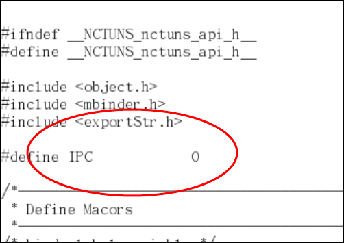
43
show where output files are generated.
2.4.1.3.1.1 An example showing how to use the first method
In this example, we assume that the new binary of NCTUns simulation
engine is named “nctuns” and placed in “/usr/local/demo_manual_sim/bin.” The
case is named “Demo29_GPRS_1_ms” and placed in the directory
“/root/NCTUns/example/”.
I. Set the value of IPC to zero
We first open the “nctuns_api.h” file and search the IPC variable. Then we
set the value of IPC to zero.
II. Set up five environment variables
For convenience, we can add shell commands that set the five NCTUns
environment variables to the .bashrc file. The following example shows that we
add these commands to the tail of the .bashrc file.
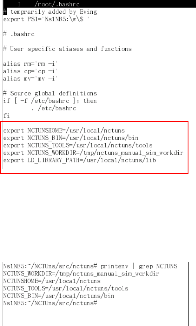
44
One can use the “printenv” command (a system utility that shows the
values of environment variables) to check whether or not the settings of these
environment variables are correct. The following shows that we use the “printenv
| grep NCTUNS” command to dump the values of NCTUns-related environment
variables ($LD_LIBRARY_PATH is not shown because it does not contain the
“NCTUns” string).
One can then use the “printenv LD_LIBRARY_PATH” command to show
the value of the $LD_LIBRARY_PATH environment variable.
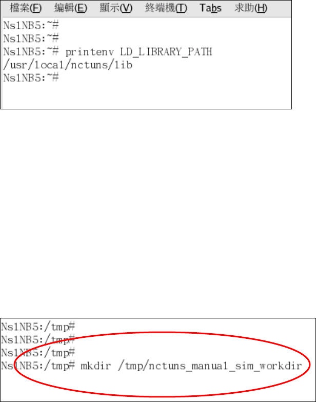
45
III. Create the $NCTUNS_WORKDIR directory
One has to make sure that the directory specified by
$NCTUNS_WORKDIR really exists. Otherwise, the user-level application
programs that will be run during the simulation will not run correctly. This is
because they will not be able to find and read their configuration files and
output their files in the specified directory.
IV. Re-compile the simulation engine
One then enters the directory storing the source codes of the simulation
engine, which is usually “src/nctuns” in the downloaded package. One should
execute the “make clean all” command to re-compile the simulation engine.
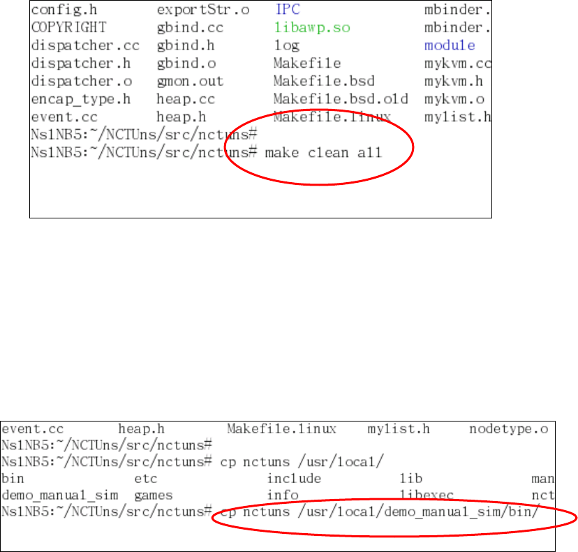
46
V. Copy the new simulation engine to a directory
After a successful compilation, one then copies the new simulation engine
to the “/usr/local/demo_manual_sim/bin” directory, which is arbitrarily chosen
for this example. Actually, one can place the new program into any directory.
VI. Put the configuration files required by user-level applications into the
$NCTUNS_WORKDIR directory
From the content of the following .tfc file, which describes what
applications should be run during the simulation (the detailed format of this file
is explained in section 2.4.2), it can be seen that the “stg” program needs a
configuration file named “stg.config” and the “rtg” program will generate a log
file named “log1.” Remember that all the files required by user-level programs
should be placed in $NCTUNS_WORKDIR and the output files generated by
user-level programs will be placed in $NCTUNS_WORKDIR. Because in this
example $NCTUNS_WORKDIR is “/tmp/nctuns_manual_sim_workdir/,” we
copy “stg.config” into “/tmp/nctuns_manual_sim_workdir.”
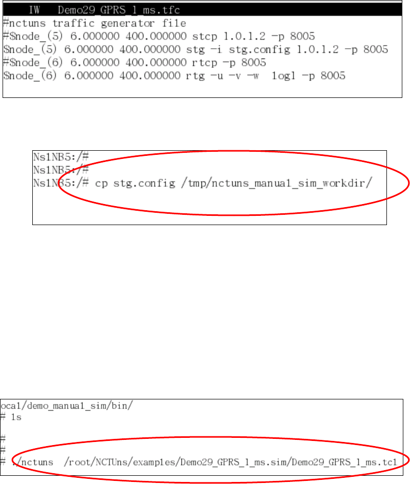
47
VII. Run a simulation manually
Here, we run a simulation case specified by a .tcl file, whose full path is
“/root/NCTUns/examples/Demo29_GPRS_1_ms.sim/Demo29_GPRS_1_ms.tcl
.” The following figure shows the command used to run this simulation.
VIII. Check output files
Remember that the output files generated by the simulation engine are placed
in the same directory as the given .tcl file and the output files generated by
user-level programs are placed in the $NCTUNS_WORKDIR directory. As
shown in the following two figures, the packet trace file (.ptr file) is placed in
“/root/NCTUns/examples/Demo29_GPRS_1_ms.sim,” and the “log1” output file,
which is generated by the “rtg” program, is placed in the
$NCTUNS_WORKDIR directory (“/tmp/nctuns_manual_sim_workdir”).
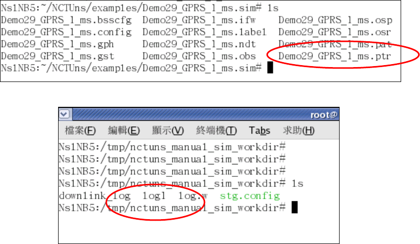
48
2.4.1.3.2 The second method
When describing the first method, we show that the directory where the
files describing a simulation case are stored can be different from the
directory where configuration files required by user-level application
programs are stored. Although the first method is correct, it may confuse
users because normally these files are regarded as “input files” for a
simulation case and most users would think that they should all be placed in
the same directory. As such, here we show the second method by which these
files can all be stored in the same directory. Actually, the second method is
the method used by the coordinator to manage the placement of files when
the GUI is used.
Using the second method, one needs to create a new directory for a
simulation case first. Then, one has to set $NCTUNS_WORKDIR to the path
of this directory so that this new directory will be used as the working
directory for a simulation. Next, one has to put the files that are used to
describe a simulation case, such as $CASENAME.tcl, $CASENAME.tfc, etc,
into this directory. Since this directory is the working directory for a
simulation case, the files required by user-level application programs should
be placed into this directory as well. Finally, one can enter the directory in
which the stand-alone version of the simulation engine is stored and then
start a simulation manually with the command, “./nctuns
$NCTUNS_WORKDIR/$CASENAME.tcl”.

49
Using the second method, one need not worry about where to store these
files because they are all placed in the same directory. Also, the output files
generated by the simulation engine, protocol modules, and user-level
programs will all be placed in the $NCTUNS_WORKDIR directory as well.
Although the second method is not as flexible as the first method, it
simplifies the placement of input and output files and may be more
acceptable for some users.
2.4.1.3.2.1 An example showing how to use the second method
I. Set the value of IPC to zero
We first open the “nctuns_api.h” file and search the IPC variable. Then we
set the value of IPC to zero.
II. Set up environment variables properly
For convenience, we can add shell commands that set the five NCTUns
environment variables to the .bashrc file. Note that in the second method, the
path specified by $NCTUNS_WORKDIR is no longer fixed. Instead, it may
need to be changed each time when one wants to start a new simulation. The
following example shows that we add the commands for setting up these
variables to the tail of the .bashrc file.

50
One can use the “printenv” command (a system utility that shows the
values of environment variables) to check whether or not the settings of these
environment variables are correct. The following shows that we use the “printenv
| grep NCTUNS” command to dump the values of NCTUns-related environment
variables ($LD_LIBRARY_PATH is not shown because it does not contain the
“NCTUns” string).
One can use the “printenv LD_LIBRARY_PATH” command to show the
value of the environment variable $LD_LIBRARY_PATH.
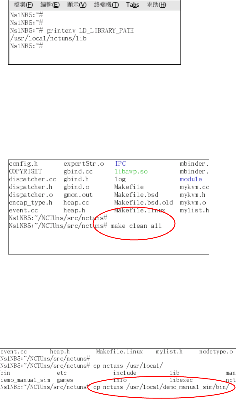
51
III. Re-compile the simulation engine
One then enters the directory storing the source codes of the simulation
engine, which is usually “src/nctuns” in the downloaded package. One should
execute the “make clean all” command to re-compile the simulation engine.
IV. Copy the new simulation engine to a directory
After a successful compilation, one then copies the new simulation engine
to the “/usr/local/demo_manual_sim/bin” directory, which is arbitrarily chosen
for this example. Actually, one can place the new program into any directory.
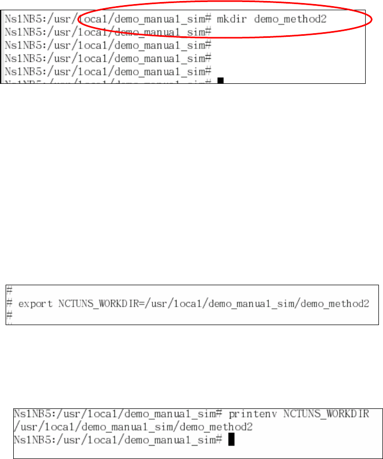
52
V. Create a new directory as the working directory
Using the second method, one has to create a new directory to be the
working directory for the simulation case. In this case, we create a new
directory named “demo_method2” in the “/usr/local/demo_manual_sim”
directory.
VI. Set $NCTUNS_WORKDIR to the path of this new directory
To make the new created directory as the working directory, one then
needs to set $NCTUNS_WORKDIR to the path of this new directory. In
bash/Linux, setting up an environment variable can be done with the “export”
command, which is a built-in command of bash. In this case, the command
used is “export
NCTUNS_WORKDIR=/usr/local/demo_manual_sim/demo_method2”.
As mentioned above, one can use “printenv NCTUNS_WORKDIR”
command to check if $NCTUNS_WORKDIR is properly configured or not.
VII. Put files required by the simulation engine and user-level application
programs into the $NCTUNS_WORKDIR directory
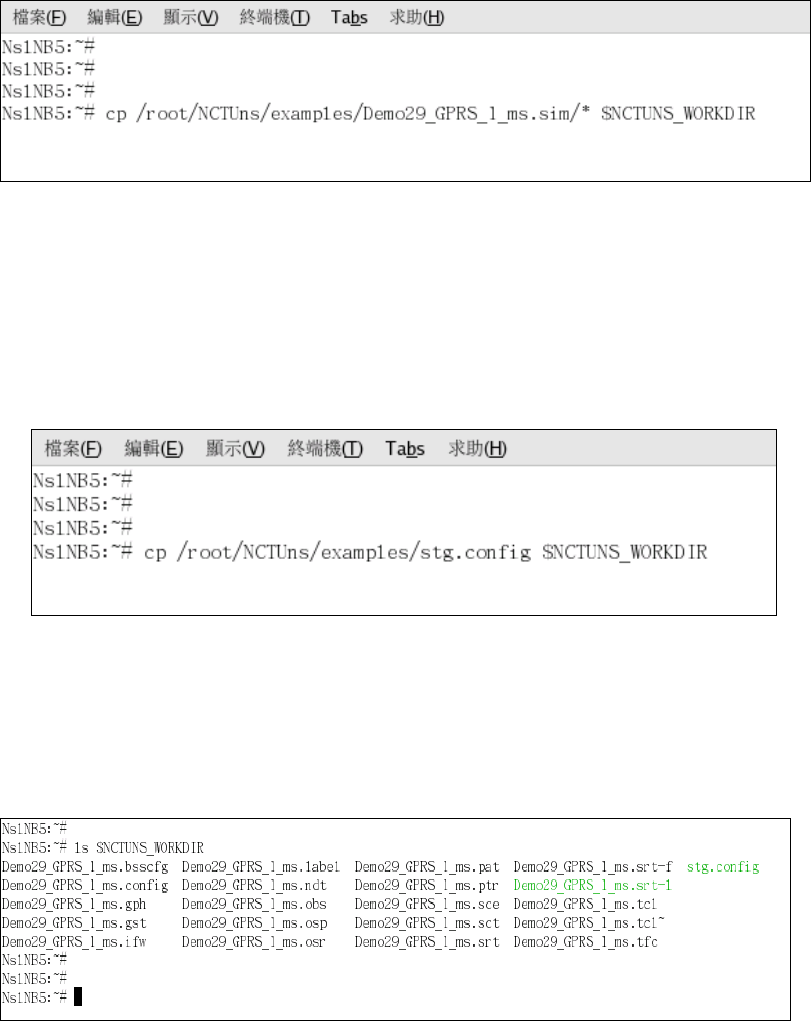
53
Using the second method, one needs to generate and put the files that
describe a simulation case (i.e., the files required by the simulation engine)
into the $NCTUNS_WORKDIR directory. We assume that these files have
been properly generated by some way (e.g., they may have been generated by
the GUI and thus we can simply copy them into this directory).
Also note that one has to make sure that the configuration files required
by user-level application programs should also be placed into the
$NCTUNS_WORKDIR directory. In this case, we copy stg.config, which is
required by stg program, into the $NCTUNS_WORKDIR directory.
Finally, one needs to make sure that all required files are placed in the
$NCTUNS_WORKDIR directory. One should double-check to make sure
that every setting is correct before starting a simulation.
VIII. Run a simulation manually using the second method
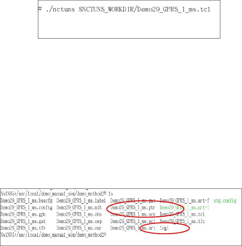
54
If all of the above steps have been performed, one can enter the
directory where the stand-alone version of the simulation engine is placed
and then manually start a simulation with the “./nctuns
$NCTUNS_WORKDIR/$CASENAME.tcl” command. ($CASENAME
denotes the prefix of the file name of “.tcl file” for the simulation case.) The
following figure shows the command used in this example.
IX. Check output files
Remember that the output files generated by the simulation engine and the
output files generated by user-level programs will be placed in the same
$NCTUNS_WORKDIR directory using the second method. As shown in the
following figure, the packet trace file (.ptr file) and the “log1” output file, which
is generated by the user-level “rtg” program, are both placed in the
$NCTUNS_WORKDIR directory, which is
“/usr/local/demo_manual_sim/demo_method2” in this example.
2.5 Formats and Usages of Simulation Description Files
In this section, we present the usages of the files that together describe a
simulation case and explain their formats.
55
(1) Simulation Network Description File
A simulation network description file is named $CASE.tcl. Here, $CASE
denotes the case name for a simulation case. A simulation network description
file is the main description file for a simulation, inside which the connectivity
of nodes, types of nodes, and configurations of protocol stacks of all nodes are
specified in this plain text file. The detailed format of a simulation network
description file is described in previous sections of this chapter.
(2) Traffic Description File
A traffic description file has the “.tfc” as its filename suffix. A traffic
description file describes when to execute what user-level application programs
on which nodes. Every line is independent and represents an execution
invocation of a user-level application program. The format of a line is:
$node_(NID) + starting time + termination time + the command line for
executing this application program.
An example is shown as follows:
$node_(1) 10.0 100.0 stg –u 1400 100 1.0.1.2
The first field in the above line specifies that the application should be run
on node 1. The next two fields specify that this application should be executed at
10th second and terminated at 100th second in simulation time. The command line
to execute this application then follows the “termination time” field. The
arguments given to this application are “stg,” “-u,” “1400,” “100,” and “1.0.1.2”
in sequence. The first argument is “stg” (“stg” is the abbreviation of “Sending
side traffic generator”), the name of this application program. The second one
indicates that this traffic generator is configured to generate UDP packets, and
the following argument specifies that the length of each packet is 1400 bytes.
The fourth one specifies that the execution duration of this “stg” application is
100 seconds in simulation time. The last argument specifies the IP address of the
destination node of these UDP packets. This example shows how to specify in
a .tfc file to run up the “stg” application during simulation. Actually, any
real-world user-level application program can be run up with NCTUns.
(3) Scenario Description File
56
A scenario description file has the “.sce” as its filename suffix and is used to
describe the static movements of mobile nodes. The detailed format is shown in
the following:
$node_(NID) + x + y + z + arrival time + pause time + speed
The fields, x, y, z, forms a triplet (x, y, z) that represents a location in the
simulated field. The arrival time specifies the time when this node should arrive
at the (x, y, z) location, and the pause time specifies how long this node should
stay at (x, y, z). The speed specifies how fast this node should move to the next
point after the pause. Here, the next point is specified in the next line for the
same node.
Note that for tactic and active mobile ad hoc networks where the moving
paths of mobile nodes are dynamically generated and controlled by the tactic
agent running on the mobile nodes, the moving paths of mobile nodes need not
be set.
(4) Obstacle Description File
An obstacle description file has the “.obs” as its filename suffix. This file
describes locations, lengths, and properties of obstacles in the simulation field. In
an obstacle description file, each obstacle is represented by a 9-tuple (sx, sy, dx,
dy, width, whether_block_view, whether_block_movement,
whether_block_wireless_signal, attenuation).
The pairs of (sx, sy) and (dx, dy) denote the two end points of an obstacle,
respectively. The width field indicates the width of this obstacle. Besides, there
are several fields to describe the properties of an obstacle. The
whether_block_view field indicates whether this obstacle should block the line
of sight of nodes; the whether_block_movement field indicates whether this
obstacle should block the movements of nodes, and the
whether_block_wireless_signal field indicates whether this obstacle should
reduce the strength of the wireless signal or not. If so, the attenuation field
specifies the amount of signal loss in dbm that a wireless signal should
experience when going through the obstacle.
Note that the intelligence of not going through an obstacle that is specified
to block a mobile node‟s movement is implemented by the tactic agent program
(see the chapter about tactic agent in this manual) running on the mobile node,
rather than implemented by the simulation engine. Similarly, the effects of a
57
mobile node not being able to see the things behind an obstacle that is specified
to block a node‟s view is implemented by the tactic agent program rather than by
the simulation engine. This design makes the simulation engine clean and easy to
manage. In contrast, the effect that a wireless signal is blocked or attenuated by
an obstacle that is specified to block or attenuate wireless signal is implemented
and enforced by the simulation engine.
(5) System Routing Table Description File
A system routing table description file has the “.srt-l” as its filename suffix.
(Note: “-l” means that the route command format of this .srt file is for Linux
operating system.) Routing entries for each node are specified in the “.srt-l file.”
Each entry is represented in the same format used by the “route” command,
which is a system utility program provided on most UNIX systems. We show
two examples in the following to demonstrate the two most common formats
used in this file.
The first example shows the first format. It is a route command in Linux.
This command specifies that the packets sent from the node whose IP is 1.0.1.1
and destined to subnet 1.0.2.X should be directed to the tun1 interface in the
kernel for transmission.
route add -net 1.1.2.0/24 tun1
The second example shows the second format.
route add -net 2.1.1.0/24 gw 2.1.2.2
This routing entry specifies that if packets are sent from the node whose IP
is 1.0.2.1 and destined to the subnet 1.0.1.X, these packets should be routed to
the node whose IP is 1.0.2.2.
(6) Mobile Routing Table Description File
A mobile routing table description file has the “.mrt” as its filename suffix.
This file describes the changes of routing entries on each mobile node and is
used only by the GOD routing module. A simulation case that does not use the
GOD routing module for the mobile nodes need not provide this file. Its format
is shown as follows:
58
$node_(NID) + entry-changing time + "set-next-hop" + SrcNode + DstNode
+ NextHop + "chan" + channel
An example is shown below:
$node_(1) 3.000000000 set-next-hop 1 3 2 chan 1
The above line specifies that a routing entry on node 1 is added or changed
at the 3rd second in simulation time. The entry shows that node 1 chooses node 2
as the next hop for its routes to node 3. In addition, the channel used by the
wireless interface is channel 1. Another special example is shown below:
$node_(1) 3.000000000 set-next-hop 1 3 999999 chan 0
The above example specifies that there is no route from node 1 to node 3
when the simulation time advances to the 3rd second. Using 999999 for the
NextHop indicates that no node can be the next hop for the route from node 1 to
node 3.
The routing entry updates in this file are the most “perfect” routing entry
updates that could only be calculated by the god. In the real life, no routing
protocol can detect node movements so quickly to generate these precise routing
entry updates. However, these perfect routing entry updates represent the best
performance that any routing protocol could possibly achieve. As such, the GOD
routing daemon can be used as a comparison target when one would like to see
how well a new routing protocol performs as compared with the most “perfect”
routing protocol.
When generating thie file, the GUI program by default updates the locations
of mobile nodes and updates the routing entries every 0.1 second. Because
starting from NCTUns 5.0 the wireless channel models used by moble nodes are
more realistic models and need heavy CPU computation, generating this file
becomes very time-consuming. To solve this problem, the GUI program now
provides a option window in which the user can choose how often to update the
locations of mobile nodes and do the recalculation. The update interval can be set
to 0.1 second, 1 second, or other values, or even “no update at all” if no mobile
node moves during the simulation to save time.
(7) Optical Switching Protection Ring File
59
An optical switching protection ring file has the “.osr” as its filename
suffix. To specify a protection ring, one has to describe the configuration of
optical protection rings in this file. Each line in the “.osr” file represents a
protection ring. A protection ring is composed of several triplets. Each triplet
is made up of the incoming port number, node ID, and the outgoing port
number. The following example shows how to specify a protection ring:
2 12 1 2 14 1 2 13 1 2 11 1 1 10 2 1 8 2
The above line specifies a protection ring containing nodes 12, 14, 13, 11,
10, and 8. Every three numbers form a triplet. For the first triplet, the first
number “2” is an incoming port number of node “12,” which is specified by the
following number, and the third number “1” is the outgoing port number of
node “12.” The second triplet (2, 14, 1) describes that packets departing from
port 1 of node 12 (the previous node on the ring) will enter node 14 via port 2
and leave node 14 via port 1. To close the ring, the last triplet indicates that
packets that depart from node 8 via port 2 will enter node 12 via port 2.
(8) Optical Switching Edge Router-to-Edge Router File
An optical switching edge router-to-edge router file has the “.osp” as its
filename suffix. Each line in this file describes an edge router-to-edge router
routing path, in which the first two numbers denote the node ID and the
outgoing port number of the first router on the path and the last two numbers
denote the incoming port number and the node ID of the last router on the path.
The middle part of a line is composed of several triplets, each of which
represents (incoming port number, node ID of optical switch, outgoing port
number). The following shows an example.
15 1 4 1 1 1 2 3 1 4 2 1 5 2 1 7 2 1 8 3 2 9 1 2 10 3 1 16
This example path is from router 15 to router 16. The first number “15” is
the node ID of the first router and the second number “1” is the outgoing port
number of node 15. The last number “16” denotes the node ID of the last router
and the number next to it indicates that the incoming port number is “1.”
(9) GPRS-phone Action Table Description File
60
A GPRS-phone action table description file has the “.pat” as its filename
suffix. This file describes when and which GPRS action should be performed on
which GPRS node during simulation. In a “.pat” file, each GPRS phone node has
its own action table. The format of an action table is shown below:
NODE$NID
The number of action entries
Action entry 1
Action entry 2
…
The first line is a keyword “NODE,” followed by the node ID of this phone.
The second line is a single field indicating the number of action entries in this
action table. An action entry is composed of the starting time, action type,
NSAPI, and the chosen QoS level.
(10) Base Station Configuration File
A base station configuration file has the “.bsscfg” as its filename suffix. It
specifies several important parameters for a GPRS base station. This
configuration file is composed of base station description blocks (BSDB) of all
base stations in a simulation. A BSDB consists of two sections. The first (local)
section describes the attributes of a base station. It contains the node ID, the base
station identity code (BSIC), the routing area identity (RAI), and the assigned
channel range for the base station. The second (neighbor) section contains a list
of the local sections of neighboring base stations.
GSM/GPRS system divides the wireless frequency into two groups, each of
which has 125 channels. The first channel group ranging from 0 to 124 is
dedicated to uplink traffic while the second group ranging from 125 to 249 is
dedicated to downlink traffic. An uplink channel with a channel ID ch1 and a
downlink channel with the (ch1+125) channel ID form a pair of bi-directional
link for a connection. Since the assignment of uplink/downlink channels is
symmetric, the configuration file describes the assigned channel range by
specifying only the range of uplink channels. Note that the lowest downlink
channel ID assigned to a base station implicitly specifies the broadcast channel
ID of a base station. For example, if a base station is assigned some uplink
channels ranging from 1 to 5, its broadcast channel ID is (1+125), i.e., 126.
The following is an example of a base station description file. The key
words BSS_DES_START and BSS_DES_END denote the start and the end of a
61
base station description block. A block has exactly one local section but may
have zero or multiple neighbor sections. The key word pair, LOCAL_SECTION
and END_LOCAL_SECTION, forms a local section that describes several
important attributes of a base station. In this example, a base station node with
NID 2 is assigned a BSIC 0 and RAI 3. Its assigned uplink channels are 1 to 5
and its downlink channel range is from 126 to 130. The base station with NID 8
is included in this block as a neighbor section. The meanings of the fields in a
neighbor section are the same as those in a local section. If base station A is
included as a neighbor section for base station B, base station A is viewed as a
neighboring base station of base station B. That is, base station B should have the
system information of base station A and similarly base station A should have the
system information of base station B. A base station should periodically
broadcast the system information of its neighboring base stations so that its
mobile phones know which base stations are close to the current base station and
providing services. Using this information, a mobile phone can constantly
monitor the signal strength of these neighboring base stations and roam quickly
to a better base station if necessary.
BSS_DES_START
LOCAL_SECTION
NID 2
BSIC 0
RAI 3
CHANNEL_RANGE 1 5
END_LOCAL_SECTION
NEIGHBOR_SECTION
NID 8
BSIC 0
RAI 7
CHANNEL_RANGE 11 15
END_NEIGHBOR_SECTION
BSS_DES_END
(11) Traffic Stream Classifier Description File

62
A traffic stream classifier description file has the “.tsc” as its filename suffix.
This file defines the classification of traffic flows on network nodes that supports
IEEE 802.11(e) protocol. The format of this file is explained in the following.
The traffic flow definition for a node is composed of several node traffic flow
description blocks, which have at least two separated lines. The first line stores the
node ID of this description block, and the second line stores the number of traffic
flows defined in the successive lines.
Consequently, if a node does not have any pre-defined traffic flows, the second
line will store the number zero, and the description block ends. A traffic flow is
defined by a set of parameters, listed in the table below in sequence. Note that these
parameters should be stored in the same line and should be separated by “blank space”
symbol or “tab” symbol only. They cannot be separated by the “end-of-line” marker
such as “carriage return” or “line feed” ASCII codes.
Parameter Name
Meaning
Start Time
The time that this flow classification is
activated.
Finish Time
The time that this flow classification is
deactivated.
Direction
Downlink (the direction from an AP to
an MS) or uplink (the direction from an
MS to an AP)
Transport Protocol
TCP or UDP
Source Port Number
The transport layer protocol port number
on the source node
Destination Port Number
The transport layer protocol port number
on the destination node
Traffic Stream ID
The ID assigned to this traffic stream,
ranged from 8 to 16
Mean Data Rate (kbps)
The average throughput that this traffic
stream requests
Nominal Packet Size (byte)
The size of packets sent by the
application program
Maximum Delay Bound
The maximum allowable interval, used
by the IEEE 802.11(e) MAC layer,
between the time a packet is enqueued
into the transmission queue of the MAC

63
layer and the time it is successfully
transmitted
Maximum Service Interval
The maximum interval between the two
successive polling requests sent by an
IEEE 802.11(e) AP
The following is an example of the traffic stream classifier description file.
4
0
5
1`
0.000000 80.000000 Uplink UDP 0 8001 8 200 1024 1024 20
6
2
0.000000 80.000000 Downlink TCP 0 8001 9 200 1460 1460 20
0.000000 80.000000 Uplink TCP 0 8000 8 100 1460 1460 20
There are three node traffic flow description blocks. The first one is defined for
node with node ID 4. The second line of this block indicates that node 4 does not have
any pre-defined traffic stream.
The second one is composed of three lines. The first line indicates that the this
block is for node with ID 5 while the second line shows that there is one traffic stream
defined in this block. The third line defines this traffic stream, which is activated and
deactivated at the 0‟th second and at the 8‟th second, respectively. It indicates that this
traffic stream is an uplink UDP flow and the destination port number is 8001.
The 7‟th parameter specifies that the traffic stream ID is 8; the 8‟th parameter
shows that the average throughput that this traffic stream requests is 200 kbps; and,
the 9‟th parameter defines the nominal packet size, which is 1024 byte. The last two
parameters define the maximum delay bound and the maximum service interval,
whose values are 1024 milliseconds and 20 milliseconds, respectively. The final block
defines node 6‟s traffic streams. Since the meanings of the parameters are explained
previously, we do not repeat the explanation for the description block of node 6.
(12) Address Resolution Protocol File
An address resolution protocol (ARP) file has the “.arp” as its filename suffix
and is used to describe the mapping between an IP address and its corresponding
MAC address. The detailed format is shown in the following example:

64
IP MAC
1.0.1.1.1 0:1:0:0:0:2
(13) Car Agent Configuration Profile File
A car agent configuration profile file has the “.car_prof_cfg” as its filename
suffix and is used to describe how many percentages of car agents use which profile$,
where $ stands for a number. A profile$ is used to describe the moving characteristics
of the car. The detailed format is shown below.
The Car Agent Configuration Profile.
In this example, car agent 2 uses profile1.
Node number profile
2 profile1
An example content of one profile
MaxSpeed=18 (m/sec)
MaxAcceleration=1 (m/sec2)
MaxDeceleration=4 (m/sec2)
(14) WAVE Service Configuration File
A WAVE Service configuration file has the “.wme_cfg” as its filename suffix and
is used to describe the WAVE‟s application primitives. The detailed format and
examples are shown in the following:
WAVE service configuration profile format.
Parameter Name
Meaning
SIB_Begin
The service information block begins
here.
NID
It specifies the Node ID. The
information following this NID
statement until the next NID statement
applies to this particular node.
CDB
The configuration description begins
here.
Time
It specifies the start time for an

65
application to execute this primitive
(e.g., wme_app_req) to create a
service. (The time unit is 10-7 seconds.)
CMD
It specifies the WME-Application
primitive that should be executed. The
supported primitives for this variable
are “wme_app_req” (for making a
request) and “wme_app_reg” (for
making a registration).
PSID
It specifies the identifier of this created
provider service. (0X00000001
through 0X7FFFFFFF.)
RegAction
Its value is Add_provider (for
registering a provider with the WME)
or Add_user (for registering a user with
the WME).
AppPriority
It specifies the priority of the created
service. (63 is the highest value; 0 is
the lowest value.)
Channel
It specifies the channel number used by
this service. (174, 175, 176, 180, 181,
182)
SerProMacAdd
It specifies the MAC address of the
device on which this application,
which creates this service) is run.
PSC
It specifies the application‟s provider
service context and can be any string.
ReqType
The action supported by the
“wme_app_req” primitive. Currently,
only “active” is supported.
PeerMacAdd
It specifies the MAC address of the
device on which the WME is run.
Repeats
It specifies how many times (0~7) this
service announcement should appear in
a control channel interval.
Persistence
It specifies whether the service
announcement should be sent only
once in the current control interval (0)

66
or periodically in every control channel
interval (1).
CBJ
It specifies whether the WME should
confirm with the application before
joining a provider service. This option
is for a device that registers with WME
expressing that it is interested in
becoming a WAVE user. Currently, its
value is always set to FALSE.
CDE
The configuration description ends
here.
SIB_End
The service information block ends
here.
An example of “WAVE user” settings.
In this example, node 16 registers for PSID 1 and PSID 2 at 1‟st second during
simulation, expressing that it is interested in joining a service whose PSID is 1 or
joining a service whose PSID is 2.
NID 16
CDB
Time 10000000
CMD wme_app_reg
PSID 1
RegAction Add_user
CBJ 0
CDE
CDB
Time 10000000
CMD wme_app_reg
PSID 2
RegAction Add_user
CBJ 0
CDE
An example of “WAVE provider” settings.
In this example, node 12 registers one service whose PSID is 1 at 1st second during
simulation. Then, at 2nd second during simulation, it starts to provide the service.

67
NID 12
CDB
Time 10000000
CMD wme_app_reg
PSID 1
RegAction Add_provider
AppPriority 1
Channel 174
SerProMacAdd 0:1:0:0:0:12
CDE
CDB
Time 20000000
CMD wme_app_req
PSID 1
PSC ""
ReqType active
PeerMacAdd 0:1:0:0:0:12
Repeats 3
Persistence 1
Channel 174
CDE
(15) DVB-RCS Frequency Configuration File
A DVB-RCS frequency configuration file has the “.dvbrcs.freq” as its filename
suffix and is used to describe the mapping between a channel number and its
corresponding frequency in DVB-RCS satellite networks.
(16) IEEE 802.16 Network Description File
An IEEE 802.16 network description file has the “.ieee80216_network_des” as
its filename suffix and is used to describe the setting for IEEE 802.16 networks. It
includes the network ID, subscriber station list, and authentication method.
(17) IEEE 802.16 Mesh Routing Tree File
An IEEE mesh routing tree file has the “.meshrt” as its filename suffix and is
used to describe the next hop routing information for WiMAX mesh routing
68
.
(18) WiMAX Neighbor Base Station List File
A WiMAX neighbor base station list file has the “.nbrbs_list” as its filename
suffix and is used to describe the node ID, channel ID and MAC address of a WiMAX
base station.
(19) Node Type List File
A node type list file has the “.ndt” as its filename suffix and is used to describe
the mapping between node type and node id in an optical network.
(20) WiMAX Node Configuration File
A WiMAX node configuration file has the “.nodecfg” as its filename suffix and
is used to describe the WiMAX mapping between the node ID and the MAC address.
(21) Road Position File
A road position file has the “.road” as its filename suffix and is used to describe
the positions, directions, and other properties of all roads and intersections in the GUI
program.
(22) Road Structure File
A road structure file has the “.road_structure” as its filename suffix and is used to
describe the construction relations between a road‟s block, lane and edge.
(23) System Command File
A system command file has the “.sct” as its filename suffix and is used to
describe the system commands to be issued during simulation. These system
commands can be specified in the GUI program. The format of “.sct” file is: Target
Time (second) + Command + Output file name.
(24) Signal Agent Configuration File
A signal agent configuration file has the “.sig” as its filename suffix and is used
69
to describe the position and direction of a traffic signal agent. Signal agents are used
in an Intelligent Transportation Systems (ITS) simulation, where cars move on roads
and pass intersections.
(25) WiMAX Configuration File
A WiMAX configuration file has the “.wimax-config” as its filename suffix and
specifies classes of QoS provisioning, classes of QoS service, and rules for
classification.
(26) Mobile WiMAX Configuration File
A mobile WiMAX configuration file has the “.mobilewimax_cfg” as its filename
suffix and is used to describe the setting of mobile station‟s QoS in mobile WiMAX
networks.
(27) Mobile WiMAX Neighboring Base Station List File
A mobile WiMAX neighboring base station list file has the “.nbrbs_list” as its
filename suffix and is used to list each base station‟s node ID, channel ID, and MAC
address.
(28) Mobile Relay WiMAX Transparent Mode Configuration File
A mobile relay WiMAX transparent mode configuration file has the
“.mobilerelaywimax_cfg” as its filename suffix and is used to describe the setting of
mobile station‟s QoS in mobile relay WiMAX transparent mode networks.
(29) Mobile Relay WiMAX Transparent Mode Neighboring Base Station
List File
A mobile relay WiMAX transparent mode neighboring base station list file has
the “.mr_nbrbs_list” as its filename suffix and is used to list each base station‟s node
ID, channel ID, and MAC address.
(30) Mobile Relay WiMAX Non-transparent Mode Configuration File
A mobile relay WiMAX non-transparent mode configuration file has the
70
“.mr_wimax_nt_cfg” as its filename suffix and is used to describe the setting of
mobile station‟s QoS in mobile relay WiMAX non-transparent networks.
(31) Mobile Relay WiMAX Non-transparent Mode Neighboring Base
Station List File
A mobile relay WiMAX non-transparent mode neighboring base station list file
has the “.mr_nbrbs_nt_list” as its filename suffix and is used to list each base station‟s
node ID, channel ID, and MAC address.
(32) Emulation Configuration File
An emulation configuration file has the “.emu” as its filename suffix and is used
to describe the external routing table settings. This file is used when emulation rather
than simulation is performed.
(33) Satellite Module Connection File
A satellite module connection file has the “.smc” as its filename suffix and is
used to describe the DVB-RCS networks connection configuration.
(34) Wired Link Graph File
A wired link graph file has the “.gph” as its filename suffix and is used to
describe the wired link connection in an optical network. The detailed format is
shown in the following:
1st line: The number of links that follow.
Each following line: FromNodeID, ToNodeID, FromPortID, ToPortID, which
means that this link starts at the “FromNodeID” node and the “FromPortID” port, and
ends at the “ToNodeID” node and the “ToPortID” port.
(35) GPRS GGSN Service Table File
A GPRS GGSN service table file has the “.gst” as its filename suffix and is used
to describe the NSAPI, QoS level, and GGSN IP address mapping in each line.
Currently, the NSAPI and QoS level are all set to 0.
Chapter 3 High-level Architecture of
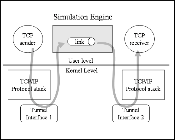
71
NCTUns
NCTUns uses a distributed architecture to support remote simulations and
concurrent simulations. It also uses an open-system architecture to enable protocol
modules to be easily added to the simulator. In the following we describe some
important features and components of NCTUns.
3.1 Simulation Methodology
NCTUns is based on a novel simulation methodology -- the kernel re-entering
simulation methodology. It uses the existing real-world Linux protocol stack to
generate high-fidelity TCP/IP network simulation results. Figure 3.1.1 depicts this
concept.
1
Figure 3.1.1. The kernel re-entering simulation methodology
In Figure 3.1.1, the TCP/IP protocol stack used in the simulation is the existing
real-life stack in the kernel. Although there are two TCP/IP protocol stack depicted,
actually they are the same one – the protocol stack inside the Linux kernel. The tunnel
interface is a pseudo network interface that does not have a real physical network
attached to it. From the kernel‟s point of view, the tunnel interface is no different from
any real Ethernet network interface.
In Figure 3.1.1, the TCP sender sends a packet into the kernel, and the packet
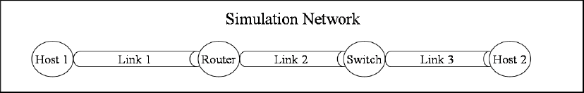
72
goes through the kernel‟s TCP/IP protocol stack just as an Ethernet packet would do.
Because we configure the tunnel interface 1 as the packet‟s output device, the packet
will be inserted to tunnel interface 1‟s output queue. The simulation engine will
immediately detect such an event and issue a read system call to get this packet
through tunnel interface 1‟s special file. (Note that every tunnel interface has a
corresponding device special file in the /dev directory.) After experiencing the
simulation of transmission delay and link‟s propagation delay, the simulation engine
will issue a write system call to put the packet into tunnel interface 2‟s input queue.
The kernel will then raise a software interrupt and put the packet into the TCP/IP
protocol stack. Then, the packet will be put into the receive queue of the socket that
the TCP receiver creates. Finally, the TCP receiver will use a read system call to get
packet out of the kernel.
In the case of Figure 3.1.1, the packet sent by the TCP sender passes through the
kernel two times. This is the property of the kernel re-entering simulation
methodology. By re-entering the kernel multiple times, we can create an illusion that
a packet passes through several different hosts (i.e., the packet thinks that it passes
through several different TCP/IP protocol stack). Actually, the packet is always in the
same machine and passes through the same TCP/IP protocol stack. The following
figures (Figure 3.1.2 and Figure 3.1.3) further illustrate this concept.
Figure 3.1.2 shows an example simulation network topology and Figure 3.1.3
illustrates how the kernel re-entering simulation methodology works in Figure 3.1.2.
In the example topology, host 1, host 2 and the router are layer-3 devices while the
switch is a layer-2 device. (Here we use the OSI 7-layer standard.) We directly use
those protocols that are higher than the layer-3 protocol (i.e., the network or IP layer)
in the kernel. As such, if any device is a layer-3 device, we only need to simulate its
layer-1 and layer-2 protocol in the simulation engine and its other protocols can be
simulated by directly using those protocols already in the kernel. Therefore, in Figure
3.1.2, when a packet is passed through the two hosts or the router, it will be passed
into the kernel. As we can see in Figure 3.1.3, if a packet wants to traverse the
simulation network from host 1 to host 2, it needs to be put into the kernel three
times.
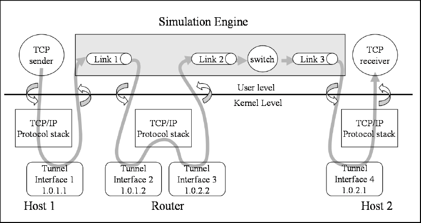
73
3.2 Job Dispatcher and Coordinator
NCTUns uses a distributed architecture to support remote simulations and
concurrent simulations. The job dispatcher is used to do this task. It should be
executed and remain alive all the time to manage multiple simulation machines. On
every simulation machine, the coordinator needs to be executed and remain alive to
let the job dispatcher know whether currently this machine is busy running a
simulation case or not. Figure 3.2 depicts the distributed architecture of NCTUns.
Figure 3.1.2. The simulation network topology
Figure 3.1.3. The packet trace of a packet that will traverse the simulation
network from host 1 to host 2.
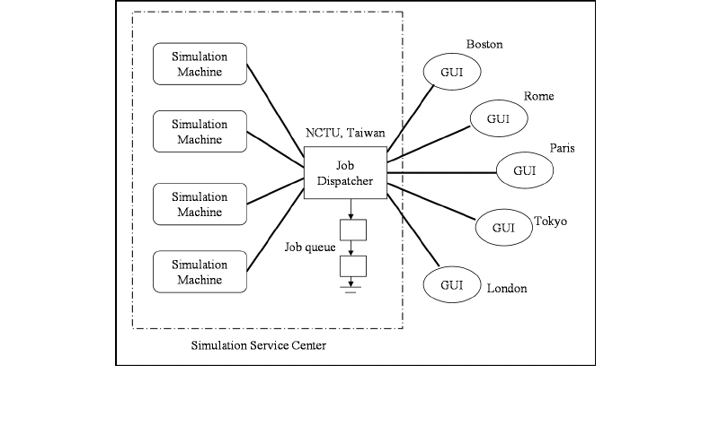
74
For example, the job dispatcher in the simulation service center can accept
simulation jobs from the whole world. When a user submits a simulation job to the
job dispatcher, the dispatcher selects an available simulation machine to service the
job. If there is no available simulation machine, the job will be put into the job queue
of the job dispatcher. Every simulation machine always has a running coordinator to
communicate with the GUI program and the job dispatcher. The coordinator will
notify the job dispatcher whether the simulation machine managed by itself is
available or not. When the coordinator receives a simulation job from the job
dispatcher, it forks (executes) a simulation engine process to simulate the specified
network and protocols. When the simulation engine process is running, the
coordinator will communicate with the job dispatcher and the GUI program. For
example, periodically the simulation engine process will send the current virtual time
of the simulation network to the coordinator. Then the coordinator will relay the
information to the GUI program. This enables the GUI user to know the progress of
the simulation. During a simulation, the user can also on-line set or get a protocol
module‟s value (e.g. to query or set a switch‟s switch table). Message exchanges
happening between the simulation engine process and the GUI program are all done
via the coordinator.
3.3 Simulation Engine Design
The simulation engine is a user-level program and has complex functions. It
functions like a small operating system. Through a defined API, it provides useful and
Figure 3.2. The distributed architecture of NCTUns
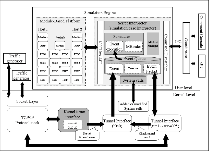
75
basic simulation services to protocol modules. These services contain virtual clock
maintenance, timer management, event scheduling, variable registration, script
interpreter, IPC interface, etc. At the same time, it manages all of the tools and
daemons that are used in a simulation case and decides when to start these programs,
when to finish them, and when to run them. Figure 3.3.1 shows an architecture
diagram of NCTUns.
Figure 3.3.1. The architecture of NCTUns
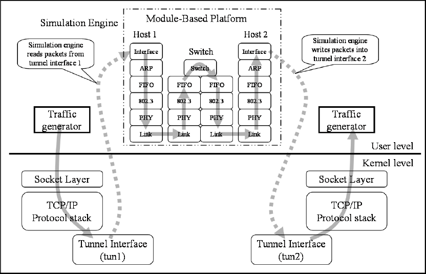
76
In Figure 3.3.1, we can see the whole architecture of NCTUns. In the section, we
first describe the organization of the simulation engine. In section 3.4, we will explain
how the kernel supports the simulation engine. We can simply divide the simulation
engine into several components:
I. Script Interpreter
The script interpreter reads a script file of a simulation case to construct the
simulation network environment, the network conditions, protocol module settings,
and the network traffic.
II. Module Manager
The module manager manages all protocol modules that users registered and
used in a simulation. When the script interpreter parses the script file, the module
manager dynamically constructs the corresponding C++ objects and organizes them
to build a simulation network environment. In Figure 3.3.1, those modules in the box
of the module-based platform form a simple simulation network.
III. Command Dispatcher
Figure 3.3.2: The module based platform
77
The command dispatcher is used to communicate with other external
components such as the coordinator, command console (It is a modified tcsh.), and
the GUI program.
IV. NCTUns APIs
All protocol modules can ask for the simulation engine‟s services via the
NCTUns APIs such as registering modules, processing events, setting timers,
creating/freeing packets, etc.
V. Event Queue
The event queue has three kinds of data structure type inside it: event, timer, and
event packet. The event is used to encapsulate messages that are exchanged between
protocol modules. Every event has a timestamp inside it used to decide when to
process it. The timer can be used to set what to do at a specified time. If an event
encapsulates a packet (e.g., an IP packet), such an event is an event packet. In the
event queue, all events or timers are sorted according to their timestamps.
VI. Scheduler
The main job of the scheduler is to execute the event or timer in the event queue.
The scheduler always picks up the event or timer that has the smallest timestamp to
execute. In the meantime, the scheduler will advance the simulation time to the
timestamp of the event.
VII. System calls and tunnel interface t0e0
Two approaches are used to enable the simulation engine to communicate with
the Linux kernel. The first approach is through system calls. The simulation engine
can use system calls that are added or modified to register/get information into/from
the kernel. This approach suits the situation when the simulation engine actively
wants to get or set some kernel parameters. The second approach is through using a
tunnel interface. If the kernel wants to actively inform the simulation engine of some
information, the tunnel interface t0e0 is used. The kernel can fill a packet with some
information and insert it into the tunnel interface t0e0. Then the simulation engine can
issue a read() system call to get the packet and further get the information inside it.
78
This mechanism is mostly used by the kernel timeout event and the tunnel check
event. (We will describe this in section 3.5 of part I).
VIII. IPC (Inter-Process Communication)
The IPC in the simulation engine is used to communicate with the coordinator.
When a GUI user wants to send a command to the simulation engine such as pause a
simulation, stop a simulation, send command to a protocol module etc., the GUI
should send the command to the coordinator and then the coordinator relays the
command to the simulation engine via IPC. After the simulation engine processes the
command, it will send the result back to the coordinator and then the coordinator will
relay the result to GUI.
Due to the module-based platform, we can dynamically construct or change the
network protocol of a device. For example, Figure 3.3.2 shows a simple simulation
case: the switch is a two-port layer-2 device and is connected with the host 1 and host
2 (host 1, 2 are both layer-3 devices). We can easily change the protocol module
settings of host 1. We can just replace the FIFO module with a RED (Random Early
Drop) module in the script file and then the module manager will dynamically
construct corresponding protocol module settings according to the script file. We can
also build a network device via the module-based platform. The switch device in
Figure 3.3.2 is a layer-2 device and all components of the device are represented by
modules. In addition to protocol modules, the layer-3 devices (such as host 1, host 2)
will need kernel supports because we directly use the layer-3 protocols in the kernel.
Figure 3.3.2 also shows the flow path that a packet will take when it is
exchanged between the two traffic generators via the module-based platform. We
already explained how a packet will pass through the kernel in section 3.1. When the
packet is read by the simulation engine from tunnel interface 1 (tun1), the packet will
follow the trace of Figure 3.3.2 and then the simulation engine will insert it into
tunnel interface 2. Finally, the kernel will send it to the traffic generator.
3.4 Kernel Modifications
In order to enable the kernel re-entering simulation methodology to properly
work, some kernel source needs to be modified according to these requirements.
These requirements include:
79
I. Allow the S.S.D.S IP Scheme to Work
In order to route packets in the same kernel, we proposed a special IP scheme --
S.S.D.D IP format. Readers can refer to [1] and [13] to get the detailed definition.
As such, we should add some mechanisms into the TCP/IP protocol stack to
correctly translate the IP address of a packet.
II. Modify the Tunnel Interface Device Driver
Modifying the tunnel driver is necessary to enable the S.S.D.D IP scheme to
work because we want the packet to have the normal IP scheme when it is read
by the simulation engine. Also, we want the packet to have the S.S.D.D format
when it is inserted into a tunnel interface.
III. Perform Port Number Mapping
We use an example to illustrate this requirement. If there are two Web servers
running on the same simulation network, both of them may want to use the
default port number 80 as their listening port number. However, because they are
running on the same system (using the same TCP/IP protocol stack), only one of
them can successfully bind to port number 80. To solve this problem, we should
do port mapping in the kernel to enable the program running on different
simulated nodes to use the same port number.
IV. Add or Modify System Calls
We need to add or modify some system calls to provide services that the
simulation engine will require. For example, when a traffic generator is forked
by the simulation engine, the simulation engine immediately needs to tell the
kernel that the traffic generator belongs to which node. This operation is needed
because we have to use this information to translate the IP address of those
packets sent by the traffic generator.
V. Let Kernel Timers to be based on the Virtual Time
Because all of the events or timers in the simulation engine‟s event queue are
based on the virtual time, all of kernel timers used for NCTUns should also use
the virtual time. For example, when the TCP control block (i.e., a TCP socket
handler) transmits out a packet, it may set a retransmission timer. If the TCP
control block is used for a simulation network, the timer should use the virtual
time. In addition, all of the system calls that are involved with real time may
need to use virtual time. These system calls include select(), alarm(), sleep(),
80
gettimeofday(), etc.
VI. Kernel Events
There are two kinds of kernel event. The first is the kernel timeout event. When
the kernel wants to schedule a timer and the timer is based on the virtual time,
we should use the tunnel interface t0e0 to tell the simulation engine when to
trigger this event. The second is the tunnel check event. When any packet is
queued into a tunnel interface‟s output queue, the kernel will insert a tunnel
check event into the tunnel interface t0e0 to let the simulation engine know
which tunnel interface has packets to send.
3.5 Discrete Event Simulation
The discrete event simulation methodology is applied to NCTUns to speed up its
simulations. The challenge is to combine the kernel re-entering simulation
methodology with the discrete event simulation methodology. The objects simulated
in NCTUns are not contained in a single program; rather, they are contained in
multiple independent programs running concurrently on a UNIX machine such as
traffic generators, the simulation engine, the UNIX kernel, etc. Therefore, we need
the kernel to provide some information or services to communicate with the
simulation engine. As such, the simulation engine can manage all events and timers at
user level. In other words, our goal is to manage and trigger all of the events in the
simulation engine regardless of whether the events are kernel events or not.
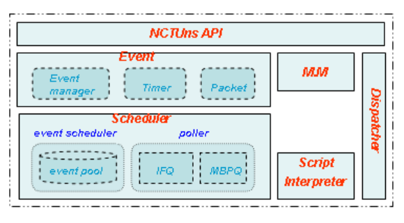
81
Chapter 4 Simulation Engine – S.E
4.1 Architecture of the Simulation Engine
The Simulation Engine (S.E) is the core of NCTUns. It provides a module-based
platform for users to develop their protocols and integrate them into our simulator. By
linking modules in a controlled way, users can easily create any arbitrary network
device on our network simulator. Similarly, by connecting network devices together,
users can arbitrarily create a network topology and simulate it. Figure 4.1 depicts the
architecture of the Simulation Engine in NCTUns. As this figure shows, the S.E is
composed of six components. They are Scheduler, Event, Module Manager, Script,
Interpreter, Dispatcher, and NCTUns APIs, which we already discussed roughly in
Chapter 3.
When the simulator starts, the Script Interpreter component will parse a topology
file. The parsing results from the Script Interpreter are then passed to the M.M
component. The M.M component creates a simulation network according to these
information. After that, the S.E initiates its Scheduler component to start its timer.
Then the scheduler will poll each tunnel network interface periodically to try to read a
packet from a tunnel network interface. Upon reading a packet from a tunnel interface,
the scheduler calls the first module in a node and passes the packet to it. After
processing the packet, the first module continues to pass the packet to the second
module, third module and so on in the same node. In the modules, modules could
request a service from the S.E. through the NCTUns APIs. For example, they could set
up a timer through the timer APIs. When the timer expires, the scheduler will call a
function which is specified by a function pointer in the timer structure.
FIGURE 4.1: THE ARCHITECTURE OF THE SIMULATION ENGINE.
82
4.2 Event
The event is the most basic interface in the S.E that is used to communicate with
the Scheduler component. For a module, the module could ask for an event from the
S.E to notify the scheduler when to call a handler function. For example, a module
may get an event for simulating packet transmissions (Upon expiration time, a handler
function is called to transmit a packet). As another example, a module may ask for an
event from the S.E to implement its polling mechanism. Hence, if a module wants to
request a service from the S.E, it should encapsulate its request as an event. Then the
scheduler will accept and provide services for it.
In addition, an event also provides a platform for easily building a high-level
service for modules. As Figure 4.1 shows, the event component contains three smaller
components – Packet, Timer and Event Manager. These components provide a
high-level service to modules based on the event interface:
1. For the Packet component, it encapsulates packet as an event. We name this
kind of event “ePacket”. By encapsulating a packet as an ePacket, the packet
can directly be scheduled in the Scheduler component.
2. For the Timer component, it provides a timer mechanism for modules. For
modules, they may have many chances to use the timer mechanism. For
example, in a MAC (Media access control) module, we may ask for a timer
to know if the MAC should retransmit a packet that was sent before – (While
the MAC sends a packet, it also sets a timer. When the timer expires but no
ACK has been received yet, the MAC will know that the outgoing packet
was lost and should be retransmitted again).
3. For the Event Manager, users can register a periodical event with the Event
manager. The periodical event is an event which will be periodically
processed by the event Scheduler. Under the control of the Event manager,
users can dynamically enable or disable a scheduling event through either a
tcsh command interpreter or a GUI environment.
struct event {
u_int64_t timeStamp_;
u_int64_t perio_;
NslObject *calloutObj_;
int (NslObject::*memfun_)(struct event *);
int (*func_)(struct event *);
83
void *DataInfo_;
u_char priority_;
struct event *next_ep;
};
The above data structure lists the declaration of an event structure. In this data
structure, the „timeStamp_‟ is the expiration time of an event. Note that there is a
system global virtual time maintained in the Scheduler component. Once this virtual
time equals to this „timeStamp_‟, the scheduler component will call the handler
function which is specified in the event structure. The middle fields of the above
declaration are used to specify a handler function. In these statements we can see that
the handler function could be either a normal function or a member function of an
object. If a handler function is a normal function, the „func_‟ is used and this handler
function that the „func_‟ points to should be in the following form:
int <Handler>(Event *ep) {
…………………………………
…………………………………
}
Similarly, if a handler function is a member function of an object, both the
„calloutObj_‟ and the „memfun_‟ are used and the handler function which both the
„calloutObj_‟ and the „memfun_‟ specify should be in the following form:
int <Object>::<Handler>(Event *ep) {
………………………………..
………………………………..
}
Above, the <Handler> is a handler function name. The <Object> is an object
name. Note that the only parameter in a handler function, no matter whether the
handler function is a normal function or a member function, is a pointer to an event.
This event is an event which causes a handler function to be called by the Scheduler.
For example, if the Scheduler component processes an event B and then call out a
handler function which is specified in that event, the parameter in the handler function
will be a pointer to B.
84
The „perio_‟ member in the event data structure is used to indicate if an event is
a periodic event. The periodical event is an event that the Scheduler needs to process
periodically. If this field, „perio_‟ is set to zero in an event, we call this event a normal
event. Otherwise, we call it a periodic event. The „DataInfo_‟ is a pointer to an
unknown data type. Hence, for an event it could attach any information to it. By
setting this value, we could implement any kind of high level services for modules,
just as the three components mentioned above – Packet, Timer and „Event Manager‟.
The „priority_‟ is the priority of an event. Presently, it is only used in the Module
Binder, which will be discussed in the section 4.3. Finally, the „next_ep‟ is a pointer
used to chain events in a single linked-list.
4.2.1 Timer
The S.E in NCTUns provides a timer mechanism for modules. Its
implementation in the S.E is based on the event interface. Briefly speaking, a timer is
an event in the S.E. However, the functionality of a timer is more powerful than that
of an event. In the following, we list the declaration of the timer structure in the S.E:
class timerObj {
public:
Event_ *callout_event;
u_char busy_; /* timer state */
u_char paused_;
u_int64_t rtime_; /* remaining time */
timerObj();
~timerObj();
virtual void cancel();
virtual void start(u_int64_t time, u_int64_t pero);
virtual void pause();
virtual int resume(u_int64_t time);
virtual int resume();
………………………………………………………………………….
………………………………………………………………………….
};
In the above structure, the „callout_event‟ is a pointer to an event. If any
85
component wants to communicate with the Scheduler, it should use an event interface.
Through this event interface, the component could ask for a request from the
Scheduler. Here the „timerObj‟ uses such an event interface, the „callout_event‟, to
communicate with the Scheduler. The „busy_‟ is a status variable used to indicate the
idle or busy state of a timer. The busy state means that the timer is being scheduled in
the Scheduler. Otherwise an idle state is set in „busy_‟ to indicate an idle timer. The
„paused_‟ is a flag used to indicate if a timer which is in the busy sate is paused or not.
If a timer is paused, the timer will leave the Scheduler and the „rtime_‟ will be set to a
time which indicates the remaining time of the timer. For a timer, if we want, we can
resume it if it was paused before.
About the timer manipulation, the timer mechanism provides four operations to
manipulate a timer:
1. start() The start() operation is used to start a timer. Whenever a module
asks for a timer from the S.E, it should use this operation to start the timer.
cancel() The cancel() operation is used to cancel a timer which is in the
busy state. There are many chances to use this operation in a module. For
example, when a packet is sent in a sender, a timer should be set. After that,
if an ACK is received in the sender before the timer expires, the timer should
be canceled.
2. pause() Whenever a timer is in the Scheduler, the pause() could be used to
pause an active timer for a moment. Later, on another operation, resume(),
can be used to resume the timer.
3. resume() The resume() operation is used to resume a paused timer. In the
S.E, the timer mechanism provides two types of resume operation for a
module. If a timer is paused, a resume(void), which has no parameter, could
be used to simply resume the timer. Otherwise, another resume(extra-time)
operation, which has a parameter, could be used. In addition to resume a
paused timer, the resume(extra-time), which has a parameter, could extend a
timer‟s expiration time. The parameter in this type of resume() is the extra
time, which will extend the original time in a timer to extra-time + original
expiration time.
The timer mechanism provides an extensible mechanism for users. If a more
powerful functionality of a timer than that of a basic timer is needed, users can
extend the current timer mechanism to have more powerful functionality.
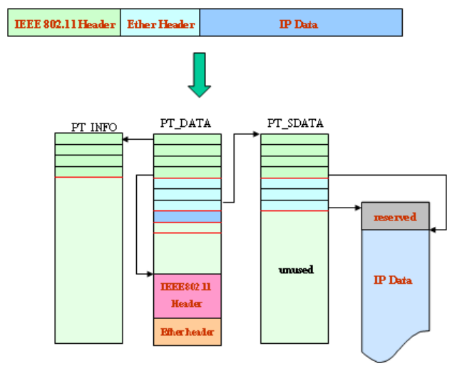
86
4.2.2 Packet
A Packet-Object is a data structure used to encapsulate user data in a well-known
format in NCTUns. Every user data in a simulated network should be encapsulated as
a Packet-Object. Through this Packet-Object interface, all of the modules in a
simulated network could process it. Figure 4.2.1 depicts how an IEEE 802.11 frame is
encapsulated in the Packet-Object format.
FIGURE 4.2.1: DATA IS ENCAPSULATED AS A PACKET-OBJECT.
From this figure, we can see that the user-data is encapsulated as an IEEE 802.11
frame. In the real-world network, this IEEE 802.11 frame will be stored in a
continuous space. But in our network simulator, the whole IEEE 802.11 frame is
stored into two different and discontinuous memory spaces – the IEEE 802.11 header
and Ether header are stored in a PT_DATA memory buffer and the whole IP datagram
is stored in a PT_SDATA memory buffer. The PT_DATA or PT_SDATA shown in the
figure is a memory buffer, which we call a “Packet Buffer” (pbuf). The pbuf is the
most basic unit in a Packet-Object used to store user data. For each pbuf, its buffer
size is 128 bytes by default. In NCTUns, there are three types of pbuf used in a
Packet-Object – the PT_DATA, PT_SDATA, and PT_INFO pbufs.
As mentioned before, the event interface could be used to construct a high-level
service for modules. Because of this mechanism, if a Packet-Object is attached to an
event, then we call this type of data structure an “Event-Packet” (ePacket). Briefly
87
speaking, this Event-Packet is an event. But in fact, an Event-Packet has more
powerful functionality than that of an event. If a Packet-Object wants to be passed to
a module, this Packet-Object should be attached to an event to form an ePacket. This
is because the only data type which is used to communicate between module and
module or module and the Scheduler is the ePacket data type.
A Packet-Object may contain all types of pbuf, which are shown in Figure 4.2.2.
For each Packet-Object, it is only allowed to contain one PT_DATA pbuf and one
PT_SDATA pbuf. However, for the PT_INFO pbuf, a Packet-Object is allowed to
contain more than one types of pbuf. This is because the PT_INFO pbuf is not used
to store user data but instead is used to store some information about the user data.
For a module, it is not permitted to directly access a pbuf in a Packet-Object. If a
module wants to access user data stored in a Packet-Object, the Packet-Object
provides some packet-related APIs for the module to do it. These API functions are
listed in Appendix B.
4.2.2.1 Packet Buffer (pbuf)
The Packet buffer (pbuf) is the most basic unit in a Packet-Object. For each pbuf,
the size of a pbuf is of length of 128 bytes by default. In Figure 4.2.2, it depicts these
three types of pbuf: the PT_DATA, PT_SDATA and PT_INFO pbufs. From this figure,
we can see that all of the types of pbuf have their special headers. However they also
have a common header, which is shown below:
struct p_hdr {
struct pbuf *ph_next;
short ph_type;
int ph_len;
char *ph_data;
};
#define p_next p_hdr.ph_next
#define p_type p_hdr.ph_type
#define p_len p_hdr.ph_len
#define p_dat p_hdr.ph_data
The „p_next‟ is a pointer to a pbuf in chain. Note that, only the PT_DATA and
PT_INFO pbufs can be chained together. The PT_SDATA pbuf can not be chained

88
with the PT_DATA and PT_INFO. We can see from Figure 4.2.1, the PT_SDATA
pbuf is pointed by a field in the PT_DATA pbuf header. The „p_len‟ specifies how
many data are stored in a pbuf. Its value can not exceed the whole length of a pbuf.
From Figure 4.2.2, we can see that for a pbuf, the whole length of it is 128 bytes, and
the usable space depends on the type of pbuf. Hence, for a PT_DATA pbuf, the
maximal usable space is 128 Bytes – sizeof(struct p_hdr) – sizeof(sturct s_exthdr) =
98Bytes. For a PT_INFO pbuf, the maximal usable space is 128 Bytes – sizeof(struct
p_hdr) = 114 Bytes and for a PT_SDATA pbuf, maximal usable space is 128 Bytes –
sizeof(struct p_hdr) – sizeof(struct s_exthdr) = 98 Bytes. The “p_dat” pointer points
to a memory address in a pbuf. As Figure 4.2.2 shows it points to the starting address
of the usable space inside a pbuf. Note that, the „p_dat‟ in the PT_SDATA pbuf
doesn‟t point to somewhere in its pbuf. Instead, it points to a cluster buffer, which will
be discussed latter. The last member, „p_type‟, in the common header is used to
specify the type of a pbuf. Table 4.2.1 shows all of the types of a pbuf. Note that the
last type “PT_SDATA | PT_SINFO”, in fact, is a PT_SDATA pbuf. The only
difference is that besides that the PT_SDATA|PT_SINFO pbuf is used to store user
data, this type of pbuf is also used to store packet information. However, a
PT_SDATA pbuf is just used to stored user data. In this case if packet information is
needed, it should be stored in aPT_SINFO pbuf.
TABLE 4.2.1: THE VALUE OF THE P_TYPE.
p_type
Description
PT_DATA
PT_SDATA
PT_INFO
PT_SINFO | PT_SDATA
This type of pbuf is used to store user data and will be duplicated if the
pkt_copy() API is used to duplicate a packet.
This pbuf is used to store user data and won‟t be duplicated if the
pkt_copy() is used to duplicate a packet. Instead, the member, “p_refcnt”,
will be increased to indicate how many packet-objects share this pbuf. The
purpose of using this type of pbuf is to save memory spaces and
avoid data copy.
This type of pbuf is not used to store user data. Instead, some information
about user data is stored.
User data is not stored in the usable space in the PT_SDATA pbuf. Instead,
it is stored in a cluster buffer. Hence if this usable space is used to stored
packet information, then this flag will be set.
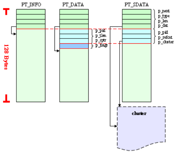
89
FIGURE 4.2.2: THE PBUF TYPES.
4.2.2.2 PT_DATA pbuf
The PT_DATA pbuf is used to store user data. As we mentioned before, its
maximal usable size is 128 Bytes – sizeof(struct p_hdr) – sizeof(sturct s_exthdr) = 98
Bytes. However, this usable size is only for those pbufs with PF_EXTEND flag unset.
If this type of pbuf with PF_EXTEND flag is set, a cluster buffer whose size is 1024
Bytes by default is attached to it. The PF_EXTEND is for those data whose size
exceeds 98 Bytes and destine to store in a PT_DATA pbuf. The special header in a
PT_DATA type pbuf is shown in Figure 4.2.3 and its data structure is shown below:
struct s_exthdr {
u_int64_t com1;
u_int32_t com2;
char *com3;
}
#define p_pid p_data.EHDR.exthdr.com1
#define p_tlen p_data.EHDR.exthdr.com2
#define p_sptr p_data.EHDR.exthdr.com3
#define p_flags p_data.EHDR.e_data.DHDR.flags

90
#define p_extclstr p_data.EHDR.e_data.DHDR.d_data.DHDR0.ext
The „p_pid‟ is a packet ID. For every Packet-object, they have their own unique
packet ID. However, there is one kind of Packet-Object that does not follow this rule.
It is the duplicate Packet-Object. The duplicate Packet-Object is a Packet-Object
which is duplicated from an existing Packet-Object. For a Packet-Object duplicated
from another Packet-Object, the new Packet-Object will have the same packet ID as
the original Packet-Object‟s packet ID. The „p_tlen‟ is the total length of user data
which is encapsulated as a Packet-Object. This length includes the length of data
which are stored in PT_DATA and PT_SDATA pbuf. Note that the data stored in a
PT_INFO pbuf is not added to the „p_tlen‟. The „p_sptr‟ is a pointer points to a
PT_SDATA pbuf. If a Packet-Object contains a PT_SDATA pbuf, the „p_sptr‟ will
point to it. As for the „p_flags‟, there are five independent values for it, which are
shown in Table 4.2.2. The last member, „p_extclstr‟, is available only if the
PF_EXTEND is set in „p_flags‟. If the PF_EXTEND is set in a Packet-Object, the
Packet-Object will generate a cluster buffer and the „p_extclstr‟ will point to it, just as
Figure 4.2.3 shows. For a cluster buffer in a PT_DATA pbuf, the size of it is 1024
bytes by default. The reason why we introduce a cluster buffer mechanism in a
PT_DATA pbuf is to avoid the problem that the size of stored data may exceed the
usable space in a PT_DATA pbuf.
TABLE 4.2.2: THE VALUE OF P_FLAGS
P_flags
Description
PF_SEND
PF_RECV
PF_WITHSHARED
PF_WITHINFO
PF_EXTEND
Indicate that a Packet-Object is an outgoing packet.
Indicate that a Packet-Object is an incoming packet.
If a Packet-Object contains a PT_SDATA pbuf, then this value
will be set.
If a Packet-Object contains more than one PT_INFO pbuf then
this value will bet set.
If the size of a user data stored in a PT_DATA pbuf is larger than
the useable space in a PT_SDATA, then this value will be set and
the data will be stored in an extended cluster. (See Figure
5.2.3)
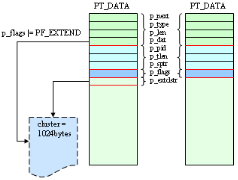
91
FIGURE 4.2.3: THE PT_DATA PBUF.
4.2.2.3 PT_SDATA pbuf
The PT_SDATA pbuf is also used to store user data. However, as its name
indicates, the PT_SDATA pbuf is dedicated to store data which is shared between
Packet-Objects. The PT_SDATA pbuf is introduced in the packet mechanism to save
that memory space and avoid data copy. On the right-hand side of Figure 4.2.1, it
shows a PT_SDATA pbuf is used to store data. From this figure, we can clearly see
that when a PT_SDATA pbuf is created, a cluster buffer is always attached to it. The
length of a cluster buffer depends on the size of user data that will be stored in it. In
the following, we show the special header in a PT_SDATA pbuf:
struct s_exthdr {
u_int64_t com1;
u_int32_t com2;
char *com3;
}
#define p_pid p_data.EHDR.exthdr.com1
#define p_refcn p_data.EHDR.exthdr.com2
#define p_cluster p_data.EHDR.exthdr.com3
The „p_pid‟ is a packet ID. For each Packet-Object, it maintains a packet ID in it.
If a Packet-Object is duplicated from another Packet-Object, the duplicate
Packet-Object will have the same packet ID as the original Packet-Object‟s packet ID.
The „p_refcnt‟ is a reference count used to indicate how many Packet-Objects share
this pbuf. The „p_cluster‟ is a pointer that points to a cluster buffer. When a
PT_SDATA pbuf is created, a cluster buffer is generated and attached to it.
92
The maximal usable size of a PT_SDATA pbuf is unlimited. It is different from
that of a PT_DATA pbuf (The maximal usable size of a PT_DATA is 1024Bytes by
default). This is because a user data to be stored in a PT_SDATA pbuf will be stored
in a cluster buffer and its size depends on the size of a user data. From Figure 4.2.1
we can see that the cluster buffer of the PT_SDATA pbuf has a reserved space. This
reserved space is of length of 98 bytes, which is the size of total usable space in a
PT_DATA pbuf. The purpose of this reserved space is for the pkt_aggregate() packet
API. A user data encapsulated as a Packet-Object may be divided into two parts and
stored in different types of pbuf. Just as Figure 4.2.1 shows, a whole IEEE 802.11
frame is divided into two parts and are stored in a PT_DATA and a PT_SDATA pbuf,
respectively. Hence a continuous frame is divided into more than one fragment and
these small fragments will be stored in different pbufs separately. By doing so, the
contents of a packet may be discontinuous. A discontinuous packet in some situation
may cause some problems. For example, if users want to access the whole data which
is encapsulated as a Packet-Object and stored in different pbufs, then it will cause the
simulator to crash when users access a discontinuous point. We can clearly see this
situation from Figure 4.2.1. The IEEE 802.11 frame which is encapsulated as a
Packet-Object is divided into two small fragments (One for IEEE 802.11 header plus
ether header and one for IP datagram). Users can access this frame via the pkt_get()
packet API which is supported by NCTUns. The pkt_get() API returns the head of a
frame. Under this situation in Figure 4.2.1, users can only directly access the data
stored in a PT_DATA pbuf through this API (in this case IEEE 802.11 header and
ether header). If users try to access the data which are not stored in the PT_DATA
field (in this case, IP datagram), the simulator will crash. This crash results from the
fact that whole IEEE 802.11 frame is not stored in a continuous space. NCTUns
provides another API for users to directly access the whole user data – the
pkt_aggregate(). If users want to directly access the whole data which is encapsulated
as a Packet-Object, they can use the pkt_aggregate() API first to get the whole data
which is stored in a continuous space. The operation that the pkt_aggregate() API
does is to copy user data stored in a PT_DATA pbuf to the reserved space in a cluster
buffer of a PT_SDATA pbuf. This is why the length of the reserved space in a cluster
buffer of a PT_SDATA pbuf equals to that of the usable space in a PT_DATA pbuf.
However, this API will generate a performance overhead. Whenever this API is used,
it will copy data from a PT_DATA pbuf to a PT_SDATA pbuf. This will lower the
simulation performance.
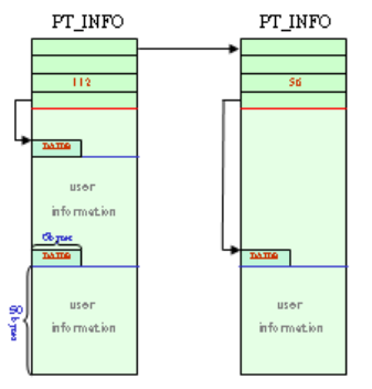
93
4.2.2.4 PT_INFO pbuf
The PT_INFO pbuf is not used to store user data. Instead, it is used to store
information about stored data. The packet information is something about data
description. For example, a receiving host in a simulated network may need to know
from which host an incoming packet originates. This information may be stored in a
PT_INFO pbuf by the originating host. The PT_INFO pbuf has no special header. It
only has a command header. Hence the usable size of this type of pbuf is 114 Bytes
(128Bytes – sizeof(struct p_hdr) = 114 Bytes).
The PT_INFO pbuf uses a special way to store user‟s data information. It divides
the usable space in a PT_INFO pbuf into many small blocks. By default, each block is
56 Bytes in length (6 Bytes for information name and 50Bytes for packet information).
Hence for each PT_INFO pbuf, it can store only two user‟s packet information
(114/56 = 2). Figure 4.2.4 shows the architecture of a PT_INFO pbuf. We can clearly
see that the size of each block is 50bytes plus 6byes. If any packet-information is
stored in a PT_INFO pbuf, we should give it a unique name. The length of this unique
name is 5bytes and the last byte is „\0‟. This name will be used by a Packet-Object to
uniquely identify a packet-information in a PT_INFO pbuf. From this figure, we also
can see that all the PT_INFO pbufs are chained together. As we said before, each
PT_INFO pbuf can store only two user‟s packet-information. Hence if more than two
packet-informations need to be stored in a Packet-Object, then the Packet-Object will
generate two PT_INFO pbufs and chain them together. This makes that there is no
limitation for a Packet-Object to have a limited number of PT_INFO pbuf.
FIGURE 4.2.4: THE PT_INFO PBUF.

94
4.2.3 Event Manager
The Event Manager is a component in the S.E used to manage all static events.
The static event is an event which is not originated from any module. Instead, the
static event is originated from an event table at the starting time of a simulation. The
event table is a table used to record all events which are registered with the event table
by users. It keeps all of the information about every static event. At the initial state of
a simulation, the S.E reads the event table and generates a static event for each entry
in the event table for Scheduler dynamically. After the initial state, users can
dynamically enable or disable a static event which is being scheduled in the Scheduler
component through the dispatcher component in the S.E. For the event table, we list
its data structure below:
struct event-table {
char *name; /* event name */
char flag; /* the state of current event: Active/Inactive */
u_int64_t period; /* periodical time to call handler */
void *data; /* the parameter to handler */
/* call out handler: either a normal function
* or a member function of an object */
NslObject *calloutObj;
int (NslObject::*memfun)(Event *);
int (*func)(Event *);
};
4.3 Scheduler
The Scheduler in the S.E is the most important component. It maintains a system
global virtual time. Every events, no matter whether generated by a module or the
event table, should be triggered based on this system global virtual time. According to
Figure 4.1, we can see that the Scheduler component implements two small
mechanisms. Hence, in the following, we illustrate these two mechanisms with the
following piece of code:
for(currentTime_=0; currentTime_<simulateTime_; currentTime_++) {
/* Event-Scheduler mechanism implementation*/

95
{
/* schedule all inserted events */
while( some expired events exist ) {
call out the handler function specified in the expired event
}
/* schedule all inserted timer */
while ( some expired events exist ) {
call out the handler function specified in the expired timer
}
}
/* Polling mechanism implementation */
{
/* IFQ Polling implementation */
while( all used tunnel interface ) {
if there is a packet in a tunnel interface,
pass the packet to its corresponding module stream
}
/* MBPQ Polling implementation */
while( all registered MB ) {
if a packet in a queue in the MB could be passed to a module,
then we call the module with this packet as an argument.
}
}
}
1. Event Scheduler
The event scheduler is used to schedule all events which are inserted into the
Scheduler. In the Scheduler, it maintains a system global virtual time. If this
time equals to the timeStamp_ in an event, the event will be processed by the
Scheduler. From the above pseudo code, we can see that the implementation
of the event scheduler contains two sub-mechanisms:
a. event scheduling
The event scheduling is used to schedule all events. It maintains a heap
data structure to hold all inserted events. If an event is inserted, it will
be placed in the heap according to the timeStamp_ in the event. When
the timeStamp_ in an event equals to the system global virtual time, the
Scheduler will call the handler function which is specified by the
96
expired event. In addition, the expired event will also be passed to the
handler function as an argument.
b. timer scheduling
The timer scheduling maintains a single linked-list to hold all registered
timer. A timer, in fact, is an event. However, there is still some
differences between them, which were mentioned before. If a timer is
inserted into the Scheduler, the timer scheduling will store it in the
single linked-list according to the timeStamp_ in the timer. Similarly,
when the timeStamp_ in a timer equals to the system global virtual time,
the timer will be processed by the Scheduler.
2. Poller
The Poller mechanism is used in the following mechanism:
a. IFQ polling
The Interface Queue (IFQ) is a queue which holds each registered
tunnel network interface used in a simulated network. Before a
simulation starts, each used tunnel network interface should be
registered with the Scheduler. Therefore, the Scheduler will poll the
IFQ periodically to check if there is any packet in a tunnel network
interface queue. If yes, the packet will be read out of a tunnel network
interface where the packet is queued. Then the Scheduler will call a
module stream and pass the packet to it as an argument. The module
stream will be discussed in the next chapter.
b. MBPQ polling
The MBPQ (Module Binder Polling Queue) is a queue for the module
binder polling mechanism. The module binder is a component in a
module used to bind modules together. For a module binder, it
maintains a queue to hold packets. Once a packet is hold in a queue in a
module binder, the module binder will ask for a polling request from
the Scheduler. The Scheduler then will insert this request to the MBPQ.
In every time unit of the system global virtual time, the Scheduler will
check the request in the MBPQ and polls each registered module binder.
If the Scheduler finds that a packet in a module binder queue could be
pushed into its corresponding module, the module will be called with
the packet as an argument.
97
4.4 Dispatcher
The Dispatcher in the S.E is used to communicate with other external
components. In NCTUns, GUI or tcsh can dynamically add a module to or remove a
module from a node through the network/IPC mechanism while the simulator is
running. For example, when NCTUns is running, users can use tcsh to dynamically
add a tcpdump module to some nodes to capture packets that they interest. Figure
4.2.5 depicts the communication mechanism of NCTUns. Where the Coordinator
(C.O) is a translator used to encapsulate messages exchanged between the simulator
and GUI/tcsh, which are special messages known by C.O and S.E only. From this
figure, the simulator uses the Dispatcher component in the S.E to communicate with
other external components. Hence there must be some special message known by the
Dispatcher and C.O, which are shown below:
1. Messages from C.O to Dispatcher:
From [C.O | GUI | tcsh ID] : Opcode Instruction-Format
From [C.O | GUI | tcsh ID] : generated from C.O
Opcode Instruction-Format generated from GUI/tcsh
2. Messages from Dispatcher to C.O:
To [C.O | GUI | tcsh ID] : Opcode Instruction-Format
To [C.O | GUI | tcsh ID] : generated from Dispatcher
Opcode Instruction-Format generated from Modules or Dispatcher itself
The Instruction-Format shown above depends on the Opcode. For the components
which are on the left-hand side of Figure 4.2.5, the commands they generate are only
in the “Opcode Instruction-Format” format. Once the C.O receives a command from
them, the C.O will encapsulate the command as “From [C.O | GUI | tcsh ID] :
Opcode Instruction-Format” format and send it to the Dispatcher. Then the
Dispatcher will interpret it. Contrarily, if the C.O receives a command from the
Dispatcher, the command will be in “To [C.O | GUI | tcsh ID] : Opcode
Instruction-Format” format. The C.O has the responsibility to de-encapsulate the
message as “Opcode Instruction-Format” format and sends it to GUI/tcsh. For
example, in NCTUns, it provides a service for users to get information about a
module while the simulation is running. In this case, the Opcode which the Dispatcher
provides is “Get”. The instruction format of the “Get” Opcode is as follows:
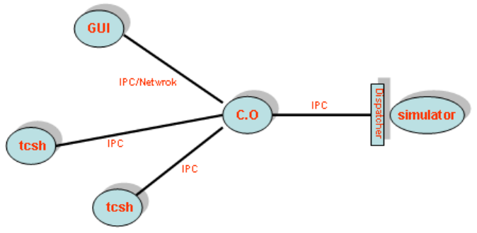
98
Get nodeID portID module_name var_name
By using this opcode, the tcsh can send a “Get 1 1 IFQUEUE queue-length”
command to the C.O to get a queue length of port 1 in IFQUEUE module on node 1.
When the C.O receives this command, it encapsulates it as “From tcsh 1001 : Get 1 1
IFQUEUE queue-length” and sends it to the Dispatcher. After the Dispatcher
receives this command, it de-encapsulates the command as “Get 1 1 IFQUEUE
queue-length” and parses it. For this “Get” request, the Dispatcher will find a module,
named IFQUEUE, with portID=1 and nodeID=1 and then pass the „var_name‟,
„queue-length‟, to that found module. The module will return the value of its
queue-length to the Dispatcher. The Dispatcher then again encapsulates it as “To tcsh
1001 : Data 100” and sends it to the C.O. The C.O de-encapsulates the command as
“Data 100” and then sends it to tcsh, which is numbered 1001. The number 1001 is
an ID of a tcsh. For each tcsh on the simulator, it should have a unique ID to be
identified by the simulator and C.O.
FIGURE 4.2.5: THE SIMULATION ENGINE COMMUNICATES WITH
EXTERNAL COMPONENTS.
4.5 Module Manager
The Module Manager (M.M) component in NCTUns manages all modules that it
creates. When the simulation starts, the module manager uses the topology
information, which is generated from the Script Interpreter component, to create a
99
network topology and network nodes. A network topology is formed by connecting
nodes together and a node is composed of modules. Hence, the module manager
keeps all the information about each node‟s organization and their connectivity. In the
following, we will discuss a Module-Register Table used in the Module Manager:
struct Module_Info {
char *cname_;
NslObject* (*create_comp_)
(u_int32_t, u_int32_t, u_int32_t, char *);
SLIST_HEAD(, Instance) hdInst_;/* pointer to Instance */
SLIST_ENTRY(Module_Info) nextInfo_;
} ;
The above data structure is a Module-Register Table used for module registration.
Any module used in a simulation should be registered with this table. In this table, the
„cname_‟ is a module name. For each registered module, it should have a unique name.
Next, „create_comp_‟ is a function pointer to a module creation function. If a module
is used, a corresponding module creation function should be called to create a module
instance. The „hdInst_‟ is a pointer to an instance list, which is a list used to chain all
instances generated from the same module in a link-list. For the Instance List, Figure
4.2.6 depicts an example of the Module-Register Table:
struct Instance {
NslObject *obj_; /* pointer to Instance */
struct Module_Info *mInfo_; /* pointer to module info */
SLIST_ENTRY(Instance) nextInst_; /* next Instance */
};
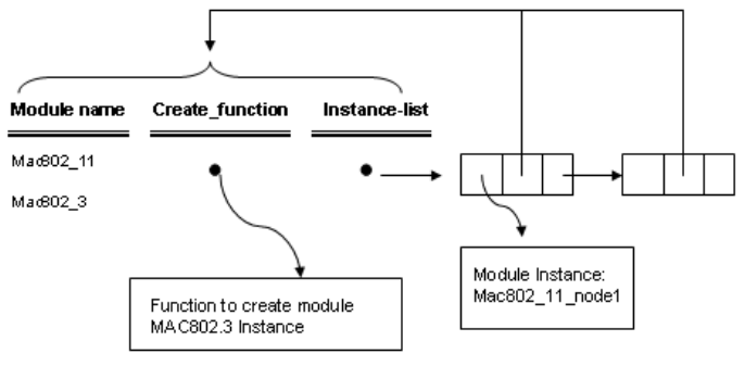
100
FIGURE 4.2.6: AN EXAMPLE OF THE MODULE-REGISTER TABLE.
As Figure 4.2.6 shows, when a module is used, the M.M will find its
corresponding module name and call its module create function to generate a new
instance. Then the new instance will be chained to the instance list. The M.M uses this
table to manage all modules in a simulated network.
In addition to the table mentioned above, the M.M also maintains a special
module for each node, which we call this special module “Node Module”. This
module maintains a table about all modules that it uses, which is shown below:
struct mTree {
NslObject *obj_; /* pointer to module Instance */
struct Module_Info *mInfo_; /* pointer to Module Name */
SLIST_ENTRY(mTree) nextmt_;
};
#define Module_List struct mTree
/*data structure for Port-List table */
struct pTree {
u_int32_t portid_; /* port ID */
SLIST_HEAD(, mTree) hdrMod_; /* pointer to module tree */
SLIST_ENTRY(pTree) nextpt_;
}
struct pTree *Port_Lis;t
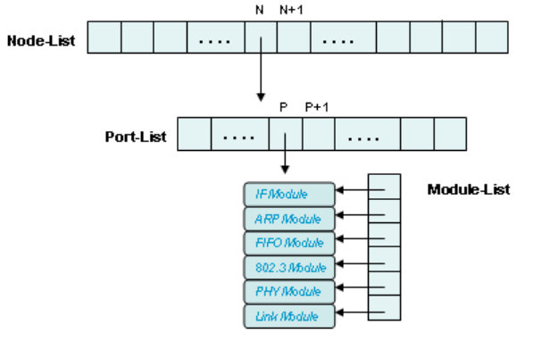
101
FIGURE 4.2.7: MODULE MANAGEMENT IN A NODE MODULE.
As Figure 4.2.7 and above data structure show, a node module uses a Port-List
table to maintain all modules in a node. In this table, each entry of it is a pointer
points to a Module-List, which is shown in this figure. Besides the tables mentioned
above, there is a Node-List table used to maintain all node modules. The M.M keeps
this table to manage these special modules.
4.6 Script Interpreter
The Script Interpreter component in the S.E is used to parse a topology file to
create a network topology in the simulation. The topology file is a file used to
describe a network topology and the organizations of nodes. Like what we said before,
NCTUns allows users to create any network device such as switch, hub, etc. However,
modules must be connected in a controlled way. After a topology is parsed, the M.M
component is responsible for dynamically creating and managing a network topology
according to the information from the Script Interpreter component. For the topology
file, the Script Interpreter component uses a simple syntax to describe a network
topology. In the following, we list a framework of a topology file:
[ Global Variable Section ]
[ Node-Organization Section ]
[ Line Connectivity Section ]
Run <Simulation Time>
1. Global Variable Section
This section is used to initialize some variables used in NCTUns. This section is
102
optional. If nothing needs to be initialized, this section does not need to exist in a
topology file. The syntax of this section is shown below:
Set Variable_Name = value
2. Node Organization Section
This section is used to describe a node‟s organization. The syntax of this section
is shown below:
Create Node [node_ID] as [Device_Type] with name = [Device_Name]
Define Port [Port_ID]
[Module Declaration Subsection]
[Binding Subsection]
[Variable Setting Subsection]
EndPort
EndCreate
For the Create statement, it may contain more than one port section. The port
section is used to describe a port organization. In a port section, it also contains
three subsections:
a. Module declaration: Module [Module_Name] : [Module_Instance_Name]
The subsection is used to describe a port‟s organization. For example, in
the port 1 of a switch node, it may contain a FIFO Module, 802.3 MAC
Module and a PHY Module, which are showing below:
Define Port 1
Module FIFO : FIFO_Port_1
Module MAC8023 : MAC_Port_1
Module PHY : PHY_Port_1
EndDefine
In the above example, the FIFO, MAC8023 and PHY are the module
name. Whenever a module is developed, it should be registered with
NCTUns and give it a name. This name is the Module_Name. The
FIFO_Port_1, MAC_Port_1 and PHY_Port_1 are the
Module_Instance_Name. It means that a module instance is generated
from a registered module.
b. Binding: Bind [Module_Instance_Name] [Module_Instance_Name]
The Bind subsection is used to bind together modules used in a port. A
module may have input entries to accept packets destined for it and
output entries to push packets to other modules. The Binding subsection
103
is used to tell a module which modules are at its input entries and which
modules are at its output entries. For the above example, the binding
subsection should be as follows:
Bind FIFO_Port_1 MAC_Port_1
Bind MAC_Port_1 PHY_Port_1
In the above statements, they describe that the output entry of
FIFO_Port_1 is MAC_Port_1 and the input entry of MAC_Port_1 is
FIFO_Port_1. Similarly, the output entry of MAC_Port_1
isPHY_Port_1 and the input entry of PHY_Port_1 is MAC_Port_1.
c. Variable Setting: Set [Module_Instance_Name].Variable = value
The Variable Setting subsection is used to initialize a variable in a
module. As the above statement shows, the “Variable_Name” is a name
of a variable. We use the notation
Module_Instance_Name.Variable_Name to uniquely identify a variable
in a module.
3. Line Connectivity Section
This section is used to describe a node‟s line connectivity. The syntax of this
section is as follows:
Connect [WIRE | WIRELESS] NodeID.Module_Instance NodeID.Module_Instance
4. Run <Simulation_Time>
This section is used to start a simulation. The <Simulation_Time> is the time to
simulate.
In the Script Interpreter component, it maintains a command table for parsing a
script file. The data structure of this command table is shown below:
struct cmdTable {
char *cmd_name_; /* command name */
int (TclObject::*method_)(int, char **); /* action code */
};
We discussed that the Script Interpreter provides a „Set‟ command for setting
variable values in a module. Besides the command table mentioned before, the Script
Interpreter maintains a variable-binding table for each node for this command
implementation. When the Script Interpreter reads a „Set‟ statement, it will use a
variable name in the „Set‟ statement to look up its corresponding variable in the
variable-binding table. If it finds that the variable has been registered with the
variable-binding table, the corresponding variable in the variable-binding table will
be set to a value which is specified in the „Set‟ statement. Otherwise, another
104
mechanism for the „Set‟ command is used. This mechanism will be discussed in
subsection 5.4.2. In the following, we show the data structure of a variable-binding
table:
typedef struct bindLisst {
char *vname;
void *var;
int (TclBinder::*func_)(void *, char *);
} bindList;
typedef struct bindTable {
struct bindTable *next_;
NslObject *obj_;
bindList varlist_[MAX_BIND_VARS];
int blidx_; /* index of bind list */
} bindTable;
For each node, the Script Interpreter component maintains such a table for it.
Each variable in a module should be registered with this table if it wants to be
initialized in a topology file when a simulation starts. For such a table, it has a
limitation on the number of bound variables in a node. It is indicated by the
MAX_BIND_VARS.
4.7 The NCTUns APIs
The S.E provides many APIs for modules. Any request to the S.E from a module
should be through these APIs. For the detailed descriptions of these APIs, please see
Chapter 6 in this document.
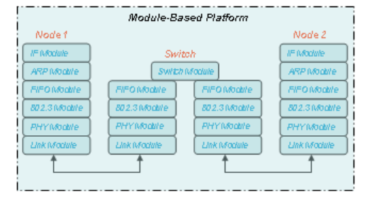
105
Chapter 5 Module-Based Platform
5.1 Introduction
NCTUns provides a module-based platform for module developers to easily
develop their modules and integrate them into our network simulator. A module may
be a network protocol such as IEEE 802.3 MAC protocol. By developing and
combining modules of interest to them on this platform, they can create a special
device node on our network simulator. Figure 5.1 depicts a network topology
consisting of three nodes and the organization of each node.
FIGURE 5.1: THE MODULE-BASED PLATFORM.
In the module-based platform, NCTUns connects all modules in a node to form a
stream. A stream is a full-duplex processing of packets and a packet transfer between
the kernel and the event scheduler on our simulator. Figure 5.1.2 depicts an example
of a node‟s stream mechanism in NCTUns. In this figure, packets are generated from
the kernel and the event scheduler has the responsibility for reading a packet from the
kernel and pushing it into the stream of the node. As the figure shows, the stream
comprises module 1, module 2, module 3 and module 4. For each module here, it is an
implementation of a network protocol. If a module receives a packet from its previous
module, the module will process it and then try to push it to next module. We use „try‟
here is because the next module may be busy. If it is busy, then it will reject the
processing request from its previous module. Note that a node‟s previous or next
module depends on the flow direction. For example, in the downstream, the previous
module of module 2 is module 1 and the next module is module 3. Contrarily, in the
upstream, the previous module of module 2 is module 3 and next module is module 1.
The module which is pushing a packet to its next module will queue the packet
in its queue, if its next module cannot accept the processing request of the packet
immediately. Hence, for each module, it at least contains a pair of queues – a send
queue for downstream and a receive queue for upstream. The send queue and receive

106
queue in a module buffer packets which should be delivered to the module‟s next
module. But, the send queue buffers downstream packets and the receive queue
buffers upstream packets. If a packet is queued in a module due to the fact of that the
module‟s next module is busy, the module will make a polling request to the
Scheduler. When the busy module becomes idle, the Scheduler will push the packet
into it immediately.
In the stream architecture, the downstream is used to simulate a node‟s packet
transmissions and the upstream is used to simulate a node‟s packet receptions in
NCTUns. In which, the message type transmission between modules in a stream is an
ePacket_ (The ePacket_ was discussed in chapter 4). In this chapter, we will discuss
the architecture of a module and how to bind modules together to form a stream (or a
node). In addition, we will also discuss the communication in a module.
FIGURE 5.1.2: A STREAM MODEL IN NCTUNS.
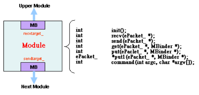
107
5.2 Module Framework
NCTUns provides a basic module prototype. Every module developed by users
must inherit from this basic module prototype. Figure 5.2.1 shows such a prototype.
In this figure, we can see that a module at least contains a recvtarget_ and a
sendtarget_, which are in the type of MBinder (MB). The Mbinder is a data structure
used to bind modules together. We will discuss it in the next subsection. For a module,
it can have more than two MBinders. For instance, for a 12-port switching module, it
could have 12 MBinders to bind its next modules. On the right-hand side of the same
figure, it depicts that a module should implement seven special member functions.
Due to these member functions, a module framework with a stream mechanism can be
constructed.
FIGURE 5.2.1: THE MODULE FRAMEWORK.
Figure 5.2.2 shows the data structure of a basic module, which we call it
NslObject. As we said before, any module should inherit from this basic module.
Hence for a module data structure declaration, we should have the following
statements:
Class <Object_Name> : public NslObject {
};
In the declaration of the basic module data structure, which is shown in Figure
5.2.2, we can divide it into three parts – module identifier, module binder and
implementation. In the following, we will discuss them separately.
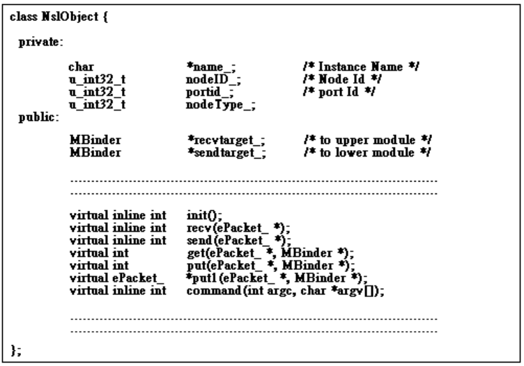
108
FIGURE 5.2.2: MODULE DATA STRUCTURE.
5.2.1 Module Identifier
From Figure 5.2.2, we can see that we use four variables to uniquely identify a
module – name_, portID_, nodeID_ and nodeType_. As discussion in section 4.6, a
module is created by the following command in a script file (or topology):
Module <Module_Name> : Module_Instance_Name
The Module_Instance_Name in the above command is assigned to the variable
„name_‟. But the nodeID_ and nodeType_ depend on the following script command:
Create Node <Node_ID> as <Node_Type> with name = <Device_Name>
The <Node_ID> and <Node_type> in above command is assigned to the „nodeID_‟
and „nodeType_‟, respectively. As for the „portID_‟, when the following command is
read, this value will be assigned automatically:
Define Port <Port_ID>
…………………………….
EndDefine
As mentioned before, any module used in NCTUns should inherit from the
NslObject module. This makes that the module identifier of a module which is
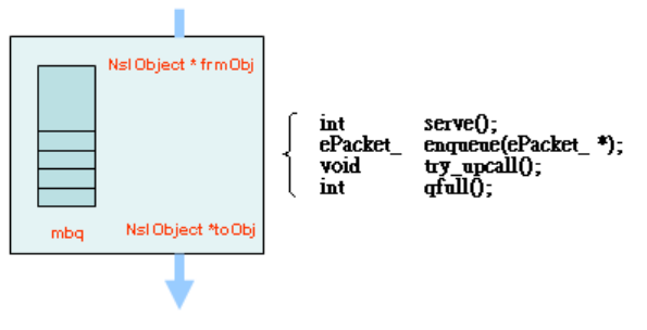
109
inherited from the NslObject module automatically be set. If an access to the
information is needed, the NslObject module provides several APIs for module
identifier access.
5.2.2 Module Binder
For each module, the module binder is used in a module to bind to its next
module. As Figure 5.1.2 shows, all modules are bound together to form a stream. In
such a simple stream, it can be divided further into downstream and upstream. For the
downstream, it is used to simulate packet transmissions. Contrarily, for an upstream, it
is used to simulate packet receptions on a node. Hence, for the downstream of a
stream mechanism, a module binder (here the sendtarget_ variable shown in Figure
5.2.2) should be used in each module to bind to its next module. Contrarily, for the
upstream, a module binder (here the recvtarget_ in Figure 5.2.2) is also needed in
each module to bind to its next module. Generally, a module at least should have two
module binders (both sendtarget_ and recvtarget_) to bind to its next module in both
stream flow directions – upstream and downstream.
Figure 5.2.3 depicts the module binder architecture. In this figure, there is a
queue which we call mbq in a module binder. This queue is used to hold a packet
which can not be pushed to a module‟s next module immediately. As we said before,
after the processing of a packet in a module, the module will push the packet to its
next module. If its next module is in the busy state, then the packet will be hold in a
queue of its module binder. The queue here is the mbq as shown in Figure 5.2.3. In
this figure, there are two variables in a module binder. One is a pointer to next module
and the other is a pointer to the original module. The original module here is the
module itself which uses module binder to binder its next module.
FIGURE 5.2.3: THE MODULE BINDER ARCHITECTURE.
110
In the module binder, there are four basic functions provided by each module
binder, which are shown on the left-hand side of Figure 5.2.3. In the following, we
introduce them separately:
1. enqueue() This function is used to queue a packet into the mbq in a MB.
The return value of this function may be a NULL value or a pointer to a
packet. If a packet is successfully queued in an mbq, then a NULL value is
returned. Otherwise a pointer to the packet is returned. When a non-NULL
value is returned, it means that the mbq is full. If the mbq is full, the MB will
compare the priority of the incoming packet with those packets in the mbq. If
the incoming packet has the lowest priority, then it won‟t be queued into the
mbq. Instead, it will be returned to caller immediately. If it has a higher
priority than those of packets which are already in the mbq, the packet with
the lowest priority in the mbq will be swapped out and returned to caller. And
the incoming packet will be successfully queued into the mbq.
2. qfull() The qfull() in the MB is used to check if a mbq is full or not. By
default, the number of packets an mbq can hold is one packet. However, in
NCTUns, it provides some APIs for users to modify this value.
3. serve() In general, the serve() function is called by a poller of the scheduler.
Every time, if module A‟s next module is busy, the packet will be queued in
the mbq of module A‟s MB. Once a packet is queued in the mbq, the MB will
request a polling service from the scheduler. Due to this request, the
scheduler will poll the mbq every time unit. When the scheduler finds that
there is a packet in the mbq and module A‟s next module is idle, the serve()
function of the MB will be called to push the packet in the mbq into module
A‟s next module, which „toOBj‟ points to.
4. try_upcall() For a MB, it provides a mechanism for users to set an upcall
function in the MB. This upcall function will be called when a packet in the
mbq is pushed to a module. About the upcall mechanism, we will discuss it in
subsection 5.2.2.1.
5.2.2.1 Upcall
The upcall in a MB is a mechanism used to call a specified function upon a
packet in the mbq is pushed to a module by serve() function. In the following, we list
the upcall data structure in a MB:
union {
struct {
111
NslObject*coObject_;
int(NslObject::*upcallm_)(MBinder *);
} str_1;
int(*upcallf_)(MBinder *);
} un;
#define coObj un.str_1.coObject_
#define m_upcall un.str_1.upcallm_
#define f_upcall un.upcallf_
In the above declaration, we can see that an upcall function could be either a
member function or a general function. But for any type of upcall function, its
function prototype should be in the following form:
int <Function_Name | Method_Name> (MBinder mb*) {
}
The „mb‟ parameter in the above prototype may be a pointer to either the
sendtarget_ or the recvtarget_, both of which are module binders and shown in Figure
5.2.1. It depends on which module binder calls the upcall function.
The upcall mechanism in an MB is often used in those modules which maintain
another queue. For example, in a FIFO module, it should maintain a FIFO queue in
the module itself. If the mbq in the MB of a FIFO module is full, the FIFO module
should queue packets into its FIFO queue. In this condition, once the scheduler pushes
a packet in the mbq to a module, the MB will have the responsibility for calling an
upcall function to push a packet in the FIFO module queue to the mbq. If no upcall is
made, the packets in the FIFO module queue won‟t have any chance to be pushed to
the next module, except when a timer is set to periodically poll the FIFO queue to
push packets to the next module.
5.2.2.2 Priority
For each packet, it has a priority field, which is shown in the event data structure.
Figure 5.2.4 depicts the usage of this priority field. As this figure shows, bit-7 and
bit-6 are used to indicate a packet priority. For a packet, it has a four-level priority
ranging from level-1 to level-4. In which, the level-1 is the lowest priority while the
level-4 is the highest priority.
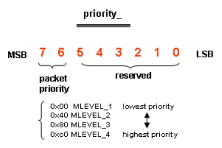
112
FIGURE 5.2.4: THE USAGE OF PRIORITY FIELD.
The packet priority field is used in the module binder. In an mbq, packets with
higher priority are in the front of the mbq and packets with lower priority are in the
tail. Hence whenever serve() function de-queues a packet from a mbq, the packet with
the highest priority will always be chosen. If an mbq is full and there is still a packet
which needs to be queued to the mbq, then the module binder will swap out a packet
with the lowest priority among the packets in the mbq and the incoming packet. The
swapped out packet will be returned to caller. The caller here is a module itself.
5.2.3 Important member functions
Figure 5.2.2 shows that there are seven important member functions in a module.
For a module developer, these seven functions must be implemented, which are
discussed in the followings separately:
1. init() The init() always is called at the simulation start time. For module
initialization, the simulator gives each module a chance to initiate itself.
2. command() The command() is a very import member function in a module.
It is used to communicate with other modules or other components. As
Figure 5.2.2 shows, it has two arguments – argc and argv. The argc is the
number of strings in the argv. And the argv is an array pointer points to each
string. The format of the argv is as follows:
argv = { “string 1”, “string 2”, “string 3”, NULL };
argc = 3
3. recv() If a node receives a packet, the recv() member function of all
modules in the node will be called. Figure 5.2.5 depicts this circumstance.
When a packet is received on a node, the recv() function of all modules in the
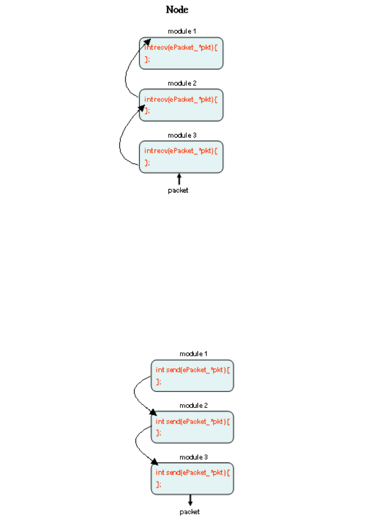
113
node will be called to handle packet reception. As this figure shows, upon
packet is received, the recv() in module 3 is called. After that, the recv() in
module 2 is called by put() or put1() of module 3 and so on. By continuously
calling each module‟s recv() function , an incoming packet could be
processed by every modules on a node.
FIGURE 5.2.5: PACKET RECEPTION.
4. send() The send() is contrary to the recv() function mentioned above. As
Figure 5.2.6 shows, whenever a packet is sent, the send() of the first module
(in this case module 1) will be called. After the process of the first module,
the send() of second module (in the case module 2) will be called by put() or
put1() of module 1. By continuously calling send() function in each module
on a node, the outgoing packet can be processed on every modules to
simulate packet transmissions.
FIGURE 5.2.6: PACKET TRANSMISSION.
114
5. put() The put() function is used in a module to push a packet to the
module‟s next module. If this function is called, it will try to push a packet to
a module. If the module is busy, it will queue the packet to the mbq in the
module binder. If the mbq is full, the packet with the lowest priority among
packets in the mbq and the outgoing packet will be dropped.
6. put1() This function is the same as put(). The only difference between them
is that if the mbq in a module binder is full, a packet with the lowest priority
among packets in the mbq and the outgoing packet will be returned to caller.
This will give the caller a chance to handle the swapped out packet.
7. get() The get() function is used to dispatch packet to send() or recv()
function in a module. Generally, this function is called by put() or put1() of a
module‟s previous module. In this function, it will check a packet flag to see
if the packet is an outgoing or incoming packet. If it is for outgoing, the send()
is called. Otherwise, the recv() is called for the incoming packet.
Figure 5.2.7 depicts the relationship among the get(), put(), put1(), recv() and
send() functions. When the put() function is called in the module 1, the put() function
will try to call get() in module 2. When get() is called in module 2, it will dispatch the
packet to recv() or send(), which depends on whether the packet is an incoming or an
outgoing packet. To distinguish an incoming or outgoing packet, we should check a
flag in the packet structure which indicates whether the packet is an incoming or an
outgoing packet. The dotted line in the figure indicates that the packet in module 1
could not be passed to module 2 immediately. As it depicts, in this case, the put() in
module 1 will queue the packet into the mbq in the module binder. Upon module 2
becomes idle, the scheduler will push the packet in the mbq to get() function of
module 2. The thick line indicates that the module 2 is idle and the put() function of
module 1 can push the packet to module 2 immediately.
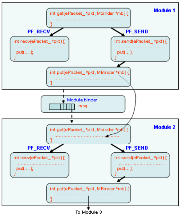
115
FIGURE 6.2.7: THE RELATIONSHIP BETWEEN PUT(), GET() AND SEND().
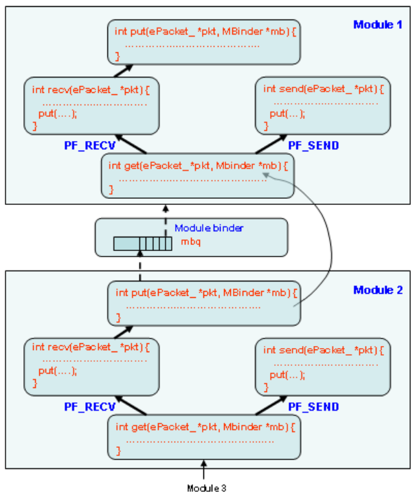
116
FIGURE 5.2.8: THE RELATIONSHIP BETWEEN PUT(), GET() AND RECV().
5.3 Module Communication (M.C)
The module in NCTUns supports a communication mechanism. This
communication mechanism could be divided into two types of communication. One
type of the communication is the communication between modules on a node. We call
this type of communicate as Inter-Module Communication (IMC). The other type is
the communication between module and other external components. Using the IMC, a
module may use some resources in other modules on the same node. If it happens, the
IMC could be used. Using the communication with other external components (e.g.,
the Dispatcher component, GUI, tcsh…etc.). The GUI can communicate with a
module on a node to gather some information about the module. If this happens, this
type of communication should be used. In the following subsection, we will discuss
these two types of communication mechanism separately.
117
5.3.1 Inter-Module Communication (I.M.C)
In a module, the variables it uses could be shared with other modules on the
same node. Before providing shared variables, a module should register the variables
by storing it into a var-register-table on a node first. For example, the MAC 802.3
module in Figure 5.1 may need a variable (here bandwidth) which is used in a PHY
module. The PHY module could register its variable - bandwidth to var-register-table.
Hence the MAC 802.11 module could read this variable through the IMC mechanism.
For each node, NCTUns maintains a special module which we name the Node Module.
This special module is used to manage all module-related information on a node. For
a node‟s var-register-table, it is kept on such a special module. The data structure of a
var-register-table is shown as follows:
struct varRegtbl {
SLIST_ENTRY(varRegtbl) vnext_; /* to next shared variable */
NslObject *obj_; /* pointer to a module */
char *vname_; /* variable name */
void *var_; /* the value of shared variable */
};
NCTUns provides two APIs for IMC manipulations – REG_VAR() and
GET_REG_VAR(). The REG_VAR() is used in a module to register its shared variable
to a node‟s var-register-table. The prototype of this API is as follows:
REG_VAR(vname, var);
The first parameter of above API is a pointer to a name. This name will be used
to uniquely identify a shared variable. The second parameter is a pointer to a shared
variable. Contrarily, the GET_REG_VAR() is an API used to reference a shared
variable in a var-register-table. The prototype of it is shown as follows:
GET_REG_VAR(portid, vname, type);
Where, the parameter, „portid‟ is used to specify the port ID of a shared variable.
The vname is the name of a registered variable. And the „type‟ is used to caste the type
of the returned value.
118
In optical networks, GET_REG_VAR1(portlist, vname, type) must be used
instead of GET_REG_VAR(portid, vname, type) because of the two-layer port
architecture used for optical networks.
5.3.2 Communication with other components
The S.E provides an open mechanism for modules to communicate with other
components. For example, as shown in Figure 3.1 of Chapter 3, we can use tcsh shell
to dynamically set or get a value of the queue length in a FIFO module. Figure 5.2.1
depicts the framework of a module and in this figure we can see that the framework
contains a special member function – command(int argc, char *argv[]). This special
function is provided for the communication between other components. In additional,
this member function is also used in the module manager (M.M) of the S.E to manage
a module.
In the command() member function, it is free for module developers to define
their own syntax in a module. For example, a module may capture incoming or
outgoing packets if a „log‟ command is set through its command() member function.
In this case, it may have the following statements in the command() function.:
int ModuleA::command(int argc, char *argv[]) {
if (argc == 1&& !strcmp(argv[0], “log”)
pkt_capture();
return(1);
}
Whenever a command and a target module are specified (in this case the „log‟
command and Module A module), the S.E dispatches command to the Module A‟s
command() function. The Module A‟s command() function will have the responsibility
to interpret and process the received command.
To respond information to other components, the S.E. provides a message buffer
for each module to reply their information. Only storing information in this message
buffer, the dispatcher is responsible for sending a message to corresponding
components. NCTUns provides two APIs for message buffer manipulation, which is
shown in Chapter 6.
Besides the communication purpose, the command() member function also
provides a module variable setting at the initial state of a simulation. As mentioned
119
before, at the simulation initial state, the S.E reads a script file to create a simulation
network topology. In this script file, it contains a section to describe each node‟s
organization. And in this section, it also has one sub section to initiate each module‟s
variables. To initialize a variable, a „Set‟ command is used in a script file. Once the
Script Interpreter find a „Set‟ statement, it pass this statement to the corresponding
module through this command() of that corresponding module. The following shows
an example:
„Set‟ statement in Script File: Set ModuleA.myvar = 100
int ModuleA::command(int argc, char *argv[]) {
/* argv[0] = “Set”, argv[1] = “myvar”,
* argv[2] = “=”, argv[3] = “100”
*/
if (argc <= 0) return(-1);
if (!strcmp(argv[0], “Set”) && !strcmp(argv[1], “myvar”)) {
myvar = atoi(argv[3]);
return(1);
}
return(0);
}
In fact, the Script Interpreter maintains a variable-binding table. If a „Set‟
command is read, it will look up the variable in the corresponding variable-binding
table. If the variable specified in the „Set‟ command was registered with the
variable-binding table, the variable specified in „Set‟ command is set and the Script
Interpreter won‟t pass the command to command() of the corresponding module.
Otherwise, the command is passed to command(). The detail description of the
variable-binding table is discussed in section 4.6
120
Chapter 6 NCTUns Simulation Engine APIs
6.1 Timer APIs
API Name: init(), start(), cancel(), expire()
Class Name: timerObj
Synopsis:
#include <timer.h>
virtual void init(void)
virtual void start(u_int64_t time, u_int64_t pero)
virtual void cancel(void)
inline u_int64_t expire(void)
Return value:
The function expire() returns the expiration time of a timer. The time unit of
the return value is one clock tick in a simulated system‟s virtual time. By default,
this clock tick in a simulated system‟s virtual time is set to 100ns. If any
modification to this attribute is needed, the following command could be used in
a script file:
Set Tick = 200 ; # 1 clock tick = 200ns
If you want to speed up the simulation, this attribute could be set to a larger
value (e.g., 10 microseconds). However, if a higher accuracy of simulation result
is needed or a simulating a link with very high bandwidth is needed, this attribute
should be set to a smaller value such as 10ns.
Description:
The function init() initialize a timer. When a timer is generated, the init()
function should be called to initialize its internal data structure.
The start() function sets the timestamp of a timer and then inserts the timer
into the S.E scheduler. The first parameter is the timestamp which is the time to
expire this timer. The time unit of this parameter is a clock tick in a simulated
121
system‟s virtual time. The second parameter, „pero‟ is an interval used to
periodically trigger the timer. If its value is zero, the timer is only triggered once.
Otherwise, after the first trigger by the S.E scheduler, every „pero‟ time the timer
will be triggered again. When a timer is active after calling the start() function, a
flag „busy_‟ in the timer will be set to 1 to indicate an active timer.
After a timer is started (in the S.E scheduler), we still have a chance to
cancel the timer. The function cancel() is used for this purpose. When this
function is used, the timer which is in the active state will be set to in the inactive
state. Its flag „busy_‟ will also be set to zero to indicate an inactive timer.
If a timer is active, the function expire() could be used to get the expiration
time of the timer. Note that the time unit of the return value is 1 clock tick in a
simulated system‟s virtual time.
API Name: pause(), resume()
Class Name: timerObj
Synopsis:
#include <timer.h>
virtual void pause(void);
virtual int resume(void)
virtual int resume(u_int64_t time)
Return value:
The function resume() will return value1 if the function call succeeded.
Otherwise, 0 will be returned.
Description:
The function pause() suspends an active timer temporarily. If an active timer
is suspended, the counter of the timer won‟t be counted down until another
function resume() is called to resume the suspended timer. Once a timer is
suspended by using the pause() function, the flag „paused_‟ in the timer will be
set to 1.
122
Once a timer is suspended, the only way to resume it is by calling the
resume() function. The resume() function could continue the count-down of a
timer counter. To resume a suspended timer, two types of resume() function
could be used – one without any parameter while the other with a parameter. The
first one (without parameter) just resumes the suspended timer. The expiration
time won‟t be modified. Contrarily, the second one (with parameter) not only
resumes a suspended timer, it also adds the „time‟ into the expiration time. This
results in that the expiration time of the resumed timer will be extended. For the
resume() function with a parameter, the time unit of its parameter is 1 clock tick
in a simulated system‟s virtual time.
API Name: setCallOutObj(), setCallOutFunc()
Class Name: timerObj
Synopsis:
#include <timer.h>
int setCallOutObj(NslObject *obj, int
(NslObject::*memfunc)(Event_ *))
int setCallOutFunc(int (*fun)(Event_ *ep))
Return value:
The return value of both setCallOutObj() and setCallOutFunc() functions is
1 if these calls succeed.. Otherwise 0 is returned.
Description:
The functions setCallOutObj() and setCallOutFunc() set a handler function
in a timer. When a timer expires, the handler function set by one of these
functions will be called. For a handler function, it could be either a general
function or a member function of an object.
The function setCallOutFunc() is used to specify a general function as a
handler function in a timer. The parameter, „fun‟, of this function is a pointer to a
function, which should be in the following function prototype:
123
int <handler_name> (Event_ *ep) {
}
The parameter of the above handler function is unused so far. Hence it will
be set to a NULL value. The other function setCallOutObj() is used to specify a
member function in an object as a handler function in a timer. The parameter „obj‟
is a pointer to an object and the „memfunc‟ is a member function of its object. For
this kind of handler function, it should use the following prototype:
int <Object_name>::<handler_name> (Event_ *ep) {
}
As with the previous function, the parameter „ep‟ of this kind of handler function
is unused. Thus the value will be set to NULL.
6.2 Packet APIs
API Name: release()
Class Name: Packet
Synopsis:
virtual int release(void)
Return Value:
The return value of the function release() is always 1.
Description:
The function release() releases the memory space what is used by a
Packet-Object. A Packet-Object may contain a PT_DATA pbuf, a PT_SDATA
pbuf and more than one PT_INFO pbufs. The release() function always releases
the PT_DATA pbuf and PT_INFO pbuf. If a Packet-Object contains a
PT_SDATA pbuf, the release() function decreases the reference count in the
124
PT_SDATA pbuf. When the reference count reaches zero, the PT_SDATA pbuf
will be released by the release() function.
API Name: copy()
Class Name: Packet
Synopsis:
#include <packet.h>
virtual Packet *copy(void)
Return Value:
The return value is a pointer to a new packet, which is a duplicated packet
of the original one if this function succeeds. Otherwise, a NULL value is
returned.
Description:
The copy() function duplicates an original Packet-Object. A Packet-Object
may contain a PT_DATA pbuf, a PT_SDATA pbuf and more than one PT_INFO
pbufs. Among these three types of pbuf used in a Packet-Object, the copy()
function only duplicates the PT_DATA pbuf and PT_INFO pbuf. The
PT_SDATA pbuf won‟t be duplicated by the copy() function because the
PT_SDATA pbuf is a shared pbuf, which is shared by Packet-Objects that are
duplicated from the same Packet-Object. If a Packet-Object which contains a
PT_SDATA pbuf is duplicated through the copy() function, a reference count in
its PT_SDATA pbuf will be increased and a pointer in both the original
Packet-Object and the duplicated Packet-Object will point to the shared
PT_SDATA pbuf. The following figure depicts a Packet-Object duplication
operation, in which the Packet-Object contains a PT_DATA pbuf, a PT_INFO
and a PT_SDATA pbuf:
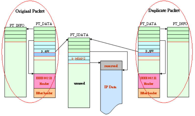
125
FIGURE 6.2.1: A PACKET-OBJECT DUPLICATION.
API Name: pkt_malloc()
Class Name: Packet
Synopsis:
char *pkt_malloc(int len)
Return Value:
The return value is a pointer to the beginning of a free space in a PT_DATA
pbuf. If there is not enough space for this request, a NULL value is returned to
indicate the failed operation.
Description:
The pkt_malloc() function allocates „len‟ bytes of memory space in a
PT_DATA pbuf which is contained in a Packet-Object. The allocated space could
be used for storage of any transmitted data. If the pkt_malloc() succeeds, the data
length of both PT_DATA pbuf and the whole Packet-Object is increased by the
length of „len‟.Up to 98 bytes usable memory space is allowed in a PT_DATA
126
pbuf. If a larger space is requested, the PT_DATA pbuf will allocate another
cluster (1024 bytes by default) for storage of data. Note that pkt_malloc() does
NOT normally initialize the returned memory in a PT_DATA pbuf to zero bytes.
The following is a usage example:
char data2[500];
int main(int argc, char *argv[]) {
Packet *mypkt;
ether_header *eh;
char *ptr;
/* Create a packet-object */
mypkt = new Packet;
/* Store ether-header in PT_DATA pbuf */
eh = (ether_header *)mypkt->pkt_malloc(sizeof(struct ether_header));
(void)memcpy(eh->ether_dhost, dst_mac_addr, 6);
(void)memcpy(eh->ether_shost, src_mac_addr, 6);
eh->ether_type = ETHERTYPE_IP;
/* Store 500bytes data in PT_DATA pbuf */
ptr = mypkt->pkt_malloc(500);
(void)memcpy(ptr, data2, 500);
}
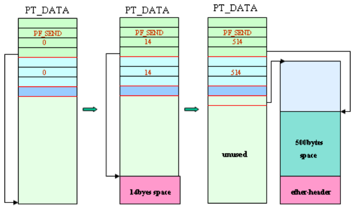
127
FIGURE 6.2.2: AN EXAMPLE OF PKT_MALLOC().
API Name: pkt_prepend(), pkt_sprepend()
Class Name: Packet
Synopsis:
virtual int pkt_prepend(char *data, int length)
virtual int pkt_sprepend(char *data, int length)
Return Value:
The return value of both the pkt_prepend() and pkt_spreoend() is 1 for
success and -1 for failure.
Description:
The pkt_prepend() and pkt_sprepend() functions copy the data specified by
„data‟ parameter into a Packet-Object. The difference between pkt_prepend() and
pkt_sprepend() is that the pkt_prepend() stores the data into the PT_DATA pbuf
in a Packet-Object but the pkt_sprepend() stores data into the PT_SDATA pbuf.
If the „length‟ parameter of pkt_prepend() is larger than the “PCluster” (the
PCluster is the maximum storage size of data that could be stored in a PT_DATA
128
pbuf), this function call will fail and return -1.Contrarily, this limitation won‟t
apply to pkt_sprepend() function because this function has no maximal storage
size limitation. However there is still a limitation on this function. If a
Packet-Object has not had a PT_SDATA pbuf attached to it, this function call of
pkt_sprepend() will fail and return -1.
Although the pkt_prepend() function is somewhat like pkt_malloc(), there is
still a difference between them. The pkt_malloc() only allocates a usable space in
a PT_DATA pbuf. It does not copy data to the allocated space. The pkt_prepend()
function, besides allocating a usable space in a PT_DATA pbuf, copies data to
the allocated space.
API Name: pkt_seek()
Class Name: Packet
Synopsis:
virtual int pkt_seek(int offset)
Return Value:
The pkt_seek() function always returns 1 to the caller.
Description:
The pkt_seek() function strips data from a Packet-Object. If this function is
used, the data in the PT_DATA pbuf of the Packet-Object is stripped off first.
When there is no data in the PT_DATA pbuf, the pkt_seek() tries to strip data
from the PT_SDATA pbuf if there exists a PT_SDATA pbuf in the Packet-Object.
The „offset‟ parameter indicates the length of data to be stripped off. Its value
could be either a positive or a negative value. For a positive value, data in a
Packet-Object is stripped off. For a negative value, the length of a Packet-Object
is increased instead.
129
API Name: pkt_get(), pkt_sget()
Class Name: Packet
Synopsis:
virtual char *pkt_get(void)
virtual char *pkt_get(int offset)
virtual char *pkt_sget(void)
Return Value:
The return value of pkt_get() function is a pointer to the beginning of stored
data in a PT_DATA pbuf. Similarly, the pkt_sget() function returns a pointer to
the caller. But the pointer points to the beginning address of stored data in a
PT_SDATA pbuf if a Packet-Object contains a PT_SDATA pbuf. Otherwise, a
NULL value is returned.
Description:
The pkt_get() and pkt_sget() APIs access data stored in a packet. For the
pkt_get() API, this API could access data which is stored either in the PT_DATA
or PT_SDATA pbuf. If no data in the PT_DTA pbuf, pkt_get() tries to access the
data in the PT_SDATA pbuf. Only if a Packet-Object contains a PT_SDATA
pbuf, will the pkt_get() try to access this type of pbuf.
The „offset‟ parameter in the pkt_get() indicates the offset from which to
access a Packet-Object. For example, suppose that a frame consists of a 14-bytes
ether-header and 100-bytes IP datagram. In this condition, the pkt_get() returns a
pointer to the ether header, but the pkt_get(14) returns a pointer to the
IP-datagram instead of the ether-header.
The function of another API, pkt_sget() is the same as that of pkt_get(). The
only difference between them is that the pkt_sget() only access data in a
PT_SDATA pbuf if the packet has a attached PT_SDATA pbuf. The pkt_get(), on
the other hand, could access both PT_DATA and PT_SDATA pbuf.
130
API Name: pkt_sattach(), pkt_sdeattach()
Class Name: Packet
Synopsis:
virtual char *pkt_sattach(int length)
virtual int pkt_sdeattach(void)
Return Value:
The pkt_sattach() function returns a pointer to the beginning address of a
usable memory space for success. Otherwise, a NULL value is returned. The
pkt_sdeattach() returns 1 for success and -1 for failure.
Description:
The pkt_sattach() function attaches a PT_SDATA pbuf to a Packet-Object.
When a Packet-Object is created, only a PT_DATA pbuf is involved. If a shared
memory space is needed, the pkt_sattach() could be used to attach a shared
PT_SDATA pbuf to the Packet-Object. The „length‟ parameter in pkt_sattach()
indicates the cluster size of a PT_SDATA pbuf. For a PT_SDATA pbuf, it does
not store data in its pbuf. Instead of storing data in the PT_SDATA pbuf, the
PT_SDATA pbuf allocates another cluster to store a great deal of data. The size
of this cluster is not fixed. Instead, the cluster size is specified by the
„length‟ parameter of pkt_sattach() function.
The pkt_sdeattach() function detaches a PT_SDATA pbuf from a
Packet-Object. The memory space used by the PT_SDATA pbuf which is
detached from a Packet-Object will be released only if the reference count in the
PT_SDATA pbuf reaches zero.
API Name: pkt_addinfo(), pkt_saddinfo()
Class Name: Packet
Synopsis:
131
int pkt_addinfo(char *iname, char *info, int length)
int pkt_saddinfo(char *iname, char *info, int length)
Return Value:
The return value is 1 for success, otherwise -1 for failure.
Description:
The pkt_addinfo() copies the packet information specified in „info‟ to a
PT_INFO pbuf in a Packet-Object. The packet information is a description about
the data which is stored in PT_DATA and PT_SDATA pbuf. For example, in
wireless network a PT_INFO pbuf might be used to store the frequency used to
transmit data. If the Packet-Object (the data is encapsulated as a Packet-Object)
contains no PT_INFO pbuf or the PT_INFO pbuf doesn‟t have enough space for
the request, a new PT_INFO pbuf is created by pkt_addinfo() function.
The pkt_saddinfo() function also copies packet information specified by the
„info‟ parameter to a Packet-Object. But the destination pbuf that the
pkt_saddinfo() copies to is a PT_SDATA not a PT_INFO pbuf. For any
PT_SDATA pbuf, a transmitted data is stored in a cluster but not in the
PT_SDATA pbuf itself. The space of a PT_SDATA pbuf is used to store packet
information, which is difference from a PT_INFO pbuf. The packet information
which is stored in a PT_SDATA pbuf is shared information. Because a
PT_SDATA pbuf may be shared by more than one Packet-Object, all
Packet-Objects that share the same PT_SDATA pbuf could have the same
property described by the packet information.
Every packet-information stored in PT_INFO pbuf should have a name.
This name is specified in the parameter „iname‟. The length of packet
information is specified in the „length‟ parameter. Note that the length of a
packet-information should not exceed 50 bytes. This is because each PT_INFO
pbuf is divided into many small blocks to store packet information and each of
them is 50 bytes by default.
132
API Name: pkt_getinfo(), pkt_sgetinfo()
Class Name: Packet
Synopsis:
char *pkt_getinfo(char *iname)
char *pkt_sgetinfo(char *iname)
Return Value:
The return value of both of these two functions is a pointer to a memory
address, which is the starting address of a packet-info buffer if success.
Otherwise, a NULL value is returned.
Description:
The pkt_getinfo() function searches all the PT_INFO pbufs in a
Packet-Object and finds the packet-information which is specified in the „iname‟
parameter. The pkt_sgetinfo() also finds the packet-information specified in the
„iname‟ parameter, but it searches the desired packet information in a
PT_SDATA not in a PT_INFO pbuf. Each packet-information should not exceed
50 Bytes. This is because each PT_INFO pbuf is divided into many small blocks
to store packet-information and each of them is 50 bytes by default.
API Name: pkt_getlen(), pkt_getpid(),
pkt_getpbuf(), pkt_getflags()
rt_gateway()
Class Name: Packet
Synopsis:
virtual int pkt_getlen(void)
u_int64_t pkt_getpid(void)
inline struct pbuf *pkt_getpbuf(void)
inline short pkt_getflags(void)
inline u_long rt_gateway(void)
133
Description:
The pkt_getlen() function gets the total packet length of a Packet-Object.
This total packet length only contains the data stored in the PT_DATA and
PT_SDATA pbuf. The data stored in a PT_INFO pbuf is not treated as normal
data. Hence pkt_getlen() won‟t contains the length of data stored in a PT_INFO
pbuf.
The pkt_getpid() returns a packet ID. Each Packet-Object which doesn‟t
include duplicate Packet-Object always has a packet ID. If a Packet-Object is
duplicated, the duplicated Packet-Object will have the same packet ID as the
original Packet-Object. For example, suppose that Packet-Object A is a
Packet-Object with ID 100. If Packet-Object B is a Packet-Object duplicated
from Packet-Object A, then the packet ID of Packet-Object A and B will be the
same.
The pkt_getpbuf() returns a pointer to a PT_DATA pbuf in a Packet-Object.
If the address of the PT_DATA pbuf is returned, we could use this PT_DATA
pbuf to access the whole pbufs in the Packet-Object.
The pkt_getflags() returns the value of the „p_flags‟ flag in a PT_DATA
pbuf. About the value of this flag, please see the packet introduction.
The rt_gateway() gets a gateway in a Packet-Object. For each
Packet-Object, it has a gateway information. This information may be used in a
routing module to specify the next hop of a Packet-Object.
API Name: pkt_setflow(), rt_setgw()
Class Name: Packet
Synopsis:
inline void pkt_setflow(short flow)
inline void rt_setgw(u_long gw)
134
Description:
The pkt_setflow() marks a Packet-Object as an outgoing or incoming packet.
For an outgoing packet, the PF_SEND should be set in the „flow‟ parameter.
Contrarily, the PF_RECV should be set for an incoming packet.
The rt_setgw() sets the gateway in a Packet-Object. For each Packet-Object,
it has a gateway information. This information may be used in a module that
needs to specify the next hop of a Packet-Object.
API Name: pkt_aggregate()
Class Name: Packet
Synopsis:
inline char *pkt_aggreagate(void)
Return Value:
The return value of pkt_aggregate() function is a pointer to the data stored
in a Packet-Object.
Description:
The pkt_aggregate() gets the data stored in a Packet-Object. It is somewhat
like the pkt_get() or pkt_sget() function. But in fact, the pkt_get() only could
access the data stored in ether PT_DATA or PT_SDATA pbuf, and the pkt_sget()
only could access the PT_SDATA pbuf. If data is divided into two parts and
stored in PT_DATA and PT_SDATA pbufs, respectively, neither pkt_get() nor
pkt_sget() function could access the whole data in the Packet-Object. The
pkt_aggregate() function has no such a limitation. If data is stored in PT_DATA
and PT_SDATA pbufs separately, the pkt_aggreaget() will copy data in both the
PT_DATA and PT_SDATA pbufs into a continuous space to form continuous
data.
A PT_SDATA pbuf has a cluster buffer to store a great deal of data. Besides
135
the space used to store data, the cluster also contains a usable space, whose
length equals to the length of a usable PT_DATA pbuf, which is 98 bytes. If
pkt_aggregate() is called, the pkt_aggregate() tries to copy the data stored in a
PT_DATA pbuf to the usable space in the PT_SDATA. Hence, the data could be
in a continuous space.
Note that if a Packet-Object‟s PF_EXTEND flag is set, the pkt_aggregate()
won‟t copy data in PT_DATA pbuf to PT_SDATA pbuf. Instead, only data stored
in PT_SDATA pbuf is accessed. This is because with PF_EXTEND flag set, the
PT_DATA pbuf in a Packet-Object will use a cluster buffer to store data instead
of the 98 bytes usable space in a PT_DATA pbuf.
API Name: pkt_setHandler(), pkt_callout()
Class Name: Packet
Synopsis:
inline int pkt_setHandler(NslObject *obj, int
(NslObject::*meth_)(Event_ *))
inline int pkt_setHandler(int (func_ *)(Event_ *))
inline int pkt_callout(ePacket_ *pkt)
Return Value:
For the pkt_setHandler() function, the return value is always 1. For the
pkt_callout() function, if success, 1 is returned. Otherwise, -1 is returned.
Description:
The pkt_setHandler() function sets a handler function in a Packet-Object. If
this handler function is set, a module could cause this handler function to be
called anytime. For example, if a module finds some error occurs in a
Packet-Object, it could call the handler function set in the Packet-Object to deal
properly with this packet. A handler function should use one of the following
136
types:
int <Object_Name>::<Handler_name> (ePacket_ *pkt)) {
}
int <Handler_name> (ePacket_ *pkt)) {
}
The „pkt‟ parameter above is a pointer to an ePacket (Event-Packet). When a
handler function is called, the ePacket which specifies the handler will be used as
a parameter of the handler function.
The pkt_callout() function causes a handler function specified in a Packet-Object
to be called. If a handler function is set in a Packet-Object, the pkt_callout() calls
out the handler function. Otherwise, nothing is done and -1 is returned.
6.3 NCTUns APIs
API Name: str_to_macaddr(), macaddr_to_str()
Synopsis:
#include <nctuns_api.h>
void str_to_macaddr(char *str, u_char *mac)
void macaddr_to_str(u_char *mac, char *str)
Description:
The str_to_macaddr() function forms a 48-bits IEEE 802 address with
numerical representation by analyzing input-string, which contains the IEEE 802
address with textual representation. The „str‟ parameter is a 6-bytes IEEE 802
address with textual representation. The „mac‟ parameter is a pointer to the space,
which is filled with numerical representation of address.
The macaddr_to_str() function forms an IEEE 802 mac address of the form
137
xx:xx:xx:xx:xx:xx, which is the textual representation formed by converting
numerical representation of 48-bits IEEE 802 mac address. The parameter „mac‟
is a pointer to a 48-bits IEEE 802 mac address with numerical representation.
The „str‟ is a pointer to a buffer space to store the IEEE 802 mac address with
textual representation.
API Name: ipv4addr_to_str(), str_to_ipv4addr()
Synopsis:
void ipv4addr_to_str(u_long ipv4addr, char *str)
void str_to_ipv4addr(char *str, u_long ipv4addr)
Description:
The ipv4addr_to_str() function forms an IPv4 address of the form
xx.xx.xx.xx, which is the textual representation formed by converting a
numerical representation of the IPv4 address. The „ipv4addr‟ parameter is an
unsigned-long integer used to store the IPv4 address with the numerical
representation of 32-bit IPv4 address. The „str‟ parameter is a pointer to a space
where the resulting IPv4 address in textual representation is stored.
The str_to_ipv4addr() function forms an IPv4 address in numerical
representation by converting the textual representation of the IPv4 address. The
„str‟ parameter is a pointer to an IPv4 address in textual representation and the
„ipv4addr‟ is an unsigned-long integer used to store the resulting address in
numerical representation.
API Name: vbind(), vbind_bool(), vbind_ip(), vbind_mac()
Synopsis:
int vbind(NslObject *obj, char *name, int *var)
int vbind(NslObject *obj, char *name, double *var)
int vbind(NslObject *obj, char *name, float *var)
int vbind(NslObject *obj, char *name, u_char *var)
int vbind(NslObject *obj, char *name, char **var)
int vbind_bool(NslObject *obj, char *name, u_char *var)
int vbind_ip(NslObject *obj, char *name, u_long *var)
int vbind_mac(NslObject *obj, char *name, u_char *var)
138
Return Value:
The return value of above functions is 1 for success and < 0 for failure.
Description:
The functions listed above bind a variable in a module to a script file.
Whenever a variable is bound to a script file, the vbind() function registers the
variable with a variable-binding table, which is maintained in the S.E. Once the
simulation starts, the S.E in the simulator reads and parses a script file at its
initial state. In the meantime, upon matching a variable with one registered with
the variable-binding table, the S.E will initialize that variable with the value
specified in the script file. The present binding functions provided by S.E are
listed as below:
1. vbind() The variable the vbind() function binds could be one of
the following data types:
. integer
. double
. float
. unsigned char
2. vbind_bool() vbind_bool() binds a Boolean variable to a script file.
3. vbind_ip() binds an IPv4 address to a script file.
4. vbind_mac() binds a IEEE 802 MAC address to a script file.
API Name: createEvent(), freeEvent()
Synopsis:
Event_ *createEvent(void)
int freeEvent(Event_ *ep)
Return Value:
The return value of createEvent() function is a pointer to a new event. If a
NULL value is returned, it means that the function failed. The return value of
freeEvent() is 1 on success and < 0 on failure.
139
Description:
The createEvent() function creates a new event structure and the freeEvent()
functions releases the space of the event. An event structure has a DataInfo_ field
used to hold any type of data. When the freeEvent() is used to release the
memory space of an event, the freeEvent() first checks the DataInfo_ field in the
event structure to see if it has data attached. If yes, the freeEvent() tries to release
the memory space used by the data pointed by DataInfo_ field.
API Name: setEventTimeStamp(), setEventResume(), scheduleInsertEvent()
setEventCallOutFunc(), setEventCallOutObj()
Synopsis:
int setEventTimeStamp(Event_ *ep, u_int64_t
timeStamp, u_int64_t perio)
int setEventResume(Event_ *ep)
int scheduleInsertEvent(Event_ *ep)
int setEventCallOutFunc(Event_ *ep, int (*fun)(Event_ *),
void *data)
int setEventCallOutObj(Event_ *ep, NslObject *obj,
int (NslObject::*memf)(Event_ *), void *data)
Return Value:
The return value of above functions is 1 on success and < 0 on failure.
Description:
The setEventTimeStamp() function sets the timestamp of an event. The time
unit of a timestamp is 1 clock tick in the simulator‟s virtual time. The first
parameter „ep‟ is a pointer to an event. The second parameter „timeStamp‟ is the
expiration time, whose time unit is 1 clock tick in the simulator‟s virtual time.
The „perio‟ parameter, if it is a non-zero value, causes the event to become a
periodical event.
The setEventResume() function resumes a periodic event. When an event
with a non-zero „perio‟ expires, the setEventResume() could be used to resume
that event immediately without resetting its timestamp. The next expiration time
140
which the setEventResume() sets will be set to the current time + perio. After
that, the event will be reinserted into the scheduler to wait for the next expiration.
The scheduleInsertEvent() inserts an event to the event scheduler. After
setting the event, this function should be used to insert an event into the event
scheduler.
The setEventCallOutFunc() and setEventCallOutObj() functions set a
handler function in an event. For a handler function, it could be either a normal
function or a member function of an object. The setEventCallOutFunc() is for the
normal function and the setEventCallOutObj() is for a member function. The
following shows the prototypes of these two handler function, in which the „ep‟
parameter is a pointer to an event which causes the handler function to be called:
int <Handler_name> (Event_ *ep)
}
int <Object_name>::<Handler_name> (Event_ *ep) {
}
API Name: setFuncEvent(), setObjEvent()
Synopsis:
int setFuncEvent(Event_ *ep, u_int64_t timeStamp,
u_int64_t perio, int (*func)(Event_ *), void *data)
int setObjEvent(Event_ *ep, u_int64_t timeStamp, u_int64_t
perio, NslObject *obj, int (NslObject::*memf)(Event_ *),
void *data)
Return Value:
The return value of above functions is 1 for success and < 0 for failure.
141
Description:
The setFuncEvent() and setObjEvent() functions set an event and then insert
it into the event scheduler. These functions are equivalent to the following
operations:
setFuncEvent() == setEventTimeStamp() + setEventCallOutFunc() +
scheduleInsertEvent()
or
setObjEvent() == setEventToimeStamp() + setEventCallOutObj() +
scheduleInsertEvent()
Sometimes, this kind of function is more convenient for setting and starting an
event.
API Name: set_tuninfo()
Synopsis:
int set_tuninfo(u_int32_t nid, u_int32_t portid, u_int32_t tid,
u_long *ip, u_long *netmask, u_char *mac)
Return Value:
The return value is 1 for success and < 0 for failure.
Description:
The set_tuninfo() function configures a tunnel network interface (in case the
tunnel interface) when a simulation starts. When a node needs a network
interface, this function should be used to assign a tunnel network interface to it.
For a tunnel network interface configuration, the following information should
be configured to it:
. nid node ID the tunnel belongs to.
. portid port ID of the node which use a tunnel network interface.
. tid tunnel ID
. ip for each tunnel, it is treated as a real network interface.
142
Hence an IP should be assigned.
. netmask the netmask of an assigned IPv4 address.
. mac the IEEE 802 mac address a tunnel associates with.
API Name: RegToMBPoller()
Synopsis:
int RegToMBPoller(MBinder *mbinder)
Return Value:
The return value is 1 for success and < 0 for failure.
Description:
The RegToMBPoller() function registers a polling request of a
Module-Binder(MB) with the Module-Binder Poller(MBP). The MB is a
mechanism to bind two modules together. In the MB, there is a queue used to
hold packets. If a packet could not be pushed to the next module immediately,
this packet will be queued in a queue and a polling request is issued. Later, if the
module can process another packet, the S.E scheduler will dequeue the packet
from the queue in the MB and push it to the next module.
API Name: nodeid_to_ipv4addr(), ipv4addr_to_nodeid()
Synopsis:
u_int32_t nodeid_to_ipv4addr(u_int32_t nid, u_int32_t port)
u_int32_t ipv4addr_to_nodeid(u_long ip)
Return Value:
The return value of nodeid_to_ipv4addr() is a 32-bit IPv4 address if the
function call succeeds. Otherwise, a zero value is returned. Contrarily, the return
value of ipv4addr_to_nodeid() is a 32-bit node ID which owns this IPv4 address.
Description:
143
The nodeid_to_ipv4addr() function uses both node ID and port ID to find a
corresponding IPv4 address in a node. One node may have more than one tunnel
network interface. Hence if an IPv4 address is queried in such a node, the port ID
should be specified, which should range from 1 to n, to this node where n is the
total number of tunnel network interfaces attached.
Contrarily, the ipv4addr_to_nodeid() function uses an IPv4 address to query
a corresponding node who has a tunnel interface with this IPv4 address.
API Name: ipv4addr_to_macaddr(), macaddr_to_ipv4addr()
Synopsis:
u_char *ipv4addr_to_macaddr(u_long ip)
u_long macaddr_to_ipv4addr(u_char *mac)
Return Value:
The return value of ipv4addr_to_macaddr() is a pointer to an IEEE 802 mac
address in numerical representation. If a NULL value is returned, it means that
the function failed. The returned value of macaddr_to_ipv4addr() is an IPv4
address in 32-bit numerical representation. If a zero value is returned, the
function call failed.
Description:
The ipv4addr_to_macaddr() function uses an IPv4 address as a key to get
the corresponding IEEE 802 mac address. For each tunnel interface, it is always
associated with an IPv4 address and an IEEE 802 mac address. This function is
used to do the mapping from an IPv4 address to an IEEE 802 mac address. The
other function, macaddr_to_ipv4addr() is used to do the reverse mapping. It
maps a given IEEE 802 mac address to an IPv4 address.
144
API Name: macaddr_to_nodeid()
Synopsis:
u_int32_t macaddr_to_nodeid(u_cahr *mac)
Return Value:
The return value of macaddr_to_nodeid() is a node ID. If a zero value is
returned, it means that the function call failed.
Description:
The macaddr_to_nodeid() function uses an IEEE 802 mac address which is
specified in „mac‟ parameter as a key to find a corresponding node ID. A node
may have more than one tunnel network interfaces attached to it. Each of them
will be associated with an IEEE 802 mac address. The macaddr_to_nodeid()
function is used to map a mac address to its corresponding node ID.
API Name: is_ipv4_broadcast()
Synopsis:
u_char is_ipv4_broadcasat(u_int32_t nid, u_long ip)
Return Value:
If the return value is 1, the examined address is an IPv4 broadcast address.
If a zero value is returned, the examined IPv4 address is an IPv4 address that is
not used for broadcasting.
Description:
145
The is_ipv4_broadcast() function examines a given IPv4 address to see if it
is a layer 3 broadcast address. In the function, the first parameter is a node ID
and the second is an examined IPv4 address.
API Name: getifnamebytunid(), getportbytunid()
Synopsis:
char *getifnamebytunid(u_int32_t tid)
u_int32_t getportbytunid(u_int32_t tid)
Return Value:
The returned value of getifnamebytunid() is a pointer to a interface name. If
a NULL value is returned, the function call failed. The returned value of
getportbytunid() is a port number of a node.
Description:
The getifnamebytunid() function gets a tunnel network interface name. For
each tunnel interface used in a simulated node, the simulator always gives it an
interface name such as fxp0. If an interface name is wanted, this function could
be used to get its name.
The getportbytunid() function gets the port number of a tunnel interface in a
simulated node. For each simulated node, it may have more than one tunnel
interfaces. Similarly, each used tunnel interface should be associated with its
local unique port number. For example, tunnel 2 with port number 1 and tunnel 5
with port number 2 are used in a simulated node 1, respectively. The
getporbytunid(2) returns port number 1 and getportbytunid(5) returns port
number 2.
API Name: GetCurrentTime(), GetNodeCurrentTime()
GetSimulationTime()
Synopsis:
u_int64_t GetCurrentTime(void)
146
u_int64_t GetNodeCurrentTime(u_int32_t nid)
u_int64_t GetSimulationTime(void)
Return Value:
The return value of the above functions is a time in a simulator system‟s
virtual time.
Description:
The GetCurrentTime() function gets the global simulator system‟s virtual
time. In the simulator, the S.E maintains a global system virtual time. All the
components in the simulator use this global time.
The GetNodeCurrentTime() function gets one node‟s virtual time. In order
to reflect the fact that in a real network it is likely that the clocks of nodes are
different from each other, each node should maintain a local virtual time. The
GetNodeCurrentTime() is used to get each node‟s virtual time.
The GetSimulationTime() gets the simulation time in a simulation.
API Name: InstanceLookup()
Synopsis:
NslObject *InstanceLookup(u_int32_t Nid, char *Iname)
NslObject *InstanceLookup(u_int32_t Nid, u_int32_t Pid, char *Mname)
NslObject *InstacneLookup(u_long ip, char *Mname)
Return Value:
The return value of this function is a pointer to a module instance. If a
NULL value is returned, the function call failed.
Description:
The InstanceLookup() function uses some index information to find a
module instance. Those index information include node id (Nid), module name
(Mname), module instance name (Iname), port id (Pid), and interface‟s IP
147
address (ip).
Note that the module instance name is not a module name. The module
name is a name used to register a module with the simulator, but the module
instance name is used to register with the module manager. In the script file, a
module declaration may look like as follows:
Module MAC802_3 : Node1_Mac8023
The MAC802_3 is the module name and the Node1_Mac8023 is the
module instance name. The syntax of module declaration in a script file is shown
below:
Module <Module_Name> : <Module_Instance_Name>
API Name: reg_regvar(), get_regvar()
Synopsis:
int reg_regvar(NslObject *obj, char *name, void *var)
void *get_regvar(u_int32_t nid, u_int32_t portid, char
*vname)
Return Value:
The return value of reg_regvar() is 1 for success and < 0 for failure.
Description:
The reg_regvar() and get_regvar() functions are for the Inter-Module
Communications (IMC) occurring in the same node. NCTUns uses a stream
mechanism to chain all modules together in a node. Hence it provides an IMC
mechanism for modules to communicate with other modules in the same node.
The reg_regvar() function registers a variable in a module with the
register-table. For each variable to be accessed by all modules in the same node,
it should be registered to var-register table. The reg_regvar() is provided for this
purpose. A macro REG_VAR() is also provided for an alias of the reg_regvar()
function. The prototype is shown as follows:
148
REG_VAR(var_name, variable)
The „var_name‟ of REG_VAR() macro and the „name‟ of reg_regvar() are a
variable name to be registered. And the „variable‟ of REG_VAR() and „var‟ of
reg_regvar() is a pointer to a variable to be registered.
The get_regvar() function accesses a variable which has registered with the
var-register table. After a variable is registered with a var-register table, the
other modules in the same node could use this function to read or write that
variable. Also a macro GET_REG_VAR() is provided for an alias of this
function. The prototype of it is shown as follows:
GET_REG_VAR(portid, var_name, type)
The „portid‟ of GET_REG_VAR() macro and „portid‟ of get_regvar() specify a
ID of the port where the desired variable is in. The „vname‟ of get_regvar() and
„var_name‟ of GET_REG_VAR() macro are the names of a desired variable.
Note that the „type‟ of GET_REG_VAR() is a data type used to cast a returned
value. For example, if GET_REG_VAR(1, “test”, char *) is used, then the
retuned value will be cast to a data type of char pointer.
API Name: GetNodeLoc(), GetNodeAntenna()
Synopsis:
int GetNodeLoc(u_int32_t nid, double &x, double &y,
double &z)
int GetNodeAntenna(u_int32_t, double &x, double &y,
double &z)
Return value:
The return value of above functions is 1 for success and < 0 for failure.
Description:
The GetNodeLoc() function gets the current position of a node. The
returned information of a node position will be stored in the parameter „x‟, „y‟
149
and „z‟. Each node in a simulation has its position information. This position
information is updated periodically by the S.E in the simulator. When a
simulation starts, the simulator reads a scenario file to create events to
periodically update a node‟s position. The syntax of the scenario file is shown as
follows:
$node_(<node_id>) set <X > <Y> <Z> <arrival_time> <pause_time> <speed>
The above syntax says that the node_id arrives at (X, Y, Z) position at time
arrival_time at a speed of speed. Before moving next, the node will pause for the
time specified in pause_time.
The GetNodeAntenna() function gets an Antenna position of a node. Only a
wireless node could have an antenna. Hence this function is used for a wireless
node.
API Name: nctuns_export(), export_addline()
Synopsis:
int nctuns_export(NslObject *modu, char *name,
u_char flags)
int export_addline(char *cm)
Return Value:
The return value is 1 for success and < 0 for failure.
Description:
The nctuns_export() function exports a variable in a module to external
component. This function is provided by the S.E for module communication with
other external components. If a module variable is exported, the external
components such as tcsh or GUI could access that variable through the
dispatcher component in the S.E. The parameter „mdou‟ and „name‟ specify
which module exports a variable. The „flags‟ parameter indicates the attribute of
an exported variable, whose value is shown as follows:
E_RONLY the exported variable is read only
E_WONLY the exported variable is write only
150
E_RONLY | E_WONLY the exported variable has both read and writer permission
NCTUns also provides an alias name for this function. It is the EXPORT() macro.
The syntax of it is shown as follows:
EXPORT(name, flags)
The parameter „name‟ and „flags‟ are the same as nctuns_export() function.
The export_addline() function permits a module to send a message to external
components though the S.E dispatcher. The dispatcher in the S.E provides a
buffer to store any type of data. Modules could use this function to send their
information to external components. Also NCTUns provides an alias name for
this function, which is shown below:
EXPORT_ADDLINE(cm)
The „cm‟ parameter of export_addline() function, and the EXPORT_ADDLINE()
macro stands for a pointer to a message.
API Name: tun_write(), tun_read()
Synopsis:
int tun_write(int tunfd, ePacket_ *pkt)
int tun_read(int tunfd, ePacket_ *pkt)
Return Value:
If tun_write() succeeds, it returns the number of bytes that it writes.
Otherwise, a negative value is returned.
For tun_read() function, the return value is described as follows:
-1 illegal tunnel file descriptor or illegal packet format.
-2 the packet structure already has a PT_SDATA
pbuf attached.
151
-3 read error.
Otherwise the number of bytes read from the tunnel interface.
Description:
The tun_write() function writes a packet into a tunnel interface to simulate
packet receptions. Before using this function, make sure that a tunnel network
interface has been registered with the interface-poller (IF-Poller). If a packet is
successfully written to a tunnel interface, this packet will be written to the O.S
kernel and be processed in the kernel TCP/IP protocol stack, just as a normal
packet reception.
The tun_read() function reads a packet from a tunnel interface to simulate
packet transmission. Before using this function, be sure that a tunnel interface
has been registered with interface-poller (IF-Poller). Whenever the O.S kernel
sends a packet through a tunnel interface, the packet will be queued in the tunnel
interface queue. The tun_read() could be used to read a packet from this queue.
The „tunfd‟ parameter of these two functions is a file descriptor to a tunnel.
For a tunnel, the O.S kernel always treats it as a file. Hence, in order to identify a
tunnel, a file descriptor is used. The „pkt‟ parameter is a pointer to a packet. The
data stored in a packet would be written to or read from a tunnel interface.
API Name: reg_IFpolling()
Synopsis:
u_long reg_IFpolling(NslObject *obj, int
(NslObject::*meth)(Event_ *), int *fd)
Return Value:
The return value is 0 for failure. Otherwise is a tunnel ID.
Description:
The reg_IFpolling() function registers a tunnel interface with the Interface
152
Polling Queue (IFPQ). If a tunnel interface is registered, the Interface Poller (IFP)
polls the tunnel interface to see if it has packets in its tunnel interface queue. If
the queue has packets, the IFP calls a handler function specified by the parameter
„obj‟ and „meth‟. Therefore, for each tunnel interface used in a simulation, it
should be registered to IFPQ so that packets could be read from and written to
the tunnel interface. The reg_IFpolling() also opens a device file of a tunnel
interface. In UNIX system, a tunnel interface is treated as a file. Hence the file
descriptor is used to identify a tunnel interface. After re_IFpolling() opens a
tunnel device file, the file descriptor is assigned to the parameter „fd‟. This file
descriptor then will be passed to caller.
API Name: getConnectNode()
Synopsis:
u_int32_t getConnectNode(u_int32_t nid, u_int32_t portid)
Return Value:
The return value is a node ID. If a zero value is returned, it means the
execution of this function fails.
Description:
The getConnectNode() function gets the ID of a node‟s neighboring node.
The parameter „nid‟ and „portid‟ are used to uniquely specify the ID of a node‟s
neighboring node, which is directly connected to the port in that node. For
example, if node 2 has two ports and port 1 connects to node 1 and port 2
connects to node 3, respectively. The function call, getConnectNode(2, 1) will
return node 1 and getConnectNode(2, 2) will return node 3.
API Name: getTypeName(), getNodeName()
153
getNodeLayer(), getModuleName()
Synopsis:
char *getTypeName(NslObject *node)
char *getNodeName(u_int32_t nid)
u_char getNodeLayer(u_int32_t nid)
char *getModuleName(NslObject *obj)
Description:
The getTypeName() function gets a device type of a node. Similarly, the
getNodeName() gets a node‟s name. In a script file, the Create command shown
below is used to create a node:
Create Node <Node_id> as <Device_type> with name = <Node_name>
The getTypeName() will return the <Device_type> and the getNodeName() will
return the <Node_name>. These information are described by the Create
command in a script file.
The getNodeLayer() function returns a number that indicates the OSI layer
to which the specified node belongs.
The getModuleName() function gets a name of a module instance. The „obj‟
parameter of this function is a module instance. For each module instance, it may
belong to a specific module, which could be developed by general users. Before
a module is added into the simulator, this module should be registered with the
simulator and should be given a name. This name is called the module name.
API Name: getScriptName(), getNumOfNodes()
Synopsis:
char *getScriptName(void)
u_int32_t getNumOfNodes(void)
Description:
The getScriptName() function returns a script file name. The script file is a
file used to describe a network topology and its setting. Once a simulation starts,
154
the simulation engine reads a script file to simulate the network described in the
script file.
The getNumOfNodes() function returns the total number of nodes the
simulator simulates on a simulated network environment. Here the network
environment and nodes are described in a script file.
API Name: sendRuntimeMsg()
Synopsis:
void sendRuntimeMsg(u_int32_t type, int nodeID, char*
module, char* message)
Description:
The sendRuntimeMsg() function sends run-time messages to the GUI
during simulation. This API allows users to obtain the prearranged error, warning,
or information messages that show the run-time conditions of protocol modules
when a simulation is running.
The message argument should carry the message string that will be shown
on the GUI‟s message-showing dialog box. The module argument should carry
the name string of the protocol module which sends out the message. The
nodeID argument should carry the node identifier of the station to which the
protocol module belongs.
Three message types are supported. Different message type is for different
run-time condition. A protocol module developer should use appropriate type
when arranging run-time messages within protocol modules. When the type
argument is set to RTMSG_INFORMATION, the GUI‟s message-showing
dialog box only shows the carried node identifier, module name, and message.
This type of message should be used to show any informative message that does
not indicate an abnormal condition. When the type argument is set to
RTMSG_WARNING, the GUI not only shows the carried information but also
lets the user determine whether to stop the simulation or not. This type of
message should be used to indicate abnormal/unexpected conditions that may
cause incorrect/undefined simulation results. When the type argument is set to
RTMSG_FATAL_ERROR, the GUI not only shows the carried information but
also automatically stops the simulation. This type of message should be used to
indicate abnormal conditions that will cause assertions or segmentation faults
155
during simulation.
6.4 Packet Transmission/Reception Log Mechanism
The events of packet transmission and reception can be logged within protocol
modules. The log can be used by the GUI to show packet transmission/reception
events in text or in animation. This helps users to trace the packet
transmission/reception activities after the simulation is done.
In Fig. 6.4.1, the packet transmission/reception log mechanism is depicted. An
example is taken in Fig. 6.4.1 to show how a transmission log record and a reception
log record are obtained. In the example, Node 1 sends a network packet to Node 2
through a wired or wireless medium. Four events should occur during the whole
procedure: StartTX (at t1), SuccessTX/DropTX (at t2), StartRX (at t3), and
SuccessRX/DropRX (at t4). A protocol module developer has to catch these events at
the appropriate places within appropriate protocol modules, such as those protocol
modules implemented to operate some media access control (MAC) protocols.
A protocol module developer can use the macro named INSERT_TO_HEAP to
insert the above-mentioned events to the log heap. The macro is defined within
~/NCTUns-*.*/src/nctuns/module/misc/log/logmacro.h. The format of the event is
defined by the data structure named logEvent, which can be found within ~/
NCTUns-*.*/src/nctuns/module/misc/log/logHeap.h. A logEvent stores the protocol
type, the event‟s starting time, and an arbitrary data structure into which the developer
can put any required log information. Some example data structures can be found
within ~/ NCTUns-*.*/src/nctuns/module/misc/log/logHeap.h.
The events inserted into the log heap are retrieved every 100 ms, which is
already implemented in ~/ NCTUns-*.*/src/nctuns/module/misc/log/logHeap.cc. A
TX record should be composed of a pair of TX events (e.g., StartTX and
SuccessTX/DropTX) while a RX record should be composed of a pair of RX events
(e.g., StartRX and SuccessRX/DropRX). When an event is retrieved from the log
heap (e.g., StartTX), it should be temporarily stored in a log chain to wait for its
counterpart (e.g., SuccessTX or DropTX) to be retrieved. A new log chain should be
created by the protocol module developer for supporting a new type of network.
When both of the complementary events are retrieved from the log heap, a TX/RX
record becomes completed and should be written into the log file which is named with
the suffix “.ptr” (ptr means packet trace). For the above operations of (1) log chain
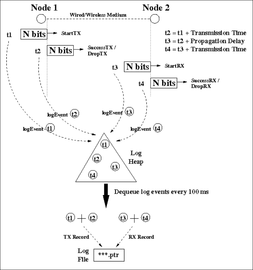
156
storing, (2) log chain counterparts matching, and (3) log file writing, the protocol
module developer should implement them by himself/herself within ~/
NCTUns-*.*/src/nctuns/module/misc/log/logHeap.cc.
Because the log file is a binary format file, users cannot read this file directly
using a text editor. The NCTUns package provides a parser program named printPtr to
translate binary-format log records into text-format log records. The source files of
the parser program are placed under ~/ NCTUns-*.*/tools/misc/printPtr/. A protocol
module developer needs to modify the parser so that it can recognize the packet types
of the newly-added log records and translate them into appropriate text formats.
Fig. 6.4.1 The packet transmission/reception log mechanism
157
Chapter 7 Tactical and Active Mobile Ad
hoc Networks
7.1 Introduction
As the technologies of emerging wireless ad hoc networks are advancing, more
and more interesting applications for the wireless ad hoc network are introduced. One
of the most important applications is the mobile tactical communication system. As
implied by its name, a mobile tactical communication system is used to transmit
important messages such as military commands, strategy information, and the
intelligence, over the battlefield. A network formed by a mobile tactical
communication system is referred to as a “tactical mobile ad hoc network” in this
document. In such a network, a soldier or a military vehicle is assumed to be equipped
with a wireless radio to communicate with each other.
Since a soldier or a military vehicle is able to move dynamically according to
military commands that they receive, the topology of this tactical mobile ad-hoc
network can be changed “actively.” That is, nodes in such a network may move in a
coordinated manner for some objectives, for example, to maximize the coverage of
the ad-hoc network, to form a safe, guaranteed communication path for transmitting
some emergent information, and to chase their target nodes.
One of the most famous mobile tactical communication systems is “Future
Combat System” (FCS), developed by the U.S. Army. The goal of FCS is to build up
a 21st century force that is more agile and more lethal. In such a FCS-equipped force,
soldiers, vehicles, weapons such as cannons and mortars, and unattended sensors, are
equipped with advanced wireless radios to form a cooperative communication
platform. As such, important intelligence, tactical strategies and military commands,
are shared and updated throughout the whole force much more quickly and reliably
than before.
Using FCS an army is able to balance and optimize its battlefield dominance and
deployment because the military operations can be highly cooperated and integrated.
Due to the advantage of agility, speed, and information circulation, the army gains
more comprehensive understanding of the battlefield than its enemy and thus gains
more advantage in the campaign. For example, with the aid of FCS the army can
engage the enemy beyond the range of the weapons of its enemy force and maneuver
to a strategic position with the advantages of agility and speed.
Due to the importance of the tactical mobile ad hoc network, NCTUns provides
developers with a suite of API functions to support the development for such type of
158
networks. Besides the military use, these API functions can be used for developing
other types of networks, including vehicular networks, active sensor networks, and so
on.
The following sections of this chapter are organized as follows. In section 7.2,
we explain the essential capabilities and components for a tactical MANET
simulation. In section 7.3, we describe the design principles for supporting such a
tactical MANET simulation. In section 7.4, the design and implement of a tactical
MANET simulation in NCTUns is elaborated. In section 7.5, we show the skeleton of
a tactical agent program, the role of which in a tactical MANET simulation will be
explained later in section 7.3. In section 7.6, the usages of plentiful supporting API
functions for the tactical MANET simulation are described clearly. Finally, in section
7.7 we give five example cases from the simplest one to the most complex one to
demonstrate how to use these API functions to build up a tactical mobile ad hoc
network.
7.2 Tactical MANET Simulation
In this section, we explain the capabilities provided by NCTUns for a tactical
mobile ad hoc network. Two simulation modes are supported by NCTUns. The first
one is “pure simulation,” which is useful for studying tactical strategies. The second
one is “human-in-the-loop simulation,” which is useful for training people to respond
to various battlefield situations properly. Also, essential network components,
including obstacles, chasing mobile nodes, and target mobile nodes, will be
introduced. At the end of this section, we will discuss how this capability of NCTUns
can be used to study other types of networks.
7.2.1 Simulation Mode
There are two simulation modes supported by NCTUns for a tactical mobile ad
hoc network, pure simulation and human-in-the-loop simulation modes, which are
explained in sequence in the two following subsections.
7.2.1.1 Pure Simulation (useful for developing tactical strategies)
Under the pure simulation mode, the simulation proceeds as a closed system.
Namely, the simulation runs without interacting with humans. In such a simulation
mode, the simulation can be performed as fast as possible. Investigating a tactical may
require conducting a large number of simulations with diverse strategic heuristics and
various combinations of parameter values. In such a condition, the pure simulation
159
mode can generate more simulation results than the other mode within the same
amount of time.
7.2.1.2 Human-in-the-loop Simulation (useful for training people)
Under the “human-in-the-loop” simulation mode, a human can control the
behaviors of a network mobile node during the simulation. In this mode, the ongoing
simulation results produced by the simulation engine are passed to the GUI program
on-the-fly. That is, the display of the working area in GUI is refreshed frequently
(usually within hundreds of milliseconds). With the help of the GUI program, one can
interact with the simulation engine using the arrow keys of a keypad during the
simulation. For example, one can change the moving direction of a mobile node
(which may represent a soldier) or dynamically change the strategy used by a mobile
node. As such, the human-in-the-loop simulation mode is very useful for military
trainings. By interacting with a tactical MANET simulator, a tactical trainee can be
required to respond to a great diversity of battlefield situations and make an
appropriate strategy. In such a condition, a trainee can observe the effect of the
strategy that he (she) just made and adjust his (her) strategy based on the resulting
effects on the battlefield.
7.2.2 Simulation Environment
Before we explain the design principles and detailed implementation for
supporting tactical mobile ad hoc network simulations, some terminologies used in
such networks are defined first. In this subsection, we explain the essential
components in a tactical mobile ad hoc network. The properties of these components
are presented as well.
7.2.2.1 Field, Obstacle, and Their Properties
The field of a simulation is the space within which mobile nodes are allowed to
move around, while a battlefield is defined as an area within which members of forces
such as soldiers, tanks, etc, can move to perform military operations. As such, the
field of a simulation can be viewed as the battlefield of a campaign, and the members
of forces can be considered as mobile nodes moving on the simulation field. The field
is usually defined by a rectangle, described by its length and width.
An obstacle is another essential component used to model a real battlefield. In
the real world, there are various buildings and hills, which may represent some kinds
of obstacles for members of forces. For example, a river can stop the movement of
160
humans and vehicles, and a mountain may block human‟s line of sight. In addition,
from the perspective of a wireless signal, everything that it has to pass through may
become an obstacle which can reduce its signal strength.
To meet all of these simulation requirements, we design an obstacle such that it
has four other important attributes in addition to the locations of its starting and
ending points. The first one is its width. The second one is whether it blocks the
movements of mobile nodes. The third one is whether it blocks the line-of-sight of
humans. The final one is whether it reduces the strength of a wireless signal or not. In
such a case, the amount of the signal strength attenuation can be specified. In
NCTUns, these four attributes can be set via the obstacle dialog box of the GUI
program.
7.2.2.2. Mobile Nodes and Their Tactical Agents
In the real world, forces have various kinds of members, including soldiers, tanks,
helicopters, and fighter planes. Each force member may be equipped with an
advanced wireless radio. For example, in the U.S. Army‟s future combat system, a
soldier is equipped with an advanced wireless radio to communicate with other force
members and receive military commands. Although there are so many kinds of force
members, all of them can be modeled as mobile nodes in a tactical mobile ad hoc
network simulation. The differences among them can be modeled by different
attribute values such as the moving speed, the capabilities of their wireless radio, the
range of its line of sight, etc.
Besides the capabilities of movement and communication, the role of a mobile
node (force member) may be different from those of other nodes. Take a platoon as an
example, there is a platoon leader to command his (her) soldiers to perform a military
operation, such as searching for an enemy, attacking and occupying some strategic
place. In such a case, the platoon leader has the leadership of his (her) team and thus
plays a quite different role than his (her) soldiers.
The roles of the force members are not fixed and may be changed dynamically
based on fast-changing battlefield situations and strategies. For example, initially a
tank that is going to attack its enemy plays the role of a scout. When it finds an enemy,
it becomes an attacker. However, should the tank be sieged by the enemy and receive
a “fall back” command, it will become a runner. At the same time, it becomes the
target of its enemy.
Since the roles of such force members are defined case by case, the NCTUns
simulation engine does not define the roles of mobile nodes for them. Instead, in a
tactical mobile ad hoc network simulation, a mobile node is required to run a tactical
agent program on it. A tactical agent is responsible for declaring the node‟s tactical
161
role and controlling the node‟s action appropriately. By this generic design, NCTUns
can be used to study other types of active MANET.
For example, if a node is the leader of a searching team, its agent may have to
periodically broadcast the node‟s location to other team members and make a decision
to change the searching direction of its team if they encounter an obstacle. For a node
acting as a team member, its tactical agent is responsible for notifying the team leader
of finding obstacles, receiving commands from the team leader, and making an action
to respond to a received command.
In such a design, tactical policies and strategies are implemented solely by
tactical agents, and NCTUns only provides application-neutral API functions to
agents. These API functions can control the movements of nodes, transmit a message
to other agents via a simulated radio link, and so forth.
Writing an agent program requires a comprehensive understanding of tactical
strategies, and the objective of a military operation. Most importantly, it also requires
that an agent writer clearly understands how a user-level program runs on NCTUns.
In NCTUns, an incorrect programming style may result in run-time anomalies or even
cause machine crashes. The correct programming style for a tactical agent program is
elaborated on in section 7.5.
7.2.2.3 Three Application Areas
As we explained in subsection 7.2.2.2, the tactical policies are separated from the
mechanisms of controlling nodes‟ movements and communications. Although this
architecture is designed for tactic mobile ad hoc network simulations, in fact, this
flexible architecture can be applied to other types of networks. We take two examples,
the vehicular networks and the active sensor networks to show how this architecture is
generic enough to satisfy the needs of other active MANETs.
For a vehicular network, each vehicle moves on the roads and is equipped with a
wireless radio. As such, these vehicles form a mobile ad hoc network naturally. For
the simulation of such a network, a vehicle can be modeled as a mobile node on
which an agent program is executed. The agent program may have at least two tasks.
One is to exchange its locally-collected information with other vehicles and keep
track of the information received from other vehicles. The other is to make a decision
or an action for the vehicle based on some objective such as forming a reliable routing
path between two specific vehicles.
In conclusion, a vehicular network simulation requires modeling the movements,
communications of vehicles. In addition, it may also require using coordination
protocols for various purposes, including data routing, topology controlling, and so on.
162
Both of these needs can be satisfied by the architecture designed for tactic mobile ad
hoc network simulation.
Another possible application is for active sensor networks. An active sensor
network is formed by sensors that are assumed to have the capability of moving. In
such a case, a sensor is capable of moving around within a limited range of an area.
Using the architecture introduced in this chapter, a mobile node can represent an
active sensor and the agent program running on it. The movement of a sensor can be
controlled by the agent program running on it based on some heuristics.
Besides these two types of networks, this architecture is suitable for a network
inside which mobile nodes can communicate and coordinate with each other. For
instance, a group of coordinated automatic robots can be easily simulated by this
architecture.
7.3 Design Principles
The design principles used for supporting tactic mobile ad hoc network
simulations is to separate the used tactic policy from the underlying fundamental
mechanism. The tactic policy in such a network includes numerous tactics and
strategies and they often can be changed during an engagement. The underlying
fundamental mechanism includes the communication among force members and the
capabilities to obtain the information about the battlefield situation, such as the
locations of its enemy and allies. The first mechanism is realized over a simulated
mobile ad hoc network, in which each force member communicates with each other
and receives important military information. The second mechanism is supported by
calling auxiliary tactic API functions.
Due to the diversity and the complexity of various tactic policies, integrating
such policies into the simulation engine will complicate the design of the simulation
engine and make it unmanageable. Therefore, in our architecture the simulation
engine is not involved in making tactical decisions. In stead, we introduce a user-level
application program, referred to as a “tactical agent program,” to do such work. For
the simulation engine, it only deals with the necessary functionalities needed by a
tactical agent program.
There are two types of capabilities essential for a tactical agent program. The
first one is the capability of communicating with other agents. As we described
previously, each force member is assumed to be equipped with a wireless radio and all
of them form a mobile ad hoc network for communication. The simulation engine is
responsible for simulating such a kind of ad hoc network. Using the first functionality,
an agent program can send out its collected information or its tactical decisions as
163
packets in a mobile ad hoc network.
The second one is the capability of obtaining the information of the battlefield.
Using the second functionality, an agent program is capable of notifying the
simulation engine of the information in which it is interested. The simulation engine
has the responsibility to send the agent program a reply message containing the
information that the agent requests. Besides, an agent program can request the
simulation engine to watch out some type of events for it. When such events occur
during the simulation, the simulation engine will send the agent program a
notification message.
The details about the design and implementation of the NCTUns architecture for
supporting tactical and active MANET simulations are explained below.
7.4 Design and Implementation
In this section, we explain the detailed design and implementation for supporting
tactical mobile ad hoc network simulations in NCTUns. In our architecture, an agent
is a user-level process. An agent program has to use the tactical API functions to gain
the functionalities it needs, such as communicating with the simulation engine.
Without the help of the tactical API functions, an agent process cannot know what
happens inside the tactical mobile ad hoc network to which it belongs. This is because
the status of the network is kept in another independent user-level process, the
simulation engine process.
Beside, the tactical API functions provide a plenty of wrapper functions to
simplify the complexity and the number of code statements for an agent program. For
example, the tactical API functions provide a function,
getVisableMobileNodesFromThePosition() to help an agent know which nodes that it
can see. Without the aid of this API function, an agent has to read the obstacle
description file and check if there are obstacles between the node to which it belongs
and other nodes. This will make the agent program more complex and unreadable.
As shown in Figure 7.4.1, the agent logic contains core statements of an agent
program that performs specific tasks such as making a strategy based on the current
conditions of the battlefield. The tactical API functions have to be included in an
agent program to provide the agent logic with the essential services. According to the
uses of these tactical API functions, they can be partitioned into five groups, each of
which is represented by a numbered arrow in Figure 7.4.1.
The functions of the first group are used for the following purposes: creating a
TCP connection (through the loop-back interface) to the simulation engine for
communication (i.e., sending IPC commands to the simulation engine and receiving
164
information returned by the simulation engine). The arrow labeled 1.a denotes IPC
commands sent from an agent process to the simulation engine process, and the arrow
labeled 1.b denotes the ACK and REPLY messages returned by the simulation engine
process.
The second group of the tactical API functions is used to register some types of
events in which an agent program is interested. For example, the agent may want to
be notified when the node on which it is running is going to collide with an obstacle.
Before the simulation engine can send events to an agent process, there are some
tasks that an agent program has to do first. First, it has to create a passive UDP socket.
Then, it needs to pass this UDP socket to the simulation engine process via the
createTCPSocketForCommunicationWithSimulationEngine() function, which is a
function in group 1. Next, it should send IPC commands to the simulation engine to
register the event types that it wants to receive. After finishing the registration, the
simulation engine will send a notification message to the agent process through the
passed UDP socket when the events registered by the agent process occur. Thus far,
the five example agent programs included in the NCTUns package do not use this
functionality.
The third group is composed of several socket wrapper functions. These wrapper
functions deal with some standardized statements for using normal socket API
functions. Using these functions, an agent program can be more concise, clearer, and
easier to read. Note that these wrapper functions are not essential for an agent
program. An agent program can invoke normal socket API functions in its own way.
The fourth group is the functions that interact with the operating system kernel,
which are very important for our architecture. This group of functions usually calls
modified system calls, which perform some specific tasks to make the simulation run
correctly.
For example, the usleepAndReleaseCPU() function takes three parameters, the
TCP socket file descriptor that this agent process uses to communicate with the
simulation engine process, the ID of the node to which this agent process belongs, and
the number of microseconds for which this agent would like to sleep. This function
first notifies the simulation engine of the amount of time for which this agent program
will sleep. Upon receiving this message, the simulation engine computes the amount
of simulation time that it can advance safely. Next, this function makes the agent
program sleep for the amount of simulation time specified by the third parameter.
A tactical agent program is a kind of interactive programs, whose behavior
highly depends on those of other nodes. Unlike a traffic generator program, which
generates data packets in a specific manner without considering the situations of its
surroundings, a tactical agent program has to observe the battlefield situations and the
165
statuses of other nodes to make some corresponding actions as the simulation is going
on.
For example, suppose that there are two chasing nodes, A and B, and a target
node, C, on the field. Nodes A and B are equipped with a wireless radio, respectively.
When node B finds out node C (node C is found but not yet captured), node A may
change its moving direction towards the area where node B detected node C. In this
case, node B will first send a notification message to node A via the mobile ad hoc
network they formed. Upon receiving the message transmitted by node B, node A
knows the possible position of node C.
Based on the strategy used by nodes A and B, they may change their moving
directions in order to capture node C. Changing the moving direction and speed of a
node also generates some kind of events for the simulation engine. Assuming that if
the distance between two nodes is less than or equal to 15 meters, they are able to see
each other if there is no obstacle blocking their lines of sight. Let‟s further assume that,
if the distance between a chasing node and its target node is within 5 meters, the
chasing node can capture the target node.
Suppose that node B sees node C in 10‟th second and node B‟s agent program
checks if it can see node C every 5 seconds. Since the NCTUns simulation engine is
event-driven, the simulation engine will advance a huge amount of simulation time if
there is no event to be executed in its event list. In this case, the simulation clock will
be advanced with a large amount of time after the simulation is just started because
node B‟s agent will not generate any notification message to node A‟s agent until the
10‟th second. For example, the simulation engine may find that there are no events in
the future at the beginning of the simulation and thinks that it is safe to advance the
simulation clock by a great amount of time, say, 12 seconds. After the simulation
engine advances its simulation clock to 12‟th second, it releases its use of CPU. Later
on, node B‟s agent process gains the use of CPU and it finds that it cannot see node C
at 12‟th second. Because node B did not detect that it can see node C at 10‟th second
and react properly at that time, the results of this simulation are incorrect.
The final group of the tactical API functions consists of those functions that use
the information provided by the simulation related files, such as obstacle description
file. For example, the
getNearestCollisionPointAlongTheMovingDirectionViewedOnGUIScreen() function
uses the information of the obstacle description file (.obs file) to compute the nearest
point where the agent node will collide with an obstacle.
Besides the tactical API functions, like other user-level programs running on
NCTUns, a tactical agent program can use the normal socket API functions to send
and receive packets through a simulated network.
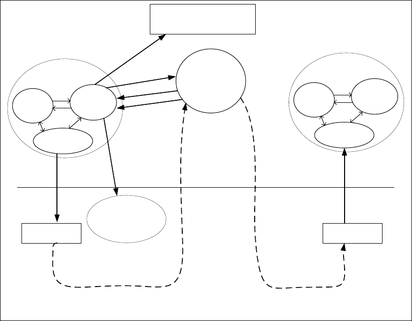
166
Agent
logic
Tactic API
functions
Agent program 1 S.E.
Simulation related files
(.obs and .sce files)
Tunnel device Tunnel device
1.a
1.b
2
4
5
System call service
routines for tactic agent
programs
Normal socket
Interface
3
Agent
logic
Tactic API
functions
Agent program 2
Normal socket
Interface
3
Figure 7.4.1. The architecture supporting tactical MANET simulations in NCTUns

167
7.5 Writing a Tactical Agent
Although an agent program is a user-level program like other tools in NCTUns,
writing such a program requires understanding how NCTUns works clearly. Also,
there are several tips that an agent program writer needs to know to make his (her)
agent program work correctly. In this section, we show the framework of an agent
program and discuss several important designs.
7.5.1 Framework of an Agent Program
Figure 7.5.1. The framework of an agent program
1 int main(int argc, char *argv[]) {
2
3 mynid = getMyNodeID();
4
5 myTCPsockfd = createTCPSocketForCommunicationWithSimulationEngine();
6
7 constructGridMapofTheWholeField();
8
9 n = getInitialNodePosition(mynid, curX, curY, curZ);
10
11 newMovingDirectionInDegree = random() % 360;
12
13 getNearestCollisionPointAlongTheMovingDirectionViewedOnGUIScreen();
14
15 curspeed = 10; /* moving speed: meter/second */
16
17 n = setNextWaypointAndMovingSpeed(myTCPsockfd, mynid, nextX, nextY,
nextZ, curspeed, 1);
18
19 usleepAndReleaseCPU(myTCPsockfd, mynid, 1);
20
21 while (1) {
22
23 usleepAndReleaseCPU();
24 }
25 }
168
As shown in Figure 7.5.1, an agent program has several basic operations. First, it
has to get the ID of the node to which it belongs via the getMyNodeID() function.
Second, it has to establish a TCP connection to the simulation engine. This can be
done by calling the createTCPSocketForCommunicationWithSimulationEngine()
function. Next, as shown in the statements on lines 9 to 17, the agent program has to
determine its initial moving direction and the first turning waypoint.
After setting up the first turning point, the agent program has to explicitly call
the usleepAndReleaseCPU() function, a special tactical API function, for two
purposes. The first purpose is to make this agent sleep for a while, even for just one
microsecond. This is because user-level programs running on NCTUns has to release
the control of CPU periodically to allow the simulation engine process to have a
chance to use CPU. If the simulation engine process does not have any chance to be
executed by CPU, the simulation clock will not be advanced. In such a situation, the
simulation will get blocked.
The second purpose is to insert a notification event in the kernel to notify the
simulation engine of the time amount for which this agent process will sleep. With
this notification, the simulation engine will not advance its simulation clock too fast
and skip over the time that the agent process should be waked up. On the contrary,
without this notification event, the simulation engine is very likely to advance its
simulation time more than the time amount for which this agent program wants to
sleep. In such a case, the agent program may miss some important events, causing
incorrect simulation results.
The statements on lines 21 to 25 are the core while loop for an agent program.
An agent writer can embed the strategic decision logic statements inside this while
loop. For example, it may check if some enemy nodes are within the agent‟s visible
range. Note that the usleepAndReleaseCPU() function has to be put at the end of this
while loop to make this agent program release CPU periodically. The reason why
using this function instead of the normal usleep()function has been explained before.
7.5.2 Communication between Agent and Agent
In the framework shown in Figure 7.5.1, the pseudo-code of the agent program
does not deal with any communications to other agent process. However, it is very
possible that an agent process needs to exchange messages with other agent processes.
In fact, like other user-level application programs running on Nocturnes, an agent
program can use normal socket API interface to communicate with other agent
process. Using the normal socket API functions, a packet sent by an agent program
will be placed in the transmission queue of a tunnel interface. Then, the packet will be
169
captured by the simulation engine, and then the packet will be transmitted over a
network simulated by NCTUns until this packet reaches its destination node. As such,
the agent-to-agent communication using the socket API interface is built on top of a
simulated tactical mobile ad hoc network. This makes sense because in the real
battlefield two soldiers have to communicate with each other via their equipped
wireless radios, which in fact form a wireless mobile ad hoc network.
7.5.3 Communication between Agent and Simulation Engine
The communication between an agent process and the simulation engine is based
on a message-passing protocol over a TCP connection. An agent can send a request
message to the simulation engine for requesting some service. Upon receiving a
request message, the simulation engine has to explicitly reply an acknowledge
message to the agent for notifying the agent of its successful reception of this request
message. Also, the simulation engine has to send the information required by the
agent back via the TCP connection between itself and the agent.
However, an agent program need not understand the detailed format of this
message-passing protocol since the tactical API functions provide plentiful wrapper
functions that hide the details of the protocol for every service provided by the
simulation engine. An agent program can call these API functions to request every
kind of service provided by the simulation engine without forming IPC commands on
its own. As such, an agent program writer can save time spent on dealing with such
tedious details and instead focus more on the code of his (her) agent program.
7.6 Tactical MANET API Functions
7.6.1 Functions for Communication between Agent and Simulation
Engine
Function name: createTCPSocketForCommunicationWithSimulationEngine
Parameter list: int mynid,
int gid1, int gid2, int gid3, int gid4,
int gid5, int gid6, int gid7, int gid8,
int humanControlled,
int&UDPsocketFd2,
int moreMsgFollowing
170
Return value type: socket file descriptor (integer)
Description:
This API function creates and returns a TCP socket by which the calling agent
program can use IPC commands to communicate with the simulation engine. Since
IPC commands exchanges between an agent program and the simulation engine
should take no time, before creating this socket, this function internally calls an
NCTUns system call to tell the kernel that the created socket should be treated
differently from other sockets created for communication with other agent programs.
This is because packets sent out via the former should not go through the
simulated network while the latter should. More specifically, packets sent out via the
former should be looped back via the loopback interface in the kernel to the socket
used by the simulation engine without going through any network simulation;
however, packets sent out via the latter should be sent into the simulated network via
a tunnel interface and may go through multi-hop wireless transmission simulation
until they reach the socket used by another agent program. What this system call does
is to deregister the created socket from the kernel so that it will not be treated as the
latter type of socket (which is the default type when a socket is created in an
application program running on NCTUns). The argument mynid should be filled in
with the node ID of the tactical agent. A tactical agent can simultaneously belong to at
most 8 different groups. If it belongs to i'th group, the argument gid(i) should be set to
1; otherwise, gid(i) should be set to 0. The movement of a mobile node can be
automatically controlled by its agent program or manually controlled by a human. In
the former case, the humanControlled flag argument should be set to 0 while in the
latter case the humanControlled flag argument should be set to 1. When a mobile
node is configured to be controlled by a human, its agent program will obey the
moving directions issued by a human pressing the right/left/up/down arrow keys on
the keyboard.
This function packs the provided arguments into an IPC command and sends it to
the simulation engine via the just created socket to register this tactical agent. In the
future, when the simulation engine has a particular event to notify the tactical agent, it
sends a notification message to the tactical agent, which can be received by the
tactical agent via this created socket (or the passed UDP socket).
The moreMsgFollowing argument tells the simulation engine whether more IPC
commands will follow this IPC command and that they all need to be processed
atomically. That is, if moreMsgFollowing is 1, after processing this IPC command
and sending back an ACK packet, the simulation engine should freeze its simulation
clock and wait for more IPC commands to come. In contrast, if moreMsgFollowing is
171
0, the simulation engine can advance its simulation clock after processing this IPC
command and process other events.
Function name: setCurrentWaypoint
Parameter list: int myTCPsockfd, int mynid,
double x, double y, double z,
int moreMsgFollowing
Return value type: integer
Description:
This API function forms an IPC command and sends it to the simulation
engine. Upon receiving this command, the simulation engine sets the current
waypoint of the specified mobile node to the position specified by (curX, curY, curZ).
The position of the next waypoint of this mobile node remains unchanged. The
moving direction (unit vector) of this mobile node is automatically adjusted inside the
simulation engine according to the new specified waypoint. The moving speed of this
mobile node remains unchanged.
Note that a mobile node moves from its current waypoint to its next waypoint
linearly at a given constant speed. The current position of the mobile node returned by
getCurrentPosition() is calculated based on the following formula: currentWaypoint +
movingDirectionUnitVector * MovingSpeed * (CurTime -
theTimeWhenTheCurrentWaypointIsReached). Therefore, after reaching its next
waypoint, the mobile node will keep moving in the current direction unless its next
waypoint (which affects its movingDirectionUnitVector) is set to another location.
Note that when setCurrentWaypoint() is called, if the agent program
immediately calls getCurrentPosition(), according to the above formula, the reported
current position of the mobile node will be the specified current waypoint (curX, curY,
curZ). Therefore, if the specified position is not the same as the current position
reported by getCurrentPosition(), the mobile node may unrealistically jump in the
field. To avoid this unrealistic phenomenon, the (curX, curY, curZ) arguments
provided to setCurrentWaypoint() normally should be the current position of the
mobile node, which can be provided by getCurrentPosition().
The moreMsgFollowing argument tells the simulation engine whether
more IPC commands will follow this IPC command and that they all need to be
processed atomically. That is, if moreMsgFollowing is1, after processing this IPC
command and sending back an ACK packet, the simulation engine should freeze its
simulation clock and wait for more IPC commands to come. In contrast, if
172
moreMsgFollowing is 0, the simulation engine can advance its simulation clock after
processing this IPC command and process other events. This function returns 0 if it
executes successfully; otherwise, it returns -1, which indicates something is wrong.
Function name: getCurrentWaypoint
Parameter list: int myTCPsockfd, int mynid,
double &x, double &y, double &z,
int moreMsgFollowing
Return value type: integer
Description:
This API function forms an IPC command and sends it to the simulation engine
asking it to return the current waypoint of the specified mobile node via (x, y, z). The
moreMsgFollowing argument tells the simulation engine whether more IPC
commands will follow this IPC command and that they all need to be processed
atomically. That is, if moreMsgFollowing is 1, after processing this IPC command
and sending back an ACK packet, the simulation engine should freeze its simulation
clock and wait for more IPC commands to come. In contrast, if moreMsgFollowing
is 0, the simulation engine can advance its simulation clock after processing this IPC
command and process other events. This function returns 0 if it executes successfully;
otherwise, it returns -1, which indicates something is wrong.
Function name: setNextWaypoint
Parameter list: int myTCPsockfd, int mynid,
double x, double y, double z, int moreMsgFollowing
Return value type: integer
Description:
This API function forms an IPC command and sends it to the simulation engine.
Upon receiving this command, the simulation engine sets the next waypoint of the
specified mobile node to the position specified by (x, y, z). The current waypoint of
this mobile node remains unchanged. However, the moving direction unit vector of
this mobile node is adjusted corresponding to the new next waypoint. The moving
speed of this mobile node remains unchanged. Note that calling setNextWaypoint()
without calling setCurrentWaypoint() at the same time may cause the mobile node to
unrealistically jump in the field. This is because getCurrentPosition() uses the
173
following formula:
currentPosition = currentWaypoint +
movingDirectionUnitVector * movingSpeed *
(curTime - theTimeWhenTheCurrentWaypointIsReached)
to report the current position of the mobile node. To avoid this unrealistic
phenomenon, the simulation engine internally calls
setNodeCurrentWaypoint(getNodePosition()) before calling
setNodeNextWaypoint(nextX, nextY, nextZ). That is, the current waypoint is first set
to the current position before the simulation engine sets the next waypoint of the
mobile node.
The moreMsgFollowing argument tells the simulation engine whether more IPC
commands will follow this IPC command and that they all need to be processed
atomically. That is, if moreMsgFollowing is 1, after processing this IPC command
and sending back an ACK packet, the simulation engine should freeze its simulation
clock and wait for more IPC commands to come. In contrast, if moreMsgFollowing is
0, the simulation engine can advance its simulation clock after processing this IPC
command and process other events. This function returns 0 if it executes successfully;
otherwise, it returns -1, which indicates something is wrong.
Function name: getCurrentMovingDirectionViewedOnGUIScreen
Parameter list: int myTCPsockfd, int mynid, double &angle,
int moreMsgFollowing
Return value type: integer
Description:
This API function forms an IPC command and sends it to the simulation
engine. Upon receiving this command, the simulation engine returns the current
moving direction of the specified mobile node via angle. Note that the moving
direction is viewed on the GUI screen rather than in the normal coordinate system.
The moreMsgFollowing argument tells the simulation engine whether
more IPC commands will follow this IPC command and that they all need to be
processed atomically. That is, if moreMsgFollowing is 1, after processing this IPC
command and sending back an ACK packet, the simulation engine should freeze its
simulation clock and wait for more IPC commands to come. In contrast, if
moreMsgFollowing is 0, the simulation engine can advance its simulation clock after
174
processing this IPC command and process other events. This function returns 0 if it
executes successfully; otherwise, it returns -1, which indicates something is wrong.
Function name: setCurrentAndNextWaypoint
Parameter list: int myTCPsockfd, int mynid,
double curX, double curY, double curZ,
double nextX, double nextY, double nextZ,
int moreMsgFollowing
Return value type: integer
Description:
This API function forms an IPC command and sends it to the simulation engine.
Upon receiving this command, the simulation engine sets the specified mobile node's
current waypoint to (curX, curY, curZ) and its next waypoints to (nextX, nextY,
nextZ). The moreMsgFollowing argument tells the simulation engine whether
more IPC commands will follow this IPC command and that they all need to be
processed atomically. That is, if moreMsgFollowing is 1, after processing this IPC
command and sending back an ACK packet, the simulation engine should freeze its
simulation clock and wait for more IPC commands to come. In contrast, if
moreMsgFollowing is 0, the simulation engine can advance its simulation clock after
processing this IPC command and process other events. This function returns 0 if it
executes successfully; otherwise, it returns -1, which indicates something is wrong.
Function name: setCurrentMovingSpeed
Parameter list: int myTCPsockfd, int mynid, double curSpeed,
int moreMsgFollowing
Return value type: integer
Description:
This API function forms an IPC command and sends it to the simulation engine.
Upon receiving this command, the simulation engine sets the moving speed of the
specified mobile node to curSpeed. Because the current position of the mobile node
returned by getCurrentPosition() is based on the following formula:
currentPosition =
175
currentWaypoint + movingDirectionUnitVector * movingSpeed *
(curTime - theTimeWhenTheCurrentWaypointIsReached)
The mobile node may unrealistically jump in the field when its moving speed is
changed. To avoid this unrealistic phenomenon, the simulation engine
internally calls setNodeCurrentWaypoint(getNodePosition()) before calling
setNodeSpeed().
The moreMsgFollowing argument tells the simulation engine whether more IPC
commands will follow this IPC command and that they all need to be
processed atomically. That is, if moreMsgFollowing is 1, after processing this IPC
command and sending back an ACK packet, the simulation engine should freeze its
simulation clock and wait for more IPC commands to come. In contrast, if
moreMsgFollowing is 0, the simulation engine can advance its simulation clock after
processing this IPC command and process other events. This function returns 0 if it
executes successfully; otherwise, it returns -1, which indicates something is wrong.
Function name: getCurrentMovingSpeed
Parameter list: int myTCPsockfd, int mynid,
double &curSpeed, int moreMsgFollowing
Return value type: integer
Description:
This API function forms an IPC command and sends it to the simulation engine.
Upon receiving this command, the simulation engine returns the current moving speed
of the specified mobile node via curSpeed. The moreMsgFollowing argument tells the
simulation engine whether more IPC commands will follow this IPC command and
that they all need to be processed atomically. That is, if moreMsgFollowing is 1, after
processing this IPC command and sending back an ACK packet, the simulation
engine should freeze its simulation clock and wait for more IPC commands to come.
In contrast, if moreMsgFollowing is 0, the simulation engine can advance its
simulation clock after processing this IPC command and process other events. This
function returns 0 if it executes successfully; otherwise, it returns -1, which indicates
something is wrong.
Function name: setNextWaypointAndMovingSpeed
176
Parameter list: int myTCPsockfd, int mynid,
double nextX, double nextY, double nextZ,
double curSpeed,
int moreMsgFollowing
Return value type: integer
Description:
This API function forms an IPC command and sends it to the simulation
engine. Upon receiving this command, the simulation engine sets the specified mobile
node's next waypoints to (nextX, nextY, nextZ), and its current speed to curSpeed.
Because the current position of the mobile node returned by getCurrentPosition() is
based on the following formula:
currentPosition =
currentWaypoint + movingDirectionUnitVector * movingSpeed *
(curTime - theTimeWhenTheCurrentWaypointIsReached)
the mobile node may unrealisticaly jump in the field when its next waypoint and(or)
moving speed is changed. To avoid this unrealistic phenomenon, the simulation
engine internally calls setNodeCurrentWaypoint(getNodePosition()) before calling
setNodeSpeed() and setNodeNextWaypoint().
The moreMsgFollowing argument tells the simulation engine whether more IPC
commands will follow this IPC command and that they all need to be processed
atomically. That is, if moreMsgFollowing is 1, after processing this IPC command
and sending back an ACK packet, the simulation engine should freeze its simulation
clock and wait for more IPC commands to come. In contrast, if moreMsgFollowing is
0, the simulation engine can advance its simulation clock after processing this IPC
command and process other events. This function returns 0 if it executes successfully;
otherwise, it returns -1, which indicates something is wrong.
Function name: getCurrentPosition
Parameter list: int myTCPsockfd, int mynid,
double &curX, double &curY, double &curZ,
int moreMsgFollowing
Return value type: integer
177
Description:
This API function forms an IPC command and sends it to the simulation engine.
Upon receiving this command, the simulation engine calculates the current position of
the mobile node specified by mynid and returns its current position via (curX, curY,
curY). The current position of a mobile node returned by getCurrentPosition() is
based on the following formula:
currentPosition =
currentWaypoint + movingDirectionUnitVector * movingSpeed *
(curTime - theTimeWhenTheCurrentWaypointIsReached)
Therefore, after reaching its next waypoint, a mobile node will keep moving in the
current direction unless its next waypoint (which affects its
movingDirectionUnitVector) is set to another location. It will not stay at its next
waypoint. The current waypoint, next waypoint, moving direction, and moving speed
of this mobile node all remain unchanged when this function is called.
The moreMsgFollowing argument tells the simulation engine whether more IPC
commands will follow this IPC command and that they all need to be processed
atomically. That is, if moreMsgFollowing is 1, after processing this IPC command
and sending back an ACK packet, the simulation engine should freeze its simulation
clock and wait for more IPC commands to come. In contrast, if moreMsgFollowing
is 0, the simulation engine can advance its simulation clock after processing this IPC
command and process other events. This function returns 0 if it executes successfully;
otherwise, it returns -1, which indicates something is wrong.
Function name: getCurrentPositionOfAGroupOfNode
Parameter list: int myTCPsockfd, int mynid, int gid,
struct nodePosition **groupNodePositionArray,
int &numNodeInThisArray,
int moreMsgFollowing
Return value type: integer
Description:
This API function forms an IPC command and sends it to the simulation engine.
Upon receiving this command, the simulation engine calculates the current position of
every mobile node that belongs to the group specified by gid and collects such
178
information into an array of struct nodePosition and returns the pointer to this array
via groupNodePositionArray. The number of struct nodePosition in the returned array
is returned via numNodeInThisArray. After using this array, the agent program is
responsible for releasing the memory space occupied by this array by calling free
(groupNodePositionArray).
The moreMsgFollowing argument tells the simulation engine whether more IPC
commands will follow this IPC command and that they all need to be processed
atomically. That is, if moreMsgFollowing is 1, after processing this IPC command
and sending back an ACK packet, the simulation engine should freeze its simulation
clock and wait for more IPC commands to come. In contrast, if moreMsgFollowing is
0, the simulation engine can advance its simulation clock after processing this IPC
command and process other events. This function returns 0 if it executes successfully;
otherwise, it returns -1, which indicates something is wrong.
Function name: requestNotificationWhenAnotherNodeHasApproachedMe
Parameter list: int myTCPsockfd, int mynid, int registrationID,
int timeIntervalInMilliseconds, int anotherNodeID,
int gid, double withinRangeinMeter,
int moreMsgFollowing
Return value type: integer
Description:
This API function forms an IPC command and sends it to the simulation
engine. Upon receiving this command, the simulation engine creates and registers a
struct registeredApproachingCheckingRecord entry in its triggering system. The
triggering system is invoked periodically by the simulation engine at a fine grain
(once every 0.1 second) to check whether the registered circumstance has happened or
not.
If timeIntervalInMilliseconds is set to 0, the triggering system will use its default
frequency to check and report the checking results. If timeIntervalInMilliseconds is
set to a value greater than 0, the triggering system will check the registered
circumstance once every timeIntervalInMilliseconds milliseconds. If anotherNodeID
is greater than 0, this function asks the triggering system to monitor whether the
mobile node specified by anotherNodeID has approached the mobile node specified
by mynid within a distance specified by withinRangeInMeter. If anotherNodeID is
less than 0, it means that a group of nodes rather than a single node should be
monitored and in this case the value of gid should be used.
179
If gid is greater than 0, the triggering system will monitor any mobile node
belonging to the group specified by gid. If gid is less than 0, the simulation engine
will ignore it. When the registered circumstance occurs, the simulation engine will
send a struct SimulationEngineNotificationWhenAnotherNodeHasApproachedMe
notification IPC message to the agent program running on the node specified by
mynid.
When the registered circumstance persists, the triggering system will
continuously send a
SimulationEngineNotificationWhenAnotherNodeHasApproachedMe notification IPC
message to the agent program running on the node specified by mynid. As long as the
registered circumstance persists, the triggering system will send such an IPC message
to the agent program every time when it is invoked. This continuous message sending
will stop when the registered circumstance no longer exists.
The argument withinRangeInMeter can be set to 0. In such a setting, a mobile
node may have collided with another mobile node when such a situation is detected. If
withinRangeInMeter is set to a larger value, a mobile node will have more space to
make turns to avoid collisions.
The registrationID must be provided by the agent program and be unique across
all registered notification requests issued within the agent program. Later on, the
agent program may cancel, suspend, or resume a registered notification request by
providing its corresponding registrationID.
After receiving a notification IPC message, the agent program needs to send
back an ACK packet (struct
GeneralACKBetweenAgentClientAndSimulationEngine) to the simulation
engine. The ACK packet carries a moreMsgFollowing field to indicate whether the
agent program wants to issue more IPC commands to the simulation engine after this
ACK packet. In case the carried moreMsgFollowing is 0, the simulation
engine can process its other events and advance its simulation clock. Otherwise, it
must wait until all following IPC commands have been processed.
The moreMsgFollowing argument tells the simulation engine whether more IPC
commands will follow this IPC command and that they all need to be processed
atomically. That is, if moreMsgFollowing is 1, after processing this IPC command
and sending back an ACK packet, the simulation engine should freeze its simulation
clock and wait for more IPC commands to come. In contrast, if moreMsgFollowing
is 0, the simulation engine can advance its simulation clock after processing this IPC
command and process other events. This function returns 0 if it executes successfully;
otherwise, it returns -1, which indicates something is wrong.
180
Function name: cancelNotificationWhenAnotherNodeHasApproachedMe
Parameter list: int myTCPsockfd, int mynid, int registrationID,
int moreMsgFollowing
Return value type: integer
Description:
This API function forms an IPC command and sends it to the simulation engine
to cancel a previously registered notification request. Upon receiving this command,
the simulation engine uses the provided node ID (mynid) and registration ID
(registrationID) to search and remove the specified request record. The
moreMsgFollowing argument tells the simulation engine whether more IPC
commands will follow this IPC command and that they all need to be processed
atomically. That is, if moreMsgFollowing is 1, after processing this IPC command
and sending back an ACK packet, the simulation engine should freeze its simulation
clock and wait for more IPC commands to come. In contrast, if moreMsgFollowing is
0, the simulation engine can advance its simulation clock after processing this IPC
command and process other events. This function returns 0 if it executes successfully;
otherwise, it returns -1, which indicates something is wrong.
Function name: suspendNotificationWhenAnotherNodeHasApproachedMe
Parameter list: int myTCPsockfd, int mynid, int registrationID,
int timeIntervalInMilliseconds,
int moreMsgFollowing
Return value type: integer
Description:
This API function forms an IPC command and sends it to the simulation engine
to suspend a previously registered notification request. Upon receiving this command,
the simulation engine uses the provided node ID (mynid) and registration ID
(registrationID) to locate and suspend the specified request record. If
timeIntervalInMilliseconds is set to 0, the request will be suspended forever. If
timeIntervalInMilliseconds is set to a value greater than 0, the request will be
suspended from now to (now + timeIntervalInMilliseconds) only.
The moreMsgFollowing argument tells the simulation engine whether more IPC
commands will follow this IPC command and that they all need to be processed
atomically. That is, if moreMsgFollowing is 1, after processing this IPC command
181
and sending back an ACK packet, the simulation engine should freeze its simulation
clock and wait for more IPC commands to come. In contrast, if moreMsgFollowing is
0, the simulation engine can advance its simulation clock after processing this IPC
command and process other events. This function returns 0 if it executes successfully;
otherwise, it returns -1, which indicates something is wrong.
Function name: resumeNotificationWhenAnotherNodeHasApproachedMe
Parameter list: int myTCPsockfd, int mynid, int registrationID,
int moreMsgFollowing
Return value type: integer
Description:
This API function forms an IPC command and sends it to the simulation engine
to resume a previously registered notification request that is suspended. Upon
receiving this command, the simulation engine uses the provided node ID (mynid)
and registration ID (registrationID) to locate and resume the specified request record.
The moreMsgFollowing argument tells the simulation engine whether more IPC
commands will follow this IPC command and that they all need to be processed
atomically. That is, if moreMsgFollowing is 1, after processing this IPC command
and sending back an ACK packet, the simulation engine should freeze its simulation
clock and wait for more IPC commands to come. In contrast, if moreMsgFollowing is
0, the simulation engine can advance its simulation clock after processing this IPC
command and process other events.
This function returns 0 if it executes successfully; otherwise, it returns -1, which
indicates something is wrong.
Function name: destroyMobileNode
Parameter list: int myTCPsockfd, int targetNid, int moreMsgFollowing
Return value type: integer
Description:
This API function forms an IPC command and sends it to the simulation engine
to tell it that the mobile node specified by targetNid no longer exists in the simulated
network (because it may have been captured or destroyed by the enemy force). Upon
receiving this command, the simulation engine sets the moving speed of the
182
specified mobile node to zero and turns off the "UP" flag in the mobile node's control
block to indicate this fact. When the triggering system is invoked to detect whether
any registered circumstance has occurred, a "DOWN" mobile node is not taken into
account in the checking.
The moreMsgFollowing argument tells the simulation engine whether
more IPC commands will follow this IPC command and that they all need to be
processed atomically. That is, if moreMsgFollowing is 1, after processing this IPC
command and sending back an ACK packet, the simulation engine should freeze its
simulation clock and wait for more IPC commands to come. In contrast, if
moreMsgFollowing is 0, the simulation engine can advance its simulation clock after
processing this IPC command and process other events. This function returns 0 if it
executes successfully; otherwise, it returns -1, which indicates something is wrong.
Function name: stopSimulation
Parameter list: int myTCPsockfd, int mynid
Return value type: integer
Description:
This API function forms an IPC command and sends it to the simulation engine
to ask it to stop the whole simulation. Upon receiving this command, the simulation
engine stops the simulation in the same way as it receives a "STOP" command from
the GUI. The simulation results are then transferred back to the GUI.
Function name: usleepAndReleaseCPU
Parameter list: int myTCPsockfd, int mynid, int usecond
Return value type: void
Description:
This API function forms an IPC command and sends it to the simulation engine
to release the use of CPU. At the same time, it also puts the agent program to sleep for
the amount of microseconds specified by usecond. These two operations are done
atomically to avoid the simulation engine from advancing its simulation clock.
183
Function name: selectAndReleaseCPU
Parameter list: int myTCPsockfd, int mynid, int nfds,
fd_set *inp, fd_set *outp, fd_set *exp, timeval *tvp
Return value type: integer
Description:
This API function forms an IPC command and sends it to the simulation engine
to release the use of CPU. At the same time, it also puts the agent program to select on
a few file descriptors for the amount of time specified by timeout. These two
operations are done atomically to avoid the simulation engine from advancing its
simulation clock.
Function name: getApproachingNotificationInformation
Parameter list: int myTCPsockfd, int &anid,
double &ax, double &ay, double &az,
double &aspeed, double &aangle,
double &distance
Return value type: integer
Description:
This API function reads an IPC command --
SIMULATION_ENGINE_NOTIFICATION_WHEN_ANOTHER_NODE_HAS_AP
PROACHED_ME sent to the agent program by the simulation engine and returns an
ACK to the simulation engine. The information of the node that has approached this
agent program is returned. anid is the ID of such a node. (ax, ay, az) is the position of
such a node. aspeed is the speed of such a node. “aangle” is the moving angle of such
a node. “distance” is the distance between the agent program node and such a node.
This function returns 0 if it executes successfully; otherwise, it returns -1, which
indicates something is wrong.
184
7.6.2 Miscellaneous API Functions
Function name: getMyNodeID
Parameter list: empty
Return value type: integer
Description:
This API function returns the node ID on which the calling agent program is
running.
Function name: twoPointsDistance
Parameter list: double x1, double y1, double x2, double y2)
Return value type: double
Description:
This API function returns the distance between (x1, y1) and (x2, y2).
7.6.3 Functions for Obtaining Information from Simulation-related
Files
Function name: constructGridMapofTheWholeField
Parameter list: empty
Return value type: void
Description:
This API function is not an IPC command. Instead, it reads the obstacle file
exported by the GUI, which is placed in the .sim directory with all other files exported
by the GUI. Since all files in the .sim directory will be tarred and copied to a working
directory on the simulation engine machine during simulation, this function tries to
locate this working directory to successfully open the obstacle file.
The obstacle file contains the field sizes (maxXMeter, maxYMeter, maxZMeter),
which are returned to the programmer via the maxXMeter, maxYMeter, maxZMeter
global variables. This file also contains the attributes of every obstacle in the field.
Every obstacle is represented as a rectangular and has the following attributes:
The positions of the four corners of the rectangular obstacle: (X1, Y1), (X2, Y2),
185
(X3, Y3), (X4, Y4), These four positions can be interpreted as either clockwise or
counterclockwise. At present, Z axis is not used. Each obstacle has three attributes as
follows:
Block_Node_View ?
Block_Node_Movement ?
Block_Wireless_Signal ?
The attributes of each obstacle is read out from the obstacle file and stored in an
obstacle control block (struct obstacle). These control blocks are linked to form a list
and the pointer to this list is returned to the programmer via the obstacleListP global
variable. The number of obstacles in this list is returned via the Num_obstacle global
variable. In addition to the information contained in the obstacle file, one input to this
function is the width of a grid (used for X, Y, and Z grids) that should be used in the
map. Its unit is meter. Based on this information the sizes of the X, Y, and Z
dimensions of the gridMap are returned via the maxXGrid, maxYGrid, and maxZGrid)
global variables. Their values are maxXMeter/gridWidthMeter,
maxYMeter/gridWidthMeter, and maxZMeter/gridWidthMeter, respectively. With
these values, this function dynamically allocates memory space for the gridMap.
unsigned char *gridMap = malloc(maxXGrid * maxYGrid);
and returns the pointer to GridMap to the programmer via the gridMapP global
variable. (Currently, Z axis is not used.)
Based on the obstacle information, each element of the gridMap matrix is filled
in with one of the values of 0, and 1. A value of 0 represents that the element is not
occupied by any obstacle. A value of 1 instead represents that it is in the interior space
of an obstacle.
This function automatically fills the borders of the gridMap matrix with four
obstacles (top/down/left/right) to make the field a closed field. This setting ensures
that a mobile node will not move out of the field. The returned value indicates
whether this function executes successfully (0), or fails (1).
Function name: getInitialNodePosition
Parameter list: int mynid, double &initX, double &initY, double &initZ
186
Return value type: integer
Description:
This API function is not an IPC command. It reads the .sce file exported by the
GUI and returns the initial position of the specified mobile node via (initX, initY,
initZ). This function returns 0 if the initial position of the specified node can be found,
otherwise, it returns -1 indicating something is wrong.
Function name:
getNearestCollisionPointAlongTheMovingDirectionViewedOnGUIScreen
Parameter list: double curX, double curY, double curZ,
double movingDirectionInDegreeViewedOnGUIScreen,
double &collisionX, double &collisionY, double &collisionZ,
double &distance, double &obstacleAngle)
Return value type: void
Description:
This API function is not an IPC command. Based on the information of the
obstacles contained in the obstacleListP list, this function calculates the nearest
collision point (collisionX, collisionY, collisionZ) along the specified moving
direction from the specified position (curX, curY, curZ). The distance between the
two points is returned via distance. The direction of the encountered obstacle is
returned via obstacleAngle.
Function name:
getFarthestVisablePointAlongTheMovingDirectionViewedOnGUIScreen
Parameter list: double curX, double curY, double curZ,
double movingDirectionInDegreeViewedOnGUIScreen,
double &visualX, double &visualY, double &visualZ,
double &distance
Return value type: void
Description:
187
This API function is not an IPC command. Based on the information of the
obstacles contained in the obstacleListP list, this function calculates the farthest point
(visualX, visualY, visualZ) that can be seen along the specified moving direction
(movingDirectionInDegreeViewedOnGUIScreen) from the specified position (curX,
curY, curZ). The distance between the two points is returned in distance.
Function name: inObstacleGridLocation
Parameter list: double x, double y, double z
Return value type: integer
Description:
This API function is not an IPC command. It checks whether the point (x, y, z)
falls into a grid location that is occupied by an obstacle. Currently, z is ignored.
Function name: getVisableMobileNodesFromThePosition
Parameter list: double x, double y, double z,
struct nodePosition *groupNodePositionArray,
int numNodeInTheArray,
struct nodePosition **visableNodePositionArray,
int &numNodeVisable
Return value type: void
Description:
This API function is not an IPC command. Based on the provided obstacle list
(which is pointed to by obstacleListP and its obstacle number is given by
Num_obstacle), for each mobile node in the nodePosition array pointed to by
groupNodePositionArray, this function checks whether it can be "seen" from the
position specified by (x, y, z). The numNodeInTheArray argument indicates the
number of entries in this array. The positions of the mobile nodes that can be seen are
grouped to form an array of struct nodePosition pointed to by
visableNodePositionArray. The number of entries in this array is returned via
numNodeVisable. The agent program is responsible for freeing the memory space
occupied by the returned visableNodePositionArray after its use.
Here "seen" means that there is no obstacle sitting on the visual line connecting
the specified position (x, y, z) with the position of the checked mobile node. An agent
program can use this function to implement its "eyes" by itself without burdening the
188
simulation engine.
Function name: getSurroundingViews
Parameter list: double x, double y, double z,
double **viewDistance360Degree
Return value type: void
Description:
This API function is not an IPC command. Based on the given obstacle list
pointed to by obstacleListP (whose number is given by Num_obstacle), for each
degree from 0 to 359, this function calculates how far the mobile node whose
position is specified by (x, y, z) can "see" before its view is blocked by some
obstacle. The calculated distance information is returned via an array with consisting
of 360 distances of "double" type, which is pointed to by viewDistance360Degree.
The agent program is responsible for freeing the memory space occupied by the
returned array pointed to by viewDistance360Degree. Note that the degree is viewed
on the GUI screen. Therefore, degree 0 points to the right, degree 90 points to the top,
degree 180 points to the left, and degree 270 points to the down. An agent program
can use this function to implement its "eyes" by itself without burdening the
simulation engine.

189
7.7 Five Examples
In this section, we demonstrate five example cases from the simplest one to the
most complex one to show how to build various tactical agent programs correctly.
Through these five example cases, one can learn the correct programming style for an
agent program and understand how to embed a tactical strategy in such an agent
program.
7.7.1 Example 1: Magent1.cc
Mobile Node
Figure 7.7.1. The scenario of example 1
The first agent program is written for the following scenario. As Figure 7.7.1
shows, a single mobile node is located within a closed area which is surrounded by
several obstacles. It moves linearly at a constant speed toward a direction until it
collides with one obstacle. At that time, it bounces back (i.e., changes its moving
direction) and moves toward another direction. The mobile node continues to move in
this way until the simulated time has elapsed. In the following, we show the codes of
the main() function in Magent1.cc.
78 int main(int argc, char *argv[]) {
79
80 mynid = getMyNodeID();
81 myTCPsockfd = createTCPSocketForCommunicationWithSimulationEngine(
82 mynid, 1, -1, -1, -1, -1, -1, -1, -1, 0, socketfd2, 1);
83 constructGridMapofTheWholeField();
84 n = getInitialNodePosition(mynid, curX, curY, curZ);
85 newMovingDirectionInDegree = random() % 360;
190
86 getNearestCollisionPointAlongTheMovingDirectionViewedOnGUIScreen(
87 curX, curY, curZ, newMovingDirectionInDegree, nextX, nextY,
88 nextZ, distance, obsAngle);
89 curspeed = 10; /* moving speed: meter/second */
90 n = setNextWaypointAndMovingSpeed(myTCPsockfd, mynid, nextX, nextY,
91 nextZ, curspeed, 1);
92 usleepAndReleaseCPU(myTCPsockfd, mynid, 1);
93
94 while (1) {
95
96 n = getCurrentPosition(myTCPsockfd, mynid, curX, curY, curZ, 1);
97 if (twoPointsDistance(curX, curY, nextX, nextY) <= 10) {
98 /* The node has reached the next specified waypoint. Now, we
99 needs to change its moving direction.
100 */
101 newMovingDirectionInDegree = (2 * obsAngle -
102 newMovingDirectionInDegree);
103 if (newMovingDirectionInDegree < 0) newMovingDirectionInDegree += 360;
104 else {
105 newMovingDirectionInDegree = fmod(newMovingDirectionInDegree, 360);
106 }
107 getNearestCollisionPointAlongTheMovingDirectionViewedOnGUIScreen(
108 curX, curY, curZ, newMovingDirectionInDegree, nextX, nextY,
109 nextZ, distance, obsAngle);
110 n = setNextWaypoint(myTCPsockfd, mynid, nextX, nextY, nextZ, 1);
111 } else {
112 /* The node has not reached its next-point position. So,
113 we do nothing here to keep it moving along the current moving
114 direction.
115 */
116 }
117 usleepAndReleaseCPU(myTCPsockfd, mynid, 200000);
118
119 }
120 }
On line 80, the Magent1 agent gets the node ID of the node on which it is running.
On line 81 the agent creates a TCP connection between the agent itself and the
191
simulation engine. On the statement of line 83, the agent calls the
constructGridMapofTheWholeField() function to construct a field map represented by
grids based on the obstacle description file (.obs file). Next, it calls the
getInitialNodePosition() function to obtain the initial location of the node to which it
belongs. On line 85 the agent determines its initial moving direction arbitrarily.
On the statements on lines 86 to 90, the agent first determines the nearest
collision point along the moving direction it is going to move and uses this
information to set its next waypoint and moving speed. On line 92, the agent calls
usleepAndReleaseCPU() to release the CPU.
The statements between lines 94 and 117 form the main while loop of the
Magent1 agent program. In this while loop, the agent first obtains its current position
and checks if it is very close to the next waypoint. If the distance between its current
position and the next waypoint is less than ten meters, it thinks that it has reached the
next waypoint and starts to compute a new waypoint. If not, the agent thinks that it
has not reached the next waypoint and does nothing. After performing such a
checking, the agent has to call the usleepAndReleaseCPU() function again to release
CPU.
7.7.2 Example 2: Magent2.cc
The scenario of the second example is shown in Figure 7.7.2. Multiple mobile
nodes are located within a closed field whose borders are occupied by obstacles. Each
of them moves linearly at a constant speed along a moving direction until it is about to
collide with one obstacle or another mobile node. At that time, it changes its current
moving direction and moves along a new direction. When two mobile nodes collide,
they exchange their moving directions to simulate the "bouncing" effect. These
mobile nodes continue to move until the simulated time has elapsed. In this example,
all mobile nodes belong to group 1.
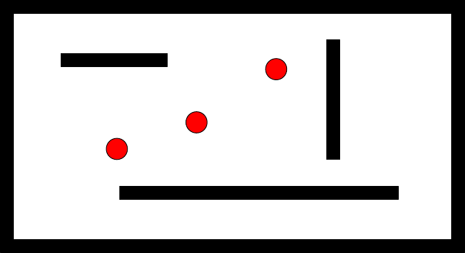
192
Mobile Node 1
Mobile Node 3
Mobile Node 2
Figure 7.7.2. The scenario of example 2
The following is the code piece of the main() function in Magent2.cc.
87 int main(int argc, char *argv[]) {
88
89 mynid = getMyNodeID();
90 myTCPsockfd = createTCPSocketForCommunicationWithSimulationEngine(
91 mynid, 1, -1, -1, -1, -1, -1, -1, -1, 0, socketfd2, 1);
92 constructGridMapofTheWholeField();
93 n = getInitialNodePosition(mynid, curX, curY, curZ);
94 newMovingDirectionInDegree = random() % 360;
95 getNearestCollisionPointAlongTheMovingDirectionViewedOnGUIScreen(
96 curX, curY, curZ, newMovingDirectionInDegree, nextX, nextY,
97 nextZ, distance, obsAngle);
98 curspeed = 10; /* moving speed: meter/second */
99 n = setNextWaypointAndMovingSpeed(myTCPsockfd, mynid, nextX, nextY,
100 nextZ, curspeed, 1);
101 usleepAndReleaseCPU(myTCPsockfd, mynid, 2000000);
102
103 while (1) {
104
105 n = getCurrentPosition(myTCPsockfd, mynid, curX, curY, curZ, 1);
106 if (twoPointsDistance(curX, curY, nextX, nextY) <= 10) {
107 /* The node has reached the next specified waypoint. Now, we
108 needs to change its moving direction.
193
109 */
110 newMovingDirectionInDegree = (2 * obsAngle -
111 newMovingDirectionInDegree);
112 if (newMovingDirectionInDegree < 0) newMovingDirectionInDegree += 360;
113 else {
114 newMovingDirectionInDegree = fmod(newMovingDirectionInDegree, 360);
115 }
116 getNearestCollisionPointAlongTheMovingDirectionViewedOnGUIScreen(
117 curX, curY, curZ, newMovingDirectionInDegree, nextX, nextY,
118 nextZ, distance, obsAngle);
119 n = setNextWaypoint(myTCPsockfd, mynid, nextX, nextY, nextZ, 1);
120 } else {
121 /* The node has not reached its next-point position. So,
122 we do nothing here to keep it moving along the current moving
123 direction.
124 */
125 }
126
127 if (downCount >= 0) goto skip;
128 n = getCurrentPositionOfAGroupOfNode(myTCPsockfd, mynid, 1, &NPArray,
129 numNodeInThisGroup, 1);
130 tmpNPArray = NPArray;
131 for (i=0; i<numNodeInThisGroup; i++) {
132 ax = NPArray->x;
133 ay = NPArray->y;
134 if (NPArray->nid == mynid) {
135 // A mobile node should not check the withinRange with itself.
136 NPArray++;
137 continue;
138 }
139 if ((NPArray->nid == ignoreID) && (downCount2 > 0)) {
140 // After just changing the moving direction,
141 // a mobile node should temporarily ignore the withinRange
142 // alerts caused by the node that just collided with itself.
143 // Withdoing so, we will see that the two mobile nodes keep
144 // exchanging their moving directions until they eventually
145 // move out of the withinRange (20 m) distance from each other.
146 //
194
147 // The ignoring period is downCount2 = 10 checking intervals
148 // long.
149 downCount2--;
150 NPArray++;
151 continue;
152 }
153 distance = twoPointsDistance(curX, curY, ax, ay);
154 if ((distance < 20) && (distance < minDist)) {
155
156 // Find the nearest mobile node that has approached me.
157 // To allow the two colliding mobile nodes to have time to
158 // exchange their moving direction, a mobile node should not
159 // change its moving angle to the moving direction of the other
160 // mobile node immediately. Otherwise, due to the detection time
161 // difference, the second mobile node will get the new moving
162 // direction of the first mobile node (which is the same as its
163 // current moving direction) resulting that the two mobile nodes
164 // move along the same moving direction of the second mobile node.
165 //
166 // For this reason, the actual moving direction change is delayed
167 // and performed downCount = 10 checking intervals later.
168 //
169 // Even with this careful design, sometimes the above problem
170 // still happens. This is because in some rare cases,
171 // due to the detection time differences between the two mobile
172 // nodes and their relative high speed movements, the first
173 // mobile node may detect the second mobile node but the second
174 // mobile node may not detect the first mobile node. This
175 // phenomenon is normal and can be explained.
176
177 minDist = distance;
178 n = getCurrentMovingDirectionViewedOnGUIScreen(myTCPsockfd,
179 NPArray->nid, aangle, 1);
180 ignoreID = NPArray->nid;
181 downCount = 10;
182 }
183 NPArray++;
184 }
195
185 free((char *) tmpNPArray);
186 skip:
187 downCount--;
188 if (downCount == 0) {
189 downCount2 = 10;
190 newMovingDirectionInDegree = aangle;
191 getNearestCollisionPointAlongTheMovingDirectionViewedOnGUIScreen(
192 curX, curY, curZ, newMovingDirectionInDegree, nextX, nextY,
193 nextZ, distance, obsAngle);
194 n = setNextWaypointAndMovingSpeed(myTCPsockfd, mynid, nextX,
195 nextY, nextZ, 10, 1);
196 }
197 skip2:
198 usleepAndReleaseCPU(myTCPsockfd, mynid, 100000);
199 }
200 }
The statements on lines 89 to 101 in Magent2.cc do the same task as the
statements of lines 80 to 92 in Magent1.cc. The main difference between these two
agents is the code piece between lines 127 and 198 in Magent2.cc. In this code piece,
the Magent2 agent first gets the location information of other nodes. This is done by
calling the getCurrentPositionOfAGroupOfNode() API function. Note that all mobile
nodes in this case belong to the same group -- group 1. The location information of all
nodes can be retrieved with a single getCurrentPositionOfAGroupOfNode() call,
which stores the location information in the NPArray parameter.
Next, using a loop, the Magent2 agent checks if there are other mobile nodes that
will collide with the node on which it is running. If so, it determines which one is the
node with which it will collide first. Then, the agent calls the
getCurrentMovingDirecitonViewedOnGUIScreen() function to get that node‟s
moving direction represented in degree. Thus, it can use the moving direction to
compute the nearest position that it is going to collide with an obstacle. Finally, it sets
a new waypoint as its next turning position (line 194). This agent will change its
moving direction each time it reaches or is very close to the next waypoint.
Note that this agent uses two counters, downCount and downCount2. The
downCount counter controls how often the Magent2 agent program checks the
location information for other nodes. And the downCount2 counter is used to make
the agent program not change its moving direction again in a short time after it just
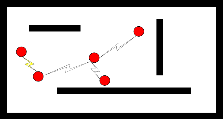
196
has changed its moving direction.
7.7.3 Example 3: Magent3.cc
As shown in Figure 7.7.3, multiple mobile nodes are located within a closed field.
They form a group and move in the same direction. Initially, they all move in a
randomly chosen moving direction. When any mobile node is about to collide with an
obstacle, it changes its moving direction and sends a message to all other mobile
nodes to notify them of this new moving direction. Upon receiving the message, each
mobile node sets its moving direction to the one just received and keeps moving. The
whole process repeats until the simulated time has elapsed.
In this case, all mobile nodes belong to group 1. Initially, all mobile nodes are
placed within the wireless transmission range of each other so that they can receive
messages from each other. The routing protocol used among all mobile nodes can be
AODV.
Mobile Node 1
Mobile Node 3
Mobile Node 2
Mobile Node 4
Mobile Node 5
Figure 7.7.3. The scenario of example 3
The following is the code piece of the main() function in Magent3.cc.
97 int main(int argc, char *argv[]) {
98
99 mynid = getMyNodeID();
100
101 sprintf(portNumStr, "%d", agentUDPportNum);
102 myUDPsockfd = passiveUDP(portNumStr);
197
103 printf("Agent(%d) created myUDPsockfd %d\n", mynid, myUDPsockfd);
104 if (myUDPsockfd < 0) {
105 printf("Agent(%d): Creating myUDPsockfd failed\n", mynid);
106 exit(0);
107 }
108 n = fcntl(myUDPsockfd, F_SETFL, O_NONBLOCK);
109
110 myTCPsockfd = createTCPSocketForCommunicationWithSimulationEngine(
111 mynid, 1, -1, -1, -1, -1, -1, -1, -1, 0, socketfd2, 1);
112 constructGridMapofTheWholeField();
113 n = getInitialNodePosition(mynid, curX, curY, curZ);
114 newMovingDirectionInDegree = random() % 360;
115 getNearestCollisionPointAlongTheMovingDirectionViewedOnGUIScreen(
116 curX, curY, curZ, newMovingDirectionInDegree, nextX, nextY,
117 nextZ, distance, obsAngle);
118 curspeed = 10; /* moving speed: meter/second */
119 n = setNextWaypointAndMovingSpeed(myTCPsockfd, mynid, nextX, nextY,
120 nextZ, curspeed, 1);
121 usleepAndReleaseCPU(myTCPsockfd, mynid, 2000000);
122
123 while (1) {
124
125 n = getCurrentPosition(myTCPsockfd, mynid, curX, curY, curZ, 1);
126
127 // Check whether some agent has sent me a message
128 len = sizeof(struct sockaddr);
129 n = recvfrom(myUDPsockfd, &msg, sizeof(struct
130 GUIChangeNodeMovingDirection), 0, (struct sockaddr *) &cli_addr,
131 (socklen_t*)&len);
132
133 if (n > 0) { // Some one has sent me a message asking me to change
134 // my moving direction.
135 if (msg.type != GUI_CHANGE_NODE_MOVING_DIRECTION) {
136 printf("Agent(%d): msg.type !=
GUI_CHANGE_NODE_MOVING_DIRECTION\n",
137 mynid);
138 exit(0);
139 }
198
140 printf("Agent(%d) received a new angle %lf degree from Agent(%d)\n",
141 mynid, msg.angle, msg.nid);
142 newMovingDirectionInDegree = msg.angle;
143 getNearestCollisionPointAlongTheMovingDirectionViewedOnGUIScreen(
144 curX, curY, curZ, newMovingDirectionInDegree, nextX, nextY,
145 nextZ, distance, obsAngle);
146 n = setNextWaypoint(myTCPsockfd, mynid, nextX, nextY, nextZ, 1);
147 goto skip;
148 } else { // No message has arrived so we do nothing special here.
149 }
150
151 if (twoPointsDistance(curX, curY, nextX, nextY) <= 10) {
152 /* The node has reached the next specified waypoint. Now, we
153 needs to change its moving direction.
154 */
155 newMovingDirectionInDegree = (2 * obsAngle -
156 newMovingDirectionInDegree);
157 if (newMovingDirectionInDegree < 0) newMovingDirectionInDegree += 360;
158 else {
159 newMovingDirectionInDegree = fmod(newMovingDirectionInDegree, 360);
160 }
161 getNearestCollisionPointAlongTheMovingDirectionViewedOnGUIScreen(
162 curX, curY, curZ, newMovingDirectionInDegree, nextX, nextY,
163 nextZ, distance, obsAngle);
164 n = setNextWaypoint(myTCPsockfd, mynid, nextX, nextY, nextZ, 1);
165
166 // We also send a message to every other agent that is current up
167 // to ask it to move in my new moving direction.
168 n = getCurrentPositionOfAGroupOfNode(myTCPsockfd, mynid, 1, &NPArray,
169 numNodeInThisGroup, 1);
170 tmpNPArray = NPArray;
171
172 msg.type = GUI_CHANGE_NODE_MOVING_DIRECTION;
173 msg.nid = mynid;
174 msg.angle = newMovingDirectionInDegree;
175
176 for (i=0; i<numNodeInThisGroup; i++) {
177
199
178 if (NPArray->nid == mynid) {
179 // A mobile node should not send a message to itself.
180 NPArray++;
181 continue;
182 }
183
184 sprintf(hostname, "1.0.1.%d", NPArray->nid);
185 bzero( &cli_addr, sizeof(cli_addr) );
186 cli_addr.sin_family = AF_INET;
187 cli_addr.sin_port = htons(agentUDPportNum);
188 cli_addr.sin_addr.s_addr = inet_addr( hostname );
189
190 len = sizeof(struct sockaddr);
191 n = sendto(myUDPsockfd, &msg, sizeof(struct
192 GUIChangeNodeMovingDirection), 0, (struct sockaddr *) &cli_addr,
193 len);
194 if (n < 0) {
195 printf("Agent(%d) Sendto() failed\n", mynid);
196 exit(0);
197 }
198 NPArray++;
199
200 }
201 free((char *) tmpNPArray);
202
203 } else {
204 /* The node has not reached its next-point position. So,
205 we do nothing here to keep it moving along the current moving
206 direction.
207 */
208 }
209
210 skip:
211 usleepAndReleaseCPU(myTCPsockfd, mynid, 100000);
212 }
213 }
In the main() function of the Magent3 agent, the agent first gets the node ID of
200
the node to which it belongs. Second, it creates a passive UDP socket for
communicating with other agents. Notice that on line 108 the agent sets this UDP
socket to be non-blocking via the fcntl() function. It is essential for this agent because
this agent program cannot be blocked when it tries to receive packets sent from other
agents. Besides receiving packets from other agents, the Magent3 agent still has
several works to do. For example, it has to check whether it is going to collide with an
obstacle or not. If the agent is blocked for waiting packets from other agents, it will
sleep until there is a packet in the socket buffer of the UDP socket. However, the node
on which this agent is running may have collided with one obstacle or other nodes
when the agent code is blocked. As such, the agent will not have a chance to respond
to such an event, and hence the generated simulation results are incorrect.
On lines 110 to 112, the agent first establishes a TCP connection for
communicating with the simulation engine. It then constructs the grid map by calling
constructGridMapofTheWholeField() function. Next, it gets the initial location of the
node on which it is running using the getInitialNodePosition() API function on line
113.
The statements on lines 114 to 119 do the following tasks: (1) randomly
determine the initial moving direction represented in degree. (2) According to the
node‟s current position and the chosen moving direction, the agent computes the next
collision point via the
getNearestCollisionPointAlongTheMovingDirectionViewedOnGUIScreen() function.
(3) The agent passes the nearest collision point computed in step (2) and a chosen
moving speed to the setNextWaypointAndMovingSpeed() function. This function will
notify the simulation engine of the information of these two parameters to set the next
waypoint for this node. Finally, it uses the usleepAndReleaseCPU() function to
release CPU.
In the main while loop, which is composed of the statements on lines 123 to 212,
the agent first obtains the current position of the node to which it belongs on line 125.
Second, it uses the recvfrom() socket API function call to check if there are packets
from other agents to be read. Since the UDP socket is set as non-blocking, the agent
will not sleep in this function if there is no packet to be read. If there is a packet from
other node, the agent first determines the type of the message contained in this packet.
The only message type that the Magent3 agent recognizes is
GUI_CHANGE_NODE_MOVING_DIRECTION. If the agent receives any messages
with other types, it will terminate the execution immediately.
Upon receiving a message with the
GUI_CHANGE_NODE_MOVING_DIRECTION type, the agent extracts the value
of the angle field contained in this message. Then, it set its moving direction to this

201
angle.
On the statements of lines 151 to 208, the agent first checks if it is about to
collide with an obstacle or other nodes. If so, it computes and sets its next waypoint.
Also, it needs to broadcast a message to other nodes to notify them of this moving
direction change. On line 168, it uses the getCurrentPositionOfAGroupOfNode()
function to know the number of nodes that is alive at this time. On lines 172 to and
174, it forms a notification message with the
GUI_CHANGE_NODE_MOVING_DIRECTION message type, its node ID, and the
new moving direction represented in degree. On the loop of lines 176 to 200, the
agent iteratively sends the notification message to every other node.
At the end of the main while loop, this agent uses the usleepAndReleaseCPU()
function to release CPU.
7.7.4 Example 4: Magent4.cc
Mobile Node
Figure 7.7.4. The scenario of example 4
The scenario of example 4 is shown in Figure 7.7.4. A mobile node is located in
a closed maze filled with many obstacles. It chooses a random destination position
(Dx, Dy) and moves toward that place. To get there, it uses the A* path search
algorithm and the maze map to find a path to that destination. The path is composed
of a sequence of turning points (X1, Y1), (X2, Y2), ..., (Xm == Dx, Ym = Dy).
The mobile node removes the head point from the path and sets it as the
next-point position. Then it moves linearly toward its next-point position. After
reaching its next way point position, it repeats the above operation until the path
becomes empty, which means that the mobile node has reached its destination point.
At this time, the mobile node chooses a new random position and again uses the A*
202
algorithm to construct a path. The above process is repeated until the simulation is
finished.
In the following, we show the contents of Magent4.cc.
83 int mynid, n, myTCPsockfd, socketfd2, count;
84 double curX, curY, curZ, nextX, nextY, nextZ, newMovingDirectionInDegree;
85 double curspeed, distance, obsAngle, destX, destY, prevX, prevY;
86 PATH_LIST *pList, *filteredListP;
87
88
89 void findNewDestination() {
90
91 retry:
92 destX = fmod((double) random(), maxXMeter);
93 destY = fmod((double) random(), maxYMeter);
94 if (m_Map->InObstacleGrid(destX, destY) == true)
95 goto retry; // Occupied by an obstacle
96 if (grid_n(destX) == grid_n(curX) && grid_n(destY) == grid_n(curY))
97 goto retry; // Source and Destination fall into the same grid tile
98 if (twoPointsDistance(curX, curY, destX, destY) < 200)
99 goto retry; // New destination point is too near
100 pList->clear();
101 if (m_Map->FindPathToList(curX, curY, destX, destY, pList) == false)
102 goto retry; // There is no path to reach the new destination point
103
104 filteredListP->clear();
105 prevX = curX;
106 prevY = curY;
107
108 while (!pList->empty()) {
109 nextX = pList->front().first; // get the head point
110 nextY = pList->front().second;
111 if (twoPointsDistance(prevX, prevY, nextX, nextY) < 15) {
112 // Filter out consecutive waypoint points that are too
113 // close to each other
114 pList->pop_front();
115 continue;
116 } else {
203
117 LOCATION loc(nextX, nextY);
118 filteredListP->push_back(loc);
119 pList->pop_front();
120 prevX = nextX;
121 prevY = nextY;
122 }
123 }
124
125 }
126
127
128 int main(int argc, char *argv[]) {
129
130 mynid = getMyNodeID();
131 myTCPsockfd = createTCPSocketForCommunicationWithSimulationEngine(
132 mynid, 1, -1, -1, -1, -1, -1, -1, -1, 0, socketfd2, 1);
133 constructGridMapofTheWholeField();
134 n = getInitialNodePosition(mynid, curX, curY, curZ);
135 pList = new PATH_LIST();
136 filteredListP = new PATH_LIST();
137
138 // Choose a good and interesring random destination point
139 findNewDestination();
140
141 nextX = filteredListP->front().first; // get the head point
142 nextY = filteredListP->front().second;
143 printf("Agent(%d): Set next waypoint to (%lf, %lf)\n", mynid, nextX, nextY);
144 filteredListP->pop_front(); // remove the head point
145
146 curspeed = 10; /* moving speed: meter/second */
147 n = setNextWaypointAndMovingSpeed(myTCPsockfd, mynid, nextX, nextY,
148 nextZ, curspeed, 1);
149 usleepAndReleaseCPU(myTCPsockfd, mynid, 1);
150
151 while (1) {
152
153 n = getCurrentPosition(myTCPsockfd, mynid, curX, curY, curZ, 1);
154 if (twoPointsDistance(curX, curY, nextX, nextY) <= 10) {
204
155 /* The node has reached the next specified waypoint. Now, we
156 needs to change its waypoint based on the constructed path.
157 */
158 if (filteredListP->empty()) {
159 // This node has reached the destination of the current path.
160 // Now we need to choose a new random destination point for the
161 // node and make the node move toward it as before.
162
163 // Choose a good and interesring random destination point
164 findNewDestination();
165
166 } else {
167 // There is still a waypoint in the current constructed path,
168 // so we need not construct a new path.
169 }
170 nextX = filteredListP->front().first; // get the head point
171 nextY = filteredListP->front().second;
172 filteredListP->pop_front(); // remove the head point
173 n = setNextWaypoint(myTCPsockfd, mynid, nextX, nextY, nextZ, 1);
174 } else {
175 /* The node has not reached its next-point position. So,
176 we do nothing here to keep it moving along the current moving
177 direction.
178 */
179 }
180 usleepAndReleaseCPU(myTCPsockfd, mynid, 200000);
181 }
182 }
In the findNewDestination() function, the Magent4 agent program tries to find a
good position as its next destination position with the A* algorithm. It first randomly
chooses a location (destX, destY). Then, it checks whether the location (destX, destY)
is good enough based on the following criteria: (1) if it is within one obstacle or not,
(2) if it is within the same grid in which the current position is, (3) if it is very close to
the current position, and (4) if there is a path from the current position to the newly
chosen position.
If a good destination position can be found, the path from the current position to
the destination position is generated when the m_Map->FindPathToList(curX, curY,

205
destX, destY, pList) function call is performed. The generated path list is stored in the
pList parameter. On lines 108 to 123, the agent tries to merge two consecutive
waypoints if they are too close. This can reduce the frequency of setting next
waypoints and thus increase simulation speeds.
On lines 130 to 149, which is the top half of the main() function, the agent does
the almost same task as the agents introduced previously. In addition, on lines 135 and
136, it initializes two path list instances, pList and filteredListP. Then, the agent calls
the findNewDestination() function, explained previously, to find a good destination
position and a path from the current position to the destination position. Next, it pops
the first element in the path and uses the information of this element to set its next
way point by calling the setNextWaypointAndMovingSpeed() function.
In the bottom half of the main() function, which is the main while loop, the
Magent4 agent first gets the current position of the node on which it is running. On
line 154, it examines whether the distance between the current position and the next
waypoint is within ten meters. If so, the agent pops the top element of the path list and
sets the information of that element as its next waypoint unless the path list is already
empty. In such a case, the agent will call the findNewDestination() function to choose
another good destination position and fill the pList and filteredListP fields with the
newly generated path from the current position to the new destination position.
At the end of this while loop, it is necessary to invoke the usleepAndReleaseCPU()
call. The reason why the agent has to call this function has been explained previously.
7.7.5 Example 5: Magent5.cc
Chasing Node
Target Node
Figure 7.7.5. The scenario of example 5
The scenario of this example is shown in Figure 7.7.5. Two mobile nodes are
206
located in a maze filled with many obstacles. One mobile node (here MNODE(2)) is
the target node while the other node is the chasing node. During the simulation, each
mobile node knows the position of the other node at all time (assuming that this
location information is provided by a third body through a satellite). With this
information on hand, the target node tries to run away from the chasing node in the
opposite direction of the chasing node. During the simulation, the target node detects
the position of the chasing node and recalculates a new escaping path when the
distance between the two nodes falls within a threshold.
The behavior of the chasing node is described as follows. Initially, it uses the
position of the chasing node as the destination point to construct an A* path to chase
the target node. Then it moves along the path to try to capture the target node. During
the chasing, it detects the position of the target node and recalculates a new A* path to
chase the target node once every a few seconds.
In this case, the target node belongs to group 1 while the chasing node belongs to
group 2. The moving speed of the target node is set to a value higher than that set to
the chasing node. The chasing process continues until the target node is captured
(collided with) by the chasing node or the simulation time has elapsed.
In the following, we show the codes of a chasing agent program, Magent5-c, and
a target agent program, Magent5-t, in sequence.
Magent5-c.cc (the codes of the chasing agent program)
92 int dangerNid, i, mynid, n, myTCPsockfd, socketfd2, count, numNodeInThisGroup;
93 double curX, curY, curZ, nextX, nextY, nextZ, newMovingDirectionInDegree;
94 double curspeed, distance, minDist, obsAngle, destX, destY, prevX, prevY;
95 double targetX, targetY, dangerX, dangerY, pl;
96 PATH_LIST *pList, *filteredListP, *chaseP, *filteredToChaseP;
97 struct nodePosition *NPArray;
98 int recalculateCount;
99
100 void filterPathList(double startx, double starty, PATH_LIST *pList,
101 PATH_LIST *filteredListP) {
102
103 double nextX, nextY, prevX, prevY;
104
105 prevX = startx;
106 prevY = starty;
107 while (!pList->empty()) {
207
108 nextX = pList->front().first; // get the head point
109 nextY = pList->front().second;
110 if (twoPointsDistance(prevX, prevY, nextX, nextY) < 10) {
111 // Filter out consecutive waypoint points that are too
112 // close to each other
113 pList->pop_front();
114 continue;
115 } else {
116 LOCATION loc(nextX, nextY);
117 filteredListP->push_back(loc);
118 pList->pop_front();
119 prevX = nextX;
120 prevY = nextY;
121 }
122 }
123
124 }
125
126
127 void findNewDestination() {
128
129 int count1 = 0, count2 = 0;
130
131 retry:
132
133 if (count1 > 3 || count2 > 10) {
134 stopSimulation(myTCPsockfd, mynid);
135 sleep(10);
136 }
137 count2++;
138 destX = fmod((double) random(), maxXMeter);
139 destY = fmod((double) random(), maxYMeter);
140 if (m_Map->InObstacleGrid(destX, destY) == true)
141 goto retry; // Occupied by an obstacle
142 if (grid_n(destX) == grid_n(curX) && grid_n(destY) == grid_n(curY))
143 goto retry; // Source and Destination fall into the same grid tile
144 if (twoPointsDistance(curX, curY, destX, destY) < 100)
145 goto retry; // New destination point is too near
208
146 pList->clear();
147 if (m_Map->FindPathToList(curX, curY, destX, destY, pList) == false) {
148 count1++;
149 goto retry; // There is no path to reach the new destination point
150 }
151 filteredListP->clear();
152 filterPathList(curX, curY, pList, filteredListP);
153 }
154
155
156 int main(int argc, char *argv[]) {
157
158 mynid = getMyNodeID();
159 myTCPsockfd = createTCPSocketForCommunicationWithSimulationEngine(
160 mynid, -1, 1, -1, -1, -1, -1, -1, -1, 0, socketfd2, 1);
161 constructGridMapofTheWholeField();
162 n = getInitialNodePosition(mynid, curX, curY, curZ);
163 pList = new PATH_LIST();
164 filteredListP = new PATH_LIST();
165 chaseP = new PATH_LIST();
166
167 // Choose a random destination point
168 findNewDestination();
169
170 nextX = filteredListP->front().first; // get the head point
171 nextY = filteredListP->front().second;
172 filteredListP->pop_front(); // remove the head point
173
174 curspeed = 10; /* moving speed: meter/second */
175 n = setNextWaypointAndMovingSpeed(myTCPsockfd, mynid, nextX, nextY,
176 nextZ, curspeed, 1);
177 usleepAndReleaseCPU(myTCPsockfd, mynid, 1);
178
179 recalculateCount = 5 * 10; // every 10 seconds
180
181 while (1) {
182 n = getCurrentPosition(myTCPsockfd, mynid, curX, curY, curZ, 1);
183 n = getCurrentPositionOfAGroupOfNode(myTCPsockfd, mynid, 1, &NPArray,
209
184 numNodeInThisGroup, 1);
185
186 targetX = NPArray->x;
187 targetY = NPArray->y;
188 free((char *) NPArray);
189
190 if (m_Map->InObstacleGrid(targetX, targetY) == true)
191 {
192 for (int k=1; k<10; k++)
193 {
194 double off = 10.0*k;
195 if (m_Map->InObstacleGrid(targetX+off, targetY+off) == false)
196 {
197 targetX += off;
198 targetY += off;
199 } else if (m_Map->InObstacleGrid(targetX-off, targetY+off) == false)
200 {
201 targetX -= off;
202 targetY += off;
203 } else if (m_Map->InObstacleGrid(targetX+off, targetY-off) == false)
204 {
205 targetX += off;
206 targetY -= off;
207 } else if (m_Map->InObstacleGrid(targetX-off, targetY-off) == false)
208 {
209 targetX -= off;
210 targetY -= off;
211 }
212 else
213 {
214 continue;
215 }
216 break;
217 }
218 }
219
220
221
210
222
223
224 if (twoPointsDistance(curX, curY, targetX, targetY) <= 15) {
225 printf("Agent(%d) has captured the target node.\n", mynid);
226 stopSimulation(myTCPsockfd, mynid);
227 sleep(10);
228 }
229
230 recalculateCount--;
231
232 if (recalculateCount == 0) {
233 recalculateCount = 50;
234
235 chaseP->clear();
236 m_Map->FindPathToList(curX, curY, targetX, targetY, chaseP);
237
238 filteredListP->clear();
239
240 filterPathList(curX, curY, chaseP, filteredListP);
241
242 nextX = filteredListP->front().first; // get the head point
243 nextY = filteredListP->front().second;
244 filteredListP->pop_front(); // remove the head point
245 n = setNextWaypoint(myTCPsockfd, mynid, nextX, nextY, nextZ, 1);
246 usleepAndReleaseCPU(myTCPsockfd, mynid, 200000);
247 continue;
248 }
249
250 if (twoPointsDistance(curX, curY, nextX, nextY) <= 10) {
251 /* The node has reached the next specified waypoint. Now, we
252 * needs to change its waypoint based on the constructed path.
253 */
254 if (filteredListP->empty()) {
255 // This node has reached the destination of the current path.
256 // Now we need to find a new path to chase the target node.
257
258 n = getCurrentPositionOfAGroupOfNode(myTCPsockfd, mynid, 1, &NPArray,
259 numNodeInThisGroup, 1);
211
260
261 targetX = NPArray->x;
262 targetY = NPArray->y;
263 free((char *) NPArray);
264
265 chaseP->clear();
266 m_Map->FindPathToList(curX, curY, targetX, targetY, chaseP);
267
268 filteredListP->clear();
269 filterPathList(curX, curY, chaseP, filteredListP);
270
271 } else {
272 // There is still a waypoint in the current constructed path,
273 // so we need not construct a new path.
274 }
275 nextX = filteredListP->front().first; // get the head point
276 nextY = filteredListP->front().second;
277 filteredListP->pop_front(); // remove the head point
278 n = setNextWaypoint(myTCPsockfd, mynid, nextX, nextY, nextZ, 1);
279 } else {
280 /* The node has not reached its next-point position. So,
281 we do nothing here to keep it moving along the current moving
282 direction.
283 */
284 }
285
286 usleepAndReleaseCPU(myTCPsockfd, mynid, 200000);
287 }
288 }
289
The filterPathList() function takes four parameters, startx, starty, pList,
filteredListP. The startx and starty parameters form a position (startx, starty) and the
pList and filteredListP parameters are two path lists. Initially, this function compares
the start position and the first waypoint in the pList path list. If the distance between
them is less than ten meters, it filters the first waypoint in the pList path list. Next, the
function traverses the whole pList path list to check the distances between any two
212
consecutive way points. If there are two waypoints that are too close, i.e., the distance
between them is less than ten meters, the function will merge these two waypoints.
The filtered path list is stored in the filteredListP parameter.
In the findNewDestination() function, the agent program tries to find a good
position to be its next destination position using the A* algorithm. It first randomly
chooses a location (destX, destY). Then, it checks whether the location (destX, destY)
is good enough based on the following criteria: (1) if it is within one obstacle or not,
(2) if it is within the same grid in which the current position is, (3) if it is very close to
the current position, and (4) if there is a path from the current position to the newly
chosen position.
If a good destination position is determined, the path from the current position to
the newly chosen destination position is generated when the
m_Map->FindPathToList(curX, curY, destX, destY, pList) call is performed. The
generated path list is stored in the pList parameter.
In the main() function, before the main while loop, the Magent5-c agent
performs almost the same task as the Magent4 agent except that the Magent5-c agent
uses an additional path list variable, chaseP, to store the generated path list from the
current position to the target node‟s position.
In the main while loop, the Magent5-c agent first gets its current position. And
then it calls the getCurrentPositionOfAGroupOfNode() function to enquire the
simulation engine for the current positions of every node in group 1, to which the
target node belongs. After knowing the current position of the target node, the
Magent5-c agent checks if the grid in which the target node is currently located
contains an obstacle or not. If the grid contains an obstacle, it will be marked as an
unreachable grid. Since the A* algorithm tries to compute a valid path to reach the
destination position based on the grid map, in such a case it will never find out a valid
path and the agent program may not work correctly.
Therefore, on statements of lines 190 to 218 the agent tries to find out a new
destination position, whose corresponding grid does not contain an obstacle and is the
closest one to the grid where the target node is. On lines 192 to 217, from a position
nearest to the original destination position, the agent iteratively checks if the grid in
which a chosen position is located contains an obstacle or not until it finds out a
suitable position or it has run out of positions that it can choose (the number of
positions that the Magent5-c agent can choose is predefined by the number of
iterations of the loop between lines 192 and 217).
After knowing (or adjusting if needed) the current position of the target node, the
agent checks if the distance between itself and the target node is less than 15 meters.
If so, it means that the chasing node has captured the target node, and thus the
213
Magent5-c agent terminates the simulation. Otherwise, on lines 232 to 248 the
chasing agent will recompute a new path list based on the current positions of itself
and the target node if the recalculateCount counter counts down to zero.
On line 250, the chasing agent checks if the distance between the current position
and the next waypoint is less than 10 meters, that is, whether it is very close to that
waypoint. In such a case, it extracts the top element of the path list and uses the
position information in that element as its next turning point. In the case that the path
list is empty, the agent will compute a new path list based on the current positions of
itself and the target node.
At the end of this while loop, it is necessary to call the usleepAndReleaseCPU()
function. The reason that an agent needs to use this function has been explained
previously. Also, note that the chasing node uses the usleepAndReleaseCPU()
function to sleep for 200,000 microseconds (that is, 0.2 second) periodically. Since
the initial value of the recalculateCount counter is set as 50, the chasing agent will
recompute the path list from itself to the target node every ten seconds.
Magent5-t.cc (the codes of the target agent program)
91 double curX, curY, curZ, nextX, nextY, nextZ, newMovingDirectionInDegree;
92 double curspeed, distance, minDist, obsAngle, destX, destY, prevX, prevY;
93 double chaseX, chaseY, dangerX, dangerY, pl;
94 double tlx, tly, blx, bly, trx, tryy, brx, bry;
95 struct nodePosition *NPArray, *tmpNPArray;
96 int dangerNid, i, mynid, n, myTCPsockfd, socketfd2, count, numNodeInThisGroup;
97 int delayCount = 0;
98 PATH_LIST *pList, *filteredListP, *tochaseP, *filteredToChaseP;
99
100
101
102 void filterPathList(double startx, double starty, PATH_LIST *pList,
103 PATH_LIST *filteredListP) {
104
105 double nextX, nextY, prevX, prevY;
106 int count = 0;
107
108 prevX = startx;
109 prevY = starty;
110 while (!pList->empty()) {
214
111 nextX = pList->front().first; // get the head point
112 nextY = pList->front().second;
113 if ( pList->size()>5 && twoPointsDistance(prevX, prevY, nextX, nextY) < 10) {
114 // Filter out consecutive waypoint points that are too
115 // close to each other
116 } else {
117 LOCATION loc(nextX, nextY);
118 filteredListP->push_back(loc);
119 prevX = nextX;
120 prevY = nextY;
121 }
122 pList->pop_front();
123 }
124
125 }
126
127
128 void findNewDestination(double hintx, double hinty) {
129
130 int count1 = 0, count2 = 0;
131
132 if (m_Map->InObstacleGrid(curX, curY) == true)
133 {
134 // printf("%s #%d InObstacleGrid (%lf, %lf)\n", __FILE__, __LINE__, curX, curY);
135 if (m_Map->InObstacleGrid(curX+10.0, curY+10.0) == false)
136 {
137 curX += 10.0;
138 curY += 10.0;
139 } else if (m_Map->InObstacleGrid(curX-10.0, curY+10.0) == false)
140 {
141 curX -= 10.0;
142 curY += 10.0;
143 } else if (m_Map->InObstacleGrid(curX+10.0, curY-10.0) == false)
144 {
145 curX += 10.0;
146 curY -= 10.0;
147 } else if (m_Map->InObstacleGrid(curX-10.0, curY-10.0) == false)
148 {
215
149 curX -= 10.0;
150 curY -= 10.0;
151 }
152 // printf("(3) Now Target is in obstacle grid: (%lf, %lf)\n", curX, curY);
153 }
154
155 retryy:
156
157 if (count1 > 2 || count2 > 20) {
158 printf("Agent(%d) findNewDestination() failed. curX %lf curY %lf\n", mynid, curX,
curY);
159 stopSimulation(myTCPsockfd, mynid);
160 sleep(10);
161 }
162
163 if (count1 == 0 && count2 == 0) {
164 if (hintx > 0) {
165 destX = hintx;
166 } else {
167 destX = fmod((double) random(), maxXMeter);
168 }
169 if (hinty > 0) {
170 destY = hinty;
171 } else {
172 destY = fmod((double) random(), maxYMeter);
173 }
174 } else {
175 destX = fmod((double) random(), maxXMeter);
176 destY = fmod((double) random(), maxYMeter);
177 }
178 count2++;
179 if (m_Map->InObstacleGrid(destX, destY) == true)
180 goto retryy; // Occupied by an obstacle
181 if (grid_n(destX) == grid_n(curX) && grid_n(destY) == grid_n(curY))
182 goto retryy; // Source and Destination fall into the same grid tile
183 if (twoPointsDistance(curX, curY, destX, destY) < 200)
184 goto retryy; // New destination point is too near
185 pList->clear();
216
186 if (m_Map->FindPathToList(curX, curY, destX, destY, pList) == false) {
187 count1++;
188 goto retryy; // There is no path to reach the new destination point
189 }
190 filteredListP->clear();
191 // delete filteredListP;
192 // filteredListP = new PATH_LIST;
193 filterPathList(curX, curY, pList, filteredListP);
194 }
195
196
197 double pathLength(PATH_LIST *filteredListp) {
198
199 double dist, totalDist, lprevX, lprevY, lnextX, lnextY;
200 PathListItor pl;
201
202 if (filteredListp->empty()) {
203 return(0);
204 }
205
206 pl = filteredListp->begin();
207 lprevX = pl->first;
208 lprevY = pl->second;
209
210 totalDist = 0;
211 while (pl != filteredListp->end()) {
212
213 count++;
214 lnextX = pl->first; // get the head point
215 lnextY = pl->second;
216 dist = twoPointsDistance(lprevX, lprevY, lnextX, lnextY);
217 totalDist += dist;
218 lprevX = lnextX;
219 lprevY = lnextY;
220
221 pl++;
222 }
223 return(totalDist);
217
224 }
225
226
227 double minPointToPathDistance(double dangerX, double dangerY, PATH_LIST
228 *filteredListp) {
229
230 double minDist, dist, d1, d2, x, y, prevX, prevY, prox, proy;
231 int n, count = 0;
232 PathListItor pl;
233
234 prevX = filteredListp->front().first; // get the head point
235 prevY = filteredListp->front().second;
236 filteredListp->pop_front();
237
238 pl = filteredListp->begin();
239 minDist = 9999999; // infinity
240 while (pl != filteredListp->end()) {
241 x = pl->first; // get the head point
242 y = pl->second;
243
244 n = NodeProjection_InLineSegment(dangerX, dangerY, prevX, prevY, x, y,
245 prox, proy);
246 if (n == 1) {
247 dist = twoPointsDistance(dangerX, dangerY, prox, proy);
248 } else {
249 d1 = twoPointsDistance(dangerX, dangerY, prevX, prevY);
250 d2 = twoPointsDistance(dangerX, dangerY, x, y);
251 if (d1 < d2) dist = d1;
252 else dist = d2;
253 }
254 if (dist < minDist) minDist = dist;
255 prevX = x;
256 prevY = y;
257
258 pl++;
259 }
260 return(minDist);
261 }
218
262
263
264 void findFourCornerPoints() {
265
266 tlx = 0;
267 tly = 0;
268 while (m_Map->InObstacleGrid(tlx, tly) == true) {
269 tlx += gridWidthMeter;
270 tly += gridWidthMeter;
271 }
272
273 trx = maxXMeter;
274 tryy = 0;
275 while (m_Map->InObstacleGrid(trx, tryy) == true) {
276 trx -= gridWidthMeter;
277 tryy += gridWidthMeter;
278 }
279
280 blx = 0;
281 bly = maxYMeter;
282 while (m_Map->InObstacleGrid(blx, bly) == true) {
283 blx += gridWidthMeter;
284 bly -= gridWidthMeter;
285 }
286
287 brx = maxXMeter;
288 bry = maxYMeter;
289 while (m_Map->InObstacleGrid(brx, bry) == true) {
290 brx -= gridWidthMeter;
291 bry -= gridWidthMeter;
292 }
293
294 }
295
296
297 int main(int argc, char *argv[]) {
298
299 mynid = getMyNodeID();
219
300 myTCPsockfd = createTCPSocketForCommunicationWithSimulationEngine(
301 mynid, 1, -1, -1, -1, -1, -1, -1, -1, 0, socketfd2, 1);
302 constructGridMapofTheWholeField();
303 findFourCornerPoints();
304
305 n = getInitialNodePosition(mynid, curX, curY, curZ);
306 pList = new PATH_LIST();
307 filteredListP = new PATH_LIST();
308 tochaseP = new PATH_LIST();
309 filteredToChaseP = new PATH_LIST();
310
311 // Choose a random destination point
312 findNewDestination(0, 0);
313
314 nextX = filteredListP->front().first; // get the head point
315 nextY = filteredListP->front().second;
316 filteredListP->pop_front(); // remove the head point
317
318 curspeed = 15; /* moving speed: meter/second */
319 n = setNextWaypointAndMovingSpeed(myTCPsockfd, mynid, nextX, nextY,
320 nextZ, curspeed, 1);
321 usleepAndReleaseCPU(myTCPsockfd, mynid, 1);
322
323 while (1) {
324 n = getCurrentPosition(myTCPsockfd, mynid, curX, curY, curZ, 1);
325 delayCount--;
326 if (delayCount > 0) goto skipApproachChecking;
327
328 n = getCurrentPositionOfAGroupOfNode(myTCPsockfd, mynid, 2, &NPArray,
329 numNodeInThisGroup, 1);
330 tmpNPArray = NPArray;
331
332 minDist = 9999999; // infinity
333 dangerNid = -1; // Assuming none
334
335 for (i = 0; i < numNodeInThisGroup; i++) {
336
337 chaseX = NPArray->x;
220
338 chaseY = NPArray->y;
339
340 if (m_Map->InObstacleGrid(chaseX, chaseY) == true)
341 {
342 // printf("(3) Target is in obstacle grid: (%lf, %lf)\n", chaseX, chaseY);
343
344 if (m_Map->InObstacleGrid(chaseX+10.0, chaseY+10.0) == false)
345 {
346 chaseX += 10.0;
347 chaseY += 10.0;
348 } else if (m_Map->InObstacleGrid(chaseX-10.0, chaseY+10.0) == false)
349 {
350 chaseX -= 10.0;
351 chaseY += 10.0;
352 } else if (m_Map->InObstacleGrid(chaseX+10.0, chaseY-10.0) == false)
353 {
354 chaseX += 10.0;
355 chaseY -= 10.0;
356 } else if (m_Map->InObstacleGrid(chaseX-10.0, chaseY-10.0) == false)
357 {
358 chaseX -= 10.0;
359 chaseY -= 10.0;
360 }
361 // printf("(3) Now Target is in obstacle grid: (%lf, %lf)\n", chaseX, chaseY);
362 }
363 if (m_Map->InObstacleGrid(curX, curY) == true)
364 {
365 //printf("(4) Curr is in obstacle grid: (%lf, %lf)\n", curX, curY);
366 }
367
368 distance = twoPointsDistance(curX, curY, chaseX, chaseY);
369 if (distance > 200) {
370 // The physical distance between the two nodes is > 100
371 // No immediate threat at the present time
372 NPArray++;
373 continue;
374 } else if (distance < minDist) {
375 tochaseP->clear();
221
376 m_Map->FindPathToList(curX, curY, chaseX, chaseY, tochaseP);
377 filteredToChaseP->clear();
378 filterPathList(curX, curY, tochaseP, filteredToChaseP);
379 pl = pathLength(filteredToChaseP);
380 if (pl > 200) {
381 // The length of the path connecting the two nodes is > 100
382 // No immediate threat at the present time
383 NPArray++;
384 continue;
385 } else if (pl < minDist) {
386 // Identify the most dangerous (nearest) chasing node
387 minDist = pl;
388 dangerX = chaseX;
389 dangerY = chaseY;
390 dangerNid = NPArray->nid;
391 }
392 }
393 NPArray++;
394
395 }
396 free((char *) tmpNPArray);
397
398 if (dangerNid > 0) {
399 // There exists a dangerous chasing node.
400
401 // Check the directions to the four corners and see which way is
402 // good enough.
403 distance = 0;
404 if (distance < 100) {
405 if (twoPointsDistance(tlx, tly, curX, curY) > 210 ) {
406 findNewDestination(tlx, tly);
407 distance = minPointToPathDistance(dangerX, dangerY, filteredListP);
408 }
409 }
410 if (distance < 100) {
411 if (twoPointsDistance(trx, tryy, curX, curY) > 210 ) {
412 findNewDestination(trx, tryy);
413 distance = minPointToPathDistance(dangerX, dangerY, filteredListP);
222
414 }
415 }
416 if (distance < 100) {
417 if (twoPointsDistance(brx, bry, curX, curY) > 210 ) {
418 findNewDestination(brx, bry);
419 distance = minPointToPathDistance(dangerX, dangerY, filteredListP);
420 }
421 }
422 if (distance < 100) {
423 if (twoPointsDistance(blx, bly, curX, curY) > 210 ) {
424 findNewDestination(blx, bly);
425 distance = minPointToPathDistance(dangerX, dangerY, filteredListP);
426 }
427 }
428
429 delayCount = 60; // Allow the new escaping plan some time to take effect
430 nextX = filteredListP->front().first; // get the head point
431 nextY = filteredListP->front().second;
432 filteredListP->pop_front(); // remove the head point
433 n = setNextWaypoint(myTCPsockfd, mynid, nextX, nextY, nextZ, 1);
434 usleepAndReleaseCPU(myTCPsockfd, mynid, 200000);
435 continue;
436 }
437
438 skipApproachChecking:
439
440 if (twoPointsDistance(curX, curY, nextX, nextY) <= 10) {
441 /* The node has reached the next specified waypoint. Now, we
442 needs to change its waypoint based on the constructed path.
443 */
444 if (filteredListP->empty()) {
445 // This node has reached the destination of the current path.
446 // Now we need to choose a new random destination point for the
447 // node and make the node move toward it as before.
448
449 // Choose a random destination point
450 findNewDestination(0, 0);
451 } else {
223
452 // There is still a waypoint in the current constructed path,
453 // so we need not construct a new path.
454 }
455 nextX = filteredListP->front().first; // get the head point
456 nextY = filteredListP->front().second;
457 filteredListP->pop_front(); // remove the head point
458 n = setNextWaypoint(myTCPsockfd, mynid, nextX, nextY, nextZ, 1);
459 } else {
460 /* The node has not reached its next-point position. So,
461 we do nothing here to keep it moving along the current moving
462 direction.
463 */
464 }
465 usleepAndReleaseCPU(myTCPsockfd, mynid, 200000);
466 }
467 }
468
The filterPathList() function takes four parameters, startx, starty, pList,
filteredListP. The startx and starty parameters form a position (startx, starty) and the
pList and filteredListP parameters are two path lists. The filterPathList() function
traverses the whole pList path list to check the distances between any two consecutive
waypoints. If there are two way points that are too close, i.e., the distance between
them is less than ten meters, the function will merge these two waypoints. The filtered
path list is stored in the filteredListP parameter. Note that on line 113 the
filterPathList() function examines the number of elements currently in pList. If the
pList list contains less than or equal to 5, the function stops the merging process. That
is, the filterPathList() function retains the last five elements of the pList list to avoid
emptying out pList.
The version of the findNewDestination() function for the Magent5-t agent is
slightly different from that for the Magent5-c agent. The new version of this function
takes two arguments, hintx and hinty, which represents a preferred destination
position (hintx, hinty). Before starting the procedure to find a path for the current
position to one other position, the function adjusts the current position on which the
agent is running if the node is located in a grid containing an obstacle.
Next, instead of choosing a random destination position, this function first
checks if the position (hintx, hinty) is good enough or not. If so, it takes this position
224
to compute a path from the current position to the indicated destination position (hintx,
hinty). Otherwise, it restarts the above procedure with another random destination
position. Note that if the (hintx, hinty) is (0, 0), it means that the caller function wants
the findNewDestination() function to determine the destination position arbitrarily.
The pathlength() function takes the filteredListP pathlist as a parameter. This
function computes and returns the total physical length of this path list. If the path list
is emptied, it returns zero.
The minPointToPathDistance() takes three parameters, dangerX, dangerY, and
filteredListp. The dangerX and dangerY parameters represent the current position of
the node that will be encountered first. The filteredListP parameter is a path list. This
function computes the minimum distance between the position (dangerX, dangerY)
and each way point in the filteredListP path list. On line 244, if the projection point
(prox, proy) is on the line segment formed by the positions (prevX, prevY) and (x, y),
the NodeProjection_InLineSegment() function returns one, otherwise it returns zero.
In the former case, the minimum distance from the position (dangerX, dangerY)
to the line segment (prevX, prevY, x, y) is the distance between (dangerX, dangerY)
and its projection point (prox, proy). In the latter case, the function has to compute the
distance between (dangerX, dangerY) and (prevX, prevY) and the distance between
(dangerX, dangerY) and (x, y). Then, it chooses the smaller one as the distance from
(dangerX, dangerY) to the line segment.
The findFourCornerPoints() function finds the four corner points, each of which
is not within a grid element that is occupied by an obstacle. The
findFourcornerPoints() function does not return anything since it directly
manipulates several global variables, such as tlx, tly, blx, bly, trx, tryy, brx, bry,
which denote the positions of the four corners. For example, tlx and tly form a pair
(tlx, tly) which stands for the position of the top-left corner.
In the main() function, the Magent5-t agent first gets the node ID of the node on
which it is running on line 299 and creates a TCP connection between itself and the
simulation engine on line 300 On lines 302 and 303, it constructs a grid map for the
whole field with the constructGridMapofTheWholeField() function and tries to
determine the positions of the four corners of this field with the
findFourCornerPoints() function. On line 305, the agent gets the current position of
the node to which it belongs using getInitialNodePosition(). On the statements of lines
307 to 309, the agent initializes four path lists, pList, filteredListP, tochaseP, and
filteredToChaseP.
Next, on line 312 the Magent5-t agent chooses a proper random destination
position by calling findNewDestination() with parameters (0,0). On lines 314 to 319,
the agent first takes the first element of the path list generated by
225
findNewDestination() and uses the position information of this element as its next
turning point. Then, it invokes the usleepAndReleaseCPU() function to release CPU.
In the main while loop, the agent first gets the current position of the node to
which it belongs. On lines 325 and 326, the agent uses a counter, delayCount, to
control how often it checks the positions of chasing nodes and reconstructs a new path
list based on the positions of those chasing nodes at that point of time. If the
delayCount counter counts down to zero, the agent will start the procedure defined on
statements of lines 328 to 436 to construct a new path list. Otherwise, the execution of
the program will go to the statement labeled as skipApproachChecking, and the agent
will perform the statements defined by lines 440 to 466.
The procedure defined by lines 328 to 436 is described as follows. The
Magent5-t agent first uses the getCurrentPositionOfAGroupOfNode() function to
retrieve the current positions of chasing nodes. Since all of the chasing nodes belong
to group 1, the agent has to pass the group ID 1 as the sixth parameter to that function.
The getCurrentPositionOfAGroupOfNode() function will store the position
information of each node belonging to the specified group in the NPArray field and
store the number of alive nodes of the specified group in the numNodeInThisGroup
field.
Next, the agent uses a loop between lines 335 and 395 to determine which
chasing node it will meet first. In the if clause of lines 398 to 436, the agent checks
the directions to the four corners to determine which one is the best new escaping
direction if there exists a chasing node that is a threat for this agent. If the best
escaping direction is chosen, the new path list will be generated at the same time. On
lines 430 to 433, the agent uses the position information of the first element of the
new path list as its next way point.
On the statements defined by lines 440 to 466, the agent checks if the distance
between the current position and the next waypoint is less than 10 meters. If so, it
extracts the first element of the path list and then sets the next waypoint with the
information of the element it just extracted. In the case that the path list is already
empty, the agent first constructs a new path list with a random position using the
findNewDestination(0, 0) statement. Then it takes the position information specified
in the first element of this new path list as its next way point.
Note that on lines 434 and 465, the Magent5-t agent calls the
usleepAndReleaseCPU() function. It is necessary to use this function at the end of
each executing of the main while loop. The reason why we should use this function
instead of the normal usleep() API function was explained previously.
226
Chapter 8 IEEE 802.16(d) WiMAX Networks
In this chapter, we explain the concept of the IEEE 802.16(d) network and the
protocol stacks of network nodes in this network. Besides, the simulation description
files for describing an IEEE 802.16(d) network case are also explained.
8.1 Introduction
The IEEE 802.16(d) standard (802.16-2004) aims to provide users with
high-speed and large-coverage Internet access. In 2006, the IEEE 802.16 working
group passed the IEEE 802.16(e) standard, which is an amendment to the IEEE
802.16(d) standard. The IEEE 802.16(e) standard defines procedures for the mobility
management of mobile nodes and supports a wider range of Quality-of-Service (QoS)
flows. The NCTUns package currently supports only IEEE 802.16(d) networks.
Implementing the IEEE 802.16(e) network is planned to be a part of the future work.
The IEEE 802.16(d) standard defines two operational modes: the
Point-to-Multi-Point mode and the mesh mode. The PMP mode defines one-hop
communication between a base station and a subscriber station. It is designed to
replace current last-mile technologies (e.g., xDSL). In the IEEE 802.16(e) standard,
the PMP mode supports mobility management and thus becomes a strong candidate
for the next-generation telecommunication network.
The other operational mode is the mesh mode, which is designed for
constructing a backbone network. In the mesh mode, the control-plane bandwidth is
divided into transmission opportunities and the data-plane bandwidth is divided into
mini slots. Both of the transmission opportunity and the mini slot are fixed-length
time-division period that can be used to transmit control messages and data packets,
respectively.
The mesh mode has three scheduling modes: centralized scheduling, distributed
coordinated scheduling, and distributed uncoordinated scheduling. The centralized
scheduling mode is similar to the PMP mode. Using this mode, the bandwidth of the
network is controlled by base stations. The centralized scheduling mode, however,
allows multi-hop communications and partitions the network into several tree-based
clusters.
In contrast, in the distributed coordinated and uncoordinated scheduling modes,
network bandwidth is allocated in a distributed manner. Every node contends for the
control-plane bandwidth using a pseudo-random algorithm and negotiates data
schedules using a three-way handshake procedure. The distributed uncoordinated
scheduling mode is similar to the distributed coordinated counterpart, except for the

227
transmission timing of its control message. Control messages of the distributed
uncoordinated mode are only allowed to be transmitted on transmission opportunities
not used by the other two modes. NCTUns only supports the distributed coordinated
scheduling mode for the IEEE 802.16(d) mesh network in the version-4 release.
The reminder of this chapter is organized as follows. In Section 8.2, the protocol
stacks of simulated network nodes are illustrated and explained. In Section 8.3, the
simulation description files for creating an IEEE 802.16(d) network case are also
explained.
8.2 Protocol Stacks of IEEE 802.16 Network Nodes
8.2.1 The PMP Mode
In the PMP mode, network nodes are divided into three types: PMP Base Station
(BS), PMP Gateway Subscriber Station (Gateway SS), and PMP Host Subscriber
Station (Host SS) nodes. Fig. 8.2.1 shows the icons of these three node types in the
GUI program, respectively. As shown in Fig. 8.2.2, a BS node is responsible for
servicing several SS nodes. An SS gateway node can connect to a private subnet and
is capable of routing packets from/to the subnet connecting to itself. In contrast, a
PMP Host SS node is a network node equipped with an IEEE 802.16(d) PMP radio
and can only connect to an IEEE 802.16(d) PMP network.
Fig. 8.2.1 The icons of PMP-mode network nodes
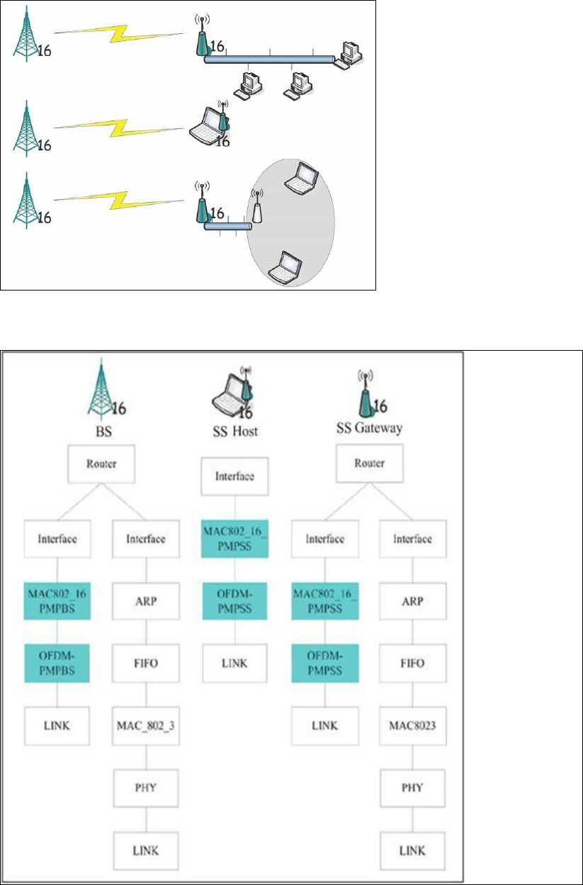
228
Fig. 8.2.2 The usages of PMP-mode network nodes
Fig. 8.2.3 The protocol stacks of PMP-mode network nodes
229
The protocol stacks of these three node types are shown in Fig. 8.2.3. Gateway
nodes, such as BS gateway nodes and SS gateway nodes, have multiple protocol
stacks. One is the protocol stack of an IEEE 802.16 wireless radio, and the others are
protocol stacks connecting to fixed networks. The protocol stack of an IEEE 802.16
radio comprises three modules: interface, MAC, and OFDM modules. The interface
module connects the IP layer in the Linux kernel to the MAC layer in the simulation
engine. The MAC module is responsible for simulating a node‟s MAC-layer functions.
For a PMP BS gateway node, its MAC-layer module is the “MAC802_16_PMPBS”
module, which deals with resource management and BS-related procedures. For PMP
Gateway SS and PMP Host SS nodes, they use the “MAC802_16_PMPSS” module to
simulate SS-related MAC-layer functions, e.g., the encoding/decoding of control
messages, the frame fragmentation, and data integrity checking. In the current release,
the PMP mode does not support QoS flows, i.e., all data packets are processed using
the best-effort class. The bottom module is the “OFDM” module. The IEEE 802.16
standard defines four technologies, OFDM, OFDMA, SC, and SCa. NCTUns
currently supports only the OFDM module.
On transmitting a MAC-layer frame, the OFDM module computes the number of
symbols required to transmit this MAC-layer frame. It next adds the necessary
information needed by receiving nodes (for computing signal-to-noise ratio) into the
frame (using the out-of-band field, PT_INFO, provided by the NCTUns packet
structure). The OFDM module will then encapsulate the MAC-layer frame into a
physical-layer frame and finally transmit this physical-layer frame to other OFDM
modules. On receiving a physical-layer frame, the OFDM module will determine
whether within the received frame some symbols should become erroneous due to
signal decay or fading effects. If so, the module will invert the values of these
erroneous symbols. The module will next perform demodulation and decoding to
convert this physical-layer frame into a MAC-layer frame. After this, the OFDM
module will send this packet to the MAC layer. The MAC layer will first perform
integrity checking for the frame and then determine if this frame is corrupted or not,
depending on the result of its integrity checking.
8.2.2 The mesh Mode
The IEEE 802.16(d) mesh mode is designed to construct a backbone network.
Figure 8.2.2.1 shows an example of the IEEE 802.16(d) mesh network. The mesh BS
node is a gateway device connecting a fixed network with the mesh network which it
services. It is also responsible for processing network registration requests from SS
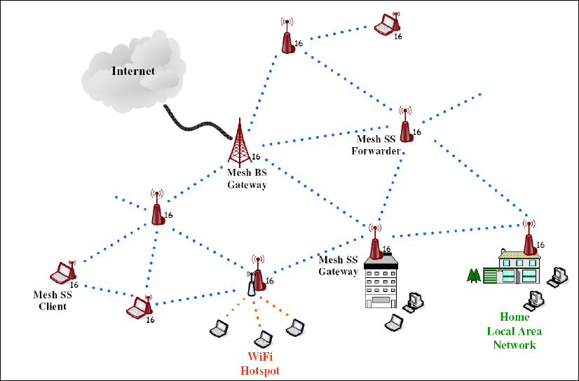
230
nodes. A mesh SS node can be used as either an end-user device (Mesh SS Client
Node) or a hot-spot access point (Mesh SS Forwarder Node). Besides, a mesh SS
node (Mesh SS Gateway Node) can be used as a gateway connecting a mesh
backbone network and a private network. The protocol stacks of these mesh-mode
network nodes are shown in Fig. 8.2.2.2. Nodes capable of performing the gateway
function have two protocol stacks. One is the protocol stack of an IEEE 802.16(d)
mesh-mode radio, and the other is that of an IEEE 802.3 interface card. Regarding
nodes excluding the gateway function, such as Mesh SS forwarder and Mesh SS
Client, they have only an IEEE 802.16(d) mesh-mode radio. In the following, we
introduce the functions of the four mesh-mode modules belonging to the protocol
stack of an IEEE 802.16(d) mesh-mode radio.
Fig. 8.2.2.1 An example of the IEEE 802.16(d) mesh network
The first one is the “MeshRoute” module. The MeshRoute module is responsible
for determining the next-hop node of an outgoing packet. Before simulation starts, it
builds a routing table with the .meshrt file as an input. (The .meshrt file is generated
by the “nctunsclient” program.) On receiving a packet from upper-layer modules, the
MeshRoute module will lookup the routing table using the source and destination IPs
as an index to find the corresponding next-hop node ID. After successfully inquiry,
the MeshRoute module will add the next-hop node ID into the PT_INFO field of the
packet to notify the MAC layer of this information.
The second module is the “mac80216_meshss” module. This module performs the
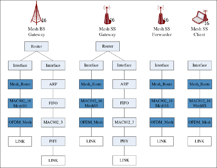
231
network initialization process of a SS node (the SS part of the network entry process).
It is also in charge of establishing logic links, establishing data schedules, and
resolving contention for transmitting control messages. The “mac80216_meshss”
module currently supports the distributed coordinated scheduling mode only. Since
the packet buffer of each logic link is maintained in this module, advanced queue
discipline methods and scheduling algorithms can be implemented inside this module.
Another MAC-layer module is the “mac80216_meshbs” module, which inherits the
“mac80216_meshss” module. The “mac80216_meshbs” module is capable of
performing all of the “mac80216_meshss” module‟s functions. Besides, it should
perform the BS part of the network entry process (and should optionally schedule the
allocation of network bandwidth, if the centralized scheduling mode is implemented).
The final module is the “OFDM_Mesh” module, which is responsible for
performing physical-layer function. It simulates the details of frame transmission and
frame reception. For example, the propagation delay of a packet is computed based on
the distance between the source and destination nodes. The signal-to-noise value of
the received frame is computed using the applied model. In addition, the
“OFDM_Mesh” module is also in charge of detecting collisions of frames.
Fig. 8.2.2.2 The protocol stacks of mesh-mode network nodes
232
8.3 Simulation Description File for IEEE 802.16 Networks
8.3.1 $CASENAME.wimax-config file
The .wimax-config file specifies classes of QoS provisioning, classes of QoS
service, and rules for classification. The “wmanIfBsProvisionedSfTable” table defines
the provisioned QoS flow classes. The entry of this table comprises five fields. The
“Service-Flow-ID” denotes the ID of the provisioned QoS flow to be defined. The
“SS-MAC” field denotes the MAC address that belongs to this service flow. The
“direction” field specifies the direction of this provisioned flow. The value of the
“direction” field is either D (Downlink) or U (Uplink). The “QoS-Index” field is an
index used to associate the corresponding entries in other tables. For example, the
entry whose “QoS-Index” index is 2 in the “wmanIfBsServiceClassTable” table
associates the entry whose “QoS-Index” index is 2 in the
“wmanIfBsProvisionedSfTable” table.

233
Table wmanIfBsProvisionedSfTable
Entry
Service-Flow-ID = 1
SS-MAC = 0:1:0:0:0:5
Direction = U
QoS-Index = 1
Service-Flow-State = provisionedState
End Entry
Entry
Service-Flow-ID = 2
SS-MAC = 0:1:0:0:0:7
Direction = U
QoS-Index = 2
Service-Flow-State = provisionedState
End Entry
End Table
Table wmanIfBsServiceClassTable
Entry
QoS-Index = 1
Class-Name = Gold
Max-Sustained-Rate = 40000
End Entry
Entry
QoS-Index = 2
Class-Name = Gold
Max-Sustained-Rate = 40000
End Entry
End Table
Table wmanIfBsClassifierRuleTable
Entry
Rule-Index = 101
Service-flow-ID = 1
Inet-Dst-Addr = 1.0.4.2
Inet-Dst-Mask = 255.255.255.255
End Entry
Entry
Rule-Index = 102
Service-flow-ID = 2
Inet-Dst-Addr = 1.0.4.3
Inet-Dst-Mask = 255.255.255.255
End Entry
End Table
Fig. 8.3.1.1 An example of .wimax-config file
The “wmanIfBsServiceClassTable” table defines the requirements of service
flows. An entry of this table comprises three fields: QoS-index, Class-Name, and
Max-Sustained-Rate. The “QoS-index” field is an index used to associate the
corresponding entries in other tables. The “Class-Name” field specifies the name of

234
this service class. The “Max-Sustained-Rate” field specifies the maximum MAC-layer
data rate (KByte) provided for a flow.
8.3.2 .meshrt file
The .meshrt file specifies the routing entries of each node. The format is defined as
follows:
$node_(NID) destination_ip/netmask next_hop_node_ID,
where NID denotes the ID of the node for which this entry is defined,
destination_ip is the IP address of a packet‟s destination node, netmask is a bit
mask for an IP address to identify its subnet ID, and next_hop_node_ID.
The following figure shows a piece of an example .meshrt file. For node 1, it has
four routing entries to nodes 2, 3, 4, and 5. These four entries specify that every
packet from node 1 to nodes 2, 3, 4, and 5 should be transmitted to node 2. On
receiving packets from node 1, node 2 can either receive the packets or forward them
to their next-hop nodes.
$node_(1) 1.0.1.2/32 2
$node_(1) 1.0.1.3/32 2
$node_(1) 1.0.1.4/32 2
$node_(1) 1.0.1.5/32 2
8.3.3 .ieee80216_network_des file
The .ieee80216_network_des file is used for the mac80216_meshbs and
mac80216_meshss modules to initialize several essential system parameters. This file
contains one or more network description blocks. A network description file has four
fields. The “network ID” field denotes the name of the network for which this block is
defined. The “BS$num_IP” field specifies the IP addresses of BS nodes in this
network. Here, $num is a positive integer to indicate which BS node‟s IP is specified.
The SSList and Authentication fields are currently not implemented. The former is
used to specify which SS node IDs belong to this network, while the latter is a flag to
indicate the authentication procedures is enabled or not.

235
NetworkDesBlock
Network_ID = NCTUNSL
BS1_IP = 1.0.1.21
SSList:
2,3,4,5,6,7,8,9,10
Authentication = Disabled
EndNetworkDesBlock
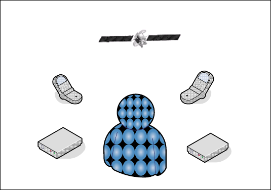
236
Chapter 9 Multi-interface Mobile Node
In this chapter, we introduce the concept and internal design of the
multi-interface mobile node. The required modifications of simulation description
files for a multi-interface mobile node simulation are also explained.
9.1 Introduction
GPRS/3G
Phone
WLAN/WiMAX
Phone
User
WiMAX Modem
Fixed Network
Modem
Satellite Terminal
Fig. 9.1.1 A variety of communication products may exist in the future
Multi-interface network node is a mobile node equipped with multiple radio
devices. It is formerly called “super-node” because it can flexibly create a new
network node type comprising multiple different single-radio devices. Fig. 9.1.1
shows a variety of communication products available for consumers in the next
decade. For broadband communications, one can use xDSL and WiMAX modems to
access wired networks. For mobile communications, one can utilize GSM/UMTS
cellular phones or mobile WLAN\WiMAX handheld devices. In addition, satellite
communications has been ready for commercial use for years. For example, the
DVBS2/RCST satellite network has been proposed to deploy an interactive satellite
network in Europe. For always-on access to Internet, one may carry numerous
communication devices and use one of them for accessing Internet at any time. As the
technology of IC industry advances, there is a tendency to merge more and more
radios into one device. Such multi-interface network devices have enabled new
research topics such as heterogenous networking.
To provide a convenient platform for studying heterogeneous networks,
NCTUns now supports multi-interface node simulations. In NCTUns, a
multi-interface node is equipped with four types of radios: IEEE 802.11(b)
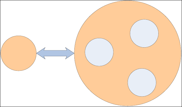
237
infrastructure mode, IEEE 802.11(b) ad-hoc mode, GPRS, and DVBS2/RCST. Using
such radios, a multi-interface node is capable of accessing wireless LAN, mobile
ad-hoc networks, telecommunication networks, and satellite networks at the same
time.
The multi-interface node design has two advantages. The first advantage is
decreasing the design complexity of the GUI program (“nctunsclient”), the source
codes of which have exceeded 120,000 lines. The multi-interface node can eliminate
the need of adding a bulk of source codes to support diverse multi-radio devices and
thus make the nctunsclient program manageable. The other advantage is flexibly
creating a new type of network nodes for study even if it does not exist in the real
world (This functionality is not supported by NCTUns yet and is an item of future
work).
In the following, we explain the design of the multi-interface node in Section 9.2.
We then elaborate on required modifications to simulation description files for
multi-interface node simulations in Section 9.3.
9.2 The Design of the Multi-interface Network Node
Multi-interface
Node
D.N
D.N
D.N
Fig. 9.2.1 The relationship between the multi-interface node and the device node
In NCTUns, the multi-interface node is a representative node standing for a set
of ordinary network nodes. As shown in Fig. 9.2.1, on creating a multi-interface node,
one should specify which and how many radios the multi-interface node contains.
Such a radio is called a device node because the simulation engine simulates this radio
using a single-interface network node. After one selects the specified radios, the GUI
program will first create the corresponding node structures for the chosen radios as if
they were ordinary single-interface network nodes. It then generates a multi-interface
node description block to specify which nodes should be grouped together to form a
238
multi-interface node and the node ID of this multi-interface node. Finally, the GUI
program generates the moving pattern for the created multi-interface node and, of
course, disables the original moving pattern of each device node.
Before starting a simulation, the simulation engine will first read and parse
the .tcl file, which describes the network topology and nodes‟ protocol stacks for a
case. On identifying a multi-interface node description block, the simulation engine
will create a new node structure to describe this multi-interface node. The simulation
engine then maps the protocol stacks of the corresponding device nodes into this
multi-interface node‟s node structure. Fig. 9.2.2 shows an example of the
multi-interface node structure. In this multi-interface node, it has four radios:
802.11(b) infrastructure-mode, GPRS, DVB-RCS satellite, and 802.11(b)
ad-hoc-mode radios. The protocol stacks of these four device nodes will be inserted
into the multi-interface node‟s node structure before the simulation is started. As such,
when the simulation is run, only a multi-interface node comprising the four protocol
stacks is created and simulated. For the four device nodes, since their protocol stacks
have been moved into the multi-interface node‟s node structure, they will not be
created during simulation.
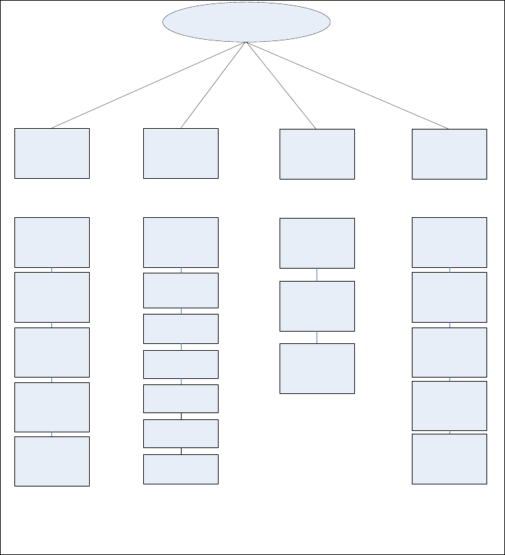
239
Interface
ARP
FIFO
802.11(b)
infra-mode
MAC
WPHY
1.0.1.1
Interface
SNDCP/
GMM
LLC
FIFO
RLC
1.0.2.1
Interface
802.16(e)
MAC
OFDM
1.0.3.1
Interface
ARP
FIFO
802.11(b)
ad-hoc-mode
MAC
WPHY
1.0.4.1
TUN 1 TUN 4TUN 3
TUN 2
WLAN NIC GPRS NIC 802.16(e) NIC 802.11(b)
ad-hoc mode
NIC
Multi-interface Node
MAC
Radio Link
Fig. 9.2.2 An example of a multi-interface node structure
Another issue is how application programs can utilize the four heterogeneous
network radios on a multi-interface node. By exploiting the pseudo network interface
(tunnel device driver) scheme of NCTUns, application programs can directly use
these four radios without modifications. They can create sockets for each interface as
normal and use these sockets in an ordinary manner. For example, during simulation,
the process P3 first creates two sockets: one is bound to IP address 1.0.3.1 and the
other to IP address 1.0.4.1. After creating the sockets, P3 can transmit/receive packets
using these two sockets as if it were run on a node equipped with two different radios.
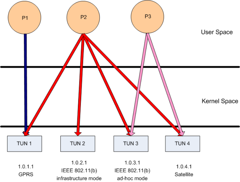
240
Fig. 9.2.3 An example of a multi-interface node structure
9.3 Exploiting Multiple Heterogeneous Network Interfaces
To utilize multiple heterogeneous interfaces, application programs running over a
simulated multi-interface node should know the IP addresses of the underlying
interfaces. One should explicitly provide such information for application programs
using command-line arguments because so far no system calls can be used for
application programs to obtain the information of a simulated node‟s all network
interfaces. Using the IP addresses of the underlying interfaces, application programs
can open sockets for these interfaces and then bind the sockets to these IP addresses.
This “bind” operation can explicitly specify an outgoing interface for a socket when
packets are transmitted through the socket. With explicit binding, application
programs over a multi-interface are able to utilize multiple heterogeneous network
interfaces to transmit/receive packets at the same time.
Note that an application program need not locally bind a socket to its local
address to transmit packets on a single-interface node. This is because the operating
system can automatically use the correct interface by looking up the routing table. On
a multi-interface node, however, if an application program did not associate the IP
address with the open socket, the operating system will use a default interface to

241
transmit packets from this socket, which may be undesired for the application
program.
9.4 Simulation Description File for the Multi-Interface Network
Node
9.4.1 .tcl file
A multi-interface network node is essentially a representative node comprising
several single-radio nodes. NCTUns uses a sophisticated design to decrease the added
design complexity for supporting the multi-interface network node. From the
perspective of the GUI program, it considers a multi-interface device node as a
“virtual” simulated node entity and its corresponding device nodes as “real” simulated
node entities. This means that the GUI program only needs to generate the node
description blocks of those comprising device nodes and use minimum information to
describe the existence of a multi-interface node. On the other hand, from the
perspective of the simulation enging, it only creates the multi-interface node during
simulation and treats the corresponding device nodes as “faked nodes.” The
simulation engine will create the protocol stacks of these single-radio device nodes
and move them into their representative multi-interface node‟s node structure.
To support the “multi-interface node” simulation, the GUI program first
generates an extension block, named “super-node extension block,” (we call this
extension block as “super-node extension block” because it can flexibly describe any
combinations of various radios) to describe the relationship between a multi-interface
node and its corresponding device nodes. It next generates the node description blocks
of these single-radio device nodes as normal. The format of a super-node extension
block is shown as follows. The block starts with the “Group SN Node” keywords. The
$nid field denotes the ID of the representative multi-interface node; the $dnum field
describes the number of device nodes belonging to this multi-interface node; and the
$dnidX fields specify the IDs of these corresponding device nodes in sequence, where
X is a positive integer.
Group SN Node $nid as SUPERNODE with name = SUPERNODE$nid and $dnum DN $dnid1 $dnid2 ...
Fig. 9.4.1 shows three examples of the supernode description block. Node 30 is a
multi-interface node that has 2 device nodes: nodes 1 and 2. Node 31 has three device
nodes: node 10, node 12, and node 13, respectively. Similarly, node 32 has three
device nodes whose node IDs are 9, 11, and 14, respectively.

242
Group SN Node 30 as SUPERNODE with name = SUPERNODE30 and 2 DN 1 2
Group SN Node 31 as SUPERNODE with name = SUPERNODE31 and 3 DN 10 12 13
Group SN Node 32 as SUPERNODE with name = SUPERNODE32 and 3 DN 9 11 14
Fig. 9.4.1 An example of supernode description block
9.4.2 .mrt file
The .mrt file specifies the routing entries of simulated mobile nodes. Since a
multi-interface node comprises several device nodes, the GUI program should modify
the routing entries of these device nodes as follows. The GUI program changes the
node IDs of these device nodes‟ mrt entries to be the multi-interface node ID. This is
because during simulation, all of these device nodes will belong to a part of the
multi-interface node.
Fig. 9.4.2 shows the modified mrt entries for the three aforementioned
multi-interface nodes. We can see that node 31 has four mrt entries originally for node
10, node 32 has four mrt entries originally belonging to node 9, and node 30 has four
mrt entries originally for node 1.
$node_(31) 0.000000000 set-next-hop 10 14 1 chan 3
$node_(31) 0.000000000 set-next-hop 10 13 13 chan 3
$node_(31) 0.000000000 set-next-hop 10 9 1 chan 3
$node_(31) 0.000000000 set-next-hop 10 1 1 chan 3
$node_(32) 0.000000000 set-next-hop 9 14 14 chan 3
$node_(32) 0.000000000 set-next-hop 9 13 1 chan 3
$node_(32) 0.000000000 set-next-hop 9 10 1 chan 3
$node_(32) 0.000000000 set-next-hop 9 1 1 chan 3
$node_(30) 0.000000000 set-next-hop 1 14 9 chan 3
$node_(30) 0.000000000 set-next-hop 1 13 10 chan 3
$node_(30) 0.000000000 set-next-hop 1 10 10 chan 3
$node_(30) 0.000000000 set-next-hop 1 9 9 chan 3
Fig. 9.4.2 An example of the mrt entries for multi-interface nodes
9.4.3 .sce file
The .sce file specifies the moving pattern of each simulated mobile node.
Regarding simulation cases involving multi-interface nodes, the GUI program should

243
create the moving patterns of such multi-interface nodes and remove the moving
patterns of their corresponding device nodes. Fig. 9.3.3 shows the modified .sce file
for the multi-interface nodes shown in Fig. 9.3.1. The GUI program generates the sce
entries for these three nodes and then disables the sce entries of their device nodes,
such as 1, 2, 9, 10, 11, 12, 13, and 14.
$node_(30) set 193.000000 178.000000 0.0 0.0 0.000000 10.000000
#$node_(1) set 193.000000 178.000000 0.0 0.0 0.000000 10.000000
#$node_(2) set 186.000000 209.000000 0.0 0.0 0.000000 10.000000
$node_(3) set 501.000000 209.000000 0.0 0.0 0.0 0.0
$node_(4) set 719.000000 212.000000 0.0 0.0 0.0 0.0
$node_(5) set 616.000000 210.000000 0.0 0.0 0.0 0.0
$node_(6) set 847.000000 217.000000 0.0 0.0 0.0 0.0
$node_(7) set 952.000000 219.000000 0.0 0.0 0.0 0.0
$node_(8) set 245.000000 311.000000 0.0 0.0 0.0 0.0
$node_(32) set 247.000000 404.000000 0.0 0.0 0.000000 10.000000
#$node_(9) set 247.000000 404.000000 0.0 0.0 0.000000 10.000000
$node_(31) set 384.000000 102.000000 0.0 0.0 0.000000 10.000000
#$node_(10) set 384.000000 102.000000 0.0 0.0 0.000000 10.000000
#$node_(11) set 278.000000 409.000000 0.0 0.0 0.000000 10.000000
#$node_(12) set 425.000000 104.000000 0.0 0.0 0.000000 10.000000
#$node_(13) set 460.000000 110.000000 0.0 0.0 0.000000 10.000000
#$node_(14) set 312.000000 422.000000 0.0 0.0 0.000000 10.000000
Fig. 9.3.3 An example of the modified sce file

244
Reference
[1] S.Y. Wang and H.T Kung, “A Simple Methodology for Constructing Extensible
and High-Fidelity TCP/IP Network Simulators, “IEEE INFOCOM‟99, March
21-25, 1999, New York, USA.
[2] Harvard TCP/IP network simulator 1.0, available at
http://www.eecs.harvard.edu/networking/simulator.html.
[3] Gray R. Wright and Richard Stevens, “TCP/IP Illustrated Volume 2,” Addison
Wesely, 1995.
[4] S. McCanne,S. Floyd, ns-LBNL Network Simulator.
(http://www-nrg.ee.lb.gov/ns/)
[5] S. Keshav, “REAL: A Network Simulator,” Technical Report, Dept. of
computer Science, UC Berkeley, 1988.
[6] OPNET Technologies, Inc. home page,
http://www.opnet.com/products/home.html.
[7] Uresh Vahalia, “UNIX Internals: the New Frontiers,” Prentice-Hall, 1996.
[8] W. Richard Stevens, “UNIX Network Programming Volume 1, Networking
APIs: Sockets and XTI”, 2nd, Prentice-Hall, 1998.
[9] Chang-Ching Chiou, “Improve the Performance of the NCTUns Network
Simulator”, Master thesis, National Chiao Tung University, Hsinchu, Taiwan,
2001.
[10] S.Y. Wang and H.T. Kung, “A New Methodology for Easily Constructing
Extensible and High-Fidelity TCP/IP Network Simulators," Computer Networks,
Vol. 40, Issue 2, October 2002, pp. 257-278.
[11] S.Y. Wang, C.L. Chou, C.H. Huang, C.C. Hwang, Z.M. Yang, C.C. Chiou, and
C.C. Lin, “The Design and Implementation of NCTUns 1.0 Network Simulator,”
Computer Networks, Vol. 42, Issue 2, June 2003, pp. 175-197.
[12] S.Y. Wang and Y.B. Lin, “NCTUns Network Simulation and Emulation for
Wireless Resource Management”, Wireless Communication and Mobile
245
Computing, Wiley, Vol. 5, Issue 8, December 2005.
[13] S.Y. Wang, C.L. Chou, C.C. Lin, “The Design and Implementation of the
NCTUns Network Simulation Engine”, Simulation Modelling Practice and
Theory, 15 (2007) 57-81.
[14] S.Y. Wang, C.L. Chou, Y.H. Chiu, Y.S. Tseng, M.S. Hsu, Y.W. Cheng, W.L.
Liu, and T.W. Ho, “NCTUns 4.0: An Integrated Simulation Platform for
Vehicular Traffic, Communication, and Network Researches,” 1st IEEE WiVec
2007 (International Symposium on Wireless Vehicular Communications),
September 30 – October 1, 2007, Baltimore, MD, USA
