(The Wiley Finance Series) Timothy Jury Cash Flow Analysis And Forecasting The Definitive Guide To

(The%20Wiley%20Finance%20Series)%20Timothy%20Jury-Cash%20Flow%20Analysis%20and%20Forecasting_%20The%20Definitive%20Guide%20to%20

User Manual:

Open the PDF directly: View PDF .
Page Count: 323 [warning: Documents this large are best viewed by clicking the View PDF Link!]

Cash Flow Analysis

and Forecasting

For other titles in the Wiley Finance series

please see www.wiley.com/ﬁnance

Cash Flow Analysis

and Forecasting

The Deﬁnitive Guide to Understanding

and Using Published Cash Flow Data

Timothy D.H. Jury

A John Wiley & Sons, Ltd., Publicatio

This edition ﬁrst published 2012

Registered Ofﬁce

John Wiley & Sons Ltd, The Atrium, Southern Gate, Chichester, West Sussex, PO19 8SQ,

United Kingdom

For details of our global editorial ofﬁces, for customer services and for information about how to

apply for permission to reuse the copyright material in this book please see our website at

www.wiley.com.

The right of the author to be identiﬁed as the author of this work has been asserted in accordance with

the Copyright, Designs and Patents Act 1988.

transmitted, in any form or by any means, electronic, mechanical, photocopying, recording or

otherwise, except as permitted by the UK Copyright, Designs and Patents Act 1988, without the prior

permission of the publisher.

Wiley also publishes its books in a variety of electronic formats and by print-on-demand. Some

content that appears in standard print versions of this book may not be available in other formats. For

more information about Wiley products, visit us at www.wiley.com.

Designations used by companies to distinguish their products are often claimed as trademarks. All

brand names and product names used in this book are trade names, service marks, trademarks or

registered trademarks of their respective owners. The publisher is not associated with any product or

vendor mentioned in this book. This publication is designed to provide accurate and authoritative

information in regard to the subject matter covered. It is sold on the understanding that the publisher

is not engaged in rendering professional services. If professional advice or other expert assistance is

required, the services of a competent professional should be sought.

Library of Congress Cataloging-in-Publication Data:

ISBN 978-1-119-96265-6

A catalogue record for this book is available from the British Library.

Set in 10/12pt Times by Aptara Inc., New Delhi, India

Printed in Great Britain by TJ International Ltd, Padstow, Cornwall, UK

To my mother and father,

brother and sisters for always being there

Contents

Introduction ix

SECTION ONE HISTORIC CASH FLOW ANALYSIS

1 Understanding How Cash Flows in a Business 3

2 Understanding Cash Flows Properly 21

3 Start-up, Growth, Mature, Decline 47

4 Restating the Cash Flows of a Real Business 59

5 Restating US GAAP Cash Flows 83

6 Analysing the Cash Flows of Mature Businesses 99

7 Analysing the Cash Flows of Growth Businesses 135

8 Growth and Mature – Further Analysis Issues 153

9 Analysing the Cash Flows of Start-up Businesses 171

10 Analysing the Cash Flows of Decline Businesses 179

11 What to do about Bad Cash Flows 185

12 Cash Versus Proﬁt as a Measure of Performance 191

viii Contents

13 Cash Flow Analysis and Credit Risk 201

14 Cash Flow Analysis and Performance Measurement 215

15 Analysing Direct Cash Flow Statements 223

16 Generating a Cash Flow Summary from Proﬁt and Loss Account

and Balance Sheet Data 231

17 Summarising Historic Free Cash Flow 247

SECTION TWO FORECASTING CASH FLOWS

18 Introduction 255

19 Spreadsheet Risk 263

20 Good Practice Spreadsheet Development 275

21 The Use of Assumptions in Spreadsheet Models 295

Index 305

Introduction

This book is the deﬁnitive guide to cash ﬂow analysis. It is designed to be the

deﬁnitive ﬁrst reference on all aspects of historic cash ﬂow analysis. It also provides

an incisive overview of the risks to be managed in preparing cash ﬂow forecasts.

It has been written from a cash ﬂow-centric point of view. Other ﬁnancial and

analytical information is introduced whenever relevant to support the process of

cash ﬂow analysis.

This book is designed for people trying to understand and analyse cash ﬂows,

probably in a professional context. Whilst it contains some theoretical content, the

primary objective is to offer a practical handbook of cash ﬂow analysis.

Ideally, it should ﬁrst be read like a novel and then dipped into chapter-by-

chapter as required; a detailed guide to the contents of each chapter follows this

introduction. Much of the information in the book has been laid out to facilitate

direct reference from the index; also allowing it to be used as a pure reference text.

Considerable effort has been expended to make the book as user friendly as

possible. It has been designed to be relevant and useful both to persons who are

coming to cash ﬂows for the ﬁrst time, and to those who are more experienced

in the perils of ﬁnancial statement analysis! I have paid particular attention to the

needs of those who are not native English speakers. I have tried to keep the use

of English as clear and concise as possible whilst avoiding the use of unnecessary

complexity.

Whilst the book is written primarily for those employed as ﬁnancial analysts,

I have identiﬁed four other major user groups whose needs are speciﬁcally dealt

with in different sections of the book. They are:

•Novices in ﬁnancial analysis and other persons new to, or relatively unfamiliar

with, cash ﬂows in general and their analysis in particular, in all ﬁelds of

endeavour, who wish to improve their understanding of cash ﬂow.

x Introduction

•Bankers, credit analysts and others involved in business lending and the man-

agement of credit exposures and credit risk.

•Investors, fund managers and credit analysts involved in taking investment

decisions.

•Entrepreneurs, managers and business people involved in controlling business

entities.

The guide to the book, which follows this introduction, provides an indication

of the content of each chapter and its relevance to different users. For example,

persons who have no desire to actually perform the analysis of the cash ﬂows of

a business themselves, but who still wish to understand cash ﬂow, will initially

gain little from Chapters 4 and 5 as they are written for persons who are seeking

to practically apply the technique for the restatement of published cash ﬂows.

THE LOGIC OF THE BOOK DESIGN

Years of experience as a ﬁnancial trainer have taught me that people acquire

technical knowledge in a very random way from a variety of sources as they come

across information relevant to their needs. This sometimes results in a partial,

incomplete and often inaccurate understanding of the particular subject in issue.

As a trainer and author my objective is to organise the information relevant to a

subject or task in a logical and structured way to facilitate and ease the assimilation

process. The metaphor I like to use is that of a jigsaw. My audiences will typically

have many of the pieces of the jigsaw already in their possession; however, until

I facilitate the process of assimilation they have not previously assembled the

pieces into a complete picture. When working as a trainer not only do I assist in

completing the jigsaw, I also provide the missing pieces, which are different for

each participant!

For this reason the book has been organised into speciﬁc blocks of knowledge.

It can be read sequentially. It can also be used as a reference to provide answers

to speciﬁc queries and problems by dipping into the relevant part of the book.

COMPLEXITY

The word complex is regularly misused to mean difﬁcult, or beyond the users

present comprehension. When things labelled complex are analysed it often be-

comes clear that what is actually meant is there is a lot of information to assimilate

before comprehension of the whole can be gained. The information itself is not

particularly demanding to comprehend; there is, however, a lot of it! Writing com-

puter software or learning a musical instrument or foreign language are typical

examples.

Introduction xi

My strategy for this type of assimilation problem is to chop the information up

into lots of little bits that are sufﬁciently elemental that they can be adequately

digested by the person seeking to assimilate the whole area of knowledge and then

build the knowledge in a pyramid form by adding blocks and layers in an ordered

way. This is the approach I have taken in writing this book.

THE USE OF CASE STUDIES IN THE BOOK

Once the initial chapters have introduced the concepts upon which the analysis

of cash ﬂows rely, the book includes a number of case studies that illustrate the

use of the technique for cash ﬂow analysis offered. Most of these cases are based

on ﬁnancial information taken from the accounting statements of real business

entities. I prefer to do this because there is then no challenge as to the reality of

business behaviour. If I create ﬁctional cases for the book there is a risk users will

question my conclusions about them and cash ﬂow analysis in general on the basis

that the examples are ﬁctionalised and therefore do not represent a reasonable

representation of business reality.

However, this inevitably results in problems with dates! The question of how

to deal with dates in the book is one that has vexed me signiﬁcantly. The problem

for the publisher and I is that the book will soon appear dated if we show the

years from which the case studies were taken in the original. Users may wrongly

assume the message and content of the book is somehow less relevant because the

material used to illustrate the logic of the technique offered is ageing.

The logic of the cash ﬂow analysis technique offered in the book is essentially

timeless, it should work virtually anywhere and anytime ﬁnancial information is

available to perform the analysis. For this reason I have partially disguised the

original dates of the material used to illustrate the cases. The timeline of most of

the case studies offered is incidental; the examples are there to illustrate the use

and beneﬁts of the cash ﬂow analysis technique that is the basis of this book.

Experienced analysts will know that in performing any business analysis the

economic context in which the company operates is sometimes highly relevant.

Matters such as inﬂation, interest rates and the state of the economy may affect the

conclusions drawn about the relative performance of a business. For this reason,

in a small number of cases and where the context of the example warrants it, I

have left the dates as they were originally. This allows the reader to put the case

into the context of the economic conditions prevailing at the time.

Considerable effort has been expended to keep the various examples, tables and

other information both numerically and factually correct, however, it is inevitable

in a work of this length that, despite our best efforts, errors may still creep into

print. Please do not hesitate to bring these to my attention, to further improve the

book as it develops.

xii Introduction

I hope this book changes your life. For those whose job is to analyse cash ﬂows

for a living it may actually do so!

Capitalisation

Throughout the book, where you see CAPITALISED WORDS, these refer directly

to key words in tables and ﬁgures that are being discussed and explained in the

text.

GUIDE TO THE BOOK

The book is organised into two sections, the ﬁrst dealing with the analysis of

historic cash ﬂow data, the second dealing with the forecasting of cash ﬂow

information.

Section One – Historic Cash Flow Analysis

Chapter 1 – Understanding How Cash Flows in a Business

Level basic – the chapter is designed as a layperson’s introduction to the whole

subject of cash ﬂow in business. In addition to introducing the cash ﬂow patterns

seen in business, it outlines a number of other fundamental issues and risks that

managers must overcome in order to trade successfully. No prior knowledge of

cash ﬂow is assumed. The material is presented from the ground up through the

use of straightforward examples.

Despite being offered as a basic introduction everyone seeking to utilise the

cash ﬂow analysis technique presented in the book should read this chapter as it

introduces and deﬁnes part of the terminology used throughout the book.

Chapter 2 – Understanding Cash Flows Properly

Level intermediate – this chapter explains the knowledge and the steps required

to analyse cash ﬂows properly. It then commences the process by explaining all

the terminology used in a simple cash ﬂow example and introduces the analysis

technique for the ﬁrst time.

Chapter 3 – Start-up, Growth, Mature, Decline

Level intermediate – this chapter introduces the non-ﬁnancial information needed

to get the most out of the cash ﬂow analysis technique offered in the book.

Everything offered in this chapter is covered in more detail in Chapters 6 to 10.

Introduction xiii

Chapter 4 – Restating the Cash Flows of a Real Business

Level advanced – readers without some prior knowledge of ﬁnancial statement

analysis and accounting will ﬁnd this chapter demanding. Considerable effort has

gone into explaining the accounting and analytical knowledge required to properly

utilise the cash ﬂow analysis technique offered. The example chosen to illustrate

the process being taken from a business preparing its accounts using International

Financial Reporting Standards.

Chapter 5 – Restating US GAAP Cash Flows

Level advanced – this follows on from the previous chapter by taking an example

of the technique based on a business following US ﬁnancial accounting rules in

the preparation of its ﬁnancial statements. It is necessary to be familiar with the

content of the previous chapter in order to get most beneﬁt from this one.

Chapter 6 – Analysing the Cash Flows of Mature Businesses

Level advanced – this chapter deﬁnes the term ‘mature’ and presents the informa-

tion required to comprehensively analyse the cash ﬂows of a mature business.

Chapter 7 – Analysing the Cash Flows of Growth Businesses

Level advanced – this chapter deﬁnes the term ‘growth’ and presents the informa-

tion required to comprehensively analyse the cash ﬂows of a growth business.

Chapter 8 – Growth and Mature – Further Analysis Issues

Level advanced – this chapter presents two important further issues relevant to the

analysis of both growth and mature businesses.

Chapter 9 – Analysing the Cash Flows of Start-up Businesses

Level advanced – this chapter deﬁnes the term ‘start-up’ and presents the infor-

mation required to comprehensively analyse the cash ﬂows of a start-up business.

Chapter 10 – Analysing the Cash Flows of Decline Businesses

Level advanced – this chapter deﬁnes the term ‘decline’ and presents the informa-

tion required to comprehensively analyse the cash ﬂows of a decline business.

xiv Introduction

Chapter 11 – What to do about Bad Cash Flows

Level advanced – this chapter offers a variety of strategies to make decisions about

cash ﬂows that are bad. It suggests a number of questions that the analyst should

seek to answer, before coming to conclusions about bad cash ﬂows.

Chapter 12 – Cash Versus Proﬁt as a Measure of Performance

Level advanced – this chapter explains in detail the differences between proﬁt and

cash generation as a measure of performance. It points out the pitfalls of using

proﬁt alone as a performance indicator.

Chapter 13 – Cash Flow Analysis and Credit Risk

Level advanced – this chapter explains how to tailor the cash ﬂow analysis tech-

nique offered speciﬁcally to the needs of bankers and others who are exposed to

credit risk.

Chapter 14 – Cash Flow Analysis and Performance Measurement

Level advanced – this chapter looks at ways the cash ﬂow analysis technique

offered in the book can be used for business performance measurement.

Chapter 15 – Analysing Direct Cash Flow Statements

Level advanced – this chapter deals with the differences between direct and indirect

cash ﬂow statements and how to deal with them in applying the cash ﬂow analysis

technique. It is necessary to be familiar with the earlier content of the book in

order to get the most out of this chapter.

Chapter 16 – Generating a Cash Flow Summary from Proﬁt and Loss

Account and Balance Sheet Data

Level advanced – this chapter illustrates how to arrive at a summary of the cash

ﬂows of a business entity that does not produce a cash ﬂow statement as part of

their ﬁnancial information. It is essential to be familiar with all the earlier content

of the book in order to get the most out of this chapter.

Chapter 17 – Summarising Historic Free Cash Flow

Level advanced – this chapter illustrates how to identify the historic free cash ﬂow

of a business entity from the cash ﬂow information derived by using the cash ﬂow

Introduction xv

analysis technique presented earlier in the book. It is necessary to be familiar with

the earlier content of the book in order to get the most out of this chapter.

Section Two – Forecasting Cash Flows

Chapter 18 – Introduction

Level advanced – this chapter discusses the risks and beneﬁts of forecasting when

compared to the analysis of historic information.

Chapter 19 – Spreadsheet Risk

Level advanced – this chapter introduces spreadsheet risk and offers strategies to

minimise the problem.

Chapter 20 – Good Practice Spreadsheet Development

Level advanced – this chapter introduces a number of techniques to reduce spread-

sheet risk through good modelling practice. It illustrates four examples of common

cash ﬂow forecasting models.

Chapter 21 – The Use of Assumptions in Spreadsheet Models

Level advanced – this chapter offers guidance on dealing with assumptions in

spreadsheet forecasting models. It then discusses the use of scenarios for risk

analysis using spreadsheet forecasts.

Section One

Historic Cash Flow Analysis

Cash Flow Analysis and Forecasting: The Definitive Guide to

Understanding and Using Published Cash Flow Data

by Timothy D.H. Jury

Understanding How Cash Flows in

a Business

INTRODUCTION

This chapter is designed to enable those with less direct experience of the operation

of businesses to grasp the fundamental ﬁnancial and economic logic that governs

how successful businesses operate. It represents the starting point for our journey

through the landscape of cash ﬂow analysis. In order to gain beneﬁt from this

chapter no prior knowledge of either cash ﬂow or business is required.

We start our journey by developing a model of how the cash ﬂows in a simple

business work. We then develop our knowledge of cash ﬂows by incrementally

adding complexity to this model.

Whilst developing this model based on the cash ﬂows of a business we also

introduce some fundamental logic about what different types of business must do

in order to be successful.

THERE IS NOTHING NEW ABOUT BUSINESS

Humans have been engaging in trade for thousands of years, initially through

some sort of barter process. Archaeologists have discovered ancient manufactured

goods such as pottery and metal objects that have travelled vast distances from

their point of manufacture. There are numerous examples of early Greek and

Roman shipwrecks being discovered in many different parts of the Mediterranean

dating back 2000 years or more. In the 1960s evidence was ﬁnally discovered

that proved that the Vikings were the ﬁrst Europeans to discover America some

500 years before Columbus. The remains of a Norse settlement at L’Anse aux

Meadows on the northern tip of Newfoundland have been authenticated and dated

to around 1000AD. During the excavation of the site over 100 objects of European

manufacture were unearthed.

A more recent development in human history was the introduction of money

in the form of coinage and, later, notes. Whilst there is much debate about what

should be recognised as the ﬁrst coin, a good candidate would be a small lump

of electrum (a natural alloy of gold and silver) stamped with a design and minted

around 600BC in Lydia, Asia Minor (now known as Turkey). Paper money seems

to have emerged in China at about the same time.

Cash Flow Analysis and Forecasting: The Definitive Guide to

Understanding and Using Published Cash Flow Data

by Timothy D.H. Jury

4 Cash Flow Analysis and Forecasting

This innovation, together with many others such as agriculture, settlements, the

wheel and writing led to the modern, technologically based world economy we

have today. Trade or business, in one form or another, has probably been part of

the human condition from our earliest origins.

UNDERSTANDING MONEY IN BUSINESS

We are going to start with two simple examples of business activity. The ﬁrst

one represents one of the simplest forms of business. (More complex business

examples follow over the next few pages.)

The Simplest Form of Business

Newspaper vending, by which I mean the activity of selling newspapers to passers-

by on a street corner, is a good example of a really simple business. The vendor,

or businessman, buys the newspapers from the publisher or a wholesaler and then

retails them to passers-by for a price that gives him a margin over the cost of

purchasing the newspapers.

A second example of a really simple business is an antique dealer, someone

who buys and sells old objects. We will work with this example from now on.

The Debate About the Purpose and Objectives of a Business

The varying cultures around the world place different emphasis on how the beneﬁts

generated by a successful business should be shared amongst its stakeholders.

I do not propose to examine the merits or otherwise of these views. There is

considerable literature on what measures should be used to assess success or

failure in business. Both growth and proﬁt increase look like good candidates but

fail as measures of success if the improvement in growth or proﬁts is achieved by

investing disproportionate amounts of cash. I do not propose to go much further

with this debate other than to say that increasing the value of a business over

time is now considered the most appropriate measure of success. This is achieved

by continually improving the present and future cash ﬂows of a business on an

ongoing basis.

So, at this point in my explanation, I am assuming that the business I am

describing is being run with the objective of wealth maximisation for the owners.

For the purposes of this book I deﬁne that as maximising the future cash ﬂows of

the business.

Understanding How Cash Flows in a Business 5

The Objective of Being in Business is to Generate More Cash

It is important to introduce the purpose of a business here because specifying the

objective of the business deﬁnes the task of the business person, entrepreneur,

manager or other business controller (which is to get more cash). In both the

business examples introduced so far we have a trader or dealer who buys and sells,

typically without changing or modifying the items traded in any way. This is the

simplest form of business.

The trader’s objective is to generate more cash than they started with. (Note that

I have not used the terms proﬁt or gain as we are developing a model containing

only items that represent the cash ﬂows in a business. What we mean by proﬁt is

actually quite an abstract concept. This is dealt with in more detail in Chapter 12.)

How Does a Trading Business Add Value?

An initial observation might be that these businesses make money by buying things

for less than they can sell them. While this is an accurate observation of what a

successful trading business does, this fails to explain why or how the business is

able to achieve this beneﬁcial outcome.

What is the key skill for an antique dealer? Is it knowledge of the antiques

traded in? Whilst this may help, much of this information is available from books.

Is it renovation skills? Again this may or may not add value to the items being

renovated depending on consumer taste at the time. The key skill is probably,

knowing where to buy cheaply and where to sell expensively. Here is an example

of what I mean.

For many years the typical vehicle of choice for a British antique dealer has

been the Volvo estate, which is used to travel to distant parts of Scotland and Wales

so that the dealer can purchase furniture and other antiques from remote house

sales and auctions where they are often sold cheaply. The goods purchased are

then transported to London where they can be auctioned through the major auction

houses or retailed to wealthy collectors at collectors’ fairs or from retail premises.

What this antique dealer is doing is relocating the goods traded from a place

where they can be bought cheaply to a place where they can be sold more expen-

sively. It’s all about the relocation of the goods. Why is this so important?

Consider what happens when you get up in the morning. Do you travel to Java

for your coffee beans, Florida for your orange juice, Jamaica for your sugar, and

to your local farm for your milk?

This is unlikely. What most of us do is go to the nearest convenience store,

which may be just down the street and buy what we wish to consume for our

breakfast. So, what then is the owner of the convenience store doing to add value?

What he does is relocate a range of goods he knows we are likely to consume for

6 Cash Flow Analysis and Forecasting

breakfast to a place convenient for us to make our purchases as consumers. The

convenience of the location is the most important thing, the goods offered are in

a sense irrelevant, they are whatever we want to consume.

So, the key to most trading, retail and wholesale businesses is location. What

these businesses do is relocate goods from their places of production or, if second-

hand, their present location, to a location convenient for the target consumer to

consume them. It follows that there is little point in locating a business in a

remote part of the world as there are few consumers there! The ideal location for

newspaper vending is directly outside a major railway station in central London

or any other major city in the world, this is where you will have thousands of

potential consumers passing by every hour of the working day. In other words,

you will sell more newspapers. The location is the essence of the business’s ability

to generate cash.

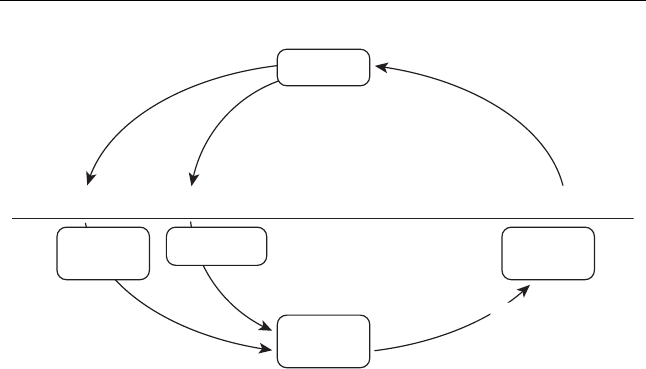
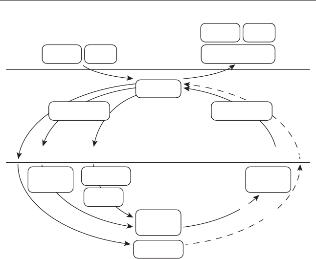
So, the cash ﬂows of our simplest business look like the model shown in

Fig. 1.1. Overheads is the term commonly used in business to refer to all the costs

of trading other than inventory costs.

Using CASH the trader makes purchases of goods, which he holds as INVEN-

TORY. Some time later he resells the goods acquired for more than he paid for

them, receiving cash in exchange for the items. He will typically incur some

OVERHEADS in the process, in our example of the antique dealer these will be

transport, location and communication costs.

This is effectively all a trading, retail or distribution business does, repeating the

journey round the circle many times. Now let us look at a more complex business,

one where work is performed on the purchased inputs of the business.

Cash

Inventory

Overheads

Cash

Non-Cash

Purchase Purchase

Added

value Relocation

knowledge

Sale

Figure 1.1 Diagram of the cash ﬂows of a simple trading business

Understanding How Cash Flows in a Business 7

THE SIMPLE MANUFACTURING BUSINESS

In my other life as a ﬁnancial trainer I have travelled all over the world offering

training seminars on ﬁnancial analysis and related subjects. One of the places I

have visited on my travels is Nairobi in Kenya. When travelling from Nairobi

airport to the training location I noticed business people selling beds and other

simple items of furniture outside their workshops by the side of the road. This

then is the next example we will examine; a simple manufacturing business.

How Does a Simple Manufacturing Business Add Value?

What do manufacturers do to create wealth for themselves? They take raw materials

and change them into something more useful; economists talk about adding utility.

For example, I could sleep on a log. However, this would not be particularly

comfortable, the bark would make my back itch and I might roll off! If the log is

cut up into timber and then turned into a bed frame I am likely to be willing to pay

more for it in this form. Now, I could of course do this myself with the aid of a saw

and a few basic woodworking tools, so why do I not normally bother? There are

three reasons: time, quality and cost. I could make the bed, but it would take me

three days whilst the manufacturer does it in half an hour. Secondly, the result I

achieve might not have the quality of the professionally manufactured alternative

and, ﬁnally, it would almost certainly be more expensive when the opportunity

cost of my time as well as the cost of the raw materials is taken into account.

So, manufacturers do not just convert things (raw materials) into more useful

things (ﬁnished goods), they are experts at the process of doing so. Successful

manufacturers do it very quickly and efﬁciently to a very high standard. The key

word here is expert. If you are analysing the performance of a manufacturing

business and ﬁnd that it receives many customer complaints and returned goods

due to manufacturing defects, or is experiencing signiﬁcant difﬁculties actually

producing goods, this suggests they are not experts. To use a metaphor: it implies

they are amateurs rather than professionals. Any business being operated in a non-

professional way is at a higher risk of poor ﬁnancial performance and eventual

failure than its more professional and competent competitors. The extreme levels

of professionalism required just to be competitive in most manufacturing activities

is simply a consequence of competition over long periods of time.

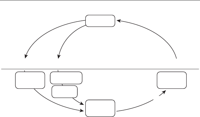
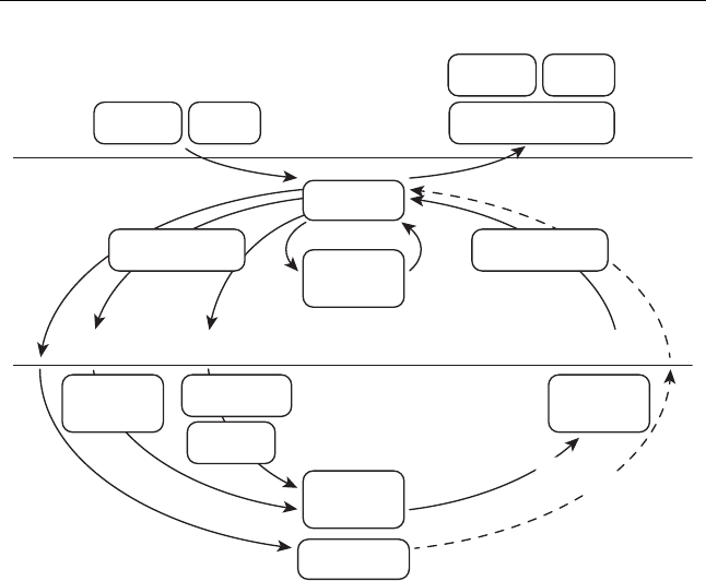
So the cash ﬂows of our simple manufacturing business look like the model

shown in Fig. 1.2.

Using CASH the manufacturer makes a purchase of RAW MATERIALS and

does work on them, so converting them to WORK IN PROGRESS and eventually

FINISHED GOODS. These items being akin to INVENTORY in our previous

model. Some time later he resells the ﬁnished goods for more than the cash costs

of producing them, receiving cash in exchange for the items. He will typically

8 Cash Flow Analysis and Forecasting

Cash

Work in

Progress

Raw

Materials

Finished

Goods

Overheads

Cash

Non-Cash

Purchase Purchase

Added

value Conversion

knowledge

Sale

Figure 1.2 Diagram one of the cash ﬂows of a manufacturing business

incur some OVERHEADS in the process of conversion, these being purchasing,

manufacturing, premises, and selling costs in our example.

This is what the cash ﬂows of a new small manufacturing business look like.

Cash is generated by repeating the journey round the circle many times. Now let

us see how this develops as the business evolves over time.

Developing Our Model – the Next Step

Continuing with our example of an African entrepreneur who has recently estab-

lished himself as a manufacturer of furniture, let us assume his new business is

successful. Our entrepreneur is working many hours a day and all the product he

produces sells well. What is likely to be his ﬁrst major issue in developing his

business?

Given his location his next move is most likely to be adding labour to the

business to increase output and hence cash ﬂow. This is because there is much

labour available and, given the emerging market location of the business, this

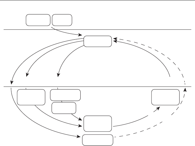
labour is available relatively cheaply (Fig. 1.3).

LABOUR now joins overheads as an item purchased and consumed by the

business to add value to raw materials.

If our entrepreneur furniture designer was in Munich in Germany the decision

might be quite different. In this location the economic environment is different

to that in Nairobi in Kenya. In Germany labour costs are signiﬁcantly higher per

hour and employees are protected in many ways by a mass of social legislation

Understanding How Cash Flows in a Business 9

Cash

Work in

Progress

Raw

Materials

Finished

Goods

Overheads

Labour

Cash

Non-Cash

Purchase Purchase

Added

value Conversion

knowledge

Sale

Figure 1.3 Diagram two of the cash ﬂows of a manufacturing business

giving them extensive rights and obliging employers to compensate employees in

the event of job losses. From an economic point of view the cost of labour is higher

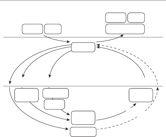
and the cost itself is less variable. In Germany the ﬁrst major initiative to build our

business is more likely to be the purchase of machinery (i.e. ﬁxed assets) to increase

output and hence cash ﬂow, rather than the addition of more labour (Fig. 1.4).

Why is the decision different depending on the location of the business? This is

because the economic environment is different. Factors that affect the decision of

whether to employ labour or purchase ﬁxed assets would be things like, the law

and regulations affecting the cost and ﬂexibility of labour, the local environment

governing labour and investment in ﬁxed assets, and the availability and quality

of labour.

There are other issues that might inform or determine the decision. Machines

have certain characteristics that could arguably make them superior to labour in

many situations. They do not go on strike; they can, assuming they are properly

maintained, produce a succession of perfect and identical output 24 hours a day

without requiring sleep or food. But, there are also some key negative charac-

teristics of machines. They usually require infrastructure such as electricity, gas,

compressed air and water constantly available without interruption. They are very

good at doing the same thing again and again; they are not so good when the

required output keeps changing. Any change to the product manufactured may

necessitate hours of re-engineering and re-programming of the machine before

productive output recommences.

10 Cash Flow Analysis and Forecasting

Cash

Fixed assets

Work in

Progress

Raw

Materials

Finished

Goods

Overheads

Labour

Cash

Non-Cash

Purchase Purchase

Added

value Conversion

knowledge

Sale

Figure 1.4 Diagram three of the cash ﬂows of a manufacturing business

Labour, despite its imperfections, is very ﬂexible. It can make the tea, collect

the raw materials, deliver ﬁnished product and paint the wall, in addition to

being available to produce product as required. It copes well with a succession

of variable tasks. The negatives are that it can go on strike, it requires a safe

and healthy working environment and protection from the risk of injury or death

(known collectively as health and safety). It also needs constant breaks for food

and rest, and it can produce substandard and defective work if not properly trained

and supervised.

So, labour is ﬂexible but inconsistent, machinery is inﬂexible but consistent. As

our example business grows, whether situated in Kenya or Germany, labour and

ﬁxed assets will be added as required according to their relative utility to cost in

the local environment.

You may have noticed the use of a dotted line to denote the sale of ﬁxed assets.

This is because when we acquire ﬁxed assets we intend to keep them to assist us

in the process of producing or trading our goods and services. We do not intend

to sell them or trade them during their useful lives. Only when they are no longer

of operational use to us do we sell them if we can. The cash ﬂow we get when we

sell them is usually small relative to the cash ﬂow spent on new assets.

The Consequences of Growth and Success

As the business develops it becomes more complex, typically because growth

means an increase in everything. The numbers of labour, machines, products,

Understanding How Cash Flows in a Business 11

customers and suppliers can all increase. With this complexity comes new risks.

When a business is small it can be controlled by one person. As it grows this

becomes more and more difﬁcult because too many things that require control are

happening simultaneously. Delegation of authority to others is required, which

implies the creation of a management structure.

Similarly the cash ﬂows involved in the business all get larger. Turnover, costs,

investment, debtors and creditors all increase. At this point it is sensible to consider

limiting the risk of the owner. How can this be achieved?

The owner can sell the business to a limited company owned by him or herself.

Until this point our example business has been trading as a sole trader. In English

law there are three different ways a person can trade, as a sole trader, as a partner

in a partnership and through the use of some sort of company owned by the

person.

As a sole trader or partner an individual’s risk is unlimited. Should there be any

negative event that results in signiﬁcant liabilities for the business in which they are

involved, the sole trader and any partner are personally liable for the full amount.

Should a business operating as a limited company suffer an event that leads to

huge liabilities the company itself is the party responsible for the liabilities, not the

owners. The owners are only liable to the extent they have subscribed for shares,

(in other words they may lose the equity they own in the company). As long as

the directors have acted lawfully they cannot be made personally liable for the

liabilities of the company. This means if the company collapses into bankruptcy

the director owner can keep his house, pension fund and other personal assets that

are separate from the limited company in which the business resides.

So, from a risk management viewpoint, are companies a good idea or a bad idea?

For society as a whole they appear to be a good idea, partly because they facilitate

the pooling of investment for new projects. A developed nation has extensive

infrastructure in the form of roads, railways, airports, pipelines, communications,

electricity and oil and gas infrastructure which requires the capital of hundreds of

thousands of individuals to create. By issuing shares to millions of people, each

of which is a part owner of the business, these beneﬁcial assets for society can

be created and maintained. They also encourage risk-taking in the form of new

business creation because entrepreneurs can protect their personal assets by using

a limited company as the vehicle for their new ventures.

The negative aspects of companies arise if you are a creditor of a company.

Banks, suppliers and employees lose money when companies fall into bankruptcy.

In extreme situations a limited company can be used deliberately to acquire the

cash ﬂow of a business, which is then stolen by the owners. This is of course

criminal and fraudulent. This is why it is essential that stakeholders who are

creditors monitor the creditworthiness (or credit risk) of any company they are

involved with as a creditor.

Figure 1.5 introduces equity (and debt) to the model.

12 Cash Flow Analysis and Forecasting

Cash

Fixed assets

Work in

Progress

Raw

Materials

Finished

Goods

Overheads

Labour

DebtEquity

Cash

Non-Cash

Purchase Purchase

Added

value Conversion

knowledge

Sale

Figure 1.5 Diagram four of the cash ﬂows of a manufacturing business

The business is now owned by an independent legal entity (a company) that

is separate from the person or persons who formerly owned it. Their interest is

represented by their shareholding in the EQUITY of the company. The company

may also have raised cash to invest in the company by borrowing, perhaps from a

bank, which is recognised in Fig. 1.5 as DEBT.

Debt, in the form of loans or leases may be used by the company to acquire ﬁxed

assets such as factory premises and machines. Debt may also be used to provide

working capital in the form of an overdraft facility or via the use of factoring or

invoice discounting.

Having introduced these new sources of capital we need to add further items to

the model to keep it consistent with reality. Cash borrowed from banks is not lent

for nothing. Banks charge INTEREST (essentially a rent) for the period that the

money is advanced to the borrower. Similarly, if the company is successful it may

pay DIVIDENDS to its shareholders. Finally, most governments demand that the

company pay TAXATION on any taxable proﬁts from trading or other investment

income generated by the company.

These potential cash outﬂows do not represent operating costs because they

arise for reasons that differ from the other cash outﬂows required to operate the

Understanding How Cash Flows in a Business 13

Cash

Fixed assets

Work in

Progress

Raw

Materials

Finished

Goods

Overheads

Labour

DebtEquity Dividends

TaxationInterest

Cash

Non-Cash

Purchase Purchase

Added

value Conversion

knowledge

Sale

Figure 1.6 Diagram ﬁve of the cash ﬂows of a manufacturing business

business. DIVIDENDS and INTEREST represent rewards paid to ﬁnanciers as a

consequence of their investment. TAXATION is a government levy on surpluses

generated by the company. All the other operating costs of the business should be

incurred because they are necessary in order to generate the operating cash ﬂow of

the business. When we add these items our model of the cash ﬂows of the business

looks like Fig. 1.6.

The Implications of Supplier and Customer Credit

So far we have assumed that all transactions in the business take place in cash.

In the real world this is not so. There is often a difference between the time we

take physical delivery of something we have purchased and when we pay for it.

Conversely, it is common to sell something to a customer allowing them a period

of time to pay, the cash due on the sale of the product being received some time

later.

14 Cash Flow Analysis and Forecasting

Let us consider the example of our business of our African entrepreneur some

years on. He is no longer manufacturing furniture outside his home; he now has

a substantial factory full of machinery and labour, owned by a limited company

controlled by him.

When he buys timber he does not collect it on foot with a handcart any more.

He telephones his timber merchant and asks him to deliver three truckloads of

timber. When the timber arrives he does not pay for it, he signs a delivery note.

A CREDITOR (or PAYABLE) is created at this point (being the money due to

the supplier in payment for the goods) which may be settled (paid) one to three

months later.

Similarly when the business sells a bed it is no longer sold for cash on the

side of the road. Instead the beds are now manufactured in the form of ﬂat packs,

stuffed in a container and sent to IKEA, a major global discount furniture retailer.

When IKEA receive the beds they do not pay cash, they sign a delivery note for the

goods and create a DEBTOR (or RECEIVABLE), (being the money due from the

customer for the goods sold to them) which may be settled one to three months later.

So, CREDITORS effectively grant the business a short-term interest-free loan

whilst the liability to them remains unpaid. Conversely, our furniture business

essentially lends its DEBTORS short-term, interest-free funds for the duration of

the period whilst the debt owed to the furniture business remains unpaid.

These time delays have a substantial and important effect on the cash ﬂows of a

business and must therefore be incorporated in our model. Our model now evolves

further (Fig. 1.7).

The model is now essentially complete; it contains all the cash ﬂows relating

to a single business entity. We can see clearly how the cash ﬂows round a busi-

ness. Having constructed this model, we can now work with it to develop our

understanding of cash ﬂow and business practice. What else is important to our

understanding of cash ﬂow?

The Working Capital Cycle

We can now see that cash ﬂows round the business as follows:

1. The business orders goods and services (these being either RAW MATERIALS,

LABOUR or OVERHEADS).

2. The goods and services are delivered, creating a CREDITOR. They enter

production or are consumed in the production process.

3. The RAW MATERIALS are converted into WORK IN PROGRESS and ﬁnally

FINISHED GOODS.

4. The FINISHED GOODS are then sold, creating a DEBTOR.

5. The DEBTOR pays the invoice some time later providing CASH to the business.

6. The CASH is used to pay CREDITORS as they fall due.

Understanding How Cash Flows in a Business 15

Cash

Fixed assets

Work in

Progress

Raw

Materials

Finished

Goods

Creditors

Overheads

Labour

Debt

Debtors

Equity Dividends

Ta xInterest

Cash

Non-Cash

Purchase Purchase

Added

value Conversion

knowledge

Sale

Figure 1.7 Diagram six of the cash ﬂows of a manufacturing business

This movement of cash and resources around the business is known as the

WORKING CAPITAL CYCLE. It represents the most active and volatile set

of cash ﬂows through most businesses. It is the most demanding area of cash

management to control. Experienced managers know that managing the working

cash ﬂows is a demanding exercise. Most of the daily tasks of management arise

from problems achieving the timely supply of goods and services at the right level

of quality to the business, and the problems of manufacturing the product right

ﬁrst time without quality defects. Both tasks have to be satisfactorily completed

before delivery and invoicing can take place in turn resulting in cash ﬂow from

customers to the business.

The investment requirements of a business and the amount of business risk

inherent in a particular business are both affected by the nature and behaviour of

the working capital cycle. Understanding the working capital cycle is therefore

very important. The main problem is recognising the risk implications – of the

impact of time – on the business.

You may be wondering what time has to do with all this. Timing is the essence

of working capital management which, in turn, is the key component of cash ﬂow

management. Let us take two examples:

16 Cash Flow Analysis and Forecasting

On day one Tesco plc (a leading UK supermarket group) orders a truckload

of beans from Heinz plc (a major global food manufacturer). The beans arrive at

Tesco’s distribution depot on day three and arrive in the store on day four. By the

end of day ﬁve all the beans are sold to customers for cash or credit card payment

with Tesco in possession of cleared funds by day seven. Tesco then holds the cash

for 53 days before paying Heinz for the beans. Contrast this with Airbus Industrie

(a major civil aircraft manufacturer) who are constructing an Airbus A380 for a

major airline.

Following years of negotiation Airbus receives an order for a number of aircraft,

this in turn initiates the thousands of orders necessary to obtain the various compo-

nents and sub-assemblies required from their respective suppliers. Over a period

of many months raw materials are received and the aircraft is assembled (being

work in progress at this point, which takes about 12 months), then completed and

tested (becoming ﬁnished goods at this point). Finally, after further performance

tests by Airbus and the purchasing airline the aircraft is accepted into service

and paid for. The journey round the working capital cycle takes between one and

two years.

What conclusions can we draw from these two deliberately extreme examples?

If Tesco has agreed 60 day settlement terms with Heinz they will be able to sell

the beans and hold the resultant cash for 53 days before settling their liability to

Heinz. In other words Tesco plc generates cash from the working asset cycle as

a consequence of trading. No external ﬁnance is required to trade. All the cash

required comes from credit provided by suppliers. The operating creditors of Tesco

exceed the inventory and there are no debtors. Where the operating creditors of

a business exceed the amounts invested in the inventory and operating debtors of

a business we say the business has negative net working asset investment. In this

situation the more turnover increases the more cash is generated from working

assets. Another way of illustrating the beneﬁts of this is that Tesco would have the

beneﬁt of this cash for 53 days and be able to earn interest on it even if Tesco sold

the goods acquired with trade credit at the same price they were purchased from

the supplier.

Airbus Industrie enjoys much less favourable working asset behaviour. They

have to invest many millions of euros in the working capital cycle to manufacture

each Airbus A380. The funding of the working capital requirement for each major

contract is a major undertaking. Each aircraft sells for approximately $US320

million. The more successful Airbus is at selling the Airbus A380 aircraft the

more cash has to be found to invest in working capital. Airbus has to invest vast

sums into the working asset cycle in order to trade. Increased trading requires

more cash to be invested in the working capital cycle. Airbus has positive working

asset investment. No cash is generated from working assets; as the business grows

cash is typically absorbed by working asset investment.

Understanding How Cash Flows in a Business 17

Investing in Fixed Assets

Cash is also required to invest in FIXED ASSETS as required. The need for

investment is determined largely by the nature of competition in the markets

in which the business operates. In a competitive market, changes in consumer

expectations and technology will constantly drive suppliers to design better and

cheaper products to satisfy consumer needs, the ﬁxed asset investment needed to

do this must then be committed before production can take place. Depending on

the nature of the ﬁxed assets acquired, it may be possible to borrow much of the

funds required to ﬁnance acquisition or construction.

Timing is also important when investing in ﬁxed assets. Invest too early and you

may not achieve sufﬁcient utilisation to recover your investment, invest too late

and your competitors may have already captured markets and reduced operating

costs ahead of you.

HOW DOES ANY BUSINESS GENERATE CASH?

In order to generate cash the business must go round the WORKING ASSET

CYCLE at least once. Every time the business completes a circuit more cash is

generated. It follows from this that it makes sense to get very good at going round

the working asset cycle very quickly as this will generate more and more surplus

cash! This is what good businesses seek to optimise. Delays in completing a circuit

can wipe out the extra cash simply due to the cost of ﬁnancing the working asset

investment. If you can regularly make a circuit round the WORKING ASSET

CYCLE faster than your competitors you have a competitive advantage.

What Causes Businesses to Fail?

There is only one answer to this question. It is because they have run out of cash.

In a crisis all the boxes in the model become temporary or short term sources of

cash, ﬁxed assets can be sold, inventory reduced, creditors increased, overheads

reduced, and so on. However, there is a natural limit to this process, there comes

a point where the assets left in the business and overheads remaining are those

without which it cannot continue to trade. As the business is distressed equity

providers and lenders are no longer interested in supporting the business. At this

point the business has run out of sources of cash.

More speciﬁcally, businesses fail because two adverse events take place simul-

taneously. A creditor demands payment in respect of a liability and the business

does not have the cash available to pay as is demanded. As a result the creditor

successfully forces the business into bankruptcy.

The rules regarding the actions to take when a business becomes insolvent vary

depending on the location of the business. In countries with Roman law legal

18 Cash Flow Analysis and Forecasting

Cash

Fixed assets

Surplus

Cash

Work in

Progress

Raw

Materials

Finished

Goods

Creditors

Overheads

Labour

Debt

Debtors

Equity Dividends

Ta xInterest

Cash

Non-Cash

Purchase Purchase

Added

value Conversion

knowledge

Sale

Figure 1.8 Diagram seven of the cash ﬂows of a manufacturing business

systems the directors may be obliged to apply for court supervision and direction

when the business becomes insolvent.

In Anglo-Saxon law countries it is usually an offence to trade whilst knowingly

insolvent. However, exactly what constitutes this condition is not tightly speci-

ﬁed. So, if there is no creditor who has any interest in forcing the business into

bankruptcy it is unlikely to happen, irrespective of the state of the balance sheet

or the availability of liquidity.

Remember the only sustainable (and most important) source of cash generation

is the cash generated from operating the business (for which I use the term the

OPERATING CASH MARGIN), which is the extra cash generated each time

the business goes round the inner circle in the model (which I have labelled the

WORKING CAPITAL CYCLE). This is shown in Fig. 1.8.

THE COMPLETE REAL BUSINESS MODEL

Our model is now almost complete. We see the WORKING CAPITAL CYCLE,

we see cash spent on FIXED ASSETS and we see the sources of the cash invested

in the business, these being labelled EQUITY and DEBT in the model.

Understanding How Cash Flows in a Business 19

For the purposes of this model and any further discussion in this book, DEBT

represents all forms of borrowing, such as loans, mortgages, commercial paper,

bonds, lease ﬁnance, hire purchase, factoring, invoice discounting and any other

form of external debt ﬁnancing. Basically, if the company pays interest in some

form or other in exchange for the loan of the cash, the liability that results is a

debt liability.

Any cash surpluses generated that are not paid out are retained in the business as

SURPLUS CASH. When this is added to the model the model is complete. This

represents an accurate and comprehensive representation of all the signiﬁcant

cash ﬂows of a single business entity. The descriptions on the left-hand side of the

diagram refer to the nature of the items shown in the model. Debtors, creditors

and cash are items generally denominated as cash values. The non-cash items,

inventory, overheads, labour and ﬁxed assets all represent real as opposed to

monetary items.

SUMMARY OF THE CHAPTER

Running a business is all about cash. More speciﬁcally it is about generating as

much cash as possible from going round the working capital cycle again and again.

The primary objective is to receive more cash when we sell goods or services than

we paid out in ﬁxed asset investment, overheads, labour and raw materials to make

or create them.

Businesses receive cash from the following sources:

•From successful trading (this being the OPERATING CASH MARGIN)

•From owners in the form of EQUITY

•From lenders and other cash providers in the form of DEBT

•In certain businesses (such a supermarkets) from the WORKING CAPITAL

CYCLE itself

Businesses spend cash in the following ways.

Within the trading cycle of the business to pay for:

•RAW MATERIALS, LABOUR and OVERHEADS

•Investing in the WORKING ASSET CYCLE

•Investing in FIXED ASSETS

They also make payments to external ﬁnance providers and the government in

the form of:

•INTEREST

•DIVIDENDS

•TAXATION

20 Cash Flow Analysis and Forecasting

•Debt repayment

•Equity buy backs and redemptions

Any cash held but not invested in the operations of the business is deﬁned as

SURPLUS CASH. This cash may be the accumulation of historic surpluses or be

debt and equity not yet invested in the business itself. It may be retained in order

to display that the business has adequate liquidity to operate in the future and to

reinforce its credibility as a reliable counter-party.

CONCLUSION

Irrespective of the level of your prior knowledge you should now have an under-

standing of the way a business operates from a cash ﬂow centric point of view.

You should also now appreciate some of the fundamental logic that underpins

business operation. The purpose of this chapter is to provide an adequate grasp

of the fundamentals of business, and more speciﬁcally cash ﬂow, to assist in the

assimilation of the more advanced material that follows.

Understanding Cash Flows

Properly

INTRODUCTION

It is human nature to seek short cuts when engaged in any repetitive process. The

main purpose of these shortcuts being to save time and expense.

In my other life as a trainer I have observed experienced ﬁnancial analysts adopt

a number of strategies to try to reduce the amount of time they spend evaluating

ﬁnancial statements in order to come up with the required output. Many use pre-

prepared spreadsheet models and groups of ratios with which they are familiar.

Less experienced analysts generally seek to oversimplify the task, ignoring im-

portant information they do not yet understand and placing too much emphasis

on what they believe are the most important numbers. The tendency is to overem-

phasise and over-analyse what they know about and to underemphasise the source

information that is beyond their current level of comprehension.

However, there comes a point where omitting to gain a proper understanding

of the task and then failing to complete the analysis fully leads to the wrong

conclusions.

I have added the word ‘properly’ to this chapter heading in order to empha-

sise that it is necessary to acquire a solid understanding of cash ﬂow analysis,

accounting theory, business strategy and ﬁnancial control issues, before drawing

conclusions about a business entities cash ﬂows. Those seeking immediate short

cuts are going to be disappointed! Although I would always encourage users of

this book to read as widely as possible around the subject, this book contains all

the knowledge required in order to complete this task.

There are three discrete steps involved in the process of analysing the reported

cash ﬂows of a business. These are as follows:

1. We need to be able to understand a published cash ﬂow statement.

2. We need to know how restate it into a more user-friendly format.

3. Finally, we need to understand what the restated values and totals signify.

This chapter deals with these tasks.

Cash Flow Analysis and Forecasting: The Definitive Guide to

Understanding and Using Published Cash Flow Data

by Timothy D.H. Jury

22 Cash Flow Analysis and Forecasting

THE NATURE OF THE BEAST

We will start by familiarising ourselves with the basic anatomy of a cash ﬂow

statement. Table 2.1 is a fairly simple cash ﬂow statement. This is in the format of

a typical cash ﬂow statement prepared in accordance with International Accounting

Standard 7 – Cash Flow Statements (IAS 7).

Table 2.1 A typical cash ﬂow statement

Simple Limited

Cash Flow Statement Euros Euros

For the year ended 31st December 20XX ’000 ’000

Cash ﬂows from operating activities

Proﬁt before taxation 5600

Adjustments for:

Depreciation 550

Increase in operating provision 30

Investment income −500

Interest expense 350

6030

Increase in trade and other receivables −600

Decrease in inventories 1100

Decrease in trade payables −1690

Cash generated from operations 4840

Interest paid −310

Income taxes paid −1800

Net cash from operating activities 2730

Cash ﬂows from investing activities

Acquisition of subsidiary X net of cash acquired −650

Purchase of property plant and equipment −460

Proceeds from sale of equipment 30

Interest received 350

Dividends received 320

Net cash used in investing activities −410

Cash ﬂow from ﬁnancing activities

Proceeds from issue of share capital 400

Proceeds from long term borrowings 360

Payment of ﬁnance lease liabilities −110

Dividends paid −1450

Net cash used in ﬁnancing activities −800

Net increase in cash and cash equivalents 1520

Understanding Cash Flows Properly 23

Looking at the statement in its entirety the ﬁrst thing that is evident is the cash

ﬂow is split into three main sections. These have the following headings:

•Cash ﬂows from operating activities,

•Cash ﬂows from investing activities, and

•Cash ﬂows from ﬁnancing activities.

These primary headings have been used since the ﬁrst standards on cash ﬂows

were introduced in 1987. It appears the choice of these headings was quite arbitrary,

the objective being to make the cash ﬂow statement more logical for the user.

Remember that the cash ﬂow statement is still a relatively new invention when

compared to the balance sheet and proﬁt and loss account. They have been around

for hundreds of years.

Let us see what each section contains.

CASH FLOWS FROM OPERATING ACTIVITIES

This section of a cash ﬂow statement discloses two things:

1. The cash generated by the business, which is derived from generating more

cash from selling goods or services than the cash costs of production.

2. The amount invested or generated from the net working assets of the business.

In this example both these values sub-total to an item headed ‘Cash generated

from operations’. This section also contains the cash interest paid and the cash

taxes paid.

What is the Cash Generated from Operations?

In Chapter 1 Understanding How Cash Flows in a Business I introduced a cash

ﬂow model, which I call the complete real business model. I offered the observation

that modern ﬁnancial theory implies that the purpose of running a business is to

generate cash ﬂow by selling goods and/or services for more cash than it costs to

produce them. Typically this is achieved in a manufacturing business by purchasing

raw materials and other inputs such as labour and overheads, which are combined

into ﬁnished products and then sold.

Notice I am talking solely in terms of cash, not proﬁt. Proﬁt and cash ﬂow are

not the same thing. Over the past few decades the issue of what is proﬁt has

become very complex. This will be discussed in more detail later in the book.

For a single product the cycle begins when we purchase the raw materials and

ends when the debt relating to the sale of the ﬁnished goods to the customer is

24 Cash Flow Analysis and Forecasting

paid. In an established business it is usual to enjoy a period of credit from suppliers

when purchasing raw materials and other overheads. To summarise, in order to

generate a cash ﬂow from producing products we typically do the following:

1. Purchase inputs, typically RAW MATERIALS, LABOUR and OVERHEADS,

being granted credit by suppliers (and so creating a CREDITOR) in the

process.

2. Process these inputs through WORK IN PROGRESS into FINISHED GOODS.

3. Sell the FINISHED GOODS to a customer, typically granting them a credit

period as well (so creating a DEBTOR).

4. Collect the cash due from the customer at the appropriate time.

Intuitively it appears obvious that the cash generated from operations is likely to

be the value of the cash value received from customers when they have purchased

ﬁnished goods minus the cash costs of purchasing the inputs required to produce

them, such as raw materials, labour and overheads. There is, however, something

else we have to do in order to get this cash ﬂow from customers.

We need to recognise that we have to invest cash in raw materials, work in

progress and ﬁnished goods. We also have to invest cash in lending money to our

customers until they pay us. Offsetting this is the fact that we get an interest free

loan from our suppliers for the period that they grant us credit when we purchase

goods from them. The amount invested in the inventory and debtors minus the

amount invested in operating creditors is known as the amount invested in net

working assets.

At the beginning of the reporting period we already have cash invested in these

items. As we proceed through the year it may be necessary to adjust the values

invested making them higher or lower depending on the ﬂow of work through our

business and changes in the price and credit period granted in respect of inputs

to our business and the effects of changing our prices and the credit we give to

customers.

So, the effects of these changes to net working assets are also recognised in

the cash ﬂow statement. They are to be found in the cash ﬂow from operating

activities section of the cash ﬂow statement together with the cash generated from

operations value.

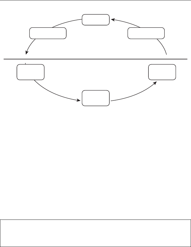
To summarise, the business generates cash by going round the circle (Fig. 2.1)

at least once (and ideally many times) in a given period.

The business also needs to have cash invested in DEBTORS and INVENTORY,

less any contribution from CREDITORS, in order to trade. These three values may

also increase or decrease in any given reporting period.

Let us now go through this section in detail to understand its contents more

thoroughly.

Understanding Cash Flows Properly 25

Cash

Work in

Progress

Raw

Materials

Finished

Goods

Creditors Debtors

Cash

Non-Cash

Figure 2.1 Diagram of the working asset cycle

CASH FLOWS FROM OPERATING

ACTIVITIES – DETAILED REVIEW

Proﬁt Before Taxation

The ﬁrst item shown is the proﬁt before taxation. You may be wondering what a

proﬁt number is doing in the cash ﬂow. Most published cash ﬂows are prepared

using the indirect method. This means the reported cash ﬂows are identiﬁed by

deriving them from data contained in the proﬁt and loss account of the business for

the period and by identifying changes between the values disclosed in the opening

and closing balance sheets for the same period.

There is a second method of preparing a cash ﬂow statement in published

accounts known as the direct method. This method is explained in more detail

in chapter 15 – Analysing direct cash ﬂow statements.

When preparing an indirect cash ﬂow statement the process commences by taking

one of the proﬁt values disclosed in the proﬁt and loss account. This is then

converted into the value of the operating cash ﬂow by adjusting the proﬁt value for

non-cash items that have already been added or deducted. Non-cash expenses are

added back and non-cash income items are removed. In this particular example

the cash ﬂow statement begins with the proﬁt before taxation value from the proﬁt

and loss account of Simple Limited.

26 Cash Flow Analysis and Forecasting

Indirect cash ﬂow statements can start from other proﬁt values in the proﬁt

and loss account. This depends on local GAAP variations and local custom in

preparing cash ﬂow statements. Usually the starting value is either the proﬁt

before interest and tax (also known as earnings before interest and tax ‘EBIT’,

or operating proﬁt) or the proﬁt after tax (also known as net income). These

variations are explained in more detail later in the book

GAAP stands for Generally Accepted Accounting Principles. This acronym

being used to encompass the laws, regulations, standards and customs used in

a particular jurisdiction to arrive at a set of published accounts.

A non-cash item is an income or expense item that appears in the proﬁt and

loss account for which there is no corresponding cash ﬂow. Typically, the most

substantial of these is the amount charged in the period for depreciation (also

known in some regions as amortisation). Depreciation is a non-cash item. You do

not write a cheque to anyone for depreciation!

Depreciation

Depreciation is an accounting adjustment. Its purpose is to charge the original cost

of purchasing an asset to the proﬁt and loss account in a series of instalments over

its estimated useful life. Depreciation was invented by accountants a long time

ago to make the proﬁt and loss account more meaningful as a document seeking

to communicate the annual performance of a business to its owners. If we did

not have depreciation in accounts and capital expenditure was simply a cost, the

business would show losses every time a substantial number of new ﬁxed assets

were acquired and much higher proﬁts in periods when no ﬁxed asset expenditure

took place.

The effect of depreciation is to spread the cost effect of acquiring capital assets

over their estimated useful life. This is a reasonable way of dealing with ﬁxed

assets because we continue to have the use of the ﬁxed assets to assist us in

producing goods for the duration of their useful life. Another way of considering

the nature of depreciation is to think of it as a notional rent for the use of the ﬁxed

assets from the balance sheet to the proﬁt and loss account, which is charged each

year of the life of an asset to the proﬁt and loss account.

The cash ﬂow statement deals solely with cash ﬂows. Depreciation is not a cash

ﬂow. We must therefore adjust for the value of depreciation charged to proﬁts in

identifying the cash ﬂow generated from operations because it is a non-cash item.

When depreciation is deducted in the proﬁt and loss account it is a cost or

expense item. Thus, when we adjust for it in the cash ﬂow statement we are adding

it back to the disclosed proﬁt before taxation value from the proﬁt and loss account

in the process of arriving at the operating cash margin. This is why depreciation

appears as a positive value when disclosed in the cash ﬂow statement.

Understanding Cash Flows Properly 27

Increase in Operating Provision

In a typical indirect cash ﬂow statement there may be a number of further items

listed representing other non-cash items of income or expenditure in the proﬁt and

loss account. In this particular example, in order to arrive at the correct value for

the cash generated from operations we are also adjusting the proﬁt before taxation

value for an increase in operating provision. This label is a little vague. It does

not tell us exactly what operating provision is involved. For example, it might be

a provision relating to warranty claims on the years production, or further costs to

be incurred in respect of a recent product recall.

Vague labels of this type crop up again and again in published cash ﬂow

statements. The fact that the label is vague is merely irritating, it will not affect our

ability to analyse the cash ﬂow statement as long as we know what to do with the

item. As this item appears within the section of the cash ﬂow statement labelled

‘adjustments’ we know it represents another add back to the proﬁt before taxation

value required in order to arrive at the cash generated from operations value. It

is listed as an adjustment because movements in provisions do not represent cash

ﬂows. They represent the recognition in this period’s accounts of the value of

a future expected cost related to activities within the current accounting period,

(an example of this might be the future warranty costs arising on this year’s

production).

The recognition of an expected future cost in the current periods proﬁt and loss

account is not a cash ﬂow. The fundamental accounting concept known as the

prudence concept requires that we recognise this future expected cost as soon as

we are aware of it. However, we do not expend any cash ﬂow in respect of this

item until customers actually claim from the business in respect of warranties. The

cash costs involved therefore arise in future accounting periods and are shown as

such in the cash ﬂow statement at that time.

The value of an increase in operating provision is shown as a positive number

in the cash ﬂow statement. This is because, once again, we are reversing an item

that originally represented an increase in a future expected cost when charged to

the proﬁt and loss account.

Conversely, the value of a decrease in operating provision is shown as a negative

number in the cash ﬂow statement, this is because we are reversing an item that

originally represented a reduction in a future expected cost in the proﬁt and loss

account.

Investment Income

This value represents the amount of investment income recognised in the proﬁt

and loss account in the current period. Once again we are showing it here in the

cash ﬂow statement as a reversing item because we need to remove it in order to

arrive at the correct value for the cash generated from operations.

28 Cash Flow Analysis and Forecasting

As we have mentioned before this cash ﬂow statement commences with the

value proﬁt before taxation. The investment income of the business has already

been recognised in the proﬁt and loss account before arriving at this value. In order

to arrive at the correct value for the cash generated from operations we need to

remove this value. This doesn’t mean that the investment income is left out of the

cash ﬂow statement. It is included in the cash ﬂow statement elsewhere. We ﬁnd

it in the investing activities section where it appears as dividends received.

You may recognise that the value shown in the cash ﬂows from investing

activities as dividends received of 320 from the example cash ﬂow statement

of Simple Limited (Table 2.1) does not match the value of investment income

adjusted for in the cash ﬂow from operating activities section of minus 500.

Again, differences of this type crop up regularly in cash ﬂow statements; the rules

for recognising income and expense in the proﬁt and loss account are different

from the recognition of the underlying cash ﬂow itself.

The fundamental accounting concept known as the ‘accruals concept’ requires

us to match revenues and costs consistently as time passes. It may be possible then

that the business has accrued investment income in the proﬁt and loss account

(perhaps because a dividend has been declared and approved for payment in a

company in which the business has an investment). However, at the period end,

the relevant dividend has not yet been paid and therefore is not recognised in the

cash ﬂow statement even though it is recognised in the proﬁt and loss account.

This is because the cash ﬂow statement only deals with cash ﬂows.

Interest Expense

This value represents the amount of interest expense recognised in the proﬁt and

loss account in the current period. Once again we are showing it here in the cash

ﬂow statement as an add back item because we need to adjust for it in order to

arrive at the correct value for the cash generated from operations.

As we have mentioned before this cash ﬂow statement commences with the

value proﬁt before taxation. The interest expense of the business has already been

recognised in the proﬁt and loss account before arriving at this value. In order

to arrive at the correct value for the cash generated from operations we need to

remove this value. This does not mean that the interest expense is left out of

the cash ﬂow statement. It is included in the cash ﬂows from operating activities

section further down where it appears as interest paid.

You will note that the value shown in the cash ﬂows from operating activities as

interest expense of 350 from the example cash ﬂow statement of Simple Limited

does not match the value of interest paid further down the same section of minus

310. Again, differences of this type crop up regularly in cash ﬂow statements; this

is due to the different rules for recognising income and expense in the proﬁt and

loss account. The fundamental accounting concept known as the accruals concept

Understanding Cash Flows Properly 29

requires us to match revenues and costs consistently as time passes. It may be

possible then that the business has accrued interest expense in the proﬁt and loss

account (because interest is accrued but is not yet due for payment). Only interest

actually paid in the period should be recognised in the cash ﬂow statement because

the cash ﬂow statement only deals with cash ﬂows.

The First Total of 6030

This represents the cash generated from selling goods or services less the cash costs

of production. It is an important measure of performance and a key component of

the cash generated from operations. The term OPERATING CASH MARGIN is

used in this book to describe this item.

Increase in Trade and Other Receivables

This represents the difference in value between the trade and other receivables (i.e.

DEBTORS) at the beginning and end of the accounting period to which the cash

ﬂow statement relates. When the value in the cash ﬂow is negative it represents an

increase in the value invested in providing credit to the business’s customers. In

order to lend our customers more cash we have to invest more cash in trade and

other receivables.

Decrease in Inventories

This item is equal to the change in the value of the inventories in the business

between the beginning and end of the accounting period. In this example the

inventory value has decreased, so resulting in a cash inﬂow to the business. This

means less cash is invested in inventory at the end of the period than at the

beginning. We have recovered some of the cash invested.

Decrease in Trade Payables

This item represents the change in the value of the trade payables (i.e. CREDI-

TORS) between the beginning and end of the accounting period. In this case the

amount owed to trade creditors has reduced. Cash has been expended to achieve

this. To reduce the amount invested in the creditors of a business it is necessary to

pay out cash to repay some of the trade credit granted by the supplier.

Cash Generated from Operations

This is the ﬁrst major summary total appearing in this example. The cash generated

from operations is 4840. This represents the difference between the cash cost of

30 Cash Flow Analysis and Forecasting

inputs to the manufacturing process and the cash received in respect of outputs,

as well as the changes in the amount invested in the net working assets of the

business.

The contents of this section of the cash ﬂow so far are summarised in Table 2.2.

Table 2.2 Analysis of the cash generated from operations total

€’000

Cash generated by the business from the cash

margin on its products

6030

Cash invested or generated from the net working

assets of the business

(1190)

Cash generated from operations 4840

These are the two key totals normally to be found in this section. When we

come to introducing the recommended method used to analyse cash ﬂows, the

reasons why this split is extremely important will be made clear. For the moment

let us say that the split is important because different causative factors affect each

value:

•The cash generated by the business from the cash margin on its products is af-

fected amongst other things by macro economic conditions, sector fundamentals,

input cost issues, customer demand, manufacturing efﬁciency, and competitive

pressure on output pricing.

•The cash invested or generated from the net working assets of the business is

affected by the style of production (lean, just in time, etc.), the need to carry

inventory to satisfy consumer needs and the typical sector structure of working

assets. (For example, retailers generally sell for cash and therefore do not need

to invest in providing credit to their customers.)

As a consequence each key total communicates different information to the

analyst about the state of the business when analysing the cash ﬂows of the

business.

There are two remaining values left in the cash ﬂows from operating activities

section. They are the interest paid and the income taxes paid. IAS 7 makes it clear

that both interest and dividends can appear in any of the three main sections, as

there is no consensus on the classiﬁcation of these cash ﬂows for entities other

than ﬁnancial institutions. Taxes are generally shown in this section unless the

cash tax paid relates to an investing or ﬁnancing activity in which case the relevant

amount of tax may be allocated to those sections as appropriate. What do these

values represent?

Understanding Cash Flows Properly 31

Interest Paid

This is the amount of cash interest paid in the accounting period. This number

may not match the proﬁt and loss account charge for interest paid because there

are different rules for the recognition of interest in the proﬁt and loss account.

The major difference is that it is normal to accrue for interest due but not paid

in the proﬁt and loss account. It is also normal in the proﬁt and loss account to

accrue the notional interest on other forms of debt with non-typical features such

as deep discount bonds where no interest is paid during the life of the instrument.

Income Taxes Paid

This is the value of the cash taxes paid during the ﬁnancial period. This number

is normally different to the value shown in the proﬁt and loss account because

taxes are usually paid in arrears. In small- and medium-sized businesses the cash

taxes paid in the current period often relate to the trading of the previous period.

For large businesses the law often requires quarterly payment of Corporation Tax

during the period to which it relates with one ﬁnal balancing payment in respect

of the accounting period after the period end. This means there is unlikely to

be any signiﬁcant relationship between the current period’s cash generated from

operations and the taxes shown in the same cash ﬂow statement.

Cash Flows From Operating Activities – Summary

The ﬁrst section of most published cash ﬂow statements deals with the cash ﬂows

from operating activities. Whilst there may be a bewildering array of adjusting

items, the bulk of the content can be summarised by two key totals: the cash

generated by the business from the cash margin on its products (known as the

operating cash margin); and the cash invested or generated from the net working

assets of the business (known as the movement or change in the Net Working

Assets). In Table 2.1 the cash interest paid and the cash taxes paid are also

disclosed in this section. The sum of all these cash ﬂows is labelled the net cash

from operating activities. We may also refer to these as the cash ﬂows relating to

TRADING.

CASH FLOWS FROM INVESTING ACTIVITIES

This section of a cash ﬂow statement also discloses two things:

1. The cash spent on purchasing or creating tangible and intangible ﬁxed as-

sets, and the cash received on disposing of obsolete or unwanted tangible or

intangible ﬁxed assets.

32 Cash Flow Analysis and Forecasting

2. The cash spent on purchasing other businesses or investing in other businesses

as associates or joint ventures or buying shares in other businesses as invest-

ments or to gain inﬂuence or to speculate and the cash received on disposing of

businesses or shares in associates or interests in joint ventures or investments.

These represent the main elements of the investing activities section. In this

particular business example we also ﬁnd the cash interest received and the cash

dividends received.

The headings in this section are reasonably self-explanatory. Typically we ﬁnd

two types of investment transaction in this section. The ﬁrst relates to the purchase,

creation or disposal of tangible and intangible ﬁxed assets. By tangible ﬁxed

assets we mean items such as property or land and buildings, plant and machinery,

ﬁxtures and ﬁttings, computer hardware and software, vehicles, ships and aircraft.

Typically these represent the pool of tangible ﬁxed assets used by the business to

generate operating cash ﬂow.

More rarely we may also encounter the purchase, creation or disposal of certain

intangible ﬁxed assets such as patents and know how and overheads relating to

the creation of capital assets which have been capitalised as permitted by IAS 38.

We may also refer to both of these as ASSET level cash ﬂows.

The second type of investment transaction is where a business purchases or

disposes of an interest in another business. This may range from, buying one share

in (or lending one euro/dollar/yen/pound sterling to) the business, up to purchasing

the whole of the business outright. Similarly it also encompasses disposing of the

same. The interest may be an investment, recognised as an associate or joint

venture, or giving control to the acquirer in which case the business acquired will

be consolidated after acquisition as a subsidiary. We may also refer to all of these

as BUSINESS level cash ﬂows.

CASH FLOWS FROM INVESTING ACTIVITIES –

DETAILED REVIEW

Acquisition of Subsidiary, X Limited, Net of Cash Acquired

This represents cash expended on the acquisition of a new business, X Limited.

This will represent the purchase of a majority of, or all of, the share capital of X

Limited. Goodwill will have been created if Simple Limited has paid more than

the net asset value (less cash) of the balance sheet of X Limited. The goodwill will

subsequently appear in the consolidated balance sheet of Simple Limited.

You may be wondering why this is shown net of cash acquired. To put this

simply there is no point in acquiring cash when buying a business. The reason

for this is you would be exchanging cash for cash if you bought cash, which is

pointless. If, for some reason, cash is acquired in the balance sheet purchased it

Understanding Cash Flows Properly 33

simply becomes part of the new groups cash pool. This is why it is normal to see

the words ‘net of cash acquired’.

The value of €10 today is €10. How much would you give me for €10? Answer

€10!

As a consequence of this, it is normal practice for the vendor to strip any

surplus cash out of a business to be disposed of prior to the sale, usually by paying

a dividend.

Purchase of Property Plant and Equipment

This represents the cash expended in the accounting period on the purchase of

new property, plant and equipment. Analysts and others commonly refer to this

value as capital expenditure. It is often abbreviated to the term Capex.

Proceeds from Sale of Equipment

This represents the cash received when we have disposed of equipment that is no

longer required. Typically this is because it is obsolete or worn out.

Do not confuse the proceeds from sale of equipment with the proﬁt on sale of

equipment, even though the two terms sound very similar. The proﬁt on sale of

ﬁxed assets is an adjustment value to the cash generated from operations and

is explained in more detail later in the book.

The proceeds of sale value is often insigniﬁcant in the context of the other cash

ﬂows. When summarising cash ﬂows for analysis it is common to offset it with the

period Capex to arrive at the value known as net Capex. Net Capex is the capital

expenditure on new ﬁxed assets minus the proceeds of sale of old ﬁxed assets.

Interest Received

This value represents the cash interest received on cash surpluses held in the

business during the accounting period. These surpluses may be recognised in the

notes to the cash ﬂow and accounts as cash and cash equivalents. The deﬁnition

of cash equivalents varies across different GAAPs.

IAS 7 deﬁnes cash equivalents as short-term, highly liquid investments that

are readily convertible to known amounts of cash and which are subject to an

insigniﬁcant risk of changes in value.

34 Cash Flow Analysis and Forecasting

This deﬁnition is designed to distinguish between investments that are very near

to cash in nature and investments that may suffer from material price (or value)

changes in the period over which they are held, even if this is relatively short term.

Dividends Received

This value represents dividends received from all interests in other business held

by Simple Limited other than interests in subsidiaries. When a subsidiary pays a

dividend to its parent company the transaction cancels out on consolidation. This

means it will not appear in the consolidated statement of cash ﬂows.

This amount will typically be reported in the proﬁt and loss account as invest-

ment income.

Cash Flows from Investing Activities – Summary

This second section of most published cash ﬂows deals with the cash ﬂows relating

to investment activities. Once again the section can usually be summarised by two

key totals: the cash ﬂows relating to ASSET level transactions; and the cash ﬂows

relating to BUSINESS level transactions.

In this example the cash interest received and the cash dividends received were

also disclosed in this section. The sum of all these cash ﬂows is labelled the net

cash used in investing activities.

CASH FLOWS FROM FINANCING ACTIVITIES

The ﬁnal section of the cash ﬂow statement discloses two things:

1. The cash ﬂows relating to changes in the business’s equity capital.

2. The cash ﬂows relating to changes in the business’s debt position.

These are the main elements of the section. In this particular example we also

ﬁnd the cash dividends paid.

This section of the cash ﬂows deals with the funding and liquidity of the

business. If the business is using cash it reveals to us how this has been ﬁnanced.

If the business is generating cash it reveals what the cash surplus has been used for

(reducing debt for example). Generally it is useful to summarise this information

into two main values: the change in equity and the change in debt.

Understanding Cash Flows Properly 35

CASH FLOWS FROM FINANCING ACTIVITIES –

DETAILED REVIEW

Proceeds from Issue of Share Capital

This represents the cash received from the sale of new shares to investors; it may

be shown net of issue expenses, although these are usually disclosed if they are

material.

This value shown in the cash ﬂow statement may not agree with the change in

share capital in the balance sheet as the shares may have been issued at a premium

or discount to their par value. Any premium over par value is usually shown in the

balance sheet equity as share premium or its local equivalent.

Proceeds from Long Term Borrowings

This value represents the cash received from banks or investors in respect of an

increase in long-term borrowings. In other words this represents a debt increase.

Payments of Finance Lease Liabilities

This value represents the reduction in the liability outstanding in respect of ﬁnance

leases entered into by Simple Limited. As a ﬁnance lease represents an interest

bearing liability this item is part of the changes to debt in the accounting period.

In other words this represents debt repayment.

Dividends Paid

This value represents the cash dividends paid out to investors in Simple Limited

during the ﬁnancial period. This value may not agree to the amount of dividends

shown in the proﬁt and loss account due to timing differences between the dividend

being proposed, approved and paid. For example the ﬁnal dividend for period one

is usually paid in period two.

Cash Flows from Financing Activities – Summary

The ﬁnal section of most published cash ﬂows deals with the cash ﬂows relating to

ﬁnancing activities. The section can usefully be summarised down to a change in

EQUITY and a change in DEBT. In our example in Table 2.1, the cash dividends

paid are also disclosed in this section. The total of all these cash ﬂows is labelled

the net cash used in ﬁnancing activities.

36 Cash Flow Analysis and Forecasting

Cash and Cash Equivalents

The ﬁnal value in the cash ﬂow statement is the net increase in cash and cash

equivalents. This represents the increase or decrease in cash and cash equivalents

held by the business in the period. In this example it is an increase of 1520.

THE NATURE OF THE BEAST – CONCLUSION

We have now examined, in some detail, the basic anatomy of a cash ﬂow. We have

learned that all the values disclosed represent pure cash ﬂows, and that many of

them do not agree to their corresponding values in the proﬁt and loss account and

balance sheet for technical reasons.

However, it is not enough to know what each value means. This is simply a

starting point. We need to know what to do with each of these values in order to

learn something useful about the business. The sort of questions we seek to answer

are as follows:

•Is the business performing satisfactorily?

•Can we lend more money to this business?

•Can this business pay me if I supply it?

•Should I invest in this business?

•Is this business good or bad?

Unfortunately, the published cash ﬂow does not answer these questions by

providing convenient, user-friendly disclosure in an appropriate format. We have

to work for our supper! In the next section we look at ways to overcome this

problem.

SUMMARISING AND RESTATING CASH FLOWS FOR

ANALYSIS – INTRODUCTION

Now that we understand what the contents of a simple cash ﬂow statement repre-

sents we can now start to consider how best to summarise and restate these cash

ﬂows in order to best understand what is going on in the business.

Before we start to get radical, let us consider what we can glean directly from the

information offered. For convenience the cash ﬂow statement of Simple Limited

is repeated (Table 2.3).

Understanding Cash Flows Properly 37

Table 2.3 A typical cash ﬂow statement

Simple Limited

Cash ﬂow statement Euros Euros

For the year ended 31st December 20XX ’000 ’000

Cash ﬂows from operating activities

Proﬁt before taxation 5600

Adjustments for:

Depreciation 550

Increase in operating provision 30

Investment income −500

Interest expense 350

6030

Increase in trade and other receivables −600

Decrease in inventories 1100

Decrease in trade payables −1690

Cash generated from operations 4840

Interest paid −310

Income taxes paid −1800

Net cash from operating activities 2730

Cash ﬂows from investing activities

Acquisition of subsidiary X net of cash acquired −650

Purchase of property plant and equipment −460

Proceeds from sale of equipment 30

Interest received 350

Dividends received 320

Net cash used in investing activities −410

Cash ﬂow from ﬁnancing activities

Proceeds from issue of share capital 400

Proceeds from long term borrowings 360

Payment of ﬁnance lease liabilities −110

Dividends paid −1450

Net cash used in ﬁnancing activities −800

Net increase in cash and cash equivalents 1520

The initial and most obvious way of summarising the cash ﬂows disclosed is to

examine what the totals of each section communicate as in (Table 2.4).

Table 2.4 Unadjusted cash ﬂow section totals

Simple Limited – Summary cash ﬂow:

Year ended 31st Dec 20XX €’000

% of operating

cash item

Net cash from operating activities 2730 100%

Net cash used in investing activities (410) 15%

Net cash used in ﬁnancing activities (800) 29%

Net increase in cash and cash equivalents 1520 56%

38 Cash Flow Analysis and Forecasting

On the face of it these values look healthy. Simple Limited appears to be

generating a healthy surplus from operations after dealing with the cost of working

asset investment, interest paid and taxes. Investment and ﬁnancing needs appear

modest with the resulting increase in cash and cash representing over 50% of the

net cash from operating activities. However, by summarising to this level we are

losing a lot of potentially valuable information.

In investing activities the Capex and business level investment has been offset by

substantial amounts of interest and dividends received, which implies this business

has a substantial non-operating surplus of cash, cash equivalents and investments

in its balance sheet.

In ﬁnancing activities we have in fact increased the amount of cash invested in

the business. This has been offset by the substantial dividend paid by the business.

IAS 7 allows those who prepare ﬁnancial statements to show dividends paid as

either a ﬁnancing cash ﬂow or an operating cash ﬂow. Let us see what happens to

the summary cash ﬂow if we make this one adjustment (Table 2.5).

Table 2.5 Adjusted cash ﬂow section totals

Simple Limited – Summary cash ﬂow. Dividends paid

shown as part of cash ﬂow from operating activities

rather than ﬁnancing activities: Year ended

31st Dec 20XX €’000

%of

operating

cash item

Net cash from operating activities 1280 100%

Net cash used in investing activities (410) 32%

Net cash used in ﬁnancing activities 650 51%

Net increase in cash and cash equivalents 1520 119%

The cash ﬂows in the summary have changed dramatically. More importantly,

the apparent relationship between the values is now different. Whilst Simple

Limited still appears healthy, the amount of net cash from operating activities

expended in investing activities now appears to have doubled relative to the ﬁrst

example. The net cash used in ﬁnancing activities has become net cash generated

from ﬁnancing activities. The increase in cash and cash equivalents now appears

to be derived partly from operations and partly from new ﬁnance.

CONCLUSION

In Table 2.5 we have only made one simple adjustment, a variation that is allowed

by IAS GAAP. The result is to change completely the apparent relationships

between the numbers. Remember that it is also acceptable to show interest paid

and interest and dividends received in any of the three sections and corporate

Understanding Cash Flows Properly 39

taxes can appear in sections other than operating if they relate to an investing or

ﬁnancing activity.

These permitted variations make a mockery of attempting to analyse cash ﬂow

performance directly from a published cash ﬂow statement. This also means there

is no direct comparability between cash ﬂow statements, as their layout can vary

markedly without contravening IAS GAAP.

So, how do we get around this problem? The answer is to use a standard layout.

What characteristics should this layout have? We need something that is suf-

ﬁciently simple to allow us to assimilate quickly and effectively what the cash

ﬂows represent in terms of performance. However, we also require sufﬁcient de-

tail to enable us to avoid the distortions that would arise if we net off too much

information as we did in the earlier example.

It is imperative to use a standard layout in order to gain comparability and

eliminate the layout distortions arising from IAS GAAP alternatives. What is this

layout?

The recommended template is shown in Table 2.6.

Table 2.6 Jury’s master cash ﬂow template

Simple Limited

Summary group cash ﬂow statement Euros

Year ended 31st December 20XX ’000

OPERATING CASH MARGIN 6030

(INVESTED)/GENERATED FROM NET WORKING

ASSETS

−1190

NET CAPITAL EXPENDITURE −430

TAXATION −1800

CASH AVAILABLE TO SATISFY FINANCE

PROVIDERS

2610

NET INTEREST 40

NET DIVIDENDS −1130

OTHER NON-OPERATING INCOME/(EXPENDITURE) −650

NET CASH GENERATED/(ABSORBED) BEFORE

FINANCING

870

Financed by:

INCREASE/(DECREASE) IN EQUITY 400

INCREASE/(DECREASE) IN DEBT 250

(INCREASE)/DECREASE IN CASH −1520

TOTAL CHANGE IN FINANCING −870

What follows is an introduction to the template. After we have reviewed this we

will revisit our analysis of the cash ﬂows of Simple Limited to see if this layout is

any more helpful in assisting us in understanding the business.

40 Cash Flow Analysis and Forecasting

Later in the book we will develop our understanding of the power of this

approach and develop our knowledge of the meaning of each line item as we

examine a number of examples of the use of my template. This chapter merely

serves as an initial introduction to my template.

Operating Cash Margin

This represents the cash generated from selling goods or services less the cash

costs of production. It is derived from values disclosed in the cash ﬂow from the

operating activities section of a published cash ﬂow statement. You will notice

that the value is the same as that shown by the ﬁrst total in the Simple Limited

cash ﬂow statement. In the Simple Limited example it is the value of the proﬁt

before taxation together with the sum of the four adjustments below it.

This value can essentially be considered as the cash ﬂow equivalent of proﬁt.

It measures the success with which a business generates a cash ﬂow surplus from

doing things! Businesses with negative operating cash margin are receiving less

cash for the goods and services they sell than the cash costs of materials and cash

overheads suffered in producing them.

This value is the equivalent to the cash generated from going round the circle

in the complete real business model.

(Invested)/Generated from Net Working Assets

This represents the net change in the amount invested in the net working assets of

the business. The amount invested in the net working assets is the amount invested

in inventories and the trade and other debtors, less the amount of interest free

credit received from suppliers and other creditors because the business is trading.

Inventories represent the amount invested in raw materials, work in progress

and ﬁnished goods less provisions for slow moving, damaged and obsolete items.

Seeing this value as a distinct total, independent of the cash generated from

operations total, is important because the amount invested or generated from net

working assets can be volatile and is affected by different drivers of change to the

operating cash margin. Movements in this value convey a lot of useful information

to the cash ﬂow analyst about management quality, sectoral investment needs and

relative efﬁciency.

Net Capital Expenditure

Represents the amount invested in new ﬁxed assets in the period less the proceeds

of selling old ﬁxed assets. This is where we show the cash ﬂows relating to ASSET

level transactions.

Understanding Cash Flows Properly 41

The level of capital expenditure in a business is inﬂuenced by a number of

factors, such as the market and business growth rate, technological change, changes

in consumer demand and the need to invest to maintain competitiveness.

Taxation

This represents the taxes actually paid in the period.

Cash Available to Satisfy Finance Providers

This total represents the cash available after the business has satisﬁed its ﬁxed

and working asset investment needs and paid its taxes. In the long run a business

needs to generate sufﬁcient cash in order to satisfy ﬁnance providers, to service

its interest burden, repay debt due in the period and provide the expected dividend

to shareholders.

This value represents a key total for the cash ﬂow analyst. Intriguingly, it doesn’t

appear at all in a published cash ﬂow statement!

Net Interest

This is the value of the cash interest paid, less the value of any cash interest

received. Essentially this communicates to the analyst the cost to the businesses of

its net debt ﬁnancing position. Net debt is the amount of interest bearing liabilities

less the value of cash and cash equivalents.

Net Dividends

This is the value of the cash dividends paid, less the value of the cash dividends

received.

Netting off dividends in this way simpliﬁes the cash ﬂow summary without

losing much information. There are arguments that the net dividend cost is a more

useful value to examine (the shareholders indirectly own the dividends receivable

anyway!)

If more detail is required it is available from the source cash ﬂow statement

used to make the template. The template can of course be expanded should this be

needed. It is up to the user how best to summarise the raw data for analysis.

Other Non-Operating Income/(Expenditure)

This is where we capture the BUSINESS level cash ﬂows, such as the cash

spent on purchasing other businesses or investing in other businesses as associates

or joint ventures or buying shares in other businesses as investments and the

42 Cash Flow Analysis and Forecasting

cash received on disposing of businesses or shares in associates or interests in

joint ventures or investments. We would also introduce here any grants, subsidies

or other government assistance received in respect of business acquisition or

development. Again, the title is meant to be largely self-explanatory. If it is not

an operating cash ﬂow item or an item related to the purchase or disposal of ﬁxed

assets it probably goes here!

Net Cash Generated/(Absorbed) Before Financing

This is the second key total. This total represents the cash surplus or deﬁcit for the

period after all cash costs incurred in the period have been satisﬁed. The remainder

of the template deals with the impact of changes in the ﬁnancing of the business.

Again, it is unusual for this value to be stated implicitly in a published cash ﬂow

statement.

Increase/(Decrease) in Equity

This represents the net cash change in equity during the period. Businesses raise

new equity by issuing shares and, in most countries, larger businesses are able to

buy back or cancel some of their equity should they wish to do so.

Increase/(Decrease) in Debt

This represents the net cash change in the total debt of the business in the period.

By netting in this way we eliminate the effects of re-ﬁnancing (this being replacing

old debt with new debt) leaving us with a view of the actual debt change in the

period.

(Increase)/Decrease in Cash

This represents the change in the value of cash and cash equivalents during the

period. Notice that in my template the signage of this value is reversed compared

to the value disclosed in a typical published cash ﬂow statement. An increase in

cash and cash equivalents is shown as a negative number, a decrease in cash and

cash equivalents is shown as a positive number.

It is necessary to reverse the sign of the last number to take advantage of

a property of the cash ﬂow statement that is not obvious from the published

version and is particularly valuable to the analyst. A cash ﬂow statement bal-

ances just like a balance sheet. As is clear from the master template the net cash

generated/(absorbed) before ﬁnancing is always equal in value to the ﬁnancing

cash ﬂows themselves (after adjusting the signage of the cash and cash equiva-

lents). This balancing property enables us to conﬁrm that we have not made any

Understanding Cash Flows Properly 43

arithmetic errors or omitted any of the values from the original cash ﬂow state-

ment, so improving accuracy. Bear in mind that having balanced the cash ﬂow

template it is still possible to make errors of allocation by entering a source value

into the wrong heading.

Why is the signage of the last cash and cash equivalents number in a typical

cash ﬂow statement different to the signage used in the template?

Cash Change Signage – Algebraic Explanation

It has to do with the way a published cash ﬂow statement is laid out. As you can

see from Simple Limited the published cash ﬂow statement is not laid out as a

balancing statement. The cash ﬂows are summarised and then added up to arrive

at a ﬁnal total or difference. The effect of this layout is to make the signage of the

last number only in the cash ﬂow incorrect should we wish to make a layout with

the balancing feature. This is a problem with virtually all published cash ﬂows

irrespective of their national origin.

We can show this algebraically. A typical published cash ﬂow is laid out like

this:

O±I±F=C

where

O=The cash ﬂows from operating activities

I=The cash ﬂows from investing activities

F=The cash ﬂows from ﬁnancing activities

C=The change in cash and cash equivalents

In the template, in order to have two balancing totals which cancel each other

out to zero we bring the cash value to the left side of the formula so it looks like

this:

O±I±F−C=0

So, in order to make the layout in my template mathematically consistent it is

necessary to change the sign of the ﬁnal cash value shown in the published cash

ﬂow.

Cash Change Signage – Double Entry Explanation

A second explanation relies on the process of double entry accounting to illuminate

what is actually going on. If you have any familiarity with book keeping you will

know that every transaction in a set of double entry accounts has two entries. These

two entries for each transaction are known as a debit entry and a credit entry. At

the end of a period all the entries are added up, if no arithmetic errors have been

44 Cash Flow Analysis and Forecasting

made all the debits and all the credits will total to the same value. In other words

they will be in balance.

Balance Sheet

Debit side Credit side

ASSETS LIABILITIES

When I designed the template I had a choice as to how I dealt with the signage

of the equity, debt and cash numbers. I chose to represent an increase in equity as

positive, because for most people this is the intuitive signage to use for an increase,

as debt is also on the same side of the balance sheet (a liability item) an increase

in debt must also be positive, which again is largely intuitive for most people.

Cash, however, is not a liability. It is an asset item, this means an increase in

cash must have the opposite signage to the equivalent equity and debt value for the

three numbers to set off correctly in arriving at the balancing total. This inevitably

means that showing the cash increase as negative is not particularly intuitive for

most people, however, I believe it is preferable to reversing the signage of the

other two items – equity and debt – because it leaves us with only one value whose

sign is counter-intuitive rather than two.

Balance Sheet

Debit side Credit side

ASSETS LIABILITIES

Cash Debt and Equity

If you mentally take the values shown above for the equity, debt and cash of

Simple Limited and insert them in the above diagram it should become clear why

it is necessary to change the sign associated with cash.

I have provided two explanations as to why it is necessary to change the last

number only of a published cash ﬂow in order to balance the master template.

Increased familiarity by the user with the restatement of published cash ﬂows

will inevitably reinforce this point until it is no longer an issue in the mind of

the user.

To summarise, unless the published cash ﬂow statement is laid out as a balancing

statement (something I have observed on a few rare occasions) it will always be

necessary to reverse the sign of the last cash number in the cash ﬂow statement

only in order to get the master template values to balance correctly.

Understanding Cash Flows Properly 45

ANALYSING THE CASH FLOWS IN THE

MASTER TEMPLATE

So, we have successfully summarised the published cash ﬂows into the template.

What does it tell us?

By having a standardised layout we have eliminated the distortions that might

arise due to positional differences in the disclosure of interest, dividend and

taxation values. We have also laid out the values in such a way that two key totals

not shown in the original published cash ﬂow statement are exposed for analysis

and assessment (Table 2.7).

Table 2.7 The completed Jury’s master cash ﬂow template for Simple Limited

Simple Limited

Summary group cash ﬂow statement Euros

Year ended 31st December 20XX ’000

OPERATING CASH MARGIN 6030

(INVESTED)/GENERATED FROM NET WORKING ASSETS −1190

NET CAPITAL EXPENDITURE −430

TAXATION −1800

CASH AVAILABLE TO SATISFY FINANCE PROVIDERS 2610

NET INTEREST 40

NET DIVIDENDS −1130

OTHER NON-OPERATING INCOME/(EXPENDITURE) −650

NET CASH GENERATED/(ABSORBED) BEFORE FINANCING 870

Financed by:

INCREASE/(DECREASE) IN EQUITY 400

INCREASE/(DECREASE) IN DEBT 250

(INCREASE)/DECREASE IN CASH −1520

TOTAL CHANGE IN FINANCING −870

Here is an explanation of what the cash ﬂows of Simple Limited might reveal

to an analyst experienced in the application of the analysis techniques explained

in more detail as we proceed to the more advanced parts of the book.

Simple Limited appears to enjoy a healthy operating cash margin with ap-

proximately 20% of it being absorbed in working capital changes. Net capital

expenditure appears low (we know this because we can compare it with the depre-

ciation value in the adjustments part of the cash ﬂows from operating activities),

net capital expenditure is 78% of the period depreciation charge. IAS depreciation

is based on writing off assets over their estimated useful life and therefore provides

a crude estimate of the amount required each year to replace ﬁxed assets. Thus it

appears the business is investing less in ﬁxed assets than it needs to compensate

for the wearing out of the existing assets each year.

46 Cash Flow Analysis and Forecasting

Taxes appear consistent with a business with no net debt. The taxation value is

28% of the operating cash margin, which may not signify anything if the taxation

paid this year relates to cash generated in the previous year. If taxes are in arrears the

tax paid implies the business’s last accounting period enjoyed a similar operating

cash margin value assuming no net leverage. The cash available to satisfy ﬁnance

providers is a surplus of €2610.

The net interest value is positive, implying no net debt on average over the year,

the net dividend is a substantial outﬂow even after offsetting dividends received.

Simple Limited has made a small acquisition during the year. The remaining

surplus of €870, together with the net increase in equity and debt has resulted in

an increase in cash retained in the business of €1520.

These cash ﬂows are typical of an established and successful mature business.

Notice that everything mentioned above has been derived solely from the cash

ﬂow statement, no reference is made anywhere to any other value available in the

full set of accounts.

THE STATE OF PLAY

So far we have started to address the nature of a cash ﬂow statement and what

this tells us about the cash ﬂows of a business. Secondly we have introduced

Jury’s Cash Flow Template and restated the cash ﬂows of Simple Limited into the

template.

Finally, we have scratched the surface of what we can glean from the restated

cash ﬂows. It is now time to develop a deeper and more thorough understanding of

this process. In the next chapter we introduce a further element of the knowledge

set required to fully grasp cash ﬂow analysis.

Start-up, Growth, Mature, Decline

INTRODUCTION

In order to gain further beneﬁt and insight from the results of our cash ﬂow

restatement we need to understand what a typical set of ‘good’ cash ﬂows should

look like.

The typical ‘good’ pattern of cash ﬂows varies dramatically between different

businesses. The most important reason for this variety is to do with where the

business is in its life cycle.

In this section we look at the typical cash ﬂows of a business at start-up, in

the growth phase, the mature phase, and ﬁnally the decline phase. To make this

section as useful as possible to the analyst I have included a short discussion of

exactly what we mean by the terms start-up, growth, maturity and decline when

applied to business analysis.

Later in the book there are separate chapters on each of the four phases. They go

into more detail about various aspects of analysis relevant to that particular phase.

All cash ﬂow values quoted in the text from the examples represent thousands.

THE START-UP PHASE

When does business commence?

As any entrepreneur knows, there are a number of steps that precede the com-

mencement of trade.

Most entrepreneurs start with an idea for a new product or service. They then

research the viability of the idea, the initiatives required, assess the feasibility of

operations, the business risks involved and develop a business plan. This part of

the process can take years. Assuming the viability of the project looks good, the

entrepreneur at some point raises capital and invests in the necessary initiatives to

develop the product or service.

At some point, once operations are established on a commercial scale, sales

commence to customers of the business. This is when the ﬁrst cash inﬂows from

operations arrive. Prior to this point we do not have a true business. You could

say we have a charity! Some person or persons (the project sponsors) are giving

money to other persons to do things for them.

Why is this issue of what constitutes a true business so signiﬁcant?

Cash Flow Analysis and Forecasting: The Definitive Guide to

Understanding and Using Published Cash Flow Data

by Timothy D.H. Jury

48 Cash Flow Analysis and Forecasting

In the past I have observed numerous situations where entrepreneurs and busi-

nessman have claimed to be running a business, but in fact there is no true

business there. There may be products, factories, employees, sales literature and

administration. What missing is sales and hence cash ﬂow from customers! In

other words demand for the product or service provided has not yet been proven

to exist.

I recollect visiting a start-up business that had developed a new form of solar

heating device, I was shown a completed version of the product, met employees

and was shown a factory containing various machinery purchased to manufacture

the product. However, at this point, there was no sales activity at all! The business

closed having run out of cash before any material level of sales had been achieved.

So, for the purposes of analysing cash ﬂows, my deﬁnition of ‘a start-up busi-

ness’ is the achievement of regular operating cash ﬂow from customers. The

business may not be proven to be viable in the long run at this point; however,

some important milestones will have been passed.

1. The product or service is being delivered successfully.

2. Someone, somewhere (a customer) is willing to pay for it.

3. Customers are continuing to consume the product or service after their ﬁrst

purchase (there are repeat purchases).

The business will almost certainly still be cash negative and loss making at

this point. The long journey to success is not yet complete. However, the basic

credibility of the business model has been demonstrated. In the later chapter on

the start-up phase we will discuss in more detail what happens in the period before

this point.

So, in this initial example, my start-up business has already designed the ﬁrst

product or service to be sold and invested sufﬁciently to deliver this. Customers

are starting to buy the product.

The cash ﬂows of a start-up business could look like the example in Table 3.1.

Let us assume that an entrepreneur has recently started a new business. The busi-

ness is manufacturing some sort of consumer product that requires an investment

in machinery.

The restated cash ﬂow summary reports the cash ﬂows over the ﬁrst year of

operation. Let us review what the template tells us about the business.

The operating cash margin is negative as the business is still producing goods

for more cash cost than they receive in sales income. This is because the volume

through the plant is still too low to capture the necessary economies of scale to

be proﬁtable. The workforce is still learning to manufacture the product to the

required levels of quality in an efﬁcient manner. Production is not yet particularly

efﬁcient.

The business is investing in the net working assets it requires. The business has

to invest in inventory; it must have sufﬁcient raw materials, work in progress and

Start-up, Growth, Mature, Decline 49

Table 3.1 The cash ﬂows of a start-up business

Start-up example

Restated cash ﬂows Dollars

Year 1 ’000

OPERATING CASH MARGIN −10

(INVESTED)/GENERATED FROM NET WORKING ASSETS −200

NET CAPITAL EXPENDITURE −500

TAXATION 0

CASH AVAILABLE TO SATISFY FINANCE PROVIDERS −710

NET INTEREST 30

NET DIVIDENDS 0

OTHER NON-OPERATING INCOME/(EXPENDITURE) 300

NET CASH GENERATED/(ABSORBED) BEFORE FINANCING −380

Financed by:

INCREASE/(DECREASE) IN EQUITY 500

INCREASE/(DECREASE) IN DEBT 0

(INCREASE)/DECREASE IN CASH −120

TOTAL CHANGE IN FINANCING 380

ﬁnished goods to be able to satisfy customer needs as required. In addition it will

be obliged to provide trade credit to its customers (invest in debtors) as it acquires

them if this is normal practice in the market in which the business operates. It will

enjoy little if any trade credit from its suppliers, however, due to the newness of

the business and lack of track record on which the suppliers could base a credit

assessment. Most raw material purchases will be in cash.

The business is investing in ﬁxed assets. In this year the entrepreneur has

purchased the ﬁrst machine required to commence production as well as other

ﬁxed assets needed to package and distribute the product.

The business pays no taxes at this point, as it has never made a proﬁt, indeed

there is likely to be a tax loss carried forward at the end of the year.

The cash available to satisfy ﬁnance providers is a substantial negative. This is

typically what we expect to see at this point in the start-up businesses development.

The business has a small amount of interest received due to the having a net

cash position in its balance sheet. There is no interest payable as the business has

no debt at this point in its development.

The business does not pay a dividend at this point because any cash available

at this point is used for investment and because it’s probably illegal! In many

countries dividends can only be paid out of positive revenue reserves. At this point

the revenue reserves of the business are negative in the balance sheet.

50 Cash Flow Analysis and Forecasting

The business receives a substantial grant from the government because it is

creating employment in its location. The entrepreneur has employed ﬁve persons

on start-up.

The net cash absorbed before ﬁnancing at the end of the ﬁrst year’s trading is

$380. This is ﬁnanced by the introduction of $500 in equity from the entrepreneur,

her family and other investors. At the end of the period $120 of this new equity

remains in the business cash account unspent.

This is a typical set of start-up cash ﬂows. Generally the business is cash

negative, the shortfall being ﬁnanced by investors.

THE GROWTH PHASE

The next three most important objectives are to achieve a positive cash ﬂow

position, to break even and to make this sustainable into the future. Ideally these

objectives are achieved in the ﬁrst two to three years of the life of the business.

The business then enters the growth phase.

What exactly do we mean by a growth business? We mean a business whose

VOLUME of output (or if it is a service business, its scale of operations) is

growing. Inevitably this requires investment in both working assets and ﬁxed assets

(Table 3.2).

Table 3.2 The cash ﬂows of a growth business

Growth example

Restated cash ﬂows Dollars

Year 4 ’000

OPERATING CASH MARGIN 1000

(INVESTED)/GENERATED FROM NET WORKING ASSETS −400

NET CAPITAL EXPENDITURE −900

TAXATION −300

CASH AVAILABLE TO SATISFY FINANCE PROVIDERS −600

NET INTEREST −100

NET DIVIDENDS 0

OTHER NON-OPERATING INCOME/(EXPENDITURE) 100

NET CASH GENERATED/(ABSORBED) BEFORE FINANCING −600

Financed by:

INCREASE/(DECREASE) IN EQUITY 300

INCREASE/(DECREASE) IN DEBT 210

(INCREASE)/DECREASE IN CASH 90

TOTAL CHANGE IN FINANCING 600

Start-up, Growth, Mature, Decline 51

Let us assume our example manufacturing business has successfully negotiated

the start-up phase, the business is now growing strongly. How does this change

what we see?

The operating cash margin is now positive and the business is generating

a healthy cash surplus against its cash costs every time it sells its product to

customers.

The business is still investing in net working assets because it is growing

its unit output strongly. It therefore requires investment in increasing its inven-

tory and its debtors. The business is now able to obtain some trade credit from

its major suppliers as it is trading proﬁtably and has a three-year track record

available for analysis. This offsets some of the investment required in inventory

and debtors.

The business is still investing in ﬁxed assets because it is still growing; further

machinery is purchased as required to increase output as the business expands.

Periodically the factory itself may require expansion.

The business is now paying some taxes; however, the liability is not large.

As a consequence of the capital investment there is substantial tax depreciation

available to reduce the tax liability.

The cash available to satisfy ﬁnance providers is still negative. Again, this is

typically what we expect in a growth business. The reason it is negative is that

the business is making the ﬁxed and working asset investment required to keep

pace with growth in demand for its products faster than it is generating cash from

the operating cash margin. The presumption when the investment is made is that

the investment in ﬁxed and working assets in the current period will yield more

operating cash margin from the resulting increases in the volume of output in

future years as the business continues to grow. Investors are prepared to ﬁnance

this if they believe the future increase in operating cash ﬂow as a result of the

investment will be sufﬁcient to recover or exceed the cash they invest in the new

ﬁxed and working assets.

The business is now paying interest. In our example, ﬁnance leases have been

used to acquire some of the machinery and represent part of the capital expenditure.

The young business in the growth phase is still too risky for most commercial banks

to consider lending medium-term ﬁnance. However, leasing companies are less

concerned about the business risk issues as they have the security of the machinery

(against which they have lent) to rely on should the business cease to make the

monthly payments required for any reason.

No dividends are being paid at this time, as the business is still cash negative.

All surplus resources are focused on continuing the rapid growth of the business.

The business continues to receive grants from the government in respect of em-

ployment creation as it continues to take on more new employees for the ﬁrst time.

The net cash absorbed before ﬁnancing at the end of the fourth year’s trading

is $600. This is ﬁnanced by the introduction of $300 in equity from growth stage

52 Cash Flow Analysis and Forecasting

investors and the introduction of $210 of debt being the principal outstanding in

respect of the ﬁnance leases on new ﬁxed assets. The remaining $90 required has

come from cash and cash equivalents already in the business as the beginning of

year four.

This is a typical set of growth cash ﬂows. The business is still cash negative

in this stage, because it is investing more in ﬁxed and working assets in a given

period than it is generating in operating cash margin. The shortfall is ﬁnanced by

growth investors, lenders with an appetite for lending to such businesses and the

cash, which was retained in the business from previous periods.

THE MATURE PHASE

In a business analysis context the term ‘mature’ is somewhat ambiguous. All busi-

nesses want to grow if they can, including businesses considered by investors and

analysts to be mature. They continue to invest signiﬁcant amounts of management

time and effort in seeking ways to increase turnover, proﬁts and cash ﬂows.

So, what exactly do I mean by a business that is mature? I will start by deﬁning

a business that is mature as one that is no longer growing the VOLUME of its

output. This means that the new investment in ﬁxed and working assets to grow

the output of the business is no longer required. In a successful mature business

the overall cash ﬂows are positive (Table 3.3).

Table 3.3 The cash ﬂows of a mature business

Mature example

Restated cash ﬂows Dollars

Year 9 ’000

OPERATING CASH MARGIN 3500

(INVESTED)/GENERATED FROM NET WORKING ASSETS −600

NET CAPITAL EXPENDITURE −1000

TAXATION −1000

CASH AVAILABLE TO SATISFY FINANCE PROVIDERS 900

NET INTEREST −400

NET DIVIDENDS −400

OTHER NON-OPERATING INCOME/(EXPENDITURE) 0

NET CASH GENERATED/(ABSORBED) BEFORE FINANCING 100

Financed by:

INCREASE/(DECREASE) IN EQUITY 0

INCREASE/(DECREASE) IN DEBT −100

(INCREASE)/DECREASE IN CASH 0

TOTAL CHANGE IN FINANCING −100

Start-up, Growth, Mature, Decline 53

Let us assume our example business is now mature. The business has reached

a position in the geographic markets in which it chooses to compete where it

controls a signiﬁcant market share and enjoys adequate competitive advantages

to sustain its position. At this point it has no immediate plans for further new

investment or growth in the planned volume of its output.

The operating cash margin is now substantial, the business is generating a

healthy cash surplus against its cash costs each time it sells its products to cus-

tomers. It has thousands of customers spread over a wide geographic area. It has

learned how to manufacture its product in a highly efﬁcient way and has used cap-

ital expenditure over many years to lower costs and improve quality. It is selling

its product in millions of units a year. The volume of output is not growing or is

growing very slowly.

The business is still investing in net working assets. Why is this?

The business does not require further investment in net working assets in respect

of volume growth because there is none! However, there is one other external

variable affecting the business that may still trigger a need for further investment

each year. This is the effect of inﬂation on the business. If the economy in which

the business operates suffers inﬂation at say 2% a year this means that it will

cost 2% more at the end of the year to replace the same physical inventory that

was present at the beginning of the year. The same logic applies to debtors.

Conversely the interest-free loan that represents supplier credit will increase 2%

a year in respect of the same physical purchasing. So, even in a mature business,

it may be necessary to invest in net working assets each period to offset inﬂation

effects.

The business is still investing in ﬁxed assets. Again, it may not immediately

be obvious why. The business is no longer growing so it does not require ﬁxed

asset investment to provide increased output capacity. As with the net working

assets there is a second driver of investment at work. Machines wear out, vehicles

and computers need replacing regularly. We have a name for this type of capital

expenditure (this term often being abbreviated to Capex). This is known as main-

tenance or replacement Capex. This distinguishes it clearly from growth Capex,

which is new capital expenditure made with the intention of increasing output or

operations.

So, when a business stops growing its output Capex doesn’t drop to zero. It

drops to a lower number representing the maintenance or replacement Capex. For

a business to maintain its productive capacity it needs to keep its ﬁxed assets

in appropriate productive condition. Competitive and technological changes may

also stimulate ﬁxed asset replacement even in conditions of no growth of output.

So our mature business will still have net capital expenditure, this being devoted

mainly to maintenance or replacement Capex.

The business is now paying a substantial amount in cash taxes, as there is less

capital expenditure to reduce the tax bill through accelerated tax depreciation.

54 Cash Flow Analysis and Forecasting

Remember that the amount shown in respect of taxes in this year’s cash ﬂow

statement may in some countries relate to the previous year’s proﬁts and this

means the value may have no direct relationship with this year’s operating cash

margin.

The cash available to satisfy ﬁnance providers is now positive. This is what we

expect to see in a successful mature business. All mature businesses should be

producing a positive cash ﬂow available to satisfy ﬁnance providers. If the cash

ﬂow is negative at this point it means the business is not generating sufﬁcient

operating cash ﬂow to cover investment needs and taxes, a situation that is not

sustainable. The business is probably distressed and without signiﬁcant change

may collapse at some point in the future. If a business cannot meet its mainte-

nance investment needs and pay its taxes from the operating cash margin it is in

serious trouble. Remember that this measure of performance is before we con-

sider the additional cash outﬂows relating to the servicing of debt and providing

dividends to investors. Neglecting either of these will also result in problems in

the future.

The business is now paying interest. It is now nine years old and has built

up a substantial balance sheet full of assets. It should be an attractive lending

opportunity for most lenders and the business should have little trouble in raising

any kind of debt as it requires it. Our example business now has bank debt in its

balance sheet as well as ﬁnance leases.

The business now pays a dividend. Whist the decision to pay a dividend is

largely a matter of tax efﬁciency in a private company it would be essential in a

mature public company if the business were to sustain a reasonable share price.

Corporate ﬁnance theory suggests mature businesses should be distributing cash

back to investors because they no longer require their cash surpluses for investment

in the business.

Other non-operating income/(expenditure) is zero as the business is not engaged

in the acquisition or disposal of other businesses or investments and is no longer

receiving any grants.

There is a small cash surplus before ﬁnancing at the end of the ninth year’s

trading of $100. There is no longer any need to introduce further new equity to

the business. If the business required investment for any reason it would normally

borrow to fund it. In this example the $100 has been used to reduce the debt

outstanding. Other than that required for day to day liquidity there is no cash in

the business as it now has a net debt position. This is why there is no movement

in the cash change value.

This is a typical set of mature cash ﬂows. The business is generating cash

at both the cash available to satisfy ﬁnance providers total and the net cash

generated/(absorbed) total. It now has net debt and pays dividends. Other than

maintaining its ﬁxed and working assets its investment needs are minimal.

Start-up, Growth, Mature, Decline 55

THE DECLINE PHASE

The word ‘decline’ is used by analysts for a variety of purposes. A business

that is suffering poor performance may be referred to as being ‘in decline’. In

this sense a business can be in decline in any of the four phases. The whole

issue of bad performance in each of the four phases is dealt with the later in

Chapters 6–11, which go into more depth about what constitutes ‘good’ and ‘bad’

cash ﬂows.

What we are going to examine here is the effect on the cash ﬂows of being a

successful business whose product or service markets are in decline. That is to

say they are reducing in size year on year. This implies that the volume of output

produced by the business is falling year on year. What will the cash ﬂow look like

now?

This is not a poorly managed business or failing business. What is illustrated

in Table 3.4 is a successful business in a declining market. The best example

available at the moment is probably a cigarette manufacturing company. In Eu-

rope cigarette consumption is declining at about 3% a year. The cash ﬂow decline

example is included at this point to illustrate to the reader what should be hap-

pening to the behaviour of the cash ﬂows in such a situation in a successful

business.

Table 3.4 The cash ﬂows of a decline business

Decline example

Restated cash ﬂows Dollars

Year 20 ’000

OPERATING CASH MARGIN 7000

(INVESTED)/GENERATED FROM NET WORKING ASSETS 1000

NET CAPITAL EXPENDITURE 1500

TAXATION −3200

CASH AVAILABLE TO SATISFY FINANCE PROVIDERS 6300

NET INTEREST −1000

NET DIVIDENDS −3000

OTHER NON-OPERATING INCOME/(EXPENDITURE) 0

NET CASH GENERATED/(ABSORBED) BEFORE FINANCING 2300

Financed by:

INCREASE/(DECREASE) IN EQUITY −1000

INCREASE/(DECREASE) IN DEBT −1300

(INCREASE)/DECREASE IN CASH 0

TOTAL CHANGE IN FINANCING −2300

56 Cash Flow Analysis and Forecasting

We expect to see something along the following lines: The operating cash margin

is substantial. The business is generating a healthy cash surplus against its cash

costs each time it sells its product to customers. It has learned how to manufacture

its product in a highly efﬁcient way and has been exploiting a signiﬁcant position in

its market for decades. It is selling its product in millions of units a year. Turnover

is declining at a few percent a year. The operating cash margin is still substantial

but is falling slowly year on year.

The business is now recovering its investment in working assets. As the business

turnover declines the need to invest in inventory and debtors – less the interest-free

loan from suppliers – disappears and, as the amount invested in working assets

declines, the cash invested in working assets in the growth phase of the business

returns to the business as a cash inﬂow.

The business is now recovering its investment in ﬁxed assets. As volume output

reduces manufacturing capacity is rationalised. Factories that are not required are

closed and where possible the plant and machinery is sold to others or relocated. As

the factory was built decades ago in or near centres of population the land on which

it sits may be very valuable for redevelopment. Production is concentrated in the

lowest cost and most modern facilities, further increasing margins. Maintenance

Capex may still be required. However, this is minimal due to the availability of

surplus assets elsewhere to substitute for it. The proceeds of sale of ﬁxed assets

exceeds the replacement Capex, so resulting in a cash inﬂow from net capital

expenditure.

The business pays a very substantial amount in cash taxes, as there is minimal

capital expenditure to reduce the tax bill through accelerated tax depreciation.

The cash available to satisfy ﬁnance providers is now massively positive. This

is what should be happening in a successful decline business. Not only are we

receiving the operating cash margin, we are recovering the investment in net

working assets and ﬁxed assets.

In our example the business now carries a signiﬁcant amount of debt and now

pays a lot of interest. If the business is large the management may be increasing

the debt in the business periodically and using the cash inﬂow to buy back equity,

so supporting the share price. The massive operating cash ﬂow is used to service

interest and repay debt. Every few years the process of adding more debt to buy

back equity may be repeated.

In our example the business also pays a massive dividend. If the business is

listed this is the only reason to invest in the business as there is no longer any

expected future volume growth. Investors assess a share in such a company on the

basis of its dividend yield relative to debt yields.

Other non-operating income/(expenditure) is zero as the business is not engaged

in the acquisition or disposal of other businesses or investments and is no longer

receiving any grants.

Start-up, Growth, Mature, Decline 57

There is a massive cash surplus before ﬁnancing at the end of the years trading of

$2300. This is used to buy back equity and repay debt. A process that theoretically

could continue until the business ﬁnally self liquidates.

This is a typical set of successful decline cash ﬂows. It is included to provide

a complete understanding of how the basic patterns of cash ﬂow should appear in

the four phases of the life of a successful business. In the real world a declining

business rarely displays this sort of cash ﬂow performance. This is discussed in

more detail in Chapter 10.

CONCLUSION

We should now have gained an understanding of what we expect the cash ﬂows of

business to look like through the four phases of a successful businesses existence.

This is summarised in Table 3.5.

Table 3.5 The cash ﬂows through the four phases of a successful business

Summary example Start-up Growth Mature Decline

Restated cash ﬂows $’000 $’000 $’000 $’000

OPERATING CASH MARGIN −10 1000 3500 7000

(INV)/GEN FROM NET WORKING

ASSETS

−200 −400 −600 1000

NET CAPITAL EXPENDITURE −500 −900 −1000 1500

TAXATION 0 −300 −1000 −3200

CATS FINANCE PROVIDERS −710 −600 900 6300

NET INTEREST 30 −100 −400 −1000

NET DIVIDENDS 0 0 −400 −3000

OTHER NON-OPERATING INC/(EXP) 300 100 0 0

NET CASH GEN/(ABS) BEFORE

FINANCING

−380 −600 100 2300

Financed by:

INCREASE/(DECREASE) IN EQUITY 500 300 0 −1000

INCREASE/(DECREASE) IN DEBT 0 210 −100 −1300

(INCREASE)/DECREASE IN CASH −120 90 0 0

TOTAL CHANGE IN FINANCING 380 600 −100 −2300

58 Cash Flow Analysis and Forecasting

SUMMARY

The goal of this chapter was to present to the reader a typical set of cash ﬂows for

a successful business in the four phases in the life of that business, these being:

Start-up, Growth, Mature and Decline. These examples provide a sort of budget

or ideal against which we can examine actual cash ﬂows taken from the real

world.

It should now be clear that each line of the cash ﬂow template is driven by

different cash ﬂow drivers or behaviours. By developing our understanding of

these drivers we can improve our ability to evaluate the cash ﬂows of a business

when presented in the Jury’s Template format.

Restating the Cash Flows

of a Real Business

INTRODUCTION

This chapter commences the more detailed part of the book. The following chapters

present everything the ﬁnancial analyst may require to become fully conversant

with historic cash ﬂow analysis.

This chapter seeks to present all the information required by an analyst to

summarise and restate an indirect cash ﬂow statement into a common format for

analysis.

The restatement process that is described is essentially a technical exercise.

Accordingly, this chapter is organised to be as user friendly as possible when

read for the ﬁrst time and easily accessible subsequently when used as a technical

reference.

OUR OBJECTIVE

We have a cash ﬂow statement to analyse, how do we go about our task?

There are two possible ways of preparing and presenting a cash ﬂow statement,

these are known as the direct method and the indirect method. The ﬁrst task to

ascertain is whether the cash ﬂow is a direct cash ﬂow or an indirect cash ﬂow.

In this chapter we will concentrate on the restatement of indirect cash ﬂows.

The reason for this is most of the published cash ﬂows in the world are prepared

using the indirect method. Cash ﬂow statements prepared using the direct method

are rare. If you wish to know more about direct cash ﬂows at this point Chapter

15 is devoted entirely to direct cash ﬂows.

A direct cash ﬂow is prepared by taking the cash records of the business, coding

each cash transaction during the period into its relevant cash ﬂow constituent

and then summarising the resulting information into a cash ﬂow statement.

Cash Flow Analysis and Forecasting: The Definitive Guide to

Understanding and Using Published Cash Flow Data

by Timothy D.H. Jury

60 Cash Flow Analysis and Forecasting

We can identify whether a cash ﬂow statement is direct or indirect by examining

the ﬁrst few lines of the cash ﬂow statement. In the case of direct cash ﬂow

statements instead of starting with a proﬁt value taken from the proﬁt and loss

account the cash ﬂow typically starts with receipts from customers and payments

to employees and suppliers.

An indirect cash ﬂow is prepared by identifying the various cash ﬂows required

to prepare the cash ﬂow statement from information contained within the proﬁt

and loss account and the current and previous balance sheet of the business.

THE IMPLICATION OF DIFFERENT GAAPs

GAAP is an acronym for Generally Accepted Accounting Principles. The next

question we need to consider is, under which GAAP rules has the cash ﬂow

statement been prepared?

Whilst most countries follow a broadly similar approach to the preparation and

presentation of cash ﬂow statements, there are differences in the minutiae of the

different GAAP rules. This chapter starts by showing how to summarise cash

ﬂows prepared under International Accounting Standards (IAS) GAAP rules.

Once you are familiar with a variety of the cash ﬂow statements from different

countries, you will be able to anticipate the typical problems that you will be

likely to encounter when restating particular countries cash ﬂows. For this reason,

Chapter 5 is devoted to the speciﬁc issues involved in analysing the cash ﬂows of

entities prepared using US GAAP.

We can now proceed to understanding in detail the restatement process. We

will work through this process section by section using the a cash ﬂow statement

taken from the accounts of Nokia (the global mobile telephone group) as an initial

example. Nokia has been producing IAS accounts for many years.

Arithmetic Signage in the Cash Flows

By signage we mean whether a cash ﬂow is positive (an inﬂow) or negative (an

outﬂow). Generally the treatment of the signage of values contained within a

cash ﬂow statement is straightforward. Positive values represent cash inﬂows and

negative values represent cash outﬂows. All signage should be summarised into

Jury’s Template as observed.

In the template, brackets are used with certain of the labels to signify the

meaning of the signage of the cash ﬂow, in the examples brackets or a minus sign

may be used to signify negative cash ﬂows.

The only exception to this rule is the last number in the cash ﬂow statement,

which is usually the change in cash, or the change in cash and cash equivalents.

Restating the Cash Flows of a Real Business 61

Unless the published cash ﬂow is laid out as a balancing statement the ﬁnal cash

value shown will require its signage reversing to make the restated cash ﬂow

template balance. The reasons for this being explained in Chapter 2.

Acronyms

From now on we will start to use the following acronyms to describe certain

values. The ﬁrst time the term is used in the text the acronym will normally follow.

EBIT Earning before interest and tax

EBITDA Earnings before interest, tax, depreciation and amortisation

P&L Proﬁt and loss account

IAS International Accounting Standard

IFRS International Financial Reporting Standard

M or m Million meaning 1 000 000

RESTATING THE CASH FLOWS FROM

OPERATING ACTIVITIES

The information in Table 4.1 is taken from the published accounts of Nokia.

Table 4.1 is the cash ﬂow from operating activities part of the full IFRS cash

ﬂow statement.

Table 4.1 Summary of net cash from operating activities

20XX

FINANCIAL YEAR ENDED DECEMBER 31st Notes €M

CASH FLOW FROM OPERATING ACTIVITIES

Proﬁt attributable to equity holders of the parent 3988

Adjustments, total 32 3469

Change in net working capital 32 −2546

Cash generated from operations 4911

Interest received 416

Interest paid −155

Other ﬁnancial income and expenses, net received −195

Income taxes paid, net received −1780

NET CASH FROM OPERATING ACTIVITIES 3197

62 Cash Flow Analysis and Forecasting

Generally the cash ﬂow from operating activities section of a published cash

ﬂow statement contains values relating to the ﬁrst two lines of the template. It may

also contain other values relating to interest and taxation. The persons responsible

for the preparation of the cash ﬂow statement can choose to disclose them here.

So, in Table 4.2 we are going to extract the values relating to the items shown in

bold below.

Table 4.2 Building up the template – dealing with the ﬁrst two lines

OPERATING CASH MARGIN

(INVESTED)/GENERATED FROM NET WORKING ASSETS

NET CAPITAL EXPENDITURE

TAXATION

CASH AVAILABLE TO SATISFY FINANCE PROVIDERS

NET INTEREST

NET DIVIDENDS

OTHER NON-OPERATING INCOME/(EXPENDITURE)

NET CASH GENERATED/(ABSORBED) BEFORE FINANCING

Financed by:

INCREASE/(DECREASE) IN EQUITY

INCREASE/(DECREASE) IN DEBT

(INCREASE)/DECREASE IN CASH

TOTAL CHANGE IN FINANCING

IDENTIFYING THE OPERATING CASH MARGIN

The cash ﬂow statement starts with the value net proﬁt. Where does this come

from in the proﬁt and loss account (P&L)?

In Table 4.3, we can see that this is identical to the value of the proﬁt after tax

and minority interests (shown as the Proﬁt attributable to equity holders of the

parent in Table 4.3). In other words the cash ﬂow statement starts with the proﬁt

after interest and after tax and minority interests. This means that we will expect

to ﬁnd the following values as add-backs in Note 32 when we examine it.

1. Minority interests

2. Tax

3. Financial income and expenses

4. Share of results of associated companies

5. Depreciation and amortisation

6. Proﬁt and loss on sale of ﬁxed assets

7. Movements on provisions and other non-cash adjustments

Why do I know this before examining the note? The reason is that the ﬁrst

value we require for the template, the OPERATING CASH MARGIN, is typically

Restating the Cash Flows of a Real Business 63

Table 4.3 Nokia – Consolidated proﬁt and loss account

20XX

FINANCIAL YEAR ENDED DECEMBER 31st Notes €M

Net sales 50 710

Cost of sales −33 337

Gross proﬁt 17 373

Research and development expenses −5968

Selling and marketing expenses −4380

Administrative and general expenses −1284

Other income 6 420

Other expenses 6,7 −1195

Operating proﬁt 2–9,22 4966

Share of results of associated companies 14,31 6

Financial income and expenses 10 −2

Proﬁt before tax 4970

Tax 11 −1081

Proﬁt before minority interests 3889

Minority interests 99

Proﬁt attributable to equity holders of the parent 3988

similar in value to (but not the same as) the proﬁt and loss sub-total known as

EBITDA (Earnings before interest, tax depreciation and amortisation). (In Nokia’s

accounts EBIT is labelled Operating proﬁt.) That means that the ﬁrst ﬁve items in

the list above must be added back just to get to this value. The reason the EBITDA is

not he same as the OPERATING CASH MARGIN is to do with the last two items.

Remember that in the last chapter we learned that the OPERATING CASH

MARGIN is actually the cash received from selling goods and services less the

cash paid out in creating those same goods and services. Unfortunately the proﬁt

and loss account does not disclose these values implicitly. The nearest we get from

the Nokia P&L is the ﬁrst four values shown in the P&L in Table 4.3:

Nokia 20XX

Consolidated proﬁt and loss accounts, IFRS €M

Net sales 50 710

Cost of sales −33 337

Research and development expenses −5968

Selling and marketing expenses −4380

Administrative and general expenses −1284

POSSIBLE OPERATING CASH MARGIN 5741

64 Cash Flow Analysis and Forecasting

Is this the correct answer? Unfortunately it is not! The reason for this is that

certain of the expense items above shown contain within them other items which

have been recognised as expenses and are non-cash items.

Typically there are three commonly recurring non-cash items included in these

expenses.

1. Depreciation and Amortisation

The terms depreciation and amortisation essentially mean the same thing. In

certain countries such as the UK it is a convention to use the word depreciation

for tangible assets and the word amortisation for intangible assets. In the USA the

word amortisation is used for both tangible and intangible assets.

Depreciation was created as a concept a long time ago to make the P&L more

meaningful to users. Imagine for a moment a world without depreciation. In

periods where a business acquired ﬁxed assets it would show a big loss in the P&L

(because buying the asset is simply treated as a cost like any other). In years when

little or no asset purchase took place it would show a proﬁt. This would make it

very difﬁcult to assess whether the business was in fact consistently successful at

generating a proﬁt from its activities.

Even more worrying the asset is still contributing to the generation of proﬁt

after the year in which it is shown as a cost. So we have a matching problem,

in subsequent periods we have the beneﬁt of the asset (the income generated

by the asset) but no corresponding cost of the asset. If there was no concept of

depreciation we would be showing all the cost at the beginning of the life of the

asset even though we have the beneﬁt of the asset for many accounting periods

after this.

So, depreciation was created to spread the cost of assets in the P&L over their

estimated useful lives and that is exactly what it does. In order to calculate the

periodic depreciation charge on an asset the person responsible for preparing the

accounts estimates the assets useful life and residual value at the end of its useful

life. The difference between original cost and residual value is then written off

over the estimated useful life. This can be expressed as a formula:

Periodic depreciation charge =Original cost −Estimated residual value

Estimated useful life

So we now know what depreciation (and amortisation) represents. Why does it

appear as an adjustment to net proﬁt in the cash ﬂow statement? This is because it

is a non-cash cost. No one writes a cheque for depreciation.

Restating the Cash Flows of a Real Business 65

Let us consider what happens in cash terms when we buy and use an asset.

There are only two cash transactions involved, buying the asset (known as capital

expenditure or capex) and selling the asset when it has reached the end of its useful

life (known as the proceeds from the sale of ﬁxed assets). The transactions in the

P&L relating to the recognition of depreciation as a cost are not cash ﬂows. So,

the amount relating to depreciation and amortisation must be added back to the net

proﬁt value to arrive at the correct value for the OPERATING CASH MARGIN.

2. Proﬁt or Loss on the Disposal of Fixed Assets

The label on this adjustment does little to explain the true nature of this item. The

proﬁt or loss on the disposal of ﬁxed assets is a non-cash, balancing adjustment

to depreciation that arises on disposal. The label itself is misleading; it should

be called additional depreciation arising on disposal or, alternatively, reduction in

depreciation arising on disposal. What follows is a detailed explanation of how

the proﬁt or loss on disposal of ﬁxed assets arises and what it represents.

When a ﬁxed asset is disposed of, various book entries are required in the nom-

inal ledger of the business to complete the bookkeeping relating to the disposal.

The most convenient way to explain this is to show the entries required. A disposal

account is opened each time an asset is sold or scrapped. The ﬁrst entry to this

account is the proceeds of sale, (which is the cash or consideration we receive

when we dispose of the asset when we no longer want it). This is debited to the

cashbook and credited to the disposal account. As the ﬁxed asset has now been

disposed of, the next thing we need to do is remove the original cost from the nom-

inal ledger of the business. To do this we credit the original cost account and debit

the disposal account. We also need to remove the accumulated depreciation on the

asset by debiting the accumulated depreciation account and crediting the disposal

account, at which point the process of removing the asset appears complete. This

is what the disposal account might look like at this point.

Disposal Account – example one

Original cost 20 000 Proceeds of sale 2000

Accumulated depreciation 14 000

However, there is a problem. As you can see, there is a difference between the

two sides of the disposal account. We have to deal with this difference in some

way; this is achieved by writing off the difference to the P&L as a proﬁt or loss

on disposal of ﬁxed asset. In the example below a loss on disposal of ﬁxed assets

arises of 4000.

66 Cash Flow Analysis and Forecasting

Disposal Account – example two

Original cost 20 000 Proceeds of sale 2000

Accumulated depreciation 14 000

Loss on disposal of ﬁxed asset 4000

Total 20 000 Total 20 000

In the next example the proceeds of sale have been increased to 8000. As a

consequence of this we now have a proﬁt on disposal of ﬁxed assets of 2000.

Disposal Account – example three

Original cost 20 000 Proceeds of sale 8000

Accumulated depreciation 14 000

Proﬁt on disposal of ﬁxed assets 2000

22 000 22 000

Does this represent a real proﬁt? A little thought should reveal the insight that

proﬁt is made when goods and services are sold for more than it costs to produce

them. Generally we are not in the business of generating proﬁts from selling our

ﬁxed assets, most businesses buy ﬁxed assets such as buildings and plant to assist

them in making proﬁts from selling goods and services. Typically we will have

sold our ﬁxed asset for a small fraction of what we paid for it as it is obsolete and

no longer required. So this is not really proﬁt as such. The key question that ﬁnally

reveals the nature of this item is: which of the transactions shown above are cash

transactions?

Disposal Account – example four

Original cost – CASH 20 000 Proceeds of sale – CASH 2000

Accumulated depreciation 14 000

Loss on disposal of ﬁxed asset 4000

20 000 20 000

The proceeds of sale is a recent cash item and the original cost was a cash item

when the asset was originally purchased. The accumulated depreciation is not a

cash item and the loss on disposal is not a cash item either. In the above example,

what has happened is we have purchased the asset for 20 000, charged depreciation

on it of 14 000, and sold it for 2000. In other words we have under-depreciated

Restating the Cash Flows of a Real Business 67

the asset. The loss on disposal of the ﬁxed asset simply represents additional

depreciation that should have been charged over the asset’s estimated useful life.

It means the original estimate of useful life or residual value was optimistic or the

asset has suddenly become surplus due to some other unexpected external change

affecting the business.

I am going to take this opportunity to propose that from now on the loss on

disposal of ﬁxed assets be renamed ‘additional depreciation arising on disposal’

because that’s what it actually is!

Let us consider the second example.

Disposal Account – example ﬁve

Original cost 20 000 Proceeds of sale 8000

Accumulated depreciation 14 000

Proﬁt on disposal of ﬁxed assets 2000

22 000 22 000

Here we bought the asset for 20 000 depreciated it 14 000 and sold it for 8000.

This means we have over-depreciated the asset. The proﬁt on disposal isn’t a real

proﬁt, it represents a reversal of the over-depreciation of the asset.

I am going to take this further opportunity to propose that from now on the

proﬁt on disposal of ﬁxed assets be renamed ‘reduction of depreciation arising on

disposal’ because that is what it actually is!

To summarise, the proﬁt or loss on disposal of ﬁxed assets represents a ﬁnal

positive or negative balancing adjustment to depreciation required on disposal

to make the carrying value on disposal match the proceeds of sale. As such it is

identical in nature to depreciation. It is a non-cash income or expense item charged

to the P&L that needs to be adjusted for when identifying the OPERATING CASH

MARGIN.

3. Movements in Provisions and Other Adjustments Within the Operating

Income and Expenses in the Proﬁt and Loss Account Relating to Non-Cash

Items

The third item which is typically disclosed as an adjustment is any movements in

provisions charged as operating expenses in the P&L and other adjustments for

items which are either non-cash, or belong in another cash ﬂow category such as

ﬁnancing costs.

Let us now look at the note to the cash ﬂow statement from the Nokia accounts

and see what items are not yet accounted for in our reconciliation of operating

cash margin to net proﬁt (Table 4.4).

68 Cash Flow Analysis and Forecasting

Table 4.4 Nokia consolidated accounts note 32

20XX

32. Notes to cash ﬂow statement €M

Adjustments for:

Depreciation and amortisation (Note 9) 1617

(Proﬁt)/loss on sale of property, plant and equipment and −11

available-for-sale investments

Income taxes (Note 11) 1081

Share of results of associated companies (Note 14) −6

Minority Interest −99

Financial income and expenses (Note 10) 2

Impairment charges (Note 7) 149

Retirements (Note 8, 12) 186

Share based compensation (Note 22) 74

Restructuring charges 448

Customer ﬁnancing impairment charges and reversals −

Finnish pension settlement (Note 5) 152

Other income and expenses −124

Adjustments, total 3469

Change in net working capital

Increase in short-term receivables −534

Decrease(+)/Increase(−) in Inventories 321

Decrease (−)/Increase(+) in interest-free short-term −2333

liabilities

Change in net working capital −2546

Compare this with the proﬁt and loss account shown at Table 4.3, we can

immediately match the following four items:

Income taxes 1081

Share of results of associated companies 6

Minority interest 99

Financial income and expenses 2

Depreciation and amortisation is also here as a reversing item as expected. So

we are left with the following outstanding items to consider:

Restating the Cash Flows of a Real Business 69

(Proﬁt)/loss on sale of property, plant and equipment and available-for-sale

investments

−11

Impairment charges 149

Retirements 186

Share based compensation 74

Restructuring charges 448

Customer ﬁnancing impairment charges and reversals 0

Finnish pension settlement 152

Other income and expenses −124

Items from the Table Above Representing Movements in Provisions

Impairment charges 149

Retirements 186

Restructuring charges 448

Customer ﬁnancing impairment charges and reversals 0

These items both relate to movements in provisions for foreseeable losses, or

the write-off of assets formerly carried at higher values.

Impairment Charges

Impairment charges could be viewed as an emergency depreciation charge.

IAS 36 – Impairment charges – is the relevant international accounting standard.

For a detailed understanding of the accounting GAAP on impairment you should

read the standard itself. What follows is a brief pr´

ecis of the main provisions.

Impairment charges are required whenever an asset or cash-generating unit is

being carried in the accounts at more than its recoverable amount. Its recoverable

amount is the higher of its fair value less costs to sell and its value in use. Value in

use is deﬁned as the present value of the future cash ﬂows expected to be derived

from an asset or cash-generating unit.

To summarise, whenever you expect to get less back in the future (adjusted for

the time cost of money) than the current carrying value, the asset is considered

impaired and IAS 36 requires an impairment charge for the difference to be

recognised in the P&L. The impairment charge is, of course, a non-cash item

as we have not sold or disposed of the asset or cash-generating unit at this point.

Another way of expressing this is that we are recognising in the P&L an unrealised

loss. Unrealised means we have not yet sold it, we have just changed our mind

70 Cash Flow Analysis and Forecasting

about what it’s worth! The same logic applies to the reversal of an impairment

charge in later periods.

Retirements

Retirements is an unusual heading. Reviewing the accounts of Nokia reveals that

most of this relates to the acquisition of Symbian. Symbian is the entity that

licences the operating system used in a number of PDA-style mobile phones

produced by Nokia and others; during the reporting period Nokia increased its

ownership of Symbian from 47.9% to 100%. Nokia wished to establish an open

source framework for the operating system and therefore donated the Symbian

software and S60 platform software to a foundation set up to licence the Symbian

platform. This means that the group has to write off the existing carrying values of

the software which are €55 million for the Symbian identiﬁable intangible assets

and €110 million for the value of capitalised S60 development costs. So, in this

case, this is similar in nature to an impairment adjustment. As no cash ﬂow is

involved this represents another add-back or adjustment required to arrive at the

operating cash margin.

Restructuring Charges

Restructuring charges typically represents provisions for restructuring activities

within the group, the recognition of such an item as a cost is an application of the

prudence concept which obliges the preparers of accounts to provide for losses as

soon as they are foreseeable. Again there is no cash outﬂow until the actual costs

of the restructuring are actually incurred in future accounting periods.

Customer Financing Impairment Charges and Reversals

Customer-ﬁnancing impairment charges and reversals are essentially movements

in bad-debt provisions. Customer ﬁnancing may be provided as trade credit or as a

more complex (and usually longer term) lending transaction (this is often referred

to as vendor ﬁnance). It is normal practice to provide for doubtful debts each year,

which are debts where you believe you may not receive payment. Bad debts are

already written off in the period to sales. Again we come across the concept of an

unrealised and realised loss. The provision for doubtful debts is a provision for

an unrealised loss (or a loss that is not yet certain). Realised losses (losses where

we are certain we will not get the money back) are recognised in the P&L as

expense. So, customer ﬁnance impairment charges and reversals are also non-cash

movements in provisions for foreseeable losses. As they do not represent cash

ﬂows we reverse them out when identifying the operating cash margin.

Restating the Cash Flows of a Real Business 71

Other Adjustments Within the Operating Income and Expenses in the

Proﬁt and Loss Account Relating to Non-Cash Items

Three items are now left from Note 32. We will deal with each one in turn.

(Proﬁt)/loss on sale of property, plant and equipment

and available-for-sale investments

−11

The (proﬁt)/loss on sale of property, plant and equipment is another way of

labelling the proﬁt or loss on disposal of ﬁxed assets. The nature of this has already

been explained in detail earlier in the chapter. The (proﬁt)/loss on available-for-sale

investments is something new. What is this?

First of all we know this represents some sort of unrealised proﬁt or loss,

otherwise it would not be shown as an adjusting item. An examination of Nokia’s

accounting policies reveals that this is the recognition in the P&L of changes to

the fair value of a pool of investments that Nokia classiﬁes as available-for-sale.

IAS 39 – Financial instruments – recognition and measurement requires that

investments be shown at their fair value each year and the proﬁt or loss be charged

to the P&L. This is, of course, an unrealised proﬁt or loss, as we have not sold the

investments at this point.

This is another example of a misleading label. The use of the terms proﬁt and

loss implies the investments have been disposed of when in fact they haven’t.

Using the term change in the value of, or recognition of the change in value of

available-for-sale investments would be clearer. It would then be more obvious

these items do not represent cash ﬂows.

Share based compensation 74

Share-based compensation arises when employees are granted rights over shares

in Nokia that can be exercised in the future. They are typically share options. No

cash ﬂow arises when they are granted as they represent a right to buy shares at a

speciﬁed price at some point in the future.

IFRS 2 – Share-based payment – requires that these rights be valued using

option-pricing models and the resulting cost be recognised in the P&L as pay. As

this is non-cash it needs to be adjusted for in the cash ﬂow statement.

Finnish pension settlement 152

Following a signiﬁcant re-organisation of the way it recognises and administers

its pension obligations Nokia has changed the way it accounts for certain pension

liabilities so that they are treated as deﬁned beneﬁt pension liabilities in the

accounts.

72 Cash Flow Analysis and Forecasting

IAS19 – employee beneﬁts – requires that any deﬁcit be recognised as a liability.

However this only represents a change in the value of the liability recognised in

the balance sheet and is not a cash ﬂow.

Other income and expenses −124

This label turns up a lot in accounts! This is extremely annoying for any analyst

as it can be used to hide things that should be disclosed. Its use is acceptable where

the amounts disclosed are immaterial to the overall analysis (as they are in the

Nokia accounts). The comments about materiality above are relevant. Again as

Nokia have applied these values as adjustments we will assume they are appropriate

and accept them. The notes to the accounts reveal a variety of items some of which

constitute this item. Once again this represents non-cash items.

We have now explored much of the minutiae involved in correctly identifying

the value of the OPERATING CASH MARGIN when restating cash ﬂows. We

will continue this process in a number of further examples. We have now identiﬁed

the ﬁrst value in the template (Table 4.5).

Table 4.5 Building up the template – completing line one

OPERATING CASH MARGIN 7457

(INVESTED)/GENERATED FROM NET WORKING ASSETS

NET CAPITAL EXPENDITURE

TAXATION

CASH AVAILABLE TO SATISFY FINANCE PROVIDERS

NET INTEREST

NET DIVIDENDS

OTHER NON-OPERATING INCOME/(EXPENDITURE)

NET CASH GENERATED/(ABSORBED) BEFORE FINANCING

Financed by:

INCREASE/(DECREASE) IN EQUITY

INCREASE/(DECREASE) IN DEBT

(INCREASE)/DECREASE IN CASH

TOTAL CHANGE IN FINANCING

Identifying the Amount (Invested)/Generated from Net Working Assets

Typically, the second part of the cash ﬂow from operating activities section deals

with the amount invested or generated from changes in the amounts invested in

net working assets.

In the Nokia example the net value has been disclosed as a total in the cash ﬂow

statement and an analysis of that value is shown in a note as follows (€M):

Restating the Cash Flows of a Real Business 73

Change in net working capital

Increase in short-term receivables −534

Decrease(+)/Increase(−) in Inventories 321

Decrease (−)/Increase(+) in interest free short term liabilities −2333

Change in net working capital −2546

Identifying the changes in the amounts invested in net working assets in this

example is therefore straightforward. In future examples we will see that identify-

ing which values to include can sometimes be more difﬁcult. It is quite common

to see movements in provisions included as a working asset item (it is, of course,

an adjustment to the operating cash margin).

It is tempting to see if these asset change values can be reconciled to relevant

changes disclosed in the balance sheet. In a simple business this may be possible,

however, for Nokia it is not possible. This is explained in a note directly underneath

the cash ﬂow statement.

The ﬁgures in the consolidated cash ﬂow statement cannot be directly traced

from the balance sheet without additional information as a result of acquisitions

and disposals of subsidiaries and net foreign exchange differences arising on

consolidation.

The implications of this will be explained in detail in chapter 16 which deals

with the creation of a notional cash ﬂow statement from proﬁt and loss account

and balance sheet data.

Identifying the Taxation and Net Interest Values

Again, in the case of Nokia this is relatively straightforward, there is one taxation

value disclosed and three values relating to ﬁnance costs. Interest received and

interest paid are clear and self-explanatory. What do we do with other ﬁnancial

income and expenses, net received?

Finance costs include all costs relating to ﬁnancing the business using debt

instruments, this must include arrangement fees and other income or expenses

relating to instruments used to hedge or modify debt such as interest rate and

currency swaps and other derivatives forming part of the debt ﬁnancing of the

business. So, it is reasonable to include this item in the NET INTEREST line of

the restated cash ﬂows as it is part of the overall ﬁnancial cost (or income) of Nokia.

We can now complete those elements of Jury’s Template that relate to the cash

ﬂows from operating activities (Table 4.6).

74 Cash Flow Analysis and Forecasting

Table 4.6 Building up the template – Cash ﬂow from operating activity items

OPERATING CASH MARGIN 7457

(INVESTED)/GENERATED FROM NET WORKING ASSETS −2546

NET CAPITAL EXPENDITURE

TAXATION −1780

CASH AVAILABLE TO SATISFY FINANCE PROVIDERS

NET INTEREST 66

NET DIVIDENDS

OTHER NON-OPERATING INCOME/(EXPENDITURE)

NET CASH GENERATED/(ABSORBED) BEFORE FINANCING

Financed by:

INCREASE/(DECREASE) IN EQUITY

INCREASE/(DECREASE) IN DEBT

(INCREASE)/DECREASE IN CASH

TOTAL CHANGE IN FINANCING

Restating the Cash Flows from Investing Activities

The information in Table 4.7 is taken from the published accounts of Nokia (€M)

Table 4.7 Summary of net cash from investing activities

Nokia cash ﬂow statement

Cash ﬂow from investing activities

Acquisition of Group companies, net of acquired cash −5962

Purchase of current available-for sale investments, liquid assets −669

Purchase of non-current available-for-sale investments −121

Purchase of shares in associated companies −24

Additions to capitalised development costs −131

Long term loans made to customers −

Proceeds from repayment and sale of long-term loans receivable 129

Recovery of impaired long-term loans made to customers −

Proceeds from (+)/payment of (−) other long–term receivables −1

Proceeds from (+)/payment of (−) short–term loans receivable −15

Capital expenditures −889

Proceeds from disposal of shares in associated companies 3

Proceed from disposal of businesses 41

Proceeds from maturities and sale of current available-for-sale

investments, liquid assets

4664

Proceeds from sale of non-current available-for-sale investments 10

Proceeds from sale of ﬁxed assets 54

Dividends received 6

Net cash from (+)/used in (−) investing activities −2905

Table 4.7 shows the cash ﬂow from the investing activities part of the full IFRS

cash ﬂow statement.

Restating the Cash Flows of a Real Business 75

Generally, the cash ﬂow from investing activities section of a published cash

ﬂow statement contains values relating to NET CAPITAL EXPENDITURE and

OTHER NON-OPERATING INCOME/(EXPENDITURE) from the template. It

may also contain other values relating to interest, taxation or dividends should it

be the preferences of the persons responsible for the preparation of the cash ﬂow

statement to disclose them here. So, in Table 4.8 we are going to extract the values

relating to the items shown in bold.

Table 4.8 Building up the template – Investing cash ﬂow items

OPERATING CASH MARGIN 7457

(INVESTED)/GENERATED FROM NET WORKING ASSETS −2546

NET CAPITAL EXPENDITURE

TAXATION −1780

CASH AVAILABLE TO SATISFY FINANCE PROVIDERS

NET INTEREST 66

NET DIVIDENDS – the dividend received part of this value

OTHER NON-OPERATING INCOME/(EXPENDITURE)

NET CASH GENERATED/(ABSORBED) BEFORE FINANCING

Financed by:

INCREASE/(DECREASE) IN EQUITY

INCREASE/(DECREASE) IN DEBT

(INCREASE)/DECREASE IN CASH

TOTAL CHANGE IN FINANCING

Identifying the Net Capital Expenditure

The number of items disclosed in Nokia’s cash ﬂows from investing activities

appears extensive. Reading through them reveals that most of the items relate to

the purchase or sale of investments or businesses owned by Nokia. Which of the

remaining items relate to net capital expenditure?

The two values we expect to see are as follows:

Capital expenditures −889

Proceeds from sales of ﬁxed assets 54

This is the amount spent on new ﬁxed assets and the cash received on disposing

of old, unwanted ﬁxed assets. In this example there is one other value that should

76 Cash Flow Analysis and Forecasting

be included in the net capital expenditure.

Additions to capitalised development costs −131

IAS 38 – Intangible Assets – allows businesses to recognise internally cre-

ated intangible assets in certain circumstances. Essentially, these are cash ﬂows

spent on internal projects that are expected to generate probable future economic

beneﬁts and all the resources are available to complete the project, together with

the intention to use or sell the intangible asset. So, the additions to capitalised

development costs represent investments in intangible ﬁxed assets. They should

be included in capital expenditure as they are intended to contribute to the pool of

assets that generate the businesses operating cash margin. So, the NET CAPITAL

EXPENDITURE is the sum of these three values or −€966 million.

Identifying the Other Non-Operating Income/(Expenditure)

In the Nokia example the other non-operating income/(expenditure) is everything

else in this section other than the value of dividends received at the bottom of the

section.

Careful examination of these items will reveal that they relate to four things:

1. Acquisition and disposal if interests in group companies, (by which I think they

mean subsidiaries).

2. Purchase or sale of interests in associated companies.

3. Purchase or sale of investments representing the investment of cash surpluses

in things other than cash equivalents.

4. Vendor-ﬁnancing activities such as lending or receiving repayment of loans

to customers and the proceeds of securitising future cash ﬂows due from cus-

tomers.

In certain circumstances it might be beneﬁcial to disclose some of this sub-analysis

by modifying Jury’s Template to accommodate the additional data. This idea will

be explored in later chapters dealing with the speciﬁc interests of groups such as

lenders and equity analysts. For the moment we are going to report all these values

as one number in the template.

Identifying the Dividend Received

This is the last number in this section. Its meaning is self-explanatory. So we can

now summarise the investing cash ﬂows into the template (Table 4.9).

We have now sufﬁcient information to identify the cash available to satisfy

ﬁnance providers. I have inserted the total, which is €2165 million.

Restating the Cash Flows of a Real Business 77

Table 4.9 Building up the template – inserting the investing cash ﬂow items

OPERATING CASH MARGIN 7457

(INVESTED)/GENERATED FROM NET WORKING ASSETS −2546

NET CAPITAL EXPENDITURE −966

TAXATION −1780

CASH AVAILABLE TO SATISFY FINANCE PROVIDERS 2165

NET INTEREST 66

NET DIVIDENDS – the dividend received part of this value 6

OTHER NON-OPERATING INCOME/(EXPENDITURE) −1945

NET CASH GENERATED/(ABSORBED) BEFORE FINANCING

Financed by:

INCREASE/(DECREASE) IN EQUITY

INCREASE/(DECREASE) IN DEBT

(INCREASE)/DECREASE IN CASH

TOTAL CHANGE IN FINANCING

Restating the Cash Flows from Financing Activities

The information below is taken from the published accounts of Nokia.

Nokia cash ﬂow statement

Cash ﬂows from ﬁnancing activities

Proceeds from stock options exercises 53

Purchase of treasury shares −3121

Proceeds from long-term borrowings 714

Repayment of long-term borrowings −34

Proceeds from (+)/ repayment of (−) short-term borrowings 2891

Dividends paid −2048

Net cash used in ﬁnancing activities −1545

This is cash ﬂow from ﬁnancing activities part of the full IFRS cash ﬂow

statement.

Generally, the cash ﬂow from ﬁnancing activities section of a published cash

ﬂow statement contains values relating to the last three lines of the template. It

may also contain other values relating to interest, taxation and dividends should

it be the preferences of the persons responsible for the preparation of the cash

78 Cash Flow Analysis and Forecasting

ﬂow statement to disclose them here. So in Table 4.10 we are going to extract the

values relating to the items shown in bold below.

Table 4.10 Building up the template – ﬁnancing cash ﬂow items

OPERATING CASH MARGIN 7457

(INVESTED)/GENERATED FROM NET WORKING ASSETS −2546

NET CAPITAL EXPENDITURE −966

TAXATION −1780

CASH AVAILABLE TO SATISFY FINANCE PROVIDERS 2165

NET INTEREST 66

NET DIVIDENDS – the dividend paid part of this value 6

OTHER NON-OPERATING INCOME/(EXPENDITURE) −1945

NET CASH GENERATED/(ABSORBED) BEFORE FINANCING

Financed by:

INCREASE/(DECREASE) IN EQUITY

INCREASE/(DECREASE) IN DEBT

(INCREASE)/DECREASE IN CASH

TOTAL CHANGE IN FINANCING

Identifying the Change in Equity

The ﬁrst three lines of the cash ﬂow from ﬁnancing activities section relate to

cash equity changes. The proceeds from stock option exercises is cash received

for new equity issued to employees and directors in respect of stock options. The

purchase of treasury shares is the cash expended on buying back Nokia’s own

equity from the stock market. In some countries this is only allowed if the shares

are then cancelled; under Finnish company law it appears to be allowed to retain

these shares in the company for later re-sale. I know this because the treasury

shares appear in the balance sheet as a negative equity item, implying the shares

still exist and can be resold.

Identifying the Change in Debt

The next three line items relate to changes in debt. They are all clearly labelled as

such and simply require summarising into one value.

Identifying the Dividend Paid

This is the last number in this section. Its meaning is self-explanatory. So we can

now summarise the investing cash ﬂows into the template (Table 4.11).

Restating the Cash Flows of a Real Business 79

Table 4.11 Building up the template – ﬁnancing cash ﬂow items

OPERATING CASH MARGIN 7457

(INVESTED)/GENERATED FROM NET WORKING ASSETS −2546

NET CAPITAL EXPENDITURE −966

TAXATION −1780

CASH AVAILABLE TO SATISFY FINANCE PROVIDERS 2165

NET INTEREST 66

NET DIVIDENDS −2042

OTHER NON-OPERATING INCOME/(EXPENDITURE) −1945

NET CASH GENERATED/(ABSORBED) BEFORE FINANCING −1756

Financed by:

INCREASE/(DECREASE) IN EQUITY −3068

INCREASE/(DECREASE) IN DEBT 3571

(INCREASE)/DECREASE IN CASH

TOTAL CHANGE IN FINANCING

Identifying the Cash Change Value and Balancing the Template

Our template is almost complete; we now need to input the ﬁnal values in respect of

the movement in cash and cash equivalents to the template in order to complete it.

Foreign exchange adjustment −49

Net increase (+)/ decrease (−) in cash and cash equivalents −1302

Cash and cash equivalents at beginning of period 6850

Cash and cash equivalents at end of period 5548

NOTE VALUE CHANGE 6050 BECOMES 6850

To complete the restatement process we need to identify the overall change in

cash and cash equivalents. The value required is shown below.

Foreign exchange adjustment −49

(Increase)/decrease in cash and cash equivalents 1302

(INCREASE)/DECREASE IN CASH 1253

Foreign Exchange Adjustment

The foreign exchange adjustment represents the gain or loss on restating the

opening cash value of cash held locally or overseas in currencies other than the

reporting currency at the rate of exchange used to prepare the accounts at the

period end. This adjustment is required as a consequence of consolidation and is

80 Cash Flow Analysis and Forecasting

necessary or the cash ﬂow statement (and balance sheet) will not reconcile with

the previous year.

An example will make this clearer.

A European group has a foreign subsidiary in the US. The group reports in

euros, to consolidate the US subsidiary all accounting values are translated at

the closing exchange rate at the end of each accounting period. The table below

summarises the effect of this process on the cash change value over two years:

End of period

cash dollars

End of period

exchange

rate $ : €

End of period

translated €value

31 Dec 20XX 10 000 1 : 0.9 9000

31 Dec 20XY 8000 1 : 1.2 9600

Change (2000) 600

In dollar terms we see a decrease in cash of 2000. After translation this appears

to be an increase in euro currency terms of 600. This means a cash ﬂow statement

prepared in dollar terms will appear to be out of balance, when translated, if the

opening euro cash value is same as the previous period closing cash value in

the cash ﬂow statement. The reason for this is because we take the opening cash

value at its value in euros using last year’s exchange rate (we have to do this to

reconcile from one period cash and cash equivalents value to the next). In order

for the statements to remain in balance on translation we have to restate last year’s

opening cash balance using this years closing exchange rate. When this is done all

the values disclosed in the cash ﬂow statement remain equivalent on translation.

End of period

cash dollars

End of period

exchange

rate $ : €

End of period

translated €

value

31 Dec 20XX dollar cash 10 000 1 : 0.9 9000

Foreign exchange adjustment 3000

31 Dec 20XX restated at

20XY rate

10 000 1 : 1.2 12 000

31 Dec 20XY dollar cash 8000 1 : 1.2 9600

Change in dollar cash (2000) (2400)

By restating the opening cash value using the closing exchange rate we restore

the correct relationship between the dollar and euro exchange rate cash value.

Now the change in cash in dollars is equivalent to the change in the same values

expressed in euros at the closing exchange rate. To reconcile between the two

Restating the Cash Flows of a Real Business 81

periods closing cash position we need both the foreign exchange adjustment and

the cash change value expressed in the reporting currency.

The foreign exchange adjustment is not a cash ﬂow. It represents the gain

or loss in value of the opening cash held in currencies other than the reporting

currency due to changes in exchange rates during the accounting period. The need

to make this adjustment arises solely as a consequence of consolidation. We have

not repatriated the cash or spent it and there has been no real gain or loss because

the currency has not actually been converted to euros. The cash is still held in

dollars. In that sense the value of the dollars shown at the period end in euro terms

is a notional value on that date, (this is the value of the cash if the dollars were

converted at the closing exchange rate used to consolidate the rest of the accounts).

The day after the accounting period end the notional value of the dollars in euros

will have changed again due to exchange rate changes.

(Increase)/Decrease in Cash and Cash Equivalents

The decrease in cash and cash equivalents value in the cash ﬂow statement of

Nokia is shown as −€1302 million. It is arrived as follows:

Nokia 20XX

Summary cash ﬂow statement €M

Net cash from operating activities 3197

Net cash used in investing activities −2905

Net cash used in ﬁnancing activities −1545

Foreign exchange adjustment −49

Net increase (+)/decrease (−) in cash and cash equivalents −1302

The value is negative because it is the sum of the items above. This cash ﬂow

statement is not laid out as a balancing statement. If we modiﬁed the layout to

make the total at the bottom zero (this is a balancing layout where the cash inﬂows

precisely equal the cash outﬂows in the cash ﬂow statement), look at what happens

to the signage of the last number.

Nokia 20XX

Summary cash ﬂow statement €M

Net cash from operating activities 3197

Net cash used in investing activities −2905

Net cash used in ﬁnancing activities −1545

Foreign exchange adjustment −49

Net increase (−)/decrease (+) in cash and cash equivalents 1302

Total 0

82 Cash Flow Analysis and Forecasting

The change in cash and cash equivalents is still a decrease. However, its sign

changes to positive to represent a decrease in a balancing layout. In this version

the cash ﬂows in precisely equal the cash ﬂows out. This is the form taken in

the cash ﬂow template, and this is why it is necessary to change the sign of

the last number (in the case of Nokia from negative to positive). This issue is

explained in more detail in Chapter 2. When we do this we sum it with the foreign

exchange adjustment and enter it into the template; the template cash ﬂows balance

(Table 4.12).

Table 4.12 Building up the template – the completed balanced template

OPERATING CASH MARGIN 7457

(INVESTED)/GENERATED FROM NET WORKING ASSETS −2546

NET CAPITAL EXPENDITURE −966

TAXATION −1780

CASH AVAILABLE TO SATISFY FINANCE PROVIDERS 2165

NET INTEREST 66

NET DIVIDENDS −2042

OTHER NON-OPERATING INCOME/(EXPENDITURE) −1945

NET CASH GENERATED/(ABSORBED) BEFORE FINANCING −1756

Financed by:

INCREASE/(DECREASE) IN EQUITY −3068

INCREASE/(DECREASE) IN DEBT 3571

(INCREASE)/DECREASE IN CASH 1253

TOTAL CHANGE IN FINANCING 1756

CONCLUSION

We have successfully summarised the cash ﬂows of Nokia for the accounting

period ending December 31, 20XX into the template and balanced it. We know

what the constituents of each value represent and we have created two new totals

that do not appear in the published cash ﬂow statement. We are now ready to

analyse the resulting data.

Restating US GAAP Cash Flows

INTRODUCTION

In the United States all entities subject to the US Securities and Exchange Com-

mission (SEC) control have been required to publish a cash ﬂow statement as part

of their statutory disclosure since 1998.

In Chapter 4 we analysed in detail the cash ﬂow statement of Nokia, a business

that has been reporting using IAS GAAP for some years.

Rather than repeating in detail the general issues involved in restating the oper-

ating, investing and ﬁnancing cash ﬂows into the recommended template, in this

chapter we will look at the essential points of difference between the IAS GAAP

restatement and a US GAAP restatement. This approach will also be used in the

following chapters when discussing differences between types of GAAP and IAS.

This means if you have started with this chapter because you only wish to

analyse a US GAAP cash ﬂow, you should initially read Chapter 4 covering IAS

GAAP restatement as well.

THE US GAAP CASH FLOW ANALYSIS PROCESS

We have a US GAAP cash ﬂow statement to analyse, how do we go about our

task?

There are two possible ways of preparing and presenting a cash ﬂow statement,

these are known as the direct method and the indirect method. The ﬁrst task to

ascertain is whether the cash ﬂow is a direct cash ﬂow or an indirect cash ﬂow.

FAS 95 – Statement of cash ﬂows – encourages US companies to use the direct

method. Despite this guidance from the standard setters I have yet to come across a

US GAAP cash ﬂow statement prepared using the direct method. All the US GAAP

cash ﬂow statements I have ever seen were prepared using the indirect method.

A direct cash ﬂow is prepared by taking the cash records of the business, coding

each cash transaction during the period into its relevant cash ﬂow constituent

and then summarising the resulting information into a cash ﬂow statement.

Cash Flow Analysis and Forecasting: The Definitive Guide to

Understanding and Using Published Cash Flow Data

by Timothy D.H. Jury

84 Cash Flow Analysis and Forecasting

We can identify whether a cash ﬂow statement is direct or indirect by examining

the ﬁrst few lines of the cash ﬂow statement. In the case of direct cash ﬂow

statements instead of starting with a proﬁt value taken from the proﬁt and loss

account the cash ﬂow typically starts with receipts from customers and payments

to employees and suppliers.

An indirect cash ﬂow is prepared by identifying the various cash ﬂows required

to prepare the cash ﬂow statement from information contained within the proﬁt

and loss account and balance sheet of the business. All the US GAAP cash

ﬂow statements I have ever analysed were indirect cash ﬂow statements.

We can now proceed to understanding in detail the restatement process for a

US GAAP reporting entity. We will deal with this issue section by section using

Black & Decker, the US manufacturer of DIY power tools as an example.

Arithmetic Signage in the Cash Flows

By signage we mean whether a cash ﬂow is positive (an inﬂow) or negative (an

outﬂow). Generally the treatment of the signage of values contained within a

cash ﬂow statement is straightforward. Positive values represent cash inﬂows and

negative values represent cash outﬂows. All signage should be summarised into

the template as observed.

In the template, brackets are used with certain of the labels to signify the

meaning of the signage of the cash ﬂow, in the examples brackets or a minus sign

may be used to signify negative cash ﬂows.

The only exception to this rule is the last number in the cash ﬂow statement,

which is usually the change in cash, or the change in cash and cash equivalents.

Unless the published cash ﬂow is laid out as a balancing statement the ﬁnal cash

value shown will require its signage reversing to make the restated cash ﬂow

template balance. The reasons for this are explained in Chapter 3.

Acronyms

From now on we will start to use the following acronyms to describe certain

values. The ﬁrst time the term is used in the text the acronym will normally follow.

EBIT Earning before interest and tax

EBITDA Earnings before interest, tax, depreciation and amortisation

P&L Proﬁt and loss account

IAS International accounting standard

IFRS International ﬁnancial reporting standard

M or m Million meaning 1 000 000

Restating US GAAP Cash Flows 85

SOURCES OF CASH FLOW DATA

All ﬁlings of businesses listed on US stock markets are available online at

www.sec.gov/edgar.shtml.

Domestic US entities ﬁle a Form 10-K. Overseas entities ﬁle a Form 20-F. These

forms are the regulatory equivalents of annual reports, they contain the same

information, but in a highly organised regulatory format, with much additional

disclosure required by US regulators. Many larger companies also issue a glossy

annual report and accounts, which is typically available as a pdf ﬁle download

from the group’s corporate web site.

The Major Differences Between US GAAP Cash Flows and IAS GAAP

Cash Flows

Firstly, indirect US GAAP cash ﬂows start with the value net income or net

earnings. This is the proﬁt value from the P&L that represents the equity providers’

earnings. It is the value of proﬁt after interest, tax and minority interests. As a

consequence of this we expect to see a signiﬁcant number of add-backs in the

operating cash ﬂow section of the cash ﬂow statement in order to arrive at the

OPERATING CASH MARGIN.

Secondly, we do not ﬁnd the values relating to interest-paid or taxation-paid in

the cash ﬂow. As a consequence if we restate all of the numbers in a US GAAP cash

ﬂow into the template we have no entries for interest or taxation in the template

and the resulting OPERATING CASH MARGIN value at the top of the template

is actually the operating cash margin after interest and taxes.

The good news is that the values of interest and tax paid are usually disclosed

elsewhere in the 10-K Form. In the case of Black & Decker the interest payments

are shown in Note 8 to the accounts and the taxation payments are shown in

Note 11. Sometimes these values are disclosed in a note referring to cash ﬂows;

sometimes they are shown as additional information directly underneath the cash

ﬂow statement.

RESTATING THE CASH FLOWS FROM

OPERATING ACTIVITIES

The information in Table 5.1 is taken from the form 10-K of Black & Decker for

a sample year.

This is cash ﬂow from the operating activities part of the full 10-K cash ﬂow

statement.

Generally the cash ﬂow from operating activities section of a published cash

ﬂow statement contains values relating to the ﬁrst two lines of the template.

Because of the omission of interest and taxation information from the published

86 Cash Flow Analysis and Forecasting

Table 5.1 Consolidated statement of cash ﬂows, the Black & Decker Corporation

and subsidiaries (millions of dollars)

YEAR ENDED DECEMBER 31st

OPERATING ACTIVITIES

Net earnings $518.1

Adjustments to reconcile net earnings to cash ﬂow

from operating activities of continuing operations:

Loss from discontinued operations –

Non-cash charges and credits:

Depreciation and amortisation 143.4

Stock-based compensation 25.9

Amortization of actuarial losses and prior service costs 25.7

Tax settlement (153.4)

Restructuring and exit costs 19.0

Other .5

Changes in selected working capital items

(net of effects of businesses acquired or divested):

Trade receivables 99.4

Inventories (32.0)

Trade accounts payable 32.6

Other current liabilities 33.3

Restructuring spending (1.0)

Other assets and liabilities 14.4

CASH FLOW FROM OPERATING ACTIVITIES 725.9

OF CONTINUING OPERATIONS

CASH FLOW FROM OPERATING ACTIVITIES –

OF DISCONTINUED OPERATIONS

CASH FLOW FROM OPERATING ACTIVITIES 725.9

cash ﬂow there will be no reference to either value in the cash ﬂow statement

itself.

How then do we analyse the cash ﬂows of a US entity reporting under US

GAAP?

Our strategy is to ﬁrst complete Jury’s Template without the interest or taxation

values inserted and make it balance, so conﬁrming that we have avoided arithmetic

errors in our extraction and summarising of the cash ﬂow statement. In this form

the template will be incomplete.

The most important thing to remember is that without the interest and tax values

inserted the top line does not represent the operating cash margin, it represents the

operating cash margin after interest and tax payments.

Restating US GAAP Cash Flows 87

Table 5.2 Building up the template – dealing with the ﬁrst two lines

BLACK & DECKER – Summary cash ﬂow template

OPERATING CASH MARGIN (after interest and tax payments)

(INVESTED)/GENERATED FROM NET WORKING ASSETS

NET CAPITAL EXPENDITURE

TAXATION

CASH AVAILABLE TO SATISFY FINANCE PROVIDERS

NET INTEREST

NET DIVIDENDS

OTHER NON-OPERATING INCOME/(EXPENDITURE)

NET CASH GENERATED/(ABSORBED) BEFORE FINANCING

Financed by:

INCREASE/(DECREASE) IN EQUITY

INCREASE/(DECREASE) IN DEBT

(INCREASE)/DECREASE IN CASH

TOTAL CHANGE IN FINANCING

Once we have summarised all three sections into the template and made it

balance we will then add the interest and tax values and adjust the operating cash

margin value accordingly. This is an important step that should not be omitted, the

reason for this is that it changes the CASH AVAILABLE TO SATISFY FINANCE

PROVIDERS to the correct value. Without the interest and tax values inserted this

value is incorrect and the template is incomplete.

IDENTIFYING THE OPERATING CASH MARGIN

(AFTER INTEREST AND TAX PAYMENTS)

The cash ﬂow statement starts with the value net earnings/(loss). Where does

this come from in the proﬁt and loss account (P&L)? The full P&L is shown in

Table 5.3, from this it can be seen that it is identical to the net earnings value in the

P&L, which is the share of proﬁt ‘owned’ by the equity providers. In US GAAP

it is also the value on which the net earnings per common share is calculated.

The second line of the cash ﬂow then explains that the next few items are

‘adjustments to reconcile net earnings to cash ﬂow from operating activities’.

These are the add-backs (or reversals) required in order to identify the operating

cash margin after interest and taxes. Once again we have a misleading label in the

US GAAP cash ﬂow, the item referred to as cash ﬂow from operating activities, is

actually the cash ﬂow from operating activities after interest and taxation.

88 Cash Flow Analysis and Forecasting

Table 5.3 Consolidated statement of earnings, the Black & Decker Corporation and

subsidiaries (dollars in millions except per share data)

YEAR ENDED DECEMBER 31st

SALES $6563.2

Cost of goods sold 4336.2

Selling, general, and administrative expenses 1625.8

Restructuring and exit costs 19.0

OPERATING INCOME 582.2

Interest expense (net of interest income of

$19.8 for 2007, $29.6 for 2006, and $36.5 for 2005) 82.3

Other expense (income) 2.3

EARNINGS FROM CONTINUING OPERATIONS

BEFORE INCOME TAXES 497.6

Income taxes (beneﬁt) (20.5)

NET EARNINGS FROM CONTINUING OPERATIONS 518.1

Loss from discontinued operations (net of income taxes) –

NET EARNINGS 518.1

BASIC EARNINGS PER COMMON SHARE

Continuing operations 8.06

Discontinued operations –

NET EARNINGS PER COMMON SHARE – BASIC 8.06

DILUTED EARNINGS PER COMMON SHARE

Continuing operations 7.85

Discontinued operations –

NET EARNINGS PER COMMON SHARE –

ASSUMING DILUTION 7.85

See Notes to Consolidated Financial Statements.

The adjustments to reconcile net earnings to cash ﬂow from operating assets

from the cash ﬂow statement of Black and Decker are listed below:

•Loss from discontinued operations

•Non-cash charges and credits:

Depreciation and amortisation

Stock-based compensation

Amortisation of actuarial losses and prior service costs

Tax settlement

Restructuring and exit costs

Other

Restating US GAAP Cash Flows 89

The loss from discontinued operation is split out because cash ﬂows relating to

discontinued operations are disclosed separately in the cash ﬂow statement.

The nature of depreciation and amortisation has been adequately covered in the

previous chapter. However, there are a number of items we have not come across

earlier.

Stock-Based Compensation

Stock-based compensation is the removal of the recognition as a cost of the value

of employee compensation in the form of stock options or similar arrangements.

From June 2005 FASB Statement 123R – Share Based Payment – requires the

recognition of share options or other forms of deferred equity reward to be recog-

nised as a cost at their value when granted. We are adding this back because there

is no cash ﬂow at the time the share option is awarded to the employee.

Amortisation of Actuarial Losses and Prior Service Costs

Amortisation of actuarial losses and prior service costs relates to the writing off

through the P&L of liabilities recognised in respect of pension plans operated by

the company for its employees. Again there is no cash ﬂow associated with this

charge so it is added back.

Tax Settlement

Tax settlement is an unusual item, examination of the notes reveals this is result

of settling litigation between Black & Decker and the US government on this

year’s taxes of reinstating capital losses originally disallowed in previous years.

We remove this in the cash ﬂow because it is essentially a prior-year adjustment.

It saves cash in the current year but relates to matters arising in previous years.

Restructuring and Exit Costs

Restructuring and exit costs is likely to be a provision or accrual and hence non-

cash.

Other

‘Other’ is not helpful as a label for the analyst, but can be forgiven, as the amounts

involved are immaterial.

Whilst it is useful to understand what these add-backs relate to, it is not essential

as the cash ﬂow statement tells us these are all adjustments to reconcile net earnings

to cash ﬂow from operating activities. As long as we are comfortable that the cash

ﬂow has been properly prepared we can normally accept these items at face value.

90 Cash Flow Analysis and Forecasting

Working Capital Items

The second element in the operating activities section is headed ‘Changes in

selected working asset items’. This is where we expect to ﬁnd the changes in

inventory, debtors and creditors and, indeed, we do!

The only item that appears out of place is ‘restructuring spending’, if this label

is correct I consider it should be treated as an operating cost rather than a working

asset change item. So, in my answer, I have classiﬁed this item as part of the

operating cash margin.

We have now explored the major point of difference between this cash ﬂow and

the earlier example involved in correctly identifying the value of the OPERAT-

ING CASH MARGIN and the amount (INVESTED)/GENERATED FROM NET

WORKING ASSETS when restating cash ﬂows. We have now identiﬁed the ﬁrst

two values in Jury’s Template (Table 5.4).

Table 5.4 Building up the template – competing the ﬁrst two lines

BLACK & DECKER – Summary cash ﬂow template

OPERATING CASH MARGIN (after interest and tax payments) 578.2

(INVESTED)/GENERATED FROM NET WORKING ASSETS 147.7

NET CAPITAL EXPENDITURE

TAXATION

CASH AVAILABLE TO SATISFY FINANCE PROVIDERS

NET INTEREST

NET DIVIDENDS

OTHER NON-OPERATING INCOME/(EXPENDITURE)

NET CASH GENERATED/(ABSORBED) BEFORE FINANCING

Financed by:

INCREASE/(DECREASE) IN EQUITY

INCREASE/(DECREASE) IN DEBT

(INCREASE)/DECREASE IN CASH

TOTAL CHANGE IN FINANCING

RESTATING THE CASH FLOWS FROM

INVESTING ACTIVITIES

The information in Table 5.5 is taken from the Form 10-K of Black & Decker.

Generally the cash ﬂow from investing activities section of a US GAAP cash

ﬂow statement contains values relating to NET CAPITAL EXPENDITURE and

OTHER NON OPERATING INCOME/(EXPENDITURE). So in this example we

are going to extract the values relating to the items shown in bold in Table 5.6.

Restating US GAAP Cash Flows 91

Table 5.5 Consolidated statement of cash ﬂows, the Black & Decker Corporation

and subsidiaries (millions of dollars)

YEAR ENDED DECEMBER 31st

INVESTING ACTIVITIES

Capital expenditures (116.4)

Proceeds from disposal of assets 13.0

Purchase of business, net of cash acquired –

Reduction in purchase price of previously acquired

business

–

Proceeds from sale of business, net of cash transferred –

Proceeds from sale of discontinued operations, net of

cash transferred

–

Cash inﬂow from hedging activities 2.0

Cash outﬂow from hedging activities (47.4)

Other investing activities, net (1.0)

CASH FLOW FROM INVESTING ACTIVITIES (149.8)

See Notes to Consolidated Financial Statements.

Table 5.6 Building up the template – Investing cash ﬂow items

BLACK & DECKER – Summary cash ﬂow template

OPERATING CASH MARGIN (after interest and tax payments) 5193

(INVESTED)/GENERATED FROM NET WORKING ASSETS 299

NET CAPITAL EXPENDITURE

TAXATION −1368

CASH AVAILABLE TO SATISFY FINANCE PROVIDERS

NET INTEREST 219

NET DIVIDENDS

OTHER NON-OPERATING INCOME/(EXPENDITURE)

NET CASH GENERATED/(ABSORBED) BEFORE FINANCING

Financed by:

INCREASE/(DECREASE) IN EQUITY

INCREASE/(DECREASE) IN DEBT

(INCREASE)/DECREASE IN CASH

TOTAL CHANGE IN FINANCING

92 Cash Flow Analysis and Forecasting

Identifying the Net Capital Expenditure

There are nine items disclosed in the cash ﬂows from investing activities of Black

& Decker. Reading through them reveals that many of the items relate to the

purchase or sale of investments or businesses owned by Black & Decker. We also

have cash ﬂow relating to hedging activities to consider. Which of the remaining

items relate to net capital expenditure?

The two values we expect to see are as follows:

Capital expenditures −116.4

Proceeds from disposal of assets 13.0

This is the amount spent on new ﬁxed assets and the cash received on disposing

of old, unwanted ﬁxed assets. So, the NET CAPITAL EXPENDITURE is the sum

of these two values or –$103.4 million.

Identifying the Other Non-Operating Income/(Expenditure)

In the Black & Decker example, the other non-operating income/(expenditure) is

everything else in this section other than the two cash ﬂows relating to hedging

activities.

This consists of:

Purchase of business, net of cash acquired

Reduction in purchase price of previously acquired business

Proceeds from the sale of business, net of cash transferred

Proceeds from sales of discontinued operations, net of cash transferred

Other investing activities, net

The ﬁrst four headings all relate to the purchase or sale of businesses, the last

one is ambiguous and immaterial so we will include it here. There is little point

in spending any signiﬁcant time on non-material items with unhelpful labels such

as ‘Other’. This is because, irrespective of where you put them in the template,

they will not affect the resulting value signiﬁcantly, or alter your analysis of the

resulting template summary.

The Cash Flows Relating to Hedging Activities

These cash ﬂows almost certainly relate to ﬁnancial hedging activities such as

swapping ﬁxed and ﬂoating interest rates and possibly different currencies to

reduce risk. Accordingly they represent part of the ﬁnance costs of the business

Restating US GAAP Cash Flows 93

and therefore will be shown in the template in the net interest line. So we can now

summarise the investing cash ﬂows into the template (Table 5.7).

We now have all the information we are able to get from the cash ﬂow statement

to identify the cash available to satisfy ﬁnance providers. I have inserted the total,

which is $622.5 million.

Table 5.7 Building up the template – inserting the investing cash ﬂow items

BLACK & DECKER – Summary cash ﬂow template

OPERATING CASH MARGIN (after interest and tax payments) 578.2

(INVESTED)/GENERATED FROM NET WORKING ASSETS 147.7

NET CAPITAL EXPENDITURE −103.4

TAXATION

CASH AVAILABLE TO SATISFY FINANCE PROVIDERS 622.5

NET INTEREST −45.4

NET DIVIDENDS

OTHER NON-OPERATING INCOME/(EXPENDITURE) −1

NET CASH GENERATED/(ABSORBED) BEFORE FINANCING

Financed by:

INCREASE/(DECREASE) IN EQUITY

INCREASE/(DECREASE) IN DEBT

(INCREASE)/DECREASE IN CASH

TOTAL CHANGE IN FINANCING

RESTATING THE CASH FLOWS FROM FINANCING

ACTIVITIES AND DEALING WITH THE FINAL

CASH BALANCE

The information in Table 5.8 is taken from the form 10-K of Black & Decker

Generally, the cash ﬂow from the ﬁnancing activities section of a published

cash ﬂow statement contains values relating to the last three lines of the template.

As in this case it may also contain other values relating to dividends. So, in this

example, we are going to extract the values relating to the items shown in bold in

Table 5.9. When this is completed correctly the template should balance.

Identifying the Change in Equity

The change in equity consists of three things. The purchase and issuance of

common stock represents cash changes to the common equity of the business. The

repayment of preferred stock of subsidiary also represents a cash change to the

94 Cash Flow Analysis and Forecasting

Table 5.8 Consolidated statement of cash ﬂows, the Black & Decker Corporation

and subsidiaries (millions of dollars)

YEAR ENDED DECEMBER 31st

FINANCING ACTIVITIES

Net increase (decrease) in short-term borrowings 68.8

Proceeds from issuance of long-term debt (net of debt issue

cost of $2.4 for 2006)

–

Payments on long-term debt (150.3)

Repayment of preferred stock of subsidiary –

Purchase of common stock (461.4)

Issuance of common stock 83.3

Cash dividends (108.6)

CASH FLOW FROM FINANCING ACTIVITIES (568.2)

Effect of exchange rate changes on cash 13.5

INCREASE (DECREASE) IN CASH AND CASH

EQUIVALENTS

21.4

Cash and cash equivalents at beginning of year 233.3

CASH AND CASH EQUIVALENTS AT END OF YEAR 254.7

See Notes to Consolidated Financial Statements.

Table 5.9 Building up the template – ﬁnancing cash ﬂow items

BLACK & DECKER – Summary cash ﬂow template

OPERATING CASH MARGIN (after interest and tax payments) 578.2

(INVESTED)/GENERATED FROM NET WORKING ASSETS 147.7

NET CAPITAL EXPENDITURE −103.4

TAXATION

CASH AVAILABLE TO SATISFY FINANCE PROVIDERS 622.5

NET INTEREST −45.4

NET DIVIDENDS

OTHER NON-OPERATING INCOME/(EXPENDITURE) −1

NET CASH GENERATED/(ABSORBED) BEFORE FINANCING

Financed by:

INCREASE/(DECREASE) IN EQUITY

INCREASE/(DECREASE) IN DEBT

(INCREASE)/DECREASE IN CASH

TOTAL CHANGE IN FINANCING

Restating US GAAP Cash Flows 95

total equity employed by the group and so must also be included in the equity

change value.

Identifying the Change in Debt

The ﬁrst three line items in the cash ﬂows from ﬁnancing activities section relate

to changes in debt. They are all clearly labelled as such and simply require

summarising into one value.

Identifying the Dividend Paid

This is the last number in this section. Its meaning is self-explanatory. So we can

now summarise the investing cash ﬂows into the template (Table 5.10).

Table 5.10 Building up the template – inserting the ﬁnancing cash ﬂows

BLACK & DECKER – Summary cash ﬂow template

OPERATING CASH MARGIN (after interest and tax payments) 578.2

(INVESTED)/GENERATED FROM NET WORKING ASSETS 147.7

NET CAPITAL EXPENDITURE −103.4

TAXATION

CASH AVAILABLE TO SATISFY FINANCE PROVIDERS 622.5

NET INTEREST −45.4

NET DIVIDENDS −108.6

OTHER NON-OPERATING INCOME/(EXPENDITURE) −1

NET CASH GENERATED/(ABSORBED) BEFORE FINANCING 467.5

Financed by:

INCREASE/(DECREASE) IN EQUITY −378.1

INCREASE/(DECREASE) IN DEBT −81.5

(INCREASE)/DECREASE IN CASH

TOTAL CHANGE IN FINANCING

Identifying the Cash Change Value and Balancing the Template

Our template is almost complete. We now need to input the ﬁnal values in respect of

the movement in cash and cash equivalents to the template in order to complete it.

To complete the restatement process we need to identify the overall change in

cash and cash equivalents. The value required is shown in the following.

96 Cash Flow Analysis and Forecasting

Effect of exchange rate changes on cash 13.5

(Increase)/decrease in cash and cash equivalents −21.4

(INCREASE)/DECREASE IN CASH -7.9

Notice that I have once again reversed the signage of the last cash ﬂow value

only. The value still represents an increase as it did in the original cash ﬂow

statement. Its signage is reversed to allow the template to show two balancing

values, which, when summed, equal zero.

The need for the signage reversal is explained in detail in Chapter 2. The reason

for the recognition of the effect of exchange rate changes on cash is explained in

detail in Chapter 4.

We have now completed summarising all the cash ﬂows shown in the cash ﬂow

statement of Black & Decker into the template (Table 5.11). The good news is

that the template balanced as predicted, so reassuring us that we have avoided any

errors relating to incorrect values being inserted in the template.

It is still possible to make errors of classiﬁcation, for example, by putting values

under the wrong heading. Indeed, you may not necessarily agree with the decisions

I have made about where things go in the template. Whatever you consider to be

appropriate remember that if the value is small it is unlikely to have much impact

on the outcome of your analysis; the most important values to get right are the

large ones!

Table 5.11 Building up the template – the completed balanced template

BLACK & DECKER – Summary cash ﬂow template

OPERATING CASH MARGIN (after interest and tax payments) 578.2

(INVESTED)/GENERATED FROM NET WORKING ASSETS 147.7

NET CAPITAL EXPENDITURE −103.4

TAXATION

CASH AVAILABLE TO SATISFY FINANCE PROVIDERS 622.5

NET INTEREST −45.4

NET DIVIDENDS −108.6

OTHER NON-OPERATING INCOME/(EXPENDITURE) −1

NET CASH GENERATED/(ABSORBED) BEFORE FINANCING 467.5

Financed by:

INCREASE/(DECREASE) IN EQUITY −378.1

INCREASE/(DECREASE) IN DEBT −81.5

(INCREASE)/DECREASE IN CASH −7.9

TOTAL CHANGE IN FINANCING −467.5

Restating US GAAP Cash Flows 97

Remember also that we have not yet completed the task of summarising the

cash ﬂows of Black & Decker. We still have no values for interest or taxation in the

template. Remember the −45.1 shown earlier in the template related to hedging

activities. It is now time to introduce them.

INTRODUCING THE INTEREST AND TAXATION CASH

FLOWS TO A US GAAP CASH FLOW TEMPLATE

The numbers, which are taken from the notes in the Form 10-K are shown below:

Information from the notes ($millions)

Interest payments – Note 8 −104.3

Taxation payments – Note 11 −139.5

We can now introduce these values to the template. Having brought them into

the interest and taxation lines we must also add the same value to the OPERATING

CASH MARGIN line in order for the template to be correct. This will also change

the value of the CASH AVAILABLE TO SATISFY FINANCE PROVIDERS total

(Table 5.12).

Table 5.12 Building up the template – the completed template with interest and

taxes included

BLACK & DECKER – Summary cash ﬂow template

OPERATING CASH MARGIN 822.0

(INVESTED)/GENERATED FROM NET WORKING ASSETS 147.7

NET CAPITAL EXPENDITURE −103.4

TAXATION −139.5

CASH AVAILABLE TO SATISFY FINANCE PROVIDERS 726.8

NET INTEREST −149.7

NET DIVIDENDS −108.6

OTHER NON-OPERATING INCOME/(EXPENDITURE) −1

NET CASH GENERATED/(ABSORBED) BEFORE FINANCING 467.5

Financed by:

INCREASE/(DECREASE) IN EQUITY −378.1

INCREASE/(DECREASE) IN DEBT −81.5

(INCREASE)/DECREASE IN CASH −7.9

TOTAL CHANGE IN FINANCING −467.5

98 Cash Flow Analysis and Forecasting

CONCLUSION

We have successfully summarised the cash ﬂows of Black & Decker into Jury’s

Template, we know what the constituents of each value represent and we have

created two new totals that do not appear in the published cash ﬂow statement. We

are now ready to analyse the resulting data to gain insights about the performance

and cash ﬂow behaviour of the business.

Notice that we have taken a complicated looking document (the published cash

ﬂow statement) and simpliﬁed it considerably, it is now simpler and clearer, this

will assist us when we interpret the values.

Analysing the Cash Flows of

Mature Businesses

In Chapter 3, covering Start-up, Growth, Mature, Decline we introduced the typical

cash ﬂow patterns to be observed in successful businesses in the four phases of the

life of a business. The purpose of this was to develop an understanding of what

the cash ﬂows should look like in the four phases and to introduce some of the

drivers of each line of the cash ﬂow. The word ‘driver’ being used to denote the

fundamental economic and market forces or management decisions that causes

cash ﬂows to change.

In this chapter we are going to go into more detail about what we mean by the

word ‘mature’ when used in this context. We will also look at what constitutes

success from a cash ﬂow point of view when managing a mature company and

ﬁnally examine the cash ﬂows of a number of real-world, mature businesses taken

from different countries around the world.

WHAT DO WE MEAN BY ‘MATURE’?

Earlier in the book I made the point that all businesses want to grow and that gen-

erally a mature business is no longer growing the volume of its output signiﬁcantly

and hence has reduced investment needs compared to a growth business. However,

these insights, whilst useful, are insufﬁcient if we are seeking to understand the

cash ﬂows of mature businesses properly.

THE FIRST PROBLEM: INFLATION

Table 6.1 has been assembled from data sets maintained by the International

Labour Organisation in Geneva. I am indebted to them for this dataset. It shows the

inﬂation in consumer prices including housing costs over the year 2005–2006. This

period has been chosen because it was the moment when inﬂation in Zimbabwe

was getting out of control.

The data has been sorted to display lowest to highest inﬂation. Where a country

has been omitted, it is because the data for 2006 was not present in the sample.

Cash Flow Analysis and Forecasting: The Definitive Guide to

Understanding and Using Published Cash Flow Data

by Timothy D.H. Jury

100 Cash Flow Analysis and Forecasting

Table 6.1 A snapshot of global country inﬂation rates

INTERNATIONAL LABOUR ORGANISATION Geneva

LABORSTA Labour Statistics Database Consumer price inﬂation for one year 2005 to 2006

COUNTRY INFLATION COUNTRY INFLATION COUNTRY INFLATION

Kiribati

India

Seychelles

Niger

Brunei

Darussalam

Japan

Taiwan, China

Kosovo (Serbia)

Cayman Islands

Switzerland

Singapore

Poland

Netherlands

Sweden

China

Maldives

Austria

Faeroe Islands

Mali

Finland

Germany

France

Tuvalu

Belgium

Algeria

Bahamas

Denmark

Guinea-Bissau

Peru

Gambia

Canada

Guadeloupe

Italy

Bahrain

−1.52%

−0.40%

−0.37%

0.08%

0.20%

0.30%

0.60%

0.61%

0.77%

0.98%

1.00%

1.03%

1.15%

1.36%

1.40%

1.43%

1.50%

1.53%

1.56%

1.60%

1.66%

1.68%

1.73%

1.79%

1.80%

1.83%

1.91%

1.97%

2.00%

2.04%

2.05%

French Guiana

Hong Kong,

China

San Marino

Vanuatu

Senegal

Israel

Korea,

Republic of

Saudi Arabia

Togo

Norway

Niue

Saint Lucia

Papua New

Guinea

Burkina Faso

Albania

Martinique

Cˆ

ote d’Ivoire

Slovenia

Cyprus

Panama

Fiji

R´

eunion

Greenland

Czech

Republic

Dominica

Gibraltar

Burundi

Luxembourg

Malta

French

Polynesia

2.09%

2.10%

2.11%

2.16%

2.17%

2.20%

2.21%

2.25%

2.26%

2.31%

2.35%

2.36%

2.37%

2.39%

2.43%

2.46%

2.49%

2.51%

2.54%

2.56%

2.58%

2.62%

2.64%

2.67%

2.72%

2.74%

New Caledonia

Jersey

American

Samoa

Isle of Man

Bermuda

Kuwait

Saint Vincent

and the

Grenadines

Oman

Portugal

Macedonia,

The former

Yugoslav

Rep. of

United

Kingdom

Croatia

Greece

Andorra

United States

Netherlands

Antilles

Ecuador

Morocco

New Zealand

Cook Islands

Chile

Oman

Armenia

Spain

Australia

Malaysia

Mexico

2.88%

2.94%

2.99%

3.01%

3.03%

3.05%

3.09%

3.15%

3.19%

3.20%

3.23%

3.25%

3.30%

3.32%

3.34%

3.36%

3.39%

3.44%

3.51%

3.52%

3.55%

3.60%

3.63%

(Continued)

Analysing the Cash Flows of Mature Businesses 101

Table 6.1 (Continued)

INTERNATIONAL LABOUR ORGANISATION Geneva

LABORSTA Labour Statistics Database Consumer price inﬂation for one year 2005 to 2006

COUNTRY INFLATIONCOUNTRY INFLATIONCOUNTRY INFLATION

Aruba

Lithuania

Benin

West Bank and

Gaza Strip

Samoa

Hungary

Ireland

Colombia

Gabon

El Salvador

Brazil

Saint Helena

Bolivia

Marshall

Islands

Slovakia

Tunisia

Belize

Estonia

Thailand

South Africa

Cambodia

Northern

Mariana

Islands

Bhutan

Namibia

India

Cuba

Cameroon

3.64%

3.74%

3.75%

3.76%

3.83%

3.90%

3.95%

3.97%

4.03%

4.04%

4.18%

4.25%

4.28%

4.35%

4.44%

4.46%

4.48%

4.67%

4.69%

4.77%

4.89%

5.00%

5.04%

5.10%

5.11%

5.14%

Macau, China

Swaziland

Cape Verde

Kyrgyzstan

Honduras

Lesotho

India

Bosnia and

Herzegovina

Mauritania

Philippines

Jordan

Viet Nam

Uruguay

Congo

Guatemala

Romania

Latvia

Central African

Republic

Lebanon

Guyana

Iceland

Bangladesh

Lao People’s

Dem. Rep.

India

Belarus

Tonga

Tanzania

(Tanganyika)

5.15%

5.29%

5.39%

5.55%

5.62%

5.94%

5.99%

6.12%

6.24%

6.26%

6.33%

6.41%

6.52%

6.56%

6.59%

6.62%

6.69%

6.76%

6.77%

6.79%

6.90%

7.00%

7.19%

7.20%

Bulgaria

Barbados

Uganda

Norfolk

Island

Dominican

Republic

Nepal

Egypt

Pakistan

Solomon

Islands

Sierra Leone

Anguilla

Chad

Nigeria

Trinidad and

Tobago

Azerbaijan

Kazakhstan

Jamaica

Rwanda

Mauritius

Zambia

Ukraine

Nicaragua

Georgia

United Arab

Emirates

Sierra Leone

Turkey

7.26%

7.31%

7.38%

7.41%

7.55%

7.61%

7.65%

7.92%

8.02%

8.06%

8.10%

8.21%

8.24%

8.33%

8.57%

8.62%

8.84%

8.92%

9.02%

9.08%

9.16%

9.29%

9.54%

9.60%

(Continued)

102 Cash Flow Analysis and Forecasting

Table 6.1 (Continued)

INTERNATIONAL LABOUR ORGANISATION Geneva

LABORSTA Labour Statistics Database Consumer price inﬂation for one year 2005 to 2006

COUNTRY INFLATION COUNTRY INFLATION COUNTRY INFLATION

Russian

Federation

Syrian Arab

Republic

Paraguay

Madagascar

Ghana

Argentina

Suriname

Costa Rica

Botswana

Guam

Serbia

Qatar

9.67%

10.03%

10.58%

10.73%

10.87%

10.90%

11.27%

11.46%

11.56%

11.58%

11.70%

11.84%

Iran, Islamic

Rep. of

Haiti

Moldova,

Republic of

Indonesia

Mozambique

Angola

Ethiopia

Mozambique

Venezuela,

Bolivarian

Rep. of

Sri Lanka

11.93%

12.33%

12.78%

13.10%

13.25%

13.31%

13.50%

13.58%

13.66%

13.69%

Malawi

Ethiopia

Puerto Rico

Kenya

Myanmar

Yemen

Sao Tome and

Principe

Guinea

Iraq

Zimbabwe

13.90%

13.98%

14.66%

19.56%

20.00%

21.31%

23.07%

34.69%

53.23%

1016.68%

Some countries appear more than once due to data being sourced from different

agencies within the country.

Table 6.1 provides an overview of consumer price inﬂation from a worldwide

perspective and demonstrates that inﬂation is still a signiﬁcant issue in many

countries.

In 2006 the United Kingdom was experiencing retail price inﬂation at about

3%, India was at about 6%, Indonesia 13% and Zimbabwe 1016%. Zimbabwe

was experiencing runaway inﬂation. Inﬂation is still a signiﬁcant global problem

and there are many commentators who think it may become a much more serious

problem in the next decade. Why is inﬂation important?

If we make the assumption that our mature company is not going to expand

geographically or invest signiﬁcantly to increase the volume of its output the ﬁrst

thing a mature business must do is make sure its sales match the rate of inﬂation in

nominal turnover terms. This means its turnover will represent the same volume

of output as it enjoyed in the previous year.

Analysing the Cash Flows of Mature Businesses 103

So, if a business faces 6% inﬂation in its market, it must increase its prices by

6% a year at a constant volume of output (with all other things being equal)

in order to be in the same position at the end of the year as it was in the

beginning.

We use the term ‘nominal’ to denote the values we observe in annual reports.

In most countries the monetary values shown in accounts are after the effects

of inﬂation, unless they originate from countries that adjust for inﬂation each

year, a practice known as current purchasing parity (CPP) accounting. We use the

term ‘real’ to denote what is actually happening, to show the performance of the

business before the effects of inﬂation on the monetary values.

This means that, unless we are in a zero inﬂation economy (such as Japan), we

expect all mature companies to increase their turnover year on year in nominal

terms, however, this does not necessarily mean they have increased their output!

Indeed, it may have dropped in real terms!

THE SECOND PROBLEM: THE MARKET GROWTH RATE

Mature companies produce most of the products that we see in a modern supermar-

ket. For many of the segments served demand is driven mainly by demography.

The market for food products is large, as everyone in the entire population is

a potential consumer. However, the growth rate of the market is very small. It

grows at less than 1% a year (this due to population change). Within this mar-

ket each individual product faces competition from similar versions produced by

competitors and the supermarkets themselves. Some segments achieve growth

rates greater than the whole market due to changes in consumer preferences. For

example, there has been a trend towards convenience for some years, consumers

preferring to purchase partly prepared or fully prepared meals instead of purchas-

ing raw ingredients and preparing the whole meal themselves. Businesses focused

on this market may have growth rates in double digits as the market abandons

more traditional products in favour of convenience foods.

So, the second thing a mature company must do in order to be in the same

situation as it was in the previous year is to match the market growth rate. This

may be negligible or it may be 15% or more if there is signiﬁcant change in the

mature segment served by the business.

So, mature businesses must match both inﬂation and the market growth rate

of the segments they serve, in order to stand still in real terms relative to their

competitors. If the market growth rate is say 2% and inﬂation 3% this means a 5%

increase in turnover and proﬁts each year is equivalent to standing still. Less than

this and the business is in decline relative to competitors. Another way of looking

104 Cash Flow Analysis and Forecasting

at this is to say the business must maintain its market share in nominal turnover

terms each year.

THE THIRD PROBLEM: DO WE REALLY MEAN

‘MATURE’ COMPANY?

When we talk about a mature company in an analysis context what we actually

mean is a company operating in a mature market. As I have mentioned already all

companies want to grow if they can.

So, why does competing in a mature market result in many companies achieving

low or zero growth?

In most mature markets adoption took place decades or centuries ago. By

adoption we are referring to consumers adopting the use of the product for the

ﬁrst time. Adoption of foods such as rice as a staple food goes back to the very

origins of agriculture. Tea, coffee, beer and milk have been around for centuries!

This means that the businesses competing in these markets have been around a

very long time. These industries have spent hundreds of years improving the way

things are done and reducing unit costs. They are, in many ways, hyper-efﬁcient

producers. They have had a lot of time to think about it.

How then do businesses grow in these markets? Occasionally, small shifts in

consumer preferences offer opportunities to grow market share. Whilst the product

is usually a commodity there may be opportunities in repackaging or repositioning

the product to better satisfy sub-groups of consumers. M¨

uller have reinvented the

yoghurt concept with a double product where the consumer mixes the two items

just before consumption. This is a good example from the dairy industry. Cans

are a relatively recent innovation in the brewing industry; prior to the use of cans,

beer was only available in draught form or in bottles.

However, growth in mature markets is different to growth in growth mar-

kets. In a growth market all participants can grow in a given year. In a mature

market if one participant grows more than the market growth rate in one year

it follows that its direct competitors have lost market share and hence sales.

The market itself is effectively a zero sum game. Generally, competitors re-

spond aggressively to any innovation that results in lost sales to a competitor,

the usual response is to copy the innovation and reﬂect it in their own products

and business so negating the advantage over time and returning to some sort of

equilibrium.

Other growth options are to acquire your competitors or to expand the markets in

which you operate. The result of this over time is very large companies! Anheuser-

Busch Inc, InBev, Nestl´

e and Unilever all had their corporate origins over

100 years ago.

Analysing the Cash Flows of Mature Businesses 105

•Anheuser-Busch Inc has it roots in 1852 in a Bavarian brewery.

•Inbev has its roots in Den Horen in Leuven, Belgium. It began making beer

in 1366.

•In 1866, Henry Nestl´

e developed a food for babies who were unable to

breastfeed.

•In 1890, William Lever, founder of Lever brothers, wrote down his ideas for

Sunlight soap.

So, when we talk about a mature company we usually mean a business operating

in a mature market. The business itself may be experiencing zero, negative or

positive growth in any given measurement period depending on sector conditions.

It is a consequence of the nature of mature markets that it is very difﬁcult to grow

a successful mature business consistently.

THE FOURTH PROBLEM: WHERE MATURE

BUSINESSES COMPETE

Having deﬁned a mature business as a business operating in a mature market, the

ﬁnal issue is location. All of the above discussion about the meaning of mature is

relative to where a business chooses to compete.

The business may compete in a single town, or in a county, state or province or

it may be regional or national, or it may be transnational, operating in a number

of countries, or it may be a multinational operating across whole continents.

The point being that the market may be mature in one location, but growth

in another! So the market for after-market replacement exhaust systems in the

UK is mature (a little further explanation may help here for some readers, after-

market means an exhaust or mufﬂer produced by a supplier other than the original

supplied by the car manufacturer). There are dozens of companies in the UK listed

in national directories all competing ﬁercely to supply wholesalers and retailers.

As a consequence margins for producers are tiny. When I visited Egypt in the

1990s there were two manufacturing businesses operating in this market, one

being dominant. Competition was minimal and huge growth opportunities were

available. Many markets that are mature in developed nations are in the growth

phase in emerging market countries.

So, it is the market conditions in the location where the business chooses to

operate that deﬁne whether we should treat the business as mature or not for the

purpose of analysing its cash ﬂows.

106 Cash Flow Analysis and Forecasting

IN CASH FLOW TERMS, WHAT CONSTITUTES SUCCESS

FOR MATURE COMPANIES?

The analysis of the cash ﬂows of a mature business can be summed up in one

sentence.

In the long run, mature businesses must generate sufﬁcient Cash Available

to Satisfy Finance Providers to cover interest, dividends and scheduled debt

repayment.

In order to develop our understanding of the sentence let us start by looking at an

example of a really successful mature business. Here is the Jury’s Template version

of the cash ﬂows of Coca-Cola taken from a recent Form 10-K and summarised into

the recommended format. This is one of the most successful mature businesses in

the world. The cash ﬂow available to satisfy ﬁnance providers has averaged $5397

million over the three years shown in Table 6.2!

Table 6.2 An example of the cash ﬂows of a successful mature company

COCA COLA 20XX 20XW 20XV

Summary Cash Flows $millions $millions $millions

Cash from operations 8909 8182 7667

Change in NWA 6 −615 430

Net Capex −1409 −1295 −811

Cash taxes −1596 −1601 −1676

CASH FLOW AVAILABLE TO 5910 4671 5610

SATISFY CAPITAL PROVIDERS

Net interest −169 −92

Net dividends −3149 −2911 −2678

Other −5310 −405 −685

NET CASH INFLOW/(OUTFLOW) −2718 1346 2249

Inc/(Dec) in equity −219 −2268 −1825

Inc/(Dec) in debt 4341 −1404 −2282

(Inc)/Dec in cash −1404 2326 1858

FINANCING CASH FLOW 2718 −1346 −2249

Note – Interest received value taken from P&L

Really successful mature businesses may generate substantial surpluses of cash

after their interest, dividend and debt repayment needs. Businesses that are capable

Analysing the Cash Flows of Mature Businesses 107

of this usually have signiﬁcant competitive advantages not generally available to

their competitors or new entrants.

THE CONSEQUENCES OF FAILURE TO GENERATE

SUFFICIENT CASH FLOW

However, to understand the sentence better let us consider what happens to mature

companies when they fail to achieve the equilibrium state summarised above. To

do this we will use a ﬁctional example.

Let us assume we are analysing a medium sized manufacturing group whose

products are widely used by a variety of other industries. The business is listed on

a stock exchange and has recently seen a fall in performance. Demand for the core

products is falling due to changes in technology and fashion. A failure to innovate

at the same speed as competitors has reduced ﬁnancial performance. At the end

of the year the cash available to satisfy ﬁnance providers is insufﬁcient to cover

interest and dividends. What actions do the senior managers typically take at this

point in time?

Observation of a number of early distress business scenarios has revealed the

usual response of managers at this point is to borrow. Whether the business can

borrow is largely determined by the existing leverage. If the business has low or

negligible net debt it is normally easy to borrow substantial sums without problems.

The business is well established with mature products selling to thousands of

customers in markets with good geographic spread, the balance sheet is strong at

this point with substantial ﬁxed assets to provide asset backing for the lenders.

Even if the business has typical levels of leverage it is still likely to be feasible to

borrow more money.

Managers rarely take more vigorous action at this point; they still believe that

the factors causing underperformance are either outside their control or temporary

in nature.

Let us assume that despite the signals from the business of continuing under-

performance the managers again fail to take sufﬁciently robust action. Another

six months of underperformance ensues. What actions would the senior managers

now take at this point? Observation of real businesses in this condition reveals the

usual response is to borrow even more money!

In one sense they have no choice; the business requires cash to operate and this

has to come from somewhere, if the operating cash margin is falling, the only

other quick source of cash is by borrowing. Banks will be more wary at this point,

only providing further funds against better security, documentation and at a higher

interest rate (due to the existing leverage and increasing credit risk). The business

may now be reaching the limits of the leverage available to it.

108 Cash Flow Analysis and Forecasting

Eventually, perhaps in the following six months, there will come the point

at which more radical actions will have to be taken. In markets more wedded to

aggressive styles of capitalism this will involve early management change, with the

chairman, chief executive and possibly the ﬁnance director all being vulnerable

to replacement. Job losses (redundancies), cost reduction and restructuring all

commence. The disposal of non-core businesses, or secondary elements of the

core business may be considered.

It may also be necessary at this point to reduce or eliminate the dividend

temporarily. Mature businesses are always reluctant to mess with the dividend

because any negative announcement regarding dividends will have a negative

impact on the share price. By maintaining the dividend in the early stages of what

has now developed into a crisis the managers are signalling that the problems

are considered to be temporary. Managers will do this even if they are paying

an uncovered dividend. (An uncovered dividend is a dividend not paid for out of

the current period’s proﬁts. This means the business may have to borrow, or use

cash generated in previous years, to pay the dividend.) Disturbing announcements

regarding dividends occur late in the succession of adverse events. The same logic

applies to raising further equity capital; announcements of the intention to raise

new equity will normally adversely affect the stock price. Moreover, the additional

equity means the business has to generate even more returns to provide the same

reward per share as it achieved before the cash ﬂow problems arose.

So what eventually emerges from this process is a smaller, more focused, ma-

ture business whose Cash Available to Satisfy Finance Providers is greater than

or equal to its need to pay interest, dividends and any scheduled debt repayment.

It is rare for listed groups of mature businesses to fail completely; they usu-

ally go through this restructuring and divestment process until they recover their

ability to perform. Takeover by a larger competitor is also a possibility at this

point.

So, to summarise, in the long run mature businesses must generate sufﬁcient

Cash Available to Satisfy Finance Providers to cover interest, dividends and sched-

uled debt repayment. In the short run (by which I mean six months to three years)

they may fail to do so, surviving on historic surpluses and leverage. However, time

is running out in this scenario and at some point action has to be taken to rectify

the underperformance. If managers fail to act, external forces on the business will

typically force the issue.

Invensys

Invensys is a good example of the above. Between 1960 and 1998 this business,

formerly known as Siebe, had developed, through acquisition and organic growth,

Analysing the Cash Flows of Mature Businesses 109

from a small UK-based safety business to being a multinational engineering group

with sales of £3900 million focused on control systems. In 1999, one year after

new CEO Allan Yurko was appointed, the group acquired a number of companies

including BTR, a large UK-based industrial and engineering conglomerate, and

changed its name to Invensys. As a consequence, the groups leverage increased

signiﬁcantly. 1999 marked the start of a signiﬁcant global recession that hit the

group hard. Despite this they continued acquiring companies, particularly in in-

dustrial software and services. One of these was the Dutch software company

Baan (purchased for $700m in June 2000).

In October 2001 the leadership changed again. A new CEO, Rick Haythorn-

thwaite, was appointed. By this time Invensys had reduced its workforce by

23 000, the share price had dropped from 195p to 27p, and the group had over

£3500 million of debt. The debt was so large that disposing of signiﬁcant parts of

the group was the only option. Over the next ﬁve years the group made a number

of signiﬁcant disposals one of which was the sale in June 2003 of Baan to SSA

Global technologies for $135m – a loss of $565m.

The cash ﬂows of Invensys for the 10 years to 2008 summarised into the template

are shown in Table 6.3.

The cash ﬂow generally exhibits the behaviour outlined in the earlier ﬁctional

example used to illustrate our summarising sentence (in the long run, mature

businesses must generate sufﬁcient Cash Available to Satisfy Finance Providers

to cover interest, dividends and scheduled debt repayment). The operating cash

margin was in decline from 1999. By 2001 the group is unable to service in-

terest and dividends from current-period cash generation and debt increases by

£605 million in this year. In 2002 the company is unable to increase debt further

because it is not available on reasonable terms.

It achieves debt service by cutting Capex (depreciation in this year being

£260 million), by recovering money invested in net working assets and busi-

ness disposal. In 2003 the group starts selling signiﬁcant parts of the group raising

£1473 million from disposals, which is used to service and reduce outstanding

debt. This process continues for the next ﬁve years. The group is cash negative from

2001 until 2007 when once again the cash available to satisfy ﬁnance providers is

sufﬁcient to cover interest and dividends. In 2007 and 2008 business disposal and

debt reduction is still continuing.

Notice that, despite problems being evident from 2001, the dividend is not

eliminated until 2004, when the company also raises new equity because it has no

other acceptable options.

What we end up with is a smaller, mature engineering group, which is generating

sufﬁcient cash available to satisfy ﬁnance providers to cover interest, dividends

and scheduled debt repayment.

Let us now look at a number of examples of other mature businesses.

Table 6.3 An example of the cash ﬂows of an underperforming mature business

INVENSYS PLC

SUMMARY CASH FLOW £ millions 2008 2007 2006 2005 2004 2003 2002 2001 2000 1999

OPERATING CASH MARGIN 205 274 102 80 5 315 446 883 1239 1370

INV/(GEN)FROM NET WORKING ASSETS −45 27 10 30 −212 −105 90 −560 −171 −135

NET CAPITAL EXPENDITURE −57 −71 −66 −74 −122 −103 −98 −236 −458 −580

TAXATION −37 −23 −25 −76 −73 −62 −43 −135 −60 −292

CASH FLOW AVAILABLE TO 66 207 21 −40 −402 45 395 −48 550 363

SATISFY FINANCE PROVIDERS

NET INTEREST −57 −112 −110 −113 −119 −113 −167 −210 −174 −208

NET DIVIDENDS −1−300−2−73 −220 −276 −331 −451

OTHER NON-OPERATING INC/(EXP) 264 162 179 347 493 1473 178 −298 903 3050

NET CASH IN/(OUT) BEFORE FINANCING 272 254 90 194 −30 1332 186 −832 948 2754

Financed by:

CHANGE IN EQUITY INCREASE/(DECREASE) −13 323 0 0 448 0 0 4 −990 −1596

CHANGE IN DEBT INCREASE/(DECREASE) −363 −697 −305 −111 −165 −1417 0 605 −117 −1639

CHANGE IN CASH (INCREASE)/DECREASE 104 120 215 −83 −253 85 −186 223 159 481

TOTAL CHANGE IN FINANCING −272 −254 −90 −194 30 −1332 −186 832 −948 −2754

Analysing the Cash Flows of Mature Businesses 111

Black & Decker

The Black & Decker Corporation, is a leading global manufacturer and marketer

of power tools and accessories, hardware and home improvement products, and

technology-based fastening systems. With products and services marketed in over

100 countries, the corporation enjoys worldwide recognition of its strong brand

names and a superior reputation for quality, design, innovation, and value. The

corporation is one of the world’s leading producers of power tools, power tool

accessories, and residential security hardware, and the corporation’s product lines

hold leading market share positions in these industries. The corporation is also a

major global supplier of engineered fastening and assembly systems.

The above paragraph is extracted from the most recent Form 10-K ﬁling for

Black & Decker. The markets in which it operates are mature and ﬁercely com-

petitive. There are numerous other manufacturers of similar products to those

produced by Black & Decker.

I am now going to illustrate a cash ﬂow centric analysis exercise. That is to say

I start with cash ﬂow data and pull in other data as I require it.

Table 6.4 shows a sample six years’ cash ﬂows of Black & Decker summarised

in Jury’s Template form. What do they tell us?

In each of the six years, the cash ﬂow to satisfy ﬁnance providers has exceeded

the value spent on net interest and net dividends by a factor of two or three.

In ﬁve of the six years the business has achieved a cash surplus at the net cash

inﬂow/(outﬂow) line. In 20X4 the only time the business failed to generate a

surplus at the net cash inﬂow/(outﬂow) line the group made a major acquisition

(Other non-operating income/(expenditure) line −727.10). This was ﬁnanced in

that year by the residual cash ﬂow generated in that year plus an increase in equity

and debt.

The business has repaid debt in four of the six years illustrated. In the two years

where debt increased 20X4 was the year of the acquisition mentioned above. In

the other year (20X5) the business added leverage by increasing debt and using

this to reduce equity, so improving the return to shareholders.

Already it should be clear this is a good set of cash ﬂows. From the template I can

deduce much of what has been changing in the business. Whilst it is always useful

to read the ﬁnancial report in full I can use the template to monitor performance

very effectively without looking at any other data. Indeed, with experience, once

the cash ﬂows have been summarised in this way, they can be assessed in seconds.

This time saving for the analyst can be invaluable. It is one of the most powerful

aspects of this style of analysis.

Let us review the business year on year. All the insights below come directly

from Jury’s Template alone. If we wish to be more speciﬁc about the cause of any

particular movement or change in the cash ﬂow values we can, of course, look at

all the other information disclosed in the Form 10-K ﬁled by Black & Decker:

Table 6.4 Six years cash ﬂows for Black and Decker

20X7 20X6 20X5 20X4 20X3 20X2

BLACK AND DECKER $m$m$m$m$m$m

Cash from operations 822.00 1018.00 981.20 728.10 574.70 513.10

Change in Net Working Assets 147.70 −75.60 −107.00 57.70 158.20 86.30

Net Capex −103.40 −89.90 −98.40 −91.80 −87.50 −89.70

Cash taxes −139.50 −221.70 −165.80 −89.50 −82.00 −47.00

CASH FLOW AVAILABLE TO 726.80 630.80 610.00 604.50 563.40 462.70

SATISFY CAPITAL PROVIDERS

Net interest −149.70 −111.40 −91.80 −77.90 −80.30 −100.80

Net dividends −108.60 −109.10 −88.60 −67.50 −44.30 −38.60

Other −1.00 −137.70 61.30 −727.10 −280.60 −0.90

NET CASH INFLOW/(OUTFLOW) 467.50 272.60 490.90 −268.00 158.20 322.40

Inc/(Dec) in equity −378.10 −847.80 −591.80 168.00 −65.90 −22.30

Inc/(Dec) in debt −81.50 −168.00 565.10 291.40 −315.50 −41.10

(Inc)/Dec in cash −7.90 743.20 −464.20 −191.40 223.20 −259.00

FINANCING CASH FLOW −467.50 −272.60 −490.90 268.00 −158.20 −322.40

Analysing the Cash Flows of Mature Businesses 113

In 20X2 the major issues were:

•A healthy operating cash margin.

•A reduction in the amount invested in net working assets. This implies a reduc-

tion in debtors and/or inventory and/or an increase in the operating creditors.

•The resulting cash surplus being used to reduce debt and equity and increase

closing cash by $259 million.

In 20X3 the major issues were:

•A healthy operating cash margin.

•A further reduction in the amount invested in net working assets.

•There was net acquisition activity costing $280 million.

•The business generated a cash surplus that was used to reduce debt and equity.

•Closing cash was reduced by $223 million.

In 20X4 the major issues were:

•An impressive increase in operating cash margin.

•A further reduction in the amount invested in net working assets.

•A major net acquisition costing $727 million. This being ﬁnanced from the

year’s cash ﬂow surplus and a modest increase in debt and equity.

•Closing cash increased by $191 million.

In 20X5 the major issues were:

•A further increase in operating cash margin.

•An increase in the amount invested in net working assets.

•Some modest business level disposals.

•A healthy cash surplus on the year.

•A reduction in equity ﬁnanced largely by an increase in debt.

•Closing cash increased by $464 million.

In 20X6 the major issues were:

•A modest increase in operating cash margin.

•A modest increase in the amount invested in net working assets.

•Some acquisition activity.

•A major reduction in equity ﬁnanced by the surplus on cash for the year.

•An increase in debt.

•A major reduction in the cash surplus built up over previous years of

$743 million.

In 20X7 the major issues were:

•A reduction in the operating cash margin of about 20%.

•This was partially offset by a reduction in the amount invested in net working

assets.

114 Cash Flow Analysis and Forecasting

•The business was still generating a healthy net cash surplus.

•The cash surplus was used to reduce equity and debt.

The big question that now arises is: is the reduction in the operating cash margin

a serious problem?

Notice how the template tells us a story about the business in each of the years

in question. We can deduce many of the major initiatives taken by the business

without actually reading anything else in the accounts!

From the six years’ cash ﬂow summarised into the template we can observe the

following:

•Emphasis on operating cash margin improvement.

•Good working asset control.

•Signiﬁcant acquisition activity in two of the years.

•A decision taken in 2005 to reduce equity and increase the leverage used by the

group to improve equity performance.

Notice also I have not commented signiﬁcantly about capital expenditure, taxes,

interest or dividends. This is because none of these numbers stand out as particu-

larly exceptional or unusual in this example.

What is particularly impressive about Black & Decker is the consistency of their

performance. They operate in highly competitive markets. They have reduced their

exposure to cyclical effects by operating on a global basis where possible. They

acquire other companies in complimentary areas of their business where they see

opportunities for further growth or value generation.

There are other things we can do to further assess performance. At this point,

whilst our tentative conclusion is that all is well, we are not certain that the

operating cash margin performance is as good as it looks because the business

may have been recovering from a very poor performance at the beginning of the

sample period. Maybe the operating cash margin should be higher. What can we

do to examine this?

Table 6.5 shows the sales, operating cash margin and other non-operating cash

income and expenditure line from the cash ﬂow, together with some percentage

change data.

Firstly, we can see that when the sales grew substantially there was signiﬁcant

acquisition activity in the previous year. It is probable that much of the sales

increase can be attributed to the acquisitions.

Reviewing the Form 10-K conﬁrms this. In the last three years sales have been

ﬂat, this being classic behaviour for a mature business operating in a mature

market.

Secondly, the operating cash ﬂow margin as a percentage of sales is remarkably

consistent at 13%. In 20X5 and 20X6 it exceeded this level, possibly due to the

beneﬁts of the previous acquisition activity and/or beneﬁcial sector conditions or

Analysing the Cash Flows of Mature Businesses 115

Table 6.5 Six years sales data for Black and Decker

20X7 20X6 20X5 20X4 20X3 20X2

BLACK & DECKER $m$m$m$m$m$m

Sales 6563.2 6447.3 6523.7 5398.4 4482.7 4291.8

Sales increase/

(decrease) year %

1.80% −1.17% 20.85% 20.43% 4.45%

Cash from operations 822.00 1018.00 981.20 728.10 574.70 513.10

Cash operations/

Sales %

12.5% 15.8% 15.0% 13.4% 12.8% 12.0%

Other non-operating

inc/(exp)

−1.00 −137.70 61.30 −727.10 −280.60 −0.90

currency movements. This sample of performance suggests that Black & Decker

is capable of sustaining this margin in normal economic and sector conditions. It

also means that the fall observed in the most recent years’ performance may not

be due to management failure.

By comparing the operating cash ﬂow margin data with sales we are able to

satisfy ourselves that the operating cash values are not distorted by a previous

period of underperformance. We can, of course, compare this data with other

similar companies within the hand tool sector and elsewhere. This would give us

further evidence for over or underperformance.

There is one other exercise we can perform at this point to satisfy ourselves

that all is well with Black & Decker. Another reason they may be generating

such healthy net cash surpluses from their business is they may be underinvesting,

running down their capital assets and harvesting the resulting cash ﬂow. This

approach can lead to disaster when our ageing capital assets are no longer efﬁcient

or in extreme cases fail completely. What can we do to examine this issue?

Table 6.6 shows the depreciation and amortisation values from the Form 10-K.

For the most recent three years we have the depreciation value only. The net Capex

is from the cash ﬂow.

Before we can interpret this data there are a number of issues that must be consid-

ered. The depreciation and amortisation value includes an element of amortisation

of intangible assets. Examination of Form 10-K reveals that this amortisation is

in relation to customer relationships, technology and patents and trademarks and

trade names. The depreciation value alone is quoted in Form 10-K for 20X7 as

relating solely to tangible assets. For this reason I have calculated the ratio for the

last three years only.

When Black & Decker acquires a business the cash expended in acquir-

ing the business is in the cash ﬂow template on the other non-operating

116 Cash Flow Analysis and Forecasting

Table 6.6 Six years depreciation and capex data for Black and Decker

20X7 20X6 20X5 20X4 20X3 20X2

BLACK & DECKER $m$m$m$m$m$m

Depreciation &

amortisation

143.4 154.9 150.6 142.5 133.4 122.4

Depreciation 132.65 146.2 146

Capital expenditures −116.4 −104.6 −111.1 −117.80 −102.50 −94.30

Proceeds from disposal

of assets

13 14.7 12.7 26.00 15.00 4.60

Net Capex −103.40 −89.90 −98.40 −91.80 −87.50 −89.70

New Capex/

Depreciation %

−88% −72% −76%

income/(expenditure) line. What Black & Decker recognises in its balance sheet in

exchange for this is the net assets of the business together with excess paid which

is treated as goodwill. This means that when acquisitions are made, ﬁxed assets

arrive in the balance sheet which have not appeared as Capex in the cash ﬂow.

What net Capex represents in the cash ﬂow is the net value spent by the group on

ﬁxed assets other than those acquired in the same period as part of a business. The

same logic applies in reverse when the group makes material disposal of entire

businesses by sale of their equity. This means the ratio above will not be mean-

ingful in any year where there is material acquisition (or disposal) of businesses

from the group.

However, the cash ﬂow template shows us there was no material acquisition or

disposal activity in 20X7. In this year Black & Decker invested in new Capex at a

rate 88% of its depreciation charge. This appears to be low.

Given that the apparent trend over the six years looks similar there may be

reasons why this particular sector has unusually low investment needs going

forward, compared to its historic investment rate. It could be that the cost of new

machinery is lower for the same output than was the case historically (meaning

that there could be price deﬂation in the machinery used by the sector). It could

be there has been little technological change in the last few years compared to

earlier periods thus requiring much less investment. It could be that, as a mature

group with numerous manufacturing units all over the world, investment needs

are limited to maintenance asset replacement of computer, machines and transport

only. It could be that the group over depreciates its assets by writing them off

before their useful life is in fact over. It is not clear whether this pattern of

apparent underinvestment is sustainable or not.

Analysing the Cash Flows of Mature Businesses 117

Finally, there is a reasonable contribution to cash ﬂow from proceeds of disposal

of ﬁxed assets. It could be that the group has been steadily concentrating production

in fewer and fewer low cost centres thus slowly realising its older, less efﬁcient

manufacturing facilities back to cash.

Comparing the charge for depreciation with the level of Capex can give us

insights about the level of investment taking place in a business. It can be a useful

addition to the examination of the cash ﬂows in the template form. Bear in mind

that it is not a particularly exact relationship; it is affected by inﬂation, acquisitions

and disposals, technology change, and demand supply change in the markets for

capital assets themselves. Generally we expect the Capex of a mature business

to be similar to ﬁxed asset depreciation (when the depreciation is calculated in

accordance with IAS standards by writing off the asset over its estimated useful life

to an estimate of its residual value) because the business has no growth investment

needs. It is merely maintaining its output, replacing machinery and other assets,

as required.

Black & Decker is a good example of a successful mature business operating in

mature markets. Let us now consider the cash ﬂows of another mature business.

Dairy Crest

The main activity of Dairy Crest Group plc is the manufacture and trading of

milk and dairy products. The Group’s strategy continues to be focused on grow-

ing its branded business together with the value added elements of its key re-

tailer relationships. The group is one the leading national milk processing groups

in the UK.

Table 6.7 is a sample of the cash ﬂows of Dairy Crest, summarised in Jury’s

Template form.

The operating cash margin peaked in 20X4 and has been falling since then. In

four of the six years the cash ﬂow to satisfy ﬁnance providers has exceeded the

value spent on net interest and net dividends. In two of the six years the business

has achieved a cash surplus at the net cash inﬂow/(outﬂow) line. The group made

major acquisitions in 20X3, 20X6 and 20X7. A brief examination of the template

data suggests this is a less attractive business from a cash ﬂow point of view than

Black & Decker.

Let us review the business year on year.

In 20X2 the major issues were:

•A reasonable operating cash margin.

•What looks like a big increase in the amount invested in net working assets,

(which implies an increase in debtors and/or inventory and/or a decrease in the

operating creditors).

118 Cash Flow Analysis and Forecasting

Table 6.7 A further sample of the cash ﬂows of a mature business

DAIRY CREST PLC

TEMPLATE SUMMARY CASH FLOWS

20X7 20X6 20X5 20X4 20X3 20X2

£m £m £m £m £m £m

Operating cash margin 97.0 89.7 122.4 126.4 111.0 100.6

Change in NWA −2.8 −16.3 20.6 10.2 −6.1 −52.1

Net Capex −26.6 −34.6 −29.5 −29.7 −27.0 −52.3

Cash taxes −6.1 −15.5 −12.6 −8.7 −4.1 −5.3

CASH FLOW AVAILABLE TO 61.5 23.3 100.9 98.2 73.8 −9.1

SATISFY CAPITAL PROVIDERS

Net interest −15.3 −16.4 −17.7 −20.6 −22.0 −18.7

Net dividends −18.8 −16.6 −23.9 −19.9 −17.4 −15.9

Other −235.0 −43.7 −9.7 6.6 −93.4 1.1

NET CASH INFLOW/(OUTFLOW) −207.6 −53.4 49.6 64.3 −59.0 −42.6

Inc/(Dec) in equity 39.7 0.7 3.6 0.2 1.0 4.4

Inc/(Dec) in debt 178.4 39.9 −42.6 −57.7 65.2 35.9

(Inc)/Dec in cash −10.5 12.8 −10.6 −6.8 −7.2 2.3

FINANCING CASH FLOW 207.6 53.4 −49.6 −64.3 59.0 42.6

•This, together with extremely high net Capex, resulted in a negative cash ﬂow

to satisfy ﬁnance providers and indicates a negative net cash ﬂow performance.

•The year results in a cash deﬁcit of £42.6 million, which is ﬁnanced largely by

an increase in debt.

In 20X3 the major issues were:

•The operating cash margin increases by 11%.

•There is a further small increase in the amount invested in net working assets.

•Net Capex is much reduced at £27 million.

•The cash ﬂow available to satisfy ﬁnance providers is now positive and sufﬁcient

to cover interest and dividend service.

•The business spent £93.4 million on acquisitions.

•This resulted in a net cash outﬂow for the year £59 million, which was again

ﬁnanced largely by an increase in debt.

In 20X4 the major issues were:

•The operating cash margin increases by 13%.

•The amount invested in net working assets reduces by £10.2 million.

•The cash ﬂow available to satisfy ﬁnance providers is improved and is sufﬁcient

to cover interest and dividend service by a factor of more than two.

Analysing the Cash Flows of Mature Businesses 119

•The resulting net cash inﬂow of £64.3 million is used mainly to reduce debt.

•This is the peak year for cash ﬂow performance.

In 20X5 the major issues were:

•The operating cash margin is starting to decline compared to the previous year.

•There is a reduction in the amount invested in net working assets of £20.6

million.

•The cash ﬂow available to satisfy ﬁnance providers is further improved and

sufﬁcient to cover interest and dividend service by a factor of over two.

•The resulting cash surplus of £49.6 million is used to reduce debt and increase

cash.

In 20X6 the major issues were:

•Operating cash margin continuing to decline (with a drop of 25%).

•An increase in the amount invested in net working assets of £16.3 million.

•The cash ﬂow available to satisfy ﬁnance providers is dramatically reduced and

is insufﬁcient to cover interest and dividend service.

•There is a deﬁcit before acquisition activity of £9.7 million.

•After acquisitions of £43.7 million the resulting net cash outﬂow of £53.4 million

is ﬁnanced by an increase in debt and utilising cash reserves from previous years.

In 20X7 the major issues were:

•A increase in the operating cash margin of about 8%, but still well below the

peak of 20X4.

•There is a small increase in the amount invested in net working assets.

•The cash ﬂow available to satisfy ﬁnance providers is adequate to cover interest

and dividend service leaving a modest surplus before acquisition activity.

•There is major acquisition activity of £235 million.

•The deﬁcit for the year of £207.6 million being ﬁnanced by some equity, a large

increase in debt and some of the existing cash surplus.

Notice how the template tells us a story about the business in each of the years

in question. We can deduce many of the major initiatives taken by the business

without actually reading anything else in the accounts!

From the six years’ cash ﬂow summarised into the template we can observe the

following:

•A variable operating cash margin which appears to be in decline.

•Signiﬁcant variation in working asset investment with increases in the years

when cash available to satisfy is inadequate to cover interest and dividends.

•Signiﬁcant acquisition activity in three of the years.

•Signiﬁcant reliance on debt.

120 Cash Flow Analysis and Forecasting

Notice also I have not said much about taxes, interest or dividends. This is

because none of these numbers stand out as particularly exceptional or unusual in

this example.

The cash ﬂows of Dairy Crest are not as good as those of Black & Decker. They

show a lot more variability, a signiﬁcant reliance on debt for ﬁnancing as required

and mediocre operating cash margin performance.

Some of this is likely to be attributable to the nature of the market in which Dairy

Crest operates (analysts generally refer to this as sector risk). The basic business

of milk processing is brutally competitive and distribution to consumers is via the

major supermarket groups who often regard milk merely as a major trafﬁc builder

for their stores (and therefore seek to offer it a cheaply as possible). There is huge

low cost emphasis throughout the value chain. The sector itself has gone through

a series of step changes in the last decade as the delivery model moved from home

delivery in glass bottles to supermarket purchase in plastic containers. There has

been massive consolidation in the processing and distribution of milk.

The farmer has also been affected. The minimum economic size of a primary

milk producer has increased to the point where super farms are now being created

to capture the necessary economies of scale required to keep milk production a

viable business.

Dairy Crest is aware of these fundamentals. It is seeking to move into areas

where it can generate more value added and hence cash ﬂow for itself from the

products it produces. As the managing director points out in a recent report the

group’s strategy continues to be focused on growing its branded business together

with the value added elements of its key retailer relationships.

What this means is moving towards branded products where better retail margins

are available for producers and only working with supermarkets whenever there is

an adequate return. The group is expanding in cheese and spreads, products with

more potential to add value for the producer.

Notice that, whilst I am still stressing a cash-centric approach, some sector

knowledge is invaluable for putting the numbers onto context whenever the ana-

lysts seeks to understand business performance through cash ﬂows. As in the last

example it would seem sensible to examine the operating cash margin relationship

to sales (Table 6.8).

Given that we have inﬂation at about 2% the ﬁrst ﬁve years sales performance

is average at best. The business is losing turnover in real terms. Let us look at this

in more detail. Table 6.9 uses the data from Table 6.8 with an inﬂation adjustment

added.

Before continuing let me note that there are many potential pitfalls for the

analyst in adjusting data for inﬂation. Some of the problems are:

•Selecting an index which has a meaningful relationship with the dataset to be

adjusted (to do this well can take a signiﬁcant amount of time).

Analysing the Cash Flows of Mature Businesses 121

Table 6.8 Six years sales data for Diary Crest

20X7 20X6 20X5 20X4 20X3 20X2

DAIRY CREST £m £m £m £m £m £m

Sales 1309.3 1161.0 1348.8 1361.8 1326.1 1366.7

Sales increase/

(decrease) year %

12.8% −13.9% −1.0% 2.7% −3.0%

Cash from operations 97.0 89.7 122.4 126.4 111.0 100.6

Cash operations/

Sales %

7.4% 7.7% 9.1% 9.3% 8.4% 7.4%

Other non-operating

inc/(exp)

−235.0 −43.7 −9.7 6.6 −93.4 1.1

•Identifying the correct values to be used (it’s easier to work with the index series

data rather than the percentage change data).

•Avoiding errors in setting up the spreadsheet formulae.

•Recognising that the outcome of the exercise is not correct in any sense unless

the index used has constituents that match the constituents of turnover in the

business. The result is an approximation.

Table 6.9 Six years inﬂation adjusted sales data for Diary Crest

20X7 20X6 20X5 20X4 20X3 20X2

DAIRY CREST £m £m £m £m £m £m

Sales 1309.3 1161.0 1348.8 1361.8 1326.1 1366.7

Nominal sales inc/

(dec) year %

12.8% −13.9% −1.0% 2.7% −3.0%

Inﬂation UK RPI

excluding housing

2.70% 2.60% 1.60% 1.20% 1.70% 1.40%

Index 13 January

1987 =100

183.2 178.3 173.7 170.9 168.9 166.0

Real sales inc/(dec)

year in 20X7 money

1309.3 1192.9 1422.6 1459.8 1438.4 1508.3

Real sales inc/(dec)

year %

9.8% −16.1% −2.6% 1.5% −4.6%

Cash from operations 97.0 89.7 122.4 126.4 111.0 100.6

Cash operations/

Sales %

7.4% 7.7% 9.1% 9.3% 8.4% 7.4%

Other non-operating

inc/(exp)

−235.0 −43.7 −9.7 6.6 −93.4 1.1

122 Cash Flow Analysis and Forecasting

When we see the adjusted data it is clear that the business is failing to grow

at all in real terms. The increase in turnover in the most recent period is likely

to be largely due to the acquisition of two businesses in France and Italy during

the ﬁnancial year. Segment analysis reveals the majority of the group’s turnover

(70%) is still in the lower value-added milk-processing area with the remaining

30% in foods.

So we can see that the business is still dealing with the step changes in its tradi-

tional market. The milk business is being steadily rationalised and consolidated to

reduce costs and attain greater economies of scale. To use a military metaphor, this

is a little like a rearguard action, seeking to preserve as much proﬁtable business

as possible whilst managing the transitions. The group sees its future in branded

foods and is steadily moving in this direction to improve its return on investment.

Finally, let us examine the relationships between Capex and depreciation

(Table 6.10).

Table 6.10 Six years depreciation and capex data for Dairy Crest

20X7 20X6 20X5 20X4 20X3 20X2

DAIRY CREST £m £m £m £m £m £m

Depreciation 40.6 38.3 34.4 36 35.8 37

Payment to acquire Property −37.4 −44.3 −37.7 −41.7 −61.6 −60.2

Plant and Equipment

Grant received 1.1 0.3

Proceeds from disposal 9.7 9.4 8.2 12 34.6 7.9

Net Capex −26.60 −34.60 −29.50 −29.70 −27.00 −52.30

New Capex/Depreciation % 92% 116% 110% 116% 172% 163%

Dairy Crest has a net Capex below depreciation in the last ﬁve years of the

sample. Investigation of this reveals that the proceeds of sale from the steady

rationalisation of the historic investment in milk processing is offsetting the new

Capex. The level of investment in new Capex is above depreciation in every year

except 20X7. New Capex in 20X2 and 20X3 was considerably above depreciation.

This could be due to changes in health regulations, technological change or it could

be due to investment needed to create new facilities at the size required to capture

economies of scale.

Dairy Crest is a mature business operating in a low value-added mature market

undergoing fundamental sector change. It appears to be in the latter stages of a

business transformation designed to optimise the returns from the historic business

(milk) and move the business into products related to its historic core business

(milk based) with higher potential value-added available to the group. Cash ﬂows

are volatile and there is evidence of gradual decline in performance. It may be that

Analysing the Cash Flows of Mature Businesses 123

the move to higher value added markets is not taking place fast enough to offset

the decline.

Fiat Group

Our next example is taken from Europe. Fiat Group is a diversiﬁed industrial group

involved in car, truck, bus, agricultural and construction equipment manufacture.

All the markets in which the group operates are mature, many facing intense

competition on a global basis. Sectors such as cars, trucks and agricultural products

have seen steady rationalisation and consolidation over the last few years. At this

point Fiat controls the following car brands, Fiat, Lancia, Alfa Romeo, Maserati

and Ferrari.

The cash ﬂows of the group for the sample seven years chosen are shown in

Table 6.11.

Before we commence our analysis of the seven years of Fiat performance the

ﬁrst thing we should notice is that the template has changed. A new line item

‘(Increase)/Decrease in vendor ﬁnanced assets’ and a further sub-total have been

added. I will brieﬂy discuss the variation between this template and the earlier

versions of the template.

The Issue of Vendor Financing

Over the last 50 years or so it has become more and more common for sellers of

capital goods in particular not only to sell the product, but also provide a loan,

deferred purchase arrangement or lease arrangement to the customer which is then

paid off from the cash ﬂows generated by using the product, directly or indirectly.

For example Ford Motor Credit, the original ﬁnance business of the Ford Motor

Company, was founded in 1959. FCE Bank plc, the European arm of Ford’s vendor

ﬁnancing activities, was founded in 1964.

This approach to selling capital goods is common not only for vehicles but

also for most moveable plant and machinery. The technique has also been ex-

tended to include assets such as immovable plant and machinery, power stations,

bridges, pipelines and mobile phone networks, where it is more normally known

as project ﬁnancing or non-recourse project ﬁnancing. In these larger projects

both the vendors in house ﬁnance operation and external ﬁnance providers will be

involved.

The provision of a loan to a customer is a banking activity. The risks inherent

in such a loan are identical to those taken by any banking institution that lends

money to a customer to buy a vehicle.

For this reason it is preferable for us to keep the cash ﬂows associated with

the ﬁnancing of customers (other than typical trade credit) separate from the cash

ﬂows of the rest of the business. This separation means that we can assess the

Table 6.11 Seven years cash ﬂows for Fiat Group

FIAT GROUP - SEVEN YEAR SUMMARY

FIAT GROUP 2007 2006 2005 2004 2003 2002 2001

Operating cash margin 5637 4864 4817 617 −232 −511 339

(Inv)/Gen from net working assets 1588 812 114 −609 −1282 2016 2388

Net Capital expenditure −3726 −3402 −2625 −1754 2156 460 −786

Taxation paid in period estimate −833 −551 −419 −292 −132 −660 −660

CATS (before investment in leased assets) 2666 1723 1887 −2038 510 1305 1281

(Increase)/Decrease in vendor ﬁnanced assets −1032 −876 −251 2976 1146 2456 −189

Cash Available To Satisfy Finance Providers 1634 847 1636 938 1656 3761 1092

Net interest paid estimate −564 −576 −843 −74 −301 208 368

Net dividends −229 46 18 165 −15 −228 −380

Other 220 2665 2500 −45 2660 −645 −2027

Net cash 1061 2982 3311 984 4000 3096 −947

Increase/(Decrease) in equity −390 22 0 20 1842 1138 −266

Increase/(Decrease) in debt −1675 −1730 −2839 −2735 −3055 −2703 1364

Decrease/(Increase) in cash 1004 −1274 −472 1731 −2787 −1531 −151

−1061 −2982 −3311 −984 −4000 −3096 947

CATS is an abbreviation of Cash Available To Satisfy (Finance Providers)

All amounts €millions

Analysing the Cash Flows of Mature Businesses 125

performance of the businesses business activities separate from the businesses

banking activities!

Whilst it is my preference to keep Jury’s Template absolutely standard and to

deal with variations due to sector differences by way of explanation, it is clear

to me that an exception should be made in the case of vendor ﬁnancing. I have

introduced a new line to deal with the vendor ﬁnancing activities of a business

after the Cash available to Satisfy Finance Providers value (CATS) and before

the Net interest paid. After inserting the movement in Vendor Financed Assets

I have created a second Cash Available to Satisfy Finance Providers Total after

Vendor Financing. This has the effect of separating the cash ﬂow related to vendor

ﬁnancing, and so on from the remaining cash ﬂows of the business.

Bear in mind that in larger groups the ﬁnancing subsidiary itself may raise

ﬁnance directly from capital markets to engage in its chosen activities. These

loans will end up being consolidated as part of the group debt. This means that the

change in debt value in the group cash ﬂow statement will include both ﬁnance

raised to invest in the manufacturing and other business activities of the group and

ﬁnance raised for vendor ﬁnancing purposes.

The Use of Estimates for Interest and Taxation

In the case of Fiat the original cash ﬂow statements from which Jury’s Cash Flow

Template was prepared contain no interest or taxation numbers. This is because

the commencing proﬁt value is the net result (this being the proﬁt after interest

and taxation from the P&L).

To complete the template I have used the values of net interest and taxation

taken from the notes to the annual report and accounts. Where a taxation or net

interest paid value has been disclosed I have used it. I have adjusted the taxa-

tion value to remove the change in the deferred tax provision, which is not a

cash ﬂow. I have assumed the remaining taxes disclosed are cash taxes paid in

the period in which they are disclosed. It is unlikely that the cash net interest

value is materially different from the P&L value; this is because the only dif-

ferences should be for opening and closing accruals of interest due but not yet

paid, and any interest recognised in the P&L on deep discount bonds and other

debt instruments that do not require any cash interest service during the life of

the loan.

Taxation may be distorted if the taxes recognised in the current period P&L are

paid over in the following year. I do not know whether this is the case for Fiat

or not.

Note that to change our perception of the performance of the Fiat Group business

from a cash ﬂow point of view the estimation error on these values would have

to be large. The magnitude of the net interest and taxation values used is small

relative to the other values in Jury’s Template.

126 Cash Flow Analysis and Forecasting

I have chosen Fiat Group to illustrate what a worrying set of mature company

cash ﬂows look like. It is public knowledge that the Fiat Group has gone through

a sustained period of underperformance. In the period 2001 to 2004 the operating

cash margin was wholly inadequate to sustain the group and in 2002 and 2003 it

was negative! Since 2005 the top line performance has improved to a point where,

in 2008, the group is trying to expand its sales with important new model launches.

Let us review the business year on year.

In 2001 the major issues were:

•Severely inadequate operating cash margin.

•€2.3 billion recovered from a reduction in the amount invested in working assets.

•Massively reduced Capex.

•Positive CATS Finance Providers of €1.2 billion.

•A small increase in vendor ﬁnanced assets.

•Net interest receivable – this includes the interest earned on vendor ﬁnancing

receivables.

•Major acquisition activity of €2 billion resulting in a negative net cash position

of just under €1 billion.

•The deﬁcit on the year being ﬁnanced by an increase in debt of €1.4 billion with

a reduction in equity and an increase in cash.

In 2002 the major issues were:

•A negative operating cash margin, this means that overall the business spent

more cash on the expenses of its operating business than it generated from

customers, a very worrying result.

•The amount invested in net working assets reduces by a further €2 billion, which

is the main reason the business has a positive CATS Finance Providers.

•The net Capex is a positive value implying signiﬁcant ﬁxed assets disposal

during the year.

•The decrease in vendor assets of €2.4 billion is the other major contributor to

cash.

•The net cash surplus of €3.1 billion is used to repay debt of €2.7 billion.

•A share issue raises €1.1 billion and cash has increased by €1.5 billion.

In 2003 the major issues were:

•Another year of negative operating cash margin.

•The investment in net working assets now increases by €1.2 billion.

•The net Capex is a positive value implying substantial assets disposal in the

year.

•Dividend payments cease. Notice how late this action occurs in the process of

recovering performance.

•There is a further decrease in vendor assets of €1.1 billion.

Analysing the Cash Flows of Mature Businesses 127

•This, together with net business disposals of €2.7 billion, generates sufﬁcient

cash to repay €3.1 billion of debt.

•There is a further equity issue raising €1.8 billion.

•Cash increases by €2.7 billion.

In 2004 the major issues were:

•A modest improvement in operating cash margin; however, it is still signiﬁcantly

below the sort of value needed to sustain the group.

•Investment in net Capex recommences.

•There is another huge reduction in vendor receivables of €3.0 billion.

•This allows the business to ﬁnish with a cash surplus of €1.0 billion.

•Debt reduces by a further €2.7 billion, with €1.7 billion of this coming from

cash.

In 2005 the major issues were:

•A signiﬁcant recovery of performance at the operating cash margin.

•Control of working asset investment looks good.

•Net Capex returning to more normal levels.

•Vendor ﬁnanced assets now start to increase.

•Interest paid has increased.

•There is signiﬁcant business disposal raising €2.5 billion.

•Debt reduces again, by €2.8 billion.

In 2006 the numbers all start to look as they should in a successful mature

business:

•Investment in working assets further reduces.

•Major business disposals raise €2.7 billion.

•Debt is reduced again by €1.7 billion with a cash increase of €1.3 billion.

In 2007:

•The operating cash margin appears healthy with further net working asset re-

duction.

•Vendor ﬁnancing activities are increasing and absorb €1 billion.

•Dividend payment is resumed.

•Debt is reduced again by €1.7 billion.

•Equity is reduced, cash reduces by €1 billion.

This is the third example we have considered. By now you should be starting to

become familiar with the process. The template tells us a story about what is going

on in the business. In the ﬁrst four years of the time line we can see a seriously

underperforming mature business. The effect of this on the business is to cause

128 Cash Flow Analysis and Forecasting

the ﬁnance providers (mainly debt providers), to lose faith in the company, which

results in the need for constant debt reduction over the ensuing few years.

Fiat Group becomes unable to access the short-term credit market directly. This

means the business is then unable to offer its own vendor ﬁnance. Fiat has to enter

into joint ventures with other banks in order to continue to provide vendor ﬁnance

to its customers, this also means sharing the rewards of such business with third

parties so reducing the ﬁnancial beneﬁt ﬂowing to the group.

In order to survive the complete loss of operating cash margin (mainly due to

losses in the car business) the group sells off ﬁxed assets and recovers the amount

invested in historic vendor ﬁnance transactions as the customers repay their loans

without new loans being added and sells interests in a number of businesses. Over

the six years 2002 to 2007 the group has reduced debt by €14.7 billion.

A review of the annual reports and the group’s Form 20-F reveals that the group

is an industrial engineering conglomerate involved in hundreds of business around

the world. The recovery story is a classic one of asset and business disposal, cost

reduction and business reinvention. Notice that it took at least ﬁve years before the

business entered the recovery phase in cash ﬂow terms. Notice also that despite

being recognised as a seriously damaged business it never entered any formal

insolvency process. Recovery was achieved by refocussing the business.

Let us see how this compares with the cash margin to sales data (Table 6.12).

Table 6.12 Seven years sales data for Fiat Group

2007 2006 2005 2004 2003 2002 2001

FIAT GROUP €M€M€M€M€M€M€M

Sales 58 529 51 832 46 544 45 637 48 346 55 427 57 525

Sales increase/

(decrease)

year %

12.9% 11.4% 2.0% −5.6% −12.8% −3.6%

Cash from

operations

5637 4864 4817 617 −232 −511 339

Cash operations/

Sales %

10% 9% 10% 1% 0% −1% 1%

Other non-operating

inc/(exp)

220 2665 2550 −45 2660 −645 −2027

Notice both the falling turnover and negligible margin in the ﬁrst four years. The

group is downsizing, concentrating on the most proﬁtable parts of the business,

and dropping those that are less proﬁtable. When we take inﬂation into account

turnover does not begin to increase until 2006. During the period 2003 to 2007 the

group has disposed of about €8 billion of business interests.

Once again let us examine the relationships between Capex and depreciation

(Table 6.13).

Analysing the Cash Flows of Mature Businesses 129

Table 6.13 Seven years depreciation and capex data for Fiat Group

2007 2006 2005 2004 2003 2002 2001

FIAT GROUP €m€m€m€m€m€m€m

Depreciation 2738 2969 2590 2168 2269 2614 2880

Investments in Fixed Assets −3985 −3789 −3052 −2112 −2011 −2771 −3438

Proceeds from disposal 259 387 427 358 4167 3231 2652

Net Capex −3726 −3402 −2625 −1754 2156 460 −786

New Capex/Depreciation % 146% 128% 118% 97% 89% 106% 119%

Net Capex/Depreciation % 136% 115% 101% 81% Neg Neg 27%

Notice ﬁrst that the depreciation charge itself falls then rises through time; the

business is contracting from 2001 to 2004. The same pattern can be seen in the new

Capex where there are two years where new Capex is lower than depreciation. The

proceeds from disposal show us there were substantial disposals of ﬁxed assets in

2001 to 2003. Once again the data appears consistent with the portrait of a poorly

performing mature business group engaged in a prolonged period of restructuring

and business reinvention.

As expected, this additional analysis essentially conﬁrms what we have already

deduced from the template cash ﬂows themselves, the business has been through

four years of losses followed by three years of recovery, which is ongoing.

ISSUES RELATED TO MATURE BUSINESS DIVERSITY

All three examples we have looked at are groups of businesses. The ﬁrst two are

groups which have a relatively narrow strategic and market focus: Black & Decker

(various tools containing small electric motors); and Dairy Crest (milk processing

distribution and derivative products).

Fiat has a broader strategic focus. The 2007 annual report lists the reporting

segments as follows:

•Automobiles.

•Agricultural and construction equipment.

•Trucks and commercial vehicles.

•Components and production systems (virtually all vehicle related).

•Other businesses (publishing and group services).

Again, all these segments are essentially mature markets. This is why the

example ﬁts for the purpose for which it has been designed. However, groups are

not always this homogeneous.

130 Cash Flow Analysis and Forecasting

When I commenced writing this chapter I spent some time trying to develop

an example of a mature market around the market for televisions. Having written

half a page or so I realised this is not suitable, the reason being that elements of

the market for television were not mature. The market for televisions based on

cathode ray tube technology is in terminal decline. The market for plasma and

LCD based screens is a growth market. In most developed economies the market

for televisions themselves as a category is a mature market (initial adoption of the

product having taken place 40 years ago), with the overall market going through

an important step change to a new delivery technology. In emerging markets the

market for televisions is a growth market with fundamental technology change

taking place. Finally, the products themselves are produced by very large mature

groups (Sony, Panasonic, Toshiba, Samsung Phillips and LG, for example).

So, when we discuss ‘mature’ in the context of a group we need to be careful. As

you can see from the above examples this works if the group has a narrow focus,

it also works if most of the businesses in a group serve mature markets. It does

not work if the group consists of a mix of mature businesses, growth businesses,

decline businesses and possibly even start-up businesses.

This does not mean it is pointless to analyse the group cash ﬂows of such an

entity, the exercise will still reveal much about the performance, cash efﬁciency

and investment pattern of the group. It will be difﬁcult or impossible, however,

to relate this to particular external drivers of change other than the most basic

macro economic changes. In order to do this for a group it will be necessary

to disaggregate its activities into elements that are more amenable to in-depth

analysis, and then analyse the cash ﬂows of each one.

It may be possible to disaggregate the activities by reporting by segment, sector

or market. Alternatively, it may be possible to group mature segments and growth

segments separately. Every group is different, it is this important point that makes

analysis both challenging and interesting. Making elegant decisions about how to

go about identifying the true performance of a business entity is the essence of

good analysis practice.

ISSUES RELATED TO BUSINESS SIZE

Earlier in this chapter I presented the idea of a sort of mature business, cash ﬂow

break-even point as follows. I said that the analysis of the cash ﬂows of a mature

business could be encapsulated in one sentence:

In the long run, mature businesses must generate sufﬁcient Cash Available

to Satisfy Finance Providers to cover interest, dividends and scheduled debt

repayment.

Analysing the Cash Flows of Mature Businesses 131

To apply this in the real world we need to break this down further, into large,

medium and small examples. What do I mean by this?

The Large Business

A large business will almost certainly be a group. It is often a business sufﬁciently

large that it is essentially immune to problems involving the raising of ﬁnance.

It can raise debt or equity at any time should it wish to do so. It does not need

banks as lenders as it is sufﬁciently large that it can issue bonds, medium-term

notes and commercial paper directly into capital markets in a variety of geographic

locations.

Most businesses of this type are publicly listed entities with their shares traded

on one or more major stock markets. There is a small group of large private

companies that also qualiﬁes – examples are the Mars Group (a confectionery and

pet food producer) and Maersk (the Danish shipping group).

Such businesses usually have permanent leverage. If you look in their accounts

you will ﬁnd both short- and long-term debt items. However, when these are due

for renewal they are rolled over into whatever debt instrument is most cost effective

at the time. They fund themselves as cheaply as possible in any currency using a

variety of sophisticated ﬁnancing techniques to do so (using, for example, swaps,

options, derivatives). Unless they have made fundamental management errors they

are unlikely ever to be in a situation where they are faced with the need to repay

all their debt quickly.

Where such a large mature group has ‘normal’ leverage the sentence can be

restated as follows:

In the long run, large mature businesses must generate sufﬁcient Cash Available

to Satisfy Finance Providers to cover interest and dividends.

For large listed entities the dividend is as important as interest service. This

is because the share price will drop rapidly if the business announces dividend

reduction or omission. Senior managers are largely rewarded on stock price per-

formance, so paying the dividend is to them as important as interest service despite

not being a contractual obligation.

If the group has ‘abnormal’ leverage then the situation is as stated in the

original version of the one sentence, in addition to interest and dividend service,

debt repayment may be required. The typical scenario where this may occur

is where large amounts of debt ﬁnance have been raised to make a substantial

acquisition. As a result the group’s leverage is signiﬁcantly above a level that

would be regarded as normal or sustainable. Large groups in this position will

normally place signiﬁcant emphasis on debt repayment until their leverage is once

132 Cash Flow Analysis and Forecasting

more at a level considered ‘normal’ for their sector after which they will resume

the pattern of rolling over debt into whatever instrument is most suitable at the

time.

The Small Business

A small business is typically a private company or sole trader. Access to debt

is almost exclusively via banks and other debt ﬁnance providers, which act as

intermediaries between the business and capital markets. Small businesses are

therefore vulnerable to banking cycles, event risk that affects debt markets, and

fashion in banks, which can result in the withdrawal of liquidity at quite short

notice. Unlike large businesses, small businesses cannot assume that they can

reﬁnance on demand. This means they should always seek to generate sufﬁcient

Cash Available To Satisfy Finance Providers to be able repay scheduled debt

obligations without reﬁnancing or replacing them.

However, small businesses do not need to pay dividends, and many do not.

Dividend payment is largely a decision driven by tax considerations. If paying a

dividend is the most tax effective way of extracting cash from a small business then

the business may pay a dividend. However, there are no negative consequences

in not paying a dividend, the dividend is truly discretionary. So we can exclude

dividends from the sentence for small businesses. It now becomes:

In the long run, small mature businesses must generate sufﬁcient Cash Available

to Satisfy Finance Providers to cover interest and scheduled debt repayment.

The Medium-Sized Business

We are now left with the remainder – medium-sized businesses. They may be

small- and medium-sized listed groups, or medium and large private businesses.

Businesses in this group may have the need to service dividend and may also be

too small to guarantee access to reﬁnancing as required. For them the original

sentence still stands:

In the long run, medium-sized mature businesses must generate sufﬁcient

Cash Available to Satisfy Finance Providers to cover interest, dividends and

scheduled debt repayment.

So, a business that is able to comply with the one sentence test is performing in

a cash ﬂow sense.

If a business passes the test consistently this tells us its cash ﬂows are sufﬁcient

for the business to sustain itself. The most successful businesses from a cash ﬂow

Analysing the Cash Flows of Mature Businesses 133

point of view are those that generate vast amounts of surplus cash, this can be paid

out as dividend, used to reduce equity or debt, or retained for future investment.

SUMMARY

This chapter has covered much of the knowledge of cash ﬂows required to assess

whether a mature business is performing or not. Additional insights, which are

also relevant to mature business analysis, are contained in the following chapters

on growth, decline and start-up.

Summarising reported cash ﬂows into Jury’s Cash Flow Template and analysing

them is an efﬁcient and powerful method of analysis that avoids many of the

problems of seeking to evaluate performance from the P&L.

Analysing the Cash Flows of

Growth Businesses

In Chapter 3 on Start-up, Growth, Mature, Decline we introduced the typical cash

ﬂow patterns to be observed in successful businesses in the four phases of the

life of a business. The purpose of this was to develop an understanding of what

the cash ﬂows should look like in the four phases and to introduce some of the

drivers of each line of the cash ﬂow. The word ‘driver’ being used to denote the

fundamental economic and market forces or management decisions that cause

cash ﬂows to change.

In this chapter we are going to go into more detail about what we mean by the

word ‘growth’ when used in this context. We will also look at what constitutes

success from a cash ﬂow point of view when managing a growth company and,

ﬁnally, examine the cash ﬂows of a number of real growth businesses taken

from different countries around the world. As some of the commentary assumes

knowledge of the previous chapter, this chapter should be read in conjunction with

the previous chapter discussing the analysis of mature businesses.

WHAT DO WE MEAN BY ‘GROWTH’?

When we talk about a growth business what we usually mean is a business

operating in a growth market. A growth market is a market where adoption of

new products or services is taking place for the ﬁrst time. Some of the big growth

markets of the last 25 years have been mobile phones, computers and freight

containerisation.

Growth markets are different to mature markets. In a growth market all the

businesses participating in the market can grow at the market rate. If a market

is expanding at say 40% a year this means all the businesses involved can also

grow at 40% a year on average. This makes such markets very attractive places

to invest. Once a new growth market is recognised as such – and assuming there

are no unusual barriers to entry – we can expect many new entrants in the early

growth phase. Typically, these will be existing businesses that have the knowledge

and expertise to supply the new growth product or service.

As the new market becomes established and develops, those participants who

can capture market share faster than their competitors will start to enjoy any

Cash Flow Analysis and Forecasting: The Definitive Guide to

Understanding and Using Published Cash Flow Data

by Timothy D.H. Jury

136 Cash Flow Analysis and Forecasting

economies of scale that are available earlier than their competitors, so leading to

a cost advantage for them over time. In the latter stages of the development of

the new market the growth rate starts to reduce year on year. In this latter part of

the growth phase (which is sometimes referred to as ‘shake-out’) we expect to

see the gradual consolidation of the numerous competitors as they get taken over,

merge or exit leaving a handful of large players in an increasingly static market

structure. Over the last decade Dell and HP Compaq have been the dominant

players in desktop computers and Nokia was the clear leader in mobile phones

although this is rapidly changing.

It follows from this that once a growth market has been identiﬁed as such and

the decision is made to enter, strategy is usually all about gaining market share.

The more the better! So, what are the problems of growth?

IRRATIONAL INVESTOR BEHAVIOUR

Growth markets are so attractive that investors will invest in them at almost any

price. This can result in extreme and absurd outcomes. The most recent example

of this was the dot-com boom. In 1990, Tim Berners-Lee started developing a

GUI browser at CERN. He made up WorldWideWeb as a name for the program

and World Wide Web as a name for the project, which was initially an internal

CERN initiative. By 1994 the load on the ﬁrst web server (info.cern.ch) was 1000

times what it had been three years earlier. On 1 October 1994 the world wide web

consortium (W3C) was founded. Over the next ﬁve years, knowledge of this new

platform became widely disseminated. Once the signiﬁcance of the browser/web

combination was recognised this resulted in a frenzy of web site development to

exploit this new way of interacting with potential consumers.

The term Silicon Valley came into use to describe the concentration of new IT

companies in the Santa Clara Valley outside San Francisco. Here could be found

young entrepreneurs busy developing concepts for consumer web sites. These

businesses were able to raise millions of dollars from venture capitalists or IPO on

NASDAQ, to spend on web site development. Many of these businesses regarded

their project as successful if they generated thousands of hits a day, meaning

their site was been surfed by thousands of users a day. Share prices valued these

companies in the millions and values often rocketed.

However, a web site is not a business. In the introductory chapter on start-ups

I pointed out that my deﬁnition for a business (as opposed to a charity) is one

where products or services are being supplied to customers in exchange for cash.

In other words there is cash ﬂow from customers. This in turn implies that the

product or service has some economic value to the consumer. Many of these web

sites were proud to inform investors that it was too early to get users to subscribe

for or otherwise pay for content, the argument being that building a user base

(measured in hits) or developing markets share was more important. The ﬂaw

Analysing the Cash Flows of Growth Businesses 137

in this argument is that the service may have no real economic value when a

charge is made, with consumers simply identifying a cheaper or free substitute, or

abandoning the service altogether because they do not really need it.

Whilst a small number of these companies went on to success in the late 1990s,

most collapsed spectacularly. History now recognises this as the dot-com bubble.

The term ‘bubble’ referring to the collective hysteria that results in stock prices

in such companies rising to levels that bear no relationship with reality. This has

happened many times before in many different markets – Europe has lived through

the Dutch tulip bulb bubble (difﬁcult to pronounce!) and the South-Sea Company

bubble hundreds of years ago.

So, my ﬁrst observation about the nature of growth is that attractive new growth

markets can lead to irrational investor behaviour and a general delusion about the

real cash ﬂow potential of the new growth market.

NEGATIVE CASH FLOWS

The second problem with growth companies is that they require investment in order

to grow. Going back to my deﬁnition of a growth business as one that has already

demonstrated the viability of its offer by gaining real sales from customers, the

next problem for the business is to build the necessary infrastructure to produce and

sell the product to the target customer group. This can involve so much investment

that the net cash ﬂow is negative for years.

Even though a successful growth company may be earning a healthy margin

from its existing customers, the need to invest in working assets, and new facto-

ries, distribution facilities and possibly retail outlets typically results in a negative

value for Cash Flow Available to Satisfy Finance Providers and Net Cash In-

ﬂow/(Outﬂow). Cash may also be consumed in the late growth phase acquiring

the businesses and/or assets of former competitors.

So, my second observation about growth is that we expect the net cash ﬂows of

many successful growth businesses to be negative!

CORPORATE COLLAPSE

Over the previous decade we have observed the failure of a number of large listed

businesses. The most high proﬁle of these was Enron, others were Worldcom and

Global Crossing. All of these businesses were exploiting growth markets. In the

rest of the world we have seen the failure of Daiwoo and Parmalat.

It is striking how many of these business are growth businesses or, in the case

of business failures involving fraud, seeking to give the impression that they are

growth businesses. The reason they collapse is that they run out of cash and there

are no other cash generative businesses available within the group to offset this. It

138 Cash Flow Analysis and Forecasting

is far less likely for large mature businesses to collapse in this way for the reasons

already stated in the previous chapter.

In the early 1990s there were two large growth business failures in the United

Kingdom – these were Tiphook and Brent Walker. When Brent Walker collapsed

there were 65 banks that had lent money to various parts of the group. This means

that 65 different credit functions had looked at the credit risk inherent in their

exposure to the group and decided that the risks involved were acceptable. This

implies to me some sort of systemic failure. It implies that identifying whether

growth companies are in fact viable business entities is a challenging and difﬁcult

problem. It implies the performance of growth businesses is difﬁcult to analyse.

So, my third observation about growth is that we expect growth companies to

be cash negative, even if seeking equity or debt for investment. It appears there is

a self-fulﬁlling prophesy at work.

We are growing, so we are cash negative, therefore we need funds.

This accords with investor’s perceptions, so they provide ﬁnance, even though

in some cases the growth is false (not real) in some way. This false growth only

becoming apparent to many investors after the businesses collapse. To make

this even more obvious I could restate the above statement as:

We are running a fraud, so we are cash negative, therefore we need funds.

or, if not a fraud:

We are spending lots of money on something that might or might not be

successful in the future, so we are cash negative, therefore we need funds.

TO SUMMARISE THIS INTRODUCTION

•New growth markets may be so attractive that this leads to irrational investor

behaviour and a general delusion about the real business potential of the new

growth market.

•We expect the cash ﬂows of many successful growth businesses to be negative.

•Growth companies justify their need for funds by using a circular argument. We

are growing, so we are cash negative, therefore we need funds. Unfortunately,

the only growth business worth funding in the long run is a growth business

that results in a sustainable, cash generative mature business. During the market

growth phase it is extremely difﬁcult to predict whether this will be the eventual

outcome for a growth market business.

Analysing the Cash Flows of Growth Businesses 139

IN CASH FLOW TERMS, WHAT CONSTITUTES SUCCESS

FOR GROWTH BUSINESSES?

There are a wide variety of patterns that we can encounter when looking at growth

company cash ﬂows. We can usefully characterise these as follows:

1. The success – a self ﬁnancing growth company.

2. The investor – a growth company investing in more operating assets each year

to expand output.

3. The acquirer – a growth company acquiring other growth companies to achieve

apparent or real strategic beneﬁts.

4. The investor/acquirer – a growth company both investing and acquiring.

5. The aspirant – a growth company yet to properly validate its growth model as

viable in the long term.

Let us introduce the proﬁle of each one in turn.

The Success

The success is a business that is growing and generating sufﬁcient operating cash

margin from the sale of its goods and/or services to provide for all of its investment

needs. The investment needs being the investment required to maintain and expand

market share in its chosen markets (generally known as research and developments

costs) and the expenditure in ﬁxed assets and net working assets needed to grow

its output.

Generally, research and development (R&D) costs are absorbed as part of the

cash costs put against sales in identifying the operating cash margin, as a result we

do not see them identiﬁed separately in Jury’s Template. Working asset expenditure

and capital expenditure (Capex) appear in the template as separate items.

Such a business will generate a surplus at both the Cash Available To Satisfy

Finance Providers line and the Net Cash Inﬂow/(Outﬂow) line. I have labelled this

type of business ‘The success’ because it is entirely self-ﬁnancing and is likely to

achieve a very high valuation if offered for sale. Its destiny is entirely in the hands

of its owners and managers, as it does not require further investment from equity

or debt providers. It can move forward irrespective of any disruption or fashion

issues that may be affecting the availability of capital from capital markets.

The Investor

The ‘investor’ is a business that has demonstrated to investors and customers it

has a viable long-term business model and is growing its output. It is not able to

do this entirely from internally generated cash ﬂow. In order to grow its output the

business requires investment in working assets and Capex. This investment may

140 Cash Flow Analysis and Forecasting

Table 7.1 Illustration of the patterns in growth cash ﬂows

Growth Growth Growth Growth

Example 1

£’000

Example 2

£’000

Example 3

£’000

Example 4

£’000

OPERATING CASH MARGIN 5500 4000 2500 1000

(INV)/GEN FROM NWA −500 −500 −500 −500

NET CAPITAL EXPENDITURE −2000 −2000 −2000 −2000

TAXATION −1200 −700 −400 −200

CATS Finance Providers 1800 800 −400 −1700

NET INTEREST −1000 −1000 −1000 −1000

NET DIVIDENDS −400 −200 0 0

OTHER NON-OP INC/(EXP) 0 0 0 0

NET CASH GENERATED/

(ABSORBED) BEFORE

FINANCING

400 −400 −1400 −2700

Financed by:

CHANGE IN EQUITY –

INC/(DEC)

100 650 1200

CHANGE IN DEBT – INC/(DEC) 200 650 1300

CHANGE IN CASH – (INC)/DEC −400 100 100 100

TOTAL CHANGE IN

FINANCING

−400 400 1400 2600

or may not be ﬁnanced from operating cash ﬂow. This can result in a variety of

cash ﬂow outcomes as shown in Table 7.1.

In Example 1 we see the business has generated sufﬁcient cash ﬂow to cover all

its investment needs, taxes and interest costs. Only the dividend payment results

in a deﬁcit, which is ﬁnanced from existing cash reserves. This business is still in

the well performing category.

In Example 2 the business is generating sufﬁcient cash ﬂow to cover all its

investment needs and pay taxes. It does not have sufﬁcient cash to cover all its

interest and dividend payments. Unless this cash deﬁcit can be ﬁnanced from

existing cash reserves it will require further equity or debt ﬁnance to continue

to trade.

In Example 3 we see the business not generating sufﬁcient cash ﬂow to cover

its investment needs and taxes. It has a deﬁcit at the CATS Finance Providers line

and a larger deﬁcit at the net cash inﬂow/(outﬂow) level. Unless the business has

considerable cash reserves it will require further equity or debt ﬁnance to continue

to trade.

In Example 4 we see the business is only generating a modest proportion of

the cash required to ﬁnance its investment needs and taxes. It has a substantial

Analysing the Cash Flows of Growth Businesses 141

deﬁcit at the CATS Finance Providers line and a larger deﬁcit at the net cash

inﬂow/(outﬂow) level. Unless the business has considerable cash reserves it will

require substantial injections of further equity or debt ﬁnance to continue to trade.

In Examples 2, 3 and 4 the business is vulnerable to ﬁnancing risk, the possibility

that investors will not wish to invest more in the business. Their willingness to

do so will be determined by their view of the effect on future periods cash ﬂow

of the investment in increased output. Will it increase the operating cash margin

sufﬁciently for the business to be cash generative in the future?

In other words, in these examples the business is more sensitive to investors

future expectations about the cash ﬂows of the business. In turn these expectations

change with external economic conditions.

It should also be clear from these examples that, in general, default risk (credit

risk) is increasing as we move from left to right across the cases illustrated.

We know that Examples 1 and 2 are probably ﬁne in terms of their viability as

businesses, because they are generating a surplus CATS Finance Providers after

investing to grow their output. Even if Example 2 has too much leverage, new

investors might purchase the business from old investors because it is likely to

continue to be cash generative and hence has a positive value.

Examples 3 and 4 are more difﬁcult to test because the key numbers are negative.

The management will be justifying their current cash ﬂow position by claiming

that the investment in working assets and Capex in this year will increase the

operating cash margin generated in future years, so tipping the cash ﬂows back

to positive sometime in the future. The problem for the analyst is identifying

whether this is a likely outcome or not. Remember the self-fulﬁlling prophecy

I mentioned earlier. The management says, ‘We are a growth company, we are

cash negative, therefore we need funds for investment’. The investor (lender or

equity provider) says, ‘Of course, you are a growth company, therefore you are

cash negative’. In normal market conditions the investor will most likely then

invest.

The real issue, however, is whether the growth business will ever reach the point

of cash ﬂow break even (or cash neutrality). The eventual outcome being affected

by both management actions (internal factors) and equity and debt market condi-

tions, sovereign and sector risk and market, technology and competitor behaviour

(external factors).

The Acquirer

At certain point in their development, growth businesses may acquire other busi-

ness. This may be for offensive or defensive reasons. If the business is a market

leader, acquiring similar businesses in adjacent territories to those the business is

already operating in may save years of start-up time. These businesses may then

be re-branded and integrated into the existing operations of the growth company.

142 Cash Flow Analysis and Forecasting

Other offensive reasons for acquisition activity might be to acquire brands, market

share, technology or even customers.

Defensive reasons for acquisitions are likely to be market share related, in the

shake-out phase of a growth market when increasing consolidation takes place.

For example, at the beginning of the shake-out phase there may be 100 companies.

Later, the market may end up with just 15. Four of these are large and the rest

niche specialists. Number three may acquire number four to become number two,

particularly if there are material economies of scale involved in the industry. In the

last decade we have seen this type of acquisition activity in personal computers

(e.g. HP/Compaq) and in aluminium producers (e.g. Rio Tinto/Alcan).

The examples identiﬁed above represent reasons for acquisitions that appear

strategically sound. Managers may also make acquisitions for many reasons that

are not necessarily strategically sound. Advisers may approach companies seeking

to initiate both sales and purchases. Companies may underperform to the extent

they become vulnerable to acquisition.

Finally, there is a substantial academic literature that concludes 50% of all

acquisitions fail in terms of delivering the expected outcome (wealth, success,

value) to the acquirer. The failure rate rises to 75% when the acquisition is an

unrelated industry or sector.

Whilst the consolidated P&L of the acquirer will have more turnover and proﬁt

in it at the end of a year involving acquisitions, the acquisitions themselves do not

represent any growth in value for the acquirer. This is because the company has

paid to purchase the business what it considers to be the present value of the future

cash ﬂows of the business acquired. We have not added value, we have merely

exchanged cash or shares or both for the future cash ﬂows of a business.

The added value comes when additional beneﬁts in economies of scale, mar-

ket share, technology and cost savings are achieved. Collectively these things are

known as synergies, these being beneﬁts that will typically arise by taking man-

agement action after the acquisition. It is common for sellers to demand a share of

the present value of the planned synergies in the purchase price. If the acquiring

managers give away too much at this point the transaction may destroy value in

the medium term rather than adding it. It is common knowledge that gaining the

ﬁnancial beneﬁt of the synergies in the post acquisition phase may be difﬁcult,

or indeed, may never be achieved. The purported synergies may not in fact exist!

Many acquisitions fail for these kind of reasons.

Finally, we have problems with information asymmetry. The seller knows all

about the business being sold, the buyer knows far less. Buyers try to compensate

for this by carrying out a due diligence process. This means checking that every-

thing offered is in fact bona ﬁde. This process can never deliver 100% certainty

and every year there are stories of acquisitions of companies that turn out to be

carrying substantial undisclosed liabilities. In extreme cases this has resulted in

bankruptcy for the acquirer.

Analysing the Cash Flows of Growth Businesses 143

So, when growth companies make acquisitions, they are considerably increasing

their business risk in the short term. Until the acquisition is properly digested into

the acquiring group, the extra burden of managing two businesses at the same time

may cause more problems than the acquisition was meant to solve.

In cash ﬂow terms, the success of an acquisition cannot usually be measured

for two years. This is because in the year after acquisition we usually see the one-

off costs associated with redundancies, plant closures and other reorganisation

and restructuring. It is only after these costs have passed that we can look at the

operating cash margin and assess whether it has increased sufﬁciently to justify

the earlier acquisition cost.

When analysing the cash ﬂows of an entity, if we ﬁnd evidence of acquisition

activity in a business we should consider the following:

•The size of the acquisition relative to the present business of the acquirer. How

material is the transaction?

•The leverage and cash position after the transaction. Does the business have a

cushion of surplus cash or debt facilities to deal with any unexpected costs or

losses in the post acquisition phase?

•The strength and sustainability of the operating cash ﬂow margin of the existing

business. Is it resilient or is it vulnerable to known cycle or sector risks?

•The managements track record of managing acquisition activity in the past.

Have they successfully completed and integrated acquisitions in the past?

•The strategic logic underpinning the acquisition activity. Does it make sense?

The Investor/Acquirer

In this scenario we have a business that is both investing in operating assets at

a rate ahead of its ability to generate operating cash margin and acquiring other

businesses.

It should be obvious from my earlier observations that this is a high-risk com-

bination. The metaphor that springs to mind is that of tightrope walking. For the

managers pursuing such a strategy there is no margin for error. The amount of

change that is being managed is immense. As well as opening new factories/outlets

and managing the changes associated with rapid growth, they also have the burden

of integrating newly acquired businesses.

In very attractive growth markets there may be periods where taking such risks

is justiﬁed, the result being a bigger market share and lower costs than competitors.

For this strategy to be justiﬁed the potential beneﬁts should bear some relationship

to the risks involved. In the last few years we have seen a spate of ill-advised

takeovers in the banking industry in the UK and Holland which have effectively

ruined the businesses of the acquirers, all of whom have required state assistance

to survive. For the acquiring group these transactions appear to be more about

getting bigger than adding value.

144 Cash Flow Analysis and Forecasting

The Aspirant

The aspirant is a business that is selling its product for a reasonable margin and

is growing its turnover. However, it has not yet reached a point where it is cash

positive at the Net Cash Inﬂow/(Outﬂow) Total. The usual reason for this is because

adoption is not taking place at the rate foreseen when the decision to invest was

taken. The business has not yet reached the size necessary to establish itself as a

long-term member of the sector in which it operates. The junior stock markets of

those nations that have them are full of such companies. These businesses have

not yet demonstrated that they have a viable long-term cash generative business.

Turnover is small but growing, they may or may not be proﬁtable; cash ﬂow is not

yet adequate to be self-sustaining.

Whilst we may be conﬁdent about our predictive abilities, as analysts we should

not anticipate whether the business will or will not make it to viability. All we can

do is assess the signiﬁcance of the principle factors that will affect the outcome, and

express an opinion about our view of the likelihood of success. This is essentially

a forecasting exercise. Forecasting cash ﬂow is dealt with as a separate subject in

section two of this book.

What we can look at is the resources available to support the business until its

viability is properly secured and demonstrated. This is represented by the cash

and banking facilities that are in place for the business to draw on in the short- and

medium-term. These can be compared to the rate at which cash is being consumed,

which is why a focus on cash ﬂow is essential for those running the business and

for those seeking to analyse it. From this we can estimate how many months or

years the business can continue assuming there are no changes to the business.

When developing your analysis, making any assumption is dangerous. We may

fail to recognise threats and weaknesses that cause a more rapid business decline

than history suggests is likely. In general, however, the no change assumption is

generally a conservative assumption.

Managers are there to manage change, so, if we assume competence in

management, we normally expect to observe a succession of beneﬁcial changes

in the business. In other words, in most cases, there will be a general bias in

management actions towards positive change. In a few cases there will be adverse

events, which make the effects of change negative, this will of course accelerate

the speed at which the business proceeds towards bankruptcy unless there are

later positive changes.

We are using this assumption because it enables us to develop a useful measure.

Lets call this measure the no-change time to default. If we are looking at default

risk in particular, for example, we may be comfortable if this measure reveals the

business has three years’ worth of ﬁnance but less happy if this measure is only

six months of ﬁnance.

Having reviewed the different proﬁles of growth companies let us consider a

number of examples.

Analysing the Cash Flows of Growth Businesses 145

GROWTH CASH FLOW EXAMPLES: THE SUCCESS

Nokia is a good example of a successful growth company from the last decade.

Table 7.2 shows the cash ﬂows for a recent six year period.

In each of the six years Nokia has generated a surplus at both the Cash Available

to Satisfy Finance Providers line and for ﬁve years at the Net Cash Inﬂow/(Outﬂow)

line. In all years the Cash Available to Satisfy Finance Providers has been more

than sufﬁcient to cover interest and dividends. The only reason the Net Cash

before Financing was negative in 2008 was due to two major acquisitions for

Nokia. They purchased Navtec, a US-based GPS and mapping specialist and they

increased their remaining ownership of Symbian from 47.5% to 100%. At this

point in time, this is, by any standards, a very successful business having evolved

to become the world’s number one supplier of mobile phones.

Table 7.2

Nokia

Summary group cash ﬂow

statement 20X8 20X7 20X6 20X5 20X4 20X3

Year ended 31st December €m€m€m€m€m€m

OPERATING CASH MARGIN 7457 8474 6163 5390 5193 6545

(INV)/GEN FROM NET

WORKING ASSETS

−2546 605 −793 −366 299 −194

NET CAPITAL EXPENDITURE −966 −800 −748 −593 −643 −631

TAXATION −1780 −1457 −1163 −1254 −1368 −1440

CASH FLOW AVAILABLE TO 2165 6822 3459 3177 3481 4280

SATISFY FINANCE

PROVIDERS

NET INTEREST 66 260 271 374 219 341

NET DIVIDENDS −2042 −1748 −1553 −1530 −1391 −1354

OTHER NON-OPERATING

INC/(EXP)

−1945 78 1754 2436 292 −2608

NET CASH GEN/(ABS)

BEFORE FINANCING

−1756 5412 3931 4457 2601 659

Financed by:

INCREASE/(DECREASE) IN

EQUITY

−3068 −2832 −3325 −4256 −2648 −1332

INCREASE/(DECREASE) IN

DEBT

3571 760 −88 217 −257 −70

(INCREASE)/DECREASE IN

CASH

1253 −3340 −518 −418 304 743

TOTAL CHANGE IN

FINANCING

1756 −5412 −3931 −4457 −2601 −659

146 Cash Flow Analysis and Forecasting

There is not a lot more to say, the Jury’s Cash Flow Template is eloquent in

illustrating the cash ﬂow consequences of success.

GROWTH CASH FLOW EXAMPLES: THE INVESTOR

Vestas (a Danish company) is at this point in time the worlds leading supplier

of wind turbines for electricity production with a market share of 23% in 20X7.

In 20X4 it acquired NEG Micon to become the market-leading business in wind

power. In Table 7.3 we can see some examples of the typical growth pattern cash

ﬂows over the past six years.

Table 7.3 Six years cash ﬂows for Vestas

VESTAS

Summary group cash ﬂow

statement 20X7 20X6 20X5 20X4 20X3 20X2

Year ended 31st December €m€m€m€m€m€m

OPERATING CASH MARGIN 639 353 44.1 36.5 171.9 145.6

(INV)/GEN FROM NET

WORKING ASSETS

190 376 186.8 −15.5 11.2 −244.4

NET CAPITAL EXPENDITURE −317 −168 −126.6 −118.4 −111.1 −136

TAXATION −128 −91 −40.6 −10.3 −8.6 −13.3

CASH FLOW AVAILABLE TO

SATISFY

384 470 63.7 −107.7 63.4 −248.1

FINANCE PROVIDERS

NET INTEREST 0 −40 −42.4 −40.5 −21.4 −13.9

NET DIVIDENDS 0 0 0 0 −10.6 −21.2

OTHER NON-OPERATING

INC/(EXP)

024−10.2 −82.2 −7.4 139

NET CASH

INFLOW/(OUTFLOW)

384 454 11.1 −230.4 24 −144.2

Financed by:

INCREASE/(DECREASE) IN

EQUITY

−30 183 0 283.1 0 1.8

INCREASE/(DECREASE) IN

DEBT

−24 −284 −46.3 174.4 −9 36.3

(INCREASE)/DECREASE IN

CASH

−330 −353 35.2 −227.1 −15 106.1

TOTAL CHANGE IN

FINANCING

−384 −454 −11.1 230.4 −24 144.2

In 20X2:

•The group was substantially negative at both the Cash Available to Satisfy

Finance Providers and Net Cash Inﬂow/(Outﬂow).

Analysing the Cash Flows of Growth Businesses 147

•This appears to be due to large investments in Net Working Assets and Capex.

•This was ﬁnanced by using existing cash reserves and increasing debt.

In 20X3:

•The cash ﬂow performance looked healthy although the business was still in-

vesting substantially in ﬁxed assets.

In 20X4:

•The group had both negative Cash Available to Satisfy Finance Providers and

Net Cash Inﬂow/(Outﬂow).

•This appears to be due to the large investment in Capex.

•This was ﬁnanced by an increase in equity and debt.

In 20X5:

•The situation in 20X5 would have been the same were it not for the reduction in

the amount invested in Net Working Assets of €186.8 million, which resulted

in a small surplus at the Net Cash inﬂow/(Outﬂow) total.

In 20X6 and 20X7 the cash ﬂow performance has been spectacular:

This was partly due to a substantial contribution to the cash ﬂows from a

reduction in the amount invested in Net Working Assets. This beneﬁt to the cash

ﬂows has arisen due to a reduction in inventories and an increase in prepayments

received from customers. While the business remains in the growth phase the

prepayments from customers may increase year on year, however, the reduction

in inventory is unlikely to be sustained, and will at some point in the future revert

to its normal behaviour in the growth phase, a year on year increase.

Table 7.4 shows the revenue growth over the same period.

Table 7.4 Six years sales data for Vestas

VESTAS 20X7 20X6 20X5 20X4 20X3 20X2

Revenue Summary €m€m€m€m€m€m

Group revenue 4861 3854 3583 2363 1653 1394

Growth in Sales % 26% 8% 52% 43% 19%

Operating cash margin 639.0 353.0 44.1 36.5 171.9 145.6

Cash operations/Sales % 13% 9% 1% 2% 10% 10%

Revenue is doubling approximately every three years – this is impressive

growth! Notice how the operating cash margin is much more volatile than in

our examples of mature companies. This is because growth equals change. Every-

thing continues to change in a growth market faster than in a mature market where

there is comparative stability. Not only must the business add capacity fast enough

to satisfy demand and maintain market share, it must also invest sufﬁciently in

research and product development to maintain its position. In addition there are

148 Cash Flow Analysis and Forecasting

the small matters of creating a worldwide distribution and service network and

developing and maintaining systems to control everything! This is a signiﬁcant

management challenge.

Not only is the operating cash margin more variable, so is the investment in

net working assets, as this is also difﬁcult to manage in the growth phase. In a

growth company we would normally expect a signiﬁcant net investment each year

as inventory and debtors grow with turnover. We do not see this in Vestas for

reasons explained further down the page.

In Chapter 6 on mature businesses we looked at the relationship between depre-

ciation and Capex, let us see how this changes when we examine the cash ﬂows

of a growth company once again using Vestas as our example (Table 7.5).

Table 7.5 Six years of depreciation and Capex data for Vestas

VESTAS

Depreciation to 20X7 20X6 20X5 20X4 20X3 20X2

Capex analysis $m$m$m$m$m$m

Depreciation &

amortisation

136 128 125.1 112.6 68.1 50.8

Capital expenditures −347 −188 −144.8 −127.30 −112.80 −138.00

Proceeds from

disposal of assets

30 20 18.2 26.00 8.90 2.00

Net Capex −317.00 −168.00 −126.60 −101.30 −103.90 −136.00

New Capex/

Depreciation %

255% 147% 116% 113% 166% 272%

Net Capex/

Depreciation %

233% 131% 101% 90% 153% 268%

As you can see, there is a marked difference when this is compared with, say,

Black & Decker in the previous chapter. Here we see investment in Capex is way

ahead of depreciation. In three of the years the Capex is more than two times

depreciation. This is because the business has to put in place the factories, plant

and equipment to increase its output. If turnover is doubling approximately every

three years the capacity of the group’s manufacturing facilities needs to match it.

We would normally expect to see the same sort of cash ﬂow behaviour in the

Net Working Assets investment. We do not see this here for a number of reasons

unique to this business. Firstly, the group adopted a policy of holding inventory in

the early years to try to smooth ﬂuctuations in demand and get better utilisation

of its manufacturing facilities. As the business has grown, both in volume and

geographic spread the problem of a lumpy order ﬂow has reduced signiﬁcantly so

they have been able to reduce the investment in inventory. Secondly, demand for

wind turbines has resulted in the group being able to get advances from customers

in order to reserve production. In this market customers are subsidising the need

for working asset investment in the growth phase. When the market for wind

Analysing the Cash Flows of Growth Businesses 149

turbines starts to mature, which could be many years in the future, I would expect

this subsidy effect to disappear.

CASH FLOW GROWTH EXAMPLES: THE ACQUIRER

TomTom is at this point in time the worlds leading provider of navigation solutions

and digital maps. It sells a variety of GPS solutions throughout the world. Formerly

known as Palmtop, it evolved from a software house specialising in applications

for the Symbian platform. Over the last ﬁve years its success has been spectacular

(See Table 7.6 overleaf).

In 20X7 TomTom moved to acquire its mapping provider buying 29.9% of

Tele Atlas for €816 million. In 20X8 TomTom purchased the remaining shares

expending a further €1833 million. TomTom did this because it realised, following

other major companies such as Nokia buying mapping companies, that it might be

vulnerable to losing its most important resource. This was a defensive acquisition,

securing for the group the resource on which most of its products are based. It

eliminated the possibility that a competitor might at some future date acquire their

mapping supplier so putting them at a competitive disadvantage. This appears to

be an example of a strategically sound acquisition, which adds to the competitive

advantages of the whole group. It was, however, expensive, requiring the formerly

debt-free group to take on €1387 million of debt.

Looking at the levels of Cash Available to Satisfy Finance Providers it should

be possible, if the company wishes, to clear the debt in about ﬁve years.

CASH FLOW GROWTH EXAMPLES: THE ASPIRANT

Torotrak is the world leader in full-toroidal traction-drive transmission technology,

focused on the development of IVT (InﬁnitelyVariable Transmission) and TCVT

(Toroidal Continuously Variable Transmission) systems which deliver outstanding

levels of performance, functionality and commercial advantage in automotive, truck,

bus, outdoor power equipment, agricultural and off highway applications.

This introduction is taken from Torotrac’s most recent annual report.

Essentially the business owns the intellectual property associated with a new

form of transmission for wheeled vehicles, which has a number of superior features

relative to the existing solution (manual or automatic gearboxes). It does not intend

to manufacture the product. It seeks to licence it to others for use in wheeled

vehicles generally. The company joined the stock market in 1998 and has spent

the last 10 years attempting to get adoption of the new technology. This has proved

difﬁcult. However, in the last two years, more signiﬁcant progress has been made

towards cash break-even.

The cash ﬂows of Torotrak in Jury’s Template format are shown in Table 7.7.

The business has spent the last decade steadily developing its transmission prod-

uct, spending signiﬁcant amounts on research and patenting each year. In 20X8 the

Table 7.6 Five years cash ﬂows for TomTom

TomTom

Summary group cash ﬂow statement 20X8 20X7 20X6 20X5 20X4

Year ended 31st December €’000 €’000 €’000 €’000 €’000

OPERATING CASH MARGIN 407 074 506 442 382 136 236 966 46 949

(INV)/GEN FROM NET WORKING

ASSETS

55 705 28 957 9982 −134 564 −2485

NET CAPITAL EXPENDITURE −69 638 −50 537 −28 570 −21 421 −2974

TAXATION −79 214 −113 407 −110 011 −62 528 −8387

CASH FLOW AVAILABLE TO 313 927 371 455 253 537 18 453 33 103

SATISFY FINANCE PROVIDERS

NET INTEREST −29 462 19 121 9400 3136 169

NET DIVIDENDS 0 0 0 0 0

OTHER NON-OPERATING

INC/(EXP)

−1 833 792 −816 030 0 0 0

NET CASH GEN/(ABS) BEFORE

FINANCING

−1 549 327 −425 454 262 937 21 589 33 272

Financed by:

INCREASE/(DECREASE) IN

EQUITY

20 378 453 417 1113 116 546 0

INCREASE/(DECREASE) IN DEBT 1 387 1370000

(INCREASE)/DECREASE IN CASH 141 812 −27 963 −264 050 −138 135 −33 272

TOTAL CHANGE IN FINANCING 1 549 327 425 454 −262 937 −21 589 −33 272

Table 7.7 Six years cash ﬂows for Torotrac

TOROTRAC

SUMMARY CASH FLOW

£ millions 20X8 20X7 20X6 20X5 20X4 20X3

OPERATING CASH MARGIN −2063 −3470 −4260 −5544 −6613 −6151

(INV)/GEN FROM NET WORKING

ASSETS

2589 −674 −198 23 −182 −119

NET CAPITAL EXPENDITURE −404 −688 3010 −276 −316 −411

TAXATION 0 629 749 876 2016 1447

CASH FLOW AVAILABLE TO 122 −4203 −699 −4921 −5095 −5234

SATISFY FINANCE PROVIDERS

NET INTEREST 381 266 304 487 505 836

NET DIVIDENDS 0 0 0 0 0 0

OTHER NON-OPERATING

INC/(EXP)

00−6000

NET CASH IN/(OUT) BEFORE

FINANCING

503 −3937 −401 −4434 −4590 −4398

Financed by:

CHANGE IN EQUITY

INCREASE/(DECREASE)

6741 805 550 23 0 0

CHANGE IN DEBT

INCREASE/(DECREASE)

000000

CHANGE IN CASH

(INCREASE)/DECREASE

−7244 3132 −149 4411 4590 4398

TOTAL CHANGE IN FINANCING −503 3937 401 4434 4590 4398

152 Cash Flow Analysis and Forecasting

Table 7.8 Six years of sales data for Torotrac

TOROTRAK

SUMMARY OF TURNOVER

£ million 20X8 20X7 20X6 20X5 20X4 20X3

Revenue 3.7 2.7 2.1 0.5 0.2 0.1

% annual increase 37% 29% 320% 150% 100%

company achieved a signiﬁcant breakthrough. A major European manufacturer of

trucks and buses signed licence agreements and development contracts valued at

some £7 million over the next four years. Tata Motors also completed a licence for

the technology in 20X8. Torotrac is cash positive because the European company

has advanced a signiﬁcant sum to the company during the year.

So the group has reached a situation where it is a classic aspirant. It is licensing

its technology successfully and growing turnover. It achieved cash break-even in

2008 but only because of an advance from a customer (it is not yet positive at the

operating cash margin).

The business has £11.5 million available which gives it at least another four-

year window to achieve cash break-even if we make the no change time to default

assumption.

SUMMARY

Analysing growth businesses with a view to assessing their medium-term viability

is one of the most difﬁcult analytical exercises to attempt. The general attractive-

ness of growth markets to investors and others tends to skew the judgement of

market stakeholders towards rampant optimism. Outcomes are rarely as attractive

as those forecasted due to unforeseen factors negatively impacting the growth

market over time.

Whilst a successful growth business may, in the short term, experience periods

of spectacular results, the overwhelming need to retain cost efﬁciency, competitor

response and the demand from consumers for low-cost products and services

tends to remove the opportunity to make exceptional levels of proﬁt or cash ﬂow

generation in the medium and long term.

This chapter has covered much of the knowledge of cash ﬂows required to

assess whether a growth business is performing satisfactorily or not. The next

chapter looks at further matters relevant to both mature and growth businesses.

Summarising reported cash ﬂows into the Jury’s Cash Flow Template and

analysing them is an efﬁcient and powerful method of analysis that avoids many

of the problems of seeking to evaluate performance from the P&L.

Growth and Mature – Further

Analysis Issues

Those readers who are employed as professional analysts typically spend most of

their time analysing growth and mature businesses simply because they represent

the majority of the business entities out there!

For this reason we will now introduce certain other cash ﬂow analysis techniques

of importance when looking at these types of business. These are the nature of

net working assets and their behaviour, and the restatement of the Jury’s Template

cash ﬂows on a no-growth basis.

Understanding both these concepts provides analysts and others with further

tools to aid comprehension of the performance of the growth and mature businesses

being analysed.

ANALYSING NET WORKING ASSETS FROM A CASH

FLOW VIEWPOINT

The periodic changes in the amounts invested in net working assets can provide

much useful information to the analyst. This is because the control of net working

assets is one of the most important challenges for the management of any business.

Secondly, different sectors of the economy enjoy completely different patterns

of working asset investment. In Chapter 1 we contrasted the major supermarket

group Tesco with civil aircraft manufacturer Airbus Industrie to illustrate this.

The Supermarket

Let us consider this further. Table 8.1 shows the cash ﬂows of Tesco plc for a six

year period summarised in Jury’s Cash Flow Template format.

Tesco’s overall cash ﬂow performance is spectacular, with the operating cash

margin increasing steadily year on year. Cash Flow Available to Satisfy Finance

Providers is signiﬁcantly ahead of interest and dividend service every year except

20X3. Why are successful supermarket groups so cash generative?

The change in net working asset value in the template is positive (representing

a cash inﬂow) in all the years observed. Why is this? Supermarket businesses are

in a segment of the retailing industry known as FMCG (fast moving consumer

Cash Flow Analysis and Forecasting: The Definitive Guide to

Understanding and Using Published Cash Flow Data

by Timothy D.H. Jury

154 Cash Flow Analysis and Forecasting

Table 8.1 Six years cash ﬂows for Tesco

TESCO PLC 20X8 20X7 20X6 20X5 20X4 20X3

SUMMARYCASHFLOW £m£m£m£m£m£m

OPERATING CASH MARGIN 3905 3521 3173 2571 2547 2097

(INV)/GEN FROM NET

WORKING ASSETS

194 11 239 438 455 289

NET CAPITAL EXPENDITURE −2386 −2043 −1897 −1374 −2177 −2000

TAXATION −346 −545 −429 −483 −326 −366

CASH FLOW AVAILABLE TO 1367 944 1086 1152 499 20

SATISFY FINANCE

PROVIDERS

NET INTEREST −282 −294 −268 −267 −61 −218

NET DIVIDENDS −706 −343 −359 −313 −303 −368

OTHER NON-OPERATING

INC/(EXP)

−784 −506 −243 −345 −272 −436

NET CASH IN/(OUT) BEFORE

FINANCING

−405 −199 216 227 −137 −1002

Financed by:

CHANGE IN EQUITY

INCREASE/(DECREASE)

−621 −334 64 3 817 21

CHANGE IN DEBT

INCREASE/(DECREASE)

1827 268 −115 −206 −178 950

CHANGE IN CASH

(INCREASE)/DECREASE

−801 265 −165 −24 −502 31

TOTAL CHANGE IN

FINANCING

405 199 −216 −227 137 1002

goods) and understanding what this means is the key to this segments fantastic

cash ﬂow performance. It also explains why this retailing segment is so attractive

and why as a consequence it is so competitive.

Supermarket groups are only interested in offering goods which turn over

quickly in the store. They do not want to offer anything that may sit on the

shelf for weeks or months before being sold. Amongst other things this strategy

avoids problems with obsolescence, fashion and freshness. There are also massive

beneﬁts in working capital terms.

Consider what happens when a supermarket buys product from its supplier. The

product is ordered and delivered to store in two or three days, it then sells within a

week for cash, the business then enjoys the beneﬁt of the cash for the remainder of

the supplier credit period at which time the products are paid for. The supermarket

does not do this just once; it is doing this continually. The result is that there is a

signiﬁcant contribution to the capital employed by the supermarket business from

Growth and Mature – Further Analysis Issues 155

Table 8.2 Six years of net working asset data for Tesco

TESCO PLC

SUMMARY OF NET 20X8 20X7 20X6 20X5 20X4 20X3

WORKING ASSETS £m £m £m £m £m £m

Inventories 2430 1931 1464 1309 1199 1140

Trade and other receivables 1311 1079 892 769 840 662

Trade and other payables −7177 −6046 −5083 −4974 −2434 −2196

TOTAL NET WORKING

ASSETS

−3436 −3036 −2727 −2896 −395 −394

its suppliers, who are essentially granting permanent short-term interest free loans

to the supermarket whist they continue to trade with it.

Supermarket groups have no signiﬁcant trade debtors/receivables; although they

accept credit cards they are essentially cash businesses. Despite the value shown

in Table 8.2 for trade debtors/receivables appearing quite large it represents just

ten days of sales in 20X8. Four days of this relates to prepayments and accrued

income and amounts owed by joint ventures and associates leaving the true trade

debtor at about six days of sales. Some of this probably relates to debtors arising

on asset disposal and the two or three days outstanding on credit card transactions.

Goods are sold for cash or for tender in debit or credit cards, which become cash

for the retailer typically within one to three days.

Because the goods they sell turn over so quickly they do not carry much

inventory. In 20X8 Tesco inventory was about 19 days of sales in its supply

chain. Remember that many products sold by Tesco are ﬁrst delivered to large

central distribution warehouses before being delivered by Tesco to their own

supermarkets. Some suppliers may deliver bulky items, such as bread and milk,

directly to the stores. The trade credit it can obtain from its suppliers is on average

about 45 days in the UK (this varies dramatically internationally depending on

local conditions, I have heard of 100 days’ credit being expected in some overseas

markets). This means Tesco enjoys a cash subsidy to its business from suppliers

of about one month of turnover all the time. In 20X8 the Tesco trade creditor

represented about 55 days of sales. This is a huge sum of money once a supermarket

group is large – for Tesco the value in 20X8 was £7277 million.

This also means that Tesco effectively has no money of its own invested in net

working assets. Indeed, when we add up the three values of debtors, inventory and

creditors we get a negative value as you can see in Table 8.2. This is why analysts

refer to supermarkets as having negative net working assets.

There are other business segments that enjoy this attractive working asset be-

haviour. Mail order companies receive orders for goods in their catalogues, which

156 Cash Flow Analysis and Forecasting

are paid for by cash or credit card; generally they do not hold much inventory

themselves. Rather, they send an instruction to the supplier to despatch goods to

the customer, only then being billed by the supplier. The result of this is that they

also enjoy a negative net working asset behaviour.

Similarly, package holiday companies, usually require payment for holidays

some weeks before departure and as a result they receive payment from customers

weeks or months before incurring the costs of ﬂights and hotels. This also results

in them enjoying negative net working asset behaviour.

Generally business that sell their goods for cash or receive payments in advance,

whilst buying their inputs on credit, will have a negative net working asset position.

In contrast, let us look at the net working assets of a typical manufacturing

entity.

The Manufacturer

Intimas plc is a supplier of ladies clothing. It manufactures and sells ranges of

lingerie and swimwear to retailers. Table 8.3 shows a summary of its net working

assets over a sample six year period.

Table 8.3 Six years of net working asset data for Intimas

INTIMAS GROUP PLC

SUMMARY OF NET 20X7 20X6 20X5 20X4 20X3 20X2

WORKING ASSETS £’000 £’000 £’000 £’000 £’000 £’000

Inventories 5372 5005 4268 4712 6420 6910

Trade & other receivables 5267 6258 4656 4967 5136 8003

Trade & other payables −3655 −5703 −2420 −2134 −3132 −2946

TOTAL NET WORKING

ASSETS

6984 5560 6504 7545 8424 11 967

The investment in inventory and debtors is substantial. The credit provided by

suppliers is insufﬁcient to offset the trade debtors and inventory has to be ﬁnanced

in addition. This means the net amount invested in net working assets is positive.

Unlike supermarkets, this requires ﬁnancing by the business as part of its operating

assets.

The riskiness of the amounts invested in working assets is also higher. The

customers of the business expect to be offered a credit period, they are in a strong

bargaining position and can demand this as a normal element of their trading

relationship. This exposes manufacturers to default risk on their debtors. Should

customers have a grievance about the quality or performance of a product or

a dispute about returned goods they are likely to withhold payment for all the

Growth and Mature – Further Analysis Issues 157

goods being purchased by them. Should a customer get into trading difﬁculties or

become bankrupt, there is a risk of non-payment of the whole debtor. Cash ﬂow

management of the business is more demanding, as customers may not necessarily

pay when they are supposed to.

Inventory is also riskier. The inventory of a manufacturer typically consists of

raw material, work-in-progress and ﬁnished goods. Raw materials are the items

used to produce the ﬁnished products of the business. Ideally, the manufacturer

does not want to hold any inventory if it is possible to operate the business in this

way. Some industries, such as the car industry, come close to achieving this by

using just-in-time and other techniques developed after the Second World War by

Japanese manufacturers to minimise inventory. Nevertheless, many businesses do

hold signiﬁcant amounts of raw materials.

This may be for a variety of reasons. It may be necessary to buy in bulk to

achieve a sufﬁciently low price; there may be minimum order quantities from

suppliers. It may be important to hold inventory to optimise the efﬁciency of the

manufacturing process so production does not cease due to lack of raw material.

Customer demand may vary in unpredictable ways, so requiring buffer inventory

to smooth ﬂuctuations.

Work-in-progress represents the value of inventory of partly built products

moving through the factory. Again, it may be necessary to build up work-in-

progress at certain points in the manufacturing process due to the nature of the

process used to create the product. For example many manufacturers produce their

product in batches, particularly if there is a signiﬁcant variation in the products

produced on a daily or weekly basis.

Finished goods are the completed products awaiting delivery. Again this may

be a signiﬁcant value because customers demand is uncertain, or because it is

the policy of the business to deliver from inventory, rather than make to order.

Finished goods are vulnerable to the risks of ageing. Many products have a shelf

life. They may deteriorate if kept too long. Clothing and personal apparel are

fashion products, ﬁnished goods may become unsellable due to changes in con-

sumer fashion preferences. Finally, electrical and IT products are vulnerable to

technological obsolescence, newer goods may be cheaper or have more features

for the same price.

All inventory is also vulnerable to theft and damage. It needs to be stored in

a secure place and properly protected from weather and environmentally related

risks. Management error or incompetence can also reduce the value of inventory

or render inventory worthless. Manufacturing a product incorrectly so that it is

defective or to the wrong speciﬁcation, for example, or contaminating a product

with a dangerous substance (a major risk in the food industry).

By now it should be clear that there are a whole host of potential risks associated

with inventory. This is why in the last 50 years so much effort has gone into

developing ways of manufacturing that reduce or eliminate much of the inventory

158 Cash Flow Analysis and Forecasting

from the manufacturing process. Managing inventory is one of the key challenges

of any manufacturing business.

So, manufacturers face risks in working assets that are far less signiﬁcant for

retailers. Retailers typically buy ﬁnished goods only, in perfect condition, and sell

them to consumers as fast as they can. They should be carrying only the inventory

they need to hold.

INTERPRETING THE MOVEMENT IN NET

WORKING ASSETS

Each year we expect movements in the net working assets due to known factors.

The main two, which have already been mentioned, are the effects of inﬂation

and the growth in output. The net working asset investment may also move due

to other known factors such as a change in the pattern of trade, seasonality or the

mix of product sold.

There may also be unexpected changes in the net working assets, let us consider

what these might be for each of the three components of the net working assets –

debtors, inventory and creditors.

Changes to Debtors

Generally, inﬂationary economic conditions imply that the business will be raising

prices each year. If the market in which the business operates is suffering inﬂation

at say 5% then we expect, in general, output prices will be increased by at least

5% during the year.

This is not because the management want to raise their prices; it is because the

business is suffering the same inﬂation effect on its inputs, which typically consist

of raw materials, overheads and labour. In order to stand still, or keep the effects of

inﬂation neutral for the business, sales prices will have to rise 5%. It follows that

debtors will also have to rise by 5% at the same level of output. As this represents

an increase in the interest-free loan made to customers this is a cash outﬂow from

the business.

If output is increasing this will also cause an increase in debtors (more sales

equals more debtors at a given price). We expect these effects and we can relate

any movement in these values in a business to data about inﬂation and the real

growth in sales of the same business.

Unexpected changes to debtors arise when the business has problems. If debtors

have increased suddenly for reasons that have nothing to do with growth or

inﬂation, this is usually a bad sign. What could cause such an outcome?

There can be two possible explanations. Either customers are not paying, or the

business is not collecting the debtors.

Growth and Mature – Further Analysis Issues 159

Customers may not be paying for a variety of reasons:

•They cannot – they are distressed. This reason represents a credit control failure

of the business selling the goods. It is always important to check that the customer

has the ability to pay before trading on credit with them. If there is doubt about

this, only cash terms should be offered or deposits taken when accepting the

order.

•They can but they do not want to – usually because of some sort of dispute.

The dispute may be for valid reason or be a front to attempt to defer payment.

If there are no grounds for a dispute then the business should proceed with

collection aggressively. If there are grounds for a dispute such as non-delivery,

substandard goods, goods damaged on arrival, goods not to speciﬁcation, or

goods inadequately packed or labelled, then the businesses management should

resolve the dispute as rapidly as possible by doing whatever is necessary to

rectify the situation or concede some value to the customer to resolve the dispute

and settle the matter.

To reduce the scope for this problem, competent management will ensure there

is documentation to support the fact that a contract exists between the customer

and the business. Typically this is in the form of an order conﬁrmation sent by

the business. The goal being to avoid the need to litigate about the nature of the

contract itself, any dispute arising should only be about whether the contract is

satisﬁed or not.

The business is not collecting its customer debts.

The other reason for an unexpected increase in debtors is the business may

not be collecting the debt. Unfortunately, this is not a passive process. Despite

that fact that customers know they have an obligation to pay many will not do

so unless constantly reminded by letter, fax, e-mail and telephone contact. In

larger businesses a separate function called credit control is usually responsible

for cash collection. If this is under resourced or neglected the collection period

will lengthen.

More serious causes may be to do with failures in the invoicing and record

keeping process, IT failures, loss of the relevant accounting data and loss of key

employees. Collectively these are known as failures in the ﬁnancial control of the

business.

It should be clear from the above that a sudden unexpected increase in debtors

represents a failure of management one way or another. It is the responsibility of

management to manage the risks outlined above so that cash ﬂow is not disrupted

or lost due to these factors. Analysts should be very interested in any sudden

unexpected increase in debtors as this is likely to be for negative, rather than

positive reasons.

160 Cash Flow Analysis and Forecasting

Changes to Inventories

Much of the same logic applies to inventory. Again, we expect inﬂation and

changes in output to reﬂect in inventory to some degree. In low inﬂation countries,

good management practice is typically to minimise inventory. In high inﬂation

countries, inventory may be used as a place to hold the cash surpluses of the

business, particularly if the inventory does not deteriorate over time. This is

because real assets hold their intrinsic value but cash does not. Inﬂation leads

to a fall in the value of cash over time; the inventory, however, is increasing in

nominal currency value over time.

Where inventory is falling for other reasons it is typically because management

is ﬁnding ways to operate with less and less inventory. I mentioned earlier that

much of the world has now adopted practices to minimise inventory pioneered in

Japan after the Second World War, such as business process re-engineering (BPR)

and just-in-time (JIT) systems. Occasionally inventory may fall due to supply

shortages, which are typically temporary effects.

When inventory is rising for unexpected reasons it is, once again, usually a bad

sign. In many situations inventory rises suddenly because production continues

when demand has fallen for the product produced. It may be necessary to produce

the product in consistent daily volumes in order to capture economies of scale.

The car industry is a good example of this, producers will park up thousands of

unsold cars, ﬁlling entire airﬁelds with them rather than cut production because

there are substantial one-off costs associated with changing the rate of production

or ceasing production temporarily. Similarly, the production of iron and steel is a

continuous process, which must continue whether or not the business can sell the

resulting product proﬁtably or not.

Inventory may also rise because it is less saleable than it was earlier. Again,

demand may be falling for reasons to do with fashion, technological obsolescence,

competitor initiatives and changes to legislation and regulation. Internal reasons

for inventory increase may be to do with bad resource allocation and management

decision making about priorities, putting too much effort into the wrong products

and neglecting products for which there is substantial untapped demand. The

issue of where to focus management resources and effort is a difﬁcult one when

the business produces ﬁve thousand different products from one factory!

Changes to Creditors

The expected changes to creditors also arise for the same reasons as for debtors

and inventory. The effects of inﬂation and changes to the volume of output will

affect the amount of the outstanding creditors in predictable ways. Again, these

changes can be compared with inﬂation data and real volume change data from

the business.

Growth and Mature – Further Analysis Issues 161

There may be other reasons for creditor increase that are less welcome for the

business! Most consumer products are sold together with some sort of warranty

or guarantee; in ﬁnancial terms these represent contingent liabilities. Should there

be some underlying defect in the product that causes it to fail, the manufacturer

suddenly has a substantial cost to incur in rectifying it, which was not planned for.

Expensive product recalls occur in the car industry and in the consumer electronics

market. Toyota and many other car manufacturers have had to do product recalls

on thousands of vehicles to remedy manufacturing design failures. In the recent

past Sony and Dell have had to recall lithium batteries due to safety issues. All

product-based markets are vulnerable to this problem.

In other business such as those that supply capital goods and in contracting,

additional liabilities may arise due to the need to rectify and repair defective

machinery, buildings and other capital goods produced for customers.

Creditors can rise for other reasons to do with the business itself. It may be that

the business is not settling its liabilities as quickly as it used to. This could be

because it doesn’t want to or because it cannot do so!

The business itself may have disputes with its suppliers over problems with

their supplies. For example, withholding payment is one way to put pressure on a

supplier to conform with the wishes of the business.

The business may not be able to pay, because it has some sort of liquidity

problem. This may be for reasons which are understandable like a major customer

failing to pay when due, or it may be because of persistent underperformance,

failure to forecast and manage cash ﬂows, or failure to ﬁnance the business properly

from debt and equity markets. Collectively, these problems represent failures in

ﬁnancial control.

Once again, these causes of unexpected movements in creditors represent fail-

ures of management, who are supposed to be there to anticipate these negative

scenarios well before they arise and avoid them.

Decreases in creditors are generally good; it means we have fewer liabilities

to others. However, we don’t expect creditors to be paid off over time in most

cash generative businesses. In developed countries management practice is to

take as much supplier credit as the market will tolerate because this represents a

cheap form of ﬁnance for the business. Careful examination of the value chains

of particular industries often reveals that the larger, more proﬁtable business in

the chain often provide working capital to those in the more marginal and less

proﬁtable parts of the chain.

For example, painting contractors will usually buy the paint and other materials

required for a particular contract, do the job, receive payment from the customer

and then pay for the paint! For one-off jobs this is essentially the normal working

capital behaviour for this particular market. Many other tradesmen adopt this

approach to ﬁnancing their work in progress.

162 Cash Flow Analysis and Forecasting

MOVEMENTS IN NET WORKING ASSETS –

CONCLUSIONS

When analysing the amount (invested in)/generated from net working assets in

Jury’s Cash Flow Template, in a well-run business we expect changes consistent

with the effects of inﬂation and growth on the business. Other movements require

further analysis to determine their cause. It may be necessary to disaggregate

the change into its debtor, inventory and creditor components to properly assimi-

late what is occurring in the business. Generally, unexpected increases in any of

the three elements are likely to be a bad sign. Thus, it is reasonable to conclude that

working asset behaviour tells us much about management quality. If we see regular

substantial unexpected increases in any of the elements this implies inadequate

management performance.

RESTATEMENT OF THE TEMPLATE CASH FLOWS

ON A NO-GROWTH BASIS

Earlier in the book we considered the cash ﬂows of mature and growth business

and came up with certain rules for their analysis. We also began to consider the

use of scenarios to evaluate the condition of a business when we introduced the

idea in Chapter 7 of the no-change time to default.

We are now going to look at the development of another scenario that is useful

for extending our understanding of a businesses performance. I have entitled this

the restatement of the cash ﬂows on a no-growth basis. This means restating the

template cash ﬂows as if the business had not invested in any new capacity during

the period. In other words its volume output had remained constant (not grown)

in the reporting period.

Why do I want to restate the cash ﬂow of a business on a no-growth basis? When

I have adjusted the cash ﬂows of a business to reﬂect this scenario they represent

approximately what the business cash ﬂows would look like if the business had not

grown in the period being examined. In other words they reﬂect what the business

would look like if it was mature. We can then apply the logic introduced in the

chapter on mature to the resulting values namely:

In the long run, mature businesses must generate sufﬁcient Cash Available

to Satisfy Finance Providers to cover interest, dividends and scheduled debt

repayment.

In other words, once we have restated the cash ﬂows on a no-growth basis,

if the cash available to satisfy ﬁnance providers is insufﬁcient to cover interest,

dividends and scheduled debt repayment, we have an underperforming business.

Growth and Mature – Further Analysis Issues 163

This is a very powerful analytical technique, because we can perform this

analysis on growth companies and then come to some preliminary conclusions

about their medium-term viability, even though their current template cash ﬂow

generation is typically negative.

It is also useful to perform this restatement on mature companies, because they

are rarely growing at a zero rate. They usually have some positive growth, which

distorts the analysis a little unless the cash ﬂows are restated.

WHAT DOES NO-GROWTH MEAN?

In the cash ﬂow template we are seeking to capture what the cash ﬂows would

look like if the operating assets of the business did not grow at all in the period

being examined. How does this affect the cash ﬂows?

Let us start by saying growth equals investment. In order to grow our business

we need ﬁrst of all additional manufacturing capacity (or in the case of service

businesses, outlets). Once that capacity is in place we need the net working assets

to operate it so we also expect increases in debtors, inventory and creditors if a

business is growing.

To examine this in more detail we will consider each heading from Jury’s Cash

Flow Template separately.

The Operating Cash Margin

This represents the cash difference between the cash costs of production less the

cash received from customers. If the business has added output during the year we

would expect this to increase. If the business we are analysing is large, we would

not expect this to be much, it might be as little as 1% to 3%. Bear in mind that the

new capacity is only going to be available for part of the ﬁnancial year. Having

commissioned the new investment, there may still be a period where performance

is built up to a point where it makes a positive cash return. In other words, for

everything but small, early growth stage businesses, the contribution to operating

cash margin from new investment in the ﬁnancial period is likely to be small, the

major beneﬁt coming from increases in later years.

The Amount (Invested in)/Generated from Net Working Assets

Any change in the value invested in net working assets is typically driven by two

things: the effects of inﬂation, and the additional working capital needed when

capacity is increased. The inﬂation effects have been explained earlier in this

chapter. If we invest in a new factory (or indeed a number of new outlets) we need

the inventory necessary to operate these, additional creditors will be created, also

additional debtors will be created if we trade on credit with our customers.

164 Cash Flow Analysis and Forecasting

The Net Capital Expenditure (Capex)

The amount invested in Capex is driven by two things. The amount invested in

maintenance Capex and the amount invested in growth or new Capex. Maintenance

Capex is the Capex required to maintain the viability of our existing operating

assets. Machines, trucks and other vehicles wear out, computers and customer-

facing technology requires constant renewal. We have to make these investments

even if the business is not growing (mature). Growth Capex is the investment in

ﬁxed assets to increase output, new factories, machines, distribution, additional

outlets, ﬁxtures and so on. This outlay is required only if we decide to increase

capacity in some way.

The Taxation Paid

The taxation paid by businesses is usually derived from an adjusted proﬁt value

derived from the proﬁt and loss account (P&L). The depreciation charge applied in

the accounts using IAS GAAP is disallowed as a deduction. The business then is

allowed a deduction related to capital expenditure according to the local corporate

taxation rules. In the UK these tax deductions are known as capital allowances

and for the purposes of this book I will refer to this as government depreciation.

The depreciation shown in the annual report I will call manager’s depreciation.

Where a business invests in growth Capex it will be able to claim government

depreciation on the relevant expenditure. This means that a business investing in

growing its capacity or output enjoys a lower charge for taxation than a business

that is merely maintaining its ﬁxed assets. Growth companies pay less tax per

dollar of proﬁt than mature companies because they can deduct more government

depreciation from their taxable proﬁt.

We should now understand what the effects of growth are on the ﬁrst four values

in the cash ﬂow template. We can now consider restating them.

If you are comfortable with manipulating numbers and using spreadsheets, it

is not particularly difﬁcult to adjust all the four numbers individually. The analyst

can identify appropriate drivers for change and use them to restate each of the

ﬁgures to arrive at an adjusted total for the no-growth cash ﬂow available to satisfy

ﬁnance providers. Here are some examples of the data that might be used to adjust

the actual cash ﬂow values to no-growth estimates:

•Operating cash margin – percentage growth in sales, percentage increase in

outlets, percentage increase in ﬂoor space, percentage increase in volume output,

percentage increase in production units, percentage change in tonnage extracted.

•Movement in net working assets – retail, consumer or producer inﬂation indexes,

to take out the increase due to inﬂation, the remainder being due to growth or

other factors. The amount of increase due to growth can be derived from the

analysis of historic debtor, inventory and creditor days.

Growth and Mature – Further Analysis Issues 165

•Net Capex – the maintenance Capex value if disclosed, IAS depreciation as an

estimate of maintenance Capex or some percentage of cost if depreciation data

is local or heavily accelerated and not representative of maintenance capital

expenditures.

•Taxation – using the assumptions made in the net Capex section adjust the

taxation for the capital allowances related to growth expenditure at a notional

marginal percentage derived from local government depreciation rates.

There may be situations where the time and effort involved in performing this

sort of scenario analysis is justiﬁed. However, in many situations there is no need

to examine the no-growth scenario in so much detail in order to gain beneﬁt from

it.

A more straightforward starting point is to make one simple adjustment to the

actual cash ﬂows: replace the actual Capex with an estimate of the no-growth or

maintenance Capex and see what effect this has on the values disclosed. Why are

we doing this?

Firstly, of all the values in the template, Capex is the one that typically shows

the most variation between growth and mature businesses.

Secondly, there is a certain degree of offset between the change net working

assets value and the taxation paid. When adjusting these values to examine the no-

growth scenario, the net working asset value is likely to go down and the taxation

paid value will typically rise due to their being less government depreciation

available as a deduction.

Thirdly, this single adjustment is usually sufﬁcient to reveal if the business is

stressed in cash ﬂow terms or not.

PHIBRO ANIMAL HEALTH CORPORATION

Phibro is a global leader in animal health and performance products based in the

US. It was recently listed on the Alternative Investments Market in the UK. Over

the three years shown the business has been developing rapidly. The turnover

values for the group are shown in Table 8.4.

Table 8.4 Three years of sales data for Phibro

PHIBRO ANIMAL HEALTH

SUMMARY OF TURNOVER 20X8 20X7 20X6

YEARS ENDED 30th JUNE $’000 $’000 $’000

TURNOVER 511 437 453 045 398 402

% INCREASE IN TURNOVER NOMINAL 13% 14%

166 Cash Flow Analysis and Forecasting

It should be clear from this that Phibro is a growth company. Examination of the

ﬁnancial information disclosed by Phibro reveals that this growth was achieved

historically, mainly through organic growth. In the future, further expansion is

expected to come from both organic growth and by acquiring businesses in their

ﬁeld of operations.

In Chapter 7 on analysing growth cash ﬂows I characterised this sort of business

as an investor/acquirer. It is making the necessary investments to grow its output

as well as acquiring other companies when appropriate. As I mentioned then, this

type of entity constitutes a very high risk combination because of the high rate of

change being faced by the group. The need to manage the new investment as well

as assimilate third party businesses into the group at the same time is extremely

challenging for management.

Phibro’s cash ﬂows for the last three years summarised in Jury’s Cash Flow

Template format (Table 8.5).

Table 8.5 Three years of cash ﬂows for Phibro

PHIBRO ANIMAL HEALTH

CONSOLIDATED STATEMENT OF

CASH FLOWS 20X8 20X7 20X6

YEARS ENDED 30th JUNE $’000 $’000 $’000

OPERATING CASH MARGIN 36 778 24 441 22 455

(INVESTED)/GENERATED FROM NET

WORKING ASSETS

−24 212 −3260 5616

NET CAPITAL EXPENDITURE −19 589 −10 120 −5097

TAXATION −4640 −5596 −5084

CASH FLOW AVAILABLE TO SATISFY

FINANCE PROVIDERS

−11 663 5465 17 890

NET INTEREST −28 275 −29 171 −22 178

NET DIVIDENDS 0 0 0

OTHER NON-OPERATING

INCOME/(EXPENDITURE)

717 −1809 −205

NET CASH GENERATED/(ABSORBED)

BEFORE FINANCING

−39 221 −25 515 −4493

Financed by:

INCREASE/(DECREASE) IN EQUITY 41 046 −577 0

INCREASE/(DECREASE) IN DEBT −6829 29 286 −542

(INCREASE)/DECREASE IN CASH 5004 −3194 5035

TOTAL CHANGE IN FINANCING 39 221 25 515 4493

Let us review this information. The most striking item here is the interest

payments. Examination of the balance sheet, which is reproduced later in this

chapter (Table 8.6), reveals that the group at the 20X8 year end carries $249 million

Growth and Mature – Further Analysis Issues 167

Table 8.6 Three years balance sheets for Phibro

Consolidated balance sheets

As of June 30th 2008 2007 2006

(in thousands)

ASSETS

Cash and cash equivalents $6994 $11 994 $8688

Accounts receivable, net 90 869 76 112 58 990

Inventories 110 437 89 394 96 803

Prepaid expenses and other current assets 17 304 14 003 12 165

Total current assets 225 604 191 503 176 646

Property, plant and equipment, net 75 188 53 592 51 326

Intangibles, net 5996 7382 8784

Other assets 18 287 19 373 11 520

$325 075 $271 850 $248 276

LIABILITIES AND SHAREHOLDERS’ DEFICIT

Loans payable to banks $—$—$8500

Current portion of long-term debt 435 546 1317

Accounts payable 54 064 45 998 41 639

Accrued expenses and other current liabilities 40 515 42 761 49 499

Total current liabilities 95 014 89 305 100 955

Domestic senior credit facility 5850 8485 —

Long-term debt 241 418 240 080 209 810

Other liabilities 21 185 22 019 21 264

Total liabilities 363 467 359 889 332 029

Commitments and contingencies

Preferred shares — — 521

Common shares 7 6 6

Paid-in capital 40 622 800 856

Accumulated deﬁcit (93 143) (96 646) (89 932)

Accumulated other comprehensive income 14 122 7801 4796

Total shareholders’ deﬁcit (38 392) (88 039) (83 753)

$325 075 $271 850 $248 276

of debt, with negative equity of $38 million. Phibro is a highly leveraged entity. It

is, what we call technically bankrupt, its liabilities exceed its assets on the balance

sheet.

It appears that, sometime in the past, Jack Bendheim, the owner of the business,

rather than selling the group, chose to realise much of the value built up in the

business by leveraging it and extracting the resulting cash ﬂow as some sort of

dividend or share buy-back, I have inferred this from the information disclosed as

168 Cash Flow Analysis and Forecasting

the available annual reports do not go back far enough to conﬁrm this explicitly.

In 20X8, 3i (a UK-based private equity house) acquired 29.9% of the business

from BFI Co LLC, the family investment vehicle controlled by the family of Jack

Bendheim. This was achieved by buying 19.5% from BFI for $57.2 million, and

by buying the remaining 10.4% following the admission of Phibro to AIM in April

20X8 for a consideration of $44.6 million. After expenses this is what constitutes

the $41 million new equity in the Cash Flow Template.

Reviewing the cash ﬂow template in the previous two years we can see why this

additional fundraising became necessary. The business has not been generating

sufﬁcient cash available to satisfy ﬁnance providers to cover the groups inter-

est burden. In 20X7 the shortfall was in excess of $25 million. In analysing

this performance we have one further problem, the shortfall in cash genera-

tion might be due to the growth investments needs of the business. Phibro’s

no-growth cash ﬂows for the last three years are summarised in the template

below. The only adjustment that has been made is to substitute the amortisation

value for net Capex in the template. As expected, this means the template no longer

balances (Table 8.7).

Table 8.7 Three years of no-growth restated cash ﬂows for Phibro

PHIBRO ANIMAL HEALTH

NO-GROWTH RESTATEMENT OF

CASH FLOWS 20X8 20X7 20X6

YEARS ENDED 30th JUNE $’000 $’000 $’000

OPERATING CASH MARGIN 36 778 24 441 22 455

(INVESTED)/GENERATED FROM NET

WORKING ASSETS

−24 212 −3260 5616

NO-GROWTH MAINTAINANCE CAPEX

ESTIMATE

−10 007 −10 717 −13 991

TAXATION −4640 −5596 −5084

CASH FLOW AVAILABLE TO SATISFY

FINANCE PROVIDERS

−2081 4868 8996

NET INTEREST −28 275 −29 171 −22 178

NET DIVIDENDS 0 0 0

OTHER NON-OPERATING

INCOME/(EXPENDITURE)

717 −1809 −205

NET CASH GENERATED/(ABSORBED)

BEFORE FINANCING

−29 639 −26 112 −13 387

Financed by:

INCREASE/(DECREASE) IN EQUITY 41 046 −577 0

INCREASE/(DECREASE) IN DEBT −6829 29 286 −542

(INCREASE)/DECREASE IN CASH 5004 −3194 5035

TOTAL CHANGE IN FINANCING 39 221 25 515 4493

Growth and Mature – Further Analysis Issues 169

Remember that this adjustment gives us a crude representation of what the cash

ﬂow of the business might look like if Phibro had not invested in growth in each of

the three years. Comparing this with the previous version is illuminating. In 20X6

the actual Capex was just 36% of the amortisation charge for that year. Clearly this

is not a sustainable reduction as it implies the group was failing to invest enough

to maintain its existing ﬁxed assets in this particular year, perhaps because of the

need to prioritise interest payments. The values for 20X7 were similar in both

summaries because Capex in 20X7 was almost the same as amortisation. Since

we are looking at a proxy for the cash ﬂows of the business when mature this

implies a shortfall in the generation of operating cash margin in 20X7 of some

$26 million. This is a signiﬁcant deﬁcit. This deﬁcit was covered by an increase

in debt.

In 20X8 the CATS Finance Providers deﬁcit has reduced signiﬁcantly in the

no-growth example, as there was signiﬁcant growth Capex in this year, which the

restatement removes. However, CATS Finance Providers is still negative before

ﬁnance costs, perhaps because of the exceptional level of net working asset in-

vestment in this year. Bear in mind the increase in net working assets is probably

a one-off and is unlikely to keep repeating at this level in future years, unless the

business continues to increase output dramatically.

The analysis reveals that there is a gap of about $30 million between the actual

cash-ﬂow generation performance of Phibro and its cash-ﬂow obligations on a

no-growth basis. Given the nature of the business and the sector it operates in it

is difﬁcult to see how this shortfall could be met from improvements in operating

performance alone. This implies, in the absence of signiﬁcant restructuring, that

the business may collapse into ofﬁcial bankruptcy at some point in the future. (In

this case the senior lenders are likely to end up owning the business.)

We have been able to develop much of this hypothesis from Jury’s Cash Flow

Template alone. This implies this an efﬁcient way of gaining such insights. Bear

in mind that a good analyst should analyse all of the information available before

coming to any conclusions about the business. The fact that the Phibro balance

sheet is signiﬁcantly negative is also a big clue about its ﬁnancial condition.

Analysing the Cash Flows of

Start-up Businesses

In Chapter 3 I introduced the concept of start-up, growth, mature, decline as

a way of comprehending the signiﬁcance of cash ﬂow information. One of the

problems with the English language is that terminology expressed in English is

often imprecise, meaning different things in different contexts. Terms in English

are vulnerable to misunderstanding if the context in which the term is used is not

deﬁned.

The term ‘start-up’ can mean too many different things. We need to explore this

difﬁculty further.

Early in the entrepreneurial process it means the intention to turn an idea into

a business. Three years later the business may still be called a start-up because it

has not yet begun to sell product. Indeed the term start-up may be used until the

business turns a proﬁt. From an analytical point of view this is a problem because

the entrepreneurial entity is changing fundamentally throughout this process.

So, how do we analyse start-ups from a cash ﬂow point of view?

In the early stages there is no cash ﬂow from the business because trading with

customers has not yet commenced. Earlier in the book I used the term ‘charity’ in

a derogatory fashion for such situations because at this point owners and investors

are essentially giving money to the entrepreneurial entity who, in turn, gives it to

other stakeholders (employees, suppliers) with no immediate cash inﬂows arising.

Let us call the business a ‘start-up project’ for this period, reserving the term

‘start-up’ for the point in time when the business achieves regular (recurring)

operating cash ﬂow from customers. So, the test I am using for a start-up project

to become a business is as follows:

The business has reached a point where it has demonstrated it can successfully

produce a product or service and sell it to customers, who then continue to

consume it.

There are still many uncertainties about the future viability of the business at

this point. The price charged for the product needs to generate sufﬁcient returns

to satisfy ﬁnance providers. If the owners of the business are selling goods or

Cash Flow Analysis and Forecasting: The Definitive Guide to

Understanding and Using Published Cash Flow Data

by Timothy D.H. Jury

172 Cash Flow Analysis and Forecasting

services below this price as a penetration strategy the viability of the business

is not proven until it charges an economic price for its output which may be

sometime later. There may also be volume targets that need to be achieved before

economies of scale come into play. The management challenge is still immense.

The business has not demonstrated viability until it achieves cash break-even on a

regular period-by-period basis.

Other uncertainties such as competitor response, technology change, shifts in

fashion change, new regulations or recession may also affect the business to some

degree. However, these are issues faced by all businesses. They are a consequence

of being part of a sector or market. In other words, they are a consequence of being

in trade (we also label these types of risk as ‘business risk’).

ANALYSING THE CASH FLOWS OF A

START-UP PROJECT

As everyone who has invested in such situations knows, the only real cash ﬂow

indicator that can be examined in this phase is the ‘cash burn’ rate. What is this?

We can identify the liquidity available to the project, in the form of cash already

raised together with any other irrevocably committed ﬁnancing and compare this

with the monthly cash ﬂow cost of continuing to pursue the idea on which the

start-up project is founded. If we divide the amount of liquidity available by the

expected average monthly cash burn we get a period of time expressed in months

to the point at which liquidity is completely consumed. This is the cash burn rate.

Here is an example.

Burning Limited

Cash and facilities available £1.5 million

Monthly cash consumption £0.15 million

CASH BURN RATE 10 months (£1.5 million divided by £0.15 million)

It implies the window of opportunity available to the start-up project sponsors

to make sufﬁcient progress with their project to either be cash positive, or to be

in a position to raise further investment from ﬁnance providers. If no action to

reﬁnance is taken and no progress is made to improve the cash ﬂow position, the

business will collapse at about this point.

The progress benchmarks are generally non-ﬁnancial at this point. To illustrate

this, Table 9.1 shows the typical steps required to get a new product to market.

Investors will generally continue to invest in a project if they can observe what

they consider to be reasonable progress (top to bottom in Table 9.1). In many

business segments this can take years. Jury’s Template cash ﬂows in this period

are substantially negative with a negative operating cash margin, investment in net

Analysing the Cash Flows of Start-up Businesses 173

Table 9.1 The entrepreneurs route to success

SUMMARY OF THE ENTREPRENEURIAL PROCESS

Come up with an idea for a new product!

Research the viability of the idea

Can it be manufactured?

Can it be manufactured at an acceptable price?

Who are the customers?

Why will they adopt the product?

In what volumes will they want it?

Who will invest in the start-up project?

Create business plan and ﬁnancing proposal

Identify potential investors

Get investment

SIGNIFICANT CASH OUTFLOWS USUALLY START HERE

Design the product

Prototype the product

Prove the product viability

Establish ﬁnancial control function

Establish production function

Design manufacture of the product

Who? How? Where?

Build pilot plant

Commence pilot production, prove process

Establish marketing, selling

Build production plant

Commence mass production

Design marketing of the product

Literature

Web site

Advertising and promotion

Sales organisation

Sell the product

OPERATING CASH INFLOWS USUALLY START HERE

Evidence of true customer adoption and market acceptance

Evidence of medium term business viability

DEFINITION POINT FOR ‘START-UP’ IS HERE

Grow sales

Grow production

Control the business

CASH BREAK-EVEN OCCURS SOME PERIODS LATER HERE – THE

BUSINESS GRADUATES TO ‘GROWTH’ TYPE SOMETIME IN THIS

PERIOD

174 Cash Flow Analysis and Forecasting

working assets and net Capex. All cash inﬂows are coming from ﬁnance providers.

The junior stock market in the UK (known as AIM – the Alternative Investments

Market), has many businesses of this type.

NXT plc was established to exploit ﬂat panel loudspeaker technology, which the

group had developed and protected with a number of patents. The initial business

model was to licence the technology to manufacturers for various uses such as

in-car entertainment, domestic and commercial sound systems, ﬂat panel TV, and

so on. This business model had worked successfully for ARM, the UK-based low

power semiconductor designer. ARM does not make any chips; it simply designs

them and then licences the design to chip foundries, who then produce the chips.

Over time it became clear that although this model worked for ARM it could not

generate adequate added value for NXT plc as manufacturers were not willing to

pay a royalty large enough to provide a reasonable operating cash margin to NXT.

This may be because NXT competes with an existing mature technology which

essentially puts a ceiling on the maximum price the market is willing to pay for

their product (there is a close substitute for their product).

As a result of this NXT plc has steadily downsized its activities to move closer

to break even and has extended the business model into providing greater services

to their target markets. In Hong Kong they have established a facility that will

design and implement products for their customers. In essence they have moved

closer to producing the product themselves without actually doing so. They have

also continued to develop the technology behind the product becoming experts

in resonance and ﬂat panels in general. The cash ﬂows of NXT summarised into

Jury’s Cash Flow Template format are shown in Table 9.2.

As we can see, the business has never produced a positive operating cash

margin. Whilst it continues to creep closer and closer to cash break-even at the

CATS Finance Providers line it is still some £2.5 million away at the end of

20X8. In order to break even it need revenues some two to three times larger than

it currently enjoys. Turnover growth over the last 12 months was 5% nominal.

It may be that there simply is not sufﬁcient margin in the product to support a

business operating on any other model than primary manufacture. This business is

still a start-up as it has not yet demonstrated that there is a viable business model,

its present level of activity is signiﬁcantly below that required to do so.

So, if we are analysing start-up projects, the two issues we are concerned with

is the cash burn rate compared to the progress made towards true viability and the

possibility of raising further ﬁnance or achieving cash break-even.

Table 9.3 shows the balance sheet of NXT at the 30 June 20X8. Let us use this

to consider the cash burn rate.

We can see from the cash ﬂow NXT is burning about £2.5 million a year. The

balance sheet shows no debt and about £1 million of surplus cash. This means, if

we assume no change, the business has to raise further ﬁnance within the next six

months, or restructure to get its business costs in line with its revenues.

Table 9.2 Six years cash ﬂows for NXT

NXT plc 20X8 20X7 20X6 20X5 20X4 20X3

SUMMARY CASH FLOW £’000 £’000 £’000 £’000 £’000 £’000

At 30th June

OPERATING CASH MARGIN −2775 −4228 −3853 −5754 −7998 −9070

(INV)/GEN FROM NET WORKING ASSETS −212 757 151 529 −430 465

NET CAPITAL EXPENDITURE −13 −58 2 −58 −40 −139

TAXATION 346 382 378 389 538 1780

CASH FLOW AVAILABLE TO −2654 −3147 −3322 −4894 −7930 −6964

SATISFY FINANCE PROVIDERS

NET INTEREST 21 74 211 297 401 322

NET DIVIDENDS 000000

OTHER NON-OPERATING INC/(EXP) 0 0 0 118 0 0

NET CASH IN/(OUT) BEFORE FINANCING −2633 −3073 −3111 −4479 −7529 −6642

Financed by:

CHANGE IN EQUITY INCREASE/(DECREASE) 3033 6 138 2544 9388 0

CHANGE IN DEBT INCREASE/(DECREASE) 0 0 0 −66 764 412

CHANGE IN CASH (INCREASE)/DECREASE −400 3067 2973 2001 −2623 6230

TOTAL CHANGE IN FINANCING 2633 3073 3111 4479 7529 6642

176 Cash Flow Analysis and Forecasting

Table 9.3 NXT consolidated balance sheet

NXT plc

Consolidated Balance Sheet 20X8

At 30th June 20X8 £’000

Assets

Non-current asets

Property, Plant and Equipment 43

Intangible assets 301

Long-term debtors 50

394

Current assets

Trade and other receivables 1079

Current tax recoverable 175

Cash and cash equivalents 945

2199

Total assets 2593

Equity and liabilities

Share capital 1436

Deferred share capital 22 682

Share premium account 86 595

Other reserve 282

Stock option reserve 571

Retained earnings −109 825

1741

Non-current liabilities

Long-term provisions 0

Current liabilities

Trade and other payables 431

Short-term provisions 421

852

Total liabilities 852

Total equity and liabilities 2593

AFTER THE POINT DEFINED ABOVE AS ‘START-UP’

EARLIER IN THIS CHAPTER

The key value that measures success from a cash ﬂow point of view is the operating

cash margin, until this is consistently positive the business has not yet demonstrated

its viability. So, we are most interested in the operating cash margin value or, more

Analysing the Cash Flows of Start-up Businesses 177

importantly, its trend. Is this improving over time? Until this goes positive the

business has not generated enough cash ﬂow from customers to cover its regular

operating cash overheads. Once this has become consistently positive we will

normally start thinking of the business as a ‘growth’ business. See Chapter 7 on

analysing growth cash ﬂows to analyse the performance from this point.

In most cases the overall cash ﬂow will still be negative for some time. This is

due to the investment needs of the business to grow production constantly in order

to match customer demand.

The analytical emphasis changes from ensuring sufﬁcient cash is available to

fund the burn rate to monitoring the trends in each of the values in the template.

The ideal scenario is to monitor what is happening on a monthly basis. The key

question is: are the monthly cash ﬂows improving over time?

If you are analysing listed businesses you may only have access to quarterly,

half yearly or annual data, nevertheless the same logic applies: are we seeing

incremental increases in the operating cash margin and general improvement

towards cash break-even?

Table 9.4 shows the summary cash ﬂows of NXT for the six months to

31 December 20X8, the period immediately following the cash ﬂow summary

shown earlier.

Table 9.4 NXT cash ﬂow update

NXT plc 20X8

SUMMARY CASH FLOW £’000

6 months

OPERATING CASH MARGIN 299

INV/(GEN)FROM NET WORKING ASSETS −1226

NET CAPITAL EXPENDITURE −36

TAXATION 188

CASH FLOW AVAILABLE TO −775

SATISFY FINANCE PROVIDERS

NET INTEREST 3

NET DIVIDENDS

OTHER NON-OPERATING INC/(EXP) 0

NET CASH IN/(OUT) BEFORE FINANCING −772

Financed by:

CHANGE IN EQUITY INCREASE/(DECREASE) 0

CHANGE IN DEBT INCREASE/(DECREASE) 0

CHANGE IN CASH (INCREASE)/DECREASE 772

TOTAL CHANGE IN FINANCING 772

178 Cash Flow Analysis and Forecasting

For the ﬁrst time NXT has achieved break-even at the operating cash margin. The

cash outﬂow seen above is associated mainly with a big increase in trade and other

receivables due to a signiﬁcant increase in royalty and licensing income. There was

adequate cash to ﬁnance this in the business. Working asset investment like this is

unlikely to recur at this level unless turnover continues to increase dramatically. It

may be that we can now start to think of NXT as a growth business!

Analysing the Cash Flows of

Decline Businesses

In Chapter 3 I introduced the concept of assessing business cash ﬂows by relating

them to the pattern we expect to see for a business in the life cycle of the markets

in which it operates. The ﬁnal part of the business life cycle we need to examine

is decline.

I deﬁne this as a business operating in a market where demand is falling. It is a

consequence of change, which may be technological, environmental, demographic

or be related to consumer tastes or fashion, and it occurs at some point in all

industries and markets.

I do not mean a business that is being badly managed, although the label decline

is also used in general English for this, a business can be badly managed in any of

the four phases of its potential life.

Over the past 20 years there have been huge global changes in places where

goods are manufactured. I have ﬁrst hand experience of the effects of globalisation

on the footwear and clothing industries in particular, as I have lived in an area

seriously affected by these changes for much of my life. In both industries the

majority of volume production of product for the mass market in the UK now

takes place in other countries.

Many other industries, such as shipbuilding, car manufacturing, electronics and

engineering have also faced similar pressures. These changes have come about

due to a number of factors which have reduced the economic cost of operating

at a distance from consumers. It is a combination of containerisation, cheap air

travel, global courier services, computerisation, the fax machine and subsequently

the internet, and a relatively benign regulatory environment, that has made it cost

effective for large producers to supply global markets from a handful of factories

situated in economies with a low cost of labour.

Any business in a high labour cost economy where the production process

is necessarily labour intensive has been vulnerable to being undercut (that is,

competitors selling what you produce at a price you cannot match without losing

money) and eventually being pushed out of their traditional markets by similar

businesses operating in lower cost economies.

What choices do businesses have when faced by such a situation? Remember

that the goal of wealth maximising businesses is to seek to optimise cash ﬂows at

all times, even in decline.

Cash Flow Analysis and Forecasting: The Definitive Guide to

Understanding and Using Published Cash Flow Data

by Timothy D.H. Jury

180 Cash Flow Analysis and Forecasting

There are both offensive and defensive strategies available for businesses.

Offensive strategies are as follows:

•Relocate production to a low cost location.

•Use technology to gain an offsetting cost advantage for higher labour costs.

•If economies of scale are available at a larger size, acquire other similar busi-

nesses to gain sufﬁcient volume to take advantage of them.

•Use the cash ﬂow from declining markets to diversify the business into new

markets that require similar core competences to those exploited in the markets

being abandoned.

•Use the cash ﬂow from declining markets to diversify the business into com-

pletely new markets for the business.

Defensive strategies are as follows:

•Exit now or later by selling the business.

•Exit now or later by winding the business down in a orderly way and realising

the assets.

•If the decline is in its early stages recognise the volume decline as inevitable and

manage the business to maintain cash ﬂow whilst reducing operating capacity

until it is no longer economic to continue.

Generally, owners and managers seek continuity. Indeed, the nature of capital

investment (spend now, get beneﬁts later) means that it is necessary to think and

plan in terms of years in order to get a return from the initial investment. So it is

unusual to see owners and managers who are content to manage a business in a

decline market by accepting the turnover fall until exit is inevitable.

Generally they seek instead to diversify the business away from the decline

market into new markets (for the business). They use the cash ﬂows from the

existing mature and decline business areas to make their entry into the new mar-

ket, which may be start-up, growth or mature. Nokia is a good example of this,

originally commencing its existence as a paper works in 1865. Nokia Corporation

as we know it today was formed from the merger of Nokia Ab, the Finnish Rubber

Works and the Finnish Cable works which formally merged in 1967.

HOW DOES DECLINE AFFECT CASH FLOWS?

One of the consequences of decline is that price competition between the remaining

competitors in a market is likely to be intense. This is because each individual

business is still trying to maintain or grow its volume output, even though the

overall volume consumed by the market is dropping. Due to overcapacity amongst

producers the market is oversupplied with product so allowing customers to seek

lower and lower prices by threatening to transfer to other suppliers.

Analysing the Cash Flows of Decline Businesses 181

So, we expect to see a steady erosion of the operating cash margin over time,

indeed this is a late signal that the business is facing permanent rather than

temporary problems in the choice of markets in which it chooses to compete.

Dawson International is a leading supplier of cashmere to the textile industry.

Based in Scotland, it operates in three divisions spinning, knitwear and home

furnishings. It has been in steady decline for the last decade (Table 10.1).

Table 10.1 Eight years sales and proﬁt data for Dawson International

DAWSON INTERNATIONAL

TURNOVER AND OPERATING RESULT

20X7 20X6 20X5 20X4 20X3 20X2 20X1 20X0

Ongoing operations 47.7 53.5 63.9 70.2 68.3 61.2 75.5 90.7

Acquisitions – Dorma bed linen 44.9 48.5 47.7

Discontinued operations 10.3

TURNOVER 92.6 102 111.6 70.2 68.3 61.2 75.5 101

Operating proﬁt/(loss) −1.1 −3.1 3.9 2.6 −18.1 −8.3 −4.3 −1.7

In 20X5 Dawson acquired the bed linen business of Dorma. I have continued to

show the split of turnover after this date so the decline in the underlying Dawson

business is clear (Table 10.1). The turnover of the cashmere business has almost

halved in eight years. This is likely to be due to competition from suppliers of the

same products who are situated in countries with lower costs, particularly with

lower labour costs.

The cash ﬂows of Dawson International for the same eight years are summarised

in Table 10.2. The operating cash margin is generally negative. This item contains

both the positive or negative cash margin from trading in the year and the one-off

costs associated with reducing the size of the business year on year. One of the

features of the legal and regulatory environment of developed nations is that there

are barriers to exit (the opposite of barriers to entry) in the form of redundancy

costs (payments required by law in the UK to employees to compensate them for

the loss of their employment) when labour numbers are reduced, together with

other one-off costs associated with the reduction in size or cessation of business.

In some years working asset investment is contributing to cash ﬂow, as the

value invested in inventory and debtors less creditors reduces. Capex is low and in

some years the proceeds of disposal of Capex is also contributing to cash ﬂows.

One of the difﬁculties of being in decline is that if you sell off your ﬁxed assets

cheaply to someone else you may create a competitor with lower costs than your

own until those ﬁxed assets wear out. The solution to this problem used to be to

sell the assets into a territory where you do not compete. However, this does not

Table 10.2 Eight years cash ﬂows of Dawson International

DAWSON INTERNATIONAL

SUMMARY TEMPLATE CASH FLOWS

Amounts in £ millions 20X7 20X6 20X5 20X4 20X3 20X2 20X1 20X0

Operating cash margin −4.3 −2.5 1.3 0.2 −9.6 −7.4 −2.1 0.8

Change in net working assets 0.2 −5.7 5.3 0.2 5.1 −4.8 11.8 −13.4

Net Capex 2.6 −1.4 −2.3 0.3 −0.9 0.2 −20.2

Cash taxes −0.3 −0.4 −0.5 0.3 0.1 0 −0.2 −0.2

CASH FLOW AVAILABLE TO −1.8 −10.0 3.8 1 −5.3 −12 7.5 −12.6

SATISFY CAPITAL PROVIDERS

Net interest −0.9 −0.7 −0.7 −1.2 −1.1 −0.2 0.1 0.1

Net dividends 0.0 0.0 0 0 0 0 0 −25

Other 0.0 −1.1 −6.9 16.5 1.3 −1.1 1.1 8.8

NET CASH INFLOW/(OUTFLOW) −2.7 −11.8 −3.8 16.3 −5.1 −13.3 8.7 −28.7

Increase/(Decrease) in equity 0.0 0.0 1.4 0 0 0 0 0

Increase/(Decrease) in debt 6.0 1.9 −0.7 1.8 3.5 −0.7 0.3 −0.6

(Increase)/Decrease in cash −3.3 9.9 3.1 −18.1 1.6 14 −9 29.3

FINANCING CASH FLOW 2.7 11.8 3.8 −16.3 5.1 13.3 −8.7 28.7

Analysing the Cash Flows of Decline Businesses 183

work any more as the goods produced using the discounted assets can still end up

competing in your market due to the ease with which goods move internationally.

With the exception of the Dorma acquisition the Dawson group has been steadily

selling off businesses and assets. The most recent transaction being the sale and

leaseback in 20X7 of the manufacturing site at Kinross generating £3.5 million

cash. The business carried net debt of £5.7 million at the end of 2007. The cash

ﬂows of Dawson International represent a good example of decline-phase cash

ﬂows.

In a true decline scenario the ﬁrst management challenge is to recognise that

the situation is almost certainly irreversible and inevitable. I have observed many

instances where owners and managers appear unable to accept that this is the

situation they are now in. They continue to run their business as if it were mature,

despite falling turnover, cash ﬂow and proﬁts and, if they remain in denial, collapse

into bankruptcy or are taken over by others who are more realistic about the real

future prospects of the business. Those managers who do recognise their business

is now operating in decline markets can then act to optimise the impact of the

subsequent decline for all the stakeholders in the business, sometimes for many

years. Finally, at some point in the future, they can make a planned and orderly

exit from the markets affected.

CONCLUSIONS ABOUT DECLINING MARKETS

Any adverse trend in the performance of a business is a warning sign. The difﬁculty

faced by managers in declining markets is recognising that what is happening to

their business is more than the effect of short-term competitive changes, and that

their situation is unlikely to improve unless they recognise that in the long term

their existing market position is no longer viable.

The most important management action is to recognise the inevitability of

decline once it is established and that in the long term there are no positive

outcomes for the business without a dramatic change in the business model.

After that the choices available are as shown in the section on strategies at the

beginning of the chapter. Managers who fail to recognise this and act will almost

certainly end up with a failed business at some point in the future.

What to do about Bad

Cash Flows

In this chapter we are going to consider how to approach the situation where we

discover ‘bad’ cash ﬂows in a business we are analysing. I am using the term ‘bad’

as shorthand for any situation where we identify a set of cash ﬂows that is not

in accordance with our understanding of what constitutes a satisfactory cash ﬂow

performance. When we are examining ‘bad’ cash ﬂows, the context needs to be

considered before we discuss what actions can be taken.

If you are approaching this situation as an analyst, you are almost certainly

examining the cash ﬂows in the context of either a credit decision or an investment

decision. The questions you are seeking to answer are likely to be as follows:

•What is the cause of the cash ﬂow shortfall?

•Is the cause of the cash ﬂow shortfall temporary or permanent?

•How long will it be before the business recovers its performance?

•Will the business default on its loans, debt or trade creditors?

•Will the business survive?

If you are approaching this situation as a manager, director or entrepreneur

running the business entity you will also be keen to know the answers to the

questions above. However, in these circumstances, we can ask two more questions

in addition to those above:

•Were the causes of the shortfall inside or outside our control?

•What actions can we take to remedy the situation?

So, we will approach this subject initially from the viewpoint of the analyst,

after which we will consider the problems faced by the manager.

THE ANALYST’S VIEWPOINT

Let’s start by attempting to identify some analytical logic to help us with this

problem. A neutral cash ﬂow is one where the value of the cash inﬂows is sufﬁcient

to cover the cash outﬂows. This is not working very well as a maxim because all

cash ﬂow statements balance! The inﬂows must match the outﬂows.

So, what then do we need to focus on? Lets start with the statement from

Chapter 6:

Cash Flow Analysis and Forecasting: The Definitive Guide to

Understanding and Using Published Cash Flow Data

by Timothy D.H. Jury

186 Cash Flow Analysis and Forecasting

In the long run the Cash Available to Satisfy Finance Providers must be sufﬁ-

cient to cover interest, dividends and scheduled debt repayment.

There are two key totals in Jury’s Cash Flow Template, these are:

•The Cash Available to Satisfy Finance Providers.

•The Net Cash Generated/(Absorbed) before ﬁnancing.

The Cash Available to Satisfy Finance Providers Total

This total is important because it is what it says it is! This is the cash available to

satisfy ﬁnance providers. For cash ﬂow to be ‘satisfactory’ we need sufﬁcient cash

here to cover interest, dividends and scheduled debt repayment in any particular

period. However, we know already from the earlier sections on start-up and growth

that there will be situations where we expect thecashﬂowstobenegativeat

this total.

So the ﬁrst point is that the state of development of the business is highly

relevant. Is it start-up/growth or is it mature/decline?

If it is start-up/growth the question is whether the cash ﬂow shortfall exceeds

our expectation of what is reasonable. Again, this will be a subjective judgment

based on business plans, trends and sector knowledge.

If the business with the shortfall is a mature/decline business we know there is

deﬁnitely a problem because the cash ﬂow at this total should always be sufﬁcient

to cover interest, dividends and scheduled debt repayment at this total. If the

business is failing to achieve this we need to seek to understand why.

The Net Cash Generated/(Absorbed) before Financing Total

If a business is positive at this total it is generating cash from that period’s activity.

If a business is negative at this total it is expending more cash than it has

generated from the period’s activity. This then has to be ﬁnanced; the cash can

come from exiting cash reserves held over from previous trading periods, or from

new debt or equity.

Let us consider each of the questions posed earlier.

What is the Cause of the Cash Flow Shortfall?

Initially we should consider the other information revealed by Jury’s Cash Flow

Template. Examining each of the ﬁrst four values disclosed and comparing it with

previous periods should provide insights as to which value or values are deﬁcient.

The operating cash ﬂow may have dropped; a good way to check this is to look

at the operating cash ﬂow to sales ratio. If this is trending down it implies there is

a problem with margins.

What to do about Bad Cash Flows 187

The net working asset investment may have risen signiﬁcantly. Chapter 8 dis-

cusses the possible causes of such an event in some detail. It may be necessary

to disaggregate the various components of the net working asset change value to

ascertain which item is the culprit.

The Capex may be high relative to the historic trend. This can be assessed by

comparing the Capex value to sales and to depreciation as a percentage. If the

value is high the next question to answer is: will future improvements in cash

returns offset this?

The taxation value may have risen. Why has this occurred? If the taxation paid

value relates to the previous period. The answer is probably to be found in the

previous year’s accounts.

The goal should be to understand the cause of the cash ﬂow shortfall.

Is the Cause of the Cash Flow Shortfall Temporary or Permanent?

The challenge here is to come to some view as to whether the negative trend

observed is a one-off, an effect associated with the economic or sector cycle, or

a more permanent change in the market caused by technological obsolescence,

fashion or overall market decline.

Is the cause only going to affect this periods values or will it affect future

periods?

How Long will it be before the Business Recovers its Performance?

Will the Business Default on its Loans, Debt or Trade Creditors?

Will the Business Survive?

In seeking to answer these questions we are moving towards an attempt to pre-

dict the future. We are moving from analysing known historic performance, to

considering the extent of a range of possible future outcomes.

In order to arrive at any conclusions about these three questions the goal should

be to understand the probable duration of any shortfall (if temporary) and then

assess whether the business has the cash or ﬁnancing resources to survive the

interim period until cash ﬂow recovers.

This is inevitably an imperfect process because of the dynamic nature of busi-

ness. The most important variable is probably the quality of management. Good

managers will react early to any negative trend in the business with a range of

initiatives designed to recover cash ﬂow performance. Less good managers will

under react, being both slow to respond and limited in the scope of the initiatives

they choose to take.

188 Cash Flow Analysis and Forecasting

Other key issues to consider are (amongst other things) the effect of changes

in the economy, the sector fundamentals, technology change, fashion change,

regulatory change, market effects such as competitor changes, commodity price

change and currency effects.

CONCLUSIONS FROM THE ANALYST’S VIEWPOINT

‘Bad’ cash ﬂows can occur at any time in the life cycle of a business. It can occur in

the start-up phase, or any of the other three phases already discussed, these being

growth, mature and decline. Until this chapter I have concentrated on explaining

what ‘good’ cash ﬂows should look like in each of the four phases, the negative

inference being that anything that is not ‘good’ is ‘bad’.

Once we have identiﬁed that the cash ﬂow performance of an entity is somehow

inadequate, the key question then becomes; how inadequate (or how ‘bad’)?

There are literally hundreds of possible negative scenarios, which might explain

an observed cash ﬂow shortfall. Rather than attempt to list them, which would

inevitably result in omissions, it is more elegant to use the logic just described.

THE MANAGER’S, DIRECTOR’S OR

ENTREPRENEUR’S VIEWPOINT

If you are responsible for the management of a business entity you will almost

certainly have a good deal more information available to you than anyone else

to assist in ascertaining the cause of any negative trends in cash ﬂow. In addition

to the above questions it may be helpful to consider the further questions noted

below.

Were the Causes of the Shortfall Inside or Outside our Control?

A well-run business should have a range of management information – about sales,

costs, asset performance and efﬁciency – that is not available to external analysts

and others interested in the business. This should provide managers with a major

advantage in understanding the causes of any cash ﬂow shortfall they experience.

Internal issues that may give rise to cash ﬂow shortfalls are (amongst other

things), lack of volume, changes in the mix of products produced, shortfalls

in resources such as skilled labour, errors and mistakes, system and machinery

failures, inventory build up and losses and poor ﬁnancial control including credit

control.

External issues that may give rise to cash ﬂow shortfalls are (amongst other

things), raw material and labour shortages, environmental risks such as ad-

verse weather events and volcanic activity, political and risk events such as riot,

revolution, legal and regulatory changes, theft and fraud, changes in the nature

What to do about Bad Cash Flows 189

and structure of the competition, fashion change, technology change and social

change.

What Actions can We Take to Remedy the Situation?

There are literally hundreds of possible actions managers can take when faced

with adverse cash ﬂow trends.

If the operating cash margin is in decline the logic is well understood, we can

lower costs and/or increase revenue and margins. There are many other sources

of information in books and on the web on cost control, manufacturing efﬁciency

and selling and marketing. None of these things are easy to achieve in competitive

markets, due to the existing intensity of competition.

If the net working asset investment is increasing we can consider reducing

inventory relative to sales. Concepts originating in Japan such as just-in-time

manufacture and business process engineering are relevant here. Improving ﬁnan-

cial control systems and monitoring and controlling inventory properly may help.

We can also improve credit control and consider changing our trading model to

generate cash faster from sales. Finally we can look at ways of taking more credit

from suppliers.

If the net Capex is increasing, we can look at ways of getting more from our

existing assets, do we work our machines 24 hours a day, seven days a week? Can

we increase output by achieving better machine efﬁciencies?

If taxation is increasing, are there routes available to reduce the liability?

CONCLUSION FROM A MANAGER’S VIEWPOINT

Whatever actions are chosen the most important thing is probably to act early and

act with sufﬁcient initial vigour to have a materially positive impact on the cause

of the cash ﬂow shortfall. When examining the history of failed business all too

often we can observe that managers failed to recognise that the problem they were

facing was as severe as it turned out to be and that the actions they took to remedy

this were too little and too late.

One of the biggest problems in making signiﬁcant changes to any established

business is that when changes are made there is usually a lead-time of some

months before any positive effects can be observed. This is why early detection

and response to any adverse trends is so important.

It is far better to overreact to a perceived threat and then scale back the actions

taken later, than under react and ﬁnd you are in even more trouble as time passes.

Forecasting cash ﬂows can be a powerful technique to assist managers and

analysts in understanding the likely future performance of the entity. This is

covered in section two of the book.

Cash Versus Proﬁt as a Measure

of Performance

In order to put in context the quality of cash ﬂow information compared to the

P&L it is ﬁrst necessary to understand something of the history of the P&L, the

assumptions that underpin its use and the areas in accounts that are vulnerable to

manipulation by those seeking to bias their reporting of performance. Finally, this

is contrasted with the information about performance disclosed in the cash ﬂows.

HISTORY OF THE P&L

For centuries, proﬁt has been the accepted measure of success in business, a good

business being one that is consistently and highly proﬁtable. The concept of proﬁt

(as opposed to loss) being that the business received more in income than it spent

on costs in a particular measurement period.

In a cash business (a business where all the income is received as cash and

all the costs are paid for in cash at the time of purchase) the cash surplus and

the proﬁt is the same amount. In the sixteenth and seventeenth centuries this

simple approach to performance measurement was probably adequate for most

businesses. In the eighteenth century the industrial revolution bought new problems

and opportunities, one major innovation was the pooling of capital by investors to

undertake larger and larger projects. First the canals and then the railways were

constructed, to facilitate the movement of both raw materials and ﬁnished goods. At

the same time factories came into being to exploit the economies of scale created by

mechanisation: originally water powered, subsequently steam powered. As energy

markets developed in sophistication diesel fuel, gas and electricity subsequently

took over as the energy source to power the plant and machinery in the factory.

These innovations, which resulted in the development of the accounting concept

of depreciating assets, bought further complexity to the measurement of proﬁt.

In the last century other innovations such as pension funds, deferred taxes, ever

more complex opportunities for provisioning and the accounting for ﬁnancial

instruments such as swaps, options and futures have made the identiﬁcation of

proﬁt ever more technical and demanding.

In many ways the proﬁt and loss account has been overwhelmed by the desire of

regulators and rule setters to fairly state proﬁt after allowing for all these additional

complexities, in a particular period. It has moved the proﬁt and loss account from

Cash Flow Analysis and Forecasting: The Definitive Guide to

Understanding and Using Published Cash Flow Data

by Timothy D.H. Jury

192 Cash Flow Analysis and Forecasting

being a straightforward two column summation of income and cost to being a dense

multi column (sometimes as many as eight columns for two years numbers) table

of ﬁgures disclosing values relating to continuing and discontinued operations,

associates and joint ventures, reorganisation and restructuring and other matters

outside the identiﬁcation of proﬁt from trading activities, such as the gain or loss

on hedging activities.

SO, WHAT CAUSES THE DIVERGENCE BETWEEN

PROFIT AND CASH FLOW?

There are a number of different factors at work. A good place to start is to

understand the effect of the fundamental accounting concepts on the recognition

of proﬁt. The IASB summarises these in a document that is not a standard, it is

entitled ‘Framework for the Preparation and Presentation of Financial Statements’.

WHAT ARE FUNDAMENTAL ACCOUNTING CONCEPTS?

In order to reduce and summarise the operations of a business down to a few pieces

of paper (the accounts) we need to make some rules and assumptions about how

we proceed. These are known as fundamental accounting concepts.

Essentially we are seeking to summarise the transactions of the entity (there

may be millions of these) down to something users can comprehend.

The fundamental accounting concepts can be summarised in the order they

appear in the Framework as follows:

•Accrual basis

•Going concern

•Prudence

•Comparability

Other important ideas that affect proﬁt recognition are:

•Materiality

•Substance over form

•Neutrality

•Completeness

The Framework also mentions other qualitative characteristics of ﬁnancial

statements:

•Understandability

•Relevance

•Reliability

•Faithful representation

Cash Versus Proﬁt as a Measure of Performance 193

Let us examine each one in turn and understand its effect on proﬁt and cash

ﬂow recognition.

Accrual Basis

Financial statements disclose the actual sales achieved and costs incurred in a

period rather than the cash paid or received in respect of the input or output. What

this means, for a manufacturer for example, is we recognise the sales value of

the goods despatched and the costs of the raw materials consumed and overheads

incurred in achieving those sales in a particular measurement period. The cash

received from customers or paid to employees and suppliers may occur some

time before or after the income or cost is recognised. The idea is to report in

monetary values what is actually physically occurring in a particular period. So,

sales or turnover typically represents the physical goods despatched in a particular

period.

In order to do this we need to adjust the transaction records at a particular

period end to take account of accruals (and prepayments). We accrue for costs for

which we have not yet recorded as a transaction. Examples are: goods received

not yet invoiced by the supplier and expenses which are billed periodically such

as telephone and energy bills. We also accrue for labour costs where we have not

yet paid for the labour.

Certain expenses are paid for in advance; insurance is one example of this type of

cost. Here the opposite happens to an accrual. We remove from the proﬁt and loss

account that part of the cost that is paid for in advance (which is the prepayment).

Similarly, if customers have paid in advance for goods not yet delivered we don’t

show this as sales until the goods are despatched in a later period (this is known

in accounts as deferred income).

As a consequence of this it should be clear that the value of cash received from

customers in a particular period is not the same as the sales or turnover recognised

in the same period. The same can be said for all cost and expense items.

Going Concern

This is the term used to identify the assumption made when we prepare ﬁnancial

statements that the business will continue to trade into the future indeﬁnitely. This

assumption allows us to avoid showing our assets and liabilities in the balance

sheet at their realisable value at the date of the balance sheet (because we have no

intention of selling them at this time).

Inventories are valued at the lower of cost or net realisable value, the assumption

being that unless the inventory is impaired it will be sold for more than its original

cost value later, however, we only show that proﬁt when it is actually sold in a

future period.

194 Cash Flow Analysis and Forecasting

Likewise, ﬁxed assets are carried in the balance sheet at their original cost less

accumulated depreciation, this being a fair estimate of their value to the business

given the assumption that we continue to use them in the future and as long as

they remain productive.

Depreciation is another idea related to the going-concern concept. Depreciation

is a concept introduced to spread the cost of ﬁxed assets over their useful life

evenly in the proﬁt and loss account. This is achieved by transferring a proportion

of the historic cost of an asset from ﬁxed assets to the proﬁt and loss account each

period. The key point to grasp about depreciation is that it is non-cash. You do

not write a cheque or make a payment to anybody in respect of depreciation. It is

an internal accounting adjustment. The result is that the reported proﬁt and loss

does not leap about as it would if we showed ﬁxed asset purchase as an overhead.

The idea behind depreciation is that we should spread the cost of the asset in

the P&L account over the number of years we expect to have the beneﬁt of that

asset. Depreciation is an invention designed to make the accounts more useful, it

is inherently artiﬁcial.

Prudence (or Conservatism)

Financial statements do not deal with proﬁt and loss in the same way. The prudence

concept dictates that we should treat proﬁt and loss differently. We should only

recognise a proﬁt when we have earned it; however, we recognise a loss as soon

as we are aware of it, which may be years before the loss actually results in cash

outﬂows. The treatment of proﬁt and loss is thus asymmetric.

The recognition of proﬁt or loss is largely driven by the accounting policies

governing recognition of sale. IAS 18, which deals with this issue, says that we

should recognise a sale when the business selling has transferred to the customer

the signiﬁcant risks and rewards of ownership of the goods. For example, this

wording allows a retailer to recognise a sale when the goods are initially sold

despite the possibility that the customer may have the option to return the goods

within a given period for a full refund.

When we recognise a loss we normally make a provision for the expected future

costs associated with the event causing the loss in the next arising ﬁnancial state-

ments. Inevitably, this is an estimate and is therefore vulnerable to manipulation

by the preparers of accounts.

Comparability (or Consistency)

This is the assumption that the same accounting policies are used and applied

consistently each period. In the 1960s, companies would change accounting poli-

cies each year so making the values disclosed not comparable with the previous

period. This practice was controlled by allowing companies to change policies

Cash Versus Proﬁt as a Measure of Performance 195

only if they improved the quality of ﬁnancial reporting and by making companies

restate all previous period data as if the new policy had applied throughout, so

preserving consistency within one set of published accounts.

Materiality

Financial statements are only materially correct. The Framework deﬁnes infor-

mation as material if its omission or misstatement would inﬂuence the economic

decisions of users taken on the basis of the ﬁnancial statements. This means if

some element of the accounts is wrong but the error or difference is small it may

not be adjusted for in the ﬁnal ﬁnancial statements.

Substance over Form

Financial statements should disclose the economic reality of the business rather

than the strict legal form. A good example of this is the accounting treatment of

ﬁnancial leases. When a business buys an asset in a ﬁnancial lease arrangement it

is required to show the asset as if it were purchased at the start of the lease and

show the amount outstanding as a debt item in the liabilities, even though in law

the asset is still owned by the lessor.

This is because the business has the future economic beneﬁts of the asset,

indeed it may have to insure it, maintain it and protect it as well! Economically

this arrangement is almost identical to ownership in terms of responsibilities and

rewards.

The concept of substance over form allows the preparer of accounts to ignore

the strict legal nature of a transaction where it may mislead the user regarding the

true economic reality.

Neutrality

The Framework states that accounts should be free from bias. The reality is they

are not. The main reason for bias is taxation. Generally businesses will seek to

disclose a little proﬁt as possible in order to minimise taxation liabilities, auditors

are generally comfortable with this because they don’t normally get sued when

companies disclose less proﬁt than they have actually made.

Where a business is listed on a stock exchange the opposite bias applies, the

directors will be under considerable pressure to deliver constant improvements in

sales and proﬁts. If performance is inadequate it will be tempting to use whatever

leeway is available within GAAP to improve the numbers.

So, in performing any analysis, it is prudent to assume there may be a bias until

there is sufﬁcient evidence to the contrary.

196 Cash Flow Analysis and Forecasting

Completeness

The Framework explains that, to be reliable, accounts must be complete within

the bounds of materiality and cost. An omission can cause information to be false

or misleading and thus unreliable.

For this reason, rather than reading a set of ﬁnancial statements from the begin-

ning, I always turn initially to the section containing the audited accounts, which

usually starts at somewhere in the middle of the report. Auditors make consider-

able efforts to ensure there is no material omission in the audited accounts. So, in

this section I will ﬁnd disclosure, usually in the notes, of all the bad news. The

chairman’s report and the operating and ﬁnancial review at the beginning of the

accounts do not form part of the audited accounts, so the usual way of dealing

with bad news in this part of the accounts is to omit it! Generally these parts of the

accounts are a bit like an advertisement; highlighting the things the business wants

you to know about with glossy pictures and elegant graphs of the good news. Bad

news is simply omitted, or, if already in the public domain as news, dealt with as

a positive experience.

When the part of the accounts containing the real information is encountered,

(the audited accounts) the information may be printed in a small font in grey

ink on a light grey background, (I have observed this a number of times). Notes

are laid out in a way that makes them as confusing as possible to decipher. Key

subtotals may be omitted in the ﬁnancial statements and the notes to avoid any

negative values and make data appear superﬁcially better than it is. In other words

presentational tricks are used to make information difﬁcult to decipher unless you

are an expert.

Analysts and others who are seeking to understand the real performance of

a business should initially concentrate their attention on the audited part of the

annual report and accounts, this is where the most useful and signiﬁcant disclosures

are likely to be found.

CONCLUSIONS – FUNDAMENTAL

ACCOUNTING CONCEPTS

The reason for explaining the fundamental accounting concepts is twofold, ﬁrstly

it is surprising how many users of accounts, are unaware of some or all of these

concepts, despite the fact that they are assumed by preparers and auditors of

accounts to by fully familiar with both the ideas themselves and the implications

of these ideas when it comes to misstatements in accounts. In other words, if we

view the accounts as an artiﬁcial representation or model of the business, (which

they are), these fundamental accounting concepts are the underlying assumptions

which underpin the model.

Cash Versus Proﬁt as a Measure of Performance 197

Secondly, most forms of accounting abuse arise from either failing to report

data in accordance with the spirit of the relevant concept, or by exploiting conﬂicts

between the different concepts.

Accounting Abuse

Before continuing we need to understand what accounting abuse means. This is

the term generally used to describe a practice of disclosure in accounts that is

within GAAP, the law and any other regulations dealing with ﬁnancial reporting,

but results in disclosures in the accounts that are misleading for the user.

This is to distinguish accounting abuse from fraud and misrepresentation, which

is lying in accounts or inventing the information or other data that is relied upon by

others. In most legal jurisdictions this is a criminal (as opposed to civil) offence.

Most major corporate collapses involve an element of fraud.

Table 12.1 shows many of the typical accounting abuses and techniques used

to misrepresent data in the proﬁt and loss account.

Table 12.2 shows many of the typical accounting abuses and techniques used

to misrepresent data in the balance sheet.

Provisioning

It should now be evident that the main conduit for the manipulation of accounts is

provisioning. The practice of provisioning comes about to recognise in one period

the effects of actions or omissions in that period that will give rise to losses in

future periods, provisions are necessary due to the impact on the accounts of the

accruals and the prudence concept.

The problem for analysts and other users of accounts is that provisions are

inherently subjective. The directors estimate what they believe the future cost

might be, typically by reference to past experience, and estimate the provision

required. Businesses that do not seek to manipulate their accounts usually apply

some sort of guideline to this process, and, if in doubt will over-provide.

Businesses that seek to manipulate their accounts usually do so because the

directors believe that external stakeholders, equity or debt providers will seek

change in order to protect their exposure to the business. They use provisions

to smooth their proﬁt reporting, seeking to disclose proﬁt when the underlying

business is in fact loss making or insufﬁciently proﬁtable.

Depreciation is also vulnerable to director subjectivity, because the amount

charged for depreciation in respect of each asset is determined by estimating the

useful life of the asset and its residual value and then writing off the difference

using either the reducing balance or the straight-line method. No one actually

knows the useful life of the asset or its residual value at that point in the future, so

these values can also be biased should the directors wish to make them so.

198 Cash Flow Analysis and Forecasting

Table 12.1 Abuses relevant to the Proﬁt and Loss Account

Heading Abuse

Concept incorrectly

applied

Sales or turnover Acceleration of recognition

ahead of reality.

Cut off manipulation, taking

sales from one period into

another

Increase/decrease of bad debt

reserve for reasons other

than bad/doubtful debts

Prudence, consistency

if there has been a

change in

recognition of sale

Cost of sales/other

overheads

Inappropriate deferral of cost

into later periods

Cut off manipulation

Inappropriate capitalisation of

cost

Prudence, consistency

if there has been a

change in

recognition of cost

Inventory Increasing/decreasing

provisions for, slow moving,

obsolete and damaged

inventory

Prudence, consistency

Operating provisions,

such as warranty

provisions, returns,

guarantees

Increasing/decreasing

provisions for proﬁt/loss

effect rather than because of

commercial need

Prudence, consistency,

accruals

Reorganisation and

restructuring

Excessive provision taken,

treated as exceptional,

material and shown

separately

Provisions then used to move

cost from proﬁt and loss

account in subsequent years

so increasing reported proﬁt

Consistency, accruals

Asset write down Excessive write down used to

reduce need for depreciation

in future years

Consistency, accruals

Ownership level change

of subsidiaries,

associates, joint

ventures, investments

Used to reduce eliminate need

to consolidate losses, may

not be an arms length

arrangement

Substance over form

Cash Versus Proﬁt as a Measure of Performance 199

Table 12.2 Abuses relevant to the Balance Sheet

Heading Abuse

Concept incorrectly

applied

Fixed assets Excessive write down to reduce

depreciation in future years

Excessive revaluation upwards

to improve leverage ratio

Overstated carrying values in

recession conditions not

subjected to impairment

adjustment

Prudence, consistency

Depreciation Under-depreciating Prudence, consistency

Connected party debtors,

related company trade

or ﬁnancing

Shown as asset when worthless Prudence

Inventory Overstated to create proﬁt.

Understated to reduce taxes

Prudence, consistency

Debtors Recognised as a debtor despite

being uncollectable

Prudence

Operating liabilities Understatement/omission of

known liabilities

Prudence

Provisions Understated to preserve proﬁts

Overstated to hide proﬁts, defer

proﬁt to future period or

reduce taxes

Consistency

Rents, operating leases,

preference shares,

pension deﬁcits, off

balance sheet debt

All these items are quasi-debt

(like debt or interest on debt)

Substance over form

Cash Flow Versus Proﬁt

The foregoing extended explanation of fundamental accounting concepts and

accounting abuse was necessary in order to justify my next assertion.

Cash ﬂows are a more reliable indicator of performance than proﬁts.

Why is this?

We have seen above that many of the problems with proﬁt recognition stem from

the complexity of the modern proﬁt and loss account and the need for subjective

estimates in order to satisfy the fundamental accounting concepts underlying the

200 Cash Flow Analysis and Forecasting

model of the business the ﬁnancial statements represent. In contrast the cash ﬂow

statement seeks to represent the cash ﬂowing through the business and no more,

it shows where the cash was generated and where the cash was spent.

In doing so we remove or eliminate most of the accounting issues that cause

the proﬁt value to be vulnerable to accounting abuse. How does this happen?

In reporting the operating cash margin, we are seeking to report the cash received

from customers for goods or services less the cash paid to suppliers, employees

and others for inputs. Depreciation is added back (essentially eliminated). The

proﬁt or loss on disposal of ﬁxed assets (essentially a depreciation adjustment on

disposal) is added back. Provisions are added back (also eliminated). The only

abuse that may continue to affect the operating cash margin is manipulation of the

inventory value. However, this potential distortion is cancelled out by the change

in inventory in line two of the template.

Rather than dealing with the value of ﬁxed assets the cash ﬂow statement only

shows the money spent on new ﬁxed assets (Capex) and the money received on

selling old ﬁxed assets (the proceeds of sale). The cash ﬂow statement only shows

the realised gains or losses on the disposal of investments in other businesses

(investment, joint venture, associate or subsidiary) and ﬁnancial instruments, it

does not attempt to deal with unrealised gains and losses.

In other words, most of the abuses that are possible in the proﬁt and loss account

and balance sheet are not possible in the cash ﬂow statement.

Statisticians talk in terms of data quality. What they are discussing is whether

the data they are using to come up with a hypothesis about the data is good enough.

There are many errors that can arise in data sets, measurement errors, variation

in the frequency and range of the data measured, transposition errors, errors of

omission, (counting what you see as opposed to what is actually there), loss of

data, falsiﬁcation of data, and so on. So, in terms of data quality:

The cash ﬂow statement represents better data quality, because it is less vul-

nerable to bias due to estimation error.

In this case ‘estimation error’ means errors in the estimates underpinning the

accounts, such as depreciation and provisioning.

CONCLUSION

When seeking to assess the performance of a business entity a summary of a

businesses cash ﬂows in Jury’s Cash Flow Template format is probably a better

place to start than the P&L. This is because reported cash ﬂows are signiﬁcantly

less vulnerable to manipulation by those responsible for the preparation of accounts

than reported proﬁts or losses.

Cash Flow Analysis and

Credit Risk

This chapter is focused on the needs of bankers, credit analysts and others involved

in business or corporate lending and the management of credit exposures and credit

risk.

Before reading this chapter it is assumed that the reader has read and digested

the earlier chapters on summarising and evaluating cash ﬂows in Jury’s Cash Flow

Template format.

WHAT IS CREDIT RISK?

Credit risk is usually deﬁned as the probability of default. Default is the failure by

one party to pay cash due to another party at the time speciﬁed by some contract

between them.

The contract may be related to ﬁnancing activities such as lending, leasing,

factoring or invoice discounting. Lending encompasses the provision of short-,

medium- and long-term loans, such as overdrafts, syndicated loans and mort-

gages, the issuance of bonds, debentures, commercial paper, medium-term loans,

convertible bonds and all other forms of debt.

Alternatively, the contract may be related to some form of trade activity such

as the supply of goods or services (trade credit) or the supply of higher value

capital goods with some sort of deferred payment arrangement (vendor ﬁnancing,

leasing, hire purchase, project ﬁnancings).

Thirdly the contract may relate to some form of investing activity, such as

investments in derivative ﬁnancial instruments such as swaps, options or any other

asset where a counterparty pays (or receives) periodic variable payments to (from)

the seller of the derivative.

For those readers less familiar with the workings of capital markets it should be

clear from the wide variety of credit related activities summarised above that credit

risk is a major issue for virtually every participant in ﬁnancial markets. Credit

risk is everywhere in business and in capital markets. It needs to be managed

carefully to avoid losses due to non-payment of interest and or principle due from

counterparties.

Cash Flow Analysis and Forecasting: The Definitive Guide to

Understanding and Using Published Cash Flow Data

by Timothy D.H. Jury

202 Cash Flow Analysis and Forecasting

CASH VERSUS PROFITS

From a cash ﬂow perspective a simple bank loan consists of:

1. A cash outﬂow to the customer at the commencement (the advance).

2. A series of variable or ﬁxed, cash interest payments over the duration of the

loan.

3. Repayment of the loan in cash instalments during the loan period or as a lump

sum of cash at the end.

The ﬁrst observation is that it is cash that repays outstanding interest and debt

due, not proﬁts. It would appear logical then to centre the credit risk analysis

process on cash ﬂows rather than the condition of the proﬁt and loss account and

balance sheet. Chapter 12 – Cash Flow Versus Proﬁt deals in some detail with the

issues affecting proﬁt as a measure of performance.

Put simply, if the business runs out of cash it will be unable to honour its

contracts to deliver cash to third parties as agreed. It is the cash ﬂow that is

primary rather than proﬁts or the state of the balance sheet.

Having said this, should cash ﬂow generation turn negative, the state of the

balance sheet becomes highly relevant as it determines the window of opportunity

available to restore the cash ﬂow generation.

WHICH CASH FLOWS SHOULD WE BE INTERESTED IN?

The cash ﬂow available to satisfy ﬁnance providers is exactly what it says it is. It

represents the cash generated by the business that is available to satisfy lenders

and other investors’ needs. It does not mean that this money automatically gets

paid to them.

Why is this a key value? Table 13.1 shows the cash ﬂows of Dairy Crest plc, a

milk processor and dairy product producer, which we looked at in the Chapter 6

covering the analysis of mature business cash ﬂows.

In examining the template we notice that the ﬁrst four values represent the fol-

lowing. The operating cash margin represents the cash generated from trading by

the business. The amount invested or generated from net working assets represents

the need of the business to invest each period in its net working assets, the net

Capex represents the need of the business to invest each period in its ﬁxed assets.

Finally the business is obliged by law to pay the taxes due to the government on a

regular periodic basis.

In the long run, all these payments are essential if the business is going to

sustain itself into the future. The business can always defer some or all of these

expenditures temporarily, however, this does not eliminate the need to make the

expenditure later. So, in the long run, the cash available to satisfy ﬁnance providers

is essentially the cash available for debt service.

Cash Flow Analysis and Credit Risk 203

Table 13.1 Six years cash ﬂows of Dairy Crest

DAIRY CREST PLC

TEMPLATE SUMMARY CASH FLOWS

Six years to 31st March 20X7

20X7 20X6 20X5 20X4 20X3 20X2

£m £m £m £m £m £m

Operating cash margin 97.0 89.7 122.4 126.4 111.0 100.6

Change in NWA −2.8 −16.3 20.6 10.2 −6.1 −52.1

Net Capex −26.6 −34.6 −29.5 −29.7 −27.0 −52.3

Cash taxes −6.1 −15.5 −12.6 −8.7 −4.1 −5.3

CASH FLOW AVAILABLE TO 61.5 23.3 100.9 98.2 73.8 −9.1

SATISFY CAPITAL PROVIDERS

Net interest −15.3 −16.4 −17.7 −20.6 −22.0 −18.7

Net dividends −18.8 −16.6 −23.9 −19.9 −17.4 −15.9

Other −235.0 −43.7 −9.7 6.6 −93.4 1.1

NET CASH INFLOW/(OUTFLOW) −207.6 −53.4 49.6 64.3 −59.0 −42.6

Inc/(Dec) in equity 39.7 0.7 3.6 0.2 1.0 4.4

Inc/(Dec) in debt 178.4 39.9 −42.6 −57.7 65.2 35.9

(Inc)/Dec in cash −10.5 12.8 −10.6 −6.8 −7.2 2.3

FINANCING CASH FLOW 207.6 53.4 −49.6 −64.3 59.0 42.6

Why do I say this when dividends are also shown after interest in the template?

When a business is operating normally both interest service and dividend payment

takes place because the business has generated sufﬁcient cash for it to do so.

Should there be problems with cash generation debt normally has priority over

equity in any situation where there is a conﬂict. If a business defaults on any

payment due to the lender the provisions of a typical contract between the lender

and the customer usually give the lender some control over the business, directly

or indirectly. In other words, in most situations where there is a conﬂict over which

ﬁnance provider gets cash, lenders have priority over equity providers. To put this

another way, the equity providers are usually last in the queue. They can take cash

out of the business (as dividends or equity redemption) only after all the other

stakeholders are satisﬁed.

So, to evaluate the historic performance of a business in generating sufﬁ-

cient cash to satisfy its debt obligations we can restate the cash ﬂows as shown

in Table 13.2.

In the lines below the cash available to satisfy ﬁnance providers total we see

the interest and dividends deducted to arrive at a new total, which represents the

cash ﬂow available for debt repayment.

204 Cash Flow Analysis and Forecasting

Table 13.2 Six years restated cash ﬂows of Dairy Crest

DAIRY CREST PLC

TEMPLATE SUMMARY CASH FLOWS – DEBT SERVICE AVAILABILITY

Six years to 31st March 20X7

20X7 20X6 20X5 20X4 20X3 20X2

£m £m £m £m £m £m

Operating cash margin 97.0 89.7 122.4 126.4 111.0 100.6

Change in NWA −2.8 −16.3 20.6 10.2 −6.1 −52.1

Net Capex −26.6 −34.6 −29.5 −29.7 −27.0 −52.3

Cash taxes −6.1 −15.5 −12.6 −8.7 −4.1 −5.3

CASH FLOW AVAILABLE TO 61.5 23.3 100.9 98.2 73.8 −9.1

SATISFY CAPITAL PROVIDERS

Net interest −15.3 −16.4 −17.7 −20.6 −22.0 −18.7

Net dividends −18.8 −16.6 −23.9 −19.9 −17.4 −15.9

CASH FLOW AVAILABLE FOR 27.4 −9.7 59.3 57.7 34.4 −43.7

DEBT REPAYMENT

WHY INCLUDE THE DIVIDEND?

For most public companies servicing the dividend is as important to the directors as

paying interest. This is because any reduction or elimination of dividend payments

will result in a substantial fall in the quoted price of the company’s equity. This of

course is only the case for public companies. Dairy Crest falls into this category,

therefore we leave the dividends in the revised template.

Private businesses can do as they wish with the dividend. Indeed, to understand

how to treat different types of business, we need to segment our types of business

some more before we properly understand the implications of both size and public

versus private company status. We will do this later in this chapter. However, for

the moment, let us carry on examining Table 13.2. Let us just say at this point that

it is up to the user whether to include dividends or not when making the analysis

of debt service capability.

The ﬁnal step in the exercise is to compare the amount of cash available for

debt repayment with the total amount of net debt in the business. It is convenient

to express the resulting values as a ratio as follows.

Total Net debt

Cash available for debt repayment =The number of years to repay debt

assuming no change in the business

Cash Flow Analysis and Credit Risk 205

This value is useful because it can be compared across a sample of both healthy

and failed companies to come up with some typical values. The values noted below

can be used as a starting point for consideration.

No of years to repay What it means

0–6 Typical range for healthy mature companies

6–10 Leverage high, cash ﬂow fully utilised

10+Too much debt, business disposals and/or

restructuring may be required to reduce debt in

the near future.

Table 13.3 shows the Dairy Crest example with the above calculation completed.

In 20X2 and 20X6 the cost of interest and dividend service exceeds the cash

ﬂow available to satisfy ﬁnance providers. In these years Dairy Crest is either

borrowing or spending surplus cash or both to ﬁnance the difference. In 20X2

the problem was caused by the increase in the investment in net working assets.

In 20X6 the problem was a signiﬁcant reduction in the operating cash margin

compared to the previous year and the effect of some acquisition activity.

Table 13.3 Six years further restated cash ﬂows of Dairy Crest

DAIRY CREST PLC

TEMPLATE SUMMARY NO GROWTH CASH FLOWS – DEBT SERVICE

YEARS TO REPAY

Six years to 31st March 20X7

20X7 20X6 20X5 20X4 20X3 20X2

£m £m £m £m £m £m

Operating cash margin 97.0 89.7 122.4 126.4 111.0 100.6

Change in NWA −2.8 −16.3 20.6 10.2 −6.1 −52.1

Net Capex −26.6 −34.6 −29.5 −29.7 −27.0 −52.3

Cash taxes −6.1 −15.5 −12.6 −8.7 −4.1 −5.3

CASH FLOW AVAILABLE TO 61.5 23.3 100.9 98.2 73.8 −9.1

SATISFY CAPITAL PROVIDERS

Net interest −15.3 −16.4 −17.7 −20.6 −22.0 −18.7

Net dividends −18.8 −16.6 −23.9 −19.9 −17.4 −15.9

CASH FLOW AVAILABLE FOR 27.4 −9.7 59.3 57.7 34.4 −43.7

DEBT REPAYMENT

TOTAL NET(DEBT)/CASH −444.9 −280.5 −227.5 −279.7 −345.2 −284.9

NUMBER OF YEARS TO REPAY 16.2 never 3.8 4.8 10.0 never

206 Cash Flow Analysis and Forecasting

In 20X3 and 20X7 the measure, number of years to repay is 10 years or above.

The reason for the increase in both years is that the group has made signiﬁcant

acquisitions using debt to ﬁnance them. When this situation is observed the area

of doubt is whether the operating cash margin will rise sufﬁciently as a result of

the acquisition to offset the negative effect of the extra debt taken on to ﬁnance the

acquisition. After the acquisition in 20X3 the operating cash margin did increase,

leverage appeared sensible in 20X4 and 20X5 as a result. Whether the same

behaviour will be seen in 20X8 depends on the nature of the business acquired

and management’s ability to successfully integrate it into the group.

The ﬁnal check we can make is to do the same analysis as above but restating

the cash ﬂows on a no-growth basis. This concept has already been explained more

fully in Chapter 8, Growth and Mature – Further Analysis Issues. The reason we are

doing this is to remove any distortions caused by the ﬁxed asset investment pattern.

The idea is that we substitute the value charged as depreciation this value being

a proxy (or estimate) for the replacement (or maintenance) Capex requirement of

the business for the actual Capex.

This restatement of the cash ﬂows (Table 13.4) reveals that the actual Capex of

Dairy Crest has been below depreciation for the last ﬁve years. In some industries

this could imply underinvestment in ﬁxed assets, a strategy which eventually

Table 13.4 Six years restated no-growth cash ﬂows of Dairy Crest

DAIRY CREST PLC

TEMPLATE SUMMARY NO GROWTH CASH FLOWS – DEBT SERVICE

YEARS TO REPAY

Six years to 31st March 20X7

20X7 20X6 20X5 20X4 20X3 20X2

£m £m £m £m £m £m

Operating cash margin 97.0 89.7 122.4 126.4 111.0 100.6

Change in NWA −2.8 −16.3 20.6 10.2 −6.1 −52.1

No-growth maintenance capex −40.6 −38.3 −34.4 −36 −35.8 −37

Cash taxes −6.1 −15.5 −12.6 −8.7 −4.1 −5.3

CASH FLOW AVAILABLE TO 47.5 19.6 96.0 91.9 65.0 6.2

SATISFY CAPITAL PROVIDERS

Net interest −15.3 −16.4 −17.7 −20.6 −22.0 −18.7

Net dividends −18.8 −16.6 −23.9 −19.9 −17.4 −15.9

CASH FLOW AVAILABLE FOR 13.4 −13.4 54.4 51.4 25.6 −28.4

DEBT REPAYMENT

TOTAL NET(DEBT)/CASH −444.9 −280.5 −227.5 −279.7 −345.2 −284.9

NUMBER OF YEARS TO REPAY 33.2 never 4.2 5.4 13.5 never

Cash Flow Analysis and Credit Risk 207

results in a loss of cost effectiveness relative to more technologically advanced

and capital intensive competitors. However, in the food processing industries this

is quite common to observe, it is probably due to the very homogeneous nature

of the products produced and the maturity of the technology in the plant and

machinery used in processing. There are also cash inﬂows from the disposal

of ﬁxed assets as the processing and distribution of the product becomes more

centralised and streamlined. Put simply, capital investment needs appear to be

lower than in markets where there is more product and technology change. So, in

reality, the leverage issues identiﬁed in the ﬁrst actual cash ﬂow debt service years

to repay example (Table 13.3), could be worse as the underinvestment in ﬁxed

assets cannot continue indeﬁnitely.

Dairy Crest is a good example of the effectiveness of this technique for examin-

ing the ability of a business to support its leverage. Using the template the analyst

is able to avoid being bogged down in the overwhelming amount of data disclosed

in a typical annual report and concentrate on exactly the cash ﬂow values that

matter. To further demonstrate the power of this technique let us look at some

other examples.

BRITISH TELECOM AND 3G LICENCES

Table 13.5 shows the cash ﬂows of BT plc, the UK’s largest telecom business

from 1999 to 2001. In the year 2000, BT acquired UK licence number three in the

3G auctions, bidding £4003 million for it. BT also went on to acquire control of

Viag Intercom who had bid £5164 million for a licence in Germany. BT also spent

about £13 billion on other acquisitions designed to position the group as a major

contender in the 3G mobile market.

The restated no-growth cash ﬂows in the table show what the cash ﬂows of BT

would look like in 2001 if it had not bid for the 3G licences, (some of the price paid

being part of Capex). In other words, we are looking at what BT would look like,

with no new growth investment in Capex in the three years. This reveals that, by

the end of 2001, it would take 1164 years to repay debt from the cash ﬂow of the

existing business! The only way this debt could be reduced on a sensible timescale

was by breaking up the group. Over the next few years BT sold its Yellow Pages

business (now called Yell) and its mobile phone business (now known as mmO2)

to reduce the debt back to manageable levels.

208 Cash Flow Analysis and Forecasting

Table 13.5 Three years cash ﬂow data for BT Group

BT Group

TEMPLATE SUMMARY ACTUAL CASH FLOWS

2001 2000 1999

£m £m £m

Cash generated from operations 6193 6095 6067

(Invested in)/Generated from Net Working

Assets

−296 −241 −30

Net Capital expenditure −8524 −3425 −3077

Taxation paid in period −669 −1311 −630

Cash available to satisfy capital providers −3296 1118 2330

(CATS Fin Pro)

Net Interest −727 −163 −328

Net Dividends −1432 −1364 −1186

Other non-operating income/(expenditure) −13 672 −6732 2156

Net cash generated/(absorbed) before

ﬁnancing

−19 127 −7141 2972

Financing:

Increase/(Decrease) in equity 185 559 174

Increase/(Decrease) in debt 19 550 5400 −632

(Increase)/Decrease in cash −608 1182 −2514

Total change in ﬁnancing 19 127 7141 −2972

BT Group

TEMPLATE SUMMARY NO-GROWTH CASH FLOWS – DEBT SERVICE

YEARS TO REPAY

2001 2000 1999

£m £m £m

Cash generated from operations 6193 6095 6067

(Invested in)/Generated from Net Working

Assets

−296 −241 −30

Depreciation (maintenance capex proxy) −3045 −2752 −2581

Taxation paid in period −669 −1311 −630

Cash available to satisfy capital providers on

a no growth basis

2183 1791 2826

(CATS Fin Pro on a no-growth)

Net Interest −727 −163 −328

Net Dividends −1432 −1364 −1186

Cash available for debt service 24 264 1312

Total net debt of BT −27 942 −8700 −953

YEARS TO REPAY 1164.3 33.0 0.7

Cash Flow Analysis and Credit Risk 209

CONCLUSIONS ABOUT THIS STYLE OF ANALYSIS

Using Jury’s Template as a primary tool for credit risk evaluation offers a number

of advantages to the credit analyst.

1. It shows the actual cash available for interest service and debt repayment, a

value that does not appear anywhere in a published cash ﬂow statement.

2. It points to the reasons for any shortfall, for example it could be reduction in

the operating cash margin, or a signiﬁcant increase in the amount invested in

net working assets. This can then be researched further if necessary, in order to

properly understand what has occurred.

3. If the cash ﬂows are summarised into the template on a multi year basis, as

shown in many of the examples in this book, it conveys an impression of the

historic effects of both economic and sector cycles on the business, and the

degree of variability in the cash ﬂows of the business itself.

INTEREST, DIVIDENDS AND DEBT REPAYMENT – THE

IMPLICATIONS OF SIZE

It is common to see the credit functions within large lending institutions segment

the corporate market into three categories, these are:

1. Large/major corporates.

2. Medium-sized/mid corporates.

3. Other smaller businesses.

This segmentation is also of assistance in understanding how to use the debt

service, years to repay restatement of the template.

Large Corporates

Large corporates can be deﬁned as businesses that don’t need banks for borrowing

purposes! If they wish, they can raise debt directly from investors, by issuing

commercial paper, medium-term notes or corporate bonds. This doesn’t mean

they don’t borrow from banks, indeed, they are often huge borrowers from banks,

it means that, unlike smaller businesses, they are not restricted to banks alone

as the source of debt ﬁnance. This means that businesses of this size are largely

insulated from issues to do with the availability (or lack of) bank lending.

Typically they are very large businesses such as oil and mineral extraction

companies, consumer goods producers, and large industrial groups. Essentially,

many of these businesses carry permanent debt. Depending on the groups’ view

as to what leverage is appropriate, they will ﬁnance a certain percentage of their

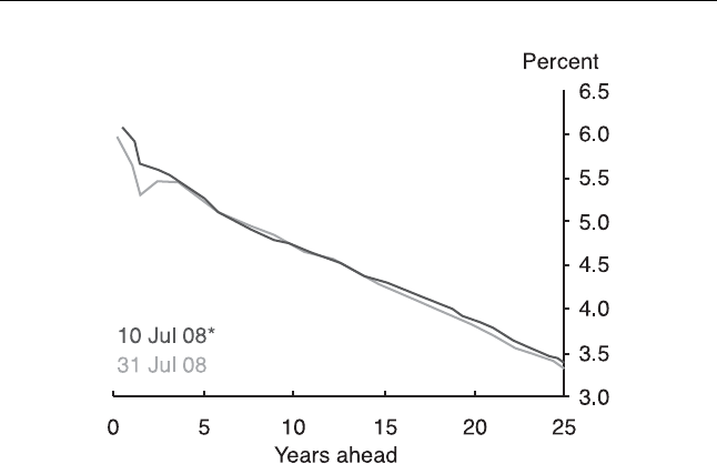
210 Cash Flow Analysis and Forecasting

Figure 13.1 UK instantaneous commercial bank liability forward curve

balance sheet with debt permanently. The debt itself may short-, medium- or long-

term debt. Whether they borrow short or long depends on the state of the interest

rate yield curve. Generally they will seek to source debt as cheaply as possible,

changing the structure of their debt portfolio as the yield curve changes. Whether

the debt is short or long when it is due for repayment it is simply replaced with

new debt. Figure 13.1 shows an example of a yield curve published by the Bank of

England whose components consist of commercial debt priced mainly off LIBOR.

It should be clear from Figure 13.1 that, in July 2008, it was a lot cheaper to

borrow money at a 15 to 20 year duration than it was to borrow short-term.

So, to summarise, large corporates generally have permanent debt. They do not

repay as such, rather rolling over debt that is due into some new form of debt.

This means they generally only need to have sufﬁcient cash available to satisfy

ﬁnance providers to service interest and dividends. Remember for large corporates

the dividend is as important to the directors as interest, any reduction or failure

to pay dividends would have an immediate adverse effect on the share price of

the quoted equity. As we saw when discussing what happens to large, mature

businesses when they fail to generates sufﬁcient cash, if businesses of this size run

into cash ﬂow problems they will usually borrow in the early stages rather than

cut or eliminate the dividend.

Unless their leverage has increased beyond what could be considered normal

they don’t actually make repayment as such, when debt is due for repayment they

simply roll it over into a new debt instrument. The exception to this is when they

make a large acquisition or other investment which takes their debt above what

Cash Flow Analysis and Credit Risk 211

would be considered normal leverage for a business of this type, then the business

will need sufﬁcient cash ﬂows to reduce the debt, in addition to achieving interest

and dividend service.

Smaller Businesses

These businesses are usually private companies, they may also be public companies

listed on junior stock markets around the world. Unless they are very large, most

private companies seeking debt ﬁnance must obtain it from commercial banks in

the form of overdraft facilities, factoring, leasing, loans, mortgages, and so on.

From a credit risk analysis perspective, the key difference between small and large

corporates is that they may not be able to roll over debt whenever they wish if

the supply of credit is restricted or liquidity has disappeared from the lending

market, a scenario that arises quite regularly, usually due to economic recession.

This means they must be able to make both interest and repayment of principal as

required, even when the cash ﬂows are stressed. For smaller businesses repayment

of principle is compulsory, rather than optional, even in a recession, if they wish

to avoid bankruptcy. Conversely, smaller companies rarely need to pay dividends

if they do not wish to do so. For them, the dividend is optional. This means they

only need to have sufﬁcient cash available to satisfy ﬁnance providers to service

interest and debt principal repayment due.

Medium-Sized Corporates

Mid corporates are larger private companies and smaller public companies. Mid

corporates are in the worst situation, they are also obliged to raise most if not all of

their ﬁnance from commercial banks. This means they are in the same position as

smaller private companies when it comes to debt repayment. If they are listed they

may also need to regard their dividend payments as obligatory, or risk a substantial

fall in stock price. This means they need to have sufﬁcient cash available to satisfy

ﬁnance providers to service interest, dividends and debt principal repayment.

COVENANTING AND CASH FLOWS

For centuries it has been usual practice for lenders to restrict the use to which

money lent to borrowers is put using a variety of methods. This represents a

form of risk reduction for the lender. A good example of this is acquiring prop-

erty using a mortgage. The borrower of a mortgage typically never actually has

possession of the money they have borrowed. The advance typically going, via

a lawyer or notary, directly to the seller of the property concerned at the time

the borrower acquires it. This practice occurs because the provider of funds does

not wish to allow the borrower the opportunity to use the funds for any other

212 Cash Flow Analysis and Forecasting

purpose. It is a restriction on the use of the funds, designed to avoid the risk of

misappropriation.

Covenants are another form of restriction negotiated between the lender and

the borrower. They are legally binding undertakings to do, or not do certain things

whilst the loan remains outstanding. Amongst other things, they usually restrict

the rights of the managers of the business to do things that reduce the resources

available to service and repay the loan. Restrictions on things such as dividends,

employee loans, Capex, asset disposals, acquisitions, share repurchase, bonuses

and new debt are typical.

When a borrower breaches a covenant this typically gives the lender the right

to demand immediate repayment of all outstanding debt. Usually the borrower

will not be able to do this (as they cannot easily replace the debt when their

business is deteriorating), and they cannot immediately repay it from cash ﬂow.

So the economic effect of such a covenant is to transfer control of the business

to the borrower who can then demand whatever outcome they prefer (change of

management, restructuring, disposal of the business or bankruptcy).

Financial covenants are one type of covenant. They typically place a limit on the

relationship between two values taken from the published ﬁnancial information

of the borrower. Typically, ﬁnancial covenants seek to deﬁne that the borrower

maintains, throughout the period of the loan:

1. A certain minimum net worth in the business.

2. A minimum working capital in the business.

3. A limit on the total leverage of the business.

4. A minimum interest cover.

5. A minimum debt service cover.

Research into the precise covenants adopted by individual lenders reveals a wide

variation in the minutiae of deﬁning the covenant. They are often described in loan

documentation in terms of balance sheet and proﬁt and loss account values. The

ﬁrst two ﬁnancial covenants above are typically deﬁned by reference to values

taken from the balance sheets. As this book is about cash ﬂow, I only wish to

examine and comment on those matters within covenanting that are related to

cash ﬂows. Generally, this is the last three items above.

Leverage Covenants

Generally, leverage covenants are also couched in terms of balance sheet values

such as debt to net worth or tangible net worth. Sometimes leverage covenants are

related to cash ﬂow proxies such as debt to EBITDA. The use of EBITDA in this

way requires signiﬁcant further examination and explanation.

Cash Flow Analysis and Credit Risk 213

Traditionally, EBITDA had no proﬁle as a measure of anything until the 1980s.

Two things brought EBITDA to prominence, the emergence of the leveraged

buyout and the dot-com boom.

EBITDA and the Leveraged Buyout

Due to the massive leverage typically mobilised in a leveraged buyout the business

may have little or no positive equity and no proﬁts after interest service, accordingly

leverage ratios based on traditional approaches are of little use. Lenders, looking

for an alternative, which would be meaningful when lending 100% debt to a

business entity, identiﬁed EBITDA as a value against which they thought they

could meaningfully covenant.

EBITDA and the dot-com Boom

The dot.com boom spawned many new technology businesses, typically focused

around the emergence of the internet, who had no meaningful earnings in their

formative phase. In the terms I offered earlier in Chapter 9 they represented ‘Start-

up Projects’. Net income, earnings after tax, earnings before tax and earning

before interest and tax and EBITDA were all negative. EBITDA was seen as the

ﬁrst earnings value that went positive when a business approached cash break-

even. EBITDA was then seized upon as a proxy for value creation by those venture

capitalists who were buying and selling these businesses, who then used EBITDA

multiples as a way of expressing their view of the value of an entity. This method of

deriving a value becoming common despite the fact these business were typically

still loss making start-up projects who had not yet established they had a viable

business to exploit. When the dot-com bubble collapsed it became clear that most

would never achieve viability.

Thirdly, lenders, and to a certain extent their lawyers, are traditionally conser-

vative. They have traditionally expressed covenants in terms of balance sheet and

proﬁt and loss account values, even when they are seeking to apply a covenant

in terms of cash ﬂow. As I said earlier, EBITDA is seen as a cash ﬂow proxy.

It is seen as a substitute, derived from the P&L, for the OPERATING CASH

MARGIN value from Jury’s Template. In a published cash ﬂow statement the

equivalent value is assumed to be the cash from operations value (excluding in-

terest and taxes) before working asset investment. Typically the value of EBITDA

will be similar to the OPERATING CASH MARGIN, however, they are not the

same! A review of a published cash ﬂow statement reveals many other items that

are added back to EBIT in addition to depreciation and amortisation in order to

arrive at the OPERATING CASH MARGIN. These items have been covered in

detail in the earlier chapters of this book.

214 Cash Flow Analysis and Forecasting

I have explained earlier that debt is serviced and repaid from cash ﬂows, not

proﬁt. It follows that covenants should ideally follow this logic, and be deﬁned in

cash ﬂow terms. By deﬁning covenants in EBITDA terms the covenant may fail

to achieve the intended outcome.

By covenanting the relationship between total debt and the OPERATING CASH

MARGIN, we are essentially creating another form of debt service covenant; it

is labelled as a leverage covenant because one of the elements is total debt or net

debt. However, it triggers more like a debt service covenant.

Interest Service Covenants

Before we had cash ﬂow statements in accounts, the traditional way of covenanting

interest service was the interest cover ratio. This was the relationship between

operating proﬁt (EBIT) and the interest payable, expressed as a multiple of the

interest payable. For example the interest cover ratio might be set at 3.5 times.

This means that the EBIT should never be less than 3.5 times the interest payable

in a particular period.

Following the development of cash ﬂow statements it was common to see two

kinds of interest cover ratios in loan documents. The ﬁrst one is to covenant

OPERATING CASH MARGIN to interest paid as a multiple. This is the cash ﬂow

equivalent of the P&L derived interest cover ratio.

The second is to covenant the CASH AVAILABLE TO SATISFY FINANCE

PROVIDERS value from the template as a multiple of interest paid/(due) in a

period. As should be clear from previous chapters this value does represent the

cash available for debt service, so this is probably the most meaningful value

against which to covenant.

Debt Service Covenants

Debt service covenants are similar to interest service covenants; the only differ-

ence is that, instead of covenanting a multiple of interest service, we also bring

in any principal repayment due. So, the relationship covenanted as a multiple is

the relationship between OPERATING CASH MARGIN or the CASH AVAIL-

ABLE TO SATISFY FINANCE PROVIDERS and the sum of interest service and

principal debt repayment due in the period.

CONCLUSION

Debt is serviced and repaid from cash ﬂow, not proﬁt. It follows that lenders and

credit functions should be cash ﬂow centric rather than P&L centric in performing

analysis of the creditworthiness of existing and potential borrowers, and other

counterparties.

Cash Flow Analysis and

Performance Measurement

This part of the book is intended for entrepreneurs, managers, investors and others

who are interested in using cash ﬂow information to assess or monitor the viability,

health or performance of a business.

Before reading this chapter it is assumed that the reader has read and digested

most of the earlier chapters on summarising and evaluating cash ﬂows in Jury’s

Cash Flow Template format.

HOW CAN WE USE CASH FLOW INFORMATION?

Those who are interested in analysing business performance can use the data

contained within Jury’s Cash Flow Template in a variety of ways.

When buying or valuing a business we can think of the valuation as being in

two parts.

1. The value of the present (largely derived from the existing surplus cash ﬂow

generated).

2. The value of the future, which can be considered as the present value of the

potential growth of the future surplus cash ﬂows of the business.

The template provides an elegant way of summarising the existing performance

of the business. A review of the historic cash ﬂow patterns in the template will

reveal the extent and cyclicality of the ability of a business to generate cash

surpluses for investors. I recommend that analysts prepare a spreadsheet with

sufﬁcient history in it to see the business through a full economic cycle. Given the

recent pattern of global economic behavior it may be appropriate to go back up to

twelve years in order to achieve this.

Analysis of the historic cash ﬂow performance will also reveal the past relation-

ships between growth and investment in working assets and ﬁxed assets, so acting

as a reasonableness check on any assumptions made about future performance.

The second issue all business controllers face is the need to monitor and control

the businesses in which they are interested. Again, the cash ﬂow template can

be used as a primary indicator of performance. As a controller I should be able

to target a particular level of operating cash margin, usually from some sort of

Cash Flow Analysis and Forecasting: The Definitive Guide to

Understanding and Using Published Cash Flow Data

by Timothy D.H. Jury

216 Cash Flow Analysis and Forecasting

budgetary, planning or forecasting process. This in turn will imply a given level

of working asset investment, and capital investment. All these values can then be

forecasted and targeted.

This target can then be used to compare with weekly, monthly or quarterly

performance. Each major component of the template can be broken down as

required to reveal more information about performance as required.

The other beneﬁt of using the template as a primary reporting tool is that

managers become more aware of the cash ﬂow implications of changes in the way

the business operates. For example, step changes in volume output of the business

will have working asset and possibly capex effects, which are, to a certain extent,

predictable.

WHAT IS SUCCESS IN BUSINESS?

In order to identify what cash ﬂow measures we are going to seek to focus on we

need to discuss what constitutes success in business. We are seeking to identify

concise, elegant measures that can be used for performance assessment.

In the earlier chapters I brieﬂy discussed what success is – ﬁrstly discounting

proﬁts or growth as measures on their own because they fail to take account of

the amount of capital expended to get the particular level of proﬁts or growth

achieved.

I also indicated that the current thinking was that the best measure of success

is to look at the increase in the value of a business period on period. Unfortu-

nately, the value of a business is not only inﬂuenced by its ability to generate

cash surpluses both now and in the future, but also by external factors such as

economic conditions, the availability of ﬁnance, fashion trends in investment and

technological and social change.

So, we need to try to identify a measure that we can use which is generated

from the internal data available in a business. Of all the possible ratios to consider,

the most appropriate is probably return on investment. What do we mean by this?

Investment is the cash invested in the business; return is the excess cash gener-

ated over the economic cost of the cash invested in the business. Applying even

this apparently simple measure is not straightforward because the cost of equity is

difﬁcult to estimate with any reliability. It is generally assumed to be higher than

the cost of debt, because the future expected returns from the equity are assumed

to be more risky than the returns to debt.

Technically we should be using both the opportunity cost of debt and the

opportunity cost of equity in arriving at the cost of capital. The concept is as

follows: as an investor in, or owner of, a business I expect to receive on my

investment a return at least as good as I could get investing in other investments

of similar risk. Analysts generally use historic returns data from stock markets to

estimate what these values might be for debt and for equity and combine them

Cash Flow Analysis and Performance Measurement 217

into a single percentage expected return estimate which is typically known as the

weighted average cost of capital.

This value is speciﬁc to the business to which it relates because it contains

various assumptions unique to that business. These are: an assumption about the

long term leverage of the business; an assumption of the extra return required

on all equity relative to debt; and an adjustment for the relative riskiness of the

particular sector in which the business operates relative to the overall market. Once

we have identiﬁed this value we can apply it to the amount invested in the business

to come up with the expected periodic cash generation required to compensate

investors. This can then be compared with the actual Cash Available to Satisfy

Finance Providers total as a value and a percentage.

CASH FLOWS AND INVESTMENT

Investors are another class of stakeholder who may see beneﬁts from understanding

the cash ﬂows of businesses they invest in. Investors in quoted equity face many

problems. The easiest way to comprehend this is to use the concept of the perfect

investment.

What is the Perfect Investment?

A little thought should yield the following insights. The perfect investment would

yield massive returns, be growing strongly and have negligible business risk! This

is essentially the holy grail of investing.

Whilst, occasionally, companies appear that ﬁt this proﬁle for a period, they are

the rare exception rather than the norm. Generally companies cannot be all three

things at the same time. If a company is growing strongly and yielding good returns

it is probably in a growth market where there are signiﬁcant business risks to do

with technology, adoption and competitor behaviour. Companies facing negligible

business risk are usually in mature, low margin sectors such as utilities and food

retail.

Going back to our perfect investment we could also add that the investor ide-

ally wants to identify such an investment in ﬁve minutes! Investors have further

problems to do with the overwhelming amount of information they have to in-

terface with in order to pick a share, in the form of regulatory announcements

and ﬁlings, annual and periodic reports, prospectuses, news, databases, analysts

recommendations, comparative analysis and so on.

As a consequence they seek shortcuts. They seek to identify measures of perfor-

mance that appear simple and are convenient to use. Examples of this are measures

such as Earnings per Share and Dividend Yield, both of these being derived from

the proﬁt and loss account.

218 Cash Flow Analysis and Forecasting

They also need to consider the affordability of a share or stock. Is too expensive

or cheap, given the existing and future prospects of the business? Investors use

measures such as the Price Earnings ratio (PE ratio) and Tobin’s Q ratio (which

seeks to capture the relationship between the market value of a business and the

replacement value of the same business, which is assumed to be similar to the

book value).

All of these measures are vulnerable to manipulation or abuse. This was ex-

plained in detail in Chapter 12 – Cash versus Proﬁt. Cash ﬂow data compared to

the number of shares and share price may represent better, less biased, indicators

of current performance and the relative affordability of a share.

For example, from an investor viewpoint, the two most important values from

the template are probably the OPERATING CASH MARGIN and the CASH

AVAILABLE TO SATISFY FINANCE PROVIDERS values. Why is this?

The OPERATING CASH MARGIN is the cash generated from going round

the working asset cycle. It represents the difference between the cash costs of

producing the product or service and the resulting cash revenue when it is sold.

It is the reason the business exists. In a successful mature business it pays for all

the necessary cash outﬂows below it in the template. Loosely it can be considered

to be the cash ﬂow equivalent of operating proﬁt (EBIT). It is the most important

number in the template because, in the long run, it pays for everything else. In

other words, the perfect business (or investment) is one that generates massive

(and ideally, growing) OPERATING CASH MARGIN.

The CASH AVAILABLE TO SATISFY FINANCE PROVIDERS is also im-

portant because it represents the residual cash ﬂow available to reward investors.

As I mentioned earlier this doesn’t mean that investors actually receive any or all

of it.

As a measure it is similar to Earnings per share in nature, which identiﬁes

the value of the earnings after tax, minority share interests and preference share

dividends attributable to each ordinary share in the business. This doesn’t signify

that the shareholder receives their earnings per share as, for example, a dividend.

Earnings per share represents how much of the earnings of the business each share

notionally ‘owns’.

The CASH AVAILABLE TO SATISFY FINANCE PROVIDERS is similar in

concept to another term used by analysts, the enterprise cash ﬂow. This means the

cash ﬂow generated by the enterprise, before we consider how this is split between

the debt and equity investors. Bear in mind that the enterprise cash ﬂow is the

cash ﬂow of the entity when debt free. This is important because, as interest is

tax deductible, the taxation actually paid by the business varies depending on the

amount of debt carried by the entity. So, the CASH AVAILABLE TO SATISFY

FINANCE PROVIDERS is not the same as the enterprise cash ﬂow.

Both of these values can be compared with the capital invested in the busi-

ness, the market capitalisation of the equity and the total debt outstanding, or be

Table 14.1 Six years of cash ﬂow based returns data for Nokia

Nokia

TEMPLATE SUMMARY CASH FLOWS 20X8 20X7 20X6 20X5 20X4 20X3

Years to 31st December €m€m€m€m€m€m

Operating cash margin 7457 8474 6163 5390 5193 6545

Change in NWA −2546 605 −793 −366 299 −194

Net Capex −966 −800 −748 −593 −643 −631

Cash taxes −1780 −1457 −1163 −1254 −1368 −1440

CASH FLOW AVAILABLE TO 2165 6822 3459 3177 3481 4280

SATISFY CAPITAL PROVIDERS

Net interest 66 260 271 374 219 341

Net dividends −2042 −1748 −1553 −1530 −1391 −1354

CASH FLOW AVAILABLE AFTER 189 5334 2177 2021 2309 3267

INTEREST AND DIVIDENDS

Debt none none none none none none

Equity invested (Share cap & share premium) 3994 4189 2953 2724 2552 2560

Number of shares at the year-end millions 3697 3846 3966 4172 4593 4761

Share price on or near 31st Dec in euros 11.5 26.42 15.51 15.45 11.4 13.75

Market capitalisation (millions) 42 516 101 611 61 513 64 457 52 360 65 464

Cash ﬂow return on capital invested 54% 163% 117% 117% 136% 167%

(CATS Fin Pro/Equity Invested %)

Cash ﬂow return on market capital invested 5% 7% 6% 5% 7% 7%

(CATS Fin Pro/Mkt Cap %)

Table 14.2 Six years of cash ﬂow based returns data for Dairy Crest

DAIRY CREST PLC 20X8 20X7 20X6 20X5 20X4 20X3

TEMPLATE SUMMARY CASH FLOWS £m £m £m £m £m £m

Operating cash margin 115.8 97 89.7 122.4 126.4 111

Change in NWA −7.4 −2.8 −16.3 20.6 10.2 −6.1

Net Capex −20.8 −26.6 −34.6 −29.5 −29.7 −27

Cash taxes −6.7 −6.1 −15.5 −12.6 −8.7 −4.1

CASH FLOW AVAILABLE TO SATISFY

CAPITAL PROVIDERS (CATS Fin Pro)

80.9 61.5 23.3 100.9 98.2 73.8

Net interest −30.7 −15.3 −16.4 −17.7 −20.6 −22

Net dividends −23.5 −18.8 −16.6 −23.9 −19.9 −17.4

CASH FLOW AVAILABLE AFTER

INTEREST AND DIVIDENDS

26.7 27.4 −9.7 59.3 57.7 34.4

Net debt 474.8 444.9 280.5 227.5 279.7 345.2

Equity invested (Share capital & share

premium)

103.5 99.8 60.1 59.4 55.8 55.2

Number of shares at the year-end millions 132.3 127.2 124.8 123.4 122.6 120.7

Share price on or near 31st March in pence 478.75 666.5 477 485 394.5 330.83

Market capitalisation (millions) 633.39 847.79 595.3 598.49 483.66 399.31

Cash ﬂow return on capital invested (CATS Fin

Pro/Equity Invested +Net Debt %)

14% 11% 7% 35% 29% 18%

Cash ﬂow return on market capital invested

(CATS Fin Pro/Mkt Cap +Net Debt %)

7% 5% 3% 12% 13% 10%

Cash ﬂow return on equity invested (CATS Fin

Pro- Net Interest/Equity invested %)

49% 46% 11% 140% 139% 94%

Cash ﬂow return on market capitalisation (CATS

Fin Pro- Net Interest/Mkt Cap %)

8% 5% 1% 14% 16% 13%

Cash Flow Analysis and Performance Measurement 221

considered before or after debt service as a per share value by dividing the totals

by the number of shares in issue.

Bear in mind that whether a business is growth or mature has a huge impact

on what we expect to see. For the reasons explained earlier in the chapters on

growth and mature, due to the fast pace of change, and volume increase, growth

businesses may have little OPERATING CASH MARGIN and negative CASH

AVAILABLE TO SATISFY FINANCE PROVIDERS. Restating their cash ﬂows

on a no-growth basis may be necessary to get a better picture of their underlying

performance.

Table 14.1 shows the cash ﬂows of Nokia with some cash ﬂow to equity ratios

appended. As Nokia has no debt (it runs a huge surplus cash position) I have only

calculated the cash ﬂow return on equity values.

Mature companies are likely to be more amenable to performance measurement

in this way as we expect them to have low investment needs and be cash positive at

both the OPERATING CASH MARGIN value and the CASH AVAILABLE TO

SATISFY FINANCE PROVIDERS value. M&A activity may distort the picture

and need to be adjusted for. The cash ﬂows of Dairy Crest together with a variety

of cash ﬂow based returns ratios are summarised in Table 14.2.

This analysis makes it clear that Dairy Crest has struggled to generate an

adequate performance since making major acquisitions in 2006 and 2007. Further

comparison with a sector peer group would reveal more about whether the current

performance is typical or not.

CONCLUSION

Entrepreneurs, managers and investors will typically have grasped the utility and

value of looking at a business through the application of Jury’s Cash Flow Template

as they have proceeded through the earlier parts of this book. The concepts intro-

duced above are merely suggestions as to how this knowledge might be utilised.

Users can and should tailor the concepts offered to their particular needs.

Analysing Direct Cash

Flow Statements

This chapter explains the nature of direct cash ﬂows, the difference between

indirect and direct cash ﬂows and how to analyse them into Jury’s Cash Flow

Template.

IAS 7 – Cash Flow Statements – gives preparers the option of reporting cash

ﬂows using the direct method, whereby major classes of gross cash receipts and

gross cash payments are disclosed, or the indirect method.

The standard goes on to say, ‘Entities are encouraged to report cash ﬂows

from operating activities using the direct method. The indirect method provides

information which may be useful in estimating future cash ﬂows and which is not

available under the indirect method.’ Later on in the chapter we will see whether

this advice is acted upon.

Direct cash ﬂows are rare, I have never yet seen an example from the UK, US,

Germany or France and indeed many other countries, all of which seem to prefer

to use the indirect method for preparing cash ﬂow statements.

When they do appear in the published accounts of large businesses it is usually

because the local GAAP used to prefer it or required it, and this habit has been

continued when IAS GAAP was adopted. So the same information forms the

published cash ﬂow statement for the annual report and any ﬁlings required for

US listings such as the form 20-F for overseas ﬁlers.

Both of the examples used in this chapter are Portuguese listed companies, as

Portuguese companies generally continue to offer direct cash ﬂow statements in

their annual reports.

Unicer – Bebidas de Portugal, SGPS, S.A. is Portugal’s largest beverages com-

pany. Its core business is beers and bottled spring waters. Unicer trades in seg-

ments that also include juice and soft drinks, wines, coffee, production and sale

of malt and hotel management. The Unicer cash ﬂow statement is reproduced in

Table 15.1.

Cash Flow Analysis and Forecasting: The Definitive Guide to

Understanding and Using Published Cash Flow Data

by Timothy D.H. Jury

224 Cash Flow Analysis and Forecasting

Table 15.1 Unicer direct cash ﬂow statement

CONSOLIDATED FINANCIAL STATEMENTS

ANNUAL REPORT AND ACCOUNTS 2006

UNICER – Bebidas de Portugal, SGPS, S.A.

Notes 20X6 20X5

CASH FLOW FROM OPERATING

ACTIVITIES

Receipts from customers 465.732.523 445.548.238

Payments to suppliers & employees (344.379.427) (310.043.874)

NET CASH FROM OPERATING

ACTIVITIES

121.353.096 135.504.364

Interest paid

Income tax paid 4.229.044 (3.501.577)

Other receipts/payments from operating

activity

(44.278.973) (62.233.978)

Net cash from operating activities 81.303.167 69.768.809

CASH FLOWS FROM INVESTING

ACTIVITIES

Purchase of tangible ﬁxed assets (32.794.582) (33.806.897)

Tangible ﬁxed assets 759.626 1.510.380

Purchase of intangible assets (4.093.855) (2.516.414)

Financial Investments (114.412)

Subsidies received 522.773 700.627

Interest received 4.297

Net cash used in investing activities (35.606.038) (34.222.419)

CASH FLOWS FROM FINANCING

ACTIVITIES

Bank loans payments (4.489.304)

Interest and similar costs paid (9.207.578) (8.010.690)

Proceeds from bank loans 1.063.843 2.230.761

Dividends paid – Equity holders (31.500.000) (31.500.000)

Dividends paid – Minority interest (270.651)

Net cash from ﬁnancing activities (44.403.690) (37.279.929)

(Decrease)/increase in cash and cash

equivalents

1.293.439 (1.733.539)

Cash and cash equivalents, beginning of year 1.865.362 3.598.901

Effects of exchange rate changes

Cash and cash equivalents, end of year 28 3.158.801 1.865.3

Analysing Direct Cash Flow Statements 225

Table 15.2 Comparison of cash from customers to turnover for Unicer

UNICER

Amounts expressed in €20X6 20X5

Receipts from customers 465 732 523 445 548 238

Sales and services rendered 479 758 364 442 960 881

Difference −14 025 841 2 587 357

WHAT IS DIFFERENT ABOUT A DIRECT CASH

FLOW STATEMENT?

A careful examination of the cash ﬂow statement (Table 15.1) will reveal that it

is the section cash ﬂow from operating activities that is different to a cash ﬂow

prepared using the indirect method. The other sections are typically the same as

would be disclosed in an indirect cash ﬂow statement.

Instead of starting with a proﬁt value the direct cash ﬂow statement starts with

receipts from customers and payments to suppliers and employees. This represents

exactly what it says it does. However, the receipts from customers is not the same

as turnover. Why is this? Let us compare the two values (Table 15.2).

The receipts from customers represents the cash received from customers during

the ﬁnancial year. It does not represent the amounts billed to customers. In other

words it encompasses both the turnover billed and the change in the outstanding

receivables. In 2006 the group received €14 025 841 less in cash than it billed.

This implies that trade debtors should have increased by the same amount. Ideally

we would like to reconcile this to the movement in trade receivables in the balance

sheet. Let us look at this in Table 15.3.

Whilst receivables have increased the value is approximately half of the number

we are looking for. Where then is the rest of the difference? Unfortunately, this is

not clear from the accounts, and, indeed, may never be explained from the other

information available in the annual report. I can seek other values in the balance

Table 15.3 Identifying the change in trade receivables for Unicer

UNICER

Amounts expressed in €

Receivables from customers 20X6 81 809 764

Receivables from customers 20X5 74 194 153

Difference 7 615 611

226 Cash Flow Analysis and Forecasting

sheet that might represent part of the difference such as ‘other receivables’. It is

also possible that movements on liabilities such as ‘deposits received on returnable

packaging in transit’ might constitute part of the movement. Finally the accounts

reveal that loans are made to customers, which are paid off via discounts granted on

sales volumes. This type of arrangement is a common practice amongst brewers,

who will often assist a customer with loans and supply the equipment needed by

the retailer to serve the product in exchange for an exclusive supply arrangement.

This means movements on customer loans may also be involved.

So, it seems we don’t necessarily get more information in a direct cash ﬂow

after all. Indeed in this case we get less information than we would have obtained

from an indirect cash ﬂow statement from the same business. How does this affect

the template?

When the available values are summarised into the template (Table 15.4) we

lose the split between the operating cash margin and the changes in the amounts

invested in the net working assets of the business. In Chapter 8, Growth and

Mature – Further Analysis, I noted that there was much useful information about

management quality that can be implied from the changes in the net working

Table 15.4 Two years summary cash ﬂows for Unicer

UNICER – Bebidas de Portugal, SGPS, S.A.

SUMMARY CASH FLOWS

Amounts expressed in €20X6 20X5

OPERATING CASH MARGIN 77 074 123 73 270 386

(INVESTED)/GENERATED FROM NET

WORKING ASSETS

NET CAPITAL EXPENDITURE −36 128 811 −34 812 931

TAXATION 4 229 044 −3 501 577

CASH FLOW AVAILABLE TO 45 174 356 34 955 878

SATISFY FINANCE PROVIDERS

NET INTEREST −9 207 578 −8 006 393

NET DIVIDENDS −31 770 651 −31 500 000

OTHER NON-OPERATING

INCOME/(EXPENDITURE)

522 773 586 215

NET CASH INFLOW/(OUTFLOW) 4 718 900 −3 964 300

Financed by:

INCREASE/(DECREASE) IN EQUITY

INCREASE/(DECREASE) IN DEBT −3 425 461 2 230 761

(INCREASE)/DECREASE IN CASH −1 293 439 1 733 539

TOTAL CHANGE IN FINANCING −4 718 900 3 964 300

Analysing Direct Cash Flow Statements 227

assets. This information is essential to the analyst and should not be omitted

before attempting to assess the information contained within the template.

One way of dealing with this problem is to extract from the balance sheet what

appear to be the relevant values and ‘reverse engineer’ the change in net working

asset data from this. In order to achieve this I have gone through the notes to the

accounts selecting the values which appear to represent the net working assets of

Unicer. Notice I have excluded all assets and liabilities relating to the ﬁxed assets,

corporate taxation and debt of Unicer as these are not part of the net working

assets. I have also excluded non-cash items such as movements in provisions,

accruals and prepayments. Table 15.5 shows the required data from the balance

sheet of Unicer.

There is much useful information about changes in the business here for the

analyst. Inventories have not moved much at all. Receivables from customers has

increased by about €8 million. This has been offset by a reduction in the amount

due from government of about €10 million, leaving a net change of €2 million

reduction in total receivables. Trade payables have increased by about €9 million

this is offset by modest reductions in other liabilities taking the ﬁnal increase in

creditors to about €6.5 million. The overall net effects on net working assets is

a reduction of about €8 million. In the cash ﬂow template this represents a cash

inﬂow to the business. We can reverse engineer this information into the template

as shown in Table 15.6.

Table 15.5 Identifying the net working asset change values for Unicer

UNICER

Amounts expressed in €

SUMMARY OF CHANGE IN

NET WORKING ASSETS 20X6 20X5 Change

Inventories 26 921 820 26 647 525 −274 295

Receivables from customers 81 809 764 74 194 153 −7 615 611

Other receivables 25 498 523 24 896 153 −602 370

Other assets – government receivables 8 852 406 19 201 043 10 348 637

TOTAL ASSUMED RECEIVABLES 116 160 693 118 291 349 2 130 656

Deposits received on packaging in transit 16 755 114 18 127 286 −1 372 172

Other non-current creditors 1 833 032 2 373 262 −540 230

Trade payables 39 822 122 31 034 865 8 787 257

Other payables 13 796 725 13 675 230 121 495

Other liabilities – government payables 4 590 088 5 060 630 −470 542

TOTAL ASSUMED PAYABLES 76 797 081 70 271 273 6 525 808

TOTAL NET WORKING ASSETS 66 285 432 74 667 601 8 382 169

228 Cash Flow Analysis and Forecasting

Table 15.6 Restated 20X6 cash ﬂows for Unicer

UNICER – Bebidas de Portugal, SGPS, S.A.

SUMMARY CASH FLOWS Original Restated

Amounts expressed in €20X6 20X6

OPERATING CASH MARGIN 77 074 123 68 691 954

(INVESTED)/GENERATED FROM NET

WORKING ASSETS

8 382 169

NET CAPITAL EXPENDITURE −36 128 811 −36 128 811

TAXATION 4 229 044 4 229 044

CASH FLOW AVAILABLE TO 45 174 356 45 174 356

SATISFY FINANCE PROVIDERS

NET INTEREST −9 207 578 −9 207 578

NET DIVIDENDS −31 770 651 −31 770 651

OTHER NON-OPERATING

INCOME/(EXPENDITURE)

522 773 522 773

NET CASH INFLOW/(OUTFLOW) 4 718 900 4 718 900

Financed by:

INCREASE/(DECREASE) IN EQUITY

INCREASE/(DECREASE) IN DEBT −3 425 461 −3 425 461

(INCREASE)/DECREASE IN CASH −1 293 439 −1 293 439

TOTAL CHANGE IN FINANCING −4 718 900 −4 718 900

At this point we have the same level of information in the right hand column

as we would have obtained from an indirect cash ﬂow. However, remember this

is our estimate of the change in net working assets, derived from selected balance

sheet data. It should be viewed as approximate rather than exact.

Table 15.7 shows another example of the operating cash ﬂow section of a direct

cash ﬂow taken from the form 20-F of Portugal Telecom.

Again, with the direct cash ﬂow of Portugal Telecom we have the same problem,

whilst there is a little more analysis of the various elements of the operating cash

ﬂows, we still do not get any disclosure of the movements in the net working

assets.

CONCLUSIONS ABOUT DIRECT CASH FLOWS

The direct cash ﬂow discloses more information about the cash inﬂows and out-

ﬂows that generate the operating cash ﬂow of the business than an indirect cash

ﬂow. However, in doing so, the disclosures found in an indirect cash ﬂow relating

Table 15.7 Three years cash ﬂow data for Portugal Telecom

PORTUGAL TELECOM, SGPS, SA

CONSOLIDATED STATEMENT OF CASH FLOWS

FOR THE YEARS ENDED 31 DECEMBER 20X7 AND 20X6

(Amounts stated in Euro)

Notes 20X7 20X6 20X5

OPERATING ACTIVITIES

Collections from clients 7 070 397 265 6 763 769 410 6 503 131 136

Payments to suppliers (3 653 519 418) (3 277 388 237) (3 411 857 036)

Payments to employees (654 757 374) (653 682 324) (625 591 295)

Payments relating to income taxes 44.a (206 528 920) (51 626 295) (67 361 504)

Payments relating to post retirement beneﬁts 9.4 (284 159 570) (580 789 898) (699 806 967)

Payments relating to indirect taxes and other 44.b (610 407 039) (572 755 719) (534 931 734)

Cash ﬂow from operating activities from continued operations 1 661 024 944 1 627 526 937 1 163 582 600

Cash ﬂow from operating activities from discontinued operations 20 198 182 708 194 134 513 228 717 368

Cash ﬂow from operating activities(1) 1 859 207 652 1 821 661 450 1 392 299 968

230 Cash Flow Analysis and Forecasting

to changes in the amounts invested in net working assets are lost. This data can be

estimated by extracting the changes in the various net working asset values from

the balance sheet and adjusting the operating cash ﬂow value accordingly.

Other than this the content of the rest of a direct cash ﬂow is essentially the

same as an indirect cash ﬂow. The restatement and analysis of these values into

the template being the same process as for an indirect cash ﬂow statement.

Generating a Cash Flow Summary

from Proﬁt and Loss Account and

Balance Sheet Data

This chapter deals with the process of estimating cash ﬂow information from proﬁt

and loss account (P&L) and balance sheet data.

Before reading this chapter it is essential that the reader has read and digested

the earlier chapters on summarising and evaluating cash ﬂows in Jury’s Cash Flow

Template format. Virtually all of the terminology used in this chapter has been

introduced and explained earlier in the book.

THE NATURE OF THE PROBLEM

There are a variety of risk management scenarios where there may be a desire

on the part of the analyst or a counterparty to identify and assess the cash ﬂow

performance of a business that does not publish a cash ﬂow statement. Those

involved in credit-based transactions and those who are considering the purchase

of a business are two examples.

Small- and medium-sized businesses in the UK are not required to publish cash

ﬂow statements when they ﬁle accounts. This concession to smaller businesses is

common in other parts of the world. Business performance information is typically

presented to an analyst or other interested parties in the form of a proﬁt and

loss account (P&L) and balance sheet. Secondly, much management information,

particularly in product-based companies is focused around P&L and balance sheet

information.

So, if we wish to examine an entities cash ﬂow performance, what can we do

about this problem?

Earlier in the book we found out that cash ﬂow statements can be prepared

using two possible methods, the direct method and the indirect method. The

indirect method derives the cash ﬂow statement from P&L and balance sheet data.

It follows that it should be possible for an analyst to do the same in the absence of

a published cash ﬂow statement and, indeed, it is!

Cash Flow Analysis and Forecasting: The Definitive Guide to

Understanding and Using Published Cash Flow Data

by Timothy D.H. Jury

232 Cash Flow Analysis and Forecasting

Before we examine the process, it is important to understand the limitations of

assembling the estimated cash ﬂow information in this way. What we will end up

with is typically not identical to the equivalent published cash ﬂow statement. It

will be an approximation of the true cash ﬂow performance. Typically, the numbers

we end up with are likely to be within, say, 10% of the actual cash ﬂow values,

indeed, they may be considerably more accurate than this.

Why do these differences arise?

Accruals and Prepayments

The values disclosed in the P&L and balance sheet are adjusted for items that

have been used or consumed but not invoiced or paid for (accruals) and items

that have been paid for in advance but not fully consumed (prepayments). These

adjustments do not represent cash ﬂows and should be reversed. This concept has

already been explained in detail in Chapter 12 – Cash Versus Proﬁt as a Measure

of Performance.

It is not usually possible to adjust for these individually because there is typically

no disclosure of them individually. However, in situations where the business is

operating normally this should not distort the resulting cash ﬂow estimation too

much because the same process of identifying and adjusting for accruals and

prepayments occurred at the beginning of the ﬁnancial period. In other words

when we use an income or expense value from the P&L for cash ﬂow estimation

purposes, we are not using the actual cash ﬂow received or paid in the period (of

say 12 months), we are using a value that represents the 12 months actual physical

sales or cost consumed. Both relate to 12 months of income or expense, however,

the cash received or paid typically lags the values reported in the P&L by the

credit period granted or received from customers and suppliers.

Lack of Disclosure

When we studied the detailed restatement of the operating cash ﬂow of a business

in Chapter 4 we discovered a whole variety of adjustments that might be required

to restate the operating proﬁt (EBIT) value (or other proﬁt value starting point),

to reﬂect the corresponding OPERATING CASH MARGIN. Typically, some of

these adjustments will not be disclosed when working from P&L and balance

sheet data. Therefore, we won’t be aware of them and, as a result, they will be

absent from our ﬁnal estimates.

The most signiﬁcant adjustment to proﬁt is typically depreciation/amortisation;

this is usually disclosed in the P&L and or balance sheet. We may also have

disclosure of the proﬁt/loss on disposal of ﬁxed assets in the notes to the P&L. We

are unlikely to have detailed information disclosed about movements in provisions

and other non-cash items. Ideally, we should have all these in order to correctly

arrive at the OPERATING CASH MARGIN.

Generating a Cash Flow Summary from Proﬁt and Loss Account 233

Changes in the Composition of a Group

If we are seeking to identify the cash ﬂows of a group, and the group has acquired

or disposed of subsidiaries during the year, the changes identiﬁed from the balance

sheet for both working assets and ﬁxed assets are unlikely to match the values that

would be revealed were there a cash ﬂow statement available. To illustrate why

this might be the case consider inventory. If I acquire a business during the year

with holdings of inventory this will be measured and consolidated at the period

end, however the opening inventory of the acquisition will not be in the opening

balance sheet inventory value. If we are aware of this problem we can attempt to

adjust for it if there is sufﬁcient disclosure. Usually this is not the case.

SO, IS AN ESTIMATED CASH FLOW SUMMARY USEFUL?

Does this mean there is no value in trying to create a summary of cash ﬂows from

P&L and balance sheet data? I believe the process is still meaningful, because of

the concept of materiality. If we identify the signiﬁcant values approximating to

the actual cash ﬂow values we will still obtain a useful impression of the overall

cash ﬂow performance of the entity under examination. It is not necessary for our

cash ﬂow values to absolutely correct for us to gain beneﬁcial insights about the

cash ﬂow performance of the entities.

So, what is the process?

Rather than attempting to reconstruct a complete cash ﬂow statement in ac-

cordance with IAS GAAP the recommended approach is to come up with a best

estimate of the cash ﬂow values that appear in each line of Jury’s Cash Flow

Template. This requires far less knowledge of double entry bookkeeping and the

preparation of statutory accounts than would be required to attempt to complete a

statutory cash ﬂow statement. Let us now examine each line of the template and

discuss how best to identify the appropriate values for each line (Table 16.1).

The contents of each line of the template have already been explained in detail

in Chapters 1, 2 and 4. I do not intend to repeat that material here. It is assumed

that readers have already familiarised themselves with this material. I will simply

summarise what each line of the template represents before explaining the various

methods for developing a best estimate from the P&L and balance sheet data.

Readers should revisit the earlier chapters if they are unfamiliar with any of the

terms or methods mentioned.

1. OPERATING CASH MARGIN

The operating cash margin in the template represents the cash received from selling

goods and services less the cash costs of producing them. In a cash ﬂow statement

prepared using the indirect method this value is derived by taking a proﬁt value

234 Cash Flow Analysis and Forecasting

Table 16.1 Labelling the content of the template

DATA LINE JURY’S CASH FLOW TEMPLATE

NUMBER SUMMARY CASH FLOW HEADINGS

1OPERATING CASH MARGIN

2(INVESTED)/GENERATED FROM NET WORKING

ASSETS

3NET CAPITAL EXPENDITURE

4TAXATION

Sub-total CASH FLOW AVAILABLE TO SATISFY FINANCE

PROVIDERS

5NET INTEREST

6NET DIVIDENDS

7OTHER NON-OPERATING INCOME/(EXPENDITURE)

Balancing total NET CASH IN/(OUT) BEFORE FINANCING

Financed by:

8CHANGE IN EQUITY INCREASE/(DECREASE)

9CHANGE IN DEBT INCREASE/(DECREASE)

10 CHANGE IN CASH (INCREASE)/DECREASE

Balancing total TOTAL CHANGE IN FINANCING

from the P&L, adjusting it for non-cash income or expense items and removing

any other income or expense recognised as proﬁt or loss which does not relate to

operations.

The ﬁrst quick crude estimate of the OPERATING CASH MARGIN is EBITDA

(earnings before interest, tax, depreciation and amortisation). In the simplest

situation, where there are no other adjustments for non-cash items, EBITDA is

the OPERATING CASH MARGIN. When there are a number of adjustments

disclosed, the add-back of depreciation and amortisation is usually by far the

largest item adjusted for.

Typically there will also be a value disclosed in the notes to the P&L for the

proﬁt and loss on the disposal of ﬁxed assets. This also represents a non-cash

adjustment to depreciation and should also be used to adjust the starting EBIT

value. Be careful to get the signage right when adding back or deducting the value.

In some situations there may also be some disclosure of movements in provisions

in the notes to the accounts (this may be also deduced indirectly by looking at

the changes in any operating provisions disclosed separately in the opening and

closing balance sheet). If there is adequate disclosure of movements in operating

provisions the EBIT value can also be adjusted for these items.

Generating a Cash Flow Summary from Proﬁt and Loss Account 235

These are typically the main items. If there is any other disclosure of items

relevant to the estimation of the OPERATING CASH MARGIN then they can

also be adjusted for to further improve the quality of the resulting estimate.

2. (INVESTED)/GENERATED FROM NET WORKING ASSETS

The amount invested or generated from net working assets in the template repre-

sents the sum of the change during the reporting period in the amounts invested in

inventory, debtors (receivables) and creditors (payables).

The usual way of determining this value is to take the opening and closing

values for the three items from the opening and closing balance sheet and identify

the differences. An illustration of this is shown in Table 16.2.

Table 16.2 Identiﬁcation of the change in net working assets for Tesco

TESCO PLC 20X8 20X7 Change

SUMMARY OF NET WORKING ASSET CHANGE £m £m £m

Increase in inventories 2430 1931 −499

Increase in trade and other receivables 1311 1079 −232

Increase in trade payables & other payables −7177 −6046 1131

Totals −3436 −3036 400

When working out the change value be careful to get the signage right. For

example, an increase in inventories is a cash outﬂow (we have to expend cash in

order to increase the number of boxes in our warehouse). An increase in debtors is

also a cash outﬂow (we are lending more money to our customers). Conversely an

increase in creditors is a cash inﬂow (our suppliers are lending more money to us).

There is sometimes difﬁculty in deciding which elements of current assets,

current liabilities and non-current liabilities represent working asset values. Let

us consider each in turn.

Current Assets

•Inventories. This value may be disclosed as one number; alternatively it may be

shown as raw materials, work-in-progress and ﬁnished goods.

•Debtors and prepayments. This is the value we would typically take for working

assets, this may be disclosed separately as trade debtors, other debtors and

prepayments. Other debtors relating to asset or business disposal should be

excluded from the working asset calculation.

•Other current assets such as cash and cash equivalents, pension fund surpluses,

and items relating to investments (equity and debt) and ﬁnancial instruments

should also be excluded.

236 Cash Flow Analysis and Forecasting

Current Liabilities

•Exclude current liabilities relating to dividends, interest and taxation, they are

dealt with elsewhere in the template.

•Exclude current liabilities relating to pension fund deﬁcits and asset or business

acquisition or disposal. What should be left is the operating liabilities such as

trade creditors, accruals and other creditors, we require the sum of these values.

Non-current Liabilities

•As with current liabilities you will ﬁnd two kinds of item, non-current liabil-

ities relating to debt and other non-current liabilities. Exclude all non-current

liabilities relating to debt and ﬁnancial instruments.

Typically what is left is any creditors due after more than one year and the

provision for deferred tax. All we require for the working assets value is any

operating creditor due after more than one year. Deferred tax should be excluded.

3. NET CAPITAL EXPENDITURE

The net capital expenditure in the template is the amount spent on new ﬁxed assets

in the period, less any proceeds of sale of any old ﬁxed assets disposed of in the

period.

If there is a note in the accounts in respect of ﬁxed assets it should be possible

to identify the value of the additions to ﬁxed assets in the period from the note.

This represents the value of the ﬁxed assets purchased and delivered in the period.

Note that there may be outstanding creditors in respect of ﬁxed assets at the end

of the year, in other words this value does not necessarily represent the cash spent

on new ﬁxed assets. However, typically, it will not be materially different to the

cash ﬂow value, and where there is little purchase of ﬁxed assets near the end of

the year, may be the same value.

In the simplest and fastest cash ﬂow estimation exercise, this may be the only

value you need for the template. This is because there is typically little value in the

disposal of old ﬁxed assets. If there are any proceeds of disposal the value is usually

immaterial when compared with the expenditure on new ﬁxed assets. There are

of course exceptions to this, if the business has disposed of entire factories, or

moved from one factory to another or made other substantial disposals there may

be signiﬁcant values involved in the disposal of ﬁxed assets. Such events would

normally be considered sufﬁciently material for there to be speciﬁc disclosure in

the accounts of the sums involved.

A second method involves the use of some simple accounting tricks to obtain

an estimate. The following logic gives a materially correct answer if there are no

Generating a Cash Flow Summary from Proﬁt and Loss Account 237

material disposals in the period.

Opening ﬁxed assets +additions −depreciation =Closing ﬁxed assets

This means if you have a value for the opening and closing net book value of ﬁxed

assets from the two balance sheets and a value for depreciation from the P&L or

notes you can develop an estimate for the value of ﬁxed asset additions. The above

statement can be rearranged so that:

Additions =Closing ﬁxed assets −opening ﬁxed assets +depreciation

This may be more than adequate when dealing with the accounts of smaller

businesses. Where there is a ﬁxed asset note in the accounts the other information

in the note together with the proﬁt/(loss) on disposal from the notes to the P&L

can be used to identify the proceeds of disposal as follows:

Original cost of assets disposed of −accumulated depreciation of assets

disposed of −loss/(proﬁt) on sale of ﬁxed assets

=Proceeds of sale of assets disposed of

If a loss on disposal of ﬁxed assets is disclosed – deduct it.

If a proﬁt on disposal of ﬁxed assets is disclosed – add it.

4. TAXATION

The item taxation in the template represents the cash paid in taxes on corporate

proﬁts in the ﬁnancial period.

Initially it would appear logical to use the corresponding P&L charge for taxa-

tion. However, this could lead to error for a variety of reasons.

•The P&L charge to taxation consists of two things:

1. The taxation charge on proﬁts for the year.

2. The movement in the deferred tax provision.

We need to exclude the movement in the provision for deferred taxes as it

is a non-cash item.

•The taxation recognised in this period is not necessarily paid in the same period.

We have a lag between recognition in the P&L and payment.

In the UK if the business is small or medium sized it pays taxes nine months

after the year-end. This means this year’s tax charge in the P&L is paid in the

following year. If the business is large, tax is paid quarterly on account with a

ﬁnal payment in the ﬁrst quarter of the following year. Internationally there is no

consistent rule; taxation is paid over to the respective government in accordance

with the tax legislation for the country concerned. It may be necessary to ﬁnd out

what the rules are before developing an estimate for the tax paid in the period.

238 Cash Flow Analysis and Forecasting

There are other ways of estimating the tax paid value. Once again we can use

some simple accounting tricks to identify the value if we have sufﬁcient detail in

the notes on creditors. Here is another chunk of accounting logic:

Opening tax creditor +tax payable on proﬁts for the year −tax payment

for the year

=Closing tax creditor

It is usual to show the tax creditor separately in the notes relating to current

liabilities. This means we can identify the opening and closing tax creditor, the

tax charge for the year should be in the taxation note relating to the P&L. This

means we can identify the tax paid during the period. The above statement can be

rearranged so that:

Tax payment for the year

=Opening tax creditor +tax payable on proﬁts for the year

−closing tax creditor

CASH AVAILABLE TO SATISFY FINANCE PROVIDERS

Summing the four values arrived at above gives us our ﬁrst sub-total from the

template, the cash available to satisfy ﬁnance providers. This may be sufﬁcient

information if all the user of this method is seeking to do is see whether a business

is cash generative or not. However, it is better to try to complete the whole template

because the resulting difference that is likely to arise in the two balancing values

(due to the problems noted at the beginning of the chapter) should give the analyst

an idea of the scope of any error in the estimation process (i.e. is the difference

large or small?).

5. NET INTEREST

The net interest value in the template is the cash interest received less the cash

interest paid. If the net debt in the business is relatively constant throughout the

period the P&L charge is typically a reasonable estimate of the cash interest paid

or received. Once again, the P&L interest charge will have any accrued interest

added, however, this will also have been adjusted for at the beginning of the year.

So the P&L charge should be close in value to the cash interest paid.

The only exceptions to this would be situations where interest has been recog-

nised in the P&L but has not actually been paid. The use of deep discount bonds

or payment in kind notes would achieve this result. Private equity debt structures

often have features like this.

Generating a Cash Flow Summary from Proﬁt and Loss Account 239

A useful check is to try to reconcile the average net debt for the year to the

interest paid. It is now common for the liabilities notes to detail both the individual

debt items and the associated interest rate being paid on them, which facilitates

this process.

6. NET DIVIDEND

The net dividend in the template is the value of dividends received less the value

of any dividends paid in the period.

It is common practice for businesses to pay a dividend twice a year. The ﬁrst

dividend paid in an accounting period is known as the interim dividend payment

(being an interim partial payment of the dividend which will be paid on the proﬁts

for the relevant accounting period). The second payment is known as the ﬁnal

dividend and is typically paid out sometime in the following accounting period,

however, this dividend is recognised as a cost in the current ﬁnancial period. This

means the value of dividends shown in the P&L is not a good measure of the cash

dividends paid. Typically the cash dividends paid in a given period will be the

ﬁnal dividend for the previous accounting period and the interim dividend for the

current accounting period. It may be possible to estimate this value from the notes

to the accounts.

There is another way to estimate this value, we can use the same accounting

trick we have used for taxation. Here is another chunk of accounting logic:

Opening dividend creditor +dividends declared for the period

−dividend payments for the period =Closing dividend creditor

It is usual to show the dividend creditor separately in the notes relating to current

liabilities. This means we can identify the opening and closing dividend creditor,

the dividends declared for the year should be in the dividend recognised in the

P&L. This means we can identify the dividend paid during the period. The above

statement can be rearranged so that

Dividend payments for the period

=Opening dividend creditor +dividends declared for the period

−closing dividend creditor

The value of dividends received is usually the cash value. This is because we

don’t usually recognise a dividend as income, until we have received it. Note that

if a business due to receive a dividend knows its payer has declared (but not paid)

a dividend it is possible the business receiving such a dividend could show this

as income with a corresponding debtor for the dividend due. It should be evident

from the notes to the accounts if this is the case.

240 Cash Flow Analysis and Forecasting

7. OTHER NON-OPERATING INCOME/(EXPENDITURE)

The value of other non-operating income/(expenditure) in the template picks up

the remaining cash ﬂows that are not part of the Categories 1 to 6 and are not

ﬁnancing cash ﬂows. Typically these are cash ﬂows relating to the following:

•The purchase or sale of interests in subsidiaries.

•The purchase or sale of interests in associates or joint ventures.

•The purchase or sale of other equity or debt interests in other businesses (this

includes investment activities and long-term customer ﬁnance where not dealt

with by adding a line for vendor ﬁnance to the template. It does not include

ﬁnancial instruments unless bought as investments).

•The receipt of grant or other assistance from governments and others.

Many smaller businesses will go for years without having any of these items in

their cash ﬂows. In larger businesses the buying and selling of interests in other

businesses is more common. Again the notes to the P&L and balance sheet should

tell us something about these types of activities if they are relevant to cash ﬂow

analysis.

NET CASH IN/(OUT) BEFORE FINANCING

This is the second key total from the template. This represents the net cash

inﬂow/(outﬂow) for the period before ﬁnancing. This value should balance with

the value of the ﬁnancing cash ﬂows and cash movement when adjusted for signage

issues.

8. CHANGE IN EQUITY

The change in equity from the template represents the cash change in equity during

the accounting period. Remember that the movement in retained proﬁts, which is

a change to equity in the balance sheet, is not a cash ﬂow. What we are seeking to

identify is the cash received in respect of new equity issued and/or the cash spent

on buying back equity or treasury shares.

A review of the notes to the balance sheet, if they are available, should reveal

this information. If there are no notes the movement on share capital and any share

premium account should correspond to the cash received from the sale of new

equity assuming the equity was, in fact, exchanged for cash. Bear in mind that if

a business, or an interest in a business, was acquired the equity may have been

exchanged for shares or net assets instead.

Generating a Cash Flow Summary from Proﬁt and Loss Account 241

9. CHANGE IN DEBT

The change in debt from the template represents the movement in the capital value

of interest bearing liabilities for the period. If the balance sheet or notes contain

a split of the creditors due within one year and the creditors due after one year it

should be straightforward to extract the various debt items, summarise them and

identify the change to debt during the year.

Remember that debt for the purposes of this analysis is deﬁned as any liability

that is interest bearing. This includes, for example, loans, overdrafts, mortgages,

debentures, bonds, ﬁnance leases, commercial paper, items recognised as ﬁnance

leases and factoring advances.

Once all the debt items have been identiﬁed it should be straightforward to

calculate the movement between opening and closing values. An increase in debt

is a cash inﬂow (positive) a decrease in debt is a cash outﬂow (negative).

10. CHANGE IN CASH

The change in cash and cash equivalents from the template represents the move-

ment in cash and cash equivalents during the period. Cash equivalents is the term

used in the IAS standard on cash ﬂows for cash surpluses held in a business as

short-term bank deposits or invested in short-term debt securities.

Identify the values of cash and any cash equivalents from the balance sheet

and notes. Calculate the movement for the period. Once this is done introduce the

movement to the template values with the signage reversed.

TOTAL CHANGE IN FINANCING

The ﬁnal total from the template is the total change in ﬁnancing. This is the sum

of the change in equity, debt and cash. Take care to get the signage of all three

values correct. When summarising a published cash ﬂow statement this template

value should be the same as the net cash in/(out) before ﬁnancing value from the

template, but with the signage reversed. In a template developed from the opening

and closing balance sheets and associated P&L data it is unlikely these values will

be the same. This is due to the problems identiﬁed at the beginning of the chapter.

Generally we would expect the two values to be similar. If the two totals are

materially different this suggests an error has been made during the development

of the estimated cash ﬂows in the template. If so, consider the following;

•Have you used all the values disclosed in the balance sheet or deliberately

omitted them if not relevant?

•Have you checked all the signage is correct?

•Have you checked all calculations are correct?

•If the difference remains does the data (or lack of it) suggest a plausible reason

why it might occur? If so, can we validate this?

242 Cash Flow Analysis and Forecasting

Table 16.3 Proﬁt and loss account for Pizza Express

Pizza Express plc

Abridged Proﬁt & Loss Account

Year to 30th June 2XXX

2XXX

£m

Group Turnover 126.6

Cost of Sales −88.4

Gross Proﬁt 38.2

Sales, general & administrative costs −3.1

Depreciation −5.4

Operating proﬁt 29.7

Net interest payable −0.3

Proﬁt on ordinary activites before tax 29.4

Taxation −5.9

Proﬁt on Ordinary activites after taxation 23.5

Dividends on equity shares −2.7

Retained proﬁt for the ﬁnncial year 20.8

Tables 16.3 and 16.4 shows an example of the process of assembling the cash ﬂow

template data based on historic data taken from the published accounts of Pizza

Express plc. Certain values have been amended to ensure the resulting template

balances precisely.

Have a go!

Should you wish you can attempt to summarise the above data (Tables 16.3

and 16.4) into the template format before looking at the information in Table 16.5

which summarises how it is done. This is the best way of learning even if you

don’t ﬁnish the task as it gets you to internalise the information presented in your

own mind.

Alternatively you can reverse engineer the information provided in the answer

to understand its derivation (Table 16.5).

Generating a Cash Flow Summary from Proﬁt and Loss Account 243

Table 16.4 Balance sheets for Pizza Express

Pizza Express plc

Abridged Balance Sheets

For the year ended 30th June 2XXX

Current Year Previous Year

2XXX £m 2XXW £m

Fixed Assets

Tangible Assets 84.6 65.7

Current Assets

Stocks 5.1 4.1

Debtors 4.7 5

Cash at bank and in hand 6.2 5.4

16 14.5

Total Assets 100.6 80.2

Creditors

Within one year

Overdraft 0.6 11

Other loans 3.9 5.6

Dividends 2.8 2.1

Other creditors 26.2 21.2

Total short creditors 33.5 39.9

After one year

Loans 0 0

Other creditors 0.1 3.1

Total long creditors 0.1 3.1

Provisions for liabilities & charges 0 0.4

Capital & Reserves

Called up share capital 7.1 6.9

Share premium account 45.1 35.9

Proﬁt & Loss Account 14.8 −6

67 36.8

Total Liaibilities 100.6 80.2

244 Cash Flow Analysis and Forecasting

Table 16.5 Jury’s cash ﬂow template data

Pizza Express plc

Cash Flow Statement derived from the P&L and Balance Sheet

For the year ended 30th June 2XXX

2XXX £m

Cash from operations

Operating proﬁt 29.7

Add back depreciation 5.4

Change in Provisions −0.4

CASH FROM OPERATIONS 34.7

Change in Net Working Assets

Change in Stocks −1

Change in Debtors 0.3

Change in short other creditors 5

Change in Long other creditors −3

TOTAL CHANGE IN NWA 1.3

Net Capex −24.3

Taxation −5.9

CASH FLOW AVAILABLE TO 5.8

SATISFY CAPITAL PROVIDERS

Net Interest −0.3

Net Dividends −2

NET CASH INFLOW/(OUTFLOW) 3.5

Change in Equity Inc/(Dec) 9.4

Change in Debt Inc/(Dec) −12.1

Change in Cash (Inc)/Dec −0.8

Total funding cash ﬂows −3.5

Notes to the Case Explaining the Derivation of Each of the Values

in the Answer

Cash from Operations

The operating proﬁt and depreciation values come direct from the proﬁt and loss

account.

The change in provisions is derived from the difference between the balance

sheet values headed Provision for Liabilities and Charges. Note that the provision

has reduced in the balance sheet signifying a reversal, this will increase proﬁt by

the same amount. As this is not a cash ﬂow we reduce the Cash from Operations

accordingly.

Generating a Cash Flow Summary from Proﬁt and Loss Account 245

Change in Net Working Assets

These values are the differences between the previous and current balance sheet

values for the items listed. Take care to get the signage right.

Net Capex

Uses the formula shown earlier:

Additions =Closing ﬁxed assets −opening ﬁxed assets +depreciation

So, additions =84.6−65.7+5.4=24.3

This means the value of additions is 24.3. This goes into the template as −24.3

as it represents a cash outﬂow.

Taxation

As we have no information about the opening and closing tax creditor we cannot

use the formula approach, we only have the P&L data so we will use this value,

as it is the only data we have.

There may be a signiﬁcant error in the use of this estimate. We should bear this

in mind if there is a signiﬁcant difference when we try to balance the template at

the end of the process.

The value used is therefore −5.9

Net Interest

The value used is the value disclosed in the P&L, namely −0.3

Net Dividends

Uses the formula shown earlier:

Dividend payments for the period

=Opening dividend creditor +dividends declared for the period

−closing dividend creditor

Dividend payments for the period =2.1+2.7−2.8=2.0

This means the value of the dividends paid is 2.0. This goes into the template

as −2.0 because it represents a cash outﬂow.

246 Cash Flow Analysis and Forecasting

Change in Equity Inc/(Dec)

This represents the sum of the change in the Called up Share Capital and the Share

premium account.

Change in Debt inc/(Dec)

This represents the sum of the change in the Overdraft and Other Loans in Creditors

within one year and the change in Loans in the creditors after one year.

Change in Cash (Inc)/Dec

This represents the change in Cash at bank and in hand.

If all the amounts have been correctly extracted from the source data and entered

into the template with the correct signage this particular template will balance as

I have engineered the values to ensure it does so. In a real example do not expect

to get a precise balance, if this example were based on the real values the error

caused by not having the true taxation paid value available would almost certainly

throw out the balancing totals.

CONCLUSION

This method of estimating the template values from the published proﬁt and loss

and balance sheet data will in most cases result in a summary of the cash ﬂows in

template format that is within a few percent of reality. This method will typically

provide sufﬁcient information to assess the state of the cash ﬂow performance of

an entity in the absence of a published cash ﬂow statement.

Summarising Historic

Free Cash Flow

This chapter deals with the identiﬁcation and analysis of the historic free cash

ﬂows of a business. Before we commence the actual process of analysis it is

probably useful to offer some brief contextual remarks to those readers who are

less familiar with the fundamentals of corporate ﬁnance theory.

THE ORIGIN OF FREE CASH FLOW

In the last 50 years we have seen the development of a new methodology for as-

sessing the value of a project, based on the idea of forecasting and then discounting

the future cash ﬂows relating to the project to arrive at the present value of the

project. Sometime later it was recognised that this method could also be used to

arrive at the valuation of a business (this in turn coming from the insight that a

business can be viewed as a bunch of projects in various stages of their life cycles).

In order to complete the process of valuing a business in this way it is typical

to forecast the future free cash ﬂows of the business a number of years into the

future and then discount them using an estimate of the businesses cost of capital;

the resulting annual free cash ﬂow values then being summed.

The estimated cash ﬂows after the forecast period are dealt with by assuming

they represent a perpetuity of some kind, the value which is, in turn, also discounted

to ﬁnd its present value. The resulting value is known as the residual value.

As this is a forecasting exercise the process of completing this is dealt with in

Section 2 Chapter 20. Before attempting to develop a forecast of the future cash

ﬂows of the business for the purposes of valuation it is always wise to ﬁrst identify

and assess the historic performance of the business in some detail.

If performing such an exercise for real I would recommend taking the most

recent 10 years’ accounts from the entity concerned (if the business has been in

existence for more than this period) and summarising each of the three primary

accounting statements into a spreadsheet programme in columnar format. It may

surprise you that I consider there is any value in looking at accounting information

from anything up to a decade into the past. However, the beneﬁt of this exercise is

that we should be able to see how the business performed throughout the duration

of at least one economic cycle.

Cash Flow Analysis and Forecasting: The Definitive Guide to

Understanding and Using Published Cash Flow Data

by Timothy D.H. Jury

248 Cash Flow Analysis and Forecasting

Businesses vary dramatically in the extent to which they are affected by eco-

nomic cycles, it is important to understand the degree to which the cash ﬂows of

a business entities are likely to be affected should a recession arise at some point

in the future. The best starting point for this is to examine the historic perfor-

mance through at least one economic cycle. It may be necessary to go back further

if there has been an extended period without severe recession as we have recently

experienced.

Having summarised the accounting information in this way we should be able

to assess the variability of sales, proﬁts and cash ﬂows throughout the cycle.

Once the relevant ﬁgures have been identiﬁed it may make everything clearer if

we then graph the data. We can then take this further and compare the graphed

data with other similar businesses, economic and sector indices and other relevant

sector indicators to assess the relative overperformance or underperformance of

the business through the economic cycle.

Having prepared a summary of the last 10 years’ cash ﬂow statements we are

now in a position to take things to the next step. Using the techniques outlined

in Chapters 2, 3 and 4 we can then summarise this data into the template format.

This gives us an overview of the cash ﬂow performance of the business for the

previous 10 years.

WHAT THEN, ARE THE FREE CASH FLOWS

OF A BUSINESS?

Let us start with a deﬁnition and then examine what this actually means.

The free cash ﬂow of an entity is the cash ﬂow the business would generate,

before ﬁnance costs, assuming the business has no debt.

The free cash ﬂow of an entity for a given period is the sum of the four values

shown in Table 17.1.

The observant amongst you will notice that the above summation is very similar

to Jury’s cash ﬂow template! This is not an accident – the ﬁrst three values are

the same. However, there is one key difference: Jury’s cash ﬂow template shows

Table 17.1 Template illustrating the elements of free cash ﬂow

Example Limited

Summary of the historic free cash ﬂows 2XX0 2XX1 2XX2 2XX3 2XX4

Operating cash ﬂow

(Invested)/Generated from Net Working Assets

Net capital expenditure

Unlevered taxes

FREE CASH FLOW (The sum of the four

items above)

Summarising Historic Free Cash Flow 249

the actual taxes paid rather than the unlevered taxes as shown in Table 17.1. The

cash ﬂow template was originally designed to facilitate and simplify the process

of analysing historic cash ﬂow statements. As such it deals with cash ﬂows as

they are. There are no adjustments made to the published values, they are simply

summarised into the template.

In order to arrive at a summary of the historic free cash ﬂows from a set of

template cash ﬂows it is necessary to adjust the last of the four values. We need to

adjust the actual tax paid to show the taxes the business would have paid as if it had

no leverage. This exercise is often referred to as ‘unlevering the actual tax charge’.

Why do we need to perform this adjustment?

In summarising the free cash ﬂows we are seeking to identify the cash ﬂows

available to investors from the business before we have any knowledge as to

how the business is ﬁnanced. The description usually used for this process is

‘identifying the enterprise free cash ﬂows’. The cash ﬂows of the enterprise being

the residual cash generated from the operating assets of the business before we

consider the effects of ﬁnancing.

At this point we do not know whether there is any debt ﬁnance used in the

business or not. Another way of looking at this is that we are seeking to identify

what the cash ﬂows of the business would look like if the business was ﬁnanced

entirely by equity. Why is this important?

THE CASH FLOW EFFECTS OF DEBT FINANCING

When debt is used to ﬁnance a business, the interest paid on the debt is normally

allowable as a tax deduction before the calculation of the amount of corporate

taxes due in a period. For example, if we assume a tax rate of 30% for a business,

when we pay €1000 of interest to a bank this is going to save us €1000 ×30% =

€300 when we pay our taxes. In other words the actual net interest cost of debt for

the corporate is €700 rather than the €1000 paid to the bank because we are able

to reduce our taxes by €300 as a consequence of paying interest of €1000. So, the

actual cost of debt for a business is the after-tax cost of debt.

Thus, when we observe the actual tax charge of a business we are looking at the

taxes due after this deduction in respect of the interest paid in a particular period.

In order to arrive at the unlevered tax charge we adjust the actual tax charge

as follows. Identify the net interest paid in the period, multiply this value by the

applicable tax rate and add the resulting total to the actual taxes. The resulting

value, known as the unlevered tax charge, represents the amount of tax the business

would have paid if the business had been ﬁnanced entirely by equity. Table 17.2

shows an example.

The typical way to effect this adjustment to the template cash ﬂows would

be to create the appropriate functionality within a spreadsheet and then develop

a summary of the free cash ﬂows. These values can then be examined and

250 Cash Flow Analysis and Forecasting

Table 17.2 Identifying the unlevered tax value

Example limited

Actual corporation tax payable for the period $500 000

Net interest payable in the period $1 500 000

Tax rate applicable to interest 30%

Tax value of the deduction for interest $450 000

Unlevered taxes for the period $950 000

(this being $500 000 +$450 000)

subjected to analysis by looking at trend data and by comparing with other

similar businesses. It can also be compared with data such as stock price, market

capitalisation, dividends, stock indexes and other economic data to gain insights

about the behaviour and variability of the free cash ﬂows. This kind of analysis is

invaluable should it be necessary to attempt the exercise of predicting the future

free cash ﬂows of the business.

Table 17.3 shows the identiﬁcation of the historic free cash ﬂows of Dairy Crest

the milk processing business examined earlier in the book.

The second example of the identiﬁcation of the historic free cash ﬂows (Table

17.4) is a restatement of Vestas, the wind turbine business. I have assumed a tax

rate for the ﬁrst two years of the sample as the accounts are no longer on the

company web site.

It should be clear from a comparison of the two examples shown that the free

cash ﬂows of Vestas are signiﬁcantly more volatile than the cash ﬂows of Dairy

Crest. There are two years where the free cash ﬂows are signiﬁcantly negative,

this being due to investment in ﬁxed and working assets.

Dairy Crest is an example of a typical mature company, Vestas is an example

of a typical growth company.

Summarising Historic Free Cash Flow 251

Table 17.3 Derivation of the free cash ﬂow of Dairy Crest

DAIRY CREST PLC

TEMPLATE SUMMARY CASH FLOWS

Six years to 31st March 20X7

20X7 20X6 20X5 20X4 20X3 20X2

£m £m £m £m £m £m

Operating cash margin 97.0 89.7 122.4 126.4 111.0 100.6

Change in NWA −2.8 −16.3 20.6 10.2 −6.1 −52.1

Net Capex −26.6 −34.6 −29.5 −29.7 −27.0 −52.3

Cash taxes −6.1 −15.5 −12.6 −8.7 −4.1 −5.3

CASH FLOW AVAILABLE TO 61.5 23.3 100.9 98.2 73.8 −9.1

SATISFY CAPITAL PROVIDERS

Net interest −15.3 −16.4 −17.7 −20.6 −22.0 −18.7

Effective Tax rate 30% 30% 30% 30% 30% 30%

Tax shelter value of interest −4.6 −4.9 −5.3 −6.2 −6.6 −5.6

DAIRY CREST PLC

HISTORIC FREE CASH FLOWS

Six years to 31st March 20X7

20X7 20X6 20X5 20X4 20X3 20X2

£m £m £m £m £m £m

Operating cash margin 97 89.7 122.4 126.4 111 100.6

Change in NWA −2.8 −16.3 20.6 10.2 −6.1 −52.1

Net Capex −26.6 −34.6 −29.5 −29.7 −27 −52.3

Ungeared taxes −10.7 −20.4 −17.9 −14.9 −10.7 −10.9

HISTORIC FREE CASH FLOW 56.9 18.4 95.6 92.0 67.2 −14.7

252 Cash Flow Analysis and Forecasting

Table 17.4 Derivation of the free cash ﬂow of Vestas

VESTAS

Summary group cash ﬂow

statement 20X7 20X6 20X5 20X4 20X3 20X2

Year ended 31st December €m€m€m€m€m€m

OPERATING CASH MARGIN 639.0 353.0 44.1 36.5 171.9 145.6

(INV)/GEN FROM NET

WORKING ASSETS

190.0 376.0 186.8 −15.5 11.2 −244.4

NET CAPITAL EXPENDITURE −317.0 −168.0 −126.6 −118.4 −111.1 −136.0

TAXATION −128.0 −91.0 −40.6 −10.3 −8.6 −13.3

CASH FLOW AVAILABLE TO

SATISFY

384.0 470.0 63.7 −107.7 63.4 −248.1

FINANCE PROVIDERS

NET INTEREST 0 −40 −42.4 −40.5 −21.4 −13.9

Effective tax rate 34% 31% 21% 32% 30% 30%

Tax shelter value of interest 0.0 −12.4 −8.9 −13.0 −6.4 −4.2

VESTAS

HISTORIC FREE CASH FLOW 20X7 20X6 20X5 20X4 20X3 20X2

Six years to 31st December 20X7 €m€m€m€m€m€m

OPERATING CASH MARGIN 639.0 353.0 44.1 36.5 171.9 145.6

(INV)/GEN FROM NET

WORKING ASSETS

190.0 376.0 186.8 −15.5 11.2 −244.4

NET CAPITAL EXPENDITURE −317.0 −168.0 −126.6 −118.4 −111.1 −136.0

UNGEARED TAXATION −128.0 −103.4 −49.5 −23.3 −15.0 −17.5

HISTORIC FREE CASH FLOW 384.0 457.6 54.8 −120.7 57.0 −252.3

CONCLUSION

The term ‘free cash ﬂow’ is used to describe the amount of cash generated by a

business that is available to satisfy the ﬁnance providers to the business, before

we have any knowledge of how the business is actually ﬁnanced. It shows us the

cash ﬂow the business would generate if it were completely ﬁnanced by equity.

When debt is used to ﬁnance a business this has a beneﬁcial effect on the actual

cash ﬂows before interest service. In most jurisdictions interest is allowed as a tax

deduction in arriving at the taxable proﬁt. This means as the interest paid increases

the tax charge reduces, so increasing the available free cash ﬂow. This is one of

the reasons the leveraged buy-out market and the private equity market have been

able to establish themselves as a permanent part of the ﬁnancial landscape.

Section Two

Forecasting Cash Flows

Cash Flow Analysis and Forecasting: The Definitive Guide to

Understanding and Using Published Cash Flow Data

by Timothy D.H. Jury

Introduction

I have chosen to deal with forecasting cash ﬂows as a separate section because

it represents a different universe of risk for those engaged in the process, when

compared to the task of analysing historic cash ﬂows. What follows is a discussion

of the major points of difference between the analysis of historic cash ﬂows (and

data in general) and the process of forecasting cash ﬂows (and forecasting in

general).

FORECASTING VERSUS ANALYSING HISTORIC DATA

In examining historic cash ﬂows we are essentially conducting our analysis exer-

cise after the fact. We are seeking to make published and other historic data more

useful and accessible by manipulating and simplifying it. This is similar to the

process carried out by a detective in seeking to solve a crime. The facts (clues) are

there, it is a matter of identifying them and piecing them together to tell the full

story of what actually happened.

In most situations we will make an assumption that the published cash ﬂow

data that represents the starting point for our analysis is fact. Occasionally, due to

accounting manipulation and abuse, fraud or misrepresentation, this assumption

will turn out to be wrong, so invalidating our analysis of what actually happened.

From this initial insight we can immediately attempt a maxim.

All assumptions are dangerous.

For example, if you have developed a comprehensive historical cash ﬂow anal-

ysis of a business from published audited accounts, perhaps because your or-

ganisation or client intends to purchase the entity owning the business and then

presented your report and witnessed the subsequent acquisition of the business,

only to ﬁnd much later that all the cash ﬂow data on which your analysis was

based was ﬁctional, you could ﬁnd yourself in trouble, simply because you made

this perfectly reasonable assumption.

Why is the assumption reasonable? Normally, we would assume that the ﬁ-

nancial information used for the analysis was produced by a competent individual

(who was probably qualiﬁed to do so by some accounting organisation). Secondly,

it was then audited by another organisation (the auditors) who were speciﬁcally

Cash Flow Analysis and Forecasting: The Definitive Guide to

Understanding and Using Published Cash Flow Data

by Timothy D.H. Jury

256 Cash Flow Analysis and Forecasting

tasked with checking the data and who have a general duty to identify fraud if it is

evident from their enquiries. Typically they would also certify in the audit or other

report that they consider the published data that results from the whole exercise to

be materially accurate.

Observation of the real world suggests that in, say, ninety-nine cases out of a

hundred the assumption that the accounting data we are using fairly reﬂects the

activities of the underlying entity would turn out to be reasonable. The problem

posed by my example scenario is you would have been caught out by the one case

in a hundred.

This issue of how we deal with risks that are remote, occur infrequently and have

possibly severe consequences, has become more topical of late. This is largely

due to the monumental errors of assumption made by hundreds of intelligent,

extremely well paid investment bankers. If you wish to consider the whole subject

of infrequent event risk in more detail I would recommend a book called The Black

Swan by Nicholas Taleb. His insights about infrequent event risk are invaluable to

anyone involved in forecasting.

So, the purpose of this largely philosophical discussion about risk is to prepare

you for my ﬁrst key observation about forecasting.

All forecasts are fantasies.

At ﬁrst sight this may appear an extreme position to take. After all, I can forecast

that the sun will rise tomorrow and, as long as I am situated somewhere on the

planet’s surface, there is a very high probability it will do so. However, there will

eventually come a day, hopefully many millions of years into the future, when

something else happens. In other words, there are many future expected events

that we assume to be certain, when in fact they are not absolutely certain. It is the

gap between assumed to be certain and absolutely certain which causes problems.

It’s not what you do know (and should have analysed thoroughly) which sur-

prises you, it’s the unknown or unexpected risk event that catches you unawares

and unprepared.

If you don’t wish to be caught out by infrequent event risk it is always important

to be aware of, and consider the possible consequences of what you don’t know

as well as what you do know when taking business decisions. This is one of the

most important observations about risk I can offer the reader.

FORECASTS AND PREDICTION

So, when we developing a forecast, are we attempting to predict the future?

In the context of preparing a cash ﬂow forecast the answer must be no. Again,

there is extensive literature on the subject of attempting to predict the future.

Introduction 257

Essentially, this is what a gambler seeks to do. Those readers who have stud-

ied the subject will know that the laws of probability have a signiﬁcant inﬂu-

ence on the process of gambling (not the outcome of a speciﬁc bet, which is

fundamentally uncertain). What mathematical analysis reveals is that we may

appear to predict the future successfully a number of times. However, our out-

comes are in fact simply luck and we are still bound by the rules of probability,

eventually we will make a prediction that will fail, and suffer a negative out-

come. Unfortunately the laws of probability don’t tell us exactly when this will

happen.

A Forecast is a Plausible Future Scenario

What then are we attempting to do when we prepare a forecast? I would put to

you that we are seeking to develop what I call plausible future scenarios. What do

I mean by this?

Let us start with the word plausible. Forecasts are not right or wrong as such,

because they are not based on scientiﬁc fact, they are simply plausible. In other

words, they represent what we think is more or most likely to happen in the future,

rather than some other less likely scenario. A single forecast is subject to the laws

of probability, it represents one probable future. There are always other parallel

probable futures.

So, taken even more literally, plausible means we like this forecast more than

any other forecast. This, then, is a subjective judgment; it is more plausible to us.

In other words prejudice and opinion are also a factor to consider in the process

of preparing and using forecasts.

The term future scenarios is more self-explanatory. Let me repeat this because

it is so important: forecasts are not right or wrong as such. In order to create a

forecast it is necessary to make certain assumptions about the future. The forecast

itself, which consists of apparently factual numbers with the same authority as

any other accounting information, is actually nothing more than a scenario based

on the particular set of assumptions used to make it. It is neither right nor wrong.

It follows from this that much of the difﬁculty in forecasting arises from the

assumptions we make and the way we use them in our forecast model. A forecast

does not represent fact (what will happen), it represents what might happen, given

a particular set of circumstances (the assumptions).

REASONS FOR PREPARING CASH FLOW FORECASTS

Why do we prepare cash ﬂow forecasts? The usual reason for doing this is to assist

with some sort of decision making in the present.

The preparation of a cash ﬂow forecast starts with its purpose. What is the

forecast for?

258 Cash Flow Analysis and Forecasting

Typical reasons for preparing forecasts of a businesses cash ﬂow are:

•Do we have enough cash to run our business next month, quarter, year?

•Do we have enough cash to buy, invest in X?

•When do we think we will we get paid by our customers?

•Can we afford to pay for asset X?

•How do we pay for asset X?

•How much should we invest in project X?

•How much do we think business X is worth?

In order to assist us in making these decisions it may be helpful to create one or

more forecasts of the expected cash inﬂows and outﬂows relevant to the decision.

In other words, the purpose of the forecast should dictate the scope of the forecast.

There are a number of issues that necessarily need to be considered in deﬁning

the scope of the exercise before commencing the preparation of the forecast.

One of the early architectural decisions required in the process is dealing with

the time base. Is it a daily, weekly, monthly, quarterly or annual forecast, or a

combination of various different timescales? This is a decision that needs careful

consideration because it is usually not practical to change the timescale of a

forecast model after it has been created.

Secondly, the level of detail is important. Too much detail will make preparation

more expensive and time consuming, too little detail will mean important cause

and effect relationships within the forecast may be overlooked. This is why the

preparation of a good forecast is an art rather than a science. A good forecast

is elegant in the way it captures the input data, uses it and displays the required

information without unnecessary complexity.

FORECASTS AND THE COST OF NEGATIVE EVENTS

Returning to the subject of the beneﬁts of forecasting, I would put it to you that the

major pay-off from a good forecast is that it improves your understanding of what

might happen in the future. This is because it provides information about cause

and effect and other limitations in the execution of the project. This is particularly

apparent when you manipulate the variables in the completed model to simulate

different outcomes or scenarios. I will illustrate this with an example.

In the world of project ﬁnance it is normal to have to deal with vast forecasts

extending for 50 years or more into the future. I have seen such documents

associated with the ﬁnancing of infrastructure such as major toll bridges (e.g. the

second suspension bridge crossing the Bristol Channel in the UK), the construction

of mobile telephone networks and oil and gas projects such as LPG plants and

their associated transport infrastructure.

The reason for the extreme length of these forecasts is that it is necessary

to forecast the construction costs, and the revenues and costs of the subsequent

Introduction 259

operation of the asset until the point when the asset has paid back the capital

invested to construct it in the ﬁrst place. This may be 35 years or more for a toll

bridge for example.

Once a forecast model for such a project has been constructed, it can then

be manipulated in order to assess the consequences of events not occurring as

predicted.

One common risk in the construction phase of any project is the consequences

of delay. Delay can occur for many reasons, some of which are under the con-

trol of the project managers. Examples are, shortage of labour and raw materials,

delay in the construction of critical sub-components by suppliers, disputes with

suppliers, regulatory delays and strikes. Another group of events, which are not

completely under the control of management, may also cause delays. Examples are

catastrophic failure of major items of plant such as cranes critical to the construc-

tion process, a collision with the structure whilst under construction and extreme

weather events such as extremely high or low temperatures, wind, hurricane and

so on, which give rise to damage and/or delay.

When the effects of this sort of event are modeled in a forecast, usually by

extending the construction phase by three to six months in the model, it is normal to

discover the project is no longer viable! Delay turns out to be extremely expensive.

Why is this?

If we consider the cash ﬂows of the project, the construction phase is when all

the cash required to construct the asset is being spent, and the end of construction

is the point at which the cash outﬂows are at their highest point in the whole life

of the project. The monthly interest accruing at this point is so high that a delay of

as little as three months may make the project non-viable in terms of delivering a

positive return to its sponsors.

The sponsor will only be aware of this if a comprehensive ﬁnancial model of

the project has been constructed and then been manipulated to assess the impact of

such possible events. This high cost of delay turns out to be typical in all ‘lumpy’

projects.

Lumpy Projects

What do I mean by a lumpy project? A lumpy project is one where you have to

spend all the money required at the beginning in order to get the beneﬁt of the asset

required. Bridges and tunnels are good examples; a half built bridge or tunnel is of

no economic beneﬁt to any one other than base jumpers and mushroom farmers!

Contrast this with building or extending a factory. As the need for space grows

additional space can be constructed, there is no need to build a huge factory at

the inception of the project. This ability to chop up the project turns out to be

very valuable to the sponsor, not only because it reduces the ﬁnancial outlay in

the early years of the project, but also because it introduces a valuable option

260 Cash Flow Analysis and Forecasting

not available to the sponsors of bridge or tunnel projects, the option to abandon

further investment if not viable or not required. The option to abandon can save

you money many years in the future if events turn out to vary signiﬁcantly from

those predicted at the inception of the project.

Anyone working in project ﬁnance is already likely to be aware of these insights

about project risk. However, for those of us who have not previously been involved

in signiﬁcant capital expenditure decisions this information may be invaluable.

Once we are aware of this risk (of delay) we can plan and manage accordingly to

mitigate it. (In the context of risk management ‘to mitigate’ means to minimise

the effect of, or remove, the risk completely.)

Forecasting and the Economic and Financial Consequences of

Negative Risk Events

Once the economic and ﬁnancial consequences of possible negative risk events are

properly understood, this is likely to change the amount of time and effort allocated

to dealing with them before they occur. If we have the appropriate analytical skills

to build these risk analysis models, knowledge of the effects of risks can come

directly from our examination and manipulation of the ﬁnancial model constructed

to examine the risks of the project and their ﬁnancial consequences.

All this work can be performed before any capital is committed to the project

itself. For the manager or entrepreneur this is invaluable as it involves only a

minimal ﬁnancial outlay in preparing these models, which then provide a powerful

risk management tool. Indeed the analysis may reveal that the project, although

superﬁcially attractive, is actually unviable.

By modelling any project properly there is the possibility of developing a sort

of beneﬁcial feedback loop. By manipulating the model we gain insights into

the costs and consequences of variations in our assumptions, which changes our

priorities about mitigating those risks, which reduces their possible impact on the

project. Corporate ﬁnance theory tells us that if we reduce the risk of a project

whilst keeping the ﬁnancial outcome constant we have increased the value of the

project. This implies risk reduction is valuable in its own right. We know this to

be true because there are whole industries in the market place whose sole function

is to reduce risk – hedging currency risk is an example. Futures markets exist

because they provide an economically useful service; they offer producers and

users of commodities the ability to ﬁx their prices many months into the future.

The example we have discussed above deals with the management of one

particular risk, the risk of delay. Typically, there are many more risks that should

also be examined and assessed for their probability and effect before committing

to a project.

Examples are: variation in the rate of adoption of the product or service; changes

in the volume and price of our output; the effects of difﬁculties with sourcing key

Introduction 261

raw materials; disruption to output due to labour shortages or strikes; temporary

loss of capital assets for various reasons; and changes in inﬂation rates, interest

rates and taxes.

A good cash ﬂow model provides an elegant tool to achieve this because, if

constructed well, it should mimic the ﬁnancial behavior of the actual project, or

indeed any other set of cash ﬂows given the circumstances input as assumptions.

So, forecasts are invaluable for the management of future risk, not because they

predict the future (they don’t), but because they enable us to consider the ﬁnancial

and other effects of the future changes we have chosen to model before they

occur. Put simply, the intelligent use of forecast models can improve our ability

to successfully manage the future into the present. They are proactive rather than

retrospective.

This is important because I believe the primary goal of management is to

successfully manage the future into the present.

OTHER BENEFITS OF FORECASTING MODELS

When someone new to forecasting initially produces a model for the ﬁrst time

they are obliged to make a number of assumptions. Let us assume they use their

best endeavours to develop a model of the monthly cash ﬂows of a business for

the next 12 months.

As soon as one month has passed they will be able to compare their model of

the cash ﬂows of the business with what actually happened. Learning from the

differences between the model and reality they will be able to reiterate the model

with improvements and modiﬁcations to the structure and the assumptions.

At the end of the second month they will be able to do this again, and so on,

in the third and subsequent months. This iterative process delivers a number of

beneﬁts; it obliges the person responsible for the model to confront the differences

between the forecast and what actually happened each month, so improving their

understanding of the behaviour of the assumptions used to generate the model.

In other words it makes the users understand the risks affecting the cash ﬂows of

the business better. When this information is shared with the management team

responsible for the business it should result in a better understanding of the risks

affecting the whole business and, if appropriate actions are taken, improve the

overall performance of the business.

If no initial forecast is made there is no template in place to compare with reality.

This typically results in the management viewing unexpected change rather like

the weather (sometimes bad things happen and there is nothing we can do about it),

rather than being considered as a foreseeable risk and managed accordingly.

The use of forecasts is, of course, similar to the use of budgets. However, a

budget is usually present to serve a number of other objectives such as cost alloca-

tion, manufacturing performance measurement and management accountability.

262 Cash Flow Analysis and Forecasting

It is better to use a rolling cash ﬂow forecast for the purpose of evaluating and

understanding the future risks faced by the business.

Forecasting is best carried out as an ongoing, iterative process: as reality diverges

from the forecast this becomes part of the forecasting process itself.

Enough has now been said in the abstract about cash ﬂow forecasting; let us

now start to consider a number of issues relevant to the forecasting models we can

use to help us manage risk. However, before we do this we need to consider other

risks that are inherent in the forecast modelling process itself.

Spreadsheet Risk

INTRODUCTION

We could of course start developing our cash ﬂow model by summarising the

required cash ﬂow information on paper, perhaps using some sort of multi col-

umn pad. Indeed for some very simple tasks this may be more than adequate.

However, whilst this may be satisfactory for capturing the source data, its short-

comings would soon become evident as soon as we start to try to manipulate

the data.

In order to present the ﬁnancial information required, in a way that is both

organised and capable of easy manipulation, we need a software tool. The main

tool of choice for most analysts is spreadsheet software. The ﬁrst ever spreadsheet

software, called Visicalc, was invented in 1979 and was initially released on

the Apple platform. As this occurred before software patents were invented it

was never patented. This allowed many others to develop their version of the

spreadsheet, the most famous of these being Microsoft’s Excel.

What made spreadsheets special, particularly for accountants and analysts,

who, until then, had done everything on paper, was their ability to recalculate

all values on a particular sheet after any individual cell was changed. Prior to

the invention of spreadsheets making changes of this kind to forecast data could

take hours with an eraser or correction ﬂuid! The use of spreadsheets allowed

for signiﬁcant productivity gains. However, it also meant users became more

ambitious, developing and using ever more complex spreadsheets to achieve

their aims. This in turn led to the recognition of the problem of spreadsheet

risk.

SPREADSHEET RISK

What then is spreadsheet risk? Put simply, this is the possibility that you are using

the information in a spreadsheet to take economic decisions and the spreadsheet

you are using contains errors that you don’t know about. In extreme situations

spreadsheet risk could (has) cost employees their jobs and their employers millions

in losses.

The subject of spreadsheet risk has achieved some recognition in the academic

world. I was ﬁrst made aware of this many years ago when I was referred to a

Cash Flow Analysis and Forecasting: The Definitive Guide to

Understanding and Using Published Cash Flow Data

by Timothy D.H. Jury

264 Cash Flow Analysis and Forecasting

paper entitled ‘What We Know About Spreadsheet Errors’ published by Professor

Raymond R. Panko at the University of Hawaii in 1998. This paper explained

the problem of spreadsheet risk and pointed to a number of previous audits of

spreadsheets in use in large businesses carried out by audit ﬁrms and others. At the

time of writing this paper is still available on the Internet. These audits revealed

that, without exception, in a given population of large spreadsheets in use there

were a signiﬁcant number of errors, with multiple errors often been present in

individual spreadsheets.

Why is this error rate actually inevitable? There are a number of reasons. Firstly,

unlike other commercial software, where inputs are controlled and validated by

checksums and formatting limits, there are essentially no controls as to what a

user can do in a spreadsheet. Any number (or label or formula) can be input to any

cell at any time. For example the total at the bottom of a list of ﬁgures could be

derived from anywhere else in the sheet. Even if the formula constituting a total

is correctly coded to give the sum of the values above it may still not agree with

the values displayed on the screen or printout (this being due to formatting issues

which will be explained later).

Secondly, even though we have input the correct data we may make errors of

logic in the structure of the model resulting in calculations that appear to result in

valid output but in fact do not.

Thirdly, even if the information and logic in a spreadsheet is correct at one point

in time, any cell can subsequently be overwritten. For example a cell may contain

a formula, which, when the spreadsheet is presented to a user is overwritten by

a value to illustrate some point. The rest of the sheet is still dynamic. However,

the one cell overwritten is now ﬁxed. Should the sheet be saved again this error

becomes effectively permanent but is not visible when inspecting the output from

the spreadsheet onscreen or in printed form.

Fourthly, there are risks associated with the misuse of a spreadsheet function

called drag and drop. This enables the person constructing the sheet to quickly

replicate whole groups of cells in adjacent parts of the spreadsheet. It is very easy

to fail to drag the elements being written or overwritten to the precise location that

was intended, so leaving parts of the sheet updated and others in their previous

conﬁguration.

Fifthly, we have known for many years prior to Professor Panko’s paper about

keying errors. Keying errors are the errors made by keyboard operators when

inputting data. Numerous studies were made of this phenomenon in the 1980s and

1990s revealing that this is a persistent problem. It is not possible to input hundreds

of keystrokes of data error free. If you are a regular user of computer keyboards

you will be familiar with the number of corrections necessary as a document is

typed due to errors when keying. When inputting numeric values this type of error

is more difﬁcult to detect, as it doesn’t stand out as obviously wrong in the way a

misspelled word does.

Spreadsheet Risk 265

I hope by now you are sufﬁciently convinced by the above observations to

accept that spreadsheet risk is a real problem. If you are not you should research

the subject of spreadsheet risk further. There are many resources on the internet

to enable you to do so until you are.

MANAGING SPREADSHEET RISK

So, spreadsheet risk exists. What can we do about it?

There are a number of risk management approaches we can adopt to try to

reduce, and ideally eliminate, the risk of unknown errors in our spreadsheets.

Size and Complexity

Our cash ﬂow model can be as simple or as complicated as circumstances and the

resources available to build it and manage it warrant. However, remember KISS!

KISS stands for ‘keep it simple, stupid!’ It is a reminder that complexity for

the sake of it is pointless. The optimum way to perform most tasks is usually the

simplest.

There should always be an identiﬁable beneﬁt when adding to the complexity

in a model. If there is no beneﬁt or payoff, don’t bother. Transparency and clarity

should always be more important than complexity. Increasing complexity and size

in a model brings hidden dangers, which are explained in more detail later in this

chapter.

Planning and Speciﬁcation

As a tool for the analyst or accountant the spreadsheet programme is seductive.

The ease with which we can start introducing information to a blank page simply

by inserting a number of values and labels leads to a delusion. The delusion being

that we can construct all spreadsheets simply by trial and error. This works ﬁne

for small spreadsheets where we can see and observe most of what’s going on in

a screen or so of information. However, as soon as our spreadsheet is a couple of

hundred rows down the page and 10 worksheets deep we can no longer observe

the cause and effect relationships as they occur when we change a cell. Very

rapidly the whole spreadsheet can become unmanageable and at some point we

may lose our way and be obliged to start again, because we have lost sight of how

the spreadsheet works and broken the logic somewhere. Why does this outcome

occur?

The logic of a typical spreadsheet model works as shown in Figure 19.1. We

have some input data. We perform some calculations on the input data. This

results in output data. When we develop a spreadsheet using trial and error we

follow this route in developing our spreadsheet. If we make early design errors

266 Cash Flow Analysis and Forecasting

FLOW OF MODEL LOGIC

CALCULATIONS

INPUTS OUTPUTS

PROCESS OF MODEL SPECIFICATION

Figure 19.1 The information ﬂow of a spreadsheet model

or compromises it may turn out to be difﬁcult or impossible to get the output we

need. What we should be doing is as follows:

1. Decide exactly what outputs we want.

2. Identify the inputs that are required and the calculations and logic required to

achieve our output.

3. Code the model accordingly.

For anything but the smallest spreadsheet it is wise to adopt a more formal

approach to the whole process of construction. The process I recommend contains

the following steps:

A. Scope

B. Specify

C. Design

D. Build

E. Test

F. Document and Use

Scope

•Consider the objectives of the model. What is the model for? Who will use it?

How will it be used? What is its estimated working life?

•Decide what needs to be in the model and what can be omitted.

•Consider the level of detail required in the input and logical assumptions. Un-

derstand in outline how all the logic in the model will work.

•Estimate the time and resources required to develop and test the model.

•Agree the above with all the main stakeholders.

Spreadsheet Risk 267

A valuable step in these initial negotiations is to mock up the proposed output

schedules in a spreadsheet to show stakeholders what the output will look like.

This reduces the possibility of challenge later on in the construction process as to

what was required. Put in the title, labels and some sample outputs formatted as

you intend to present them and make sure this is what users are expecting. Get

them to sign this off if necessary. Remember, users are usually only interested in

the output and its information quality. The inputs and logic required to get to the

output are typically the sole province of the person responsible for the development

of the model.

Specify

Specify the structure and logic sufﬁciently to provide an unambiguous statement

as to how the results or output will be generated. (If you don’t know this before

you commence coding the model you will not have the skills to make the model

work without outside assistance or training.) Essentially, the developer should

understand the inputs and calculations necessary to complete the whole model.

There should be no surprises during the actual coding process, everything should

have been researched and thought out at this stage.

If there are new or unusual features in the model that the developer is not

familiar with it may be wise to try them out by constructing a pilot model. This is

a prototype for the part of the model where there is any uncertainty about how the

logic of the model will be constructed. It is a check that the functionality of the

spreadsheet works as anticipated.

Design

Having completed all the intellectual preparation required, develop a plan of the

actual layout and structure of the model.

Build

Only now should you load the spreadsheet programme and commence coding the

model. There are a number of beneﬁts in following this process. When you are

coding you are only thinking about creating the layout structure and formulae

required, there is no need to constantly consider the direction and overall logic

because this has already been speciﬁed.

If the trial and error approach is adopted rather than the process recommended

above the spreadsheet model development is actually starting at this point. The

person coding is burdened with the need to develop the model logic on the ﬂy

as well as inputting the necessary labels, input ﬁelds and formulae. This tends to

result in a model that is more complex than necessary and which takes longer to

268 Cash Flow Analysis and Forecasting

build because assumptions are made and functionality is created that is not needed

later in the process to generate the required output.

Test

Once the model is complete it is important to test it by inputting simple data

through the model. If it behaves as expected then follow this with extreme input

value data to see whether the model is robust. Sometimes extreme, zero or negative

values will break a model that works ﬁne with typical or expected data values. If

the logic and structure of the model is correct this should not be possible. Failure

here implies formulae have been used that are incomplete or inappropriate for

their purpose.

Another effective test is to have another person, take the model and review its

function and try test data through it. New eyes may see ﬂaws not evident to the

original architect of the model.

Document and Use

Once the model is ready for use we should add narrative and guidance to the

model.

This is usually achieved by adding a front sheet to the model containing a

narrative of all the information required by the user to use the model.

The goal of the person preparing the model for use should be to make the model

self-explanatory. There should be no need for any verbal guidance when a user is

seeking to use the model; all the guidance required should be built into the model.

Timescales for Development

Here is a starting point for considering the time required for the various steps.

Scope 5%

Specify 25%

Design 10%

Build 25%

Test 25%

Document and use 10%

OWNERSHIP

Spreadsheets were originally designed as personal productivity tools. They were

not designed for group working.

Spreadsheet Risk 269

Those working with spreadsheet models tend to start with the assumption that

when one person develops a model they understand how it works (because they

built it). Even this may not be true unless the functionality of the spreadsheet has

been documented at the time it was produced and is veriﬁable. If you spend a

couple of weeks building a complex spreadsheet and then do not use it for some

months, you will probably have forgotten some of how you made it work in the

ﬁrst place. This means that if you now make further changes to the model you

may damage its functionality in ways you may not be aware of.

Where more than one person is involved in the construction of a spreadsheet

model the risk of disaster is much higher.

If I build a complex spreadsheet model and then allow some other person to

change its functionality without them showing me exactly what was done, then

neither of us knows how the composite result works!

The safest approach to managing this problem is to have one person manage

and maintain complex spreadsheet models. Others may propose changes and even

suggest how they might be coded. However, only the model owner should actually

make the changes. If this is not possible then the models under joint ownership

must be properly documented and changes made in a controlled manner. The tools

and approaches used by professional software programmers are relevant here –

documenting, versioning and testing everything before releasing changes.

Even this approach is fraught with risk. At some point in the future the nominated

person changes job, the business is then left with many complex spreadsheet

models on which it depends for its operation with nobody employed who actually

knows how they work.

If there is a need to develop and work as a group with spreadsheet type analysis,

then there are other ﬁnancial analysis software tools, that are not spreadsheets,

available in the market that are designed for group use. Typically, the structure of

these software tools is that the logic is designed by a group responsible for that

task and then frozen. The users cannot change or interfere with the logic of the

sheet because they do not have the necessary access. They can only input data and

examine the resulting output.

CONCLUSIONS ABOUT SPREADSHEET RISK

The foregoing represents a summary of the major risk issues to consider before

commencing a cash ﬂow forecasting exercise using spreadsheet software. As

further knowledge of spreadsheet forecasting is presented there will be many

more methods, tips and tricks exposed to assist the spreadsheet model developer

in avoiding spreadsheet risk.

It is impossible to be too structured or deliberate in the development of any

complex spreadsheet model. The time spent in preparation is saved many times

over in the debugging and completion phase.

270 Cash Flow Analysis and Forecasting

GOOD SPREADSHEET TECHNIQUE

What follows is a primer of the most important risk issues to be aware of when

developing spreadsheets or using spreadsheets developed by others.

There is a chicken and egg problem here in that I want readers who are less

familiar with spreadsheets to understand the issues that result in the possibility

of spreadsheet error; however, I am not seeking to teach readers how to code

spreadsheets. There are many books written about the process of coding and using

spreadsheets. The easiest way to become familiar with spreadsheet development

is simply to start doing it. As with most software there is nothing to break if things

go wrong. You can always delete and start again or go back a step (there is even a

function that does this for you, called ‘undo’).

Whilst many of the actions required to make a spreadsheet are fairly intuitive,

the way certain spreadsheet functionality operates is not intuitive and can result in

unexpected difﬁculties.

Entering Data to Cells

Entering data to cells in a sheet is a potential mineﬁeld of errors and misunder-

standing! It is essential to understand exactly what a spreadsheet actually does

when handling cell data rather than making assumptions about what you guess

might be happening.

Spreadsheets generally recognise four types of cell usage. A cell can contain a

label, a number, which may be a date and/or time, or a formula.

Labels

Labels are generally text, so headings and other descriptive information are usually

entered as labels. Text is deﬁned as any combination of numbers, spaces and

nonnumeric characters. So, 123abc is treated as text (because it contains non-

numeric characters) as is 123 456 (because it contains a space).

There are situations in the real world where, as a spreadsheet user, you might

deliberately want a spreadsheet to treat something it would recognise as a number

by default as a text entry. Examples are inventory part numbers. If this is input as

a number it will be checked for calculation every time the sheet recalculates so

slowing the sheet down. If the number is input as text it no longer participates in

the recalculation process (it is ignored). This also reduces the possibility of error

(the number is actually a label so let’s treat it as a label in the spreadsheet). So,

if you want to force the spreadsheet to recognise a number as text (an inventory

part number, for instance) you can force this by preceding the number with ‘ prior

to entry. For example if I input ‘123456 to a cell it will treat the number as a text

entry.

Spreadsheet Risk 271

By default text is left justiﬁed, this means the text is displayed from the left

hand side of the cell. You can change the alignment of the contents of a cell using

the format cells command. However, I recommend that you do not do so until

the very end of the worksheet development process (if at all). The fact that a left

justiﬁed cell is a label by default is of considerable beneﬁt when we are seeking

to identify bugs and make our spreadsheet work. Change this at your peril!

The signiﬁcance of items being treated as text is that all cells containing text

are essentially ignored when the spreadsheet recalculates.

Numbers

The ﬁrst thing to be aware of is that the basic input handling of numbers and dates

in your version of the spreadsheet is typically deﬁned when the operating system is

installed, rather than in the spreadsheet programme itself. The defaults are found

in the control panel or equivalent under the heading ‘date, time, language and

regional variations’. Thus, as is the convention in the UK, I am used to using the

full stop symbol as my decimal separator, however, I have taught ﬁnance in other

countries where the usual default decimal separator is a comma. This situation is

also the case for the symbol used to separate the various elements of a date or time

input such as /– and so on.

In Excel, for example, the only characters that can be used as numbers are 0 1 2

3456789+–(), / $%.Ee.Generally, entering numbers is fairly intuitive. Any

number without a preceding sign is assumed to be positive. Negative numbers can

be entered with a preceding minus sign or by placing them in parentheses. Use of

the dollar sign will change the cell format to a currency setting. Use of the % sign

after the number when input will result in the value being identiﬁed and displayed

as a percentage (21% also being decimal 0.21).

To avoid confusion regarding where the decimal should be I recommend that all

values be input as decimal values. For example, a row may represent a percentage

growth rate. I could enter the data in a cell as 25, meaning 25% and then construct

formulae to apply this growth rate to sales values each period. If I subsequently

change the formatting of the row to percentage the spreadsheet would display this

as 2500%. It is better to input the growth rate as decimal, that is, 0.25 and construct

formulas using this accordingly. Any change in formatting will still result in the

value being recognised by the spreadsheet as 25%.

Dates and/or Time

Another surprise you may experience the ﬁrst time a spreadsheet is used is the way

it handles dates. If you commence entering a date in a cell using / or – as a separator

the spreadsheet will recognise this as a date, format it and display it as a date. It

stores it as a serial number commencing from 1 January 1900 if on a Windows

272 Cash Flow Analysis and Forecasting

machine and 2 January 1904 if on an Apple machine. A spreadsheet created in

one machine environment is automatically converted to the second environment if

opened there. For example inputting the date 01/01/2000 to a Windows machine

results in the number 36526 being stored in the cell. This also happens if you input

Jan–00. When I ﬁrst came across this feature I was only seeking to display the

date as a label and the way the spreadsheet kept changing my input was annoying.

When trying to input dates as labels I learned to precede the input with ‘to force

the cell to text format.

The reason dates are converted to numbers is to facilitate their use in formulae;

it is easier to do calculations involving them in this form.

By default, numbers are right justiﬁed in the cell, this means they appear to

be adjacent to the right hand side of the cell. Once again it is a good idea not to

change this default, so that the basic rule is labels are left justiﬁed and numbers

(and dates and times) are right justiﬁed throughout the sheet.

Formulae

One of the most impressive things about spreadsheets is their power to effect

complex arithmetic manipulations effortlessly. This is achieved by inputting for-

mulae to the sheet. To signify that a cell is going to contain a formula any input is

preceded by an equals sign =. I can input =2+3–5*10 to a cell, press enter and

the spreadsheet will automatically solve the function and display the result (–45).

Notice that the spreadsheet deals with the multiplication before the addition and

subtraction, if you don’t want this outcome use brackets to achieve the desired

affect. This functionality, coupled with the use of cell references in formulae rather

than numbers makes this feature incredibly powerful. So, if I input =A1 +A2

into cell A3 the spreadsheet will add the contents of cells A1 and A2 showing the

result in cell A3.

There are over a hundred functions available that can be called as required by

naming them in a formula. A function is a small pre-programmed formula that

performs some arithmetic manipulation related to its name. They are listed in

the Insert, Function menu item. If you intend to develop complex spreadsheets it

is well worth expending the time required to get to know the functions that are

relevant to your task and how they work. Each one is explained in the help menus.

Do not assume you know how they work from their names; some of them are quite

abstract in their actual operation.

One of the consequences of this architecture is that the formulae themselves are

not normally visible in the sheet. The formula in a single cell can be observed by

selecting the cell, the contents of the cell being displayed in the input line above

the worksheet itself. All the formulas in a sheet can be displayed and/or printed

by selecting the Tools, Options, View, Window options, Formulas tick box.

Spreadsheet Risk 273

As with numbers, the default behaviour of the spreadsheet programme is that

the output of formulae cells is right justiﬁed.

Data Entry Risks

By now it should be clear that a spreadsheet is more like a box of chocolates than a

process. You pick what you like and use it as you wish. In developing spreadsheets

the creators have striven to provide as much ﬂexibility and functionality as they can

with little regard to consistency. It is possible to create a list of numbers, format

them as labels, right justify them and show a total at the bottom that appears

to be the sum of the numbers but may not be, indeed it could be a label or a

formula arising from anywhere else in the sheet or even another sheet. Changing

any number in a column so created will not change the total when the spreadsheet

recalculates. This could be right next to a column of numbers that are numbers

and via a formula sum correctly to a total at the bottom. Changing any number in

this second column resulting in the total being restated correctly.

Dates are evaluated and treated differently depending on the operating system

environment in which the spreadsheet is opened.

In one sense spreadsheets could be viewed as a fraudsters paradise in that they

can be made to look like anything you want. The fact that a spreadsheet appears

to be laid out logically doesn’t mean that it actually is! Remember that formulae

are hidden in the normal view.

Before addressing how we might seek to minimise the possibility of spread-

sheet error let us consider one other issue fundamental to our understanding of

spreadsheet risk.

Formatting

Spreadsheet programmes allow you to change how the contents of a cell are

displayed by formatting the cell. We have already come across a number of these

possible formats in our earlier discussion of data entry. The default for numbers

is a format called General, it allows display of up to 11 digits, it simply displays

whatever you input unless it overﬂows the cell boundary in which case it truncates

what is displayed and rounds up the last digit if above 0.5.

The maximum size a number can be in a cell is 15 digits, any additional digits

arising being treated as zeros.

Selecting the Number format allows the user to decide how many digits are

displayed in the cell after the decimal place. However, it does not suppress the

remaining digits, they are still retained in the cell memory. This means you can

input a series of decimal numbers, format them to whole numbers and then select

a function to sum them. The total that arises will not agree with the numbers as

274 Cash Flow Analysis and Forecasting

displayed by the sheet because the hidden decimals that are not visible are added

into the total.

This can be a problem when we use formulae to apply a percentage change

value to a data number as is common in forecasting. This can easily generate

trailing decimals which then mess up our totals as displayed. One way to deal with

this is to suppress all trailing decimals when they arise in the model. There are a

number of ways of doing this.

•Function INT – This rounds down the number input or generated by a for-

mula to the nearest integer. You can nest INT in a formula so inputting to a

cell =(INT(A1*0.15*100))/100 will generate a value of 15% of the number in

cell A1 to 2 decimal places, the remainder always being rounded down. This is

an elegant way of calculating VAT in a model without creating unwanted trailing

decimals after the two decimal places required to display pence or cents.

•Function ROUND – This rounds a number to a speciﬁed number of digits. The

format is =ROUND(number, num-digits). So ROUND(5.149, 1) will output

5.1. Unlike INT this function rounds 0.5 up and 0.49 down.

•Function ROUNDDOWN and ROUNDUP do what you would

expect! =ROUNDDOWN(A1*0.15, 2) generates the same result as the

INT function demonstrated earlier. There are other functions that perform

similar manipulations such as FLOOR, CEILING, ODD and EVEN. When

using such functions it is important to understand exactly how they work as this

may not be as assumed, each function has a separate entry in the help menu

explaining its functionality.

Another operation provided by the formatting menu is to change whether the

contents of a cell are right or left justiﬁed or centred. As I have already stressed

changing the defaults can result in cells appearing to be something they are not, so

only do so if it improves the clarity or layout of a sheet. For example, I sometimes

right justify date labels and currency symbols above columns so that they are

directly above the values in the column itself.

CONCLUSIONS ABOUT SPREADSHEET RISK

The spreadsheet represents both heaven and hell. It can perform a mass of ex-

tremely complex calculations instantly and display the required output as num-

bers, in tables or as graphs. Recalculation after changing any input is normally

trivial. Elegant, useful cash ﬂow forecasting models can be constructed that add

signiﬁcantly to our understanding of the likely consequences of future events.

However, the lack of any controls on input and use means that the spreadsheet

is vulnerable to malicious manipulation, error and mistake, the result being false

or misleading outputs. The next chapter presents and discusses a number of ways

to minimise this problem.

Good Practice Spreadsheet

Development

DATA ENTRY, FORMATTING AND

SPREADSHEET ERROR

Now that you are familiar with the innate vulnerabilities of spreadsheets and the

ease and ﬂexibility with which a spreadsheet can be made to appear exactly as the

user wishes, we need to consider how to try to minimise the risk of spreadsheet

error arising in our cash ﬂow forecasts and models.

We will start by considering some general strategies to keep our spreadsheet

efforts manageable and keep the risk of spreadsheet error to a minimum.

LAYOUT

There are certain conventions used when developing spreadsheets carried over

from the original pen and paper world, which are good practice. This is to start

with a logical and consistent layout, which is then used throughout a particular

model even if it contains many different worksheets. (A worksheet is a single

spreadsheet page, a complex spreadsheet model may consist of a number of linked

worksheet pages in one or more ﬁles.)

Laying Out a Worksheet

Typically the ﬁrst three or more lines of the sheet will contain headings about

who, what and when. Who is it for, what is it, and when is the timescale or period

covered? The ﬁnancial headings will then usually run vertically down the sheet

with time being dealt with horizontally across the sheet (Table 20.1).

When we commence laying out the data and formulae our goal is to make the

layout clear, transparent and ﬂowing. Ideally, the layout should always be self-

explanatory; there should be no need to explain what is going on verbally to the

user of a spreadsheet. This means the descriptions used on the labels on the left

hand side should always be relevant and clear. Where a convention is adopted this

should be explained in a front sheet attached to the model, together with any other

important background information.

Cash Flow Analysis and Forecasting: The Definitive Guide to

Understanding and Using Published Cash Flow Data

by Timothy D.H. Jury

276 Cash Flow Analysis and Forecasting

Table 20.1 Good practice layout illustration

Example Limited

Cash ﬂow forecast January February March

Year to 31st December 20XX $’000 $’000 $’000

CASH INFLOWS

Deposits received from customers

Receipts from trade debtors

CASH OUFLOWS

Payments in respect of trade creditors

Here are some other guidelines.

There is Plenty of Room

A single worksheet is 65 536 rows vertically and 256 columns horizontally; there

is plenty of room to do whatever is required. There is no need to economise on

space, so, do not show constants as one number on the left, repeat them in each

column in the assumptions area of the sheet. Break up the layout so the ﬂow of

logic and information through it remains absolutely clear. Don’t use a complex

formula in one row when the operation can be more clearly laid out in simpler

steps over 10 rows. This practice aids in debugging the model as it makes it easier

to see errors. Don’t worry about what the output will look like for printing at this

stage either. Creating a sheet to use for printing out can be done by linking all the

cells in the calculation sheet to another sheet that is then separately prepared for

printing by hiding unneeded rows and columns and creating additional subtotals

or totals as required. This is discussed further later in the chapter.

Never Embed Data in Formulae

Even things like VAT rates can change. Show them at the top of the sheet in

an area titled assumptions. Then refer to the cell reference when building the

formula. Indeed things like the numbers of days in a month are better left in the

assumptions section as well. Ideally formulae should contain only cell references

and occasionally the odd mathematical constant (Table 20.2).

Keep Formulae Simple

Never do in one formula what you can do in three or four simpler formulae.

When manipulating data it is better to display the steps being taken to arrive at

the required output in a series of simple formulae so the intermediate results are

Good Practice Spreadsheet Development 277

Table 20.2 Good practice assumptions layout illustration

Example Limited

Cash ﬂow forecast January February March

Year to 31st December 20XX $’000 $’000 $’000

ASSUMPTIONS

Days in the month 31 28 31

Corporate tax rate 0.3 0.3 0.3

VAT rate 0.175 0.2 0.2

displayed in the sheet. This approach also facilitates the identiﬁcation of errors and

debugging. A good rule is if you need to get a calculator out to check a formula is

working you are probably trying to do too much in one cell.

Keep Formulae Symmetrical, It Facilitates Error Recognition

Try to use the same formula for a particular operation right across the sheet. If

data is brought forward the ﬁrst column may be different to all the others, make a

positive decision how to handle this, either have all of the ﬁrst column different or

use an IF function to allow the same formula in a row of cells to do two different

things (the logic being if in column one do this otherwise do this).

Introduce Controls and Balancing Features Wherever Possible

Features such as making elements that have to balance with each other are a

self-checking mechanism to expose errors. If the sheet doesn’t balance, there is

an error. This is one of the most elegant ways of achieving a more robust design,

it also provides a way of justifying that the resulting output is valid to sceptical

users.

Remember the cash ﬂow template introduced in the ﬁrst part of the book is a

balancing template; this was a deliberate design decision on my part. If it is not in

balance there is an error in its compilation or in the source data.

Calculation

By default whenever a number or formula cell is changed the whole spreadsheet is

recalculated. This occurs when the revised entry is ﬁnalised by pressing the enter

key or moving to another cell. Be aware this can be switched off in the Tools,

Options, Calculation menu in which case recalculation only takes place when F9

is pressed.

278 Cash Flow Analysis and Forecasting

This feature is included because it is possible to design sheets where the calcu-

lation process takes so much time that it is more convenient to input a number of

changes before allowing recalculation to take place.

Don’t Get Hung up about What It Will Look Like When Printing

Spreadsheet users often wish to achieve a layout that is convenient for printing.

This is evident when the layout of a spreadsheet conveniently ﬁts one or more

pages of A4 paper.

In order to achieve this within a single spreadsheet, users may make design

shortcuts such as concealing some of the spreadsheet logic within dense for-

mulae to compress the number of cells required to get the required output.

This is a mistake – the original spreadsheet used to develop the required out-

put should be as large as is necessary without losing any transparency, clarity

or ﬂow.

It is easy to create a mirror of the original sheet by linking all the cells in the ﬁrst

sheet to a second worksheet. This is achieved by opening the second worksheet,

inputting =and then pointing to the same cell in the original worksheet and

pressing enter, (for example if you enter =in cell A1 of sheet 2 and then click

on cell A1 of sheet 1 and press enter, cell A1 of sheet 2 will contain whatever

is in cell A1 of sheet 1). The resulting formula is then dragged horizontally and

vertically until it mirrors the original sheet.) The resulting mirror sheet changes

whenever the original sheet is modiﬁed. Rows and columns can then be hidden

or deleted and extra content introduced in the second spreadsheet to arrive at the

layout required for printing.

Use a Filename Saving Hierarchy

If you continually save models in the same name as you incrementally improve

them you are overwriting the previous version with your newer version each

time. This means you lose the previous version. This is ﬁne until you break your

model with a formula or input that results in numerous errors throughout the

model.

At this point you realise it would have been helpful to go back to a previous

version of the model before you introduced the faulty logic that has caused the

problem. So, rather than using the same name it is useful to have a system of ﬁle-

names that means each save results in a new ﬁle. The simplest way of doing this is

to call the ﬁles newmodel1.xls, newmodel2.xls, newmodel3.xls etc. Alternatively

you can use date and time as part of the name. This sequence of ﬁles should be

retained until you are sure the ﬁnal model has adequate integrity and works the

way you expect.

Good Practice Spreadsheet Development 279

TYPES OF CASH FLOW SPREADSHEET MODELS

Businesses and others seek to forecast cash ﬂows for a variety of different purposes.

Here are four generic types of model:

•Forecast models to monitor and control monthly cash ﬂows.

•Forecast models to decide whether to proceed with a capital project.

•Forecast models for strategy and planning purposes.

•Forecast models for cash ﬂow valuation purposes.

Models for Cash Flow Monitoring and Management

These models typically consist of weekly, periodic or monthly forecasts of rev-

enues and costs (essentially a forecast P&L account). The cash ﬂow revenue part

typically starts with one or more sales values and a lagging assumption to recognise

the credit period granted to customers. It includes the VAT on sales as a separate

item. The objective of the model being to capture as accurately as possible the

expected cash inﬂow from revenues each period.

The cost part consists of a number of sections dealing with different kinds of

cost. An elegant way to organise this section is to split costs into those that carry

VAT and those that do not. This allows the model to identify the VAT inputs and

outputs each month and predict the resulting payment that will be required each

month or quarter.

These values are then used to derive a summary of the forecasted cash ﬂows by

applying a lagging assumption to the P&L data to reﬂect when cash is actually

received or paid. Table 20.3 is an example of a small part of such a model.

Note that the second column describes what the assumptions represent. ‘No’

stands for number, so the days in a month are shown as a number. ‘Dec’ stands for

decimal. In Chapter 19 I made it clear it is better to put all values into spreadsheets

as decimals, it makes the formulae using them simpler. It also means that if the

cells are reformatted to display the decimal as a percentage this works as expected

(0.015 becoming 1.5%, if we had 1.5 in the cell this would become 150% on

reformatting the cell).

As you can see in Table 20.3 we have identiﬁed the cash received each month

from sales by using a proportional assumption. What proportion of sales is received

as cash this month? What proportion of sales is received as cash next month? To

make this work in the spreadsheet the rule is that the resulting proportions must

add to one so that all the sales value is allocated to the cash ﬂow forecast as time

passes.

Table 20.3 shows all the cash collected over just three different months. How-

ever, this could easily be extended to cover as many months as is necessary. To

keep the illustration of the logic clear I have left out the cash that would be received

from sales in the previous year, which would of course be included in a real model.

280 Cash Flow Analysis and Forecasting

Table 20.3 Sample of a cash ﬂow forecasting model

Example Limited

Cash ﬂow forecast Historic Forecast Forecast Forecast

Year to 31st December 20XX 20XX Jan Feb Mar

ASSUMPTIONS

Days in the month No 31 28 31

Inﬂation forecast Dec 0.01 0.005 0.02

Real change in sales month Dec 0.02 0.00 0.03

Sales paid for this month Dec 0.1 0.15 0.2

Sales paid for next month Dec 0.7 0.70 0.6

Sales paid for +2 months Dec 0.2 0.25 0.2

CONTROL (must add to 1) Dec 1 1 1

VAT RATE Dec 0.175 0.20 0.20

PROFIT AND LOSS

ACCOUNT DATA

Sales 10 000 10 302 10 354 10 686

CASH FLOW DATA

This month sales cash ﬂow 1030 1553 2137

Last months sales cash ﬂows 7200 7248

−2 months sales cash ﬂow 2060

TOTAL CASH RECEIVED 1030 8753 11 445

Note: No =Number, Dec =Decimal.

The same strategy can be used to deal with the expenses of the business, forecast

the monthly P&L cost and then lag it to show the normal payment behaviour of

the business.

Those new to this should now be realising that the preparation of these models is

not trivial, there will be many lines of assumptions and data to capture something

that comes close to tracking the actual performance of a typical, well established

business. Remember to add only as much complexity as you need and make the

logic you have used as transparent as possible. Ideally someone else should be able

to review the model and understand how it is constructed without any explanation

from the creator.

The only items remaining required to make the cash ﬂow forecasting part of

the model complete are the capital (or balance sheet) inﬂows and outﬂows, these

are normally sufﬁciently simple that they can be directly input to the model.

The two main items are typically capital expenditure and debt repayment. Capital

expenditure is typically an item that is scheduled many months before or otherwise

known before being actually committed, so there is usually plenty of data available

Good Practice Spreadsheet Development 281

to provide values for the forecast. Likewise, scheduled debt repayment is usually

known about many years in advance.

Finally we can add some logic, which identiﬁes the monthly interest paid or

received on the net cash/debt position each month. This typically looks something

like Table 20.4.

Table 20.4 Sample of the interest treatment in a cash ﬂow forecasting model

Example Limited

Cash ﬂow forecast January February March

Year to 31st December 20XX $’000 $’000 $’000

IN THE CASH INFLOWS PART

Interest received on previous month closing balance 21 12

AT THE BOTTOM OF THE WORKSHEET

Cash beginning of month 0 5000 3000

Movement in the month 5000 (2000) 6000

Cash end of month 5000 3000 9000

Forecast Models to Analyse Whether to Proceed with a Project

In the chapter introducing the subject of forecasting I suggested that the main

pay-off from preparing forecasts was the facility to understand the cash ﬂow

consequences of changes to a project.

In deciding whether to proceed with a project we are, in addition, normally

seeking to see if the project is actually viable. We want to know if the project will

increase our wealth (cash).

We do this by forecasting all the cash outﬂows and inﬂows for the project and

then discounting them to reﬂect the time cost of money. There are a series of steps

to be followed, they are:

1. Identify the relevant project cash ﬂows.

2. Summarise them to identify the periodic net cash ﬂow relating to the project.

3. Discount the resulting values using an appropriate discount rate.

4. Sum the resulting values to identify the Net Present Value of the project.

5. Evaluate the result.

Identify the Relevant Poject Cash Flows

This is the most demanding part of the exercise; it might take weeks or months to

gather all the necessary information for a large project. The remaining four steps

can be completed in an afternoon.

282 Cash Flow Analysis and Forecasting

Our objective is to identify and forecast all the cash inﬂows and outﬂows that

the project will generate. If we are purchasing a machine to produce a product

we are seeking to forecast the value of the output attributable to the work done

by the machine. For example, if we purchase an injection moulding machine to

produce say washing up bowls we would be interested in the value of a completed

washing up bowl less the cost of the raw plastic that goes in it. This is the value

generated by investing in the machine. So the cash inﬂow from the machine is

likely to be the cash margin generated over the raw material cost times the number

of bowls produced per measurement period (probably months for this example).

The relevant cash outﬂows would be the direct costs of operating the machine

(electricity, gas, water etc.) and all other costs such as maintenance, servicing,

premises, security and the cost of the tool to produce the washing up bowls. There

would also be a labour cost in operating the machine.

So, even for this simple example, there are a lot of variables to consider. Just

imagine what the forecast would look like for a toll bridge or power station with

a timescale extending 25 to 40 years into the future.

Summarise Them to Identify the Periodic Net Cash Flow Relating

to the Project

Having identiﬁed the relevant cash inﬂows and outﬂows we then need to summarise

them into a spreadsheet. For a small project we might choose to do this by month

or by quarter. For a large multi year project we might choose half years or full

years.

Again, the issue here is, does the smaller measurement period add value to our

analytical process? If it does not, do not do it. If quarters will give you what you

need to know, do not produce a forecast in months.

Table 20.5 shows an example of the ﬁrst year of the forecast for a simple project.

Here we can see the capital cost of the machine and its installation costs, we are

assuming it takes three months to install the machine. In the second quarter we see

the value of the output of the machine, which then grows as sales increase over

the next six months.

The duration of the forecast is important; it should reﬂect the life of the project.

In our example this should probably be the predicted operating life of the machine

as we are producing something that is unlikely to go out of fashion. This means we

could be attempting to forecast 10 years or more into the future. This means our

forecast is subject to more and more uncertainty as it goes forward. However, it is

important to remember the points made in the introductory chapter on forecasting.

We are not trying to predict the future. We are saying, if the future looks like this,

what are the consequences for the cash inﬂows and cash outﬂows of the project?

If the product we are intending to produce on our machine is an item subject to

fashion trends, then we may forecast the period we consider we will have demand

Good Practice Spreadsheet Development 283

Table 20.5 Sample of the layout of a project evaluation model

Machine project

Discounted cash ﬂow forecast Forecast Forecast Forecast Forecast

Year to 31st December 20XX Jan–Mar Apr–Jun Jul–Sep Oct–Dec

ASSUMPTIONS

Days in the quarter No 91 92 92

Inﬂation forecast Dec 0.01 0.005 0.02

Cash inﬂows

Cash margin from sales 10 000 15 000 20 000

Cash outﬂows

Purchase of machine 100 000

Installation cost 20 000

Utility connection cost 6000

Labour cost operation 2000 2100 2200

Utilities cost 2000 1800 2100

Maintenance cost 200 200 1000

Net Cash inﬂow/(outﬂow) (126 000) 5800 10 900 14 700

for the product if we think demand for the product will cease before the life of

the machine to produce it has expired. Remember to bring in the cash inﬂow from

selling the machine (and the costs of decommissioning) at the end of the period if

this is the scenario.

Discount the Resulting Values Using an Appropriate Discount Rate

Having identiﬁed the expected cash ﬂows of the project we now need to discount

them to reﬂect the time cost of money.

If interest rates are positive real, the value of a sum of money received some

time in the future is lower than the value of the same sum of money received today.

If you are unfamiliar with the theory behind discounted cash ﬂow and the time

value of money I suggest you read an appropriate corporate ﬁnance textbook that

explains this concept.

Generally we are seeking to apply to the project a discount rate that reﬂects the

riskiness of the project. A good way of modelling this is to consider what it would

cost to ﬁnance the project in equity and debt if it was taken to venture capitalists,

business angels or banks for ﬁnancing. In our example it might be possible to

ﬁnance 80% of the purchase price of the machine by leasing it, the remainder

being ﬁnanced by equity. From this we can deduce a discount factor.

284 Cash Flow Analysis and Forecasting

If the project is incremental to the activities of an existing business it may

be reasonable to use the cost of capital of the existing business. This approach

assumes the project is of similar risk to the level of business risk faced by that

business.

If the forecast is quarterly we need to construct a quarterly discount factor to

match the measurement period (Table 20.6).

Table 20.6 Sample illustrating the use of the discount factor in a project

evaluation model

Machine project

Discounted cash ﬂow forecast Forecast Forecast Forecast Forecast

Year to 31st December 20XX Jan–Mar Apr–Jun Jul–Sep Oct–Dec

ASSUMPTIONS

Decimal year No 0 0.25 0.5 0.75

Cash inﬂows

Cash from sales 10 000 15 000 20 000

Cash Outﬂows

Purchase of machine 100 000

Installation cost 20 000

Utility connection cost 6000

Labour cost operation 2000 2100 2200

Utilities cost 2000 1800 2100

Maintenance cost 200 200 1000

Net Cash inﬂow/(outﬂow) (126 000) 5800 10 900 14 700

Discount factor 0.1 1 0.976 0.953 0.931

Present value (126 000) 5663 10 393 13 686

The easiest way to do this is to set up a formula that takes the annual discount

factor from the position on the left, ﬁx this location in the formula using the $

signs in front of the cell reference and take the power from the decimal period

data assumption. You should end up with a formula that looks something like this.

The ˆ symbol means to the power of in Excel:

1/(1 +Discount factor)ˆdecimal period.

So for the April–June period the formula would be 1/(1 +0.1) ˆ0.25 giving an

answer of 0.976454.

Good Practice Spreadsheet Development 285

Sum the Resulting Values to Identify the Net Present Value of the Project

Finally we sum the individual present values to end up with the Net Present Value

of the project (Table 20.7).

Table 20.7 Sample of a part model illustrating the identiﬁcation of the net present

value of the project

Net Cash inﬂow/(outﬂow) (126 000) 5800 10 900 14 700

Discount factor 0.1 1 0.976 0.953 0.931

Present value (126 000) 5663 10 393 13 686

Project Net Present Value 154 963

Bear in mind that the sample in Table 20.7 only displays the ﬁrst four periods of

the project, let us assume the full model forecasts out for 10 years. In our example

we see a positive net present value for the project of 154 963. What does this

actually signify?

Evaluate the Result

It means that if the project is executed and the cash ﬂows arise as predicted the

sponsor will be 154 963 better off than if they had not committed to the project.

The interesting bit about discounting cash ﬂows in this way is when you are better

off. The answer is at the beginning of the project!

If you could borrow and lend at the same interest rate as the project, you could

borrow 154 963 at the beginning of the project and spend it. Assuming the cash

ﬂows arise as predicted and interest rates are ﬁxed the project would pay off the

loan arising exactly. This is why the value is known as the Net Present Value of the

project, it is the amount by which it increases your wealth now (at the beginning

of the project).

So, in general, positive Net Present Values are good, they imply you will have

more wealth by executing the project. Negative Net Present Values are bad; they

imply you will lose wealth if you execute the project.

Conclusions about Discounting the Cash Flow of a Project

This technique is useful, but not because it predicts the future, (it does not). By

completing a model of the cash inﬂows and cash outﬂows of a project it makes

us consider the variability and risks associated with each individual cash ﬂow and

provides a model that can them be manipulated to look at the effects of delay,

non-performance, cost inﬂation and other risks.

It also gives us some sense of the value to us of the project, for example a

project may have a Net Present Value of £1000, but not be worth doing as it does

286 Cash Flow Analysis and Forecasting

not compensate us adequately for the other resources not necessarily captured in

the cash ﬂow forecast such as the management time required in order to complete

the project.

Multi Year Models for Strategic Planning and Valuation

The ﬁnal type of cash ﬂow forecasting model we are going to consider are those

used for strategic planning and valuation purposes. These typically consist of a

multi year proﬁt and loss account (P&L), a balance sheet and a summary cash

ﬂow.

Why is it typical to produce all three accounting statements?

Firstly, managers and entrepreneurs tend to think in terms of the proﬁt and loss

account (and balance sheet) rather than in terms of cash ﬂow.

In running a manufacturing business, for example, managers typically target

given levels of sales and costs, usually through some sort of budgeting process.

They tend to think in terms of proﬁt and loss account values. To a general manager,

sales simply represent a given volume of output at a given price from the factory.

For a production manager the challenge is to produce the volume required to

satisfy the sales (within given cost constraints) within a set period.

If you ask a manger to predict the cash received in a period, he has no easy

intuitive method of arriving at a value. However, if you ask a manager what the

level of sales will be in a given month he is more likely to come up with a

reasonable estimate based on his knowledge of the historic buying patterns and

of the market served. This is partly because sales represents the actual physical

goods delivered in a given period, and this is in some ways easier to visualise. If

you also ask the manager what is the typical credit period taken by his customers

he is likely to be able to give an answer very close to the likely future outcome

most of the time.

From these two inputs the person developing the cash ﬂow model can derive

the forecast cash to be received each period.

So, the point is, when making multi year forecasts into the future, it does make

sense to derive the future cash ﬂows from a forecasted P&L and balance sheet,

rather than in isolation. Managers will be better at arriving at useful forecast of the

values required by starting with a P&L forecast, followed by the resulting balance

sheet.

Secondly there is another beneﬁt to producing a model that contains all three

statements; the model can be constructed so that all three statements are linked

through their actual real world relationships. In other words, if we produce a

surplus in the proﬁt and loss account this results in an increase in the assets or a

decrease in the liabilities in the balance sheet and an equivalent change in the cash

ﬂows. The whole model can effectively be made so that all three statements are in

balance at all times.

Good Practice Spreadsheet Development 287

This can be very useful as it provides a reality check on the assumptions made

about the future. For example, if a growth company forecasts aggressive levels of

growth for the next ﬁve years it may discover it runs out of cash/debt facilities due

to the increased investment required in ﬁxed and working assets within 18 months.

Likewise the growth scenario may reveal that ﬁxed asset investment may need to

double in order to keep capacity ahead of the required output. If the relationships

between the statements are accurately modelled we can see the consequences in

terms of assets and liabilities of changes to the forecasted P&L and observe the

resulting cash ﬂow behaviour.

The basic template to create this functionality is shown in Table 20.8. The steps

required to complete the model are explained on each line.

This model illustrates the fundamental underlying logic required to create a

three-statement model with each element balancing and linked to the other ele-

ments. It shown the minimum logic required to achieve this; there are essentially

eleven inputs required.

Building these models is not trivial, it can take weeks to produce a model that

is sufﬁciently tailored to a business to be realistic in the way it reﬂects changes in

the assumptions into the statement values. This is the sort of model that requires

the formal construction process I recommended in Chapter 19 on Spreadsheet

Risk. The commentary that follows assumes the reader is an experienced user of

spreadsheet software who already has some experience of attempting to create

models of this type.

What follows is a guide to using this basic structure to create models of varying

complexity. There a number of steps required to complete this model.

Enter EBITDA for the Year

Start by preparing a proﬁt and loss account at the level of detail desired. Depending

on your purpose this may be 10 to 20 lines or 100 to 200 lines. The ﬁrst key value

required for the three-statement logic is the value of EBITDA. The P&L can have

as much sales, cost of sales and overhead detail as is required for purpose. Indeed,

the modeller may choose to produce a model with sales and costs in a variety

of separate worksheets, which summarise to the P&L worksheet as one or more

totals.

Enter Depreciation

The assumptions required can be as simple as a percentage of sales assumption,

or as complex as a full model to calculate depreciation by asset class for all

existing and forecasted capital expenditure (a model like this is considerably more

complicated to produce than the three statement model). The modeller can leave

the decision as to how to drive this value until later in the process if preferred and

288 Cash Flow Analysis and Forecasting

Table 20.8 Illustration of the logic required for a three statement model

Jury’s master three statement model

Proﬁt & Loss Cash Flow

Balance

Sheet

Change

Step Spreadsheet operation Dr Cr Dr Cr Dr Cr

1Enter EBITDA for the year 50 000 50 000 0

2Enter depreciation 5000 0 5000

3Enter interest 12 000 0 12 000

4Enter taxes 30 000 0 30 000

5Enter dividends 2000 0 2000

6 Sum the two sides of the P&L 49 000 50 000

& identify the proﬁt and loss

7 Proﬁt or Loss for the period 1000 0 0 1000

(transfer to the Balance Sheet)

8Enter Capex for the year 20 000 20 000 0

9Enter change in inventories 4000 0 4000

10 Enter change in debtors 1000 1000 0

11 Enter change in creditors 1500 0 1500

12 Enter new equity changes 2000 0 2000

13 Enter new debt changes 8000 0 8000

14 Sum the cash ﬂows 65 500 65 000

& balance the balance sheet

Change in Debt/Cash for the 0 500 500 0

period (transfer to the

Balance Sheet)

15 Sum the statements to 50 000 50 000 65 500 65 500 21 500 21 500

ensure a balance

simply enter a value in the spreadsheet for the moment if the ﬁrst priority is to

have a fully functioning three-statement model. I sometimes refer to these values

as placeholders, they are there to allow the modeller to develop the rest of the

model logic, and will be replaced with a more appropriate value (possibly derived

from elsewhere) later in the process.

Good Practice Spreadsheet Development 289

Enter Interest

Again the initial assumption driving this line is likely to be scheduled interest on

any existing debt. Later on, after the model has been shown to work, we might

create a deliberate circularity enabling us to calculate the interest received or paid

on the net debt arising from the model each period. The modeller can leave the

decision as to how to drive this value until later in the process if preferred and

simply enter a value in the chosen location for the moment if the ﬁrst priority is

to have a fully functioning three-statement model.

Enter Taxes

A common way to drive this line in our model is to take a percentage of the proﬁt

before tax value as our expected taxation value, this percentage being known as

the effective tax rate. Alternatively we can develop a full tax computation using

appropriate values taken from other parts of the model such as Capex. The modeller

can leave the decision as to how to drive this value until later in the process if

preferred and simply enter a value in for the moment if the ﬁrst priority is to have

a fully functioning three-statement model.

Enter Dividends

If the business has traditionally paid a dividend we can initially put in a percentage

payout assumption for the moment. As dividend payout policy is entirely under

the control of management, the values (or percentages required) can simply be

scheduled into the assumptions. The modeller can leave the decision as to how

to drive this value until later in the process if preferred and simply put a value in

for the moment if the ﬁrst priority is to have a fully functioning three-statement

model.

Complete the Proﬁt and Loss Account Forecast

At this point the model should have a full proﬁt and loss account. This can then

be copied (dragged) to the right across the sheet to provide as many periods/years

as is required for the purposes of the model. Strategy and planning models are

typically 3–12 years into the future.

The issue of how long the forecast might be is dictated by things such as the

product replacement cycle (this is 8–12 years for a business producing something

like a motor car for example). This is another decision that is important, as we

ideally want to capture cycle effects such as the effects of boom/recession and

other sector cycle effects. The more uncertainty about the future the shorter the

timescale of the planning model should be.

290 Cash Flow Analysis and Forecasting

A valuation model should ideally have an explicit forecast period as long as

possible as it reduces the signiﬁcance of the terminal value in the whole process.

I suggest 10 years as a good starting point.

Commence the Balance Sheet

We now start to build the logic for the balance sheet. Unless this is a new business

project there will be an opening balance sheet in existence. The value each year

in the forecast being built directly from this. What the assumptions in the three-

statement model generate is balance sheet change values, these are then added or

subtracted from the opening balance sheet values to get to the periodic forecast

balance sheets.

Enter Capex for the Year

As Capex is generally planned well in advance, this should be straightforward. The

main logic driving this is that there is sufﬁcient capacity available from production

to produce the forecasted sales; if we are forecasting signiﬁcant sales growth it

follows we expect higher Capex also. In most circumstances we can assume ﬁxed

asset disposal will be negligible in which case we can use the simpler logic of:

Opening ﬁxed assets value +Capex −depreciation =Closing ﬁxed assets value

Alternatively we can model the whole of the ﬁxed asset note and use the result

to drive the forecast Capex and Fixed Asset values.

Enter Change in Inventories

The next task is to model the movements in the net working assets of the entity.

The ﬁrst item we deal with here is the change in inventory. If the business is

mature with a stable product mix the assumption driving this value is unlikely to

vary signiﬁcantly year on year. The usual way of driving this value is by making

an assumption about the number of days of sales the inventory represents (an

inventory days assumption). We generate a value for the end of period inventory

by taking a number of days of sales. So, if sales are increasing over time this

implies inventory will increase in tandem. The change in inventory then comes

into the cash ﬂow statement as a working asset change item and into the current

assets in the balance sheet.

Whilst one assumption will be sufﬁcient in many cases, multiple assumptions

can be used if there are different product lines with different inventory behaviours.

Good Practice Spreadsheet Development 291

Enter Change in Debtors

Again, it is normal to deal with the change in debtors by expressing it as a number

of days of sales, this means as sales levels change so does the amount invested in

debtors. Depending on the need of the users it may be helpful to break this value

up into trade debtors and other debtors or, indeed, further items; all of them can

be driven in the same way unless there is better information elsewhere about the

level of the value in the future in which case this can be used instead.

Enter Change in Creditors

The same logic applies to creditors, a number of days of sales assumption will

usually work ﬁne as it is a reasonable measure of volume change. Again it may

help to split the item into trade creditors and other creditors. Further detail can be

included if there is added value for users, the taxation and dividend creditor can

be shown separately by incorporating the following logic into the sheet:

Opening taxation creditor +this year’s tax −tax paid =Closing creditor

Opening dividend creditor

+this year’s dividend −dividend paid =Closing dividend creditor

Bear in mind we now need to drive the tax and dividend paid items in the cash

ﬂow with a unique assumption (probably last years P&L tax value). The dividend

may be one dividend or an interim dividend in the current and a ﬁnal dividend

paid in the following period.

Enter Equity Changes

Here we can put in as an assumption showing the amount of equity increase or

decrease we wish to have in the model. This allows us to introduce new capital

should it be required in the forecast model as a scheduled fundraising. This may

be necessary if the forecast shows the business is running out of funds due to the

rate of growth.

Enter Debt Changes

The nature of debt is that the payments associated with it are normally known

many years into the future. Thus it should be straightforward to identify these and

incorporate them into the model. This should also be viable for variable rate debt

as we will have a forecast variable interest rate (and margin) assumption for each

separate element of debt in the model.

292 Cash Flow Analysis and Forecasting

At this point we have all the information required to complete the balance sheet

except the change in cash value, which will come from the completed cash ﬂow

statement.

So it is also time to complete the cash ﬂow statement and link the resulting

change in cash item to the balance sheet. If you have not made any errors of coding

all three statement should now add up and balance as shown in the illustration of

the three-statement model above.

Having made the model work, it can now be enhanced by improving the way

individual assumptions are driven if this is needed. For example, we can improve

the quality of the depreciation calculation, and taxation calculation to make them

more realistic in the way they deal with changes in the other assumptions. Also the

net debt can be summarised each period and the resulting cash debt balance used

to identify the interest due on the period. The model can then be made circular by

linking this to the interest value in the P&L. Alternatively, This can then be added

manually if you do not like circularities in models.

It is also important to test the model with other data to make sure it does what is

expected of it, try large, zero and negative values in the ﬁelds to ensure it operates

as expected.

Conclusions about Strategic Planning and Valuation Forecasts

Building these multi year integrated models is both challenging and extremely

satisfying. Whilst their construction is not trivial, if the guidelines regarding good

modelling practice are adhered to there is no reason why an elegant model cannot

be constructed over a couple of weeks.

The beneﬁt of having such a model is that managers and others can examine

the impact on an entity’s future performance of changes in sales, margins, costs,

working assets behaviour, interest rates, leverage and any other assumption in the

model before taking any decision regarding the same.

One important issue is to think in scenarios rather than just changing one or

more assumptions in isolation. For example, the onset of recession implies the

following, a fall in sales and margins, an initial increase in inventory as sales slow,

followed by a planned reduction in inventory, an increase in debtor days due to

recession cash ﬂow problems for customers, possible step change cost cutting and

labour reduction if sales show a permanent fall to a lower value, a suspension of

Capex and a rapid reduction in available debt capacity. So, in coming up with

a scenario to examine the effects of recession all these assumptions should be

manipulated in tandem to reﬂect the position.

The best way of using models like this is to come up with both positive and

negative future scenarios that are related to possible future realities and examine

the effect on the three statements of the changes made to the assumptions.

Good Practice Spreadsheet Development 293

CONCLUSIONS ABOUT GOOD PRACTICE

SPREADSHEET DEVELOPMENT

In this chapter I have tried to provide sufﬁcient information about the four generic

types of cash ﬂow forecasting model for users new to the subject to develop the

architecture of their own model built to satisfy their own particular needs.

It is difﬁcult to standardise the cash ﬂow forecast modelling process because

every individual business is different. Issues such as precise nature of the business,

size, sector and location all conspire to make our ideal model different to one that

might be produced for a similar business elsewhere.

The best way of learning about the difﬁculties of spreadsheet modelling is simply

to start doing it. As the process is normally non-destructive there is nothing to

break!

The Use of Assumptions in

Spreadsheet Models

INTRODUCTION

In the previous chapter, I illustrated the four generic types of model:

•Forecast models to monitor and control monthly cash ﬂows.

•Forecast models to decide whether to proceed with a capital project.

•Forecast models for strategy and planning purposes.

•Forecast models for cash ﬂow valuation purposes.

I hope by now it is clear that a model is only as good as the assumptions used

to drive it. If these have been carefully researched so that their likely range and

behaviour in different economic conditions are well understood, and they have

been coded into the model with appropriate logic that behaves as desired, the

model should be a useful tool to show us what future cash ﬂow performance may

look like given variations in the assumptions.

What follows is a more detailed discussion of some of the remaining issues

involved in introducing assumptions to cash ﬂow spreadsheet models.

HOW ASSUMPTIONS ARE USED IN A SPREADSHEET

The assumptions are there to allow us to create forecast values for the income,

costs, balance sheet and hence cash ﬂow. For example, the cash ﬂow from sales

is typically derived by adding a second assumption (debtor days) describing the

time it takes customers to pay for the sales.

So, we might drive the sales line by showing an increase in sales of 5% for the

ﬁrst forecast period. The logic being the spreadsheet would then take the historic

value and increase it by 5% to represent sales in the ﬁrst forecast period.

In the second forecast period the forecasted percentage increase might by 10%.

The logic being to take the ﬁrst period forecast value and increase that by 10% to

get the second forecast period value. This logic results in a daisy chain of formulae

driving the sales line. This is the usual way of creating a multi period forecast

(Table 21.1).

This is probably the simplest way of creating the forecast values required, the

use of one simple assumption. In many situations this may be perfectly adequate.

Cash Flow Analysis and Forecasting: The Definitive Guide to

Understanding and Using Published Cash Flow Data

by Timothy D.H. Jury

296 Cash Flow Analysis and Forecasting

Table 21.1 Illustration of the effect of a daisy chain assumption

Historic Forecast Forecast

Example Limited 20XX 20X1 20X2

Assumption

Increase in sales year on year % 5 10

Sales 10 000 10 500 11 550

If I change the percentage used as an assumption in the ﬁrst forecast period it

is important to remember that it will affect all the later periods (Table 21.2).

Table 21.2 Illustration of the effect of a change in a daisy chain assumption

Historic Forecast Forecast

Example Limited 20XX 20X1 20X2

Assumption

Increase in sales year on year % 10 10

Sales 10 000 11 000 12 100

If this is not considered desirable, the formulae can be constructed so the

percentage change is always relative to the historic period sales (Table 21.3).

Table 21.3 Illustration of the effect of a non-daisy chain assumption

Historic Forecast Forecast

Example Limited 20XX 20X1 20X2

Assumption

Increase in sales relative to 20XX % 10 20

Sales 10 000 11 000 12 000

Notice how I have changed the description of the assumption to make this

clear. The goal is always to construct and document the spreadsheet so that it

is entirely self-explanatory. It is always important to ensure that the labels used

for the assumptions are not misleading. If there is any doubt add a comment

(Insert,Comment) to the cell explaining exactly what is going on.

The Use of Assumptions in Spreadsheet Models 297

THE SELECTION OF ASSUMPTIONS

In Chapter 18, I suggested the goal of a competent analyst was to produce forecast

models that avoid unnecessary complexity and deal elegantly with the variables

and assumptions used to drive the model.

One objective is to have the forecasted variables behave as we would expect

given changes in the external and internal environment. This means we have to

consider carefully what are the exact drivers of change. Some of these are internal

(management actions) and some of these are external (the impact of an economic

recession for example).

The next section deals with the introduction of macroeconomic assumptions to

spreadsheets.

MACROECONOMIC ASSUMPTIONS

The main macroeconomic assumptions we will consider are:

•Inﬂation rates

•Interest rates

•Taxation rates

•Currency movements

•Commodity price changes

In preparing a model I may also add to this group of items any constants I may

use in the sheet such as days in the month or decimal periods. I prefer to have

all data shown as an assumption (even if it is considered a constant), rather than

embedding data in formulae. It is better that all formulae simply consist of cell

references (I make this a rule in spreadsheet preparation). The danger is that once

data is in a formula and you wish to change it, it may be extremely time consuming

to locate all instances of that same data in formulae throughout a number of large

worksheets to correct the value, indeed failing to update the sheet properly may

introduce spreadsheet error to the sheet. For example, if you embed the VAT rate

in a formula, which is then subsequently changed (as has recently happened in the

UK) you will then need to review all the formulae in the sheet that might contain

the VAT rate for amendments to reﬂect the new VAT rate.

The Inﬂation Assumption

Inﬂation is a perennial feature of markets. It is best thought of as an exchange rate.

It measures changes in the relationship between the value of money and the value

of real assets.

298 Cash Flow Analysis and Forecasting

Nominal Versus Real Forecasts

There are various schools of thought as to how best to deal with the effects of

inﬂation in forecasting models.

One view is to ignore it, and forecast all values in terms of real (rather than

nominal) money.

In order to use such a forecast to compare with actual performance, a user

would have to either uplift the real forecast for the actual inﬂation experienced

each period and then compare it with the actual performance values. Alternatively

the user could rebase the current period actual values to the original forecast base

date and compare the performance in real terms.

Creating a real forecast is reasonable where a project is essentially independent

of local inﬂation effects. Examples are oil and gas projects where costs may be

paid in a local currency but revenues are taken in US dollars when the oil or gas

is sold into world markets, the construction of the original capital asset also being

ﬁnanced in US dollars.

The second view is to forecast the values in nominal terms and include in the

model an inﬂation assumption. For example, the increase in sales each period

would now have two components, the increase in sales due to inﬂation and the

real increase achieved. This is illustrated in Table 21.4.

Table 21.4 Illustration of the effect of a percentage inﬂation

assumption in a model

Historic Forecast Forecast

Example Limited 20XX 20X1 20X2

Assumption

Inﬂation forecast % 3 4

Real change in sales year on year % 5 10

Sales 10 000 10 815 12 372

Looking at the above example it appears that inﬂation over the two year forecast

is 7%. However, this is not the case as the values compound each period. The actual

value is 7.12% (this being the sum of (1.03 ×1,04) –1). This difference gets bigger

if you compound more and more years.

One alternative to this layout is to use an inﬂation index (rather than an

inﬂation rate) as an assumption. This is illustrated in Table 21.5. The index is

easier to work with in formulae than a percentage periodic increase because the

compounding is already built in. For example, to uplift the historic value by the

inﬂation rate is simply:

Historic sales/historic index∗forecast period index

10000/117.9∗121.44

The Use of Assumptions in Spreadsheet Models 299

Table 21.5 Illustration of the use of an inﬂation index in a model

Historic Forecast Forecast

Example Limited 20XX 20X1 20X2

Assumption

Inﬂation forecast % 3 4

Inﬂation index 117.90 121.44 126.30

Real change in sales year on year % 5 10

Sales 10 000 10 815 12 372

The same inﬂation value would be used to uplift costs each year and to identify

the change in inventory, debtors and creditors due to inﬂation effects.

This approach is probably better for most projects where capital costs, borrow-

ings, revenues and costs are all in the same local currency. Why is this?

The behaviour of consumers, markets and sectors changes as the level of inﬂa-

tion increases in a local currency. Variations in the periodic rate of inﬂation causes

changes to consumer and business behaviour. When inﬂation is very low (say 2%

or less) business and consumers tend to ignore it in most of their business dealings.

As inﬂation increases (which is normally accompanied by an increase in interest

rates) the effect is to make the cost of providing credit to others more and more

expensive. As a result trade credit starts to disappear and the cost of debt becomes

prohibitive. Eventually a point is reached where no one wants to hold money

when they get it because it is losing its value so quickly, so when they receive

money they immediately buy real assets with it. A business may stop holding cash

and instead buy more raw materials or commodities to shelter surpluses, as these

will hold their value. The other option is to convert the money immediately into

a harder currency if the business is located in a country where currency can be

freely converted (some countries do not allow citizens to have bank accounts in

foreign currencies).

So, the relationship between different assumptions in a forecasting model will

change as economic circumstances change. By including inﬂation as an assump-

tion, scenarios can be created that remain internally consistent as inﬂation in-

creases.

Interest Rates

It is usual to have an interest rate assumption in forecasting models. This allows

the model to calculate the cost of debt in the business and also to generate the value

of interest receivable if the business has a cash surplus. Indeed if the business has

a variety of different ﬁnancing arrangements there may be many different rates of

interest reﬂected as assumptions in the model.

300 Cash Flow Analysis and Forecasting

Rather than assuming one rate for debt and another for cash surpluses it is more

elegant to forecast the future base rate and show the margin paid over this for debt

and the margin under this as a deposit rate. By designing the assumptions to work

in this way it allows the model values to easily change as forecasted or actual base

rates change (Table 21.6).

Table 21.6 Illustration of the use of interest rate assumptions in a model

Historic Forecast Forecast

Example Limited 20XX 20X1 20X2

Assumption

Base rate (LIBOR) % 4.5 5 6

Debt margin % 2.5 2.5 2.0

Deposit margin −1−1−1

Calculated variables

Debt cost % 7 7.5 8

Deposit interest rate % 3.5 4 5

Taxation Rates

Most forecasting models will need a tax rate to drive the corporate tax due on proﬁts

value. One value is probably sufﬁcient if the model if a multi year projection for

strategy or valuation purposes.

If the forecast model is for monitoring and control purposes it may be necessary

to include a VAT rate and possibly the average value of the deduction from wages

and salaries in income taxes as a percentage. The level of detail required is largely

driven by the variability of the values in the forecast. If the business being modelled

is relatively stable there is less need for complexity in the model.

Currency Movements

If the business being modelled operates in a variety of currencies it is usual to view

everything in terms of the reporting currency, this being the currency in which the

annual report and accounts is prepared. Cash ﬂows originating in other currencies

need to be converted to the currency of the forecast. This requires us to have a view

about future changes in exchange rates. Whatever assumptions are made need to

be consistent with inﬂation expectations and the purchasing power parity model.

Commodity Price Changes

As well as the producers themselves, certain other kinds of business are very

vulnerable to particular commodity costs. For example, a big cost for airlines is

The Use of Assumptions in Spreadsheet Models 301

aviation fuel, which moves in price with the price of crude oil. Businesses who

process plastics are in a similar position as most plastics are also derived from oil.

Where a signiﬁcant element of the cost of sales is represented by an input that is

a commodity or is closely related to a commodity it may be more elegant to have

the commodity price as an assumption and link the cost item to this.

THE APPROPRIATE AND INAPPROPRIATE

USE OF ASSUMPTIONS

In the ﬁnal part of this chapter we will discuss how to get the best out of our

models when we use them. Remember that in Chapter 18, I introduced the idea

that when we create these models to assist in management decision-making we

are trying to develop plausible future scenarios.

Base Case

For example, if we are forecasting the future cash ﬂows of a business for the next

ﬁve years for strategic purposes we tend to start with what is referred to as the

‘base case’.

This is the version of the model using the assumptions that management deems

most likely to occur. The output is meant to give an impression of the likely

future performance of the business given everything the managers know today

(this of course excludes unknown or unexpected future events). By deﬁnition this

is subjective (an opinion).

Even this may be contentious, owners and other capital providers may imme-

diately express dissatisfaction with the expected outcome on the grounds that it

is simply insufﬁcient. They may seek more returns. The next set of scenarios we

should consider are more positive scenarios.

Positive Scenarios

The next likely process is to develop some scenarios that produce higher returns in

the future, usually by implementing more radical change in the business. Examples

are:

•New product introduction

•Geographic expansion

•Capacity expansion

•Cost reduction and efﬁciency improvement

•Relocation

•Changes to the value chain (outsourcing, subcontracting etc.)

•Research and development

•Capital expenditure

302 Cash Flow Analysis and Forecasting

The point being made here is that merely varying one or more assumptions to

see the effect on proﬁt may be a meaningless exercise. For example, we may note

that increasing sales by an additional 5% over the entire forecast period results in

an increase in 15% in proﬁts.

However, we may have failed to add the additional incremental costs that

might be required in extra salesman, advertising and promotion, travel costs and

distribution to achieve this. In addition we may not have anticipated external

effects such as competitor response that adversely impact the initiative.

So, varying a single assumption only has one useful beneﬁt, it tells us by how

much the situation improves (or deteriorates) assuming no other changes to the

business. This is known as sensitivity analysis. It is useful to understand how much

proﬁt you lose each year if you allow gross margins to drop by 1% for example.

One exercise is to examine sensitivities using the base case model by varying

each assumption by 1% or one unit. The outcome is usually interesting. Some

assumptions have signiﬁcant effects on returns and cash ﬂow, other assumptions

have very little effect. This is a useful exercise because it focuses attention on the

assumptions to which the business is most sensitive.

Going back to the issue of positive scenarios, each scenario should ideally cap-

ture all the effects on the business of the possible initiative. So if we are examining

geographic expansion we need to consider all the consequences of expanding our

trading area, including cultural differences, language issues, distribution issues,

taxes, competitor response, and so on. The scenario should be a complete entity

in its own right.

Finally, we need to consider the degree of ambition inherent in a given scenario.

As the upside plans become more ambitions they also become harder and harder to

deliver in the real world. Running an existing business is relatively low risk because

everything required is already happening. Launching new products, or developing

or buying new businesses is far riskier, many of the risks being unknown – for

example, new technology required, loss of key staff in a takeover, or competitor

response to new product initiatives. So, while the very aggressive scenarios may

look extremely ﬁnancially attractive they may not be deliverable due to unexpected

or unanticipated real world responses and difﬁculties.

Negative Scenarios

The same sorts of issue arise in examining negative or conservative scenarios.

Once again, just to drop a single assumption by a few percent tells us little. Ideally

we need to come up with a variety of plausible adverse scenarios and examine

their effects on the business. A review of the history of the business can be helpful

here. If the business is more than 10 years old it will have experienced recession in

the past: what were the effects then and how did the business respond? Similarly

other forms of disruption such as ﬁres, strikes, disruption to the supply chain, and

so on can be examined.

The Use of Assumptions in Spreadsheet Models 303

If direct competitors have experienced signiﬁcant negative events ﬁnancial

analysis of the subsequent cost impact and other effects on their performance can

be beneﬁcial for creating more realistic scenarios.

We can usefully group negative scenarios as follows:

•Macro economic events, such as recession (economic cycles), interest rate in-

crease, inﬂation increase, taxation increase, infrastructure problems.

•Sector level events such as raw material scarcity, labour scarcity, overcapacity

(sector cycles), adverse competitive change, threat of substitutes, technological

change.

•Legal and regulatory events such as adverse changes to laws and regulations

increasing costs or reducing competitive advantages.

•Weather and peril related events such as earthquake, tsunami, hurricane, storms,

other exceptional weather events, ﬂood, ﬁre, theft and others causing loss to the

business directly or indirectly.

So, each of the above categories can be assessed for their possible impact on

the business and, where possible, managers can effect risk management initiatives

to try to eliminate or mitigate the effects of some of these risks. The point is to

have a plan for these types of event, rather than to experience them as an act of

god and react after the event. The objective of management should be to make the

business as resilient as is cost effective to all known possible adverse events.

To make this clear I deﬁne a risk as anything that can disrupt the cash ﬂows

of the business. Managers should seek to have the business continue to operate

successfully in virtually all conditions – indeed this can represent a competitive

advantage, allowing the continuation of trade when other competitors are prevented

from doing so by some adverse event.

Worst Case Scenarios

One of the problems with real life is that it is rarely predictable in the long run, if

we are going to examine worst case scenarios the words should be taken seriously.

For example, in the world of credit everyone is aware of the impact of reces-

sions. However, banks in general consistently fail to mitigate the consequences

of recession in terms of bad debts and lost performance. One of the reasons for

this is that the cause (or trigger) of each recession is different, so when things go

wrong there is rarely one discrete cause, rather there are a number of apparently

disconnected events occurring simultaneously that cause the recession and hence

losses, the causes only being identiﬁed with hindsight. For this reason prudent

lenders will, before lending, consider the effects on their proposed loan servicing

and repayment of:

•Economic cycles (recession)

•Sector overcapacity

304 Cash Flow Analysis and Forecasting

•Adverse legal or regulatory change

•Loss of key management/employees

However, examining the worst case means considering the effects of all these

adverse events occurring at the same time.

So in coming up with a worst case scenarios we should be looking at not one

but a number of adverse events impacting the entity being examined, at the same

time.

CONCLUSIONS ABOUT FORECASTING CASE FLOWS

The forecasting of cash ﬂows is a powerful tool for the analyst, investor, lender,

entrepreneur, or manager to have at their disposal.

A well developed forecast, that successfully mimics the actual behaviour of a

business as variables change, is a valuable tool because it is proactive (it looks

forward into the future) rather than reactive (telling us about the past).

Used intelligently it enables the user to examine the effects of adverse events on

the business before they occur so giving management the opportunity to mitigate

risks as far as is possible. Examining the positive scenarios allows managers to

assess the most cost effective ways of improving performance.

CONCLUSIONS ABOUT CASH FLOW ANALYSIS

This is the end of the book, if you have got this far you should now know

signiﬁcantly more about cash ﬂow analysis.

Business is about cash ﬂow. Without it a business dies. Lenders and investors

are rewarded with cash returns. It follows that a cash ﬂow centric approach to

managing, lending and investing is not only sensible but also absolutely essential!

I have written this book to help people manage and lend and invest smarter. I

hope it adds value to your endeavours in the future.

Index

3G licences 207, 208

accounting abuse 197, 198–200

accounting concepts 192–200

accounts requirements, small businesses

231

accruals/accrual basis 28–29, 193,

232

acquisitions

Black & Decker 114–115

cash ﬂows from 32–33

Dairy Crest 206

growth businesses 141–143, 149, 150,

166

Nokia 69–70

acronyms, use of 61, 84

actuarial losses amortisation 89

added value

acquisitions 142

manufacturing businesses 7–8

trading businesses 5–6

adjustments

cash ﬂow statements 27

foreign exchange 79–81

for inﬂation 120–121

proﬁt and loss account 67–82

adverse event scenarios 302–304

AIM (Alternative Investments Market)

174

algebraic explanation, cash change

signage 43

Alternative Investments Market (AIM)

174

amortisation 64–65

actuarial losses/prior service costs 89

mature businesses 115–116

operating income/expenses 68

(The Wiley Finance Series) Timothy Jury Cash Flow Analysis And Forecasting The Definitive Guide To

(The%20Wiley%20Finance%20Series)%20Timothy%20Jury-Cash%20Flow%20Analysis%20and%20Forecasting_%20The%20Definitive%20Guide%20to%20

Navigation menu

Versions of this User Manual:

Views

Navigation