The Algorithm Design Manual [Skiena 1997]
User Manual: manual pdf -FilePursuit
Open the PDF directly: View PDF ![]() .
.
Page Count: 1766 [warning: Documents this large are best viewed by clicking the View PDF Link!]
- Local Disk
- The Algorithm Design Manual
- Preface
- Acknowledgments
- Caveat
- Contents
- Index
- The Algorithm Design Manual
- Lecture Notes -- Analysis of Algorithms
- The Stony Brook Algorithm Repository
- Techniques
- Introduction to Algorithms
- Data Structures and Sorting
- Breaking Problems Down
- Graph Algorithms
- Combinatorial Search and Heuristic Methods
- Intractable Problems and Approximations
- How to Design Algorithms
- Resources
- A Catalog of Algorithmic Problems
- Algorithmic Resources
- References
- About this document ...
- Correctness and Efficiency
- Correctness
- Efficiency
- Expressing Algorithms
- Keeping Score
- The RAM Model of Computation
- Best, Worst, and Average-Case Complexity
- The Big Oh Notation
- Growth Rates
- Logarithms
- Modeling the Problem
- About the War Stories
- War Story: Psychic Modeling
- Exercises
- Fundamental Data Types
- Containers
- Dictionaries
- Binary Search Trees
- Priority Queues
- Specialized Data Structures
- Sorting
- Applications of Sorting
- Approaches to Sorting
- Data Structures
- Incremental Insertion
- Divide and Conquer
- Randomization
- Bucketing Techniques
- War Story: Stripping Triangulations
- War Story: Mystery of the Pyramids
- War Story: String 'em Up
- Exercises
- Dynamic Programming
- Fibonacci numbers
- The Partition Problem
- Approximate String Matching
- Longest Increasing Sequence
- Minimum Weight Triangulation
- Limitations of Dynamic Programming
- War Story: Evolution of the Lobster
- War Story: What's Past is Prolog
- War Story: Text Compression for Bar Codes
- Divide and Conquer
- Fast Exponentiation
- Binary Search
- Square and Other Roots
- Exercises
- The Friendship Graph
- Data Structures for Graphs
- War Story: Getting the Graph
- Traversing a Graph
- Breadth-First Search
- Depth-First Search
- Applications of Graph Traversal
- Connected Components
- Tree and Cycle Detection
- Two-Coloring Graphs
- Topological Sorting
- Articulation Vertices
- Modeling Graph Problems
- Minimum Spanning Trees
- Prim's Algorithm
- Kruskal's Algorithm
- Shortest Paths
- Dijkstra's Algorithm
- All-Pairs Shortest Path
- War Story: Nothing but Nets
- War Story: Dialing for Documents
- Exercises
- Backtracking
- Constructing All Subsets
- Constructing All Permutations
- Constructing All Paths in a Graph
- Search Pruning
- Bandwidth Minimization
- War Story: Covering Chessboards
- Heuristic Methods
- Simulated Annealing
- Traveling Salesman Problem
- Maximum Cut
- Independent Set
- Circuit Board Placement
- Neural Networks
- Genetic Algorithms
- War Story: Annealing Arrays
- Parallel Algorithms
- War Story: Going Nowhere Fast
- Exercises
- Problems and Reductions
- Simple Reductions
- Hamiltonian Cycles
- Independent Set and Vertex Cover
- Clique and Independent Set
- Satisfiability
- The Theory of NP-Completeness
- 3-Satisfiability
- Difficult Reductions
- Integer Programming
- Vertex Cover
- Other NP-Complete Problems
- The Art of Proving Hardness
- War Story: Hard Against the Clock
- Approximation Algorithms
- Approximating Vertex Cover
- The Euclidean Traveling Salesman
- Exercises
- Data Structures
- Dictionaries
- Priority Queues
- Suffix Trees and Arrays
- Graph Data Structures
- Set Data Structures
- Kd-Trees
- Numerical Problems
- Solving Linear Equations
- Bandwidth Reduction
- Matrix Multiplication
- Determinants and Permanents
- Constrained and Unconstrained Optimization
- Linear Programming
- Random Number Generation
- Factoring and Primality Testing
- Arbitrary-Precision Arithmetic
- Knapsack Problem
- Discrete Fourier Transform
- Combinatorial Problems
- Sorting
- Searching
- Median and Selection
- Generating Permutations
- Generating Subsets
- Generating Partitions
- Generating Graphs
- Calendrical Calculations
- Job Scheduling
- Satisfiability
- Graph Problems: Polynomial-Time
- Connected Components
- Topological Sorting
- Minimum Spanning Tree
- Shortest Path
- Transitive Closure and Reduction
- Matching
- Eulerian Cycle / Chinese Postman
- Edge and Vertex Connectivity
- Network Flow
- Drawing Graphs Nicely
- Drawing Trees
- Planarity Detection and Embedding
- Graph Problems: Hard Problems
- Clique
- Independent Set
- Vertex Cover
- Traveling Salesman Problem
- Hamiltonian Cycle
- Graph Partition
- Vertex Coloring
- Edge Coloring
- Graph Isomorphism
- Steiner Tree
- Feedback Edge/Vertex Set
- Computational Geometry
- Robust Geometric Primitives
- Convex Hull
- Triangulation
- Voronoi Diagrams
- Nearest Neighbor Search
- Range Search
- Point Location
- Intersection Detection
- Bin Packing
- Medial-Axis Transformation
- Polygon Partitioning
- Simplifying Polygons
- Shape Similarity
- Motion Planning
- Maintaining Line Arrangements
- Minkowski Sum
- Set and String Problems
- Set Cover
- Set Packing
- String Matching
- Approximate String Matching
- Text Compression
- Cryptography
- Finite State Machine Minimization
- Longest Common Substring
- Shortest Common Superstring
- Software systems
- LEDA
- Netlib
- Collected Algorithms of the ACM
- The Stanford GraphBase
- Combinatorica
- Algorithm Animations with XTango
- Programs from Books
- Discrete Optimization Algorithms in Pascal
- Handbook of Data Structures and Algorithms
- Combinatorial Algorithms for Computers and Calculators
- Algorithms from P to NP
- Computational Geometry in C
- Algorithms in C++
- Data Sources
- Textbooks
- On-Line Resources
- Literature
- People
- Software
- Professional Consulting Services
- Index
- Index A
- Index B
- Index C
- Index D
- Index E
- Index F
- Index G
- Index H
- Index I
- Index J
- Index K
- Index L
- Index M
- Index N
- Index O
- Index P
- Index Q
- Index R
- Index S
- Index T
- Index U
- Index V
- Index W
- Index X
- Index Y
- Index Z
- Index (complete)
- 1.4.4 Shortest Path
- 1.2.5 Constrained and Unconstrained Optimization
- 1.6.4 Voronoi Diagrams
- 1.4.7 Eulerian Cycle / Chinese Postman
- Online Bibliographies
- About the Book -- The Algorithm Design Manual
- Copyright and Disclaimers
- Image Mosaic
- CD-ROM Installation
- Thanks!
- CD-ROM Installation
- Binary Search in Action
- About the Video Lectures
- Postscript version of the lecture notes
- Algorithm Repository -- Algorithms Courses
- Lecture 1 - analyzing algorithms
- Lecture 2 - asymptotic notation
- Lecture 3 - recurrence relations
- Lecture 4 - heapsort
- Lecture 5 - quicksort
- Lecture 6 - linear sorting
- Lecture 7 - elementary data structures
- Lecture 8 - binary trees
- Lecture 9 - catch up
- Lecture 10 - tree restructuring
- Lecture 11 - backtracking
- Lecture 12 - introduction to dynamic programming
- Lecture 13 - dynamic programming applications
- Lecture 14 - data structures for graphs
- Lecture 15 - DFS and BFS
- Lecture 16 - applications of DFS and BFS
- Lecture 17 - minimum spanning trees
- Lecture 18 - shortest path algorthms
- Lecture 19 - satisfiability
- Lecture 20 - integer programming
- Lecture 21 - vertex cover
- Lecture 22 - techniques for proving hardness
- Lecture 23 - approximation algorithms and Cook's theorem
- About this document ...
- 1.1.6 Kd-Trees
- 1.1.3 Suffix Trees and Arrays
- 1.5.1 Clique
- 1.6.2 Convex Hull
- Tools and Utilities
- Visual Links Index
- Interesting Data Files
- About the Ratings
- 1.1 Data Structures
- 1.2 Numerical Problems
- 1.3 Combinatorial Problems
- 1.4 Graph Problems -- polynomial-time problems
- 1.5 Graph Problems -- hard problems
- 1.6 Computational Geometry
- 1.7 Set and String Problems
- C++ Language Implementations
- C Language Implementations
- Pascal Language Implementations
- FORTRAN Language Implementations
- Mathematica Language Implementations
- Lisp Language Implementations
- Algorithm Repository -- Most Wanted List
- Algorithm Repository -- Citations
- Practical Algorithm Design -- User Feedback
- Goldberg's Network Optimization Codes
- LEDA - A Library of Efficient Data Types and Algorithms
- Discrete Optimization Methods
- Netlib / TOMS -- Collected Algorithms of the ACM
- Xtango and Polka Algorithm Animation Systems
- Combinatorica
- file:///E|/WEBSITE/IMPLEMEN/GRAPHBAS/IMPLEMNT.HTM
- 1.4.1 Connected Components
- 1.5.9 Graph Isomorphism
- 1.2.3 Matrix Multiplication
- 1.6.14 Motion Planning
- 1.4.9 Network Flow
- 1.1.2 Priority Queues
- 1.5.10 Steiner Tree
- 1.4.5 Transitive Closure and Reduction
- About the Book -- The Algorithm Design Manual
- Adaptive Simulated Annealing
- Genocop -- Optimization via Genetic Algorithms
- 1.2.6 Linear Programming
- 1.2.7 Random Number Generation
- 1.3.10 Satisfiability
- Fortune's 2D Voronoi diagram code
- Qhull - higher dimensional convex hull program
- Joseph O'Rourke's Computational Geometry
- 1.6.5 Nearest Neighbor Search
- 1.6.7 Point Location
- 1.6.10 Medial-Axis Transformation
- 1.6.3 Triangulation
- Nijenhuis and Wilf: Combinatorial Algorithms
- 1.5.5 Hamiltonian Cycle
- 1.4.6 Matching
- A compendium of NP optimization problems
- 1.6.9 Bin Packing
- 1.6.12 Simplifying Polygons
- 1.6.13 Shape Similarity
- 1.6.11 Polygon Partitioning
- 1.4.3 Minimum Spanning Tree
- 1.6.15 Maintaining Line Arrangements
- 1.3.7 Generating Graphs
- 1.2.11 Discrete Fourier Transform
- 1.5.8 Edge Coloring
- 1.3.3 Median and Selection
- 1.3.1 Sorting
- Plugins for use with the CDROM
- Footnotes
- Implementation Challenges
- Implementation Challenges
- Implementation Challenges
- Implementation Challenges
- Implementation Challenges
- Implementation Challenges
- Caveats
- 1.1.1 Dictionaries
- 1.1.4 Graph Data Structures
- 1.1.5 Set Data Structures
- 1.2.1 Solving Linear Equations
- 1.2.2 Bandwidth Reduction
- 1.2.4 Determinants and Permanents
- 1.2.8 Factoring and Primality Testing
- 1.2.9 Arbitrary Precision Arithmetic
- 1.2.10 Knapsack Problem
- 1.3.2 Searching
- 1.3.4 Generating Permutations
- 1.3.5 Generating Subsets
- 1.3.6 Generating Partitions
- 1.3.8 Calendrical Calculations
- 1.3.9 Job Scheduling
- 1.4.2 Topological Sorting
- 1.4.8 Edge and Vertex Connectivity
- 1.4.10 Drawing Graphs Nicely
- 1.4.11 Drawing Trees
- 1.4.12 Planarity Detection and Embedding
- 1.5.2 Independent Set
- 1.5.3 Vertex Cover
- 1.5.4 Traveling Salesman Problem
- 1.5.6 Graph Partition
- 1.5.7 Vertex Coloring
- 1.5.11 Feedback Edge/Vertex Set
- 1.6.1 Robust Geometric Primitives
- 1.6.6 Range Search
- 1.6.8 Intersection Detection
- 1.6.16 Minkowski Sum
- 1.7.1 Set Cover
- 1.7.2 Set Packing
- 1.7.3 String Matching
- 1.7.4 Approximate String Matching
- 1.7.5 Text Compression
- 1.7.6 Cryptography
- 1.7.7 Finite State Machine Minimization
- 1.7.8 Longest Common Substring
- 1.7.9 Shortest Common Superstring
- Handbook of Algorithms and Data Structures
- Moret and Shapiro's Algorithms P to NP
- Index A
- Index B
- Index C
- Index D
- Index E
- Index F
- Index G
- Index H
- Index I
- Index K
- Index L
- Index M
- Index N
- Index O
- Index P
- Index Q
- Index R
- Index S
- Index T
- Index U
- Index V
- Index W
- Index (complete)
- file:///E|/SOUNDS/LEC1_7.HTM
- file:///E|/SOUNDS/LEC1_8.HTM
- file:///E|/SOUNDS/LEC1_10.HTM
- file:///E|/SOUNDS/LEC1_11.HTM
- file:///E|/SOUNDS/LEC1_12.HTM
- file:///E|/SOUNDS/LEC1_13.HTM
- file:///E|/SOUNDS/LEC1_14.HTM
- file:///E|/SOUNDS/LEC1_15.HTM
- file:///E|/SOUNDS/LEC2_1.HTM
- file:///E|/SOUNDS/LEC2_2.HTM
- file:///E|/SOUNDS/LEC2_3.HTM
- file:///E|/SOUNDS/LEC2_4.HTM
- file:///E|/SOUNDS/LEC2_5.HTM
- file:///E|/SOUNDS/LEC2_6.HTM
- file:///E|/SOUNDS/LEC2_7.HTM
- file:///E|/SOUNDS/LEC2_8.HTM
- file:///E|/SOUNDS/LEC2_9.HTM
- file:///E|/SOUNDS/LEC2_10.HTM
- file:///E|/SOUNDS/LEC2_11.HTM
- file:///E|/SOUNDS/LEC2_12.HTM
- file:///E|/SOUNDS/LEC2_13.HTM
- file:///E|/SOUNDS/LEC2_14.HTM
- file:///E|/SOUNDS/LEC2_15.HTM
- file:///E|/SOUNDS/LEC3_1.HTM
- file:///E|/SOUNDS/LEC3_2.HTM
- file:///E|/SOUNDS/LEC3_3.HTM
- file:///E|/SOUNDS/LEC3_4.HTM
- file:///E|/SOUNDS/LEC3_5.HTM
- file:///E|/SOUNDS/LEC3_6.HTM
- file:///E|/SOUNDS/LEC3_7.HTM
- file:///E|/SOUNDS/LEC3_8.HTM
- file:///E|/SOUNDS/LEC3_9.HTM
- file:///E|/SOUNDS/LEC3_10.HTM
- file:///E|/SOUNDS/LEC3_11.HTM
- file:///E|/SOUNDS/LEC3_12.HTM
- file:///E|/SOUNDS/LEC3_13.HTM
- file:///E|/SOUNDS/LEC3_14.HTM
- file:///E|/SOUNDS/LEC4_1.HTM
- file:///E|/SOUNDS/LEC4_2.HTM
- file:///E|/SOUNDS/LEC4_3.HTM
- file:///E|/SOUNDS/LEC4_4.HTM
- file:///E|/SOUNDS/LEC4_5.HTM
- file:///E|/SOUNDS/LEC4_6.HTM
- file:///E|/SOUNDS/LEC4_8.HTM
- file:///E|/SOUNDS/LEC4_9.HTM
- file:///E|/SOUNDS/LEC4_10.HTM
- file:///E|/SOUNDS/LEC4_11.HTM
- file:///E|/SOUNDS/LEC4_12.HTM
- file:///E|/SOUNDS/LEC4_14.HTM
- file:///E|/SOUNDS/LEC4_15.HTM
- file:///E|/SOUNDS/LEC4_16.HTM
- file:///E|/SOUNDS/LEC4_17.HTM
- file:///E|/SOUNDS/LEC4_19.HTM
- file:///E|/SOUNDS/LEC4_20.HTM
- file:///E|/SOUNDS/LEC4_22.HTM
- file:///E|/SOUNDS/LEC5_1.HTM
- file:///E|/SOUNDS/LEC5_2.HTM
- file:///E|/SOUNDS/LEC5_3.HTM
- file:///E|/SOUNDS/LEC5_4.HTM
- file:///E|/SOUNDS/LEC5_5.HTM
- file:///E|/SOUNDS/LEC5_6.HTM
- file:///E|/SOUNDS/LEC5_7.HTM
- file:///E|/SOUNDS/LEC5_8.HTM
- file:///E|/SOUNDS/LEC5_9.HTM
- file:///E|/SOUNDS/LEC5_10.HTM
- file:///E|/SOUNDS/LEC5_11.HTM
- file:///E|/SOUNDS/LEC5_12.HTM
- file:///E|/SOUNDS/LEC5_13.HTM
- file:///E|/SOUNDS/LEC5_14.HTM
- file:///E|/SOUNDS/LEC5_15.HTM
- file:///E|/SOUNDS/LEC6_1.HTM
- file:///E|/SOUNDS/LEC6_2.HTM
- file:///E|/SOUNDS/LEC6_3.HTM
- file:///E|/SOUNDS/LEC6_4.HTM
- file:///E|/SOUNDS/LEC6_5.HTM
- file:///E|/SOUNDS/LEC6_6.HTM
- file:///E|/SOUNDS/LEC6_7.HTM
- file:///E|/SOUNDS/LEC6_8.HTM
- file:///E|/SOUNDS/LEC6_10.HTM
- file:///E|/SOUNDS/LEC6_11.HTM
- file:///E|/SOUNDS/LEC6_12.HTM
- file:///E|/SOUNDS/LEC7_1.HTM
- file:///E|/SOUNDS/LEC7_2.HTM
- file:///E|/SOUNDS/LEC7_3.HTM
- file:///E|/SOUNDS/LEC7_4.HTM
- file:///E|/SOUNDS/LEC7_5.HTM
- file:///E|/SOUNDS/LEC7_6.HTM
- file:///E|/SOUNDS/LEC7_7.HTM
- file:///E|/SOUNDS/LEC7_8.HTM
- file:///E|/SOUNDS/LEC7_9.HTM
- file:///E|/SOUNDS/LEC7_10.HTM
- file:///E|/SOUNDS/LEC7_11.HTM
- file:///E|/SOUNDS/LEC7_13.HTM
- file:///E|/SOUNDS/LEC7_14.HTM
- file:///E|/SOUNDS/LEC7_15.HTM
- file:///E|/SOUNDS/LEC7_16.HTM
- file:///E|/SOUNDS/LEC7_17.HTM
- file:///E|/SOUNDS/LEC7_18.HTM
- file:///E|/SOUNDS/LEC7_19.HTM
- file:///E|/SOUNDS/LEC8_1.HTM
- file:///E|/SOUNDS/LEC8_2.HTM
- file:///E|/SOUNDS/LEC8_3.HTM
- file:///E|/SOUNDS/LEC8_4.HTM
- file:///E|/SOUNDS/LEC8_5.HTM
- file:///E|/SOUNDS/LEC8_6.HTM
- file:///E|/SOUNDS/LEC8_7.HTM
- file:///E|/SOUNDS/LEC8_8.HTM
- file:///E|/SOUNDS/LEC8_9.HTM
- file:///E|/SOUNDS/LEC8_10.HTM
- file:///E|/SOUNDS/LEC8_12.HTM
- file:///E|/SOUNDS/LEC8_13.HTM
- file:///E|/SOUNDS/LEC8_14.HTM
- file:///E|/SOUNDS/LEC8_15.HTM
- file:///E|/SOUNDS/LEC8_16.HTM
- file:///E|/SOUNDS/LEC8_17.HTM
- file:///E|/SOUNDS/LEC8_18.HTM
- file:///E|/SOUNDS/LEC8_19.HTM
- file:///E|/SOUNDS/LEC9_1.HTM
- file:///E|/SOUNDS/LEC10_1.HTM
- file:///E|/SOUNDS/LEC10_2.HTM
- file:///E|/SOUNDS/LEC10_3.HTM
- file:///E|/SOUNDS/LEC10_4.HTM
- file:///E|/SOUNDS/LEC10_5.HTM
- file:///E|/SOUNDS/LEC10_6.HTM
- file:///E|/SOUNDS/LEC10_7.HTM
- file:///E|/SOUNDS/LEC10_8.HTM
- file:///E|/SOUNDS/LEC10_9.HTM
- file:///E|/SOUNDS/LEC10_10.HTM
- file:///E|/SOUNDS/LEC10_11.HTM
- file:///E|/SOUNDS/LEC10_12.HTM
- file:///E|/SOUNDS/LEC10_13.HTM
- file:///E|/SOUNDS/LEC10_14.HTM
- file:///E|/SOUNDS/LEC11_2.HTM
- file:///E|/SOUNDS/LEC11_3.HTM
- file:///E|/SOUNDS/LEC11_4.HTM
- file:///E|/SOUNDS/LEC11_5.HTM
- file:///E|/SOUNDS/LEC11_6.HTM
- file:///E|/SOUNDS/LEC11_7.HTM
- file:///E|/SOUNDS/LEC11_8.HTM
- file:///E|/SOUNDS/LEC11_9.HTM
- file:///E|/SOUNDS/LEC11_11.HTM
- file:///E|/SOUNDS/LEC11_12.HTM
- file:///E|/SOUNDS/LEC12_4.HTM
- file:///E|/SOUNDS/LEC12_5.HTM
- file:///E|/SOUNDS/LEC12_1.HTM
- file:///E|/SOUNDS/LEC12_6.HTM
- file:///E|/SOUNDS/LEC12_9.HTM
- file:///E|/SOUNDS/LEC12_10.HTM
- file:///E|/SOUNDS/LEC12_11.HTM
- file:///E|/SOUNDS/LEC12_12.HTM
- file:///E|/SOUNDS/LEC12_13.HTM
- file:///E|/SOUNDS/LEC13_3.HTM
- file:///E|/SOUNDS/LEC13_4.HTM
- file:///E|/SOUNDS/LEC13_5.HTM
- file:///E|/SOUNDS/LEC13_6.HTM
- file:///E|/SOUNDS/LEC13_10.HTM
- file:///E|/SOUNDS/LEC13_9.HTM
- file:///E|/SOUNDS/LEC13_11.HTM
- file:///E|/SOUNDS/LEC13_1.HTM
- file:///E|/SOUNDS/LEC14_5.HTM
- file:///E|/SOUNDS/LEC14_6.HTM
- file:///E|/SOUNDS/LEC14_7.HTM
- file:///E|/SOUNDS/LEC14_8.HTM
- file:///E|/SOUNDS/LEC14_9.HTM
- file:///E|/SOUNDS/LEC14_10.HTM
- file:///E|/SOUNDS/LEC14_11.HTM
- file:///E|/SOUNDS/LEC14_1.HTM
- file:///E|/SOUNDS/LEC14_2.HTM
- file:///E|/SOUNDS/LEC14_3.HTM
- file:///E|/SOUNDS/LEC14_4.HTM
- file:///E|/SOUNDS/LEC15_1.HTM
- file:///E|/SOUNDS/LEC15_2.HTM
- file:///E|/SOUNDS/LEC15_3.HTM
- file:///E|/SOUNDS/LEC15_4.HTM
- file:///E|/SOUNDS/LEC15_5.HTM
- file:///E|/SOUNDS/LEC15_6.HTM
- file:///E|/SOUNDS/LEC15_7.HTM
- file:///E|/SOUNDS/LEC16_2.HTM
- file:///E|/SOUNDS/LEC16_3.HTM
- file:///E|/SOUNDS/LEC16_4.HTM
- file:///E|/SOUNDS/LEC16_5.HTM
- file:///E|/SOUNDS/LEC16_6.HTM
- file:///E|/SOUNDS/LEC16_8.HTM
- file:///E|/SOUNDS/LEC15_8.HTM
- file:///E|/SOUNDS/LEC16_10.HTM
- file:///E|/SOUNDS/LEC16_11.HTM
- file:///E|/SOUNDS/LEC16_12.HTM
- file:///E|/SOUNDS/LEC17_3.HTM
- file:///E|/SOUNDS/LEC17_4.HTM
- file:///E|/SOUNDS/LEC17_5.HTM
- file:///E|/SOUNDS/LEC17_6.HTM
- file:///E|/SOUNDS/LEC17_8.HTM
- file:///E|/SOUNDS/LEC17_9.HTM
- file:///E|/SOUNDS/LEC17_10.HTM
- file:///E|/SOUNDS/LEC16_1.HTM
- file:///E|/SOUNDS/LEC17_1.HTM
- file:///E|/SOUNDS/LEC17_7.HTM
- file:///E|/SOUNDS/LEC17_12.HTM
- file:///E|/SOUNDS/LEC17_13.HTM
- file:///E|/SOUNDS/LEC17_14.HTM
- file:///E|/SOUNDS/LEC17_16.HTM
- file:///E|/SOUNDS/LEC19_4.HTM
- file:///E|/SOUNDS/LEC19_5.HTM
- file:///E|/SOUNDS/LEC18_2.HTM
- file:///E|/SOUNDS/LEC18_3.HTM
- file:///E|/SOUNDS/LEC18_4.HTM
- file:///E|/SOUNDS/LEC18_5.HTM
- file:///E|/SOUNDS/LEC18_6.HTM
- file:///E|/SOUNDS/LEC18_8.HTM
- file:///E|/SOUNDS/LEC18_9.HTM
- file:///E|/SOUNDS/LEC18_10.HTM
- file:///E|/SOUNDS/LEC18_11.HTM
- file:///E|/SOUNDS/LEC19_6.HTM
- file:///E|/SOUNDS/LEC19_7.HTM
- file:///E|/SOUNDS/LEC19_8.HTM
- file:///E|/SOUNDS/LEC19_9.HTM
- file:///E|/SOUNDS/LEC20_7.HTM
- file:///E|/SOUNDS/LEC19_1.HTM
- file:///E|/SOUNDS/LEC19_3.HTM
- file:///E|/SOUNDS/LEC19_10.HTM
- file:///E|/SOUNDS/LEC20_1.HTM
- file:///E|/SOUNDS/LEC20_2.HTM
- file:///E|/SOUNDS/LEC20_3.HTM
- file:///E|/SOUNDS/LEC20_4.HTM
- file:///E|/SOUNDS/LEC20_5.HTM
- file:///E|/SOUNDS/LEC20_8.HTM
- file:///E|/SOUNDS/LEC20_9.HTM
- file:///E|/SOUNDS/LEC20_10.HTM
- file:///E|/SOUNDS/LEC20_11.HTM
- file:///E|/SOUNDS/LEC20_12.HTM
- file:///E|/SOUNDS/LEC21_7.HTM
- file:///E|/SOUNDS/LEC21_8.HTM
- file:///E|/SOUNDS/LEC21_9.HTM
- file:///E|/SOUNDS/LEC21_10.HTM
- file:///E|/SOUNDS/LEC21_11.HTM
- file:///E|/SOUNDS/LEC22_2.HTM
- file:///E|/SOUNDS/LEC22_3.HTM
- file:///E|/SOUNDS/LEC22_4.HTM
- file:///E|/SOUNDS/LEC22_5.HTM
- file:///E|/SOUNDS/LEC22_10.HTM
- file:///E|/SOUNDS/LEC22_7.HTM
- file:///E|/SOUNDS/LEC22_8.HTM
- file:///E|/SOUNDS/LEC22_9.HTM
- file:///E|/SOUNDS/LEC22_6.HTM
- file:///E|/SOUNDS/LEC24_2.HTM
- file:///E|/SOUNDS/LEC24_3.HTM
- file:///E|/SOUNDS/LEC24_4.HTM
- file:///E|/SOUNDS/LEC24_5.HTM
- file:///E|/SOUNDS/LEC24_6.HTM
- file:///E|/SOUNDS/LEC24_7.HTM
- file:///E|/SOUNDS/LEC24_8.HTM
- file:///E|/SOUNDS/LEC24_9.HTM
- file:///E|/SOUNDS/LEC24_10.HTM
- file:///E|/SOUNDS/LEC25_1.HTM
- file:///E|/SOUNDS/LEC25_2.HTM
- file:///E|/SOUNDS/LEC25_3.HTM
- file:///E|/SOUNDS/LEC25_4.HTM
- file:///E|/SOUNDS/LEC25_5.HTM
- file:///E|/SOUNDS/LEC25_6.HTM
- file:///E|/SOUNDS/LEC25_7.HTM
- file:///E|/SOUNDS/LEC26_2.HTM
- file:///E|/SOUNDS/LEC26_3.HTM
- file:///E|/SOUNDS/LEC26_4.HTM
- file:///E|/SOUNDS/LEC26_5.HTM
- file:///E|/SOUNDS/LEC26_6.HTM
- file:///E|/SOUNDS/LEC26_7.HTM
- file:///E|/SOUNDS/LEC26_8.HTM
- file:///E|/SOUNDS/LEC27_2.HTM
- file:///E|/SOUNDS/LEC26_1.HTM
- file:///E|/SOUNDS/LEC27_3.HTM
- file:///E|/SOUNDS/LEC27_4.HTM
- file:///E|/SOUNDS/LEC27_5.HTM
- file:///E|/SOUNDS/LEC27_6.HTM
- file:///E|/SOUNDS/LEC27_1.HTM
- file:///E|/SOUNDS/LEC27_7.HTM
- file:///E|/SOUNDS/LEC27_8.HTM
- file:///E|/SOUNDS/LEC27_9.HTM
- Ranger - Nearest Neighbor Search in Higher Dimensions
- DIMACS Implementation Challenges
- Stony Brook Project Implementations
- Neural-Networks for Cliques and Coloring
- Clarkson's higher dimensional convex hull code
- file:///E|/WEBSITE/BIBLIO/TESTDATA/AIRPLANE
- file:///E|/WEBSITE/BIBLIO/TESTDATA/PEOPLE_N
- SimPack/Sim++ Simulation Toolkit
- Fire-Engine and Spare-Parts String and Language Algorithms
- Algorithms in C++ -- Sedgewick
- Geolab -- Computational Geometry System
- Grail: finite automata and regular expressions
- Calendrical Calculations
- LINK -- Programming and Visualization Environment for Hypergraphs
- David Eppstein's Knuth-Morris-Pratt Algorithm and Minkowski sum code
- GraphViz -- graph layout programs
- Mike Trick's Graph Coloring Resources
- Joe Culberson's Graph Coloring Resources
- Frank Ruskey's Combinatorial Generation Resources
- Triangle: A Two-Dimensional Quality Mesh Generator
- Arrange - maintainance of arrangements with point location
- Linprog -- low dimensional linear programming
- LP_SOLVE: Linear Programming Code
- PARI - Package for Number Theory
- file:///E|/WEBSITE/IMPLEMEN/GRAPHED/IMPLEMEN.HTM
- TSP solvers
- FFTPACK -- Fourier Transform Library
- PHYLIP -- inferring phylogenic trees
- Salowe's Rectilinear Steiner trees
- Skeletonization Software (2-D)
- SNNS - Stuttgart Neural Network Simulator
- agrep - Approximate General Regular Expression Pattern Matcher
- HT/DIG -- image compression codes
- CAP -- Contig Assembly Program
- Shape similarity testing via turning functions
- NAUTY -- Graph Isomorphism
- POSIT - Propositional Satisfiability Testbed
- BIPM -- Bipartite Matching Codes
- GEOMPACK - triangulation and convex decomposition codes
- LAPACK and LINPACK -- Linear Algebra PACKages
- Mathematica -- Assorted Routines
- User Comments
- telospub.com
The Algorithm Design Manual
Next: Preface Up: Main Page
The Algorithm Design
Manual
Steven S. Skiena
Department of Computer Science
State University of New York
Stony Brook, NY 11794-4400
algorith@cs.sunysb.edu
Copyright © 1997 by Springer-Verlag, New York
● Contents
● Techniques
❍ Introduction to Algorithms
❍ Data Structures and Sorting
❍ Breaking Problems Down
❍ Graph Algorithms
❍ Combinatorial Search and Heuristic Methods
❍ Intractable Problems and Approximations
❍ How to Design Algorithms
● Resources
❍ A Catalog of Algorithmic Problems
❍ Algorithmic Resources
● References
● Index
● About this document ...
file:///E|/BOOK/BOOK/BOOK.HTM (1 of 2) [19/1/2003 1:27:29]
The Algorithm Design Manual
Algorithms
Mon Jun 2 23:33:50 EDT 1997
file:///E|/BOOK/BOOK/BOOK.HTM (2 of 2) [19/1/2003 1:27:30]

Preface
Next: Acknowledgments Up: The Algorithm Design Manual Previous: The Algorithm Design Manual
Preface
Most of the professional programmers that I've encountered are not well prepared to tackle algorithm
design problems. This is a pity, because the techniques of algorithm design form one of the core practical
technologies of computer science. Designing correct, efficient, and implementable algorithms for real-
world problems is a tricky business, because the successful algorithm designer needs access to two
distinct bodies of knowledge:
● Techniques - Good algorithm designers understand several fundamental algorithm design
techniques, including data structures, dynamic programming, depth-first search, backtracking, and
heuristics. Perhaps the single most important design technique is modeling, the art of abstracting a
messy real-world application into a clean problem suitable for algorithmic attack.
● Resources - Good algorithm designers stand on the shoulders of giants. Rather than laboring from
scratch to produce a new algorithm for every task, they know how to find out what is known
about a particular problem. Rather than reimplementing popular algorithms from scratch, they
know where to seek existing implementations to serve as a starting point. They are familiar with a
large set of basic algorithmic problems, which provides sufficient source material to model most
any application.
This book is intended as a manual on algorithm design, providing access to both aspects of combinatorial
algorithms technology for computer professionals and students. Thus this book looks considerably
different from other books on algorithms. Why?
● We reduce the design process to a sequence of questions to ask about the problem at hand. This
provides a concrete path to take the nonexpert from an initial problem statement to a reasonable
solution.
● Since the practical person is usually looking for a program more than an algorithm, we provide
pointers to solid implementations whenever they are available. We have collected these
implementations on the enclosed CD-ROM and at one central FTP/WWW site for easy retrieval.
Further, we provide recommendations to make it easier to identify the correct code for the job.
With these implementations available, the critical issue in algorithm design becomes properly
modeling your application, more so than becoming intimate with the details of the actual
algorithm. This focus permeates the entire book.
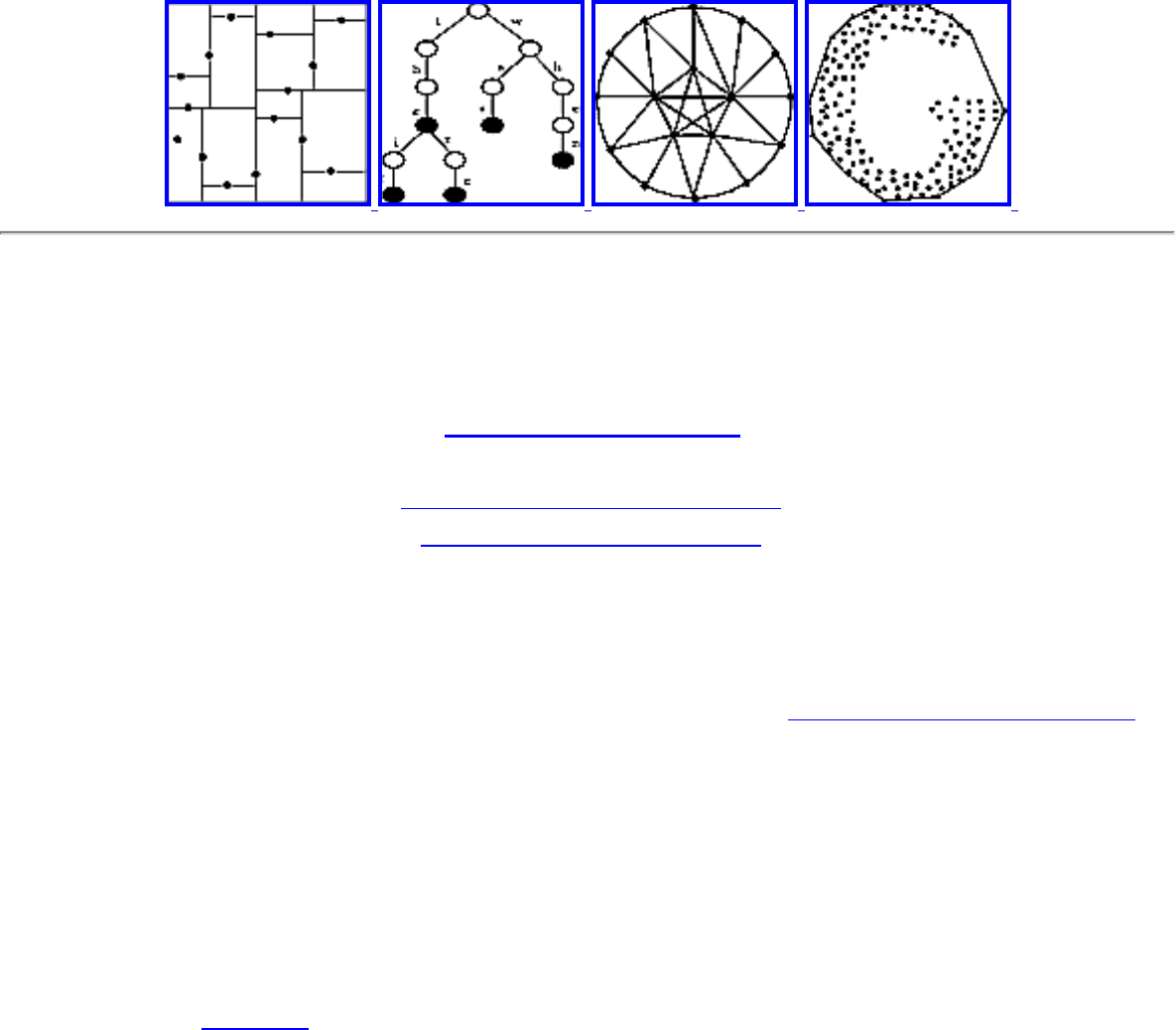
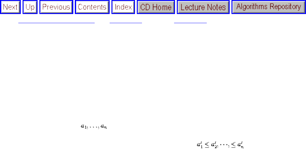
● Since finding out what is known about a problem can be a difficult task, we provide a catalog of
important algorithmic problems as a major component of this book. By browsing through this
file:///E|/BOOK/BOOK/NODE1.HTM (1 of 3) [19/1/2003 1:27:32]
Preface
catalog, the reader can quickly identify what their problem is called, what is known about it, and
how they should proceed to solve it. To aid in problem identification, we include a pair of
``before'' and ``after'' pictures for each problem, illustrating the required input and output
specifications.
● For each problem in the catalog, we provide an honest and convincing motivation, showing how it
arises in practice. If we could not find such an application, then the problem doesn't appear in this
book.
● In practice, algorithm problems do not arise at the beginning of a large project. Rather, they
typically arise as subproblems when it suddenly becomes clear that the programmer does not
know how to proceed or that the current program is inadequate. To provide a better perspective on
how algorithm problems arise in the real world, we include a collection of ``war stories,'' tales
from our experience on real problems. The moral of these stories is that algorithm design and
analysis is not just theory, but an important tool to be pulled out and used as needed.
Equally important is what we do not do in this book. We do not stress the mathematical analysis of
algorithms, leaving most of the analysis as informal arguments. You will not find a single theorem
anywhere in this book. Further, we do not try to be encyclopedic in our descriptions of algorithms, but
only in our pointers to descriptions of algorithms. When more details are needed, the reader should
follow the given references or study the cited programs. The goal of this manual is to get you going in
the right direction as quickly as possible.
But what is a manual without software? This book comes with a substantial electronic supplement, an
ISO-9660 compatible, multiplatform CD-ROM, which can be viewed using Netscape, Microsoft
Explorer, or any other WWW browser. This CD-ROM contains:
● A complete hypertext version of the full printed book. Indeed, the extensive cross-references
within the book are best followed using the hypertext version.
● The source code and URLs for all cited implementations, mirroring the Stony Brook Algorithm
Repository WWW site. Programs in C, C++, Fortran, and Pascal are included, providing an
average of four different implementations for each algorithmic problem.
● More than ten hours of audio lectures on the design and analysis of algorithms are provided, all
keyed to the on-line lecture notes. Following these lectures provides another approach to learning
algorithm design techniques. These notes are linked to an additional twenty hours of audio over
the WWW. Listening to all the audio is analogous to taking a one-semester college course on
algorithms!
This book is divided into two parts, techniques and resources. The former is a general guide to
techniques for the design and analysis of computer algorithms. The resources section is intended for
browsing and reference, and comprises the catalog of algorithmic resources, implementations, and an
extensive bibliography.
Altogether, this book covers material sufficient for a standard Introduction to Algorithms course, albeit
file:///E|/BOOK/BOOK/NODE1.HTM (2 of 3) [19/1/2003 1:27:32]

Preface
one stressing design over analysis. We assume the reader has completed the equivalent of a second
programming course, typically titled Data Structures or Computer Science II. Textbook-oriented features
include:
● In addition to standard pen-and-paper exercises, this book includes ``implementation challenges''
suitable for teams or individual students. These projects and the applied focus of the text can be
used to provide a new laboratory focus to the traditional algorithms course. More difficult
exercises are marked by (*) or (**).
● ``Take-home lessons'' at the beginning of each chapter emphasize the concepts to be gained from
the chapter.
● This book stresses design over analysis. It is suitable for both traditional lecture courses and the
new ``active learning'' method, where the professor does not lecture but instead guides student
groups to solve real problems. The ``war stories'' provide an appropriate introduction to the active
learning method.
● A full set of lecture slides for teaching this course is available on the CD-ROM and via the World
Wide Web, both keyed to unique on-line audio lectures covering a full-semester algorithm course.
Further, a complete set of my videotaped lectures using these slides is available for interested
parties. See http://www.cs.sunysb.edu/ algorith for details.
Next: Acknowledgments Up: The Algorithm Design Manual Previous: The Algorithm Design Manual
Algorithms
Mon Jun 2 23:33:50 EDT 1997
file:///E|/BOOK/BOOK/NODE1.HTM (3 of 3) [19/1/2003 1:27:32]

Acknowledgments
Next: Caveat Up: The Algorithm Design Manual Previous: Preface
Acknowledgments
I would like to thank several people for their concrete contributions to this project. Ricky Bradley built
up the substantial infrastructure required for both the WWW site and CD-ROM in a logical and
extensible manner. Zhong Li did a spectacular job drawing most of the catalog figures using xfig and
entering the lecture notes that served as the foundation of Part I of this book. Frank Ruscica, Kenneth
McNicholas and Dario Vlah all came up big in the pinch, redoing all the audio and helping as the
completion deadline approached. Filip Bujanic, David Ecker, David Gerstl, Jim Klosowski, Ted Lin,
Kostis Sagonas, Kirsten Starcher, Brian Tria, and Lei Zhao all made contributions at various stages of the
project.
Richard Crandall, Ron Danielson, Takis Metaxas, Dave Miller, Giri Narasimhan, and Joe Zachary all
reviewed preliminary versions of the manuscript and/or CD-ROM; their thoughtful feedback helped to
shape what you see here. Thanks also to Allan Wylde, the editor of my previous book as well as this one,
and Keisha Sherbecoe and Robert Wexler of Springer-Verlag.
I learned much of what I know about algorithms along with my graduate students Yaw-Ling Lin,
Sundaram Gopalakrishnan, Ting Chen, Francine Evans, Harald Rau, Ricky Bradley, and Dimitris
Margaritis. They are the real heroes of many of the war stories related within. Much of the rest I have
learned with my Stony Brook friends and colleagues Estie Arkin and Joe Mitchell, who have always
been a pleasure to work and be with.
Finally, I'd like to send personal thanks to several people. Mom, Dad, Len, and Rob all provided moral
support. Michael Brochstein took charge of organizing my social life, thus freeing time for me to actually
write the book. Through his good offices I met Renee. Her love and patience since then have made it all
worthwhile.
Next: Caveat Up: The Algorithm Design Manual Previous: Preface
Algorithms
file:///E|/BOOK/BOOK/NODE2.HTM (1 of 2) [19/1/2003 1:27:33]
Acknowledgments
Mon Jun 2 23:33:50 EDT 1997
file:///E|/BOOK/BOOK/NODE2.HTM (2 of 2) [19/1/2003 1:27:33]
Caveat
Next: Contents Up: The Algorithm Design Manual Previous: Acknowledgments
Caveat
It is traditional for the author to magnanimously accept the blame for whatever deficiencies remain. I
don't. Any errors, deficiencies, or problems in this book are somebody else's fault, but I would appreciate
knowing about them so as to determine who is to blame.
Steven S. Skiena Department of Computer Science State University of New York Stony Brook, NY
11794-4400 http://www.cs.sunysb.edu/ skiena May 1997
Algorithms
Mon Jun 2 23:33:50 EDT 1997
file:///E|/BOOK/BOOK/NODE3.HTM [19/1/2003 1:27:33]

Contents
Next: Techniques Up: The Algorithm Design Manual Previous: Caveat
Contents
● Techniques
❍ Introduction to Algorithms
■ Correctness and Efficiency
■ Correctness
■ Efficiency
■ Expressing Algorithms
■ Keeping Score
■ The RAM Model of Computation
■ Best, Worst, and Average-Case Complexity
■ The Big Oh Notation
■ Growth Rates
■ Logarithms
■ Modeling the Problem
■ About the War Stories
■ War Story: Psychic Modeling
■ Exercises
❍ Data Structures and Sorting
■ Fundamental Data Types
■ Containers
■ Dictionaries
■ Binary Search Trees
■ Priority Queues
■ Specialized Data Structures
■ Sorting
■ Applications of Sorting
■ Approaches to Sorting
■ Data Structures
■ Incremental Insertion
■ Divide and Conquer
■ Randomization
■ Bucketing Techniques
■ War Story: Stripping Triangulations
file:///E|/BOOK/BOOK/NODE4.HTM (1 of 7) [19/1/2003 1:27:35]

Contents
■ War Story: Mystery of the Pyramids
■ War Story: String 'em Up
■ Exercises
❍ Breaking Problems Down
■ Dynamic Programming
■ Fibonacci numbers
■ The Partition Problem
■ Approximate String Matching
■ Longest Increasing Sequence
■ Minimum Weight Triangulation
■ Limitations of Dynamic Programming
■ War Story: Evolution of the Lobster
■ War Story: What's Past is Prolog
■ War Story: Text Compression for Bar Codes
■ Divide and Conquer
■ Fast Exponentiation
■ Binary Search
■ Square and Other Roots
■ Exercises
❍ Graph Algorithms
■ The Friendship Graph
■ Data Structures for Graphs
■ War Story: Getting the Graph
■ Traversing a Graph
■ Breadth-First Search
■ Depth-First Search
■ Applications of Graph Traversal
■ Connected Components
■ Tree and Cycle Detection
■ Two-Coloring Graphs
■ Topological Sorting
■ Articulation Vertices
■ Modeling Graph Problems
■ Minimum Spanning Trees
■ Prim's Algorithm
■ Kruskal's Algorithm
■ Shortest Paths
■ Dijkstra's Algorithm
file:///E|/BOOK/BOOK/NODE4.HTM (2 of 7) [19/1/2003 1:27:35]

Contents
■ All-Pairs Shortest Path
■ War Story: Nothing but Nets
■ War Story: Dialing for Documents
■ Exercises
❍ Combinatorial Search and Heuristic Methods
■ Backtracking
■ Constructing All Subsets
■ Constructing All Permutations
■ Constructing All Paths in a Graph
■ Search Pruning
■ Bandwidth Minimization
■ War Story: Covering Chessboards
■ Heuristic Methods
■ Simulated Annealing
■ Traveling Salesman Problem
■ Maximum Cut
■ Independent Set
■ Circuit Board Placement
■ Neural Networks
■ Genetic Algorithms
■ War Story: Annealing Arrays
■ Parallel Algorithms
■ War Story: Going Nowhere Fast
■ Exercises
❍ Intractable Problems and Approximations
■ Problems and Reductions
■ Simple Reductions
■ Hamiltonian Cycles
■ Independent Set and Vertex Cover
■ Clique and Independent Set
■ Satisfiability
■ The Theory of NP-Completeness
■ 3-Satisfiability
■ Difficult Reductions
■ Integer Programming
■ Vertex Cover
■ Other NP-Complete Problems
■ The Art of Proving Hardness
file:///E|/BOOK/BOOK/NODE4.HTM (3 of 7) [19/1/2003 1:27:35]

Contents
■ War Story: Hard Against the Clock
■ Approximation Algorithms
■ Approximating Vertex Cover
■ The Euclidean Traveling Salesman
■ Exercises
❍ How to Design Algorithms
● Resources
❍ A Catalog of Algorithmic Problems
■ Data Structures
■ Dictionaries
■ Priority Queues
■ Suffix Trees and Arrays
■ Graph Data Structures
■ Set Data Structures
■ Kd-Trees
■ Numerical Problems
■ Solving Linear Equations
■ Bandwidth Reduction
■ Matrix Multiplication
■ Determinants and Permanents
■ Constrained and Unconstrained Optimization
■ Linear Programming
■ Random Number Generation
■ Factoring and Primality Testing
■ Arbitrary-Precision Arithmetic
■ Knapsack Problem
■ Discrete Fourier Transform
■ Combinatorial Problems
■ Sorting
■ Searching
■ Median and Selection
■ Generating Permutations
■ Generating Subsets
■ Generating Partitions
■ Generating Graphs
■ Calendrical Calculations
■ Job Scheduling
■ Satisfiability
file:///E|/BOOK/BOOK/NODE4.HTM (4 of 7) [19/1/2003 1:27:35]

Contents
■ Graph Problems: Polynomial-Time
■ Connected Components
■ Topological Sorting
■ Minimum Spanning Tree
■ Shortest Path
■ Transitive Closure and Reduction
■ Matching
■ Eulerian Cycle / Chinese Postman
■ Edge and Vertex Connectivity
■ Network Flow
■ Drawing Graphs Nicely
■ Drawing Trees
■ Planarity Detection and Embedding
■ Graph Problems: Hard Problems
■ Clique
■ Independent Set
■ Vertex Cover
■ Traveling Salesman Problem
■ Hamiltonian Cycle
■ Graph Partition
■ Vertex Coloring
■ Edge Coloring
■ Graph Isomorphism
■ Steiner Tree
■ Feedback Edge/Vertex Set
■ Computational Geometry
■ Robust Geometric Primitives
■ Convex Hull
■ Triangulation
■ Voronoi Diagrams
■ Nearest Neighbor Search
■ Range Search
■ Point Location
■ Intersection Detection
■ Bin Packing
■ Medial-Axis Transformation
■ Polygon Partitioning
■ Simplifying Polygons
file:///E|/BOOK/BOOK/NODE4.HTM (5 of 7) [19/1/2003 1:27:35]

Contents
■ Shape Similarity
■ Motion Planning
■ Maintaining Line Arrangements
■ Minkowski Sum
■ Set and String Problems
■ Set Cover
■ Set Packing
■ String Matching
■ Approximate String Matching
■ Text Compression
■ Cryptography
■ Finite State Machine Minimization
■ Longest Common Substring
■ Shortest Common Superstring
❍ Algorithmic Resources
■ Software systems
■ LEDA
■ Netlib
■ Collected Algorithms of the ACM
■ The Stanford GraphBase
■ Combinatorica
■ Algorithm Animations with XTango
■ Programs from Books
■ Discrete Optimization Algorithms in Pascal
■ Handbook of Data Structures and Algorithms
■ Combinatorial Algorithms for Computers and Calculators
■ Algorithms from P to NP
■ Computational Geometry in C
■ Algorithms in C++
■ Data Sources
■ Textbooks
■ On-Line Resources
■ Literature
■ People
■ Software
■ Professional Consulting Services
● References
● Index
file:///E|/BOOK/BOOK/NODE4.HTM (6 of 7) [19/1/2003 1:27:35]

Index
Next: About this document Up: The Algorithm Design Manual Previous: References
Index
This index provides fast access to important keywords and topics in the on-line Book. The menu below
partitions the index entries by the first letter of the alphabet, for ease of access. A full document index is
also provided.
Be aware that the index pointer typically resides at the end of the relevant paragraph in the document, so
we recommend scrolling once towards the front of the document before reading.
A similar index has been provided for the Lecture Notes, which may also be of interest.
A B C D E F G H
I J K L M N O P
Q R S T U V W X
Y Z
Complete Index
(note: the complete index is large; it will take a bit of time to load)
Algorithms
Mon Jun 2 23:33:50 EDT 1997
file:///E|/BOOK/BOOK5/NODE233.HTM [19/1/2003 1:27:36]
The Algorithm Design Manual
The Algorithm Design Manual
The CD-ROM
Steven S. Skiena
Department of Computer Science
State University of New York
Stony Brook, NY 11794-4400
What is a manual without software? The electronic supplement to this book is a ISO-9660 compatible,
multiplatform CD-ROM, which can be viewed using Netscape, Microsoft Explorer, or any other WWW
browser. This CD-ROM contains:
● The Algorithm Design Manual: Hypertext Edition A complete hypertext version of the full printed book.
Indeed, the extensive cross-references within the book are best followed using the hypertext version.
● The Algorithm Repository Website -- The source code and URLs for all cited implementations,
mirroring the Stony Brook Algorithm Repository WWW site. Programs in C, C++, Fortran, and Pascal
are included, providing an average of four different implementations for each algorithmic problem.
● Algorithms Lectures -- More than 30 hours of audio lectures on the design and analysis of algorithms are
provided, all keyed to on-line lecture notes. Following these lectures provides another approach to
learning algorithm design techniques. Listening to all the audio is analogous to taking a one-semester
file:///E|/INDEX.HTM (1 of 2) [19/1/2003 1:27:37]

The Algorithm Design Manual
college course on algorithms!
● Bibliographic References -- Pointers to the net's most important collections of references on algorithms.
Local copies of two large bibliographies are included.
● About the Book
● Copyright Notice and Disclaimers
● Graphics Gallery
● Send us Mail
● Guide to Configuring Browsers
● Thanks!
file:///E|/INDEX.HTM (2 of 2) [19/1/2003 1:27:37]
Lecture Notes -- Analysis of Algorithms
CSE 373/548 - Analysis of Algorithms
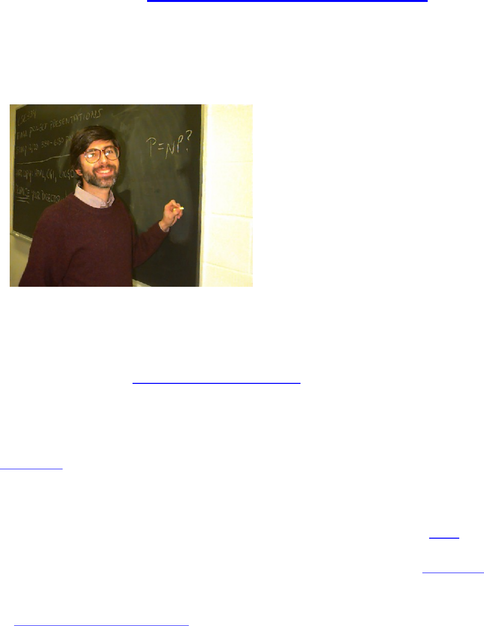
Lecture Notes with Audio
Steven Skiena
Department of Computer Science
SUNY Stony Brook
In Spring 1996, I taught my Analysis of Algorithms
course via EngiNet, the SUNY Stony Brook distance
learning program. Each of my lectures that semester was
videotaped, and the tapes made available to off-site
students. I found it an enjoyable experience.
As an experiment in using the Internet for distance
learning, we have digitized the complete audio of all 23
lectures, and have made this available on the WWW. We
partitioned the full audio track into sound clips, each
corresponding to one page of lecture notes, and linked
them to the associated text.
In a real sense, listening to all the audio is analogous to sitting through a one-semester college course on
algorithms! Properly compressed, the full semester's audio requires less than 300 megabytes of storage,
which is much less than I would have imagined. The entire semesters lectures, over thirty hours of audio
files, fit comfortably on The Algorithm Design Manual CD-ROM, which also includes a hypertext
version of the book and a substantial amount of software. All exercise numbers refer to Corman,
Leiserson, and Rivest's Introduction to Algorithms, the textbook I used that particular year.
The sound quality is amazingly good, considering it was me that they were taping. Unfortunately, the
Shockwave format we used is only supported under Windows and Macintoshes, so the sound cannot be
heard under UNIX. On certain browsers, a new window is opened for each sound bite, so be sure to close
these windows before they cause trouble.
Because of space requirements, we did not digitize much of the corresponding video, which would have
made the presentation even more interesting. Still, I hope you find that these audio lectures expand your
understanding of both algorithm design and educational multimedia. The full video tapes themselves are
also available.
● Postscript lecture transparencies
file:///E|/LEC/LECTURES/ALL.HTM (1 of 3) [19/1/2003 1:27:38]

Lecture Notes -- Analysis of Algorithms
● A Guide to Configuring Browsers
● Binary Search Animation
● Other Algorithms Courses
Links To Individual Lectures
● Lecture 1 - analyzing algorithms
● Lecture 2 - asymptotic notation
● Lecture 3 - recurrence relations
● Lecture 4 - heapsort
● Lecture 5 - quicksort
● Lecture 6 - linear sorting
● Lecture 7 - elementary data structures
● Lecture 8 - binary trees
● Lecture 9 - catch up
● Lecture 10 - tree restructuring
● Lecture 11 - backtracking
● Lecture 12 - introduction to dynamic programming
● Lecture 13 - dynamic programming applications
● Lecture 14 - data structures for graphs
● Lecture 15 - DFS and BFS
● Lecture 16 - applications of DFS and BFS
● Lecture 17 - minimum spanning trees
● Lecture 18 - shortest path algorthms
● Lecture 19 - satisfiability
● Lecture 20 - integer programming
● Lecture 21 - vertex cover
● Lecture 22 - techniques for proving hardness
● Lecture 23 - approximation algorithms and Cook's theorem
● Index
● About this document ...
Next: Lecture 1 - analyzing Up: Main Page
file:///E|/LEC/LECTURES/ALL.HTM (2 of 3) [19/1/2003 1:27:38]
Lecture Notes -- Analysis of Algorithms
Algorithms
Mon Jun 2 09:21:39 EDT 1997
file:///E|/LEC/LECTURES/ALL.HTM (3 of 3) [19/1/2003 1:27:38]
The Stony Brook Algorithm Repository
The Stony Brook Algorithm Repository
Steven S. Skiena
Department of Computer Science
State University of New York
Stony Brook, NY 11794-4400
This WWW page is intended to serve as a comprehensive collection of algorithm implementations for
over seventy of the most fundamental problems in combinatorial algorithms. The problem taxonomy,
implementations, and supporting material are all drawn from my book The Algorithm Design Manual .
Since the practical person is more often looking for a program than an algorithm, we provide pointers to
solid implementations of useful algorithms, when they are available.
Because of the volatility of the WWW, we provide local copies for many of the implementations. We
encourage you to get them from the original sites instead of Stony Brook, because the version on the
original site is more likely to be maintained. Further, there are often supporting files and documentation
which we did not copy, and which may be of interest to you. The local copies of large implementations
are maintained as gzip tar archives and, where available, DOS zip archives. Software for decoding these
formats is readily available .
Many of these codes have been made available for research or educational use, although commercial use
requires a licensing arrangement with the author. Licensing terms from academic institutions are usually
surprisingly modest. The recognition that industry is using a particular code is important to the authors,
often more important than the money. This can lead to enhanced support or future releases of the
software. Do the right thing and get a license -- information about terms or who to contact is usually
available embedded within the documentation, or available at the original source site.
Use at your own risk. The author and Springer-Verlag make no representations, express or implied, with
respect to any software or documentation we describe. The author and Springer-Verlag shall in no event
be liable for any indirect, incidental, or consequential damages.
file:///E|/WEBSITE/INDEX.HTM (1 of 3) [19/1/2003 1:27:40]

The Stony Brook Algorithm Repository
About the Book Graphics Gallery Graphic Index
Audio Algorithm Lectures Bibliography References Data Sources
About the Ratings Copyright Notice and Disclaimers Top-Level CD-ROM Page
Problems by Category
● 1.1 Data Structures
● 1.2 Numerical Problems
● 1.3 Combinatorial Problems
● 1.4 Graph Problems -- polynomial-time problems
● 1.5 Graph Problems -- hard problems
● 1.6 Computational Geometry
● 1.7 Set and String Problems
Implementations By Language
● C++ Language Implementations
● C Language Implementations
● Pascal Language Implementations
● FORTRAN Language Implementations
● Mathematica Language Implementations
● Lisp Language Implementations
Other information on this site
● Order the Book
● Most Wanted List
● Tools and Utilities
● Repository Citations
● Video tapes
● Feedback
● Thanks!
file:///E|/WEBSITE/INDEX.HTM (2 of 3) [19/1/2003 1:27:40]


Techniques
Next: Introduction to Algorithms Up: The Algorithm Design Manual Previous: Contents
Techniques
● Introduction to Algorithms
❍ Correctness and Efficiency
❍ Expressing Algorithms
❍ Keeping Score
❍ The Big Oh Notation
❍ Growth Rates
❍ Logarithms
❍ Modeling the Problem
❍ About the War Stories
❍ War Story: Psychic Modeling
❍ Exercises
● Data Structures and Sorting
❍ Fundamental Data Types
❍ Specialized Data Structures
❍ Sorting
❍ Applications of Sorting
❍ Approaches to Sorting
❍ War Story: Stripping Triangulations
❍ War Story: Mystery of the Pyramids
❍ War Story: String 'em Up
❍ Exercises
● Breaking Problems Down
❍ Dynamic Programming
❍ Limitations of Dynamic Programming
❍ War Story: Evolution of the Lobster
❍ War Story: What's Past is Prolog
❍ War Story: Text Compression for Bar Codes
file:///E|/BOOK/BOOK/NODE5.HTM (1 of 3) [19/1/2003 1:27:41]

Techniques
❍ Divide and Conquer
❍ Exercises
● Graph Algorithms
❍ The Friendship Graph
❍ Data Structures for Graphs
❍ War Story: Getting the Graph
❍ Traversing a Graph
❍ Applications of Graph Traversal
❍ Modeling Graph Problems
❍ Minimum Spanning Trees
❍ Shortest Paths
❍ War Story: Nothing but Nets
❍ War Story: Dialing for Documents
❍ Exercises
● Combinatorial Search and Heuristic Methods
❍ Backtracking
❍ Search Pruning
❍ Bandwidth Minimization
❍ War Story: Covering Chessboards
❍ Heuristic Methods
❍ War Story: Annealing Arrays
❍ Parallel Algorithms
❍ War Story: Going Nowhere Fast
❍ Exercises
● Intractable Problems and Approximations
❍ Problems and Reductions
❍ Simple Reductions
❍ Satisfiability
❍ Difficult Reductions
❍ Other NP-Complete Problems
❍ The Art of Proving Hardness
❍ War Story: Hard Against the Clock
❍ Approximation Algorithms
❍ Exercises
● How to Design Algorithms
file:///E|/BOOK/BOOK/NODE5.HTM (2 of 3) [19/1/2003 1:27:41]
Techniques
Algorithms
Mon Jun 2 23:33:50 EDT 1997
file:///E|/BOOK/BOOK/NODE5.HTM (3 of 3) [19/1/2003 1:27:41]
Introduction to Algorithms
Next: Correctness and Efficiency Up: Techniques Previous: Techniques
Introduction to Algorithms
What is an algorithm? An algorithm is a procedure to accomplish a specific task. It is the idea behind any computer program.
To be interesting, an algorithm has to solve a general, well-specified problem. An algorithmic problem is specified by describing
the complete set of instances it must work on and what properties the output must have as a result of running on one of these
instances. This distinction between a problem and an instance of a problem is fundamental. For example, the algorithmic
problem known as sorting is defined as follows:
Input: A sequence of n keys .
Output: The permutation (reordering) of the input sequence such that . An instance of sorting might be an array
of names, such as {Mike, Bob, Sally, Jill, Jan}, or a list of numbers like {154, 245, 568, 324, 654, 324}. Determining whether
you in fact have a general problem to deal with, as opposed to an instance of a problem, is your first step towards solving it. This
is true in algorithms as it is in life.
An algorithm is a procedure that takes any of the possible input instances and transforms it to the desired output. There are many
different algorithms for solving the problem of sorting. For example, one method for sorting starts with a single element (thus
forming a trivially sorted list) and then incrementally inserts the remaining elements so that the list stays sorted. This algorithm,
insertion sort, is described below:
InsertionSort(A)
for i = 1 to n-1 do
for j = i+1 to 2 do
if (A[j] < A[j-1]) then swap(A[j],A[j-
1])
Note the generality of this algorithm. It works equally well on names as it does on numbers, given the appropriate < comparison
operation to test which of the two keys should appear first in sorted order. Given our definition of the sorting problem, it can be
readily verified that this algorithm correctly orders every possible input instance.
In this chapter, we introduce the desirable properties that good algorithms have, as well as how to measure whether a given
algorithm achieves these goals. Assessing algorithmic performance requires a modest amount of mathematical notation, which
we also present. Although initially intimidating, this notation proves essential for us to compare algorithms and design more
efficient ones.
While the hopelessly ``practical'' person may blanch at the notion of theoretical analysis, we present this material because it is
useful. In particular, this chapter offers the following ``take-home'' lessons:
file:///E|/BOOK/BOOK/NODE6.HTM (1 of 2) [19/1/2003 1:27:42]
Introduction to Algorithms
● Reasonable-looking algorithms can easily be incorrect. Algorithm correctness is a property that must be carefully
demonstrated.
● Algorithms can be understood and studied in a machine independent way.
● The ``big Oh'' notation and worst-case analysis are tools that greatly simplify our ability to compare the efficiency of
algorithms.
● We seek algorithms whose running times grow logarithmically, because grows very slowly with increasing n.
● Modeling your application in terms of well-defined structures and algorithms is the most important single step towards a
solution.
● Correctness and Efficiency
❍ Correctness
❍ Efficiency
● Expressing Algorithms
● Keeping Score
❍ The RAM Model of Computation
❍ Best, Worst, and Average-Case Complexity
● The Big Oh Notation
● Growth Rates
● Logarithms
● Modeling the Problem
● About the War Stories
● War Story: Psychic Modeling
● Exercises
Next: Correctness and Efficiency Up: Techniques Previous: Techniques
Algorithms
Mon Jun 2 23:33:50 EDT 1997
file:///E|/BOOK/BOOK/NODE6.HTM (2 of 2) [19/1/2003 1:27:42]
Data Structures and Sorting
Next: Fundamental Data Types Up: Techniques Previous: Implementation Challenges
Data Structures and Sorting
When things go right, changing a data structure in a slow program works the same way an organ
transplant does in a sick patient. For several classes of abstract data types, such as containers,
dictionaries, and priority queues, there exist many different but functionally equivalent data structures
that implement the given data type. Changing the data structure does not change the correctness of the
program, since we presumably replace a correct implementation with a different correct implementation.
However, because the new implementation of the data type realizes different tradeoffs in the time to
execute various operations, the total performance of an application can improve dramatically. Like a
patient in need of a transplant, only one part might need to be replaced in order to fix the problem.
It is obviously better to be born with a good heart than have to wait for a replacement. Similarly, the
maximum benefit from good data structures results from designing your program around them in the first
place. Still, it is important to build your programs so that alternative implementations can be tried. This
involves separating the internals of the data structure (be it a tree, a hash table, or a sorted array) from its
interface (operations like search, insert, delete). Such data abstraction is an important part of producing
clean, readable, and modifiable programs. We will not dwell on such software engineering issues here,
but such a design is critical if you are to experiment with the impact of different implementations on
performance.
In this chapter we will also discuss sorting, stressing how sorting can be applied to solve other problems
more than the details of specific sorting algorithms. In this sense, sorting behaves more like a data
structure than a problem in its own right. Sorting is also represented by a significant entry in the problem
catalog; namely Section .
The key take-home lessons of this chapter are:
● Building algorithms around data structures such as dictionaries and priority queues leads to both
clean structure and good performance.
● Picking the wrong data structure for the job can be disastrous in terms of performance. Picking the
very best data structure is often not as critical, for there are typically several choices that perform
similarly.
● Sorting lies at the heart of many different algorithms. Sorting the data is one of the first things any
algorithm designer should try in the quest for efficiency.
● Sorting can be used to illustrate most algorithm design paradigms. Data structure techniques,
file:///E|/BOOK/BOOK/NODE22.HTM (1 of 2) [19/1/2003 1:27:43]
Data Structures and Sorting
divide-and-conquer, randomization, and incremental construction all lead to popular sorting
algorithms.
● Fundamental Data Types
❍ Containers
❍ Dictionaries
❍ Binary Search Trees
❍ Priority Queues
● Specialized Data Structures
● Sorting
● Applications of Sorting
● Approaches to Sorting
❍ Data Structures
❍ Incremental Insertion
❍ Divide and Conquer
❍ Randomization
❍ Bucketing Techniques
● War Story: Stripping Triangulations
● War Story: Mystery of the Pyramids
● War Story: String 'em Up
● Exercises
Next: Fundamental Data Types Up: Techniques Previous: Implementation Challenges
Algorithms
Mon Jun 2 23:33:50 EDT 1997
file:///E|/BOOK/BOOK/NODE22.HTM (2 of 2) [19/1/2003 1:27:43]

Breaking Problems Down
Next: Dynamic Programming Up: Techniques Previous: Implementation Challenges
Breaking Problems Down
One of the most powerful techniques for solving problems is to break them down into smaller, more
easily solved pieces. Smaller problems are less overwhelming, and they permit us to focus on details that
are lost when we are studying the entire problem. For example, whenever we can break the problem into
smaller instances of the same type of problem, a recursive algorithm starts to become apparent.
Two important algorithm design paradigms are based on breaking problems down into smaller problems.
Dynamic programming typically removes one element from the problem, solves the smaller problem,
and then uses the solution to this smaller problem to add back the element in the proper way. Divide and
conquer typically splits the problem in half, solves each half, then stitches the halves back together to
form a full solution.
Both of these techniques are important to know about. Dynamic programming in particular is a
misunderstood and underappreciated technique. To demonstrate its utility in practice, we present no
fewer than three war stories where dynamic programming played the decisive role.
The take-home lessons for this chapter include:
● Many objects have an inherent left-to-right ordering among their elements, such as characters in a
string, elements of a permutation, points around a polygon, or leaves in a search tree. For any
optimization problem on such left-to-right objects, dynamic programming will likely lead to an
efficient algorithm to find the best solution.
● Without an inherent left-to-right ordering on the objects, dynamic programming is usually
doomed to require exponential space and time.
● Once you understand dynamic programming, it can be easier to work out such algorithms from
scratch than to try to look them up.
● The global optimum (found, for example, using dynamic programming) is often noticeably better
than the solution found by typical heuristics. How important this improvement is depends upon
your application, but it can never hurt.
● Binary search and its variants are the quintessential divide-and-conquer algorithms.
file:///E|/BOOK/BOOK/NODE42.HTM (1 of 2) [19/1/2003 1:27:43]
Breaking Problems Down
● Dynamic Programming
❍ Fibonacci numbers
❍ The Partition Problem
❍ Approximate String Matching
❍ Longest Increasing Sequence
❍ Minimum Weight Triangulation
● Limitations of Dynamic Programming
● War Story: Evolution of the Lobster
● War Story: What's Past is Prolog
● War Story: Text Compression for Bar Codes
● Divide and Conquer
❍ Fast Exponentiation
❍ Binary Search
❍ Square and Other Roots
● Exercises
Next: Dynamic Programming Up: Techniques Previous: Implementation Challenges
Algorithms
Mon Jun 2 23:33:50 EDT 1997
file:///E|/BOOK/BOOK/NODE42.HTM (2 of 2) [19/1/2003 1:27:43]
Graph Algorithms
Next: The Friendship Graph Up: Techniques Previous: Implementation Challenges
Graph Algorithms
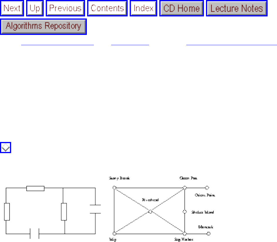
A graph G=(V,E) consists of a set of vertices V together with a set E of vertex pairs or edges. Graphs are
important because they can be used to represent essentially any relationship. For example, graphs can
model a network of roads, with cities as vertices and roads between cities as edges, as shown in Figure
. Electronic circuits can also be modeled as graphs, with junctions as vertices and components as
edges.
Figure: Modeling road networks and electronic circuits as graphs
The key to understanding many algorithmic problems is to think of them in terms of graphs. Graph
theory provides a language for talking about the properties of graphs, and it is amazing how often messy
applied problems have a simple description and solution in terms of classical graph properties.
Designing truly novel graph algorithms is a very difficult task. The key to using graph algorithms
effectively in applications lies in correctly modeling your problem as a standard graph property, so you
can take advantage of existing algorithms. Becoming familiar with many different graph algorithmic
problems is more important than understanding the details of particular graph algorithms, particularly
since Part II of this book can point you to an implementation as soon as you know the name of your
problem.
In this chapter, we will present basic data structures and traversal operations for graphs, which will
enable you to cobble together solutions to rudimentary graph problems. We will also describe more
sophisticated algorithms for problems like shortest paths and minimum spanning trees in some detail. But
we stress the primary importance of correctly modeling your problem. Time spent browsing through the
catalog now will leave you better informed of your options when a real job arises.
file:///E|/BOOK/BOOK2/NODE59.HTM (1 of 3) [19/1/2003 1:27:44]
Graph Algorithms
The take-home lessons of this chapter include:
● Graphs can be used to model a wide variety of structures and relationships.
● Properly formulated, most applications of graphs can be reduced to standard graph properties and
using well-known algorithms. These include minimum spanning trees, shortest paths, and several
problems presented in the catalog.
● Breadth-first and depth-first search provide mechanisms to visit each edge and vertex of the
graph. They prove the basis of most simple, efficient graph algorithms.
● The Friendship Graph
● Data Structures for Graphs
● War Story: Getting the Graph
● Traversing a Graph
❍ Breadth-First Search
❍ Depth-First Search
● Applications of Graph Traversal
❍ Connected Components
❍ Tree and Cycle Detection
❍ Two-Coloring Graphs
❍ Topological Sorting
❍ Articulation Vertices
● Modeling Graph Problems
● Minimum Spanning Trees
❍ Prim's Algorithm
❍ Kruskal's Algorithm
● Shortest Paths
❍ Dijkstra's Algorithm
❍ All-Pairs Shortest Path
● War Story: Nothing but Nets
● War Story: Dialing for Documents
● Exercises
file:///E|/BOOK/BOOK2/NODE59.HTM (2 of 3) [19/1/2003 1:27:44]

Combinatorial Search and Heuristic Methods
Next: Backtracking Up: Techniques Previous: Implementation Challenges
Combinatorial Search and Heuristic
Methods
We have seen how clever algorithms can reduce the complexity of sorting from to , which is good.
However, the algorithmic stakes can be even higher for combinatorially explosive problems, whose time
grows exponentially in the size of the problem. Looking back at Figure will make clear the
limitations of exponential-time algorithms on even modest-sized problems.
By using exhaustive search techniques, we can solve small problems to optimality, although the time
complexity may be enormous. For certain applications, it may well pay to spend extra time to be certain
of the optimal solution. A good example occurs in testing a circuit or a program on all possible inputs.
You can prove the correctness of the device by trying all possible inputs and verifying that they give the
correct answer. Proving such correctness is a property to be proud of. However, claiming that it works
correctly on all the inputs you tried is worth much, much less.
In this section, we present backtracking as a technique for listing all configurations representing possible
solutions for a combinatorial algorithm problem. We then discuss techniques for pruning search that
significantly improve efficiency by eliminating irrelevant configurations from consideration. We
illustrate the power of clever pruning techniques to speed up real search applications. For problems that
are too large to contemplate using brute-force combinatorial search, we introduce heuristic methods such
as simulated annealing. Such heuristic methods are an important weapon in the practical algorist's
arsenal.
The take-home lessons from this chapter are:
● Combinatorial search, augmented with tree pruning techniques, can be used to find the optimal
solution of small optimization problems. How small depends upon the specific problem, but the
size limit is likely to be somewhere between items.
● Clever pruning techniques can speed up combinatorial search to an amazing extent. Proper
pruning will have a greater impact on search time than any other factor.
● Simulated annealing is a simple but effective technique to efficiently obtain good but not optimal
solutions to combinatorial search problems.
file:///E|/BOOK/BOOK2/NODE83.HTM (1 of 2) [19/1/2003 1:27:45]
Combinatorial Search and Heuristic Methods
● Backtracking
❍ Constructing All Subsets
❍ Constructing All Permutations
❍ Constructing All Paths in a Graph
● Search Pruning
● Bandwidth Minimization
● War Story: Covering Chessboards
● Heuristic Methods
❍ Simulated Annealing
❍ Neural Networks
❍ Genetic Algorithms
● War Story: Annealing Arrays
● Parallel Algorithms
● War Story: Going Nowhere Fast
● Exercises
Next: Backtracking Up: Techniques Previous: Implementation Challenges
Algorithms
Mon Jun 2 23:33:50 EDT 1997
file:///E|/BOOK/BOOK2/NODE83.HTM (2 of 2) [19/1/2003 1:27:45]

Intractable Problems and Approximations
Next: Problems and Reductions Up: Techniques Previous: Implementation Challenges
Intractable Problems and
Approximations
In this chapter, we will concentrate on techniques for proving that no efficient algorithm exists for a
given problem. The practical reader is probably squirming at the notion of proving anything and will be
particularly alarmed at the idea of investing time to prove that something does not exist. Why will you be
better off knowing that something you don't know how to do in fact can't be done at all?
The truth is that the theory of NP-completeness is an immensely useful tool for the algorithm designer,
even though all it does is provide negative results. That noted algorithm designer Sherlock Holmes once
said, ``When you have eliminated the impossible, what remains, however improbable, must be the truth.''
The theory of NP-completeness enables the algorithm designer to focus her efforts more productively, by
revealing that the search for an efficient algorithm for this particular problem is doomed to failure. When
one fails to show that a problem is hard, that means there is likely an algorithm that solves it efficiently.
Two of the war stories in this book describe happy results springing from bogus claims of hardness.
The theory of NP-completeness also enables us to identify exactly what properties make a particular
problem hard, thus providing direction for us to model it in different ways or exploit more benevolent
characteristics of the problem. Developing a sense for which problems are hard and which are not is a
fundamental skill for algorithm designers, and it can come only from hands-on experience proving
hardness.
We will not discuss the complexity-theoretic aspects of NP-completeness in depth, limiting our treatment
to the fundamental concept of reductions, which show the equivalence of pairs of problems. For a
discussion, we refer the reader to [GJ79], the truly essential reference on the theory of intractability.
The take-home lessons from this chapter are:
● Reductions are a way to show that two problems are essentially identical. A fast algorithm for one
of the problems implies a fast algorithm for the other.
● In practice, a small set of NP-complete problems (3-SAT, vertex cover, integer partition, and
Hamiltonian cycle) suffice to prove the hardness of most other hard problems.
file:///E|/BOOK/BOOK3/NODE104.HTM (1 of 2) [19/1/2003 1:27:46]
Intractable Problems and Approximations
● Approximation algorithms guarantee answers that are always close to the optimal solution and can
provide an approach to dealing with NP-complete problems.
● Problems and Reductions
● Simple Reductions
❍ Hamiltonian Cycles
❍ Independent Set and Vertex Cover
❍ Clique and Independent Set
● Satisfiability
❍ The Theory of NP-Completeness
❍ 3-Satisfiability
● Difficult Reductions
❍ Integer Programming
❍ Vertex Cover
● Other NP-Complete Problems
● The Art of Proving Hardness
● War Story: Hard Against the Clock
● Approximation Algorithms
❍ Approximating Vertex Cover
❍ The Euclidean Traveling Salesman
● Exercises
Next: Problems and Reductions Up: Techniques Previous: Implementation Challenges
Algorithms
Mon Jun 2 23:33:50 EDT 1997
file:///E|/BOOK/BOOK3/NODE104.HTM (2 of 2) [19/1/2003 1:27:46]

How to Design Algorithms
Next: Resources Up: Techniques Previous: Implementation Challenges
How to Design Algorithms
Designing the right algorithm for a given application is a difficult job. It requires a major creative act,
taking a problem and pulling a solution out of the ether. This is much more difficult than taking someone
else's idea and modifying it or tweaking it to make it a little better. The space of choices you can make in
algorithm design is enormous, enough to leave you plenty of freedom to hang yourself.
This book is designed to make you a better algorithm designer. The techniques presented in Part I of this
book provide the basic ideas underlying all combinatorial algorithms. The problem catalog of Part II will
help you with modeling your application and point you in the right direction of an algorithm or
implementation. However, being a successful algorithm designer requires more than book knowledge; it
requires a certain attitude, the right problem-solving approach. It is difficult to teach this mindset in a
book; yet getting it is essential to become a successful designer.
The key to algorithm design (or any other problem-solving task) is to proceed by asking yourself a
sequence of questions to guide your thought process. What if we do this? What if we do that? Should you
get stuck on the problem, the best thing to do is move onto the next question. In any group brainstorming
session, the most useful person in the room is the one who keeps asking, ``Why can't we do it this way?''
not the person who later tells them why. Because eventually she will stumble on an approach that can't be
shot down.
Towards this end, we provide below a sequence of questions to guide your search for the right algorithm
for your problem. To use it effectively, you must not only ask the questions, but answer them. The key is
working through the answers carefully, by writing them down in a log. The correct answer to, ``Can I do
it this way?'' is never ``no,'' but ``no, because ....'' By clearly articulating your reasoning as to why
something doesn't work, you can check if it really holds up or whether you have just glossed over a
possibility that you didn't want to think hard enough about. You will be surprised how often the reason
you can't find a convincing explanation for something is because your conclusion is wrong.
An important distinction to keep aware of during any design process is the difference between strategy
and tactics. Strategy represents the quest for the big picture, the framework around which we construct
our path to the goal. Tactics are used to win the minor battles we must fight along the way. In problem
solving, it is important to check repeatedly whether you are thinking on the right level. If you do not have
a global strategy of how you are going to attack your problem, it is pointless to worry about the tactics.
An example of a strategic question is, ``How best can I model my application as a graph algorithm
file:///E|/BOOK/BOOK3/NODE124.HTM (1 of 5) [19/1/2003 1:27:48]

How to Design Algorithms
problem?'' A tactical question might be, ``Should I use an adjacency list or adjacency matrix data
structure to represent my graph?'' Of course, such tactical decisions are critical to the ultimate quality of
the solution, but they can be properly evaluated only in light of a successful strategy.
When faced with a design problem, too many people freeze up in their thinking. After reading or hearing
the problem, they sit down and realize that they don't know what to do next. They stare into space, then
panic, and finally end up settling for the first thing that comes to mind. Avoid this fate. Follow the
sequence of questions provided below and in most of the catalog problem sections. We'll tell you what to
do next!
Obviously, the more experience you have with algorithm design techniques such as dynamic
programming, graph algorithms, intractability, and data structures, the more successful you will be at
working through the list of questions. Part I of this book has been designed to strengthen this technical
background. However, it pays to work through these questions regardless of how strong your technical
skills are. The earliest and most important questions on the list focus on obtaining a detailed
understanding of the problem and do not require specific expertise.
This list of questions was inspired by a passage in that wonderful book about the space program The
Right Stuff [Wol79]. It concerned the radio transmissions from test pilots just before their planes crashed.
One might have expected that they would panic, so that ground control would hear the pilot yelling
Ahhhhhhhhhhh --, terminated only by the sound of smacking into a mountain. Instead, the pilots ran
through a list of what their possible actions could be. I've tried the flaps. I've checked the engine. Still got
two wings. I've reset the --. They had ``the Right Stuff.'' Because of this, they sometimes managed to
miss the mountain.
I hope this book and list will provide you with ``the Right Stuff'' to be an algorithm designer. And I hope
it prevents you from smacking into any mountains along the way.
1. Do I really understand the problem?
1. What exactly does the input consist of?
2. What exactly are the desired results or output?
3. Can I construct an example input small enough to solve by hand? What happens when I try
to solve it?
4. How important is it to my application that I always find an exact, optimal answer? Can I
settle for something that is usually pretty good?
5. How large will a typical instance of my problem be? Will I be working on 10 items? 1,000
items? 1,000,000 items?
6. How important is speed in my application? Must the problem be solved within one
second? One minute? One hour? One day?
7. How much time and effort can I invest in implementing my algorithm? Will I be limited to
simple algorithms that can be coded up in a day, or do I have the freedom to experiment
file:///E|/BOOK/BOOK3/NODE124.HTM (2 of 5) [19/1/2003 1:27:48]
How to Design Algorithms
with a couple of approaches and see which is best?
8. Am I trying to solve a numerical problem? A graph algorithm problem? A geometric
problem? A string problem? A set problem? Might my problem be formulated in more
than one way? Which formulation seems easiest?
2. Can I find a simple algorithm or heuristic for the problem?
1. Can I find an algorithm to solve my problem correctly by searching through all subsets or
arrangements and picking the best one?
1. If so, why am I sure that this algorithm always gives the correct answer?
2. How do I measure the quality of a solution once I construct it?
3. Does this simple, slow solution run in polynomial or exponential time? Is my
problem small enough that this brute-force solution will suffice?
4. If I can't find a slow, guaranteed correct algorithm, why am I certain that my
problem is sufficiently well-defined to have a correct solution?
2. Can I solve my problem by repeatedly trying some simple rule, like picking the biggest
item first? The smallest item first? A random item first?
1. If so, on what types of inputs does this heuristic work well? Do these correspond to
the data that might arise in my application?
2. On what types of inputs does this heuristic work badly? If no such examples can be
found, can I show that it always works well?
3. How fast does my heuristic come up with an answer? Does it have a simple
implementation?
3. Is my problem in the catalog of algorithmic problems in the back of this book?
1. If it is, what is known about the problem? Is there an implementation available that I can
use?
2. If I don't see my problem, did I look in the right place? Did I browse through all the
pictures? Did I look in the index under all possible keywords?
3. Are there relevant resources available on the World-Wide Web? Did I do a Lycos, Alta
Vista, or Yahoo search? Did I go to the WWW page associated with this book, ?
4. Are there special cases of the problem that I know how to solve exactly?
1. Can I solve the problem efficiently when I ignore some of the input parameters?
2. What happens when I set some of the input parameters to trivial values, such as 0 or 1?
Does the problem become easier to solve?
3. Can I simplify the problem to the point where I can solve it efficiently? Is the problem
now trivial or still interesting?
file:///E|/BOOK/BOOK3/NODE124.HTM (3 of 5) [19/1/2003 1:27:48]

How to Design Algorithms
4. Once I know how to solve a certain special case, why can't this be generalized to a wider
class of inputs?
5. Is my problem a special case of a more general problem in the catalog?
5. Which of the standard algorithm design paradigms are most relevant to my problem?
1. Is there a set of items that can be sorted by size or some key? Does this sorted order make
it easier to find the answer?
2. Is there a way to split the problem in two smaller problems, perhaps by doing a binary
search? How about partitioning the elements into big and small, or left and right? Does this
suggest a divide-and-conquer algorithm?
3. Do the input objects or desired solution have a natural left-to-right order, such as
characters in a string, elements of a permutation, or the leaves of a tree? If so, can I use
dynamic programming to exploit this order?
4. Are there certain operations being repeatedly done on the same data, such as searching it
for some element, or finding the largest/smallest remaining element? If so, can I use a data
structure to speed up these queries? What about a dictionary/hash table or a heap/priority
queue?
5. Can I use random sampling to select which object to pick next? What about constructing
many random configurations and picking the best one? Can I use some kind of directed
randomness like simulated annealing in order to zoom in on the best solution?
6. Can I formulate my problem as a linear program? How about an integer program?
7. Does my problem seem something like satisfiability, the traveling salesman problem, or
some other NP-complete problem? If so, might the problem be NP-complete and thus not
have an efficient algorithm? Is it in the problem list in the back of Garey and Johnson
[GJ79]?
6. Am I still stumped?
1. Am I willing to spend money to hire an expert to tell me what to do? If so, check out the
professional consulting services mentioned in Section .
2. Why don't I go back to the beginning and work through these questions again? Did any of
my answers change during my latest trip through the list?
Problem solving is not a science, but part art and part skill. It is one of the skills most worth developing.
My favorite book on problem solving remains Pólya's How to Solve It [Pol57], which features a catalog
of problem solving techniques that are fascinating to browse through, both before and after you have a
problem.
file:///E|/BOOK/BOOK3/NODE124.HTM (4 of 5) [19/1/2003 1:27:48]

Resources
Next: A Catalog of Algorithmic Up: The Algorithm Design Manual Previous: How to Design
Algorithms
Resources
● A Catalog of Algorithmic Problems
❍ Data Structures
❍ Numerical Problems
❍ Combinatorial Problems
❍ Graph Problems: Polynomial-Time
❍ Graph Problems: Hard Problems
❍ Computational Geometry
❍ Set and String Problems
● Algorithmic Resources
❍ Software systems
❍ Data Sources
❍ Textbooks
❍ On-Line Resources
❍ Professional Consulting Services
Algorithms
Mon Jun 2 23:33:50 EDT 1997
file:///E|/BOOK/BOOK3/NODE125.HTM [19/1/2003 1:27:48]

A Catalog of Algorithmic Problems
Next: Caveats Up: Resources Previous: Resources
A Catalog of Algorithmic Problems
This is a catalog of algorithmic problems that arise commonly in practice. It describes what is known
about them and gives suggestions about how best to proceed if the problem arises in your application.
What is the best way to use this catalog? First, think a little about your problem. If you recall the name of
your problem, look up the catalog entry in the index or table of contents and start reading. Read through
the entire entry, since it contains pointers to other relevant problems that might be yours. If you don't
find what you are looking for, leaf through the catalog, looking at the pictures and problem names to see
if something strikes a chord. Don't be afraid to use the index, for every problem in the book is listed there
under several possible keywords and applications. If you still don't find something relevant, your
problem is either not suitable for attack by combinatorial algorithms or else you don't fully understand it.
In either case, go back to step one.
The catalog entries contain a variety of different types of information that have never been collected in
one place before. Different fields in each entry present information of practical and historical interest.
To make this catalog more easily accessible, we introduce each problem with a pair of graphics
representing the problem instance or input on the left and the result of solving the problem on this
instance on the right. We have invested considerable thought in selecting stylized images and examples
that illustrate desired behaviors, more than just definitions. For example, the minimum spanning tree
example illustrates how points can be clustered using minimum spanning trees. We hope that people
without a handle on algorithmic terminology can flip through the pictures and identify which problems
might be relevant to them. We augment these pictures with more formal written input and problem
descriptions in order to eliminate any ambiguity inherent in a purely pictorial representation.
Once you have identified your problem of interest, the discussion section tells you what you should do
about it. We describe applications where the problem is likely to arise and special issues associated with
data from them. We discuss the kind of results you can hope for or expect and, most importantly, what
you should do to get them. For each problem, we outline a quick-and-dirty algorithm and pointers to
algorithms to try next if the first attempt is not sufficient. We also identify other, related problems in the
catalog.
file:///E|/BOOK/BOOK3/NODE126.HTM (1 of 4) [19/1/2003 1:27:49]
A Catalog of Algorithmic Problems
For most if not all of the problems presented, we identify readily available software implementations,
which are discussed in the implementation field of each entry. Many of these routines are quite good,
and they can perhaps be plugged directly into your application. Others will be incomplete or inadequate
for production use, but they hopefully can provide a good model for your own implementation. In
general, the implementations are listed in order of descending usefulness, but we will explicitly
recommend the best one available for each problem if a clear winner exists. More detailed information
for many of these implementations appears in Chapter . Essentially all of the implementations are
available via the WWW site associated with this book, reachable at http://www.cs.sunysb.edu/
algorith.
Finally, in deliberately smaller print, we discuss the history of each problem and present results of
primarily theoretical interest. We have attempted to report the best results known for each problem and
point out empirical comparisons of algorithms if they exist. This should be of interest to students and
researchers, and also to practitioners for whom our recommended solutions prove inadequate and who
need to know if anything better is possible.
● Data Structures
❍ Dictionaries
❍ Priority Queues
❍ Suffix Trees and Arrays
❍ Graph Data Structures
❍ Set Data Structures
❍ Kd-Trees
● Numerical Problems
❍ Solving Linear Equations
❍ Bandwidth Reduction
❍ Matrix Multiplication
❍ Determinants and Permanents
❍ Constrained and Unconstrained Optimization
❍ Linear Programming
❍ Random Number Generation
❍ Factoring and Primality Testing
❍ Arbitrary-Precision Arithmetic
❍ Knapsack Problem
❍ Discrete Fourier Transform
● Combinatorial Problems
file:///E|/BOOK/BOOK3/NODE126.HTM (2 of 4) [19/1/2003 1:27:49]

A Catalog of Algorithmic Problems
❍ Sorting
❍ Searching
❍ Median and Selection
❍ Generating Permutations
❍ Generating Subsets
❍ Generating Partitions
❍ Generating Graphs
❍ Calendrical Calculations
❍ Job Scheduling
❍ Satisfiability
● Graph Problems: Polynomial-Time
❍ Connected Components
❍ Topological Sorting
❍ Minimum Spanning Tree
❍ Shortest Path
❍ Transitive Closure and Reduction
❍ Matching
❍ Eulerian Cycle / Chinese Postman
❍ Edge and Vertex Connectivity
❍ Network Flow
❍ Drawing Graphs Nicely
❍ Drawing Trees
❍ Planarity Detection and Embedding
● Graph Problems: Hard Problems
❍ Clique
❍ Independent Set
❍ Vertex Cover
❍ Traveling Salesman Problem
❍ Hamiltonian Cycle
❍ Graph Partition
❍ Vertex Coloring
❍ Edge Coloring
❍ Graph Isomorphism
❍ Steiner Tree
❍ Feedback Edge/Vertex Set
● Computational Geometry
❍ Robust Geometric Primitives
❍ Convex Hull
file:///E|/BOOK/BOOK3/NODE126.HTM (3 of 4) [19/1/2003 1:27:49]
A Catalog of Algorithmic Problems
❍ Triangulation
❍ Voronoi Diagrams
❍ Nearest Neighbor Search
❍ Range Search
❍ Point Location
❍ Intersection Detection
❍ Bin Packing
❍ Medial-Axis Transformation
❍ Polygon Partitioning
❍ Simplifying Polygons
❍ Shape Similarity
❍ Motion Planning
❍ Maintaining Line Arrangements
❍ Minkowski Sum
● Set and String Problems
❍ Set Cover
❍ Set Packing
❍ String Matching
❍ Approximate String Matching
❍ Text Compression
❍ Cryptography
❍ Finite State Machine Minimization
❍ Longest Common Substring
❍ Shortest Common Superstring
Next: Caveats Up: Resources Previous: Resources
Algorithms
Mon Jun 2 23:33:50 EDT 1997
file:///E|/BOOK/BOOK3/NODE126.HTM (4 of 4) [19/1/2003 1:27:49]

Algorithmic Resources
Next: Software systems Up: Resources Previous: Shortest Common Superstring
Algorithmic Resources
This chapter describes resources that the practical algorithm designer should be familiar with. Although
some of this information has appeared at various points in the catalog, the most important pointers have
been collected here for general reference. These resources take the form of software systems and
libraries, books, and other bibliographic sources. Many of the most interesting resources are available on-
line.
● Software systems
❍ LEDA
❍ Netlib
❍ The Stanford GraphBase
❍ Combinatorica
❍ Algorithm Animations with XTango
❍ Programs from Books
● Data Sources
● Textbooks
● On-Line Resources
❍ Literature
❍ People
❍ Software
● Professional Consulting Services
Algorithms
Mon Jun 2 23:33:50 EDT 1997
file:///E|/BOOK/BOOK5/NODE210.HTM [19/1/2003 1:27:50]
References
Next: Index Up: The Algorithm Design Manual Previous: Professional Consulting Services
References
AB95 D. Avis and D. Bremner. How good are convex hull algorithms? In Proc. 11th Annual ACM
Symposium on Computational Geometry, pages 20-28, 1995.
ABCC95
D. Applegate, R. Bixby, V. Chvatal, and W. Cook. Finding cuts in the TSP (a preliminary report).
Technical Report 95-05, DIMACS, Rutgers University, Piscataway NJ, 1995.
Abd80N. N. Abdelmalek. A Fortran subroutine for the solution of overdetermined systems of linear
equations. ACM Trans. Math. Softw., 6(2):228-230, June 1980.
AC75 A. Aho and M. Corasick. Efficient string matching: an aid to bibliographic search.
Communications of the ACM, 18:333-340, 1975.
AC91 D. Applegate and W. Cook. A computational study of the job-shop scheduling problem. ORSA
Journal on Computing, 3:149-156, 1991.
ACH 91
E. M. Arkin, L. P. Chew, D. P. Huttenlocher, K. Kedem, and J. S. B. Mitchell. An efficiently
computable metric for comparing polygonal shapes. IEEE Trans. PAMI, 13(3):209-216, 1991.
ACI92D. Alberts, G. Cattaneo, and G. Italiano. An empirical study of dynamic graph algorithms. In Proc.
Seventh ACM-SIAM Symp. Discrete Algorithms (SODA), pages 192-201, 1992.
ADKF70
V. Arlazarov, E. Dinic, M. Kronrod, and I. Faradzev. On economical construction of the transitive
closure of a directed graph. Soviet Mathematics, Doklady, 11:1209-1210, 1970.
Adl94a
file:///E|/BOOK/BOOK5/NODE232.HTM (1 of 50) [19/1/2003 1:28:01]
References
L. Adleman. Algorithmic number theory - the complexity contribution. In Proc. 35th IEEE Symp.
Foundations of Computer Science (FOCS), pages 88-113, 1994.
Adl94b
L. M. Adleman. Molecular computations of solutions to combinatorial problems. Science,
266:1021-1024, November 11, 1994.
AE83 D. Avis and H. ElGindy. A combinatorial approach to polygon similarity. IEEE Trans. Inform.
Theory, IT-2:148-150, 1983.
AF92 D. Avis and K. Fukuda. A pivoting algorithm for convex hulls and vertex enumeration of
arrangements and polyhedra. Discrete Comput. Geom., 8:295-313, 1992.
AG86 A. Apostolico and R. Giancarlo. The Boyer-Moore-Galil string searching strategies revisited.
SIAM J. Computing, 15:98-105, 1986.
AGSS89
A. Aggarwal, L. Guibas, J. Saxe, and P. Shor. A linear-time algorithm for computing the Voronoi
diagram of a convex polygon. Discrete and Computational Geometry, 4:591-604, 1989.
AGU72
A. Aho, M. Garey, and J. Ullman. The transitive reduction of a directed graph. SIAM J.
Computing, 1:131-137, 1972.
Aho90A. Aho. Algorithms for finding patterns in strings. In J. van Leeuwen, editor, Handbook of
Theoretical Computer Science: Algorithms and Complexity, volume A, pages 255-300. MIT Press,
1990.
AHU74
A. Aho, J. Hopcroft, and J. Ullman. The Design and Analysis of Computer Algorithms. Addison-
Wesley, Reading MA, 1974.
AHU83
A. Aho, J. Hopcroft, and J. Ullman. Data Structures and Algorithms. Addison-Wesley, Reading
MA, 1983.
Aig88 M. Aigner. Combinatorial Search. Wiley-Teubner, 1988.
file:///E|/BOOK/BOOK5/NODE232.HTM (2 of 50) [19/1/2003 1:28:01]

References
AK89 E. Aarts and J. Korst. Simulated annealing and Boltzman machines: A stochastic approach to
combinatorial optimization and neural computing. John Wiley and Sons, 1989.
AKD83
J. H. Ahrens, K. D. Kohrt, and U. Dieter. Sampling from gamma and Poisson distributions. ACM
Trans. Math. Softw., 9(2):255-257, June 1983.
AM93 S. Arya and D. Mount. Approximate nearest neighbor queries in fixed dimensions. In Proc. Fourth
ACM-SIAM Symp. Discrete Algorithms (SODA), pages 271-280, 1993.
AMN 94
S. Arya, D. Mount, N. Netanyahu, R. Silverman, and A. Wu. Approximate nearest neighbor
queries in fixed dimensions. In Proc. Fifth ACM-SIAM Symp. Discrete Algorithms (SODA), pages
573-582, 1994.
AMO93
R. Ahuja, T. Magnanti, and J. Orlin. Network Flows. Prentice Hall, Englewood Cliffs NJ, 1993.
AMOT88
R. Ahuja, K. Mehlhorn, J. Orlin, and R. Tarjan. Faster algorithms for the shortest path problem.
Technical Report 193, MIT Operations Research Center, 1988.
AMWW88
H. Alt, K. Mehlhorn, H. Wagener, and E. Welzl. Congruence, similarity and symmetries of
geometric objects. Discrete Comput. Geom., 3:237-256, 1988.
And76G. Andrews. The Theory of Partitions. Addison-Wesley, Reading, Mass., 1976.
Apo85A. Apostolico. The myriad virtues of subword trees. In A. Apostolico and Z. Galil, editors,
Combinatorial algorithms on words. Springer-Verlag, 1985.
APT79B. Aspvall, M. Plass, and R. Tarjan. A linear-time algorithm for testing the truth of certain
quantified boolean formulas. Info. Proc. Letters, 8:121-123, 1979.
Aro96 S. Arora. Polynomial time approximations schemes for Euclidean TSP and other geometric
file:///E|/BOOK/BOOK5/NODE232.HTM (3 of 50) [19/1/2003 1:28:01]
References
problems. In Proc. 37th IEEE Foundations of Computer Science (FOCS '96), pages 1-10, 1996.
AS89 C. Aragon and R. Seidel. Randomized search trees. In Proc. 30th IEEE Symp. Foundations of
Computer Science, pages 540-545, 1989.
Ata83 M. Atallah. A linear time algorithm for the Hausdorff distance between convex polygons. Info.
Proc. Letters, 8:207-209, 1983.
Ata84 M. Atallah. Checking similarity of planar figures. Internat. J. Comput. Inform. Sci., 13:279-290,
1984.
Aur91F. Aurenhammer. Voronoi diagrams: a survey of a fundamental data structure. ACM Computing
Surveys, 23:345-405, 1991.
Baa88 S. Baase. Computer Algorithms. Addison-Wesley, Reading MA, second edition, 1988.
BCGR92
D. Berque, R. Cecchini, M. Goldberg, and R. Rivenburgh. The SetPlayer system for symbolic
computation on power sets. J. Symbolic Computation, 14:645-662, 1992.
BCW90
T. Bell, J. Cleary, and I. Witten. Text Compression. Prentice Hall, Englewood Cliffs NJ, 1990.
BDH97
C. Barber, D. Dobkin, and H. Huhdanpaa. The Quickhull algorithm for convex hulls. ACM Trans.
on Mathematical Software, 22:469-483, 1997.
Bel58 R. Bellman. On a routing problem. Quarterly of Applied Mathematics, 16:87-90, 1958.
Ben75 J. L. Bentley. Multidimensional binary search trees used for associative searching.
Communications of the ACM, 18:509-517, 1975.
Ben86 J. Bentley. Programming Pearls. Addison-Wesley, Reading MA, 1986.
file:///E|/BOOK/BOOK5/NODE232.HTM (4 of 50) [19/1/2003 1:28:01]

References
Ben90 J. Bentley. More Programming Pearls. Addison-Wesley, Reading MA, 1990.
Ben92a
J. Bentley. Fast algorithms for geometric traveling salesman problems. ORSA J. Computing, 4:387-
411, 1992.
Ben92b
J. L. Bentley. Software exploratorium: The trouble with qsort. UNIX Review, 10(2):85-93,
February 1992.
Ber89 C. Berge. Hypergraphs. North-Holland, Amsterdam, 1989.
BETT94
G. Di Battista, P. Eades, R. Tamassia, and I. Tollis. Algorithms for drawing graphs: An annotated
bibliography. Computational Geometry: Theory and Applications, 4, 1994.
BFP 72
M. Blum, R. Floyd, V. Pratt, R. Rivest, and R. Tarjan. Time bounds for selection. J. Computer and
System Sciences, 7:448-461, 1972.
BG95 J. Berry and M. Goldberg. Path optimization and near-greedy analysis for graph partitioning: An
empirical study. In Proc. 6th ACM-SIAM Symposium on Discrete Algorithms, pages 223-232,
1995.
BGL 95
C. Di Battista, A. Garg, G. Liotta, R. Tamassia, E. Tassinari, and F. Vargiu. An experimental
comparison of three graph drawing algorithms. In Proc. 11th ACM Symposium on Computational
Geometry, pages 306-315, 1995.
BGS95M Bellare, O. Goldreich, and M. Sudan. Free bits, PCPs, and non-approximability - towards tight
results. In Proc. IEEE 36th Symp. Foundations of Computer Science, pages 422-431, 1995.
BH90 F. Buckley and F. Harary. Distances in Graphs. Addison-Wesley, Redwood City, Calif., 1990.
BJ85 S. Bent and J. John. Finding the median requires 2n comparisons. In Proc. 17th ACM Symp. on
Theory of Computing, pages 213-216, 1985.
file:///E|/BOOK/BOOK5/NODE232.HTM (5 of 50) [19/1/2003 1:28:01]

References
BJL 91
A. Blum, T. Jiang, M. Li, J. Tromp, and M. Yanakakis. Linear approximation of shortest
superstrings. In Proc. 23rd ACM Symp. on Theory of Computing., pages 328-336, 1991.
BJLM83
J. Bentley, D. Johnson, F. Leighton, and C. McGeoch. An experimental study of bin packing. In
Proc. 21st Allerton Conf. on Communication, Control, and Computing, pages 51-60, 1983.
BL77 B. P. Buckles and M. Lybanon. Generation of a vector from the lexicographical index. ACM
Trans. Math. Softw., 3(2):180-182, June 1977.
BLS91D. Bailey, K. Lee, and H. Simon. Using Strassen's algorithm to accelerate the solution of linear
systems. J. Supercomputing, 4:357-371, 1991.
Blu67 H. Blum. A transformation for extracting new descriptions of shape. In W. Wathen-Dunn, editor,
Models for the Perception of speech and Visual Form, pages 362-380. MIT Press, 1967.
BLW76
N. L. Biggs, E. K. Lloyd, and R. J. Wilson. Graph Theory 1736-1936. Clarendon Press, Oxford,
1976.
BM53 G. Birkhoff and S. MacLane. A survey of modern algebra. Macmillian, New York, 1953.
BM72 R. Bayer and E. McCreight. Organization and maintenance of large ordered indexes. Acta
Informatica, 1:173-189, 1972.
BM77 R. Boyer and J. Moore. A fast string-searching algorithm. Communications of the ACM, 20:762-
772, 1977.
BM89 J. Boreddy and R. N. Mukherjee. An algorithm to find polygon similarity. Inform. Process. Lett.,
33(4):205-206, 1989.
BO79 J. Bentley and T. Ottmann. Algorithms for reporting and counting geometric intersections. IEEE
file:///E|/BOOK/BOOK5/NODE232.HTM (6 of 50) [19/1/2003 1:28:01]

References
Transactions on Computers, C-28:643-647, 1979.
BO83 M. Ben-Or. Lower bounds for algebraic computation trees. In Proc. Fifteenth ACM Symp. on
Theory of Computing, pages 80-86, 1983.
BP76 E. Balas and M. Padberg. Set partitioning - a survey. SIAM Review, 18:710-760, 1976.
BR80 I. Barrodale and F. D. K. Roberts. Solution of the constrained linear approximation problem.
ACM Trans. Math. Softw., 6(2):231-235, June 1980.
BR95 A. Binstock and J. Rex. Practical Algorithms for Programmers. Addison-Wesley, Reading MA,
1995.
Bre73 R. Brent. Algorithms for minimization without derivatives. Prentice-Hall, Englewood Cliffs NJ,
1973.
Bre74 R. P. Brent. A Gaussian pseudo-random number generator. Commun. ACM, 17(12):704-706,
December 1974.
Brè79 D. Brèlaz. New methods to color the vertices of a graph. Communications of the ACM, 22:251-
256, 1979.
Bri74 E. Brigham. The Fast Fourier Transform. Prentice Hall, Englewood Cliffs NJ, 1974.
Bro74 F. Brooks. The Mythical Man-Month. Addison-Wesley, Reading MA, 1974.
Bro88 R. Brown. Calendar queuing method for future event list manipulation. Comm. ACM, 30, 1988.
Brz64 J. Brzozowski. Derivatives of regular expressions. J. ACM, 11:481-494, 1964.
BS76
file:///E|/BOOK/BOOK5/NODE232.HTM (7 of 50) [19/1/2003 1:28:01]

References
J. Bentley and M. Shamos. Divide-and-conquer in higher-dimensional space. In Proc. Eighth ACM
Symp. Theory of Computing, pages 220-230, 1976.
BS81 I. Barrodale and G. F. Stuart. A Fortran program for solving . ACM Trans. Math. Softw.,
7(3):391-397, September 1981.
BS86 G. Berry and R. Sethi. From regular expressions to deterministic automata. Theoretical Computer
Science, 48:117-126, 1986.
BS93 E. Biham and A. Shamir. Differential Cryptanalysis of the Data Encryption Standard. Springer-
Verlag, Berlin, 1993.
BS96 E. Bach and J. Shallit. Algorithmic Number Theory: Efficient Algorithms, volume 1. MIT Press,
Cambridge MA, 1996.
BS97 R. Bradley and S. Skiena. Fabricating arrays of strings. In Proc. First Int. Conf. Computational
Molecular Biology (RECOMB '97), pages 57-66, 1997.
BT92 J. Buchanan and P. Turner. Numerical methods and analysis. McGraw-Hill, New York, 1992.
Buc94 A. G. Buckley. A Fortran 90 code for unconstrained nonlinear minimization. ACM Trans. Math.
Softw., 20(3):354-372, September 1994.
BW91 G. Brightwell and P. Winkler. Counting linear extensions is #P-complete. In Proc. 23rd ACM
Symp. Theory Computing (STOC), pages 175-181, 1991.
BYGNR94
R. Bar-Yehuda, D. Geiger, J. Naor, and R. Roth. Approximation algorithms for the vertex
feedback set problem with applications to constraint satisfaction and Bayesian inference. In Proc.
Fifth ACM-SIAM Symp. Discrete Algorithms, pages 344-354, 1994.
Can87J. Canny. The complexity of robot motion planning. MIT Press, Cambridge MA, 1987.
file:///E|/BOOK/BOOK5/NODE232.HTM (8 of 50) [19/1/2003 1:28:01]
References
CC92 S. Carlsson and J. Chen. The complexity of heaps. In Proc. Third ACM-SIAM Symp. on Discrete
Algorithms, pages 393-402, 1992.
CCDG82
P. Chinn, J. Chvátolvá, A. K. Dewdney, and N. E. Gibbs. The bandwidth problem for graphs and
matrices - a survey. J. Graph Theory, 6:223-254, 1982.
CD85 B. Chazelle and D. Dobkin. Optimal convex decompositions. In G. Toussaint, editor,
Computational Geometry, pages 63-133. North-Holland, Amsterdam, 1985.
CDT95
G. Carpento, M. Dell'Amico, and P. Toth. CDT: A subroutine for the exact solution of large-scale,
asymmetric traveling salesman problems. ACM Trans. Math. Softw., 21(4):410-415, December
1995.
CE92 B. Chazelle and H. Edelsbrunner. An optimal algorithm for intersecting line segments. J. ACM,
39:1-54, 1992.
CG94 B. Cherkassky and A. Goldberg. On implementing push-relabel method for the maximum flow
problem. Technical Report 94-1523, Department of Computer Science, Stanford University, 1994.
CGJ96E. G. Coffman, M. R. Garey, and D. S. Johnson. Approximation algorithms for bin packing: a
survey. In D. Hochbaum, editor, Approximation algorithms. PWS Publishing, 1996.
CGL85
B. Chazelle, L. Guibas, and D. T. Lee. The power of geometric duality. BIT, 25:76-90, 1985.
CGPS76
H. L. Crane Jr., N. F. Gibbs, W. G. Poole Jr., and P. K. Stockmeyer. Matrix bandwidth and profile
reduction. ACM Trans. Math. Softw., 2(4):375-377, December 1976.
CGR93
B. Cherkassky, A. Goldberg, and T. Radzik. Shortest paths algorithms: theory and experimental
evaluation. Technical Report 93-1480, Department of Computer Science, Stanford University,
1993.
Cha71
file:///E|/BOOK/BOOK5/NODE232.HTM (9 of 50) [19/1/2003 1:28:01]
References
J. M. Chambers. Partial sorting. Commun. ACM, 14(5):357-358, May 1971.
Cha91B. Chazelle. Triangulating a simple polygon in linear time. Discrete and Computational Geometry,
6:485-524, 1991.
Che80T-Y. Cheung. A program for the multifacility location problem with rectilinear distance by the
minimum-cut approach. ACM Trans. Math. Softw., 6(3):430-431, September 1980.
Chr76N. Christofides. Worst-case analysis of a new heuristic for the traveling salesman problem.
Technical report, Graduate School of Industrial Administration, Carnegie-Mellon University,
Pittsburgh PA, 1976.
CHT90
J. Cai, X. Han, and R. Tarjan. New solutions to four planar graph problems. Technical report, New
York University, 1990.
Chv83V. Chvatal. Linear Programming. Freeman, San Francisco, 1983.
CK70 D. Chand and S. Kapur. An algorithm for convex polytopes. J. ACM, 17:78-86, 1970.
CK75 N. Christofides and S. Korman. A computational survey of methods for the set covering problem.
Management Science, 21:591-599, 1975.
CK80 W. Cheney and D. Kincaid. Numerical Mathematics and Computing. Brooks/Cole, Monterey CA,
1980.
CK94 A. Chetverin and F. Kramer. Oligonucleotide arrays: New concepts and possibilities.
Bio/Technology, 12:1093-1099, 1994.
Cla92 K. L. Clarkson. Safe and effective determinant evaluation. In Proc. 31st IEEE Symposium on
Foundations of Computer Science, pages 387-395, Pittsburgh, PA, 1992.
CLR90
file:///E|/BOOK/BOOK5/NODE232.HTM (10 of 50) [19/1/2003 1:28:01]
References
T. Cormen, C. Leiserson, and R. Rivest. Introduction to Algorithms. MIT Press, Cambridge MA,
1990.
CM69 E. Cuthill and J. McKee. Reducing the bandwidth of sparse symmetric matrices. In Proc. 24th Nat.
Conf. ACM, pages 157-172, 1969.
Cof76 E. Coffman. Computer and Job shop Scheduling. Wiley, New York, 1976.
Coh94E. Cohen. Estimating the size of the transitive closure in linear time. In 35th Annual Symposium on
Foundations of Computer Science, pages 190-200. IEEE, 1994.
Coo71S. Cook. The complexity of theorem proving procedures. In Proc. Third ACM Symp. Theory of
Computing, pages 151-158, 1971.
CP90 R. Carraghan and P. Paradalos. An exact algorithm for the maximum clique problem. In
Operations Research Letters, volume 9, pages 375-382, 1990.
CR76 J. Cohen and M. Roth. On the implementation of Strassen's fast multiplication algorithm. Acta
Informatica, 6:341-355, 1976.
CR94 M. Crochemore and W. Rytter. Text Algorithms. Oxford University Press, New York, 1994.
Cra94 R. Crandall. Topics in Scientific Computation. Telos/Springer-Verlag, New York, 1994.
CS93 J. Conway and N. Sloane. Sphere packings, lattices, and groups. Springer-Verlag, New York,
1993.
CT65 J. Cooley and J. Tukey. An algorithm for the machine calculation of complex Fourier series.
Mathematics of Computation, 19:297-301, 1965.
CT71 M. W. Coleman and M. S. Taylor. Circular integer partitioning. Commun. ACM, 14(1):48, January
file:///E|/BOOK/BOOK5/NODE232.HTM (11 of 50) [19/1/2003 1:28:01]
References
1971.
CT80 G. Carpaneto and P. Toth. Solution of the assignment problem. ACM Trans. Math. Softw., 6(1):104-
111, March 1980.
CT92 Y. Chiang and R. Tamassia. Dynamic algorithms in computational geometry. Proc. IEEE, 80:1412-
1434, 1992.
CW79B. Commentz-Walter. A string matching algorithm fast on the average. In Proc. Sixth Int. Coll. on
Automata, Languages, and Programming (ICALP), pages 118-132. Springer Verlag, Lecture Notes
in Computer Science, 1979.
CW87D. Coppersmith and S. Winograd. Matrix multiplication via arithmetic progressions. In Proc.
Nineteenth ACM Symp. Theory of Computing, pages 1-6, 1987.
Dan63G. Dantzig. Linear programming and extensions. Princeton University Press, Princeton NJ, 1963.
Dau92I. Daubechies. Ten Lectures on Wavelets. SIAM, Philadelphia, 1992.
DB74 G. Dahlquist and A. Bjorck. Numerical Methods. Prentice-Hall, Englewood Cliffs NJ, 1974.
DB86 G. Davies and S. Bowsher. Algorithms for pattern matching. Software - Practice and Experience,
16:575-601, 1986.
Den82D. Denning. Cryptography and Data Security. Addison-Wesley, Reading MA, 1982.
DF79 E. Denardo and B. Fox. Shortest-route methods: 1. reaching, pruning, and buckets. Operations
Research, 27:161-186, 1979.
DFJ54G. Dantzig, D. Fulkerson, and S. Johnson. Solution of a large-scale traveling-salesman problem.
Operations Research, 2:393-410, 1954.
file:///E|/BOOK/BOOK5/NODE232.HTM (12 of 50) [19/1/2003 1:28:01]
References
dFPP88
H. de Fraysseix, J. Pach, and R. Pollack. Small sets supporting Fary embeddings of planar graphs.
In Proc. of the 20th Symposium on the Theory of Computing, pages 426-433. ACM, 1988.
DG87 J. Dongarra and E. Grosse. Distribution of mathematical software via electronic mail.
Communications of the ACM, 30:403-407, 1987.
DGKK79
R. Dial, F. Glover, D. Karney, and D. Klingman. A computational analysis of alternative
algorithms and labeling techniques for finding shortest path trees. Networks, 9:215-248, 1979.
DH73 R. Duda and P. Hart. Pattern Classification and Scene Analysis. Wiley-Interscience, New York,
1973.
DH92 D. Du and F. Hwang. A proof of Gilbert and Pollak's conjecture on the Steiner ratio. Algorithmica,
7:121-135, 1992.
Dij59 E. W. Dijkstra. A note on two problems in connection with graphs. Nuerische Mathematik, 1:269-
271, 1959.
DJ92 G. Das and D. Joseph. Minimum vertex hulls for polyhedral domains. Theoret. Comput. Sci.,
103:107-135, 1992.
DL76 D. Dobkin and R. Lipton. Multidimensional searching problems. SIAM J. Computing, 5:181-186,
1976.
DLR79
D. Dobkin, R. Lipton, and S. Reiss. Linear programming is log-space hard for P. Info. Processing
Letters, 8:96-97, 1979.
DM80 D. Dobkin and J. I. Munro. Determining the mode. Theoretical Computer Science, 12:255-263,
1980.
DM97
file:///E|/BOOK/BOOK5/NODE232.HTM (13 of 50) [19/1/2003 1:28:01]

References
K. Daniels and V. Milenkovic. Multiple translational containment. part I: an approximation
algorithm. Algorithmica, 1997.
DMBS79
J. Dongarra, C. Moler, J. Bunch, and G. Stewart. LINPACK User's Guide. SIAM Publications,
Philadelphia, 1979.
DNRT81
J. J. Ducroz, S. M. Nugent, J. K. Reid, and D. B. Taylor. Solution of real linear equations in a
paged virtual store. ACM Trans. Math. Softw., 7(4):537-541, December 1981.
Dor94 S. Dorward. A survey of object-space hidden surface removal. Int. J. Computational Geometry
Theory and Applications, 4:325-362, 1994.
DP73 D. H. Douglas and T. K. Peucker. Algorithms for the reduction of the number of points required to
represent a digitized line or its caricature. Canadian Cartographer, 10(2):112-122, December
1973.
DP84 N. Deo and C. Pang. Shortest path algorithms: Taxonomy and annotation. Networks, 14:275-323,
1984.
DR90 N. Dershowitz and E. Reingold. Calendrical calculations. Software - Practice and Experience,
20:899-928, 1990.
DR97 N. Dershowitz and E. Reingold. Calendrical Calculations. Cambridge University Press, New
York, 1997.
DRR 95
S. Dawson, C.R. Ramakrishnan, I.V. Ramakrishnan, K. Sagonas, S. Skiena, T. Swift, and D.S.
Warren. Unification factoring for efficient execution of logic programs. In 22nd ACM Symposium
on Principles of Programming Languages (POPL '95), pages 247-258, 1995.
DS88 D. Dobkin and D. Silver. Recipes for geometry and numerical analysis. In Proc. 4th ACM Symp.
Computational Geometry, pages 93-105, 1988.
Duf81
file:///E|/BOOK/BOOK5/NODE232.HTM (14 of 50) [19/1/2003 1:28:01]
References
S. Duff. Permutations for a zero-free diagonal. ACM Trans. Math. Softw., 7(3):387-390, September
1981.
dVS82G. de V. Smit. A comparison of three string matching algorithms. Software - Practice and
Experience, 12:57-66, 1982.
DZ95 D. Dor and U. Zwick. Selecting the median. In Proc. Sixth ACM-SIAM Symp. Discrete Algorithms
(SODA), pages 28-37, 1995.
Ebe88 J. Ebert. Computing Eulerian trails. Info. Proc. Letters, 28:93-97, 1988.
Edd77W. F. Eddy. CONVEX: a new convex hull algorithm for planar sets. ACM Trans. Math. Softw.,
3(4):411-412, December 1977.
Ede87 H. Edelsbrunner. Algorithms for Combinatorial Geometry. Springer-Verlag, Berlin, 1987.
Edm65
J. Edmonds. Paths, trees, and flowers. Canadian J. Math., 17:449-467, 1965.
Edm71
J. Edmonds. Matroids and the greedy algorithm. Mathematical Programming, 1:126-136, 1971.
EG60 P. Erdös and T. Gallai. Graphs with prescribed degrees of vertices. Mat. Lapok (Hungarian),
11:264-274, 1960.
EG89 H. Edelsbrunner and L. Guibas. Topologically sweeping an arrangement. J. Computer and System
Sciences, 38:165-194, 1989.
EG91 H. Edelsbrunner and L. Guibas. Corrigendum: Topologically sweeping an arrangement. J.
Computer and System Sciences, 42:249-251, 1991.
EGIN92
D. Eppstein, Z. Galil, G. F. Italiano, and A. Nissenzweig. Sparsification: A technique for speeding
up dynamic graph algorithms. In Proc. 33rd IEEE Symp. on Foundations of Computer Science
file:///E|/BOOK/BOOK5/NODE232.HTM (15 of 50) [19/1/2003 1:28:01]
References
(FOCS), pages 60-69, 1992.
EGS86H. Edelsbrunner, L. Guibas, and J. Stolfi. Optimal point location in a monotone subdivision. SIAM
J. Computing, 15:317-340, 1986.
EJ73 J. Edmonds and E. Johnson. Matching, Euler tours, and the Chinese postman. Math.
Programming, 5:88-124, 1973.
EKA84
M. I. Edahiro, I. Kokubo, and T. Asano. A new point location algorithm and its practical efficiency
- comparison with existing algorithms. ACM Trans. Graphics, 3:86-109, 1984.
EKS83H. Edelsbrunner, D. Kirkpatrick, and R. Seidel. On the shape of a set of points in the plane. IEEE
Trans. on Information Theory, IT-29:551-559, 1983.
ELS93P. Eades, X. Lin, and W. F. Smyth. A fast and effective heuristic for the feedback arc set problem.
Info. Proc. Letters, 47:319-323, 1993.
EM94 H. Edelsbrunner and Ernst P. Mücke. Three-dimensional alpha shapes. ACM Transactions on
Graphics, 13:43-72, 1994.
ES74 P. Erdös and J. Spencer. Probabilistic Methods in Combinatorics. Academic Press, New York,
1974.
ES86 H. Edelsbrunner and R. Seidel. Voronoi diagrams and arrangements. Discrete and Computational
Geometry, 1:25-44, 1986.
ESS93H. Edelsbrunner, R. Seidel, and M. Sharir. On the zone theorem for hyperplane arrangements.
SIAM J. Computing, 22:418-429, 1993.
ESV96F. Evans, S. Skiena, and A. Varshney. Optimizing triangle strips for fast rendering. In Proc. IEEE
Visualization '96, pages 319-326, 1996.
file:///E|/BOOK/BOOK5/NODE232.HTM (16 of 50) [19/1/2003 1:28:02]
References
Eul36 L. Euler. Solutio problematis ad geometriam situs pertinentis. Commentarii Academiae
Scientiarum Petropolitanae, 8:128-140, 1736.
Eve79a
S. Even. Graph Algorithms. Computer Science Press, Rockville MD, 1979.
Eve79b
G. Everstine. A comparison of three resequencing algorithms for the reduction of matrix profile
and wave-front. Int. J. Numerical Methods in Engr., 14:837-863, 1979.
F48 I. Fáry. On straight line representation of planar graphs. Acta. Sci. Math. Szeged, 11:229-233,
1948.
Faj87 S. Fajtlowicz. On conjectures of Graffiti. Discrete Mathematics, 72:113-118, 1987.
FF62 L. Ford and D. R. Fulkerson. Flows in Networks. Princeton University Press, Princeton NJ, 1962.
Fis95 P. Fishwick. Simulation Model Design and Execution: Building Digital Worlds. Prentice Hall,
Englewood Cliffs, NJ, 1995.
FJ95 A. Frieze and M. Jerrum. An analysis of a Monte Carlo algorithm for estimating the permanent.
Combinatorica, 15, 1995.
Fle74 H. Fleischner. The square of every two-connected graph is Hamiltonian. J. Combinatorial Theory,
B, 16:29-34, 1974.
Fle80 R. Fletcher. Practical Methods of Optimization: Unconstrained Optimization, volume 1. John
Wiley, Chichester, 1980.
Flo62 R. Floyd. Algorithm 97 (shortest path). Communications of the ACM, 7:345, 1962.
Flo64 R. Floyd. Algorithm 245 (treesort). Communications of the ACM, 18:701, 1964.
file:///E|/BOOK/BOOK5/NODE232.HTM (17 of 50) [19/1/2003 1:28:02]
References
FM71 M. Fischer and A. Meyer. Boolean matrix multiplication and transitive closure. In IEEE 12th
Symp. on Switching and Automata Theory, pages 129-131, 1971.
For87 S. Fortune. A sweepline algorithm for Voronoi diagrams. Algorithmica, 2:153-174, 1987.
For92 S. Fortune. Voronoi diagrams and Delaunay triangulations. In D.-Z. Du and F. Hwang, editors,
Computing in Euclidean Geometry, volume 1, pages 193-234. World Scientific, 1992.
FP75aD. Fayard and G. Plateau. Resolution of the 0-1 knapsack problem: Comparison of methods. Math.
Programming, 8:272-307, 1975.
FP75bH. Feng and T. Pavlidis. Decomposition of polygons into simpler components: feature generation
for syntactic pattern recognition. IEEE Transactions on Computers, C-24:636-650, 1975.
FR75 R. Floyd and R. Rivest. Expected time bounds for selection. Communications of the ACM, 18:165-
172, 1975.
FR94 M. Fürer and B. Raghavachari. Approximating the minimum-degree Steiner tree to within one of
optimal. J. Algorithms, 17:409-423, 1994.
Fra79 D. Fraser. An optimized mass storage FFT. ACM Trans. Math. Softw., 5(4):500-517, December
1979.
Fre62 E. Fredkin. Trie memory. Communications of the ACM, 3:490-499, 1962.
FT87 M. Fredman and R. Tarjan. Fibonacci heaps and their uses in improved network optimization
algorithms. J. ACM, 34:596-615, 1987.
Fuj96 T. Fujito. A note on approximation of the vertex cover and feedback vertex set problems. Info.
Proc. Letters, 59:59-63, 1996.
file:///E|/BOOK/BOOK5/NODE232.HTM (18 of 50) [19/1/2003 1:28:02]
References
FvW93
S. Fortune and C. van Wyk. Efficient exact arithmetic for computational geometry. In Proc. 9th
ACM Symp. Computational Geometry, pages 163-172, 1993.
FW77 S. Fiorini and R. Wilson. Edge-colourings of graphs. Research Notes in Mathematics 16, Pitman,
London, 1977.
FW93 M. Fredman and D. Willard. Surpassing the information theoretic bound with fusion trees. J.
Computer and System Sci., 47:424-436, 1993.
Gab76H. Gabow. An efficient implementation of Edmond's algorithm for maximum matching on graphs.
J. ACM, 23:221-234, 1976.
Gab77H. Gabow. Two algorithms for generating weighted spanning trees in order. SIAM J. Computing,
6:139-150, 1977.
Gal86 Z. Galil. Efficient algorithms for finding maximum matchings in graphs. ACM Computing Surveys,
18:23-38, 1986.
GBDS80
B. Golden, L. Bodin, T. Doyle, and W. Stewart. Approximate traveling salesman algorithms.
Operations Research, 28:694-711, 1980.
GBY91
G. Gonnet and R. Baeza-Yates. Handbook of Algorithms and Data Structures. Addison-Wesley,
Wokingham, England, second edition, 1991.
GGJ77
M. Garey, R. Graham, and D. Johnson. The complexity of computing Steiner minimal trees. SIAM
J. Appl. Math., 32:835-859, 1977.
GGJK78
M. Garey, R. Graham, D. Johnson, and D. Knuth. Complexity results for bandwidth minimization.
SIAM J. Appl. Math., 34:477-495, 1978.
GH85 R. Graham and P. Hell. On the history of the minimum spanning tree problem. Annals of the
file:///E|/BOOK/BOOK5/NODE232.HTM (19 of 50) [19/1/2003 1:28:02]
References
History of Computing, 7:43-57, 1985.
GHMS93
L. J. Guibas, J. E. Hershberger, J. S. B. Mitchell, and J. S. Snoeyink. Approximating polygons and
subdivisions with minimum link paths. Internat. J. Comput. Geom. Appl., 3(4):383-415, December
1993.
GHR95
R. Greenlaw, J. Hoover, and W. Ruzzo. Limits to Parallel Computation: P-completeness theory.
Oxford University Press, New York, 1995.
GI89 D. Gusfield and R. Irving. The Stable Marriage Problem: structure and algorithms. MIT Press,
Cambridge MA, 1989.
GI91 Z. Galil and G. Italiano. Data structures and algorithms for disjoint set union problems. ACM
Computing Surveys, 23:319-344, 1991.
Gib76 N. E. Gibbs. A hybrid profile reduction algorithm. ACM Trans. Math. Softw., 2(4):378-387,
December 1976.
GJ77 M. Garey and D. Johnson. The rectilinear Steiner tree problem is NP-complete. SIAM J. Appl.
Math., 32:826-834, 1977.
GJ79 M. R. Garey and D. S. Johnson. Computers and Intractability: A Guide to the theory of NP-
completeness. W. H. Freeman, San Francisco, 1979.
GJPT78
M. Garey, D. Johnson, F. Preparata, and R. Tarjan. Triangulating a simple polygon. Info. Proc.
Letters, 7:175-180, 1978.
GK79 A. Goralcikiova and V. Konbek. A reduct and closure algorithm for graphs. In Mathematical
Foundations of Computer Science, pages 301-307. Springer Verlag, Lecture Notes in Computer
Science V. 74, 1979.
GK93 A. Goldberg and R. Kennedy. An efficient cost scaling algorithm for the assignment problem.
file:///E|/BOOK/BOOK5/NODE232.HTM (20 of 50) [19/1/2003 1:28:02]
References
Technical Report 93-1481, Department of Computer Science, Stanford University, 1993.
GKK74
F. Glover, D. Karney, and D. Klingman. Implementation and computational comparisons of primal-
dual computer codes for minimum-cost network flow problems. Networks, 4:191-212, 1974.
GKP89
R. Graham, D. Knuth, and O. Patashnik. Concrete Mathematics. Addison-Wesley, Reading MA,
1989.
Glo89a
F. Glover. Tabu search - Part 1. ORSA Journal on Computing, 1(3):190-206, 1989.
Glo89b
F. Glover. Tabu search - Part 2. ORSA Journal on Computing, 2(1):4-32, 1989.
Glo90 F. Glover. Tabu search: A tutorial. Interfaces, Vol. 20, :4, 74-94, 1990.
GM86G. Gonnet and J.I. Munro. Heaps on heaps. SIAM J. Computing, 15:964-971, 1986.
Gol89 D. E. Goldberg. Genetic Algorithms in Search, Optimization, and Machine Learning. Addison-
Wesley, 1989.
Gol92 A. Goldberg. An efficient implementation of a scaling minimum-cost flow algorithm. Technical
Report 92-1439, Department of Computer Science, Stanford University, 1992.
Gol93 L. Goldberg. Efficient Algorithms for Listing Combinatorial Structures. Cambridge University
Press, 1993.
GP68 E. Gilbert and H. Pollak. Steiner minimal trees. SIAM J. Applied Math., 16:1-29, 1968.
GP79 B. Gates and C. Papadimitriou. Bounds for sorting by prefix reversals. Discrete Mathematics,
27:47-57, 1979.
GPS76
file:///E|/BOOK/BOOK5/NODE232.HTM (21 of 50) [19/1/2003 1:28:02]
References
N. Gibbs, W. Poole, and P. Stockmeyer. A comparison of several bandwidth and profile reduction
algorithms. ACM Trans. Math. Software, 2:322-330, 1976.
Gra53F. Gray. Pulse code communication. US Patent 2632058, March 17, 1953.
Gra72R. Graham. An efficient algorithm for determining the convex hull of a finite planar point set. Info.
Proc. Letters, 1:132-133, 1972.
GS62 D. Gale and L. Shapely. College admissions and the stability of marriages. American Math.
Monthly, 69:9-14, 1962.
GS78 L. Guibas and R. Sedgewick. A dichromatic framework for balanced trees. In Proc. 19th IEEE
Symp. Foundations of Computer Science, pages 8-21, 1978.
GT88 A. Goldberg and R. Tarjan. A new approach to the maximum flow problem. J. ACM, pages 921-
940, 1988.
GT89 H. Gabow and R. Tarjan. Faster scaling algorithms for network problems. SIAM J. Computing,
18:1013-1036, 1989.
Gup66R. P. Gupta. The chromatic index and the degree of a graph. Notices of the Amer. Math. Soc.,
13:66T-429, 1966.
Gus97D. Gusfield. String Algorithms. Cambridge University Press, 1997.
GW95M. Goemans and D. Williamson. .878-approximation algorithms for MAX CUT and MAX 2SAT.
J. ACM, 42:1115-1145, 1995.
HD80 P. Hall and G. Dowling. Approximate string matching. ACM Computing Surveys, 12:381-402,
1980.
HG95
file:///E|/BOOK/BOOK5/NODE232.HTM (22 of 50) [19/1/2003 1:28:02]

References
P. Heckbert and M. Garland. Fast polygonal approximation of terrains and height fields. Technical
Report CMU-CS-95-181, School of Computer Science, Carnegie-Mellon University, 1995.
Him94M. Himsolt. GraphEd: A graphical platform for the implementation of graph algorithms. In Proc.
Graph Drawing (GD '94), volume 894, pages 182-193, 1994.
Hir75 D. Hirschberg. A linear-space algorithm for computing maximum common subsequences.
Communications of the ACM, 18:341-343, 1975.
HJS84R. E. Haymond, J. P. Jarvis, and D. R. Shier. Minimum spanning tree for moderate integer
weights. ACM Trans. Math. Softw., 10(1):108-111, March 1984.
HK73 J. Hopcroft and R. Karp. An algorithm for maximum matchings in bipartite graphs. SIAM J.
Computing, 2:225-231, 1973.
HK90 D. P. Huttenlocher and K. Kedem. Computing the minimum Hausdorff distance for point sets
under translation. In Proc. 6th Annu. ACM Sympos. Comput. Geom., pages 340-349, 1990.
HM83S. Hertel and K. Mehlhorn. Fast triangulation of simple polygons. In Proc. 4th Internat. Conf.
Found. Comput. Theory, pages 207-218. Lecture Notes in Computer Science, Vol. 158, 1983.
HMMN84
S. Hertel, K. Mehlhorn, M. Mäntylä, and J. Nievergelt. Space sweep solves intersection of two
convex polyhedra elegantly. Acta Informatica, 21:501-519, 1984.
Hoa61C. A. R. Hoare. Algorithm 63 (partition) and algorithm 65 (find). Communications of the ACM,
4:321-322, 1961.
Hoa62C. A. R. Hoare. Quicksort. Computer Journal, 5:10-15, 1962.
Hoc96D. Hochbaum, editor. Approximation Algorithms for NP-hard Problems. PWS Publishing, Boston,
1996.
file:///E|/BOOK/BOOK5/NODE232.HTM (23 of 50) [19/1/2003 1:28:02]
References
Hof82 C. M. Hoffmann. Group-theoretic algorithms and graph isomorphism, volume 136 of Lecture
Notes in Computer Science. Springer-Verlag Inc., New York, 1982.
Hof89 C. Hoffman. The problem of accuracy and robustness in geometric computation. Computer, 22:31-
42, 1989.
Hol75 J. H. Holland. Adaptation in Natural and Artificial Systems. University of Michigan Press, Ann
Arbor, 1975.
Hol81 I. Holyer. The NP-completeness of edge colorings. SIAM J. Computing, 10:718-720, 1981.
Hol92 J. H. Holland. Genetic algorithms. Scientific American, 267(1):66-72, July 1992.
Hop71J. Hopcroft. An algorithm for minimizing the states in a finite automaton. In Z. Kohavi,
editor, The theory of machines and computations, pages 189-196. Academic Press, New York,
1971.
Hor80R. N. Horspool. Practical fast searching in strings. Software - Practice and Experience, 10:501-
506, 1980.
HP73 F. Harary and E. Palmer. Graphical enumeration. Academic Press, New York, 1973.
HRW92
R. Hwang, D. Richards, and P. Winter. The Steiner Tree Problem, volume 53 of Annals of Discrete
Mathematics. North Holland, Amsterdam, 1992.
HS77 J. Hunt and T. Szymanski. A fast algorithm for computing longest common subsequences.
Communications of the ACM, 20:350-353, 1977.
HS94 J. Hershberger and J. Snoeyink. An implementation of the Douglas-Peucker algorithm
for line simplification. In Proc. 10th Annu. ACM Sympos. Comput. Geom., pages 383-384, 1994.
file:///E|/BOOK/BOOK5/NODE232.HTM (24 of 50) [19/1/2003 1:28:02]
References
HSS87J. Hopcroft, J. Schwartz, and M. Sharir. Planning, geometry, and complexity of robot motion.
Ablex Publishing, Norwood NJ, 1987.
HT73aJ. Hopcroft and R. Tarjan. Dividing a graph into triconnected components. SIAM J. Computing,
2:135-158, 1973.
HT73bJ. Hopcroft and R. Tarjan. Efficient algorithms for graph manipulation. Communications of the
ACM, 16:372-378, 1973.
HT74 J. Hopcroft and R. Tarjan. Efficient planarity testing. J. ACM, 21:549-568, 1974.
HT84 D. Harel and R. E. Tarjan. Fast algorithms for finding nearest common ancestors. SIAM J.
Comput., 13:338-355, 1984.
Hua92X. Huang. A contig assembly program based on sensitive detection of fragment overlaps.
Genomics, 1992.
Hua94X. Huang. On global sequence alignment. CABIOS, 10:227-235, 1994.
Huf52 D. Huffman. A method for the construction of minimum-redundancy codes. Proc. of the IRE,
40:1098-1101, 1952.
HW74J. E. Hopcroft and J. K. Wong. Linear time algorithm for isomorphism of planar graphs. In Proc.
Sixth Annual ACM Symposium on Theory of Computing, pages 172-184, 1974.
HWK94
T. He, S. Wang, and A. Kaufman. Wavelet-based volume morphing. In Proc. IEEE Visualization
'94, pages 85-92, 1994.
HWL87
Jr. H. W. Lenstra. Factoring integers with elliptic curves. Annals of Mathematics, 126:649-673,
1987.
file:///E|/BOOK/BOOK5/NODE232.HTM (25 of 50) [19/1/2003 1:28:02]
References
IK75 O. Ibarra and C. Kim. Fast approximation algorithms for knapsack and sum of subset problems. J.
ACM, 22:463-468, 1975.
Ita78 A. Itai. Two commodity flow. J. ACM, 25:596-611, 1978.
JAMS91
D. Johnson, C. Aragon, C. McGeoch, and D. Schevon. Optimization by simulated annealing: an
experimental evaluation; partII, graph coloring and number partitioning. In Operations Research,
volume 39, pages 378-406, 1991.
Jan76 W. Janko. A list insertion sort for keys with arbitrary key distribution. ACM Trans. Math. Softw.,
2(2):204-206, June 1976.
Jar73 R. A. Jarvis. On the identification of the convex hull of a finite set of points in the plane. Info.
Proc. Letters, 2:18-21, 1973.
JD88 A. Jain and R. Dubes. Algorithms for Clustering Data. Prentice-Hall, Englewood Cliffs NJ, 1988.
JM93 D. Johnson and C. McGeoch, editors. Network Flows and Matching: First DIMACS
Implementation Challenge, volume 12. American Mathematics Society, Providence RI, 1993.
Joh63 S. M. Johnson. Generation of permutations by adjacent transpositions. Math. Computation, 17:282-
285, 1963.
Joh74 D. Johnson. Approximation algorithms for combinatorial problems. J. Computer and System
Sciences, 9:256-278, 1974.
Joh90 D. S. Johnson. A catalog of complexity classes. In J. van Leeuwen, editor, Handbook of
Theoretical Computer Science: Algorithms and Complexity, volume A, pages 67-162. MIT Press,
1990.
Jon86 D. W. Jones. An empirical comparison of priority-queue and event-set implementations.
file:///E|/BOOK/BOOK5/NODE232.HTM (26 of 50) [19/1/2003 1:28:02]
References
Communications of the ACM, 29:300-311, 1986.
Kah67D. Kahn. The Code breakers: the story of secret writing. Macmillan, New York, 1967.
Kah80D. A. Kahamer. Fortran implementation of heap programs for efficient table maintenance. ACM
Trans. Math. Softw., 6(3):444-449, September 1980.
Kar72R. M. Karp. Reducibility among combinatorial problems. In R. Miller and J. Thatcher, editors,
Complexity of Computer Computations, pages 85-103. Plenum Press, 1972.
Kar84N. Karmarkar. A new polynomial-time algorithm for linear programming. Combinatorica, 4:373-
395, 1984.
Kar96a
D. Karger. Minimum cuts in near-linear time. In Proc. 28th ACM Symp. Theory of Computing,
pages 56-63, 1996.
Kar96b
H. Karloff. How good is the Goemans-Williamson MAX CUT algorithm? In Proc. Twenty-Eighth
Annual ACM Symposium on Theory of Computing, pages 427-434, 1996.
Kei85 M. Keil. Decomposing a polygon into simpler components. SIAM J. Computing, 14:799-817,
1985.
KGV83
S. Kirkpatrick, C. D. Gelatt, Jr., and M. P. Vecchi. Optimization by simulated annealing. Science,
220:671-680, 1983.
KH80 J. Kennington and R. Helgason. Algorithms for Network Programming. Wiley-Interscience, New
York, 1980.
Kha79L. Khachian. A polynomial algorithm in linear programming. Soviet Math. Dokl., 20:191-194,
1979.
Kir79
file:///E|/BOOK/BOOK5/NODE232.HTM (27 of 50) [19/1/2003 1:28:02]
References
D. Kirkpatrick. Efficient computation of continuous skeletons. In Proc. 20th IEEE Symp.
Foundations of Computing, pages 28-35, 1979.
Kir83 D. Kirkpatrick. Optimal search in planar subdivisions. SIAM J. Computing, 12:28-35, 1983.
KKT95
D. Karger, P. Klein, and R. Tarjan. A randomized linear-time algorithm to find minimum spanning
trees. J. ACM, 42:321-328, 1995.
KL70 B. W. Kernighan and S. Lin. An efficient heuristic procedure for partitioning graphs. The Bell
System Technical Journal, pages 291-307, 1970.
KM72V. Klee and G. Minty. How good is the simplex algorithm. In Inequalities III, pages 159-172, New
York, 1972. Academic Press.
KM95J. D. Kececioglu and E. W. Myers. Combinatorial algorithms for DNA sequence assembly.
Algorithmica, 13(1/2):7-51, January 1995.
KMP77
D. Knuth, J. Morris, and V. Pratt. Fast pattern matching in strings. SIAM J. Computing, 6:323-350,
1977.
Kno79H. D. Knoble. An efficient one-way enciphering algorithm. ACM Trans. Math. Softw., 5(1):108-
111, March 1979.
Knu73a
D. E. Knuth. The Art of Computer Programming, Volume 1: Fundamental Algorithms. Addison-
Wesley, Reading MA, second edition, 1973.
Knu73b
D. E. Knuth. The Art of Computer Programming, Volume 3: Sorting and Searching. Addison-
Wesley, Reading MA, 1973.
Knu81D. E. Knuth. The Art of Computer Programming, Volume 2: Seminumerical Algorithms. Addison-
Wesley, Reading MA, second edition, 1981.
file:///E|/BOOK/BOOK5/NODE232.HTM (28 of 50) [19/1/2003 1:28:02]
References
Knu94D. Knuth. The Stanford GraphBase: a platform for combinatorial computing. ACM Press, New
York, 1994.
KO63 A. Karatsuba and Yu. Ofman. Multiplication of multi-digit numbers on automata. Sov. Phys. Dokl.,
7:595-596, 1963.
KOS91
A. Kaul, M. A. O'Connor, and V. Srinivasan. Computing Minkowski sums of regular polygons. In
Proc. 3rd Canad. Conf. Comput. Geom., pages 74-77, 1991.
Koz92J. R. Koza. Genetic Programming. MIT Press, Cambridge, MA, 1992.
KPS89B. Korte, H. Prömel, and A. Steger. Steiner trees in VLSI-layout. In B. Korte, L. Lovasz,
H. Prömel, and A. Schrijver, editors, Paths, Flows, and VLSI-layout, pages 185-214. Springer-
Verlag, Berlin, 1989.
KR87 R. Karp and M. Rabin. Efficient randomized pattern-matching algorithms. IBM J. Research and
Development, 31:249-260, 1987.
KR91 A. Kanevsky and V. Ramachandran. Improved algorithms for graph four-connectivity. J. Comp.
Sys. Sci., 42:288-306, 1991.
Kru56J. B. Kruskal. On the shortest spanning subtree of a graph and the traveling salesman problem.
Proc. of the American Mathematical Society, 7:48-50, 1956.
KS85 M. Keil and J. R. Sack. Computational Geometry, chapter Minimum decomposition of geometric
objects, pages 197-216. North-Holland, 1985.
KS86 D. Kirkpatrick and R. Siedel. The ultimate planar convex hull algorithm? SIAM J. Computing,
15:287-299, 1986.
KS90 K. Kedem and M. Sharir. An efficient motion planning algorithm for a convex rigid polygonal
file:///E|/BOOK/BOOK5/NODE232.HTM (29 of 50) [19/1/2003 1:28:02]
References
object in 2-dimensional polygonal space. Discrete and Computational Geometry, 5:43-75, 1990.
Kuh75H. W. Kuhn. Steiner's problem revisited. In G. Dantzig and B. Eaves, editors, Studies in
Optimization, pages 53-70. Mathematical Association of America, 1975.
Kur30K. Kuratowski. Sur le problème des courbes gauches en topologie. Fund. Math., 15:217-283, 1930.
Kwa62M. Kwan. Graphic programming using odd and even points. Chinese Math., 1:273-277, 1962.
Lat91 J.-C. Latombe. Robot Motion Planning. Kluwer Academic Publishers, Boston, 1991.
Law76E. Lawler. Combinatorial Optimization: Networks and Matroids. Holt, Rinehart, and Winston,
Fort Worth TX, 1976.
Lee82 D. T. Lee. Medial axis transformation of a planar shape. IEEE Trans. Pattern Analysis and
Machine Intelligence, PAMI-4:363-369, 1982.
Lee94 H. Leeb. pLab - a system for testing random numbers. In Proc. Int. Workshop Parallel Numerics,
pages 89-99. Slovak Academy of Science, Institute for Informatics, Slovakia, 1994. Also available
via ftp from http://random.mat.sbg.ac.at/ftp/pub/publications/leeb/smolenice/.
Len87 T. Lengauer. Efficient algorithms for finding minimum spanning forests of hierarchically defined
graphs. J. Algorithms, 8, 1987.
Len89 T. Lengauer. Hierarchical planarity testing algorithms. J. ACM, 36(3):474-509, July 1989.
Len90 T. Lengauer. Combinatorial Algorithms for Integrated Circuit Layout. Wiley, Chichester, England,
1990.
Lev92 J. L. Leva. A normal random number generator. ACM Trans. Math. Softw., 18(4):454-455,
December 1992.
file:///E|/BOOK/BOOK5/NODE232.HTM (30 of 50) [19/1/2003 1:28:02]
References
Lew82J. G. Lewis. The Gibbs-Poole-Stockmeyer and Gibbs-King algorithms for reordering sparse
matrices. ACM Trans. Math. Softw., 8(2):190-194, June 1982.
Lin65 S. Lin. Computer solutions of the traveling salesman problem. Bell System Tech. J., 44:2245-2269,
1965.
LK73 S. Lin and B. Kernighan. An effective heuristic algorithm for the traveling salesman problem.
Operations Research, 21:498-516, 1973.
LLK83
J. K. Lenstra, E. L. Lawler, and A. Rinnooy Kan. Theory of Sequencing and Scheduling. Wiley,
New York, 1983.
LLKS85
E. Lawler, J. Lenstra, A. Rinnooy Kan, and D. Shmoys. The Traveling Salesman Problem. John
Wiley, 1985.
LLS92L. Lam, S.-W. Lee, and C. Suen. Thinning methodologies - a comprehensive survey. IEEE Trans.
Pattern Analysis and Machine Intelligence, 14:869-885, 1992.
LP86 L. Lovász and M. Plummer. Matching Theory. North-Holland, Amsterdam, 1986.
LPW79
T. Lozano-Perez and M. Wesley. An algorithm for planning collision-free paths among polygonal
obstacles. Comm. ACM, 22:560-570, 1979.
LR93 K. Lang and S. Rao. Finding near-optimal cuts: An empirical evaluation. In Proc. 4th Annual ACM-
SIAM Symposium on Discrete Algorithms (SODA '93), pages 212-221, 1993.
LS87 V. Lumelski and A. Stepanov. Path planning strategies for a point mobile automaton moving
amidst unknown obstacles of arbitrary shape. Algorithmica, 3:403-430, 1987.
LS95 Y.-L. Lin and S. Skiena. Algorithms for square roots of graphs. SIAM J. Discrete Mathematics,
file:///E|/BOOK/BOOK5/NODE232.HTM (31 of 50) [19/1/2003 1:28:02]
References
8:99-118, 1995.
LT79 R. Lipton and R. Tarjan. A separator theorem for planar graphs. SIAM Journal on Applied
Mathematics, 36:346-358, 1979.
LT80 R. Lipton and R. Tarjan. Applications of a planar separator theorem. SIAM J. Computing, 9:615-
626, 1980.
Luc91 E. Lucas. Récréations Mathématiques. Gauthier-Villares, Paris, 1891.
Luk80E. M. Luks. Isomorphism of bounded valence can be tested in polynomial time. In Proc. of the
21st Annual Symposium on Foundations of Computing, pages 42-49. IEEE, 1980.
LV93 M. Li and P. Vitáni. An introduction to Kolmogorov complexity and its applications. Springer-
Verlag, New York, 1993.
LW77 D. T. Lee and C. K. Wong. Worst-case analysis for region and partial region searches in
multidimensional binary search trees and balanced quad trees. Acta Informatica, 9:23-29, 1977.
LW88 T. Lengauer and E. Wanke. Efficient solution of connectivity problems on hierarchically defined
graphs. SIAM J. Computing, 17:1063-1080, 1988.
LY93 C. Lund and M. Yannakakis. On the hardness of approximating minimization problems. In Proc.
25th ACM Symp. Theory of Computing (STOC), pages 286-293, 1993.
Man89U. Manber. Introduction to Algorithms. Addison-Wesley, Reading MA, 1989.
Mar83S. Martello. An enumerative algorithm for finding Hamiltonian circuits in a directed graph. ACM
Trans. Math. Softw., 9(1):131-138, March 1983.
Mat87D. W. Matula. Determining edge connectivity in O(nm). In 28th Ann. Symp. Foundations of
file:///E|/BOOK/BOOK5/NODE232.HTM (32 of 50) [19/1/2003 1:28:02]

References
Computer Science, pages 249-251. IEEE, 1987.
McC76
E. McCreight. A space-economical suffix tree construction algorithm. J. ACM, 23:262-272, 1976.
McH90
J. McHugh. Algorithmic Graph Theory. Prentice-Hall, Englewood Cliffs NJ, 1990.
McN83
J. M. McNamee. A sparse matrix package - part II: Special cases. ACM Trans. Math. Softw.,
9(3):344-345, September 1983.
Meg83N. Megiddo. Linear time algorithm for linear programming in and related problems. SIAM J.
Computing, 12:759-776, 1983.
Meh84K. Mehlhorn. Data structures and algorithms, volume 1-3. Springer-Verlag, Berlin, 1984.
Men27K. Menger. Zur allgemeinen kurventheorie. Fund. Math., 10:96-115, 1927.
MGH81
J. J. Moré, B. S. Garbow, and K. E. Hillstrom. Fortran subroutines for testing unconstrained
optimization software. ACM Trans. Math. Softw., 7(1):136-140, March 1981.
MH78R. Merkle and M Hellman. Hiding and signatures in trapdoor knapsacks. IEEE Trans. Information
Theory, 24:525-530, 1978.
Mic92 Z. Michalewicz. Genetic Algorithms + Data Structures = Evolution Programs. Springer, Berlin,
1992.
Mie58 W. Miehle. Link-minimization in networks. Operations Research, 6:232-243, 1958.
Mil76 G. Miller. Reimann's hypothesis and tests for primality. J. Computer and System Sciences, 13:300-
317, 1976.
Mil89
file:///E|/BOOK/BOOK5/NODE232.HTM (33 of 50) [19/1/2003 1:28:02]
References
V. Milenkovic. Double precision geometry: a general technique for calculating line and segment
intersections using rounded arithmetic. In Proc. 30th IEEE Symp. Foundations of Computer
Science (FOCS), pages 500-505, 1989.
Mil97 V. Milenkovic. Multiple translational containment. part II: exact algorithms. Algorithmica, 1997.
Min78H. Minc. Permanents, volume 6 of Encyclopedia of Mathematics and its Applications. Addison-
Wesley, Reading MA, 1978.
Mit96 J. Mitchell. Guillotine subdivisions approximate polygonal subdivisions: Part II - A simple
polynomial-time approximation scheme for geometric k-MST, TSP, and related problems.
University at Stony Brook, Part I appears in SODA'96, pp. 402-408, 1996.
MM90U. Manber and G. Myers. Suffix arrays: A new method for on-line string searches. In Proceedings
First ACM-SIAM Symposium on Discrete Algorithms, pages 319-327. SIAM, 1990.
MMI72
D. Matula, G. Marble, and J. Isaacson. Graph coloring algorithms. In R. C. Read, editor, Graph
Theory and Computing, pages 109-122. Academic Press, 1972.
MN95 K. Mehlhorn and S. Näher. LEDA, a platform for combinatorial and geometric computing.
Communications of the ACM, 38:96-102, 1995.
MO63L. E. Moses and R. V. Oakford. Tables of Random Permutations. Stanford University Press,
Stanford, Calif., 1963.
Moo59E. F. Moore. The shortest path in a maze. In Proc. International Symp. Switching Theory, pages
285-292. Harvard University Press, 1959.
MP78 D. Muller and F. Preparata. Finding the intersection of two convex polyhedra. Theoretical
Computer Science, 7:217-236, 1978.
MP80 W. Masek and M. Paterson. A faster algorithm for computing string edit distances. J. Computer
file:///E|/BOOK/BOOK5/NODE232.HTM (34 of 50) [19/1/2003 1:28:02]
References
and System Sciences, 20:18-31, 1980.
MR95 R. Motwani and P. Raghavan. Randomized Algorithms. Cambridge University Press, New York,
1995.
MRRT53
N. Metropolis, A. W. Rosenbluth, M. N. Rosenbluth, and A. H. Teller. Equation of state
calculations by fast computing machines. Journal of Chemical Physics, 21(6):1087-1092, June
1953.
MS91 B. Moret and H. Shapiro. Algorithm from P to NP: Design and Efficiency. Benjamin/Cummings,
Redwood City, CA, 1991.
MS93 M. Murphy and S. Skiena. Ranger: A tool for nearest neighbor search in high dimensions. In Proc.
Ninth ACM Symposium on Computational Geometry, pages 403-404, 1993.
MS95aD. Margaritis and S. Skiena. Reconstructing strings from substrings in rounds. Proc. 36th IEEE
Symp. Foundations of Computer Science (FOCS), 1995.
MS95b
J. S. B. Mitchell and S. Suri. Separation and approximation of polyhedral objects. Comput. Geom.
Theory Appl., 5:95-114, 1995.
MT85 S. Martello and P. Toth. A program for the 0-1 multiple knapsack problem. ACM Trans. Math.
Softw., 11(2):135-140, June 1985.
MT87 S. Martello and P. Toth. Algorithms for knapsack problems. In S. Martello, editor, Surveys in
Combinatorial Optimization, volume 31 of Annals of Discrete Mathematics, pages 213-258. North-
Holland, 1987.
MT90a
S. Martello and P. Toth. Knapsack problems: algorithms and computer implementations. Wiley,
New York, 1990.
MT90b
K. Mehlhorn and A. Tsakalidis. Data structures. In J. van Leeuwen, editor, Handbook of
file:///E|/BOOK/BOOK5/NODE232.HTM (35 of 50) [19/1/2003 1:28:02]

References
Theoretical Computer Science: Algorithms and Complexity, volume A, pages 301-341. MIT Press,
1990.
Mul94K. Mulmuley. Computational Geometry: an introduction through randomized algorithms. Prentice-
Hall, New York, 1994.
MV80
S. Micali and V. Vazirani. An O algorithm for finding maximum matchings in general
graphs. In Proc. 21st. Symp. Foundations of Computing, pages 17-27, 1980.
MW93J. More and S. Wright. Optimization Software Guide. SIAM, Philadelphia PA, 1993.
Mye86E. Myers. An O(n d) difference algorithm and its variations. Algorithmica, 1:514-534, 1986.
NC88 T. Nishizeki and N. Chiba. Planar Graphs: Theory and Algorithms. North-Holland, Amsterdam,
1988.
NH93 J. Nievergelt and K. Hinrichs. Algorithms and Data Structures with applications to graphics and
geometry. Prentice Hall, Englewood Cliffs NJ, 1993.
NU95 Stefan Näher and C. Uhrig. The LEDA user manual, version r3.2. Available by ftp from ftp.mpi-
sb.mpg.de in directory /pub/LEDA, 1995.
NW78A. Nijenhuis and H. Wilf. Combinatorial Algorithms for Computers and Calculators. Academic
Press, Orlando FL, second edition, 1978.
NW86J. C. Nash and R. L. C. Wang. Subroutines for testing programs that compute the generalized
inverse of a matrix. ACM Trans. Math. Softw., 12(3):274-277, September 1986.
NZ80 I. Niven and H. Zuckerman. An Introduction to the Theory of Numbers. Wiley, New York, fourth
edition, 1980.
file:///E|/BOOK/BOOK5/NODE232.HTM (36 of 50) [19/1/2003 1:28:02]
References
Ogn93R. Ogniewicz. Discrete Voronoi Skeletons. Hartung-Gorre Verlag, Konstanz, Germany, 1993.
O'R87J. O'Rourke. Art Gallery Theorems and Algorithms. Oxford University Press, Oxford, 1987.
O'R94J. O'Rourke. Computational Geometry in C. Cambridge University Press, New York, 1994.
Ort88 J. Ortega. Introduction to Parallel and Vector Solution of Linear Systems. Plenum, New York,
1988.
OvL81M. Overmars and J. van Leeuwen. Maintenance of configurations in the plane. J. Computer and
System Sciences, 23:166-204, 1981.
OW85J. O'Rourke and R. Washington. Curve similarity via signatures. In G. T. Toussaint, editor,
Computational Geometry, pages 295-317. North-Holland, Amsterdam, Netherlands, 1985.
Pag74 R. L. Page. A minimal spanning tree clustering method. Commun. ACM, 17(6):321-323, June
1974.
Pal85 E. M. Palmer. Graphical Evolution: An Introduction to the Theory of Random Graphs. Wiley-
Interscience, New York, 1985.
Pap76a
C. Papadimitriou. The complexity of edge traversing. J. ACM, 23:544-554, 1976.
Pap76b
C. Papadimitriou. The NP-completeness of the bandwidth minimization problem. Computing,
16:263-270, 1976.
Pap80 U. Pape. Shortest path lengths. ACM Trans. Math. Softw., 6(3):450-455, September 1980.
Par90 G. Parker. A better phonetic search. C Gazette, 5-4, June/July 1990.
file:///E|/BOOK/BOOK5/NODE232.HTM (37 of 50) [19/1/2003 1:28:02]
References
Pav82 T. Pavlidis. Algorithms for Graphics and Image Processing. Computer Science Press, Rockville
MD, 1982.
PFTV86
W. Press, B. Flannery, S. Teukolsky, and W. T. Vetterling. Numerical Recipes: the art of scientific
computing. Cambridge University Press, 1986.
PGD82
D. Phillips and A. Garcia-Diaz. Fundamentals of Network Analysis. Prentice-Hall, Englewood
Cliffs NJ, 1982.
PH80 M. Padberg and S. Hong. On the symmetric traveling salesman problem: a computational study.
Math. Programming Studies, 12:78-107, 1980.
PL94 P. A. Pevzner and R. J. Lipshutz. Towards DNA sequencing chips. In 19th Int. Conf. Mathematical
Foundations of Computer Science, volume 841, pages 143-158, Lecture Notes in Computer
Science, 1994.
PM88 S. Park and K. Miller. Random number generators: Good ones are hard to find. Communications of
the ACM, 31:1192-1201, 1988.
Pol57 G. Polya. How to Solve it. Princeton University Press, Princeton NJ, second edition, 1957.
Pom84C. Pomerance. The quadratic sieve factoring algorithm. In T. Beth, N. Cot, and I. Ingemarrson,
editors, Advances in Cryptology, volume 209, pages 169-182. Lecture Notes in Computer Science,
Springer-Verlag, 1984.
PR79 S. Peleg and A. Rosenfield. Breaking substitution ciphers using a relaxation algorithm. Comm.
ACM, 22:598-605, 1979.
Pra75 V. Pratt. Every prime has a succinct certificate. SIAM J. Computing, 4:214-220, 1975.
Pri57 R. C. Prim. Shortest connection networks and some generalizations. Bell System Technical
file:///E|/BOOK/BOOK5/NODE232.HTM (38 of 50) [19/1/2003 1:28:02]
References
Journal, 36:1389-1401, 1957.
Prü18 H. Prüfer. Neuer beweis eines satzes über permutationen. Arch. Math. Phys., 27:742-744, 1918.
PS82 C. Papadimitriou and K. Steiglitz. Combinatorial Optimization: Algorithms and Complexity.
Prentice-Hall, Englewood Cliffs, NJ, 1982.
PS85 F. Preparata and M. Shamos. Computational Geometry. Springer-Verlag, New York, 1985.
PSW92
T. Pavlides, J. Swartz, and Y. Wang. Information encoding with two-dimensional bar-codes. IEEE
Computer, 25:18-28, 1992.
Pug90 W. Pugh. Skip lists: A probabilistic alternative to balanced trees. Communications of the ACM,
33:668-676, 1990.
PW83 S. Pizer and V. Wallace. To compute numerically: concepts and strategies. Little, Brown, Boston,
1983.
Rab80M. Rabin. Probabilistic algorithm for testing primality. J. Number Theory, 12:128-138, 1980.
Rab95F. M. Rabinowitz. A stochastic algorithm for global optimization with constraints. ACM Trans.
Math. Softw., 21(2):194-213, June 1995.
Raw92G. Rawlins. Compared to What? Computer Science Press, New York, 1992.
RC55 Rand-Corporation. A million random digits with 100,000 normal deviates. The Free Press,
Glencoe, IL, 1955.
RDC93
E. Reingold, N. Dershowitz, and S. Clamen. Calendrical calculations II: Three historical calendars.
Software - Practice and Experience, 22:383-404, 1993.
file:///E|/BOOK/BOOK5/NODE232.HTM (39 of 50) [19/1/2003 1:28:02]
References
Rei72 E. Reingold. On the optimality of some set algorithms. J. ACM, 19:649-659, 1972.
Rei91 G. Reinelt. TSPLIB - a traveling salesman problem library. ORSA J. Computing, 3:376-384, 1991.
Rei94 G. Reinelt. The traveling salesman problem: Computational solutions for TSP applications. In
Lecture Notes in Computer Science 840, pages 172-186. Springer-Verlag, Berlin, 1994.
Ren84R. J. Renka. Triangulation and interpolation at arbitrarily distributed points in the plane. ACM
Trans. Math. Softw., 10(4):440-442, December 1984.
RHS89
A. Robison, B. Hafner, and S. Skiena. Eight pieces cannot cover a chessboard. Computer Journal,
32:567-570, 1989.
Riv77 R. Rivest. On the worst-case behavior of string-searching algorithms. SIAM J. Computing, 6:669-
674, 1977.
Riv92 R. Rivest. The MD5 message digest algorithm. RFC 1321, 1992.
RND77
E. Reingold, J. Nievergelt, and N. Deo. Combinatorial algorithms: theory and practice. Prentice-
Hall, Englewood Cliffs NJ, 1977.
RS96 H. Rau and S. Skiena. Dialing for documents: an experiment in information theory. Journal of
Visual Languages and Computing, pages 79-95, 1996.
RSA78R. Rivest, A. Shamir, and L. Adleman. A method for obtaining digital signatures and public-key
cryptosystems. Communications of the ACM, 21:120-126, 1978.
RSL77D. Rosenkrantz, R. Stearns, and P. M. Lewis. An analysis of several heuristics for the traveling
salesman problem. SIAM J. Computing, 6:563-581, 1977.
RSST96
file:///E|/BOOK/BOOK5/NODE232.HTM (40 of 50) [19/1/2003 1:28:02]
References
N. Robertson, D. Sanders, P. Seymour, and R. Thomas. Efficiently four-coloring planar graphs. In
Proc. 28th ACM Symp. Theory of Computing, pages 571-575, 1996.
RT81 E. Reingold and J. Tilford. Tidier drawings of trees. IEEE Trans. Software Engineering, 7:223-
228, 1981.
Rus97 F. Ruskey. Combinatorial generation. book in preparation, 1997.
Ryt85 W. Rytter. Fast recognition of pushdown automaton and context-free languages. Information and
Control, 67:12-22, 1985.
SA95 M. Sharir and P. Agarwal. Davenport-Schinzel sequences and their geometric applications.
Cambridge University Press, New York, 1995.
Sam90a
H. Samet. Applications of spatial data structures. Addison-Wesley, Reading MA, 1990.
Sam90b
H. Samet. The design and analysis of spatial data structures. Addison-Wesley, Reading MA,
1990.
Sax80 J. B. Saxe. Dynamic programming algorithms for recognizing small-bandwidth graphs in
polynomial time. SIAM J. Algebraic and Discrete Methods, 1:363-369, 1980.
Sch94 B. Schneier. Applied Cryptography. Wiley, New York, 1994.
SD75 M. Syslo and J. Dzikiewicz. Computational experiences with some transitive closure algorithms.
Computing, 15:33-39, 1975.
SD76 D. C. Schmidt and L. E. Druffel. A fast backtracking algorithm to test directed graphs for
isomorphism using distance matrices. J. ACM, 23:433-445, 1976.
SDK83
M. Syslo, N. Deo, and J. Kowalik. Discrete Optimization Algorithms with Pascal Programs.
file:///E|/BOOK/BOOK5/NODE232.HTM (41 of 50) [19/1/2003 1:28:02]
References
Prentice Hall, Englewood Cliffs NJ, 1983.
Sed77 R. Sedgewick. Permutation generation methods. Computing Surveys, 9:137-164, 1977.
Sed78 R. Sedgewick. Implementing quicksort programs. Communications of the ACM, 21:847-857, 1978.
Sed92 R. Sedgewick. Algorithms in C++. Addison-Wesley, Reading MA, 1992.
SF92 T. Schlick and A. Fogelson. TNPACK - a truncated Newton minimization package for large-scale
problems: I. algorithm and usage. ACM Trans. Math. Softw., 18(1):46-70, March 1992.
SFG82M. Shore, L. Foulds, and P. Gibbons. An algorithms for the Steiner problem in graphs. Networks,
12:323-333, 1982.
SH75 M. Shamos and D. Hoey. Closest point problems. In Proc. Sixteenth IEEE Symp. Foundations of
Computer Science, pages 151-162, 1975.
SH76 M. Shamos and D. Hoey. Geometric intersection problems. In Proc. 17th IEEE Symp. Foundations
of Computer Science, pages 208-215, 1976.
Sha78 M. Shamos. Computational Geometry. PhD thesis, Yale University, UMI #7819047, 1978.
Sha87 M. Sharir. Efficient algorithms for planning purely translational collision-free motion in two and
three dimensions. In Proc. IEEE Internat. Conf. Robot. Autom., pages 1326-1331, 1987.
Sha93 R. Sharda. Linear and Discrete Optimization and Modeling Software: A Resource Handbook.
Lionheart Publishing Inc., 1993.
She78 A. H. Sherman. NSPIV: a Fortran subroutine for sparse Gaussian elimination with partial pivoting.
ACM Trans. Math. Softw., 4(4):391-398, December 1978.
file:///E|/BOOK/BOOK5/NODE232.HTM (42 of 50) [19/1/2003 1:28:02]
References
She96 J. R. Shewchuk. Robust adaptive floating-point geometric predicates. In Proc. 12th ACM
Computational Geometry, pages 141-150, 1996.
SK83 D. Sankoff and J. Kruskal. Time Warps, String Edits, and Macromolecules: the theory and
practice of sequence comparison. Addison-Wesley, Reading MA, 1983.
SK86 T. Saaty and P. Kainen. The Four-Color Problem. Dover, New York, 1986.
SK93 R. Skeel and J. Keiper. Elementary Numerical computing with Mathematica. McGraw-Hill, New
York, 1993.
Ski88 S. Skiena. Encroaching lists as a measure of presortedness. BIT, 28:775-784, 1988.
Ski90 S. Skiena. Implementing Discrete Mathematics. Addison-Wesley, Redwood City, CA, 1990.
Sla61 P. Slater. Inconsistencies in a schedule of paired comparisons. Biometrika, 48:303-312, 1961.
SM73 L. Stockmeyer and A. Meyer. Word problems requiring exponential time. In Proc. Fifth ACM
Symp. Theory of Computing, pages 1-9, 1973.
Smi91 D. M. Smith. A Fortran package for floating-point multiple-precision arithmetic. ACM Trans.
Math. Softw., 17(2):273-283, June 1991.
Sou96 E. Southern. DNA chips: analysing sequence by hybridization to oligonucleotides on a large scale.
Trends in Genetics, 12:110-115, 1996.
SPP76A. Schönhage, M. Paterson, and N. Pippenger. Finding the median. J. Computer and System
Sciences, 13:184-199, 1976.
SR83 K. Supowit and E. Reingold. The complexity of drawing trees nicely. Acta Informatica, 18:377-
file:///E|/BOOK/BOOK5/NODE232.HTM (43 of 50) [19/1/2003 1:28:02]
References
392, 1983.
SR95 R. Sharda and G. Rampal. Algebraic modeling languages on PCs. OR/MS Today, 22-3:58-63,
1995.
SS71 A. Schönhage and V. Strassen. Schnele multiplikation grosser zahlen. Computing, 7:281-292,
1971.
SS90 J. T. Schwartz and M. Sharir. Algorithmic motion planning. In J. van Leeuwen, editor, Handbook
of Theoretical Computer Science: Algorithms and Complexity, volume A, pages 391-430. MIT
Press, 1990.
SSS74 I. Sutherland, R. Sproull, and R. Shumacker. A characterization of ten hidden surface algorithms.
ACM Computing Surveys, 6:1-55, 1974.
ST85 D. Sleator and R. Tarjan. Self-adjusting binary search trees. J. ACM, 32:652-686, 1985.
Sta90 J. Stasko. Tango: A framework and system for algorithm animation. Computer, 23:27-39, 1990.
Sta95 W. Stallings. Protect your Privacy: a guide for PGP Users. Prentice Hall PTR, Englewood Cliffs
NJ, 1995.
Ste94 G. A. Stephen. String Searching Algorithms. Lecture-Notes-Series-on-Computing. World-
Scientific-Publishing, October 1994.
Sto88 J. Storer. Data compression: methods and theory. Computer Science Press, Rockville MD, 1988.
Str69 V. Strassen. Gaussian elimination is not optimal. Numerische Mathematik, 14:354-356, 1969.
SV87 J. Stasko and J. Vitter. Pairing heaps: Experiments and analysis. Communications of the ACM,
30(3):234-249, 1987.
file:///E|/BOOK/BOOK5/NODE232.HTM (44 of 50) [19/1/2003 1:28:02]
References
SV88 B. Schieber and U. Vishkin. On finding lowest common ancestors: simplification and
parallelization. SIAM J. Comput., 17(6):1253-1262, December 1988.
SW86 D. Stanton and D. White. Constructive Combinatorics. Springer-Verlag, New York, 1986.
SW94 M. Stoer and F. Wagner. A simple min cut algorithm. In European Symp. Algorithms (ESA),
volume 855, pages 141-147. Springer Verlag Lecture Notes in Computer Science, 1994.
SW95 J. Salowe and D. Warme. Thirty-five-point rectilinear Steiner minimal trees in a day. Networks: An
International Journal, 25, 1995.
SWM95
J. Shallit, H. Williams, and F. Moraine. Discovery of a lost factoring machine. The Mathematical
Intelligencer, 17-3:41-47, Summer 1995.
Tar95 G. Tarry. Le problème de labyrinthes. Nouvelles Ann. de Math., 14:187, 1895.
Tar72 R. Tarjan. Depth-first search and linear graph algorithms. SIAM J. Computing, 1:146-160, 1972.
Tar75 R. Tarjan. Efficiency of a good by not linear set union algorithm. J. ACM, 22:215-225, 1975.
Tar79 R. Tarjan. A class of algorithms which require non-linear time to maintain disjoint sets. J.
Computer and System Sciences, 18:110-127, 1979.
Tar83 R. Tarjan. Data Structures and Network Algorithms. Society for Industrial and Applied
Mathematics, Philadelphia, 1983.
Tho68K. Thompson. Regular expression search algorithm. Communications of the ACM, 11:419-422,
1968.
Tho96
file:///E|/BOOK/BOOK5/NODE232.HTM (45 of 50) [19/1/2003 1:28:02]

References
Mikkel Thorup. On RAM priority queues. In Proc. Seventh Annual ACM-SIAM Symposium on
Discrete Algorithms, pages 59-67, 1996.
Tin90 G. Tinhofer. Generating graphs uniformly at random. Computing, 7:235-255, 1990.
Tro62 H. F. Trotter. Perm (algorithm 115). Comm. ACM, 5:434-435, 1962.
Tur88 J. Turner. Almost all k-colorable graphs are easy to color. J. Algorithms, 9:63-82, 1988.
TW88 R. Tarjan and C. Van Wyk. An O algorithm for triangulating a simple polygon. SIAM J.
Computing, 17:143-178, 1988.
Ukk92E. Ukkonen. Constructing suffix trees on-line in linear time. In Intern. Federation of Information
Processing (IFIP '92), pages 484-492, 1992.
Vai88 P. Vaidya. Geometry helps in matching. In Proc. 20th ACM Symp. Theory of Computing, pages
422-425, 1988.
Val79 L. Valiant. The complexity of computing the permanent. Theoretical Computer Science, 8:189-
201, 1979.
Var91 I. Vardi. Computational Recreations in Mathematica. Addison-Wesley, Redwood City CA, 1991.
Vau80J. Vaucher. Pretty printing of trees. Software Practice and Experience, 10:553-561, 1980.
vEBKZ77
P. van Emde Boas, R. Kaas, and E. Zulstra. Design and implementation of an efficient priority
queue. Math. Systems Theory, 10:99-127, 1977.
Veg90 G. Vegter. The visibility diagram: a data structure for visibility problems and motion planning. In
Proc. second Scand. Workshop on Algorithm Theory (SWAT), volume 447, pages 97-110. Springer
Verlag Lecture Notes in Computer Science, 1990.
file:///E|/BOOK/BOOK5/NODE232.HTM (46 of 50) [19/1/2003 1:28:02]
References
Vit89 J. S. Vitter. Dynamic Huffman coding. ACM Trans. Math. Softw., 15(2):158-167, June 1989.
Viz64 V. G. Vizing. On an estimate of the chromatic class of a p-graph (in Russian). Diskret. Analiz, 3:23-
30, 1964.
vL90a J. van Leeuwen. Graph algorithms. In J. van Leeuwen, editor, Handbook of Theoretical Computer
Science: Algorithms and Complexity, volume A, pages 525-631. MIT Press, 1990.
vL90bJ. van Leeuwen, editor. Handbook of Theoretical Computer Science: Algorithms and Complexity,
volume A. MIT Press, 1990.
vN63 J. von Neumann. Various techniques used in connection with random digits. In A. H. Traub,
editor, John von Neumann, Collected Works, volume 5. Macmillan, 1963.
Vos92 S. Voss. Steiner's problem in graphs: heuristic methods. Discrete Applied Mathematics, 40, 1992.
War62S. Warshall. A theorem on boolean matrices. J. ACM, 9:11-12, 1962.
Wat95M. Waterman. Introduction to Computational Biology. Chapman Hall, London, 1995.
WBCS77
J. Weglarz, J. Blazewicz, W. Cellary, and R. Slowinski. An automatic revised simplex method for
constrained resource network scheduling. ACM Trans. Math. Softw., 3(3):295-300, September
1977.
Wei73P. Weiner. Linear pattern-matching algorithms. In Proc. 14th IEEE Symp. on Switching and
Automata Theory, pages 1-11, 1973.
Wei92M. Weiss. Data Structures and Algorithm Analysis. Benjamin/Cummings, Redwood City, CA,
1992.
file:///E|/BOOK/BOOK5/NODE232.HTM (47 of 50) [19/1/2003 1:28:02]
References
Wel84T. Welch. A technique for high-performance data compression. IEEE Computer, 17-6:8-19, 1984.
Wes83D. H. West. Approximate solution of the quadratic assignment problem. ACM Trans. Math. Softw.,
9(4):461-466, December 1983.
WF74 R. A. Wagner and M. J. Fischer. The string-to-string correction problem. J. ACM, 21:168-173,
1974.
Whi32H. Whitney. Congruent graphs and the connectivity of graphs. American J. Mathematics, 54:150-
168, 1932.
Wig83A. Wigerson. Improving the performance guarantee for approximate graph coloring. J. ACM,
30:729-735, 1983.
Wil64 J. W. J. Williams. Algorithm 232 (heapsort). Communications of the ACM, 7:347-348, 1964.
Wil84 H. Wilf. Backtrack: An O(1) expected time algorithm for graph coloring. Info. Proc. Letters,
18:119-121, 1984.
Wil85 D. E. Willard. New data structures for orthogonal range queries. SIAM J. Computing, 14:232-253,
1985.
Wil89 H. Wilf. Combinatorial Algorithms: an update. SIAM, Philadelphia PA, 1989.
Win68S. Winograd. A new algorithm for inner product. IEEE Trans. Computers, C-17:693-694, 1968.
Win80S. Winograd. Arithmetic Complexity of Computations. SIAM, Philadelphia, 1980.
WM92a
S. Wu and U. Manber. Agrep - a fast approximate pattern-matching tool. In Usenix Winter 1992
Technical Conference, pages 153-162, 1992.
file:///E|/BOOK/BOOK5/NODE232.HTM (48 of 50) [19/1/2003 1:28:02]

References
WM92b
S. Wu and U. Manber. Fast text searching allowing errors. Comm. ACM, 35:83-91, 1992.
Wol79T. Wolfe. The Right Stuff. Bantam Books, Toronto, 1979.
Woo93D. Wood. Data Structures, Algorithms, and Performance. Addison-Wesley, Reading MA, 1993.
WS79 C. Wetherell and A. Shannon. Tidy drawing of trees. IEEE Trans. Software Engineering, 5:514-
520, 1979.
WW95F. Wagner and A. Wolff. Map labeling heuristics: provably good and practically useful. In Proc.
11th ACM Symp. Computational Geometry, pages 109-118, 1995.
Yao81A. C. Yao. A lower bound to finding convex hulls. J. ACM, 28:780-787, 1981.
Yao90F. Yao. Computational geometry. In J. van Leeuwen, editor, Handbook of Theoretical Computer
Science: Algorithms and Complexity, volume A, pages 343-389. MIT Press, 1990.
YS96 F. Younas and S. Skiena. Randomized algorithms for identifying minimal lottery ticket sets.
Journal of Undergraduate Research, 2-2:88-97, 1996.
YY76 A. Yao and F. Yao. The complexity of searching in an ordered random table. In Proc. 17th IEEE
Symp. Foundations of Computer Science, pages 173-177, 1976.
ZL78 J. Ziv and A. Lempel. A universal algorithm for sequential data compression. IEEE Trans.
Information Theory, IT-23:337-343, 1978.
file:///E|/BOOK/BOOK5/NODE232.HTM (49 of 50) [19/1/2003 1:28:02]
References
Algorithms
Mon Jun 2 23:33:50 EDT 1997
file:///E|/BOOK/BOOK5/NODE232.HTM (50 of 50) [19/1/2003 1:28:02]
About this document ...
Up: The Algorithm Design Manual Previous: Index
About this document ...
The Algorithm Design Manual
This document was generated using the LaTeX2HTML translator Version 96.1 (Feb 5, 1996) Copyright
© 1993, 1994, 1995, 1996, Nikos Drakos, Computer Based Learning Unit, University of Leeds.
The command line arguments were:
latex2html book.tex.
The translation was initiated by Algorithms on Mon Jun 2 23:33:50 EDT 1997
Algorithms
Mon Jun 2 23:33:50 EDT 1997
file:///E|/BOOK/BOOK5/NODE234.HTM [19/1/2003 1:28:03]
Correctness and Efficiency
Next: Correctness Up: Introduction to Algorithms Previous: Introduction to Algorithms
Correctness and Efficiency
Throughout this book we will seek algorithms that are correct and efficient, while being easy to
implement. All three goals are obviously desirable, but they may not be simultaneously achievable. For
this reason, one or more of them are often ignored. Theoretical algorithm designers have traditionally
been unconcerned with implementation complexity, since they often do not program their algorithms.
Instead, theoreticians focus on efficiency and correctness. Conversely, quick-and-dirty is typically the
rule of thumb in industrial settings. Any program that seems to give good enough answers without
slowing the application down is acceptable, regardless of whether a better algorithm exists. The issue of
finding the best possible answer or achieving maximum efficiency usually does not arise in industry until
serious troubles do.
Here, we stress the importance of recognizing the difference between algorithms, which always produce
a correct result, and heuristics, which often do a good job without providing any guarantee. We also
emphasize the potential efficiency gains resulting from using faster algorithms.
● Correctness
● Efficiency
Algorithms
Mon Jun 2 23:33:50 EDT 1997
file:///E|/BOOK/BOOK/NODE7.HTM [19/1/2003 1:28:04]
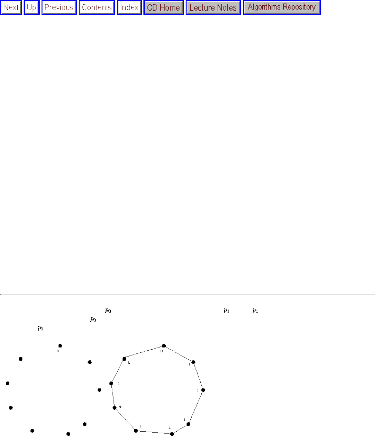
Correctness
Next: Efficiency Up: Correctness and Efficiency Previous: Correctness and Efficiency
Correctness
It is seldom obvious whether a given algorithm correctly solves a given problem. This is why correct algorithms usually come
with a proof of correctness, which is an explanation of why we know that the algorithm correctly takes all instances of the
problem to the desired result. In this book, we will not stress formal proofs of correctness, primarily because they take
substantial mathematical maturity to properly appreciate and construct. However, before we go further it is important to
demonstrate why ``it's obvious'' never suffices as a proof of correctness and usually is flat-out wrong.
To illustrate, let us consider a problem that often arises in manufacturing, transportation, and testing applications. Suppose we
are given a robot arm equipped with a tool, say a soldering iron. In manufacturing circuit boards, all the chips and other
components must be fastened onto the substrate. More specifically, each chip has a set of contact points (or wires) that must
be soldered to the board. To program the robot arm to perform this soldering job, we must first construct an ordering of the
contact points, so that the robot visits (and solders) the first contact point, then visits the second point, third, and so forth until
the job is done. The robot arm must then proceed back to the first contact point to prepare for the next board, thus turning the
tool-path into a closed tour, or cycle.
Since robots are expensive devices, we want to find the tour that minimizes the time it takes to assemble the circuit board. A
reasonable assumption is that the robot arm moves with fixed speed, so that the time it takes to travel between two points is
the same as its distance. In short, we must solve the following algorithm problem:
Input: A set S of n points in the plane.
Output: What is the shortest cycle tour that visits each point in the set S? You are given the job of programming the robot arm.
Stop right now and think about an algorithm to solve this problem. I'll be happy to wait until you find one.
Several possible algorithms might come to mind to solve this problem. Perhaps the most popular idea is the nearest-neighbor
heuristic. Starting from some point , we walk first to its nearest neighbor . From , we walk to its nearest unvisited
neighbor, thus excluding only as a candidate. We now repeat this process until we run out of unvisited points, at which time
we return to to close off the tour. In pseudocode, the nearest-neighbor heuristic looks like this:
Figure: A good example for the nearest neighbor heuristic
file:///E|/BOOK/BOOK/NODE8.HTM (1 of 5) [19/1/2003 1:28:06]
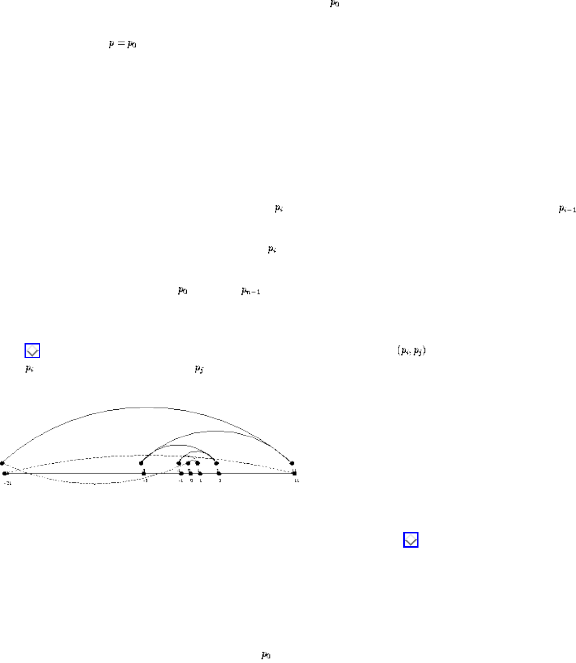
Correctness
NearestNeighborTSP(P)
Pick and visit an initial point from P
i = 0
While there are still unvisited points
i = i+1
Select to be the closest unvisited point to
Visit
Return to from
This algorithm has a lot to recommend it. It is simple to understand and implement. It makes sense to visit nearby points
before we visit faraway points if we want to minimize the total travel time. The algorithm works perfectly on the example in
Figure . The nearest neighbor rule is very efficient, for it looks at each pair of points at most twice, once when
adding to the tour, the other when adding . Against all these positives there is only one problem. This algorithm is
completely wrong.
Figure: A bad example for the nearest neighbor heuristic
Wrong? How can it be wrong? The algorithm always finds a tour, but the trouble is that it doesn't necessarily find the shortest
possible tour. It doesn't necessarily even come close. Consider the set of points in Figure , all of which lie spaced along a
line. The numbers describe the distance that each point lies to the left or right of the point labeled `0'. When we start from the
point `0' and repeatedly walk to the nearest unvisited neighbor, you will see that we keep jumping left-right-left-right over `0'.
A much better (indeed optimal) tour for these points starts from the leftmost point and visits each point as we walk right
before returning at the rightmost point. Try now to imagine your boss's delight as she watches a demo of your robot arm
hopscotching left-right-left-right during the assembly of such a simple board.
``But wait,'' you might be saying. ``The problem was in starting at point `0'. Instead, why don't we always start the nearest-
neighbor rule using the leftmost point as the starting point ? By doing this, we will find the optimal solution on this
file:///E|/BOOK/BOOK/NODE8.HTM (2 of 5) [19/1/2003 1:28:06]
Correctness
example.''
That is 100% true, at least until we rotate our example 90 degrees. Now all points are equally leftmost. If the point `0' were
moved just slightly to the left, it would be picked as the starting point. Now the robot arm will hopscotch up-down-up-down
instead of left-right-left-right, but the travel time will be just as bad as before. No matter what you do to pick the first point,
the nearest neighbor rule is doomed not to work correctly on certain point sets.
Maybe what we need is a different approach. Always walking to the closest point is too restrictive, since it seems to trap us
into making moves we didn't want. A different idea would be to repeatedly connect the closest pair of points whose
connection will not cause a cycle or a three-way branch to be formed. Eventually, we will end up with a single chain
containing all the points in it. At any moment during the execution of this closest-pair heuristic, we will have a set of partial
paths to merge, where each vertex begins as its own partial path. Connecting the final two endpoints gives us a cycle. In
pseudocode:
ClosestPairTSP(P)
Let n be the number of points in set P.
For i=1 to n-1 do
For each pair of endpoints (,t) of distinct partial
paths
if then , ,
and d = dist(,t)
Connect by an edge
Connect the two endpoints by an edge
This closest-pair rule does the right thing on the example in Figure . It starts by connecting `0' to its immediate neighbors,
the points 1 and -1. Subsequently, the next closest pair will alternate left-right, growing the central path by one link at a time.
The closest-pair heuristic is somewhat more complicated and less efficient than the previous one, but at least it gives the right
answer. On this example.
file:///E|/BOOK/BOOK/NODE8.HTM (3 of 5) [19/1/2003 1:28:06]
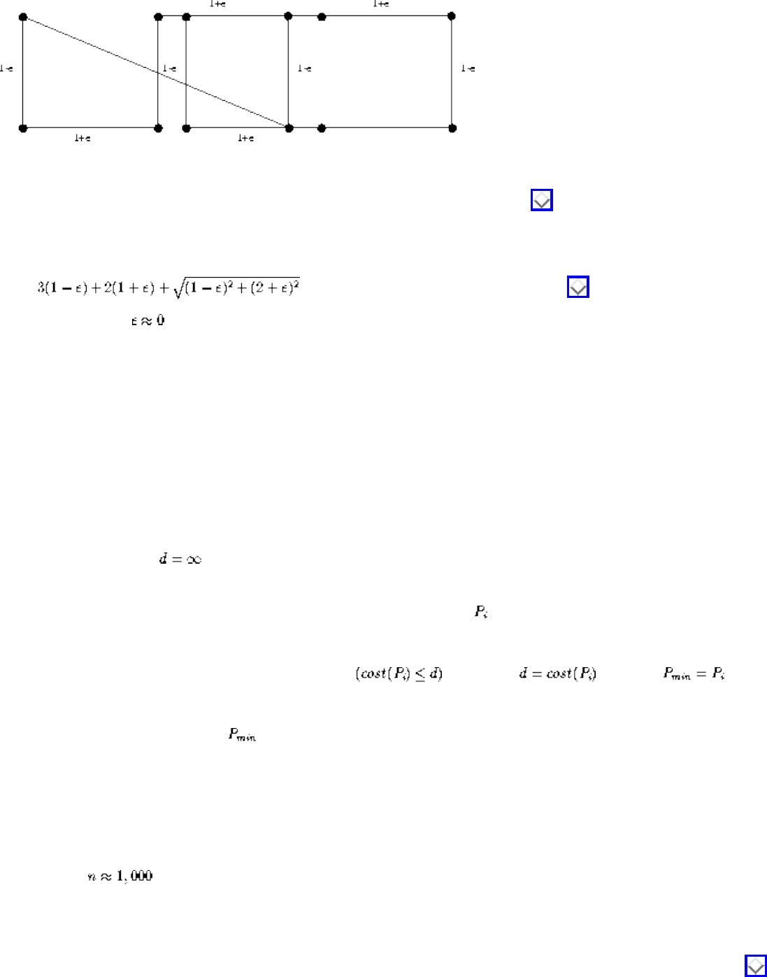
Correctness
Figure: A bad example for the closest-pair heuristic.
But not all examples. Consider what the algorithm does on the point set in Figure (a). It consists of two rows of equally
spaced points, with the rows slightly closer together (distance 1-e) than the neighboring points are spaced within each row
(distance 1+e). Thus the closest pairs of points stretch across the gap, not around the boundary. After we pair off these points,
the closest remaining pairs will connect these pairs alternately around the boundary. The total path length of the closest-pair
tour is . Compared to the tour shown in Figure (b), we travel over 20% farther
than necessary when . Examples exist where the penalty is considerably worse than this.
Thus this second algorithm is also wrong. Which one of these algorithms performs better? You can't tell just by looking at
them. Clearly, both heuristics can end up with very bad tours on very innocent-looking input.
At this point, you might wonder what a correct algorithm for the problem looks like. Well, we could try all enumerating all
possible orderings of the set of points, and then select the ordering that minimizes the total length:
OptimalTSP(P)
For each of the n! permutations of points P
If then and
Return
Since all possible orderings are considered, we are guaranteed to end up with the shortest possible tour. This algorithm is
correct, since we pick the best of all the possibilities. The problem is that it is also extremely slow. The fastest computer in the
world couldn't hope to enumerate all 20! = 2,432,902,008,176,640,000 orderings of 20 points within a day. For real circuit
boards, where , forget about it. All of the world's computers working full time wouldn't come close to finishing your
problem before the end of the universe, at which point it presumably becomes moot.
The quest for an efficient algorithm to solve this so-called traveling salesman problem will take us through much of this book.
If you need to know how the story ends, check out the catalog entry for the traveling salesman problem in Section .
Hopefully, this example has opened your eyes to some of the subtleties of algorithm correctness. Ensuring the optimal answer
file:///E|/BOOK/BOOK/NODE8.HTM (4 of 5) [19/1/2003 1:28:06]

Correctness
on all possible inputs is a difficult but often achievable goal. Seeking counterexamples that break pretender algorithms is a
tricky business, but it is an important part of the algorithm design process.
Next: Efficiency Up: Correctness and Efficiency Previous: Correctness and Efficiency
Algorithms
Mon Jun 2 23:33:50 EDT 1997
file:///E|/BOOK/BOOK/NODE8.HTM (5 of 5) [19/1/2003 1:28:06]
Efficiency
Next: Expressing Algorithms Up: Correctness and Efficiency Previous: Correctness
Efficiency
The skilled algorithm designer is an efficiency expert. Through cunning and experience we seek to get
jobs done as quickly as possible. The benefits of finding an efficient algorithm for a computationally
expensive job can be mind-boggling, as illustrated by several of the war stories scattered through this
book. Section shows how clever algorithms yielded a program that was 30,000 times faster than our
initial attempt!
Upon realizing that a given application runs too slowly, the practical person usually asks the boss to buy
them a faster machine. Sometimes this is the cheapest option. However, the potential win from faster
hardware is typically limited to a factor of ten or so, due to technical constraints (they don't make faster
machines) or economic ones (the boss won't pay for it).
To realize larger performance improvements, we must seek better algorithms. As we will show, a faster
algorithm running on a slower computer will always win for sufficiently large instances. Always.
Usually, problems don't have to get very large before the faster algorithm wins.
Be aware that there are situations where finding the most efficient algorithm for a job is a complete waste
of programmer effort. In any program, there is usually one bottleneck that takes the majority of
computing time. The typical claim is that 90% of the run time of any program is spent in 10% of the
code. Optimizing the other 90% of the program will have little impact on the total run time. Further,
many programs are written with only one or two special instances in mind. If the program will be run just
a few times, or if the job can easily be run overnight, it probably does not pay to make the programmer
work harder in order to reduce cycle consumption.
Next: Expressing Algorithms Up: Correctness and Efficiency Previous: Correctness
Algorithms
Mon Jun 2 23:33:50 EDT 1997
file:///E|/BOOK/BOOK/NODE9.HTM [19/1/2003 1:28:06]
Expressing Algorithms
Next: Keeping Score Up: Introduction to Algorithms Previous: Efficiency
Expressing Algorithms
Describing algorithms requires a notation for expressing a sequence of steps to be performed. The three
most common options are (1) English, (2) pseudocode, or (3) a real programming language. Pseudocode
is perhaps the most mysterious of the bunch, but it is best defined as a programming language that never
complains about syntax errors. All three methods can be useful in certain circumstances, since there is a
natural tradeoff between greater ease of expression and precision. English is the most natural but least
precise language, while C and Pascal are precise but difficult to write and understand. Pseudocode is
useful because it is a happy medium.
The correct choice of which notation is best depends upon which of the three methods you are most
comfortable with. I prefer to describe the ideas of an algorithm in English, moving onto a more formal,
programming-language-like pseudocode to clarify sufficiently tricky details of the algorithm. A common
mistake among my students is to use pseudocode to take an ill-defined idea and dress it up so that it looks
more formal. In the real world, you only fool yourself when you pull this kind of stunt.
The implementation complexity of an algorithm is usually why the fastest algorithm known for a problem
may not be the most appropriate for a given application. An algorithm's implementation complexity is
often a function of how it has been described. Fast algorithms often make use of very complicated data
structures, or use other complicated algorithms as subroutines. Turning these algorithms into programs
requires building implementations of every substructure. Each catalog entry in Section points out
available implementations of algorithms to solve the given problem. Hopefully, these can be used as
building blocks to reduce the implementation complexity of algorithms that use them, thus making more
complicated algorithms worthy of consideration in practice.
Next: Keeping Score Up: Introduction to Algorithms Previous: Efficiency
Algorithms
Mon Jun 2 23:33:50 EDT 1997
file:///E|/BOOK/BOOK/NODE10.HTM [19/1/2003 1:28:07]
Keeping Score
Next: The RAM Model of Up: Introduction to Algorithms Previous: Expressing Algorithms
Keeping Score
Algorithms are the most important, durable, and original part of computer science because they can be
studied in a language- and machine-independent way. This means that we need techniques that enable us
to compare algorithms without implementing them. Our two most important tools are (1) the RAM
model of computation and (2) asymptotic analysis of worst-case complexity.
This method of keeping score will be the most mathematically demanding part of this book. However, it
is important to understand why we need both of these tools to analyze the performance of algorithms.
Once you understand the intuition behind these ideas, the formalism becomes a lot easier to deal with.
● The RAM Model of Computation
● Best, Worst, and Average-Case Complexity
Algorithms
Mon Jun 2 23:33:50 EDT 1997
file:///E|/BOOK/BOOK/NODE11.HTM [19/1/2003 1:28:07]

The RAM Model of Computation
Next: BestWorst, and Average-Case Up: Keeping Score Previous: Keeping Score
The RAM Model of Computation
Machine-independent algorithm design depends upon a hypothetical computer called the Random Access
Machine or RAM. Under this model of computation, we are confronted with a computer where:
● Each ``simple'' operation (+, *, -, =, if, call) takes exactly 1 time step.
● Loops and subroutines are not considered simple operations. Instead, they are the composition of
many single-step operations. It makes no sense for ``sort'' to be a single-step operation, since
sorting 1,000,000 items will take much longer than sorting 10 items. The time it takes to run
through a loop or execute a subprogram depends upon the number of loop iterations or the
specific nature of the subprogram.
● Each memory access takes exactly one time step, and we have as much memory as we need. The
RAM model takes no notice of whether an item is in cache or on the disk, which simplifies the
analysis.
Under the RAM model, we measure the run time of an algorithm by counting up the number of steps it
takes on a given problem instance. By assuming that our RAM executes a given number of steps per
second, the operation count converts easily to the actual run time.
The RAM is a simple model of how computers perform. A common complaint is that it is too simple,
that these assumptions make the conclusions and analysis too coarse to believe in practice. For example,
multiplying two numbers takes more time than adding two numbers on most processors, which violates
the first assumption of the model. Memory access times differ greatly depending on whether data sits in
cache or on the disk, thus violating the third assumption. Despite these complaints, the RAM is an
excellent model for understanding how an algorithm will perform on a real computer. It strikes a fine
balance by capturing the essential behavior of computers while being simple to work with. We use the
RAM model because it is useful in practice.
Every model has a size range over which it is useful. Take, for example, the model that the earth is flat.
You might argue that this is a bad model, since the earth is not flat. However, when laying the foundation
of a house, the flat earth model is sufficiently accurate that it can be reliably used. Further, it is so much
easier to manipulate a flat-earth model that it is inconceivable that you would try to think spherically
when you don't have to.
The same situation is true with the RAM model of computation. We make an abstraction that in general
is very useful. It is quite difficult to design an algorithm such that the RAM model will give you
file:///E|/BOOK/BOOK/NODE12.HTM (1 of 2) [19/1/2003 1:28:08]

The RAM Model of Computation
substantially misleading results, by performing either much better or much worse in practice than the
model suggests. The robustness of the RAM enables us to analyze algorithms in a machine-independent
way.
Next: BestWorst, and Average-Case Up: Keeping Score Previous: Keeping Score
Algorithms
Mon Jun 2 23:33:50 EDT 1997
file:///E|/BOOK/BOOK/NODE12.HTM (2 of 2) [19/1/2003 1:28:08]
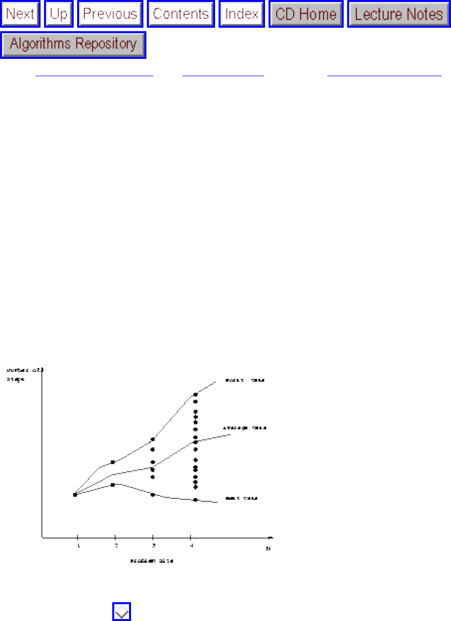
Best, Worst, and Average-Case Complexity
Next: The Big Oh Notation Up: Keeping Score Previous: The RAM Model of
Best, Worst, and Average-Case Complexity
Using the RAM model of computation, we can count how many steps our algorithm will take on any
given input instance by simply executing it on the given input. However, to really understand how good
or bad an algorithm is, we must know how it works over all instances.
To understand the notions of the best, worst, and average-case complexity, one must think about running
an algorithm on all possible instances of data that can be fed to it. For the problem of sorting, the set of
possible input instances consists of all the possible arrangements of all the possible numbers of keys. We
can represent every input instance as a point on a graph, where the x-axis is the size of the problem (for
sorting, the number of items to sort) and the y-axis is the number of steps taken by the algorithm on this
instance. Here we assume, quite reasonably, that it doesn't matter what the values of the keys are, just
how many of them there are and how they are ordered. It should not take longer to sort 1,000 English
names than it does to sort 1,000 French names, for example.
Figure: Best, worst, and average-case complexity
As shown in Figure , these points naturally align themselves into columns, because only integers
represent possible input sizes. After all, it makes no sense to ask how long it takes to sort 10.57 items.
Once we have these points, we can define three different functions over them:
● The worst-case complexity of the algorithm is the function defined by the maximum number of
steps taken on any instance of size n. It represents the curve passing through the highest point of
file:///E|/BOOK/BOOK/NODE13.HTM (1 of 2) [19/1/2003 1:28:09]
Best, Worst, and Average-Case Complexity
each column.
● The best-case complexity of the algorithm is the function defined by the minimum number of
steps taken on any instance of size n. It represents the curve passing through the lowest point of
each column.
● Finally, the average-case complexity of the algorithm is the function defined by the average
number of steps taken on any instance of size n.
In practice, the most useful of these three measures proves to be the worst-case complexity, which many
people find counterintuitive. To illustrate why worst-case analysis is important, consider trying to project
what will happen to you if you bring n dollars to gamble in a casino. The best case, that you walk out
owning the place, is possible but so unlikely that you should place no credence in it. The worst case, that
you lose all n dollars, is easy to calculate and distressingly likely to happen. The average case, that the
typical person loses 87.32% of the money that they bring to the casino, is difficult to compute and its
meaning is subject to debate. What exactly does average mean? Stupid people lose more than smart
people, so are you smarter or dumber than the average person, and by how much? People who play craps
lose more money than those playing the nickel slots. Card counters at blackjack do better on average than
customers who accept three or more free drinks. We avoid all these complexities and obtain a very useful
result by just considering the worst case.
The important thing to realize is that each of these time complexities defines a numerical function,
representing time versus problem size. These functions are as well-defined as any other numerical
function, be it or the price of General Motors stock as a function of time. Time
complexities are complicated functions, however. In order to simplify our work with such messy
functions, we will need the big Oh notation.
Next: The Big Oh Notation Up: Keeping Score Previous: The RAM Model of
Algorithms
Mon Jun 2 23:33:50 EDT 1997
file:///E|/BOOK/BOOK/NODE13.HTM (2 of 2) [19/1/2003 1:28:09]
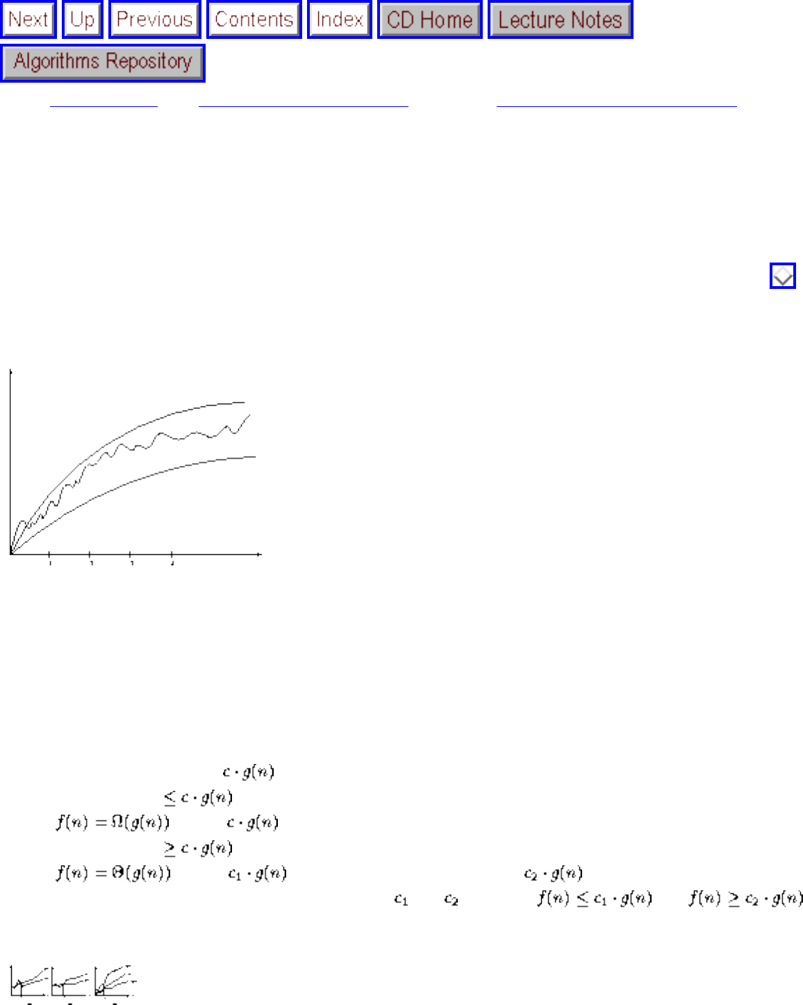
The Big Oh Notation
Next: Growth Rates Up: Introduction to Algorithms Previous: BestWorst, and Average-Case
The Big Oh Notation
We have agreed that the best, worst, and average-case complexities of a given algorithm are numerical
functions of the size of the instances. However, it is difficult to work with these functions exactly
because they are often very complicated, with many little up and down bumps, as shown in Figure .
Thus it is usually cleaner and easier to talk about upper and lower bounds of such functions. This is
where the big Oh notation comes into the picture.
Figure: Upper and lower bounds smooth out the behavior of complex functions
We seek this smoothing in order to ignore levels of detail that do not impact our comparison of
algorithms. Since running our algorithm on a machine that is twice as fast will cut the running times of
all algorithms by a multiplicative constant of two, such constant factors would be washed away in
upgrading machines. On the RAM we ignore such constant factors anyway and therefore might as well
ignore them when comparing two algorithms. We use the following notation:
● f(n) = O(g(n)) means is an upper bound on f(n). Thus there exists some constant c such that
f(n) is always , for large enough n.
● means is a lower bound on f(n). Thus there exists some constant c such that
f(n) is always , for large enough n.
● means is an upper bound on f(n) and is a lower bound on f(n), for
large enough n. Thus there exists constants and such that and .
This means that g(n) is a nice, tight bound on f(n).
file:///E|/BOOK/BOOK/NODE14.HTM (1 of 2) [19/1/2003 1:28:11]
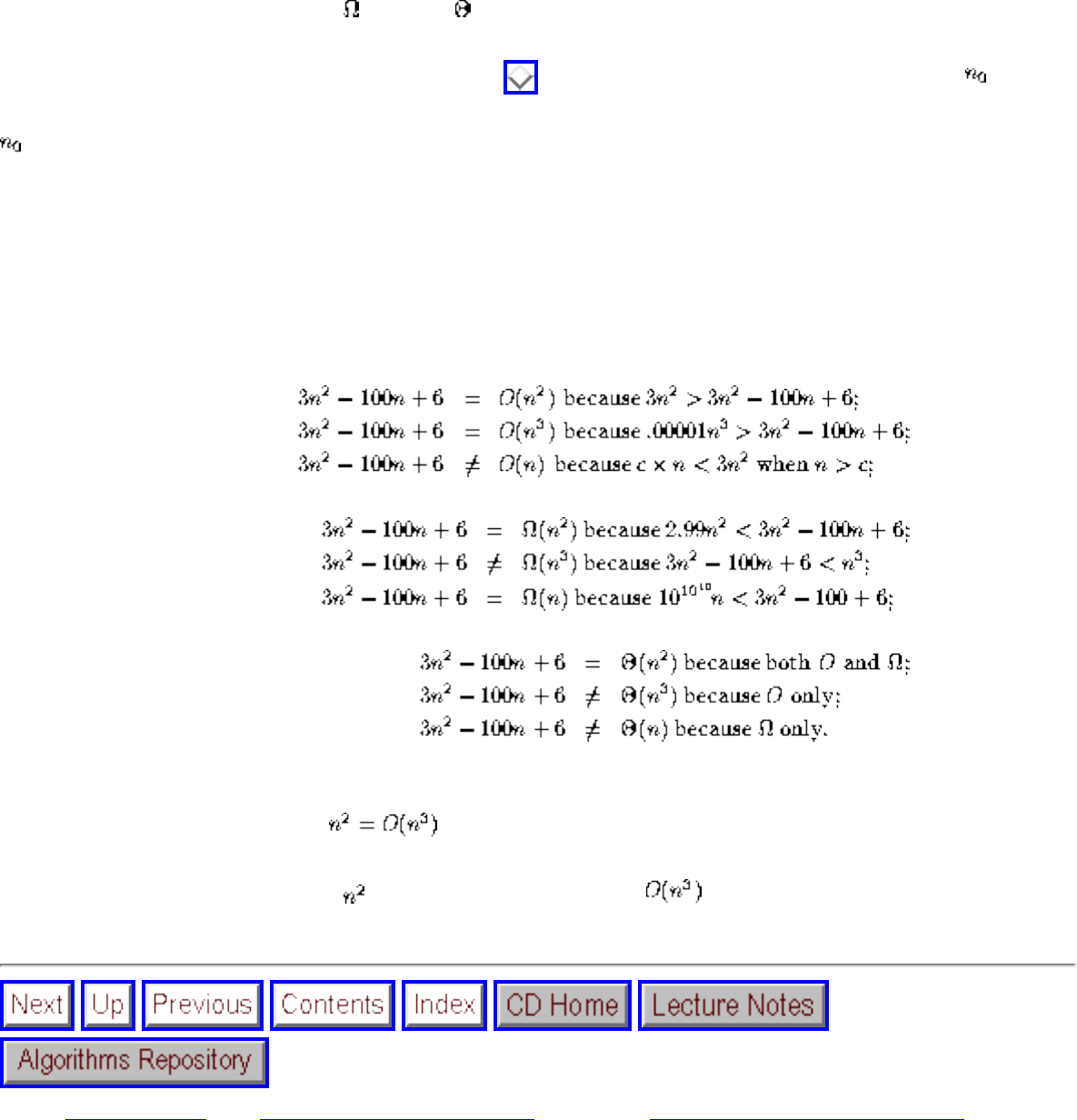
The Big Oh Notation
Figure: Illustrating the (a) O, (b) , and (c) notations
Got it? These definitions are illustrated in Figure . All of these definitions imply a constant beyond
which they are always satisfied. We are not concerned about small values of n, i.e. anything to the left of
. After all, do you really care whether one sorting algorithm sorts six items faster than another
algorithm, or which one is faster when sorting 1,000 or 1,000,000 items? The big Oh notation enables us
to ignore details and focus on the big picture.
Make sure you understand this notation by working through the following examples. We choose certain
constants in the explanations because they work and make a point, but you are free to choose any
constant that maintains the same inequality:
The big Oh notation provides for a rough notion of equality when comparing functions. It is somewhat
jarring to see an expression like , but its meaning can always be resolved by going back to the
definitions in terms of upper and lower bounds. It is perhaps most instructive to read `=' as meaning one
of the functions that are. Clearly, is one of functions that are .
Next: Growth Rates Up: Introduction to Algorithms Previous: BestWorst, and Average-Case
Algorithms
Mon Jun 2 23:33:50 EDT 1997
file:///E|/BOOK/BOOK/NODE14.HTM (2 of 2) [19/1/2003 1:28:11]
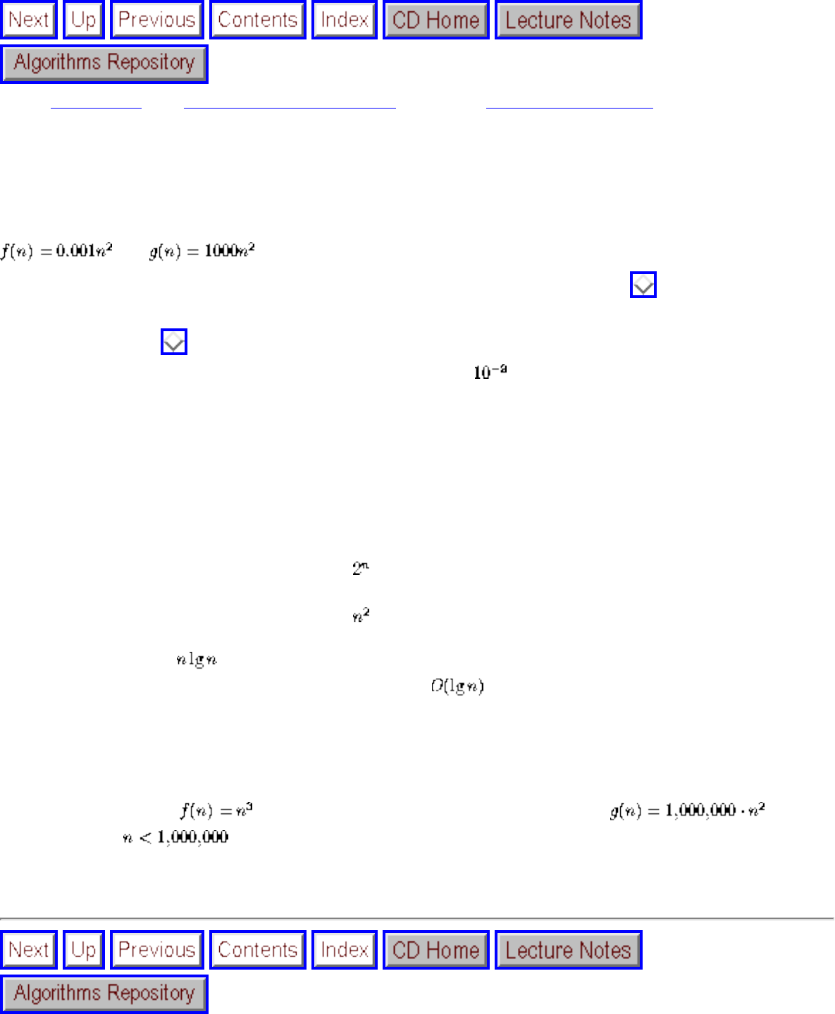
Growth Rates
Next: Logarithms Up: Introduction to Algorithms Previous: The Big Oh Notation
Growth Rates
In working with the big Oh notation, we cavalierly discard the multiplicative constants. The functions
and are treated identically, even though g(n) is a million times larger than
f(n) for all values of n. The method behind this madness is illustrated by Figure , which tabulates the
growth rate of several functions arising in algorithm analysis, on problem instances of reasonable size.
Specifically, Figure shows how long it takes for algorithms that use f(n) operations to complete on a
fast computer where each operation takes one nanosecond ( seconds). Study the table for a few
minutes and the following conclusions become apparent:
Figure: Growth rates of common functions measured in nanoseconds
● All of these algorithms take about the same amount of time for n=10.
● The algorithm whose running time is n! becomes useless well before n=20.
● The algorithm whose running time is has a greater operating range, but it becomes impractical
for n > 40.
● The algorithm whose running time is is perfectly reasonable up to about n=100, but it quickly
deteriorates with larger inputs. For n > 1,000,000 it likely to be hopeless.
● Both the n and algorithms remain practical on inputs of up to one billion items.
● You can't hope to find a real problem where an algorithm is going to be too slow in
practice.
The bottom line is that even by ignoring constant factors, we can get an excellent idea of whether a given
algorithm will be able to run in a reasonable amount of time on a problem of a given size. An algorithm
whose running time is seconds will beat one whose running time is seconds
only so long as . Such enormous constant factor differences between algorithms occur in
practice far less frequently than such large problems do.
file:///E|/BOOK/BOOK/NODE15.HTM (1 of 2) [19/1/2003 1:28:12]

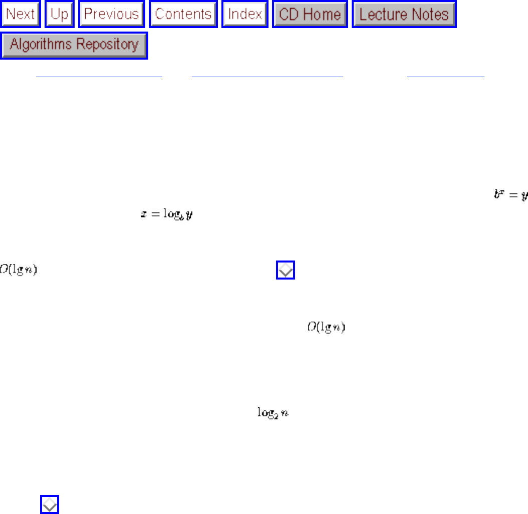
Logarithms
Next: Modeling the Problem Up: Introduction to Algorithms Previous: Growth Rates
Logarithms
Logarithm is an anagram of algorithm, but that's not why the wily algorist needs to know what
logarithms are and where they come from. You've seen the button on your calculator but have likely
forgotten why it is there. A logarithm is simply an inverse exponential function. Saying is
equivalent to saying that . Exponential functions are functions that grow at a distressingly fast
rate, as anyone who has ever tried to pay off a mortgage or bank loan understands. Thus inverse
exponential functions, i.e. logarithms, grow refreshingly slowly. If you have an algorithm that runs in
time, take it and run. As shown by Figure , this will be blindingly fast even on very large
problem instances.
Binary search is an example of an algorithm that takes time. In a telephone book with n names,
you start by comparing the name that you are looking for with the middle, or (n/2)nd name, say Monroe,
Marilyn. Regardless of whether you are looking someone before this middle name (Dean, James) or after
it (Presley, Elvis), after only one such comparison you can forever disregard one half of all the names in
the book. The number of steps the algorithm takes equals the number of times we can halve n before only
one name is left. By definition, this is exactly . Thus twenty comparisons suffice to find any name
in the million-name Manhattan phone book! The power of binary search and logarithms is one of the
most fundamental ideas in the analysis of algorithms. This power becomes apparent if we could imagine
living in a world with only unsorted telephone books.
Figure is another example of logarithms in action. This table appears in the Federal Sentencing
Guidelines, used by courts throughout the United States. These guidelines are an attempt to standardize
criminal sentences, so that a felon convicted of a crime before one judge receives the same sentence as
they would before a different judge. To accomplish this, the judges have prepared an intricate point
function to score the depravity of each crime and map it to time-to-serve.
file:///E|/BOOK/BOOK/NODE16.HTM (1 of 3) [19/1/2003 1:28:14]
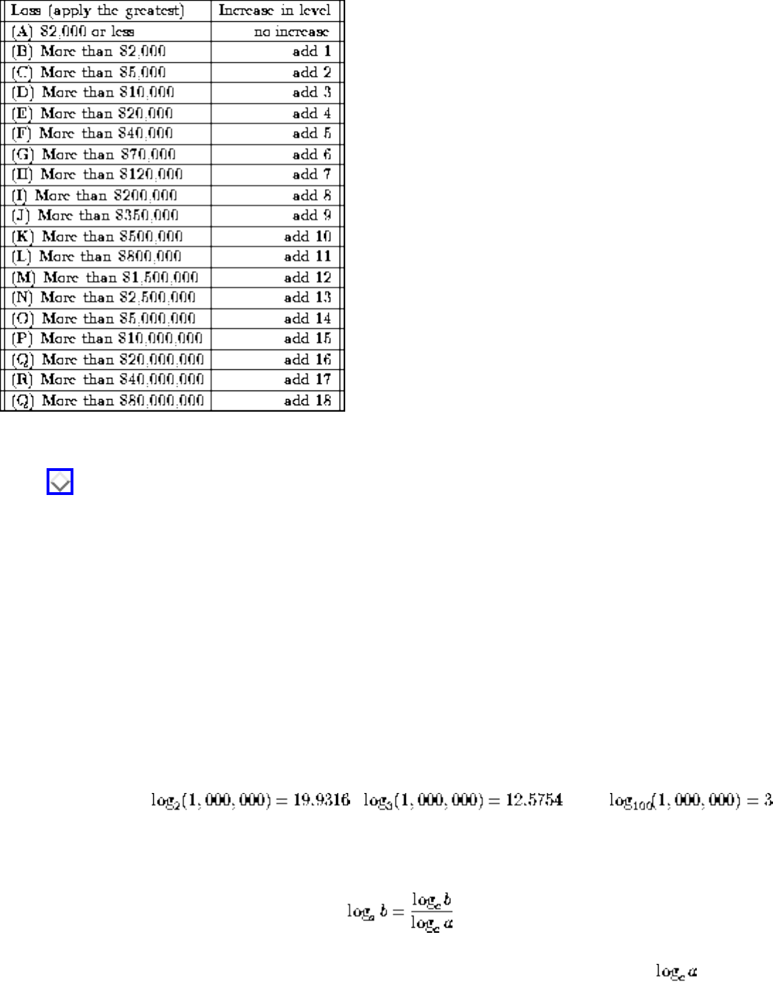
Logarithms
Figure: The Federal Sentencing Guidelines for Fraud
Figure gives the actual point function for fraud, a table mapping dollars stolen to points. Notice that
the punishment increases by one level each time the amount of money stolen roughly doubles. That
means that the level of punishment (which maps roughly linearly to the amount of time served) grows
logarithmically with the amount of money stolen. Think for a moment about the consequences of this.
Michael Milken sure did. It means that the total sentence grows extremely slowly with the amount of
money you steal. Knocking off five liquor stores for $10,000 each will get you far more time than
embezzling $100,000 once. The corresponding benefit of stealing really large amounts of money is even
greater. The moral of logarithmic growth is clear: ``If you are gonna do the crime, make it worth the
time!''
Two mathematical properties of logarithms are important to understand:
● The base of the logarithm has relatively little impact on the growth rate: Compare the following
three values: , , and . A
big change in the base of the logarithm produces relatively little difference in the value of the log.
This is a consequence of the formula for changing the base of the logarithm:
Changing the base of the log from a to c involves multiplying or dividing by . This will be
lost to the big Oh notation whenever a and c are constants, as is typical. Thus we are usually
file:///E|/BOOK/BOOK/NODE16.HTM (2 of 3) [19/1/2003 1:28:14]
Logarithms
justified in ignoring the base of the logarithm when analyzing algorithms.
When performing binary search in a telephone book, how important is it that each query split the
book exactly in half? Not much. Suppose we did such a sloppy job of picking our queries such
that each time we split the book 1/3 to 2/3 instead of 1/2 to 1/2. For the Manhattan telephone
book, we now use queries in the worst case, not a significant change from
. The power of binary search comes from its logarithmic complexity, not the
base of the log.
● Logarithms cut any function down to size: The growth rate of the logarithm of any polynomial
function is . This follows because
The power of binary search on a wide range of problems is a consequence of this observation. For
example, note that doing a binary search on a sorted array of things requires only twice as many
comparisons as a binary search on n things. Logarithms efficiently cut any function down to size.
Next: Modeling the Problem Up: Introduction to Algorithms Previous: Growth Rates
Algorithms
Mon Jun 2 23:33:50 EDT 1997
file:///E|/BOOK/BOOK/NODE16.HTM (3 of 3) [19/1/2003 1:28:14]
Modeling the Problem
Next: About the War Stories Up: Introduction to Algorithms Previous: Logarithms
Modeling the Problem
Modeling is the art of formulating your application in terms of precisely described, well-understood
problems. Proper modeling is the key to applying algorithmic design techniques to any real-world
problem. Indeed, proper modeling can eliminate the need to design or even implement algorithms by
relating your application to what has been done before. Proper modeling is the key to effectively using
the problem catalog in Part II of this book.
Real-world applications involve real-world objects. You might be working on a system to route traffic in
a network, to find the best way to schedule classrooms in a university, or to search for patterns in a
corporate database. Most algorithms, however, are designed to work on rigorously defined abstract
structures such as permutations, graphs, and sets. After all, if you can't define what you want to do, you
can't hope to compute it. You must first describe your problem abstractly, in terms of fundamental
structures and properties.
Whatever your application is, odds are very good that others before you have stumbled upon the same
algorithmic problem, perhaps in substantially different contexts. Therefore, to find out what is known
about your particular ``widget optimization problem,'' you can't hope to look in a book under widget. You
have to formulate widget optimization in terms of computing properties of abstract structures such as:
● Permutations, which are arrangements, or orderings, of items. For example, and
are two distinct permutations of the same set of four integers. Permutations are likely
the object in question whenever your problem seeks an ``arrangement,'' ``tour,'' ``ordering,'', or
``sequence.''
● Subsets, which represent selections from a set of items. For example, and are two
distinct subsets of the first four integers. Order does not matter in subsets the way it does with
permutations, so the subsets and would be considered identical. Subsets are likely
the object in question whenever your problem seeks a ``cluster,'' ``collection,'' ``committee,''
``group,'' ``packaging,'' or ``selection.''
file:///E|/BOOK/BOOK/NODE17.HTM (1 of 3) [19/1/2003 1:28:15]
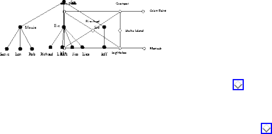
Modeling the Problem
Figure: Modeling real-world structures with trees and graphs
● Trees, which represent hierarchical relationships between items. Figure (a) illustrates a portion
of the family tree of the Skiena clan. Trees are likely the object in question whenever your
problem seeks a ``hierarchy,'' ``dominance relationship,'' ``ancestor/decendant relationship,'' or
``taxonomy.''
● Graphs, which represent relationships between arbitrary pairs of objects. Figure (b) models a
network of roads as a graph, where the vertices are cities and the edges are roads connecting pairs
of cities. Graphs are likely the object in question whenever you seek a ``network,'' ``circuit,''
``web,'' or ``relationship.''
● Points, which represent locations in some geometric space. For example, the locations of
McDonald's restaurants can be described by points on a map/plane. Points are likely the object in
question whenever your problems work on ``sites,'' ``positions,'' ``data records,'' or ``locations.''
● Polygons, which represent regions in some geometric space. For example, the borders of a
country can be described by a polygon on a map/plane. Polygons and polyhedra are likely the
object in question whenever you are working on ``shapes,'' ``regions,'' ``configurations,'' or
``boundaries.''
● Strings, which represent sequences of characters or patterns. For example, the names of students
in a class can be represented by strings. Strings are likely the object in question whenever you are
dealing with ``text,'' ``characters,'' ``patterns,'' or ``labels.''
These fundamental structures all have associated problems and properties, which are presented in the
catalog of Part II. Familiarity with all of these problems is important, because they provide the language
we use to model applications. To become fluent in this vocabulary, browse through the catalog and study
the input and output pictures for each problem. Understanding all or most of these problems, even at a
cartoon/definition level, will enable you to know where to look later when the problem arises in your
application.
Examples of successful application modeling will be presented in the war stories spaced throughout this
book. However, some words of caution are in order. The act of modeling reduces your application to one
of a small number of existing problems and structures. Such a process is inherently constraining, and
certain details might not fit easily into the given model. Also, certain problems can be modeled in several
different ways, some much better than others.
Modeling is only the first step in designing an algorithm for a problem. Be alert for how the details of
file:///E|/BOOK/BOOK/NODE17.HTM (2 of 3) [19/1/2003 1:28:15]

Modeling the Problem
your applications differ from a candidate model. But don't be too quick to say that your problem is
unique and special. Temporarily ignoring details that don't fit can free the mind to ask whether they were
fundamental in the first place.
Next: About the War Stories Up: Introduction to Algorithms Previous: Logarithms
Algorithms
Mon Jun 2 23:33:50 EDT 1997
file:///E|/BOOK/BOOK/NODE17.HTM (3 of 3) [19/1/2003 1:28:15]
About the War Stories
Next: War Story: Psychic Modeling Up: Introduction to Algorithms Previous: Modeling the Problem
About the War Stories
The best way to become convinced that careful algorithm design can have a significant impact on
performance is to look at case studies. By carefully studying other people's experiences, we learn how
they might apply to our work.
Jon Bentley's Programming Pearls columns are probably the most interesting collection of algorithmic
``war stories'' currently available. Originally published in the Communications of the ACM, they have
been collected in two books [Ben86, Ben90]. Fredrick Brooks's The Mythical Man Month [Bro74] is
another wonderful collection of war stories, focused more on software engineering than algorithm
design, but they remain a source of considerable wisdom. Every programmer should read all three of
these books, for pleasure as well as insight.
Scattered throughout this text are several of our own war stories, presenting our successful (and
occasionally unsuccessful) algorithm design efforts on real applications. We hope that the reader will be
able to internalize these experiences so that they will serve as models for their own attacks on problems.
Every one of the war stories is true. Of course, the stories improve somewhat in the retelling, and the
dialogue has been punched up to make it more interesting to read. However, I have tried to honestly trace
the process of going from a raw problem to a solution, so you can watch how the process unfolded.
The Oxford English Dictionary defines an algorist as ``one skillful in reckonings or figuring.'' In these
stories, I have tried to capture some of the attitude, or mindset, of the algorist in action as they attack a
problem.
The various war stories usually involve at least one and often several problems from the problem catalog
in Part II. The appropriate section of the catalog is referenced wherever it occurs. This emphasizes the
benefits of modeling your application in terms of standard algorithm problems. By using the catalog, you
will be able to pull out what is known about any problem whenever it is needed.
file:///E|/BOOK/BOOK/NODE18.HTM (1 of 2) [19/1/2003 1:28:16]

War Story: Psychic Modeling
Next: Exercises Up: Introduction to Algorithms Previous: About the War Stories
War Story: Psychic Modeling
The call came for me out of the blue as I sat in my office.
``Professor Skiena, I hope you can help me. I'm the President of Lotto Systems Group Inc., and we need an algorithm for a
problem arising in our latest product.''
``Sure,'' I replied. After all, the dean of my engineering school is always eager for our faculty to interact with industry.
``At Lotto Systems Group, we market a program designed to improve our customers' psychic ability to predict winning
lottery numbers. In a standard lottery, each ticket consists of 6 numbers selected from, say, 1 to 44. Thus any given ticket
has only a very small chance of winning. However, after proper training, our clients can visualize a set of, say, 15 numbers
out of the 44 and be certain that at least 4 of them will be on the winning ticket. Are you with me so far?''
``Probably not,'' I replied. But then I recalled how my dean wants us to interact with industry.
``Our problem is this. After the psychic has narrowed the choices down to 15 numbers and is certain that at least 4 of them
will be on the winning ticket, we must find the most efficient way to exploit this information. Suppose that a cash prize is
awarded whenever you pick at least three of the correct numbers on your ticket. We need an algorithm to construct the
smallest set of tickets that we must buy in order to guarantee that we win at least one prize.''
``Assuming the psychic is correct?''
``Yes, assuming the psychic is correct. We need a program that prints out a list of all the tickets that the psychic should buy
in order to minimize their investment. Can you help us?''
I thought about the problem for a minute. Maybe they did have psychic ability, for they had clearly come to the right place.
Identifying the best subset of tickets to buy was very much a combinatorial algorithm problem. It was going to be some type
of covering problem, where each ticket we buy was going to ``cover'' some of the possible 4-element subsets of the
psychic's set. Finding the absolute smallest set of tickets to cover everything was a special instance of the NP-complete
problem set cover (discussed in Section ) and presumably computationally intractable.
file:///E|/BOOK/BOOK/NODE19.HTM (1 of 5) [19/1/2003 1:28:18]
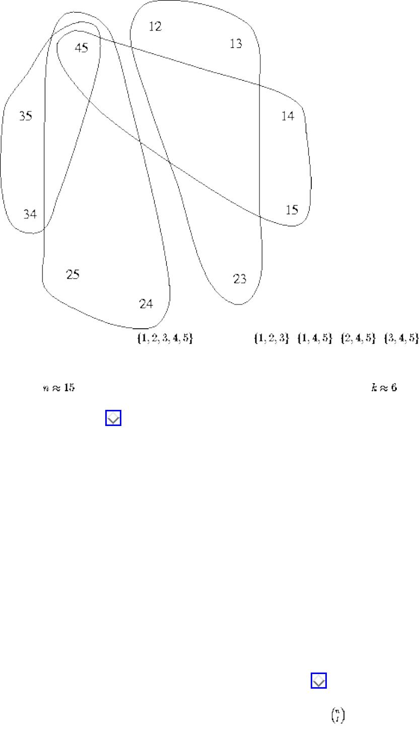
War Story: Psychic Modeling
Figure: Covering all pairs of with tickets , , ,
It was indeed a special instance of set cover, completely specified by only four numbers: the size n of the candidate set S
(typically ), the number of k slots for numbers on each ticket (typically ), the number of psychically promised
correct numbers j from S (say j=4), and finally, the number of numbers l matching the winning ticket necessary to win a
prize (say l=3). Figure illustrates a covering of a smaller instance, where n=5, k=3, and j=l=2.
``Although it will be hard to find the exact minimum set of tickets to buy, with heuristics I should be able to get you pretty
close to the cheapest covering ticket set,'' I told him. ``Will that be good enough?''
``So long as it generates better ticket sets than my competitor's program, that will be fine. His system doesn't always provide
enough coverage to guarantee a win. I really appreciate your help on this, Professor Skiena.''
``One last thing. If your program can train people to pick lottery winners, why don't you use it to win the lottery yourself?''
``I look forward to talking to you again real soon, Professor Skiena. Thanks for the help.''
I hung up the phone and got back to thinking. It seemed like a fun problem, and the perfect project to give to a bright
undergraduate. After it was modeled in terms of sets and subsets, the basic components of a solution seemed fairly
straightforward:
● We needed the ability to generate all subsets of k numbers from the candidate set S. Algorithms for generating and
ranking/unranking subsets of sets are presented in Section .
● We needed the right formulation of what it meant to have a covering set of purchased tickets. The obvious criteria
would be to pick a small set of tickets such that for each of the l-subsets of S that might pay off with the prize, we
file:///E|/BOOK/BOOK/NODE19.HTM (2 of 5) [19/1/2003 1:28:18]
War Story: Psychic Modeling
have purchased at least one ticket that contains it.
● For each new ticket we decided to buy, we would need to keep track of which prize combinations we have thus far
covered. Presumably, we would want to buy tickets to cover as many thus-far-uncovered prize combinations as
possible. The currently covered combinations are a subset of all possible combinations, so we would need a data
structure to represent the subset. Such data structures are discussed in Section . The best candidate seemed to be a
bit vector, which would permit a constant time query of ``is this combination already covered?'' in concert with a
way to rank the subset, i.e. hash it to a unique integer.
● We would need a search mechanism to decide which ticket to buy next. For small enough set sizes, we could do an
exhaustive search over all possible subsets of tickets and pick the smallest one. For larger sizes, a randomized search
process like simulated annealing (see Section ) would select tickets-to-buy to cover as many uncovered
combinations as possible. By repeating this randomized procedure several times and picking the best solution, we
would be likely to come up with a very good set of tickets.
Excluding the search mechanism, the pseudocode for the bookkeeping looked something like this:
LottoTicketSet(n,k,l)
Initialize the -element bit-vector V to all false
While there exists a false entry of V
Select a k-subset T of as the next
ticket to buy
For each of the l-subsets of T,
Report the set of tickets bought
The bright undergraduate, Fayyaz Younas, rose to the challenge. Based on this framework, he implemented a brute-force
search algorithm and found optimal solutions for problems with in a reasonable time. To solve larger problems, he
implemented a random search procedure, tweaking it for a while before settling on the best variant. Finally, the day arrived
when we could call Lotto Systems Group and announce that we had solved the problem.
``See, our program found that optimal solution for n=15, k=6, j=6, l=3 meant buying 28 tickets.''
``Twenty-eight tickets!'' complained the president. ``You must have a bug. Look, these five tickets will suffice to cover
everything twice over: , , , , .''
file:///E|/BOOK/BOOK/NODE19.HTM (3 of 5) [19/1/2003 1:28:18]
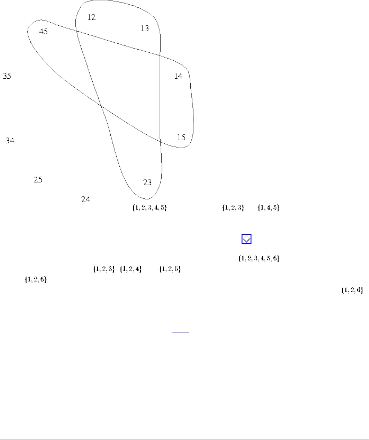
War Story: Psychic Modeling
Figure: Guaranteeing a winning ticket from using only tickets and
We fiddled with this example for a while before admitting that he was right. We hadn't modeled the problem correctly! In
fact, we didn't need to explicitly cover all possible winning combinations. Figure illustrates the principle by giving a
better solution to the previous small example. As a different example, suppose we needed three numbers on a five element
ticket to win, and the psychic had promised us that four numbers would be from . Suppose that we had bought
tickets that covered the subsets , , and . There would be no need to buy a ticket that explicitly
covered , because if 1 and 2 and two other psychic numbers were on a winning ticket, then at least one of the other
two psychic numbers would have to be either 3, 4, or 5. If 1 and 2 were not on the winning ticket, a ticket covering
would do us absolutely no good. Thus we were trying to cover too many combinations, and the penny-pinching psychics
were unwilling to pay for such extravagance.
Fortunately, this story has a happy ending, as reported in [YS96]. The general outline of our search-based solution described
above still holds for the real problem. All that is needed to fix it is to change how many uncovered subsets we credit for
covering with a given set of tickets. After this modification, we obtained the kind of results they were hoping for. Lotto
Systems Group gratefully accepted our program to incorporate into their products, and we hope they hit the jackpot with it.
The moral of this story is to make sure that you correctly model the problem before trying to solve it. In our case, we came
up with a reasonable model for the problem but didn't work hard enough to validate it before we started to program. Our
misinterpretation would have become obvious had we worked out a small but non-trivial example by hand and bounced it
off our sponsor before beginning work. Our success in recovering from the error is a tribute to the basic correctness of our
initial formulation and our use of well-defined routines and abstractions for such tasks as (1) ranking/unranking k-subsets,
(2) the set data structure, and (3) combinatorial search.
file:///E|/BOOK/BOOK/NODE19.HTM (4 of 5) [19/1/2003 1:28:18]

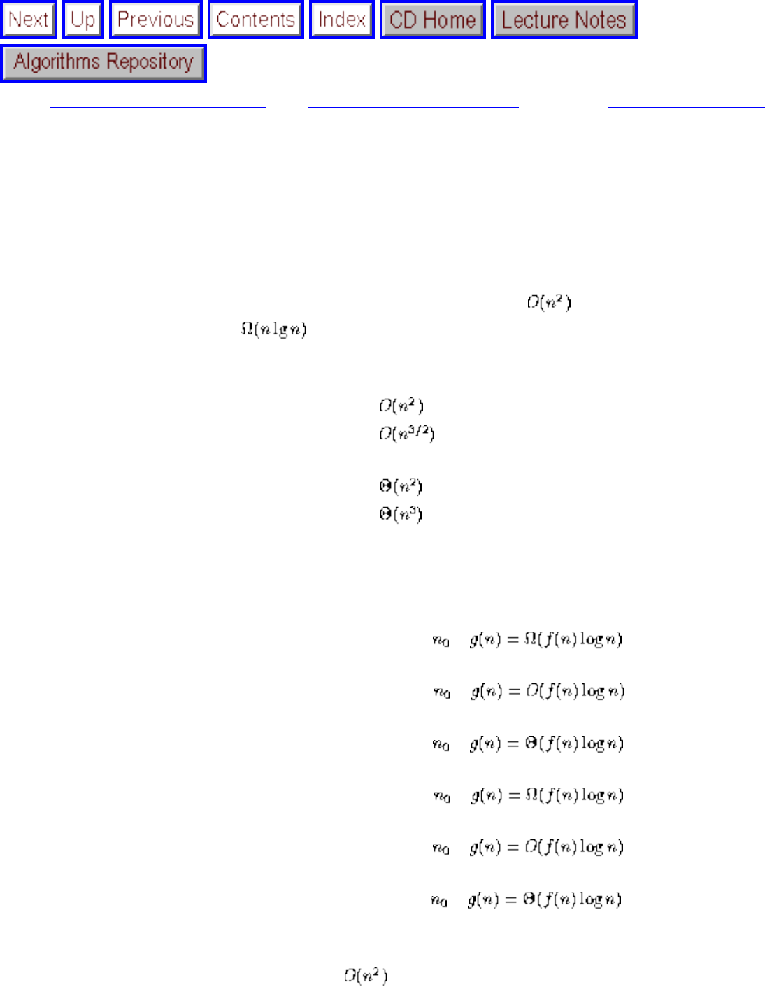
Exercises
Next: Implementation Challenges Up: Introduction to Algorithms Previous: War Story: Psychic
Modeling
Exercises
1. Let P be a problem. The worst-case time complexity of P is . The worst-case time
complexity of P is also . Let A be an algorithm that solves P. Which subset of the
following statements are consistent with this information about the complexity of P?
❍ A has worst-case time complexity .
❍ A has worst-case time complexity .
❍ A has worst-case time complexity O(n).
❍ A has worst-case time complexity .
❍ A has worst-case time complexity .
2. Suppose that an algorithm A runs in worst-case time f(n) and that algorithm B runs in worst-case
time g(n). For each of the following questions, answer either yes, no, or can't tell and explain
why.
(a) Is A faster than B for all n greater than some if ?
(b) Is A faster than B for all n greater than some if ?
(c) Is A faster than B for all n greater than some if ?
(d) Is B faster than A for all n greater than some if ?
(e) Is B faster than A for all n greater than some if ?
(f) Is B faster than A for all n greater than some if ?
3. For each of these questions, briefly explain your answer.
(a) If I prove that an algorithm takes worst-case time, is it possible that it takes O(n) on
some inputs?
file:///E|/BOOK/BOOK/NODE20.HTM (1 of 3) [19/1/2003 1:28:20]
Exercises
(b) If I prove that an algorithm takes worst-case time, is it possible that it takes O(n) on all
inputs?
(c) If I prove that an algorithm takes worst-case time, is it possible that it takes O(n) on
some inputs?
(d) If I prove that an algorithm takes worst-case time, is it possible that it takes O(n) on all
inputs?
(e) Is the function , where for even n and for odd
n?
4. For each of the following, answer yes, no, or can't tell. Explain your reasoning!
(a) Is ?
(b) Is ?
(c) Is ?
(d) Is ?
5. (*) Give a proof or counterexample to the following claim: if f(n) = O(F(n)) and g(n) = O(G(n)),
then f(n)/g(n) = O(F(n)/G(n)).
6. (*) Does f(n) = O(g(n)) imply that ? Explain your reasoning!
7. (*) Give a proof or counterexample to the following claim: for all functions f(n) and g(n), either
f(n) = O(g(n)) or g(n) = O(f(n)).
8. (*) When you first learned to multiply numbers, you were told that means add x a total of y
times, so . What is the time complexity of multiplying two n-digit
numbers in base b (people work in base 10, of course, while computers work in base 2) using the
repeated addition method, as a function of n and b. Assume that single-digit by single-digit
addition or multiplication takes O(1) time. (hint: how big can y be as a function of n and b?)
9. (*) In grade school, you learned to multiply long numbers on a digit by digit basis, so that
. Analyze the time complexity of multiplying
two n-digit numbers with this method as a function of n (assume constant base size). Assume that
single-digit by single-digit addition or multiplication takes O(1) time.
file:///E|/BOOK/BOOK/NODE20.HTM (2 of 3) [19/1/2003 1:28:20]

Fundamental Data Types
Next: Containers Up: Data Structures and Sorting Previous: Data Structures and Sorting
Fundamental Data Types
An abstract data type is a collection of well-defined operations that can be performed on a particular
structure. The operations define what the data type does, but not how it works. Abstract data types are
black boxes that we dare not open when we design algorithms that use them.
For each of the most important abstract data types, several competing implementations, or data
structures, are available. Often, alternative data structures realize different design tradeoffs that make
certain operations (say, insertion) faster at the cost of other operations (say, search). In some
applications, certain data structures yield simpler code than other implementations of a given abstract
data type, or have some other specialized advantages.
We assume that the reader has had some previous exposure to elementary data structures and some
fluency in pointer manipulation. Therefore, we do not discuss these topics here. The reader who wants to
review elementary data structures is referred to any of the books in Section . Instead, we focus on
three fundamental abstract data types: containers, dictionaries, and priority queues. Detailed discussion
of the tradeoffs between implementations of these data types is deferred to the relevant catalog entry.
● Containers
● Dictionaries
● Binary Search Trees
● Priority Queues
Algorithms
Mon Jun 2 23:33:50 EDT 1997
file:///E|/BOOK/BOOK/NODE23.HTM [19/1/2003 1:28:21]

Containers
Next: Dictionaries Up: Fundamental Data Types Previous: Fundamental Data Types
Containers
Containers are abstract data types that hold stuff. They don't do much more than hold it so that it can be
retrieved later. Still, they are critical to the functioning of society. We will use the term container to
denote a data structure that permits storage and retrieval of data items independently of content. The two
fundamental operations of any container are:
● Put(C,x): Insert a new data item x into the container C.
● Get(C): Retrieve the next item from the container C. Different types of containers support
different retrieval orders, based on insertion order or position.
Containers are typically most useful when they will contain only a limited number of items and when the
retrieval order is predefined or irrelevant. The most popular type of containers are:
● Stacks: Supports retrieval in last in, first out order (LIFO). Stacks are simple to implement, and
very efficient. Indeed, stacks are probably the right container to use when the retrieval order
doesn't matter at all, as when processing batch jobs. The put and get operations for stacks are
usually called push and pop.
● Queues: Supports retrieval in first in, first out order (FIFO). FIFO may seem the fairest way to
control waiting times. However, for many applications, data items have infinite patience. Queues
are trickier to implement than stacks and are appropriate only for applications (like certain
simulations) where the order is important. The put and get operations for queues are usually called
enqueue and dequeue.
● Tables: Supports retrieval by position, so that put and get each accept an index as an argument.
Tables are naturally implemented using arrays.
Each of these containers can be implemented using either arrays or linked lists. With the exception of
tables, the choice of lists versus tables probably doesn't matter very much. The key issue is whether an
upper bound on the size of the container is known in advance, thus permitting a statically allocated array.
Using arrays, put and get can be implemented in constant time per operation for each of the containers.
file:///E|/BOOK/BOOK/NODE24.HTM (1 of 2) [19/1/2003 1:28:22]

Dictionaries
Next: Binary Search Trees Up: Fundamental Data Types Previous: Containers
Dictionaries
Dictionaries are a form of container that permits access to data items by content. You put a word into a
dictionary because you know you can look it up when you need it.
The primary operations dictionaries support are:
● Search(D,k): Given a search key k, return a pointer to the element in dictionary D whose key
value is k, if one exists.
● Insert(D,x): Given a data item x, add it to the set of items in the dictionary D.
● Delete(D,x): Given a pointer to a given data item x in the dictionary D, remove it from D.
Perhaps the simplest possible dictionary implementation maintains an unsorted linked list as a data
structure. Insertion and deletion are supported in constant time, although a query requires potentially
traversing the entire linked list. Basing an implementation on a stored array speeds up the query
operation to by binary search. Making room for a new item or filling a hole left by a deletion may
require moving arbitrarily many items, so insertion and deletion become linear-time operations.
Many other dictionary implementations are available. Binary search trees are discussed in some detail in
the next section. Hash tables are another attractive option in practice. A complete discussion of different
dictionary data structures is presented catalog Section . We encourage the reader to browse through
the data structures section of the catalog in order to learn what your options are.
Certain dictionary data structures also efficiently support the following useful operations:
● Max(D) or Min(D): Retrieve the item with the largest (or smallest) key from D. This enables the
dictionary to serve as a priority, as discussed below.
● Predecessor(D,k) or Successor(D,k): Retrieve the item from D whose key is immediately before
(or after) k in sorted order. By starting from the first item Min(D) and repeatedly calling Successor
until we obtain Max(D), we traverse all elements in sorted order.
file:///E|/BOOK/BOOK/NODE25.HTM (1 of 2) [19/1/2003 1:28:23]

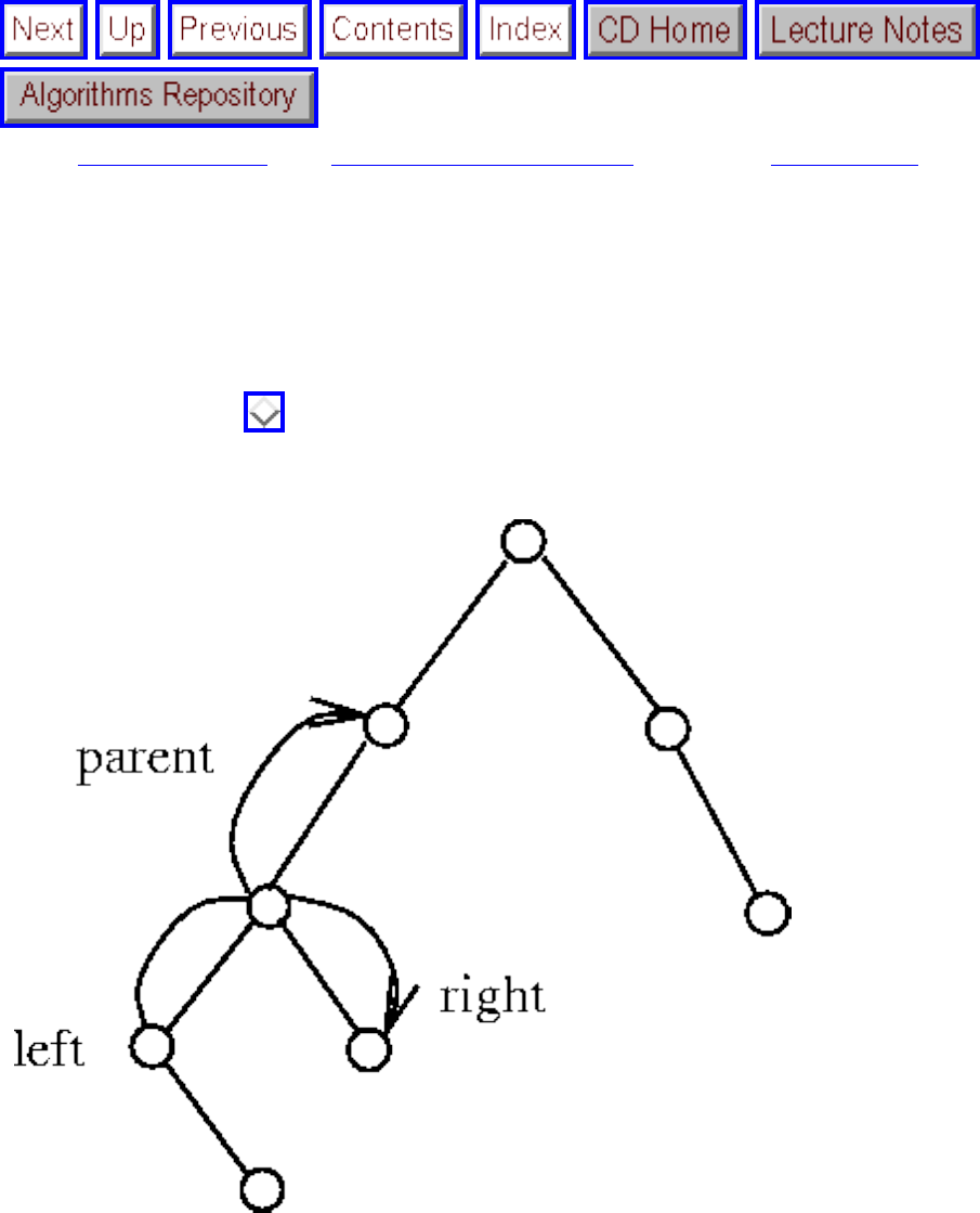
Binary Search Trees
Next: Priority Queues Up: Fundamental Data Types Previous: Dictionaries
Binary Search Trees
Fast support of all dictionary operations is realized by binary search trees. A binary tree is a rooted tree
where each node contains at most two children. Each child can be identified as either a left or right child.
As shown in Figure , a binary tree can be implemented where each node has left and right pointer
fields, an (optional) parent pointer, and a data field.
Figure: Relationships in a binary search tree
A binary search tree labels each node in a binary tree with a single key such that for any node labeled x,
all nodes in the left subtree of x have keys < x while all nodes in the right subtree of x have keys > x. The
search tree labeling enables us to find where any key is. Start at the root. If it does not contain the key we
are searching for, proceed either left or right depending upon whether what we want occurs before or after
the root key. This algorithm works because both the left and right subtrees of a binary search tree are
binary search trees; the recursive structure yields a recursive algorithm. Accordingly, the dictionary Query
operation can be performed in O(h) time, where h is the height of the tree.
file:///E|/BOOK/BOOK/NODE26.HTM (1 of 3) [19/1/2003 1:28:24]
Binary Search Trees
BinaryTreeQuery(x, k)
if
then return x
if (k < key[x])
then return BinaryTreeQuery(left[x],k)
else return BinaryTreeQuery(right[x],k)
To insert a new item x with key k into a binary search tree T, it is important to place it where it can be
later be found. There is only one such location in any binary search tree, namely by replacing the nil
pointer found in T after an unsuccessful query for k. Replacing this nil pointer with a pointer to x is a
simple, constant-time operation after the search has been performed in O(h) time.
Deletion is somewhat more tricky than insertion, because the node selected to die may not be a leaf. Leaf
nodes may be deleted without mercy, by clearing the pointer to the given node. However, internal nodes
have children that must remain accessible after the deletion. By restructuring or relabeling the tree,
however, the item to delete can always be made into a leaf and then removed. Details appear in any data
structures text.
When implemented using binary search trees, all three dictionary operations take O(h) time, where h is
the height of the tree. The smallest height we could hope for occurs when the tree is perfectly balanced,
where . In fact, if we insert the keys in random order, with high probability the tree will have
height. However, if we get unlucky with our order of insertion or deletion, we can end up with a
linear-height tree in the worst case. The worst case is a serious potential problem. Indeed, it occurs
whenever the keys are inserted in sorted order.
To avoid such worst-case performance, more sophisticated balanced binary search tree data structures
have been developed that guarantee the height of the tree always to be . Therefore, all dictionary
operations (insert, delete, query) take time each. Implementations of such balanced tree data
structures as red-black trees are discussed in Section .
file:///E|/BOOK/BOOK/NODE26.HTM (2 of 3) [19/1/2003 1:28:24]

Binary Search Trees
From an algorithm design viewpoint, it is most important to know that these trees exist and that they can
be used as black boxes to provide an efficient dictionary implementation. When figuring the costs of
dictionary operations for algorithm analysis, assume the worst-case complexities of balanced binary trees
to be a fair measure.
Next: Priority Queues Up: Fundamental Data Types Previous: Dictionaries
Algorithms
Mon Jun 2 23:33:50 EDT 1997
file:///E|/BOOK/BOOK/NODE26.HTM (3 of 3) [19/1/2003 1:28:24]
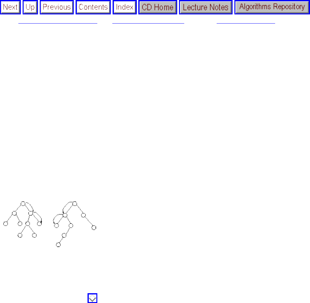
Priority Queues
Next: Specialized Data Structures Up: Fundamental Data Types Previous: Binary Search Trees
Priority Queues
Many algorithms process items according to a particular order. For example, suppose you have to schedule a list of jobs given
the deadline by which each job must be performed or else its importance relative to the other jobs. Scheduling jobs requires
sorting them by time or importance, and then performing them in this sorted order.
Priority queues provide extra flexibility over sorting, which is required because jobs often enter the system at arbitrary
intervals. It is much more cost-effective to insert a new job into a priority queue than to re-sort everything. Also, the need to
perform certain jobs may vanish before they are executed, meaning that they must be removed from the queue.
The basic priority queue supports three primary operations:
● Insert(Q,x): Given an item x with key k, insert it into the priority queue Q.
● Find-Minimum(Q) or Find-Maximum(Q): Return a pointer to the item whose key value is smaller (larger) than any
other key in the priority queue Q.
● Delete-Minimum(Q) or Delete-Maximum(Q) - Remove the item from the priority queue Q whose key is minimum
(maximum).
Figure: The maximum and minimum element in a binary search tree
All three of these priority queue operations can be implemented in time by representing the heap with a binary search tree.
Implementing the find-minimum operation requires knowing where the minimum element in the tree is. By definition, the
smallest key must reside in the left subtree of the root, since all keys in the left subtree have values less than that of the root.
Therefore, as shown in Figure , the minimum element must be the leftmost decendent of the root. Similarly, the maximum
element must be the rightmost decendent of the root.
Find-Maximum(x)
Find-Minimum(x)
while
while
do x = right[x]
do x = left[x]
return x
return x
file:///E|/BOOK/BOOK/NODE27.HTM (1 of 2) [19/1/2003 1:28:25]
Priority Queues
Repeatedly traversing left (or right) pointers until we hit a leaf takes time proportional to the height of the tree, or if the
tree is balanced. The insert operation can be implemented exactly as binary tree insertion. Delete-Min can be implemented by
finding the minimum element and then using standard binary tree deletion. It follows that each of the operations can be
performed in time.
Priority queues are very useful data structures. Indeed, they are the hero of the war story described in Section . A complete
set of priority queue implementations is presented in Section .
Next: Specialized Data Structures Up: Fundamental Data Types Previous: Binary Search Trees
Algorithms
Mon Jun 2 23:33:50 EDT 1997
file:///E|/BOOK/BOOK/NODE27.HTM (2 of 2) [19/1/2003 1:28:25]
Specialized Data Structures
Next: Sorting Up: Data Structures and Sorting Previous: Priority Queues
Specialized Data Structures
The basic data structures thus far described all represent an unstructured set of items so as to facilitate
retrieval operations. These data structures are well known to most programmers. Not as well known are
high-powered data structures for representing more structured or specialized kinds of objects, such as
points in space, strings, and graphs.
The design principles of these data structures are the same as for basic objects. There exists a set of basic
operations we need to perform repeatedly. We seek a data structure that supports these operations very
efficiently. These efficient, specialized data structures are as important for efficient graph and geometric
algorithms as lists and arrays are for basic algorithms, so one should be aware of their existence. Details
appear throughout the catalog.
● String data structures - Character strings are typically represented by arrays of characters, with
perhaps a special character to mark the end of the string. Suffix trees/arrays are special data
structures that preprocess strings to make pattern matching operations faster. See Section for
details.
● Geometric data structures - Geometric data typically consists of collections of data points and
regions. Regions in the plane are usually described by polygons, where the boundary of the
polygon is given by a chain of line segments. Polygons can be represented using an array of
points , such that is a segment of the boundary. Spatial data structures such
as kd-trees organize points and regions by geometric location to support fast search. See Section
for details.
● Graph data structures - Graphs are typically represented by either adjacency matrices or
adjacency lists. The choice of representation can have a substantial impact on the design of the
resulting graph algorithms, as discussed in Chapter . Implementation aspects of graph data
structures are presented in Section .
● Set data structures - Subsets of items are typically represented using a dictionary, to support fast
membership queries. A variety of data structures for manipulating sets is presented in Section .
file:///E|/BOOK/BOOK/NODE28.HTM (1 of 2) [19/1/2003 1:28:26]

Sorting
Next: Applications of Sorting Up: Data Structures and Sorting Previous: Specialized Data Structures
Sorting
By the time they graduate, computer science students are likely to have studied the basic sorting
algorithms in their introductory programming class, then in their data structures class, and finally in their
algorithms class. Why is sorting worth so much attention? There are several reasons:
● Sorting is the basic building block around which many other algorithms are built. By
understanding sorting, we obtain an amazing amount of power to solve other problems.
● Historically, computers have spent more time sorting than doing anything else. A quarter of all
mainframe cycles are spent sorting data [Knu73b]. Although it is unclear whether this remains
true on smaller computers, sorting remains the most ubiquitous combinatorial algorithm problem
in practice.
● Sorting is the most throughly studied problem in computer science. Literally dozens of different
algorithms are known, most of which possess some advantage over all other algorithms in certain
situations. To become convinced of this, the reader is encouraged to browse through [Knu73b],
with hundreds of pages of interesting sorting algorithms and analysis.
● Most of the interesting ideas used in the design of algorithms appear in the context of sorting,
such as divide-and-conquer, data structures, and randomized algorithms.
Algorithms
Mon Jun 2 23:33:50 EDT 1997
file:///E|/BOOK/BOOK/NODE29.HTM [19/1/2003 1:28:26]
Applications of Sorting
Next: Approaches to Sorting Up: Data Structures and Sorting Previous: Sorting
Applications of Sorting
An important key to algorithm design is to use sorting as a basic building block, because once a set of
items is sorted, many other problems become easy. Consider the following applications:
● Searching - Binary search enables you to test whether an item is in a dictionary in time,
once the keys are all sorted. Search preprocessing is perhaps the single most important application
of sorting.
● Closest pair - Given a set of n numbers, how do you find the pair of numbers that have the
smallest difference between them? After the numbers are sorted, the closest pair of numbers will
lie next to each other somewhere in sorted order. Thus a linear-time scan through them completes
the job, for a total of time including the sorting.
● Element uniqueness - Are there any duplicates in a given a set of n items? The most efficient
algorithm is to sort them and then do a linear scan though them checking all adjacent pairs. This is
a special case of the closest-pair problem above, where we ask if there is a pair separated by a gap
of zero.
● Frequency distribution - Given a set of n items, which element occurs the largest number of times
in the set? If the items are sorted, we can sweep from left to right and count them, since all
identical items will be lumped together during sorting. To find out how often an arbitrary element
k occurs, start by looking up k using binary search in a sorted array of keys. By walking to the left
of this point until the element is not k and then walking to the right, we can find this count in
time, where c is the number of occurrences of k. The number of instances of k can be
found in time by using binary search to look for the positions of both and ,
where is arbitrarily small, and then taking the difference of these positions.
● Selection - What is the kth largest item in the set? If the keys are placed in sorted order in an
array, the kth largest can be found in constant time by simply looking at the kth position of the
array. In particular, the median element (see Section ) appears in the (n/2)nd position in sorted
order.
file:///E|/BOOK/BOOK/NODE30.HTM (1 of 2) [19/1/2003 1:28:28]
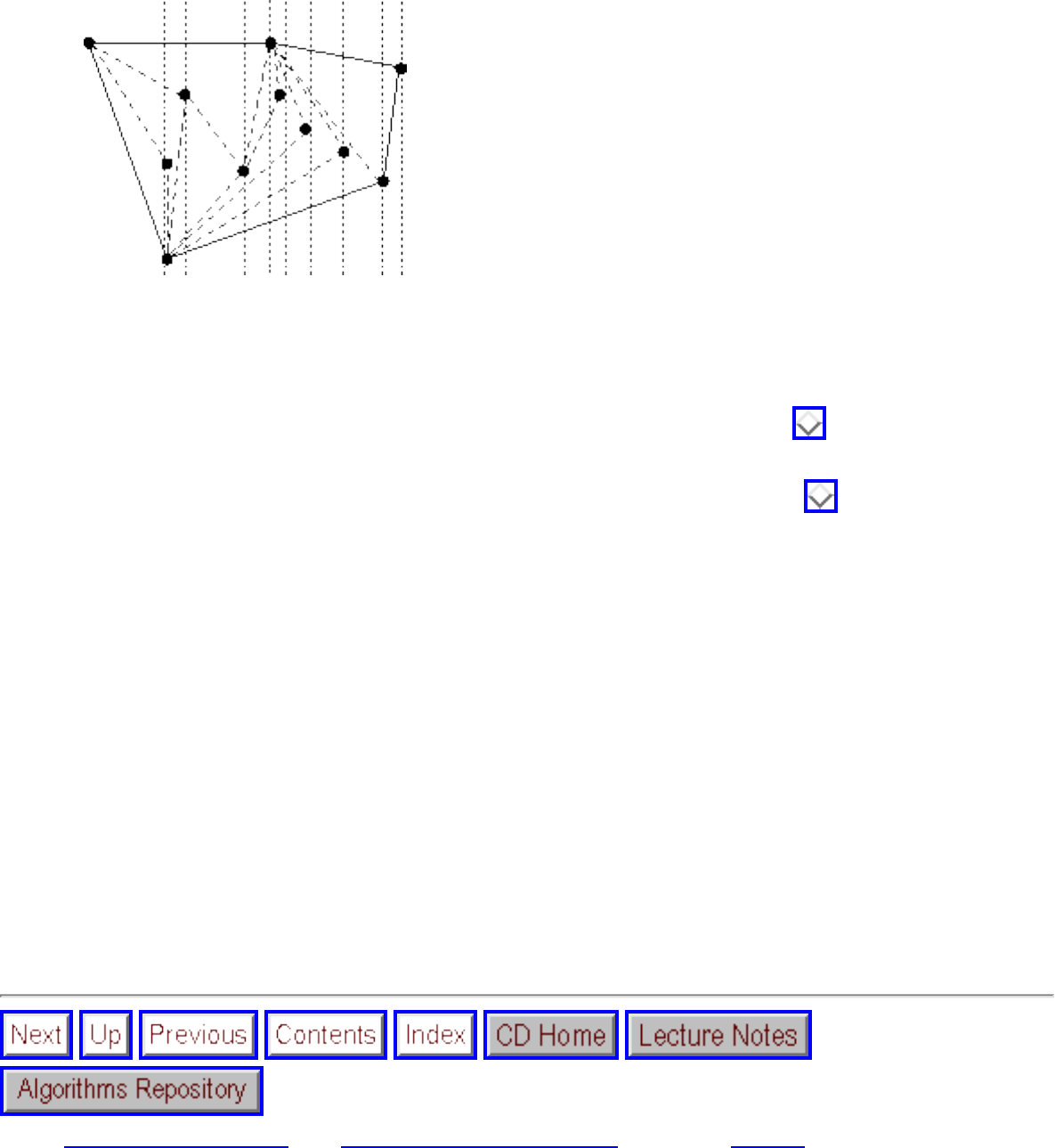
Applications of Sorting
Figure: Constructing the convex hull of points in the plane
● Convex hulls - Given n points in two dimensions, what is the polygon of smallest area that
contains them all? The convex hull is like a rubber band stretched over the points in the plane and
then released. It compresses to just cover the points, as shown in Figure . The convex hull
gives a nice representation of the shape of the points and is the most important building block for
more sophisticated geometric algorithms, as discussed in catalog Section .
But how can we use sorting to construct the convex hull? Once you have the points sorted by x-
coordinate, the points can be inserted from left to right into the hull. Since the rightmost point is
always on the boundary, we know that it will be inserted into the hull. Adding this new rightmost
point might cause others to be deleted, but we can quickly identify these points because they lie
inside the polygon formed by adding the new point. These points to delete will be neighbors of
the previous point we inserted, so they will be easy to find. The total time is linear after the
sorting has been done.
While some of these problems (particularly median and selection) can be solved in linear time using
more sophisticated algorithms, sorting provides quick and easy solutions to all of these problems. It is a
rare application whose time complexity is such that sorting proves to be the bottleneck, especially a
bottleneck that could have otherwise been removed using more clever algorithmics. Don't ever be afraid
to spend time sorting whenever you use an efficient sorting routine.
Next: Approaches to Sorting Up: Data Structures and Sorting Previous: Sorting
Algorithms
Mon Jun 2 23:33:50 EDT 1997
file:///E|/BOOK/BOOK/NODE30.HTM (2 of 2) [19/1/2003 1:28:28]
Approaches to Sorting
Next: Data Structures Up: Data Structures and Sorting Previous: Applications of Sorting
Approaches to Sorting
Sorting is a natural laboratory for studying basic algorithm design paradigms, since many useful
techniques lead to interesting sorting algorithms. Indeed, we introduce several techniques here that will
be described further in subsequent chapters. Consider the algorithms below as case studies for each of the
relevant techniques.
● Data Structures
● Incremental Insertion
● Divide and Conquer
● Randomization
● Bucketing Techniques
Algorithms
Mon Jun 2 23:33:50 EDT 1997
file:///E|/BOOK/BOOK/NODE31.HTM [19/1/2003 1:28:28]
Data Structures
Next: Incremental Insertion Up: Approaches to Sorting Previous: Approaches to Sorting
Data Structures
Perhaps the most dramatic algorithmic improvement made possible by using appropriate data structures
occurs in sorting. Selection sort is a simple-to-code algorithm that repeatedly extracts the smallest
remaining element from the unsorted part of the set:
SelectionSort(A)
For i = 1 to n do
Sort[i] = Find-Minimum from A
Delete-Minimum from A
Return(Sort)
Selection sort is typically implemented by partitioning the input array into sorted and unsorted regions.
To find the smallest item, we perform a linear sweep through the unsorted portion of the array. The
smallest item is then swapped with the ith item in the array before moving on the next iteration. Selection
sort performs n iterations, where the average iteration takes n/2 steps, for a total of time.
But what if we improve the data structure? It takes O(1) time to remove a particular item from an
unsorted array once it has been located, but O(n) time to find the smallest item. These two are exactly the
operations supported by priority queues. So what happens if we replace the data structure with a better
priority queue implementation, either a heap or a balanced binary tree. Operations within the loop now
take time each, instead of O(n). By using such a priority queue implementation, selection sort is
sped up to from . The name typically given to this algorithm, heapsort, obscures the
relationship between them, but heapsort is nothing but an implementation of selection sort with the right
data structure.
file:///E|/BOOK/BOOK/NODE32.HTM (1 of 2) [19/1/2003 1:28:29]

Data Structures
Algorithms
Mon Jun 2 23:33:50 EDT 1997
file:///E|/BOOK/BOOK/NODE32.HTM (2 of 2) [19/1/2003 1:28:29]
Incremental Insertion
Next: Divide and Conquer Up: Approaches to Sorting Previous: Data Structures
Incremental Insertion
Now consider a different approach to sorting that grows the sorted set one element at a time. Select an
arbitrary element from the unsorted set, and put it in the proper position in the sorted set.
InsertionSort(A)
for i = 1 to n-1 do
j=i
while (A[j] > A[j-1]) do swap(A[j],A[j-1])
Although insertion sort takes in the worst case, it will perform considerably better if the data is almost
sorted, since few iterations of the inner loop will suffice to sift it into the proper position. Insertion sort is
perhaps the simplest example of the incremental insertion technique, where we build up a complicated
structure on n items by first building it on n-1 items and then making the necessary changes to fix things in
adding the last item. Incremental insertion proves a particularly useful technique in geometric algorithms.
Algorithms
Mon Jun 2 23:33:50 EDT 1997
file:///E|/BOOK/BOOK/NODE33.HTM [19/1/2003 1:28:29]
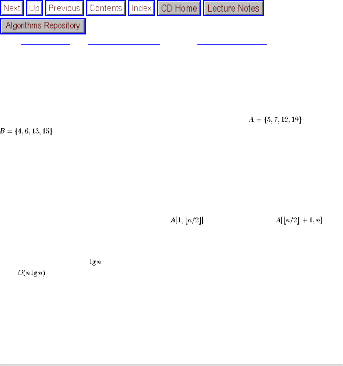
Divide and Conquer
Next: Randomization Up: Approaches to Sorting Previous: Incremental Insertion
Divide and Conquer
Suppose we take the n elements to sort and split them into piles S and T, each with half the elements.
After sorting both piles, it is easy to combine the two sorted piles. To merge and
, note that the smallest item must sit at the top of one of the two lists. Once identified,
the smallest element can be removed, and the second smallest item will again be atop one of the two lists.
Repeating this operation merges the two sorted lists in O(n) time. This provides the basis for a recursive
algorithm.
Mergesort(A[1,n])
Merge( MergeSort( ), MergeSort( ) )
Because the recursion goes levels deep and a linear amount of work is done per level, Mergesort
takes time in the worst case.
Mergesort is a classic divide-and-conquer algorithm. Whenever we can break one large problem into two
smaller problems, we are ahead of the game because the smaller problems are easier. The trick is taking
advantage of the two partial solutions to put together a solution of the full problem. The merge operation
takes care of the reassembly in mergesort, but not all problems can be so neatly decomposed.
Algorithms
Mon Jun 2 23:33:50 EDT 1997
file:///E|/BOOK/BOOK/NODE34.HTM [19/1/2003 1:28:30]

Randomization
Next: Bucketing Techniques Up: Approaches to Sorting Previous: Divide and Conquer
Randomization
Suppose we select, at random, one of the n items we seek to sort. Call this element p. In quicksort, we
separate the n-1 other items into two piles: a low pile containing all the elements that will appear before p
in sorted order and a high pile containing all the elements that will appear after p in sorted order. After
sorting the two piles and arranging the piles correctly, we have succeeded in sorting the n items.
Quicksort(A, low, high)
if (low < high)
ploc = Partition(A,low,high)
Quicksort(A,low, ploc - 1)
Quicksort(A, ploc+1, high)
Partition(A,low,high)
swap(A[low],A[random( )])
pivot = A[low]
leftwall = low
file:///E|/BOOK/BOOK/NODE35.HTM (1 of 3) [19/1/2003 1:28:31]
Randomization
for i = low+1 to high
if (A[i] < pivot) then
leftwall = leftwall+1
swap(A[i],A[leftwall])
swap(A[low],A[leftwall])
Mergesort ran in time because we split the keys into two equal halves, sorted them recursively, and
then merged the halves in linear time. Thus whenever our pivot element is near the center of the sorted
array (i.e. the pivot is close to the median element), we get a good split and realize the same performance as
mergesort. Such good pivot elements will often be the case. After all, half the elements lie closer to the
middle than one of the ends. On average, Quicksort runs in time. If we are extremely unlucky and
our randomly selected elements always are among the largest or smallest element in the array, Quicksort
turn into selection sort and runs in . However, the odds against this are vanishingly small.
Randomization is a powerful, general tool to improve algorithms with bad worst-case but good average-
case complexity. The worst case examples still exist, but they depend only upon how unlucky we are, not
on the order that the input data is presented to us. For randomly chosen pivots, we can say that
``Randomized quicksort runs in time on any input, with high probability.''
If instead, we used some deterministic rule for selecting pivots (like always selecting A[(low+high)/2] as
pivot), we can make no claim stronger than
``Quicksort runs in time if you give me random input data, with high probability.''
Randomization can also be used to drive search techniques such as simulated annealing, which are
discussed in Section .
file:///E|/BOOK/BOOK/NODE35.HTM (2 of 3) [19/1/2003 1:28:31]

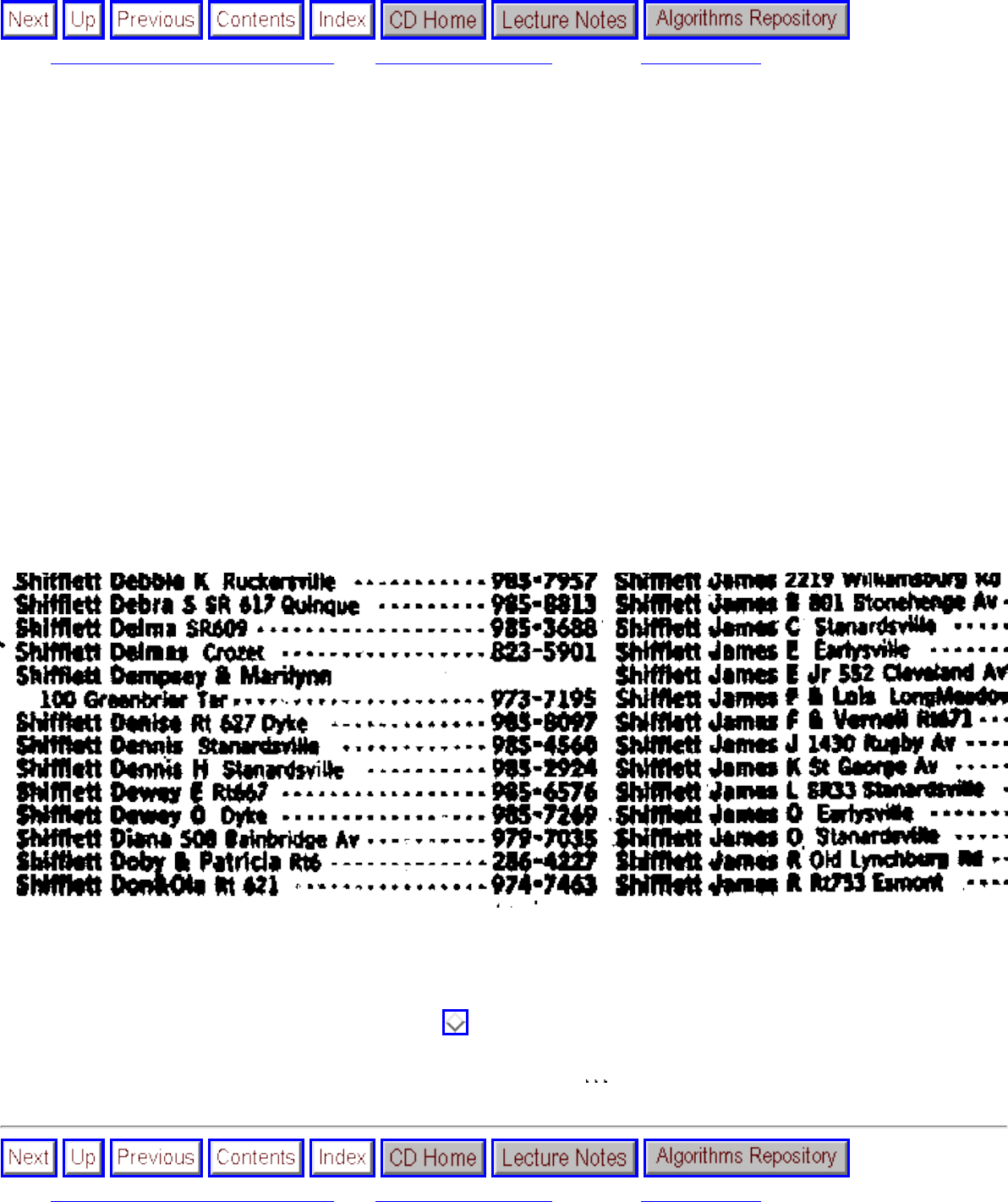
Bucketing Techniques
Next: War Story: Stripping Triangulations Up: Approaches to Sorting Previous: Randomization
Bucketing Techniques
If we were sorting names for the telephone book, we could start by partitioning the names according to the first letter of the last
name. That will create 26 different piles, or buckets, of names. Observe that any name in the J pile must occur after every name
in the I pile but before any name in the K pile. Therefore, we can proceed to sort each pile individually and just concatenate the
bunch of piles together.
If the names are distributed fairly evenly among the buckets, as we might expect, the resulting 26 sorting problems should each
be substantially smaller than the original problem. Further, by now partitioning each pile based on the second letter of each
name, we generate smaller and smaller piles. The names will be sorted as soon as each bucket contains only a single name. The
resulting algorithm is commonly called bucketsort or distribution sort.
Bucketing is a very effective idea whenever we are confident that the distribution of data will be roughly uniform. It is the idea
that underlies hash tables, kd-trees, and a variety of other practical data structures. The downside of such techniques is that the
performance can be terrible whenever the data distribution is not what we expected. Although data structures such as binary
trees offer guaranteed worst-case behavior for any input distribution, no such promise exists for heuristic data structures on
unexpected input distributions.
Figure: A small subset of Charlottesville Shiffletts
To show that non-uniform distributions occur in real life, consider Americans with the uncommon last name of Shifflett. The
1997 Manhattan telephone directory, with over one million names, contains exactly five Shiffletts. So how many Shiffletts
should there be in a small city of 50,000 people? Figure shows a small portion of the two and a half pages of Shiffletts in
the Charlottesville, Virginia telephone book. The Shifflett clan is a fixture of the region, but it would play havoc with any
distribution sort program, as refining buckets from S to Sh to Shi to Shif to to Shifflett results in no significant partitioning.
Next: War Story: Stripping Triangulations Up: Approaches to Sorting Previous: Randomization
file:///E|/BOOK/BOOK/NODE36.HTM (1 of 2) [19/1/2003 1:28:32]
Bucketing Techniques
Algorithms
Mon Jun 2 23:33:50 EDT 1997
file:///E|/BOOK/BOOK/NODE36.HTM (2 of 2) [19/1/2003 1:28:32]
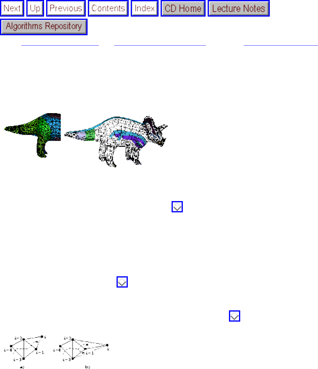
War Story: Stripping Triangulations
Next: War Story: Mystery of Up: Data Structures and Sorting Previous: Bucketing Techniques
War Story: Stripping Triangulations
Figure: (a) A triangulated model of a dinosaur (b) Several triangle strips in the model
The most common type of geometric model used for computer graphics describes the geometry of the
object as a triangulated surface, as shown in Figure a. High-performance rendering engines have
special hardware for rendering and shading triangles. This hardware is so fast that the bottleneck of
rendering is simply feeding the structure of the triangulation into the hardware engine.
Although each triangle can be described by specifying its three endpoints and any associated
shading/normal information, an alternative representation is more efficient. Instead of specifying each
triangle in isolation, suppose that we partition the triangles into strips of adjacent triangles and walk
along the strip, as shown in Figure (b). Since each triangle shares two vertices in common with its
neighbors, we save the cost of retransmitting the two extra vertices and any associated normals. To make
the description of the triangles unambiguous, the Silicon Graphics triangular-mesh renderer OpenGL
assumes that all turns alternate from left to right (as shown in Figure ).
Figure: Partitioning a triangular mesh into strips: (a) with left-right turns (b) with the flexibility of
arbitrary turns
The problem of finding a small number of strips that cover each triangle in a mesh can be thought of as a
graph problem, where this graph has a vertex for every triangle of the mesh, and there is an edge
between every pair of vertices representing adjacent triangles. This dual graph representation of the
file:///E|/BOOK/BOOK/NODE37.HTM (1 of 4) [19/1/2003 1:28:34]
War Story: Stripping Triangulations
planar subdivision representing the triangulation (see Section ) captures all the information about the
triangulation needed to partition it into triangle strips. Section describes our experiences constructing
the graph from the triangulation.
Once we had the dual graph available, the project could begin in earnest. We sought to partition the
vertices of the dual graph into as few paths or strips as possible. Partitioning it into one path implied that
we had discovered a Hamiltonian path, which by definition visits each vertex exactly once. Since finding
a Hamiltonian path was NP-complete (see Section ), we knew not to look for an optimal algorithm,
but to concentrate instead on heuristics.
It is always best to start with simple heuristics before trying more complicated ones, because simple
might well suffice for the job. The most natural heuristic for strip cover would be to start from an
arbitrary triangle and then do a left-right walk from there until the walk ends, either by hitting the
boundary of the object or a previously visited triangle. This heuristic had the advantage that it would be
fast and simple, although there could be no reason to suspect that it should find the smallest possible set
of left-right strips for a given triangulation.
A heuristic more likely to result in a small number of strips would be greedy. Greedy heuristics always
try to grab the best possible thing first. In the case of the triangulation, the natural greedy heuristic would
find the starting triangle that yields the longest left-right strip, and peel that one off first.
Being greedy also does not guarantee you the best possible solution, since the first strip you peel off
might break apart a lot of potential strips we would have wanted to use later. Still, being greedy is a good
rule of thumb if you want to get rich. Since removing the longest strip would leave the fewest number of
triangles for later strips, it seemed reasonable that the greedy heuristic would out-perform the naive
heuristic.
But how much time does it take to find the largest strip to peel off next? Let k be the length of the walk
possible from an average vertex. Using the simplest possible implementation, we could walk from each
of the n vertices per iteration in order to find the largest remaining strip to report in time. With
the total number of strips roughly equal to n/k, this yields an -time implementation, which would be
hopelessly slow on a typical model of 20,000 triangles.
How could we speed this up? It seems wasteful to rewalk from each triangle after deleting a single strip.
We could maintain the lengths of all the possible future strips in a data structure. However, whenever we
peel off a strip, we would have to update the lengths of all the other strips that will be affected. These
strips will be shortened because they walked through a triangle that now no longer exists. There are two
aspects of such a data structure:
file:///E|/BOOK/BOOK/NODE37.HTM (2 of 4) [19/1/2003 1:28:34]
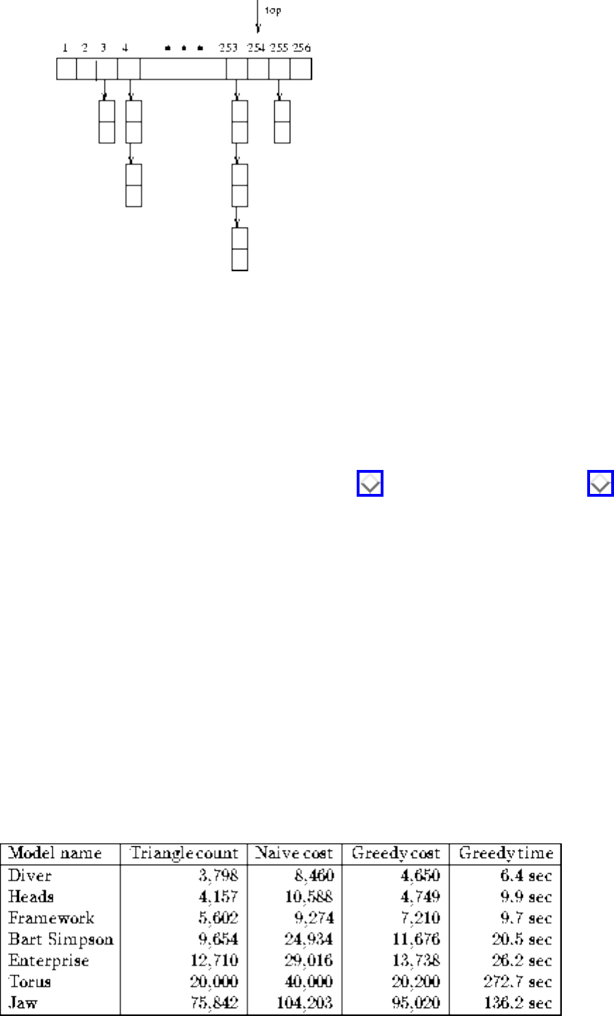
War Story: Stripping Triangulations
Figure: A bounded height priority queue for triangle strips
● Priority Queue - Since we were repeatedly interested in identifying the longest possible next strip,
we needed a priority queue to store the strips, ordered according to length. The next strip to peel
would always be the top of the queue. Our priority queue had to permit reducing the priority of
arbitrary elements of the queue whenever we updated the strip lengths to reflect what triangles
were peeled away. Because all of the strip lengths were bounded by a fairly small integer
(hardware constraints prevent any strip from having more than 256 vertices), we used a bounded
height priority queue (shown in Figure and described in Section ). An ordinary heap would
also have worked just fine.
To update a queue entry associated with a triangle, we needed to be able to quickly find where it
was. This meant that we also needed a ...
● Dictionary - For each triangle in the mesh, we needed a way to find where it was in the queue.
This meant storing a pointer for each triangle. Since each triangle was defined by three integer
vertex numbers, either a hash table or an array of lists of triangles would suffice. By integrating
this dictionary with the priority queue, we built a data structure capable of a wider range of
operations.
Although there were various other complications, such as quickly recalculating the length of the strips
affected by the peeling, the key idea needed to obtain better performance was to use the priority queue.
Run time improved by several orders of magnitude after employing these data structures.
file:///E|/BOOK/BOOK/NODE37.HTM (3 of 4) [19/1/2003 1:28:34]
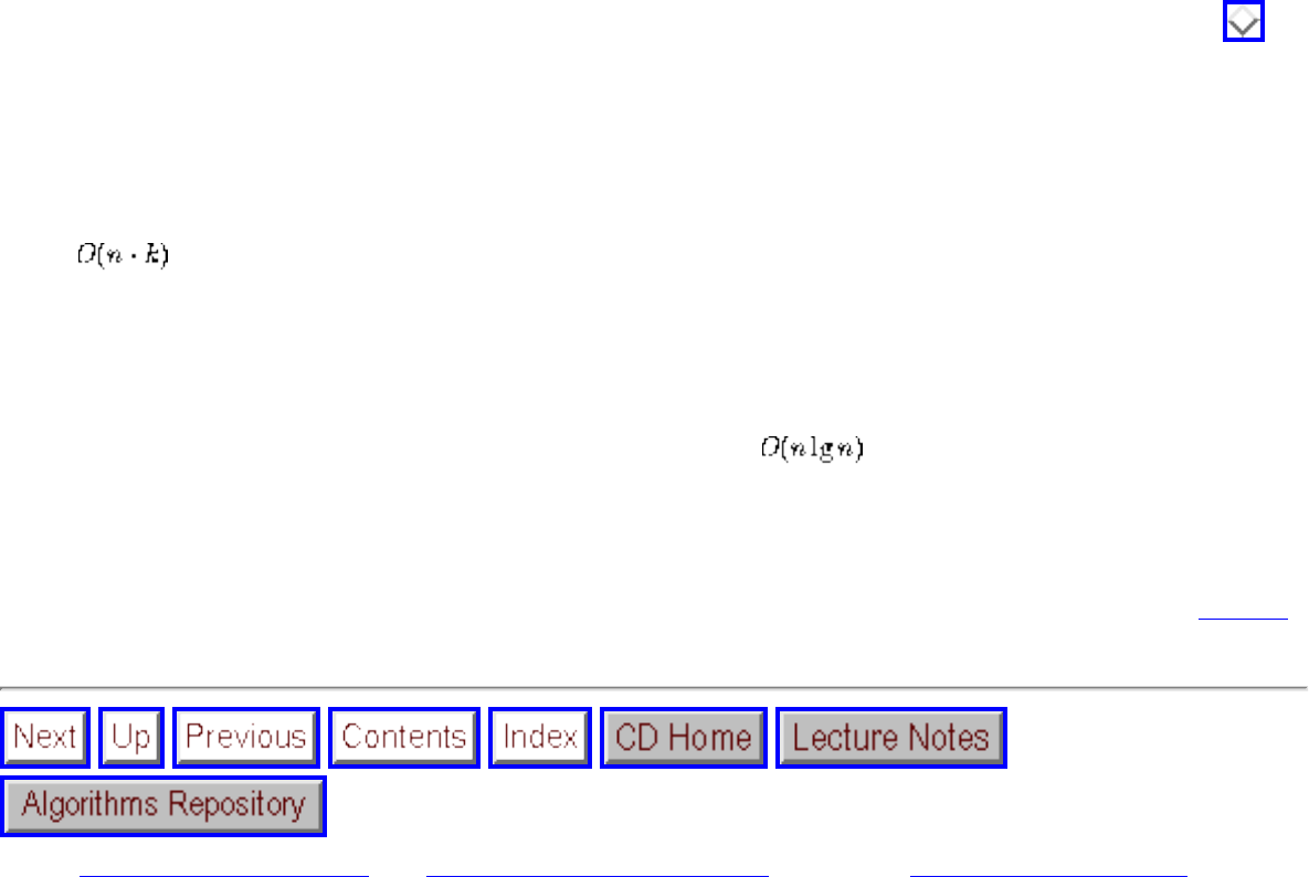
War Story: Stripping Triangulations
Figure: A comparison of the naive versus greedy heuristics for several triangular meshes
How much better did the greedy heuristic do than the naive heuristic? Consider the table in Figure . In
all cases, the greedy heuristic led to a set of strips that cost less, as measured by the total size of the
strips. The savings ranged from about 10% to 50%, quite remarkable, since the greatest possible
improvement (going from three vertices per triangle down to one) could yield a savings of only 66.6%.
After implementing the greedy heuristic with our priority queue data structure, our complete algorithm
ran in time, where n is the number of triangles and k is the length of the average strip. Thus the
torus, which consisted of a small number of very long strips, took longer than the jaw, even though the
latter contained over three times as many triangles.
There are several lessons to be gleaned from this story. First, whenever we are working with a large
enough data set, only linear or close to linear algorithms (say ) are likely to be fast enough.
Second, choosing the right data structure is often the key to getting the time complexity down to this
point. Finally, using a greedy or somewhat smarter heuristic over the naive approach is likely to
significantly improve the quality of the results. How much the improvement is likely to be can be
determined only by experimentation. Our final, optimized triangle strip program is described in [ESV96].
Next: War Story: Mystery of Up: Data Structures and Sorting Previous: Bucketing Techniques
Algorithms
Mon Jun 2 23:33:50 EDT 1997
file:///E|/BOOK/BOOK/NODE37.HTM (4 of 4) [19/1/2003 1:28:34]
War Story: Mystery of the Pyramids
Next: War Story: String 'em Up: Data Structures and Sorting Previous: War Story: Stripping
Triangulations
War Story: Mystery of the Pyramids
That look in his eyes should have warned me even before he started talking.
``We want to use a parallel supercomputer for a numerical calculation up to 1,000,000,000, but we need
a faster algorithm to do it.''
I'd seen that distant look before. Eyes dulled from too much exposure to the raw horsepower of
supercomputers. Machines so fast that brute force seemed to eliminate the need for clever algorithms. So
it always seemed, at least until the problems got hard enough.
``I am working with a Nobel prize winner to use a computer on a famous problem in number theory. Are
you familiar with Waring's problem?''
I knew some number theory [NZ80]. ``Sure. Waring's problem asks whether every integer can be
expressed at least one way as the sum of at most four integer squares. For example,
. It's a cute problem. I remember proving that four squares suffice in
my undergraduate number theory class. Yes, it's a famous problem, sure, but one that got solved about
200 years ago.''
``No, we are interested in a different version of Waring's problem. A pyramidal number is a number of
the form , for . Thus the first several pyramidal numbers are 1, 4, 10, 20, 35, 56, 84,
120, and 165. The conjecture since 1928 is that every integer can be represented by the sum of at most
five such pyramidal numbers. We want to use a supercomputer to prove this conjecture on all numbers
from 1 to 1,000,000,000.''
``Doing a billion of anything will take a serious amount of time,'' I warned. ``The time you spend to
compute the minimum representation of each number will be critical, because you are going to do it one
billion times. Have you thought about what kind of an algorithm you are going to use?''
``We have already written our program and run it on a parallel supercomputer. It works very fast on
file:///E|/BOOK/BOOK/NODE38.HTM (1 of 4) [19/1/2003 1:28:35]
War Story: Mystery of the Pyramids
smaller numbers. Still, it take much too much time as soon as we get to 100,000 or so.''
``Terrific,'' I thought. Our supercomputer junkie had discovered asymptotic growth. No doubt his
algorithm ran in something like quadratic time, and he got burned as soon as n got large.
``We need a faster program in order to get to one billion. Can you help us? Of course, we can run it on
our parallel supercomputer when you are ready.''
I'll confess that I am a sucker for this kind of challenge, finding better algorithms to speed up programs. I
agreed to think about it and got down to work.
I started by looking at the program that the other guy had written. He had built an array of all the
pyramidal numbers from 1 to n. To test each number k in this range, he did a brute force test to establish
whether it was the sum of two pyramidal numbers. If not, the program tested whether it was the sum of
three of them, then four, and finally five of them, until it first got an answer. About 45% of the integers
are expressible as the sum of three pyramidal numbers, while most of the remaining 55% require the sum
of four; usually each can be represented many different ways. Only 241 integers are known to require the
sum of five pyramidal numbers, the largest one being 343,867. For about half of the n numbers, this
algorithm presumably went through all of the three-tests and at least some of the four-tests before
terminating. Thus the total time for this algorithm would be at least time, where n=
1,000,000,000. No wonder his program cried uncle.
Anything that was going to do significantly better on a problem this large had to avoid explicitly testing
all triples. For each value of k, we were seeking the smallest number of pyramidal numbers that sum
exactly to k. This problem has a name, the knapsack problem, and it is discussed in Section . In our
case of interest, the weights are the set of pyramidal numbers no greater than n, with an additional
constraint that the knapsack holds exactly k items.
The standard approach to solving knapsack precomputes the sum of smaller subsets of the items for use
in computing larger subsets. In other words, if we want to know whether k is expressible as the sum of
three numbers, and we have a table of all sums of two numbers, all we have to do is ask whether our
number is expressible as the sum of a single number plus a number in this two-table.
Thus what I needed was a table of all integers less than n that could be expressed as the sum of two of the
1,818 pyramidal numbers less than 1,000,000,000. There could be at most = 3,305,124 of them.
Actually, there would be only about half this many because we could eliminate duplicates, or any sum
bigger than our target. Building a data structure, such as a sorted array, to hold these numbers would be
no big deal. Call this data structure the two-table.
To find the minimum decomposition for a given k, I would start out by checking whether it was one of
file:///E|/BOOK/BOOK/NODE38.HTM (2 of 4) [19/1/2003 1:28:35]
War Story: Mystery of the Pyramids
the 1,818 pyramidal numbers. If not, I would then search to see whether k was in the sorted table of the
sums of two pyramidal numbers. If it wasn't, to see whether k was expressible as the sum of three such
numbers, all I had to do was check whether k - p[i] was in the two-table for . This could be
done quickly using binary search. To see whether k was expressible as the sum of four pyramidal
numbers, I had to check whether k - two[i] was in the two-table for all . However, since
almost every k was expressible in many ways as the sum of four pyramidal numbers, this latter test
would terminate quickly, and the time taken would be dominated by the cost of the threes. Testing
whether k was the sum of three pyramidal numbers would take . Running this on each of the n
integers gives an algorithm for the complete job. Comparing this to his algorithm for n=
1,000,000,000 suggested that my algorithm was a cool 30,000 times faster than the original!
My first attempt to code this up solved up to n=1,000,000 on my crummy Sparc ELC in about 20
minutes. From here, I experimented with different data structures to represent the sets of numbers and
different algorithms to search these tables. I tried using hash tables and bit vectors instead of sorted
arrays and experimented with variants of binary search such as interpolation search (see Section ). My
reward for this work was solving up to n=1,000,000 in under three minutes, a factor of six improvement
over my original program.
With the real thinking done, I worked to tweak a little more performance out of the program. I avoided
doing a sum-of-four computation on any k when k-1 was the sum-of-three, since 1 is a pyramidal
number, saving about 10% of the total run time on this trick alone. Finally, I got out my profiler and tried
some low-level tricks to squeeze a little more performance out of the code. For example, I saved another
10% by replacing a single procedure call with in-line code.
At this point, I turned the code over to the supercomputer guy. What he did with it is a depressing tale,
which is reported in Section .
In writing up this war story, I went back to rerun our program almost five years later. On my desktop
Sparc 5, getting to 1,000,000 now took 167.5 seconds using the cc compiler without turning on any
compiler optimization. With level 2 optimization, the job ran in only 81.8 seconds, quite a tribute to the
quality of the optimizer. The gcc compiler with optimization did even better, taking only 74.9 seconds to
get to 1,000,000. The run time on my desktop machine had improved by a factor of about three over a
four-year period. This is probably typical for most desktops.
The primary importance of this war story is to illustrate the enormous potential for algorithmic speedups,
as opposed to the fairly limited speedup obtainable via more expensive hardware. I sped his program up
by about 30,000 times. His million-dollar computer had 16 processors, each reportedly five times faster
on integer computations than the $3,000 machine on my desk. That gave a maximum potential speedup
of less than 100 times. Clearly, the algorithmic improvement was the big winner here, as it is certain to
be in any sufficiently large computation.
file:///E|/BOOK/BOOK/NODE38.HTM (3 of 4) [19/1/2003 1:28:35]

War Story: String 'em Up
Next: Exercises Up: Data Structures and Sorting Previous: War Story: Mystery of
War Story: String 'em Up
Biologists are hard at work on a fifteen-year project to sequence the human genome. This pattern of
nucleotides encodes all the information necessary to build the proteins that we are built of. This project
has already had an enormous impact on medicine and molecular biology.
Algorists have become interested in the human genome project as well, for several reasons:
● DNA sequences can be accurately represented as strings of characters on the four-letter alphabet
(A,C,T,G). Biologist's needs have sparked new interest in old algorithmic problems (such as string
matching - see Section ) as well as creating new problems of substantial interest (such as
shortest common superstring - see Section ).
● DNA sequences are very long strings. The human genome is approximately three billion base
pairs (or characters) long. Thus sophisticated computational techniques are necessary to deal with
them. Such large problem sizes means that asymptotic (big-Oh) complexity analysis is usually
fully justified on biological problems.
● Enough money is being invested in the human genome project for computer scientists to want to
claim their piece of the action.
My particular interest in computational biology has revolved around a recently proposed but
algorithmically intensive technique for DNA sequencing called sequencing by hybridization (SBH)
[CK94, PL94]. The traditional sequencing by hybridization procedure attaches a set of probes to an array,
forming a sequencing chip. Each of these probes determines whether or not the probe string occurs as a
substring of the DNA target. The target DNA can now be sequenced based on the constraints of which
strings are and are not substrings of the target.
One problem with SBH is that enormous arrays (say strings) are necessary to sequence
relatively short pieces of DNA (typically about 200 base pairs long). The major reason is that all of these
probes are made at the same time. If you want to look up a name in the telephone book but are only
allowed to consult the book once, you must copy down every single name from the book at that time. But
if you are allowed to ask ``is the name before Mendoza?'' and wait for the answer before asking your next
question, you can use binary search to greatly reduce your total effort.
file:///E|/BOOK/BOOK/NODE39.HTM (1 of 5) [19/1/2003 1:28:38]
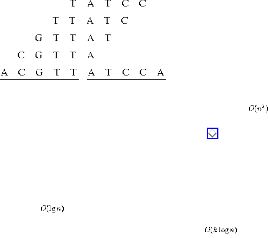
War Story: String 'em Up
We were convinced that using several small arrays would be more efficient than using one big array. We
even had theory to justify our technique, but biologists aren't very inclined to believe theory. They
demand experiments for proof. Hence we had to implement our algorithms and use simulation to prove
that they worked.
So much for motivation. The rest of this tale will demonstrate the impact that clever data structures can
have on a string processing application.
Our technique involved identifying all the strings of length 2k that are possible substrings of an unknown
string S, given that we know all length k substrings of S. For example, suppose we know that AC, CA,
and CC are the only length-2 substrings of S. It is certainly possible that ACCA is a substring of S, since
the center substring is one of our possibilities. However, CAAC cannot be a substring of S, since we
know that AA is not a substring of S. We needed to find a fast algorithm to construct all the consistent
length-2k strings, since S could be very long.
Figure: The concatentation of two fragments can be in S only if all subfragments are
The simplest algorithm to build the 2k strings would be to concatenate all pairs of k-strings
together, and then for each pair to make sure that all (k-1) length-k substrings spanning the boundary of
the concatenation were in fact substrings, as shown in Figure . For example, the nine possible
concatenations of AC, CA, and CC are ACAC, ACCA, ACCC, CAAC, CACA, CACC, CCAC, CCCA, and
CCCC. Only CAAC can be eliminated because of the absence of AA.
We needed a fast way of testing whether each of the k-1 substrings straddling the concatenation was a
member of our dictionary of permissible k-strings. The time it takes to do this depends upon which kind
of data structure we use to maintain this dictionary. With a binary search tree, we could find the correct
string within comparisons, where each comparison involved testing which of two length-k strings
appeared first in alphabetical order. Since each such comparison could require testing k pairs of
characters, the total time using a binary search tree would be .
That seemed pretty good. So my graduate student Dimitris Margaritis implemented a binary search tree
data structure for our implementation. It worked great up until the moment we ran it.
file:///E|/BOOK/BOOK/NODE39.HTM (2 of 5) [19/1/2003 1:28:38]
War Story: String 'em Up
``I've tried the fastest computer in our department, but our program is too slow,'' Dimitris complained.
``It takes forever on strings of length only 2,000 characters. We will never get up to 50,000.''
For interactive SBH to be competitive as a sequencing method, we had to be able to sequence long
fragments of DNA, ideally over 50 kilobases in length. If we couldn't speed up the program, we would be
in the embarrassing position of having a biological technique invented by computer scientists fail
because the computations took too long.
We profiled our program and discovered that almost all the time was spent searching in this data
structure, which was no surprise. For each of the possible concatenations, we did this k-1 times. We
needed a faster dictionary data structure, since search was the innermost operation in such a deep loop.
``What about using a hash table?'' I suggested. ``If we do it right, it should take O(k) time to hash a k-
character string and look it up in our table. That should knock off a factor of , which will mean
something when 2,000.''
Dimitris went back and implemented a hash table implementation for our dictionary. Again, it worked
great up until the moment we ran it.
``Our program is still too slow,'' Dimitris complained. ``Sure, it is now about ten times faster on strings
of length 2,000. So now we can get up to about 4,000 characters. Big deal. We will never get up to
50,000.''
``We should have expected only a factor ten speedup,'' I mused. ``After all, . We need a
faster data structure to search in our dictionary of strings.''
``But what can be faster than a hash table?'' Dimitris countered. ``To look up a k-character string, you
must read all k characters. Our hash table already does O(k) searching.''
``Sure, it takes k comparisons to test the first substring. But maybe we can do better on the second test.
Remember where our dictionary queries are coming from. When we concatenate ABCD with EFGH, we
are first testing whether BCDE is in the dictionary, then CDEF. These strings differ from each other by
only one character. We should be able to exploit this so that each subsequent test takes constant time to
perform....''
``We can't do that with a hash table,'' Dimitris observed. ``The second key is not going to be anywhere
near the first in the table. A binary search tree won't help, either. Since the keys ABCD and BCDE differ
according to the first character, the two strings will be in different parts of the tree.''
file:///E|/BOOK/BOOK/NODE39.HTM (3 of 5) [19/1/2003 1:28:38]
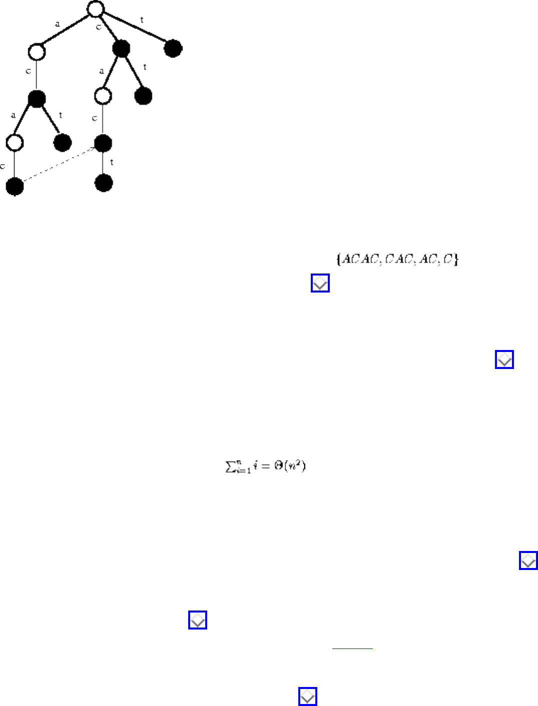
War Story: String 'em Up
Figure: Suffix tree on ACAC and CACT, with the pointer to the suffix of ACAC
``But we can use a suffix tree to do this,'' I countered. ``A suffix tree is a trie containing all the suffixes of
a given set of strings. For example, the suffixes of ACAC are . Coupled with
suffixes of string CACT, we get the suffix tree of Figure . By following a pointer from ACAC to its
longest proper suffix CAC, we get to the right place to test whether CACT is in our set of strings. One
character comparison is all we need to do from there.''
Suffix trees are amazing data structures, discussed in considerably more detail in Section . Dimitris
did some reading about them, then built a nice suffix tree implementation for our dictionary. Once again,
it worked great up until the moment we ran it.
``Now our program is faster, but it runs out of memory,'' Dimitris complained. ``And this on a 128
megabyte machine with 400 megabytes virtual memory! The suffix tree builds a path of length k for each
suffix of length k, so all told there can be nodes in the tree. It crashes when we go beyond
2,000 characters. We will never get up to strings with 50,000 characters.''
I wasn't yet ready to give up. ``There is a way around the space problem, by using compressed suffix
trees,'' I recalled. ``Instead of explicitly representing long paths of character nodes, we can refer back to
the original string.'' Compressed suffix trees always take linear space, as described in Section .
Dimitris went back one last time and implemented the compressed suffix tree data structure. Now it
worked great! As shown in Figure , we ran our simulation for strings of length n= 65,536 on a
SPARCstation 20 without incident. Our results, reported in [MS95a], showed that interactive SBH could
be a very efficient sequencing technique. Based on these simulations, we were able to arouse interest in
our technique from biologists. Making the actual wet laboratory experiments feasible provided another
computational challenge, which is reported in Section .
file:///E|/BOOK/BOOK/NODE39.HTM (4 of 5) [19/1/2003 1:28:38]
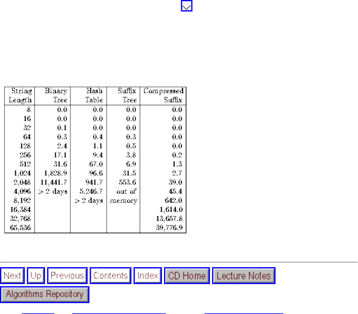
War Story: String 'em Up
The take home lessons for programmers from Figure should be apparent. We isolated a single
operation (dictionary string search) that was being performed repeatedly and optimized the data structure
we used to support it. We started with a simple implementation (binary search trees) in the hopes that it
would suffice, and then used profiling to reveal the trouble when it didn't. When an improved dictionary
structure still did not suffice, we looked deeper into what kinds of queries we were performing, so that
we could identify an even better data structure. Finally, we didn't give up until we had achieved the level
of performance we needed. In algorithms, as in life, persistence usually pays off.
Figure: Run times (in seconds) for the SBH simulation using various data structures
Next: Exercises Up: Data Structures and Sorting Previous: War Story: Mystery of
Algorithms
Mon Jun 2 23:33:50 EDT 1997
file:///E|/BOOK/BOOK/NODE39.HTM (5 of 5) [19/1/2003 1:28:38]
Exercises
Next: Implementation Challenges Up: Data Structures and Sorting Previous: War Story: String 'em
Exercises
1. Newt Gingrich is given the job of partitioning 2n players into two teams of n players each. Each
player has a numerical rating that measures how good he/she is at the game. Newt seeks to divide
the players as unfairly as possible, so as to create the biggest possible talent imbalance between
team A and team B. Show how Newt can do the job in time.
2. Take as input a sequence of 2n real numbers. Design an algorithm that partitions the
numbers into n pairs, with the property that the partition minimizes the maximum sum of a pair.
For example, say we are given the numbers (1,3,5,9). The possible partitions are ((1,3),(5,9)),
((1,5),(3,9)), and ((1,9),(3,5)). The pair sums for these partitions are (4,14), (6,12), and (10,8).
Thus the third partition has 10 as its maximum sum, which is the minimum over the three
partitions.
3. Assume that we are given as input n pairs of items, where the first item is a number and the
second item is one of three colors (red, blue, or yellow). Further, assume that the items are sorted
by number. Give an O(n) algorithm to sort the items by color (all reds before all blues before all
yellows) such that the numbers for identical colors stay sorted.
For example: (1,blue), (3,red), (4,blue), (6,yellow), (9,red) should become (3,red), (9,red),
(1,blue), (4,blue), (6,yellow).
4. (*) The mode of a set of numbers is the number that occurs most frequently in the set. The set
(4,6,2,4,3,1) has a mode of 4.
1. Give an efficient and correct algorithm to compute the mode of a set of n numbers.
2. Suppose we know that there is an (unknown) element that occurs n/2+1 times in the set.
Give a worst-case linear-time algorithm to find the mode. For partial credit, your algorithm
may run in expected linear time.
5. Given two sets and (each of size n), and a number x, describe an algorithm for
finding whether there exists a pair of elements, one from and one from , that add up to x.
(For partial credit, give a algorithm for this problem.)
6. For each of the following problems, give an algorithm that finds the desired numbers within the
given amount of time. To keep your answers brief, feel free to use algorithms from the book as
subroutines. For the example, , 19-3 maximizes the difference, while 8-6
minimizes the difference.
file:///E|/BOOK/BOOK/NODE40.HTM (1 of 4) [19/1/2003 1:28:40]
Exercises
(a) Let S be an unsorted array of n integers. Give an algorithm that finds the pair that
maximizes |x-y|. Your algorithm must run in O(n) worst-case time.
(b) Let S be a sorted array of n integers. Give an algorithm that finds the pair that
maximizes |x-y|. Your algorithm must run in O(1) worst-case time.
(c) Let S be an unsorted array of n integers. Give an algorithm that finds the pair that
minimizes |x-y|, for . Your algorithm must run in worst-case time.
(d) Let S be a sorted array of n integers. Give an algorithm that finds the pair that
minimizes |x-y|, for . Your algorithm must run in O(n) worst-case time.
7. (*) Describe how to modify any balanced tree data structure such that search, insert, delete,
minimum, and maximum still take time each, but successor and predecessor now take O(1)
time each. Which operations have to be modified to support this?
8. (*) In one of my research papers [Ski88], I give a comparison-based sorting algorithm that runs in
. Given the existence of an lower bound for sorting, how can this be
possible?
9. (*) Suppose you have access to a balanced dictionary data structure, which supports each of the
operations search, insert, delete, minimum, maximum, successor, and predecessor in time.
Explain how to modify the insert and delete operations so they still take but now
minimum and maximum take O(1) time. (Hint: think in terms of using the abstract dictionary
operations, instead of mucking about with pointers and the like.)
10. (*) Mr. B. C. Dull claims to have developed a new data structure for priority queues that supports
the operations Insert, Maximum, and Extract-Max, all in O(1) worst-case time. Prove that he is
mistaken. (Hint: the argument does not involve a lot of gory details-just think about what this
would imply about the lower bound for sorting.)
11. Use the partitioning step of Quicksort to give an algorithm that finds the median element of an
array of n integers in expected O(n) time.
12. (*) You are given the task of reading in n numbers and then printing them out in sorted order.
Suppose you have access to a balanced dictionary data structure, which supports each of the
operations search, insert, delete, minimum, maximum, successor, and predecessor in time.
❍ Explain how you can use this dictionary to sort in time using only the following
abstract operations: minimum, successor, insert, search.
❍ Explain how you can use this dictionary to sort in time using only the following
abstract operations: minimum, insert, delete, search.
❍ Explain how you can use this dictionary to sort in time using only the following
abstract operations: insert and in-order traversal.
13. The running time for Quicksort depends upon both the data being sorted and the partition rule
file:///E|/BOOK/BOOK/NODE40.HTM (2 of 4) [19/1/2003 1:28:40]
Exercises
used to select the pivot. Although Quicksort is on average, certain partition rules cause
Quicksort to take time if the array is already sorted.
(a) Suppose we always pick the pivot element to be the key from the last position of the subarray.
On a sorted array, does Quicksort now take , , or ?
(b) Suppose we always pick the pivot element to be the key from the middle position of the
subarray. On a sorted array, does Quicksort now take , , or ?
(c) Suppose we always pick the pivot element to be the key of the median element of the first
three keys of the subarray. (The median of three keys is the middle value, so the median of 5, 3, 8
is five.) On a sorted array, does Quicksort now take , , or ?
(d) Suppose we always pick the pivot element to be the key of the median element of the first,
last, and middle elements of the subarray. On a sorted array, does Quicksort now take ,
, or ?
14. (*) Given a set S of n integers and an integer T, give an algorithm to test whether k of
the integers in S sum up to T.
15. (**) Design a data structure that allows one to search, insert, and delete an integer X in O(1) time
(i.e. constant time, independent of the total number of integers stored). Assume that and
that there are m+n units of space available for the symbol table, where m is the maximum number
of integers that can be in the table at any one time. (Hint: use two arrays A[1..n] and B[1..m].) You
are not allowed to initialize either A or B, as that would take O(m) or O(n) operations. This means
the arrays are full of random garbage to begin with, so you must be very careful.
16. (*) Let P be a simple, but not necessarily convex, polygon and q an arbitrary point not necessarily
in P. Design an efficient algorithm to find a line segment originating from q that intersects the
maximum number of edges of P. In other words, if standing at point q, in what direction should
you aim a gun so the bullet will go through the largest number of walls. A bullet through a vertex
of P gets credit for only one wall. An algorithm is possible.
17. (**) The onion of a set of n points is the series of convex polygons that result from finding the
convex hull, striping it from the point set, and repeating until no more points are left. Give an
algorithm for determining the onion of a point set.
Next: Implementation Challenges Up: Data Structures and Sorting Previous: War Story: String 'em
Algorithms
file:///E|/BOOK/BOOK/NODE40.HTM (3 of 4) [19/1/2003 1:28:40]
Exercises
Mon Jun 2 23:33:50 EDT 1997
file:///E|/BOOK/BOOK/NODE40.HTM (4 of 4) [19/1/2003 1:28:40]

Dynamic Programming
Next: Fibonacci numbers Up: Breaking Problems Down Previous: Breaking Problems Down
Dynamic Programming
After you understand it, dynamic programming is probably the easiest algorithm design technique to
apply in practice. In fact, I find that dynamic programming algorithms are usually easier to reinvent than
to try to look up in a book. Until you understand it, however, dynamic programming seems like magic.
You have to figure out the trick before you can use it.
In algorithms for problems such as sorting, correctness tends to be easier to verify than efficiency. This is
not the case for optimization problems, where we seek to find a solution that maximizes or minimizes
some function. In designing algorithms for an optimization problem, we must prove that our algorithm
always gives the best possible solution.
Greedy algorithms, which make the best local decision at each step, occasionally happen to produce a
global optimum for certain problems. These are typically efficient. However, you need a proof to show
that you always end up with the best answer. Exhaustive search algorithms, which try all possibilities and
select the best, by definition must always produce the optimum result, but usually at a prohibitive cost in
terms of time complexity.
Dynamic programming combines the best of both worlds. The technique systematically considers all
possible decisions and always selects the one that proves to be the best. By storing the consequences of
all possible decisions to date and using this information in a systematic way, the total amount of work is
minimized. Dynamic programming is best learned by carefully studying a number of examples until
things start to click.
● Fibonacci numbers
● The Partition Problem
● Approximate String Matching
● Longest Increasing Sequence
● Minimum Weight Triangulation
file:///E|/BOOK/BOOK2/NODE43.HTM (1 of 2) [19/1/2003 1:28:40]

Dynamic Programming
Algorithms
Mon Jun 2 23:33:50 EDT 1997
file:///E|/BOOK/BOOK2/NODE43.HTM (2 of 2) [19/1/2003 1:28:40]
Fibonacci numbers
Next: The Partition Problem Up: Dynamic Programming Previous: Dynamic Programming
Fibonacci numbers
The tradeoff between space and time exploited in dynamic programming is best illustrated in evaluating
recurrence relations, such as the Fibonacci numbers. The Fibonacci numbers were originally defined by
the Italian mathematician Fibonacci in the thirteenth century to model the growth of rabbit populations.
Rabbits breed, well, like rabbits. Fibonacci surmised that the number of pairs of rabbits born in a given
year is equal to the number of pairs of rabbits born in each of the two previous years, if you start with
one pair of rabbits in the first year. To count the number of rabbits born in the nth year, he defined the
following recurrence relation:
with basis cases and . Thus , , and the series continues
. As it turns out, Fibonacci's formula didn't do a very good job of counting
rabbits, but it does have a host of other applications and interesting properties.
Since they are defined by a recursive formula, it is easy to write a recursive program to compute the nth
Fibonacci number. Most students have to do this in one of their first programming courses. Indeed, I
have particularly fond memories of pulling my hair out writing such a program in 8080 assembly
language. In pseudocode, the recursive algorithm looks like this:
Fibonacci[n]
if (n=0) then return(0)
else if (n=1) then return(1)
else return(Fibonacci[n-1]+Fibonacci[n-2])
file:///E|/BOOK/BOOK2/NODE44.HTM (1 of 3) [19/1/2003 1:28:42]
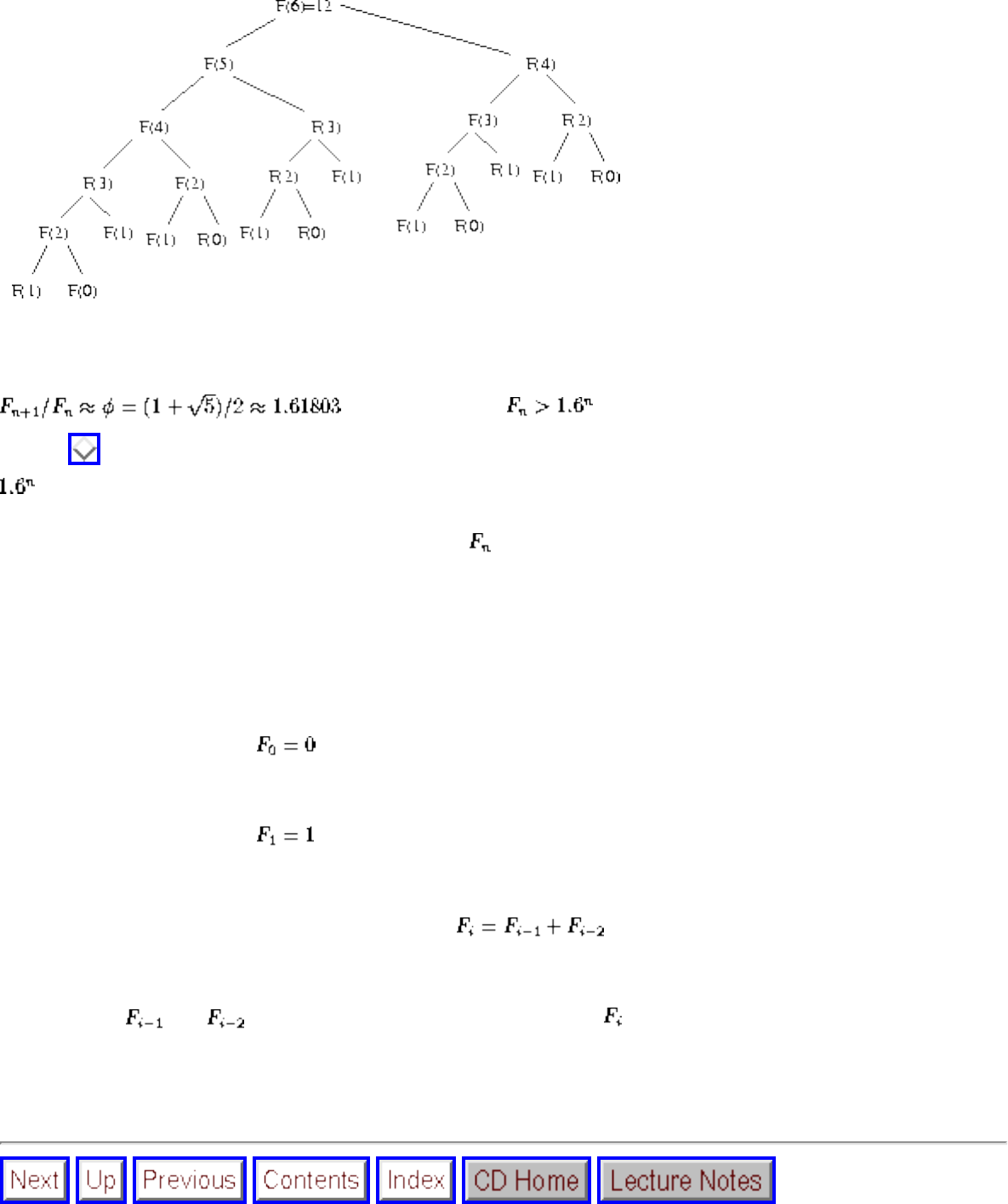
Fibonacci numbers
Figure: The computation tree for computing Fibonacci numbers recursively
How much time does this algorithm take to compute Fibonacci[n]? Since
, this means that . Since our recursion tree, illustrated in
Figure , has only 0 and 1 as leaves, summing up to such a large number means we must have at least
leaves or procedure calls! This humble little program takes exponential time to run!
In fact, we can do much better. We can calculate in linear time by storing all values. We trade space
for time in the algorithm below:
Fibonacci[n]
For i=1 to n,
Because we evaluate the Fibonacci numbers from smallest to biggest and store all the results, we know
that we have and ready whenever we need to compute . Thus each of the n values is computed
as the simple sum of two integers in total O(n) time, which is quite an improvement over exponential
time.
file:///E|/BOOK/BOOK2/NODE44.HTM (2 of 3) [19/1/2003 1:28:42]

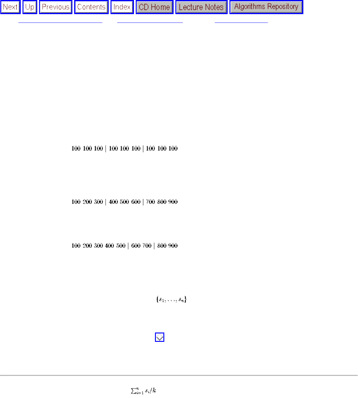
The Partition Problem
Next: Approximate String Matching Up: Dynamic Programming Previous: Fibonacci numbers
The Partition Problem
Suppose that three workers are given the task of scanning through a shelf of books in search of a given piece of information. To
get the job done fairly and efficiently, the books are to be partitioned among the three workers. To avoid the need to rearrange
the books or separate them into piles, it would be simplest to divide the shelf into three regions and assign each region to one
worker.
But what is the fairest way to divide the shelf up? If each book is the same length, say 100 pages, the job is pretty easy. Just
partition the books into equal-sized regions,
so that everyone has 300 pages to deal with.
But what if the books are not the same length? Suppose we used the same partition when the book sizes looked like this:
I, for one, would volunteer to take the first section, with only 600 pages to scan, instead of the last one, with 2,400 pages. The
fairest possible partition for this shelf would be
where the largest job is only 1,700 pages and the smallest job 1,300.
In general, we have the following problem:
Input: A given arrangement S of non-negative numbers and an integer k.
Output: Partition S into k ranges, so as to minimize the maximum sum over all the ranges. This so-called linear partition
problem arises often in parallel processing, since we seek to balance the work done across processors so as to minimize the
total elapsed run time. Indeed, the war story of Section revolves around a botched solution to this problem.
Stop for a few minutes and try to find an algorithm to solve the linear partition problem.
The beginning algorist might suggest a heuristic as the most natural approach to solve the partition problem. Perhaps they
would compute the average size of a partition, , and then try to insert the dividers so as to come close to this average.
However, such heuristic methods are doomed to fail on certain inputs, because they do not systematically evaluate all
possibilities.
Instead, consider a recursive, exhaustive search approach to solving this problem. Notice that the kth partition starts right after
we placed the (k-1)st divider. Where can we place this last divider? Between the ith and (i+1)st elements for some i, where
file:///E|/BOOK/BOOK2/NODE45.HTM (1 of 5) [19/1/2003 1:28:44]
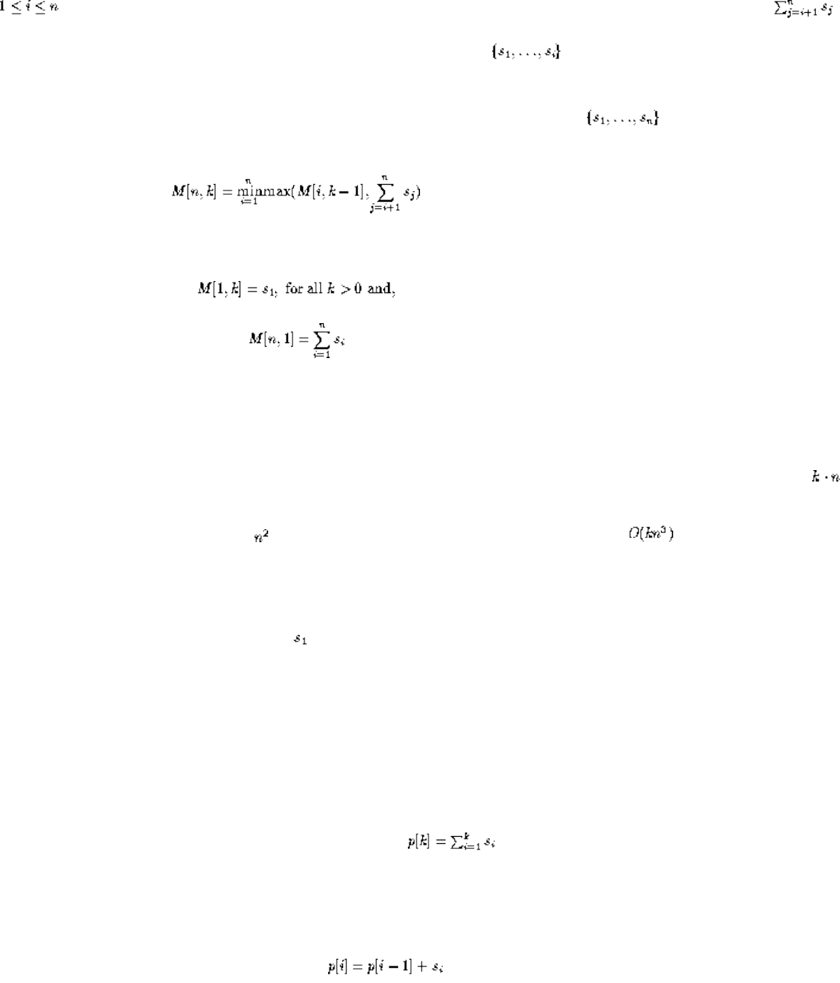
The Partition Problem
. What is the cost of this? The total cost will be the larger of two quantities, (1) the cost of the last partition
and (2) the cost of the largest partition cost formed to the left of i. What is the size of this left partition? To minimize our total,
we would want to use the k-2 remaining dividers to partition the elements as equally as possible. This is a smaller
instance of the same problem, and hence can be solved recursively!
Therefore, let us define M[n,k] to be the minimum possible cost over all partitionings of into k ranges, where the
cost of a partition is the largest sum of elements in one of its parts. Thus defined, this function can be evaluated:
with the natural basis cases of
By definition, this recurrence must return the size of the optimal partition. But how long does it take? If we evaluate the
recurrence without storing partial results, we will be doomed to spend exponential time, repeatedly recalculating the same
quantities. However, by storing the computed values and looking them up as needed, we can save an enormous amount of time.
How long does it take to compute this when we store the partial results? Well, how many results are computed? A total of
cells exist in the table. How much time does it take to compute the result M[n',k']? Well, calculating this quantity involves
finding the minimum of n' quantities, each of which is the maximum of the table lookup and a sum of at most n' elements. If
filling each of k n boxes takes at most time per box, the total recurrence can be computed in time.
To complete the implementation, we must specify the boundary conditions of the recurrence relation and an order to evaluate it
in. These boundary conditions always settle the smallest possible values for each of the arguments of the recurrence. For this
problem, the smallest reasonable value of the first argument is n=1, meaning that the first partition consists of a single element.
We can't create a first partition smaller than regardless of how many dividers are used. The smallest reasonable value of the
second argument is k=1, implying that we do not partition S at all.
The evaluation order computes the smaller values before the bigger values, so that each evaluation has what it needs waiting for
it. Full details are provided in the pseudocode below:
Partition[S,k]
(* compute prefix sums: *)
p[0] = 0
for i=1 to n do
(* initialize boundary conditions *)
file:///E|/BOOK/BOOK2/NODE45.HTM (2 of 5) [19/1/2003 1:28:44]
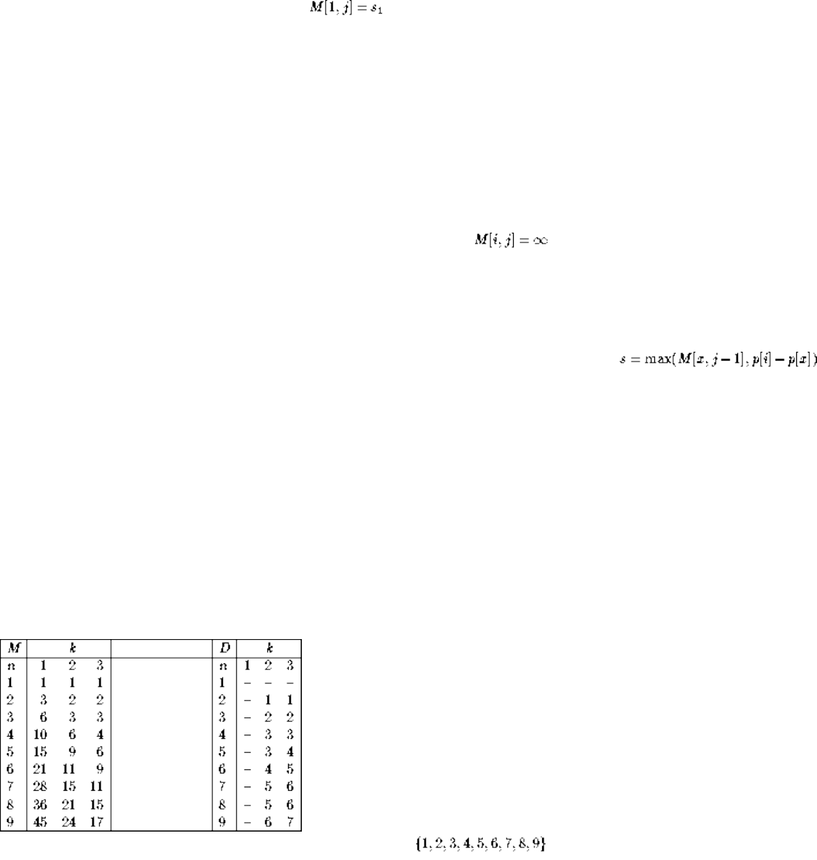
The Partition Problem
for i=1 to n do M[i,1] = p[i]
for i=1 to k do
(* evaluate main recurrence *)
for i=2 to n do
for j = 2 to k do
for x = 1 to i-1 do
if (M[i,j] > ) then
M[i,j] =
D[i,j] = x
Figure: Dynamic programming matrices M and D in partitioning
file:///E|/BOOK/BOOK2/NODE45.HTM (3 of 5) [19/1/2003 1:28:44]
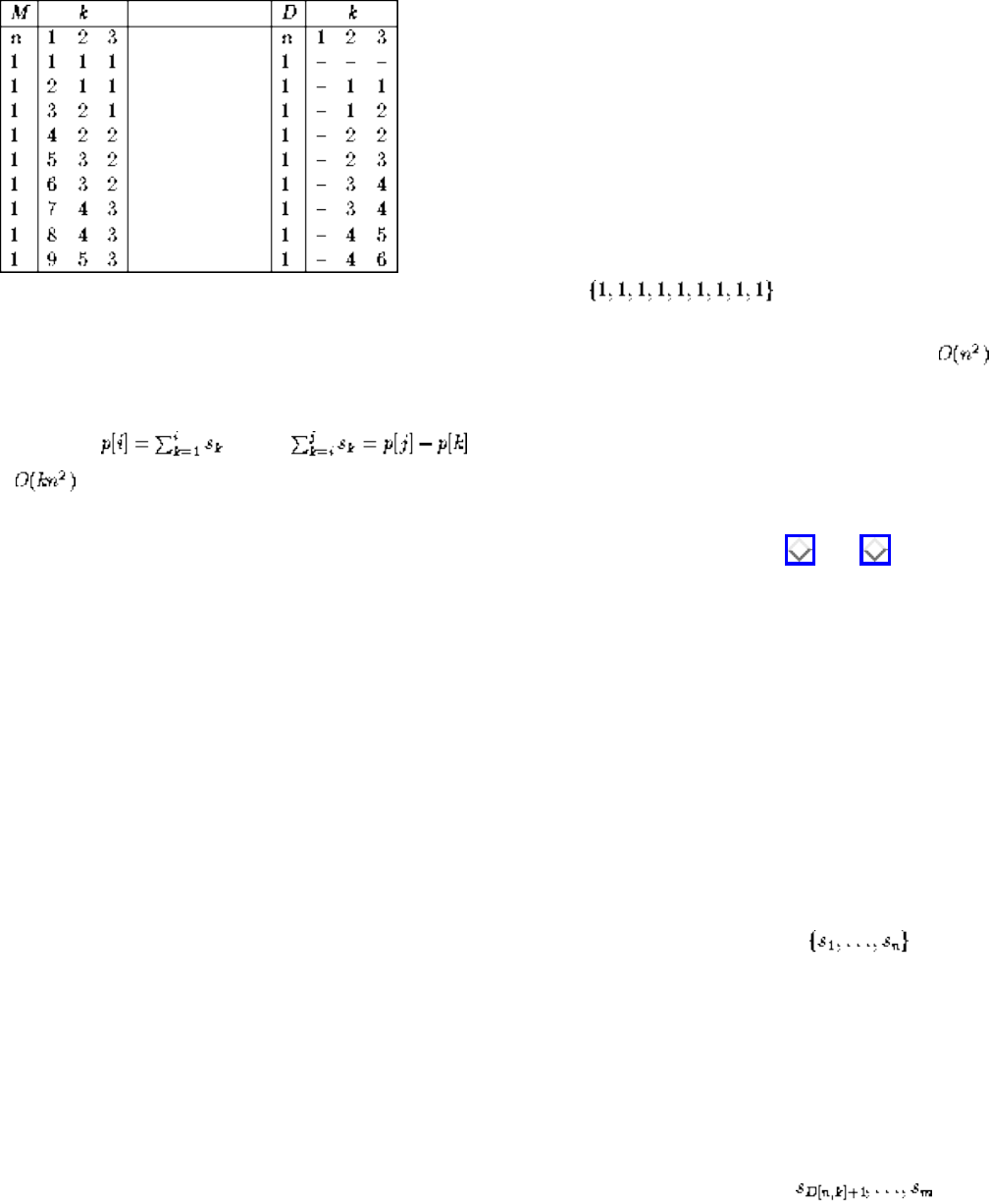
The Partition Problem
Figure: Dynamic programming matrices M and D in partitioning
The implementation above in fact runs faster than advertised. Our original analysis assumed that it took time to update
each cell of the matrix. This is because we selected the best of up to n possible points to place the divider, each of which
requires the sum of up to n possible terms. In fact, it is easy to avoid the need to compute these sums by storing the set of n
prefix sums , since . This enables us to evaluate the recurrence in linear time per cell, yielding
an algorithm.
By studying the recurrence relation and the dynamic programming matrices of Figures and , you should be able to
convince yourself that the final value of M(n,k) will be the cost of the largest range in the optimal partition. However, what
good is that? For most applications, what we need is the actual partition that does the job. Without it, all we are left with is a
coupon for a great price on an out-of-stock item.
The second matrix, D, is used to reconstruct the optimal partition. Whenever we update the value of M[i,j], we record which
divider position was required to achieve that value. To reconstruct the path used to get to the optimal solution, we work
backward from D[n,k] and add a divider at each specified position. This backwards walking is best achieved by a recursive
subroutine:
ReconstructPartition(S,D,n,k)
If (k = 1) then print the first partition
else
ReconstructPartition(S,D,D[n,k],k-1)
Print the kth partition { }
It is important to catch the distinction between storing the value of a cell and what decision/move it took to get there. The latter
is not used in the computation but is presumably the real thing that you are interested in. For most of the examples in this
chapter, we will not worry about reconstructing the answer. However, study this example closely to ensure that you know how
to obtain the winning configuration when you need it.
file:///E|/BOOK/BOOK2/NODE45.HTM (4 of 5) [19/1/2003 1:28:44]

Approximate String Matching
Next: Longest Increasing Sequence Up: Dynamic Programming Previous: The Partition Problem
Approximate String Matching
An important task in text processing is string matching - finding all the occurrences of a word in the text. Unfortunately,
many words in documents are mispelled (sic). How can we search for the string closest to a given pattern in order to
account for spelling errors?
To be more precise, let P be a pattern string and T a text string over the same alphabet. The edit distance between P and T is
the smallest number of changes sufficient to transform a substring of T into P, where the changes may be:
1. Substitution - two corresponding characters may differ: KAT CAT.
2. Insertion - we may add a character to T that is in P: CT CAT.
3. Deletion - we may delete from T a character that is not in P: CAAT CAT.
For example, P=abcdefghijkl can be matched to T=bcdeffghixkl using exactly three changes, one of each of the above
types.
Approximate string matching arises in many applications, as discussed in Section . It seems like a difficult problem,
because we have to decide where to delete and insert characters in pattern and text. But let us think about the problem in
reverse. What information would we like to have in order to make the final decision; i.e. what should happen with the last
character in each string? The last characters may be either be matched, if they are identical, or otherwise substituted one for
the other. The only other options are inserting or deleting a character to take care of the last character of either the pattern or
the text.
More precisely, let D[i,j] be the minimum number of differences between and the segment of T ending at j.
D[i, j] is the minimum of the three possible ways to extend smaller strings:
1. If , then D[i-1, j-1], else D[i-1, j-1]+1. This means we either match or substitute the ith and jth characters,
depending upon whether they do or do not match.
2. D[i-1, j]+1. This means that there is an extra character in the pattern to account for, so we do not advance the text
pointer and pay the cost of an insertion.
3. D[i, j-1]+1. This means that there is an extra character in the text to remove, so we do not advance the pattern pointer
and pay the cost of a deletion.
The alert reader will notice that we have not specified the boundary conditions of this recurrence relation. It is critical to get
the initialization right if our program is to return the correct edit distance. The value of D[0,i] will correspond to the cost of
matching the first i characters of the text with none of the pattern. What this value should be depends upon what you want
to compute. If you seek to match the entire pattern against the entire text, this means that we must delete the first i
characters of the text, so D[0,i] = i to pay the cost of the deletions. But what if we want to find where the pattern occurs in a
long text? It should not cost more if the matched pattern starts far into the text than if it is near the front. Therefore, the
starting cost should be equal for all positions. In this case, D[0,i] = 0, since we pay no cost for deleting the first i characters
of the text. In both cases, D[i,0] = i, since we cannot excuse deleting the first i characters of the pattern without penalty.
file:///E|/BOOK/BOOK2/NODE46.HTM (1 of 3) [19/1/2003 1:28:46]
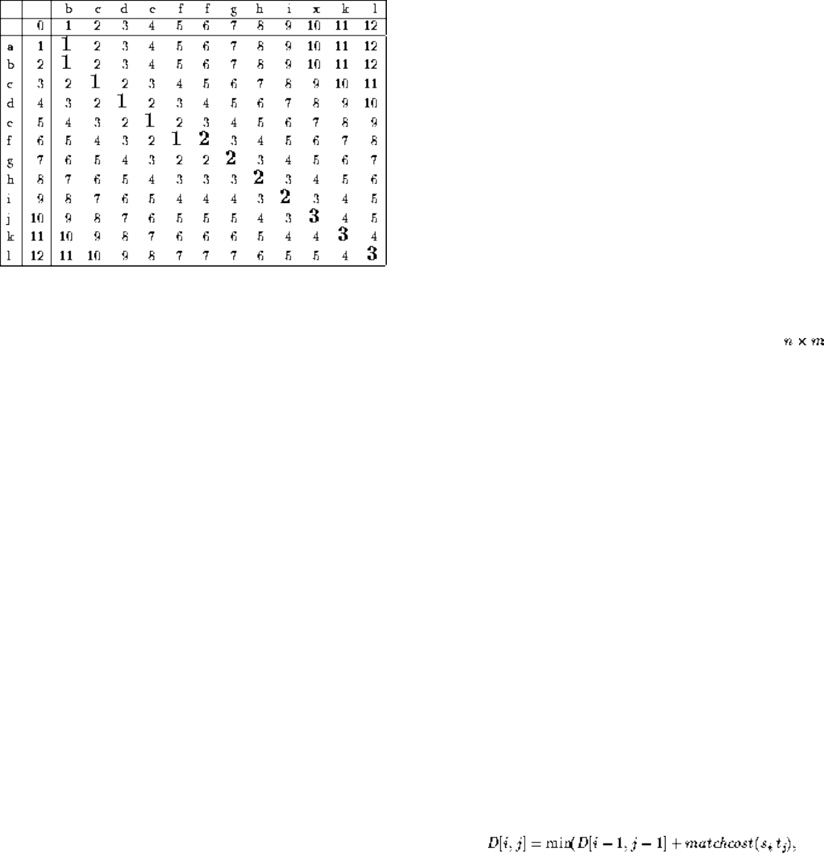
Approximate String Matching
Figure: Example dynamic programming matrix for edit distance computation, with the optimal alignment path highlighted
in bold
Once you accept the recurrence, it is straightforward to turn it into a dynamic programming algorithm that creates an
matrix D, where n = |P| and m = |T|. Here it is, initialized for full pattern matching:
EditDistance(P,T)
(*initialization*)
For i = 0 to n do D[i,0] = i
For i = 0 to m do D[0,i] = i
(*recurrence*)
For i = 1 to n do
For j = 1 to m do
D[i-1,j]+1, D[i,j-
1]+1 )
How much time does this take? To fill in cell D[i,j], we need only compare two characters and look at three other cells.
Since it requires only constant time to update each cell, the total time is O(mn).
file:///E|/BOOK/BOOK2/NODE46.HTM (2 of 3) [19/1/2003 1:28:46]
Approximate String Matching
The value to return as the answer to our pattern matching problem depends on what we are interested in. If we only needed
the cost of comparing all of the pattern against all of the text, such as in comparing the spelling of two words, all we would
need is the cost of D[n,m], as shown in Figure . But what if we need to identify the best matching substring in the text?
Assuming that the initialization was performed correctly for such substring matching, we seek the cheapest matching of the
full pattern ending anywhere in the text. This means the cost equals , i.e. the smallest cost on the last row of
D.
Of course, this only gives the cost of the optimal matching, while we are often interested in reconstructing the actual
alignment - which characters got matched, substituted, and deleted. These can be reconstructed from the pattern/text and
table without an auxiliary storage, once we have identified the cell with the lowest cost. From this cell, we want to walk
upwards and backwards through the matrix. Given the costs of its three neighbors and the corresponding characters, we can
reconstruct which choice was made to get to the goal cell. The direction of each backwards step (to the left, up, or diagonal
to the upper left) identifies whether it was an insertion, deletion, or match/substitution. Ties can be broken arbitrarily, since
either way costs the same. We keep walking backwards until we hit the end of the matrix, specifying the starting point. This
backwards-walking phase takes O(n+m) time, since we traverse only the cells involved in the alignment.
The alert reader will notice that it is unnecessary to keep all O(mn) cells to compute the cost of an alignment. If we evaluate
the recurrence by filling in the columns of the matrix from left to right, we will never need more than two columns of cells
to store what is necessary for the computation. Thus O(m) space is sufficient to evaluate the recurrence without changing
the time complexity at all. Unfortunately, without the full matrix we cannot reconstruct the alignment.
Saving space in dynamic programming is very important. Since memory on any computer is limited, O(nm) space proves
more of a bottleneck than O(nm) time. Fortunately, there is a clever divide-and-conquer algorithm that computes the actual
alignment in O(nm) time and O(m) space. This algorithm is discussed in Section .
Next: Longest Increasing Sequence Up: Dynamic Programming Previous: The Partition Problem
Algorithms
Mon Jun 2 23:33:50 EDT 1997
file:///E|/BOOK/BOOK2/NODE46.HTM (3 of 3) [19/1/2003 1:28:46]
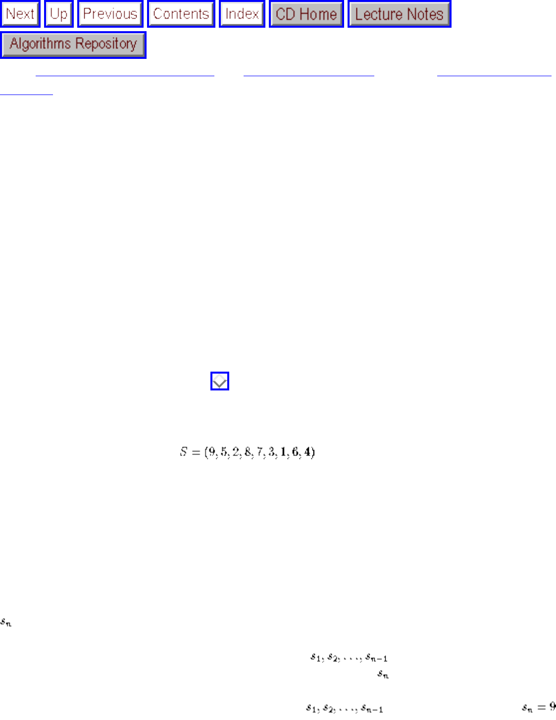
Longest Increasing Sequence
Next: Minimum Weight Triangulation Up: Dynamic Programming Previous: Approximate String
Matching
Longest Increasing Sequence
Hopefully, a pattern is emerging. Every dynamic programming solution has three components:
1. Formulate the answer as a recurrence relation or recursive algorithm.
2. Show that the number of different values of your recurrence is bounded by a (hopefully small)
polynomial.
3. Specify an order of evaluation for the recurrence so you always have the partial results you need
available when you need them.
To see how this is done, let's see how we would develop an algorithm to find the longest monotonically
increasing sequence in a sequence of n numbers. This problem arises in pattern matching on
permutations, as described in Section . We distinguish an increasing sequence from a run, in that the
selected elements need not be neighbors of each other. The selected elements must be in sorted order
from left to right. For example, consider the sequence
The longest increasing subsequence of has length 3 and is either (2,3,4) or (2,3,6). The longest increasing
run is of length 2, either (2,8) or (1,6).
Finding the longest increasing run in a numerical sequence is straightforward, indeed you should be able
to devise a linear-time algorithm fairly easily. However, finding the longest increasing subsequence is
considerably trickier. How can we identify which scattered elements to skip? To apply dynamic
programming, we need to construct a recurrence computing the length of the longest sequence. To find
the right recurrence, ask what information about the first n-1 elements of S, coupled with the last element
, would enable you to find the answer for the entire sequence?
● The length of the longest increasing sequence in seems a useful thing to know. In
fact, this will be the longest increasing sequence in S, unless extends it or another increasing
sequence of the same length. Unfortunately, knowing just this length is not enough. Suppose I
told you that the longest increasing sequence in was of length 5 and that .
file:///E|/BOOK/BOOK2/NODE47.HTM (1 of 3) [19/1/2003 1:28:48]
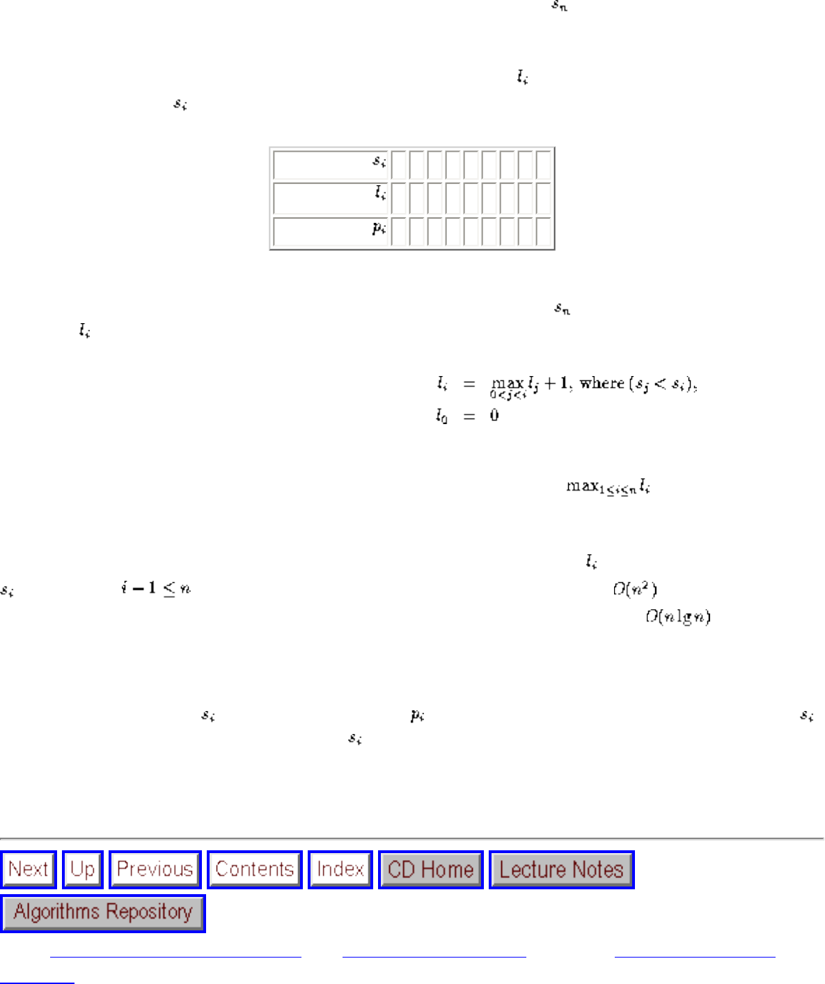
Longest Increasing Sequence
Will the length of the final longest increasing subsequence of S be 5 or 6?
● Therefore, we also need the length of the longest sequence that will extend. To be certain we
know this, we really need the length of the longest sequence that any possible number can extend.
This provides the idea around which to build a recurrence. Define to be the length of the longest
sequence ending with . Verify that the following table is correct:
sequence 9 5 2 8 7 3 1 6 4
length 1 1 1 2 2 2 1 3 3
predecessor - - - 2 2 3 - 6 6
The longest increasing sequence containing the nth number will be formed by appending it to the longest
increasing sequence to the left of n that ends on a number smaller than . The following recurrence
computes :
These values define the length of the longest increasing sequence ending at each number. The length of
the longest increasing subsequence of the entire permutation is given by , since the winning
sequence will have to end somewhere.
What is the time complexity of this algorithm? Each one of the n values of is computed by comparing
against up to values to the left of it, so this analysis gives a total of time. In fact, by
using dictionary data structures in a clever way, we can evaluate this recurrence in time.
However, the simple recurrence would be easy to program and therefore is a good place to start.
What auxiliary information will we need to store in order to reconstruct the actual sequence instead of its
length? For each element , we will store the index of the element that appears immediately before
in the longest increasing sequence ending at . Since all of these pointers go towards the left, it is a
simple matter to start from the last value of the longest sequence and follow the pointers so as to
reconstruct the other items in the sequence.
Next: Minimum Weight Triangulation Up: Dynamic Programming Previous: Approximate String
Matching
file:///E|/BOOK/BOOK2/NODE47.HTM (2 of 3) [19/1/2003 1:28:48]
Longest Increasing Sequence
Algorithms
Mon Jun 2 23:33:50 EDT 1997
file:///E|/BOOK/BOOK2/NODE47.HTM (3 of 3) [19/1/2003 1:28:48]
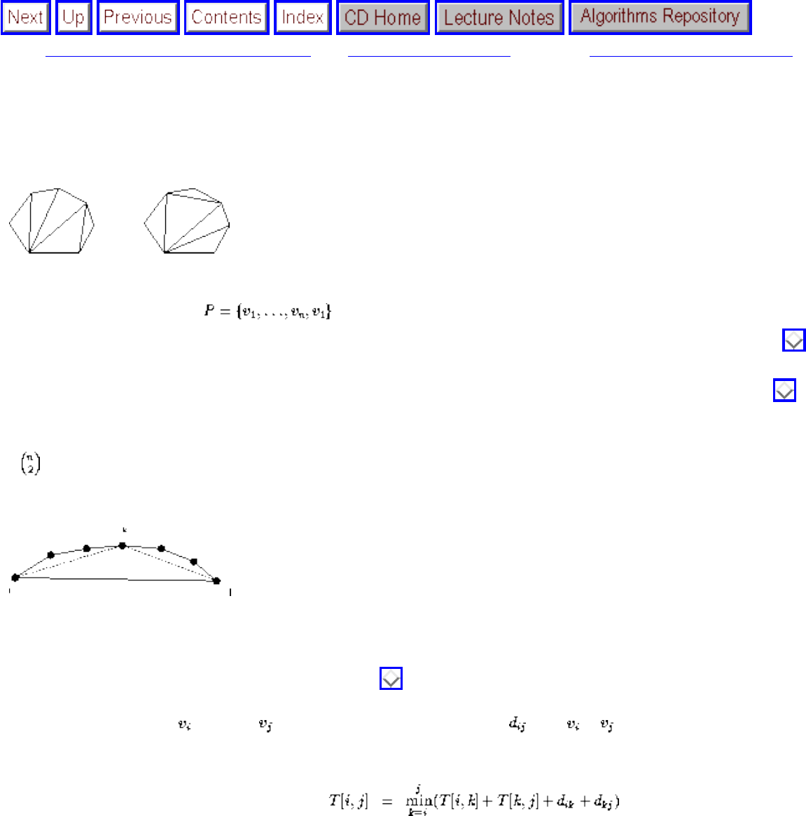
Minimum Weight Triangulation
Next: Limitations of Dynamic Programming Up: Dynamic Programming Previous: Longest Increasing Sequence
Minimum Weight Triangulation
Figure: Two different triangulations of a given convex seven-gon
A triangulation of a polygon is a set of non-intersecting diagonals that partitions the polygon into
triangles. We say that the weight of a triangulation is the sum of the lengths of its diagonals. As shown in Figure ,
any given polygon may have many different triangulations. For any given polygon, we seek to find its minimum weight
triangulation. Triangulation is a fundamental component of most geometric algorithms, as discussed in Section .
To apply dynamic programming, we need a way to carve up the polygon into smaller pieces. A first idea might be to try
all possible chords, each of which partitions the polygon into two smaller polygons. Using dynamic programming,
this will work to give a polynomial-time algorithm. However, there is a slicker approach.
Figure: Selecting the vertex k to pair with an edge (i,j) of the polygon
Observe that every edge of the input polygon must be involved in exactly one triangle. Turning this edge into a triangle
means identifying the third vertex, as shown in Figure . Once we find the correct connecting vertex, the polygon
will be partitioned into two smaller pieces, both of which need to be triangulated optimally. Let T[i,j] be the cost of
triangulating from vertex to vertex , ignoring the length of the chord from to . The latter clause avoids
double counting these internal chords in the following recurrence:
The basis condition applies when i and j are immediate neighbors, as T[i,i+1] = 0.
Since the number of vertices in each subrange of the right side of the recurrence is smaller than that on the left side,
evaluation can proceed in terms of the gap size from i to j:
Minimum-Weight-Triangulation(P)
file:///E|/BOOK/BOOK2/NODE48.HTM (1 of 2) [19/1/2003 1:28:49]
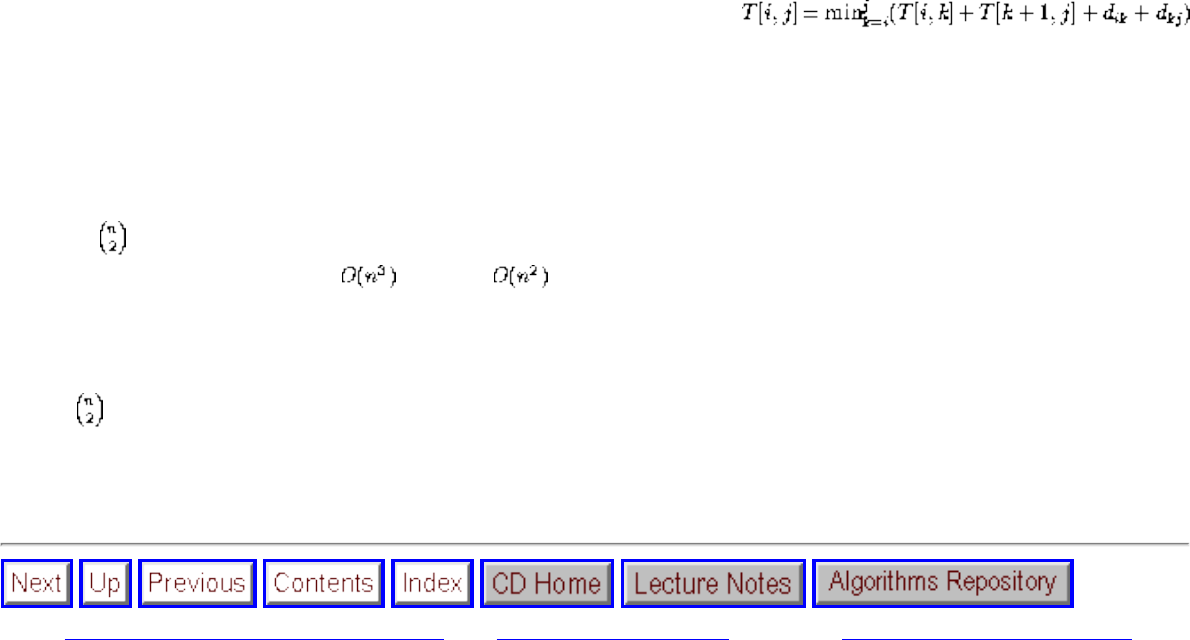
Minimum Weight Triangulation
for i=1 to n do T[i, j]=0
for gap=1 to n-1
for i=1 to n-gap do
j=i+gap
return T[1, n]
There are values of T, each of which takes O(j-i) time if we evaluate the sections in order of increasing size. Since j-i
= O(n), complete evaluation takes time and space.
What if there are points in the interior of the polygon? Then dynamic programming does not apply in the same way,
because each of the triangulation edges does not necessarily cut the boundary into two distinct pieces as before. Instead
of only possible subregions, the number of subregions now grows exponentially. In fact, no efficient algorithm for
this problem is known. More surprisingly, there is also no known proof of hardness. Minimum weight triangulation is
one of the few well-studied algorithmic problems that remain in this limbo state.
Next: Limitations of Dynamic Programming Up: Dynamic Programming Previous: Longest Increasing Sequence
Algorithms
Mon Jun 2 23:33:50 EDT 1997
file:///E|/BOOK/BOOK2/NODE48.HTM (2 of 2) [19/1/2003 1:28:49]
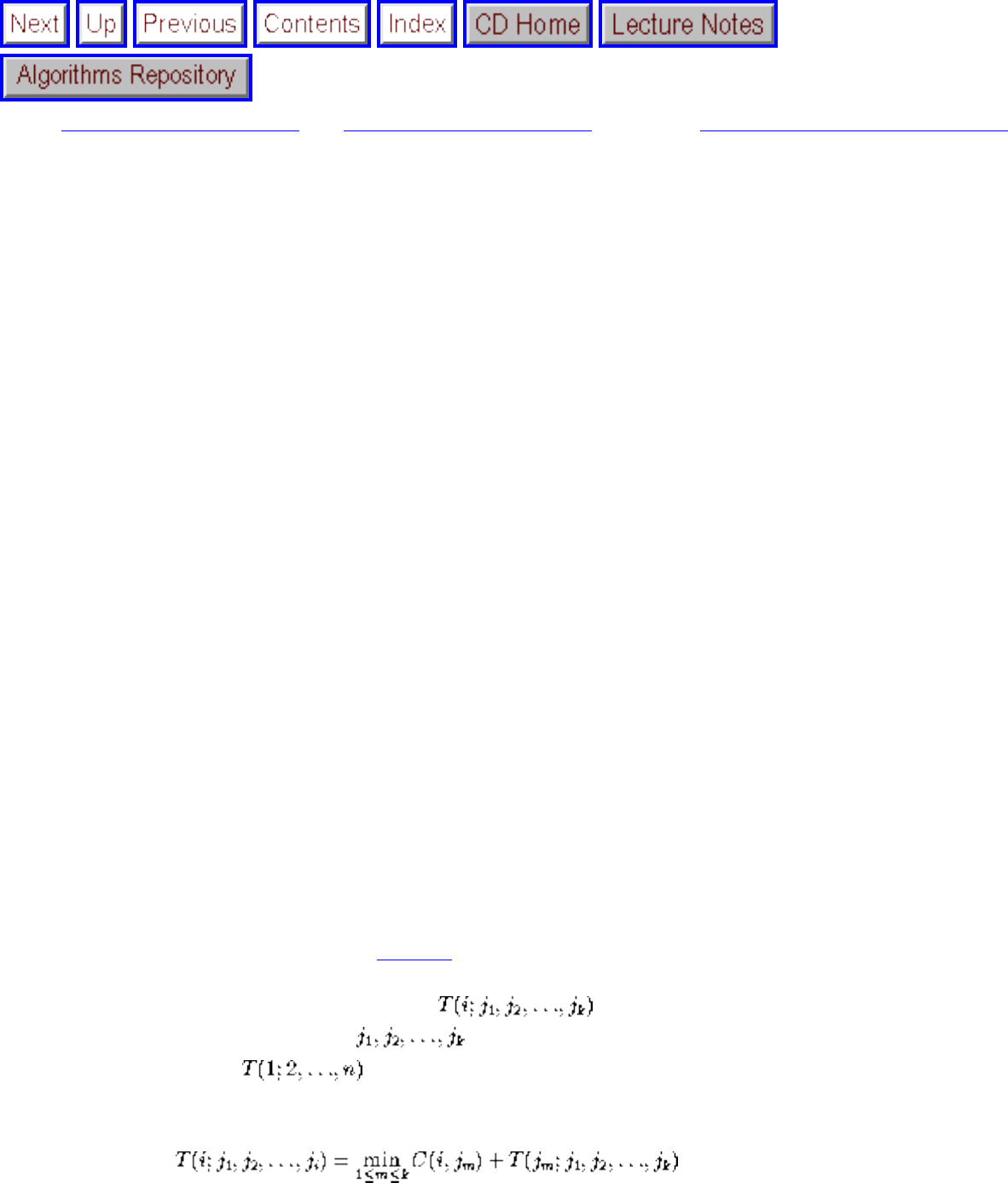
Limitations of Dynamic Programming
Next: War Story: Evolution of Up: Breaking Problems Down Previous: Minimum Weight Triangulation
Limitations of Dynamic Programming
Dynamic programming can be applied to any problem that observes the principle of optimality. Roughly
stated, this means that partial solutions can be optimally extended with regard to the state after the partial
solution instead of the partial solution itself. For example, to decide whether to extend an approximate
string matching by a substitution, insertion, or deletion, we do not need to know exactly which sequence
of operations was performed to date. In fact, there may be several different edit sequences that achieve a
cost of C on the first p characters of pattern P and t characters of string T. Future decisions will be made
based on the consequences of previous decisions, not the actual decisions themselves.
Problems do not satisfy the principle of optimality if the actual operations matter, as opposed to just the
cost of the operations. Consider a form of edit distance where we are not allowed to use combinations of
operations in certain particular orders. Properly formulated, however, most combinatorial problems
respect the principle of optimality.
The biggest limitation on using dynamic programming is the number of partial solutions we must keep
track of. For all of the examples we have seen, the partial solutions can be completely described by
specifying the stopping places in the input. This is because the combinatorial objects being worked on
(strings, numerical sequences, and polygons) all have an implicit order defined upon their elements. This
order cannot be scrambled without completely changing the problem. Once the order is fixed, there are
relatively few possible stopping places or states, so we get efficient algorithms. If the objects are not
firmly ordered, however, we have an exponential number of possible partial solutions and are doomed to
need an infeasible amount of memory.
To illustrate this, consider the following dynamic programming algorithm for the traveling salesman
problem, discussed in greater detail in [RND77]. Recall that solving a TSP means finding the order that
visits each site exactly once, while minimizing the total distance traveled or cost paid. Let C(i,j) to be the
edge cost to travel directly from i to j. Define to be the cost of the optimal tour from i to
1 that goes through each of the cities exactly once, in any order. The cost of the optimal TSP
tour is thus defined to be and can be computed recursively by identifying the first edge in
this sequence:
using the basis cases
file:///E|/BOOK/BOOK2/NODE49.HTM (1 of 2) [19/1/2003 1:28:50]
Limitations of Dynamic Programming
This recurrence, although somewhat complicated to understand, is in fact correct. However, each partial
solution is described by a vertex subset . Since there are subsets of n vertices, we require
time and space to evaluate this recurrence. Whenever the input objects do not have an inherent left-
right order, we are typically doomed to having an exponential-sized state space. Occasionally this is
manageable - indeed, is a big improvement over enumerating all O(n!) possible TSP tours. Still,
dynamic programming is most effective on well-ordered objects.
Next: War Story: Evolution of Up: Breaking Problems Down Previous: Minimum Weight Triangulation
Algorithms
Mon Jun 2 23:33:50 EDT 1997
file:///E|/BOOK/BOOK2/NODE49.HTM (2 of 2) [19/1/2003 1:28:50]
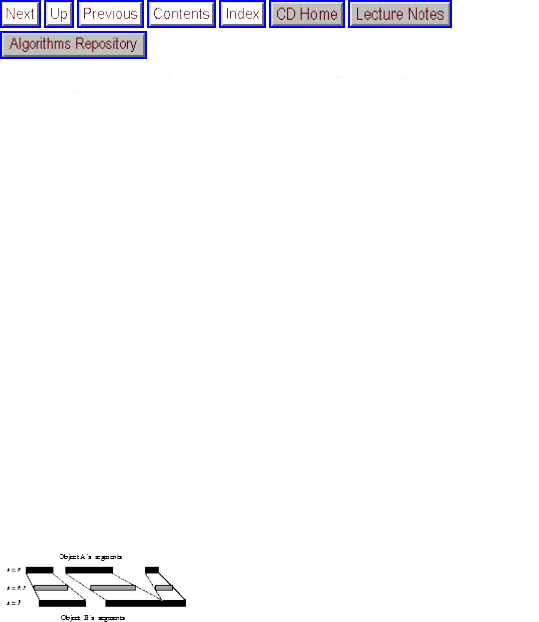
War Story: Evolution of the Lobster
Next: War Story: What's Past Up: Breaking Problems Down Previous: Limitations of Dynamic
Programming
War Story: Evolution of the Lobster
I'll confess that I'm always surprised to see graduate students stop by my office early in the morning.
Something about working through the night makes that time inconvenient for them. But there they were,
two future Ph.D.s working in the field of high-performance computer graphics. They studied new
techniques for rendering pretty computer images. The picture they painted for me that morning was
anything but pretty, however.
``You see, we want to build a program to morph one image into another,'' they explained.
``What do you mean by morph?'' I asked.
``For special effects in movies, we want to construct the intermediate stages in transforming one image
into another. Suppose we want to turn you into Humphrey Bogart. For this to look realistic, we must
construct a bunch of in-between frames that start out looking like you and end up looking like him.''
``If you can realistically turn me into Bogart, you have something,'' I agreed.
``But our problem is that it isn't very realistic.'' They showed me a dismal morph between two images.
``The trouble is that we must find the right correspondence between features in the two images. It looks
real bad when we get the correspondence wrong and try to morph a lip into an ear.''
``I'll bet. So you want me to give you an algorithm for matching up lips?''
Figure: A successful alignment of two lines of pixels
``No, even simpler. We just morph each row of the initial image into the identical row of the final image.
You can assume that we give you two lines of pixels, and you have to find the best possible match
between the dark pixels in a row from object A to the dark pixels in the corresponding row of object B.
file:///E|/BOOK/BOOK2/NODE50.HTM (1 of 4) [19/1/2003 1:28:52]
War Story: Evolution of the Lobster
Like this,'' they said, showing me images of successful matchings like those in Figure .
``I see,'' I said. ``You want to match big dark regions to big dark regions and small dark regions to small
dark regions.''
``Yes, but only if the matching doesn't shift them too much to the left or the right. We might prefer to
merge or break up regions rather than shift them too far away, since that might mean matching a chin to
an eyebrow. What is the best way to do it?''
``One last question. Will you ever want to match two intervals to each other in such a way that they
cross?''
``No, I guess not. Crossing intervals can't match. It would be like switching your left and right eyes.''
I scratched my chin and tried to look puzzled, but I'm just not as good an actor as Bogart. I'd had a hunch
about what needed to be done the instant they started talking about lines of pixels. They want to
transform one array of pixels into another array, with the minimum amount of changes. That sounded
like editing one string of pixels into another string, which is a classic application of dynamic
programming. See Sections and for discussions of approximate string matching.
The fact that the intervals couldn't cross just sealed things up. It meant that whenever a stretch of dark
pixels from A was mapped to a stretch from B, the problem would be split into two smaller subproblems,
i.e. the pixels to the left of the match and the pixels to the right of the match. The cost of the global match
would ultimately be the cost of this match plus those of matching all the pixels to the left and of
matching all the pixels to the right. Constructing the optimal match on the left side is a smaller problem
and hence simpler. Further, there can be only possible left subproblems, since each is completely
described by the pair of one of n top pixels and one of n bottom pixels.
``Your algorithm will be based on dynamic programming,'' I pronounced. ``However, there are several
possible ways to do things, depending upon whether you want to edit pixels or runs. I would probably
convert each row into a list of black pixel runs, with the runs sorted by right endpoint and each run
labeled with its starting position and length. You will maintain the cost of the cheapest match between
the leftmost i runs and the leftmost j runs for all i and j. The possible edit operations are:
file:///E|/BOOK/BOOK2/NODE50.HTM (2 of 4) [19/1/2003 1:28:52]
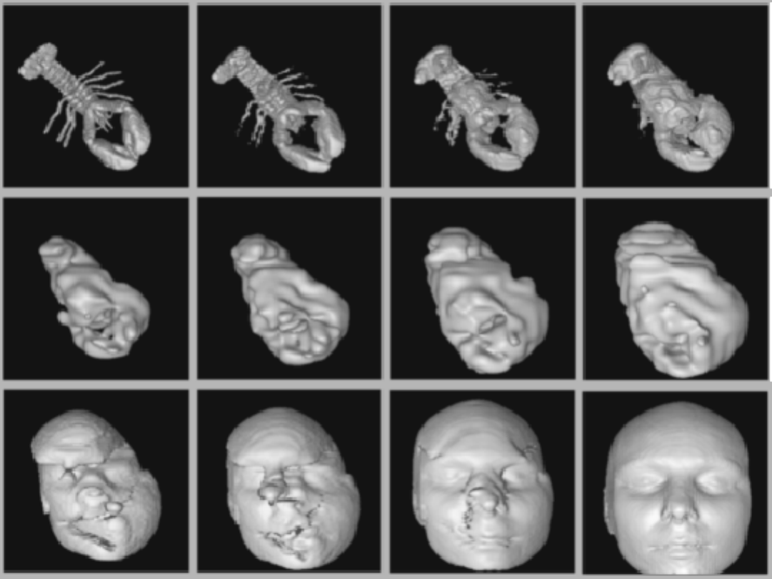
War Story: Evolution of the Lobster
Figure: Morphing a lobster into a head via dynamic programming
● Full run match: We may match run i on top to run j on the bottom for a cost that is a function of
the difference in the lengths of the two runs and their positions.
● Merging runs: We may match a string of consecutive runs on top to a run on the bottom. The cost
will be a function of the number of runs, their relative positions, and their lengths.
● Splitting runs: We may match a big run on top to a string of consecutive runs on the bottom. This
is just the converse of the merge. Again, the cost will be a function of the number of runs, their
relative positions, and their lengths.
``For each pair of runs (i,j) and all the cases that apply, we compute the cost of the edit operation and add
to the (already computed and stored) edit cost to the left of the start of the edit. The cheapest of these
cases is what we will take for the cost of c[i,j].''
The pair of graduate students scribbled this down, then frowned. ``So we are going to have a cost
measure for matching two runs that is a function of their lengths and positions. How do we decide what
the relative costs should be?''
file:///E|/BOOK/BOOK2/NODE50.HTM (3 of 4) [19/1/2003 1:28:52]
War Story: Evolution of the Lobster
``That is your business. The dynamic programming serves to optimize the matchings once you know the
cost functions. It is up to your aesthetic sense to decide what penalties there should be for line length
changes or offsets. My recommendation is that you implement the dynamic programming and try
different values for the constants effecting the relative penalties on each of several different images. Then
pick the setting that seems to do what you want.''
They looked at each other and smiled, then ran back into the lab to implement it. Using dynamic
programming to do their alignments, they completed their morphing system, which is described in
[HWK94]. They produced the images shown in Figure , morphing a lobster into a man.
Unfortunately, they never got around to turning me into Humphrey Bogart.
Next: War Story: What's Past Up: Breaking Problems Down Previous: Limitations of Dynamic
Programming
Algorithms
Mon Jun 2 23:33:50 EDT 1997
file:///E|/BOOK/BOOK2/NODE50.HTM (4 of 4) [19/1/2003 1:28:52]

War Story: What's Past is Prolog
Next: War Story: Text Compression Up: Breaking Problems Down Previous: War Story: Evolution of
War Story: What's Past is Prolog
``But our heuristic works very, very well in practice.'' He was simultaneously boasting and crying for
help.
Unification is the basic computational mechanism in logic programming languages like Prolog. A Prolog
program consists of a set of rules, where each rule has a head and an associated action whenever the rule
head matches or unifies with the current computation.
An execution of a Prolog program starts by specifying a goal, say p(a,X,Y), where a is a constant and X
and Y are variables. The system then systematically matches the head of the goal with the head of each of
the rules that can be unified with the goal. Unification means binding the variables with the constants, if
it is possible to match them. For the nonsense program below, p(X,Y,a) unifies with either of the first two
rules, since X and Y can be bound to match the extra characters. The goal p(X,X,a) would only match the
first rule, since the variable bound to the first and second positions must be the same.
p(a,a,a) := h(a);
p(b,a,a) := h(a) * h(b);
p(c,b,b) := h(b) + h(c);
p(d,b,b) := h(d) + h(b);
file:///E|/BOOK/BOOK2/NODE51.HTM (1 of 4) [19/1/2003 1:28:54]
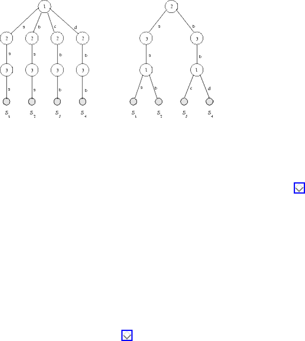
War Story: What's Past is Prolog
Figure: Two different tries for the given set of rule heads
``In order to speed up unification, we want to preprocess the set of rule heads so that we can quickly
determine which rules match a given goal. We must organize the rules in a trie data structure for fast
unification.''
Tries are extremely useful data structures in working with strings, as discussed in Section . Every leaf
of the trie represents one string. Each node on the path from root to leaf is labeled with exactly one
character of the string, with the ith node of the path corresponding to the ith character of the string.
``I agree. A trie is a natural way to represent your rule heads. Building a trie on a set of strings of
characters is straightforward - just insert the strings one after another starting from the root. So what is
your problem?'' I asked.
``The efficiency of our unification algorithm depends very much on minimizing the number of edges in
the trie. Since we know all the rules in advance, we have the freedom to reorder the character positions in
the rules. Instead of the root node always representing the first argument in the rule, we can choose to
have it represent the third argument. We would like to use this freedom to build a minimum-size trie for
the set of rules.''
He showed me the example in Figure . A trie constructed according to the original string position
order (1, 2, 3) uses a total of 12 edges. However, by permuting the character order to (2, 3, 1), we can
obtain a trie with only 8 edges.
``Why does the speed of unification depend on minimizing the number of edges in the trie?''
``An open goal is one with all distinct variables in its arguments, like p(X,Y,Z). Open goals match
everything. In unifying an open goal against a set of clause heads, each symbol in all the clause heads
will be bound to some variable. By doing a depth-first traversal of this minimum-edge trie, we minimize
file:///E|/BOOK/BOOK2/NODE51.HTM (2 of 4) [19/1/2003 1:28:54]
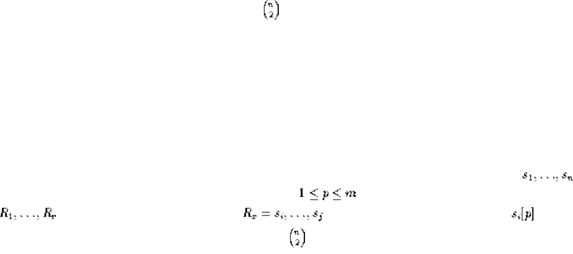
War Story: What's Past is Prolog
the number of operations in unifying the goal with all of the clause heads,'' he explained quickly.
``Interesting...'' I started to reply before he cut me off again.
``One other constraint. For most applications we must keep the leaves of the trie ordered, so that the
leaves of the underlying tree go left-to-right in the same order as the rules appear on the page.''
``But why do you have to keep the leaves of the trie in the given order?'' I asked.
``The order of rules in Prolog programs is very, very important. If you change the order of the rules, the
program returns different results.''
Then came my mission.
``We have a greedy heuristic for building good but not optimal tries, based on picking as the root the
character position that minimizes the degree of the root. In other words, it picks the character position
that has the smallest number of distinct characters in it. This heuristic works very, very well in practice.
But we need you to prove that finding the best trie is NP-complete so our paper is, well, complete.''
I agreed to think about proving the hardness of the problem and chased him from my office. The problem
did seem to involve some non-trivial combinatorial optimization to build the minimal tree, but I couldn't
see how to factor the left-to-right order of the rules into a hardness proof. In fact, I couldn't think of any
NP-complete problem that had such a left-right ordering constraint. After all, if a given set of rules
contained a character position in common to all the rules, that character position must be probed first in
any minimum-size tree. Since the rules were ordered, each node in the subtree must represent the root of
a run of consecutive rules, so there were only possible nodes to choose from for this tree....
Bingo! That settled it.
The next day I went back to the professor and told him. ``Look, I cannot prove that your problem is NP-
complete. But how would you feel about an efficient dynamic programming algorithm to find the best
trie!'' It was a pleasure watching his frown change to a smile as the realization took hold. An efficient
algorithm to compute what he needed was infinitely better than a proof saying you couldn't do it!
My recurrence looked something like this. Suppose that we are given n ordered rule heads ,
each with m arguments. Probing at the pth position, , partitioned the rule heads into runs
, where each rule in a given run had the same character value of . The rules
in each run must be consecutive, so there are only possible runs to worry about. The cost of probing at
position p is the cost of finishing the trees formed by each of the created runs, plus one edge per tree to
link it to probe p:
file:///E|/BOOK/BOOK2/NODE51.HTM (3 of 4) [19/1/2003 1:28:54]
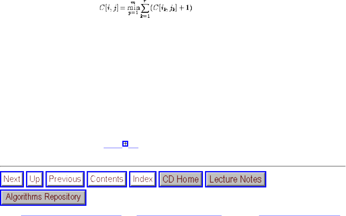
War Story: What's Past is Prolog
A graduate student immediately set to work implementing dynamic programming to compare with their
heuristic. On many programs the optimal and greedy algorithms constructed the exact same trie.
However, for some examples, dynamic programming gave a 20% performance improvement over
greedy, i.e. 20% better than very, very well in practice. The run time spent in doing the dynamic
programming was sometimes a bit larger than with greedy, but in compiler optimization you are always
happy to trade off a little extra compilation time for better execution time performance of your program.
Is a 20% improvement worth it? That depends upon the situation. For example, how useful would you
find a 20% increase in your salary?
The fact that the rules had to remain ordered was the crucial property that we exploited in the dynamic
programming solution. Indeed, without it, I was able to prove that the problem was NP-complete,
something we put in the paper [DRR 95] to make it complete.
Next: War Story: Text Compression Up: Breaking Problems Down Previous: War Story: Evolution of
Algorithms
Mon Jun 2 23:33:50 EDT 1997
file:///E|/BOOK/BOOK2/NODE51.HTM (4 of 4) [19/1/2003 1:28:54]

War Story: Text Compression for Bar Codes
Next: Divide and Conquer Up: Breaking Problems Down Previous: War Story: What's Past
War Story: Text Compression for Bar
Codes
Ynjiun waved his laser wand over the torn and crumpled fragments of a bar code label. The system
hesitated for a few seconds, then responded with a pleasant blip sound. He smiled at me in triumph.
``Virtually indestructible.''
I was visiting the research laboratories of Symbol Technologies, of Bohemia NY, the world's leading
manufacturer of bar code scanning equipment. Next time you are in the checkout line at a grocery store,
check to see what type of scanning equipment they are using. Likely it will say Symbol on the housing.
Although we take bar codes for granted, there is a surprising amount of technology behind them. Bar
codes exist primarily because conventional optical character recognition (OCR) systems are not
sufficiently reliable for inventory operations. The bar code symbology familiar to us on each box of
cereal or pack of gum encodes a ten-digit number with sufficient error correction such that it is virtually
impossible to scan the wrong number, even if the can is upside-down or dented. Occasionally, the cashier
won't be able to get a label to scan at all, but once you hear that blip you know it was read correctly.
The ten-digit capacity of conventional bar code labels means that there is only room to store a single ID
number in a label. Thus any application of supermarket bar codes must have a database mapping 11141-
47011 to a particular size and brand of soy sauce. The holy grail of the bar code world has long been the
development of higher-capacity bar code symbologies that can store entire documents, yet still be read
reliably. Largely through the efforts of Theo Pavlidis and Ynjiun Wang at Stony Brook [PSW92],
Symbol Technologies was ready to introduce the first such product.
Figure: A two-dimensional bar-code label of the Gettysburg Address using PDF-417
``PDF-417 is our new, two-dimensional bar code symbology,'' Ynjiun explained. A sample label is
file:///E|/BOOK/BOOK2/NODE52.HTM (1 of 4) [19/1/2003 1:28:55]
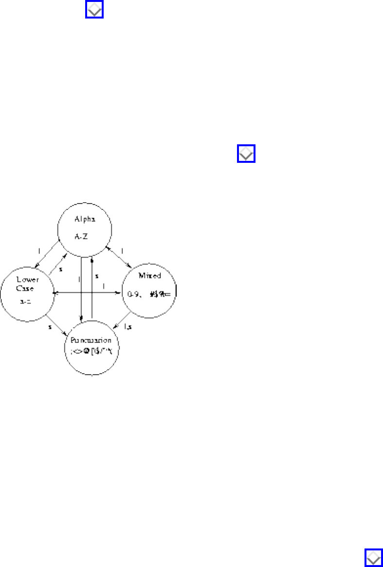
War Story: Text Compression for Bar Codes
shown in Figure .
``How much data can you fit in a typical one-inch square label?'' I asked him.
``It depends upon the level of error correction we use, but about 1,000 bytes. That's enough for a small
text file or image,'' he said.
``Interesting. You will probably want to use some data compression technique to maximize the amount
of text you can store in a label.'' See Section for a discussion of standard data compression
algorithms.
Figure: Mode switching in PDF-417
``We do incorporate a data compaction method,'' he explained. ``We figure there are several different
types of files our customers will want to use our labels for. Some files will be all in uppercase letters,
while others will use mixed-case letters and numbers. We provide four different text modes in our code,
each with a different subset of ASCII characters available. So long as we stay within a mode, we can
describe each character using only five bits. When we have to switch modes, we issue a mode switch
command first (taking an extra five bits) and then the new code.''
``I see. So you designed the mode character sets to try to minimize the number of mode switch
operations on typical text files.'' The modes are illustrated in Figure .
``Right. We put all the digits in one mode and all the punctuation characters in another. We also included
both mode shift and mode latch commands. In a mode shift, we switch into a new mode just for the next
character, say to produce a punctuation mark. This way, we don't pay a cost for returning back to text
mode after a period. Of course, we can also latch permanently into a different mode if we will be using a
run of several characters from there.''
``Wow!'' I said. ``With all of this mode switching going on, there must be many different ways to encode
file:///E|/BOOK/BOOK2/NODE52.HTM (2 of 4) [19/1/2003 1:28:55]
War Story: Text Compression for Bar Codes
any given text as a label. How do you find the smallest such encoding.''
``We use a greedy-type algorithm. We look a few characters ahead and then decide which mode we
would be best off in. It works fairly well.''
I pressed him on this. ``How do you know it works fairly well? There might be significantly better
encodings that you are simply not finding.''
``I guess I don't know. But it's probably NP-complete to find the optimal coding.'' Ynjiun's voice trailed
off. ``Isn't it?''
I started to think. Every encoding started in a given mode and consisted of a sequence of intermixed
character codes and mode shift/latch operations. At any given position in the text, we could output the
next character code (if it was available in our current mode) or decide to shift. As we moved from left to
right through the text, our current state would be completely reflected by our current character position
and current mode state. For a given position/mode pair, we would have been interested in the cheapest
way of getting there, over all possible encodings getting to this point....
My eyes lit up so bright they cast shadows on the walls.
``The optimal encoding for any given text in PDF-417 can be found using dynamic programming. For
each possible mode and each character position , we will maintain the cheapest
encoding found of the string to the left of i ending in mode m. From each mode/position, we can either
match, shift, or latch, so there are only few possible operations to consider. Each of the 4n cells can be
filled in constant time, so it takes time linear in the length of the string to find the optimal encoding.''
Ynjiun was skeptical, but he encouraged us to implement an optimal encoder. A few complications arose
due to weirdnesses of PDF-417 mode switching, but my student Yaw-Ling Lin rose to the challenge.
Symbol compared our encoder to theirs on 13,000 labels and concluded that dynamic programming lead
to an 8% tighter encoding on average. This was significant, because no one wants to waste 8% of their
potential storage capacity, particularly in an environment where the capacity is only a few hundred bytes.
For certain applications, this 8% margin permitted one bar code label to suffice where previously two
had been required. Of course, an 8% average improvement meant that it did much better than that on
certain labels. While our encoder took slightly longer to run than the greedy encoder, this was not
significant, since the bottleneck would be the time needed to print the label, anyway.
Our observed impact of replacing a heuristic solution with the global optimum is probably typical of
most applications. Unless you really botch your heuristic, you are probably going to get a decent
solution. But replacing it with an optimal result usually gives a small but non-trivial improvement, which
can have pleasing consequences for your application.
file:///E|/BOOK/BOOK2/NODE52.HTM (3 of 4) [19/1/2003 1:28:55]

Divide and Conquer
Next: Fast Exponentiation Up: Breaking Problems Down Previous: War Story: Text Compression
Divide and Conquer
Divide and conquer was a successful military strategy long before it became an algorithm design
paradigm. Generals observed that it was easier to defeat one army of 50,000 men, followed by another
army of 50,000 men than it was to beat a single 100,000 man army. Thus the wise general would attack
so as to divide the enemy army into two forces and then mop up one after the other.
To use divide and conquer as an algorithm design technique, we must divide the problem into two
smaller subproblems, solve each of them recursively, and then meld the two partial solutions into one
solution to the full problem. Whenever the merging takes less time than solving the two subproblems, we
get an efficient algorithm. Mergesort, discussed in Section , is the classic example of a divide-and-
conquer algorithm. It takes only linear time to merge two sorted lists of n/2 elements each of which was
obtained in time.
Divide and conquer is a design technique with many important algorithms to its credit, including
mergesort, the fast Fourier transform, and Strassen's matrix multiplication algorithm. However, with the
exception of binary search, I find it to be a difficult technique to apply in practice. Therefore, the
examples below will illustrate binary search and its variants, which yield simple algorithms to solve a
surprisingly wide range of problems.
● Fast Exponentiation
● Binary Search
● Square and Other Roots
Algorithms
file:///E|/BOOK/BOOK2/NODE53.HTM (1 of 2) [19/1/2003 1:28:56]
Divide and Conquer
Mon Jun 2 23:33:50 EDT 1997
file:///E|/BOOK/BOOK2/NODE53.HTM (2 of 2) [19/1/2003 1:28:56]
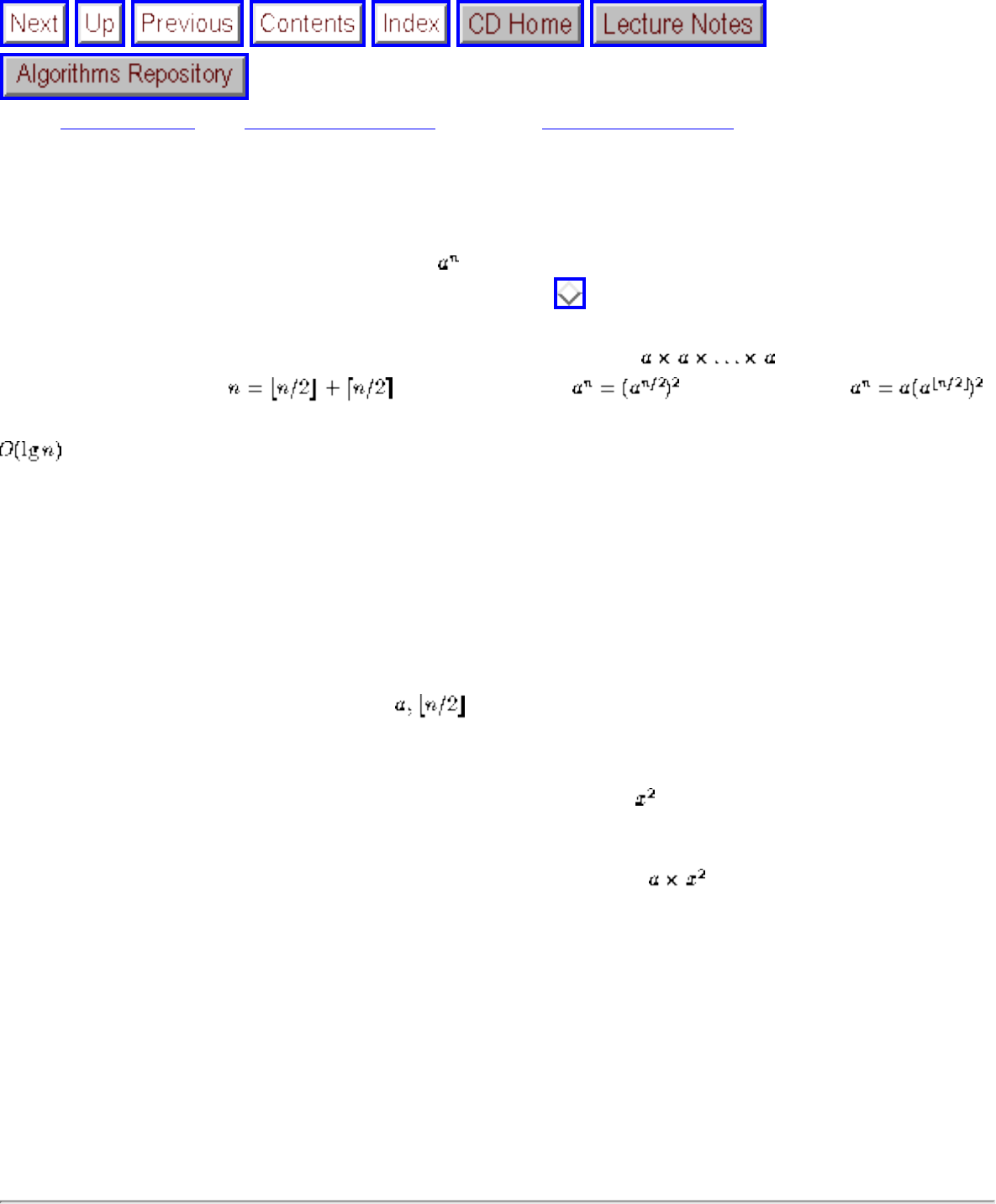
Fast Exponentiation
Next: Binary Search Up: Divide and Conquer Previous: Divide and Conquer
Fast Exponentiation
Suppose that we need to compute the value of for some reasonably large n. Such problems occur in
primality testing for cryptography, as discussed in Section .
The simplest algorithm performs n-1 multiplications, by computing . However, we can do
better by observing that . If n is even, then . If n is odd, then .
In either case, we have halved the size of our exponent at the cost of at most two multiplications, so
multiplications suffice to compute the final value.
function power(a,n)
if (n = 0) return(1)
x = power( )
if (n is even) then return( )
else return( )
This simple algorithm illustrates an important principle of divide and conquer. It always pays to divide a
job as evenly as possible. This principle applies to real life as well. When n is not a power of two, the
problem cannot always be divided perfectly evenly, but a difference of one element between the two
sides cannot cause any serious imbalance.
file:///E|/BOOK/BOOK2/NODE54.HTM (1 of 2) [19/1/2003 1:28:57]
Fast Exponentiation
Algorithms
Mon Jun 2 23:33:50 EDT 1997
file:///E|/BOOK/BOOK2/NODE54.HTM (2 of 2) [19/1/2003 1:28:57]
Binary Search
Next: Square and Other Roots Up: Divide and Conquer Previous: Fast Exponentiation
Binary Search
Binary search is a fast algorithm for searching in a sorted array S of keys. To search for key q, we
compare q to the middle key S[n/2]. If q appears before S[n/2], it must reside in the top half of our set; if
not, it must reside in the bottom half of our set. By recursively repeating this process on the correct half,
we find the key in a total of comparisons, a big win over the n/2 we expect with sequential search.
This much you probably know. What is important is to have a sense for just how fast binary search is.
Twenty questions is a popular children's game, where one player selects a word, and the other repeatedly
asks true/false questions in an attempt to identify the word. If the word remains unidentified after 20
questions, the first party wins; otherwise, the second player takes the honors. In fact, the second player
always has a winning strategy, based on binary search. Given a printed dictionary, the player opens it in
the middle, selects a word (say ``move''), and asks whether the unknown word is before ``move'' in
alphabetical order. Since standard dictionaries contain 50,000 to 200,000 words, we can be certain that
the process will always terminate within twenty questions.
Other interesting algorithms follow from simple variants of binary search. For example, suppose we have
an array A consisting of a run of 0's, followed by an unbounded run of 1's, and would like to identify the
exact point of transition between them. Binary search on the array would provide the transition point in
tests, if we had a bound n on the number of elements in the array. In the absence of such a bound,
we can test repeatedly at larger intervals (A[1], A[2], A[4], A[8], A[16], ) until we find a first non-zero
value. Now we have a window containing the target and can proceed with binary search. This one-
sided binary search finds the transition point p using at most comparisons, regardless of how large the
array actally is. One-sided binary search is most useful whenever we are looking for a key that probably
lies close to our current position.
Next: Square and Other Roots Up: Divide and Conquer Previous: Fast Exponentiation
Algorithms
Mon Jun 2 23:33:50 EDT 1997
file:///E|/BOOK/BOOK2/NODE55.HTM [19/1/2003 1:28:58]
Square and Other Roots
Next: Exercises Up: Divide and Conquer Previous: Binary Search
Square and Other Roots
The square root of n is the number r such that . Square root computations are performed inside
every pocket calculator, but it is instructive to develop an efficient algorithm to compute square roots.
First, observe that the square root of must be at least 1 and at most n. Let l=1 and r=n. Consider the
midpoint of this interval, m=(l+r)/2. How does compare to n? If , then the square root must be
greater than m, so the algorithm repeats with l=m. If , then the square root must be less than m, so
the algorithm repeats with r=m. Either way, we have halved the interval with only one comparison.
Therefore, after only rounds we will have identified the square root to within .
This bisection method, as it is called in numerical analysis, can also be applied to the more general
problem of finding the roots of an equation. We say that x is a root of the function f if f(x)=0. Suppose
that we start with values l and r such that f(l) > 0 and f(r) < 0. If f is a continuous function, there must be
a root between l and r. Depending upon the sign of f(m), where m=(l+r)/2, we can cut this window
containing the root in half with each test and stop when our estimate becomes sufficiently accurate.
Root-finding algorithms that converge faster than binary search are known for both of these problems.
Instead of always testing the midpoint of the interval, these algorithms interpolate to find a test point
closer to the actual root. Still, binary search is simple, robust, and works as well as possible without
additional information on the nature of the function to be computed.
Algorithms
Mon Jun 2 23:33:50 EDT 1997
file:///E|/BOOK/BOOK2/NODE56.HTM [19/1/2003 1:28:59]
Exercises
Next: Implementation Challenges Up: Breaking Problems Down Previous: Square and Other Roots
Exercises
1. Consider the problem of storing n books on shelves in a library. The order of the books is fixed by
the cataloging system and so cannot be rearranged. Therefore, we can speak of a book , where
, that has a thickness and height . The length of each bookshelf at this library is L.
Suppose all the books have the same height h (i.e. for all i, j) and the shelves are all
separated by a distance of greater than h, so any book fits on any shelf. The greedy algorithm
would fill the first shelf with as many books as we can until we get the smallest i such that does
not fit, and then repeat with subsequent shelves. Show that the greedy algorithm always finds the
optimal shelf placement, and analyze its time complexity.
2. (*) This is a generalization of the previous problem. Now consider the case where the height of
the books is not constant, but we have the freedom to adjust the height of each shelf to that of the
tallest book on the shelf. Thus the cost of a particular layout is the sum of the heights of the
largest book on each shelf.
❍ Give an example to show that the greedy algorithm of stuffing each shelf as full as possible
does not always give the minimum overall height.
❍ Give an algorithm for this problem, and analyze its time complexity. Hint: use dynamic
programming.
3. (*) Consider a city whose streets are defined by an grid. We are interested in walking from
the upper left-hand corner of the grid to the lower right-hand corner.
Unfortunately, the city has bad neighborhoods, which are defined as intersections we do not want
to walk in. We are given an matrix BAD, where BAD[i,j] = ``yes'' if and only if the
intersection between streets i and j is somewhere we want to avoid.
(a) Give an example of the contents of BAD such that there is no path across the grid avoiding bad
neighborhoods.
(b) Give an O( X Y ) algorithm to find a path across the grid that avoids bad neighborhoods.
file:///E|/BOOK/BOOK2/NODE57.HTM (1 of 4) [19/1/2003 1:29:01]
Exercises
(c) Give an O( X Y ) algorithm to find the shortest path across the grid that avoids bad
neighborhoods. You may assume that all blocks are of equal length. For partial credit, give an
algorithm.
4. (*) Consider the same situation as the previous problem. We have a city whose streets are defined
by an grid. We are interested in walking from the upper left-hand corner of the grid to the
lower right-hand corner. We are given an matrix BAD, where BAD[i,j] = ``yes'' if and only
if the intersection between streets i and j is somewhere we want to avoid.
If there were no bad neighborhoods to contend with, the shortest path across the grid would have
length (X-1) + (Y-1) blocks, and indeed there would be many such paths across the grid. Each path
would consist of only rightward and downward moves.
Give an algorithm that takes the array BAD and returns the number of safe paths of length X+Y-2.
For full credit, your algorithm must run in O( X Y ).
5. (*) Given an array of n real numbers, consider the problem of finding the maximum sum in any
contiguous subvector of the input. For example, in the array
the maximum is achieved by summing the third through seventh elements, where 59+26+(-
53)+58+97 = 187. When all numbers are positive, the entire array is the answer, while when all
numbers are negative, the empty array maximizes the total at 0.
❍ Give a simple, clear, and correct -time algorithm to find the maximum contiguous
subvector.
❍ Now give a -time dynamic programming algorithm for this problem. To get partial
credit, you may instead give a correct divide-and-conquer algorithm.
6. In the United States, coins are minted with denominations of 1, 5, 10, 25, and 50 cents. Now
consider a country whose coins are minted with denominations of units. They seek an
algorithm that will enable them to make change of n units using the minimum number of coins.
(a) The greedy algorithm for making change repeatedly uses the biggest coin smaller than the
amount to be changed until it is zero. Show that the greedy algorithm does not always give the
minimum number of coins in a country whose denominations are .
(b) Give an efficient algorithm that correctly determines the minimum number of coins needed to
make change of n units using denominations . Analyze its running time.
7. (*) In the United States, coins are minted with denominations of 1, 5, 10, 25, and 50 cents. Now
consider a country whose coins are minted with denominations of units. They want to
count how many distinct ways C(n) there are to make change of n units. For example, in a country
file:///E|/BOOK/BOOK2/NODE57.HTM (2 of 4) [19/1/2003 1:29:01]
Exercises
whose denominations are , C(5) = 1, C(6) to C(9)=2, C(10)=3, and C(12)=4.
1. How many ways are there to make change of 20 units from ?
2. Give an efficient algorithm to compute C(n), and analyze its complexity. (Hint: think in
terms of computing C(n,d), the number of ways to make change of n units with highest
denomination d. Be careful to avoid overcounting.)
8. (**) Consider the problem of examining a string of characters from an alphabet on
k symbols, and a multiplication table over this alphabet, and deciding whether or not it is possible
to parenthesize x in such a way that the value of the resulting expression is a, where a belongs to
the alphabet. The multiplication table is neither commutative or associative, so the order of
multiplication matters.
a b c
a a c c
b a a b
c c c c
For example, consider the following multiplication table and the string bbbba. Parenthesizing it
(b(bb))(ba) gives a, but ((((bb)b)b)a) gives c.
Give an algorithm, with time polynomial in n and k, to decide whether such a parenthesization
exists for a given string, multiplication table, and goal element.
9. (*) Consider the following data compression technique. We have a table of m text strings, each of
length at most k. We want to encode a data string D of length n using as few text strings as
possible. For example, if our table contains (a,ba,abab,b) and the data string is bababbaababa,
the best way to encode it is (b,abab,ba,abab,a) - a total of five code words. Give an O(nmk)
algorithm to find the length of the best encoding. You may assume that the string has an encoding
in terms of the table.
10. A company database consists of 10,000 sorted names, 40% of whom are known as good
customers and who together account for 60% of the accesses to the data base. There are two data
structure options to consider for representing the database:
❍ Put all the names in a single array and use binary search.
❍ Put the good customers in one array and the rest of them in a second array. Only if we do
not find the query name on a binary search of the first array do we do a binary search of
the second array.
Demonstrate which option gives better expected performance. Does this change if linear search on
an unsorted array is used instead of binary search for both options?
11. Suppose you are given an array A of n sorted numbers that has been circularly shifted k positions
to the right. For example, is a sorted array that has been circularly shifted k=2
file:///E|/BOOK/BOOK2/NODE57.HTM (3 of 4) [19/1/2003 1:29:01]
Exercises
positions, while has been shifted k=4 positions.
❍ Suppose you know what k is. Give an O(1) algorithm to find the largest number in A.
❍ Suppose you do not know what k is. Give an algorithm to find the largest number in
A. For partial credit, you may give an O(n) algorithm.
12. (*) Suppose that you are given a sorted sequence of distinct integers . Give an
algorithm to determine whether there exists an index i such at . For example, in
, . In , there is no such i.
Next: Implementation Challenges Up: Breaking Problems Down Previous: Square and Other Roots
Algorithms
Mon Jun 2 23:33:50 EDT 1997
file:///E|/BOOK/BOOK2/NODE57.HTM (4 of 4) [19/1/2003 1:29:01]
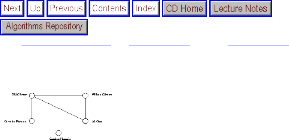
The Friendship Graph
Next: Data Structures for Graphs Up: Graph Algorithms Previous: Graph Algorithms
The Friendship Graph
Figure: A portion of the friendship graph
To demonstrate the importance of proper modeling, let us consider a graph where the vertices are people,
and there is an edge between two people if and only if they are friends. This graph is well-defined on any
set of people, be they the people in your neighborhood, at your school or place of business, or even the
entire world. There are many interesting aspects of people that are best understood as properties of this
friendship graph.
We use this opportunity to define important graph theory terminology. ``Talking the talk'' proves to be an
important part of ``walking the walk''.
● If I am your friend, does that mean you are my friend?
A graph is undirected if edge (x,y) always implies (y,x). Otherwise, the graph is said to be
directed. The ``heard-of'' graph is directed, since many famous people who I have heard of have
never heard of me! The ``had-sex-with'' graph is presumably undirected, since the critical
operation always requires a partner. I'd like to think that the ``friendship'' graph is always an
undirected graph.
● Am I my own friend?
An edge of the form (x,x) is said to be a loop. If x was y's friend several times over, we can model
this relationship using multiedges, multiple edges between the same pair of vertices. A graph is
said to be simple if it contains no loops and no multiple edges. Simple graphs really are often
simpler to work with in practice. Therefore, we might be better off if no one was their own friend.
● How close a friend are you?
A graph is said to be weighted if each edge has an associated numerical attribute. We could model
file:///E|/BOOK/BOOK2/NODE60.HTM (1 of 3) [19/1/2003 1:29:02]
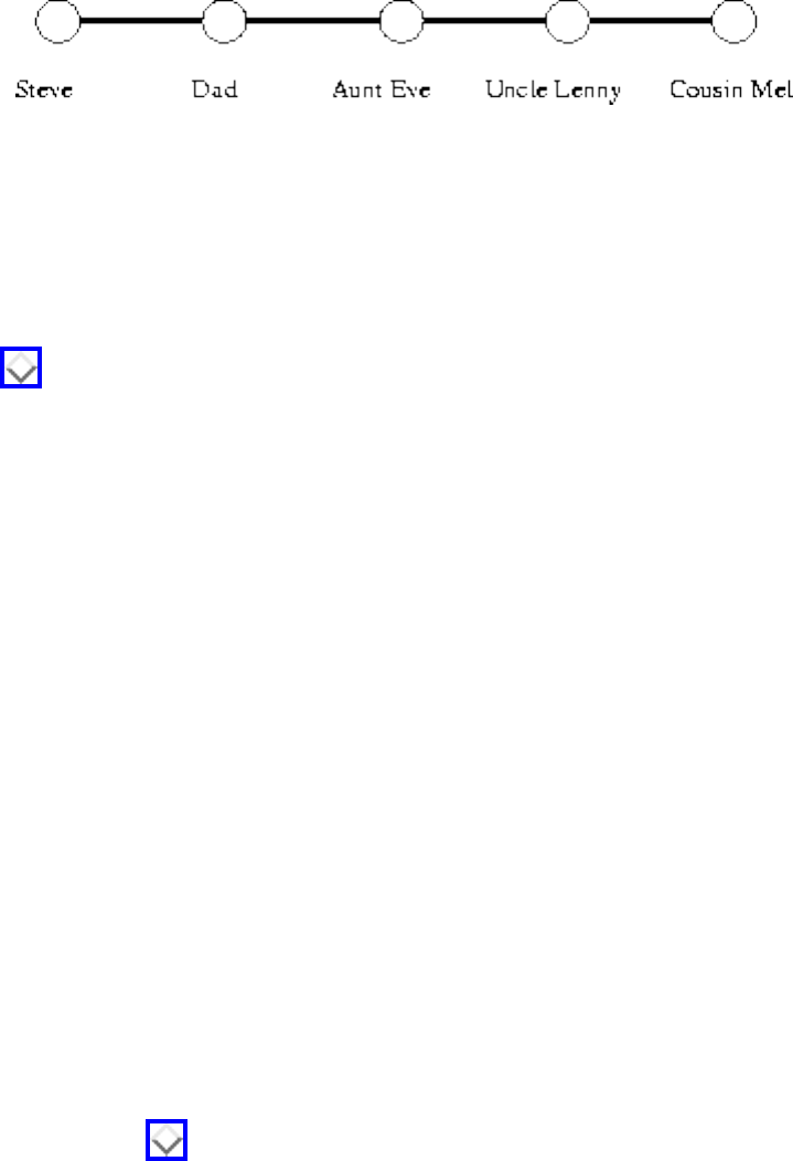
The Friendship Graph
the strength of a friendship by associating each edge with an appropriate number, say from 0
(enemies) to 10 (blood brothers). The edges of a road network graph might be weighted with their
length, drive-time, or speed limit, depending upon the application. A graph is said to be
unweighted if all edges are assumed to be of equal weight.
Figure: Mel Brooks is my father's sister's husband's cousin
● Am I linked by some chain of friends to a star?
A path is a sequence of edges connecting two vertices. Since Mel Brooks is my father's sister's
husband's cousin, there is a path in the friendship graph between me and him, shown in Figure
. This is true even though the two of us have never met.
● How close is my link to that star?
If I were trying to impress you with how tight I am with Mel Brooks, I would be much better off
saying that my Uncle Lenny grew up with him than to go into the details of how connected I am
to Uncle Lenny. Through Uncle Lenny, I have a path of length 2 to Cousin Mel, while the path is
of length 4 by blood and marriage. I could make the path even longer by linking in people who
know both me and my father, or are friends of Aunt Eve and Uncle Lenny. This multiplicity of
paths hints at why finding the shortest path between two nodes is important and instructive, even
in non-transportation applications.
● Is there a path of friends between every two people in the world?
The ``six degrees of separation'' theory argues that there is always a short path linking every two
people in the world. We say that a graph is connected if there is a path between any two vertices.
A directed graph is strongly connected if there is always a directed path between any two vertices.
If a graph is not connected, we call each connected piece a connected component. If we envision
tribes in remote parts of the world that have yet not been encountered, each such tribe would form
a connected component in the friendship graph. A remote hermit, or extremely unpleasant fellow
(see Figure ) would represent a connected component of one vertex, or an isolated vertex.
● Who has the most friends? The fewest friends?
The degree of a vertex is the number of edges adjacent to it. The most popular person defines the
vertex of highest degree in the friendship graph. Remote hermits will be associated with degree-
zero vertices. In dense graphs, most vertices have high degree, as opposed to sparse graphs with
relatively few edges. In regular graphs, each vertex has exactly the same degree. A regular
file:///E|/BOOK/BOOK2/NODE60.HTM (2 of 3) [19/1/2003 1:29:02]

The Friendship Graph
friendship graph would truly be the ultimate in social-ism.
● What is the largest clique?
A social clique is a group of mutual friends who all hang around together. A graph-theoretic
clique is a complete subgraph, where each vertex pair has an edge between them. Cliques are the
densest possible subgraphs. Within the friendship graph, we would expect to see large cliques
corresponding to workplaces, neighborhoods, religious organizations, and schools.
● How long will it take for my gossip to get back to me?
A cycle is a path where the last vertex is adjacent to the first. A cycle in which no vertex repeats
(such as 1-2-3-1 verus 1-2-3-2-1) is said to be simple. The shortest cycle in the graph defines the
graph's girth, while a simple cycle that passes through every vertex once is said to be a
Hamiltonian cycle. An undirected graph with no cycles is said to be a tree if it is connected;
otherwise it is a forest. A directed graph with no directed cycles is said to be a DAG, or directed
acyclic graph.
Next: Data Structures for Graphs Up: Graph Algorithms Previous: Graph Algorithms
Algorithms
Mon Jun 2 23:33:50 EDT 1997
file:///E|/BOOK/BOOK2/NODE60.HTM (3 of 3) [19/1/2003 1:29:02]
Data Structures for Graphs
Next: War Story: Getting the Up: Graph Algorithms Previous: The Friendship Graph
Data Structures for Graphs
Selecting the right data structure to represent graphs can have an enormous impact on the performance of
an algorithm. Your two basic choices are adjacency matrices and adjacency lists, illustrated in Figure
.
An adjacency matrix is an matrix M where (typically) M[i,j] = 1 if there is an edge from vertex i to
vertex j and M[i,j]=0 if there is not. Adjacency matrices are the simplest way to represent graphs.
However, they doom you to using space no matter how many edges are in the graph. For large
graphs, this will kill you. Remember that 1,000,000, and work up from there. Although there is
some potential for saving space by packing multiple bits per word or simulating a triangular matrix for
undirected graphs, these cost some of the simplicity that makes adjacency matrices so appealing.
Figure: The adjacency matrix and adjacency list of a given graph
Beyond simplicity, there are certain algorithmic operations that prove faster on adjacency matrices than
adjacency lists. In particular, it takes time to test whether edge (i,j) is in a graph represented by an
adjacency matrix. All we must do is read the appropriate bit.
An adjacency list consists of an n-element array of pointers, where the ith element points to a linked list
of the edges incident on vertex i. To test whether edge (i,j) is in the graph, we search the ith list for j.
This takes , where is the degree of the ith vertex. For a complete or almost complete graph,
, so testing the existence of an edge can be very expensive relative to adjacency matrices.
However, can be much less than n when the graph is sparse. Most of the graphs that one encounters in
real life tend to be sparse. Recall the friendship graph as an example. Further, a surprising number of the
most efficient graph algorithms can be and have been designed to avoid such edge-existence queries. The
key is processing the edges in a systematic order like breadth-first or depth-first search.
For most applications, adjacency lists are the right way to go. The main drawback is the complexity of
dealing with linked list structures. Things can be made arbitrarily hairy by adding extra pointers for
special purposes. For example, the two versions of each edge in an undirected graph, (i,j) and (j,i), can be
file:///E|/BOOK/BOOK2/NODE61.HTM (1 of 2) [19/1/2003 1:29:04]
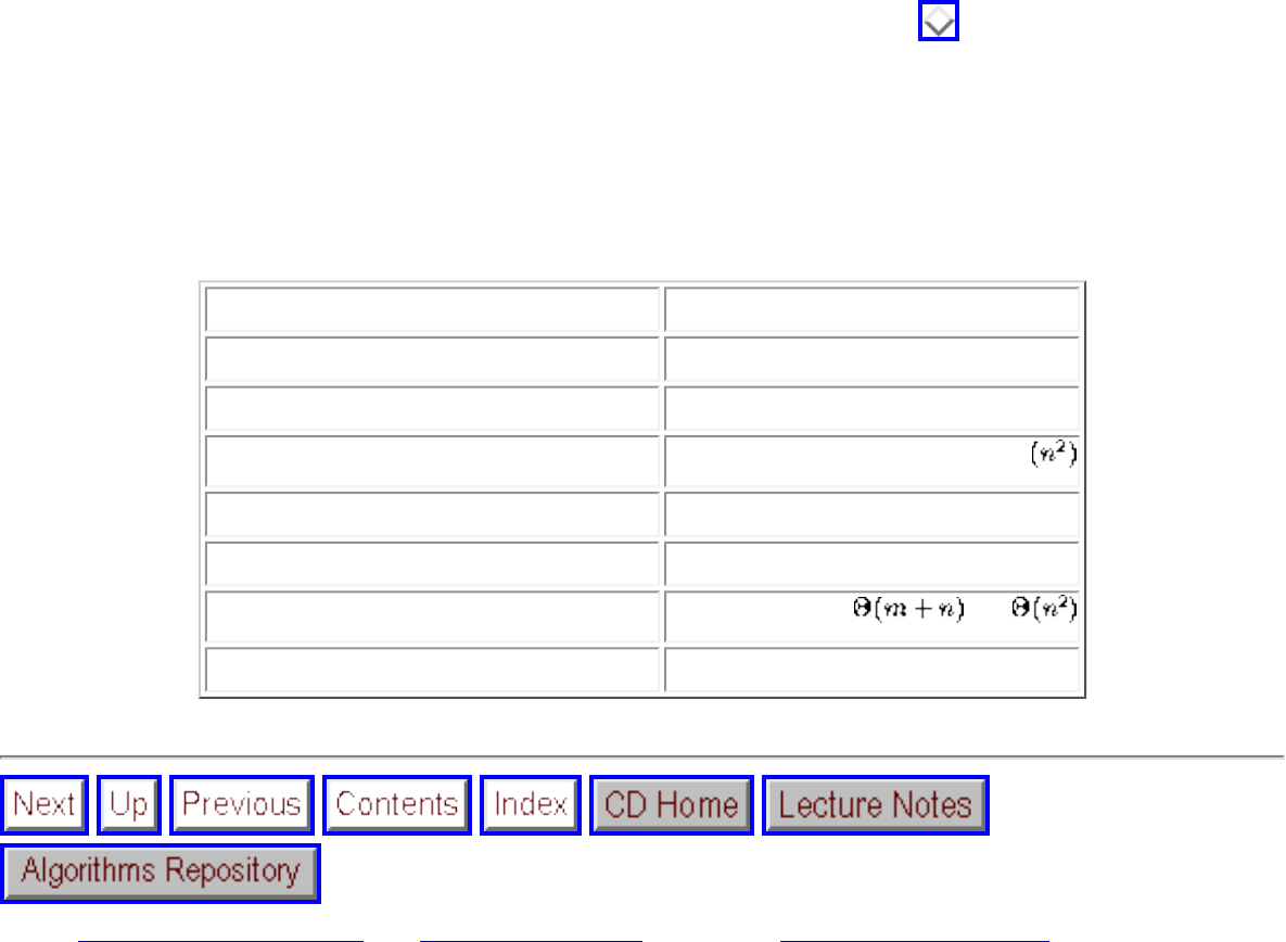
Data Structures for Graphs
linked together by a pointer to facilitate deletions. Also, depending upon the operations you will perform
on each list, you may or may not want it to be doubly linked, so that you can move backwards as easily
as you move forwards.
It is a good idea to use a well-designed graph data type as a model for building your own, or even better
as the foundation for your application. We recommend LEDA (see Section ) as the best-designed
general-purpose graph data structure currently available. It may be more powerful (and hence somewhat
slower/larger) than what you need, but it does so many things right that you are likely to lose most of the
potential do-it-yourself benefits through clumsiness.
In summary, we have the following tradeoffs between adjacency lists and matrices:
Comparison Winner
Faster to test if (x, y) is in graph? adjacency matrices
Faster to find the degree of a vertex? adjacency lists
Less memory on small graphs? adjacency lists (m+n) vs.
Less memory on big graphs? adjacency matrices (a small win)
Edge insertion or deletion? adjacency matrices O(1) vs. O(d)
Faster to traverse the graph? adjacency lists vs.
Better for most problems? adjacency lists
Next: War Story: Getting the Up: Graph Algorithms Previous: The Friendship Graph
Algorithms
Mon Jun 2 23:33:50 EDT 1997
file:///E|/BOOK/BOOK2/NODE61.HTM (2 of 2) [19/1/2003 1:29:04]
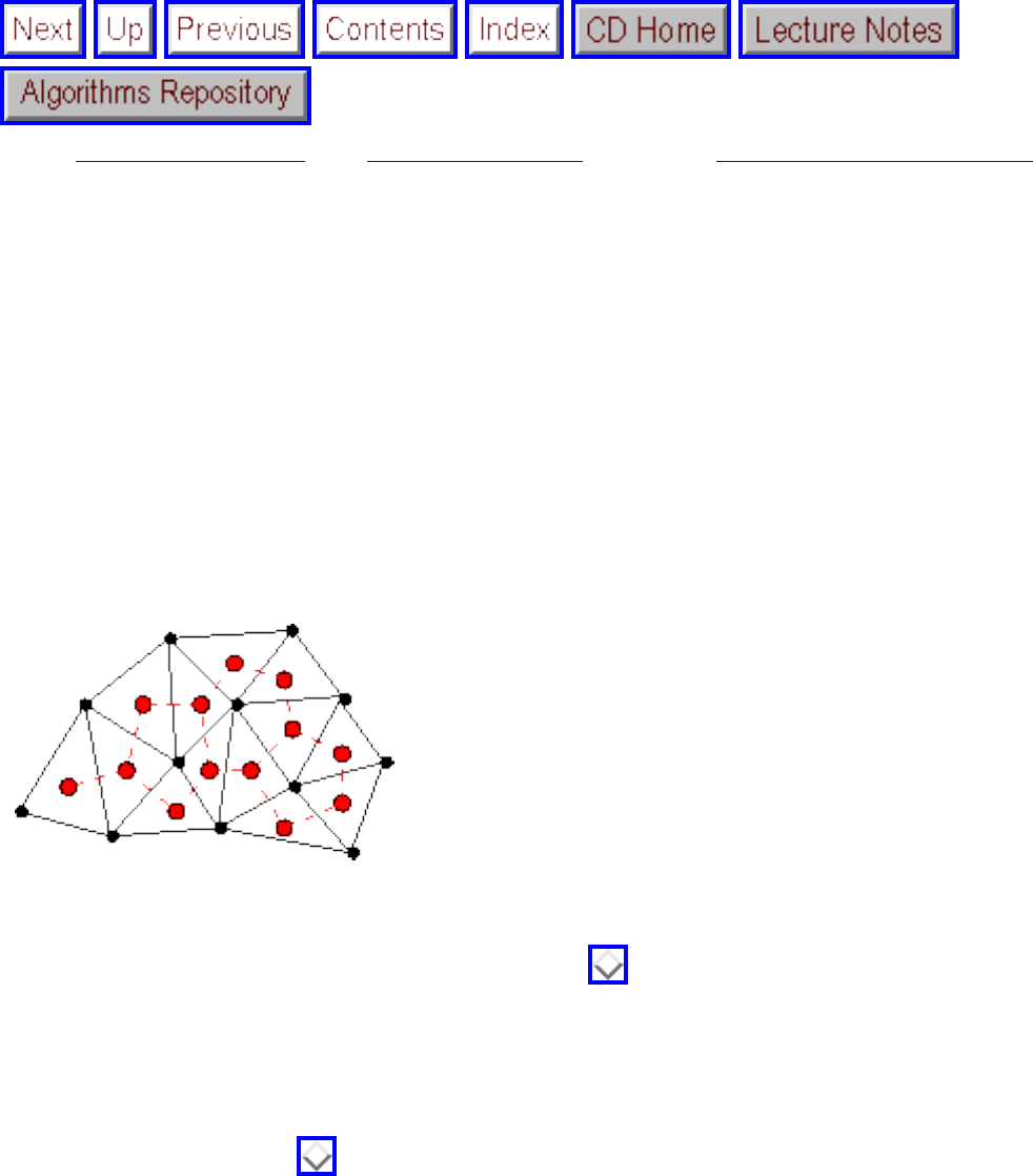
War Story: Getting the Graph
Next: Traversing a Graph Up: Graph Algorithms Previous: Data Structures for Graphs
War Story: Getting the Graph
``It takes five minutes just to read the data. We will never have time to make it do something
interesting.''
The young graduate student was bright and eager, but green to the power of data structures. She would
soon come to appreciate the power.
Figure: The dual graph (dashed lines) of a triangulation
As described in a previous war story (see Section ), we were experimenting with algorithms for
extracting triangular strips for the fast rendering of triangulated surfaces. The task of finding a small
number of strips that cover each triangle in a mesh could be modeled as a graph problem, where the
graph has a vertex for every triangle of the mesh, and there is an edge between every pair of vertices
representing adjacent triangles. This dual graph representation of the planar subdivision representing the
triangulation (see Figure ) captures all the information about the triangulation needed to partition it
into triangle strips.
The first step in crafting a program that constructs a good set of strips was to build the dual graph of the
triangulation. This I sent the student off to do. A few days later, she came back and announced that it
took over five CPU minutes just to construct this dual graph of an object with a few thousand triangles.
``Nonsense!'' I proclaimed. ``You must be doing something very wasteful in building the graph. What
format is the data in?''
file:///E|/BOOK/BOOK2/NODE62.HTM (1 of 3) [19/1/2003 1:29:05]

War Story: Getting the Graph
``Well, it starts out with a list of the 3D-coordinates of the vertices used in the model and then follows
with a list of triangles. Each triangle is described by a list of three indices into the vertex coordinates.
Here is a small example:''
VERTICES 4
0.000000 240.000000 0.000000
204.000000 240.000000 0.000000
204.000000 0.000000 0.000000
0.000000 0.000000 0.000000
TRIANGLES 2
0 1 3
1 2 3
``I see. So the first triangle must use all but the third point, since all the indices start from zero. The two
triangles must share an edge formed by points 1 and 3.''
``Yeah, that's right,'' she confirmed.
``OK. Now tell me how you built your dual graph from this file.''
``Well, I can pretty much ignore the vertex information, once I know how many vertices there will be.
The geometric position of the points doesn't affect the structure of the graph. My dual graph is going to
have as many vertices as the number of triangles. I set up an adjacency list data structure with that many
vertices. As I read in each triangle, I compare it to each of the others to check whether it has two
numbers in common. Whenever it does, I add an edge from the new triangle to this one.''
I started to sputter. ``But that's your problem right there! You are comparing each triangle against every
other triangle, so that constructing the dual graph will be quadratic in the number of triangles. Reading in
the input graph should take linear time!''
``I'm not comparing every triangle against every other triangle. On average, it only tests against half or a
third of the triangles.''
``Swell. But that still leaves us with an algorithm. That is much too slow.''
She stood her ground. ``Well, don't just complain. Help me fix it!''
Fair enough. I started to think. We needed some quick method to screen away most of the triangles that
would not be adjacent to the new triangle (i,j,k). What we really needed was just a list of all the triangles
that go through each of the points i, j, and k. Since each triangle goes through three points, the average
point is incident on three triangles, so this would mean comparing each new triangle against fewer than
ten others, instead of most of them.
file:///E|/BOOK/BOOK2/NODE62.HTM (2 of 3) [19/1/2003 1:29:05]
War Story: Getting the Graph
``We are going to need a data structure consisting of an array with one element for every vertex in the
original data set. This element is going to be a list of all the triangles that pass through that vertex. When
we read in a new triangle, we will look up the three relevant lists in the array and compare each of these
against the new triangle. Actually, only two of the three lists are needed, since any adjacent triangle will
share two points in common. For anything sharing two vertices, we will add an adjacency to our graph.
Finally, we will add our new triangle to each of the three affected lists, so they will be updated for the
next triangle read.''
She thought about this for a while and smiled. ``Got it, Chief. I'll let you know what happens.''
The next day she reported that the graph could be built in seconds, even for much larger models. From
here, she went on to build a successful program for extracting triangle strips, as reported in Section .
The take-home lesson here is that even elementary problems like initializing data structures can prove to
be bottlenecks in algorithm development. Indeed, most programs working with large amounts of data
have to run in linear or almost linear time. With such tight performance demands, there is no room to be
sloppy. Once you focus on the need for linear-time performance, an appropriate algorithm or heuristic
can usually be found to do the job.
Next: Traversing a Graph Up: Graph Algorithms Previous: Data Structures for Graphs
Algorithms
Mon Jun 2 23:33:50 EDT 1997
file:///E|/BOOK/BOOK2/NODE62.HTM (3 of 3) [19/1/2003 1:29:05]

Traversing a Graph
Next: Breadth-First Search Up: Graph Algorithms Previous: War Story: Getting the
Traversing a Graph
Perhaps the most fundamental graph problem is to traverse every edge and vertex in a graph in a
systematic way. Indeed, most of the basic algorithms you will need for bookkeeping operations on
graphs will be applications of graph traversal. These include:
● Printing or validating the contents of each edge and/or vertex.
● Copying a graph, or converting between alternate representations.
● Counting the number of edges and/or vertices.
● Identifying the connected components of the graph.
● Finding paths between two vertices, or cycles if they exist.
Since any maze can be represented by a graph, where each junction is a vertex and each hallway an edge,
any traversal algorithm must be powerful enough to get us out of an arbitrary maze. For efficiency, we
must make sure we don't get lost in the maze and visit the same place repeatedly. By being careful, we
can arrange to visit each edge exactly twice. For correctness, we must do the traversal in a systematic
way to ensure that we don't miss anything. To guarantee that we get out of the maze, we must make sure
our search takes us through every edge and vertex in the graph.
The key idea behind graph traversal is to mark each vertex when we first visit it and keep track of what
we have not yet completely explored. Although bread crumbs or unraveled threads are used to mark
visited places in fairy-tale mazes, we will rely on Boolean flags or enumerated types. Each vertex will
always be in one of the following three states:
● undiscovered - the vertex in its initial, virgin state.
● discovered - the vertex after we have encountered it, but before we have checked out all its
incident edges.
● completely-explored - the vertex after we have visited all its incident edges.
Obviously, a vertex cannot be completely-explored before we discover it, so over the course of the
traversal the state of each vertex progresses from undiscovered to discovered to completely-explored.
We must also maintain a structure containing all the vertices that we have discovered but not yet
file:///E|/BOOK/BOOK2/NODE63.HTM (1 of 2) [19/1/2003 1:29:05]
Traversing a Graph
completely explored. Initially, only a single start vertex is considered to have been discovered. To
completely explore a vertex, we must evaluate each edge going out of it. If an edge goes to an
undiscovered vertex, we mark it discovered and add it to the list of work to do. If an edge goes to a
completely-explored vertex, we will ignore it, since further contemplation will tell us nothing new about
the graph. We can also ignore any edge going to a discovered but not completely-explored vertex, since
the destination must already reside on the list of vertices to completely explore.
Regardless of which order we use to fetch the next vertex to explore, each undirected edge will be
considered exactly twice, once when each of its endpoints is explored. Directed edges will be consider
only once, when exploring the source vertex. Every edge and vertex in the connected component must
eventually be visited. Why? Suppose the traversal didn't visit everything, meaning that there exists a
vertex u that remains unvisited whose neighbor v was visited. This neighbor v will eventually be
explored, and we will certainly visit u when we do so. Thus we must find everything that is there to be
found.
The order in which we explore the vertices depends upon the container data structure used to store the
discovered but not completely-explored vertices. There are two important possibilities:
● Queue - by storing the vertices in a first in, first out (FIFO) queue, we explore the oldest
unexplored vertices first. Thus our explorations radiate out slowly from the starting vertex,
defining a so-called breadth-first search.
● Stack - by storing the vertices in a last in, first out (LIFO) stack, we explore the vertices by
lurching along a path, visiting a new neighbor if one is available, and backing up only when we
are surrounded by previously discovered vertices. Thus our explorations quickly wander away
from our starting point, defining a so-called depth-first search.
● Breadth-First Search
● Depth-First Search
Next: Breadth-First Search Up: Graph Algorithms Previous: War Story: Getting the
Algorithms
Mon Jun 2 23:33:50 EDT 1997
file:///E|/BOOK/BOOK2/NODE63.HTM (2 of 2) [19/1/2003 1:29:05]
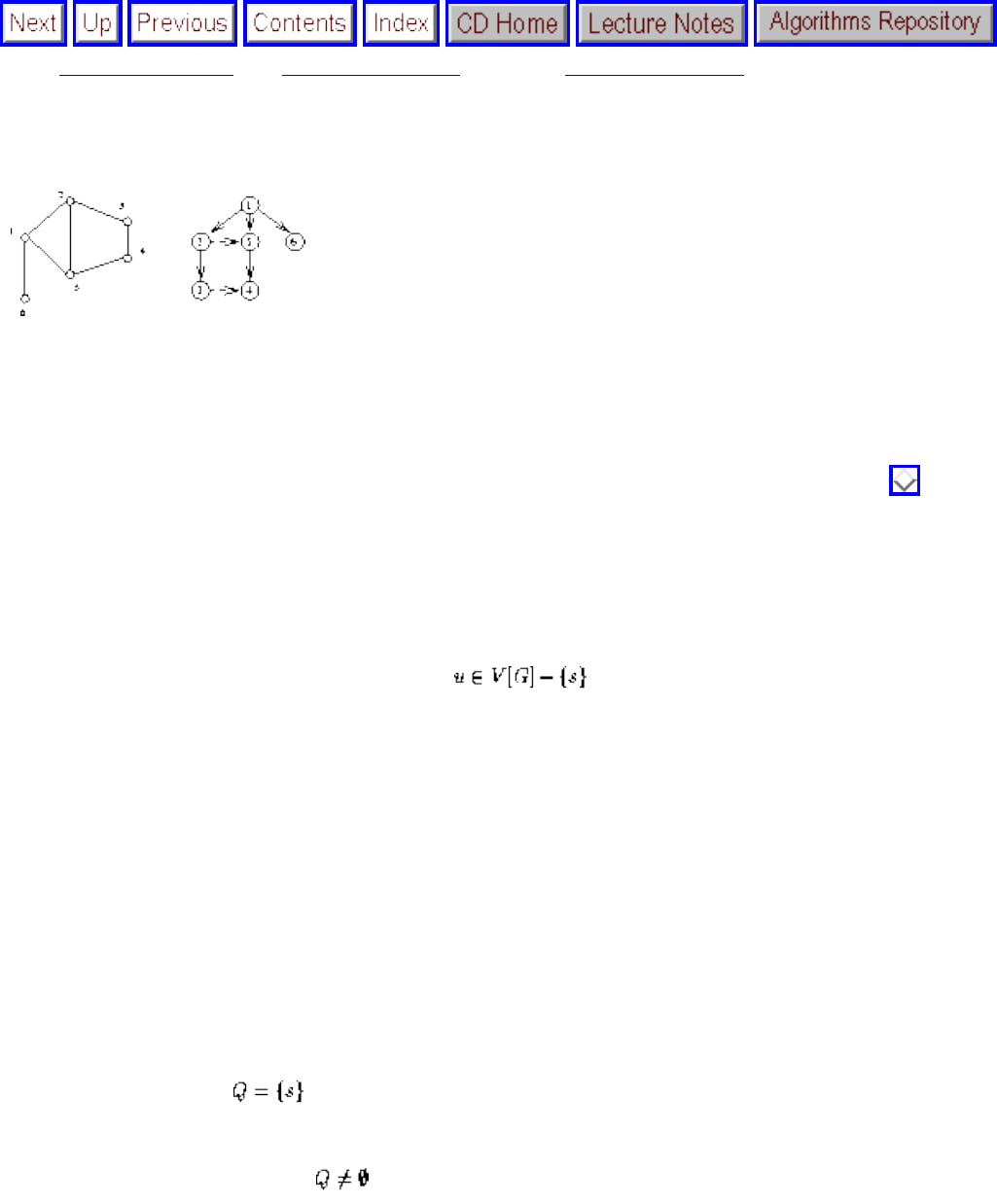
Breadth-First Search
Next: Depth-First Search Up: Traversing a Graph Previous: Traversing a Graph
Breadth-First Search
Figure: An undirected graph and its breadth-first search tree
The basic breadth-first search algorithm is given below. At some point during the traversal, every node in the graph changes
state from undiscovered to discovered. In a breadth-first search of an undirected graph, we assign a direction to each edge,
from the discoverer u to the discovered v. We thus denote u to be the parent p[v]. Since each node has exactly one parent,
except for the root, this defines a tree on the vertices of the graph. This tree, illustrated in Figure , defines a shortest path
from the root to every other node in the tree. This property makes breadth-first search very useful in shortest path problems.
BFS(G,s)
for each vertex do
state[u] = ``undiscovered''
p[u] = nil, i.e. no parent is in the BFS tree
state[] = ``discovered''
p[] = nil
while do
u = dequeue[Q]
process vertex u as desired
file:///E|/BOOK/BOOK2/NODE64.HTM (1 of 2) [19/1/2003 1:29:06]
Breadth-First Search
for each do
process edge (u,v) as desired
if state[v] = ``undiscovered'' then
state[v] =
``discovered''
p[v] = u
enqueue[Q,v]
state[u] = ``completely-explored''
The graph edges that do not appear in the breadth-first search tree also have special properties. For undirected graphs, non-
tree edges can point only to vertices on the same level as the parent vertex or to vertices on the level directly below the
parent. These properties follow easily from the fact that each path in the tree must be the shortest path in the graph. For a
directed graph, a back-pointing edge can exist whenever v lies closer to the root than u does.
The breadth-first search algorithm above includes places to optionally process each vertex and edge, say to copy them, print
them, or count them. Each vertex and directed edge is encountered exactly once, and each undirected edge is encountered
exactly twice.
Next: Depth-First Search Up: Traversing a Graph Previous: Traversing a Graph
Algorithms
Mon Jun 2 23:33:50 EDT 1997
file:///E|/BOOK/BOOK2/NODE64.HTM (2 of 2) [19/1/2003 1:29:06]
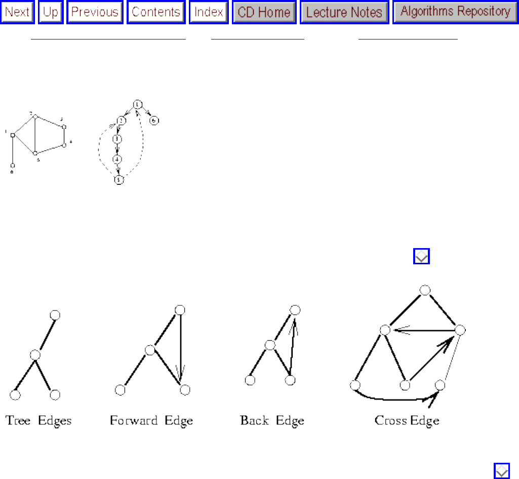
Depth-First Search
Next: Applications of Graph Traversal Up: Traversing a Graph Previous: Breadth-First Search
Depth-First Search
Figure: An undirected graph and its depth-first search tree
Depth-first search turns out to be, in general, even more useful than breadth-first search. The reason is that a depth-first
search of a graph organizes the edges of the graph in a very precise way, which is quite different from breadth-first search. As
with BFS, we assign a direction to each edge when we discover it, as shown in Figure .
Figure: Edge possibilities for search trees
Although there are four conceivable classes of edges resulting from such labelings, as shown in Figure , only two of them
can occur with undirected graphs. In a DFS of an undirected graph, every edge is either in the tree or goes directly back to an
ancestor. Why? Suppose we encountered a forward edge (x,y) directed toward a decendant vertex. In this case, we would
have discovered (x,y) when exploring y, making it a back edge. Suppose we encounter a cross edge (x,y), linking two
unrelated vertices. Again, we would have discovered this edge when we explored y, making it a tree edge. For directed
graphs, depth-first search labelings can take on a wider range of possibilities.
Depth-first search has a neat recursive implementation, which eliminates the need to explicitly use a stack:
DFS(G,u)
state[u] = ``discovered''
process vertex u if desired
file:///E|/BOOK/BOOK2/NODE65.HTM (1 of 3) [19/1/2003 1:29:07]

Depth-First Search
for each do
process edge (u,v) if desired
if state[v] = ``undiscovered'' then
p[v] = u
DFS(G,v)
state[u] = ``completely-explored''
As with BFS, this implementation of the depth-first search algorithm includes places to optionally process each vertex and
edge, say to copy them, print them, or count them. Both algorithms will traverse all edges in the same connected component
as the starting point. Since we need to start with a vertex in each component in order to traverse a disconnected graph, we
must start from any vertex remaining undiscovered after a component search. With the proper initialization, this completes
the traversal algorithm:
DFS-graph(G)
for each vertex do
state[u] = ``undiscovered''
for each vertex do
if state[u] = ``undiscovered'' then
initialize new component, if
desired
DFS[G,u]
file:///E|/BOOK/BOOK2/NODE65.HTM (2 of 3) [19/1/2003 1:29:07]

Applications of Graph Traversal
Next: Connected Components Up: Graph Algorithms Previous: Depth-First Search
Applications of Graph Traversal
Most elementary graph algorithms involve making one or two traversals of the graph, while we update
our knowledge of the graph as we visit each edge and vertex. Properly implemented using adjacency
lists, any such algorithm is destined to be very fast. Both BFS and DFS run in O(n+m) on both directed
and undirected graphs where, as usual, n is the number of vertices and m the number of edges in the
graph. This is optimal, since it is as fast as one can hope to read the graph. The trick is seeing when
traversal approaches are destined to work. We present several examples below.
● Connected Components
● Tree and Cycle Detection
● Two-Coloring Graphs
● Topological Sorting
● Articulation Vertices
Algorithms
Mon Jun 2 23:33:50 EDT 1997
file:///E|/BOOK/BOOK2/NODE66.HTM [19/1/2003 1:29:08]
Connected Components
Next: Tree and Cycle Detection Up: Applications of Graph Traversal Previous: Applications of Graph
Traversal
Connected Components
Either breadth-first or depth-first search can be used to identify the connected components of an
undirected graph and label each vertex with the identifier of its components. In particular, we can modify
the DFS-graph algorithm to increment a counter for the current component number and label each vertex
accordingly as it is discovered in DFS.
For directed graphs, there are two distinct notions of connectivity, leading to algorithms for finding both
weakly connected and strongly connected components. Both of these can be found in O(n+m) time, as
discussed in Section .
Algorithms
Mon Jun 2 23:33:50 EDT 1997
file:///E|/BOOK/BOOK2/NODE67.HTM [19/1/2003 1:29:08]
Tree and Cycle Detection
Next: Two-Coloring Graphs Up: Applications of Graph Traversal Previous: Connected Components
Tree and Cycle Detection
Trees are connected, undirected graphs that do not contain cycles. They are perhaps the simplest
interesting class of graphs. Testing whether a graph is a tree is straightforward using depth-first search.
During search, every edge will be labeled either a tree edge or a back edge, so the graph is a tree if and
only if there are no back edges. Since m=n-1 for any tree, this algorithm can be said to run in time linear
in the number of vertices.
If the graph is not a tree, it must contain a cycle. Such a cycle can be identified as soon as the first back
edge (u,v) is detected. If (u,v) is a back edge, then there must be a path in the tree from v to u. Coupled
with edge (u,v), this defines a cycle.
Algorithms
Mon Jun 2 23:33:50 EDT 1997
file:///E|/BOOK/BOOK2/NODE68.HTM [19/1/2003 1:29:09]
Two-Coloring Graphs
Next: Topological Sorting Up: Applications of Graph Traversal Previous: Tree and Cycle Detection
Two-Coloring Graphs
In vertex coloring, we seek to assign a color to each vertex of a graph G such that no edge links two
vertices of the same color. We can avoid all conflicts by assigning each vertex its own color. However,
the goal is to use as few colors as possible. Vertex coloring problems arise often in scheduling
applications, such as register allocation in compilers. See Section for a full treatment of vertex
coloring algorithms and applications.
A graph is bipartite if it can be colored without conflicts while using only two colors. Bipartite graphs
are important because they arise often in practice and have more structure than arbitrary graphs. For
example, consider the ``had-sex-with'' graph in a heterosexual world. Men have sex only with women,
and vice versa. Thus gender defines a legal two-coloring. Irrespective of the accuracy of the model, it
should be clear that bipartite graphs are simpler to work with than general graphs.
But how can we find an appropriate two-coloring of a graph, thus separating the men from the women?
Suppose we assume that the starting vertex is male. All vertices adjacent to this man must be female,
assuming the graph is indeed bipartite.
We can augment either breadth-first or depth-first search so that whenever we discover a new vertex, we
color it the opposite of its parent. For each non-discovery edge, we check whether it links two vertices of
the same color. Such a conflict means that the graph cannot be two-colored. However, we will have
constructed a proper two-coloring whenever we terminate without conflict. We can assign the first vertex
in any connected component to be whatever color/sex we wish. Although we can separate the men from
the women, we can't tell them apart just using the graph.
Next: Topological Sorting Up: Applications of Graph Traversal Previous: Tree and Cycle Detection
Algorithms
Mon Jun 2 23:33:50 EDT 1997
file:///E|/BOOK/BOOK2/NODE69.HTM [19/1/2003 1:29:09]
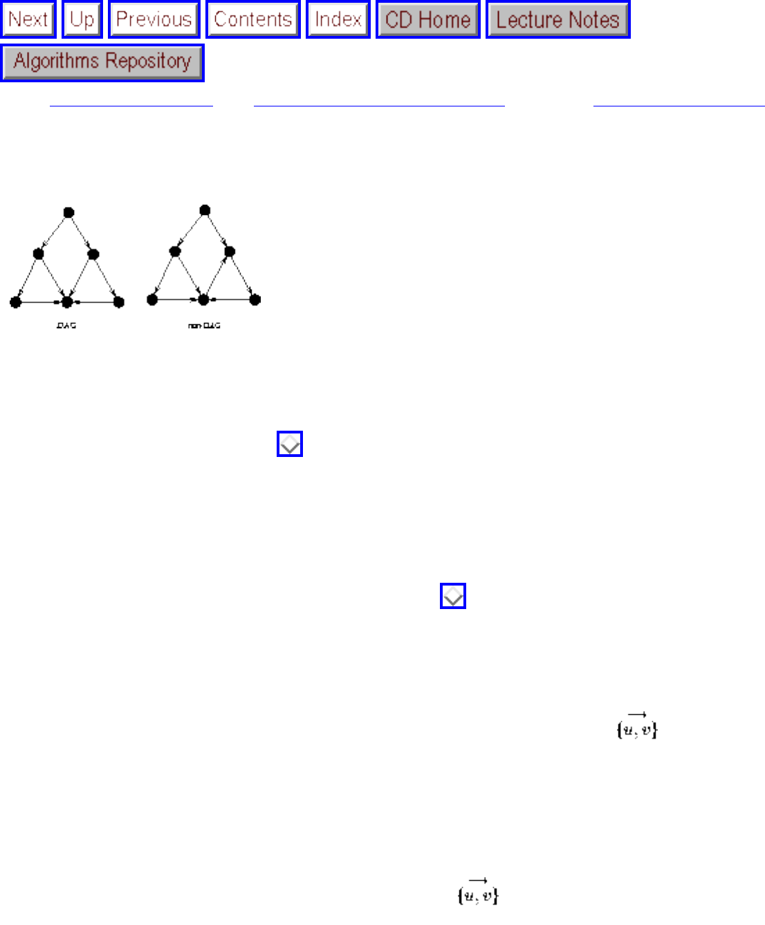
Topological Sorting
Next: Articulation Vertices Up: Applications of Graph Traversal Previous: Two-Coloring Graphs
Topological Sorting
Figure: Directed acyclic and cyclic graphs
A directed, acyclic graph, or DAG, is a directed graph with no directed cycles. Although undirected
acyclic graphs are limited to trees, DAGs can be considerably more complicated. They just have to avoid
directed cycles, as shown in Figure .
A topological sort of a directed acyclic graph is an ordering on the vertices such that all edges go from
left to right. Only an acyclic graph can have a topological sort, because a directed cycle must eventually
return home to the source of the cycle. However, every DAG has at least one topological sort, and we can
use depth-first search to find such an ordering. Topological sorting proves very useful in scheduling jobs
in their proper sequence, as discussed in catalog Section .
Depth-first search can be used to test whether a graph is a DAG, and if so to find a topological sort for it.
A directed graph is a DAG if and only if no back edges are encountered during a depth-first search.
Labeling each of the vertices in the reverse order that they are marked completely-explored finds a
topological sort of a DAG. Why? Consider what happens to each directed edge as we encounter it
during the exploration of vertex u:
● If v is currently undiscovered, then we then start a DFS of v before we can continue with u. Thus v
is marked completely-explored before u is, and v appears before u in the topological order, as it
must.
● If v is discovered but not completely-explored, then is a back edge, which is forbidden in a
DAG.
● If v is completely-explored, then it will have been so labeled before u. Therefore, u appears before
v in the topological order, as it must.
file:///E|/BOOK/BOOK2/NODE70.HTM (1 of 2) [19/1/2003 1:29:10]

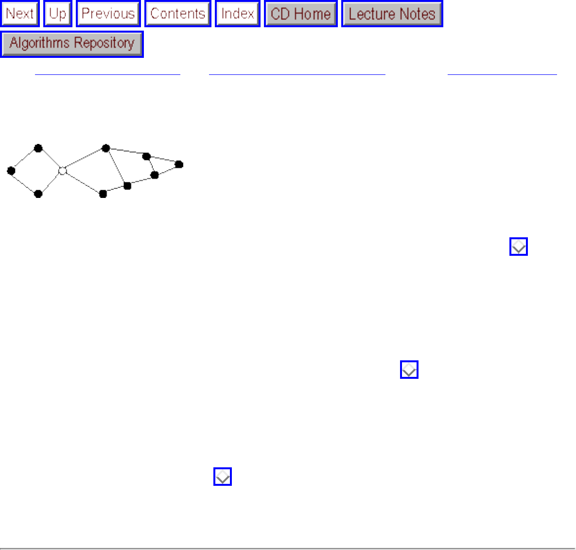
Articulation Vertices
Next: Modeling Graph Problems Up: Applications of Graph Traversal Previous: Topological Sorting
Articulation Vertices
Figure: An articulation vertex is the weakest point in the graph
Suppose you are a terrorist seeking to disrupt the telephone network. Which station in Figure should
you choose to blow up to cause the maximum amount of damage? An articulation vertex is a vertex of a
connected graph whose deletion disconnects the graph. Any graph that contains an articulation vertex is
inherently fragile, because deleting that single vertex causes a loss of connectivity.
In general, the connectivity of a graph is the smallest number of vertices whose deletion will disconnect
the graph. For graphs with an articulation vertex, the connectivity is one. Connectivity is an important
measure of robustness in network design, as discussed in catalog Section .
A simple application of either depth-first or breadth-first search suffices to find all the articulation
vertices in a graph in O(n (m+n)). For each vertex v, delete it and then do a BFS traversal of the
remaining graph to establish whether it is still connected. In fact, there is a clever O(n+m) algorithm that
tests all the vertices using only a single depth-first search. Additional information on edge and vertex
connectivity testing appears in Section .
Algorithms
Mon Jun 2 23:33:50 EDT 1997
file:///E|/BOOK/BOOK2/NODE71.HTM [19/1/2003 1:29:11]
Modeling Graph Problems
Next: Minimum Spanning Trees Up: Graph Algorithms Previous: Articulation Vertices
Modeling Graph Problems
Proper modeling is the key to making effective use of graph algorithms. We have seen a variety of
definitions of graph properties, and algorithms for computing them. All told, about two dozen different
graph problems are presented in the catalog, mostly in Sections and . These problems provide a
framework for modeling most applications.
The applications below demonstrate the power of proper modeling. Each of them arose in a real-world
application as stated, and each can be modeled as a graph problem. Some of the modelings are quite
clever, but they illustrate the versatility of graphs in representing relationships. As you read the problem,
try to devise an appropriate graph representation before peeking to see how we did it.
● ``I'm looking for an algorithm to design natural routes for video-game characters to follow
through an obstacle-filled room. How should I do it?''
Presumably the route that is wanted is the path that looks most like the one that an intelligent
being would choose. Since intelligent beings are either lazy or efficient, this should be modeled as
some kind of shortest path problem.
But what is the graph? One approach would be to lay a grid of points in the room and have a
vertex for each point that is a valid place for the character to stand, i.e. so it does not lie within an
obstacle. There will be an edge between any pair of nearby vertices, weighted according to the
distance between them. The shortest path between two vertices will be close to the shortest path
between the points. Although direct geometric methods are known for shortest paths (see Section
), it is easier to model this discretely as a graph.
● ``In DNA sequencing, we are given experimental data consisting of small fragments. For each
fragment f, we have certain other fragments that are forced to lie to the left of f, certain fragments
forced to be to the right of f, and the remaining fragments, which are free to go on either side.
How can we find a consistent ordering of the fragments from left to right that satisfies all the
constraints?''
Create a directed graph, where each fragment is assigned a unique vertex. Insert a directed edge
from any fragment l that is forced to be to the left of f, and a directed edge to any
file:///E|/BOOK/BOOK2/NODE72.HTM (1 of 3) [19/1/2003 1:29:12]
Modeling Graph Problems
fragment r forced to be to the right of f. We seek an ordering of the vertices such that all the edges
go from left to right. This is exactly a topological sort of the resulting directed acyclic graph. The
graph must be acyclic for this to work, because cycles make finding a consistent ordering
impossible.
● ``In my graphics work I need to solve the following problem. Given an arbitrary set of rectangles
in the plane, how can I distribute them into a minimum number of buckets such that the subset of
rectangles in the same bucket do not intersect each other? In other words, there should not be any
overlapping area between any two rectangles in the same bucket.''
We can formulate a graph where each vertex is a rectangle, and there is an edge if two rectangles
intersect. Each bucket corresponds to an independent set of rectangles, so there is no overlap
between any two. A vertex coloring of a graph is a partition of the vertices into independent sets,
so minimizing the number of colors is exactly what you want.
● ``In porting code from UNIX to DOS, I have to shorten the names of several hundred files down to
at most 8 characters each. I can't just take the first eight characters from each name, because
``filename1'' and ``filename2'' will get assigned the exact same name. How can I shorten the
names while ensuring that they do not collide?''
Construct a graph with vertices corresponding to each original file name for , as well
as a collection of acceptable shortenings for each name . Add an edge between each
original and shortened name. Given such a formulation, we seek a set of n edges that have no
vertices in common, because the file name of each is thus mapped to a distinct acceptable
substitute. Bipartite matching, discussed in Section , is exactly this problem of finding an
independent set of edges in a graph.
● ``In organized tax fraud, criminals submit groups of phony tax returns in the hopes of getting
undeserved refunds. These phony returns are all similar, but not identical. How can we detect
clusters of similar forms so the IRS can nail the cheaters?''
A natural graph model treats each form as a vertex and adds an edge between any two tax forms
that are suspiciously similar. A cluster would correspond to a group of forms with many edges
between them. In particular, a clique is a set of k vertices with all possible edges between them.
Any sufficiently large clique identifies a cluster worth studying.
● ``In the optical character-recognition system that we are building, we need a way to separate the
lines of text. Although there is some white space between the lines, problems like noise and the tilt
of the page makes it hard to find. How can we do line segmentation?
Consider the following graph formulation. Treat each pixel in the image as a vertex in the graph,
with an edge between two neighboring pixels. The weight of this edge should be proportional to
how dark the pixels are. A segmentation between two lines is a path in this graph from the left to
right side of the page. Of all possible paths, we seek a relatively straight path that avoids as much
blackness as possible. This suggests that the shortest path in the pixel graph will likely find a
file:///E|/BOOK/BOOK2/NODE72.HTM (2 of 3) [19/1/2003 1:29:12]

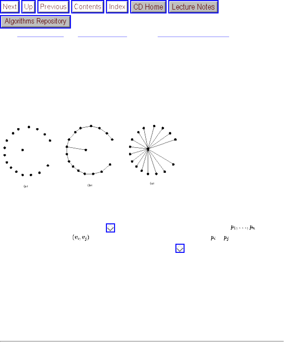
Minimum Spanning Trees
Next: Prim's Algorithm Up: Graph Algorithms Previous: Modeling Graph Problems
Minimum Spanning Trees
A tree is a connected graph with no cycles. A spanning tree is a subgraph of G that has the same set of
vertices of G and is a tree. A minimum spanning tree of a weighted graph G is the spanning tree of G
whose edges sum to minimum weight.
Figure: Two spanning trees of point set (a); the minimum spanning tree (b), and the shortest path from
center tree (c)
Minimum spanning trees are useful in finding the least amount of wire necessary to connect a group of
homes or cities, as illustrated in Figure . In such geometric problems, the point set defines a
complete graph, with edge assigned a weight equal to the distance from to . Additional
applications of minimum spanning trees are discussed in Section .
A minimum spanning tree minimizes the total length over all possible spanning trees. However, there can
be more than one minimum spanning tree in any graph. Consider a graph G with m identically weighted
edges. All spanning trees of G are minimum spanning trees, since each contains exactly n-1 equal-weight
edges. For general weighted graphs, however, the problem of finding a minimum spanning tree is more
difficult. It can, however, be solved optimally using two different greedy algorithms. Both are presented
below, to illustrate how we can demonstrate the optimality of certain greedy heuristics.
file:///E|/BOOK/BOOK2/NODE73.HTM (1 of 2) [19/1/2003 1:29:13]


Prim's Algorithm
Next: Kruskal's Algorithm Up: Minimum Spanning Trees Previous: Minimum Spanning Trees
Prim's Algorithm
Every vertex will appear in the minimum spanning tree of any connected graph G. Prim's minimum spanning tree algorithm
starts from one vertex and grows the rest of the tree one edge at a time.
In greedy algorithms, we make the decision of what to do next by selecting the best local option from all available choices
without regard to the global structure. Since we seek the tree of minimum weight, the natural greedy algorithm for minimum
spanning tree repeatedly selects the smallest weight edge that will enlarge the tree.
Figure: Where Prim's algorithm goes bad? No, because
Prim-MST(G)
Select an arbitrary vertex to start the tree from.
While (there are still non-tree vertices)
Select the edge of minimum weight between a tree and
non-tree vertex
Add the selected edge and vertex to the tree .
Prim's algorithm clearly creates a spanning tree, because no cycle can be introduced by adding edges between tree and non-tree
vertices. However, why should it be of minimum weight over all spanning trees? We have seen ample evidence of other
natural greedy heuristics that do not yield a global optimium. Therefore, we must be particularly careful to demonstrate any
such claim.
Suppose that there existed a graph G for which Prim's algorithm did not return a minimum spanning tree. Since we are
building the tree incrementally, this means that there must have been some particular instant where we went wrong. Before we
file:///E|/BOOK/BOOK2/NODE74.HTM (1 of 2) [19/1/2003 1:29:14]
Prim's Algorithm
inserted edge (x,y), consisted of a set of edges that was a subtree of a minimum spanning tree , but choosing edge
(x,y) took us away from a minimum spanning tree. But how could it? There must be a path p from x to y in , using an edge
, where is in but is not. This edge must have weight at least that of (x,y), or else Prim's algorithm would
have selected it instead of (x,y) when it had the chance. Inserting (x,y) and deleting from leaves a spanning tree no
larger than before, meaning that Prim's algorithm could not have made a fatal mistake in selecting edge (x,y). Therefore, by
contradiction, Prim's algorithm has to construct a minimum spanning tree.
Prim's algorithm is correct, but how efficient is it? That depends on which data structures are used to implement it, but it
should be clear that O(nm) time suffices. In each of n iterations, we will scan through all the m edges and test whether the
current edge joins a tree with a non-tree vertex and whether this is the smallest edge seen thus far. By maintaining a Boolean
flag along with each vertex to denote whether it is in the tree or not, this test can be performed in constant time. In fact, better
data structures lead to a faster, , implementation by avoiding the need to sweep through more than n edges in any
iteration.
Next: Kruskal's Algorithm Up: Minimum Spanning Trees Previous: Minimum Spanning Trees
Algorithms
Mon Jun 2 23:33:50 EDT 1997
file:///E|/BOOK/BOOK2/NODE74.HTM (2 of 2) [19/1/2003 1:29:14]
Kruskal's Algorithm
Next: Shortest Paths Up: Minimum Spanning Trees Previous: Prim's Algorithm
Kruskal's Algorithm
Kruskal's algorithm is an alternative approach to finding minimum spanning trees that is more efficient on sparse graphs.
Like Prim's, Kruskal's algorithm is greedy; unlike Prim's, it does not start with a particular vertex.
Kruskal's algorithm works by building up connected components of the vertices. Initially, each vertex forms its own separate
component in the tree-to-be. The algorithm repeatedly considers the lightest remaining edge and tests whether the two
endpoints lie within the same connected component. If so, the edge will be discarded, because adding it will create a cycle in
the tree-to-be. If the endpoints are in different components, we insert the edge and merge the components. Since each
connected component is always a tree, we need never explicitly test for cycles:
Kruskal-MST(G)
Put the edges in a priority queue ordered by weight.
count=0
while (count < n-1) do
get next edge (v,w)
if (component (v) component(w))
add to
merge component(v) and component(w)
This algorithm adds n-1 edges without creating a cycle, so clearly it creates a spanning tree of any connected graph. But why
must this be a minimum spanning tree? Suppose it wasn't. As with the correctness proof of Prim's algorithm, there must be
some graph for which it fails, and in particular there must a single edge (x,y) whose insertion first prevented the tree
from being a minimum spanning tree . Inserting edge (x,y) in will create a cycle with the path from x to y. Since x
and y were in different components at the time of inserting (x,y), at least one edge on this path would have been
considered by Kruskal's algorithm after (x,y) was. But this means that , so exchanging the two edges yields
file:///E|/BOOK/BOOK2/NODE75.HTM (1 of 2) [19/1/2003 1:29:15]
Kruskal's Algorithm
a tree of weight at most . Therefore, we could not have made a mistake in selecting (x,y), and the correctness follows.
What is the time complexity of Kruskal's algorithm? Inserting and retrieving m edges from a priority queue such as a heap
takes time. The while loop makes at most m iterations, each testing the connectivity of two trees plus an edge. In
the most simple-minded approach, this can be implemented by a breadth-first or depth-first search in a graph with at most n
edges and n vertices, thus yielding an O(mn) algorithm.
However, a faster implementation would result if we could implement the component test in faster than O(n) time. In fact, the
union-find data structure, discussed in Section , can support such queries in time. With this data structure,
Kruskal's algorithm runs in time, which is faster than Prim's for sparse graphs. Observe again the impact that the
right data structure can have in implementing a straightforward algorithm.
Next: Shortest Paths Up: Minimum Spanning Trees Previous: Prim's Algorithm
Algorithms
Mon Jun 2 23:33:50 EDT 1997
file:///E|/BOOK/BOOK2/NODE75.HTM (2 of 2) [19/1/2003 1:29:15]
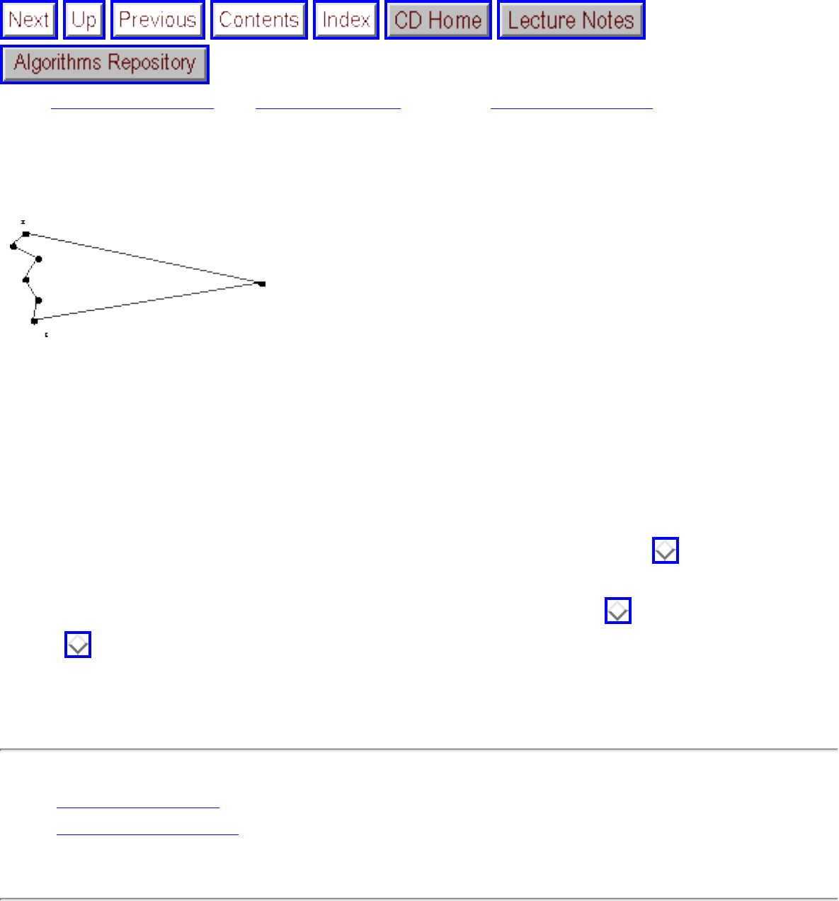
Shortest Paths
Next: Dijkstra's Algorithm Up: Graph Algorithms Previous: Kruskal's Algorithm
Shortest Paths
Figure: The shortest path from to t can pass through many intermediate vertices.
The shortest path between two vertices and t in an unweighted graph can be constructed using a breadth-
first search from . When we first encounter t in the search, we will have reached it from using the
minimum number of possible edges. This minimum-link path is recorded in the breadth-first search tree,
and it provides the shortest path when all edges have equal weight. However, in an arbitrary weighted
graph, the weight of a path between two vertices is the sum of the weights of the edges along the path.
The shortest path might use a large number of edges, just as the shortest route (timewise) from home to
office may involve shortcuts using backroads and many turns, as shown in Figure .
Shortest paths have a surprising variety of applications. See catalog Section and the war story of
Section for further examples.
● Dijkstra's Algorithm
● All-Pairs Shortest Path
Algorithms
Mon Jun 2 23:33:50 EDT 1997
file:///E|/BOOK/BOOK2/NODE76.HTM [19/1/2003 1:29:16]
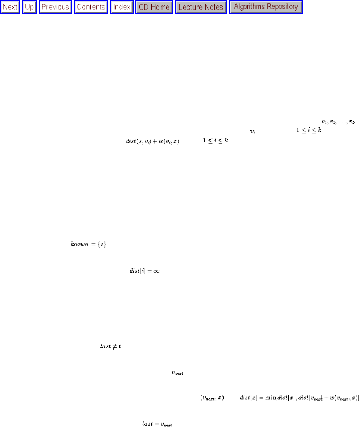
Dijkstra's Algorithm
Next: All-Pairs Shortest Path Up: Shortest Paths Previous: Shortest Paths
Dijkstra's Algorithm
We can use Dijkstra's algorithm to find the shortest path between any two vertices (,t) in a weighted graph, where each edge has
non-negative edge weight. Although most applications of shortest path involve graphs with positive edge weights, such a
condition is not needed for either Prim's or Kruskal's algorithm to work correctly. The problems that negative edges cause
Dijkstra's algorithm will become apparent once you understand the algorithm.
The principle behind Dijkstra's algorithm is that given the shortest path between and each of a given set of vertices ,
there must exist some other vertex x such that the shortest path from to x must go from to to x, for some .
Specifically, it is the vertex x that minimizes over all , where w(i,j) is the length of the edge from i
to j and dist(i,j) is the length of the shortest path between them.
This suggests a dynamic programming-like strategy. The shortest path from to itself is trivial unless there are negative weight
edges, so dist(,)=0. Armed with the shortest path to , if (,y) is the lightest edge incident to , then d(,y) = w(,y). As soon as we
decide that we have determined the shortest path to a node x, we search through all the outgoing edges of x to see whether there
is a better path from to some unknown vertex through x:
ShortestPath-Dijkstra(G,s,t)
for i=1 to n,
for each edge (, v), dist[v]=w(, v)
last=
while ( )
select , the unknown vertex minimizing dist[v]
for each edge ,
file:///E|/BOOK/BOOK2/NODE77.HTM (1 of 2) [19/1/2003 1:29:17]
Dijkstra's Algorithm
To be certain of finding the shortest path between and t, we might have to first find the shortest path between and all other
vertices. This defines a shortest path spanning tree rooted in . For undirected graphs, this will be the breadth-first search tree,
but in general it provides the shortest path between and all other vertices.
What is the running time of this algorithm? When implemented using adjacency lists and a Boolean array to mark what is
known about each vertex, the complexity is . This is the same running time as a proper version of Prim's algorithm;
indeed, except for the extension condition, it is the same algorithm as Prim's.
Next: All-Pairs Shortest Path Up: Shortest Paths Previous: Shortest Paths
Algorithms
Mon Jun 2 23:33:50 EDT 1997
file:///E|/BOOK/BOOK2/NODE77.HTM (2 of 2) [19/1/2003 1:29:17]
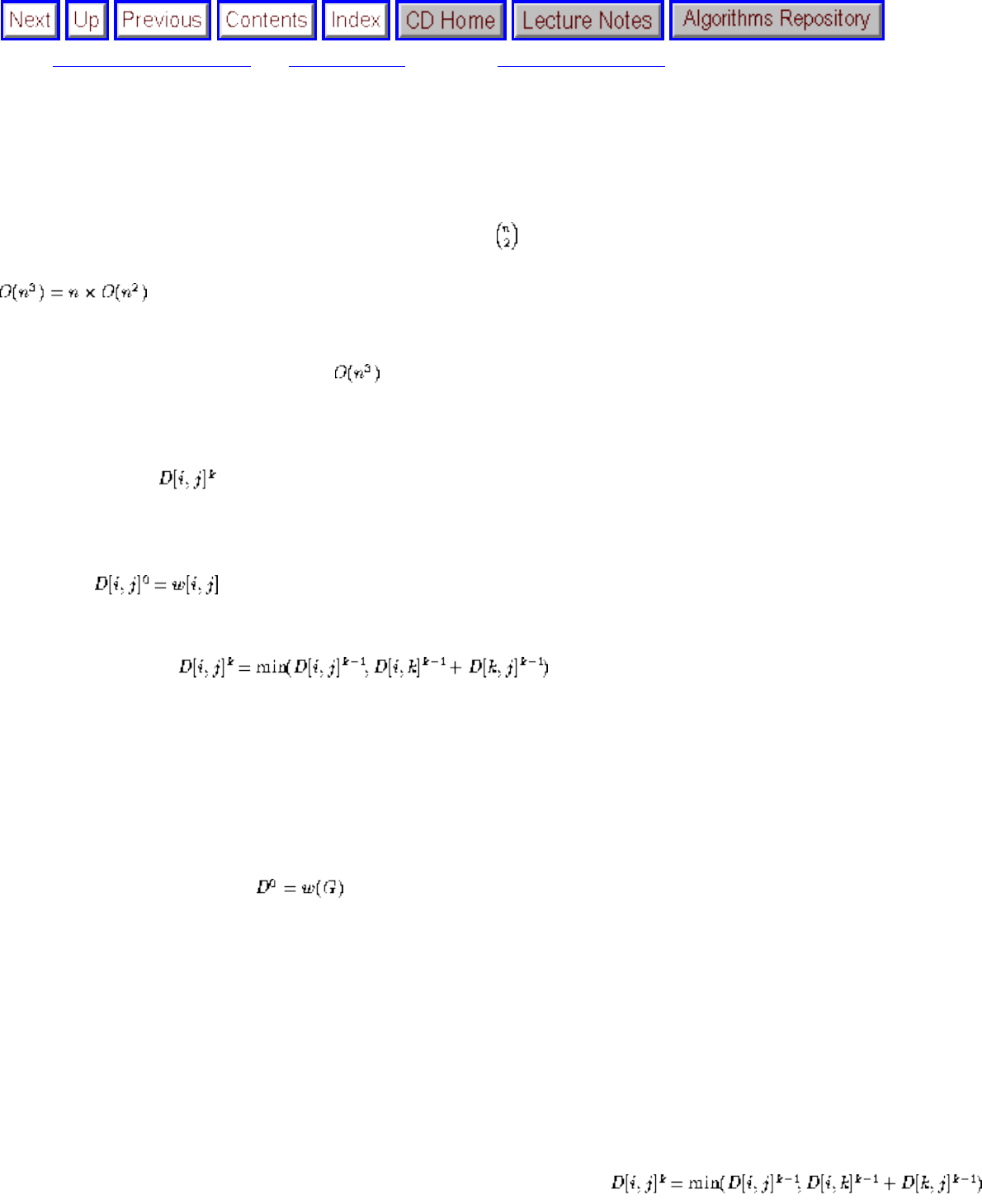
All-Pairs Shortest Path
Next: War Story: Nothing but Up: Shortest Paths Previous: Dijkstra's Algorithm
All-Pairs Shortest Path
If we want to find the length of the shortest path between all pairs of vertices, we could run Dijkstra's algorithm n
times, once from each possible starting vertex. This yields a cubic time algorithm for all-pairs shortest path, since
.
Can we do better? Significantly improving the complexity is still an open question, but there is a superslick dynamic
programming algorithm that also runs in .
There are several ways to characterize the shortest path between two nodes in a graph. The Floyd-Warshall algorithm
starts by numbering the vertices of the graph from 1 to n. We use these numbers here not to label the vertices, but to
order them. Define to be the length of the shortest path from i to j using only vertices numbered from 1, 2,..., k
as possible intermediate vertices.
What does this mean? When k = 0, we are allowed no intermediate vertices, so that every path consists of at most one
edge. Thus . In general, adding a new vertex k+1 as a possible intermediary helps only if there is a short
path that goes through it, so
This recurrence performs only a constant amount of work per cell. The following dynamic programming algorithm
implements the recurrence:
Floyd(G)
Let , the weight matrix of G
for k=1 to n
for i=1 to n
for j=1 to n
file:///E|/BOOK/BOOK2/NODE78.HTM (1 of 2) [19/1/2003 1:29:18]

All-Pairs Shortest Path
The Floyd-Warshall all-pairs shortest path runs in time, which asymptotically is no better than n calls to Dijkstra's
algorithm. However, the loops are so tight and the program so short that it runs better in practice. It is also notable as
one of the rare algorithms that work better on adjacency matrices than adjacency lists.
Algorithms
Mon Jun 2 23:33:50 EDT 1997
file:///E|/BOOK/BOOK2/NODE78.HTM (2 of 2) [19/1/2003 1:29:18]
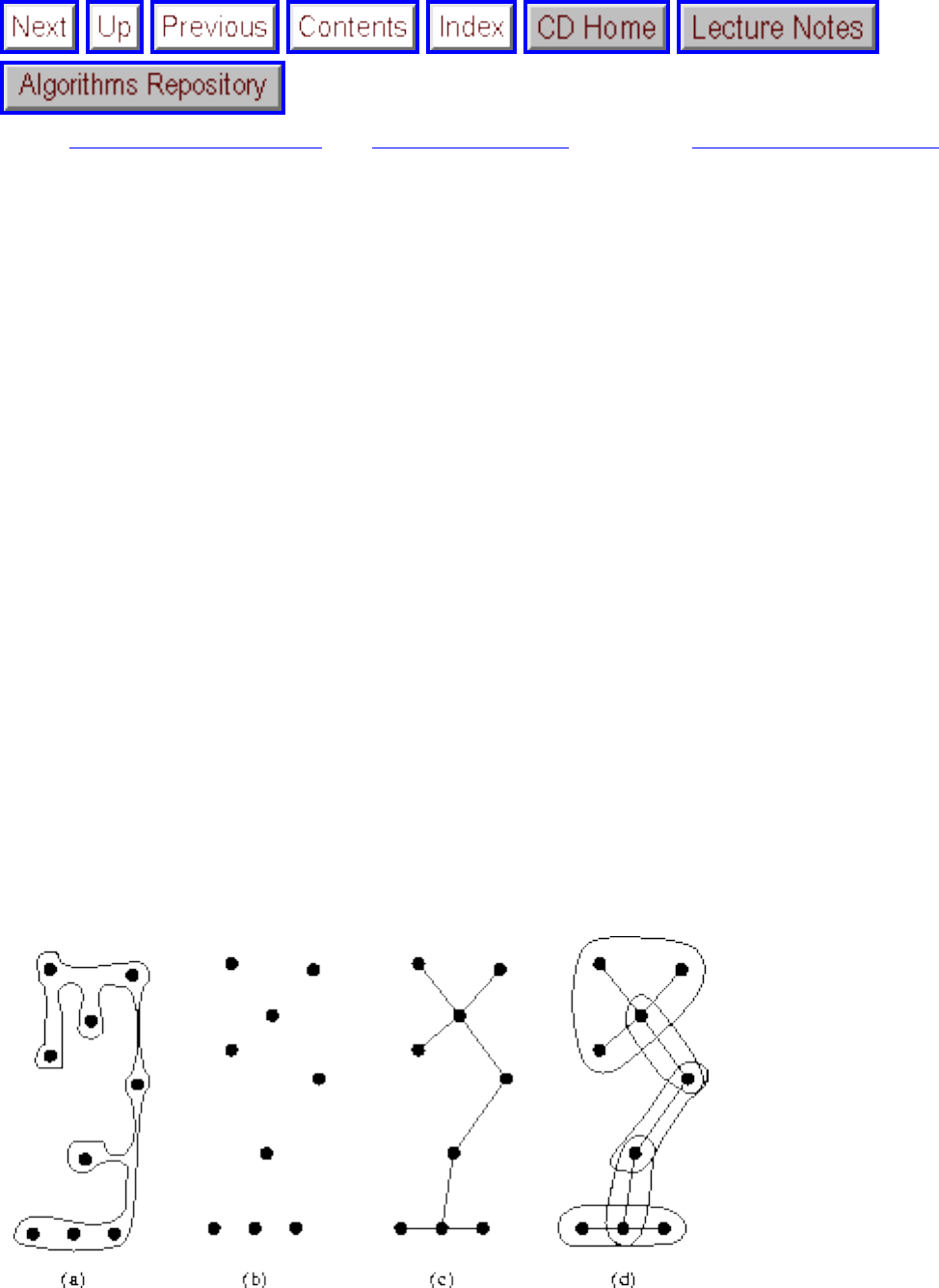
War Story: Nothing but Nets
Next: War Story: Dialing for Up: Graph Algorithms Previous: All-Pairs Shortest Path
War Story: Nothing but Nets
I'd been tipped off about a small printed-circuit board testing company nearby that was in need of some
algorithmic consulting. And so I found myself inside a typically non-descript building in a typically non-
descript industrial park, talking with the president of Integri-Test, along with one of his lead technical
people.
``We're the leaders in robotic printed-circuit board testing devices. Our customers have very high
reliability requirements for their PC-boards. They must check that each and every board has no wire
breaks before filling it with components. This means testing that each and every pair of points on the
board that are supposed to be connected are connected.''
``How do you do the testing?'' I asked.
``We have a robot with two arms, each with electric probes. To test whether two points are properly
connected, the arms simultaneously contact both of the points. If the two points are propertly connected,
then the probes will complete a circuit. For each net, we hold one arm fixed at one point and move the
other to cover the rest of the points.''
``Wait!'' I cried. ``What is a net?''
Figure: An sample net showing (a) the metal connection layer, (b) the contact points, (c) their minimum
spanning tree, and (d) the points partitioned into clusters
file:///E|/BOOK/BOOK2/NODE79.HTM (1 of 4) [19/1/2003 1:29:19]

War Story: Nothing but Nets
``On a circuit board there are certain sets of points that are all connected together with a metal layer. This
is what we mean by a net. Sometimes a net consists of two points, i.e. is an isolated wire. Sometimes a
net can have 100 to 200 points, like all the connections to power or ground.''
``I see. So you have a list of all the connections between pairs of points on the circuit board, and you
want to trace out these wires.''
He shook his head. ``Not quite. The input for our testing program consists only of the net contact points,
as shown in Figure (b). We don't know where the actual wires are, but we don't have to. All we have
to do is verify that all the points in a net are connected together. We do this by putting the left robot arm
on the leftmost point in the net, then having the right arm move around to all the other points in the net to
test if they are connected to the left point. If they are all connected to the left point, it means that they
must all be connected to each other.''
I thought for a moment about what this meant. ``OK. So your right arm has to visit all the other points in
the net. How do you choose the order to visit them?''
The technical guy spoke up. ``Well, we sort the points from left to right and then go in that order. Is that
a good thing to do?''
``Have you ever heard of the traveling salesman problem?'' I asked.
He was an electrical engineer, not a computer scientist. ``No, what's that?'' he asked.
``Traveling salesman is the name of the exact problem that you are trying to solve. Given a set of points
you have to visit, how do you order them so as to minimize the travel time. Algorithms for the traveling
salesman problem have been extensively studied. For small nets, by doing an exhaustive search you will
be able to find the optimal tour. For big nets, there are heuristics that will get you very close to the
optimal tour.'' I would have pointed them to Section if I had had this book handy.
The president scribbled down some notes and then frowned. ``Fine. Maybe you can order the points in a
net better for us. But that is not our real problem. When you watch our robot in action, the right arm
sometimes has to run all the way to the right side of the board on a given net, while the left arm just sits
there. It seems we would benefit by breaking a net into smaller pieces to balance things out.''
I sat down and thought. The left and right arms were each going to have interlocking TSP problems to
solve. The left arm would move between the leftmost points of each net, while the right arm was going to
visit all the other points in each net as ordered by the left TSP tour. By breaking each net into smaller
nets, so that each net occupies a small chunk of real estate, we would avoid making the right arm cross
all the way across the board. Further, a lot of little nets meant there would be more points in the left TSP,
so each left-arm movement was likely to be short, too.
file:///E|/BOOK/BOOK2/NODE79.HTM (2 of 4) [19/1/2003 1:29:19]
War Story: Nothing but Nets
``You are right. We should win if we can break big nets into small nets. We want the nets to be small,
both in the number of points and in the area of the net. But we must be sure that if we validate the
connectivity of each small net, we will have confirmed that the big net is connected. Whenever there is
one point in common between two little nets, that is enough to show that the bigger net formed by the
two little nets is connected, since current can flow between any pair of points.''
Now we had to break each net into overlapping pieces, where each piece was small. This is a clustering
problem. Minimum spanning trees are often used for clustering, as discussed in Section . In fact, that
was the answer! We could find the minimum spanning tree of the net points and break it into little
clusters whenever a spanning tree edge got too long. As shown in Figure (d), each cluster would share
exactly one point in common with another cluster, with connectivity ensured because we are covering the
edges of a spanning tree. The shape of the clusters would reflect the points in the net, exactly as we
would want. If the points lay along a line across the board, the minimum spanning tree would be a path,
and the clusters would be pairs of points. If the points all fell in a tight region, there would be one nice fat
cluster that the right arm would just scoot around.
So I explained the idea of constructing the minimum spanning tree of a graph. The boss listened,
scribbled more notes, and frowned again.
``I like your clustering idea. But these minimum spanning trees you talk about are defined on graphs. All
you got are points. Where do the weights of the edges come from?''
``Oh, we can think of it as a complete graph, where every pair of points are connected. The weight of the
edge defined by the two points is simply the distance. Or is it...?''
I went back to thinking. The edge cost between two points should reflect the travel time between them.
While the distance was related to the travel time, it wasn't necessarily exactly the same thing.
``Hey. I have a question about your robot. Does it take the same amount of time to move the arm left-
right as it does up-down?''
They thought a minute. ``Yeah, it does. We use the same type of motors to control horizontal and vertical
movements. Further, since the two motors for each arm are independent, we can simultaneously move
each arm both horizontally and vertically.''
``That so? The time to move both one foot left and one foot up is exactly the same as just moving one
foot left? This means that the weight cost for each edge in the graph should not be the Euclidean distance
between the two points, but the biggest difference between either the x- or y-coordinate. This is
something we call the metric, but we can capture it by changing the edge weights in the graph.
Anything else funny about your robots?'' I asked.
file:///E|/BOOK/BOOK2/NODE79.HTM (3 of 4) [19/1/2003 1:29:19]

War Story: Nothing but Nets
``Well, it takes some time for the robot to come up to speed. We should probably also factor in
acceleration and deceleration of the arms.''
``Darn right. The more accurately you can model the time your arm takes to move between two points,
the better our solution will be. But now we have a very clean formulation. Let's code it up and let's see
how well it works!''
They were somewhat skeptical whether this approach would do any good, but they agreed to think about
it. A few weeks later they called me back and reported that the new algorithm reduced testing time by
about 30% over their previous approach, at a cost of a little more computational preprocessing. However,
since their testing machine costs $200,000 a pop and a PC costs $2,000, this is an excellent tradeoff. It is
particularly advantageous since the preprocessing need only be done once when testing multiple
instances of the same board.
The key idea leading to the successful solution was knowing how to model the job in terms of classical
algorithmic graph problems. I smelled TSP the instant they started talking about minimizing robot
motion. Once I realized that they were implicitly forming a star-shaped spanning tree to ensure
connectivity, it was natural to ask whether a minimum spanning tree would perform any better. This idea
led to a natural way to think about clustering, and thus partitioning each net into smaller nets. Finally, by
carefully constructing our distance metric to accurately model the costs of the robot itself, we get to
incorporate quite complicated properties (such as acceleration and differences between horizontal and
vertical speeds) without changing our fundamental graph model or algorithm design.
Next: War Story: Dialing for Up: Graph Algorithms Previous: All-Pairs Shortest Path
Algorithms
Mon Jun 2 23:33:50 EDT 1997
file:///E|/BOOK/BOOK2/NODE79.HTM (4 of 4) [19/1/2003 1:29:19]

War Story: Dialing for Documents
Next: Exercises Up: Graph Algorithms Previous: War Story: Nothing but
War Story: Dialing for Documents
I was part of a group visiting Periphonics, an industry leader in building telephone voice-response
systems. These are more advanced versions of the Press 1 for more options, Press 2 if you didn't press 1
telephone systems that have come to blight everyone's lives in recent years. We were being given the
standard tour when someone from our group asked, ``Why don't you guys use voice recognition for data
entry. It would be a lot less annoying than typing things out on the keypad.''
The tour guide reacted smoothly. ``Our customers have the option of incorporating speech recognition
into our products, but very few of them do. User-independent, connected-speech recognition is not
accurate for most applications. Our customers prefer building systems around typing text on the
telephone keyboards.''
``Prefer typing, my pupik!'', came a voice from the rear of our group. ``I hate typing on a telephone.
Whenever I call my brokerage house to get stock quotes, I end up talking to some machine, which asks
me to type in the three letter code. To make it worse, I have to hit two buttons to type in one letter, in
order to distinguish between the three letters printed on each key of the telephone. I hit the 2 key and it
says Press 1 for `A', Press 2 for `B', Press 3 for `C'. Pain the neck if you ask me.''
``Maybe you don't really have to hit two keys for each letter?'' I chimed in. ``Maybe the system could
figure out the correct letter from context?''
``There isn't a whole lot of context when you type in three letters of stock market code.''
``Sure, but there would be plenty of context if we were typing in English sentences. I'll bet that we could
reconstruct English sentences correctly if they were typed in a telephone at one keystroke per letter.''
The guy from Periphonics gave me a disinterested look, then continued the tour. But when I got back to
the office, I decided to give it a try.
It was clear that not all letters were equally likely to be typed on a telephone. In fact, not all letters can be
typed, since `Q' and `Z' are not labeled on the standard American telephone. Therefore, we adopted the
convention that `Q', `Z', and space were all on the * key. We could take advantage of the uneven
file:///E|/BOOK/BOOK2/NODE80.HTM (1 of 6) [19/1/2003 1:29:21]
War Story: Dialing for Documents
distribution of letter frequencies to help us decode the text. For example, if you hit the 3 key while typing
English, you were more likely to have meant to type an `E' than either a `D' or `F'. By taking into account
the frequencies of a window of three characters, we could predict the typed text. Indeed, this is what
happened when I tried it on the Gettysburg Address:
enurraore ane reten yeasr ain our ectherr arotght eosti on ugis aootinent a oey oation aoncdivee in licesty
ane eedicatee un uhe rrorosition uiat all oen are arectee e ual
ony ye are enichde in a irect aitil yar uestini yhethes uiat oatioo or aoy oation ro aoncdivee ane ro
eedicatee aan loni eneure ye are oet on a irect aattlediele oe uiat yar ye iate aone un eedicate a rostion oe
uiat eiele ar a einal restini rlace eor uiore yin iere iate uhdis lives uiat uhe oation ogght live it is aluniethes
eittini ane rrores uiat ye rioule en ugir
att in a laries reore ye aan oou eedicate ye aan oou aoorearate ye aan oou ialloy ugis iroune the arate oen
litini ane eeae yin rustgilee iere iate aoorearatee it ear aante our roor rowes un ade or eeuraat the yople yill
little oote oor loni renences yiat ye ray iere att it aan oetes eosiet yiat uhfy eie iere it is eor ur uhe litini
rathes un ae eedicatee iere un uhe undiniside yopl yhici uhfy yin entght iere iate uiur ear ro onaky
aetancde it is rathes eor ur un ae iere eedicatee un uhe irect uarl rencinini adeore ur uiat eron uhere ioooree
eeae ye uale inarearee eeuotion uo tiat aaure eor yhici uhfy iere iate uhe lart eull oearure oe eeuotioo tiat
ye iere iggily rerolue uiat uhere eeae riall oou iate eide io
The trigram statistics did a decent job of translating it into Greek, but a terrible job of transcribing
English. One reason was clear. This algorithm knew nothing about English words. If we coupled it with a
dictionary, we might be on to something. The difficulty was that often two words in the dictionary would
be represented by the exact same string of phone codes. For an extreme example, the code string
``22737'' collides with eleven distinct English words, including cases, cares, cards, capes, caper, and
bases. As a first attempt, we reported the unambiguous characters of any words that collided in the
dictionary, and used trigrams to fill in the rest of the characters. We were rewarded with:
eourscore and seven yearr ain our eatherr brought forth on this continent azoey nation conceivee in liberty
and dedicatee uo uhe proposition that all men are createe equal
ony ye are engagee in azipeat civil yar uestioi whether that nation or aoy nation ro conceivee and ro
dedicatee aan long endure ye are oet on azipeat battlefield oe that yar ye iate aone uo dedicate a rostion oe
that field ar a final perthni place for those yin here iate their lives that uhe nation oight live it is altogether
fittinizane proper that ye should en this
aut in a larges sense ye aan oou dedicate ye aan oou consecrate ye aan oou hallow this ground the arate
men litioi and deae yin strugglee here iate consecratee it ear above our roor power uo ade or detract the
world will little oote oor long remember what ye ray here aut it aan meter forget what uhfy die here it is
for ur uhe litioi rather uo ae dedicatee here uo uhe toeioisgee york which uhfy yin fought here iate thus ear
ro mocky advancee it is rather for ur uo ae here dedicatee uo uhe great task renagogoi adfore ur that from
there honoree deae ye uale increasee devotion uo that aause for which uhfy here iate uhe last eull measure
oe devotion that ye here highky resolve that there deae shall oou iate fide io vain that this nation under ioe
shall iate azoey birth oe freedom and that ioternmenu oe uhe people ay uhe people for uhe people shall
oou perish from uhe earth
file:///E|/BOOK/BOOK2/NODE80.HTM (2 of 6) [19/1/2003 1:29:21]
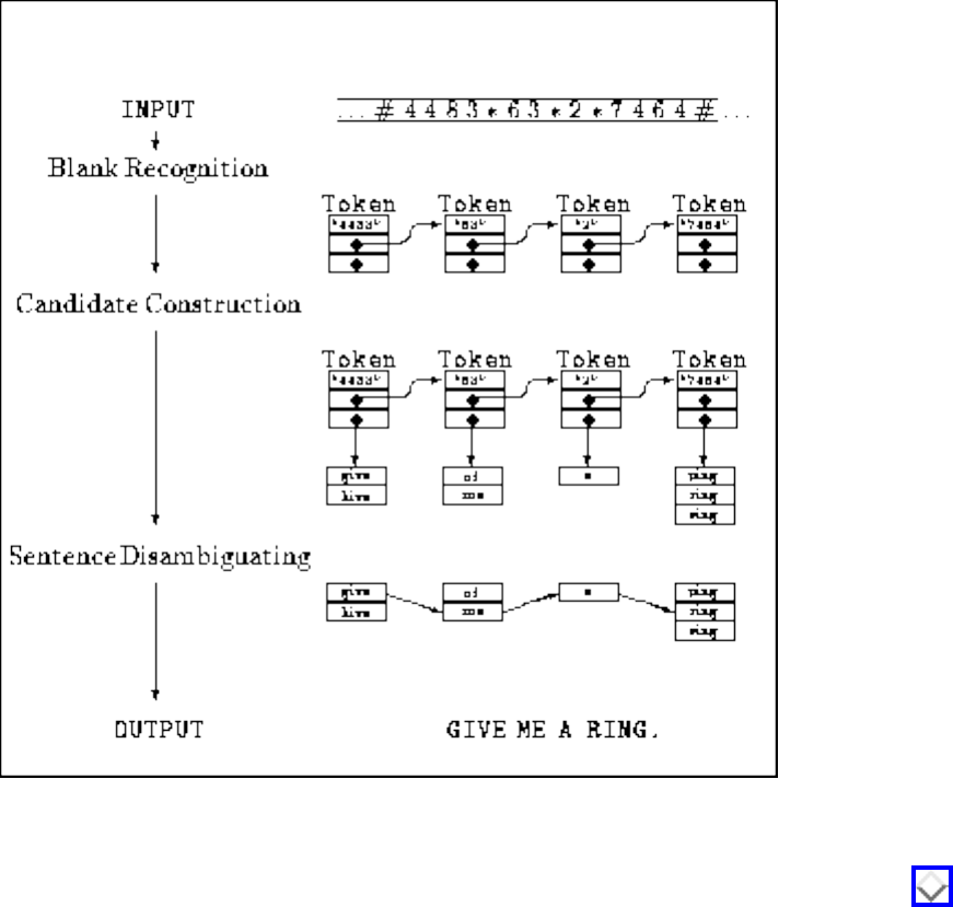
War Story: Dialing for Documents
If you were a student of American history, maybe you could recognize it, but you certainly couldn't read
it. Somehow we had to distinguish between the different dictionary words that got hashed to the same
code. We could factor in the relative popularity of each word, which would help, but this would still
make too many mistakes.
At this point I started working with Harald Rau on the project, who proved a great collaborator for two
reasons. First, he was a bright and peristent graduate student. Second, as a native German speaker he
would believe every lie I told him about English grammar.
Figure: The phases of the telephone code reconstruction process
Harald built up a phone code reconstruction program on the lines of Figure . It worked on the input
one sentence at a time, identifying dictionary words that matched each code string. The key problem was
how to incorporate the grammatical constraints.
``We can get good word-use frequencies and grammatical information using this big text database called
the Brown Corpus. It contains thousands of typical English sentences, each of which is parsed according
to parts of speech. But how do we factor it all in?'' Harald asked.
``Let's try to think about it as a graph problem,'' I suggested.
file:///E|/BOOK/BOOK2/NODE80.HTM (3 of 6) [19/1/2003 1:29:21]
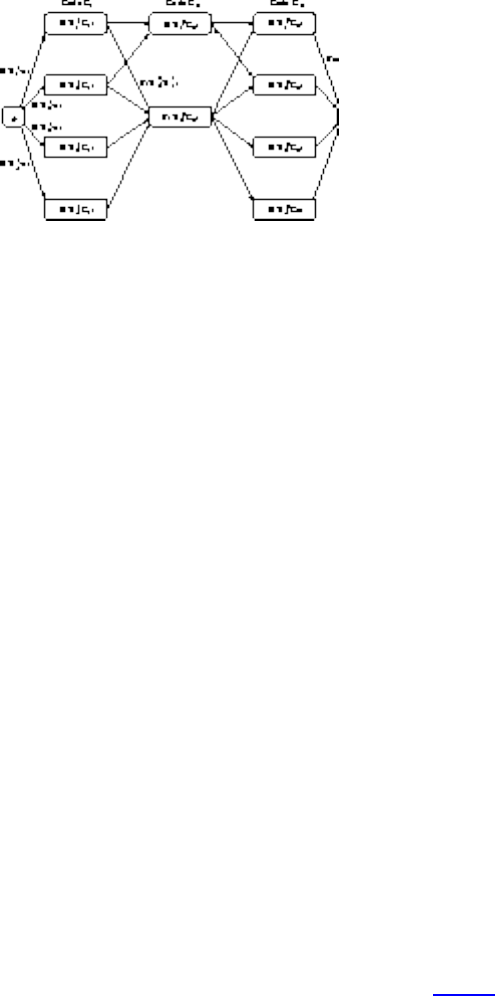
War Story: Dialing for Documents
``Graph problem? What graph problem? Where is there even a graph?''
``Think of a sentence as a list of phone tokens, each representing a word in the sentence. For each phone
token, we have a list of words from the dictionary that match it. How can we choose which one is right?
Each possible sentence interpretation can be thought of as a path in a graph. The vertices of this graph
will be the complete set of possible word choices. There will be an edge from a possible choice for the
ith word to each possible choice for the (i+1)st word. The cheapest path across this graph is the right
interpretation of the sentence.''
Figure: The minimum-cost path through the graph defines the best interpretation for a sentence
``But all the paths look the same. They have the same number of edges. Wait. Now I see! To make the
paths different, we have to weight the edges.''
``Exactly! The cost of an edge will reflect how likely it is that we will want to travel through the given
pair of words. Maybe we can count how often that pair of words occurred together in previous texts. Or
we can weight by what part of speech each word is. Maybe nouns don't like to be next to nouns as much
as they like being next to verbs.''
``It will be hard to keep track of word-pair statistics, since there are so many of them. But we certainly
know the frequency of each word. How can we factor that into things?''
``We can pay a cost for walking through a particular vertex that depends upon the frequency of the word.
Our best sentence will be given by the shortest path across the graph.''
``But how do we figure out the relative weights of these factors?''
``Well, try what seems natural to you and then we can experiment with it.''
Harald incorported this shortest-path algorithm. With proper grammatical and statistical constraints, the
system performed great, as reported in [RS96]. Look at the Gettysburg Address now, with all the
reconstruction errors highlighted:
FOURSCORE AND SEVEN YEARS AGO OUR FATHERS BROUGHT FORTH ON THIS
file:///E|/BOOK/BOOK2/NODE80.HTM (4 of 6) [19/1/2003 1:29:21]
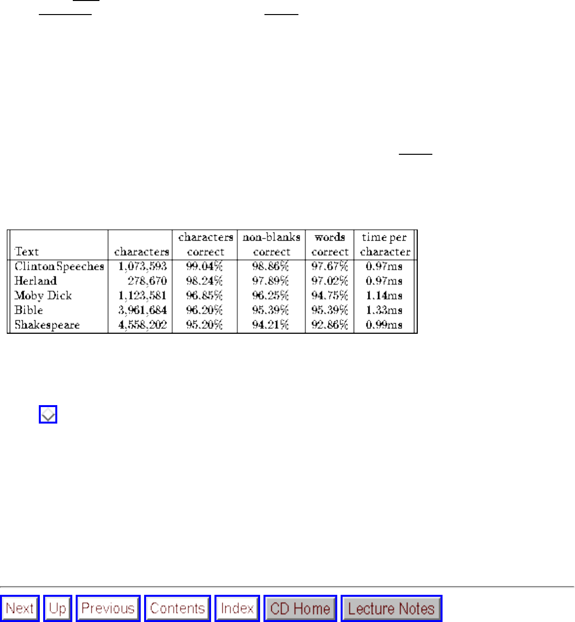
War Story: Dialing for Documents
CONTINENT A NEW NATION CONCEIVED IN LIBERTY AND DEDICATED TO THE
PROPOSITION THAT ALL MEN ARE CREATED EQUAL. NOW WE ARE ENGAGED IN A
GREAT CIVIL WAR TESTING WHETHER THAT NATION OR ANY NATION SO CONCEIVED
AND SO DEDICATED CAN LONG ENDURE. WE ARE MET ON A GREAT BATTLEFIELD OF
THAT WAS. WE HAVE COME TO DEDICATE A PORTION OF THAT FIELD AS A FINAL
SERVING PLACE FOR THOSE WHO HERE HAVE THEIR LIVES THAT THE NATION MIGHT
LIVE. IT IS ALTOGETHER FITTING AND PROPER THAT WE SHOULD DO THIS. BUT IN A
LARGER SENSE WE CAN NOT DEDICATE WE CAN NOT CONSECRATE WE CAN NOT
HALLOW THIS GROUND. THE BRAVE MEN LIVING AND DEAD WHO STRUGGLED HERE
HAVE CONSECRATED IT FAR ABOVE OUR POOR POWER TO ADD OR DETRACT. THE
WORLD WILL LITTLE NOTE NOR LONG REMEMBER WHAT WE SAY HERE BUT IT CAN
NEVER FORGET WHAT THEY DID HERE. IT IS FOR US THE LIVING RATHER TO BE
DEDICATED HERE TO THE UNFINISHED WORK WHICH THEY WHO FOUGHT HERE HAVE
THUS FAR SO NOBLY ADVANCED. IT IS RATHER FOR US TO BE HERE DEDICATED TO THE
GREAT TASK REMAINING BEFORE US THAT FROM THESE HONORED DEAD WE TAKE
INCREASED DEVOTION TO THAT CAUSE FOR WHICH THEY HERE HAVE THE LAST FULL
MEASURE OF DEVOTION THAT WE HERE HIGHLY RESOLVE THAT THESE DEAD SHALL
NOT HAVE DIED IN VAIN THAT THIS NATION UNDER GOD SHALL HAVE A NEW BIRTH OF
FREEDOM AND THAT GOVERNMENT OF THE PEOPLE BY THE PEOPLE FOR THE PEOPLE
SHALL NOT PERISH FROM THE EARTH.
Figure: Our telephone-code reconstruction system applied to various text samples
While we still made a few mistakes, the results are clearly good enough for a variety of applications.
Periphonics certainly thought so, for they later licensed our program to incorporate into their products.
Figure shows that we were able to reconstruct over 99% of the characters correctly on a megabyte of
President Clinton's speeches, so if Bill had phoned them in, we would certainly still be able to understand
it. The reconstruction time is fast enough, indeed faster than you can type it in on the phone keypad.
The constraints associated with many different pattern recognition problems can be formulated as
shortest path problems in graphs. In fact, there is a particularly convenient dynamic programming
solution for these problems known as the Viterbi algorithm, which is used in speech and handwriting
recognition systems. Despite the fancy name, all the Viterbi algorithm is doing is solving a shortest path
problem. Hunting for a graph formulation for any given problem is always a good way to proceed.
file:///E|/BOOK/BOOK2/NODE80.HTM (5 of 6) [19/1/2003 1:29:21]

Exercises
Next: Implementation Challenges Up: Graph Algorithms Previous: War Story: Dialing for
Exercises
1. Present correct and efficient algorithms to convert between the following graph data structures,
for an undirected graph G with n vertices and m edges. You must give the time complexity of
each algorithm.
1. Convert from an adjacency matrix to adjacency lists.
2. Convert from an adjacency list to an incidence matrix. An incidence matrix M has a row
for each vertex and a column for each edge, such that M[i,j]=1 if vertex i is part of edge j,
otherwise M[i,j] = 0.
3. Convert from an incidence matrix to adjacency lists.
2. Is the path between a pair of vertices in a minimum spanning tree necessarily a shortest path
between the two vertices in the full graph? Give a proof or a counterexample.
3. Assume that all edges in the graph have distinct edge weights (i.e. no pair of edges have the same
weight). Is the path between a pair of vertices in a minimum spanning tree necessarily a shortest
path between the two vertices in the full graph? Give a proof or a counterexample.
4. Suppose G is a connected undirected graph. An edge e whose removal disconnects the graph is
called a bridge. Must every bridge e be an edge in a depth-first search tree of G, or can e be a
back edge? Give a proof or a counterexample.
5. (*) In breadth-first and depth-first search, an undiscovered node is marked discovered when it is
first encountered, and marked completely-explored when it has been completely searched. At any
given moment, several nodes might be simultaneously in the discovered state.
(a) Describe a graph on n vertices and a particular starting vertex v such that during a breadth-first
search starting from v, nodes are simultaneously in the discovered state.
(b) Describe a graph on n vertices and a particular starting vertex v such that during a depth-first
search starting from v, nodes are simultaneously in the discovered state.
(c) Describe a graph on n vertices and a particular starting vertex v such that at some point during
a depth-first search starting from v, nodes remain undiscovered, while nodes have been
completely-explored. (Note, there may also be discovered nodes.)
6. Given the pre-order and in-order traversals of a binary tree, is it possible to reconstruct the tree? If
file:///E|/BOOK/BOOK2/NODE81.HTM (1 of 3) [19/1/2003 1:29:23]
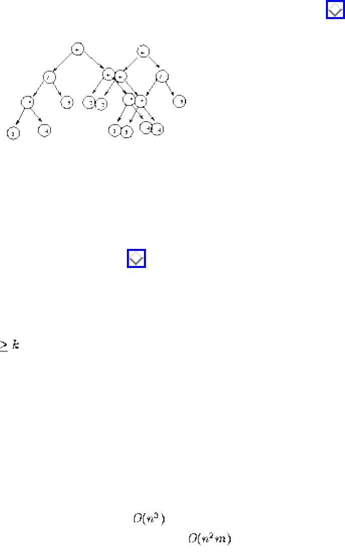
Exercises
so, sketch an algorithm to do it. If not, give a counterexample. Repeat the problem if you are
given the pre-order and post-order traversals.
7. Suppose an arithmetic expression is given as a tree. Each leaf is an integer and each internal node
is one of the standard arithmetical operations (+,-,*,/). For example, the expression
2+3*4+(3*4)/5 could be represented by the tree in Figure (a).
Figure: Expression 2+3*4+(3*4)/5 as a tree and a DAG.
Give an O(n) algorithm for evaluating such an expression, where there are n nodes in the tree.
8. (*) Suppose an arithmetic expression is given as a DAG (directed acyclic graph) with common
subexpressions removed. Each leaf is an integer and each internal node is one of the standard
arithmetical operations (+,-,*,/). For example, the expression 2+3*4+(3*4)/5 could be represented
by the DAG in Figure (b). Give an O(n+m) algorithm for evaluating such a DAG, where there
are n nodes and m edges in the DAG. Hint: modify an algorithm for the tree case to achieve the
desired efficiency.
9. (*) Given an undirected graph G with n vertices and m edges, and an integer k, give an O(m+n)
algorithm that finds the maximum induced subgraph H of G such that each vertex in H has degree
, or prove that no such graph exists. An induced subgraph F=(U,R) of a graph G=(V,E) is a
subset of U of the vertices V of G, and all edges R of G such that both vertices of each edge are in
U.
10. (*) An articulation vertex of a graph G is a vertex whose deletion disconnects G. Let G be a graph
with n vertices and m edges. Give a simple O(n+m) algorithm for finding a vertex of G that is not
an articulation vertex, i.e. whose deletion does not disconnect G.
11. (*) Following up on the previous problem, give an O(n+m) algorithm that finds a deletion order
for the n vertices such that no deletion disconnects the graph. (Hint: think DFS/BFS.)
12. (*) Let G be a weighted directed graph with n vertices and m edges, where all edges have positive
weight. A directed cycle is a directed path that starts and ends at the same vertex and contains at
least one edge. Give an algorithm to find a directed cycle in G of minimum total weight.
Partial credit will be given for an algorithm.
13. (*) Suppose we are given the minimum spanning tree T of a given graph G (with n vertices and m
edges) and a new edge e=(u,v) of weight w that we will add to G. Give an efficient algorithm to
find the minimum spanning tree of the graph G + e. Your algorithm should run in O(n) time to
receive full credit, although slower but correct algorithms will receive partial credit.
14. (*) (a) Let T be a minimum spanning tree of a weighted graph G. Construct a new graph G' by
adding a weight of k to every edge of G. Do the edges of T form a minimum spanning tree of G'?
file:///E|/BOOK/BOOK2/NODE81.HTM (2 of 3) [19/1/2003 1:29:23]
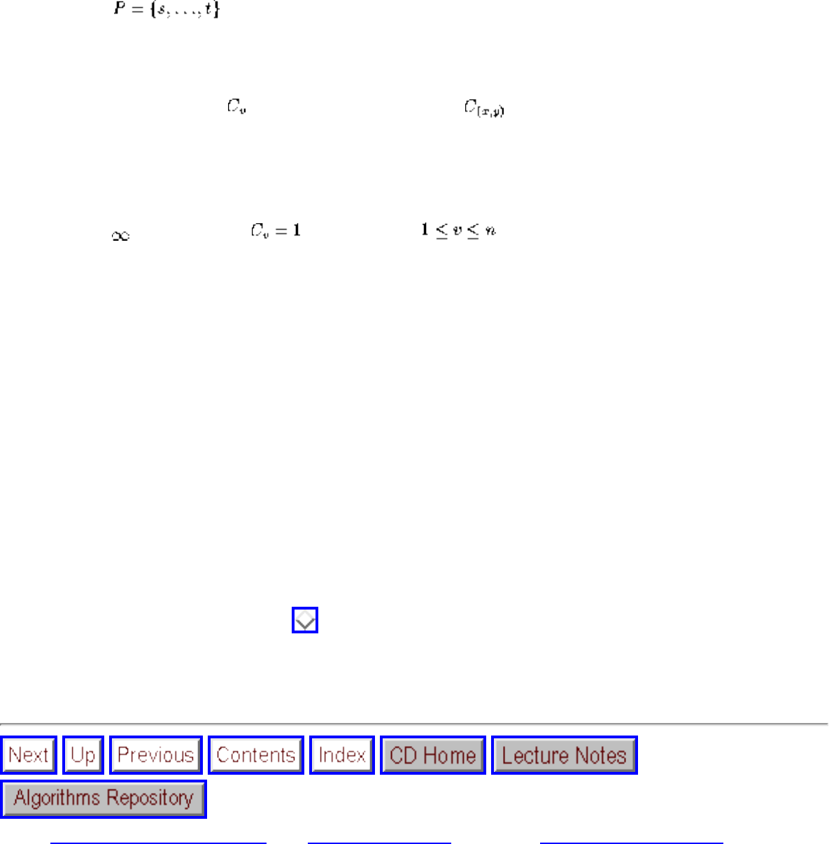
Exercises
Prove the statement or give a counterexample.
(b) Let describe a shortest weighted path between vertices and t of a weighted graph
G. Construct a new graph G' by adding a weight of k to every edge of G. Does P describe a
shortest path from to t in G'? Prove the statement or give a counterexample.
15. (*) In certain graph problems, vertices have can have weights instead of or in addition to the
weights of edges. Let be the cost of vertex v, and the cost of the edge (x,y). This problem
is concerned with finding the cheapest path between vertices a and b in a graph G. The cost of a
path is the sum of the costs of the edges and vertices encountered on the path.
❍ Suppose that each edge in the graph has a weight of zero (while non-edges have a cost of
). Assume that for all vertices (i.e. all vertices have the same cost). Give
an efficient algorithm to find the cheapest path from a to b and its time complexity. For
partial credit, give a less efficient but correct algorithm.
❍ Now suppose that the vertex costs are not constant (but are all positive) and the edge costs
remain as above. Give an efficient algorithm to find the cheapest path from a to b and its
time complexity. For partial credit, give a less efficient but correct algorithm.
❍ Now suppose that both the edge and vertex costs are not constant (but are all positive).
Give an efficient algorithm to find the cheapest path from a to b and its time complexity.
For partial credit, give a less efficient but correct algorithm.
16. (*) Devise and analyze an algorithm that takes a weighted graph G and finds the smallest change
in the cost of a non-MST edge that causes a change in the minimum spanning tree of G. Your
algorithm must be correct and run in polynomial time.
17. An arborescence of a directed graph G is a rooted tree such that there is a directed path from the
root to every other vertex in the graph. Give an efficient and correct algorithm to test whether G
contains an arborescence, and its time complexity.
18. (**) The war story of Section describes an algorithm for constructing the dual graph of the
triangulation efficiently, although it does not guarantee linear time. Give a worst-case linear
algorithm for the problem.
Next: Implementation Challenges Up: Graph Algorithms Previous: War Story: Dialing for
Algorithms
Mon Jun 2 23:33:50 EDT 1997
file:///E|/BOOK/BOOK2/NODE81.HTM (3 of 3) [19/1/2003 1:29:23]
Backtracking
Next: Constructing All Subsets Up: Combinatorial Search and Heuristic Previous: Combinatorial Search and Heuristic
Backtracking
Backtracking is a systematic way to go through all the possible configurations of a space. These configurations may be all
possible arrangements of objects (permutations) or all possible ways of building a collection of them (subsets). Other
applications may demand enumerating all spanning trees of a graph, all paths between two vertices, or all possible ways to
partition the vertices into color classes.
What these problems have in common is that we must generate each one of the possible configurations exactly once.
Avoiding both repetitions and missing configurations means that we must define a systematic generation order among the
possible configurations. In combinatorial search, we represent our configurations by a vector , where
each element is selected from an ordered set of possible candidates for position i. As shown below, this representation
is general enough to encode most any type of combinatorial object naturally.
The search procedure works by growing solutions one element at a time. At each step in the search, we will have
constructed a partial solution with elements fixed for the first k elements of the vector, where . From this partial
solution , we will construct the set of possible candidates for the (k+1)st position. We will then try to
extend the partial solution by adding the next element from . So long as the extension yields a longer partial solution,
we continue to try to extend it.
However, at some point, might be empty, meaning that there is no legal way to extend the current partial solution. If
so, we must backtrack, and replace , the last item in the solution value, with the next candidate in . It is this
backtracking step that gives the procedure its name:
Backtrack(A)
Compute , the set of candidate first elements of solution A.
k = 1
while k > 0 do
while do (*advance*)
= the next element from
file:///E|/BOOK/BOOK2/NODE84.HTM (1 of 3) [19/1/2003 1:29:24]
Backtracking
if is a solution,
report it.
k = k + 1
compute , the set of candidate
kth elements of solution A.
k = k - 1 (*backtrack*)
Backtracking constructs a tree of partial solutions, where each vertex is a partial solution. There is an edge from x to y if
node y was created by advancing from x. This tree of partial solutions provides an alternative way to think about
backtracking, for the process of constructing the solutions corresponds exactly to doing a depth-first traversal of the
backtrack tree. Viewing backtracking as depth-first search yields a natural recursive implementation of the basic algorithm:
Backtrack-DFS(A,k)
if is a solution, report it.
else
k = k +1
compute
while do
= an element in
=
file:///E|/BOOK/BOOK2/NODE84.HTM (2 of 3) [19/1/2003 1:29:24]

Backtracking
Backtrack(a,k)
Although a breadth-first search could also be used to enumerate all solutions, depth-first search is greatly preferred because
of the amount of storage required. In depth-first search, the current state of the search is completely represented by the path
from the root to the current search node, which requires space proportional to the height of the tree. In breadth-first search,
the queue stores all the nodes at the current level, which is proportional to the width of the search tree. For most interesting
problems, the width of the tree will grow exponentially in its height.
To really understand how backtracking works, you must see how such objects as permutations and subsets can be
constructed by defining the right state spaces. Examples of several state spaces are described below.
● Constructing All Subsets
● Constructing All Permutations
● Constructing All Paths in a Graph
Next: Constructing All Subsets Up: Combinatorial Search and Heuristic Previous: Combinatorial Search and Heuristic
Algorithms
Mon Jun 2 23:33:50 EDT 1997
file:///E|/BOOK/BOOK2/NODE84.HTM (3 of 3) [19/1/2003 1:29:24]
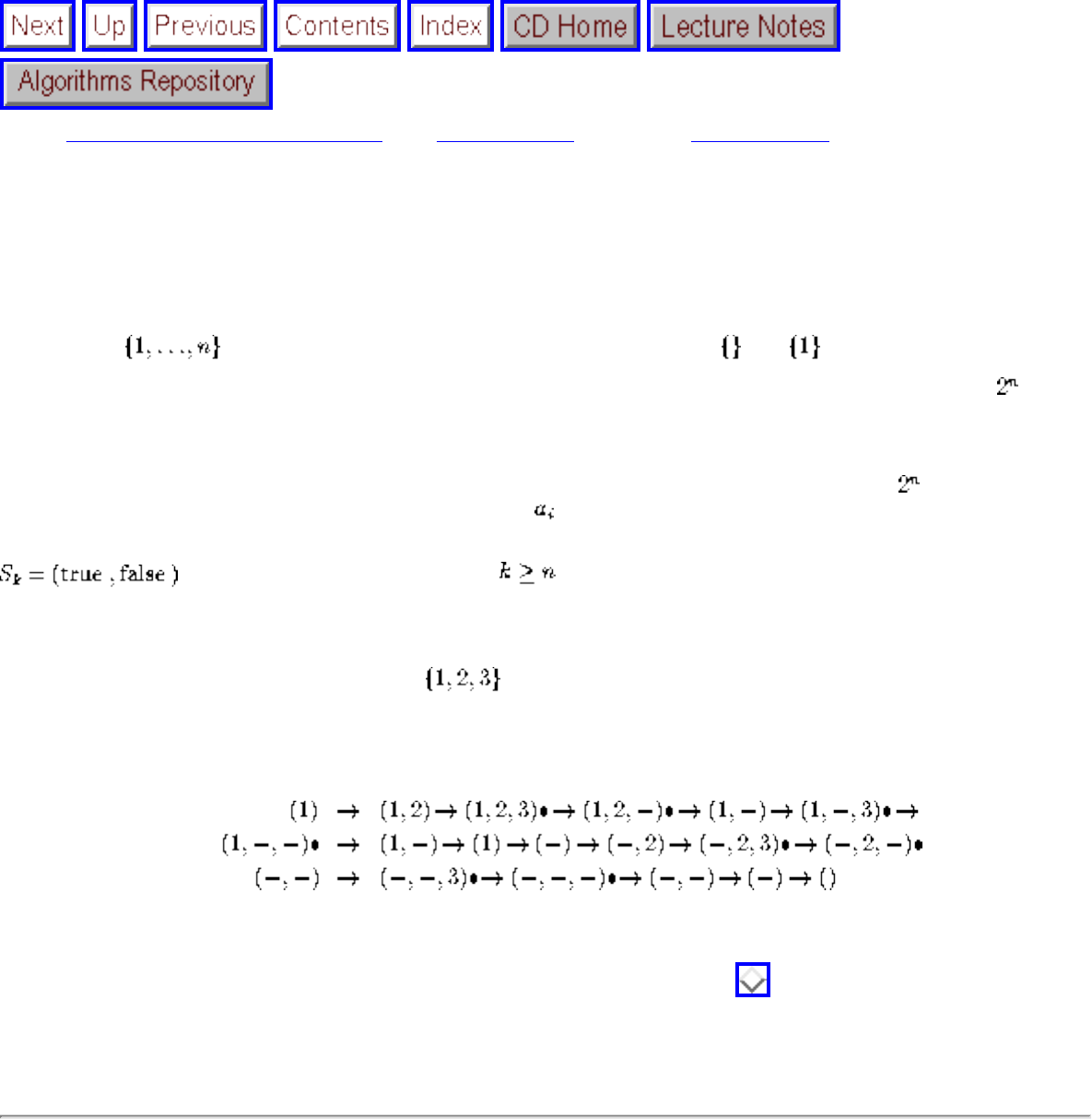
Constructing All Subsets
Next: Constructing All Permutations Up: Backtracking Previous: Backtracking
Constructing All Subsets
To design a suitable state space for representing a collection of combinatorial objects, it is important to
know how many objects you will need to represent. How many subsets are there of an n-element set, say
the integers ? There are exactly two subsets for n=1 namely and , four subsets for n=2,
and eight subsets for n=3. Since each new element doubles the number of possibilities, there are
subsets of n elements.
Each subset is described by stating which elements are in it. Therefore, to construct all subsets, we can
set up an array/vector of n cells, where the value of is either true or false, signifying whether the ith
item is or is not in the given subset. To use the notation of the general backtrack algorithm,
, and A is a solution whenever .
Using this state space representation, the backtracking algorithm constructs the following sequence of
partial solutions in finding the subsets of . Final solutions, i.e. complete subsets, are marked with
a *. False choices correspond to dashes in the partial solution, while true in position i is denoted by i
itself:
Trace through this example carefully to make sure you understand the backtracking procedure. The
problem of generating subsets is more thoroughly discussed in Section .
Algorithms
Mon Jun 2 23:33:50 EDT 1997
file:///E|/BOOK/BOOK2/NODE85.HTM [19/1/2003 1:29:25]
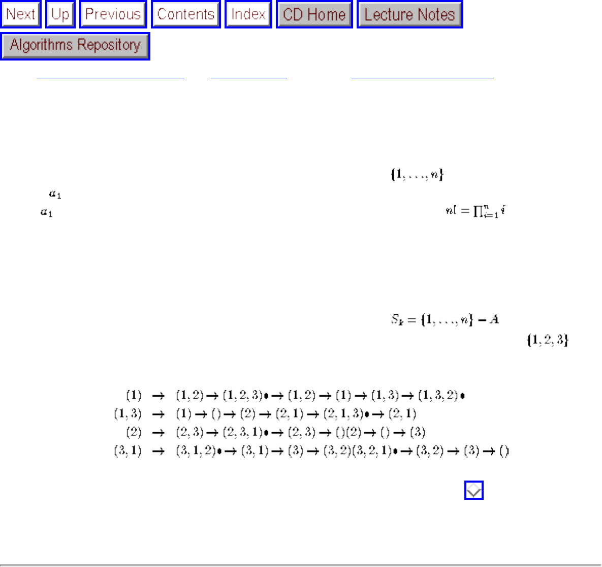
Constructing All Permutations
Next: Constructing All Paths in Up: Backtracking Previous: Constructing All Subsets
Constructing All Permutations
To design a suitable state space for representing permutations, we start by counting them. There are n
distinct choices for the value of the first element of a permutation of . Once we have fixed this
value of , there are n-1 candidates remaining for the second position, since we can have any value
except (repetitions are forbidden). Repeating this argument yields a total of distinct
permutations.
This counting argument suggests a suitable representation. To construct all n! permutations, set up an
array/vector A of n cells. The set of candidates for the ith position will be the set of elements that have
not appeared in the (i-1) elements of the partial solution, corresponding to the first i-1 elements of the
permutation. To use the notation of the general backtrack algorithm, . The vector A
contains a full solution whenever k = n+1. This representation generates the permutations of in
the following order:
The problem of generating permutations is more thoroughly discussed in Section .
Algorithms
Mon Jun 2 23:33:50 EDT 1997
file:///E|/BOOK/BOOK2/NODE86.HTM [19/1/2003 1:29:26]
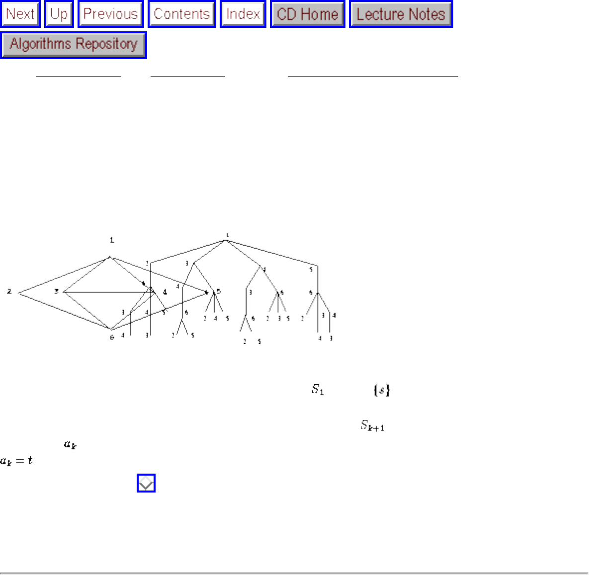
Constructing All Paths in a Graph
Next: Search Pruning Up: Backtracking Previous: Constructing All Permutations
Constructing All Paths in a Graph
Enumerating all the simple paths from to t through a given graph is a somewhat more complicated
problem than listing permutations or subsets. Unlike the earlier problems, there is no explicit formula
that counts the number of solutions as a function of the number of edges or vertices, because the number
of paths depends upon the structure of the graph.
Figure: The search tree enumerating all simple paths from vertex 1 in the graph
Since the starting point of any path from to t is always , must be . The set of possible candidates for
the second position are the vertices v such that (,v) is an edge of the graph, for the path wanders from
vertex to vertex using edges to define the legal steps. In general, consists of the set of vertices
adjacent to that have not been used in the partial solution A. We can report a successful path whenever
. The solution vector A must have room for all n vertices, although most paths are likely to be
shorter than this. Figure shows the search tree giving all paths from a particular vertex in an example
graph.
Algorithms
Mon Jun 2 23:33:50 EDT 1997
file:///E|/BOOK/BOOK2/NODE87.HTM [19/1/2003 1:29:26]
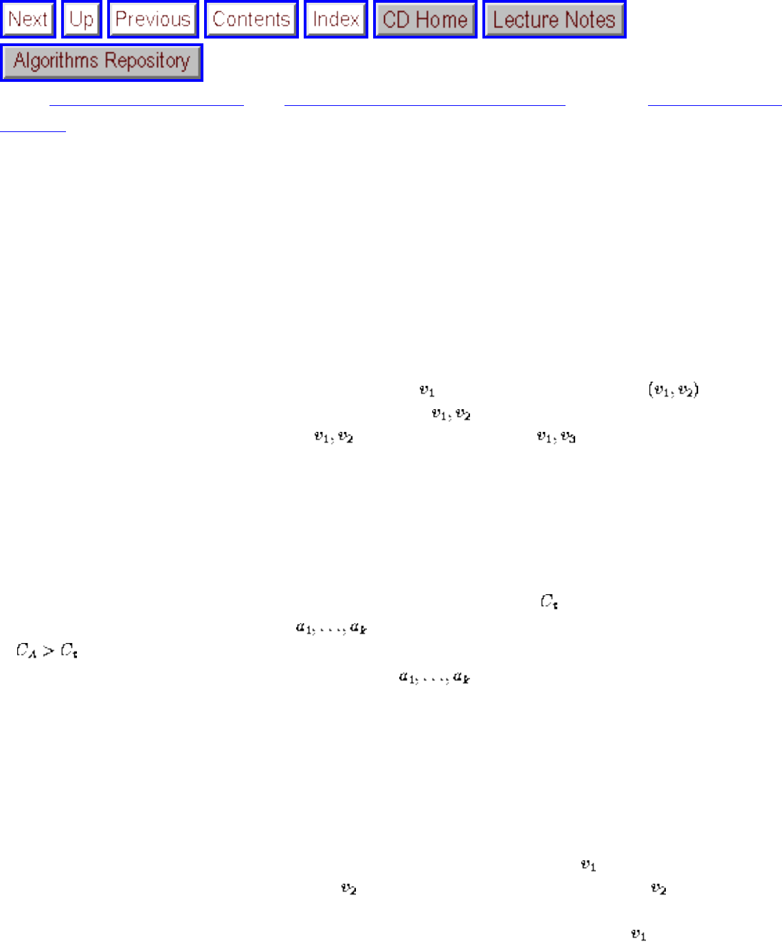
Search Pruning
Next: Bandwidth Minimization Up: Combinatorial Search and Heuristic Previous: Constructing All
Paths in
Search Pruning
Backtracking ensures correctness by enumerating all possibilities. For example, a correct algorithm to
find the optimal traveling salesman tour could enumerate all n! permutations of n vertices of the graph
and selecting the best one. For each permutation, we could check whether each of the n edges implied in
the tour really exists in the graph G, and if so, sum the weights of these edges together.
For most graphs, however, it would be pointless to construct all the permutations first and then analyze
them later. Suppose we started our search from vertex , and it happened that edge was not in G.
Enumerating all the (n-2)! permutations beginning with would be a complete waste of effort. Much
better would be to prune the search after and continue next with . By carefully restricting the
set of next elements to reflect only the moves that are legal from the current partial configuration, we
reduce the search complexity significantly.
Pruning is the technique of cutting off search the instant we have established that this partial solution
cannot be extended into the solution that we want. For example, in our traveling salesman search
program, we seek the cheapest tour that visits all vertices before returning to its starting position.
Suppose that in the course of our search we find a tour t whose cost is . As the search continues,
perhaps we will find a partial solution , where k < n and the sum of the edges on this partial tour
is . Can there be any reason to continue exploring this node any further? No, assuming all edges
have positive cost, because any tour with the prefix will have cost greater than tour t, and hence
is doomed to be non-optimal. Cutting away such failed partial tours as soon as possible can have an
enormous impact on running time.
Exploiting symmetry is a third avenue for reducing combinatorial search. It is clearly wasteful to
evaluate the same candidate solution more than once, because we will get the exact same answer each
time we consider it. Pruning away partial solutions identical to those previously considered requires
recognizing underlying symmetries in the search space. For example, consider the state of our search for
an optimal TSP tour after we have tried all partial positions beginning with . Can it pay to continue the
search with partial solutions beginning with ? No. Any tour starting and ending at can be viewed as
starting and ending at or any other vertex, for these tours are cycles. There are thus only (n-1)! distinct
tours on n vertices, not n!. By restricting the first element of the tour to always be , we save a factor of
n in time without missing any interesting solutions. Detecting such symmetries can be subtle, but once
identified they can usually be easily exploited by a search program.
file:///E|/BOOK/BOOK2/NODE88.HTM (1 of 2) [19/1/2003 1:29:27]

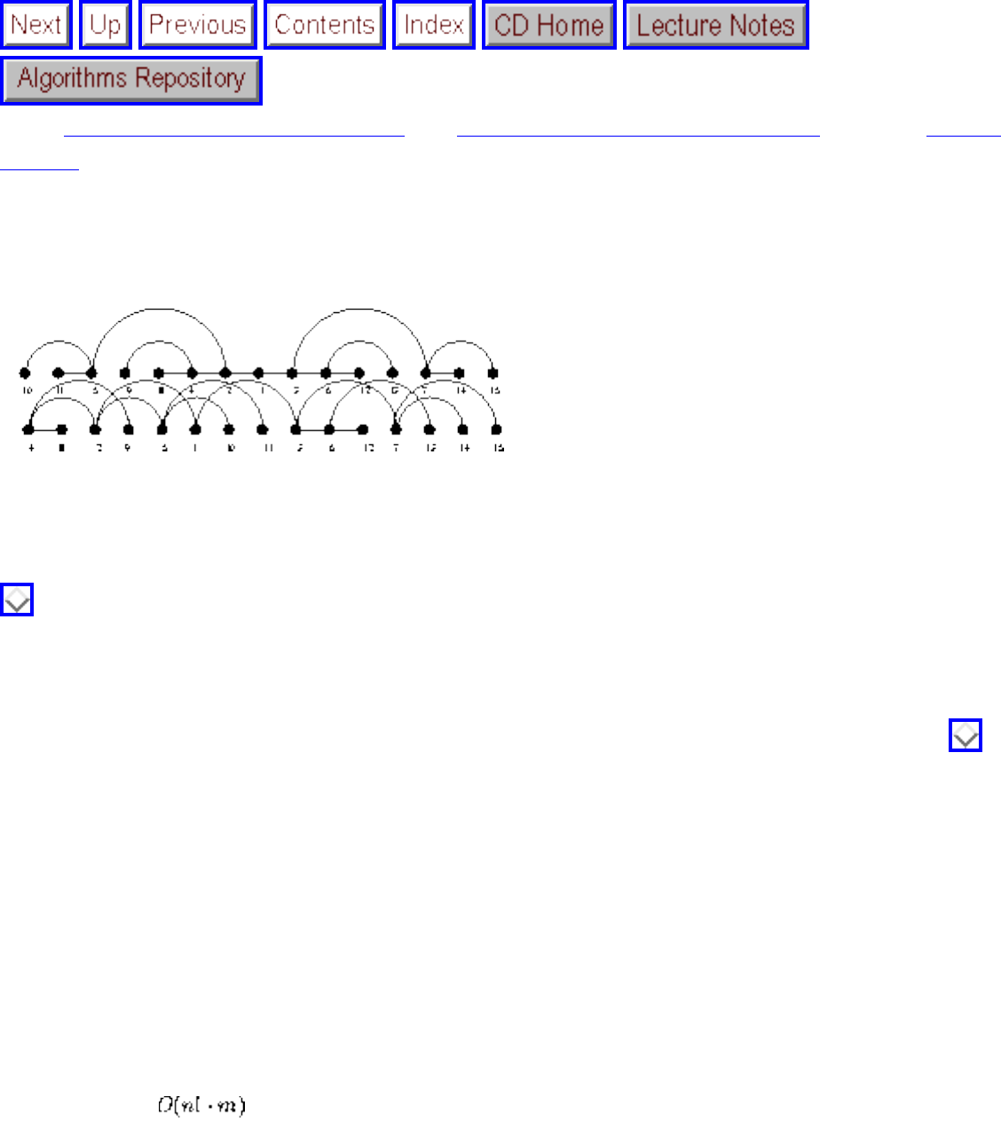
Bandwidth Minimization
Next: War Story: Covering Chessboards Up: Combinatorial Search and Heuristic Previous: Search
Pruning
Bandwidth Minimization
Figure: A pretty bandwidth-4 layout of a binary tree atop an ugly bandwidth-3 layout
To better demonstrate the power of pruning and symmetry detection, let's apply these ideas to producing
a search program that solves the bandwidth minimization problem, discussed in detail in catalog Section
. I annually run competitions for the fastest bandwidth-minimization program for students in my
algorithms courses; the timings below are drawn from these experiences.
The bandwidth problem takes as input a graph G, with n vertices and m edges. The goal is to find a
permutation of the vertices on the line that minimizes the maximum length of any edge. Figure gives
two distinct layouts of a complete binary tree on 15 vertices. The clean, neat layout on the top has a
longest edge of length 4, but the seemingly cramped layout on the bottom realizes the optimal bandwidth
of 3.
The bandwidth problem has a variety of applications, including circuit layout, linear algebra, and
optimizing memory usage in hypertext documents. The problem is NP-complete, which implies that no
polynomial time worst-case algorithm is known for the problem. It remains NP-complete even for very
restricted classes of trees.
Since the bandwidth problem seeks a particular permutation, a backtracking program that iterates through
all the n! possible permutations and computes the length of the longest edge for each gives a
straightforward algorithm. Depending upon how well it is programmed, and how fast a machine
it is running on, such an algorithm can expect to solve instances of approximately 8 to 12 vertices within
one CPU minute.
To speed up this search, we can try to exploit symmetry. For any permutation p, its reverse permutation
will realize the exact same bandwidth, since the length of each edge is the same. Hence we can
file:///E|/BOOK/BOOK2/NODE89.HTM (1 of 3) [19/1/2003 1:29:29]
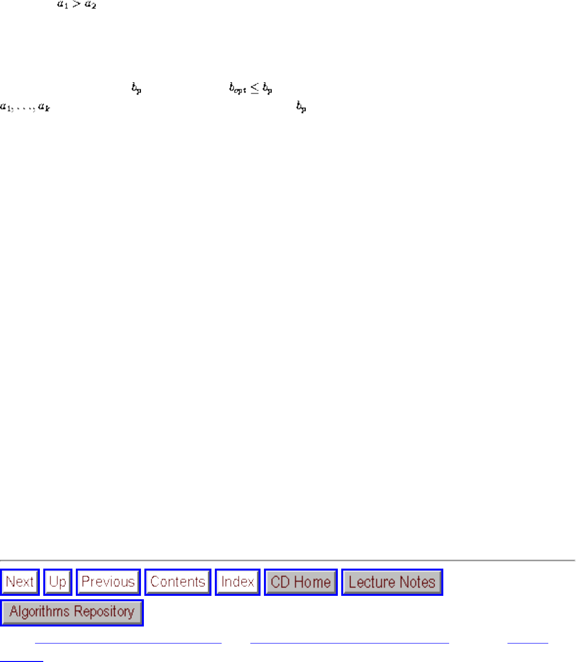
Bandwidth Minimization
immediately eliminate half of our search space. The reverse copies are easily removed by placing the
leftmost and rightmost elements of the permutation as the first two elements of the vector and then
pruning if . Because we are dealing with an exponential search, removing a single factor of two
can only be of limited usefulness. Such symmetry elimination might add one to the size of the problem
we can do within one CPU minute.
For more serious speedups, we need to prune partial solutions. Say we have found a permutation p that
yields a longest edge of . By definition, . Suppose that among the elements in a partial layout
, where k < n, there is an edge that is at least in length. Can this partial solution expand to
provide a better bandwidth solution? Of course not! By pruning the search the instant we have created a
long edge, typical instances of 15 to 20 vertices can be solved in one CPU minute, thus providing a
substantial improvement.
Efforts to further improve the search algorithm must strive for even greater pruning. By using a heuristic
method to find the best solution we can before starting to search, we save time by realizing early length
cutoffs. In fact, most of the effort in a combinatorial search is typically spent after the optimal solution is
found, in the course of proving that no better answer exists. By observing that the optimal bandwidth
solution must always be at least half the degree of any vertex (think about the incident edges), we have a
lower bound on the size of the optimal solution. We can terminate search soon as we find a solution
matching the lower bound.
One limitation of this pruning strategy is that only partial solutions of length >b can be pruned, where b
is the bandwidth of the best solution to date, since we must place b+1 vertices before we can generate
any edges of length at least b. To achieve earlier cutoffs, we can alternately fill in the leftmost and
rightmost slots of the configuration, instead of always proceeding from the left. This way, whenever
there is an edge between a vertex on the left side and a vertex on the right side, this edge is likely long
enough to achieve a cutoff. Pruning can easily occur while positioning the second vertex in the solution
vector.
Using these enhancements, top-notch programs are capable of solving typical problems on up to 30
vertices consistently within one CPU minute, operating literally millions of times faster than unpruned,
untuned efforts. The speed difference between the final and initial versions of the program dwarf the
difference between a supercomputer and a microcomputer. Clever search algorithms can easily have a
bigger impact on performance than expensive hardware.
Next: War Story: Covering Chessboards Up: Combinatorial Search and Heuristic Previous: Search
Pruning
file:///E|/BOOK/BOOK2/NODE89.HTM (2 of 3) [19/1/2003 1:29:29]
Bandwidth Minimization
Algorithms
Mon Jun 2 23:33:50 EDT 1997
file:///E|/BOOK/BOOK2/NODE89.HTM (3 of 3) [19/1/2003 1:29:29]
War Story: Covering Chessboards
Next: Heuristic Methods Up: Combinatorial Search and Heuristic Previous: Bandwidth Minimization
War Story: Covering Chessboards
Every researcher dreams of solving a classical problem, one that has remained open and unsolved for
over a hundred years. There is something romantic about communicating across the generations, being
part of the evolution of science, helping to climb another rung up the ladder of human progress. There is
also a pleasant sense of smugness that comes from figuring out how to do something that nobody else
could do before you.
There are several possible reasons why a problem might stay open for such a long period of time.
Perhaps the problem is so difficult and profound that it requires a uniquely powerful intellect to solve. A
second reason is technological - the ideas or techniques required to solve the problem may not have
existed when the problem was first posed. A final possibility is that no one may have cared enough about
the problem in the interim to seriously bother with it. Once, I was involved in solving a problem that had
been open for over a hundred years. Decide for yourself which reason best explains why.
Chess is a game that has fascinated mankind for thousands of years. In addition, it has inspired a number
of combinatorial problems of independent interest. The combinatorial explosion was first recognized in
the legend that the inventor of chess demanded as payment one grain of rice for the first square of the
board, and twice the amount of the ith square for the (i+1)st square, for a total of
36,893,488,147,419,103,231 grains. In beheading him, the wise king first established pruning as a
technique for dealing with the combinatorial explosion.
In 1849, Kling posed the question of whether all 64 squares on the board can be simultaneously
threatened by an arrangement of the eight main pieces on the chess board - the king, queen, two knights,
two rooks, and two oppositely colored bishops. Configurations that simultaneously threaten 63 squares
have been known for a long time, but whether this was the best possible remained an open problem. This
problem seemed ripe for solution by exhaustive combinatorial searching, although whether it was
solvable would depend upon the size of the search space.
Consider the 8 main pieces in chess (king, queen, two rooks, two bishops, two knights). How many ways
can they be positioned on a chessboard? The trivial bound is
positions. Anything much larger than about positions would be unreasonable to search on a modest
computer in a modest amount of time.
Getting the job done would require significant pruning. The first idea is to remove symmetries.
file:///E|/BOOK/BOOK2/NODE90.HTM (1 of 3) [19/1/2003 1:29:30]
War Story: Covering Chessboards
Considering the orthogonal and diagonal symmetries, there are only ten distinct positions for the queen.
Once the queen is placed, there are 2,080 distinct ways to position a pair of rooks or knights, 64 places to
locate the king, and 32 spots for each of the white and black bishops. Thus to perform an exhaustive
search, we must test 2,835,349,504,000 distinct positions, still much too large to try.
We could use backtracking to construct all of the positions, but we had to find a way to prune the search
space significantly if we could hope to finish in our lifetime. Pruning the search meant that we needed a
quick way to prove, for a partially filled-in position, that there was no possible way to complete it so as
to cover all 64 squares. Suppose we had already placed seven pieces on the board, and together they
covered all but 10 squares of the board. Say the remaining piece was the king. Is there any possible
position to place the king so that all squares are threatened? The answer must be no, because the king can
threaten at most eight squares according to the rules of chess. There can be no reason to bother testing
any of the subsequent positions. By pruning these positions, we might win big.
Optimizing this pruning strategy required carefully ordering the evaluation of the pieces. Each piece
could threaten a certain maximum number of squares: the queen 27, the king 8, the rook 14, and the
bishop 13. To maximize the chances of a cutoff, we would want to insert the pieces in decreasing order
of mobility. Whenever the number of unthreatened squares exceeds the sum of the maximum coverage of
the unplaced pieces, we can prune. This sum is minimized by using the decreasing order of mobility.
When we implemented backtrack search with this pruning strategy, we found that it eliminated over
of the search space. After optimizing our move generation, our program could search over 1,000
positions per second. But this was still too slow, for seconds meant 1,000 days! Although
we might further tweak the program to speed it up by an order of magnitude or so, what we really needed
was to find a way to prune more nodes.
Effective pruning meant eliminating large numbers of positions at a single stroke. Our previous attempt
was too weak. What if instead of placing up to eight pieces on the board simultaneously, we placed more
than eight pieces. Obviously, the more pieces we placed simultaneously, the less likely it would be that
they didn't threaten all 64 squares. But if they didn't cover, all subsets of eight distinct pieces from the set
couldn't possibly threaten all squares. The potential existed to eliminate a vast number of positions by
pruning a single node.
Thus the nodes of our search tree corresponded to chessboards that could have any number of pieces, and
more than one piece on a square. For a given board, we would distinguish two kinds of attack on a
square: strong and weak. The notion of strong attack corresponds to the usual notion of attack in chess. A
square is weakly attacked if the square is strongly attacked by some subset of the board, that is, weak
attack ignores any possible blocking effects of intervening pieces. All 64 squares can be weakly attacked
with eight pieces.
Our algorithm consists of two passes. The first pass lists all boards such that every square is weakly
file:///E|/BOOK/BOOK2/NODE90.HTM (2 of 3) [19/1/2003 1:29:30]
War Story: Covering Chessboards
attacked. The second pass filters the list by considering blocking and reports any boards with n or fewer
safe squares. The advantage of separating weak and strong attack computations is that weak attack is
faster to compute (no blocking to worry about), and yet the strong attack set is always a subset of the
weak attack set. Whenever there was a non-weakly-threatened square, the position could be pruned.
This program was efficient enough to complete the search on a machine as slow as a 1988-era IBM PC-
RT in under one day. More details of our searching procedure and results appear in our paper [RHS89]. It
did not find a single position covering all 64 squares with the bishops on opposite colored squares.
However, our program showed that it is possible to cover the board with seven pieces if a queen and a
knight can occupy the same square.
The take-home lesson of this war story should be clear. Clever pruning can make short work of
surprisingly hard combinatorial search problems.
Next: Heuristic Methods Up: Combinatorial Search and Heuristic Previous: Bandwidth Minimization
Algorithms
Mon Jun 2 23:33:50 EDT 1997
file:///E|/BOOK/BOOK2/NODE90.HTM (3 of 3) [19/1/2003 1:29:30]
Heuristic Methods
Next: Simulated Annealing Up: Combinatorial Search and Heuristic Previous: War Story: Covering
Chessboards
Heuristic Methods
The techniques we have discussed thus far seek to find the optimal answer to a combinatorial problem as
quickly as possible. Traditional algorithmic methods fail whenever the problem is provably hard (as
discussed in Chapter ), or the problem is not clean enough to lead to a nice formulation.
Heuristic methods provide a way to approach difficult combinatorial optimization problems.
Combinatorial search gives us a method to construct possible solutions and find the best one, given a
function that measures how good each candidate solution is. However, there may be no algorithm to find
the best solution short of searching all configurations. Heuristic methods such as simulated annealing,
genetic algorithms, and neural networks provide general ways to search for good but not optimal
solutions.
In this section we discuss such heuristic methods. Each of these three techniques relies on a simple model
of a real-world physical process. We devote the bulk of our attention to simulated annealing, which is the
easiest method to apply in practice, as well as the most reliable.
● Simulated Annealing
❍ Traveling Salesman Problem
❍ Maximum Cut
❍ Independent Set
❍ Circuit Board Placement
● Neural Networks
● Genetic Algorithms
Algorithms
file:///E|/BOOK/BOOK2/NODE91.HTM (1 of 2) [19/1/2003 1:29:30]
Heuristic Methods
Mon Jun 2 23:33:50 EDT 1997
file:///E|/BOOK/BOOK2/NODE91.HTM (2 of 2) [19/1/2003 1:29:30]
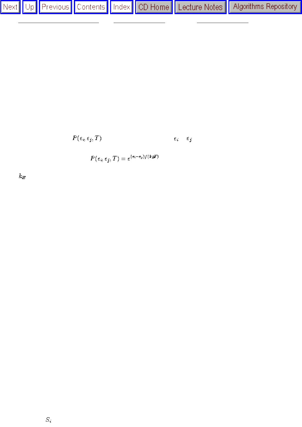
Simulated Annealing
Next: Traveling Salesman Problem Up: Heuristic Methods Previous: Heuristic Methods
Simulated Annealing
The inspiration for simulated annealing comes from the physical process of cooling molten materials down to the solid state.
When molten steel is cooled too quickly, cracks and bubbles form, marring its surface and structural integrity. To end up with
the best final product, the steel must be cooled slowly and evenly. Annealing is a metallurgical technique that uses a
disciplined cooling schedule to efficiently bring the steel to a low-energy, optimal state.
In thermodynamic theory, the energy state of a system is described by the energy state of each of the particles constituting it.
The energy state of each particle jumps about randomly, with such transitions governed by the temperature of the system. In
particular, the probability of transition from energy to at temperature T is given by
where is a constant, called Boltzmann's constant.
What does this formula mean? Consider the value of the exponent under different conditions. The probability of moving from
a high-energy state to a lower-energy state is very high. However, there is also a non-zero probability of accepting a
transition into a high-energy state, with small energy jumps much more likely than big ones. The higher the temperature, the
more likely such energy jumps will occur.
What relevance does this have for combinatorial optimization? A physical system, as it cools, seeks to go to a minimum-
energy state. For any discrete set of particles, minimizing the total energy is a combinatorial optimization problem. Through
random transitions generated according to the above probability distribution, we can simulate the physics to solve arbitrary
combinatorial optimization problems.
Simulated-Annealing()
Create initial solution S
Initialize temperature t
repeat
for i=1 to iteration-length do
Generate a random transition
from S to
file:///E|/BOOK/BOOK2/NODE92.HTM (1 of 3) [19/1/2003 1:29:34]
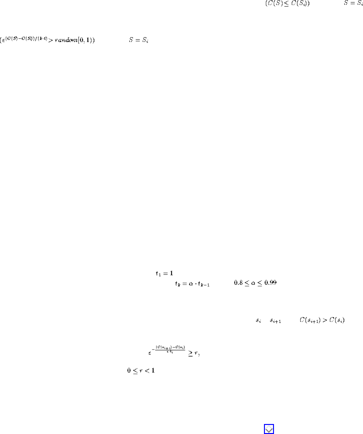
Simulated Annealing
If then
else if
then
Reduce temperature t
until (no change in C(S))
Return S
There are three components to any simulated annealing algorithm for combinatorial search:
● Concise problem representation - The problem representation includes both a representation of the solution space and
an appropriate and easily computable cost function C() measuring the quality of a given solution.
● Transition mechanism between solutions - To move from one state to the next, we need a collection of simple
transition mechanisms that slightly modify the current solution. Typical transition mechanisms include swapping the
position of a pair of items or inserting/deleting a single item. Ideally, the effect that these incremental changes have on
measuring the quality of the solution can be computed incrementally, so cost function evaluation takes time
proportional to the size of the change (typically constant) instead of linear in the size of the solution.
● Cooling schedule - These parameters govern how likely we are to accept a bad transition as a function of time. At the
beginning of the search, we are eager to use randomness to explore the search space widely, so the probability of
accepting a negative transition is high. As the search progresses, we seek to limit transitions to local improvements
and optimizations. The cooling schedule can be regulated by the following parameters:
❍ Initial system temperature - Typically .
❍ Temperature decrement function - Typically , where . This implies an exponential
decay in the temperature, as opposed to a linear decay.
❍ Number of iterations between temperature change - Typically, 100 to 1,000 iterations might be permitted
before lowering the temperature.
❍ Acceptance criteria - A typical criterion is to accept any transition from to when and to
accept a negative transition whenever
where r is a random number . The constant c normalizes this cost function, so that almost all
transitions are accepted at the starting temperature.
❍ Stop criteria - Typically, when the value of the current solution has not changed or improved within the last
iteration or so, the search is terminated and the current solution reported.
Creating the proper cooling schedule is somewhat of a trial and error process. It might pay to start from an existing
implementation of simulated annealing, pointers to which are provided in Section .
file:///E|/BOOK/BOOK2/NODE92.HTM (2 of 3) [19/1/2003 1:29:34]

Simulated Annealing
We provide several examples below to demonstrate how these components can lead to elegant simulated annealing
algorithms for real combinatorial search problems.
● Traveling Salesman Problem
● Maximum Cut
● Independent Set
● Circuit Board Placement
Next: Traveling Salesman Problem Up: Heuristic Methods Previous: Heuristic Methods
Algorithms
Mon Jun 2 23:33:50 EDT 1997
file:///E|/BOOK/BOOK2/NODE92.HTM (3 of 3) [19/1/2003 1:29:34]
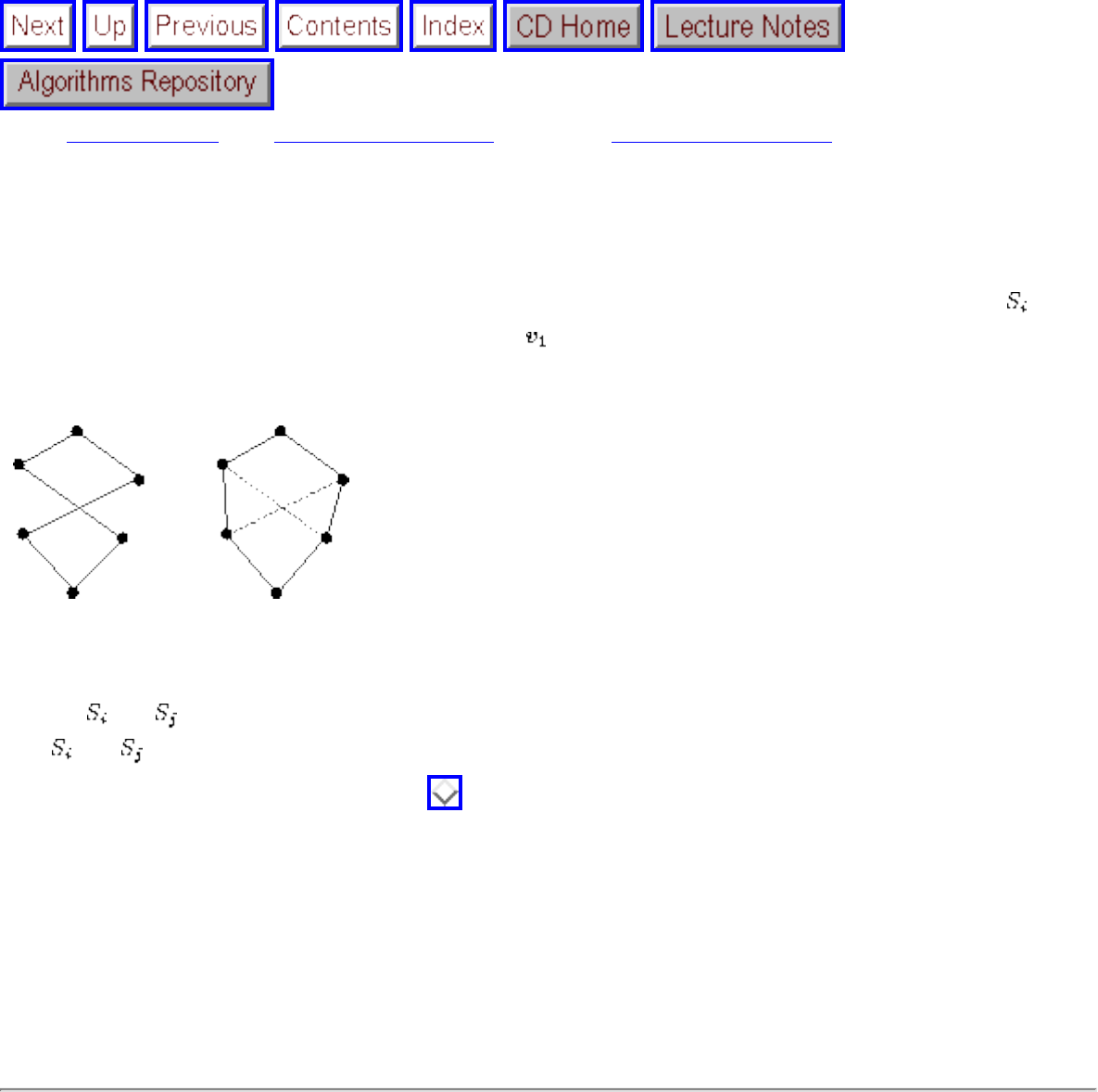
Traveling Salesman Problem
Next: Maximum Cut Up: Simulated Annealing Previous: Simulated Annealing
Traveling Salesman Problem
The solution space for traveling salesman consists of the set of all (n-1)! possible circular permutations of
the vertices. A candidate solution can thus be represented using an array S of n-1 vertices, where
defines the (i+1)st vertex on the tour starting from . The cost function evaluating a candidate solution
is equally straightforward, for we can sum up the costs of the edges defined by S.
Figure: Improving a TSP tour by swapping a pair of edges
The most obvious transition mechanism would be to swap the current tour positions of a random pair of
vertices and . This changes up to eight edges on the tour, deleting the edges currently adjacent to
both and , and adding their replacements. Better would be to swap two edges on the tour with two
others that replace it, as shown in Figure . Since only four edges change in the tour, the transitions can
be performed and evaluated faster. Faster transitions mean that we can evaluate more positions in the
given amount of time.
In practice, problem-specific heuristics for TSP outperform simulated annealing, but the simulated
annealing solution works admirably, considering it uses very little knowledge about the problem.
Algorithms
Mon Jun 2 23:33:50 EDT 1997
file:///E|/BOOK/BOOK3/NODE93.HTM [19/1/2003 1:29:34]
Maximum Cut
Next: Independent Set Up: Simulated Annealing Previous: Traveling Salesman Problem
Maximum Cut
For a weighted graph G, the maximum cut problem seeks to partition the vertices into sets and so as
to maximize the weight (or number) of edges with one vertex in each set. When the graph specifies an
electronic circuit, the maximum cut in the graph defines the largest amount of data communication that
can take place in the circuit simultaneously. As discussed in catalog Section , maximum cut is an NP-
complete version of graph partitioning.
How can we formulate maximum cut for simulated annealing? The solution space consists of all
possible vertex partitions; we save a factor of two over all vertex subsets because we can assume that
vertex is fixed to be on the left side of the partition. The subset of vertices accompanying it can be
represented using a bit vector. The cost of a solution will be the sum of the weights cut in the current
configuration. A natural transition mechanism is to select one vertex at random and move it across the
partition by simply flipping the corresponding bit in the bit vector. The change in the cost function will
be the weight of its old neighbors minus the weight of its new neighbors, so it can be computed in time
proportional to the degree of the vertex.
This kind of simple, natural modeling is the right type of heuristic to seek in practice.
Algorithms
Mon Jun 2 23:33:50 EDT 1997
file:///E|/BOOK/BOOK3/NODE94.HTM [19/1/2003 1:29:35]
Independent Set
Next: Circuit Board Placement Up: Simulated Annealing Previous: Maximum Cut
Independent Set
An independent set of a graph G is a subset of vertices S such that there is no edge with both endpoints in
S. The maximum independent set of a graph is the largest such empty induced subgraph. The need to find
large independent sets arises in dispersion problems associated with facility location and coding theory,
as discussed in catalog Section .
The natural state space for a simulated annealing solution would be all subsets of the vertices,
represented as a bit vector. As with maximum cut above, a simple transition mechanism would be to add
or delete one vertex from S.
One natural cost function for subset S might be 0 if S contains an edge, and |S| if it is indeed an
independent set. This function ensures that we work towards an independent set at all times. However,
this condition is strict enough that we are liable to move only in a narrow portion of the possible search
space. More flexibility in the search space and quicker cost function computations can result from
allowing non-empty graphs at the early stages of cooling. Better in practice would be a cost function like
, where is a constant, T is the temperature, and is the number of edges in the
subgraph induced by S. The dependence of C(S) on T ensures that the search will drive the edges out
faster as the system cools.
Algorithms
Mon Jun 2 23:33:50 EDT 1997
file:///E|/BOOK/BOOK3/NODE95.HTM [19/1/2003 1:29:36]
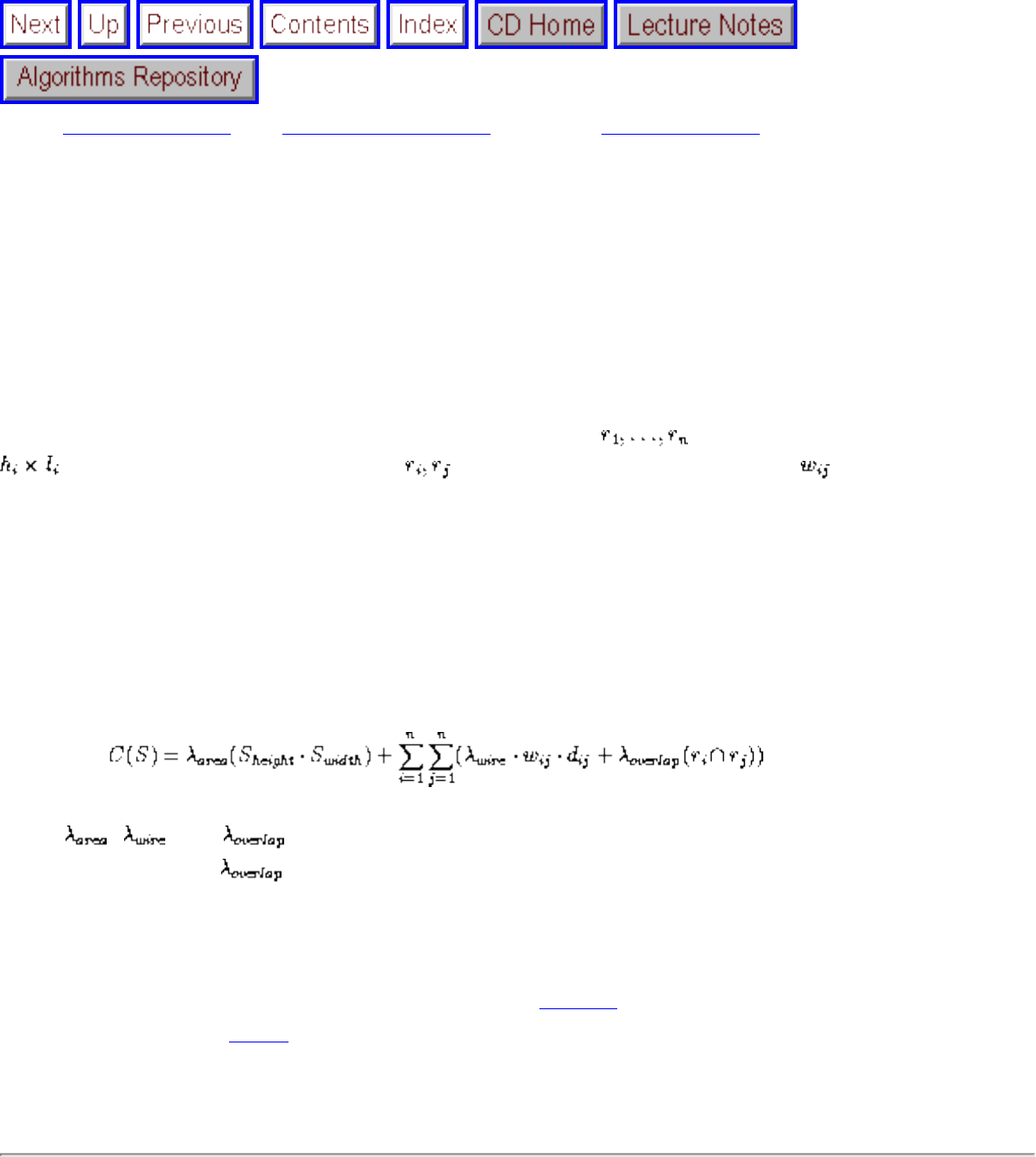
Circuit Board Placement
Next: Neural Networks Up: Simulated Annealing Previous: Independent Set
Circuit Board Placement
In designing printed circuit boards, we are faced with the problem of positioning modules (typically
integrated circuits) on the board. Desired criteria in a layout include (1) minimizing the area or aspect
ratio of the board, so that it properly fits within the allotted space, and (2) minimizing the total or longest
wire length in connecting the components. Circuit board placement is an example of the kind of messy,
multicriterion optimization problems for which simulated annealing is ideally suited.
Formally, we are given a collection of a rectangular modules , each with associated dimensions
. Further, for each pair of modules , we are given the number of wires that must connect
the two modules. We seek a placement of the rectangles that minimizes area and wire-length, subject to
the constraint that no two rectangles overlap each other.
The state space for this problem must describe the positions of each rectangle. To provide a discrete
representation, the rectangles can be restricted to lie on vertices of an integer grid. Reasonable transition
mechanisms including moving one rectangle to a different location, or swapping the position of two
rectangles. A natural cost function would be
where , , and are constants governing the impact of these components on the cost
function. Presumably, should be an inverse function of temperature, so after gross placement it
adjusts the rectangle positions so they are distinct.
Simulated annealing performs well on such module placement problems. Indeed, a similar application
appeared in the original paper on simulated annealing [KGV83]. More details on these and other
applications appear in [AK89].
Algorithms
Mon Jun 2 23:33:50 EDT 1997
file:///E|/BOOK/BOOK3/NODE96.HTM [19/1/2003 1:29:37]

Neural Networks
Next: Genetic Algorithms Up: Heuristic Methods Previous: Circuit Board Placement
Neural Networks
Neural networks are a computational paradigm inspired by the architecture of the human brain. The
intuition is that since brains are good at solving problems, machines built in the same way should be, too.
The basic computational component of the brain is a neuron, a simple unit that produces a non-linear,
weighted sum of its inputs, which are connections from other neurons. Neural networks are weighted
digraphs with neurons as vertices and weights on edges denoting the connection strength of the pair.
Brains are very good at learning and recognizing certain patterns. Learning in brains seems to work by
adding connections between different pairs of neurons and changing the strengths of the connections.
Modifying connection strength in response to training examples provides a natural way to ``teach'' a
neural network.
Although there have been attempts to apply neural networks to solving combinatorial optimization
problems, the successes have been rather limited. Simulated annealing is a much more straightforward
and efficient approach to optimization.
Neural networks have been more successful in classification and forecasting applications, such as optical
character recognition, gene prediction, and stock-market time-series prediction. A set of features for the
given patterns is selected, and each training example is represented in terms of its features. The network
is trained on a series of positive and negative examples, with the strengths of the connections adjusted to
recognize these examples. Output cells for each class of item are provided and the strength of these cells
on a given input used to determine the classification. Once the network is trained, feature vectors
corresponding to unknown items can be entered and a classification made.
Because neural networks are black boxes, with the strength of edges adjusted only by the training
examples, there is usually no way to figure out exactly why they are making the decisions that they are.
A particularly amusing instance where this led to trouble is reported in Section . Still, they can be
useful in certain pattern-recognition applications.
file:///E|/BOOK/BOOK3/NODE97.HTM (1 of 2) [19/1/2003 1:29:37]

Genetic Algorithms
Next: War Story: Annealing Arrays Up: Heuristic Methods Previous: Neural Networks
Genetic Algorithms
Genetic algorithms draw their inspiration from evolution and natural selection. Through the process of
natural selection, organisms adapt to optimize their chances for survival in a given environment. Random
mutations occur to the genetic description of an organism, which is then passed on to its children. Should
a mutation prove helpful, these children are more likely to survive to reproduce. Should it be harmful,
these children are less likely to reproduce, so the bad trait will die with them.
Genetic algorithms maintain a ``population'' of solution candidates for the given problem. Elements are
drawn at random from this population and allowed to ``reproduce'', by combining some aspects of the
two parent solutions. The probability that an element is chosen to reproduce is based on its ``fitness'',
essentially a function of the cost of the solution it represents. Eventually, unfit elements die from the
population, to be replaced by successful-solution offspring.
The idea behind genetic algorithms is extremely appealing. However, they just don't seem to work as
well on practical combinatorial optimization problems as simulated annealing does. There are two
primary reasons for this. First, it is quite unnatural to model most applications in terms of genetic
operators like mutation and crossover on bit strings. The pseudobiology adds another level of complexity
between you and your problem. Second, genetic algorithms take a very long time on non-trivial
problems. The crossover and mutation operations make no real use of problem-specific structure, so a
large fraction of transitions lead to inferior solutions, and convergence is slow. Indeed, the analogy with
evolution, where significant improvements require millions of years, can be quite appropriate.
We will not discuss genetic algorithms further, in order to discourage you from considering them for
your applications. However, pointers to implementations of genetic algorithms are provided in Section
if you really insist on playing with them.
Next: War Story: Annealing Arrays Up: Heuristic Methods Previous: Neural Networks
file:///E|/BOOK/BOOK3/NODE98.HTM (1 of 2) [19/1/2003 1:29:38]
Genetic Algorithms
Algorithms
Mon Jun 2 23:33:50 EDT 1997
file:///E|/BOOK/BOOK3/NODE98.HTM (2 of 2) [19/1/2003 1:29:38]
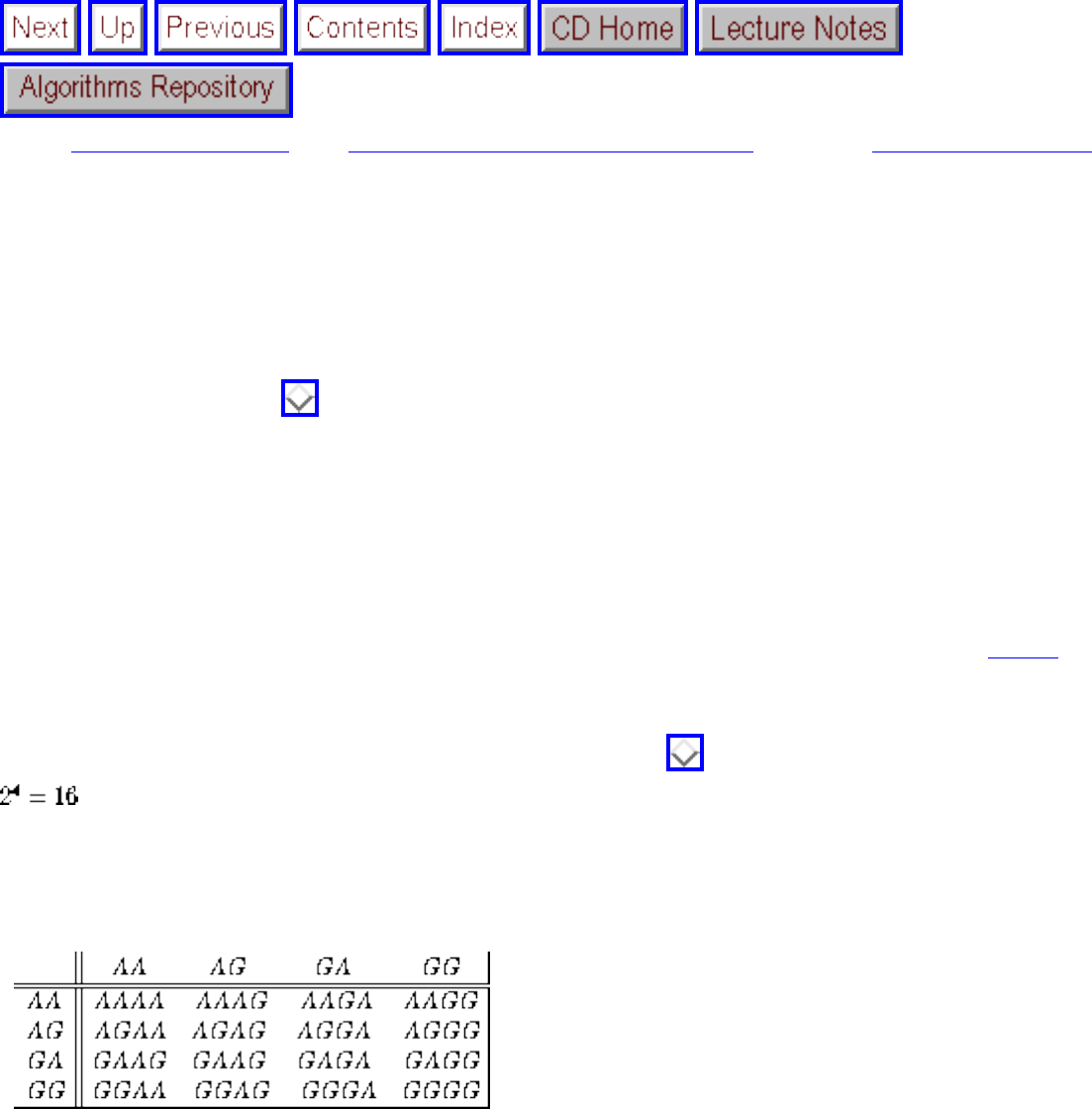
War Story: Annealing Arrays
Next: Parallel Algorithms Up: Combinatorial Search and Heuristic Previous: Genetic Algorithms
War Story: Annealing Arrays
The war story of Section reported how we used advanced data structures to simulate a new method
for sequencing DNA. Our method, interactive sequencing by hybridization (SBH), involved building
arrays of specific oligonucleotides on demand. Although the simulation results were very promising to
us, most biologists we encountered were suspicious. They needed to see our technique proven in the lab
before they would take it seriously.
But we got lucky. A biochemist at Oxford University, got interested in our technique, and moreover he
had in his laboratory the equipment we needed to test it out. The Southern Array Maker [Sou96],
manufactured by Beckman Instruments, could prepare discrete oligonucleotide sequences in 64 parallel
rows across a polypropylene substrate. The device constructs arrays by appending single characters to
each cell along specific rows and columns of arrays. Figure shows how to construct an array of all
purine (A or G) 4-mers by building the prefixes along rows and the suffixes along columns. This
technology provided an ideal environment for testing the feasibility of interactive SBH in a laboratory,
because with proper programming it gave an inexpensive way to fabricate a wide variety of
oligonucleotide arrays on demand.
Figure: A prefix-suffix array of all purine 4-mers.
But we had to provide the proper programming. Fabricating complicated arrays requires solving a
difficult combinatorial problem. We were given as input a set S of n strings (representing
oligonucleotides) to fabricate an array (where m=64 on the Southern apparatus). We had to produce a
schedule of row and column commands to realize the set of strings S. We proved that the problem of
designing dense arrays was NP-complete, but that didn't really matter. My student Ricky Bradley and I
had to solve it anyway.
file:///E|/BOOK/BOOK3/NODE99.HTM (1 of 4) [19/1/2003 1:29:40]
War Story: Annealing Arrays
``If it's hard, it's hard. We are going to have to use a heuristic,'' I told him. ``So how do we model this
problem?''
``Well, for each string we can identify the possible prefix and suffix pairs that will realize it. For
example, the string `ACC' can be realized in four different ways: prefix `' and suffix `ACC', prefix `A'
and suffix `CC', prefix `AC' and suffix `C', or prefix `ACC' and suffix `'. We seek the smallest set of
prefixes and suffixes that together realize all the given strings,'' Ricky said.
``Good. This gives us a natural representation for simulated annealing. The state space will consist of all
possible subsets of prefixes and suffixes. The natural transitions between states might include inserting or
deleting strings from our subsets, or swapping a pair in or out.''
``What's a good cost function?'' he asked.
``Well, we need as small an array as possible that covers all the strings. How about something like the
maximum of number of rows (prefixes) or columns (suffixes) used in our array, plus the number of
strings from S that are not yet covered. Try it and let's see what happens.''
Ricky went off and implemented a simulated annealing program along these lines. Printing out the state
of the solution each time a transition was accepted, it was fun to watch. Starting from a random solution,
the program quickly kicked out unnecessary prefixes and suffixes, and the array began shrinking rapidly
in size. But after several hundred iterations, progress started to slow. A transition would knock out an
unnecessary suffix, wait a while, then add a different suffix back again. After a few thousand iterations,
no real improvement was happening.
``The program doesn't seem to recognize when it is making progress. The evaluation function only gives
credit for minimizing the larger of the two dimensions. Why not add a term to give some credit to the
other dimension.''
Ricky changed the evaluation function, and we tried again. This time, the program did not hesitate to
improve the shorter dimension. Indeed, our arrays started to be skinny rectangles instead of squares.
``OK. Let's add another term to the evaluation function to give it points for being roughly square.''
Ricky tried again. Now the arrays were the right shape, and progress was in the right direction. But the
progress was slow.
``Too many of the prefix/suffix insertion moves don't really seem to affect many strings. Maybe we
should skew the random selections so that the important prefix/suffixes get picked more often.''
Ricky tried again, Now it converged faster, but sometimes it still got stuck. We changed the cooling
schedule. It did better, but was it doing well? Without a lower bound knowing how close we were to
file:///E|/BOOK/BOOK3/NODE99.HTM (2 of 4) [19/1/2003 1:29:40]
War Story: Annealing Arrays
optimal, it couldn't really tell how good our solution was. We tweaked and tweaked until our program
stopped improving.
Our final solution refined the initial array by applying the following random moves:
● swap - swap a prefix/suffix on the array with one that isn't.
● add - add a random prefix/suffix to the array.
● delete - delete a random prefix/suffix from the array.
● useful add - add the prefix/suffix with the highest usefulness to the array.
● useful delete - delete the prefix/suffix with the lowest usefulness from the array.
● string add - randomly select a string not on the array, and add the most useful prefix and/or suffix
that covers this string (additional preference is given to a prefix/suffix whose corresponding
suffix/prefix is already on the array).
A standard annealing schedule was used, with an exponentially decreasing temperature (dependent upon
the problem size) and a temperature-dependent Boltzmann criterion for accepting states that have higher
costs. Our final cost function was defined as
where max is the size of the maximum chip dimension, min is the size of the minimum chip dimension, ,
and is the number of strings in S currently on the chip.
Careful analysis of successful moves over the course of the annealing process suggested a second phase
of annealing to speed convergence. Once the temperature reaches a predetermined cutoff point, the
temperature schedule was changed to force the temperature to decrease more rapidly, and the probability
distribution for choosing moves was altered to include only swap, add, and delete, with preference given
to swap moves. This modification sped up late convergence, which had been slower than it was in the
early stages of the annealing process.
file:///E|/BOOK/BOOK3/NODE99.HTM (3 of 4) [19/1/2003 1:29:40]
War Story: Annealing Arrays
Figure: Compression of the HIV array by simulated annealing - after 0, 500, 1,000, and 5,750 iterations
How well did we do? As reported in our paper [BS97], Figure shows the convergence of a custom
array consisting of the 5,716 unique 7-mers of the HIV-virus. Figure shows snapshots of the state of
the chip at four points during the annealing process (0, 500, 1,000, and the final chip at 5,750 iterations).
Black pixels represent the first occurrence of an HIV 7-mer, while white pixels represent either
duplicated HIV 7-mers or strings not in the HIV input set. The final chip size here is , quite an
improvement over the initial size of . It took about fifteen minutes' worth of computation on a
desktop workstation to complete the optimization, which was perfectly acceptable for the application.
But how well did we do? Since simulated annealing is only a heuristic, we really don't know how close
to optimal our solution is. I think we did pretty well, but I can't really be sure. In conclusion, simulated
annealing can be the right way to handle complex optimization problems. However, to get the best
results, expect to spend more time tweaking and refining your program than you did in writing it in the
first place. This is dirty work, but sometimes you have to do it.
Next: Parallel Algorithms Up: Combinatorial Search and Heuristic Previous: Genetic Algorithms
Algorithms
Mon Jun 2 23:33:50 EDT 1997
file:///E|/BOOK/BOOK3/NODE99.HTM (4 of 4) [19/1/2003 1:29:40]

Parallel Algorithms
Next: War Story: Going Nowhere Up: Combinatorial Search and Heuristic Previous: War Story:
Annealing Arrays
Parallel Algorithms
Two heads are better than one, and more generally, n heads are better than n-1. In our era of computing
plenty, parallel processing seems like an exciting technique for solving combinatorial optimization
problems. Today many facilities contain networks of workstations, most of them idle at night and
underutilized during the day. Why not put them to work?
Parallelism seems like the easy way out of hard problems. Indeed, sometimes, for some problems,
parallel algorithms are the most effective solution. High-resolution, real-time graphics applications must
render thirty frames per second for realistic animation. Assigning each frame to a distinct processor, or
dividing each image into regions assigned to different processors might be the only way to get the job
done in time. Large systems of linear equations for scientific applications are routinely solved in parallel.
However, there are several pitfalls associated with parallel algorithms that one should be aware of:
● There is often a small upper bound on the potential win - Suppose that you have access to twenty
workstations that can be devoted exclusively to your job. Potentially, these could be used to speed
up the fastest sequential program by up to a factor of twenty. That is nice, but much greater
performance gains are potentially possible by finding a better sequential algorithm and
implementing that. Your time spent parallelizing a code might well be better spent enhancing the
sequential version. Performance-tuning tools such as profilers are better developed for sequential
machines than for parallel models.
● Speedup means nothing - Suppose my parallel program runs 16 times faster on a 16-processor
machine then it does on one processor. That's great, isn't it? If you always get linear speedup and
have an arbitrary number of processors, you will eventually beat any sequential algorithm.
However, a carefully designed sequential algorithm can often beat an easily parallelized code
running on a typical parallel machine. The one-processor parallel version of your algorithm is
likely to be a crummy sequential algorithm, so measuring speedup typically provides an unfair
test of the benefits of parallelism.
The classic example of this occurs in the minimax game-tree search algorithms used in computer
chess programs. Brute-force tree search is embarrassingly easy to parallelize; just put each subtree
on a different processor. However, a lot of work gets wasted because the same positions get
considered on different machines. Moving from brute-force search to the more clever alpha-beta
file:///E|/BOOK/BOOK/NODE100.HTM (1 of 2) [19/1/2003 1:29:41]

Parallel Algorithms
pruning algorithm can easily save over 99.99% of the work, thus dwarfing any benefits of parallel
brute-force search. Alpha-beta can be parallelized, but not easily, and speedups are typically
limited to a factor of six or so regardless of how many processors you have.
● Parallel algorithms are tough to debug - Unless your problem can be decomposed into several
independent jobs, the different processors will have to communicate with each other in order to
end up with the correct final result. Unfortunately, the non-deterministic nature of this
communication makes parallel programs notoriously difficult to debug. Perhaps the best example
is Deep Blue, the world-champion chess computer. Although it beat Kasparov, over the years it
has lost several games in embarrassing fashion due to bugs, mostly associated with its extensive
parallelism.
I recommend considering parallel processing only after repeated attempts at solving the problem
sequentially prove too slow. Even then, I would restrict attention to algorithms that parallelize the
problem by partitioning the input into distinct tasks, where no communication is needed between the
processors, except in collecting the final results. Such large-grain, naive parallelism can be simple
enough to be readily implementable and debuggable, because it really reduces to producing a good
sequential implementation. Still, there can be pitfalls in this approach, as discussed in the war story
below.
Next: War Story: Going Nowhere Up: Combinatorial Search and Heuristic Previous: War Story:
Annealing Arrays
Algorithms
Mon Jun 2 23:33:50 EDT 1997
file:///E|/BOOK/BOOK/NODE100.HTM (2 of 2) [19/1/2003 1:29:41]
War Story: Going Nowhere Fast
Next: Exercises Up: Combinatorial Search and Heuristic Previous: Parallel Algorithms
War Story: Going Nowhere Fast
In Section , I related our efforts to build a fast program to test Waring's conjecture for pyramidal
numbers. At that point, my code was fast enough that it could complete the job in a few weeks running in
the background on a desktop workstation. This option did not appeal to my supercomputing colleague,
however.
``Why don't we do it in parallel?'' he suggested. ``After all, you have an outer loop doing the same type
of calculation on each integer from 1 to 1,000,000,000. I can split this range of numbers into different
intervals and run each one of these on a different processor. Watch, it will be easy.''
He set to work trying to do our computations on an Intel IPSC-860 hypercube using 32 nodes, with 16
megabytes of memory per node. However, instead of getting answers, over the next few weeks I was
treated to a regular stream of e-mail about system reliability:
● ``Our code is running fine, except one processor died last night. I will rerun.''
● ``This time the machine was rebooted by accident, so our long-standing job was killed.''
● ``We have another problem. The policy on using our machine is that nobody can command the
entire machine for more than thirteen hours, under any condition.''
Still, eventually, he rose to the challenge. Waiting until the machine was stable, he locked out 16
processors (half the computer), divided the integers from 1 to 1,000,000,000 into 16 equal-sized
intervals, and ran each interval on its own processor. He spent the next day fending off angry users who
couldn't get their work done because of our rogue job. The instant the first processor completed
analyzing the numbers from 1 to 62,500,000, he announced to all the people yelling at him that the other
processors would soon follow.
But they didn't. He failed to realize that the time to test each integer increased as the numbers got larger.
After all, it would take longer to test whether 1,000,000,000 could be expressed as the sum of three
pyramidal number than it would for 100. Thus at slower and slower intervals, each new processor would
announce its completion. Because of the architecture of the hypercube, he couldn't return any of the
processors until our entire job was completed. Eventually, half the machine and most of its users were
held hostage by one, final interval.
file:///E|/BOOK/BOOK3/NODE101.HTM (1 of 2) [19/1/2003 1:29:41]
War Story: Going Nowhere Fast
When the job finally completed, the numbers were passed on to the Nobel Prize winner who had
requested them. It turns out he had been curious about the problem because his father had made the
conjecture back in 1928. There had never been a more important scientific reason to justify the
computation in the first place. Indeed, no results from the computation ever appeared in print.
What conclusions can be drawn from this? Before devoting heroic efforts to solve a problem efficiently,
make sure that it really needs to be solved, and solved quickly. If you are going to parallelize a problem,
be sure to balance the load carefully among the processors. Proper load balancing, using either back-of-
the-envelope calculations or the partition algorithm of Section , would have significantly reduced the
time we needed the machine, and his exposure to the wrath of his colleagues.
Next: Exercises Up: Combinatorial Search and Heuristic Previous: Parallel Algorithms
Algorithms
Mon Jun 2 23:33:50 EDT 1997
file:///E|/BOOK/BOOK3/NODE101.HTM (2 of 2) [19/1/2003 1:29:41]

Exercises
Next: Implementation Challenges Up: Combinatorial Search and Heuristic Previous: War Story: Going
Nowhere
Exercises
1. (*) A derangement is a permutation p of such that no item is in its proper position, i.e.
for all . Write an efficient backtracking program with pruning that constructs all
the derangements of n items.
2. (*) Multisets are allowed to have repeated elements. A multiset of n items may thus have fewer
than n! distinct permutations. For example, has only six different permutations:
, , , , , and . Design and implement an
efficient algorithm for constructing all permutations of a multiset.
3. (*) Design and implement an algorithm for testing whether two graphs are isomorphic to each
other. The graph isomorphism problem is discussed in Section . With proper pruning, graphs
on hundreds of vertices can be tested reliably.
4. (**) Design and implement an algorithm for solving the subgraph isomorphism problem. Given
graphs G and H, does there exist a subgraph H' of H such that G is isomorphic to H'. How does
your program perform on such special cases of subgraph isomorphism as Hamiltonian cycle,
clique, independent set, and graph isomorphism.
5. (*) Design and implement an algorithm for solving the set cover problem, discussed in Section
. Use it to solve special-case vertex cover problems as well as general set cover problems.
6. (**) In the turnpike reconstruction problem, you are given n(n-1)/2 distances in sorted order. The
problem is to find the positions of the points on the line that give rise to these distances. For
example, the distances can be determined by placing the second point 1 unit from
the first, the third point 3 from the second, and the fourth point 2 from the third. Design and
implement an efficient algorithm to report all solutions to the turnpike reconstruction problem.
Exploit additive constraints when possible to minimize search. With proper pruning, problems
with hundreds of points can be solved reliably.
file:///E|/BOOK/BOOK3/NODE102.HTM (1 of 2) [19/1/2003 1:29:42]


Problems and Reductions
Next: Simple Reductions Up: Intractable Problems and Approximations Previous: Intractable Problems and
Approximations
Problems and Reductions
Throughout this book we have encountered problems, such as the traveling salesman problem, for which we couldn't find
any efficient algorithm. By the early 1970s, literally hundreds of problems were stuck in this swamp. The theory of NP-
completeness provided the tools needed to show that all of these problems were really the same thing.
The key idea behind demonstrating the hardness of a problem is that of a reduction. Suppose that I gave you the following
algorithm to solve the Bandersnatch problem:
Bandersnatch(G)
Translate the input G to an instance of the Bo-billy problem Y.
Call the subroutine Bo-billy on Y to solve this instance.
Return the answer of Bo-billy(Y) as the answer to Bandersnatch(G).
It is important to see that this algorithm correctly solves the Bandersnatch problem provided that the translation to Bo-billy
always preserves the correctness of the answer. In other words, the translation has the property that for any instance of G,
Bandersnatch(G) = Bo-billy(Y). A translation of instances from one type of problem to instances of another type such that
the answers are preserved is called a reduction.
Now suppose this reduction translates G to Y in O(P(n)) time. There are two possible implications:
● If my Bo-billy subroutine ran in O(P'(n)), this means I could solve the Bandersnatch problem in O(P(n)+P'(n)) by
spending the time to translate the problem and then the time to execute the Bo-Billy subroutine.
● If I know that is a lower bound on computing Bandersnatch, meaning there definitely exists no faster way to
solve it, then must be a lower bound to compute Bo-billy. Why? If I could solve Bo-billy any faster,
then I could solve Bandersnatch in faster time by using the above simulation, thus violating my lower bound. This
implies that there can be no way to solve Bo-billy any faster than claimed.
This second argument is the approach that we will use to prove problems hard. Essentially, this reduction shows that Bo-
billy is at least as hard as Bandersnatch, and therefore once we believe that Bandersnatch is hard, we have a tool for proving
other problems hard.
Reductions, then, are operations that convert one problem into another. To describe them, we must be somewhat rigorous in
our definition of a problem. A problem is a general question, with parameters for the input and conditions on what
constitutes a satisfactory answer or solution. An instance is a problem with the input parameters specified. The difference
file:///E|/BOOK/BOOK3/NODE105.HTM (1 of 2) [19/1/2003 1:29:43]
Problems and Reductions
can be made clear by an example. The traveling salesman problem is defined thus:
Input: A weighted graph G.
Output: Which tour minimizes ?
Thus any weighted graph defines an instance of TSP. Each particular instance has at least one minimum cost tour. The
general traveling salesman problem asks for an algorithm to find the optimal tour for all possible instances.
Any problem with answers restricted to yes and no is called a decision problem. Most interesting optimization problems can
be phrased as decision problems that capture the essence of the computation. For example, the traveling salesman decision
problem can be defined thus:
Input: A weighted graph G and integer k.
Output: Does there exist a TSP tour with cost ? It should be clear that the decision version captures the heart of the
traveling salesman problem, for if you had a program that gave fast solutions to the decision problem, you could do a binary
search with different values of k to quickly hone in on the correct solution.
Therefore, from now on we will talk only about decision problems, because it is easier to reduce one problem to another
when the only possible answers to both are true or false.
Next: Simple Reductions Up: Intractable Problems and Approximations Previous: Intractable Problems and
Approximations
Algorithms
Mon Jun 2 23:33:50 EDT 1997
file:///E|/BOOK/BOOK3/NODE105.HTM (2 of 2) [19/1/2003 1:29:44]

Simple Reductions
Next: Hamiltonian Cycles Up: Intractable Problems and Approximations Previous: Problems and
Reductions
Simple Reductions
Since they can be used either to prove hardness or to give efficient algorithms, reductions are powerful
tools for the algorithm designer to be familiar with. The best way to understand reductions is to look at
some simple ones.
● Hamiltonian Cycles
● Independent Set and Vertex Cover
● Clique and Independent Set
Algorithms
Mon Jun 2 23:33:50 EDT 1997
file:///E|/BOOK/BOOK3/NODE106.HTM [19/1/2003 1:29:44]
Hamiltonian Cycles
Next: Independent Set and Vertex Up: Simple Reductions Previous: Simple Reductions
Hamiltonian Cycles
The Hamiltonian cycle problem is one of the most famous in graph theory. It seeks a tour that visits each vertex of a given
graph exactly once. It has a long history and many applications, as discussed in Section . Formally, it is defined:
Input: An unweighted graph G.
Output: Does there exist a simple tour that visits each vertex of G without repetition? Hamiltonian cycle has some obvious
similarity to the traveling salesman problem. Both problems ask for a tour to visit each vertex exactly once. There are also
differences between the two problems. TSP works on weighted graphs, while Hamiltonian cycle works on unweighted
graphs. The following reduction from Hamiltonian cycle to traveling salesman shows that the similarities are greater than
the differences:
HamiltonianCycle(G=(V,E))
Construct a complete weighted graph G'=(V',E') where V'=V.
n = |V|
for i = 1 to n do
for j = 1 to n do
if then w(i,j) = 1
else w(i,j) = 2
Return the answer to Traveling-Salesman(G',n).
The actual reduction is quite simple, with the translation from unweighted to weighted graph easily performed in linear
time. Further, this translation is designed to ensure that the answers of the two problems will be identical. If the graph G
has a Hamiltonian cycle , then this exact same tour will correspond to n edges in E', each with weight 1.
Therefore, this gives a TSP tour of G' of weight exactly n. If G does not have a Hamiltonian cycle, then there can be no
such TSP tour in G', because the only way to get a tour of cost n in G would be to use only edges of weight 1, which
implies a Hamiltonian cycle in G.
This reduction is both efficient and truth preserving. A fast algorithm for TSP would imply a fast algorithm for Hamiltonian
cycle, while a hardness proof for Hamiltonian cycle would imply that TSP is hard. Since the latter is the case, this reduction
shows that TSP is hard, at least as hard as Hamiltonian cycle.
file:///E|/BOOK/BOOK3/NODE107.HTM (1 of 2) [19/1/2003 1:29:45]

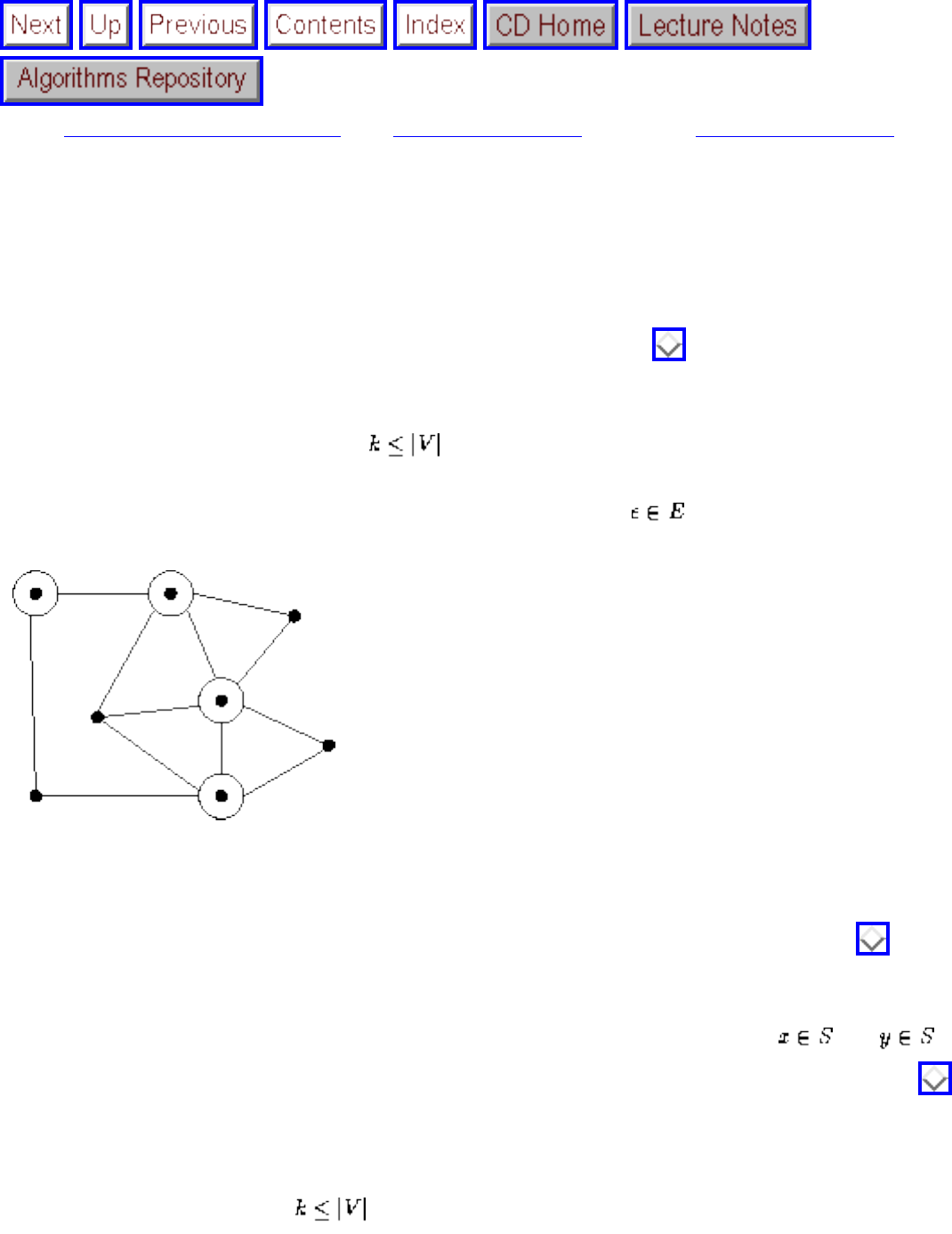
Independent Set and Vertex Cover
Next: Clique and Independent Set Up: Simple Reductions Previous: Hamiltonian Cycles
Independent Set and Vertex Cover
The vertex cover problem, discussed more thoroughly in Section , asks for a small set of vertices that
contacts each edge in a graph. More formally:
Input: A graph G=(V, E) and integer .
Output: Is there a subset S of at most k vertices such that every has at least one vertex in S?
Figure: Circled vertices form a vertex cover, the dark vertices an independent set
It is trivial to find a vertex cover of a graph, for the cover can consist of all of the vertices. More tricky is
to cover the edges using as small a set of vertices as possible. For the graph of Figure , four of the
eight vertices are sufficient to cover.
A set of vertices S of graph G is independent if there are no edges (x,y) where and , meaning
there are no edges between any two vertices in the independent set. As discussed in Section , the
independent set problem arises in facility location problems. The maximum independent set decision
problem is formally defined:
Input: A graph G and integer .
Output: Does there exist an independent set of k vertices in G? Both vertex cover and independent set are
file:///E|/BOOK/BOOK3/NODE108.HTM (1 of 2) [19/1/2003 1:29:46]

Independent Set and Vertex Cover
problems that revolve around finding special subsets of vertices, the first with representatives of every
edge, the second with no edges. If S is the vertex cover of G, the remaining vertices S-V must form an
independent set, for if there were an edge with both vertices in S-V, then S could not have been a vertex
cover. This gives us a reduction between the two problems:
VertexCover(G,k)
G' = G
k' = |V| - k
Return the answer to IndependentSet(G',k')
Again, a simple reduction shows that the problems are identical. Notice how this translation occurs
without any knowledge of the answer. We transform the input, not the solution. This reduction shows
that the hardness of vertex cover imples that independent set must also be hard. It is easy to reverse the
roles of the two problems in this reduction, thus proving that both of these problems are equally hard.
Next: Clique and Independent Set Up: Simple Reductions Previous: Hamiltonian Cycles
Algorithms
Mon Jun 2 23:33:50 EDT 1997
file:///E|/BOOK/BOOK3/NODE108.HTM (2 of 2) [19/1/2003 1:29:46]
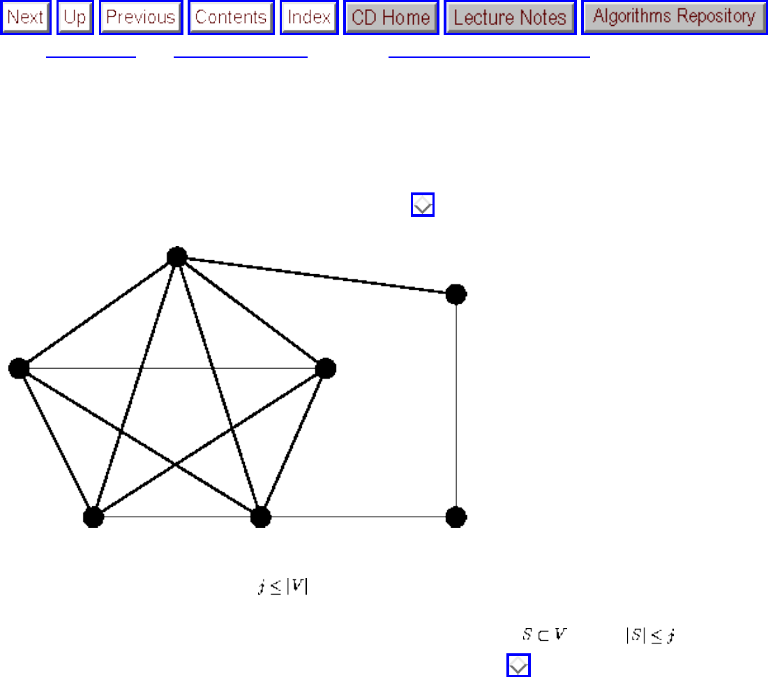
Clique and Independent Set
Next: Satisfiability Up: Simple Reductions Previous: Independent Set and Vertex
Clique and Independent Set
Consider the clique problem, further discussed in Section :
Figure: A small graph with a five-vertex clique
Input: A graph G=(V,E) and integer .
Output: Does the graph contain a clique of j vertices; i.e. is there a subset , where , such that every pair
of vertices in S defines an edge of G? For example, the graph in Figure contains a clique of five vertices. In the
independent set problem, we looked for a subset S with no edges between two vertices of S. However, for a clique,
we insist that there always be an edge between two vertices. A reduction between these problems results by
reversing the roles of edges and non-edges, an operation known as complementing the graph:
IndependentSet(G,k)
Construct a graph G=(V',E') where V'=V, and
For all (i,j) not in E, add (i,j) to E'
Return the answer to Clique(G',k)
file:///E|/BOOK/BOOK3/NODE109.HTM (1 of 2) [19/1/2003 1:29:47]

Clique and Independent Set
These last two reductions provide a chain linking three different problems. The hardness of clique is implied by the
hardness of independent set, which is implied by the hardness of vertex cover. By constructing reductions in a chain,
we link together pairs of problems in implications of hardness. Our work is done as soon as all these chains begin
with a single problem that is accepted as hard. Satisfiability is the problem that serves as the first link in this chain.
Algorithms
Mon Jun 2 23:33:50 EDT 1997
file:///E|/BOOK/BOOK3/NODE109.HTM (2 of 2) [19/1/2003 1:29:47]
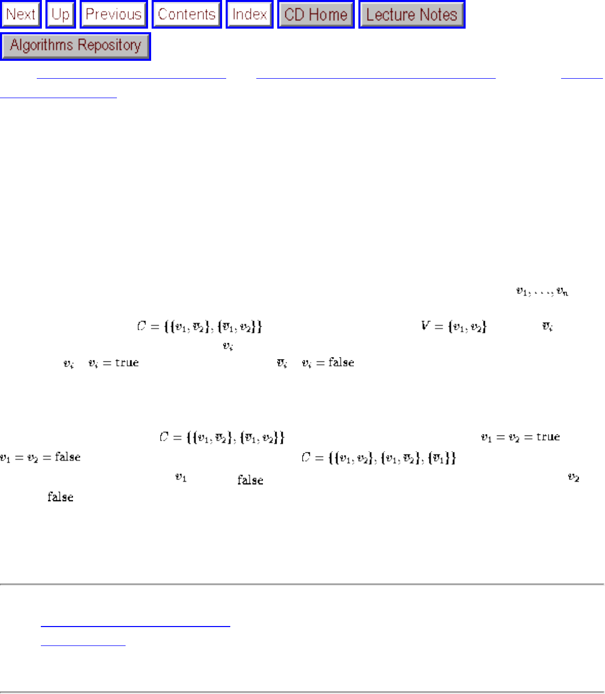
Satisfiability
Next: The Theory of NP-Completeness Up: Intractable Problems and Approximations Previous: Clique
and Independent Set
Satisfiability
To prove the hardness of different problems using reductions, we need to start with a single problem that
is absolutely, certifiably, undeniably hard. The mother of all NP-complete problems is a logic problem
named satisfiability:
Input: A set of Boolean variables V and a set of clauses C over V.
Output: Does there exist a satisfying truth assignment for C, i.e. a way to set the variables either
true or false so that each clause contains at least one true literal? This can be made clearer with two
examples. Suppose that over the Boolean variables . We use to
denote the complement of the variable , so we would get credit for satisfying a particular clause
containing if , or a clause containing if . Therefore, satisfying a particular set of
clauses involves making a series of n true or false decisions, trying to find the right truth assignment to
satisfy all of them.
This example set of clauses can be satisfied by simply setting or
. However, consider the set of clauses . There can be no
satisfying assignment because must be in order to satisfy the third clause, which means that
must be to satisfy the second clause, which then leaves the first clause unsatisfiable. Although you
try, and you try, and you try and you try, you can't get no satisfaction.
● The Theory of NP-Completeness
● 3-Satisfiability
Algorithms
file:///E|/BOOK/BOOK3/NODE110.HTM (1 of 2) [19/1/2003 1:29:48]
Satisfiability
Mon Jun 2 23:33:50 EDT 1997
file:///E|/BOOK/BOOK3/NODE110.HTM (2 of 2) [19/1/2003 1:29:48]
The Theory of NP-Completeness
Next: 3-Satisfiability Up: Satisfiability Previous: Satisfiability
The Theory of NP-Completeness
For a variety of social and technical reasons, it is well accepted that satisfiability is a hard problem, one
for which no worst-case polynomial-time algorithm exists. Literally every top-notch algorithm expert in
the world (and countless lesser lights) has directly or indirectly tried to come up with a fast algorithm to
test whether a given set of clauses is satisfiable, but all have failed. Further, many strange and impossible-
to-believe things in the field of computational complexity have been shown to be true if there exists a fast
satisfiability algorithm. Satisfiability is a hard problem, and it is important to accept this. See Section
for more on the satisfiability problem and its applications.
The theory of NP-completeness rests on a foundation of rigorous but subtle definitions from automata
and formal language theory. This terminology is typically confusing to or misused by beginners who lack
a mastery of these foundations, and it is not really essential to the practical aspects of designing and
applying reductions. For completeness, however, we briefly define the key terms below.
A problem is said to be polynomial (or in the class P) if it can be solved in time polynomial in its size. A
problem is said to be nondeterministically polynomial (or in the class NP) if a conjectured answer can be
verified in time polynomial in its size. The traveling salesman decision problem is not known to be in P,
because there is no known polynomial-time algorithm for it. However, the problem is in NP, because if
we are given a candidate tour, we can efficiently add up the cost of the associated edges and verify
whether the total is at most the cost bound k. It is typically straightforward to verify whether the answer
to a problem is correct, and it certainly can be no harder than actually finding the answer in the first place.
Through a complicated proof, it has been established that satisfiability is at least as hard as any problem
in NP. This means that if a fast (i.e. polynomial-time) algorithm is discovered for solving satisfiability,
this will yield a fast algorithm for every problem in NP. Since essentially every problem mentioned this
book is in NP, this would be an enormously powerful and surprising result. We say that a problem is NP-
hard if, like satisfiability, it is at least as hard as any problem in NP. We say that a problem is NP-
complete if it is NP-hard, and also in NP itself. Because NP is such a large class of problems, most NP-
hard problems you encounter will in fact be complete, and the issue can always be settled by giving a
(usually simple) verification strategy for the problem.
file:///E|/BOOK/BOOK3/NODE111.HTM (1 of 2) [19/1/2003 1:29:48]

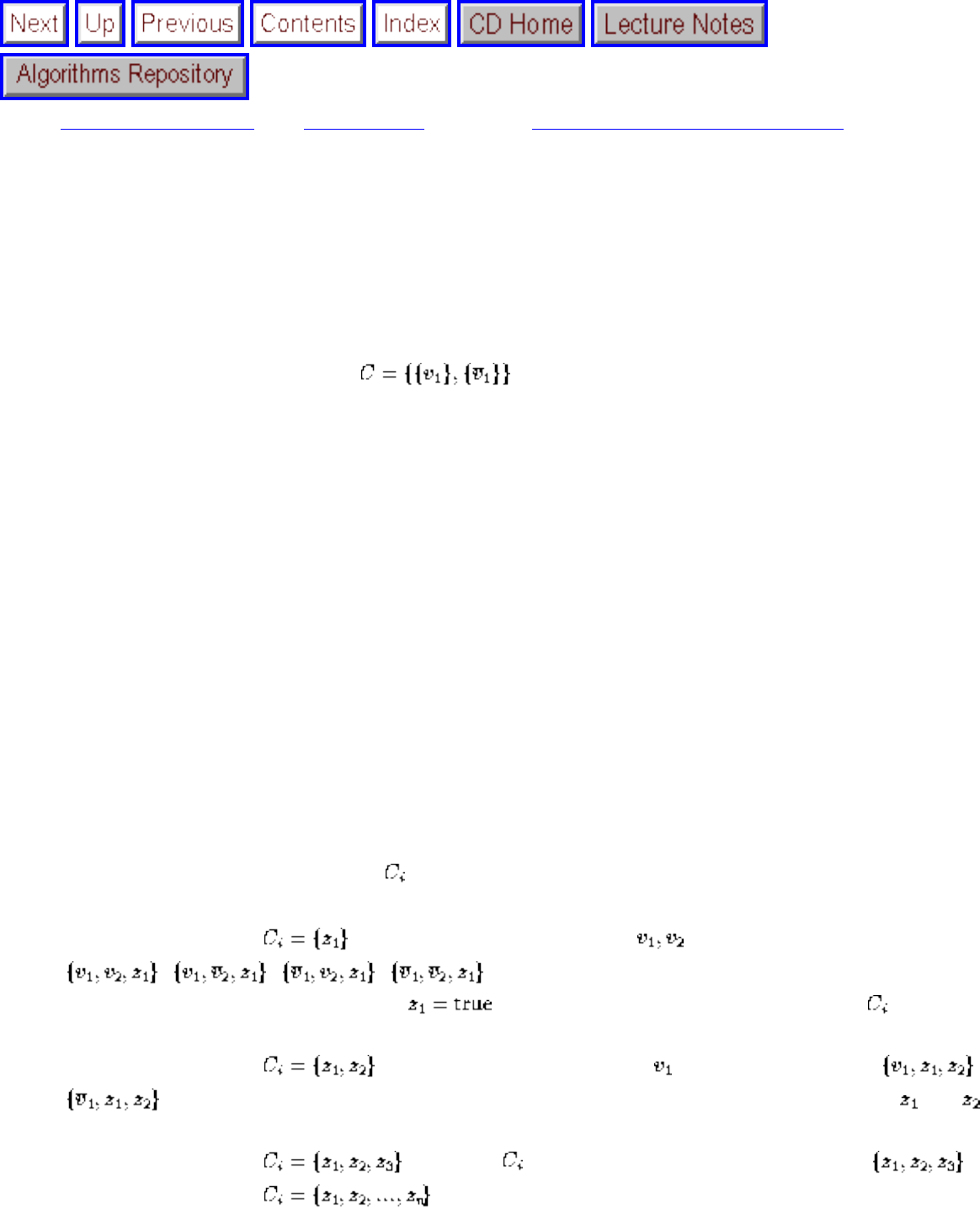
3-Satisfiability
Next: Difficult Reductions Up: Satisfiability Previous: The Theory of NP-Completeness
3-Satisfiability
Satisfiability's role as the first NP-complete problem implies that the problem is hard to solve in the
worst case, but certain instances of the problem are not necessarily so tough. Suppose that each clause
contains exactly one literal. To satisfy such a clause, we have to appropriately set that literal, so we can
repeat this argument for every clause in the problem instance. Only when we have two clauses that
directly contradict each other, such as , will the set not be satisfiable.
Since clause sets with only one literal per clause are easy to satisfy, we are interested in slightly larger
classes. Exactly what is the clause size at which the problem turns from polynomial to hard? This
transition occurs when each clause contains three literals, the so-called 3-satisfiability problem, or 3-
SAT:
Input: A collection of clauses C where each clause contains exactly 3 literals, over a set of Boolean
variables V.
Output: Is there a truth assignment to V such that each clause is satisfied? Since this is a more restricted
problem than satisfiablity, the hardness of 3-SAT implies that satisfiability is hard. The converse isn't
true, as the hardness of general satisfiability might depend upon having long clauses. We can show the
hardness of 3-SAT using a reduction that translates every instance of satisfiability into an instance of 3-
SAT without changing the result of whether it is satisfiable.
This reduction transforms each clause independently based on its length, by adding new Boolean
variables along the way. Suppose clause contained k literals:
● If k=1, meaning that , we create two new variables and four new 3-literal clauses:
, , , . Note that the only way that all four of these clauses
can be simultaneously satisfied is if , which must be the case if the original were to be
satisfied.
● If k=2, meaning that , we create one new variable and two new clauses: ,
. Again, the only way to satisfy both of these clauses is to have at least one of and
be true.
● If k=3, meaning that , we copy into the 3-SAT instance unchanged: .
● If k>3, meaning that , create n-3 new variables and n-2 new clauses in a chain,
file:///E|/BOOK/BOOK3/NODE112.HTM (1 of 2) [19/1/2003 1:29:50]
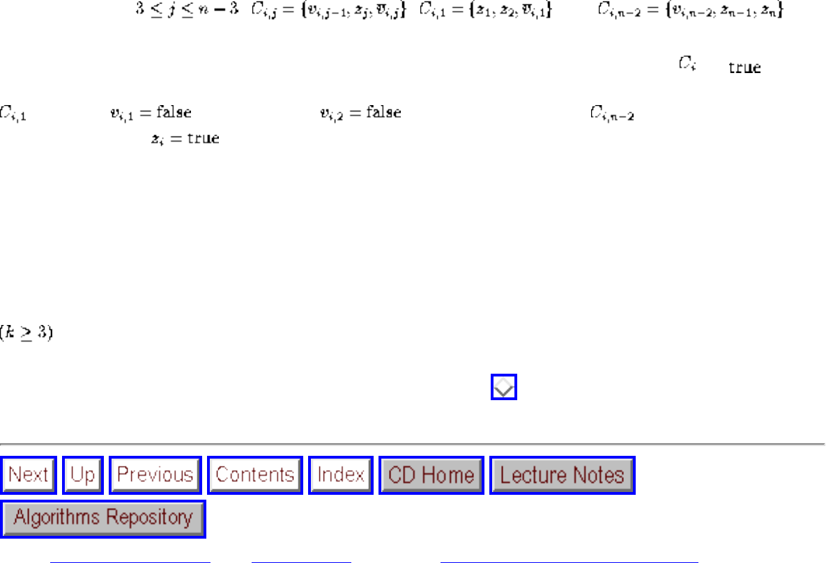
3-Satisfiability
where for , , , and .
The most complicated case is that of the large clauses. If none of the original variables are , then
there are not enough additional variables to be able to satisfy all of the new subclauses. You can satisfy
by setting , but this forces , and so on until finally cannot be satisfied. But
if any single literal , then we have n-3 free variables and n-3 remaining 3-clauses, so we can
satisfy each of them.
This transform takes O(m+n) time if there were n clauses and m total literals in the SAT instance. Since
any SAT solution also satisfies the 3-SAT instance and any 3-SAT solution sets the variables giving a
SAT solution, the transformed problem is equivallent to the original.
Note that a slight modification to this construction would serve to prove that 4-SAT, 5-SAT, or any
-SAT is also NP-complete. However, this construction breaks down when we try to use it for 2-
SAT, since there is no way to stuff anything into the chain of clauses. It turns out that resolution gives a
polynomial-time algorithm for 2-SAT, as discussed in Section .
Next: Difficult Reductions Up: Satisfiability Previous: The Theory of NP-Completeness
Algorithms
Mon Jun 2 23:33:50 EDT 1997
file:///E|/BOOK/BOOK3/NODE112.HTM (2 of 2) [19/1/2003 1:29:50]
Difficult Reductions
Next: Integer Programming Up: Intractable Problems and Approximations Previous: 3-Satisfiability
Difficult Reductions
Now that both satisfiability and 3-SAT are known to be hard, we can use either of them in reductions.
What follows are a pair of more complicated reductions, designed to serve both as examples for how to
proceed and to increase our repertoire of known hard problems from which we can start. Many
reductions are quite intricate, because we are essentially programming one problem in the language of a
significantly different problem.
One perpetual point of confusion is getting the direction of the reduction right. Recall that we must
transform every instance of a known NP-complete problem into an instance of the problem we are
interested in. If we perform the reduction the other way, all we get is a slow way to solve the problem of
interest, by using a subroutine that takes exponential time. This always is confusing at first, for this
direction of reduction seems bass-ackwards. Check to make sure you understand the direction of
reduction now, and think back to this whenever you get confused.
● Integer Programming
● Vertex Cover
Algorithms
Mon Jun 2 23:33:50 EDT 1997
file:///E|/BOOK/BOOK3/NODE113.HTM [19/1/2003 1:29:50]
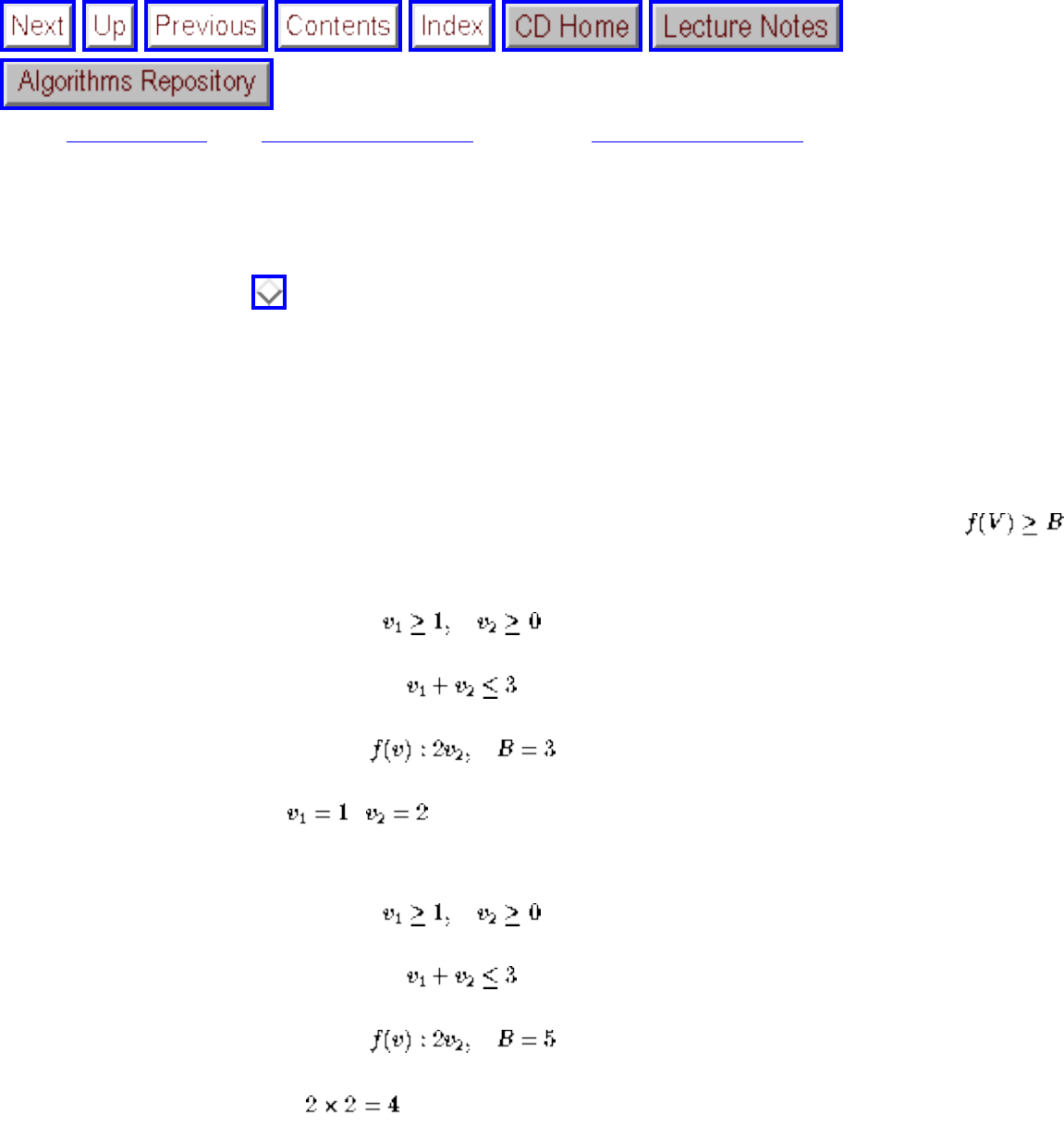
Integer Programming
Next: Vertex Cover Up: Difficult Reductions Previous: Difficult Reductions
Integer Programming
As discussed in Section , integer programming is a fundamental combinatorial optimization problem.
It is best thought of as linear programming with the variables restricted to take only integer (instead of
real) values.
Input: A set V of integer variables, a set of inequalities over V, a maximization function f(V), and an
integer B.
Output: Does there exist an assignment of integers to V such that all inequalities are true and ?
Consider the following two examples. Suppose
A solution to this would be , . Not all problems have realizable solutions, however. For the
following problem:
the maximum value of f(v) is (given the constraints), and so there can be no solution to the
associated decision problem.
We show that integer programming is hard using a reduction from 3-SAT. For this particular reduction,
general satisfiability would work just as well, although usually 3-SAT makes reductions easier.
In which direction must the reduction go? We want to prove integer programming that is hard, and we
know that 3-SAT is hard. If I could solve 3-SAT using integer programming and integer programming
file:///E|/BOOK/BOOK3/NODE114.HTM (1 of 3) [19/1/2003 1:29:52]
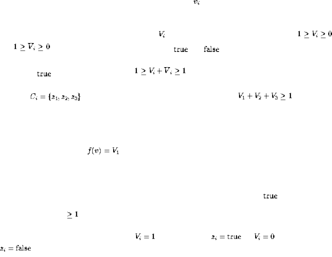
Integer Programming
were easy, this would mean that satisfiability would be easy. Now the direction should be clear; we have
to translate 3-SAT into integer programming.
What should the translation look like? Every satisfiability instance contains Boolean (true/false) variables
and clauses. Every integer programming instance contains integer variables (values restricted to 0,1,2,...)
and constraints. A reasonable idea is to make the integer variables correspond to Boolean variables and
have constraints serve the same role as the clauses do in the original problem.
Our translated integer programming problem will have twice as many variables as the SAT instance, one
for each variable and one for its complement. For each variable in the set problem, we will add the
following constraints:
● To restrict each integer programming variable to values of 0 or 1, we add constraints
and . Thus they correspond to values of and .
● To ensure that exactly one of the two integer programming variables associated with a given SAT
variable is , add constraints so that .
For each clause in the 3-SAT instance, construct a constraint: . To satisfy
this constraint, at least one the literals per clause must be set to 1, thus corresponding to a true literal.
Satisfying this constraint is therefore equivalent to satisfying the clause.
The maximization function and bound prove relatively unimportant, since we have already encoded the
entire 3-SAT instance. By using and B=0, we ensure that they will not interfere with any
variable assignment satisfying all the inequalities. Clearly, this reduction can be done in polynomial time.
To establish that this reduction preserves the answer, we must verify two things:
● Any SAT solution gives a solution to the IP problem - In any SAT solution, a literal
corresponds to a 1 in the integer program, since the clause is satisfied. Therefore, the sum in each
clause inequality is .
● Any IP solution gives a SAT solution - In any solution to this integer programming instance, all
variables must be set to either 0 or 1. If , then set literal . If , then set literal
. No Boolean variable and its complement can both be true, so it is a legal assignment,
which must also satisfy all the clauses.
The reduction works both ways, so integer programming must be hard. Notice the following properties,
which hold true in general for NP-complete:
● The reduction preserved the structure of the problem. It did not solve the problem, just put it into a
different format.
● The possible IP instances that can result from this transformation are only a small subset of all
file:///E|/BOOK/BOOK3/NODE114.HTM (2 of 3) [19/1/2003 1:29:52]

Integer Programming
possible IP instances. However, since some of them are hard, the general problem must be hard.
● The transformation captures the essence of why IP is hard. It has nothing to do with having big
coefficients or big ranges on variables; since restricting them to 0/1 is enough. It has nothing to do
with having inequalties with large numbers of variables. Integer programming is hard because
satisfying a set of constraints is hard. A careful study of the properties needed for a reduction can
tell us a lot about the problem.
Next: Vertex Cover Up: Difficult Reductions Previous: Difficult Reductions
Algorithms
Mon Jun 2 23:33:50 EDT 1997
file:///E|/BOOK/BOOK3/NODE114.HTM (3 of 3) [19/1/2003 1:29:52]
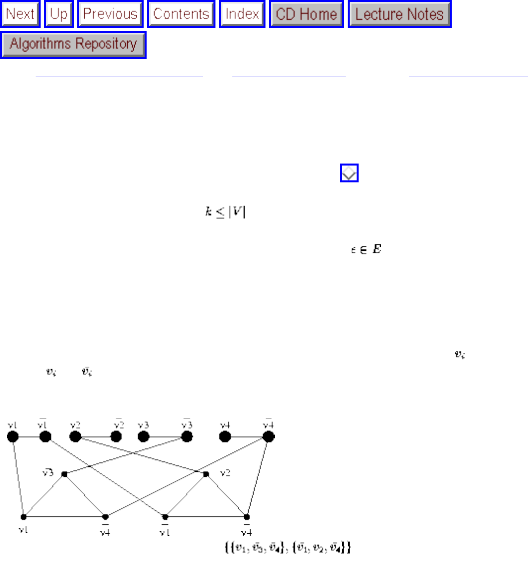
Vertex Cover
Next: Other NP-Complete Problems Up: Difficult Reductions Previous: Integer Programming
Vertex Cover
Algorithmic graph theory proves to be a fertile ground for hard problems. The prototypical NP-complete
graph problem is vertex cover, previously defined in Section as follows:
Input: A graph G=(V, E) and integer .
Output: Is there a subset S of at most k vertices such that every has at least one vertex in S?
Demonstrating the hardness of vertex cover proves more difficult than the previous reductions we have
seen, because the structure of the two relevant problems is very different. A reduction from 3-
satisfiability to vertex cover has to construct a graph G and bound k from the variables and clauses of the
satisfiability instance.
First, we translate the variables of the 3-SAT problem. For each Boolean variable , we create two
vertices and connected by an edge. To cover these edges, at least n vertices will be needed, since no
two of the edges will share a vertex.
Figure: Reducing satisfiability instance to vertex cover
Second, we translate the clauses of the 3-SAT problem. For each of the c clauses, we create three new
vertices, one for each literal in each clause. The three vertices of each clause will be connected so as to
form c triangles. At least two vertices per triangle must be included in any vertex cover of these triangles.
Finally, we will connect these two sets of components together. Each literal in the vertex ``gadgets'' is
connected to corresponding vertices in the clause gadgets (triangles) that share the same literal. From a 3-
SAT instance with n variables and c clauses, this constructs a graph with 2n+3c vertices. The complete
file:///E|/BOOK/BOOK3/NODE115.HTM (1 of 2) [19/1/2003 1:29:53]
Vertex Cover
reduction for the 3-SAT problem is shown in Figure .
This graph has been designed to have a vertex cover of size n+2c if and only if the original expression is
satisfiable. By the earlier analysis, any vertex cover must have at least n+2c vertices, since adding extra
edges to the graph can only increase the size of the vertex cover. To show that our reduction is correct,
we must demonstrate that:
● Every satisfying truth assignment gives a vertex cover - Given a satisfying truth assignment for
the clauses, select the n vertices from the vertex gadgets that correspond to literals to be
members of the vertex cover. Since this is a satisfying truth assignment, a true literal from each
clause will have covered one of the three cross edges connecting each clause triangle to a vertex
gadget. Therefore, by selecting the other two vertices of each clause triangle, we can also pick up
the remaining cross edges and complete the cover.
● Every vertex cover gives a satisfying truth assignment - Given any vertex cover C of size n+2c,
exactly n of the vertices must belong to the vertex gadgets. Let these first stage vertices define the
truth assignment, while the 2c remaining cover vertices must be distributed at two per clause
gadget; otherwise a clause gadget edge must go uncovered. These clause gadget vertices can
cover only two of the three connecting cross edges per clause. Therefore, if C gives a vertex
cover, at least one cross edge per clause must be covered, meaning that the corresponding truth
assignment satisfies.
This proof of the hardness of vertex cover, chained with the clique and independent set arguments of
Section , gives us a library of hard graph problems that we can use to make future hardness proofs
easier.
Next: Other NP-Complete Problems Up: Difficult Reductions Previous: Integer Programming
Algorithms
Mon Jun 2 23:33:50 EDT 1997
file:///E|/BOOK/BOOK3/NODE115.HTM (2 of 2) [19/1/2003 1:29:53]
Other NP-Complete Problems
Next: The Art of Proving Up: Intractable Problems and Approximations Previous: Vertex Cover
Other NP-Complete Problems
Clique, vertex cover, and integer programming are just three of the literally hundreds of problems that
have been shown to be NP-complete. It is important to be aware of which kinds of problems tend to be
hard, so you recognize them when you see them in applications, and also to provide a suitable class of
candidates for future reductions. Some, but by no means all, of the hard problems from the catalog
include:
● Integer partition - Can you partition n integers into two subsets such that the sums of the subsets
are equal? See Section for details.
● Bin packing - How many bins of a given size do you need to hold n items of variable size? See
Section for details.
● Chromatic number - How many colors do you need to color a graph such that no neighboring
vertices are of the same color? See Section for details.
● Bandwidth - Which permutation p of the vertices of a graph minimizes the length of the longest
edge when the vertices are ordered on a line, i.e. ? See Section for
details.
A few other catalog problems exist in a limbo state, where it is not known whether the problem has a fast
algorithm or is NP-complete. The most prominent of these are graph isomorphism (see Section ) and
primality testing (see Section ). That this limbo list is so short is quite a tribute to the state of the art in
algorithm design and the power of NP-completeness. For almost every important problem for which we
do not know a fast algorithm, we have a good solid reason for why one doesn't exist.
The same should hold true for the problems you encounter in your work. One way or another they should
be resolved as being either hard or polynomial. Leaving them in a limbo state is a sure sign of a bush-
league algorithm designer.
It takes experience to be able to sense whether a problem is likely to be hard or not. Perhaps the quickest
way to gain this experience is through careful study of the catalog. Note that slightly changing the
wording of a problem can make the difference between it being polynomial or NP-complete. Finding the
shortest path in a graph is easy, while finding the longest path in a graph is hard. Constructing a tour that
visits all the edges once in a graph is easy, while constructing a tour that visits all the vertices once is
file:///E|/BOOK/BOOK3/NODE116.HTM (1 of 2) [19/1/2003 1:29:54]

Other NP-Complete Problems
hard.
The first thing to do when you suspect a problem might be NP-complete is look in Garey and Johnson's
book Computers and Intractability [GJ79], which contains a list of several hundred problems known to
be NP-complete. Likely you will find the problem you are interested in.
Next: The Art of Proving Up: Intractable Problems and Approximations Previous: Vertex Cover
Algorithms
Mon Jun 2 23:33:50 EDT 1997
file:///E|/BOOK/BOOK3/NODE116.HTM (2 of 2) [19/1/2003 1:29:54]
The Art of Proving Hardness
Next: War Story: Hard Against Up: Intractable Problems and Approximations Previous: Other NP-
Complete Problems
The Art of Proving Hardness
Proving that problems are hard is a skill. But once you get the hang of it, reductions can be surprisingly
straightforward and pleasurable to do. Indeed, the dirty little secret of NP-completeness proofs is that
they are usually easier to create than explain, in the same way that it is often easier to rewrite old code
than it is to understand and modify it.
I offer the following advice to those seeking to prove the hardness of a given problem:
● Make your source problem as simple (i.e. restricted) as possible.
Never try to use the general traveling salesman problem (TSP) as a source problem. Better, use
Hamiltonian cycle, i.e. TSP where all the weights are 1 or . Even better, use Hamiltonian path
instead of cycle, so you don't have to worry about closing up the path. Best of all, use Hamiltonian
path on directed planar graphs where each vertex has total degree 3. All of these problems are
equally hard, and the more you can restrict the problem that you are reducing, the less work your
reduction has to do.
As another example, never try to use full satisfiability to prove hardness. Start with 3-
satisfiability. In fact, you don't even have to use full 3-satisfiability. Instead, consider planar 3-
satisfiability, where there is a way to draw the clauses as a graph in the plane such you can
connect all instances of the same literal together without edges crossing. This property tends to be
useful in proving the hardness of geometric problems. All these problems are equally hard, and
hence NP-completeness reductions using any of them are equally convincing.
● Make your target problem as hard as possible.
Don't be afraid to add extra constraints or freedoms in order to make your problem more general.
Perhaps your undirected graph problem can be generalized into a directed graph problem and can
hence be easier to prove hard. Once you have a proof of hardness for the general problem, you
can then go back and try to simplify the target.
● Select the right source problem for the right reason.
Selecting the right source problem makes a big difference in how difficult it is to prove a problem
hard. Although theoretically any particular problem is as good as another, this is the first and
file:///E|/BOOK/BOOK3/NODE117.HTM (1 of 3) [19/1/2003 1:29:55]

The Art of Proving Hardness
easiest place to go wrong. When faced with trying to prove that a problem is hard, some people
fish around through dozens of problems, looking for the one that seems the best fit. These people
are amateurs; odds are they never will recognize what they are looking for when they see it.
I use four and only four problems as candidates for my hard source problem. Limiting them to
four means that I can know a lot about each of these problems, such as which variants of these
problems are hard and which are soft. My favorite problems are:
❍ 3-SAT: The old reliable. When none of the three problems below seem appropriate, I go
back to the original source.
❍ Integer partition: This is the one and only choice for problems whose hardness seems to
require using large numbers.
❍ Vertex cover: This is the answer for any graph problems whose hardness depends upon
selection. Chromatic number, clique, and independent set all involve trying to select the
correct subset of vertices or edges.
❍ Hamiltonian path: This is my choice for any graph problem whose hardness depends upon
ordering. If you are trying to route or schedule something, Hamiltonian path is likely your
lever into the problem.
● Amplify the penalties for making the undesired selection.
Many people are too timid in their thinking about hardness proofs. You are trying to translate one
problem into another, while keeping the problems as close to their original identities as as
possible. The easiest way to do this is to be bold with your penalties, to punish anyone for trying
to deviate from your intended solution. Your thinking should be, ``if you select this element, then
you have to pick up this huge set that prevents you from finding an optimal solution.'' The sharper
the consequences for doing what is undesired, the easier it is to prove if and only if.
● Think strategically at a high level, then build gadgets to enforce tactics.
You should be asking yourself the following types of questions. ``How can I force that either A or
B but not both are chosen?'' ``How can I force that A is taken before B?'' ``How can I clean up the
things I did not select?'' After you have an idea of what you want your gadgets to do, you can
worry about how to actually craft them.
● When you get stuck, alternate between looking for an algorithm or a reduction.
Sometimes the reason you cannot prove hardness is that there exists an efficient algorithm to
solve your problem! Techniques such as dynamic programming or reducing to polynomial-time
graph problems such as matching or network flow sometimes yield surprising polynomial
algorithms. Whenever you can't prove hardness, it likely pays to alter your opinion occasionally to
keep yourself honest.
file:///E|/BOOK/BOOK3/NODE117.HTM (2 of 3) [19/1/2003 1:29:55]

War Story: Hard Against the Clock
Next: Approximation Algorithms Up: Intractable Problems and Approximations Previous: The Art of
Proving
War Story: Hard Against the Clock
My class's attention span was running down like sand through an hourglass. Eyes were starting to glaze
even in the front row. Breathing had become soft and regular in the middle of the room. Heads were
tilted back and eyes shut in the rear.
There were fifteen minutes left to go in my lecture on NP-completeness, and I couldn't really blame
them. They had already seen several reductions like the ones presented here, but NP-completeness
reductions are easier to create than to understand or explain. They had to watch one being created in
order to appreciate this.
I reached for my trusty copy of Garey and Johnson's book [GJ79], which contains a list of over four
hundred different known NP-complete problems in an appendix in the back.
``Enough of this!'' I announced loudly enough to startle those in the back row. ``NP-completeness proofs
are routine enough that we can construct them on demand. I need a volunteer with a finger. Can anyone
help me?''
A few students in the front held up their hands. A few students in the back held up their fingers. I opted
for one from the front row.
``Select a problem at random from the back of this book. I can prove the hardness of any of these
problems in the now twelve minutes remaining in this class. Stick your finger in and read me a problem.''
I had definitely gotten their attention. But I could have done that by offering to juggle chainsaws. Now I
had to deliver results without cutting myself into ribbons.
The student picked out a problem. ``OK, prove that Inequivalence of Programs with Assignments is
hard,'' she said.
``Huh? I've never heard of that problem before. What is it? Read me the entire description of the problem
so I can write it on the board.'' The problem was as follows:
file:///E|/BOOK/BOOK3/NODE118.HTM (1 of 4) [19/1/2003 1:29:56]
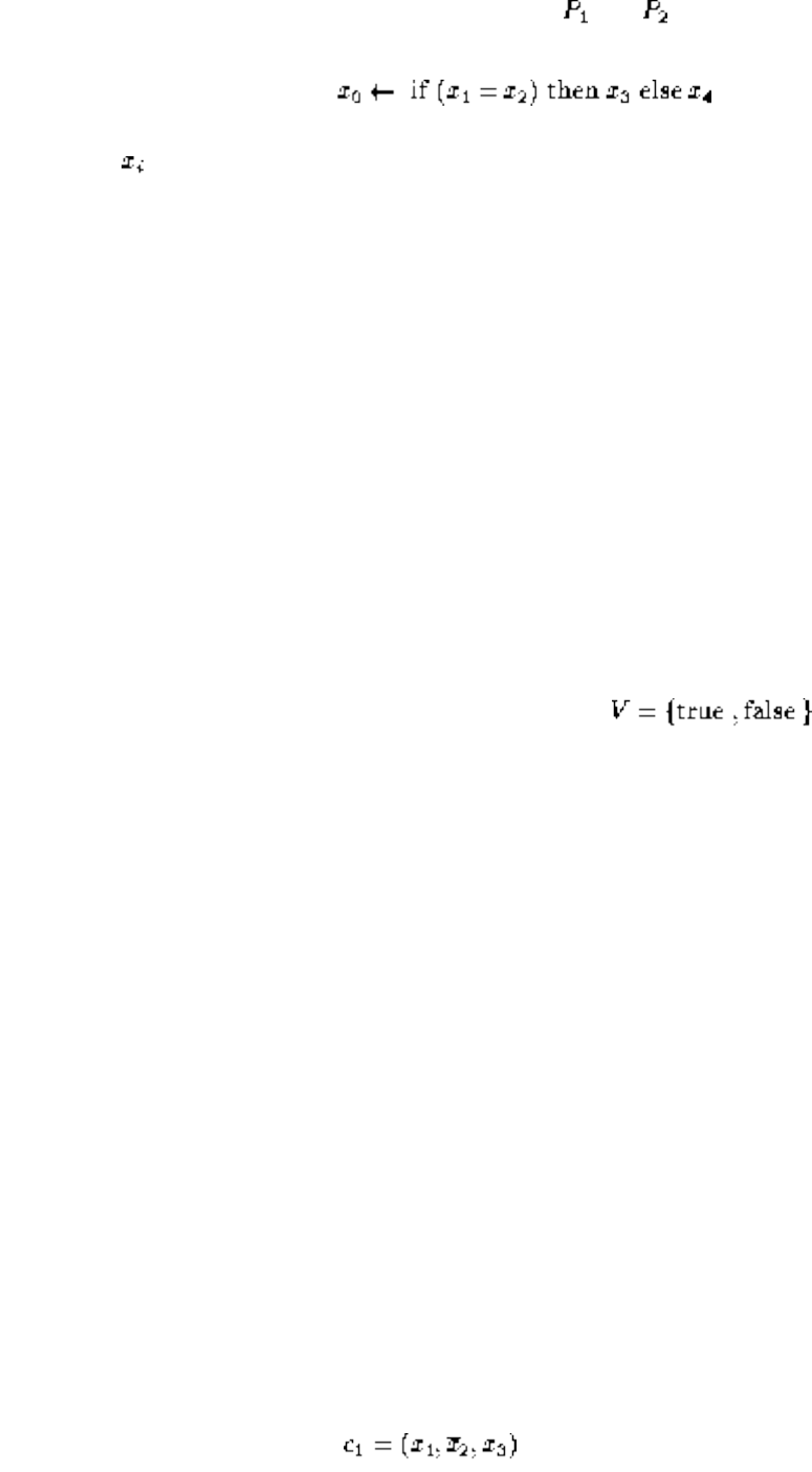
War Story: Hard Against the Clock
Input: A finite set X of variables, two programs and , each a sequence of assignments of the form
where the are in X; and a value set V.
Output: Is there an initial assignment of a value from V to each variable in X such that the two programs
yield different final values for some variable in X?
I looked at my watch. Ten minutes to go. But now everything was on the table. I was faced with a
language problem. The input was two programs with variables, and I had to test to see whether they
always do the same thing.
``First things first. We need to select a source problem for our reduction. Do we start with integer
partition? 3-satisfiability? Vertex cover or Hamiltonian path?''
Since I had an audience, I tried thinking out loud. ``Our target is not a graph problem or a numerical
problem, so let's start thinking about the old reliable: 3-satisfiability. There seem to be some similarities.
3-SAT has variables. This thing has variables. To be more like 3-SAT, we could try limiting the variables
in this problem so they only take on two values, i.e. . Yes. That seems convenient.''
My watch said nine minutes left. ``So, class, which way does the reduction go. 3-SAT to language or
language to 3-SAT?''
The front row correctly murmured, ``3-SAT to language.''
``Right. So we have to translate our set of clauses into two programs. How can we do that? We can try to
split the clauses into two sets and write separate programs for each of them. But how do we split them? I
don't see any natural way how to do it, because eliminating any single clause from the problem might
suddenly make an unsatisfiable formula satisfiable, thus completely changing the answer. Instead, let's
try something else. We can translate all the clauses into one program, and then make the second program
be trivial. For example, the second program might ignore the input and always outputs either only true or
only false. This sounds better. Much better.''
I was still talking out loud to myself, which wasn't that unusual. But I had people listening to me, which
was.
``Now, how can we turn a set of clauses into a program? We want to know whether the set of clauses can
be satisfied, or if there is an assignment of the variables such that it is true. Suppose we constructed a
program to evaluate whether is satisfied. We can do it like this ....''
file:///E|/BOOK/BOOK3/NODE118.HTM (2 of 4) [19/1/2003 1:29:56]
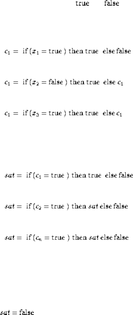
War Story: Hard Against the Clock
It took me a few minutes worth of scratching before I found the right program. I assumed that I had
access to constants for and , which seemed reasonable, in the sense that it shouldn't make the
problem algorithmically harder. Once my proof worked, I could later worry about removing the extra
assumption if desired.
``Great. Now I have a way to evaluate the truth of each clause. I can do the same thing to evaluate
whether all the clauses are satisfied.''
Now the back of the classroom was getting excited. They were starting to see a ray of hope that they
would get to leave on time. There were two minutes left in class.
``Great. So now we have a program that can evaluate to be true if and only if there is a way to assign the
variables so as to satisfy the set of clauses. We need a second program to finish the job. What about
? Yes, that is all we need. Our language problem asks whether the two programs always
output the same thing, regardless of the possible variable assignments. If the clauses are satisfiable, that
means that there must be an assignment of the variables such that the long program would output true.
Testing whether the programs are equivalent is exactly the same as asking if the clauses are satisfiable.''
I lifted my arms in triumph. ``And so, the problem is neat, sweet, and NP-complete.'' I got the last word
out just before the bell rang.
This exercise was so much fun that I repeated it the next time I taught the course, using a different
randomly selected problem. The audio from my ultimately successful attempt to prove hardness is
accessible from the CD-ROM, if you want to hear what the creation of an NP-completeness proof sounds
file:///E|/BOOK/BOOK3/NODE118.HTM (3 of 4) [19/1/2003 1:29:56]


Approximation Algorithms
Next: Approximating Vertex Cover Up: Intractable Problems and Approximations Previous: War Story:
Hard Against
Approximation Algorithms
For the practical person, demonstrating that a problem is NP-complete is never the end of the line.
Presumably, there was a reason why you wanted to solve it in the first place. That reason for wanting the
solve it will not have gone away on being told that there is no polynomial-time algorithm. You still seek
a program that solves the problem of interest. All you know is that you won't find one that quickly solves
the problem to optimality in the worst case. You still have the following options:
● Algorithms fast in the average case - Examples of such algorithms include backtracking
algorithms with substantial pruning.
● Heuristics - Heuristic methods like simulated annealing or greedy approaches can be used to find
a solution with no requirement that it be the best one.
● Approximation algorithms - The theory of NP-completeness does not stipulate that it is hard to get
close to the answer, only that it is hard to get the optimal answer. With clever, problem-specific
heuristics, we can often get provably close to the optimal answer.
Approximation algorithms return solutions with a guarantee attached, namely that the optimal solution
can never be much better than this given solution. Thus you can never go too far wrong in using an
approximation algorithm. No matter what your input instance is and how lucky you are, you are doomed
to do all right. Further, approximation algorithms realizing provably good bounds often are conceptually
simple, very fast, and easy to program.
One thing that is usually not clear, however, is how well the solution from an approximation algorithm
compares to what you might get from a heuristic that gives you no guarantees. The answer could be
worse or it could be better. Leaving your money in a savings account in a bank guarantees you 3%
interest without risk. Still, you likely will do much better putting your money in stocks than in the bank,
even though performance is not guaranteed.
One way to get the best of approximation algorithms and heuristics is to run both of them on the problem
instance and pick the solution giving the better answer. This way, you get a solution that comes with a
guarantee and a second chance to do even better. When it comes to heuristics for hard problems,
sometimes you can have it both ways.
file:///E|/BOOK/BOOK3/NODE119.HTM (1 of 2) [19/1/2003 1:29:57]
Approximation Algorithms
● Approximating Vertex Cover
● The Euclidean Traveling Salesman
Next: Approximating Vertex Cover Up: Intractable Problems and Approximations Previous: War Story:
Hard Against
Algorithms
Mon Jun 2 23:33:50 EDT 1997
file:///E|/BOOK/BOOK3/NODE119.HTM (2 of 2) [19/1/2003 1:29:57]
Approximating Vertex Cover
Next: The Euclidean Traveling Salesman Up: Approximation Algorithms Previous: Approximation Algorithms
Approximating Vertex Cover
As we have seen before, finding the minimum vertex cover of a graph is NP-complete. However, a very simple procedure
can efficiently find a cover that is at most twice as large as the optimal cover:
VertexCover(G=(V,E))
while do:
Select an arbitrary edge
Add both u and v to the vertex cover
Delete all edges from E that are incident on either
u or v.
It should be apparent that this procedure always produces a vertex cover, since each edge is only deleted immediately after an
incident vertex has been added to the cover. More interesting is the claim that any vertex cover must use at least half as many
vertices as this one. Why? Consider just the edges selected by the algorithm. No two of these edges can share a vertex.
Therefore, any cover of just these edges must include at least one vertex per edge, which makes it at least half the size of the
greedy cover.
There are several interesting things to notice about this algorithm:
● Although the procedure is simple, it is not stupid - Many seemingly smarter heuristics can give a far worse
performance in the worst case. For example, why not modify the procedure above to select only one of the two
vertices for the cover instead of both. After all, the selected edge will be equally well covered by only one vertex.
However, consider the star-shaped graph of Figure . This heuristic will produce a two-vertex cover, while the
single vertex heuristic can return a cover as large as n-1 vertices, should we get unlucky and repeatedly select the leaf
instead of the center as the cover vertex.
file:///E|/BOOK/BOOK3/NODE120.HTM (1 of 2) [19/1/2003 1:29:58]
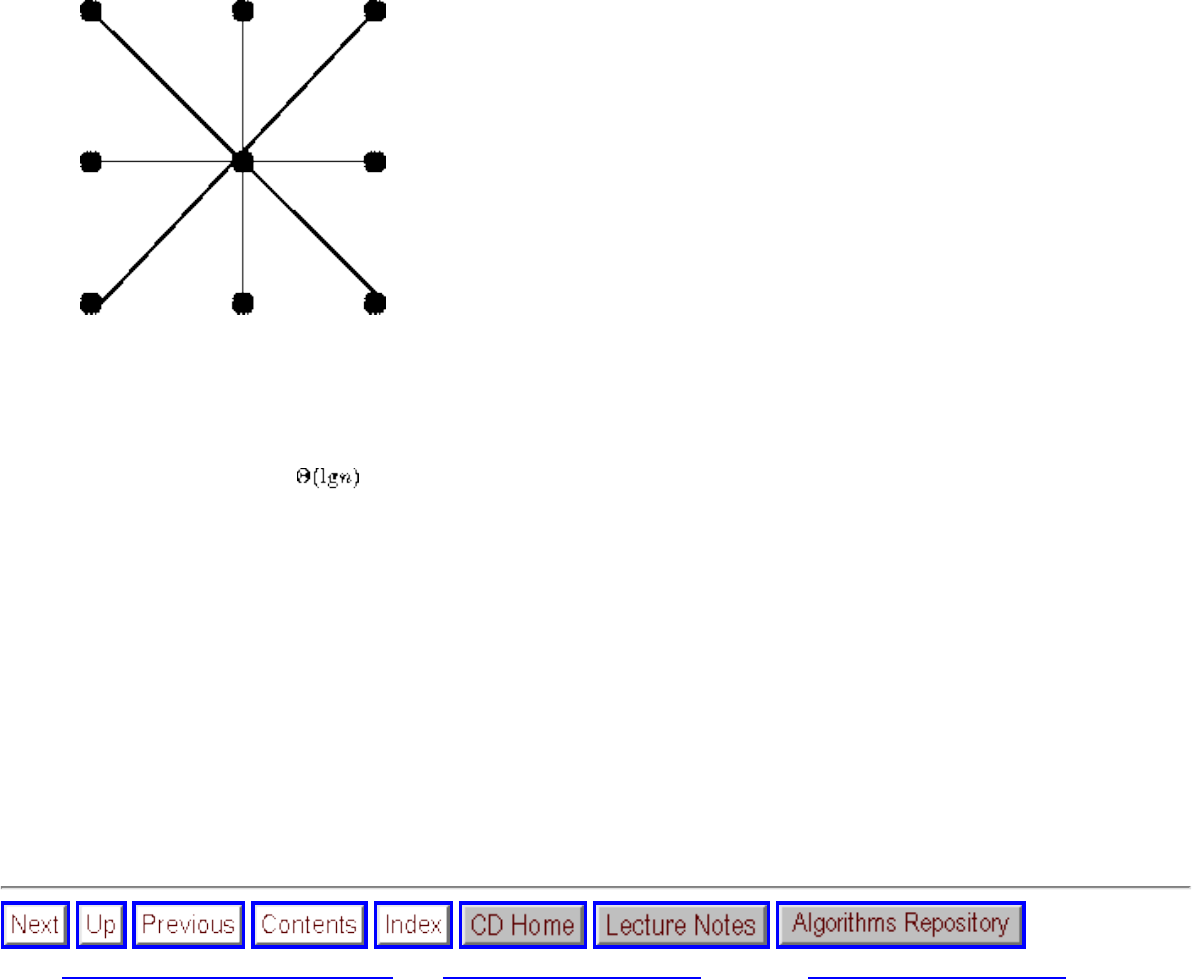
Approximating Vertex Cover
Figure: Neglecting to pick the center vertex leads to a terrible vertex cover
● Greedy isn't always the answer - Perhaps the most natural heuristic for this problem would repeatedly select and
delete the vertex of highest remaining degree for the vertex cover. After all, this vertex will cover the largest number
of possible edges. However, in the case of ties or near ties, this heuristic can go seriously astray and in the worst case
can yield a cover that is times optimal.
● Making a heuristic more complicated does not necessarily make it better - It is easy to complicate heuristics by adding
more special cases or details. For example, the procedure above does not specify which edge should be selected next.
It might seem reasonable always to select the edge whose endpoints have highest degree. However, this does not
improve the worst-case bound and just makes it more difficult to analyze.
● A postprocessing cleanup step can't hurt - The flip side of designing simple heuristics is that they can often be
modified to yield better-in-practice solutions without weakening the approximation bound. For example, a
postprocessing step that deletes any unnecessary vertex from the cover can only improve things in practice, even
though it won't help the worst-case bound.
The important property of approximation algorithms is relating the size of the solution produced directly to a lower bound on
the optimal solution. Instead of thinking about how well we might do, we have to think about the worst case i.e. how badly
we might perform.
Next: The Euclidean Traveling Salesman Up: Approximation Algorithms Previous: Approximation Algorithms
Algorithms
Mon Jun 2 23:33:50 EDT 1997
file:///E|/BOOK/BOOK3/NODE120.HTM (2 of 2) [19/1/2003 1:29:58]
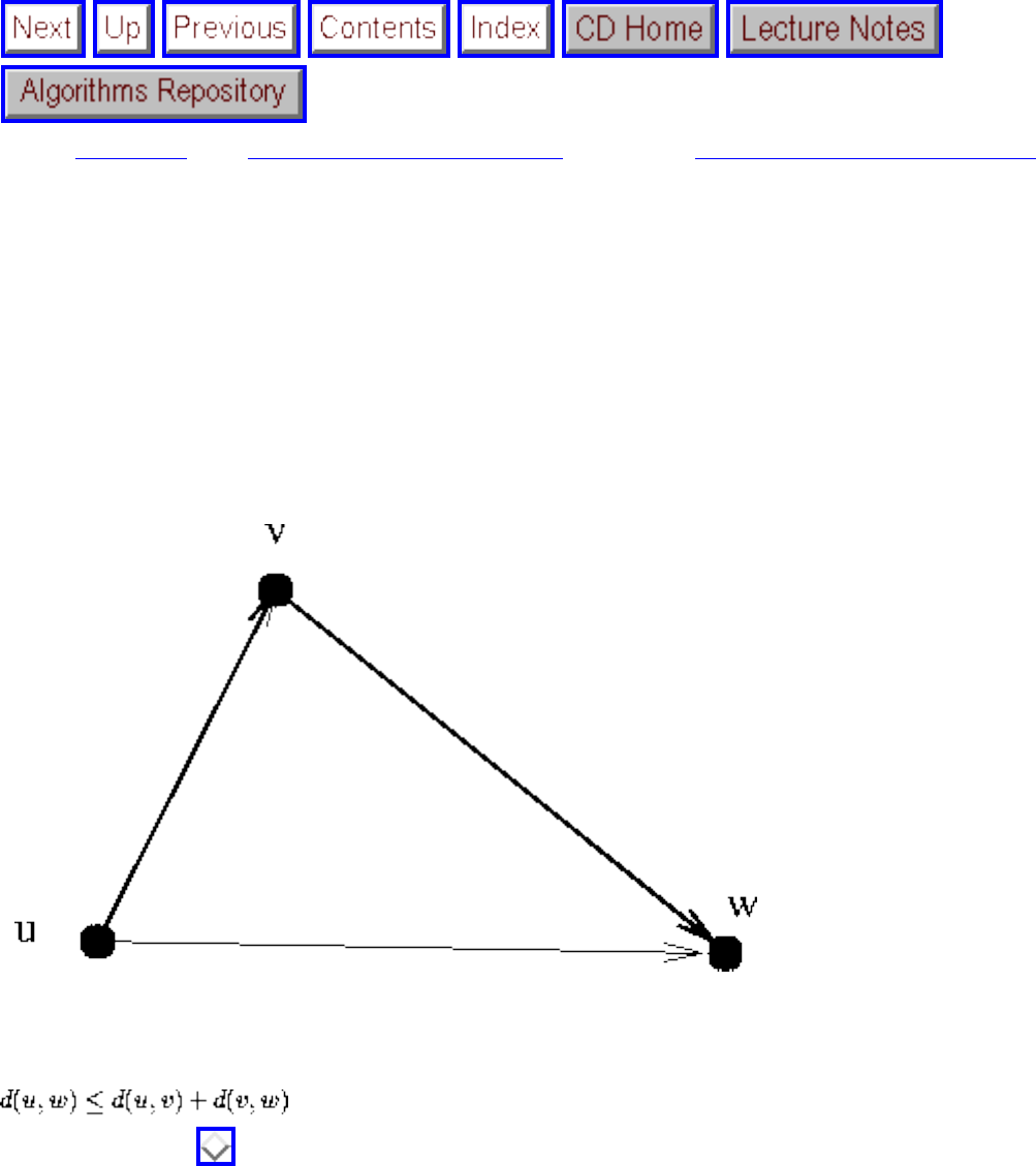
The Euclidean Traveling Salesman
Next: Exercises Up: Approximation Algorithms Previous: Approximating Vertex Cover
The Euclidean Traveling Salesman
In most natural applications of the traveling salesman problem, direct routes are inherently shorter than
indirect routes. For example, if the edge weights of the graph are ``as the crow flies'', straight-line
distances between pairs of cities, the shortest path from x to y will always be to fly directly.
Figure: The triangle inequality typically holds in geometric and weighted graph problems.
The edge weights induced by Euclidean geometry satisfy the triangle inequality, which insists that
for all triples of vertices u, v, and w. The reasonableness of this condition is
shown in Figure . Note that the cost of airfares is an example of a distance function that violates the
triangle inequality, since it is sometimes cheaper to fly through an intermediate city than to fly to the
destination directly. TSP remains hard when the distances are Euclidean distances in the plane.
Whenever a graph obeys the triangle inequality, we can approximate the optimal traveling salesman tour
using minimum spanning trees. First, observe that the weight of a minimum spanning tree is a lower
bound on the cost of the optimal tour. Why? Deleting any edge from a tour leaves a path, the total weight
of which must be no greater than that of the original tour. This path has no cycles, and hence is a tree,
which means its weight is at least that of the minimum spanning tree. Thus the minimum spanning tree
cost gives a lower bound on the optimal tour.
file:///E|/BOOK/BOOK3/NODE121.HTM (1 of 3) [19/1/2003 1:29:59]
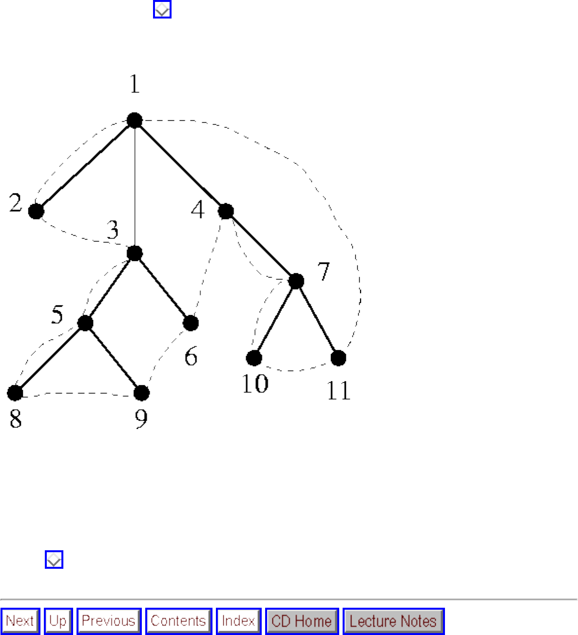
The Euclidean Traveling Salesman
Consider now what happens in performing a depth-first traversal of a spanning tree. Suppose we walk
through each tree edge as we process it in a depth-first search. We will visit each edge twice, once going
down the tree when exploring it and once going up after exploring the entire subtree. For example, in the
depth-first search of Figure , we visit the vertices in order 1-2-1-3-5-8-5-9-5-3-6-3-1-4-7-10-7-11-7-4-
1, thus using every tree edge exactly twice. Therefore, this tour has weight twice that of the minimum
spanning tree, and hence at most twice optimal.
Figure: A depth-first traversal of a spanning tree, with the shortcut tour
However, vertices will be repeated on this depth-first search tour. To remove the extra vertices, at each
step we can take a shortest path to the next unvisited vertex. The shortcut tour for the tree above is 1-2-3-
5-8-9-6-4-7-10-11-1. Because we have replaced a chain of edges by a single direct edge, the triangle
inequality ensures that the tour can only get shorter. Thus the shortcut tour is within weight twice that of
optimal. More complicated but better approximation algorithms for Euclidean TSP are mentioned in
Section . No approximation algorithms exist for TSPs that do not satisfy the triangle inequality.
file:///E|/BOOK/BOOK3/NODE121.HTM (2 of 3) [19/1/2003 1:29:59]

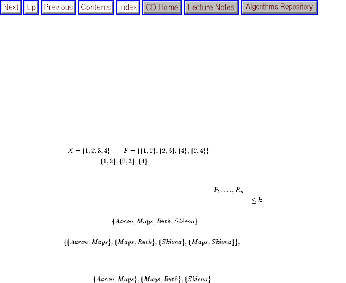
Exercises
Next: Implementation Challenges Up: Intractable Problems and Approximations Previous: The Euclidean Traveling
Salesman
Exercises
1. Prove that the vertex cover problem (does there exist a subset S of k vertices in a graph G such that every edge in
G is incident upon at least one vertex in S?) remains NP-complete even when all the vertices in the graph are
restricted to have even degree.
2. An instance of the set cover problem consists of a set X of n elements, a family F of subsets of X, and an integer
k. The question is, do there exist k subsets from F whose union is X?
For example, if and , there does not exist a solution for k=2 but there
does for k=3 (for example, ).
Prove that set cover is NP-complete with a reduction from vertex cover.
3. The baseball card collector problem is as follows. Given packets , each of which contains a subset of
that year's baseball cards, is it possible to collect all the year's cards by buying packets?
For example, if the players are and the packets are
there does not exist a solution for k=2 but there does for k=3, such as
Prove that the baseball card collector problem is NP-hard using a reduction from vertex cover.
4. (*) An Eulerian cycle is a tour that visits every edge in a graph exactly once. An Eulerian subgraph is a subset of
the edges and vertices of a graph that has an Eulerian cycle. Prove that the problem of finding the number of
edges in the largest Eulerian subgraph of a graph is NP-hard. (Hint: the Hamiltonian circuit problem is NP-hard
even if each vertex in the graph is incident upon exactly three edges.)
5. The low degree spanning tree problem is as follows. Given a graph G and an integer k, does G contain a
spanning tree such that all vertices in the tree have degree at most k (obviously, only tree edges count towards
the degree)? For example, in the following graph, there is no spanning tree such that all vertices have degree less
than three.
file:///E|/BOOK/BOOK3/NODE122.HTM (1 of 3) [19/1/2003 1:30:00]
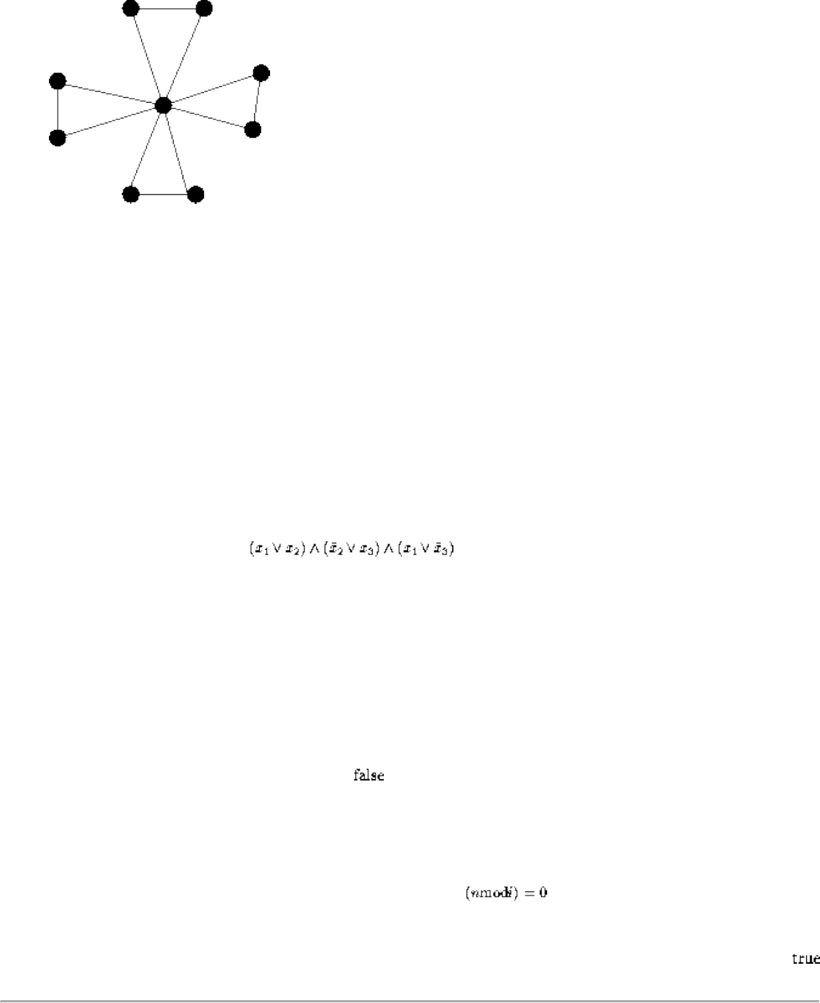
Exercises
1. Prove that the low degree spanning tree problem is NP-hard with a reduction from Hamiltonian path.
2. Now consider the high degree spanning tree problem, which is as follows. Given a graph G and an
integer k, does G contain a spanning tree whose highest degree vertex is at least k? In the previous
example, there exists a spanning tree of highest degree 8. Give an efficient algorithm to solve the high
degree spanning tree problem, and an analysis of its time complexity.
6. (*) The problem of testing whether a graph G contains a Hamiltonian path is NP-hard, where a Hamiltonian path
P is a path that visits each vertex exactly once. There does not have to be an edge in G from the ending vertex to
the starting vertex of P, unlike in the Hamiltonian cycle problem.
Given a directed acyclic graph G (a DAG), give an O(n+m)-time algorithm to test whether or not it contains a
Hamiltonian path. (Hint: think about topological sorting and DFS.)
7. (**) The 2-SAT problem is, given a Boolean formula in 2-conjunctive normal form (CNF), decide whether the
formula is satisfiable. 2-SAT is like 3-SAT, except that each clause can have only two literals. For example, the
following formula is in 2-CNF:
Give a polynomial-time algorithm to solve 2-SAT.
8. (*) It is an open question whether the decision problem ``Is integer n a composite number, in other words, not
prime?" can be computed in time polynomial in the size of the input. Why doesn't the following algorithm
suffice to prove it is in P, since it runs in O(n) time?
PrimalityTesting(n)
composite :=
for i := 2 to n-1 do
if then
composite :=
file:///E|/BOOK/BOOK3/NODE122.HTM (2 of 3) [19/1/2003 1:30:00]

Data Structures
Next: Dictionaries Up: A Catalog of Algorithmic Previous: Caveats
Data Structures
Data structures are not really algorithms that you can find and plug into your application. Instead, they
are the fundamental constructs for you to build your program around. Becoming fluent in what data
structures can do for you is essential to get full value from them.
Because of this, this section is slightly out of sync with the rest of the catalog. Perhaps the most useful
aspect of it will be the pointers to implementations of various data structures. Many of these data
structures are nontrivial to implement well, so the programs we point to will likely be useful as models
even if they do not do exactly what you need. Certain fundamental data structures, like kd-trees and
suffix trees, are not as well known as they should be. Hopefully, this catalog will serve to better
publicize them.
There is a large number of books on elementary data structures available. Our favorites include:
● Gonnet and Baeza-Yates [GBY91] - The book is a comprehensive reference to fundamental
searching, sorting, and text searching algorithms. It features over 2,000 references and
implementations in C and Pascal. These programs are now available by ftp/WWW. See Section
for more details.
● Weiss [Wei92] - A nice text, emphasizing data structures more than algorithms. Comes in
Pascal, C++, and Ada editions.
● Wood [Woo93] - A thorough and accessible treatment of modern data structures, including suffix
trees and geometric data structures. Pascal implementations for many of the data structures are
provided.
Mehlhorn and Tsakalidis [MT90b] provide a detailed and up-to-date survey of research in data
structures. The student who took only an elementary course in data structures is likely to be impressed by
the volume and quality of recent work on the subject.
● Dictionaries
file:///E|/BOOK/BOOK3/NODE128.HTM (1 of 2) [19/1/2003 1:30:01]
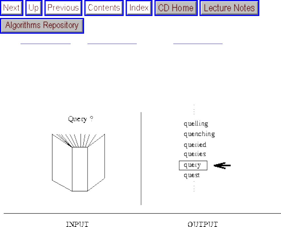
Dictionaries
Next: Priority Queues Up: Data Structures Previous: Data Structures
Dictionaries
Input description: A set of n records, each identified by one or more key fields.
Problem description: Build and maintain a data structure to efficiently locate, insert, or delete the record
associated with any query key q.
Discussion: The abstract data type ``dictionary'' is one of the most important structures in computer
science. Dozens of different data structures have been proposed for implementing dictionaries including
hash tables, skip lists, and balanced/unbalanced binary search trees - so choosing the right one can be
tricky. Depending on the application, it is also a decision that can significantly impact performance. In
practice, it is more important to avoid using a bad data structure than to identify the single best option
available.
An essential piece of advice is to carefully isolate the implementation of the dictionary data structure
from its interface. Use explicit calls to subroutines that initialize, search, and modify the data structure,
rather than embedding them within the code. This leads to a much cleaner program, but it also makes it
easy to try different dictionary implementations to see how they impact performance. Do not obsess
about the cost of the procedure call overhead inherent in such an abstraction. If your application is so
time-critical that such overhead can impact performance, then it is even more essential that you be able to
file:///E|/BOOK/BOOK3/NODE129.HTM (1 of 5) [19/1/2003 1:30:03]
Dictionaries
easily experiment with different implementations of your dictionary.
In choosing the right data structure for your dictionary, ask yourself the following questions:
● How many items will you typically have in your data structure? - Will you know this number in
advance? Are you looking at a problem small enough that the simple data structure will be best, or
will it be so large that we must worry about using too much memory or swapping?
● Do you know the relative number of insertions, deletions, and search queries? - Will there be any
modifications to the data structure after it is first constructed, or will it be static from that point
on?
● Do you have an understanding of the relative frequency with which different keys will be
accessed? - Can we assume that the access pattern will be uniform and random, or will it exhibit a
skewed access distribution (i.e. certain elements are much more popular than others) or a sense of
locality (i.e. elements are likely to be repeatedly accessed in clusters, instead of at fairly random
intervals). Usually, the world is both skewed and clustered.
● Is it critical that individual operations be fast, or only that the total amount of work done over the
entire program be minimized? - When response time is critical, such as in a program controlling a
heart-lung machine, you can't wait too long between steps. When you have a program that is doing
a lot of queries over the database, such as identifying all sex offenders who happen to be
Republicans, it is not so critical that you pick out any particular congressman quickly as that you
get them all with the minimum total effort.
Once you understand what your needs are, try to identify the best data structure from the list below:
● Unsorted linked lists or arrays - For small data sets, say up to 10 to 20 items, an unsorted array is
probably the easiest and most efficient data structure to maintain. They are easier to work with
than linked lists, and if the dictionary will be kept this small, you cannot possibly save a
significant amount of space over allocating a full array. If your dictionary will be too much larger,
the search time will kill you in either case.
A particularly interesting and useful variant is a self-organizing list. Whenever a key is accessed
or inserted, always move it to head of the list. Thus if the key is accessed again in the near future,
it will be near the front and so require only a short search to find it. Since most applications
exhibit both uneven access frequencies and locality of reference, the average search time for a
successful search in a self-organizing list is typically much better than in a sorted or unsorted list.
Of course, self-organizing data structures can be built from arrays as well as linked lists.
● Sorted linked lists or arrays - Maintaining a sorted linked list is usually not worth the effort
(unless you are trying to eliminate duplicates), since we cannot perform binary search in such a
data structure. A sorted array will be appropriate if and only if there are not many insertions or
deletions. When the array gets so large that it doesn't fit in real memory, think B-trees instead.
● Hash tables - For applications involving a moderate-to-large number of keys (say between 100
and 1,000,000), a hash table with bucketing is probably the right way to go. In a hash table, we
file:///E|/BOOK/BOOK3/NODE129.HTM (2 of 5) [19/1/2003 1:30:03]
Dictionaries
use a function that maps keys (be they strings, numbers, or whatever) to integers between 0 and m-
1. We maintain an array of m buckets, each typically implemented using an unsorted linked list.
For a given key, the hash function immediately identifies which bucket will contain it. If we use a
hash function that spreads the keys out nicely and a sufficiently large hash table, each bucket
should contain very few items, thus making linear search acceptable. Insertion and deletion from a
hash table reduce to insertion and deletion from the bucket/list.
A well-tuned hash table will likely outperform a sorted array in most applications. However,
several design decisions go into creating a well-tuned hash table:
❍ How big should the table be? Typically, m should about the same as the maximum number
of items you expect to put in the table. Make sure that m is a prime number, so as to
minimize the dangers of a bad hash function.
❍ What hash function should I use? For strings, something like
should work, where is the size of the alphabet and char(x) is the function that maps each
character x to its ASCII character code. For long strings, 8 to 10 characters should be
sufficient to hash upon, provided they are unlikely to be padded blanks or some other
invariant. Use Horner's rule to implement this hash function computation efficiently, as
discussed in Section .
Regardless of which hash function you decide to use, print statistics on the distribution of keys per
bucket to see how uniform it really is. Odds are the first hash function you try will not prove to be
the best. Botching up the hash function is an excellent way to slow down any application.
● Binary search trees - Binary search trees are elegant data structures that support fast insertions,
deletions, and queries. The big distinction between different types of trees is whether they are
explicitly rebalanced after insertion or deletion, and how this rebalancing takes place. In random
search trees, no rebalancing takes place and we simply insert a node at the leaf position where we
can find it. Although search trees perform well under random insertions, most applications are not
really random. Indeed, unbalanced search trees constructed by inserting keys in sorted order are a
disaster, performing like a linked list.
Balanced search trees use local rotation operations to restructure search trees, moving more
distant nodes closer to the root while maintaining the in-order search structure of the tree. Among
balanced search trees, AVL and 2/3 trees are now passé, and red-black trees seem to be more
popular. A particularly interesting self-organizing data structure is the splay tree, which uses
rotations to move any accessed key to the root. Frequently used or recently accessed nodes thus sit
near the top of the tree, allowing fast search.
file:///E|/BOOK/BOOK3/NODE129.HTM (3 of 5) [19/1/2003 1:30:03]
Dictionaries
Bottom line: Which binary search tree is best for your application? Probably the balanced tree for
which you have the best implementation readily available. See the choices below. Which flavor of
balanced tree is probably not as important as how good the programmer was who coded it.
● B-trees - For data sets so large that they will not fit in main memory (say more than 1,000,000
items) your best bet will be some flavor of a B-tree. As soon as the data structure gets outside of
main memory, the search time to access a particular location on a disk or CD-ROM can kill you,
since this is several orders of magnitude slower than accessing RAM.
The idea behind a B-tree is to collapse several levels of a binary search tree into a single large
node, so that we can make the equivalent of several search steps before another disk access is
needed. We can thereafter reference enormous numbers of keys using only a few disk accesses. To
get the full benefit from using a B-tree, it is important to understand explicitly how the secondary
storage device and virtual memory interact, through constants such as page size and virtual/real
address space.
Even for modest-sized data sets, unexpectedly poor performance of a data structure may be due to
excessive swapping, so listen to your disk to help decide whether you should be using a B-tree.
● Skip lists - These are somewhat of a cult data structure. Their primary benefits seem to be ease of
implementation relative to balanced trees. If you are using a canned tree implementation, and thus
not coding it yourself, this benefit is eliminated. I wouldn't bother with them.
Implementations: LEDA (see Section ) provides an extremely complete collection of dictionary data
structures in C++, including hashing, perfect hashing, B-trees, red-black trees, random search trees, and
skip lists. Given all of these choices, their default dictionary implementation is a randomized search tree
[AS89], presumably reflecting which structure they expect to be most efficient in practice.
XTango (see Section ) is an algorithm animation system for UNIX and X-windows that includes
animations of such dictionary data structures as AVL trees, binary search trees, hashing, red-black trees,
and treaps (randomized search trees). Many of these are interesting and quite informative to watch.
Further, the C source code for each animation is included.
The 1996 DIMACS implementation challenge focused on elementary data structures like dictionaries.
The world's best available implementations were likely to be identified during the course of the
challenge, and they are accessible from http://dimacs.rutgers.edu/ .
Bare bones implementations in C and Pascal of a dizzying variety of dictionary data structures appear in
[GBY91], among them several variations on hashing and binary search trees, and optimal binary search
tree construction. See Section for details.
file:///E|/BOOK/BOOK3/NODE129.HTM (4 of 5) [19/1/2003 1:30:03]
Dictionaries
Implementation-oriented treatments of a variety of dictionary data structures appear in [BR95], including
hashing, splay trees, red-black trees, and what looks like a thorough implementation of B-trees. Code in
C for these data structures is included in the text and is available on disk for a modest fee.
Notes: Mehlhorn and Tsakalidis [MT90b] give a thorough survey of the state of the art in modern data
structures. Knuth [Knu73a] provides a detailed analysis and exposition on fundamental dictionary data
structures but misses such modern data structures as red-black and splay trees. Gonnet and Baeza-Yates
[GBY91] provide implementations (in C and Pascal), detailed references, and experimental results for a
wide variety of dictionary data structures. We defer to these sources to avoid giving original references
for each of the data structures described above.
Good expositions on red-black trees [GS78] include [BR95, CLR90, Woo93]. Good expositions on splay
trees [ST85] include [Tar83, Woo93]. Good expositions on B-trees [BM72] include [BR95, CLR90].
Good expositions on hashing includes [Meh84, Woo93].
Several modern data structures, such as splay trees, have been studied via amortized analysis, where we
bound the total amount of time used by any sequence of operations. In an amortized analysis, we show
that if a single operation is very expensive, this is because we have already benefited from enough cheap
operations before it to pay off the higher cost. A data structure realizing an amortized complexity of
O(f(n)) is less desirable than one whose worst-case complexity is O(f(n)) (since a very bad operation
might still occur) but better than one with an average-case complexity O(f(n)), since the amortized bound
will achieve this average on any input.
Newer dictionary data structures that explicitly incorporate randomization into the construction include
randomized search trees [AS89] and skip lists [Pug90].
Related Problems: Sorting (see page ), Searching (see page ).
Next: Priority Queues Up: Data Structures Previous: Data Structures
Algorithms
Mon Jun 2 23:33:50 EDT 1997
file:///E|/BOOK/BOOK3/NODE129.HTM (5 of 5) [19/1/2003 1:30:03]
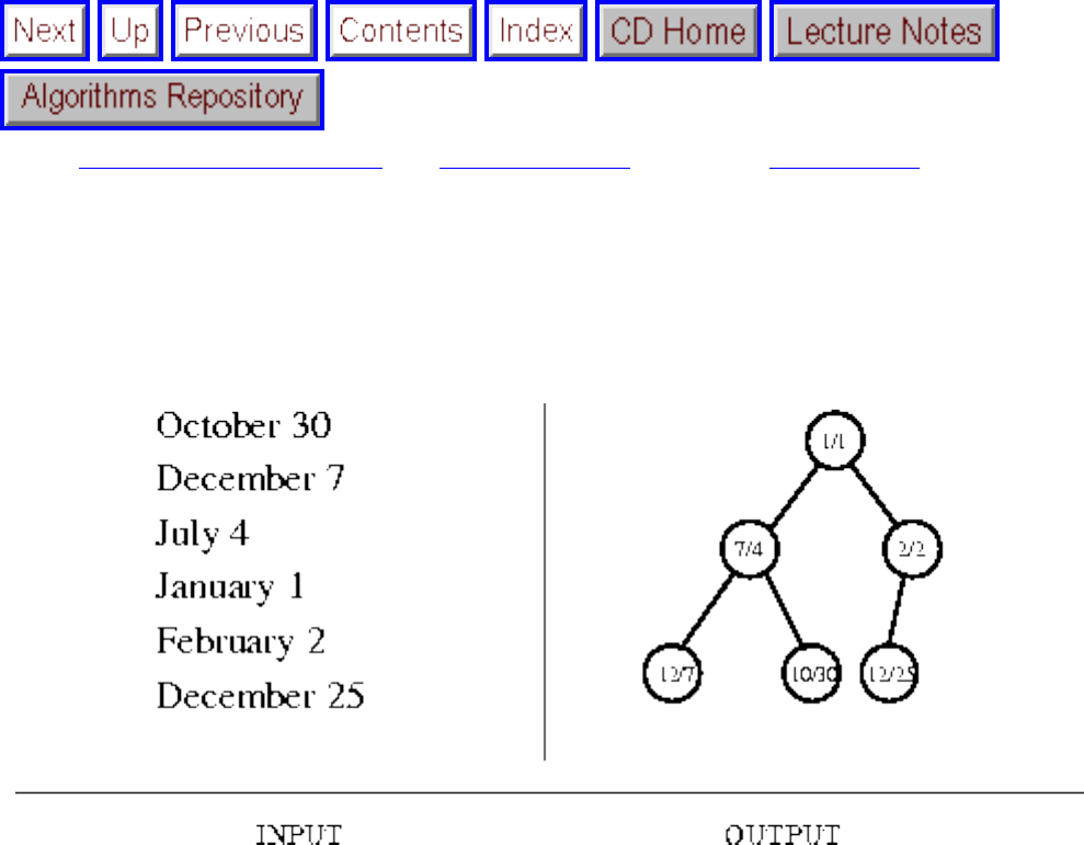
Priority Queues
Next: Suffix Trees and Arrays Up: Data Structures Previous: Dictionaries
Priority Queues
Input description: A set of records with numerically or otherwise totally ordered keys.
Problem description: Build and maintain a data structure for quickly inserting and deleting records,
while enabling quick access to the smallest or largest key in the set.
Discussion: Priority queues are useful data structures in simulations, particularly for maintaining a set of
future events ordered by time so that we can quickly retrieve what the next thing to happen is. They are
called ``priority'' queues because they enable you to retrieve items not by the insertion time (as in a stack
or queue), nor by a key match (as in a dictionary), but by which item has the highest priority of retrieval.
If your application performs no insertions after the first query, there is no need for an explicit priority
queue. Simply sort the records by priority and proceed from top to bottom, maintaining a pointer to the
last record deleted. This situation occurs in Kruskal's minimum spanning tree algorithm, or when
simulating a completely scripted set of events.
However, if you are mixing insertions, deletions, and queries, you need a real priority queue. The
following questions will help select the right one:
file:///E|/BOOK/BOOK3/NODE130.HTM (1 of 4) [19/1/2003 1:30:05]
Priority Queues
● Besides access to the smallest element, what other operations will you need? - Will you be
searching for arbitrary keys, or just searching for the smallest? Will you be deleting arbitrary
elements from the data, or just repeatedly deleting the top or smallest element?
● Will you know the maximum size of your data structure in advance, or might an arbitrary number
of items be inserted into it? - The issue here is whether you can preallocate space for the data
structure.
● Will you be changing the priority of elements already in the queue, or simply inserting and
removing them? - Changing the priority of elements implies that we must be able to look up
elements in the queue based on their key, in addition to being able to retrieve the largest element.
Depending upon the answers, you have the following basic priority queue choices:
● Sorted array or list - In a sorted array, it is very efficient to find and (by decrementing the top
index) delete the smallest element. However, maintaining sortedness makes the insertion of new
elements slow. Sorted arrays are suitable when there will be few insertions into the priority queue.
● Binary heaps - This simple, elegant data structure supports both insertion and extract-min in
time each. Heaps maintain an implicit binary tree structure in an array, such that the
key of the root of any subtree is less than that of all its descendents. Thus the minimum key is
always at the root of the heap. New keys can be inserted by placing them at an open leaf and
percolating the element upwards until it sits at its proper place in the partial order.
Binary heaps are the right answer whenever you know an upper bound on the number of items in
your priority queue, since you must specify the array size at creation time.
● Bounded height priority queue - This array-based data structure permits constant-time insertion
and find-min operations whenever the range of possible key values is limited. Suppose we know
that all key values will be integers between 1 and n. We can set up an array of n linked lists, such
that the ith list serves as a bucket containing all items with key i. We will maintain a pointer top to
the smallest nonempty list. To insert an item with key k into the priority queue, add it to the kth
bucket and set . To extract the minimum, report the first item from bucket top,
delete it, and move top down if the bucket is now empty.
Bounded height priority queues are very useful in maintaining the vertices of a graph sorted by
degree, which is a fundamental operation in graph algorithms. Still, they are not as widely
known as they should be. They are usually the right priority queue for any small, discrete range of
keys.
● Binary search trees - Binary search trees make effective priority queues, since the smallest
element is always the leftmost leaf, while the largest element is always the rightmost leaf. The
min (max) is found by simply tracing down left (right) pointers until the next pointer is nil. Binary
tree heaps prove most appropriate when you also need to search a dictionary of the values, or if
you have an unbounded key range and do not know the maximum priority queue size in advance.
● Fibonacci and pairing heaps - These complicated priority queues are designed to speed up
decrease-key operations, where the priority of an item already in the priority queue is reduced.
file:///E|/BOOK/BOOK3/NODE130.HTM (2 of 4) [19/1/2003 1:30:05]
Priority Queues
This arises, for example, in shortest path computations whenever we discover a shorter route to a
vertex v than we had previously established. Thus v has a higher priority of being accessed next.
Properly implemented and used, they lead to better performance on very large computations. Still,
they are sufficiently complicated that you shouldn't mess with them unless you really know what
you are doing.
Implementations: LEDA (see Section ) provides a complete collection of priority queues in C++,
including Fibonacci heaps, pairing heaps, Emde-Boas trees, and bounded height priority queues.
Fibonacci heaps are their default implementation.
SimPack/Sim++ is a library of routines for implementing discrete event simulations, built by Robert
Cubert and Paul Fishwick, of the University of Florida. Priority queues are integral to such
simulations, and Sim++ contains implementations of linked, binary, leftist, and calendar heaps [Bro88].
If you need a priority queue to control a simulation, check out http://www.cis.ufl.edu/
fishwick/simpack/simpack.html. An associated book [Fis95] describes model design using SimPack.
Bare bones implementations in C and Pascal of the basic priority queue data structures appear in
[GBY91]. Most notable is the inclusion of implementations of exotic priority queues such as P-trees and
pagodas. See Section for further details.
XTango (see Section ) is an algorithm animation system for UNIX and X-windows, that includes
animations of such advanced priority queue data structures as binomial and Fibonacci heaps, as well as a
spiffy animation of heapsort.
Many textbooks provide implementations of simple priority queues, including [MS91] (see Section ).
Algorithm 561 [Kah80] of the Collected Algorithms of the ACM is a Fortran implementation of a heap
(see Section ).
Notes: Good expositions on efficient heap construction algorithms include [Baa88, Ben86, CLR90,
Man89, MT90b]. See [GBY91] for a description of several exotic priority queues. Empirical
comparisons between priority queue data structures include [Jon86].
Bounded height priority queues are useful data structures in practice, but they do not have good worst-
case performance bounds when arbitrary insertions and deletions are permitted. However, von Emde
Boas priority queues [vEBKZ77] support insertion, deletion, search, max, and min operations
where each key is an element from 1 to n.
file:///E|/BOOK/BOOK3/NODE130.HTM (3 of 4) [19/1/2003 1:30:05]
Priority Queues
Fibonacci heaps [FT87] support insert and decrease-key operations in O(1) amortized time, with
amortized time extract-min and delete operations. The constant-time decrease-key operation leads to
faster implementations of classical algorithms for shortest-paths, weighted bipartite-matching, and
minimum-spanning-tree. In practice, Fibonacci heaps are nontrivial to implement and have large
constant factors associated with them. However, pairing heaps have been proposed to realize the same
bounds with less overhead. Experiments with pairing heaps are reported in [SV87].
Heaps define a partial order that can be built using a linear number of comparisons. The familiar linear-
time merging algorithm for heap construction is due to Floyd [Flo64]. In the worst case, 1.625n
comparisons suffice [GM86] and comparisons are necessary [CC92].
Related Problems: Dictionaries (see page ), sorting (see page ), shortest path (see page ).
Next: Suffix Trees and Arrays Up: Data Structures Previous: Dictionaries
Algorithms
Mon Jun 2 23:33:50 EDT 1997
file:///E|/BOOK/BOOK3/NODE130.HTM (4 of 4) [19/1/2003 1:30:05]
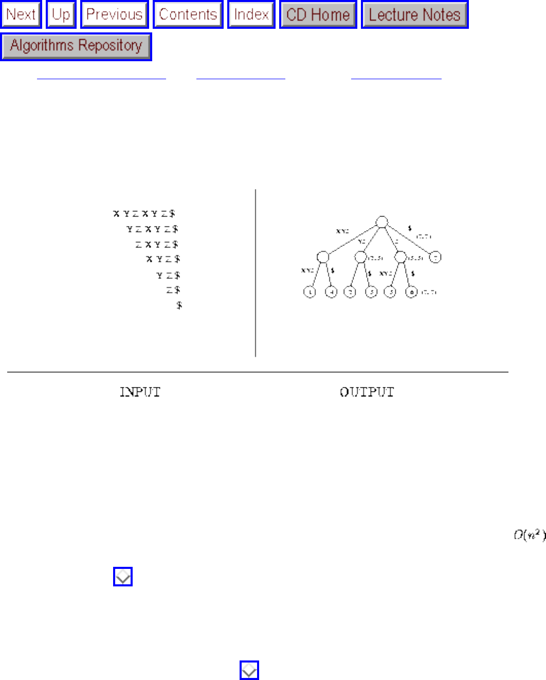
Suffix Trees and Arrays
Next: Graph Data Structures Up: Data Structures Previous: Priority Queues
Suffix Trees and Arrays
Input description: A reference string S.
Problem description: Build a data structure for quickly finding all places where an arbitrary query string
q is a substring of S.
Discussion: Suffix trees and arrays are phenomenally useful data structures for solving string problems
efficiently and with elegance. If you need to speed up a string processing algorithm from to linear
time, proper use of suffix trees is quite likely the answer. Indeed, suffix trees are the hero of the war story
reported in Section . In its simplest instantiation, a suffix tree is simply a trie of the n strings that
are suffixes of an n-character string S. A trie is a tree structure, where each node represents one
character, and the root represents the null string. Thus each path from the root represents a string,
described by the characters labeling the nodes traversed. Any finite set of words defines a trie, and two
words with common prefixes will branch off from each other at the first distinguishing character. Each
leaf represents the end of a string. Figure illustrates a simple trie.
file:///E|/BOOK/BOOK3/NODE131.HTM (1 of 4) [19/1/2003 1:30:07]
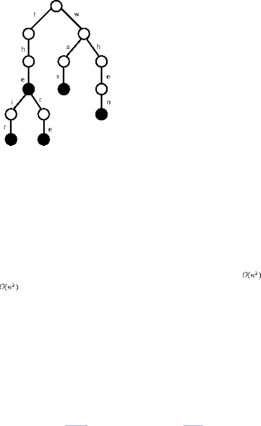
Suffix Trees and Arrays
Figure: A trie on strings the, their, there, was, and when
Tries are useful for testing whether a given query string q is in the set. Starting with the first character
of q, we traverse the trie along the branch defined by the next character of q. If this branch does not exist
in the trie, then q cannot be one of the set of strings. Otherwise we find q in |q| character comparisons
regardless of how many strings are in the trie. Tries are very simple to build (repeatedly insert new
strings) and very fast to search, although they can be expensive in terms of memory.
A suffix tree is simply a trie of all the proper suffixes of S. The suffix tree enables you to quickly test
whether q is a substring of S, because any substring of S is the prefix of some suffix (got it?). The search
time is again linear in the length of q.
The catch is that constructing a full suffix tree in this manner can require time and, even worse,
space, since the average length of the n suffices is n/2 and there is likely to be relatively little
overlap representing shared prefixes. However, linear space suffices to represent a full suffix tree by
being clever. Observe that most of the nodes in a trie-based suffix tree occur on simple paths between
branch nodes in the tree. Each of these simple paths corresponds to a substring of the original string. By
storing the original string in an array and collapsing each such path into a single node described by the
starting and ending array indices representing the substring, we have all the information of the full suffix
tree in only O(n) space. The output figure for this section displays a collapsed suffix tree in all its glory.
Even better, there exist linear-time algorithms to construct this collapsed tree that make clever use of
pointers to minimize construction time. The additional pointers used to facilitate construction can also be
used to speed up many applications of suffix trees.
But what can you do with suffix trees? Consider the following applications. For more details see the
books by Gusfield [Gus97] or Crochemore and Rytter [CR94]:
file:///E|/BOOK/BOOK3/NODE131.HTM (2 of 4) [19/1/2003 1:30:07]
Suffix Trees and Arrays
● Find all occurrences of q as a substring of S - Just as with a trie, we can walk down from the root
to find the node associated with q. The positions of all occurrences of q in S are represented by
the descendents of , which can be identified using a depth-first search from . For collapsed
suffix trees, this takes O(|q|+k) time if there are k occurrences of q in S.
● Longest substring common to a set T of strings - Build a single collapsed suffix tree
containing all suffixes of all strings, with each leaf labeled with its original string. In the course of
doing a depth-first search on this tree, we can label each node with both the length of its common
prefix and the number of distinct strings from T that are children of it. Thus the best node can be
selected in linear time.
● Find the longest palindrome in S - A palindrome is a string that reads the same if the order of
characters is reversed, such as madam. To find the longest palindrome in a string S, build a single
suffix tree containing all suffixes of S and the reversal of S, with each leaf identified by its starting
position. A palindrome is defined by any node in this tree that has forward and reversed children
from the same position.
Since the linear time suffix tree construction algorithm is tricky, I recommend either starting from an
existing implementation or using a simple, potentially quadratic-time incremental-insertion algorithm to
build a compressed suffix tree. Another good option is to use suffix arrays, discussed below.
Suffix arrays do most of what suffix trees do, while typically using four times less memory than suffix
trees. They are also easier to implement. A suffix array is basically just an array that contains all the n
suffixes of S in sorted order. Thus a binary search of this array for string q suffices to locate the prefix of
a suffix that matches q, permitting efficient substring search in string comparisons. In fact, only
character comparisons need be performed on any query, since we can identify the next character
that must be tested in the binary search. For example, if the lower range of the search is cowabunga and
the upper range is cowslip, all keys in between must share the same first three letters, so only the fourth
character of any intermediate key must be tested against q.
The space savings of suffix arrays result because as with compressed suffix trees, it suffices to store
pointers into the original string instead of explicitly copying the strings. Suffix arrays use less memory
than suffix trees by eliminating the need for explicit pointers between suffixes since these are implicit in
the binary search. In practice, suffix arrays are typically as fast or faster to search than suffix trees. Some
care must be taken to construct suffix arrays efficiently, however, since there are characters in the
strings being sorted. A common solution is to first build a suffix tree, then perform an in-order traversal
of it to read the strings off in sorted order!
Implementations: Ting Chen's and Dimitris Margaritis's C language implementations of suffix trees,
reported in the war story of Section , are available on the algorithm repository WWW site:
http://www.cs.sunysb.edu/ algorith.
Bare bones implementations in C of digital and Patricia trie data structures and suffix arrays appear in
file:///E|/BOOK/BOOK3/NODE131.HTM (3 of 4) [19/1/2003 1:30:07]
Suffix Trees and Arrays
[GBY91]. See Section for details.
Notes: Tries were first proposed by Fredkin [Fre62], the name coming from the central letters of the
word ``retrieval''. A survey of basic trie data structures with extensive references appears in [GBY91].
Expositions on tries include [AHU83].
Efficient algorithms for suffix tree construction are due to Weiner [Wei73], McCreight [McC76], and
Ukkonen [Ukk92]. Good expositions on these algorithms include Crochmore and Wytter [CR94] and
Gusfield [Gus97]. Textbooks include [Woo93] and [AHU74], where they are called position trees.
Several applications of suffix trees to efficient string algorithms are discussed in [Apo85].
Suffix arrays were invented by Manber and Myers [MM90], although an equivalent idea called Pat trees
due to Gonnet and Baeza-Yates appears in [GBY91].
The power of suffix trees can be further augmented by using a data structure for computing the least
common ancestor of any pair of nodes x, y in a tree in constant time, after linear-time preprocessing of
the tree. The original data structure is due to Harel and Tarjan [HT84], but it was significantly
simplified by Schieber and Vishkin [SV88]. Expositions include Gusfield [Gus97]. The least common
ancestor (LCA) of two nodes in a suffix tree or trie defines the node representing the longest common
prefix of the two associated strings. Being able to answer such queries in constant time is amazing, and
useful as a building block for many other algorithms. The correctness of the LCA data structure is
difficult to see; however, it is implementable and can perform well in practice.
Related Problems: string matching (see page ), longest common substring (see page ).
Next: Graph Data Structures Up: Data Structures Previous: Priority Queues
Algorithms
Mon Jun 2 23:33:50 EDT 1997
file:///E|/BOOK/BOOK3/NODE131.HTM (4 of 4) [19/1/2003 1:30:07]
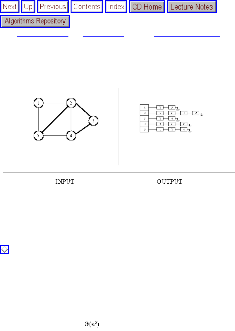
Graph Data Structures
Next: Set Data Structures Up: Data Structures Previous: Suffix Trees and Arrays
Graph Data Structures
Input description: A graph G.
Problem description: Give a flexible, efficient data structure to represent G.
Discussion: While there are several possible variations, the two basic data structures for graphs are
adjacency matrices and adjacency lists. What these data structures actually are is discussed in Section
. The issues in deciding which one to use include:
● How big will your graph be? - How many vertices will it have, both typically and in the worse
case? Ditto for the number of edges? If your graph has 100 vertices, your adjacency matrix
contains 10,000 entries. If your graph has 1,000 vertices, your adjacency matrix contains
1,000,000 entries. If your graph has 10,000 vertices, your adjacency matrix contains 100,000,000
entries - so forget about it. Adjacency matrices work only for small or very dense graphs.
● How dense will your graph be? - If the graph is very dense, meaning that a large fraction of the
vertex pairs define edges, there is probably no compelling reason to use adjacency lists, since you
will be doomed to using space, anyway.
● Which algorithms will you be implementing? - Certain algorithms are easier on adjacency
matrices (such as all-pairs shortest path) and others on adjacency lists (such as most DFS-based
file:///E|/BOOK/BOOK3/NODE132.HTM (1 of 5) [19/1/2003 1:30:08]

Graph Data Structures
algorithms). Adjacency matrices win for algorithms that repeatedly ask, ``Is (i,j) in G?'' However,
most graph algorithms can be modified to eliminate such queries.
● Will you be modifying the graph over the course of your application, and if so, how? - Repeated
edge insertions and (particularly) deletions argue for adjacency matrices, or perhaps for fancier
versions of adjacency lists such as binary search trees. However, more likely than modifying the
topology of graph is modifying the attributes of a vertex or edge of the graph, such as size,
weight, or color. Attributes are best handled as extra fields in the vertex or edge records of
adjacency lists.
Building a good general-purpose graph type is surprisingly tricky and difficult. For this reason, we
suggest that you check out existing implementations (particularly LEDA) before hacking up your own.
Note that it costs only time linear in the size of the larger data structure to convert between adjacency
matrices and adjacency lists. This conversion is unlikely to be the bottleneck in any application, if you
decide you want to use both data structures and have the space to store them. This usually isn't necessary
but might prove simplest if you are confused about the alternatives.
Planar graphs are those that can be drawn in the plane so that no two edges cross. Many graphs arising
in applications are planar by definition, such as maps of countries, while others are planar by
happenstance, like any tree. Planar graphs are always sparse, since any n-vertex planar graph can have
at most 3n-6 edges, so they should usually be represented by adjacency lists. If the planar drawing (or
embedding) of the graph is fundamental to what is being computed, planar graphs are best represented
geometrically. See Section for algorithms for constructing planar embeddings from graphs, and
Section for algorithms maintaining graphs implicit in the arrangements of geometric objects like
lines and polygons.
Hypergraphs are generalized graphs where each edge may link subsets of more than two vertices. For
example, suppose we want to represent who is on which Congressional committee. The vertices of our
hypergraph would be the individual congressmen, while each hyperedge would represent one committee.
Such arbitrary collections of subsets of a set are naturally thought of as hypergraphs.
Two basic data structures for hypergraphs are:
● Incidence matrices, which are analogous to adjacency matrices and require space, where m
is the number of hyperedges. Each row corresponds to a vertex, and each column to an edge,
with a nonzero entry in M[i,j] iff vertex i is incident to edge j. For standard graphs, there are two
nonzero entries in each column. The degree of each vertex governs the number of nonzero entries
in each row.
● Bipartite incidence structures, which are analogous to adjacency lists, and hence suited for sparse
hypergraphs. There is a vertex of the incidence structure associated with each edge and vertex of
the hypergraphs, and an edge (i,j) in the incidence structure if vertex i of the hypergraph is in edge
j of the hypergraph. Adjacency lists are typically used to represent this incidence structure. This
bipartite incidence structure also provides a natural way to visualize the hypergraph, by drawing
file:///E|/BOOK/BOOK3/NODE132.HTM (2 of 5) [19/1/2003 1:30:08]
Graph Data Structures
the associated bipartite graph.
Special efforts must be taken to represent very large graphs efficiently. However, interesting problems
have been solved on graphs with millions of edges and vertices. The first step is to make your data
structure as lean as possible, by packing your adjacency matrix as a bit vector (see Section ) or
removing extra pointers from your adjacency list representation. For example, in a static graph (no edge
insertions or deletions) each edge list can be replaced by a packed array of vertex identifiers, thus
eliminating pointers and saving potentially half the space.
At some point it may become necessary to switch to a hierarchical representation of the graph, where the
vertices are clustered into subgraphs that are compressed into single vertices. Two approaches exist for
making such a hierarchical decomposition. The first breaks things into components in a natural or
application-specific way. For example, knowing that your graph is a map of roads and cities suggests a
natural decomposition - partition the map into districts, towns, counties, and states. The other approach
runs a graph partition algorithm as in Section . If you are performing the decomposition for space or
paging reasons, a natural decomposition will likely do a better job than some naive heuristic for an NP-
complete problem. Further, if your graph is really unmanageably large, you cannot afford to do a very
good job of algorithmically partitioning it. You should first verify that standard data structures fail on
your problem before attempting such heroic measures.
Implementations: LEDA (see Section ) provides the best implemented graph data type currently
available in C++. If at all possible, you should use it. If not, you should at least study the methods it
provides for graph manipulation, so as to see how the right level of abstract graph type makes
implementing algorithms very clean and easy. Although a general graph implementation like LEDA
may be 2 to 5 times slower and considerably less space efficient than a stripped-down special-purpose
implementation, you have to be a pretty good programmer to realize this performance improvement.
Further, this speed is likely to come at the expense of simplicity and clarity.
GraphEd [Him94], written in C by Michael Himsolt, is a powerful graph editor that provides an interface
for application modules and a wide variety of graph algorithms. If your application demands interaction
and visualization more than sophisticated algorithmics, GraphEd might be the right place to start,
although it can be buggy. GraphEd can be obtained by anonymous ftp from forwiss.uni-passau.de
(132.231.20.10) in directory /pub/local/graphed. See Section for more details on GraphEd and other
graph drawing systems.
The Stanford Graphbase (see Section ) provides a simple but flexible graph data structure in CWEB, a
literate version of the C language. It is instructive to see what Knuth does and does not place in his basic
data structure, although we recommend LEDA as a better basis for further development.
LINK is an environment for combinatorial computing that provides special support for hypergraphs,
file:///E|/BOOK/BOOK3/NODE132.HTM (3 of 5) [19/1/2003 1:30:08]
Graph Data Structures
including the visualization of hypergraphs. Although written in C++, it provides a Scheme language
interface for interacting with the graphs. LINK is available from
http://dimacs.rutgers.edu/Projects/LINK.html .
An elementary implementation of a ``lazy'' adjacency matrix in Pascal, which does not have to be
initialized, appears in [MS91]. See Section .
Simple graph data structures in Mathematica are provided by Combinatorica [Ski90], with a library of
algorithms and display routines. See Section .
Notes: It was not until the linear-time algorithms of Hopcroft and Tarjan [HT73b, Tar72] that the
advantages of adjacency list data structures for graphs became apparent. The basic adjacency list and
matrix data structures are presented in essentially all books on algorithms or data structures, including
[CLR90, AHU83, Tar83].
An interesting question concerns minimizing the number of bits needed to represent arbitrary graphs on n
vertices, particularly if certain operations must be supported efficiently. Such issues are discussed in
[vL90b].
Dynamic graph algorithms are essentially data structures that maintain quick access to an invariant (such
as minimum spanning tree or connectivity) under edge insertion and deletion. Sparsification [EGIN92]
is a general and interesting approach to constructing dynamic graph algorithms. See [ACI92] for an
experimental study on the practicality of dynamic graph algorithms.
Hierarchically-defined graphs often arise in VLSI design problems, because designers make extensive
use of cell libraries [Len90]. Algorithms specifically for hierarchically-defined graphs include planarity
testing [Len89], connectivity [LW88], and minimum spanning trees [Len87].
The theory of hypergraphs is presented by Berge [Ber89].
Related Problems: Set data structures (see page ), graph partition (see page ).
Next: Set Data Structures Up: Data Structures Previous: Suffix Trees and Arrays
Algorithms
file:///E|/BOOK/BOOK3/NODE132.HTM (4 of 5) [19/1/2003 1:30:08]
Graph Data Structures
Mon Jun 2 23:33:50 EDT 1997
file:///E|/BOOK/BOOK3/NODE132.HTM (5 of 5) [19/1/2003 1:30:08]
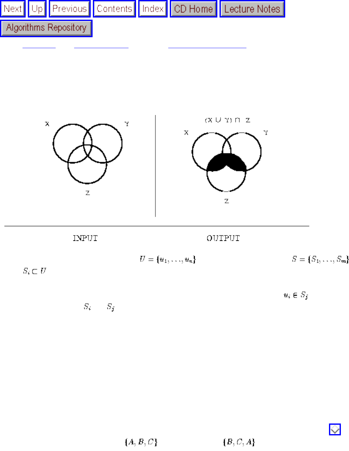
Set Data Structures
Next: Kd-Trees Up: Data Structures Previous: Graph Data Structures
Set Data Structures
Input description: A universe of items and a collection of subsets ,
where .
Problem description: Represent each subset so as to efficiently (1) test whether , (2) find the
union or intersection of and , and (3) insert or delete members of S.
Discussion: In mathematical terms, a set is an unordered collection of objects drawn from a fixed
universal set. However, it is usually useful for implementation to represent each set in a single canonical
order, typically sorted, so as to speed up or simplify various operations. Sorted order turns the problem
of finding the union or intersection of two subsets into a linear-time operation - just sweep from left to
right and see what you are missing. It also makes possible element searching in sublinear time. Finally,
printing the elements of a set in a canonical order paradoxically reminds us that order really doesn't
matter.
We distinguish sets from two other kinds of objects: strings and dictionaries. If there is no fixed-size
universal set, a collection of objects is best thought of as a dictionary, as discussed in Section . If the
order does matter in a subset, i.e. if is not the same as , then your structure is more
file:///E|/BOOK/BOOK3/NODE133.HTM (1 of 4) [19/1/2003 1:30:10]
Set Data Structures
profitably thought of as a string, so see Sections and .
When each subset has cardinality exactly two, they form edges in a graph whose vertices are the
universal set. A system of subsets with no restrictions on the cardinality of its members is called a
hypergraph. It often can be profitable to consider whether your problem has a graph-theoretical analogy,
like connected components or shortest path in a hypergraph.
Your primary alternatives for representing arbitrary systems of subsets are:
● Bit vectors - If your universal set U contains n items, an n-bit vector or array can represent any
subset . Bit i will be 1 if , otherwise bit i is 0. Since only one bit is used per element,
bit vectors can be very space efficient for surprisingly large values of |U|. Element insertion and
deletion simply flips the appropriate bit. Intersection and union are done by ``and-ing'' or ``or-ing''
the bits together. The only real drawback of a bit vector is that for sparse subsets, it takes O(n)
time to explicitly identify all members of S.
● Containers or dictionaries - A subset can also be represented using a linked list, array, binary
tree, or dictionary containing exactly the elements in the subset. No notion of a fixed universal set
is needed for such a data structure. For sparse subsets, dictionaries can be more space and time
efficient than bit vectors and easier to work with and program. For efficient union and intersection
operations, it pays to keep the elements in each subset sorted, so a linear-time traversal through
both subsets identifies all duplicates.
In many applications, the subsets are all pairwise disjoint, meaning that each element is in exactly one
subset. For example, consider maintaining the connected components of a graph or the party affiliations
of politicians. Each vertex/hack is in exactly one component/party. Such a system of subsets is called a
set partition. Algorithms for constructing partitions of a given set are provided in Section .
For data structures, the primary issue is maintaining a given set partition as things change over time,
perhaps as edges are added or party members defect. The queries we are interested in include ``which set
is a particular item in?'' and ``are two items in the same set?'' as we modify the set by (1) changing one
item, (2) merging or unioning two sets, or (3) breaking a set apart. Your primary options are:
● Dictionary with subset attribute - If each item in a binary tree has associated a field recording the
name of the subset it is in, set identification queries and single element modifications can be
performed in the time it takes to search in the dictionary, typically . However, operations
like performing the union of two subsets take time proportional to (at least) the sizes of the
subsets, since each element must have its name changed. The need to perform such union
operations quickly is the motivation for the ...
● Union-Find Data Structure - Suppose we represent a subset using a rooted tree, where each node
points to its parent instead of its children. Further, let the name of the subset be the name of the
item that is the root. Finding out which subset we are in is simple, for we keep traversing up the
file:///E|/BOOK/BOOK3/NODE133.HTM (2 of 4) [19/1/2003 1:30:10]
Set Data Structures
parent pointers until we hit the root. Unioning two subsets is also easy. Just make the root of one
of two trees point to the other, so now all elements have the same root and thus the same subset
name.
Certain details remain, such as which subset should be the ultimate root of a union, but these are
described in most every algorithms text. Union-Find is a fast, extremely simple data structure that
every programmer should know about. It does not support breaking up subsets created by unions,
but usually this is not an issue.
Neither of these options provides access to all of the items in a particular subset without traversing all the
items in the set. However, both can be appropriately augmented with extra pointers if it is important that
this operation be fast.
Implementations: LEDA (see Section ) provides dictionary data structures to maintain sets and the
union-find data structure to maintain set partitions, all in C++.
LINK is an environment for combinatorial computing that provides special support for hypergraphs,
including visualization of hypergraphs. Although written in C++, it provides an additional Scheme
language interface for interacting with the graphs. LINK is available from
http://dimacs.rutgers.edu/Projects/LINK.html.
Many textbooks contain implementations of the union-find data structure, including [MS91] (see Section
). An implementation of union-find underlies any implementation of Kruskal's minimum spanning
tree algorithm. Section contains a selection of minimum spanning tree codes.
Notes: Optimal algorithms for such set operations as intersection and union were presented in [Rei72].
Good expositions on set data structures include [AHU83].
Galil and Italiano [GI91] survey data structures for disjoint set union. Expositions on the union-find
data structure appear in most algorithm texts, including [CLR90, MS91]. The upper bound of
on m union-find operations on an n-element set is due to Tarjan [Tar75], as is a matching
lower bound on a restricted model of computation [Tar79]. The inverse Ackerman function
grows notoriously slowly, so this performance is close to linear. Expositions on the Ackerman bound
include [AHU74]. An interesting connection between the worst-case of union-find and the length of
Davenport-Schintzl sequences, a combinatorial structure that arises in computational geometry, is
established in [SA95].
The power set of a set S is the collection of all subsets of S. Explicit manipulation of power sets
quickly becomes intractable due to their size. Implicit representations of power sets in symbolic form
becomes necessary for nontrivial computations. See [BCGR92] for algorithms for and computational
file:///E|/BOOK/BOOK3/NODE133.HTM (3 of 4) [19/1/2003 1:30:10]
Set Data Structures
experience with symbolic power set representations.
Related Problems: Generating subsets (see page ), generating partitions (see page ), set cover (see
page ), minimum spanning tree (see page ).
Next: Kd-Trees Up: Data Structures Previous: Graph Data Structures
Algorithms
Mon Jun 2 23:33:50 EDT 1997
file:///E|/BOOK/BOOK3/NODE133.HTM (4 of 4) [19/1/2003 1:30:10]

Kd-Trees
Next: Numerical Problems Up: Data Structures Previous: Set Data Structures
Kd-Trees
Input description: A set S of n points in k dimensions.
Problem description: Construct a tree that partitions the space by half-planes such that each point is
contained in its own box-shaped region.
Discussion: Although many different flavors of kd-trees have been devised, their purpose is always to
hierarchically decompose space into a relatively small number of cells such that no cell contains too
many input objects. This provides a fast way to access any input object by position. We traverse down
the hierarchy until we find the cell containing the object and then scan through the few objects in the cell
to identify the right one.
Typical algorithms construct kd-trees by partitioning point sets. Each node in the tree is defined by a
plane through one of the dimensions that partitions the set of points into left/right (or up/down) sets, each
with half the points of the parent node. These children are again partitioned into equal halves, using
planes through a different dimension. Partitioning stops after levels, with each point in its own leaf
cell. Alternate kd-tree construction algorithms insert points incrementally and divide the appropriate cell,
although such trees can become seriously unbalanced.
file:///E|/BOOK/BOOK3/NODE134.HTM (1 of 4) [19/1/2003 1:30:12]
Kd-Trees
The cutting planes along any path from the root to another node defines a unique box-shaped region of
space, and each subsequent plane cuts this box into two boxes. Each box-shaped region is defined by 2k
planes, where k is the number of dimensions. Indeed, the `kd' in kd-tree is short for k-dimensional tree. In
any search performed using a kd-tree, we maintain the current region defined by the intersection of these
half-spaces as we move down the tree.
Different flavors of kd-trees differ in exactly how the splitting plane is selected. Options include:
● Cycling through the dimensions - partition first on , then before cycling back to .
● Cut along the largest dimension - select the partition dimension so as to make the resulting boxes
as square or cube-like as possible. Selecting a plane to partition the points in half does not mean
selecting a splitter in the middle of the box-shaped regions, since all the points may be in the left
side of the box.
● Quadtrees or Octtrees - Instead of partitioning with single planes, use all axis-parallel planes
that pass through a given partition point. In two dimensions, this means creating four child cells,
in 3D this means eight child cells. Quadtrees seem particularly popular on image data, where leaf
cells imply that all pixels in the regions have the same color.
Nonorthogonal (i.e. not axis-parallel) cutting planes have also been used, although they make
maintaining the cell boundaries more complicated.
Ideally, our partitions evenly split both the space (ensuring nice, fat, regular regions) and the set of points
(ensuring a log height tree) evenly, but this can be impossible for a given point set. The advantages of fat
cells become clear in many applications of kd-trees:
● Point location - To identify which cell a query point q lies in, we start at the root and test which
side of the partition plane contains q. By repeating this process on the appropriate child node, we
travel the tree to find the leaf cell containing q in time proportional to its height. See Section
for more on point location.
● Nearest neighbor search - To find the point in S closest to a query point q, we perform point
location to find the cell c containing q. Since c is bordered by some point p, we can compute the
distance d(p,q) from p to q. Point p is likely very close to q, but it might not be the single closest
neighbor. Why? Suppose q lies right at the boundary of a cell. Then q's nearest neighbor might lie
just to the left of the boundary in another cell. Thus we must traverse all cells that lie within a
distance of d(p,q) of cell c and verify that none of them contain closer points. With nice, fat cells,
very few cells should need to be tested. See Section for more on nearest neighbor search.
● Range search - Which points lie within a query box or region? Starting from the root, check to
see whether the query region intersects or contains the cell defining the current node. If it does,
check the children; if not, none of the leaf cells below this node can possibly be of interest. We
quickly prune away the irrelevant portions of the space. See Section for more on range search.
● Partial key search - Suppose we want to find a point p in S, but we do not have full information
file:///E|/BOOK/BOOK3/NODE134.HTM (2 of 4) [19/1/2003 1:30:12]
Kd-Trees
about p. Say we are looking for someone of age 35 and height 5'8'' but of unknown weight in a 3d-
tree with dimensions age, weight, and height. Starting from the root, we can identify the correct
decendant for all but the weight dimension. To be sure we find the right point, we must search
both children of this node. We are better off the more fields we know, but such partial key search
can be substantially faster than checking all points against the key.
Kd-trees are most effective data structures for small and moderate numbers of dimensions, say from 2 up
to maybe 20 dimensions. As the dimensionality increases, they lose effectiveness, primarily because the
ratio of the volume of a unit sphere in k-dimensions shrinks exponentially compared to a unit cube in k-
dimensions. Thus exponentially many cells will have to be searched within a given radius of a query
point, say for nearest-neighbor search. Also, the number of neighbors for any cell grows to 2k and
eventually become unmanageable.
The bottom line is that you should try to avoid working in high-dimensional spaces, perhaps by
discarding the least important dimensions.
Implementations: Ranger is a tool for visualizing and experimenting with nearest neighbor and
orthogonal range queries in high-dimensional data sets, using multidimensional search trees. Four
different search data structures are supported by Ranger: naive kd-trees, median kd-trees, nonorthogonal
kd-trees, and the vantage point tree. For each of these, Ranger supports queries in up to 25 dimensions
under any Minkowski metric. It includes generators for a variety of point distributions in arbitrary
dimensions. Finally, Ranger provides a number of features to aid in visualizing multidimensional data,
best illustrated by the accompanying video [MS93]. To identify the most appropriate projection at a
glance, Ranger provides a matrix of all two-dimensional projections of the data set. Ranger is
written in C, runs on Silicon Graphics and HP workstations, and is available from the algorithm
repository.
The 1996 DIMACS implementation challenge focuses on data structures for higher-dimensional data
sets. The world's best kd-tree implementations were likely to be identified in the course of the challenge,
and they are accessible from http://dimacs.rutgers.edu/.
Bare bones implementations in C of kd-tree and quadtree data structures appear in [GBY91]. See Section
for details on how to ftp them.
Notes: The best reference on kd-trees and other spatial data structures are two volumes by Samet
[Sam90a, Sam90b], in which all major variants are developed in substantial detail.
Bentley [Ben75] is generally credited with developing kd-trees, although they have the typically murky
history associated with most folk data structures. The most reliable history is likely from Samet
[Sam90b].
file:///E|/BOOK/BOOK3/NODE134.HTM (3 of 4) [19/1/2003 1:30:12]
Kd-Trees
An exposition on kd-trees for orthogonal range queries in two dimensions appears in [PS85].
Expositions of grid files and other spatial data structures include [NH93].
Algorithms that quickly produce a point provably close to the query point are a recent development in
higher-dimensional nearest neighbor search. A sparse weighted-graph structure is built from the data
set, and the nearest neighbor is found by starting at a random point and walking greedily in the graph
towards the query point. The closest point found during several random trials is declared the winner.
Similar data structures hold promise for other problems in high-dimensional spaces. See [AM93, AMN
94].
Related Problems: Nearest-neighbor search (see page ), point location (see page ), range search
(see page ).
Next: Numerical Problems Up: Data Structures Previous: Set Data Structures
Algorithms
Mon Jun 2 23:33:50 EDT 1997
file:///E|/BOOK/BOOK3/NODE134.HTM (4 of 4) [19/1/2003 1:30:12]
Numerical Problems
Next: Solving Linear Equations Up: A Catalog of Algorithmic Previous: Kd-Trees
Numerical Problems
If most problems you encounter are numerical in nature, there is a good chance that you are reading the
wrong book. Numerical Recipes [PFTV86] gives a terrific overview to the fundamental problems in
numerical computing, including linear algebra, numerical integration, statistics, and differential
equations. Different flavors of the book include source code for all the algorithms in C, Pascal, and
Fortran. Their coverage is skimpier on the combinatorial/numerical problems we consider in this section,
but you should be aware of that book.
Numerical algorithms tend to be different beasts than combinatorial algorithms, for at least two distinct
reasons:
● Issues of Precision and Error - Numerical algorithms typically perform repeated floating-point
computations, which accumulate error at each operation until, eventually, the results are
meaningless. An amusing example [SK93] concerns the Vancouver Stock Exchange, which over
a twenty-two month period accumulated sufficient round-off error to reduce its index from the
correct value of 1098.982 to 574.081.
A simple and dependable way to test for round-off errors in numerical programs is to run them
both at single and double precision, and then think hard whenever there is a disagreement.
● Extensive Libraries of Codes - Large, high-quality libraries of numerical routines have existed
since the 1960s, which is still not the case for combinatorial algorithms. This is true for several
reasons, including (1) the early emergence of Fortran as a standard for numerical computation, (2)
the nature of numerical computations to remain independent rather than be embedded within large
applications, and (3) the existence of large scientific communities needing general numerical
libraries.
Regardless of why, you should exploit this software base. There is probably no reason to
implement algorithms for any of the problems in this section instead of stealing existing codes.
Searching Netlib (see Section ) is always a good place to start.
Most scientist's and engineer's ideas about algorithms derive from Fortran programming and numerical
methods, while computer scientists grew up programming with pointers and recursion, and so are
comfortable with the more sophisticated data structures required for combinatorial algorithms. Both sides
can and should learn from each other, since several problems such as pattern recognition can be modeled
file:///E|/BOOK/BOOK3/NODE135.HTM (1 of 3) [19/1/2003 1:30:13]
Numerical Problems
either numerically or combinatorially.
There is a vast literature on numerical algorithms. In addition to Numerical Recipes, recommended books
include:
● Skeel and Keiper [SK93] - A readable and interesting treatment of basic numerical methods,
avoiding overly detailed algorithm descriptions through its use of the computer algebra system
Mathematica. I like it.
● Pizer and Wallace [PW83] - A numerical analysis book written for computer scientists, not
engineers. The organization is by issues instead of problems. A different but interesting
perspective.
● Cheney and Kincaid [CK80] - A traditional Fortran-based numerical analysis text, with
discussions of optimization and Monte Carlo methods in addition to such standard topics as root-
finding, numerical integration, linear systems, splines, and differential equations.
● Buchanan and Turner [BT92] - Thorough language-independent treatment of all standard topics,
including parallel algorithms. Most comprehensive of the texts described here.
● Solving Linear Equations
● Bandwidth Reduction
● Matrix Multiplication
● Determinants and Permanents
● Constrained and Unconstrained Optimization
● Linear Programming
● Random Number Generation
● Factoring and Primality Testing
● Arbitrary-Precision Arithmetic
● Knapsack Problem
● Discrete Fourier Transform
Next: Solving Linear Equations Up: A Catalog of Algorithmic Previous: Kd-Trees
Algorithms
file:///E|/BOOK/BOOK3/NODE135.HTM (2 of 3) [19/1/2003 1:30:13]
Numerical Problems
Mon Jun 2 23:33:50 EDT 1997
file:///E|/BOOK/BOOK3/NODE135.HTM (3 of 3) [19/1/2003 1:30:13]
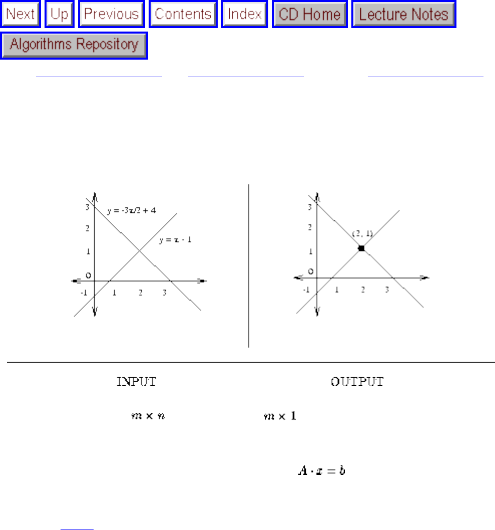
Solving Linear Equations
Next: Bandwidth Reduction Up: Numerical Problems Previous: Numerical Problems
Solving Linear Equations
Input description: An matrix A, and an vector b, together representing m linear equations
on n variables.
Problem description: What is the vector x such that ?
Discussion: The need to solve linear systems arises in an estimated 75% of all scientific computing
problems [DB74]. For example, applying Kirchhoff's laws to analyze electric circuits generates a
system of equations, the solution of which gives currents through each branch of the circuit. Analysis of
the forces acting on a mechanical truss generates a similar set of equations. Even finding the point of
intersection between two or more lines reduces to solving a (small) linear system.
Not all systems of equations have solutions; consider the equations 2x+3y = 5 and 2x+3y = 6. Some
systems of equations have multiple solutions; consider the equations 2x+3y=5 and 4x+6y=10. Such
degenerate systems of equations are called singular, and they can be recognized by testing whether the
determinant of the coefficient matrix is zero.
Solving linear systems is a problem of such scientific and commercial importance that excellent codes
are readily available. There is likely no good reason to implement your own solver, even though the basic
file:///E|/BOOK/BOOK3/NODE136.HTM (1 of 4) [19/1/2003 1:30:15]
Solving Linear Equations
algorithm (Gaussian elimination) is one we learned in high school. This is especially true if you are
working with large systems.
Gaussian elimination is based on the fact that the solution to a system of linear equations is invariant
under scaling (multiplying both sides by a constant; i.e. if x=y, then 2x=2y) and adding equations (i.e. the
solution to the equations x=y and w=z is the same as the solution to x=y and x+w=y+z). Gaussian
elimination scales and adds equations so as to eliminate each variable from all but one equation, leaving
the system in such a state that the solution can just be read off from the equations.
The time complexity of Gaussian elimination on an system of equations is , since for the ith
variable we add a scaled copy of the n-term ith row to each of the n-1 other equations. On this problem,
however, constants matter. Algorithms that only partially reduce the coefficient matrix and then
backsubstitute to get the answer use 50% fewer floating-point operations than the naive algorithm.
Issues to worry about include:
● Are roundoff errors and numerical stability affecting my solution? - Implementing Gaussian
elimination would be quite straightforward except for round-off errors, which accumulate with
each row operation and can quickly wreak havoc on the solution, particularly with matrices that
are almost singular.
To eliminate the danger of numerical errors, it pays to substitute the solution back into each of the
original equations and test how close they are to the desired value. Iterative methods for solving
linear systems refine initial solutions to obtain more accurate answers - good linear systems
packages will include such routines.
The key to minimizing roundoff errors in Gaussian elimination is selecting the right equations and
variables to pivot on, and to scale the equations so as to eliminate large coefficients. This is an
art as much as a science, which is why you should use one of the many well-crafted library
routines described below.
● Which routine in the library should I use? - Selecting the right code is also somewhat of an art. If
you are taking your advice from this book, you should start with the general linear system solvers.
Hopefully they will suffice for your needs. But search through the manual for more efficient
procedures for solving special types of linear systems. If your matrix happens to be one of these
special types, the solution time can reduce from cubic to quadratic or even linear.
● Is my system sparse? - The key to recognizing that you might have a special-case linear system
is establishing how many matrix elements you really need to describe A. If there are only a few
nonzero elements, your matrix is sparse and you are in luck. If these few nonzero elements are
clustered near the diagonal, your matrix is banded and you are in even more luck. Algorithms for
reducing the bandwidth of a matrix are discussed in Section . Many other regular patterns of
sparse matrices can also be exploited, so see the manual of your solver or a better book on
numerical analysis for details.
file:///E|/BOOK/BOOK3/NODE136.HTM (2 of 4) [19/1/2003 1:30:15]
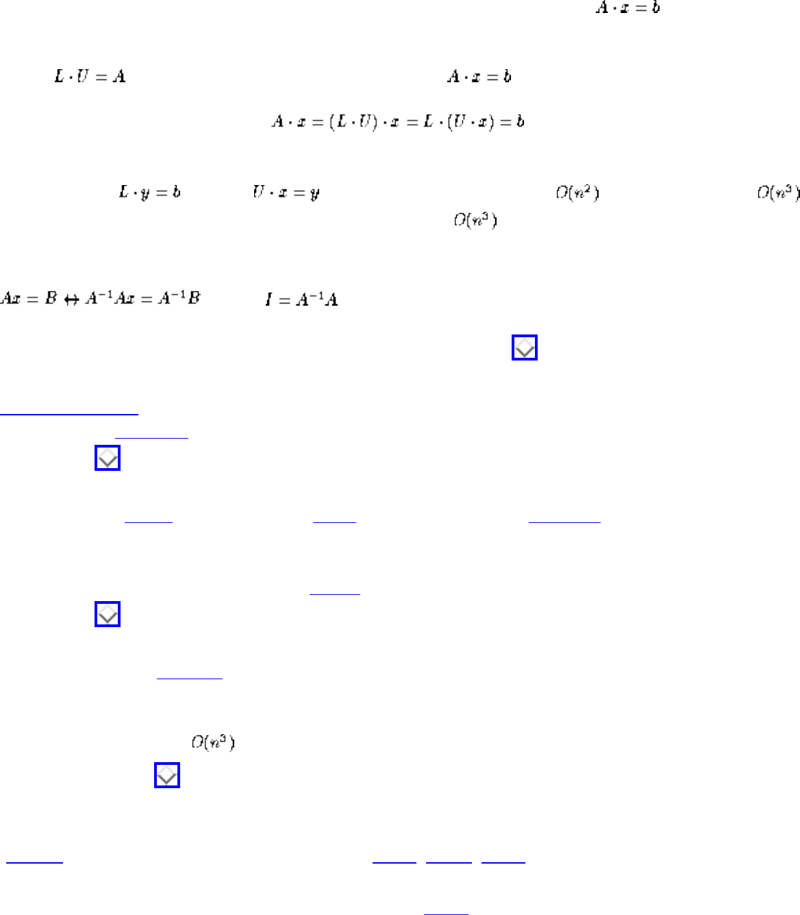
Solving Linear Equations
● Will I be solving many systems with the same coefficient matrix? - In certain applications, such as
least-squares curve fitting and differential equations, we have to solve repeatedly with
different b vectors. For efficiency, we seek to preprocess A to make this easier. The lower-
upper or LU-decomposition of A creates lower- and upper-triangular matrices L and U such that
. We can use this decomposition to solve , since
This is efficient since backsubstitution solves a triangular system of equations in quadratic time.
Solving and then gives the solution x using two steps instead of one
step, once the LU-decomposition has been found in time.
The problem of solving linear systems is equivalent to that of matrix inversion, since
, where is the identity matrix. However, avoid it, since matrix
inversion proves to be three times slower than Gaussian elimination. LU-decompositions prove useful in
inverting matrices as well as computing determinants (see Section ).
Implementations: The library of choice for solving linear systems is apparently LAPACK, a descendant
of LINPACK [DMBS79]. Both of these Fortran codes, as well as many others, are available from Netlib.
See Section .
Algorithm 533 [She78], Algorithm 576 [BS81], and Algorithm 578 [DNRT81] of the Collected
Algorithms of the ACM are Fortran codes for Gaussian elimination. Algorithm 533 is designed for
sparse systems, algorithm 576 to minimize roundoff errors, and algorithm 578 to optimize virtual
memory performance. Algorithm 645 [NW86] is a Fortran code for testing matrix inversion programs.
See Section for details on fetching these programs.
Numerical Recipes [PFTV86] provides routines for solving linear systems. However, there is no
compelling reason to use these ahead of the free codes described in this section.
C++ implementations of algorithms to solve linear equations and invert matrices are embedded in
LEDA (see Section ).
Notes: Good expositions on algorithms for Gaussian elimination and LU-decomposition include
[CLR90] and a host of numerical analysis texts [BT92, CK80, SK93].
Parallel algorithms for linear systems are discussed in [Ort88]. Solving linear systems is one of relatively
few problems where parallel architectures are widely used in practice.
file:///E|/BOOK/BOOK3/NODE136.HTM (3 of 4) [19/1/2003 1:30:15]
Solving Linear Equations
Matrix inversion, and hence linear systems solving, can be done in matrix multiplication time using
Strassen's algorithm plus a reduction. Good expositions on the equivalence of these problems include
[AHU74, CLR90].
Certain types of nonsparse systems can be solved efficiently via special algorithms. In particular,
Toeplitz matrices are constructed so that all the elements along a particular diagonal are identical, and
Vandermonde matrices are defined by an n-element vector x where .
Related Problems: Matrix multiplication (see page ), determinant/permanent (see page ).
Next: Bandwidth Reduction Up: Numerical Problems Previous: Numerical Problems
Algorithms
Mon Jun 2 23:33:50 EDT 1997
file:///E|/BOOK/BOOK3/NODE136.HTM (4 of 4) [19/1/2003 1:30:15]
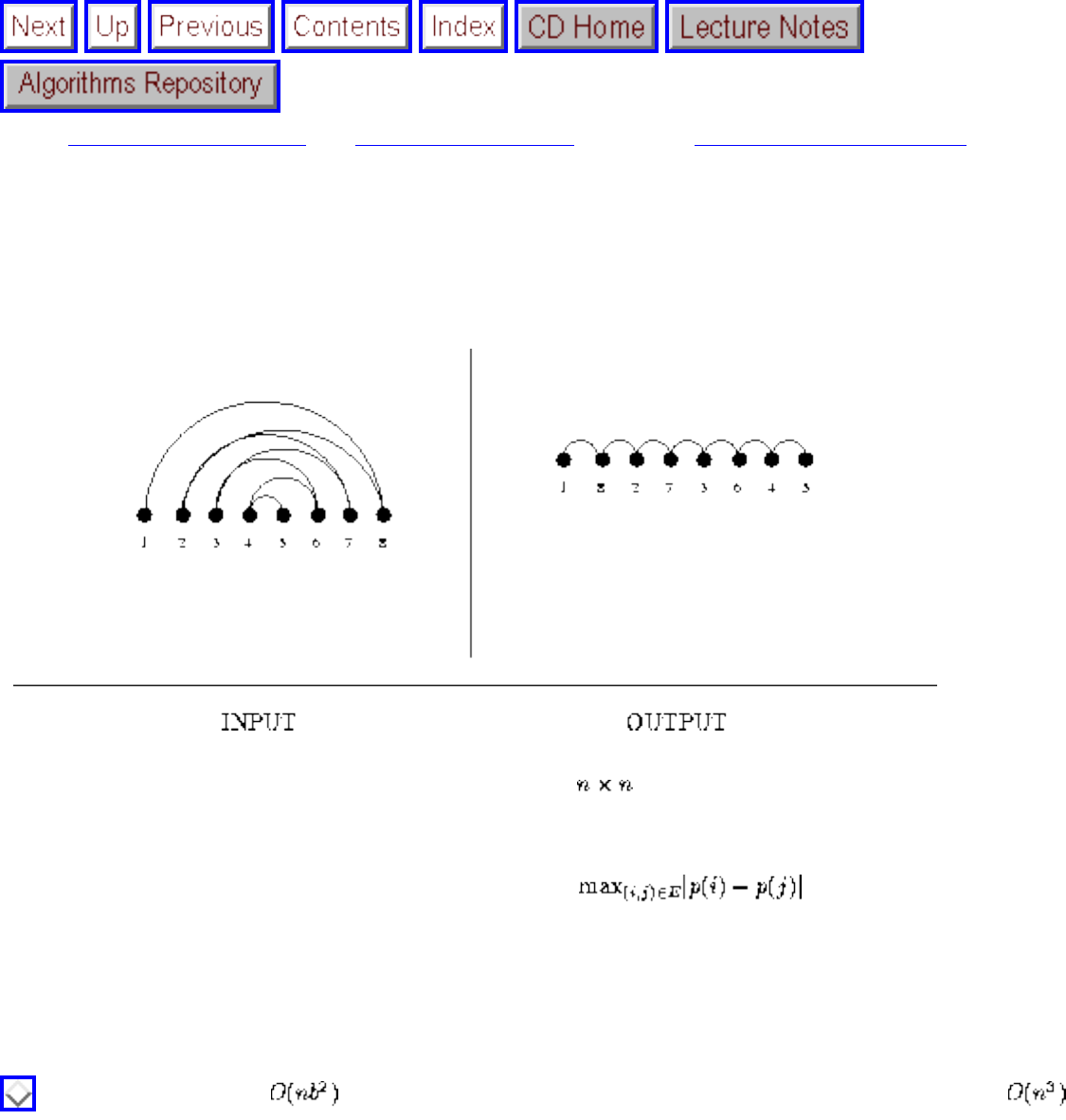
Bandwidth Reduction
Next: Matrix Multiplication Up: Numerical Problems Previous: Solving Linear Equations
Bandwidth Reduction
Input description: A graph G=(V,E), representing an matrix M of zero and nonzero elements.
Problem description: Which permutation p of the vertices of V minimizes the length of the longest edge
when the vertices are ordered on a line, i.e. minimizes ?
Discussion: Bandwidth reduction lurks as a hidden but important problem for both graphs and matrices,
and it is important to see how it arises so as to properly recognize it. Applied to matrices, it permutes the
rows and columns of a sparse matrix so as to minimize the distance b of any nonzero entry from the
center diagonal. This is important in solving linear systems, because Gaussian elimination (see Section
) can be performed in on matrices of bandwidth b. This is a big win over the general
algorithm if b << n.
Bandwidth minimization on graphs arises in more subtle ways. Arranging a set of n circuit components
in a line on a circuit board so as to minimize the length of the longest wire (and hence time delay) is a
bandwidth problem, where each vertex of our graph corresponds to a circuit component and there is an
edge for every wire linking two components. Alternatively, consider a hypertext application where we
must store large objects (say images) on a magnetic tape. From each image there is a set of possible
images we can go to next (i.e. the hyperlinks). To minimize the search time, we seek to place linked
file:///E|/BOOK/BOOK3/NODE137.HTM (1 of 3) [19/1/2003 1:30:16]
Bandwidth Reduction
images near each other on the tape. This is exactly the bandwidth problem. More general formulations,
such as rectangular circuit layouts and magnetic disks, inherit the same hardness and classes of heuristics
from the linear versions.
Unfortunately, bandwidth minimization is NP-complete. It stays NP-complete even if the input graph is a
tree whose maximum vertex degree is 3, which is an unusually strong condition. Further, there is no
known approximation algorithm for bandwidth reduction, even for trees. Thus our only options are
brute-force search or ad hoc heuristics.
Fortunately, ad hoc heuristics have been well-studied in the numerical analysis community, and
production-quality implementations of the best heuristics are available. These are based on performing a
breadth-first search from a given vertex v, where v is placed at the leftmost point of the ordering. All of
the vertices that are distance 1 from v are placed to its immediate right, followed by all the vertices at
distance 2, and so forth until we reach the vertex furthest from v. We then continue the breadth-first
search from the vertex immediately to the right of v until all vertices in G are accounted for. The popular
heuristics differ according to how many different start vertices are considered and how equidistant
vertices are ordered among themselves. However, breaking ties with low-degree vertices over to the left
seems to be a good idea.
Implementations of the most popular heuristics, the Cuthill-McKee and Gibbs-Poole-Stockmeyer
algorithms, are discussed in the implementation section. The worst case of the Gibbs-Poole-Stockmeyer
algorithm is , which would wash out any possible savings in solving linear systems, but its
performance in practice is close to linear.
Brute-force search programs can find the exact minimum bandwidth work by backtracking through the
set of n! possible permutations of vertices. Considerable pruning can be achieved to reduce the search
space by starting with a good heuristic bandwidth solution and alternately adding vertices to the left- and
rightmost open slots in the partial permutation. The first edge connecting a vertex on the left to a vertex
on the right will likely define an edge whose length is greater than our best example to date, thus leading
to fast pruning. In our experience, graphs of size n=30 or so can be solved to optimality. See the
discussion on backtracking in Section . However, for almost any application such an exact solution
will not be worth the expense of finding it.
Implementations: Fortran language implementations of both the Cuthill-McKee algorithm [CGPS76,
Gib76, CM69] and the Gibbs-Poole-Stockmeyer algorithm [Lew82, GPS76] are available from Netlib.
See Section . Empirical evaluations of these and other algorithms on a test suite of 30 matrices are
discussed in [Eve79b], showing Gibbs-Poole-Stockmeyer to be the consistent winner.
Brute-force implementations written by Ingmar Bitter, Christian Joita, and Dario Vlah in C and C++ as
Stony Brook class projects and capable of solving instances of size n=30 to optimality are provided on
the algorithm repository http://www.cs.sunysb.edu/ algorith.
file:///E|/BOOK/BOOK3/NODE137.HTM (2 of 3) [19/1/2003 1:30:16]
Bandwidth Reduction
Notes: An excellent survey on graph-theoretic and algorithmic results on the bandwidth problem to 1981
appears in [CCDG82]. Ad hoc heuristics have been widely studied, a tribute to its importance in
numerical computation. Everstine [Eve79b] cites no less than 49 different bandwidth reduction
algorithms!
The hardness of the bandwidth problem was first established by Papadimitriou [Pap76b], and its hardness
on trees of maximum degree 3 in [GGJK78]. There are algorithms that run in polynomial time for fixed
bandwidth k [Sax80]. An exposition on the hardness of the linear arrangement problem appears in
[Eve79a].
Related Problems: Solving linear equations (see page ), topological sorting (see page ).
Next: Matrix Multiplication Up: Numerical Problems Previous: Solving Linear Equations
Algorithms
Mon Jun 2 23:33:50 EDT 1997
file:///E|/BOOK/BOOK3/NODE137.HTM (3 of 3) [19/1/2003 1:30:16]
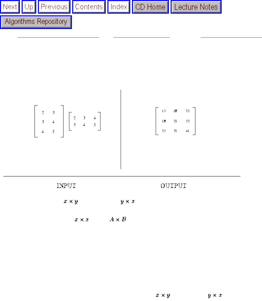
Matrix Multiplication
Next: Determinants and Permanents Up: Numerical Problems Previous: Bandwidth Reduction
Matrix Multiplication
Input description: An matrix A and a matrix B.
Problem description: The matrix .
Discussion: Although matrix multiplication is an important problem in linear algebra, its main
significance for combinatorial algorithms is its equivalence to a variety of other problems, such as
transitive closure and reduction, solving linear systems, and matrix inversion. Thus a faster algorithm for
matrix multiplication implies faster algorithms for all of these problems. Matrix multiplication arises in
its own right in computing the results of such coordinate transformations as scaling, rotation, and
translation for robotics and computer graphics.
The straightforward algorithm to compute the product of matrix A and matrix B runs in O(x y
z) time and is tough to beat in practice:
for i=1 to x do
file:///E|/BOOK/BOOK3/NODE138.HTM (1 of 4) [19/1/2003 1:30:18]
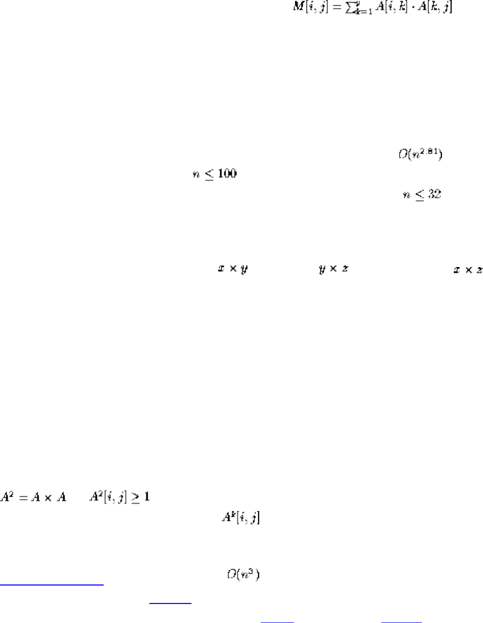
Matrix Multiplication
for j = 1 to z
In two multiplying bandwidth-b matrices, where all nonzero elements of A and B lie within b elements of
the main diagonals, a speedup to O(x b z) is possible, since zero elements will not contribute to the
product.
Asymptotically faster algorithms for matrix multiplication exist, based on clever divide-and-conquer
recurrences. However, these prove difficult to program and require very large matrices to beat the trivial
algorithm. In particular, some empirical results show that Strassen's algorithm is unlikely to beat
the straightforward algorithm for , and it is less numerically stable to boot. Other studies have
been more encouraging, claiming that the crossover point is as low as . Still, I consider it unlikely
that you will speed up any serious application by implementing Strassen's algorithm.
There is a better way to save computation when you are multiplying a chain of more than two matrices
together. Recall that multiplying an matrix by a matrix creates an matrix. Thus
multiplying a chain of matrices from left to right might create large intermediate matrices, each taking a
lot of time to compute. Matrix multiplication is not commutative, but it is associative, so we can
parenthesize the chain in whatever manner we deem best without changing the final product. A
standard dynamic programming algorithm can be used to construct the optimal parenthesization.
Whether it pays to do this optimization will depend upon whether your matrices are large enough or your
chain is multiplied often enough to justify it. Note that we are optimizing over the sizes of the
dimensions in the chain, not the actual matrices themselves. If all your matrices are the same dimensions,
you are out of luck, since no such optimization is possible.
Matrix multiplication has a particularly interesting interpretation in counting the number of paths
between two vertices in a graph. Let A be the adjacency matrix of a graph G, meaning A[i,j] = 1 if
there is an edge between i and j. Otherwise, A[i,j] = 0. Now consider the square of this matrix,
. If , this means that there must be a k such that A[i,k]=A[k,j]=1, so i to k to j is a
path of length 2 in G. More generally, counts the number of paths of length exactly k between i
and j. This count includes nonsimple paths, where vertices are repeated, such as i to k to i.
Implementations: The quick and dirty algorithm will be your best bet unless your matrices are
very large. For example, [CLR90] suggests that n>45 before you have a hope of winning. Experimental
results suggest that n > 100 is more realistic [CR76], with Bailey [BLS91] finding a crossover point of
n=128 for Cray systems. Strassen's algorithm is difficult to implement efficiently because of the data
structures required to maintain the array partitions. That said, an implementation of Strassen's
algorithm in Mathematica by Stan Wagon is offered ``without promise of efficiency'' on the algorithm
repository WWW site.
file:///E|/BOOK/BOOK3/NODE138.HTM (2 of 4) [19/1/2003 1:30:18]
Matrix Multiplication
The linear algebra library of choice is LAPACK, a descendant of LINPACK [DMBS79], which includes
several routines for matrix multiplication. These Fortran codes are available from Netlib as discussed in
Section .
Algorithm 601 [McN83] of the Collected Algorithms of the ACM is a sparse matrix package written in
Fortran that includes routines to multiply any combination of sparse and dense matrices. See Section
for details.
XTango (see Section ) is an algorithm animation system for UNIX and X-windows that includes an
animation of the matrix multiplication algorithm. A C++, implementation of matrix
multiplication is embedded in LEDA (see Section ).
Notes: Winograd's algorithm for fast matrix multiplication reduces the number of multiplications by a
factor of two over the straightforward algorithm. It is implementable, although the additional
bookkeeping required makes it doubtful whether it is a win. Expositions on Winograd's algorithm
[Win68] include [CLR90, Man89, Win80].
In my opinion, the history of theoretical algorithm design began when Strassen published his -
time matrix multiplication algorithm. For the first time, improving an algorithm in the asymptotic sense
became a respected goal in its own right. Good expositions on Strassen's algorithm [Str69] include
[Baa88, CLR90, Cra94]. Progressive improvements to Strassen's algorithm have gotten progressively
less practical. The current best result for matrix multiplication is Coppersmith and Winograd's [CW87]
algorithm, while the conjecture is that suffices.
The interest in the squares of graphs goes beyond counting paths. Fleischner [Fle74] proved that the
square of any biconnected graph has a Hamiltonian cycle. See [LS95] for results on finding the
square roots of graphs, i.e. finding A given .
The problem of Boolean matrix multiplication can be reduced to that of general matrix multiplication
[CLR90]. The four-Russians algorithm for Boolean matrix multiplication [ADKF70] uses preprocessing
to construct all subsets of rows for fast retreival in performing the actual multiplication, yielding a
complexity of . Additional preprocessing can improve this to [Ryt85]. An
exposition on the four-Russians algorithm, including this speedup, appears in [Man89].
Good expositions of the matrix-chain algorithm include [Baa88, CLR90], where it is a standard example
of dynamic programming.
file:///E|/BOOK/BOOK3/NODE138.HTM (3 of 4) [19/1/2003 1:30:18]

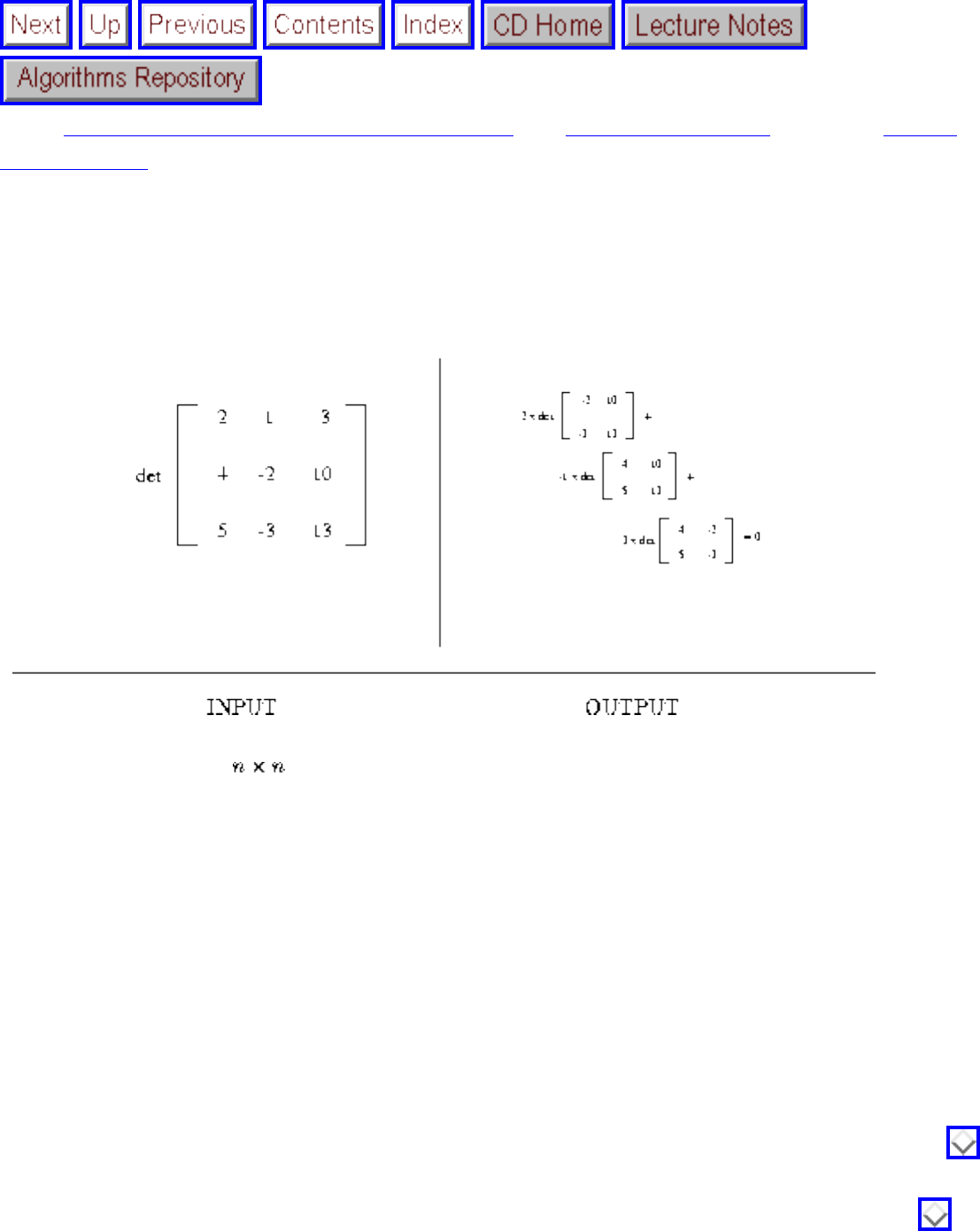
Determinants and Permanents
Next: Constrained and Unconstrained Optimization Up: Numerical Problems Previous: Matrix
Multiplication
Determinants and Permanents
Input description: An matrix M.
Problem description: What is the determinant |M| or the permanent perm(M) of the matrix m?
Discussion: Determinants of matrices provide a clean and useful abstraction in linear algebra that can
used to solve a variety of problems:
● Testing whether a matrix is singular, meaning that the matrix does not have an inverse. A matrix
M is singular iff |M| = 0.
● Testing whether a set of d points lies on a plane in fewer than d dimensions. If so, the system of
equations they define is singular, so |M| = 0.
● Testing whether a point lies to the left or right of a line or plane. This problem reduces to
testing whether the sign of a determinant is positive or negative, as discussed in Section .
● Computing the area or volume of a triangle, tetrahedron, or other simplicial complex. These
quantities are a function of the magnitude of the determinant, as discussed in Section .
file:///E|/BOOK/BOOK3/NODE139.HTM (1 of 3) [19/1/2003 1:30:19]
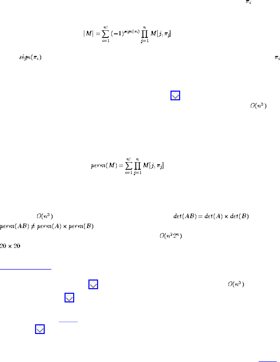
Determinants and Permanents
The determinant of a matrix M is defined as the sum over all n! possible permutations of the n columns
of M:
where is the number of pairs of elements out of order (called inversions) in permutation .
A direct implementation of this definition yields an O(n!) algorithm, as does the cofactor expansion
method we learned in high school. However, better algorithms are available to evaluate determinants
based on LU-decomposition. They are discussed in Section . The determinant of M is simply the
product of the diagonal elements of the LU-decomposition of M, which can be found in time.
A closely related function, called the permanent, arises often in combinatorial problems. For example,
the permanent of the adjacency matrix of a graph G counts the number of perfect matchings in G. The
permanent of a matrix M is defined by
differing from the determinant only in that all products are positive.
Surprisingly, it is NP-hard to compute the permanent, even though the determinant can easily be
computed in time. The fundamental difference is that , while
. Fortunately, there are permanent algorithms that prove to be
considerably faster than the O(n!) definition, running in time. Thus finding the permanent of a
matrix is not out of the realm of possibility.
Implementations: The linear algebra package LINPACK contains a variety of Fortran routines for
computing determinants, optimized for different data types and matrix structures. It can be obtained from
Netlib, as discussed in Section . A C++ program to compute determinants in time is embedded
in LEDA (see Section ).
Nijenhuis and Wilf [NW78] provide an efficient Fortran routine to compute the permanent of a matrix.
See Section .
Notes: Cramer's rule reduces the problems of matrix inversion and solving linear systems to that of
computing determinants. However, algorithms based on LU-determination are faster. See [BM53] for an
file:///E|/BOOK/BOOK3/NODE139.HTM (2 of 3) [19/1/2003 1:30:19]
Determinants and Permanents
exposition on Cramer's rule.
Determinants can be computed in time using fast matrix multiplication, as shown in [AHU83].
Section discusses such algorithms. A fast algorithm for computing the sign of the determinant, an
important problem for performing robust geometric computations, is due to Clarkson [Cla92].
The problem of computing the permanent was shown to be #P-complete by Valiant [Val79], where #P is
the class of problems solvable on a ``counting'' machine in polynomial time. A counting machine
returns the number of distinct solutions to a problem. Counting the number of Hamiltonian cycles in a
graph is a #P-complete problem that is trivially NP-hard (and presumably harder), since any count
greater than zero proves that the graph is Hamiltonian. Counting problems can be #P-complete even if
the corresponding decision problem can be solved in polynomial time, as shown by the permanent and
perfect matchings.
Minc [Min78] is the definitive work on permanents. A variant of an -time algorithm due to Ryser
for computing the permanent is presented in [NW78]. Recently, probabilistic algorithms have been
developed for estimating the permanent [FJ95].
Related Problems: Solving linear systems (see page ), matching (see page ), geometric primitives
(see page ).
Next: Constrained and Unconstrained Optimization Up: Numerical Problems Previous: Matrix
Multiplication
Algorithms
Mon Jun 2 23:33:50 EDT 1997
file:///E|/BOOK/BOOK3/NODE139.HTM (3 of 3) [19/1/2003 1:30:19]
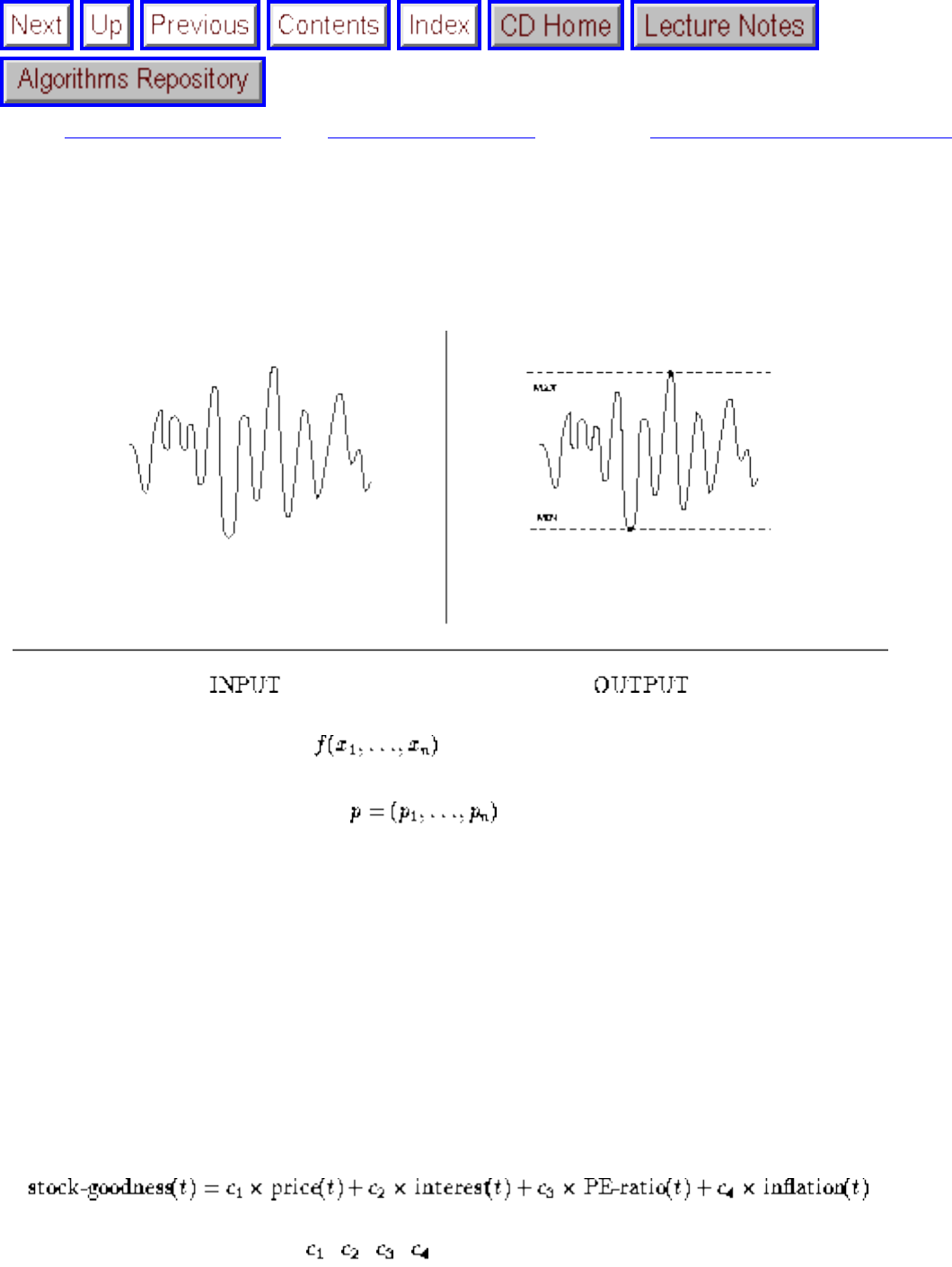
Constrained and Unconstrained Optimization
Next: Linear Programming Up: Numerical Problems Previous: Determinants and Permanents
Constrained and Unconstrained Optimization
Input description: A function .
Problem description: What point maximizes (or minimizes) the function f?
Discussion: Most of this book concerns algorithms that optimize one thing or another. This section
considers the general problem of optimizing functions where, due to lack of structure or knowledge, we
are unable to exploit the problem-specific algorithms seen elsewhere in this book.
Optimization arises whenever there is an objective function that must be tuned for optimal performance.
Suppose we are building a program to identify good stocks to invest in. We have available certain
financial data to analyze, such as the price-earnings ratio, the interest and inflation rates, and the stock
price, all as a function of time t. The key question is how much weight we should give to each of these
factors, where these weights correspond to coefficents of a formula:
We seek the numerical values , , , whose stock-goodness function does the best job of evaluating
stocks. Similar issues arise in tuning evaluation functions for game playing programs such as chess.
file:///E|/BOOK/BOOK3/NODE140.HTM (1 of 4) [19/1/2003 1:30:21]
Constrained and Unconstrained Optimization
Unconstrained optimization problems also arise in scientific computation. Physical systems from
protein structures to particles naturally seek to minimize their ``energy functions.'' Thus programs that
attempt to simulate nature often define energy potential functions for the possible configurations of
objects and then take as the ultimate configuration the one that minimizes this potential.
Global optimization problems tend to be hard, and there are lots of ways to go about them. Ask the
following questions to steer yourself in the right direction:
● Am I doing constrained or unconstrained optimization? - In unconstrained optimization, there
are no limitations on the values of the parameters other than that they maximize the value of f.
Often, however, there are costs or constraints on these parameters. These constraints make certain
points illegal, points that might otherwise be the global optimum. Constrained optimization
problems typically require mathematical programming approaches like linear programming,
discussed in Section .
● Is the function I am trying to optimize described by a formula or data? - If the function that you
seek to optimize is presented as an algebraic formula (such as the minimum of
), the solution is to analytically take its derivative f'(n) and see for which
points p' we have f'(p') = 0. These points are either local maxima or minima, which can be
distinguished by taking a second derivative or just plugging back into f and seeing what happens.
Symbolic computation systems such as Mathematica and Maple are fairly effective at
computing such derivatives, although using computer algebra systems effectively is somewhat of
a black art. They are definitely worth a try, however, and you can always use them to plot a
picture of your function to get a better idea of what you are dealing with.
● How expensive is it to compute the function at a given point? - If the function f is not presented as
a formula, what to do depends upon what is given. Typically, we have a program or subroutine
that evaluates f at a given point, and so can request the value of any given point on demand. By
calling this function, we can poke around and try to guess the maxima. Our freedom to search in
such a situation depends upon how efficiently we can evaluate f. If f is just a complicated formula,
evaluation will be very fast. But suppose that f represents the effect of the coefficients
on the performance of the board evaluation function in a computer chess program, such that is
how much a pawn is worth, is how much a bishop is worth, and so forth. To evaluate a set of
coefficients as a board evaluator, we must play a bunch of games with it or test it on a library of
known positions. Clearly, this is time-consuming, so we must be frugal in the number of
evaluations of f we use.
● How many dimensions do we have? How many do we need? - The difficulty in finding a global
maximum increases rapidly with the number of dimensions (or parameters). For this reason, it
often pays to reduce the dimension by ignoring some of the parameters. This runs counter to
intuition, for the naive programmer is likely to incorporate as many variables as possible into their
evaluation function. It is just too hard to tweak such a complicated function. Much better is to
start with the 3 to 5 seemingly most important variables and do a good job optimizing the
coefficients for these.
file:///E|/BOOK/BOOK3/NODE140.HTM (2 of 4) [19/1/2003 1:30:21]
Constrained and Unconstrained Optimization
● How smooth is my function? The main difficulty of global optimization is getting trapped in local
optima. Consider the problem of finding the highest point in a mountain range. If there is only
one mountain and it is nicely shaped, we can find the top by just walking in whatever direction is
up. However, if there are many false summits or other mountains in the area, it is difficult to
convince ourselves whether we are really at the highest point. Smoothness is the property that
enables us to quickly find the local optimum from a given point. We assume smoothness in
seeking the peak of the mountain by walking up. If the height at any given point was a completely
random function, there would be no way we could find the optimum height short of sampling
every single point.
Efficient algorithms for unconstrained global optimization use derivatives and partial derivatives to find
local optima, to point out the direction in which moving from the current point does the most to increase
or decrease the function. Such derivatives can sometimes be computed analytically, or they can be
estimated numerically by taking the difference between values of nearby points. A variety of steepest
descent and conjugate gradient methods to find local optima have been developed, similar in many ways
to numerical root-finding algorithms.
It is a good idea to try out several different methods on any given optimization problem. For this reason,
we recommend experimenting with the implementations below before attempting to implement your own
method. Clear descriptions of these algorithms are provided in several numerical algorithms books, in
particular [PFTV86].
For constrained optimization, finding points that satisfy all the constraints is often the difficult problem.
One approach is to use a method for unconstrained optimization, but add a penalty according to how
many constraints are violated. Determining the right penalty function is problem-specific, but it often
makes sense to vary the penalties as optimization proceeds. At the end, the penalties should be very high
to ensure that all constraints are satisfied.
Simulated annealing is a fairly robust and simple approach to constrained optimization, particularly when
we are optimizing over combinatorial structures (permutations, graphs, subsets) instead of continuous
functions. Techniques for simulated annealing are described in Section .
Implementations: Several of the Collected Algorithms of the ACM are Fortran codes for unconstrained
optimization, most notably Algorithm 566 [MGH81], Algorithm 702 [SF92], and Algorithm 734
[Buc94]. Algorithm 744 [Rab95] does unconstrained optimization in Lisp. They are available from
Netlib (see Section ). Also check out the selection at GAMS, the NIST Guide to Available
Mathematical Software, at http://gams.nist.gov.
NEOS (Network-Enabled Optimization System) provides a unique service, the opportunity to solve your
problem on computers and software at Argonne National Laboratory, over the WWW. Linear
programming and unconstrained optimization are both supported. This is worth checking out at
file:///E|/BOOK/BOOK3/NODE140.HTM (3 of 4) [19/1/2003 1:30:21]
Constrained and Unconstrained Optimization
http://www.mcs.anl.gov/home/otc/Server/ when you need a solution instead of a program.
General purpose simulated annealing implementations are available and probably are the best place to
start experimenting with this technique for constrained optimization. Particularly popular is Adaptive
Simulated Annealing (ASA), written in C and retrievable via anonymous ftp from ftp.alumni.caltech.edu
[131.215.139.234] in the /pub/ingber directory. To get on the ASA mailing list send e-mail to asa-
request@alumni.caltech.edu.
Genocop, by Zbigniew Michalewicz [Mic92], is a genetic algorithm-based program for constrained and
unconstrained optimization, written in C. I tend to be quite skeptical of genetic algorithms (see Section
), but many people find them irresistible. Genocop is available from ftp://ftp.uncc.edu/coe/evol/ for
noncommercial purposes.
Notes: Steepest-descent methods for unconstrained optimization are discussed in most books on
numerical methods, including [PFTV86, BT92]. Unconstrained optimization is the topic of several
books, including [Bre73, Fle80].
Simulated annealing was devised by Kirkpatrick et. al. [KGV83] as a modern variation of the Metropolis
algorithm [MRRT53]. Both use Monte Carlo techniques to compute the minimum energy state of a
system. Good expositions on simulated annealing include [AK89].
Genetic algorithms were developed and popularized by Holland [Hol75, Hol92]. Expositions on genetic
algorithms include [Gol89, Koz92, Mic92]. Tabu search [Glo89a, Glo89b, Glo90] is yet another
heuristic search procedure with a devoted following.
Related Problems: Linear programming (see page ), satisfiability (see page ).
Next: Linear Programming Up: Numerical Problems Previous: Determinants and Permanents
Algorithms
Mon Jun 2 23:33:50 EDT 1997
file:///E|/BOOK/BOOK3/NODE140.HTM (4 of 4) [19/1/2003 1:30:21]
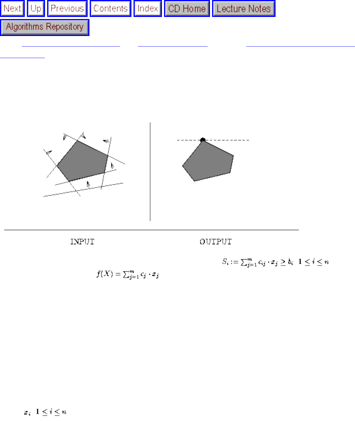
Linear Programming
Next: Random Number Generation Up: Numerical Problems Previous: Constrained and Unconstrained
Optimization
Linear Programming
Input description: A set S of n linear inequalities on m variables , , and a
linear optimization function .
Problem description: Which variable assignment X' maximizes the objective function f while satisfying
all inequalities S?
Discussion: Linear programming is the most important problem in mathematical optimization and
operations research. Applications include:
● Resource allocation - We seek to invest a given amount of money so as to maximize our return.
Our possible options, payoffs, and expenses can usually be expressed as a system of linear
inequalities, such that we seek to maximize our possible profit given the various constraints. Very
large linear programming problems are routinely solved by airlines and other corporations.
● Approximating the solution of inconsistent equations - A set of m linear equations on n variables
, , is overdetermined if m > n. Such overdetermined systems are often inconsistent,
meaning that no assignment of variables simultaneously solves all the equations. To find the
file:///E|/BOOK/BOOK3/NODE141.HTM (1 of 5) [19/1/2003 1:30:23]
Linear Programming
variable assignment that best fits the equations, we can replace each variable by and
solve the new system as a linear program, minimizing the sum of the error terms.
● Graph algorithms - Many of the standard graph problems described in this book, such as shortest
paths, bipartite matching, and network flow, can all be solved as special cases of linear
programming. Most of the rest, including traveling salesman, set cover, and knapsack, can be
solved using integer linear programming.
The standard algorithm for linear programming is called the simplex method. Each constraint in a linear
programming problem acts like a knife that carves away a region from the space of possible solutions.
We seek the point within the remaining region that maximizes (or minimizes) f(X). By appropriately
rotating the solution space, the optimal point can always be made to be the highest point in the region.
Since the region (simplex) formed by the intersection of a set of linear constraints is convex, we can find
the highest point by starting from any vertex of the region and walking to a higher neighboring vertex.
When there is no higher neighbor, we are at the highest point.
While the basic simplex algorithm is not too difficult to program, there is a considerable art to producing
an efficient implementation capable of solving large linear programs. For example, large programs tend
to be sparse (meaning that most inequalities use few variables), so sophisticated data structures must be
used. There are issues of numerical stability and robustness, as well as which neighbor we should walk
to next (so called pivoting rules). Finally, there exist sophisticated interior-point methods, which cut
through the interior of the simplex instead of walking along the outside, that beat simplex in many
applications.
The bottom line on linear programming is this: you are much better off using an existing LP code than
writing your own. Further, you are much better off paying money than surfing the net. Linear
programming is one algorithmic problem of such economic importance that commercial implementations
are far superior to free versions.
Issues that arise in linear programming include:
● Do any variables have integrality constraints? - It is impossible to send 6.54 airplanes from New
York to Washington each business day, even if that value maximizes profit according to your
model. Such variables often have natural integrality constraints. A linear program is called an
integer program when all its variables have integrality constraints, or a mixed integer progam if
some of them do.
Unfortunately, it is NP-complete to solve integer or mixed programs to optimality. However,
there are techniques for integer programming that work reasonably well in practice. Cutting
plane techniques solves the problem first as a linear program, and then adds extra constraints to
enforce integrality around the optimal solution point before solving it again. After a sufficient
number of iterations, the optimum point of the resulting linear program matches that of the
original integer program. As with most exponential-time algorithms, run times for integer
file:///E|/BOOK/BOOK3/NODE141.HTM (2 of 5) [19/1/2003 1:30:23]

Linear Programming
programming depend upon the difficulty of the problem instance and are unpredictable. If they do
not make progress quickly, they are unlikely make much progress over longer periods of time.
Therefore, if you have multiple implementations available, it may well pay to try the same
problem using different codes in the hopes that one can complete in a reasonable amount of time.
● What if my optimization function or constraints are not linear? - In least-squares curve fitting, we
seek the line that best approximates a set of points by minimizing the sum of squares of the
distance between each point and the line. In formulating this as a mathematical program, the
natural objective function is no longer linear, but quadratic. Unfortunately, quadratic
programming is NP-complete, even without integer variables.
There are three possible courses of action when you must solve a nonlinear program. The best is
to see if you can model it in some other way, as is the case with least-squares fitting. The second
is to try to track down special codes for quadratic programming, which do exist. Finally, you
can model your problem as a constrained or unconstrained optimization problem and try to solve
it with the codes discussed in Section .
● What if my model does not match the input format of my LP solver? - Many linear programming
implementations accept models only in so-called standard form, where all variables are
constrained to be nonnegative, the object function must be minimized, and all constraints must be
equalities (instead of inequalities). Do not fear. There exist standard transformations to map
arbitrary LP models into standard form. To convert a maximization problem to a minimization
one, simply multiply each coefficient of the objective function by -1. The remaining problems can
be solved by adding slack variables to the model. See any textbook on linear programming for
details.
Implementations: A very useful resource on solving linear programs is the USENET frequently asked
question (FAQ) list, maintained by John W. Gregory. In particular, it provides a list of available codes
with descriptions of experiences. Check out the plaintext version at
ftp://rtfm.mit.edu/pub/usenet/sci.answers/linear-programming-faq or a slicker WWW version at
http://www.skypoint.com/ ashbury/linear-programming-faq.html.
The noncommercial code of choice appears to be lp_solve, written in ANSI C by Michel Berkelaar,
who has solved problems as large as 30,000 variables and 50,000 constraints. Lp_solve can also handle
(smaller) integer and mixed-integer problems. It is available by anonymous ftp from
ftp://ftp.es.ele.tue.nl/pub/lp_solve but is not in the public domain. A user community for lp_solve exists,
which has ported it to a variety of different platforms.
NEOS (Network-Enabled Optimization System) provides a unique service, an opportunity to solve your
problem on computers and software at Argonne National Laboratory via the WWW. Linear
programming and unconstrained optimization are both supported. This is worth checking out at
http://www.mcs.anl.gov/home/otc/Server/ if you need an answer instead of a program.
If you are serious about solving large linear programs, you likely need a commercial implementation.
file:///E|/BOOK/BOOK3/NODE141.HTM (3 of 5) [19/1/2003 1:30:23]
Linear Programming
The book [MW93] provides an overview of commercial linear programming systems, online at
http://www.mcs.anl.gov/home/otc/Guide/SoftwareGuide/index.html. Surveys of commercial LP codes
appear in [SR95, Sha93] and in the linear programming FAQ. I have heard good things from various
people about CPLEX and AMPL, but do your own research before spending money.
For low-dimensional linear programming problems, computational geometry algorithms can outperform
more general LP codes. See ftp://icemcfd.com/pub/linprog.a for a C language implementation of
Seidel's randomized incremental LP algorithm, by Mike Hohmeyer.
Algorithm 551 [Abd80] and Algorithm 552 [BR80] of the Collected Algorithms of the ACM are simplex-
based codes for solving overdetermined systems of linear equations, in Fortran. See Section for
details.
Pascal implementations of the revised and dual simplex methods for linear programming, as well as
cutting plane and explicit enumeration algorithms for integer programming, are provided in [SDK83].
See Section . These are likely to work only for small problems.
Sedgewick [Sed92] provides a bare bones implementation of the simplex algorithm in C++. See Section
for details.
Notes: Good expositions on the simplex and ellipsoid algorithms for linear programming include [PS82,
Chv83]. Expositions on low-dimensional linear programming include [PS85]. For an implementation-
oriented exposition on linear and integer programming, with references to experimental work, see
[SDK83].
The need for optimization via linear programming arose in logistics problems in World War II. The
simplex algorithm was invented by George Danzig in 1947 [Dan63]. Klee and Minty [KM72] proved
that the simplex algorithm is exponential in worst case, but it is very efficient in practice. Khachian's
ellipsoid algorithm [Kha79] proved that linear programming was polynomial in 1979. Karmarkar's
algorithm [Kar84] is an interior-point method that has proven to be both a theoretical and practical
improvement of the ellipsoid algorithm, as well as a challenge for the simplex method.
Linear programming is P-complete under log-space reductions [DLR79]. This makes it unlikely to have
an NC parallel algorithm, where a problem is in NC iff it can be solved on a PRAM in polylogarithmic
time using a polynomial number of processors. Any problem that is P-complete under log-space
reduction cannot be in NC unless P=NC. See [GHR95] for a thorough exposition of the theory of P-
completeness, including an extensive list of P-complete problems.
Related Problems: Constrained and unconstrained optimization (see page ), network flow (see page
file:///E|/BOOK/BOOK3/NODE141.HTM (4 of 5) [19/1/2003 1:30:23]

Random Number Generation
Next: Factoring and Primality Testing Up: Numerical Problems Previous: Linear Programming
Random Number Generation
Input description: Nothing, or perhaps a seed.
Problem description: Generate a sequence of random integers.
Discussion: Random number generation forms the foundation behind such standard algorithmic
techniques as simulated annealing and Monte Carlo integration. Discrete event simulations, used to
model everything from transportation systems to casino poker, all run on streams of random numbers.
Initial passwords and cryptographic keys are typically generated randomly. New developments in
randomized algorithms for graph and geometric problems are revolutionizing these fields and
establishing randomization as one of the fundamental ideas of computer science.
Unfortunately, generating random numbers is a task that looks a lot easier than it really is, primarily
because it is fundamentally impossible to produce truly random numbers on any deterministic device.
Von Neumann [vN63] said it best: ``Anyone who considers arithmetical methods of producing random
digits is, of course, in a state of sin.'' All we can hope for are pseudorandom numbers, a stream of
numbers that appear as if they were generated randomly.
There can be serious consequences to using a bad random number generator. For example, the security of
file:///E|/BOOK/BOOK4/NODE142.HTM (1 of 5) [19/1/2003 1:30:27]
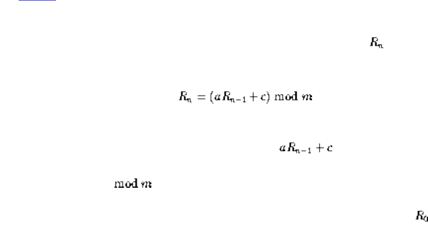
Random Number Generation
an Internet password scheme was recently invalidated with the discovery that its keys were produced
using a random number generator of such small period that brute-force search quickly exhausted all
possible passwords. The accuracy of simulations is regularly compromised or invalidated by poor
random number generation. Bottom line: This is an area where people shouldn't mess around, but they
do. Issues to think about include:
● Should my program use the same ``random'' numbers each time it runs? - A poker game that
deals you the exact same hand each time you play quickly loses interest. One common solution is
to use the lower-order bits of the machine clock as a seed or source for random numbers, so that
each time the program runs it does something different.
Such methods are perhaps adequate for games, but not for serious simulations. There are liable to
be periodicities in the distribution of random numbers whenever calls are made in a loop. Also,
debugging is seriously complicated by the fact that the results are not repeatable. If the program
crashes, you cannot go back and discover why. One possible compromise is to use a deterministic
pseudorandom number generator, but write the current seed to a file between runs. During
debugging, this file can be overwritten with a fixed initial value or seed.
● How good is my compiler's built-in random number generator? - If you need uniformly generated
random numbers, and you are not going to bet the farm on the accuracy of your simulation, my
recommendation is simply to use what your compiler provides. Your best opportunity to mess it
up is with a bad choice of starting seed, so read the manual for its recommendations.
If you are going to bet the farm on the quality of your simulation, you had better test your random
number generator. Be aware that it is very difficult to eyeball the results and decide whether the
output is really random. This is because people have very skewed ideas of how random sources
should behave and often see patterns that don't really exist. To evaluate a random number
generator, several different tests should be used and the statistical significance of the results
established. Such tests are implemented in plab and DIEHARD (discussed below) and explained
in [Knu81].
● What if I have to implement my own random number generator? - The algorithm of choice is the
linear congruential generator. It is fast, simple, and (if instantiated with the right constants)
gives reasonable pseudorandom numbers. The nth random number is a function of the (n-1)st
random number:
In theory, linear congruential generators work the same way roulette wheels do. The long path of
the ball around and around the wheel (captured by ) ends in one of a relatively small
number of bins, the choice of which is extremely sensitive to the length of the path (captured by
the truncation of the ).
A substantial theory has been developed to select the constants a, c, m, and . The period length
file:///E|/BOOK/BOOK4/NODE142.HTM (2 of 5) [19/1/2003 1:30:27]

Random Number Generation
is largely a function of the modulus m, which is typically constrained by the word length of the
machine. A presumably safe choice for a 32-bit machine would be , a = 1366, c=150889,
and m=714025. Don't get creative and change any of the constants, unless you use the theory or
run tests to determine the quality of the resulting sequence.
● What if I don't want large, uniformly distributed random integers? - The linear congruential
generator produces a uniformly distributed sequence of large integers, which can be scaled to
produce other uniform distributions. For uniformly distributed real numbers between 0 and 1,
use . Note that 1 cannot be realized this way, although 0 can. If you want uniformly distributed
integers between l and h, use .
Generating random numbers according to a given nonuniform distribution can be a tricky
business. The most reliable way to do this correctly is the acceptance-rejection method. Suppose
we bound the desired probability distribution function or geometric region to sample from a box
and then select a random point p from the box. This point can be selected by p by generating the x
and y coordinates independently, at random. If this p is within the distribution, or region, we can
return p as selected at random. If p is in the portion of the box outside the region of interest, we
throw it away and repeat with another random point. Essentially, we throw darts at random and
report those that hit the target.
This method is correct, but it can be slow. If the volume of the region of interest is small relative
to that of the box, most of our darts will miss the target. Efficient generators for Gaussian and
other special distributions are described in the references and implementations below.
Be cautious about inventing your own technique, however, since it can be tricky to obtain the
right probability distribution. For example, an incorrect way to select points uniformly from a
circle of radius r would be to generate polar coordinates and select an angle from 0 to and a
displacement between 0 and r, both uniformly at random. In such a scheme, half the generated
points will lie within r/2 of the radius, when only one-fourth of them should be! This is a
substantial enough difference to seriously skew the results, while being subtle enough that it
might escape detection.
● How long should I run my Monte Carlo simulation to get the best results? - It makes sense that
the longer you run a simulation, the more accurately the results will approximate the limiting
distribution, thus increasing accuracy. However, this is only true until you exceed the period, or
cycle length, of your random number generator. At that point, your sequence of random numbers
repeats itself, and further runs generate no additional information. Check the period length of your
generator before you jack up the length of your simulation. You are liable to be very surprised by
what you learn.
Implementations: An excellent WWW page on random number generation and stochastic simulation is
available at http://random.mat.sbg.ac.at/others/. It includes pointers to papers and literally dozens of
implementations of random number generators. From there are accessible pLab [Lee94] and DIEHARD,
systems for testing the quality of random number generators.
file:///E|/BOOK/BOOK4/NODE142.HTM (3 of 5) [19/1/2003 1:30:27]
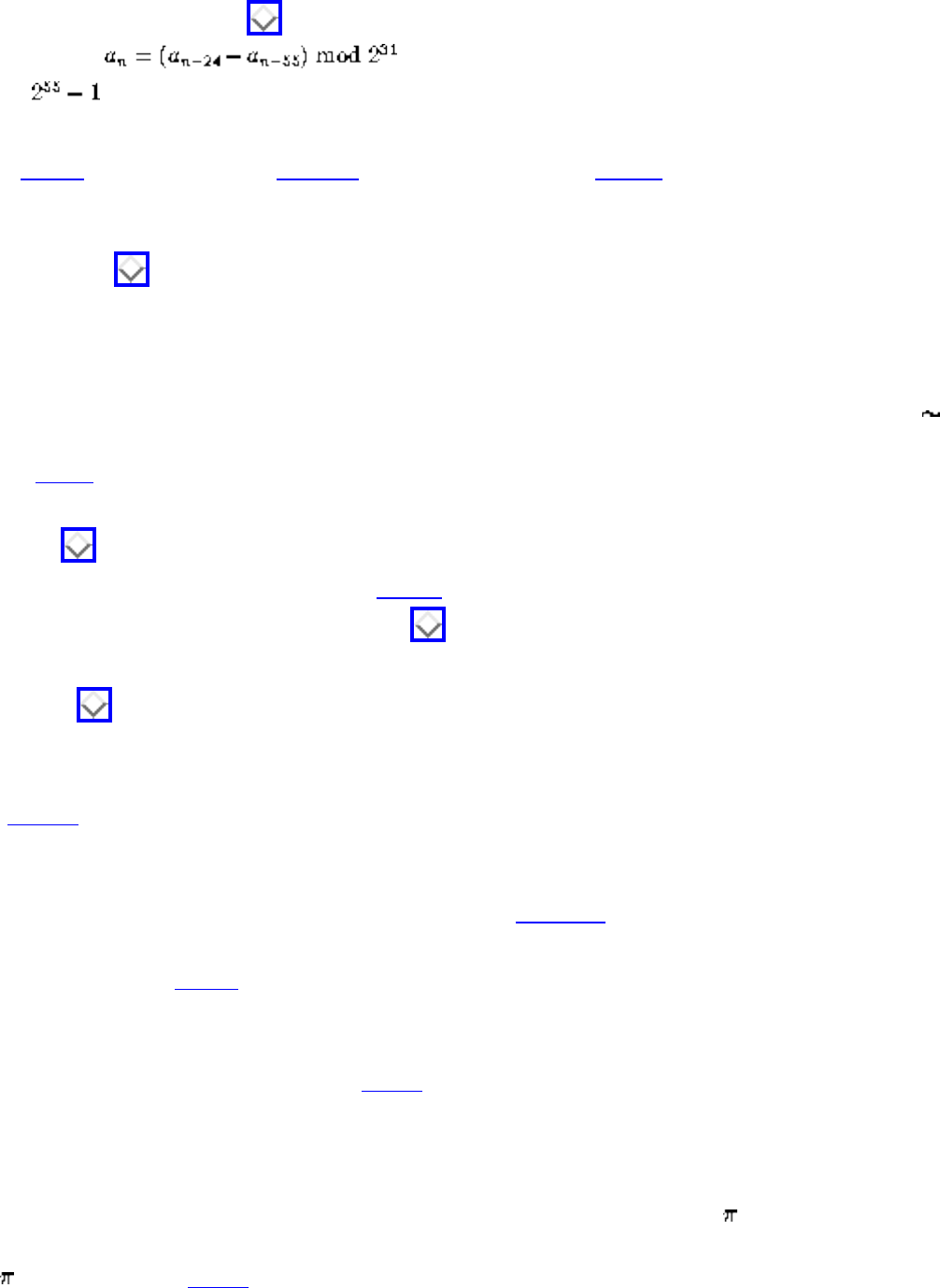
Random Number Generation
The Stanford Graphbase (see Section ) contains a machine-independent random number generator
based on the recurrence . With the proper initialization, this generator has a
period of at least .
Algorithm 488 [Bre74], Algorithm 599 [AKD83], and Algorithm 712 [Lev92] of the Collected
Algorithms of the ACM are Fortran codes for generating random numbers according to several
probability distributions, including normal, exponential, and Poisson distributions. They are available
from Netlib (see Section ).
Sim++ is a library of routines for implementing discrete event simulations, built by Robert Cubert and
Paul Fishwick, of the University of Florida. It contains random number generators for a variety of
different distributions, including uniform, exponential, and normal. Check out http://www.cis.ufl.edu/
fishwick/simpack/simpack.html if you need a random number generator to control a simulation.
Fishwick's book [Fis95] describes model design using SimPack.
LEDA (see Section ) provides a comprehensive random source in C++ for generating random bits,
integers, and double precision reals. Sedgewick [Sed92] provides simple implementations of linear and
additive congruential generators in C++. See Section for details.
XTango (see Section ) is an algorithm animation system for UNIX and X-windows, which includes
an animation illustrating the uniformity of random number generation.
Notes: Knuth [Knu81] has a thorough and interesting discussion of random number generation, which I
heartily recommend. He presents the theory behind several methods, including the middle square and
shift-register methods we have not described here, as well as a detailed discussion of statistical tests for
validating random number generators. Another good source is [PFTV86] - our recommended constants
for the linear congruential generator are drawn from here. Comparisons of different random number
generators in practice include [PM88].
Tables of random numbers appear in most mathematical handbooks, as relics from the days before there
was ready access to computers. Most notable is [RC55], which provides one million random digits.
The deep relationship between randomness, information, and compressibility is explored within the
theory of Kolmogorov complexity, which measures the complexity of a string by its compressibility.
Truly random strings are incompressible. The string of seemingly random digits of cannot be random
under this definition, since the entire sequence is defined by any program implementing a series
expansion for . Li and Vitáni [LV93] provide a thorough introduction to the theory of Kolmogorov
complexity.
file:///E|/BOOK/BOOK4/NODE142.HTM (4 of 5) [19/1/2003 1:30:27]
Random Number Generation
Related Problems: Constrained and unconstrained optimization (see page ), generating permutations
(see page ), generating subsets (see page ), generating partitions (see page ).
Next: Factoring and Primality Testing Up: Numerical Problems Previous: Linear Programming
Algorithms
Mon Jun 2 23:33:50 EDT 1997
file:///E|/BOOK/BOOK4/NODE142.HTM (5 of 5) [19/1/2003 1:30:27]
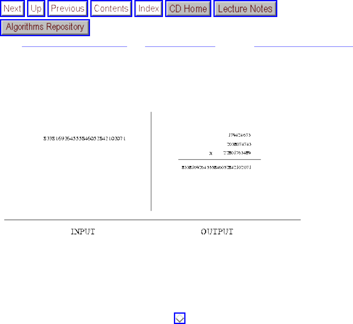
Factoring and Primality Testing
Next: Arbitrary-Precision Arithmetic Up: Numerical Problems Previous: Random Number Generation
Factoring and Primality Testing
Input description: An integer n.
Problem description: Is n a prime number, and if not what are the factors of n?
Discussion: The dual problems of factoring integers and testing primality have surprisingly many
applications for a problem long suspected of being only of mathematical interest. The security of the
RSA public-key cryptography system (see Section ) is based on the computational intractability of
factoring large integers. As a more modest application, hash table performance typically improves
when the table size is a prime number. To get this benefit, an initialization routine must identify a prime
near the desired table size. Finally, prime numbers are just interesting to play with. It is no coincidence
that programs to generate large primes often reside in the games directory of UNIX systems.
Although factoring and primality testing are related problems, algorithmically they are quite different.
There exist algorithms that can demonstrate that an integer is composite (i.e. not prime) without actually
giving the factors. To convince yourself of the plausibility of this, note that you can demonstrate the
compositeness of any nontrivial integer whose last digit is 0, 2, 4, 5, 6, or 8 without doing the actual
division.
file:///E|/BOOK/BOOK4/NODE143.HTM (1 of 4) [19/1/2003 1:30:28]
Factoring and Primality Testing
The simplest algorithm for both of these problems is brute-force trial division. To factor n, compute
the remainder of n/i for all . The prime factorization of n will contain at least one instance of
every i such that , unless n is prime. Make sure you handle the multiplicities correctly and
account for any primes larger than .
Such algorithms can be sped up by using a precomputed table of small primes to avoid testing all
possible i. Surprisingly large numbers of primes can be represented in surprisingly little space by using
bit vectors (see Section ). A bit vector of all odd numbers less than 1,000,000 fits in under 64
kilobytes. Even tighter encodings become possible by eliminating all multiples of three and other small
primes.
Considerably faster factoring algorithms exist, whose correctness depends upon more substantial number
theory. The fastest known algorithm, the number field sieve, uses randomness to construct a system of
congruences, the solution of which usually gives a factor of the integer. Integers with as many at 128
digits have been factored using this method, although such feats require enormous amounts of
computation.
Randomized algorithms make it much easier to test whether an integer is prime. Fermat's little theorem
states that for all a, when n is prime. Suppose we pick a random value of and
compute the residue of . If this residue is not 1, we have just proven that n cannot be prime.
Such randomized primality tests are very efficient. PGP (see Section ) finds 300+ digit primes using
hundreds of these tests in minutes, for use as cryptographic keys.
Although the primes are scattered in a seemingly random way throughout the integers, there is some
regularity to their distribution. The prime number theorem states that the number of primes less than n,
commonly denoted by , is approximately . Further, there are never large gaps between
primes, so in general, one would expect to examine about integers if one wanted to find the first
prime larger than n. This distribution and the fast randomized primality test explain how PGP can find
such large primes so quickly.
Implementations: My first choice for factoring or primality testing applications would be PARI, a
system capable of handling complex number-theoretic problems on integers with up to 300,000 decimal
digits, as well as reals, rationals, complex numbers, polynomials, and matrices. It is written mainly in C,
with assembly code for inner loops on major architectures, and includes more than 200 special
predefined mathematical functions. PARI can be used as a library, but it also possesses a calculator
mode that gives instant access to all the types and functions. The main advantage of PARI is its speed.
On a Unix platform, it is between 5 to 100 times faster than Maple or Mathematica, depending on the
applications. PARI is available for PC, Amiga, Macintosh, and most Unix platforms by anonymous ftp at
ftp://megrez.ceremab.u-bordeaux.fr/pub/pari/.
file:///E|/BOOK/BOOK4/NODE143.HTM (2 of 4) [19/1/2003 1:30:28]
Factoring and Primality Testing
A Mathematica implementation by Ilan Vardi of Lenstra's elliptic curve method of factorization is
available in Packages/NumberTheory/FactorIntegerECM.m of the standard Mathematica distribution and
MathSource. It is designed to find prime factors of up to about 18 digits in reasonable time, extending
Mathematica's ability to factor all numbers of up to 40 digits. It is faster when factoring the product of
small primes.
Notes: Bach and Shallit's book [BS96] is the most comprehensive reference on computational number
theory, while Adleman's excellent survey [Adl94a] describes the state of the art, as well as open
problems. Good expositions on modern algorithms for factoring and primality testing include [CLR90].
The Miller-Rabin [Mil76, Rab80] randomized primality testing algorithm eliminates problems with
Carmichael numbers, which are composite integers that always satisfy Fermat's theorem. The best
algorithms for integer factorization include the quadratic-sieve [Pom84] and the elliptic-curve methods
[HWL87].
Mechanical sieving devices provided the fastest way to factor integers surprisingly far into the computing
era. See [SWM95] for a fascinating account of one such device, built during World War I. Hand-cranked,
it proved the primality of in fifteen minutes of sieving time.
An important problem in computational complexity theory is whether P = NP co-NP. The decision
problem ``is n a composite number?'' is perhaps the best candidate for a counterexample. By exhibiting
the factors of n, it is trivially in NP. It can be shown to be in co-NP, since every prime has a short proof
of its primality [Pra75]. However, there is no evidence it is in P. For more information on complexity
classes, see [GJ79, Joh90].
A group headed by Arjen Lenstra has regularly broken records for general-purpose integer factoring,
using an Internet-distributed implementation of the quadratic sieve factoring method. The June 1993
factorization of RSA-120 took approximately 830 MIP-years of computation. The April 1994
factorization of RSA-129, famous for appearing in the original RSA paper [RSA78], was factored in
eight months using over 1,600 computers. This was particularly noteworthy because in [RSA78] they
had originally predicted such a factorization would take 40 quadrillion years using 1970s technology.
Related Problems: Cryptography (see page ), high precision arithmetic (see page ).
Next: Arbitrary-Precision Arithmetic Up: Numerical Problems Previous: Random Number Generation
file:///E|/BOOK/BOOK4/NODE143.HTM (3 of 4) [19/1/2003 1:30:28]
Factoring and Primality Testing
Algorithms
Mon Jun 2 23:33:50 EDT 1997
file:///E|/BOOK/BOOK4/NODE143.HTM (4 of 4) [19/1/2003 1:30:28]
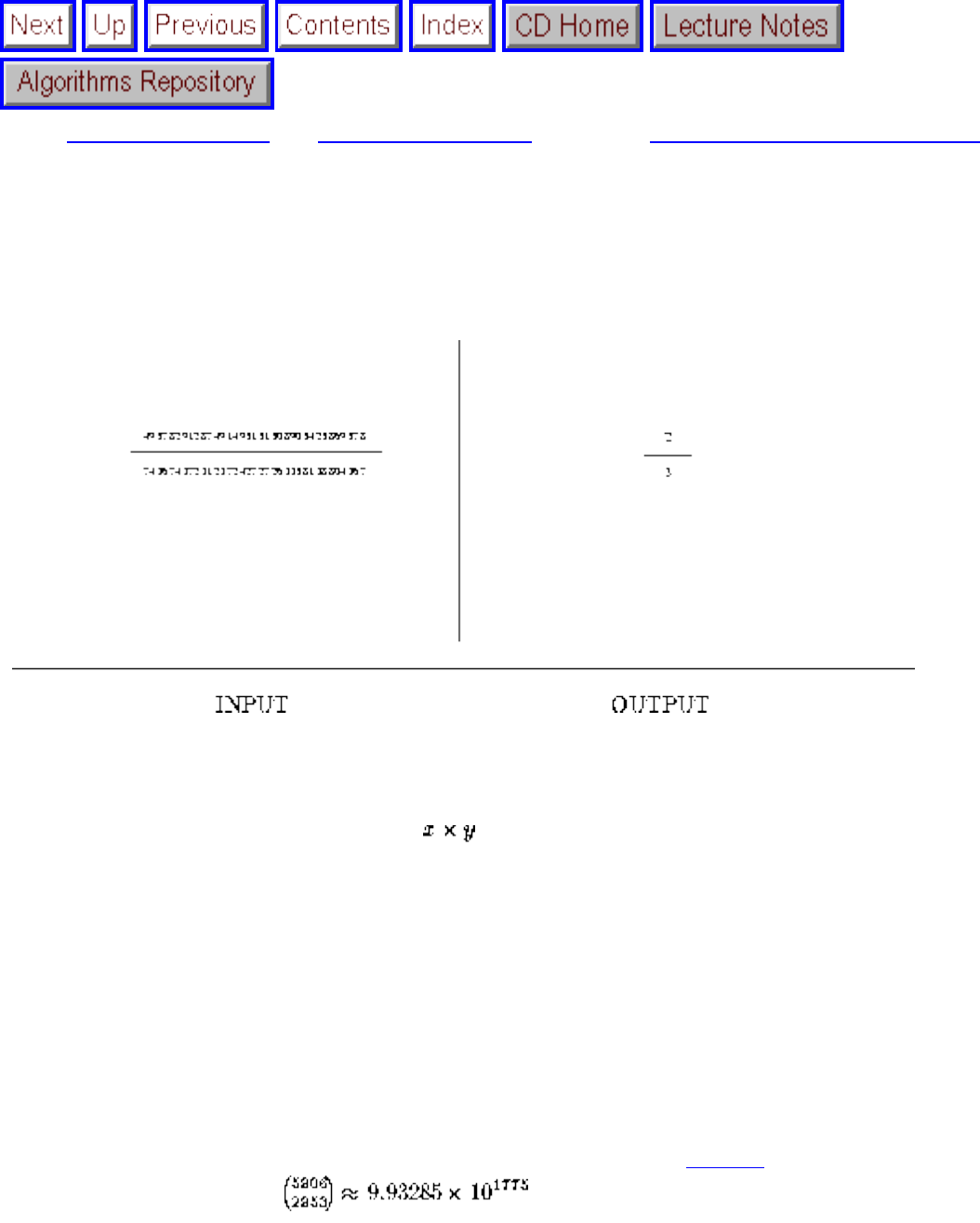
Arbitrary-Precision Arithmetic
Next: Knapsack Problem Up: Numerical Problems Previous: Factoring and Primality Testing
Arbitrary-Precision Arithmetic
Input description: Two very large integers, x and y.
Problem description: What is x+y, x-y, , and x / y?
Discussion: Any programming language whose level rises above basic assembler supports single- and
perhaps double-precision integer/real addition, subtraction, multiplication, and division. But what if we
wanted to represent the national debt of the United States in pennies? One trillion dollars worth of
pennies requires 15 decimal digits, which is far more than can fit into a 32-bit integer.
In other applications much larger integers are needed. The RSA algorithm for public-key cryptography
requires integer keys of at least 100 digits to achieve any level of security, and 1000 digits are
recommended. Experimenting with number-theoretic conjectures for fun or research always requires
playing with large numbers. I once solved a minor open problem [GKP89] by performing an exact
computation on the integer .
What should you do when you need large integers?
● Am I solving a problem instance requiring large integers, or do I have an embedded application? -
file:///E|/BOOK/BOOK4/NODE144.HTM (1 of 5) [19/1/2003 1:30:30]
Arbitrary-Precision Arithmetic
If you just need the answer to a specific problem with large integers, such as in the number theory
application above, you would be well advised to consider using a computer algebra system like
Maple or Mathematica. These use arbitrary-precision arithmetic as a default and use nice Lisp-
like programming languages as a front end, together often reducing your problem to a 5 to 10 line
program.
If instead you have an embedded application requiring high-precision arithmetic, you would be
well advised to use an existing library. In addition to the four basic operations, you are likely to
get additional functions for computing things like greatest common divisor in the bargain. See
the implementations below for details.
● Do I need high- or arbitrary-precision arithmetic? - Is there an upper bound on how big your
integers can get, or do you really need arbitrary-precision, i.e. unbounded. This determines
whether you can use a fixed-length array to represent your integers as opposed to a linked-list of
digits. The array is likely to be simpler and will not be a constraint in most applications.
● What base should I do arithmetic in? - It is conceptually simplest to implement your own high-
precision arithmetic package in decimal and represent each integer as a string of base-10 digits, at
one digit per node. However, it is far more efficient to use a higher base, ideally the square root
of the largest integer supported fully by hardware arithmetic.
Why? The higher the base, the fewer digits we need to represent the number (compare 64 decimal
with 1000000 binary). Since hardware addition usually takes one clock cycle independent of the
actual numbers, best performance is achieved using the highest base. The reason for limiting us
to is that in performing high-precision multiplication, we will multiply two of these
``digits'' together and need to avoid overflow.
The only complication of using a larger base is that integers must be converted to and from base-
10 for input and output, but the conversion is easily performed once all four high-precision
arithmetical operations are supported.
● How low-level are you willing to get for fast computation? Hardware addition is much faster than
a subroutine call, so you are going to take a significant hit on speed whenever your package is
used where low-precision arithmetic suffices. High-precision arithmetic is one of few problems
in this book where inner loops in assembly language can be the right idea to speed things up.
Finally, using bit-level masking and shift operations instead of arithmetical operations can be a
win.
The algorithm of choice for each of the five basic arithmetic operations is as follows:
● Addition - The basic schoolhouse method of lining up the decimal points and then adding the
digits from right to left with carries works in time linear in the number of digits. More
sophisticated carry-look-ahead parallel algorithms are available for low-level hardware
implementation. Hopefully they are used on your chip for low-precision addition.
● Subtraction - Depending upon the sign bits of the numbers, subtraction can be a special case of
file:///E|/BOOK/BOOK4/NODE144.HTM (2 of 5) [19/1/2003 1:30:30]
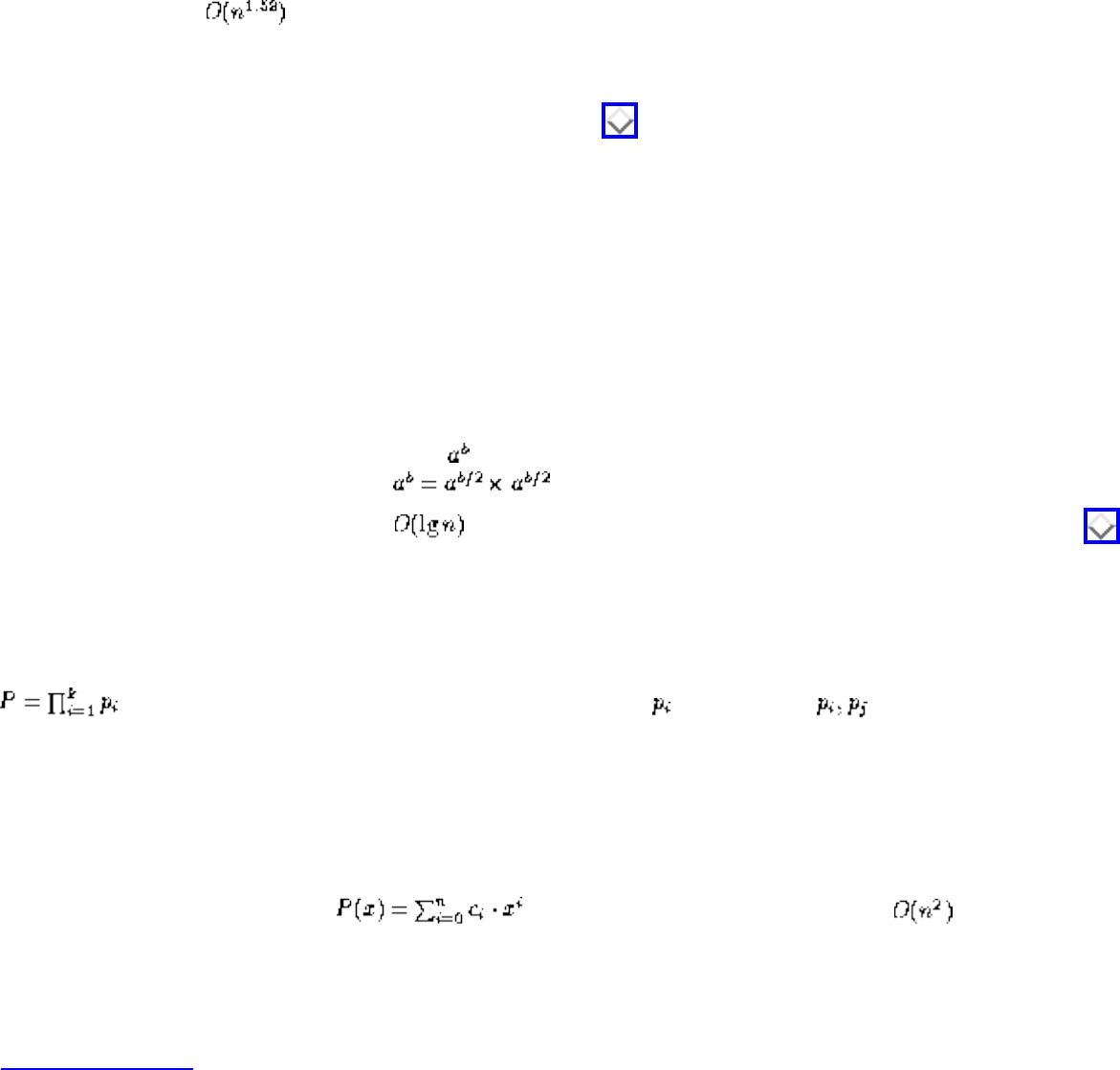
Arbitrary-Precision Arithmetic
addition: (A - (-B)) = (A+B). The tricky part of subtraction is performing the borrow. This can be
simplified by always subtracting from the number with the larger absolute value and adjusting the
signs afterwards, so we can be certain there will always be something to borrow from.
● Multiplication - The simplest method of repeated addition will take exponential time on large
integers, so stay away. The digit-by-digit schoolhouse method is reasonable to program and will
work much better, presumably well enough for your application. On very large integers,
Karatsuba's divide-and-conquer algorithm (cited in the notes) wins. Dan Grayson, author
of Mathematica's arbitrary-precision arithmetic, found that the switch-over happened at well under
100 digits. Even faster on very large integers is an algorithm based on Fourier transforms. A
discussion of such algorithms appears in Section .
● Division - Repeated subtraction will take exponential time, so the easiest reasonable algorithm to
use is the long-division method you hated in school. This is a far more complicated algorithm
than needed for the other operations, requiring arbitrary-precision multiplication and subtraction as
subroutines, as well as trial and error to determine the correct digit to use at each position of the
quotient.
In fact, integer division can be reduced to integer multiplication, although in a nontrivial way, so if
you are implementing asymptotically fast multiplication, you can reuse that effort in long division.
See the references below for details.
● Exponentiation - We can compute in the obvious manner using b-1 multiplications, but a better
way is to exploit the fact that . By repeatedly squaring the results of our partial
product, we can escape using multiplications, a big win when b is large. See Section
for a discussion of this algorithm.
High- but not arbitrary-precision arithmetic can be conveniently performed using the Chinese remainder
theorem and modular arithmetic. The Chinese remainder theorem states that an integer between 1 and
is uniquely determined by its set of residues mod , where each are relatively prime
integers. Addition, subtraction, and multiplication (but not division) can be supported using such residue
systems, with the advantage that large integers can be manipulated without complicated data structures.
Many of these algorithms for computations on long integers can be directly applied to computations on
polynomials. See the references for more details. A particularly useful algorithm is Horner's rule for fast
polynomial evaluation. When is blindly evaluated term by term, multiplications
will be performed. Much better is observing that , the evaluation of which uses only a linear number of
operations.
Implementations: All major commercial computer algebra systems incorporate high-precision
arithmetic, including Maple, Mathematica, Axiom, and Macsyma. If you have access to one of these,
this is your best option for a quick, nonembedded application. The rest of this section focuses on source
code available for embedded applications.
file:///E|/BOOK/BOOK4/NODE144.HTM (3 of 5) [19/1/2003 1:30:30]
Arbitrary-Precision Arithmetic
PARI, developed by Henri Cohen and his colleagues in France, is a system capable of handling complex
number-theoretic problems on integers with up to 300,000 decimal digits, as well as reals, rationals,
complex numbers, polynomials, and matrices. It is probably the most powerful free software available
for number theory. Written mainly in C (with assembly-language code for speed-critical routines), it
includes more than 200 special predefined mathematical functions. PARI can be used as a library, but it
possesses also a powerful calculator mode that gives instant access to all the types and functions. The
main advantage of PARI is its speed. On a Unix platform, it runs between 5 to 100 times faster than
Maple or Mathematica, depending on the applications. PARI is available for PC, Amiga, Macintosh, and
most Unix platforms by anonymous ftp at ftp://megrez.ceremab.u-bordeaux.fr/pub/pari/.
Algorithm 693 [Smi91] of the Collected Algorithms of the ACM is a Fortran implementation of floating-
point, multiple-precision arithmetic. See Section .
An implementation of arbitrary-precision integer and rational arithmetic in C++ is embedded in LEDA
(see Section ), including GCD, square roots, and logarithms as well as the basic four operations.
Sparc assembler code is used for certain time-critical functions.
Implementations in C of a high-precision calculator with all four elementary operations appear in [BR95].
The authors use base 10 for arithmetic and arrays of digits to represent long integers, with short integers
as array indices, thus limiting computations to 32,768 digits. The code for these algorithms is printed in
the text and available on disk for a modest fee.
Bare bones implementations in C of high-precision multiplication and in Pascal of such special functions
as logarithm and arctangent appear in [GBY91]. See Section for further details. Sedgewick [Sed92]
provides a bare bones implementation of polynomial arithmetic in C++. See Section for details.
Notes: Knuth [Knu81] is the primary reference on algorithms for all basic arithmetic operations,
including implementations of them in the MIX assembly language. Bach and Shallit [BS96] provide a
more recent treatment of computational number theory.
Expositions on the -time divide-and-conquer algorithm for multiplication [KO63] include [AHU74,
Man89]. An FFT-based algorithm multiplies two n-bit numbers in time and is due to Schönhage and
Strassen [SS71]. Expositions include [AHU74, Knu81]. The reduction between integer division and
multiplication is presented in [AHU74, Knu81].
Good expositions of algorithms for modular arithmetic and the Chinese remainder theorem include
[AHU74, CLR90]. A good exposition of circuit-level algorithms for elementary arithmetic algorithms is
[CLR90].
file:///E|/BOOK/BOOK4/NODE144.HTM (4 of 5) [19/1/2003 1:30:30]
Arbitrary-Precision Arithmetic
Euclid's algorithm for computing the greatest common divisor of two numbers is perhaps the oldest
interesting algorithm. Expositions include [CLR90, Man89].
Related Problems: Factoring integers (see page ), cryptography (see page ).
Next: Knapsack Problem Up: Numerical Problems Previous: Factoring and Primality Testing
Algorithms
Mon Jun 2 23:33:50 EDT 1997
file:///E|/BOOK/BOOK4/NODE144.HTM (5 of 5) [19/1/2003 1:30:30]
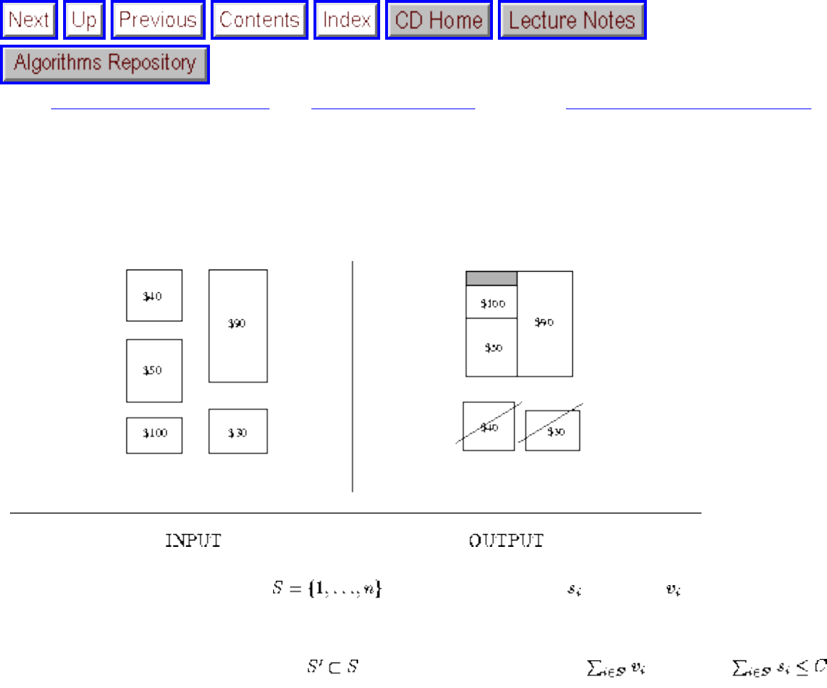
Knapsack Problem
Next: Discrete Fourier Transform Up: Numerical Problems Previous: Arbitrary-Precision Arithmetic
Knapsack Problem
Input description: A set of items , where item i has size and value . A knapsack
capacity C.
Problem description: Find the subset that maximizes the value of given that ;
i.e. all the items fit in a knapsack of size C.
Discussion: The knapsack problem arises whenever there is resource allocation with financial
constraints. Given a fixed budget, how do you select what things you should buy. Everything has a cost
and value, so we seek the most value for a given cost. The term knapsack problem invokes the image of
the backbacker who is constrained by a fixed-size knapsack and so must fill it only with the most useful
items.
The typical formulation in practice is the 0/1 knapsack problem, where each item must be put entirely in
the knapsack or not included at all. Objects cannot be broken up arbitrarily, so its not fair taking one can
of coke from a six-pack or opening the can to take just a sip. It is this 0/1 property that makes the
knapsack problem hard, for a simple greedy algorithm finds the optimal selection whenever we are
allowed to subdivide objects arbitrarily. For each item, we could compute its ``price per pound'', and
take as much of the most expensive item until we have it all or the knapsack is full. Repeat with the next
file:///E|/BOOK/BOOK4/NODE145.HTM (1 of 4) [19/1/2003 1:30:33]
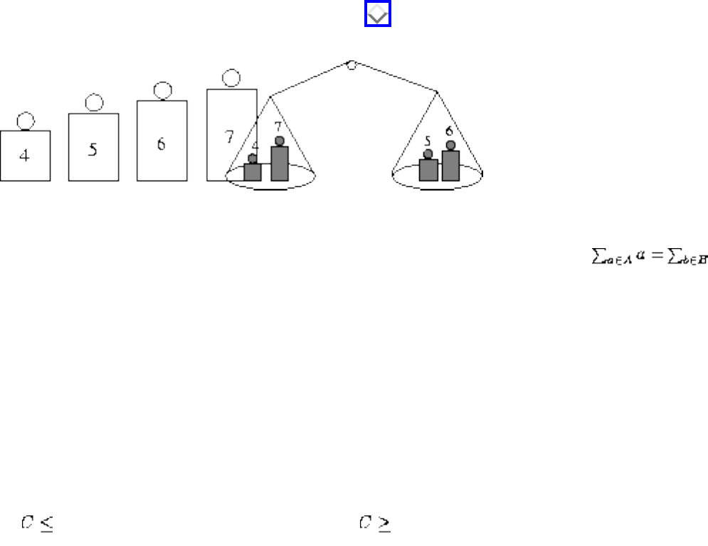
Knapsack Problem
most expensive item, until the knapsack is full. Unfortunately, this 0/1 constraint is usually inherent in
most applications.
Issues that arise in selecting the best algorithm include:
● Does every item have the same cost/value or the same size? - If each item is worth the same
amount to us as any other item, say $1, I maximize my value by taking the greatest number of
items. In this case the optimal solution is to sort the items in order of increasing size and insert
them into the knapsack in this order until nothing fits. The problem is solved similarly when
each object has the same size but the costs are different. These are the easy cases of knapsack.
● Does each item have the same ``price per pound''? - In this case, our problem is equivalent to
ignoring the price and just trying to minimize the amount of empty space left in the knapsack.
Unfortunately, even this restricted version of the problem is NP-complete, and so we cannot
expect an efficient algorithm that always solves the problem. Don't lose hope, however, because
knapsack proves to be an ``easy'' hard problem, one that can usually be handled with the
algorithms described below.
An important special case of constant ``price-per-pound'' knapsack is the integer partition
problem, presented in cartoon form in Figure .
Figure: Integer partition is a variant of the Knapsack problem
Here, we seek to partition the elements of S into two sets A and B such that , or
alternately make the difference as small as possible. Integer partition can be thought of as bin
packing with two equal-sized bins or knapsack with a capacity of half the total weight, so all three
problems are closely related and NP-complete.
The constant `price-per-pound' knapsack problem is often called the subset sum problem, because
given a set of numbers, we seek a subset that adds up to a specific target number, i.e. the
capacity of our knapsack.
● Are all the sizes relatively small integers? - When the sizes of the items and the knapsack capacity
C are all integers, there is an efficient dynamic programming algorithm that finds the optimal
solution in time O(n C) and O(C) space. Whether this is good for you depends upon how big C is.
For 1,000, this might be great, but not for 10,000,000.
The algorithm works as follows: Let S' be a set of items, and let C[i,S'] be true if and only if there
file:///E|/BOOK/BOOK4/NODE145.HTM (2 of 4) [19/1/2003 1:30:33]
Knapsack Problem
is a subset of S' whose size adds up exactly to i. For the empty set, is false for .
One by one we add a new item to S' and update the affected values of C[i,S']. Observe that
iff either C[i,S'] or is true, since either we use in our subset or we
don't. By performing n sweeps through all C elements, one for each , , and updating
the array, we identify which sums of sizes can be realized. The knapsack solution is the largest
realizable size. In order to reconstruct the winning subset, we must store the name of the item
number that turned C[i] from false to true, for each , and then scan backwards through
the array.
The dynamic programming formulation described above ignored the values of the items. To
generalize the algorithm, add a field to each element of the array to store the value of the best
subset to date summing up to i. We now update not only when C[i] turns from false to true, but
when the sum of the cost of plus the cost of is better than the previous cost of C[i].
● What if I have multiple knapsacks? - When there are multiple knapsacks, your problem is
probably better thought of as a bin packing problem. See Section .
When the knapsack capacity gets too large for dynamic programming, exact solutions can be found using
integer programming or backtracking. A 0/1 integer variable is used to denote whether item i is
present in the optimal subset. We maximize given the constraint that .
Algorithms and implementations of integer and linear programming are discussed in Section .
When exact solutions prove too costly to compute, heuristics should be used. The simple greedy heuristic
inserts items according to the maximum `price per pound' rule, described above. Often this heuristic
solution is close to optimal, but it can be arbitrarily bad depending upon the problem instance. The
``price per pound'' rule can also be used to reduce the size of the problem instance in exhaustive search-
based algorithms by eliminating ``cheap but heavy'' objects from future consideration.
Another heuristic is based on scaling. Dynamic programming works well if the capacity of the knapsack
is a reasonably small integer, say . But what if we have a problem with capacity ? We scale
down the sizes of all items by a factor of , round the size down to an integer, and then use dynamic
programming on the scaled items. Scaling works well in practice, especially when the range of sizes of
items is not too large.
Implementations: Martello and Toth's book [MT90a] comes with a disk of Fortran implementations of a
variety of knapsack algorithms. This is likely the best source of code currently available.
Algorithm 632 [MT85] of the Collected Algorithms of the ACM is a Fortran code for the 0/1 knapsack
problem, with the twist that it supports multiple knapsacks. See Section .
file:///E|/BOOK/BOOK4/NODE145.HTM (3 of 4) [19/1/2003 1:30:33]
Knapsack Problem
Pascal implementations of several knapsack algorithms, including backtracking and a refined greedy
algorithm, are provided in [SDK83]. See Section for details.
Notes: Martello and Toth's book [MT90a] and survey article [MT87] are the standard references on the
knapsack problem, including most theoretical and experimental results. An excellent exposition on
integer programming approaches to knapsack problems appears in [SDK83]. See [FP75a] for a
computational study of algorithms for 0-1 knapsack problems.
A polynomial-time approximation scheme is an algorithm that approximates the optimal solution of a
problem in time polynomial in both its size and the approximation factor . This very strong condition
implies a smooth tradeoff between running time and approximation quality. Good expositions on the
polynomial-time approximation scheme [IK75] for knapsack and subset sum includes [Baa88, CLR90,
GJ79, Man89].
The first algorithm for generalized public key encryption by Merkle and Hellman [MH78] was based on
the hardness of the knapsack problem. See [Sch94] for an exposition.
Related Problems: Bin packing (see page ), integer programming (see page ).
Next: Discrete Fourier Transform Up: Numerical Problems Previous: Arbitrary-Precision Arithmetic
Algorithms
Mon Jun 2 23:33:50 EDT 1997
file:///E|/BOOK/BOOK4/NODE145.HTM (4 of 4) [19/1/2003 1:30:33]
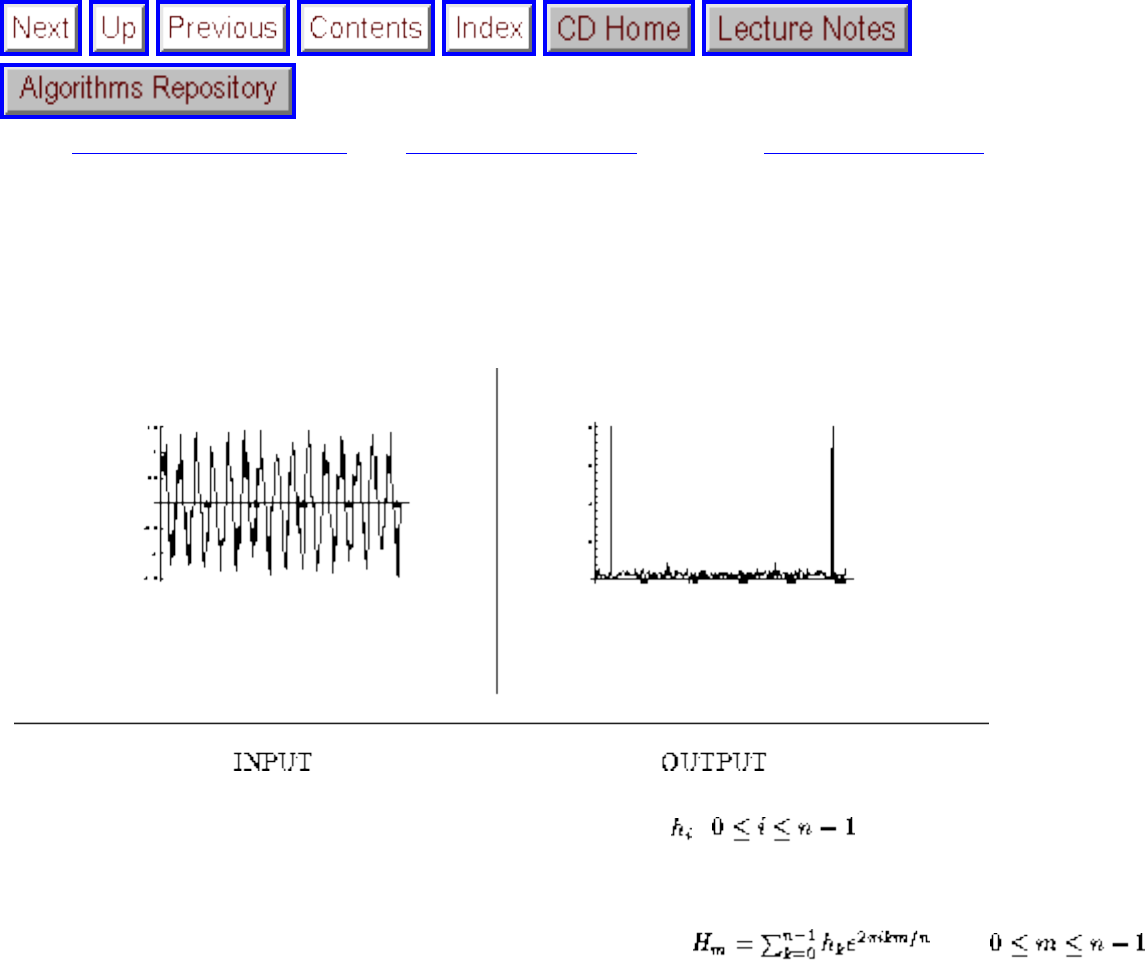
Discrete Fourier Transform
Next: Combinatorial Problems Up: Numerical Problems Previous: Knapsack Problem
Discrete Fourier Transform
Input description: A sequence of n real or complex values , , sampled at uniform
intervals from a function h.
Problem description: The discrete Fourier transform H of h, , for .
Discussion: Although computer scientists tend to be relatively unfamiliar with Fourier transforms,
electrical engineers and signal processors eat them for breakfast. Functionally, Fourier transforms
provide a way to convert samples of a standard time-series into the ``frequency domain''. This provides a
``dual'' representation of the function, in which certain operations become easier than in the time domain.
Applications of Fourier transforms include:
● Filtering - Taking the Fourier transform of a function is equivalent to representing it as the sum of
sine functions. By eliminating undesirable high- and/or low-frequency components (i.e.
dropping some of the sine functions) and taking an inverse Fourier transform to get us back into
the time domain, we can filter an image to remove noise and other artifacts. For example, the
sharp spike in the figure above describes the period of a single sine function that closely models
the input data.
● Image Compression - A smoothed, filtered image contains less information than a noisy image,
file:///E|/BOOK/BOOK4/NODE146.HTM (1 of 4) [19/1/2003 1:30:34]
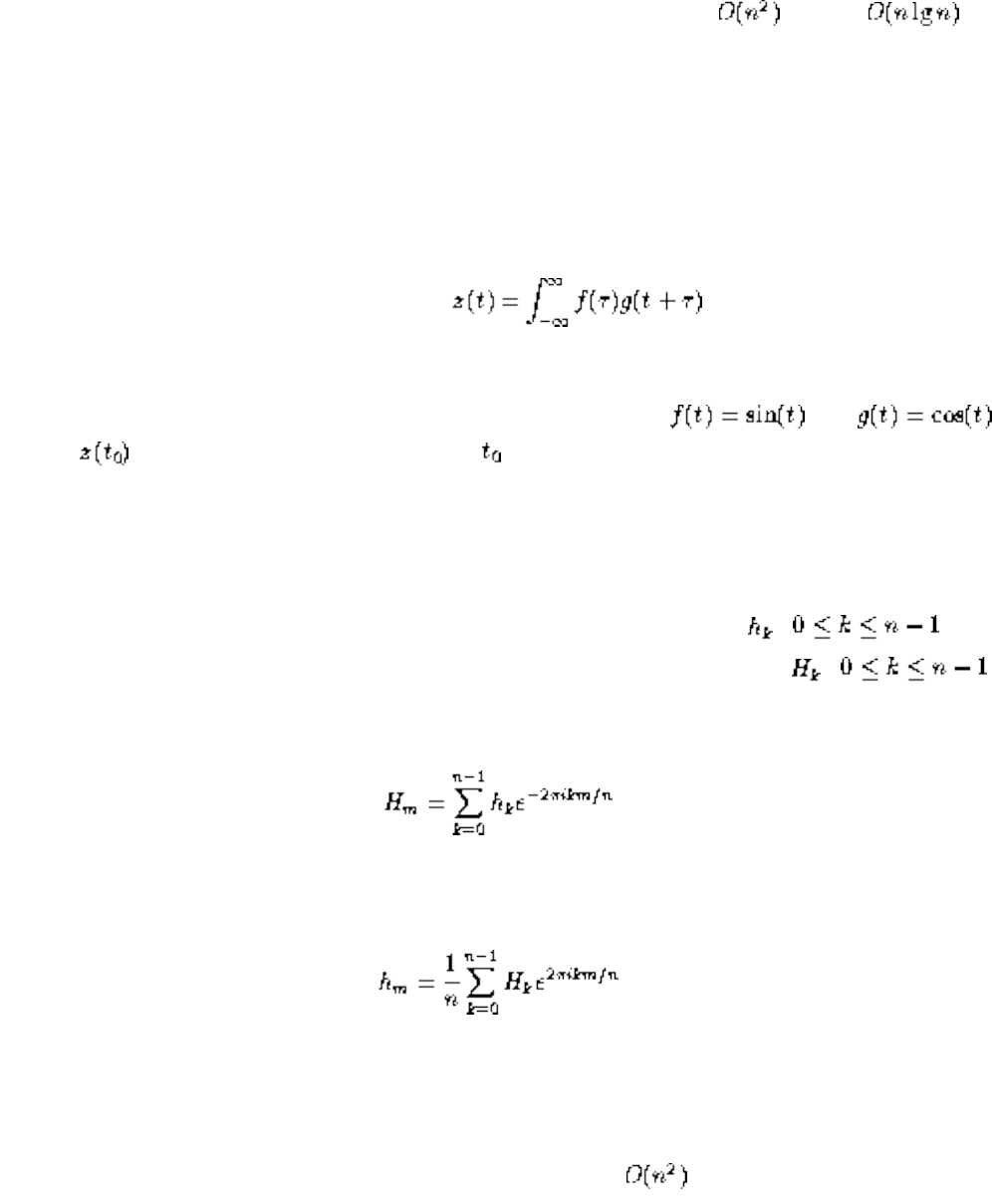
Discrete Fourier Transform
while retaining a similar appearance. Thus encoding the smoothed image will require fewer bits to
represent than the original image. By eliminating the coefficients of sine functions that
contribute relatively little to the image, we can further reduce the size of the image, at little cost in
image fidelity.
● Convolution and Deconvolution - Fourier transforms can be used to efficiently compute
convolutions of two sequences. A convolution is the pairwise product of elements from two
different sequences, such as in multiplying two n-variable polynomials f and g or multiplying two
long integers. Implementing the product directly takes , while suffices using the
fast Fourier transform. Another example comes from image processing. Because a scanner
measures the darkness of an image patch instead of a single point, the scanned input is always
blurred. A reconstruction of the original signal can be obtained by deconvoluting the input signal
with a Gaussian point-spread function.
● Computing the correlation of functions - The correlation function of two functions f(t) and g(t) is
defined by
and can be easily computed using Fourier transforms. Note that if the two functions are similar in
shape but one is shifted relative to the other (such as and ), the value of
will be large at this shift offset . As an application, suppose that we want to detect
whether there are any funny periodicities in our random number generator. We can generate a
large series of random numbers, turn it into a time series (the ith number at time i), and take the
Fourier transform of this series. Any funny spikes will correspond to potential periodicities.
The discrete Fourier transform takes as input n complex numbers , , corresponding to
equally spaced points in a time series, and outputs n complex numbers , , each
describing a sine function of given frequency. The discrete Fourier transform is defined by
and the inverse Fourier transform is defined by
which enables us move easily between h and H.
Since the output of the discrete Fourier transform consists of n numbers, each of which can be computed
using a formula on n numbers, they can be computed in time. The fast Fourier transform (FFT) is
file:///E|/BOOK/BOOK4/NODE146.HTM (2 of 4) [19/1/2003 1:30:34]
Discrete Fourier Transform
an algorithm that computes the discrete Fourier transform in . This is arguably the most
important algorithm known, as measured by practical impact, for it opened the door to modern image
processing. There are several different algorithms that call themselves FFTs, all of which are based on a
divide-and-conquer approach. Essentially, the problem of computing the discrete Fourier transform on n
points is reduced to computing two transforms on n/2 points each and is then applied recursively
The FFT usually assumes that n is a power of two. If this is not the case for your data, you are usually
better off padding your data with zeros to create elements rather than hunting for a more general
code.
Since many image processing systems have strong real-time constraints, FFTs are often implemented in
hardware, or at least in assembly language tuned to the particular machine. Be aware of this possibility if
the codes below prove too slow.
Implementations: FFTPACK is a package of Fortran subprograms for the fast Fourier transform of
periodic and other symmetric sequences, written by P. Swartzrauber. It includes complex, real, sine,
cosine, and quarter-wave transforms. A C language translation of the main routines is also provided.
FFTPACK resides on Netlib (see Section ) at http://www.netlib.org/fftpack.
Algorithm 545 [Fra79] of the Collected Algorithms of the ACM is an implementation of the fast Fourier
transform optimizing virtual memory performance and written in Fortran. See Section for further
information.
XTango (see Section ) is an algorithm animation system for UNIX and X-windows, which includes
an interesting animation of the fast Fourier transform.
A Pascal implementation of the fast Fourier transform for points appears in [MS91]. For more
details, see Section . Sedgewick [Sed92] provides a bare bones implementation of the fast Fourier
transform in C++. See Section for details.
Notes: Brigham [Bri74] is an excellent introduction to Fourier transforms and the FFT and is strongly
recommended, as is the exposition in [PFTV86]. Expositions in algorithms texts on the fast Fourier
transform include [AHU74, Baa88, CLR90, Man89].
Credit for inventing the fast Fourier transform is usually given to Cooley and Tukey [CT65], although it
is not completely deserved. See [Bri74] for a complete history.
An interesting divide-and-conquer algorithm for polynomial multiplication [KO63] does the job in
file:///E|/BOOK/BOOK4/NODE146.HTM (3 of 4) [19/1/2003 1:30:34]
Discrete Fourier Transform
time and is discussed in [AHU74, Man89]. An FFT-based algorithm that multiplies two n-bit
numbers in time is due to Schönhage and Strassen [SS71] and is presented in [AHU74].
In recent years, wavelets have been proposed to replace Fourier transforms in filtering. See [Dau92] for
an introduction to wavelets.
Related Problems: Data compression (see page ), high-precision arithmetic (see page ).
Next: Combinatorial Problems Up: Numerical Problems Previous: Knapsack Problem
Algorithms
Mon Jun 2 23:33:50 EDT 1997
file:///E|/BOOK/BOOK4/NODE146.HTM (4 of 4) [19/1/2003 1:30:34]
Combinatorial Problems
Next: Sorting Up: A Catalog of Algorithmic Previous: Discrete Fourier Transform
Combinatorial Problems
In this section, we consider several classic algorithmic problems of a purely combinatorial nature. These
include sorting and permutation generation, both of which were among the first nonnumerical problems
arising on electronic computers. Sorting, searching, and selection can all be classified in terms of
operations on a partial order of keys. Sorting can be viewed as identifying or imposing the total order on
the keys, while searching and selection involve identifying specific keys based on their position in the
total order.
The rest of this section deals with other combinatorial objects, such as permutations, partitions, subsets,
calendars, and schedules. We are particularly interested in algorithms that rank and unrank
combinatorial objects, i.e. that map each distinct object to and from a unique integer. Once we have rank
and unrank operations, many other tasks become simple, such as generating random objects (pick a
random number and unrank) or listing all objects in order (iterate from 1 to n and unrank).
We conclude with the problem of generating graphs. Graph algorithms are more fully presented in
subsequent sections.
Books on general combinatorial algorithms, in this restricted sense, include:
● Nijenhuis and Wilf [NW78] - This book specializes in algorithms for constructing basic
combinatorial objects such as permutations, subsets, and partitions. Such algorithms are often
very short but hard to locate and usually are surprisingly subtle. Fortran programs for all of the
algorithms are provided, as well as a discussion of the theory behind each of them. See Section
for details.
● Ruskey [Rus97] - On its completion, this manuscript in preparation will become the standard
reference on generating combinatorial objects. A preview is available via the WWW at
http://www-csc.uvic.ca/home/fruskey/cgi-bin/html/main.html .
● Knuth [Knu73a, Knu73b] - The standard reference on searching and sorting, with significant
material on combinatorial objects such as permutations.
● Reingold, Nievergelt, Deo [RND77] - A comprehensive algorithms text with a particularly
thorough treatment of combinatorial generation and search.
● Stanton and White [SW86] - An undergraduate combinatorics text with algorithms for generating
permutations, subsets, and set partitions. It contains relevant programs in Pascal.
file:///E|/BOOK/BOOK4/NODE147.HTM (1 of 2) [19/1/2003 1:30:35]
Combinatorial Problems
● Skiena [Ski90] - This description of Combinatorica, a library 230 Mathematica functions for
generating combinatorial objects and graph theory (see Section ) provides a distinctive view of
how different algorithms can fit together. Its author is uniquely qualified to write a manual on
algorithm design.
● Sorting
● Searching
● Median and Selection
● Generating Permutations
● Generating Subsets
● Generating Partitions
● Generating Graphs
● Calendrical Calculations
● Job Scheduling
● Satisfiability
Next: Sorting Up: A Catalog of Algorithmic Previous: Discrete Fourier Transform
Algorithms
Mon Jun 2 23:33:50 EDT 1997
file:///E|/BOOK/BOOK4/NODE147.HTM (2 of 2) [19/1/2003 1:30:35]
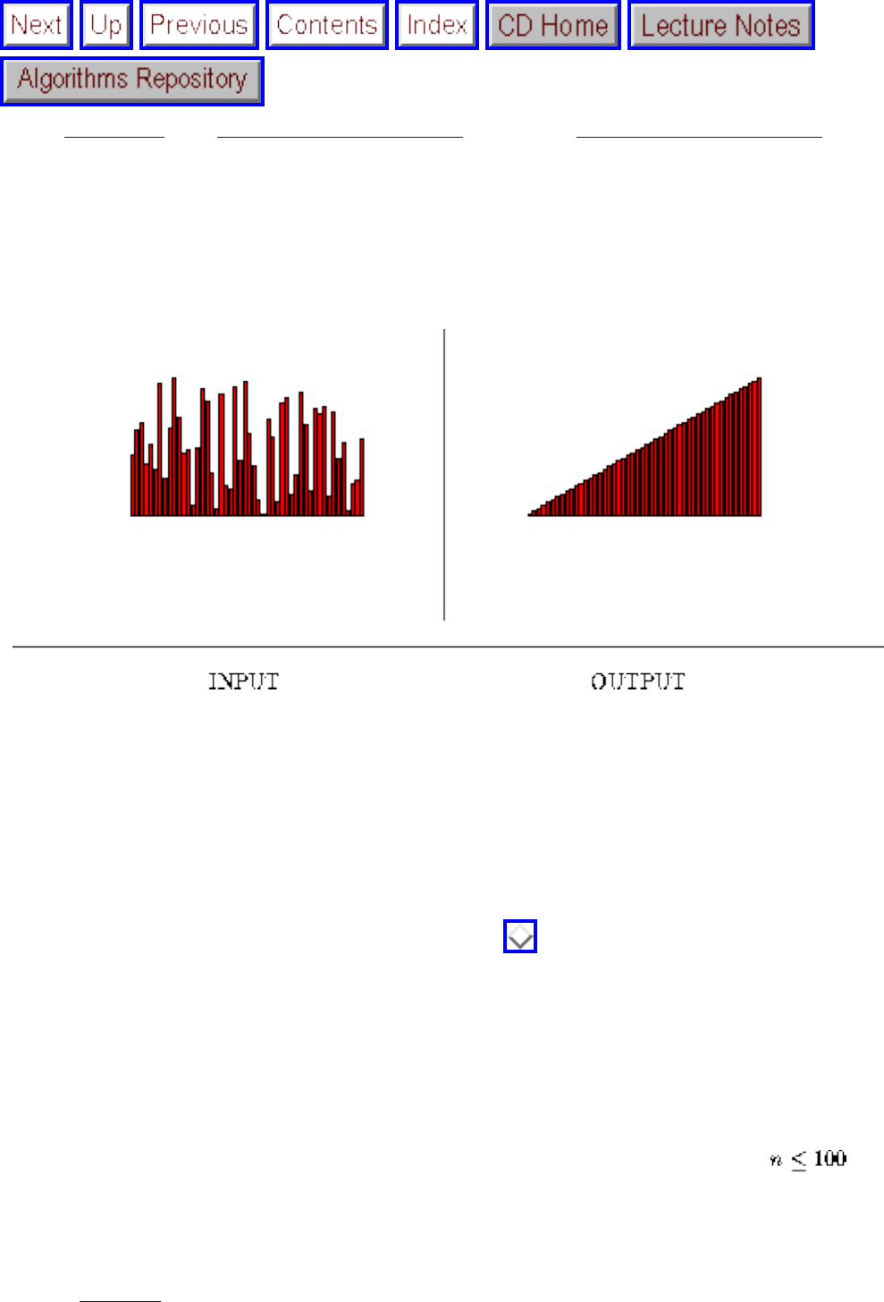
Sorting
Next: Searching Up: Combinatorial Problems Previous: Combinatorial Problems
Sorting
Input description: A set of n items.
Problem description: Arrange the items in increasing order.
Discussion: Sorting is the fundamental algorithmic problem in computer science. Learning the different
sorting algorithms is like learning scales for a musician. Sorting is the first step in solving a host of
other algorithm problems, as discussed in Section . Indeed, ``when in doubt, sort'' is one of the first
rules of algorithm design.
Sorting is also used to illustrate the standard paradigms of algorithm design. The result is that most
programmers are familiar with many different sorting algorithms, which sows confusion as to which
should be used for a given application. The following criteria can help you decide:
● How many keys will you be sorting? - For small amounts of data (say ), it really doesn't
matter much which of the quadratic-time algorithms you use. Insertion sort is faster, simpler, and
less likely to be buggy than bubblesort. Shellsort is much faster than insertion sort, but it
involves somewhat trickier programming and looking up good insert sequences in Knuth
[Knu73b].
file:///E|/BOOK/BOOK4/NODE148.HTM (1 of 5) [19/1/2003 1:30:37]
Sorting
If you have more than 100 items to sort, it is important to use an -time algorithm, like
heapsort, quicksort, or mergesort. If you have more than 1,000,000 items to sort, you probably
need an external-memory algorithm that minimizes disk access. Both types of algorithms are
discussed below.
● Will there be duplicate keys in the data? - When all items have distinct keys, the sorted order is
completely defined. However, when two items share the same key, something else must
determine which one comes first. For many applications it doesn't matter, so any sorting algorithm
is equally good. Often, ties are broken by sorting on a secondary key, like the first name or initial
if the family names collide.
Occasionally, ties need to be broken by their initial position in the data set. If the 5th and 27th
items of the initial data set share the same key in such a case, the 5th item must be before the 27th
in the final order. A stable sorting algorithm preserves the original ordering in case of ties. Most
of the quadratic-time sorting algorithms are stable, while many of the algorithms are not.
If it is important that your sort be stable, it is probably better to explicitly use the initial position
as a secondary key rather than trust the stability of your implementation.
● What do you know about your data? - In special applications, you can often exploit knowledge
about your data to get it sorted faster or more easily. Of course, general sorting is a fast
algorithm, so if the time spent sorting is really the bottleneck in your application, you are a
fortunate person indeed.
❍ Is the data already partially sorted? If so, algorithms like insertion sort perform better than
they otherwise would.
❍ Do you know the distribution of the keys? If the keys are randomly or uniformly
distributed, a bucket or distribution sort makes sense. Throw the keys into bins based on
their first letter, and recur until each bin is small enough to sort by brute force. This is
very efficient when the keys get evenly distributed into buckets. However, bucket sort
would be bad news sorting names on the mailing list of the ``Smith Society.''
❍ Are your keys very long or hard to compare? If your keys are long text strings, it might
pay to use a radix or bucket sort instead of a standard comparison sort, because the time of
each comparison can get expensive. A radix sort always takes time linear in the number
of characters in the file, instead of times the cost of comparing two keys.
❍ Is the range of possible keys very small? If you want to sort a subset of n/2 distinct
integers, each with a value from 1 to n, the fastest algorithm would be to initialize an n-
element bit vector, turn on the bits corresponding to keys, then scan from left to right and
report which bits are on.
● Do I have to worry about disk accesses? - In massive sorting problems, it may not be possible to
keep all data in memory simultaneously. Such a problem is called external sorting, because one
must use an external storage device. Traditionally, this meant tape drives, and Knuth [Knu73b]
describes a variety of intricate algorithms for efficiently merging data from different tapes.
Today, it usually means virtual memory and swapping. Any sorting algorithm will work with
virtual memory, but most will spend all their time swapping.
file:///E|/BOOK/BOOK4/NODE148.HTM (2 of 5) [19/1/2003 1:30:37]
Sorting
The simplest approach to external sorting loads the data into a B-tree (see Section ) and then
does an in-order traversal of the tree to read the keys off in sorted order. Other approaches are
based on mergesort. Files containing portions of the data are sorting using a fast internal sort, and
then these files are merged in stages using 2- or k-way merging. Complicated merging patterns
based on the properties of the external storage device can be used to optimize performance.
● How much time do you have to write and debug your routine? - If I had under an hour to
deliver a working routine, I would probably just use a simple selection sort. If I had an afternoon
to build an efficient sort routine, I would probably use heapsort, for it delivers reliable
performance without tuning. If I was going to take the time required to build a fast system sort
routine, I would carefully implement quicksort.
The best general-purpose sorting algorithm is quicksort (see Section ), although it requires
considerable tuning effort to achieve maximum performance. Indeed, you are probably better off using
a library function instead of doing it yourself. A poorly written quicksort will likely run more slowly than
a poorly written heapsort.
If you are determined to implement your own quicksort, use the following heuristics, which make a big
difference in practice:
● Use randomization - By randomly permuting (see Section ) the keys before sorting, you can
eliminate the potential embarrassment of quadratic-time behavior on nearly-sorted data.
● Median of three - For your pivot element, use the median of the first, last, and middle elements
of the array, to increase the likelihood of partitioning the array into roughly equal pieces. Some
experiments suggest using a larger sample on big subarrays and a smaller sample on small ones.
● Leave small subarrays for insertion sort - Terminating the quicksort recursion and switching to
insertion sort makes sense when the subarrays get small, say fewer than 20 elements. You should
experiment to determine the best switchpoint for your implementation.
● Do the smaller partition first - Assuming that your compiler is smart enough to remove tail
recursion, you can minimize runtime memory by processing the smaller partition before the larger
one. Since successive stored calls are at most half as large as before, only stack space is
needed.
Before you get started, see Bentley's article on building a faster quicksort [Ben92b].
Implementations: Pascal implementations of all the primary sorting algorithms are available from
[MS91]. See Section for details. Timing comparisons show an optimized version of quicksort to be
the winner.
Bare bones implementations of all basic sorting algorithms, in C and Pascal, appear in [GBY91]. Most
notable is the inclusion of implementations of external memory sorting algorithms. Sedgewick includes
file:///E|/BOOK/BOOK4/NODE148.HTM (3 of 5) [19/1/2003 1:30:37]
Sorting
similar sort routine fragments in C++. See Section for details.
XTango (see Section ) is an algorithm animation system for UNIX and X-windows, which includes
animations of all the basic sorting algorithms, including bubblesort, heapsort, mergesort, quicksort, radix
sort, and shellsort. Many of these are quite interesting to watch. Indeed, sorting is the canonical problem
for algorithm animation.
Algorithm 410 [Cha71] and Algorithm 505 [Jan76] of the Collected Algorithms of the ACM are Fortran
codes for sorting. The latter is an implementation of Shellsort on linked lists. Both are available from
Netlib (see Section ).
C language implementations of Shellsort, quicksort, and heapsort appear in [BR95]. The code for these
algorithms is printed in the text and available on disk for a modest fee.
A bare bones implementation of heapsort in Fortran from [NW78] can be obtained in Section . A
bare bones implementation of heapsort in Mathematica from [Ski90] can be obtained in Section .
Notes: Knuth [Knu73b] is the best book that has been written on sorting and indeed is the best book that
will ever be written on sorting. It is now almost twenty-five years old, and a revised edition is promised,
but it remains fascinating reading. One area that has developed since Knuth is sorting under
presortedness measures. A newer and noteworthy reference on sorting is [GBY91], which includes
pointers to algorithms for partially sorted data and includes implementations in C and Pascal for all of the
fundamental algorithms.
Expositions on the basic internal sorting algorithms appear in every algorithms text, including [AHU83,
Baa88, CLR90, Man89]. Treatments of external sorting are rarer but include [AHU83]. Heapsort was
first invented by Williams [Wil64]. Quicksort was invented by Hoare [Hoa62], with careful analysis and
implementation by Sedgewick [Sed78]. Von Neumann is credited with having produced the first
implementation of mergesort, on the EDVAC in 1945. See Knuth for a full discussion of the history of
sorting, dating back to the days of punched-card tabulating machines.
Sorting has a well-known lower bound under the algebraic decision tree model [BO83].
Determining the exact number of comparisons required for sorting n elements, for small values of n, has
generated considerable study. See [Aig88, Raw92] for expositions.
This lower-bound does not hold under different models of computation. Fredman and Willard [FW93]
present an algorithm for sorting under a model of computation that permits arithmetic
operations on keys. Under a similar model, Thorup [Tho96] developed a priority queue supporting
file:///E|/BOOK/BOOK4/NODE148.HTM (4 of 5) [19/1/2003 1:30:37]
Sorting
operations, implying an sorting algorithm.
Related Problems: Dictionaries (see page ), searching (see page ), topological sorting (see page
).
Next: Searching Up: Combinatorial Problems Previous: Combinatorial Problems
Algorithms
Mon Jun 2 23:33:50 EDT 1997
file:///E|/BOOK/BOOK4/NODE148.HTM (5 of 5) [19/1/2003 1:30:37]
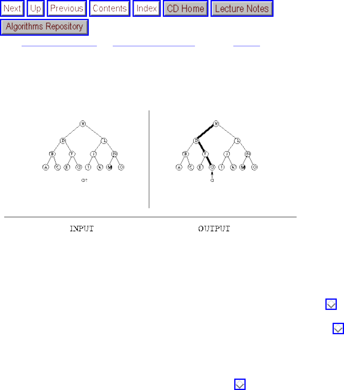
Searching
Next: Median and Selection Up: Combinatorial Problems Previous: Sorting
Searching
Input description: A set S of n keys, a query key q.
Problem description: Where is q in S?
Discussion: Searching means different things to different people. Searching for the global maximum or
minimum of a function is the problem of unconstrained optimization and is discussed in Section .
Chess playing programs search for the best move to make next by using alpha-beta minimax search,
which is an exhaustive search of the possible moves using a variation of backtracking (see Section ).
Here we consider the simple task of searching for a key in a list or in an array, which is a fundamental
problem associated with information retrieval. Dictionary data structures maintain efficient access to
sets of keys under insertion and deletion and are discussed in Section . Typical dictionaries include
binary trees and hash tables.
We treat searching here as a problem distinct from dictionaries because simpler and more efficient
solutions emerge when our primary interest is static searching. These little data structures can yield
file:///E|/BOOK/BOOK4/NODE149.HTM (1 of 4) [19/1/2003 1:30:39]
Searching
large performance improvements when properly employed in an innermost loop. Also, several of the
ideas from list and array searching, such as binary search and self-organization, apply to other problems
and justify our attention.
There are two basic approaches to array searching: sequential search and binary search. Both are simple,
yet have interesting and subtle variations. In sequential search, we simply start from the front of our list
or array of keys and compare each successive item against the key until we find a match or reach the end.
In binary search, we start with a sorted array of keys. To search for key q, we compare q to the middle
key . If q is before , it must reside in the top half of our set; if not, it must reside in the bottom
half of our set. By repeating this process on the correct half, we find the key in a total of
comparisons. This is a big win over the n/2 comparisons we expect with sequential search. See Section
for more on binary search.
Sequential search is the simplest algorithm, and likely to be fastest on up to 10-20 elements. For such
tiny problems, forget about binary search. Beyond 50-100 elements, there is no question that binary
search will be more efficient than sequential search, even factoring in the cost of the sorting (assuming
multiple queries). Other issues do come into play, however, particularly in identifying the proper variant
of the algorithm:
● How much time can you spend programming? - Binary search is a notoriously tricky algorithm
to program correctly. It took seventeen years after its invention until the first correct version of
binary search was published! Don't be afraid to start from one of the implementations described
below. Test it completely by writing a driver that searches for every key in the set S as well as
between the keys.
● Are certain items accessed more often than other ones? - Certain English words (such as ``the'')
are much more likely to occur than others (such as ``defenestrate''). We can reduce the number
of comparisons in a sequential search by putting the most popular words at the top of the list and
the least popular ones at the bottom. Further, nonuniform access is typically the rule, not the
exception. Many real-world distributions, such as word use in English, are more accurately
modeled by Zipf's law. Under Zipf's law, the ith most frequently accessed key is selected with
probability (i-1)/i times the probability of the (i-1)st most popular key, for all .
However, preordering the list to exploit a skewed access pattern requires knowing the access
pattern in advance. For many applications, it can be difficult to obtain such information. Far
easier are self-organizing lists, where the order of the keys changes in response to the queries.
The simplest and best self-organizing scheme is move-to-front; that is, we move the most recently
searched-for key from its current position to the front of the list. Popular keys keep getting
boosted to the front, while unsearched-for keys drift towards the back of the list. There is no need
to keep track of the frequency of access; just move the keys on demand. Self-organizing lists
also exploit locality of reference, since accesses to a given key are likely to occur in clusters.
Any key will be maintained near the top of the list during a cluster of accesses, even if other keys
have proven more popular in the past.
file:///E|/BOOK/BOOK4/NODE149.HTM (2 of 4) [19/1/2003 1:30:39]
Searching
Self-organization can extend the useful size range of sequential search. However, you should
switch to binary search beyond 50-100 elements.
● Is the key close by? - Suppose we know that the target key is to the right of position p, and we
think it is close by. Sequential search is fast if we are correct, but we will be punished severely
whenever we guess wrong. A better idea is to test repeatedly at larger intervals (p+1, p+2, p+4,
p+8, p+16, ) to the right until we find a key to the right of our target. After this, we have a
window containing the target and we can proceed with binary search.
Such a one-sided binary search finds the target at position p+l using at most comparisons,
so it is faster than binary search when l < < n, yet it can never be much worse. One-sided binary
search is particularly useful in unbounded search problems, such as in numerical root finding.
● Is my data structure sitting on external memory? - Once the number of keys grows too large,
as in a CD-ROM telephone directory of all the people in the United States, binary search loses its
status as the best search technique. Binary search jumps wildly around the set of keys looking for
midpoints to compare, and it becomes very expensive to read in a new page from a secondary
storage device for each comparison. Much better are data structures such as B-trees (see Section
), which cluster the keys into pages so as to minimize the number of disk accesses per search.
● Can I guess where the key should be? - In interpolation search, we exploit our understanding of
the distribution of keys to guess where to look next. Interpolation search is probably a more
accurate description of how we use a telephone book than binary search. For example, suppose we
are searching for Washington, George in a sorted telephone book. We would certainly be safe
making our first comparison three-fourths of the way down the list, essentially doing two
comparisons for the price of one.
Although interpolation search is an appealing idea, we caution against it for three reasons: First,
you have to work very hard to optimize your search algorithm before you can hope for a speedup
over binary search. Second, even if you get lucky and beat binary search, it is unlikely to be by
enough to have justified the exercise. Third, your program will be much less robust and efficient
when the distribution changes, such as when your application gets put to work on French words
instead of English.
Implementations: The basic sequential and binary search algorithms are simple enough to implement
that you should likely do them yourself. Still, the routines described below may be useful as models.
Gonnet and Baeza-Yates provides code fragments in C and Pascal for sequential, binary, and
interpolation search, as well as for related dictionary structures. LEDA (see Section ) provides a
sorted array data type in C++ that supports binary search. Many textbooks include implementations of
binary search, including [MS91]. See Section for details.
file:///E|/BOOK/BOOK4/NODE149.HTM (3 of 4) [19/1/2003 1:30:39]
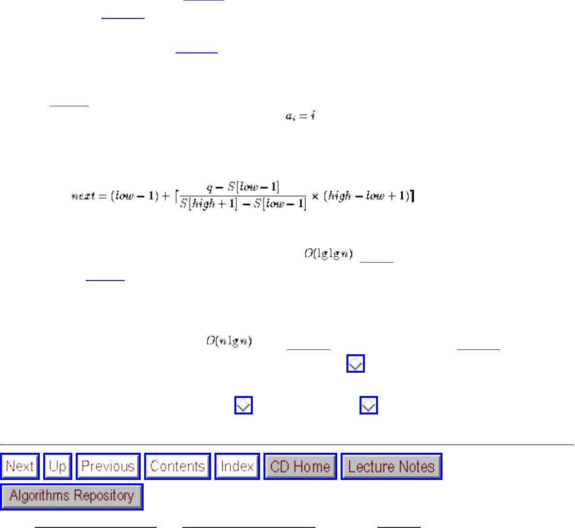
Searching
Notes: Mehlhorn and Tsakalidis [MT90b] give a through survey of the state-of-the-art in modern data
structures. Knuth [Knu73a] provides a detailed analysis and exposition on all fundamental search
algorithms and dictionary data structures but omits such modern data structures as red-black and splay
trees. Gonnet and Baeza-Yates [GBY91] provide detailed references and experimental results for a wide
variety of search algorithms.
Manber [Man89] provides an interesting discussion of variations of binary search, including one-sided
binary search and searching for an index in A where .
In linear interpolation search on an array of sorted numbers, the next position probed is given by
where q is the query numerical key and S the sorted numerical array. If the keys are drawn independently
from a uniform distribution, the expected search time is [YY76]. Expositions on interpolation
search include [Raw92].
Nonuniform access patterns can be exploited in binary search trees by structuring them so that popular
keys are located near the root, thus minimizing search time. Dynamic programming can be used to
construct such optimal search trees in time [Knu73b]. Expositions include [AHU74]. Splay
trees are self-organizing tree structures, as discussed in Section .
Related Problems: Dictionaries (see page ), sorting (see page ).
Next: Median and Selection Up: Combinatorial Problems Previous: Sorting
Algorithms
Mon Jun 2 23:33:50 EDT 1997
file:///E|/BOOK/BOOK4/NODE149.HTM (4 of 4) [19/1/2003 1:30:39]
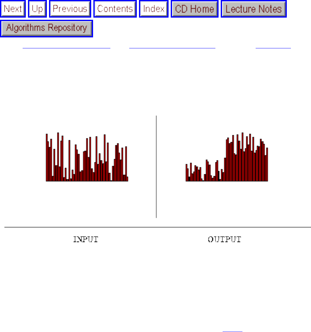
Median and Selection
Next: Generating Permutations Up: Combinatorial Problems Previous: Searching
Median and Selection
Input description: A set of n numbers or keys, and an integer k.
Problem description: Find the key that is smaller than exactly k of the n keys.
Discussion: Median finding is an essential problem in statistics, where it provides a more robust notion
of average than the mean. The mean wealth of people who have published research papers on sorting
is significantly affected by the presence of one William Gates [GP79], although his effect on the median
wealth is merely to cancel out one starving graduate student.
Median finding is a special case of the more general selection problem, which asks for the ith element in
sorted order. Selection arises in several applications:
● Filtering outlying elements - In dealing with noisy data samples, it is usually a good idea to throw
out the largest and smallest 10% or so of them. Selection can be used to identify the items
defining the tenth and ninetieth percentiles, and the outliers are then filtered out by comparing
each item to the two selected elements.
● Identifying the most promising candidates - In a computer chess program, we might quickly
evaluate all possible next moves, and then decide to study the top 25% more carefully. Selection
file:///E|/BOOK/BOOK4/NODE150.HTM (1 of 3) [19/1/2003 1:30:40]
Median and Selection
followed by filtering is the way to go.
● Order statistics - Particularly interesting special cases of selection include finding the smallest
element (i=1), the largest element (i=n), and the median element (i= n/2).
The mean of n numbers can be easily computed in linear time by summing the elements and dividing by
n. However, finding the median is a more difficult problem. Algorithms that compute the median can
easily be generalized to arbitrary selection.
The most elementary median-finding algorithm sorts the items in time and then returns the item
sitting the (n/2)nd position. The good thing is that this gives much more information than just the
median, enabling you to select the ith element (for all ) in constant time after the sort. However,
there are faster algorithms if all you want is the median.
In particular, there is an O(n) expected-time algorithm based on quicksort. Select a random element in the
data set as a pivot, and use it to partition the data into sets of elements less than and greater than the
pivot. From the sizes of these sets, we know the position of the pivot in the total order, and hence
whether the median lies to the left or right of the pivot. Now we recur on the appropriate subset until it
converges on the median. This takes (on average) iterations, with the cost of each iteration being
roughly half that of the previous one. This defines a geometric series that converges to a linear-time
algorithm, although if you are very unlucky it takes the same time as quicksort, .
More complicated algorithms are known that find the median in worst-case linear time. However, the
expected-time algorithm will likely win in practice. Just make sure to select random pivots in order to
avoid the worst case.
Beyond mean and median, a third notion of average is the mode, defined to be the element that occurs the
greatest number of times in the data set. The best way to compute the mode sorts the set in
time, which places all identical elements next to each other. By doing a linear sweep from left to right on
this sorted set, we can count the length of the longest run of identical elements and hence compute the
mode in a total of time.
In fact, there is no faster worst-case algorithm possible to compute the mode, since the problem of testing
whether there exist two identical elements in a set (called element uniqueness) can be shown to have an
lower bound. Element uniqueness is equivalent to asking if the mode is . Possibilities
exist, at least theoretically, for improvements when the mode is large by using fast median computations.
Implementations: A bare bones implementation in C of the recursive k-selection algorithm appears in
[GBY91]. See Section for further details.
XTango (see Section ) is an algorithm animation system for UNIX and X-windows, which includes
file:///E|/BOOK/BOOK4/NODE150.HTM (2 of 3) [19/1/2003 1:30:40]
Median and Selection
an animation of the linear-time selection algorithm. This animation is a good one.
Notes: The linear expected-time algorithm for median and selection is due to Hoare [Hoa61]. Floyd and
Rivest [FR75] provide an algorithm that uses fewer comparisons on average. Good expositions on linear-
time selection include [AHU74, Baa88, CLR90, Raw92], with [Raw92] being particularly enlightening.
A sport of considerable theoretical interest is determining exactly how many comparisons are sufficient
to find the median of n items. The linear-time algorithm of Blum et. al. [BFP 72] proves that
suffice, but we want to know what c is. A lower bower bound of 2n comparisons for median finding was
given by Bent and John [BJ85]. In 1976, Schönhage, Paterson, and Pippenger [SPP76] presented an
algorithm using 3n comparisons. Recently, Dor and Zwick [DZ95] proved that 2.95 n comparisons
suffice. These algorithms attempt to minimize the number of element comparisons but not the total
number of operations, and hence do not lead to faster algorithms in practice.
Tight combinatorial bounds for selection problems are presented in [Aig88]. An optimal algorithm for
computing the mode is presented in [DM80].
Related Problems: Priority queues (see page ), sorting (see page ).
Next: Generating Permutations Up: Combinatorial Problems Previous: Searching
Algorithms
Mon Jun 2 23:33:50 EDT 1997
file:///E|/BOOK/BOOK4/NODE150.HTM (3 of 3) [19/1/2003 1:30:40]
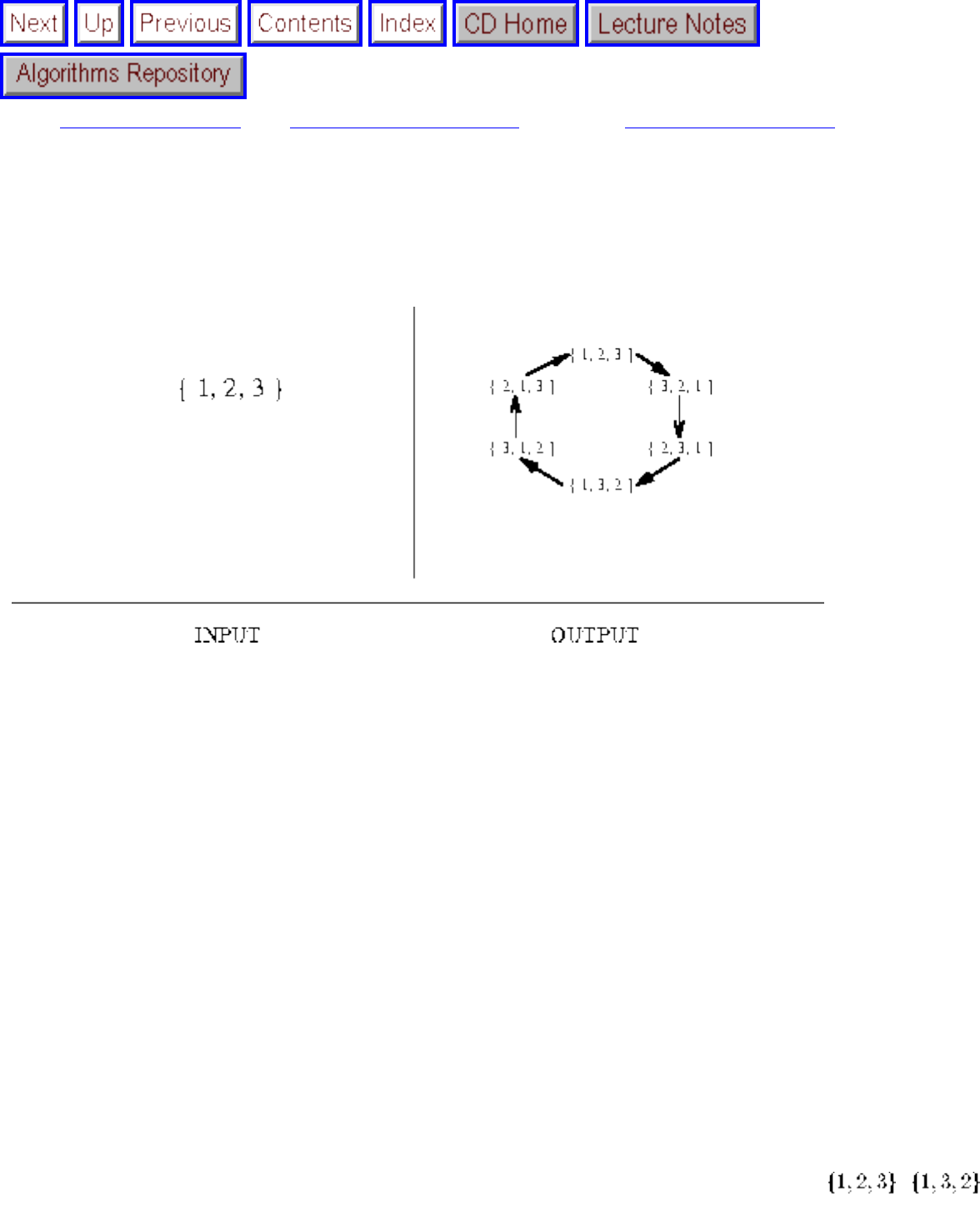
Generating Permutations
Next: Generating Subsets Up: Combinatorial Problems Previous: Median and Selection
Generating Permutations
Input description: An integer n.
Problem description: Generate (1) all or (2) a random or (3) the next permutation of length n.
Discussion: A permutation describes an arrangement, or ordering, of things. Many algorithmic problems
in this catalog seek the best way to order a set of objects, including traveling salesman (the least-cost
order to visit n cities), bandwidth (order the vertices of a graph on a line so as to minimize the length
of the longest edge), and graph isomorphism (order the vertices of one graph so that it is identical to
another). Any algorithm for solving such problems exactly must construct a series of permutations along
the way.
There are n! permutations of n items, which grows so quickly that you can't expect to generate all
permutations for n > 11, since 11! = 39,916,800. Numbers like these should cool the ardor of anyone
interested in exhaustive search and help explain the importance of generating random permutations.
Fundamental to any permutation-generation algorithm is a notion of order, the sequence in which the
permutations are constructed, from first to last. The most natural generation order is lexicographic, the
order they would appear if they were sorted numerically. Lexicographic order for n=3 is ,
file:///E|/BOOK/BOOK4/NODE151.HTM (1 of 5) [19/1/2003 1:30:42]
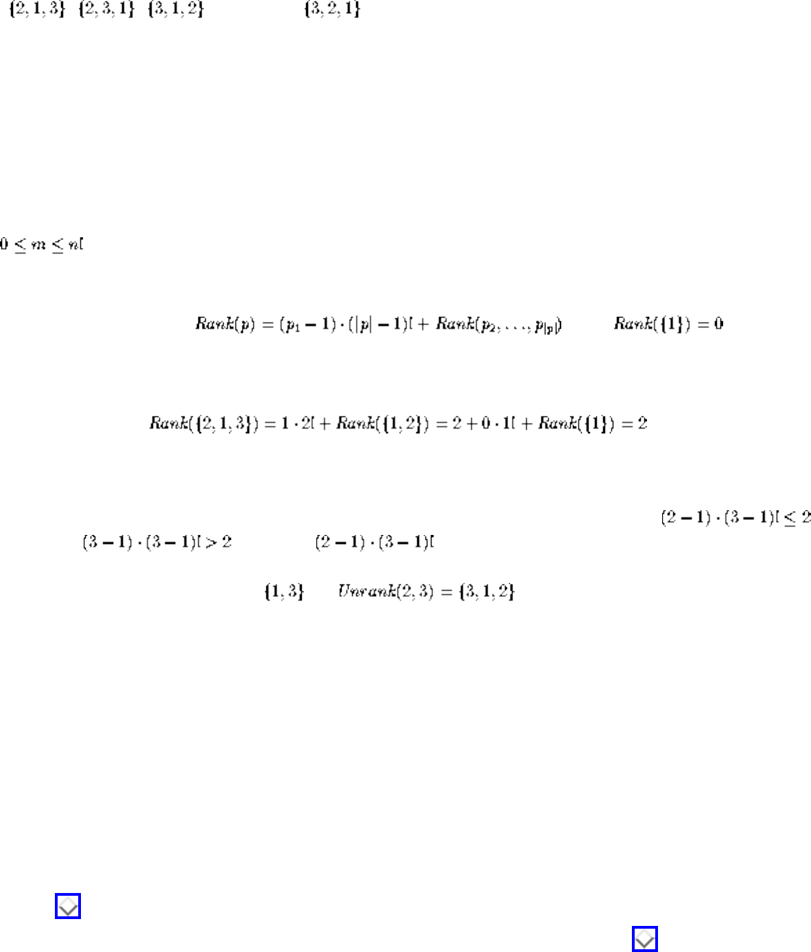
Generating Permutations
, , , , and finally . Although lexicographic order is aesthetically pleasing,
there is often no particular reason to use it. For example, if you are searching through a collection of
files, it does not matter whether the filenames are encountered in sorted order, so long as you search
through all of them. Indeed, nonlexicographic orders lead to faster and simpler permutation generation
algorithms.
There are two different paradigms for constructing permutations: ranking/unranking and incremental
change methods. Although the latter are more efficient, ranking and unranking can be applied to solve
a much wider class of problems, including the other combinatorial generation problems in this book. The
key is to define functions rank and unrank on all permutations p and integers n, m, where |p| = n and
.
● Rank(p) - What is the position of p in the given generation order? A typical ranking function is
recursive, such as , with . Getting
this right means relabeling the elements of the smaller permutation to reflect the deleted first
element. Thus
● Unrank(m,n) - Which permutation is in position m of the n! permutations of n items? A typical
unranking function finds the number of times (n-1)! goes into m and proceeds recursively.
Unrank(2,3) tells us that the first element of the permutation must be `2', since
but . Deleting from m leaves the smaller problem Unrank(0,2).
The ranking of 0 corresponds to the total order, and the total order on the two remaining elements
(since `2' has been used) is , so .
What the actual rank and unrank functions are does not matter as much as the fact that they must be
inverses. In other words, p = Unrank(Rank(p), n) for all permutations p. Once you define ranking and
unranking functions for permutations, you can solve a host of related problems:
● Sequencing permutations - To determine the next permutation that occurs in order after p, we
can Rank(p), add 1, and then Unrank(p). Similarly, the permutation right before p in order is
Unrank(Rank(p)-1,|p|). Counting through the integers from 0 to n!-1 and unranking them is
equivalent to generating all permutations.
● Generating random permutations - Select a random integer from 0 to n!-1 and unrank it.
● Keep track of a set of permutations - Suppose we want to construct random permutations and act
only when we encounter one we have not seen before. We can set up a bit vector (see Section
) with n! bits, and set bit i to 1 if permutation Unrank(i,n) has been seen. A similar
technique was employed with k-subsets in the Lotto application of Section .
file:///E|/BOOK/BOOK4/NODE151.HTM (2 of 5) [19/1/2003 1:30:42]
Generating Permutations
The rank/unrank method is best suited for small values of n, since n! quickly exceeds the capacity of
machine integers, unless arbitrary-precision arithmetic is available (see Section ). The incremental
change methods work by defining the next and previous operations to transform one permutation into
another, typically by swapping two elements. The tricky part is to schedule the swaps so that
permutations do not repeat until all of them have been generated. See the output picture above for an
ordering of the six permutations of with a single swap between successive permutations.
Incremental change algorithms for sequencing permutations are tricky, but they are concise enough that
they can be expressed in a dozen lines of code. See the implementation section for pointers to code.
Because the incremental change is a single swap, these algorithms can be extremely fast - on average,
constant time - which is independent of the size of the permutation! The secret is to represent the
permutation using an n-element array to facilitate the swap. In certain applications, only the change
between permutations is important. For example, in a brute-force program to search for the optimal tour,
the cost of the tour associated with the new permutation will be that of the previous permutation, with the
addition and deletion of four edges.
Throughout this discussion, we have assumed that the items we are permuting are all distinguishable.
However, if there are duplicates (meaning our set is a multiset), you can save considerable time and
effort by avoiding identical permutations. For example, there are only ten permutations of ,
instead of 120. To avoid duplicates use backtracking and generate the permutations in lexicographic
order.
Generating random permutations is an important little problem that people stumble across often, and
often botch up. The right way is the following two-line, linear-time algorithm. We assume that
Random[i,n] generates a random integer between i and n, inclusive.
for i=1 to n do a[i] = i;
for i=1 to n-1 do swap[ a[i], a[ Random[i,n] ];
That this algorithm generates all permutations uniformly at random is not obvious. If you think so,
explain convincingly why the following algorithm does not generate permutations uniformly:
for i=1 to n do a[i] = i;
for i=1 to n-1 do swap[ a[i], a[ Random[1,n] ];
file:///E|/BOOK/BOOK4/NODE151.HTM (3 of 5) [19/1/2003 1:30:42]
Generating Permutations
Such subtleties demonstrate why you must be very careful with random generation algorithms. Indeed,
we recommend that you try some reasonably extensive experiments with any random generator before
really believing it. For example, generate 10,000 random permutations of length 4 and see whether all 24
of them occur approximately the same number of times. If you understand how to measure statistical
significance, you are in even better shape.
Implementations: The best source on generating combinatorial objects is Nijenhuis and Wilf [NW78],
who provide efficient Fortran implementations of algorithms to construct random permutations and to
sequence permutations in minimum-change order. Also included are routines to extract the cycle
structure of a permutation. See Section for details.
An exciting WWW site developed by Frank Ruskey of the University of Victoria contains a wealth of
material on generating combinatorial objects of different types, including permutations, subsets,
partitions, and certain graphs. Specifically, there is an interactive interface that lets you specify which
type of objects you would like to construct and quickly returns the objects to you. It is well worth
checking this out at http://sue.csc.uvic.ca/ cos/.
Combinatorica [Ski90] provides Mathematica implementations of algorithms that construct random
permutations and sequence permutations in minimum change and lexicographic orders. It also
provides a backracking routine to construct all distinct permutations of a multiset, and it supports various
permutation group operations. See Section .
The Stanford GraphBase (see Section ) contains routines to generate all permutations of a multiset.
Notes: The primary reference on permutation generation is the survey paper by Sedgewick [Sed77].
Good expositions include [NW78, RND77, Rus97].
The fast permutation generation methods make only a single swap between successive permutations. The
Johnson-Trotter algorithm [Joh63, Tro62] satisfies an even stronger condition, namely that the two
elements being swapped are always adjacent.
In the days before ready access to computers, books with tables of random permutations [MO63] were
used instead of algorithms. The swap-based random permutation algorithm presented above was first
described in [MO63].
Related Problems: Random number generation (see page ), generating subsets (see page ),
file:///E|/BOOK/BOOK4/NODE151.HTM (4 of 5) [19/1/2003 1:30:42]

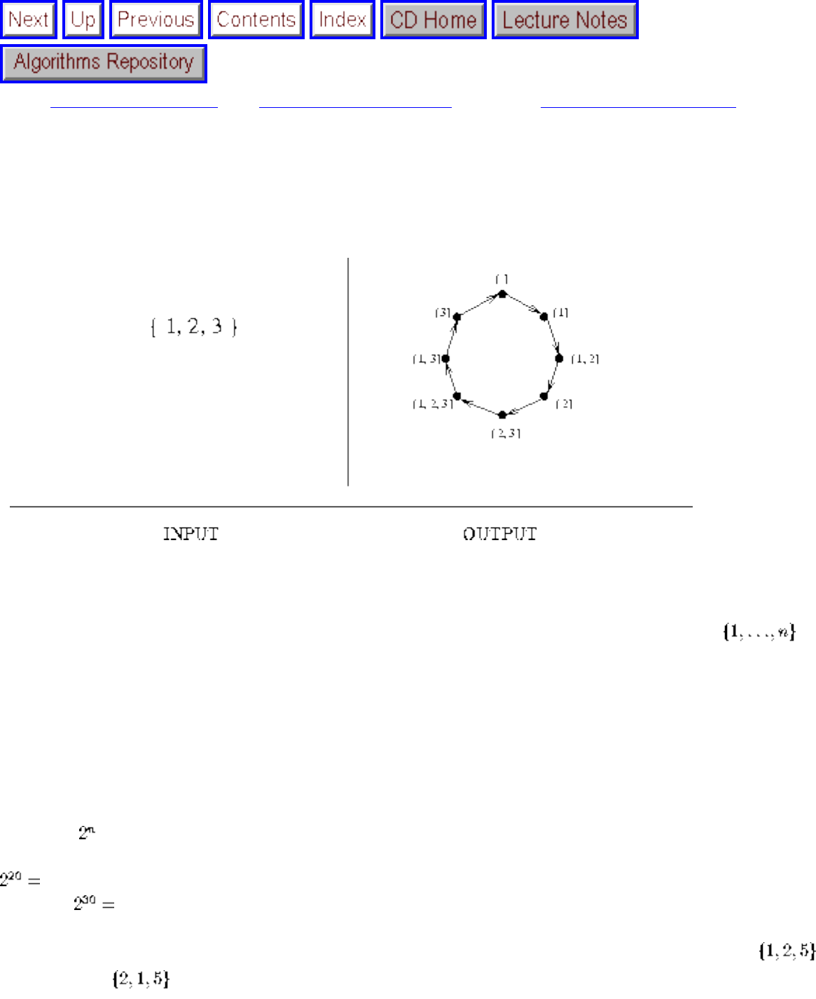
Generating Subsets
Next: Generating Partitions Up: Combinatorial Problems Previous: Generating Permutations
Generating Subsets
Input description: An integer n.
Problem description: Generate (1) all or (2) a random or (3) the next subset of the integers .
Discussion: A subset describes a selection of objects, where the order among them does not matter.
Many of the algorithmic problems in this catalog seek the best subset of a group of things: vertex cover
seeks the smallest subset of vertices to touch each edge in a graph; knapsack seeks the most profitable
subset of items of bounded total size; and set packing seeks the smallest subset of subsets that together
cover each item exactly once.
There are distinct subsets of an n-element set, including the empty set as well as the set itself. This
grows exponentially, but at a considerably smaller rate than the n! permutations of n items. Indeed, since
1,048,576, a brute-force search through all subsets of 20 elements is easily manageable, although
by n=30, 1,073,741,824, so you will certainly be pushing things.
By definition, the relative order among the elements does not distinguish different subsets. Thus
is the same as . However, it is a very good idea to maintain your subsets in a sorted or canonical
order, in order to speed up such operations as testing whether two subsets are identical or making them
file:///E|/BOOK/BOOK4/NODE152.HTM (1 of 4) [19/1/2003 1:30:44]
Generating Subsets
look right when printed.
As with permutations (see Section ), the key to subset generation problems is establishing a numerical
sequence among all subsets. There are three primary alternatives:
● Lexicographic order - Lexicographic order is sorted order, and often the most natural order for
generating combinatorial objects. The eight subsets of in lexicographic order are , ,
, , , , , and . Unfortunately, it is surprisingly difficult to generate
subsets in lexicographic order. Unless you have a compelling reason to do so, forget about it.
● Gray Code - A particularly interesting and useful subset sequence is the minimum change order,
wherein adjacent subsets differ by the insertion or deletion of exactly one element. Such an
ordering, called a Gray code, appears in the output picture above.
Subset generation in Gray code order can be very fast, because there is a nice recursive
construction to sequence subsets. Further, since only one element changes between subsets,
exhaustive search algorithms built on Gray codes can be quite efficient. A set cover program
would only have to update the change in coverage by the addition or deletion of one subset. See
the implementation section below for Gray code subset generation programs.
● Binary counting - The simplest approach to subset generation problems is based on the
observation that any subset S' of S is defined by which of the n=|S| items are in S'. We can
represent S' by a binary string of n bits, where bit i is 1 iff the ith element of S is in S'. This
defines a bijection between the binary strings of length n, and the subsets of n items. For
n=3, binary counting generates subsets in the following order: {}, {3}, {2}, {2,3}, {1}, {1,3},
{1,2}, {1,2,3}.
This binary representation is the key to solving all subset generation problems. To generate all
subsets in order, simply count from 0 to . For each integer, successively mask off each of
the bits and compose a subset of exactly the items corresponding to `1' bits. To generate the next
or previous subset, increment or decrement the integer by one. Unranking a subset is exactly the
masking procedure, while ranking constructs a binary number with 1's corresponding to items in S
and then converts this binary number to an integer.
To generate a random subset, you could generate a random integer from 0 to and unrank,
although you are probably asking for trouble because any flakiness with how your random
number generator rounds things off means that certain subsets can never occur. Therefore, a better
approach is simply to flip a coin n times, with the ith flip deciding whether to include element i in
the subset. A coin flip can be robustly simulated by generating a random real or large integer and
testing whether it is bigger or smaller than half the range. A Boolean array of n items can thus be
used to represent subsets as a sort of premasked integer. The only complication is that you must
explicitly handle the carry if you seek to generate all subsets.
file:///E|/BOOK/BOOK4/NODE152.HTM (2 of 4) [19/1/2003 1:30:44]
Generating Subsets
Generation problems for two closely related problems arise often in practice:
● k-subsets - Instead of constructing all subsets, we may only be interested in the subsets
containing exactly k elements. There are such subsets, which is substantially less than ,
particularly for small values of k.
The best way to construct all k-subsets is in lexicographic order. The ranking function is based
on the observation that there are k-subsets whose smallest element is f. Using this, it is
possible to determine the smallest element in the mth k-subset of n items. We then proceed
recursively for subsequent elements of the subset. See the implementations below for details.
● Strings - Generating all subsets is equivalent to generating all strings of true and false. To
generate all or random strings on alphabets of size , the same basic techniques apply, except
there will be strings in total.
Implementations: Nijenhuis and Wilf [NW78] provide efficient Fortran implementations of algorithms
to construct random subsets and to sequence subsets in Gray code and lexicographic order. They also
provide routines to construct random k-subsets and sequence them in lexicographic order. See Section
for details on ftp-ing these programs. Algorithm 515 [BL77] of the Collected Algorithms of the ACM
is another Fortran implementation of lexicographic k-subsets, available from Netlib (see Section ).
An exciting WWW site developed by Frank Ruskey of the University of Victoria contains a wealth of
material on generating combinatorial objects of different types, including permutations, subsets,
partitions, and certain graphs. Specifically, it provides an interactive interface that lets you specify which
type of objects you would like to construct and then returns the objects to you. Check this out at
http://sue.csc.uvic.ca/ cos/.
Combinatorica [Ski90] provides Mathematica implementations of algorithms to construct random
subsets and to sequence subsets in Gray code, binary, and lexicographic order. They also provide
routines to construct random k-subsets and strings, and sequence them lexicographically. See Section
for further information on Combinatorica.
Notes: The primary expositions on subset generation include [NW78, RND77, Rus97]. Wilf [Wil89]
provides an update of [NW78], including a thorough discussion of modern Gray code generation
problems.
Gray codes were first developed [Gra53] to transmit digital information in a robust manner over an
analog channel. By assigning the code words in Gray code order, the ith word differs only slightly from
the (i+1)st, so minor fluctuations in analog signal strength corrupts only a few bits. Gray codes have a
particularly nice correspondence to Hamiltonian cycles on the hypercube. See any of the references
file:///E|/BOOK/BOOK4/NODE152.HTM (3 of 4) [19/1/2003 1:30:44]
Generating Subsets
above for details. An exposition on the more general problem of constructing Gray codes for k items
(instead of subsets) appears in [Man89].
The popular puzzle Spinout, manufactured by Binary Arts Corporation, can be solved using Gray codes.
Related Problems: Generating permutations (see page ), generating partitions (see page ).
Next: Generating Partitions Up: Combinatorial Problems Previous: Generating Permutations
Algorithms
Mon Jun 2 23:33:50 EDT 1997
file:///E|/BOOK/BOOK4/NODE152.HTM (4 of 4) [19/1/2003 1:30:44]
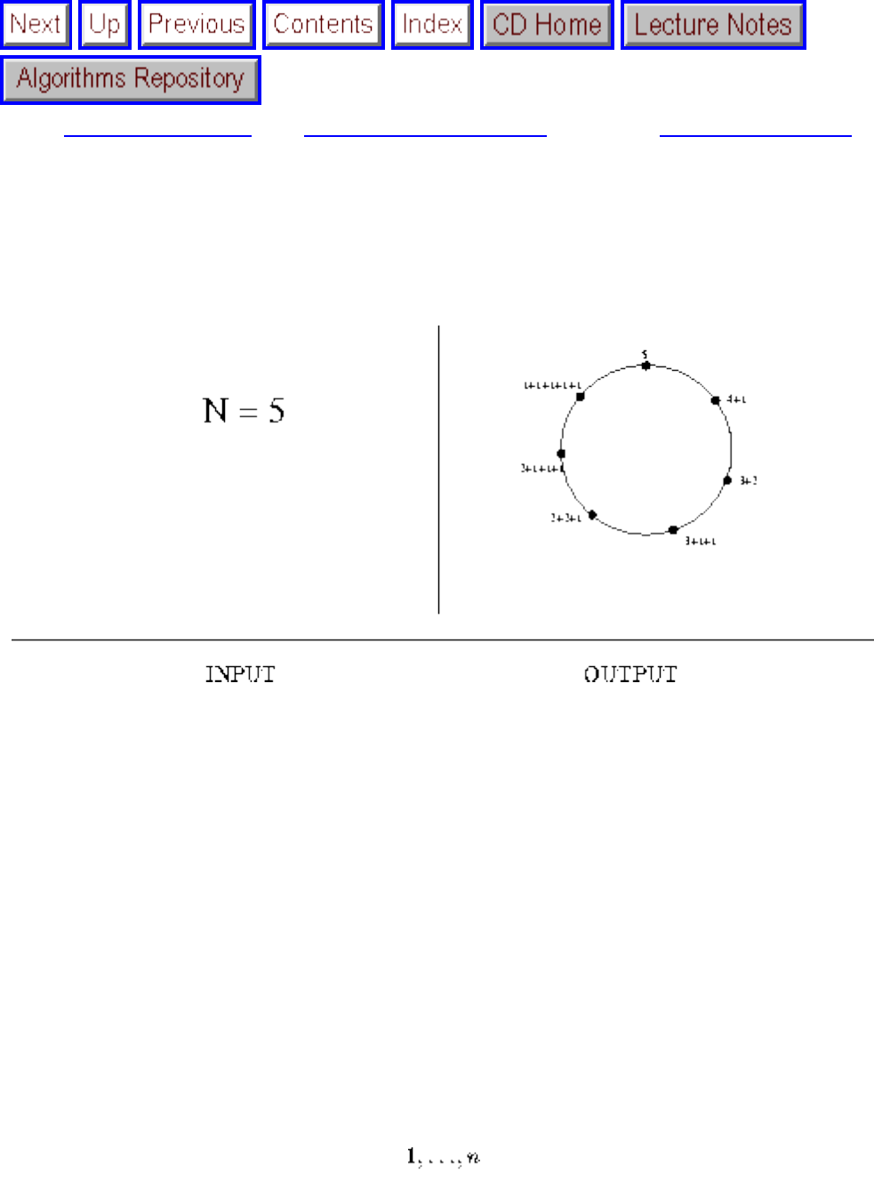
Generating Partitions
Next: Generating Graphs Up: Combinatorial Problems Previous: Generating Subsets
Generating Partitions
Input description: An integer n.
Problem description: Generate (1) all or (2) a random or (3) the next integer or set partitions of length n.
There are two different types of combinatorial objects denoted by the term ``partition'', namely integer
partitions and set partitions. Although they are quite different beasts, it is a good idea to make both a
part of your vocabulary:
● Integer partitions of n are sets of nonzero integers that add up to exactly n. For example, the seven
distinct integer partitions of 5 are {5}, {4,1}, {3,2}, {3,1,1}, {2,2,1}, {2,1,1,1}, and {1,1,1,1,1}.
An interesting application I encountered that required the generation of integer partitions was in a
simulation of nuclear fission. When an atom is smashed, the nucleus of protons and neutrons is
broken into a set of smaller clusters. The sum of the particles in the set of clusters must equal the
original size of the nucleus. As such, the integer partitions of this original size represent all the
possible ways to smash the atom.
● Set partitions divide the elements into nonempty subsets. For example, there are fifteen
distinct set partitions of n=4: {1234}, {123,4}, {124,3}, {12,34}, {12,3,4}, {134,2}, {13,24},
{13,2,4}, {14,23}, {1,234}, {1,23,4}, {14,2,3}, {1,24,3}, {1,2,34}, and {1,2,3,4}. Several of
the problems in this catalog return set partitions as results, such as vertex coloring and connected
components.
file:///E|/BOOK/BOOK4/NODE153.HTM (1 of 4) [19/1/2003 1:30:46]
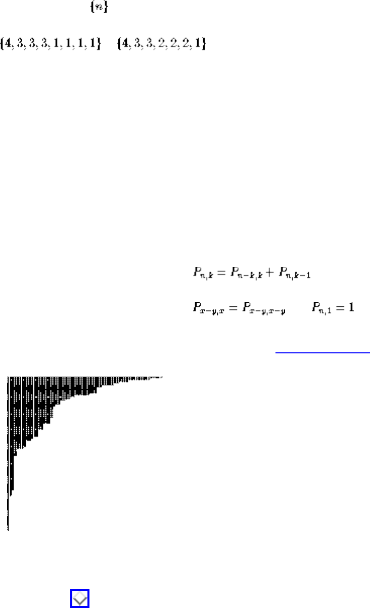
Generating Partitions
Although the number of integer partitions grows exponentially with n, they do so at a refreshingly slow
rate. There are only 627 partitions of n=20, and it is even possible to enumerate all partitions of n=100,
since there there are only 190,569,292 of them.
The best way to generate all partitions is to construct them in lexicographically decreasing order. The
first partition is itself. The general rule is to subtract 1 from the smallest part that is >1 and then
collect all the 1's so as to match the new smallest part >1. For example, the partition after
is , since the five 1's left after 3-1=2 becomes the smallest part are best
packaged as 2,2,1. When the partition is all 1's, we have completed one trip through all the partitions.
This algorithm is not particularly complicated, but it is sufficiently intricate that you should consider
using one of the implementations below. In either case, test it to make sure that you get exactly 627
distinct partitions for n=20.
Generating integer partitions uniformly at random is a trickier matter than generating random
permutations or subsets. This is because selecting the first (i.e. largest) element of the partition has a
dramatic effect on the number of possible partitions that can be generated. Observe that no matter how
large n is, there is only one partition of n whose largest part is 1. The number of partitions of n with
largest part at most k is given by the recurrence
with the two boundary conditions and . This function can be used to select the
largest part of your random partition with the correct probabilities and, by proceeding recursively, to
eventually construct the entire random partition. Implementations are cited below.
Figure: The Ferrers diagram of a random partition of n=1000
Random partitions tend to have large numbers of fairly small parts, best visualized by a Ferrers diagram
as in Figure . Each row of the diagram corresponds to one part of the partition, with the size of each
part represented by that many dots.
file:///E|/BOOK/BOOK4/NODE153.HTM (2 of 4) [19/1/2003 1:30:46]
Generating Partitions
Set partitions can be generated using techniques similar to integer partitions. Each set partition is
encoded as a restricted growth function, , where and , for
. Each distinct digit identifies a subset, or block, of the partition, while the growth condition
ensures that the blocks are sorted into a canonical order based on the smallest element in each block. For
example, the restricted growth function 0,1,1,2,0,3,1 defines the set partition {{1,5}, {2,3,7}, {4}, {6} }.
Since there is a one-to-one equivalence between set partitions and restricted growth functions, we can use
lexicographic order on the restricted growth functions to order the set partitions. Indeed, the fifteen
partitions of {1,2,3,4} listed above are sequenced according to the lexicographic order of their restricted
growth function (check it out).
To randomly generate set partitions, we use a similar counting strategy as with integer partitions. The
Stirling numbers of the second kind S(n,k) count the number of partitions of 1,...,n with exactly k blocks.
They are computed using the recurrence S(n,k) = S(n-1,k-1) + k*S(n-1,k) with the boundary conditions
S(n,n)=1. The reader is referred to the references and implementations for more details and code.
Implementations: The best source on generating combinatorial objects is Nijenhuis and Wilf [NW78],
who provide efficient Fortran implementations of algorithms to construct random and sequential integer
partitions, set partitions, compositions, and Young tableaux. See Section for details on ftp-ing these
programs.
An exciting WWW site developed by Frank Ruskey of the University of Victoria contains a wealth of
material on generating combinatorial objects of different types, including permutations, subsets,
partitions, and certain graphs. It is well worth checking this out at http://sue.csc.uvic.ca/~cos/.
Combinatorica [Ski90] provides Mathematica implementations of algorithms to construct random and
sequential integer partitions, compositions, strings, and Young tableaux, as well as to count and
manipulate these objects. See Section .
Algorithm 403 [BL77] of the Collected Algorithms of the ACM is a Fortran code for constructing integer
partitions with k parts. It is available from Netlib (see Section ). The Stanford GraphBase (see
Section ) also contains generators for constructing all integer partitions.
Notes: The standard references on combinatorial generation [NW78, RND77, Rus97] all present
algorithms for generating integer and/or set partitions. Andrews is the primary reference on integer
partitions and related topics.
Interestingly, the set of all 52 set partitions for n=5 appears in the form of Murasaki diagrams in the oldest
novel known, The Tale of Genji.
file:///E|/BOOK/BOOK4/NODE153.HTM (3 of 4) [19/1/2003 1:30:46]
Generating Partitions
Two related combinatorial objects are Young tableaux and integer compositions, although they are less
likely to emerge in applications. Generation algorithms for both are presented in [NW78, RND77, Rus97]
Young tableaux are two-dimensional configurations of integers {1,...,n} where the number of elements in
each row is defined by an integer partition of n. Further, the elements of each row and column are sorted
in increasing order, and the rows are left-justified. This notion of shape captures a wide variety of
structures as special cases. They have many interesting properties, including the existance of a bijection
between pairs of tableaux and permutations.
Compositions represent the set of possible assignments of a set of n indistinguishable balls to k
distinguishable boxes. For example, we can place three balls into two boxes as {3,0}, {2,1}, {1,2}, or
{0,3}. Compositions are most easily constructed sequentially in lexicographic order. To construct them
randomly, pick a random (k-1)-subset of n+k-1 items using the algorithm of the previous section, and
count the number of unselected items between the selected ones. For example, if k=5 and n=10, the (5-1)-
subset {1,3,7,14} of 1,..., (n+k-1)=14 defines the composition {0,1,3,6,0}, since there are no items to the
left of element 1 nor right of element 14.
Related Problems: Generating permutations (see page ), generating subsets (see page ).
Next: Generating Graphs Up: Combinatorial Problems Previous: Generating Subsets
Algorithms
Mon Jun 2 23:33:50 EDT 1997
file:///E|/BOOK/BOOK4/NODE153.HTM (4 of 4) [19/1/2003 1:30:46]
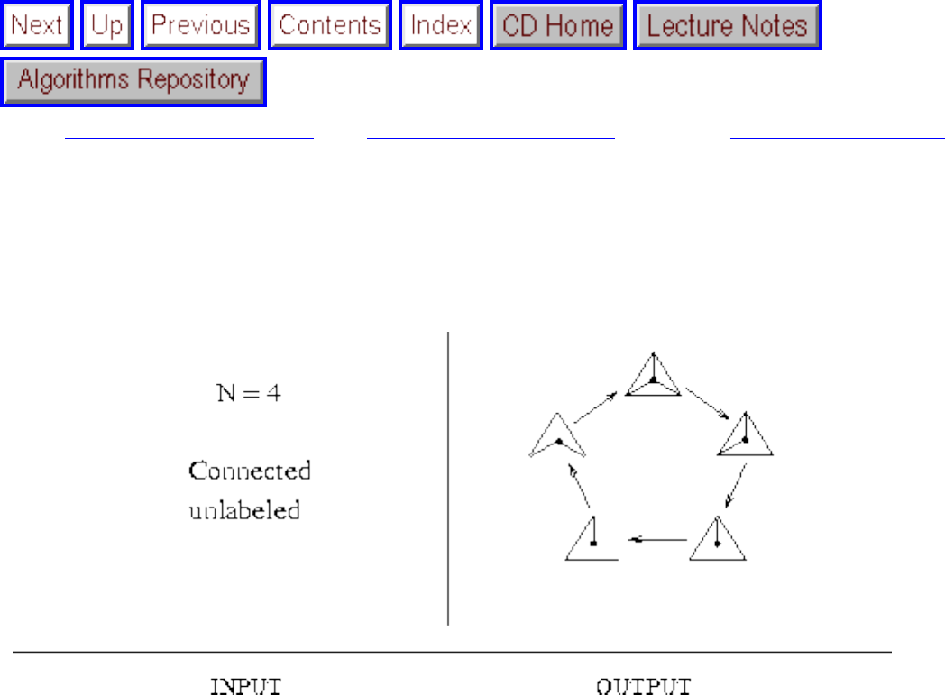
Generating Graphs
Next: Calendrical Calculations Up: Combinatorial Problems Previous: Generating Partitions
Generating Graphs
Input description: Parameters describing the desired graph, such as the number of vertices n, the
number of edges m, or the edge probability p.
Problem description: Generate (1) all or (2) a random or (3) the next graph satisfying the parameters.
Discussion: Graph generation typically arises in constructing test data for programs. Perhaps you have
two different programs that solve the same problem, and you want to see which one is faster or make
sure that they always give the same answer. Another application is experimental graph theory, verifying
whether a particular property is true for all graphs or how often it is true. It is much easier to conjecture
the four-color theorem once you have demonstrated 4-colorings for all planar graphs on 15 vertices.
A different application of graph generation arises in network design. Suppose you need to design a
network linking ten machines using as few cables as possible, such that the network can survive up to
two vertex failures. One approach is to test all the networks with a given number of edges until you find
one that will work. For larger graphs, more heuristic approaches, like simulated annealing, will likely be
necessary.
Many factors complicate the problem of generating graphs. First, make sure you know what you want to
file:///E|/BOOK/BOOK4/NODE154.HTM (1 of 5) [19/1/2003 1:30:48]
Generating Graphs
generate:
● Do I want labeled or unlabeled graphs? - The issue here is whether the names of the vertices
matter in deciding whether two graphs are the same. In generating labeled graphs, we seek to
construct all possible labelings of all possible graph topologies. In generating unlabeled graphs,
we seek only one representative for each topology and ignore labelings. For example, there are
only two connected unlabeled graphs on three vertices - a triangle and a simple path. However,
there are four connected labeled graphs on three vertices - one triangle and three 3-vertex paths,
each distinguished by their central vertex. In general, labeled graphs are much easier to generate.
However, there are so many more of them that you quickly get swamped with isomorphic copies
of the same few graphs.
● What do I mean by random? - There are two primary models of random graphs, both of which
generate graphs according to different probability distributions. The first model is parameterized
by a given edge probability p. Typically, p=0.5, although smaller values can be used to construct
sparser random graphs. In this model a coin is flipped for each pair of vertices x and y to decide
whether to add an edge (x,y). All labeled graphs will be generated with equal probability when
p=1/2.
The second model is parameterized by the desired number of edges m. It selects m distinct edges
uniformly at random. One way to do this is by drawing random (x,y)-pairs and creating an edge if
that pair is not already in the graph. An alternative approach to computing the same things
constructs the set of possible edges and selects a random m-subset of them, as discussed in
Section .
Which of these options best models your application? Probably none of them. Random graphs, by
definition, have very little structure. In most applications, graphs are used to model relationships, which
are often highly structured. Experiments conducted on random graphs, although interesting and easy to
perform, often fail to capture what you are looking for.
An alternative to random graphs is to use ``organic'' graphs, graphs that reflect the relationships among
real-world objects. The Stanford GraphBase, discussed below, is an outstanding source of organic
graphs. Further, there are many raw sources of relationships electronically available via the Internet that
can be turned into interesting organic graphs with a little programming and imagination. Consider the
graph defined by a set of WWW pages, with any hyperlink between two pages defining an edge. Or
what about the graph implicit in railroad, subway, or airline networks, with vertices being stations and
edges between two stations connected by direct service? As a final example, every large computer
program defines a call graph, where the vertices represent subroutines, and there is an edge (x,y) if x calls
y.
Two special classes of graphs have generation algorithms that have proven particularly useful in practice:
file:///E|/BOOK/BOOK4/NODE154.HTM (2 of 5) [19/1/2003 1:30:48]
Generating Graphs
● Trees - Prüfer codes provide a simple way to rank and unrank labeled trees and thus solve all
the standard generation problems discussed in Section . There are exactly labeled trees
on n vertices, and exactly that many strings of length n-2 on the alphabet .
The key to Prüfer's bijection is the observation that every tree has at least two vertices of degree 1.
Thus in any labeled tree, the vertex v incident on the leaf with lowest label is well-defined. We
take v to be , the first character in the code. We then delete the associated leaf and repeat the
procedure until only two vertices are left. This defines a unique code S for any given labeled tree
that can be used to rank the tree. To go from code to tree, observe that the degree of vertex v in
the tree is one more than the number of times v occurs in S. The lowest-labeled leaf will be the
smallest integer missing from S, which when paired with determines the first edge of the tree.
The entire tree follows by induction.
Algorithms for efficiently generating unlabeled rooted trees are presented in the implementation
section below.
● Fixed degree sequence graphs - The degree sequence of a graph G is an integer partition
where is the degree of the ith highest-degree vertex of G. Since each edge
contributes to the degree of two vertices, p is a partition of 2m, where m is the number of edges in
G.
Not all partitions correspond to degree sequences of graphs. However, there is a recursive
construction that constructs a graph with a given degree sequence if one exists. If a partition is
realizable, the highest-degree vertex can be connected to the next highest-degree vertices in
G, or the vertices corresponding to parts . Deleting and decrementing
yields a smaller partition, which we recur on. If we terminate without ever creating negative
numbers, the partition was realizable. Since we always connect the highest-degree vertex to other
high-degree vertices, it is important to reorder the parts of the partition by size after each iteration.
Although this construction is deterministic, a semirandom collection of graphs realizing this
degree sequence can be generated from G using edge-flipping operations. Suppose edges (x,y)
and (w,z) are in G, but (x,w) and (y,z) are not. Exchanging these pairs of edges creates a different
(not necessarily connected) graph without changing the degrees of any vertex.
Implementations: The Stanford GraphBase [Knu94] is perhaps most useful as an instance generator for
constructing a wide variety of graphs to serve as test data for other programs. It incorporates graphs
derived from interactions of characters in famous novels, Roget's Thesaurus, the Mona Lisa, expander
graphs, and the economy of the United States. It also contains routines for generating binary trees, graph
products, line graphs, and other operations on basic graphs. Finally, because of its machine-independent
random number generators, it provides a way to construct random graphs such that they can be
reconstructed elsewhere, thus making them perfect for experimental comparisons of algorithms. See
Section for additional information.
file:///E|/BOOK/BOOK4/NODE154.HTM (3 of 5) [19/1/2003 1:30:48]
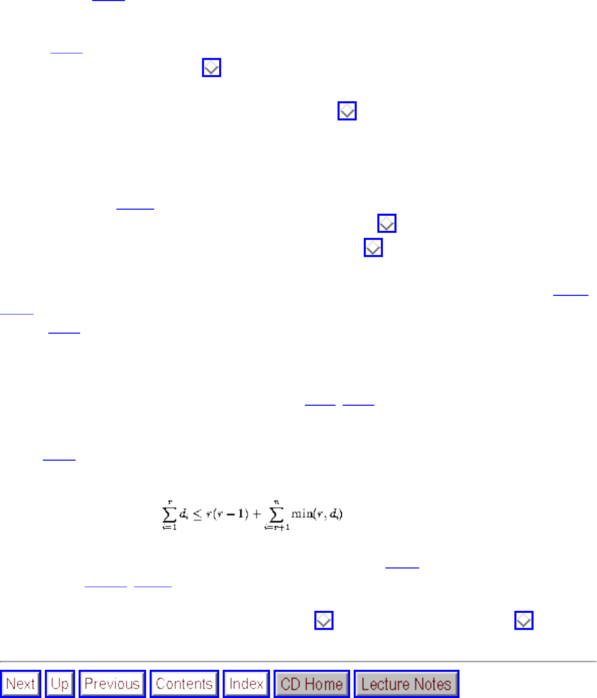
Generating Graphs
Combinatorica [Ski90] provides Mathematica generators for basic graphs such as stars, wheels, complete
graphs, random graphs and trees, and graphs with a given degree sequence. Further, it includes
operations to construct more interesting graphs from these, including join, product, and line graph.
Graffiti [Faj87], a collection of almost 200 graphs of graph-theoretic interest, are available in
Combinatorica format. See Section .
The graph isomorphism testing program nauty (see Section ), by Brendan D. McKay of the
Australian National University, has been used to generate catalogs of all nonisomorphic graphs with up
to 11 vertices. This extension to nauty, named makeg, can be obtained by anonymous ftp from
bellatrix.anu.edu.au (150.203.23.14) in the directory pub/nauty19.
Nijenhuis and Wilf [NW78] provide efficient Fortran routines to enumerate all labeled trees via Prüfer
codes and to construct random unlabeled rooted trees. See Section . A collection of generators for
standard families of graphs is included with LEDA (see Section ).
Notes: An extensive literature exists on generating graphs uniformly at random. Surveys include [Gol93,
Tin90]. Closely related to the problem of generating classes of graphs is counting them. Harary and
Palmer [HP73] survey results in graphical enumeration.
Random graph theory is concerned with the properties of random graphs. Threshold laws in random
graph theory define the edge density at which properties such as connectedness become highly likely to
occur. Expositions on random graph theory include [ES74, Pal85].
An integer partition is graphic if there exists a simple graph with that degree sequence. Erd•s and
Gallai [EG60] proved that a degree sequence is graphic if and only if the sequence observes the
following condition for each integer r < n:
The bijection between n-2 strings and labeled trees is due to Prüfer [Prü18]. Good expositions on this
result include [Eve79a, NW78].
Related Problems: Generating permutations (see page ), graph isomorphism (see page ).
file:///E|/BOOK/BOOK4/NODE154.HTM (4 of 5) [19/1/2003 1:30:48]

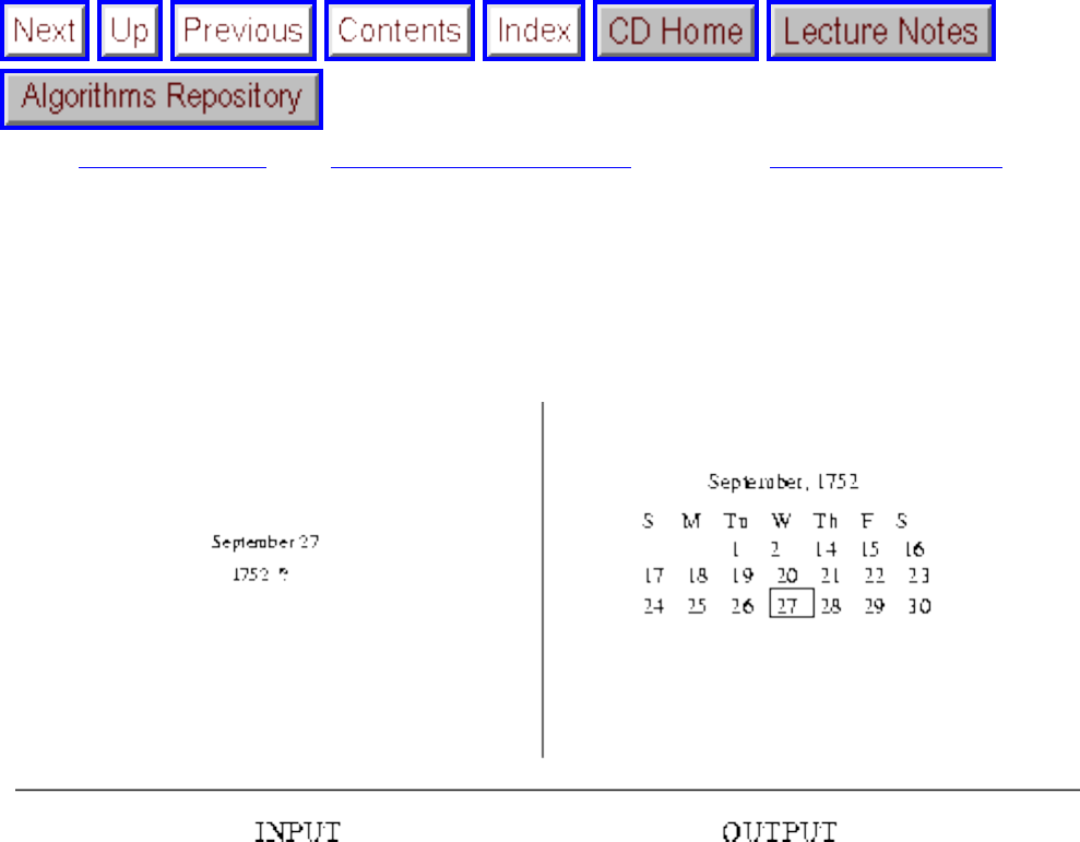
Calendrical Calculations
Next: Job Scheduling Up: Combinatorial Problems Previous: Generating Graphs
Calendrical Calculations
Input description: A particular calendar date d, specified by month, day, and year.
Problem description: Which day of the week did d fall on according to the given calendar system?
Discussion: Many business applications need to perform calendrical calculations. Perhaps we want to
display a calendar of a specified month and year. Maybe we need to compute what day of the week or
year some event occurs, as in figuring out the date on which a 180-day futures contract comes due. The
importance of correct calendrical calculations is perhaps best revealed by the furor over the ``millennium
bug,'' the crisis in legacy programs that allocate only two digits for storing the year.
More complicated questions arise in international applications, because different nations and ethnic
groups around the world use different calendar systems. Some of these, like the Gregorian calendar used
in most of the world, are based on the sun, while others, like the Hebrew calendar, are lunar calendars.
How would you tell today's date according to the Chinese or Arabic calendar?
The algorithms associated with calendrical calculations are different from the other problems in this
book, because calendars are historical objects, not mathematical ones. The issues revolve around
specifying the rules of the calendrical system and simply implementing them correctly, rather than
file:///E|/BOOK/BOOK4/NODE155.HTM (1 of 3) [19/1/2003 1:30:49]

Calendrical Calculations
designing efficient shortcuts for the computation.
The basic approach behind calendar systems is to start with a particular reference date and count from
there. The particular rules for wrapping the count around into months and years is what distinguishes a
given calendar system from another. To implement a calendar, we need two functions, one that given a
date returns the integer number of days that have elapsed since the reference start date, the other of which
takes an integer n and returns the calendar date exactly n days from the reference date. This is analogous
to the ranking and unranking rules for combinatorial objects, such as permutations (see Section ).
The major source of complications in calendar systems is that the solar year is not an integer number of
days long. Thus if a calendar seeks to keep its annual dates in sync with the seasons, leap days must be
added at both regular and irregular intervals. Since a solar year is 365 days and 5:49:12 hours long, an
extra 10:48 minutes would have to be accounted for at the end of each year if we were simply to add a
leap day every four years.
The original Julian calendar (from Julius Caesar) did not account for these extra minutes, which had
accumulated to ten days by 1582 when Pope Gregory XIII proposed the Gregorian calendar used today.
Gregory deleted the ten days and eliminated leap days in years that are multiples of 100 but not 400.
Supposedly, riots ensued because the masses feared their lives were being shortened by ten days. Outside
the Catholic church, resistance to change slowed the reforms. The deletion of days did not occur in
England and America until September 1752, and not until 1927 in Turkey.
The rules for most calendrical systems are sufficiently complicated and pointless that you should lift
code from a reliable place rather than attempt to write your own. We identify suitable implementations
below.
There are a variety of ``impress your friends'' algorithms that enable you to compute in your head on
which day of the week a particular date occurred. Such algorithms often fail to work reliably outside the
given century and should be avoided for computer implementation.
Implementations: Dershowitz and Reingold provide a uniform algorithmic presentation [DR90,
RDC93] for a variety of different calendar systems, including the Gregorian, ISO, Julian, Islamic, and
Hebrew calendars, as well as other calendars of historical interest. Further, they provide Common Lisp
and C++ routines to convert dates between calendars, day of the week computations, and the
determination of secular and religious holidays. These are likely to be the most comprehensive and
reliable calendrical routines you will be able to get your hands on, and are available at
http://emr.cs.uiuc.edu:80/reingold/calendars.html.
A nice package for calendrical computations in Mathematica by Ilan Vardi is available in the
Packages/Miscellaneous directory of the standard Mathematica distribution, and also from MathSource.
Vardi's book [Var91] discusses the theory behind the implementation, which provides support for the
file:///E|/BOOK/BOOK4/NODE155.HTM (2 of 3) [19/1/2003 1:30:49]
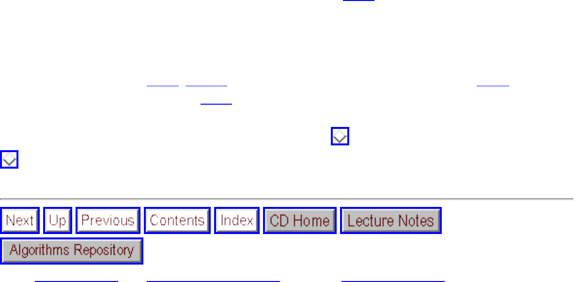
Calendrical Calculations
Gregorian, Julian, and Islamic calendars.
Gregorian calendar computations implemented in C appear in [BR95]. This code uses 1582 as the date of
the calendar reform, instead of the standard UNIX date of 1752. The code for these algorithms is printed
in the text and are available on disk for a modest fee.
Notes: The most comprehensive discussion of calendrical computation algorithms are the papers by
Dershowitz and Reingold [DR90, RDC93]. These papers are superseded by their book [DR97]. Histories
of the Gregorian calendar appear in [BR95].
Related Problems: Arbitrary-precision arithmetic (see page ), generating permutations (see page
).
Next: Job Scheduling Up: Combinatorial Problems Previous: Generating Graphs
Algorithms
Mon Jun 2 23:33:50 EDT 1997
file:///E|/BOOK/BOOK4/NODE155.HTM (3 of 3) [19/1/2003 1:30:49]
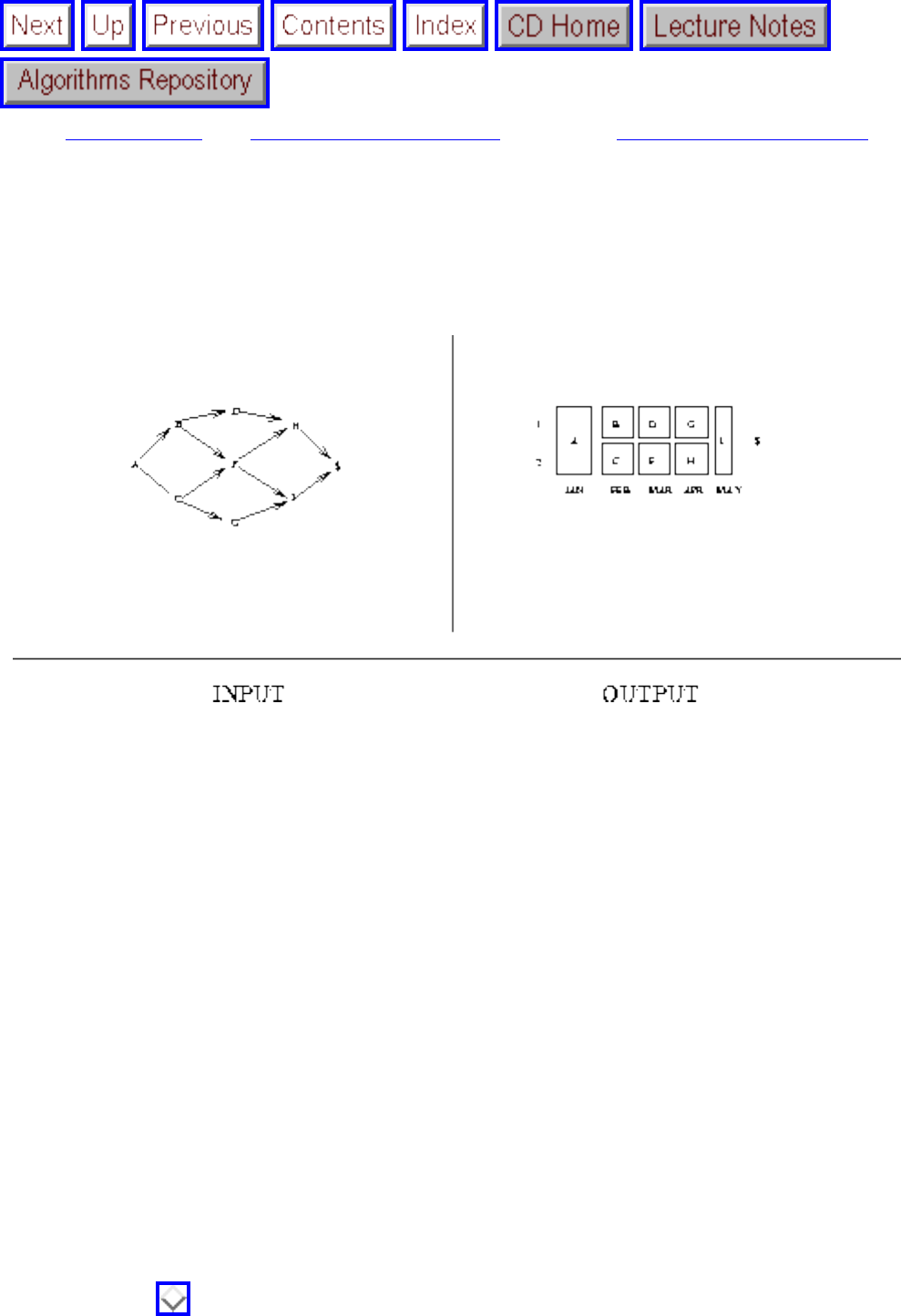
Job Scheduling
Next: Satisfiability Up: Combinatorial Problems Previous: Calendrical Calculations
Job Scheduling
Input description: A directed acyclic graph G=(V,E), where the vertices represent jobs and the edge
(u,v) implies that task u must be completed before task v.
Problem description: What schedule of tasks completes the job using the minimum amount of time or
processors?
Discussion: Devising a proper schedule to satisfy a set of constraints is fundamental to many
applications. A critical aspect of any parallel processing system is the algorithm mapping tasks to
processors. Poor scheduling can leave most of the expensive machine sitting idle while one bottleneck
task is performed. Assigning people to jobs, meetings to rooms, or courses to final exam periods are all
different examples of scheduling problems.
Scheduling problems differ widely in the nature of the constraints that must be satisfied and the type of
schedule desired. For this reason, several other catalog problems have a direct application to various
kinds of scheduling:
● To construct a schedule consistent with the precedence constraints, see topological sorting in
Section .
file:///E|/BOOK/BOOK4/NODE156.HTM (1 of 4) [19/1/2003 1:30:50]
Job Scheduling
● To assign a set of jobs to people who have the appropriate skills for them, see bipartite matching
in Section .
● To assign a set of jobs to time slots such that no two jobs that interfere are assigned the same time
slot, see vertex and edge coloring in Sections and .
● To construct the most efficient route for a delivery person to visit a given set of locations, see the
traveling salesman problem in Section . To construct the most efficient route for a snowplow
or mailman to completely traverse a given set of edges, see the Eulerian cycle problem in Section
.
In this section, we focus on precedence-constrained scheduling problems for directed acyclic graphs.
These problems are often called PERT/CPM, for Program Evaluation and Review Technique/Critical
Path Method. Suppose you have broken a big job into a large number of smaller tasks. For each task
you know how long it should take (or perhaps an upper bound on how long it might take). Further, for
each pair of tasks you know whether it is essential that one task be performed before another. The fewer
constraints we have to enforce, the better our schedule can be. These constraints must define a directed
acyclic graph, acyclic because a cycle in the precedence constraints represents a Catch-22 situation that
can never be resolved.
We are interested in several problems on these networks:
● Minimum completion time - assuming that we have an unlimited number of workers, what is the
fastest we can get this job completed while respecting precedence constraints. If there were no
precedence constraints, each task could be worked on by its own worker, and the total time would
be that of the longest single task. If there were such strict precedence constraints that each task
had to follow the completion of its immediate predecessor, the minimum completion time would
be obtained by summing up the times for each task.
The minimum completion time for a DAG can be easily computed in O(n+m) time. Initialize the
completion time for all the vertices to 0, except the start vertex, which is initialized to the length
of the start task. Perform a topological sort to order the vertices such that all precedences will
have been considered by the time we evaluate each vertex. For each vertex u, consider all the
edges (u,v) leaving u. The completion time of these vertices is the maximum of the current
completion time for v plus the completion time of u plus the task time of v.
● Critical path - The longest path from the start vertex to the completion vertex defines the critical
path. This can be important to know, for the only way to shorten the minimum total completion
time is to reduce the time of one of the tasks on each critical path. The tasks on the critical paths
can be determined in O(n+m) time using the simple dynamic programming presented in Section
.
● What is the tradeoff between number of workers and completion time? - What we would really be
interested in knowing is how best to complete the schedule with a given number of workers.
Unfortunately, this and most similar problems are NP-complete.
file:///E|/BOOK/BOOK4/NODE156.HTM (2 of 4) [19/1/2003 1:30:50]
Job Scheduling
An even more general formulation seeks critical paths in networks where certain jobs are restricted to
certain people. Such networks are known as disjunctive networks. Finding critical paths on such
networks is more complicated than CPM/PERT, but implementations are described below.
In any sufficiently large and sufficiently real scheduling application, there will be combinations of
constraints that are difficult or impossible to model using these techniques. There are two reasonable
ways to deal with such problems. First, we can ignore enough constraints that the problem reduces to one
of the types that we have described here, solve it, and then see how bad it is using the other constraints.
Perhaps the schedule can be easily modified by hand to satisfy constraints like keeping Joe and Bob apart
so they can't kill each other. Another approach is to formulate your scheduling problem via linear-integer
programming (see Section ) in all its complexity. This method can be better only if you really know
enough about your desired schedule to formulate the right linear program, and if you have the time to
wait for the program to give you the solution. I would start out with something simpler and see what
happens first.
Another fundamental scheduling problem takes a set of jobs without precedence constraints and assign
them to identical machines so as to minimize the total elapsed time. Consider a copy shop with k Xerox
machines and a stack of jobs to finish by the end of the day. Such tasks are called job-shop scheduling.
They can be modeled as bin-packing problems (see Section ), where each job is assigned a number
equal to the number of hours it will take and each machine is represented by a bin with space equal to the
number of hours in a day.
More sophisticated variations of job-shop scheduling provide each task with allowable start and required
finishing times. Effective heuristics are known, based on sorting the tasks by size and finishing time. We
refer the reader to the references for more information. Note that these scheduling problems become hard
only when the tasks cannot be broken up onto multiple machines or interrupted (preempted) and then
rescheduled. If your application has these degrees of freedom, you should exploit them.
Implementations: Pascal implementations of Balas's algorithm for disjunctive network scheduling and
Hu's algorithm for assigning jobs to processors with precedence constraints appear in [SDK83]. See
Section .
Algorithm 520 [WBCS77] of the Collected Algorithms of the ACM is a Fortran code for multiple-
resource network scheduling. It is available from Netlib (see Section ).
Notes: The literature on scheduling algorithms is a vast one. For a more detailed survey of the field, we
refer the reader to [Cof76, LLK83].
Good expositions on CPM/PERT include [Eve79a, Law76, PGD82, SDK83]. Good expositions on job-
file:///E|/BOOK/BOOK4/NODE156.HTM (3 of 4) [19/1/2003 1:30:50]
Job Scheduling
shop scheduling include [AC91, SDK83].
Related Problems: Topological sorting (see page ), matching (see page ), vertex coloring (see
page ), edge coloring (see page ), bin packing (see page ).
Next: Satisfiability Up: Combinatorial Problems Previous: Calendrical Calculations
Algorithms
Mon Jun 2 23:33:50 EDT 1997
file:///E|/BOOK/BOOK4/NODE156.HTM (4 of 4) [19/1/2003 1:30:50]
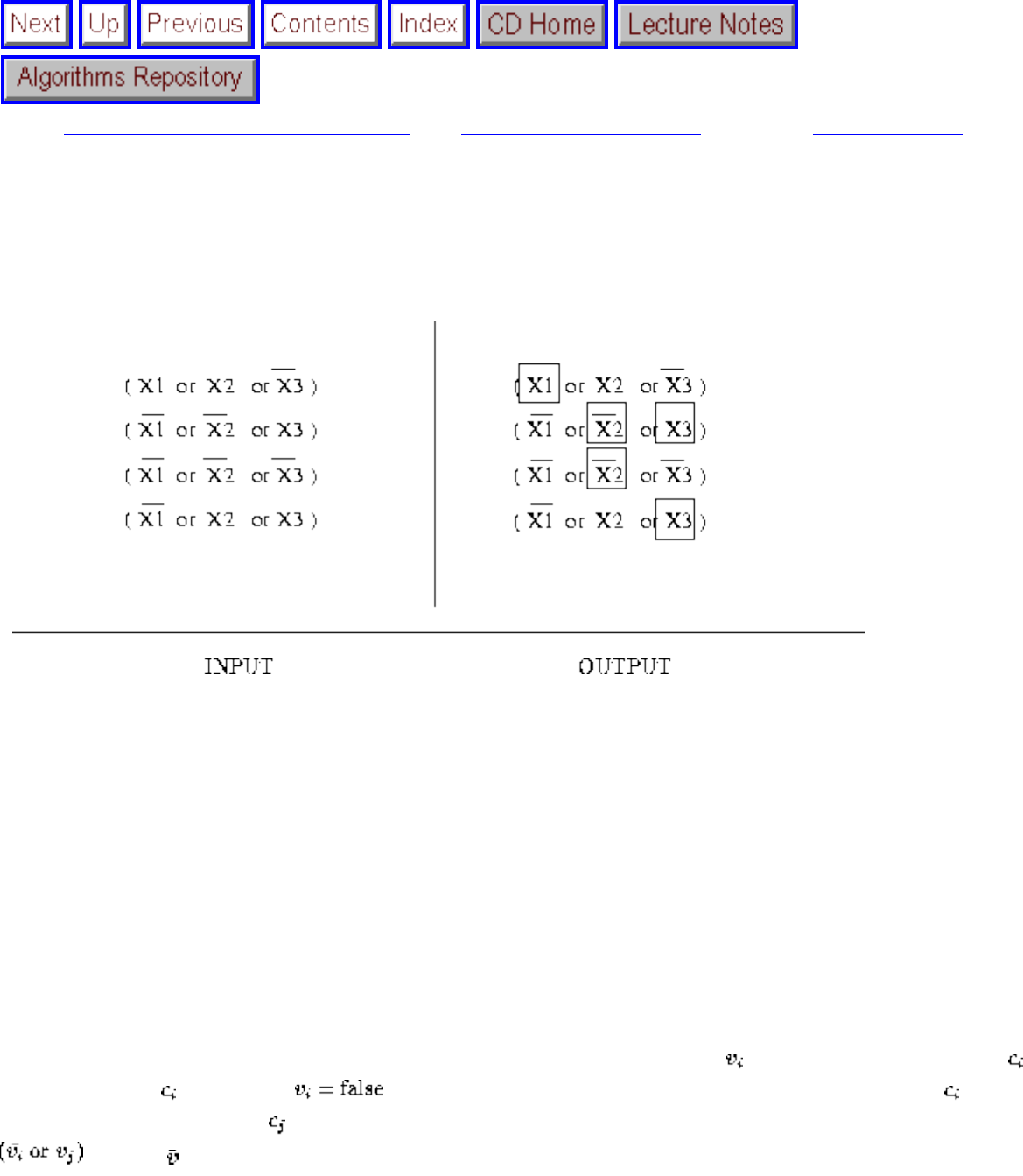
Satisfiability
Next: Graph Problems: Polynomial-Time Up: Combinatorial Problems Previous: Job Scheduling
Satisfiability
Input description: A set of clauses in conjunctive normal form.
Problem description: Is there a truth assignment to the Boolean variables such that every clause is
simultaneously satisfied?
Discussion: Satisfiability arises whenever we seek a configuration or object that must be consistent with
(i.e. satisfy) a given set of constraints. For example, consider the problem of drawing name labels for
cities on a map. For the labels to be legible, we do not want the labels to overlap, but in a densely
populated region many labels need to be drawn in a small space. How can we avoid collisions?
For each of the n cities, suppose we identify two possible places to position its label, say right above or
right below each city. We can represent this choice by a Boolean variable , which will be true if city
's label is above , otherwise . Certain pairs of labels may be forbidden, such as when 's
above label would obscure 's below label. This pairing can be forbidden by the two-element clause
, where means ``not v''. Finding a satisfying truth assignment for the resulting set of clauses
yields a mutually legible map labeling if one exists.
Satisfiability is the original NP-complete problem. Despite its applications to constraint satisfaction,
file:///E|/BOOK/BOOK4/NODE157.HTM (1 of 4) [19/1/2003 1:30:52]
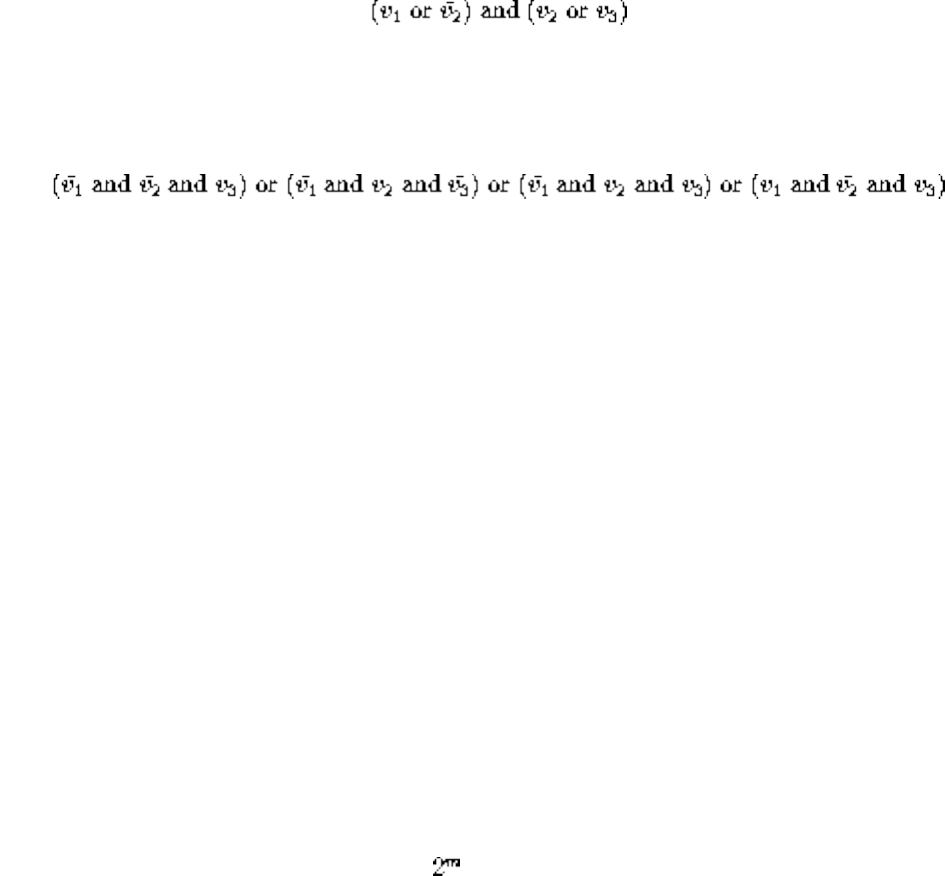
Satisfiability
logic, and automatic theorem proving, it is perhaps most important theoretically as the root problem from
which all other NP-completeness proofs originate.
● Is your formula in CNF or DNF? - In satisfiability, the constraints are specified as a logical
formula. There are two primary ways of expressing logical formulas, conjunctive normal form
(CNF) and disjunctive normal form (DNF). In CNF formulas, we must satisfy all clauses, where
each clause is constructed by and-ing or's of literals together, such as
In DNF formulas, we must satisfy any one clause, where each clause is constructed by or-ing ands
of literals together. The formula above can be written in DNF as
Solving DNF-satisfiability is trivial, since any DNF formula can be satisfied unless every clause
contains both a literal and its complement (negation). However, CNF-satisfiability is NP-
complete. This seems paradoxical, since we can use De Morgan's laws to convert CNF-formulae
into equivalent DNF-formulae and vice versa. The catch is that an exponential number of terms
might be constructed in the course of translation, so that the translation itself might not run in
polynomial time.
● How big are your clauses? - k-SAT is a special case of satisfiability when each clause contains at
most k literals. The problem of 1-SAT is trivial, since we must set true any literal appearing in any
clause. The problem of 2-SAT is not trivial, but it can still be solved in linear time. This is very
interesting, because many problems can be modeled as 2-SAT using a little cleverness. Observe
that the map labeling problem described above is an instance of 2-SAT and hence can be solved in
time linear in the number of clauses, which might be quadratic in the number of variables.
The good times end as soon as clauses contain three literals each, i.e. 3-SAT, for 3-SAT is NP-
complete. Thus in general it will not be helpful to model a problem as satisfiability unless we can
do it with two-element clauses.
● Does it suffice to satisfy most of the clauses? - Given an instance of general satisfiability, there is
not much you can do to solve it except by backtracking algorithms such as the Davis-Putnam
procedure. In the worst case, there are truth assignments to be tested, but fortunately, there are
lots of ways to prune the search. Although satisfiability is NP-complete, how hard it is in practice
depends on how the instances are generated. Naturally defined ``random'' instances are often
surprisingly easy to solve, and in fact it is nontrivial to generate instances of the problem that are
truly hard.
Still, we would likely benefit by relaxing the problem so that the goal is to satisfy as many clauses
as possible. Here optimization techniques such as simulated annealing can be put to work to refine
random or heuristic solutions. Indeed, any random truth assignment to the variables will satisfy
file:///E|/BOOK/BOOK4/NODE157.HTM (2 of 4) [19/1/2003 1:30:52]
Satisfiability
any particular k-SAT clause with probability , so our first attempt is likely to satisfy
most of the clauses. Finishing off the job is the hard part. Finding an assignment that satisfies the
maximum number of clauses is NP-complete even for nonsatisfiable instances.
When faced with a problem of unknown complexity, proving the problem NP-complete can be an
important first step. If you think your problem might be hard, the first thing to do is skim through Garey
and Johnson [GJ79] looking for your problem. If you don't find it, my recommendation is to put the book
away and try to prove hardness from first principles, using one of the basic problems in this catalog,
particularly 3-SAT, vertex cover, independent set, integer partition, clique, and Hamiltonian cycle. I find
it much easier to start from these than some complicated problem I stumble over in the book, and more
insightful too, since the reason for the hardness is not obscured by the hidden hardness proof for the
complicated problem. Chapter focuses on strategies for proving hardness.
Implementations: Programs for solving satisfiability problems were sought for the Second DIMACS
Implementation Challenge, held in October 1993. Programs and data from the challenge are available by
anonymous ftp from dimacs.rutgers.edu in the directory /pub/challenge/sat. In particular, sato is a
decision procedure for propositional logic written in C by Hantao Zhang. There is also a random formula
generator named mwff.c for constructing hard satisfiability instances in C by Bart Selman. Several other
solvers and instance generators are also available from this site.
The propositional satisfiability tester POSIT, by Jon W. Freeman, is based on a highly optimized version
of the Davis-Putnum procedure. It is available by anonymous ftp from ftp.cis.upenn.edu in
/pub/freeman/posit-1.0.tar.Z.
Notes: The primary reference on NP-completeness is [GJ79], featuring a list of roughly four hundred NP-
complete problems. Although the list is now fifteen years old, it remains an extremely useful reference; it
is perhaps the book I reach for most often. An occasional column by David Johnson in the Journal of
Algorithms has helped to update the book. In [Joh90], Johnson gives a thorough and readable survey of
the relationship between different complexity classes.
Good expositions of Cook's theorem [Coo71], where satisfiability is proven hard, include [CLR90, GJ79,
PS82]. The importance of Cook's result became clear in Karp's paper [Kar72] showing that it implied the
hardness of over twenty different combinatorial problems.
A linear-time algorithm for 2-satisfiability appears in [APT79]. The application of 2-satisfiability to map
labeling is taken from [WW95].
Related Problems: Constrained optimization (see page ), traveling salesman problem (see page ).
file:///E|/BOOK/BOOK4/NODE157.HTM (3 of 4) [19/1/2003 1:30:52]


Graph Problems: Polynomial-Time
Next: Connected Components Up: A Catalog of Algorithmic Previous: Satisfiability
Graph Problems: Polynomial-Time
Algorithmic graph problems constitute approximately one third of all the problems in this catalog.
Further, several problems from other sections can be formulated strictly in terms of graphs. Identifying
the name of a graph-theoretic invariant or problem is one of the primary skills of a good algorist. Indeed,
this catalog will tell you exactly how to proceed as soon as you figure out your particular problem's
name.
We have partitioned the bulk of the algorithmic graph problems in this book between this and the
subsequent section. Here, we deal only with problems for which there exist efficient algorithms to solve
them. As there is often more than one way to model a given application, it makes sense to look here
before proceeding on to the harder formulations.
The algorithms presented here have running times that grow slowly with the size of the graph. We adopt
throughout the standard convention that n refers to the number of vertices in a graph, while m is the
number of edges.
Although graphs are combinatorial objects, describing a binary relation on a set of objects, graphs are
usually best understood as drawings. Beyond just the problems of visualization, many interesting graph
properties follow from the nature of a particular type of drawing, such as planar graphs. In this chapter,
we also present a variety of different problems and algorithms associated with graph drawing.
Most advanced graph algorithms are difficult to program. However, good implementations are often
available if you know where to look. The best single source is LEDA, discussed in Section , although
faster special-purpose codes exist for many problems.
Books specializing in graph algorithms include:
● Even [Eve79a] - This is a good book on graph algorithms, fairly advanced, with a particularly
thorough treatment of planarity-testing algorithms.
● Ahuja, Magnanti, and Orlin [AMO93] - While purporting to be a book on network flows, it
covers the gamut of graph algorithms with emphasis on operations research. Strongly
file:///E|/BOOK/BOOK4/NODE158.HTM (1 of 2) [19/1/2003 1:30:53]
Graph Problems: Polynomial-Time
recommended.
● van Leeuwen [vL90a] - A 100+ page survey on research results in graph algorithms, this is the
best source to determine what is known in algorithmic graph theory.
● McHugh [McH90] - A more elementary but comprehensive treatment of basic graph algorithms,
including parallel algorithms.
● Connected Components
● Topological Sorting
● Minimum Spanning Tree
● Shortest Path
● Transitive Closure and Reduction
● Matching
● Eulerian Cycle / Chinese Postman
● Edge and Vertex Connectivity
● Network Flow
● Drawing Graphs Nicely
● Drawing Trees
● Planarity Detection and Embedding
Next: Connected Components Up: A Catalog of Algorithmic Previous: Satisfiability
Algorithms
Mon Jun 2 23:33:50 EDT 1997
file:///E|/BOOK/BOOK4/NODE158.HTM (2 of 2) [19/1/2003 1:30:53]
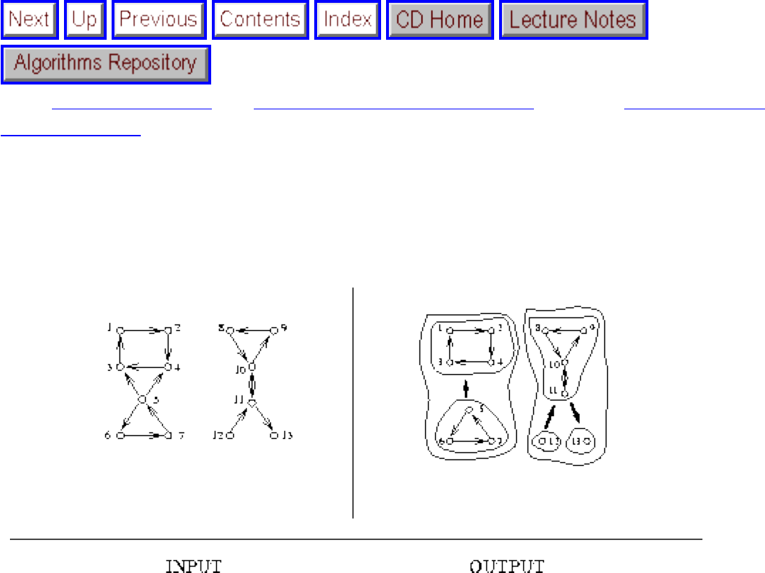
Connected Components
Next: Topological Sorting Up: Graph Problems: Polynomial-Time Previous: Graph Problems:
Polynomial-Time
Connected Components
Input description: A directed or undirected graph G.
Problem description: Traverse each edge and vertex of all connected components of G.
Discussion: The connected components of a graph represent, in grossest terms, the pieces of the graph.
Two vertices are in the same component of G if and only if there is some path between them.
Finding connected components is at the heart of many graph applications. For example, consider the
problem of identifying clusters in a set of items. We can represent each item by a vertex and add an
edge between each pair of items that are deemed ``similar.'' The connected components of this graph
correspond to different classes of items.
Testing whether a graph is connected is an essential preprocessing step for every graph algorithm. Such
tests can be performed so quickly and easily that you should always verify that your input graph is
connected, even when you know it has to be. Subtle, difficult-to-detect bugs often result when your
algorithm is run only on one component of a disconnected graph.
file:///E|/BOOK/BOOK4/NODE159.HTM (1 of 4) [19/1/2003 1:30:54]

Connected Components
Testing the connectivity of any undirected graph is a job for either depth-first or breadth-first search, as
discussed in Section . Which one you choose doesn't really matter. Both traversals initialize a
component-number field for each vertex to 0, and then start the search for component 1 from vertex .
As each vertex is visited, the value of this field is set to the current component number. When the initial
traversal ends, the component number is incremented, and the search begins again from the first vertex
with component-number still 0. Properly implemented using adjacency lists, this runs in O(n+m), or time
linear in the number of edges and vertices.
Other notions of connectivity also arise in practice:
● What if my graph is directed? - There are two distinct definitions of connected components for
directed graphs. A directed graph is weakly connected if it would be connected by ignoring the
direction of edges. Thus a weakly connected graph consists of a single piece. A directed graph is
strongly connected if there is a directed path between every pair of vertices. This distinction is
best made clear by considering a network of one- and two-way streets in a city. The network is
strongly connected if it is possible to drive legally between every two positions. The network is
weakly connected if it is possible to drive legally or illegally between every two positions. The
network is disconnected if there is no possible way to drive from a to b.
The weakly and strongly connected components define unique partitions on the vertices. The
output figure above illustrates a directed graph consisting of two weakly connected or five
strongly connected components (also called blocks of G).
Testing whether a directed graph is weakly connected can be done easily in linear time. Simply
turn all edges into undirected edges and use the DFS-based connected components algorithm
described above. Tests for strong connectivity are somewhat more complicated. The simplest
algorithm performs a breadth-first search from each vertex and verifies that all vertices have been
visited on each search. Thus in O(mn) time, it can be confirmed whether the graph is strongly
connected. Further, this algorithm can be modified to extract all strongly connected components if
it is not.
In fact, strongly connected components can be found in linear time using one of two more
sophisticated DFS-based algorithms. See the references below for details. It is probably easier to
start from an existing implementation below than a textbook description.
● How reliable is my network; i.e. how well connected is it? - A chain is only as strong as its
weakest link. When it is missing one or more links, it is disconnected. The notion of
connectivity of graphs measures the strength of the graph - how many edges or vertices must be
removed in order to break it, or disconnect it. Connectivity is an essential invariant for network
design and other structural problems.
Algorithmic connectivity problems are discussed in Section . In particular, biconnected
components are pieces of the graph that result by cutting the edges incident on a single vertex. All
file:///E|/BOOK/BOOK4/NODE159.HTM (2 of 4) [19/1/2003 1:30:54]
Connected Components
biconnected components can be found in linear time using a DFS-based algorithm. Vertices whose
deletion disconnects the graph belong to more than one biconnected component, although edges
are uniquely partitioned among them.
● Is the graph a tree? How can I find a cycle if one exists? - The problem of cycle identification
often arises, particularly with respect to directed graphs. For example, testing if a sequence of
conditions can deadlock often reduces to cycle detection. If I am waiting for Fred, and Fred is
waiting for Mary, and Mary is waiting for me, we are all deadlocked.
For undirected graphs, the analogous problem is tree identification. A tree is, by definition, an
undirected, connected graph without any cycles. As described above, a depth-first search can be
used to test whether it is connected. If the graph is connected and has n-1 edges for n vertices, it is
a tree.
Depth-first search can be used to find cycles in both directed and undirected graphs. Whenever we
encounter a back edge in our DFS, i.e. an edge to an ancestor vertex in the DFS tree, the back
edge and the tree together define a directed cycle. No other such cycle can exist in a directed
graph. Directed graphs without cycles are called DAGs (directed acyclic graphs). Topological
sorting (see Section ) is the fundamental operation on DAGs.
Implementations: LEDA (see Section ) provides good implementations of breadth-first and depth-
first search, connected components and strongly connected components, all in C++. XTango (see Section
) is an algorithm animation system for UNIX and X-windows, which includes an animation of depth-
first search.
Pascal implementations of BFS, DFS, and biconnected and strongly connected components appear in
[MS91]. See Section for details. Combinatorica [Ski90] provides Mathematica implementations of
the same routines. See Section .
The Stanford GraphBase (see Section ) contains routines to compute biconnected and strongly
connected components. An expository implementation of BFS and DFS in Fortran appears in [NW78]
(see Section ).
Notes: Depth-first search was first used in algorithms for finding paths out of mazes, and dates back to
the nineteenth century [Luc91, Tar95]. Breadth-first search was first reported to find the shortest path out
of mazes by Moore in 1957 [Moo59].
Hopcroft and Tarjan [HT73b, Tar72] first established depth-first search as a fundamental technique for
efficient graph algorithms. Expositions on depth-first and breadth-first search appear in every book
file:///E|/BOOK/BOOK4/NODE159.HTM (3 of 4) [19/1/2003 1:30:54]
Connected Components
discussing graph algorithms, with [CLR90] perhaps the most thorough description available.
The first linear-time algorithm for strongly connected components is due to Tarjan [Tar72], with
expositions including [Baa88, Eve79a, Man89]. Another algorithm, simpler to program and slicker, to
find strongly connected components is due to Sharir and Kosaraju. Good expositions of this algorithm
appear in [AHU83, CLR90].
Related Problems: Edge-vertex connectivity (see page ), shortest path (see page ).
Next: Topological Sorting Up: Graph Problems: Polynomial-Time Previous: Graph Problems:
Polynomial-Time
Algorithms
Mon Jun 2 23:33:50 EDT 1997
file:///E|/BOOK/BOOK4/NODE159.HTM (4 of 4) [19/1/2003 1:30:54]
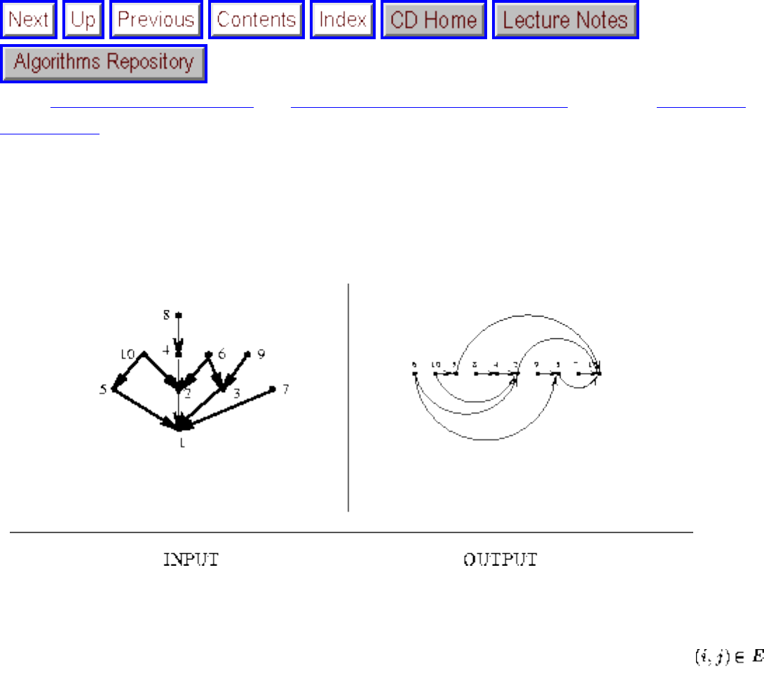
Topological Sorting
Next: Minimum Spanning Tree Up: Graph Problems: Polynomial-Time Previous: Connected
Components
Topological Sorting
Input description: A directed acyclic graph G=(V,E), also known as a partial order or poset.
Problem description: Find a linear ordering of the vertices of V such that for each edge , vertex
i is to the left of vertex j.
Discussion: Topological sorting arises as a natural subproblem in most algorithms on directed acyclic
graphs. Topological sorting orders the vertices and edges of a DAG in a simple and consistent way and
hence plays the same role for DAGs that depth-first search does for general graphs.
Topological sorting can be used to schedule tasks under precedence constraints. Suppose we have a set
of tasks to do, but certain tasks have to be performed before other tasks. These precedence constraints
form a directed acyclic graph, and any topological sort (also known as a linear extension) defines an
order to do these tasks such that each is performed only after all of its constraints are satisfied.
Three important facts about topological sorting are:
● Only directed acyclic graphs can have linear extensions, since any directed cycle is an inherent
file:///E|/BOOK/BOOK4/NODE160.HTM (1 of 3) [19/1/2003 1:30:55]

Topological Sorting
contradiction to a linear order of tasks.
● Every DAG can be topologically sorted, so there must always be at least one schedule for any
reasonable precedence constraints among jobs.
● DAGs typically allow many such schedules, especially when there are few constraints. Consider n
jobs without any constraints. Any of the n! permutations of the jobs constitutes a valid linear
extension.
A linear extension of a given DAG is easily found in linear time. The basic algorithm performs a depth-
first search of the DAG to identify the complete set of source vertices, where source vertices are vertices
without incoming edges. At least one such source must exist in any DAG. Note that source vertices
can appear at the start of any schedule without violating any constraints. After deleting all the outgoing
edges of the source vertices, we will create new source vertices, which can sit comfortably to the
immediate right of the first set. We repeat until all vertices have been accounted for. Only a modest
amount of care with data structures (adjacency lists and queues) is needed to make this run in O(n+m)
time.
This algorithm is simple enough that you should be able to code up your own implementation and expect
good performance, although implementations are described below. Two special considerations are:
● What if I need all the linear extensions, instead of just one of them? - In certain applications, it is
important to construct all linear extensions of a DAG. Beware, because the number of linear
extensions can grow exponentially in the size of the graph. Even the problem of counting the
number of linear extensions is NP-hard.
Algorithms for listing all linear extensions in a DAG are based on backtracking. They build all
possible orderings from left to right, where each of the in-degree zero vertices are candidates for
the next vertex. The outgoing edges from the selected vertex are deleted before moving on.
Constructing truly random linear extensions is a hard problem, but pseudorandom orders can be
constructed from left to right by selecting randomly among the in-degree zero vertices.
● What if your graph is not acyclic? - When the set of constraints is not a DAG, but it contains
some inherent contradictions in the form of cycles, the natural problem becomes to find the
smallest set of jobs or constraints that if eliminated leaves a DAG. These smallest sets of
offending jobs (vertices) or constraints (edges) are known as the feedback vertex set and the
feedback arc set, respectively, and are discussed in Section . Unfortunately, both of them are
NP-complete problems.
Since the basic topological sorting algorithm will get stuck as soon as it identifies a vertex on a
directed cycle, we can delete the offending edge or vertex and continue. This quick-and-dirty
heuristic will eventually leave a DAG.
Implementations: Many textbooks contain implementations of topological sorting, including [MS91]
file:///E|/BOOK/BOOK4/NODE160.HTM (2 of 3) [19/1/2003 1:30:55]
Topological Sorting
(see Section ) and [Sed92] (see Section ). LEDA (see Section ) includes a linear-time
implementation of topological sorting in C++.
XTango (see Section ) is an algorithm animation system for UNIX and X-windows, which includes
an animation of topological sorting.
Combinatorica [Ski90] provides Mathematica implementations of topological sorting and other
operations on directed acyclic graphs. See Section .
Notes: Good expositions on topological sorting include [CLR90, Man89]. Brightwell and Winkler
[BW91] proved that it is #P-complete to count the number of linear extensions of a partial order. The
complexity class #P includes NP, so any #P-complete problem is at least NP-hard.
Related Problems: Sorting (see page ), feedback edge/vertex set (see page ).
Next: Minimum Spanning Tree Up: Graph Problems: Polynomial-Time Previous: Connected
Components
Algorithms
Mon Jun 2 23:33:50 EDT 1997
file:///E|/BOOK/BOOK4/NODE160.HTM (3 of 3) [19/1/2003 1:30:55]
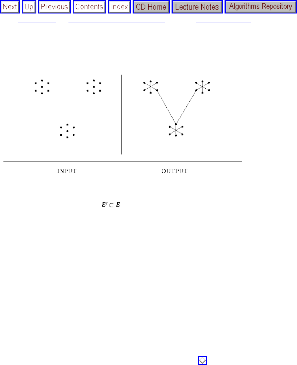
Minimum Spanning Tree
Next: Shortest Path Up: Graph Problems: Polynomial-Time Previous: Topological Sorting
Minimum Spanning Tree
Input description: A graph G = (V,E) with weighted edges.
Problem description: The subset of of minimum weight forming a tree on V.
Discussion: The minimum spanning tree (MST) of a graph defines the cheapest subset of edges that keeps the graph in one
connected component. Telephone companies are particularly interested in minimum spanning trees, because the
minimum spanning tree of a set of sites defines the wiring scheme that connects the sites using as little wire as possible. It
is the mother of all network design problems.
Minimum spanning trees prove important for several reasons:
● They can be computed quickly and easily, and they create a sparse subgraph that reflects a lot about the original
graph.
● They provide a way to identify clusters in sets of points. Deleting the long edges from a minimum spanning tree
leaves connected components that define natural clusters in the data set, as shown in the output figure above.
● They can be used to give approximate solutions to hard problems such as Steiner tree and traveling salesman.
● As an educational tool, minimum spanning tree algorithms provide graphic evidence that greedy algorithms can give
provably optimal solutions.
Two classical algorithms efficiently construct minimum spanning trees, namely Prim's and Kruskal's. Brief overviews of
both algorithms are given below, with correctness arguments in Section . We refer the reader to the codes for
implementation details.
Prim's algorithm starts with an arbitrary vertex v and ``grows'' a tree from it, repeatedly finding the lowest-cost edge that
will link some new vertex into this tree. During execution we will label each vertex as either in the tree, fringe - meaning
there exists an edge from a tree vertex, or unseen - meaning the vertex is more than one edge away from the tree.
file:///E|/BOOK/BOOK4/NODE161.HTM (1 of 4) [19/1/2003 1:30:57]
Minimum Spanning Tree
Prim(G)
Select an arbitrary vertex to start
While (there are fringe vertices)
select minimum-weight edge between tree and fringe
add the selected edge and vertex to the tree
This creates a spanning tree for any connected graph, since no cycle can be introduced via edges between tree and fringe
vertices. That it is in fact a tree of minimum weight can be proven by contradiction, and the proof is in Section . With
simple data structures, Prim's algorithm can be implemented in time.
Kruskal's algorithm is also greedy. It starts with each vertex as a separate tree and merges these trees together by
repeatedly adding the lowest cost edge that merges two distinct subtrees (i.e. does not create a cycle).
Kruskal(G)
Sort the edges in order of increasing weight
count=0
while (count < n-1) do
get next edge (v,w)
if (component (v) component(w))
add to T
component(v) = component(w)
The ``which component?'' tests are efficiently implemented using the union-find data structure of Section , to yield an
algorithm.
Minimum spanning tree is only one of several spanning tree problems that arise in practice. The following questions will
file:///E|/BOOK/BOOK4/NODE161.HTM (2 of 4) [19/1/2003 1:30:57]
Minimum Spanning Tree
help you sort your way through them:
● Are the weights of all edges of your graph identical? - Every spanning tree on n points contains exactly n-1 edges.
Thus if your graph is unweighted, any spanning tree will be a minimum spanning tree. Either breadth-first or
depth-first search can be used to find a rooted spanning tree in linear time. Depth-first search trees tend to be long
and thin, while breadth-first search trees better reflect the distance structure of the graph, as discussed in Section .
● Should I use Prim's or Kruskal's algorithm? - As described, Prim's algorithm runs in , while Kruskal's
algorithm takes time. Thus Prim's algorithm is faster on dense graphs, while Kruskal's is faster on sparse
graphs. Although Prim's algorithm can be implemented in time using more advanced data structures (in
particular, Fibonacci heaps), this will not be worth the trouble unless you have extremely large, fairly sparse graphs.
I personally find Kruskal's algorithm easier to understand and implement than Prim's, but that is just a matter of
taste.
● What if my input is points in the plane, instead of a graph? - Geometric instances, comprising n points in d-
dimensions, can be solved by constructing the complete distance graph in and then finding the MST of this
complete graph. However, for points in two or even three dimensions, it can be more efficient to solve the geometric
version of the problem directly. To find the minimum spanning tree of n points, first construct the Delaunay
triangulation of these points (see Sections and ). In two dimensions, this gives a graph with O(n) edges that
contains all the edges of the minimum spanning tree of the point set. Running Kruskal's algorithm on this sparse
graphs finishes the job in time.
● How do I find a spanning tree that avoids vertices of high degree? - Another common goal of spanning tree
problems is to minimize the maximum degree, typically to minimize the fan out in an interconnection network.
Unfortunately, finding a spanning tree of maximum degree 2 is clearly NP-complete, since this is identical to the
Hamiltonian path problem. Efficient algorithms are known, however, that construct spanning trees whose maximum
degree at most one more than required. This is likely to suffice in practice. See the references below.
Implementations: Pascal implementations of Prim's, Kruskal's, and the Cheriton-Tarjan algorithm are provided in [MS91],
along with extensive empirical analysis that shows that the implementation of Prim's algorithm with the appropriate priority
queue is fastest on most graphs. See Section .
The Stanford GraphBase (see Section ) contains implementations of four different minimum spanning tree algorithms,
and the result of timing experiments suggesting that Kruskal's algorithm is best. The results are reported in terms of memory
accesses (mems) instead of seconds, to make them independent of processor speed.
A C++ implementation of Kruskal's algorithm is provided in LEDA (see Section ). Alternative implementations of
Prim's and Kruskal's algorithms are provided in Pascal [SDK83] and C++ [Sed92]. See Section Section . XTango (see
Section ) includes an animation of both Prim's and Kruskal's algorithms.
Algorithm 479 [Pag74] and Algorithm 613 [HJS84] of the Collected Algorithms of the ACM are Fortran codes for minimum
spanning tree, the former in an implementation of a point clustering algorithm. They are available from Netlib (see
Section ). A bare bones Fortran implementation is provided in [NW78], including the enumeration of all spanning trees.
See Section .
Combinatorica [Ski90] provides Mathematica implementations of Kruskal's minimum spanning tree algorithm and quickly
file:///E|/BOOK/BOOK4/NODE161.HTM (3 of 4) [19/1/2003 1:30:57]
Minimum Spanning Tree
counting the number of spanning trees of a graph. See Section .
Notes: Good expositions on Prim's [Pri57] and Kruskal's [Kru56] algorithms will appear in any textbook on algorithms, but
include [Baa88, CLR90, Man89, Tar83]. The fastest implementations of Prim's and Kruskal's algorithms use Fibonacci
heaps [FT87]. Expositions of faster algorithms for geometric instances include [PS85].
A recent breakthrough on the minimum spanning tree problem is the linear-time randomized algorithm of Karger, Klein,
and Tarjan [KKT95]. Simplifications will be needed before this becomes the algorithm of choice. The history of the
minimum spanning tree problem dates back at least to Boruvka, in 1926, and is presented in [GH85]. Interestingly, it is
Boruvka's algorithm that serves as the foundation to the new randomized one.
Fürer and Raghavachari [FR94] give an algorithm that constructs a spanning tree whose maximum degree is almost
minimized, indeed is at most one more than the lowest-degree spanning tree. The situation is analogous to Vizing's theorem
for edge coloring, which also gives an approximation algorithm to within additive factor one.
Minimum spanning tree algorithms have an interpretation in terms of matroids, which are systems of subsets closed under
inclusion, for which the maximum weighted independent set can be found using a greedy algorithm. The connection
between greedy algorithms and matroids was established by Edmonds [Edm71]. Expositions on the theory of matroids
include [Law76, PS82].
Algorithms for generating spanning trees in order from minimum to maximum weight are presented in [Gab77]. Good
expositions on the matrix-tree theorem, which counts the number of spanning trees of a graph, include [Eve79a].
Related Problems: Steiner tree (see page ), traveling salesman (see page ).
Next: Shortest Path Up: Graph Problems: Polynomial-Time Previous: Topological Sorting
Algorithms
Mon Jun 2 23:33:50 EDT 1997
file:///E|/BOOK/BOOK4/NODE161.HTM (4 of 4) [19/1/2003 1:30:57]
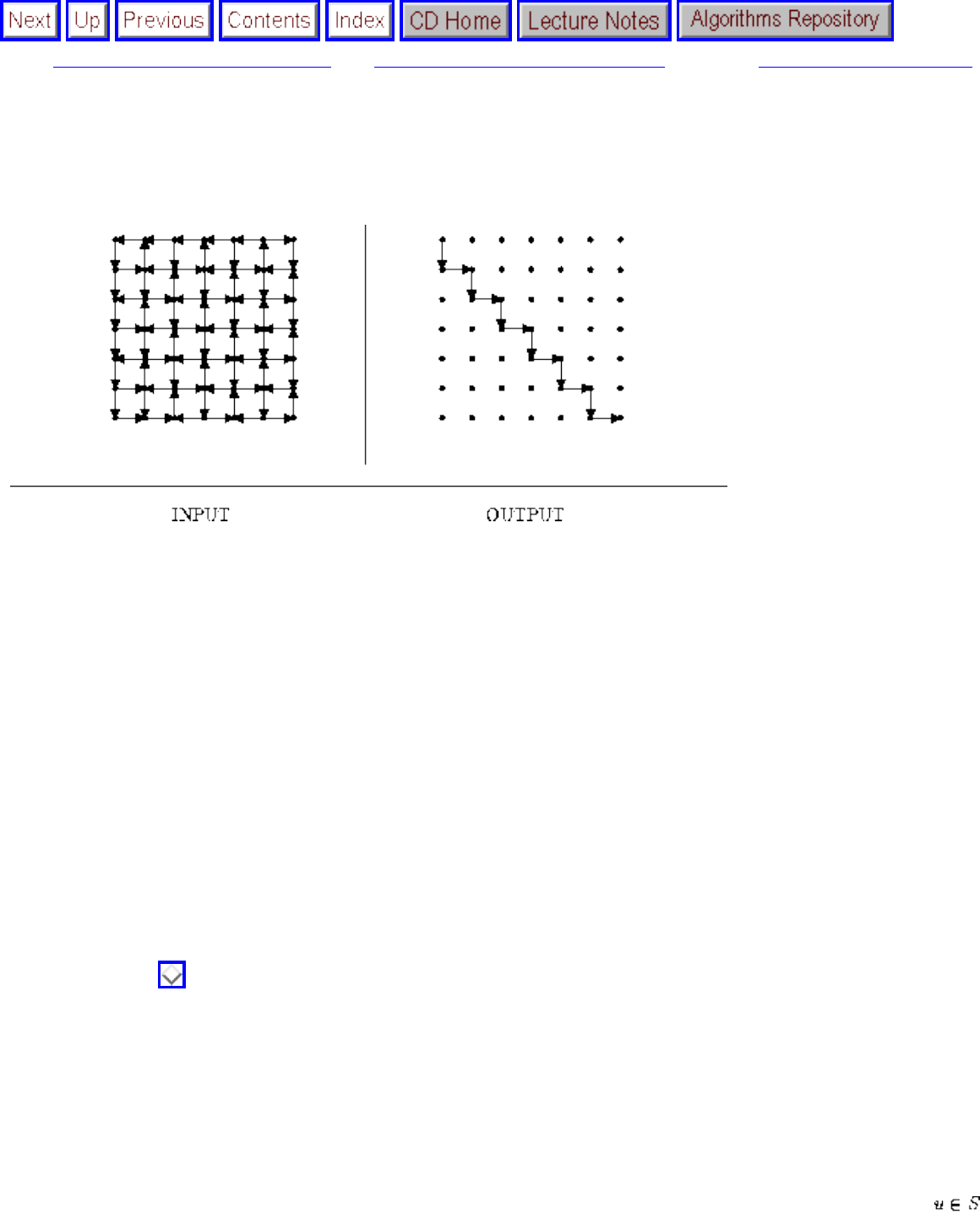
Shortest Path
Next: Transitive Closure and Reduction Up: Graph Problems: Polynomial-Time Previous: Minimum Spanning Tree
Shortest Path
Input description: An edge-weighted graph G, with start vertex and end vertex t.
Problem description: Find the shortest path from to t in G.
Discussion: The problem of finding shortest paths in a graph has a surprising variety of applications:
● The most obvious applications arise in transportation or communications, such as finding the best route to drive
between Chicago and Phoenix or figuring how to direct packets to a destination across a network.
● Consider the problem of image segmentation, that is, separating two characters in a scanned, bit-mapped image
of printed text. We need to find the separating line between two points that cuts through the fewest number of
black pixels. This grid of pixels can be modeled as a graph, with any edge across a black pixel given a high cost.
The shortest path from top to bottom defines the best separation between left and right.
● A major problem in speech recognition is distinguishing between words that sound alike (homophones), such as
to, two, and too. We can construct a graph whose vertices correspond to possible words, with an edge between
possible neighboring words. If the weight of each edge measures the likelihood of transition, the shortest path
across the graph defines the best interpretation of a sentence. For a more detailed account of such an application,
see Section .
● Suppose we want to draw an informative picture of a graph. The center of the page should coorespond to the
``center'' of the graph, whatever that means. A good definition of the center is the vertex that minimizes the
maximum distance to any other vertex in the graph. Finding this center point requires knowing the distance (i.e.
shortest path) between all pairs of vertices.
The primary algorithm for finding shortest paths is Dijkstra's algorithm, which efficiently finds the shortest paths from a
given vertex x to all n-1 other vertices. Dijkstra's algorithm starts from x. In each iteration, it identifies a new vertex v for
which the shortest path from x to v is known. We maintain a set of vertices S to which we currently know the shortest
path from v, and this set grows by one vertex in each iteration. In each iteration, we identify the edge (u,v) where
file:///E|/BOOK/BOOK4/NODE162.HTM (1 of 5) [19/1/2003 1:31:00]
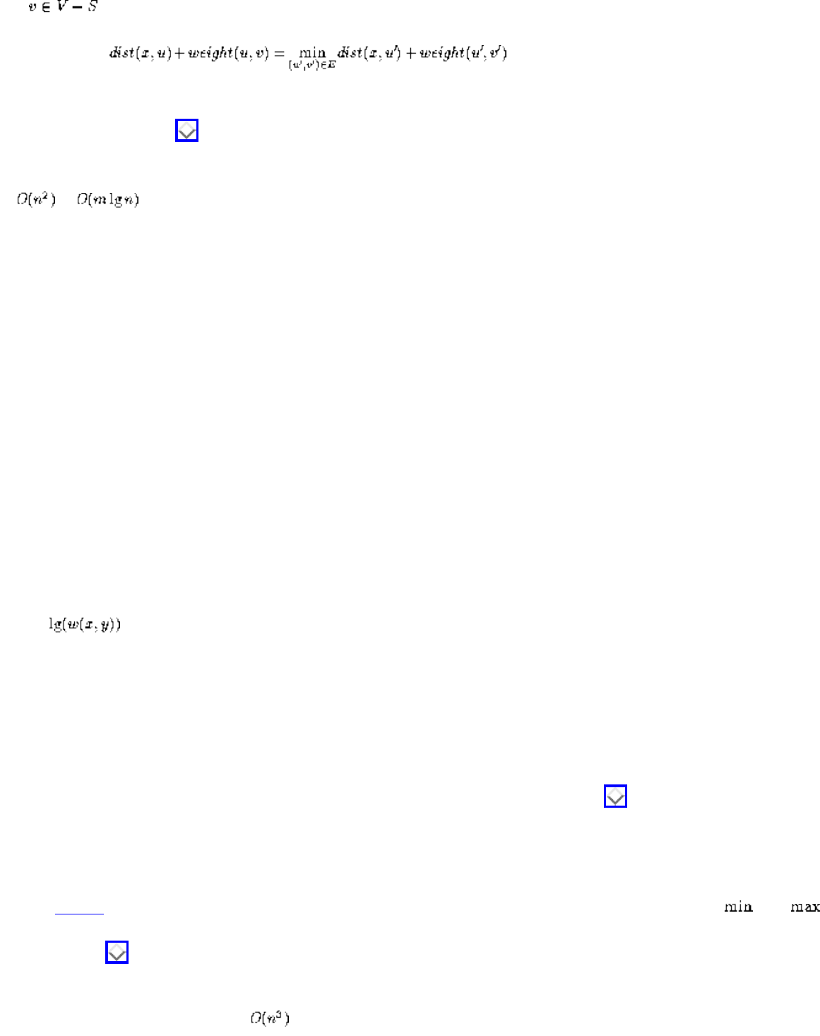
Shortest Path
and such that
This edge (u,v) gets added to a shortest path tree, whose root is x and which describes all the shortest paths from x. See
the discussion in Section for more details.
The straightforward implementation of this algorithm is O(m n). However, with simple data structures it can be reduced
to or time. Theoretically faster times can be achieved using significantly more complicated data
structures, as described below. If we are just interested in knowing the shortest path from x to y, simply stop as soon as y
enters S.
Dijkstra's algorithm is the right choice for single-source shortest path on positively weighted graphs. However, special
circumstances dictate different choices:
● Is your graph weighted or unweighted? - If your graph is unweighted, a simple breadth-first search starting from
the source vertex will find the shortest path in linear time. It is only when edges have different weights that you
need more sophisticated algorithms. Breadth-first search is both simpler and faster than Dijkstra's algorithm.
● Does your graph have negative cost weights? - Dijkstra's algorithm assumes that all edges have positive cost. If
your graph has edges with negative weights, you must use the more general but less efficient Bellman-Ford
algorithm. If your graph has a cycle of negative cost, than the shortest path between any two vertices in the
graph is not defined, since we can detour to the negative cost cycle and loop around it an arbitrary number of
times, making the total cost as small as desired. Note that adding the same amount of weight to each edge to make
it positive and running Dijkstra's algorithm does not find the shortest path in the original graph, since paths that
use more edges will be rejected in favor of longer paths using fewer edges.
Why might one ever need to find shortest paths in graphs with negative cost edges? An interesting application
comes in currency speculation. Construct a graph where each vertex is a nation and there is an edge weighted
from x to y if the exchange rate from currency x to currency y is w(x,y). In arbitrage, we seek a cycle
to convert currencies so that we end up with more money than we started with. For example, if the exchange rates
are 12 pesos per dollar, 5 pesos per franc, and 2 francs per dollar, by simply moving money around we can
convert $1 to $1.20. In fact, there will be a profit opportunity whenever there exists a negative cost cycle in this
weighted graph.
● Is your input a set of geometric obstacles instead of a graph? - If you seek the shortest path between two points
in a geometric setting, like an obstacle-filled room, you may either convert your problem into a graph of distances
and feed it to Dijkstra's algorithm or use a more efficient geometric algorithm to compute the shortest path directly
from the arrangement of obstacles. For such geometric algorithms, see Section on motion planning.
● Does your graph have cycles in it, or is it a DAG? - If your graph is a directed acyclic graph (DAG), than the
shortest path can be found in linear time. Perform a topological sort to order the vertices such that all edges go
from left to right, then do dynamic programming on the left-to-right ordered vertices. Indeed, most dynamic
programming problems can be easily formulated as shortest paths on specific DAGs. The algorithm is discussed in
[Man89] if you cannot figure it out from this description. Note that the same algorithm (replacing with )
also suffices for finding the longest path in a DAG. which is useful in many applications like scheduling (see
Section ).
● Do you need the shortest path between all pairs of points? - If you are interested in the shortest path between all
pairs of vertices, one solution is to run Dijkstra n times, once with each vertex as the source. However, the Floyd-
Warshall algorithm is a slick dynamic programming algorithm for all-pairs shortest path, which is faster and
file:///E|/BOOK/BOOK4/NODE162.HTM (2 of 5) [19/1/2003 1:31:00]
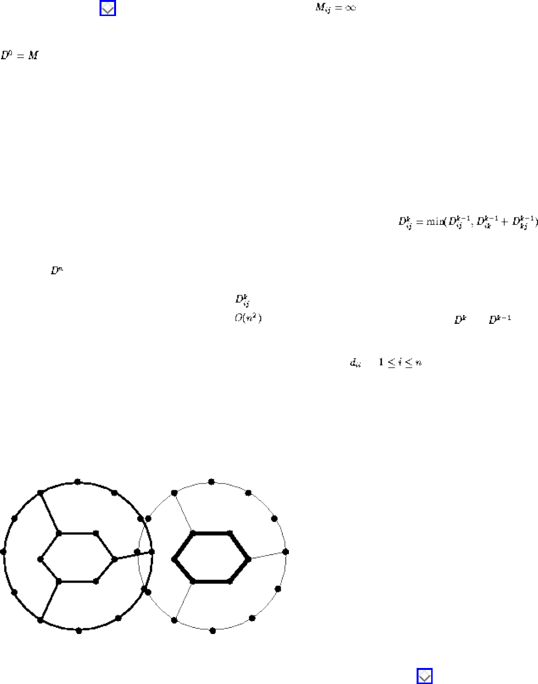
Shortest Path
easier to program than Dijkstra and which works with negative cost edges (but not cycles). It is discussed more
thoroughly in Section . Let M denote the distance matrix, where if there is no edge (i,j).
for k = 1 to n do
for i = 1 to n do
for j = 1 to n do
Return
The key to understanding Floyd's algorithm is that denotes ``the length of the shortest path from i to j that goes
through at most k intermediate vertices.'' Note that space suffices, since we need keep only and
around at time k.
● How do I find the shortest cycle in a graph? - One application of all-pairs shortest path is to find the shortest
cycle in a graph, called its girth. Floyd's algorithm can be used to compute for , which is the length of
the shortest way to get from vertex i to i, in other words the shortest cycle through i.
This might be exactly what you want. However, the shortest cycle through x is likely to go from x to y back to x,
using the same edge twice. A simple cycle is one that visits no edge or vertex twice. To find the shortest simple
cycle, the easiest approach is to compute the lengths of the shortest paths from i to all other vertices, and then
explicitly check whether there is an acceptable edge from each vertex back to i.
Figure: The girth, or shortest cycle, in a graph
Finding the longest cycle in a graph includes the special case of Hamiltonian cycle (see ), so it is NP-
file:///E|/BOOK/BOOK4/NODE162.HTM (3 of 5) [19/1/2003 1:31:00]
Shortest Path
complete.
The all-pairs shortest path matrix can be used to compute several useful invariants of any graph G, that are related to the
center of G. The eccentricity of a vertex v in a graph is the shortest-path distance to the farthest vertex from v. From the
eccentricity come other graph invariants. The radius of a graph is the smallest eccentricity of any vertex, while the center
is the set of vertices whose eccentricity is the radius. The diameter of a graph is the maximum eccentricity of any vertex.
Implementations: The highest performance code (for both Dijkstra and Bellman-Ford) available for finding shortest
paths in graphs is SPLIB [CGR93], developed in C language by Cherkassky, Goldberg, and Radzik. They report solving
instances with over one million vertices in under two minutes on a Sun Sparc-10 workstation. Their codes are available
from http://www.neci.nj.nec.com/homepages/avg.html for noncommercial use.
LEDA (see Section ) provides good implementations in C++ for all of the shortest-path algorithms we have
discussed, including Dijkstra, Bellman-Ford, and Floyd's algorithms.
Pascal implementations of Dijkstra, Bellman-Ford, and Floyd's algorithms are given in [SDK83]. See Section .
XTango (see Section ) includes animations of both Dijkstra's and Floyd's shortest-path algorithms.
Combinatorica [Ski90] provides Mathematica implementations of Dijkstra's and Floyd's algorithms for shortest paths,
acyclicity testing, and girth computation for directed/undirected and weighted/unweighted graphs. See Section .
The Stanford GraphBase (see Section ) contains an implementation of Dijkstra's algorithm, used for computing
word ladders in a graph defined by five-letter words, as well as an implementation of a program to bound the girth of
graphs. Algorithm 562 [Pap80] of the Collected Algorithms of the ACM is a Fortran program to find shortest paths in
graphs (see Section ).
Notes: Good expositions on Dijkstra's algorithm [Dij59] and Floyd's all-pairs-shortest-path algorithm [Flo62] include
[Baa88, CLR90, Man89]. Good expositions of the Bellman-Ford algorithm [Bel58, FF62] are slightly rarer, but include
[CLR90, Eve79a, Law76]. Expositions on finding the shortest path in a DAG include [Law76].
A survey on shortest-path algorithms with 222 references appears in [DP84]. Included are citations to algorithms for
related path problems, like finding the kth-shortest path and shortest paths when edge costs vary with time. Expositions
on finding the kth-shortest path include [Law76].
The theoretically fastest algorithms known for single-source shortest path for positive edge weight graphs are variations
of Dijkstra's algorithm with Fibonacci heaps [FT87]. Experimental studies of shortest-path algorithms include [DF79,
DGKK79]. However, these experiments were done before Fibonacci heaps were developed. See [CGR93] for a more
recent study.
Theoretically faster algorithms exist when the weights of the edges are small; i.e. their absolute values are each bounded
by W. For positive edge weights, the single-source-shortest-path can be found in [AMOT88], while
suffices for graphs with negative edge weights [GT89]
file:///E|/BOOK/BOOK4/NODE162.HTM (4 of 5) [19/1/2003 1:31:00]

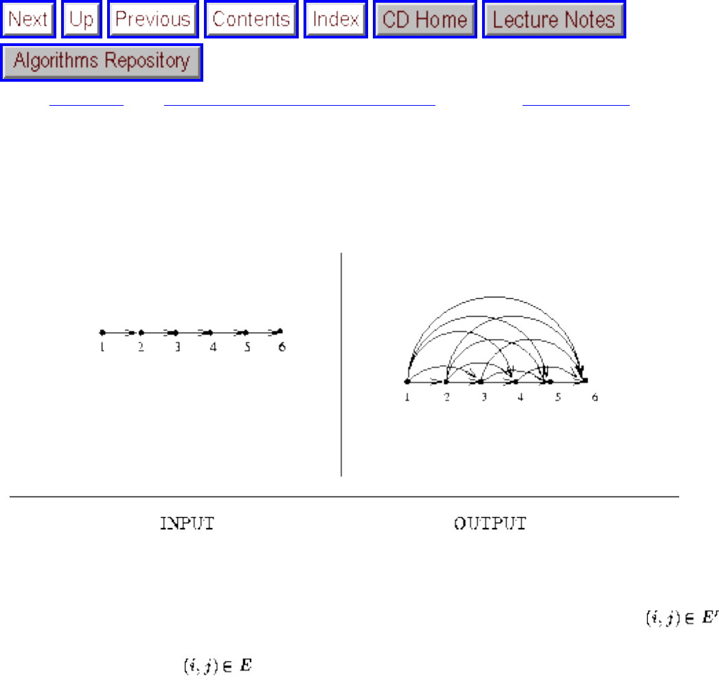
Transitive Closure and Reduction
Next: Matching Up: Graph Problems: Polynomial-Time Previous: Shortest Path
Transitive Closure and Reduction
Input description: A directed graph G=(V,E).
Problem description: For transitive closure, construct a graph G'=(V,E') with edge iff there is
a directed path from i to j in G. For transitive reduction, construct a small graph G'=(V,E') with a directed
path from i to j in G' iff .
Discussion: Transitive closure can be thought of as establishing a data structure that makes it possible to
solve reachability questions (can I get to x from y?) efficiently. After the preprocessing of constructing
the transitive closure, all reachability queries can be answered in constant time by simply reporting a
matrix entry. Transitive closure is fundamental in propagating the consequences of modified attributes
of a graph G. For example, consider the graph underlying any spreadsheet model, where the vertices are
cells and there is an edge from cell i to cell j if the result of cell j depends on cell i. When the value of a
given cell is modified, the values of all reachable cells must also be updated. The identity of these cells is
revealed by the transitive closure of G. Many database problems reduce to computing transitive closures,
for analogous reasons.
There are three basic algorithms for computing transitive closure:
file:///E|/BOOK/BOOK4/NODE163.HTM (1 of 4) [19/1/2003 1:31:01]
Transitive Closure and Reduction
● The simplest algorithm just performs a breadth-first or depth-first search from each vertex and
keeps track of all vertices encountered. Doing n such traversals gives an O(n (n+m) ) algorithm,
which degenerates to cubic time if the graph is dense. This algorithm is easily implemented, runs
well on sparse graphs, and is likely the right answer for your application.
● If the transitive closure of G will be dense, a better algorithm exploits the fact that the strongly
connected components of G can be computed in linear time (see Section ). All pairs of
vertices in each strongly connected component are mutually reachable. Further, if (x,y) is an edge
between two vertices in different strongly connected components, every vertex in y's component
is reachable from each vertex in x's component. Thus the problem reduces to finding the transitive
closure on a graph of strongly connected components, which should have considerably fewer
edges and vertices than G.
● Warshall's algorithm constructs transitive closures in with a simple, slick algorithm that is
identical to Floyd's all-pairs-shortest-path algorithm of Section . If we are interested only in
the transitive closure, and not the length of the resulting paths, we can reduce storage by retaining
only one bit for each matrix element. Thus iff j is reachable from i using only vertices
as intermediates.
Another related algorithm, discussed in the references, runs in the same time as matrix
multiplication. You might conceivably win for large n by using Strassen's fast matrix
multiplication algorithm, although I for one wouldn't bother trying. Since transitive closure is
provably as hard as matrix multiplication, there is little hope for a significantly faster algorithm.
Transitive reduction (also known as minimum equivalent digraph) is essentially the inverse operation of
transitive closure, namely reducing the number of edges while maintaining identical reachability
properties. The transitive closure of G is identical to the transitive closure of the transitive reduction of
G. The primary application of transitive reduction is space minimization, by eliminating redundant
edges from G that do not effect reachability. Transitive reduction also arises in graph drawing, where it
is important to eliminate as many unnecessary edges as possible in order to reduce the visual clutter.
Although the transitive closure of G is uniquely defined, a graph may have many different transitive
reductions, including G itself. We want the smallest such reduction, but there can be multiple
formulations of the problem:
● A linear-time, quick-and-dirty transitive reduction algorithm identifies the strongly connected
components of G, replaces each by a simple directed cycle, and adds these edges to those bridging
the different components. Although this reduction is not provably minimal, it is likely to be pretty
close on typical graphs.
One catch with this heuristic is that it can add edges to the transitive reduction of G that are not in
G. This may or may not be a problem for your application.
● If, in fact, all edges of the transitive reduction of G must be in G, we must abandon hope of
file:///E|/BOOK/BOOK4/NODE163.HTM (2 of 4) [19/1/2003 1:31:01]
Transitive Closure and Reduction
finding the minimum size reduction. To see why, consider a directed graph consisting of one
strongly connected component, so that every vertex can reach every other vertex. The smallest
possible transitive reduction will be a simple directed cycle, consisting of exactly n edges. This is
possible as a subset of edges only if G is Hamiltonian, thus proving that finding the smallest
subset of edges is NP-complete.
A heuristic for finding such a transitive reduction is to consider each edge successively and delete
it if its removal does not change the transitive reduction. Implementing this efficiently means
minimizing the time spent on reachability tests. Observe that directed edge (i,j) can be eliminated
whenever there is another path from i to j avoiding this edge.
● If we are allowed to have arbitrary pairs of vertices as edges in the reduction and need the
minimum size reduction, it can be found in time. See the references below for details.
However, the quick-and-dirty algorithm above will likely suffice for most applications and will be
easier to program as well as more efficient.
Implementations: LEDA (see Section ) provides an implementation of transitive closure in C++
using O(n m) time [GK79].
Combinatorica [Ski90] provides Mathematica implementations of transitive closure and reduction, as
well as the display of partial orders requiring transitive reduction. See Section .
Notes: Van Leeuwen [vL90a] provides an excellent survey on transitive closure and reduction, including
33 references. Good expositions of Warshall's algorithm [War62] include [Baa88, CLR90, Man89]. The
equivalence between matrix multiplication and transitive closure was proven by Fischer and Meyer
[FM71], with good expositions including [AHU74].
The equivalence between transitive closure and reduction, as well as the reduction algorithm, was
established in [AGU72]. Empirical studies of transitive closure algorithms include [SD75].
Estimating the size of the transitive closure is important in database query optimization. A linear-time
algorithm for estimating the size of the closure is given by Cohen [Coh94].
Related Problems: Connected components (see page ), shortest path (see page ).
Next: Matching Up: Graph Problems: Polynomial-Time Previous: Shortest Path
file:///E|/BOOK/BOOK4/NODE163.HTM (3 of 4) [19/1/2003 1:31:01]
Transitive Closure and Reduction
Algorithms
Mon Jun 2 23:33:50 EDT 1997
file:///E|/BOOK/BOOK4/NODE163.HTM (4 of 4) [19/1/2003 1:31:01]
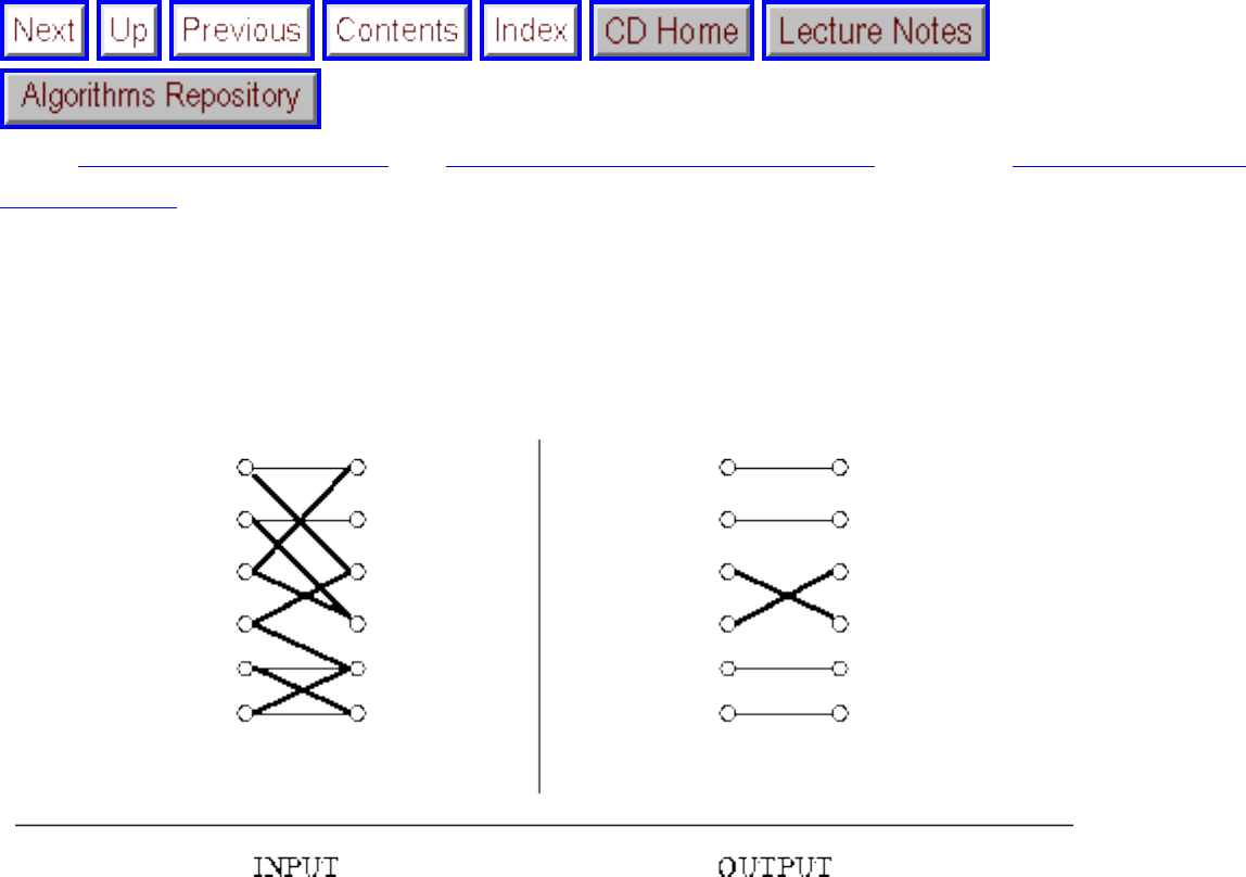
Matching
Next: Eulerian Cycle / Chinese Up: Graph Problems: Polynomial-Time Previous: Transitive Closure
and Reduction
Matching
Input description: A (weighted) graph G=(V,E).
Problem description: Find the largest-size set of edges S from E such that each vertex in V is incident to
at most one edge of S.
Discussion: Consider a set of employees, each of whom is capable of doing some subset of the tasks that
must be performed. We seek to find an assignment of employees to tasks such that each task is
assigned to a unique employee. Each mapping between an employee and a task they can handle defines
an edge, so what we need is a set of edges with no employee or job in common, i.e. a matching.
Efficient algorithms for constructing matchings are based on constructing augmenting paths in graphs.
Given a (partial) matching M in a graph G, an augmenting path P is a path of edges where every odd-
numbered edge (including the first and last edge) is not in M, while every even-numbered edge is.
Further, the first and last vertices must not be already in M. By deleting the even-numbered edges of P
from M and replacing them with the odd-numbered edges of P, we enlarge the size of the matching by
one edge. Berge's theorem states that a matching is maximum if and only if it does not contain any
augmenting path. Therefore, we can construct maximum-cardinality matchings by searching for
file:///E|/BOOK/BOOK4/NODE164.HTM (1 of 4) [19/1/2003 1:31:03]

Matching
augmenting paths and stopping when none exist.
This basic matching framework can be enhanced in several ways, while remaining essentially the same
assignment problem:
● Is your graph weighted or unweighted? - Many matching applications are based on unweighted
graphs. Perhaps we seek to maximize the number of tasks performed, where each task is as good
as another. Such a problem seeks a maximum cardinality matching. We say that a matching is
perfect if every vertex is involved in the matching.
For certain applications, we need to augment each edge with a weight, perhaps reflecting the
salary of the employee or their effectiveness at a given task. The problem now becomes
constructing a maximum weighted matching, i.e. the set of independent edges of maximum total
cost. By setting all edge weights to be 1, any algorithm for finding weighted matchings can be
used to solve maximum cardinality matching.
● What if certain employees can be given multiple jobs? - In a natural generalization of the
assignment problem, certain employees can given more than one task to do. We do not seek a
matching so much as a covering with small ``stars''. Such multiple jobs can be modeled by simply
replicating the employee vertex as many times as the number of jobs she can handle. By adding
sufficiently complicated constraints on the solution, we will eventually require the use of full
integer programming.
● Is your graph bipartite? - Many common matching problems involve bipartite graphs, as in the
classical assignment problem of jobs to workers. This is fortunate because faster and simpler
algorithms exist for bipartite matching. General graphs prove trickier because it is possible to
have augmenting paths that are odd-length cycles, i.e. the first and last vertices are the same.
Such cycles (or blossoms) are impossible in bipartite graphs, which by definition do not contain
odd-length cycles.
The standard algorithms for bipartite matching are based on network flow, using a simple
transformation to convert a bipartite graph into an equivalent flow graph.
Another common ``application'' of bipartite matching is in marrying off a set of boys to a set of girls such
that each boy gets a girl he likes. This can be modeled as a bipartite matching problem, with an edge
between any compatible boy and girl. This is possible only for graphs with perfect matchings. An
interesting related problem seeks a matching such that no parties can be unhappy enough to seek to break
the matching. That is, once each of the boys has ranked each of the girls in terms of desirability, and the
girls do the same to the boys, we seek a matching with the property that there are no marriages of the
form and , where and in fact prefer each other to their own spouses. In real life,
these two would run off with each other, breaking the marriages. A marriage without any such couples
is said to be stable.
It is a surprising fact that no matter how the boys and girls rate each other, there is always at least one
file:///E|/BOOK/BOOK4/NODE164.HTM (2 of 4) [19/1/2003 1:31:03]
Matching
stable marriage. Further, such a marriage can be found in time. An important application of stable
marriage occurs in the annual matching of medical residents to hospitals.
Implementations: The highest performance code available for constructing a maximum-cardinality
bipartite matching of maximum weight in graphs is CSA [GK93], developed in the C language by
Goldberg and Kennedy. This code is based on a cost-scaling network flow algorithm. They report
solving instances with over 30,000 vertices in a few minutes on a Sun Sparc-2 workstation. Their codes
are available for noncommercial use from http://www.neci.nj.nec.com/homepages/avg.html
The First DIMACS Implementation Challenge [JM93] focused on network flows and matching. Several
instance generators and implementations for maximum weight and maximum cardinality matching were
collected, which can be obtained by anonymous ftp from dimacs.rutgers.edu in the directory
pub/netflow/matching. These include:
● A maximum-cardinality matching solver in Fortran 77 by R. Bruce Mattingly and Nathan P.
Ritchey that seems capable of solving instances of 5,000 nodes and 60,000 edges in under 30
seconds.
● A maximum-cardinality matching solver in C by Edward Rothberg, that implements Gabow's
algorithm.
● A maximum-weighted matching solver in C by Edward Rothberg. This is slower but more general
than his unweighted solver described above. For example, it took over 30 seconds on a weighted
graph with 500 nodes and 4,000 edges.
LEDA (see Section ) provides efficient implementations in C++ for both maximum cardinality and
maximum weighted matching, on both bipartite and general graphs. Sedgewick [Sed92] provides a
simple implementation of the stable marriage theorem in C++. See Section for details.
Pascal implementations of maximum cardinality matching appears in [SDK83]. Alternative Pascal
maximum-cardinality and bipartite matching codes appear in [MS91]. All are discussed in Section .
The Stanford GraphBase (see Section ) contains an implementation of the Hungarian algorithm for
bipartite matching. To provide readily visualized weighted bipartite graphs, Knuth uses a digitized
version of the Mona Lisa and seeks row/column disjoint pixels of maximum brightness. Matching is also
used to construct clever, resampled ``domino portraits.''
Algorithm 548 [CT80] presents a Fortran code for the assignment problem. Algorithm 575 [Duf81]
permutes a matrix so as to minimize the number of zeros along the diagonal, which involves solving a
matching problem. Both codes are available from Netlib (see Section ).
file:///E|/BOOK/BOOK4/NODE164.HTM (3 of 4) [19/1/2003 1:31:03]
Matching
Combinatorica [Ski90] provides a (slow) Mathematica implementations of bipartite and maximal
matching, as well as the stable marriage theorem. See Section .
Notes: Lovász and Plummer [LP86] is the definitive reference on matching theory and algorithms.
Survey articles on matching algorithms include [Gal86]. Good expositions on network flow algorithms
for bipartite matching include [CLR90, Eve79a, Man89], and those on the Hungarian method include
[Law76, PS82]. The best algorithm for maximum bipartite matching, due to Hopcroft and Karp [HK73],
repeatedly finds the shortest augmenting paths instead of using network flow, and runs in .
Expositions on the augmenting path method include [Man89, PS82, SDK83].
Edmond's algorithm [Edm65] for maximum-cardinality matching is of great historical interest for
provoking questions about what problems can be solved in polynomial time. Expositions on Edmond's
algorithm include [Law76, PS82, Tar83]. Gabow's [Gab76] implementation of Edmond's algorithm runs
in time. The best algorithm known for general matching runs in [MV80]. A faster
algorithm for matching in geometic graphs appears in [Vai88].
The theory of stable matching is thoroughly treated in [GI89]. The original algorithm for finding stable
marriages is due to Gale and Shapely [GS62] with expositions including [Law76].
Related Problems: Eulerian cycle (see page ), network flow (see page ).
Next: Eulerian Cycle / Chinese Up: Graph Problems: Polynomial-Time Previous: Transitive Closure
and Reduction
Algorithms
Mon Jun 2 23:33:50 EDT 1997
file:///E|/BOOK/BOOK4/NODE164.HTM (4 of 4) [19/1/2003 1:31:03]
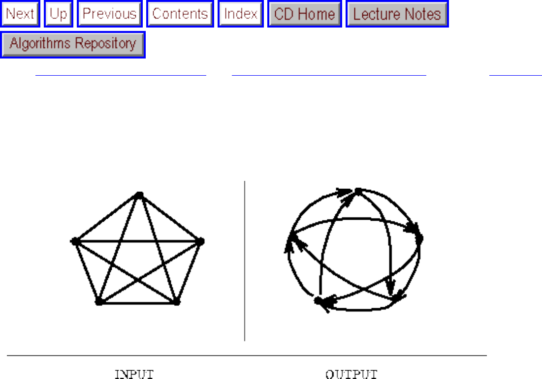
Eulerian Cycle / Chinese Postman
Next: Edge and Vertex Connectivity Up: Graph Problems: Polynomial-Time Previous: Matching
Eulerian Cycle / Chinese Postman
Input description: A graph G=(V,E).
Problem description: Find the shortest tour of G visiting each edge at least once.
Discussion: Suppose you are given the map of a city and charged with designing the routes for garbage
trucks, snow plows, or postmen. In all of these applications, every road in the city must be completely
traversed at least once in order to ensure that all deliveries or pickups are made. For efficiency, you seek
to minimize total drive time, or equivalently, the total distance or number of edges traversed.
Such applications are variants of the Eulerian cycle problem, best characterized by the children's puzzle
that asks them to draw a given figure completely without lifting their pencil off the paper and without
repeating any edges. We seek a path or cycle through a graph that visits each edge exactly once.
There are well-known conditions for determining whether a graph contains an Eulerian cycle, or path:
● An undirected graph contains an Eulerian cycle iff (1) it is connected and (2) each vertex is of
even degree.
● An undirected graph contains an Eulerian path iff (1) it is connected and (2) all but two vertices
file:///E|/BOOK/BOOK4/NODE165.HTM (1 of 4) [19/1/2003 1:31:06]

Eulerian Cycle / Chinese Postman
are of even degree. These two vertices will be the start and end points of the path.
● A directed graph contains an Eulerian cycle iff (1) it is connected and (2) each vertex has the
same in-degree as out-degree.
● Finally, a directed graph contains an Eulerian path iff (1) it is connected and (2) all but two
vertices have the same in-degree as out-degree, and these two vertices have their in-degree and
out-degree differ by one.
Given this characterization of Eulerian graphs, it is easy to test in linear time whether such a cycle exists:
test whether the graph is connected using DFS or BFS, and then count the number of odd-degree
vertices. Actually constructing such a cycle also takes linear time. Use DFS to find a cycle in the graph.
Delete this cycle and repeat until the entire set of edges has been partitioned into a set of edge-disjoint
cycles. Since deleting a cycle reduces each vertex degree by an even number, the remaining graph will
continue to satisfy the same Eulerian degree-bound conditions. For any connected graph, these cycles
will have common vertices, and so by splicing these cycles in a ``figure eight'' at a shared vertex, we can
construct a single circuit containing all of the edges.
An Eulerian cycle, if one exists, solves the motivating snowplow problem, since any tour that visits each
edge only once must have minimum length. However, it is unlikely that any real road network would
happen to satisfy the degree conditions that make it Eulerian. We need to solve the more general
Chinese postman problem, which minimizes the length of a cycle that traverses every edge at least once.
In fact, it can be shown that this minimum cycle never visits any edge more than twice, so good tours
exist for any road network.
The optimal postman tour can be constructed by adding the appropriate edges to the graph G so as to
make it Eulerian. Specifically, we find the shortest path between each pair of odd-degree vertices in G.
Adding a path between two odd-degree vertices in G turns both of them to even-degree, thus moving us
closer to an Eulerian graph. Finding the best set of shortest paths to add to G reduces to identifying a
minimum-weight perfect matching in a graph on the odd-degree vertices, where the weight of edge (i,j) is
the length of the shortest path from i to j. For directed graphs, this can be solved using bipartite matching,
where the vertices are partitioned depending on whether they have more ingoing or outgoing edges. Once
the graph is Eulerian, the actual cycle can be extracted in linear time using the procedure described
above.
Implementations: Unfortunately, we have not able to identify a suitable Chinese postman
implementation. However, it should not be difficult for you to roll your own by using a matching code
from Section and all-pairs shortest path from Section . Matching is by far the hardest part of the
algorithm.
Combinatorica [Ski90] provides Mathematica implementations of Eulerian cycles and de Bruijn
sequences. See Section .
file:///E|/BOOK/BOOK4/NODE165.HTM (2 of 4) [19/1/2003 1:31:06]
Eulerian Cycle / Chinese Postman
Nijenhuis and Wilf [NW78] provide an efficient Fortran routine to enumerate all Eulerian cycles of a
graph by backtracking. See Section .
Notes: The history of graph theory began in 1736, when Euler [Eul36] first solved the seven bridges of
Königsberg problem. Königsberg (now Kaliningrad) is a city on the banks of the Pregel river. In
Euler's day there were seven bridges linking the banks and two islands, which can be modeled as a
multigraph with seven edges and four vertices. Euler sought a way to walk over each of the bridges
exactly once and return home, i.e. an Eulerian cycle. Since all four of the vertices had odd degree, Euler
proved that such a tour is impossible. The bridges were destroyed in World War II. See [BLW76] for a
translation of Euler's original paper and a history of the problem.
Expositions on linear algorithms for constructing Eulerian cycles [Ebe88] include [Eve79a, Man89].
Fleury's algorithm [Luc91] is a direct and elegant approach to constructing Eulerian cycles. Start walking
from any vertex, and erase any edge that has been traversed. The only criterion in picking the next edge
is that we avoid using a bridge (edges whose deletion) unless there is no other alternative. No Eulerian
graph contains a bridge, but what remains at some point on the walk ceases to be biconnected.
The Euler's tour technique is an important paradigm in parallel graph algorithms. See [Man89] for an
exposition. Efficient algorithms exist to count the number of Eulerian cycles in a graph [HP73].
The problem of finding the shortest tour traversing all edges in a graph was introduced by Kwan
[Kwa62], hence the name Chinese postman. The bipartite matching algorithm for solving Chinese
postman is due to Edmonds and Johnson [EJ73]. This algorithm works for both directed and undirected
graphs, although the problem is NP-complete for mixed graphs [Pap76a]. Mixed graphs contain both
directed and undirected edges. Expositions of the Chinese postman algorithm include [Law76].
A de Bruijn sequence S of span n on an alphabet of size is a circular string of length containing all
strings of length n as substrings of S, each exactly once. For example, for n=3 and , the
circular string 00011101 contains the following substrings in order: 000, 001, 011, 111, 110, 101, 010,
100. De Bruijn sequences can be thought of as ``safe cracker'' sequences, describing the shortest
sequence of dial turns with positions sufficient to try out all combinations of length n.
De Bruijn sequences can be constructed by building a graph whose vertices are all strings of length
n-1, where there is an edge (u,v) iff and . Any Eulerian cycle on this
graph describes a de Bruijn sequence. For expositions on de Bruijn sequences and their construction, see
[Eve79a, Ski90].
Related Problems: Matching (see page ), Hamiltonian cycle (see page ).
file:///E|/BOOK/BOOK4/NODE165.HTM (3 of 4) [19/1/2003 1:31:06]

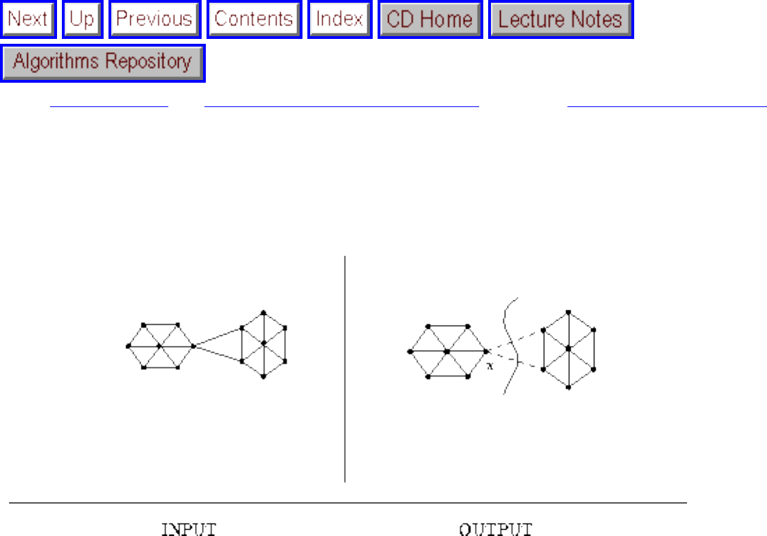
Edge and Vertex Connectivity
Next: Network Flow Up: Graph Problems: Polynomial-Time Previous: Eulerian Cycle / Chinese
Edge and Vertex Connectivity
Input description: A graph G. Optionally, a pair of vertices and t.
Problem description: What is the smallest subset of vertices (edges) whose deletion will disconnect G?
Alternatively, what is the smallest subset of vertices (edges) that will separate from t?
Discussion: Graph connectivity often arises in problems related to network reliability. In the context
of telephone networks, the vertex connectivity is the smallest number of switching stations that a terrorist
must bomb in order to separate the network, i.e. prevent two unbombed stations from talking to each
other. The edge connectivity is the smallest number of wires that need to be cut to accomplish the same
thing. One well-placed bomb or snipping the right pair of cables suffices to disconnect the network
above.
The edge (vertex) connectivity of a graph G is the smallest number of edge (vertex) deletions sufficient
to disconnect G. There is a close relationship between the two quantities. The vertex connectivity is
always no smaller than the edge connectivity, since deleting one vertex incident on each edge in a cut set
succeeds in disconnecting the graph. Of course, smaller vertex subsets may be possible. The minimum
vertex degree is an upper bound on both the edge and vertex connectivity, since deleting all its neighbors
(or the edges to all its neighbors) disconnects the graph into one big and one single-vertex component.
file:///E|/BOOK/BOOK4/NODE166.HTM (1 of 4) [19/1/2003 1:31:08]
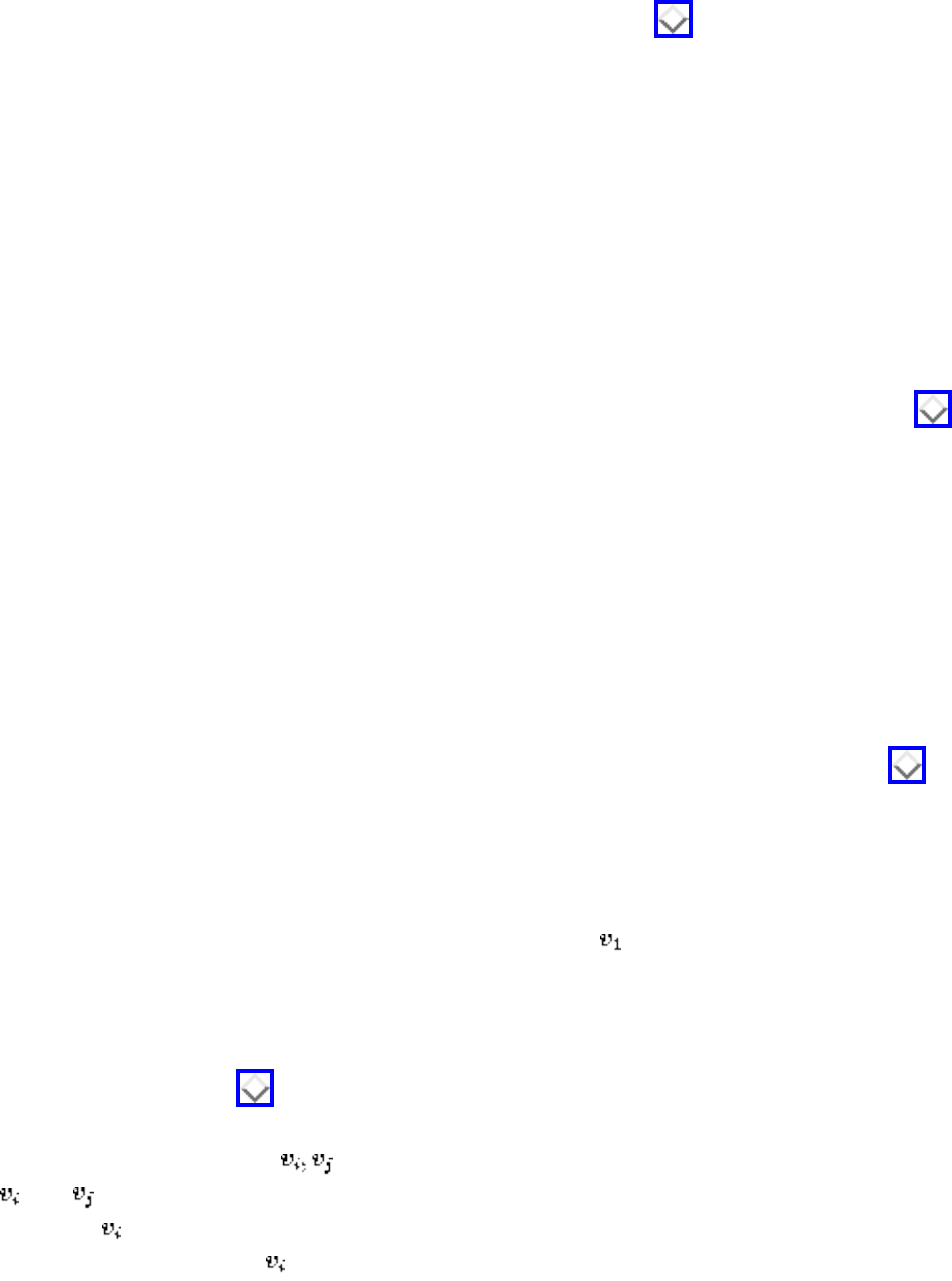
Edge and Vertex Connectivity
Several connectivity problems prove to be of interest:
● Is the graph already disconnected? - The simplest connectivity problem is testing whether the
graph is in fact connected. A simple depth-first or breadth-first search suffices to identify all
components in linear time, as discussed in Section . For directed graphs, the issue is whether
the graph is strongly connected, meaning there is a directed path between any pair of vertices.
In a weakly connected graph, there may exist paths to nodes from which there is no way to return.
● What if I want to split the graph into equal-sized pieces? - Often, what is sought is not the
smallest set of edges or vertices whose deletion will disconnect the graph, but a small set that
breaks the graph into roughly equal-sized pieces. For example, suppose we want to break a
computer program spread across several files into two maintainable units. Construct a graph
where the vertices are subroutines, with an edge between any two subroutines that interact, say by
one calling the other. We seek to partition the routines into equal-sized sets so that the fewest
pairs of interacting routines are spread across the set.
This is the graph partition problem, which is further discussed in Section . Although the
problem is NP-complete, reasonable heuristics exist to solve it.
● Is there one weak link in my graph? - We say that G is biconnected if no single vertex deletion is
sufficient to disconnect G. Any vertex that is such a weak point is called an articulation vertex.
A bridge is the analogous concept for edges, meaning a single edge whose deletion disconnects
the graph.
The simplest algorithms for identifying articulation vertices (or bridges) would try deleting
vertices (or edges) one by one, and then using DFS or BFS to test whether the resulting graph is
still connected. More complicated but linear-time algorithms exist for both problems, based on
depth-first search. Implementations are described below and in Section .
● Are arbitrary cuts OK, or must I separate a given pair of vertices? - There are two flavors of the
general connectivity problem. One asks for the smallest cutset for the graph, the other for the
smallest set to separate from t. Any algorithm for (-t)-connectivity can be used with each of the
n(n-1)/2 possible pairs of vertices to give an algorithm for general connectivity. Less obviously, n-
1 runs will suffice, since we know that vertex must end up in a different component from at
least one of the other n-1 vertices in any cut set.
Both edge and vertex connectivity can be found using network flow techniques. Network flow,
discussed in Section , interprets a weighted graph as a network of pipes where the maximum capacity
of an edge is its weight, and seeks to maximize the flow between two given vertices of the graph. The
maximum flow between in G is exactly the weight of the smallest set of edges to disconnect G with
and in different components. Thus the edge connectivity can be found by minimizing the flow
between and each of the n-1 other vertices in an unweighted graph G. Why? After deleting the
minimum-edge cut set, must be separated from some other vertex.
file:///E|/BOOK/BOOK4/NODE166.HTM (2 of 4) [19/1/2003 1:31:08]
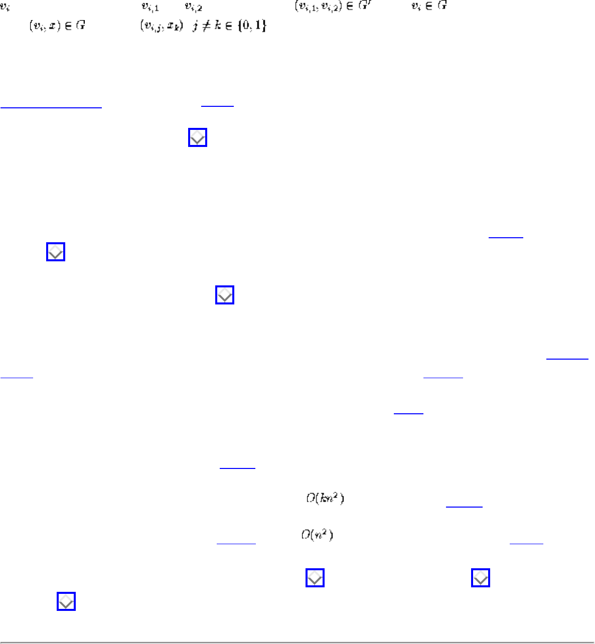
Edge and Vertex Connectivity
Vertex connectivity is characterized by Menger's theorem, which states that a graph is k-connected if
and only if every pair of vertices is joined by at least k vertex-disjoint paths. Network flow can again be
used to perform this calculation, since in an unweighted graph G a flow of k between a pair of vertices
implies k edge-disjoint paths. We must construct a graph G' with the property that any set of edge-
disjoint paths in G' corresponds to vertex-disjoint paths in G. This can be done by replacing each vertex
of G with two vertices and , such that edge for all , and by replacing every
edge by edges , in G'. Thus two edge-disjoint paths in G' correspond to
vertex-disjoint paths in G, and as such, the minimum maximum-flow in G' gives the vertex connectivity
of G.
Implementations: Combinatorica [Ski90] provides Mathematica implementations of edge and vertex
connectivity, as well as connected, biconnected, and strongly connected components with bridges and
articulation vertices. See Section .
LEDA does not currently seem to have biconnected components and bridges, but it does contain all the
tools to implement connectivity algorithms, including network flow.
Pascal implementations of biconnected and strongly connected components appear in [MS91]. See
Section for details.
The Stanford GraphBase (see Section ) contains routines to compute biconnected and strongly
connected components.
Notes: Good expositions on the network-flow approach to edge and vertex connectivity include [Eve79a,
Ski90]. The correctness of these algorithms is based on Menger's theorem [Men27] that the connectivity
is determined by the number of edge and vertex disjoint paths separating a pair of vertices. The
maximum-flow, minimum-cut theorem is due to Ford and Fulkerson [FF62].
Efficient randomized algorithms for computing graph connectivity have recently been developed by
Karger. See Motwani and Raghavan [MR95] for an excellent treatment of randomized algorithms.
A nonflow-based algorithm for edge k-connectivity in is due to Matula [Mat87]. Faster k-
connectivity algorithms are known for certain small values of k. All three-connected components of a
graph can be generated in linear time [HT73a], while suffices to test 4-connectivity [KR91].
Related Problems: Connected components (see page ), network flow (see page ), graph partition
(see page ).
file:///E|/BOOK/BOOK4/NODE166.HTM (3 of 4) [19/1/2003 1:31:08]

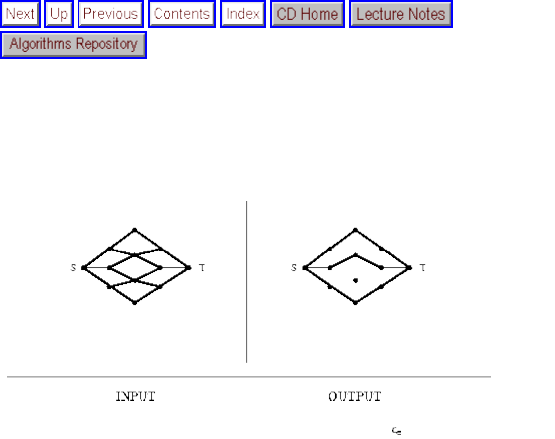
Network Flow
Next: Drawing Graphs Nicely Up: Graph Problems: Polynomial-Time Previous: Edge and Vertex
Connectivity
Network Flow
Input description: A graph G, where each edge e=(i,j) has a capacity . A source node and sink node t.
Problem description: What is the maximum flow you can route from to t while respecting the capacity
constraint of each edge?
Discussion: Applications of network flow go far beyond plumbing. Finding the most cost-effective way
to ship goods between a set of factories and a set of stores defines a network flow problem, as do
resource-allocation problems in communications networks and a variety of scheduling problems.
The real power of network flow is that a surprising variety of linear programming problems that arise in
practice can be modeled as network flow problems, and that special-purpose network flow algorithms
can solve such problems much faster than general-purpose linear programming methods. Several of the
graph problems we have discussed in this book can be modeled as network flow, including bipartite
matching, shortest path, and edge/vertex connectivity.
The key to exploiting this power is recognizing that your problem can be modeled as network flow. This
is not easy, and it requires experience and study. My recommendation is to first construct a linear
file:///E|/BOOK/BOOK4/NODE167.HTM (1 of 4) [19/1/2003 1:31:10]
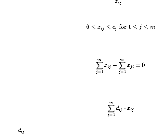
Network Flow
programming model for your problem and then compare it with the linear program for minimum-cost
flow on a directed network G=(V,E). Let be a variable accounting for the flow from vertex i through
edge j. The flow through edge j is constrained by its capacity, so
Further, at each nonsource or sink vertex, as much flow comes in as goes out, so
where we seek the assignment that minimizes
where is the cost of a unit of flow from i through j.
Special considerations include:
● What if all my costs are identical? - Simpler and faster algorithms exist for solving the simple (as
opposed to min-cost) maximum flow problem. This problem arises in many applications,
including connectivity and bipartite matching.
● What if all arc capacities are identical, either 0 or 1? - Faster algorithms exist for 0-1 network
flows. See the references for details.
● What if I have multiple sources and/or sinks? - Such problems can be handled by modifying the
network to create a vertex to serve as a super-source that feeds all the sources and a super-sink
that drains all the sinks.
● What if I have multiple types of material moving through the network? - In modeling a
telecommunications network, every message has a given source and destination. Each destination
needs to receive exactly those calls sent to it, not a given quantity of communication from
arbitrary places. This can be modeled as a multicommodity flow problem, where each call defines
a different commodity and we seek to satisfy all demands without exceeding the total capacity of
any edge.
Linear programming will suffice for multicommodity flow if fractional flows are permitted.
Unfortunately, multicommodity integral flow is NP-complete, even with only two commodities.
Network flow algorithms can be complicated, and significant engineering is required to optimize
performance. Thus we strongly recommend that you use an existing code if possible, rather than
implement your own. Excellent codes are available and are described below. The two primary classes of
algorithms are:
file:///E|/BOOK/BOOK4/NODE167.HTM (2 of 4) [19/1/2003 1:31:10]
Network Flow
● Augmenting path methods - These algorithms repeatedly find a path of positive capacity from
source to sink and add it to the flow. It can be shown that the flow through a network of rational
capacities is optimal if and only if it contains no augmenting path, and since each augmentation
adds to the flow, we will eventually find the maximum. The difference between network flow
algorithms is in how they select the augmenting path. If we are not careful, each augmenting path
will add but a little to the total flow, and so the algorithm might take a long time to converge.
● Preflow-push methods - These algorithms push flows from one vertex to another, ignoring until
the end the constraint that the in-flow must equal the out-flow at each vertex. Preflow-push
methods prove faster than augmenting path methods, essentially because multiple paths can be
augmented simultaneously. These algorithms are the method of choice and are implemented in the
best codes described below.
Implementations: The highest-performance code available for solving maximum-flow in graphs is PRF
[CG94], developed in the C language by Cherkassky and Goldberg. They report solving instances with
over 250,000 vertices in under two minutes on a Sun Sparc-10 workstation. For minimum-cost max-
flow, the highest-performance code available is CS [Gol92], capable of solving instances of over 30,000
vertices in a few minutes on Sun Sparc-2 workstations. Both of their codes are available by ftp for
noncommercial use from http://www.neci.nj.nec.com/homepages/avg.html.
The First DIMACS Implementation Challenge on Network Flows and Matching [JM93] collected several
implementations and generators for network flow, which can be obtained by anonymous ftp from
dimacs.rutgers.edu in the directory pub/netflow/maxflow. These include:
● A preflow-push network flow implementation in C by Edward Rothberg. It took under a second
on a test graph of 500 nodes and 4,000 edges, but over an hour with 5,000 nodes and 40,000
edges.
● An implementation of eleven network flow variants in C, including the older Dinic and Karzanov
algorithms by Richard Anderson and Joao Setubal. On an instance of 8,000 vertices and 12,000
edges, all options finished within two seconds.
Nijenhuis and Wilf [NW78] provide a Fortran implementation of Karzanov's algorithm for network flow.
See Section . Fortran minimum-cost flow codes are given in [PGD82] and [KH80].
LEDA (see Section ) provides C++ implementations of maximum-flow and minimum-cost max-flow
algorithms. It also provides an implementation of minimum cut.
Pascal implementations of max-flow and minimum-cost flow algorithms are provided in [SDK83].
Alternative Pascal max-flow implementations appear in [MS91]. For both codes, see Section .
file:///E|/BOOK/BOOK4/NODE167.HTM (3 of 4) [19/1/2003 1:31:10]
Network Flow
Combinatorica [Ski90] provides a (slow) Mathematica implementation of network flow, with
applications to connectivity testing and matching. See Section .
Notes: The definitive book on network flows and its applications is [AMO93]. Good expositions on
preflow-push algorithms [GT88] include [CLR90]. Older augmenting path algorithms are discussed in
[Eve79a, Man89, PS82]. Expositions on min-cost flow include [Law76, PS82, SDK83]. Expositions on
the hardness of multicommodity flow [Ita78] include [Eve79a].
Conventional wisdom holds that network flow should be computable in O(nm) time, and there has been
steady progress in lowering the time complexity. See [AMO93] for a history of algorithms for the
problem. The fastest known general network flow algorithm runs in time [GT88].
Empirical studies of minimum-cost flow algorithms include [GKK74, Gol92].
Although network flow can be used to find minimum cut sets in graphs, faster algorithms are available,
including [SW94] and [MR95].
Related Problems: Linear programming (see page ), matching (see page ), connectivity (see page
).
Next: Drawing Graphs Nicely Up: Graph Problems: Polynomial-Time Previous: Edge and Vertex
Connectivity
Algorithms
Mon Jun 2 23:33:50 EDT 1997
file:///E|/BOOK/BOOK4/NODE167.HTM (4 of 4) [19/1/2003 1:31:10]
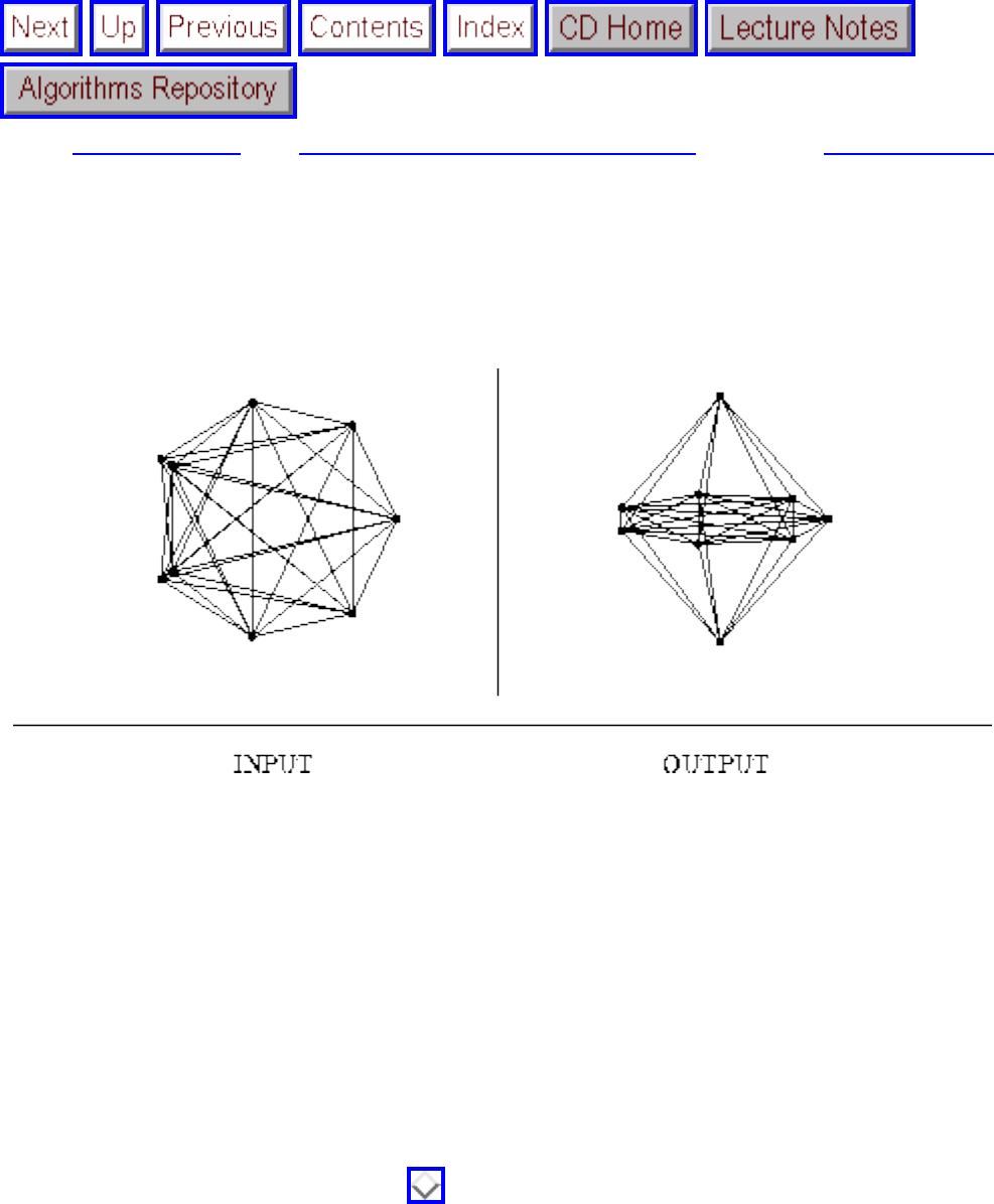
Drawing Graphs Nicely
Next: Drawing Trees Up: Graph Problems: Polynomial-Time Previous: Network Flow
Drawing Graphs Nicely
Input description: A graph G.
Problem description: Draw a graph G so as to accurately reflect its structure.
Discussion: Drawing graphs nicely is a problem that constantly arises in applications, such as displaying
file directory trees or circuit schematic diagrams. Yet it is inherently ill-defined. What exactly does
nicely mean? We seek an algorithm that shows off the structure of the graph so the viewer can best
understand it. We also seek a drawing that looks aesthetically pleasing. Unfortunately, these are ``soft''
criteria for which it is impossible to design an optimization algorithm. Indeed, it is possible to come up
with two or more radically different drawings of certain graphs and have each be most appropriate in
certain contexts. For example, page contains three different drawings of the Petersen graph. Which of
these is the ``right'' one?
Several ``hard'' criteria can partially measure the quality of a drawing:
● Crossings - We seek a drawing with as few pairs of crossing edges as possible, since they are
distracting.
● Area - We seek a drawing that uses as little paper as possible, while ensuring that no pair of
file:///E|/BOOK/BOOK4/NODE168.HTM (1 of 4) [19/1/2003 1:31:12]
Drawing Graphs Nicely
vertices are placed too close to each other.
● Edge length - We seek a drawing that avoids long edges, since they tend to obscure other features
of the drawing.
● Aspect ratio - We seek a drawing whose aspect ratio (width/height) reflects that of the desired
output medium (typically a computer screen at 4/3) as close as possible.
Unfortunately, these goals are mutually contradictory, and the problem of finding the best drawing under
any nonempty subset of them will likely be NP-complete.
Two final warnings before getting down to business. For graphs without inherent symmetries or structure
to display, it is likely that no really nice drawing exists, especially for graphs with more than 10 to 15
vertices. Even when a large, dense graph has a natural drawing, the shear amount of ink needed to draw it
can easily overwhelm any display. A drawing of the complete graph on 100 vertices, , contains
approximately 5,000 edges, which on a pixel display works out to 200 pixels an edge. What
can you hope to see except a black blob in the center of the screen?
Once all this is understood, it must be admitted that certain graph drawing algorithms can be quite
effective and fun to play with. To choose the right one, first ask yourself the following questions:
● Must the edges be straight, or can I have curves and/or bends? - Straight-line drawing algorithms
are simpler than those with polygonal lines, but to visualize complicated graphs such as circuit
designs, orthogonal polyline drawings seem to work best. Orthogonal means that all lines must be
drawn either horizontal or vertical, with no intermediate slopes. Polyline means that each graph
edge is represented by a chain of straight-line segments, connected by vertices or bends.
● Can you build a natural, application-specific drawing algorithm? - If your graph represents a
network of cities and roads, you are unlikely to find a better drawing than placing the vertices in
the same position as the cities on a map. This same principle holds for many different applications.
● Is your graph either planar or a tree? - If so, use one of the special planar graph or tree drawing
algorithms of Sections and .
● How fast must your algorithm be? - If it is being used for interactive update and display, your
graph drawing algorithm had better be very fast. You are presumably limited to using incremental
algorithms, which change the positions of the vertices only in the immediate neighborhood of the
edited vertex. If you need to print a pretty picture for extended study, you can afford to be a little
more extravagant.
As a first, quick-and-dirty drawing for most applications, I recommend simply spacing the vertices
evenly on a circle, and then drawing the edges as straight lines between vertices. Such drawings are easy
to program and fast to construct, and have the substantial advantage that no two edges can obscure each
other, since no three vertices will be nearly collinear. As soon as you allow internal vertices into your
drawing, such artifacts can be hard to avoid. An unexpected pleasure with circular drawings is the
symmetry that is sometimes revealed because consecutive vertices appear in the order they were inserted
into the graph. Simulated annealing can be used to permute the circular vertex order so as to minimize
file:///E|/BOOK/BOOK4/NODE168.HTM (2 of 4) [19/1/2003 1:31:12]

Drawing Graphs Nicely
crossings or edge length, and thus significantly improve the drawing.
A good, general-purpose heuristic for drawing graphs models the graph as a system of springs and then
uses energy minimization to space the vertices. Let adjacent vertices attract each other with a force
proportional to the logarithm of their separation, while all nonadjacent vertices repel each other with a
force proportional to their separation distance. These weights provide incentive for all edges to be as
short as possible, while spreading the vertices apart. The behavior of such a system can be approximated
by determining the force acting on each vertex at a particular time and then moving each vertex a small
amount in the appropriate direction. After several such iterations, the system should stabilize on a
reasonable drawing. The input and output figures above demonstrate the effectiveness of the spring
embedding on a particular small graph.
If you need a polyline graph drawing algorithm, my recommendation is that you study several of the
implementations presented below, particularly graphEd and GraphViz, and see whether one of them can
do the job. You will have to do a significant amount of work before you can hope to develop a better
algorithm.
Once you have a graph drawn, this opens another can of worms, namely where to place the edge/vertex
labels. We seek to position the labels very close to the edges or vertices they identify, and yet to place
them such that they do not overlap each other or important graph features. Map labeling heuristics are
described in [WW95]. Optimizing label placement can be shown to be an NP-complete problem, but
heuristics related to bin packing (see Section ) can be effectively used.
Implementations: Georg Sander maintains a comprehensive WWW page on graph drawing at
http://www.cs.uni-sb.de/RW/users/sander/html/gstools.html. This is well worth checking out and
probably should be your first stop in hunting down programs for graph drawing.
The best ftp-able package of graph drawing algorithms is GraphEd, by Michael Himsolt. GraphEd
[Him94] is a powerful interactive editor that enables the user to construct and manipulate both directed
and undirected graphs. It contains a variety of graph and tree drawing algorithms, including planar
drawings, polyline drawings, upward drawings of directed acyclic graphs (DAGs), and spring
embeddings, and allows variations in node, edge, and label styles. Sgraph is an interface to GraphEd to
support user-specific extensions written in C. It includes a modest library of algorithms for planarity
testing, maximum flow, matching, and connectivity testing. GraphEd can be obtained by anonymous ftp
from forwiss.uni-passau.de (132.231.20.10) in directory /pub/local/graphed. GraphEd is free for
noncommercial use. Graphlet is a more recent project by the same group, available at http://www.fmi.uni-
passau.de/Graphlet.
GraphViz is a popular graph drawing program developed by Stephen North of Bell Laboratories. It
represents edges as splines and can construct useful drawings of quite large and complicated graphs. I
recommend it, even though licensing considerations make it impossible to include on the Algorithm
Repository or CD-ROM. A noncommercial license is available from http://portal.research.bell-
file:///E|/BOOK/BOOK4/NODE168.HTM (3 of 4) [19/1/2003 1:31:12]
Drawing Graphs Nicely
labs.com/orgs/ssr/book/reuse/.
Combinatorica [Ski90] provides Mathematica implementations of several graph drawing algorithms,
including circular, spring, and ranked embeddings. See Section for further information on
Combinatorica.
daVinci is a graph drawing and editing system whose layout algorithm seeks to minimize edge crossings
and line bends, from Michael Froehlich at the University of Bremen. Information about daVinci is
available from http://www.informatik.uni-bremen.de/ davinci. Binaries are available for a variety of
UNIX workstations, although source code is not available.
Notes: A significant community of researchers in graph drawing has emerged in recent years, fueled by
or fueling an annual conference on graph drawing, the proceedings of which are published by Springer-
Verlag's Lecture Notes in Computer Science series. Perusing a volume of the proceedings will provide a
good view of the state of the art and of what kinds of ideas people are thinking about.
The best reference available on graph drawing is the annotated bibliography on graph drawing algorithms
by Giuseppe Di Battista, Peter Eades, and Roberto Tamassia [BETT94], which is also available from
http://www.cs.brown.edu/ rt. See [BGL 95] for an experimental study of graph drawing algorithms.
Although it is trivial to space n points evenly along the boundary of a circle, the problem is considerably
more difficult on the surface of a sphere. Extensive tables of such spherical codes for in up to five
dimensions have been construction by Sloane, Hardin, and Smith, and are available from netlib (see
Section ) in att/math/sloane.
Related Problems: Drawing trees (see page ), planarity testing (see page ).
Next: Drawing Trees Up: Graph Problems: Polynomial-Time Previous: Network Flow
Algorithms
Mon Jun 2 23:33:50 EDT 1997
file:///E|/BOOK/BOOK4/NODE168.HTM (4 of 4) [19/1/2003 1:31:12]
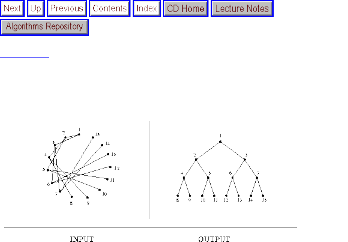
Drawing Trees
Next: Planarity Detection and Embedding Up: Graph Problems: Polynomial-Time Previous: Drawing
Graphs Nicely
Drawing Trees
Input description: A tree T, which is a graph without any cycles.
Problem description: A nice drawing of the tree T.
Discussion: There are as many reasons to want to draw trees as there are types of structures that trees
represent. Consider software and debugging tools that illustrate the hierarchical structure of file system
directories, or that trace the execution of a program through its subroutines.
The primary issue in drawing trees is establishing whether you are drawing free or rooted trees:
● Rooted trees define a hierarchical order, emanating from a single source node identified as the
root. Any drawing must reflect this hierarchical structure, as well as any additional application-
dependent constraints on the order in which children must appear. For example, family trees are
rooted, with sibling nodes typically drawn from left to right in the order of birth.
● Free trees do not encode any structure beyond their connection topology. For example, there is
no root associated with the minimum spanning tree of any graph, so a hierarchical drawing can be
misleading. Such free trees might well inherit their drawing from that of the full underlying graph,
file:///E|/BOOK/BOOK4/NODE169.HTM (1 of 3) [19/1/2003 1:31:13]

Drawing Trees
such as the map of the cities whose distances define the minimum spanning tree.
Since trees are always planar graphs, they can and should be drawn such that no two edges cross. Any
of the planar drawing algorithms of Section could be used to do so. However, such algorithms are
overkill, because much simpler algorithms can be used to construct planar drawings of trees. The spring-
embedding heuristics of Section also work well on free trees, although they may be too slow for
many applications.
The most natural tree-drawing algorithms work with rooted trees. However, they can be used equally
well with free trees by selecting one vertex to serve as the root of the drawing. This faux-root can be
selected arbitrarily, or, even better, by using a center vertex of the tree. A center vertex minimizes the
maximum distance to other vertices. For trees, the center always consists of either one vertex or two
adjacent vertices, so pick either one of them. Further, the center of a tree can be identified in linear time
by repeatedly trimming all the leaves until only the center remains.
Your two primary options for drawing rooted trees are ranked and radial embeddings:
● Ranked embeddings - Place the root in the top center of your page, and then partition the page into
the root-degree number of top-down strips. Deleting the root creates the root-degree number of
subtrees, each of which is assigned to its own strip. Draw each subtree recursively, by placing its
new root (the vertex adjacent to the old root) in the center of its strip a fixed distance from the top,
with a line from old root to new root. The output figure above is a nicely ranked embedding of a
balanced binary tree.
Such ranked embeddings are particularly effective for rooted trees used to represent a hierarchy,
be it a family tree, a data structure, or a corporate ladder. The top-down distance illustrates how
far each node is from the root. Unfortunately, such a repeated subdivision eventually produces
very narrow strips, until most of the vertices are crammed into a small region of the page. You
should adjust the width of each strip to reflect the total number of nodes it will contain, or even
better, the maximum number of nodes on a single level.
● Radial embeddings - A better way to draw free trees is with a radial embedding, where the
root/center of the tree is placed in the center of the drawing. The space around this center vertex
is divided into angular sectors for each subtree. Although the same problem of cramping will
eventually occur, radial embeddings make better use of space than ranked embeddings and appear
considerably more natural for free trees. The rankings of vertices in terms of distance from the
center is illustrated by the concentric circles of vertices.
Implementations: Georg Sander maintains a comprehensive WWW page on graph drawing at
http://www.cs.uni-sb.de/RW/users/sander/html/gstools.html. This should probably be your first stop in
hunting down programs for tree drawing.
file:///E|/BOOK/BOOK4/NODE169.HTM (2 of 3) [19/1/2003 1:31:13]
Drawing Trees
The best FTP-able package of graph drawing algorithms is GraphEd, by Michael Himsolt
(himsolt@fmi.uni-passau.de). It contains a variety of graph and tree drawing algorithms and an
interface to support user-specific extensions written in C. See Section for more details on GraphEd
and other graph drawing systems.
Combinatorica [Ski90] provides Mathematica implementations of several tree drawing algorithms,
including radial and rooted embeddings. See Section for further information on Combinatorica.
Notes: The best reference available on graph drawing is the annotated bibliography on graph drawing
algorithms by Giuseppe Di Battista, Peter Eades, and Roberto Tamassia [BETT94], also available via
http://www.cs.brown.edu/ rt.
Heuristics for tree layout have been studied by several researchers [RT81, Vau80, WS79], although
under certain aesthetic criteria the problem is NP-complete [SR83].
Related Problems: Drawing graphs (see page ), planar drawings (see page ).
Next: Planarity Detection and Embedding Up: Graph Problems: Polynomial-Time Previous: Drawing
Graphs Nicely
Algorithms
Mon Jun 2 23:33:50 EDT 1997
file:///E|/BOOK/BOOK4/NODE169.HTM (3 of 3) [19/1/2003 1:31:13]
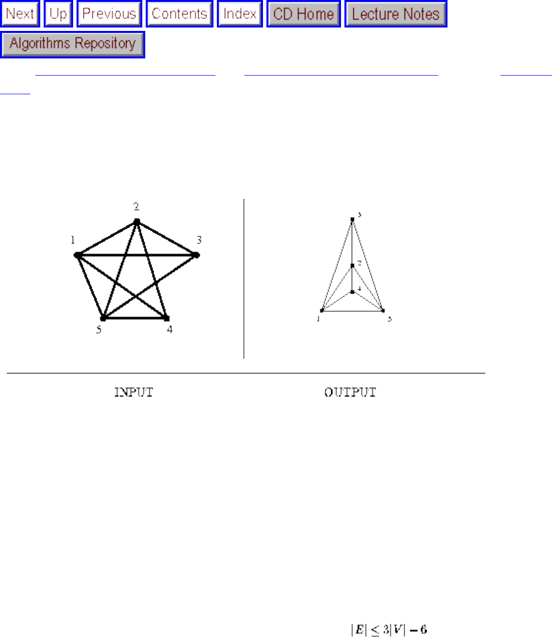
Planarity Detection and Embedding
Next: Graph Problems: Hard Problems Up: Graph Problems: Polynomial-Time Previous: Drawing
Trees
Planarity Detection and Embedding
Input description: A graph G.
Problem description: Can G be drawn in the plane such that no two edges cross? If so, produce such a
drawing.
Discussion: Planar drawings (or embeddings) make it easy to understand the structure of a given graph
by eliminating crossing edges, which are often confused as additional vertices. Graphs arising in many
applications, such as road networks or printed circuit boards, are naturally planar because they are
defined by surface structures.
Planar graphs have a variety of nice properties, which can be exploited to yield faster algorithms for
many problems on planar graphs. Perhaps the most important property is that every planar graph is
sparse. Euler's formula shows that for planar graph G=(V,E), , so every planar graph
contains a linear number of edges, and further, every planar graph must contain a vertex of degree at
most 5. Since every subgraph of a planar graph is planar, this means that there is always a sequence of
low-degree vertices whose deletion from G eventually leaves the empty graph.
file:///E|/BOOK/BOOK4/NODE170.HTM (1 of 3) [19/1/2003 1:31:14]
Planarity Detection and Embedding
The study of planarity has motivated much of the development of graph theory. To get a better
appreciation of the subtleties of planar drawings, the reader is urged to construct a planar (noncrossing)
embedding for the graph , the complete graph on five vertices with any single edge deleted.
Then construct such an embedding where all the edges are straight. Finally, attempt to do the same for
itself.
It is useful to distinguish the problem of planarity testing (does a graph have a planar drawing) from
constructing planar embeddings (actually finding the drawing), although both can be done in linear
time. Surprisingly, many efficient algorithms for planar graphs do not make use of the drawing but use
the low-degree deletion sequence described above.
Algorithms for planarity testing begin by embedding an arbitrary cycle from the graph in the plane and
then considering additional paths in G between vertices on this cycle. Whenever two such paths cross,
one must be drawn outside the cycle and one inside. When three such paths mutually cross, there is no
way to resolve the problem, and so the graph cannot be planar. Linear-time algorithms for planarity
detection are based on depth-first search, but they are subtle and complicated enough that you would be
wise to use an existing implementation if you can.
Such path-crossing algorithms can be used to construct a planar embedding by inserting the paths into the
drawing one by one. Unfortunately, because they work in an incremental manner, nothing prevents
them from inserting many vertices and edges into a relatively small area of the drawing. Such cramping
makes the drawing ugly and hard to understand, and is a major problem with planar-embedding
algorithms. More recently, algorithms have been devised that construct planar-grid embeddings, where
each vertex lies on a grid. Thus no region can get too cramped and no edge can get too
long. Still, the resulting drawings tend not to look as natural as one might hope.
For nonplanar graphs, what is often sought is a drawing that minimizes the number of crossings.
Unfortunately, computing the crossing number is NP-complete. A useful heuristic extracts a large
planar subgraph of G, embeds this subgraph, and then inserts the remaining edges one by one so as to
minimize the number of crossings. This won't do much for dense graphs, which are doomed to have a
large number of crossings, but it will work well for graphs that are almost planar, such as road networks
with overpasses or printed circuit boards with multiple layers. Large planar subgraphs can be found by
modifying planarity-testing algorithms to delete troublemaking edges.
Implementations: LEDA (see Section ) provides a nice set of data structures and algorithms to
support working on planar subdivisions. Included are both linear-time planarity testing and
constructing straight-line planar-grid embeddings.
GraphEd includes an implementation of both planarity testing and planar graph layout. See Section
for more details on GraphEd. Combinatorica [Ski90] provides a (slow) Mathematica implementation of
file:///E|/BOOK/BOOK4/NODE170.HTM (2 of 3) [19/1/2003 1:31:14]
Planarity Detection and Embedding
planarity testing. See Section .
Notes: Kuratowski [Kur30] gave the first characterization of planar graphs, namely that they do not
contain a subgraph homeomorphic to or . Thus if you are still working on the exercise to
embed , now is an appropriate time to give it up. Fary's theorem [F48] states that every planar graph
can be drawn such that each edge is straight.
Hopcroft and Tarjan [HT74] gave the first linear-time algorithm for drawing graphs. Expositions on
linear-time planarity testing include [Eve79a]. Nishizeki and Chiba [NC88] provide a good reference to
the algorithmic theory of planar graphs. Efficient algorithms for planar grid embeddings were first
developed by [dFPP88]. See [CHT90] for an algorithm to find the maximum planar subgraph of a
nonplanar graph. Outerplanar graphs are those that can be drawn such that all vertices lie on the outer
face of the drawing. Such graphs can be characterized as having no subgraph homeomorphic to and
can be recognized and embedded in linear time.
Related Problems: Graph partition (see page ), drawing trees (see page ).
Next: Graph Problems: Hard Problems Up: Graph Problems: Polynomial-Time Previous: Drawing
Trees
Algorithms
Mon Jun 2 23:33:50 EDT 1997
file:///E|/BOOK/BOOK4/NODE170.HTM (3 of 3) [19/1/2003 1:31:14]

Graph Problems: Hard Problems
Next: Clique Up: A Catalog of Algorithmic Previous: Planarity Detection and Embedding
Graph Problems: Hard Problems
A cynical view of graph algorithms is that ``everything we want to do is hard.'' Indeed, no polynomial-
time algorithms are known for any of the problems in this section. Further, with the exception of graph
isomorphism, all of them are provably NP-complete.
The theory of NP-completeness demonstrates that if any NP-complete problem has a polynomial-time
algorithm, then polynomial-time algorithms must exist for all NP-complete problems. This seems
sufficiently preposterous that NP-completeness suffices as a de facto proof that no efficient worst-case
algorithm exists for the given problem.
Still, do not abandon hope if your problem resides in this chapter. For each of these problems, we
provide a recommended line of attack, be it through combinatorial search, heuristics, or approximation
algorithms. For every problem, there exist restricted input instances that are polynomial-time solvable,
and if you are lucky, perhaps your data happens to fall into one of these classes. Hard problems require a
different methodology to work with than polynomial-time problems, but with care they can usually be
dealt with successfully.
The following books will help you deal with NP-complete problems:
● Garey and Johnson [GJ79] - This is the classic reference on the theory of NP-completeness. Most
notably, it contains a concise catalog of over four hundred NP-complete problems, with associated
references and comments. As soon as you begin to doubt the existence of an efficient algorithm
for a given problem, browse through the catalog. Indeed, this is the book that I reach for most
often.
● Hochbaum [Hoc96] - This book surveys the state of the art in approximation algorithms for NP-
complete problems. Approximation algorithms efficiently produce solutions to problems that are
always provably close to optimal.
● Crescenzi and Kann - This compendium of approximation algorithms for optimization problems
is available at http://www.nada.kth.se/nada/theory/problemlist.html and is the place to look first
for a provably good heuristic for any given problem.
file:///E|/BOOK/BOOK4/NODE171.HTM (1 of 2) [19/1/2003 1:31:15]
Graph Problems: Hard Problems
● Clique
● Independent Set
● Vertex Cover
● Traveling Salesman Problem
● Hamiltonian Cycle
● Graph Partition
● Vertex Coloring
● Edge Coloring
● Graph Isomorphism
● Steiner Tree
● Feedback Edge/Vertex Set
Next: Clique Up: A Catalog of Algorithmic Previous: Planarity Detection and Embedding
Algorithms
Mon Jun 2 23:33:50 EDT 1997
file:///E|/BOOK/BOOK4/NODE171.HTM (2 of 2) [19/1/2003 1:31:15]
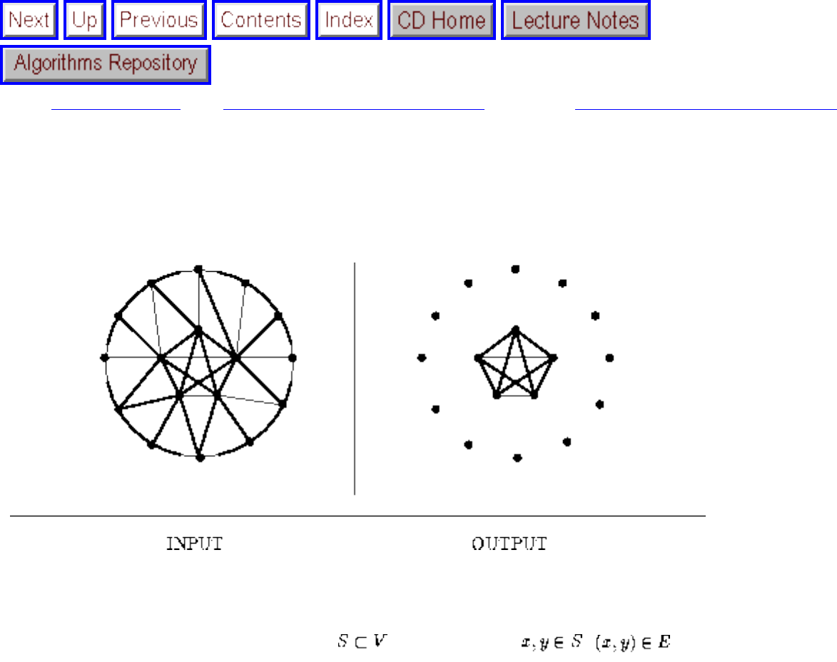
Clique
Next: Independent Set Up: Graph Problems: Hard Problems Previous: Graph Problems: Hard Problems
Clique
Input description: A graph G=(V,E).
Problem description: What is the largest such that for all , ?
Discussion: When I went to high school, everybody complained about the ``clique'', a group of friends
who all hung around together and seemed to dominate everything social. Consider a graph whose
vertices represent a set of people, with edges between any pair of people who are friends. Thus the clique
in high school was in fact a clique in this friendship graph.
Identifying ``clusters'' of related objects often reduces to finding large cliques in graphs. One example is
in a program recently developed by the Internal Revenue Service (IRS) to detect organized tax fraud,
where groups of phony tax returns are submitted in the hopes of getting undeserved refunds. The IRS
constructs graphs with vertices corresponding to submitted tax forms and with edges between any two
tax-forms that appear suspiciously similar. A large clique in this graph points to fraud.
Since any edge in a graph represents a clique of two vertices, the challenge lies not in finding a clique,
but in finding a large one. And it is indeed a challenge, for finding a maximum clique is NP-complete.
To make matters worse, not only is no good approximation algorithm known, it is provably hard to
file:///E|/BOOK/BOOK4/NODE172.HTM (1 of 3) [19/1/2003 1:31:17]
Clique
approximate even to within a factor of . Theoretically, clique is about as hard as a problem in this
book can get. So what can we hope to do about it?
● Will a maximal clique suffice? - A maximal clique is a subset of vertices, each pair of which
defines an edge, that cannot be enlarged by adding any additional vertex. This doesn't mean that it
has to be large relative to the largest possible clique, but it might be. To find a nice maximal
clique, sort the vertices from highest degree to lowest degree, put the first vertex in the clique, and
then test each of the other vertices in order to see whether it is adjacent to all the clique vertices
thus far. If so, add it; if not, continue down the list. In O(n m) time you will have a maximal, and
hopefully large, clique. An alternative approach would be to incorporate some randomness into
your vertex ordering and accept the largest maximal clique you find after a certain number of
trials.
● What if I am looking for a large, dense subgraph instead of a perfect clique? - Insisting on perfect
cliques to define clusters in a graph can be risky, since the loss of a single edge due to error will
eliminate that vertex from consideration. Instead, we should seek large dense subgraphs, i.e.
subsets of vertices that contain a large number of edges between them. Cliques are, by definition,
the densest subgraphs possible.
A simple linear-time algorithm can be used to find the largest set of vertices whose induced
(defined) subgraph has minimum vertex degree , beginning by repeatedly deleting all the
vertices whose degree is less than k. This may reduce the degree of other vertices below k if they
were adjacent to any deleted low-degree vertices. By repeating this process until all remaining
vertices have degree , we eventually construct the largest dense subgraph. This algorithm can
be implemented in O(n+m) time by using adjacency lists and the constant-width priority queue of
Section . By continuing to delete the lowest-degree vertices, we will eventually end up with a
clique, which may or may not be large depending upon the graph.
● What if the graph is planar? - Planar graphs cannot have cliques of size larger than four, or else
they cease to be planar. Since any edge defines a clique of size two, the only interesting cases are
cliques of 3 and 4 vertices. Efficient algorithms to find such small cliques consider the vertices
from lowest to highest degree. Any planar graph must contain a vertex of degree at most 5 (see
Section ), so there is only a constant-sized neighborhood to check exhaustively for a clique.
Once we finish with this vertex, we delete it to leave a smaller planar graph with at least one low-
degree vertex. Repeat until the graph is empty.
If you really need to find the largest clique in a graph, an exhaustive search via backtracking provides the
only real solution. We search through all k-subsets of the vertices, pruning a subset as soon as it
contains a vertex that is not connected to all the rest. We never need consider a subset of size larger than
the highest vertex degree in the graph, since the maximum degree gives an upper bound on the size of the
largest clique in the graph. Similarly, as soon as we discover a clique of size k, no vertex of degree
can help find a larger clique. To speed our search, we should delete all such useless vertices from G.
file:///E|/BOOK/BOOK4/NODE172.HTM (2 of 3) [19/1/2003 1:31:17]
Clique
Heuristics for finding large cliques based on randomized techniques such as simulated annealing are
likely to work reasonably well.
Implementations: Programs for the closely related problems of finding cliques and independent sets
were sought for the Second DIMACS Implementation Challenge, held in October 1993. Programs and
data from the challenge are available by anonymous ftp from dimacs.rutgers.edu. Source codes are
available under pub/challenge/graph and test data under pub/djs.
In particular, two C language programs by David S. Johnson and David L. Applegate are available. The
dfmax.c implements a simple-minded branch-and-bound algorithm similar to that of [CP90]. The
dmclique.c uses a ``semi-exhaustive greedy'' scheme for finding large independent sets described in
[JAMS91]. Performance data for both programs is available in files results.dfmax and results.dmclique in
directories /pub/challenge/graph/benchmarks/clique and /pub/challenge/graph/benchmarks/volume.
Combinatorica [Ski90] provides (slow) Mathematica implementations of cliques, independent sets, and
vertex covers. See Section .
Notes: Good expositions of the proof that clique is NP-complete [Kar72] include [CLR90, GJ79,
Man89]. It is also given in Section . This reduction established that clique, vertex cover, and
independent set are very closely related problems, so heuristics and programs that solve one of them may
also produce reasonable solutions for the other two.
The linear-time algorithm for constructing maximal induced subgraphs is discussed in [Man89]. That
clique cannot be approximated to within a factor of is shown in [BGS95].
Related Problems: Independent set (see page ), vertex cover (see page ).
Next: Independent Set Up: Graph Problems: Hard Problems Previous: Graph Problems: Hard Problems
Algorithms
Mon Jun 2 23:33:50 EDT 1997
file:///E|/BOOK/BOOK4/NODE172.HTM (3 of 3) [19/1/2003 1:31:17]
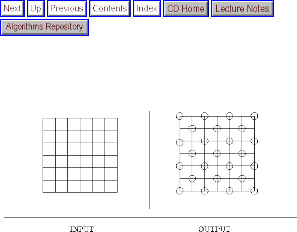
Independent Set
Next: Vertex Cover Up: Graph Problems: Hard Problems Previous: Clique
Independent Set
Input description: A graph G=(V,E).
Problem description: What is the largest subset S of vertices of V such that no pair of vertices in S
defines an edge of E between them?
Discussion: The need to find large independent sets typically arises in dispersion problems, where we
seek a set of mutually separated points. For example, suppose you are trying to identify locations for a
new franchise service such that no two locations are close enough to compete with each other.
Construct a graph where the vertices are possible locations, and add edges between any two locations
deemed close enough to interfere. The maximum independent set gives you the maximum number of
franchises you can sell without cannibalizing sales.
Independent sets avoid conflicts between elements and hence arise often in coding theory and scheduling
problems. Define a graph whose vertices represent the set of possible code words, and add edges
between any two code words sufficiently similar to be confused due to noise. The maximum independent
set of this graph defines the highest capacity code for the given communication channel.
Independent set is closely related to two other NP-complete problems:
file:///E|/BOOK/BOOK4/NODE173.HTM (1 of 3) [19/1/2003 1:31:18]
Independent Set
● Vertex coloring - A coloring of a graph G is in fact a partitioning of the vertices of G into a small
number of independent sets, since any two vertices of the same color cannot have an edge
between them. In fact, most scheduling applications of independent set are really coloring
problems, since all tasks eventually must be completed.
● Clique - The complement of a graph G = (V,E) is a graph G' = (V,E'), where iff (i,j) is
not in E. In other words, we replace each edge by a nonedge and vica versa. The maximum
independent set in G is exactly the maximum clique in G', so these problems are essentially
identical. Algorithms and implementations in Section can thus be easily used for independent
set.
The simplest reasonable heuristic is to find the lowest-degree vertex, add it to the independent set, and
delete it and all vertices adjacent to it. Repeating this process until the graph is empty gives a maximal
independent set, in that it can't be made larger just by adding vertices. Using randomization or perhaps
some exhaustive search to distinguish among the low-degree vertices might result in somewhat larger
independent sets.
The independent set problem is in some sense dual to the graph matching problem. The former asks for
a large set of vertices with no edge in common, while the latter asks for a large set of edges with no
vertex in common. This suggests trying to rephrase your problem as a matching problem, which can be
computed in polynomial time, while the maximum independent set problem is NP-complete.
The maximum independent set of a tree can be found in linear time by (1) stripping off the leaf nodes,
(2) adding them to the independent set, (3) deleting the newly formed leaves, and then (4) repeating from
the first step on the resulting tree until it is empty.
Implementations: Programs for the closely related problems of finding cliques and independent sets
were sought for the Second DIMACS Implementation Challenge, held in October 1993. Programs and
data from the challenge are available by anonymous ftp from dimacs.rutgers.edu. Source codes are
available under pub/challenge/graph and test data under pub/djs. See Section .
Combinatorica [Ski90] provides (slow) Mathematica implementations of cliques, independent sets, and
vertex covers. See Section for further information on Combinatorica.
Neural-network heuristics for vertex cover and related problems such as clique and vertex coloring have
been implemented in C and Mathematica by Laura Sanchis and Arun Jagota, and are available in the
algorithm repository http://www.cs.sunysb.edu/ algorith.
Notes: Independent set remains NP-complete for planar cubic graphs [GJ79]. However, it can be solved
efficiently for bipartite graphs [Law76].
file:///E|/BOOK/BOOK4/NODE173.HTM (2 of 3) [19/1/2003 1:31:18]
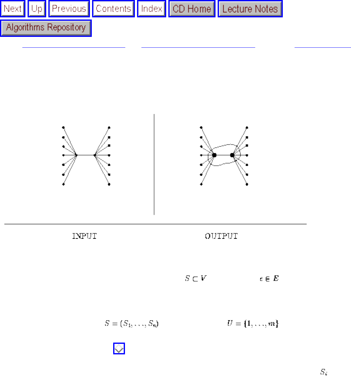
Vertex Cover
Next: Traveling Salesman Problem Up: Graph Problems: Hard Problems Previous: Independent Set
Vertex Cover
Input description: A graph G=(V,E).
Problem description: What is the smallest subset of such that each contains at least one
vertex of S?
Discussion: Vertex cover is a special case of the more general set cover problem, which takes as input an
arbitrary collection of subsets of the universal set . We seek the smallest
subset of subsets from S whose union is U. Set cover arises in many applications, including Boolean
logic minimization. See Section for a discussion of set cover.
To turn vertex cover into a set cover problem, let U be the complete set of edges, and create to be the
set of edges incident on vertex i. A set of vertices defines a vertex cover in graph G iff the corresponding
subsets define a set cover in the given instance. However, since each edge can be in only two different
subsets, vertex cover instances are simpler than general set cover. The primary reason for distinguishing
between the two problems is that vertex cover is a relative lightweight among NP-complete problems,
and so can be effectively solved.
file:///E|/BOOK/BOOK4/NODE174.HTM (1 of 3) [19/1/2003 1:31:19]
Vertex Cover
Vertex cover and independent set are very closely related graph problems. Since every edge in E is (by
definition) incident on a vertex in a cover S, there can be no edge for which both endpoints are not in S.
Thus V-S must be an independent set. Further, since minimizing S is the same as maximizing V-S, a
minimum vertex cover defines a maximum independent set, and vice versa. This equivalence means that
if you have a program that solves independent set, you can use it on your vertex cover problem. Having
two ways of looking at it can be helpful if you expect that either the cover or independent set is likely to
contain only a few vertices, for it might pay to search all possible pairs or triples of vertices if you think
that it will pay off.
The simplest heuristic for vertex cover selects the vertex with highest degree, adds it to the cover, deletes
all adjacent edges, and then repeats until the graph is empty. With the right data structures, this can be
done in linear time, and the cover you get ``usually'' should be ``pretty good''. However, for certain input
graphs the resulting cover can be times worse than the optimal cover.
Much better is the following approximation algorithm, discussed in Section , which always finds a
vertex cover whose size is at most twice as large as optimal. Find a maximal matching in the graph, i.e.
a set of edges no two of which share a vertex in common and that cannot be made larger by adding
additional edges. Such a maximal matching can be built incrementally, by picking an arbitrary edge e in
the graph, deleting any edge sharing a vertex with e, and repeating until the graph is out of edges. Taking
both of the vertices for each edge in the matching gives us a vertex cover, since we only delete edges
incident to one of these vertices and eventually delete all the edges. Because any vertex cover must
contain at least one of the two vertices in each matching edge just to cover the matching, this cover must
be at most twice as large as that of the minimum cover.
This heuristic can be tweaked to make it perform somewhat better in practice, without losing the
performance guarantee or costing too much extra time. We can select the matching edges so as to ``kill
off'' as many edges as possible, which should reduce the size of the maximal matching and hence the
number of pairs of vertices in the vertex cover. Also, some vertices selected for our cover may in fact not
be necessary, since all of their incident edges could also have been covered using other selected vertices.
By making a second pass through our cover, we can identify and delete these losers. If we are really
lucky, we might halve the size of our cover using these techniques.
A problem that might seem closely related to vertex cover is edge cover, which seeks the smallest set of
edges such that each vertex is included in one of the edges. In fact, edge cover can be efficiently solved
by finding a maximum cardinality matching in G (see Section ) and then selecting arbitrary edges to
account for the unmatched vertices.
Implementations: Programs for the closely related problems of finding cliques and independent sets
were sought for the Second DIMACS Implementation Challenge, held in October 1993. See Section
for details.
file:///E|/BOOK/BOOK4/NODE174.HTM (2 of 3) [19/1/2003 1:31:19]
Vertex Cover
Combinatorica [Ski90] provides (slow) Mathematica implementations of cliques, independent sets, and
vertex covers. See Section for further information on Combinatorica.
Neural-network heuristics for vertex cover and related problems such as clique and vertex coloring have
been implemented in C and Mathematica by Laura Sanchis and Arun Jagota, and are available in the
algorithm repository http://www.cs.sunysb.edu/ algorith.
Notes: Good expositions of the proof that vertex-cover is NP-complete [Kar72] include [CLR90, GJ79,
Man89]. Good expositions on the 2-approximation algorithm include [CLR90]. The example that the
greedy algorithm can be as bad as times optimal is due to [Joh74] and is presented in [PS82].
Related Problems: Independent set (see page ), set cover (see page ).
Next: Traveling Salesman Problem Up: Graph Problems: Hard Problems Previous: Independent Set
Algorithms
Mon Jun 2 23:33:50 EDT 1997
file:///E|/BOOK/BOOK4/NODE174.HTM (3 of 3) [19/1/2003 1:31:19]
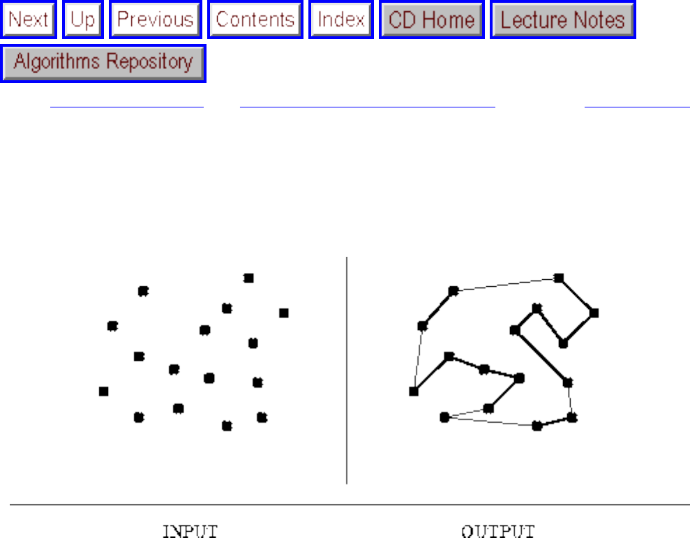
Traveling Salesman Problem
Next: Hamiltonian Cycle Up: Graph Problems: Hard Problems Previous: Vertex Cover
Traveling Salesman Problem
Input description: A weighted graph G.
Problem description: Find the cycle of minimum cost that visits each of the vertices of G exactly once.
Discussion: The traveling salesman problem is the most notorious NP-complete problem. This is a
function of its general usefulness, and because it is easy to explain to the public at large. Imagine a
traveling salesman who has to visit each of a given set of cities by car. What is the shortest route that will
enable him to do so and return home, thus minimizing his total driving?
Although the problem arises in transportation applications, its most important applications arise in
optimizing the tool paths for manufacturing equipment. For example, consider a robot arm assigned to
solder all the connections on a printed circuit board. The shortest tour that visits each solder point
exactly once defines the most efficient path for the robot. A similar application arises in minimizing the
amount of time taken by a graphics plotter to draw a given figure.
Several issues arise in solving TSPs:
● Is the graph unweighted? - If the graph is unweighted, or all the edges have one of two cost
file:///E|/BOOK/BOOK4/NODE175.HTM (1 of 5) [19/1/2003 1:31:21]
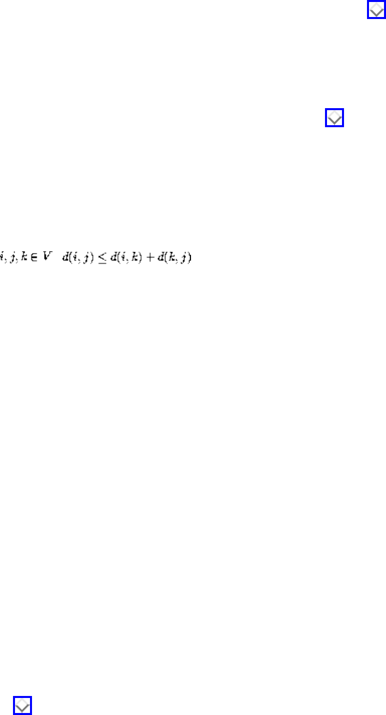
Traveling Salesman Problem
values, the problem reduces to finding a Hamiltonian cycle. See Section for a discussion of
this problem.
● Are you given as input n points or a weighted graph? - Geometric points are often easier to work
with than a graph representation, for several reasons. First, they define a complete graph, so
there is never an issue of finding a tour, just a good one. Second, although we always could
construct the complete distance graph on the points and feed it to a graph solver, it might be more
efficient to construct a sparse nearest-neighbor graph (see Section ) and work primarily from
that. Finally, geometric instances inherently satisfy the triangle inequality, discussed below.
● How important is the restriction against visiting each vertex more than once? - The restriction
that the tour not revisit any vertex may be important in certain applications, but it often is
irrelevant. For example, the cheapest way to visit all vertices might involve repeatedly visiting a
hub site, as is common in modern air travel.
This issue does not arise whenever the graph observes the triangle inequality; that is, for all
vertices , . In graphs that observe the triangle inequality, the
shortest tour visits each vertex once. Heuristics work much better on graphs that do obey the
triangle inequality.
● How important is that that you find the optimal tour? - If you insist on solving your TSP to
optimality (and you probably shouldn't bother), there are two common approaches. Cutting plane
methods model the problem as an integer program, then solve the linear programming relaxation
of it. If the optimal solution is not at integer points, additional constraints designed to force
integrality are added. Branch-and-bound algorithms perform a combinatorial search while
maintaining careful upper and lower bounds on the cost of a tour or partial tour. In the hands of
professionals, problems with thousands of vertices can be solved. In the hands of one gleaning
their knowledge from this book, problems with 50 to maybe 100 vertices are potentially solvable,
using the implementations discussed below.
Almost any flavor of TSP is going to be NP-complete, so the right way to proceed is with heuristics.
These are often quite successful, typically coming within a few percent of the optimal solution, which is
close enough for engineering work. Unfortunately, there have been literally dozens of heuristics
proposed for TSPs, so the situation can be confusing. Empirical results in the literature are sometime
contradictory. However, we recommend choosing from among the following heuristics:
● Minimum spanning trees - A simple and popular heuristic, especially when the sites represent
points in the plane, is based on the minimum spanning tree of the points. By doing a depth-first
search of this tree, we walk over each edge of the tree exactly twice, once going down when we
discover the new vertex and once going up when we backtrack. We can then define a tour of the
vertices according to the order in which they were discovered and use the shortest path between
each neighboring pair of vertices in this order to connect them. This path must be a single edge if
the graph is complete and obeys the triangle inequality, as with points in the plane. As discussed
in Section , the resulting tour is always at most twice the length of the minimum TSP tour. In
file:///E|/BOOK/BOOK4/NODE175.HTM (2 of 5) [19/1/2003 1:31:21]
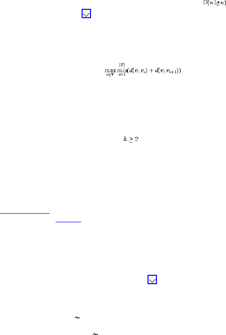
Traveling Salesman Problem
practice, it is usually better, typically 15% to 20% over optimal. Further, the time of the algorithm
is bounded by that of computing the minimum spanning tree, only in the case of points in
the plane (see Section ).
● Incremental insertion methods - A different class of heuristics inserts new points into a partial
tour one at a time (starting from a single vertex) until the tour is complete. The version of this
heuristic that seems to work best is furthest point insertion: of all remaining points, insert the
point v into partial tour T such that
The minimum ensures that we insert the vertex in the position that adds the smallest amount of
distance to the tour, while the maximum ensures that we pick the worst such vertex first. This
seems to work well because it first ``roughs out'' a partial tour before filling in details. Typically,
such tours are only 5% to 10% longer than optimal.
● k-optimal tours - Substantially more powerful are the Kernighan-Lin, or k-opt class of heuristics.
Starting from an arbitrary tour, the method applies local refinements to the tour in the hopes of
improving it. In particular, subsets of edges are deleted from the tour and the k remaining
subchains rewired in a different way to see if the resulting tour is an improvement. A tour is k-
optimal when no subset of k edges can be deleted and rewired so as to reduce the cost of the tour.
Extensive experiments suggest that 3-optimal tours are usually within a few percent of the cost of
optimal tours. For k > 3, the computation time increases considerably faster than solution quality.
Two-opting a tour is a fast and effective way to improve any other heuristic. Simulated
annealing provides an alternate mechanism to employ edge flips to improve heuristic tours.
Implementations: The world-record-setting traveling salesman program is by Applegate, Bixby,
Chvatal, and Cook [ABCC95], which has solved instances as large as 7,397 vertices to optimality. At
this time, the program is not being distributed. However, the authors seem willing to use it to solve TSPs
sent to them. In their paper, they describe this work as neither theory nor practice, but sport - an almost
recreational endeavor designed principally to break records. It is a very impressive piece of work,
however.
The TSPLIB library of test instances for the traveling salesman problem is available from Netlib, and by
anonymous ftp from softlib.cs.rice.edu. See Section .
Tsp_solve is a C++ code by Chad Hurwitz and Robert Craig that provides both heuristic and optimal
solutions. Geometric problems of size up to 100 points are manageable. It is available from
http://www.cs.sunysb.edu/ algorith or by e-mailing Chad Hurrwitz at churritz@crash.cts.com. A
heuristic Euclidean TSP solver in C due to Lionnel Maugis is available from
http://www.cenaath.cena.dgac.fr/ maugis/tsp.shar.
file:///E|/BOOK/BOOK4/NODE175.HTM (3 of 5) [19/1/2003 1:31:21]
Traveling Salesman Problem
Pascal implementations of branch-and-bound search and the insertion and Kerighan-Lin heuristics (for 2-
opt and 3-opt) appear in [SDK83]. For details, see Section .
Algorithm 608 [Wes83] of the Collected Algorithms of the ACM is a Fortran implementation of a
heuristic for the quadratic assignment problem, a more general problem that includes the traveling
salesman as a special case. Algorithm 750 [CDT95] is a Fortran code for the exact solution of
asymmetric TSP instances. See Section for details.
XTango (see Section ) includes animations of both the minimum spanning tree heuristic and a genetic
algorithm for TSP. The latter converges sufficiently slowly to kill one's interest in genetic algorithms.
Combinatorica [Ski90] provides (slow) Mathematica implementations of exact and approximate TSP
solutions. See Section .
Notes: The definitive reference on the traveling salesman problem is the book by Lawler et. al.
[LLKS85]. Experimental results on heuristic methods for solving large TSPs include [Ben92a, GBDS80,
Rei94]. Typically, it is possible to get within a few percent of optimal with such methods. TSPLIB
[Rei91] provides the standard collection of hard instances of TSPs that arise in practice.
The Christofides heuristic is an improvement of the minimum-spanning tree heuristic and guarantees a
tour whose cost is at most 3/2 times optimal on Euclidean graphs. It runs in , where the bottleneck
is the time it takes to find a minimum-weight perfect matching (see Section ). Good expositions of
the Christofides heuristic [Chr76] include [Man89, PS85]. Expositions of the minimum spanning tree
heuristic [RSL77] include [CLR90, O'R94, PS85].
Polynomial-time approximation schemes for Euclidean TSP have been recently developed by Arora
[Aro96] and Mitchell [Mit96], which offer factor approximations in polynomial time for any .
They are of great theoretical interest, although any practical consequences remain to be determined.
The history of progress on optimal TSP solutions is somewhat inspiring. In 1954, Dantzig, Fulkerson,
and Johnson solved a symmetric TSP instance of 42 United States cities [DFJ54]. In 1980, Padberg and
Hong solved an instance on 318 vertices [PH80]. Applegate et. al. [ABCC95] have recently solved
problems that are twenty times larger than this. Some of this increase is due to improved hardware, but
most is due to better algorithms. The rate of growth demonstrates that exact solutions to NP-complete
problems can be obtained for large instances if the stakes are high enough. Unfortunately, they seldom
are. Good expositions on branch-and-bound methods include [PS82, SDK83]. Good expositions of the
Kernighan-Lin heuristic [LK73, Lin65] include [MS91, PS82, SDK83].
file:///E|/BOOK/BOOK4/NODE175.HTM (4 of 5) [19/1/2003 1:31:21]
Traveling Salesman Problem
Size is not the only criterion for hardness. One can easily construct an enormous graph consisting of one
cheap cycle, for which it would be easy to find the optimal solution. For sets of points in convex position
in the plane, the minimum TSP tour is described by its convex hull (see Section ), which can be
computed in time. Other easy special cases are known.
Related Problems: Hamiltonian cycle (see page ), minimum spanning tree (see page ), convex
hull (see page ).
Next: Hamiltonian Cycle Up: Graph Problems: Hard Problems Previous: Vertex Cover
Algorithms
Mon Jun 2 23:33:50 EDT 1997
file:///E|/BOOK/BOOK4/NODE175.HTM (5 of 5) [19/1/2003 1:31:21]
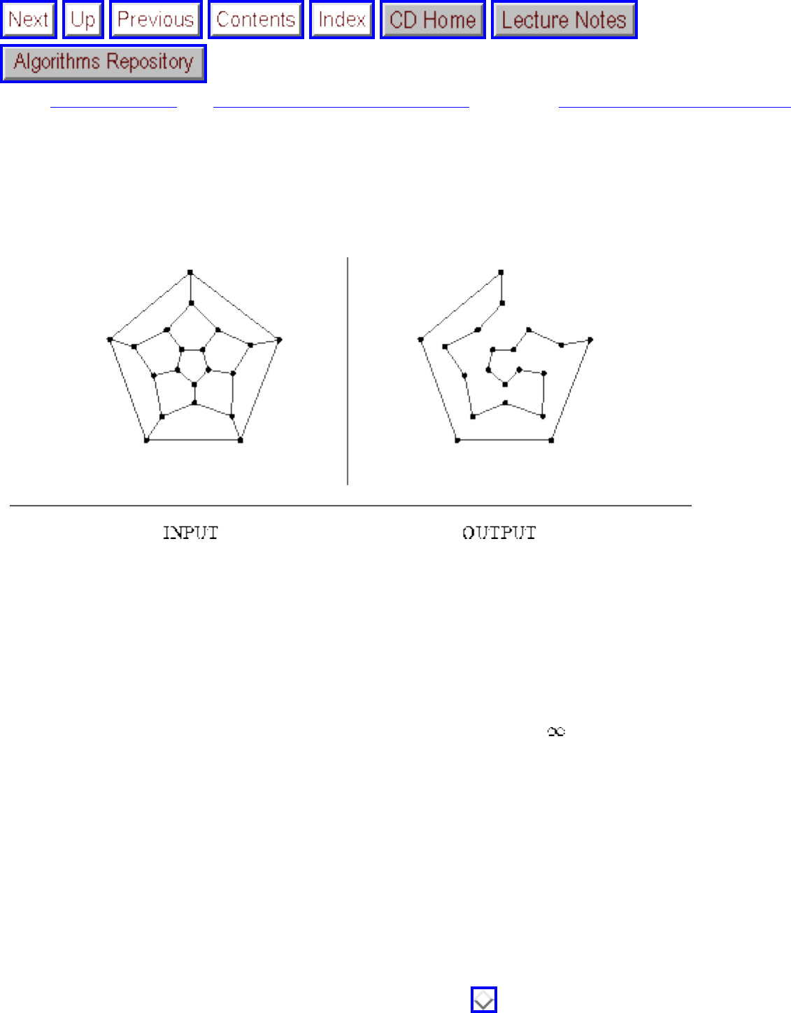
Hamiltonian Cycle
Next: Graph Partition Up: Graph Problems: Hard Problems Previous: Traveling Salesman Problem
Hamiltonian Cycle
Input description: A graph G = (V,E).
Problem description: Find an ordering of the vertices such that each vertex is visited exactly once.
Discussion: The problem of finding a Hamiltonian cycle or path in a graph is a special case of the
traveling salesman problem, one where each pair of vertices with an edge between them is considered to
have distance 1, while nonedge vertex pairs are separated by distance .
Closely related is the problem of finding the longest path or cycle in a graph, which occasionally arises in
pattern recognition problems. Let the vertices in the graph correspond to possible symbols, and let
edges link symbols that can possibly be next to each other. The longest path through this graph is likely
the correct interpretation.
The problems of finding longest cycles and paths are both NP-complete, even on very restrictive classes
of unweighted graphs. There are several possible lines of attack, however:
● Do you have to visit all the vertices or all the edges? - First verify that you really have a
Hamiltonian cycle problem. As discussed in Section , fast algorithms exist for edge-tour, or
file:///E|/BOOK/BOOK4/NODE176.HTM (1 of 3) [19/1/2003 1:31:23]
Hamiltonian Cycle
Eulerian cycle, problems, where you must visit all the edges without repetition. With a little
cleverness, it is sometimes possible to reformulate a Hamiltonian cycle problem in terms of
Eulerian cycles. Perhaps the most famous such instance is the problem of constructing de Bruijn
sequences, discussed in Section .
● Is there a serious penalty for visiting vertices more than once? - By phrasing the problem as
minimizing the total number of vertices visited on a complete tour, we have an optimization
problem that now allows room for heuristics and approximation algorithms. For example,
finding a spanning tree of the graph and doing a depth-first search, as discussed in Section ,
yields a tour with at most 2n vertices. Using randomization or simulated annealing might bring
the size of this down considerably.
● Am I seeking the longest path in a directed acyclic graph (DAG)? - The problem of finding the
longest path in a DAG can be solved in linear time using dynamic programming. This is about the
only interesting case of longest path for which efficient algorithms exist.
● Is my graph dense? - For sufficiently dense graphs, there always exists at least one Hamiltonian
cycle, and further, such a cycle can be found quickly. An efficient algorithm for finding a
Hamiltonian cycle in a graph where all vertices have degree is given in [Man89].
If you really must know whether your graph is Hamiltonian, backtracking with pruning is your only
possible solution. Before you search, it pays to check whether your graph is biconnected (see Section
). If not, this means that the graph has an articulation vertex whose deletion will disconnect the
graph and so cannot be Hamiltonian.
Implementations: The football program of the Stanford GraphBase (see Section ) uses a stratified
greedy algorithm to solve the asymmetric longest path problem. The goal is to derive a chain of football
scores in order to establish the superiority of one football team over another. After all, if Virginia beat
Illinois by 30 points, and Illinois beat Stony Brook by 14 points, then by transitivity Virginia would beat
Stony Brook by 44 points if they played, right? We seek the longest path in a graph where the weight of
an edge (x,y) is the number of points x beat y by.
Nijenhuis and Wilf [NW78] provide an efficient routine to enumerate all Hamiltonian cycles of a graph
by backtracking. See Section . Algorithm 595 [Mar83] of the Collected Algorithms of the ACM is a
similar Fortran code that can be used as either an exact procedure or a heuristic by controlling the amount
of backtracking. See Section .
XTango (see Section ) is an algorithm animation system for UNIX and X-windows, which includes
an animation of a backtracking solution to the knight's tour problem.
Combinatorica [Ski90] provides a Mathematica backtracking implementation of Hamiltonian cycle.
file:///E|/BOOK/BOOK4/NODE176.HTM (2 of 3) [19/1/2003 1:31:23]
Hamiltonian Cycle
See Section .
Notes: Hamiltonian cycles - circuits that visit each vertex of a graph exactly once - apparently first arose
in Euler's study of the knight's tour problem, although they were popularized by Hamilton's ``Around the
World'' game in 1839. Good expositions of the proof that Hamiltonian cycle is NP-complete [Kar72]
include [Baa88, CLR90, GJ79].
Techniques for solving optimization problems in the laboratory using biological processes have recently
attracted considerable attention. In the original application of these ``biocomputing'' techniques,
Adleman [Adl94b] solved a seven-vertex instance of the directed Hamiltonian path problem.
Unfortunately, this approach requires an exponential number of molecules, and Avogadro's number
implies that such experiments are inconceivable for graphs beyond .
Related Problems: Eulerian cycle (see page ), traveling salesman (see page ).
Next: Graph Partition Up: Graph Problems: Hard Problems Previous: Traveling Salesman Problem
Algorithms
Mon Jun 2 23:33:50 EDT 1997
file:///E|/BOOK/BOOK4/NODE176.HTM (3 of 3) [19/1/2003 1:31:23]
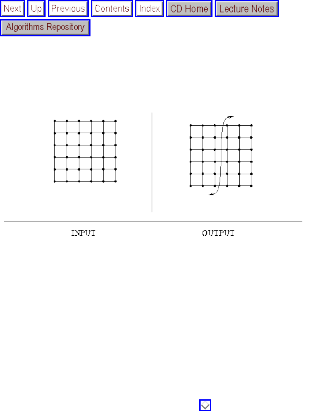
Graph Partition
Next: Vertex Coloring Up: Graph Problems: Hard Problems Previous: Hamiltonian Cycle
Graph Partition
Input description: A (weighted) graph G=(V,E) and integers j, k, and m.
Problem description: Partition the vertices into m subsets such that each subset has size at most j, while
the cost of the edges spanning the subsets is bounded by k.
Discussion: Graph partitioning arises as a preprocessing step to divide-and-conquer algorithms, where it
is often a good idea to break things into roughly equal-sized pieces. It also arises when dealing with
extremely large graphs, when we need to cluster the vertices into logical components for storage (to
improve virtual memory performance) or for drawing purposes (to collapse dense subgraphs into single
nodes in order to reduce cluttering).
Several different flavors of graph partitioning arise depending on the desired objective function:
● Minimum cut set - The smallest set of edges to cut that will disconnect a graph can be efficiently
found using network flow methods. See Section for more on connectivity algorithms. Since
the smallest cutset can split off only a single vertex, the resulting partition might be very
unbalanced. Hence ...
● Graph partition - A better partition criterion seeks a small cut that partitions the vertices into
file:///E|/BOOK/BOOK4/NODE177.HTM (1 of 3) [19/1/2003 1:31:24]
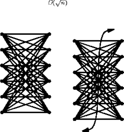
Graph Partition
roughly equal-sized pieces. Unfortunately, this problem is NP-complete. Fortunately, heuristics
discussed below work well in practice.
Certain special graphs always have small separators, which partition the vertices into balanced
pieces. For any tree, there always exists a single vertex whose deletion partitions the tree so that
no component contains more than n/2 of the original n vertices. These components need not
always be connected. For example, consider the separating vertex of a star-shaped tree. However,
the separating vertex can be found in linear time using depth first-search. Similarly, every planar
graph has a set of vertices whose deletion leaves no component with more than 2n/3
vertices. Such separators provide a particularly useful way to decompose planar graphs.
Figure: The maximum cut of a graph
● Maximum cut - Given an electronic circuit specified by a graph, the maximum cut defines the
largest amount of data communication that can simultaneously take place in the circuit. The
highest-speed communications channel should thus span the vertex partition defined by the
maximum edge cut. Finding the maximum cut in a graph is NP-complete, despite the existence of
algorithms for min-cut. However, heuristics similar to those of graph partitioning can work well.
The basic approach to dealing with graph partitioning or max-cut problems is to construct an initial
partition of the vertices (either randomly or according to some problem-specific strategy) and then sweep
through the vertices, deciding whether the size of the cut would increase or decrease if we moved this
vertex over to the other side. The decision to move v can be made in time proportional to its degree by
simply counting whether more of v's neighbors are on the same team as v or not. Of course, the desirable
side for v will change if many of its neighbors jump, so multiple passes are likely to be needed before the
process converges on a local optimum. Even such a local optimum can be arbitrarily far away from the
global max-cut.
There are many variations of this basic procedure, by changing the order we test the vertices in or
moving clusters of vertices simultaneously. Using some form of randomization, particularly simulated
file:///E|/BOOK/BOOK4/NODE177.HTM (2 of 3) [19/1/2003 1:31:24]
Graph Partition
annealing, is almost certain to be a good idea.
Implementations: Jon Berry's implementations of several graph partitioning heuristics, including
Kernighan-Lin, simulated annealing, and path optimization are available from
http://www.elon.edu/users/f/berryj/www/.
A non-network-flow-based implementation of minimum cut is included with LEDA (see Section ).
Notes: The fundamental heuristic for graph partitioning is due to Kernighan and Lin [KL70]. Empirical
results on graph partitioning heuristics include [BG95, LR93].
The planar separator theorem and an efficient algorithm for finding such a separator are due to Lipton
and Tarjan [LT79, LT80]. Although network flow can be used to find minimum cut sets in graphs, faster
algorithms are available, including [SW94] and [Kar96a].
Expositions on the hardness of max-cut [Kar72] include [Eve79a]. Note that any random vertex partition
will expect to cut half of the edges in the graph, since the probability that the two vertices defining an
edge end up on different sides of the partition is 1/2. Goemans and Williamson [GW95] gave an 0.878-
factor approximation algorithm for maximum-cut, based on semidefinite programming techniques.
Tighter analysis of this algorithm followed by Karloff [Kar96b].
Related Problems: Edge/vertex connectivity (see page ), network flow (see page ).
Next: Vertex Coloring Up: Graph Problems: Hard Problems Previous: Hamiltonian Cycle
Algorithms
Mon Jun 2 23:33:50 EDT 1997
file:///E|/BOOK/BOOK4/NODE177.HTM (3 of 3) [19/1/2003 1:31:24]
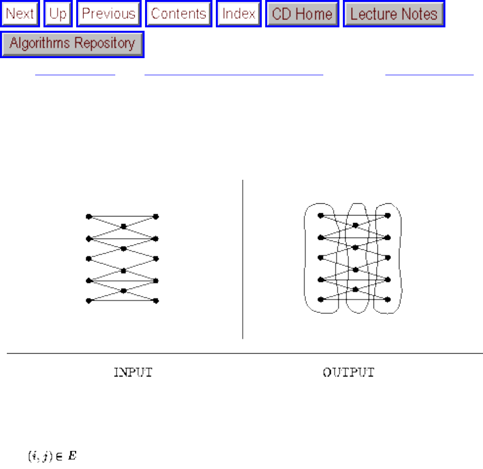
Vertex Coloring
Next: Edge Coloring Up: Graph Problems: Hard Problems Previous: Graph Partition
Vertex Coloring
Input description: A graph G=(V,E).
Problem description: Color the vertices of V using the minimum number of colors such that for each
edge , vertices i and j have different colors.
Discussion: Vertex coloring arises in a variety of scheduling and clustering applications. Compiler
optimization is the canonical application for coloring, where we seek to schedule the use of a finite
number of registers. In a program fragment to be optimized, each variable has a range of times during
which its value must be kept intact, in particular, after it is initialized and before its final use. Any two
variables whose life spans intersect cannot be placed in the same register. Construct a graph where there
is a variable associated with each vertex and add an edge between any two vertices whose variable life
spans intersect. A coloring of the vertices of this graph assigns the variables to classes such that two
variables with the same color do not clash and so can be assigned to the same register.
No conflicts can occur if each vertex is colored with a distinct color. However, our goal is to find a
coloring using the minimum number of colors, because computers have a limited number of registers.
The smallest number of colors sufficient to vertex color a graph is known as its chromatic number.
file:///E|/BOOK/BOOK4/NODE178.HTM (1 of 4) [19/1/2003 1:31:26]
Vertex Coloring
Several special cases of interest arise in practice:
● Can I color the graph using only two colors? - An important special case is testing whether a
graph is bipartite, meaning it can be colored using two different colors. Such a coloring of the
vertices of a bipartite graph means that the graph can be drawn with the red vertices on the left
and the blue vertices on the right such that all edges go from left to right. Bipartite graphs are
fairly simple, yet they arise naturally in such applications as mapping workers to possible jobs.
Fast, simple algorithms exist for problems such as matching (see Section ) on bipartite graphs.
Testing whether a graph is bipartite is easy. Color the first vertex blue, and then do a depth-first
search of the graph. Whenever we discover a new, uncolored vertex, color it opposite that of its
parent, since the same color would cause a clash. If we ever find an edge where both vertices have
been colored identically, then the graph cannot be bipartite. Otherwise, this coloring will be a 2-
coloring, and it is constructed in O(n+m) time.
● Is the graph planar, or are all vertices of low degree? - The famous 4-color theorem states that
every planar graph can be vertex colored using at most 4 distinct colors. Efficient algorithms for
finding a 4-coloring are known, although it is NP-complete to decide whether a given planar
graph is 3-colorable.
There is a very simple algorithm that finds a vertex coloring of any planar graph using at most 6
colors. In any planar graph, there exists a vertex of degree at most five. Delete this vertex and
recursively color the graph. This vertex has at most five neighbors, which means that it can
always be colored using one of the six colors that does not appear as a neighbor. This works
because deleting a vertex from a planar graph leaves a planar graph, so we always must have a
low-degree vertex to delete. The same idea can be used to color any graph of maximum degree
using colors in time.
● Is this an edge coloring problem? - Certain vertex coloring problems can be modeled as edge
coloring, where we seek to color the edges of a graph G such that no two edges with a vertex in
common are colored the same. The payoff is that there is an efficient algorithm that always
returns a near-optimal edge coloring. Algorithms for edge coloring are the focus of Section .
Computing the chromatic number of a graph is NP-complete, so if you need an exact solution you must
resort to backtracking, which can be surprisingly effective in coloring certain random graphs. It remains
hard to compute a provably good approximation to the optimal coloring, so expect no guarantees.
Incremental methods appear to be the heuristic of choice for vertex coloring. As in the previous
algorithm for planar graphs, vertices are colored sequentially, with the colors chosen in response to
colors already assigned in the vertex's neighborhood. These methods vary in how the next vertex is
selected and how it is assigned a color. Experience suggests inserting the vertices in nonincreasing order
of degree, since high-degree vertices have more color constraints and so are most likely to require an
file:///E|/BOOK/BOOK4/NODE178.HTM (2 of 4) [19/1/2003 1:31:26]
Vertex Coloring
additional color if inserted late.
Incremental methods can be further improved by using color interchange. Observe that taking a
properly colored graph and exchanging two of the colors (painting the red vertices blue and the blue
vertices red) leaves a proper vertex coloring. Now suppose we take a properly colored graph and delete
all but the red and blue vertices. If the remaining graph (the induced subgraph) consists of two or more
connected components, we can repaint one or more of the components, again leaving a proper coloring.
After such a recoloring, some vertex v previously adjacent to both red and blue vertices might now be
only adjacent to blue vertices, thus freeing v to be colored red.
Color interchange is a win in terms of producing better colorings, at a cost of increased time and
implementation complexity. Implementations are described below. Simulated annealing algorithms that
incorporate color interchange to move from state to state are likely to be even more effective.
Implementations: Graph coloring has been blessed with two distinct and useful WWW resources.
Michael Trick's page, http://mat.gsia.cmu.edu/COLOR/color.html, provides a nice overview of
applications of graph coloring, an annotated bibliography, and a collection of over seventy graph
coloring instances arising in applications such as register allocation and printed circuit board testing.
Finally, it contains a C language implementation of an exact coloring algorithm, DSATUR. Joseph C.
Culberson's WWW page on graph coloring, http://web.cs.ualberta.ca/ joe/Coloring/, provides an
extensive bibliography and a collection of programs to generate hard graph coloring instances.
Programs for the closely related problems of finding cliques and vertex coloring graphs were sought for
the Second DIMACS Implementation Challenge, held in October 1993. Programs and data from the
challenge are available by anonymous ftp from dimacs.rutgers.edu. Source codes are available under
pub/challenge/graph and test data under pub/djs, including a simple ``semi-exhaustive greedy'' scheme
used in the graph coloring algorithm XRLF [JAMS91].
Pascal implementations of backtracking algorithms for vertex coloring and several heuristics, including
largest-first and smallest-last incremental orderings and color interchange, appear in [SDK83]. See
Section .
XTango (see Section ) is an algorithm animation system for UNIX and X-windows, and includes an
animation of vertex coloring via backtracking.
Nijenhuis and Wilf [NW78] provide an efficient Fortran implementation of chromatic polynomials and
vertex coloring by backtracking. See Section .
Combinatorica [Ski90] provides Mathematica implementations of bipartite graph testing, heuristic
colorings, chromatic polynomials, and vertex coloring by backtracking. See Section .
file:///E|/BOOK/BOOK4/NODE178.HTM (3 of 4) [19/1/2003 1:31:26]
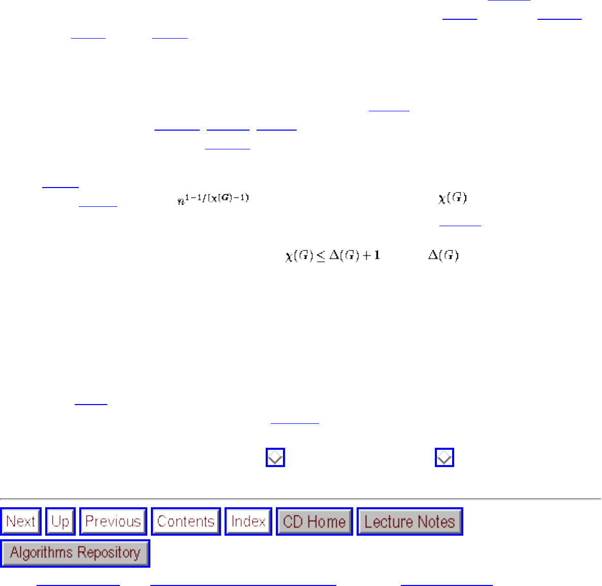
Vertex Coloring
Notes: An excellent source on vertex coloring heuristics is Syslo, Deo, and Kowalik [SDK83], which
includes experimental results. Heuristics for vertex coloring include Brèlaz [Brè79], Matula [MMI72],
and Turner [Tur88]. Wilf [Wil84] proved that backtracking to test whether a random graph has chromatic
number k runs in constant time, dependent on k but independent of n. This is not as interesting as it
sounds, because only a vanishingly small fraction of such graphs are indeed k-colorable.
Expositions on algorithms to recognize bipartite graphs include [Man89]. Expositions on the hardness of
3-coloring graphs include [AHU74, Eve79a, Man89]. An interesting application of vertex coloring to
scheduling traffic lights appears in [AHU83].
Baase [Baa88] gives a very good description of approximation algorithms for graph coloring, including
Wigderson's [Wig83] factor of approximation algorithm, where is the chromatic
number of G. Hardness of approximation results for vertex coloring include [BGS95].
Brook's theorem states that the chromatic number , where is the maximum degree
of a vertex of G. Equality holds only for odd-length cycles (which have chromatic number 2) and
complete graphs.
The most famous problem in the history of graph theory is the four-color problem, first posed in 1852
and finally settled in 1976 by Appel and Haken using a proof involving extensive computation. Any
planar graph can be 5-colored using a variation of the color interchange heuristic. Despite the four-color
theorem, it is NP-complete to test whether a particular planar graph requires four colors or whether three
suffice. See [SK86] for an exposition on the history of the four-color problem and the proof. An efficient
algorithm to four-color a graph is presented in [RSST96].
Related Problems: Independent set (see page ), edge coloring (see page ).
Next: Edge Coloring Up: Graph Problems: Hard Problems Previous: Graph Partition
Algorithms
Mon Jun 2 23:33:50 EDT 1997
file:///E|/BOOK/BOOK4/NODE178.HTM (4 of 4) [19/1/2003 1:31:26]
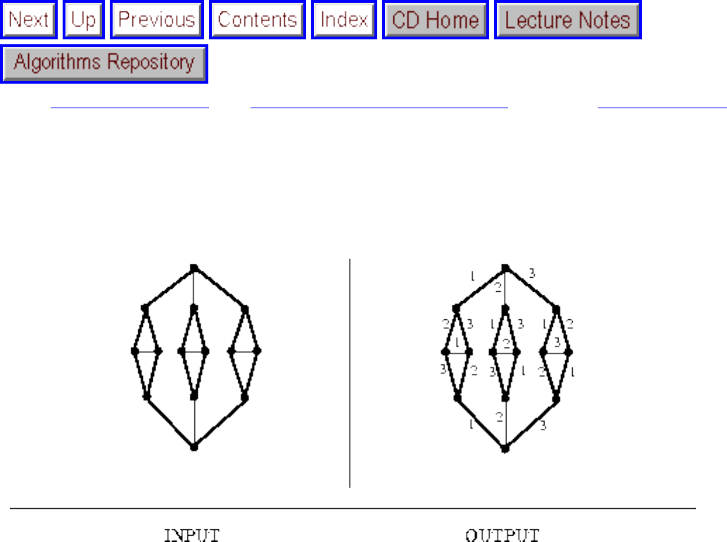
Edge Coloring
Next: Graph Isomorphism Up: Graph Problems: Hard Problems Previous: Vertex Coloring
Edge Coloring
Input description: A graph G=(V,E).
Problem description: What is the smallest set of colors needed to color the edges of E such that no two
same-color edges share a vertex in common?
Discussion: The edge coloring of graphs arises in a variety of scheduling applications, typically
associated with minimizing the number of noninterfering rounds needed to complete a given set of tasks.
For example, consider a situation where we need to schedule a given set of two-person interviews,
where each interview takes one hour. All meetings could be scheduled to occur at distinct times to avoid
conflicts, but it is less wasteful to schedule nonconflicting events simultaneously. We can construct a
graph whose vertices are the people and whose edges represent the pairs of people who want to meet. An
edge coloring of this graph defines the schedule. The color classes represent the different time periods in
the schedule, with all meetings of the same color happening simultaneously.
The National Football League solves such an edge coloring problem each season to make up its schedule.
Each team's opponents are determined by the records of the previous season. Assigning the opponents
to weeks of the season is the edge-coloring problem, presumably complicated by the constraints of
spacing out rematches and making sure that there is a good game every Monday night.
file:///E|/BOOK/BOOK4/NODE179.HTM (1 of 3) [19/1/2003 1:31:27]
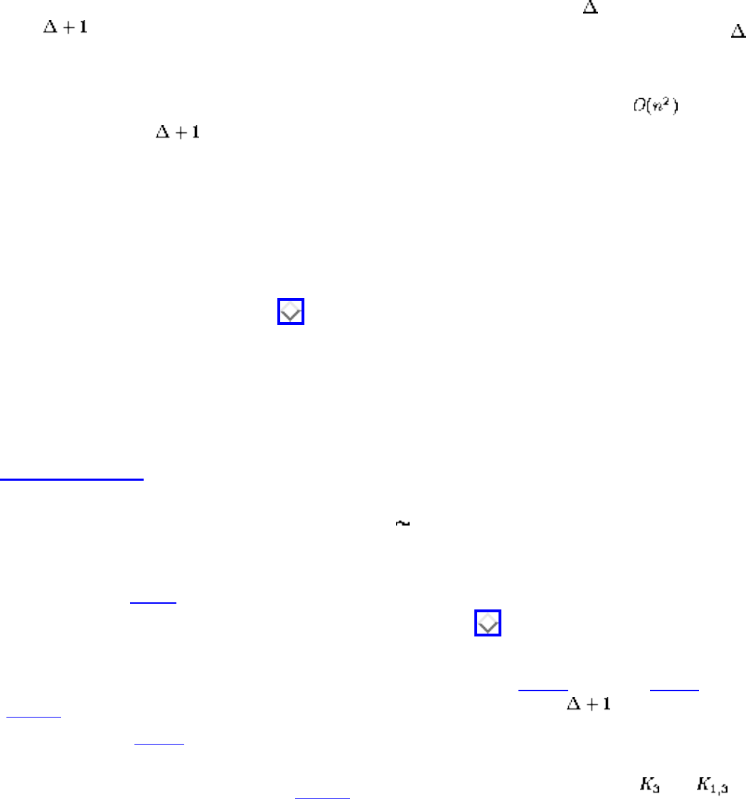
Edge Coloring
The minimum number of colors needed to edge color a graph is called by some its edge-chromatic
number and others its chromatic index. To gain insight into edge coloring, note that a graph consisting
of an even-length cycle can be edge-colored with 2 colors, while odd-length cycles have an edge-
chromatic number of 3.
Edge coloring has a better (if less famous) theorem associated with it than does vertex coloring.
Vizing's theorem states that any graph with a maximum vertex degree of can be edge colored using at
most colors. To put this in perspective, note that any edge coloring must have at least colors,
since each of the edges incident on any vertex must be distinct colors.
Further, the proof of Vizing's theorem is constructive and can be turned into an algorithm to find an
edge-coloring with colors, which gives us an edge coloring using at most one extra color. Since it
is NP-complete to decide whether we can save this one color, it hardly seems worth the effort to worry
about it. An implementation of Vizing's theorem is described below.
Any edge coloring problem on G can be converted to the problem of finding a vertex coloring on the
line graph L(G), which has a vertex of L(G) for each edge of G and an edge of L(G) if and only if the two
edges of G share a common vertex. Line graphs can be constructed in time linear to their size, and any
vertex coloring code from Section can be employed to color them.
Although any edge coloring problem can be so formulated as a vertex coloring problem, this is usually a
bad idea, since the edge coloring problem is easier to solve. Vizing's theorem is our reward for the extra
thought needed to see that we have an edge coloring problem.
Implementations: Yan Dong produced an implementation of Vizing's theorem in C++ as a course
project for my algorithms course while a student at Stony Brook. It can be found on the algorithm
repository WWW site http://www.cs.sunysb.edu/ algorith, as can an alternative program by Mark
Goldberg and Amir Sehic.
Combinatorica [Ski90] provides Mathematica implementations of edge coloring, via the line graph
transformation and vertex coloring routines. See Section for further information on Combinatorica.
Notes: Graph-theoretic results on edge coloring are surveyed in [FW77]. Vizing [Viz64] and Gupta
[Gup66] both proved that any graph can be edge colored using at most colors. Despite these tight
bounds, Holyer [Hol81] proved that computing the edge-chromatic number is NP-complete.
Whitney, in introducing line graphs [Whi32], showed that with the exception of and , any two
connected graphs with isomorphic line graphs are isomorphic. It is an interesting exercise to show that
the line graph of an Eulerian graph is both Eulerian and Hamiltonian, while the line graph of a
Hamiltonian graph is always Hamiltonian.
file:///E|/BOOK/BOOK4/NODE179.HTM (2 of 3) [19/1/2003 1:31:27]

Graph Isomorphism
Next: Steiner Tree Up: Graph Problems: Hard Problems Previous: Edge Coloring
Graph Isomorphism
Input description: Two graphs, G and H.
Problem description: Find a (or all) mappings f of the vertices of G to the vertices of H such that G and
H are identical; i.e. (x,y) is an edge of G iff (f(x),f(y)) is an edge of H.
Discussion: Isomorphism is the problem of testing whether two graphs are really the same. Suppose we
are given a collection of graphs and must perform some operation on each of them. If we can identify
which of the graphs are duplicates, they can be discarded so as to avoid redundant work.
We need some terminology to settle what is meant when we say two graphs are the same. Two labeled
graphs and are identical when iff . The isomorphism
problem consists of finding a mapping from the vertices of G to H such that they are identical. Such a
mapping is called an isomorphism.
Identifying symmetries is another important application of graph isomorphism. A mapping of a graph to
itself is called an automorphism, and the collection of automorphisms (its automorphism group)
provides a great deal of information about symmetries in the graph. For example, the complete graph
has n! automorphisms (any mapping will do), while an arbitrary random graph is likely to have few or
file:///E|/BOOK/BOOK4/NODE180.HTM (1 of 4) [19/1/2003 1:31:29]
Graph Isomorphism
perhaps only one, since G is always identical to itself.
Several variations of graph isomorphism arise in practice:
● Is graph G contained in (not identical to) graph H? - Instead of testing equality, we are often
interested in knowing whether a small pattern graph G is a subgraph of H. Such problems as
clique, independent set, and Hamiltonian cycle are important special cases of subgraph
isomorphism.
There are two distinct notions of ``contained in'' with respect to graphs. Subgraph isomorphism
asks whether there is a subset of edges and vertices of G that is isomorphic to a smaller graph H.
Induced subgraph isomorphism asks whether there is a subset of vertices of G whose deletion
leaves a subgraph isomorphic to a smaller graph H. For induced subgraph isomorphism, all edges
of G must be present in H, but also all nonedges of G must be nonedges of H. Clique happens to
be an instance of both subgraph problems, while Hamiltonian cycle is an example of vanilla
subgraph isomorphism.
Be aware of this distinction in your application. Subgraph isomorphism problems tend to be
harder than graph isomorphism, and induced subgraph problems tend to be even harder than
subgraph isomorphism. Backtracking is your only viable approach.
● Are your graphs labeled or unlabeled? - In many applications, vertices or edges of the graphs are
labeled with some attribute that must be respected in determining isomorphisms. For example,
in comparing two bipartite graphs, each with ``worker'' vertices and ``job'' vertices, any
isomorphism that equated a job with a worker would make no sense.
Labels and related constraints can be factored into any backtracking algorithm. Further, such
constraints can be used to significantly speed up the search by creating more opportunities for
pruning whenever two vertex labels do not match up.
● Are you testing whether two trees are isomorphic? - There are faster algorithms for certain
special cases of graph isomorphism, such as trees and planar graphs. Perhaps the most important
case is detecting isomorphisms among trees, a problem that arises in language pattern matching
and parsing applications. A parse tree is often used to describe the structure of a text; two parse
trees will be isomorphic if the underlying pair of texts have the same structure.
Efficient algorithms for tree isomorphism begin with the leaves of both trees and work inward
towards the center. Each vertex in one tree is assigned a label representing the set of vertices in
the second tree that might possibly be isomorphic to it, based on the constraints of labels and
vertex degrees. For example, all the leaves in tree are initially potentially equivalent to all
leaves of . Now, working inward, we can partition the vertices adjacent to leaves in into
classes based on how many leaves and nonleaves they are adjacent to. By carefully keeping track
of the labels of the subtrees, we can make sure that we have the same distribution of labeled
subtrees for and . Any mismatch means , while completing the process partitions the
file:///E|/BOOK/BOOK4/NODE180.HTM (2 of 4) [19/1/2003 1:31:29]
Graph Isomorphism
vertices into equivalence classes defining all isomorphisms. See the references below for more
details.
No polynomial-time algorithm is known for graph isomorphism, but neither is it known to be NP-
complete. Along with integer factorization (see Section ), it one of the few important algorithmic
problems whose rough computational complexity is still not known. The conventional wisdom is that
isomorphism is a problem that lies between P and NP-complete if P NP.
Although no worst-case polynomial-time algorithm is known, testing isomorphism in practice is usually
not very hard. The basic algorithm backtracks through all n! possible relabelings of the vertices of graph
h with the names of vertices of graph g, and then tests whether the graphs are identical. Of course, we
can prune the search of all permutations with a given prefix as soon as we detect any mismatch between
edges both of whose vertices are in the prefix.
However, the real key to efficient isomorphism testing is to preprocess the vertices into ``equivalence
classes'', partitioning them into sets of vertices such that two vertices in different sets cannot possibly be
mistaken for each other. All vertices in each equivalence class must share the same value of some
invariant that is independent of labeling. Possibilities include:
● Vertex degree - This simplest way to partition vertices is based on their degree, the number of
edges incident on the vertex. Clearly, two vertices of different degree cannot be identical. This
simple partition can often be a big win, but it won't do much for regular graphs, where each vertex
has the same degree.
● Shortest path matrix - For each vertex v, the all-pairs shortest path matrix (see Section )
defines a multiset of n-1 distances (possibly with repeats) representing the distances between v
and each of the other vertices. Any two vertices that are identical in isomorphic graphs will define
the exact same multiset of distances, so we can partition the vertices into equivalence classes
defining identical distance multisets.
● Counting length-k paths - Taking the adjacency matrix of G and raising it to the kth power gives
a matrix where counts the number of (nonsimple) paths from i to j. For each vertex and
each k, this matrix defines a multiset of path-counts, which can be used for partitioning as with
distances above. You could try all or beyond, and use any single deviation as an excuse
to partition.
Using these invariants, you should be able to partition the vertices of each graph into a large number of
small equivalence classes. Finishing the job off with backtracking, using the name of each equivalence
class as a label, should usually be quick work. If the sizes of the equivalence classes of both graphs are
not identical, then the graphs cannot be isomorphic. It is harder to detect isomorphisms between graphs
with high degrees of symmetry than it is for arbitrary graphs, because of the effectiveness of these
equivalence-class partitioning heuristics.
file:///E|/BOOK/BOOK4/NODE180.HTM (3 of 4) [19/1/2003 1:31:29]
Graph Isomorphism
Implementations: The world's fastest isomorphism testing program is Nauty, by Brendan D. McKay.
Nauty (No AUTomorphisms, Yes?) is a set of very efficient C language procedures for determining the
automorphism group of a vertex-colored graph. Nauty is also able to produce a canonically labeled
isomorph of the graph, to assist in isomorphism testing. It was the basis of the first program to generate
all the 11-vertex graphs without isomorphs, and can test most graphs of fewer than one hundred vertices
in well under a second. Nauty has been successfully ported to a variety of operating systems and C
compilers. It may be obtained from http://cs.anu.edu.au/people/bdm/. It is free for educational and
research applications, but for commercial use contact the author at bdm@cs.anu.edu.au.
Combinatorica [Ski90] provides (slow) Mathematica implementations of graph isomorphism and
automorphism testing. See Section for further information on Combinatorica.
Notes: Graph isomorphism is an important problem in complexity theory. Monographs on isomorphism
detection include Hoffmann [Hof82].
Polynomial-time algorithms are known for planar graph isomorphism [HW74] and for graphs where the
maximum vertex degree is bounded by a constant [Luk80]. The all-pairs shortest path heuristic is due to
[SD76], although there exist nonisomorphic graphs that realize the same set of distances [BH90]. A
linear-time tree isomorphism algorithm for both labeled and unlabeled trees is presented in [AHU74].
A problem is said to be isomorphism-complete if it is provably as hard as isomorphism. Testing the
isomorphism of bipartite graphs is isomorphism-complete, since any graph can be made bipartite by
replacing each edge by two edges connected with a new vertex. Clearly, the original graphs are
isomorphic if and only if the transformed graphs are.
Related Problems: Shortest path (see page ), string matching (see page ).
Next: Steiner Tree Up: Graph Problems: Hard Problems Previous: Edge Coloring
Algorithms
Mon Jun 2 23:33:50 EDT 1997
file:///E|/BOOK/BOOK4/NODE180.HTM (4 of 4) [19/1/2003 1:31:29]
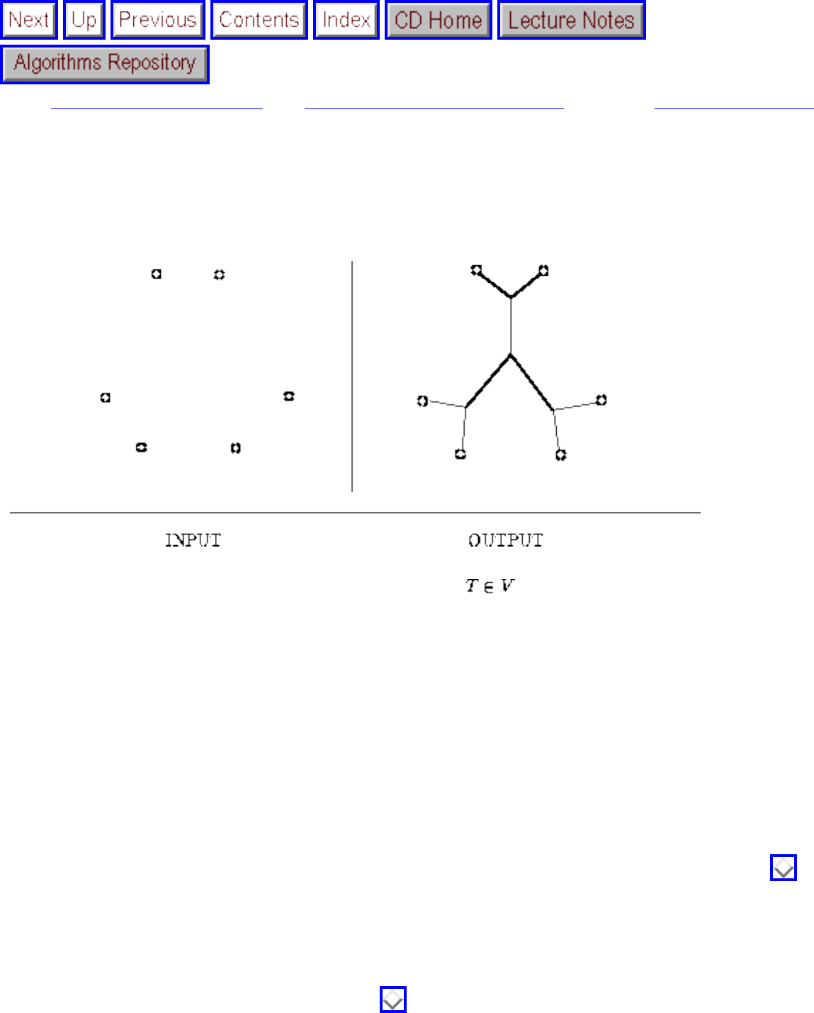
Steiner Tree
Next: Feedback Edge/Vertex Set Up: Graph Problems: Hard Problems Previous: Graph Isomorphism
Steiner Tree
Input description: A graph G=(V,E). A subset of vertices .
Problem description: Find the smallest tree connecting all the vertices of T.
Discussion: Steiner tree often arises in network design and wiring layout problems. Suppose we are
given a set of sites that must be connected by wires as cheaply as possible. The minimum Steiner tree
describes the way to connect them using the smallest amount of wire. Analogous problems arise in
designing networks of water pipes or heating ducts in buildings. Similar considerations also arise in
VLSI circuit layout, where we seek to connect a set of sites to (say) ground under constraints such as
material cost, signal propagation time, or reducing capacitance.
The Steiner tree problem is distinguished from the minimum spanning tree problem (see Section ) in
that we are permitted to construct or select intermediate connection points to reduce the cost of the tree.
Issues in Steiner tree construction include:
● How many points do you have to connect? - The Steiner tree of a pair of vertices is simply the
shortest path between them (see Section ). The Steiner tree of all the vertices, when S=V,
file:///E|/BOOK/BOOK4/NODE181.HTM (1 of 4) [19/1/2003 1:31:31]
Steiner Tree
simply defines the minimum spanning tree of G. Despite these special cases, the general
minimum Steiner tree problem is NP-hard and remains so under a broad range of restrictions.
● Is the input a set of geometric points or a distance graph? - Geometric versions of Steiner tree
take as input a set of points, typically in the plane, and seek the smallest tree connecting the
points. A complication is that the set of possible intermediate points is not given as part of the
input but must be deduced from the set of points. These possible Steiner points must satisfy
several geometric properties, which can be used to reduce the set of candidates down to a finite
number. For example, every Steiner point will have degree exactly three in a minimum Steiner
tree, and the angles formed between any two of these edges will be exactly 120 degrees.
● Are there constraints on the edges we can use? - Many wiring problems correspond to geometric
versions of the problem where all edges are restricted to being either horizontal or vertical, which
is the so-called rectilinear Steiner problem. A different set of angular and degree conditions
applies for rectilinear Steiner trees than for Euclidean trees. In particular, all angles must be
multiples of 90 degrees, and each vertex is of degree up to four.
● Do I really need an optimal tree? - In certain applications, such as minimum cost communications
networks, construction costs are high enough to invest large amounts of computation in finding
the best possible Steiner tree. This implies an exhaustive search technique such as backtracking
or branch-and-bound. There are many opportunities for pruning search based on geometric
constraints. For graph instances, network reduction procedures can reduce the problem to a graph
typically one-quarter the size of the input graph.
Still, Steiner tree remains a hard problem. Through exhaustive search methods, instances as large
as 32 points for the Euclidean and 30 for the rectilinear problems can be confidently solved to
optimality. We recommend experimenting with the implementations described below before
attempting your own.
● How can I reconstruct Steiner vertices I never knew about? - A very special type of Steiner tree
arises in classification and evolution. A phylogenic tree illustrates the relative similarity between
different objects or species. Each object represents (typically) a terminal vertex of the tree, with
intermediate vertices representing branching points between classes of objects. For example, an
evolutionary tree of animal species might have leaf nodes including (human, dog, snake) and
internal nodes corresponding to the taxa (animal, mammal, reptile). A tree rooted at animal with
dog and human classified under mammal implies that humans are closer to dogs than to snakes.
Many different phylogenic tree construction algorithms have been developed, which vary in the
data they attempt to model and what the desired optimization criterion is. Because they all give
different answers, identifying the correct algorithm for a given application is somewhat a matter
of faith. A reasonable procedure is to acquire a standard package of implementations, discussed
below, and then see what happens to your data under all of them.
Fortunately, there is a good, efficient heuristic for finding Steiner trees that works well on all versions of
the problem. Construct a graph modeling your input, with the weight of edge (i,j) equal to the distance
from point i to point j. Find a minimum spanning tree of this graph. You are guaranteed a provably good
approximation for both Euclidean and rectilinear Steiner trees.
file:///E|/BOOK/BOOK4/NODE181.HTM (2 of 4) [19/1/2003 1:31:31]
Steiner Tree
The worst case for a minimum spanning tree approximation of the Euclidean distance problem is three
points forming an equilateral triangle. The minimum spanning tree will contain two of the sides (for a
length of 2), whereas the minimum Steiner tree will connect the three points using an interior point, for a
total length of . This ratio of is always achieved, and in practice the easily-computed
minimum spanning tree is usually within a few percent of the optimal Steiner tree. For rectilinear Steiner
trees, the ratio with rectilinear minimum spanning trees is always .
Such a minimum spanning tree can be refined by inserting a Steiner point whenever the edges of the
minimum spanning tree incident on a vertex form an angle of less than 120 degrees between them.
Inserting these points and locally readjusting the tree edges can move the solution a few more percent
towards the optimum. Similar optimizations are possible for rectilinear spanning trees.
An alternative heuristic for graphs is based on shortest path. Start with a tree consisting of the shortest
path between two terminals. For each remaining terminal t, find the shortest path to a vertex v in the tree
and add this path to the tree. The time complexity and quality of this heuristic depend upon the insertion
order of the terminals and how the shortest-path computations are performed, but something simple and
fairly effective is likely to result.
Implementations: Salowe and Warme [SW95] have developed a program for computing exact
rectilinear Steiner minimal trees. It is available by anonymous ftp from ftp.cs.virginia.edu in the directory
pub/french/salowe/newsteiner.tar.Z. It should be capable of handling up to 30 points routinely. A
heuristic program by Robins and Zhang is available from the algorithm repository
http://www.cs.sunysb.edu/ algorith.
PHYLIP is an extensive and widely used package of programs for inferring phylogenic trees. It contains
over twenty different algorithms for constructing phylogenic trees from data. Although many of them are
designed to work with molecular sequence data, several general methods accept arbitrary distance
matrices as input. With versions written in C and Pascal, it is available on the WWW from
http://evolution.genetics.washington.edu/phylip.html.
Notes: The most complete reference on the Steiner tree problem is the monograph by Hwang, Richards,
and Winter [HRW92]. Surveys on the problem include [Kuh75]. Steiner tree problems arising in VLSI
design are discussed in [KPS89, Len90]. Empirical results on Steiner tree heuristics include [SFG82,
Vos92].
The Euclidean Steiner problem dates back to Fermat, who asked how to find a point p in the plane
minimizing the sum of the distances to three given points. This was solved by Torricelli before 1640.
Steiner was apparently one of several mathematicians who worked the general problem for n points, and
he was mistakenly credited with the problem. An interesting, more detailed history appears in [HRW92].
file:///E|/BOOK/BOOK4/NODE181.HTM (3 of 4) [19/1/2003 1:31:31]
Steiner Tree
Gilbert and Pollak [GP68] first conjectured that the ratio of the length of the minimum Steiner tree over
the minimum spanning tree is always . After twenty years of active research, the Gilbert-
Pollak ratio was finally proven by Du and Hwang [DH92]. The Euclidean minimum spanning tree for n
points in the plane can be constructed in time [PS85].
Expositions on the proof that the Steiner tree problem for graphs is hard [Kar72] include [Eve79a].
Expositions on exact algorithms for Steiner trees in graphs include [Law76]. The hardness of Steiner tree
for Euclidean and rectilinear metrics was established in [GGJ77, GJ77]. Euclidean Steiner tree is not
known to be in NP, because of numerical issues in representing distances.
Analogies can be drawn between minimum Steiner trees and minimum energy configurations in certain
physical systems. The case that such analog systems, including the behavior of soap films over wire
frames, ``solve'' the Steiner tree problem is discussed in [Mie58].
Related Problems: Minimum spanning tree (see page ), shortest path (see page ).
Next: Feedback Edge/Vertex Set Up: Graph Problems: Hard Problems Previous: Graph Isomorphism
Algorithms
Mon Jun 2 23:33:50 EDT 1997
file:///E|/BOOK/BOOK4/NODE181.HTM (4 of 4) [19/1/2003 1:31:31]
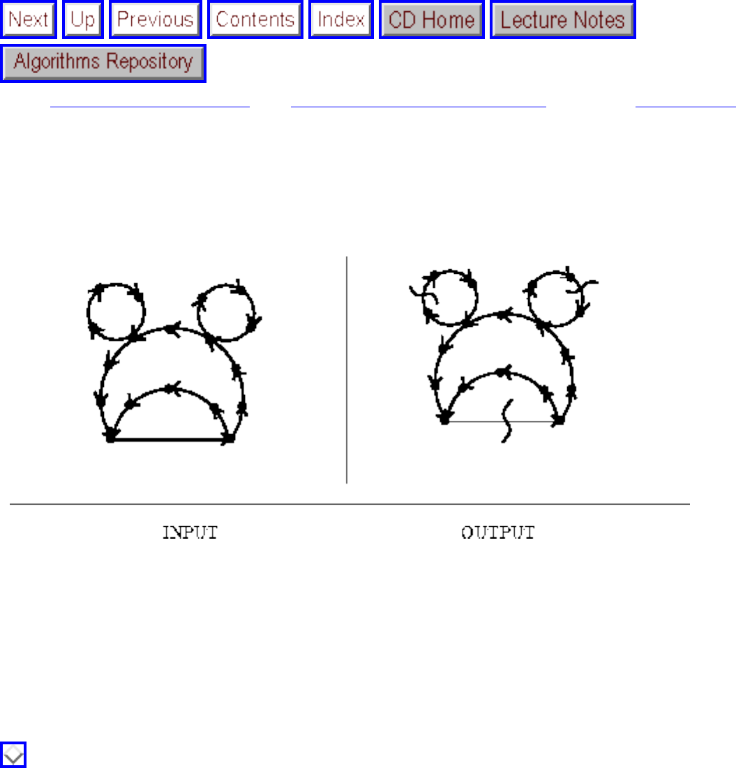
Feedback Edge/Vertex Set
Next: Computational Geometry Up: Graph Problems: Hard Problems Previous: Steiner Tree
Feedback Edge/Vertex Set
Input description: A (directed) graph G=(V,E).
Problem description: What is the smallest set of edges E' or vertices V' whose deletion leaves an acyclic
graph?
Discussion: Feedback set problems arise because many algorithmic problems are much easier or much
better defined on directed acyclic graphs than on arbitrary digraphs. Topological sorting (see Section
) can be used to test whether a graph is a DAG, and if so, to order the vertices so as to respect the
edges as precedence scheduling constraints. But how can you design a schedule if there are cyclic
constraints, such as A must be done before B, which must be done before C, which must be done before
A?
By identifying a feedback set, we identify the smallest number of constraints that must be dropped so as
to permit a valid schedule. In the feedback edge (or arc) set problem, we drop precedence constraints
(job A must come before job B). In the feedback vertex set problem, we drop entire jobs and any
associated constraints. It is also referred to in the literature as the maximum acyclic subgraph problem.
● Do any constraints have to be dropped? - Not if the graph is a DAG, which can be tested via
file:///E|/BOOK/BOOK4/NODE182.HTM (1 of 3) [19/1/2003 1:31:32]
Feedback Edge/Vertex Set
topological sort in linear time, Further, topological sorting also gives a simple way to find a
feedback set if we modify the algorithm to delete the edge or vertex whenever a contradiction is
found instead of simply printing a warning. The catch is that this feedback set might be much
larger than needed, no surprise since both feedback edge set and feedback vertex set are NP-
complete on directed graphs.
● How can I find a good feedback edge set? - A simple but effective linear-time heuristic constructs
a vertex ordering, just as in the topological sort heuristic above, and deletes any arc going from
right to left. This heuristic builds up the ordering from the outside in based on the in- and out-
degrees of each vertex. Any vertex of in-degree 0 is a source and can be placed first in the
ordering. Any vertex of out-degree 0 is a sink and can be placed last in the ordering, again without
violating any constraints. If not, we find the vertex with the maximum difference between in- and
out-degree, and place it on the side of the permutation that will salvage the greatest number of
constraints. Delete any vertex from the DAG after positioning it and repeat until the graph is
empty.
● How can I find a good feedback vertex set? - The following variant of the above heuristic should
be effective. Keep any source or sink we encounter. If none exist, add to the feedback set a vertex
v that maximizes , since this vertex is furthest from becoming either a source or sink.
Again, delete any vertex from the DAG after positioning it and repeat until the graph is empty.
● What if I want to break all cycles in an undirected graph? - The problem of finding feedback sets
from undirected graphs is different for digraphs, and in one case actually easier. An undirected
graph without cycles is a tree. It is well known that any tree on n vertices has exactly n-1 edges.
Thus the smallest feedback edge set of any undirected graph is |E| - (n-1), and it can be found by
deleting all the edges not in any given spanning tree. Spanning trees can be most efficiently
constructed using depth-first search, as discussed in Section . The feedback vertex set problem
remains NP-complete for undirected graphs, however.
Finding an optimal feedback set is NP-complete, and for most applications it is unlikely to be worth
searching for the smallest set. However, in certain applications it would pay to try to refine the heuristic
solutions above via randomization or simulated annealing. To move between states, we modify the
vertex permutation by swapping pairs in order or inserting/deleting vertices into the feedback set.
Implementations: The econ_order program of the Stanford GraphBase (see Section ) permutes the
rows and columns of a matrix so as to minimize the sum of the numbers below the main diagonal.
Using an adjacency matrix as the input and deleting all edges below the main diagonal leaves an acyclic
graph.
Notes: The feedback set problem first arose in [Sla61]. Heuristics for feedback set problems include
[BYGNR94, ELS93, Fuj96]. Expositions of the proofs that feedback minimization is hard [Kar72]
include [AHU74, Eve79a]. Both feedback vertex and edge set remain hard even if no vertex has in-
degree or out-degree greater than two [GJ79].
file:///E|/BOOK/BOOK4/NODE182.HTM (2 of 3) [19/1/2003 1:31:32]
Feedback Edge/Vertex Set
An interesting application of feedback arc set to economics is presented in [Knu94]. For each pair A,B of
sectors of the economy, we are given how much money flows from A to B. We seek to order the sectors
to determine which sectors are primarily producers to other sectors, and which deliver primarily to
consumers.
Related Problems: Bandwidth reduction (see page ), topological sorting (see page ), scheduling
(see page ).
Next: Computational Geometry Up: Graph Problems: Hard Problems Previous: Steiner Tree
Algorithms
Mon Jun 2 23:33:50 EDT 1997
file:///E|/BOOK/BOOK4/NODE182.HTM (3 of 3) [19/1/2003 1:31:32]

Computational Geometry
Next: Robust Geometric Primitives Up: A Catalog of Algorithmic Previous: Feedback Edge/Vertex Set
Computational Geometry
Computational geometry is the algorithmic study of geometric problems and objects. Compared to the
other topics in this book, computational geometry emerged as a field quite recently, with Shamos's Ph.D.
thesis [Sha78] typically cited as its founding event. Its emergence coincided with the explosion of
computer graphics and windowing systems, which directly or indirectly provide much of the motivation
for geometric computing. The past twenty years have seen enormous growth in computational geometry,
resulting in a significant body of useful algorithms, software, textbooks, and research results.
Good books on computational geometry include:
● Preparata and Shamos [PS85] - Although aging a bit, this book remains the best general
introduction to computational geometry, stressing algorithms for convex hulls, Voronoi diagrams,
and intersection detection.
● O'Rourke [O'R94] - Perhaps the best practical introduction to computational geometry. The
emphasis is on careful and correct implementation (in C language) of the fundamental algorithms
of computational geometry. These implementations are available from
http://grendel.csc.smith.edu/ orourke/.
● Edelsbrunner [Ede87] - This is the definitive book on arrangements, a topic that runs through
most of computational geometry. Although not appropriate for beginners, it provides an important
perspective for advanced geometers.
● Mulmuley [Mul94] - An approach to computational geometry through randomized incremental
algorithms. Very interesting, but likely too narrow to serve as a general introduction.
● Nievergelt and Hindrichs [NH93] - This idiosyncratic algorithms text focuses on problems in
graphics and geometry. Good coverage of line drawing, intersection algorithms, and spatial data
structures, but with too many topics touched on too lightly to serve as an effective reference.
The leading conference in computational geometry is the ACM Symposium on Computational Geometry,
held annually in late May or early June. Although the primary results presented at the conference are
theoretical, there has been a concerted effort on the part of the research community to increase the
presence of applied, experimental work through video reviews and poster sessions. The other major
annual conference is the Canadian Conference on Computational Geometry (CCCG), typically held in
early August. Useful literature surveys include [Yao90].
A unique source of computational geometry information is geom.bib, a community effort to maintain a
file:///E|/BOOK/BOOK4/NODE183.HTM (1 of 3) [19/1/2003 1:31:33]

Computational Geometry
complete bibliography on computational geometry. It references over eight thousand books, papers, and
reports and includes detailed abstracts for many of them. Grep-ing through the geom.bib is an amazingly
efficient way to find out about previous work without leaving your office. It is available via anonymous
ftp from ftp.cs.usask.ca, in the file pub/geometry/geombib.tar.Z.
There is a growing body of implementations of geometric algorithms. We point out specific
implementations where applicable in the catalog, but the reader should be aware of three specific WWW
sites:
● The Geometry Center's directory of computational geometry software, maintained by Nina
Amenta, is the ``official'' site for all computational geometry software. Check here first to see
what is available: http://www.geom.umn.edu/software/cglist/.
● Graphics Gems is a series of books dedicated to collecting small codes of interest in computer
graphics. Many of these programs are geometric in nature. All associated codes are available from
ftp://ftp-graphics.stanford.edu/pub/Graphics/GraphicsGems.
● CGAL (Computational Geometry Algorithms Library) is a joint European project now underway
to produce a comprehensive library of geometric algorithms. This will likely become the
definitive geometric software project. Check out its progress at http://www.cs.ruu.nl/CGAL/.
● Robust Geometric Primitives
● Convex Hull
● Triangulation
● Voronoi Diagrams
● Nearest Neighbor Search
● Range Search
● Point Location
● Intersection Detection
● Bin Packing
● Medial-Axis Transformation
● Polygon Partitioning
● Simplifying Polygons
● Shape Similarity
● Motion Planning
● Maintaining Line Arrangements
● Minkowski Sum
file:///E|/BOOK/BOOK4/NODE183.HTM (2 of 3) [19/1/2003 1:31:33]


Robust Geometric Primitives
Next: Convex Hull Up: Computational Geometry Previous: Computational Geometry
Robust Geometric Primitives
Input description: A point p and a line segment l, or two line segments and .
Problem description: Does p lie over, under, or on l? Does intersect ?
Discussion: Implementing basic geometric primitives is a task fraught with peril, even for such simple
tasks as returning the intersection point of two lines. What should you return if the two lines are
parallel, meaning they don't intersect at all? What if the lines are identical, so the intersection is not a
point but the entire line? What if one of the lines is horizontal, so that in the course of solving the
equations for the intersection point you are likely to divide by zero? What if the two lines are almost
parallel, so that the intersection point is so far from the origin as to cause arithmetic overflows? These
issues become even more complicated for intersecting line segments, since there are a bunch of other
special cases that must be watched for and treated specially.
If you are new to implementing geometric algorithms, I suggest that you study O'Rourke's
Computational Geometry in C [O'R94] for practical advice and complete implementations of basic
geometric algorithms and data structures. You are likely to avoid many headaches by following in his
footsteps.
file:///E|/BOOK/BOOK4/NODE184.HTM (1 of 5) [19/1/2003 1:31:35]
Robust Geometric Primitives
There are two different issues at work here: geometric degeneracy and numerical stability. Degeneracy
refers to annoying special cases that must be treated in substantially different ways, such as when two
lines intersect in more or less than a single point. There are three primary approaches to dealing with
degeneracy:
● Ignore it - Make as an operating assumption that your program will work correctly only if no
three points are collinear, no three lines meet at a point, no intersections happen at the endpoints
of line segments, etc. This is probably the most common approach, and what I would recommend
for short-term projects if you can live with frequent crashes. The drawback is that interesting data
often comes from points sampled on a grid and is inherently very degenerate.
● Fake it - Randomly or symbolically perturb your data so that it seems nondegenerate. By moving
each of your points a small amount in a random direction, you can break many of the existing
degeneracies in the data, hopefully without creating too many new problems. This probably
should be the first thing to try as soon as you decide that your program is crashing too often. One
problem with random perturbations is that they do change the shape of your data in subtle ways,
which may be intolerable for your application. There also exist techniques to ``symbolically''
perturb your data to remove degeneracies in a consistent manner, but these require serious study
to apply correctly.
● Deal with it - Geometric applications can be made more robust by writing special code to handle
each of the special cases that arise. This can work well if done with care at the beginning, but not
so well if kludges are added whenever the system crashes. Expect to expend a lot of effort if you
are determined to do it right.
Geometric computations often involve floating-point arithmetic, which leads to problems with overflows
and numerical precision. There are three basic approaches to the issue of numerical stability:
● Integer arithmetic - By forcing all points of interest to lie on a fixed-size integer grid, you can
perform exact comparisons to test whether any two points are equal or two line segments
intersect. The cost is that the intersection point of two lines may not be exactly representable. This
is likely to be the simplest and best method, if you can get away with it.
● Double precision reals - By using double-precision floating point numbers, you may get lucky
and avoid numerical errors. Your best bet might be to keep all the data as single-precision reals,
and use double-precision for intermediate computations.
● Arbitrary precision arithmetic - This is certain to be correct, but also to be slow. This approach
seems to be gaining favor in the research community with the observation that careful analysis
can minimize the need for high-precision arithmetic, and thus the performance penalty. Still, you
should expect high-precision arithmetic to be several orders of magnitude slower than standard
floating-point arithmetic.
The difficulties associated with producing robust geometric software are still under attack by researchers.
The best practical technique is to base your applications on a small set of geometric primitives that
handle as much of the low-level geometry as possible. These primitives include:
file:///E|/BOOK/BOOK4/NODE184.HTM (2 of 5) [19/1/2003 1:31:35]
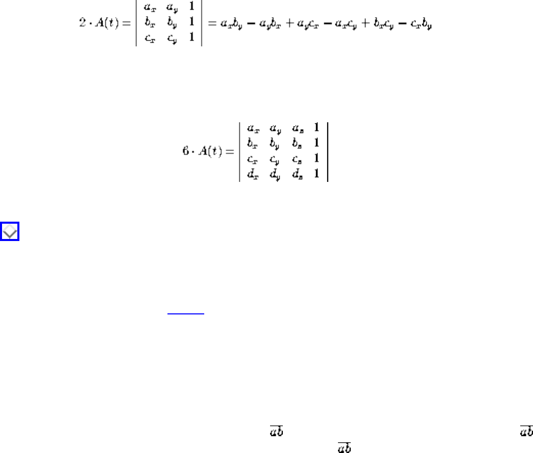
Robust Geometric Primitives
● Area of a triangle - Although it is well-known that the area A(t) of a triangle t=(a,b,c) is half the
base times the height, computing the length of the base and altitude is messy work with
trigonometric functions. It is better to use the determinant formula for twice the area:
This formula generalizes to compute d! times the volume of a simplex in d dimensions. Thus 3! =
6 times the volume of a tetrahedron t=(a,b,c,d) in three dimensions is
Note that these are signed volumes and can be negative, so take the absolute value first. Section
explains how to compute determinants.
The conceptually simplest way to compute the area of a polygon (or polyhedron) is to triangulate
it and then sum up the area of each triangle. An implementation of a slicker algorithm that avoids
triangulation is discussed in [O'R94].
● Above-below-on test - Does a given point c lie above, below, or on a given line l? A clean way to
deal with this is to represent l as a directed line that passes through point a before point b, and ask
whether c lies to the left or right of the directed line l. It is up to you to decide whether left means
above or below.
This primitive can be implemented using the sign of the area of a triangle as computed above. If
the area of t(a,b,c) > 0, then c lies to the left of . If the area of t(a,b,c) = 0, then c lies on .
Finally, if the area of t(a,b,c) < 0, then c lies to the right of . This generalizes naturally to three
dimensions, where the sign of the area denotes whether d lies above or below the oriented plane
(a,b,c).
● Line segment intersection - The above-below primitive can be used to test whether a line
intersects a line segment. It does iff one endpoint of the segment is to the left of the line and the
other is to the right. Segment intersection is similar but more complicated, and we refer you to
implementations described below. The decision whether two segments intersect if they share an
endpoint depends upon your application and is representative of the problems of degeneracy.
● In-circle test - Does the point d lie inside or outside the circle defined by points a, b, and c in the
plane? This primitive occurs in all Delaunay triangulation algorithms and can be used as a robust
way to do distance comparisons. Assuming that a, b, c are labeled in counterclockwise order
around the circle, compute the determinant:
file:///E|/BOOK/BOOK4/NODE184.HTM (3 of 5) [19/1/2003 1:31:35]
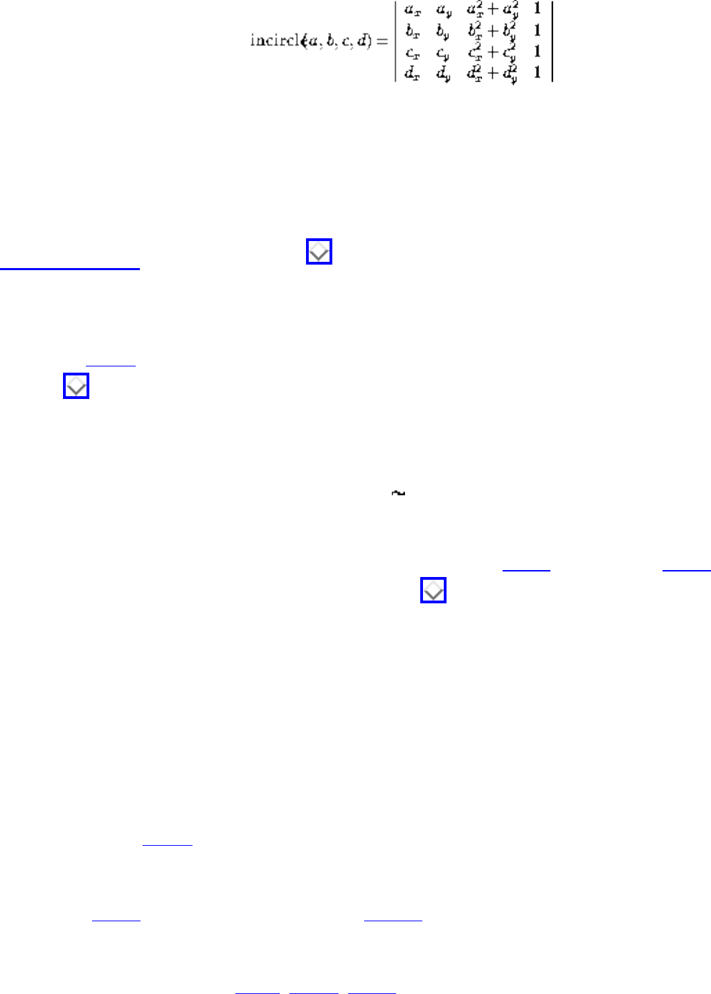
Robust Geometric Primitives
Incircle will return 0 if all four points are cocircular, a positive value if d is inside the circle, and
negative if d is outside.
Check out the implementations described below before you attempt to build your own.
Implementations: LEDA (see Section ) provides a very complete set of geometric primitives for
planar geometry, written in C++. If you are writing a significant geometric application, you should
consider basing it on LEDA. At least check them out before you try to write your own.
O'Rourke [O'R94] provides implementations in C of most of the primitives discussed in this section. See
Section . These primitives were implemented primarily for exposition rather than production use, but
they should be quite reliable and might be more appropriate than LEDA for small applications.
A robust implementation of the basic geometric primitives in C++ using exact arithmetic, by Jonathan
Shewchuk, is available at http://www.cs.cmu.edu/ quake/robust.html. Don't expect them to be very
fast.
Pascal implementations of basic geometric primitives appear in [MS91]. Sedgewick [Sed92] provides
fragments of the basic primitives in C++. See Section for both of them.
An alternative C++ library of geometric algorithms and data structures (although you are almost certainly
better off sticking to LEDA) is Geolab, written by Pedro J. de Rezende, Welson R. Jacometti, Cesar N.
Gon, and Laerte F. Morgado, Universidade Estadual de Campinas, Brazil. Geolab requires the SUN C++
compiler, but a Sparc binary and visualization environment is included along with all source code.
Geolab appears to be primarily for the brave, since its robustness is uncertain and it contains little
documentation, but it does provide 40 algorithms, including such advanced topics as farthest point
Voronoi diagrams, nearest neighbor search, and ray shooting.
Notes: O'Rourke [O'R94] provides an implementation-oriented introduction to computational geometry,
which stresses robust geometric primitives and is recommended reading.
Shewchuk [She96] and Fortune and van Wyk [FvW93] present careful studies on the costs of using
arbitrary-precision arithmetic for geometric computation. By being careful about when to use it,
reasonable efficiency can be maintained while achieving complete robustness. Other approaches to
achieving robustness include [DS88, Hof89, Mil89].
file:///E|/BOOK/BOOK4/NODE184.HTM (4 of 5) [19/1/2003 1:31:35]

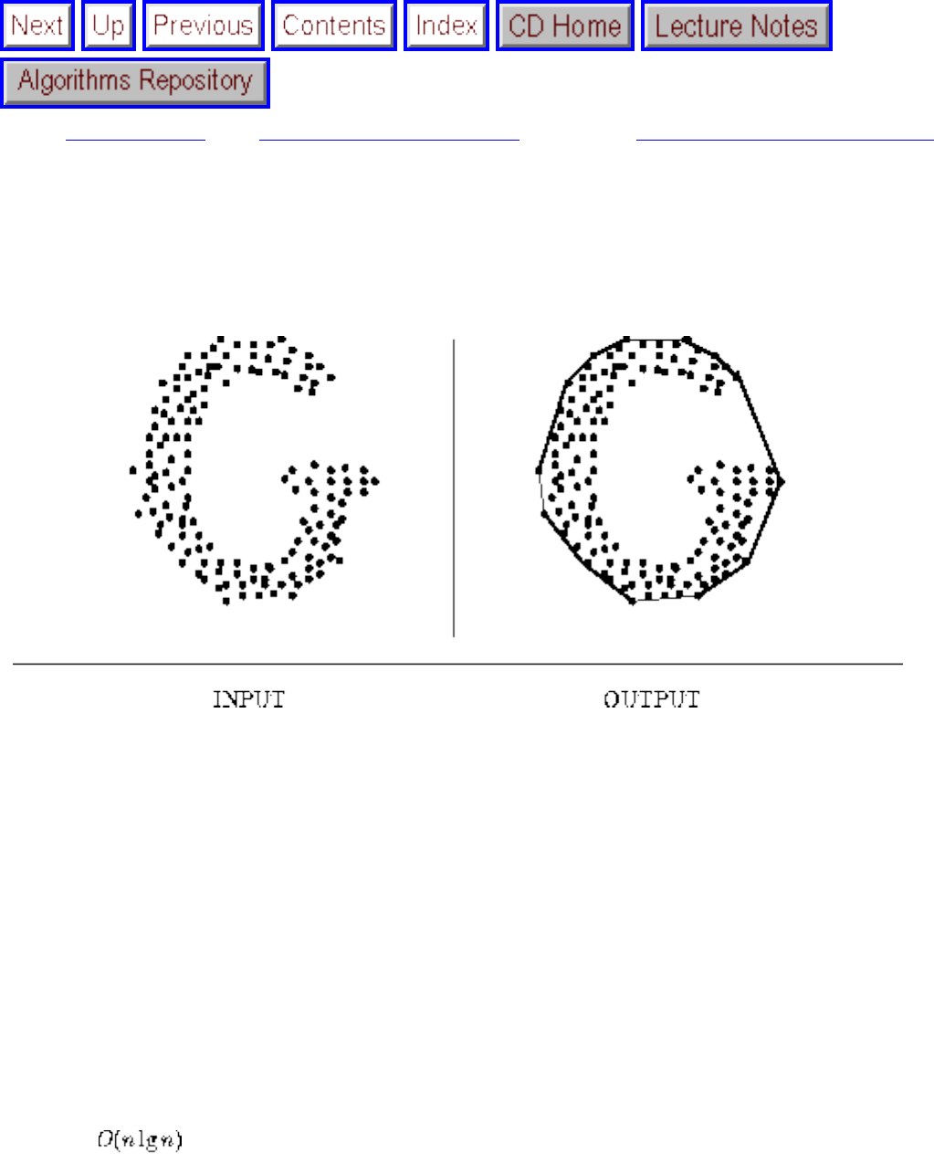
Convex Hull
Next: Triangulation Up: Computational Geometry Previous: Robust Geometric Primitives
Convex Hull
Input description: A set S of n points in d-dimensional space.
Problem description: Find the smallest convex polygon containing all the points of S.
Discussion: Finding the convex hull of a set of points is the most elementary interesting problem in
computational geometry, just as minimum spanning tree is the most elementary interesting problem in
graph algorithms. It arises because the hull quickly captures a rough idea of the shape or extent of a data
set.
Convex hull also serves as a first preprocessing step to many, if not most, geometric algorithms. For
example, consider the problem of finding the diameter of a set of points, which is the pair of points a
maximum distance apart. The diameter will always be the distance between two points on the convex
hull. The algorithm for computing diameter proceeds by first constructing the convex hull, then
for each hull vertex finding which other hull vertex is farthest away from it. This so-called ``rotating-
calipers'' method can be used to move efficiently from one hull vertex to another.
There are almost as many convex hull algorithms as there are sorting algorithms. Answer the following
questions to help choose between them:
file:///E|/BOOK/BOOK4/NODE185.HTM (1 of 5) [19/1/2003 1:31:37]
Convex Hull
● How many dimensions are you working with? - Convex hulls in two and even three dimensions
are fairly easy to work with. However, as the dimension of a space increases, certain assumptions
that were valid in lower dimensions break down. For example, any n-vertex polygon in two
dimensions has exactly n edges. However, the relationship between the numbers of faces and
vertices is more complicated even in three dimensions. A cube has 8 vertices and 6 faces, while an
octahedron has 8 faces and 6 vertices. This has implications for data structures that represent hulls
- are you just looking for the hull points or do you need the defining polyhedron? The need to find
convex hulls in high-dimensional spaces arises in many applications, so be aware of such
complications if your problem takes you there.
Gift-wrapping is the basic algorithm for constructing higher-dimensional convex hulls. Observe
that a three-dimensional convex polyhedron is composed of two-dimensional faces, or facets,
which are connected by one-dimensional lines, or edges. Each edge joins exactly two facets
together. Gift-wrapping starts by finding an initial facet associated with the lowest vertex and then
conducting a breadth-first search from this facet to discover new, additional facets. Each edge e
defining the boundary of a facet must be shared with one other facet, so by running through each
of the n points we can identify which point defines the next facet with e. Essentially, we ``wrap''
the points one facet at a time by bending the wrapping paper around an edge until it hits the first
point.
The key to efficiency is making sure that each edge is explored only once. Implemented properly
in d dimensions, gift-wrapping takes , where is the number of facets
and is the number of edges in the convex hull. Thus gift-wrapping can be very efficient when
there is only a constant number of facets on the hull. However, this can be as bad as
when the convex hull is very complex.
Better convex hull algorithms are available for the important special case of three dimensions,
where time in fact suffices. For three or higher dimensions, I recommend that you use
one of the codes described below rather than roll your own.
● Is your data given as vertices or half-spaces? - The problem of finding the intersection of a set of
n half-spaces in d dimensions is dual to that of computing convex hulls of n points in d
dimensions. Thus the same basic algorithm suffices for both problems. The necessary duality
transformation is discussed in Section .
● How many points are likely to be on the hull? - If your points are selected ``randomly'', it is likely
that most of them lie within the interior of the hull. Planar convex hull programs can be made
more efficient in practice using the observation than the leftmost, rightmost, topmost, and
bottommost points must all be on the convex hull. Unless the topmost is leftmost and bottommost
is rightmost, this gives a set of either three or four distinct points, defining a triangle or
quadrilateral. Any point inside this region cannot be on the convex hull and can be discarded in a
linear sweep through the points. Ideally, only a few points will then remain to run through the full
convex hull algorithm.
file:///E|/BOOK/BOOK4/NODE185.HTM (2 of 5) [19/1/2003 1:31:37]
Convex Hull
This trick can also be applied beyond two dimensions, although it loses effectiveness as the
dimension increases.
● How do I find the shape of my point set? - Although convex hulls provide a gross measure of
shape, any details associated with concavities are lost. For example, the shape of the `G' would be
indistinguishable from the shape of the `O'. A more general structure, called alpha-shapes, can be
parameterized so as to retain arbitrarily large concavities. Implementations and references on
alpha-shapes are included below.
The primary convex hull algorithm in the plane is the Graham scan. Graham scan starts with one point p
known to be on the convex hull (say the point with lowest x-coordinate) and sorts the rest of the points in
angular order around p. Starting with a hull consisting of p and the point with the smallest angle, we
proceed counterclockwise around v adding points. If the angle formed by the new point and the last hull
edge is less than 180 degrees, we add this new point to the hull. If the angle formed by the new point and
the last ``hull'' edge is greater than 180 degrees, then a chain of vertices starting from the last hull edge
must be deleted to maintain convexity. The total time is , since the bottleneck is sorting the
points around v.
The basic Graham scan procedure can also be used to construct a nonself-intersecting (or simple)
polygon passing through all the points. Sort the points around v, but instead of testing angles simply
connect the points in angular order. Connecting this to v gives a polygon without self-intersection,
although it typically has many skinny protrusions.
The gift-wrapping algorithm becomes especially simple in two dimensions, since each ``facet'' becomes
an edge, each ``edge'' becomes a vertex of the polygon, and the ``breadth-first search'' simply walks
around the hull in a clockwise or counterclockwise order. The 2D gift-wrapping, or Jarvis march,
algorithm runs in O(n h) time, where h is the number of vertices on the convex hull. I would recommend
sticking with Graham scan unless you really know in advance that there cannot be too many vertices on
the hull.
Implementations: O'Rourke [O'R94] provides a robust implementation of the Graham scan in two
dimensions and an implementation of an incremental algorithm for convex hulls in three
dimensions. Both are written in C. The latter has been proven capable of solving 10,000-point problems
in a few minutes on a modern workstation. See Section .
Qhull [BDH97] appears to be the convex hull code of choice for general dimensions (in particular from 2
to about 8 dimensions). It is written in C and can also construct Delaunay triangulations, Voronoi
vertices, furthest-site Voronoi vertices, and half-space intersections. Qhull has been widely used in
scientific applications and has a well-maintained home page at
http://www.geom.umn.edu/software/qhull/.
An alternative higher-dimensional convex hull code in ANSI C is Ken Clarkson's Hull, available at
file:///E|/BOOK/BOOK4/NODE185.HTM (3 of 5) [19/1/2003 1:31:37]
Convex Hull
http://www.cs.att.com/netlib/voronoi/hull.html. It does not appear to be as widely used or actively
maintained as Qhull, but it also does alpha-shapes. For an excellent alpha-shapes code, originating from
the work of Edelsbrunner and Mucke [EM94], check out http://fiaker.ncsa.uiuc.edu/alpha/.
Fukuda's cdd program is the best choice for nonsimplicial polytopes in about 6D and higher. See
ftp://ifor13.ethz.ch/pub/fukuda/cdd/. It may be used for computing convex hulls and half-space
intersection.
XTango (see Section ) provides animations of the Graham scan and Jarvis march algorithms in the
plane.
A Pascal implementation of Graham scan appears in [MS91]. See Section . C++ implementations of
planar convex hulls includes LEDA (see Section ). Algorithm 523 [Edd77] of the Collected
Algorithms of the ACM is a Fortran code for planar convex hulls. It is available from Netlib (see Section
).
Notes: Constructing planar convex hulls plays a similar role in computational geometry as sorting does
in algorithm theory. Like sorting, convex hull is a fundamental problem for which a wide variety of
different algorithmic approaches lead to interesting or optimal algorithms. Preparata and Shamos [PS85]
give a good exposition of several such algorithms, including quickhull and mergehull, both inspired by
the sorting algorithms. In fact, a simple construction involving points on a parabola reduces sorting to
convex hull, so the information-theoretic lower bound for sorting implies that planar convex hull requires
time to compute. A stronger lower bound is established in [Yao81].
Good expositions of the Graham scan algorithm [Gra72] and the Jarvis march [Jar73] include [CLR90,
PS85]. The gift wrapping algorithm was introduced by Chand and Kapur [CK70]. Noteworthy among
planar convex hull algorithms is Seidel and Kirkpatrick [KS86], which takes time, where h is the
number of hull vertices, which captures the best performance of both Graham scan and gift wrapping and
is (theoretically) better in between.
Alpha-hulls, introduced in [EKS83], provide a useful notion of the shape of a point set. A generalization
to three dimensions, with an implementation, is presented in [EM94].
Reverse-search algorithms for constructing convex hulls are effective in higher dimensions [AF92],
although constructions demonstrating the poor performance of convex hull algorithms for nonsimplicial
polytopes are presented in [AB95]. Through a clever lifting-map construction [ES86], the problem of
building Voronoi diagrams in d-dimensions can be reduced to constructing convex hulls in (d+1)-
dimensions. See Section for more details.
file:///E|/BOOK/BOOK4/NODE185.HTM (4 of 5) [19/1/2003 1:31:37]
Convex Hull
Dynamic algorithms for convex-hull maintenance are data structures that permit inserting and deleting
arbitrary points while always representing the current convex hull. The first such dynamic data structure
[OvL81] supported insertions and deletions in time. Expositions of this result include [PS85].
Related Problems: Sorting (see page ), Voronoi diagrams (see page ).
Next: Triangulation Up: Computational Geometry Previous: Robust Geometric Primitives
Algorithms
Mon Jun 2 23:33:50 EDT 1997
file:///E|/BOOK/BOOK4/NODE185.HTM (5 of 5) [19/1/2003 1:31:37]
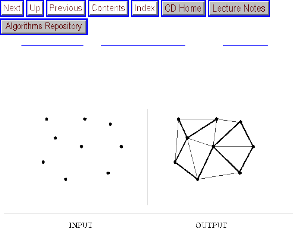
Triangulation
Next: Voronoi Diagrams Up: Computational Geometry Previous: Convex Hull
Triangulation
Input description: A set of points or a polyhedon.
Problem description: Partition the interior of the point set or polyhedron into triangles.
Discussion: Triangulation is a fundamental problem in computational geometry, because the first step in
working with complicated geometric objects is to break them into simple geometric objects. The simplest
geometric objects are triangles in two dimensions, and tetrahedra in three. Classical applications of
triangulation include finite element analysis and computer graphics.
A particularly interesting application of triangulation is surface or function interpolation. Suppose that
we have sampled the height of a mountain at a certain number of points. How can we estimate the height
at any point q in the plane? If we project the points on the plane, and then triangulate them, the
triangulation completely partitions the plane into regions. We can estimate the height of q by interpolating
among the three points of the triangle that contains it. Further, this triangulation and the associated height
values define a surface of the mountain suitable for graphics rendering.
In the plane, a triangulation is constructed by adding nonintersecting chords between the vertices until no
more such chords can be added. Specific issues arising in triangulation include:
file:///E|/BOOK/BOOK4/NODE186.HTM (1 of 4) [19/1/2003 1:31:39]
Triangulation
● Does the shape of the triangles in your triangulation matter? - There are usually many different
ways to partition your input into triangles. Consider a set of n points in convex position in the
plane. The simplest way to triangulate them would be to add to the convex hull diagonals from the
first point to all of the others. However, this has the tendency to create skinny triangles.
If the shape of the triangles matters for your application, you will usually want to avoid skinny
triangles, or equivalently, small angles in the triangulation. The Delaunay triangulation of a point
set minimizes the maximum angle over all possible triangulations. This isn't exactly what we are
looking for, but it is pretty close, and the Delaunay triangulation has enough other interesting
properties (including that it is dual to the Voronoi diagram) to make it the quality triangulation of
choice. Further, it can be constructed in time, with implementations described below.
● What dimension are we working in? - As always, three-dimensional problems are harder than two-
dimensional problems. The three-dimensional generalization of triangulation involves partitioning
the space into four-vertex tetrahedra by adding nonintersecting faces. One important difficulty is
that for certain polyhedra there is no way to tetrahedralize the interior without adding extra
vertices. Further, it is NP-complete to decide whether such a tetrahedralization exists, so we should
not feel afraid to add extra vertices to simplify our problem.
● What constraints does the input have? - When we are triangulating a polygon or polyhedra, we are
restricted to adding chords that do not intersect any of the boundary facets. In general, we may
have a set of obstacles or constraints that cannot be intersected by inserted chords. The best such
triangulation is likely to be the so-called constrained Delaunay triangulation. Implementations are
described below.
● Are you allowed to add extra points? - When the shape of the triangles does matter, it might pay to
strategically add a small number of extra ``Steiner'' points to the data set to facilitate the
construction of a triangulation (say) with no small angles. As discussed above, there may be no
triangulation possible for certain polyhedra without adding Steiner points.
To construct a triangulation of a convex polygon in linear time, just pick an arbitrary starting vertex v and
insert chords from v to each other vertex in the polygon. Because the polygon is convex, we can be
confident that none of the boundary edges of the polygon will be intersected by these chords and that all
of them lie within the polygon. The simplest algorithm for constructing general polygon triangulations
tries each of the possible chords and inserts them if they do not intersect a boundary edge or
previously inserted chord. There are practical algorithms that run in time and theoretically
interesting algorithms that run in linear time. See the implementations and notes below for details.
Implementations: Triangle, by Jonathan Shewchuk of Carnegie-Mellon University, is a C language code
that generates Delaunay triangulations, constrained Delaunay triangulations (forced to have certain
edges), and quality-conforming Delaunay triangulations (which avoid small angles by inserting extra
points). It has been widely used for finite element analysis and other applications and is fast and robust.
Triangle is the first thing I would try if I needed a two-dimensional triangulation code. Although Triangle
is available at http://www.cs.cmu.edu/ quake/triangle.html, it is copyrighted by the author and may not
be sold or included in commercial products without a license.
file:///E|/BOOK/BOOK4/NODE186.HTM (2 of 4) [19/1/2003 1:31:39]
Triangulation
GEOMPACK is a suite of Fortran 77 codes by Barry Joe of the University of Alberta, for 2- and 3-
dimensional triangulation and convex decomposition problems. In particular, it does both Delaunay
triangulation and convex decompositions of polygonal and polyhedral regions, as well as arbitrary-
dimensional Delaunay triangulations. They can be obtained from ftp://ftp.cs.ualberta.ca/pub/geompack.
Steve Fortune is the author of a widely used 2D code for Voronoi diagrams and Delaunay triangulations,
written in C. This code is smaller and probably simpler to work with than either of the above, if all you
need is the Delaunay triangulation of points in the plane. It is based on Fortune's own sweepline algorithm
[For87] for Voronoi diagrams and is available from Netlib (see Section ) at http://netlib.bell-
labs.com/netlib/voronoi/index.html.
O'Rourke [O'R94] provides asymptotically slow implementations in C of polygon triangulation (in )
and Delaunay triangulation (in ). These will be unusable for more than modest numbers of points,
but see Section if interested. See Section .
Algorithm 624 [Ren84] of the Collected Algorithms of the ACM is a Fortran implementation of
triangulation for surface interpolation. See Section . A linear-time implementation for triangulating a
planar map is included with LEDA (see Section ).
Higher-dimensional Delaunay triangulations are a special case of higher-dimensional convex hulls, and
Qhull [BDH97] appears to be the convex hull code of choice for general dimensions (i.e. three
dimensions and beyond). It is written in C, and it can also construct Voronoi vertices, furthest-site
Voronoi vertices, and half-space intersections. Qhull has been widely used in scientific applications and
has a well-maintained home page at http://www.geom.umn.edu/software/qhull/.
Notes: After a long search, Chazelle [Cha91] discovered a linear-time algorithm for triangulating a simple
polygon. This algorithm is sufficiently hopeless to implement that it qualifies more as an existence proof.
The first algorithm for polygon triangulation was given by [GJPT78]. An algorithm by
Tarjan and Van Wyk [TW88] followed before Chazelle's result. Expositions on polygon and point set
triangulation include [O'R94, PS85].
Linear-time algorithms for triangulating monotone polygons have been long known [GJPT78] and are the
basis of algorithms for triangulating simple polygons. A polygon is monotone when there exists a
direction d such that any line with slope d intersects the polygon in at most two points.
A heavily studied class of optimal triangulations seeks to minimize the total length of the chords used.
The computational complexity of constructing this minimum weight triangulation is a long-standing open
problem in computational geometry, so the interest has shifted to provably good approximation
algorithms. The minimum weight triangulation of a convex polygon can be found in time using
file:///E|/BOOK/BOOK4/NODE186.HTM (3 of 4) [19/1/2003 1:31:39]
Triangulation
dynamic programming, as discused in Section .
Related Problems: Voronoi diagrams (see page ), polygon partitioning (see page ).
Next: Voronoi Diagrams Up: Computational Geometry Previous: Convex Hull
Algorithms
Mon Jun 2 23:33:50 EDT 1997
file:///E|/BOOK/BOOK4/NODE186.HTM (4 of 4) [19/1/2003 1:31:39]
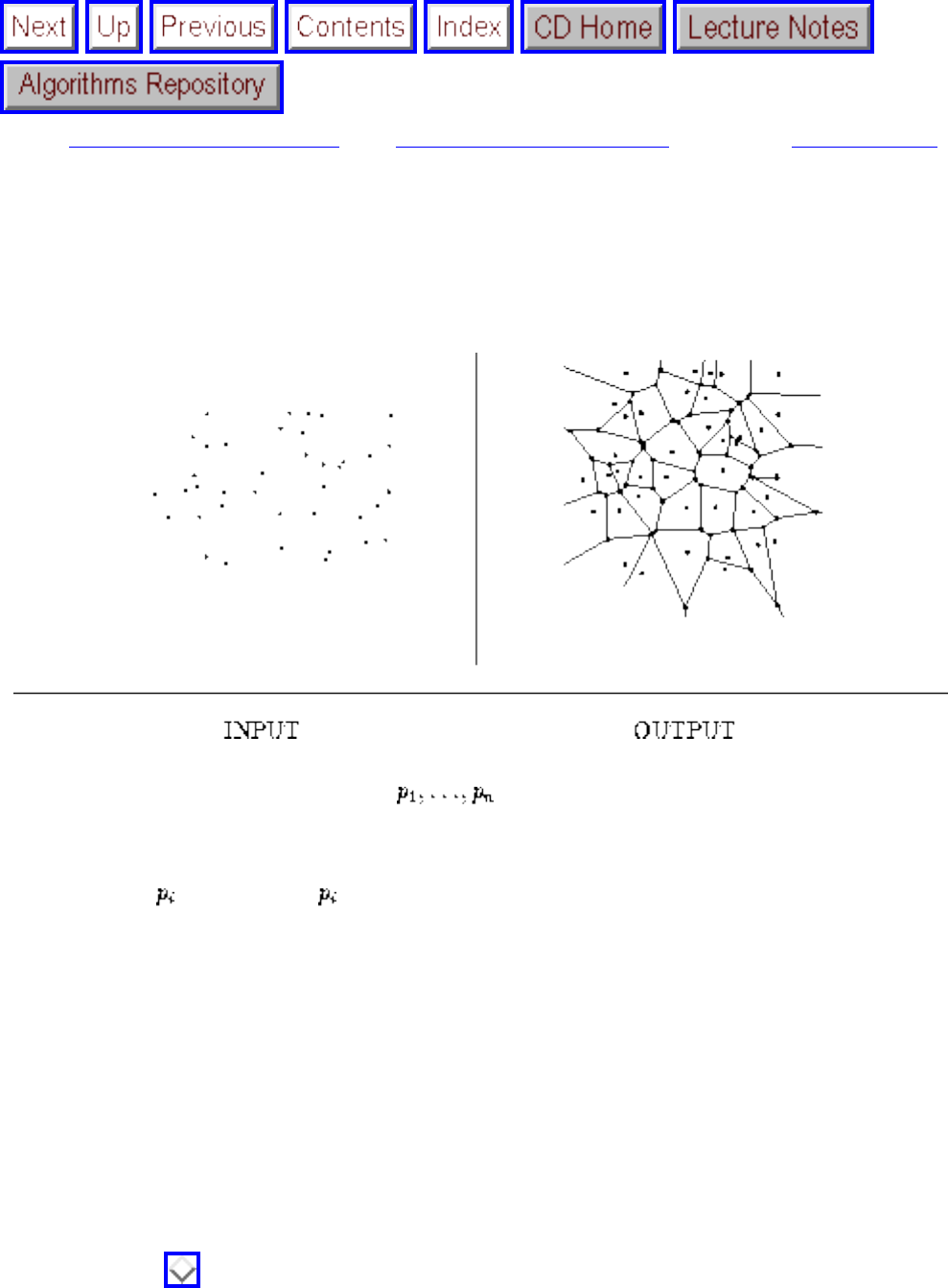
Voronoi Diagrams
Next: Nearest Neighbor Search Up: Computational Geometry Previous: Triangulation
Voronoi Diagrams
Input description: A set S of points .
Problem description: Decompose space into regions around each point such that all the points in the
region around are closer to than they are to any other point in S.
Discussion: Voronoi diagrams represent the region of influence around each of a given set of sites. If
these sites represent the locations of McDonald's restaurants, the Voronoi diagram partitions space into
cells around each restaurant. For each person living in a particular cell, the defining McDonald's
represents the closest place to get a Big Mac.
Voronoi diagrams have a surprising variety of uses:
● Nearest neighbor search - For a query point q, finding its nearest neighbor from a fixed set of
points S is simply a matter of determining which cell in the Voronoi diagram of S contains q. See
Section for more details.
● Facility location - Suppose McDonald's wanted to open another restaurant. To minimize
interference with existing McDonald's, it should be located as far away from the closest restaurant
as possible. This location is always at a vertex of the Voronoi diagram, and it can be found in a
file:///E|/BOOK/BOOK4/NODE187.HTM (1 of 4) [19/1/2003 1:31:41]
Voronoi Diagrams
linear-time search through all the Voronoi vertices.
● Largest empty circle - Suppose you needed to obtain a large, contiguous, undeveloped piece of
land on which to build a factory. The same condition used for picking McDonald's locations is
appropriate for other undesirable facilities, namely that it be as far as possible from any relevant
sites of interest. A Voronoi vertex defines the center of the largest empty circle among the points.
● Path planning - If the sites of S are the centers of obstacles we seek to avoid, the edges of the
Voronoi diagram define the possible channels that maximize the distance to the obstacles. Thus in
planning paths among the sites, it will be ``safest'' to stick to the edges of the Voronoi diagram.
● Quality triangulations - In triangulating a set of points, we often desire nice, fat triangles, which
avoid small angles and skinny triangles. The Delaunay triangulation maximizes the minimum
angle over all triangulations and is exactly what we want. Further, it is easily constructed as the
dual of the Voronoi diagram. See Section for details.
Each edge of a Voronoi diagram is part of the perpendicular bisector of two points in S, since this is the
line that partitions the plane between the points. The conceptually simplest method to construct Voronoi
diagrams is randomized incremental construction. To add another site to the diagram, locate the cell that
contains it and add the perpendicular bisectors between the new site and all sites defining impacted
regions. When the sites are inserted in random order, only a small number of regions are likely to be
impacted.
However, the method of choice is Fortune's sweepline algorithm, especially since robust
implementations of it are readily available. Use an existing implementation instead of trying to develop
your own. The algorithm works by projecting the set of sites in the plane into a set of cones in three
dimensions such that the Voronoi diagram is defined by projecting the cones back onto the plane. The
advantages of Fortune's algorithm are (1) it runs in optimal time, (2) it is reasonable to
implement, and (3) we need not store the entire diagram if we can use it as we sweep over it.
There is an interesting relationship between convex hulls in d+1 dimensions and Delaunay triangulations
(or equivalently Vornoi diagrams) in d-dimensions, which provides the best way to construct Voronoi
diagrams in higher dimensions. By projecting each site in into the point
, taking the convex hull of this (d+1)-dimensional point set and then projecting
back into d dimensions we obtain the Delaunay triangulation. Details are given in the references below.
Programs that compute higher-dimensional convex hulls are discussed in Section .
Several important variations of standard Voronoi diagrams arise in practice. See the references below for
details:
● Non-Euclidean distance metrics - Recall that the idea of a Voronoi diagram is to decompose space
into regions of influence around each of the given sites. Thus far, we have assumed that Euclidean
distance measures influence, but for many applications this is inappropriate. If people drive to
file:///E|/BOOK/BOOK4/NODE187.HTM (2 of 4) [19/1/2003 1:31:41]
Voronoi Diagrams
McDonald's, the time it takes to get there depends upon where the major roads are. Efficient
algorithms are known for constructing Voronoi diagrams under a variety of different metrics, and
for curved or constrained objects.
● Power diagrams - These structures decompose space into regions of influence around the sites,
where the sites are no longer constrained to have all the same power. Imagine a map of the
listening range of a set of radio stations operating at a given frequency. The region of influence
around a station depends both on the power of its transmitter and the position of neighboring
transmitters.
● kth-order and furthest-site diagrams - The idea of decomposing space into regions sharing some
property can be taken beyond closest-point Voronoi diagrams. Any point within a single cell of
the kth-order Voronoi diagram shares the same set of k closest points in S. In furthest-site
diagrams, any point within a particular region shares the same furthest point in S. Point location
(see Section ) on these structures permits fast retrieval of the appropriate points.
Implementations: Steve Fortune is the author of a widely used 2D code for Voronoi diagrams and
Delaunay triangulations, written in C. It is based on his own sweepline algorithm [For87] for Voronoi
diagrams and is likely to be the right code to try first. It is available from Netlib (see Section ) at
http://netlib.bell-labs.com/netlib/voronoi/index.html.
LEDA (see Section ) provides an implementation of a randomized incremental construction algorithm
for planar Voronoi diagrams in C++.
Higher-dimensional and furthest-site Voronoi diagrams can be constructed as a special case of higher-
dimensional convex hulls. Qhull [BDH97] appears to be the convex hull code of choice in three
dimensions and beyond. It is written in C, and it can also construct Delaunay triangulations and half-
space intersections. Qhull has been widely used in scientific applications and has a well-maintained
home page at http://www.geom.umn.edu/software/qhull/.
The Stanford GraphBase (see Section ) contains an implementation of a randomized incremental
algorithm to construct Voronoi diagrams and Delaunay triangulations for use as a generator of planar
graph instances.
Algorithm 558 [Che80] of the Collected Algorithms of the ACM is a Fortran code for the multifacility
location problem. It is based on a network flow approach, instead of using Voronoi diagrams.
Interestingly, the network flow code is taken from Nijenhuis and Wilf (see Section ). See Section .
Notes: Voronoi diagrams were studied by Dirichlet in 1850 and are occasionally referred to as Dirichlet
tessellations. They are named after G. Voronoi, who discussed them in a 1908 paper. In mathematics,
concepts get named after the last person to discover them.
file:///E|/BOOK/BOOK4/NODE187.HTM (3 of 4) [19/1/2003 1:31:41]
Voronoi Diagrams
Aurenhammer [Aur91] and Fortune [For92] provide excellent surveys on Voronoi diagrams and
associated variants such as power diagrams. The first algorithm for constructing Voronoi
diagrams was based on divide-and-conquer and is due to Shamos and Hoey [SH75]. Good expositions of
Fortune's sweepline algorithm for constructing Voronoi diagrams in [For87] include [O'R94].
Good expositions on the relationship between Delaunay triangulations and (d+1)-dimensional convex
hulls [ES86] include [O'R94].
In a kth-order Voronoi diagram, we partition the plane such that each point in a region is closest to the
same set of k sites. Using the algorithm of [ES86], the complete set of kth-order Voronoi diagrams can be
constructed in time. By doing point location on this structure, the k nearest neighbors to a query
point can be found in . Expositions on kth-order Voronoi diagrams include [O'R94, PS85].
The smallest enclosing circle problem can be solved in time using (n-1)st order Voronoi
diagrams [PS85]. In fact, there exist linear-time algorithms based on low-dimensional linear
programming [Meg83]. A linear algorithm for computing the Voronoi diagram of a convex polygon is
given by [AGSS89].
Related Problems: Nearest neighbor search (see page ), point location (see page ), triangulation
(see page ).
Next: Nearest Neighbor Search Up: Computational Geometry Previous: Triangulation
Algorithms
Mon Jun 2 23:33:50 EDT 1997
file:///E|/BOOK/BOOK4/NODE187.HTM (4 of 4) [19/1/2003 1:31:41]
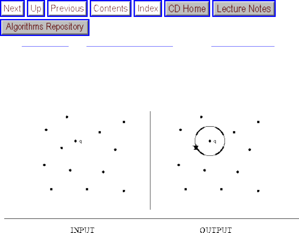
Nearest Neighbor Search
Next: Range Search Up: Computational Geometry Previous: Voronoi Diagrams
Nearest Neighbor Search
Input description: A set S of n points in d dimensions; a query point q.
Problem description: Which point in S is closest to q?
Discussion: The need to quickly find the nearest neighbor to a query point arises in a variety of
geometric applications. The classic example in two dimensions is designing a system to dispatch
emergency vehicles to the scene of a fire. Once the dispatcher learns the location of the fire, she uses a
map to find the firehouse closest to this point so as to minimize transportation delays. This situation
occurs in any application mapping customers to service providers.
Nearest-neighbor search is also important in classification. Suppose we are given a collection of data
about people (say age, height, weight, years of education, sex, and income level) each of whom has been
labeled as Democrat or Republican. We seek a classifier to decide which way a different person is likely
to vote. Each of the people in our data set is represented by a party-labeled point in d-dimensional space.
A simple classifier can be built by assigning to the new point the party affiliation of its nearest neighbor.
Such nearest-neighbor classifiers are widely used, often in high-dimensional spaces. The vector-
file:///E|/BOOK/BOOK4/NODE188.HTM (1 of 4) [19/1/2003 1:31:43]
Nearest Neighbor Search
quantization method of image compression partitions an image into pixel regions. This method uses
a predetermined library of several thousand pixel tiles and replaces each image region by the most
similar library tile. The most similar tile is the point in 64-dimensional space that is closest to the image
region in question. Compression is achieved by reporting the identifier of the closest library tile instead
of the 64 pixels, at some loss of image fidelity.
Issues arising in nearest-neighbor search include:
● How many points are you searching? - When your data set contains only a small number of points
(say ) or if only few queries are ever destined to be performed, the simple approach is
best. Compare the query point q against each of the n data points. Only when fast queries are
needed for large numbers of points does it pay to consider more sophisticated methods.
● How many dimensions are you working in? - Nearest neighbor search gets slowly but
progressively harder as the dimensionality increases. The kd-tree data structure, presented in
Section , does a very good job in moderate-dimensional spaces, even the plane. Still, above 20
or so dimensions, you might as well do a linear search through the data points. Search in high-
dimensional spaces becomes hard because a sphere of radius r, representing all the points with
distance from the center, progressively fills up less volume relative to a cube as the
dimensionality increases. Thus any data structure based on partitioning points into enclosing
volumes will become less and less effective.
In two dimensions, Voronoi diagrams (see Section ) provide an efficient data structure for
nearest-neighbor queries. The Voronoi diagram of a point set in the plane decomposes the plane
into regions such that the cell containing each data point consists of the part of the plane that is
nearer to that point than any other in the set. Finding the nearest neighbor of query point q reduces
to finding which cell in the Voronoi diagram contains q and reporting the data point associated
with it. Although Voronoi diagrams can be built in higher dimensions, their size rapidly grows to
the point of unusability.
● Is your data set static or dynamic? - Will there be occasional insertions or deletions of new data
points in your application? If these are just rare events, it might pay to build your data structure
from scratch each time. If they are frequent, select a version of the kd-tree that supports insertions
and deletions.
The nearest neighbor graph on a set S of n points links each vertex to its nearest neighbor. This graph is a
subgraph of the Delaunay triangulation and so can be computed in . This is quite a bargain
since it takes time just to discover the closest pair of points in S.
As a lower bound, the closest pair problem in one dimension reduces to sorting. In a sorted set of
numbers, the closest pair corresponds to two numbers that lie next to each other in sorted order, so we
need only check which is the minimum gap between the n-1 adjacent pairs. The limiting case of this
occurs when the closest pair are distance zero apart, meaning that the elements are not unique.
file:///E|/BOOK/BOOK4/NODE188.HTM (2 of 4) [19/1/2003 1:31:43]
Nearest Neighbor Search
Implementations: Ranger is a tool for visualizing and experimenting with nearest-neighbor and
orthogonal-range queries in high-dimensional data sets, using multidimensional search trees. Four
different search data structures are supported by Ranger: naive kd-trees, median kd-trees, nonorthogonal
kd-trees, and the vantage point tree.
For each of these, Ranger supports queries in up to 25 dimensions under any Minkowski metric. It
includes generators for a variety of point distributions in arbitrary dimensions. Finally, Ranger provides a
number of features to aid in visualizing multidimensional data, best illustrated by the accompanying
video [MS93]. To identify the most appropriate projection at a glance, Ranger provides a matrix of
all two-dimensional projections of the data set. Ranger is written in C, using Motif. It runs on Silicon
Graphics and HP workstations and is available in the algorithm repository http://www.cs.sunysb.edu/
algorith.
See Section for a complete collection of Voronoi diagram implementations. In particular, LEDA (see
Section ) provides an implementation of 2D Voronoi diagrams in C++, as well as planar point
location to make effective use of them for nearest-neighbor search.
A Pascal implementation of the divide-and-conquer algorithm for finding the closest pair of points in a
set of n points appears in [MS91]. See Section .
Notes: The best reference on kd-trees and other spatial data structures is two volumes by Samet
[Sam90b, Sam90a], where all major variants are developed in substantial detail. Good expositions on
finding the closest pair of points in the plane [BS76] include [CLR90, Man89]. These algorithms use a
divide-and-conquer approach instead of just selecting from the Delaunay triangulation.
A recent development in higher-dimensional nearest-neighbor search is algorithms that quickly produce a
point that if not the nearest neighbor lies provably close to the query point. A sparse weighted graph
structure is built from the data set, and the nearest neighbor is found by starting at a random point and
greedily walking in the graph towards the query point. The closest point found over several random trials
is declared the winner. Similar data structures hold promise for other problems in high-dimensional
spaces. See [AM93, AMN 94].
Related Problems: Kd-trees (see page ), Voronoi diagrams (see page ), range search (see page
).
file:///E|/BOOK/BOOK4/NODE188.HTM (3 of 4) [19/1/2003 1:31:43]

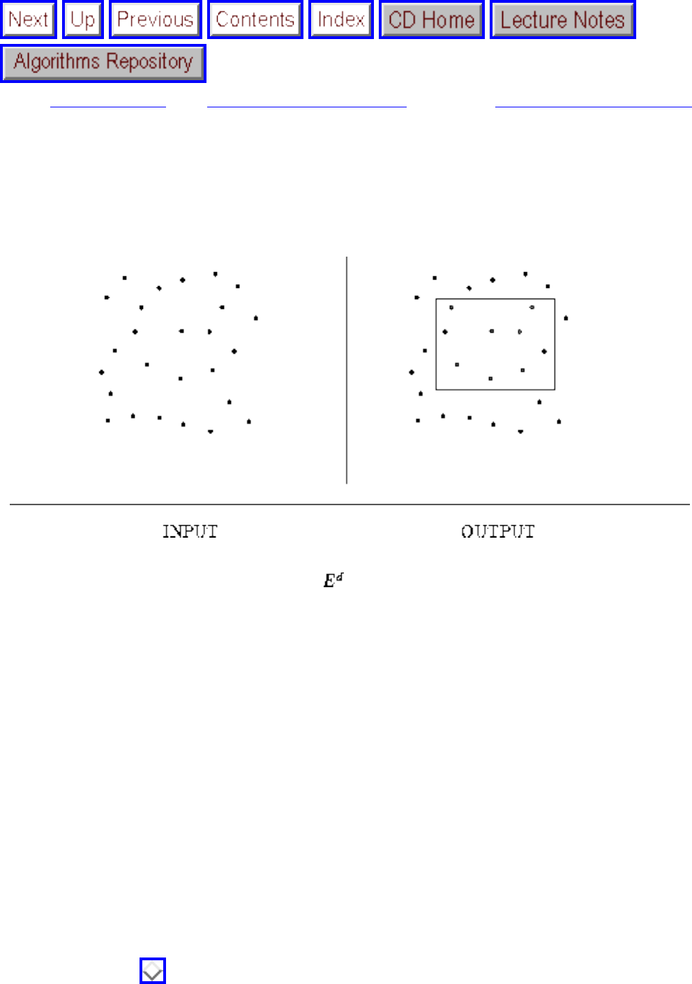
Range Search
Next: Point Location Up: Computational Geometry Previous: Nearest Neighbor Search
Range Search
Input description: A set S of n points in and a query region Q.
Problem description: Which points from S lie within Q?
Discussion: Range search problems arise in database and geographic information system (GIS)
applications. Any data object with d numerical fields, such as person with height, weight, and income,
can be modeled as a point in d-dimensional space. A range query describes a region in space and asks for
all points or the number of points in the region. For example, asking for all people with income between
$0 and $10,000, with height between 6'0'' and 7'0'', and weight between 50 and 140 lbs. defines a box
containing people whose body and wallets are both thin.
The difficulty of a range search problem depends on several factors:
● How many range queries are you going to perform? - The simplest approach to range search tests
each of the n points one by one against the query polygon Q. This works just fine if the number of
queries will be small. Algorithms to test whether a point is within a given polygon are presented
in Section .
● What shape is your query polygon? - The easiest type of regions to query against are axis-parallel
file:///E|/BOOK/BOOK4/NODE189.HTM (1 of 3) [19/1/2003 1:31:45]
Range Search
rectangles, because the inside/outside test reduces to verifying whether each coordinate lies
within a prescribed range. The figure above illustrates such an orthogonal range query.
If you are querying against a nonconvex polygon, it will pay to partition your polygon into convex
pieces or (even better) triangles and then query the point set against each one of the pieces. This is
because testing whether a point is inside a convex polygon can be done more quickly and easily
than for arbitrary polygons. Algorithms for such convex decompositions are discussed in Section
.
● How many dimensions? - The best general-purpose approach to range queries builds a kd-tree on
the point set, as discussed in Section . To perform a query, a depth-first traversal of the kd-tree
is performed, with each tree node expanded only if the associated rectangle intersects the query
region. For sufficiently large or misaligned query regions, the entire tree might have to be
traversed, but in general; kd-trees lead to an efficient solution. Although algorithms with efficient
worst-case performance are known in two dimensions, kd-trees are likely to work even better in
the plane. In higher-dimensions, kd-trees provide the only viable solution to the problem.
● Can I just count the number of points in a region, or do I have to identify them? - For many
applications it suffices to count the number of points in a region instead of returning them.
Harkening back to the introductory example, we may want to know whether there are more
thin/poor people or rich/fat ones. The need to find the densest or emptiest region in space often
naturally arises, and the problem can be solved by counting range queries.
A data structure for efficiently answering such aggregate range queries can be based on the
dominance ordering of the point set. A point x is said to dominate point y if y lies both below and
to the left of x. Let DOM(p) be a function that counts the number of points in S that are dominated
by p. The number of points m in the orthogonal rectangle defined by and
is given by
The second additive term corrects for the points for the lower left-hand corner that have been
subtracted away twice.
To answer arbitrary dominance queries efficiently, partition the space into rectangles by
drawing a horizontal and vertical line through each of the n points. The set of points dominated is
identical for each point in each rectangle, so the dominance count of the lower left-hand corner of
each rectangle can precomputed, stored, and reported for any query point within it. Queries reduce
to binary search and thus take time. Unfortunately, this data structure takes quadratic
space. However, the same idea can be adapted to kd-trees to create a more space-efficient search
structure.
Implementations: LEDA (see Section ) provides excellent support for maintaining planar
file:///E|/BOOK/BOOK4/NODE189.HTM (2 of 3) [19/1/2003 1:31:45]
Range Search
subdivisions in C++. In particular, it supports orthogonal range queries in time, where n is the
complexity of the subdivision and k is the number of points in the rectangular region.
Ranger is a tool for visualizing and experimenting with nearest-neighbor and orthogonal-range queries in
high-dimensional data sets, using multidimensional search trees. Four different search data structures are
supported by Ranger: naive kd-trees, median kd-trees, nonorthogonal kd-trees, and the vantage point
tree. For each of these, Ranger supports queries in up to 25 dimensions under any Minkowski metric. It
is available in the algorithm repository.
A bare bones implementation in C of orthogonal range search using kd-trees appears in [GBY91].
Sedgewick [Sed92] provides code fragments of the grid method for orthogonal range search in C++. See
Section for details on both of them.
Notes: Good expositions on data structures with worst-case performance for orthogonal-range
searching [Wil85] include [PS85]. An exposition on kd-trees for orthogonal range queries in two
dimensions appears in [PS85]. Their worst-case performance can be very bad; [LW77] describes an
instance in two dimensions requiring time to report that a rectangle is empty.
The problem becomes considerably more difficult for nonorthogonal range queries, where the query
region is not an axis-aligned rectangle. For half-plane intersection queries, time and linear space
suffice [CGL85]; for range searching with simplex query regions (such as a triangle in the plane), lower
bounds preclude efficient worst-case data structures. See [Yao90] for a discussion.
Related Problems: Kd-trees (see page ), point location (see page ),
Next: Point Location Up: Computational Geometry Previous: Nearest Neighbor Search
Algorithms
Mon Jun 2 23:33:50 EDT 1997
file:///E|/BOOK/BOOK4/NODE189.HTM (3 of 3) [19/1/2003 1:31:45]
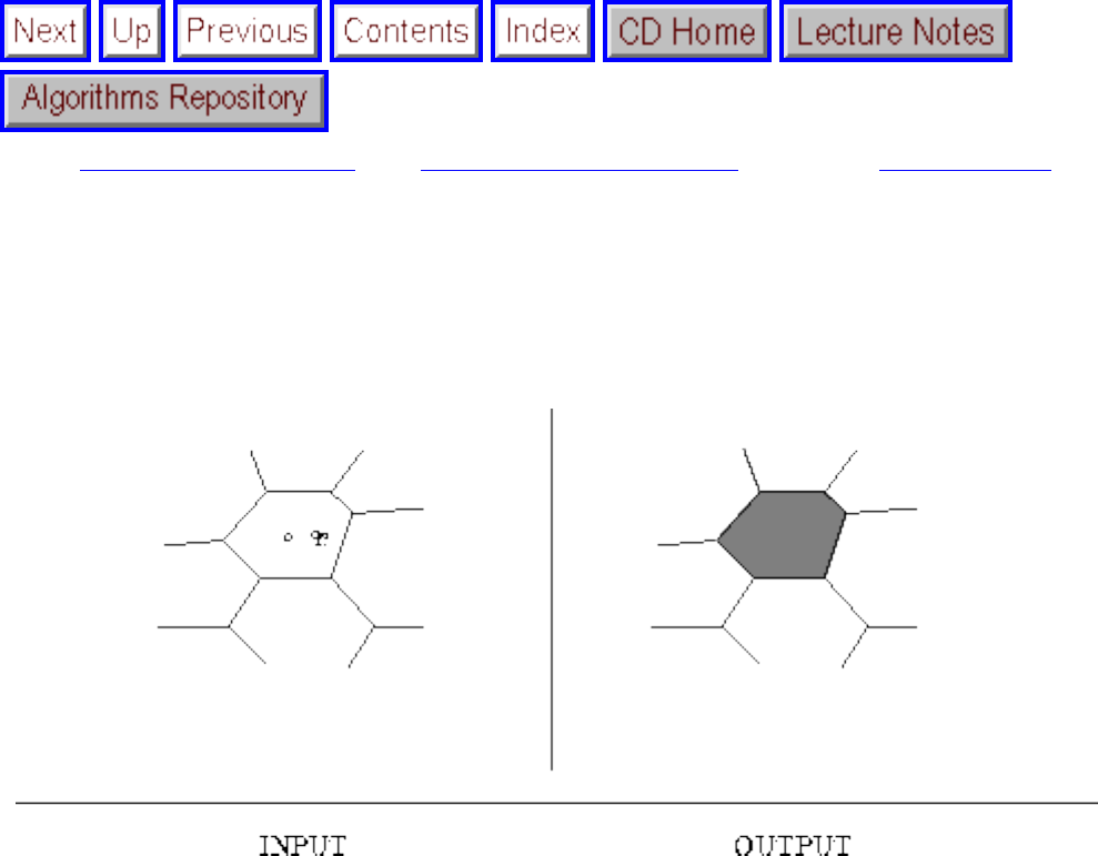
Point Location
Next: Intersection Detection Up: Computational Geometry Previous: Range Search
Point Location
Input description: A decomposition of the plane into polygonal regions and a query point q.
Problem description: Which region contains the query point q?
Discussion: Point location is a fundamental subproblem in computational geometry, usually needed as an
ingredient to solve larger geometric problems. In a dispatch system to assign policemen to the scene of a
crime, the city will be partitioned into different precincts or districts. Given a map of regions and a
query point (the crime scene), the system must identify which region contains the point. This is exactly
the problem of planar point location, variations of which include:
● Is a given point inside or outside of polygon P? - The simplest version of point location involves
only two regions, inside-P and outside-P, and asks which contains a given query point. For
polygons with lots of narrow spirals, this can be surprisingly difficult to tell by inspection. The
secret to doing it both by eye or machine is to draw a ray starting from the query point and ending
beyond the furthest extent of the polygon. Count the number of times the polygon crosses through
an edge. If this number is odd, we must be within the polygon. If it is even, we must be outside.
The case of the line passing through a vertex instead of an edge is evident from context, since we
are counting the number of times we pass through the boundary of the polygon. Testing each of
file:///E|/BOOK/BOOK4/NODE190.HTM (1 of 4) [19/1/2003 1:31:46]
Point Location
the n edges for intersection against the query ray takes O(n) time. Faster algorithms for convex
polygons are based on binary search and take time.
● How many queries will have to be performed? - When we have a subdivision with multiple
regions, it is always possible to repeat the inside-polygon test above on each region in the
subdivision. However, this is wasteful if we will be performing many such point location queries
on the same subdivision. Instead, we can construct a grid-like or tree-like data structure on top of
our subdivision to get us near the correct region quickly. Such search structures are discussed in
more detail below.
● How complicated are the regions of your subdivision? - More sophisticated inside-outside tests
are required when the regions of your subdivision are arbitrary polygons. By triangulating all
polygonal regions first, each inside-outside test reduces to testing whether a point is in a triangle.
Such a test can be made particularly fast and simple, at the minor cost of recording the full-
polygon name for each triangle. An added benefit is that the smaller your regions are, the better
grid-like or tree-like superstructures are likely to perform. Some care should be taken when you
triangulate to avoid long skinny triangles, as discussed in Section .
● How regularly sized and spaced are your regions? - If all resulting triangles are about the same
size and shape, the simplest point location method imposes a regularly-spaced grid of
horizontal and vertical lines over the entire subdivision. For each of the rectangular regions, we
maintain a list of all the regions that are at least partially contained within the rectangle.
Performing a point location query in such a grid file involves a binary search or hash table lookup
to identify which rectangle contains query point q and then searching each region in the resulting
list to identify the right one.
Such grid files will perform very well, provided that each triangular region overlaps only a few
rectangles (thus minimizing storage space) and each rectangle overlaps only a few triangles (thus
minimizing search time). Whether it will perform well is a function of the regularity of your
subdivision. Some flexibility can be achieved by spacing the horizontal lines irregularly, as a
function of the regions of the subdivision. The slab method, discussed below, is a variation on this
idea that guarantees worst-case efficient point location at the cost of quadratic space.
● How many dimensions will you be working in? - In three or more dimensions, some flavor of kd-
tree will almost certainly be the point-location method of choice. They are also likely to be the
right answer for planar subdivisions too irregular for grid files.
Kd-trees, described in Section , decompose the space into a hierarchy of rectangular boxes. At
each node in the tree, the current box is split into a small number (typically 2 or 4 or , where d
is the dimension) of smaller boxes. At the leaves of the tree, each box is labeled with the small
number of regions that are at least partially contained in the box. The point location search starts
at the root of the tree and keeps traversing down the child whose box contains the query point.
When the search hits a leaf, we test each of the relevant regions against q to see which one of
them contains the point. As with grid files, we hope that each leaf contains a small number of
regions and that each region does not cut across too many leaf cells.
file:///E|/BOOK/BOOK4/NODE190.HTM (2 of 4) [19/1/2003 1:31:46]
Point Location
The simplest algorithm to guarantee worst-case access is the slab method, which draws horizontal
lines through each vertex, thus creating n+1 ``slabs'' between the lines. Since the slabs are defined by
horizontal lines, finding the slab containing a particular query point can be done using a binary search on
the y-coordinate of q. Since there can be no vertices within any slab, looking for the region containing a
point within a slab can be done by a second binary search on the edges that cross the slab. The catch is
that a binary search tree must be maintained for each slab, for a worst-case of space if each region
intersects each slab. A more space-efficient approach based on building a hierarchy of triangulations over
the regions also achieves for search and is discussed in the notes below.
Worst-case efficient computational geometry methods either require a lot of storage or are fairly
complicated to implement. We identify implementations of worst-case methods below, which are worth
at least experimenting with. However, we recommend kd-trees for most general point-location
applications.
Implementations: LEDA (see Section ) provides excellent support for maintaining planar
subdivisions in C++ and, in particular, supports point location in time.
Arrange is a package for maintaining arrangements of polygons in either the plane or on the sphere.
Polygons may be degenerate, and hence represent arrangements of lines. A randomized incremental
construction algorithm is used, and efficient point location on the arrangement is supported. Polygons
may be inserted but not deleted from the arrangement, and arrangements of several thousand vertices and
edges can be constructed in a few seconds. Arrange is written in C by Michael Goldwasser and is
available from http://theory.stanford.edu/people/wass/wass.html.
A routine in C to test whether a point lies in a simple polygon has been provided by O'Rourke [O'R94],
and a Pascal routine for the same problem by [MS91]. For information on both, see Section .
Notes: The inside-outside test for convex polygons is described in [PS85], which has a very thorough
treatment of deterministic planar point location data structures. Expositions on the inside-outside test for
simple polygons include [Man89, PS85].
An experimental study of algorithms for planar point location is described in [EKA84]. The winner was a
bucketing technique akin to the grid file.
The elegant triangle refinement method of Kirkpatrick [Kir83] builds a hierarchy of triangulations above
the actual planar subdivision such that each triangle on a given level intersects only a constant number of
triangles on the following level. Since each triangulation is a fraction of the size of the subsequent one,
the total space is obtained by summing up a geometric series and hence is linear. Further, the height of
the hierarchy is , ensuring fast query times. An alternative algorithm realizing the same time
bounds is [EGS86]. The slab method described above is due to [DL76] and is presented in [PS85].
file:///E|/BOOK/BOOK4/NODE190.HTM (3 of 4) [19/1/2003 1:31:46]
Point Location
More recently, there has been interest in dynamic data structures for point location, which support fast
incremental updates of the planar subdivision (such as insertions and deletions of edges and vertices) as
well as fast point location. Chiang and Tamassia's [CT92] survey is an appropriate place to begin.
Related Problems: Kd-trees (see page ), Voronoi diagrams (see page ), nearest neighbor search
(see page ).
Next: Intersection Detection Up: Computational Geometry Previous: Range Search
Algorithms
Mon Jun 2 23:33:50 EDT 1997
file:///E|/BOOK/BOOK4/NODE190.HTM (4 of 4) [19/1/2003 1:31:46]
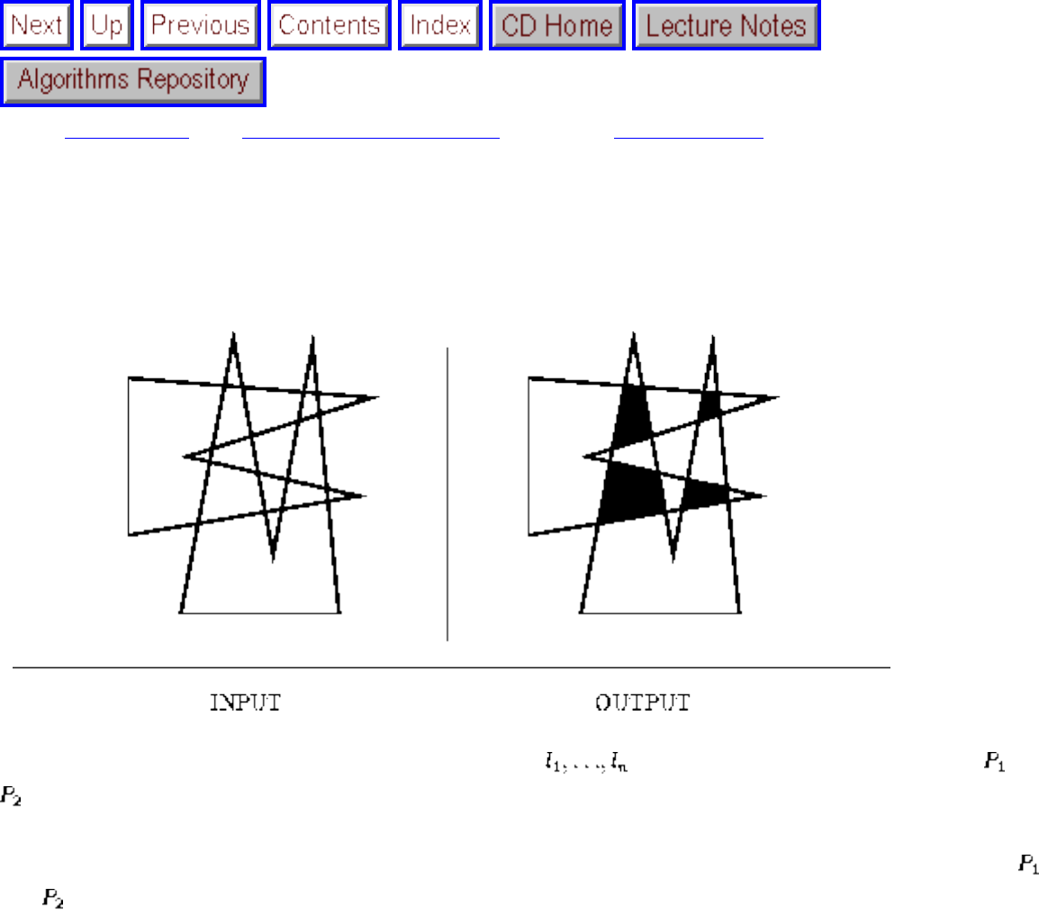
Intersection Detection
Next: Bin Packing Up: Computational Geometry Previous: Point Location
Intersection Detection
Input description: A set S of lines and line segments or a pair of polygons or polyhedra and
.
Problem description: Which pairs of line segments intersect each other? What is the intersection of
and ?
Discussion: Intersection detection is a fundamental geometric primitive that arises in many applications.
Picture a virtual-reality simulation of an architectural model for a building. The illusion of reality
vanishes the instant the virtual person walks through a virtual wall. To enforce such physical constraints,
any such intersection between polyhedral models must be immediately detected and the operator notified
or constrained.
Another application of intersection detection is design rule checking for VLSI layouts. A minor design
mistake resulting in two crossing metal strips can short out the chip, but such errors can be detected
before fabrication using programs to find all intersections between line segments.
Issues arising in intersection detection include:
file:///E|/BOOK/BOOK4/NODE191.HTM (1 of 5) [19/1/2003 1:31:48]
Intersection Detection
● Do you want to compute the intersection or just report it? - We distinguish between intersection
detection and computing the actual intersection. The latter problem is obviously harder than the
former and is not always necessary. In the virtual-reality application above, it might not be
important to know exactly where we hit the wall, just that we hit it.
● Are you intersecting lines or line segments? - The big difference here is that any two lines with
different slopes must intersect at exactly one point. By comparing each line against every other
line, all points of intersections can be found in constant time per point, which is clearly optimal.
Constructing the arrangement of the lines provides more information than just intersection points
and is discussed in Section .
Finding all the intersections between n line segments is considerably more challenging. Even the
basic primitive of testing whether two line segments intersect is not as trivial as it might seem,
and this is discussed in Section . To find all intersections, we can explicitly test each line
segment against each other line segment and thus find all intersections in time. Each
segment can always intersect each other segment, yielding a quadratic number of intersections, so
in the worst case, this is optimal. For many applications, however, this worst case is not very
interesting.
● How many intersection points do you expect? - Sometimes, as in VLSI design rule checking, we
expect the set of line segments to have few if any intersections. What we seek is an algorithm
whose time is output sensitive, taking time proportional to the number of intersection points.
Such output-sensitive algorithms exist for line-segment intersection, with the fastest algorithm
taking time, where k is the number of intersections. Such algorithms are sufficiently
complicated that you should use an existing implementation if you can. These algorithms are
based on the sweepline approach, discussed below.
● Can you see point x from point y? - Visibility queries ask whether vertex x can see vertex y
unobstructed in a room full of obstacles. This can be phrased as the following line-segment
intersection problem: does the line segment from x to y intersect any obstacle? Such visibility
problems arise in robot motion planning (see Section ) and in hidden-surface elimination for
computer graphics.
● Are the intersecting objects convex? - Better intersection algorithms exist when the line segments
form the boundaries of polygons. The critical issue here becomes whether the polygons are
convex. Intersecting a convex n-gon with a convex m-gon can be done in O(n+m) time, using a
sweepline algorithm as discussed below. This is possible because the intersection of two convex
polygons must form another convex polygon using at most n+m vertices.
However, the intersection of two nonconvex polygons is not so well behaved. Consider the
intersection of two ``combs'' generalizing the Picasso-like frontspiece to this section. As
illustrated, the intersection of nonconvex polygons may be disconnected and have quadratic size
in the worst case.
file:///E|/BOOK/BOOK4/NODE191.HTM (2 of 5) [19/1/2003 1:31:48]

Intersection Detection
Intersecting two polyhedra is somewhat more complicated than intersecting polygons, because
two polyhedra can intersect even when no edges do. Consider the example of a needle piercing
the interior of a face. In general, however, the same issues arise for both polygons and polyhedra.
● Are you searching for intersections repeatedly with the same basic objects? - In the walk-through
application described above, the room and the objects in it don't change between one scene and
the next. Only the person moves, and, further, the intersections are rare.
One common solution is to approximate the objects in the scene by simpler objects that enclose
them, such as boxes. Whenever two enclosing boxes intersect, then the underlying objects might
intersect, and so further work is necessary to decide the issue. However, it is much more efficient
to test whether simple boxes intersect than more complicated objects, so we win if collisions are
rare. Many variations on this theme are possible, but this idea can lead to large performance
improvements for complicated environments.
Planar sweep algorithms can be used to efficiently compute the intersections among a set of line
segments, or the intersection/union of two polygons. These algorithms keep track of interesting changes
as we sweep a vertical line from left to right over the data. At its leftmost position, the line intersects
nothing, but as it moves to the right, it encounters a series of events:
● Insertion - the leftmost point of a line segment may be encountered, and it is now available to
intersect some other line segment.
● Deletion - the rightmost point of a line segment is encountered. This means that we have
completely swept over the segment on our journey, and so it can be deleted from further
consideration.
● Intersection - if we maintain the active line segments that intersect the sweep line as sorted from
top to bottom, the next intersection must occur between neighboring line segments. After the
intersection, these two line segments swap their relative order.
Keeping track of what is going on requires two data structures. The future is maintained by an event
queue, a priority queue ordered by the x-coordinate of all possible future events of interest: insertion,
deletion, and intersection. See Section for priority queue implementations. The present is represented
by the horizon, an ordered list of line segments intersecting the current position of the sweepline. The
horizon can be maintained using any dictionary data structure, such as a balanced tree.
To adapt this approach to computing the intersection or union of polygons, we modify the processing of
the three event types to keep track of what has occurred to the left of the sweepline. This algorithm can
be considerably simplified for pairs of convex polygons, since (1) at most four polygon edges intersect
the sweepline, so no horizon data structure is needed and (2) no event-queue sorting is needed, since we
can start from the leftmost vertex of each polygon and proceed to the right by following the polygonal
ordering.
file:///E|/BOOK/BOOK4/NODE191.HTM (3 of 5) [19/1/2003 1:31:48]
Intersection Detection
Implementations: LEDA (see Section ) provides a C++ implementation of the Bentley-Ottmann
sweepline algorithm [BO79], finding all k intersection points between n line segments in the plane in
time.
O'Rourke [O'R94] provides a robust program in C to compute the intersection of two convex polygons.
See Section .
RAPID is a ``Rapid and Accurate Polygon Interference Detection library'' for large environments
composed of polygonal models. It is free for noncommercial use and available from
http://www.cs.unc.edu/ geom/OBB/OBBT.html.
Model Pascal subroutines for convexity testing and for finding an intersection in a set of line segments
appear in [MS91]. See Section for details. XTango (see Section ) includes an animation of
polygon clipping against a polygonal window.
Finding the mutual intersection of a collection of half-spaces is a special case of higher-dimensional
convex hulls, and Qhull [BDH97] is convex hull code of choice for general dimensions. Qhull has been
widely used in scientific applications and has a well-maintained home page at
http://www.geom.umn.edu/software/qhull/.
Notes: Good expositions on line segment intersection detection [BO79, SH75] include [CLR90, Man89,
NH93, PS85]. Good expositions on polygon and polyhedra intersection [HMMN84, MP78, SH76]
include [PS85]. Preparata and Shamos [PS85] provide a good exposition on the special case of finding
intersections and unions of axis-oriented rectangles, a problem that arises often in VLSI design.
An optimal algorithm for computing line segment intersections is due to Chazelle and
Edelsbrunner [CE92]. Simpler, randomized algorithms achieving the same time bound are thoroughly
presented by Mulmuley [Mul94].
Surveys on hidden-surface removal include [Dor94, SSS74].
Related Problems: Maintaining arrangements (see page ), motion planning (see page ).
Next: Bin Packing Up: Computational Geometry Previous: Point Location
file:///E|/BOOK/BOOK4/NODE191.HTM (4 of 5) [19/1/2003 1:31:48]
Intersection Detection
Algorithms
Mon Jun 2 23:33:50 EDT 1997
file:///E|/BOOK/BOOK4/NODE191.HTM (5 of 5) [19/1/2003 1:31:48]
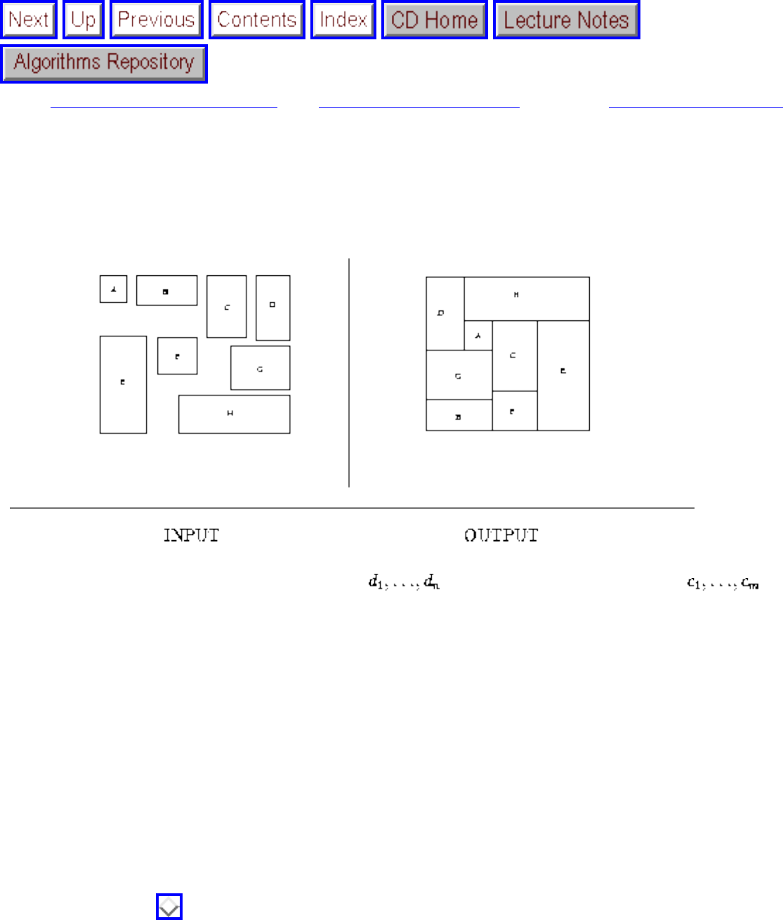
Bin Packing
Next: Medial-Axis Transformation Up: Computational Geometry Previous: Intersection Detection
Bin Packing
Input description: A set of n items with sizes . A set of m bins with capacity .
Problem description: How can you store all the items using the smallest number of bins?
Discussion: Bin packing arises in a variety of packaging and manufacturing problems. Suppose that
you are manufacturing widgets with parts cut from sheet metal, or pants with parts cut from cloth. To
minimize cost and waste, we seek to lay out the parts so as to use as few fixed-size metal sheets or bolts
of cloth as possible. Identifying which part goes on which sheet in which location is a bin-packing
variant called the cutting stock problem. After our widgets have been successfully manufactured, we
will be faced with another bin packing problem, namely how best to fit the boxes into trucks to minimize
the number of trucks needed to ship everything.
Even the most elementary-sounding bin-packing problems are NP-complete (see the discussion of integer
partition in Section ), so we are doomed to think in terms of heuristics instead of worst-case optimal
algorithms. Fortunately, relatively simple heuristics tend to work well on most bin-packing problems.
Further, many applications have peculiar, problem-specific constraints that would frustrate highly tuned
algorithms for the problem. The following factors will affect the choice of heuristic:
file:///E|/BOOK/BOOK5/NODE192.HTM (1 of 4) [19/1/2003 1:31:50]
Bin Packing
● What are the shapes and sizes of objects? - The character of the problem depends greatly on the
shapes of the objects to be packed. Packing pieces of a standard jigsaw puzzle is a different
problem than packing squares into a rectangular box. In one-dimensional bin packing, each
object's size is given simply as an integer, making it a version of the knapsack problem of Section
. This is equivalent to packing boxes of equal width into a chimney of that width. If all the
boxes are of identical size and shape, the optimal packing is simply a cubic lattice, oriented
appropriately with the walls of the bin. It is a waste to use the methods described in this section on
such simple problems.
● Are there constraints on the orientation and placement of objects? - In loading a truck, many of
the boxes will say ``this side up.'' Respecting this constraint restricts our flexibility in packing and
will likely lead to an increase in the number of trucks needed to send out the shipment. Similarly,
boxes with fragile objects may be labeled ``do not stack'' and thus are constrained to sit on top of
a pile of boxes. Most shippers seem to ignore these constraints. Indeed, your task will be simpler
if you don't have to worry about the consequences of them.
● Is the problem on-line or off-line? - Do we know the complete set of objects that we will be
packing at the beginning of the job (an off-line problem)? Or will we get them one at a time and
have to deal with them as they arrive (an on-line problem)? The difference is important,
because we can do a better job packing when we can take a global view and plan ahead. For
example, we can arrange the objects in an order that will facilitate efficient packing, perhaps by
sorting them from biggest to smallest.
The standard heuristics for bin packing order the objects by size or shape (or in an on-line problem,
simply the order they arrive in) and then insert them into bins. Typical insertion rules include (1) select
the first or leftmost bin the object fits in, (2) select the bin with the most room, (3) select the bin that
provides the tightest fit, or (4) select a random bin.
Analytical and empirical results suggest that the best heuristic is first-fit, decreasing. Sort the objects in
decreasing order of size, so that the biggest object is first and the smallest last. Insert each object one by
one into the first bin that has room for it. If no bin has room for it, we must start another bin. In the case
of one-dimensional bin packing, this can never require more than 22% more bins than necessary and
usually does much better. First-fit decreasing has an intuitive appeal to it; we pack the bulky objects first
and hope that the little objects can be used to fill up the cracks. First-fit decreasing is easily implemented
in time, where is the number of bins actually used, by doing a linear sweep
through the bins on each insertion. A faster implementation is possible by using binary tree to
keep track of the space remaining in each bin.
We can fiddle with the insertion order in such a scheme to deal with problem-specific constraints. For
example, it is reasonable to take ``do not stack'' boxes last (perhaps after artificially lowering the height
of the bins to give some room up top to work with) and to place fixed-orientation boxes at the beginning
(so we can use the extra flexibility later to stick boxes into cracks).
Packing boxes is much easier than packing arbitrary geometric shapes, enough so that a reasonable
file:///E|/BOOK/BOOK5/NODE192.HTM (2 of 4) [19/1/2003 1:31:50]
Bin Packing
approach for general shapes is to pack each part into its own box and then pack the boxes. Finding an
enclosing rectangle for a polygonal part is easy; just find the upper, lower, left, and right tangents in a
given orientation. A minimum-area enclosing rectangle can be found by determining the orientation that
leads to the smallest box.
In the case of nonconvex parts, considerable useful space can be wasted in the holes created by placing
the part in a box. One solution is to find the maximum empty rectangle within each boxed part and use
this to contain other parts if it is sufficiently large. More advanced solutions are discussed in the
references.
Implementations: Codes for the one-dimensional version of bin packing, the so-called knapsack
problem, are presented in Section .
XTango (see Section ) includes an animation of the first-fit bin packing heuristic. Test data for bin
packing is available from http://mscmga.ms.ic.ac.uk/info.html.
Notes: See [CGJ96] for a survey of the extensive literature on approximation algorithms for bin packing.
Expositions on heuristics for bin packing include [Baa88]. Experimental results on bin-packing heuristics
include [BJLM83].
Sphere packing is an important and well-studied special case of bin packing, with applications to error-
correcting codes. Particularly notorious is the ``Kepler conjecture,'' the apparently still-open problem of
establishing the densest packing of unit spheres in three dimensions. Conway and Sloane [CS93] is the
best reference on sphere packing and related problems. Sloane provides an extensive set of tables of the
best known packings, available from ftp://netlib.bell-labs.com.
Victor Milenkovic and his students have worked extensively on two-dimensional bin-packing problems
for the apparel industry, minimizing the amount of material needed to manufacture pants and other
clothing. Recent reports of this work include [DM97, Mil97].
Related Problems: Knapsack problem (see page ), set packing (see page ).
Next: Medial-Axis Transformation Up: Computational Geometry Previous: Intersection Detection
Algorithms
file:///E|/BOOK/BOOK5/NODE192.HTM (3 of 4) [19/1/2003 1:31:50]
Bin Packing
Mon Jun 2 23:33:50 EDT 1997
file:///E|/BOOK/BOOK5/NODE192.HTM (4 of 4) [19/1/2003 1:31:50]
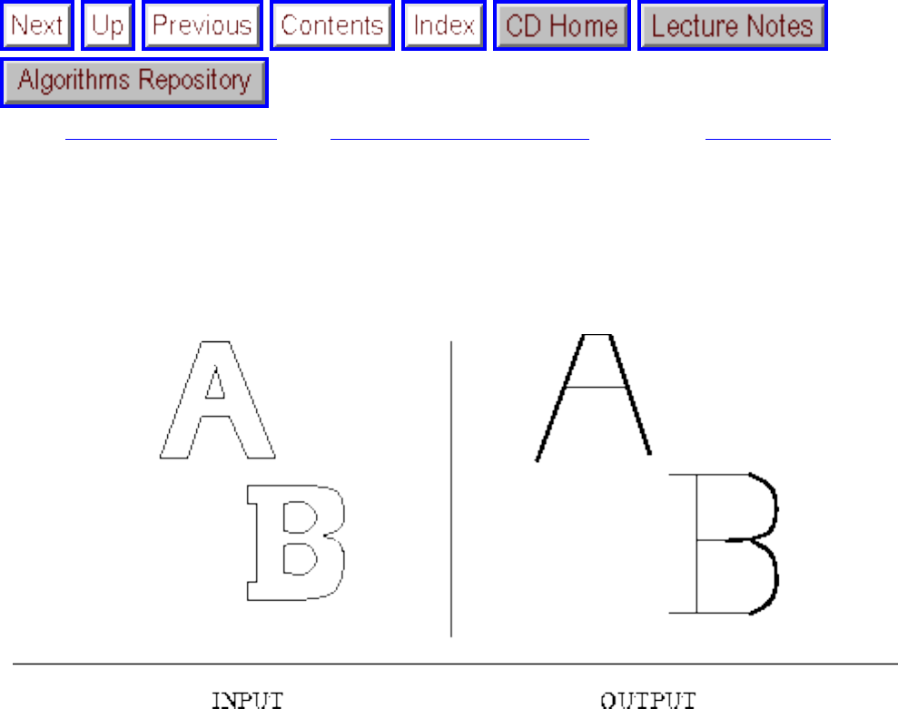
Medial-Axis Transformation
Next: Polygon Partitioning Up: Computational Geometry Previous: Bin Packing
Medial-Axis Transformation
Input description: A polygon or polyhedron P.
Problem description: What is the set of points within P that have more than one closest point on the
boundary of P?
Discussion: The medial-axis transformation is useful in thinning a polygon, or, as is sometimes said,
finding its skeleton. The goal is to extract a simple, robust representation of the shape of the polygon. As
can be seen from the figures above, the thinned versions of the letters capture the essence of the shape of
an `A' and a `B', and would be relatively unaffected by changing the thickness of strokes or by adding
font-dependent flourishes such as serifs.
The medial-axis transformation of a polygon is always a tree, making it fairly easy to use dynamic
programming to measure the ``edit distance'' between the skeleton of a known model and the skeleton of
an unknown object. Whenever the two skeletons are close enough, we can classify the unknown object as
an instance of our model. This technique has proven useful in computer vision and in optical character
recognition. The skeleton of a polygon with holes (like the `A' and `B') is not a tree, but an embedded
planar graph, but it remains easy to work with.
file:///E|/BOOK/BOOK5/NODE193.HTM (1 of 3) [19/1/2003 1:31:52]
Medial-Axis Transformation
There are two distinct approaches to computing medial-axis transforms, depending upon whether your
inputs are arbitrary geometric points or pixel images:
● Geometric data - Recall that the Voronoi diagram of a point set S decomposes the plane into
regions around each point such that each point within the region around is closer to
than to any other site in S. Similarly, the Voronoi diagram of a set of line segments L decomposes
the plane into regions around each line segment such that each point within the region
around is closer to than to any other site in L.
Any polygon is defined by a collection of line segments such that shares a vertex with . The
medial-axis transform of a polygon P is simply the portion of the line-segment Voronoi diagram
that lies within P.
Any line-segment Voronoi diagram code thus suffices to do polygon thinning. In the absence of
such a code, the most readily implementable thinning algorithm starts at each vertex of the
polygon and grows the skeleton inward with an edge bisecting the angle between the two
neighboring edges. Eventually, these two edges meet at an internal vertex, a point equally far
from three line segments. One of the three is now enclosed within a cell, while a bisector of the
two surviving segments grows out from the internal vertex. This process repeats until all edges
terminate in vertices.
● Image data - Whenever attempting geometric approaches to image processing problems, we must
remain aware that images are pixel-based and not continuous. All the pixels sit as lattice points on
an integer grid. While we can extract a polygonal description from the boundary and feed it to the
geometric algorithms above, the internal vertices of the skeleton will most likely not lie at grid
points. This may well make geometric approaches inappropriate for your intended application.
Algorithms that explicitly manipulate pixels tend to be easy to implement, because they avoid
complicated data structures. The basic pixel-based approach for constructing a skeleton directly
implements the ``brush fire'' view of thinning. Imagine a brush fire along all edges of the polygon,
burning inward at a constant speed. The skeleton is marked by all points where two or more fires
meet. The resulting algorithm traverses all the boundary pixels of the object, deletes all except
the extremal pixels, and repeats. The algorithm terminates when all pixels are extreme, leaving an
object only 1 or 2 pixels thick. When implemented properly, this takes time linear in the number
of pixels in the image.
The trouble with such pixel-based approaches is that the geometry doesn't work out exactly right.
For example, the skeleton of a polygon is no longer always a tree or even necessarily connected,
and the points in the skeleton will be close-to-but-not-quite equidistant to two boundary edges.
The usual solution is to tweak your implementation until it gives skeletons that look decent on the
data that you think is most interesting. Since you are trying to do continuous geometry in a
discrete world, there is no way to solve the problem completely. You just have to live with it.
file:///E|/BOOK/BOOK5/NODE193.HTM (2 of 3) [19/1/2003 1:31:52]
Medial-Axis Transformation
Implementations: MAT [Ogn93] is a medial-axis transform code designed for 2D skeletonization of
binary images, written by Robert Ogniewicz. MAT accepts a variety of different input formats, including
polygonal representations. This seems to be a solidly built program, and it should be your first stop on
seeking a routine for thinning. It available from http://hrl.harvard.edu/people/postdocs/rlo/rlo.dir/rlo-
soft.html.
Programs for constructing Voronoi diagrams are discussed in Section .
Notes: For a comprehensive surveys of thinning approaches in image processing, see [LLS92, Ogn93].
The medial axis transformation was introduced for shape similarity studies in biology [Blu67].
Applications of the medial-axis transformation in pattern recognition are discussed in [DH73]. Good
expositions on the medial-axis transform include [O'R94, Pav82].
The medial-axis of a polygon can be computed in time for arbitrary n-gons [Lee82], although
linear-time algorithms exist for convex polygons [AGSS89]. An algorithm for constructing
medial-axis transforms in curved regions was given by Kirkpatrick [Kir79].
Related Problems: Voronoi diagrams (see page ), Minkowski sum (see page ).
Next: Polygon Partitioning Up: Computational Geometry Previous: Bin Packing
Algorithms
Mon Jun 2 23:33:50 EDT 1997
file:///E|/BOOK/BOOK5/NODE193.HTM (3 of 3) [19/1/2003 1:31:52]
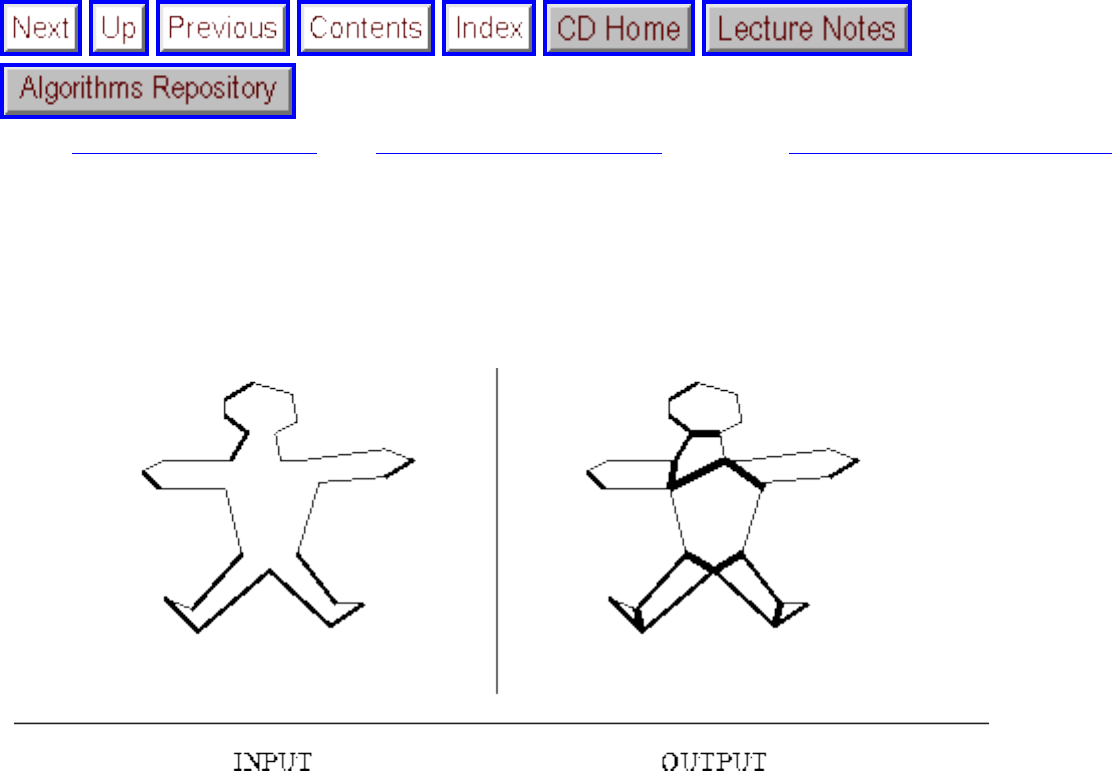
Polygon Partitioning
Next: Simplifying Polygons Up: Computational Geometry Previous: Medial-Axis Transformation
Polygon Partitioning
Input description: A polygon or polyhedron P.
Problem description: How can P be partitioned into a small number of simple (typically convex)
pieces?
Discussion: Polygon partitioning is an important preprocessing step for many geometric algorithms,
because most geometric problems are simpler and faster on convex objects than on nonconvex ones. We
are better off whenever we can partition a nonconvex object into a small number of convex pieces,
because it is easier to work with the pieces independently than with the original object.
Several flavors of polygon partitioning arise, depending upon the particular application:
● Should all the pieces be triangles? - The mother of all polygon partitioning problems is
triangulation, where the interior of the polygon is completely partitioned into triangles. Triangles
are always convex and have only three sides, so any geometric operation performed on a triangle
is destined to be as simple as it can be.
Because triangles all have three sides, all triangulations of polygons contain exactly the same
file:///E|/BOOK/BOOK5/NODE194.HTM (1 of 3) [19/1/2003 1:31:53]
Polygon Partitioning
number of pieces. Therefore, triangulation cannot be the answer if we seek a small number of
convex pieces. The goal of finding ``nice'' triangulations revolves around the shape of the
triangles. See Section for a thorough discussion of triangulation.
● Do I want to cover or partition my polygon? - Partitioning a polygon means completely dividing
the interior into nonoverlapping pieces. Covering a polygon means that our decomposition is
permitted to contain mutually overlapping pieces. Both can be useful in different situations. In
decomposing a complicated query polygon in preparation for range search (Section ), we seek
a partitioning, so that each point we locate occurs in exactly one piece. In decomposing a polygon
for painting purposes, a covering suffices, since there is no difficulty with filling in a region twice.
We will concentrate here on partitioning, since it is simpler to do right, and any application
needing a covering will accept a partitioning. The only potential drawback is that partitions can be
somewhat larger than coverings.
● Am I allowed to add extra vertices? - A final issue associated with polygon decomposition is
whether we are allowed to add Steiner vertices (either by splitting edges or adding interior points)
or whether we are restricted to adding chords between two existing vertices. The former may
result in a smaller number of pieces, at the cost of more complicated algorithms and perhaps
messier results.
The Hertel-Mehlhorn heuristic for convex decomposition using diagonals is simple, efficient, and always
produces no more than four times the minimum number of convex pieces. It starts with an arbitrary
triangulation of the polygon and then deletes a chord that leaves only convex pieces. The decision of
whether a chord deletion will create a nonconvex piece can be made locally from the chords and edges
surrounding the chord, in constant time. A vertex in a polygon is reflex if the internal angle is greater
than 180 degrees. We can delete any chord that does not create a reflex vertex.
I recommend using this heuristic unless it is critical for you to absolutely minimize the number of pieces.
By experimenting with different triangulations and various deletion orders, you may be able to obtain
somewhat better decompositions.
Dynamic programming may be used to minimize the number of diagonals used in the decomposition.
The simplest implementation, which maintains the number of pieces for all subpolygons split by a
chord, runs in . Faster algorithms use fancier data structures, running in time, where r is
the number of reflex vertices. An algorithm that further reduces the number of pieces by adding
interior vertices is cited below, although it is complex and presumably difficult to implement.
Implementations: Many triangulation codes start by finding a trapezoidal or monotone decomposition of
polygons. Further, a triangulation is a simple form of convex decomposition. Check out the codes in
Section as a starting point for most any decomposition problem.
A triangulation code of particular relevance here is GEOMPACK, a suite of Fortran 77 codes by Barry
Joe, for 2- and 3-dimensional triangulation and convex decomposition problems. In particular, it does
file:///E|/BOOK/BOOK5/NODE194.HTM (2 of 3) [19/1/2003 1:31:53]
Polygon Partitioning
both Delaunay triangulation and convex decompositions of polygonal and polyhedral regions, as well as
arbitrary-dimensional Delaunay triangulations.
Notes: Keil and Sack [KS85] given an excellent survey on what is known about partitioning and
covering polygons. Expositions on the Hertel-Mehlhorn heuristic [HM83] include [O'R94]. The
dynamic programming algorithm for minimum convex decomposition using diagonals is due
to Keil [Kei85]. The algorithm minimizing the number of convex pieces with Steiner points
appears in [CD85]. Feng and Pavlidis [FP75b] give a heuristic algorithm for polygon decomposition and
apply it to optical character recognition.
Art gallery problems are an interesting topic related to polygon covering, where we seek to position the
minimum number of guards in a given polygon such that every point in the interior of the polygon is
watched by at least one guard. This corresponds to covering the polygon with a minimum number of star-
shaped polygons. O'Rourke [O'R87] is a beautiful book which presents the art gallery problem and its
many variations.
Related Problems: Triangulation (see page ), set cover (see page ).
Next: Simplifying Polygons Up: Computational Geometry Previous: Medial-Axis Transformation
Algorithms
Mon Jun 2 23:33:50 EDT 1997
file:///E|/BOOK/BOOK5/NODE194.HTM (3 of 3) [19/1/2003 1:31:53]
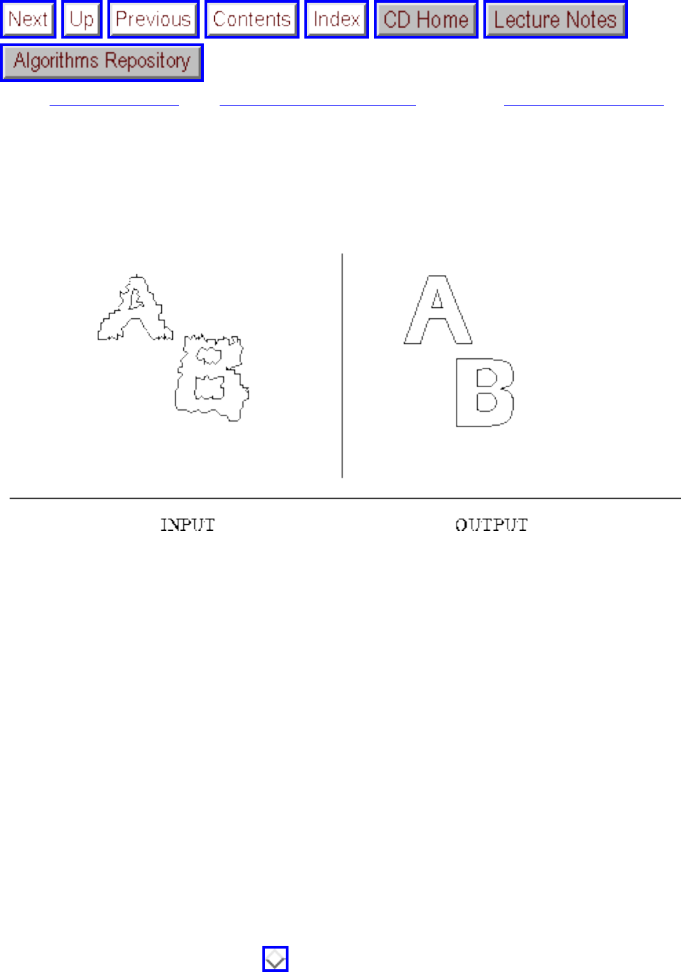
Simplifying Polygons
Next: Shape Similarity Up: Computational Geometry Previous: Polygon Partitioning
Simplifying Polygons
Input description: A polygon or polyhedron p, with n vertices.
Problem description: Find a polygon or polyhedron p' with n' vertices, where the shape of p' is close to
p and n' < n.
Discussion: Polygon simplification has two primary applications. The first is in cleaning up a noisy
representation of a polygon, perhaps obtained by scanning a picture of an object. By processing it, we
hope to remove the noise and reconstruct the original object. The second is in data compression, where
given a large and complicated object, we seek to simplify it by reducing detail. Ideally, we obtain a
polygon with far fewer vertices that looks essentially the same. This can be a big win in computer
graphics, where replacing a large model with a smaller model might have little visual impact but be
significantly faster to render.
Several issues arise in shape simplification:
● Do you want the convex hull? - The simplest way to simplify a polygon is to take the convex hull
of its vertices (see Section ). The convex hull removes all internal concavities from the
polygon. If you were simplifying a robot model for motion planning, this is a good thing, because
file:///E|/BOOK/BOOK5/NODE195.HTM (1 of 4) [19/1/2003 1:31:55]
Simplifying Polygons
you are unlikely to be able to take advantage of the concavities in finding paths. If you were
building an OCR system, the convex hull would be disastrous, because the concavities of
characters provide most of the interesting features. An `X' would be identical to an `I', since both
hulls are boxes. Another problem is that if the polygon is already convex, taking the convex hull
will do nothing to simplify it further.
● Am I allowed to insert or just delete points? - What is typically needed is a way to represent the
object as well as possible using only a given number of vertices. The simplest approaches employ
local modifications to the boundary of the polygon, in order to reduce the vertex count. For
example, if three consecutive vertices form a small-area triangle or define an extremely large
angle, the center vertex can be deleted and replaced with an edge without severely distorting the
polygon.
Methods that only delete vertices quickly melt the shape into unrecognizability, however. More
robust heuristics move vertices around to cover up the gaps that are created by deletions. Such
``split-and-merge'' heuristics can do a decent job, although nothing is guaranteed. Better results
are likely by using the Douglas-Peucker algorithm, described below.
● Must the resulting polygon be intersection-free? - A serious drawback of such incremental
procedures is that they fail to ensure simple polygons, those without self-intersections. Thus the
``simplified'' polygon may have artifacts that look ugly and that may cause problems for
subsequent routines working on the polygon. If simplicity is important, you should test all the line
segments of your polygon for any pairwise intersections, as discussed in Section .
An approach to polygon simplification that guarantees a simple approximation involves
computing minimum-link paths. The link distance of a path between points and t is the number of
straight segments on the path. An as-the-crow-flies path has a link distance of one. In general, the
link distance is one more than the number of turns. The link distance between points and t in a
scene with obstacles is defined by the minimum link distance over all paths from to t.
The link distance approach ``fattens'' the boundary of the polygon by some acceptable error
window (see Section ) in order to construct a channel around the polygon and then constructs
the minimum-link path through this channel. The minimum-link cycle in this channel represents
the simplest polygon that never deviates from the original boundary by more than . It constructs
a globally optimal simplification that will not self-intersect, at the cost of implementation and
time complexity.
● Are you given an image to clean up instead of a polygon to simplify? - The conventional,
nongeometric approach to cleaning up noise from a digital image is to take the Fourier transform
of the image, filter out the high-frequency elements, and then take the inverse transform to
recreate the image. See Section for details on the fast Fourier transform.
The Douglas-Plucker algorithm for shape simplification starts with a simple approximation and then
refines it, instead of starting with a complicated polygon and trying to simplify it. Start by selecting two
file:///E|/BOOK/BOOK5/NODE195.HTM (2 of 4) [19/1/2003 1:31:55]
Simplifying Polygons
vertices and of polygon P, and propose the degenerate polygon as a simple approximation
P'. Scan through each of the vertices of P, and select the one that is farthest from the corresponding edge
of the polygon P'. Inserting this vertex adds the triangle to P' so as to minimize the maximum deviation
from P. Points can be inserted until satisfactory results are achieved. This takes O(kn) to insert k points
when |P|=n.
Simplification becomes considerably more difficult in three dimensions. For example, it is NP-complete
to find the minimum-size surface separating two polyhedra. Higher-dimensional analogies of the planar
algorithms discussed here can be used to heuristically simplify polyhedra. See the references below.
Implementations: A program for automatically generating level-of-detail hierarchies for polygonal
models is available from http://www.cs.unc.edu/ geom/envelope.html and is free for noncommercial
use. The user specifies a single error tolerance, and the maximum surface deviation of the simplified
model from the original model, and a new, simplified model is generated. This code preserves holes and
prevents self-intersection.
Yet another approach to polygonal simplification is based on simplifying and expanding the medial-axis
transform of the polygon. The medial-axis transform (see Section ) produces a skeleton of the
polygon, which can be trimmed before inverting the transform to yield a simpler polygon. MAT [Ogn93]
is a medial-axis transform code designed for 2D skeletonization and inversion of binary images, written
by Robert Ogniewicz and available from http://hrl.harvard.edu/people/postdocs/rlo/rlo.dir/rlo-soft.html.
Notes: See [HG95] for a thorough survey of algorithms for shape simplification. It is also available from
http://www.cs.cmu.edu/afs/cs/user/ph/www/heckbert.html, along with implementations.
The Douglas-Peucker incremental refinement algorithm [DP73] is the basis for most shape simplification
schemes, with a faster implementation due to Hershberger and Snoeyink [HS94]. The link distance
approach to polygon simplification is presented in [GHMS93]. Shape simplification problems become
considerably more complex in three dimensions. Even finding the minimum-vertex convex polyhedron
lying between two nested convex polyhedra is NP-complete [DJ92], although approximation algorithms
are known [MS95b].
Testing whether a polygon is simple can be performed in linear time, at least in theory, as a consequence
of Chazelle's linear-time triangulation algorithm [Cha91].
Related Problems: Fourier transform (see page ), convex hull (see page ).
file:///E|/BOOK/BOOK5/NODE195.HTM (3 of 4) [19/1/2003 1:31:55]

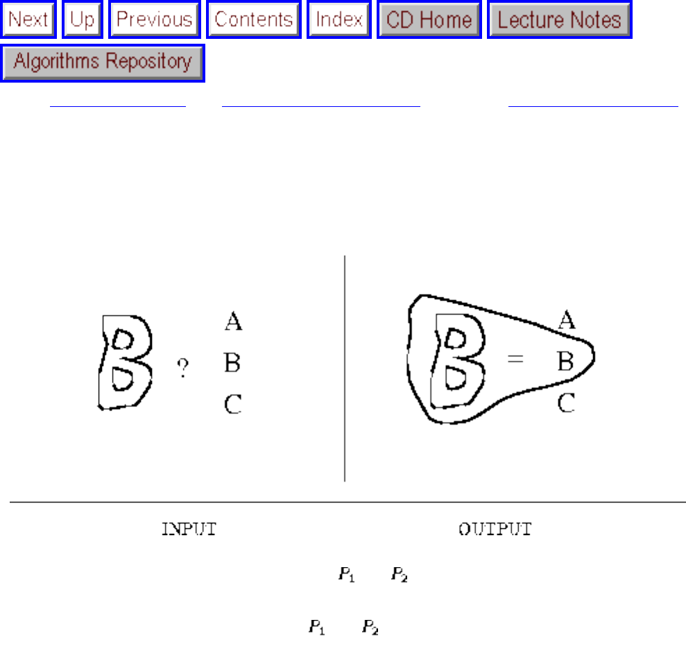
Shape Similarity
Next: Motion Planning Up: Computational Geometry Previous: Simplifying Polygons
Shape Similarity
Input description: Two polygonal shapes, and .
Problem description: How similar are and ?
Discussion: Shape similarity is a problem that underlies much of pattern recognition. Consider a system
for optical character recognition (OCR). We have a known library of shape models representing letters
and the unknown shapes we obtain by scanning a page. We seek to identify an unknown shape by
matching it to the most similar shape model.
The problem of shape similarity is inherently ill-defined, because what ``similar'' means is application
dependent. Thus no single algorithmic approach can solve all shape matching problems. Whichever
method you select, expect to spend a large chunk of time tweaking it so as to achieve maximum
performance. Don't kid yourself - this is a difficult problem.
Among your possible approaches are:
● Hamming Distance - Assume that your two polygons have been overlaid one on top of the other.
The Hamming distance measures the area of symmetric difference between the two polygons, in
file:///E|/BOOK/BOOK5/NODE196.HTM (1 of 3) [19/1/2003 1:31:56]
Shape Similarity
other words, the area of the regions lying within one of the two polygons but not both of them. If
the two polygons are identical, and properly aligned, the Hamming distance will be zero. If the
polygons differ only in a little noise at the boundary, then the Hamming distance will be small if
the polygons are properly aligned. If the two polygons are completely disjoint, then the Hamming
distance is the sum of the areas of the two polygons.
Computing the area of the symmetric difference reduces to finding the intersection or union of
two polygons, as discussed in Section , and then computing areas, as discussed in . The
difficult part of computing Hamming distance is finding the right alignment, or overlay, of the
two polygons. For certain applications, such as OCR, the overlay problem is simplified because
the characters are inherently aligned with the page and thus not free to rotate. Hamming distance
is particularly simple and efficient to compute on bit-mapped images, since after alignment all we
do is sum the differences of the corresponding pixels.
Although Hamming distance makes sense conceptually and can be simple to implement, it
captures only a crude notion of shape and is likely to be ineffective in most applications.
● Hausdorff distance - An alternative distance metric is Hausdorff distance, which identifies the
point on that is the maximum distance from and returns this distance. The Hausdorff distance
is not symmetrical, for the distance from to is not necessarily the distance from to .
Note the difference between Hamming and Hausdorff distance. A large but thin protrusion from
one of the models will have a large effect on the Hausdorff distance but little on the Hamming
distance. However, a fattening of the entire boundary of one of the models (as is liable to happen
with boundary noise) by a small amount will increase the Hamming distance yet have little effect
on the Hausdorff distance.
Which is better, Hamming or Hausdorff? It depends upon your application. As with Hamming
distance, computing the right alignment between the polygons can be difficult and time-
consuming. Again, Hausdorff distance captures only a crude notion of shape.
● Comparing Skeletons - A more powerful approach to shape similarity uses thinning (see Section
) to extract a tree-like skeleton for each object. This skeleton captures many aspects of the
original shape. The problem now reduces to comparing the shape of two such skeletons, using
such features as the topology of the tree and the lengths/slopes of the edges. This comparison can
be modeled as a form of subgraph isomorphism (see Section ), with edges allowed to match
whenever their lengths and slopes are sufficiently similar.
● Neural Networks - A final method for shape comparison uses neural networks, which are
discussed in Section . Neural nets prove a reasonable approach to recognition problems when
you have a lot of data to experiment with and no particular ideas of what to do with it. First, you
must identify a set of easily computed features of the shape, such as area, number of sides, and
number of holes. Based on these features, a black-box program (the neural network training
algorithm) takes your training data and produces a classification function. This classification
function accepts as input the values of these features and returns a measure of what the shape is,
file:///E|/BOOK/BOOK5/NODE196.HTM (2 of 3) [19/1/2003 1:31:56]
Shape Similarity
or how close it is to a particular shape.
How good are the resulting classifiers? It depends upon the application. Like any ad hoc method,
neural networks usually take a fair amount of tweaking and tuning to realize their full potential.
One caveat. Because your classifier was developed by a black box, you never really know why
your classifier is making its decisions, so you can't know when it will fail. An interesting case was
a system built for the military to distinguish between images of cars and tanks. It performed very
well on test images but disastrously in the field. Eventually, someone realized that the car images
had been filmed on a sunnier day than the tanks, and the program was classifying solely on the
presence of clouds in the background of the image!
Implementations: The Stuttgart Neural Network Simulator supports many types of networks and
training algorithms, as well as sophisticated graphical visualization tools under X11. It has been ported to
many flavors of UNIX. It is available for ftp from ftp.informatik.uni-stuttgart.de [129.69.211.2] in
directory /pub/SNNS as SNNSv4.1.tar.gz (1.4 MB, Source code) and SNNSv4.1.Manual.ps.gz (1 MB,
Documentation). It may be best to first have a look at the file SNNSv4.1.Readme. More information can
be found in the WWW under http://www.informatik.uni-stuttgart.de/ipvr/bv/projekte/snns/snns.html
An alternate distance metric between polygons can be based on its angle turning function [ACH 91].
An implementation in C of this turning function metric by Eugene K. Ressler is provided on the
algorithm repository http://www.cs.sunysb.edu/ algorith.
Notes: General books on pattern classification algorithms include [DH73, JD88]. A wide variety of
computational geometry approaches to shape similarity testing have been proposed, including
[AMWW88, ACH 91, Ata84, AE83, BM89, OW85].
A linear-time algorithm for computing the Hausdorff distance between two convex polygons is given in
[Ata83], with algorithms for the general case reported in [HK90].
Related Problems: Graph isomorphism (see page ), thinning (see page ).
Next: Motion Planning Up: Computational Geometry Previous: Simplifying Polygons
Algorithms
Mon Jun 2 23:33:50 EDT 1997
file:///E|/BOOK/BOOK5/NODE196.HTM (3 of 3) [19/1/2003 1:31:56]
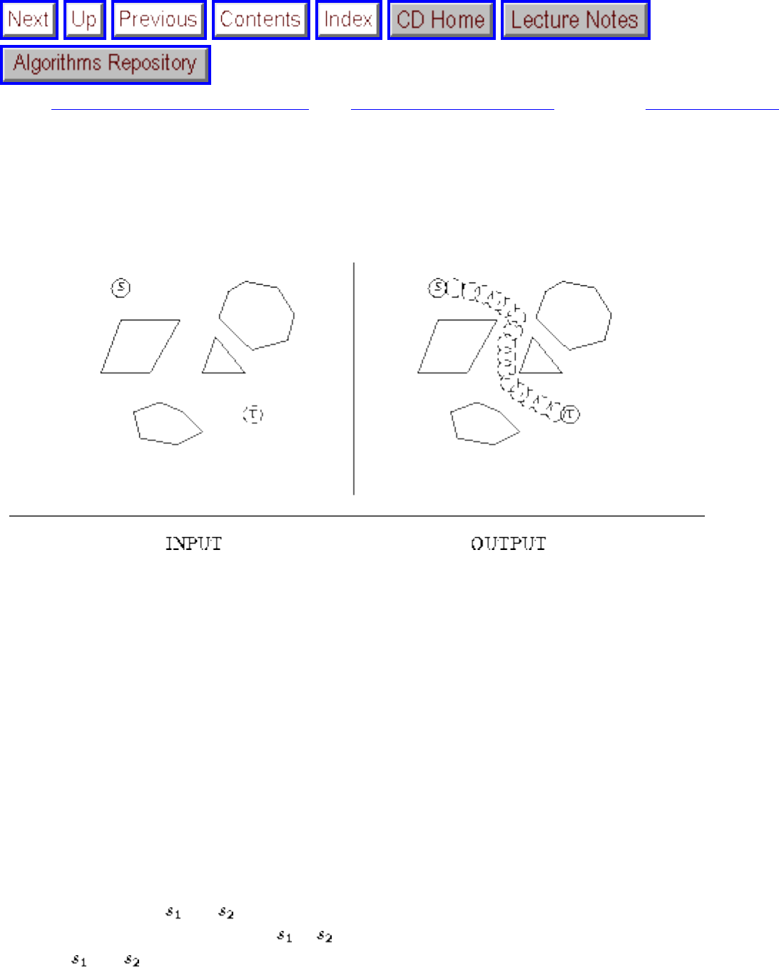
Motion Planning
Next: Maintaining Line Arrangements Up: Computational Geometry Previous: Shape Similarity
Motion Planning
Input description: A polygonal-shaped robot in a given starting position in a room containing polygonal
obstacles, with a desired ending position t.
Problem description: Find the shortest path in the room taking to t without intersecting any of the
obstacles.
Discussion: The difficulty of motion planning will be obvious to anyone who has ever had to move a
large piece of furniture into a small apartment. The problem of motion planning also arises in systems for
molecular docking. Many drugs are small molecules that act by binding to a given target model. The
problem of identifying which binding sites are accessible to a candidate drug is clearly an instance of
motion planning. Plotting paths for mobile robots is another canonical motion-planning application.
Motion planning also provides a tool for computer animation. Given a set of object models that appear in
two different scenes and , a motion planning algorithm can construct a short sequence of
intermediate motions to transform to . These motions can serve to fill in the intermediate scenes
between and , with such scene interpolation greatly reducing the amount of work the animator has to
do.
file:///E|/BOOK/BOOK5/NODE197.HTM (1 of 4) [19/1/2003 1:31:58]
Motion Planning
There is a wide range in the complexity of motion planning problems, with many factors to consider:
● Is your robot a point? - When the robot is a point, the problem becomes finding the shortest path
from to t around the obstacles, also known as geometric shortest path. The most readily
implementable approach constructs the visibility graph of the polygonal obstacles, plus the points
and t. This visibility graph has a vertex for each obstacle vertex and an edge between two obstacle
vertices if they ``see'' each other without being blocked by some obstacle edge.
A brute-force algorithm to construct the visibility graph tests each candidate edge against the
obstacle edges for a total time of time. By weighting each edge of the visibility graph with
its length and using Dijkstra's shortest-path algorithm (see Section ) on this graph, we can find
the shortest path from to t in time bounded by the time to construct the graph.
● How is your robot free to move? - Motion planning becomes considerably more difficult when the
robot becomes a polygon instead of a point. Now we must make sure that all of the corridors we
use are wide enough to permit the robot to pass through. The complexity depends upon the
number of degrees of freedom the robot has to move. Is it free to rotate as well as to translate?
Does the robot have links that are free to bend or to rotate independently, as in an arm with a
hand? Each degree of freedom corresponds to a dimension in the search space. Therefore, the
more freedom, the harder it is to compute a path between two locations, although it becomes more
likely that such a path exists.
● Can you simplify the shape of your robot? - Motion planning algorithms tend to be complex and
time-consuming. Anything you can do to simplify your environment would be a win. In
particular, consider replacing your robot by an enclosing disk. If there is a path for the disk, there
will be a path for whatever is inside of it. Further, since any orientation of a disk is equivalent to
any other orientation, rotation provides no help in finding a path Therefore, all movements are
limited to translation only.
● Are motions limited to translation only? - When rotation is not allowed, the expanded obstacles
approach can be used to reduce the problem to that of motion planning for a point robot, which is
simply the shortest path in a graph. Pick a reference point on the robot, and replace each obstacle
by the Minkowski sum of the object and the robot (see Section ). This creates a larger obstacle,
defined as the robot walks a loop around the obstacle while maintaining contact with it. Finding a
path from the initial position of the reference point to the goal point amidst these fattened
obstacles defines a legal path for the polygonal robot.
● Are the obstacles known in advance? - Thus far we have assumed that the robot starts out with a
map of its environment. This is not always true, or even possible, in applications where the
obstacles move. There are two approaches to solving motion planning problems without a map.
The first approach explores the environment, building a map of what has been seen, and then uses
this map to plan a path to the goal. A simpler strategy, which will fail in environments of
sufficient complexity, proceeds like a sightless man with a compass. Walk in the direction
towards the goal until progress is blocked by an obstacle, and then trace a path along the obstacle
until the robot is again free to proceed directly towards the goal.
file:///E|/BOOK/BOOK5/NODE197.HTM (2 of 4) [19/1/2003 1:31:58]
Motion Planning
The most practical approach to motion planning involves randomly sampling the configuration space of
the robot. The configuration space defines the set of legal positions for the robot and has one dimension
for each degree of freedom. For a planar robot capable of translation and rotation, the degrees of freedom
are the x- and y-coordinates of a reference point on the robot and the angle relative to this point. Certain
points in this space represent legal positions, while others intersect obstacles.
Construct a set of legal configuration-space points by random sampling. For each pair of points and ,
decide whether there exists a direct, nonintersecting path between them. Construct a graph with vertices
for each legal point and edges for each such traversable pair. The problem of finding a motion between
two arbitrary positions reduces to seeing if there is a direct path from the initial/final position to some
vertex in the graph, and then solving a shortest-path problem in the graph.
There are lots of ways to enhance this basic technique for specific applications, such as adding additional
vertices to regions of particular interest. This is a nice, clean approach for solving problems that would
get very messy otherwise.
Implementations: An implementation of collision detection (not really motion planning) is the
I_COLLIDE collision detection library. For more information, check out the I_COLLIDE WWW page:
http://www.cs.unc.edu/ geom/I_COLLIDE.html.
O'Rourke [O'R94] gives a toy implementation of an algorithm to plot motion for a two-jointed robot arm
in the plane. See Section .
Notes: Motion planning was originally studied by Schwartz and Sharir as the ``piano mover's problem.''
Their solution constructs the complete free space of robot positions which do not intersect obstacles, and
then finds the shortest path within the proper connected component. These free space descriptions are
very complicated, involving arrangements of higher-degree algebraic surfaces. The fundamental papers
on the piano mover's problem appear in [HSS87], with [SS90] being a survey of current results. The best
general result for this free space approach to motion planning is due to Canny [Can87], who showed that
any problem with d degrees of freedom can be solved in , although faster algorithms exist for
special cases of the general motion planning problem.
Latombe's book [Lat91] describes practical approaches to motion planning, including the random
sampling method described above. The expanded obstacle approach to motion planning is due to Lozano-
Perez and Wesley [LPW79]. The heuristic, sightless man's approach to motion planning discussed above
has been studied by Lumelski [LS87].
The time complexity of algorithms based on the free-space approach to motion planning depends
intimately on the combinatorial complexity of the arrangement of surfaces defining the free space.
Algorithms for maintaining arrangements are presented in Section . Davenport-Schintzl sequences
file:///E|/BOOK/BOOK5/NODE197.HTM (3 of 4) [19/1/2003 1:31:58]
Motion Planning
often arise in the analysis of such arrangements. Sharir and Agarwal [SA95] provide a comprehensive
treatment of Davenport-Schintzl sequences and their relevance to motion planning.
Kedem and Sharir [KS90] give an time algorithm to find a path (not necessarily shortest) to
translate a convex k-gon from to t. Vegter [Veg90] gives an optimal algorithm for moving a line
segment (often called a ladder) in the plane with both translation and rotation.
Related Problems: Shortest path (see page ), Minkowski sum (see page ).
Next: Maintaining Line Arrangements Up: Computational Geometry Previous: Shape Similarity
Algorithms
Mon Jun 2 23:33:50 EDT 1997
file:///E|/BOOK/BOOK5/NODE197.HTM (4 of 4) [19/1/2003 1:31:58]
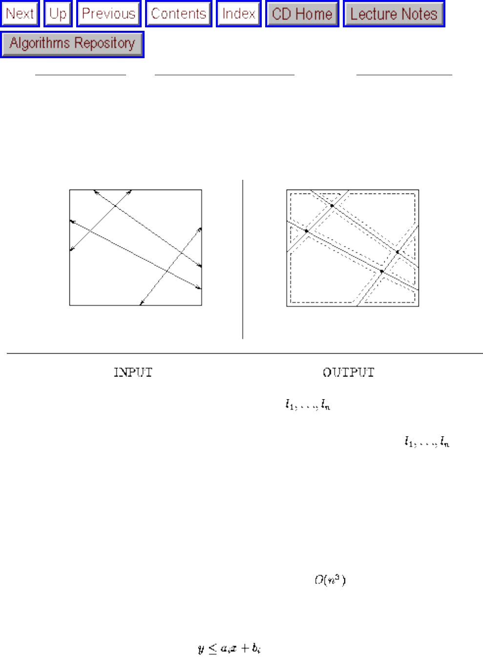
Maintaining Line Arrangements
Next: Minkowski Sum Up: Computational Geometry Previous: Motion Planning
Maintaining Line Arrangements
Input description: A set of lines and line segments .
Problem description: What is the decomposition of the plane defined by ?
Discussion: One of the most fundamental problems in computational geometry is constructing
arrangements of lines, that is, explicitly building the regions formed by the intersections of a set of n
lines. Algorithms for a surprising number of problems are based on constructing and analyzing the
arrangement of a specific set of lines:
● Degeneracy testing - Given a set of n lines in the plane, do any three of them pass through the
same point? Brute-force testing of all triples takes time. Instead, we can construct the
arrangement of the lines and then walk over each vertex and explicitly count its degree, all in
quadratic time.
● Satisfying the maximum number of linear constraints - Suppose that we are given a set of n linear
constraints, each of the form . Which point in the plane satisfies the largest number of
them? Construct the arrangement of the lines. All points in any region or cell of this arrangement
satisfy exactly the same set of constraints, so we need to test only one point per cell in order to
find the global maximum.
file:///E|/BOOK/BOOK5/NODE198.HTM (1 of 4) [19/1/2003 1:32:00]
Maintaining Line Arrangements
Thinking of geometric problems in terms of the appropriate features in an arrangement can be very useful
in formulating algorithms. Unfortunately, it must be admitted that arrangements are not as popular in
practice as might be supposed. First, a certain depth of understanding is required to apply them correctly.
Second, there have been few available implementations of the fundamental algorithms, a situation that is
partially addressed below.
● What do you want to do with the arrangement? - Given an arrangement and a query point, we are
often interested in identifying which cell of the arrangement contains the point. This is the
problem of point location, discussed in Section . Given an arrangement of lines or line
segments, we are often interested in computing all points of intersection of the lines. The problem
of intersection detection is discussed in Section .
● How big will your arrangement be? - Algorithms for constructing arrangements are incremental.
Beginning with an arrangement of one or two lines, subsequent lines are inserted into the
arrangement one at a time, building larger and larger arrangements. To insert a new line, we start
on the leftmost cell containing the line and walk over the arrangement to the right, moving from
cell to neighboring cell and splitting into two pieces those cells that contain the new line.
A geometric fact called the zone theorem implies that the kth line inserted cuts through k cells of
the arrangement, and further that O(k) total edges form the boundary of these cells. This means
that we can scan through each edge of every cell we encounter on our insertion walk, confident
that linear total work will be performed while inserting the line into the arrangement. Therefore,
the total time to insert all n lines in constructing the full arrangement is .
● Does your input consist of points instead of lines? - Although lines and points seem to be different
geometric objects, such appearances can be misleading. Through the use of duality
transformations, we can turn line L into point p and vice versa:
Duality is important because we can now apply line arrangements to point problems, often with
surprising results.
For example, suppose we are given a set of n points, and we want to know whether any three of
them all lie on the same line. This sounds similar to the degeneracy testing problem discussed
above. Not only is it similar, it is exactly the same, with only the role of points and lines
exchanged. The answer follows from taking our points, dualizing them into lines as above,
constructing the arrangement as above, and then searching for a vertex with three lines passing
through it. The dual of this vertex gives the line on which the three initial vertices lie.
Once we have constructed an arrangement through incremental methods, it often becomes useful to
traverse each face of the arrangement exactly once. Such traversals are called sweepline algorithms and
file:///E|/BOOK/BOOK5/NODE198.HTM (2 of 4) [19/1/2003 1:32:00]
Maintaining Line Arrangements
are discussed in some detail in Section . The basic procedure is to sort the intersection points by x-
coordinate and then walk from left to right while keeping track of all we have seen.
Implementations: Arrange is a package written in C by Michael Goldwasser for maintaining
arrangements of polygons in either the plane or on the sphere. Polygons may be degenerate and hence
represent arrangements of lines. A randomized incremental construction algorithm is used and efficient
point location on the arrangement supported. Polygons may be inserted but not deleted from the
arrangement, and arrangements of several thousand vertices and edges can be constructed in a few
seconds. Arrange is available from http://theory.stanford.edu/people/wass/wass.html.
LEDA (see Section ) provides a function that constructs an embedded planar graph from a set of line
segments, essentially constructing their arrangement.
Notes: Edelsbrunner [Ede87] provides a comprehensive treatment of the combinatorial theory of
arrangements, plus algorithms on arrangements with applications. It is an essential reference for anyone
seriously interested in the subject. Good expositions on constructing arrangements include [O'R94].
Arrangements generalize naturally beyond two dimensions. Instead of lines, the space decomposition is
defined by planes (or beyond 3-dimensions, hyperplanes). In general dimensions, the zone theorem states
that any arrangement of n d-dimensional hyperplanes has total complexity , and any single
hyperplane intersects cells of complexity . This provides the justification for the incremental
construction algorithm for arrangements. Walking around the boundary of each cell to find the next cell
that the hyperplane intersects takes time proportional to the number of cells created by inserting the
hyperplane.
The history of the zone theorem has become somewhat muddled, because the original proofs were later
found to be in error in higher dimensions. See [ESS93] for a discussion and a correct proof. The theory
of Davenport-Schintzl sequences is intimately tied into the study of arrangements. It is presented in
[SA95].
The naive algorithm for sweeping an arrangement of lines sorts the intersection points by x-coordinate
and hence requires time. The topological sweep [EG89, EG91] eliminates the need to sort, and
it traverses the arrangement in quadratic time. This algorithm is readily implementable and can be
applied to speed up many sweepline algorithms.
Related Problems: Intersection detection (see page ), point location (see page ).
file:///E|/BOOK/BOOK5/NODE198.HTM (3 of 4) [19/1/2003 1:32:00]

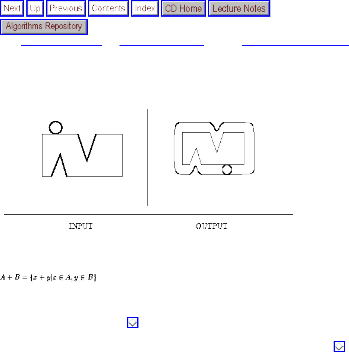
Minkowski Sum
Next: Set and String Problems Up: Computational Geometry Previous: Maintaining Line Arrangements
Minkowski Sum
Input description: Point sets or polygons A and B, with n and m vertices, respectively.
Problem description: What is the convolution of A and B, i.e. the Minkowski sum
?
Discussion: Minkowski sums are useful geometric operations that can be used to fatten objects in
appropriate ways. For example, a popular approach to motion planning for polygonal robots in a room
with polygonal obstacles (see Section ) fattens each of the obstacles by taking the Minkowski sum of
them with the shape of the robot. This reduces the problem to moving a point from the start to the goal
using a standard shortest-path algorithm. Another application is in shape simplification (see Section ),
where we fatten the boundary of an object to create a channel and then define as the shape the minimum
link path lying within this channel. Similarly, convolving an irregular object with a small circle will help
smooth out the boundaries by eliminating minor nicks and cuts.
The definition of Minkowski sum assumes that the polygons A and B have been positioned on a
coordinate system:
file:///E|/BOOK/BOOK5/NODE199.HTM (1 of 3) [19/1/2003 1:32:01]
Minkowski Sum
where x+y is the vector sum of two points. Thinking of this in terms of translation, the Minkowski sum is
the union of all translations of A by a point defined within B. Issues arising in computing Minkowski
sums include:
● Are your objects rasterized images or explicit polygons? - The definition of Minkowski
summation suggests a simple algorithm if A and B are rasterized images, and thus contain a
number of pixels proportional to their area. Initialize a sufficiently large matrix of pixels by
determining the size of the convolution of the bounding boxes of A and B. For each pair of points
in A and B, sum up their coordinates and darken the appropriate pixel. These algorithms get
somewhat more complicated if an explicit polygonal representation of the Minkowski sum is
needed.
● Are your objects convex or nonconvex? - The complexity of computing Minkowski sum depends
in a serious way on the shape of the polygons. If both A and B are convex, the Minkowski sum
can be found in O(n+m) time by tracing the boundary of one polygon with another. If one of them
is nonconvex, the size of the sum alone can be as large as . Even worse is when both A and
B are nonconvex, in which case the size of the sum can be as large as . Be aware that the
Minkowski sum of nonconvex polygons can have a certain ugliness to it. For example, holes can
be either created or destroyed.
Although more efficient algorithms exist, a straightforward approach to computing the Minkowski sum is
based on triangulation and union. First, triangulate both polygons, then compute the Minkowski sum of
each triangle of A against each triangle of B. The sum of a triangle against another triangle is easy to
compute and is a special case of convex polygons, discussed below. The union of these O(n m) convex
polygons will be A+B. Algorithms for computing the union of polygons are based on plane sweep, as
discussed in Section .
Computing the Minkowski sum of two convex polygons is easier than the general case, because the sum
will always be convex. For convex polygons, it is easiest to slide A along the boundary of B and compute
the sum edge by edge. This is the best approach for triangles against triangles as well.
Implementations: To date, we have not uncovered a suitable Minkowski sum code. When we do, it will
be made available on http://www.cs.sunysb.edu/ algorith, the Algorithm Repository site.
Notes: Good expositions on algorithms for Minkowski sums include [O'R94]. The fastest algorithms for
various cases of Minkowski sums include [KOS91, Sha87]. Kedem and Sharir [KS90] present an
efficient algorithm for translational motion planning for polygonal robots, based on Minkowski sums.
Related Problems: Thinning (see page ), motion planning (see page ), simplifying polygons (see
file:///E|/BOOK/BOOK5/NODE199.HTM (2 of 3) [19/1/2003 1:32:01]

Set and String Problems
Next: Set Cover Up: A Catalog of Algorithmic Previous: Minkowski Sum
Set and String Problems
Sets and strings both represent collections of objects. The primary difference is whether order matters.
Sets are collections of symbols whose order is assumed to carry no significance, while the arrangement
of symbols is exactly what defines a string.
The assumption of a canonical order makes it possible to solve string problems much more efficiently
than set problems, through techniques such as dynamic programming and advanced data structures like
suffix trees. The interest in and importance of string processing algorithms have been increasing, largely
due to biological and text-processing applications. A product of this interest are three recent books on
string algorithms:
● Crochemore and Rytter [CR94] - A comprehensive book on advanced string algorithms, but
somewhat formal and fairly difficult to follow.
● Stephen [Ste94] - A reasonably gentle introduction to basic string algorithmics. Possibly the best
available book for the beginner.
● Gusfield [Gus97] - This is now the most comprehesive introduction to string algorithms. It
contains a thorough discussion on suffix trees, with new, clear formulations of classical exact
string-matching algorithms.
● Set Cover
● Set Packing
● String Matching
● Approximate String Matching
● Text Compression
● Cryptography
● Finite State Machine Minimization
● Longest Common Substring
file:///E|/BOOK/BOOK5/NODE200.HTM (1 of 2) [19/1/2003 1:32:02]

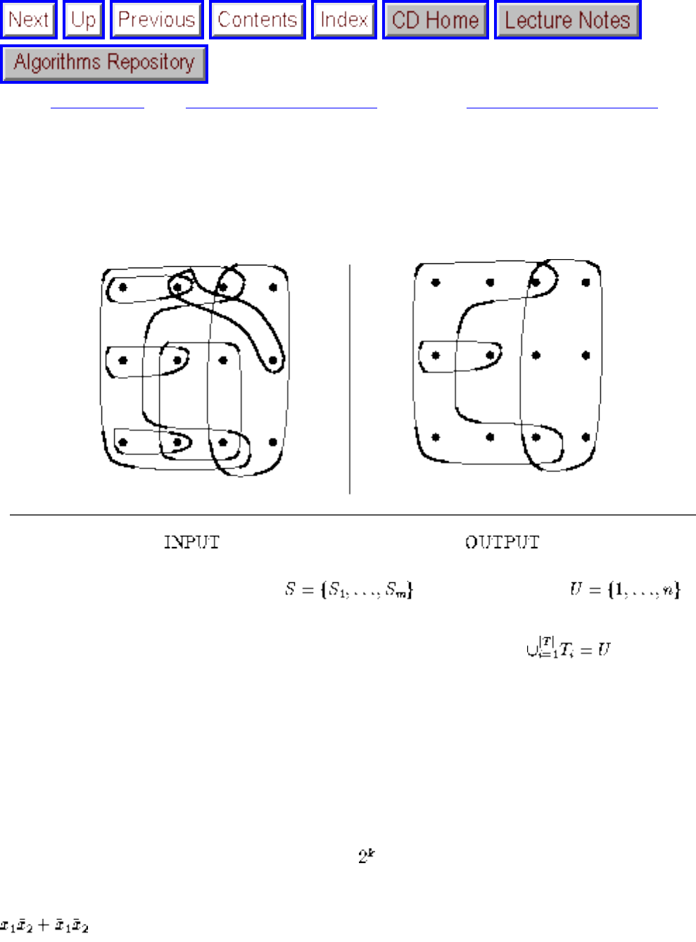
Set Cover
Next: Set Packing Up: Set and String Problems Previous: Set and String Problems
Set Cover
Input description: A set of subsets of the universal set .
Problem description: What is the smallest subset T of S such that ?
Discussion: Set cover arises when you try to efficiently acquire or represent items that have been
packaged in a fixed set of lots. You want to obtain all the items, while buying as few lots as possible.
Finding a cover is easy, because you can always buy one of each lot. However, by finding a small set
cover you can do the same job for less money.
An interesting application of set cover is Boolean logic minimization. We are given a particular Boolean
function of k variables, which for each of the possible input vectors describes whether the desired
output is 0 or 1. We seek the simplest circuit that exactly implements this function. One approach is to
find a disjunctive normal form (DNF) formula on the variables and their complements, such as
. We could build one ``and'' term for each input vector and then ``or'' them all together, but
we might save considerably by factoring out common subsets of variables. Given a set of feasible ``and''
terms, each of which covers a subset of the vectors we need, we seek to ``or'' together the smallest
number of terms that realize the function. This is exactly the set cover problem.
file:///E|/BOOK/BOOK5/NODE201.HTM (1 of 4) [19/1/2003 1:32:04]
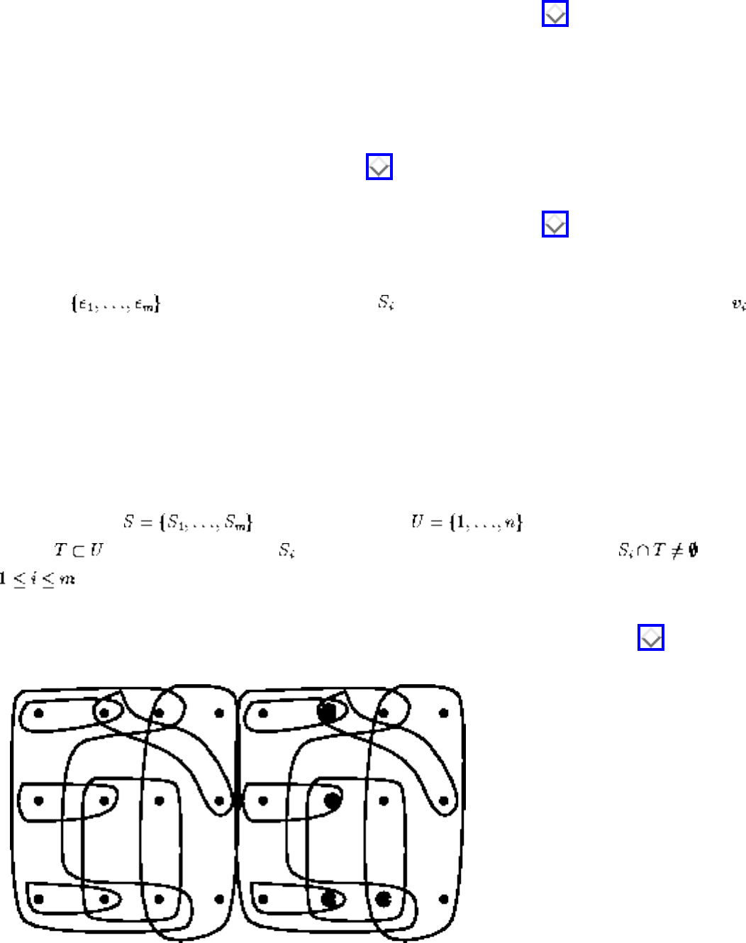
Set Cover
There are several variations of set cover problems to be aware of:
● Are you allowed to cover any element more than once? - The distinction here is between set
covering and set packing, the latter of which is discussed in Section . If we are allowed to
cover elements more than once, as in the logic minimization problem above, we should take
advantage of this freedom, as it usually results in a smaller covering.
● Are your sets derived from the edges or vertices of a graph? - Set cover is a very general problem,
and it includes several useful graph problems as special cases. Suppose instead that you seek the
smallest set of edges in a graph that covers each vertex at least once. The solution is to find a
maximum matching in the graph (see Section ), and then add arbitrary edges to cover the
remaining vertices. Suppose you seek the smallest set of vertices in a graph that covers each edge
at least once. This is the vertex cover problem, discussed in Section .
It is instructive to model vertex cover as an instance of set cover. Let the universal set U be the set
of edges . Construct n subsets, with consisting of the edges incident on vertex .
Although vertex cover is just a set cover problem in disguise, you should take advantage of the
fact that better algorithms exist for vertex cover.
● Do your subsets contain only two elements each? - When all of your subsets have at most two
elements each, you are in luck. This is about the only special case that you can solve efficiently to
optimality, by using the matching technique described above. Unfortunately, as soon as your
subsets get to have three elements each, the problem becomes NP-complete.
● Do you want to cover elements with sets, or sets with elements? - In the hitting set problem, we
seek a small number of items that together represent an entire population. Formally, we are given
a set of subsets of the universal set , and we seek the smallest
subset such that each subset contains at least one element of T. Thus for all
. Suppose we desire a small Congress with at least one representative of each ethnic
group. If each ethnic group is represented as a subset of people, the minimum hitting set is the
smallest possible politically correct Congress. Hitting set is illustrated in Figure .
file:///E|/BOOK/BOOK5/NODE201.HTM (2 of 4) [19/1/2003 1:32:04]
Set Cover
Figure: Hitting set is dual to set cover
Hitting set is, in fact, dual to set cover, meaning it is exactly the same problem in disguise.
Replace each element of U by a set of the names of the subsets that contain it. Now S and U have
exchanged roles, for we seek a set of subsets from U to cover all the elements of S. This is is
exactly the set cover problem. Thus we can use any of the set cover codes below to solve hitting
set after performing this simple translation.
Since the vertex cover problem is NP-complete, the set cover problem must be at least as hard. In fact, it
is somewhat harder. Approximation algorithms do no worse than twice optimal for vertex cover, but only
a times optimal approximation algorithm exists for set cover.
The greedy heuristic is the right approach for set cover. Begin by placing the largest subset in the set
cover, and then mark all its elements as covered. We will repeatedly add the subset containing the largest
number of uncovered elements, until all elements are covered. This heuristic always gives a set cover
using at most times as many sets as optimal, and in practice it usually does a lot better.
The simplest implementation of the greedy heuristic sweeps through the entire input instance of m
subsets for each greedy step. However, by using such data structures as linked lists and a bounded-height
priority queue (see Section ), the greedy heuristic can be implemented in O(S) time, where
is the size of the input representation.
It pays to check whether there are certain elements that exist in only a few subsets, ideally only one. If
so, we should select the biggest subsets containing these elements at the very beginning. We will have to
take them eventually, and they carry with them extra elements that we might have to pay to cover by
waiting until later.
Simulated annealing is likely to produce somewhat better set covers than these simple heuristics, if that is
important for your application. Backtracking can be used to guarantee you an optimal solution, but
typically it is not worth the computational expense.
Implementations: Pascal implementations of an exhaustive search algorithm for set packing, as well as
heuristics for set cover, appear in [SDK83]. See Section .
Notes: Survey articles on set cover include [BP76]. See [CK75] for a computational study of set cover
algorithms. An excellent exposition on algorithms and reduction rules for set cover is presented in
[SDK83].
Good expositions of the greedy heuristic for set cover include [CLR90]. An example demonstrating that
the greedy heuristic for set cover can be as bad as is presented in [Joh74, PS82]. This is not a defect
file:///E|/BOOK/BOOK5/NODE201.HTM (3 of 4) [19/1/2003 1:32:04]
Set Cover
of the heuristic. Indeed, it is provably hard to approximate set cover to within an approximation factor
better than [LY93].
Related Problems: Matching (see page ), vertex cover (see page ), set packing (see page ).
Next: Set Packing Up: Set and String Problems Previous: Set and String Problems
Algorithms
Mon Jun 2 23:33:50 EDT 1997
file:///E|/BOOK/BOOK5/NODE201.HTM (4 of 4) [19/1/2003 1:32:04]
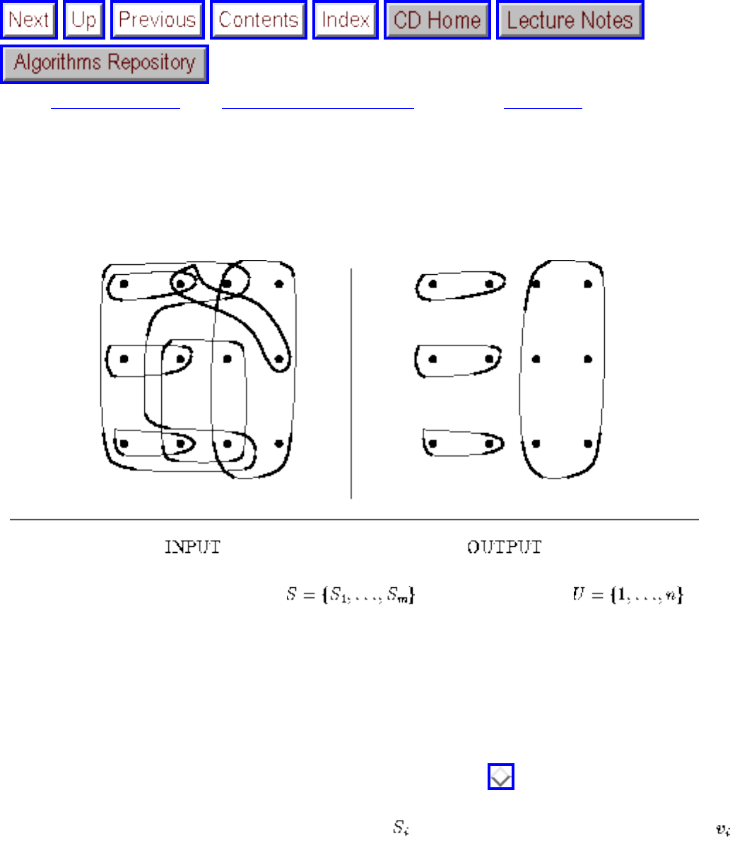
Set Packing
Next: String Matching Up: Set and String Problems Previous: Set Cover
Set Packing
Input description: A set of subsets of the universal set .
Problem description: What is the largest number of mutually disjoint subsets from S?
Discussion: Set packing problems arise in partitioning applications, where we need to partition elements
under strong constraints on what is an allowable partition. The key feature of packing problems is that no
elements are permitted to be covered by more than one set. Consider the problem of finding the
maximum independent set in a graph G, discussed in Section . We seek a large subset of vertices such
that each edge is adjacent to at most one of the selected vertices. To model this as set packing, let the
universal set consist of all edges of G, and subset consist of all edges incident on vertex . Any set
packing corresponds to a set of vertices with no edge in common, in other words, an independent set.
Scheduling airline flight crews to airplanes is another application of set packing. Each airplane in the
fleet needs to have a crew assigned to it, consisting of a pilot, copilot, and navigator. There are
constraints on the composition of possible crews, based on their training to fly different types of aircraft,
as well as any personality conflicts. Given all possible crew and plane combinations, each represented by
a subset of items, we need an assignment such that each plane and each person is in exactly one chosen
file:///E|/BOOK/BOOK5/NODE202.HTM (1 of 3) [19/1/2003 1:32:06]
Set Packing
combination. After all, the same person cannot be on two different planes, and every plane needs a crew.
We need a perfect packing given the subset constraints.
Set packing is used here to represent a bunch of problems on sets, all of which are NP-complete and all
of which are quite similar:
● Must every element from the universal set appear in one selected subset? - In the exact cover
problem, we seek some collection of subsets such that each element is covered exactly once. The
airplane scheduling problem above has the flavor of exact covering, since every plane and crew
has to be employed.
Unfortunately, exact cover is similar to that of Hamiltonian cycle in graphs. If we really must
cover all the elements exactly once, and this existential problem is NP-complete, then all we can
do is exponential search. This will be prohibitive unless there are so many solutions that we will
stumble upon one quickly.
Things will be far better if we can be content with a partial solution, say by adding each element
of U as a singleton subset of S. Thus we can expand any set packing into an exact cover by
mopping up the unpacked elements of U with singleton sets. Now our problem is reduced to
finding a minimum-cardinality set packing, which can be attacked via heuristics, as discussed
below.
● What is the penalty for covering elements twice? - In set cover (see Section ), there is no
penalty for elements existing in many selected subsets. In pure set packing, any such violation is
forbidden. For many such problems, the truth lies somewhere in between. Such problems can be
approached by charging the greedy heuristic more to select a subset that contains previously
covered elements than one that does not.
The right heuristics for set packing are greedy, and similar to those of set cover (see Section ). If we
seek a packing with many sets, then we repeatedly select the smallest subset, delete all subsets from S
that clash with it, and repeat. If we seek a packing with few subsets, we do the same but always pick the
largest possible subset. As usual, augmenting this approach with some exhaustive search or
randomization (in the form of simulated annealing) is likely to yield better packings at the cost of
additional computation.
Implementations: Since set cover is a more popular and more tractable problem than set packing, it
might be easier to find an appropriate implementation to solve the cover problem. Many such
implementations should be readily modifiable to support certain packing constraints.
Pascal implementations of an exhaustive search algorithm for set packing, as well as heuristics for set
cover, appear in [SDK83]. See Section for details on ftp-ing these codes.
file:///E|/BOOK/BOOK5/NODE202.HTM (2 of 3) [19/1/2003 1:32:06]
Set Packing
Notes: An excellent exposition on algorithms and reduction rules for set packing is presented in
[SDK83], including the airplane scheduling application discussed above. Survey articles on set packing
include [BP76].
Related Problems: Independent set (see page ), set cover (see page ).
Next: String Matching Up: Set and String Problems Previous: Set Cover
Algorithms
Mon Jun 2 23:33:50 EDT 1997
file:///E|/BOOK/BOOK5/NODE202.HTM (3 of 3) [19/1/2003 1:32:06]
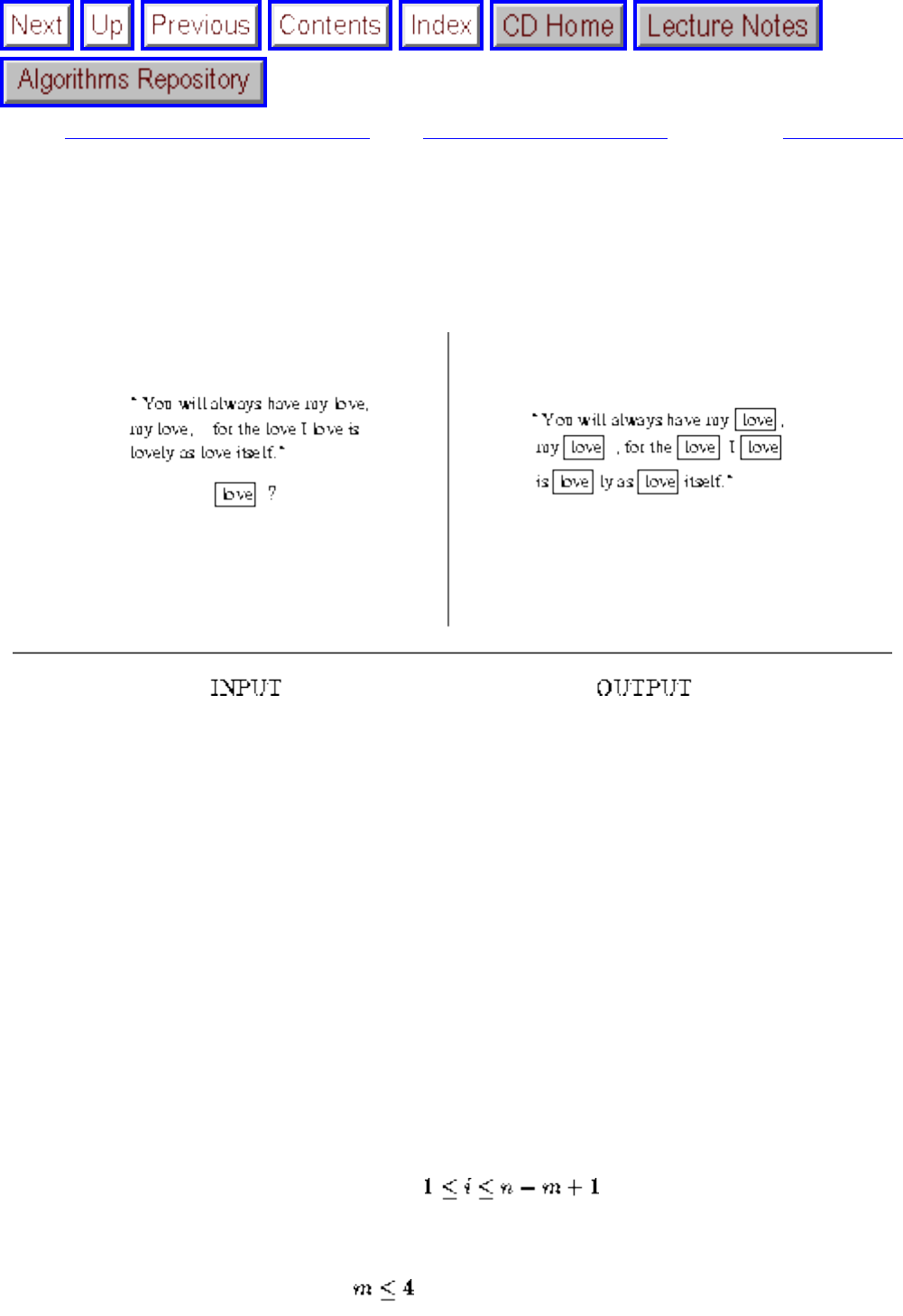
String Matching
Next: Approximate String Matching Up: Set and String Problems Previous: Set Packing
String Matching
Input description: A text string t of length n. A pattern string p of length m.
Problem description: Find the first (or all) instances of the pattern in the text.
Discussion: String matching is fundamental to database and text processing applications. Every text
editor must contain a mechanism to search the current document for arbitrary strings. Pattern matching
programming languages such as Perl and Awk derive much of their power from their built-in string
matching primitives, making it easy to fashion programs that filter and modify text. Spelling checkers
scan an input text for words in the dictionary and reject any strings that do not match.
Several issues arise in identifying the right string matching algorithm for the job:
● Are your search patterns and/or texts short? - If your strings are sufficiently short and your
queries sufficiently infrequent, the brute-force O(m n)-time search algorithm will likely suffice.
For each possible starting position , it tests whether the m characters starting
from the ith position of the text are identical to the pattern.
For very short patterns, say , you can't hope to beat brute force by much, if at all, and you
file:///E|/BOOK/BOOK5/NODE203.HTM (1 of 4) [19/1/2003 1:32:08]
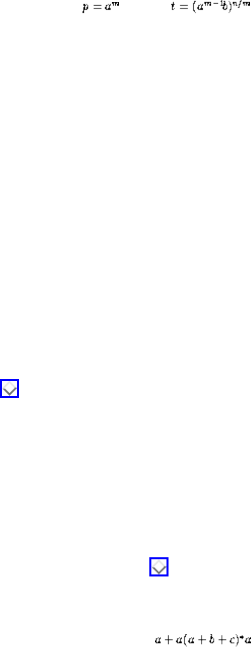
String Matching
shouldn't try. Further, since we can reject the possibility of a match at a given starting position the
instant we observe a text/pattern mismatch, we expect much better than O(mn) behavior for
typical strings. Indeed, the trivial algorithm usually runs in linear time. But the worst case
certainly can occur, as with pattern and text .
● What about longer texts and patterns? - By being more clever, string matching can be performed
in worst-case linear time. Observe that we need not begin the search from scratch on finding a
character mismatch between the pattern and text. We know something about the subsequent
characters of the string as a result of the partial match from the previous position. Given a long
partial match from position i, we can jump ahead to the first character position in the pattern/text
that will provide new information about the text starting from position i+1. The Knuth-Moris-
Pratt algorithm preprocesses the search pattern to construct such a jump table efficiently. The
details are tricky to get correct, but the resulting implementations yield short, simple programs.
Even better in practice is the Boyer-Moore algorithm, although it offers similar worst-case
performance. Boyer-Moore matches the pattern against the text from right to left, in order to avoid
looking at large chunks of text on a mismatch. Suppose the pattern is abracadabra, and the
eleventh character of the text is x. This pattern cannot match in any of the first eleven starting
positions of the text, and so the next necessary position to test is the 22nd character. If we get very
lucky, only n/m characters need ever be tested. The Boyer-Moore algorithm involves two sets of
jump tables in the case of a mismatch: one based on pattern matched so far, the other on the text
character seen in the mismatch. Although somewhat more complicated than Knuth-Morris-Pratt, it
is worth it in practice for patterns of length m > 5.
● Will you perform multiple queries on the same text? - Suppose you were building a program to
repeatedly search a particular text database, such as the Bible. Since the text remains fixed, it pays
build a data structure to speed up search queries. The suffix tree and suffix array data structures,
discussed in Section , are the right tools for the job.
● Will you search many texts using the same patterns? - Suppose you were building a program to
screen out dirty words from a text stream. Here, the set of patterns remains stable, while the
search texts are free to change. In such applications, we may need to find all occurrences of each
of k different patterns, where k can be quite large.
Performing a linear-time search for each of these patterns yields an O(k (m+n)) algorithm. If k is
large, a better solution builds a single finite automaton that recognizes each of these patterns and
returns to the appropriate start state on any character mismatch. The Aho-Corasick algorithm
builds such an automaton in linear time. Space savings can be achieved by optimizing the pattern
recognition automaton, as discussed in Section . This algorithm was used in the original
version of fgrep.
Sometimes multiple patterns are specified not as a list of strings, but concisely as a regular
expression. For example, the regular expression matches any string on (a,b,c)
that begins and ends with an a, including a itself. The best way to test whether input strings are
described by a given regular expression R is to construct the finite automaton equivalent to R and
file:///E|/BOOK/BOOK5/NODE203.HTM (2 of 4) [19/1/2003 1:32:08]

String Matching
then simulate the machine on the string. Again, see Section for details on constructing
automata from regular expressions.
When the patterns are specified by context-free grammars instead of regular expressions, the
problem becomes one of parsing, discussed in books on compilers and programming languages.
● What if our text or pattern contains a spelling error? - Finally, observe that the algorithms
discussed here work only for exact string matching. If you must allow some tolerance for spelling
errors, your problem is approximate string matching, which is throughly discussed in Section .
Implementations: SPARE Parts is a string pattern recognition toolkit, written in C++ by Bruce Watson.
It provides production-quality implementations of all major variants of the classical string matching
algorithms for single patterns (both Knuth-Morris-Pratt and Boyer-Moore) and multiple patterns (both
Aho-Corasick and Commentz-Walter). SPARE Parts is available by anonymous ftp from ftp.win.tue.nl in
/pub/techreports/pi/watson.phd/. A greatly improved commercial version is available from
www.RibbitSoft.com.
XTango (see Section ) provides animations for both the Boyer-Moore and Knuth-Morris-Pratt
algorithms. The C source code for each animation is included.
Implementations in C and Pascal of several algorithms for exact and approximate string matching appear
in [GBY91]. Sedgewick provides similar implementations of Knuth-Morris-Pratt, Rabin-Karp, and
Boyer-Moore in C++. See Section for details on both codes.
Implementations in C of the Boyer-Moore, Aho-Corasick, and regular expression matching algorithms
appear in [BR95]. The code for these algorithms is printed in the text and available on disk for a modest
fee.
Notes: All books on string algorithms contain thorough discussions of exact string matching, including
[CR94, Ste94, Gus97]. Good expositions on the Boyer-Moore [BM77] and Knuth-Morris-Pratt
algorithms [KMP77] include [Baa88, CLR90, Man89].
Aho [Aho90] provides a good survey on algorithms for pattern matching in strings, particularly where
the patterns are regular expressions instead of strings, and for the Aho-Corasick algorithm for multiple
patterns [AC75]. An algorithm merging Aho-Corasick and Boyer-Moore can be faster for small numbers
of patterns [CW79], but the window where it wins is apparently fairly narrow.
Empirical comparisons of string matching algorithms include [DB86, Hor80, dVS82]. Which algorithm
performs best depends upon the properties of the strings and the size of the alphabet. For long patterns
file:///E|/BOOK/BOOK5/NODE203.HTM (3 of 4) [19/1/2003 1:32:08]
String Matching
and texts, I recommend that you use the best implementation of Boyer-Moore that you can find.
An interesting classical problem is determining the minimum number of comparisons needed to perform
exact string matching. A version of Boyer-Moore never makes more than 2n comparisons independent of
the number of occurrences of the pattern in the text [AG86]. More recent results are very technical,
depending upon the details of the model and the alphabet size. There is a lower bound of n-m+1 text
characters that any algorithm must be examine in the worst case [Riv77]. The history of string matching
algorithms is somewhat checkered because several published proofs were incorrect or incomplete
[Gus97].
The Karp-Rabin algorithm [KR87] uses a hash function to perform string matching in linear expected
time. Its worst-case time remains quadratic, and its performance in practice appears somewhat worse
than the character comparison methods described above.
Related Problems: Suffix trees (see page ), approximate string matching (see page ).
Next: Approximate String Matching Up: Set and String Problems Previous: Set Packing
Algorithms
Mon Jun 2 23:33:50 EDT 1997
file:///E|/BOOK/BOOK5/NODE203.HTM (4 of 4) [19/1/2003 1:32:08]
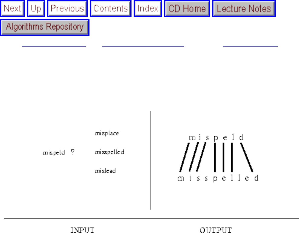
Approximate String Matching
Next: Text Compression Up: Set and String Problems Previous: String Matching
Approximate String Matching
Input description: A text string t and a pattern string p. An edit cost bound k.
Problem description: Can we transform t to p using at most k insertions, deletions, and substitutions?
Discussion: Approximate string matching is fundamental to text processing, because we live in an error-
prone world. Any spelling correction program must be able to identify the closest match for any text
string not found in a dictionary. Genbank has become a fundamental tool for molecular biology by
supporting homology (similarity) searches on DNA sequences. Suppose you were to sequence a new
gene in man, and you discovered that it is similar to the hemoglobin gene in rats. It is likely that this new
gene also produces hemoglobin, and any differences are the result of genetic mutations during evolution.
I once encountered approximate string matching in evaluating the performance of an optical character
recognition system that we built. After scanning and recognizing a test document, we needed to compare
the correct answers with those produced by our system. To improve our system, it was important to count
how often each pair of letters were getting confused and to identify gibberish when the program was
trying to make out letters where none existed. The solution was to do an alignment between the two texts.
Insertions and deletions corresponded to gibberish, while substitutions signaled errors in our recognizers.
file:///E|/BOOK/BOOK5/NODE204.HTM (1 of 5) [19/1/2003 1:32:10]
Approximate String Matching
This same principle is used in file difference programs, which identify the lines that have changed
between two versions of a file.
When no errors are permitted, the problem becomes that of exact string matching, which is presented in
Section . Here, we restrict our discussion to dealing with errors.
Dynamic programming provides the basic approach to approximate string matching, as discussed in
Section . Let D[i,j] denote the cost of editing the first i characters of the text string t into the first j
characters of the pattern string p. The recurrence follows because we must have done something with
and . The only options are matching them, substituting one for the other, deleting , or inserting a
match for . Thus D[i,j] is the minimum of the costs of these possibilities:
1. If then D[i-1,j-1] else D[i-1,j-1] + substitution cost.
2. D[i-1,j] + deletion cost of .
3. D[i,j-1] + deletion cost of .
Several issues remain before we can make full use of this recurrence:
● Do I want to match the pattern against the full text, or against a substring? - Appropriately
initializing the boundary conditions of the recurrence distinguishes between the algorithms for
string matching and substring matching. Suppose we want to align the full text against the full
pattern. Then the cost of D[i,0] must be that of deleting the first i characters of the text, so D[i,0]
= i. Similarly, D[0,j] = j.
Now suppose that the pattern may occur anywhere within the text. The proper cost of D[i,0] is
now 0, since there should be no penalty for starting the alignment in the ith position. The cost of
D[0,j] remains j, however, since the only way to match the first j pattern characters with nothing
is to delete all of them. The cost of the best pattern match against the text will be given by
.
● How should I select the substitution and insertion/deletion costs? - The basic algorithm can be
easily modified to use different costs for insertion, deletion, and the substitutions of specific pairs
of characters. Which costs you use depends upon what you are planning to do with the alignment.
The most common cost assignment charges the same for insertion, deletion, or substitution.
Charging a substitution cost of more than insertion + deletion is a good way to ensure that
substitutions never get performed, since it will be cheaper to edit both characters out of the string.
With just insertion and deletion to work with, the problem reduces to longest common
subsequence, discussed in Section . Often, it pays to tweak the edit distance costs and study
the resulting alignments until you find a set that does the job.
file:///E|/BOOK/BOOK5/NODE204.HTM (2 of 5) [19/1/2003 1:32:10]

Approximate String Matching
● How do I get the actual alignment of the strings, instead of just the cost? - To obtain the transcript
of the editing operations performed in achieving the minimum cost alignment, we can work
backwards from the complete cost matrix D. To get to cell D[n,m], we had to come from one of
D[n-1,m] (insertion), D[n,m-1] (deletion), or D[n-1,m-1] (substitution/match). Which of the three
options was chosen can be reconstructed given these costs and the characters and . By
continuing to work backwards from the previous cell, we can trace the entire path and thus
reconstruct the alignment.
● What if the two strings are very similar to each other? - The dynamic programming algorithm can
be thought of as finding a shortest path across an grid, where the cost of each edge depends
upon which operation it represents. If we seek an alignment involving a combination of at most d
insertions, deletions, and substitutions, we need only traverse the band of O(d n) cells within a
distance d of the central diagonal. If no such low-cost alignment exists within this band, then no
low-cost alignment can exist in the full cost matrix.
● How can I minimize the required storage? - Dynamic programming takes both quadratic time and
space. For many applications, the space required to store the dynamic programming table is a
much more serious problem. Observe that only space is needed to compute D[m,n],
since we need only maintain two active rows (or columns) of the matrix in order to compute the
final value. The entire matrix is required only if we need to reconstruct the actual sequence
alignment.
To save space, we can use Hirschberg's clever recursive algorithm. During one pass of the linear-
space algorithm above to compute D[m,n], we maintain all the values for the (m/2)nd column and
identify which middle-element cell D[m/2,x] was used to optimize D[m,n]. This reduces our
problem to finding the best paths from D[1,1] to D[m/2,x] and from D[m/2,x] to D[m/2,n], both of
which can be solved recursively. Each time we throw away half of the matrix elements from
consideration, and so the total time remains O(mn). This linear-space algorithm proves to be a big
win in practice on long strings, although it is somewhat more difficult to program.
● Does string similarity mean that the strings sound alike? - Other models of approximate pattern
matching become more appropriate than edit distance in certain applications. Particularly
interesting is Soundex, a hashing scheme that attempts to pair up English words that sound alike.
This can be useful in testing whether two names that have been spelled differently are likely to be
the same. For example, my last name is often spelled ``Skina'', ``Skinnia'', ``Schiena'', and
occasionally ``Skiena''. All of these hash to the same Soundex code, S25.
The algorithm works by dropping vowels and silent letters, removing doubled letters, and then
assigning the remaining letters numbers from the following classes: BFPV gets a 1, CGJKQSXZ
gets a 2, DT gets a 3, L gets a 4, MN gets a 5, and R gets a 6. The code starts with the first letter
and contains at most three digits. Although this all sounds very hokey, experience shows that it
works reasonably well. Experience indeed: Soundex has been used since the 1920's.
Implementations: The best available software tools for approximate pattern matching are glimpse and
agrep [WM92a, WM92b], developed by Manber and Wu at the University of Arizona and available from
file:///E|/BOOK/BOOK5/NODE204.HTM (3 of 5) [19/1/2003 1:32:10]
Approximate String Matching
http://glimpse.cs.arizona.edu/. Glimpse is a tool for building and using an index to search through file
systems, while agrep (approximate general regular expression pattern matcher) is a tool supporting text
search with spelling errors. Both programs are widely used and respected.
ht://Dig is an alternative WWW text search engine from Andrew Scherpbier, which contains
implementations of Soundex and Metaphone. It is available from http://htdig.sdsu.edu/ and is released
under the GNU general public license.
Implementations in C of the Soundex and dynamic programming edit-distance algorithms appear in
[BR95]. The code for these algorithms is printed in the text and is available on disk for a modest fee.
Bare bones implementations in C and Pascal of several algorithms for exact and approximate string
matching appear in [GBY91]. See Section for further details.
Notes: The wide range of applications for approximate string matching was made apparent in Sankoff
and Kruskal's book [SK83], which remains a useful historical reference for the problem. Surveys on
approximate pattern matching include [HD80]. The basic dynamic programming alignment algorithm is
attributed to [WF74], although it is apparently folklore. The edit distance between two strings is
sometimes referred to as the Levenshtein distance. Expositions of dynamic programming to compute
Levenshtein distance include [Baa88, CLR90, Man89]. Expositions of Hirschberg's linear-space
algorithm [Hir75] include [CR94, Gus97].
Masek and Paterson [MP80] compute the edit distance between m- and n-length strings in time
for constant-sized alphabets, using ideas from the four Russians algorithm for
Boolean matrix multiplication [ADKF70]. The shortest path formulation leads to a variety of algorithms
that are good when the edit distance is small, including an algorithm due to Myers [Mye86].
Longest increasing subsequence can be done in time [HS77], as presented in [Man89].
Soundex was invented and patented by M. K. Odell and R. C. Russell. Expositions on Soundex include
[BR95, Knu73b]. Metaphone is a recent attempt to improve on Soundex [BR95, Par90].
Related Problems: String matching (see page ), longest common substring (see page ).
Next: Text Compression Up: Set and String Problems Previous: String Matching
file:///E|/BOOK/BOOK5/NODE204.HTM (4 of 5) [19/1/2003 1:32:10]
Approximate String Matching
Algorithms
Mon Jun 2 23:33:50 EDT 1997
file:///E|/BOOK/BOOK5/NODE204.HTM (5 of 5) [19/1/2003 1:32:10]
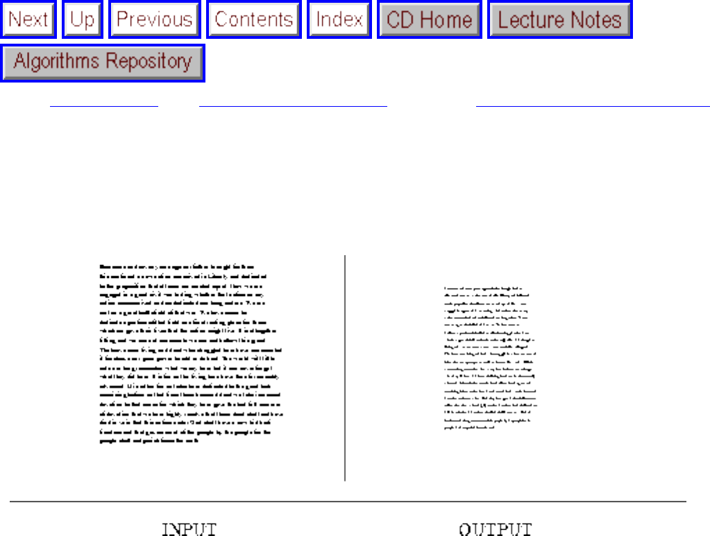
Text Compression
Next: Cryptography Up: Set and String Problems Previous: Approximate String Matching
Text Compression
Input description: A text string S.
Problem description: A shorter text string S' such that S can be correctly reconstructed from S'.
Discussion: Secondary storage devices fill up quickly on every computer system, even though their
capacity doubles each year. Decreasing storage prices have only increased interest in data compression,
since there is now more data to compress than ever before. Data compression is the algorithmic problem
of finding alternative, space-efficient encodings for a given data file. With the rise of computer networks,
a new mission for data compression has arisen, that of increasing the effective bandwidth of networks by
reducing the number of bits before transmission.
Data compression is a problem for which practical people like to invent ad hoc methods, designed for
their particular applications. Sometimes these outperform general methods, but often they do not. The
following issues arise in selecting the right data compression algorithm:
● Must we exactly reconstruct the input text after compression? - A primary issue in data
compression algorithms is the question of lossy versus lossless encodings. Text applications
typically demand lossless encodings, because users become disturbed whenever their data files
file:///E|/BOOK/BOOK5/NODE205.HTM (1 of 4) [19/1/2003 1:32:11]
Text Compression
have been corrupted. However, fidelity is not such an issue in image or video compression, where
the presence of small artifacts will be imperceptible to the viewer. Significantly greater
compression ratios can be obtained using lossy compression, which is why all image/video/audio
compression algorithms take advantage of this freedom.
● Can I simplify my data before I compress it? - The most effective way to free up space on a disk is
to delete files you don't need. Likewise, any preprocessing you can do to a file to reduce its
information content before compression will pay off later in better performance. For example, is it
possible to eliminate extra blank spaces or lines from the file? Can the document be converted
entirely to uppercase characters or have formatting information removed?
● Does it matter whether the algorithm is patented? - One concern is that many data compression
algorithms are patented, in particular the LZW variation of the Lempel-Ziv algorithm discussed
below. Further, Unisys, the owner of the patent, makes periodic attempts to collect. My personal
(although not legal) recommendation is to ignore them, unless you are in the business of selling
text compression software. If this makes you uncomfortable, note that there are other variations
on the Lempel-Ziv algorithm that are not under patent protection and perform about as well. See
the notes and implementations below.
● How do I compress image data - Run-length coding is the simplest lossless compression
algorithm for image data, where we replace runs of identical pixel values with one instance of the
pixel and an integer giving the length of the run. This works well on binary images with large
regions of similar pixels (like scanned text) and terribly on images with many quantization levels
and a little noise. It can also be applied to text with many fields that have been padded by blanks.
Issues like how many bits to allocate to the count field and the traversal order converting the two-
dimensional image to a stream of pixels can have a surprisingly large impact on the compression
ratio.
For serious image and video compression applications, I recommend that you use a lossy coding
method and not fool around with implementing it yourself. JPEG is the standard high-
performance image compression method, while MPEG is designed to exploit the frame-to-frame
coherence of video. Encoders and decoders for both are provided in the implementation section.
● Must compression and decompression both run in real time? - For many applications, fast
decompression is more important than fast compression, and algorithms such as JPEG exist to
take advantage of this. While compressing video for a CD-ROM, the compression will be done
only once, while decompression will be necessary anytime anyone plays it. In contrast, operating
systems that increase the effective capacity of disks by automatically compressing each file will
need a symmetric algorithm with fast compression times as well.
Although there are literally dozens of text compression algorithms available, they are characterized by
two basic approaches. In static algorithms, such as Huffman codes, a single coding table is built by
analyzing the entire document. In adaptive algorithms, such as Lempel-Ziv, a coding table is built on the
fly and adapts to the local character distribution of the document. An adaptive algorithm will likely prove
to be the correct answer:
● Huffman codes - Huffman codes work by replacing each alphabet symbol by a variable-length
file:///E|/BOOK/BOOK5/NODE205.HTM (2 of 4) [19/1/2003 1:32:11]
Text Compression
code string. ASCII uses eight bits per symbol in English text, which is wasteful, since certain
characters (such as `e') occur far more often than others (such as `q'). Huffman codes compress
text by assigning `e' a short code word and `q' a longer one.
Optimal Huffman codes can be constructed using an efficient greedy algorithm. Sort the symbols
in increasing order by frequency. We will merge the two least frequently used symbols x and y
into a new symbol m, whose frequency is the sum of the frequencies of its two child symbols. By
replacing x and y by m, we now have a smaller set of symbols, and we can repeat this operation n-
1 times until all symbols have been merged. Each merging operation defines a node in a binary
tree, and the left or right choices on the path from root-to-leaf define the bit of the binary code
word for each symbol. Maintaining the list of symbols sorted by frequency can be done using
priority queues, which yields an -time Huffman code construction algorithm.
Although they are widely used, Huffman codes have three primary disadvantages. First, you must
make two passes over the document on encoding, the first to gather statistics and build the coding
table and the second to actually encode the document. Second, you must explicitly store the
coding table with the document in order to reconstruct it, which eats into your space savings on
short documents. Finally, Huffman codes exploit only nonuniformity in symbol distribution,
while adaptive algorithms can recognize the higher-order redundancy in strings such as
0101010101....
● Lempel-Ziv algorithms - Lempel-Ziv algorithms, including the popular LZW variant, compress
text by building the coding table on the fly as we read the document. The coding table available
for compression changes at each position in the text. A clever protocol between the encoding
program and the decoding program ensures that both sides of the channel are always working with
the exact same code table, so no information can be lost.
Lempel-Ziv algorithms build coding tables of recently-used text strings, which can get arbitrarily
long. Thus it can exploit frequently-used syllables, words, and even phrases to build better
encodings. Further, since the coding table alters with position, it adapts to local changes in the text
distribution, which is important because most documents exhibit significant locality of reference.
The truly amazing thing about the Lempel-Ziv algorithm is how robust it is on different types of
files. Even when you know that the text you are compressing comes from a special restricted
vocabulary or is all lowercase, it is very difficult to beat Lempel-Ziv by using an application-
specific algorithm. My recommendation is not to try. If there are obvious application-specific
redundancies that can safely be eliminated with a simple preprocessing step, go ahead and do it.
But don't waste much time fooling around. No matter how hard you work, you are unlikely to get
significantly better text compression than with gzip or compress, and you might well do worse.
Implementations: A complete list of available compression programs is provided in the
comp.compression FAQ (frequently asked questions) file, discussed below. This FAQ will likely point
you to what you are looking for, if you don't find it in this section.
file:///E|/BOOK/BOOK5/NODE205.HTM (3 of 4) [19/1/2003 1:32:11]
Text Compression
The best general-purpose program for text compression is gzip, which implements a public domain
variation of the Lempel-Ziv algorithm. It is distributed under the GNU software licence and can by
obtained from ftp://prep.ai.mit.edu/pub/gnu/gzip-1.2.4.tar. Unix compress is another popular
compression program based on the patented LZW algorithm. It is available from
ftp://wuarchive.wustl.edu/packages/compression/compress-4.1.tar.
A JPEG implementation is available from ftp://ftp.uu.net/graphics/jpeg/jpegsrc.v6a.tar.gz. MPEG can be
found at ftp://havefun.stanford.edu/pub/mpeg/MPEGv1.2.2.tar.Z.
Algorithm 673 [Vit89] of the Collected Algorithms of the ACM is a Pascal implementation of dynamic
Huffman codes, which is a one-pass, adaptive text compression algorithm. See Section for details on
fetching this program.
Notes: Many books on data compression are available, but we highly recoomend Bell, Cleary, and
Witten [BCW90] and Storer [Sto88]. Another good source of information is the USENET newsgroup
comp.compression. Check out its particularly comprehensive FAQ (frequently asked questions)
compendium at location ftp://rtfm.mit.edu/pub/usenet/news.answers/compression-faq.
Good expositions on Huffman codes [Huf52] include [AHU83, BR95, CLR90, Eve79a, Man89].
Expositions on the LZW [Wel84, ZL78] algorithm include [BR95].
There is an annual IEEE Data Compression Conference, the proceedings of which should be studied
seriously before attempting to develop a new data compression algorithm. On reading the proceedings, it
will become apparent that this is a mature technical area, where much of the current work (especially for
text compression) is shooting for fairly marginal improvements on special applications. On a more
encouraging note, we remark that this conference is held annually at a world-class ski resort in Utah.
Related Problems: Shortest common superstring (see page ), cryptography (see page ).
Next: Cryptography Up: Set and String Problems Previous: Approximate String Matching
Algorithms
Mon Jun 2 23:33:50 EDT 1997
file:///E|/BOOK/BOOK5/NODE205.HTM (4 of 4) [19/1/2003 1:32:11]
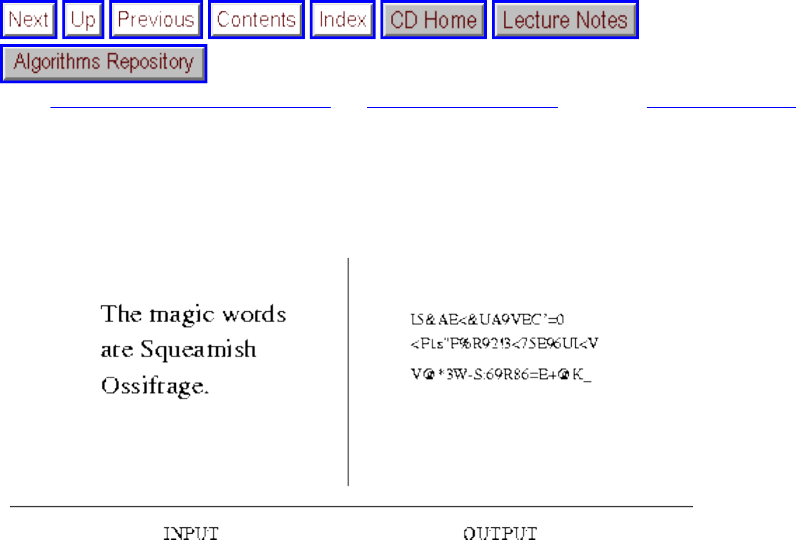
Cryptography
Next: Finite State Machine Minimization Up: Set and String Problems Previous: Text Compression
Cryptography
Input description: A plaintext message T or encrypted text E, and a key k.
Problem description: Encode T using k giving E, or decode E using k back to T.
Discussion: Cryptography has grown substantially in importance in recent years, as computer networks
have made confidential documents more vulnerable to prying eyes. Cryptography is a way to increase
security by making messages difficult to read if they fall into the wrong hands. Although the discipline of
cryptography is at least two thousand years old, its algorithmic and mathematical foundations have
recently solidified to the point where there can now be talk of provably secure cryptosystems.
There are three classes of cryptosystems everyone should be aware of:
● Caesar shifts - The oldest ciphers involve mapping each character of the alphabet to a
different letter. The weakest such ciphers rotate the alphabet by some fixed number of characters
(often 13), and thus have only 26 possible keys. Better is to use an arbitrary permutation of the
letters, so there are 26! possible keys. Even so, such systems can be easily attacked by counting
the frequency of each symbol and exploiting the fact that `e' occurs more often than `z'. While
there are variants that will make this more difficult to break, none will be as secure as DES or
file:///E|/BOOK/BOOK5/NODE206.HTM (1 of 5) [19/1/2003 1:32:13]

Cryptography
RSA.
● Data Encryption Standard (DES) - This algorithm is based on repeatedly shuffling the bits of
your text as governed by the key. The standard key length for DES (56 bits) is now considered too
short for applications requiring the highest level of security. However, a simple variant called
triple DES permits an effective key length of 112 bits by using three rounds of DES with two 56-
bit keys. In particular, first encrypt with key1, then decrypt with key2, before finally encrypting
with key1. There is a mathematical reason for using three rounds instead of two, and the encrypt-
decrypt-encrypt pattern is used so that the scheme is equivalent to single DES when key1 = key2.
● Rivest-Shamir-Adelman (RSA) - RSA is a public key cryptosystem, meaning that different
keys are used to encode and decode messages. Since the encoding key is of no help in decoding, it
can be made public at no risk to security. The security of RSA is based on the difference in the
computational complexity of factoring and primality testing (see Section ). Encoding is
(relatively) fast because it relies on primality testing to construct the key, while the hardness of
decryption follows from that of factoring. Still, RSA is slow relative to other cryptosystems,
roughly 100 to 1,000 times slower than DES.
The key issue in selecting a cryptosystem is identifying your paranoia level, i.e. deciding how much
security you need. Who are you trying to stop from reading your stuff: your grandmother, local thieves,
the Mafia, or the NSA? If you can use an accepted implementation of RSA, such as PGP discussed
below, you should feel safe against just about anybody.
If there is an implementation of DES on your machine, that will likely be good enough for most
applications. For example, I use DES to encrypt my final exam each semester, and it proved more than
sufficient the time an ambitious student broke into my office looking for it. If the NSA had been
breaking in, the story might have been different, although even here it is important to understand that the
most serious security holes are human, not algorithmic. Making sure your password is long enough,
hard to guess, and not written down is far more important than obsessing about the encryption algorithm.
Simple ciphers like the Caesar shift are fun and easy to program. For this reason, it is perhaps healthy to
use them for applications needing only a casual level of security (such as hiding the punchlines of jokes).
Since they are easy to break, they should never be used for serious security applications.
One thing that you should never do is mess around with developing your own novel cryptosystem. The
security of DES and RSA is accepted largely because these systems have both survived over twenty
years of public scrutiny. Over this period, many other cryptosystems have been proposed, proven
vulnerable to attack, and then abandoned. This is not a field for amateurs. If you are charged with
implementing a cryptosystem, carefully study a respected program such as PGP (discussed below) to see
how its author, Philip Zimmermann, skillfully handled such issues as key selection and key distribution.
A cryptosystem is as strong as its weakest link.
There are several problems related to cryptography that arise often in practice:
file:///E|/BOOK/BOOK5/NODE206.HTM (2 of 5) [19/1/2003 1:32:13]

Cryptography
● How can I validate the integrity of data against corruption? - In any communications
application, there is need to validate that the transmitted data is identical to that which has been
received. One solution is for the received to transmit the data back to the source and have the
original sender confirm that the two texts are identical. This fails when the exact inverse of an
error is made in the retransmission, but a more serious problem is that your available bandwidth is
cut in half with such a scheme.
A more efficient if less reliable method is to use a checksum, a simple mathematical function that
hashes a long text down to a simple number or digit, and then transmit the checksum along with
the text. The checksum can be recomputed on the receiving end and bells set off if the computed
checksum is not identical to what was received. Perhaps the simplest checksum scheme just adds
up the byte or character values and takes the sum modulo some constant, say .
Unfortunately, an error transposing two or more characters would go undetected under such a
scheme, since addition is commutative.
Cyclic-redundancy check (CRC) provides a more powerful method for computing checksums
and is used in most communications systems and internally in computers to validate disk drive
transfers. These codes compute the remainder in the ratio of two polynomials, the numerator of
which is a function of the input text. The design of these polynomials involves considerable
mathematical sophistication and ensures that all reasonable errors are detected. The details of
efficient computation are complicated enough that we recommend that you start from an existing
implementation, described below.
● How can I prove that a file has not been changed? - If I send you a contract in electronic form,
what is to stop you from editing the file and then claiming that your version was what we had
really agreed to? I need a way to prove that any modification to a document is fraudulent. Digital
signatures are a cryptographic way for me to stamp my document as genuine.
Given a file, I can compute a checksum for it, and then encrypt this checksum using my own
private key. I send you the file and the encrypted checksum. You can now edit the file, but to fool
the judge you must also edit the encrypted checksum such that it can be decrypted to the correct
checksum. With a suitably good checksum function, designing a file that yields the same
checksum becomes an insurmountable problem.
● How can I prove that I am me? - Authentication is the process of one party convincing another
that they are who they say they are. The historical solutions have involved passwords or keys, so I
prove that I am who I say I am because I know my credit card number or carry an ID card. The
problem with such schemes is that anyone who eavesdrops on this conversation or who steals my
physical key can now successfully impersonate me.
What we need is some way for me to convince you that I know my key, without actually telling
you the key. One such method to do so is for you to send me a random number or text, and I use
my key to encrypt your text and send it back to you. If you then decrypt this text and compare it to
the message you sent me, you gain confidence that I am who I say I am. We can repeat this
exercise on several random texts until sufficient authentication has been agreed upon. If we use a
file:///E|/BOOK/BOOK5/NODE206.HTM (3 of 5) [19/1/2003 1:32:13]
Cryptography
secure enough cryptosystem, we can be confident that an eavesdropper will not be able to deduce
my key even given several plain and encrypted texts.
Such authentication protocols of back-and-forth messages often involve the use of randomness to
frustrate eavesdroppers. Different protocols satisfy particular needs and constraints about who
has to know what. It is important to do some reading before attempting to design your own
protocols. References are provided below.
Implementations: The USENET FAQ (frequently asked questions) file on cryptography provides a
wealth of information, including pointers to implementations. Check it out at
ftp://rtfm.mit.edu/pub/usenet/news.answers/cryptography-faq/.
Distributing cryptographic software is complicated by United States export restrictions, which make it
illegal to export encryption software. PGP (Pretty Good Privacy) is such a good implementation of RSA
that its author Philip Zimmerman was charged with export violations by federal authorities. PGP may
be obtained from the Electronic Frontier Foundation (EFF) at
http://www.eff.org/pub/Net_info/Tools/Crypto/PGP/.
A good discussion on checksums and cyclic-redundancy codes, with implementations in C, appear in
[BR95]. The code for these algorithms is printed in the text and is available on disk for a modest fee.
The Stanford Graphbase (see Section ) uses checksums to ensure that data files remain unmodified
from the original distribution. Algorithm 536 [Kno79] of the Collected Algorithms of the ACM is an
encryption function for passwords, written in Fortran. See Section for further information.
Notes: Kahn [Kah67] presents the fascinating history of cryptography from ancient times to 1967 and is
particularly noteworthy in light of the secretive nature of the subject. More recent and more technical
works on cryptography include Denning [Den82] and Schneier [Sch94], the latter of which provides a
through overview of different cryptographic algorithms, including implementations for sale. Rawlins
[Raw92] provides a good introduction to cryptographic algorithms, from Caesar shift to public key to
zero-knowledge proofs. An algorithm for breaking simple substitution ciphers appears in [PR79].
Expositions on the RSA algorithm [RSA78] include [CLR90]. The RSA Laboratories home page
http://www.rsa.com/rsalabs/ is very informative. See [Sta95] for an excellent guide to PGP and its
underlying algorithms.
The history of DES is well presented in [Sch94]. Particularly controversial was the decision by the NSA
to limit key length to 56 bits, presumably short enough to be cracked by special-purpose computers
costing on the order of several million dollars. Despite some theoretical progress in breaking DES
analytically [BS93], the most significant threat remains special-purpose hardware.
file:///E|/BOOK/BOOK5/NODE206.HTM (4 of 5) [19/1/2003 1:32:13]
Cryptography
MD5 [Riv92] is the secure hashing function used by PGP to compute digital signatures. Expositions
include [Sch94, Sta95].
Related Problems: Factoring and primality testing (see page ), Text compression (see page )).
Next: Finite State Machine Minimization Up: Set and String Problems Previous: Text Compression
Algorithms
Mon Jun 2 23:33:50 EDT 1997
file:///E|/BOOK/BOOK5/NODE206.HTM (5 of 5) [19/1/2003 1:32:13]
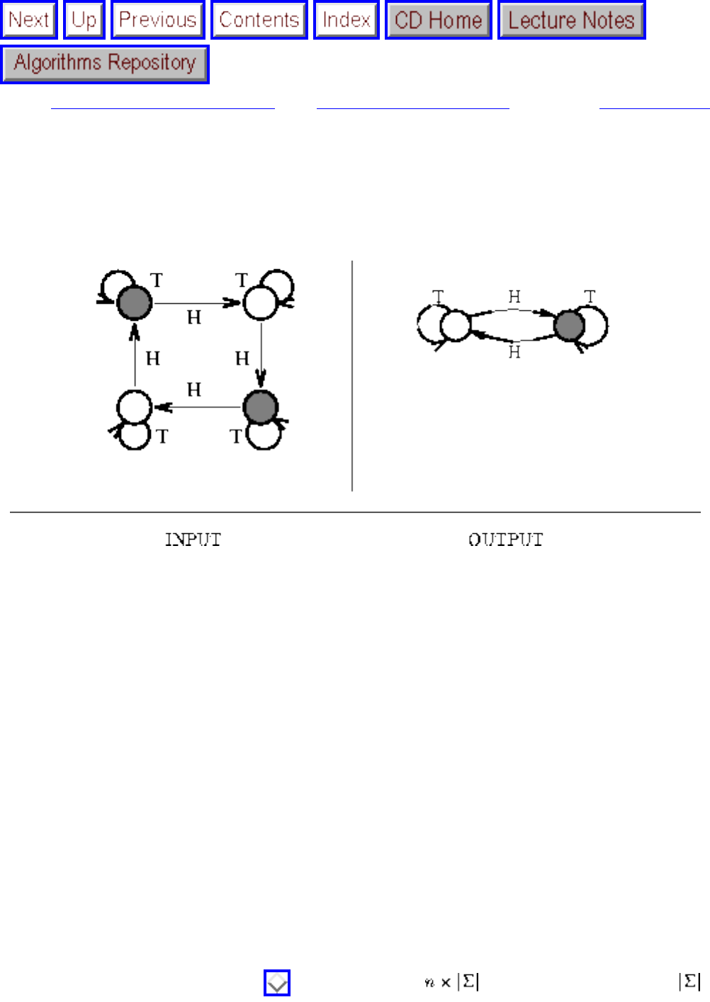
Finite State Machine Minimization
Next: Longest Common Substring Up: Set and String Problems Previous: Cryptography
Finite State Machine Minimization
Input description: A deterministic finite automaton M.
Problem description: The smallest deterministic finite automaton M' such that M' behaves identically to
M.
Discussion: Problems associated with constructing and minimizing finite state machines arise repeatedly
in software and hardware design applications. Finite state machines are best thought of as pattern
recognizers, and minimum-size machines correspond to recognizers that require less time and space.
Complicated control systems and compilers are often built using finite state machines to encode the
current state and associated actions, as well as the set of possible transitions to other states. Minimizing
the size of this machine minimizes its cost.
Finite state machines are best thought of as edge-labeled directed graphs, where each vertex represents
one of n states and each edge a transition from one state to the other on receipt of the alphabet symbol
that labels the edge. The automaton above analyzes a given sequence of coin tosses, with the dark states
signifying that an even number of heads have been observed. Automata can be represented using any
graph data structure (see Section ), or by using an transition matrix, where is the size of the
alphabet.
file:///E|/BOOK/BOOK5/NODE207.HTM (1 of 4) [19/1/2003 1:32:15]
Finite State Machine Minimization
Finite state machines are often used to specify search patterns in the guise of regular expressions, which
are patterns formed by and-ing, or-ing, and looping over smaller regular expressions. For example, the
regular expression matches any string on (a,b,c) that begins and ends with an a
(including a itself). The best way to test whether a string is described by a given regular expression
(especially if many strings will be tested) is to construct the equivalent finite automaton and then
simulate the machine on the string. See Section for alternative approaches to string matching.
We consider three different problems on finite automata:
● Minimizing deterministic finite state machines - Transition matrices for finite automata quickly
become prohibitively large for sophisticated machines, thus fueling the need for tighter encodings.
The most direct approach is to eliminate redundant states in the automaton. As the example above
illustrates, automata of widely varying sizes can compute the same function.
Algorithms for minimizing the number of states in a deterministic finite automaton (DFA) appear
in any book on automata theory. The basic approach works by partitioning the states into gross
equivalence classes and then refining the partition. Initially, the states are partitioned into
accepting, rejecting, and other classes. The transitions from each node branch to a given class on a
given symbol. Whenever two states , t in the same class C branch to elements of different classes,
the class C must be partitioned into two subclasses, one containing , the other containing t.
This algorithm makes a sweep though all the classes looking for a new partition, and repeating the
process from scratch if it finds one. This yields an algorithm, since at most n-1 sweeps need
ever be performed. The final equivalence classes correspond to the states in the minimum
automaton. In fact, a more efficient, algorithm is known with available implementations
discussed below.
● Constructing deterministic machines from nondeterministic machines - DFAs are simple to
understand and work with, because the machine is always in exactly one state at any given time.
Nondeterministic automata (NFAs) can be in more than one state at a time, so its current ``state''
represents a subset of all possible machine states.
In fact, any NFA can be mechanically converted to an equivalent DFA, which can then be
minimized as above. However, converting an NFA to a DFA can cause an exponential blowup in
the number of states, which perversely might later be eliminated in the minimization. This
exponential blowup makes automaton minimization problems NP-hard whenever you do not start
with a DFA.
The proofs of equivalence between NFAs, DFAs, and regular expressions are elementary enough
to be covered in undergraduate automata theory classes. However, they are surprisingly nasty to
implement, for reasons including but not limited to the exponential blowup of states.
Implementations are discussed below.
file:///E|/BOOK/BOOK5/NODE207.HTM (2 of 4) [19/1/2003 1:32:15]
Finite State Machine Minimization
● Constructing machines from regular expressions - There are two approaches to converting a
regular expression to an equivalent finite automaton, the difference being whether the output
automaton is to be a nondeterministic or deterministic machine. The former is easier to construct
but less efficient to simulate.
The nondeterministic construction uses -moves, which are optional transitions that require no
input to fire. On reaching a state with an -move, we must assume that the machine can be in
either state. Using such -moves, it is straightforward to construct an automaton from a depth-first
traversal of the parse tree of the regular expression. This machine will have O(m) states, if m is
the length of the regular expression. Further, simulating this machine on a string of length n takes
O(m n) time, since we need consider each state/prefix pair only once.
The deterministic construction starts with the parse tree for the regular expression, observing that
each leaf represents one of the alphabet symbols in the pattern. After recognizing a prefix of the
text, we can be left in some subset of these possible positions, which would correspond to a state
in the finite automaton. The derivatives method builds up this automaton state by state as it is
needed. Even so, some regular expressions of length m require states in any DFA
implementing them, such as . There is no way to avoid this
exponential blowup in the space required. Note, however, that it takes linear time to simulate an
input string on any automaton, regardless of the size of the automaton.
Implementations: FIRE Engine is a finite automaton toolkit, written in C++ by Bruce Watson. It
provides production-quality implementations of finite automata and regular expression algorithms.
Several finite automaton minimization algorithms have been implemented, including Hopcroft's
algorithm. Both deterministic and nondeterministic automata are supported. FIRE Engine has been used
for compiler construction, hardware modeling, and computational biology applications. It is strictly a
computing engine and does not provide a graphical user interface. FIRE Engine is available by
anonymous ftp from ftp.win.tue.nl in the directory /pub/techreports/pi/watson.phd/. A greatly improved
commercial version is available from www.RibbitSoft.com.
Grail is a C++ package for symbolic computation with finite automata and regular expressions, from
Darrell Raymond and Derrick Wood. Grail enables one to convert between different machine
representations and to minimize automata. It can handle machines with 100,000 states and dictionaries of
20,000 words. All code and documentation are accessible from the WWW site
http://www.csd.uwo.ca/research/grail, as well as pointers to a variety of other automaton packages.
Commercial use of Grail is not allowed without approval, although it is freely available to students and
educators.
An implementation in C of a regular-expression matching algorithm appears in [BR95]. The source code
for this program is printed in the text and is available on disk for a modest fee. A bare bones
implementation in C of a regular-expression pattern matching algorithm appears in [GBY91]. See
file:///E|/BOOK/BOOK5/NODE207.HTM (3 of 4) [19/1/2003 1:32:15]
Finite State Machine Minimization
Section .
XTango (see Section ) includes a simulation of a DFA. Many of the other animations (but not this
one) are interesting and quite informative to watch.
FLAP (Formal Languages and Automata Package) is a tool by Susan Rodger for drawing and simulating
finite automata, pushdown automata, and Turing machines. Using FLAP, one can draw a graphical
representation (transition diagram) of an automaton, edit it, and simulate the automaton on some input.
FLAP was developed in C++ for X-Windows. See http://www.cs.duke.edu:80/ rodger/tools/tools.html.
Notes: Aho [Aho90] provides a good survey on algorithms for pattern matching, and a particularly clear
exposition for the case where the patterns are regular expressions. The technique for regular expression
pattern matching with -moves is due to Thompson [Tho68]. Other expositions on finite automaton
pattern matching include [AHU74].
Hopcroft [Hop71] gave an optimal algorithm for minimizing the number of states in DFAs. The
derivatives method of constructing a finite state machine from a regular expression is due to Brzozowski
[Brz64] and has been expanded upon in [BS86]. Expositions on the derivatives method includes Conway
[]. Testing the equivalence of two nondeterministic finite state machines is PSPACE-complete [SM73].
Related Problems: Satisfiability (see page ). string matching (see page ).
Next: Longest Common Substring Up: Set and String Problems Previous: Cryptography
Algorithms
Mon Jun 2 23:33:50 EDT 1997
file:///E|/BOOK/BOOK5/NODE207.HTM (4 of 4) [19/1/2003 1:32:15]
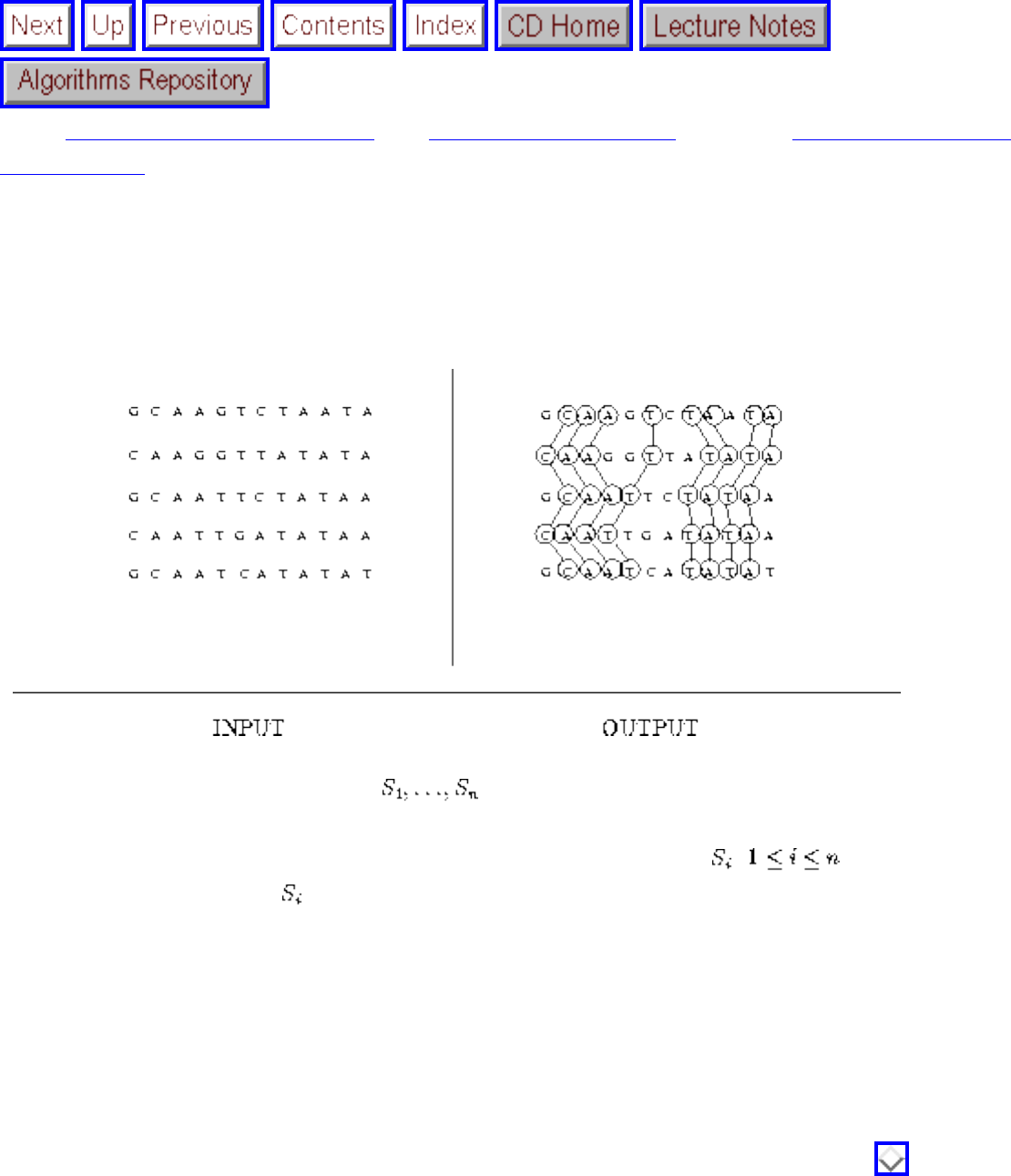
Longest Common Substring
Next: Shortest Common Superstring Up: Set and String Problems Previous: Finite State Machine
Minimization
Longest Common Substring
Input description: A set S of strings .
Problem description: What is the longest string S' such that for each , , the characters of S
appear as a subsequence of ?
Discussion: The problem of longest common subsequence arises whenever we search for similarities
across multiple texts. A particularly important application is in finding a consensus among DNA
sequences. The genes for building particular proteins evolve with time, but the functional regions must
remain consistent in order to work correctly. By finding the longest common subsequence of the same
gene in different species, we learn what has been conserved over time.
The longest common substring problem is a special case of edit distance (see Section ), when
substitutions are forbidden and only exact character match, insert, and delete are allowable edit
operations. Under these conditions, the edit distance between p and t is n+m-2 |lcs(p,t)|, since we can
delete the missing characters from p to the lcs(p,t) and insert the missing characters from t to transform p
to t. This is particularly interesting because the longest common subsequence can be faster to compute
file:///E|/BOOK/BOOK5/NODE208.HTM (1 of 4) [19/1/2003 1:32:18]
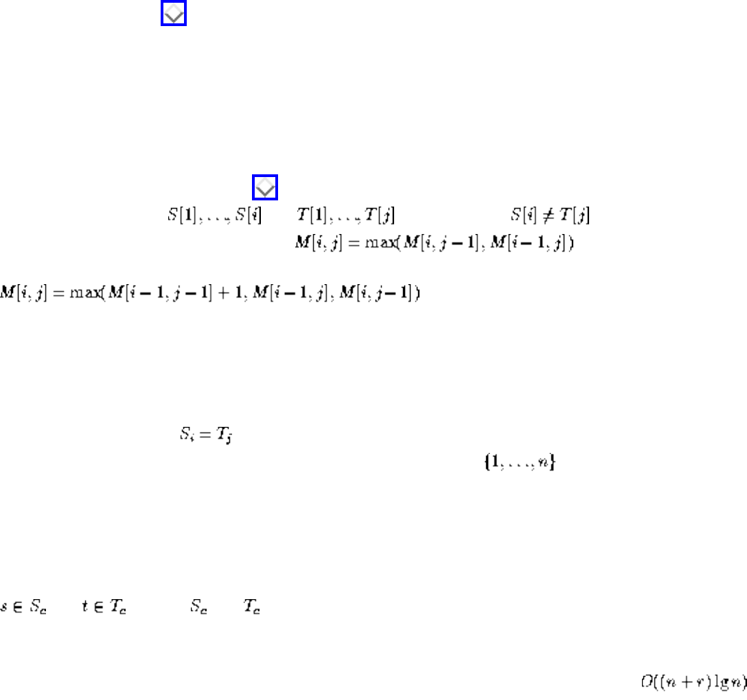
Longest Common Substring
than edit distance.
Issues arising include:
● Are you looking for a common substring or scattered subsequence? - In detecting plagiarism or
attempting to identify the authors of anonymous works, we might need to find the longest phrases
shared between several documents. Since phrases are strings of consecutive characters, we need
the longest common substring between the texts.
The longest common substring of a set of strings can be identified in linear time using suffix trees,
discussed in Section . The trick is to build a suffix tree containing all the strings, label each
leaf with the set of strings that contain it, and then do a depth-first traversal to identify the deepest
node that has descendents from each input string.
For the rest of this discussion, we will restrict attention to finding common scattered
subsequences. Dynamic programming can be used to find the longest common subsequence of
two strings, S and T, of n and m characters each. This algorithm is a special case of the edit-
distance computation of Section . Let M[i,j] denote the number of characters in the longest
common substring of and . In general, if , there is no way the
last pair of characters could match, so . If S[i] = T[j], we have
the option to select this character for our substring, so
. This gives a recurrence that computes M,
and thus finds the length of the longest common subsequence in O(nm) time. We can reconstruct
the actual common substring by walking backward from M[n,m] and establishing which
characters were actually matched along the way.
● What if there are relatively few sets of matching characters? - For strings that do not contain too
many copies of the same character, there is a faster algorithm. Let r be the number of pairs of
positions (i,j) such that . Thus r can be as large as mn if both strings consist entirely of the
same character, but r = n if the two strings are permutations of . This technique treats the
pairs of r as defining points in the plane.
The complete set of r such points can be found in O(n + m + r) time by bucketing techniques. For
each string, we create a bucket for each letter of the alphabet and then partition all of its characters
into the appropriate buckets. For each letter c of the alphabet, create a point (,t) from every pair
and , where and are buckets for c.
A common substring represents a path through these points that moves only up and to the right,
never down or to the left. Given these points, the longest such path can be found in
time. We will sort the points in order of increasing x-coordinate (breaking ties in favor of
increasing y-coordinate. We will insert these points one by one in this order, and for each k,
file:///E|/BOOK/BOOK5/NODE208.HTM (2 of 4) [19/1/2003 1:32:18]
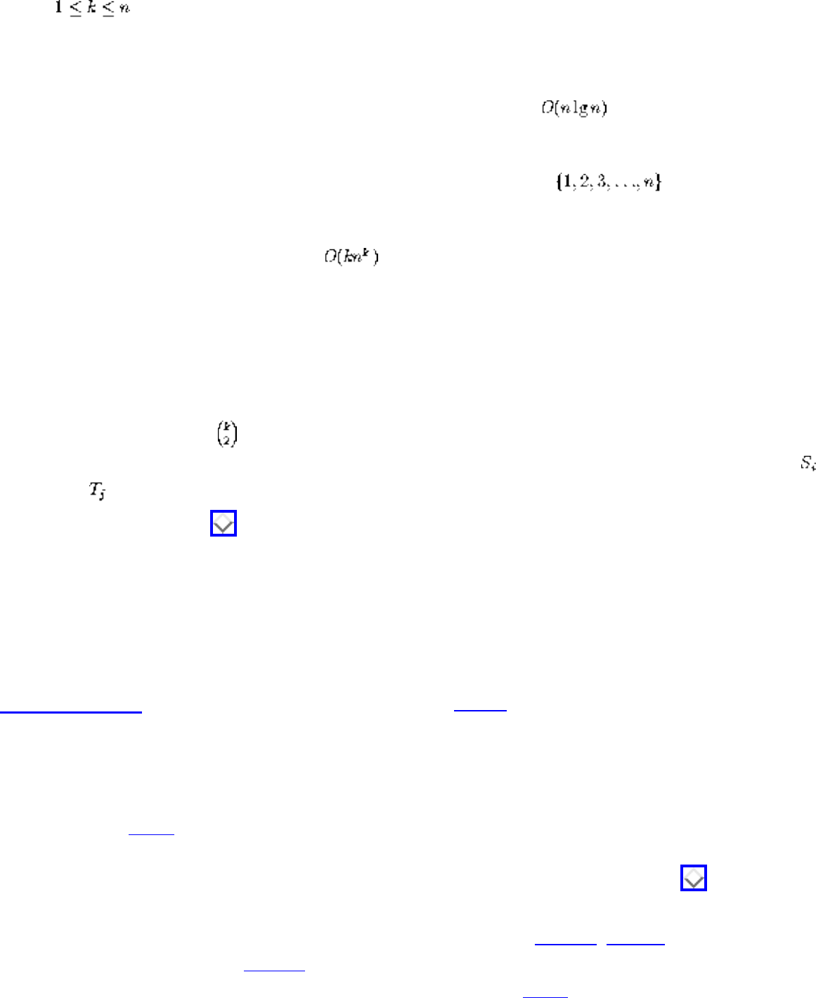
Longest Common Substring
, maintain the minimum y-coordinate of any path going through exactly k points.
Inserting a new point will change exactly one of these paths by reducing the y-coordinate of the
path whose last point is barely greater than the new point.
● What if the strings are permutations? - If the strings are permutations, then there are exactly n
pairs of matching characters, and the above algorithm runs in time. A particularly
important case of this occurs in finding the longest increasing subsequence of a sequence of
numbers. Sorting this sequence and then replacing each number by its rank in the total order gives
us a permutation p. The longest common subsequence of p and gives the longest
increasing subsequence.
● What if we have more than two strings to align? - The basic dynamic programming algorithm can
be generalized to k strings, taking time, where n is the length of the longest string. This
algorithm is exponential in the number of strings k, and so it will likely be too expensive for more
than 3 to 4 strings. Further, the problem is NP-complete, so no better exact algorithm is destined
to come along.
This problem of multiple sequence alignment has received considerable attention, and numerous
heuristics have been proposed. Many heuristics begin by computing the pairwise alignment
between each of the pairs of strings, and then work to merge these alignments. One approach is
to build a graph with a vertex for each character of each string. There will be an edge between
and if the corresponding characters are matched in the alignment between S and T. Any k-
clique (see Section ) in this graph describes a commonly aligned character, and all such cliques
can be found efficiently because of the sparse structure of this graph.
Although these cliques will define a common subsequence, there is no reason to believe that it
will be the longest such substring. Appropriately weakening the clique requirement provides a
way to increase it, but still there can be no promises.
Implementations: MAP (Multiple Alignment Program) [Hua94] by Xiaoqiu Huang is a C language
program that computes a global multiple alignment of sequences using an iterative pairwise method.
Certain parameters will need to be tweaked to make it accommodate non-DNA data. It is available by
anonymous ftp from cs.mtu.edu in the pub/huang directory.
Combinatorica [Ski90] provides a Mathematica implementation of an algorithm to construct the longest
increasing subsequence of a permutation, which is a special case of longest common subsequence. This
algorithm is based on Young tableaux rather than dynamic programming. See Section .
Notes: Good expositions on longest common subsequence include [AHU83, CLR90]. A survey of
algorithmic results appears in [GBY91]. The algorithm for the case where all the characters in each
sequence are distinct or infrequent is due to Hunt and Szymanski [HS77]. Expositions of this algorithm
file:///E|/BOOK/BOOK5/NODE208.HTM (3 of 4) [19/1/2003 1:32:18]
Longest Common Substring
include [Aho90, Man89]. Multiple sequence alignment for computational biology is treated in [Wat95].
Certain problems on strings become easier when we assume a constant-sized alphabet. Masek and
Paterson [MP80] solve longest common subsequence in for constant-sized
alphabets, using the four Russians technique.
Related Problems: Approximate string matching (see page ), shortest common superstring (see page
).
Next: Shortest Common Superstring Up: Set and String Problems Previous: Finite State Machine
Minimization
Algorithms
Mon Jun 2 23:33:50 EDT 1997
file:///E|/BOOK/BOOK5/NODE208.HTM (4 of 4) [19/1/2003 1:32:18]
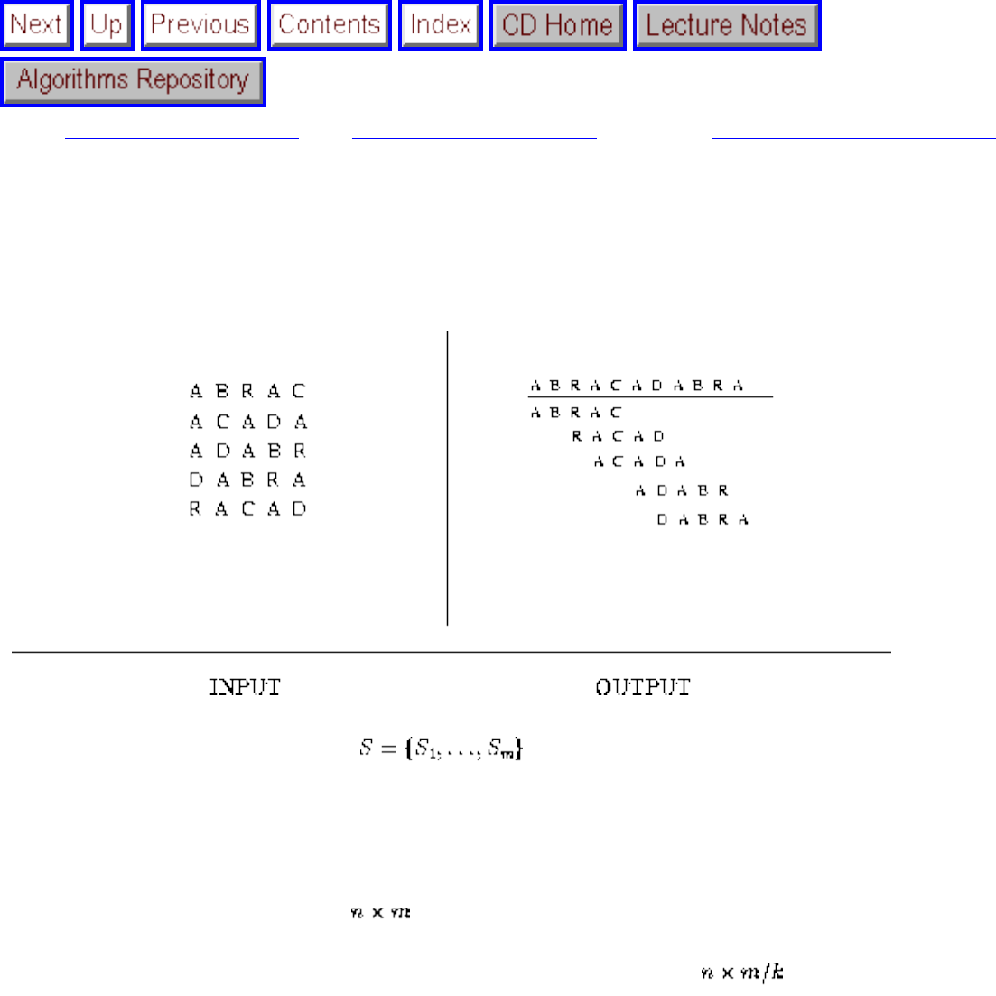
Shortest Common Superstring
Next: Algorithmic Resources Up: Set and String Problems Previous: Longest Common Substring
Shortest Common Superstring
Input description: A set of strings .
Problem description: Find the shortest string S' that contains each element of S as a substring.
Discussion: Shortest common superstring arises in a variety of applications, including sparse matrix
compression. Suppose we have an matrix with most of the elements being zero. We can partition
each row into m/k runs of k elements each and construct the shortest common superstring S' of these runs.
We now have reduced the problem to storing the superstring, plus an array of pointers into the
superstring denoting where each of the runs starts. Accessing a particular element M[i,j] still takes
constant time, but there is a space savings when |S| << mn.
Another application arises in DNA sequencing. It happens to be easy to sequence small fragments of
DNA, say up to about 500 base pairs or characters. However, the real interest is in sequencing large
molecules. The standard approach to large-scale, ``shotgun'' sequencing clones many copies of the target
molecule, breaks them randomly into small fragments, sequences the fragments, and then proposes the
shortest superstring of the fragments as the correct sequence. While it is an article of faith that the
shortest superstring will be the most likely sequence, this seems to work reasonably well in practice.
file:///E|/BOOK/BOOK5/NODE209.HTM (1 of 3) [19/1/2003 1:32:19]
Shortest Common Superstring
Finding a superstring of all the substrings is not difficult, as we can simply concatenate them all together.
It is finding the shortest such string that is problematic. Indeed, shortest common superstring remains NP-
complete under all reasonable classes of strings.
The problem of finding the shortest common superstring can easily be reduced to that of the traveling
salesman problem (see Section ). Create an overlap graph G where vertex represents string . Edge
will have weight equal to the length of minus the overlap of with . The path visiting all the
vertices of minimum total weight defines the shortest common superstring. The edge weights of this
graph are not symmetric, after all, the overlap of and is not the same as the overlap of
and . Thus only programs capable of solving asymmetric TSPs can be applied to this problem.
The greedy heuristic is the standard approach to approximating the shortest common superstring. Find the
pair of strings with the maximum number of characters of overlap. Replace them by the merged string,
and repeat until only one string remains. Given the overlap graph above, this heuristic can be efficiently
implemented by inserting all of the edge weights into a heap (see Section ) and then merging if the
appropriate ends of the two strings have not yet be used, which can be maintained with an array of
Boolean flags.
The potentially time-consuming part of this heuristic is in building the overlap graph. The brute-force
approach to finding the maximum overlap of two length-l strings takes , which must be repeated
times. Faster times are possible by appropriately using suffix trees (see Section ). Build a tree
containing all suffixes of all reversed strings of S. String overlaps with if a suffix of matches a
suffix of the reverse of . The longest overlap for each fragment can be found in time linear in its
length.
How well does the greedy heuristic perform? If we are unlucky with the input, the greedy heuristic can be
fooled into creating a superstring that is at least twice as long as optimal. Usually, it will be a lot better in
practice. It is known that the resulting superstring can never be more than 2.75 times optimal.
Building superstrings becomes more difficult with positive and negative substrings, where negative
substrings cannot be substrings of the superstring. The problem of deciding whether any such consistent
substring exists is NP-complete, unless you are allowed to add an extra character to the alphabet to use as
a spacer.
Implementations: CAP (Contig Assembly Program) [Hua92] by Xiaoqiu Huang is a C language
program supporting DNA shotgun sequencing by finding the shortest common superstring of a set of
fragments. As to performance, CAP took 4 hours to assemble 1,015 fragments of a total of 252,000
characters on a Sun SPARCstation SLC. Certain parameters will need to be tweaked to make it
accommodate non-DNA data. It is available by anonymous ftp from cs.mtu.edu in the pub/huang
directory.
file:///E|/BOOK/BOOK5/NODE209.HTM (2 of 3) [19/1/2003 1:32:19]
Shortest Common Superstring
Notes: The shortest common superstring problem and its application to DNA shotgun assembly is ably
surveyed in [Wat95]. Kececioglu and Myers [KM95] report on an algorithm for the more general version
of shortest common superstring, where the strings may have errors. Their paper is recommended reading
to anyone interested in fragment assembly.
Blum et al. [BJL 91] gave the first constant-factor approximation algorithms for shortest common
superstring, with a variation of the greedy heuristic. More recent research has beaten the constant down
to 2.75, progress towards the expected factor-two result.
Related Problems: Suffix trees (see page ), text compression (see page ).
Next: Algorithmic Resources Up: Set and String Problems Previous: Longest Common Substring
Algorithms
Mon Jun 2 23:33:50 EDT 1997
file:///E|/BOOK/BOOK5/NODE209.HTM (3 of 3) [19/1/2003 1:32:19]

Software systems
Next: LEDA Up: Algorithmic Resources Previous: Algorithmic Resources
Software systems
In this section, we describe several particularly comprehensive implementations of combinatorial
algorithms, all of which are available over the Internet. Although these codes are discussed in the
relevant sections of the catalog, they are substantial enough to warrant further attention.
A good algorithm designer does not reinvent the wheel, and a good programmer does not rewrite code
that other people have written. Picasso put it best: ``Good artists borrow. Great artists steal.''
However, a word of caution about stealing. Many of the codes described below (and throughout this
book) have been made available for research or educational use, although commercial use requires a
licensing arrangement with the author. I urge you to respect this. Licensing terms from academic
institutions are usually surprisingly modest. The recognition that industry is using a particular code is
important to the authors, often more important than the money involved. This can lead to enhanced
support or future releases of the software. Do the right thing and get a license. Information about terms or
whom to contact is usually available embedded within the documentation, or available at the source
ftp/WWW site.
Although the bulk of the systems we describe here are available by accessing our algorithm repository,
http://www.cs.sunysb.edu/ algorith (as well as on the enclosed CD-ROM), we encourage you to get
them from the original sites instead of Stony Brook. There are three reasons. First, the version on the
original site is much more likely to be maintained. Second, there are often supporting files and
documentation that we for whatever reason did not download, and which may be of interest to you.
Finally, by ftp-ing from the original sites, you will keep traffic down at the algorithm repository site,
which will minimize the complaints from our system staff that I anticipate if this service becomes very
popular.
● LEDA
● Netlib
file:///E|/BOOK/BOOK5/NODE211.HTM (1 of 2) [19/1/2003 1:32:20]
Software systems
❍ Collected Algorithms of the ACM
● The Stanford GraphBase
● Combinatorica
● Algorithm Animations with XTango
● Programs from Books
❍ Discrete Optimization Algorithms in Pascal
❍ Handbook of Data Structures and Algorithms
❍ Combinatorial Algorithms for Computers and Calculators
❍ Algorithms from P to NP
❍ Computational Geometry in C
❍ Algorithms in C++
Next: LEDA Up: Algorithmic Resources Previous: Algorithmic Resources
Algorithms
Mon Jun 2 23:33:50 EDT 1997
file:///E|/BOOK/BOOK5/NODE211.HTM (2 of 2) [19/1/2003 1:32:20]
LEDA
Next: Netlib Up: Software systems Previous: Software systems
LEDA
LEDA, for Library of Efficient Data types and Algorithms, is perhaps the best single resource available
to support combinatorial computing. It has been under development since 1988 by a group at Max-
Planck-Instutut in Saarbrücken, Germany, including Kurt Mehlhorn, Stefan Näher, Stefan Schirra,
Christian Uhrig, and Christoph Burnikel. LEDA is unique because of (1) the algorithmic sophistication
of its developers and (2) the level of continuity and resources invested in the project.
LEDA is implemented in C++ using templates, and it should compile on most new compilers, but not
some old ones. LEDA is available by anonymous ftp from ftp.mpi-sb.mpg.de in directory /pub/LEDA, or
at http://www.mpi-sb.mpg.de/LEDA/leda.html. The distribution contains all sources, installation
instructions, and a substantial users manual [NU95]. An active Usenet newsgroup comp.lang.c++.leda is
inhabited by users of LEDA. A good article on LEDA is available [MN95], and a book is promised soon.
LEDA is not in the public domain, but it can be used freely for research and teaching. Commerical
licenses are also available.
What LEDA offers is a complete collection of well-implemented data structures and types. Particularly
useful is the graph type, which supports all the basic operations one needs in an intelligent way, although
this generality comes at some cost in size and speed over handcrafted implementations. A small but
useful library of graph algorithms is included, which illustrates how cleanly and concisely these
algorithms can be implemented using the LEDA data types. Good implementations of the most important
data structures supporting such common data types as dictionaries and priority queues are provided.
There are also algorithms and data structures for computational geometry in the plane, including some
support for X-windows.
LEDA Implementation
Algorithms
Mon Jun 2 23:33:50 EDT 1997
file:///E|/BOOK/BOOK5/NODE212.HTM [19/1/2003 1:32:21]

Netlib
Next: Collected Algorithms of the Up: Software systems Previous: LEDA
Netlib
Netlib is an on-line repository of mathematical software that contains a large number of interesting
codes, tables, and papers. Netlib is a compilation of resources from a variety of places, with fairly
detailed indices and search mechanisms to help you find what is there. Netlib is important because of its
breadth and ease of access. Whenever you need a specialized piece of mathematical software, you should
look here first.
There are three ways to access netlib: by e-mail, ftp, or WWW:
● E-mail - Netlib provides an email server to send indices and sources on demand. To get an index,
send e-mail to netlib@netlib.org with the words send index on its own line in the message. The
index will provide a list of other files you can send for. The e-mail server and netlib in general are
discussed in [DG87].
● FTP - Connect by ftp to ftp.netlib.org. Log in as anonymous and use your e-mail address as
password. Use ``ls'' to see the contents of a directory, ``cd'' to move to a different directory, and
``get'' to fetch the desired file. Type ``binary'' before ``get'' in order to ensure uncorrupted
transmission, and ``quit'' to quit. Obtaining an index first can make it easier to move around.
● WWW - With your favorite browser, open the URL address http://www.netlib.org/ and prowl
around to your heart's content. There is a forms index that permits searching based on keywords.
GAMS, the Guide to Available Mathematical Software, is an indexing service for Netlib and other
related software repositories that can help you find what you want. Check it out at http://gams.nist.gov.
GAMS is a service of the National Institute of Standards and Technology (NIST).
Netlib pointers
● Collected Algorithms of the ACM
file:///E|/BOOK/BOOK5/NODE213.HTM (1 of 2) [19/1/2003 1:32:21]
Netlib
Algorithms
Mon Jun 2 23:33:50 EDT 1997
file:///E|/BOOK/BOOK5/NODE213.HTM (2 of 2) [19/1/2003 1:32:21]
Collected Algorithms of the ACM
Next: The Stanford GraphBase Up: Netlib Previous: Netlib
Collected Algorithms of the ACM
An early mechanism for the distribution of useful algorithm implementations was CALGO, the Collected
Algorithms of the ACM. It first appeared in Communications of the ACM in 1960, covering such famous
algorithms as Floyd's linear-time build heap algorithm. More recently, it has been the province of the
ACM Transactions on Mathematical Software. Each algorithm/implementation is described in a brief
journal article, with the implementation validated and collected. These implementations are maintained at
http://www.acm.org/calgo/ and at Netlib.
Over 750 algorithms have appeared to date. Most of the codes are in Fortran and are relevant to
numerical computing, although several interesting combinatorial algorithms have slithered their way into
CALGO. Since the implementations have been refereed, they are presumably more reliable than most
readily available software.
Algorithms
Mon Jun 2 23:33:50 EDT 1997
file:///E|/BOOK/BOOK5/NODE214.HTM [19/1/2003 1:32:22]
The Stanford GraphBase
Next: Combinatorica Up: Software systems Previous: Collected Algorithms of the
The Stanford GraphBase
The Stanford GraphBase is an interesting program for several reasons. First, it was composed as a
``literate program'', meaning that it was written to be read. If anybody's programs deserve to be read, it is
Knuth's, and [Knu94] contains the full source code of the system. The programming
language/environment is CWEB, which permits the mixing of text and code in particularly expressive
ways.
The GraphBase contains implementations of several important combinatorial algorithms, including
matching, minimum spanning trees, and Voronoi diagrams, as well as specialized topics like constructing
expander graphs and generating combinatorial objects. Finally, it contains programs for several
recreational problems, including constructing word ladders (flour-floor-flood-blood-brood-broad-bread)
and establishing dominance relations among football teams.
Although the GraphBase is more fun to play with than LEDA, it is not really suited for building general
applications on top of. The GraphBase is perhaps most useful as an instance generator for constructing a
wide variety of graphs to serve as test data. It incorporates graphs derived from interactions of characters
in famous novels, Roget's thesaurus, the Mona Lisa, and the economy of the United States. Further,
because of its machine-independent random number generators, the GraphBase provides a way to
construct random graphs that can be reconstructed elsewhere, making them perfect for experimental
comparisons of algorithms.
The Stanford GraphBase can be obtained by anonymous ftp from labrea.stanford.edu in the directory
pub/sgb. It may be used freely, but the files may not be modified. Installing the GraphBase requires
CWEB, which can be obtained by anonymous ftp from labrea.stanford.edu in the directory pub/cweb.
GraphBase Implementation
Algorithms
Mon Jun 2 23:33:50 EDT 1997
file:///E|/BOOK/BOOK5/NODE215.HTM [19/1/2003 1:32:23]
Combinatorica
Next: Algorithm Animations with XTango Up: Software systems Previous: The Stanford GraphBase
Combinatorica
Combinatorica [Ski90] is a collection of over 230 algorithms for combinatorics and graph theory written
in Mathematica. These routines have been designed to work together, enabling one to experiment with
discrete structures and build prototype applications. Combinatorica has been widely used for both
research and education.
Although (in my totally unbiased opinion) Combinatorica is more comprehensive and better integrated
than other libraries of combinatorial algorithms, it is also the slowest such system available. Credit for all
of these properties is largely due to Mathematica, which provides a very high-level, functional,
interpreted, and thus inefficient programming language. Combinatorica is best for finding quick solutions
to small problems, and (if you can read Mathematica code) as a terse exposition of algorithms for
translation into other languages.
Combinatorica is included with the standard Mathematica distribution in the directory
Packages/DiscreteMath/Combinatorica.m . It can also be obtained by anonymous ftp from
ftp.cs.sunysb.edu in the pub/Combinatorica directory. Included on this site are certain extensions to
Combinatorica and data sources such as the graphs of Graffiti.
Combinatorica Implementation
Algorithms
Mon Jun 2 23:33:50 EDT 1997
file:///E|/BOOK/BOOK5/NODE216.HTM [19/1/2003 1:32:23]

Algorithm Animations with XTango
Next: Programs from Books Up: Software systems Previous: Combinatorica
Algorithm Animations with XTango
XTango [Sta90] is a general-purpose algorithm animation system, developed by John Stasko of Georgia
Tech, that helps programmers develop color, real-time animations of their own algorithms and programs.
Creating animations of your own implementations is useful both for pedagogical and debugging
purposes.
Included with the XTango distribution is a large collection of animations, several of which are quite
interesting and enlightening to watch. The C language source for each animation is included. My
favorites include animations of:
● Data structures - including AVL/red-black trees, and binary/Fibonacci heaps.
● Sorting algorithms - including bubblesort, radixsort, quicksort, and shellsort.
● Backtracking - including graph coloring, and both the eight-queens and knight's tour problems.
● Geometric algorithms - including bin packing heuristics and the Graham scan/Jarvis march
convex hull algorithms.
● Graph algorithms - including minimum spanning trees and shortest paths.
● String algorithms - including the Knuth-Morris-Pratt and Boyer-Moore algorithms.
Anybody studying these algorithms might well profit from playing with the animations. The source code
for the animations contains C language implementations of these algorithms, although of uncertain
quality.
XTango is implemented on top of UNIX and X-windows. It is available via anonymous ftp from
ftp.cc.gatech.edu in directory pub/people/stasko. Also available there is Polka, a C++ algorithm
animation system that is particularly suited to animating parallel computations. POLKA provides its own
high-level abstractions to make the creation of animations easier and faster than with many other
systems. POLKA also includes an interactive front end called SAMBA that can be used to generate
animations from any type of program that can generate ASCII.
XTango Implementation
file:///E|/BOOK/BOOK5/NODE217.HTM (1 of 2) [19/1/2003 1:32:24]
Algorithm Animations with XTango
Algorithms
Mon Jun 2 23:33:50 EDT 1997
file:///E|/BOOK/BOOK5/NODE217.HTM (2 of 2) [19/1/2003 1:32:24]
Programs from Books
Next: Discrete Optimization Algorithms in Up: Software systems Previous: Algorithm Animations with
XTango
Programs from Books
Several books on algorithms include working implementations of the algorithms in a real programming
language. Although these implementations are intended primarily for exposition, they can also be useful
for computation. Since they are typically small and clean, they can prove the right foundation for simple
applications.
The most useful codes of this genre are described below. All are available from the algorithm repository,
http://www.cs.sunysb.edu/ algorith.
● Discrete Optimization Algorithms in Pascal
● Handbook of Data Structures and Algorithms
● Combinatorial Algorithms for Computers and Calculators
● Algorithms from P to NP
● Computational Geometry in C
● Algorithms in C++
Algorithms
Mon Jun 2 23:33:50 EDT 1997
file:///E|/BOOK/BOOK5/NODE218.HTM [19/1/2003 1:32:24]
Discrete Optimization Algorithms in Pascal
Next: Handbook of Data Structures Up: Programs from Books Previous: Programs from Books
Discrete Optimization Algorithms in Pascal
This is a collection of 28 programs for solving discrete optimization problems, appearing in the book by
Syslo, Deo, and Kowalik [SDK83]. The package includes programs for integer and linear programming,
the knapsack and set cover problems, traveling salesman, vertex coloring, and scheduling as well as
standard network optimization problems. They have been made available from the algorithm repository
WWW site, http://www.cs.sunysb.edu/ algorith.
This package is noteworthy for the operations-research flavor of the problems and algorithms selected.
The algorithms have been selected to solve problems, as opposed to for purely expository purposes. In
[SDK83], a description of each algorithm and extensive set of references for each problem is provided, as
well as execution times for each program on several instances on an early 1980s mainframe, an Amdahl
470 V/6.
Implementations
Algorithms
Mon Jun 2 23:33:50 EDT 1997
file:///E|/BOOK/BOOK5/NODE219.HTM [19/1/2003 1:32:25]
Handbook of Data Structures and Algorithms
Next: Combinatorial Algorithms for Computers Up: Programs from Books Previous: Discrete
Optimization Algorithms in
Handbook of Data Structures and Algorithms
The Handbook of Data Structures and Algorithms, by Gonnet and Baeza-Yates [GBY91], provides a
comprehensive reference on fundamental data structures for searching and priority queues, and
algorithms for sorting and text searching. The book covers this relatively small number of topics
comprehensively, presenting most of the major and minor variations that appear in the literature.
Perusing the book makes one aware of the tremendous range of data structures that have been developed
and the intense level of analysis many of them have been subjected to.
For each data structure or algorithm, a brief description is provided along with its asymptotic complexity
and an extensive set of references. More distinctively, an implementation in C and/or Pascal is usually
provided, along with experimental results comparing the performance of these implementations. The
programs in [GBY91] are available at a very slick WWW site, http://www.dcc.uchile.cl/
rbaeza/handbook/hbook.html.
Since many of the elementary data structures and sorting algorithms can be implemented concisely, most
of the programs are very short. They are perhaps most useful as models, or as part of an experimental
study to compare the performance on different data structures for a particular application.
Handbook Implementations
Algorithms
Mon Jun 2 23:33:50 EDT 1997
file:///E|/BOOK/BOOK5/NODE220.HTM [19/1/2003 1:32:25]
Combinatorial Algorithms for Computers and Calculators
Next: Algorithms from P to Up: Programs from Books Previous: Handbook of Data Structures
Combinatorial Algorithms for Computers and Calculators
Nijenhuis and Wilf [NW78] specializes in algorithms for constructing basic combinatorial objects such
as permutations, subsets, and partitions. Such algorithms are often very short, but they are hard to locate
and usually surprisingly subtle. Fortran programs for all of the algorithms are provided, as well as a
discussion of the theory behind each of them. The programs are usually short enough that it is reasonable
to translate them directly into a more modern programming language, as I did in writing Combinatorica
(see Section ). Both random and sequential generation algorithms are provided. Descriptions of more
recent algorithms for several problems, without code, are provided in [Wil89].
These programs are now available from our algorithm repository WWW site. We tracked them down
from Neil Sloane, who had them on a magnetic tape, while the original authors did not! In [NW78],
Nijenhuis and Wilf set the proper standard of statistically testing the output distribution of each of the
random generators to establish that they really appear uniform. We encourage you to do the same before
using these programs, to verify that nothing has been lost in transit.
Programs
Algorithms
Mon Jun 2 23:33:50 EDT 1997
file:///E|/BOOK/BOOK5/NODE221.HTM [19/1/2003 1:32:26]

Algorithms from P to NP
Next: Computational Geometry in C Up: Programs from Books Previous: Combinatorial Algorithms for
Computers
Algorithms from P to NP
This algorithms text [MS91] distinguishes itself by including Pascal implementations of many
algorithms, with careful experimental comparisons of different algorithms for such problems as sorting
and minimum spanning tree, and heuristics for the traveling salesman problem. It provides a useful
model for how to properly do empirical algorithm analysis.
The programs themselves are probably best used as models. Interesting implementations include the
eight-queens problem, plus fundamental graph and geometric algorithms. The programs in [MS91] have
been made available by anonymous ftp from cs.unm.edu in directory /pub/moret_shapiro.
Programs
Algorithms
Mon Jun 2 23:33:50 EDT 1997
file:///E|/BOOK/BOOK5/NODE222.HTM [19/1/2003 1:32:26]
Computational Geometry in C
Next: Algorithms in C++ Up: Programs from Books Previous: Algorithms from P to
Computational Geometry in C
O'Rourke [O'R94] is perhaps the best practical introduction to computational geometry available,
because of its careful and correct C language implementations of the fundamental algorithms of
computational geometry. Fundamental geometric primitives, convex hulls, triangulations, Voronoi
diagrams, and motion planning are all included. Although they were implemented primarily for
exposition rather than production use, they should be quite reliable. The codes are available from
http://grendel.csc.smith.edu/ orourke/.
Programs
Algorithms
Mon Jun 2 23:33:50 EDT 1997
file:///E|/BOOK/BOOK5/NODE223.HTM [19/1/2003 1:32:28]
Algorithms in C++
Next: Data Sources Up: Programs from Books Previous: Computational Geometry in C
Algorithms in C++
Sedgewick's popular algorithms text [Sed92] comes in several different language editions, including C,
C++, and Modula-3. This book distinguishes itself through its use of algorithm animation and in its broad
topic coverage, including numerical, string, and geometric algorithms.
The language-specific parts of the text consist of many small code fragments, instead of full programs or
subroutines. Thus they are best thought of as models, instead of working implementations. Still, the
program fragments from the C++ edition have been made available from http://heg-
school.aw.com/cseng/authors/sedgewick/algo-in-c++/algo-in-c++.html
Algorithms
Mon Jun 2 23:33:50 EDT 1997
file:///E|/BOOK/BOOK5/NODE224.HTM [19/1/2003 1:32:28]
Data Sources
Next: Textbooks Up: Algorithmic Resources Previous: Algorithms in C++
Data Sources
It is often important to have interesting data to feed your algorithms, to serve as test data to ensure
correctness or to compare different algorithms for raw speed.
Finding good test data can be surprisingly difficult. Here are some pointers:
● Combinatorica graphs - A modest collection of graphs is available from the Combinatorica ftp
site. Particularly interesting are the 190 graphs of Graffiti [Faj87], a program that formulated
conjectures in graph theory by studying the properties of these graphs. See Section for more
information on Combinatorica.
● TSPLIB - This well-respected library of test instances for the traveling salesman problem is
available from Netlib (see Section ) and by anonymous ftp from softlib.cs.rice.edu. TSPLIB
instances are large, real-world graphs, derived from applications such as circuit boards and
networks.
● Stanford GraphBase - Discussed in Section , this suite of programs by Knuth provides
portable generators for a wide variety of graphs. These include graphs arising from distance
matrices, arts, and literature, as well as graphs of more theoretical interest.
● DIMACS Challenge data - A series of DIMACS Challenge workshops have focused on evaluating
algorithm implementations of graph, logic, and data structure problems. Instance generators for
each problem have been developed, with the focus on constructing difficult or representative test
data. The products of the DIMACS Challenges are available from http://dimacs.rutgers.edu/.
● Algorithm Repository - The Algorithm Repository WWW site, http://www.cs.sunysb.edu/
algorith (and enclosed CD-ROM) contain data sources for a few of the implementation challenge
exercises. In particular, we provide an airline routes data set, and a collection of names labeled by
ethnicity.
Algorithms
Mon Jun 2 23:33:50 EDT 1997
file:///E|/BOOK/BOOK5/NODE225.HTM [19/1/2003 1:32:29]
Textbooks
Next: On-Line Resources Up: Algorithmic Resources Previous: Data Sources
Textbooks
There have emerged a number of excellent textbooks in the design and analysis of combinatorial
algorithms. Below we point out several of our favorites. In this book, we have shied away from giving a
detailed exposition or analysis of many algorithms, for our primary mission is to help the reader identify
their problem and point them to solutions. The reader is encouraged to turn to these sources for more
detail once they have found the name of what they are looking for.
Only general algorithm books are discussed here. Books on specific subareas of algorithms are reviewed
at the head of the relevant catalog chapter.
● Cormen, Leiserson, and Rivest [CLR90] - This is the one (other) book on algorithms you must
own, with its comprehensive treatment of most of the problems we discuss here, including data
structures, graph algorithms, and seminumerical algorithms.
● Baase [Baa88] - This book is more accessible than [CLR90] for those without a strong
mathematical background. It covers standard sorting, string, and graph algorithms, NP-
completeness, and more exotically, an introduction to parallel algorithms.
● Manber [Man89] - Built around the unconventional notion that induction is the fundamental
paradigm of algorithm design, this book is especially good at teaching techniques for designing
algorithms and has an outstanding collection of problems. Highly recommended.
● van Leeuwen [vL90b] - Not a textbook, but a collection of in-depth surveys on the state of the art
in algorithms and computational complexity. Although the emphasis is on theoretical results, this
book is perhaps the best single reference to point you to what is known about any given problem.
● Syslo, Deo, and Kowalik [SDK83] - This book includes printed Pascal implementations of 28
algorithms for discrete optimization problems, including mathematical programming, network
optimization, and traditional operations research problems such as knapsack and TSP. Each
algorithm is described in the book, and experimental timings (on a 1980s vintage machine) are
provided. These codes are now available by ftp, as discussed in Section . Despite its age, this
remains a useful reference, particularly with the programs now available on-line.
● Moret and Shapiro [MS91] - This algorithms text distinguishes itself by including Pascal
implementations of all algorithms and by its careful experimental comparisons of different
algorithms for such problems as sorting and minimum spanning tree. It provides a useful model for
how to properly do empirical algorithm analysis. These programs are available by ftp - see Section
for details.
file:///E|/BOOK/BOOK5/NODE226.HTM (1 of 2) [19/1/2003 1:32:30]
Textbooks
● Knuth [Knu94] - This book presents the implementation of the Stanford GraphBase, a collection of
programs for constructing different graphs and working with them. See Section for details. It is
very intriguing to browse.
● Aho, Hopcroft, and Ullman [AHU74] - This was the first modern algorithms book, and it has had
an enormous influence on how algorithms should be taught. Although it is now dated, it remains a
useful guide to certain topics in vogue in the early 1970s, such as matrix multiplication, the fast
Fourier transform, and arithmetic algorithms. A more elementary edition, focusing on data
structures, is [AHU83].
● Rawlins [Raw92] - This may well be the best self-study book available on algorithms. It is fun and
inspiring, with built-in pauses so the reader can make sure they understand what is going on. The
only drawback is a somewhat idiosyncratic set of topics, so you will miss certain important topics.
But you can get that from here. Rawlins's book can teach you the proper mindset to think about
algorithms.
● Papadimitriou and Steiglitz [PS82] - This book has more of an operations research emphasis than
most algorithms texts, with a good coverage of mathematical programming, network flow, and
combinatorial search.
● Lawler [Law76] - Particularly useful for its coverage of matroid theory, this book also provides a
thorough treatment of the network flow, matching, and shortest path algorithms known by the mid-
1970s.
● Binstock and Rex [BR95] - Although not a textbook, it includes C language implementations of an
idiosyncratic variety of algorithms for programmers. Disks containing the code are available for a
modest fee. The most interesting implementations are string and pattern matching algorithms, time
and date routines, an arbitrary-precision calculator, and a nice section on checksums and cyclic-
redundancy checks.
Next: On-Line Resources Up: Algorithmic Resources Previous: Data Sources
Algorithms
Mon Jun 2 23:33:50 EDT 1997
file:///E|/BOOK/BOOK5/NODE226.HTM (2 of 2) [19/1/2003 1:32:30]
On-Line Resources
Next: Literature Up: Algorithmic Resources Previous: Textbooks
On-Line Resources
The Internet has proven to be a fantastic resource for people interested in algorithms, as it has for many
other subjects. What follows is a highly selective list of the resources that I use most often, partitioned
into references to literature, people, and software. All of these should be in the tool chest of every
algorist.
● Literature
● People
● Software
Algorithms
Mon Jun 2 23:33:50 EDT 1997
file:///E|/BOOK/BOOK5/NODE227.HTM [19/1/2003 1:32:30]

Literature
Next: People Up: On-Line Resources Previous: On-Line Resources
Literature
There are many bibliographic sources available on the WWW, but the following I find indispensable.
● Computer Science Bibliographies - This is a collection of over 700,000 references to papers and
technical reports in Computer Science, beneath a sophisticated search engine. While there is much
duplication, this is my first stop whenever I need to look something up. The primary site is
http://liinwww.ira.uka.de/bibliography/index.html, although several mirror sites are in operation
around the world. All references are provided in bibtex format.
● Joel Seiferas' paper.lst - References to over 55,000 papers and technical reports (at last count),
mostly on algorithms and related areas of theoretical computer science. Each paper is reduced to a
one-line format, which I find easy to grep through. It is available by anonymous ftp from
ftp.cs.rochester.edu in /pub/u/joel, and a copy is included on the enclosed CD-ROM. Strongly
recommended.
● Geom.bib - The complete bibliography on anything related to computational geometry, it
references over 8,000 books, papers, and reports and includes detailed abstracts for many of them.
Grep-ing through geom.bib is an amazingly efficient way to find out about previous work without
leaving your office. It is available via anonymous ftp from ftp.cs.usask.ca, in file
pub/geometry/geombib.tar.Z, and a copy is included on the enclosed CD-ROM.
● Usenet FAQ files - The straightest, most accurate dope about any topic is likely to be had in a
USENET frequently asked questions (FAQ) file. Dedicated volunteers maintain FAQ files for
many USENET newsgroups, many of which are quite detailed, and which always emphasize other
on-line resources. Excellent FAQ files on algorithm-related topics such as cryptography, linear
programming, and data compression are currently available. A collection of current FAQ files is
maintained at ftp://rtfm.mit.edu/pub/usenet/news.answers.
Algorithms
Mon Jun 2 23:33:50 EDT 1997
file:///E|/BOOK/BOOK5/NODE228.HTM [19/1/2003 1:32:31]
People
Next: Software Up: On-Line Resources Previous: Literature
People
The easiest way to find the answer to any question is to ask someone who knows. Below, I describe some
useful resources of contact information for experts in algorithms. E-mail and the WWW make it very
easy to track down experts. In fact, maybe too easy. Please use this information responsibly, for many of
them are my friends! Limit your queries to short, specific questions; and contact them only after you
have checked the standard textbooks and references described in this section.
● comp.theory - The USENET newsgroup comp.theory is the proper forum for on-line discussions
on algorithms and related topics. Other appropriate newsgroups include comp.graphics.algorithms
and sci.math.
● TCS Virtual Address Book - This WWW-page address book is particularly useful to track down
the whereabouts of researchers in the design and analysis of algorithms. It is maintained by Ian
Parbery and is available from the ACM SIGACT WWW page http://sigact.acm.org/sigact/. An
excellent way to learn of recent progress on a particular problem is to ask a researcher who has
previously published on the problem, or at least check out their WWW page.
● Algorithm Courses - A comprehensive page of pointers to algorithm courses on the WWW is
maintained at http://www.cs.pitt.edu/ kirk/algorithmcourses/index.html. Lecture notes,
problems, and solutions are typically available, with some of the material being amazingly
thorough. Software associated with course projects is available from some of the sites.
Algorithms
Mon Jun 2 23:33:50 EDT 1997
file:///E|/BOOK/BOOK5/NODE229.HTM [19/1/2003 1:32:31]
Software
Next: Professional Consulting Services Up: On-Line Resources Previous: People
Software
There are many high-quality implementations of algorithms available on the WWW, if you know where
to look. We have placed as many of them as we could on the CD-ROM enclosed with this book. My
favorite on-line resources are:
● The Stony Brook Algorithm Repository - This is the source of the software on the enclosed CD-
ROM, organized according to the problem structure of this book. Local copies of most
implementations are maintained at http://www.cs.sunysb.edu/ algorith, along with pointers to
the latest version available from the original distribution site.
● Netlib - This is the standard resource on mathematical software, primarily numerical computation.
An enormous amount of material is available. See Section for details.
● Directory of Computational Geometry Software - Maintained by Nina Amenta, this is the source
for anything geometric. See http://www.geom.umn.edu/software/cglist/.
● Combinatorial Optimization codes - A very nice list of implementations of combinatorial
algorithms is maintained by Jiefeng Xu at http://ucsu.colorado.edu/ xu/software.html. With an
emphasis on operations research, there is a lot of useful stuff here.
Algorithms
Mon Jun 2 23:33:50 EDT 1997
file:///E|/BOOK/BOOK5/NODE230.HTM [19/1/2003 1:32:32]
Professional Consulting Services
Next: References Up: Algorithmic Resources Previous: Software
Professional Consulting Services
Algorist Technologies is a small consulting firm that provides its clients with short-term, expert help in
algorithm design and implementation. Typically, an Algorist consultant is called in for 1 to 3 days worth
of intensive, on-site discussion and analysis with the client's own development staff. Algorist has built an
impressive record of performance improvements with several companies and applications. They provide
longer-term consulting and contracting services as well.
Call 212-580-9009 or email info@algorist.com for more information on services provided by Algorist
Technologies.
Algorist Technologies 312 West 92nd St. Suite 1A New York, NY 10025 http://www.algorist.com
Algorithms
Mon Jun 2 23:33:50 EDT 1997
file:///E|/BOOK/BOOK5/NODE231.HTM [19/1/2003 1:32:32]
Index
Next: About this document Up: No Title Previous: Lecture 23 - approximation
Index
This index provides fast access to important keywords and topics in the on-line Lecture Notes The menu
below partitions the index entries by the first letter of the alphabet, for ease of access. A full document
index is also provided.
Be aware that the index pointer typically resides at the end of the relevant paragraph in the document, so
we recommend scrolling once towards the front of the document before reading.
A similar index has been provided for the book, which may also be of interest.
A B C D E F G H
I K L M N O P Q
R S T U V W
Complete Index
(note: the complete index is large; it will take a bit of time to load)
Algorithms
Mon Jun 2 09:21:39 EDT 1997
file:///E|/LEC/LECTUR16/NODE24.HTM [19/1/2003 1:32:33]

Index A
Up: Index - All
Index: A
above-below test ,
abracadabra
abstract data types
abstract graph type
academic institutions - licensing
acceptance-rejection method
Ackerman function
acyclic subgraph
Ada
adaptive compression algorithms
Adaptive Simulated Annealing (ASA)
addition
address book, TCS
adjacency list ,
adjacency matrix ,
adjacent swaps
advice - caveat
aesthetically pleasing drawings
aggregate range queries
agrep
Aho-Corasick algorithm
airline distance metric
airline scheduling ,
algorist
Algorist Technologies
algorithm animation
algorithm design
algorithmic resources
aligning DNA sequences
alignment costs
all-pairs shortest path , ,
file:///E|/BOOK/BOOK6/INDEX_A.HTM (1 of 3) [19/1/2003 1:32:35]

Index A
alpha-beta pruning ,
alpha-shapes
amortized analysis
AMPL
analog channel
ancestor
angle bisector
animation - motion planning
animation - sorting
animation - systems
annotated bibliography
approximate nearest neighbor search ,
approximate string matching , , ,
approximate string matching - related problems ,
approximate substring matching
approximation algorithms ,
approximation scheme ,
arbitrage
Arbitrary-Precision Arithmetic
arbitrary-precision arithmetic - geometry
arbitrary-precision arithmetic - related problems
architectural models
area computations - applications
area computations - triangles
area minimization
arm, robot
around the world game
Arrange ,
arrangement , ,
arrangement of objects
arrangements of lines
array
array searching
art gallery problems
articulation vertex ,
file:///E|/BOOK/BOOK6/INDEX_A.HTM (2 of 3) [19/1/2003 1:32:35]
Index A
artists steal
ASA
ASCII
aspect ratio
assembly language ,
assignment problem
associative operation
asymmetric longest path problem
asymmetric TSPs ,
asymptotic analysis
atom smashing
attitude of the algorithm designer
attribute
attribute - graph
augmenting path
augmenting path methods
authentication protocol
automorphisms
average
average-case analysis
average-case complexity
AVL tree
Avogadro's number
awk
Axiom
axis-oriented rectangles ,
axis-parallel planes
Algorithms
Tue Jun 3 11:59:38 EDT 1997
file:///E|/BOOK/BOOK6/INDEX_A.HTM (3 of 3) [19/1/2003 1:32:35]

Index B
Up: Index - All
Index: B
B-tree , , ,
backpacker
backsubstitution
backtracking , , , , , , , , ,
backtracking - animations
backtracking - applications ,
backtracking - bandwidth problem
balanced search tree , ,
banded systems ,
bandersnatch problem
bandwidth ,
bandwidth - matrix
Bandwidth Reduction
bandwidth reduction - backtracking
bandwidth reduction - related problems
bar codes
base - arithmetic
base - conversion
base of logarithm
Bellman-Ford algorithm ,
Berge's theorem
best-case complexity
Bible - searching the
bibliographic databases
biconnected components
biconnected graphs , ,
big Oh notation
bijection
binary heap
file:///E|/BOOK/BOOK6/INDEX_B.HTM (1 of 3) [19/1/2003 1:32:36]

Index B
binary representation - subsets
binary search , ,
binary search - applications ,
binary search - one-sided ,
binary search tree , , ,
binary search tree - applications
binary search tree - computational experience
Bin Packing
bin packing - applications ,
bin packing - knapsack problem
bin packing - related problems ,
biocomputing
biology
bipartite graph
bipartite graph recognition
bipartite incidence structures
bipartite matching , , ,
bipartite matching - applications ,
bit-mapped images
bit representation of graphs
bit vector , , ,
bit vector - applications ,
blind man's algorithm
block - set partition
blossoms
board evaluation function
bookshelves
Boolean logic minimization ,
Boolean matrix multiplication
borrowing
Boruvka's algorithm
boss's delight
boundaries
bounded height priority queue
file:///E|/BOOK/BOOK6/INDEX_B.HTM (2 of 3) [19/1/2003 1:32:36]
Index B
bounding boxes
Boyer-Moore algorithm
brainstorming
branch-and-bound search , ,
breadth-first search , , ,
breadth-first search - applications
bridge
bridges of Königsberg
Brook's theorem
Brooks, Mel
brush fire
brute-force search
bubblesort ,
bucketing techniques , ,
bucketing techniques - graphics
bucket sort
budget, fixed
built-in random number generator
buying fixed lots
Algorithms
Tue Jun 3 11:59:39 EDT 1997
file:///E|/BOOK/BOOK6/INDEX_B.HTM (3 of 3) [19/1/2003 1:32:36]
Index C
Up: Index - All
Index: C
C++ , , , , , , , , , , , , , , , , , , ,
, , , , , , , , , , , , ,
C++ templates
cache
Caesar shifts
calculator, arithmetic
Calendrical Calculations
call graph ,
canonically-labeled graphs
canonical order , ,
CAP
Carmichael numbers
cars and tanks
cartoons
casino analysis
casino poker
catalog WWW site
Catch-22 situation
caveat
CD-ROM , , ,
cdd
center vertex , ,
CGAL
chain of matrices
characters
checksum
chessboard coverage
chess program ,
Chinese calendar
Chinese postman problem
file:///E|/BOOK/BOOK6/INDEX_C.HTM (1 of 6) [19/1/2003 1:32:40]

Index C
Chinese remainder theorem
Christofides heuristic
chromatic index
chromatic number
chromatic polynomials
cipher
circle
circuit analysis
circuit board assembly
circuit board placement - simulated annealing
circuit layout
circuit schematic diagrams
circuit testing
circular embeddings
C language , , , , , , , , , , , , , , , , , ,
, , , , , , , , , , , , , , , , , , ,
classification
classification - nearest-neighbor
classifiers - neural networks
clauses
clipping
Clique
clique - applications ,
clique - definition
clique - hardness proof
clique - related problems
clock
closest pair heuristic
closest pair problem ,
closest point
closure
clothing - manufacturing
cloudy days
cluster
clustered access
cluster identification , ,
file:///E|/BOOK/BOOK6/INDEX_C.HTM (2 of 6) [19/1/2003 1:32:40]

Index C
clustering , ,
co-NP
coding theory
coefficients
cofactor method
coin flip
collapsing dense subgraphs
Collected Algorithms of the ACM , , , , , , , , , , , , , ,
, , , , , , ,
collection
coloring graphs
color interchange
combinatorial generation algorithms
combinatorial geometry
combinatorial problems ,
Combinatorica , , , , , , , , , , , , , , , , ,
, , , , , , , , ,
Commentz-Walter algorithm
commercial implementations
committee
committee - congressional
Common Lisp
common substrings
communication in circuits
communications networks ,
comp.graphics.algorithms
comp.theory
compaction
comparisons - minimizing
compiler
compiler construction
compiler optimization ,
compiler optimization - performance
complement
complement graph
completion time - minimum
file:///E|/BOOK/BOOK6/INDEX_C.HTM (3 of 6) [19/1/2003 1:32:40]
Index C
complexity classes
composite integer
compress ,
compression
compression - image
computational biology
computational complexity
computational geometry
computational number theory ,
computer algebra system ,
computer chess
computer graphics
computer graphics - applications ,
computer graphics - rendering
computer vision
concatenation - string
concavities
concavity elimination
configurations
configuration space
conjugate gradient methods
conjunctive normal form (CNF)
connected components , , ,
connected components - related problems ,
connected graph
connectivity , ,
consensus sequences
consistent schedule
Constrained and Unconstrained Optimization
constrained and unconstrained optimization - related problems
constrained Delaunay triangulation
constrained optimization
constrained optimization - related problems
constraint elimination
constraint satisfaction
file:///E|/BOOK/BOOK6/INDEX_C.HTM (4 of 6) [19/1/2003 1:32:40]

Index C
consulting services ,
container ,
context-free grammars
Contig Assembly Program
control systems - minimization
convex decomposition ,
convex hull ,
Convex Hull
convex hull - related problems ,
convex polygons
convex polygons - intersection
convex region
convolution - polygon
convolution - sequences
cookbook
cooling schedules
coordinate transformations
coplanar points
copying a graph
corporate ladder
correctness - algorithm
correlation function
counterexample construction
counting edges and vertices
counting Eulerian cycles
counting integer partitions
counting linear extensions
counting matchings
counting paths ,
counting spanning trees
courses, lecture notes
covering polygons with convex pieces
covering set elements
CPLEX
Cramer's rule
CRC
file:///E|/BOOK/BOOK6/INDEX_C.HTM (5 of 6) [19/1/2003 1:32:40]
Index C
critical path method
crossing number
crossings
Cryptography
cryptography - keys
cryptography - related problems , ,
CS
CSA
cubic regions
currency speculation
curve fitting
Cuthill-McKee algorithm
cut set ,
cutting plane methods ,
cutting stock problem
CWEB
cycle - shortest
cycle breaking
cycle detection ,
cycle length
cycle notation
cycle structure of permutations
cyclic-redundancy check (CRC)
Algorithms
Tue Jun 3 11:59:39 EDT 1997
file:///E|/BOOK/BOOK6/INDEX_C.HTM (6 of 6) [19/1/2003 1:32:40]

Index D
Up: Index - All
Index: D
DAG
DAG - longest path in
DAG - shortest path in
data abstraction
database algorithms
database application
database query optimization
data compression
Data Encryption Standard
data filtering
data records
data structures ,
data structures - animations
data transmission
data validation
Davenport-Schintzl sequences , ,
Davis-Putnam procedure ,
day of the week calculation
deadlock
de Bruijn sequence ,
debugging graph algorithms
debugging parallel programs
debugging randomized algorithms
debugging time
debugging tools
decimal arithmetic
decompose space
decomposing polygons
deconvolution
decrease-key
decryption
file:///E|/BOOK/BOOK6/INDEX_D.HTM (1 of 5) [19/1/2003 1:32:43]

Index D
Deep Blue
defenestrate
degeneracy
degeneracy testing
degenerate configuration
degenerate system of equations
degree, vertex ,
degree sequence
degrees of freedom
Delaunay triangulation , ,
Delaunay triangulation - applications
deletion from binary search tree
deletions - text
deliveries and pickups
delivery routing
Democrat/Republican identification
De Morgan's laws
dense graphs , ,
densest sphere packing
dense subgraph
depth-first search , , , , , , , ,
depth-first search - applications , , , , ,
depth-first search - backtracking
derangement
derivatives - automata
derivatives - calculus
DES
descendent
design process
design rule checking
determinant
determinant - related problems
Determinants and Permanents
deterministic finite automata
DFA
diameter of a graph
diameter of a point set
file:///E|/BOOK/BOOK6/INDEX_D.HTM (2 of 5) [19/1/2003 1:32:43]
Index D
Dictionaries
dictionaries - related problems ,
dictionary , ,
dictionary - applications
dictionary - related problems
dictionary - searching
DIEHARD
diff - how it works
digital geometry
digital signatures
Dijkstra's algorithm , ,
DIMACS , ,
DIMACS Challenge data
DIMACS Implementation Challenge , , , , ,
Dinic's algorithm
directed acyclic graph , , ,
directed cycle
directed graph
directed graphs - automata
directory file structures
disclaimer
discrete event simulation ,
Discrete Fourier Transform ,
discrete mathematics software
discussion section
disjoint paths
disjoint set union
disjoint subsets
disjunctive networks
disjunctive normal form ,
disk access
disk drives ,
dispatching emergency vehicles ,
dispersion problems
file:///E|/BOOK/BOOK6/INDEX_D.HTM (3 of 5) [19/1/2003 1:32:43]

Index D
distance graph
distance metrics
distinguishable elements
distributed computation
distribution sort ,
divide and conquer , , , ,
division ,
DNA
DNA sequence comparisons
DNA sequencing , ,
dominance orderings ,
DOS file names
double-precision arithmetic , ,
Douglas-Plucker algorithm
drawing graphs - related problems
Drawing Graphs Nicely
drawing puzzles
Drawing Trees
drawing trees - related problems ,
driving time minimization
drug discovery
DSATUR
dual graph ,
duality ,
duality transformations
duplicate elimination
duplicate elimination - graphs
duplicate elimination - permutations
duplicate keys
dynamic convex hulls
dynamic data structures ,
dynamic graph algorithms
dynamic Huffman codes
dynamic programming , , , , , , ,
file:///E|/BOOK/BOOK6/INDEX_D.HTM (4 of 5) [19/1/2003 1:32:43]


Index E
Up: Index - All
Index: E
eavesdropper
eccentricity of a graph
economics - applications to
edge/vertex connectivity - related problems , ,
Edge and Vertex Connectivity
edge chromatic number
edge coloring ,
edge coloring - applications
edge coloring - related problems ,
edge cover , ,
edge disjoint paths
edge flipping operation
edge labeled graphs
edge length
edge tour
edit distance ,
Edmond's algorithm
efficiency of algorithms
eight-queens problem
electrical engineers
electronic circuit analysis
electronic circuits
Electronic Frontier Foundation
element uniqueness problem ,
elimination ordering
ellipsoid algorithm
elliptic-curve method
embeddings - planar
Emde Boas priority queue
empirical results , ,
file:///E|/BOOK/BOOK6/INDEX_E.HTM (1 of 3) [19/1/2003 1:32:45]

Index E
empirical results - heuristics
empirical results - how to do
empirical results - string matching
employees to jobs - matching
empty circle - largest
empty rectangle
enclosing boxes
enclosing disk
enclosing rectangle
encryption
energy function
energy minimization ,
English language ,
English to French
enumeration of spanning trees
epsilon-moves
equilateral triangle
equivalence classes
equivalence classes - automata states
Erd•s-Gallai conditions
error
estimating closure sizes
ethnic groups in Congress
Euclid's algorithm
Euclidean minimum spanning tree
Euclidean traveling salesman
Euler's formula
Eulerian cycle - applications
Eulerian cycle - line graphs
Eulerian cycle - related problems ,
Eulerian Cycle / Chinese Postman
Eulerian path
evaluation function
even-degree vertices
even-length cycles
event queue
evolutionary tree
file:///E|/BOOK/BOOK6/INDEX_E.HTM (2 of 3) [19/1/2003 1:32:45]
Index E
exact cover problem
exact string matching
exam scheduling
exercises , , , , ,
exhaustive search ,
exhaustive search - application
exhaustive search - empirical results
exhaustive search - subsets
expanded obstacles approach
expander graphs
expected-time, linear
experimental analysis - set cover
experimental graph theory
exponential-time algorithms ,
exponential distribution
exponentiation ,
export restrictions
external-memory sorting ,
external memory
Algorithms
Tue Jun 3 11:59:40 EDT 1997
file:///E|/BOOK/BOOK6/INDEX_E.HTM (3 of 3) [19/1/2003 1:32:45]

Index F
Up: Index - All
Index: F
facets
facility location , ,
Factoring and Primality Testing
factoring and primality testing - related problems
factoring integers - related problems
factory location
family tree ,
fan out minimization for networks
FAQ file , , ,
farthest point Voronoi diagrams
Fary's theorem
faster computers
fast Fourier transform
fat cells
fattening polygons
feature sets
Federal Sentencing Guidelines
feedback edge set
Feedback Edge/Vertex Set
feedback edge/vertex set - related problems
Fermat
Fermat's theorem
Ferrer's diagram
FFT ,
FFTPACK
fgrep
Fibonacci heap , , ,
Fibonacci numbers
FIFO
file difference comparison
file directory trees
file:///E|/BOOK/BOOK6/INDEX_F.HTM (1 of 3) [19/1/2003 1:32:46]
Index F
file layout
filtering outlying elements
filtering signals
final examination
financial constraints
find operation
finite automata
finite automata minimization
finite element analysis
Finite State Machine Minimization
FIRE Engine
firehouse
first-fit - decreasing
first in, first out
fixed degree sequence graphs
FLAP
flat-earth model
Fleury's algorithm
flight crew scheduling
floating-point arithmetic
Floyd's algorithm , , ,
football program
football scheduling
Fortran , , , , , , , , , , , , , , , , , , ,
, , , , , , , , , , , ,
Fortune's algorithm
four-color problem ,
Fourier transform - applications
Fourier transform - multiplication
Fourier transform - related problems
four Russians algorithm , ,
fragment ordering
fraud - tax
freedom to hang yourself
free space
free trees
frequency distribution
file:///E|/BOOK/BOOK6/INDEX_F.HTM (2 of 3) [19/1/2003 1:32:46]

Index F
frequency domain
friend-or-foe identification
friendship graph ,
ftp - instructions
function interpolation
furniture moving
furthest-point insertion heuristic
furthest-site diagrams
furthest-site Voronoi vertices
future events
Algorithms
Tue Jun 3 11:59:40 EDT 1997
file:///E|/BOOK/BOOK6/INDEX_F.HTM (3 of 3) [19/1/2003 1:32:46]

Index G
Up: Index - All
Index: G
game-tree search
game-tree search - parallel
games directory
GAMS ,
gaps between primes
garbage trucks
Garey and Johnson
Gates, William
Gaussian distribution ,
Gaussian elimination ,
Genbank searching
Generating Graphs
Generating Partitions
generating partitions - related problems , , ,
Generating Permutations
generating permutations - related problems , , , ,
Generating Subsets
generating subsets - applications
generating subsets - related problems , , ,
genetic algorithms , , ,
Genocop
geographic information systems
Geolab
geom.bib ,
geometric algorithms - animations
geometric data structure
geometric degeneracy
geometric graphs
geometric primitives - related problems
file:///E|/BOOK/BOOK6/INDEX_G.HTM (1 of 3) [19/1/2003 1:32:48]
Index G
geometric shortest path ,
geometric spanning tree
geometric Steiner tree
geometric traveling salesman problem
geometric TSP
GEOMPACK ,
Gettysburg Address
Gibbs-Poole-Stockmeyer algorithm
gift-wrapping algorithm
Gilbert and Pollak conjecture
Gingrich, Newt
girth ,
glimpse
global optimization
Graffiti
Graffiti - graphs of ,
Graham scan
Grail
graph algorithms ,
graph algorithms - animations
graph algorithms - bandwidth problem
GraphBase , , , , , , , , , , , , ,
graph complement
graph data structures ,
graph data structures - applications
graph data structures - LEDA ,
graph density
graph drawings - clutter
GraphEd , , ,
graph embedding
graphical enumeration
graphic partitions
Graphics Gems
graphics plotter
graph isomorphism , ,
file:///E|/BOOK/BOOK6/INDEX_G.HTM (2 of 3) [19/1/2003 1:32:48]
Index G
graph isomorphism - related problems ,
graph partition ,
Graph Partition
graph partition - related problems , ,
graph products
graphs
graph theory
graph theory packages
graph traversal
GraphViz
Gray code ,
greatest common divisor
greedy heuristic , , , , , ,
greedy heuristic - Huffman codes
greedy heuristic - minimum spanning trees
greedy heuristic - superstrings
Gregorian calendar
grid embeddings
grid file ,
group - automorphism
growth rates
guarantees - importance of
guarding art galleries
Guide to Available Mathematical Software
gzip ,
Algorithms
Tue Jun 3 11:59:40 EDT 1997
file:///E|/BOOK/BOOK6/INDEX_G.HTM (3 of 3) [19/1/2003 1:32:48]

Index H
Up: Index - All
Index: H
had-sex-with graph ,
half-space intersection
Hamiltionian cycle - hypercube
Hamiltonian cycle , , ,
Hamiltonian Cycle
Hamiltonian cycle - applications
Hamiltonian cycle - counting
Hamiltonian cycle - hardness proof
Hamiltonian cycle - line graphs
Hamiltonian cycle - related problems ,
Hamiltonian path
Hamiltonian path - applications
Hamming distance
hardness of approximation
hardware arithmetic
hardware design applications
hardware implementation
hash function
hash tables
hash tables - computational experience
hash tables - size
Hausdorff distance
heap
heapsort , , ,
heard-of graph
heart-lung machine
heating ducts
Hebrew calendar
Hertel-Mehlhorn heuristic
heuristics , ,
heuristics - empirical results
file:///E|/BOOK/BOOK6/INDEX_H.HTM (1 of 3) [19/1/2003 1:32:50]

Index H
hidden-surface elimination ,
hierarchical decomposition ,
hierarchical drawings
hierarchical graph structures ,
hierarchy
high-precision arithmetic - need for
high-precision arithmetic - related problems ,
higher-dimensional data structures
higher-dimensional geometry , ,
high school algebra
high school cliques
hill climbing
historical objects
history ,
history - cryptography
history - graph theory
hitting set
HIV virus
homeomorphism
homophones
horizon
Horner's rule ,
How to Solve It
ht://Dig
hub site
Huffman codes
Hull
Human Genome Initiative
Hungarian algorithm
hypercube ,
hypergraph , ,
hyperlinks, WWW
hyperplanes
hypertext layout
file:///E|/BOOK/BOOK6/INDEX_H.HTM (2 of 3) [19/1/2003 1:32:50]

Index H
Algorithms
Tue Jun 3 11:59:41 EDT 1997
file:///E|/BOOK/BOOK6/INDEX_H.HTM (3 of 3) [19/1/2003 1:32:50]

Index I
Up: Index - All
Index: I
I_COLLIDE
identical graphs
IEEE Data Compression Conference
image compression , , ,
image data
image features
image filtering
image processing
image segmentation
image simplification
implementation challenge, DIMACS ,
implementation challenges , , , , ,
implementation complexity
implementations, caveats
implementation wanted
implicit binary tree
impress your friends algorithms
in-circle test
incidence matrices
inconsistent linear equations
increasing subsequences
incremental algorithms
incremental change methods
incremental insertion algorithm
incremental insertion algorithms - arrangements
incremental insertion algorithms - coloring
incremental insertion algorithms - graph drawing
incremental insertion algorithms - sorting
incremental insertion algorithms - suffix trees
incremental insertion algorithms - TSP
independent set ,
file:///E|/BOOK/BOOK6/INDEX_I.HTM (1 of 3) [19/1/2003 1:32:51]

Index I
independent set - alternate formulations
independent set - hardness proof
independent set - related problems , , ,
independent set - simulated annealing
index - how to use
induced subgraph ,
induced subgraph isomorphism
induction for algorithm design
inequivalence of programs with assignments
information retrieval
information theory
input/output graphics
insertion into binary search tree
insertions - text
insertion sort , , ,
inside/outside polygon
instance - definition
instance generator
integer arithmetic
integer factorization ,
integer partition , , ,
integer programming
integer programming - applications ,
Integer programming - hardness proof
integer programming - related problems
integrality constraints
interfering tasks
interior-point methods
Internal Revenue Service (IRS)
Internet , ,
interpolation search
intersection - halfspaces
intersection - set
Intersection Detection
intersection detection - applications
file:///E|/BOOK/BOOK6/INDEX_I.HTM (2 of 3) [19/1/2003 1:32:51]

Index I
intersection detection - related problems ,
intersection point
interview scheduling
invariant - graph
inverse Ackerman function
inverse Fourier transform
inverse matrix ,
inverse operations
inversions
Islamic calendar
isolated vertex
isomorphism
isomorphism - graph
isomorphism-complete
iterative methods - linear systems
Algorithms
Tue Jun 3 11:59:41 EDT 1997
file:///E|/BOOK/BOOK6/INDEX_I.HTM (3 of 3) [19/1/2003 1:32:51]

Index K
Up: Index - All
Index: K
Königsberg
k-subset - applications
k-subsets
Karatsuba's algorithm
Karazanov's algorithm
Karmarkar's algorithm
Karp-Rabin algorithm
Kd-Trees ,
kd-trees - applications
kd-trees - related problems , ,
Kepler conjecture
Kernighan-Lin heuristic ,
key length ,
key search
Kirchhoff's laws
knapsack
knapsack problem
Knapsack Problem
knapsack problem - applications
knapsack problem - related problems
knight's tour problem
Knuth-Morris-Pratt algorithm
Kolmogorov complexity
Kruskal's algorithm , , , ,
kth-order Voronoi diagrams
kth-shortest path
Kuratowski's theorem
file:///E|/BOOK/BOOK6/INDEX_K.HTM (1 of 2) [19/1/2003 1:32:52]
Index K
Algorithms
Tue Jun 3 11:59:41 EDT 1997
file:///E|/BOOK/BOOK6/INDEX_K.HTM (2 of 2) [19/1/2003 1:32:52]
Index L
Up: Index - All
Index: L
labeled graphs ,
labeling maps
label placement
labels
language pattern matching
LAPACK ,
large graphs - representation
largest element
last in, first out
layered printed circuit boards
Lazy adjacency matrix
LCA - least common ancestor
leap year
least-squares curve fitting
least common ancestor
leaves - tree
LEDA , , , , , , , , , , , , , , , , , , ,
, , , , , , , , , ,
left-right test
left-to-right ordering
Lempel-Ziv algorithms ,
Lenstra's elliptic curve method
lexicographic order , , ,
libraries
licensing arrangements
LIFO
lifting-map construction
line-point duality
linear-time graph algorithms
linear algebra ,
file:///E|/BOOK/BOOK6/INDEX_L.HTM (1 of 3) [19/1/2003 1:32:54]

Index L
linear congruential generator
linear constraint satisfaction
linear extension
linear interpolation search
linear partitioning
linear programming
Linear Programming
linear programming - models
linear programming - related problems ,
linear programming - relaxation
linear programming - special cases
line arrangements
line graph ,
line intersection ,
line segment intersection
line segment Voronoi diagram
LINK ,
link distance ,
linked lists vs. arrays ,
LINPACK , ,
LISP
list searching
literate program
locality of reference ,
local optima
locations
logarithms ,
logic minimization
logic problems
logic programming
long division
longest common prefix
longest common substring ,
longest common substring - related problems ,
file:///E|/BOOK/BOOK6/INDEX_L.HTM (2 of 3) [19/1/2003 1:32:54]
Index L
longest cycle ,
longest increasing subsequence ,
longest path ,
longest path - DAG
long keys
loop ,
lossless encodings
lossy encodings
lottery problems
Lotto problem
low-degree spanning tree ,
low-dimensional linear programming
lower bound , , ,
lower bound - range searching
lower bound - sorting
lower triangular matrix
lp_solve
LU-decomposition ,
lunar calendar
LZW algorithm ,
Algorithms
Tue Jun 3 11:59:41 EDT 1997
file:///E|/BOOK/BOOK6/INDEX_L.HTM (3 of 3) [19/1/2003 1:32:54]
Index M
Up: Index - All
Index: M
machine-independent random number generator
machine clock
Macsyma
mafia
magnetic tape
mail routing
maintaining arrangements - related problems ,
Maintaining Line Arrangements
makeg
manufacturing applications ,
map labeling
Maple
map making
marriage problems
MAT ,
matching ,
matching - applications
matching - dual to
matching - number of perfect
matching - related problems , , , ,
matching shapes
Mathematica , , , , , , , , , , , , , , , , , ,
, , , , , , , , ,
mathematical notation
mathematical programming ,
mathematical software - netlib
matrix-tree theorem
matrix bandwidth
matrix compression
file:///E|/BOOK/BOOK6/INDEX_M.HTM (1 of 4) [19/1/2003 1:32:57]

Index M
matrix inversion ,
matrix multiplication
Matrix Multiplication
matrix multiplication - applications
matrix multiplication - related problems
matroids
max-cut
max-flow, min-cut theorem
maxima
maximal clique
maximal matching
maximum-cardinality matchings
maximum acyclic subgraph
maximum cut - simulated annealing
maze ,
McDonald's restaurants
MD5
mean
Mechanical computers
mechanical truss analysis
medial-axis transform ,
Medial-Axis Transformation
median - application
Median and Selection
medical residents to hospitals - matching
memory accesses
mems
Menger's theorem
mergesort , , ,
merging subsets
merging tapes
mesh generation ,
Metaphone
Metropolis algorithm
middle square method
millennium bug
Miller-Rabin algorithm
file:///E|/BOOK/BOOK6/INDEX_M.HTM (2 of 4) [19/1/2003 1:32:57]

Index M
mindset
minima
minimax search
minimizing automata
minimum-change order
minimum change order - subsets
minimum cut
minimum equivalent digraph
minimum spanning tree , , , ,
Minimum Spanning Tree
minimum spanning tree - applications ,
minimum spanning tree - drawing
minimum spanning tree - related problems , ,
minimum weight triangulation
Minkowski metric
Minkowski sum ,
Minkowski sum - applications
Minkowski sum - related problems ,
MIX assembly language
mixed-integer programming
mixed graphs
mode ,
mode-switching
modeling
modeling algorithm problems
modeling graph problems
models of computation
Modula-3
modular arithmetic
molecular docking
molecular sequence data
Mona Lisa ,
monotone decomposition
monotone polygons
Monte Carlo techniques ,
file:///E|/BOOK/BOOK6/INDEX_M.HTM (3 of 4) [19/1/2003 1:32:57]
Index M
month and year
morphing
motion planning
Motion Planning
motion planning - related problems , ,
motion planning - shape simplification
mountain climbing
move to front rule ,
moving furniture
MPEG ,
multicommodity flow
multigraph
multiple knapsacks
multiple precision arithmetic
multiple sequence alignment
multiplication ,
multiplication, matrix
multiplication algorithms
multiset ,
musical scales
Algorithms
Tue Jun 3 11:59:42 EDT 1997
file:///E|/BOOK/BOOK6/INDEX_M.HTM (4 of 4) [19/1/2003 1:32:57]

Index N
Up: Index - All
Index: N
name variations, recognizing
naming concepts
nanosecond
national debt
National Football League (NFL)
National Security Agency (NSA)
nauty ,
NC - Nick's class
nearest-neighbor heuristic
nearest neighbor - related problems
nearest neighbor graph ,
nearest neighbor search , ,
nearest neighbor search - related problems ,
negation
negative-cost cycle
negative cost edges
NEOS ,
Netlib , , , , , , , , , , ,
network
Network-Enabled Optimization System
network design , ,
network design - minimum spanning tree
network flow ,
Network Flow
network flow - applications ,
network flow - related problems , , , ,
network reliability ,
neural networks
file:///E|/BOOK/BOOK6/INDEX_N.HTM (1 of 3) [19/1/2003 1:32:59]

Index N
neural networks - classification
neural networks - coloring ,
newsgroups
next subset
Nobel Prize ,
noisy channels
noisy images ,
nonapproximability results
noncrossing drawing
nondeterministic automata
nonEuclidean distance metrics
nonnumerical problems
nonorthogonal kd-tree
nonself intersecting polygons
nonuniform access
normal distribution
notorious NP-complete problem
NP ,
NP-completeness
NP-completeness - definition of
NP-completeness - proving
NP-completeness - theory of
NP-complete problem , , ,
NP-complete problem - bandwidth
NP-complete problem - crossing number
NP-complete problem - NFA minimization
NP-complete problem - satisfiability
NP-complete problem - set packing
NP-complete problem - superstrings
NP-complete problem - tetrahedralization
NP-complete problem - tree drawing
NP-complete problem - trie minimization
NP-hard problems
nuclear fission
number field sieve
number theory ,
file:///E|/BOOK/BOOK6/INDEX_N.HTM (2 of 3) [19/1/2003 1:32:59]


Index O
Up: Index - All
Index: O
O-notation
objective function
obstacle-filled rooms
OCR
octtree
odd-degree vertices
odd-length cycles ,
off-line problem
oligonucleotide arrays
on-line algorithm resources
on-line problem
one-sided binary search ,
OpenGL graphics library
operations research ,
optical character recognition , , ,
optical character recognition - system testing
optimal binary search trees
optimization problems
ordered set
ordering ,
order statistics
organic graphs
organ transplant
orthogonal planes
orthogonal polyline drawings
orthogonal range query ,
outerplanar graphs
outlying elements
output-sensitive algorithms
overdetermined linear systems
file:///E|/BOOK/BOOK6/INDEX_O.HTM (1 of 2) [19/1/2003 1:33:00]

Index P
Up: Index - All
Index: P
P
P-completeness
p-tree
packaging
packaging applications
packing vs. covering
paging ,
pagoda
pairing heap ,
palindrome
paradigms of algorithms design
parallel algorithms ,
parallel algorithms - graphs
parallel algorithms - visualization
parallel lines
parallel processor scheduling
paranoia level
parenthesization
PARI ,
parse trees
parsing
partial key search
partial order ,
partitioning automata states
partitioning point sets
partitioning polygons into convex pieces
partitioning problems
partition problem
party affiliations
Pascal , , , , , , , , , , , , , , , , , , ,
file:///E|/BOOK/BOOK6/INDEX_P.HTM (1 of 5) [19/1/2003 1:33:02]

Index P
, , , , , , , , , ,
password ,
patented algorithms
path
path generation - backtracking
path planning
paths - counting ,
Patricia trie
pattern matching , , ,
pattern recognition ,
pattern recognition - automata
patterns
Pat tree
PDF-417
penalty functions
perfect hashing
perfect matching
performance bottlenecks
performance guarantee
performance in practice
period
periodicities
perl
permanent
permutation ,
permutation comparisons
permutation generation
permutation generation - backtracking
perpendicular bisector
personality conflicts - avoiding
PERT/CPM
Petersen graph
PGP , ,
phone company
PHYLIP
file:///E|/BOOK/BOOK6/INDEX_P.HTM (2 of 5) [19/1/2003 1:33:02]

Index P
phylogenic tree ,
piano mover's problem
Picasso, P. ,
pieces of a graph
pilots
pink panther
pivoting rules ,
pixel geometry ,
pLab
planar drawings ,
planar drawings - related problems
planar graph ,
planar graph - clique
planar graph - coloring
planar graph - instances
planar graph - isomorphism
Planarity Detection and Embedding
planarity testing - related problems
planar separators
planar subdivisions
planar sweep algorithms
plumbing
point-spread function
point distributions
pointer manipulation
point in polygon
point location ,
point location - related problems , , ,
point robots
points
point set clusters
Poisson distribution
Polka
polygonal data structure
Polygon Partitioning
polygon partitioning - related problems
file:///E|/BOOK/BOOK6/INDEX_P.HTM (3 of 5) [19/1/2003 1:33:02]

Index P
polygons
polygon triangulation
polyhedral simplification
polyline graph drawings
polynomial-time approximation scheme
polynomial-time problems
polynomial evaluation
polynomial multiplication
poor thin people
popular keys
porting code
POSIT
positions
position tree
potential function
power diagrams
power set
powers of graphs
Prüfer codes ,
precedence-constrainted scheduling
precedence constraints ,
precision
preemptive scheduling
prefix - string
preflow-push methods
preprocessing - graph algorithms
presortedness measures
Pretty Good Privacy
previous subset
PRF
price-per-pound
Prim's algorithm ,
primality testing ,
prime number
prime number theorem
principle of optimality
file:///E|/BOOK/BOOK6/INDEX_P.HTM (4 of 5) [19/1/2003 1:33:02]

Index P
printed circuit boards ,
printing a graph
priority queues ,
priority queues - applications , , , ,
priority queues - arithmetic model
priority queues - related problems
problem - definition
problem-specific algorithms
problem descriptions
problem instance
problem solving techniques ,
procedure call overhead
producer/consumer sectors
profit maximization
Program Evaluation and Review Technique
program libraries
programming languages
programming time ,
program structure
Prolog
proof of correctness
propagating consequences
propositional logic
protocol
pruning - backtracking , ,
pseudocode
pseudorandom numbers
psychic lotto prediction
public key cryptography , ,
Algorithms
Tue Jun 3 11:59:42 EDT 1997
file:///E|/BOOK/BOOK6/INDEX_P.HTM (5 of 5) [19/1/2003 1:33:02]


Index R
Up: Index - All
Index: R
rabbits
radial embeddings
radio stations
radius of a graph
radix sort ,
RAM
RAM model of computation
Random Access Machine (RAM)
random generation - testing
random graph theory ,
random graphs - generation
randomization
randomized algorithms , , , ,
randomized data structures
randomized incremental algorithms , , ,
randomized quicksort
randomized search - applications
random number generation , ,
random number generation - related problems
random permutations ,
random perturbations
random sampling - applications
random search tree
random subset
Ranger , ,
range search , ,
range search - related problems ,
ranked embedding
ranking and unranking operations , ,
file:///E|/BOOK/BOOK6/INDEX_R.HTM (1 of 3) [19/1/2003 1:33:05]

Index R
ranking combinatorial objects
ranking permutations
ranking subsets
RAPID
rasterized images
rational arithmetic
ray shooting
reachability problems
rebalancing
recommendations, caveat
rectangle
rectilinear Steiner tree
recurrence relations
recurrence relations - evaluation
recursion - applications
red-black tree
reduction ,
reduction - direction of
reflex vertices
region of influence
regions
regions formed by lines
register allocation
regular expressions ,
relationship
reliability, network
repeated vertices
representative selection
Republican sex offenders
resource allocation ,
resources - algorithm
restricted growth function
retrieval ,
reverse-search algorithms
Right Stuff, The
riots ensuing
Rivest-Shamir-Adelman
file:///E|/BOOK/BOOK6/INDEX_R.HTM (2 of 3) [19/1/2003 1:33:05]

Index R
road network , ,
robot assembly ,
robot motion planning , ,
robust geometric computations
Robust Geometric Primitives
Roget's Thesaurus ,
rooted tree ,
root finding algorithms , ,
rotating-calipers method
rotation
rotation - polygon
roulette wheels
round-off error
round-off errors
RSA-129
RSA algorithm , ,
rules of algorithm design
run-length coding
Algorithms
Tue Jun 3 11:59:42 EDT 1997
file:///E|/BOOK/BOOK6/INDEX_R.HTM (3 of 3) [19/1/2003 1:33:05]

Index S
Up: Index - All
Index: S
s-t connectivity
safe cracker sequence
satisfiability ,
satisfiability - related problems ,
satisfying constraints
sato
scaling ,
scanner, OCR
scattered subsequences
scene interpolation
scheduling ,
scheduling - precedence constraints
scheduling - related problems , ,
scheduling problems
Scheme ,
schoolhouse method
sci.math
scientific computing , ,
Searching
searching - related problems ,
search space
search time minimization - magnetic media
search tree ,
secondary key
secondary storage devices
secure hashing function
security ,
seed
file:///E|/BOOK/BOOK6/INDEX_S.HTM (1 of 8) [19/1/2003 1:33:09]

Index S
segmentation ,
segment intersection
selection , ,
selection - subsets
selection sort ,
self-intersecting polygons
self-organizing list ,
self-organizing tree ,
self-study textbook
semi-exhaustive greedy algorithm
semidefinite programming
sentence structure
separation problems
separator theorems
sequence
sequencing by hybridization
sequencing permutations
sequential search ,
set
set algorithms
Set Cover , ,
set cover - applications
set cover - exact
set cover - related problems , , ,
Set Data Structures ,
set data structures - applications
set data structures - related problems
Set Packing ,
set packing - related problems ,
set partition ,
sex offenders, Republican
shape of a point set
shape representation
shapes
file:///E|/BOOK/BOOK6/INDEX_S.HTM (2 of 8) [19/1/2003 1:33:09]

Index S
Shape Similarity
shape simplification
shape simplification - applications ,
shellsort ,
Shifflett
shift-register sequences
shipping applications
shipping problems
Shortest Common Superstring
shortest common superstring - related problems ,
shortest cycle
shortest path , , ,
Shortest Path
shortest path - applications ,
shortest path - definition
shortest path - geometric ,
shortest path - related problems , , , , , ,
shortest path matrix
shotgun sequencing
shuffling
sieving devices - mechanical
SIGACT
sign - determinant
sign - permutation
signal processing
signal propagation minimization
Sim++ ,
SimPack ,
simple cycle
simple graph
simple polygon - construction
simple polygons
simplex method
simplicial complex
simplicity testing
file:///E|/BOOK/BOOK6/INDEX_S.HTM (3 of 8) [19/1/2003 1:33:09]
Index S
simplification envelopes
Simplifying Polygons
simplifying polygons - related problems
simulated annealing , , , , , , , , , , ,
simulated annealing - satisfiability
simulated annealing - theory
simulations
simulations - accuracy
sin, state of
sine functions
single-precision numbers ,
single-source shortest path
singular matrix ,
sinks - multiple
sink vertex
sites
size of graph
skeleton ,
skewed distribution
Skiena, Len ,
skiing
skinny triangles
skip list
slab method
slack variables
small edge weights
smallest element
smallest enclosing circle problem
Smith Society
smoothing ,
smoothness
SNNS
snow plows
soap films
software engineering
software tools
file:///E|/BOOK/BOOK6/INDEX_S.HTM (4 of 8) [19/1/2003 1:33:09]
Index S
solar year
Solving Linear Equations
solving linear equations - related problems , ,
sorted array ,
sorted linked list ,
sorting , ,
sorting - applications
sorting - animations
sorting - applications ,
sorting - cost of
sorting - rationales for
sorting - related problems , , , , ,
sorting - strings
sound-alike strings
Soundex ,
sources - multiple
source vertex
space-efficient encodings
space decomposition
space minimization - digraphs
space minimization - string matching
spanning tree
SPARE Parts
sparse graph , ,
sparse matrices
sparse matrices - compression
sparse subset
sparse systems
sparsification
spatial data structure
special-purpose hardware
speech recognition
speedup - parallel
spelling correction , ,
sphere packing
file:///E|/BOOK/BOOK6/INDEX_S.HTM (5 of 8) [19/1/2003 1:33:09]

Index S
spikes
Spinout puzzle
spiral polygon
splay tree ,
SPLIB
splicing cycles
splines
split-and-merge algorithm
spreadsheet updates
spring embedding heuristics ,
square of a graph ,
square root of a graph
square roots
stable marriages ,
stable sorting
stack ,
stack - applications
stack size
standard form
Stanford GraphBase , , ,
star-shaped polygon decomposition
state elimination, automata
static tables
statistical significance
statistics
steepest descent methods
Steiner points
Steiner ratio
Steiner Tree
Steiner tree - related problems
Steiner vertices
stock exchange
stock picking
Stony Brook Algorithm Repository
Stony Brook class projects ,
file:///E|/BOOK/BOOK6/INDEX_S.HTM (6 of 8) [19/1/2003 1:33:09]

Index S
straight-line graph drawings ,
Strassen's algorithm , , , ,
strategy
strength of a graph
string
string algorithms
string algorithms - animations
string data structures , ,
String Matching ,
string matching - related problems , , ,
string overlaps
strings
strings - combinatorial
strings - generating
strongly-connected graphs
strongly connected components
strongly connected graphs ,
Stuttgart Neural Network Simulator
subgraph isomorphism
subgraph isomorphism - applications
subroutine call overhead ,
subset
subset generation
subset generation - backtracking
subset sum problem
substitution cipher
substitutions, text
substring matching ,
subtraction
suffix array
suffix trees , ,
suffix trees - applications ,
suffix trees - computational experience
suffix trees - related problems ,
file:///E|/BOOK/BOOK6/INDEX_S.HTM (7 of 8) [19/1/2003 1:33:09]

Index S
Suffix Trees and Arrays
sunny days
supercomputer
superstrings - shortest common
surface interpolation
surface structures
swap elements
swapping
sweepline algorithms , ,
symbolic computation
symbolic set representation
Symbol Technologies
symmetric difference
symmetry detection
symmetry removal
Algorithms
Tue Jun 3 11:59:43 EDT 1997
file:///E|/BOOK/BOOK6/INDEX_S.HTM (8 of 8) [19/1/2003 1:33:09]

Index T
Up: Index - All
Index: T
tables
tabu search
tactics
tail recursion
take home lessons
tape drive
tax fraud
taxonomy
technical skills
telephone books , ,
telephone dialing
terrorist ,
test data
testing planarity
test pilots
tetrahedralization
text
textbooks ,
text compression ,
Text Compression
text compression - related problems , ,
text data structures ,
text processing algorithms
text searching with errors
thermodynamics
thinning
thinning - applications
thinning - related problems ,
three-points-on-a-line
tight bound
file:///E|/BOOK/BOOK6/INDEX_T.HTM (1 of 3) [19/1/2003 1:33:11]

Index T
time-series analysis
time slot scheduling
Toeplitz matrices
tool path optimization
topological sorting ,
topological sorting - applications ,
topological sorting - related problems , , ,
topological sweep
tour
traffic light scheduling
transition matrix
transitive closure
Transitive Closure and Reduction
transitive reduction
translation - polygon
transmitter power
transportation problems , ,
transposition
trapezoidal decomposition
traveling salesman , ,
traveling salesman - applications ,
traveling salesman - approximation algorithms
traveling salesman - decision problem
traveling salesman - dynamic programming
traveling salesman - related problems , ,
traveling salesman - simulated annealing
Traveling Salesman Problem
treap
tree identification
trees ,
trees - acyclic graphs
trees - detection
trees - drawings
trees - generation
trees - hard problem in
trees - independent set
file:///E|/BOOK/BOOK6/INDEX_T.HTM (2 of 3) [19/1/2003 1:33:11]
Index T
trees - matching
trees - partition
trial division
Triangle
triangle inequality ,
triangle refinement method
triangle strips ,
triangulated surfaces
Triangulation
triangulation - applications , , ,
triangulation - minimum weight
triangulation - related problems ,
triconnected components
trie ,
trigram statistics
TSP
tsp_solve
TSPLIB ,
turnpike reconstruction problem
twenty questions
two-coloring
Algorithms
Tue Jun 3 11:59:43 EDT 1997
file:///E|/BOOK/BOOK6/INDEX_T.HTM (3 of 3) [19/1/2003 1:33:11]

Index U
Up: Index - All
Index: U
unbounded search ,
unconstrained optimization , ,
unconstrained optimization - related problems
undirected graph
uniform distribution , ,
union, set
union-find data structure
union-find data structure - applications
union of polygons
union of polygons - applications
unit cube
unit sphere
universal set
unknown data structures
unlabeled graphs ,
unranking combinatorial objects
unranking permutations
unranking subsets
unsorted array
unsorted list
unweighted graphs - spanning trees
upper bound
upper triangular matrix
Utah
Algorithms
Tue Jun 3 11:59:43 EDT 1997
file:///E|/BOOK/BOOK6/INDEX_U.HTM [19/1/2003 1:33:12]

Index V
Up: Index - All
Index: V
validation
Vancouver Stock Exchange
Vandermonde matrices
vantage point tree
variable elimination
variable length encodings
vector quantification
vector sums
Vertex Coloring , , ,
vertex coloring - applications
vertex coloring - bipartite graphs
vertex coloring - related problems , ,
vertex cover ,
vertex cover - approximation algorithm
vertex cover - hardness proof ,
vertex cover - related problems , ,
vertex degree ,
vertex disjoint paths
video - algorithm animation
video compression ,
virtual memory , ,
virtual memory - algorithms
virtual memory - performance
virtual reality applications
visibility graphs ,
Viterbi algorithm
Vizing's theorem ,
VLSI circuit layout ,
file:///E|/BOOK/BOOK6/INDEX_V.HTM (1 of 2) [19/1/2003 1:33:13]

Index V
VLSI design problems
volume computations ,
von Emde Boas queue
von Neumann, J.
Voronoi diagram
Voronoi Diagrams
Voronoi diagrams - nearest neighbor search
Voronoi diagrams - related problems , , , ,
Algorithms
Tue Jun 3 11:59:43 EDT 1997
file:///E|/BOOK/BOOK6/INDEX_V.HTM (2 of 2) [19/1/2003 1:33:13]
Index W
Up: Index - All
Index: W
walk-through
Waring's problem ,
Warshall's algorithm
war story , , , , , , , , ,
water pipes
wavelets
weakly-connected graphs ,
web
weighted graphs, applications
Winograd's algorithm
wire length minimization
wiring layout problems
word ladders ,
worker assignment - scheduling
world's record TSP
worst-case complexity
WWW site
Algorithms
Tue Jun 3 11:59:43 EDT 1997
file:///E|/BOOK/BOOK6/INDEX_W.HTM [19/1/2003 1:33:14]


Index (complete)
Up: Index - All
Index: (complete)
#P-completeness,
0/1 knapsack problem
2-SAT
2/3 tree
3-SAT,
k-optimal tours
metric
-moves
above-below test,
abracadabra
abstract data types
abstract graph type
academic institutions - licensing
acceptance-rejection method
Ackerman function
acyclic subgraph
Ada
adaptive compression algorithms
Adaptive Simulated Annealing (ASA)
addition
address book, TCS
adjacency list,
adjacency matrix,
adjacent swaps
advice - caveat
aesthetically pleasing drawings
aggregate range queries
agrep
file:///E|/BOOK/BOOK5/INDEX_AL.HTM (1 of 56) [19/1/2003 1:33:43]

Index (complete)
Aho-Corasick algorithm
airline distance metric
airline scheduling,
algorist
Algorist Technologies
algorithm animation
algorithm design
algorithmic resources
aligning DNA sequences
alignment costs
all-pairs shortest path, ,
alpha-beta pruning,
alpha-shapes
amortized analysis
AMPL
analog channel
ancestor
angle bisector
animation - motion planning
animation - sorting
animation - systems
annotated bibliography
approximate nearest neighbor search,
approximate string matching, , ,
approximate string matching - related problems,
approximate substring matching
approximation algorithms,
approximation scheme,
arbitrage
Arbitrary-Precision Arithmetic
arbitrary-precision arithmetic - geometry
arbitrary-precision arithmetic - related problems
architectural models
area computations - applications
area computations - triangles
area minimization
file:///E|/BOOK/BOOK5/INDEX_AL.HTM (2 of 56) [19/1/2003 1:33:43]

Index (complete)
arm, robot
around the world game
Arrange,
arrangement, ,
arrangement of objects
arrangements of lines
array
array searching
art gallery problems
articulation vertex,
artists steal
ASA
ASCII
aspect ratio
assembly language,
assignment problem
associative operation
asymmetric longest path problem
asymmetric TSPs,
asymptotic analysis
atom smashing
attitude of the algorithm designer
attribute
attribute - graph
augmenting path
augmenting path methods
authentication protocol
automorphisms
average
average-case analysis
average-case complexity
AVL tree
Avogadro's number
awk
Axiom
axis-oriented rectangles,
file:///E|/BOOK/BOOK5/INDEX_AL.HTM (3 of 56) [19/1/2003 1:33:43]
Index (complete)
axis-parallel planes
B-tree, , ,
backpacker
backsubstitution
backtracking, , , , , , , , ,
backtracking - animations
backtracking - applications,
backtracking - bandwidth problem
balanced search tree, ,
banded systems,
bandersnatch problem
bandwidth,
bandwidth - matrix
Bandwidth Reduction
bandwidth reduction - backtracking
bandwidth reduction - related problems
bar codes
base - arithmetic
base - conversion
base of logarithm
Bellman-Ford algorithm,
Berge's theorem
best-case complexity
Bible - searching the
bibliographic databases
biconnected components
biconnected graphs, ,
big Oh notation
bijection
binary heap
binary representation - subsets
binary search, ,
binary search - applications,
binary search - one-sided,
file:///E|/BOOK/BOOK5/INDEX_AL.HTM (4 of 56) [19/1/2003 1:33:43]

Index (complete)
binary search tree, , ,
binary search tree - applications
binary search tree - computational experience
Bin Packing
bin packing - applications,
bin packing - knapsack problem
bin packing - related problems,
biocomputing
biology
bipartite graph
bipartite graph recognition
bipartite incidence structures
bipartite matching, , ,
bipartite matching - applications,
bit-mapped images
bit representation of graphs
bit vector, , ,
bit vector - applications,
blind man's algorithm
block - set partition
blossoms
board evaluation function
bookshelves
Boolean logic minimization,
Boolean matrix multiplication
borrowing
Boruvka's algorithm
boss's delight
boundaries
bounded height priority queue
bounding boxes
Boyer-Moore algorithm
brainstorming
branch-and-bound search, ,
breadth-first search, , ,
file:///E|/BOOK/BOOK5/INDEX_AL.HTM (5 of 56) [19/1/2003 1:33:43]
Index (complete)
breadth-first search - applications
bridge
bridges of Königsberg
Brook's theorem
Brooks, Mel
brush fire
brute-force search
bubblesort,
bucketing techniques, ,
bucketing techniques - graphics
bucket sort
budget, fixed
built-in random number generator
buying fixed lots
C++, , , , , , , , , , , , , , , , , , , , , ,
, , , , , , , , , ,
C++ templates
cache
Caesar shifts
calculator, arithmetic
Calendrical Calculations
call graph,
canonically-labeled graphs
canonical order, ,
CAP
Carmichael numbers
cars and tanks
cartoons
casino analysis
casino poker
catalog WWW site
Catch-22 situation
caveat
CD-ROM, , ,
cdd
file:///E|/BOOK/BOOK5/INDEX_AL.HTM (6 of 56) [19/1/2003 1:33:43]

Index (complete)
center vertex, ,
CGAL
chain of matrices
characters
checksum
chessboard coverage
chess program,
Chinese calendar
Chinese postman problem
Chinese remainder theorem
Christofides heuristic
chromatic index
chromatic number
chromatic polynomials
cipher
circle
circuit analysis
circuit board assembly
circuit board placement - simulated annealing
circuit layout
circuit schematic diagrams
circuit testing
circular embeddings
C language, , , , , , , , , , , , , , , , , , , , ,
, , , , , , , , , , , , , , , ,
classification
classification - nearest-neighbor
classifiers - neural networks
clauses
clipping
Clique
clique - applications,
clique - definition
clique - hardness proof
clique - related problems
clock
closest pair heuristic
file:///E|/BOOK/BOOK5/INDEX_AL.HTM (7 of 56) [19/1/2003 1:33:43]
Index (complete)
closest pair problem,
closest point
closure
clothing - manufacturing
cloudy days
cluster
clustered access
cluster identification, ,
clustering, ,
co-NP
coding theory
coefficients
cofactor method
coin flip
collapsing dense subgraphs
Collected Algorithms of the ACM, , , , , , , , , , , , , , ,
, , , , , ,
collection
coloring graphs
color interchange
combinatorial generation algorithms
combinatorial geometry
combinatorial problems,
Combinatorica, , , , , , , , , , , , , , , , , , , ,
, , , , , ,
Commentz-Walter algorithm
commercial implementations
committee
committee - congressional
Common Lisp
common substrings
communication in circuits
communications networks,
comp.graphics.algorithms
comp.theory
file:///E|/BOOK/BOOK5/INDEX_AL.HTM (8 of 56) [19/1/2003 1:33:43]

Index (complete)
compaction
comparisons - minimizing
compiler
compiler construction
compiler optimization,
compiler optimization - performance
complement
complement graph
completion time - minimum
complexity classes
composite integer
compress,
compression
compression - image
computational biology
computational complexity
computational geometry
computational number theory,
computer algebra system,
computer chess
computer graphics
computer graphics - applications,
computer graphics - rendering
computer vision
concatenation - string
concavities
concavity elimination
configurations
configuration space
conjugate gradient methods
conjunctive normal form (CNF)
connected components, , ,
connected components - related problems,
connected graph
connectivity, ,
consensus sequences
file:///E|/BOOK/BOOK5/INDEX_AL.HTM (9 of 56) [19/1/2003 1:33:43]

Index (complete)
consistent schedule
Constrained and Unconstrained Optimization
constrained and unconstrained optimization - related problems
constrained Delaunay triangulation
constrained optimization
constrained optimization - related problems
constraint elimination
constraint satisfaction
consulting services,
container,
context-free grammars
Contig Assembly Program
control systems - minimization
convex decomposition,
convex hull,
Convex Hull
convex hull - related problems,
convex polygons
convex polygons - intersection
convex region
convolution - polygon
convolution - sequences
cookbook
cooling schedules
coordinate transformations
coplanar points
copying a graph
corporate ladder
correctness - algorithm
correlation function
counterexample construction
counting edges and vertices
counting Eulerian cycles
counting integer partitions
counting linear extensions
counting matchings
file:///E|/BOOK/BOOK5/INDEX_AL.HTM (10 of 56) [19/1/2003 1:33:43]

Index (complete)
counting paths,
counting spanning trees
courses, lecture notes
covering polygons with convex pieces
covering set elements
CPLEX
Cramer's rule
CRC
critical path method
crossing number
crossings
Cryptography
cryptography - keys
cryptography - related problems, ,
CS
CSA
cubic regions
currency speculation
curve fitting
Cuthill-McKee algorithm
cut set,
cutting plane methods,
cutting stock problem
CWEB
cycle - shortest
cycle breaking
cycle detection,
cycle length
cycle notation
cycle structure of permutations
cyclic-redundancy check (CRC)
DAG
DAG - longest path in
DAG - shortest path in
data abstraction
database algorithms
database application
file:///E|/BOOK/BOOK5/INDEX_AL.HTM (11 of 56) [19/1/2003 1:33:43]
Index (complete)
database query optimization
data compression
Data Encryption Standard
data filtering
data records
data structures,
data structures - animations
data transmission
data validation
Davenport-Schintzl sequences, ,
Davis-Putnam procedure,
day of the week calculation
deadlock
de Bruijn sequence,
debugging graph algorithms
debugging parallel programs
debugging randomized algorithms
debugging time
debugging tools
decimal arithmetic
decompose space
decomposing polygons
deconvolution
decrease-key
decryption
Deep Blue
defenestrate
degeneracy
degeneracy testing
degenerate configuration
degenerate system of equations
degree, vertex,
degree sequence
degrees of freedom
Delaunay triangulation, ,
Delaunay triangulation - applications
file:///E|/BOOK/BOOK5/INDEX_AL.HTM (12 of 56) [19/1/2003 1:33:43]
Index (complete)
deletion from binary search tree
deletions - text
deliveries and pickups
delivery routing
Democrat/Republican identification
De Morgan's laws
dense graphs, ,
densest sphere packing
dense subgraph
depth-first search, , , , , , , ,
depth-first search - applications, , , , ,
depth-first search - backtracking
derangement
derivatives - automata
derivatives - calculus
DES
descendent
design process
design rule checking
determinant
determinant - related problems
Determinants and Permanents
deterministic finite automata
DFA
diameter of a graph
diameter of a point set
Dictionaries
dictionaries - related problems,
dictionary, ,
dictionary - applications
dictionary - related problems
dictionary - searching
DIEHARD
diff - how it works
digital geometry
digital signatures
file:///E|/BOOK/BOOK5/INDEX_AL.HTM (13 of 56) [19/1/2003 1:33:43]
Index (complete)
Dijkstra's algorithm, ,
DIMACS, ,
DIMACS Challenge data
DIMACS Implementation Challenge, , , , ,
Dinic's algorithm
directed acyclic graph, , ,
directed cycle
directed graph
directed graphs - automata
directory file structures
disclaimer
discrete event simulation,
Discrete Fourier Transform,
discrete mathematics software
discussion section
disjoint paths
disjoint set union
disjoint subsets
disjunctive networks
disjunctive normal form,
disk access
disk drives,
dispatching emergency vehicles,
dispersion problems
distance graph
distance metrics
distinguishable elements
distributed computation
distribution sort,
divide and conquer, , , ,
division,
DNA
DNA sequence comparisons
DNA sequencing, ,
file:///E|/BOOK/BOOK5/INDEX_AL.HTM (14 of 56) [19/1/2003 1:33:44]
Index (complete)
dominance orderings,
DOS file names
double-precision arithmetic, ,
Douglas-Plucker algorithm
drawing graphs - related problems
Drawing Graphs Nicely
drawing puzzles
Drawing Trees
drawing trees - related problems,
driving time minimization
drug discovery
DSATUR
dual graph,
duality,
duality transformations
duplicate elimination
duplicate elimination - graphs
duplicate elimination - permutations
duplicate keys
dynamic convex hulls
dynamic data structures,
dynamic graph algorithms
dynamic Huffman codes
dynamic programming, , , , , , ,
dynamic programming - applications, ,
dynamic programming - initialization
dynamic programming - shortest paths
dynamic programming - space efficiency
eavesdropper
eccentricity of a graph
economics - applications to
edge/vertex connectivity - related problems, ,
Edge and Vertex Connectivity
edge chromatic number
edge coloring,
file:///E|/BOOK/BOOK5/INDEX_AL.HTM (15 of 56) [19/1/2003 1:33:44]

Index (complete)
edge coloring - applications
edge coloring - related problems,
edge cover, ,
edge disjoint paths
edge flipping operation
edge labeled graphs
edge length
edge tour
edit distance,
Edmond's algorithm
efficiency of algorithms
eight-queens problem
electrical engineers
electronic circuit analysis
electronic circuits
Electronic Frontier Foundation
element uniqueness problem,
elimination ordering
ellipsoid algorithm
elliptic-curve method
embeddings - planar
Emde Boas priority queue
empirical results, ,
empirical results - heuristics
empirical results - how to do
empirical results - string matching
employees to jobs - matching
empty circle - largest
empty rectangle
enclosing boxes
enclosing disk
enclosing rectangle
encryption
energy function
energy minimization,
English language,
file:///E|/BOOK/BOOK5/INDEX_AL.HTM (16 of 56) [19/1/2003 1:33:44]

Index (complete)
English to French
enumeration of spanning trees
epsilon-moves
equilateral triangle
equivalence classes
equivalence classes - automata states
Erd•s-Gallai conditions
error
estimating closure sizes
ethnic groups in Congress
Euclid's algorithm
Euclidean minimum spanning tree
Euclidean traveling salesman
Euler's formula
Eulerian cycle - applications
Eulerian cycle - line graphs
Eulerian cycle - related problems,
Eulerian Cycle / Chinese Postman
Eulerian path
evaluation function
even-degree vertices
even-length cycles
event queue
evolutionary tree
exact cover problem
exact string matching
exam scheduling
exercises, , , , ,
exhaustive search,
exhaustive search - application
exhaustive search - empirical results
exhaustive search - subsets
expanded obstacles approach
expander graphs
expected-time, linear
experimental analysis - set cover
experimental graph theory
file:///E|/BOOK/BOOK5/INDEX_AL.HTM (17 of 56) [19/1/2003 1:33:44]

Index (complete)
exponential-time algorithms,
exponential distribution
exponentiation,
export restrictions
external-memory sorting,
external memory
facets
facility location, ,
Factoring and Primality Testing
factoring and primality testing - related problems
factoring integers - related problems
factory location
family tree,
fan out minimization for networks
FAQ file, , ,
farthest point Voronoi diagrams
Fary's theorem
faster computers
fast Fourier transform
fat cells
fattening polygons
feature sets
Federal Sentencing Guidelines
feedback edge set
Feedback Edge/Vertex Set
feedback edge/vertex set - related problems
Fermat
Fermat's theorem
Ferrer's diagram
FFT,
FFTPACK
fgrep
Fibonacci heap, , ,
Fibonacci numbers
FIFO
file difference comparison
file:///E|/BOOK/BOOK5/INDEX_AL.HTM (18 of 56) [19/1/2003 1:33:44]
Index (complete)
file directory trees
file layout
filtering outlying elements
filtering signals
final examination
financial constraints
find operation
finite automata
finite automata minimization
finite element analysis
Finite State Machine Minimization
FIRE Engine
firehouse
first-fit - decreasing
first in, first out
fixed degree sequence graphs
FLAP
flat-earth model
Fleury's algorithm
flight crew scheduling
floating-point arithmetic
Floyd's algorithm, , ,
football program
football scheduling
Fortran, , , , , , , , , , , , , , , , , , , , ,
, , , , , , , , , ,
Fortune's algorithm
four-color problem,
Fourier transform - applications
Fourier transform - multiplication
Fourier transform - related problems
four Russians algorithm, ,
fragment ordering
fraud - tax
freedom to hang yourself
free space
file:///E|/BOOK/BOOK5/INDEX_AL.HTM (19 of 56) [19/1/2003 1:33:44]
Index (complete)
free trees
frequency distribution
frequency domain
friend-or-foe identification
friendship graph,
ftp - instructions
function interpolation
furniture moving
furthest-point insertion heuristic
furthest-site diagrams
furthest-site Voronoi vertices
future events
game-tree search
game-tree search - parallel
games directory
GAMS,
gaps between primes
garbage trucks
Garey and Johnson
Gates, William
Gaussian distribution,
Gaussian elimination,
Genbank searching
Generating Graphs
Generating Partitions
generating partitions - related problems, , ,
Generating Permutations
generating permutations - related problems, , , ,
Generating Subsets
generating subsets - applications
generating subsets - related problems, , ,
genetic algorithms, , ,
Genocop
geographic information systems
Geolab
file:///E|/BOOK/BOOK5/INDEX_AL.HTM (20 of 56) [19/1/2003 1:33:44]
Index (complete)
geom.bib,
geometric algorithms - animations
geometric data structure
geometric degeneracy
geometric graphs
geometric primitives - related problems
geometric shortest path,
geometric spanning tree
geometric Steiner tree
geometric traveling salesman problem
geometric TSP
GEOMPACK,
Gettysburg Address
Gibbs-Poole-Stockmeyer algorithm
gift-wrapping algorithm
Gilbert and Pollak conjecture
Gingrich, Newt
girth,
glimpse
global optimization
Graffiti
Graffiti - graphs of,
Graham scan
Grail
graph algorithms,
graph algorithms - animations
graph algorithms - bandwidth problem
GraphBase, , , , , , , , , , , , ,
graph complement
graph data structures,
graph data structures - applications
graph data structures - LEDA,
graph density
graph drawings - clutter
GraphEd, , ,
file:///E|/BOOK/BOOK5/INDEX_AL.HTM (21 of 56) [19/1/2003 1:33:44]
Index (complete)
graph embedding
graphical enumeration
graphic partitions
Graphics Gems
graphics plotter
graph isomorphism, ,
graph isomorphism - related problems,
graph partition,
Graph Partition
graph partition - related problems, ,
graph products
graphs
graph theory
graph theory packages
graph traversal
GraphViz
Gray code,
greatest common divisor
greedy heuristic, , , , , ,
greedy heuristic - Huffman codes
greedy heuristic - minimum spanning trees
greedy heuristic - superstrings
Gregorian calendar
grid embeddings
grid file,
group - automorphism
growth rates
guarantees - importance of
guarding art galleries
Guide to Available Mathematical Software
gzip,
had-sex-with graph,
half-space intersection
Hamiltionian cycle - hypercube
Hamiltonian cycle, , ,
file:///E|/BOOK/BOOK5/INDEX_AL.HTM (22 of 56) [19/1/2003 1:33:44]

Index (complete)
Hamiltonian Cycle
Hamiltonian cycle - applications
Hamiltonian cycle - counting
Hamiltonian cycle - hardness proof
Hamiltonian cycle - line graphs
Hamiltonian cycle - related problems,
Hamiltonian path
Hamiltonian path - applications
Hamming distance
hardness of approximation
hardware arithmetic
hardware design applications
hardware implementation
hash function
hash tables
hash tables - computational experience
hash tables - size
Hausdorff distance
heap
heapsort, , ,
heard-of graph
heart-lung machine
heating ducts
Hebrew calendar
Hertel-Mehlhorn heuristic
heuristics, ,
heuristics - empirical results
hidden-surface elimination,
hierarchical decomposition,
hierarchical drawings
hierarchical graph structures,
hierarchy
high-precision arithmetic - need for
high-precision arithmetic - related problems,
higher-dimensional data structures
file:///E|/BOOK/BOOK5/INDEX_AL.HTM (23 of 56) [19/1/2003 1:33:44]

Index (complete)
higher-dimensional geometry, ,
high school algebra
high school cliques
hill climbing
historical objects
history,
history - cryptography
history - graph theory
hitting set
HIV virus
homeomorphism
homophones
horizon
Horner's rule,
How to Solve It
ht://Dig
hub site
Huffman codes
Hull
Human Genome Initiative
Hungarian algorithm
hypercube,
hypergraph, ,
hyperlinks, WWW
hyperplanes
hypertext layout
I_COLLIDE
identical graphs
IEEE Data Compression Conference
image compression, , ,
image data
image features
image filtering
image processing
image segmentation
image simplification
file:///E|/BOOK/BOOK5/INDEX_AL.HTM (24 of 56) [19/1/2003 1:33:44]

Index (complete)
implementation challenge, DIMACS,
implementation challenges, , , , ,
implementation complexity
implementations, caveats
implementation wanted
implicit binary tree
impress your friends algorithms
in-circle test
incidence matrices
inconsistent linear equations
increasing subsequences
incremental algorithms
incremental change methods
incremental insertion algorithm
incremental insertion algorithms - arrangements
incremental insertion algorithms - coloring
incremental insertion algorithms - graph drawing
incremental insertion algorithms - sorting
incremental insertion algorithms - suffix trees
incremental insertion algorithms - TSP
independent set,
independent set - alternate formulations
independent set - hardness proof
independent set - related problems, , ,
independent set - simulated annealing
index - how to use
induced subgraph,
induced subgraph isomorphism
induction for algorithm design
inequivalence of programs with assignments
information retrieval
information theory
input/output graphics
insertion into binary search tree
insertions - text
insertion sort, , ,
file:///E|/BOOK/BOOK5/INDEX_AL.HTM (25 of 56) [19/1/2003 1:33:44]

Index (complete)
inside/outside polygon
instance - definition
instance generator
integer arithmetic
integer factorization,
integer partition, , ,
integer programming
integer programming - applications,
Integer programming - hardness proof
integer programming - related problems
integrality constraints
interfering tasks
interior-point methods
Internal Revenue Service (IRS)
Internet, ,
interpolation search
intersection - halfspaces
intersection - set
Intersection Detection
intersection detection - applications
intersection detection - related problems,
intersection point
interview scheduling
invariant - graph
inverse Ackerman function
inverse Fourier transform
inverse matrix,
inverse operations
inversions
Islamic calendar
isolated vertex
isomorphism
isomorphism - graph
isomorphism-complete
iterative methods - linear systems
jigsaw puzzle
file:///E|/BOOK/BOOK5/INDEX_AL.HTM (26 of 56) [19/1/2003 1:33:44]

Index (complete)
job-shop scheduling
job matching
Job Scheduling
Journal of Algorithms
JPEG,
Julian calendar
Königsberg
k-subset - applications
k-subsets
Karatsuba's algorithm
Karazanov's algorithm
Karmarkar's algorithm
Karp-Rabin algorithm
Kd-Trees,
kd-trees - applications
kd-trees - related problems, ,
Kepler conjecture
Kernighan-Lin heuristic,
key length,
key search
Kirchhoff's laws
knapsack
knapsack problem
Knapsack Problem
knapsack problem - applications
knapsack problem - related problems
knight's tour problem
Knuth-Morris-Pratt algorithm
Kolmogorov complexity
Kruskal's algorithm, , , ,
kth-order Voronoi diagrams
kth-shortest path
Kuratowski's theorem
labeled graphs,
labeling maps
label placement
file:///E|/BOOK/BOOK5/INDEX_AL.HTM (27 of 56) [19/1/2003 1:33:44]

Index (complete)
labels
language pattern matching
LAPACK,
large graphs - representation
largest element
last in, first out
layered printed circuit boards
Lazy adjacency matrix
LCA - least common ancestor
leap year
least-squares curve fitting
least common ancestor
leaves - tree
LEDA, , , , , , , , , , , , , , , , , , , , , ,
, , , , , , ,
left-right test
left-to-right ordering
Lempel-Ziv algorithms,
Lenstra's elliptic curve method
lexicographic order, , ,
libraries
licensing arrangements
LIFO
lifting-map construction
line-point duality
linear-time graph algorithms
linear algebra,
linear congruential generator
linear constraint satisfaction
linear extension
linear interpolation search
linear partitioning
linear programming
Linear Programming
linear programming - models
linear programming - related problems,
file:///E|/BOOK/BOOK5/INDEX_AL.HTM (28 of 56) [19/1/2003 1:33:44]

Index (complete)
linear programming - relaxation
linear programming - special cases
line arrangements
line graph,
line intersection,
line segment intersection
line segment Voronoi diagram
LINK,
link distance,
linked lists vs. arrays,
LINPACK, ,
LISP
list searching
literate program
locality of reference,
local optima
locations
logarithms,
logic minimization
logic problems
logic programming
long division
longest common prefix
longest common substring,
longest common substring - related problems,
longest cycle,
longest increasing subsequence,
longest path,
longest path - DAG
long keys
loop,
lossless encodings
lossy encodings
file:///E|/BOOK/BOOK5/INDEX_AL.HTM (29 of 56) [19/1/2003 1:33:44]
Index (complete)
lottery problems
Lotto problem
low-degree spanning tree,
low-dimensional linear programming
lower bound, , ,
lower bound - range searching
lower bound - sorting
lower triangular matrix
lp_solve
LU-decomposition,
lunar calendar
LZW algorithm,
machine-independent random number generator
machine clock
Macsyma
mafia
magnetic tape
mail routing
maintaining arrangements - related problems,
Maintaining Line Arrangements
makeg
manufacturing applications,
map labeling
Maple
map making
marriage problems
MAT,
matching,
matching - applications
matching - dual to
matching - number of perfect
matching - related problems, , , ,
matching shapes
Mathematica, , , , , , , , , , , , , , , , , , , ,
file:///E|/BOOK/BOOK5/INDEX_AL.HTM (30 of 56) [19/1/2003 1:33:44]

Index (complete)
, , , , , , ,
mathematical notation
mathematical programming,
mathematical software - netlib
matrix-tree theorem
matrix bandwidth
matrix compression
matrix inversion,
matrix multiplication
Matrix Multiplication
matrix multiplication - applications
matrix multiplication - related problems
matroids
max-cut
max-flow, min-cut theorem
maxima
maximal clique
maximal matching
maximum-cardinality matchings
maximum acyclic subgraph
maximum cut - simulated annealing
maze,
McDonald's restaurants
MD5
mean
Mechanical computers
mechanical truss analysis
medial-axis transform,
Medial-Axis Transformation
median - application
Median and Selection
medical residents to hospitals - matching
memory accesses
mems
Menger's theorem
mergesort, , ,
file:///E|/BOOK/BOOK5/INDEX_AL.HTM (31 of 56) [19/1/2003 1:33:44]

Index (complete)
merging subsets
merging tapes
mesh generation,
Metaphone
Metropolis algorithm
middle square method
millennium bug
Miller-Rabin algorithm
mindset
minima
minimax search
minimizing automata
minimum-change order
minimum change order - subsets
minimum cut
minimum equivalent digraph
minimum spanning tree, , , ,
Minimum Spanning Tree
minimum spanning tree - applications,
minimum spanning tree - drawing
minimum spanning tree - related problems, ,
minimum weight triangulation
Minkowski metric
Minkowski sum,
Minkowski sum - applications
Minkowski sum - related problems,
MIX assembly language
mixed-integer programming
mixed graphs
mode,
mode-switching
modeling
modeling algorithm problems
modeling graph problems
models of computation
Modula-3
file:///E|/BOOK/BOOK5/INDEX_AL.HTM (32 of 56) [19/1/2003 1:33:44]

Index (complete)
modular arithmetic
molecular docking
molecular sequence data
Mona Lisa,
monotone decomposition
monotone polygons
Monte Carlo techniques,
month and year
morphing
motion planning
Motion Planning
motion planning - related problems, ,
motion planning - shape simplification
mountain climbing
move to front rule,
moving furniture
MPEG,
multicommodity flow
multigraph
multiple knapsacks
multiple precision arithmetic
multiple sequence alignment
multiplication,
multiplication, matrix
multiplication algorithms
multiset,
musical scales
name variations, recognizing
naming concepts
nanosecond
national debt
National Football League (NFL)
National Security Agency (NSA)
nauty,
NC - Nick's class
nearest-neighbor heuristic
file:///E|/BOOK/BOOK5/INDEX_AL.HTM (33 of 56) [19/1/2003 1:33:44]

Index (complete)
nearest neighbor - related problems
nearest neighbor graph,
nearest neighbor search, ,
nearest neighbor search - related problems,
negation
negative-cost cycle
negative cost edges
NEOS,
Netlib, , , , , , , , , , ,
network
Network-Enabled Optimization System
network design, ,
network design - minimum spanning tree
network flow,
Network Flow
network flow - applications,
network flow - related problems, , , ,
network reliability,
neural networks
neural networks - classification
neural networks - coloring,
newsgroups
next subset
Nobel Prize,
noisy channels
noisy images,
nonapproximability results
noncrossing drawing
nondeterministic automata
nonEuclidean distance metrics
nonnumerical problems
nonorthogonal kd-tree
nonself intersecting polygons
nonuniform access
file:///E|/BOOK/BOOK5/INDEX_AL.HTM (34 of 56) [19/1/2003 1:33:44]

Index (complete)
normal distribution
notorious NP-complete problem
NP,
NP-completeness
NP-completeness - definition of
NP-completeness - proving
NP-completeness - theory of
NP-complete problem, , ,
NP-complete problem - bandwidth
NP-complete problem - crossing number
NP-complete problem - NFA minimization
NP-complete problem - satisfiability
NP-complete problem - set packing
NP-complete problem - superstrings
NP-complete problem - tetrahedralization
NP-complete problem - tree drawing
NP-complete problem - trie minimization
NP-hard problems
nuclear fission
number field sieve
number theory,
numerical analysis
numerical precision
Numerical Recipes,
numerical root finding
numerical stability,
O-notation
objective function
obstacle-filled rooms
OCR
octtree
odd-degree vertices
odd-length cycles,
off-line problem
oligonucleotide arrays
on-line algorithm resources
file:///E|/BOOK/BOOK5/INDEX_AL.HTM (35 of 56) [19/1/2003 1:33:44]

Index (complete)
on-line problem
one-sided binary search,
OpenGL graphics library
operations research,
optical character recognition, , ,
optical character recognition - system testing
optimal binary search trees
optimization problems
ordered set
ordering,
order statistics
organic graphs
organ transplant
orthogonal planes
orthogonal polyline drawings
orthogonal range query,
outerplanar graphs
outlying elements
output-sensitive algorithms
overdetermined linear systems
overlap graph
overpasses - highway
Oxford English Dictionary
P
P-completeness
p-tree
packaging
packaging applications
packing vs. covering
paging,
pagoda
pairing heap,
palindrome
paradigms of algorithms design
parallel algorithms,
parallel algorithms - graphs
file:///E|/BOOK/BOOK5/INDEX_AL.HTM (36 of 56) [19/1/2003 1:33:44]
Index (complete)
parallel algorithms - visualization
parallel lines
parallel processor scheduling
paranoia level
parenthesization
PARI,
parse trees
parsing
partial key search
partial order,
partitioning automata states
partitioning point sets
partitioning polygons into convex pieces
partitioning problems
partition problem
party affiliations
Pascal, , , , , , , , , , , , , , , , , , , , , ,
, , , , , , ,
password,
patented algorithms
path
path generation - backtracking
path planning
paths - counting,
Patricia trie
pattern matching, , ,
pattern recognition,
pattern recognition - automata
patterns
Pat tree
PDF-417
penalty functions
perfect hashing
perfect matching
performance bottlenecks
file:///E|/BOOK/BOOK5/INDEX_AL.HTM (37 of 56) [19/1/2003 1:33:44]

Index (complete)
performance guarantee
performance in practice
period
periodicities
perl
permanent
permutation,
permutation comparisons
permutation generation
permutation generation - backtracking
perpendicular bisector
personality conflicts - avoiding
PERT/CPM
Petersen graph
PGP, ,
phone company
PHYLIP
phylogenic tree,
piano mover's problem
Picasso, P.,
pieces of a graph
pilots
pink panther
pivoting rules,
pixel geometry,
pLab
planar drawings,
planar drawings - related problems
planar graph,
planar graph - clique
planar graph - coloring
planar graph - instances
planar graph - isomorphism
Planarity Detection and Embedding
planarity testing - related problems
planar separators
file:///E|/BOOK/BOOK5/INDEX_AL.HTM (38 of 56) [19/1/2003 1:33:44]

Index (complete)
planar subdivisions
planar sweep algorithms
plumbing
point-spread function
point distributions
pointer manipulation
point in polygon
point location,
point location - related problems, , ,
point robots
points
point set clusters
Poisson distribution
Polka
polygonal data structure
Polygon Partitioning
polygon partitioning - related problems
polygons
polygon triangulation
polyhedral simplification
polyline graph drawings
polynomial-time approximation scheme
polynomial-time problems
polynomial evaluation
polynomial multiplication
poor thin people
popular keys
porting code
POSIT
positions
position tree
potential function
power diagrams
power set
powers of graphs
Prüfer codes,
precedence-constrainted scheduling
file:///E|/BOOK/BOOK5/INDEX_AL.HTM (39 of 56) [19/1/2003 1:33:44]

Index (complete)
precedence constraints,
precision
preemptive scheduling
prefix - string
preflow-push methods
preprocessing - graph algorithms
presortedness measures
Pretty Good Privacy
previous subset
PRF
price-per-pound
Prim's algorithm,
primality testing,
prime number
prime number theorem
principle of optimality
printed circuit boards,
printing a graph
priority queues,
priority queues - applications, , , ,
priority queues - arithmetic model
priority queues - related problems
problem - definition
problem-specific algorithms
problem descriptions
problem instance
problem solving techniques,
procedure call overhead
producer/consumer sectors
profit maximization
Program Evaluation and Review Technique
program libraries
programming languages
programming time,
program structure
Prolog
file:///E|/BOOK/BOOK5/INDEX_AL.HTM (40 of 56) [19/1/2003 1:33:44]

Index (complete)
proof of correctness
propagating consequences
propositional logic
protocol
pruning - backtracking, ,
pseudocode
pseudorandom numbers
psychic lotto prediction
public key cryptography, ,
Qhull, , ,
quadratic-sieve method
quadratic programming
quadtree
quality triangulations
questions
queue,
queue - applications
quicksort, , ,
quicksort - applications
rabbits
radial embeddings
radio stations
radius of a graph
radix sort,
RAM
RAM model of computation
Random Access Machine (RAM)
random generation - testing
random graph theory,
random graphs - generation
randomization
randomized algorithms, , , ,
randomized data structures
randomized incremental algorithms, , ,
randomized quicksort
file:///E|/BOOK/BOOK5/INDEX_AL.HTM (41 of 56) [19/1/2003 1:33:44]

Index (complete)
randomized search - applications
random number generation, ,
random number generation - related problems
random permutations,
random perturbations
random sampling - applications
random search tree
random subset
Ranger, ,
range search, ,
range search - related problems,
ranked embedding
ranking and unranking operations, ,
ranking combinatorial objects
ranking permutations
ranking subsets
RAPID
rasterized images
rational arithmetic
ray shooting
reachability problems
rebalancing
recommendations, caveat
rectangle
rectilinear Steiner tree
recurrence relations
recurrence relations - evaluation
recursion - applications
red-black tree
reduction,
reduction - direction of
reflex vertices
region of influence
regions
regions formed by lines
register allocation
file:///E|/BOOK/BOOK5/INDEX_AL.HTM (42 of 56) [19/1/2003 1:33:44]

Index (complete)
regular expressions,
relationship
reliability, network
repeated vertices
representative selection
Republican sex offenders
resource allocation,
resources - algorithm
restricted growth function
retrieval,
reverse-search algorithms
Right Stuff, The
riots ensuing
Rivest-Shamir-Adelman
road network, ,
robot assembly,
robot motion planning, ,
robust geometric computations
Robust Geometric Primitives
Roget's Thesaurus,
rooted tree,
root finding algorithms, ,
rotating-calipers method
rotation
rotation - polygon
roulette wheels
round-off error
round-off errors
RSA-129
RSA algorithm, ,
rules of algorithm design
run-length coding
s-t connectivity
safe cracker sequence
file:///E|/BOOK/BOOK5/INDEX_AL.HTM (43 of 56) [19/1/2003 1:33:44]

Index (complete)
satisfiability,
satisfiability - related problems,
satisfying constraints
sato
scaling,
scanner, OCR
scattered subsequences
scene interpolation
scheduling,
scheduling - precedence constraints
scheduling - related problems, ,
scheduling problems
Scheme,
schoolhouse method
sci.math
scientific computing, ,
Searching
searching - related problems,
search space
search time minimization - magnetic media
search tree,
secondary key
secondary storage devices
secure hashing function
security,
seed
segmentation,
segment intersection
selection, ,
selection - subsets
selection sort,
self-intersecting polygons
self-organizing list,
file:///E|/BOOK/BOOK5/INDEX_AL.HTM (44 of 56) [19/1/2003 1:33:44]

Index (complete)
self-organizing tree,
self-study textbook
semi-exhaustive greedy algorithm
semidefinite programming
sentence structure
separation problems
separator theorems
sequence
sequencing by hybridization
sequencing permutations
sequential search,
set
set algorithms
Set Cover, ,
set cover - applications
set cover - exact
set cover - related problems, , ,
Set Data Structures,
set data structures - applications
set data structures - related problems
Set Packing,
set packing - related problems,
set partition,
sex offenders, Republican
shape of a point set
shape representation
shapes
Shape Similarity
shape simplification
shape simplification - applications,
shellsort,
Shifflett
shift-register sequences
shipping applications
shipping problems
file:///E|/BOOK/BOOK5/INDEX_AL.HTM (45 of 56) [19/1/2003 1:33:44]
Index (complete)
Shortest Common Superstring
shortest common superstring - related problems,
shortest cycle
shortest path, , ,
Shortest Path
shortest path - applications,
shortest path - definition
shortest path - geometric,
shortest path - related problems, , , , , ,
shortest path matrix
shotgun sequencing
shuffling
sieving devices - mechanical
SIGACT
sign - determinant
sign - permutation
signal processing
signal propagation minimization
Sim++,
SimPack,
simple cycle
simple graph
simple polygon - construction
simple polygons
simplex method
simplicial complex
simplicity testing
simplification envelopes
Simplifying Polygons
simplifying polygons - related problems
simulated annealing, , , , , , , , , , ,
simulated annealing - satisfiability
simulated annealing - theory
simulations
simulations - accuracy
sin, state of
file:///E|/BOOK/BOOK5/INDEX_AL.HTM (46 of 56) [19/1/2003 1:33:45]

Index (complete)
sine functions
single-precision numbers,
single-source shortest path
singular matrix,
sinks - multiple
sink vertex
sites
size of graph
skeleton,
skewed distribution
Skiena, Len,
skiing
skinny triangles
skip list
slab method
slack variables
small edge weights
smallest element
smallest enclosing circle problem
Smith Society
smoothing,
smoothness
SNNS
snow plows
soap films
software engineering
software tools
solar year
Solving Linear Equations
solving linear equations - related problems, ,
sorted array,
sorted linked list,
sorting, ,
sorting - applications
sorting - animations
file:///E|/BOOK/BOOK5/INDEX_AL.HTM (47 of 56) [19/1/2003 1:33:45]

Index (complete)
sorting - applications,
sorting - cost of
sorting - rationales for
sorting - related problems, , , , ,
sorting - strings
sound-alike strings
Soundex,
sources - multiple
source vertex
space-efficient encodings
space decomposition
space minimization - digraphs
space minimization - string matching
spanning tree
SPARE Parts
sparse graph, ,
sparse matrices
sparse matrices - compression
sparse subset
sparse systems
sparsification
spatial data structure
special-purpose hardware
speech recognition
speedup - parallel
spelling correction, ,
sphere packing
spikes
Spinout puzzle
spiral polygon
splay tree,
SPLIB
splicing cycles
splines
split-and-merge algorithm
spreadsheet updates
file:///E|/BOOK/BOOK5/INDEX_AL.HTM (48 of 56) [19/1/2003 1:33:45]

Index (complete)
spring embedding heuristics,
square of a graph,
square root of a graph
square roots
stable marriages,
stable sorting
stack,
stack - applications
stack size
standard form
Stanford GraphBase, , ,
star-shaped polygon decomposition
state elimination, automata
static tables
statistical significance
statistics
steepest descent methods
Steiner points
Steiner ratio
Steiner Tree
Steiner tree - related problems
Steiner vertices
stock exchange
stock picking
Stony Brook Algorithm Repository
Stony Brook class projects,
straight-line graph drawings,
Strassen's algorithm, , , ,
strategy
strength of a graph
string
string algorithms
string algorithms - animations
string data structures, ,
String Matching,
file:///E|/BOOK/BOOK5/INDEX_AL.HTM (49 of 56) [19/1/2003 1:33:45]

Index (complete)
string matching - related problems, , ,
string overlaps
strings
strings - combinatorial
strings - generating
strongly-connected graphs
strongly connected components
strongly connected graphs,
Stuttgart Neural Network Simulator
subgraph isomorphism
subgraph isomorphism - applications
subroutine call overhead,
subset
subset generation
subset generation - backtracking
subset sum problem
substitution cipher
substitutions, text
substring matching,
subtraction
suffix array
suffix trees, ,
suffix trees - applications,
suffix trees - computational experience
suffix trees - related problems,
Suffix Trees and Arrays
sunny days
supercomputer
superstrings - shortest common
surface interpolation
surface structures
swap elements
swapping
sweepline algorithms, ,
symbolic computation
symbolic set representation
file:///E|/BOOK/BOOK5/INDEX_AL.HTM (50 of 56) [19/1/2003 1:33:45]

Index (complete)
Symbol Technologies
symmetric difference
symmetry detection
symmetry removal
tables
tabu search
tactics
tail recursion
take home lessons
tape drive
tax fraud
taxonomy
technical skills
telephone books, ,
telephone dialing
terrorist,
test data
testing planarity
test pilots
tetrahedralization
text
textbooks,
text compression,
Text Compression
text compression - related problems, ,
text data structures,
text processing algorithms
text searching with errors
thermodynamics
thinning
thinning - applications
thinning - related problems,
three-points-on-a-line
tight bound
time-series analysis
time slot scheduling
file:///E|/BOOK/BOOK5/INDEX_AL.HTM (51 of 56) [19/1/2003 1:33:45]

Index (complete)
Toeplitz matrices
tool path optimization
topological sorting,
topological sorting - applications,
topological sorting - related problems, , ,
topological sweep
tour
traffic light scheduling
transition matrix
transitive closure
Transitive Closure and Reduction
transitive reduction
translation - polygon
transmitter power
transportation problems, ,
transposition
trapezoidal decomposition
traveling salesman, ,
traveling salesman - applications,
traveling salesman - approximation algorithms
traveling salesman - decision problem
traveling salesman - dynamic programming
traveling salesman - related problems, ,
traveling salesman - simulated annealing
Traveling Salesman Problem
treap
tree identification
trees,
trees - acyclic graphs
trees - detection
trees - drawings
trees - generation
trees - hard problem in
trees - independent set
trees - matching
trees - partition
file:///E|/BOOK/BOOK5/INDEX_AL.HTM (52 of 56) [19/1/2003 1:33:45]

Index (complete)
trial division
Triangle
triangle inequality,
triangle refinement method
triangle strips,
triangulated surfaces
Triangulation
triangulation - applications, , ,
triangulation - minimum weight
triangulation - related problems,
triconnected components
trie,
trigram statistics
TSP
tsp_solve
TSPLIB,
turnpike reconstruction problem
twenty questions
two-coloring
unbounded search,
unconstrained optimization, ,
unconstrained optimization - related problems
undirected graph
uniform distribution, ,
union, set
union-find data structure
union-find data structure - applications
union of polygons
union of polygons - applications
unit cube
unit sphere
universal set
unknown data structures
unlabeled graphs,
unranking combinatorial objects
file:///E|/BOOK/BOOK5/INDEX_AL.HTM (53 of 56) [19/1/2003 1:33:45]

Index (complete)
unranking permutations
unranking subsets
unsorted array
unsorted list
unweighted graphs - spanning trees
upper bound
upper triangular matrix
Utah
validation
Vancouver Stock Exchange
Vandermonde matrices
vantage point tree
variable elimination
variable length encodings
vector quantification
vector sums
Vertex Coloring, , ,
vertex coloring - applications
vertex coloring - bipartite graphs
vertex coloring - related problems, ,
vertex cover,
vertex cover - approximation algorithm
vertex cover - hardness proof,
vertex cover - related problems, ,
vertex degree,
vertex disjoint paths
video - algorithm animation
video compression,
virtual memory, ,
virtual memory - algorithms
virtual memory - performance
virtual reality applications
visibility graphs,
Viterbi algorithm
Vizing's theorem,
file:///E|/BOOK/BOOK5/INDEX_AL.HTM (54 of 56) [19/1/2003 1:33:45]
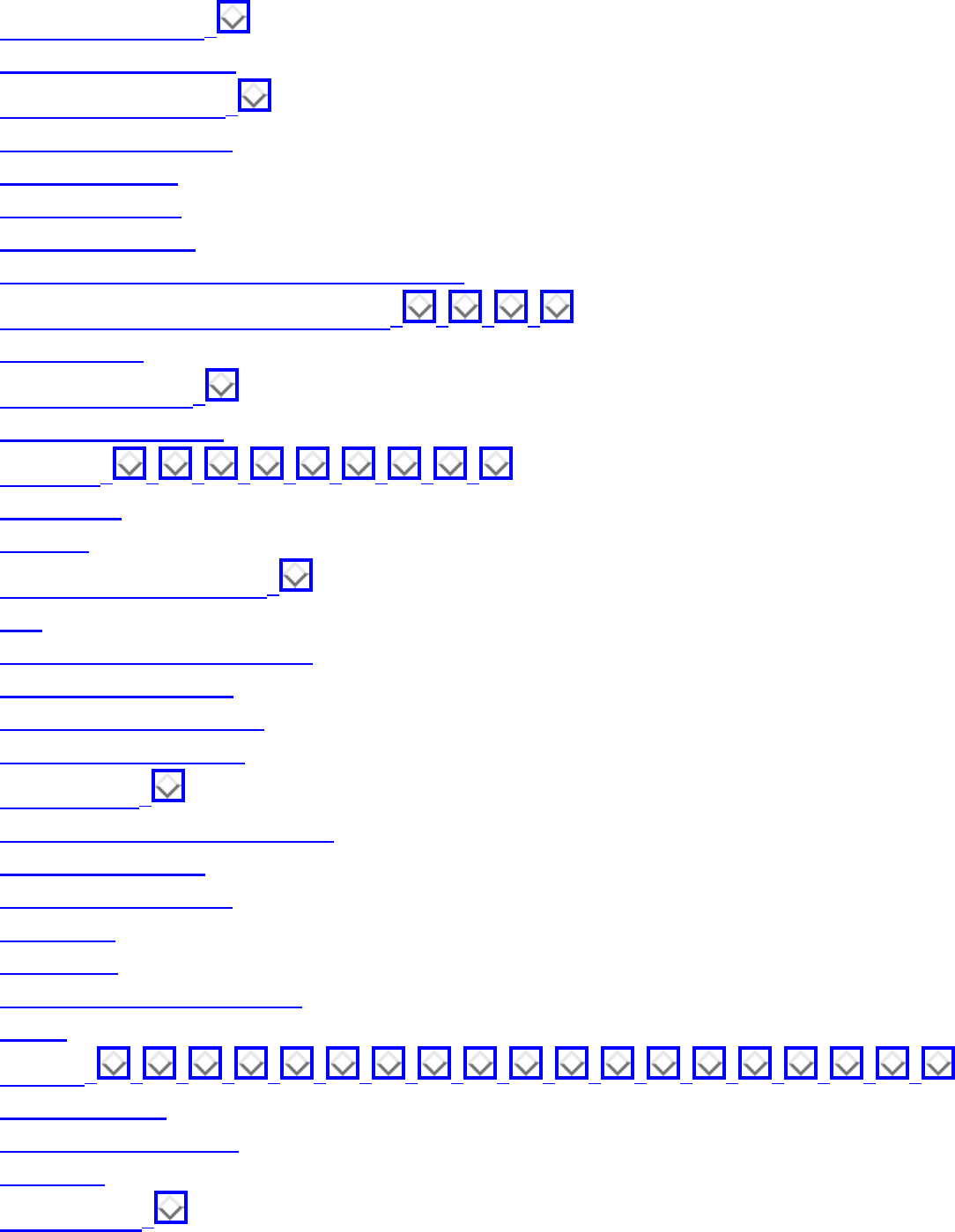
Index (complete)
VLSI circuit layout,
VLSI design problems
volume computations,
von Emde Boas queue
von Neumann, J.
Voronoi diagram
Voronoi Diagrams
Voronoi diagrams - nearest neighbor search
Voronoi diagrams - related problems, , , ,
walk-through
Waring's problem,
Warshall's algorithm
war story, , , , , , , , ,
water pipes
wavelets
weakly-connected graphs,
web
weighted graphs, applications
Winograd's algorithm
wire length minimization
wiring layout problems
word ladders,
worker assignment - scheduling
world's record TSP
worst-case complexity
WWW site
X-windows
Xerox machines - scheduling
XRLF
XTango, , , , , , , , , , , , , , , , , , ,
Young tableaux
zero-knowledge proofs
Zipf's law
zone theorem,
file:///E|/BOOK/BOOK5/INDEX_AL.HTM (55 of 56) [19/1/2003 1:33:45]

Index (complete)
Algorithms
Tue Jun 3 11:59:38 EDT 1997
file:///E|/BOOK/BOOK5/INDEX_AL.HTM (56 of 56) [19/1/2003 1:33:45]
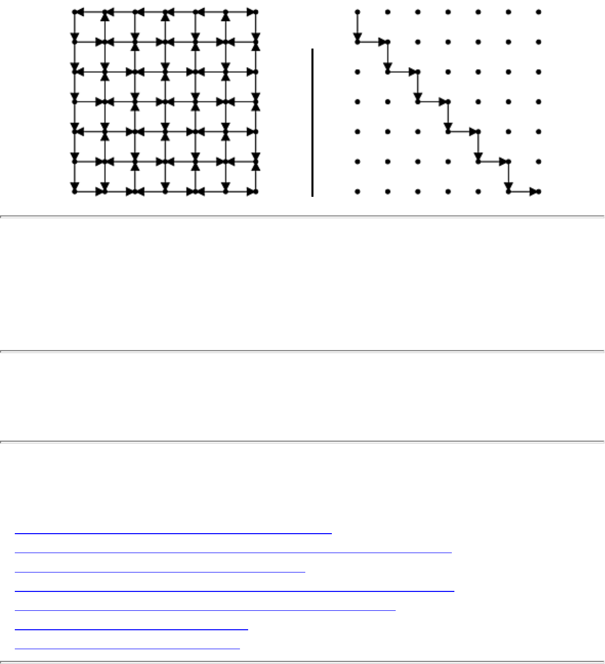
1.4.4 Shortest Path
1.4.4 Shortest Path
INPUT OUTPUT
Input Description: An edge-weighted graph G , with start vertex and end vertex t .
Problem: Find the shortest path from to t in G .
Implementations
● Goldberg's Network Optimization Codes (C) (rating 9)
● LEDA - A Library of Efficient Data Types and Algorithms (C++) (rating 7)
● Discrete Optimization Methods (Pascal) (rating 5)
● Netlib / TOMS -- Collected Algorithms of the ACM (FORTRAN) (rating 4)
● Xtango and Polka Algorithm Animation Systems (C++) (rating 4)
● Combinatorica (Mathematica) (rating 3)
● The Stanford GraphBase (C) (rating 3)
file:///E|/WEBSITE/FILES/SHORPATH.HTM (1 of 2) [19/1/2003 1:33:53]

1.4.4 Shortest Path
Related Problems
● Connected Components
● Graph Isomorphism
● Matrix Multiplication
● Motion Planning
● Network Flow
● Priority Queues
● Steiner Tree
● Transitive Closure and Reduction
Go to the corresponding chapter in the book
About the Book
Send us Mail
Go to Main Page
This page last modified on Tue Jun 03, 1997 .
file:///E|/WEBSITE/FILES/SHORPATH.HTM (2 of 2) [19/1/2003 1:33:53]
1.2.5 Constrained and Unconstrained Optimization
1.2.5 Constrained and Unconstrained Optimization
INPUT OUTPUT
Input Description: A function f(x_1,...,x_n) .
Problem: What point p = (p_z,...,p_n) maximizes (or equivallently minimizes) the function f ?
Implementations
● Netlib / TOMS -- Collected Algorithms of the ACM (FORTRAN) (rating 8)
● Adaptive Simulated Annealing (C) (rating 6)
● Genocop -- Optimization via Genetic Algorithms (C) (rating 5)
Related Problems
● Linear Programming
file:///E|/WEBSITE/FILES/UNCOTION.HTM (1 of 2) [19/1/2003 1:33:54]

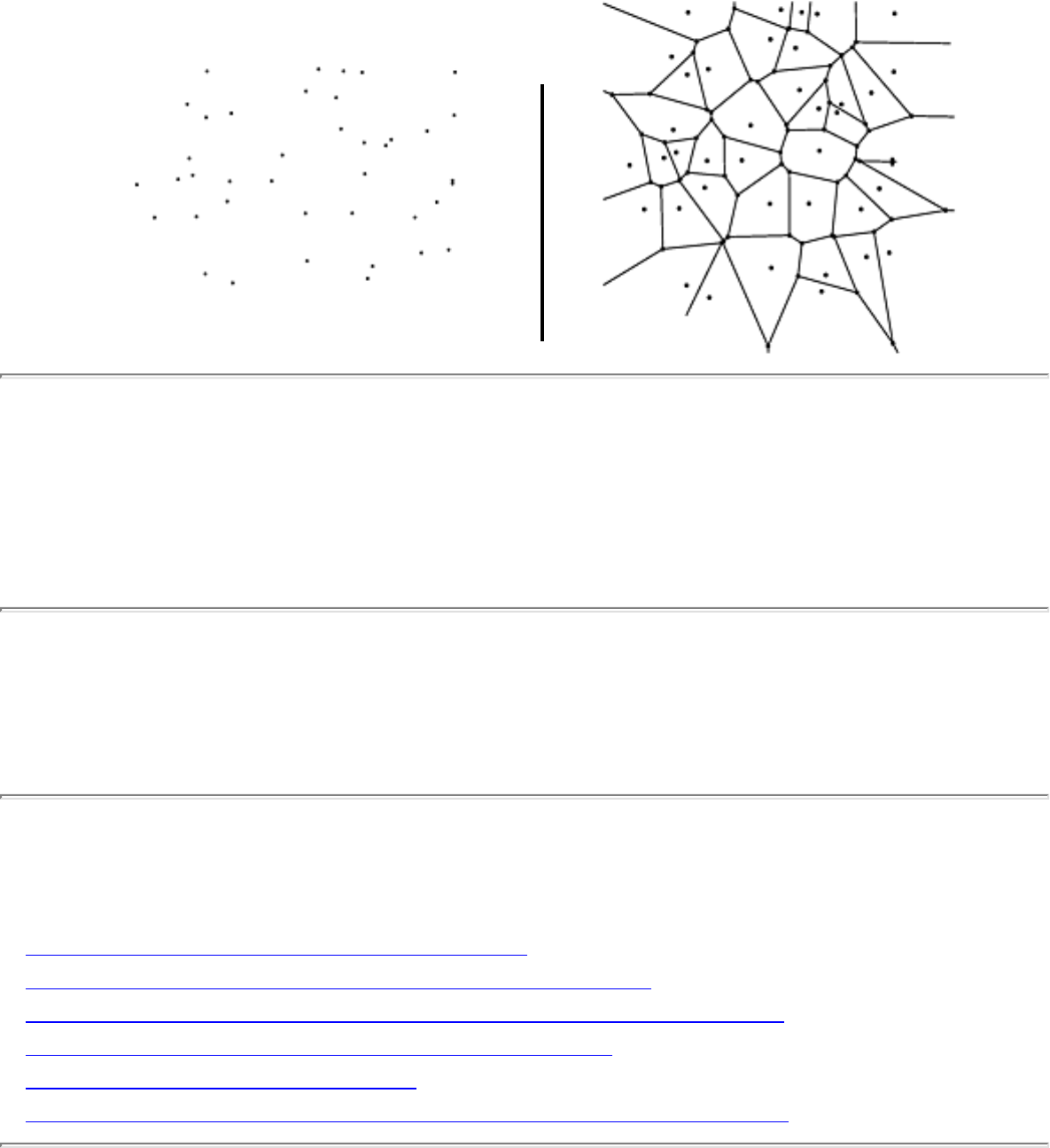
1.6.4 Voronoi Diagrams
1.6.4 Voronoi Diagrams
INPUT OUTPUT
Input Description: A set S of points p_1,...,p_n .
Problem: Decompose the space into regions around each point, such that all the points in the region
around p_i are closer to p_i than any other point in S .
Implementations
● Fortune's 2D Voronoi diagram code (C) (rating 9)
● Qhull - higher dimensional convex hull program (C) (rating 7)
● LEDA - A Library of Efficient Data Types and Algorithms (C++) (rating 6)
● Joseph O'Rourke's Computational Geometry (C) (rating 4)
● The Stanford GraphBase (C) (rating 3)
● Netlib / TOMS -- Collected Algorithms of the ACM (FORTRAN) (rating 3)
file:///E|/WEBSITE/FILES2/VORORAMS.HTM (1 of 2) [19/1/2003 1:33:56]

1.6.4 Voronoi Diagrams
Related Problems
● Convex Hull
● Nearest Neighbor Search
● Point Location
● Medial-Axis Transformation
● Triangulation
Go to the corresponding chapter in the book
About the Book
Send us Mail
Go to Main Page
This page last modified on Tue Jun 03, 1997 .
file:///E|/WEBSITE/FILES2/VORORAMS.HTM (2 of 2) [19/1/2003 1:33:56]
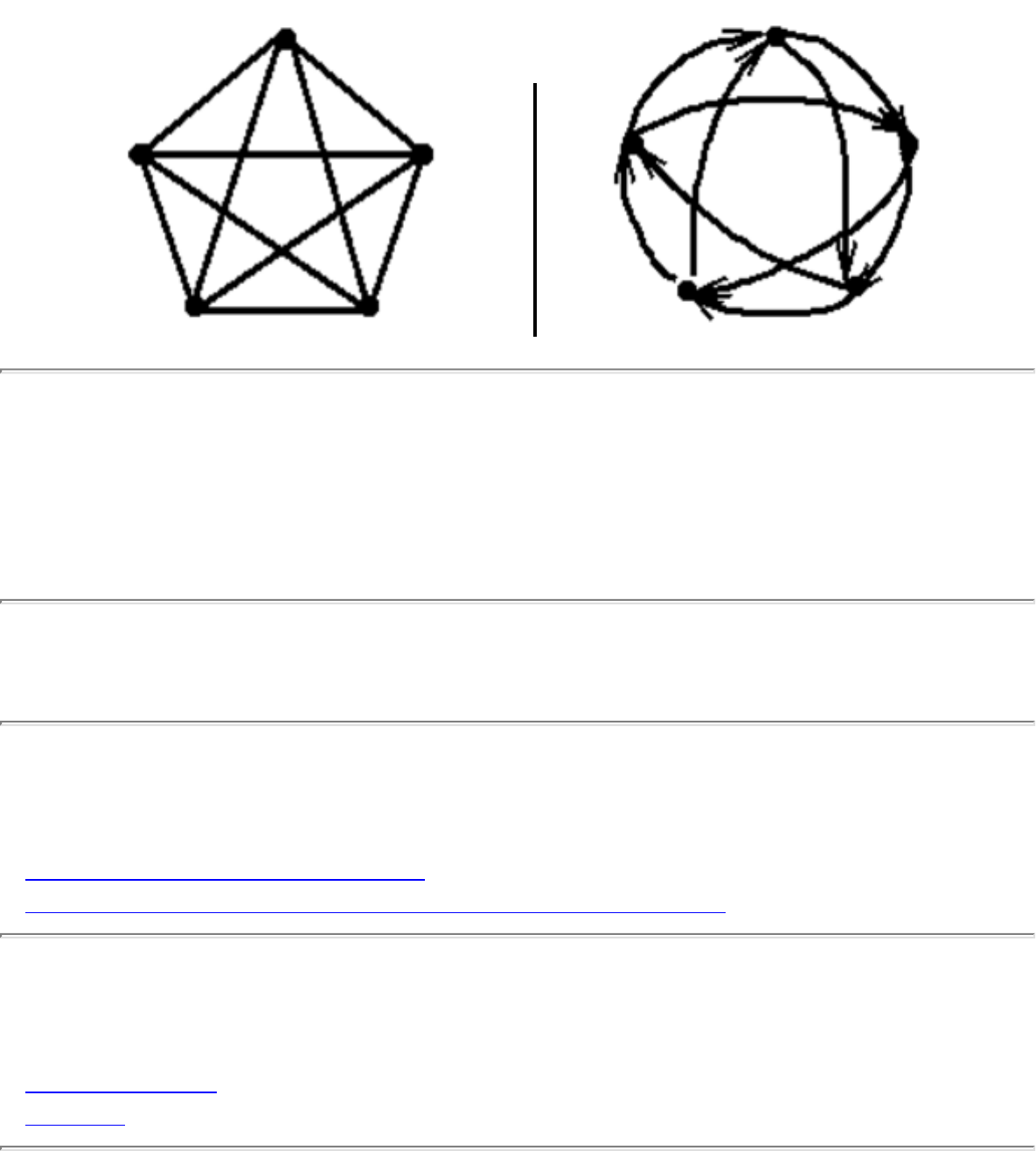
1.4.7 Eulerian Cycle / Chinese Postman
1.4.7 Eulerian Cycle / Chinese Postman
INPUT OUTPUT
Input Description: A graph G=(V,E) . Problem: Find the shortest tour of G visiting each edge at least
once.
Implementations
● Combinatorica (Mathematica) (rating 3)
● Nijenhuis and Wilf: Combinatorial Algorithms (FORTRAN) (rating 3)
Related Problems
● Hamiltonian Cycle
● Matching
file:///E|/WEBSITE/FILES/EULEYCLE.HTM (1 of 2) [19/1/2003 1:33:58]


Online Bibliographies
Online Bibliographies
There are many bibliographic sources available on the WWW, but the following I find indispensable:
● Computer Science Bibliographies -- This is a collection of over 700,000 references to papers and
technical reports in Computer Science, beneath a sophisticated search engine. While there is much
duplication, this is my first stop whenever I need to look something up. The primary site is
http://liinwww.ira.uka.de/bibliography/index.html , although several mirror sites are in operation
around the world. All references are provided in bibtex format.
● Joel Seiferas' paper.lst -- References to over 55,000 papers and technical reports (at last count),
mostly on algorithms and related areas of theoretical computer science. Each paper is reduced to a
one-line format, which I find easy to grep through. It is available by anonymous ftp from
ftp://ftp.cs.rochester.edu/pub/u/joel , but a local copy is also available. Strongly recommended.
● Geom.bib -- The complete bibliography on anything related to computational geometry, it
references over 8,000 books, papers, and reports and includes detailed abstracts for many of them.
It is available via anonymous ftp from ftp://ftp.cs.usask.ca/pub/geometry/geombib.tar.Z and a
local copy is included. Grep-ing through geom.bib is an amazingly efficient way to find out about
previous work without leaving your office.
● Compendium of Approximation Algorithms -- This compendium of approximation algorithms by
Pierluigi Crescenzi and Viggo Kann of NP-hard optimization problems is available at
http://www.nada.kth.se/nada/theory/problemlist.html, but a local copy is included. It is the place
to look to find what is known about provably good heuristics for any given problem.
About the Book
Send us Mail
Go to Main Page
file:///E|/WEBSITE/BIBLIO/BIBLIO.HTM [19/1/2003 1:33:58]
About the Book -- The Algorithm Design Manual
About the Book
Most professional programmers are not well equipped to tackle algorithm design problems. The
Algorithm Design Manual,written by Steven S. Skiena and published by Telos/Springer-Verlag is
uniquely designed to provide access to combinatorial algorithms technology for computer professionals
and students. This book is considerably different than other books on algorithms. Why?
● We reduce the design process to a sequence of questions to ask about the problem at hand. This
provides a concrete path to take the non-expert from an initial problem statement to a reasonable
solution.
● To provide a better perspective on how algorithm problems arise in the real world, we include a
collection of `war stories', tales from our experience on real problems. The moral of these stories
is that algorithm design and analysis is not just theory, but an important tool to be pulled out and
used as needed.
● Since the practical person is usually looking for a program more than an algorithm, we provide
pointers to solid implementations whenever they are available. We have collected these
implementations on an enclosed CD-ROM and at the book WWW site,
http://www.cs.sunysb.edu/~algorith for easy retrieval. With these implementations available, the
critical aspect in algorithm design becomes properly modeling your application, instead of
becoming intimate with the details of the actual algorithm. This focus permeates the entire book.
● Since finding out what is known about an algorithmic problem can be a difficult task, we provide
a catalog of the 75 most important algorithmic problems as a major component of this book. By
browsing through this catalog, the reader can quickly identify what their problem called, what is
known about it, and how they should proceed to solve it. As an aid in problem identification, we
include a pair of `before' and `after' pictures for each problem, illustrating the required input and
output specifications.
● The algorithm catalog spans numerical problems and data structures as well as graph, string, and
geometric algorithms. For each problem in the catalog, we provide an honest and convincing
motivation showing how it arises in applications. If we could not find such an application, then the
file:///E|/ABOUTBK.HTM (1 of 3) [19/1/2003 1:34:00]
About the Book -- The Algorithm Design Manual
problem doesn't appear in this book.
Equally important is what we do not do in this book. We do not stress the mathematical analysis of
algorithms, leaving most of the analysis as informal arguments. You will not find a single theorem
anywhere in this book.
But what is a manual without software? This book comes with a substantial electronic supplement, a ISO-
9660 compatible, multiplatform CD-ROM, which can be viewed using Netscape, Microsoft Explorer, or
any other WWW browser. This CD-ROM contains:
● A complete hypertext version of the full printed book. Indeed, the extensive cross-references
within the text are best followed using the hypertext version.
● The source code and URLs for all cited implementations, mirroring the Algorithm Repository
WWW site. Programs in C, C++, Fortran, and Pascal are included, providing an average of four
different implementations for each algorithmic problem.
● Over 30 hours of audio lectures on the design and analysis of algorithms are provided, all keyed to
on-line lecture notes. Following these lectures provides another approach to learning algorithm
design techniques.
Together, this book covers material sufficient for a standard Introduction to Algorithms course. Its
assumes the reader has completed the equivalent of a second programming course, typically titled Data
Structures or Computer Science II . Special textbook oriented-features include:
● In addition to standard pen-and-paper exercises, this book includes ``implementation challenges''
suitable for teams or individual students. These projects and the applied focus of the text can be
used to provide a new laboratory focus to the traditional algorithms course.
● ``Take-home lessons'' at the beginning of each chapter emphasize the concepts to be gained from
the chapter.
● This book stresses design over analysis. It is suitable for both traditional lecture courses, and the
new ``active learning'' method, where the professor does not lecture instead guides student groups
to solve real problems. The ``war stories'' provide a great introduction to the active learning
method.
● A full set of lecture slides for teaching this course is available on the CD-ROM, keyed to unique
on-line audio lectures covering a full semester algorithm course.
``I have not doubt that it will become a classic the day it is published. It has all the right ingredients: rich
contents, friendly, personal language, subtle humor, the right references, and a plethora of pointers to
resources.''
-- P. Takis Metaxas, Wellesley College.
``A major theme that runs through the book is that the most important technique to solve an algorithmic
problem from the real world is to learn how to model the problem well. I did not believe this before; the
file:///E|/ABOUTBK.HTM (2 of 3) [19/1/2003 1:34:00]

About the Book -- The Algorithm Design Manual
book did an admirable job of convincing me that there is considerable truth in it.''
-- Giri Narasimhan, The University of Memphis.
``The questions on problem solving are good enough that they ought to be talked about in every
programming class in the undergraduate curriculum.''
-- Ron Danielson, Santa Clara University.
Check out the preface and table of contents for more information. You may order this book, and are
encouraged to do so. You might also be interested in my previous book, Implementing Discrete
Mathematics .
Please leave your name and address to receive additional information about the book and notification of
significant upgrades to this site when they occur.
If your WWW client does not support forms, please send an e-mail to algorith@cs.sunysb.edu
with your name, e-mail address, and mailing address for further information.
First Name:
Last Name :
E-mail :
Company Name :
Number and Street:
City :
State :
Zip :
Phone :
Return to the home page
If you have problems with this page, please send E-mail to:
algorith@cs.sunysb.edu
file:///E|/ABOUTBK.HTM (3 of 3) [19/1/2003 1:34:00]
Reset
Register

Copyright and Disclaimers
Copyright Notice
This electronic component package is protected by federal copyright law and international treaty. The
copyright holder retains title to and ownership of the package. U.S. copyright law prohibits you from
making any copy of the CD-ROM for any reason, without the written permission of Springer-Verlag,
except that you may download and copy the contents of this CD-ROM disc for your own research,
teaching, and communications use. Springer-Verlag or its designee has the right to audit your computer
and electronic component usage to determine whether any unauthorized copies of this package have been
made.
For those programs and data contained on this CD-ROM and WWW site whereby the rights are owned
by the original creators and source, any request for permission to use their software for commercial
purposes must be directed to them.
The printed book with which this electronic component is packaged may not be translated or copied in
whole or in part without the written permission of Springer-Verlag except for brief excerpts in
connection with reviews or scholarly analysis. Use in connection with any form of information storage
and retrieval, electronic adaptation, computer software or by similar or dissimilar methodology now
known or hereafter developed is forbidden.
Springer-Verlag or the author makes no warranty of representation, either express or implied, with
respect to this CD-ROM, WWW site, or book, including their quality, merchantability, or fitness for a
particular purpose. In no event will Springer-Verlag, or the author be liable for direct, indirect, special,
incidental, or consequential damages arising out of the use or inability to use the disc, WWW site, or
book, even if Springer-Verlag or the author has been advised of the possibility of such damages.
About the Book
Send us Mail
Go to Main Page
file:///E|/WEBSITE/INFO/COPYRIGH.HTM [19/1/2003 1:34:01]
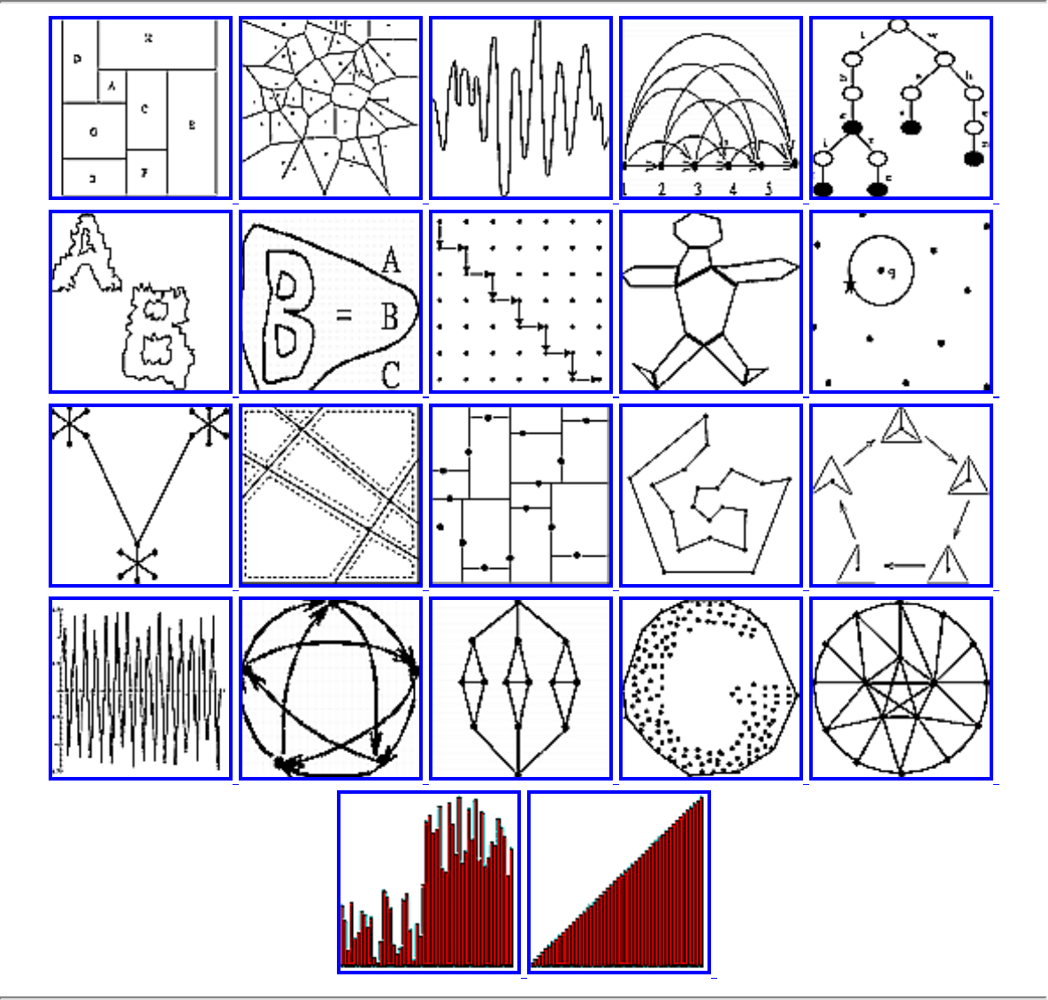

CD-ROM Installation
Installation and Users Guide
How do I start the CD-ROM?
Load the CD-ROM into your drive. Viewing the contents of the CD-ROM requires you to have a
properly installed WWW browser, such as the Netscape Navigator or Internet Explorer. A more detailed
list of supported browsers is provided below. Open up the INDEX.HTM file on the CD-ROM with your
browser, and then explore to your heart's content. The entire contents of the CD-ROM are accessible
from this page.
How do I listen to the lectures?
If you haven't already, you'll need to install the Shockwave for Director plug-in. Currently, Shockwave is
supported only on Windows and Macintosh platforms, but keep checking Macromedia's website at
www.macromedia.com for updated information about other platforms. Make sure that after installing the
plug-in you restart your browser, or the plug-in will not be recognized. Copies of these plug-ins have
been included on the CD-ROM. Click here to select the plug-in appropriate for your system.
What hardware and software do I need for this plug-
in?
For Windows: Any modern PC computer will do, but a Pentium is recommended because of its floating-
point unit. Supported browsers include the Netscape Navigator 2.02 and 3.01, Internet Explorer 3.0 and
3.01 Final Releases, (note: Internet Explorer for Windows can use the Shockwave plugins or the
Shockwave ActiveX control, which can be automatically installed at http://www.macromedia.com),
Attachmate's Emissary, Netmanage's WebSurfer, and America Online version 3.0 (note: no plug-in
installation should be necessary for the AOL browser for Windows.)
For Macintosh: Any PowerMac will do, but 68k Macs will require a hardware floating-point unit (math
co-processor). Supported browsers include Netscape Navigator 2.02 and 3.01, Microsoft Internet
Explorer 3.0 and 3.0a, Attachmate's Emissary, Netmanage's WebSurfer, and America Online version 3.0.
Commercial versions of Netscape Navigator 3.x and Microsoft Internet Explorer may come with the
appropriate plug-ins already installed. If not, copies of these plug-ins have been included on the CD-
ROM. Click here to select the plug-in appropriate for your system.
To use the CD-ROM under Unix
file:///E|/BROWSERS.HTM (1 of 3) [19/1/2003 1:34:04]

CD-ROM Installation
This CD-ROM is written as an ISO-9660 file system without Rock Ridge extensions. All filenames are
written in upper case, and unless the file system is mounted correctly the HTML links will not be found.
Unfortunately, different mount commands seem to be required for different flavors of Unix. Read your
manual page and experiment. You must first create a mount point /cdrom. Let "sr0" be the SCSI ID for
your CD-ROM drive (typically sr0 = "cdrom"). Possible mount commands which have worked on
different systems include:
mount -rt hsfs /dev/sr0 /cdrom
mount -o norock,check=relaxed -r -t iso9660 /dev/sr0 /cdrom
Once the CD-ROM is mounted, open /cdrom/index.html with your favorite browser. The entire contents
of the CD-ROM are accessible from this page. Unfortunately, the audio lecture notes are not supported
on Unix platforms.
About the Images
Your browser likely has the option to automatically display or suppress in-line images. The mathematical
symbols in the lecture notes and the textbook are represented by bit-mapped images, which might load
slowly on certain systems. If so, disabling the automatic loading of images will result in better
performance, although less readable text.
To enable/disable viewing of these images when using Netscape Navigator, choose "Options" from the
menu bar, and select "Auto Load Images". To view images on one page only, or to load images which
were not properly loaded, click the "Images" button on the graphical toolbar.
About the Sound
Sound files on this CD-ROM are recorded in Shockwave file format, and have the extension "SWA".
Thus, the file "LEC19-2.SWA" contains sounds related to the second portion of lecture 19 in the lecture
notes. Playing the audio requires a plug-in from Macromedia, which unfortunately is not available on
Unix platforms.
Click here to select the plug-in appropriate for your system.
To listen to the sounds linked to the lecture notes you must:
● Have an installed sound device configured for use on your system. If you have ever heard sound
coming from your machine, this likely has already been done. If not, you will have to acquire and
file:///E|/BROWSERS.HTM (2 of 3) [19/1/2003 1:34:04]

CD-ROM Installation
install a sound device, such as Sound Blaster for PCs or the Macintosh standard sound system.
Consult your sound device manual and the documentation for your operating system.
● Configure your browser to recognize sound files in an HTML document. In particular, the
Netscape Navigator will have to launch an application to play the sound files. If Netscape
attempts to save the audio file when you click on a sound link, this means that your sound
application has not be properly installed.
About the Postscript Lecture Notes
All the Lecture Notes are provided in Postscript format as well. To view Postscript files on Unix, use
ghostview.
Macintosh users: use the program DropPS 1.1.4, by Barebones Software.
Windows users: use the program RoPS 32
file:///E|/BROWSERS.HTM (3 of 3) [19/1/2003 1:34:04]

Thanks!
Thanks!
Four Stony Brook students made essential contributions to the production of this CD-ROM/WWW site.
I'd like to thank them for their contributions by including their images for posterity. Thanks again, guys.
Ricky Bradley
file:///E|/WEBSITE/IMAGES/HELPERS/INDEX.HTM (1 of 4) [19/1/2003 1:34:07]
Thanks!
Frank Ruscica
file:///E|/WEBSITE/IMAGES/HELPERS/INDEX.HTM (2 of 4) [19/1/2003 1:34:07]

Thanks!
Dario Vlah
file:///E|/WEBSITE/IMAGES/HELPERS/INDEX.HTM (3 of 4) [19/1/2003 1:34:07]

Thanks!
Zhong Li
Thanks also to Filip Bujanic, David Gerstl, Jim Klosowski, Kostis Sagonas, Kirsten Starcher, and Lei
Zhao, who all made contributions at various stages of the project.
Finally, I am grateful to acknowledge support from the Office of Naval Research and the National
Science Foundation, which contributed towards this research.
file:///E|/WEBSITE/IMAGES/HELPERS/INDEX.HTM (4 of 4) [19/1/2003 1:34:07]

CD-ROM Installation
Installation and Users Guide
How do I start the CD-ROM?
Load the CD-ROM into your drive. Viewing the contents of the CD-ROM requires you to have a
properly installed WWW browser, such as the Netscape Navigator or Internet Explorer. A more detailed
list of supported browsers is provided below. Open up the INDEX.HTM file on the CD-ROM with your
browser, and then explore to your heart's content. The entire contents of the CD-ROM are accessible
from this page.
How do I listen to the lectures?
If you haven't already, you'll need to install the Shockwave for Director plug-in. Currently, Shockwave is
supported only on Windows and Macintosh platforms, but keep checking Macromedia's website at
www.macromedia.com for updated information about other platforms. Make sure that after installing the
plug-in you restart your browser, or the plug-in will not be recognized. Copies of these plug-ins have
been included on the CD-ROM. Click here to select the plug-in appropriate for your system.
What hardware and software do I need for this plug-
in?
For Windows: Any PC equipped with a floating-point unit will do, but a Pentium is recommended,
especially since modern processors include a floating-point unit. Supported browsers include the
Netscape Navigator 2.02 and 3.01, Internet Explorer 3.0 and 3.01 Final Releases, (note: Internet Explorer
for Windows can use the Shockwave plugins or the Shockwave ActiveX control, which can be
automatically installed at http://www.macromedia.com), Attachmate's Emissary, Netmanage's
WebSurfer, and America Online version 3.0 (note: no plug-in installation should be necessary for the
AOL browser for Windows.)
For Macintosh: Any PowerMac will do, but 68k Macs will require a hardware floating-point unit (math
co-processor). Supported browsers include Netscape Navigator 2.02 and 3.01, Microsoft Internet
Explorer 3.0 and 3.0a, Attachmate's Emissary, Netmanage's WebSurfer, and America Online version 3.0.
Commercial versions of Netscape Navigator 3.x and Microsoft Internet Explorer may come with the
appropriate plug-ins already installed. If not, copies of these plug-ins have been included on the CD-
ROM. Click here to select the plug-in appropriate for your system.
file:///E|/WEBSITE/INFO/BROWSERS.HTM (1 of 3) [19/1/2003 1:34:07]

CD-ROM Installation
To use the CD-ROM under Unix
This CD-ROM is written as an ISO-9660 file system without Rock Ridge extensions. All filenames are
written in upper case, and unless the file system is mounted correctly the HTML links will not be found.
Unfortunately, different mount commands seem to be required for different flavors of Unix. Read your
manual page. You must first create a mount point /cdrom. Let "sr0" be the SCSI ID for your CD-ROM
drive (typically sr0 = "cdrom"). Possible mount commands which have worked on different systems
include:
mount -rt hsfs /dev/sr0 /cdrom
mount -o norock,check=relaxed -r -t iso9660 /dev/sr0 /cdrom
Once the CD-ROM is mounted, open /cdrom/index.html with your favorite browser. The entire contents
of the CD-ROM are accessible from this page. Unfortunately, the audio lecture notes are not supported
on Unix platforms.
About the Images
Your browser likely has the option to automatically display or suppress in-line images. The mathematical
symbols in the lecture notes and the textbook are represented by bit-mapped images, which might load
slowly on certain systems. If so, disabling the automatic loading of images will result in better
performance, although less readable text.
To enable/disable viewing of these images when using Netscape Navigator, choose "Options" from the
menu bar, and select "Auto Load Images". To view images on one page only, or to load images which
were not properly loaded, click the "Images" button on the graphical toolbar.
About the Sound
Sound files on this CD-ROM are recorded in Shockwave file format, and have the extension "SWA".
Thus, the file "LEC19-2.SWA" contains sounds related to the second portion of lecture 19 in the lecture
notes. Playing the audio requires a plug-in from Macromedia, which unfortunately is not available on
Unix platforms.
Click here to select the plug-in appropriate for your system.
To listen to the sounds linked to the lecture notes you must:
file:///E|/WEBSITE/INFO/BROWSERS.HTM (2 of 3) [19/1/2003 1:34:07]

CD-ROM Installation
● Have an installed sound device configured for use on your system. If you have ever heard sound
coming from your machine, this likely has already been done. If not, you will have to acquire and
install a sound device, such as Sound Blaster for PCs or the Macintosh standard sound system.
Consult your sound device manual and the documentation for your operating system.
● Configure your browser to recognize sound files in an HTML document. In particular, the
Netscape Navigator will have to launch an application to play the sound files. If Netscape
attempts to save the audio file when you click on a sound link, this means that your sound
application has not be properly installed.
About the Postscript Lecture Notes
All the Lecture Notes are provided in Postscript format as well. To view Postscript files on Unix, use
ghostview.
Macintosh users: use the program DropPS 1.1.4, by Barebones Software.
Windows-95 and NT users: use the program RoPS 32
file:///E|/WEBSITE/INFO/BROWSERS.HTM (3 of 3) [19/1/2003 1:34:07]
Binary Search in Action
Binary Search in Action
Binary search is a fast algorithm for searching in a sorted array of keys. To look up a name in a telephone
book with n names, you start by comparing the name that you want with the middle or (n/2) nd name, say
onroe, Marilyn . Regardless of whether what you are looking someone before this middle name ( Dean,
James ) or after it ( Presley, Elvis ), after this first comparison you can forever disregard one half of all
the names in the book. The number of steps the algorithm takes equals the number of times we can halve
n until only one name is left. Thus twenty comparisons suffice to find any name in the million-name
Manhattan phone book! The power of binary search and logarithms is one of the most fundamental idea
in the analysis of algorithms. This power becomes apparent if we imagine living in a world with only
unsorted telephone books.
The following animation of the first two stages of binary search is provided for your amusement. The full
video tapes are also available.
file:///E|/WEBSITE/IMAGES/BINARY/INDEX.HTM (1 of 5) [19/1/2003 1:34:09]
Binary Search in Action
file:///E|/WEBSITE/IMAGES/BINARY/INDEX.HTM (2 of 5) [19/1/2003 1:34:09]
Binary Search in Action
file:///E|/WEBSITE/IMAGES/BINARY/INDEX.HTM (3 of 5) [19/1/2003 1:34:09]
Binary Search in Action
file:///E|/WEBSITE/IMAGES/BINARY/INDEX.HTM (4 of 5) [19/1/2003 1:34:09]
Binary Search in Action
file:///E|/WEBSITE/IMAGES/BINARY/INDEX.HTM (5 of 5) [19/1/2003 1:34:09]

About the Video Lectures
For Further Information
In Spring 1996, my course on the Design and Analysis of Algorithms was offered as part of the EngiNet
distance learning program at Stony Brook. As a result, all of my lectures were professionally video taped
in a television studio. The picture and sound quality are excellent, certainly as good as possible given that
they were recording me.
EngiNet and the College of Engineering and Applied Science at Stony Brook have tentatively agreed to
make these videotapes available to all interested parties, at a price of $20 per lecture, or $500 for the
complete set of 25 lectures. Full lecture notes and audio sampled from the video tapes are available on
line .
To obtain the video tapes, please send e-mail to algorith@cs.sunysb.edu with the names of the desired
lectures, your name, e-mail address, and mailing address.
file:///E|/WEBSITE/INFO/TAPES.HTM [19/1/2003 1:34:10]
Postscript version of the lecture notes
Lecture notes in Postscript format:
These files contain postscript versions of the full lecture notes, formatted so that they are suitable for use
as transparencies. Each page of the notes corresponds to an audio clip for the HTML versions of the
notes.
An index to these notes appears in the 300+ page file ALL. However, this file is not formatted as nicely
as the individual lectures.
All Lecture 1 Lecture 2 Lecture 3 Lecture 4
Lecture 5 Lecture 6 Lecture 7 Lecture 8 Lecture 9
Lecture 10 Lecture 11 Lecture 12 Lecture 13 Lecture 14
Lecture 15 Lecture 16 Lecture 17 Lecture 18 Lecture 19
Lecture 20 Lecture 21 Lecture 22 Lecture 23
To view Postscript files, Windows-95 and NT users should use the program RoPS 32. Macintosh users
should use the program DropPS 1.1.4, by Barebones Software. On Unix, use the popular previewer
ghostview.
file:///E|/LEC/LECTURES/PS/PS.HTM [19/1/2003 1:34:11]

Algorithm Repository -- Algorithms Courses
Algorithms Courses
Instructors for combinatorial algorithms courses around the world are putting lecture notes and other
interesting material on the WWW for their classes, but there is no reason the rest of the world shouldn't
benefit as well. Below are the best course sites we have found to date. A similar collection of algorithm
courses is being maintained by Kirk Pruhs at Univ. of Pittsburgh.
● Gordon Royle -- Topics covered include graph algorithms, network flow, P=NP, travelling
salesman, string processing, greedy algorithm, cryptography, and combinatorial search. On-line
lecture notes are included.
● Steven Skiena -- Topic covered include sorting and searching, combinatorial search, dynamic
programming, graph algorithms, and intractibility. On-line lecture notes are included.
● Guy Blelloch -- Parallel algorithms and programming. Included are animations of parallel
algorithms, and information about the NESL parallel programming language they are written in.
● Algorithms in the Real World (CMU) -- An interesting collection of pointers and descriptive
material on applications of algorithms in practice.
Feel free to look around. If you find something useful, then drop us a line to let us know what we did
right. If you're looking for something that's not here yet, drop us a line and tell us that too. We're looking
for as many good implementations as we can find -- so if you have an implementation for a specific
problem, or know where one can be found, let us know and we'll see if we can't get it attached to the site.
This algorithms repository is part of the ongoing algorithms-related research conducted here in the
Department of Computer Science at the State University of New York at Stony Brook.
About the Book
Send us Mail
Go to Main Page
file:///E|/WEBSITE/INFO/COURSES.HTM [19/1/2003 1:34:11]
Lecture 1 - analyzing algorithms
Next: Lecture 2 - asymptotic Up: No Title Previous: No Title
Lecture 1 - analyzing algorithms
Listen To Part 1-7
Lecture Schedule
subject topics reading
Preliminaries Analyzing algorithms 1-32
" Asymptotic notation 32-37
" Recurrence relations 53-64
Sorting Heapsort 140-150
" Quicksort 153-167
" Linear Sorting 172-182
Searching Data structures 200-215
" Binary search trees 244-245
" Red-Black trees:insertion 262-272
`` Red-Black trees:deletion 272-277
MIDTERM 1
Comb. Search Backtracking
" Elements of dynamic programming 301-314
" Examples of dynamic programming 314-323
Graph Algorithms Data structures 465-477
for graphs
" Breadth/depth-first search 477-483
" Topological Sort/Connectivity 485-493
" Minimum Spanning Trees 498-510
" Single-source shortest paths 514-532
" All-pairs shortest paths 550-563
MIDTERM 2
Intractability P and NP 916-928
" NP-completeness 929-939
" NP-completeness proofs 939-951
file:///E|/LEC/LECTUR16/NODE1.HTM (1 of 9) [19/1/2003 1:34:15]
Lecture 1 - analyzing algorithms
" Further reductions 951-960
" Approximation algorithms 964-974
" Set cover / knapsack heuristics 974-983
FINAL EXAM
Listen To Part 1-8
What Is An Algorithm?
Algorithms are the ideas behind computer programs.
An algorithm is the thing which stays the same whether the program is in Pascal running on a Cray in New York or is
in BASIC running on a Macintosh in Kathmandu!
To be interesting, an algorithm has to solve a general, specified problem. An algorithmic problem is specified by
describing the set of instances it must work on and what desired properties the output must have.
Example: Sorting
Input: A sequence of N numbers
Output: the permutation (reordering) of the input sequence such as .
We seek algorithms which are correct and efficient.
Correctness
For any algorithm, we must prove that it always returns the desired output for all legal instances of the problem.
For sorting, this means even if (1) the input is already sorted, or (2) it contains repeated elements.
Correctness is Not Obvious!
The following problem arises often in manufacturing and transportation testing applications.
Suppose you have a robot arm equipped with a tool, say a soldering iron. To enable the robot arm to do a soldering
job, we must construct an ordering of the contact points, so the robot visits (and solders) the first contact point, then
visits the second point, third, and so forth until the job is done.
Since robots are expensive, we need to find the order which minimizes the time (ie. travel distance) it takes to
assemble the circuit board.
file:///E|/LEC/LECTUR16/NODE1.HTM (2 of 9) [19/1/2003 1:34:15]
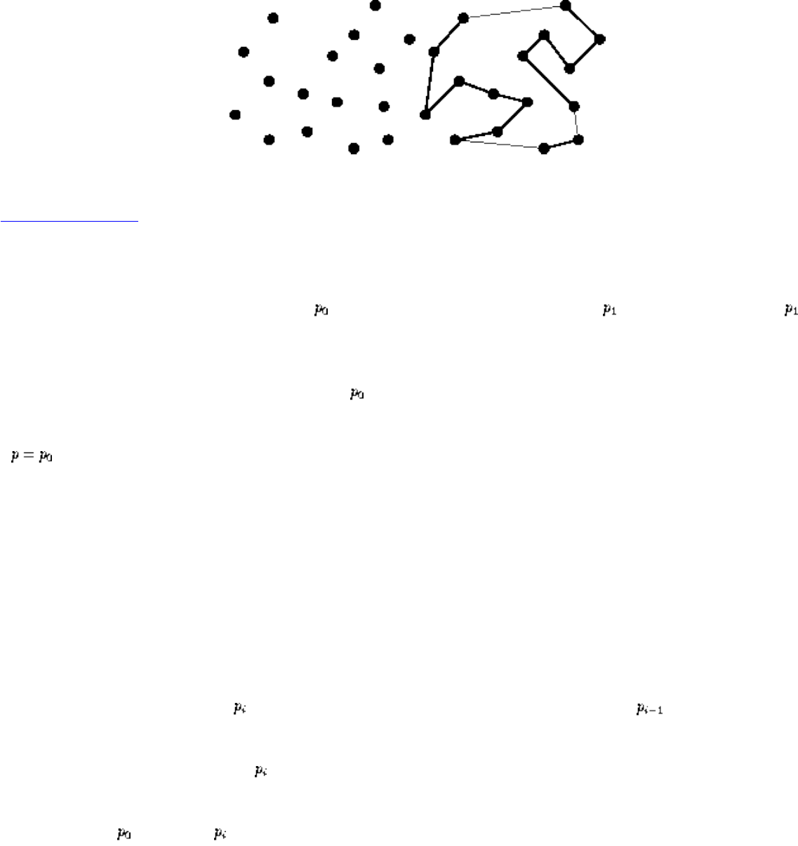
Lecture 1 - analyzing algorithms
You are given the job to program the robot arm. Give me an algorithm to find the best tour!
Listen To Part 1-10
Nearest Neighbor Tour
A very popular solution starts at some point and then walks to its nearest neighbor first, then repeats from ,
etc. until done.
Pick and visit an initial point
i = 0
While there are still unvisited points
i = i+1
Let be the closest unvisited point to
Visit
Return to from
This algorithm is simple to understand and implement and very efficient. However, it is not correct!
file:///E|/LEC/LECTUR16/NODE1.HTM (3 of 9) [19/1/2003 1:34:15]
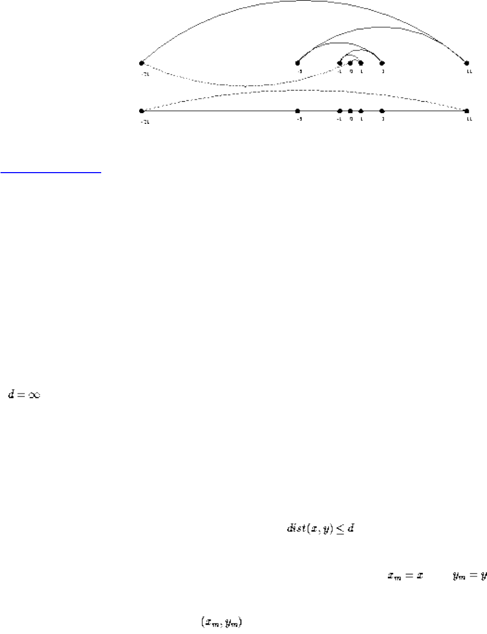
Lecture 1 - analyzing algorithms
Always starting from the leftmost point or any other point will not fix the problem.
Listen To Part 1-11
Closest Pair Tour
Always walking to the closest point is too restrictive, since that point might trap us into making moves we don't want.
Another idea would be to repeatedly connect the closest pair of points whose connection will not cause a cycle or a
three-way branch to be formed, until we have a single chain with all the points in it.
Let n be the number of points in the set
For i=1 to n-1 do
For each pair of endpoints (x,y) of partial paths
If then
, , d = dist(x,y)
Connect by an edge
Connect the two endpoints by an edge.
Although it works correctly on the previous example, other data causes trouble:
file:///E|/LEC/LECTUR16/NODE1.HTM (4 of 9) [19/1/2003 1:34:15]
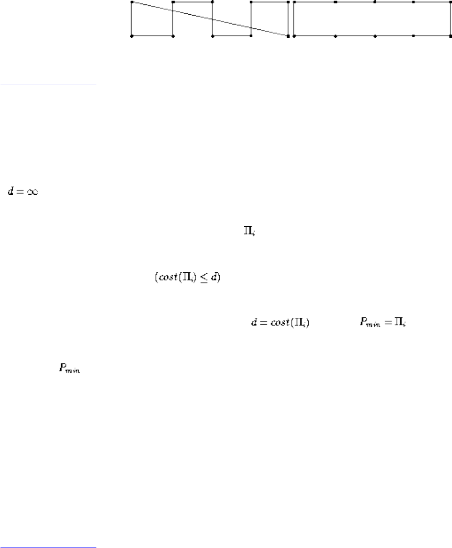
Lecture 1 - analyzing algorithms
This algorithm is not correct!
Listen To Part 1-12
A Correct Algorithm
We could try all possible orderings of the points, then select the ordering which minimizes the total length:
For each of the n! permutations of the n points
If then
and
Return
Since all possible orderings are considered, we are guaranteed to end up with the shortest possible tour.
Because it trys all n! permutations, it is extremely slow, much too slow to use when there are more than 10-20 points.
No efficient, correct algorithm exists for the traveling salesman problem, as we will see later.
Listen To Part 1-13
Efficiency
"Why not just use a supercomputer?"
Supercomputers are for people too rich and too stupid to design efficient algorithms!
A faster algorithm running on a slower computer will always win for sufficiently large instances, as we shall see.
file:///E|/LEC/LECTUR16/NODE1.HTM (5 of 9) [19/1/2003 1:34:15]

Lecture 1 - analyzing algorithms
Usually, problems don't have to get that large before the faster algorithm wins.
Expressing Algorithms
We need some way to express the sequence of steps comprising an algorithm.
In order of increasing precision, we have English, pseudocode, and real programming languages. Unfortunately, ease
of expression moves in the reverse order.
I prefer to describe the ideas of an algorithm in English, moving to pseudocode to clarify sufficiently tricky details of
the algorithm.
Listen To Part 1-14
The RAM Model
Algorithms are the only important, durable, and original part of computer science because they can be studied in a
machine and language independent way.
The reason is that we will do all our design and analysis for the RAM model of computation:
● Each "simple" operation (+, -, =, if, call) takes exactly 1 step.
● Loops and subroutine calls are not simple operations, but depend upon the size of the data and the contents of
a subroutine. We do not want ``sort'' to be a single step operation.
● Each memory access takes exactly 1 step.
We measure the run time of an algorithm by counting the number of steps.
This model is useful and accurate in the same sense as the flat-earth model (which is useful)!
Listen To Part 1-15
Best, Worst, and Average-Case
The worst case complexity of the algorithm is the function defined by the maximum number of steps taken on any
instance of size n.
file:///E|/LEC/LECTUR16/NODE1.HTM (6 of 9) [19/1/2003 1:34:15]
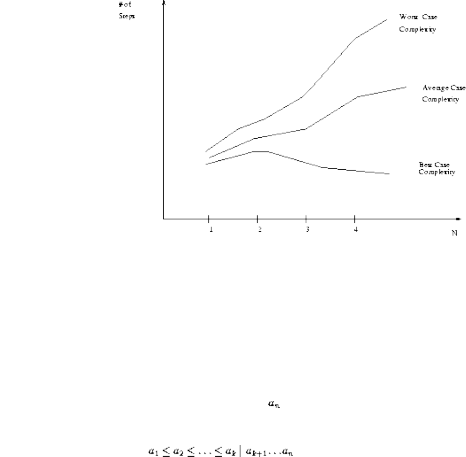
Lecture 1 - analyzing algorithms
The best case complexity of the algorithm is the function defined by the minimum number of steps taken on any
instance of size n.
The average-case complexity of the algorithm is the function defined by an average number of steps taken on any
instance of size n.
Each of these complexities defines a numerical function - time vs. size!
Insertion Sort
One way to sort an array of n elements is to start with empty list, then successively insert new elements in the
proper position:
At each stage, the inserted element leaves a sorted list, and after n insertions contains exactly the right elements. Thus
the algorithm must be correct.
But how efficient is it?
Note that the run time changes with the permutation instance! (even for a fixed size problem)
How does insertion sort do on sorted permutations?
How about unsorted permutations?
Exact Analysis of Insertion Sort
Count the number of times each line of pseudocode will be executed.
file:///E|/LEC/LECTUR16/NODE1.HTM (7 of 9) [19/1/2003 1:34:15]
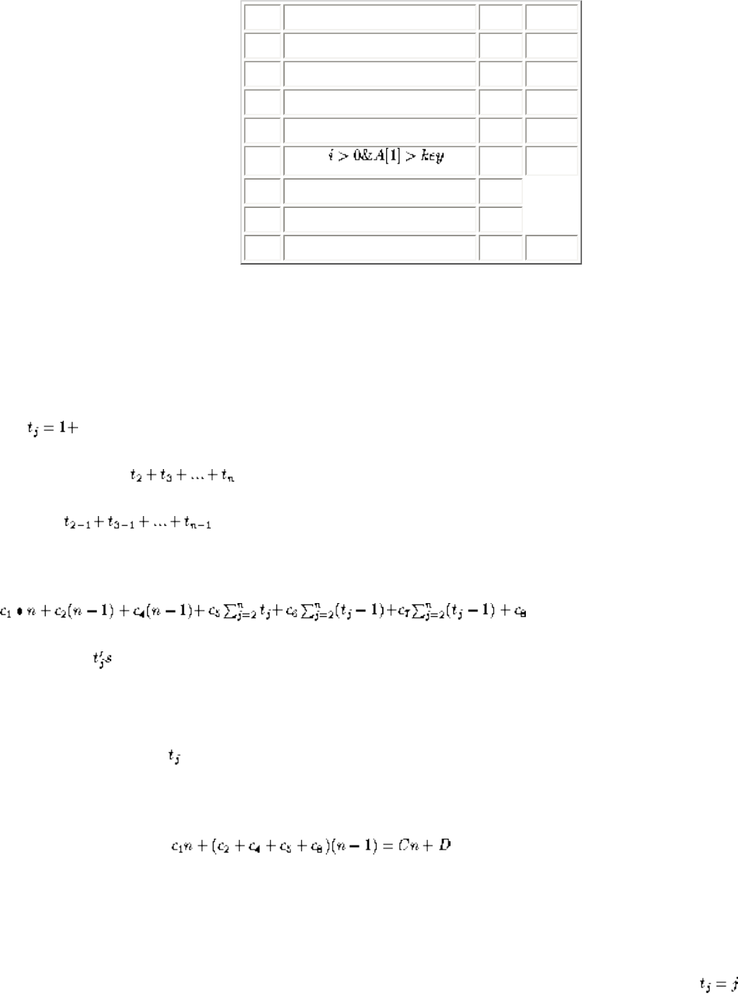
Lecture 1 - analyzing algorithms
Line InsertionSort(A) #Inst. #Exec.
1 for j:=2 to len. of A do c1 n
2 key:=A[j] c2 n-1
3 /* put A[j] into A[1..j-1] */ c3=0 /
4 i:=j-1 c4 n-1
5 while do c5 tj
6 A[i+1]:= A[i] c6
7 i := i-1 c7
8 A[i+1]:=key c8 n-1
The for statement is executed (n-1)+1 times (why?)
Within the for statement, "key:=A[j]" is executed n-1 times.
Steps 5, 6, 7 are harder to count.
Let the number of elements that have to be slide right to insert the jth item.
Step 5 is executed times.
Step 6 is .
Add up the executed instructions for all pseudocode lines to get the run-time of the algorithm:
What are the ? They depend on the particular input.
Best Case
If it's already sorted, all 's are 1.
Hence, the best case time is
where C and D are constants.
Worst Case
If the input is sorted in descending order, we will have to slide all of the already-sorted elements, so , and step 5
file:///E|/LEC/LECTUR16/NODE1.HTM (8 of 9) [19/1/2003 1:34:15]


Lecture 2 - asymptotic notation
Next: Lecture 3 - recurrence Up: No Title Previous: Lecture 1 - analyzing
Lecture 2 - asymptotic notation
Listen To Part 2-1
Problem 1.2-6: How can we modify almost any algorithm to have a good best-case running time?
To improve the best case, all we have to do it to be able to solve one instance of each size efficiently. We
could modify our algorithm to first test whether the input is the special instance we know how to solve,
and then output the canned answer.
For sorting, we can check if the values are already ordered, and if so output them. For the traveling
salesman, we can check if the points lie on a line, and if so output the points in that order.
The supercomputer people pull this trick on the linpack benchmarks!
Because it is so easy to cheat with the best case running time, we usually don't rely too much about it.
Because it is usually very hard to compute the average running time, since we must somehow average
over all the instances, we usually strive to analyze the worst case running time.
The worst case is usually fairly easy to analyze and often close to the average or real running time.
Listen To Part 2-2
Exact Analysis is Hard!
We have agreed that the best, worst, and average case complexity of an algorithm is a numerical function
of the size of the instances.
file:///E|/LEC/LECTUR16/NODE2.HTM (1 of 10) [19/1/2003 1:34:21]
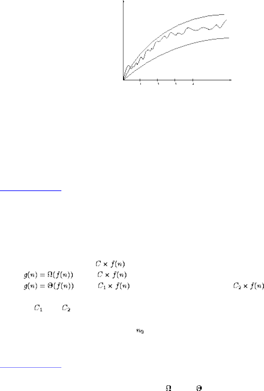
Lecture 2 - asymptotic notation
However, it is difficult to work with exactly because it is typically very complicated!
Thus it is usually cleaner and easier to talk about upper and lower bounds of the function.
This is where the dreaded big O notation comes in!
Since running our algorithm on a machine which is twice as fast will effect the running times by a
multiplicative constant of 2 - we are going to have to ignore constant factors anyway.
Listen To Part 2-3
Names of Bounding Functions
Now that we have clearly defined the complexity functions we are talking about, we can talk about upper
and lower bounds on it:
● g(n) = O(f(n)) means is an upper bound on g(n).
● means is a lower bound on g(n).
● means is an upper bound on g(n) and is a lower bound on g(n).
Got it? C, , and are all constants independent of n.
All of these definitions imply a constant beyond which they are satisfied. We do not care about small
values of n.
Listen To Part 2-4
O, , and
file:///E|/LEC/LECTUR16/NODE2.HTM (2 of 10) [19/1/2003 1:34:21]
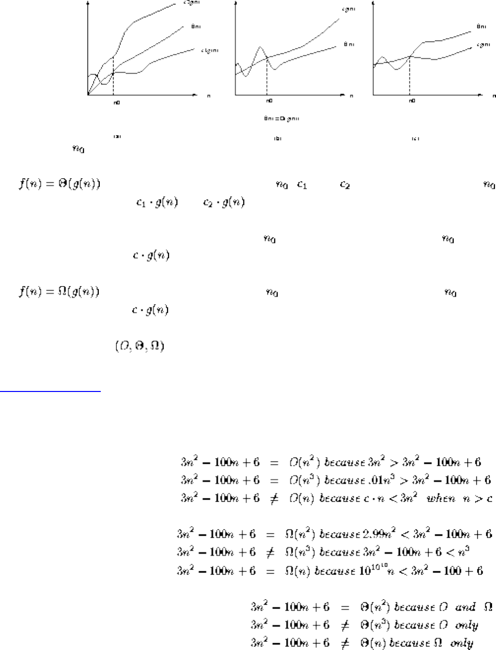
Lecture 2 - asymptotic notation
The value of shown is the minimum possible value; any greater value would also work.
(a) if there exist positive constants , , and such that to the right of , the value of
f(n) always lies between and inclusive.
(b) f(n) = O(g(n)) if there are positive constants and c such that to the right of , the value of f(n)
always lies on or below .
(c) if there are positive constants and c such that to the right of , the value of f(n)
always lies on or above .
Asymptotic notation are as well as we can practically deal with complexity functions.
Listen To Part 2-5
What does all this mean?
Think of the equality as meaning in the set of functions.
file:///E|/LEC/LECTUR16/NODE2.HTM (3 of 10) [19/1/2003 1:34:21]
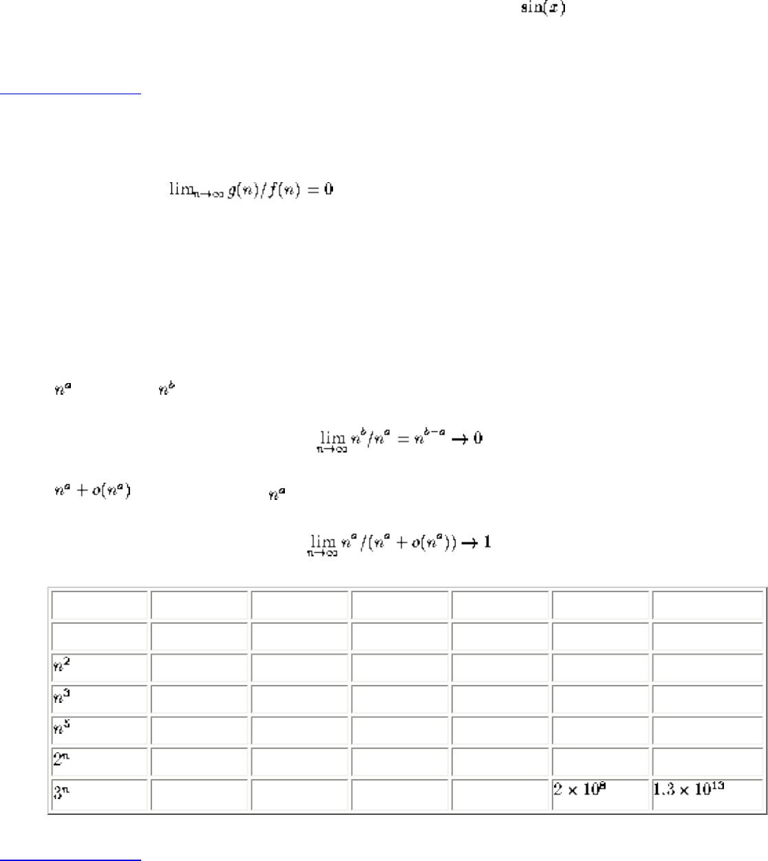
Lecture 2 - asymptotic notation
Note that time complexity is every bit as well defined a function as or you bank account as a
function of time.
Listen To Part 2-6
Testing Dominance
f(n) dominates g(n) if , which is the same as saying g(n)=o(f(n)).
Note the little-oh - it means ``grows strictly slower than''.
Knowing the dominance relation between common functions is important because we want algorithms
whose time complexity is as low as possible in the hierarchy. If f(n) dominates g(n), f is much larger (ie.
slower) than g.
● dominates if a > b since
● doesn't dominate since
Complexity 10 20 30 40 50 60
n 0.00001 sec 0.00002 sec 0.00003 sec 0.00004 sec 0.00005 sec 0.00006 sec
0.0001 sec 0.0004 sec 0.0009 sec 0.016 sec 0.025 sec 0.036 sec
0.001 sec 0.008 sec 0.027 sec 0.064 sec 0.125 sec 0.216 sec
0.1 sec 3.2 sec 24.3 sec 1.7 min 5.2 min 13.0 min
0.001 sec 1.0 sec 17.9 min 12.7 days 35.7 years 366 cent
0.59 sec 58 min 6.5 years 3855 cent cent cent
Listen To Part 2-7
Logarithms
It is important to understand deep in your bones what logarithms are and where they come from.
file:///E|/LEC/LECTUR16/NODE2.HTM (4 of 10) [19/1/2003 1:34:21]
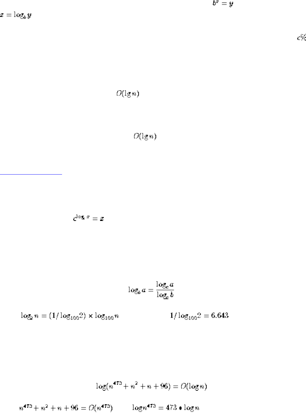
Lecture 2 - asymptotic notation
A logarithm is simply an inverse exponential function. Saying is equivalent to saying that
.
Exponential functions, like the amount owed on a n year mortgage at an interest rate of per year, are
functions which grow distressingly fast, as anyone who has tried to pay off a mortgage knows.
Thus inverse exponential functions, ie. logarithms, grow refreshingly slowly.
Binary search is an example of an algorithm. After each comparison, we can throw away half the
possible number of keys. Thus twenty comparisons suffice to find any name in the million-name
Manhattan phone book!
If you have an algorithm which runs in time, take it, because this is blindingly fast even on very
large instances.
Listen To Part 2-8
Properties of Logarithms
Recall the definition, .
Asymptotically, the base of the log does not matter:
Thus, , and note that is just a constant.
Asymptotically, any polynomial function of n does not matter:
Note that
since , and .
Any exponential dominates every polynomial. This is why we will seek to avoid exponential time
file:///E|/LEC/LECTUR16/NODE2.HTM (5 of 10) [19/1/2003 1:34:21]
Lecture 2 - asymptotic notation
algorithms.
Listen To Part 2-9
Federal Sentencing Guidelines
2F1.1. Fraud and Deceit; Forgery; Offenses Involving Altered or Counterfeit Instruments other than
Counterfeit Bearer Obligations of the United States.
(a) Base offense Level: 6
(b) Specific offense Characteristics
(1) If the loss exceeded $2,000, increase the offense level as follows:
Loss(Apply the Greatest) Increase in Level
(A) $2,000 or less no increase
(B) More than $2,000 add 1
(C) More than $5,000 add 2
(D) More than $10,000 add 3
(E) More than $20,000 add 4
(F) More than $40,000 add 5
(G) More than $70,000 add 6
(H) More than $120,000 add 7
(I) More than $200,000 add 8
(J) More than $350,000 add 9
(K) More than $500,000 add 10
(L) More than $800,000 add 11
(M) More than $1,500,000 add 12
(N) More than $2,500,000 add 13
(O) More than $5,000,000 add 14
(P) More than $10,000,000 add 15
(Q) More than $20,000,000 add 16
(R) More than $40,000,000 add 17
file:///E|/LEC/LECTUR16/NODE2.HTM (6 of 10) [19/1/2003 1:34:21]
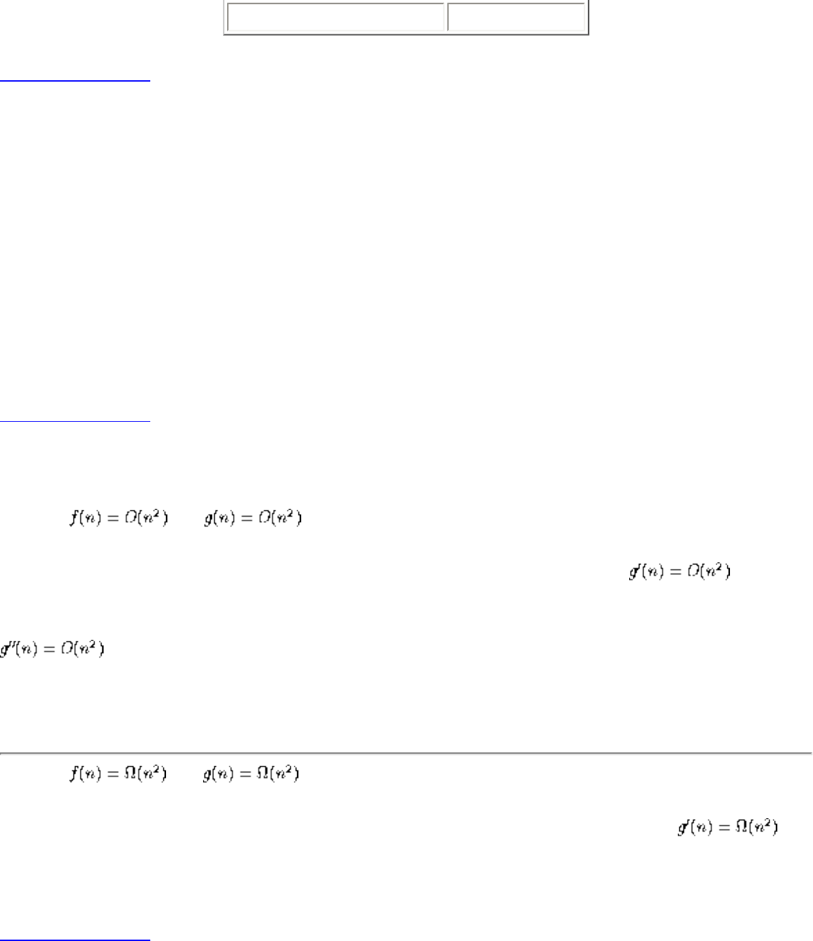
Lecture 2 - asymptotic notation
(Q) More than $80,000,000 add 18
Listen To Part 2-10
The federal sentencing guidelines are designed to help judges be consistent in assigning punishment. The
time-to-serve is a roughly linear function of the total level.
However, notice that the increase in level as a function of the amount of money you steal grows
logarithmically in the amount of money stolen.
This very slow growth means it pays to commit one crime stealing a lot of money, rather than many
small crimes adding up to the same amount of money, because the time to serve if you get caught is
much less.
The Moral: ``if you are gonna do the crime, make it worth the time!''
Listen To Part 2-11
Working with the Asymptotic Notation
Suppose and .
What do we know about g'(n) = f(n)+g(n)? Adding the bounding constants shows .
What do we know about g''(n) = f(n)-g(n)? Since the bounding constants don't necessary cancel,
We know nothing about the lower bounds on g'+g'' because we know nothing about lower bounds on f, g.
Suppose and .
What do we know about g'(n) = f(n)+g(n)? Adding the lower bounding constants shows .
What do we know about g''(n) = f(n)-g(n)? We know nothing about the lower bound of this!
Listen To Part 2-12
The Complexity of Songs
file:///E|/LEC/LECTUR16/NODE2.HTM (7 of 10) [19/1/2003 1:34:21]
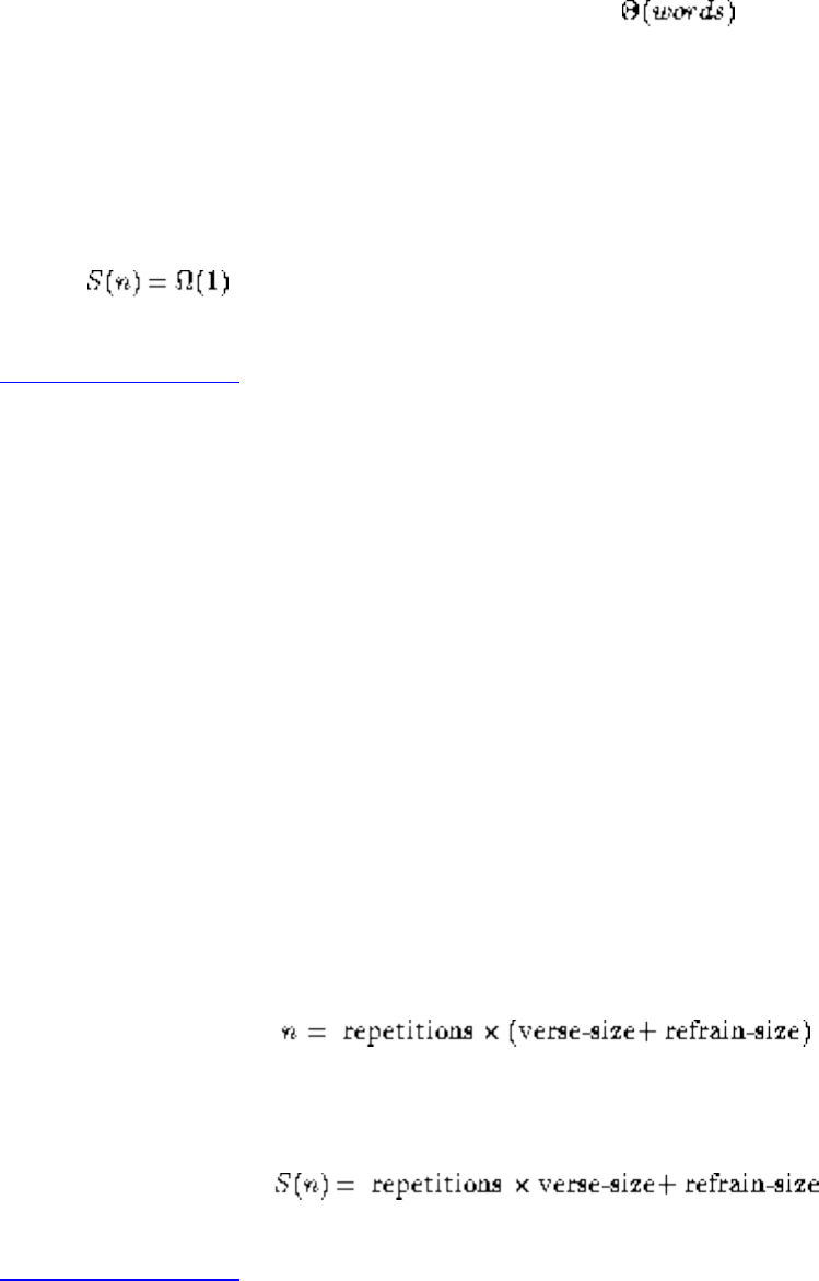
Lecture 2 - asymptotic notation
Suppose we want to sing a song which lasts for n units of time. Since n can be large, we want to
memorize songs which require only a small amount of brain space, i.e. memory.
Let S(n) be the space complexity of a song which lasts for n units of time.
The amount of space we need to store a song can be measured in either the words or characters needed to
memorize it. Note that the number of characters is since every word in a song is at most 34
letters long - Supercalifragilisticexpialidocious!
What bounds can we establish on S(n)?
● S(n) = O(n), since in the worst case we must explicitly memorize every word we sing - ``The Star-
Spangled Banner''
● , since we must know something about our song to sing it.
Listen To Part 2-13
The Refrain
Most popular songs have a refrain, which is a block of text which gets repeated after each stanza in the
song:
Bye, bye Miss American pie
Drove my chevy to the levy but the levy was dry
Them good old boys were drinking whiskey and rye
Singing this will be the day that I die.
Refrains made a song easier to remember, since you memorize it once yet sing it O(n) times. But do they
reduce the space complexity?
Not according to the big oh. If
Then the space complexity is still O(n) since it is only halved (if the verse-size = refrain-size):
Listen To Part 2-14
file:///E|/LEC/LECTUR16/NODE2.HTM (8 of 10) [19/1/2003 1:34:21]
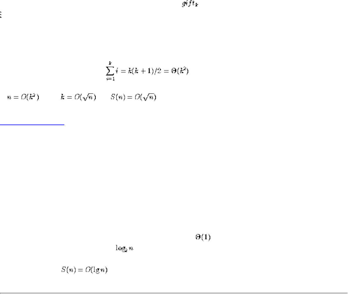
Lecture 2 - asymptotic notation
The k Days of Christmas
To reduce S(n), we must structure the song differently.
Consider ``The k Days of Christmas''. All one must memorize is:
On the kth Day of Christmas, my true love gave to me,
On the First Day of Christmas, my true love gave to me, a partridge in a pear tree
But the time it takes to sing it is
If , then , so .
Listen To Part 2-15
100 Bottles of Beer
What do kids sing on really long car trips?
n bottles of beer on the wall,
n bottles of beer.
You take one down and pass it around
n-1 bottles of beer on the ball.
All you must remember in this song is this template of size , and the current value of n. The storage
size for n depends on its value, but bits suffice.
This for this song, .
Is there a song which eliminates even the need to count?
That's the way, uh-huh, uh-huh
I like it, uh-huh, huh
Reference: D. Knuth, `The Complexity of Songs', Comm. ACM, April 1984, pp.18-24
file:///E|/LEC/LECTUR16/NODE2.HTM (9 of 10) [19/1/2003 1:34:21]

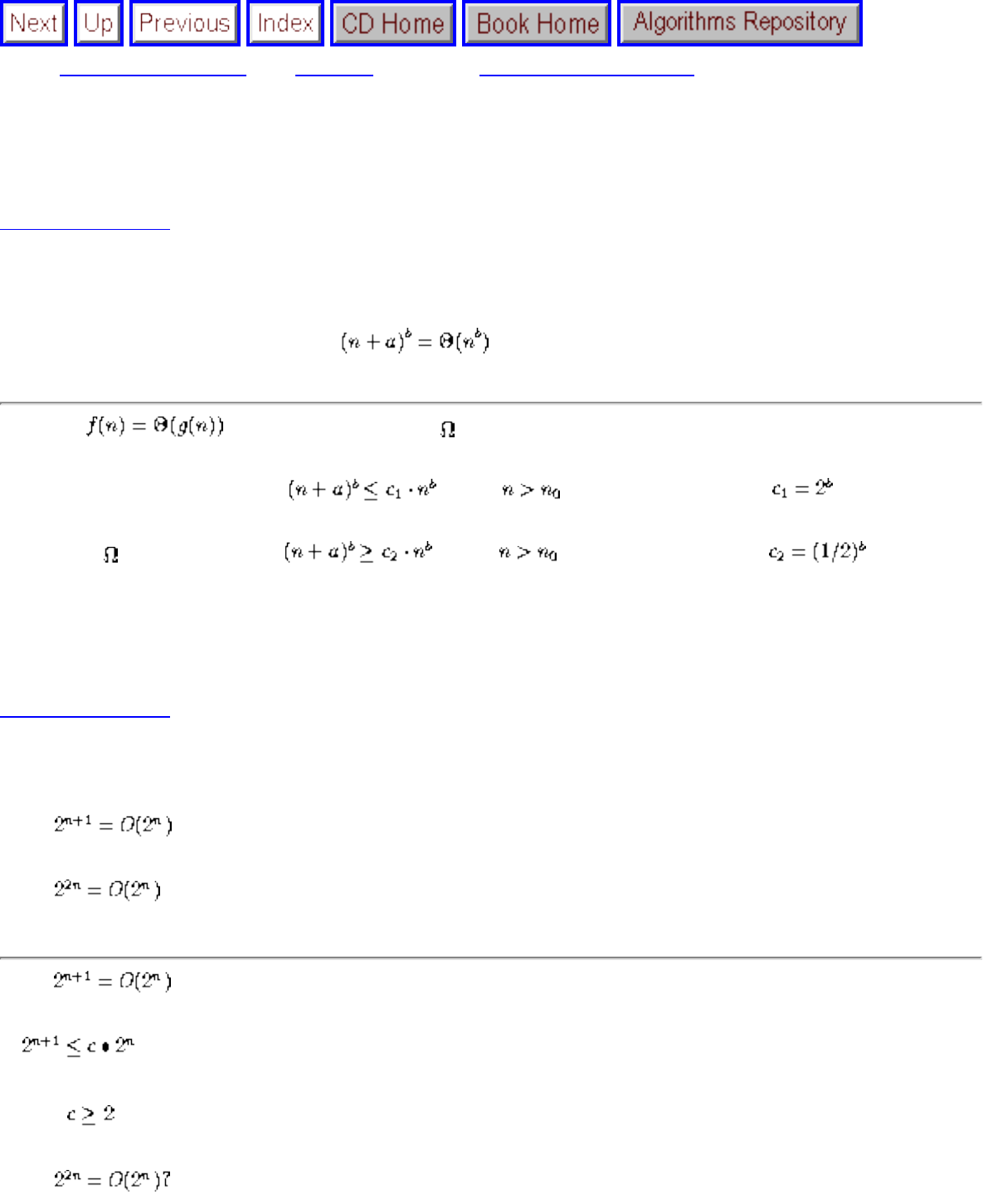
Lecture 3 - recurrence relations
Next: Lecture 4 - heapsort Up: No Title Previous: Lecture 2 - asymptotic
Lecture 3 - recurrence relations
Listen To Part 3-1
Problem 2.1-2: Show that for any real constants a and b, b > 0,
To show , we must show O and . Go back to the definition!
● Big O - Must show that for all . When is this true? If , this is true for
all n > |a| since n+a < 2n, and raise both sides to the b.
● Big - Must show that for all . When is this true? If , this is true
for all n > 3|a|/2 since n+a > n/2, and raise both sides to the b.
Note the need for absolute values.
Listen To Part 3-2
Problem 2.1-4:
(a) Is ?
(b) Is ?
(a) Is ?
Is ?
Yes, if for all n
(b) Is
file:///E|/LEC/LECTUR17/NODE3.HTM (1 of 10) [19/1/2003 1:34:27]
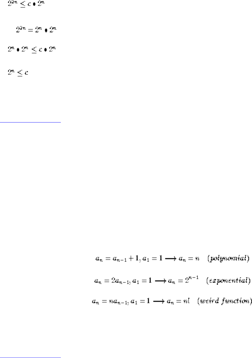
Lecture 3 - recurrence relations
Is ?
note
Is ?
Is ?
No! Certainly for any constant c we can find an n such that this is not true.
Listen To Part 3-3
Recurrence Relations
Many algorithms, particularly divide and conquer algorithms, have time complexities which are naturally
modeled by recurrence relations.
A recurrence relation is an equation which is defined in terms of itself.
Why are recurrences good things?
1. Many natural functions are easily expressed as recurrences:
2. It is often easy to find a recurrence as the solution of a counting problem. Solving the recurrence
can be done for many special cases as we will see, although it is somewhat of an art.
Listen To Part 3-4
Recursion is Mathematical Induction!
In both, we have general and boundary conditions, with the general condition breaking the problem into
smaller and smaller pieces.
file:///E|/LEC/LECTUR17/NODE3.HTM (2 of 10) [19/1/2003 1:34:27]
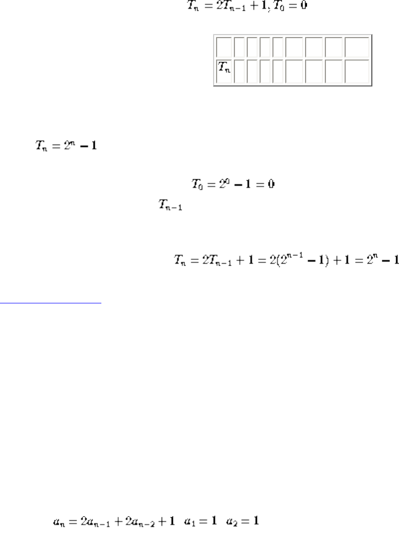
Lecture 3 - recurrence relations
The initial or boundary condition terminate the recursion.
As we will see, induction provides a useful tool to solve recurrences - guess a solution and prove it by
induction.
n 0 1 2 3 4 5 6 7
0 1 3 7 15 31 63 127
Guess what the solution is?
Prove by induction:
1. Show that the basis is true: .
2. Now assume true for .
3. Using this assumption show:
Listen To Part 3-5
Solving Recurrences
No general procedure for solving recurrence relations is known, which is why it is an art. My approach
is:
Realize that linear, finite history, constant coefficient recurrences always can be
solved
Check out any combinatorics or differential equations book for a procedure.
Consider , ,
It has history = 2, degree = 1, and coefficients of 2 and 1. Thus it can be solved mechanically! Proceed:
● Find the characteristic equation, eg.
file:///E|/LEC/LECTUR17/NODE3.HTM (3 of 10) [19/1/2003 1:34:27]
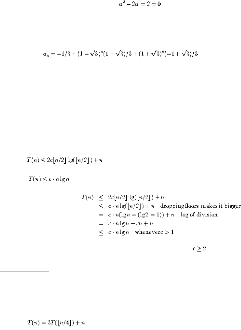
Lecture 3 - recurrence relations
● Solve to get roots, which appear in the exponents.
● Take care of repeated roots and inhomogeneous parts.
● Find the constants to finish the job.
Systems like Mathematica and Maple have packages for doing this.
Listen To Part 3-6
Guess a solution and prove by induction
To guess the solution, play around with small values for insight.
Note that you can do inductive proofs with the big-O's notations - just be sure you use it right.
Example: .
Show that for large enough c and n. Assume that it is true for n/2, then
Starting with basis cases T(2)=4, T(3)=5, lets us complete the proof for .
Listen To Part 3-7
Try backsubstituting until you know what is going on
Also known as the iteration method. Plug the recurrence back into itself until you see a pattern.
Example: .
Try backsubstituting:
file:///E|/LEC/LECTUR17/NODE3.HTM (4 of 10) [19/1/2003 1:34:27]
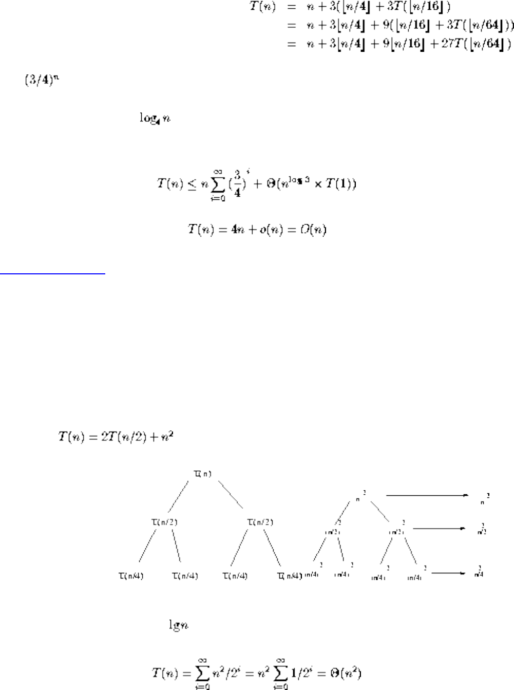
Lecture 3 - recurrence relations
The term should now be obvious.
Although there are only terms before we get to T(1), it doesn't hurt to sum them all since this is a
fast growing geometric series:
Listen To Part 3-8
Recursion Trees
Drawing a picture of the backsubstitution process gives you a idea of what is going on.
We must keep track of two things - (1) the size of the remaining argument to the recurrence, and (2) the
additive stuff to be accumulated during this call.
Example:
The remaining arguments are on the left, the additive terms on the right.
Although this tree has height , the total sum at each level decreases geometrically, so:
The recursion tree framework made this much easier to see than with algebraic backsubstitution.
file:///E|/LEC/LECTUR17/NODE3.HTM (5 of 10) [19/1/2003 1:34:27]
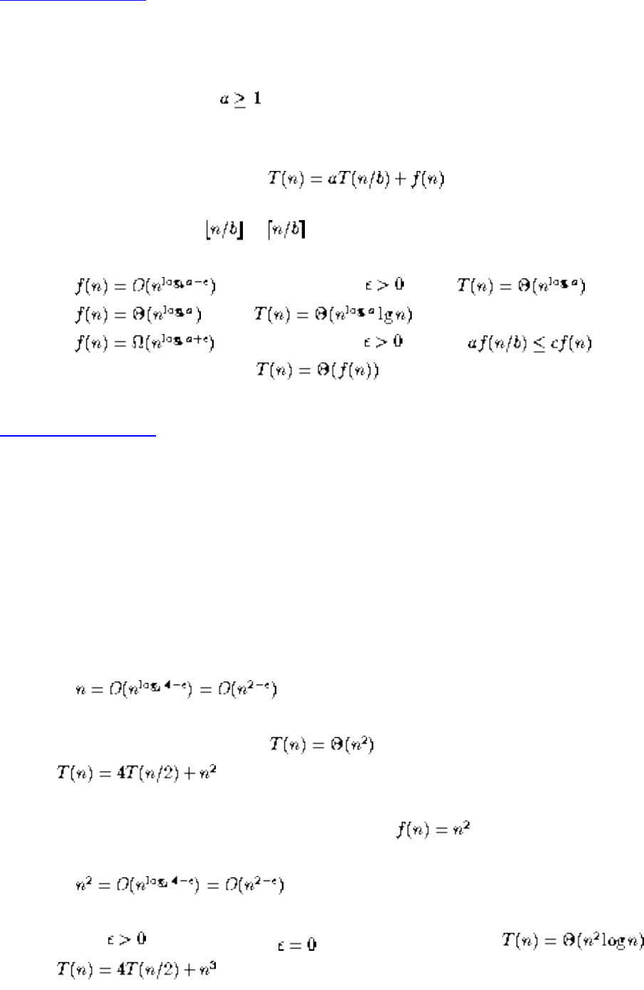
Lecture 3 - recurrence relations
Listen To Part 3-9
See if you can use the Master theorem to provide an instant asymptotic solution
The Master Theorem: Let and b>1 be constants, let f(n) be a function, and let T(n) be defined on
the nonnegative integers by the recurrence
where we interpret n/b as or . Then T(n) can be bounded asymptotically as follows:
1. If for some constant , then .
2. If , then .
3. If for some constant , and if for some constant c<1, and all
sufficiently large n, then .
Listen To Part 3-10
Examples of the Master Theorem
Which case of the Master Theorem applies?
● T(n) = 4 T(n/2) + n
Reading from the equation, a=4, b=2, and f(n) = n.
Is ?
Yes, so case 1 applies and .
●
Reading from the equation, a=4, b=2, and .
Is ?
No, if , but it is true if , so case 2 applies and .
●
file:///E|/LEC/LECTUR17/NODE3.HTM (6 of 10) [19/1/2003 1:34:27]
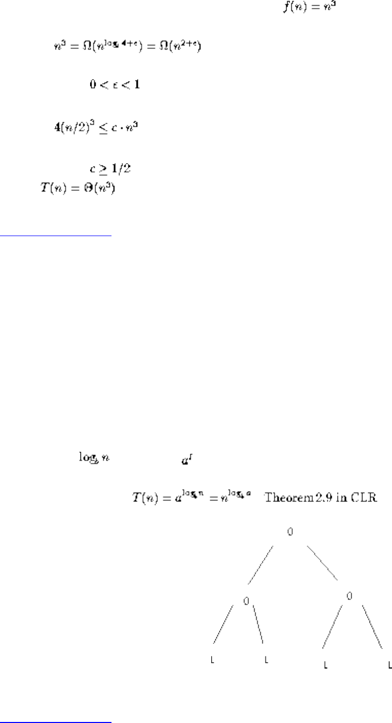
Lecture 3 - recurrence relations
Reading from the equation, a=4, b=2, and .
Is ?
Yes, for , so case 3 might apply.
Is ?
Yes, for , so there exists a c < 1 to satisfy the regularity condition, so case 3 applies and
.
Listen To Part 3-11
Why should the Master Theorem be true?
Consider T(n) = a T(n/b) + f(n).
Suppose f(n) is small enough
Say f(n)=0, ie. T(n) = a T(n/b).
Then we have a recursion tree where the only contribution is at the leaves.
There will be levels, with leaves at level l.
so long as f(n) is small enough that it is dwarfed by this, we have case 1 of the Master Theorem!
Listen To Part 3-12
file:///E|/LEC/LECTUR17/NODE3.HTM (7 of 10) [19/1/2003 1:34:27]
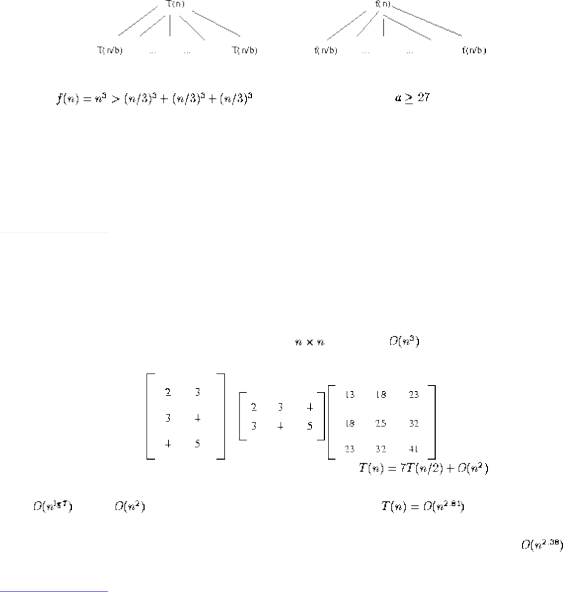
Lecture 3 - recurrence relations
Suppose f(n) is large enough
If we draw the recursion tree for T(n) = a T(n/b) + f(n).
If f(n) is a big enough function, the one top call can be bigger than the sum of all the little calls.
Example: . In fact this holds unless !
In case 3 of the Master Theorem, the additive term dominates.
In case 2, both parts contribute equally, which is why the log pops up. It is (usually) what we want to
have happen in a divide and conquer algorithm.
Listen To Part 3-13
Famous Algorithms and their Recurrence
Matrix Multiplication
The standard matrix multiplication algorithm for two matrices is .
Strassen discovered a divide-and-conquer algorithm which takes time.
Since dwarfs , case 1 of the master theorem applies and .
This has been ``improved'' by more and more complicated recurrences until the current best in .
Listen To Part 3-14
file:///E|/LEC/LECTUR17/NODE3.HTM (8 of 10) [19/1/2003 1:34:27]
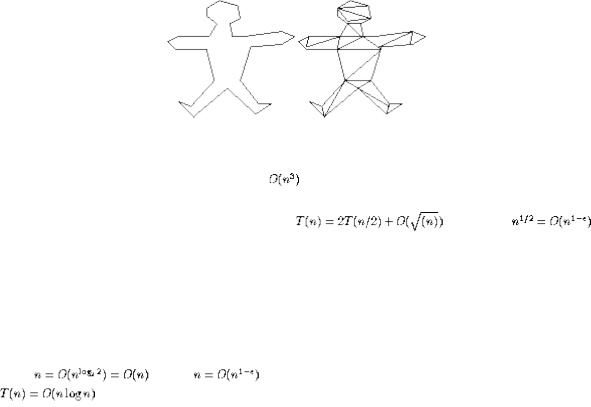
Lecture 3 - recurrence relations
Polygon Triangulation
Given a polygon in the plane, add diagonals so that each face is a triangle None of the diagonals are
allowed to cross.
Triangulation is an important first step in many geometric algorithms.
The simplest algorithm might be to try each pair of points and check if they see each other. If so, add the
diagonal and recur on both halves, for a total of .
However, Chazelle gave an algorithm which runs in time. Since
, by case 1 of the Master Theorem, Chazelle's algorithm is linear, ie. T(n) = O(n).
Sorting
The classic divide and conquer recurrence is Mergesort's T(n) = 2 T(n/2) + O(n), which divides the data
into equal-sized halves and spends linear time merging the halves after they are sorted.
Since but not , Case 2 of the Master Theorem applies and
.
In case 2, the divide and merge steps balance out perfectly, as we usually hope for from a divide-and-
conquer algorithm.
Mergesort Animations
Approaches to Algorithms Design
Incremental
Job is partly done - do a little more, repeat until done.
file:///E|/LEC/LECTUR17/NODE3.HTM (9 of 10) [19/1/2003 1:34:27]

Lecture 3 - recurrence relations
A good example of this approach is insertion sort
Divide-and-Conquer
A recursive technique
● Divide problem into sub-problems of the same kind.
● For subproblems that are really small (trivial), solve them directly. Else solve them recursively.
(conquer)
● Combine subproblem solutions to solve the whole thing (combine)
A good example of this approach is Mergesort.
Next: Lecture 4 - heapsort Up: No Title Previous: Lecture 2 - asymptotic
Algorithms
Mon Jun 2 09:21:39 EDT 1997
file:///E|/LEC/LECTUR17/NODE3.HTM (10 of 10) [19/1/2003 1:34:27]
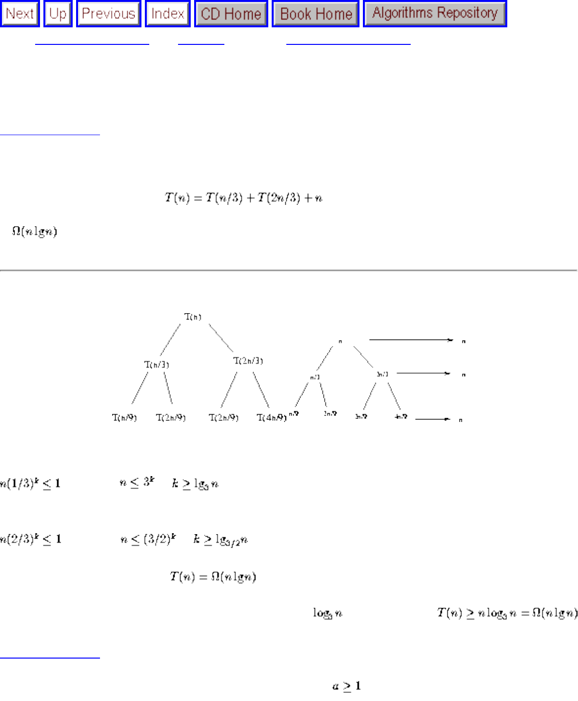
Lecture 4 - heapsort
Next: Lecture 5 - quicksort Up: No Title Previous: Lecture 3 - recurrence
Lecture 4 - heapsort
Listen To Part 4-1
4.2-2 Argue the solution to
is by appealing to the recursion tree.
Draw the recursion tree.
How many levels does the tree have? This is equal to the longest path from the root to a leaf.
The shortest path to a leaf occurs when we take the heavy branch each time. The height k is given by
, meaning or .
The longest path to a leaf occurs when we take the light branch each time. The height k is given by
, meaning or .
The problem asks to show that , meaning we are looking for a lower bound
On any full level, the additive terms sums to n. There are full levels. Thus
Listen To Part 4-2
4.2-4 Use iteration to solve T(n) = T(n-a) + T(a) + n, where is a constant.
file:///E|/LEC/LECTUR17/NODE4.HTM (1 of 14) [19/1/2003 1:34:31]
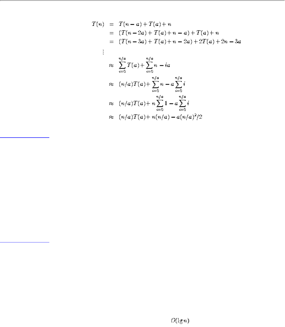
Lecture 4 - heapsort
Note iteration is backsubstitution.
Listen To Part 4-3
Why don't CS profs ever stop talking about sorting?!
1. Computers spend more time sorting than anything else, historically 25% on mainframes.
2. Sorting is the best studied problem in computer science, with a variety of different algorithms
known.
3. Most of the interesting ideas we will encounter in the course can be taught in the context of
sorting, such as divide-and-conquer, randomized algorithms, and lower bounds.
You should have seen most of the algorithms - we will concentrate on the analysis.
Listen To Part 4-4
Applications of Sorting
One reason why sorting is so important is that once a set of items is sorted, many other problems become
easy.
Searching
Binary search lets you test whether an item is in a dictionary in time.
Speeding up searching is perhaps the most important application of sorting.
file:///E|/LEC/LECTUR17/NODE4.HTM (2 of 14) [19/1/2003 1:34:31]

Lecture 4 - heapsort
Closest pair
Given n numbers, find the pair which are closest to each other.
Once the numbers are sorted, the closest pair will be next to each other in sorted order, so an O(n) linear
scan completes the job.
Listen To Part 4-5
Element uniqueness
Given a set of n items, are they all unique or are there any duplicates?
Sort them and do a linear scan to check all adjacent pairs.
This is a special case of closest pair above.
Frequency distribution - Mode
Given a set of n items, which element occurs the largest number of times?
Sort them and do a linear scan to measure the length of all adjacent runs.
Median and Selection
What is the kth largest item in the set?
Once the keys are placed in sorted order in an array, the kth largest can be found in constant time by
simply looking in the kth position of the array.
Listen To Part 4-6
Convex hulls
Given n points in two dimensions, find the smallest area polygon which contains them all.
file:///E|/LEC/LECTUR17/NODE4.HTM (3 of 14) [19/1/2003 1:34:31]
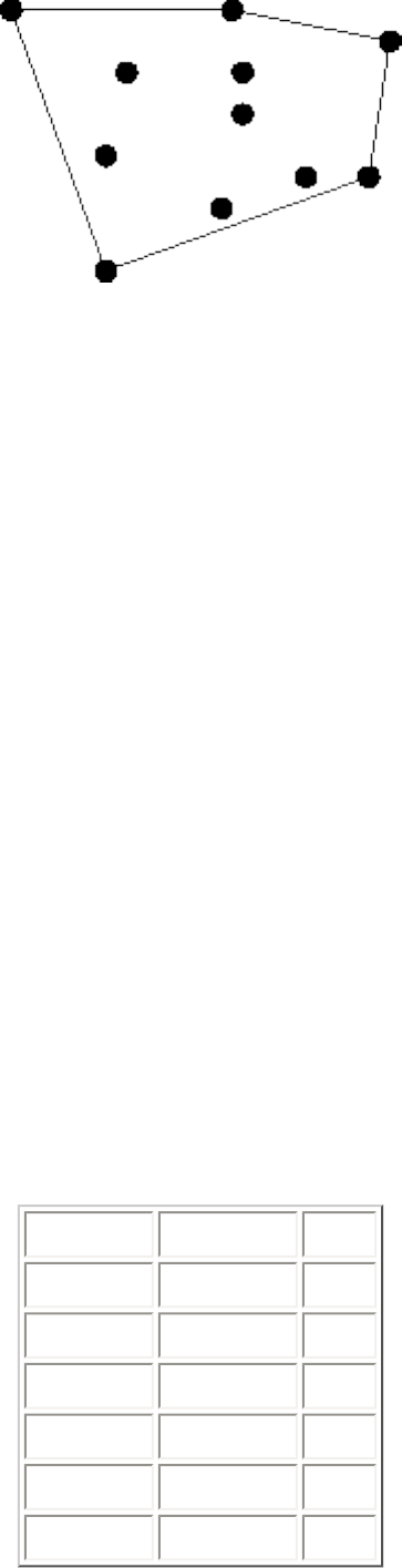
Lecture 4 - heapsort
The convex hull is like a rubber band stretched over the points.
Convex hulls are the most important building block for more sophisticated geometric algorithms.
Once you have the points sorted by x-coordinate, they can be inserted from left to right into the hull,
since the rightmost point is always on the boundary.
Without sorting the points, we would have to check whether the point is inside or outside the current hull.
Adding a new rightmost point might cause others to be deleted.
Huffman codes
If you are trying to minimize the amount of space a text file is taking up, it is silly to assign each letter
the same length (ie. one byte) code.
Example: e is more common than q, a is more common than z.
If we were storing English text, we would want a and e to have shorter codes than q and z.
To design the best possible code, the first and most important step is to sort the characters in order of
frequency of use.
Character Frequency Code
f 5 1100
e 9 1101
c 12 100
b 13 101
d 16 111
a 45 0
file:///E|/LEC/LECTUR17/NODE4.HTM (4 of 14) [19/1/2003 1:34:31]
Lecture 4 - heapsort
Listen To Part 4-8
Selection Sort
A simple sorting algorithm is selection sort.
Sweep through all the elements to find the smallest item, then the smallest remaining item, etc. until the
array is sorted.
Selection-sort(A)
for i = 1 to n
for j = i+1 to n
if (A[j] < A[i]) then
swap(A[i],A[j])
It is clear this algorithm must be correct from an inductive argument, since the ith element is in its correct
position.
It is clear that this algorithm takes time.
It is clear that the analysis of this algorithm cannot be improved because there will be n/2 iterations
which will require at least n/2 comparisons each, so at least comparisons will be made. More careful
analysis doubles this.
Thus selection sort runs in time.
Listen To Part 4-9
Binary Heaps
A binary heap is defined to be a binary tree with a key in each node such that:
file:///E|/LEC/LECTUR17/NODE4.HTM (5 of 14) [19/1/2003 1:34:31]
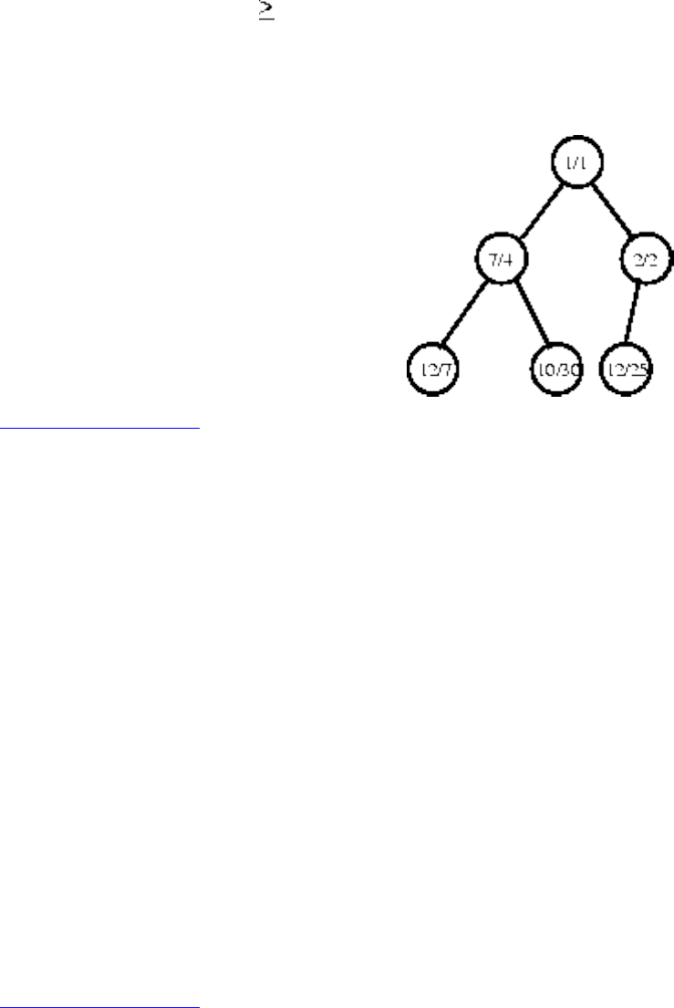
Lecture 4 - heapsort
1. All leaves are on, at most, two adjacent levels.
2. All leaves on the lowest level occur to the left, and all levels except the lowest one are completely
filled.
3. The key in root is all its children, and the left and right subtrees are again binary heaps.
Conditions 1 and 2 specify shape of the tree, and condition 3 the labeling of the tree.
Listen To Part 4-10
The ancestor relation in a heap defines a partial order on its elements, which means it is reflexive, anti-
symmetric, and transitive.
1. Reflexive: x is an ancestor of itself.
2. Anti-symmetric: if x is an ancestor of y and y is an ancestor of x, then x=y.
3. Transitive: if x is an ancestor of y and y is an ancestor of z, x is an ancestor of z.
Partial orders can be used to model heirarchies with incomplete information or equal-valued elements.
One of my favorite games with my parents is fleshing out the partial order of ``big'' old-time movie stars.
The partial order defined by the heap structure is weaker than that of the total order, which explains
1. Why it is easier to build.
2. Why it is less useful than sorting (but still very important).
Listen To Part 4-11
Constructing Heaps
Heaps can be constructed incrementally, by inserting new elements into the left-most open spot in the
array.
file:///E|/LEC/LECTUR17/NODE4.HTM (6 of 14) [19/1/2003 1:34:31]
Lecture 4 - heapsort
If the new element is greater than its parent, swap their positions and recur.
Since at each step, we replace the root of a subtree by a larger one, we preserve the heap order.
Since all but the last level is always filled, the height h of an n element heap is bounded because:
so .
Doing n such insertions takes , since the last n/2 insertions require time each.
Listen To Part 4-12
Heapify
The bottom up insertion algorithm gives a good way to build a heap, but Robert Floyd found a better
way, using a merge procedure called heapify.
Given two heaps and a fresh element, they can be merged into one by making the new one the root and
trickling down.
Build-heap(A)
n = |A|
For do
Heapify(A,i)
Heapify(A,i)
file:///E|/LEC/LECTUR17/NODE4.HTM (7 of 14) [19/1/2003 1:34:31]
Lecture 4 - heapsort
left = 2i
right = 2i+1
if then
max = left
else max = i
if and (A(right] > A[max]) then
max = right
if then
swap(A[i],A[max])
Heapify(A,max)
Rough Analysis of Heapify
Heapify on a subtree containing n nodes takes
The 2/3 comes from merging heaps whose levels differ by one. The last row could be exactly half filled.
Besides, the asymptotic answer won't change so long the fraction is less than one.
Solve the recurrence using the Master Theorem.
file:///E|/LEC/LECTUR17/NODE4.HTM (8 of 14) [19/1/2003 1:34:31]
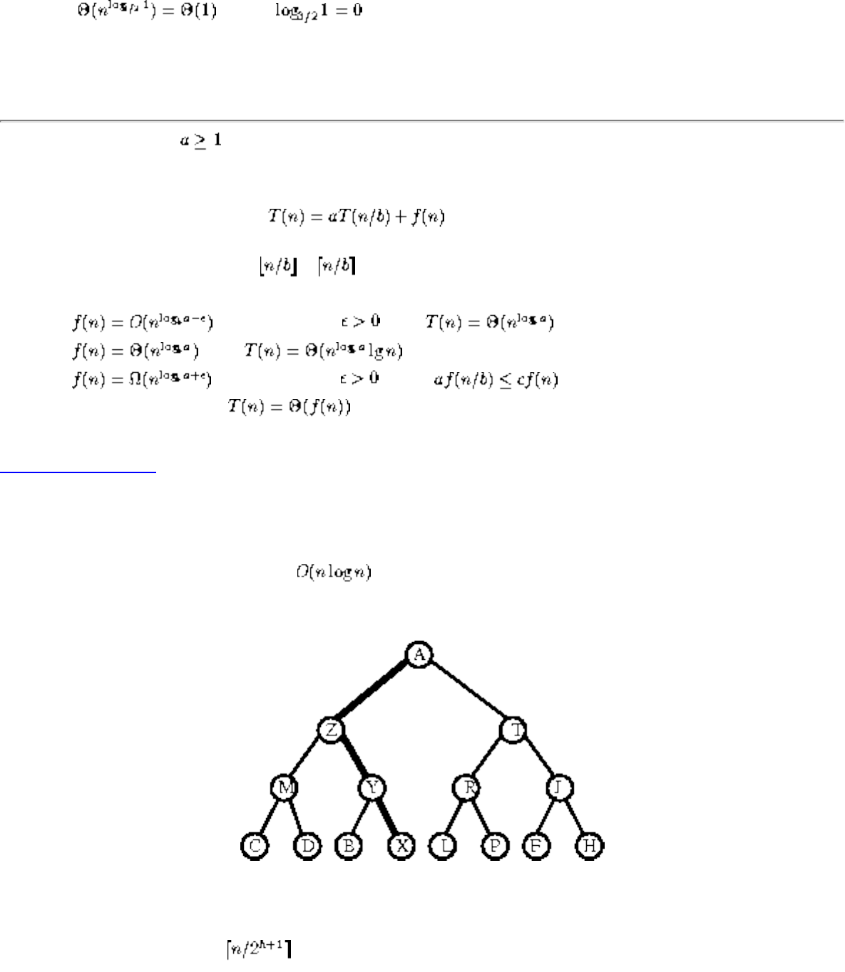
Lecture 4 - heapsort
Let a = 1, b= 3/2 and f(n) = 1.
Note that , since .
Thus Case 2 of the Master theorem applies.
The Master Theorem: Let and b>1 be constants, let f(n) be a function, and let T(n) be defined on the nonnegative
integers by the recurrence
where we interpret n/b to mean either or . Then T(n) can be bounded asymptotically as follows:
1. If for some constant , then .
2. If , then .
3. If for some constant , and if for some constant c<1, and all
sufficiently large n, then .
Listen To Part 4-14
Exact Analysis of Heapify
In fact, Heapify performs better than , because most of the heaps we merge are extremely
small.
In a full binary tree on n nodes, there are n/2 nodes which are leaves (i.e. height 0), n/4 nodes which are
height 1, n/8 nodes which are height 2, ...
In general, there are at most nodes of height h, so the cost of building a heap is:
file:///E|/LEC/LECTUR17/NODE4.HTM (9 of 14) [19/1/2003 1:34:31]
Lecture 4 - heapsort
Since this sum is not quite a geometric series, we can't apply the usual identity to get the sum. But it
should be clear that the series converges.
Listen To Part 4-15
Proof of Convergence
Series convergence is the ``free lunch'' of algorithm analysis.
The identify for the sum of a geometric series is
If we take the derivative of both sides, ...
Multiplying both sides of the equation by x gives the identity we need:
Substituting x = 1/2 gives a sum of 2, so Build-heap uses at most 2n comparisons and thus linear time.
Listen To Part 4-16
The Lessons of Heapsort, I
"Are we doing a careful analysis? Might our algorithm be faster than it seems?"
Typically in our analysis, we will say that since we are doing at most x operations of at most y time each,
the total time is O(x y).
However, if we overestimate too much, our bound may not be as tight as it should be!
file:///E|/LEC/LECTUR17/NODE4.HTM (10 of 14) [19/1/2003 1:34:31]

Lecture 4 - heapsort
Listen To Part 4-17
Heapsort
Heapify can be used to construct a heap, using the observation that an isolated element forms a heap of
size 1.
Heapsort(A)
Build-heap(A)
for i = n to 1 do
swap(A[1],A[i])
n = n - 1
Heapify(A,1)
If we construct our heap from bottom to top using Heapify, we do not have to do anything with the last
n/2 elements.
With the implicit tree defined by array positions, (i.e. the ith position is the parent of the 2ith and (2i+1)st
positions) the leaves start out as heaps.
Exchanging the maximum element with the last element and calling heapify repeatedly gives an
sorting algorithm, named Heapsort.
Heapsort Animations
The Lessons of Heapsort, II
Always ask yourself, ``Can we use a different data structure?''
file:///E|/LEC/LECTUR17/NODE4.HTM (11 of 14) [19/1/2003 1:34:31]
Lecture 4 - heapsort
Selection sort scans throught the entire array, repeatedly finding the smallest remaining element.
For i = 1 to n
A: Find the smallest of the first n-i+1 items.
B: Pull it out of the array and put it first.
Using arrays or unsorted linked lists as the data structure, operation A takes O(n) time and operation B
takes O(1).
Using heaps, both of these operations can be done within time, balancing the work and achieving
a better tradeoff.
Listen To Part 4-19
Priority Queues
A priority queue is a data structure on sets of keys supporting the following operations:
● Insert(S, x) - insert x into set S
● Maximum(S) - return the largest key in S
● ExtractMax(S) - return and remove the largest key in S
These operations can be easily supported using a heap.
● Insert - use the trickle up insertion in .
● Maximum - read the first element in the array in O(1).
● Extract-Max - delete first element, replace it with the last, decrement the element counter, then
heapify in .
Listen To Part 4-20
Applications of Priority Queues
file:///E|/LEC/LECTUR17/NODE4.HTM (12 of 14) [19/1/2003 1:34:31]
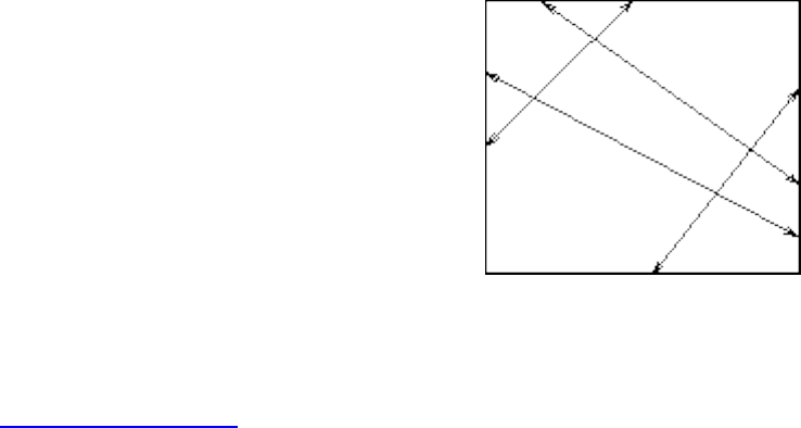
Lecture 4 - heapsort
Heaps as stacks or queues
● In a stack, push inserts a new item and pop removes the most recently pushed item.
● In a queue, enqueue inserts a new item and dequeue removes the least recently enqueued item.
Both stacks and queues can be simulated by using a heap, when we add a new time field to each item and
order the heap according it this time field.
● To simulate the stack, increment the time with each insertion and put the maximum on top of the
heap.
● To simulate the queue, decrement the time with each insertion and put the maximum on top of the
heap (or increment times and keep the minimum on top)
This simulation is not as efficient as a normal stack/queue implementation, but it is a cute demonstration
of the flexibility of a priority queue.
Discrete Event Simulations
In simulations of airports, parking lots, and jai-alai - priority queues can be used to maintain who goes
next.
The stack and queue orders are just special cases of orderings. In real life, certain people cut in line.
Sweepline Algorithms in Computational Geometry
In the priority queue, we will store the points we have not yet encountered, ordered by x coordinate. and
push the line forward one stop at a time.
Listen To Part 4-22
file:///E|/LEC/LECTUR17/NODE4.HTM (13 of 14) [19/1/2003 1:34:31]

Lecture 4 - heapsort
Greedy Algorithms
In greedy algorithms, we always pick the next thing which locally maximizes our score. By placing all
the things in a priority queue and pulling them off in order, we can improve performance over linear
search or sorting, particularly if the weights change.
Example: Sequential strips in triangulations.
Danny Heep
Next: Lecture 5 - quicksort Up: No Title Previous: Lecture 3 - recurrence
Algorithms
Mon Jun 2 09:21:39 EDT 1997
file:///E|/LEC/LECTUR17/NODE4.HTM (14 of 14) [19/1/2003 1:34:31]
Lecture 5 - quicksort
Next: Lecture 6 - linear Up: No Title Previous: Lecture 4 - heapsort
Lecture 5 - quicksort
Listen To Part 5-1
4-2 Find the missing integer from 0 to n using O(n) ``is bit[j] in A[i]'' queries.
Note - there are a total of bits, so we are not allowed to read the entire input!
Also note, the problem is asking us to minimize the number of bits we read. We can spend as much time as we
want doing other things provided we don't look at extra bits.
How can we find the last bit of the missing integer?
Ask all the n integers what their last bit is and see whether 0 or 1 is the bit which occurs less often than it is
supposed to. That is the last bit of the missing integer!
How can we determine the second-to-last bit?
Ask the numbers which ended with the correct last bit! By analyzing the bit patterns of the numbers from 0
to n which end with this bit.
By recurring on the remaining candidate numbers, we get the answer in T(n) = T(n/2) + n =O(n), by the Master
Theorem.
Listen To Part 5-2
Quicksort
Although mergesort is , it is quite inconvenient for implementation with arrays, since we need space to
merge.
In practice, the fastest sorting algorithm is Quicksort, which uses partitioning as its main idea.
Example: Pivot about 10.
17 12 6 19 23 8 5 10 - before
6 8 5 10 23 19 12 17 - after
file:///E|/LEC/LECTUR17/NODE5.HTM (1 of 10) [19/1/2003 1:34:35]

Lecture 5 - quicksort
Partitioning places all the elements less than the pivot in the left part of the array, and all elements greater than the
pivot in the right part of the array. The pivot fits in the slot between them.
Note that the pivot element ends up in the correct place in the total order!
Listen To Part 5-3
Partitioning the elements
Once we have selected a pivot element, we can partition the array in one linear scan, by maintaining three sections
of the array: < pivot, > pivot, and unexplored.
Example: pivot about 10
| 17 12 6 19 23 8 5 | 10
| 5 12 6 19 23 8 | 17
5 | 12 6 19 23 8 | 17
5 | 8 6 19 23 | 12 17
5 8 | 6 19 23 | 12 17
5 8 6 | 19 23 | 12 17
5 8 6 | 23 | 19 12 17
5 8 6 ||23 19 12 17
5 8 6 10 19 12 17 23
As we scan from left to right, we move the left bound to the right when the element is less than the pivot, otherwise
we swap it with the rightmost unexplored element and move the right bound one step closer to the left.
Listen To Part 5-4
Since the partitioning step consists of at most n swaps, takes time linear in the number of keys. But what does it
buy us?
1. The pivot element ends up in the position it retains in the final sorted order.
2. After a partitioning, no element flops to the other side of the pivot in the final sorted order.
file:///E|/LEC/LECTUR17/NODE5.HTM (2 of 10) [19/1/2003 1:34:35]

Lecture 5 - quicksort
Thus we can sort the elements to the left of the pivot and the right of the pivot independently!
This gives us a recursive sorting algorithm, since we can use the partitioning approach to sort each subproblem.
Listen To Part 5-5
Quicksort Animations
Listen To Part 5-6
Pseudocode
Sort(A)
Quicksort(A,1,n)
Quicksort(A, low, high)
if (low < high)
pivot-location = Partition(A,low,high)
Quicksort(A,low, pivot-location - 1)
Quicksort(A, pivot-location+1, high)
Partition(A,low,high)
pivot = A[low]
leftwall = low
file:///E|/LEC/LECTUR17/NODE5.HTM (3 of 10) [19/1/2003 1:34:35]
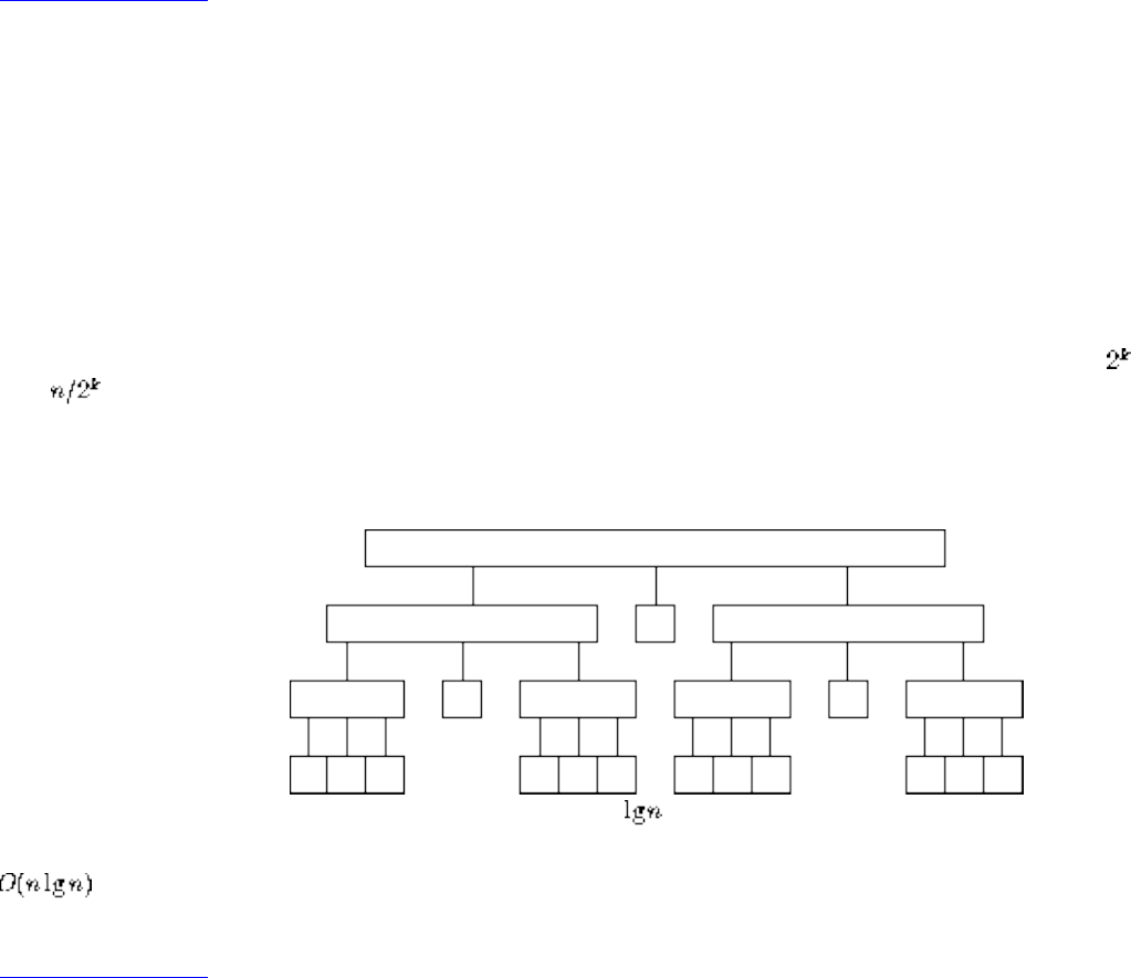
Lecture 5 - quicksort
for i = low+1 to high
if (A[i] < pivot) then
leftwall = leftwall+1
swap(A[i],A[leftwall])
swap(A[low],A[leftwall])
Listen To Part 5-7
Best Case for Quicksort
Since each element ultimately ends up in the correct position, the algorithm correctly sorts. But how long does it
take?
The best case for divide-and-conquer algorithms comes when we split the input as evenly as possible. Thus in the
best case, each subproblem is of size n/2.
The partition step on each subproblem is linear in its size. Thus the total effort in partitioning the problems of
size is O(n).
The recursion tree for the best case looks like this:
The total partitioning on each level is O(n), and it take levels of perfect partitions to get to single element
subproblems. When we are down to single elements, the problems are sorted. Thus the total time in the best case is
.
Listen To Part 5-8
file:///E|/LEC/LECTUR17/NODE5.HTM (4 of 10) [19/1/2003 1:34:35]
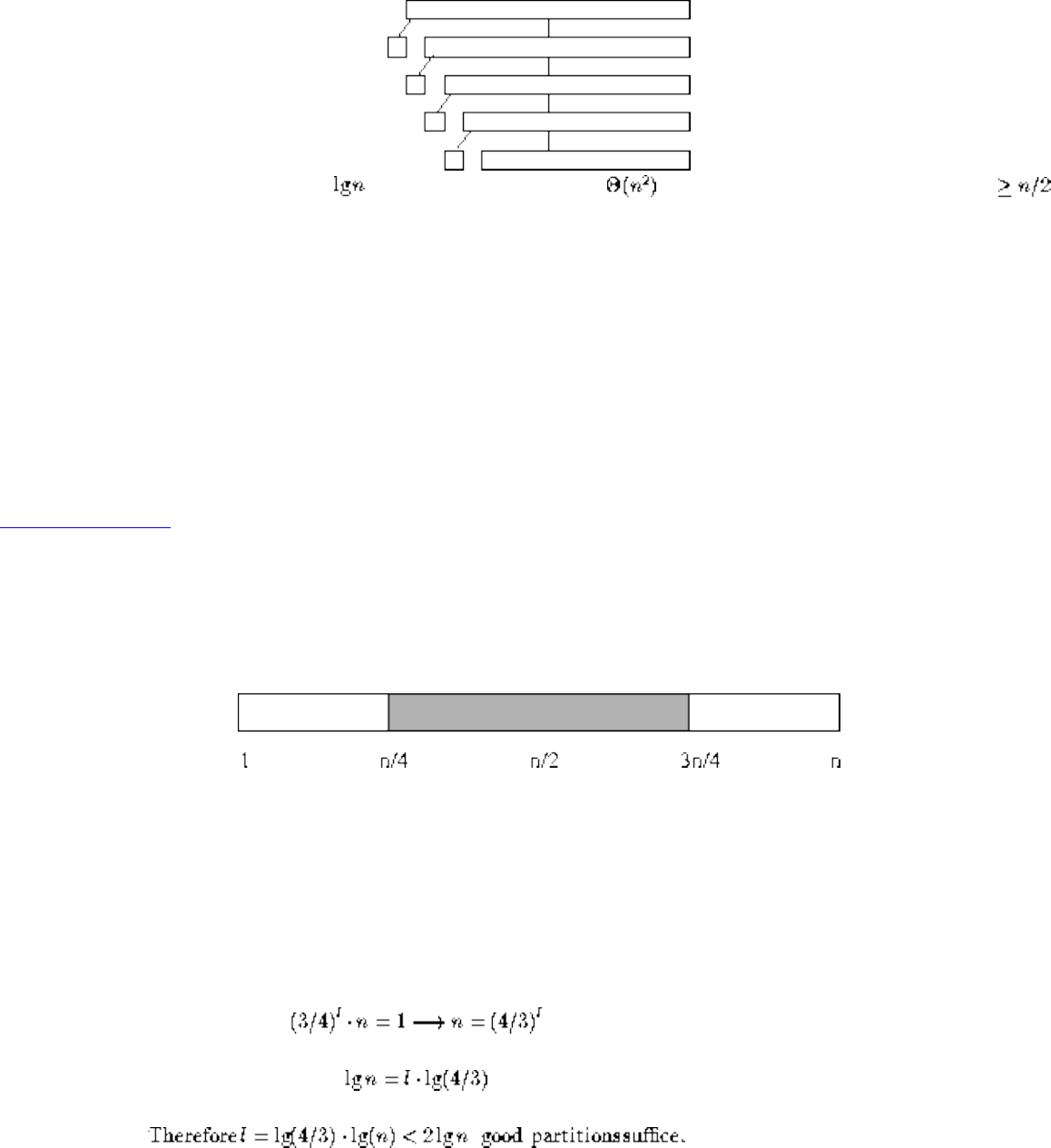
Lecture 5 - quicksort
Worst Case for Quicksort
Suppose instead our pivot element splits the array as unequally as possible. Thus instead of n/2 elements in the
smaller half, we get zero, meaning that the pivot element is the biggest or smallest element in the array.
Now we have n-1 levels, instead of , for a worst case time of , since the first n/2 levels each have
elements to partition.
Thus the worst case time for Quicksort is worse than Heapsort or Mergesort.
To justify its name, Quicksort had better be good in the average case. Showing this requires some fairly intricate
analysis.
The divide and conquer principle applies to real life. If you will break a job into pieces, it is best to make the pieces
of equal size!
Listen To Part 5-9
Intuition: The Average Case for Quicksort
Suppose we pick the pivot element at random in an array of n keys.
Half the time, the pivot element will be from the center half of the sorted array.
Whenever the pivot element is from positions n/4 to 3n/4, the larger remaining subarray contains at most 3n/4
elements.
If we assume that the pivot element is always in this range, what is the maximum number of partitions we need to
get from n elements down to 1 element?
file:///E|/LEC/LECTUR17/NODE5.HTM (5 of 10) [19/1/2003 1:34:35]
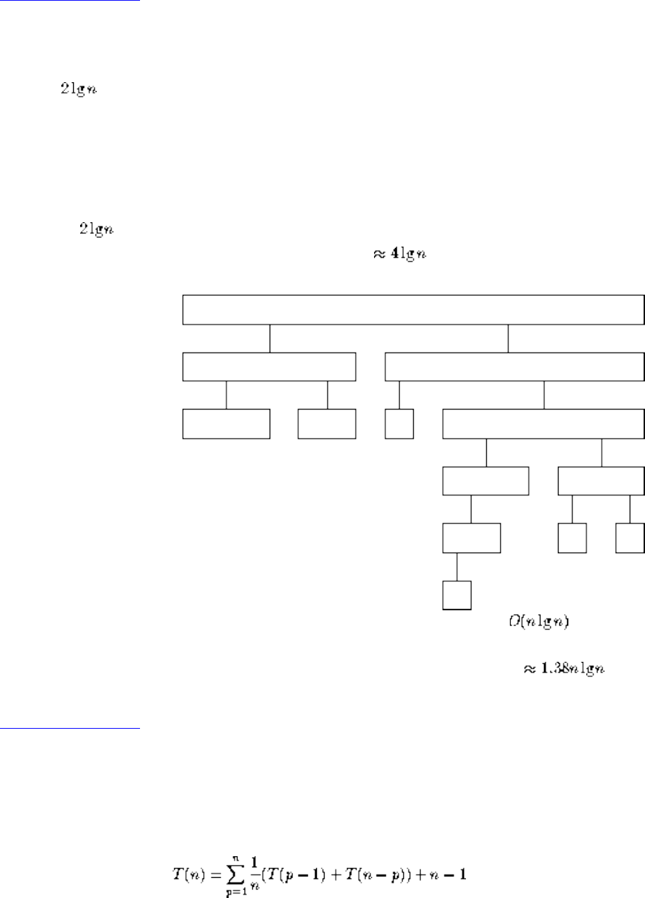
Lecture 5 - quicksort
Listen To Part 5-10
What have we shown?
At most levels of decent partitions suffices to sort an array of n elements.
But how often when we pick an arbitrary element as pivot will it generate a decent partition?
Since any number ranked between n/4 and 3n/4 would make a decent pivot, we get one half the time on average.
If we need levels of decent partitions to finish the job, and half of random partitions are decent, then on
average the recursion tree to quicksort the array has levels.
Since O(n) work is done partitioning on each level, the average time is .
More careful analysis shows that the expected number of comparisons is .
Listen To Part 5-11
Average-Case Analysis of Quicksort
To do a precise average-case analysis of quicksort, we formulate a recurrence given the exact expected time T(n):
Each possible pivot p is selected with equal probability. The number of comparisons needed to do the partition is n-
1.
file:///E|/LEC/LECTUR17/NODE5.HTM (6 of 10) [19/1/2003 1:34:35]
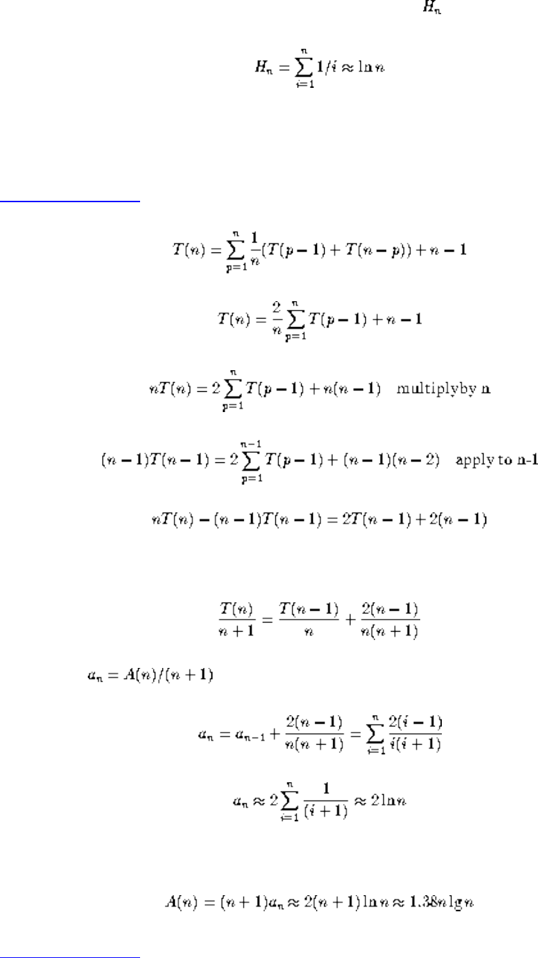
Lecture 5 - quicksort
We will need one useful fact about the Harmonic numbers , namely
It is important to understand (1) where the recurrence relation comes from and (2) how the log comes out from the
summation. The rest is just messy algebra.
Listen To Part 5-12
rearranging the terms give us:
substituting gives
We are really interested in A(n), so
Listen To Part 5-13
What is the Worst Case?
file:///E|/LEC/LECTUR17/NODE5.HTM (7 of 10) [19/1/2003 1:34:35]
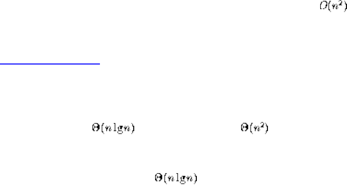
Lecture 5 - quicksort
The worst case for Quicksort depends upon how we select our partition or pivot element. If we always select either
the first or last element of the subarray, the worst-case occurs when the input is already sorted!
A B D F H J K
B D F H J K
D F H J K
F H J K
H J K
J K
K
Having the worst case occur when they are sorted or almost sorted is very bad, since that is likely to be the case in
certain applications.
To eliminate this problem, pick a better pivot:
1. Use the middle element of the subarray as pivot.
2. Use a random element of the array as the pivot.
3. Perhaps best of all, take the median of three elements (first, last, middle) as the pivot. Why should we use
median instead of the mean?
Whichever of these three rules we use, the worst case remains . However, because the worst case is no longer
a natural order it is much more difficult to occur.
Listen To Part 5-14
Is Quicksort really faster than Heapsort?
Since Heapsort is and selection sort is , there is no debate about which will be better for decent-sized
files.
But how can we compare two algorithms to see which is faster? Using the RAM model and the big Oh
notation, we can't!
When Quicksort is implemented well, it is typically 2-3 times faster than mergesort or heapsort. The primary
reason is that the operations in the innermost loop are simpler. The best way to see this is to implement both and
experiment with different inputs.
file:///E|/LEC/LECTUR17/NODE5.HTM (8 of 10) [19/1/2003 1:34:35]
Lecture 5 - quicksort
Since the difference between the two programs will be limited to a multiplicative constant factor, the details of
how you program each algorithm will make a big difference.
If you don't want to believe me when I say Quicksort is faster, I won't argue with you. It is a question whose
solution lies outside the tools we are using.
Listen To Part 5-15
Randomization
Suppose you are writing a sorting program, to run on data given to you by your worst enemy. Quicksort is good on
average, but bad on certain worst-case instances.
If you used Quicksort, what kind of data would your enemy give you to run it on? Exactly the worst-case instance,
to make you look bad.
But instead of picking the median of three or the first element as pivot, suppose you picked the pivot element at
random.
Now your enemy cannot design a worst-case instance to give to you, because no matter which data they give you,
you would have the same probability of picking a good pivot!
Randomization is a very important and useful idea. By either picking a random pivot or scrambling the
permutation before sorting it, we can say:
``With high probability, randomized quicksort runs in time.''
Where before, all we could say is:
``If you give me random input data, quicksort runs in expected time.''
Since the time bound how does not depend upon your input distribution, this means that unless we are extremely
unlucky (as opposed to ill prepared or unpopular) we will certainly get good performance.
Randomization is a general tool to improve algorithms with bad worst-case but good average-case complexity.
The worst-case is still there, but we almost certainly won't see it.
Next: Lecture 6 - linear Up: No Title Previous: Lecture 4 - heapsort
Algorithms
file:///E|/LEC/LECTUR17/NODE5.HTM (9 of 10) [19/1/2003 1:34:35]
Lecture 5 - quicksort
Mon Jun 2 09:21:39 EDT 1997
file:///E|/LEC/LECTUR17/NODE5.HTM (10 of 10) [19/1/2003 1:34:35]
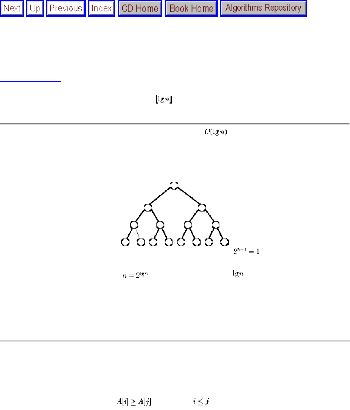
Lecture 6 - linear sorting
Next: Lecture 7 - elementary Up: No Title Previous: Lecture 5 - quicksort
Lecture 6 - linear sorting
Listen To Part 6-1
7.1-2: Show that an n-element heap has height .
Since it is balanced binary tree, the height of a heap is clearly , but the problem asks for an exact
answer.
The height is defined as the number of edges in the longest simple path from the root.
The number of nodes in a complete balanced binary tree of height h is .
Thus the height increases only when , or in other words when is an integer.
Listen To Part 6-2
7.1-5 Is a reverse sorted array a heap?
In a heap, each element is greater than or equal to each of its descendants.
In the array representation of a heap, the descendants of the ith element are the 2ith and (2i+1)th
elements.
If A is sorted in reverse order, then implies that .
file:///E|/LEC/LECTUR17/NODE6.HTM (1 of 7) [19/1/2003 1:34:38]
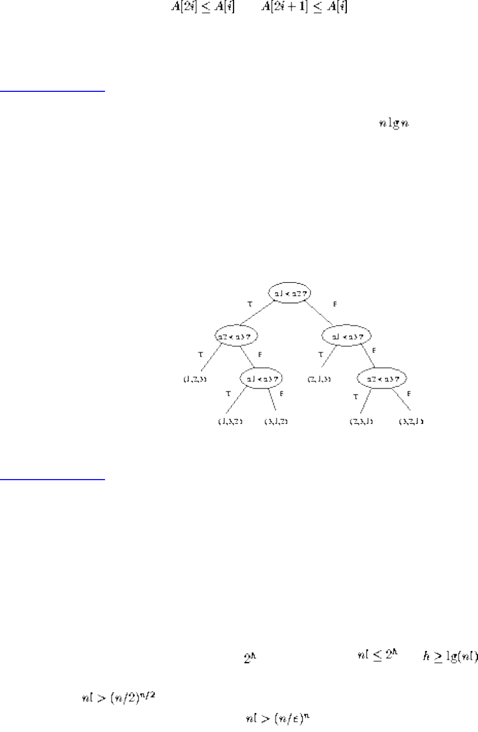
Lecture 6 - linear sorting
Since 2i > i and 2i+1 > i then and .
Thus by definition A is a heap!
Listen To Part 6-3
Can we sort in better than ?
Any comparison-based sorting program can be thought of as defining a decision tree of possible
executions.
Running the same program twice on the same permutation causes it to do exactly the same thing, but
running it on different permutations of the same data causes a different sequence of comparisons to be
made on each.
Claim: the height of this decision tree is the worst-case complexity of sorting.
Listen To Part 6-4
Once you believe this, a lower bound on the time complexity of sorting follows easily.
Since any two different permutations of n elements requires a different sequence of steps to sort, there
must be at least n! different paths from the root to leaves in the decision tree, ie. at least n! different
leaves in the tree.
Since only binary comparisons (less than or greater than) are used, the decision tree is a binary tree.
Since a binary tree of height h has at most leaves, we know , or .
By inspection , since the last n/2 terms of the product are each greater than n/2. By
Sterling's approximation, a better bound is where e=2.718.
file:///E|/LEC/LECTUR17/NODE6.HTM (2 of 7) [19/1/2003 1:34:38]
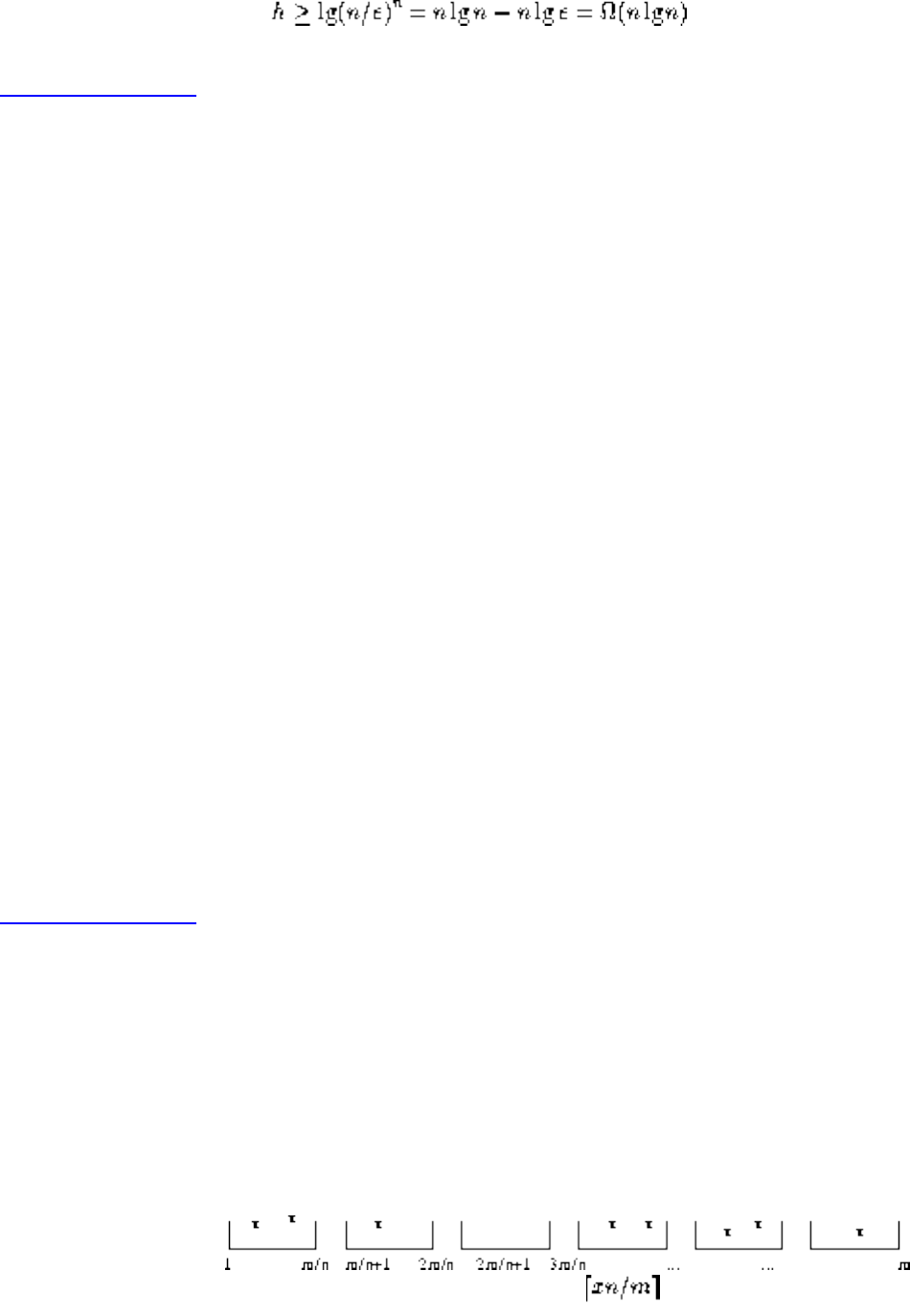
Lecture 6 - linear sorting
Listen To Part 6-5
Non-Comparison-Based Sorting
All the sorting algorithms we have seen assume binary comparisons as the basic primative, questions of
the form ``is x before y?''.
Suppose you were given a deck of playing cards to sort. Most likely you would set up 13 piles and put all
cards with the same number in one pile.
A 2 3 4 5 6 7 8 9 10 J Q K
A 2 3 4 5 6 7 8 9 10 J Q K
A 2 3 4 5 6 7 8 9 10 J Q K
A 2 3 4 5 6 7 8 9 10 J Q K
With only a constant number of cards left in each pile, you can use insertion sort to order by suite and
concatenate everything together.
If we could find the correct pile for each card in constant time, and each pile gets O(1) cards, this
algorithm takes O(n) time.
Listen To Part 6-6
Bucketsort
Suppose we are sorting n numbers from 1 to m, where we know the numbers are approximately
uniformly distributed.
We can set up n buckets, each responsible for an interval of m/n numbers from 1 to m
Given an input number x, it belongs in bucket number .
If we use an array of buckets, each item gets mapped to the right bucket in O(1) time.
file:///E|/LEC/LECTUR17/NODE6.HTM (3 of 7) [19/1/2003 1:34:38]
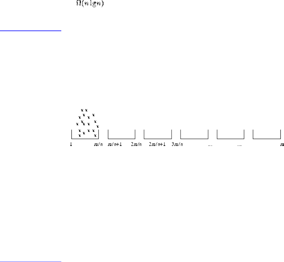
Lecture 6 - linear sorting
With uniformly distributed keys, the expected number of items per bucket is 1. Thus sorting each bucket
takes O(1) time!
The total effort of bucketing, sorting buckets, and concatenating the sorted buckets together is O(n).
What happened to our lower bound!
Listen To Part 6-7
We can use bucketsort effectively whenever we understand the distribution of the data.
However, bad things happen when we assume the wrong distribution.
Suppose in the previous example all the keys happened to be 1. After the bucketing phase, we have:
We spent linear time distributing our items into buckets and learned nothing. Perhaps we could split the
big bucket recursively, but it is not certain that we will ever win unless we understand the distribution.
Problems like this are why we worry about the worst-case performance of algorithms!
Such distribution techniques can be used on strings instead of just numbers. The buckets will correspond
to letter ranges instead of just number ranges.
The worst case ``shouldn't'' happen if we understand the distribution of our data.
Listen To Part 6-8
Real World Distributions
Consider the distribution of names in a telephone book.
● Will there be a lot of Skiena's?
● Will there be a lot of Smith's?
● Will there be a lot of Shifflett's?
Either make sure you understand your data, or use a good worst-case or randomized algorithm!
file:///E|/LEC/LECTUR17/NODE6.HTM (4 of 7) [19/1/2003 1:34:38]
Lecture 6 - linear sorting
The Shifflett's of Charlottesville
For comparison, note that there are seven Shifflett's (of various spellings) in the 1000 page Manhattan
telephone directory.
Listen To Part 6-10
Rules for Algorithm Design
The secret to successful algorithm design, and problem solving in general, is to make sure you ask the
right questions. Below, I give a possible series of questions for you to ask yourself as you try to solve
difficult algorithm design problems:
1. Do I really understand the problem?
1. What exactly does the input consist of?
2. What exactly are the desired results or output?
3. Can I construct some examples small enough to solve by hand? What happens when I
solve them?
4. Are you trying to solve a numerical problem? A graph algorithm problem? A geometric
problem? A string problem? A set problem? Might your problem be formulated in more
than one way? Which formulation seems easiest?
2. Can I find a simple algorithm for the problem?
1. Can I find the solve my problem exactly by searching all subsets or arrangements and
picking the best one?
1. If so, why am I sure that this algorithm always gives the correct answer?
2. How do I measure the quality of a solution once I construct it?
file:///E|/LEC/LECTUR17/NODE6.HTM (5 of 7) [19/1/2003 1:34:38]

Lecture 6 - linear sorting
Listen To Part 6-11
3. Does this simple, slow solution run in polynomial or exponential time?
4. If I can't find a slow, guaranteed correct algorithm, am I sure that my problem is
well defined enough to permit a solution?
2. Can I solve my problem by repeatedly trying some heuristic rule, like picking the biggest
item first? The smallest item first? A random item first?
1. If so, on what types of inputs does this heuristic rule work well? Do these
correspond to the types of inputs that might arise in the application?
2. On what types of inputs does this heuristic rule work badly? If no such examples
can be found, can I show that in fact it always works well?
3. How fast does my heuristic rule come up with an answer?
3. Are there special cases of this problem I know how to solve exactly?
1. Can I solve it efficiently when I ignore some of the input parameters?
2. What happens when I set some of the input parameters to trivial values, such as 0 or 1?
Listen To Part 6-12
3. Can I simplify the problem to create a problem I can solve efficiently? How simple do I
have to make it?
4. If I can solve a certain special case, why can't this be generalized to a wider class of
inputs?
4. Which of the standard algorithm design paradigms seem most relevant to the problem?
1. Is there a set of items which can be sorted by size or some key? Does this sorted order
make it easier to find what might be the answer?
2. Is there a way to split the problem in two smaller problems, perhaps by doing a binary
search, or a partition of the elements into big and small, or left and right? If so, does this
suggest a divide-and-conquer algorithm?
3. Are there certain operations being repeatedly done on the same data, such as searching it
for some element, or finding the largest/smallest remaining element? If so, can I use a data
structure of speed up these queries, like hash tables or a heap/priority queue?
5. Am I still stumped?
1. Why don't I go back to the beginning of the list and work through the questions again? Do
any of my answers from the first trip change on the second?
file:///E|/LEC/LECTUR17/NODE6.HTM (6 of 7) [19/1/2003 1:34:38]

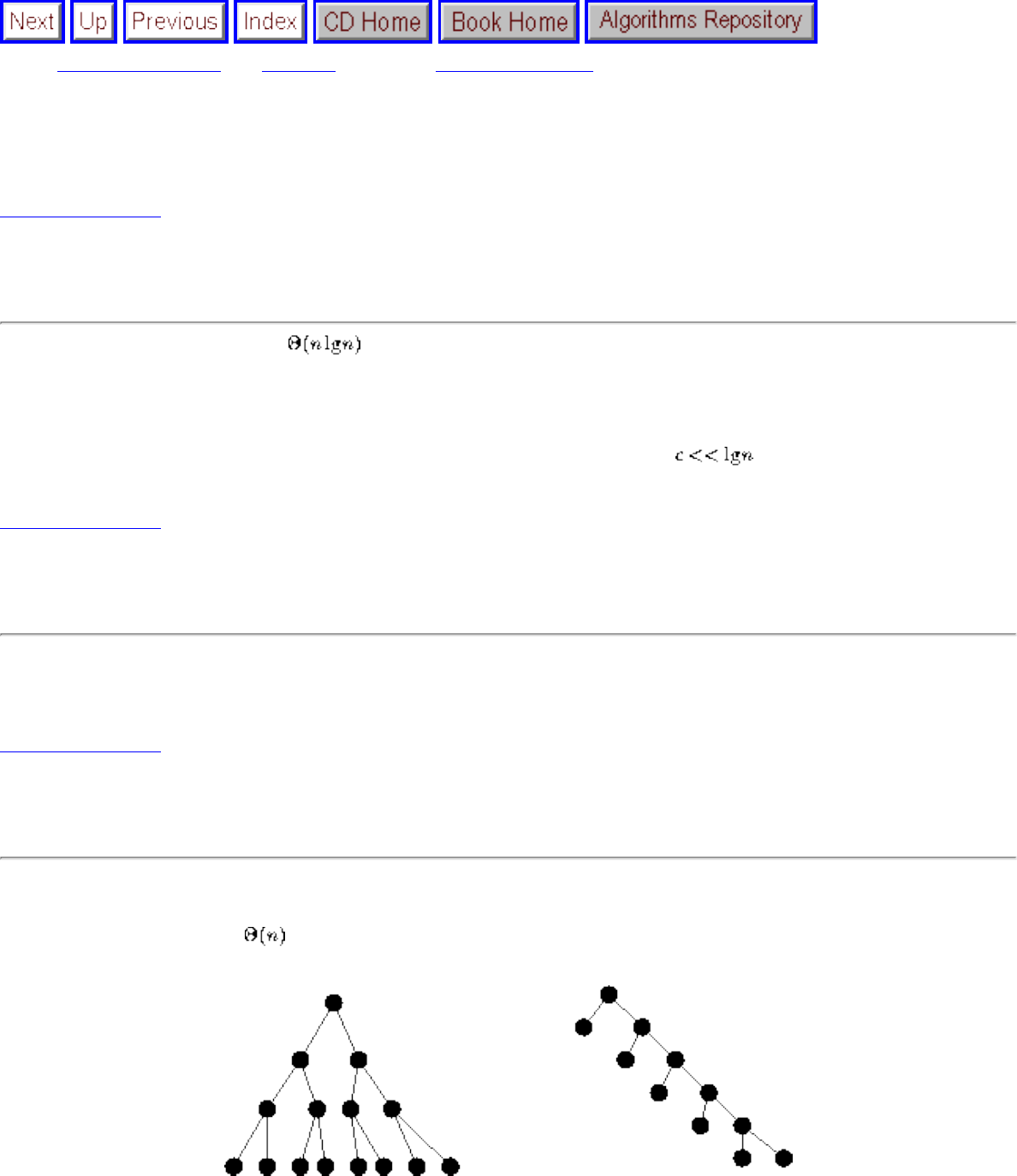
Lecture 7 - elementary data structures
Next: Lecture 8 - binary Up: No Title Previous: Lecture 6 - linear
Lecture 7 - elementary data structures
Listen To Part 7-1
8.2-3 Argue that insertion sort is better than Quicksort for sorting checks
In the best case, Quicksort takes . Although using median-of-three turns the sorted permutation into the
best case, we lose if insertion sort is better on the given data.
In insertion sort, the cost of each insertion is the number of items which we have to jump over. In the check
example, the expected number of moves per items is small, say c. We win if .
Listen To Part 7-2
8.3-1 Why do we analyze the average-case performance of a randomized algorithm, instead of the worst-case?
In a randomized algorithm, the worst case is not a matter of the input but only of luck. Thus we want to know what
kind of luck to expect. Every input we see is drawn from the uniform distribution.
Listen To Part 7-3
8.3-2 How many calls are made to Random in randomized quicksort in the best and worst cases?
Each call to random occurs once in each call to partition.
The number of partitions is in any run of quicksort!!
There is some potential variation depending upon what you do with intervals of size 1 - do you call partition on
intervals of size one? However, there is no asymptotic difference between best and worst case.
file:///E|/LEC/LECTUR17/NODE7.HTM (1 of 13) [19/1/2003 1:34:41]

Lecture 7 - elementary data structures
The reason - any binary tree with n leaves has n-1 internal nodes, each of which corresponds to a call to partition in
the quicksort recursion tree.
Listen To Part 7-4
Elementary Data Structures
``Mankind's progress is measured by the number of things we can do without thinking.''
Elementary data structures such as stacks, queues, lists, and heaps will be the ``of-the-shelf'' components we build
our algorithm from. There are two aspects to any data structure:
● The abstract operations which it supports.
● The implementation of these operations.
The fact that we can describe the behavior of our data structures in terms of abstract operations explains why we
can use them without thinking, while the fact that we have different implementation of the same abstract
operations enables us to optimize performance.
Listen To Part 7-5
Stacks and Queues
Sometimes, the order in which we retrieve data is independent of its content, being only a function of when it
arrived.
A stack supports last-in, first-out operations: push and pop.
A queue supports first-in, first-out operations: enqueue and dequeue.
A deque is a double ended queue and supports all four operations: push, pop, enqueue, dequeue.
Lines in banks are based on queues, while food in my refrigerator is treated as a stack.
Both can be used to traverse a tree, but the order is completely different.
file:///E|/LEC/LECTUR17/NODE7.HTM (2 of 13) [19/1/2003 1:34:41]
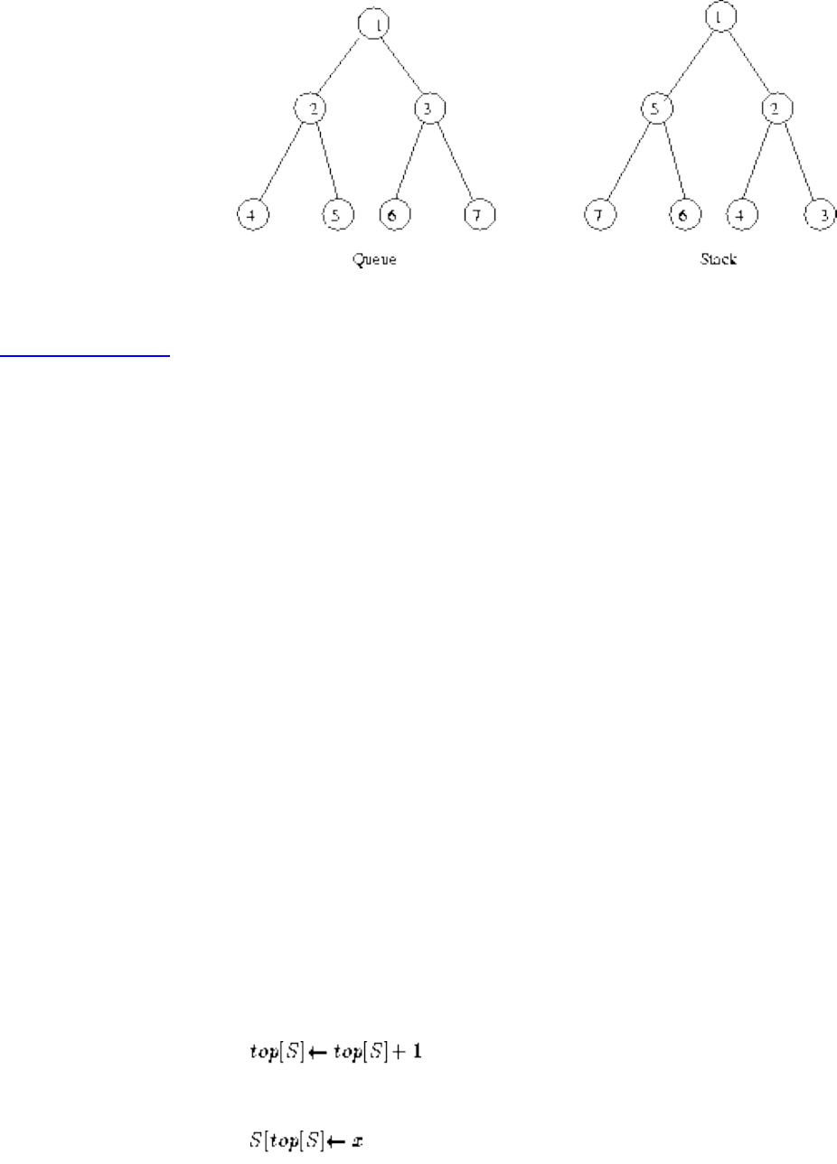
Lecture 7 - elementary data structures
Which order is better for WWW crawler robots?
Listen To Part 7-6
Stack Implementation
Although this implementation uses an array, a linked list would eliminate the need to declare the array size in
advance.
STACK-EMPTY(S)
if top[S] = 0
then return TRUE
else return FALSE
PUSH(S, x)
POP(S)
file:///E|/LEC/LECTUR17/NODE7.HTM (3 of 13) [19/1/2003 1:34:41]
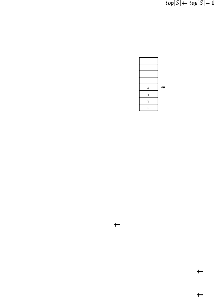
Lecture 7 - elementary data structures
if STACK-EMPTY(S)
then error ``underflow''
else
return S[top[S] + 1]
All are O(1) time operations.
Listen To Part 7-7
Queue Implementation
A circular queue implementation requires pointers to the head and tail elements, and wraps around to reuse array
elements.
ENQUEUE(Q, x)
Q[tail[Q]] x
if tail[Q] = length[Q]
then tail[Q] 1
else tail[Q] tail[Q] + 1
file:///E|/LEC/LECTUR17/NODE7.HTM (4 of 13) [19/1/2003 1:34:41]
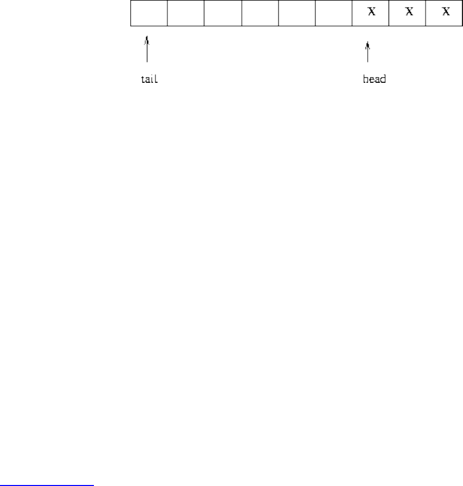
Lecture 7 - elementary data structures
DEQUEUE(Q)
x = Q[head[Q]]
if head[Q] = length[Q]
then head[Q] = 1
else head[Q] = head[Q] + 1
return x
A list-based implementation would eliminate the possibility of overflow.
All are O(1) time operations.
Listen To Part 7-8
Dynamic Set Operations
Perhaps the most important class of data structures maintain a set of items, indexed by keys.
There are a variety of implementations of these dictionary operations, each of which yield different time bounds
for various operations.
● Search(S,k) - A query that, given a set S and a key value k, returns a pointer x to an element in S such that
key[x] = k, or nil if no such element belongs to S.
● Insert(S,x) - A modifying operation that augments the set S with the element x.
● Delete(S,x) - Given a pointer x to an element in the set S, remove x from S. Observe we are given a pointer
to an element x, not a key value.
● Min(S), Max(S) - Returns the element of the totally ordered set S which has the smallest (largest) key.
file:///E|/LEC/LECTUR17/NODE7.HTM (5 of 13) [19/1/2003 1:34:41]
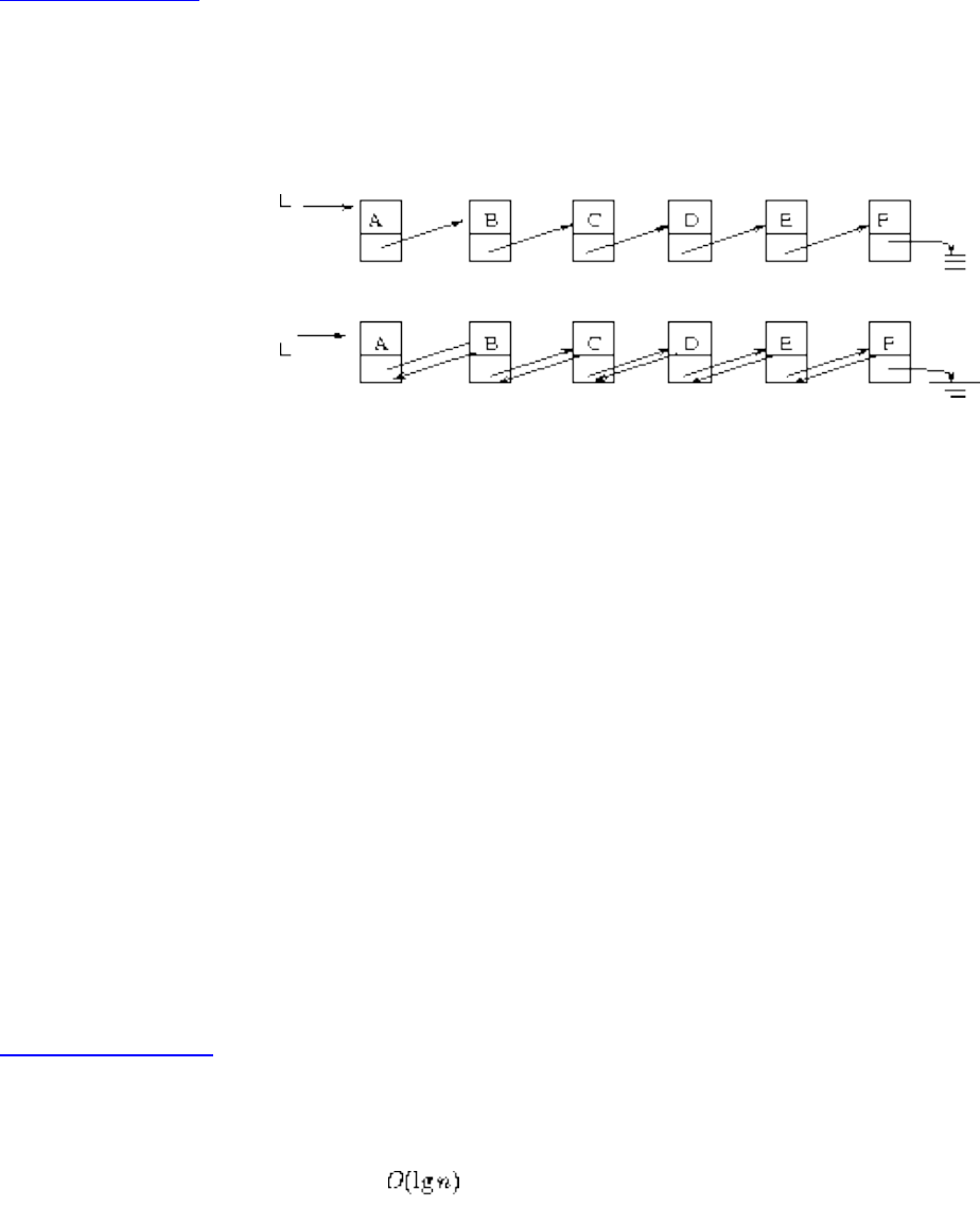
Lecture 7 - elementary data structures
● Next(S,x), Previous(S,x) - Given an element x whose key is from a totally ordered set S, returns the next
largest (smallest) element in S, or NIL if x is the maximum (minimum) element.
Listen To Part 7-9
Pointer Based Implementation
We can maintain a dictionary in either a singly or doubly linked list.
We gain extra flexibility on predecessor queries at a cost of doubling the number of pointers by using doubly-
linked lists.
Since the extra big-Oh costs of doubly-linkly lists is zero, we will usually assume they are, although it might not be
necessary.
Singly linked to doubly-linked list is as a Conga line is to a Can-Can line.
Array Based Sets
Unsorted Arrays
● Search(S,k) - sequential search, O(n)
● Insert(S,x) - place in first empty spot, O(1)
● Delete(S,x) - copy nth item to the xth spot, O(1)
● Min(S,x), Max(S,x) - sequential search, O(n)
● Successor(S,x), Predecessor(S,x) - sequential search, O(n)
Listen To Part 7-10
Sorted Arrays
● Search(S,k) - binary search,
● Insert(S,x) - search, then move to make space, O(n)
● Delete(S,x) - move to fill up the hole, O(n)
● Min(S,x), Max(S,x) - first or last element, O(1)
● Successor(S,x), Predecessor(S,x) - Add or subtract 1 from pointer, O(1)
What are the costs for a heap?
file:///E|/LEC/LECTUR17/NODE7.HTM (6 of 13) [19/1/2003 1:34:42]
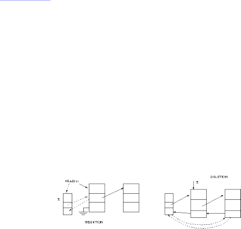
Lecture 7 - elementary data structures
Listen To Part 7-11
Unsorted List Implementation
LIST-SEARCH(L, k)
x = head[L]
while x <> NIL and key[x] <> k
do x = next[x]
return x
Note: the while loop might require two lines in some programming languages.
LIST-INSERT(L, x)
next[x] = head[L]
if head[L] <> NIL
then prev[head[L]] = x
head[L] = x
file:///E|/LEC/LECTUR17/NODE7.HTM (7 of 13) [19/1/2003 1:34:42]
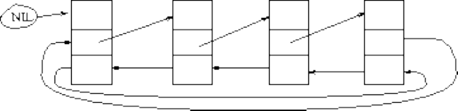
Lecture 7 - elementary data structures
prev[x] = NIL
LIST-DELETE(L, x)
if prev[x] <> NIL
then next[prev[x]] = next[x]
else head[L] = next[x]
if next[x] <> NIL
then prev[next[x]] = prev[x]
Sentinels
Boundary conditions can be eliminated using a sentinel element which doesn't go away.
LIST-SEARCH'(L, k)
x = next[nil[L]]
while x <> NIL[L] and key[x] <> k
do x = next[x]
file:///E|/LEC/LECTUR17/NODE7.HTM (8 of 13) [19/1/2003 1:34:42]

Lecture 7 - elementary data structures
return x
LIST-INSERT'(L, x)
next[x] = next[nil[L]]
prev[next[nil[L]]] = x
next[nil[L]] = x
prev[x] = NIL[L]
LIST-DELETE'(L, x)
next[prev[x]] <> next[x]
next[prev[x]] = prev[x]
Listen To Part 7-13
Hash Tables
Hash tables are a very practical way to maintain a dictionary. As with bucket sort, it assumes we know that the
distribution of keys is fairly well-behaved.
The idea is simply that looking an item up in an array is once you have its index. A hash function is a
mathematical function which maps keys to integers.
In bucket sort, our hash function mapped the key to a bucket based on the first letters of the key. ``Collisions'' were
the set of keys mapped to the same bucket.
file:///E|/LEC/LECTUR17/NODE7.HTM (9 of 13) [19/1/2003 1:34:42]
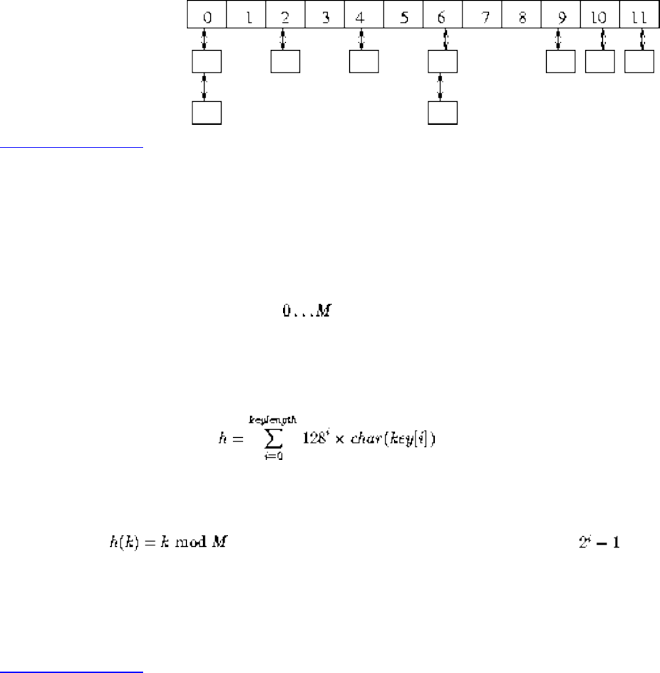
Lecture 7 - elementary data structures
If the keys were uniformly distributed, then each bucket contains very few keys!
The resulting short lists were easily sorted, and could just as easily be searched!
Listen To Part 7-14
Hash Functions
It is the job of the hash function to map keys to integers. A good hash function:
1. Is cheap to evaluate
2. Tends to use all positions from with uniform frequency.
3. Tends to put similar keys in different parts of the tables (Remember the Shifletts!!)
The first step is usually to map the key to a big integer, for example
This large number must be reduced to an integer whose size is between 1 and the size of our hash table.
One way is by , where M is best a large prime not too close to , which would just mask off
the high bits.
This works on the same principle as a roulette wheel!
Listen To Part 7-15
Good and Bad Hash functions
The first three digits of the Social Security Number
file:///E|/LEC/LECTUR17/NODE7.HTM (10 of 13) [19/1/2003 1:34:42]
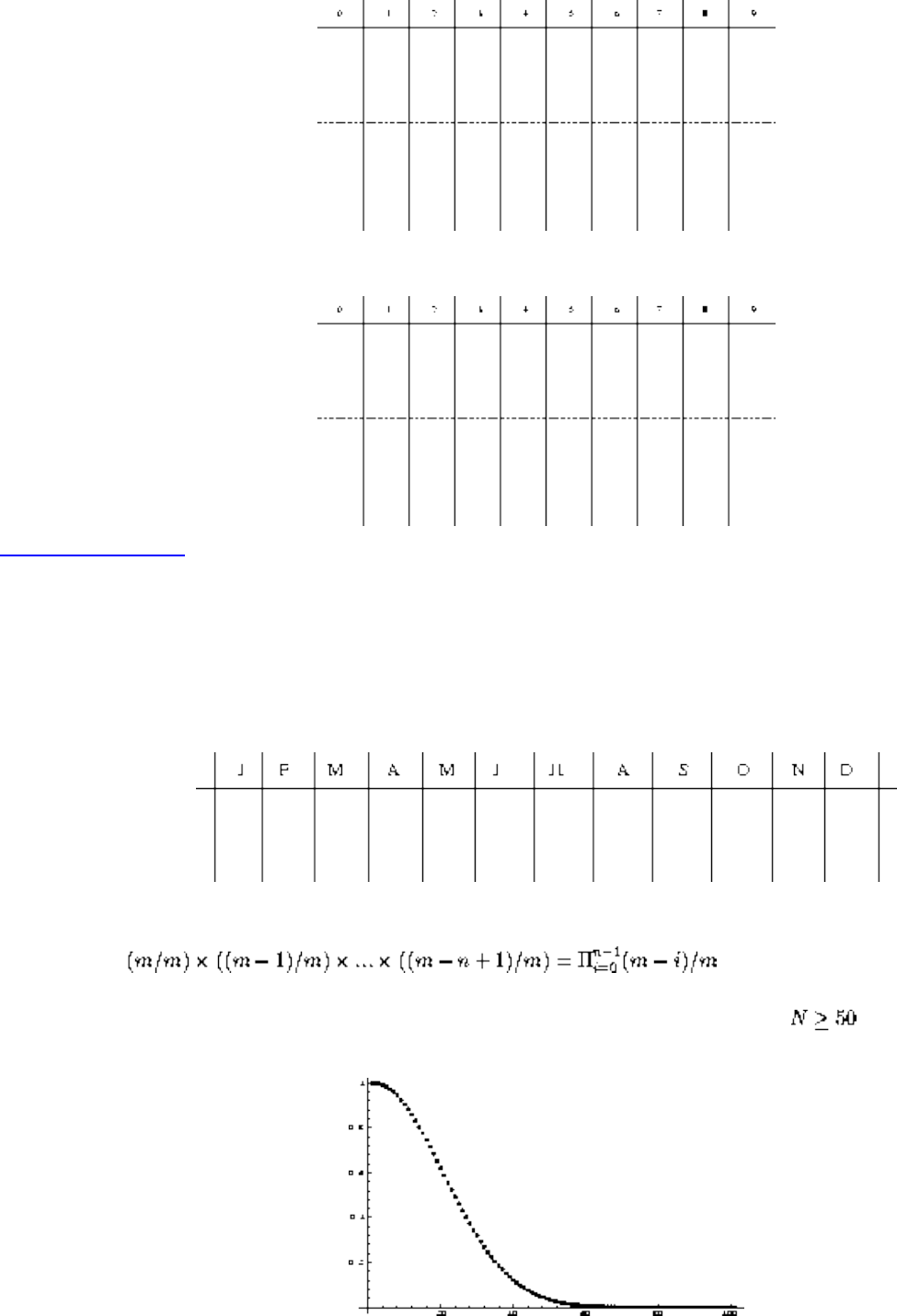
Lecture 7 - elementary data structures
The last three digits of the Social Security Number
Listen To Part 7-16
The Birthday Paradox
No matter how good our hash function is, we had better be prepared for collisions, because of the birthday
paradox.
The probability of there being no collisions after n insertions into an m-element table is
When m = 366, this probability sinks below 1/2 when N = 23 and to almost 0 when .
file:///E|/LEC/LECTUR17/NODE7.HTM (11 of 13) [19/1/2003 1:34:42]
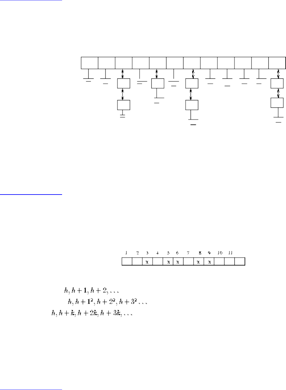
Lecture 7 - elementary data structures
Listen To Part 7-17
Collision Resolution by Chaining
The easiest approach is to let each element in the hash table be a pointer to a list of keys.
Insertion, deletion, and query reduce to the problem in linked lists. If the n keys are distributed uniformly in a table
of size m/n, each operation takes O(m/n) time.
Chaining is easy, but devotes a considerable amount of memory to pointers, which could be used to make the table
larger. Still, it is my preferred method.
Listen To Part 7-18
Open Addressing
We can dispense with all these pointers by using an implicit reference derived from a simple function:
If the space we want to use is filled, we can examine the remaining locations:
1. Sequentially
2. Quadratically
3. Linearly
The reason for using a more complicated science is to avoid long runs from similarly hashed keys.
Deletion in an open addressing scheme is ugly, since removing one element can break a chain of insertions,
making some elements inaccessible.
Listen To Part 7-19
Performance on Set Operations
With either chaining or open addressing:
file:///E|/LEC/LECTUR17/NODE7.HTM (12 of 13) [19/1/2003 1:34:42]
Lecture 7 - elementary data structures
● Search - O(1) expected, O(n) worst case
● Insert - O(1) expected, O(n) worst case
● Delete - O(1) expected, O(n) worst case
● Min, Max and Predecessor, Successor expected and worst case
Pragmatically, a hash table is often the best data structure to maintain a dictionary. However, we will not use it
much in proving the efficiency of our algorithms, since the worst-case time is unpredictable.
The best worst-case bounds come from balanced binary trees, such as red-black trees.
Next: Lecture 8 - binary Up: No Title Previous: Lecture 6 - linear
Algorithms
Mon Jun 2 09:21:39 EDT 1997
file:///E|/LEC/LECTUR17/NODE7.HTM (13 of 13) [19/1/2003 1:34:42]
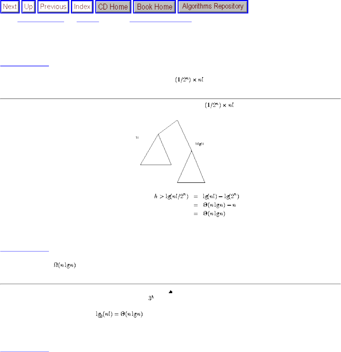
Lecture 8 - binary trees
Next: Lecture 9 - catch Up: No Title Previous: Lecture 7 - elementary
Lecture 8 - binary trees
Listen To Part 8-1
9.1-3 Show that there is no sorting algorithm which sorts at least instances in O(n) time.
Think of the decision tree which can do this. What is the shortest tree with leaves?
Moral: there cannot be too many good cases for any sorting algorithm!
Listen To Part 8-2
9.1-4 Show that the lower bound for sorting still holds with ternary comparisons.
The maximum number of leaves in a tree of height h is ,
So it goes for any constant base.
Listen To Part 8-3
Binary Search Trees
``I think that I shall never see
a poem as lovely as a tree Poem's
are wrote by fools like me but only
G-d can make a tree ``
file:///E|/LEC/LECTUR17/NODE8.HTM (1 of 13) [19/1/2003 1:34:46]
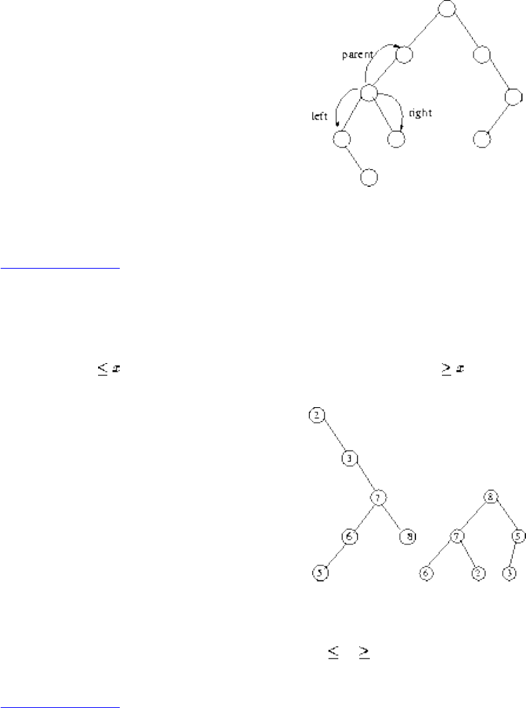
Lecture 8 - binary trees
- Joyce Kilmer
Binary search trees provide a data structure which efficiently supports all six dictionary operations.
A binary tree is a rooted tree where each node contains at most two children.
Each child can be identified as either a left or right child.
A binary tree can be implemented where each node has left and right pointer fields, an (optional) parent pointer, and a data
field.
Listen To Part 8-4
Binary Search Trees
A binary search tree labels each node in a binary tree with a single key such that for any node x, and nodes in the left subtree
of x have keys and all nodes in the right subtree of x have key's .
Left: A binary search tree. Right: A heap but not a binary search tree.
The search tree labeling enables us to find where any key is. Start at the root - if that is not the one we want, search either left
or right depending upon whether what we want is or then the root.
Listen To Part 8-5
Searching in a Binary Tree
Dictionary search operations are easy in binary trees ...
TREE-SEARCH(x, k)
file:///E|/LEC/LECTUR17/NODE8.HTM (2 of 13) [19/1/2003 1:34:46]
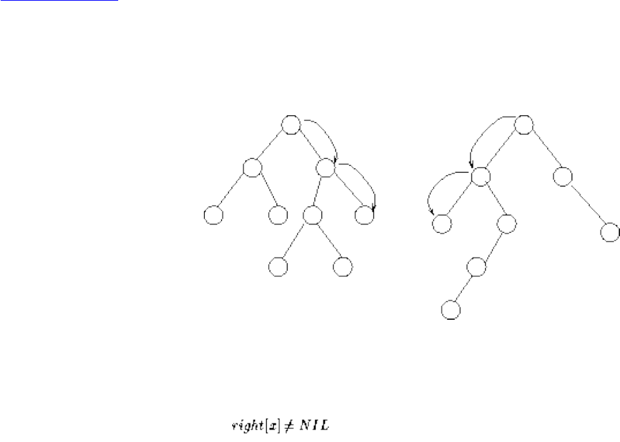
Lecture 8 - binary trees
if (x = NIL) and (k = key[x])
then return x
if (k < key[x])
then return TREE-SEARCH(left[x],k)
else return TREE-SEARCH(right[x],k)
The algorithm works because both the left and right subtrees of a binary search tree are binary search trees - recursive
structure, recursive algorithm.
This takes time proportional to the height of the tree, O(h).
Listen To Part 8-6
Maximum and Minimum
Where are the maximum and minimum elements in a binary tree?
TREE-MAXIMUM(X)
while
do x = right[x]
file:///E|/LEC/LECTUR17/NODE8.HTM (3 of 13) [19/1/2003 1:34:46]
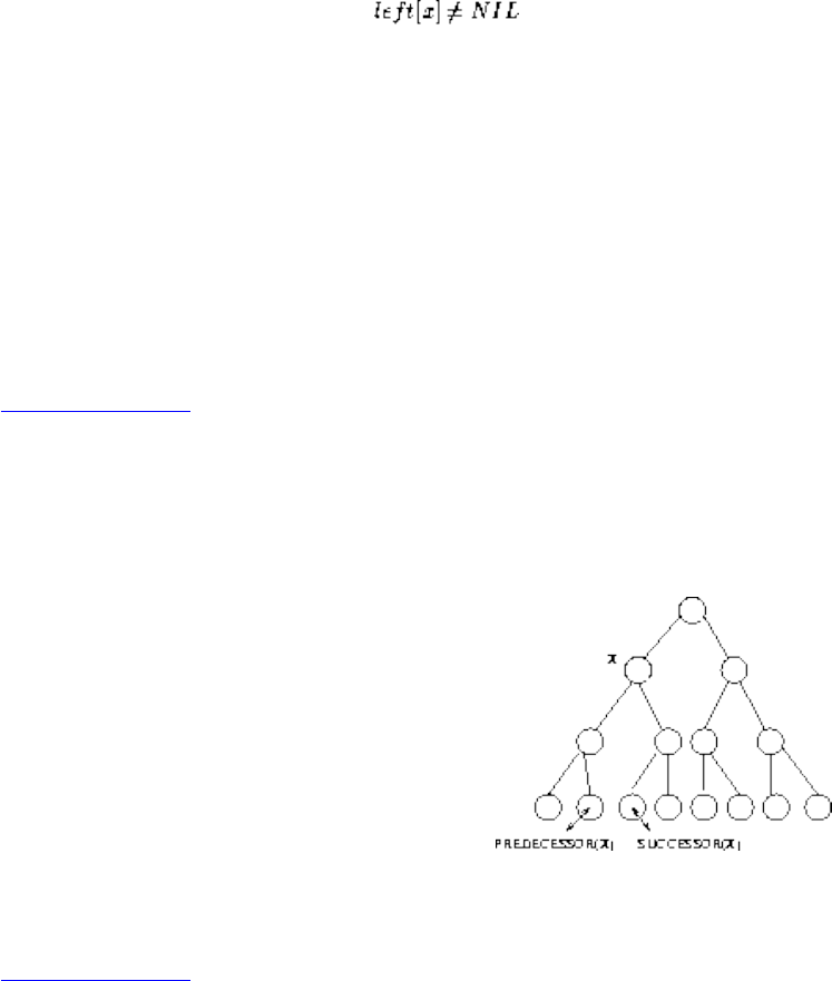
Lecture 8 - binary trees
return x
TREE-MINIMUM(x)
while
do x = left[x]
return x
Both take time proportional to the height of the tree, O(h).
Listen To Part 8-7
Where is the predecessor?
Where is the predecessor of a node in a tree, assuming all keys are distinct?
If X has two children, its predecessor is the maximum value in its left subtree and its successor the minimum value in its right
subtree.
Listen To Part 8-8
What if a node doesn't have children?
file:///E|/LEC/LECTUR17/NODE8.HTM (4 of 13) [19/1/2003 1:34:46]
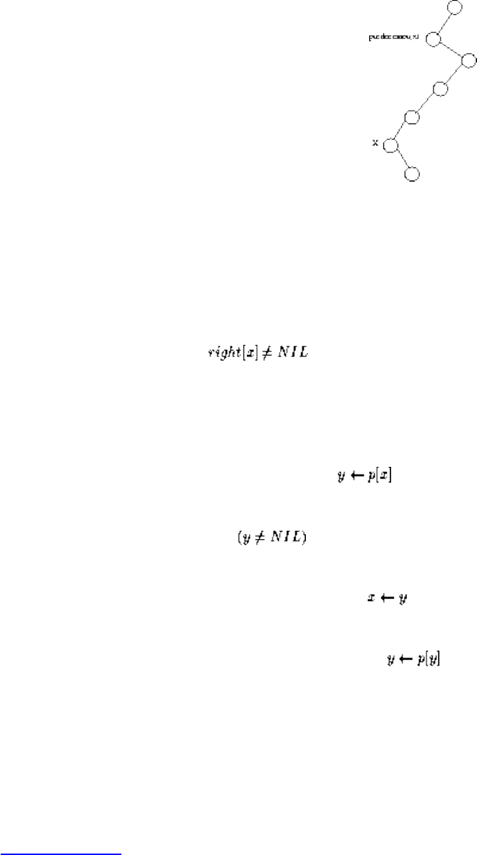
Lecture 8 - binary trees
If it does not have a left child, a node's predecessor is its first left ancestor.
The proof of correctness comes from looking at the in-order traversal of the tree.
Tree-Successor(x)
if
then return Tree-Minimum(right[x])
while and (x = right[y])
do
return y
Tree predecessor/successor both run in time proportional to the height of the tree.
Listen To Part 8-9
In-Order Traversal
file:///E|/LEC/LECTUR17/NODE8.HTM (5 of 13) [19/1/2003 1:34:46]
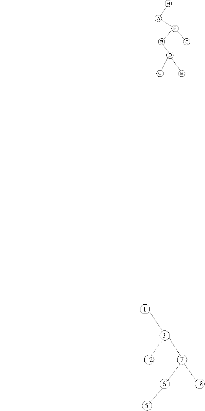
Lecture 8 - binary trees
Inorder-Tree-walk(x)
if (x <> NIL)
then Inorder-Tree-Walk(left[x])
print key[x]
Inorder-Tree-walk(right[x])
A-B-C-D-E-F-G-H
Listen To Part 8-10
Tree Insertion
Do a binary search to find where it should be, then replace the termination NIL pointer with the new item.
file:///E|/LEC/LECTUR17/NODE8.HTM (6 of 13) [19/1/2003 1:34:46]
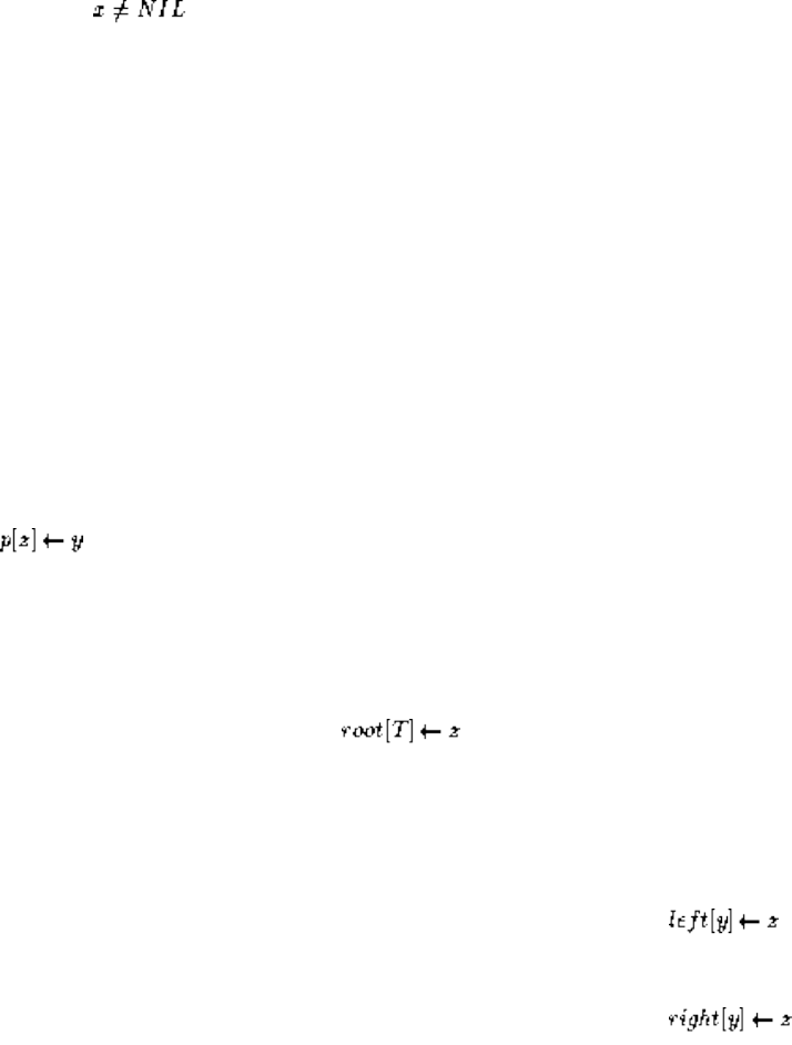
Lecture 8 - binary trees
Tree-insert(T,z)
y = NIL
x = root[T]
while
do y = x
if key[z] < key[x]
then x =
left[x]
else x =
right[x]
if y = NIL
then
else if key[z] < key[y]
then
else
y is maintained as the parent of x, since x eventually becomes NIL.
The final test establishes whether the NIL was a left or right turn from y.
Insertion takes time proportional to the height of the tree, O(h).
file:///E|/LEC/LECTUR17/NODE8.HTM (7 of 13) [19/1/2003 1:34:46]
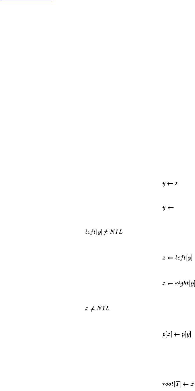
Lecture 8 - binary trees
Listen To Part 8-12
Tree Deletion
Deletion is somewhat more tricky than insertion, because the node to die may not be a leaf, and thus effect other nodes.
Case (a), where the node is a leaf, is simple - just NIL out the parents child pointer.
Case (b), where a node has one chld, the doomed node can just be cut out.
Case (c), relabel the node as its successor (which has at most one child when z has two children!) and delete the successor!
This implementation of deletion assumes parent pointers to make the code nicer, but if you had to save space they could be
dispensed with by keeping the pointers on the search path stored in a stack.
Tree-Delete(T,z)
if (left[z] = NIL) or (right[z] = NIL)
then
else Tree-Successor(z)
if
then
else
if
then
if p[y] = NIL
then
else if (y = left[p[y]])
file:///E|/LEC/LECTUR17/NODE8.HTM (8 of 13) [19/1/2003 1:34:46]
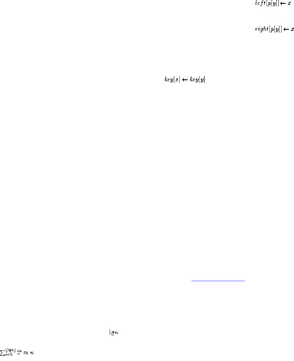
Lecture 8 - binary trees
then
else
if (y <> z)
then
/* If y has other fields, copy them,
too. */
return y
Lines 1-3 determine which node y is physically removed.
Lines 4-6 identify x as the non-nil decendant, if any.
Lines 7-8 give x a new parent.
Lines 9-10 modify the root node, if necessary
Lines 11-13 reattach the subtree, if necessary.
Lines 14-16 if the removed node is deleted, copy.
Conclusion: deletion takes time proportional to the height of the tree. Listen To Part 8-13
Balanced Search Trees
All six of our dictionary operations, when implemented with binary search trees, take O(h), where h is the height of the tree.
The best height we could hope to get is , if the tree was perfectly balanced, since
But if we get unlucky with our order of insertion or deletion, we could get linear height!
insert(a)
file:///E|/LEC/LECTUR17/NODE8.HTM (9 of 13) [19/1/2003 1:34:46]
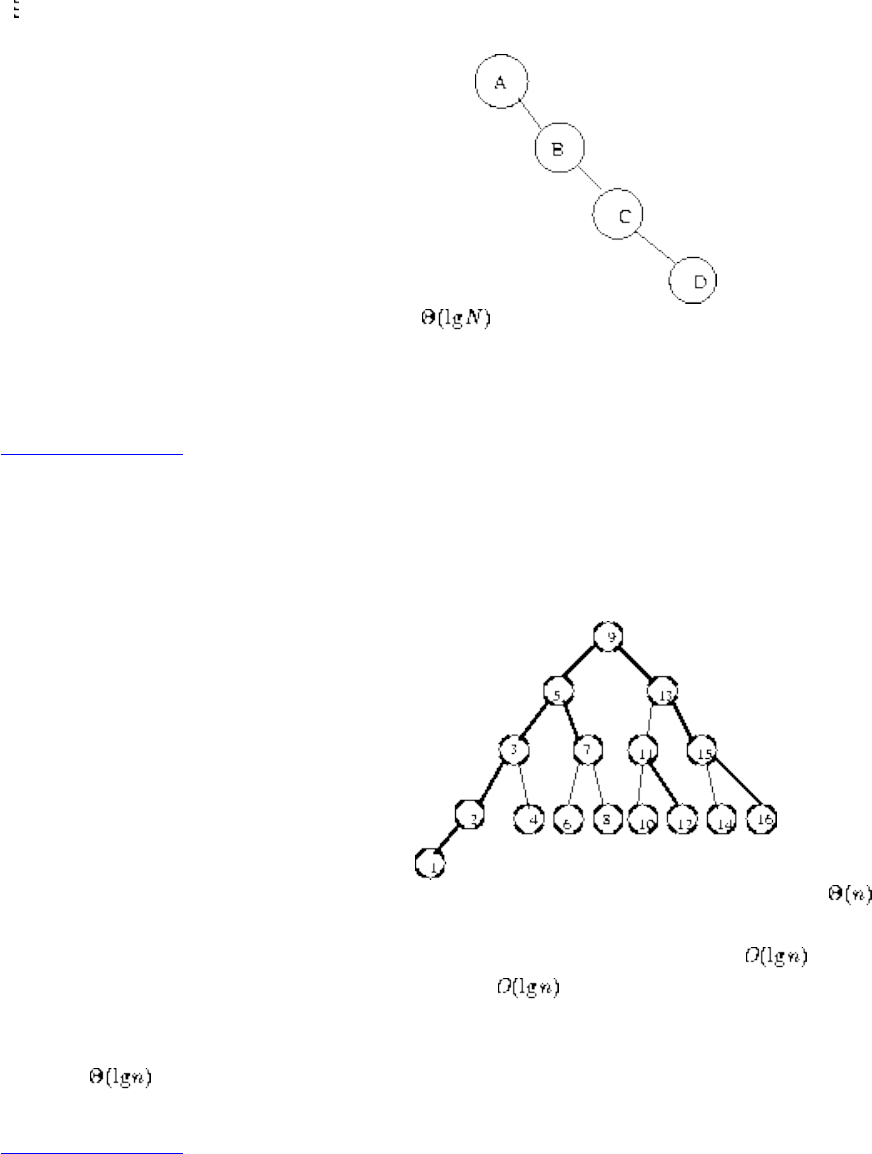
Lecture 8 - binary trees
insert(b)
insert(c)
insert(d)
In fact, random search trees on average have height, but we are worried about worst case height.
We can't easily use randomization - Why?
Listen To Part 8-14
Perfectly Balanced Trees
Perfectly balanced trees require a lot of work to maintain:
If we insert the key 1, we must move every single node in the tree to rebalance it, taking time.
Therefore, when we talk about "balanced" trees, we mean trees whose height is , so all dictionary operations (insert,
delete, search, min/max, successor/predecessor) take time.
Red-Black trees are binary search trees where each node is assigned a color, where the coloring scheme helps us maintain the
height as .
Listen To Part 8-15
file:///E|/LEC/LECTUR17/NODE8.HTM (10 of 13) [19/1/2003 1:34:46]
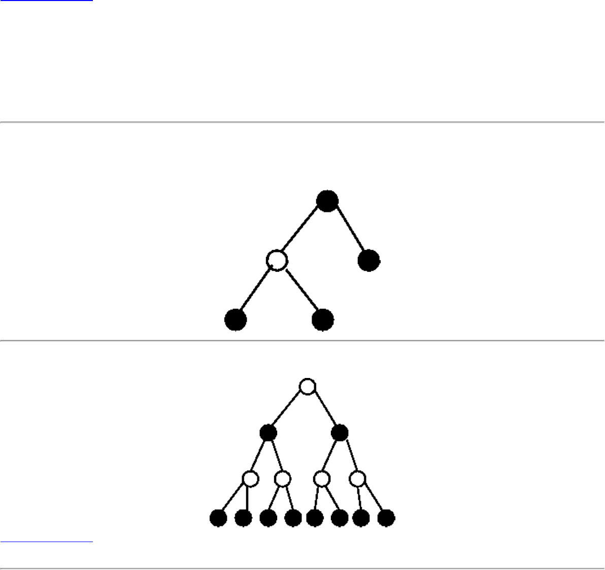
Lecture 8 - binary trees
Red-Black Tree Definition
Red-black trees have the following properties:
1. Every node is colored either red or black.
2. Every leaf (NIL pointer) is black.
3. If a node is red then both its children are black.
4. Every single path from a node to a decendant leaf contains the same number of black nodes.
Listen To Part 8-16
What does this mean?
If the root of a red-black tree is black can we just color it red?
No! For one of its children might be red.
If an arbitrary node is red can we color it black?
No! Because now all nodes may not have the same black height.
What tree maximizes the number of nodes in a tree of black height h?
Listen To Part 8-17
What does a red-black tree with two real nodes look like?
file:///E|/LEC/LECTUR17/NODE8.HTM (11 of 13) [19/1/2003 1:34:46]
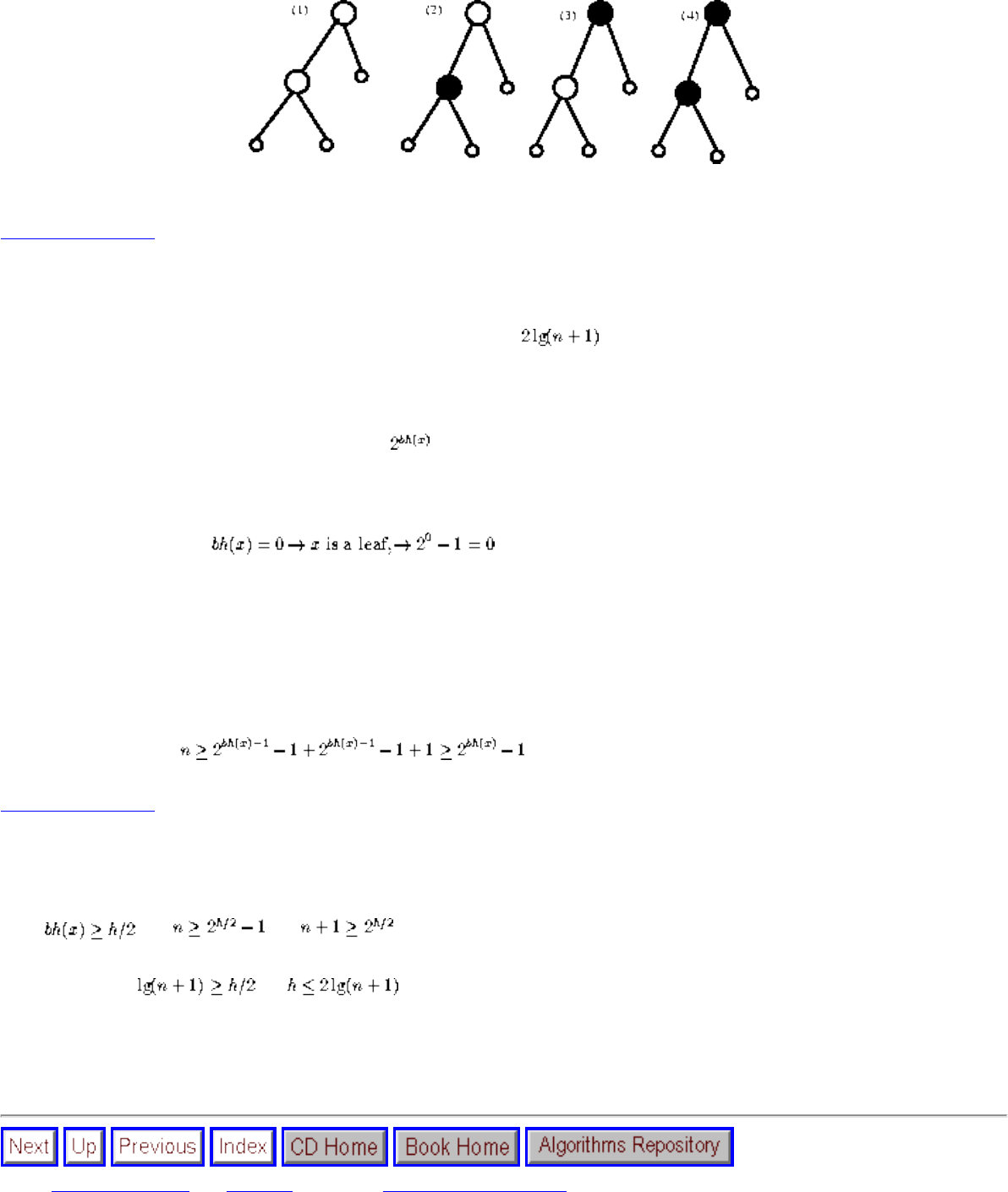
Lecture 8 - binary trees
Not (1) - consecutive reds Not (2), (4) - Non-Uniform black height
Listen To Part 8-18
Red-Black Tree Height
Lemma: A red-black tree with n internal nodes has height at most .
Proof: Our strategy; first we bound the number of nodes in any subtree, then we bound the height of any subtree.
We claim that any subtree rooted at x has at least - 1 internal nodes, where bh(x) is the black height of node x.
Proof, by induction:
Now assume it is true for all tree with black height < bh(x).
If x is black, both subtrees have black height bh(x)-1. If x is red, the subtrees have black height bh(x).
Therefore, the number of internal nodes in any subtree is
Listen To Part 8-19
Now, let h be the height of our red-black tree. At least half the nodes on any single path from root to leaf must be black if we
ignore the root.
Thus and , so .
This implies that ,so . height6pt width4pt
Therefore red-black trees have height at most twice optimal. We have a balanced search tree if we can maintain the red-black
tree structure under insertion and deletion.
Next: Lecture 9 - catch Up: No Title Previous: Lecture 7 - elementary
file:///E|/LEC/LECTUR17/NODE8.HTM (12 of 13) [19/1/2003 1:34:46]
Lecture 8 - binary trees
Algorithms
Mon Jun 2 09:21:39 EDT 1997
file:///E|/LEC/LECTUR17/NODE8.HTM (13 of 13) [19/1/2003 1:34:46]
Lecture 9 - catch up
Next: Lecture 10 - tree Up: No Title Previous: Lecture 8 - binary
Lecture 9 - catch up
Listen To Part 9-1
11-1 For each of the four types of linked lists in the following table, what is the asymptotic worst-case
running time for each dynamic-set operation listed?
singly singly doubly doubly
unsorted sorted unsorted sorted
Search(L, k) O(N) O(N) O(N) O(N)-
Insert(L, x) O(1) O(N) O(1) O(N)-
Delete(L, x) O(N)* O(N)* O(1) O(1)
Successor(L, x) O(N) O(1) O(N) O(1)
Predecessor(L, x) O(N) O(N) O(N) O(1)
Minimum(L) O(N) O(1) O(N) O(1)
Maximum(L) O(N) O(1)+ O(N) O(1)+
● I need a pointer to the predecessor! (*)
● I need a pointer to the tail! (+)
● Only bottlenecks in otherwise perfect dictionary! (-)
Next: Lecture 10 - tree Up: No Title Previous: Lecture 8 - binary
Algorithms
Mon Jun 2 09:21:39 EDT 1997
file:///E|/LEC/LECTUR17/NODE9.HTM [19/1/2003 1:34:47]
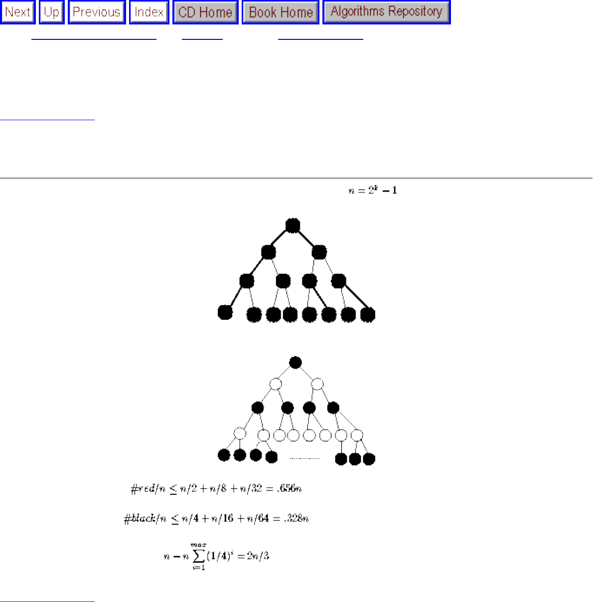
Lecture 10 - tree restructuring
Next: Lecture 11 - backtracking Up: No Title Previous: Lecture 9 - catch
Lecture 10 - tree restructuring
Listen To Part 10-1
14.1-5 Describe a Red-Black tree with the largest and smallest ratio of red nodes.
To minimize the ratio of red-black nodes, make all black (possible for )
To maximize the ratio of red nodes, interleave with red nodes as real leaves
Listen To Part 10-2
Rotations
The basic restructuring step for binary search trees are left and right rotation:
file:///E|/LEC/LECTUR16/NODE10.HTM (1 of 9) [19/1/2003 1:34:50]
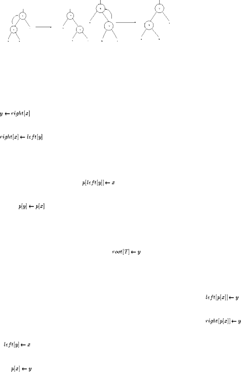
Lecture 10 - tree restructuring
1. Rotation is a local operation changing O(1) pointers.
2. An in-order search tree before a rotation stays an in-order search tree.
3. In a rotation, one subtree gets one level closer to the root and one subtree one level further from the root.
LEFT-ROTATE(T,x)
(* Set y*)
(* Turn y's left into x's right*)
if left[y]= NIL
then
(* Link x's parent to y *)
if p[x] = NIL
then
else if x= left[p[x]]
then
else
file:///E|/LEC/LECTUR16/NODE10.HTM (2 of 9) [19/1/2003 1:34:50]
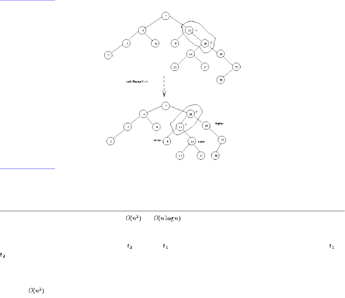
Lecture 10 - tree restructuring
Note the in-order property is preserved.
Listen To Part 10-3
Listen To Part 10-4
14.2-5 Show that any n-node tree can be transformed to any other using O(n) rotations (hint: convert to a right going
chain).
I will start by showing weaker bounds - that and rotations suffice - because that is how I proceeded when I
first saw the problem.
First, observe that creating a right-going, for path from < and reversing the same construction gives a path from to
.
Note that it will take at most n rotations to make the lowest valued key the root. Once it is root, all keys are to the right of
it, so no more rotations need go through it to create a right-going chain. Repeating with the second lowest key, third, etc.
gives that rotations suffice.
Now that if we try to create a completely balanced tree instead. To get the n/2 key to the root takes at most n rotations.
Now each subtree has half the nodes and we can recur...
file:///E|/LEC/LECTUR16/NODE10.HTM (3 of 9) [19/1/2003 1:34:50]
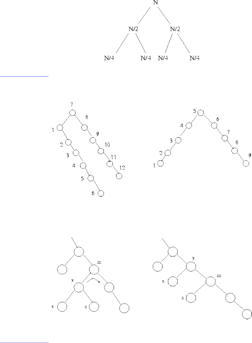
Lecture 10 - tree restructuring
Listen To Part 10-5
To get a linear algorithm, we must beware of trees like:
The correct answer is that n-1 rotations suffice to get to a rightmost chain.
By picking the lowest node on the rightmost chain which has a left ancestor, we can add one node per rotation to the right
most chain!
Initially, the rightmost chain contained at least 1 node, so after 1 rotations it contains all n. Slick!
Listen To Part 10-6
Red-Black Insertion
file:///E|/LEC/LECTUR16/NODE10.HTM (4 of 9) [19/1/2003 1:34:50]
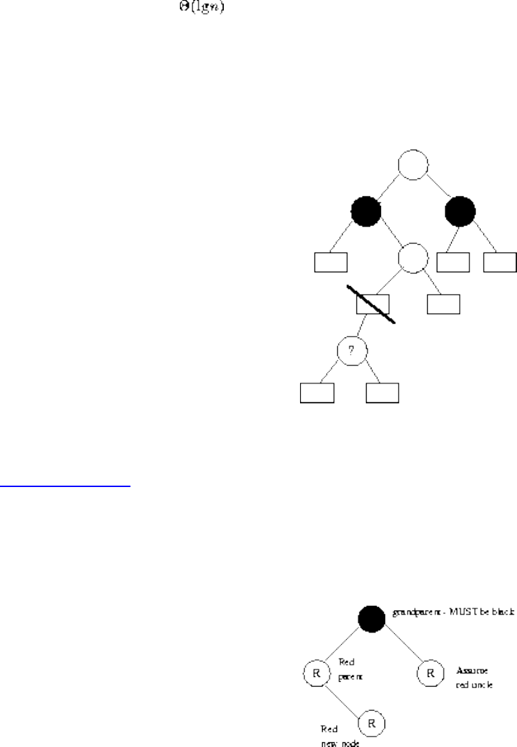
Lecture 10 - tree restructuring
Since red-black trees have height, if we can preserve all properties of such trees under insertion/deletion, we have
a balanced tree!
Suppose we just did a regular insertion. Under what conditions does it stay a red-black tree?
Since every insertion take places at a leaf, we will change a black NIL pointer to a node with two black NIL pointers.
To preserve the black height of the tree, the new node must be red. If its new parent is black, we can stop, otherwise we
must restructure!
Listen To Part 10-7
How can we fix two reds in a row?
It depends upon our uncle's color:
If our uncle is red, reversing our relatives' color either solves the problem or pushes it higher!
file:///E|/LEC/LECTUR16/NODE10.HTM (5 of 9) [19/1/2003 1:34:50]
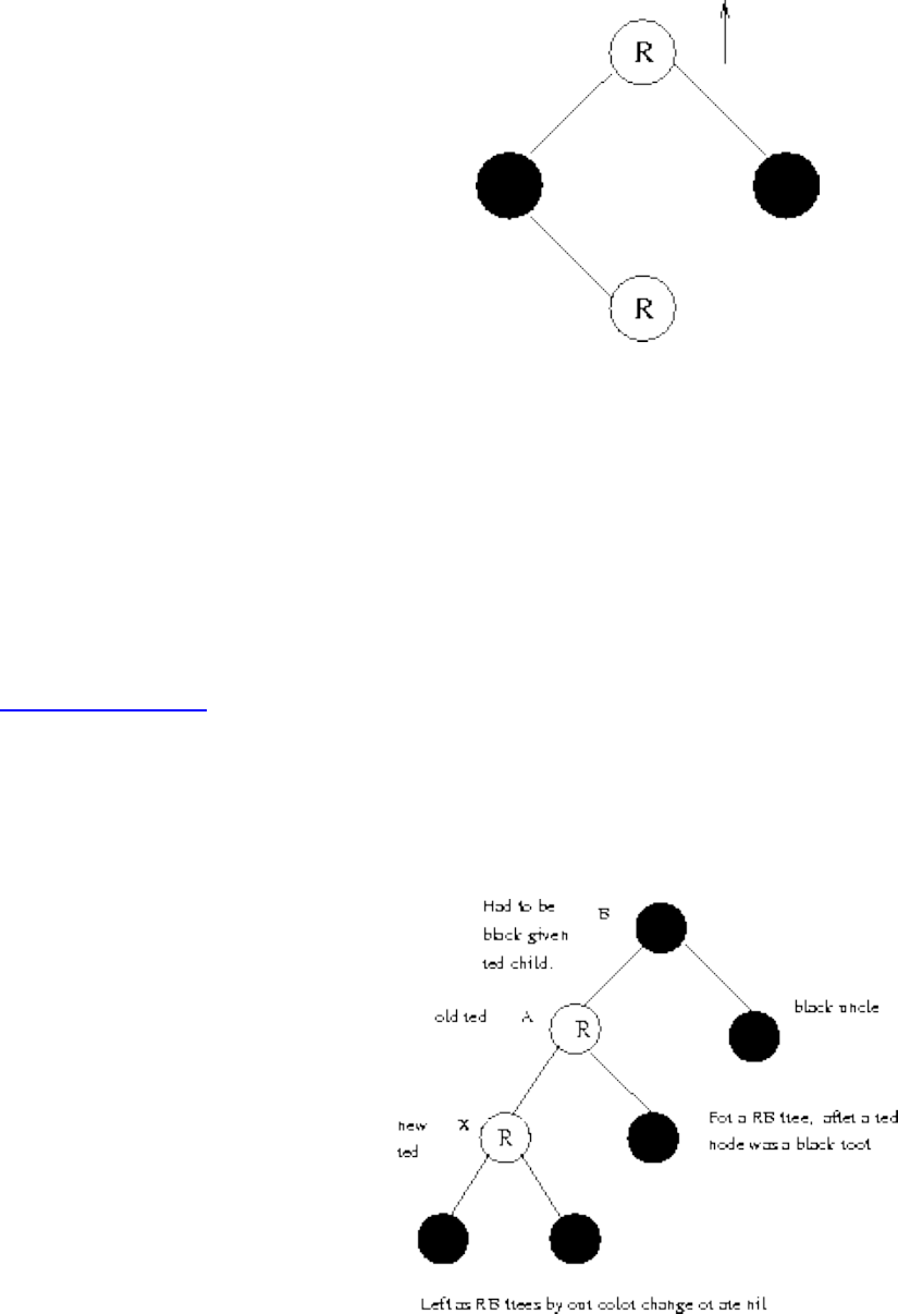
Lecture 10 - tree restructuring
Note that after the recoloring:
1. The black height is unchanged.
2. The shape of the tree is unchanged.
3. We are done if our great-grandparent is black.
If we get all the way to the root, recall we can always color a red-black tree's root black. We always will, so initially it
was black, and so this process terminates.
Listen To Part 10-8
The Case of the Black Uncle
If our uncle was black, observe that all the nodes around us have to be black:
Solution - rotate right about B:
file:///E|/LEC/LECTUR16/NODE10.HTM (6 of 9) [19/1/2003 1:34:50]
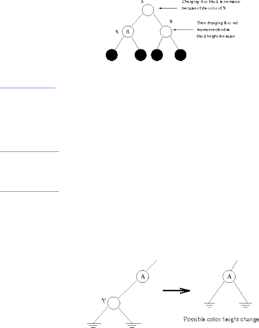
Lecture 10 - tree restructuring
Since the root of the subtree is now black with the same black-height as before, we have restored the colors and can stop!
Listen To Part 10-9
A double rotation can be required to set things up depending upon the left-right turn sequence, but the principle is the
same.
DOUBLE ROTATION ILLUSTRATION
Listen To Part 10-10
Pseudocode and Figures
Listen To Part 10-11
Deletion from Red-Black Trees
Recall the three cases for deletion from a binary tree:
Case (a) The node to be deleted was a leaf;
Case (b) The node to be deleted had one child;
file:///E|/LEC/LECTUR16/NODE10.HTM (7 of 9) [19/1/2003 1:34:51]
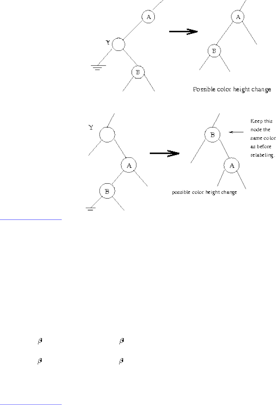
Lecture 10 - tree restructuring
Case (c) relabel to node as its successor and delete the successor.
Listen To Part 10-12
Deletion Color Cases
Suppose the node we remove was red, do we still have a red-black tree?
Yes! No two reds will be together, and the black height for each leaf stays the same.
However, if the dead node y was black, we must give each of its decendants another black ancestor. If an appropriate
node is red, we can simply color it black otherwise we must restructure.
Case (a) black NIL becomes ``double black'';
Case (b) red becomes black and black becomes ``double black'';
Case (c) red becomes black and black becomes ``double black''.
Our goal will be to recolor and restructure the tree so as to get rid of the ``double black'' node.
Listen To Part 10-13
In setting up any case analysis, we must be sure that:
1. All possible cases are covered.
file:///E|/LEC/LECTUR16/NODE10.HTM (8 of 9) [19/1/2003 1:34:51]
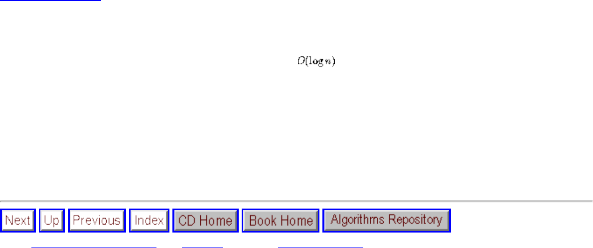
Lecture 10 - tree restructuring
2. No case is covered twice.
In the case analysis for red-black trees, the breakdown is:
Case 1: The double black node x has a red brother.
Case 2: x has a black brother and two black nephews.
Case 3: x has a black brother, and its left nephew is red and its right nephew is black.
Case 4: x has a black brother, and its right nephew is red (left nephew can be any color).
Listen To Part 10-14
Conclusion
Red-Black trees let us implement all dictionary operations in . Further, in no case are more than 3 rotations done
to rebalance. Certain very advanced data structures have data stored at nodes which requires a lot of work to adjust after a
rotation -- red-black trees ensure it won't happen often.
Example: Each node represents the endpoint of a line, and is augmented with a list of segments in its subtree which it
intersects.
We will not study such complicated structures, however.
Next: Lecture 11 - backtracking Up: No Title Previous: Lecture 9 - catch
Algorithms
Mon Jun 2 09:21:39 EDT 1997
file:///E|/LEC/LECTUR16/NODE10.HTM (9 of 9) [19/1/2003 1:34:51]
Lecture 11 - backtracking
Next: Lecture 12 - introduction Up: No Title Previous: Lecture 10 - tree
Lecture 11 - backtracking
Parallel Bubblesort
In order for me to give back your midterms, please form a line and sort yourselves in alphabetical order, from A to Z.
There is traditionally a strong correlation between the midterm grades and the number of daily problems attempted:
daily: 0, sum: 134, count: 3, avg: 44.67
daily: 1, sum: 0, count: 2, avg: 0.00
daily: 2, sum: 63, count: 1, avg: 63.00
daily: 3, sum: 194, count: 3, avg: 64.67
daily: 4, sum: 335, count: 5, avg: 67.00
daily: 5, sum: 489, count: 8, avg: 61.12
daily: 6, sum: 381, count: 6, avg: 63.50
daily: 7, sum: 432, count: 6, avg: 72.00
daily: 8, sum: 217, count: 3, avg: 72.33
daily: 9, sum: 293, count: 4, avg: 73.25
Listen To Part 11-2
Combinatorial Search
We have seen how clever algorithms can reduce sorting from to . However, the stakes are even higher for
combinatorially explosive problems:
The Traveling Salesman Problem
Given a weighted graph, find the shortest cycle which visits each vertex once.
file:///E|/LEC/LECTUR16/NODE11.HTM (1 of 8) [19/1/2003 1:34:54]

Lecture 11 - backtracking
Applications include minimizing plotter movement, printed-circuit board wiring, transportation problems, etc.
There is no known polynomial time algorithm (ie. for some fixed k) for this problem, so search-based algorithms
are the only way to go if you need an optional solution.
Listen To Part 11-3
But I want to use a Supercomputer
Moving to a faster computer can only buy you a relatively small improvement:
● Hardware clock rates on the fastest computers only improved by a factor of 6 from 1976 to 1989, from 12ns to
2ns.
● Moving to a machine with 100 processors can only give you a factor of 100 speedup, even if your job can be
perfectly parallelized (but of course it can't).
● The fast Fourier algorithm (FFT) reduced computation from to . This is a speedup of 340 times on
n=4096 and revolutionized the field of image processing.
● The fast multipole method for n-particle interaction reduced the computation from to O(n). This is a speedup
of 4000 times on n=4096.
Listen To Part 11-4
Can Eight Pieces Cover a Chess Board?
Consider the 8 main pieces in chess (king, queen, two rooks, two bishops, two knights). Can they be positioned on a
chessboard so every square is threatened?
file:///E|/LEC/LECTUR16/NODE11.HTM (2 of 8) [19/1/2003 1:34:54]
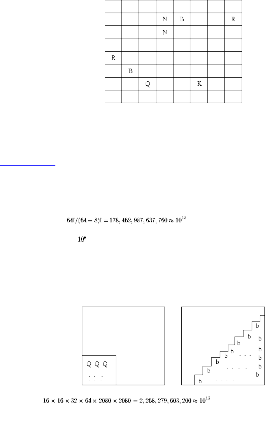
Lecture 11 - backtracking
Only 63 square are threatened in this configuration. Since 1849, no one had been able to find an arrangement with
bishops on different colors to cover all squares.
Of course, this is not an important problem, but we will use it as an example of how to attack a combinatorial search
problem.
Listen To Part 11-5
How many positions to test?
Picking a square for each piece gives us the bound:
Anything much larger than is unreasonable to search on a modest computer in a modest amount of time.
However, we can exploit symmetry to save work. With reflections along horizontal, vertical, and diagonal axis, the queen
can go in only 10 non-equivallent positions.
Even better, we can restrict the white bishop to 16 spots and the queen to 16, while being certain that we get all distinct
configurations.
Listen To Part 11-6
file:///E|/LEC/LECTUR16/NODE11.HTM (3 of 8) [19/1/2003 1:34:54]
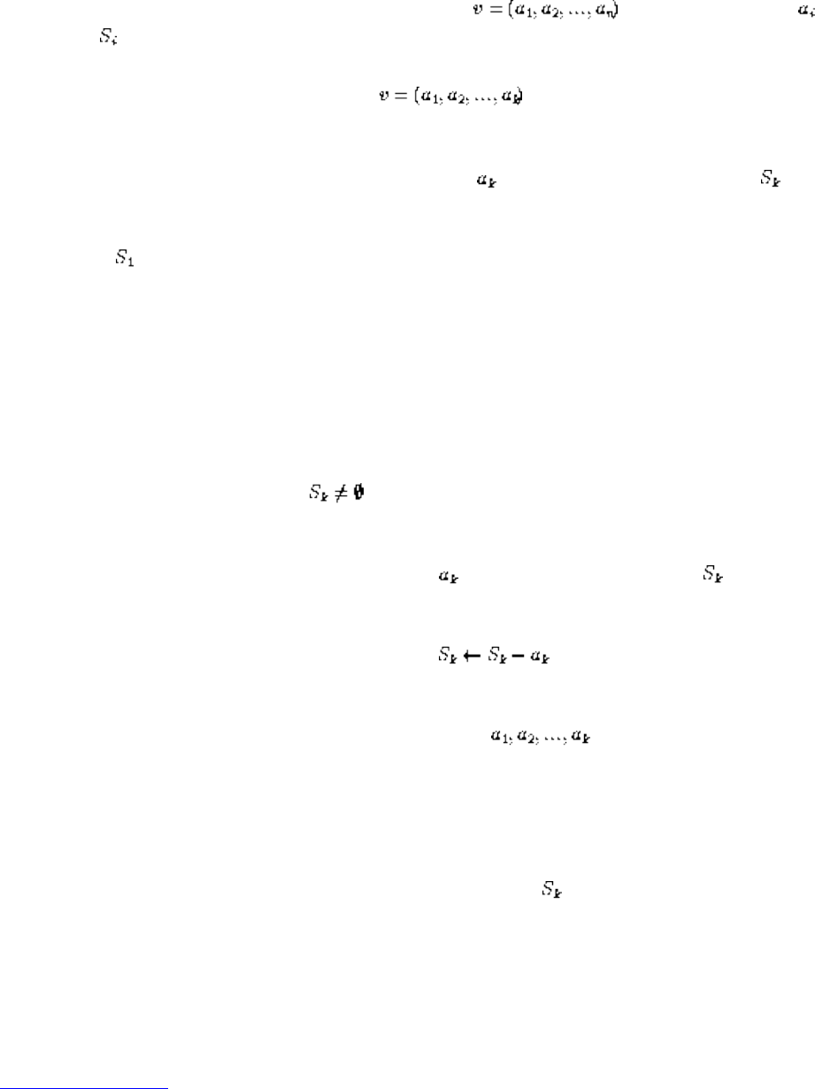
Lecture 11 - backtracking
Backtracking
Backtracking is a systematic way to go through all the possible configurations of a search space.
In the general case, we assume our solution is a vector where each element is selected from a finite
ordered set ,
We build from a partial solution of length k and try to extend it by adding another element. After
extending it, we will test whether what we have so far is still possible as a partial solution.
If it is still a candidate solution, great. If not, we delete and try the next element from :
Compute , the set of candidate first elements of v.
k = 1
While k > 0 do
While do (*advance*)
= an element in
if ( ) is solution, print!
k = k + 1
compute , the candidate kth elements given v.
k = k - 1 (*backtrack*)
Listen To Part 11-7
Recursive Backtracking
file:///E|/LEC/LECTUR16/NODE11.HTM (4 of 8) [19/1/2003 1:34:54]
Lecture 11 - backtracking
Recursion can be used for elegant and easy implementation of backtracking.
Backtrack(a, k)
if a is a solution, print(a)
else {
k = k +1
compute
while do
= an element in
=
Backtrack(a, k)
}
Backtracking can easily be used to iterate through all subsets or permutations of a set.
Backtracking ensures correctness by enumerating all possibilities.
For backtracking to be efficient, we must prune the search space.
Listen To Part 11-8
Constructing all Subsets
How many subsets are there of an n-element set?
To construct all subsets, set up an array/vector of n cells, where the value of is either true or false, signifying
file:///E|/LEC/LECTUR16/NODE11.HTM (5 of 8) [19/1/2003 1:34:54]
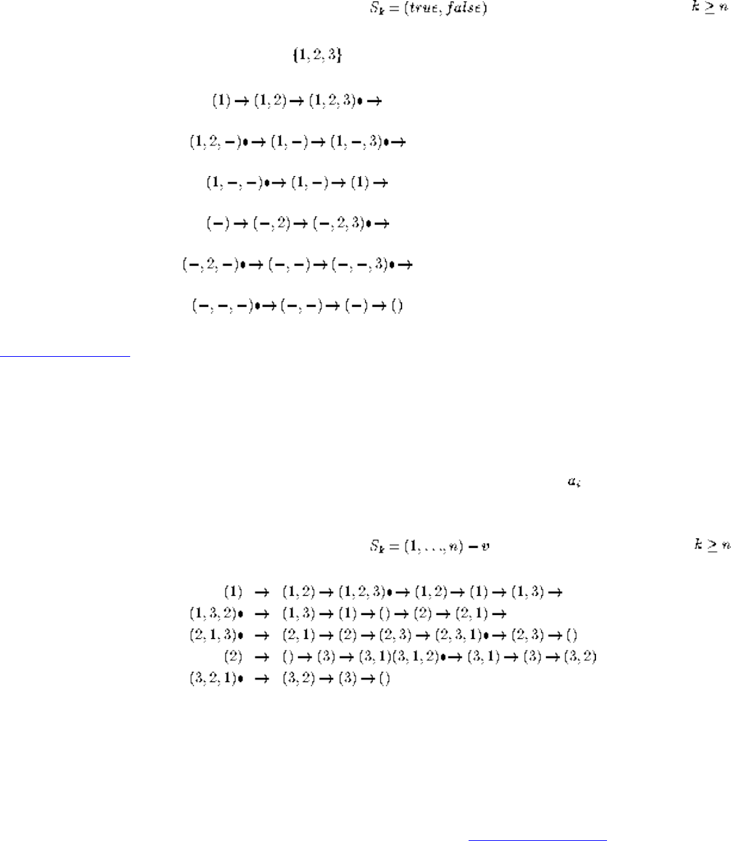
Lecture 11 - backtracking
whether the ith item is or is not in the subset.
To use the notation of the general backtrack algorithm, , and v is a solution whenever .
What order will this generate the subsets of ?
Listen To Part 11-9
Constructing all Permutations
How many permutations are there of an n-element set?
To construct all n! permutations, set up an array/vector of n cells, where the value of is an integer from 1 to n which
has not appeared thus far in the vector, corresponding to the ith element of the permutation.
To use the notation of the general backtrack algorithm, , and v is a solution whenever .
The n-Queens Problem
The first use of pruning to deal with the combinatorial explosion was by the king who rewarded the fellow who
discovered chess!
In the eight Queens, we prune whenever one queen threatens another. Listen To Part 11-11
Covering the Chess Board
In covering the chess board, we prune whenever we find there is a square which we cannot cover given the initial
configuration!
file:///E|/LEC/LECTUR16/NODE11.HTM (6 of 8) [19/1/2003 1:34:54]
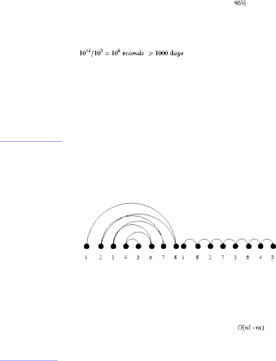
Lecture 11 - backtracking
Specifically, each piece can threaten a certain maximum number of squares (queen 27, king 8, rook 14, etc.) Whenever
the number of unthreated squares exceeds the sum of the maximum number of coverage remaining in unplaced squares,
we can prune.
As implemented by a graduate student project, this backtrack search eliminates of the search space, when the pieces
are ordered by decreasing mobility.
With precomputing the list of possible moves, this program could search 1,000 positions per second. But this is too slow!
Although we might further speed the program by an order of magnitude, we need to prune more nodes!
By using a more clever algorithm, we eventually were able to prove no solution existed, in less than one day's worth of
computing.
You too can fight the combinatorial explosion!
Listen To Part 11-12
The Backtracking Contest: Bandwidth
The bandwidth problem takes as input a graph G, with n vertices and m edges (ie. pairs of vertices). The goal is to find a
permutation of the vertices on the line which minimizes the maximum length of any edge.
The bandwidth problem has a variety of applications, including circuit layout, linear algebra, and optimizing memory
usage in hypertext documents.
The problem is NP-complete, meaning that it is exceedingly unlikely that you will be able to find an algorithm with
polynomial worst-case running time. It remains NP-complete even for restricted classes of trees.
Since the goal of the problem is to find a permutation, a backtracking program which iterates through all the n! possible
permutations and computes the length of the longest edge for each gives an easy algorithm. But the goal of this
assignment is to find as practically good an algorithm as possible.
Listen To Part 12-4
Rules of the Game
file:///E|/LEC/LECTUR16/NODE11.HTM (7 of 8) [19/1/2003 1:34:54]

Lecture 11 - backtracking
1. Everyone must do this assignment separately. Just this once, you are not allowed to work with your partner. The
idea is to think about the problem from scratch.
2. If you do not completely understand what the bandwidth of a graph is, you don't have the slightest chance of
producing a working program. Don't be afraid to ask for a clarification or explanation!!!!!
3. There will be a variety of different data files of different sizes. Test on the smaller files first. Do not be afraid to
create your own test files to help debug your program.
4. The data files are available via the course WWW page.
5. You will be graded on how fast and clever your program is, not on style. No credit will be given for incorrect
programs.
6. The programs are to run on the whatever computer you have access to, although it must be vanilla enough that I
can run the program on something I have access to.
7. You are to turn in a listing of your program, along with a brief description of your algorithm and any interesting
optimizations, sample runs, and the time it takes on sample data files. Report the largest test file your program
could handle in one minute or less of wall clock time.
8. The top five self-reported times / largest sizes will be collected and tested by me to determine the winner.
Listen To Part 12-5
Producing Efficient Programs
1. Don't optimize prematurely: Worrying about recursion vs. iteration is counter-productive until you have worked
out the best way to prune the tree. That is where the money is.
2. Choose your data structures for a reason: What operations will you be doing? Is case of insertion/deletion more
crucial than fast retrieval?
When in doubt, keep it simple, stupid (KISS).
3. Let the profiler determine where to do final tuning: Your program is probably spending time where you don't
expect.
Next: Lecture 12 - introduction Up: No Title Previous: Lecture 10 - tree
Algorithms
Mon Jun 2 09:21:39 EDT 1997
file:///E|/LEC/LECTUR16/NODE11.HTM (8 of 8) [19/1/2003 1:34:54]
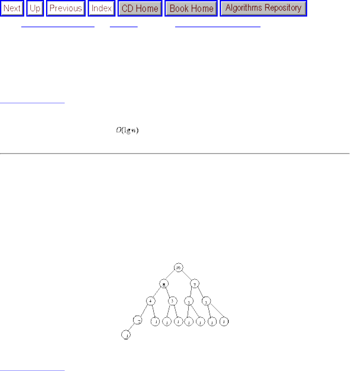
Lecture 12 - introduction to dynamic programming
Next: Lecture 13 - dynamic Up: No Title Previous: Lecture 11 - backtracking
Lecture 12 - introduction to dynamic
programming
Listen To Part 12-1
15.1-5 Given an element x in an n-node order-statistic binary tree and a natural number i, how can the
ith successor of x be determined in time.
This problem can be solved if our data structure supports two operations:
● Rank(x) - what is the position of x in the total order of keys?
● Get(i) - what is the key in the ith position of the total order of keys?
What we are interested in is Get(Rank(x)+i).
In an order statistic tree, each node x is labeled with the number of nodes contained in the subtree rooted
in x.
Implementing both operations involves keeping track of how many nodes lie to the left of our path.
Listen To Part 12-6
Optimization Problems
In the algorithms we have studied so far, correctness tended to be easier than efficiency. In optimization
problems, we are interested in finding a thing which maximizes or minimizes some function.
file:///E|/LEC/LECTUR16/NODE12.HTM (1 of 9) [19/1/2003 1:34:58]
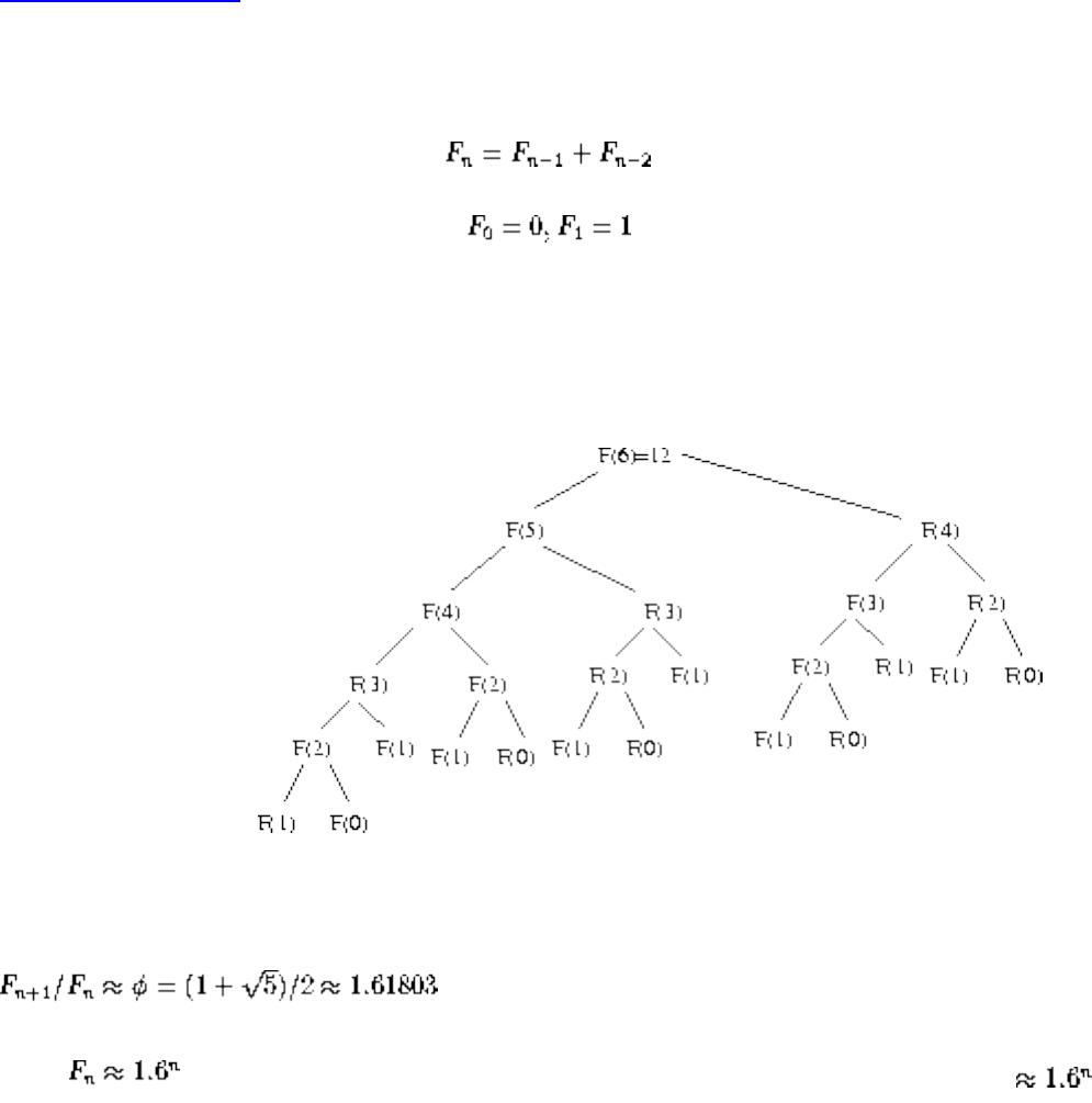
Lecture 12 - introduction to dynamic programming
In designing algorithms for optimization problem - we must prove that the algorithm in fact gives the
best possible solution.
Greedy algorithms, which makes the best local decision at each step, occasionally produce a global
optimum - but you need a proof!
Dynamic Programming
Dynamic Programming is a technique for computing recurrence relations efficiently by sorting partial
results.
Listen To Part 12-9
Computing Fibonacci Numbers
Implementing it as a recursive procedure is easy but slow!
We keep calculating the same value over and over!
How slow is slow?
Thus , and since our recursion tree has 0 and 1 as leaves, means we have calls!
file:///E|/LEC/LECTUR16/NODE12.HTM (2 of 9) [19/1/2003 1:34:58]
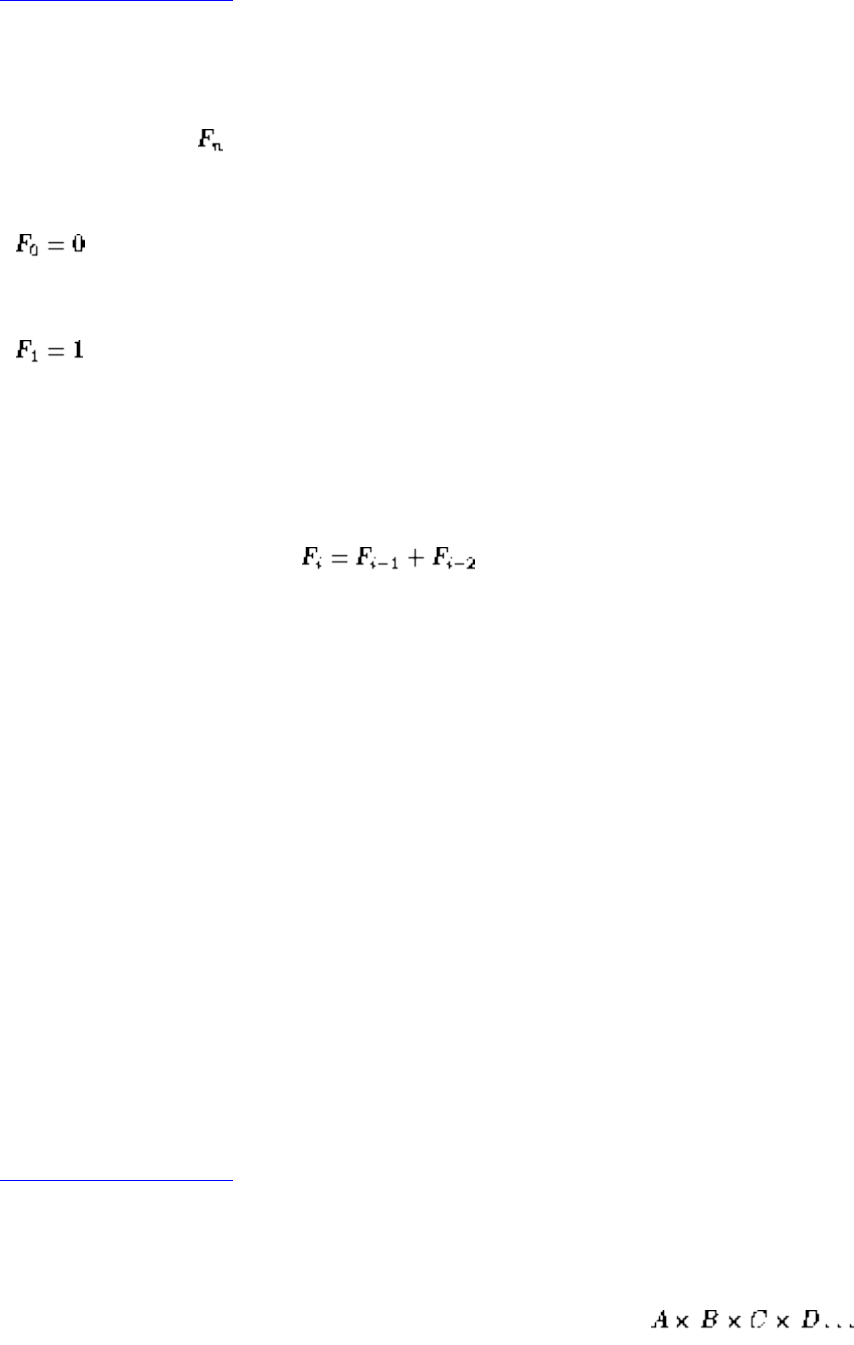
Lecture 12 - introduction to dynamic programming
Listen To Part 12-10
What about Dynamic Programming?
We can calculate in linear time by storing small values:
For i=1 to n
Moral: we traded space for time.
Dynamic programming is a technique for efficiently computing recurrences by storing partial results.
Once you understand dynamic programming, it is usually easier to reinvent certain algorithms than try to
look them up!
Dynamic programming is best understood by looking at a bunch of different examples.
I have found dynamic programming to be one of the most useful algorithmic techniques in practice:
● Morphing in Computer Graphics
● Data Compression for High Density Bar Codes
● Utilizing Grammatical Constraints for Telephone Keypads
Listen To Part 12-11
Multiplying a Sequence of Matrices
Suppose we want to multiply a long sequence of matrices .
file:///E|/LEC/LECTUR16/NODE12.HTM (3 of 9) [19/1/2003 1:34:58]
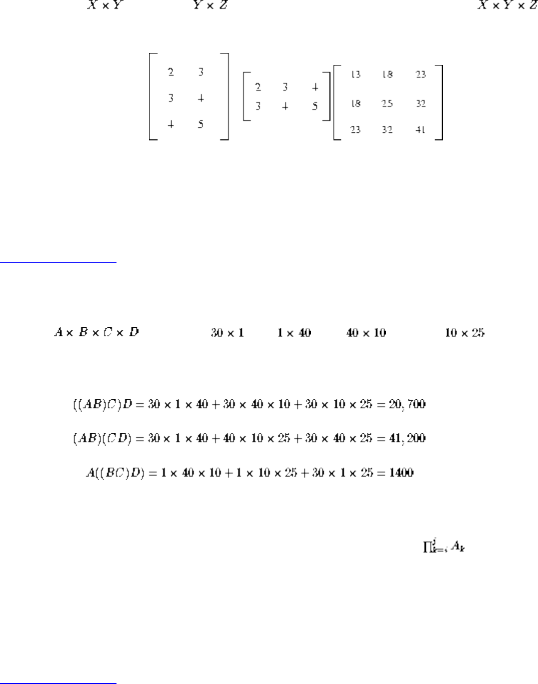
Lecture 12 - introduction to dynamic programming
Multiplying an matrix by a matrix (using the common algorithm) takes
multiplications.
We would like to avoid big intermediate matrices, and since matrix multiplication is associative, we can
parenthesise however we want.
Matrix multiplication is not communitive, so we cannot permute the order of the matrices without
changing the result.
Listen To Part 12-12
Example
Consider , where A is , B is , C is , and D is .
There are three possible parenthesizations:
The order makes a big difference in real computation. How do we find the best order?
Let M(i,j) be the minimum number of multiplications necessary to compute .
The key observations are
● The outermost parentheses partition the chain of matricies (i,j) at some k.
● The optimal parenthesization order has optimal ordering on either side of k.
Listen To Part 12-13
A recurrence for this is:
file:///E|/LEC/LECTUR16/NODE12.HTM (4 of 9) [19/1/2003 1:34:58]
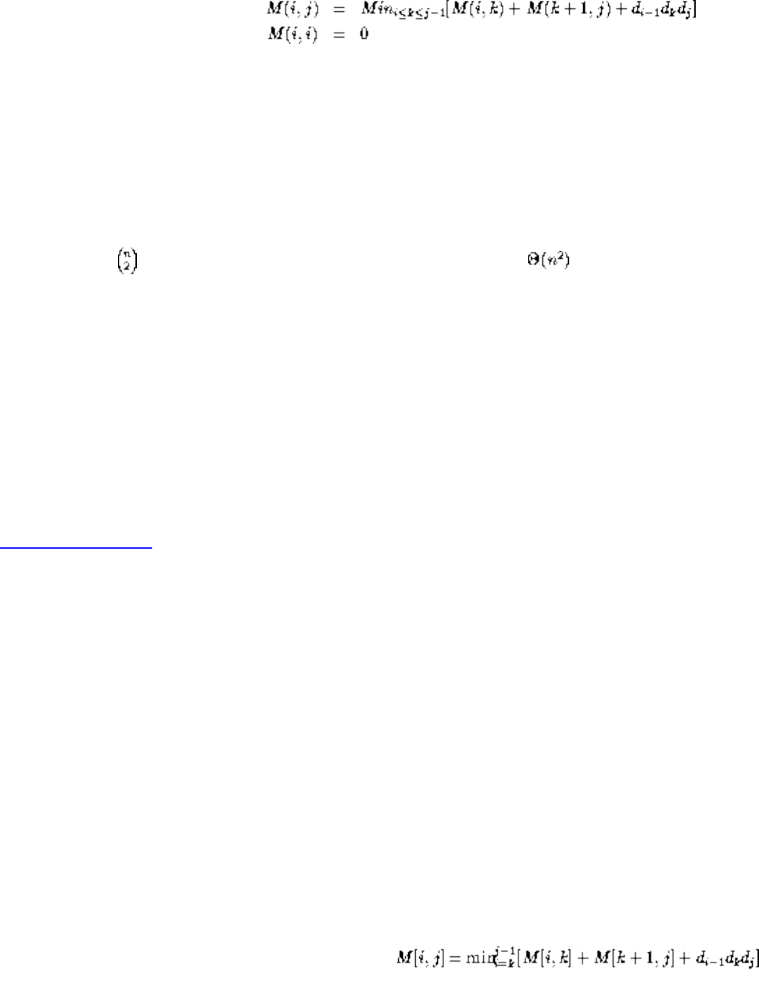
Lecture 12 - introduction to dynamic programming
If there are n matrices, there are n+1 dimensions.
A direct recursive implementation of this will be exponential, since there is a lot of duplicated work as in
the Fibonacci recurrence.
Divide-and-conquer is seems efficient because there is no overlap, but ...
There are only substrings between 1 and n. Thus it requires only space to store the optimal cost
for each of them.
We can represent all the possibilities in a triangle matrix. We can also store the value of k in another
triangle matrix to reconstruct to order of the optimal parenthesisation.
The diagonal moves up to the right as the computation progresses. On each element of the kth diagonal |j-
i| = k.
For the previous example:
Listen To Part 13-3
Procedure MatrixOrder
for i=1 to n do M[i, j]=0
for diagonal=1 to n-1
for i=1 to n-diagonal do
j=i+diagonal
file:///E|/LEC/LECTUR16/NODE12.HTM (5 of 9) [19/1/2003 1:34:58]

Lecture 12 - introduction to dynamic programming
faster(i,j)=k
return [m(1, n)]
Procedure ShowOrder(i, j)
if (i=j) write ( )
else
k=factor(i, j)
write ``(''
ShowOrder(i, k)
write ``*''
ShowOrder (k+1, j)
write ``)''
Listen To Part 13-4
A dynamic programming solution has three components:
file:///E|/LEC/LECTUR16/NODE12.HTM (6 of 9) [19/1/2003 1:34:58]
Lecture 12 - introduction to dynamic programming
1. Formulate the answer as a recurrence relation or recursive algorithm.
2. Show that the number of different instances of your recurrence is bounded by a polynomial.
3. Specify an order of evaluation for the recurrence so you always have what you need.
Listen To Part 13-5
Approximate String Matching
A common task in text editing is string matching - finding all occurrences of a word in a text.
Unfortunately, many words are mispelled. How can we search for the string closest to the pattern?
Let p be a pattern string and T a text string over the same alphabet.
A k-approximate match between P and T is a substring of T with at most k differences.
Differences may be:
1. the corresponding characters may differ: KAT CAT
2. P is missing a character from T: CAAT CAT
3. T is missing a character from P: CT CAT
Approximate Matching is important in genetics as well as spell checking.
Listen To Part 13-6
A 3-Approximate Match
A match with one of each of three edit operations is:
P = unescessaraly
T = unnecessarily
Finding such a matching seems like a hard problem because we must figure out where you add blanks,
but we can solve it with dynamic programming.
D[i, j] = the minimum number of differences between and the segment of T ending at j.
file:///E|/LEC/LECTUR16/NODE12.HTM (7 of 9) [19/1/2003 1:34:58]
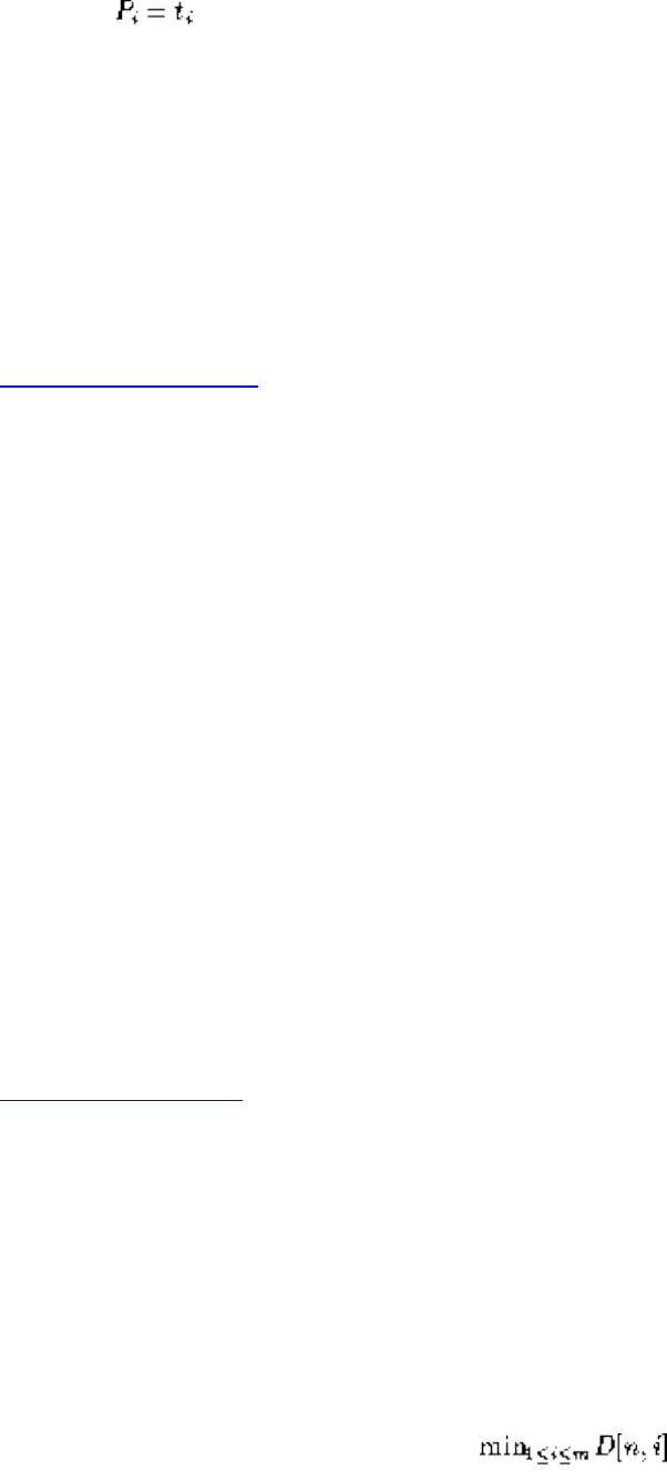
Lecture 12 - introduction to dynamic programming
D[i, j] is the minimum of the three possible ways to extend smaller strings:
1. If then D[i-1, j-1] else D[i-1, j-1]+1 (corresponding characters do or do not match)
2. D[i-1, j]+1 (extra character in text - we do not advance the pattern pointer).
3. D[i, j-1]+1 (character in pattern which is not in text).
Once you accept the recurrence it is easy.
To fill each cell, we need only consider three other cells, not O(n) as in other examples. This means we
need only store two rows of the table. The total time is O(mn).
Listen To Part 13-10
Boundary conditions for string matching
What should the value of D[0,i] be, corresponding to the cost of matching the first i characters of the text
with none of the pattern?
It depends. Are we doing string matching in the text or substring matching?
● If you want to match all of the pattern against all of the text, this meant that would have to delete
the first i characters of the pattern, so D[0,i] = i to pay the cost of the deletions.
● if we want to find the place in the text where the pattern occurs? We do not want to pay more of a
cost if the pattern occurs far into the text than near the front, so it is important that starting cost be
equal for all positions. In this case, D[0,i] = 0, since we pay no cost for deleting the first i
characters of the text.
In both cases, D[i,0] = i, since we cannot excuse deleting the first i characters of the pattern without cost.
Listen To Part 13-9
What do we return?
If we want the cost of comparing all of the pattern against all of the text, such as comparing the spelling
of two words, all we are interested in is D[n,m].
But what if we want the cheapest match between the pattern anywhere in the text? Assuming the
initialization for substring matching, we seek the cheapest matching of the full pattern ending anywhere
in the text. This means the cost equals .
file:///E|/LEC/LECTUR16/NODE12.HTM (8 of 9) [19/1/2003 1:34:58]
Lecture 12 - introduction to dynamic programming
This only gives the cost of the optimal matching. The actual alignment - what got matched, substituted,
and deleted - can be reconstructed from the pattern/text and table without an auxiliary storage, once we
have identified the cell with the lowest cost.
Listen To Part 13-11
How much space do we need?
Do we need to keep all O(mn) cells, since if we evaluate the recurrence filling in the columns of the
matrix from left to right, we will never need more than two columns of cells to do what we need. Thus
O(m) space is sufficient to evaluate the recurrence without changing the time complexity at all.
Unfortunately, because we won't have the full matrix we cannot reconstruct the alignment, as above.
Saving space in dynamic programming is very important. Since memory on any computer is limited,
O(nm) space is more of a bottleneck than O(nm) time.
Fortunately, there is a clever divide-and-conquer algorithm which computes the actual alignment in
O(nm) time and O(m) space.
Next: Lecture 13 - dynamic Up: No Title Previous: Lecture 11 - backtracking
Algorithms
Mon Jun 2 09:21:39 EDT 1997
file:///E|/LEC/LECTUR16/NODE12.HTM (9 of 9) [19/1/2003 1:34:58]
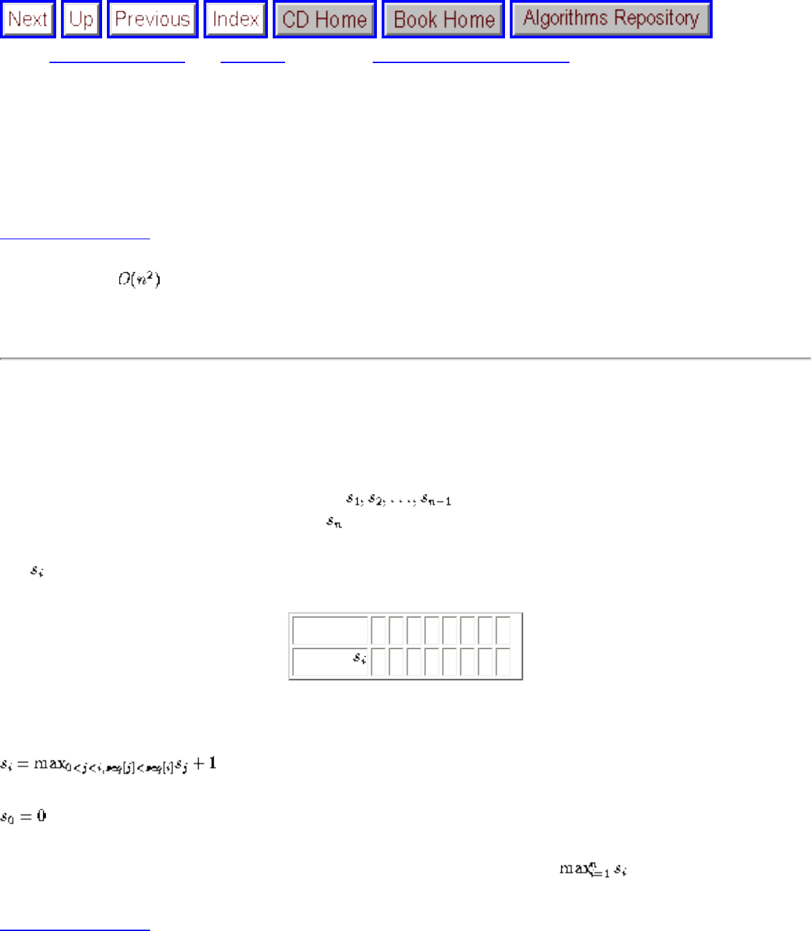
Lecture 13 - dynamic programming applications
Next: Lecture 14 - data Up: No Title Previous: Lecture 12 - introduction
Lecture 13 - dynamic programming
applications
Listen To Part 13-1
16.3-5 Give an algorithm to find the longest montonically increasing sequence in a sequence of n
numbers.
Build an example first: (5, 2, 8, 7, 1, 6, 4)
Ask yourself what would you like to know about the first n-1 elements to tell you the answer for the
entire sequence?
1. The length of the longest sequence in . (seems obvious)
2. The length of the longest sequence will extend! (not as obvious - this is the idea!)
Let be the length of the longest sequence ending with the ith character:
sequence 5 2 8 7 3 1 6 4
1 1 2 2 2 1 3 3
How do we compute i?
To find the longest sequence - we know it ends somewhere, so Length =
Listen To Part 14-5
The Principle of Optimality
file:///E|/LEC/LECTUR16/NODE13.HTM (1 of 7) [19/1/2003 1:35:01]
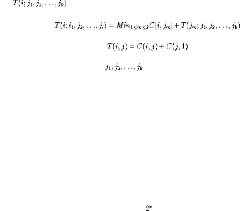
Lecture 13 - dynamic programming applications
To use dynamic programming, the problem must observe the principle of optimality, that whatever the
initial state is, remaining decisions must be optimal with regard the state following from the first
decision.
Combinatorial problems may have this property but may use too much memory/time to be efficient.
Example: The Traveling Salesman Problem
Let be the cost of the optimal tour for i to 1 that goes thru each of the other cities once
Here there can be any subset of instead of any subinterval - hence exponential.
Still, with other ideas (some type of pruning or best-first search) it can be effective for combinatorial
search.
Listen To Part 14-6
When can you use Dynamic Programming?
Dynamic programming computes recurrences efficiently by storing partial results. Thus dynamic
programming can only be efficient when there are not too many partial results to compute!
There are n! permutations of an n-element set - we cannot use dynamic programming to store the best
solution for each subpermutation. There are subsets of an n-element set - we cannot use dynamic
programming to store the best solution for each.
However, there are only n(n-1)/2 continguous substrings of a string, each described by a starting and
ending point, so we can use it for string problems.
There are only n(n-1)/2 possible subtrees of a binary search tree, each described by a maximum and
minimum key, so we can use it for optimizing binary search trees.
Dynamic programming works best on objects which are linearly ordered and cannot be rearranged -
characters in a string, matrices in a chain, points around the boundary of a polygon, the left-to-right
order of leaves in a search tree.
file:///E|/LEC/LECTUR16/NODE13.HTM (2 of 7) [19/1/2003 1:35:01]
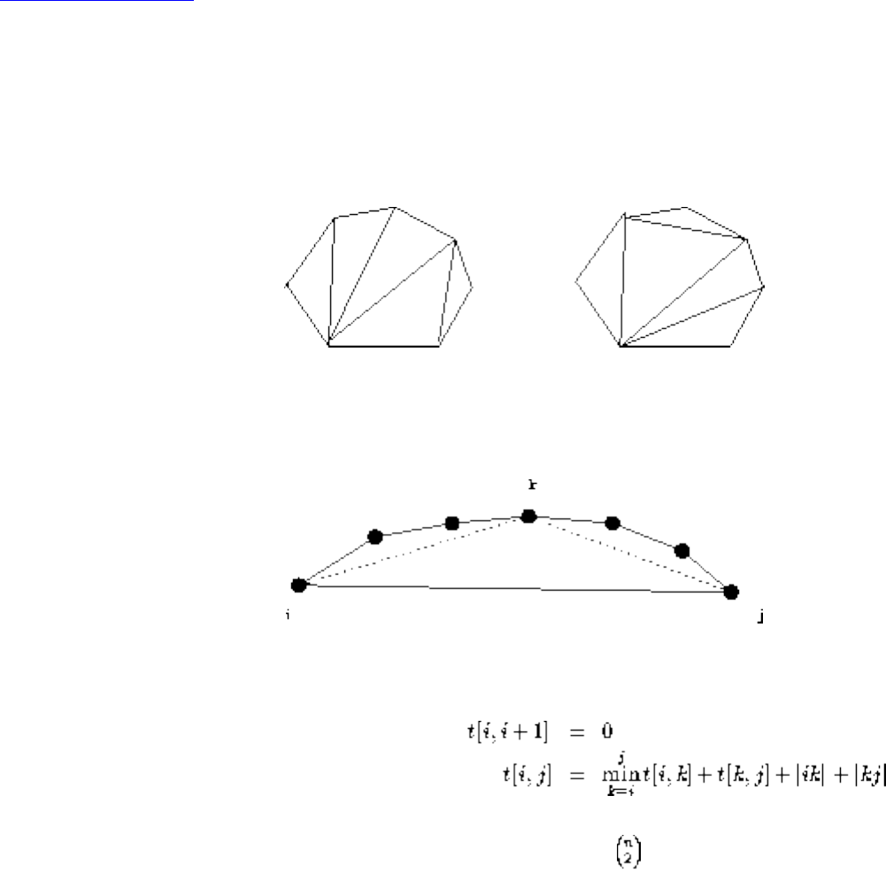
Lecture 13 - dynamic programming applications
Whenever your objects are ordered in a left-to-right way, you should smell dynamic programming!
Listen To Part 14-7
Minimum Length Triangulation
A triangulation of a polygon is a set of non-intersecting diagonals which partitions the polygon into
diagonals.
The length of a triangulation is the sum of the diagonal lengths.
We seek to find the minimum length triangulation. For a convex polygon, or part thereof:
Once we identify the correct connecting vertex, the polygon is partitioned into two smaller pieces, both
of which must be triangulated optimally!
Evaluation proceeds as in the matrix multiplication example - values of t, each of which takes O(j-i)
time if we evaluate the sections in order of increasing size.
file:///E|/LEC/LECTUR16/NODE13.HTM (3 of 7) [19/1/2003 1:35:01]
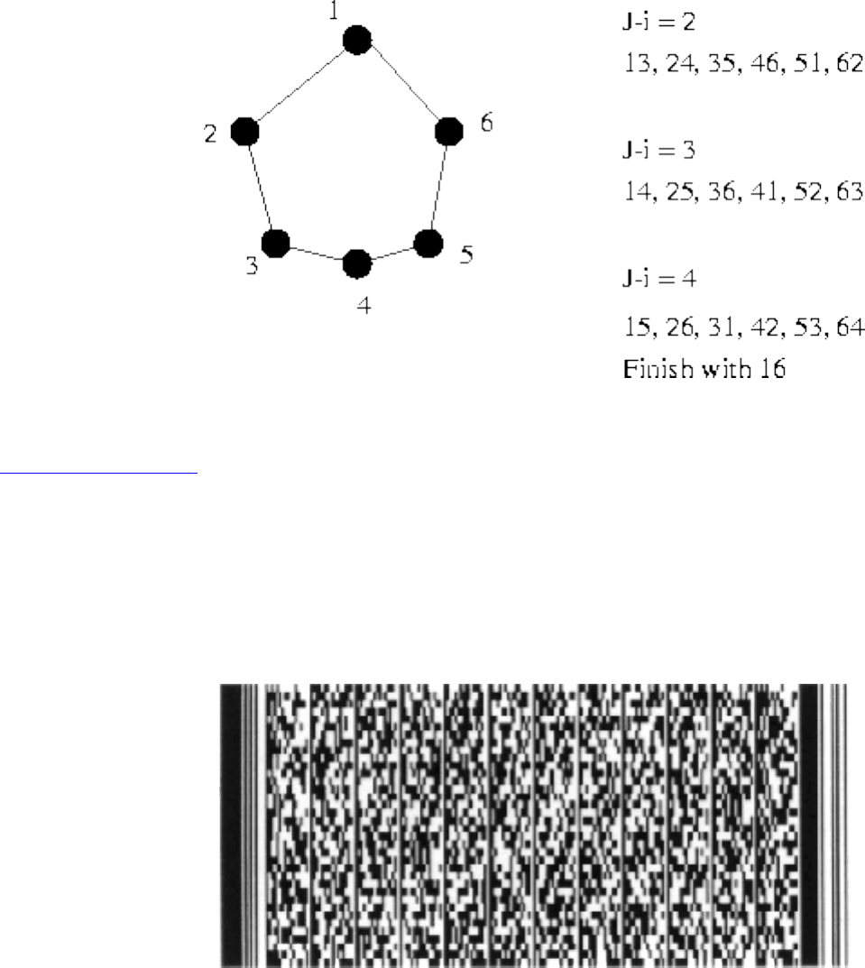
Lecture 13 - dynamic programming applications
What if there are points in the interior of the polygon?
Listen To Part 14-8
Dynamic Programming and High Density Bar Codes
Symbol Technology has developed a new design for bar codes, PDF-417 that has a capacity of several
hundred bytes. What is the best way to encode text for this design?
They developed a complicated mode-switching data compression scheme.
file:///E|/LEC/LECTUR16/NODE13.HTM (4 of 7) [19/1/2003 1:35:01]
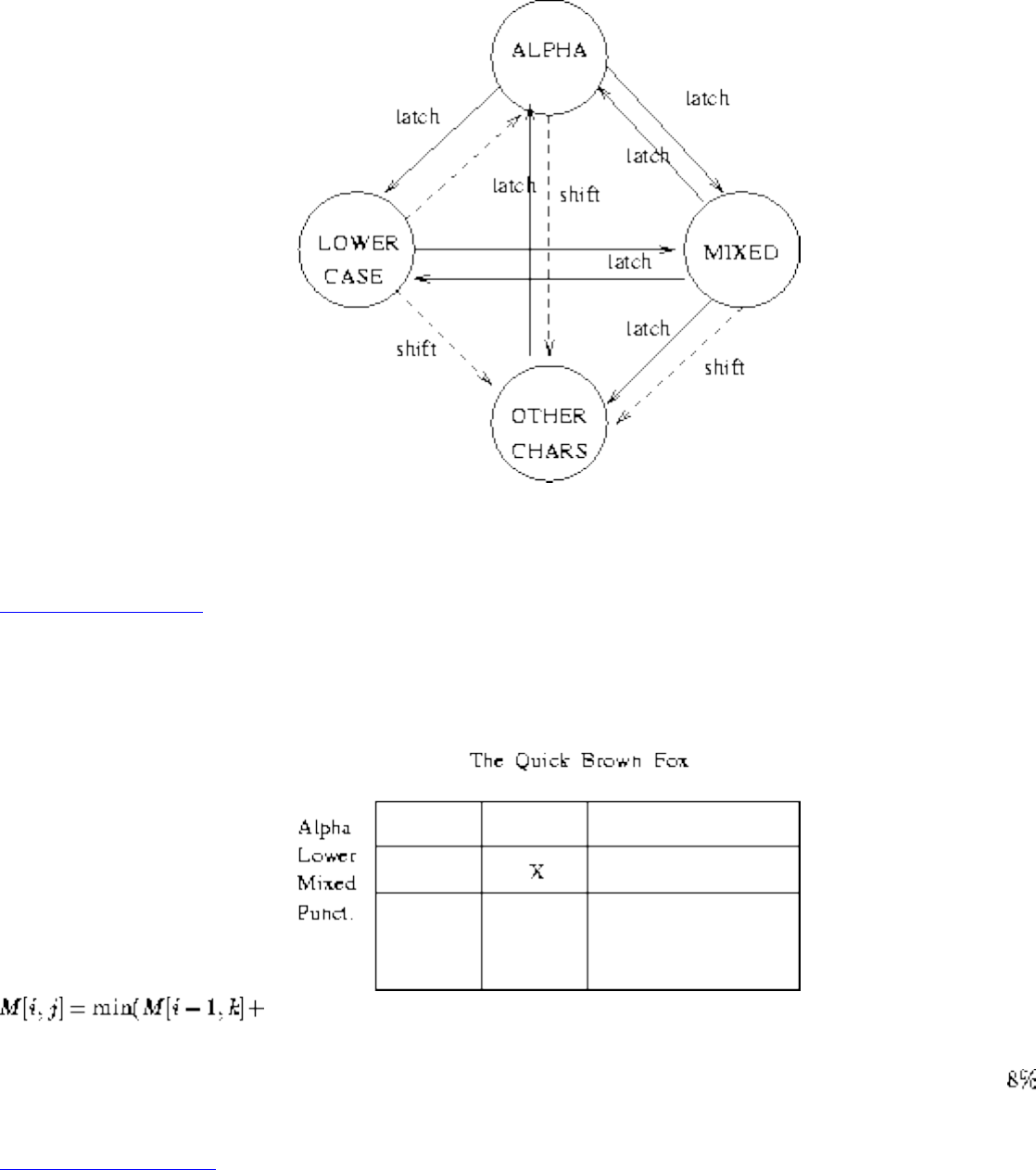
Lecture 13 - dynamic programming applications
Latch commands permanently put you in a different mode. Shift commands temporarily put you in a
different mode.
Listen To Part 14-9
Originally, Symbol used a greedy algorithm to encode a string, making local decisions only. We realized
that for any prefix, you want an optimal encoding which might leave you in every possible mode.
the cost of encoding the ith character and ending up in node j).
Our simple dynamic programming algorithm improved to capacity of PDF-417 by an average of !
Listen To Part 14-10
Dynamic Programming and Morphing
Morphing is the problem of creating a smooth series of intermediate images given a starting and ending
image.
file:///E|/LEC/LECTUR16/NODE13.HTM (5 of 7) [19/1/2003 1:35:01]
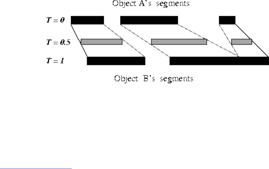
Lecture 13 - dynamic programming applications
The key problem is establishing a correspondence between features in the two images. You want to
morph an eye to an eye, not an ear to an ear.
We can do this matching on a line-by-line basis:
This should sound like string matching, but with a different set of operations:
● Full run match: We may match run i on top to run j on bottom for a cost which is a function of the
difference in the lengths of the two runs and their positions.
● Merging runs: We may match a string of consecutive runs on top to a run on bottom. The cost
will be a function of the number of runs, their relative positions, and lengths.
Listen To Part 14-11
● Splitting runs: We may match a big run on top to a string of consecutive runs on the bottom. This
is just the converse of the merge. Again, the cost will be a function of the number of runs, their
relative positions, and lengths.
This algorithm was incorported into a morphing system, with the following results:
file:///E|/LEC/LECTUR16/NODE13.HTM (6 of 7) [19/1/2003 1:35:01]
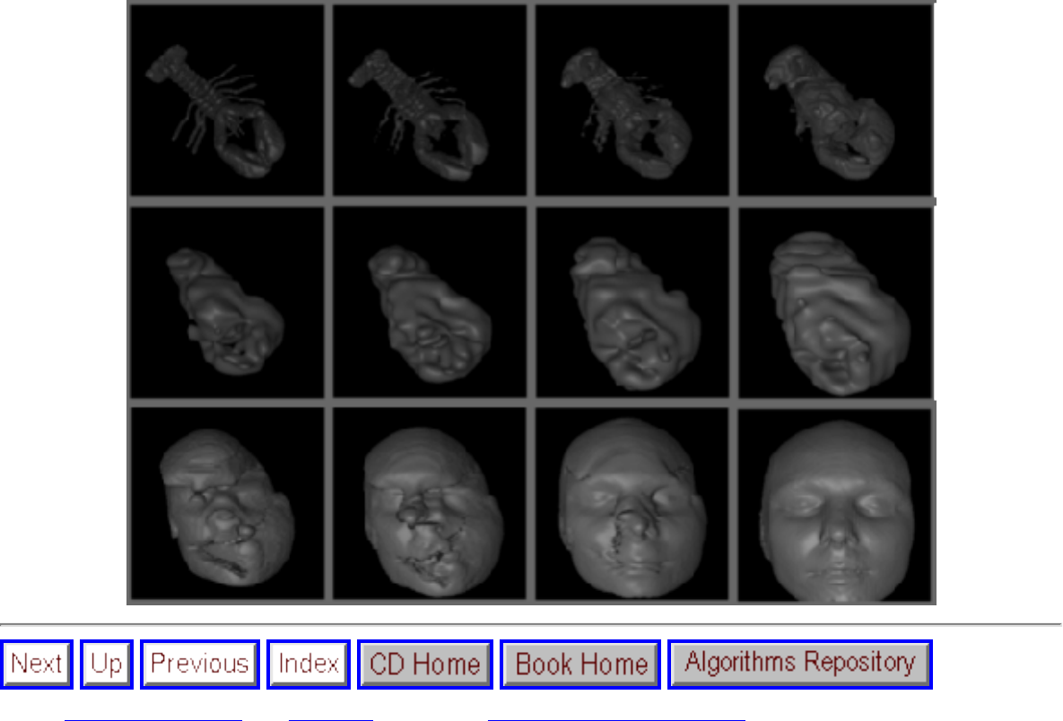
Lecture 14 - data structures for graphs
Next: Lecture 15 - DFS Up: No Title Previous: Lecture 13 - dynamic
Lecture 14 - data structures for graphs
Listen To Part 14-1
Problem Solving Techniques
Most important: make sure you understand exactly what the question is asking - if not, you have no hope
of answer it!!
Never be afraid to ask for another explanation of a problem until it is clear.
Play around with the problem by constructing examples to get insight into it.
Ask yourself questions. Does the first idea which comes into my head work? If not, why not?
Am I using all information that I am given about the problem?
Read Polya's book How to Solve it.
Listen To Part 14-2
16-1: The Euclidean traveling-salesman problem is the problem of determining the shortest closed tour
that connects a given set of n points in the plane.
Bentley suggested simplifying the problem by restricting attention to bitonic tours, that is tours which
start at the leftmost point, go strictly left to right to the rightmost point, and then go strictly right back to
the starting point.
file:///E|/LEC/LECTUR16/NODE14.HTM (1 of 12) [19/1/2003 1:35:05]
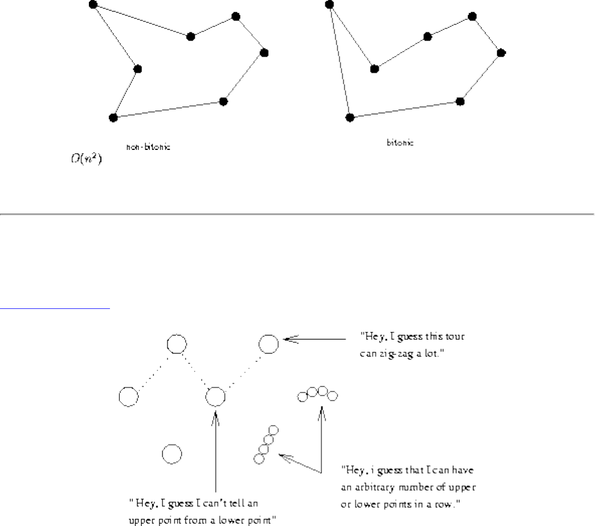
Lecture 14 - data structures for graphs
Describe an algorithm for finding the optimal bitonic tour. You may assume that no two points
have the same x-coordinate. (Hint: scan left to right, maintaining optimal possibilities for the two parts
of the tour.)
Make sure you understand what a bitonic tour is, or else it is hopeless.
First of all, play with the problem. Why isn't it trivial?
Listen To Part 14-3
Am I using all the information?
Why will they let us assume that no two x-coordinates are the same? What does the hint mean? What
happens if I scan from left to right?
If we scan from left to right, we get an open tour which uses all points to the left of our scan line.
file:///E|/LEC/LECTUR16/NODE14.HTM (2 of 12) [19/1/2003 1:35:05]
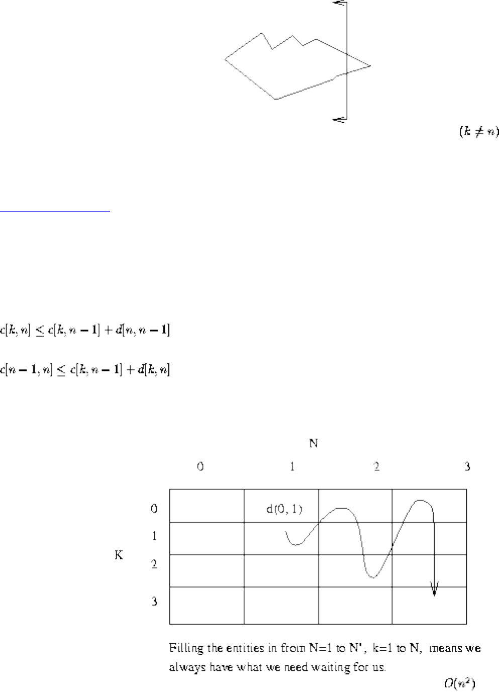
Lecture 14 - data structures for graphs
In the optimal tour, the kth point is connected to exactly one point to the left of k. Once I decide
which point that is, say x. I need the optimal partial tour where the two endpoints are x and k-1, because
if it isn't optimal I could come up with a better one.
Listen To Part 14-4
Hey, I have got a recurrence! And look, the two parameters which describe my optimal tour are the two
endpoints.
Let c[k,n] be the optimal cost partial tour where the two endpoints are k<n.
(when k < n-1)
c[0, 1]=d[0, 1]
c[n-1, n] takes O(n) to update, c[k, n] k<n-1 takes O(1) to update. Total time is .
But this doesn't quite give the tour, but just an open tour. We simply must figure where the last edge to n
file:///E|/LEC/LECTUR16/NODE14.HTM (3 of 12) [19/1/2003 1:35:05]
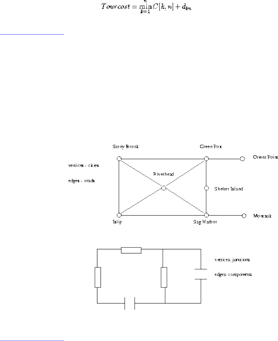
Lecture 14 - data structures for graphs
must go.
Listen To Part 15-1
Graphs
A graph G consists of a set of vertices V together with a set E of vertex pairs or edges.
Graphs are important because any binary relation is a graph, so graphs can be used to represent
essentially any relationship.
Example: A network of roads, with cities as vertices and roads between cities as edges.
Example: An electronic circuit, with junctions as vertices as components as edges.
To understand many problems, we must think of them in terms of graphs!
Listen To Part 15-2
The Friendship Graph
Consider a graph where the vertices are people, and there is an edge between two people if and only if
they are friends.
file:///E|/LEC/LECTUR16/NODE14.HTM (4 of 12) [19/1/2003 1:35:05]
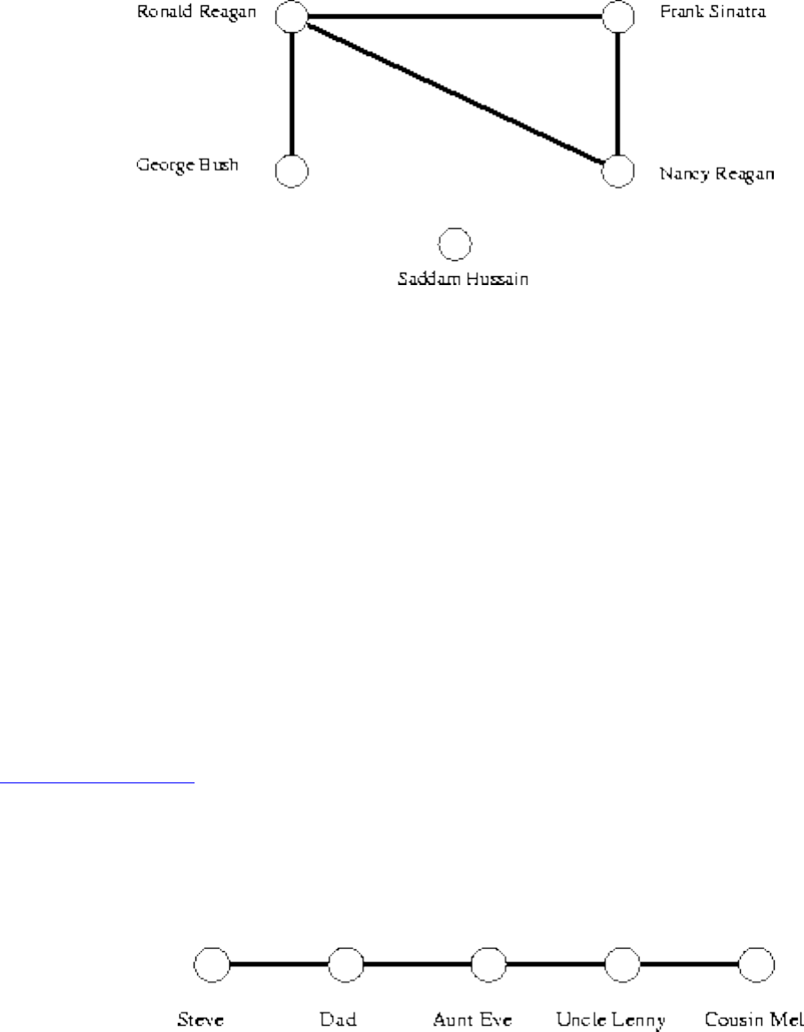
Lecture 14 - data structures for graphs
This graph is well-defined on any set of people: SUNY SB, New York, or the world.
What questions might we ask about the friendship graph?
● If I am your friend, does that mean you are my friend?
A graph is undirected if (x,y) implies (y,x). Otherwise the graph is directed. The ``heard-of'' graph
is directed since countless famous people have never heard of me! The ``had-sex-with'' graph is
presumably undirected, since it requires a partner.
● Am I my own friend?
An edge of the form (x,x) is said to be a loop. If x is y's friend several times over, that could be
modeled using multiedges, multiple edges between the same pair of vertices. A graph is said to be
simple if it contains no loops and multiple edges.
Listen To Part 15-3
● Am I linked by some chain of friends to the President?
A path is a sequence of edges connecting two vertices. Since Mel Brooks is my father's-sister's-
husband's cousin, there is a path between me and him!
● How close is my link to the President?
If I were trying to impress you with how tight I am with Mel Brooks, I would be much better off
saying that Uncle Lenny knows him than to go into the details of how connected I am to Uncle
Lenny. Thus we are often interested in the shortest path between two nodes.
● Is there a path of friends between any two people?
A graph is connected if there is a path between any two vertices. A directed graph is strongly
file:///E|/LEC/LECTUR16/NODE14.HTM (5 of 12) [19/1/2003 1:35:05]
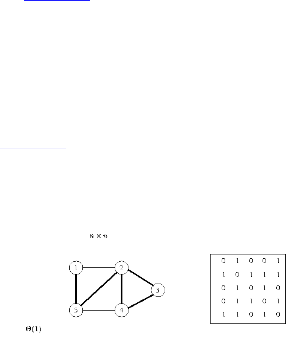
Lecture 14 - data structures for graphs
connected if there is a directed path between any two vertices.
● Who has the most friends?
The degree of a vertex is the number of edges adjacent to it.
Listen To Part 15-4
● What is the largest clique?
A social clique is a group of mutual friends who all hang around together. A graph theoretic
clique is a complete subgraph, where each vertex pair has an edge between them. Cliques are the
densest possible subgraphs. Within the friendship graph, we would expect that large cliques
correspond to workplaces, neighborhoods, religious organizations, schools, and the like.
● How long will it take for my gossip to get back to me?
A cycle is a path where the last vertex is adjacent to the first. A cycle in which no vertex repeats
(such as 1-2-3-1 verus 1-2-3-2-1) is said to be simple. The shortest cycle in the graph defines its
girth, while a simple cycle which passes through each vertex is said to be a Hamiltonian cycle.
Listen To Part 15-5
Data Structures for Graphs
There are two main data structures used to represent graphs.
Adjacency Matrices
An adjacency matrix is an matrix, where M[i,j] = 0 iff there is no edge from vertex i to vertex j
It takes time to test if (i,j) is in a graph represented by an adjacency matrix.
Can we save space if (1) the graph is undirected? (2) if the graph is sparse?
file:///E|/LEC/LECTUR16/NODE14.HTM (6 of 12) [19/1/2003 1:35:05]
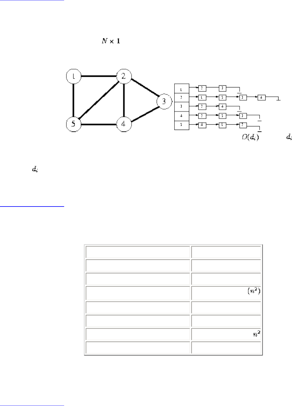
Lecture 14 - data structures for graphs
Listen To Part 15-6
Adjacency Lists
An adjacency list consists of a array of pointers, where the ith element points to a linked list of the
edges incident on vertex i.
To test if edge (i,j) is in the graph, we search the ith list for j, which takes , where is the degree of
the ith vertex.
Note that can be much less than n when the graph is sparse. If necessary, the two copies of each edge
can be linked by a pointer to facilitate deletions.
Listen To Part 15-7
Tradeoffs Between Adjacency Lists and Adjacency Matrices
Comparison Winner
Faster to test if (x, y) exists? matrices
Faster to find vertex degree? lists
Less memory on small graphs? lists (m+n) vs.
Less memory on big graphs? matrices (small win)
Edge insertion or deletion? matrices O(1)
Faster to traverse the graph? lists m+n vs.
Better for most problems? lists
Both representations are very useful and have different properties, although adjacency lists are probably
better for most problems.
Listen To Part 16-2
file:///E|/LEC/LECTUR16/NODE14.HTM (7 of 12) [19/1/2003 1:35:05]

Lecture 14 - data structures for graphs
Traversing a Graph
One of the most fundamental graph problems is to traverse every edge and vertex in a graph.
Applications include:
● Printing out the contents of each edge and vertex.
● Counting the number of edges.
● Identifying connected components of a graph.
For efficiency, we must make sure we visit each edge at most twice.
For correctness, we must do the traversal in a systematic way so that we don't miss anything.
Since a maze is just a graph, such an algorithm must be powerful enough to enable us to get out of an
arbitrary maze.
Listen To Part 16-3
Marking Vertices
The idea in graph traversal is that we must mark each vertex when we first visit it, and keep track of what
have not yet completely explored.
For each vertex, we can maintain two flags:
● discovered - have we ever encountered this vertex before?
● completely-explored - have we finished exploring this vertex yet?
We must also maintain a structure containing all the vertices we have discovered but not yet completely
explored.
Initially, only a single start vertex is considered to be discovered.
To completely explore a vertex, we look at each edge going out of it. For each edge which goes to an
undiscovered vertex, we mark it discovered and add it to the list of work to do.
Note that regardless of what order we fetch the next vertex to explore, each edge is considered exactly
twice, when each of its endpoints are explored.
Listen To Part 16-4
file:///E|/LEC/LECTUR16/NODE14.HTM (8 of 12) [19/1/2003 1:35:05]
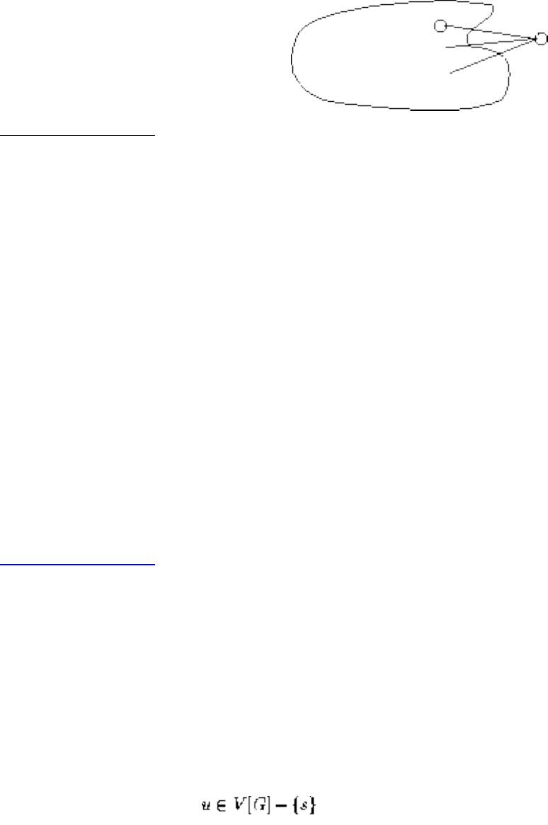
Lecture 14 - data structures for graphs
Correctness of Graph Traversal
Every edge and vertex in the connected component is eventually visited.
Suppose not, ie. there exists a vertex which was unvisited whose neighbor was visited. This neighbor will
eventually be explored so we would visit it:
Listen To Part 16-5
Traversal Orders
The order we explore the vertices depends upon what kind of data structure is used:
● Queue - by storing the vertices in a first-in, first out (FIFO) queue, we explore the oldest
unexplored vertices first. Thus our explorations radiate out slowly from the starting vertex,
defining a so-called breadth-first search.
● Stack - by storing the vertices in a last-in, first-out (LIFO) stack, we explore the vertices by
lurching along a path, constantly visiting a new neighbor if one is available, and backing up only
if we are surrounded by previously discovered vertices. Thus our explorations quickly wander
away from our starting point, defining a so-called depth-first search.
The three possible colors of each node reflect if it is unvisited (white), visited but unexplored (grey) or
completely explored (black).
Listen To Part 16-6
Breadth-First Search
BFS(G,s)
for each vertex do
file:///E|/LEC/LECTUR16/NODE14.HTM (9 of 12) [19/1/2003 1:35:05]
Lecture 14 - data structures for graphs
color[u] = white
, ie. the distance from
p[u] = NIL, ie. the parent in the BFS tree
color[u] = grey
d[] = 0
p[] = NIL
while do
u = head[Q]
for each do
if color[v] = white then
color[v] = gray
d[v] = d[u] + 1
p[v] = u
file:///E|/LEC/LECTUR16/NODE14.HTM (10 of 12) [19/1/2003 1:35:05]
Lecture 14 - data structures for graphs
enqueue[Q,v]
dequeue[Q]
color[u] = black
Listen To Part 16-8
Depth-First Search
DFS has a neat recursive implementation which eliminates the need to explicitly use a stack.
Discovery and final times are sometimes a convenience to maintain.
DFS(G)
for each vertex do
color[u] = white
parent[u] = nil
time = 0
for each vertex do
if color[u] = white then DFS-VISIT[u]
Initialize each vertex in the main routine, then do a search from each connected component. BFS must
also start from a vertex in each component to completely visit the graph.
file:///E|/LEC/LECTUR16/NODE14.HTM (11 of 12) [19/1/2003 1:35:05]
Lecture 14 - data structures for graphs
DFS-VISIT[u]
color[u] = grey (*u had been white/undiscovered*)
discover[u] = time
time = time+1
for each do
if color[v] = white then
parent[v] = u
DFS-VISIT(v)
color[u] = black (*now finished with u*)
finish[u] = time
time = time+1
Next: Lecture 15 - DFS Up: No Title Previous: Lecture 13 - dynamic
Algorithms
Mon Jun 2 09:21:39 EDT 1997
file:///E|/LEC/LECTUR16/NODE14.HTM (12 of 12) [19/1/2003 1:35:05]
Lecture 15 - DFS and BFS
Next: Lecture 16 - applications Up: No Title Previous: Lecture 14 - data
Lecture 15 - DFS and BFS
Listen To Part 15-8
23.1-5 - The square of a directed graph G=(V,E) is the graph such that iff for
some , both and ; ie. there is a path of exactly two edges.
Give efficient algorithms for both adjacency lists and matricies.
Given an adjacency matrix, we can check in constant time whether a given edge exists. To discover
whether there is an edge , for each possible intermediate vertex v we can check whether (u,v)
and (v,w) exist in O(1).
Since there are at most n intermediate vertices to check, and pairs of vertices to ask about, this takes
time.
With adjacency lists, we have a list of all the edges in the graph. For a given edge (u,v), we can run
through all the edges from v in O(n) time, and fill the results into an adjacency matrix of , which is
initially empty.
It takes O(mn) to construct the edges, and to initialize and read the adjacency matrix, a total of
O((n+m)n). Since unless the graph is disconnected, this is usually simplified to O(mn), and is
faster than the previous algorithm on sparse graphs.
Why is it called the square of a graph? Because the square of the adjacency matrix is the adjacency
matrix of the square! This provides a theoretically faster algorithm.
Listen To Part 16-10
BFS Trees
If BFS is performed on a connected, undirected graph, a tree is defined by the edges involved with the
discovery of new nodes:
file:///E|/LEC/LECTUR16/NODE15.HTM (1 of 8) [19/1/2003 1:35:08]
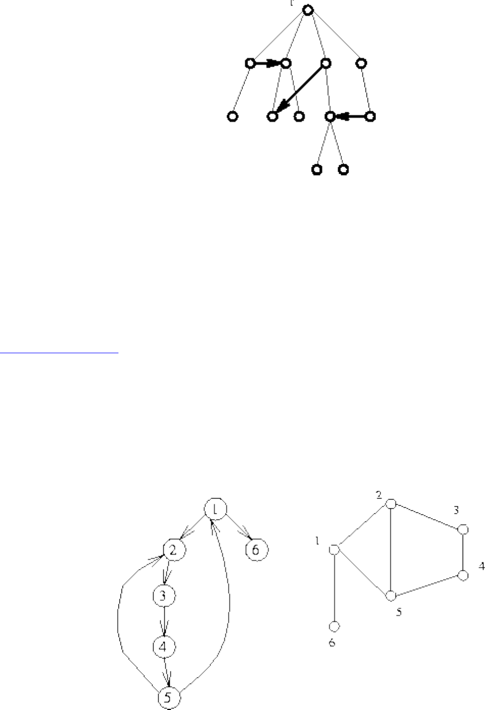
Lecture 15 - DFS and BFS
This tree defines a shortest path from the root to every other node in the tree.
The proof is by induction on the length of the shortest path from the root:
● Length = 1 First step of BFS explores all neighbors of the root. In an unweighted graph one edge
must be the shortest path to any node.
● Length = s Assume the BFS tree has the shortest paths up to length s-1. Any node at a distance of
will first be discovered by expanding a distance s-1 node.
Listen To Part 16-11
The key idea about DFS
A depth-first search of a graph organizes the edges of the graph in a precise way.
In a DFS of an undirected graph, we assign a direction to each edge, from the vertex which discover it:
In a DFS of a directed graph, every edge is either a tree edge or a black edge.
file:///E|/LEC/LECTUR16/NODE15.HTM (2 of 8) [19/1/2003 1:35:08]
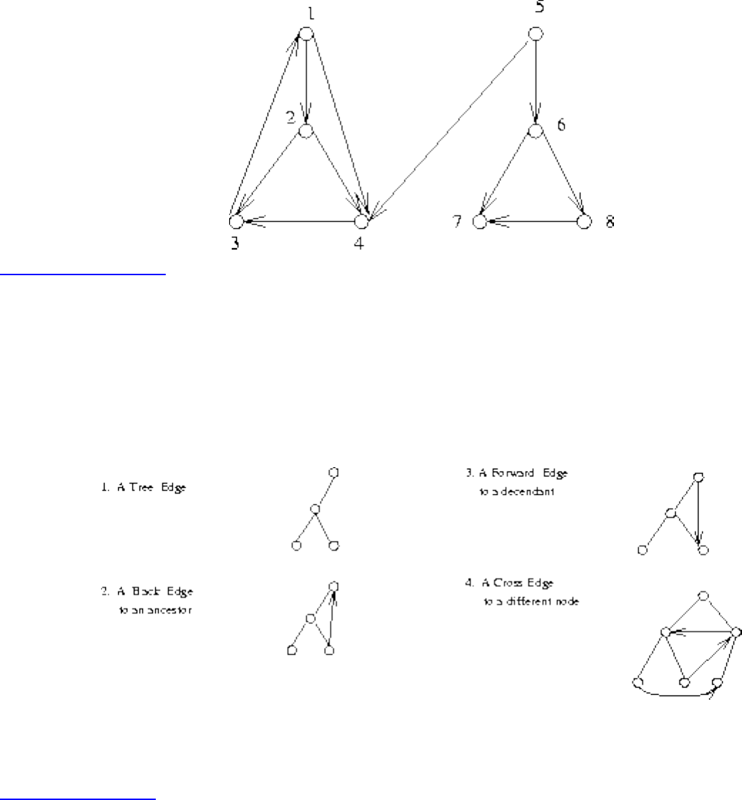
Lecture 15 - DFS and BFS
In a DFS of a directed graph, no cross edge goes to a higher numbered or rightward vertex. Thus, no
edge from 4 to 5 is possible:
Listen To Part 16-12
Edge Classification for DFS
What about the other edges in the graph? Where can they go on a search?
Every edge is either:
On any particular DFS or BFS of a directed or undirected graph, each edge gets classified as one of the
above.
Listen To Part 17-3
DFS Trees
The reason DFS is so important is that it defines a very nice ordering to the edges of the graph.
file:///E|/LEC/LECTUR16/NODE15.HTM (3 of 8) [19/1/2003 1:35:08]
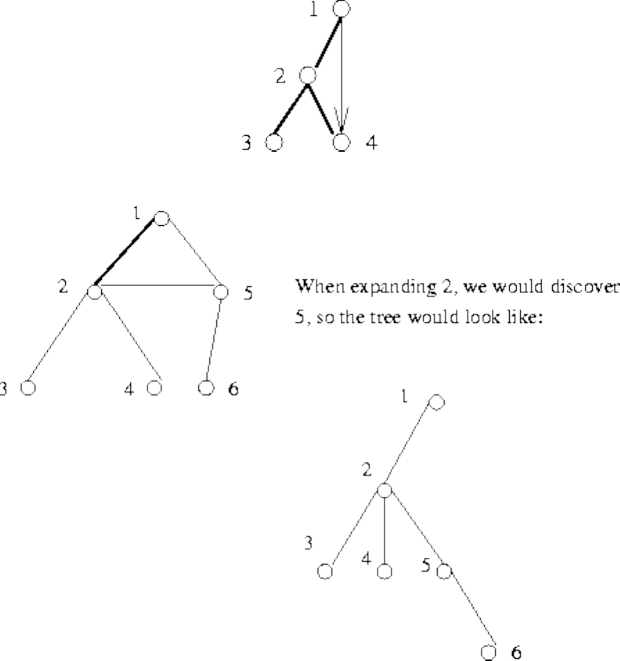
Lecture 15 - DFS and BFS
In a DFS of an undirected graph, every edge is either a tree edge or a back edge.
Why? Suppose we have a forward edge. We would have encountered (4,1) when expanding 4, so this is a
back edge.
Suppose we have a cross-edge
Paths in search trees
Where is the shortest path in a DFS?
file:///E|/LEC/LECTUR16/NODE15.HTM (4 of 8) [19/1/2003 1:35:08]
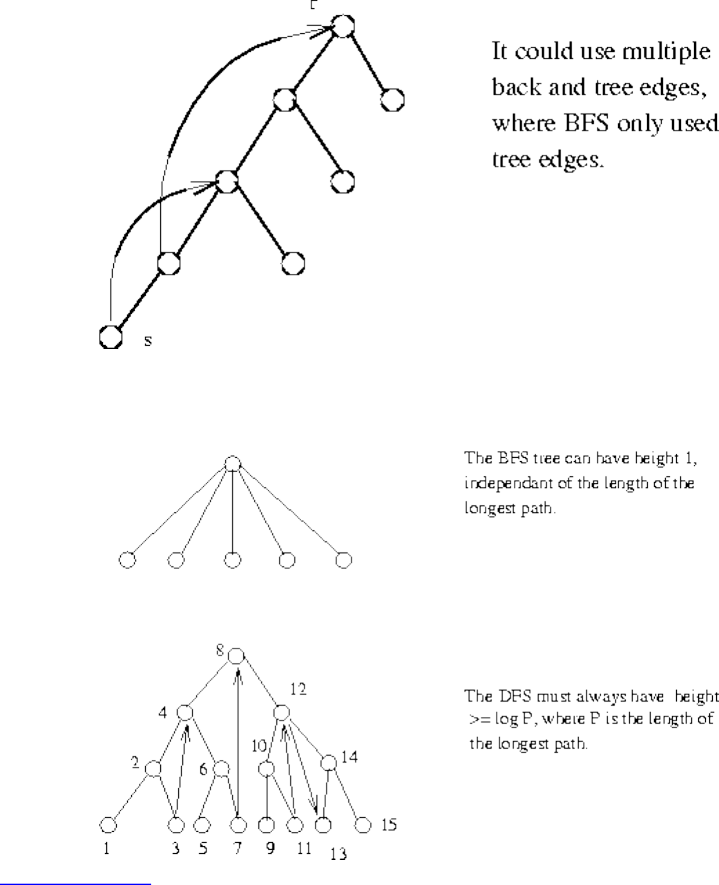
Lecture 15 - DFS and BFS
It could use multiple back and tree edges, where BFS only uses tree edges.
DFS gives a better approximation of the longest path than BFS.
Listen To Part 17-4
Topological Sorting
A directed, acyclic graph is a directed graph with no directed cycles.
file:///E|/LEC/LECTUR16/NODE15.HTM (5 of 8) [19/1/2003 1:35:08]
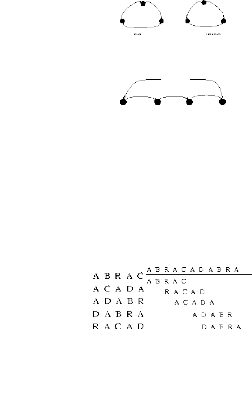
Lecture 15 - DFS and BFS
A topological sort of a graph is an ordering on the vertices so that all edges go from left to right.
Only a DAG can have a topological sort.
Any DAG has (at least one) topological sort.
Listen To Part 17-5
Applications of Topological Sorting
Topological sorting is often useful in scheduling jobs in their proper sequence. In general, we can use it
to order things given constraints, such as a set of left-right constraints on the positions of objects.
Example: Dressing schedule from CLR.
Example: Identifying errors in DNA fragment assembly.
Certain fragments are constrained to be to the left or right of other fragments, unless there are errors.
Solution - build a DAG representing all the left-right constraints. Any topological sort of this DAG is a
consistant ordering. If there are cycles, there must be errors.
A DFS can test if a graph is a DAG (it is iff there are no back edges - forward edges are allowed for DFS
on directed graph).
Listen To Part 17-6
file:///E|/LEC/LECTUR16/NODE15.HTM (6 of 8) [19/1/2003 1:35:08]
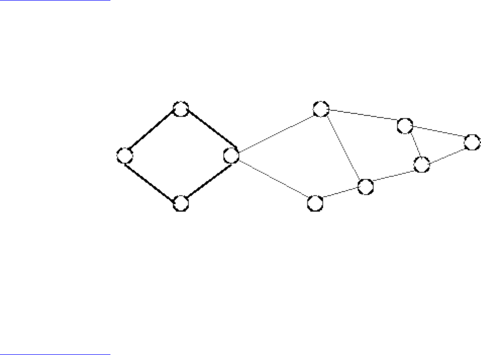
Lecture 15 - DFS and BFS
Algorithm
Theorem: Arranging vertices in decreasing order of DFS finishing time gives a topological sort of a
DAG.
Proof: Consider any directed edge u,v, when we encounter it during the exploration of vertex u:
● If v is white - we then start a DFS of v before we continue with u.
● If v is grey - then u, v is a back edge, which cannot happen in a DAG.
● If v is black - we have already finished with v, so f[v]<f[u].
Thus we can do topological sorting in O(n+m) time.
Listen To Part 17-8
Articulation Vertices
Suppose you are a terrorist, seeking to disrupt the telephone network. Which station do you blow up?
An articulation vertex is a vertex of a connected graph whose deletion disconnects the graph.
Clearly connectivity is an important concern in the design of any network.
Articulation vertices can be found in O(n(m+n)) - just delete each vertex to do a DFS on the remaining
graph to see if it is connected.
Listen To Part 17-9
A Faster O(n+m) DFS Algorithm
Theorem: In a DFS tree, a vertex v (other than the root) is an articulation vertex iff v is not a leaf and
some subtree of v has no back edge incident until a proper ancestor of v.
file:///E|/LEC/LECTUR16/NODE15.HTM (7 of 8) [19/1/2003 1:35:08]
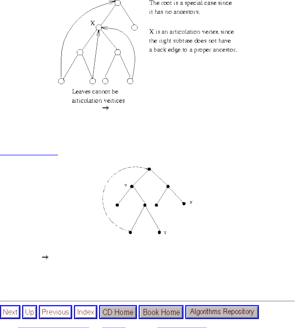
Lecture 15 - DFS and BFS
Proof: (1) v is an articulation vertex v cannot be a leaf.
Why? Deleting v must seperate a pair of vertices x and y. Because of the other tree edges, this cannot
happen unless y is a decendant of v.
Listen To Part 17-10
v separating x,y implies there is no back edge in the subtree of y to a proper ancestor of v.
(2) Conditions v is a non-root articulation vertex. v separates any ancestor of v from any decendant in
the appropriate subtree.
Actually implementing this test in O(n+m) is tricky - but believable once you accept this theorem.
Next: Lecture 16 - applications Up: No Title Previous: Lecture 14 - data
Algorithms
Mon Jun 2 09:21:39 EDT 1997
file:///E|/LEC/LECTUR16/NODE15.HTM (8 of 8) [19/1/2003 1:35:08]
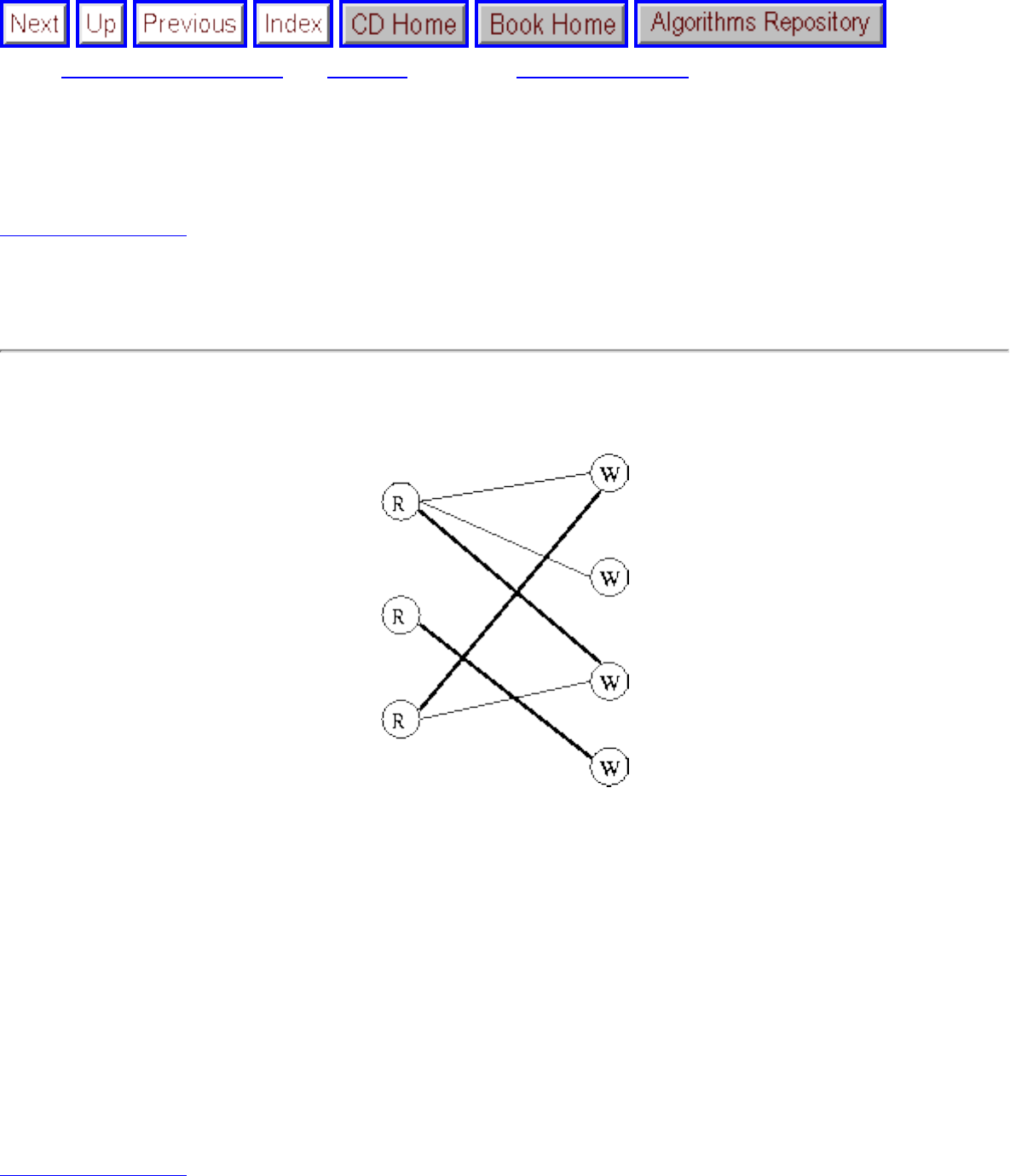
Lecture 16 - applications of DFS and BFS
Next: Lecture 17 - minimum Up: No Title Previous: Lecture 15 - DFS
Lecture 16 - applications of DFS and BFS
Listen To Part 16-1
23.2-6 Give an efficient algorithm to test if a graph is bipartite.
Bipartite means the vertices can be colored red or black such that no edge links vertices of the same
color.
Suppose we color a vertex red - what color must its neighbors be? black!
We can augment either BFS or DFS when we first discover a new vertex, color it opposited its parents,
and for each other edge, check it doesn't link two vertices of the same color. The first vertex in any
connected component can be red or black!
Bipartite graphs arise in many situations, and special algorithms are often available for them. What is the
interpretation of a bipartite ``had-sex-with'' graph?
How would you break people into two groups such that no group contains a pair of people who hate each
other?
Listen To Part 17-1
23.4-3 Give an O(n) algorithm to test whether an undirected graph contains a cycle.
file:///E|/LEC/LECTUR16/NODE16.HTM (1 of 5) [19/1/2003 1:35:10]
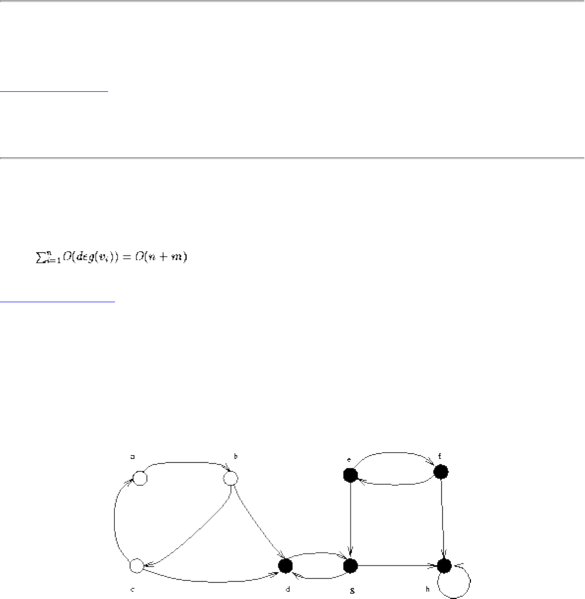
Lecture 16 - applications of DFS and BFS
If you do a DFS, you have a cycle iff you have a back edge. This gives an O(n+m) algorithm. But where
does the m go? If the graph contains more than n-1 edges, it must contain a cycle! Thus we never need
look at more than n edges if we are given an adjacency list representation!
Listen To Part 17-7
23.4-5 Show that you can topologically sort in O(n+m) by repeatedly deleting vertices of degree 0.
The correctness of this algorithm follows since in a DAG there must always be a vertex of indegree 0,
and such a vertex can be first in topological sort. Suppose each vertex is initialized with its indegree (do
DFS on G to get this). Deleting a vertex takes O(degree v). Reduce the indegree of each efficient vertex -
and keep a list of degree-0 vertices to delete next.
Time:
Listen To Part 17-12
Strongly Connected Components
A directed graph is strongly connected iff there is a directed path between any two vertices.
The strongly connected components of a graph is a partition of the vertices into subsets (maximal) such
that each subset is strongly connected.
Observe that no vertex can be in two maximal components, so it is a partition.
file:///E|/LEC/LECTUR16/NODE16.HTM (2 of 5) [19/1/2003 1:35:10]
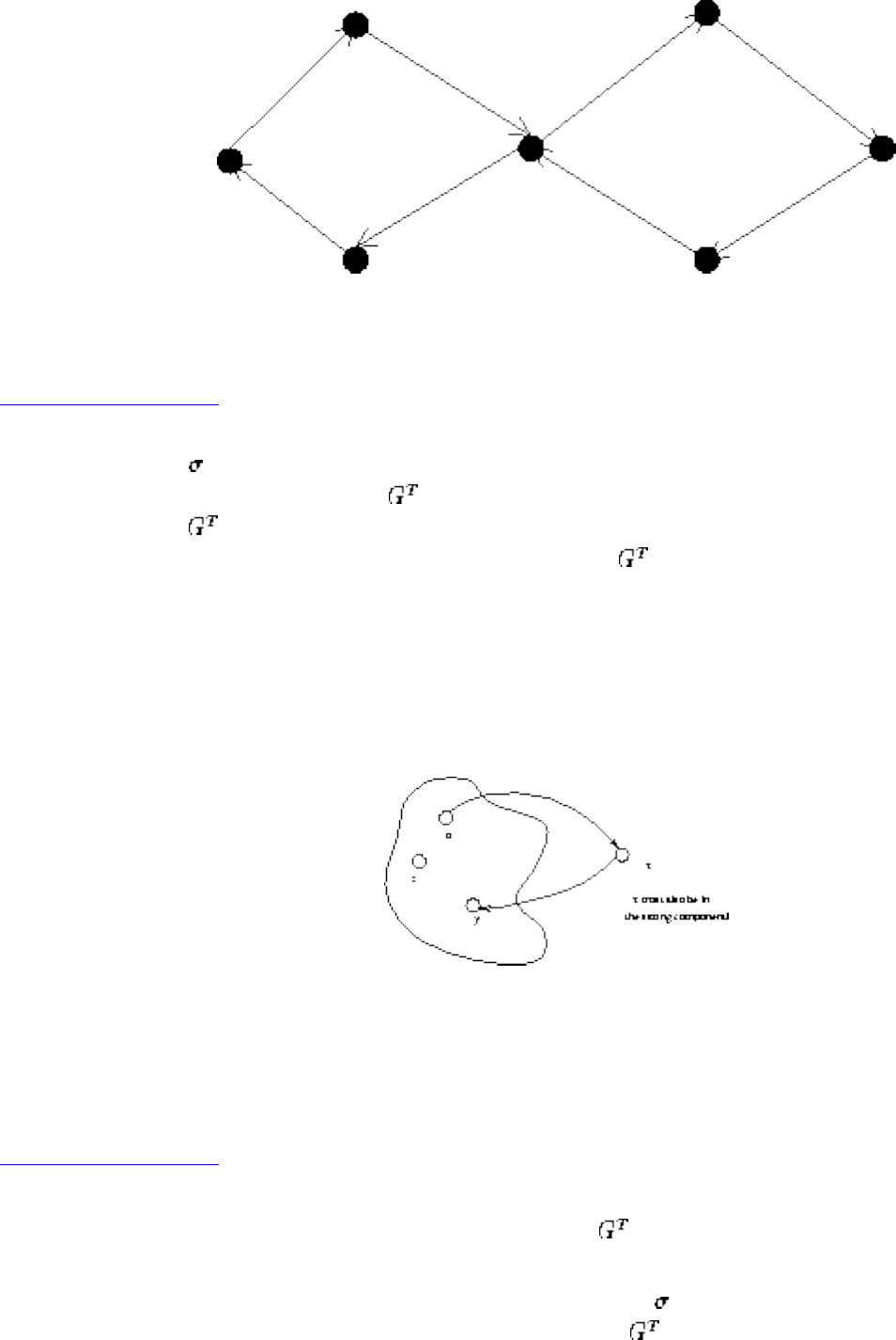
Lecture 16 - applications of DFS and BFS
There is an amazingly elegant, linear time algorithm to find the strongly connected components of a
directed graph, using DFS.
Listen To Part 17-13
● Call DFS( ) to compute finishing times for each vertex.
● Compute the transpose graph (reverse all edges in G)
● Call DFS( ), but order the vertices in decreasing order of finish time.
● The vertices of each DFS tree in the forest of DFS( ) is a strongly connected component.
This algorithm takes O(n+m), but why does it compute strongly connected components?
Lemma: If two vertices are in the same strong component, no path between them ever leaves the
component.
Lemma: In any DFS forest, all vertices in the same strongly connected component are in the same tree.
Proof: Consider the first vertex v in the component to be discovered. Everything in the component is
reachable from it, so we will traverse it before finishing with v.
Listen To Part 17-14
What does DFS( , v) Do?
It tells you what vertices have directed paths to v, while DFS( ,v) tells what vertices have directed paths
from v. But why must any vertex in the search tree of DFS( , v) also have a path from u?
file:///E|/LEC/LECTUR16/NODE16.HTM (3 of 5) [19/1/2003 1:35:10]
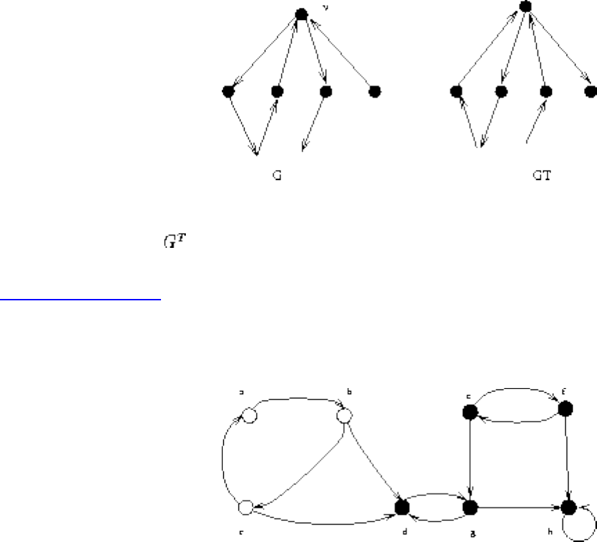
Lecture 16 - applications of DFS and BFS
Because there is no edge from any previous DFS tree into the last tree!! Because we ordered the vertices
by decreasing order of finish time, we can peel off the strongly connected components from right to left
just be doing a DFS( ).
Listen To Part 17-16
Example of Strong Components Algorithm
9, 10, 11, 12 can reach 9, oldest remaining finished is 5.
5, 6, 8 can reach 5, oldest remaining is 7.
7 can reach 7, oldest remaining is 1.
1, 2, 3 can reach 1, oldest remaining is 4.
4 can reach 4.
file:///E|/LEC/LECTUR16/NODE16.HTM (4 of 5) [19/1/2003 1:35:10]
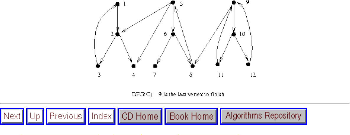
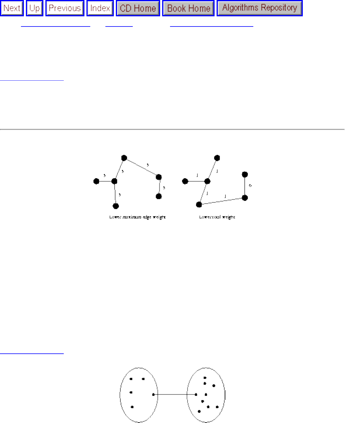
Lecture 17 - minimum spanning trees
Next: Lecture 18 - shortest Up: No Title Previous: Lecture 16 - applications
Lecture 17 - minimum spanning trees
Listen To Part 19-4
24.2-6 Describe an efficent algorithm that, given an undirected graph G, determines a spanning tree G
whose largest edge weight is minimum over all spanning trees of G.
First, make sure you understand the question
``Hey, doesn't Kruskal's algorithm do something like this.''
Certainly! Since Krushal's algorithm considers the edges in order of increasing weight, and stops the
moment these edges form a connected graph, the tree it gives must minimize the edge weight.
``Hey, but then why doesn't Prim's algorithm also work?''
It gives the same thing as Kruskal's algorithm, so it must be true that any minimum spanning tree
minimizes the maximum edge weight!
Proof: Give me a MST and consider the largest edge weight,
Listen To Part 19-5
file:///E|/LEC/LECTUR16/NODE17.HTM (1 of 11) [19/1/2003 1:35:14]
Lecture 17 - minimum spanning trees
Deleting it disconnects the MST. If there was a lower edge connects the two subtrees, I didn't have a
MST!
Listen To Part 18-2
Minimum Spanning Trees
A tree is a connected graph with no cycles. A spanning tree is a subgraph of G which has the same set of
vertices of G and is a tree.
A minimum spanning tree of a weighted graph G is the spanning tree of G whose edges sum to minimum
weight.
There can be more than one minimum spanning tree in a graph consider a graph with identical weight
edges.
The minimum spanning tree problem has a long history - the first algorithm dates back at least to 1926!.
Minimum spanning tree is always taught in algorithm courses since (1) it arises in many applications, (2)
it is an important example where greedy algorithms always give the optimal answer, and (3) Clever data
structures are necessary to make it work.
In greedy algorithms, we make the decision of what next to do by selecting the best local option from all
available choices - without regard to the global structure.
Listen To Part 18-3
Applications of Minimum Spanning Trees
Minimum spanning trees are useful in constructing networks, by describing the way to connect a set of
sites using the smallest total amount of wire. Much of the work on minimum spanning (and related
Steiner) trees has been conducted by the phone company.
Minimum spanning trees provide a reasonable way for clustering points in space into natural groups.
When the cities are points in the Euclidean plane, the minimum spanning tree provides a good heuristic
for traveling salesman problems. The optimum traveling salesman tour is at most twice the length of the
minimum spanning tree.
file:///E|/LEC/LECTUR16/NODE17.HTM (2 of 11) [19/1/2003 1:35:14]

Lecture 17 - minimum spanning trees
Listen To Part 18-4
Prim's Algorithm
If G is connected, every vertex will appear in the minimum spanning tree. If not, we can talk about a
minimum spanning forest.
Prim's algorithm starts from one vertex and grows the rest of the tree an edge at a time.
As a greedy algorithm, which edge should we pick? The cheapest edge with which can grow the tree by
one vertex without creating a cycle.
During execution we will label each vertex as either in the tree, fringe - meaning there exists an edge
from a tree vertex, or unseen - meaning the vertex is more than one edge away.
Select an arbitrary vertex to start.
While (there are fringe vertices)
select minimum weight edge between tree and fringe
add the selected edge and vertex to the tree
Clearly this creates a spanning tree, since no cycle can be introduced via edges between tree and fringe
vertices, but is it minimum?
file:///E|/LEC/LECTUR16/NODE17.HTM (3 of 11) [19/1/2003 1:35:14]
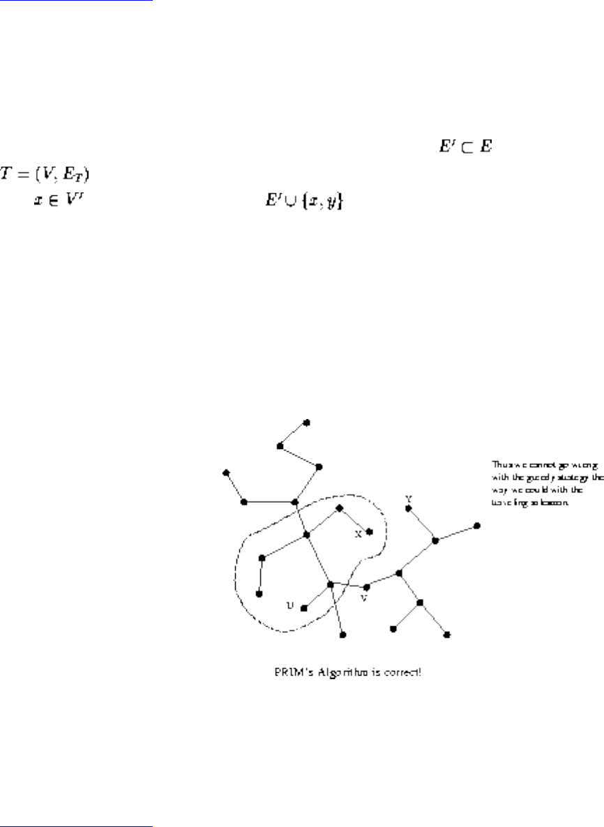
Lecture 17 - minimum spanning trees
Listen To Part 18-5
Why is Prim's algorithm correct?
Don't be scared by the proof - the reason is really quite basic:
Theorem: Let G be a connected, weighted graph and let be a subset of the edges in a MST
. Let V' be the vertices incident with edges in E'. If (x,y) is an edge of minimum weight such
that and y is not in V', then is a subset of a minimum spanning tree.
Proof: If the edge is in T, this is trivial.
Suppose (x,y) is not in T Then there must be a path in T from x to y since T is connected. If (v,w) is the
first edge on this path with one edge in V', if we delete it and replace it with (x, y) we get a spanning tree.
This tree must have smaller weight than T, since W(v,w)>W(x,y). Thus T could not have been the MST.
Prim's Algorithm is correct!
Thus we cannot go wrong with the greedy strategy the way we could with the traveling salesman
problem.
Listen To Part 18-6
But how fast is Prim's?
That depends on what data structures are used. In the simplest implementation, we can simply mark each
vertex as tree and non-tree and search always from scratch:
file:///E|/LEC/LECTUR16/NODE17.HTM (4 of 11) [19/1/2003 1:35:14]
Lecture 17 - minimum spanning trees
Select an arbitrary vertex to start.
While (there are non-tree vertices)
select minimum weight edge between tree and fringe
add the selected edge and vertex to the tree
This can be done in O(n m) time, by doing a DFS or BFS to loop through all edges, with a constant time
test per edge, and a total of n iterations.
Can we do faster? If so, we need to be able to identify fringe vertices and the minimum cost edge
associated with it, fast. We will augment an adjacency list with fields maintaining fringe information.
Vertex:
fringelink pointer to next vertex in fringe list.
fringe weight cheapest edge linking v to l.
parent other vertex with v having fringeweight.
status intree, fringe, unseen.
adjacency list the list of edges.
Listen To Part 18-8
Finding the minimum weight fringe-edge takes O(n) time - just bump through fringe list.
After adding a vertex to the tree, running through its adjacency list to update the cost of adding fringe
vertices (there may be a cheaper way through the new vertex) can be done in O(n) time.
Total time is .
Listen To Part 18-9
Kruskal's Algorithm
file:///E|/LEC/LECTUR16/NODE17.HTM (5 of 11) [19/1/2003 1:35:14]
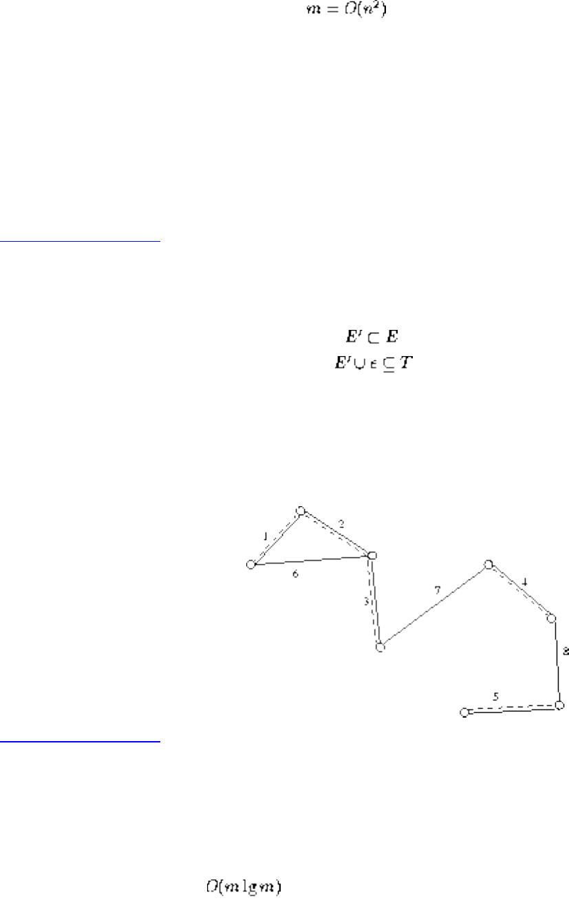
Lecture 17 - minimum spanning trees
Since an easy lower bound argument shows that every edge must be looked at to find the minimum
spanning tree, and the number of edges , Prim's algorithm is optimal in the worst case. Is that
all she wrote?
The complexity of Prim's algorithm is independent of the number of edges. Can we do better with sparse
graphs? Yes!
Kruskal's algorithm is also greedy. It repeatedly adds the smallest edge to the spanning tree that does not
create a cycle. Obviously, this gives a spanning tree, but is it minimal?
Listen To Part 18-10
Why is Kruskal's algorithm correct?
Theorem: Let G be a weighted graph and let . If E' is contained in a MST T and e is the smallest
edge in E-E' which does not create a cycle, .
Proof: As before, suppose e is not in T. Adding e to T makes a cycle. Deleting another edge from this
cycle leaves a connected graph, and if it is one from E-E' the cost of this tree goes down. Since such an
edge exists, T could not be a MST.
Listen To Part 18-11
How fast is Kruskal's algorithm?
What is the simplest implementation?
● Sort the m edges in time.
● For each edge in order, test whether it creates a cycle the forest we have thus far built - if so
discard, else add to forest. With a BFS/DFS, this can be done in O(n) time (since the tree has at
most n edges).
file:///E|/LEC/LECTUR16/NODE17.HTM (6 of 11) [19/1/2003 1:35:14]
Lecture 17 - minimum spanning trees
The total time is O(mn), but can we do better?
Kruskal's algorithm builds up connected components. Any edge where both vertices are in the same
connected component create a cycle. Thus if we can maintain which vertices are in which component
fast, we do not have test for cycles!
Put the edges in a heap
count=0
while (count < n-1) do
get next edge (v,w)
if (component (v) component(w))
add to T
component (v)=component(w)
If we can test components in , we can find the MST in !
Question: Is better than ?
Listen To Part 19-6
Union-Find Programs
Our analysis that Kruskal's MST algorithm is requires a fast way to test whether an edge links
two vertices in the same connected component.
Thus we need a data structure for maintaining sets which can test if two elements are in the same and
file:///E|/LEC/LECTUR16/NODE17.HTM (7 of 11) [19/1/2003 1:35:14]

Lecture 17 - minimum spanning trees
merge two sets together. These can be implemented by UNION and FIND operations:
Is
t= Find
u= Find
Return (Is t=u?)
Make
Union(t, u)
Find returns the name of the set and Union sets the members of t to have the same name as u.
We are interested in minimizing the time it takes to execute any sequence of unions and finds.
A simple implementation is to represent each set as a tree, with pointers from a node to its parent. Each
element is contained in a node, and the name of the set is the key at the root:
Listen To Part 19-7
file:///E|/LEC/LECTUR16/NODE17.HTM (8 of 11) [19/1/2003 1:35:14]
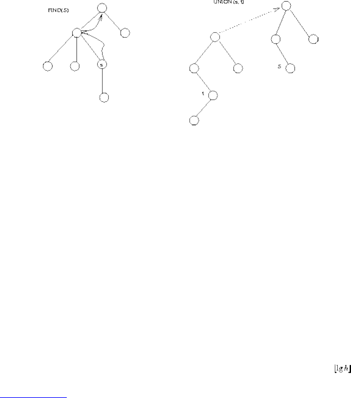
Lecture 17 - minimum spanning trees
In the worst case, these structures can be very unbalanced:
For i = 1 to n/2 do
UNION(i,i+1)
For i = 1 to n/2 do
FIND(1)
We want the limit the height of our trees which are effected by UNIONs. When we union, we can make
the tree with fewer nodes the child.
Since the number of nodes is related to the height, the height of the final tree will increase only if both
subtrees are of equal height!
Lemma: If Union(t,v) attaches the root of v as a subtree of t iff the number of nodes in t is greater than or
equal to the number in v, after any sequence of unions, any tree with h/4 nodes has height at most .
Listen To Part 19-8
Proof: By induction on the number of nodes k, k=1 has height 0.
file:///E|/LEC/LECTUR16/NODE17.HTM (9 of 11) [19/1/2003 1:35:14]
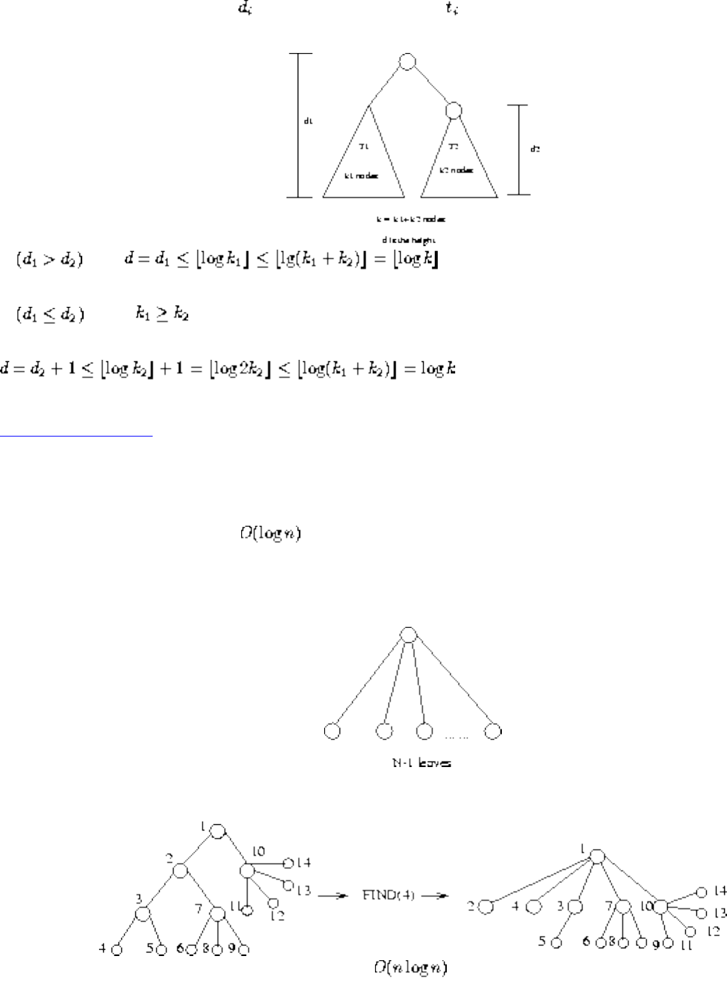
Lecture 17 - minimum spanning trees
Assume true to k-1 nodes. Let be the height of the tree
If then
If , then .
Listen To Part 19-9
Can we do better?
We can do unions and finds in , good enough for Kruskal's algorithm. But can we do better?
The ideal Union-Find tree has depth 1:
On a find, if we are going down a path anyway, why not change the pointers to point to the root?
This path compression will let us do better than for n union-finds.
file:///E|/LEC/LECTUR16/NODE17.HTM (10 of 11) [19/1/2003 1:35:14]

Lecture 17 - minimum spanning trees
O(n)? Not quite ... Difficult analysis shows that it takes time, where is the inverse
Ackerman function and number of atoms in the universe)=5.
Next: Lecture 18 - shortest Up: No Title Previous: Lecture 16 - applications
Algorithms
Mon Jun 2 09:21:39 EDT 1997
file:///E|/LEC/LECTUR16/NODE17.HTM (11 of 11) [19/1/2003 1:35:14]
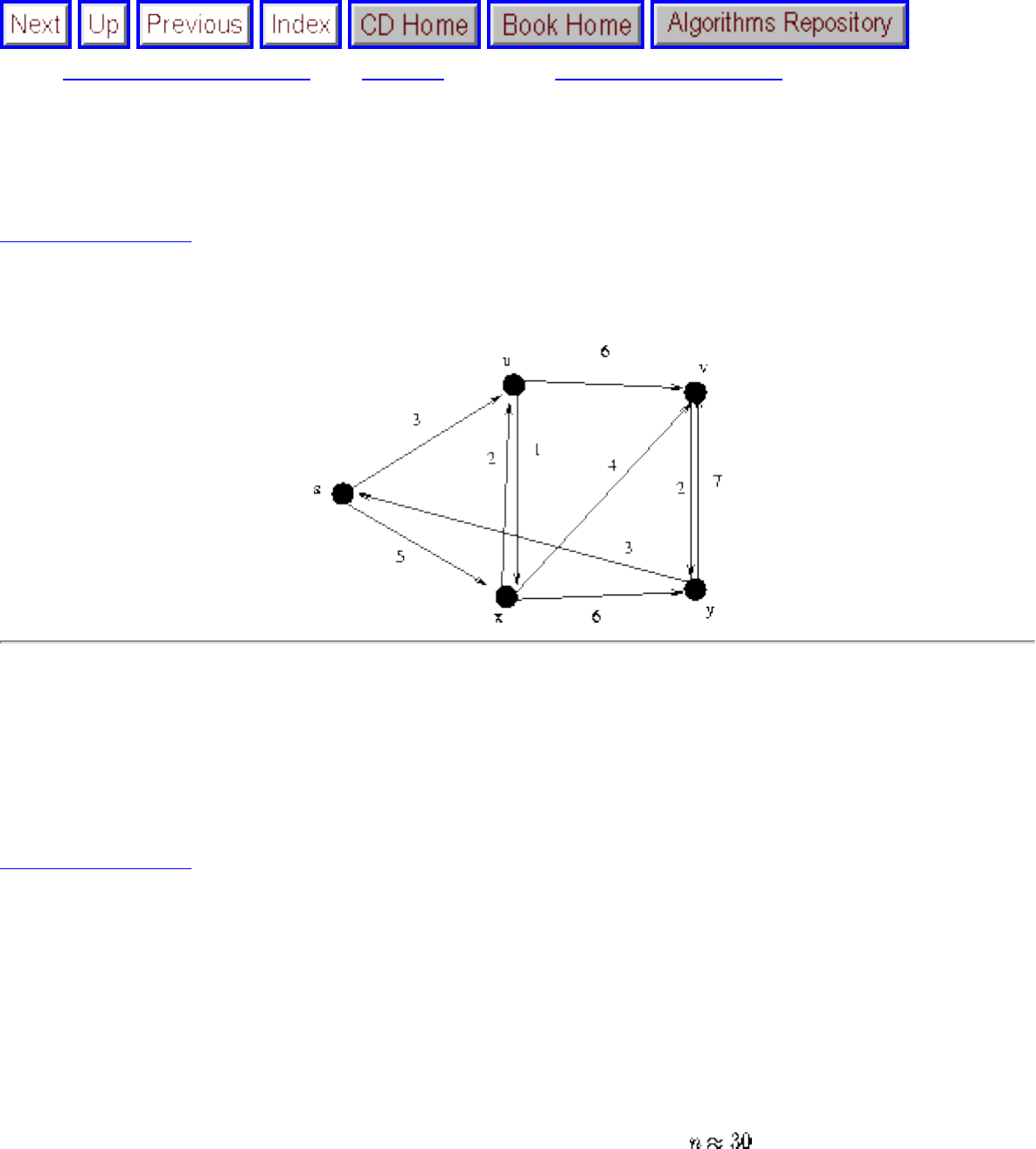
Lecture 18 - shortest path algorthms
Next: Lecture 19 - satisfiability Up: No Title Previous: Lecture 17 - minimum
Lecture 18 - shortest path algorthms
Listen To Part 20-7
25.1-1 Give two more shortest path trees for the following graph:
Run through Dijkstra's algorithm, and see where there are ties which can be arbitrarily selected.
There are two choices for how to get to the third vertex x, both of which cost 5.
There are two choices for how to get to vertex v, both of which cost 9.
Listen To Part 19-1
Lessons from the Backtracking contest
● As predicted, the speed difference between the fastest programs and average program dwarfed the
difference between a supercomputer and a microcomputer. Algorithms have a bigger impact on
performance than hardware!
● Different algorithms perform differently on different data. Thus even hard problems may be
tractable on the kind of data you might be interested in.
● None of the programs could efficiently handle all instances for . We will find out why after
the midterm, when we discuss NP-completeness.
● Many of the fastest programs were very short and simple (KISS). My bet is that many of the
enhancements students built into them actually showed them down! This is where profiling can
come in handy.
file:///E|/LEC/LECTUR16/NODE18.HTM (1 of 10) [19/1/2003 1:35:18]

Lecture 18 - shortest path algorthms
● The fast programs were often recursive.
Listen To Part 19-3
Winning Optimizations
● Finding a good initial solution via randomization or heuristic improvement helped by establishing
a good upper bound, to constrict search.
● Using half the largest vertex degree as a lower bound similarly constricted search.
● Pruning a partial permutation the instant an edge was the target made the difference in going
from (say) 8 to 18.
● Positioning the partial permutation vertices separated by b instead of 1 meant significantly earlier
cutoffs, since any edge does the job.
● Mirror symmetry can only save a factor of 2, but perhaps more could follow from partitioning the
vertices into equivalence classes by the same neighborhood.
Listen To Part 19-10
Shortest Paths
Finding the shortest path between two nodes in a graph arises in many different applications:
● Transportation problems - finding the cheapest way to travel between two locations.
● Motion planning - what is the most natural way for a cartoon character to move about a simulated
environment.
● Communications problems - how look will it take for a message to get between two places?
Which two locations are furthest apart, ie. what is the diameter of the network.
Listen To Part 20-1
Shortest Paths and Sentence Disambiguation
In our work on reconstructing text typed on an (overloaded) telephone keypad, we had to select which of
many possible interpretations was most likely.
file:///E|/LEC/LECTUR16/NODE18.HTM (2 of 10) [19/1/2003 1:35:18]
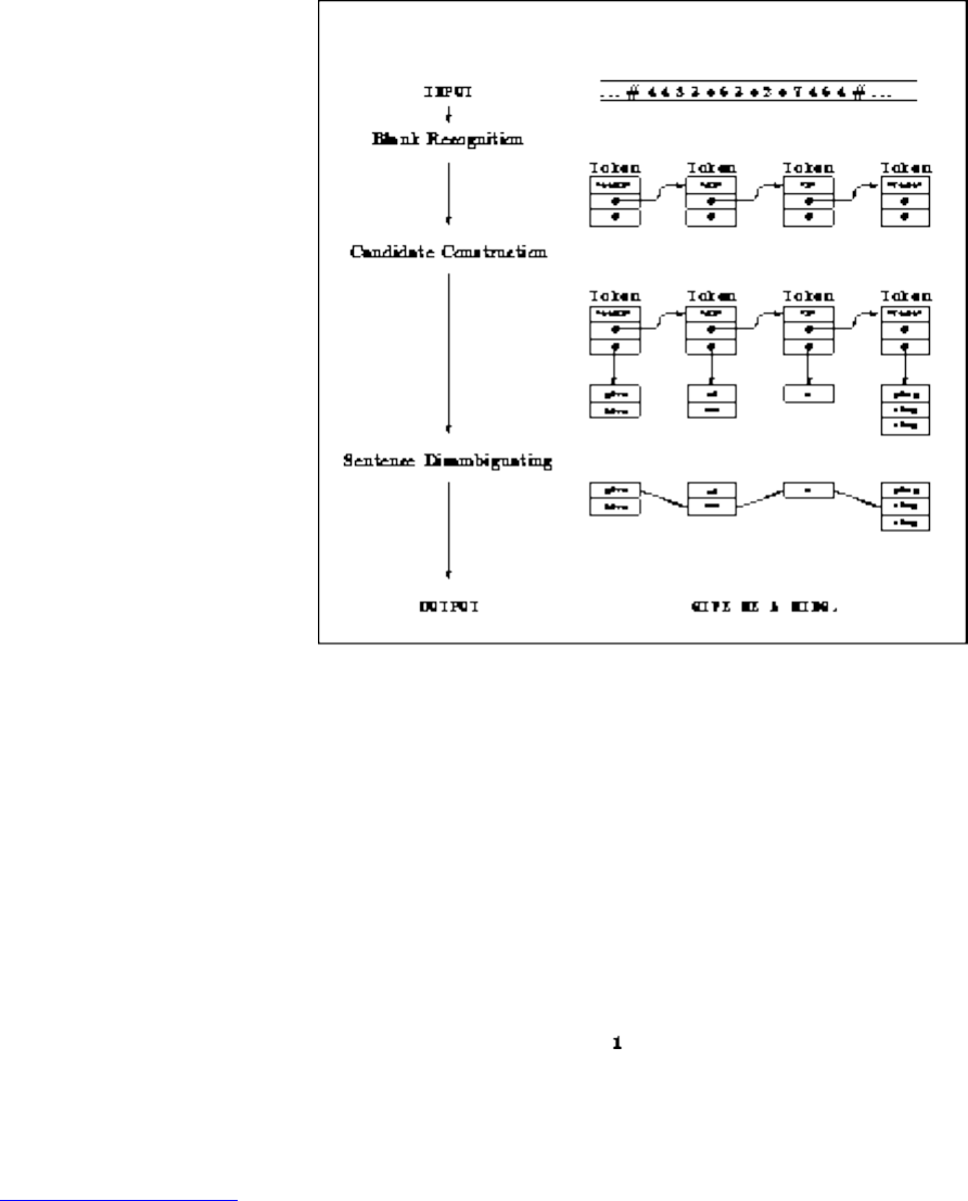
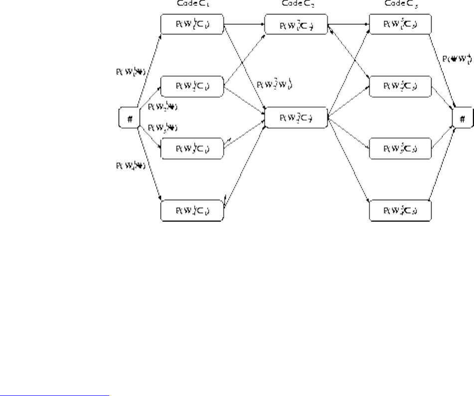
Lecture 18 - shortest path algorthms
The weight of each edge is a function of the probability that these two words will be next to each other in
a sentence. `hive me' would be less than `give me', for example.
The final system worked extremely well - identifying over 99% of characters correctly based on
grammatical and statistical constraints.
Dynamic programming (the Viterbi algorithm) can be used on the sentences to obtain the same results,
by finding the shortest paths in the underlying DAG.
Listen To Part 20-3
Finding Shortest Paths
In an unweighted graph, the cost of a path is just the number of edges on the shortest path, which can be
found in O(n+m) time via breadth-first search.
In a weighted graph, the weight of a path between two vertices is the sum of the weights of the edges on
a path.
BFS will not work on weighted graphs because sometimes visiting more edges can lead to shorter
distance, ie. 1+1+1+1+1+1+1 < 10.
Note that there can be an exponential number of shortest paths between two nodes - so we cannot report
all shortest paths efficiently.
Note that negative cost cycles render the problem of finding the shortest path meaningless, since you can
always loop around the negative cost cycle more to reduce the cost of the path.
file:///E|/LEC/LECTUR16/NODE18.HTM (4 of 10) [19/1/2003 1:35:18]
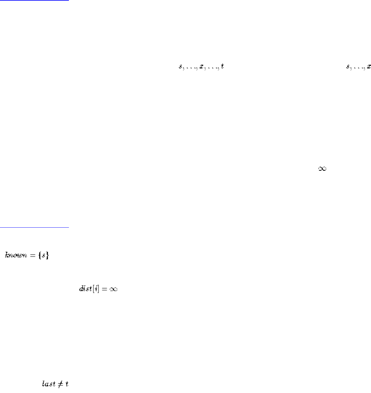
Lecture 18 - shortest path algorthms
Thus in our discussions, we will assume that all edge weights are positive. Other algorithms deal
correctly with negative cost edges.
Minimum spanning trees are uneffected by negative cost edges.
Listen To Part 20-4
Dijkstra's Algorithm
We can use Dijkstra's algorithm to find the shortest path between any two vertices and t in G.
The principle behind Dijkstra's algorithm is that if is the shortest path from to t, then
had better be the shortest path from to x.
This suggests a dynamic programming-like strategy, where we store the distance from to all nearby
nodes, and use them to find the shortest path to more distant nodes.
The shortest path from to , d(,)=0. If all edge weights are positive, the smallest edge incident to , say (,x),
defines d(,x).
We can use an array to store the length of the shortest path to each node. Initialize each to to start.
Soon as we establish the shortest path from to a new node x, we go through each of its incident edges to
see if there is a better way from to other nodes thru x.
Listen To Part 20-5
for i=1 to n,
for each edge (,v), dist[v]=d(,v)
last=
while ( )
file:///E|/LEC/LECTUR16/NODE18.HTM (5 of 10) [19/1/2003 1:35:18]
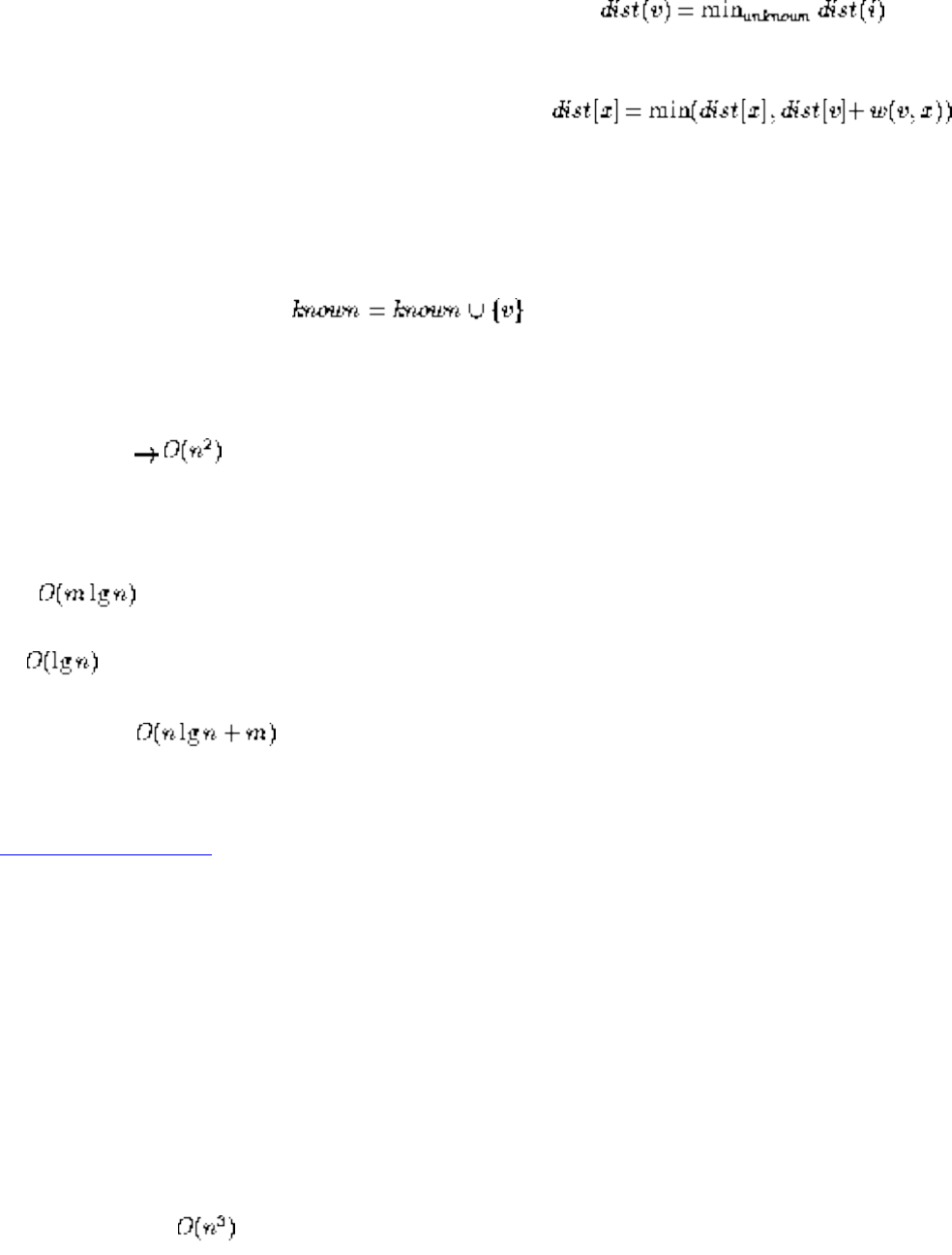
Lecture 18 - shortest path algorthms
select v such that
for each (v,x),
last=v
Complexity if we use adjacency lists and a Boolean array to mark what is known.
This is essentially the same as Prim's algorithm.
An implementation of Dijkstra's algorithm would be faster for sparse graphs, and comes from
using a heap of the vertices (ordered by distance), and updating the distance to each vertex (if necessary)
in time for each edge out from freshly known vertices.
Even better, follows from using Fibonacci heaps, since they permit one to do a decrease-key
operation in O(1) amortized time.
Listen To Part 20-8
All-Pairs Shortest Path
Notice that finding the shortest path between a pair of vertices (,t) in worst case requires first finding the
shortest path from to all other vertices in the graph.
Many applications, such as finding the center or diameter of a graph, require finding the shortest path
between all pairs of vertices.
We can run Dijkstra's algorithm n times (once from each possible start vertex) to solve all-pairs shortest
path problem in . Can we do better?
Improving the complexity is an open question but there is a super-slick dynamic programming algorithm
file:///E|/LEC/LECTUR16/NODE18.HTM (6 of 10) [19/1/2003 1:35:18]
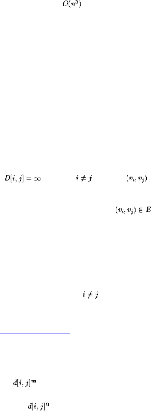
Lecture 18 - shortest path algorthms
which also runs in .
Listen To Part 20-9
Dynamic Programming and Shortest Paths
The four-step approach to dynamic programming is:
1. Characterize the structure of an optimal solution.
2. Recursively define the value of an optimal solution.
3. Compute this recurrence in a bottom-up fashion.
4. Extract the optimal solution from computed information.
From the adjacency matrix, we can construct the following matrix:
, if and is not in E
D[i,j] = w(i,j), if
D[i,j] = 0, if i=j
This tells us the shortest path going through no intermediate nodes.
There are several ways to characterize the shortest path between two nodes in a graph. Note that the
shortest path from i to j, , using at most M edges consists of the shortest path from i to k using at
most M-1 edges + W(k, j) for some k.
Listen To Part 20-10
This suggests that we can compute all-pair shortest path with an induction based on the number of edges
in the optimal path.
Let be the length of the shortest path from i to j using at most m edges.
What is ?
file:///E|/LEC/LECTUR16/NODE18.HTM (7 of 10) [19/1/2003 1:35:18]
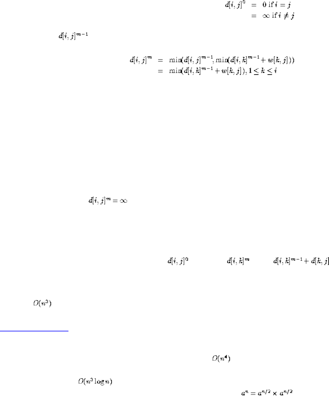
Lecture 18 - shortest path algorthms
What if we know for all i,j?
since w[k, k]=0
This gives us a recurrence, which we can evaluate in a bottom up fashion:
for i=1 to n
for j=1 to n
for k=1 to n
=Min( , )
This is an algorithm just like matrix multiplication, but it only goes from m to m+1 edges.
Listen To Part 20-11
Since the shortest path between any two nodes must use at most n edges (unless we have negative cost
cycles), we must repeat that procedure n times (m=1 to n) for an algorithm.
We can improve this to with the observation that any path using at most 2m edges is the
function of paths using at most m edges each. This is just like computing . So a
logarithmic number of multiplications suffice for exponentiation.
file:///E|/LEC/LECTUR16/NODE18.HTM (8 of 10) [19/1/2003 1:35:18]
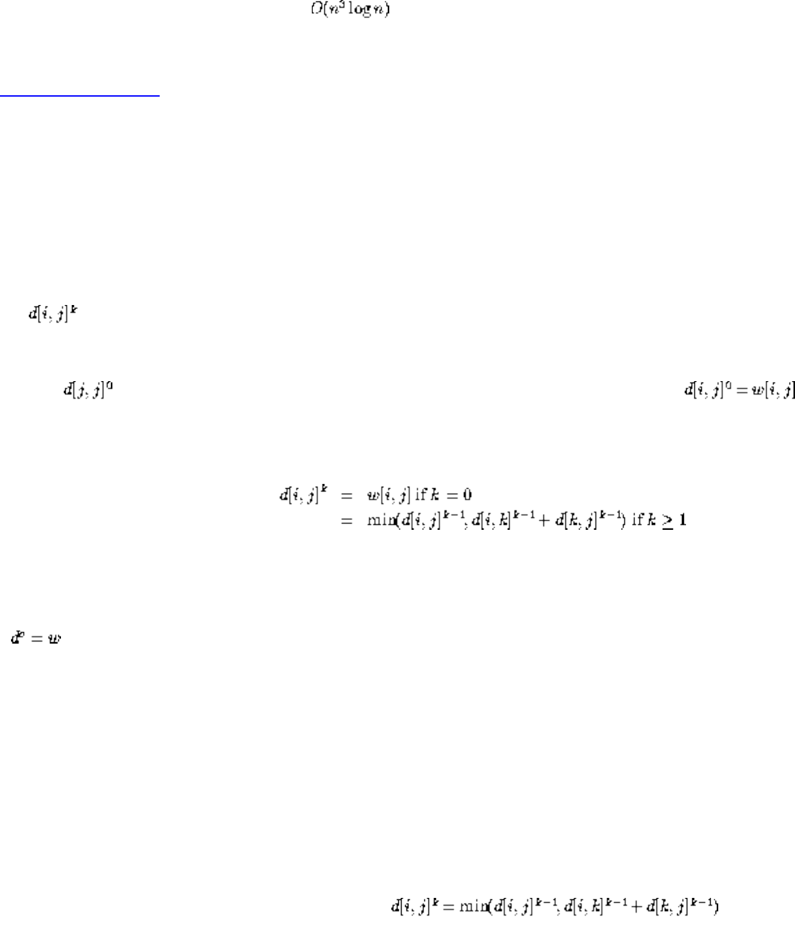
Lecture 18 - shortest path algorthms
Although this is slick, observe that even is slower than running Dijkstra's algorithm starting
from each vertex!
Listen To Part 20-12
The Floyd-Warshall Algorithm
An alternate recurrence yields a more efficient dynamic programming formulation. Number the vertices
from 1 to n.
Let be the shortest path from i to j using only vertices from 1, 2,..., k as possible intermediate
vertices.
What is ? With no intermediate vertices, any path consists of at most one edge, so .
In general, adding a new vertex k+1 helps iff a path goes through it, so
Although this looks similar to the previous recurrence, it isn't. The following algorithm implements it:
for k=1 to n
for i=1 to n
for j=1 to n
file:///E|/LEC/LECTUR16/NODE18.HTM (9 of 10) [19/1/2003 1:35:18]
Lecture 18 - shortest path algorthms
This obviously runs in time, which asymptotically is no better than a calls to Dijkstra's algorithm.
However, the loops are so tight and it is so short and simple that it runs better in practice by a constant
factor.
Next: Lecture 19 - satisfiability Up: No Title Previous: Lecture 17 - minimum
Algorithms
Mon Jun 2 09:21:39 EDT 1997
file:///E|/LEC/LECTUR16/NODE18.HTM (10 of 10) [19/1/2003 1:35:18]
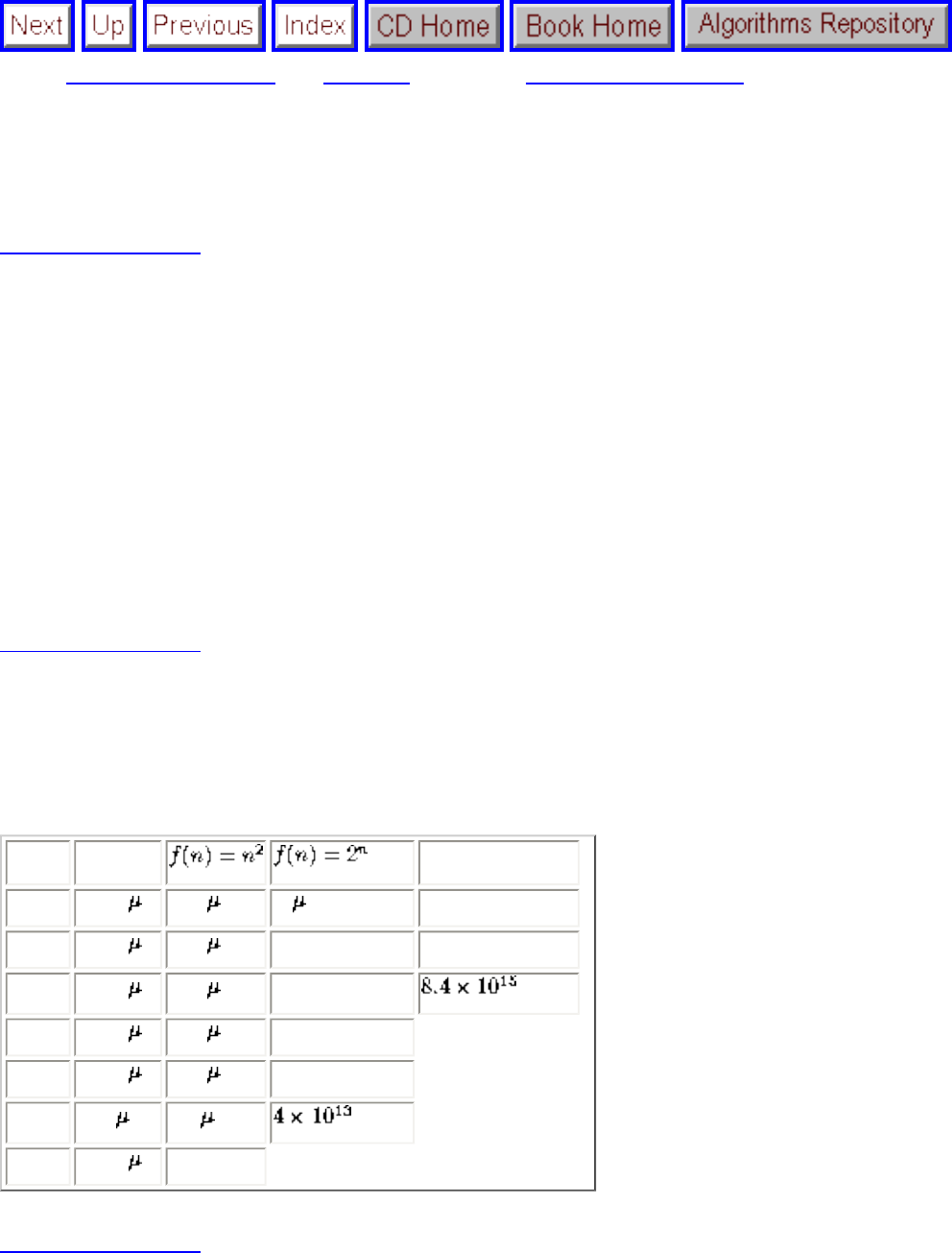
Lecture 19 - satisfiability
Next: Lecture 20 - integer Up: No Title Previous: Lecture 18 - shortest
Lecture 19 - satisfiability
Listen To Part 21-7
The Theory of NP-Completeness
Several times this semester we have encountered problems for which we couldn't find efficient algorithms,
such as the traveling salesman problem. We also couldn't prove an exponential time lower bound for the
problem.
By the early 1970s, literally hundreds of problems were stuck in this limbo. The theory of NP-Compleness,
developed by Stephen Cook and Richard Karp, provided the tools to show that all of these problems were
really the same problem.
Listen To Part 21-8
Polynomial vs. Exponential Time
n f(n) = n f(n) = n!
10 0.01 s 0.1 s 1 s 3.63 ms
20 0.02 s 0.4 s 1 ms 77.1 years
30 0.03 s 0.9 s 1 sec years
40 0.04 s 1.6 s 18.3 min
50 0.05 s 2.5 s 13 days
100 0.1 s 10 s years
1,000 1.00 s 1 ms
Listen To Part 21-9
The Main Idea
Suppose I gave you the following algorithm to solve the bandersnatch problem:
file:///E|/LEC/LECTUR16/NODE19.HTM (1 of 7) [19/1/2003 1:35:22]
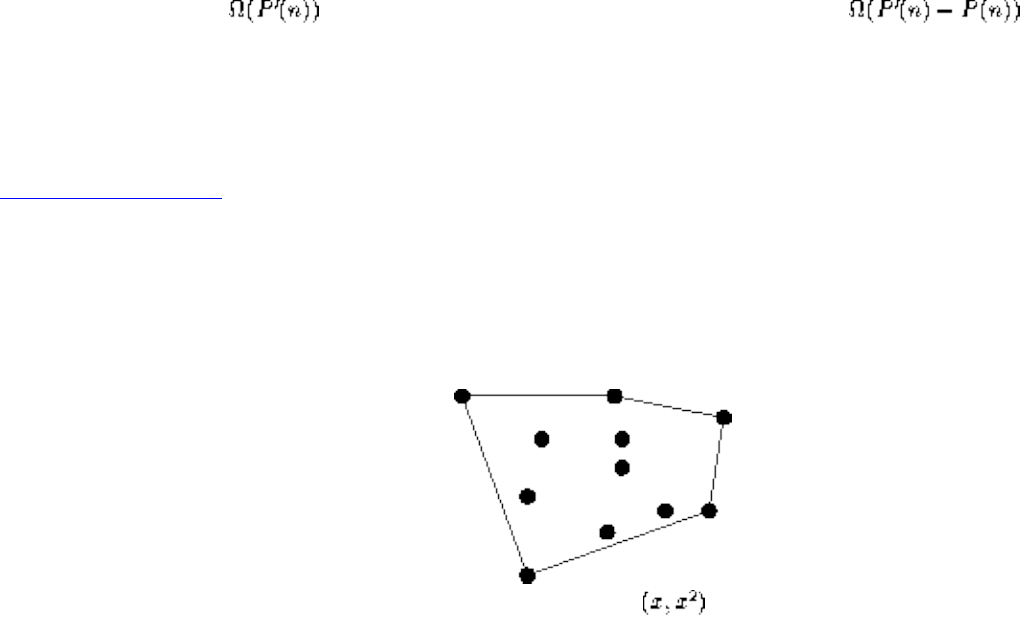
Lecture 19 - satisfiability
Bandersnatch(G)
Convert G to an instance of the Bo-billy problem Y.
Call the subroutine Bo-billy on Y to solve this instance.
Return the answer of Bo-billy(Y) as the answer to G.
Such a translation from instances of one type of problem to instances of another type such that answers are
preserved is called a reduction.
Now suppose my reduction translates G to Y in O(P(n)):
1. If my Bo-billy subroutine ran in O(P'(n)) I can solve the Bandersnatch problem in O(P(n)+P'(n))
2. If I know that is a lower-bound to compute Bandersnatch, then must be a
lower-bound to compute Bo-billy.
The second argument is the idea we use to prove problems hard!
Listen To Part 21-10
Convex Hull and Sorting
A nice example of a reduction goes from sorting numbers to the convex hull problem:
We must translate each number to a point. We can map x to .
file:///E|/LEC/LECTUR16/NODE19.HTM (2 of 7) [19/1/2003 1:35:22]
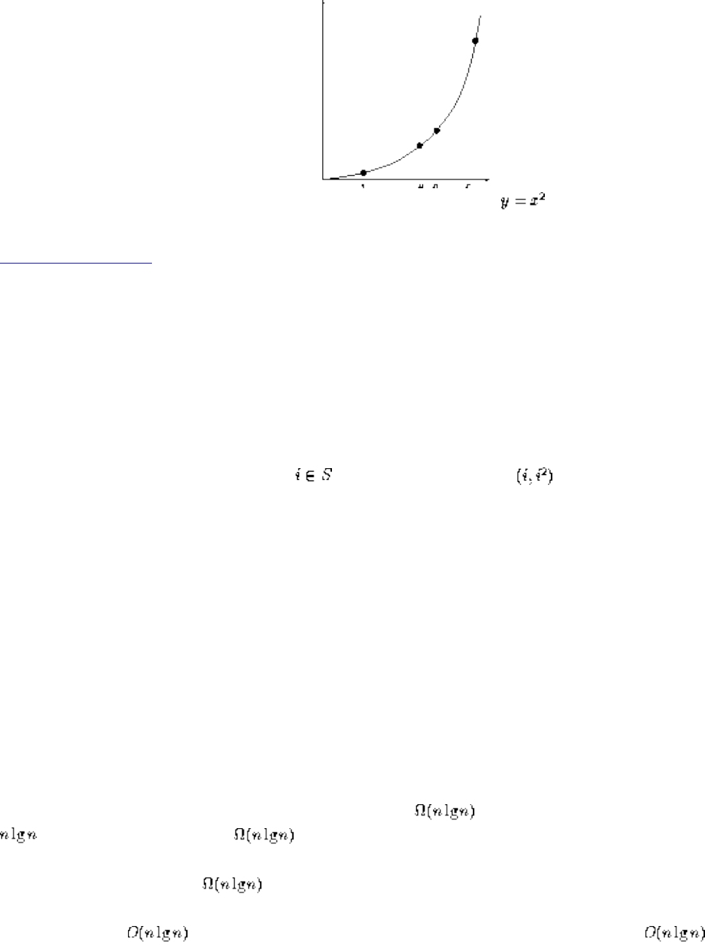
Lecture 19 - satisfiability
Why? That means each integer is mapped to a point on the parabola .
Listen To Part 21-11
Since this parabola is convex, every point is on the convex hull. Further since neighboring points on the
convex hull have neighboring x values, the convex hull returns the points sorted by x-coordinate, ie. the
original numbers.
Sort(S)
For each , create point .
Call subroutine convex-hull on this point set.
From the leftmost point in the hull,
read off the points from left to right.
Creating and reading off the points takes O(n) time.
What does this mean? Recall the sorting lower bound of . If we could do convex hull in better than
, we could sort faster than - which violates our lower bound.
Thus convex hull must take as well!!!
Observe that any convex hull algorithm also gives us a complicated but correct sorting
algorithm as well.
file:///E|/LEC/LECTUR16/NODE19.HTM (3 of 7) [19/1/2003 1:35:22]
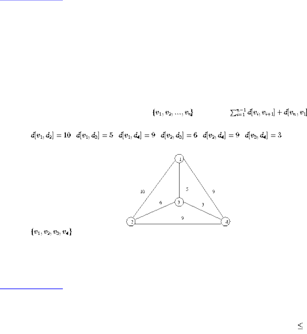
Lecture 19 - satisfiability
Listen To Part 22-2
What is a problem?
A problem is a general question, with parameters for the input and conditions on what is a satisfactory answer
or solution.
An instance is a problem with the input parameters specified.
Example: The Traveling Salesman
Problem: Given a weighted graph G, what tour minimizes .
Instance: , , , , ,
Solution: cost= 27
A problem with answers restricted to yes and no is called a decision problem. Most interesting optimization
problems can be phrased as decision problems which capture the essence of the computation.
Listen To Part 22-3
Example: The Traveling Salesman Decision Problem.
Given a weighted graph G and integer k, does there exist a traveling salesman tour with cost k?
Using binary search and the decision version of the problem we can find the optimal TSP solution.
For convenience, from now on we will talk only about decision problems.
Note that there are many possible ways to encode the input graph: adjacency matrices, edge lists, etc. All
reasonable encodings will be within polynomial size of each other.
The fact that we can ignore minor differences in encoding is important. We are concerned with the difference
file:///E|/LEC/LECTUR16/NODE19.HTM (4 of 7) [19/1/2003 1:35:22]
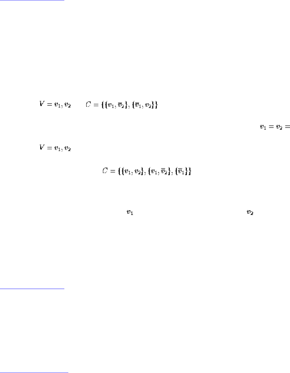
Lecture 19 - satisfiability
between algorithms which are polynomial and exponential in the size of the input.
Listen To Part 22-4
Satisfiability
Consider the following logic problem:
Instance: A set V of variables and a set of clauses C over V.
Question: Does there exist a satisfying truth assignment for C?
Example 1: and
A clause is satisfied when at least one literal in it is TRUE. C is satisfied when TRUE.
Example 2: ,
Although you try, and you try, and you try and you try, you can get no satisfaction.
There is no satisfying assigment since must be FALSE (third clause), so must be FALSE (second clause),
but then the first clause is unsatisfiable!
For various reasons, it is known that satisfiability is a hard problem. Every top-notch algorithm expert in the
world (and countless other, lesser lights) have tried to come up with a fast algorithm to test whether a given set
of clauses is satisfiable, but all have failed.
Listen To Part 22-5
Further, many strange and impossible-to-believe things have been shown to be true if someone in fact did find
a fast satisfiability algorithm.
Clearly, Satisfiability is in NP, since we can guess an assignment of TRUE, FALSE to the literals and check it
in polynomial time.
Listen To Part 22-10
P versus NP
The precise distinction between whether a problem is in P or NP is somewhat technical, requiring formal
file:///E|/LEC/LECTUR16/NODE19.HTM (5 of 7) [19/1/2003 1:35:22]
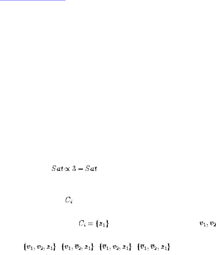
Lecture 19 - satisfiability
language theory and Turing machines to state correctly.
However, intuitively a problem is in P, (ie. polynomial) if it can be solved in time polynomial in the size of the
input.
A problem is in NP if, given the answer, it is possible to verify that the answer is correct within time
polynomial in the size of the input.
Example P - Is there a path from to t in G of length less than k.
Example NP - Is there a TSP tour in G of length less than k. Given the tour, it is easy to add up the costs and
convince me it is correct.
Example not NP - How many TSP tours are there in G of length less than k. Since there can be an exponential
number of them, we cannot count them all in polynomial time.
Don't let this issue confuse you - the important idea here is of reductions as a way of proving hardness.
Listen To Part 22-7
3-Satisfiability
Instance: A collection of clause C where each clause contains exactly 3 literals, boolean variable v.
Question: Is there a truth assignment to v so that each clause is satisfied?
Note that this is a more restricted problem than SAT. If 3-SAT is NP-complete, it implies SAT is NP-complete
but not visa-versa, perhaps long clauses are what makes SAT difficult?!
After all, 1-Sat is trivial!
Theorem: 3-SAT is NP-Complete
Proof: 3-SAT is NP - given an assignment, just check that each clause is covered. To prove it is complete, a
reduction from must be provided. We will transform each clause independantly based on its
length.
Suppose the clause contains k literals.
● If k=1, meaning , create two new variables and four new 3-literal clauses:
, , , .
file:///E|/LEC/LECTUR16/NODE19.HTM (6 of 7) [19/1/2003 1:35:22]
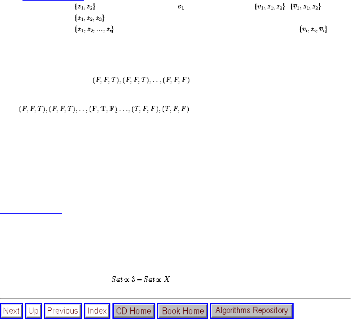
Lecture 19 - satisfiability
Note that the only way all four of these can be satisfied is if z is TRUE.
Listen To Part 22-8
● If k=2, meaning , create one new variable and two new clauses: ,
● If k=3, meaning , copy into the 3-SAT instance as it is.
● If k>3, meaning , create n-3 new variables and n-2 new clauses in a chain: , ...
If none of the original variables in a clause are TRUE, there is no way to satisfy all of them using the
additional variable:
But if any literal is TRUE, we have n-3 free variables and n-3 remaining 3-clauses, so we can satisfy each of
them.
Since any SAT solution will also satisfy the 3-SAT instance and any 3-SAT solution sets variables giving a
SAT solution - the problems are equivallent. If there were n clauses and m total literals in the SAT instance,
this transform takes O(m) time, so SAT and 3-SAT.
Note that a slight modification to this construction would prove 4-SAT, or 5-SAT,... also NP-complete.
However, it breaks down when we try to use it for 2-SAT, since there is no way to stuff anything into the
chain of clauses. It turns out that resolution gives a polynomial time algorithm for 2-SAT.
Listen To Part 22-9
Having at least 3-literals per clause is what makes the problem difficult. Now that we have shown 3-SAT is
NP-complete, we may use it for further reductions. Since the set of 3-SAT instances is smaller and more
regular than the SAT instances, it will be easier to use 3-SAT for future reductions. Remember the direction to
reduction!
Next: Lecture 20 - integer Up: No Title Previous: Lecture 18 - shortest
Algorithms
Mon Jun 2 09:21:39 EDT 1997
file:///E|/LEC/LECTUR16/NODE19.HTM (7 of 7) [19/1/2003 1:35:22]
Lecture 20 - integer programming
Next: Lecture 21 - vertex Up: No Title Previous: Lecture 19 - satisfiability
Lecture 20 - integer programming
Listen To Part 22-6
36.4-5 Give a polynomial-time algorithm to satisfy Boolean formulas in disjunctive normal form.
Satisfying one clause in DFS satisfied the whole formula. One clause can always be satisfied iff it does
not contain both a variable and its complement.
Why not use this reduction to give a polynomial-time algorithm for 3-SAT? The DNF formula can
become exponentially large and hence the reduction cannot be done in polynomial time.
Listen To Part 24-2
A Perpetual Point of Confusion
Note carefully the direction of the reduction.
We must transform every instance of a known NP-complete problem to an instance of the problem we
are interested in. If we do the reduction the other way, all we get is a slow way to solve x, by using a
subroutine which probably will take exponential time.
This always is confusing at first - it seems bass-ackwards. Make sure you understand the direction of
reduction now - and think back to this when you get confused.
Listen To Part 24-3
Integer Programming
Instance: A set v of integer variables, a set of inequalities over these variables, a function f(v) to
maximize, and integer B.
Question: Does there exist an assignment of integers to v such that all inequalities are true and ?
file:///E|/LEC/LECTUR16/NODE20.HTM (1 of 4) [19/1/2003 1:35:24]
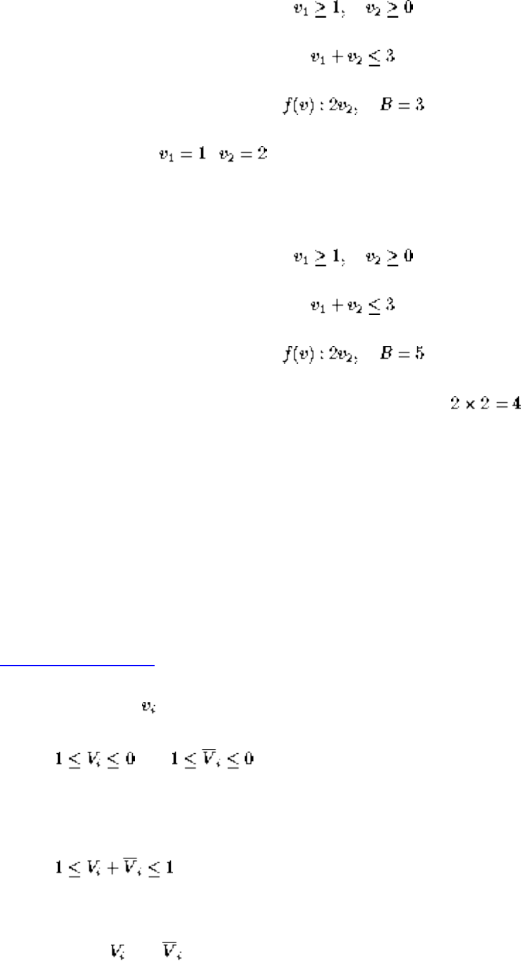
Lecture 20 - integer programming
Example:
A solution to this is , .
Example:
Since the maximum value of f(v) given the constraints is , there is no solution.
Theorem: Integer Programming is NP-Hard
Proof: By reduction from Satisfiability
Any set instance has boolean variables and clauses. Our Integer programming problem will have twice as
many variables as the SAT instance, one for each variable and its compliment, as well as the following
inequalities:
Listen To Part 24-4
For each variable in the set problem, we will add the following constraints:
● and
Both IP variables are restricted to values of 0 or 1, which makes them equivalent to boolean
variables restricted to true/false.
●
Exactly one of the IP variables associated with a given sat variable is 1. This means that exactly
one of and are true!
file:///E|/LEC/LECTUR16/NODE20.HTM (2 of 4) [19/1/2003 1:35:24]
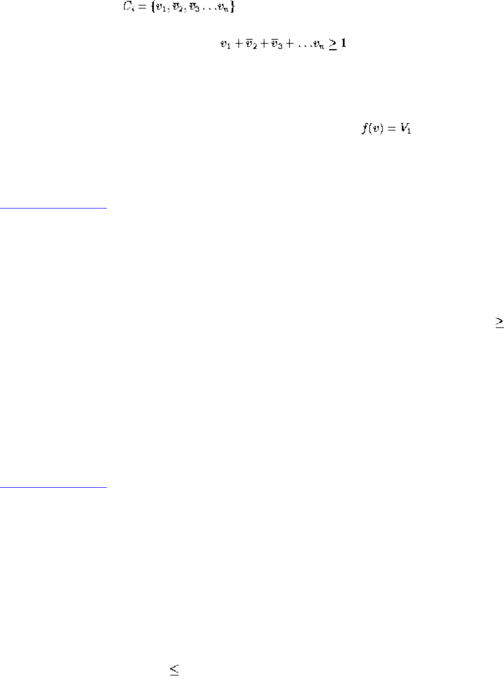
Lecture 20 - integer programming
● for each clause in the sat instance, construct a constraint:
Thus at least one IP variable must be one in each clause! Thus satisfying the constraint is
equivalent to satisfying the clause!
Our maximization function and bound are relatively unimportant: B=0.
Clearly this reduction can be done in polynomial time.
Listen To Part 24-5
We must show:
1. Any SAT solution gives a solution to the IP problem.
In any SAT solution, a TRUE literal corresponds to a 1 in the IP, since if the expression is
SATISFIED, at least one literal per clause in TRUE, so the sum in the inequality is 1.
2. Any IP solution gives a SAT solution.
Given a solution to this IP instance, all variables will be 0 or 1. Set the literals correspondly to 1
variable TRUE and the 0 to FALSE. No boolean variable and its complement will both be true, so
it is a legal assignment with also must satisfy the clauses.
Neat, sweet, and NP-complete!
Listen To Part 24-6
Things to Notice
1. The reduction preserved the structure of the problem. Note that the reduction did not solve the
problem - it just put it in a different format.
2. The possible IP instances which result are a small subset of the possible IP instances, but since
some of them are hard, the problem in general must be hard.
3. The transformation captures the essence of why IP is hard - it has nothing to do with big
coefficients or big ranges on variables; for restricting to 0/1 is enough. A careful study of what
properties we do need for our reduction tells us a lot about the problem.
4. It is not obvious that IP NP, since the numbers assigned to the variables may be too large to
write in polynomial time - don't be too hasty!
file:///E|/LEC/LECTUR16/NODE20.HTM (3 of 4) [19/1/2003 1:35:24]

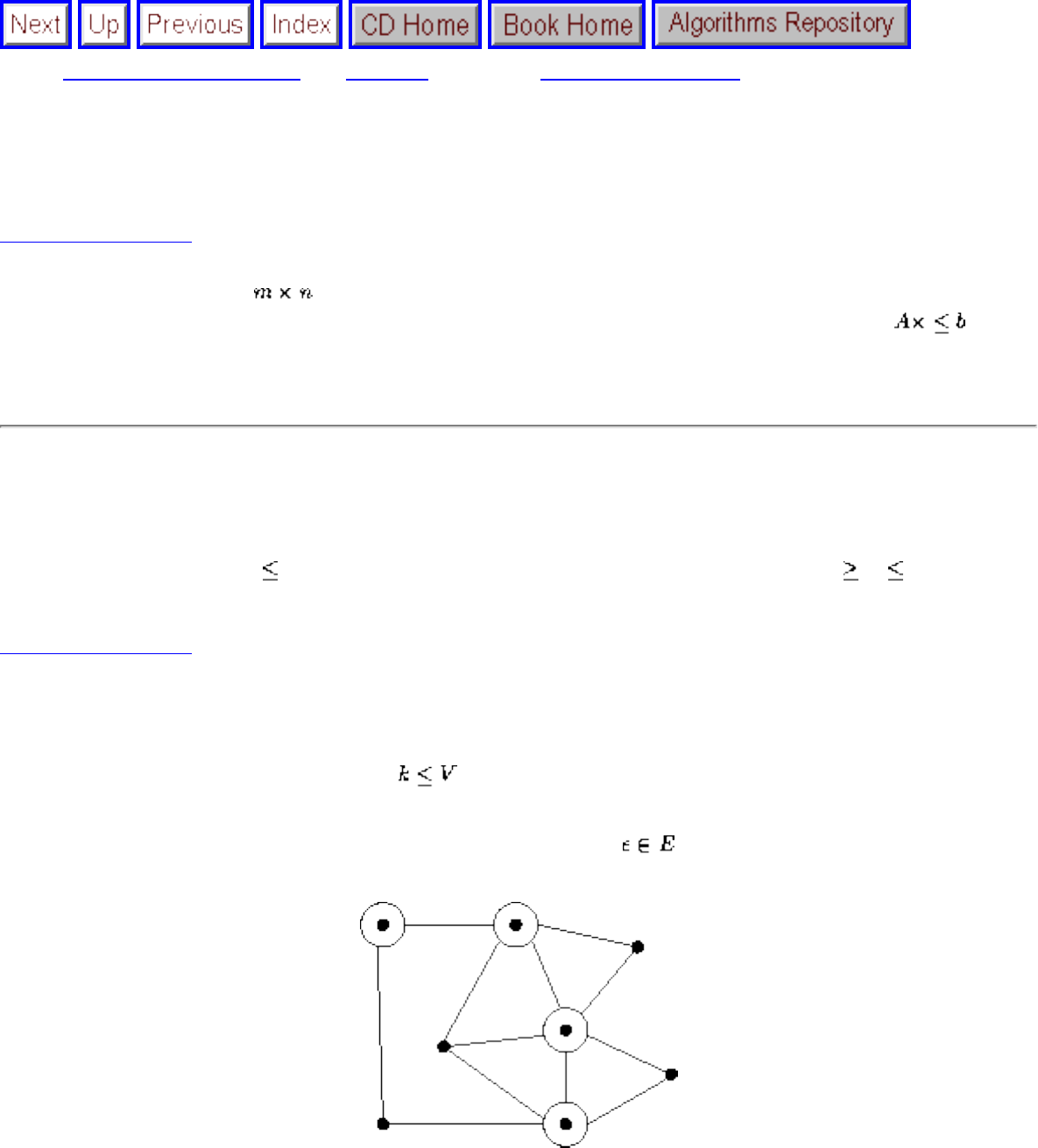
Lecture 21 - vertex cover
Next: Lecture 22 - techniques Up: No Title Previous: Lecture 20 - integer
Lecture 21 - vertex cover
Listen To Part 24-7
36.5-2 - Given an integer matrix A, and in integer m-vector b, the 0-1 integer programming
problem asks whether there is an integer n-vector x with elements in the set (0,1) such that .
Prove that 0-1 integer programming is NP-hard (hint: reduce from 3-SAT).
This is really the exact same problem as the previous integer programming problem, slightly concealed
by:
● The linear algebra notation - each row is one constraint.
● All inequalities are - multiply both sides by -1 to reverse the constraint from to if necessary.
Listen To Part 24-8
Vertex Cover
Instance: A graph G=(V, E), and integer
Question: Is there a subset of at most k vertices such that every has at least one vertex in the subset?
Here, four of the eight vertices are enough to cover. It is trivial to find a vertex cover of a graph - just
take all the vertices. The tricky part is to cover with as small a set as possible.
Theorem: Vertex cover is NP-complete.
file:///E|/LEC/LECTUR16/NODE21.HTM (1 of 7) [19/1/2003 1:35:28]
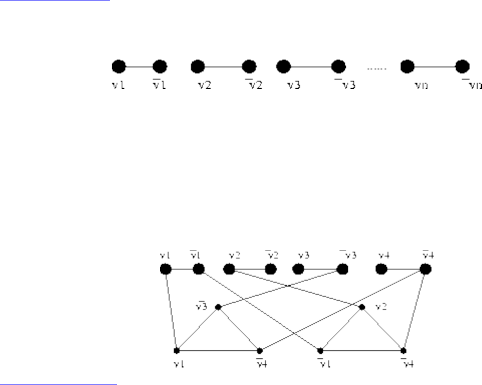
Lecture 21 - vertex cover
Proof: VC in in NP - guess a subset of vertices, count them, and show that each edge is covered.
To prove completeness, we show 3-SAT and VC. From a 3-SAT instance with n variables and C clauses,
we construct a graph with 2N+3C vertices.
Listen To Part 24-9
For each variable, we create two vertices connected by an edge:
To cover each of these edges, at least n vertices must be in the cover, one for each pair. For each clause,
we create three new vertices, one for each literal in each clause. Connect these in a triangle.
At least two vertices per triangle must be in the cover to take care of edges in the triangle, for a total of at
least 2C vertices.
Finally, we will connect each literal in the flat structure to the corresponding vertices in the triangles
which share the same literal.
Listen To Part 24-10
Claim: This graph will have a vertex cover of size N+2C if and only if the expression is satisfiable.
By the earlier analysis, any cover must have at least N+2C vertices. To show that our reduction is
correct, we must show that:
1. Every satisfying truth assignment gives a cover.
Select the N vertices cooresponding to the TRUE literals to be in the cover. Since it is a satisfying
truth assignment, at least one of the three cross edges associated with each clause must already be
covered - pick the other two vertices to complete the cover.
2. Every vertex cover gives a satisfying truth assignment.
file:///E|/LEC/LECTUR16/NODE21.HTM (2 of 7) [19/1/2003 1:35:28]
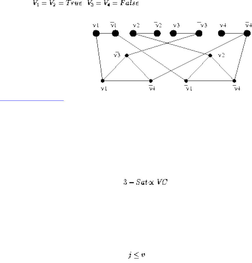
Lecture 21 - vertex cover
Every vertex cover must contain n first stage vertices and 2C second stage vertices. Let the first
stage vertices define the truth assignment.
To give the cover, at least one cross-edge must be covered, so the truth assignment satisfies.
For a cover to have N+2C vertices, all the cross edges must be incident on a selected vertex.
Let the N selected vertices from the first stage coorespond to TRUE literals. If there is a satisfying truth
assignment, that means at least one of the three cross edges from each triangle is incident on a TRUE
vertex.
By adding the other two vertices to the cover, we cover all edges associated with the clause.
Every SAT defines a cover and Every Cover Truth values for the SAT!
Example: , .
Listen To Part 25-1
Starting from the Right Problem
As you can see, the reductions can be very clever and very complicated. While theoretically any NP-
complete problem can be reduced to any other one, choosing the correct one makes finding a reduction
much easier.
As you can see, the reductions can be very clever and complicated. While theoretically any NP-complete
problem will do, choosing the correct one can make it much easier.
Maximum Clique
Instance: A graph G=(V,E) and integer .
file:///E|/LEC/LECTUR16/NODE21.HTM (3 of 7) [19/1/2003 1:35:28]
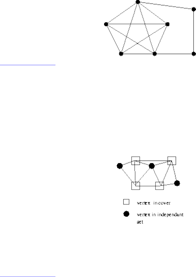
Lecture 21 - vertex cover
Question: Does the graph contain a clique of j vertices, ie. is there a subset of v of size j such that every
pair of vertices in the subset defines an edge of G?
Example: this graph contains a clique of size 5.
Listen To Part 25-2
When talking about graph problems, it is most natural to work from a graph problem - the only NP-
complete one we have is vertex cover!
Theorem: Clique is NP-complete
Proof: If you take a graph and find its vertex cover, the remaining vertices form an independent set,
meaning there are no edges between any two vertices in the independent set, for if there were such an
edge the rest of the vertices could not be a vertex cover.
Clearly the smallest vertex cover gives the biggest independent set, and so the problems are equivallent -
Delete the subset of vertices in one from the total set of vertices to get the order!
Thus finding the maximum independent set must be NP-complete!
Listen To Part 25-3
In an independent set, there are no edges between two vertices. In a clique, there are always between two
vertices. Thus if we complement a graph (have an edge iff there was no edge in the original graph), a
clique becomes an independent set and an independent set becomes a Clique!
file:///E|/LEC/LECTUR16/NODE21.HTM (4 of 7) [19/1/2003 1:35:28]
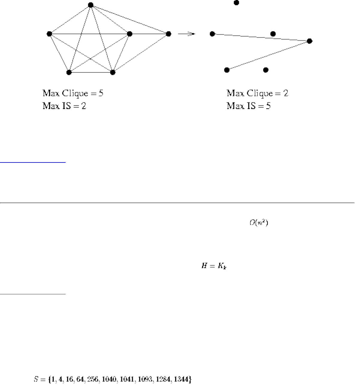
Lecture 21 - vertex cover
Thus finding the largest clique is NP-complete:
If VC is a vertex cover in G, then V-VC is a clique in G'. If C is a clique in G, V-C is a vertex cover in G'.
Listen To Part 25-4
36.5-1 Prove that subgraph isomorphism is NP-complete.
1. Guessing a subgraph of G and proving it is isomorphism to h takes time, so it is in NP.
2. Clique and subgraph isomorphism. We must transform all instances of clique into some instances
of subgraph isomorphism. Clique is a special case of subgraph isomorphism!
Thus the following reduction suffices. Let G=G' and , the complete subgraph on k nodes.
Listen To Part 25-5
Integer Partition (Subset Sum)
Instance: A set of integers S and a target integer t.
Problem: Is there a subset of S which adds up exactly to t?
Example: and T=3754
Answer: 1+16+64+256+1040+1093+1284 = T
Observe that integer partition is a number problem, as opposed to the graph and logic problems we have
file:///E|/LEC/LECTUR16/NODE21.HTM (5 of 7) [19/1/2003 1:35:28]
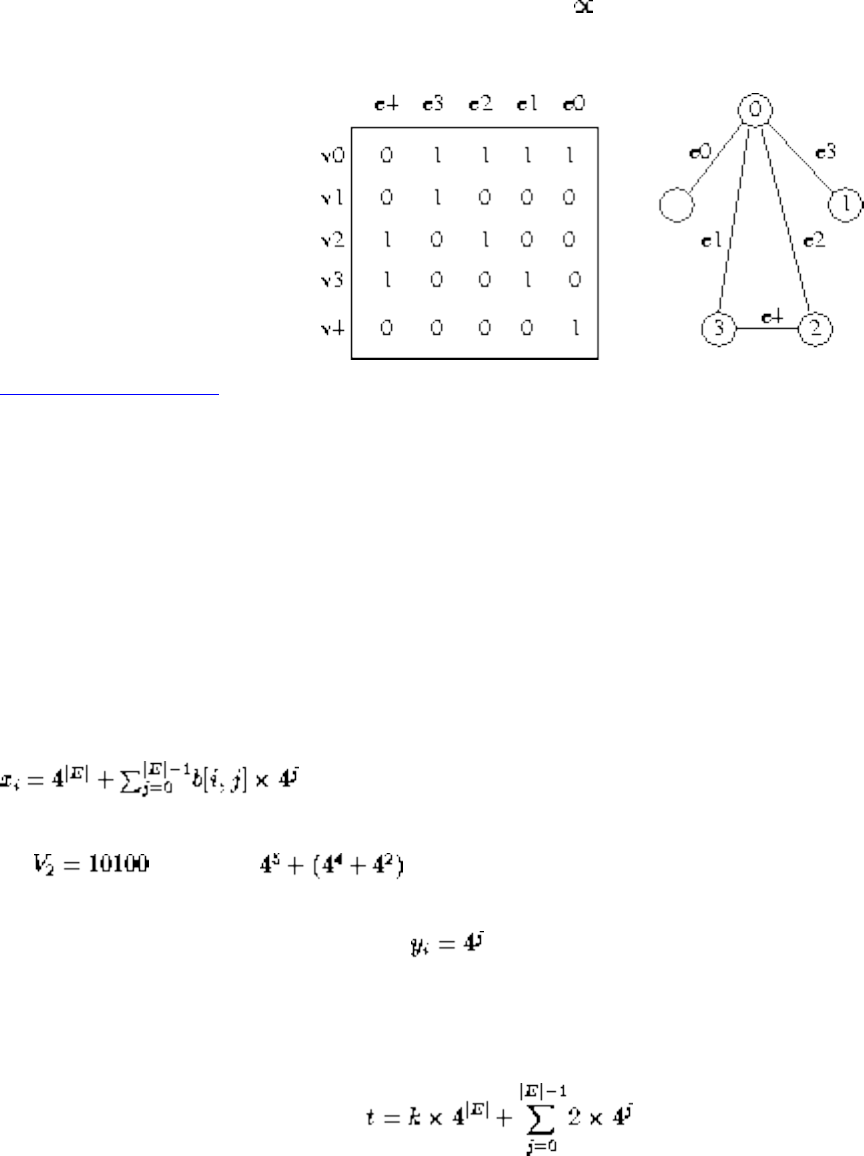
Lecture 21 - vertex cover
seen to date.
Theorem: Integer Partition is NP-complete.
Proof: First, we note that integer partition is in NP. Guess a subset of the input number and simply add
them up.
To prove completeness, we show that vertex cover integer partition. We use a data structure called an
incidence matrix to represent the graph G.
Listen To Part 25-6
How many 1's are there in each column? Exactly two.
How many 1's in a particular row? Depends on the vertex degree.
The reduction from vertex cover will create n+m numbers from G.
The numbers from the vertices will be a base-4 realization of rows from the incidence matrix, plus a high
order digit:
ie. becomes .
The numbers from the edges will be .
The target integer will be
file:///E|/LEC/LECTUR16/NODE21.HTM (6 of 7) [19/1/2003 1:35:28]
Lecture 21 - vertex cover
Why? Each column (digit) represents an edge. We want a subset of vertices which covers each edge. We
can only use k x vertex/numbers, because of the high order digit of the target.
Listen To Part 25-7
We might get only one instance of each edge in a cover - but we are free to take extra edge/numbers to
grab an extra 1 per column.
VC in G Integer Partition in S
Given k vertices covering G, pick the k cooresponding vertex/numbers. Each edge in G is incident on one
or two cover vertices. If it is one, includes the cooresponding edge/number to give two per column.
Integer Partition in S VC in G
Any solution to S must contain exactly k vertex/numbers. Why? It cannot be more because the target in
that digit is k and it cannot be less because, with at most 3 1's per edge/digit-column, no sum of these can
carry over into the next column. (This is why base-4 number were chosen).
This subset of k vertex/numbers must contain at least one edge-list per column, since if not there is no
way to account for the two in each column of the target integer, given that we can pick up at most one
edge-list using the edge number. (Again, the prevention of carrys across digits prevents any other
possibilites).
Neat, sweet, and NP-complete!
Notice that this reduction could not be performed in polynomial time if the number were written in unary
5=11111. Big numbers is what makes integer partition hard!
Next: Lecture 22 - techniques Up: No Title Previous: Lecture 20 - integer
Algorithms
Mon Jun 2 09:21:39 EDT 1997
file:///E|/LEC/LECTUR16/NODE21.HTM (7 of 7) [19/1/2003 1:35:28]
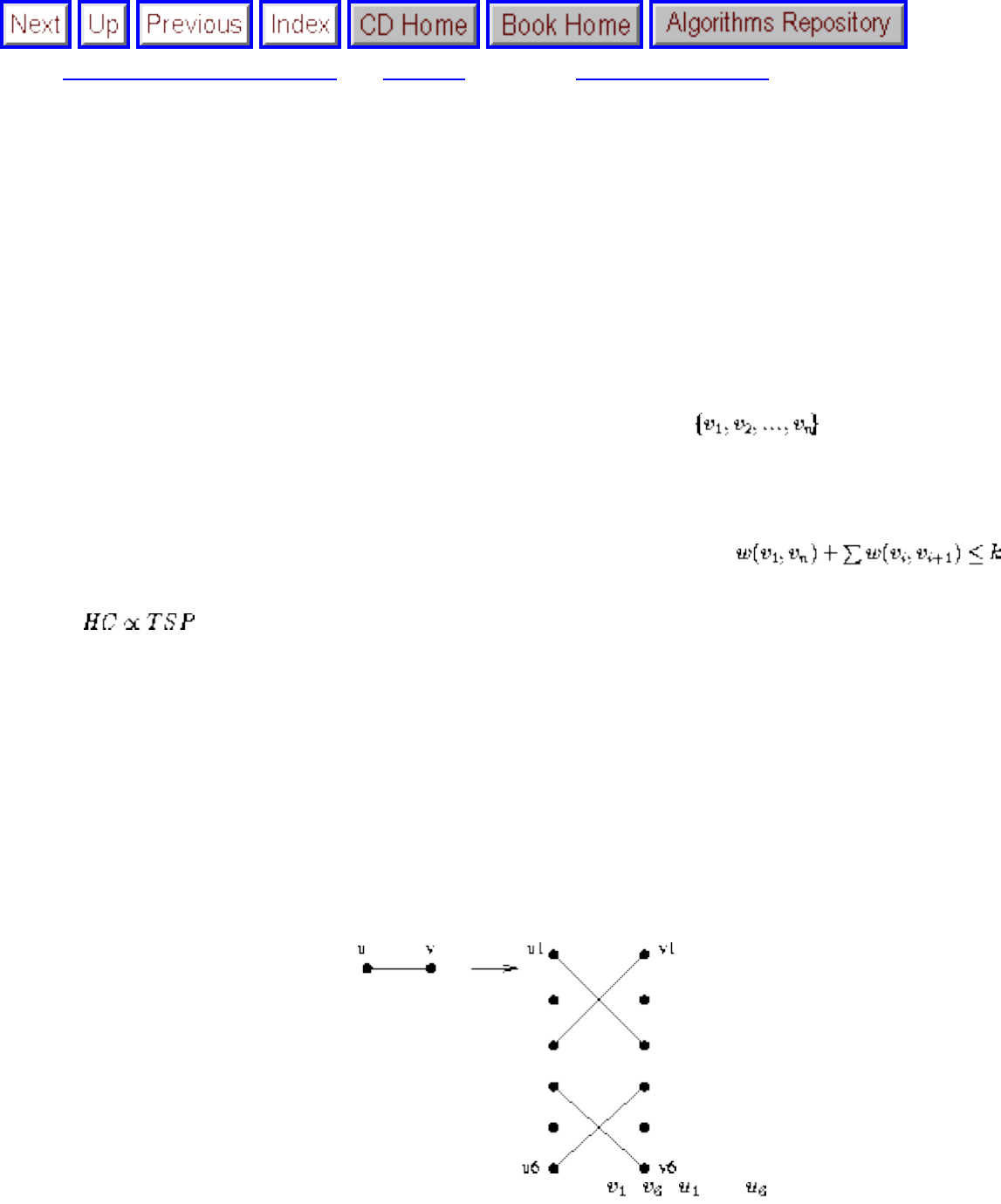
Lecture 22 - techniques for proving hardness
Next: Lecture 23 - approximation Up: No Title Previous: Lecture 21 - vertex
Lecture 22 - techniques for proving
hardness
Hamiltonian Cycle
Instance: A graph G
Question: Does the graph contains a HC, i.e. an ordered of the vertices ?
This problem is intimately relates to the Traveling Salesman.
Question: Is there an ordering of the vertices of a weighted graph such that ?
Clearly, . Assign each edge in G weight 1, any edge not in G weight 2. This new graph has a
Traveling Salesman tour of cost n iff the graph is Hamiltonian. Thus TSP is NP-complete if we can show
HC is NP-complete.
Theorem: Hamiltonian Circuit is NP-complete
Proof: Clearly HC is in NP-guess a permutation and check it out. To show it is complete, we use vertex
cover. A vertex cover instance consists of a graph and a constant k, the minimum size of an acceptable
cover. We must construct another graph. Each edge in the initial graph will be represented by the
following component:
All further connections to this gadget will be through vertices , , and . The key observation
about this gadget is that there are only three ways to traverse all the vertices:
file:///E|/LEC/LECTUR16/NODE22.HTM (1 of 7) [19/1/2003 1:35:31]
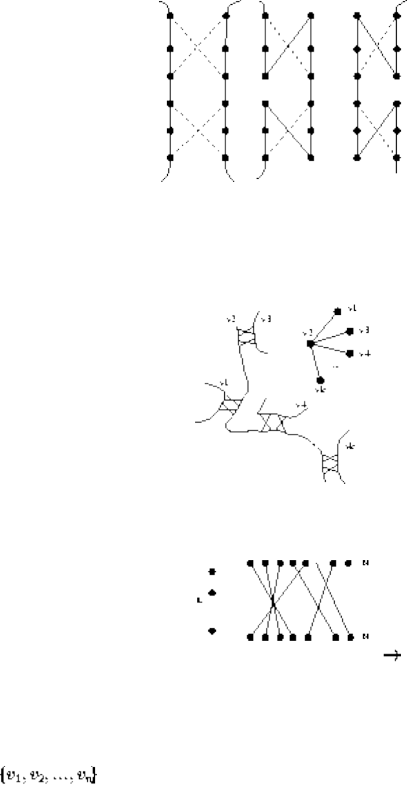
Lecture 22 - techniques for proving hardness
Note that in each case, we exit out the same side we entered. Each side of each edge gadget is associated
with a vertex. Assuming some arbitrary order to the edges incident on a particular vertex, we can link
successive gadgets by edges forming a chain of gadgets. Doing this for all vertices in the original graph
creates n intertwined chains with n entry points and n exits.
Thus we have encoded the information about the initial graph. What about k? We set up k additional
vertices and connect each of these to the n start points and n end points of each chain.
Total size of new graph: GE+K vertices and 12E+2kN+2E edges construction is polynomial in size
and time.
We claim this graph has a HC iff G has a VC of size k.
1. Suppose is a HC.
Assume it starts at one of the k selector vertices. It must then go through one of the chains of
gadgets until it reaches a different selector vertex.
Since the tour is a HC, all gadgets are traversed. The k chains correspond to the vertices in the
cover.
Note that if both vertices associated with an edge are in the cover, the gadget will be traversal in
file:///E|/LEC/LECTUR16/NODE22.HTM (2 of 7) [19/1/2003 1:35:31]
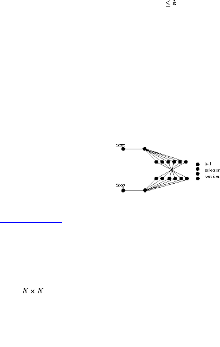
Lecture 22 - techniques for proving hardness
two pieces - otherwise one chain suffices.
To avoid visiting a vertex more than once, each chain is associated with a selector vertex.
2. Now suppose we have a vertex cover of size .
We can always add more vertices to the cover to bring it up to size k.
For each vertex in the cover, start traversing the chain. At each entry point to a gadget, check if
the other vertex is in the cover and traverse the gadget accordingly.
Select the selector edges to complete the circuit.
Neat, sweet, and NP-complete.
To show that Longest Path or Hamiltonian Path is NP-complete, add start and stop vertices and
distinguish the first and last selector vertices.
This has a Hamiltonian path from start to stop iff the original graph has a vertex cover of size k.
Listen To Part 26-2
Other NP-complete Problems
● Partition - can you partition n integers into two subsets so that the sums of the subset are equal?
● Bin Packing - how many bins of a given size do you need to hold n items of variable size?
● Chromatic Number - how many colors do you need to color a graph?
● checkers - does black have a forced win from a given position?
● Scheduling, Code Optimization, Permanent Evaluation, Quadratic Programming, etc.
Open: Graph Isomorphism, Composite Number, Minimum Length Triangulation.
Listen To Part 26-3
Polynomial or Exponential?
file:///E|/LEC/LECTUR16/NODE22.HTM (3 of 7) [19/1/2003 1:35:31]
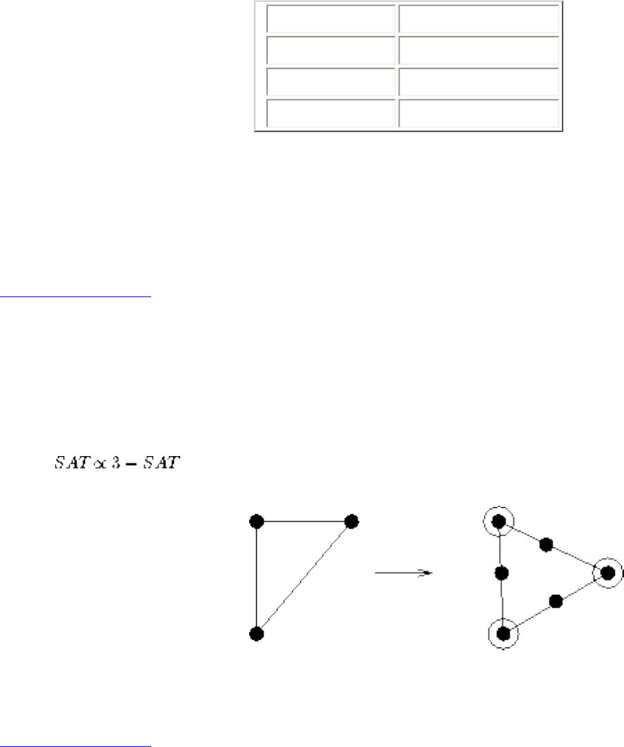
Lecture 22 - techniques for proving hardness
Just changing a problem a little can make the difference between it being in P or NP-complete:
P NP-complete
Shortest Path Longest Path
Eulerian Circuit Hamiltonian Circuit
Edge Cover Vertex Cover
The first thing you should do when you suspect a problem might be NP-complete is look in Garey and
Johnson, Computers and Intractability. It contains a list of several hundred problems known to be NP-
complete. Either what you are looking for will be there or you might find a closely related problem to use
in a reduction.
Listen To Part 26-4
Techniques for Proving NP-completeness
1. Restriction - Show that a special case of the problem you are interested in is NP-complete. For
example, the problem of finding a path of length k is really Hamiltonian Path.
2. Local Replacement - Make local changes to the structure. An example is the reduction
. Another example is showing isomorphism is no easier for bipartite graphs:
For any graph, replacing an edge with makes it bipartite.
3. Component Design - These are the ugly, elaborate constructions
Listen To Part 26-5
The Art of Proving Hardness
Proving that problems are hard is an skill. Once you get the hang of it, it is surprisingly straightforward
and pleasurable to do. Indeed, the dirty little secret of NP-completeness proofs is that they are usually
easier to recreate than explain, in the same way that it is usually easier to rewrite old code than the try to
understand it.
file:///E|/LEC/LECTUR16/NODE22.HTM (4 of 7) [19/1/2003 1:35:31]

Lecture 22 - techniques for proving hardness
I offer the following advice to those needing to prove the hardness of a given problem:
● Make your source problem as simple (i.e. restricted) as possible.
Never use the general traveling salesman problem (TSP) as a target problem. Instead, use TSP on
instances restricted to the triangle inequality. Better, use Hamiltonian cycle, i.e. where all the
weights are 1 or . Even better, use Hamiltonian path instead of cycle. Best of all, use
Hamiltonian path on directed, planar graphs where each vertex has total degree 3. All of these
problems are equally hard, and the more you can restrict the problem you are reducing, the less
work your reduction has to do.
● Make your target problem as hard as possible.
Don't be afraid to add extra constraints or freedoms in order to make your problem more general
(at least temporarily).
Listen To Part 26-6
● Select the right source problem for the right reason.
Selecting the right source problem makes a big difference is how difficult it is to prove a problem
hard. This is the first and easiest place to go wrong.
I usually consider four and only four problems as candidates for my hard source problem.
Limiting them to four means that I know a lot about these problems - which variants of these
problems are hard and which are soft. My favorites are:
❍ 3-Sat - that old reliable... When none of the three problems below seem appropriate, I go
back to the source.
❍ Integer partition - the one and only choice for problems whose hardness seems to require
using large numbers.
❍ Vertex cover - for any graph problems whose hardness depends upon selection. Chromatic
number, clique, and independent set all involve trying to select the correct subset of
vertices or edges.
❍ Hamiltonian path - for any graph problems whose hardness depends upon ordering. If you
are trying to route or schedule something, this is likely your lever.
Listen To Part 26-7
● Amplify the penalties for making the undesired transition.
You are trying to translate one problem into another, while making them stay the same as much as
possible. The easiest way to do this is to be bold with your penalties, to punish anyone trying to
deviate from your proposed solution. ``If you pick this, then you have to pick up this huge set
file:///E|/LEC/LECTUR16/NODE22.HTM (5 of 7) [19/1/2003 1:35:31]

Lecture 22 - techniques for proving hardness
which dooms you to lose.'' The sharper the consequences for doing what is undesired, the easier it
is to prove if and only if.
● Think strategically at a high level, then build gadgets to enforce tactics.
You should be asking these kinds of questions. ``How can I force that either A or B but not both
are chosen?'' ``How can I force that A is taken before B?'' ``How can I clean up the things I did
not select?''
● Alternate between looking for an algorithm or a reduction if you get stuck.
Sometimes the reason you cannot prove hardness is that there is an efficient algorithm to solve
your problem! When you can't prove hardness, it likely pays to change your thinking at least for a
little while to keep you honest.
Listen To Part 26-8
Now watch me try it!
To demonstrate how one goes about proving a problem hard, I accept the challenge of showing how a
proof can be built on the fly.
I need a volunteer to pick a random problem from the 400+ hard problems in the back of Garey and
Johnson.
Listen To Part 27-2
Dealing with NP-complete Problems
Option 1: Algorithm fast in the Average case
Examples are Branch-and-bound for the Traveling Salesman Problem, backtracking algorithms, etc.
Option 2: Heuristics
Heuristics are rules of thumb; fast methods to find a solution with no requirement that it be the best one.
Note that the theory of NP-completeness does not stipulate that it is hard to get close to the answer, only
that it is hard to get the optimal answer.
file:///E|/LEC/LECTUR16/NODE22.HTM (6 of 7) [19/1/2003 1:35:31]

Lecture 22 - techniques for proving hardness
Often, we can prove performance bounds on heuristics, that the resulting answer is within C times that of
the optimal one.
Next: Lecture 23 - approximation Up: No Title Previous: Lecture 21 - vertex
Algorithms
Mon Jun 2 09:21:39 EDT 1997
file:///E|/LEC/LECTUR16/NODE22.HTM (7 of 7) [19/1/2003 1:35:31]
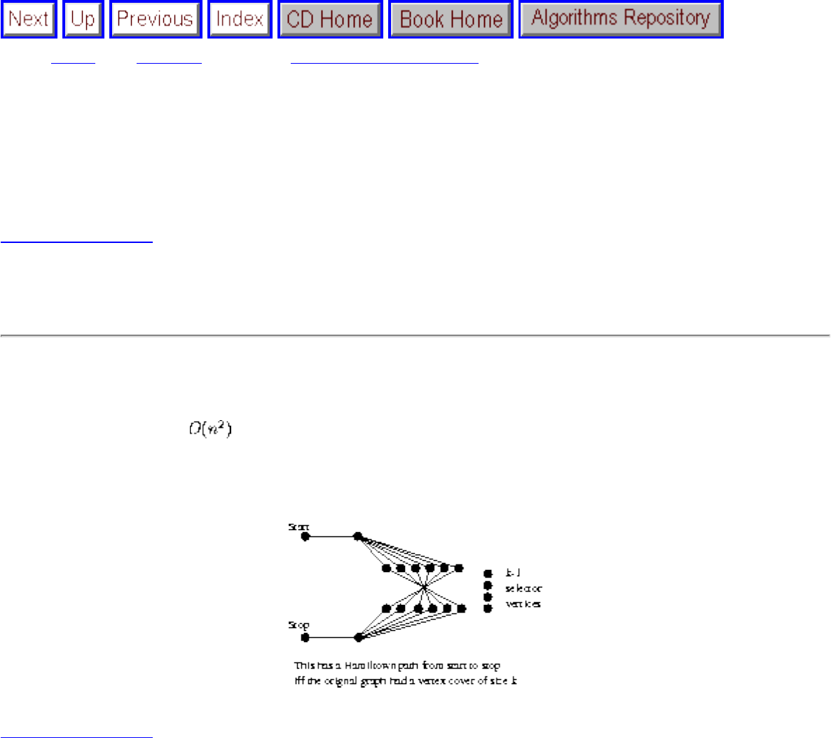
Lecture 23 - approximation algorithms and Cook's theorem
Next: Index Up: No Title Previous: Lecture 22 - techniques
Lecture 23 - approximation algorithms
and Cook's theorem
Listen To Part 26-1
36.5-5 Prove that Hamiltonian Path is NP-complete.
This is not a special case of Hamiltonian cycle! (G may have a HP but not cycle)
The easiest argument says that G contains a HP but no HC iff (x,y) in G such that adding edge (x, y) to G
causes to have a HC, so calls to a HC function solves HP.
The cleanest proof modifies the VC and HC reduction from the book:
Listen To Part 27-3
Approximating Vertex Cover
As we have seen, finding the minimum vertex cover is NP-complete. However, a very simple strategy
(heuristic) can get us a cover at most twice that of the optimal.
While the graph has edges
pick an arbitrary edge v, u
file:///E|/LEC/LECTUR16/NODE23.HTM (1 of 11) [19/1/2003 1:35:35]
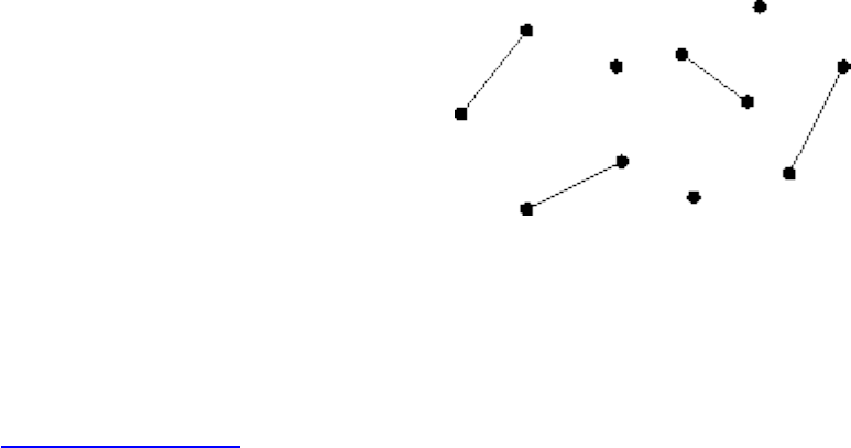
Lecture 23 - approximation algorithms and Cook's theorem
add both u and v to the cover
delete all edges incident on either u and v
If the graph is represented by an adjacency list this can be implemented in O(m+n) time.
This heuristic must always produce cover, since an edge is only deleted when it is adjacent to a cover
vertex.
Further, any cover uses at least half as many vertices as the greedy cover.
Why? Delete all edges from the graph except the edges we selected.
No two of these edges share a vertex. Therefore, any cover of just these edges must include one vertex per
edge, or half the greedy cover!
Listen To Part 27-4
Things to Notice
● Although the heuristic is simple, it is not stupid. Many other seemingly smarter ones can give a far
worse performance in the worst case.
Example: Pick one of the two vertices instead of both (after all, the middle edge is already
covered) The optimal cover is one vertex, the greedy heuristic is two vertices, while the new/bad
heuristic can be as bad as n-1.
file:///E|/LEC/LECTUR16/NODE23.HTM (2 of 11) [19/1/2003 1:35:35]
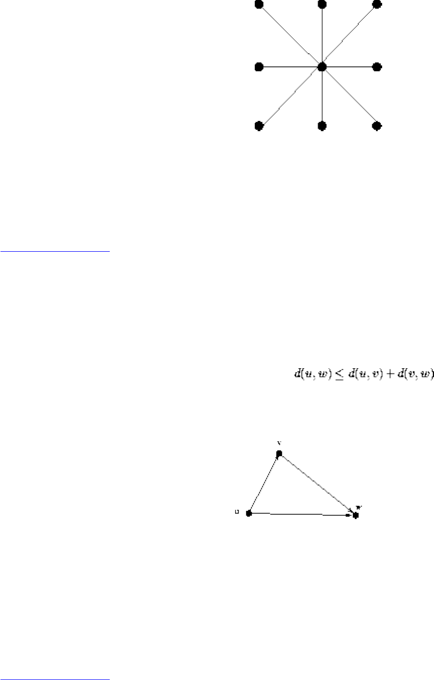
Lecture 23 - approximation algorithms and Cook's theorem
● Proving a lower bound on the optimal solution is the key to getting an approximation result.
● Making a heuristic more complicated does not necessarily make it better. It just makes it more
difficult to analyze.
● A post-processing clean-up step (delete any unecessessary vertex) can only improve things in
practice, but might not help the bound.
Listen To Part 27-5
The Euclidean Traveling Salesman
In the traditional version of TSP - a salesman wants to plan a drive to visit all his customers exactly once
and get back home.
Euclidean geometry satisfies the triangle inequality, .
TSP remains hard even when the distances are Euclidean distances in the plane.
Note that the cost of airfares is an example of a distance function which violates the triangle inequality.
However, we can approximate the optimal Euclidean TSP tour using minimum spanning trees.
Claim: the cost of a MST is a lower bound on the cost of a TSP tour.
Why? Deleting any edge from a TSP tour leaves a path, which is a tree of weight at least that of the MST!
Listen To Part 27-6
If we were allowed to visit cities more than once, doing a depth-first traversal of a MST, and then walking
out the tour specified is at most twice the cost of MST. Why? We will be using each edge exactly twice.
file:///E|/LEC/LECTUR16/NODE23.HTM (3 of 11) [19/1/2003 1:35:35]
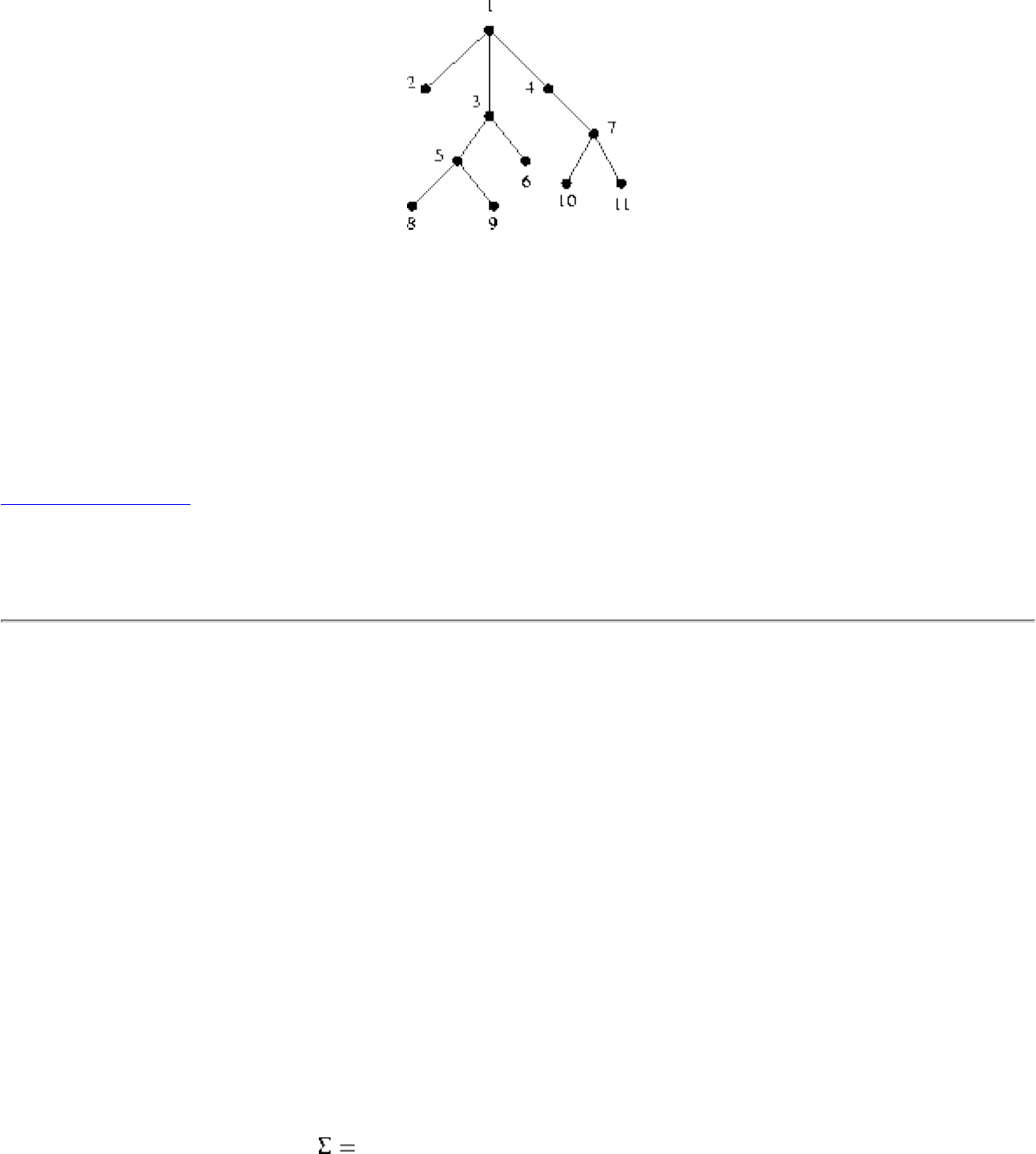
Lecture 23 - approximation algorithms and Cook's theorem
Every edge is used exactly twice in the DFS tour: 1.
However, how can we avoid revisiting cities?
We can take a shortest path to the next unvisited vertex. The improved tour is 1-2-3-5-8-9-6-4-7-10-11-1.
Because we replaced a chain of edges by the edge, the triangle inequality ensures the tour only gets
shorter. Thus this is still within twice optimal!
Listen To Part 27-1
37.1-3 Give an efficient greedy algorithm that finds an optimal vertex cover of a tree in linear time.
In a vertex cover we need to have at least one vertex for each edge.
Every tree has at least two leaves, meaning that there is always an edge which is adjacent to a leaf. Which
vertex can we never go wrong picking? The non-leaf, since it is the only one which can also cover other
edges!
After trimming off the covered edges, we have a smaller tree. We can repeat the process until the tree as 0
or 1 edges. When the tree consists only of an isolated edge, pick either vertex.
All leaves can be identified and trimmed in O(n) time during a DFS.
Formal Languages and the Theory of NP-completeness
The theory of NP-completeness is based on formal languages and Turing machines, and so we will must
work on a more abstract level than usual.
For a given alphabet of symbols 0, 1, &, we can form an infinite set of strings or words by arranging
them in any order: `&10', `111111',`&&&', and `&'.
file:///E|/LEC/LECTUR16/NODE23.HTM (4 of 11) [19/1/2003 1:35:35]
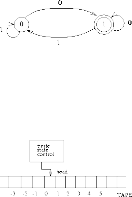
Lecture 23 - approximation algorithms and Cook's theorem
A subset of the set of strings over some alphabet is a formal language.
Formal language theory concerns the study of how powerful a machine you need to recognize whether a
string is from a particular language.
Example: Is the string a binary representation of a even number? A simple finite machine can check if the
last symbol is zero:
No memory is required, except for the current state.
Observe that solving decision problems can be thought of as formal language recognition. The problem
instances are encoded as strings and strings in the language if and only if the answer to the decision
problem is YES!
What kind of machine is necessary to recognize this language? A Turing Machine!
A Turing machine has a finite-state-control (its program), a two way infinite tape (its memory) and a read-
write head (its program counter)
So, where are we?
Each instance of an optimization or decision problem can be encoded as string on some alphabet. The set
of all instances which return True for some problem define a language.
Hence, any problem which solves this problem is equivalent to a machine which recognizes whether an
instance is in the language!
The goal of all this is going to be a formal way to talk about the set of problems which can be solved in
file:///E|/LEC/LECTUR16/NODE23.HTM (5 of 11) [19/1/2003 1:35:35]
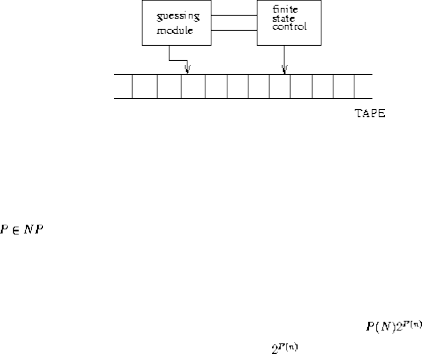
Lecture 23 - approximation algorithms and Cook's theorem
polynomial time, and the set that cannot be.
Non-deterministic Turing Machines
Suppose we buy a guessing module peripherial for our Turing machine, which looks at a Turing machine
program and problem instance and in polynomial time writes something it says is an answer. To convince
ourselves it really is an answer, we can run another program to check it.
Ex: The Traveling Salesman Problem
The guessing module can easily write a permutation of the vertices in polynomial time. We can check if it
is correct by summing up the weights of the special edges in the permutation and see that it is less than k.
The class of languages which we can recognize in time polynomial in the size of the string or a
deterministic Turing Machine (without guessing module) is called P.
The class of languages we can recognize in time polynomial in the length of the string or a non-
deterministic Turing Machine is called NP.
Clearly, , since for any DTM program we can run it on a non-deterministic machine, ignore what
the guessing module is doing, and it will just as fast.
P ?= NP
Observe that any NDTM program which takes time P(n) can simulated in time on a
deterministic machine, by running the checking program times, once on each possible guessed string.
The $10,000 question is whether a polynomial time simulation exists, or in other words whether P=NP?.
Do there exist languages which can be verified in polynomial time and still take exponential time on
deterministic machines?
This is the most important question in computer science. Since proving an exponential time lower bound
for a problem in NP would make us famous, we assume that we cannot do it.
file:///E|/LEC/LECTUR16/NODE23.HTM (6 of 11) [19/1/2003 1:35:35]
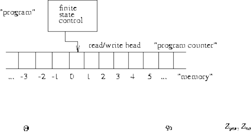
Lecture 23 - approximation algorithms and Cook's theorem
What we can do is prove that it is at least as hard as any problem in NP. A problem in NP for which a
polynomial time algorithm would imply all languages in NP are in P is called NP-complete.
Turing Machines and Cook's Theorem
Cook's Theorem proves that satisfiability is NP-complete by reducing all non-deterministic Turing
machines to SAT.
Each Turing machine has access to a two-way infinite tape (read/write) and a finite state control, which
serves as the program.
A program for a non-deterministic TM is:
1. Space on the tape for guessing a solution and certificate to permit verification.
2. A finite set of tape symbols
3. A finite set of states for the machine, including the start state and final states
4. A transition function, which takes the current machine state, and current tape symbol and returns
the new state, symbol, and head position.
We know a problem is in NP if we have a NDTM program to solve it in worst-case time p[n], where p is a
polynomial and n is the size of the input.
Cook's Theorem - Satisfiability is NP-complete!
Proof: We must show that any problem in NP is at least as hard as SAT. Any problem in NP has a non-
deterministic TM program which solves it in polynomial time, specifically P(n).
We will take this program and create from it an instance of satisfiability such that it is satisfiable if and
only if the input string was in the language.
file:///E|/LEC/LECTUR16/NODE23.HTM (7 of 11) [19/1/2003 1:35:35]
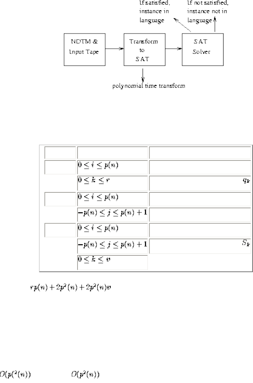
Lecture 23 - approximation algorithms and Cook's theorem
If a polynomial time transform exists, then SAT must be NP-complete, since a polynomial solution to
SAT gives a polynomial time algorithm to anything in NP.
Our transformation will use boolean variables to maintain the state of the TM:
Variable Range Intended meaning
Q[i, j] At time i, M is in
state
H[i,j] At time i, the read-write head
is scanning tape square j
S[i,j,k] At time i, the contents of
tape square j is symbol
Note that there are literals, a polynomial number if p(n) is polynomial.
We will now have to add clauses to ensure that these variables takes or the values as in the TM
computation.
The group 6 clauses enforce the transition function of the machine. If the read-write head is not on tape
square j at time i, it doesn't change ....
There are literals and clauses in all, so the transformation is done in polynomial time!
Polynomial Time Reductions
A decision problem is NP-hard if the time complexity on a deterministic machine is within a polynomial
factor of the complexity of any problem in NP.
file:///E|/LEC/LECTUR16/NODE23.HTM (8 of 11) [19/1/2003 1:35:35]
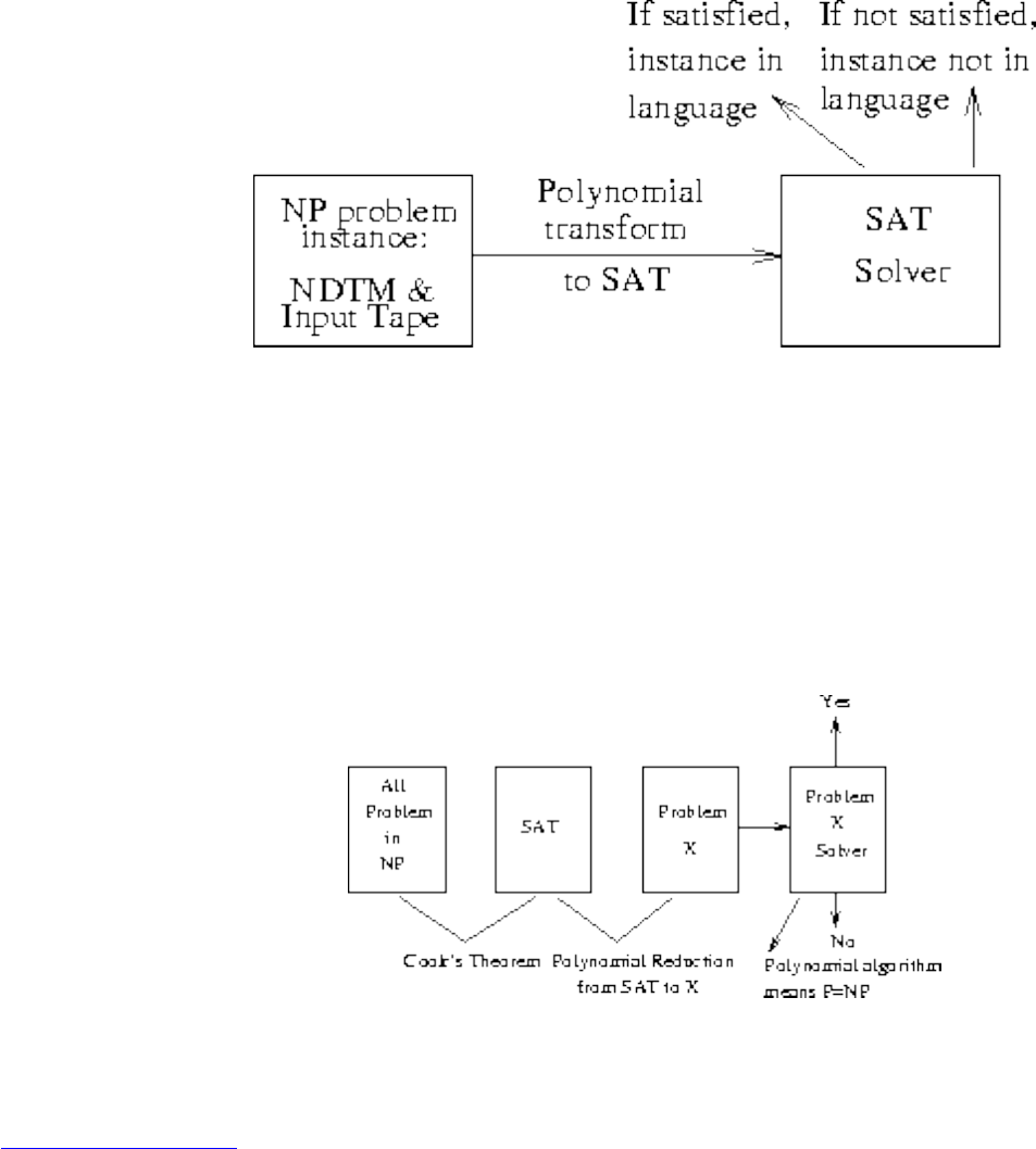
Lecture 23 - approximation algorithms and Cook's theorem
A problem is NP-complete if it is NP-hard and in NP. Cook's theorem proved SATISFIABILITY was NP-
hard by using a polynomial time reduction translating each problem in NP into an instance of SAT:
Since a polynomial time algorithm for SAT would imply a polynomial time algorithm for everything in
NP, SAT is NP-hard. Since we can guess a solution to SAT, it is in NP and thus NP-complete.
The proof of Cook's Theorem, while quite clever, was certainly difficult and complicated. We had to
show that all problems in NP could be reduced to SAT to make sure we didn't miss a hard one.
But now that we have a known NP-complete problem in SAT. For any other problem, we can prove it NP-
hard by polynomially transforming SAT to it!
Since the composition of two polynomial time reductions can be done in polynomial time, all we need
show is that SAT, ie. any instance of SAT can be translated to an instance of x in polynomial time.
Listen To Part 27-7
Finding the Optimal Spouse
1. There are up to n possible candidates we will see over our lifetime, one at a time.
2. We seek to maximize our probability of getting the single best possible spouse.
file:///E|/LEC/LECTUR16/NODE23.HTM (9 of 11) [19/1/2003 1:35:35]
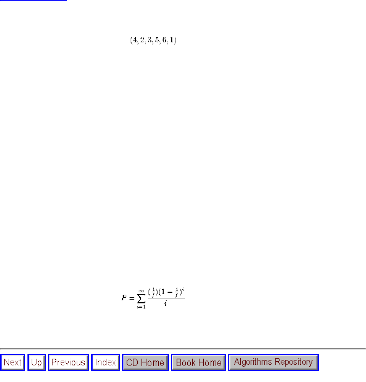
Lecture 23 - approximation algorithms and Cook's theorem
3. Our assessment of each candidate is relative to what we have seen before.
4. We must decided either to marry or reject each candidate as we see them. There is no going back
once we reject someone.
5. Each candidate is ranked from 1 to n, and all permutations are equally likely.
Listen To Part 27-8
For example, if the input permutation is
we see (3,1,2) after three candidates.
Picking the first or last candidate gives us a probability of 1/n of getting the best.
Since we seek maximize our chances of getting the best, it never pays to pick someone who is not the best
we have seen.
The optimal strategy is clearly to sample some fraction of the candidates, then pick the first one who is
better than the best we have seen.
But what is the fraction?
Listen To Part 27-9
For a given fraction 1/f, what is the probability of finding the best?
Suppose i+1 is the highest ranked person in the first n/f candidates. We win whenever the best candidate
occurs before any number from 2 to i in the last n (1- 1/f) / f candidates.
There is a 1/i probability of that, so,
In fact, the optimal is obtained by sampling the first n/e candidates.
Next: Index Up: No Title Previous: Lecture 22 - techniques
file:///E|/LEC/LECTUR16/NODE23.HTM (10 of 11) [19/1/2003 1:35:35]
Lecture 23 - approximation algorithms and Cook's theorem
Algorithms
Mon Jun 2 09:21:39 EDT 1997
file:///E|/LEC/LECTUR16/NODE23.HTM (11 of 11) [19/1/2003 1:35:35]
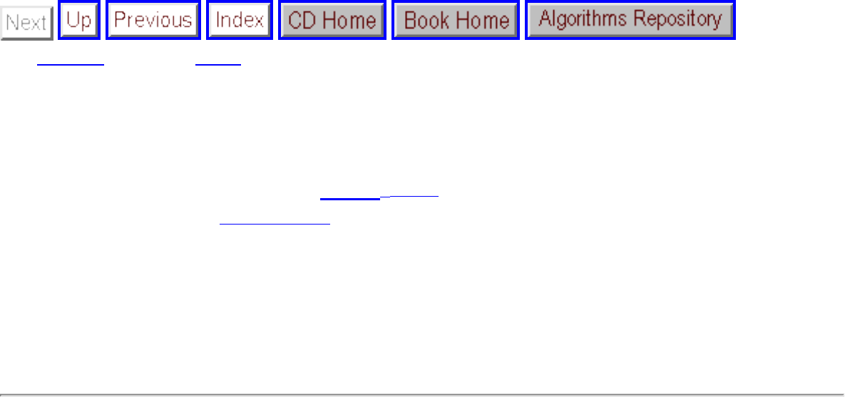
About this document ...
Up: No Title Previous: Index
About this document ...
This document was generated using the LaTeX2HTML translator Version 96.1 (Feb 5, 1996) Copyright
© 1993, 1994, 1995, 1996, Nikos Drakos, Computer Based Learning Unit, University of Leeds.
The command line arguments were:
latex2html all.tex.
The translation was initiated by Algorithms on Mon Jun 2 09:21:39 EDT 1997
Algorithms
Mon Jun 2 09:21:39 EDT 1997
file:///E|/LEC/LECTUR16/NODE25.HTM [19/1/2003 1:35:36]
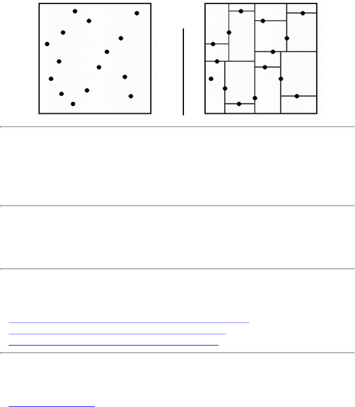
1.1.6 Kd-Trees
1.1.6 Kd-Trees
INPUT OUTPUT
Input Description: A set S of n points in k -dimensions.
Problem: Construct a tree which partitions the space by half-planes such that each point is contained in
it is own region.
Implementations
● Ranger - Nearest Neighbor Search in Higher Dimensions (C) (rating 8)
● Handbook of Algorithms and Data Structures (Pascal) (rating 3)
● DIMACS Implementation Challenges (FORTRAN) (rating 1)
Related Problems
● Nearest Neighbor Search
file:///E|/WEBSITE/FILES/00000007.HTM (1 of 2) [19/1/2003 1:35:38]

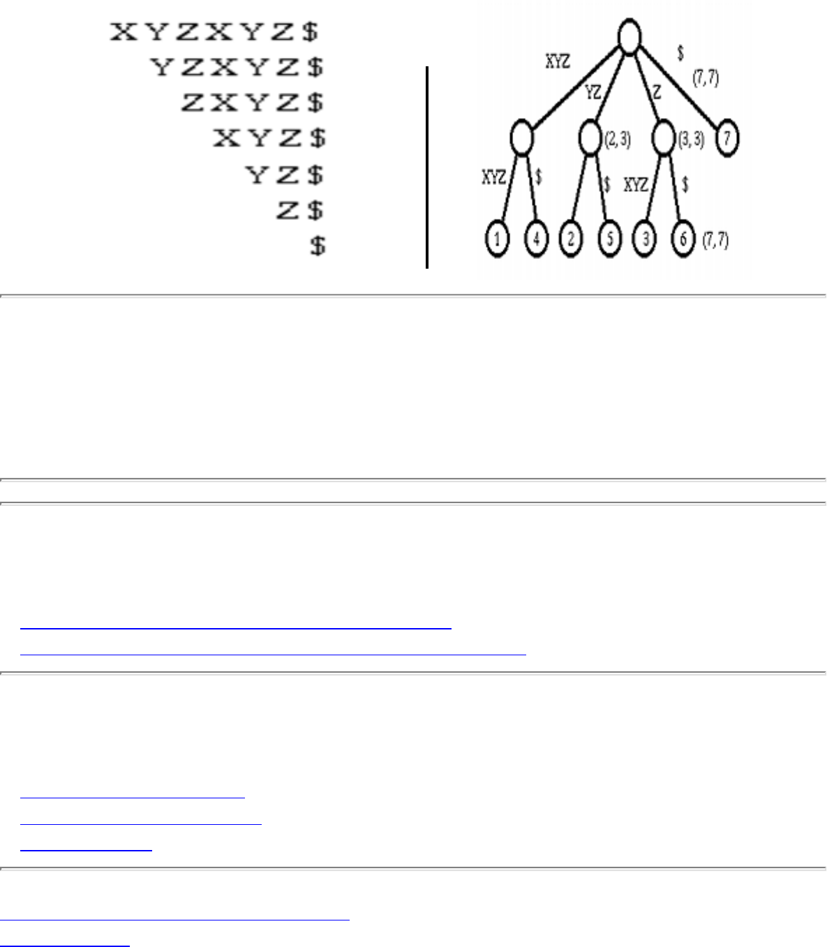
1.1.3 Suffix Trees and Arrays
1.1.3 Suffix Trees and Arrays
INPUT OUTPUT
Implementations
● Stony Brook Project Implementations (C++) (rating 6)
● Handbook of Algorithms and Data Structures (Pascal) (rating 2)
Related Problems
● Longest Common Substring
● Shortest Common Superstring
● String Matching
Go to the corresponding chapter in the book
About the Book
file:///E|/WEBSITE/FILES/SUFFREES.HTM (1 of 2) [19/1/2003 1:35:39]

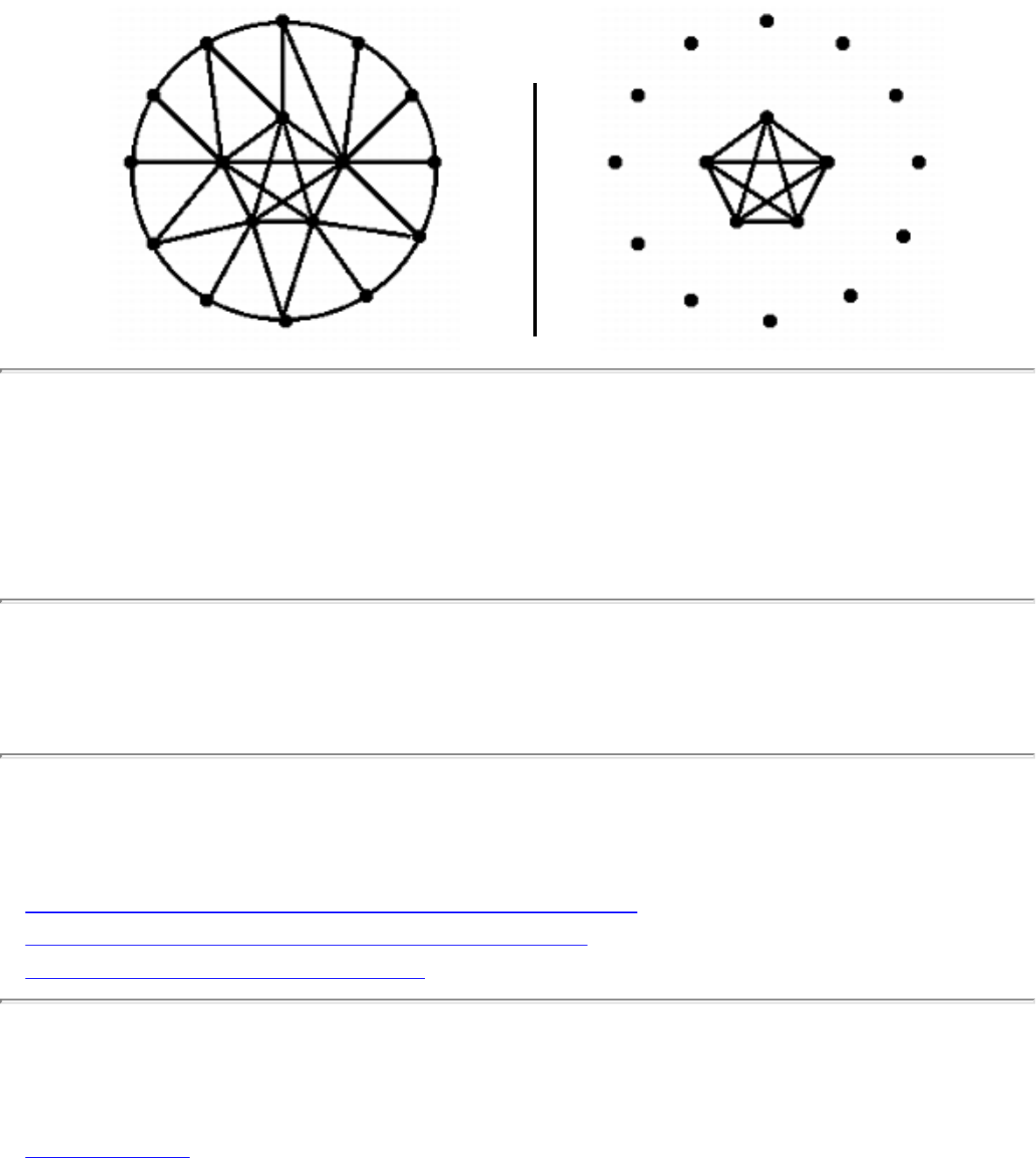
1.5.1 Clique
1.5.1 Clique
INPUT OUTPUT
Input Description: A graph G=(V,E) .
Problem: What is the largest S \subset V such that for all x,y \in S , (x,y) \in E ?
Implementations
● DIMACS Implementation Challenges (FORTRAN) (rating 9)
● Neural-Networks for Cliques and Coloring (C) (rating 6)
● Combinatorica (Mathematica) (rating 1)
Related Problems
● Independent Set
file:///E|/WEBSITE/FILES/CLIQUE05.HTM (1 of 2) [19/1/2003 1:35:40]

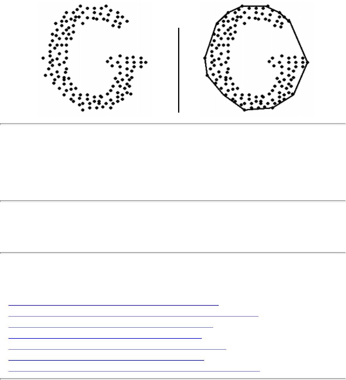
1.6.2 Convex Hull
1.6.2 Convex Hull
INPUT OUTPUT
Input Description: A set S of n points in d -dimensional space.
Problem: Find the smallest convex polygon containing all the points of S .
Implementations
● Qhull - higher dimensional convex hull program (C) (rating 10)
● LEDA - A Library of Efficient Data Types and Algorithms (C++) (rating 6)
● Clarkson's higher dimensional convex hull code (C) (rating 6)
● Joseph O'Rourke's Computational Geometry (C) (rating 6)
● Xtango and Polka Algorithm Animation Systems (C++) (rating 4)
● Moret and Shapiro's Algorithms P to NP (Pascal) (rating 3)
● Netlib / TOMS -- Collected Algorithms of the ACM (FORTRAN) (rating 3)
file:///E|/WEBSITE/FILES2/CONVHULL.HTM (1 of 2) [19/1/2003 1:35:42]

1.6.2 Convex Hull
Related Problems
● Simplifying Polygons
● Sorting
● Traveling Salesman Problem
● Voronoi Diagrams
Go to the corresponding chapter in the book
About the Book
Send us Mail
Go to Main Page
This page last modified on Tue Jun 03, 1997 .
file:///E|/WEBSITE/FILES2/CONVHULL.HTM (2 of 2) [19/1/2003 1:35:42]

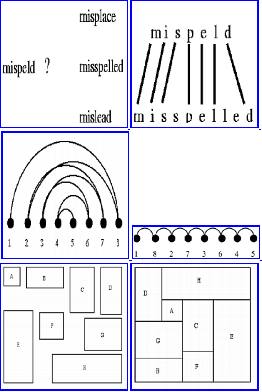
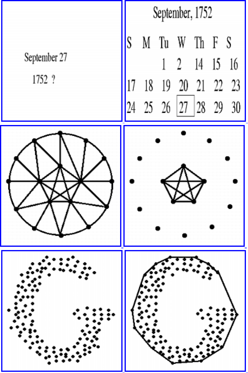
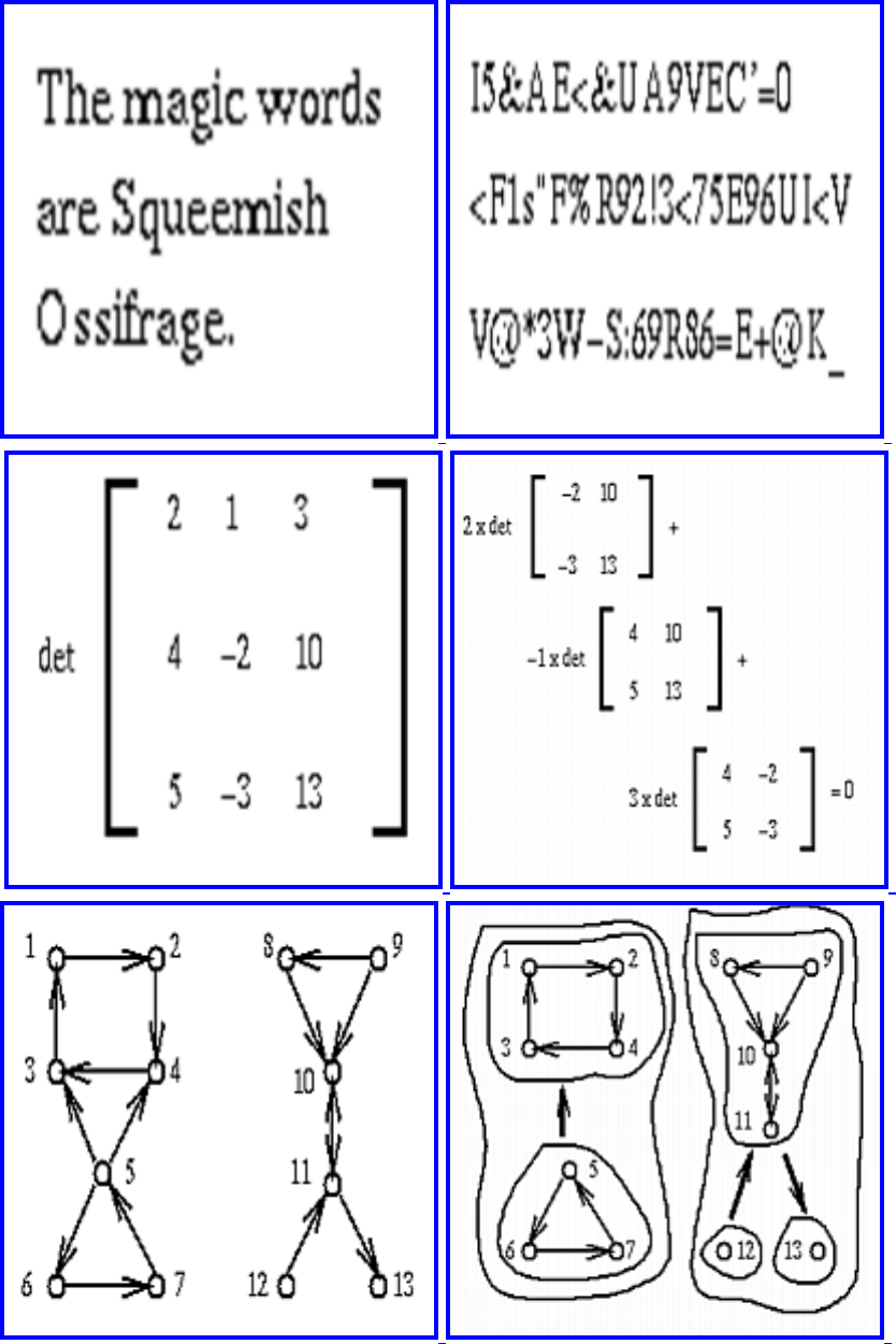
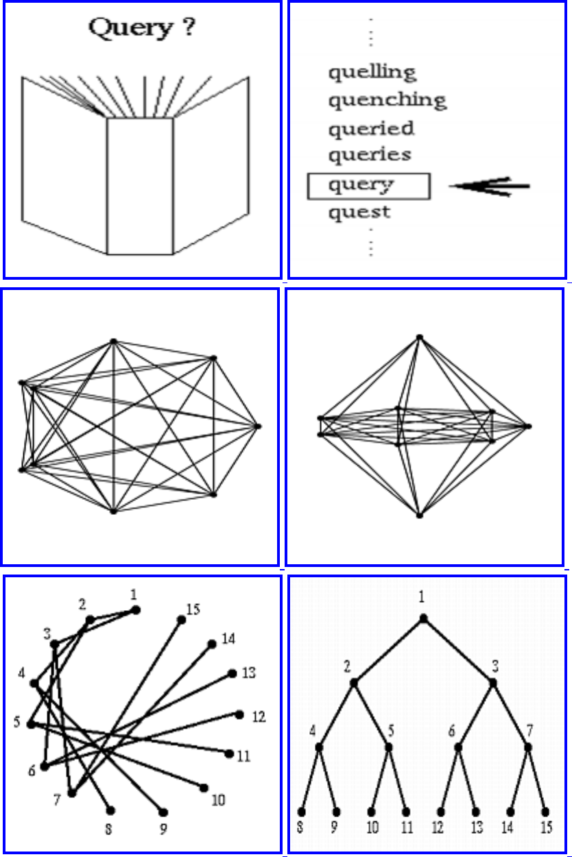
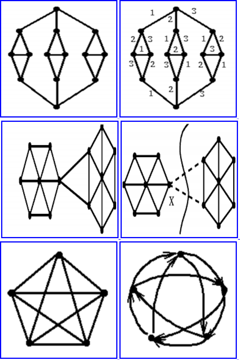
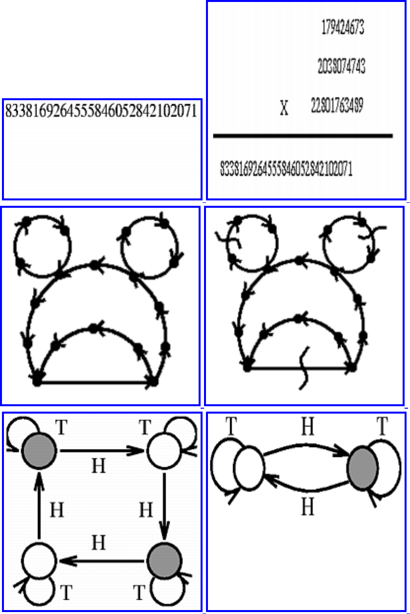
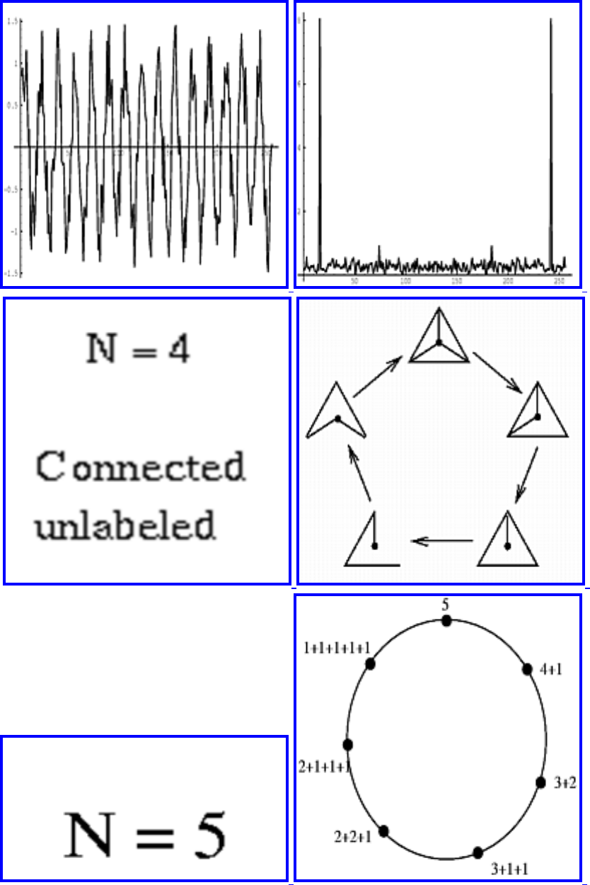
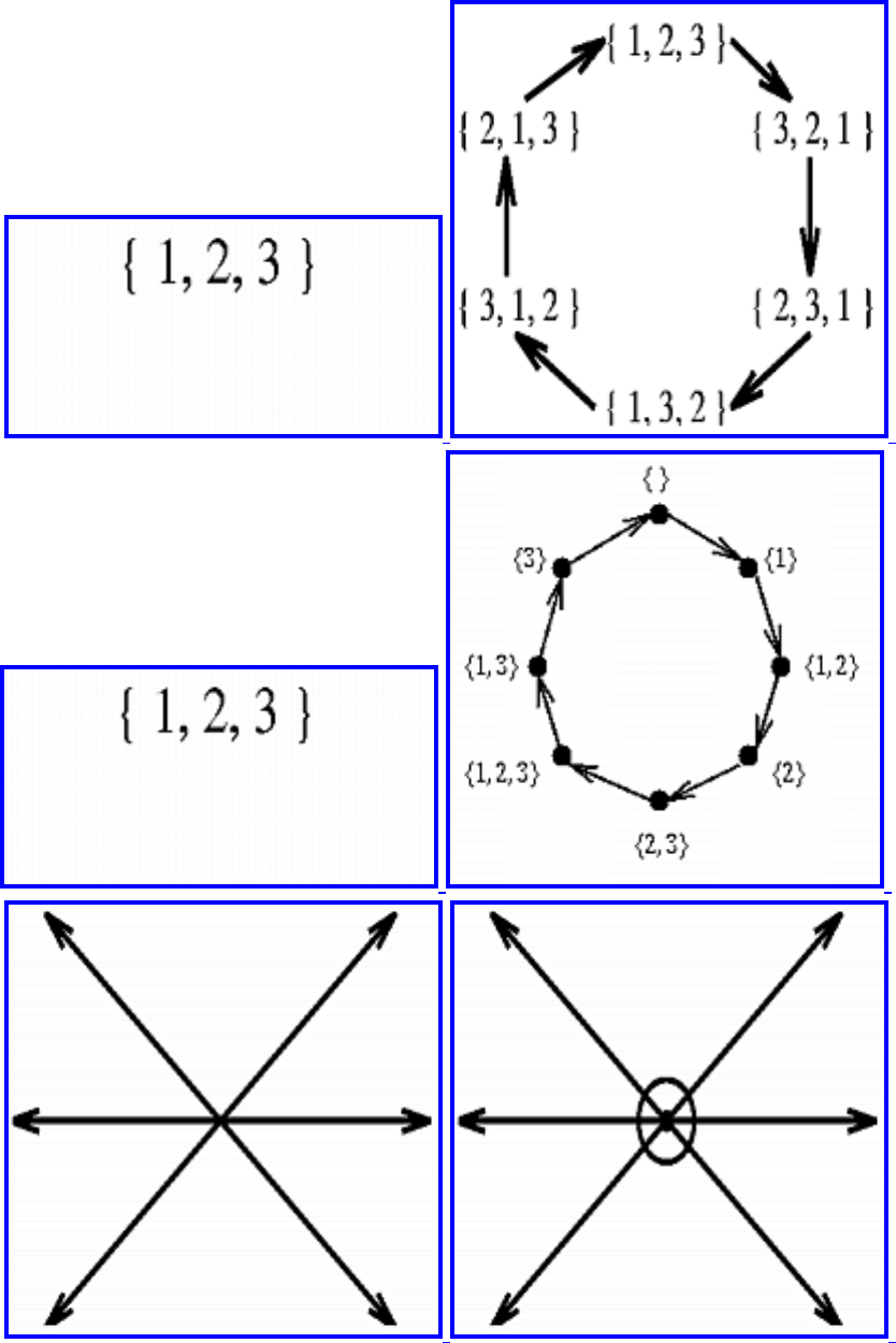
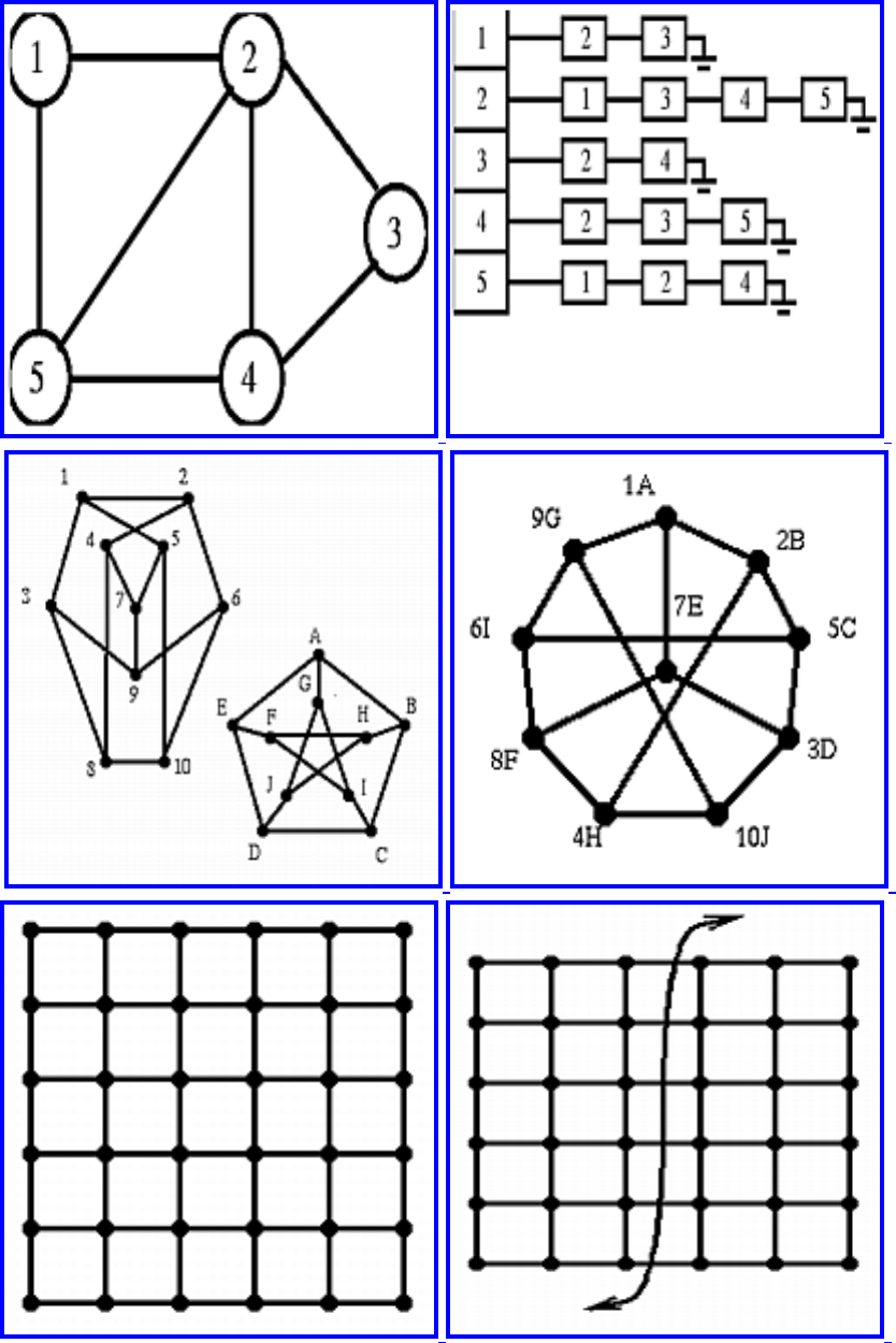
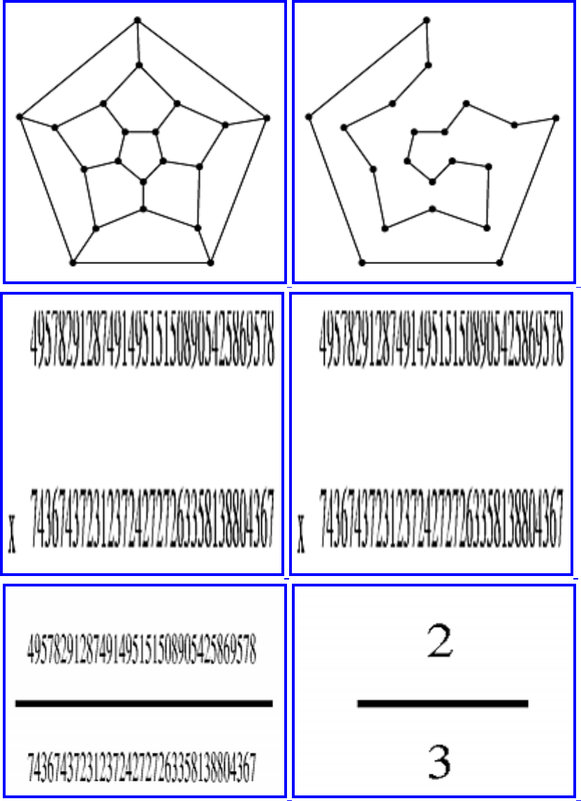
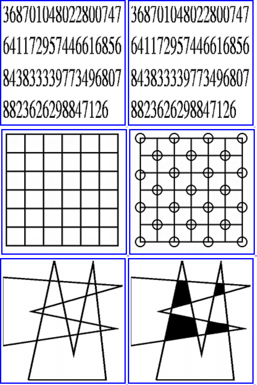
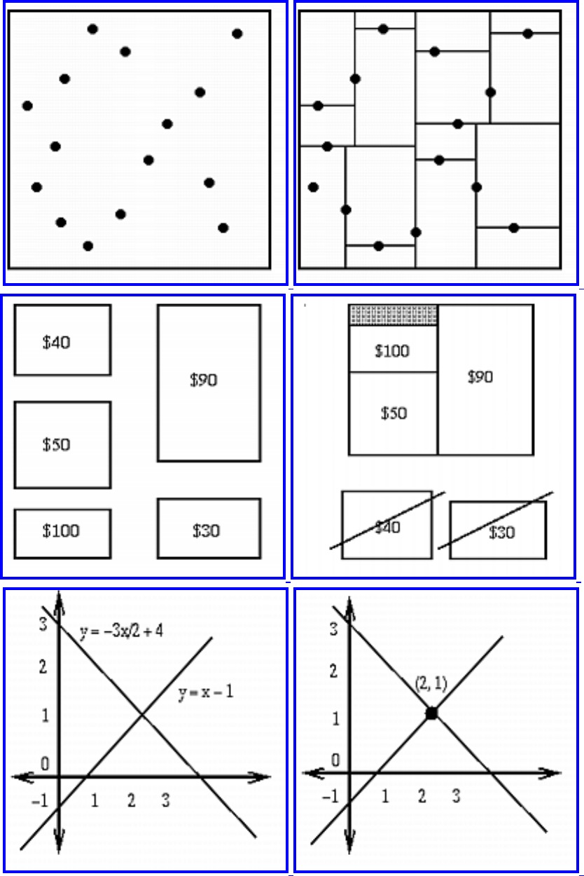
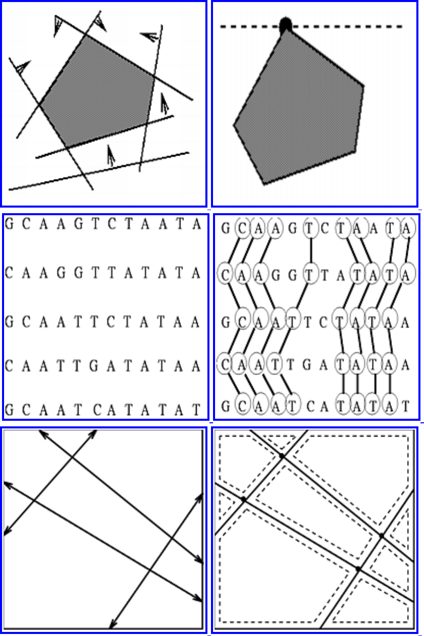
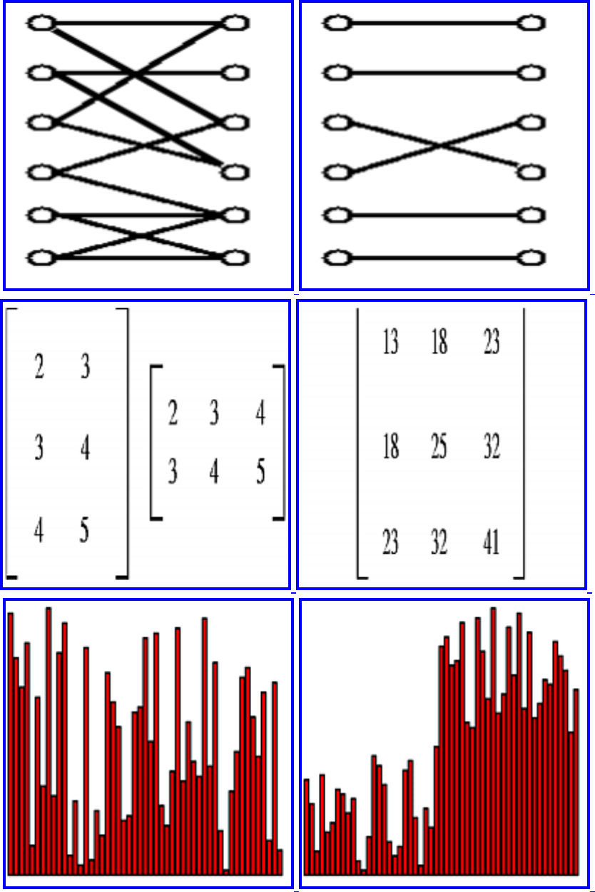
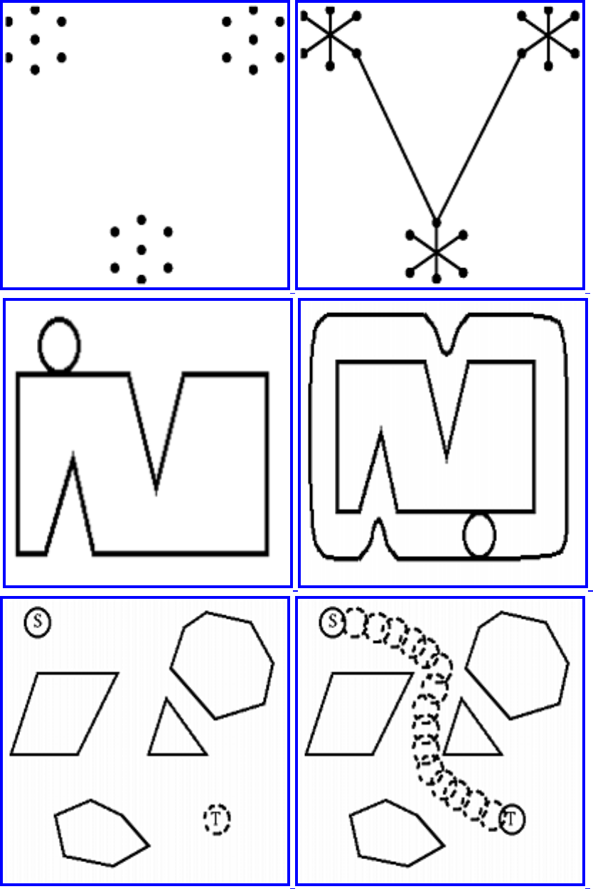
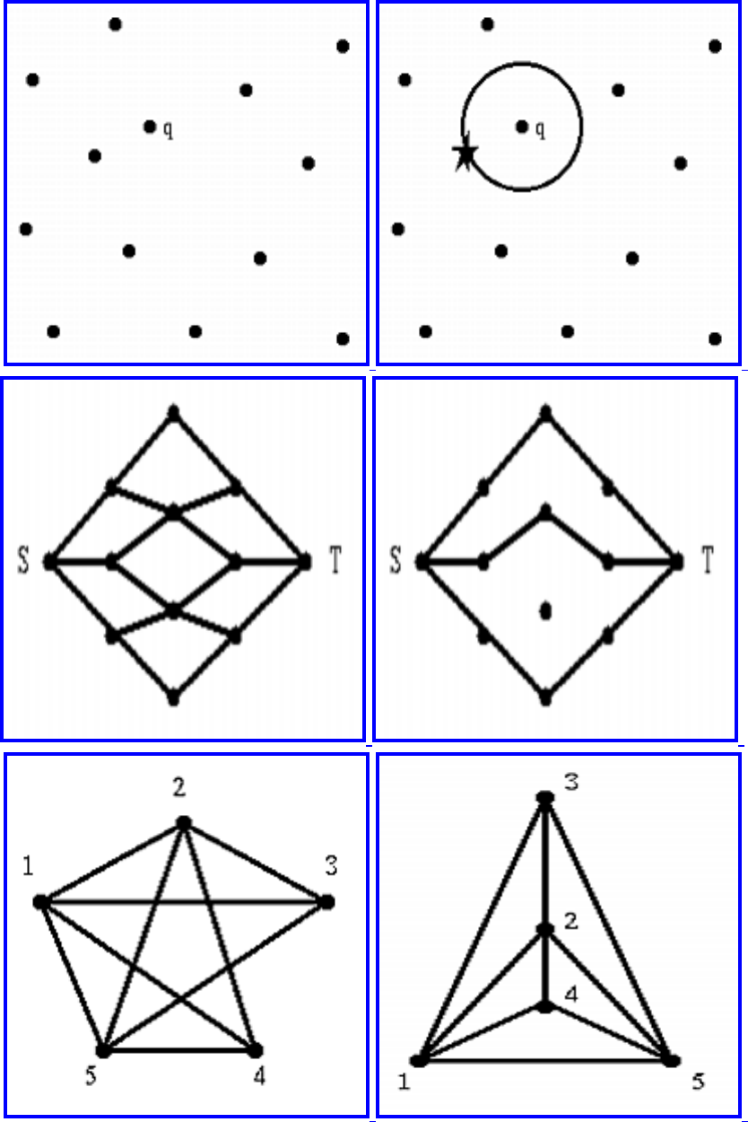
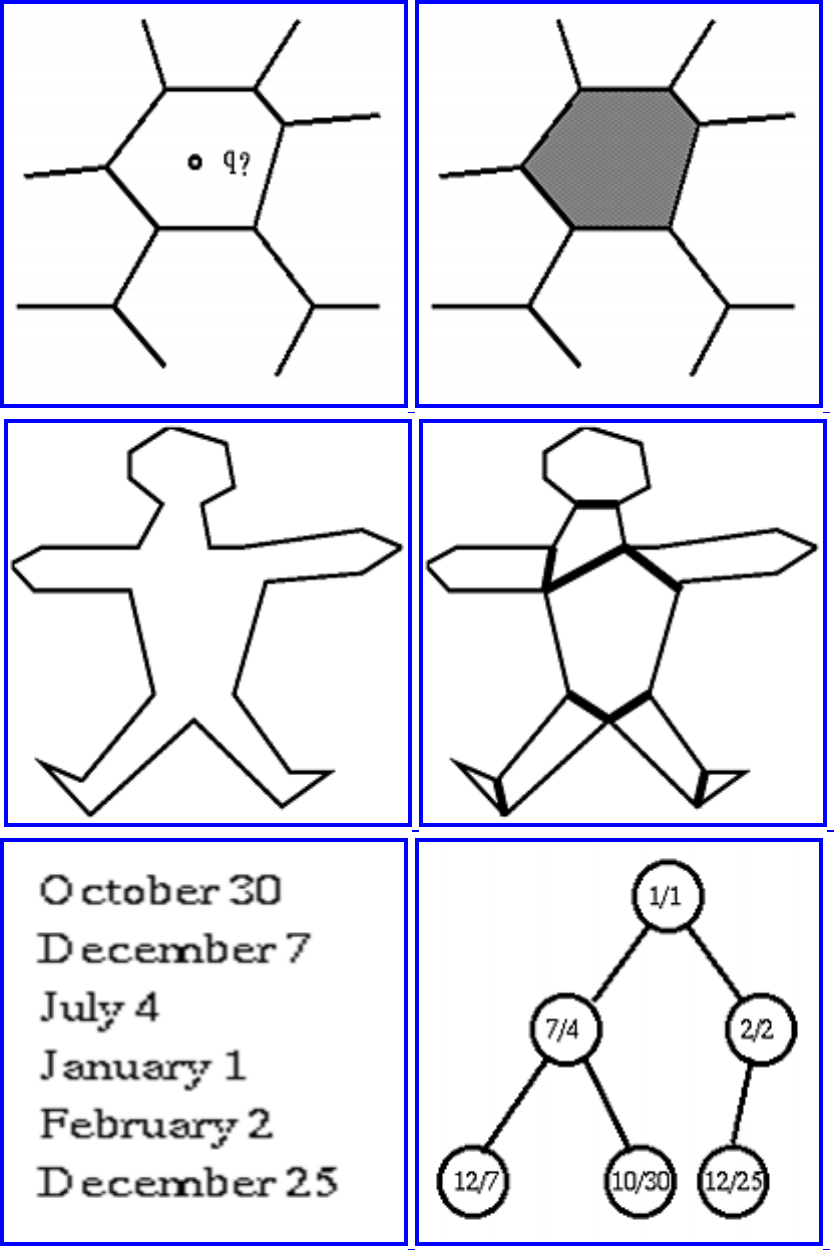
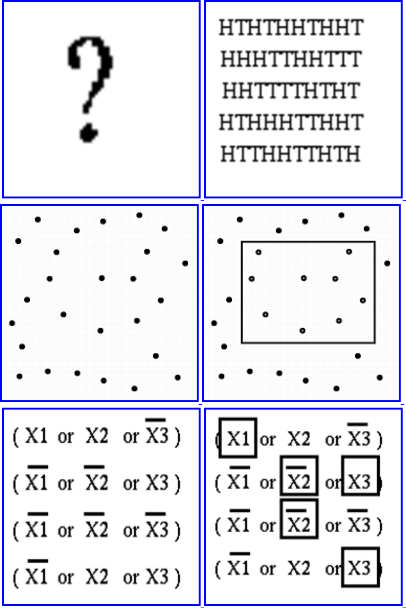
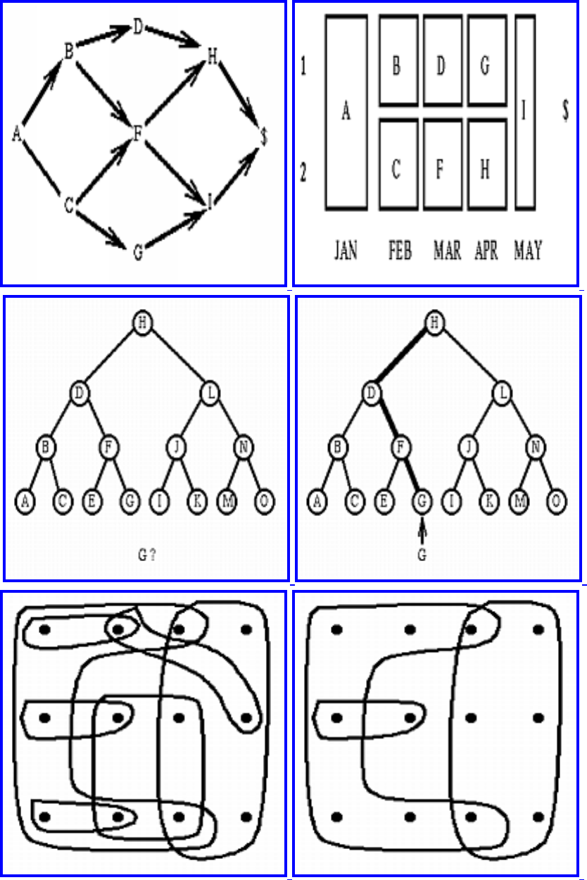
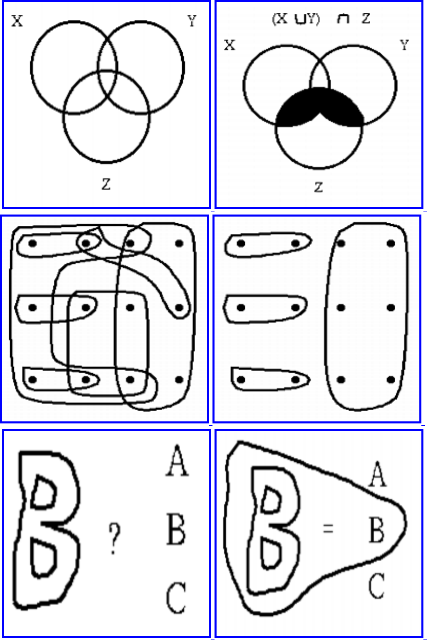
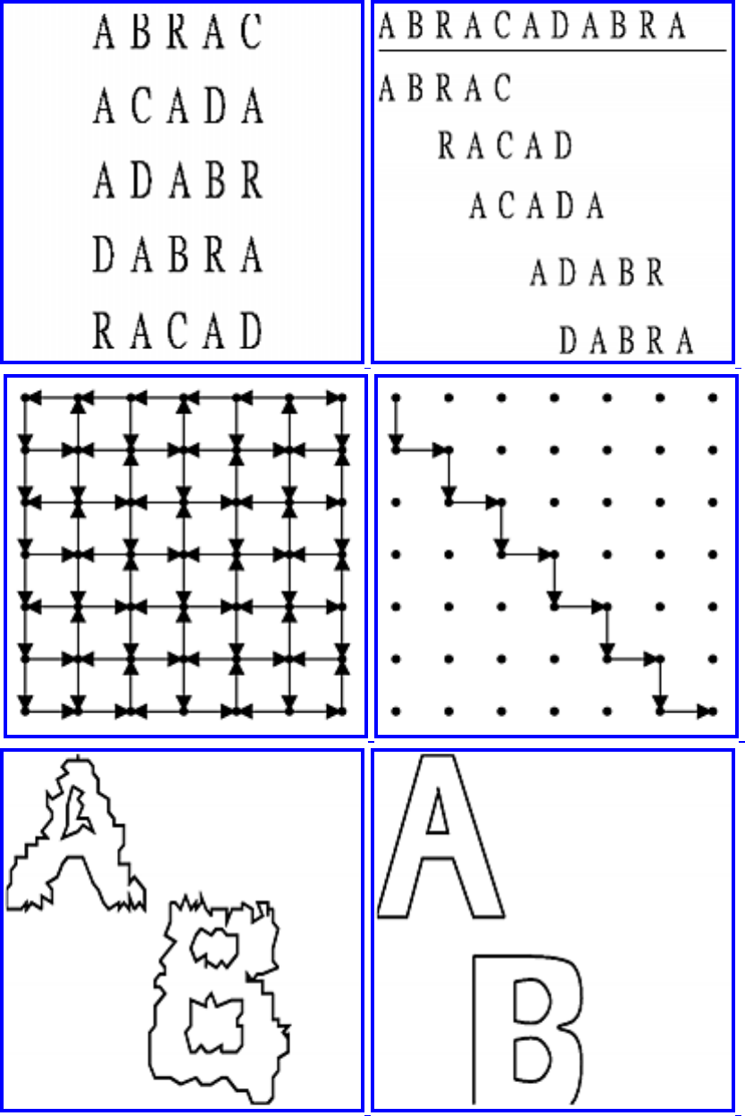
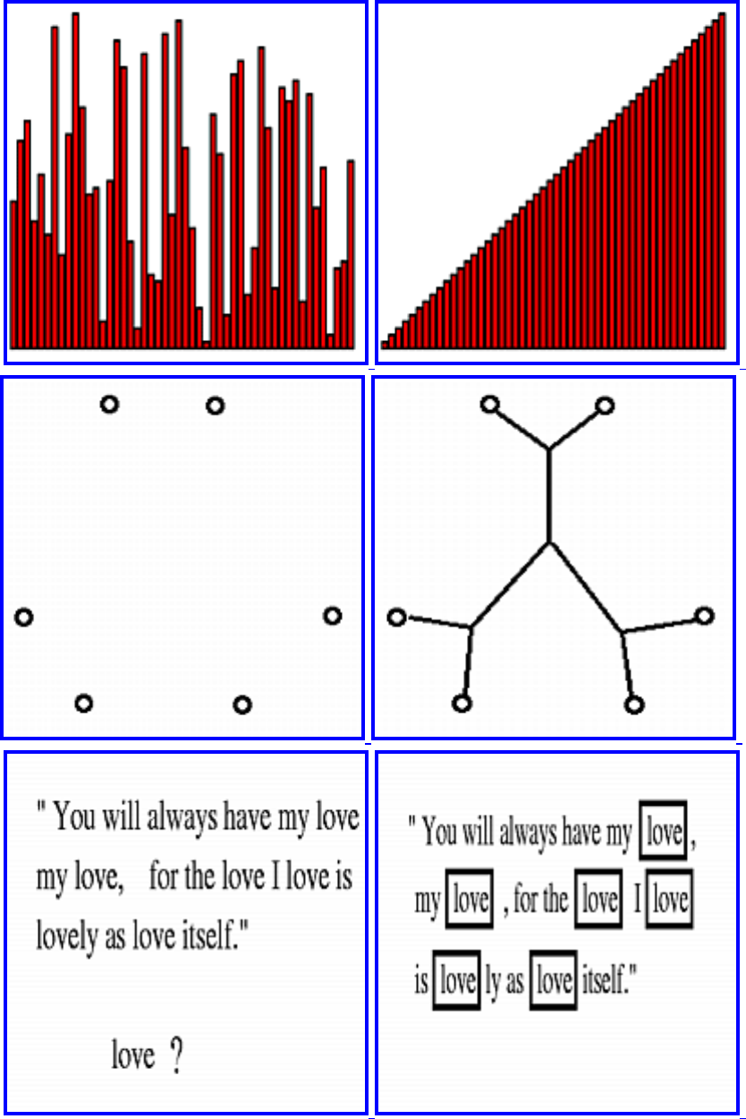
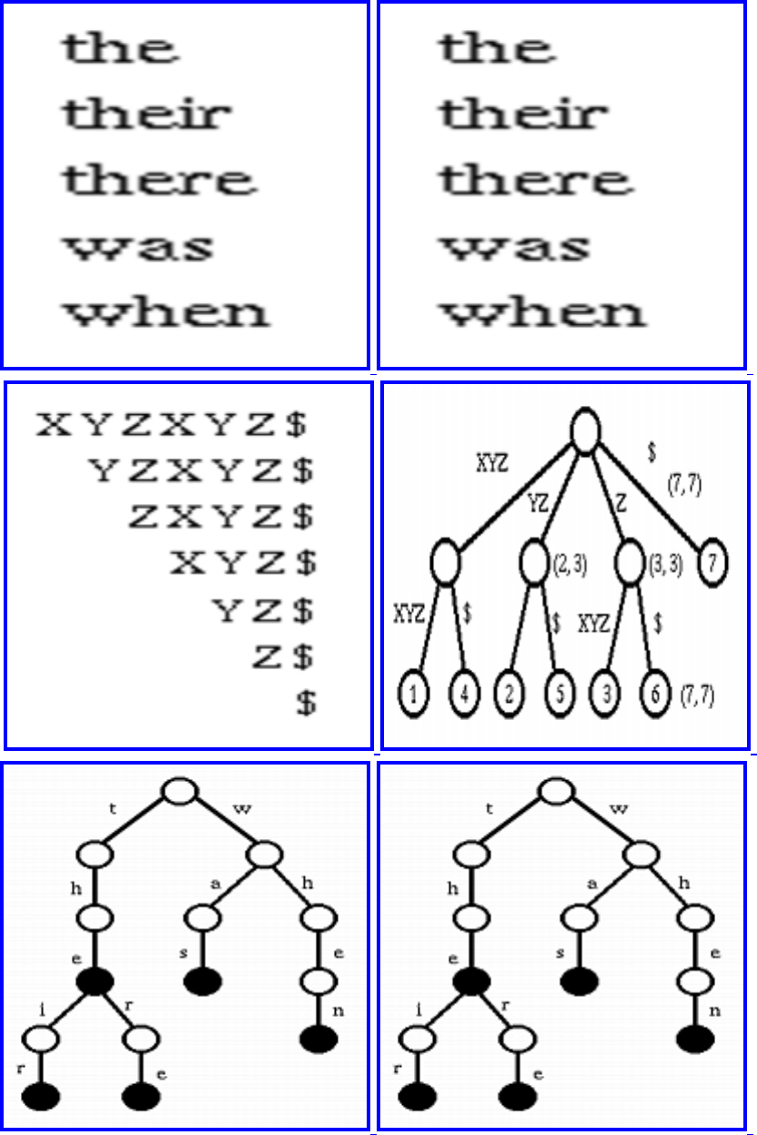
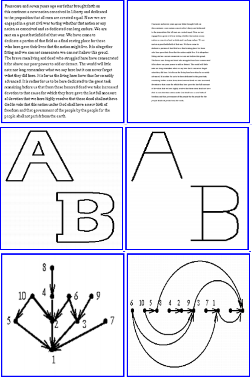
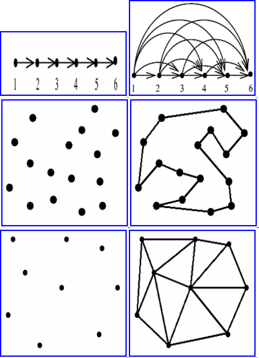
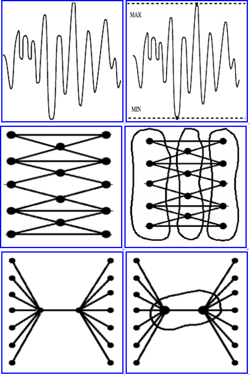
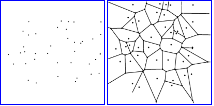

Interesting Data Files
Interesting Data Files
Below we point to several interesting data files. These files can be used as test data for several of the
Implementation Challenges given in The Algorithm Design Manual , but are also likely to be of
independent interest.
● Airplane routes and schedules (from Roberto Tamassia -- local copy)
● Name-ethnicity data; over 3000 names from several nations (local copy)
About the Book
Send us Mail
Go to Main Page
file:///E|/WEBSITE/BIBLIO/TESTDATA/DATA.HTM [19/1/2003 1:36:29]

About the Ratings
About the Ratings
Our implementations are classified by the problems they solve. For each problem, we rate all the
implementations according to usefulness on a 1 to 10 scale, with 10 meaning the most useful and 1 least
useful. The usefulness of an implementation is supposed to reflect how likely it is that someone looking
for code will be happy with what they find. Our ratings are completely subjective and reflect our
judgement. Please feel free to send corrections and feedback based on your experiences. Please note that
many of these implementations with low usefulness ratings were produced primarily for expository
purposes, and can serve as excellent models to study or emulate if not as ready-to-run code.
Go to Main Page
file:///E|/WEBSITE/INFO/RATINGS.HTM [19/1/2003 1:36:29]

1.1 Data Structures
1.1 Data Structures
Specific Algorithms
● 1.1.1 Dictionaries
● 1.1.2 Priority Queues
● 1.1.3 Suffix Trees and Arrays
● 1.1.4 Graph Data Structures
● 1.1.5 Set Data Structures
● 1.1.6 Kd-Trees
About the Book
Send us Mail
Go to Main Page
This page last modified on Tue Jun 03, 1997 .
file:///E|/WEBSITE/MAJOR_SE/1_1.HTM [19/1/2003 1:36:29]

1.2 Numerical Problems
1.2 Numerical Problems
Specific Algorithms
● 1.2.1 Solving Linear Equations
● 1.2.2 Bandwidth Reduction
● 1.2.3 Matrix Multiplication
● 1.2.4 Determinants and Permanents
● 1.2.5 Constrained and Unconstrained Optimization
● 1.2.6 Linear Programming
● 1.2.7 Random Number Generation
● 1.2.8 Factoring and Primality Testing
● 1.2.9 Arbitrary Precision Arithmetic
● 1.2.10 Knapsack Problem
● 1.2.11 Discrete Fourier Transform
About the Book
Send us Mail
Go to Main Page
This page last modified on Tue Jun 03, 1997 .
file:///E|/WEBSITE/MAJOR_SE/1_2.HTM [19/1/2003 1:36:30]

1.3 Combinatorial Problems
1.3 Combinatorial Problems
Specific Algorithms
● 1.3.1 Sorting
● 1.3.2 Searching
● 1.3.3 Median and Selection
● 1.3.4 Generating Permutations
● 1.3.5 Generating Subsets
● 1.3.6 Generating Partitions
● 1.3.7 Generating Graphs
● 1.3.8 Calendrical Calculations
● 1.3.9 Job Scheduling
● 1.3.10 Satisfiability
About the Book
Send us Mail
Go to Main Page
This page last modified on Tue Jun 03, 1997 .
file:///E|/WEBSITE/MAJOR_SE/1_3.HTM [19/1/2003 1:36:31]

1.4 Graph Problems -- polynomial-time problems
1.4 Graph Problems -- polynomial-time problems
Specific Algorithms
● 1.4.1 Connected Components
● 1.4.2 Topological Sorting
● 1.4.3 Minimum Spanning Tree
● 1.4.4 Shortest Path
● 1.4.5 Transitive Closure and Reduction
● 1.4.6 Matching
● 1.4.7 Eulerian Cycle / Chinese Postman
● 1.4.8 Edge and Vertex Connectivity
● 1.4.9 Network Flow
● 1.4.10 Drawing Graphs Nicely
● 1.4.11 Drawing Trees
● 1.4.12 Planarity Detection and Embedding
About the Book
Send us Mail
Go to Main Page
This page last modified on Tue Jun 03, 1997 .
file:///E|/WEBSITE/MAJOR_SE/1_4.HTM [19/1/2003 1:36:31]

1.5 Graph Problems -- hard problems
1.5 Graph Problems -- hard problems
Specific Algorithms
● 1.5.1 Clique
● 1.5.2 Independent Set
● 1.5.3 Vertex Cover
● 1.5.4 Traveling Salesman Problem
● 1.5.5 Hamiltonian Cycle
● 1.5.6 Graph Partition
● 1.5.7 Vertex Coloring
● 1.5.8 Edge Coloring
● 1.5.9 Graph Isomorphism
● 1.5.10 Steiner Tree
● 1.5.11 Feedback Edge/Vertex Set
About the Book
Send us Mail
Go to Main Page
This page last modified on Tue Jun 03, 1997 .
file:///E|/WEBSITE/MAJOR_SE/1_5.HTM [19/1/2003 1:36:32]

1.6 Computational Geometry
1.6 Computational Geometry
Specific Algorithms
● 1.6.1 Robust Geometric Primitives
● 1.6.2 Convex Hull
● 1.6.3 Triangulation
● 1.6.4 Voronoi Diagrams
● 1.6.5 Nearest Neighbor Search
● 1.6.6 Range Search
● 1.6.7 Point Location
● 1.6.8 Intersection Detection
● 1.6.9 Bin Packing
● 1.6.10 Medial-Axis Transformation
● 1.6.11 Polygon Partitioning
● 1.6.12 Simplifying Polygons
● 1.6.13 Shape Similarity
● 1.6.14 Motion Planning
● 1.6.15 Maintaining Line Arrangements
● 1.6.16 Minkowski Sum
About the Book
Send us Mail
Go to Main Page
This page last modified on Tue Jun 03, 1997 .
file:///E|/WEBSITE/MAJOR_SE/1_6.HTM [19/1/2003 1:36:32]

1.7 Set and String Problems
1.7 Set and String Problems
Specific Algorithms
● 1.7.1 Set Cover
● 1.7.2 Set Packing
● 1.7.3 String Matching
● 1.7.4 Approximate String Matching
● 1.7.5 Text Compression
● 1.7.6 Cryptography
● 1.7.7 Finite State Machine Minimization
● 1.7.8 Longest Common Substring
● 1.7.9 Shortest Common Superstring
About the Book
Send us Mail
Go to Main Page
This page last modified on Tue Jun 03, 1997 .
file:///E|/WEBSITE/MAJOR_SE/1_7.HTM [19/1/2003 1:36:32]

C++ Language Implementations
Algorithm Implementations in C++
● LEDA - A Library of Efficient Data Types and Algorithms
● SimPack/Sim++ Simulation Toolkit
● Fire-Engine and Spare-Parts String and Language Algorithms
● Xtango and Polka Algorithm Animation Systems
● Algorithms in C++ -- Sedgewick
● Geolab -- Computational Geometry System
● Grail: finite automata and regular expressions
● Calendrical Calculations
● Stony Brook Project Implementations
● LINK -- Programming and Visualization Environment for Hypergraphs
● David Eppstein's Knuth-Morris-Pratt Algorithm and Minkowski sum code
About the Book
Send us Mail
Go to Main Page
This page last modified on Tue Jun 03, 1997 .
file:///E|/WEBSITE/IMPLEMEN/CPP.HTM [19/1/2003 1:36:33]

C Language Implementations
Algorithm Implementations in C
● Adaptive Simulated Annealing
● Joseph O'Rourke's Computational Geometry
● The Stanford GraphBase
● GraphViz -- graph layout programs
● Handbook of Algorithms and Data Structures
● Mike Trick's Graph Coloring Resources
● Joe Culberson's Graph Coloring Resources
● DIMACS Implementation Challenges
● Fire-Engine and Spare-Parts String and Language Algorithms
● Ranger - Nearest Neighbor Search in Higher Dimensions
● Xtango and Polka Algorithm Animation Systems
● Frank Ruskey's Combinatorial Generation Resources
● Goldberg's Network Optimization Codes
● Qhull - higher dimensional convex hull program
● Clarkson's higher dimensional convex hull code
● Fortune's 2D Voronoi diagram code
● Triangle: A Two-Dimensional Quality Mesh Generator
● Arrange - maintainance of arrangements with point location
● Linprog -- low dimensional linear programming
● LP_SOLVE: Linear Programming Code
● PARI - Package for Number Theory
● GraphEd -- Graph Editor and Layout Program
● Genocop -- Optimization via Genetic Algorithms
● TSP solvers
● FFTPACK -- Fourier Transform Library
● Neural-Networks for Cliques and Coloring
● PHYLIP -- inferring phylogenic trees
● Salowe's Rectilinear Steiner trees
● Skeletonization Software (2-D)
● SNNS - Stuttgart Neural Network Simulator
● agrep - Approximate General Regular Expression Pattern Matcher
● HT/DIG -- image compression codes
● CAP -- Contig Assembly Program
● Shape similarity testing via turning functions
● NAUTY -- Graph Isomorphism
file:///E|/WEBSITE/IMPLEMEN/C.HTM (1 of 2) [19/1/2003 1:36:33]


Pascal Language Implementations
Algorithm Implementations in Pascal
● Discrete Optimization Methods
● Handbook of Algorithms and Data Structures
● Moret and Shapiro's Algorithms P to NP
● Frank Ruskey's Combinatorial Generation Resources
● PHYLIP -- inferring phylogenic trees
About the Book
Send us Mail
Go to Main Page
This page last modified on Tue Jun 03, 1997 .
file:///E|/WEBSITE/IMPLEMEN/PASCAL.HTM [19/1/2003 1:36:34]

FORTRAN Language Implementations
Algorithm Implementations in FORTRAN
● Nijenhuis and Wilf: Combinatorial Algorithms
● DIMACS Implementation Challenges
● Netlib / TOMS -- Collected Algorithms of the ACM
● GEOMPACK - triangulation and convex decomposition codes
● FFTPACK -- Fourier Transform Library
● LAPACK and LINPACK -- Linear Algebra PACKages
About the Book
Send us Mail
Go to Main Page
This page last modified on Tue Jun 03, 1997 .
file:///E|/WEBSITE/IMPLEMEN/FORTRAN.HTM [19/1/2003 1:36:34]

Mathematica Language Implementations
Algorithm Implementations in Mathematica
● Combinatorica
● Mathematica -- Assorted Routines
● Neural-Networks for Cliques and Coloring
About the Book
Send us Mail
Go to Main Page
This page last modified on Tue Jun 03, 1997 .
file:///E|/WEBSITE/IMPLEMEN/MATHEMAT.HTM [19/1/2003 1:36:34]


Algorithm Repository -- Most Wanted List
Most Wanted List
Below are a list of problems for which we do not feel that we have identified adequate codes for the
algorithm repository, and thus we would be particularly excited to hear of any programs you might know
about. In many cases, the algorithms involved are not that difficult to implement, so this is also in
invitation for students and faculty to select them for class projects and send us the resulting code.
Our most wanted list includes:
● Knapsack and Integer Partition -- We would like to see an implementation of the dynamic
programming algorithm for the knapsack, with scaling. Associated with this would be an
implementation of the primary bin-packing algorithms.
● Thinning or the Medial-Axis Transform -- Codes working on binary images and polygons are both
wanted. I have already received more than one request for such a code.
● Chinese Postman Tour -- Such an algorithm should not be too complicated to implement,
especially by using matching codes already available on this site.
● Graph Partition and Maxcut -- A flexible simulated annealing code for both problems would be
greatly appreciated.
● Feedback arc/vertex sets -- It would be good to get an implementation of the (fairly simple)
heuristics for feedback sets and see how well they do.
● Minkowski Sum -- I have already received more than one request for such a code.
● Set Cover -- I'd like to get more codes with heuristics for set cover and packing.
This algorithms repository is part of the ongoing algorithms-related research conducted here in the
Department of Computer Science at the State University of New York at Stony Brook.
About the Book
Send us Mail
Go to Main Page
file:///E|/WEBSITE/INFO/WANTED.HTM [19/1/2003 1:36:35]

Algorithm Repository -- Citations
Citations
Citations of the Stony Brook Algorithms Repository include:
● PC Webopaedia
The algorithms repository is part of the ongoing algorithms-related research conducted here in the
Department of Computer Science at the State University of New York at Stony Brook.
About the Book
Send us Mail
Go to Main Page
file:///E|/WEBSITE/INFO/CITATION.HTM [19/1/2003 1:36:36]

Practical Algorithm Design -- User Feedback
User Feedback
This page allows users to comment on issues related to the Practical Algorithm Design website.
Comments on the website, the upcoming book, implementations, and problems are all welcome, and will
be posted on a separate page for access by other users of this site.
To view comments left by other users, select:
● User Comments
To leave a comment of your own, please fill out the following form:
E-mail address:
Subject:
Enter your comments below:
Return to the home page
If you have problems with this page, please send E-mail to:
algorith@cs.sunysb.edu
file:///E|/WEBSITE/FEEDBACK/FEEDBACK.HTM (1 of 2) [19/1/2003 1:36:36]
Reset
Submit Feedback
Practical Algorithm Design -- User Feedback
file:///E|/WEBSITE/FEEDBACK/FEEDBACK.HTM (2 of 2) [19/1/2003 1:36:36]

Goldberg's Network Optimization Codes
Goldberg's Network Optimization Codes
The highest performance codes available for such network optimization problems as matching, shortest
paths, and network flow have been developed by Andrew Goldberg and his collaborators. All are written
in C. Their codes are available by ftp for non-commercial use, although a license is required for
commercial use. For information on obtaining the codes, check out Andrew Goldberg's WWW page,
http://www.neci.nj.nec.com/homepages/avg.html
Their implementations of both Dijkstra and Bellman-Ford's algorithms for finding shortest paths in
graphs is SPLIB, developed by Cherkassky, Goldberg, and Radzik. They report solving instances with
over one million vertices in under two minutes on a Sun Sparc-10 workstation.
Their code for finding a maximum cardinality bipartite matching of maximum weight shortest paths in
graphs is CSA, developed by Goldberg and Kennedy. This code is based on a cost-scaling network flow
algorithms. Their running times depend upon the density of the networks and weight distributions, but
they report solving instances with over 30,000 vertices in a few minutes on a Sun Sparc-2 workstation.
Their code for solving maximum-flow in graphs is PRF, developed by Cherkassky and Goldberg. They
report solving instances with over 250,000 vertices in under two minutes on a Sun Sparc-10 workstation.
For minimum-cost max-flow, the higher performance code available is CS, capable of solving instances
of over 30,000 vertices in a few minutes on Sun Sparc-2 workstations.
● Andrew Goldberg's home page
Problem Links
● Network Flow (10)
● Matching (9)
● Shortest Path (9)
About the Book
Send us Mail
Go to Main Page
This page last modified on Apr 23, 1997.
file:///E|/WEBSITE/IMPLEMEN/GOLDBERG/IMPLEMEN.HTM [19/1/2003 1:36:37]

LEDA - A Library of Efficient Data Types and Algorithms
LEDA - A Library of Efficient Data Types and
Algorithms
LEDA ("Library of Efficient Data types and Algorithms") has been developing since 1988 under the
efforts of a group at the Max Planck Institut in Saarbrucken Germany (including Kurt Melhorn, Stefan
Naher, Stefan Schirra, Christian Uhrig, and Christoph Burnikel). The success of LEDA has been a direct
result of a continuous resource investment on the part of its algorithmically sophisticated development
team.
Implemented in C++ using templates, LEDA may be compiled on a wide range of systems (older
compilers may not support templates, but most new C++ compilers provide facilities to implement this
feature). The standard distribution contains source code, installation information, and a complete user's
manual. Please note that LEDA is not in the public domain , but may be used freely for research and
teaching. Commercial licenses are availabe through the LEDA home page.
LEDA comprises an extensive collection of data structures and types. Libraries of algorithms using these
data types are provided, with examples illustrating the ease with which algorithmic tasks may be
accomplished given the LEDA data types.
● Download LEDA Files (German site)
● Download LEDA files (local site)
● Go to LEDA Home Page
Problem Links
● Dictionaries (10)
● Graph Data Structures (10)
● Priority Queues (9)
● Connected Components (8)
● Robust Geometric Primitives (8)
● Intersection Detection (7)
● Maintaining Line Arrangements (7)
● Matching (7)
● Planarity Detection and Embedding (7)
● Point Location (7)
● Range Search (7)
file:///E|/WEBSITE/IMPLEMEN/LEDA/IMPLEMEN.HTM (1 of 2) [19/1/2003 1:36:38]

LEDA - A Library of Efficient Data Types and Algorithms
● Searching (7)
● Shortest Path (7)
● Topological Sorting (7)
● Convex Hull (6)
● Minimum Spanning Tree (6)
● Nearest Neighbor Search (6)
● Transitive Closure and Reduction (6)
● Triangulation (6)
● Voronoi Diagrams (6)
● Generating Graphs (5)
● Arbitrary Precision Arithmetic (5)
● Network Flow (5)
● Set Data Structures (5)
● Graph Partition (4)
● Matrix Multiplication (4)
● Random Number Generation (4)
● Solving Linear Equations (3)
● Determinants and Permanents (2)
About the Book
Send us Mail
Go to Main Page
This page last modified on Feb 23, 1996.
file:///E|/WEBSITE/IMPLEMEN/LEDA/IMPLEMEN.HTM (2 of 2) [19/1/2003 1:36:38]

Discrete Optimization Methods
Discrete Optimization Methods
The Pascal procedures available in this archive are taken with permission from Discrete Optimization
Algorithms with Pascal Programs by Maciej M. Syslo, Narsingh Deo, and Janusz S. Kowalik. This text
was published in 1983 by Prentice-Hall, Inc., Englewood Cliffs, NJ. To our knowledge these programs
are available nowhere else on the Internet.
The field of discrete optimization (as viewed by the authors of the text above) consists of the areas of
linear and integer programming, cover problems, knapsack problems, graph theory, network-flow
problems, and scheduling. Their text covers these areas, using Pascal programs to elucidate methods of
attacking discrete optimization problems. Those programs are downloadable from this site (see the
previous page).
Some notes on the programs themselves
The methods used in the programs tend to speak for themselves, however for in-depth coverage of the
problems and algorithms it is advised that a copy of the text be obtained. Many of the data types
(particularly array data types) used in the Pascal procedures are assumed to be declared elsewhere (these
are more "procedures" than complete programs), and are explicitly named only in the text. As a general
rule, however, a naming convention is followed which should clear up most ambiguities.
An array of integers which has indices ranging from 1 through N, which would be declared
ARRAY[1..N] OF INTEGER , will be denoted by the data-type ARRN . Similarly, a two-dimensional
array of integers which would be declared in Pascal as ARRAY[1..N, 1..M] OF INTEGER will be
denoted by the data-type ARRNM in the procedures given.
● Download files (local site)
● Files with driver programs and datafiles (local site)
● Index of files in this distribution
Problem Links
● Set Cover (5)
● Set Packing (5)
● Shortest Path (5)
● Traveling Salesman Problem (5)
● Knapsack Problem (4)
file:///E|/WEBSITE/IMPLEMEN/SYSLO/IMPLEMNT.HTM (1 of 2) [19/1/2003 1:36:39]

Discrete Optimization Methods
● Network Flow (4)
● Job Scheduling (4)
● Vertex Coloring (4)
● Linear Programming (3)
● Matching (3)
● Minimum Spanning Tree (3)
About the Book
Send us Mail
Go to Main Page
This page last modified on Apr 28, 1997.
file:///E|/WEBSITE/IMPLEMEN/SYSLO/IMPLEMNT.HTM (2 of 2) [19/1/2003 1:36:39]

Netlib / TOMS -- Collected Algorithms of the ACM
Netlib / TOMS -- Collected Algorithms of the ACM
Netlib/TOMS -- Collected Algorithms of the ACM
An early mechanism for the distribution of useful implementations of algorithms was CALGO , the
Collected Algorithms of the ACM. It first appeared in Communications of the ACM in 1960, covering
such famous algorithms as Floyd's linear-time build heap algorithm. More recently, it has been the
province of ACM Transactions on Mathematical Software. Each algorithm/implementation is described
in a brief journal article, with the implementation validated and collected.
A total of 750 algorithms have appeared to date. Most of the codes are in Fortran, and of interest in
numerical computing, although several interesting combinatorial algorithms have slithered into CALGO.
Since the implementations have been refereed, presumably they are more reliable than most freely
available software. All the implementations below are available by ftp or WWW from Netlib. Algorithms
of combinatorial interest include:
● Bandwidth -- 508 509 529 582
● Convex Hull -- 523
● Cryptography -- 536
● Decision Trees -- 606
● Fourier Transforms -- 545
● Generating Partitions -- 403
● Generating Subsets -- 515
● Geometric Primitives -- 550
● Hamiltonian Cycle -- 595
● High Precision Arithmetic -- 693
● Knapsack -- 632
● Linear Programming -- 551 552 559
● Matching -- 548 575
● Matrix Inversion -- 645
● Minimum Cut (facility location) -- 558
● Minimum Spanning Trees -- 479 613
● Priority Queues -- 561
● Random Numbers -- 488 599 712
● Scheduling -- 520
● Shortest Path -- 562
● Solving Linear Equations -- 533 576 578
● Sorting -- 410 505
● Sparse Matrix -- 601
● Text Compression - 673
● Traveling Salesman Problem -- 608 750
file:///E|/WEBSITE/IMPLEMEN/TOMS/IMPLEMEN.HTM (1 of 3) [19/1/2003 1:36:40]

Netlib / TOMS -- Collected Algorithms of the ACM
● Triangulation -- 624
● Unconstrained Optimization -- 500 566 611 630 702 734 739 744
A bibliography and keywords appear in Algorithm 620.
● Collected Algorithms of the ACM
● Link to TOMS distribution
● Link to Netlib
Problem Links
● Bandwidth Reduction (9)
● Constrained and Unconstrained Optimization (8)
● Solving Linear Equations (7)
● Discrete Fourier Transform (6)
● Generating Partitions (6)
● Hamiltonian Cycle (6)
● Knapsack Problem (6)
● Matrix Multiplication (6)
● Random Number Generation (6)
● Traveling Salesman Problem (6)
● Arbitrary Precision Arithmetic (5)
● Minimum Spanning Tree (5)
● Text Compression (5)
● Linear Programming (4)
● Job Scheduling (4)
● Shortest Path (4)
● Sorting (4)
● Triangulation (4)
● Convex Hull (3)
● Cryptography (3)
● Generating Subsets (3)
● Matching (3)
● Priority Queues (3)
● Voronoi Diagrams (3)
file:///E|/WEBSITE/IMPLEMEN/TOMS/IMPLEMEN.HTM (2 of 3) [19/1/2003 1:36:40]


Xtango and Polka Algorithm Animation Systems
Xtango and Polka Algorithm Animation Systems
XTANGO is a general purpose algorithm animation system, developed by John Stasko of Georgia Tech,
that supports programmers developing color, real-time, 2 & 1/2 dimensional, smooth animations of their
own algorithms and programs. The focus of the system is on ease-of-use. XTANGO utilizes the path-
transition animation paradigm which helps move animation design to an abstract, high level.
Programmers need not be graphics experts to develop their own animations.
XTANGO is implemented on top of UNIX and the X11 Window System. It can be run on either color or
black-and-white monitors. XTANGO is available for use via anonymous ftp from ftp.cc.gatech.edu in
directory pub/people/stasko.
Included with the XTANGO distribution is a large collection of animations. Several of which are quite
fun to watch. My favorites include:
● AVL trees (avl)
● Binomial heaps (binoheap)
● Boyer-Moore string matching (boyer)
● Bin Packing (bpack)
● Bubble sort (bsort)
● Convex Hull (conhull)
● Fast Fourier Transform (fft)
● Fibonacci heaps (fiboheap)
● Heapsort (heap)
● Knight's tour (knight)
● K-selection (ksel)
● Eight Queens (queens)
● Quicksort (quicksort)
● Radix sort (radix)
● Treaps (treap)
The basic process of animation consists of implementing the algorithm in C (another language can be
used, but it must just produce a trace file which is read by a C program driver) and then deciding on the
important events to be portrayed during the execution of the algorithm. These events then activate
animation routines implemented in a separate file using the XTANGO animation package to create and
manipulate objects (circles, squares, lines, and so on). Transitions on objects include movement, color
change, resizing, and filling, as well as others. For example, the animation for binary search consists of a
series of rectangles, each representaing one of the elements being searched. A bouncing circle hits the
current dividing element, which changes color. The ball then bounces to the next dividing element and
continues to do this until the desired element has been found. To learn more about XTANGO, see the
September 1990 issue of IEEE Computer which has an article about the TANGO system, a ancestor of
file:///E|/WEBSITE/IMPLEMEN/XTANGO/IMPLEMEN.HTM (1 of 3) [19/1/2003 1:36:41]

Xtango and Polka Algorithm Animation Systems
XTANGO.
POLKA is a general purpose animation system that is particularly well-suited to building animations of
programs, algorithms and computations, especially parallel computations. POLKA supports color, real-
time, 2 & 1/2 dimensional, smooth animations. The focus of the system is on a balance of power and ease-
of-use. POLKA provides its own high-level abstractions to make the creation of animations easier and
faster than with many other systems. Programmers need not be graphics experts to develop their own
animations. POLKA also includes a hot new interactive front-end called SAMBA that can be used to
generate animations from any type of program that can generate ASCII.
POLKA is implemented in C++ on top of UNIX and the X11 Window System, and it requires the Motif
or Athena widget set. (Because it supports Athena widgets, if you're running Linux, you should be able to
get Polka to build there.) It can be run on either color (much better) or black-and-white monitors. POLKA
is available for use via anonymous ftp from ftp.cc.gatech.edu under pub/people/stasko.
● Link to Xtango distribution
● Download Files (local site)
Problem Links
● Sorting (6)
● Dictionaries (5)
● Convex Hull (4)
● Median and Selection (4)
● Minimum Spanning Tree (4)
● Priority Queues (4)
● Shortest Path (4)
● Vertex Coloring (4)
● Bin Packing (3)
● Discrete Fourier Transform (3)
● Hamiltonian Cycle (3)
● Random Number Generation (3)
● String Matching (3)
● Traveling Salesman Problem (3)
● Connected Components (2)
● Matrix Multiplication (2)
● Topological Sorting (2)
● Finite State Machine Minimization (1)
file:///E|/WEBSITE/IMPLEMEN/XTANGO/IMPLEMEN.HTM (2 of 3) [19/1/2003 1:36:41]


Combinatorica
Combinatorica
Combinatorica is a collection of over 230 algorithms for discrete mathematics and graph theory written
in Mathematica. These routines have been designed to work together, enabling one to experiment with
discrete structures and build prototype applications. Combinatorica has been widely used for both
research and education.
Although (in my totally unbiased opinion) Combinatorica is more comprehensive and better integrated
than other libraries of combinatorial algorithms, it is also the slowest such system available. Credit for all
of these properties is largely due to Mathematica, which provides a very high-level, functional,
interpreted, and thus inefficient programming language. Combinatorica is best for finding quick solutions
to small problems, and (if you can read Mathematica code) as a terse exposition of algorithms for
translation into other languages.
Combinatorica is best described in my book:
Steven S. Skiena, Implementing Discrete Mathematics: Combinatorics and Graph Theory in
Mathematica , Advanced Book Division, Addison-Wesley, Redwood City CA, June 1990. ISBN number
0-201-50943-1. Japanese translation published by Toppan, Tokyo, July 1992.
Combinatorica is included with the standard Mathematica distribution in the directory
Packages/DiscreteMath/Combinatorica.m . It can also be obtained by anonymous ftp from
ftp.cs.sunysb.edu in the directory pub/Combinatorica. For this FTP site with the latest version of
Combinatorica, databases of interesting graphs, and related programs, click here
● Link to Combinatorica distribution
● Implementing Discrete Mathematics
● Download Files (local site)
Problem Links
● Generating Graphs (8)
● Generating Partitions (7)
● Generating Permutations (7)
● Generating Subsets (7)
● Drawing Graphs Nicely (6)
● Drawing Trees (6)
file:///E|/WEBSITE/IMPLEMEN/COMBINAT/IMPLEMEN.HTM (1 of 2) [19/1/2003 1:36:42]

Combinatorica
● Graph Data Structures (6)
● Determinants and Permanents (4)
● Edge Coloring (4)
● Edge and Vertex Connectivity (4)
● Transitive Closure and Reduction (4)
● Vertex Cover (4)
● Connected Components (3)
● Eulerian Cycle / Chinese Postman (3)
● Graph Isomorphism (3)
● Hamiltonian Cycle (3)
● Matching (3)
● Minimum Spanning Tree (3)
● Network Flow (3)
● Shortest Path (3)
● Topological Sorting (3)
● Traveling Salesman Problem (3)
● Vertex Coloring (3)
● Longest Common Substring (2)
● Planarity Detection and Embedding (2)
● Sorting (2)
● Clique (1)
About the Book
Send us Mail
Go to Main Page
This page last modified on Dec 20, 1996.
file:///E|/WEBSITE/IMPLEMEN/COMBINAT/IMPLEMEN.HTM (2 of 2) [19/1/2003 1:36:42]

file:///E|/WEBSITE/IMPLEMEN/GRAPHBAS/IMPLEMNT.HTM
The Stanford GraphBase
The Stanford GraphBase is a collection of programs and datasets which generate and manipulate graphs
and networks. This package is the work of Donald Knuth at Stanford University, and the most recent
version of this software is always available by anonymous ftp from the Computer Science Department at
Stanford (see previous page for link information).
The programs themselves are written in CWEB , which is a mix of the C programming language and
Knuth's TEX typesetting language. To install and use this package, therefore, it is necessary to first
download and install CWEB on your system. We have made CWEB and the GraphBase available on
this site, as well as providing links to the original sites.
Files in GraphBase which have the .dat extension are data files, including dictionary-type data, map
distance data, data for reconstructing the painting of the Mona Lisa, football score data, and so on. Much
of the emphasis in the example GraphBase programs is on novel uses for graphs (for instance
constructing word ladders: "flour - floor - flood - blood - brood - broad - bread"), while implementing
efficient algorithmic methods to manipulate graphs and networks in general.
The text The Stanford GraphBase: A Platform for Combinatorial Computing is available from Addison-
Wesley Publishing Company (ISBN 0-201-54275-7), and is a helpful overview of the system. This book
shows the recreational approach of the author to the field of algorithms while providing a useful
GraphBase reference.
● Download GraphBase Files (Stanford site)
● Download CWEB Files (Stanford site)
● Download GraphBase and CWEB files (local site)
● Go to Stanford Computer Science Home Page
Problem Links
● Generating Graphs (10)
● Graph Data Structures (6)
● Random Number Generation (6)
● Generating Partitions (5)
● Generating Permutations (5)
● Connected Components (4)
● Edge and Vertex Connectivity (4)
file:///E|/WEBSITE/IMPLEMEN/GRAPHBAS/IMPLEMNT.HTM (1 of 2) [19/1/2003 1:36:43]

file:///E|/WEBSITE/IMPLEMEN/GRAPHBAS/IMPLEMNT.HTM
● Feedback Edge/Vertex Set (4)
● Hamiltonian Cycle (4)
● Matching (4)
● Minimum Spanning Tree (4)
● Cryptography (3)
● Shortest Path (3)
● Topological Sorting (3)
● Voronoi Diagrams (3)
● Priority Queues (2)
About the Book
Send us Mail
Go to Main Page
This page last modified on Feb 23, 1996.
file:///E|/WEBSITE/IMPLEMEN/GRAPHBAS/IMPLEMNT.HTM (2 of 2) [19/1/2003 1:36:43]
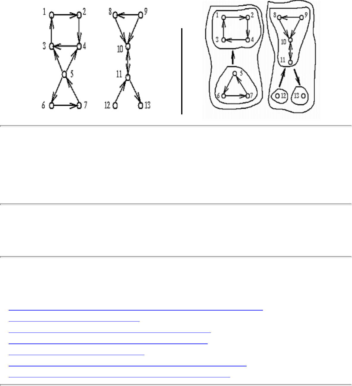
1.4.1 Connected Components
1.4.1 Connected Components
INPUT OUTPUT
Input Description: A directed or undirected graph G . A start vertex .
Problem: Traverse each edge and vertex of the connected component containing .
Implementations
● LEDA - A Library of Efficient Data Types and Algorithms (C++) (rating 8)
● The Stanford GraphBase (C) (rating 4)
● GraphEd -- Graph Editor and Layout Program (C) (rating 4)
● Moret and Shapiro's Algorithms P to NP (Pascal) (rating 4)
● Combinatorica (Mathematica) (rating 3)
● Nijenhuis and Wilf: Combinatorial Algorithms (FORTRAN) (rating 2)
● Xtango and Polka Algorithm Animation Systems (C++) (rating 2)
file:///E|/WEBSITE/FILES/DFS_BFS4.HTM (1 of 2) [19/1/2003 1:36:43]

1.4.1 Connected Components
Related Problems
● Edge and Vertex Connectivity
● Shortest Path
● Transitive Closure and Reduction
Go to the corresponding chapter in the book
About the Book
Send us Mail
Go to Main Page
This page last modified on Tue Jun 03, 1997 .
file:///E|/WEBSITE/FILES/DFS_BFS4.HTM (2 of 2) [19/1/2003 1:36:43]
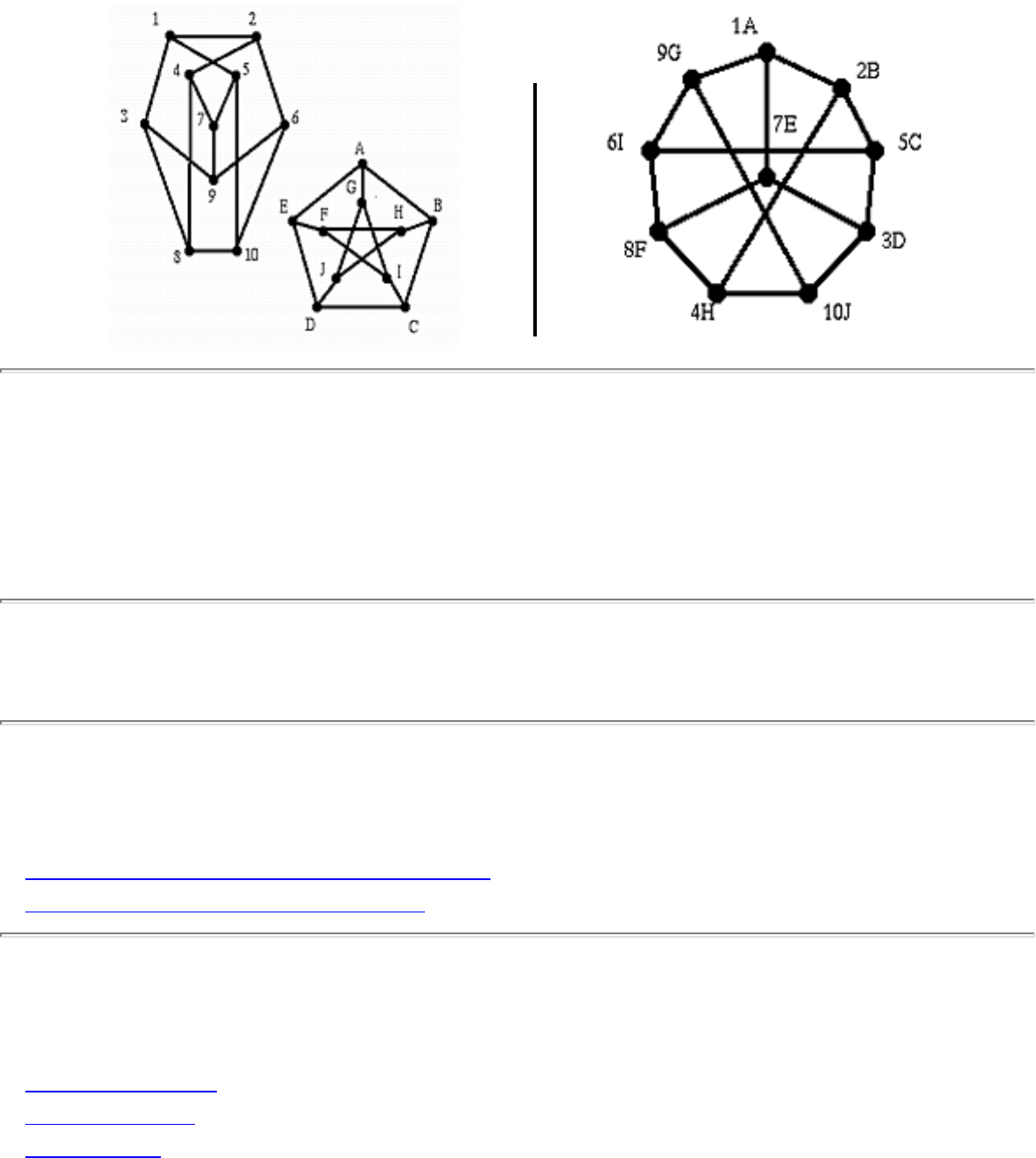
1.5.9 Graph Isomorphism
1.5.9 Graph Isomorphism
INPUT OUTPUT
Input Description: Two graphs, g and h .} Problem: Find a (all) mappings f of the vertices of g to the
vertices of h such that g and h are identical, ie. (x,y) is an edge of g iff (f(x),f(y)) is an edge of h .
Implementations
● NAUTY -- Graph Isomorphism (C) (rating 10)
● Combinatorica (Mathematica) (rating 3)
Related Problems
● Generating Graphs
● Shape Similarity
● Shortest Path
file:///E|/WEBSITE/FILES/GRAPHISM.HTM (1 of 2) [19/1/2003 1:36:44]

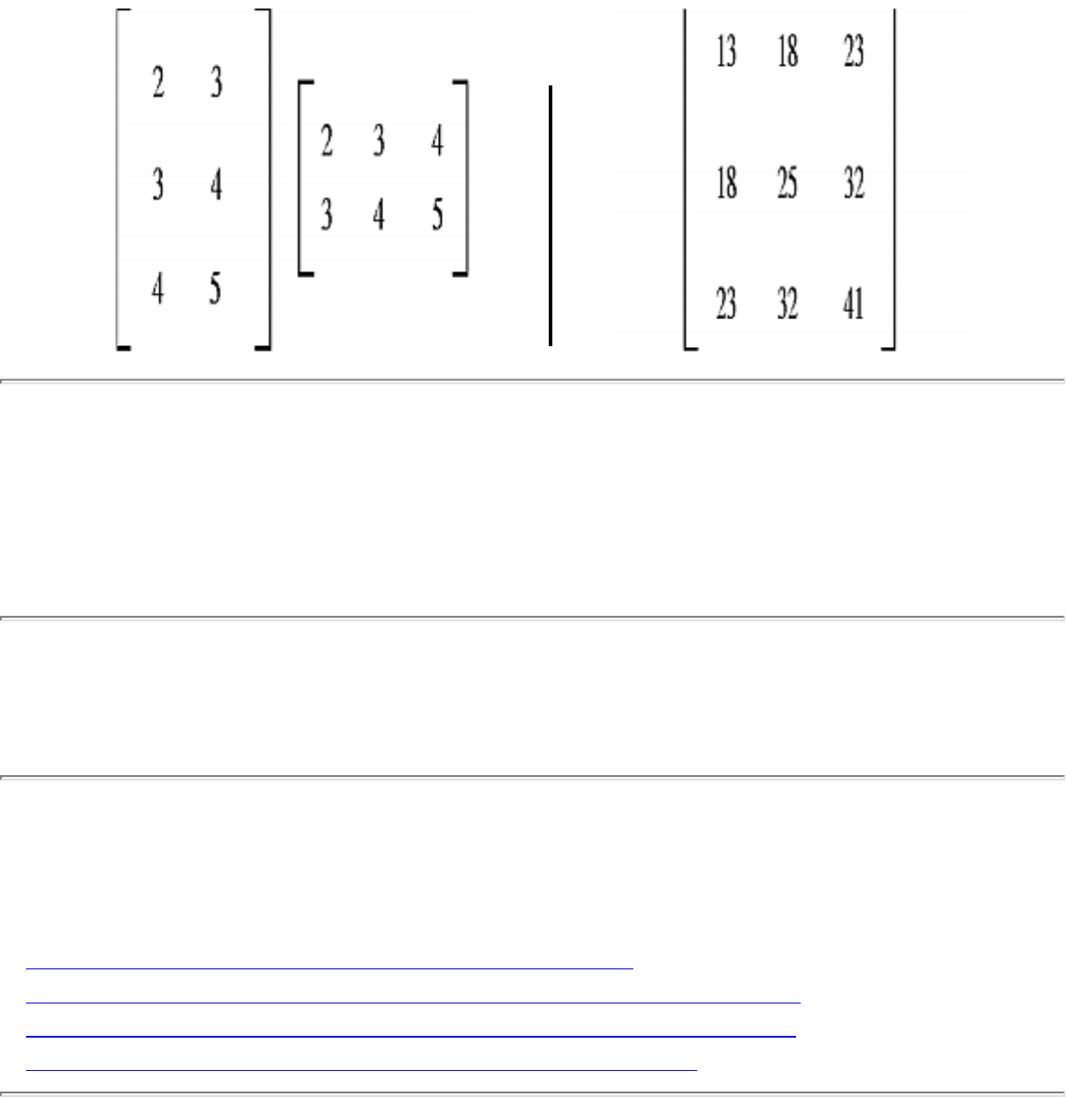
1.2.3 Matrix Multiplication
1.2.3 Matrix Multiplication
INPUT OUTPUT
Input Description: An x x y matrix A , and an y x z matrix B .
Problem: The x x z matrix A x B .
Implementations
● () (rating 7)
● Mathematica -- Assorted Routines (Mathematica) (rating 6)
● Netlib / TOMS -- Collected Algorithms of the ACM (FORTRAN) (rating 6)
● LEDA - A Library of Efficient Data Types and Algorithms (C++) (rating 4)
● Xtango and Polka Algorithm Animation Systems (C++) (rating 2)
Related Problems
file:///E|/WEBSITE/FILES/MATRTION.HTM (1 of 2) [19/1/2003 1:36:44]

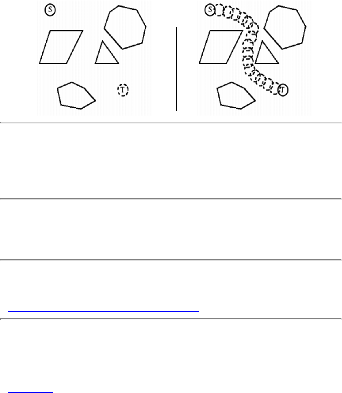
1.6.14 Motion Planning
1.6.14 Motion Planning
INPUT OUTPUT
Input Description: A polygonal-shaped robot in a given starting position in a room containing
polygonal obstacles, with a desired ending position t .
Problem: Find the shortest path in the room taking to t without going through any of the obstacles.
Implementations
● Joseph O'Rourke's Computational Geometry (C) (rating 3)
Related Problems
● Intersection Detection
● Minkowski Sum
● Shortest Path
file:///E|/WEBSITE/FILES2/MOTINING.HTM (1 of 2) [19/1/2003 1:36:45]

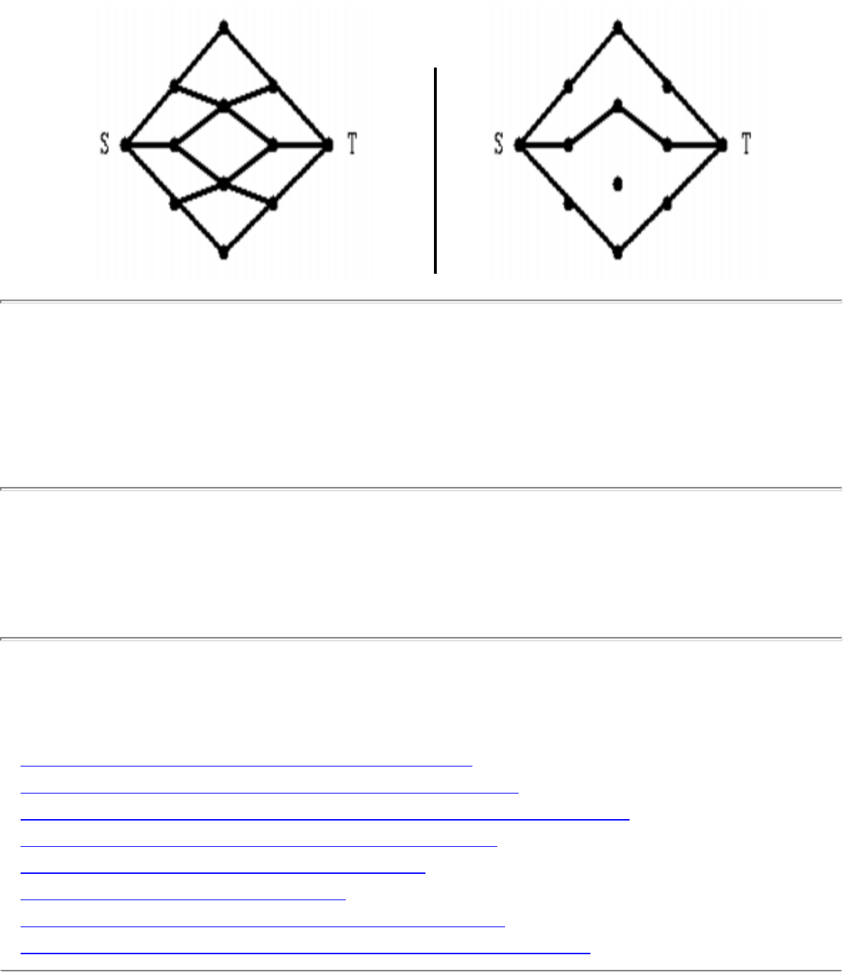
1.4.9 Network Flow
1.4.9 Network Flow
INPUT OUTPUT
Input Description: A graph G , where each edge (i,j) has a capacity c_{i,j} . A source node and sink
node t .
Problem: What is the maximum flow you can route from to t while respecting the capacity of each edge.
Implementations
● Goldberg's Network Optimization Codes (C) (rating 10)
● DIMACS Implementation Challenges (FORTRAN) (rating 8)
● LEDA - A Library of Efficient Data Types and Algorithms (C++) (rating 5)
● Moret and Shapiro's Algorithms P to NP (Pascal) (rating 4)
● Discrete Optimization Methods (Pascal) (rating 4)
● Combinatorica (Mathematica) (rating 3)
● GraphEd -- Graph Editor and Layout Program (C) (rating 3)
● Nijenhuis and Wilf: Combinatorial Algorithms (FORTRAN) (rating 3)
file:///E|/WEBSITE/FILES/NETWFLOW.HTM (1 of 2) [19/1/2003 1:36:45]

1.4.9 Network Flow
Related Problems
● Edge and Vertex Connectivity
● Graph Partition
● Linear Programming
● Matching
● Shortest Path
Go to the corresponding chapter in the book
About the Book
Send us Mail
Go to Main Page
This page last modified on Tue Jun 03, 1997 .
file:///E|/WEBSITE/FILES/NETWFLOW.HTM (2 of 2) [19/1/2003 1:36:45]
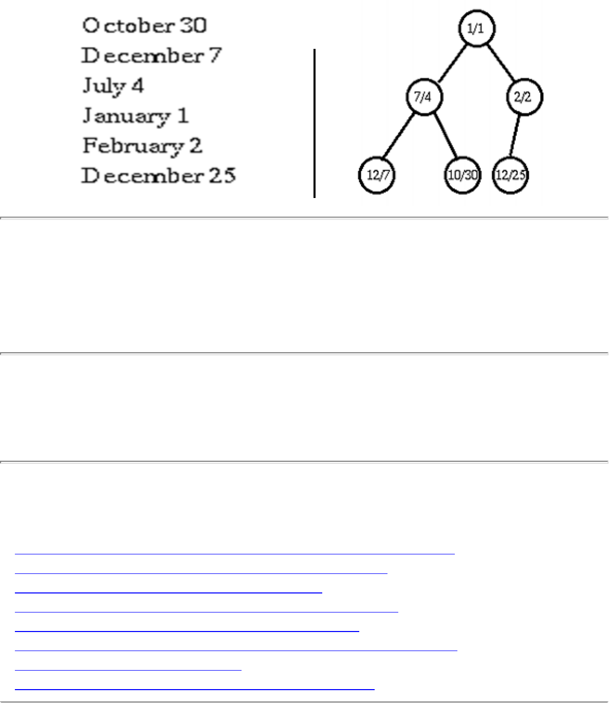
1.1.2 Priority Queues
1.1.2 Priority Queues
INPUT OUTPUT
Input Description: A set of records with numerical or otherwise totally ordered keys.
Problem: Build and maintain a data structures for quickly inserting and deleting records, while
maintaining quick access to the smallest or largest key in the set.
Implementations
● LEDA - A Library of Efficient Data Types and Algorithms (C++) (rating 9)
● Handbook of Algorithms and Data Structures (Pascal) (rating 7)
● SimPack/Sim++ Simulation Toolkit (C++) (rating 7)
● Xtango and Polka Algorithm Animation Systems (C++) (rating 4)
● Moret and Shapiro's Algorithms P to NP (Pascal) (rating 3)
● Netlib / TOMS -- Collected Algorithms of the ACM (FORTRAN) (rating 3)
● The Stanford GraphBase (C) (rating 2)
● DIMACS Implementation Challenges (FORTRAN) (rating 1)
file:///E|/WEBSITE/FILES/PRIOEUES.HTM (1 of 2) [19/1/2003 1:36:46]

1.1.2 Priority Queues
Related Problems
● Dictionaries
● Median and Selection
● Shortest Path
● Sorting
Go to the corresponding chapter in the book
About the Book
Send us Mail
Go to Main Page
This page last modified on Tue Jun 03, 1997 .
file:///E|/WEBSITE/FILES/PRIOEUES.HTM (2 of 2) [19/1/2003 1:36:46]
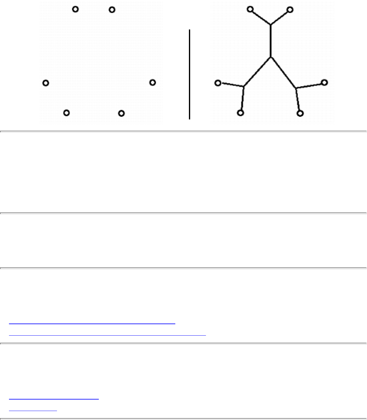
1.5.10 Steiner Tree
1.5.10 Steiner Tree
INPUT OUTPUT
Input Description: A graph G=(V,E) . A subset of vertices T \in V .
Problem: Find the smallest tree connecting all the vertices of T .
Implementations
● Salowe's Rectilinear Steiner trees (C) (rating 8)
● PHYLIP -- inferring phylogenic trees (Pascal) (rating 7)
Related Problems
● Minimum Spanning Tree
● Shortest Path
file:///E|/WEBSITE/FILES/STEITREE.HTM (1 of 2) [19/1/2003 1:36:46]

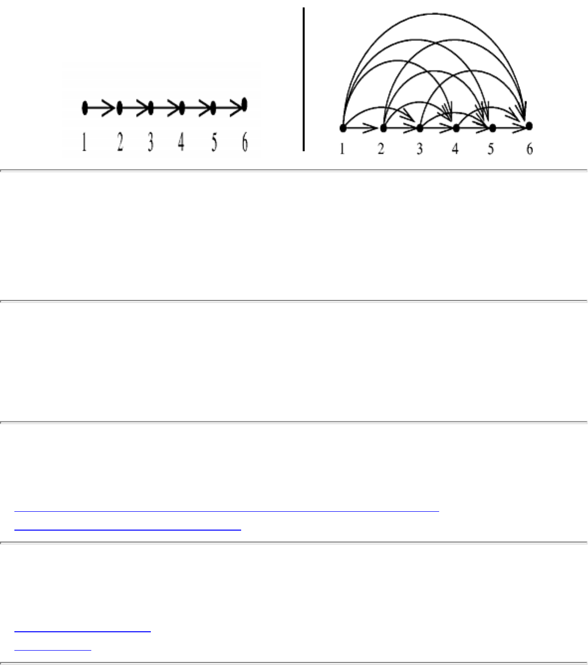
1.4.5 Transitive Closure and Reduction
1.4.5 Transitive Closure and Reduction
INPUT OUTPUT
Input Description: A directed graph G=(V,E) .
Problem: For transitive closure, construct a graph G'=(V,E') with edge (i,j) \in E' iff there is a directed
path from i to j in G . For transitive reduction, construct a small graph G'=(V,E') with a directed path
from i to j in G' iff (i,j) \in E .
Implementations
● LEDA - A Library of Efficient Data Types and Algorithms (C++) (rating 6)
● Combinatorica (Mathematica) (rating 4)
Related Problems
● Connected Components
● Shortest Path
file:///E|/WEBSITE/FILES/TRANSURE.HTM (1 of 2) [19/1/2003 1:36:47]

About the Book -- The Algorithm Design Manual
About the Book
Most professional programmers are not well equipped to tackle algorithm design problems. The
Algorithm Design Manual, written by Steven S. Skiena and published by Telos/Springer-Verlag is
uniquely designed to provide access to combinatorial algorithms technology for computer professionals
and students. This book is considerably different than other books on algorithms. Why?
● We reduce the design process to a sequence of questions to ask about the problem at hand. This
provides a concrete path to take the non-expert from an initial problem statement to a reasonable
solution.
● To provide a better perspective on how algorithm problems arise in the real world, we include a
collection of `war stories', tales from our experience on real problems. The moral of these stories
is that algorithm design and analysis is not just theory, but an important tool to be pulled out and
used as needed.
● Since the practical person is usually looking for a program more than an algorithm, we provide
pointers to solid implementations whenever they are available. We have collected these
implementations on an enclosed CD-ROM and at the book WWW site,
http://www.cs.sunysb.edu/~algorith for easy retrieval. With these implementations available, the
critical aspect in algorithm design becomes properly modeling your application, instead of
becoming intimate with the details of the actual algorithm. This focus permeates the entire book.
● Since finding out what is known about an algorithmic problem can be a difficult task, we provide
a catalog of the 75 most important algorithmic problems as a major component of this book. By
browsing through this catalog, the reader can quickly identify what their problem called, what is
known about it, and how they should proceed to solve it. As an aid in problem identification, we
include a pair of `before' and `after' pictures for each problem, illustrating the required input and
output specifications.
● The algorithm catalog spans numerical problems and data structures as well as graph, string, and
geometric algorithms. For each problem in the catalog, we provide an honest and convincing
motivation showing how it arises in applications. If we could not find such an application, then the
file:///E|/WEBSITE/INFO/FORM.HTM (1 of 3) [19/1/2003 1:36:48]
About the Book -- The Algorithm Design Manual
problem doesn't appear in this book.
Equally important is what we do not do in this book. We do not stress the mathematical analysis of
algorithms, leaving most of the analysis as informal arguments. You will not find a single theorem
anywhere in this book.
But what is a manual without software? This book comes with a substantial electronic supplement, a ISO-
9660 compatible, multiplatform CD-ROM, which can be viewed using Netscape, Microsoft Explorer, or
any other WWW browser. This CD-ROM contains:
● A complete hypertext version of the full printed book. Indeed, the extensive cross-references
within the text are best followed using the hypertext version.
● The source code and URLs for all cited implementations, mirroring the Algorithm Repository
WWW site. Programs in C, C++, Fortran, and Pascal are included, providing an average of four
different implementations for each algorithmic problem.
● Over 30 hours of audio lectures on the design and analysis of algorithms are provided, all keyed to
on-line lecture notes. Following these lectures provides another approach to learning algorithm
design techniques.
Together, this book covers material sufficient for a standard Introduction to Algorithms course. Its
assumes the reader has completed the equivalent of a second programming course, typically titled Data
Structures or Computer Science II . Special textbook oriented-features include:
● In addition to standard pen-and-paper exercises, this book includes ``implementation challenges''
suitable for teams or individual students. These projects and the applied focus of the text can be
used to provide a new laboratory focus to the traditional algorithms course.
● ``Take-home lessons'' at the beginning of each chapter emphasize the concepts to be gained from
the chapter.
● This book stresses design over analysis. It is suitable for both traditional lecture courses, and the
new ``active learning'' method, where the professor does not lecture instead guides student groups
to solve real problems. The ``war stories'' provide a great introduction to the active learning
method.
● A full set of lecture slides for teaching this course is available on the CD-ROM, keyed to unique
on-line audio lectures covering a full semester algorithm course.
``I have no doubt that it will become a classic the day it is published. It has all the right ingredients: rich
contents, friendly, personal language, subtle humor, the right references, and a plethora of pointers to
resources.''
-- P. Takis Metaxas, Wellesley College.
``A major theme that runs through the book is that the most important technique to solve an algorithmic
problem from the real world is to learn how to model the problem well. I did not believe this before; the
file:///E|/WEBSITE/INFO/FORM.HTM (2 of 3) [19/1/2003 1:36:48]

About the Book -- The Algorithm Design Manual
book did an admirable job of convincing me that there is considerable truth in it.''
-- Giri Narasimhan, The University of Memphis.
``The questions on problem solving are good enough that they ought to be talked about in every
programming class in the undergraduate curriculum.''
-- Ron Danielson, Santa Clara University.
Check out the preface and table of contents for more information. You may order this book, and are
encouraged to do so. You might also be interested in my previous book, Implementing Discrete
Mathematics .
Please leave your name and address to receive additional information about the book and notification of
significant upgrades to this site when they occur.
If your WWW client does not support forms, please send an e-mail to algorith@cs.sunysb.edu
with your name, e-mail address, and mailing address for further information.
First Name:
Last Name :
E-mail :
Company Name :
Number and Street :
City :
State :
Zip :
Phone :
Return to the home page
If you have problems with this page, please send E-mail to:
algorith@cs.sunysb.edu
file:///E|/WEBSITE/INFO/FORM.HTM (3 of 3) [19/1/2003 1:36:48]
Reset
Register

Adaptive Simulated Annealing
Adaptive Simulated Annealing
Adaptive Simulated Annealing (ASA) is a C language package which provides the framework and
mechanisms for optimization of complex systems using simulated annealing. Users may incorporate
these routines into existing C programs, or build applications from the sample ASA applications. Most
parameters are user-definable -- allowing for highly customizable optimization algorithms.
The code is maintained by Lester Ingber .
● Download ASA files (ingber.com)
● Link to Lester Ingber's ASA page
● Download Files (local site)
Problem Links
● Constrained and Unconstrained Optimization (6)
About the Book
Send us Mail
Go to Main Page
This page last modified on Mar 11, 1996.
file:///E|/WEBSITE/IMPLEMEN/ASA/IMPLEMEN.HTM [19/1/2003 1:36:48]

Genocop -- Optimization via Genetic Algorithms
Genocop -- Optimization via Genetic Algorithms
Genocop, by Zbigniew Michalewicz, is a genetic algorithm-based program for constrained and
unconstrained optimization, written in C. The Genocop system aims at finding a global optimum
(minimum or maximum: this is one of the input parameters) of a function; additional linear constraints
(equations and inequalities) can be specified as well.
The current version of Genocop should run without changes on any BSD-UN*X system (preferably on a
Sun SPARC machine). This program can also be run on a DOS system.
This software is copyright by Zbigniew Michalewicz. Permission is granted to copy and use the software
for scientific, noncommercial purposes only. The software is provided "as is", i.e., without any
warranties.
● Original FTP site
● Download Files (local site)
Problem Links
● Constrained and Unconstrained Optimization (5)
About the Book
Send us Mail
Go to Main Page
This page last modified on Aug 9, 1996.
file:///E|/WEBSITE/IMPLEMEN/GENOCOP/IMPLEMEN.HTM [19/1/2003 1:36:49]
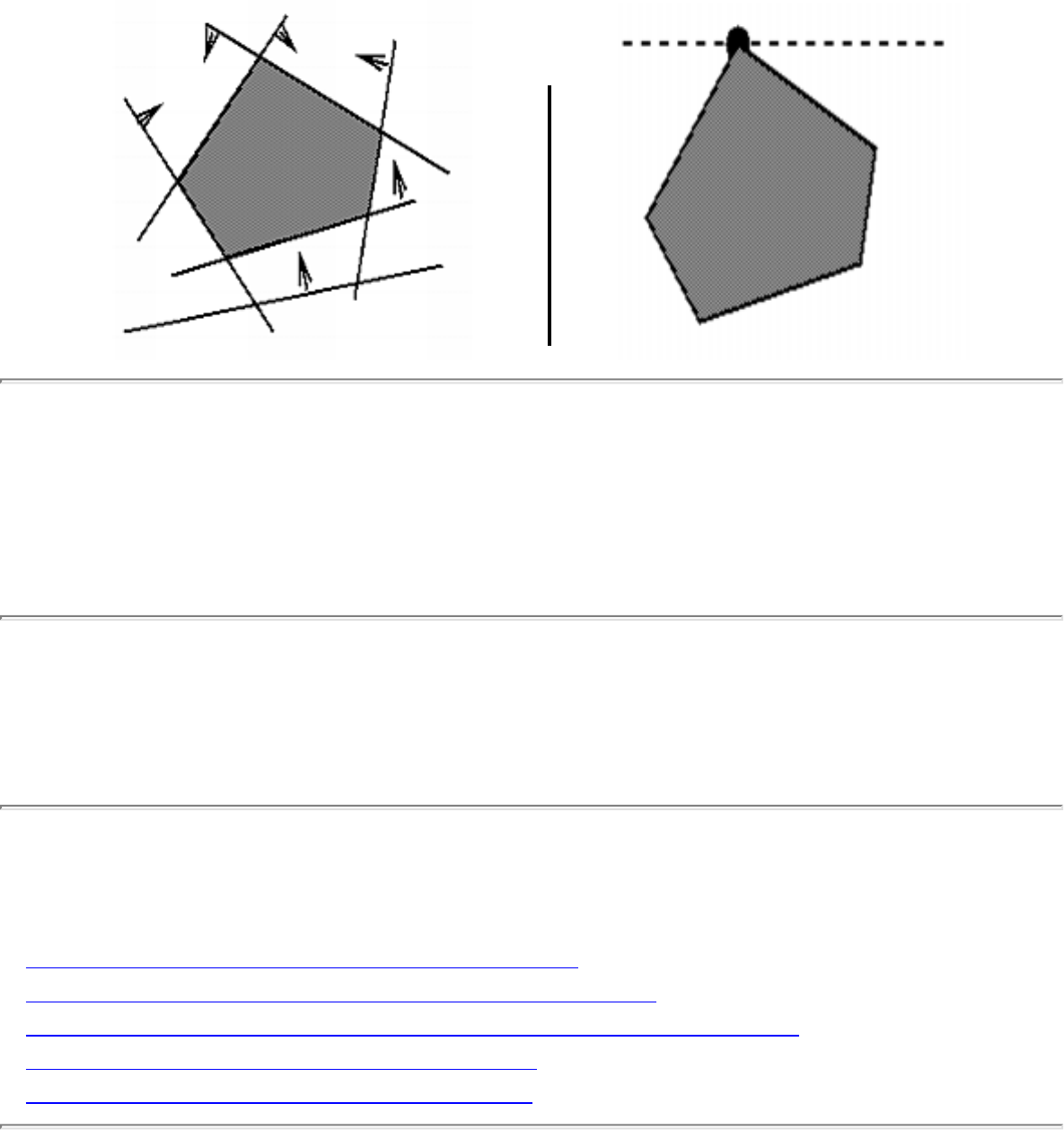
1.2.6 Linear Programming
1.2.6 Linear Programming
INPUT OUTPUT
Input Description: A set of linear inequalities, a linear objective function.
Problem: Find the assignment to the variables maximizing the objective function while satisfying all
inequalities.
Implementations
● LP_SOLVE: Linear Programming Code (C) (rating 9)
● Linprog -- low dimensional linear programming (C) (rating 4)
● Netlib / TOMS -- Collected Algorithms of the ACM (FORTRAN) (rating 4)
● Discrete Optimization Methods (Pascal) (rating 3)
● Algorithms in C++ -- Sedgewick (C++) (rating 2)
Related Problems
file:///E|/WEBSITE/FILES/LINEMING.HTM (1 of 2) [19/1/2003 1:36:50]

1.2.6 Linear Programming
● Knapsack Problem
● Network Flow
● Constrained and Unconstrained Optimization
Go to the corresponding chapter in the book
About the Book
Send us Mail
Go to Main Page
This page last modified on Tue Jun 03, 1997 .
file:///E|/WEBSITE/FILES/LINEMING.HTM (2 of 2) [19/1/2003 1:36:50]

1.2.7 Random Number Generation
1.2.7 Random Number Generation
INPUT OUTPUT
Input Description: Nothing, or perhaps a seed.
Problem: Generate a sequence of random integers.
Implementations
● SimPack/Sim++ Simulation Toolkit (C++) (rating 7)
● The Stanford GraphBase (C) (rating 6)
● Netlib / TOMS -- Collected Algorithms of the ACM (FORTRAN) (rating 6)
● LEDA - A Library of Efficient Data Types and Algorithms (C++) (rating 4)
● Algorithms in C++ -- Sedgewick (C++) (rating 3)
● Xtango and Polka Algorithm Animation Systems (C++) (rating 3)
Related Problems
file:///E|/WEBSITE/FILES/RANDBERS.HTM (1 of 2) [19/1/2003 1:36:50]

1.2.7 Random Number Generation
● Generating Partitions
● Generating Permutations
● Generating Subsets
● Constrained and Unconstrained Optimization
Go to the corresponding chapter in the book
About the Book
Send us Mail
Go to Main Page
This page last modified on Tue Jun 03, 1997 .
file:///E|/WEBSITE/FILES/RANDBERS.HTM (2 of 2) [19/1/2003 1:36:50]
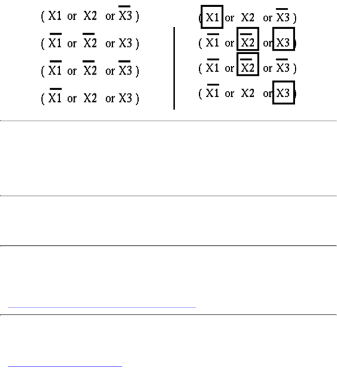
1.3.10 Satisfiability
1.3.10 Satisfiability
INPUT OUTPUT
Input Description: A set of clauses in conjunctive normal form.
Problem: Is there a truth assignment to the boolean variables such that every clause is satisfied?
Implementations
● DIMACS Implementation Challenges (FORTRAN) (rating 8)
● POSIT - Propositional Satisfiability Testbed (C) (rating 8)
Related Problems
● Finite State Machine Minimization
● Traveling Salesman Problem
file:///E|/WEBSITE/FILES/SATILITY.HTM (1 of 2) [19/1/2003 1:36:51]


Fortune's 2D Voronoi diagram code
Fortune's 2D Voronoi diagram code
This is a fairly widely-used 2D code for Voronoi diagrams and Delauney triangulations, written in C by
Steve Fortune of Bell Laboratories. It is based on Fortune's sweepline algorithm for Voronoi diagrams,
and is likely to be the right code to try first.
● Netlib Voronoi source directory
● Steve Fortune's home page
● Download Files (local site)
Problem Links
● Voronoi Diagrams (9)
● Triangulation (7)
About the Book
Send us Mail
Go to Main Page
This page last modified on Apr 23, 1996.
file:///E|/WEBSITE/IMPLEMEN/FORTUNE/IMPLEMEN.HTM [19/1/2003 1:36:51]

Qhull - higher dimensional convex hull program
Qhull - higher dimensional convex hull program
Qhull is a general dimension code for computing convex hulls, Delaunay triangulations, Voronoi
vertices, furthest-site Voronoi vertices, and halfspace intersections. It appears to be the choice for higher-
dimensional convex hull applications.
Qhull is written in C, and implements the divide-and-conquer Quickhull algorithm. It is fast and round-
off errors from floating point arithmetic. Qhull has been widely used in scientific applications and has a
well-maintained
● home page .
● Qhull home page
● Latest news
● Download Files (local site)
Problem Links
● Convex Hull (10)
● Voronoi Diagrams (7)
● Triangulation (6)
● Intersection Detection (5)
About the Book
Send us Mail
Go to Main Page
This page last modified on Apr 8, 1997.
file:///E|/WEBSITE/IMPLEMEN/QHULL/IMPLEMEN.HTM [19/1/2003 1:36:52]

Joseph O'Rourke's Computational Geometry
Joseph O'Rourke's Computational Geometry
Joseph O'Rourke is Olin Professor of Computer Science at Smith College in Northampton,
Massachusetts. His text Computational Geometry in C has become one of the definitive computational
geometry resources. The programs coded in the text have been made freely available by anonymous ftp
from Smith College and have been included at this site as well.
In this distribution are standard C language routines for simple computational geometric methods
(determining whether a point lies inside a polygon, for instance) as well as robust implementations of
complex computational geometry algorithms. Addressed are problems in motion planning, nearest
neighbor determination (through the use of Delaunay triangulations and Voronoi diagrams), polygon
intersection, convex hull computation, and polygon triangulation.
● Download Files (Smith College)
● Download Files (local site)
● Go to Joseph O'Rourke 's Home Page
Problem Links
● Convex Hull (6)
● Robust Geometric Primitives (6)
● Intersection Detection (5)
● Nearest Neighbor Search (5)
● Voronoi Diagrams (4)
● Motion Planning (3)
● Point Location (3)
● Triangulation (3)
About the Book
Send us Mail
Go to Main Page
This page last modified on Feb 23, 1996.
file:///E|/WEBSITE/IMPLEMEN/OROURKE/IMPLEMEN.HTM [19/1/2003 1:36:53]
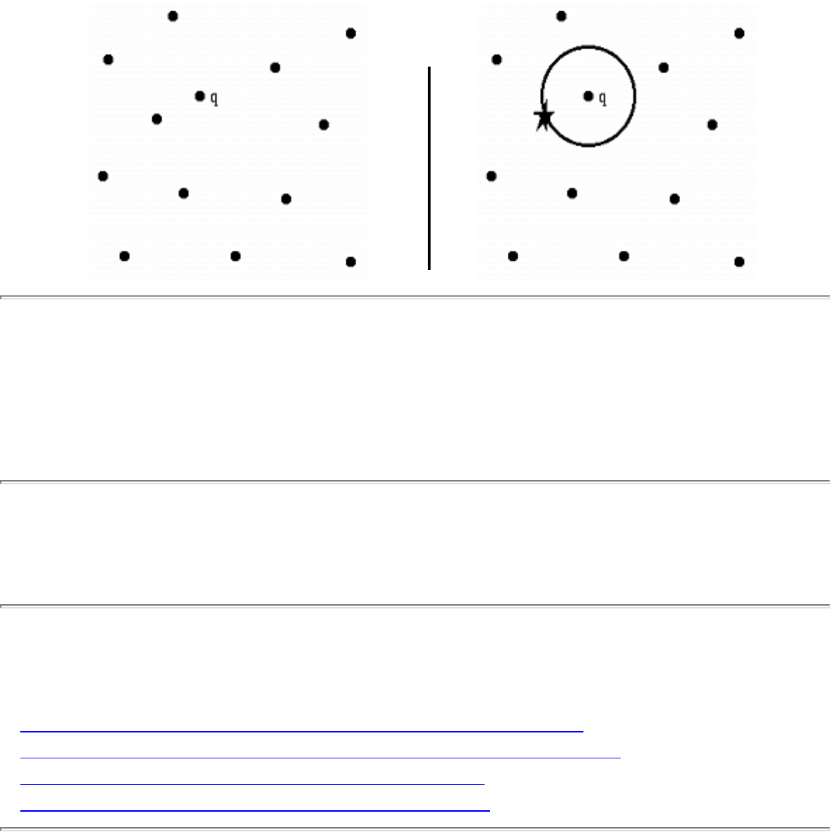
1.6.5 Nearest Neighbor Search
1.6.5 Nearest Neighbor Search
INPUT OUTPUT
Input Description: A set S of n points in d dimensions; a query point q .
Problem: Which point in S is closest to q ?
Implementations
● Ranger - Nearest Neighbor Search in Higher Dimensions (C) (rating 7)
● LEDA - A Library of Efficient Data Types and Algorithms (C++) (rating 6)
● Joseph O'Rourke's Computational Geometry (C) (rating 5)
● Moret and Shapiro's Algorithms P to NP (Pascal) (rating 3)
Related Problems
file:///E|/WEBSITE/FILES2/NEARHBOR.HTM (1 of 2) [19/1/2003 1:36:53]

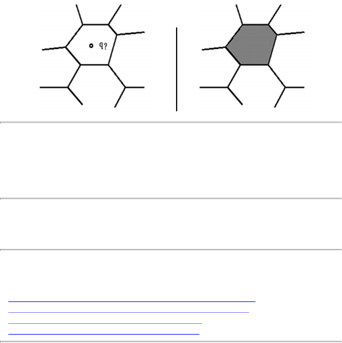
1.6.7 Point Location
1.6.7 Point Location
INPUT OUTPUT
Input Description: A decomposition of the plane into polygonal regions, and a query point q .
Problem: Which region contains the query point q ?
Implementations
● LEDA - A Library of Efficient Data Types and Algorithms (C++) (rating 7)
● Arrange - maintainance of arrangements with point location (C) (rating 6)
● Moret and Shapiro's Algorithms P to NP (Pascal) (rating 3)
● Joseph O'Rourke's Computational Geometry (C) (rating 3)
Related Problems
file:///E|/WEBSITE/FILES2/POINTION.HTM (1 of 2) [19/1/2003 1:36:54]

1.6.7 Point Location
● Kd-Trees
● Maintaining Line Arrangements
● Nearest Neighbor Search
● Range Search
● Voronoi Diagrams
Go to the corresponding chapter in the book
About the Book
Send us Mail
Go to Main Page
This page last modified on Tue Jun 03, 1997 .
file:///E|/WEBSITE/FILES2/POINTION.HTM (2 of 2) [19/1/2003 1:36:54]
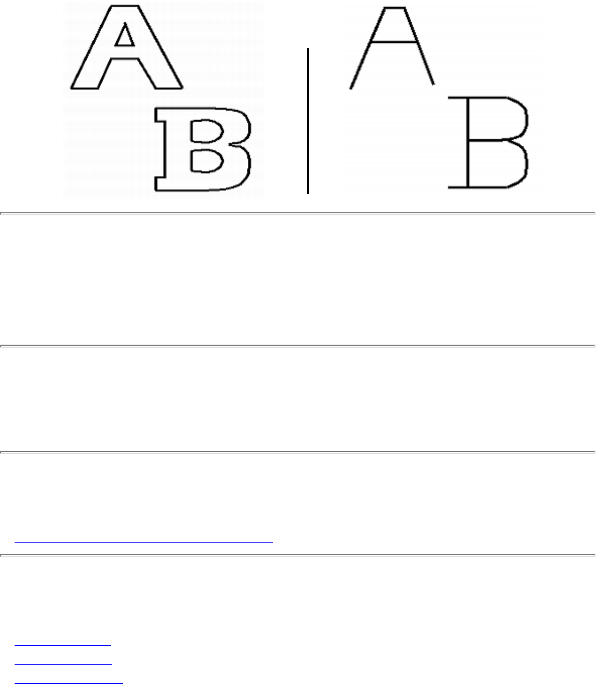
1.6.10 Medial-Axis Transformation
1.6.10 Medial-Axis Transformation
INPUT OUTPUT
Input Description: A polygon or polyhedron P .
Problem: What is the set of points within P which have more than one closest point on the boundary of
P ?
Implementations
● Skeletonization Software (2-D) (C) (rating 9)
Related Problems
● Minkowski Sum
● Shape Similarity
● Voronoi Diagrams
file:///E|/WEBSITE/FILES2/00000011.HTM (1 of 2) [19/1/2003 1:36:54]

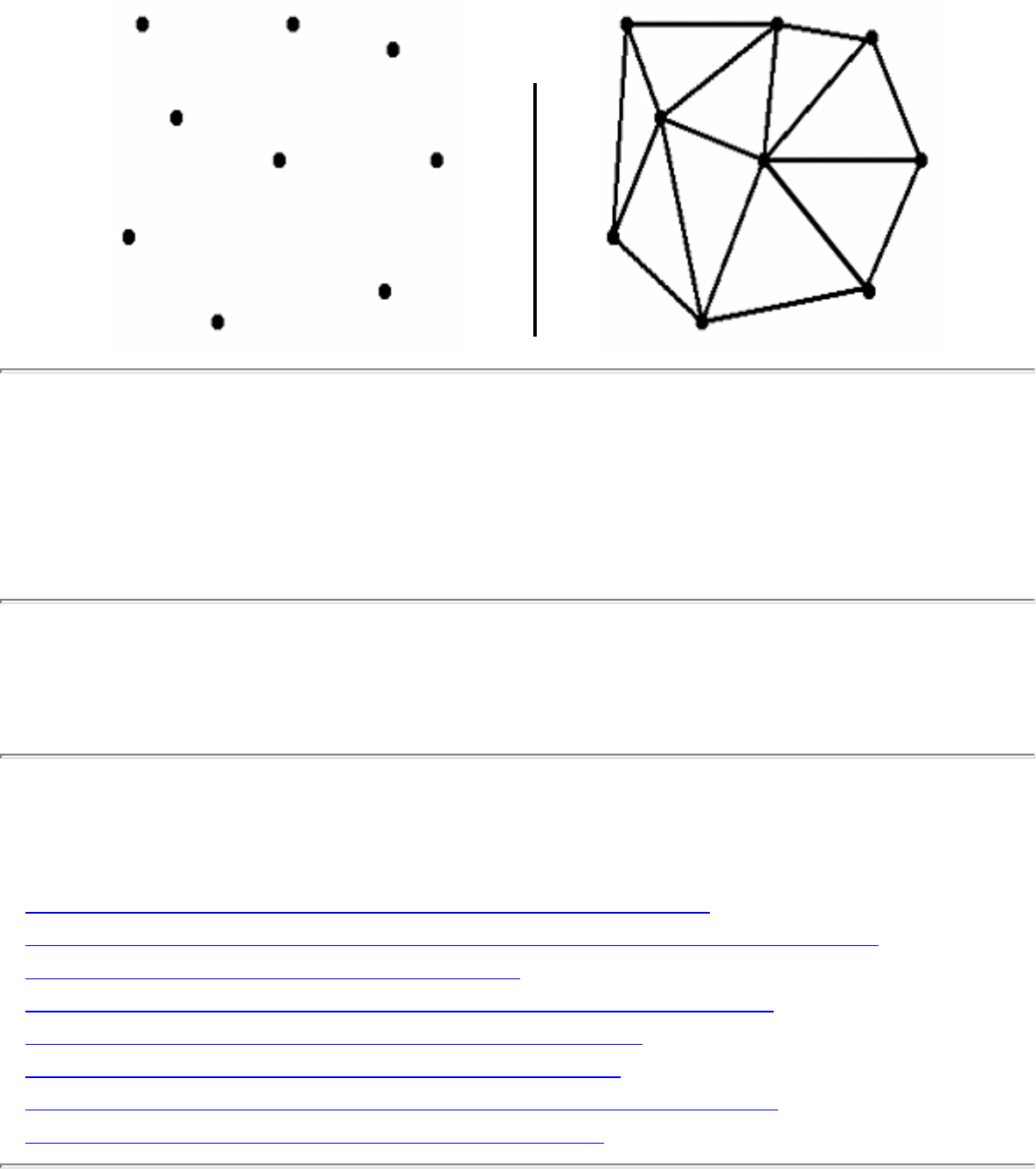
1.6.3 Triangulation
1.6.3 Triangulation
INPUT OUTPUT
Input Description: A set of points, or a polyhedron
Problem: Partition the interior of the point set or polyhedron into triangles.
Implementations
● Triangle: A Two-Dimensional Quality Mesh Generator (C) (rating 9)
● GEOMPACK - triangulation and convex decomposition codes (FORTRAN) (rating 8)
● Fortune's 2D Voronoi diagram code (C) (rating 7)
● LEDA - A Library of Efficient Data Types and Algorithms (C++) (rating 6)
● Qhull - higher dimensional convex hull program (C) (rating 6)
● GraphEd -- Graph Editor and Layout Program (C) (rating 4)
● Netlib / TOMS -- Collected Algorithms of the ACM (FORTRAN) (rating 4)
● Joseph O'Rourke's Computational Geometry (C) (rating 3)
file:///E|/WEBSITE/FILES2/TRIAIONS.HTM (1 of 2) [19/1/2003 1:36:55]


Nijenhuis and Wilf: Combinatorial Algorithms
Nijenhuis and Wilf: Combinatorial Algorithms
Nijenhuis and Wilf's Combinatorial Algorithms , published by Academic Press in 1978, specializes in
algorithms for constructing basic combinatorial objects such as permutations, subsets, and partitions;
both randomly and sequentially. Such algorithms are often very short but hard to locate and usually are
surprisingly subtle. Fortran programs for all of the algorithms are provided, as well as a discussion of the
theory behind each of them. The programs are usually short enough that it is reasonable to translate
directly into a more modern programming language, as I did with many of them in writing
Combinatorica . Descriptions of more recent algorithms for several problems, without code, are provided
in Wilf's Combinatorial Algorithms, an update , published by SIAM in 1989.
These programs are now available here on our algorithm repository WWW site. We tracked them down
from Neil Sloane, who had them on a magnetic tape where the authors did not! In their book, Nijenhuis
and Wilf set the proper standard of statistically testing the output distribution of each of the random
generators to establish that they really appear uniform. We encourage you to do the same before using
these programs to verify that nothing has been lost in transit.
● Link to Wilf's Home Page -- many interesting things
● Download Files (local site)
● Files with driver programs and test data (local site)
Problem Links
● Generating Partitions (8)
● Generating Permutations (8)
● Generating Subsets (8)
● Hamiltonian Cycle (5)
● Determinants and Permanents (4)
● Generating Graphs (4)
● Eulerian Cycle / Chinese Postman (3)
● Minimum Spanning Tree (3)
● Network Flow (3)
● Sorting (3)
● Vertex Coloring (3)
● Connected Components (2)
file:///E|/WEBSITE/IMPLEMEN/WILF/IMPLEMEN.HTM (1 of 2) [19/1/2003 1:36:55]

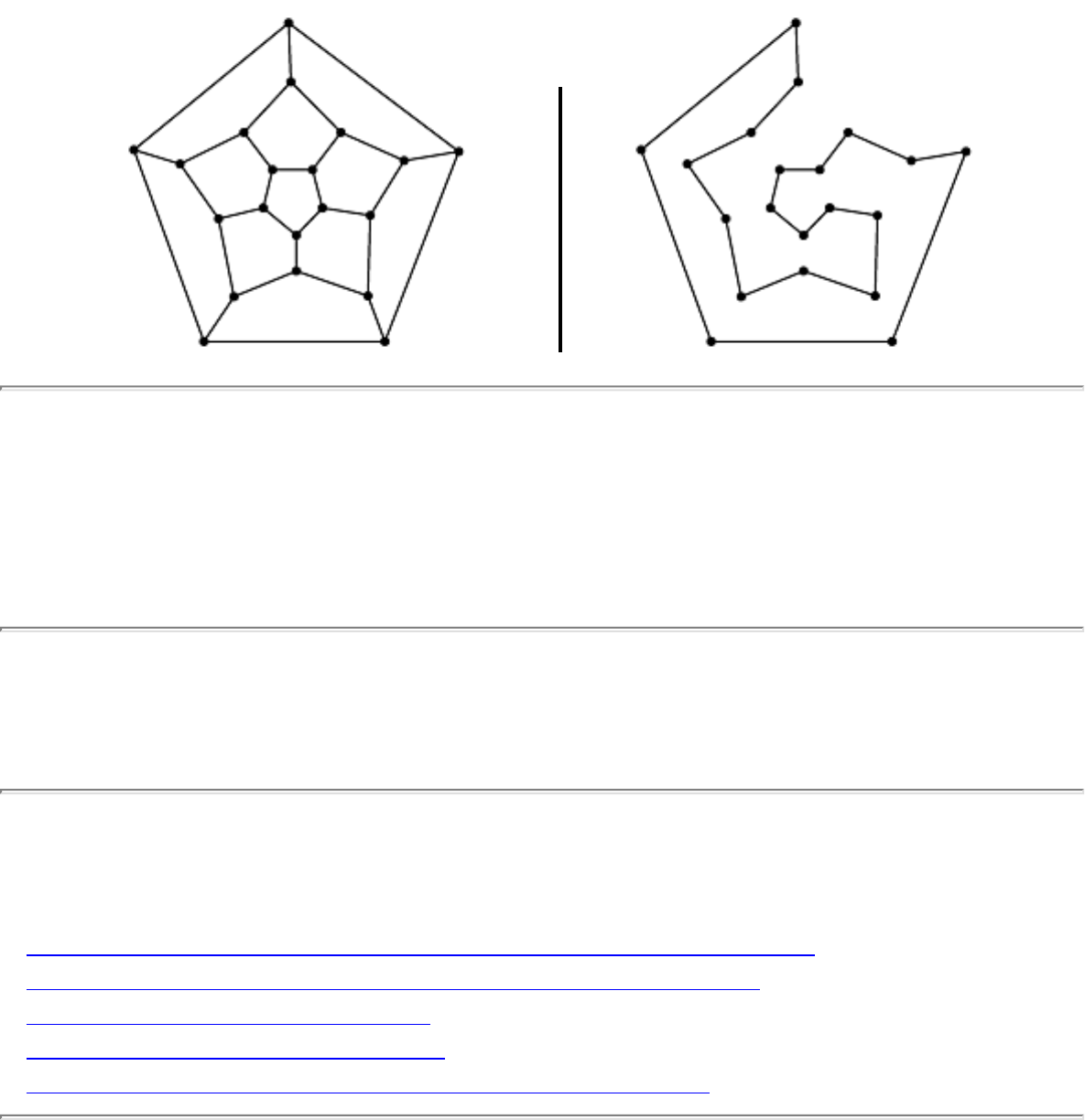
1.5.5 Hamiltonian Cycle
1.5.5 Hamiltonian Cycle
INPUT OUTPUT
Input Description: A graph G = (V,E) .
Problem: Find an ordering of the vertices such that each vertex is visited exactly once.
Implementations
● Netlib / TOMS -- Collected Algorithms of the ACM (FORTRAN) (rating 6)
● Nijenhuis and Wilf: Combinatorial Algorithms (FORTRAN) (rating 5)
● The Stanford GraphBase (C) (rating 4)
● Combinatorica (Mathematica) (rating 3)
● Xtango and Polka Algorithm Animation Systems (C++) (rating 3)
Related Problems
file:///E|/WEBSITE/FILES/HAMIYCLE.HTM (1 of 2) [19/1/2003 1:36:56]

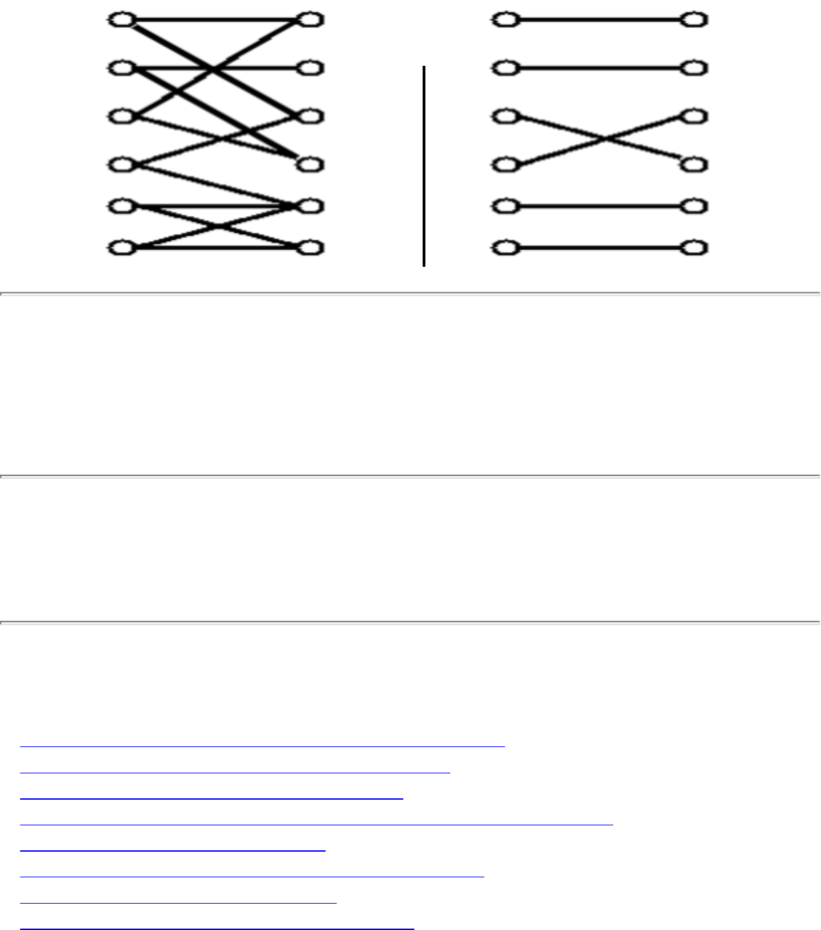
1.4.6 Matching
1.4.6 Matching
INPUT OUTPUT
Input Description: A (weighted) graph G=(V,E) .
Problem: Find the largest size set of edges S \in E such that each vertex in V is incident to at most one
edge of S .
Implementations
● DIMACS Implementation Challenges (FORTRAN) (rating 9)
● Goldberg's Network Optimization Codes (C) (rating 9)
● BIPM -- Bipartite Matching Codes (C) (rating 8)
● LEDA - A Library of Efficient Data Types and Algorithms (C++) (rating 7)
● The Stanford GraphBase (C) (rating 4)
● Moret and Shapiro's Algorithms P to NP (Pascal) (rating 4)
● Combinatorica (Mathematica) (rating 3)
● Discrete Optimization Methods (Pascal) (rating 3)
file:///E|/WEBSITE/FILES/00000034.HTM (1 of 2) [19/1/2003 1:36:57]

1.4.6 Matching
● Netlib / TOMS -- Collected Algorithms of the ACM (FORTRAN) (rating 3)
● Algorithms in C++ -- Sedgewick (C++) (rating 2)
Related Problems
● Determinants and Permanents
● Eulerian Cycle / Chinese Postman
● Network Flow
● Job Scheduling
● Set Cover
Go to the corresponding chapter in the book
About the Book
Send us Mail
Go to Main Page
This page last modified on Tue Jun 03, 1997 .
file:///E|/WEBSITE/FILES/00000034.HTM (2 of 2) [19/1/2003 1:36:57]

A compendium of NP optimization problems
A compendium of NP optimization
problems
Pierluigi Crescenzi , piluc@dsi.uniroma1.it and Viggo Kann , viggo@nada.kth.se
This is a preliminary version (April 1997) of the catalog of NP optimization problems. Please send any
comment or suggestion to one of the two authors. A printed version of the compendium will appear in:
Ausiello, G., Crescenzi, P., Gambosi, G., Kann, V., Marchetti Spaccamela, A., and Protasi, M.,
Approximate solution of NP-hard optimization problems. Springer-Verlag, 1997/1998
The latest version of the compendium is available on WWW at
http://www.nada.kth.se/theory/compendium/ . There you will also find WWW forms to report new
problems, new results on existing problems and errors.
Abstract:
Due to the fact that no NP-complete problem can be solved in polynomial time (unless P=NP), many
approximability results (both positive and negative) of NP-hard optimization problems have appeared in
the technical literature. In this compendium, we collect a large number of these results.
● Introduction
❍ NPO Problems: Definitions and Preliminaries
❍ Approximate Algorithms and Approximation Classes
❍ Completeness in Approximation Classes
❍ A list of NPO problems
❍ Improving the compendium
● Graph Theory
❍ Covering and Partitioning
❍ Subgraphs and Supergraphs
❍ Vertex Ordering
file:///E|/COMPEND/COMPED19/COMPENDI.HTM (1 of 2) [19/1/2003 1:36:58]

A compendium of NP optimization problems
❍ Iso- and Other Morphisms
❍ Miscellaneous
● Network Design
❍ Spanning Trees
❍ Cuts and Connectivity
❍ Routing Problems
❍ Flow Problems
❍ Miscellaneous
● Sets and Partitions
❍ Covering, Hitting, and Splitting
❍ Weighted Set Problems
● Storage and Retrieval
❍ Data Storage
❍ Compression and Representation
❍ Miscellaneous
● Sequencing and Scheduling
❍ Sequencing on One Processor
❍ Multiprocessor Scheduling
❍ Shop Scheduling
❍ Miscellaneous
● Mathematical Programming
● Algebra and Number Theory
● Games and Puzzles
● Logic
● Program Optimization
● Miscellaneous
● References
● Index
● About this document ...
Viggo Kann
Mon Apr 21 13:07:14 MET DST 1997
file:///E|/COMPEND/COMPED19/COMPENDI.HTM (2 of 2) [19/1/2003 1:36:58]
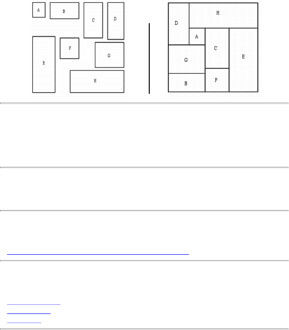
1.6.9 Bin Packing
1.6.9 Bin Packing
INPUT OUTPUT
Input Description: A set of n items with sizes d_1,...,d_n . A set of m bins with capacity c_1,...,c_m .
Problem: How do you store the set of items using the fewest number of bins?
Implementations
● Xtango and Polka Algorithm Animation Systems (C++) (rating 3)
Related Problems
● Knapsack Problem
● Job Scheduling
● Set Packing
file:///E|/WEBSITE/FILES2/BIN_KING.HTM (1 of 2) [19/1/2003 1:36:58]

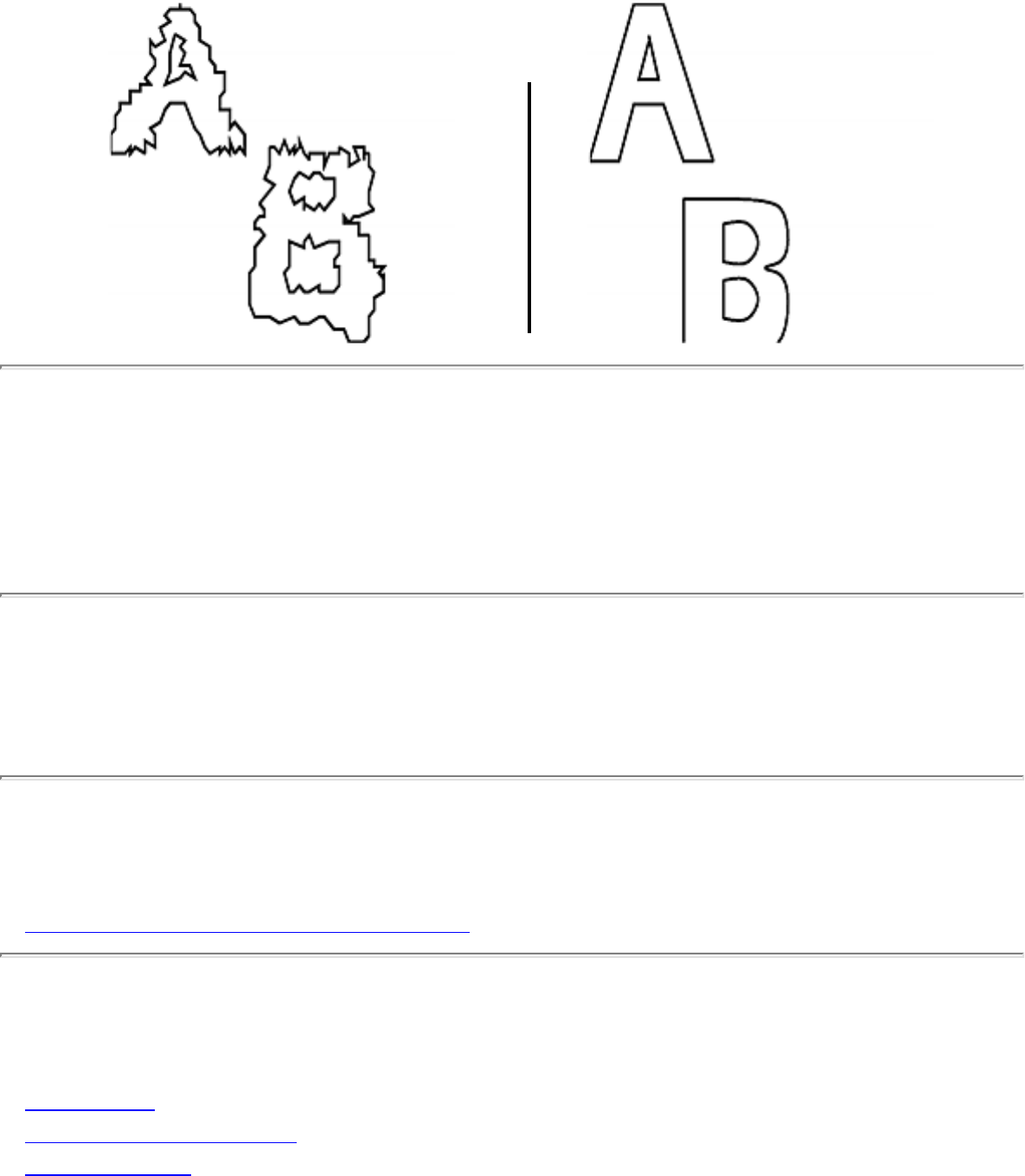
1.6.12 Simplifying Polygons
1.6.12 Simplifying Polygons
INPUT OUTPUT
Input Description: A polygon or polyhedron p , with n vertices.
Problem: Find a polygon or polyhedron p' with n' vertices, where the shape of p' is close to p while n'
<< n .
Implementations
● Skeletonization Software (2-D) (C) (rating 5)
Related Problems
● Convex Hull
● Discrete Fourier Transform
● Minkowski Sum
file:///E|/WEBSITE/FILES2/SIMPGONS.HTM (1 of 2) [19/1/2003 1:36:59]

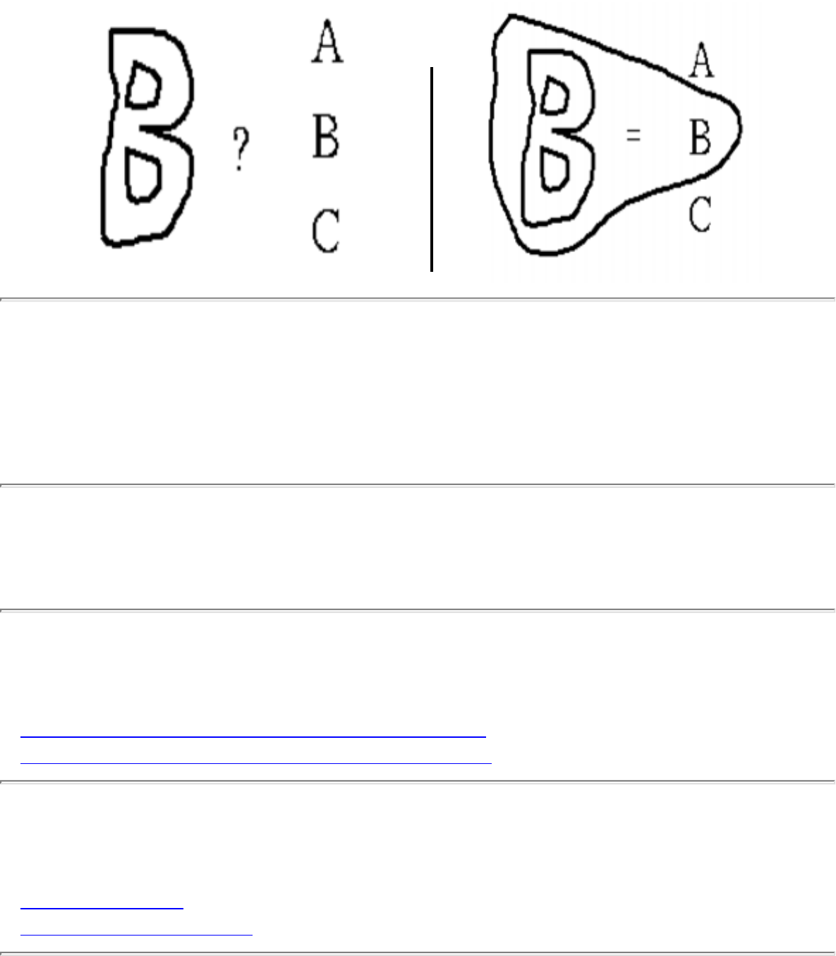
1.6.13 Shape Similarity
1.6.13 Shape Similarity
INPUT OUTPUT
Input Description: Two polygonal shapes, P_1 and P_2 .
Problem: How similar are P_1 and P_2 ?
Implementations
● SNNS - Stuttgart Neural Network Simulator (C) (rating 7)
● Shape similarity testing via turning functions (C) (rating 6)
Related Problems
● Graph Isomorphism
● Medial-Axis Transformation
file:///E|/WEBSITE/FILES2/SHAPRITY.HTM (1 of 2) [19/1/2003 1:36:59]

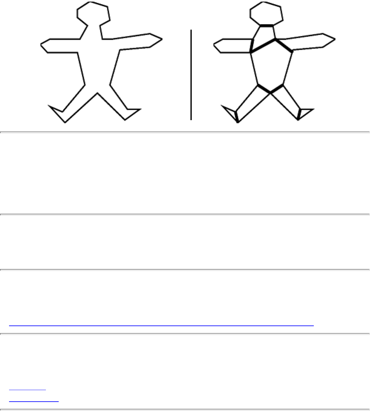
1.6.11 Polygon Partitioning
1.6.11 Polygon Partitioning
INPUT OUTPUT
Input Description: A polygon or polyhedron P .
Problem: How can P be partitioned into a small number of simple (typically convex) pieces?
Implementations
● GEOMPACK - triangulation and convex decomposition codes (FORTRAN) (rating 8)
Related Problems
● Set Cover
● Triangulation
file:///E|/WEBSITE/FILES2/POLONING.HTM (1 of 2) [19/1/2003 1:37:00]

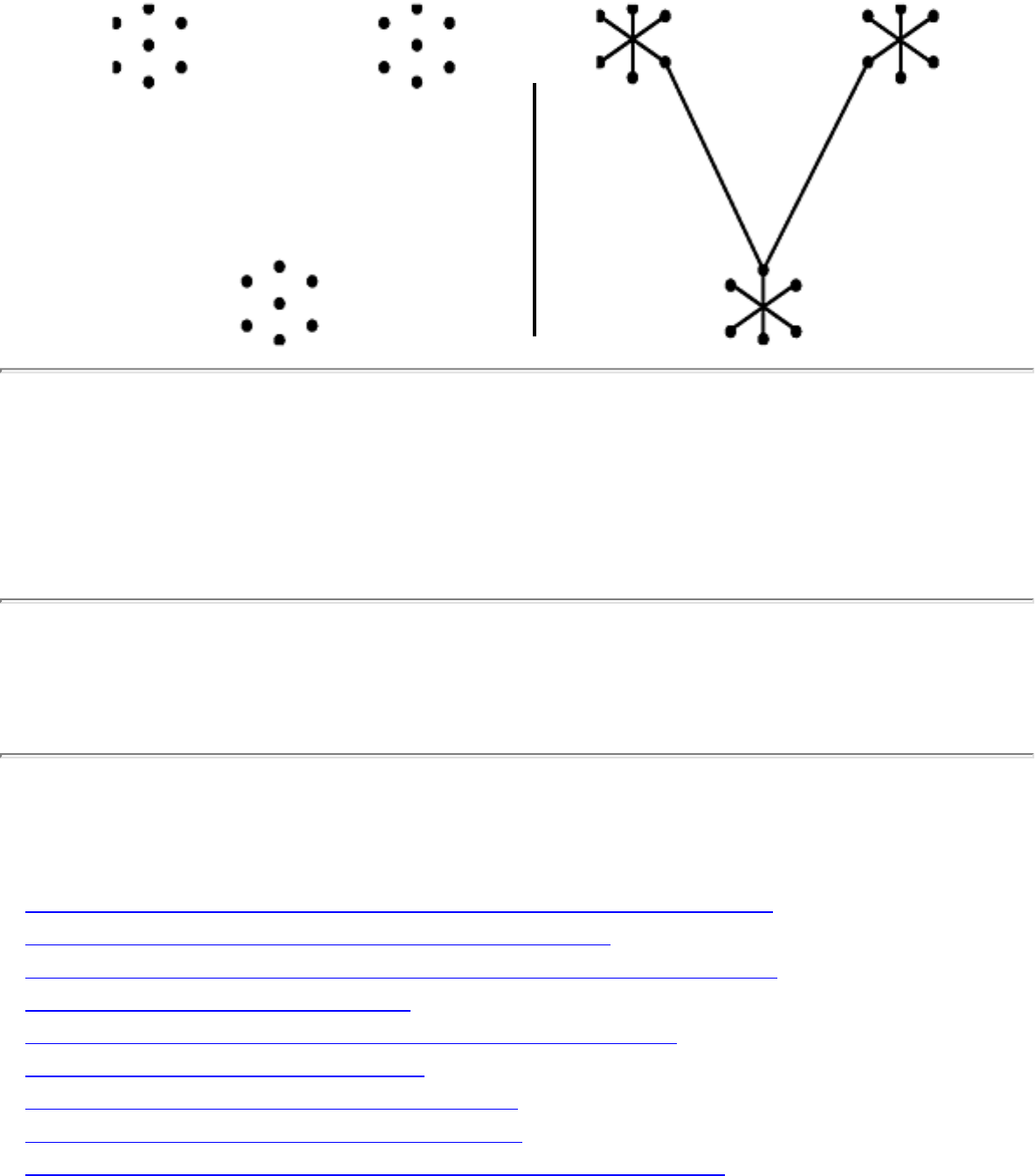
1.4.3 Minimum Spanning Tree
1.4.3 Minimum Spanning Tree
INPUT OUTPUT
Input Description: A graph G = (V,E) with weighted edges.
Problem: The subset of E of G of minimum weight which forms a tree on V .
Implementations
● LEDA - A Library of Efficient Data Types and Algorithms (C++) (rating 6)
● Moret and Shapiro's Algorithms P to NP (Pascal) (rating 5)
● Netlib / TOMS -- Collected Algorithms of the ACM (FORTRAN) (rating 5)
● The Stanford GraphBase (C) (rating 4)
● Xtango and Polka Algorithm Animation Systems (C++) (rating 4)
● Combinatorica (Mathematica) (rating 3)
● Algorithms in C++ -- Sedgewick (C++) (rating 3)
● Discrete Optimization Methods (Pascal) (rating 3)
● Nijenhuis and Wilf: Combinatorial Algorithms (FORTRAN) (rating 3)
file:///E|/WEBSITE/FILES/MINITREE.HTM (1 of 2) [19/1/2003 1:37:00]

1.4.3 Minimum Spanning Tree
Related Problems
● Set Data Structures
● Steiner Tree
● Traveling Salesman Problem
Go to the corresponding chapter in the book
About the Book
Send us Mail
Go to Main Page
This page last modified on Tue Jun 03, 1997 .
file:///E|/WEBSITE/FILES/MINITREE.HTM (2 of 2) [19/1/2003 1:37:00]
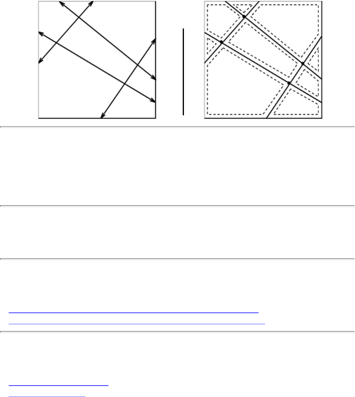
1.6.15 Maintaining Line Arrangements
1.6.15 Maintaining Line Arrangements
INPUT OUTPUT
Input Description: A set of lines and line segments l_1,...,\l_n .
Problem: What is the decomposition of the plane defined by l_1,...,\l_n ?
Implementations
● Arrange - maintainance of arrangements with point location (C) (rating 9)
● LEDA - A Library of Efficient Data Types and Algorithms (C++) (rating 7)
Related Problems
● Robust Geometric Primitives
● Intersection Detection
file:///E|/WEBSITE/FILES2/MAINENTS.HTM (1 of 2) [19/1/2003 1:37:01]

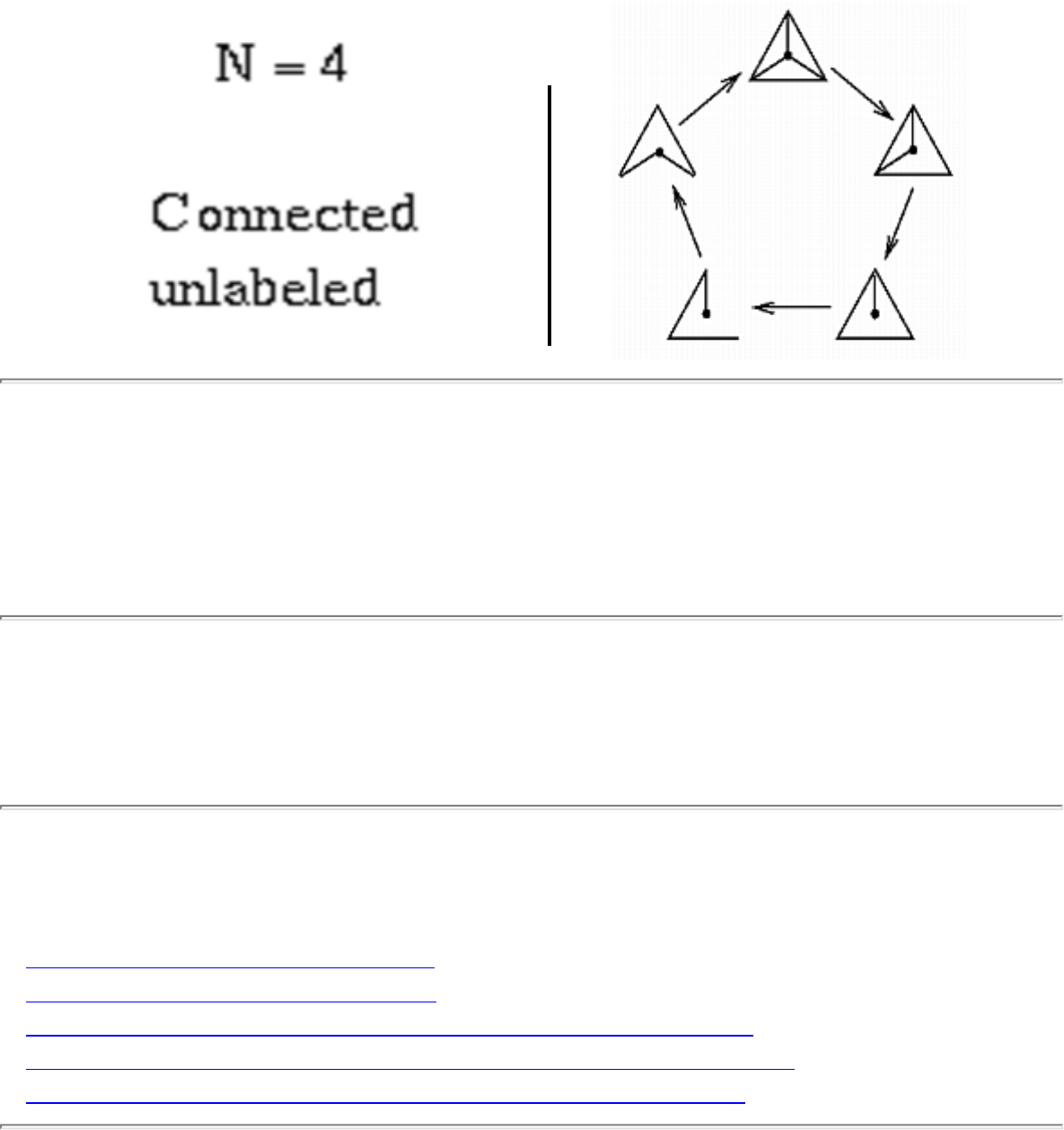
1.3.7 Generating Graphs
1.3.7 Generating Graphs
INPUT OUTPUT
Input Description: Parameters describing the desired graph, such as the number of vertices n , the
number of edges m , or the edge probability p .
Problem: Generate (1) all, or (2) a random, or (3) the next graph satisfying the parameters.
Implementations
● The Stanford GraphBase (C) (rating 10)
● Combinatorica (Mathematica) (rating 8)
● Frank Ruskey's Combinatorial Generation Resources (Pascal) (rating 7)
● LEDA - A Library of Efficient Data Types and Algorithms (C++) (rating 5)
● Nijenhuis and Wilf: Combinatorial Algorithms (FORTRAN) (rating 4)
Related Problems
file:///E|/WEBSITE/FILES/GENRAPHS.HTM (1 of 2) [19/1/2003 1:37:01]

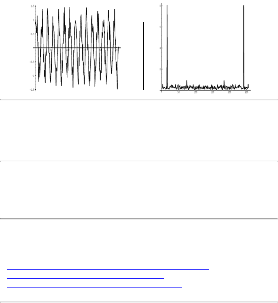
1.2.11 Discrete Fourier Transform
1.2.11 Discrete Fourier Transform
INPUT OUTPUT
Input Description: A sequence of n real or complex values h_i , 0 \leq i \leq n-1 , sampled at uniform
intervals from a function h .
Problem: The discrete Fourier transform H of h , H_m = \sum_{k=0}^{n-1} h_k e^{2 \pi i k m / n} , 0
\leq m \leq n-1 .
Implementations
● FFTPACK -- Fourier Transform Library (C) (rating 10)
● Netlib / TOMS -- Collected Algorithms of the ACM (FORTRAN) (rating 6)
● Moret and Shapiro's Algorithms P to NP (Pascal) (rating 4)
● Xtango and Polka Algorithm Animation Systems (C++) (rating 3)
● Algorithms in C++ -- Sedgewick (C++) (rating 2)
file:///E|/WEBSITE/FILES/FOUSFORM.HTM (1 of 2) [19/1/2003 1:37:02]

1.2.11 Discrete Fourier Transform
Related Problems
● Arbitrary Precision Arithmetic
● Simplifying Polygons
● Text Compression
Go to the corresponding chapter in the book
About the Book
Send us Mail
Go to Main Page
This page last modified on Tue Jun 03, 1997 .
file:///E|/WEBSITE/FILES/FOUSFORM.HTM (2 of 2) [19/1/2003 1:37:02]
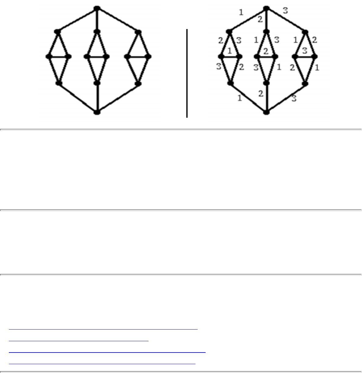
1.5.8 Edge Coloring
1.5.8 Edge Coloring
INPUT OUTPUT
Input Description: A graph G=(V,E) .
Problem: What is the smallest set of colors needed to color the edges of E such that no two edges with
the same color share a vertex in common?
Implementations
● Stony Brook Project Implementations (C++) (rating 6)
● Combinatorica (Mathematica) (rating 4)
● Joe Culberson's Graph Coloring Resources (C) (rating 4)
● Mike Trick's Graph Coloring Resources (C) (rating 4)
Related Problems
file:///E|/WEBSITE/FILES/EDGERING.HTM (1 of 2) [19/1/2003 1:37:02]

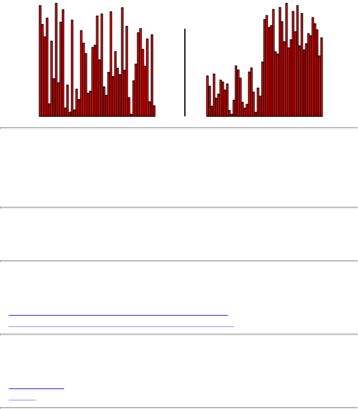
1.3.3 Median and Selection
1.3.3 Median and Selection
INPUT OUTPUT
Input Description: A set of n numbers or keys.
Problem: Find the item which is smaller than half of the items and bigger than half the items.
Implementations
● Handbook of Algorithms and Data Structures (Pascal) (rating 6)
● Xtango and Polka Algorithm Animation Systems (C++) (rating 4)
Related Problems
● Priority Queues
● Sorting
file:///E|/WEBSITE/FILES/MEDIAN03.HTM (1 of 2) [19/1/2003 1:37:03]

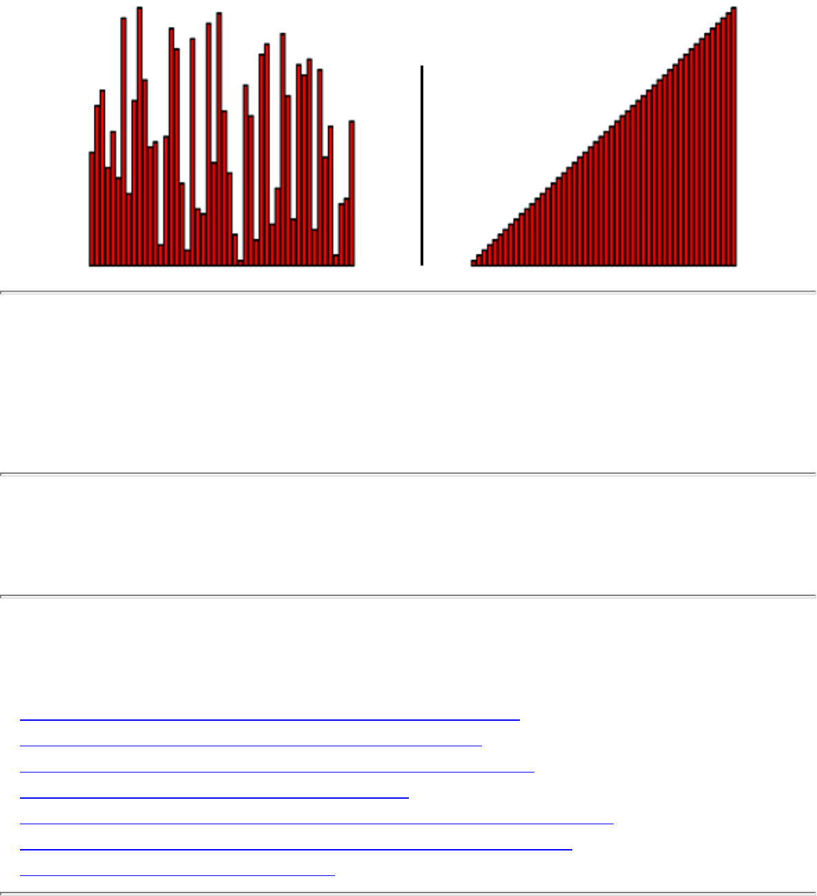
1.3.1 Sorting
1.3.1 Sorting
INPUT OUTPUT
Input Description: A set of n items.
Problem: Arrange the items in increasing order.
Implementations
● Handbook of Algorithms and Data Structures (Pascal) (rating 7)
● Moret and Shapiro's Algorithms P to NP (Pascal) (rating 7)
● Xtango and Polka Algorithm Animation Systems (C++) (rating 6)
● Algorithms in C++ -- Sedgewick (C++) (rating 5)
● Netlib / TOMS -- Collected Algorithms of the ACM (FORTRAN) (rating 4)
● Nijenhuis and Wilf: Combinatorial Algorithms (FORTRAN) (rating 3)
● Combinatorica (Mathematica) (rating 2)
file:///E|/WEBSITE/FILES/SORTING2.HTM (1 of 2) [19/1/2003 1:37:03]

1.3.1 Sorting
Related Problems
● Convex Hull
● Dictionaries
● Median and Selection
● Priority Queues
● Searching
● Topological Sorting
Go to the corresponding chapter in the book
About the Book
Send us Mail
Go to Main Page
This page last modified on Tue Jun 03, 1997 .
file:///E|/WEBSITE/FILES/SORTING2.HTM (2 of 2) [19/1/2003 1:37:03]

Plugins for use with the CDROM
Plug-Ins Available On This CD-ROM:
One of these plug-ins is required to play the audio files provided with the Lecture Notes on the CD. Click
on the appropriate plug-in on the list below, save it onto your local hard drive, and run it! The instalation
program should plug it into your browser.
● Shockwave Player Plug-In, Win95/NT
● Shockwave Player Plug-In, Windows 3.11
● Shockwave Player Plug-In, Mac 68k
● Shockwave Player Plug-In, Mac PowerPC
file:///E|/INSTALL/PLUGINS.HTM [19/1/2003 1:37:04]
Footnotes
...numbers.
Yes, this is a true story.
.
.
.
.
.
.
.
.
.
.
.
.
.
.
.
.
.
.
.
.
.
.
.
.
.
.
.
.
.
.
Algorithms
Mon Jun 2 23:33:50 EDT 1997
file:///E|/BOOK/BOOK6/FOOTNODE.HTM [19/1/2003 1:37:06]
Implementation Challenges
Next: Data Structures and Sorting Up: Introduction to Algorithms Previous: Exercises
Implementation Challenges
1. (*) Implement the two TSP heuristics of Section . Which of them gives better-quality solutions
in practice? Can you devise a heuristic that works better than both of them?
2. (*) Describe exactly how to test whether a given set of tickets proves minimum coverage in the
Lotto problem of Section . Write a program to find good ticket sets.
Algorithms
Mon Jun 2 23:33:50 EDT 1997
file:///E|/BOOK/BOOK/NODE21.HTM [19/1/2003 1:37:07]

Implementation Challenges
Next: Breaking Problems Down Up: Data Structures and Sorting Previous: Exercises
Implementation Challenges
1. Implement versions of several different dictionary data structures, such as linked lists, binary
trees, balanced binary search trees, and hash tables. Conduct experiments to assess the relative
performance of these data structures in a simple application that reads a large text file and reports
exactly one instance of each word that appears within it. This application can be efficiently
implemented by maintaining a dictionary of all distinct words that have appeared thus far in the
text and inserting/reporting each word that is not found. Write a brief report with your
conclusions.
2. Implement versions of several different sorting algorithms, such as selection sort, insertion sort,
heapsort, mergesort, and quicksort. Conduct experiments to assess the relative performance of
these algorithms in a simple application that reads a large text file and reports exactly one instance
of each word that appears within it. This application can be efficiently implemented by sorting all
the words that occur in the text and then passing through the sorted sequence to identify one
instance of each distinct word. Write a brief report with your conclusions.
Algorithms
Mon Jun 2 23:33:50 EDT 1997
file:///E|/BOOK/BOOK/NODE41.HTM [19/1/2003 1:37:08]
Implementation Challenges
Next: Graph Algorithms Up: Breaking Problems Down Previous: Exercises
Implementation Challenges
1. (*) Many types of products sold appeal more to members of one ethnic group than another.
Perhaps Greeks eat more pasta per capita than Russians do, while Japanese find baseball more
appealing than do Italians. A market researcher might be interested in having a program scan the
names on a mailing list to select the ones most likely to be, say, Greek to target for a given
mailing.
Develop a program that makes reasonable mappings between pairs of first/ last names and
ethnicities. One approach would be to compute the edit distance between query names and a
family of names of known ethnicity. Feel free to experiment with other approaches.
2. (*) In the game of Battleship, the first player hides a collection of, say, three ships on a
grid. The second player guesses a series of grid positions and is informed whether they hit
or miss a battleship. The second player continues to query until each of the battleship
positions has been probed. While the second player must succeed after making 100 different
probes, we seek a strategy to use as few probes as possible to achieve the goal.
Develop a program that tries to efficiently sink all the battleships. One reasonable algorithmic
approach would be based on divide-and-conquer or binary search.
3. (*) A Caesar shift (see Section ) is a very simple class of ciphers for secret messages.
Unfortunately, they can be broken using statistical properties of English. Develop a program
capable of decrypting Caesar shifts of sufficiently long texts.
Algorithms
Mon Jun 2 23:33:50 EDT 1997
file:///E|/BOOK/BOOK2/NODE58.HTM [19/1/2003 1:37:09]
Implementation Challenges
Next: Combinatorial Search and Heuristic Up: Graph Algorithms Previous: Exercises
Implementation Challenges
1. Airline flight schedules define a natural graph, where the vertices are the airports and there is an
edge between any two airports with direct flights between them whose weight is proportional to
the distance between them. An extensive airplane data set due to Roberto Tammasia is available
from the Algorithm Repository WWW/CD-ROM. Write a program that explicitly constructs the
airport graph from this data set.
2. This problem is a follow-up to the exercise above. Changing planes repeatedly on connecting
flights can be a hassle. Develop and implement an algorithm that finds the fewest flights needed
to get from airport A to B, regardless of waiting time.
3. (*) This problem is a follow-up to the exercise above. Develop and implement an algorithm that
finds the flight plan from airport A to B that minimizes the total distance traveled.
4. (*) This problem is a follow-up to the exercise above. Suppose that we must arrive at airport B at
time T for an important scheduled meeting. Develop and implement an algorithm that finds the
latest time one can leave airport A in time to make the meeting.
5. (*) This problem is a follow-up to the exercise above. In order to take advantage of a frequent
flyer program, we might want to fly only on a particular airline. How can we modify the above
solutions so as to accommodate such queries?
6. (**) This problem is a follow-up to the exercise above. A really devout frequent flyer might want
to find the longest flight plan between airports A and B, so as to maximize the number of miles
they get credit for. Develop and implement an algorithm to find the longest such route.
Algorithms
Mon Jun 2 23:33:50 EDT 1997
file:///E|/BOOK/BOOK2/NODE82.HTM [19/1/2003 1:37:10]

Implementation Challenges
Next: Intractable Problems and Approximations Up: Combinatorial Search and Heuristic Previous:
Exercises
Implementation Challenges
1. (*) Anagrams are rearrangements of the letters of a word or phrase into a different word or phrase.
Sometimes the results are quite striking. For example, ``MANY VOTED BUSH RETIRED'' is an
anagram of ``TUESDAY NOVEMBER THIRD,'' which correctly predicted the outcome of the
1992 U.S. presidential election. Design and implement an algorithm for finding anagrams using
combinatorial search and a dictionary.
2. (*) For any of the exercises above, design and implement a simulated annealing heuristic to get
reasonable solutions. How well does your program perform in practice?
3. (**) Design and implement a parallel sorting algorithm that distributes data across several
processors. An appropriate variation of mergesort is a likely candidate. Measure the speedup of
this algorithm as the number of processors increases. Later, compare the execution time to that of
a purely sequential mergesort implementation. What are your experiences?
Algorithms
Mon Jun 2 23:33:50 EDT 1997
file:///E|/BOOK/BOOK3/NODE103.HTM [19/1/2003 1:37:11]
Implementation Challenges
Next: How to Design Algorithms Up: Intractable Problems and Approximations Previous: Exercises
Implementation Challenges
1. Implement a translator that translates satisfiability instances into equivallent 3-SAT instances.
2. (*) Design and implement a backtracking algorithm to test whether a set of formulae are
satisfiable. What criteria can you use to prune this search?
3. (*) Implement the vertex cover to satisfiability reduction, and run the resulting clauses through a
satisfiability testing code. Does this seem like a practical way to compute things?
Algorithms
Mon Jun 2 23:33:50 EDT 1997
file:///E|/BOOK/BOOK3/NODE123.HTM [19/1/2003 1:37:12]

Caveats
Next: Data Structures Up: A Catalog of Algorithmic Previous: A Catalog of Algorithmic
Caveats
This is a catalog of algorithmic problems. It is not a cookbook. It cannot be because there are too many
possible recipes and too many possible variations on what those want to eat. My goal is to aim you in
the right direction so that you can solve your own problems. I point out the issues you are likely to
encounter along the way, problems that you are going to have to work out for yourself. In particular:
● For each problem, I suggest algorithms and directions to attack it. These recommendations are
based on my experiences and study and aimed towards what I see as typical applications. I felt it
was more important to make concrete recommendations for the masses rather than to try to cover
all possible situations. If you don't want to follow my advice, don't follow my advice. But before
you ignore me, make sure you understand the reasoning behind my recommendations and can
articulate a reason why your application violates my assumptions.
● The implementations I recommend are not necessarily complete solutions to your problem. I
point to an implementation whenever I feel it might be more useful to someone than just a
textbook description of the algorithm. Some programs are useful only as models for you to write
your own codes. Others are embedded in large systems and so might be too painful to extract and
run on their own. Assume that all of them contain bugs. Many are quite serious, so beware.
● Please respect the licensing conditions for any implementations you use commercially. Many of
these codes are not in the public domain and have restrictions. See Section for a further
discussion of this issue.
● I would be interested in hearing about your experiences with my recommendations, both positive
and negative. I would be especially interested in learning about any other implementations that
you know about. Feel free to drop me a line at algorith@cs.sunysb.edu.
Next: Data Structures Up: A Catalog of Algorithmic Previous: A Catalog of Algorithmic
Algorithms
Mon Jun 2 23:33:50 EDT 1997
file:///E|/BOOK/BOOK3/NODE127.HTM [19/1/2003 1:37:12]
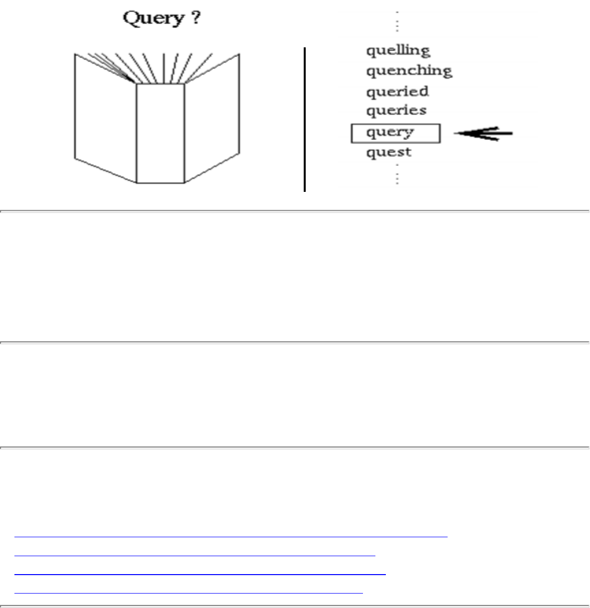
1.1.1 Dictionaries
1.1.1 Dictionaries
INPUT OUTPUT
Input Description: A set of n records, each identified by one or more key fields.
Problem: Build and maintain a data structure to efficiently locate, insert, or delete the record associated
with any query key q .
Implementations
● LEDA - A Library of Efficient Data Types and Algorithms (C++) (rating 10)
● Handbook of Algorithms and Data Structures (Pascal) (rating 8)
● Xtango and Polka Algorithm Animation Systems (C++) (rating 5)
● DIMACS Implementation Challenges (FORTRAN) (rating 1)
Related Problems
file:///E|/WEBSITE/FILES/DICTRIES.HTM (1 of 2) [19/1/2003 1:37:13]

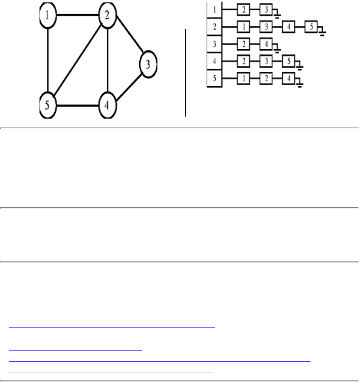
1.1.4 Graph Data Structures
1.1.4 Graph Data Structures
INPUT OUTPUT
Input Description: A graph G .
Problem: Give an efficient, flexible data structure to represent G .
Implementations
● LEDA - A Library of Efficient Data Types and Algorithms (C++) (rating 10)
● GraphEd -- Graph Editor and Layout Program (C) (rating 8)
● Combinatorica (Mathematica) (rating 6)
● The Stanford GraphBase (C) (rating 6)
● LINK -- Programming and Visualization Environment for Hypergraphs (C++) (rating 6)
● Moret and Shapiro's Algorithms P to NP (Pascal) (rating 4)
Related Problems
file:///E|/WEBSITE/FILES/GRAPURES.HTM (1 of 2) [19/1/2003 1:37:14]

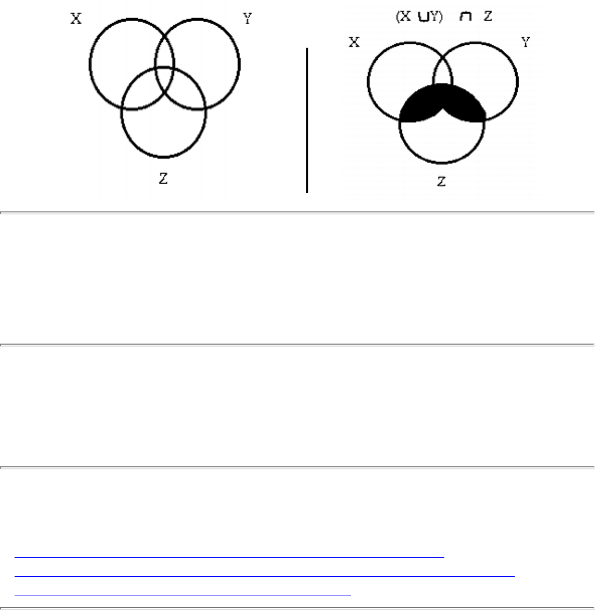
1.1.5 Set Data Structures
1.1.5 Set Data Structures
INPUT OUTPUT
Input Description: A universe of objects U = \{ u_1,...,u_n\} , and a collection of subsets S_1,...,S_m ,
S_i \subset U .
Problem: Represent each subset so as to efficiently (1) test whether u_i \in S_j , (2) find the union or
intersection of S_i and S_j , (3) insert or delete members of S_i .
Implementations
● LEDA - A Library of Efficient Data Types and Algorithms (C++) (rating 5)
● LINK -- Programming and Visualization Environment for Hypergraphs (C++) (rating 4)
● Moret and Shapiro's Algorithms P to NP (Pascal) (rating 4)
Related Problems
file:///E|/WEBSITE/FILES/SET_URES.HTM (1 of 2) [19/1/2003 1:37:14]

1.1.5 Set Data Structures
● Generating Partitions
● Generating Subsets
● Graph Data Structures
● Minimum Spanning Tree
● Set Cover
Go to the corresponding chapter in the book
About the Book
Send us Mail
Go to Main Page
This page last modified on Tue Jun 03, 1997 .
file:///E|/WEBSITE/FILES/SET_URES.HTM (2 of 2) [19/1/2003 1:37:14]
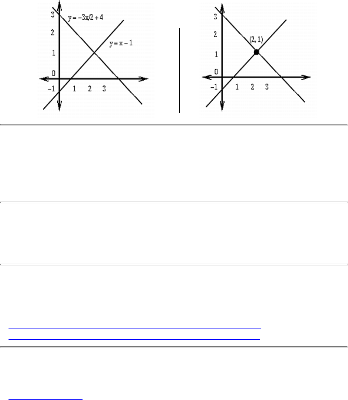
1.2.1 Solving Linear Equations
1.2.1 Solving Linear Equations
INPUT OUTPUT
Input Description: An m x n matrix A , and an m x 1 vector b , representing m linear equations with n
variables.
Problem: What is the vector x such that A \cdot x = b ?
Implementations
● LAPACK and LINPACK -- Linear Algebra PACKages (FORTRAN) (rating 10)
● Netlib / TOMS -- Collected Algorithms of the ACM (FORTRAN) (rating 7)
● LEDA - A Library of Efficient Data Types and Algorithms (C++) (rating 3)
Related Problems
● Bandwidth Reduction
file:///E|/WEBSITE/FILES/LINEIONS.HTM (1 of 2) [19/1/2003 1:37:15]

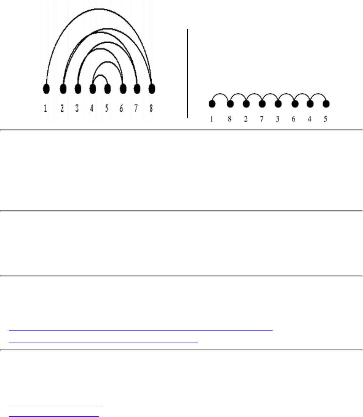
1.2.2 Bandwidth Reduction
1.2.2 Bandwidth Reduction
INPUT OUTPUT
Input Description: A graph G=(V,E) , representing an n x n matrix M of zero and non-zero elements.
Problem: Which permutation p of the vertices of V minimizes \max_{(i,j) \in E} |p(i) - p(j)| , or
equivalently the length of the longest edge when the vertices are ordered on a line.
Implementations
● Netlib / TOMS -- Collected Algorithms of the ACM (FORTRAN) (rating 9)
● Stony Brook Project Implementations (C++) (rating 6)
Related Problems
● Feedback Edge/Vertex Set
● Solving Linear Equations
file:///E|/WEBSITE/FILES/BANDIDTH.HTM (1 of 2) [19/1/2003 1:37:15]

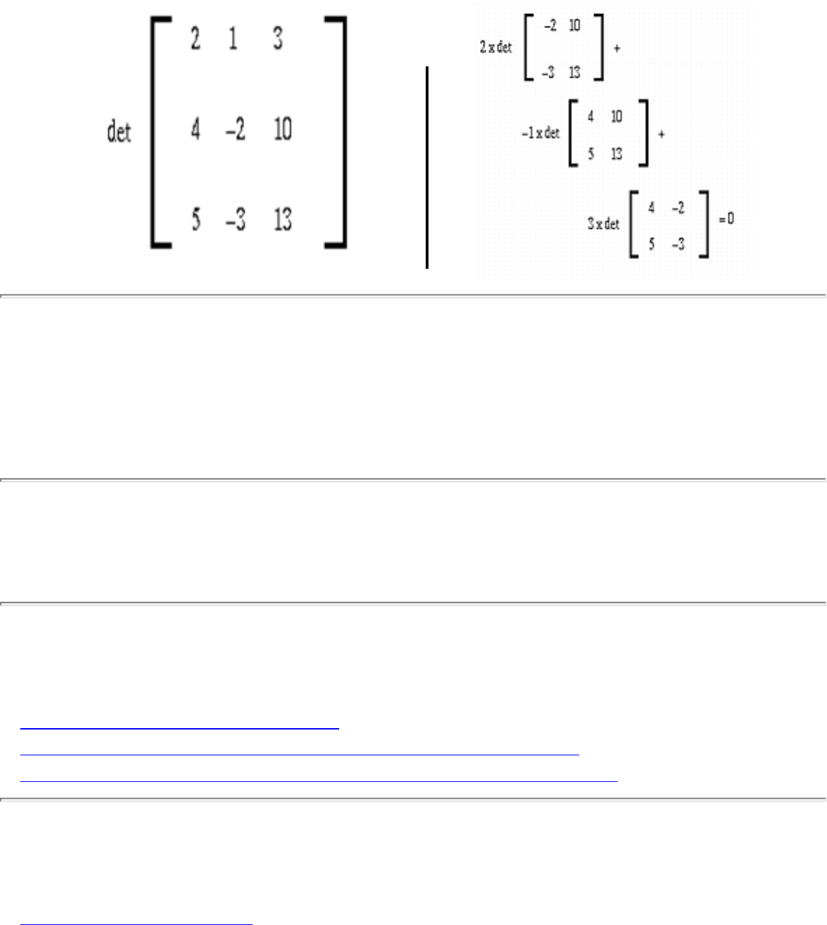
1.2.4 Determinants and Permanents
1.2.4 Determinants and Permanents
INPUT OUTPUT
Input Description: An n x n matrix M .
Problem: What is the determinant |M| or the permanent Perm(M) for matrix m ?
Implementations
● Combinatorica (Mathematica) (rating 4)
● Nijenhuis and Wilf: Combinatorial Algorithms (FORTRAN) (rating 4)
● LEDA - A Library of Efficient Data Types and Algorithms (C++) (rating 2)
Related Problems
● Robust Geometric Primitives
file:///E|/WEBSITE/FILES/DETEANTS.HTM (1 of 2) [19/1/2003 1:37:16]

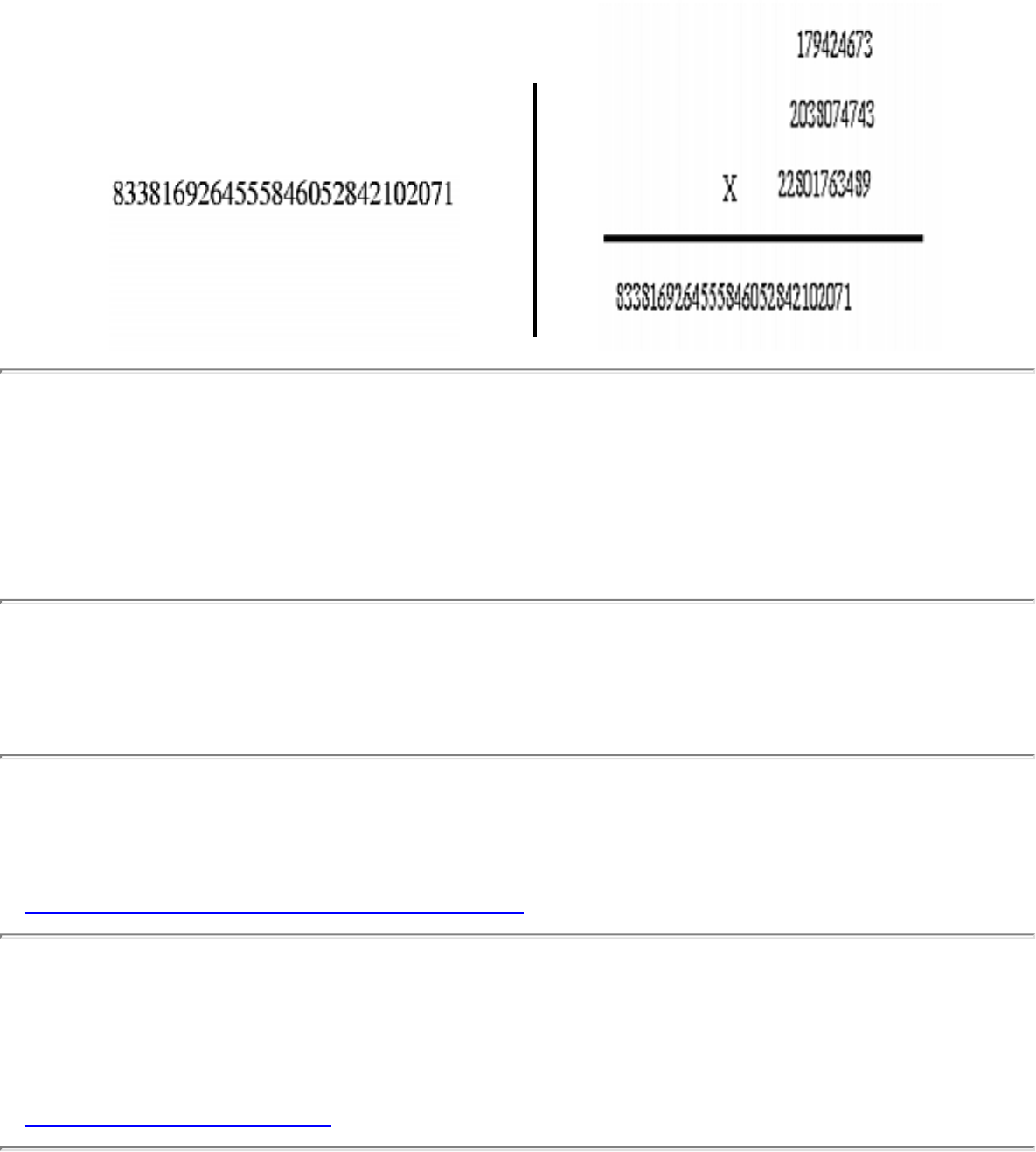
1.2.8 Factoring and Primality Testing
1.2.8 Factoring and Primality Testing
INPUT OUTPUT
Input Description: An integer n .
Problem: Is n a prime number, and if not what are the factors of n ?
Implementations
● PARI - Package for Number Theory (C) (rating 9)
Related Problems
● Cryptography
● Arbitrary Precision Arithmetic
file:///E|/WEBSITE/FILES/FACTGERS.HTM (1 of 2) [19/1/2003 1:37:16]

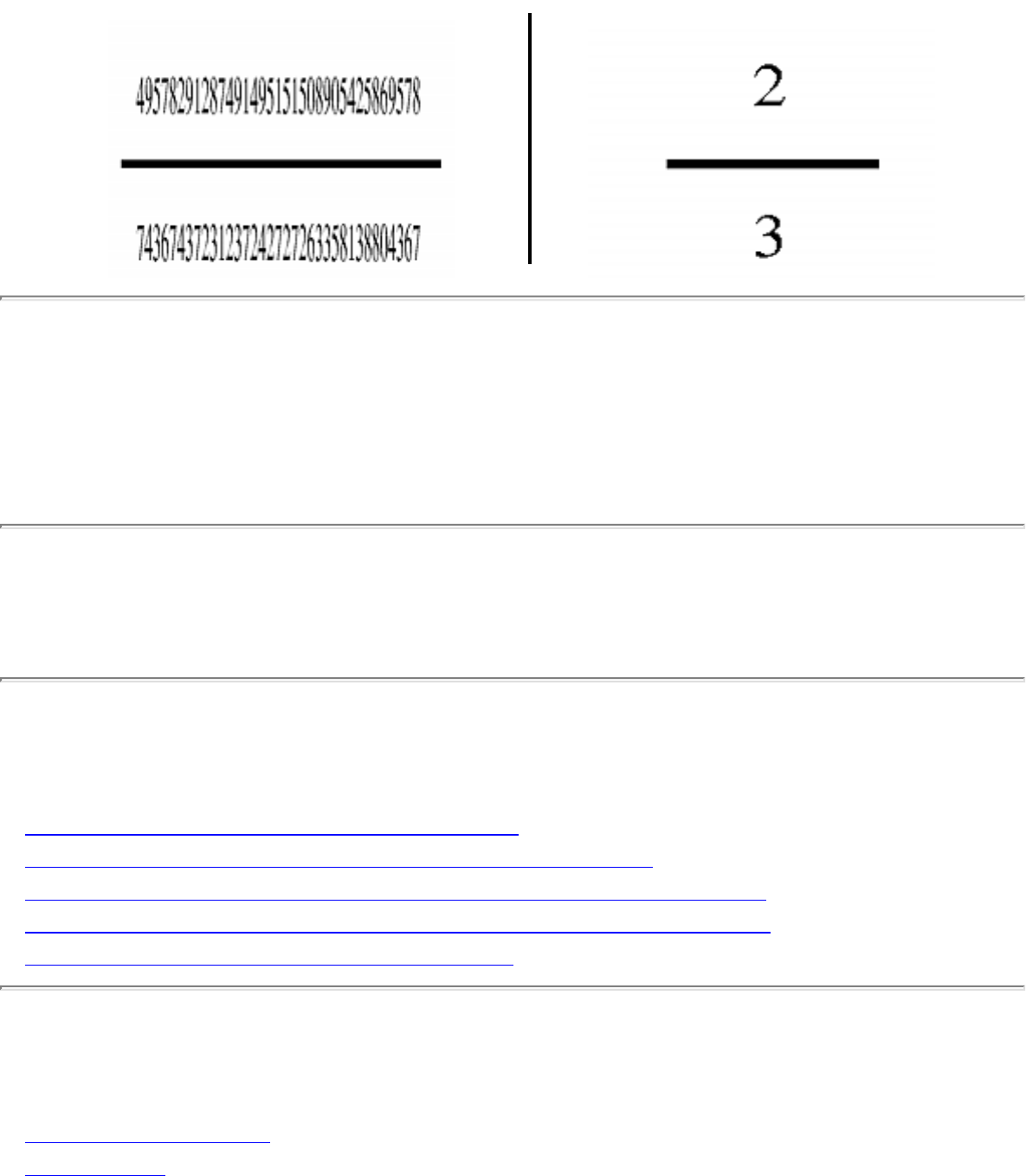
1.2.9 Arbitrary Precision Arithmetic
1.2.9 Arbitrary Precision Arithmetic
INPUT OUTPUT
Input Description: Two very large integers, x and y .
Problem: What is x+y , x-y , x x y and x / y ?
Implementations
● PARI - Package for Number Theory (C) (rating 9)
● Handbook of Algorithms and Data Structures (Pascal) (rating 6)
● LEDA - A Library of Efficient Data Types and Algorithms (C++) (rating 5)
● Netlib / TOMS -- Collected Algorithms of the ACM (FORTRAN) (rating 5)
● Algorithms in C++ -- Sedgewick (C++) (rating 3)
Related Problems
● Calendrical Calculations
● Cryptography
file:///E|/WEBSITE/FILES/HIGHETIC.HTM (1 of 2) [19/1/2003 1:37:17]

1.2.9 Arbitrary Precision Arithmetic
● Factoring and Primality Testing
● Discrete Fourier Transform
Go to the corresponding chapter in the book
About the Book
Send us Mail
Go to Main Page
This page last modified on Tue Jun 03, 1997 .
file:///E|/WEBSITE/FILES/HIGHETIC.HTM (2 of 2) [19/1/2003 1:37:17]
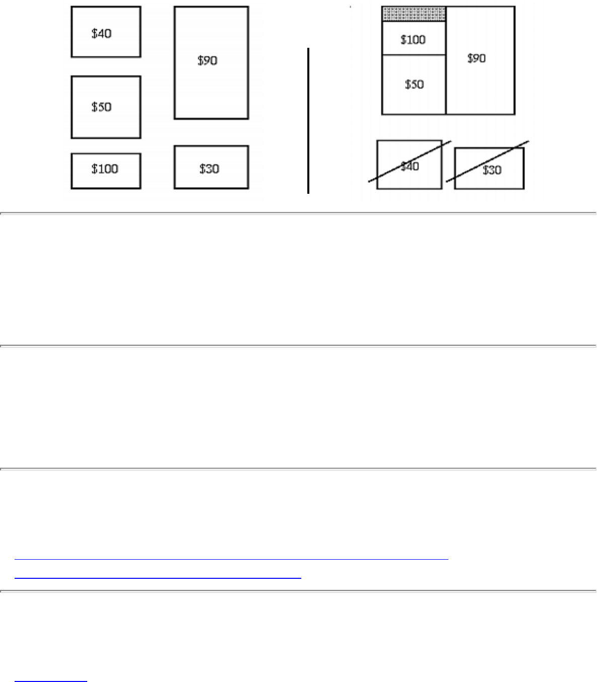
1.2.10 Knapsack Problem
1.2.10 Knapsack Problem
INPUT OUTPUT
Input Description: A set of items S=\{1,...,n\} , where item i has size s_i and value v_i . A knapsack
capacity C .
Problem: Find the subset S' \subset S which maximizes the value of \sum_{i \in S'} v_i given that
\sum_{i \in S'} s_i \leq C , ie. fits in a knapsack of size C .
Implementations
● Netlib / TOMS -- Collected Algorithms of the ACM (FORTRAN) (rating 6)
● Discrete Optimization Methods (Pascal) (rating 4)
Related Problems
● Bin Packing
file:///E|/WEBSITE/FILES/00000017.HTM (1 of 2) [19/1/2003 1:37:18]

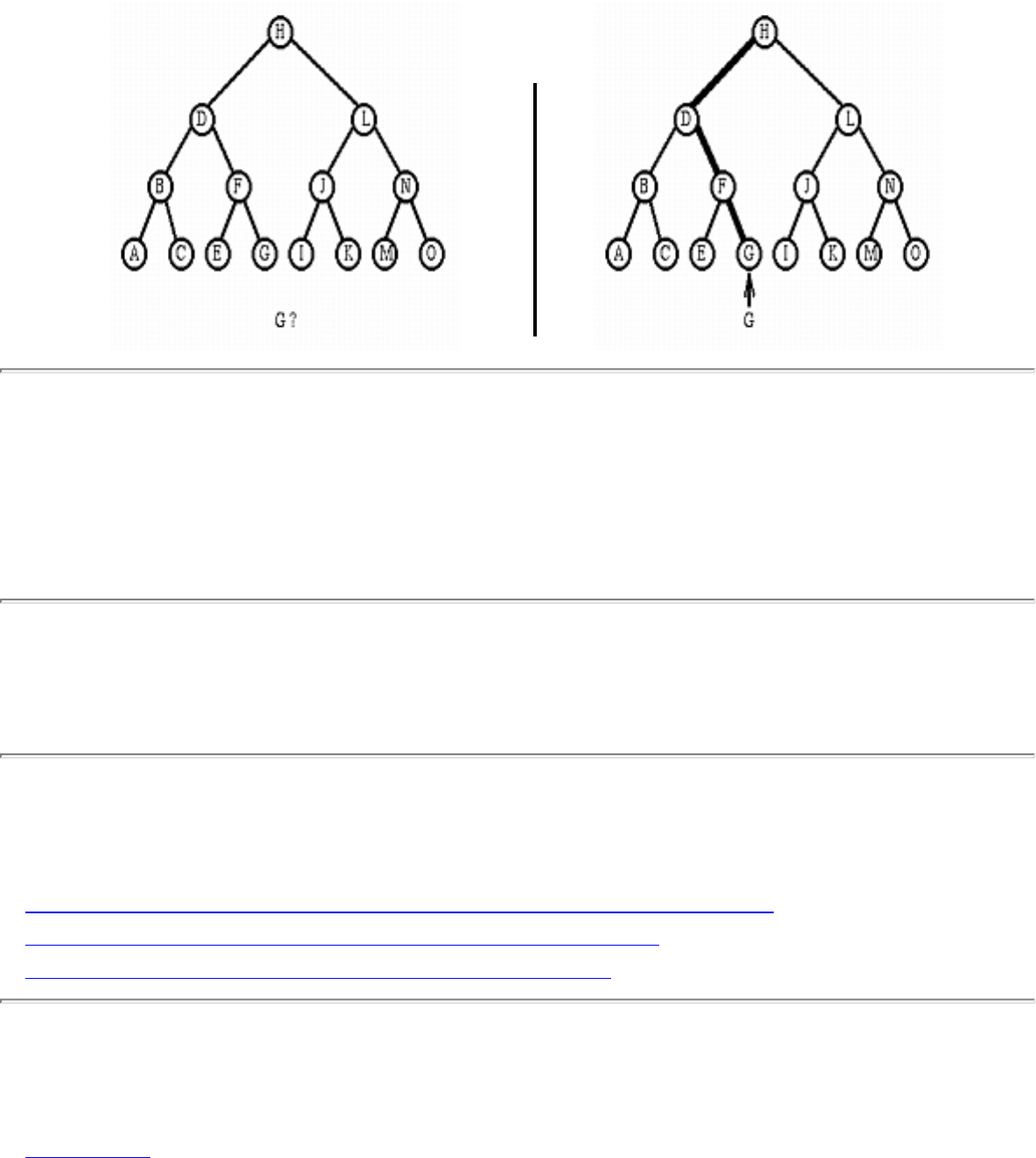
1.3.2 Searching
1.3.2 Searching
INPUT OUTPUT
Input Description: A set S of n keys, a query key q .
Problem: Where is q in S ?
Implementations
● LEDA - A Library of Efficient Data Types and Algorithms (C++) (rating 7)
● Handbook of Algorithms and Data Structures (Pascal) (rating 7)
● Moret and Shapiro's Algorithms P to NP (Pascal) (rating 3)
Related Problems
● Dictionaries
file:///E|/WEBSITE/FILES/SEARHING.HTM (1 of 2) [19/1/2003 1:37:18]

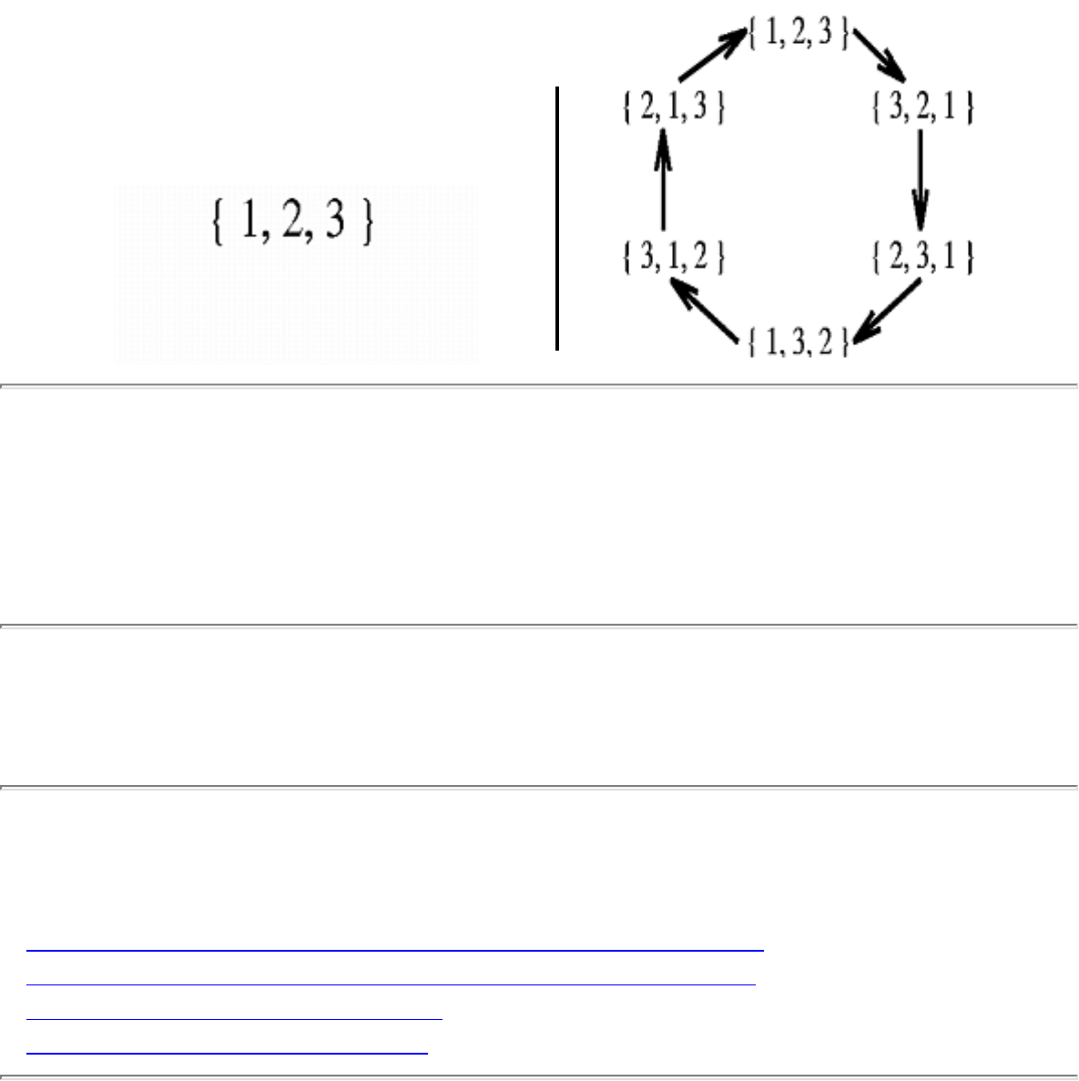
1.3.4 Generating Permutations
1.3.4 Generating Permutations
INPUT OUTPUT
Input Description: An integer n .
Problem: Generate (1) all, or (2) a random, or (3) the next permutation of length n .
Implementations
● Frank Ruskey's Combinatorial Generation Resources (Pascal) (rating 8)
● Nijenhuis and Wilf: Combinatorial Algorithms (FORTRAN) (rating 8)
● Combinatorica (Mathematica) (rating 7)
● The Stanford GraphBase (C) (rating 5)
Related Problems
file:///E|/WEBSITE/FILES/GENTIONS.HTM (1 of 2) [19/1/2003 1:37:19]

1.3.4 Generating Permutations
● Calendrical Calculations
● Generating Graphs
● Generating Partitions
● Generating Subsets
● Random Number Generation
Go to the corresponding chapter in the book
About the Book
Send us Mail
Go to Main Page
This page last modified on Tue Jun 03, 1997 .
file:///E|/WEBSITE/FILES/GENTIONS.HTM (2 of 2) [19/1/2003 1:37:19]
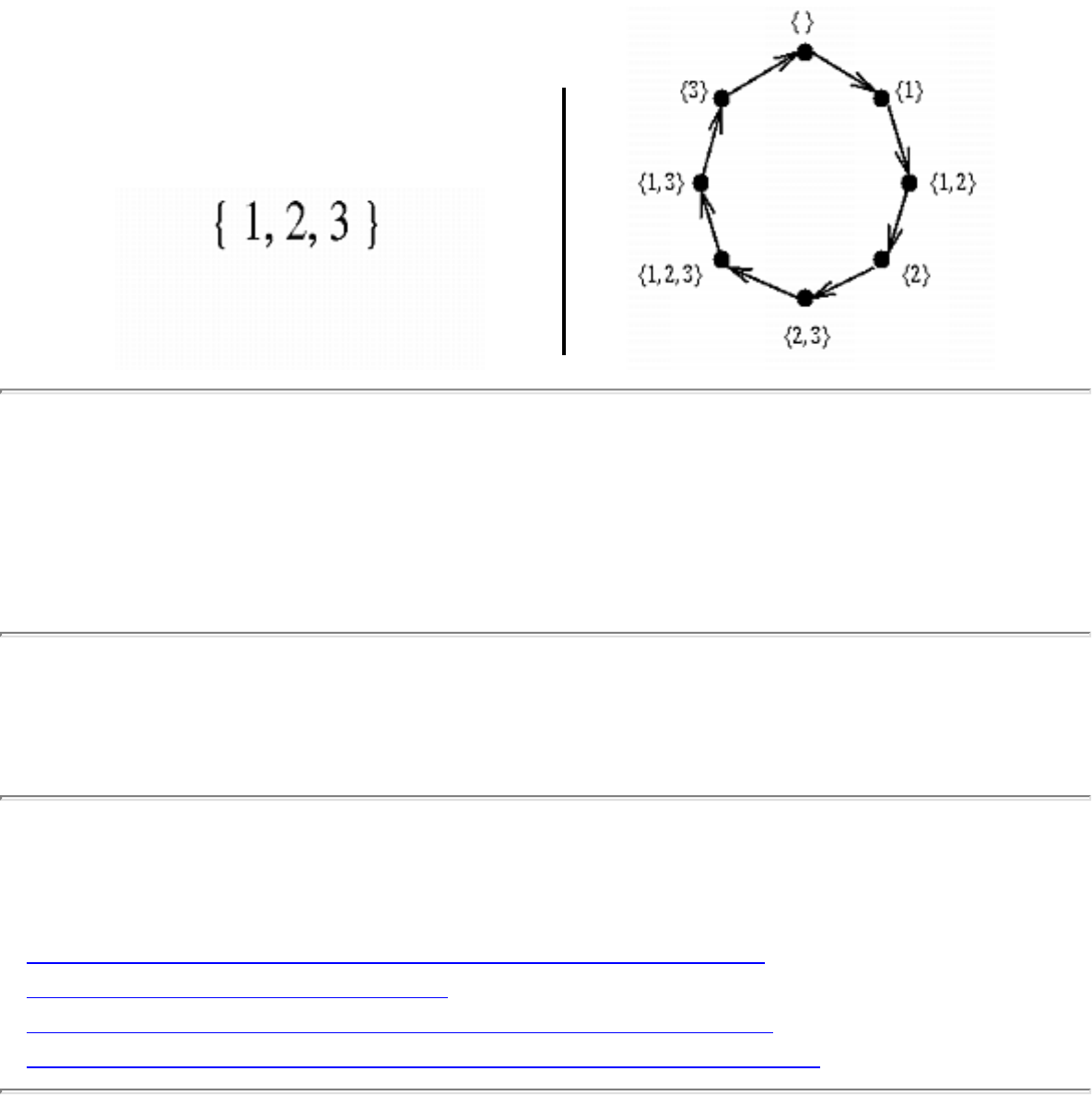
1.3.5 Generating Subsets
1.3.5 Generating Subsets
INPUT OUTPUT
Input Description: An integer n .
Problem: Generate (1) all, or (2) a random, or (3) the next subset of the integers 1 to n .
Implementations
● Nijenhuis and Wilf: Combinatorial Algorithms (FORTRAN) (rating 8)
● Combinatorica (Mathematica) (rating 7)
● Frank Ruskey's Combinatorial Generation Resources (Pascal) (rating 7)
● Netlib / TOMS -- Collected Algorithms of the ACM (FORTRAN) (rating 3)
Related Problems
file:///E|/WEBSITE/FILES/GSUBSETS.HTM (1 of 2) [19/1/2003 1:37:19]

1.3.5 Generating Subsets
● Generating Partitions
● Generating Permutations
● Random Number Generation
● Set Data Structures
Go to the corresponding chapter in the book
About the Book
Send us Mail
Go to Main Page
This page last modified on Tue Jun 03, 1997 .
file:///E|/WEBSITE/FILES/GSUBSETS.HTM (2 of 2) [19/1/2003 1:37:19]
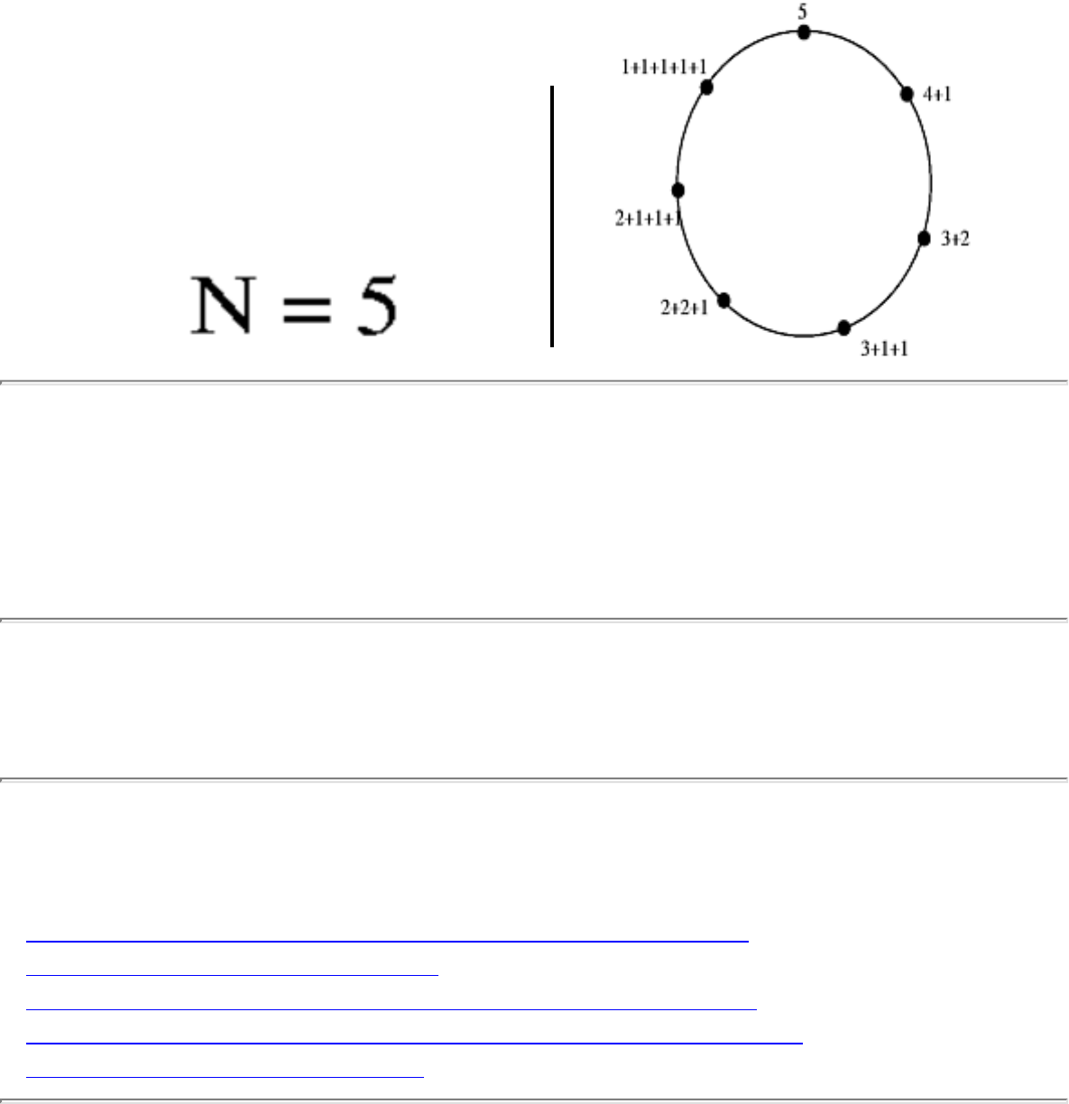
1.3.6 Generating Partitions
1.3.6 Generating Partitions
INPUT OUTPUT
Input Description: An integer n .
Problem: Generate (1) all, or (2) a random, or (3) the next integer or set partitions of length n .
Implementations
● Nijenhuis and Wilf: Combinatorial Algorithms (FORTRAN) (rating 8)
● Combinatorica (Mathematica) (rating 7)
● Frank Ruskey's Combinatorial Generation Resources (Pascal) (rating 7)
● Netlib / TOMS -- Collected Algorithms of the ACM (FORTRAN) (rating 6)
● The Stanford GraphBase (C) (rating 5)
Related Problems
file:///E|/WEBSITE/FILES/GEITIONS.HTM (1 of 2) [19/1/2003 1:37:20]

1.3.6 Generating Partitions
● Generating Permutations
● Generating Subsets
● Random Number Generation
● Set Data Structures
Go to the corresponding chapter in the book
About the Book
Send us Mail
Go to Main Page
This page last modified on Tue Jun 03, 1997 .
file:///E|/WEBSITE/FILES/GEITIONS.HTM (2 of 2) [19/1/2003 1:37:20]
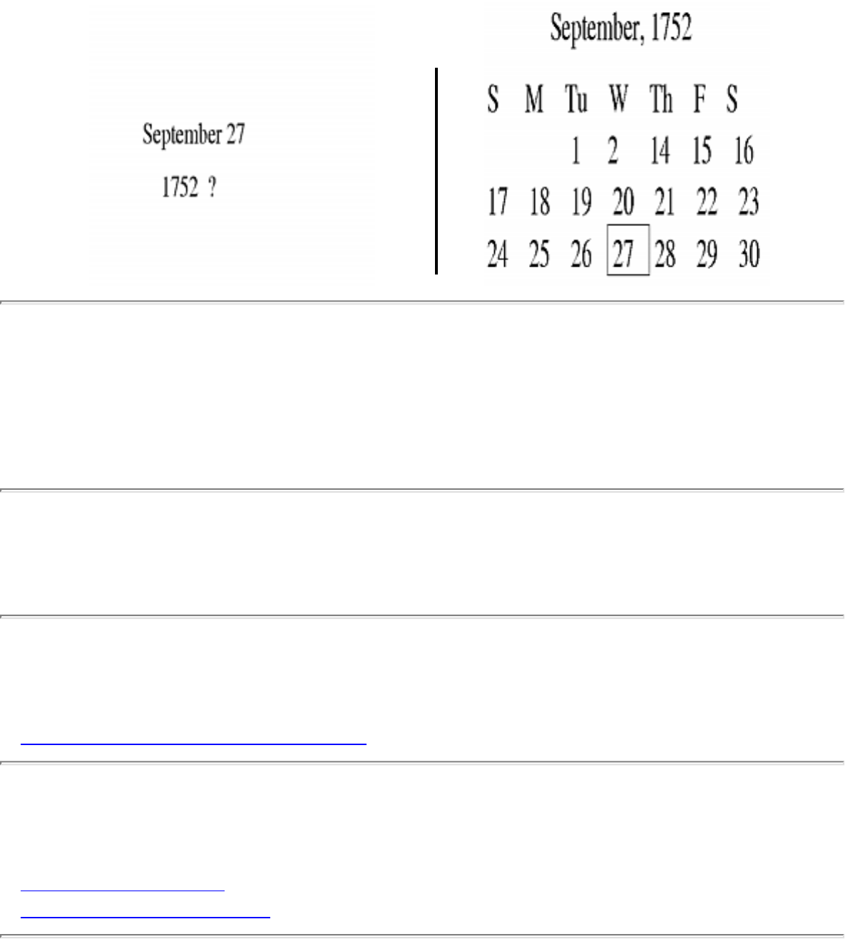
1.3.8 Calendrical Calculations
1.3.8 Calendrical Calculations
INPUT OUTPUT
Input Description: A particular calendar date d , specified by month, day and year.
Problem: Which day of the week did d fall on in the given calendar system?
Implementations
● Calendrical Calculations (C++) (rating 10)
Related Problems
● Generating Permutations
● Arbitrary Precision Arithmetic
file:///E|/WEBSITE/FILES/CALEIONS.HTM (1 of 2) [19/1/2003 1:37:21]

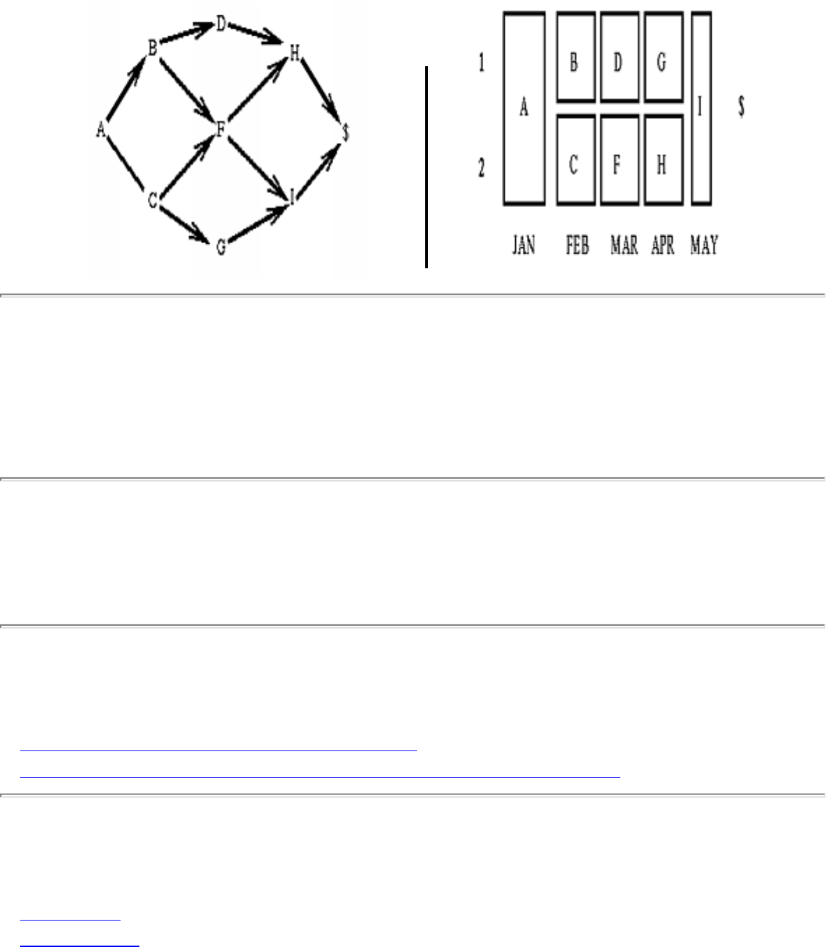
1.3.9 Job Scheduling
1.3.9 Job Scheduling
INPUT OUTPUT
Input Description: A directed acyclic graph G=(V,E) , where the vertices represent jobs and the the
edge (u,v) that task u must be completed before task v .
Problem: What schedule of tasks to completes the job using the minimum amount of time or processors?
Implementations
● Discrete Optimization Methods (Pascal) (rating 4)
● Netlib / TOMS -- Collected Algorithms of the ACM (FORTRAN) (rating 4)
Related Problems
● Bin Packing
● Edge Coloring
file:///E|/WEBSITE/FILES/SCHELING.HTM (1 of 2) [19/1/2003 1:37:21]

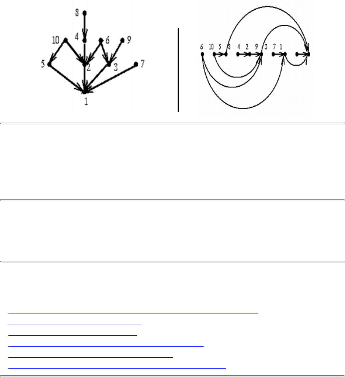
1.4.2 Topological Sorting
1.4.2 Topological Sorting
INPUT OUTPUT
Input Description: A directed, acyclic graph G=(V,E) (also known as a partial order or poset).
Problem: Find a linear ordering of the vertices of V such that for each edge (i,j) \in E , vertex i is to the
left of vertex j .
Implementations
● LEDA - A Library of Efficient Data Types and Algorithms (C++) (rating 7)
● Combinatorica (Mathematica) (rating 3)
● The Stanford GraphBase (C) (rating 3)
● Moret and Shapiro's Algorithms P to NP (Pascal) (rating 3)
● Algorithms in C++ -- Sedgewick (C++) (rating 3)
● Xtango and Polka Algorithm Animation Systems (C++) (rating 2)
file:///E|/WEBSITE/FILES/TOPOTING.HTM (1 of 2) [19/1/2003 1:37:22]

1.4.2 Topological Sorting
Related Problems
● Bandwidth Reduction
● Feedback Edge/Vertex Set
● Job Scheduling
● Sorting
Go to the corresponding chapter in the book
About the Book
Send us Mail
Go to Main Page
This page last modified on Tue Jun 03, 1997 .
file:///E|/WEBSITE/FILES/TOPOTING.HTM (2 of 2) [19/1/2003 1:37:22]
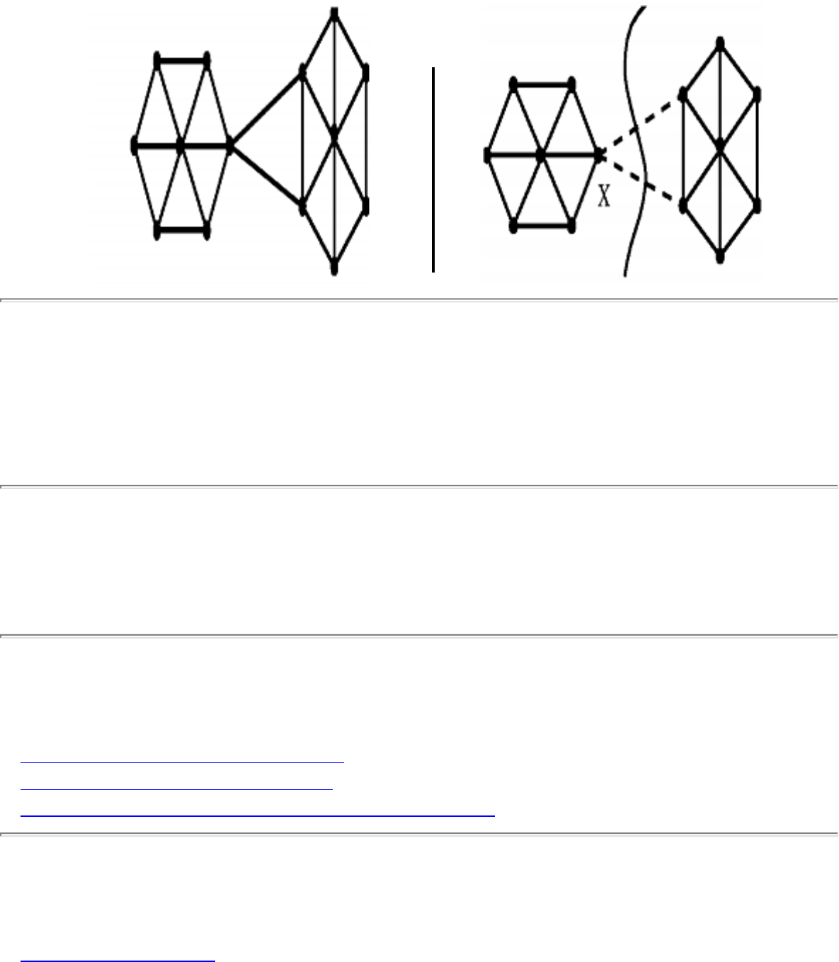
1.4.8 Edge and Vertex Connectivity
1.4.8 Edge and Vertex Connectivity
INPUT OUTPUT
Input Description: A graph G . Optionally, a pair of vertices and t .
Problem: What is the smallest subset of vertices (edges) whose deletion will disconnect G ? Alternately,
what is the smallest subset of vertices (edges) which will separate from t ?
Implementations
● Combinatorica (Mathematica) (rating 4)
● The Stanford GraphBase (C) (rating 4)
● Moret and Shapiro's Algorithms P to NP (Pascal) (rating 4)
Related Problems
● Connected Components
file:///E|/WEBSITE/FILES/EDGEVITY.HTM (1 of 2) [19/1/2003 1:37:22]

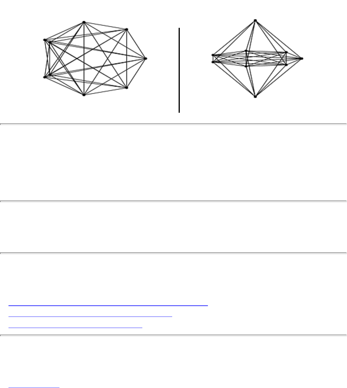
1.4.10 Drawing Graphs Nicely
1.4.10 Drawing Graphs Nicely
INPUT OUTPUT
Input Description: A graph G .
Problem: Give a drawing of graph G which accurately reflects its structure.
Implementations
● GraphEd -- Graph Editor and Layout Program (C) (rating 9)
● GraphViz -- graph layout programs (C) (rating 7)
● Combinatorica (Mathematica) (rating 6)
Related Problems
● Drawing Trees
file:///E|/WEBSITE/FILES/DRARAPHS.HTM (1 of 2) [19/1/2003 1:37:23]

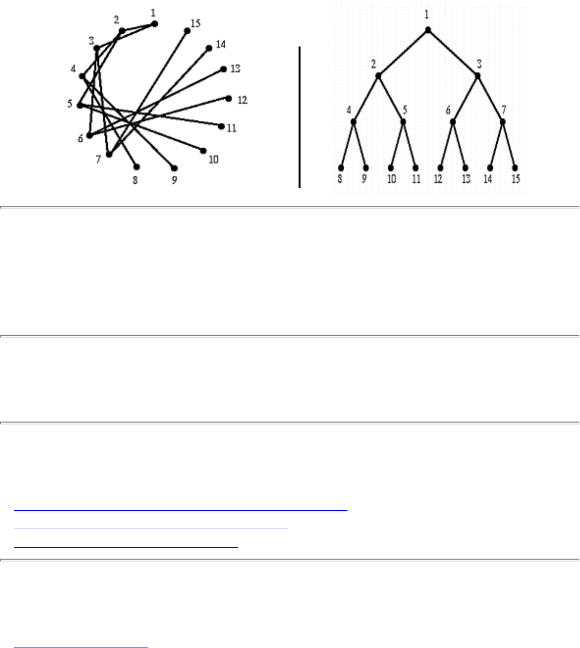
1.4.11 Drawing Trees
1.4.11 Drawing Trees
INPUT OUTPUT
Input Description: A tree (ie. graph without any cycles) T .
Problem: A nice drawing of the tree T .
Implementations
● GraphEd -- Graph Editor and Layout Program (C) (rating 9)
● GraphViz -- graph layout programs (C) (rating 7)
● Combinatorica (Mathematica) (rating 6)
Related Problems
● Drawing Graphs Nicely
file:///E|/WEBSITE/FILES/DRATREES.HTM (1 of 2) [19/1/2003 1:37:23]

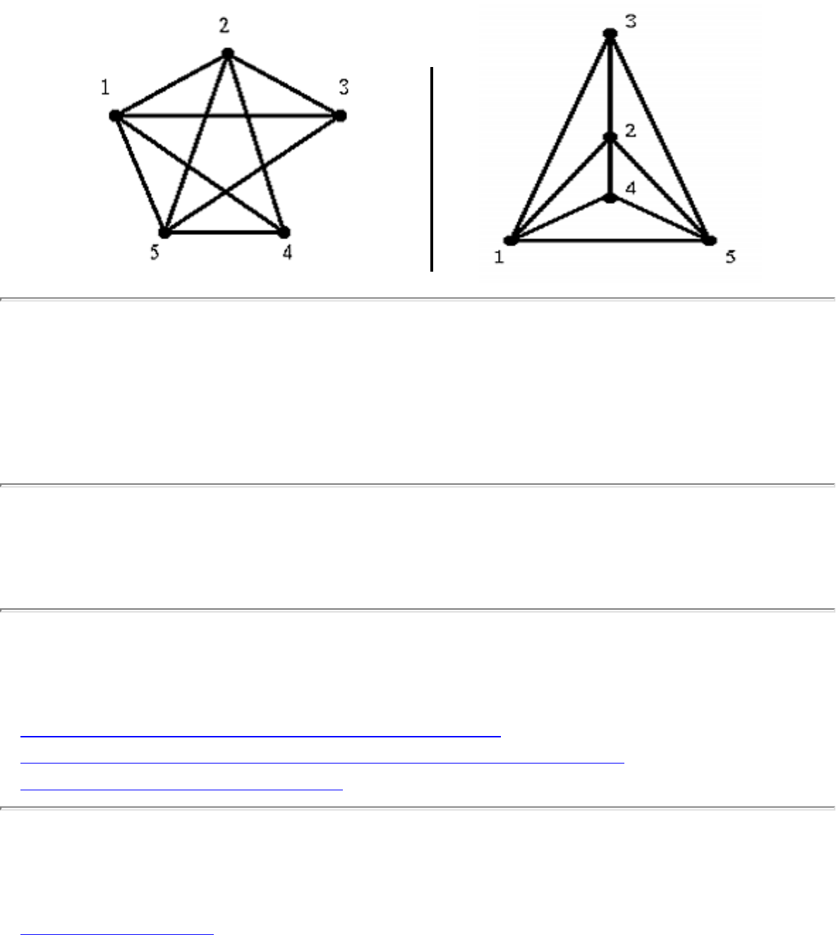
1.4.12 Planarity Detection and Embedding
1.4.12 Planarity Detection and Embedding
INPUT OUTPUT
Input Description: A graph G .
Problem: Can G be drawn in the plane such that no two edges cross? If so, produce such a drawing.
Implementations
● GraphEd -- Graph Editor and Layout Program (C) (rating 8)
● LEDA - A Library of Efficient Data Types and Algorithms (C++) (rating 7)
● Combinatorica (Mathematica) (rating 2)
Related Problems
● Drawing Graphs Nicely
file:///E|/WEBSITE/FILES/PLANWING.HTM (1 of 2) [19/1/2003 1:37:24]

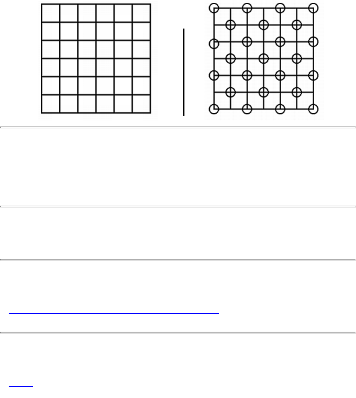
1.5.2 Independent Set
1.5.2 Independent Set
INPUT OUTPUT
Input Description: A graph G=(V,E) .
Problem: What is the largest subset of vertices of V such that no pair of vertices defines an edge of E ?
Implementations
● DIMACS Implementation Challenges (FORTRAN) (rating 7)
● Neural-Networks for Cliques and Coloring (C) (rating 5)
Related Problems
● Clique
● Set Packing
file:///E|/WEBSITE/FILES/INDE_SET.HTM (1 of 2) [19/1/2003 1:37:25]

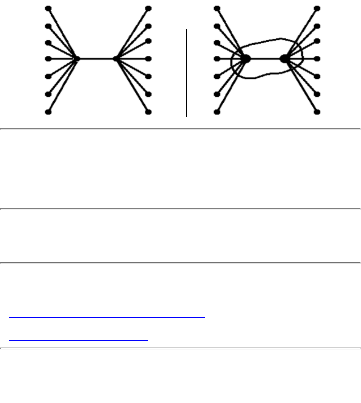
1.5.3 Vertex Cover
1.5.3 Vertex Cover
INPUT OUTPUT
Input Description: A graph G=(V,E) .
Problem: What is the smallest subset S \subset V such that each e \in E contains at least one vertex of S ?
Implementations
● Neural-Networks for Cliques and Coloring (C) (rating 6)
● DIMACS Implementation Challenges (FORTRAN) (rating 5)
● Combinatorica (Mathematica) (rating 4)
Related Problems
● Clique
file:///E|/WEBSITE/FILES/VERCOVER.HTM (1 of 2) [19/1/2003 1:37:25]

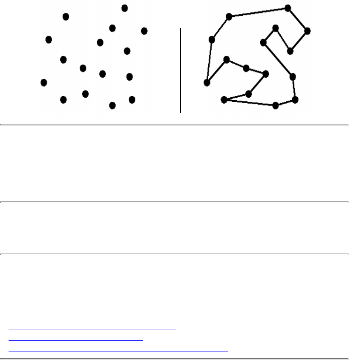
1.5.4 Traveling Salesman Problem
1.5.4 Traveling Salesman Problem
INPUT OUTPUT
Input Description: A weighted graph G .
Problem: Find the cycle of minimum cost visiting all of the vertices of G exactly once.
Implementations
● TSP solvers (C) (rating 8)
● Netlib / TOMS -- Collected Algorithms of the ACM (FORTRAN) (rating 6)
● Discrete Optimization Methods (Pascal) (rating 5)
● Combinatorica (Mathematica) (rating 3)
● Xtango and Polka Algorithm Animation Systems (C++) (rating 3)
Related Problems
file:///E|/WEBSITE/FILES/TRAESMAN.HTM (1 of 2) [19/1/2003 1:37:26]

1.5.4 Traveling Salesman Problem
● Convex Hull
● Hamiltonian Cycle
● Minimum Spanning Tree
● Satisfiability
Go to the corresponding chapter in the book
About the Book
Send us Mail
Go to Main Page
This page last modified on Tue Jun 03, 1997 .
file:///E|/WEBSITE/FILES/TRAESMAN.HTM (2 of 2) [19/1/2003 1:37:26]
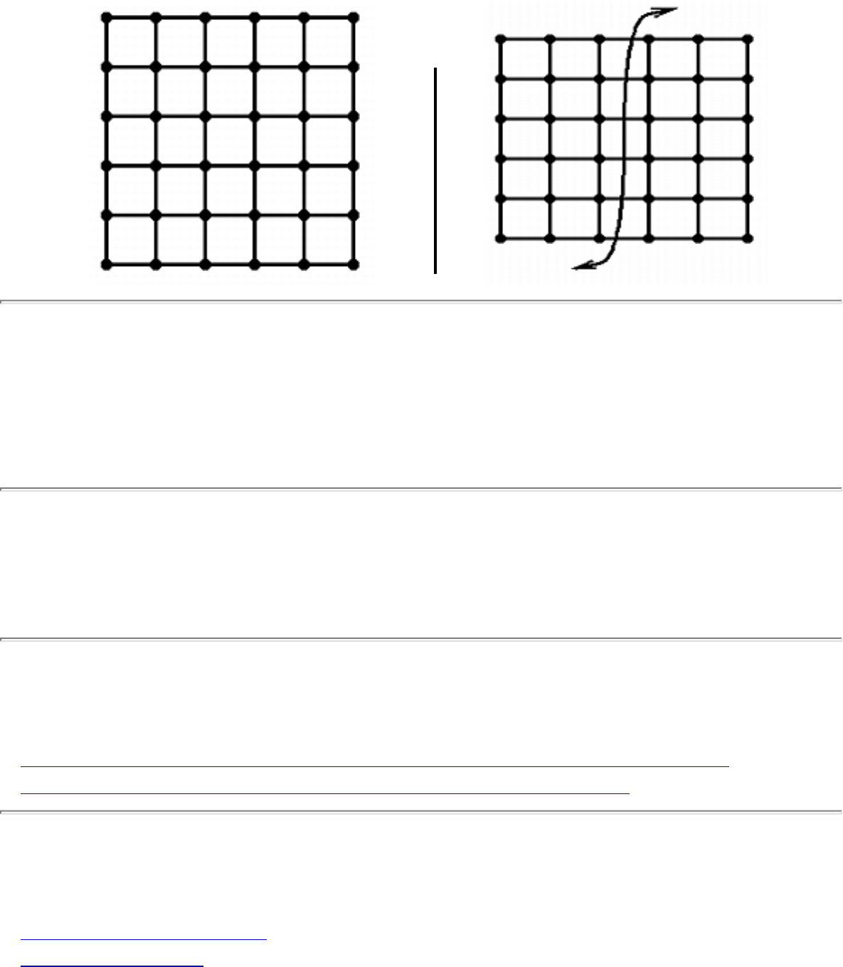
1.5.6 Graph Partition
1.5.6 Graph Partition
INPUT OUTPUT
Input Description: A (weighted) graph G=(V,E) . Integers j , k , and m .
Problem: Partition the vertices into m subsets such that each subset has size at most j , while the cost of
the edges spanning subsets is bounded by k .
Implementations
● LINK -- Programming and Visualization Environment for Hypergraphs (C++) (rating 8)
● LEDA - A Library of Efficient Data Types and Algorithms (C++) (rating 4)
Related Problems
● Edge and Vertex Connectivity
● Graph Data Structures
file:///E|/WEBSITE/FILES/GRAPTION.HTM (1 of 2) [19/1/2003 1:37:26]

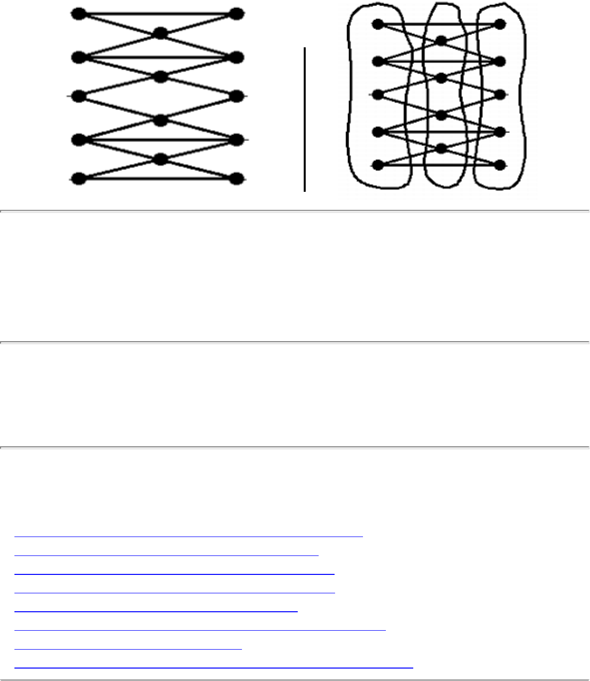
1.5.7 Vertex Coloring
1.5.7 Vertex Coloring
INPUT OUTPUT
Input Description: A graph G=(V,E) .
Problem: Color the vertices of V with the minimum number of colors such that for each edge (i,j) \in E ,
vertices i and j have different colors.
Implementations
● DIMACS Implementation Challenges (FORTRAN) (rating 7)
● Mike Trick's Graph Coloring Resources (C) (rating 7)
● Neural-Networks for Cliques and Coloring (C) (rating 6)
● Joe Culberson's Graph Coloring Resources (C) (rating 6)
● Discrete Optimization Methods (Pascal) (rating 4)
● Xtango and Polka Algorithm Animation Systems (C++) (rating 4)
● Combinatorica (Mathematica) (rating 3)
● Nijenhuis and Wilf: Combinatorial Algorithms (FORTRAN) (rating 3)
file:///E|/WEBSITE/FILES/VERTRING.HTM (1 of 2) [19/1/2003 1:37:27]

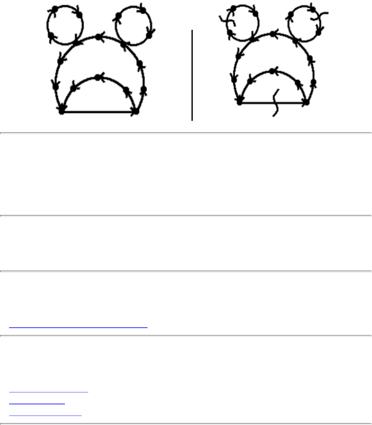
1.5.11 Feedback Edge/Vertex Set
1.5.11 Feedback Edge/Vertex Set
INPUT OUTPUT
Input Description: A (directed) graph G=(V,E) .
Problem: What is the smallest set of edges E' or vertices V' whose deletion leaves an acyclic graph?
Implementations
● The Stanford GraphBase (C) (rating 4)
Related Problems
● Bandwidth Reduction
● Job Scheduling
● Topological Sorting
file:///E|/WEBSITE/FILES2/FEED_SET.HTM (1 of 2) [19/1/2003 1:37:27]

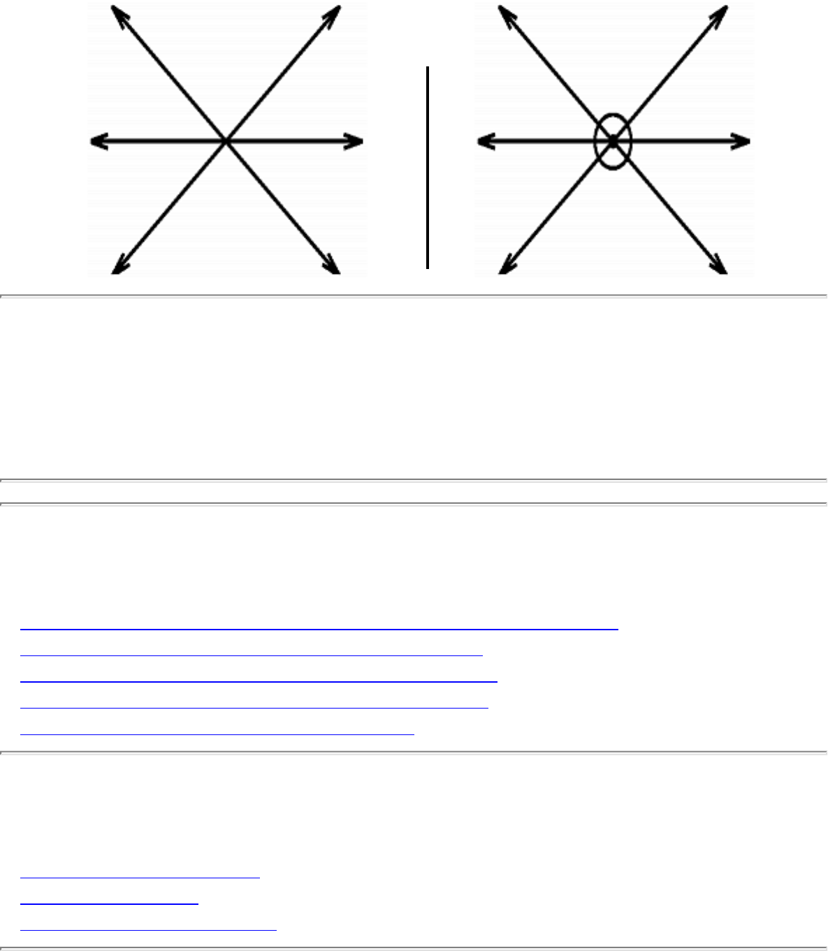
1.6.1 Robust Geometric Primitives
1.6.1 Robust Geometric Primitives
INPUT OUTPUT
Implementations
● LEDA - A Library of Efficient Data Types and Algorithms (C++) (rating 8)
● Joseph O'Rourke's Computational Geometry (C) (rating 6)
● Geolab -- Computational Geometry System (C++) (rating 5)
● Moret and Shapiro's Algorithms P to NP (Pascal) (rating 4)
● Algorithms in C++ -- Sedgewick (C++) (rating 4)
Related Problems
● Determinants and Permanents
● Intersection Detection
● Maintaining Line Arrangements
file:///E|/WEBSITE/FILES2/GEOMIVES.HTM (1 of 2) [19/1/2003 1:37:29]

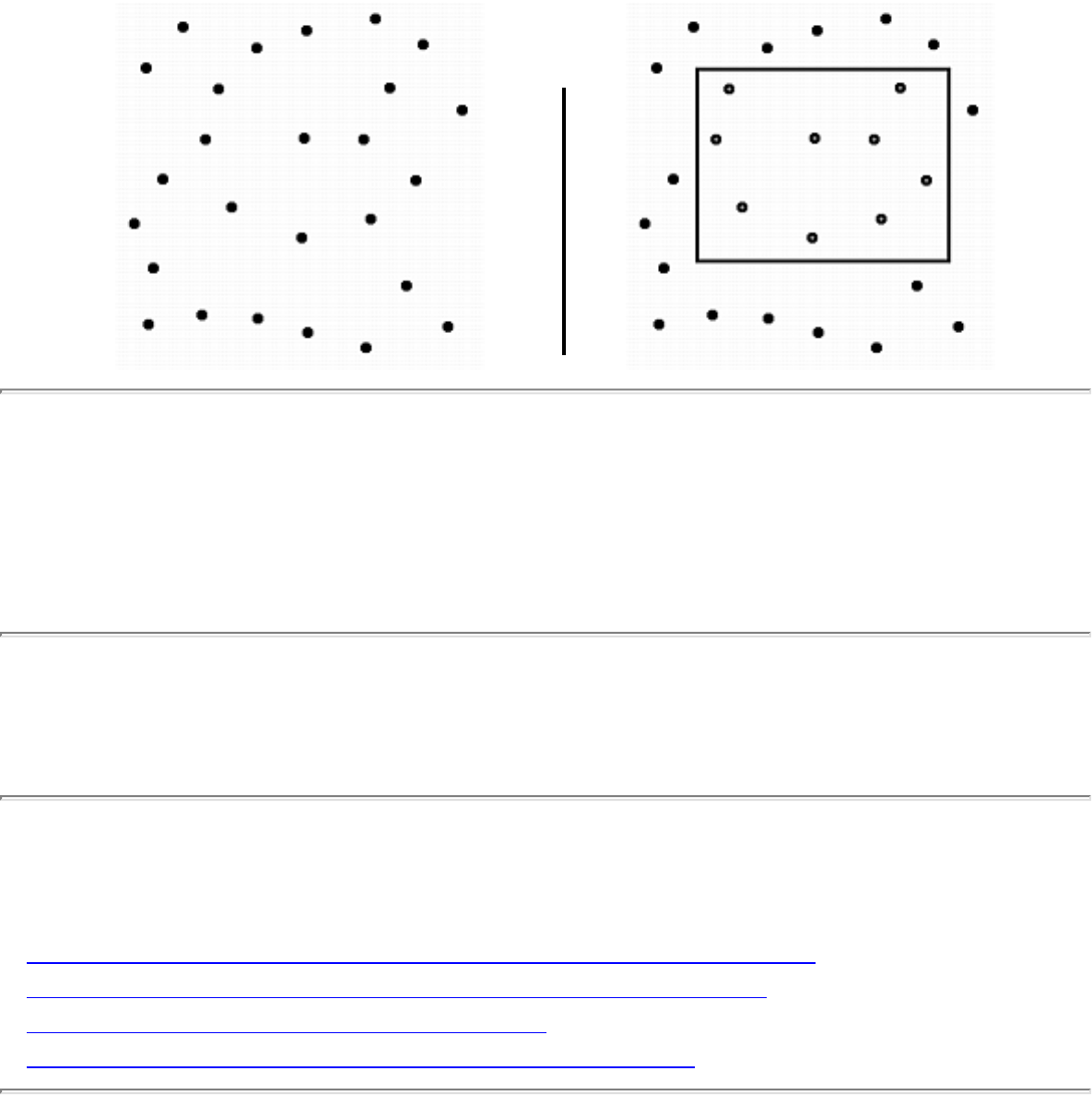
1.6.6 Range Search
1.6.6 Range Search
INPUT OUTPUT
Input Description: A set S of n points in E^d , and a query polygon Q .
Problem: Which points from S lie within Q ?
Implementations
● LEDA - A Library of Efficient Data Types and Algorithms (C++) (rating 7)
● Ranger - Nearest Neighbor Search in Higher Dimensions (C) (rating 6)
● Algorithms in C++ -- Sedgewick (C++) (rating 4)
● Handbook of Algorithms and Data Structures (Pascal) (rating 2)
Related Problems
file:///E|/WEBSITE/FILES2/RANGARCH.HTM (1 of 2) [19/1/2003 1:37:30]

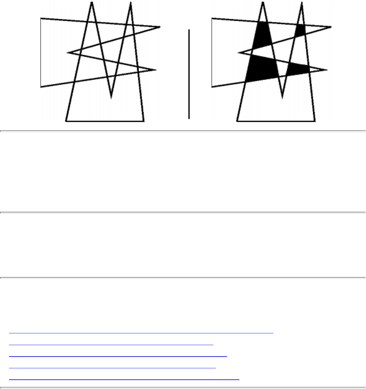
1.6.8 Intersection Detection
1.6.8 Intersection Detection
INPUT OUTPUT
Input Description: A set S of lines and line segments l_1,...,l_n , or a pair of polygons or polyhedra P_1
and P_2 .
Problem: Which pairs of line segments intersect each other? What is the intersection of P_1 and P_2 ?
Implementations
● LEDA - A Library of Efficient Data Types and Algorithms (C++) (rating 7)
● Joseph O'Rourke's Computational Geometry (C) (rating 5)
● Qhull - higher dimensional convex hull program (C) (rating 5)
● Moret and Shapiro's Algorithms P to NP (Pascal) (rating 3)
● Xtango and Polka Algorithm Animation Systems (C++) (rating 1)
Related Problems
file:///E|/WEBSITE/FILES2/INTETION.HTM (1 of 2) [19/1/2003 1:37:30]

1.6.8 Intersection Detection
● Robust Geometric Primitives
● Maintaining Line Arrangements
● Motion Planning
Go to the corresponding chapter in the book
About the Book
Send us Mail
Go to Main Page
This page last modified on Tue Jun 03, 1997 .
file:///E|/WEBSITE/FILES2/INTETION.HTM (2 of 2) [19/1/2003 1:37:30]
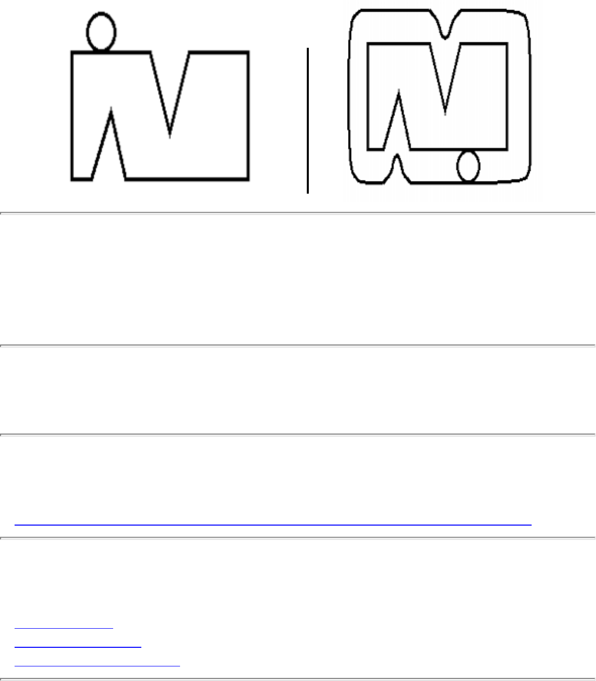
1.6.16 Minkowski Sum
1.6.16 Minkowski Sum
INPUT OUTPUT
Input Description: Point sets or polygons A and B , with n and m vertices, respectively.
Problem: What is the convolution of A and B , ie. the Minkowski sum A+B = \{x+y| x\in A, y \in B\} ?
Implementations
● David Eppstein's Knuth-Morris-Pratt Algorithm and Minkowski sum code (C++) (rating 4)
Related Problems
● Motion Planning
● Simplifying Polygons
● Medial-Axis Transformation
file:///E|/WEBSITE/FILES2/MINK_SUM.HTM (1 of 2) [19/1/2003 1:37:31]

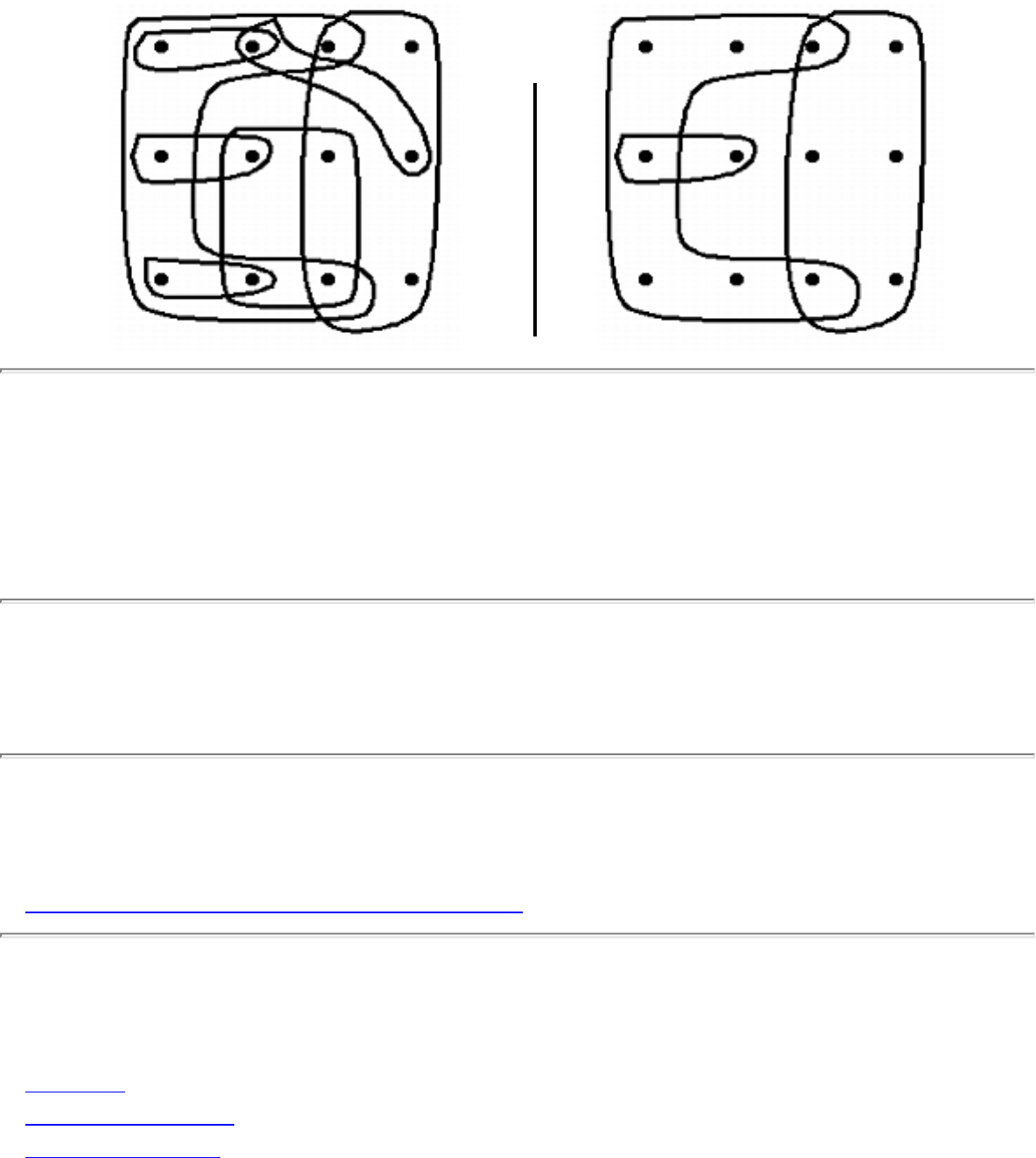
1.7.1 Set Cover
1.7.1 Set Cover
INPUT OUTPUT
Input Description: A set of subsets S_1, ..., S_m of the universal set U = \{1,...,n\} .
Problem: What is the smallest subset of subsets T \subset S such that \cup_{t_i \in T} t_i = U ?
Implementations
● Discrete Optimization Methods (Pascal) (rating 5)
Related Problems
● Matching
● Polygon Partitioning
● Set Data Structures
file:///E|/WEBSITE/FILES2/SET_OVER.HTM (1 of 2) [19/1/2003 1:37:32]

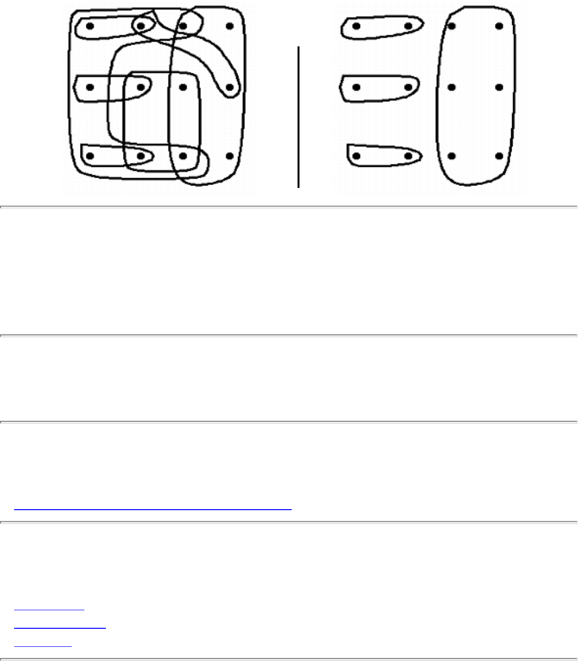
1.7.2 Set Packing
1.7.2 Set Packing
INPUT OUTPUT
Input Description: A set of subsets S = S_1, ..., S_m of the universal set U = \{1,...,n\} .
Problem: What is the largest number of mutually disjoint subsets from S ?
Implementations
● Discrete Optimization Methods (Pascal) (rating 5)
Related Problems
● Bin Packing
● Independent Set
● Set Cover
file:///E|/WEBSITE/FILES2/SET_KING.HTM (1 of 2) [19/1/2003 1:37:32]

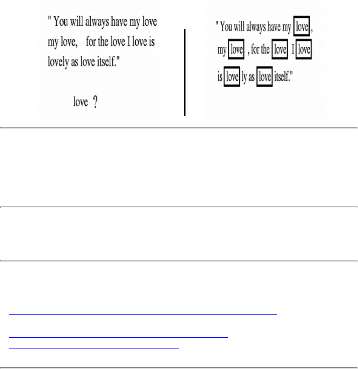
1.7.3 String Matching
1.7.3 String Matching
INPUT OUTPUT
Input Description: A text string t of length n . A patterns string p of length m .
Problem: Find the first (or all) instances of the pattern in the text.
Implementations
● Fire-Engine and Spare-Parts String and Language Algorithms (C++) (rating 7)
● David Eppstein's Knuth-Morris-Pratt Algorithm and Minkowski sum code (C++) (rating 4)
● Handbook of Algorithms and Data Structures (Pascal) (rating 4)
● Algorithms in C++ -- Sedgewick (C++) (rating 4)
● Xtango and Polka Algorithm Animation Systems (C++) (rating 3)
Related Problems
file:///E|/WEBSITE/FILES2/STRIHING.HTM (1 of 2) [19/1/2003 1:37:33]

1.7.3 String Matching
● Approximate String Matching
● Finite State Machine Minimization
● Graph Isomorphism
● Suffix Trees and Arrays
Go to the corresponding chapter in the book
About the Book
Send us Mail
Go to Main Page
This page last modified on Tue Jun 03, 1997 .
file:///E|/WEBSITE/FILES2/STRIHING.HTM (2 of 2) [19/1/2003 1:37:33]
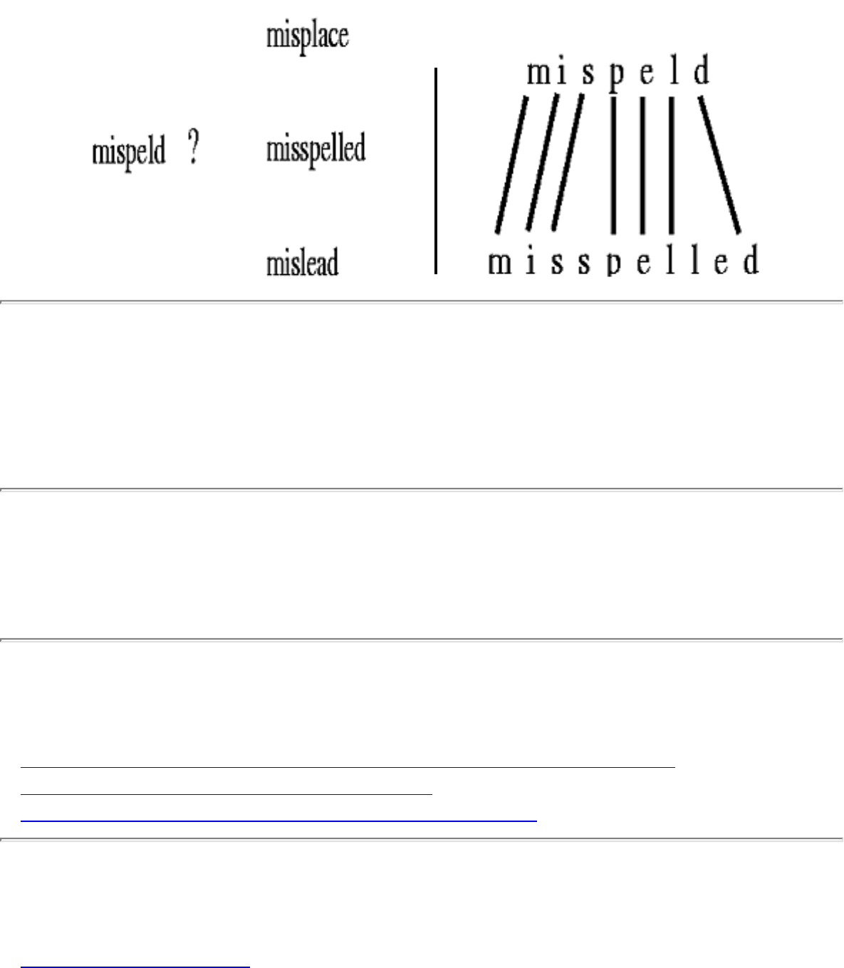
1.7.4 Approximate String Matching
1.7.4 Approximate String Matching
INPUT OUTPUT
Input Description: A text string t and a pattern string p . An edit cost bound k .
Problem: Does there exist an alignment between t and p with edit cost at most k , ie. can we transform
part of t to p using at most k additions, deletions, and substitutions.
Implementations
● agrep - Approximate General Regular Expression Pattern Matcher (C) (rating 10)
● HT/DIG -- image compression codes (C) (rating 7)
● Handbook of Algorithms and Data Structures (Pascal) (rating 2)
Related Problems
● Longest Common Substring
file:///E|/WEBSITE/FILES2/APPRHING.HTM (1 of 2) [19/1/2003 1:37:33]

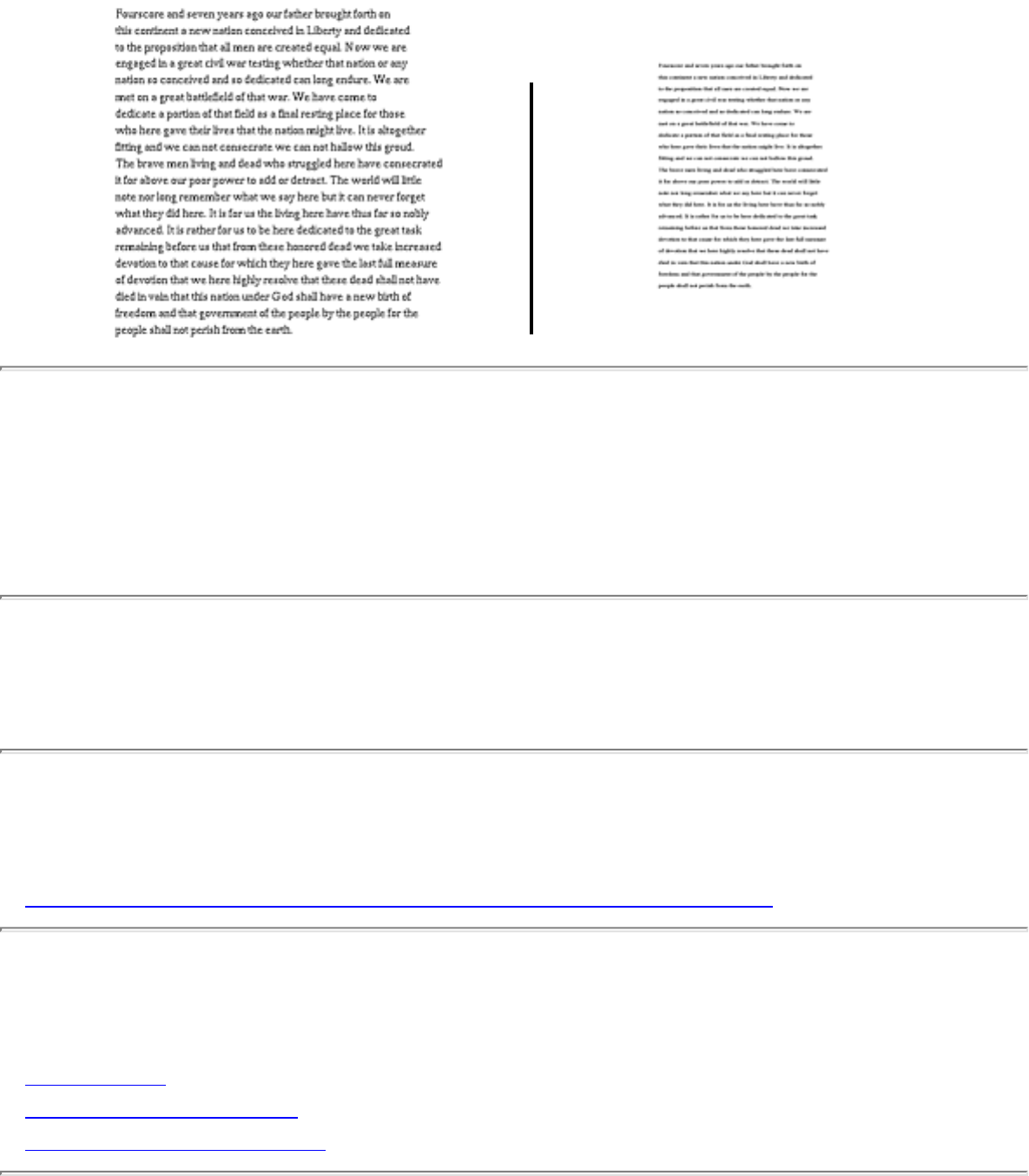
1.7.5 Text Compression
1.7.5 Text Compression
INPUT OUTPUT
Input Description: A text string S .
Problem: A shortest text string S' such that S can be reconstructed from S' .
Implementations
● Netlib / TOMS -- Collected Algorithms of the ACM (FORTRAN) (rating 5)
Related Problems
● Cryptography
● Discrete Fourier Transform
● Shortest Common Superstring
file:///E|/WEBSITE/FILES2/TEXSSION.HTM (1 of 2) [19/1/2003 1:37:34]

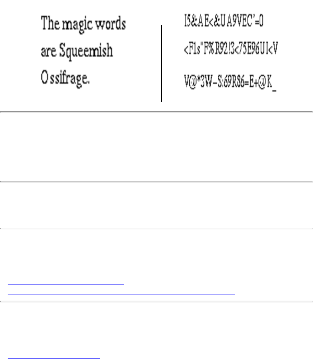
1.7.6 Cryptography
1.7.6 Cryptography
INPUT OUTPUT
Input Description: A plaintext message T or encrypted text E , and a key k .
Problem: Encode T using k giving E , or decode E using k back to T .
Implementations
● () (rating 10)
● The Stanford GraphBase (C) (rating 3)
● Netlib / TOMS -- Collected Algorithms of the ACM (FORTRAN) (rating 3)
Related Problems
● Factoring and Primality Testing
● Arbitrary Precision Arithmetic
file:///E|/WEBSITE/FILES2/CRYPAPHY.HTM (1 of 2) [19/1/2003 1:37:34]

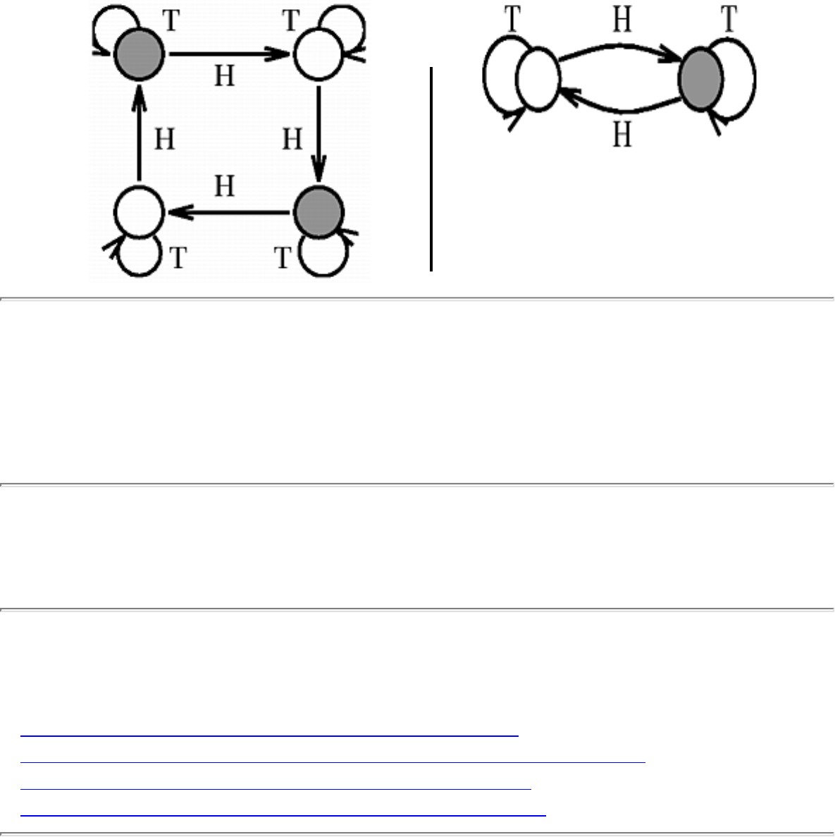
1.7.7 Finite State Machine Minimization
1.7.7 Finite State Machine Minimization
INPUT OUTPUT
Input Description: A deterministic finite automata M .
Problem: The smallest deterministic finite automata M' such that M' behaves identically to M'
Implementations
● Grail: finite automata and regular expressions (C++) (rating 9)
● Fire-Engine and Spare-Parts String and Language Algorithms (C++) (rating 8)
● Handbook of Algorithms and Data Structures (Pascal) (rating 5)
● Xtango and Polka Algorithm Animation Systems (C++) (rating 1)
Related Problems
file:///E|/WEBSITE/FILES2/FINITION.HTM (1 of 2) [19/1/2003 1:37:35]

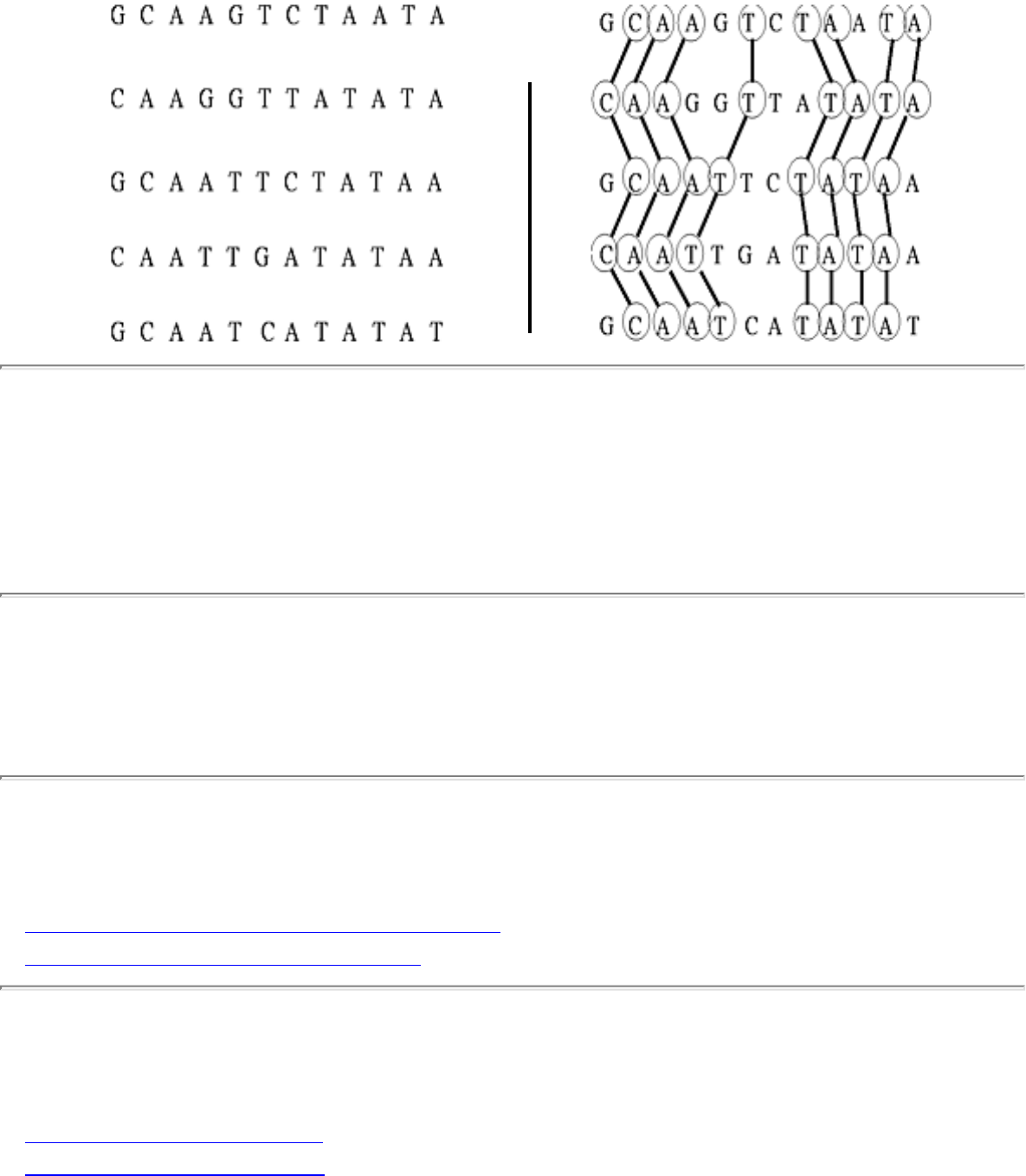
1.7.8 Longest Common Substring
1.7.8 Longest Common Substring
INPUT OUTPUT
Input Description: A set S of strings S_1,...,S_n .
Problem: What is the longest string c such that for each S_i , 1 \leq i \leq n , the characters of c appear as
a scattered subsequence of S_i ?
Implementations
● CAP -- Contig Assembly Program (C) (rating 8)
● Combinatorica (Mathematica) (rating 2)
Related Problems
● Approximate String Matching
● Shortest Common Superstring
file:///E|/WEBSITE/FILES2/LONGRING.HTM (1 of 2) [19/1/2003 1:37:35]

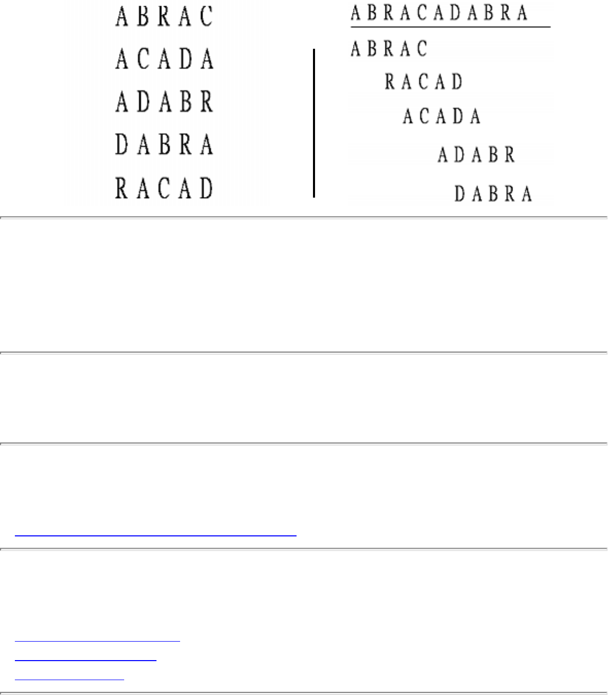
1.7.9 Shortest Common Superstring
1.7.9 Shortest Common Superstring
INPUT OUTPUT
Input Description: A set of strings s_1, ..., s_m .
Problem: Find the shortest string S which contains each s_i as a substring of S .
Implementations
● CAP -- Contig Assembly Program (C) (rating 8)
Related Problems
● Longest Common Substring
● Suffix Trees and Arrays
● Text Compression
file:///E|/WEBSITE/FILES2/SHORRING.HTM (1 of 2) [19/1/2003 1:37:36]


Handbook of Algorithms and Data Structures
Handbook of Algorithms and Data Structures
The Handbook of Data Structures and Algorithms , by Gonnet and Baeza-Yates, provides a
comprehensive reference on fundamental data structures for searching and priority queues, and
algorithms for sorting and text searching. The book covers these relatively small number of topics
comprehensively, presenting most of the major and minor variations which appear in the literature.
Perusing the book makes one aware of the tremendous range of data structures which have been
developed, and the intense level of analysis many of them have been subjected to.
For each data structure or algorithm, a brief description is provided along with its asymptotic complexity
and an extensive set of references. More distinctively, an implementation in C and/or Pascal is usually
provided, along with experimental results comparing the performance of these implementations on a
variety of distributions.
The authors have created a very slick WWW site for the book,
http://www.dcc.uchile.cl/~rbaeza/handbook/hbook.html , containing all the source code as well as the
index and table of contents. This entire site has been replicated in the local distribution site , although this
copy still contains ftp links to Chile for the algorithm implementations. However, all of these files are
also available locally . These files are all copyrighted © Addison-Wesley Publishing Co. Inc. Since many
of the elementary data structures and sorting algorithms can be implemented concisely, most of the
programs are very short. They are perhaps most useful as models, or as part of an experimental study to
compare the performance on different data structures for a particular application.
● Link to Handbook of Algorithms and Data Structures
● Local copies of all the algorithm implementations
● Local copy of original site, but with FTP calls to Chile for certain algorithm implementations
Problem Links
● Dictionaries (8)
● Priority Queues (7)
● Searching (7)
● Sorting (7)
● Arbitrary Precision Arithmetic (6)
● Median and Selection (6)
● Finite State Machine Minimization (5)
● String Matching (4)
file:///E|/WEBSITE/IMPLEMEN/HANDBOOK/IMPLEMEN.HTM (1 of 2) [19/1/2003 1:37:37]

Handbook of Algorithms and Data Structures
● Kd-Trees (3)
● Approximate String Matching (2)
● Range Search (2)
● Suffix Trees and Arrays (2)
About the Book
Send us Mail
Go to Main Page
This page last modified on May 21, 1997.
file:///E|/WEBSITE/IMPLEMEN/HANDBOOK/IMPLEMEN.HTM (2 of 2) [19/1/2003 1:37:37]

Moret and Shapiro's Algorithms P to NP
Moret and Shapiro's Algorithms P to NP
This algorithms text distinguishes itself by including Pascal implementations of many algorithms, with
careful experimental comparisons of different algorithms for such problems as sorting and minimum
spanning tree, and heuristics for the traveling salesman problem. It provides a useful model for how to
properly do empirical algorithm analysis.
The programs themselves are probably best used as models. Interesting implementations include the
eight-queens problem, fundamental graph and geometric algorithms.
The programs in the book have been made available by anonymous ftp from cs.unm.edu in directory
/pub/moret_shapiro.
● Link to Moret's Home Page - files under publications
● Download Files (local site)
Problem Links
● Sorting (7)
● Minimum Spanning Tree (5)
● Connected Components (4)
● Edge and Vertex Connectivity (4)
● Discrete Fourier Transform (4)
● Robust Geometric Primitives (4)
● Graph Data Structures (4)
● Matching (4)
● Network Flow (4)
● Set Data Structures (4)
● Convex Hull (3)
● Intersection Detection (3)
● Nearest Neighbor Search (3)
● Point Location (3)
● Priority Queues (3)
● Searching (3)
● Topological Sorting (3)
file:///E|/WEBSITE/IMPLEMEN/MORET/IMPLEMEN.HTM (1 of 2) [19/1/2003 1:37:38]


Index A
Up: Index - All
Index: A
abstract data types
adjacency list
adjacency matrix
algorithm, what is a
all-pairs shortest path
approximate string matching
approximation algorithms
articulation vertex
asymptotic notation
average-case analysis
average-case complexity
Algorithms
Mon Jun 2 14:49:38 EDT 1997
file:///E|/LEC/LECTUR16/INDEX_A.HTM [19/1/2003 1:37:38]

Index B
Up: Index - All
Index: B
back edge
backsubstitution ,
backtracking
backtracking - recursive
backtracking contest ,
balanced search tree
bandersnatch problem
bandwidth - optimizations
bandwidth problem
bar codes - high density
base of logarithm
best-case complexity ,
big Oh notation ,
binary heap ,
binary search ,
binary search tree
bin packing
bipartite graphs
birthday paradox
bitonic tours
bo-billy problem
boundary condition ,
boundary conditions - string matching
breadth-first search ,
breadth-first search - shortest paths
breadth-first search - tree
Brooks, Mel
bubblesort - parallel
bucketsort
file:///E|/LEC/LECTUR16/INDEX_B.HTM (1 of 2) [19/1/2003 1:37:39]

Index B
Algorithms
Mon Jun 2 14:49:38 EDT 1997
file:///E|/LEC/LECTUR16/INDEX_B.HTM (2 of 2) [19/1/2003 1:37:39]

Index C
Up: Index - All
Index: C
chaining
checkers
chessboard covering
chromatic number
circuit board assembly
clique
clique - hardness
closest pair heuristic
closest pair problem
clustering
coloring graphs
combinatorial search
communications problems
comparison-based sorting
component design
computer graphics
connected components
connected graph
connectivity
convex hull ,
Cook's theorem
correctness
crime
cross edge
cycle ,
Algorithms
Mon Jun 2 14:49:38 EDT 1997
file:///E|/LEC/LECTUR16/INDEX_C.HTM [19/1/2003 1:37:40]
Index D
Up: Index - All
Index: D
DAG
data structures
decision problems ,
decision tree ,
degree
delete - binary search tree
delete - red-black tree
depth-first search ,
depth-first search - edge organization
deque
diameter
dictionary data structure ,
Dijkstra's algorithm ,
directed acyclic graph
directed graph
discrete event simulation
disjunctive normal form
divide-and-conquer ,
dominance relation
duplicate elimination
dynamic programming ,
dynamic programming - components
dynamic programming - space
dynamic programming - when applicable
Algorithms
Mon Jun 2 14:49:38 EDT 1997
file:///E|/LEC/LECTUR16/INDEX_D.HTM [19/1/2003 1:37:41]


Index F
Up: Index - All
Index: F
Federal sentencing guidelines
Fibonacci numbers
flat earth model
Floyd-Warshall algorithm
formal language theory
forward edge
Fourier transform
fragment assembly
frequency distribution
friendship graph
Algorithms
Mon Jun 2 14:49:38 EDT 1997
file:///E|/LEC/LECTUR16/INDEX_F.HTM [19/1/2003 1:37:43]


Index H
Up: Index - All
Index: H
Hamiltonian cycle
Hamiltonian cycle - hardness
Hamiltonian path ,
harmonic numbers
hash function
hash table
heap data structure
heapify
heapsort ,
Heep, Danny
heuristic
Huffman codes
Algorithms
Mon Jun 2 14:49:39 EDT 1997
file:///E|/LEC/LECTUR16/INDEX_H.HTM [19/1/2003 1:37:44]

Index I
Up: Index - All
Index: I
incremental algorithms
independent set
induction ,
inorder traversal
insert - binary search tree
insert - red-black tree
insertion sort ,
instance
integer partition
integer programming - hardness ,
inverse exponential function
Algorithms
Mon Jun 2 14:49:39 EDT 1997
file:///E|/LEC/LECTUR16/INDEX_I.HTM [19/1/2003 1:37:44]


Index M
Up: Index - All
Index: M
mainframe computers
Maple
master theorem , ,
Mathematica
mathematical induction
matrix multiplication ,
matrix multiplication - applications
maze
median
mergesort
minimum spanning tree ,
mode
monotonic sequence
morphing
motion planning
movie stars
multigraph
Algorithms
Mon Jun 2 14:49:39 EDT 1997
file:///E|/LEC/LECTUR16/INDEX_M.HTM [19/1/2003 1:37:46]


Index P
Up: Index - All
Index: P
parenthesization
partial order
partitioning step
path
path compression
permutations - generation
pivot
pointers
polygon triangulation
polynomial time
predecessor
Prim's algorithm
principle of optimality
priority queue ,
problem ,
problem solving techniques ,
pseudocode
P vs. NP ,
Algorithms
Mon Jun 2 14:49:39 EDT 1997
file:///E|/LEC/LECTUR16/INDEX_P.HTM [19/1/2003 1:37:48]

Index R
Up: Index - All
Index: R
RAM model of computation
random-access machine
randomized algorithm ,
recurrence relations
recursion tree , ,
red-black tree
red-black trees
reduction ,
reduction - direction of
refrain
refrigerator
restriction
robot arm
Rolling Stones
rotation
rules for algorithm design
Algorithms
Mon Jun 2 14:49:39 EDT 1997
file:///E|/LEC/LECTUR16/INDEX_R.HTM [19/1/2003 1:37:49]

Index S
Up: Index - All
Index: S
satisfiability
satisfiability - Cook's theorem
selection
selection sort ,
sentence disambiguation
sentinel
series convergence
set data structures ,
Shifflett
shortest path ,
simple graph
simulations
social security number
solving recurrences
songs, complexity of
sorting
sorting - applications
sorting - lower bound ,
space complexity
spanning tree
sparse graphs
spouse, finding the optimal
square of graph
stack , ,
Strassen's algorithm
string matching
strongly connected components ,
subgraph isomorphism
subset generation
subset sum
file:///E|/LEC/LECTUR16/INDEX_S.HTM (1 of 2) [19/1/2003 1:37:50]

Index T
Up: Index - All
Index: T
telephone book
telephone keypad
telephone network ,
terrorist
text compression
topological sorting ,
transportation problems
traveling salesman problem , , , ,
traveling salesman problem - approximation ,
triangulation
triangulation - minimum length
Turing machine
Algorithms
Mon Jun 2 14:49:39 EDT 1997
file:///E|/LEC/LECTUR16/INDEX_T.HTM [19/1/2003 1:37:51]


Index (complete)
Up: Index - All
Index: (complete)
3-satisfiability,
abstract data types
adjacency list
adjacency matrix
algorithm, what is a
all-pairs shortest path
approximate string matching
approximation algorithms
articulation vertex
asymptotic notation
average-case analysis
average-case complexity
back edge
backsubstitution,
backtracking
backtracking - recursive
backtracking contest,
balanced search tree
bandersnatch problem
bandwidth - optimizations
bandwidth problem
bar codes - high density
base of logarithm
best-case complexity,
big Oh notation,
binary heap,
binary search,
binary search tree
file:///E|/LEC/LECTUR16/INDEX_AL.HTM (1 of 8) [19/1/2003 1:37:56]

Index (complete)
bin packing
bipartite graphs
birthday paradox
bitonic tours
bo-billy problem
boundary condition,
boundary conditions - string matching
breadth-first search,
breadth-first search - shortest paths
breadth-first search - tree
Brooks, Mel
bubblesort - parallel
bucketsort
chaining
checkers
chessboard covering
chromatic number
circuit board assembly
clique
clique - hardness
closest pair heuristic
closest pair problem
clustering
coloring graphs
combinatorial search
communications problems
comparison-based sorting
component design
computer graphics
connected components
connected graph
connectivity
convex hull,
Cook's theorem
correctness
crime
cross edge
file:///E|/LEC/LECTUR16/INDEX_AL.HTM (2 of 8) [19/1/2003 1:37:56]

Index (complete)
cycle,
DAG
data structures
decision problems,
decision tree,
degree
delete - binary search tree
delete - red-black tree
depth-first search,
depth-first search - edge organization
deque
diameter
dictionary data structure,
Dijkstra's algorithm,
directed acyclic graph
directed graph
discrete event simulation
disjunctive normal form
divide-and-conquer,
dominance relation
duplicate elimination
dynamic programming,
dynamic programming - components
dynamic programming - space
dynamic programming - when applicable
edges
edit distance
element uniqueness
exhaustive search algorithm
exponential time
Federal sentencing guidelines
Fibonacci numbers
flat earth model
Floyd-Warshall algorithm
formal language theory
forward edge
file:///E|/LEC/LECTUR16/INDEX_AL.HTM (3 of 8) [19/1/2003 1:37:56]

Index (complete)
Fourier transform
fragment assembly
frequency distribution
friendship graph
gadget
Garey and Johnson
geometric algorithms,
geometric series
girth
gossip
graphs
graph traversal
greedy heuristic,
guessing module
Hamiltonian cycle
Hamiltonian cycle - hardness
Hamiltonian path,
harmonic numbers
hash function
hash table
heap data structure
heapify
heapsort,
Heep, Danny
heuristic
Huffman codes
incremental algorithms
independent set
induction,
inorder traversal
insert - binary search tree
insert - red-black tree
insertion sort,
instance
integer partition
integer programming - hardness,
file:///E|/LEC/LECTUR16/INDEX_AL.HTM (4 of 8) [19/1/2003 1:37:56]

Index (complete)
inverse exponential function
Kruskal's algorithm,
linked list
local replacement
logarithm
logic problem
longest increasing subsequence
longest path
lower bound
lower bound - sorting
mainframe computers
Maple
master theorem, ,
Mathematica
mathematical induction
matrix multiplication,
matrix multiplication - applications
maze
median
mergesort
minimum spanning tree,
mode
monotonic sequence
morphing
motion planning
movie stars
multigraph
nearest neighbor heuristic
non-comparison based sorting
non-deterministic Turning machine
NP
NP-completeness
NP-completeness - dealing with it
open addressing
optimization problem
optimizing programs for speed
order-statistic tree
file:///E|/LEC/LECTUR16/INDEX_AL.HTM (5 of 8) [19/1/2003 1:37:56]

Index (complete)
parenthesization
partial order
partitioning step
path
path compression
permutations - generation
pivot
pointers
polygon triangulation
polynomial time
predecessor
Prim's algorithm
principle of optimality
priority queue,
problem,
problem solving techniques,
pseudocode
P vs. NP,
queens problem
queue, ,
quicksort,
quicksort - analysis
RAM model of computation
random-access machine
randomized algorithm,
recurrence relations
recursion tree, ,
red-black tree
red-black trees
reduction,
reduction - direction of
refrain
refrigerator
restriction
robot arm
file:///E|/LEC/LECTUR16/INDEX_AL.HTM (6 of 8) [19/1/2003 1:37:56]

Index (complete)
Rolling Stones
rotation
rules for algorithm design
satisfiability
satisfiability - Cook's theorem
selection
selection sort,
sentence disambiguation
sentinel
series convergence
set data structures,
Shifflett
shortest path,
simple graph
simulations
social security number
solving recurrences
songs, complexity of
sorting
sorting - applications
sorting - lower bound,
space complexity
spanning tree
sparse graphs
spouse, finding the optimal
square of graph
stack, ,
Strassen's algorithm
string matching
strongly connected components,
subgraph isomorphism
subset generation
subset sum
successor
supercomputer,
sweepline algorithms
file:///E|/LEC/LECTUR16/INDEX_AL.HTM (7 of 8) [19/1/2003 1:37:56]
Index (complete)
symmetry, exploiting
telephone book
telephone keypad
telephone network,
terrorist
text compression
topological sorting,
transportation problems
traveling salesman problem, , , ,
traveling salesman problem - approximation,
triangulation
triangulation - minimum length
Turing machine
undirected graph
union-find data structure
upper bound
vertex cover,
vertex cover - approximation
vertex cover - hardness
vertex cover - tree
vertices
Viterbi algorithm
worst-case complexity
Algorithms
Mon Jun 2 14:49:38 EDT 1997
file:///E|/LEC/LECTUR16/INDEX_AL.HTM (8 of 8) [19/1/2003 1:37:56]
file:///E|/SOUNDS/LEC1_7.HTM
Using the controls:
- To pause or resume playing, click the arrow-shaped Play button.
- To stop the sound, click the square-shaped Stop button.
- To adjust the volume, click on the Up/Down buttons on the right side of the panel.
file:///E|/SOUNDS/LEC1_7.HTM [19/1/2003 1:38:06]
file:///E|/SOUNDS/LEC1_8.HTM
Using the controls:
- To pause or resume playing, click the arrow-shaped Play button.
- To stop the sound, click the square-shaped Stop button.
- To adjust the volume, click on the Up/Down buttons on the right side of the panel.
file:///E|/SOUNDS/LEC1_8.HTM [19/1/2003 1:38:06]
file:///E|/SOUNDS/LEC1_10.HTM
Using the controls:
- To pause or resume playing, click the arrow-shaped Play button.
- To stop the sound, click the square-shaped Stop button.
- To adjust the volume, click on the Up/Down buttons on the right side of the panel.
file:///E|/SOUNDS/LEC1_10.HTM [19/1/2003 1:38:06]
file:///E|/SOUNDS/LEC1_11.HTM
Using the controls:
- To pause or resume playing, click the arrow-shaped Play button.
- To stop the sound, click the square-shaped Stop button.
- To adjust the volume, click on the Up/Down buttons on the right side of the panel.
file:///E|/SOUNDS/LEC1_11.HTM [19/1/2003 1:38:07]
file:///E|/SOUNDS/LEC1_12.HTM
Using the controls:
- To pause or resume playing, click the arrow-shaped Play button.
- To stop the sound, click the square-shaped Stop button.
- To adjust the volume, click on the Up/Down buttons on the right side of the panel.
file:///E|/SOUNDS/LEC1_12.HTM [19/1/2003 1:38:07]
file:///E|/SOUNDS/LEC1_13.HTM
Using the controls:
- To pause or resume playing, click the arrow-shaped Play button.
- To stop the sound, click the square-shaped Stop button.
- To adjust the volume, click on the Up/Down buttons on the right side of the panel.
file:///E|/SOUNDS/LEC1_13.HTM [19/1/2003 1:38:07]
file:///E|/SOUNDS/LEC1_14.HTM
Using the controls:
- To pause or resume playing, click the arrow-shaped Play button.
- To stop the sound, click the square-shaped Stop button.
- To adjust the volume, click on the Up/Down buttons on the right side of the panel.
file:///E|/SOUNDS/LEC1_14.HTM [19/1/2003 1:38:08]
file:///E|/SOUNDS/LEC1_15.HTM
Using the controls:
- To pause or resume playing, click the arrow-shaped Play button.
- To stop the sound, click the square-shaped Stop button.
- To adjust the volume, click on the Up/Down buttons on the right side of the panel.
file:///E|/SOUNDS/LEC1_15.HTM [19/1/2003 1:38:08]
file:///E|/SOUNDS/LEC2_1.HTM
Using the controls:
- To pause or resume playing, click the arrow-shaped Play button.
- To stop the sound, click the square-shaped Stop button.
- To adjust the volume, click on the Up/Down buttons on the right side of the panel.
file:///E|/SOUNDS/LEC2_1.HTM [19/1/2003 1:38:08]
file:///E|/SOUNDS/LEC2_2.HTM
Using the controls:
- To pause or resume playing, click the arrow-shaped Play button.
- To stop the sound, click the square-shaped Stop button.
- To adjust the volume, click on the Up/Down buttons on the right side of the panel.
file:///E|/SOUNDS/LEC2_2.HTM [19/1/2003 1:38:09]
file:///E|/SOUNDS/LEC2_3.HTM
Using the controls:
- To pause or resume playing, click the arrow-shaped Play button.
- To stop the sound, click the square-shaped Stop button.
- To adjust the volume, click on the Up/Down buttons on the right side of the panel.
file:///E|/SOUNDS/LEC2_3.HTM [19/1/2003 1:38:09]
file:///E|/SOUNDS/LEC2_4.HTM
Using the controls:
- To pause or resume playing, click the arrow-shaped Play button.
- To stop the sound, click the square-shaped Stop button.
- To adjust the volume, click on the Up/Down buttons on the right side of the panel.
file:///E|/SOUNDS/LEC2_4.HTM [19/1/2003 1:38:09]
file:///E|/SOUNDS/LEC2_5.HTM
Using the controls:
- To pause or resume playing, click the arrow-shaped Play button.
- To stop the sound, click the square-shaped Stop button.
- To adjust the volume, click on the Up/Down buttons on the right side of the panel.
file:///E|/SOUNDS/LEC2_5.HTM [19/1/2003 1:38:10]
file:///E|/SOUNDS/LEC2_6.HTM
Using the controls:
- To pause or resume playing, click the arrow-shaped Play button.
- To stop the sound, click the square-shaped Stop button.
- To adjust the volume, click on the Up/Down buttons on the right side of the panel.
file:///E|/SOUNDS/LEC2_6.HTM [19/1/2003 1:38:10]
file:///E|/SOUNDS/LEC2_7.HTM
Using the controls:
- To pause or resume playing, click the arrow-shaped Play button.
- To stop the sound, click the square-shaped Stop button.
- To adjust the volume, click on the Up/Down buttons on the right side of the panel.
file:///E|/SOUNDS/LEC2_7.HTM [19/1/2003 1:38:10]
file:///E|/SOUNDS/LEC2_8.HTM
Using the controls:
- To pause or resume playing, click the arrow-shaped Play button.
- To stop the sound, click the square-shaped Stop button.
- To adjust the volume, click on the Up/Down buttons on the right side of the panel.
file:///E|/SOUNDS/LEC2_8.HTM [19/1/2003 1:38:11]
file:///E|/SOUNDS/LEC2_9.HTM
Using the controls:
- To pause or resume playing, click the arrow-shaped Play button.
- To stop the sound, click the square-shaped Stop button.
- To adjust the volume, click on the Up/Down buttons on the right side of the panel.
file:///E|/SOUNDS/LEC2_9.HTM [19/1/2003 1:38:11]
file:///E|/SOUNDS/LEC2_10.HTM
Using the controls:
- To pause or resume playing, click the arrow-shaped Play button.
- To stop the sound, click the square-shaped Stop button.
- To adjust the volume, click on the Up/Down buttons on the right side of the panel.
file:///E|/SOUNDS/LEC2_10.HTM [19/1/2003 1:38:11]
file:///E|/SOUNDS/LEC2_11.HTM
Using the controls:
- To pause or resume playing, click the arrow-shaped Play button.
- To stop the sound, click the square-shaped Stop button.
- To adjust the volume, click on the Up/Down buttons on the right side of the panel.
file:///E|/SOUNDS/LEC2_11.HTM [19/1/2003 1:38:12]
file:///E|/SOUNDS/LEC2_12.HTM
Using the controls:
- To pause or resume playing, click the arrow-shaped Play button.
- To stop the sound, click the square-shaped Stop button.
- To adjust the volume, click on the Up/Down buttons on the right side of the panel.
file:///E|/SOUNDS/LEC2_12.HTM [19/1/2003 1:38:12]
file:///E|/SOUNDS/LEC2_13.HTM
Using the controls:
- To pause or resume playing, click the arrow-shaped Play button.
- To stop the sound, click the square-shaped Stop button.
- To adjust the volume, click on the Up/Down buttons on the right side of the panel.
file:///E|/SOUNDS/LEC2_13.HTM [19/1/2003 1:38:12]
file:///E|/SOUNDS/LEC2_14.HTM
Using the controls:
- To pause or resume playing, click the arrow-shaped Play button.
- To stop the sound, click the square-shaped Stop button.
- To adjust the volume, click on the Up/Down buttons on the right side of the panel.
file:///E|/SOUNDS/LEC2_14.HTM [19/1/2003 1:38:12]
file:///E|/SOUNDS/LEC2_15.HTM
Using the controls:
- To pause or resume playing, click the arrow-shaped Play button.
- To stop the sound, click the square-shaped Stop button.
- To adjust the volume, click on the Up/Down buttons on the right side of the panel.
file:///E|/SOUNDS/LEC2_15.HTM [19/1/2003 1:38:13]
file:///E|/SOUNDS/LEC3_1.HTM
Using the controls:
- To pause or resume playing, click the arrow-shaped Play button.
- To stop the sound, click the square-shaped Stop button.
- To adjust the volume, click on the Up/Down buttons on the right side of the panel.
file:///E|/SOUNDS/LEC3_1.HTM [19/1/2003 1:38:13]
file:///E|/SOUNDS/LEC3_2.HTM
Using the controls:
- To pause or resume playing, click the arrow-shaped Play button.
- To stop the sound, click the square-shaped Stop button.
- To adjust the volume, click on the Up/Down buttons on the right side of the panel.
file:///E|/SOUNDS/LEC3_2.HTM [19/1/2003 1:38:13]
file:///E|/SOUNDS/LEC3_3.HTM
Using the controls:
- To pause or resume playing, click the arrow-shaped Play button.
- To stop the sound, click the square-shaped Stop button.
- To adjust the volume, click on the Up/Down buttons on the right side of the panel.
file:///E|/SOUNDS/LEC3_3.HTM [19/1/2003 1:38:14]
file:///E|/SOUNDS/LEC3_4.HTM
Using the controls:
- To pause or resume playing, click the arrow-shaped Play button.
- To stop the sound, click the square-shaped Stop button.
- To adjust the volume, click on the Up/Down buttons on the right side of the panel.
file:///E|/SOUNDS/LEC3_4.HTM [19/1/2003 1:38:14]
file:///E|/SOUNDS/LEC3_5.HTM
Using the controls:
- To pause or resume playing, click the arrow-shaped Play button.
- To stop the sound, click the square-shaped Stop button.
- To adjust the volume, click on the Up/Down buttons on the right side of the panel.
file:///E|/SOUNDS/LEC3_5.HTM [19/1/2003 1:38:15]
file:///E|/SOUNDS/LEC3_6.HTM
Using the controls:
- To pause or resume playing, click the arrow-shaped Play button.
- To stop the sound, click the square-shaped Stop button.
- To adjust the volume, click on the Up/Down buttons on the right side of the panel.
file:///E|/SOUNDS/LEC3_6.HTM [19/1/2003 1:38:15]
file:///E|/SOUNDS/LEC3_7.HTM
Using the controls:
- To pause or resume playing, click the arrow-shaped Play button.
- To stop the sound, click the square-shaped Stop button.
- To adjust the volume, click on the Up/Down buttons on the right side of the panel.
file:///E|/SOUNDS/LEC3_7.HTM [19/1/2003 1:38:15]
file:///E|/SOUNDS/LEC3_8.HTM
Using the controls:
- To pause or resume playing, click the arrow-shaped Play button.
- To stop the sound, click the square-shaped Stop button.
- To adjust the volume, click on the Up/Down buttons on the right side of the panel.
file:///E|/SOUNDS/LEC3_8.HTM [19/1/2003 1:38:16]
file:///E|/SOUNDS/LEC3_9.HTM
Using the controls:
- To pause or resume playing, click the arrow-shaped Play button.
- To stop the sound, click the square-shaped Stop button.
- To adjust the volume, click on the Up/Down buttons on the right side of the panel.
file:///E|/SOUNDS/LEC3_9.HTM [19/1/2003 1:38:16]
file:///E|/SOUNDS/LEC3_10.HTM
Using the controls:
- To pause or resume playing, click the arrow-shaped Play button.
- To stop the sound, click the square-shaped Stop button.
- To adjust the volume, click on the Up/Down buttons on the right side of the panel.
file:///E|/SOUNDS/LEC3_10.HTM [19/1/2003 1:38:16]
file:///E|/SOUNDS/LEC3_11.HTM
Using the controls:
- To pause or resume playing, click the arrow-shaped Play button.
- To stop the sound, click the square-shaped Stop button.
- To adjust the volume, click on the Up/Down buttons on the right side of the panel.
file:///E|/SOUNDS/LEC3_11.HTM [19/1/2003 1:38:16]
file:///E|/SOUNDS/LEC3_12.HTM
Using the controls:
- To pause or resume playing, click the arrow-shaped Play button.
- To stop the sound, click the square-shaped Stop button.
- To adjust the volume, click on the Up/Down buttons on the right side of the panel.
file:///E|/SOUNDS/LEC3_12.HTM [19/1/2003 1:38:17]
file:///E|/SOUNDS/LEC3_13.HTM
Using the controls:
- To pause or resume playing, click the arrow-shaped Play button.
- To stop the sound, click the square-shaped Stop button.
- To adjust the volume, click on the Up/Down buttons on the right side of the panel.
file:///E|/SOUNDS/LEC3_13.HTM [19/1/2003 1:38:17]
file:///E|/SOUNDS/LEC3_14.HTM
Using the controls:
- To pause or resume playing, click the arrow-shaped Play button.
- To stop the sound, click the square-shaped Stop button.
- To adjust the volume, click on the Up/Down buttons on the right side of the panel.
file:///E|/SOUNDS/LEC3_14.HTM [19/1/2003 1:38:17]
file:///E|/SOUNDS/LEC4_1.HTM
Using the controls:
- To pause or resume playing, click the arrow-shaped Play button.
- To stop the sound, click the square-shaped Stop button.
- To adjust the volume, click on the Up/Down buttons on the right side of the panel.
file:///E|/SOUNDS/LEC4_1.HTM [19/1/2003 1:38:18]
file:///E|/SOUNDS/LEC4_2.HTM
Using the controls:
- To pause or resume playing, click the arrow-shaped Play button.
- To stop the sound, click the square-shaped Stop button.
- To adjust the volume, click on the Up/Down buttons on the right side of the panel.
file:///E|/SOUNDS/LEC4_2.HTM [19/1/2003 1:38:18]
file:///E|/SOUNDS/LEC4_3.HTM
Using the controls:
- To pause or resume playing, click the arrow-shaped Play button.
- To stop the sound, click the square-shaped Stop button.
- To adjust the volume, click on the Up/Down buttons on the right side of the panel.
file:///E|/SOUNDS/LEC4_3.HTM [19/1/2003 1:38:18]
file:///E|/SOUNDS/LEC4_4.HTM
Using the controls:
- To pause or resume playing, click the arrow-shaped Play button.
- To stop the sound, click the square-shaped Stop button.
- To adjust the volume, click on the Up/Down buttons on the right side of the panel.
file:///E|/SOUNDS/LEC4_4.HTM [19/1/2003 1:38:19]
file:///E|/SOUNDS/LEC4_5.HTM
Using the controls:
- To pause or resume playing, click the arrow-shaped Play button.
- To stop the sound, click the square-shaped Stop button.
- To adjust the volume, click on the Up/Down buttons on the right side of the panel.
file:///E|/SOUNDS/LEC4_5.HTM [19/1/2003 1:38:19]
file:///E|/SOUNDS/LEC4_6.HTM
Using the controls:
- To pause or resume playing, click the arrow-shaped Play button.
- To stop the sound, click the square-shaped Stop button.
- To adjust the volume, click on the Up/Down buttons on the right side of the panel.
file:///E|/SOUNDS/LEC4_6.HTM [19/1/2003 1:38:19]
file:///E|/SOUNDS/LEC4_8.HTM
Using the controls:
- To pause or resume playing, click the arrow-shaped Play button.
- To stop the sound, click the square-shaped Stop button.
- To adjust the volume, click on the Up/Down buttons on the right side of the panel.
file:///E|/SOUNDS/LEC4_8.HTM [19/1/2003 1:38:20]
file:///E|/SOUNDS/LEC4_9.HTM
Using the controls:
- To pause or resume playing, click the arrow-shaped Play button.
- To stop the sound, click the square-shaped Stop button.
- To adjust the volume, click on the Up/Down buttons on the right side of the panel.
file:///E|/SOUNDS/LEC4_9.HTM [19/1/2003 1:38:20]
file:///E|/SOUNDS/LEC4_10.HTM
Using the controls:
- To pause or resume playing, click the arrow-shaped Play button.
- To stop the sound, click the square-shaped Stop button.
- To adjust the volume, click on the Up/Down buttons on the right side of the panel.
file:///E|/SOUNDS/LEC4_10.HTM [19/1/2003 1:38:21]
file:///E|/SOUNDS/LEC4_11.HTM
Using the controls:
- To pause or resume playing, click the arrow-shaped Play button.
- To stop the sound, click the square-shaped Stop button.
- To adjust the volume, click on the Up/Down buttons on the right side of the panel.
file:///E|/SOUNDS/LEC4_11.HTM [19/1/2003 1:38:21]
file:///E|/SOUNDS/LEC4_12.HTM
Using the controls:
- To pause or resume playing, click the arrow-shaped Play button.
- To stop the sound, click the square-shaped Stop button.
- To adjust the volume, click on the Up/Down buttons on the right side of the panel.
file:///E|/SOUNDS/LEC4_12.HTM [19/1/2003 1:38:21]
file:///E|/SOUNDS/LEC4_14.HTM
Using the controls:
- To pause or resume playing, click the arrow-shaped Play button.
- To stop the sound, click the square-shaped Stop button.
- To adjust the volume, click on the Up/Down buttons on the right side of the panel.
file:///E|/SOUNDS/LEC4_14.HTM [19/1/2003 1:38:21]
file:///E|/SOUNDS/LEC4_15.HTM
Using the controls:
- To pause or resume playing, click the arrow-shaped Play button.
- To stop the sound, click the square-shaped Stop button.
- To adjust the volume, click on the Up/Down buttons on the right side of the panel.
file:///E|/SOUNDS/LEC4_15.HTM [19/1/2003 1:38:22]
file:///E|/SOUNDS/LEC4_16.HTM
Using the controls:
- To pause or resume playing, click the arrow-shaped Play button.
- To stop the sound, click the square-shaped Stop button.
- To adjust the volume, click on the Up/Down buttons on the right side of the panel.
file:///E|/SOUNDS/LEC4_16.HTM [19/1/2003 1:38:22]
file:///E|/SOUNDS/LEC4_17.HTM
Using the controls:
- To pause or resume playing, click the arrow-shaped Play button.
- To stop the sound, click the square-shaped Stop button.
- To adjust the volume, click on the Up/Down buttons on the right side of the panel.
file:///E|/SOUNDS/LEC4_17.HTM [19/1/2003 1:38:22]
file:///E|/SOUNDS/LEC4_19.HTM
Using the controls:
- To pause or resume playing, click the arrow-shaped Play button.
- To stop the sound, click the square-shaped Stop button.
- To adjust the volume, click on the Up/Down buttons on the right side of the panel.
file:///E|/SOUNDS/LEC4_19.HTM [19/1/2003 1:38:23]
file:///E|/SOUNDS/LEC4_20.HTM
Using the controls:
- To pause or resume playing, click the arrow-shaped Play button.
- To stop the sound, click the square-shaped Stop button.
- To adjust the volume, click on the Up/Down buttons on the right side of the panel.
file:///E|/SOUNDS/LEC4_20.HTM [19/1/2003 1:38:23]
file:///E|/SOUNDS/LEC4_22.HTM
Using the controls:
- To pause or resume playing, click the arrow-shaped Play button.
- To stop the sound, click the square-shaped Stop button.
- To adjust the volume, click on the Up/Down buttons on the right side of the panel.
file:///E|/SOUNDS/LEC4_22.HTM [19/1/2003 1:38:23]
file:///E|/SOUNDS/LEC5_1.HTM
Using the controls:
- To pause or resume playing, click the arrow-shaped Play button.
- To stop the sound, click the square-shaped Stop button.
- To adjust the volume, click on the Up/Down buttons on the right side of the panel.
file:///E|/SOUNDS/LEC5_1.HTM [19/1/2003 1:38:24]
file:///E|/SOUNDS/LEC5_2.HTM
Using the controls:
- To pause or resume playing, click the arrow-shaped Play button.
- To stop the sound, click the square-shaped Stop button.
- To adjust the volume, click on the Up/Down buttons on the right side of the panel.
file:///E|/SOUNDS/LEC5_2.HTM [19/1/2003 1:38:24]
file:///E|/SOUNDS/LEC5_3.HTM
Using the controls:
- To pause or resume playing, click the arrow-shaped Play button.
- To stop the sound, click the square-shaped Stop button.
- To adjust the volume, click on the Up/Down buttons on the right side of the panel.
file:///E|/SOUNDS/LEC5_3.HTM [19/1/2003 1:38:25]
file:///E|/SOUNDS/LEC5_4.HTM
Using the controls:
- To pause or resume playing, click the arrow-shaped Play button.
- To stop the sound, click the square-shaped Stop button.
- To adjust the volume, click on the Up/Down buttons on the right side of the panel.
file:///E|/SOUNDS/LEC5_4.HTM [19/1/2003 1:38:25]
file:///E|/SOUNDS/LEC5_5.HTM
Using the controls:
- To pause or resume playing, click the arrow-shaped Play button.
- To stop the sound, click the square-shaped Stop button.
- To adjust the volume, click on the Up/Down buttons on the right side of the panel.
file:///E|/SOUNDS/LEC5_5.HTM [19/1/2003 1:38:25]
file:///E|/SOUNDS/LEC5_6.HTM
Using the controls:
- To pause or resume playing, click the arrow-shaped Play button.
- To stop the sound, click the square-shaped Stop button.
- To adjust the volume, click on the Up/Down buttons on the right side of the panel.
file:///E|/SOUNDS/LEC5_6.HTM [19/1/2003 1:38:25]
file:///E|/SOUNDS/LEC5_7.HTM
Using the controls:
- To pause or resume playing, click the arrow-shaped Play button.
- To stop the sound, click the square-shaped Stop button.
- To adjust the volume, click on the Up/Down buttons on the right side of the panel.
file:///E|/SOUNDS/LEC5_7.HTM [19/1/2003 1:38:26]
file:///E|/SOUNDS/LEC5_8.HTM
Using the controls:
- To pause or resume playing, click the arrow-shaped Play button.
- To stop the sound, click the square-shaped Stop button.
- To adjust the volume, click on the Up/Down buttons on the right side of the panel.
file:///E|/SOUNDS/LEC5_8.HTM [19/1/2003 1:38:26]
file:///E|/SOUNDS/LEC5_9.HTM
Using the controls:
- To pause or resume playing, click the arrow-shaped Play button.
- To stop the sound, click the square-shaped Stop button.
- To adjust the volume, click on the Up/Down buttons on the right side of the panel.
file:///E|/SOUNDS/LEC5_9.HTM [19/1/2003 1:38:26]
file:///E|/SOUNDS/LEC5_10.HTM
Using the controls:
- To pause or resume playing, click the arrow-shaped Play button.
- To stop the sound, click the square-shaped Stop button.
- To adjust the volume, click on the Up/Down buttons on the right side of the panel.
file:///E|/SOUNDS/LEC5_10.HTM [19/1/2003 1:38:27]
file:///E|/SOUNDS/LEC5_11.HTM
Using the controls:
- To pause or resume playing, click the arrow-shaped Play button.
- To stop the sound, click the square-shaped Stop button.
- To adjust the volume, click on the Up/Down buttons on the right side of the panel.
file:///E|/SOUNDS/LEC5_11.HTM [19/1/2003 1:38:27]
file:///E|/SOUNDS/LEC5_12.HTM
Using the controls:
- To pause or resume playing, click the arrow-shaped Play button.
- To stop the sound, click the square-shaped Stop button.
- To adjust the volume, click on the Up/Down buttons on the right side of the panel.
file:///E|/SOUNDS/LEC5_12.HTM [19/1/2003 1:38:27]
file:///E|/SOUNDS/LEC5_13.HTM
Using the controls:
- To pause or resume playing, click the arrow-shaped Play button.
- To stop the sound, click the square-shaped Stop button.
- To adjust the volume, click on the Up/Down buttons on the right side of the panel.
file:///E|/SOUNDS/LEC5_13.HTM [19/1/2003 1:38:28]
file:///E|/SOUNDS/LEC5_14.HTM
Using the controls:
- To pause or resume playing, click the arrow-shaped Play button.
- To stop the sound, click the square-shaped Stop button.
- To adjust the volume, click on the Up/Down buttons on the right side of the panel.
file:///E|/SOUNDS/LEC5_14.HTM [19/1/2003 1:38:28]
file:///E|/SOUNDS/LEC5_15.HTM
Using the controls:
- To pause or resume playing, click the arrow-shaped Play button.
- To stop the sound, click the square-shaped Stop button.
- To adjust the volume, click on the Up/Down buttons on the right side of the panel.
file:///E|/SOUNDS/LEC5_15.HTM [19/1/2003 1:38:28]
file:///E|/SOUNDS/LEC6_1.HTM
Using the controls:
- To pause or resume playing, click the arrow-shaped Play button.
- To stop the sound, click the square-shaped Stop button.
- To adjust the volume, click on the Up/Down buttons on the right side of the panel.
file:///E|/SOUNDS/LEC6_1.HTM [19/1/2003 1:38:29]
file:///E|/SOUNDS/LEC6_2.HTM
Using the controls:
- To pause or resume playing, click the arrow-shaped Play button.
- To stop the sound, click the square-shaped Stop button.
- To adjust the volume, click on the Up/Down buttons on the right side of the panel.
file:///E|/SOUNDS/LEC6_2.HTM [19/1/2003 1:38:29]
file:///E|/SOUNDS/LEC6_3.HTM
Using the controls:
- To pause or resume playing, click the arrow-shaped Play button.
- To stop the sound, click the square-shaped Stop button.
- To adjust the volume, click on the Up/Down buttons on the right side of the panel.
file:///E|/SOUNDS/LEC6_3.HTM [19/1/2003 1:38:29]
file:///E|/SOUNDS/LEC6_4.HTM
Using the controls:
- To pause or resume playing, click the arrow-shaped Play button.
- To stop the sound, click the square-shaped Stop button.
- To adjust the volume, click on the Up/Down buttons on the right side of the panel.
file:///E|/SOUNDS/LEC6_4.HTM [19/1/2003 1:38:30]
file:///E|/SOUNDS/LEC6_5.HTM
Using the controls:
- To pause or resume playing, click the arrow-shaped Play button.
- To stop the sound, click the square-shaped Stop button.
- To adjust the volume, click on the Up/Down buttons on the right side of the panel.
file:///E|/SOUNDS/LEC6_5.HTM [19/1/2003 1:38:30]
file:///E|/SOUNDS/LEC6_6.HTM
Using the controls:
- To pause or resume playing, click the arrow-shaped Play button.
- To stop the sound, click the square-shaped Stop button.
- To adjust the volume, click on the Up/Down buttons on the right side of the panel.
file:///E|/SOUNDS/LEC6_6.HTM [19/1/2003 1:38:30]
file:///E|/SOUNDS/LEC6_7.HTM
Using the controls:
- To pause or resume playing, click the arrow-shaped Play button.
- To stop the sound, click the square-shaped Stop button.
- To adjust the volume, click on the Up/Down buttons on the right side of the panel.
file:///E|/SOUNDS/LEC6_7.HTM [19/1/2003 1:38:31]
file:///E|/SOUNDS/LEC6_8.HTM
Using the controls:
- To pause or resume playing, click the arrow-shaped Play button.
- To stop the sound, click the square-shaped Stop button.
- To adjust the volume, click on the Up/Down buttons on the right side of the panel.
file:///E|/SOUNDS/LEC6_8.HTM [19/1/2003 1:38:31]
file:///E|/SOUNDS/LEC6_10.HTM
Using the controls:
- To pause or resume playing, click the arrow-shaped Play button.
- To stop the sound, click the square-shaped Stop button.
- To adjust the volume, click on the Up/Down buttons on the right side of the panel.
file:///E|/SOUNDS/LEC6_10.HTM [19/1/2003 1:38:31]
file:///E|/SOUNDS/LEC6_11.HTM
Using the controls:
- To pause or resume playing, click the arrow-shaped Play button.
- To stop the sound, click the square-shaped Stop button.
- To adjust the volume, click on the Up/Down buttons on the right side of the panel.
file:///E|/SOUNDS/LEC6_11.HTM [19/1/2003 1:38:32]
file:///E|/SOUNDS/LEC6_12.HTM
Using the controls:
- To pause or resume playing, click the arrow-shaped Play button.
- To stop the sound, click the square-shaped Stop button.
- To adjust the volume, click on the Up/Down buttons on the right side of the panel.
file:///E|/SOUNDS/LEC6_12.HTM [19/1/2003 1:38:32]
file:///E|/SOUNDS/LEC7_1.HTM
Using the controls:
- To pause or resume playing, click the arrow-shaped Play button.
- To stop the sound, click the square-shaped Stop button.
- To adjust the volume, click on the Up/Down buttons on the right side of the panel.
file:///E|/SOUNDS/LEC7_1.HTM [19/1/2003 1:38:32]
file:///E|/SOUNDS/LEC7_2.HTM
Using the controls:
- To pause or resume playing, click the arrow-shaped Play button.
- To stop the sound, click the square-shaped Stop button.
- To adjust the volume, click on the Up/Down buttons on the right side of the panel.
file:///E|/SOUNDS/LEC7_2.HTM [19/1/2003 1:38:33]
file:///E|/SOUNDS/LEC7_3.HTM
Using the controls:
- To pause or resume playing, click the arrow-shaped Play button.
- To stop the sound, click the square-shaped Stop button.
- To adjust the volume, click on the Up/Down buttons on the right side of the panel.
file:///E|/SOUNDS/LEC7_3.HTM [19/1/2003 1:38:33]
file:///E|/SOUNDS/LEC7_4.HTM
Using the controls:
- To pause or resume playing, click the arrow-shaped Play button.
- To stop the sound, click the square-shaped Stop button.
- To adjust the volume, click on the Up/Down buttons on the right side of the panel.
file:///E|/SOUNDS/LEC7_4.HTM [19/1/2003 1:38:33]
file:///E|/SOUNDS/LEC7_5.HTM
Using the controls:
- To pause or resume playing, click the arrow-shaped Play button.
- To stop the sound, click the square-shaped Stop button.
- To adjust the volume, click on the Up/Down buttons on the right side of the panel.
file:///E|/SOUNDS/LEC7_5.HTM [19/1/2003 1:38:33]
file:///E|/SOUNDS/LEC7_6.HTM
Using the controls:
- To pause or resume playing, click the arrow-shaped Play button.
- To stop the sound, click the square-shaped Stop button.
- To adjust the volume, click on the Up/Down buttons on the right side of the panel.
file:///E|/SOUNDS/LEC7_6.HTM [19/1/2003 1:38:34]
file:///E|/SOUNDS/LEC7_7.HTM
Using the controls:
- To pause or resume playing, click the arrow-shaped Play button.
- To stop the sound, click the square-shaped Stop button.
- To adjust the volume, click on the Up/Down buttons on the right side of the panel.
file:///E|/SOUNDS/LEC7_7.HTM [19/1/2003 1:38:34]
file:///E|/SOUNDS/LEC7_8.HTM
Using the controls:
- To pause or resume playing, click the arrow-shaped Play button.
- To stop the sound, click the square-shaped Stop button.
- To adjust the volume, click on the Up/Down buttons on the right side of the panel.
file:///E|/SOUNDS/LEC7_8.HTM [19/1/2003 1:38:34]
file:///E|/SOUNDS/LEC7_9.HTM
Using the controls:
- To pause or resume playing, click the arrow-shaped Play button.
- To stop the sound, click the square-shaped Stop button.
- To adjust the volume, click on the Up/Down buttons on the right side of the panel.
file:///E|/SOUNDS/LEC7_9.HTM [19/1/2003 1:38:35]
file:///E|/SOUNDS/LEC7_10.HTM
Using the controls:
- To pause or resume playing, click the arrow-shaped Play button.
- To stop the sound, click the square-shaped Stop button.
- To adjust the volume, click on the Up/Down buttons on the right side of the panel.
file:///E|/SOUNDS/LEC7_10.HTM [19/1/2003 1:38:35]
file:///E|/SOUNDS/LEC7_11.HTM
Using the controls:
- To pause or resume playing, click the arrow-shaped Play button.
- To stop the sound, click the square-shaped Stop button.
- To adjust the volume, click on the Up/Down buttons on the right side of the panel.
file:///E|/SOUNDS/LEC7_11.HTM [19/1/2003 1:38:35]
file:///E|/SOUNDS/LEC7_13.HTM
Using the controls:
- To pause or resume playing, click the arrow-shaped Play button.
- To stop the sound, click the square-shaped Stop button.
- To adjust the volume, click on the Up/Down buttons on the right side of the panel.
file:///E|/SOUNDS/LEC7_13.HTM [19/1/2003 1:38:36]
file:///E|/SOUNDS/LEC7_14.HTM
Using the controls:
- To pause or resume playing, click the arrow-shaped Play button.
- To stop the sound, click the square-shaped Stop button.
- To adjust the volume, click on the Up/Down buttons on the right side of the panel.
file:///E|/SOUNDS/LEC7_14.HTM [19/1/2003 1:38:37]
file:///E|/SOUNDS/LEC7_15.HTM
Using the controls:
- To pause or resume playing, click the arrow-shaped Play button.
- To stop the sound, click the square-shaped Stop button.
- To adjust the volume, click on the Up/Down buttons on the right side of the panel.
file:///E|/SOUNDS/LEC7_15.HTM [19/1/2003 1:38:37]
file:///E|/SOUNDS/LEC7_16.HTM
Using the controls:
- To pause or resume playing, click the arrow-shaped Play button.
- To stop the sound, click the square-shaped Stop button.
- To adjust the volume, click on the Up/Down buttons on the right side of the panel.
file:///E|/SOUNDS/LEC7_16.HTM [19/1/2003 1:38:37]
file:///E|/SOUNDS/LEC7_17.HTM
Using the controls:
- To pause or resume playing, click the arrow-shaped Play button.
- To stop the sound, click the square-shaped Stop button.
- To adjust the volume, click on the Up/Down buttons on the right side of the panel.
file:///E|/SOUNDS/LEC7_17.HTM [19/1/2003 1:38:37]
file:///E|/SOUNDS/LEC7_18.HTM
Using the controls:
- To pause or resume playing, click the arrow-shaped Play button.
- To stop the sound, click the square-shaped Stop button.
- To adjust the volume, click on the Up/Down buttons on the right side of the panel.
file:///E|/SOUNDS/LEC7_18.HTM [19/1/2003 1:38:38]
file:///E|/SOUNDS/LEC7_19.HTM
Using the controls:
- To pause or resume playing, click the arrow-shaped Play button.
- To stop the sound, click the square-shaped Stop button.
- To adjust the volume, click on the Up/Down buttons on the right side of the panel.
file:///E|/SOUNDS/LEC7_19.HTM [19/1/2003 1:38:38]
file:///E|/SOUNDS/LEC8_1.HTM
Using the controls:
- To pause or resume playing, click the arrow-shaped Play button.
- To stop the sound, click the square-shaped Stop button.
- To adjust the volume, click on the Up/Down buttons on the right side of the panel.
file:///E|/SOUNDS/LEC8_1.HTM [19/1/2003 1:38:38]
file:///E|/SOUNDS/LEC8_2.HTM
Using the controls:
- To pause or resume playing, click the arrow-shaped Play button.
- To stop the sound, click the square-shaped Stop button.
- To adjust the volume, click on the Up/Down buttons on the right side of the panel.
file:///E|/SOUNDS/LEC8_2.HTM [19/1/2003 1:38:39]
file:///E|/SOUNDS/LEC8_3.HTM
Using the controls:
- To pause or resume playing, click the arrow-shaped Play button.
- To stop the sound, click the square-shaped Stop button.
- To adjust the volume, click on the Up/Down buttons on the right side of the panel.
file:///E|/SOUNDS/LEC8_3.HTM [19/1/2003 1:38:39]
file:///E|/SOUNDS/LEC8_4.HTM
Using the controls:
- To pause or resume playing, click the arrow-shaped Play button.
- To stop the sound, click the square-shaped Stop button.
- To adjust the volume, click on the Up/Down buttons on the right side of the panel.
file:///E|/SOUNDS/LEC8_4.HTM [19/1/2003 1:38:39]
file:///E|/SOUNDS/LEC8_5.HTM
Using the controls:
- To pause or resume playing, click the arrow-shaped Play button.
- To stop the sound, click the square-shaped Stop button.
- To adjust the volume, click on the Up/Down buttons on the right side of the panel.
file:///E|/SOUNDS/LEC8_5.HTM [19/1/2003 1:38:40]
file:///E|/SOUNDS/LEC8_6.HTM
Using the controls:
- To pause or resume playing, click the arrow-shaped Play button.
- To stop the sound, click the square-shaped Stop button.
- To adjust the volume, click on the Up/Down buttons on the right side of the panel.
file:///E|/SOUNDS/LEC8_6.HTM [19/1/2003 1:38:40]
file:///E|/SOUNDS/LEC8_7.HTM
Using the controls:
- To pause or resume playing, click the arrow-shaped Play button.
- To stop the sound, click the square-shaped Stop button.
- To adjust the volume, click on the Up/Down buttons on the right side of the panel.
file:///E|/SOUNDS/LEC8_7.HTM [19/1/2003 1:38:40]
file:///E|/SOUNDS/LEC8_8.HTM
Using the controls:
- To pause or resume playing, click the arrow-shaped Play button.
- To stop the sound, click the square-shaped Stop button.
- To adjust the volume, click on the Up/Down buttons on the right side of the panel.
file:///E|/SOUNDS/LEC8_8.HTM [19/1/2003 1:38:40]
file:///E|/SOUNDS/LEC8_9.HTM
Using the controls:
- To pause or resume playing, click the arrow-shaped Play button.
- To stop the sound, click the square-shaped Stop button.
- To adjust the volume, click on the Up/Down buttons on the right side of the panel.
file:///E|/SOUNDS/LEC8_9.HTM [19/1/2003 1:38:41]
file:///E|/SOUNDS/LEC8_10.HTM
Using the controls:
- To pause or resume playing, click the arrow-shaped Play button.
- To stop the sound, click the square-shaped Stop button.
- To adjust the volume, click on the Up/Down buttons on the right side of the panel.
file:///E|/SOUNDS/LEC8_10.HTM [19/1/2003 1:38:41]
file:///E|/SOUNDS/LEC8_12.HTM
Using the controls:
- To pause or resume playing, click the arrow-shaped Play button.
- To stop the sound, click the square-shaped Stop button.
- To adjust the volume, click on the Up/Down buttons on the right side of the panel.
file:///E|/SOUNDS/LEC8_12.HTM [19/1/2003 1:38:42]
file:///E|/SOUNDS/LEC8_13.HTM
Using the controls:
- To pause or resume playing, click the arrow-shaped Play button.
- To stop the sound, click the square-shaped Stop button.
- To adjust the volume, click on the Up/Down buttons on the right side of the panel.
file:///E|/SOUNDS/LEC8_13.HTM [19/1/2003 1:38:42]
file:///E|/SOUNDS/LEC8_14.HTM
Using the controls:
- To pause or resume playing, click the arrow-shaped Play button.
- To stop the sound, click the square-shaped Stop button.
- To adjust the volume, click on the Up/Down buttons on the right side of the panel.
file:///E|/SOUNDS/LEC8_14.HTM [19/1/2003 1:38:42]
file:///E|/SOUNDS/LEC8_15.HTM
Using the controls:
- To pause or resume playing, click the arrow-shaped Play button.
- To stop the sound, click the square-shaped Stop button.
- To adjust the volume, click on the Up/Down buttons on the right side of the panel.
file:///E|/SOUNDS/LEC8_15.HTM [19/1/2003 1:38:43]
file:///E|/SOUNDS/LEC8_16.HTM
Using the controls:
- To pause or resume playing, click the arrow-shaped Play button.
- To stop the sound, click the square-shaped Stop button.
- To adjust the volume, click on the Up/Down buttons on the right side of the panel.
file:///E|/SOUNDS/LEC8_16.HTM [19/1/2003 1:38:43]
file:///E|/SOUNDS/LEC8_17.HTM
Using the controls:
- To pause or resume playing, click the arrow-shaped Play button.
- To stop the sound, click the square-shaped Stop button.
- To adjust the volume, click on the Up/Down buttons on the right side of the panel.
file:///E|/SOUNDS/LEC8_17.HTM [19/1/2003 1:38:43]
file:///E|/SOUNDS/LEC8_18.HTM
Using the controls:
- To pause or resume playing, click the arrow-shaped Play button.
- To stop the sound, click the square-shaped Stop button.
- To adjust the volume, click on the Up/Down buttons on the right side of the panel.
file:///E|/SOUNDS/LEC8_18.HTM [19/1/2003 1:38:43]
file:///E|/SOUNDS/LEC8_19.HTM
Using the controls:
- To pause or resume playing, click the arrow-shaped Play button.
- To stop the sound, click the square-shaped Stop button.
- To adjust the volume, click on the Up/Down buttons on the right side of the panel.
file:///E|/SOUNDS/LEC8_19.HTM [19/1/2003 1:38:44]
file:///E|/SOUNDS/LEC9_1.HTM
Using the controls:
- To pause or resume playing, click the arrow-shaped Play button.
- To stop the sound, click the square-shaped Stop button.
- To adjust the volume, click on the Up/Down buttons on the right side of the panel.
file:///E|/SOUNDS/LEC9_1.HTM [19/1/2003 1:38:44]
file:///E|/SOUNDS/LEC10_1.HTM
Using the controls:
- To pause or resume playing, click the arrow-shaped Play button.
- To stop the sound, click the square-shaped Stop button.
- To adjust the volume, click on the Up/Down buttons on the right side of the panel.
file:///E|/SOUNDS/LEC10_1.HTM [19/1/2003 1:38:45]
file:///E|/SOUNDS/LEC10_2.HTM
Using the controls:
- To pause or resume playing, click the arrow-shaped Play button.
- To stop the sound, click the square-shaped Stop button.
- To adjust the volume, click on the Up/Down buttons on the right side of the panel.
file:///E|/SOUNDS/LEC10_2.HTM [19/1/2003 1:38:45]
file:///E|/SOUNDS/LEC10_3.HTM
Using the controls:
- To pause or resume playing, click the arrow-shaped Play button.
- To stop the sound, click the square-shaped Stop button.
- To adjust the volume, click on the Up/Down buttons on the right side of the panel.
file:///E|/SOUNDS/LEC10_3.HTM [19/1/2003 1:38:46]
file:///E|/SOUNDS/LEC10_4.HTM
Using the controls:
- To pause or resume playing, click the arrow-shaped Play button.
- To stop the sound, click the square-shaped Stop button.
- To adjust the volume, click on the Up/Down buttons on the right side of the panel.
file:///E|/SOUNDS/LEC10_4.HTM [19/1/2003 1:38:46]
file:///E|/SOUNDS/LEC10_5.HTM
Using the controls:
- To pause or resume playing, click the arrow-shaped Play button.
- To stop the sound, click the square-shaped Stop button.
- To adjust the volume, click on the Up/Down buttons on the right side of the panel.
file:///E|/SOUNDS/LEC10_5.HTM [19/1/2003 1:38:46]
file:///E|/SOUNDS/LEC10_6.HTM
Using the controls:
- To pause or resume playing, click the arrow-shaped Play button.
- To stop the sound, click the square-shaped Stop button.
- To adjust the volume, click on the Up/Down buttons on the right side of the panel.
file:///E|/SOUNDS/LEC10_6.HTM [19/1/2003 1:38:46]
file:///E|/SOUNDS/LEC10_7.HTM
Using the controls:
- To pause or resume playing, click the arrow-shaped Play button.
- To stop the sound, click the square-shaped Stop button.
- To adjust the volume, click on the Up/Down buttons on the right side of the panel.
file:///E|/SOUNDS/LEC10_7.HTM [19/1/2003 1:38:47]
file:///E|/SOUNDS/LEC10_8.HTM
Using the controls:
- To pause or resume playing, click the arrow-shaped Play button.
- To stop the sound, click the square-shaped Stop button.
- To adjust the volume, click on the Up/Down buttons on the right side of the panel.
file:///E|/SOUNDS/LEC10_8.HTM [19/1/2003 1:38:47]
file:///E|/SOUNDS/LEC10_9.HTM
Using the controls:
- To pause or resume playing, click the arrow-shaped Play button.
- To stop the sound, click the square-shaped Stop button.
- To adjust the volume, click on the Up/Down buttons on the right side of the panel.
file:///E|/SOUNDS/LEC10_9.HTM [19/1/2003 1:38:47]
file:///E|/SOUNDS/LEC10_10.HTM
Using the controls:
- To pause or resume playing, click the arrow-shaped Play button.
- To stop the sound, click the square-shaped Stop button.
- To adjust the volume, click on the Up/Down buttons on the right side of the panel.
file:///E|/SOUNDS/LEC10_10.HTM [19/1/2003 1:38:48]
file:///E|/SOUNDS/LEC10_11.HTM
Using the controls:
- To pause or resume playing, click the arrow-shaped Play button.
- To stop the sound, click the square-shaped Stop button.
- To adjust the volume, click on the Up/Down buttons on the right side of the panel.
file:///E|/SOUNDS/LEC10_11.HTM [19/1/2003 1:38:48]
file:///E|/SOUNDS/LEC10_12.HTM
Using the controls:
- To pause or resume playing, click the arrow-shaped Play button.
- To stop the sound, click the square-shaped Stop button.
- To adjust the volume, click on the Up/Down buttons on the right side of the panel.
file:///E|/SOUNDS/LEC10_12.HTM [19/1/2003 1:38:49]
file:///E|/SOUNDS/LEC10_13.HTM
Using the controls:
- To pause or resume playing, click the arrow-shaped Play button.
- To stop the sound, click the square-shaped Stop button.
- To adjust the volume, click on the Up/Down buttons on the right side of the panel.
file:///E|/SOUNDS/LEC10_13.HTM [19/1/2003 1:38:49]
file:///E|/SOUNDS/LEC10_14.HTM
Using the controls:
- To pause or resume playing, click the arrow-shaped Play button.
- To stop the sound, click the square-shaped Stop button.
- To adjust the volume, click on the Up/Down buttons on the right side of the panel.
file:///E|/SOUNDS/LEC10_14.HTM [19/1/2003 1:38:49]
file:///E|/SOUNDS/LEC11_2.HTM
Using the controls:
- To pause or resume playing, click the arrow-shaped Play button.
- To stop the sound, click the square-shaped Stop button.
- To adjust the volume, click on the Up/Down buttons on the right side of the panel.
file:///E|/SOUNDS/LEC11_2.HTM [19/1/2003 1:38:50]
file:///E|/SOUNDS/LEC11_3.HTM
Using the controls:
- To pause or resume playing, click the arrow-shaped Play button.
- To stop the sound, click the square-shaped Stop button.
- To adjust the volume, click on the Up/Down buttons on the right side of the panel.
file:///E|/SOUNDS/LEC11_3.HTM [19/1/2003 1:38:50]
file:///E|/SOUNDS/LEC11_4.HTM
Using the controls:
- To pause or resume playing, click the arrow-shaped Play button.
- To stop the sound, click the square-shaped Stop button.
- To adjust the volume, click on the Up/Down buttons on the right side of the panel.
file:///E|/SOUNDS/LEC11_4.HTM [19/1/2003 1:38:50]
file:///E|/SOUNDS/LEC11_5.HTM
Using the controls:
- To pause or resume playing, click the arrow-shaped Play button.
- To stop the sound, click the square-shaped Stop button.
- To adjust the volume, click on the Up/Down buttons on the right side of the panel.
file:///E|/SOUNDS/LEC11_5.HTM [19/1/2003 1:38:51]
file:///E|/SOUNDS/LEC11_6.HTM
Using the controls:
- To pause or resume playing, click the arrow-shaped Play button.
- To stop the sound, click the square-shaped Stop button.
- To adjust the volume, click on the Up/Down buttons on the right side of the panel.
file:///E|/SOUNDS/LEC11_6.HTM [19/1/2003 1:38:51]
file:///E|/SOUNDS/LEC11_7.HTM
Using the controls:
- To pause or resume playing, click the arrow-shaped Play button.
- To stop the sound, click the square-shaped Stop button.
- To adjust the volume, click on the Up/Down buttons on the right side of the panel.
file:///E|/SOUNDS/LEC11_7.HTM [19/1/2003 1:38:51]
file:///E|/SOUNDS/LEC11_8.HTM
Using the controls:
- To pause or resume playing, click the arrow-shaped Play button.
- To stop the sound, click the square-shaped Stop button.
- To adjust the volume, click on the Up/Down buttons on the right side of the panel.
file:///E|/SOUNDS/LEC11_8.HTM [19/1/2003 1:38:51]
file:///E|/SOUNDS/LEC11_9.HTM
Using the controls:
- To pause or resume playing, click the arrow-shaped Play button.
- To stop the sound, click the square-shaped Stop button.
- To adjust the volume, click on the Up/Down buttons on the right side of the panel.
file:///E|/SOUNDS/LEC11_9.HTM [19/1/2003 1:38:52]
file:///E|/SOUNDS/LEC11_11.HTM
Using the controls:
- To pause or resume playing, click the arrow-shaped Play button.
- To stop the sound, click the square-shaped Stop button.
- To adjust the volume, click on the Up/Down buttons on the right side of the panel.
file:///E|/SOUNDS/LEC11_11.HTM [19/1/2003 1:38:52]
file:///E|/SOUNDS/LEC11_12.HTM
Using the controls:
- To pause or resume playing, click the arrow-shaped Play button.
- To stop the sound, click the square-shaped Stop button.
- To adjust the volume, click on the Up/Down buttons on the right side of the panel.
file:///E|/SOUNDS/LEC11_12.HTM [19/1/2003 1:38:52]
file:///E|/SOUNDS/LEC12_4.HTM
Using the controls:
- To pause or resume playing, click the arrow-shaped Play button.
- To stop the sound, click the square-shaped Stop button.
- To adjust the volume, click on the Up/Down buttons on the right side of the panel.
file:///E|/SOUNDS/LEC12_4.HTM [19/1/2003 1:38:53]
file:///E|/SOUNDS/LEC12_5.HTM
Using the controls:
- To pause or resume playing, click the arrow-shaped Play button.
- To stop the sound, click the square-shaped Stop button.
- To adjust the volume, click on the Up/Down buttons on the right side of the panel.
file:///E|/SOUNDS/LEC12_5.HTM [19/1/2003 1:38:53]
file:///E|/SOUNDS/LEC12_1.HTM
Using the controls:
- To pause or resume playing, click the arrow-shaped Play button.
- To stop the sound, click the square-shaped Stop button.
- To adjust the volume, click on the Up/Down buttons on the right side of the panel.
file:///E|/SOUNDS/LEC12_1.HTM [19/1/2003 1:38:54]
file:///E|/SOUNDS/LEC12_6.HTM
Using the controls:
- To pause or resume playing, click the arrow-shaped Play button.
- To stop the sound, click the square-shaped Stop button.
- To adjust the volume, click on the Up/Down buttons on the right side of the panel.
file:///E|/SOUNDS/LEC12_6.HTM [19/1/2003 1:38:54]
file:///E|/SOUNDS/LEC12_9.HTM
Using the controls:
- To pause or resume playing, click the arrow-shaped Play button.
- To stop the sound, click the square-shaped Stop button.
- To adjust the volume, click on the Up/Down buttons on the right side of the panel.
file:///E|/SOUNDS/LEC12_9.HTM [19/1/2003 1:38:54]
file:///E|/SOUNDS/LEC12_10.HTM
Using the controls:
- To pause or resume playing, click the arrow-shaped Play button.
- To stop the sound, click the square-shaped Stop button.
- To adjust the volume, click on the Up/Down buttons on the right side of the panel.
file:///E|/SOUNDS/LEC12_10.HTM [19/1/2003 1:38:55]
file:///E|/SOUNDS/LEC12_11.HTM
Using the controls:
- To pause or resume playing, click the arrow-shaped Play button.
- To stop the sound, click the square-shaped Stop button.
- To adjust the volume, click on the Up/Down buttons on the right side of the panel.
file:///E|/SOUNDS/LEC12_11.HTM [19/1/2003 1:38:55]
file:///E|/SOUNDS/LEC12_12.HTM
Using the controls:
- To pause or resume playing, click the arrow-shaped Play button.
- To stop the sound, click the square-shaped Stop button.
- To adjust the volume, click on the Up/Down buttons on the right side of the panel.
file:///E|/SOUNDS/LEC12_12.HTM [19/1/2003 1:38:55]
file:///E|/SOUNDS/LEC12_13.HTM
Using the controls:
- To pause or resume playing, click the arrow-shaped Play button.
- To stop the sound, click the square-shaped Stop button.
- To adjust the volume, click on the Up/Down buttons on the right side of the panel.
file:///E|/SOUNDS/LEC12_13.HTM [19/1/2003 1:38:55]
file:///E|/SOUNDS/LEC13_3.HTM
Using the controls:
- To pause or resume playing, click the arrow-shaped Play button.
- To stop the sound, click the square-shaped Stop button.
- To adjust the volume, click on the Up/Down buttons on the right side of the panel.
file:///E|/SOUNDS/LEC13_3.HTM [19/1/2003 1:38:56]
file:///E|/SOUNDS/LEC13_4.HTM
Using the controls:
- To pause or resume playing, click the arrow-shaped Play button.
- To stop the sound, click the square-shaped Stop button.
- To adjust the volume, click on the Up/Down buttons on the right side of the panel.
file:///E|/SOUNDS/LEC13_4.HTM [19/1/2003 1:38:56]
file:///E|/SOUNDS/LEC13_5.HTM
Using the controls:
- To pause or resume playing, click the arrow-shaped Play button.
- To stop the sound, click the square-shaped Stop button.
- To adjust the volume, click on the Up/Down buttons on the right side of the panel.
file:///E|/SOUNDS/LEC13_5.HTM [19/1/2003 1:38:57]
file:///E|/SOUNDS/LEC13_6.HTM
Using the controls:
- To pause or resume playing, click the arrow-shaped Play button.
- To stop the sound, click the square-shaped Stop button.
- To adjust the volume, click on the Up/Down buttons on the right side of the panel.
file:///E|/SOUNDS/LEC13_6.HTM [19/1/2003 1:38:57]
file:///E|/SOUNDS/LEC13_10.HTM
Using the controls:
- To pause or resume playing, click the arrow-shaped Play button.
- To stop the sound, click the square-shaped Stop button.
- To adjust the volume, click on the Up/Down buttons on the right side of the panel.
file:///E|/SOUNDS/LEC13_10.HTM [19/1/2003 1:38:57]
file:///E|/SOUNDS/LEC13_9.HTM
Using the controls:
- To pause or resume playing, click the arrow-shaped Play button.
- To stop the sound, click the square-shaped Stop button.
- To adjust the volume, click on the Up/Down buttons on the right side of the panel.
file:///E|/SOUNDS/LEC13_9.HTM [19/1/2003 1:38:58]
file:///E|/SOUNDS/LEC13_11.HTM
Using the controls:
- To pause or resume playing, click the arrow-shaped Play button.
- To stop the sound, click the square-shaped Stop button.
- To adjust the volume, click on the Up/Down buttons on the right side of the panel.
file:///E|/SOUNDS/LEC13_11.HTM [19/1/2003 1:38:58]
file:///E|/SOUNDS/LEC13_1.HTM
Using the controls:
- To pause or resume playing, click the arrow-shaped Play button.
- To stop the sound, click the square-shaped Stop button.
- To adjust the volume, click on the Up/Down buttons on the right side of the panel.
file:///E|/SOUNDS/LEC13_1.HTM [19/1/2003 1:38:58]
file:///E|/SOUNDS/LEC14_5.HTM
Using the controls:
- To pause or resume playing, click the arrow-shaped Play button.
- To stop the sound, click the square-shaped Stop button.
- To adjust the volume, click on the Up/Down buttons on the right side of the panel.
file:///E|/SOUNDS/LEC14_5.HTM [19/1/2003 1:38:59]
file:///E|/SOUNDS/LEC14_6.HTM
Using the controls:
- To pause or resume playing, click the arrow-shaped Play button.
- To stop the sound, click the square-shaped Stop button.
- To adjust the volume, click on the Up/Down buttons on the right side of the panel.
file:///E|/SOUNDS/LEC14_6.HTM [19/1/2003 1:38:59]
file:///E|/SOUNDS/LEC14_7.HTM
Using the controls:
- To pause or resume playing, click the arrow-shaped Play button.
- To stop the sound, click the square-shaped Stop button.
- To adjust the volume, click on the Up/Down buttons on the right side of the panel.
file:///E|/SOUNDS/LEC14_7.HTM [19/1/2003 1:38:59]
file:///E|/SOUNDS/LEC14_8.HTM
Using the controls:
- To pause or resume playing, click the arrow-shaped Play button.
- To stop the sound, click the square-shaped Stop button.
- To adjust the volume, click on the Up/Down buttons on the right side of the panel.
file:///E|/SOUNDS/LEC14_8.HTM [19/1/2003 1:39:00]
file:///E|/SOUNDS/LEC14_9.HTM
Using the controls:
- To pause or resume playing, click the arrow-shaped Play button.
- To stop the sound, click the square-shaped Stop button.
- To adjust the volume, click on the Up/Down buttons on the right side of the panel.
file:///E|/SOUNDS/LEC14_9.HTM [19/1/2003 1:39:00]
file:///E|/SOUNDS/LEC14_10.HTM
Using the controls:
- To pause or resume playing, click the arrow-shaped Play button.
- To stop the sound, click the square-shaped Stop button.
- To adjust the volume, click on the Up/Down buttons on the right side of the panel.
file:///E|/SOUNDS/LEC14_10.HTM [19/1/2003 1:39:00]
file:///E|/SOUNDS/LEC14_11.HTM
Using the controls:
- To pause or resume playing, click the arrow-shaped Play button.
- To stop the sound, click the square-shaped Stop button.
- To adjust the volume, click on the Up/Down buttons on the right side of the panel.
file:///E|/SOUNDS/LEC14_11.HTM [19/1/2003 1:39:01]
file:///E|/SOUNDS/LEC14_1.HTM
Using the controls:
- To pause or resume playing, click the arrow-shaped Play button.
- To stop the sound, click the square-shaped Stop button.
- To adjust the volume, click on the Up/Down buttons on the right side of the panel.
file:///E|/SOUNDS/LEC14_1.HTM [19/1/2003 1:39:01]
file:///E|/SOUNDS/LEC14_2.HTM
Using the controls:
- To pause or resume playing, click the arrow-shaped Play button.
- To stop the sound, click the square-shaped Stop button.
- To adjust the volume, click on the Up/Down buttons on the right side of the panel.
file:///E|/SOUNDS/LEC14_2.HTM [19/1/2003 1:39:02]
file:///E|/SOUNDS/LEC14_3.HTM
Using the controls:
- To pause or resume playing, click the arrow-shaped Play button.
- To stop the sound, click the square-shaped Stop button.
- To adjust the volume, click on the Up/Down buttons on the right side of the panel.
file:///E|/SOUNDS/LEC14_3.HTM [19/1/2003 1:39:02]
file:///E|/SOUNDS/LEC14_4.HTM
Using the controls:
- To pause or resume playing, click the arrow-shaped Play button.
- To stop the sound, click the square-shaped Stop button.
- To adjust the volume, click on the Up/Down buttons on the right side of the panel.
file:///E|/SOUNDS/LEC14_4.HTM [19/1/2003 1:39:02]
file:///E|/SOUNDS/LEC15_1.HTM
Using the controls:
- To pause or resume playing, click the arrow-shaped Play button.
- To stop the sound, click the square-shaped Stop button.
- To adjust the volume, click on the Up/Down buttons on the right side of the panel.
file:///E|/SOUNDS/LEC15_1.HTM [19/1/2003 1:39:03]
file:///E|/SOUNDS/LEC15_2.HTM
Using the controls:
- To pause or resume playing, click the arrow-shaped Play button.
- To stop the sound, click the square-shaped Stop button.
- To adjust the volume, click on the Up/Down buttons on the right side of the panel.
file:///E|/SOUNDS/LEC15_2.HTM [19/1/2003 1:39:03]
file:///E|/SOUNDS/LEC15_3.HTM
Using the controls:
- To pause or resume playing, click the arrow-shaped Play button.
- To stop the sound, click the square-shaped Stop button.
- To adjust the volume, click on the Up/Down buttons on the right side of the panel.
file:///E|/SOUNDS/LEC15_3.HTM [19/1/2003 1:39:03]
file:///E|/SOUNDS/LEC15_4.HTM
Using the controls:
- To pause or resume playing, click the arrow-shaped Play button.
- To stop the sound, click the square-shaped Stop button.
- To adjust the volume, click on the Up/Down buttons on the right side of the panel.
file:///E|/SOUNDS/LEC15_4.HTM [19/1/2003 1:39:03]
file:///E|/SOUNDS/LEC15_5.HTM
Using the controls:
- To pause or resume playing, click the arrow-shaped Play button.
- To stop the sound, click the square-shaped Stop button.
- To adjust the volume, click on the Up/Down buttons on the right side of the panel.
file:///E|/SOUNDS/LEC15_5.HTM [19/1/2003 1:39:04]
file:///E|/SOUNDS/LEC15_6.HTM
Using the controls:
- To pause or resume playing, click the arrow-shaped Play button.
- To stop the sound, click the square-shaped Stop button.
- To adjust the volume, click on the Up/Down buttons on the right side of the panel.
file:///E|/SOUNDS/LEC15_6.HTM [19/1/2003 1:39:04]
file:///E|/SOUNDS/LEC15_7.HTM
Using the controls:
- To pause or resume playing, click the arrow-shaped Play button.
- To stop the sound, click the square-shaped Stop button.
- To adjust the volume, click on the Up/Down buttons on the right side of the panel.
file:///E|/SOUNDS/LEC15_7.HTM [19/1/2003 1:39:04]
file:///E|/SOUNDS/LEC16_2.HTM
Using the controls:
- To pause or resume playing, click the arrow-shaped Play button.
- To stop the sound, click the square-shaped Stop button.
- To adjust the volume, click on the Up/Down buttons on the right side of the panel.
file:///E|/SOUNDS/LEC16_2.HTM [19/1/2003 1:39:05]
file:///E|/SOUNDS/LEC16_3.HTM
Using the controls:
- To pause or resume playing, click the arrow-shaped Play button.
- To stop the sound, click the square-shaped Stop button.
- To adjust the volume, click on the Up/Down buttons on the right side of the panel.
file:///E|/SOUNDS/LEC16_3.HTM [19/1/2003 1:39:05]
file:///E|/SOUNDS/LEC16_4.HTM
Using the controls:
- To pause or resume playing, click the arrow-shaped Play button.
- To stop the sound, click the square-shaped Stop button.
- To adjust the volume, click on the Up/Down buttons on the right side of the panel.
file:///E|/SOUNDS/LEC16_4.HTM [19/1/2003 1:39:06]
file:///E|/SOUNDS/LEC16_5.HTM
Using the controls:
- To pause or resume playing, click the arrow-shaped Play button.
- To stop the sound, click the square-shaped Stop button.
- To adjust the volume, click on the Up/Down buttons on the right side of the panel.
file:///E|/SOUNDS/LEC16_5.HTM [19/1/2003 1:39:06]
file:///E|/SOUNDS/LEC16_6.HTM
Using the controls:
- To pause or resume playing, click the arrow-shaped Play button.
- To stop the sound, click the square-shaped Stop button.
- To adjust the volume, click on the Up/Down buttons on the right side of the panel.
file:///E|/SOUNDS/LEC16_6.HTM [19/1/2003 1:39:06]
file:///E|/SOUNDS/LEC16_8.HTM
Using the controls:
- To pause or resume playing, click the arrow-shaped Play button.
- To stop the sound, click the square-shaped Stop button.
- To adjust the volume, click on the Up/Down buttons on the right side of the panel.
file:///E|/SOUNDS/LEC16_8.HTM [19/1/2003 1:39:07]
file:///E|/SOUNDS/LEC15_8.HTM
Using the controls:
- To pause or resume playing, click the arrow-shaped Play button.
- To stop the sound, click the square-shaped Stop button.
- To adjust the volume, click on the Up/Down buttons on the right side of the panel.
file:///E|/SOUNDS/LEC15_8.HTM [19/1/2003 1:39:07]
file:///E|/SOUNDS/LEC16_10.HTM
Using the controls:
- To pause or resume playing, click the arrow-shaped Play button.
- To stop the sound, click the square-shaped Stop button.
- To adjust the volume, click on the Up/Down buttons on the right side of the panel.
file:///E|/SOUNDS/LEC16_10.HTM [19/1/2003 1:39:07]
file:///E|/SOUNDS/LEC16_11.HTM
Using the controls:
- To pause or resume playing, click the arrow-shaped Play button.
- To stop the sound, click the square-shaped Stop button.
- To adjust the volume, click on the Up/Down buttons on the right side of the panel.
file:///E|/SOUNDS/LEC16_11.HTM [19/1/2003 1:39:08]
file:///E|/SOUNDS/LEC16_12.HTM
Using the controls:
- To pause or resume playing, click the arrow-shaped Play button.
- To stop the sound, click the square-shaped Stop button.
- To adjust the volume, click on the Up/Down buttons on the right side of the panel.
file:///E|/SOUNDS/LEC16_12.HTM [19/1/2003 1:39:08]
file:///E|/SOUNDS/LEC17_3.HTM
Using the controls:
- To pause or resume playing, click the arrow-shaped Play button.
- To stop the sound, click the square-shaped Stop button.
- To adjust the volume, click on the Up/Down buttons on the right side of the panel.
file:///E|/SOUNDS/LEC17_3.HTM [19/1/2003 1:39:08]
file:///E|/SOUNDS/LEC17_4.HTM
Using the controls:
- To pause or resume playing, click the arrow-shaped Play button.
- To stop the sound, click the square-shaped Stop button.
- To adjust the volume, click on the Up/Down buttons on the right side of the panel.
file:///E|/SOUNDS/LEC17_4.HTM [19/1/2003 1:39:09]
file:///E|/SOUNDS/LEC17_5.HTM
Using the controls:
- To pause or resume playing, click the arrow-shaped Play button.
- To stop the sound, click the square-shaped Stop button.
- To adjust the volume, click on the Up/Down buttons on the right side of the panel.
file:///E|/SOUNDS/LEC17_5.HTM [19/1/2003 1:39:09]
file:///E|/SOUNDS/LEC17_6.HTM
Using the controls:
- To pause or resume playing, click the arrow-shaped Play button.
- To stop the sound, click the square-shaped Stop button.
- To adjust the volume, click on the Up/Down buttons on the right side of the panel.
file:///E|/SOUNDS/LEC17_6.HTM [19/1/2003 1:39:10]
file:///E|/SOUNDS/LEC17_8.HTM
Using the controls:
- To pause or resume playing, click the arrow-shaped Play button.
- To stop the sound, click the square-shaped Stop button.
- To adjust the volume, click on the Up/Down buttons on the right side of the panel.
file:///E|/SOUNDS/LEC17_8.HTM [19/1/2003 1:39:10]
file:///E|/SOUNDS/LEC17_9.HTM
Using the controls:
- To pause or resume playing, click the arrow-shaped Play button.
- To stop the sound, click the square-shaped Stop button.
- To adjust the volume, click on the Up/Down buttons on the right side of the panel.
file:///E|/SOUNDS/LEC17_9.HTM [19/1/2003 1:39:10]
file:///E|/SOUNDS/LEC17_10.HTM
Using the controls:
- To pause or resume playing, click the arrow-shaped Play button.
- To stop the sound, click the square-shaped Stop button.
- To adjust the volume, click on the Up/Down buttons on the right side of the panel.
file:///E|/SOUNDS/LEC17_10.HTM [19/1/2003 1:39:11]
file:///E|/SOUNDS/LEC16_1.HTM
Using the controls:
- To pause or resume playing, click the arrow-shaped Play button.
- To stop the sound, click the square-shaped Stop button.
- To adjust the volume, click on the Up/Down buttons on the right side of the panel.
file:///E|/SOUNDS/LEC16_1.HTM [19/1/2003 1:39:11]
file:///E|/SOUNDS/LEC17_1.HTM
Using the controls:
- To pause or resume playing, click the arrow-shaped Play button.
- To stop the sound, click the square-shaped Stop button.
- To adjust the volume, click on the Up/Down buttons on the right side of the panel.
file:///E|/SOUNDS/LEC17_1.HTM [19/1/2003 1:39:12]
file:///E|/SOUNDS/LEC17_7.HTM
Using the controls:
- To pause or resume playing, click the arrow-shaped Play button.
- To stop the sound, click the square-shaped Stop button.
- To adjust the volume, click on the Up/Down buttons on the right side of the panel.
file:///E|/SOUNDS/LEC17_7.HTM [19/1/2003 1:39:12]
file:///E|/SOUNDS/LEC17_12.HTM
Using the controls:
- To pause or resume playing, click the arrow-shaped Play button.
- To stop the sound, click the square-shaped Stop button.
- To adjust the volume, click on the Up/Down buttons on the right side of the panel.
file:///E|/SOUNDS/LEC17_12.HTM [19/1/2003 1:39:12]
file:///E|/SOUNDS/LEC17_13.HTM
Using the controls:
- To pause or resume playing, click the arrow-shaped Play button.
- To stop the sound, click the square-shaped Stop button.
- To adjust the volume, click on the Up/Down buttons on the right side of the panel.
file:///E|/SOUNDS/LEC17_13.HTM [19/1/2003 1:39:13]
file:///E|/SOUNDS/LEC17_14.HTM
Using the controls:
- To pause or resume playing, click the arrow-shaped Play button.
- To stop the sound, click the square-shaped Stop button.
- To adjust the volume, click on the Up/Down buttons on the right side of the panel.
file:///E|/SOUNDS/LEC17_14.HTM [19/1/2003 1:39:13]
file:///E|/SOUNDS/LEC17_16.HTM
Using the controls:
- To pause or resume playing, click the arrow-shaped Play button.
- To stop the sound, click the square-shaped Stop button.
- To adjust the volume, click on the Up/Down buttons on the right side of the panel.
file:///E|/SOUNDS/LEC17_16.HTM [19/1/2003 1:39:14]
file:///E|/SOUNDS/LEC19_4.HTM
Using the controls:
- To pause or resume playing, click the arrow-shaped Play button.
- To stop the sound, click the square-shaped Stop button.
- To adjust the volume, click on the Up/Down buttons on the right side of the panel.
file:///E|/SOUNDS/LEC19_4.HTM [19/1/2003 1:39:15]
file:///E|/SOUNDS/LEC19_5.HTM
Using the controls:
- To pause or resume playing, click the arrow-shaped Play button.
- To stop the sound, click the square-shaped Stop button.
- To adjust the volume, click on the Up/Down buttons on the right side of the panel.
file:///E|/SOUNDS/LEC19_5.HTM [19/1/2003 1:39:15]
file:///E|/SOUNDS/LEC18_2.HTM
Using the controls:
- To pause or resume playing, click the arrow-shaped Play button.
- To stop the sound, click the square-shaped Stop button.
- To adjust the volume, click on the Up/Down buttons on the right side of the panel.
file:///E|/SOUNDS/LEC18_2.HTM [19/1/2003 1:39:16]
file:///E|/SOUNDS/LEC18_3.HTM
Using the controls:
- To pause or resume playing, click the arrow-shaped Play button.
- To stop the sound, click the square-shaped Stop button.
- To adjust the volume, click on the Up/Down buttons on the right side of the panel.
file:///E|/SOUNDS/LEC18_3.HTM [19/1/2003 1:39:16]
file:///E|/SOUNDS/LEC18_4.HTM
Using the controls:
- To pause or resume playing, click the arrow-shaped Play button.
- To stop the sound, click the square-shaped Stop button.
- To adjust the volume, click on the Up/Down buttons on the right side of the panel.
file:///E|/SOUNDS/LEC18_4.HTM [19/1/2003 1:39:16]
file:///E|/SOUNDS/LEC18_5.HTM
Using the controls:
- To pause or resume playing, click the arrow-shaped Play button.
- To stop the sound, click the square-shaped Stop button.
- To adjust the volume, click on the Up/Down buttons on the right side of the panel.
file:///E|/SOUNDS/LEC18_5.HTM [19/1/2003 1:39:16]
file:///E|/SOUNDS/LEC18_6.HTM
Using the controls:
- To pause or resume playing, click the arrow-shaped Play button.
- To stop the sound, click the square-shaped Stop button.
- To adjust the volume, click on the Up/Down buttons on the right side of the panel.
file:///E|/SOUNDS/LEC18_6.HTM [19/1/2003 1:39:17]
file:///E|/SOUNDS/LEC18_8.HTM
Using the controls:
- To pause or resume playing, click the arrow-shaped Play button.
- To stop the sound, click the square-shaped Stop button.
- To adjust the volume, click on the Up/Down buttons on the right side of the panel.
file:///E|/SOUNDS/LEC18_8.HTM [19/1/2003 1:39:17]
file:///E|/SOUNDS/LEC18_9.HTM
Using the controls:
- To pause or resume playing, click the arrow-shaped Play button.
- To stop the sound, click the square-shaped Stop button.
- To adjust the volume, click on the Up/Down buttons on the right side of the panel.
file:///E|/SOUNDS/LEC18_9.HTM [19/1/2003 1:39:17]
file:///E|/SOUNDS/LEC18_10.HTM
Using the controls:
- To pause or resume playing, click the arrow-shaped Play button.
- To stop the sound, click the square-shaped Stop button.
- To adjust the volume, click on the Up/Down buttons on the right side of the panel.
file:///E|/SOUNDS/LEC18_10.HTM [19/1/2003 1:39:18]
file:///E|/SOUNDS/LEC18_11.HTM
Using the controls:
- To pause or resume playing, click the arrow-shaped Play button.
- To stop the sound, click the square-shaped Stop button.
- To adjust the volume, click on the Up/Down buttons on the right side of the panel.
file:///E|/SOUNDS/LEC18_11.HTM [19/1/2003 1:39:18]
file:///E|/SOUNDS/LEC19_6.HTM
Using the controls:
- To pause or resume playing, click the arrow-shaped Play button.
- To stop the sound, click the square-shaped Stop button.
- To adjust the volume, click on the Up/Down buttons on the right side of the panel.
file:///E|/SOUNDS/LEC19_6.HTM [19/1/2003 1:39:19]
file:///E|/SOUNDS/LEC19_7.HTM
Using the controls:
- To pause or resume playing, click the arrow-shaped Play button.
- To stop the sound, click the square-shaped Stop button.
- To adjust the volume, click on the Up/Down buttons on the right side of the panel.
file:///E|/SOUNDS/LEC19_7.HTM [19/1/2003 1:39:19]
file:///E|/SOUNDS/LEC19_8.HTM
Using the controls:
- To pause or resume playing, click the arrow-shaped Play button.
- To stop the sound, click the square-shaped Stop button.
- To adjust the volume, click on the Up/Down buttons on the right side of the panel.
file:///E|/SOUNDS/LEC19_8.HTM [19/1/2003 1:39:19]
file:///E|/SOUNDS/LEC19_9.HTM
Using the controls:
- To pause or resume playing, click the arrow-shaped Play button.
- To stop the sound, click the square-shaped Stop button.
- To adjust the volume, click on the Up/Down buttons on the right side of the panel.
file:///E|/SOUNDS/LEC19_9.HTM [19/1/2003 1:39:20]
file:///E|/SOUNDS/LEC20_7.HTM
Using the controls:
- To pause or resume playing, click the arrow-shaped Play button.
- To stop the sound, click the square-shaped Stop button.
- To adjust the volume, click on the Up/Down buttons on the right side of the panel.
file:///E|/SOUNDS/LEC20_7.HTM [19/1/2003 1:39:20]
file:///E|/SOUNDS/LEC19_1.HTM
Using the controls:
- To pause or resume playing, click the arrow-shaped Play button.
- To stop the sound, click the square-shaped Stop button.
- To adjust the volume, click on the Up/Down buttons on the right side of the panel.
file:///E|/SOUNDS/LEC19_1.HTM [19/1/2003 1:39:20]
file:///E|/SOUNDS/LEC19_3.HTM
Using the controls:
- To pause or resume playing, click the arrow-shaped Play button.
- To stop the sound, click the square-shaped Stop button.
- To adjust the volume, click on the Up/Down buttons on the right side of the panel.
file:///E|/SOUNDS/LEC19_3.HTM [19/1/2003 1:39:21]
file:///E|/SOUNDS/LEC19_10.HTM
Using the controls:
- To pause or resume playing, click the arrow-shaped Play button.
- To stop the sound, click the square-shaped Stop button.
- To adjust the volume, click on the Up/Down buttons on the right side of the panel.
file:///E|/SOUNDS/LEC19_10.HTM [19/1/2003 1:39:21]
file:///E|/SOUNDS/LEC20_1.HTM
Using the controls:
- To pause or resume playing, click the arrow-shaped Play button.
- To stop the sound, click the square-shaped Stop button.
- To adjust the volume, click on the Up/Down buttons on the right side of the panel.
file:///E|/SOUNDS/LEC20_1.HTM [19/1/2003 1:39:21]
file:///E|/SOUNDS/LEC20_2.HTM
Using the controls:
- To pause or resume playing, click the arrow-shaped Play button.
- To stop the sound, click the square-shaped Stop button.
- To adjust the volume, click on the Up/Down buttons on the right side of the panel.
file:///E|/SOUNDS/LEC20_2.HTM [19/1/2003 1:39:22]
file:///E|/SOUNDS/LEC20_3.HTM
Using the controls:
- To pause or resume playing, click the arrow-shaped Play button.
- To stop the sound, click the square-shaped Stop button.
- To adjust the volume, click on the Up/Down buttons on the right side of the panel.
file:///E|/SOUNDS/LEC20_3.HTM [19/1/2003 1:39:22]
file:///E|/SOUNDS/LEC20_4.HTM
Using the controls:
- To pause or resume playing, click the arrow-shaped Play button.
- To stop the sound, click the square-shaped Stop button.
- To adjust the volume, click on the Up/Down buttons on the right side of the panel.
file:///E|/SOUNDS/LEC20_4.HTM [19/1/2003 1:39:22]
file:///E|/SOUNDS/LEC20_5.HTM
Using the controls:
- To pause or resume playing, click the arrow-shaped Play button.
- To stop the sound, click the square-shaped Stop button.
- To adjust the volume, click on the Up/Down buttons on the right side of the panel.
file:///E|/SOUNDS/LEC20_5.HTM [19/1/2003 1:39:22]
file:///E|/SOUNDS/LEC20_8.HTM
Using the controls:
- To pause or resume playing, click the arrow-shaped Play button.
- To stop the sound, click the square-shaped Stop button.
- To adjust the volume, click on the Up/Down buttons on the right side of the panel.
file:///E|/SOUNDS/LEC20_8.HTM [19/1/2003 1:39:23]
file:///E|/SOUNDS/LEC20_9.HTM
Using the controls:
- To pause or resume playing, click the arrow-shaped Play button.
- To stop the sound, click the square-shaped Stop button.
- To adjust the volume, click on the Up/Down buttons on the right side of the panel.
file:///E|/SOUNDS/LEC20_9.HTM [19/1/2003 1:39:23]
file:///E|/SOUNDS/LEC20_10.HTM
Using the controls:
- To pause or resume playing, click the arrow-shaped Play button.
- To stop the sound, click the square-shaped Stop button.
- To adjust the volume, click on the Up/Down buttons on the right side of the panel.
file:///E|/SOUNDS/LEC20_10.HTM [19/1/2003 1:39:24]
file:///E|/SOUNDS/LEC20_11.HTM
Using the controls:
- To pause or resume playing, click the arrow-shaped Play button.
- To stop the sound, click the square-shaped Stop button.
- To adjust the volume, click on the Up/Down buttons on the right side of the panel.
file:///E|/SOUNDS/LEC20_11.HTM [19/1/2003 1:39:24]
file:///E|/SOUNDS/LEC20_12.HTM
Using the controls:
- To pause or resume playing, click the arrow-shaped Play button.
- To stop the sound, click the square-shaped Stop button.
- To adjust the volume, click on the Up/Down buttons on the right side of the panel.
file:///E|/SOUNDS/LEC20_12.HTM [19/1/2003 1:39:24]
file:///E|/SOUNDS/LEC21_7.HTM
Using the controls:
- To pause or resume playing, click the arrow-shaped Play button.
- To stop the sound, click the square-shaped Stop button.
- To adjust the volume, click on the Up/Down buttons on the right side of the panel.
file:///E|/SOUNDS/LEC21_7.HTM [19/1/2003 1:39:25]
file:///E|/SOUNDS/LEC21_8.HTM
Using the controls:
- To pause or resume playing, click the arrow-shaped Play button.
- To stop the sound, click the square-shaped Stop button.
- To adjust the volume, click on the Up/Down buttons on the right side of the panel.
file:///E|/SOUNDS/LEC21_8.HTM [19/1/2003 1:39:25]
file:///E|/SOUNDS/LEC21_9.HTM
Using the controls:
- To pause or resume playing, click the arrow-shaped Play button.
- To stop the sound, click the square-shaped Stop button.
- To adjust the volume, click on the Up/Down buttons on the right side of the panel.
file:///E|/SOUNDS/LEC21_9.HTM [19/1/2003 1:39:25]
file:///E|/SOUNDS/LEC21_10.HTM
Using the controls:
- To pause or resume playing, click the arrow-shaped Play button.
- To stop the sound, click the square-shaped Stop button.
- To adjust the volume, click on the Up/Down buttons on the right side of the panel.
file:///E|/SOUNDS/LEC21_10.HTM [19/1/2003 1:39:26]
file:///E|/SOUNDS/LEC21_11.HTM
Using the controls:
- To pause or resume playing, click the arrow-shaped Play button.
- To stop the sound, click the square-shaped Stop button.
- To adjust the volume, click on the Up/Down buttons on the right side of the panel.
file:///E|/SOUNDS/LEC21_11.HTM [19/1/2003 1:39:26]
file:///E|/SOUNDS/LEC22_2.HTM
Using the controls:
- To pause or resume playing, click the arrow-shaped Play button.
- To stop the sound, click the square-shaped Stop button.
- To adjust the volume, click on the Up/Down buttons on the right side of the panel.
file:///E|/SOUNDS/LEC22_2.HTM [19/1/2003 1:39:26]
file:///E|/SOUNDS/LEC22_3.HTM
Using the controls:
- To pause or resume playing, click the arrow-shaped Play button.
- To stop the sound, click the square-shaped Stop button.
- To adjust the volume, click on the Up/Down buttons on the right side of the panel.
file:///E|/SOUNDS/LEC22_3.HTM [19/1/2003 1:39:27]
file:///E|/SOUNDS/LEC22_4.HTM
Using the controls:
- To pause or resume playing, click the arrow-shaped Play button.
- To stop the sound, click the square-shaped Stop button.
- To adjust the volume, click on the Up/Down buttons on the right side of the panel.
file:///E|/SOUNDS/LEC22_4.HTM [19/1/2003 1:39:27]
file:///E|/SOUNDS/LEC22_5.HTM
Using the controls:
- To pause or resume playing, click the arrow-shaped Play button.
- To stop the sound, click the square-shaped Stop button.
- To adjust the volume, click on the Up/Down buttons on the right side of the panel.
file:///E|/SOUNDS/LEC22_5.HTM [19/1/2003 1:39:28]
file:///E|/SOUNDS/LEC22_10.HTM
Using the controls:
- To pause or resume playing, click the arrow-shaped Play button.
- To stop the sound, click the square-shaped Stop button.
- To adjust the volume, click on the Up/Down buttons on the right side of the panel.
file:///E|/SOUNDS/LEC22_10.HTM [19/1/2003 1:39:28]
file:///E|/SOUNDS/LEC22_7.HTM
Using the controls:
- To pause or resume playing, click the arrow-shaped Play button.
- To stop the sound, click the square-shaped Stop button.
- To adjust the volume, click on the Up/Down buttons on the right side of the panel.
file:///E|/SOUNDS/LEC22_7.HTM [19/1/2003 1:39:29]
file:///E|/SOUNDS/LEC22_8.HTM
Using the controls:
- To pause or resume playing, click the arrow-shaped Play button.
- To stop the sound, click the square-shaped Stop button.
- To adjust the volume, click on the Up/Down buttons on the right side of the panel.
file:///E|/SOUNDS/LEC22_8.HTM [19/1/2003 1:39:29]
file:///E|/SOUNDS/LEC22_9.HTM
Using the controls:
- To pause or resume playing, click the arrow-shaped Play button.
- To stop the sound, click the square-shaped Stop button.
- To adjust the volume, click on the Up/Down buttons on the right side of the panel.
file:///E|/SOUNDS/LEC22_9.HTM [19/1/2003 1:39:30]
file:///E|/SOUNDS/LEC22_6.HTM
Using the controls:
- To pause or resume playing, click the arrow-shaped Play button.
- To stop the sound, click the square-shaped Stop button.
- To adjust the volume, click on the Up/Down buttons on the right side of the panel.
file:///E|/SOUNDS/LEC22_6.HTM [19/1/2003 1:39:30]
file:///E|/SOUNDS/LEC24_2.HTM
Using the controls:
- To pause or resume playing, click the arrow-shaped Play button.
- To stop the sound, click the square-shaped Stop button.
- To adjust the volume, click on the Up/Down buttons on the right side of the panel.
file:///E|/SOUNDS/LEC24_2.HTM [19/1/2003 1:39:31]
file:///E|/SOUNDS/LEC24_3.HTM
Using the controls:
- To pause or resume playing, click the arrow-shaped Play button.
- To stop the sound, click the square-shaped Stop button.
- To adjust the volume, click on the Up/Down buttons on the right side of the panel.
file:///E|/SOUNDS/LEC24_3.HTM [19/1/2003 1:39:31]
file:///E|/SOUNDS/LEC24_4.HTM
Using the controls:
- To pause or resume playing, click the arrow-shaped Play button.
- To stop the sound, click the square-shaped Stop button.
- To adjust the volume, click on the Up/Down buttons on the right side of the panel.
file:///E|/SOUNDS/LEC24_4.HTM [19/1/2003 1:39:32]
file:///E|/SOUNDS/LEC24_5.HTM
Using the controls:
- To pause or resume playing, click the arrow-shaped Play button.
- To stop the sound, click the square-shaped Stop button.
- To adjust the volume, click on the Up/Down buttons on the right side of the panel.
file:///E|/SOUNDS/LEC24_5.HTM [19/1/2003 1:39:32]
file:///E|/SOUNDS/LEC24_6.HTM
Using the controls:
- To pause or resume playing, click the arrow-shaped Play button.
- To stop the sound, click the square-shaped Stop button.
- To adjust the volume, click on the Up/Down buttons on the right side of the panel.
file:///E|/SOUNDS/LEC24_6.HTM [19/1/2003 1:39:32]
file:///E|/SOUNDS/LEC24_7.HTM
Using the controls:
- To pause or resume playing, click the arrow-shaped Play button.
- To stop the sound, click the square-shaped Stop button.
- To adjust the volume, click on the Up/Down buttons on the right side of the panel.
file:///E|/SOUNDS/LEC24_7.HTM [19/1/2003 1:39:33]
file:///E|/SOUNDS/LEC24_8.HTM
Using the controls:
- To pause or resume playing, click the arrow-shaped Play button.
- To stop the sound, click the square-shaped Stop button.
- To adjust the volume, click on the Up/Down buttons on the right side of the panel.
file:///E|/SOUNDS/LEC24_8.HTM [19/1/2003 1:39:34]
file:///E|/SOUNDS/LEC24_9.HTM
Using the controls:
- To pause or resume playing, click the arrow-shaped Play button.
- To stop the sound, click the square-shaped Stop button.
- To adjust the volume, click on the Up/Down buttons on the right side of the panel.
file:///E|/SOUNDS/LEC24_9.HTM [19/1/2003 1:39:34]
file:///E|/SOUNDS/LEC24_10.HTM
Using the controls:
- To pause or resume playing, click the arrow-shaped Play button.
- To stop the sound, click the square-shaped Stop button.
- To adjust the volume, click on the Up/Down buttons on the right side of the panel.
file:///E|/SOUNDS/LEC24_10.HTM [19/1/2003 1:39:34]
file:///E|/SOUNDS/LEC25_1.HTM
Using the controls:
- To pause or resume playing, click the arrow-shaped Play button.
- To stop the sound, click the square-shaped Stop button.
- To adjust the volume, click on the Up/Down buttons on the right side of the panel.
file:///E|/SOUNDS/LEC25_1.HTM [19/1/2003 1:39:35]
file:///E|/SOUNDS/LEC25_2.HTM
Using the controls:
- To pause or resume playing, click the arrow-shaped Play button.
- To stop the sound, click the square-shaped Stop button.
- To adjust the volume, click on the Up/Down buttons on the right side of the panel.
file:///E|/SOUNDS/LEC25_2.HTM [19/1/2003 1:39:36]
file:///E|/SOUNDS/LEC25_3.HTM
Using the controls:
- To pause or resume playing, click the arrow-shaped Play button.
- To stop the sound, click the square-shaped Stop button.
- To adjust the volume, click on the Up/Down buttons on the right side of the panel.
file:///E|/SOUNDS/LEC25_3.HTM [19/1/2003 1:39:36]
file:///E|/SOUNDS/LEC25_4.HTM
Using the controls:
- To pause or resume playing, click the arrow-shaped Play button.
- To stop the sound, click the square-shaped Stop button.
- To adjust the volume, click on the Up/Down buttons on the right side of the panel.
file:///E|/SOUNDS/LEC25_4.HTM [19/1/2003 1:39:36]
file:///E|/SOUNDS/LEC25_5.HTM
Using the controls:
- To pause or resume playing, click the arrow-shaped Play button.
- To stop the sound, click the square-shaped Stop button.
- To adjust the volume, click on the Up/Down buttons on the right side of the panel.
file:///E|/SOUNDS/LEC25_5.HTM [19/1/2003 1:39:37]
file:///E|/SOUNDS/LEC25_6.HTM
Using the controls:
- To pause or resume playing, click the arrow-shaped Play button.
- To stop the sound, click the square-shaped Stop button.
- To adjust the volume, click on the Up/Down buttons on the right side of the panel.
file:///E|/SOUNDS/LEC25_6.HTM [19/1/2003 1:39:37]
file:///E|/SOUNDS/LEC25_7.HTM
Using the controls:
- To pause or resume playing, click the arrow-shaped Play button.
- To stop the sound, click the square-shaped Stop button.
- To adjust the volume, click on the Up/Down buttons on the right side of the panel.
file:///E|/SOUNDS/LEC25_7.HTM [19/1/2003 1:39:37]
file:///E|/SOUNDS/LEC26_2.HTM
Using the controls:
- To pause or resume playing, click the arrow-shaped Play button.
- To stop the sound, click the square-shaped Stop button.
- To adjust the volume, click on the Up/Down buttons on the right side of the panel.
file:///E|/SOUNDS/LEC26_2.HTM [19/1/2003 1:39:38]
file:///E|/SOUNDS/LEC26_3.HTM
Using the controls:
- To pause or resume playing, click the arrow-shaped Play button.
- To stop the sound, click the square-shaped Stop button.
- To adjust the volume, click on the Up/Down buttons on the right side of the panel.
file:///E|/SOUNDS/LEC26_3.HTM [19/1/2003 1:39:38]
file:///E|/SOUNDS/LEC26_4.HTM
Using the controls:
- To pause or resume playing, click the arrow-shaped Play button.
- To stop the sound, click the square-shaped Stop button.
- To adjust the volume, click on the Up/Down buttons on the right side of the panel.
file:///E|/SOUNDS/LEC26_4.HTM [19/1/2003 1:39:38]
file:///E|/SOUNDS/LEC26_5.HTM
Using the controls:
- To pause or resume playing, click the arrow-shaped Play button.
- To stop the sound, click the square-shaped Stop button.
- To adjust the volume, click on the Up/Down buttons on the right side of the panel.
file:///E|/SOUNDS/LEC26_5.HTM [19/1/2003 1:39:39]
file:///E|/SOUNDS/LEC26_6.HTM
Using the controls:
- To pause or resume playing, click the arrow-shaped Play button.
- To stop the sound, click the square-shaped Stop button.
- To adjust the volume, click on the Up/Down buttons on the right side of the panel.
file:///E|/SOUNDS/LEC26_6.HTM [19/1/2003 1:39:39]
file:///E|/SOUNDS/LEC26_7.HTM
Using the controls:
- To pause or resume playing, click the arrow-shaped Play button.
- To stop the sound, click the square-shaped Stop button.
- To adjust the volume, click on the Up/Down buttons on the right side of the panel.
file:///E|/SOUNDS/LEC26_7.HTM [19/1/2003 1:39:39]
file:///E|/SOUNDS/LEC26_8.HTM
Using the controls:
- To pause or resume playing, click the arrow-shaped Play button.
- To stop the sound, click the square-shaped Stop button.
- To adjust the volume, click on the Up/Down buttons on the right side of the panel.
file:///E|/SOUNDS/LEC26_8.HTM [19/1/2003 1:39:39]
file:///E|/SOUNDS/LEC27_2.HTM
Using the controls:
- To pause or resume playing, click the arrow-shaped Play button.
- To stop the sound, click the square-shaped Stop button.
- To adjust the volume, click on the Up/Down buttons on the right side of the panel.
file:///E|/SOUNDS/LEC27_2.HTM [19/1/2003 1:39:40]
file:///E|/SOUNDS/LEC26_1.HTM
Using the controls:
- To pause or resume playing, click the arrow-shaped Play button.
- To stop the sound, click the square-shaped Stop button.
- To adjust the volume, click on the Up/Down buttons on the right side of the panel.
file:///E|/SOUNDS/LEC26_1.HTM [19/1/2003 1:39:41]
file:///E|/SOUNDS/LEC27_3.HTM
Using the controls:
- To pause or resume playing, click the arrow-shaped Play button.
- To stop the sound, click the square-shaped Stop button.
- To adjust the volume, click on the Up/Down buttons on the right side of the panel.
file:///E|/SOUNDS/LEC27_3.HTM [19/1/2003 1:39:41]
file:///E|/SOUNDS/LEC27_4.HTM
Using the controls:
- To pause or resume playing, click the arrow-shaped Play button.
- To stop the sound, click the square-shaped Stop button.
- To adjust the volume, click on the Up/Down buttons on the right side of the panel.
file:///E|/SOUNDS/LEC27_4.HTM [19/1/2003 1:39:41]
file:///E|/SOUNDS/LEC27_5.HTM
Using the controls:
- To pause or resume playing, click the arrow-shaped Play button.
- To stop the sound, click the square-shaped Stop button.
- To adjust the volume, click on the Up/Down buttons on the right side of the panel.
file:///E|/SOUNDS/LEC27_5.HTM [19/1/2003 1:39:41]
file:///E|/SOUNDS/LEC27_6.HTM
Using the controls:
- To pause or resume playing, click the arrow-shaped Play button.
- To stop the sound, click the square-shaped Stop button.
- To adjust the volume, click on the Up/Down buttons on the right side of the panel.
file:///E|/SOUNDS/LEC27_6.HTM [19/1/2003 1:39:42]
file:///E|/SOUNDS/LEC27_1.HTM
Using the controls:
- To pause or resume playing, click the arrow-shaped Play button.
- To stop the sound, click the square-shaped Stop button.
- To adjust the volume, click on the Up/Down buttons on the right side of the panel.
file:///E|/SOUNDS/LEC27_1.HTM [19/1/2003 1:39:42]
file:///E|/SOUNDS/LEC27_7.HTM
Using the controls:
- To pause or resume playing, click the arrow-shaped Play button.
- To stop the sound, click the square-shaped Stop button.
- To adjust the volume, click on the Up/Down buttons on the right side of the panel.
file:///E|/SOUNDS/LEC27_7.HTM [19/1/2003 1:39:43]
file:///E|/SOUNDS/LEC27_8.HTM
Using the controls:
- To pause or resume playing, click the arrow-shaped Play button.
- To stop the sound, click the square-shaped Stop button.
- To adjust the volume, click on the Up/Down buttons on the right side of the panel.
file:///E|/SOUNDS/LEC27_8.HTM [19/1/2003 1:39:43]
file:///E|/SOUNDS/LEC27_9.HTM
Using the controls:
- To pause or resume playing, click the arrow-shaped Play button.
- To stop the sound, click the square-shaped Stop button.
- To adjust the volume, click on the Up/Down buttons on the right side of the panel.
file:///E|/SOUNDS/LEC27_9.HTM [19/1/2003 1:39:43]

Ranger - Nearest Neighbor Search in Higher Dimensions
Ranger - Nearest Neighbor Search in Higher
Dimensions
Ranger is a tool for visualizing and experimenting with nearest neighbor and orthogonal range queries in
high-dimensional data sets, using multidimensional search trees. It was developed by Michael Murphy as
his masters project under Steven Skiena at Stony Brook. Four different search data structures are
supported by Ranger:
● Naive k-d -- the original kd-tree defined by Bentley, "Multidimensional Binary Search Trees Used
for Associative Searching" ACM Sept. 1975 Vol. 18. No. 9
● Median k-d -- A refined kd-tree, using median cuts and bucketing, discussed in J.H. Friedman,
J.L. Bentley, R.A. Finkel "An Algorithm for Finding Best Matches in Logarithmic Expected
Time" ACM Transactions of Mathematical Software Vol 3 No. 3 Sept. 1977 pp. 209-226
● Sproull k-d -- Sproull's variant of the $kd$-tree. The choice of partition plane is not orthogonal,
rather, it is selected by the principal eigenvector of the covariance matrix of the points. R.F.
Sproull "Refinements to Nearest-Neighbor Searching in k-Dimensional Trees" J. Algorithmica
1990. pp. 579-589
● VP-tree - The vantage point tree is a data structure that chooses vantage points to perform a
spherical decomposition of the search space. Yianilos claims this method is suited for non-
Minkowski metrics (unlike kd-trees) and for lower dimensional objects embedded in a higher
dimensional space. P.N. Yianilos "Data Structures and Algorithms for Nearest Neighbor Search in
General Metric Spaces" SODA '93
Ranger supports queries in up to 25 dimensions for all data structures, under any Minkowski metric.
Each of these data structures can be applied each of several different applications, including $k$-nearest
neighbor graphs and orthogonal range queries. Timing data and algorithm animations can be used to
study the performance of these data structures.
Because kd-trees are heuristic data structures, their performance can be dramatically effected by the
distribution of the data. {\em Ranger} includes generators for a variety of distributions in arbitrary
dimensions, including several degenerate distributions Bentley has noted tend to frustrate heuristic data
structures.
Ranger provides a number of features to aid in visualizing multi-dimensional data. Arbitrary two- or
three-dimensional projections of a higher dimensional data set can be viewed. To identify the most
appropriate projection at a glance, Ranger provides a d*d matrix of all two-dimensional projections of
the data set. In any three-dimensional projections, rotation along arbitrary axes can be used to facilitate
understanding.
file:///E|/WEBSITE/IMPLEMEN/RANGER/IMPLEMEN.HTM (1 of 2) [19/1/2003 1:39:44]

Ranger - Nearest Neighbor Search in Higher Dimensions
For each of the four search data structures, a graphic representation of the space division is provided.
This provides considerable insight into the appropriateness of a data structure for a particular
distribution. Ideally, the search space is decomposed into fat, regularly-sized regions, but this is often not
possible with degenerate distributions. Further, Ranger can animate a nearest-neighbor search, by
highlighting each region as it is visited, for any two- or three-dimensional projection.
Ranger is written in C, using Motif. It runs on Silicon Graphics and HP workstations.
● Link to Michael Murphy's home page
● Download Files (local site)
Problem Links
● Kd-Trees (8)
● Nearest Neighbor Search (7)
● Range Search (6)
About the Book
Send us Mail
Go to Main Page
This page last modified on Feb 25, 1996.
file:///E|/WEBSITE/IMPLEMEN/RANGER/IMPLEMEN.HTM (2 of 2) [19/1/2003 1:39:44]

DIMACS Implementation Challenges
DIMACS Implementation Challenges
DIMACS is the NSF Science and Technology center for Discrete Mathematics and Theoretical
Computer Science, based at Rutgers University. Each year they sponsor an implementation challenge
workshop to stimulate research in empirical algorithms research. Each year has a different theme,
resulting in implementations for a different class of problems. Proceedings volumes for each workshop
are published in the DIMACS series by the American Mathematical Society (AMS).
The First DIMACS Implementation Challenge on Network Flows and Matching in October 1991
\cite{JM-92}. Several implementations for maximum weight and maximum cardinality matching were
collected and can be obtained by anonymous ftp from dimacs.rutgers.edu in the directory
pub/netflow/matching. These include:
● A maximum cardinality matching solver in Fortran 77 by R. Bruce Mattingly
%(FR132601@ysub.ysu.edu) and Nathan P. Ritchey (nate@macs.ysu.edu) of the Youngstown
State University, which seems capable of solving instances of 5,000 nodes and 60,000 edges in
under 30 seconds.
● A maximum cardinality matching solver in C by Edward Rothberg (rothberg@sgi.com) of Silicon
Graphics, which implements Gabow's \cite{Gabow-76} $O(n^3)$ algorithm.
● A maximum weighted matching solver in C by Edward Rothberg. This is slower than his
unweighted solver described above, but obviously more general. For example, it took over 30
seconds on a weighted graph with 500 nodes and 4,000 edges.
● A preflow-push network flow implementation in C language by Edward Rothberg of Silicon
Graphics (rothberg@sgi.com). It took under a second on a test graph of 500 nodes and 4,000
edges, but over an hour with 5,000 nodes and 40,000 edges.
● An implementation of 11 network flow variants in C, including the older Dinic and Karzanov
algorithms by Richard Anderson (anderson@cs.washington.edu) and Joao Setubal of the
University of Washington. On an instance of 8,000 vertices and 12,000 edges, all options finished
within two seconds.
Programs for the closely related problems of finding cliques, chromatic number, and independent sets
were also sought for the second DIMACS challenge. The programs and data from the challenge are
available by anonymous ftp from dimacs.rutgers.edu. Source codes are available under
pub/challenge/graph and test data under pub/djs. In particular, two C language programs by David S.
Johnson and David L. Applegate are available:
● The dfmax.c implements a simple-minded branch-and-bound algorithm very similar to that of
Carraghan and Paradalos. for cliques which should perform well on sparse graphs.
● The dmclique.c is a variant on the simple `semi-exhaustive greedy' scheme for finding large
independent sets used in the graph coloring algorithm XRLF. nmclique.c is a new version of
dmclique.c that prints out the best clique found.
file:///E|/WEBSITE/IMPLEMEN/DIMACS/IMPLEMEN.HTM (1 of 3) [19/1/2003 1:39:45]

DIMACS Implementation Challenges
Performance data on both programs is available in files results.dfmax and results.dmclique within the
directories /pub/challenge/graph/benchmarks/clique and /pub/challenge/graph/benchmarks/volume.
Also included in the Second DIMACS Implementation Challenge was satisfiablity. Programs and data
from the challenge are available by anonymous ftp from dimacs.rutgers.edu in the directory
/pub/challenge/sat. In particular, there is random formula generator named mwff.c for constructing hard
satisfiability instances in C by Bart Selman .
The Third DIMACS challenge, held in 1994, focused on parallel algorithms for graphs and game-tree
search.
The Fourth DIMACS challenge, held in 1995, focused on two problems in computational biology;
fragment assembly and sorting with reversals.
The Fifth DIMACS implementation challenge in 1996 will focus on elementary data structures like
dictionaries. The world's best available dictionary implementations are likely to be identified in the
course of the challenge.
● Link to the DIMACS home page
● Challenge 1 - network flow and matching
● Challenge 2 - clique, coloring, and satisfiability
● Challenge 3 - parallel algorithms
● Challenge 4 - computational biology; sequence assembly and genome rearrangements
● Challenge 5 - priority queues, dictionaries, and multi-dimensional point sets.
● Download Files (local site)
Problem Links
● Clique (9)
● Matching (9)
● Network Flow (8)
● Satisfiability (8)
● Independent Set (7)
● Vertex Coloring (7)
● Vertex Cover (5)
● Dictionaries (1)
● Kd-Trees (1)
file:///E|/WEBSITE/IMPLEMEN/DIMACS/IMPLEMEN.HTM (2 of 3) [19/1/2003 1:39:45]


Stony Brook Project Implementations
Stony Brook Project Implementations
These files represent implementations produced by my students at Stony Brook in the course of research
or course projects. They were not intended for distribution, often have not been tested extensively, and
hence should be viewed even more suspiciously than other codes available on this WWW site. However,
they are likely to be useful at least (if only) as models, in particular for those problems where I have been
unable to identify alternative codes.
● Edge Coloring -- Yan Dong's implementation of Vizing's theorem in C++ provides an edge
coloring of any graph using at most one more color than required. Check out the distib/Vizing
directory.
● Suffix Trees (1) -- Dimitris Margaritis' implementation of suffix trees was used in our experiments
with interactive sequencing by hybridization. Check out the distrib/dmarg directory.
● Suffix Trees (2) -- Ting Chen's implementation of suffix trees was used in a fragment assembler
for shotgun DNA sequencing. Check out the distrib/tichen directory.
● Bandwidth (1), (2) -- These are programs for exact solution of the bandwidth of a graph by
Ingmar Bitter, and Dario Vlah, as class assignments. Ingmar's is likely the best but also the
bulkiest. Check out the distrib/bandwidth directory.
● Download Files (local site)
Problem Links
● Bandwidth Reduction (6)
● Edge Coloring (6)
● Suffix Trees and Arrays (6)
About the Book
Send us Mail
Go to Main Page
This page last modified on Aug 5, 1996.
file:///E|/WEBSITE/IMPLEMEN/STONY/IMPLEMEN.HTM [19/1/2003 1:39:46]

Neural-Networks for Cliques and Coloring
Neural-Networks for Cliques and Coloring
This directory contains codes by Arun Jagota (jagota@ICSI.Berkeley.EDU) and Laura Sanchis
(laura@CS.COLGATE.EDU) exploring neural-network approaches to approximate the solution of max-
clique and vertex coloring. Implementations in both C and Mathematica are provided, along with
associated journal references.
● Download Files (local site)
Problem Links
● Clique (6)
● Vertex Coloring (6)
● Vertex Cover (6)
● Independent Set (5)
About the Book
Send us Mail
Go to Main Page
This page last modified on Aug 26, 1996.
file:///E|/WEBSITE/IMPLEMEN/CLIQUE/IMPLEMEN.HTM [19/1/2003 1:39:47]

Clarkson's higher dimensional convex hull code
Clarkson's higher dimensional convex hull code
Hull is an ANSI C program by Ken Clarkson of Bell Laboratories that computes the convex hull of a
point set in general (but small!) dimension. The input is a list of points, and the output is a list of facets of
the convex hull of the points, each facet presented as a list of its vertices. (The facets are assumed to be
simplices, such as triangles in 3d; this is enforced by tiebreaking, giving a triangulation of a facet by
"placing".) The program can also compute Delaunay triangulations and alpha shapes, and volumes of
Voronoi regions. The program uses exact arithmetic when possible, with a moderate speed penalty.
(Typically a factor of 2 or 3 for Delaunay triangulation, less for convex hulls). Output in postscript and
OFF format for geomview is supported.
● Ken Clarkson's home page
● Download Files (local site)
Problem Links
● Convex Hull (6)
About the Book
Send us Mail
Go to Main Page
This page last modified on Jun 2, 1997.
file:///E|/WEBSITE/IMPLEMEN/CLARKSON/IMPLEMEN.HTM [19/1/2003 1:39:47]
file:///E|/WEBSITE/BIBLIO/TESTDATA/AIRPLANE
From rt@cs.brown.edu Wed Apr 2 17:03:32 1997
Received: from cs.brown.edu (cs.brown.edu [128.148.128.2]) by cs.sunysb.edu (8.6.12/8.6.9) with
ESMTP id RAA07268 for <skiena@cs.sunysb.edu>; Wed, 2 Apr 1997 17:02:50 -0500
Received: from dumba.cs.brown.edu (dumba.cs.brown.edu [128.148.38.84]) by cs.brown.edu
(8.8.5/8.7.1) with ESMTP id QAA20853 for <skiena@cs.sunysb.edu>; Wed, 2 Apr 1997 16:52:50 -0500
(EST)
Received: (rt@localhost) by dumba.cs.brown.edu (8.8.3/BrownCS1.0) id QAA14003; Wed, 2 Apr 1997
16:52:48 -0500 (EST)
Date: Wed, 2 Apr 1997 16:52:48 -0500 (EST)
Message-Id: <199704022152.QAA14003@dumba.cs.brown.edu>
From: Roberto Tamassia <rt@cs.brown.edu>
To: Steve Skiena <skiena@cs.sunysb.edu>
Subject: airplane data
References: <33404594.41C67EA6@cs.sunysb.edu>
Status: RO
X-Status:
Hi Steve,
I'm enclosing a database of flights between US cities that I collected
with EasySABRE in 1992.
I have several variations of a programming assignment that uses the
data. I'm enclosing in the next messages the tex and dvi files of the
'95 version of the assignment. I am preparing a Java version for this
semester's class. It should be ready in about one week. It will be
available from the course Web page at
http://www.cs.brown.edu/courses/cs016/
I hope this is useful.
--
Roberto
#Airport information - USA
#
#Fields:
# 3 - Airport abbreviation
# 1 - <padding>
# 5 - Time Zone (offset from GMT)
# 1 - <padding>
# 3 - X coordinate on map
# 1 - <padding>
# 3 - Y coordinate on map
# 1 - <padding>
# remainder - Name of City/Airport
#
# Route information
# Starts after the '!' delimiter
#
# Fields:
# 3 - Source
# 1 - <padding>
# 3 - Destination
#
ABQ -0800 195 275 Albuquerque, New Mexico
ATL -0600 470 280 Atlanta, Georgia
BNA -0700 430 240 Nashville, Tennessee
BOS -0600 590 100 Boston, Massachusetts
DCA -0600 540 180 Washington D.C. (National)
DEN -0800 215 205 Denver, Colorado
DFW -0700 310 305 Dallas/Fort Worth, Texas
file:///E|/WEBSITE/BIBLIO/TESTDATA/AIRPLANE (1 of 67) [19/1/2003 1:40:21]
file:///E|/WEBSITE/BIBLIO/TESTDATA/AIRPLANE
DTW -0600 445 140 Detroit, Michigan
HOU -0700 330 355 Houston, Texas (Hobby)
JFK -0600 565 130 New York (Kennedy)
LAX -0900 55 270 Los Angeles, California
MIA -0600 535 390 Miami, Florida
MSP -0700 340 115 Minneapolis/St Paul, Minnesota
MSY -0700 405 345 New Orleans, Louisiana
ORD -0700 410 155 Chicago, Illinois
PHL -0600 550 155 Philadelphia, Pennsilvania/Wilmington, Delaware
PHX -0800 120 290 Phoenix, Arizona
PVD -0600 595 122 Providence/Newport, Rhode Island
RDU -0600 530 230 Raleigh/Durham, North Carolina
SEA -0900 55 45 Seattle/Tacoma, Washington
SFO -0900 10 190 San Francisco, California
STL -0700 380 210 St Louis, Missouri
TPA -0600 500 360 Tampa, Florida
!
ABQ DEN
ABQ DFW
ABQ LAX
ABQ PHX
ATL BNA
ATL MSY
ATL RDU
BNA ORD
BNA STL
BOS JFK
DCA JFK
DCA RDU
DEN DFW
DEN LAX
DEN ORD
DFW HOU
DFW STL
DTW ORD
HOU MIA
JFK PHL
LAX PHX
LAX SFO
MIA TPA
MSP ORD
MSY DFW
MSY HOU
MSY TPA
ORD STL
PVD MIA
PHX SFO
SEA SFO
#Airline Flight Schedule - USA
#
#Fields:
# 2 - Airline
# 4 - Flight
# 2 - <padding>
# 3 - Origin Airport
# 1 - <padding>
# 5 - Departure Time
# 2 - <padding>
# 3 - Destination Airport
# 1 - <padding>
file:///E|/WEBSITE/BIBLIO/TESTDATA/AIRPLANE (2 of 67) [19/1/2003 1:40:21]
file:///E|/WEBSITE/BIBLIO/TESTDATA/AIRPLANE
# 5 - Arrival Time
# 2 - <padding>
# 2 - Meals (S=snack,L=lunch,D=dinner,B=breakfast,#=depends on class)
# 4 - <padding>
# 1 - Stops during flight
# 4 - <padding>
# 3 - Aircraft type
# 12 - <padding>
# remainder - Booking Classes
#
AA 748 ABQ 257P ATL 1047P S 1 S80 F Y M Q B
TW 410 ABQ 628A DCA 132P # 1 M80 F Y B Q M
DL 660 ABQ 125P DCA 845P LD 1 757 F Y B M Q
UA 785 ABQ 645A DEN 757A S 0 733 F Y B M Q
YV 11 ABQ 715A DEN 920A 1 BE1 Y Q L H M
YV 221 ABQ 820A DEN 1010A 1 BE1 Y Q L H M
UA 982 ABQ 829A DEN 939A S 0 72S F Y B M Q
CO1594 ABQ 830A DEN 944A S 0 73S F A Y Q H
UA 718 ABQ 1020A DEN 1132A 0 72S F C Y B M
CO1708 ABQ 1026A DEN 1139A 0 733 F A Y Q H
YV 687 ABQ 1045A DEN 1235P 1 BE1 Y Q L H M
UA 470 ABQ 114P DEN 224P 0 72S F Y B M Q
CO1660 ABQ 210P DEN 322P 0 733 A Y Q H K
YV 237 ABQ 300P DEN 455P 1 BE1 Y Q L H M
UA 671 ABQ 325P DEN 437P 0 733 F Y B M Q
UA 716 ABQ 449P DEN 604P 0 733 F Y B M Q
YV 607 ABQ 500P DEN 650P 1 BE1 Y Q L H M
CO1184 ABQ 525P DEN 639P # 0 73S A Y Q H K
AA 202 ABQ 450A DFW 721A 0 72S FN YN B M H
DL1042 ABQ 630A DFW 901A # 0 72S FN YN BN MN QN
AA 880 ABQ 915A DFW 1151A V 0 72S F Y B M H
DL 768 ABQ 945A DFW 1223P S 0 M80 F Y B M Q
AA1050 ABQ 1053A DFW 134P L 0 72S F Y B M H
CO 829 ABQ 1120A DFW 358P L 1 73S A Y Q H K
DL 660 ABQ 125P DFW 403P L 0 757 F Y B M Q
AA1480 ABQ 140P DFW 418P 0 S80 F Y B M H
YV 84 ABQ 200P DFW 637P 2 BE1 Y Q L H M
AA 592 ABQ 409P DFW 701P D 0 S80 F Y B M H
DL1048 ABQ 455P DFW 730P D 0 72S F Y B M Q
AA1044 ABQ 600P DFW 832P D 0 72S F Y B M H
DL1096 ABQ 825P DFW 1054P 0 M80 FN YN BN MN QN
WN 515 ABQ 610A HOU 905A 0 733 Y K L B Q
WN 29 ABQ 1005A HOU 225P 2 733 Y K L B Q
WN 31 ABQ 1050A HOU 255P 1 73S Y K L B Q
WN 803 ABQ 1105A HOU 330P 2 73S Y K L B Q
WN 539 ABQ 845P HOU 1135P 0 73S Y K L B Q
WN 530 ABQ 700A LAX 750A 0 73S Y K L B Q
WN 532 ABQ 950A LAX 1045A 0 73S Y K L B Q
WN 343 ABQ 1125A LAX 1225P 0 73S Y K L B Q
WN 994 ABQ 100P LAX 250P 1 73S Y K L B Q
WN 430 ABQ 410P LAX 505P 0 73S Y K L B Q
WN 931 ABQ 510P LAX 700P 1 73S Y K L B Q
WN 362 ABQ 620P LAX 715P 0 733 Y K L B Q
WN 590 ABQ 730P LAX 825P 0 733 Y K L B Q
AA 880 ABQ 915A MIA 439P VL 1 72S F Y M Q B
UA 982 ABQ 829A MSP 124P SL 1 72S F Y B M Q
DL1042 ABQ 630A MSY 1105A # 1 72S F@ Y@ B@ M@ Q@
WN 41 ABQ 250P MSY 700P 1 73S Y K L B Q
AA1186 ABQ 845A ORD 1227P B 0 S80 F Y B H M
AA 134 ABQ 1154A ORD 339P L 0 S80 F Y B H M
file:///E|/WEBSITE/BIBLIO/TESTDATA/AIRPLANE (3 of 67) [19/1/2003 1:40:21]
file:///E|/WEBSITE/BIBLIO/TESTDATA/AIRPLANE
AA 748 ABQ 257P ORD 645P S 0 S80 F Y B H M
TW 88 ABQ 328P ORD 856P # 1 M80 F Y B Q M
AA1044 ABQ 600P ORD 1204A D 1 72S F Y M Q B
WN 706 ABQ 650A PHX 805A 0 733 Y K L B Q
HP 650 ABQ 700A PHX 814A 0 733 Y B H K Q
WN 600 ABQ 745A PHX 855A 0 73S Y K L B Q
WN 483 ABQ 830A PHX 940A 0 733 Y K L B Q
HP 653 ABQ 1000A PHX 1115A 0 733 F Y B H K
WN 386 ABQ 1100A PHX 1210P 0 73S Y K L B Q
WN 866 ABQ 1145A PHX 100P 0 733 Y K L B Q
HP 836 ABQ 1230P PHX 145P 0 733 Y B H K Q
WN 994 ABQ 100P PHX 210P 0 73S Y K L B Q
WN 552 ABQ 235P PHX 345P 0 73S Y K L B Q
HP 845 ABQ 255P PHX 410P 0 73S Y B H Q V
WN1745 ABQ 410P PHX 520P 0 733 Y K L B Q
WN 931 ABQ 510P PHX 625P 0 73S Y K L B Q
HP 647 ABQ 530P PHX 645P 0 733 F Y B H Q
WN 563 ABQ 620P PHX 730P 0 733 Y K L B Q
WN 812 ABQ 725P PHX 835P 0 733 Y K L B Q
HP1221 ABQ 745P PHX 859P 0 733 F Y B H K
WN 814 ABQ 910P PHX 1015P 0 733 Y K L B Q
WN 416 ABQ 1000P PHX 1105P 0 73S Y K L B Q
HP 845 ABQ 255P SEA 718P S 1 73S Y B H Q V
WN 592 ABQ 820A SFO 950A 0 733 Y K L B Q
WN 965 ABQ 205P SFO 325P 0 73S Y K L B Q
WN 971 ABQ 510P SFO 635P 0 733 Y K L B Q
WN 515 ABQ 610A STL 1120A 1 733 Y K L B Q
TW 410 ABQ 628A STL 950A B 0 M80 F Y B Q M
TW 844 ABQ 844A STL 1203P B 0 L10 F C Y B Q
WN 535 ABQ 1115A STL 220P 0 73S Y K L B Q
TW 290 ABQ 1244P STL 403P # 0 72S F Y B Q M
UA 470 ABQ 114P STL 601P S 1 72S F Y B M Q
TW 88 ABQ 328P STL 651P D 0 M80 F Y B Q M
DL 545 ATL 1144A ABQ 405P L 2 72S F Y B M Q
AA1271 ATL 440P ABQ 826P D 1 72S F Y H B M
DL1166 ATL 632A BNA 625A # 0 73S FN YN BN MN QN
DL1247 ATL 1000A BNA 1000A 0 D9S F Y B M Q
DL1045 ATL 1154A BNA 1150A 0 D9S F Y B M Q
DL1709 ATL 327P BNA 330P 0 757 F Y B M Q
DL 376 ATL 507P BNA 510P 0 M80 F Y B M Q
DL 657 ATL 708P BNA 710P 0 M80 F Y B M Q
DL 735 ATL 1147P BNA 1140P 0 D9S FN YN BN MN QN
DL 850 ATL 624A BOS 845A B 0 767 FN YN BN MN QN
DL 202 ATL 636A BOS 1004A B 1 72S F@ Y@ B@ M@ Q@
NW1856 ATL 750A BOS 1121A BS 1 D9S F Y B M H
DL 350 ATL 902A BOS 1125A B 0 72S F Y B M Q
DL 410 ATL 1003A BOS 1220P B 0 757 F Y B M Q
UA1032 ATL 1003A BOS 137P S 1 72S F Y B M Q
NW1866 ATL 1240P BOS 426P LS 1 D9S F Y B M H
DL1610 ATL 119P BOS 350P L 0 763 F Y B M Q
DL 378 ATL 319P BOS 655P S 1 72S F Y B M Q
DL 356 ATL 330P BOS 552P S 0 72S F Y B M Q
DL1420 ATL 510P BOS 740P D 0 L10 F Y B M Q
DL 326 ATL 705P BOS 935P D 0 757 F Y B M Q
DL1406 ATL 859P BOS 1125P # 0 757 F Y B M Q
DL1258 ATL 1157P BOS 210A 0 763 FN YN BN MN QN
DL 314 ATL 625A DCA 755A B 0 757 FN YN BN MN QN
US1642 ATL 650A DCA 1059A S 2 D9S FN YN BN HN QN
NW1856 ATL 750A DCA 924A B 0 D9S FN YN BN M H
DL 710 ATL 819A DCA 951A B 0 757 F Y B M Q
DL1436 ATL 1000A DCA 1140A S 0 757 F Y B M Q
file:///E|/WEBSITE/BIBLIO/TESTDATA/AIRPLANE (4 of 67) [19/1/2003 1:40:21]
file:///E|/WEBSITE/BIBLIO/TESTDATA/AIRPLANE
DL 464 ATL 1145A DCA 125P L 0 757 F Y B M Q
NW1866 ATL 1240P DCA 216P L 0 D9S F Y B M H
DL 402 ATL 120P DCA 259P L 0 757 F Y B M Q
DL 378 ATL 319P DCA 455P 0 72S F Y B M Q
DL 280 ATL 449P DCA 630P D 0 757 F Y B M Q
NW1878 ATL 545P DCA 731P D 0 D9S F Y B M H
DL 178 ATL 658P DCA 835P D 0 757 F Y B M Q
DL 394 ATL 846P DCA 1025P 0 M80 F Y B M Q
UA 717 ATL 640A DEN 804A B 0 737 F Y B M Q
CO 275 ATL 650A DEN 810A B 0 733 Y Q H K B
DL 445 ATL 857A DEN 1005A B 0 757 F Y B M Q
DL 257 ATL 1159A DEN 105P L 0 72S F Y B M Q
UA 373 ATL 310P DEN 429P S 0 737 F Y B M Q
DL1668 ATL 312P DEN 415P S 0 72S F Y B M Q
CO1759 ATL 400P DEN 520P D 0 733 A Y Q H K
DL1055 ATL 652P DEN 1130P D 2 M80 F@ Y@ B@ M@ Q@
DL 675 ATL 709P DEN 830P D 0 757 F Y B M Q
DL 785 ATL 625A DFW 735A B 0 757 FN YN BN MN QN
AA 837 ATL 725A DFW 835A B 0 72S FN YN B H M
DL 793 ATL 819A DFW 1055A # 1 763 F Y B M Q
DL 444 ATL 819A DFW 1109A S 2 72S Y B M Q H
DL 551 ATL 819A DFW 1110A S 2 M80 F Y B M Q
DL 409 ATL 820A DFW 1108A # 2 M80 F Y B M Q
DL 671 ATL 822A DFW 927A B 0 72S F Y B M Q
DL 803 ATL 825A DFW 1055A S 1 73S F Y B M Q
DL 357 ATL 826A DFW 1108A B 1 M80 F Y B M Q
DL 239 ATL 833A DFW 1105A S 1 72S F Y B M Q
DL 775 ATL 838A DFW 1108A S 1 73S F Y B M Q
AA1683 ATL 840A DFW 1002A B 0 S80 F Y B H M
DL 873 ATL 907A DFW 1108A 1 M80 F Y B M Q
DL 17 ATL 1006A DFW 1110A S 0 L15 F Y B M Q
DL1101 ATL 1144A DFW 1253P L 0 M80 F Y B M Q
DL 307 ATL 1144A DFW 227P S 1 767 F Y B M H
DL 545 ATL 1144A DFW 230P L 1 72S F Y B M Q
DL 323 ATL 1144A DFW 230P 2 M80 F Y B M Q
DL 125 ATL 1147A DFW 225P L 1 73S F Y B M Q
DL1428 ATL 1149A DFW 222P L 1 72S F Y B M Q
DL1137 ATL 1154A DFW 225P L 1 M80 F Y B M Q
DL1045 ATL 1154A DFW 204P L 1 D9S F Y B M Q
DL1457 ATL 1155A DFW 217P L 1 D9S F Y B M Q
DL 946 ATL 1157A DFW 217P S 1 D9S F Y B M Q
DL 299 ATL 1159A DFW 215P S 1 73S F Y B M Q
DL 837 ATL 1203P DFW 217P S 1 M80 F Y B M Q
AA 139 ATL 1225P DFW 143P L 0 72S F Y B H M
DL 758 ATL 122P DFW 414P S 2 M80 F Y B M Q
DL 179 ATL 124P DFW 230P L 0 L10 F Y B M Q
TW 621 ATL 139P DFW 501P 1 D9S F Y B Q M
AA 425 ATL 156P DFW 311P 0 S80 F Y B H M
DL 145 ATL 310P DFW 422P S 0 767 F Y B M Q
DL 719 ATL 310P DFW 606P S 1 M80 F Y B M Q
DL1033 ATL 310P DFW 610P S 2 M80 F Y B M Q
DL 557 ATL 312P DFW 611P S 2 757 F Y B M Q
DL 139 ATL 314P DFW 553P 1 757 F Y B M H
DL 847 ATL 323P DFW 555P 1 M80 F Y B M Q
DL 691 ATL 325P DFW 611P 2 72S F Y B M Q
DL1709 ATL 327P DFW 601P S 1 757 F Y B M Q
DL 845 ATL 327P DFW 552P 1 73S F Y B M Q
AA 385 ATL 430P DFW 547P S 0 S80 F Y B H M
DL 195 ATL 449P DFW 605P D 0 L10 F Y B M Q
DL1023 ATL 455P DFW 742P D 1 M80 F Y B M Q
file:///E|/WEBSITE/BIBLIO/TESTDATA/AIRPLANE (5 of 67) [19/1/2003 1:40:22]
file:///E|/WEBSITE/BIBLIO/TESTDATA/AIRPLANE
DL 405 ATL 641P DFW 755P D 0 M80 F Y B M
DL1153 ATL 641P DFW 840P S 1 D9S F@ Y@ B@ M@ Q@
DL 817 ATL 642P DFW 940P 2 M80 F@ Y@ B@ M@ Q@
DL 397 ATL 649P DFW 936P D 1 M80 F@ Y@ B@ M@ Q@
DL1055 ATL 652P DFW 937P D 1 M80 F@ Y@ B@ M@ Q@
DL1002 ATL 653P DFW 937P # 2 M80 F@ Y@ B@ M@ Q@
DL1081 ATL 656P DFW 923P D 1 D9S F@ Y@ B@ M@ Q@
DL 883 ATL 656P DFW 925P D 1 73S F@ Y@ B@ M@ Q@
AA 701 ATL 700P DFW 832P D 0 S80 F YN B H M
DL1507 ATL 702P DFW 946P S 1 757 F Y B M Q
DL 593 ATL 703P DFW 917P S 1 D9S F@ Y@ B@ M@ Q@
DL 657 ATL 708P DFW 937P S 1 M80 F Y B M Q
DL 970 ATL 743P DFW 939P 1 73S F@ Y@ B@ M@ Q@
DL 227 ATL 835P DFW 948P 0 763 FN YN BN MN QN
DL 585 ATL 1015P DFW 1117P 0 M80 FN YN BN MN QN
DL 955 ATL 1145P DFW 1245A 0 72S FN YN BN MN QN
NW 492 ATL 640A DTW 829A B 0 DC9 FN YN BN M H
DL 868 ATL 826A DTW 1010A B 0 72S F Y B M Q
NW 494 ATL 950A DTW 1133A 0 72S FN YN BN M H
DL 964 ATL 1004A DTW 1150A 0 M80 F Y B M Q
NW 496 ATL 1250P DTW 234P L 0 D9S F Y B M H
DL1044 ATL 127P DTW 315P L 0 M80 F Y B M Q
NW 490 ATL 400P DTW 549P S 0 D9S F Y B M H
DL 412 ATL 448P DTW 955P S 2 757 F Y B M Q
DL 766 ATL 505P DTW 655P D 0 757 F Y B
NW 498 ATL 555P DTW 745P D 0 D9S F Y B M H
DL 256 ATL 859P DTW 1050P 0 763 F Y B M Q
DL 714 ATL 1147P DTW 125A 0 M80 FN YN BN MN QN
NW 823 ATL 820A HOU 1057A S 1 D9S F Y B M H
DL1050 ATL 958A HOU 1100A S 0 D9S F Y B M Q
DL 946 ATL 1157A HOU 403P S 2 D9S F Y B M Q
DL1170 ATL 119P HOU 225P L 0 M80 F Y B M Q
DL1023 ATL 455P HOU 605P D 0 M80 F Y B M Q
DL 30 ATL 1230P JFK 238P L 0 L15 F C Y B M
DL1916 ATL 145P JFK 353P L 0 310 F C Y B M
TW 816 ATL 234P JFK 450P S 0 72S F C Y B Q
HP 44 ATL 815A LAX 1125A B 1 320 F Y B H K
DL1565 ATL 823A LAX 955A B 0 L10 F Y B M Q
DL 369 ATL 828A LAX 1130A BS 1 757 F Y B M Q
DL 269 ATL 1200N LAX 130P L 0 L10 F Y B M Q
DL 179 ATL 124P LAX 440P LS 1 L10 F Y B M Q
DL 139 ATL 314P LAX 920P D 3 757 F Y B M H
DL 157 ATL 329P LAX 455P D 0 L10 F Y B M Q
DL1049 ATL 457P LAX 630P D 0 L10 F Y B M Q
DL 187 ATL 707P LAX 855P D 0 767 F Y B M Q
DL 446 ATL 851P LAX 1040P S 0 757 F Y B M Q
DL 143 ATL 1035P LAX 1210A S 0 757 FN YN BN MN QN
DL 339 ATL 632A MIA 810A B 0 757 FN YN BN MN QN
DL 321 ATL 819A MIA 1000A B 0 757 F Y B M
AA 709 ATL 828A MIA 1015A B 0 727 F Y B M H
PA 425 ATL 835A MIA 1019A # 0 72S F Y B M Q
DL1155 ATL 1001A MIA 1145A 0 763 F Y B M H
AA1555 ATL 1100A MIA 1243P 0 72S F Y B M H
DL 449 ATL 1144A MIA 125P L 0 763 F Y
AA 825 ATL 135P MIA 333P 0 72S F Y B M H
DL 395 ATL 139P MIA 325P S 0 72S F Y B M H
DL 472 ATL 326P MIA 515P 0 757 F Y B M H
DL 491 ATL 659P MIA 845P D 0 767 F Y B M Q
AA 471 ATL 730P MIA 926P D 0 72S F Y B M H
DL 325 ATL 857P MIA 1035P 0 72S F Y B M Q
DL 469 ATL 1022P MIA 1156P 0 72S FN YN BN MN QN
file:///E|/WEBSITE/BIBLIO/TESTDATA/AIRPLANE (6 of 67) [19/1/2003 1:40:22]
file:///E|/WEBSITE/BIBLIO/TESTDATA/AIRPLANE
NW 673 ATL 710A MSP 843A B 0 DC9 FN YN BN M H
DL 954 ATL 833A MSP 1010A B 0 M80 F Y B M Q
NW 759 ATL 900A MSP 1032A B 0 D9S FN YN BN M H
NW 763 ATL 1200N MSP 135P L 0 D9S F Y B M H
DL1085 ATL 1202P MSP 145P L 0 73S F Y B M Q
DL1855 ATL 448P MSP 615P D 0 72S F Y B M Q
NW1027 ATL 510P MSP 650P D 0 M80 F Y B M H
DL 700 ATL 702P MSP 840P D 0 73S F Y B M Q
DL 793 ATL 819A MSY 850A # 0 763 F Y B M Q
DL 307 ATL 1144A MSY 1216P S 0 767 F Y B M Q
DL 139 ATL 314P MSY 345P 0 757 F Y B M Q
DL1199 ATL 457P MSY 525P S 0 M80 Y B
DL1507 ATL 702P MSY 735P S 0 757 F Y B M Q
DL 577 ATL 856P MSY 930P 0 767 F Y B M Q
DL 991 ATL 1032P MSY 1050P 0 72S FN YN BN MN QN
DL 596 ATL 626A ORD 715A B 0 72S FN YN BN MN QN
AA 833 ATL 715A ORD 804A B 0 S80 F Y B M H
UA 507 ATL 755A ORD 852A B 0 73S F Y B M Q
DL1064 ATL 821A ORD 920A B 0 72S F Y B M Q
AA1221 ATL 1010A ORD 1100A 0 727 F Y B M H
DL 820 ATL 1014A ORD 1105A 0 72S F Y B M Q
UA 721 ATL 1120A ORD 1213P S 0 72S F Y B M Q
DL 598 ATL 1147A ORD 1235P L 0 72S F Y B M Q
AA 357 ATL 105P ORD 155P # 0 S80 F Y B M H
DL 142 ATL 121P ORD 220P L 0 757 F Y B M Q
UA 631 ATL 140P ORD 234P L 0 72S F Y B M Q
DL1124 ATL 333P ORD 430P # 0 72S F Y B M Q
UA 944 ATL 359P ORD 815P # 2 733 F Y B M Q
AA1271 ATL 440P ORD 534P D 0 72S F Y B M H
DL 692 ATL 446P ORD 550P D 0 767 F Y B M Q
CO 235 ATL 500P ORD 815P # 1 737 A Y Q H K
UA 415 ATL 512P ORD 614P D 0 72S F Y B M H
DL 335 ATL 656P ORD 750P D 0 72S F Y B M Q
AA 673 ATL 757P ORD 845P 0 S80 F Y B M H
UA 633 ATL 827P ORD 921P # 0 72S F Y B M Q
DL 298 ATL 837P ORD 940P # 0 757 F Y B M Q
DL 574 ATL 1145P ORD 1230A 0 72S FN YN BN MN QN
DL 202 ATL 636A PHL 825A B 0 72S FN YN BN MN QN
US1238 ATL 715A PHL 906A B 0 73S FN YN BN HN QN
DL 726 ATL 1018A PHL 1215P 0 M80 F Y B M Q
US1714 ATL 1110A PHL 1258P S 0 D9S F Y B H Q
DL 686 ATL 119P PHL 315P L 0 757 F Y B M Q
UA1236 ATL 125P PHL 455P # 1 73S F Y B M Q
DL 860 ATL 447P PHL 640P D 0 763 F Y B M Q
US 274 ATL 450P PHL 638P S 0 D9S Y B
DL 842 ATL 701P PHL 858P D 0 M80 F Y B M Q
US 836 ATL 830P PHL 1030P S 0 100 F Y B H Q
DL1118 ATL 844P PHL 1040P 0 M80 F Y B M Q
CO 543 ATL 730A PHX 1100A B 1 72S Y Q H K B
DL 444 ATL 819A PHX 110P SL 3 72S Y B M Q H
DL 369 ATL 828A PHX 1025A B 0 757 F Y B M Q
HP 838 ATL 900A PHX 1110A S 0 733 Y B H K Q
DL 295 ATL 1146A PHX 135P L 0 757 F Y B M Q
DL1855 ATL 448P PHX 1050P D 2 72S F@ Y@ B@ M@ Q@
HP3003 ATL 455P PHX 655P D 0 320 F Y B H K
DL 901 ATL 657P PHX 900P D 0 757 F Y B M Q
US1238 ATL 715A PVD 1057A B 1 73S FN YN BN HN QN
UA1456 ATL 730A PVD 1100A B 1 73S F Y B M Q
US1202 ATL 925A PVD 1259P S 1 733 F Y B H Q
CO1016 ATL 130P PVD 531P S 1 737 A Y Q H K
file:///E|/WEBSITE/BIBLIO/TESTDATA/AIRPLANE (7 of 67) [19/1/2003 1:40:22]
file:///E|/WEBSITE/BIBLIO/TESTDATA/AIRPLANE
US1518 ATL 140P PVD 508P S 1 D9S F Y B H Q
DL1458 ATL 149P PVD 410P S 0 M80 F Y B M Q
NW 498 ATL 555P PVD 959P D 1 D9S F Y B M H
DL 470 ATL 645P PVD 900P D 0 M80 F Y B M Q
DL 806 ATL 630A RDU 740A # 0 72S FN YN BN MN QN
US1642 ATL 650A RDU 926A S 1 D9S FN YN BN HN QN
AA 190 ATL 702A RDU 815A 0 727 F Y B H M
DL1100 ATL 1011A RDU 1130A 0 73S F Y B M Q
AA1006 ATL 115P RDU 226P S 0 727 F Y B H M
DL 548 ATL 144P RDU 300P 0 72S F Y B M Q
US1633 ATL 215P RDU 438P 1 D9S F Y B H M
DL 412 ATL 448P RDU 600P S 0 757 F Y B M Q
AA 868 ATL 540P RDU 657P S 0 S80 F Y B H M
DL 724 ATL 658P RDU 815P S 0 73S F Y B M Q
DL1136 ATL 847P RDU 1010P 0 72S F Y B M Q
DL1202 ATL 1143P RDU 1255A 0 73S FN YN BN MN QN
DL 835 ATL 926A SEA 1130A B 0 L10 F Y B M Q
DL1709 ATL 327P SEA 900P SD 2 757 F Y B M Q
DL 197 ATL 646P SEA 905P D 0 763 F Y B M Q
AA 673 ATL 757P SEA 1207A # 1 S80 F Y H B M
DL 625 ATL 1031P SEA 130A S 1 72S FN YN BN MN QN
DL 270 ATL 841A SFO 1045A B 0 767 F Y B M Q
DL 307 ATL 1144A SFO 450P S 2 767 F Y B M H
DL 977 ATL 1209P SFO 215P L 0 757 Y B M Q H
DL 382 ATL 321P SFO 530P D 0 763 F Y B M Q
DL 691 ATL 325P SFO 855P D 3 72S F Y B M Q
DL1411 ATL 719P SFO 920P D 0 L10 F Y B M Q
DL 143 ATL 1035P SFO 159A S 1 757 FN YN BN MN QN
TW 73 ATL 742A STL 827A B 0 D9S F Y B Q M
DL 696 ATL 1016A STL 1050A 0 D9S F Y B M Q
TW 659 ATL 1039A STL 1127A 0 D9S F Y B Q M
DL1260 ATL 137P STL 220P 0 73S F Y B M Q
TW 621 ATL 139P STL 224P 0 D9S F Y B Q M
TW 599 ATL 439P STL 527P # 0 D9S F Y B Q M
DL1435 ATL 505P STL 540P # 0 72S F Y B M Q
DL 878 ATL 701P STL 740P # 0 D9S F Y B M Q
TW 609 ATL 756P STL 840P S 0 D9S F Y B Q M
DL1057 ATL 1026P STL 1055P 0 D9S FN YN BN MN QN
DL 273 ATL 659A TPA 815A # 0 763 FN YN BN MN QN
DL1175 ATL 833A TPA 1000A # 0 72S F Y B M Q
DL 539 ATL 1154A TPA 120P S 0 757 F Y B M Q
DL 790 ATL 141P TPA 305P 0 763 F Y B M Q
DL1597 ATL 330P TPA 450P 0 72S F Y B M Q
DL 317 ATL 457P TPA 620P S 0 757 F Y B
DL1003 ATL 702P TPA 830P S 0 763 F Y B M Q
DL 765 ATL 859P TPA 1027P 0 757 F Y B M Q
DL 389 ATL 1027P TPA 1145P 0 763 FN YN BN MN QN
DL 474 ATL 1155P TPA 110A 0 767 FN YN BN MN QN
DL 885 BNA 535A ATL 732A # 0 D9S FN YN BN MN QN
DL1154 BNA 710A ATL 908A # 0 73S F Y B M Q
DL 947 BNA 1040A ATL 1237P 0 D9S F Y B M Q
DL 784 BNA 1230P ATL 228P 0 M80 F Y B M Q
DL 511 BNA 350P ATL 544P 0 72S F Y B M Q
DL1167 BNA 725P ATL 920P 0 D9S F Y B M Q
AA 132 BNA 830A BOS 1147A B 0 S80 F Y B H M
AA 566 BNA 155P BOS 519P S 0 S80 F Y B H M
AA 530 BNA 735P BOS 1054P D 0 S80 F Y B H M
AA 350 BNA 910A DCA 1146A 0 757 F Y B H M
AA1574 BNA 215P DCA 456P 0 72S F Y B H M
US1082 BNA 705P DCA 1047P # 1 100 F Y B H Q
AA1334 BNA 730P DCA 1002P D 0 S80 F Y B H M
file:///E|/WEBSITE/BIBLIO/TESTDATA/AIRPLANE (8 of 67) [19/1/2003 1:40:22]
file:///E|/WEBSITE/BIBLIO/TESTDATA/AIRPLANE
AA1615 BNA 1000A DEN 1145A S 0 S80 F Y B H M
AA1543 BNA 854P DEN 1034P 0 S80 F Y B H M
AA1339 BNA 640A DFW 838A B 0 757 F Y B M H
AA 199 BNA 810A DFW 1008A B 0 757 F Y B M H
DL1087 BNA 855A DFW 1045A S 0 72S F Y B M Q
AA1319 BNA 1000A DFW 249P 2 727 F Y M B Q
DL1045 BNA 1220P DFW 204P L 0 D9S F Y B M Q
AA1337 BNA 100P DFW 308P L 0 S80 F Y B M H
AA 557 BNA 210P DFW 423P 0 S80 F Y B M H
AA1227 BNA 335P DFW 544P 0 S80 F Y B M H
DL1709 BNA 405P DFW 601P S 0 757 F Y B M Q
AA 521 BNA 701P DFW 908P D 0 S80 F Y B M H
DL 657 BNA 745P DFW 937P S 0 M80 F Y B M Q
AA1621 BNA 844P DFW 1037P 0 72S F Y B M H
NW1102 BNA 710A DTW 937A S 0 D9S FN YN BN M H
WN 436 BNA 730A DTW 1115A 1 73S Y K L B Q
AA1212 BNA 840A DTW 1105A V 0 S80 F Y B H M
NW1444 BNA 1015A DTW 1243P S 0 D9S F Y B M H
NW1524 BNA 130P DTW 401P 0 D9S F Y B M H
AA 604 BNA 200P DTW 430P 0 S80 F Y B H M
NW1150 BNA 500P DTW 729P S 0 D9S F Y B M H
WN1615 BNA 605P DTW 935P 1 733 Y K L B Q
AA 860 BNA 727P DTW 955P D 0 S80 F Y B H M
NW1582 BNA 750P DTW 1016P 0 DC9 FN YN BN M H
WN 443 BNA 725A HOU 1045A 2 733 Y K L B Q
WN 741 BNA 825A HOU 1020A 0 735 Y K L B Q
WN 485 BNA 1235P HOU 230P 0 73S Y K L B Q
WN 413 BNA 500P HOU 655P 0 73S Y K L B Q
WN 758 BNA 720P HOU 1035P 2 73S Y K L B Q
WN 455 BNA 955P HOU 1140P 0 733 Y K L B Q
TW 792 BNA 1221P JFK 450P S 1 72S F Y B Q M
WN 440 BNA 840A LAX 1200N 1 733 Y K L B Q
AA1045 BNA 950A LAX 1216P L 0 757 F Y B H M
AA1661 BNA 315P LAX 541P D 0 757 F Y B H M
AA1517 BNA 904P LAX 1136P S 0 757 FN YN B H M
AA1651 BNA 840A MIA 1148A B 0 72S F Y B H M
AA 687 BNA 205P MIA 525P 0 72S F Y B H M
AA 663 BNA 740P MIA 1051P D 0 72S F Y B H M
NW1051 BNA 835A MSP 1049A # 0 D9S F Y B M H
NW 709 BNA 420P MSP 634P S 0 D9S F Y B M H
WN 443 BNA 725A MSY 925A 1 733 Y K L B Q
AA1125 BNA 945A MSY 1113A 0 S80 F Y B M H
AA 881 BNA 320P MSY 448P 0 72S F Y B M H
WN 758 BNA 720P MSY 920P 1 73S Y K L B Q
AA1501 BNA 904P MSY 1035P 0 S80 FN Y B M H
AA 811 BNA 643A ORD 821A V 0 100 FN YN B M H
UA1269 BNA 728A ORD 858A S 0 72S F Y B M Q
AA 188 BNA 830A ORD 1005A V 0 100 F Y B M H
AA1285 BNA 947A ORD 1115A 0 S80 F Y B M H
UA 511 BNA 1010A ORD 1139A 0 72S F Y B M Q
AA 628 BNA 157P ORD 334P 0 S80 F Y B M H
AA1475 BNA 308P ORD 444P 0 72S F Y B M H
UA 365 BNA 420P ORD 600P 0 73S F Y B M Q
AA 593 BNA 530P ORD 716P D 0 S80 F Y B M H
AA 283 BNA 738P ORD 916P D 0 S80 F Y B M H
AA1041 BNA 854P ORD 1035P 0 100 F Y B M H
US 138 BNA 630A PHL 915A B 0 D9S FN YN BN HN QN
AA1330 BNA 840A PHL 1126A B 0 S80 F Y B H M
AA 780 BNA 205P PHL 456P 0 S80 F Y B H M
US 843 BNA 400P PHL 645P S 0 D9S F Y B H Q
file:///E|/WEBSITE/BIBLIO/TESTDATA/AIRPLANE (9 of 67) [19/1/2003 1:40:22]
file:///E|/WEBSITE/BIBLIO/TESTDATA/AIRPLANE
AA1222 BNA 740P PHL 1032P D 0 S80 F Y B H M
WN 440 BNA 840A PHX 1120A 0 733 Y K L B Q
AA 651 BNA 950A PHX 1230P L 0 S80 F Y H B M
AA1691 BNA 320P PHX 602P D 0 S80 F Y H B M
WN 394 BNA 335P PHX 605P 0 733 Y K L B Q
NW1444 BNA 1015A PVD 309P S 1 D9S F Y B M H
AA1128 BNA 830A RDU 1053A B 0 S80 F Y B M H
AA1358 BNA 205P RDU 440P 0 S80 F Y B M H
AA1068 BNA 740P RDU 1006P S 0 727 F Y B M H
AA1339 BNA 640A SEA 1146A BR 1 757 F Y B H M
DL1709 BNA 405P SEA 900P SD 1 757 F Y B M Q
AA1663 BNA 955A SFO 1250P L 0 S80 F Y B H M
AA1287 BNA 310P SFO 559P D 0 S80 F Y B H M
TW 628 BNA 700A STL 810A # 0 D9S F Y B Q M
AA1357 BNA 950A STL 1102A 0 72S F Y B H M
TW 529 BNA 1009A STL 1122A 0 727 F Y B Q M
AA1323 BNA 310P STL 414P 0 72S F Y B H M
TW 78 BNA 341P STL 451P 0 D9S F Y B Q M
TW 717 BNA 732P STL 840P 0 M80 F Y B Q M
AA1655 BNA 859P STL 1007P 0 727 F Y B H M
AA1643 BNA 840A TPA 1122A B 0 72S F Y B M H
AA1645 BNA 205P TPA 455P 0 72S F Y B M H
AA 315 BNA 740P TPA 1024P D 0 72S F Y B M H
US 599 BOS 310P ABQ 751P SD 1 733 F Y B H Q
DL 225 BOS 630A ATL 907A B 0 757 F Y B M Q
DL 655 BOS 820A ATL 1059A B 0 L10 F Y B M Q
DL 205 BOS 945A ATL 1223P B 0 767 F Y B M Q
DL 755 BOS 1145A ATL 226P L 0 757 F Y B M Q
NW1863 BOS 100P ATL 500P L 1 D9S F Y B M H
DL1149 BOS 110P ATL 345P L 0 M80 F Y B M Q
DL 867 BOS 325P ATL 605P S 0 763 F Y B M Q
DL 701 BOS 345P ATL 748P D 1 757 F Y B
DL 263 BOS 645P ATL 927P D 0 72S F Y B M Q
DL 599 BOS 830P ATL 1105P S 0 763 FN YN BN MN QN
AA1125 BOS 705A BNA 905A B 0 S80 F Y B M H
AA1691 BOS 1240P BNA 236P L 0 S80 F Y B M H
US1141 BOS 140P BNA 446P S 1 D9S F Y B H Q
AA 749 BOS 617P BNA 812P D 0 S80 F Y B M H
NW1807 BOS 700A DCA 834A B 0 D9S FN YN BN M H
US1507 BOS 700A DCA 841A B 0 733 FN YN BN HN QN
US1429 BOS 800A DCA 937A B 0 D9S F Y B H Q
NW1853 BOS 800A DCA 946A B 0 M80 F Y B M H
DL 535 BOS 820A DCA 1000A B 0 72S F Y B M Q
CO 309 BOS 830A DCA 1212P S 1 M80 F A Y Q H
US 890 BOS 900A DCA 1039A B 0 733 F Y B H Q
NW1855 BOS 900A DCA 1047A B 0 757 F Y B M H
TW 391 BOS 920A DCA 1230P 1 M80 F Y B Q M
US 768 BOS 1000A DCA 1137A S 0 73S F Y B H Q
NW1857 BOS 1000A DCA 1142A S 0 D9S F Y B M H
US 779 BOS 1100A DCA 1237P S 0 D9S F Y B H Q
NW1859 BOS 1100A DCA 1240P L 0 72S F Y B M H
NW1805 BOS 1200N DCA 141P L 0 D9S F Y B M H
US 187 BOS 1200N DCA 139P L 0 734 F Y B H Q
DL1861 BOS 1240P DCA 215P L 0 72S F Y B M Q
NW1863 BOS 100P DCA 244P L 0 D9S F Y B M H
US 363 BOS 100P DCA 237P L 0 D9S F Y B H Q
CO 319 BOS 130P DCA 459P 1 733 A Y Q H K
NW1865 BOS 200P DCA 344P S 0 M80 F Y B M H
US1635 BOS 200P DCA 339P S 0 733 F Y B H Q
NW1867 BOS 300P DCA 444P S 0 320 F Y B M H
US 143 BOS 300P DCA 439P S 0 733 F Y B H Q
file:///E|/WEBSITE/BIBLIO/TESTDATA/AIRPLANE (10 of 67) [19/1/2003 1:40:22]
file:///E|/WEBSITE/BIBLIO/TESTDATA/AIRPLANE
DL 701 BOS 345P DCA 516P 0 757 F Y B M Q
NW1869 BOS 400P DCA 549P S 0 D9S F Y B M H
US1159 BOS 400P DCA 537P S 0 D9S F Y B H Q
US1612 BOS 500P DCA 637P D 0 73S F Y B H Q
NW1871 BOS 500P DCA 648P D 0 D9S F Y B M H
NW1873 BOS 600P DCA 745P D 0 320 F Y B M H
US1610 BOS 600P DCA 739P D 0 734 F Y B H Q
NW1875 BOS 700P DCA 842P S 0 D9S F Y B M H
US1621 BOS 700P DCA 839P D 0 733 F Y B H Q
NW1877 BOS 800P DCA 940P S 0 M80 F Y B M H
US1227 BOS 800P DCA 939P S 0 733 FN YN BN HN QN
DL 663 BOS 845P DCA 1017P 0 M80 F Y B M Q
AA 379 BOS 615A DEN 1037A BR 1 757 F Y B H M
US1402 BOS 720A DEN 1146A BL 1 72S F Y B M
UA 661 BOS 810A DEN 1054A B 0 757 F Y B M Q
CO1239 BOS 830A DEN 1120A B 0 M80 A Y Q H K
UA 699 BOS 225P DEN 755P D 2 733 F Y B M Q
CO1603 BOS 245P DEN 530P S 0 M80 A Y Q H K
TW 743 BOS 335P DEN 839P D 1 M80 F Y B Q M
UA 243 BOS 340P DEN 744P SD 1 D10 F Y B M Q
CO 261 BOS 445P DEN 846P SD 1 72S Y H K B V
CO 497 BOS 500P DEN 750P D 0 M80 A Y Q H K
UA 861 BOS 516P DEN 755P D 0 757 F Y B M Q
AA 333 BOS 644A DFW 959A B 0 D10 F Y B H M
DL1283 BOS 815A DFW 1110A B 0 757 F Y B M Q
AA1371 BOS 830A DFW 1201P B 0 S80 F Y B H M
DL 169 BOS 1105A DFW 159P L 0 757 F Y B M Q
AA 565 BOS 1148A DFW 315P L 0 S80 F Y B H M
AA 607 BOS 210P DFW 546P S 0 S80 F Y B H M
DL 841 BOS 300P DFW 608P S 0 M80 F Y B M Q
AA 287 BOS 535P DFW 854P D 0 D10 F Y B H M
DL 487 BOS 650P DFW 938P D 0 757 F Y B M Q
NW 575 BOS 625A DTW 835A B 0 757 FN YN BN M H
NW 383 BOS 725A DTW 938A B 0 D9S FN YN BN M H
NW 745 BOS 910A DTW 1127A # 0 D10 F Y B M H
NW 583 BOS 1215P DTW 230P S 0 757 F Y B M H
UA 699 BOS 225P DTW 609P 1 733 F Y B M Q
NW 49 BOS 330P DTW 550P # 0 D10 F C Y B M
NW 486 BOS 525P DTW 742P # 0 72S F Y B M H
NW1197 BOS 640P DTW 855P # 0 72S F Y B M H
TW 15 BOS 617A JFK 725A 0 L10 F C Y B Q
TW 391 BOS 920A JFK 1035A 0 M80 F Y B Q M
DL1865 BOS 245P JFK 413P 0 72S F Y B M Q
TW 743 BOS 335P JFK 448P 0 M80 F Y B Q M
NW 35 BOS 400P JFK 517P 0 D9S F C Y B M
TW 223 BOS 600A LAX 130P B 2 M80 F Y B Q M
CO 459 BOS 640A LAX 1135A # 1 733 A Y Q H K
AA 333 BOS 644A LAX 1219P BL 1 D10 F Y B H M
UA 101 BOS 700A LAX 1222P BL 1 D10 F Y B M Q
UA 897 BOS 805A LAX 1133A BS 0 767 F C Y B M
NW 303 BOS 815A LAX 128P BL 1 D10 F Y B M H
AA 11 BOS 900A LAX 1218P R 0 D10 P Y B H M
US 890 BOS 900A LAX 316P BL 2 733 F Y B M
TW 31 BOS 904A LAX 217P BL 1 L10 F C Y B Q
DL 891 BOS 940A LAX 155P SL 1 757 F Y B M Q
US 187 BOS 1200N LAX 608P LD 2 734 F Y B H Q
NW 43 BOS 500P LAX 833P DS 0 757 F Y B M H
AA 103 BOS 515P LAX 832P D 0 D10 F Y B H M
QF 308 BOS 515P LAX 832P D 0 D10 F J Y
UA 133 BOS 535P LAX 904P D 0 767 F Y B M Q
file:///E|/WEBSITE/BIBLIO/TESTDATA/AIRPLANE (11 of 67) [19/1/2003 1:40:22]
file:///E|/WEBSITE/BIBLIO/TESTDATA/AIRPLANE
AA1245 BOS 700A MIA 1016A R 0 AB3 F Y B H M
PA 435 BOS 700A MIA 1025A B 0 72S F Y B M Q
US 433 BOS 740A MIA 1241P SB 1 734 F Y B H Q
DL 433 BOS 825A MIA 1136A B 0 72S F Y B M Q
US 781 BOS 920A MIA 216P # 1 733 F Y B M
US 768 BOS 1000A MIA 425P SL 2 73S F Y B H Q
US 724 BOS 1140A MIA 446P LS 1 734 F Y B H Q
AA1461 BOS 1220P MIA 341P L 0 72S F Y B H M
PA 429 BOS 220P MIA 544P S 0 72S F Y B M Q
DL 367 BOS 220P MIA 920P D 2 72S F Y B M Q
NW 779 BOS 430P MIA 917P D 1 72S F Y B M H
US1588 BOS 500P MIA 1000P D 1 734 F Y B H Q
DL 247 BOS 510P MIA 822P D 0 72S F Y B M Q
AA1577 BOS 610P MIA 930P D 0 72S F Y B H M
CO 381 BOS 630P MIA 1215A # 2 733 A Y Q H K
NW 193 BOS 635A MSP 850A B 0 320 FN YN BN M H
NW 303 BOS 815A MSP 1028A B 0 D10 F Y B M H
NW 745 BOS 910A MSP 133P # 1 D10 F Y B M H
NW 723 BOS 1125A MSP 135P L 0 757 F Y B M H
NW 725 BOS 250P MSP 508P S 0 757 F Y B M H
NW 47 BOS 425P MSP 645P D 0 D10 F C Y B M
NW 985 BOS 430P MSP 825P D 1 72S F Y B M H
NW 361 BOS 725P MSP 939P # 0 757 F Y B M H
US 233 BOS 700A MSY 1122A SB 1 73S F Y B M
AA1125 BOS 705A MSY 1113A B 1 S80 F Y B H M
UA 781 BOS 600A ORD 743A B 0 733 F Y B M Q
AA 379 BOS 615A ORD 754A B 0 757 F Y B H M
UA 101 BOS 700A ORD 844A B 0 D10 F Y B M Q
AA 525 BOS 742A ORD 923A B 0 S80 F Y B H M
UA 437 BOS 840A ORD 1028A B 0 733 F Y B M Q
NW 3 BOS 900A ORD 1053A B 0 D9S F Y B M H
AA 829 BOS 910A ORD 1043A B 0 757 F Y B H M
UA 745 BOS 1003A ORD 1145A S 0 757 F Y B M Q
AA 275 BOS 1205P ORD 146P L 0 D10 F Y B H M
UA 155 BOS 1240P ORD 217P L 0 D10 F Y B M Q
UA 345 BOS 243P ORD 415P S 0 72S F Y B M Q
AA 149 BOS 250P ORD 434P 0 S80 F Y B H M
CO 393 BOS 330P ORD 714P D 1 72S A Y Q H K
UA 243 BOS 340P ORD 515P S 0 D10 F Y B M Q
AA 267 BOS 340P ORD 529P S 0 S80 F Y B H M
NW 985 BOS 430P ORD 625P D 0 72S F Y B M H
UA 215 BOS 638P ORD 818P D 0 D10 F Y B M Q
AA1361 BOS 645P ORD 835P D 0 S80 FN YN B H M
UA 309 BOS 752P ORD 931P S 0 72S FN YN B M Q
US1723 BOS 620A PHL 741A S 0 734 F Y B H Q
US 233 BOS 700A PHL 823A S 0 73S F Y B H Q
US 433 BOS 740A PHL 901A S 0 734 F Y B H Q
DL1195 BOS 820A PHL 940A # 0 M80 F Y B M Q
US 749 BOS 850A PHL 1012A S 0 D9S F Y B H Q
US 595 BOS 1005A PHL 1125A 0 D9S F Y B H Q
US 472 BOS 1140A PHL 100P # 0 733 F Y B H Q
US 500 BOS 1245P PHL 206P # 0 733 F Y B H Q
US1141 BOS 140P PHL 300P 0 D9S F Y B H Q
DL 367 BOS 220P PHL 337P 0 72S F Y B M Q
US1631 BOS 355P PHL 516P 0 734 F Y B H M
US1616 BOS 510P PHL 631P 0 734 F Y B H Q
US1639 BOS 640P PHL 805P # 0 733 F Y B H Q
US 373 BOS 815P PHL 936P 0 733 F Y B H Q
HP 82 BOS 735A PHX 1129A B 0 757 F Y B H K
AA1691 BOS 1240P PHX 602P LD 1 S80 F Y B H M
HP 76 BOS 500P PHX 858P D 0 757 F Y B H K
file:///E|/WEBSITE/BIBLIO/TESTDATA/AIRPLANE (12 of 67) [19/1/2003 1:40:22]
file:///E|/WEBSITE/BIBLIO/TESTDATA/AIRPLANE
AA 563 BOS 704A RDU 916A B 0 D10 F Y B H M
US 323 BOS 1115A RDU 313P S 1 100 F Y B H Q
AA 223 BOS 1124A RDU 130P L 0 S80 F Y B H M
US 500 BOS 1245P RDU 421P # 1 733 F Y B H Q
US1591 BOS 415P RDU 610P S 0 D9S F Y B H Q
AA 691 BOS 600P RDU 813P D 0 S80 F Y B H M
NW 575 BOS 625A SEA 1126A B 1 757 F Y B M H
DL1283 BOS 815A SEA 335P BL 2 757 F Y B M Q
CO1239 BOS 830A SEA 205P BL 1 M80 A Y Q H K
TW 53 BOS 1203P SEA 557P # 1 M80 F Y B Q M
NW 583 BOS 1215P SEA 514P SD 1 757 F Y B M H
UA 155 BOS 1240P SEA 551P LD 1 D10 F Y B M Q
NW 47 BOS 425P SEA 925P D 1 D10 F C Y B M
DL1775 BOS 510P SEA 1025P D 1 757 F@ Y@ B@ M@ Q@
TW 223 BOS 600A SFO 1139A B 1 M80 F Y B Q M
DL 347 BOS 600A SFO 1110A B 1 757 F Y B M Q
NW1229 BOS 700A SFO 1151A B 1 72S F Y B M H
UA 53 BOS 800A SFO 1127A BS 0 D10 F Y B M Q
US 890 BOS 900A SFO 513P BL 3 733 F Y B M
US 187 BOS 1200N SFO 816P LD 3 734 F Y B H Q
TW 71 BOS 320P SFO 846P SD 1 L10 F C Y B Q
DL 957 BOS 335P SFO 845P SD 1 757 F Y B M Q
UA 861 BOS 516P SFO 1022P # 1 757 F Y B M Q
UA 93 BOS 530P SFO 914P D 0 757 F Y B M Q
NW 187 BOS 530P SFO 857P DS 0 757 F Y B M H
TW 61 BOS 630P SFO 1010P D 0 767 F C Y B Q
DL 487 BOS 650P SFO 1159P DS 1 757 F@ Y@ B@ M@ Q@
NW 361 BOS 725P SFO 1227A # 1 757 F Y B M H
TW 223 BOS 600A STL 822A B 0 M80 F Y B Q M
TW 31 BOS 904A STL 1117A B 0 L10 F C Y B Q
TW 391 BOS 920A STL 237P # 2 M80 F Y B Q M
TW 53 BOS 1203P STL 223P # 0 M80 F Y B Q M
TW 71 BOS 320P STL 534P S 0 L10 F C Y B Q
TW 255 BOS 602P STL 818P D 0 72S F Y B Q M
DL 175 BOS 800A TPA 1208P B 1 72S F Y B M Q
NW1297 BOS 830A TPA 1155A B 0 M80 FN YN BN M H
US1041 BOS 845A TPA 1210P B 0 73S F Y B H Q
US 768 BOS 1000A TPA 242P SL 1 73S F Y B H Q
DL 863 BOS 1215P TPA 318P L 0 72S F Y B M Q
DL 603 BOS 325P TPA 639P S 0 M80 F Y B M Q
US1588 BOS 500P TPA 823P D 0 734 F Y B H Q
NW 486 BOS 525P TPA 1128P # 1 72S F Y B M H
DL 527 DCA 850A ABQ 1230P BL 1 757 F Y B M Q
TW 123 DCA 943A ABQ 140P # 1 M80 F Y B Q M
DL 989 DCA 730A ATL 915A B 0 M80 F Y B M Q
NW1887 DCA 900A ATL 1043A B 0 D9S FN YN BN M H
DL 539 DCA 905A ATL 1055A S 0 757 F Y B M Q
DL1169 DCA 1050A ATL 1235P 0 757 F Y B M Q
DL 139 DCA 1240P ATL 228P L 0 757 F Y B M Q
DL 915 DCA 220P ATL 410P 0 757 F Y B M
NW1863 DCA 315P ATL 500P 0 D9S F Y B M H
DL 463 DCA 400P ATL 546P 0 757 F Y B M
DL 701 DCA 559P ATL 748P D 0 757 F Y B
NW1883 DCA 725P ATL 907P D 0 D9S F Y B M H
DL 991 DCA 755P ATL 937P # 0 72S F Y B M Q
DL1243 DCA 925P ATL 1100P 0 757 FN YN BN MN QN
AA 839 DCA 808A BNA 910A B 0 S80 F Y B H M
AA1661 DCA 129P BNA 227P # 0 757 F Y B H M
AA1105 DCA 714P BNA 813P D 0 S80 F Y B H M
DL 528 DCA 650A BOS 809A B 0 M80 FN YN BN MN QN
file:///E|/WEBSITE/BIBLIO/TESTDATA/AIRPLANE (13 of 67) [19/1/2003 1:40:22]
file:///E|/WEBSITE/BIBLIO/TESTDATA/AIRPLANE
US1553 DCA 700A BOS 826A B 0 100 FN YN BN HN QN
NW1850 DCA 700A BOS 820A B 0 D9S FN YN BN M H
US 758 DCA 800A BOS 929A B 0 D9S F Y B H Q
NW1852 DCA 800A BOS 920A B 0 D9S F Y B M H
US 658 DCA 900A BOS 1027A B 0 734 F Y B H Q
NW1854 DCA 900A BOS 1026A B 0 757 F Y B M H
US 698 DCA 1000A BOS 1123A S 0 D9S F Y B H Q
NW1856 DCA 1000A BOS 1121A S 0 D9S F Y B M H
US 674 DCA 1100A BOS 1225P S 0 D9S F Y B H Q
NW1858 DCA 1100A BOS 1221P L 0 M80 F Y B M H
US 726 DCA 1200N BOS 125P L 0 733 F Y B H Q
NW1860 DCA 1200N BOS 125P L 0 757 F Y B M H
NW1862 DCA 100P BOS 223P L 0 D9S F Y B M H
US1682 DCA 100P BOS 229P L 0 100 F Y B H Q
US1615 DCA 200P BOS 325P S 0 D9S F Y B H M
NW1864 DCA 200P BOS 321P S 0 72S F Y B M H
US1222 DCA 300P BOS 427P S 0 734 F Y B H Q
NW1866 DCA 300P BOS 426P S 0 D9S F Y B M H
NW1828 DCA 400P BOS 526P S 0 D9S F Y B M H
US1608 DCA 400P BOS 526P S 0 100 F Y B H Q
US1118 DCA 500P BOS 627P D 0 733 F Y B H Q
NW1870 DCA 500P BOS 624P D 0 M80 F Y B M H
DL 378 DCA 535P BOS 655P S 0 72S F Y B M Q
US1226 DCA 600P BOS 726P D 0 100 Y B H M K
NW1872 DCA 600P BOS 725P D 0 320 F Y B M H
NW1874 DCA 700P BOS 824P D 0 M80 F Y B M H
US1971 DCA 700P BOS 827P D 0 734 FN YN BN HN QN
DL1862 DCA 755P BOS 915P S 0 72S F Y B M Q
NW1838 DCA 800P BOS 924P S 0 D9S F Y B M H
US 442 DCA 800P BOS 927P S 0 733 FN YN BN HN QN
NW 563 DCA 910A DEN 1245P BS 1 M80 F Y B M H
AA1115 DCA 1000A DEN 111P # 1 S80 F Y B M Q
CO1515 DCA 1044A DEN 207P L 1 733 A Y Q H K
AA 705 DCA 1245P DEN 430P LS 1 S80 F Y B M Q
US 110 DCA 630P DEN 1000P S 1 72S F Y B M
AA 417 DCA 620A DFW 830A B 0 757 F Y B H M
AA 537 DCA 740A DFW 955A B 0 757 F Y B H M
DL 527 DCA 850A DFW 1052A B 0 757 F Y B M Q
US1665 DCA 1050A DFW 300P L 1 M80 F Y B H Q
AA 209 DCA 1118A DFW 144P L 0 S80 F Y B H M
AA 473 DCA 1236P DFW 301P L 0 757 F Y B H M
DL 139 DCA 1240P DFW 553P L 2 757 F Y B M H
AA1679 DCA 159P DFW 428P S 0 S80 F Y B H M
DL 277 DCA 205P DFW 415P S 0 M80 F Y B M Q
AA 885 DCA 259P DFW 534P G 0 S80 F Y B H M
DL 209 DCA 335P DFW 551P S 0 M80 F Y B M Q
AA 609 DCA 459P DFW 718P D 0 S80 F Y B H M
DL 415 DCA 545P DFW 753P D 0 M80 F Y B M Q
AA 177 DCA 559P DFW 824P D 0 757 F Y B H M
DL 571 DCA 730P DFW 932P D 0 757 F Y B M Q
NW 285 DCA 650A DTW 826A B 0 320 FN YN BN M H
NW 231 DCA 800A DTW 938A B 0 320 FN YN BN M H
NW 11 DCA 945A DTW 1122A 0 757 F C Y B M
NW 233 DCA 1100A DTW 1239P # 0 D9S F Y B M H
NW 337 DCA 100P DTW 235P # 0 320 F Y B M H
US 95 DCA 255P DTW 555P 1 D9S Y B H Q M
NW 347 DCA 420P DTW 605P 0 757 F Y B M H
NW 239 DCA 545P DTW 728P # 0 320 F Y B M H
NW 339 DCA 715P DTW 858P 0 320 F Y B M H
AA1679 DCA 159P HOU 631P S 1 S80 F Y B M H
TW 744 DCA 221P JFK 331P 0 M80 F C Y B Q
file:///E|/WEBSITE/BIBLIO/TESTDATA/AIRPLANE (14 of 67) [19/1/2003 1:40:22]
file:///E|/WEBSITE/BIBLIO/TESTDATA/AIRPLANE
DL1864 DCA 305P JFK 440P 0 72S F Y B M Q
TW 700 DCA 459P JFK 617P 0 72S F Y B Q M
TW 10 DCA 833P JFK 938P 0 72S F Y B Q M
CO 131 DCA 645A LAX 144P BL 2 M80 A Y Q H K
US 485 DCA 700A LAX 1101A B 1 733 F Y B H Q
NW 551 DCA 705A LAX 1135A B 1 757 F Y B M H
US 890 DCA 1115A LAX 316P SL 1 733 F Y B M
DL 139 DCA 1240P LAX 920P LD 4 757 F Y B M H
NW 337 DCA 100P LAX 527P # 1 320 F Y B M H
AA1661 DCA 129P LAX 541P # 1 757 F Y B H Q
US 187 DCA 215P LAX 608P D 1 734 F Y B H Q
US1157 DCA 435P LAX 848P # 1 733 F Y B H Q
AA 615 DCA 629P LAX 1053P DS 1 S80 F Y B H Q
NW 339 DCA 715P LAX 1148P S 1 320 F Y B M H
NW 311 DCA 815P LAX 1228A S 1 320 FN YN BN M H
US 809 DCA 715A MIA 1201P SB 2 734 F Y B H Q
AA 925 DCA 723A MIA 959A B 0 72S F Y B M H
PA 977 DCA 745A MIA 1020A # 0 72S F Y B
NW1825 DCA 859A MIA 1134A B 0 D9S F Y B M H
PA 495 DCA 1045A MIA 120P # 0 72S F Y B M Q
US 768 DCA 1220P MIA 425P L 1 73S F Y B H Q
AA 741 DCA 1259P MIA 342P L 0 72S F Y B M H
AA 433 DCA 329P MIA 607P S 0 727 F Y B M H
PA 423 DCA 330P MIA 605P S 0 72S F Y B M Q
AA 897 DCA 554P MIA 831P D 0 72S F Y B M H
PA2441 DCA 630P MIA 905P D 0 72S F Y B M Q
NW 111 DCA 700A MSP 845A B 0 320 F Y B M H
NW 563 DCA 910A MSP 1054A B 0 M80 F Y B M H
NW 319 DCA 1200N MSP 144P L 0 320 F Y B M H
NW 321 DCA 335P MSP 522P S 0 M80 F Y B M H
NW 711 DCA 515P MSP 655P D 0 757 F Y B M H
UA 625 DCA 600P MSP 908P D 1 72S F Y B M Q
NW 323 DCA 630P MSP 815P D 0 D9S F Y B M H
NW 311 DCA 815P MSP 950P # 0 320 FN YN BN M H
DL 139 DCA 1240P MSY 345P L 1 757 F Y B M Q
DL 991 DCA 755P MSY 1050P # 1 72S F@ Y@ B@ M@ Q@
AA 273 DCA 643A ORD 744A B 0 757 F Y B M H
UA 601 DCA 700A ORD 807A B 0 757 F Y B M Q
UA 603 DCA 800A ORD 900A B 0 72S F Y B M Q
UA 605 DCA 900A ORD 1002A B 0 72S F Y B M Q
AA1115 DCA 1000A ORD 1102A # 0 S80 F Y B M H
UA 607 DCA 1000A ORD 1059A # 0 72S F Y B M Q
UA 609 DCA 1100A ORD 1159A S 0 72S F Y B M Q
UA 611 DCA 1200N ORD 1259P L 0 72S F Y B M Q
AA1701 DCA 1200N ORD 1257P L 0 S80 F Y B M H
AA 705 DCA 1245P ORD 152P L 0 S80 F Y B M H
UA 615 DCA 100P ORD 201P L 0 72S F Y B M Q
UA 617 DCA 200P ORD 259P S 0 72S F Y B M Q
UA 619 DCA 300P ORD 358P S 0 72S F Y B M Q
AA 319 DCA 359P ORD 510P S 0 S80 F Y B M H
UA 621 DCA 400P ORD 501P S 0 72S F Y B M Q
UA 623 DCA 500P ORD 608P D 0 757 F Y B M Q
UA 625 DCA 600P ORD 708P D 0 72S F Y B M Q
AA 615 DCA 629P ORD 740P D 0 S80 F Y B M H
UA 627 DCA 700P ORD 815P D 0 72S F Y B M Q
AA 823 DCA 738P ORD 848P # 0 S80 F Y B M H
UA 629 DCA 800P ORD 858P # 0 72S F Y B M Q
AA1703 DCA 900P ORD 1010P 0 S80 FN Y B M H
US 93 DCA 700A PHX 1120A B 1 733 F Y B H Q
NW1269 DCA 745A PHX 1210P B 1 72S F Y B M H
file:///E|/WEBSITE/BIBLIO/TESTDATA/AIRPLANE (15 of 67) [19/1/2003 1:40:22]
file:///E|/WEBSITE/BIBLIO/TESTDATA/AIRPLANE
HP 91 DCA 800A PHX 1215P S 1 733 F Y B H K
US 350 DCA 340P PHX 805P SD 1 734 F Y B M
US1211 DCA 350P PHX 840P # 1 733 F Y B H Q
HP 864 DCA 440P PHX 859P S 1 733 Y B H K Q
US1691 DCA 835A PVD 950A S 0 100 F Y B H Q
US1519 DCA 1055A PVD 1206P 0 73S F Y B H Q
US 452 DCA 400P PVD 510P 0 M80 F Y B H Q
US1004 DCA 900P PVD 1013P 0 73S F Y B H Q
US1289 DCA 650A RDU 758A S 0 100 F Y B H Q
AA1083 DCA 759A RDU 917A V 0 S80 F Y B H M
AA 721 DCA 1159A RDU 109P 0 S80 F Y B H M
US1755 DCA 100P RDU 212P # 0 D9S Y B H Q M
AA 363 DCA 643P RDU 800P 0 72S F Y B H M
US1726 DCA 655P RDU 800P # 0 734 F Y B H Q
DL 523 DCA 1045A SEA 230P L 1 72S F Y B M Q
CO 891 DCA 230P SEA 820P SD 1 M80 A Y Q H K
AA 273 DCA 643A SFO 1140A BR 1 757 F Y B H M
US 890 DCA 1115A SFO 513P SL 2 733 F Y B M
CO 215 DCA 1200N SFO 524P # 1 M80 A Y H K B
US 187 DCA 215P SFO 816P DS 2 734 F Y B H Q
NW 347 DCA 420P SFO 905P D 1 757 F Y B M H
US1157 DCA 435P SFO 1113P # 2 733 F Y B H Q
US 67 DCA 520P SFO 938P SD 1 733 F Y B H Q
CO 629 DCA 540P SFO 1012P D 1 733 Y Q H K B
TW 185 DCA 700A STL 831A B 0 M80 F Y B Q M
TW 447 DCA 812A STL 945A B 0 M80 F Y B Q M
TW 123 DCA 943A STL 1112A S 0 M80 F Y B Q M
US 127 DCA 1150A STL 226P # 1 100 Y B H Q M
TW 99 DCA 1210P STL 137P L 0 M80 F C Y B Q
TW 391 DCA 107P STL 237P # 0 M80 F Y B Q M
TW 55 DCA 359P STL 527P S 0 72S F Y B Q M
TW 199 DCA 422P STL 550P D 0 72S F Y B Q M
TW 537 DCA 529P STL 702P D 0 D9S F Y B Q M
TW 703 DCA 659P STL 827P D 0 M80 F Y B Q M
US 291 DCA 830A TPA 1045A B 0 M80 F Y B H Q
NW1841 DCA 905A TPA 1126A B 0 D9S FN YN BN M H
DL 539 DCA 905A TPA 120P S 1 757 F Y B M Q
US 768 DCA 1220P TPA 242P L 0 73S F Y B H Q
NW1845 DCA 210P TPA 432P S 0 D9S F Y B M H
US1158 DCA 620P TPA 837P D 0 733 F Y B H Q
UA 691 DEN 835A ABQ 949A S 0 72S F Y B M Q
YV 236 DEN 840A ABQ 1030A 1 BE1 Y Q L H M
CO1655 DEN 845A ABQ 1002A S 0 733 A Y Q H K
YV 12 DEN 1000A ABQ 1155A 1 BE1 Y Q L H M
UA 672 DEN 1040A ABQ 1150A 0 72S F Y B M Q
CO1707 DEN 1157A ABQ 123P # 0 733 F A Y Q H
UA 509 DEN 1212P ABQ 134P # 0 733 F Y B M Q
YV 688 DEN 1240P ABQ 230P 1 BE1 Y Q L H M
CO 195 DEN 251P ABQ 410P 0 73S F A Y Q H
UA 466 DEN 300P ABQ 414P 0 733 F Y B M Q
YV 226 DEN 530P ABQ 720P 1 BE1 Y
UA 245 DEN 535P ABQ 644P # 0 72S F Y B M Q
CO1267 DEN 604P ABQ 733P # 0 73S A Y Q H K
YV 608 DEN 715P ABQ 910P 1 BE1 Y Q L H M
UA 867 DEN 836P ABQ 947P 0 733 F Y B M Q
DL 402 DEN 745A ATL 1226P B 0 757 F Y B M Q
NW 562 DEN 930A ATL 430P SL 1 M80 F Y B M H
CO1532 DEN 1020A ATL 317P L 0 733 A Y Q H K
UA 408 DEN 1024A ATL 319P L 0 733 F Y B M Q
DL 317 DEN 1100A ATL 400P L 0 757 F Y B M Q
DL1136 DEN 245P ATL 731P D 0 72S F Y B M Q
file:///E|/WEBSITE/BIBLIO/TESTDATA/AIRPLANE (16 of 67) [19/1/2003 1:40:22]
file:///E|/WEBSITE/BIBLIO/TESTDATA/AIRPLANE
CO 742 DEN 414P ATL 909P D 0 733 F A Y Q H
DL1644 DEN 615P ATL 1051P D 0 72S F Y B M Q
UA 740 DEN 633P ATL 1123P D 0 737 F Y B M Q
AA1260 DEN 935A BNA 109P R 0 S80 F Y B H M
NW 802 DEN 1000A BNA 242P S 1 D9S F Y B M H
AA 796 DEN 307P BNA 647P D 0 S80 F Y B H M
DL1278 DEN 615A BOS 210P B 1 M80 F@ Y@ B@ M@ Q@
AA1012 DEN 619A BOS 133P BL 1 S80 F Y H B M
US 884 DEN 805A BOS 322P BS 1 72S F Y B H Q
UA 352 DEN 1029A BOS 420P L 0 757 F Y B M Q
CO1234 DEN 1035A BOS 444P L 0 M80 A Y Q H K
CO 786 DEN 104P BOS 701P L 0 M80 F A Y Q H
UA 354 DEN 335P BOS 918P D 0 757 F Y B M Q
CO 578 DEN 401P BOS 1057P D 1 733 Y H K B V
CO1182 DEN 729P BOS 123A D 0 733 A Y Q H K
DL 402 DEN 745A DCA 259P BL 1 757 F Y B M Q
NW 560 DEN 755A DCA 249P SL 1 M80 F Y B M H
CO1156 DEN 855A DCA 341P B 1 M80 A Y Q H K
US1520 DEN 1055A DCA 544P L 1 72S F Y B H Q
TW 240 DEN 419P DCA 1108P # 1 M80 F Y B Q M
AA 820 DEN 435A DFW 728A 0 S80 FN YN B Q M
DL1278 DEN 615A DFW 900A B 0 M80 FN YN BN MN QN
UA 216 DEN 645A DFW 933A B 0 735 F Y B M Q
AA1166 DEN 704A DFW 1001A B 0 S80 F Y B Q M
AA1498 DEN 845A DFW 1152A B 0 S80 F Y B Q M
DL 544 DEN 940A DFW 1224P S 0 72S F Y B M Q
AA1274 DEN 1023A DFW 127P L 0 S80 F Y B Q M
CO 840 DEN 1025A DFW 120P # 0 73S F A Y Q H
UA 794 DEN 1031A DFW 115P L 0 72S F Y B M Q
AA 730 DEN 1150A DFW 256P L 0 S80 F Y B Q M
DL 605 DEN 120P DFW 415P L 0 M80 Y B M Q H
AA 50 DEN 120P DFW 424P # 0 S80 F Y B Q M
CO 280 DEN 120P DFW 407P S 0 M80 F A Y Q H
UA 450 DEN 309P DFW 606P # 0 737 F Y B M Q
CO 496 DEN 405P DFW 659P # 0 733 A Y Q H K
AA1326 DEN 405P DFW 716P D 0 S80 F Y B Q M
DL 742 DEN 505P DFW 750P D 0 72S F Y B M Q
AA1195 DEN 605P DFW 858P D 0 S80 F Y B Q M
UA 664 DEN 633P DFW 924P D 0 72S F Y B M Q
CO1760 DEN 733P DFW 1025P S 0 D9S A Y Q H K
DL 661 DEN 750P DFW 1034P S 0 72S FN YN BN MN QN
AA1698 DEN 845P DFW 1138P 0 S80 F YN B Q M
NW1224 DEN 810A DTW 1251P B 0 D9S F Y B M H
YX 522 DEN 940A DTW 340P BS 1 DC9 Y H M B K
UA 680 DEN 1029A DTW 310P L 0 733 F Y B M Q
CO1704 DEN 1034A DTW 327P L 0 72S F A Y Q H
NW1226 DEN 1115A DTW 404P L 0 72S F Y B M H
NW 564 DEN 130P DTW 744P S 1 M80 F Y B M H
NW1228 DEN 250P DTW 739P D 0 72S F Y B M H
UA 458 DEN 307P DTW 744P D 0 72S F Y B M Q
UA 496 DEN 645P DTW 1128P D 0 733 F Y B M Q
CO1650 DEN 728P DTW 1216A D 0 72S F A Y Q H
UA 514 DEN 1044A HOU 207P L 0 737 F Y B M Q
UA 908 DEN 639P HOU 1002P D 0 737 F Y B M Q
TW 870 DEN 948A JFK 325P L 0 M80 F Y B Q M
UA 263 DEN 645A LAX 809A B 0 735 F Y B M Q
UA 193 DEN 845A LAX 1011A B 0 D10 F Y B M Q
CO1245 DEN 849A LAX 1021A B 0 M80 A Y Q H K
CO 479 DEN 1200N LAX 129P L 0 AB3 F A Y Q H
UA 169 DEN 1215P LAX 136P L 0 D10 F Y B M Q
file:///E|/WEBSITE/BIBLIO/TESTDATA/AIRPLANE (17 of 67) [19/1/2003 1:40:22]
file:///E|/WEBSITE/BIBLIO/TESTDATA/AIRPLANE
CO 347 DEN 244P LAX 410P S 0 M80 A Y Q H K
UA 497 DEN 252P LAX 414P S 0 733 F Y B M Q
DL 309 DEN 425P LAX 710P SD 1 757 F Y B M Q
UA 857 DEN 545P LAX 700P D 0 D10 F Y B M Q
CO1629 DEN 600P LAX 724P D 0 AB3 A Y Q H K
HP 38 DEN 603P LAX 830P S 1 733 Y B H K Q
UA 539 DEN 615P LAX 737P D 0 737 F Y B M H
UA 239 DEN 826P LAX 945P # 0 757 F Y B M Q
CO 211 DEN 826P LAX 947P 0 733 F A Y Q H
UA 230 DEN 921A MIA 604P LS 1 733 F
UA 382 DEN 310P MIA 1011P D 1 72S F Y B M Q
CO1212 DEN 403P MIA 1102P D 1 733 Y H K B V
UA 986 DEN 700A MSP 945A B 0 737 F Y B M Q
NW 560 DEN 755A MSP 1045A S 0 M80 FN YN BN M H
NW 562 DEN 930A MSP 1220P S 0 M80 F Y B M H
UA 982 DEN 1033A MSP 124P L 0 72S F Y B M Q
CO1722 DEN 1034A MSP 135P L 0 M80 F A Y Q H
NW 568 DEN 1100A MSP 145P S 0 D9S F Y B M H
NW 564 DEN 130P MSP 418P S 0 M80 F Y B M H
UA 636 DEN 307P MSP 602P S 0 737 F Y B M Q
CO1674 DEN 402P MSP 703P S 0 72S F A Y Q H
NW 566 DEN 505P MSP 755P S 0 72S F Y B M H
UA 572 DEN 643P MSP 938P D 0 733 F Y B M Q
CO1754 DEN 719P MSP 1014P # 0 73S A Y Q H K
UA 956 DEN 1033A MSY 212P L 0 735 F Y B M H
CO1568 DEN 1035A MSY 216P L 0 733 A Y Q H K
CO1212 DEN 403P MSY 739P D 0 733 Y H K B V
CO 530 DEN 409P MSY 1151P 3 72S A Y Q H K
UA 434 DEN 635P MSY 1016P D 0 737 F Y B M H
AA1012 DEN 619A ORD 945A B 0 S80 F Y B H M
UA 220 DEN 705A ORD 1017A B 0 D10 F Y B M Q
ZK 76 DEN 845A ORD 315P 5 BE1 Y M H Q V
AA1276 DEN 909A ORD 1245P R 0 S80 F Y B H M
UA 226 DEN 920A ORD 1238P L 0 72S F Y B M Q
UA 230 DEN 921A ORD 1245P L 0 733 F Y B M Q
CO1514 DEN 1034A ORD 152P L 0 M80 F A Y Q H
UA 228 DEN 1050A ORD 210P L 0 D10 F Y B M Q
ZK 403 DEN 1120A ORD 520P 4 BE1 Y M H Q V
AA 768 DEN 1141A ORD 309P L 0 757 F Y B H M
UA 940 DEN 1153A ORD 309P L 0 D10 F C Y B M
UA 730 DEN 1231P ORD 350P L 0 757 F Y B M Q
CO 806 DEN 115P ORD 432P L 0 M80 F A Y Q H
UA 234 DEN 315P ORD 626P D 0 D10 F Y B M Q
AA1362 DEN 330P ORD 717P D 0 S80 F Y B H M
UA 246 DEN 345P ORD 703P D 0 D10 F Y B M Q
CO 136 DEN 412P ORD 739P D 0 72S F A Y Q H
NW 566 DEN 505P ORD 947P S 1 72S F Y B M H
AA 388 DEN 545P ORD 915P D 0 S80 F Y B H M
UA 238 DEN 655P ORD 1004P D 0 D10 F Y B M Q
CO 598 DEN 732P ORD 1046P S 0 M80 F A Y Q H
UA 242 DEN 850P ORD 1157P # 0 72S F Y B M Q
UA 270 DEN 1038A PHL 356P L 0 D10 F Y B M Q
CO1602 DEN 1040A PHL 416P L 0 M80 A Y Q H K
AA 768 DEN 1141A PHL 726P LD 1 757 F Y H B M
UA 494 DEN 330P PHL 850P D 0 757 F Y B M Q
CO 780 DEN 401P PHL 940P D 0 M80 F A Y Q H
HP 844 DEN 645A PHX 842A 0 733 Y B H K Q
UA 847 DEN 835A PHX 1036A B 0 733 F Y B M Q
CO 735 DEN 855A PHX 1100A # 0 M80 A Y Q H K
HP 854 DEN 1140A PHX 141P S 0 73S Y B H K Q
UA 419 DEN 1155A PHX 144P L 0 72S F Y B M Q
file:///E|/WEBSITE/BIBLIO/TESTDATA/AIRPLANE (18 of 67) [19/1/2003 1:40:22]
file:///E|/WEBSITE/BIBLIO/TESTDATA/AIRPLANE
CO1247 DEN 1207P PHX 200P # 0 72S F A Y Q H
CO 201 DEN 245P PHX 436P S 0 733 A Y Q H K
HP1523 DEN 320P PHX 519P # 0 733 F Y B H K
HP 97 DEN 450P PHX 649P 0 733 Y B H K Q
UA 439 DEN 519P PHX 707P D 0 72S F Y B M Q
CO 249 DEN 605P PHX 810P # 0 72S F A Y Q H
HP 840 DEN 655P PHX 854P S 0 73S Y B H K Q
UA 695 DEN 824P PHX 1008P 0 72S F Y B M Q
CO 467 DEN 825P PHX 1020P 0 M80 F A Y Q H
AA1362 DEN 330P PVD 1058P # 1 S80 F Y H B M
DL1136 DEN 245P RDU 1010P D 1 72S F Y B M Q
AA1326 DEN 405P RDU 1139P D 1 S80 F Y H B M
HP 844 DEN 645A SEA 1157A S 1 733 Y B H K Q
UA 293 DEN 835A SEA 1027A B 0 D10 F Y B M Q
CO1257 DEN 858A SEA 1102A B 0 72S F A Y Q H
UA 319 DEN 930A SEA 1128A B 0 735 F Y B M Q
UA 455 DEN 1157A SEA 144P L 0 D10 F Y B M Q
CO1239 DEN 1209P SEA 205P L 0 M80 F A Y Q H
CO1259 DEN 247P SEA 443P S 0 72S A Y Q H K
UA 427 DEN 325P SEA 520P D 0 733 F Y B M Q
UA1547 DEN 543P SEA 728P D 0 D10 F Y B M Q
CO 171 DEN 630P SEA 829P D 0 AB3 F A Y Q H
HP 840 DEN 655P SEA 1158P S 1 73S Y B H K Q
CO 255 DEN 828P SEA 1014P 0 M80 F A Y Q H
UA 227 DEN 842P SEA 1032P # 0 757 F Y B M Q
UA 681 DEN 640A SFO 820A B 0 733 F Y B M Q
UA 819 DEN 837A SFO 1016A B 0 D10 F Y B M Q
CO 395 DEN 850A SFO 1028A B 0 72S F A Y Q H
UA 315 DEN 930A SFO 1116A B 0 737 Y B M Q H
UA 343 DEN 1149A SFO 130P L 0 757 F Y B M Q
CO 445 DEN 1205P SFO 157P L 0 AB3 F A Y Q H
HP 603 DEN 105P SFO 440P 1 733 Y B H K Q
UA 247 DEN 150P SFO 316P S 0 72S F Y B M Q
UA 347 DEN 430P SFO 609P S 0 735 F Y B M H
UA 207 DEN 519P SFO 830P D 1 735 F Y B M Q
UA1727 DEN 530P SFO 703P D 0 757 F Y B M H
CO 173 DEN 635P SFO 813P D 0 AB3 A Y Q H K
CO1765 DEN 831P SFO 1010P # 0 733 F A Y Q H
UA 861 DEN 851P SFO 1022P # 0 757 F Y B M Q
TW 402 DEN 700A STL 1000A B 0 72S F Y B Q M
TW 450 DEN 855A STL 1203P B 0 72S F Y B Q M
UA 854 DEN 1046A STL 146P L 0 733 F Y B M Q
TW 118 DEN 100P STL 404P # 0 72S F Y B Q M
UA 470 DEN 305P STL 601P S 0 72S F Y B M Q
TW 240 DEN 419P STL 727P D 0 M80 F Y B Q M
UA 476 DEN 637P STL 933P D 0 72S F Y B M Q
CO1568 DEN 1035A TPA 519P L 1 733 A Y Q H K
DL 317 DEN 1100A TPA 620P LS 1 757 F Y B
US 529 DEN 115P TPA 838P LD 1 72S F Y B H Q
DL 581 DFW 812A ABQ 905A # 0 M80 F Y B M Q
AA1067 DFW 921A ABQ 1003A V 0 72S F Y B M H
YV 81 DFW 1030A ABQ 120P 2 BE1 Y Q L H M
AA1257 DFW 1118A ABQ 1207P L 0 S80 F Y B M H
DL 527 DFW 1147A ABQ 1230P L 0 757 F Y B M Q
AA 329 DFW 227P ABQ 315P 0 S80 F Y B M H
DL 545 DFW 321P ABQ 405P 0 72S F Y B M Q
AA 305 DFW 358P ABQ 446P 0 72S F Y B M H
AA 163 DFW 633P ABQ 724P D 0 S80 F Y B M H
DL 441 DFW 642P ABQ 740P D 0 M80 F Y B M Q
AA1111 DFW 1000P ABQ 1043P 0 72S FN YN B M H
file:///E|/WEBSITE/BIBLIO/TESTDATA/AIRPLANE (19 of 67) [19/1/2003 1:40:22]
file:///E|/WEBSITE/BIBLIO/TESTDATA/AIRPLANE
DL 333 DFW 1028P ABQ 1110P 0 72S FN YN BN MN QN
DL 16 DFW 615A ATL 918A B 0 L15 F Y B M Q
DL 500 DFW 615A ATL 1055A # 2 M80 F Y B M H
DL 636 DFW 615A ATL 1100A # 2 M80 F@ Y@ B@ M@ Q@
DL1198 DFW 640A ATL 1233P # 3 M80 F@ Y@ B@ M@ Q@
DL 542 DFW 641A ATL 1051A B 1 M80 F@ Y@ B@ M@ Q@
AA 864 DFW 656A ATL 953A B 0 S80 FN YN B H M
DL1190 DFW 805A ATL 1105A B 0 757 F Y B M Q
DL 408 DFW 806A ATL 1235P S 1 M80 Y B M Q H
DL 353 DFW 809A ATL 1237P # 1 M80 F Y B M Q
AA 752 DFW 816A ATL 1124A B 0 72S FN YN B H M
DL 790 DFW 940A ATL 1242P S 0 763 F Y B M Q
DL 784 DFW 1020A ATL 228P 1 M80 F Y B M Q
DL 508 DFW 1041A ATL 227P S 1 D9S F Y B M Q
DL1007 DFW 1125A ATL 410P L 1 M80 F Y B M Q
DL1046 DFW 1125A ATL 409P 2 M80 F Y B M Q
DL 472 DFW 1138A ATL 235P L 0 757 F Y B M Q
DL1028 DFW 1140A ATL 401P L 1 M80 F Y B M Q
DL 904 DFW 1143A ATL 355P L 1 73S F Y B M Q
DL 833 DFW 1144A ATL 406P L 1 73S F Y B M Q
DL 941 DFW 1145A ATL 405P L 1 M80 F Y B M Q
DL1094 DFW 1201P ATL 359P S 1 M80 F Y B M Q
AA 504 DFW 1245P ATL 340P L 0 S80 F Y B H M
DL1066 DFW 100P ATL 410P L 0 L10 F Y B M Q
DL 756 DFW 100P ATL 559P S 2 72S F Y B M Q
DL 335 DFW 106P ATL 556P S 2 72S F Y B M Q
DL1074 DFW 108P ATL 556P 2 M80 F Y B M Q
DL 618 DFW 115P ATL 554P S 1 757 F Y B M Q
DL1264 DFW 122P ATL 549P L 1 M80 F Y B M Q
DL 783 DFW 141P ATL 548P S 1 M80 F Y B M Q
AA 482 DFW 238P ATL 538P S 0 S80 F Y B H M
DL 688 DFW 300P ATL 600P S 0 L10 F Y B M Q
DL1544 DFW 304P ATL 730P D 1 D9S F Y B M Q
DL 394 DFW 305P ATL 755P D 1 M80 F Y B M Q
DL 940 DFW 314P ATL 738P D 1 73S F Y B M Q
DL 722 DFW 450P ATL 744P D 0 L10 F Y B M Q
DL 556 DFW 453P ATL 935P S 2 73S F@ Y@ B@ M@ Q@
AA 222 DFW 516P ATL 817P D 0 727 F Y B H M
DL1061 DFW 557P ATL 1033P 2 73S F@ Y@ B@ M@ Q@
DL 592 DFW 557P ATL 1039P S 2 73S F@ Y@ B@ M@ Q@
DL 260 DFW 558P ATL 1054P S 2 M80 F@ Y@ B@ M@ Q@
DL 908 DFW 641P ATL 1101P 1 D9S F@ Y@ B@ M@ Q@
DL 832 DFW 645P ATL 942P D 0 M80 F Y B M Q
AA 496 DFW 804P ATL 1102P # 0 727 FN YN B H M
DL 154 DFW 808P ATL 1105P # 0 767 FN YN BN MN QN
DL1008 DFW 1027P ATL 115A 0 D9S FN YN BN MN QN
DL1080 DFW 1138P ATL 223A 0 M80 FN YN BN MN QN
AA1144 DFW 645A BNA 826A B 0 S80 F Y B M H
AA1280 DFW 807A BNA 958A B 0 S80 F Y B M H
AA 410 DFW 814A BNA 1245P 2 727 F Y M B H
DL 784 DFW 1020A BNA 1200N 0 M80 F Y B M Q
AA1444 DFW 1102A BNA 1246P S 0 S80 F Y B M H
AA1086 DFW 1251P BNA 240P L 0 S80 F Y B M H
DL1192 DFW 110P BNA 302P L 0 72S F Y B M Q
AA1406 DFW 239P BNA 423P 0 S80 F Y B M H
DL1078 DFW 453P BNA 635P D 0 73S F Y B M Q
AA 352 DFW 520P BNA 722P D 0 757 F Y B M H
AA 440 DFW 803P BNA 956P 0 757 F Y B M H
DL 478 DFW 831P BNA 1015P 0 72S F Y B M Q
DL 996 DFW 610A BOS 1146A B 1 72S F Y B M Q
AA 728 DFW 635A BOS 1058A B 0 S80 F Y B H M
file:///E|/WEBSITE/BIBLIO/TESTDATA/AIRPLANE (20 of 67) [19/1/2003 1:40:22]
file:///E|/WEBSITE/BIBLIO/TESTDATA/AIRPLANE
AA1364 DFW 813A BOS 1253P B 0 S80 F Y B H M
DL1278 DFW 941A BOS 210P B 0 M80 F Y B M Q
AA 108 DFW 103P BOS 525P # 0 D10 F Y B H M
DL 358 DFW 107P BOS 555P L 0 757 F Y B M Q
US1473 DFW 140P BOS 757P SD 1 733 F Y B H Q
AA 634 DFW 223P BOS 644P G 0 757 F Y B H M
DL1620 DFW 507P BOS 944P D 0 M80 F Y B M Q
AA 154 DFW 519P BOS 948P D 0 D10 F Y B H M
AA 568 DFW 656A DCA 1033A B 0 S80 F Y B H M
DL 874 DFW 820A DCA 1205P B 0 72S F Y B M Q
AA 804 DFW 827A DCA 1214P B 0 757 F Y B H M
AA1284 DFW 924A DCA 105P R 0 S80 F Y B H M
US 349 DFW 925A DCA 255P B 1 M80 F Y B H Q
DL 400 DFW 955A DCA 140P B 0 M80 F Y B M Q
AA 236 DFW 1051A DCA 231P L 0 S80 F Y B H M
DL1040 DFW 100P DCA 705P S 2 72S F Y B M Q
DL 522 DFW 102P DCA 459P L 0 M80 F Y B M Q
AA1256 DFW 106P DCA 447P # 0 757 F Y B H M
AA1322 DFW 243P DCA 628P S 0 S80 F Y B H M
DL 394 DFW 305P DCA 1025P D 2 M80 F Y B M Q
DL 660 DFW 500P DCA 845P D 0 757 F Y B M Q
AA 846 DFW 516P DCA 904P D 0 757 F Y B H M
AA 834 DFW 800P DCA 1136P S 0 757 F Y B H M
DL 462 DFW 824P DCA 1205A S 0 M80 F Y B M Q
UA1483 DFW 700A DEN 802A B 0 733 F Y B M Q
AA1697 DFW 700A DEN 810A B 0 S80 F Y B Q M
CO 277 DFW 700A DEN 805A S 0 733 A Y Q H K
DL 888 DFW 807A DEN 900A B 0 72S FN YN BN MN QN
AA 861 DFW 811A DEN 913A B 0 S80 F Y B Q M
AA1281 DFW 934A DEN 1036A 0 S80 F Y B Q M
CO1219 DFW 1010A DEN 1104A S 0 D9S A Y Q H K
UA 985 DFW 1014A DEN 1113A S 0 735 F Y B M Q
AA 419 DFW 1108A DEN 1207P S 0 S80 F Y B Q M
DL 233 DFW 1140A DEN 1237P L 0 M80 F Y B M Q
AA 527 DFW 222P DEN 320P 0 S80 F Y B Q M
DL 309 DFW 301P DEN 355P 0 757 F Y B M Q
UA 851 DFW 340P DEN 437P # 0 733 F Y B M Q
AA 51 DFW 355P DEN 455P 0 S80 F Y B Q M
CO 885 DFW 432P DEN 525P # 0 73S A Y Q H K
AA 193 DFW 635P DEN 740P D 0 S80 F Y B Q M
CO 233 DFW 645P DEN 734P # 0 733 A Y Q H K
UA 577 DFW 646P DEN 748P D 0 737 F Y B M Q
DL 509 DFW 656P DEN 755P D 0 72S FN YN BN MN QN
AA1631 DFW 803P DEN 904P 0 S80 F YN B Q M
AA 313 DFW 953P DEN 1049P 0 S80 FN YN B Q M
DL1055 DFW 1033P DEN 1130P 0 M80 FN YN BN MN QN
AA 198 DFW 700A DTW 1019A B 0 72S F Y B H M
NW 690 DFW 800A DTW 1118A B 0 D9S FN YN BN M H
NW1560 DFW 915A DTW 1236P B 0 D9S FN YN BN M H
AA 382 DFW 940A DTW 107P R 0 S80 F Y B H M
DL 672 DFW 949A DTW 120P B 0 73S F Y B M Q
NW 692 DFW 1220P DTW 350P L 0 D9S F Y B M H
DL 262 DFW 116P DTW 455P L 0 M80 F Y B M Q
UA 446 DFW 206P DTW 708P # 1 72S F Y B M Q
AA1132 DFW 232P DTW 559P S 0 S80 F Y B H M
NW 696 DFW 400P DTW 728P D 0 D9S F Y B M H
DL 588 DFW 501P DTW 830P D 0 72S F Y B M Q
NW 694 DFW 505P DTW 847P D 0 D9S FN YN BN M H
AA1168 DFW 515P DTW 849P D 0 S80 F Y B H M
AA 212 DFW 521P DTW 1040P D 1 D10 F Y B M H
file:///E|/WEBSITE/BIBLIO/TESTDATA/AIRPLANE (21 of 67) [19/1/2003 1:40:22]
file:///E|/WEBSITE/BIBLIO/TESTDATA/AIRPLANE
AA 158 DFW 757P DTW 1111P # 0 72S F Y B H M
DL1177 DFW 617A HOU 715A S 0 D9S FN YN BN MN QN
AA 8 DFW 652A HOU 756A # 0 S80 F Y B M H
DL 408 DFW 806A HOU 910A S 0 M80 F Y B M Q
AA 371 DFW 810A HOU 918A # 0 72S F Y B M H
AA 803 DFW 1050A HOU 1157A 0 S80 F Y B M H
TW 130 DFW 1100A HOU 1200N 0 72S F Y B Q M
DL 877 DFW 1152A HOU 1255P 0 D9S F Y B M Q
AA1344 DFW 1251P HOU 159P 0 S80 F Y B M H
AA 856 DFW 230P HOU 339P 0 S80 F Y B M H
DL 946 DFW 301P HOU 403P 0 D9S F Y B M Q
AA1179 DFW 354P HOU 458P 0 72S F Y B M H
AA1679 DFW 514P HOU 631P 0 S80 F Y B M H
AA1509 DFW 630P HOU 738P 0 S80 F Y B M H
DL 853 DFW 651P HOU 755P 0 73S F Y B M Q
AA 401 DFW 951P HOU 1057P 0 S80 FN YN B M H
DL1228 DFW 1027P HOU 1125P 0 73S FN YN BN MN QN
AA 926 DFW 1116P HOU 1215A 0 72S FN YN B M H
TW 130 DFW 1100A JFK 450P L 1 72S F Y B Q M
DL1870 DFW 1155A JFK 440P L 0 72S F Y B M Q
AA 862 DFW 1249P JFK 525P L 0 72S F Y B H M
AA1165 DFW 700A LAX 811A R 0 S80 F Y B H M
AA 509 DFW 805A LAX 921A R 0 S80 F Y B H M
DL 131 DFW 806A LAX 920A B 0 L10 F Y B M Q
DL 859 DFW 812A LAX 1019A BS 1 72S F Y B M Q
DL1715 DFW 812A LAX 1016A B 1 72S F Y B M Q
AA 227 DFW 924A LAX 1017A R 0 D10 F Y B H M
AA 333 DFW 1120A LAX 1219P L 0 D10 F Y B H M
DL 285 DFW 1151A LAX 100P L 0 763 F Y B M Q
AA 625 DFW 1253P LAX 200P L 0 S80 F Y B H M
AA 281 DFW 239P LAX 337P S 0 D10 F Y B H M
DL 819 DFW 300P LAX 508P S 1 72S F Y B M Q
DL 309 DFW 301P LAX 710P SD 2 757 F Y B M Q
DL 179 DFW 340P LAX 440P S 0 L10 F Y B M Q
AA 49 DFW 400P LAX 504P D 0 D10 F Y B H M
AA 603 DFW 514P LAX 625P D 0 S80 F Y B H M
AA 389 DFW 642P LAX 746P D 0 D10 F Y B H M
DL1215 DFW 650P LAX 909P D 1 72S F Y B
DL 139 DFW 652P LAX 920P D 1 757 F Y B M Q
DL 161 DFW 710P LAX 820P D 0 L10 F Y B M Q
AA 717 DFW 800P LAX 907P S 0 S80 F Y B H M
AA1261 DFW 959P LAX 1056P S 0 D10 FN YN B H M
DL 279 DFW 1050P LAX 1158P S 0 763 FN YN BN MN QN
DL1700 DFW 640A MIA 1010A B 0 72S F Y B M Q
AA 857 DFW 645A MIA 1007A B 0 757 F Y B H M
AA 614 DFW 815A MIA 1151A B 0 D10 F Y B H M
DL 546 DFW 940A MIA 110P B 0 72S F Y B M Q
AA1614 DFW 1100A MIA 235P L 0 72S F Y B H M
DL 472 DFW 1138A MIA 515P L 1 757 F Y B M H
AA 880 DFW 1257P MIA 439P L 0 72S F Y B H M
DL 174 DFW 107P MIA 445P L 0 72S F Y
AA 498 DFW 225P MIA 604P S 0 72S F Y B H M
PA 737 DFW 515P MIA 901P D 0 72S F Y B M Q
AA 734 DFW 519P MIA 902P D 0 757 F Y B H M
AA1328 DFW 805P MIA 1136P # 0 757 F Y B H M
DL 558 DFW 846P MIA 1215A # 0 L10 F Y B M Q
NW 516 DFW 630A MSP 836A B 0 D9S F Y B M H
AA 832 DFW 809A MSP 1029A B 0 S80 F Y B M H
NW 400 DFW 830A MSP 1038A B 0 D9S F Y B M H
AA 629 DFW 1055A MSP 109P L 0 S80 F Y B M H
NW 402 DFW 1115A MSP 130P L 0 D9S FN YN BN M H
file:///E|/WEBSITE/BIBLIO/TESTDATA/AIRPLANE (22 of 67) [19/1/2003 1:40:22]
file:///E|/WEBSITE/BIBLIO/TESTDATA/AIRPLANE
AA 438 DFW 1251P MSP 305P L 0 S80 F Y B M H
AA 760 DFW 236P MSP 459P 0 S80 F Y B M H
NW 404 DFW 425P MSP 637P D 0 D9S F Y B M H
NW 406 DFW 550P MSP 759P D 0 D9S F Y B M H
AA 822 DFW 756P MSP 1009P # 0 S80 F Y B M H
DL 824 DFW 617A MSY 735A # 0 M80 FN YN BN MN QN
AA 548 DFW 635A MSY 751A # 0 72S F Y B M H
AA1342 DFW 812A MSY 945A # 0 S80 F Y B M H
DL1042 DFW 942A MSY 1105A 0 72S F Y B M Q
AA 616 DFW 102P MSY 232P 0 S80 F Y B M
DL 618 DFW 115P MSY 250P S 0 757 F Y B M Q
DL1716 DFW 448P MSY 605P S 0 757 F Y B M Q
AA 374 DFW 514P MSY 643P S 0 S80 F Y B M
AA 654 DFW 806P MSY 933P 0 S80 F Y B M
DL1720 DFW 824P MSY 950P 0 757 F Y B M Q
AA1542 DFW 1111P MSY 1233A 0 S80 F YN B M H
DL 694 DFW 1149P MSY 105A 0 757 FN YN BN MN QN
AA 580 DFW 700A ORD 915A B 0 757 F Y B M H
UA 224 DFW 805A ORD 1013A B 0 72S F Y B M Q
AA 470 DFW 811A ORD 1019A B 0 D10 F Y B M H
DL 310 DFW 820A ORD 1040A B 0 72S F Y B M Q
AA 360 DFW 925A ORD 1131A V 0 S80 F Y B M H
AA 784 DFW 1054A ORD 1256P L 0 757 F Y B M H
UA 252 DFW 1057A ORD 101P L 0 72S F Y B M Q
DL 124 DFW 100P ORD 314P L 0 72S F Y B M Q
DL 335 DFW 106P ORD 750P SD 3 72S F Y B M Q
AA1554 DFW 108P ORD 315P # 0 D10 F Y B M H
UA 446 DFW 206P ORD 406P # 0 72S F Y B M Q
AA1502 DFW 233P ORD 434P # 0 D10 F Y B M H
DL 721 DFW 311P ORD 520P S 0 72S F Y B M Q
AA 224 DFW 352P ORD 606P S 0 757 F Y B M H
DL1240 DFW 450P ORD 705P D 0 D9S F Y B M Q
UA 280 DFW 508P ORD 725P D 0 733 F Y B M Q
AA 212 DFW 521P ORD 741P D 0 D10 F Y B M H
AA 476 DFW 645P ORD 915P D 0 72S F Y B M H
UA 776 DFW 700P ORD 912P D 0 733 F Y B M Q
AA 150 DFW 808P ORD 1015P # 0 D10 F Y B M H
AA1044 DFW 1000P ORD 1204A 0 72S FN YN B M H
AA 456 DFW 1110P ORD 114A 0 S80 FN YN B M H
AA 124 DFW 657A PHL 1049A B 0 S80 F Y B H M
AA 360 DFW 925A PHL 303P VL 1 S80 F Y M H B
DL1006 DFW 1003A PHL 210P B 0 73S F Y B M Q
YX 305 DFW 1050A PHL 430P L 1 DC9 Y H M B
US 96 DFW 1220P PHL 546P L 1 734 F Y B H Q
AA1010 DFW 1257P PHL 459P L 0 S80 F Y B H M
DL1295 DFW 112P PHL 530P L 0 M80 F Y B M Q
AA1388 DFW 232P PHL 628P S 0 S80 F Y B H M
AA 586 DFW 513P PHL 913P D 0 S80 F Y B H M
AA1074 DFW 755P PHL 1141P # 0 S80 F Y B H M
DL 252 DFW 845P PHL 1245A S 0 757 FN YN BN MN QN
HP 622 DFW 705A PHX 836A S 0 73S Y B H K Q
AA1349 DFW 805A PHX 935A B 0 S80 F Y B H M
DL 995 DFW 814A PHX 945A B 0 72S F Y B M Q
AA 475 DFW 930A PHX 1100A V 0 S80 F Y B H M
AA1447 DFW 1112A PHX 1244P L 0 S80 F Y B H M
DL 444 DFW 1153A PHX 110P L 0 72S F Y B M Q
HP 834 DFW 240P PHX 412P S 0 733 F Y B H K
DL1019 DFW 317P PHX 440P S 0 72S F Y B M Q
AA1441 DFW 356P PHX 517P S 0 D10 F Y B H M
HP 862 DFW 514P PHX 646P S 0 733 F Y B H K
file:///E|/WEBSITE/BIBLIO/TESTDATA/AIRPLANE (23 of 67) [19/1/2003 1:40:22]
file:///E|/WEBSITE/BIBLIO/TESTDATA/AIRPLANE
AA 25 DFW 637P PHX 801P D 0 D10 F Y B H M
DL 219 DFW 651P PHX 820P D 0 72S F Y B M Q
HP 636 DFW 734P PHX 903P S 0 733 Y B H K Q
AA 503 DFW 957P PHX 1116P 0 72S FN YN B H M
DL1705 DFW 1022P PHX 1140P # 0 72S FN YN BN MN QN
UA1098 DFW 145P PVD 722P LS 1 733 F Y B M Q
US 794 DFW 420P PVD 1025P S 1 M80 F Y B H Q
AA1254 DFW 814A RDU 1149A B 0 72S F Y B M H
AA 320 DFW 930A RDU 109P R 0 S80 F Y B M H
DL1114 DFW 946A RDU 126P B 0 73S F Y B M Q
AA 840 DFW 1057A RDU 231P L 0 S80 F Y B M H
AA 810 DFW 1251P RDU 418P L 0 72S F Y B M H
AA 844 DFW 241P RDU 612P D 0 S80 F Y B M H
AA 852 DFW 517P RDU 904P D 0 S80 F Y B M H
AA1326 DFW 810P RDU 1139P 0 S80 F Y B M H
DL 926 DFW 823P RDU 1155P # 0 M80 F Y B M Q
DL1717 DFW 808A SEA 1120A B 1 72S F Y B M Q
HP 847 DFW 845A SEA 111P S 1 73S Y B H K Q
AA1339 DFW 928A SEA 1146A R 0 757 F Y B H M
AA 395 DFW 1055A SEA 104P L 0 72S F Y B H M
DL 703 DFW 1143A SEA 140P L 0 72S F Y B M Q
DL1283 DFW 1203P SEA 335P L 1 757 F Y B M Q
DL 887 DFW 314P SEA 510P D 0 72S F Y B M Q
DL1735 DFW 345P SEA 710P SD 1 757 F Y B M Q
AA 251 DFW 403P SEA 625P D 0 S80 F Y B H M
HP 843 DFW 415P SEA 852P S 1 73S Y B H K Q
AA 217 DFW 634P SEA 858P D 0 S80 F Y B H M
DL1709 DFW 650P SEA 900P D 0 757 F Y B M Q
AA 583 DFW 953P SEA 1208A 0 S80 FN YN B H M
AA 203 DFW 810A SFO 947A B 0 757 F Y B H M
DL 825 DFW 811A SFO 955A B 0 767 F Y B M Q
UA 397 DFW 840A SFO 1018A B 0 72S F Y B M Q
AA 125 DFW 934A SFO 1125A R 0 S80 F Y B H M
AA1143 DFW 1055A SFO 1225P L 0 D10 F Y B H M
DL 669 DFW 1148A SFO 125P L 0 763 Y B M Q H
DL 307 DFW 314P SFO 450P S 0 767 F Y B M Q
AA 71 DFW 402P SFO 543P D 0 757 F Y B H M
AA1119 DFW 509P SFO 705P D 0 S80 F Y B H M
AA 79 DFW 638P SFO 830P D 0 767 F Y B H M
DL 691 DFW 704P SFO 855P D 0 72S F Y B M Q
AA1191 DFW 958P SFO 1143P S 0 S80 FN YN B H M
DL 487 DFW 1024P SFO 1159P S 0 757 FN YN BN MN QN
TW 563 DFW 641A STL 827A B 0 D9S F Y B Q M
TW 522 DFW 801A STL 945A B 0 DC9 F Y B Q M
AA1640 DFW 812A STL 1006A B 0 S80 F Y B M H
AD1215 DFW 935A STL 120P 3 SWM Y K Q V H
TW 278 DFW 1025A STL 1207P 0 D9S F Y B Q M
TW 695 DFW 1235P STL 215P # 0 D9S F Y B Q M
AA 344 DFW 1252P STL 229P L 0 S80 F Y B M H
AD1274 DFW 225P STL 610P 3 SWM Y K Q V H
TW 674 DFW 230P STL 413P 0 D9S F Y B Q M
AA 464 DFW 239P STL 420P 0 S80 F Y B M H
TW 487 DFW 354P STL 537P 0 D9S F Y B Q M
AA 216 DFW 515P STL 704P S 0 S80 F Y B M H
TW 664 DFW 537P STL 722P D 0 D9S F Y B Q M
AA 328 DFW 759P STL 934P 0 S80 F Y B M H
AA1474 DFW 1115P STL 1251A 0 72S FN YN B M H
DL 276 DFW 624A TPA 930A B 0 72S F Y B M Q
AA1378 DFW 658A TPA 1009A B 0 72S F Y B M H
DL 790 DFW 940A TPA 305P S 1 763 F Y B M Q
AA 206 DFW 1106A TPA 218P L 0 72S F Y B M H
file:///E|/WEBSITE/BIBLIO/TESTDATA/AIRPLANE (24 of 67) [19/1/2003 1:40:22]
file:///E|/WEBSITE/BIBLIO/TESTDATA/AIRPLANE
DL 584 DFW 116P TPA 440P L 0 757 F Y B M Q
AA1100 DFW 235P TPA 551P # 0 72S F Y B M H
AA 178 DFW 518P TPA 838P D 0 72S F Y B M H
DL 364 DFW 524P TPA 840P D 0 767 F Y B M Q
AA 618 DFW 755P TPA 1101P # 0 72S F Y B M H
DL1158 DFW 835P TPA 1155P S 0 763 F Y B M Q
AA 305 DTW 105P ABQ 446P # 1 72S F Y H B M
DL 201 DTW 550A ATL 737A B 0 72S FN YN BN MN QN
NW 491 DTW 715A ATL 915A B 0 72S FN YN BN M H
DL 821 DTW 845A ATL 1029A S 0 757 F Y B M Q
NW 495 DTW 1030A ATL 1229P 0 DC9 F Y B M H
NW 799 DTW 1225P ATL 223P L 0 D9S FN YN BN M H
DL 501 DTW 1240P ATL 235P L 0 M80 F Y B M Q
DL 817 DTW 405P ATL 554P 0 M80 F Y B M Q
NW 499 DTW 440P ATL 636P 0 D9S F Y B M H
DL 951 DTW 545P ATL 733P D 0 M80 F Y B M Q
NW 795 DTW 645P ATL 841P D 0 DC9 F
DL 818 DTW 750P ATL 937P 0 757 F Y B M Q
NW1565 DTW 720A BNA 800A S 0 D9S FN YN BN M H
AA1663 DTW 840A BNA 912A # 0 S80 F Y B H M
NW1567 DTW 935A BNA 1019A S 0 D9S FN YN BN M H
NW1569 DTW 1210P BNA 1249P 0 D9S FN YN BN M H
AA1057 DTW 203P BNA 233P 0 S80 F Y B H M
WN 413 DTW 300P BNA 440P 1 73S Y K L B Q
NW1523 DTW 500P BNA 540P 0 D9S F Y B M H
NW1497 DTW 640P BNA 720P 0 DC9 F Y B M H
AA1543 DTW 730P BNA 806P S 0 S80 F Y B H M
US 852 DTW 700A BOS 1017A BS 1 D9S FN YN BN HN QN
NW 380 DTW 730A BOS 918A B 0 72S F Y B M H
NW 932 DTW 1025A BOS 1215P S 0 320 F Y B M H
NW 386 DTW 140P BOS 330P 0 757 F Y B M H
NW 330 DTW 310P BOS 503P 0 320 F Y B M H
NW 48 DTW 455P BOS 649P # 0 D10 F C Y B M
NW 390 DTW 655P BOS 850P S 0 72S F Y B M H
NW 394 DTW 845P BOS 1037P 0 D10 FN YN BN M H
NW 338 DTW 720A DCA 846A B 0 757 FN YN BN M H
NW 232 DTW 1025A DCA 1151A 0 320 F Y B M H
NW1109 DTW 1215P DCA 140P # 0 D9S F Y B M H
NW 234 DTW 135P DCA 259P 0 757 F Y B M H
NW 236 DTW 315P DCA 440P 0 D9S F Y B M H
NW 12 DTW 440P DCA 607P 0 M80 F Y B M H
NW 286 DTW 500P DCA 626P # 0 320 F Y B M H
NW 417 DTW 655P DCA 821P # 0 757 F Y B M H
NW 250 DTW 835P DCA 959P 0 320 F Y B M H
UA 307 DTW 657A DEN 810A B 0 733 F Y B M Q
CO 395 DTW 700A DEN 810A B 0 72S F A Y Q H
NW1223 DTW 915A DEN 1031A B 0 72S F Y B M H
UA 701 DTW 945A DEN 1058A L 0 733 F Y B M Q
NW1219 DTW 1230P DEN 143P L 0 72S F Y B M
CO 249 DTW 418P DEN 516P S 0 72S A Y Q H K
UA 699 DTW 646P DEN 755P D 0 733 F Y B M Q
NW1225 DTW 650P DEN 810P D 0 D9S F Y
AA1543 DTW 730P DEN 1034P S 1 S80 F Y H B M
AA1433 DTW 655A DFW 836A B 0 S80 F Y B M H
AA1541 DTW 810A DFW 954A B 0 72S F Y B M H
DL1271 DTW 900A DFW 1033A B 0 M80 F Y B M Q
NW 691 DTW 930A DFW 1137A B 0 D9S FN YN BN M H
DL 940 DTW 1220P DFW 203P L 0 73S F Y B M Q
NW 693 DTW 1230P DFW 238P L 0 D9S FN YN BN M H
AA 305 DTW 105P DFW 250P # 0 72S F Y B M H
file:///E|/WEBSITE/BIBLIO/TESTDATA/AIRPLANE (25 of 67) [19/1/2003 1:40:22]
file:///E|/WEBSITE/BIBLIO/TESTDATA/AIRPLANE
NW1185 DTW 310P DFW 515P 0 D9S FN YN BN M H
AA1509 DTW 350P DFW 540P S 0 S80 F Y B M H
DL 645 DTW 400P DFW 550P S 0 73S F Y B M Q
DL 817 DTW 405P DFW 940P 3 M80 F@ Y@ B@ M@ Q@
AA1699 DTW 645P DFW 838P D 0 S80 F Y B M H
NW 695 DTW 655P DFW 903P D 0 D9S F
NW 697 DTW 940P DFW 1142P 0 D9S F Y B M H
WN 531 DTW 700A HOU 1040A 2 733 Y K L B Q
NW 271 DTW 930A HOU 1146A B 0 D9S FN YN BN M H
NW 273 DTW 1225P HOU 244P L 0 D9S FN YN BN M H
WN 413 DTW 300P HOU 655P 2 73S Y K L B Q
AA1509 DTW 350P HOU 738P S 1 S80 F Y H B M
WN 505 DTW 440P HOU 910P 3 733 Y K L B Q
NW 275 DTW 650P HOU 910P D 0 D9S F Y B M H
TW 766 DTW 300P JFK 449P 0 72S F Y B Q M
NW 333 DTW 925A LAX 1130A B 0 D10 F Y B M H
NW 335 DTW 1225P LAX 235P L 0 757 F Y B M H
NW 337 DTW 315P LAX 527P S 0 320 F Y B M H
NW 51 DTW 700P LAX 900P D 0 D10 F C Y B M
AA 435 DTW 815P LAX 1129P S 1 D10 F YN H B M
NW 339 DTW 940P LAX 1148P S 0 320 FN YN BN M H
PA 437 DTW 715A MIA 1016A B 0 72S F Y B M Q
AA1551 DTW 755A MIA 1205P B 1 72S F Y B M H
NW 995 DTW 910A MIA 1215P B 0 D9S F Y B M H
NW 993 DTW 1030A MIA 135P L 0 D9S F B M H
NW 997 DTW 1210P MIA 311P L 0 72S FN YN BN M H
US 169 DTW 225P MIA 645P S 1 733 F Y B H Q
PA 421 DTW 235P MIA 536P S 0 72S F Y B M Q
US 537 DTW 525P MIA 1038P S 1 73S F Y B H Q
NW 999 DTW 640P MIA 942P D 0 D9S B
NW 123 DTW 700A MSP 920A S 1 320 F Y B M H
NW 101 DTW 730A MSP 827A S 0 D10 F Y B M H
NW 115 DTW 800A MSP 1027A S 1 320 F Y B M H
NW 165 DTW 910A MSP 1127A 1 72S F Y B M H
NW 743 DTW 925A MSP 1021A 0 757 F Y B M H
NW 745 DTW 1235P MSP 133P S 0 D10 F Y B M H
UA 567 DTW 202P MSP 417P 1 72S F Y B M H
NW 747 DTW 310P MSP 358P 0 72S F Y B M H
NW1073 DTW 430P MSP 635P S 1 DC9 F Y
NW 751 DTW 540P MSP 638P S 0 744 F Y B M H
NW 753 DTW 700P MSP 804P S 0 D10 F Y B M H
NW 755 DTW 850P MSP 942P 0 M80 FN YN BN M H
NW 757 DTW 1000P MSP 1052P 0 D10 FN YN BN M H
NW1473 DTW 935A MSY 1119A B 0 D9S F Y B M H
NW 297 DTW 650P MSY 947P D 1 72S F Y B M H
NW 123 DTW 700A ORD 714A S 0 320 F Y B M H
UA 223 DTW 710A ORD 722A S 0 D10 F Y B M Q
AA 73 DTW 745A ORD 801A # 0 D10 F Y B M V
NW 115 DTW 800A ORD 816A S 0 320 F Y B M H
UA 723 DTW 830A ORD 839A S 0 72S F Y B M Q
NW 165 DTW 910A ORD 920A 0 72S F Y B M H
AA 117 DTW 1035A ORD 1051A 0 767 F Y B M V
UA 461 DTW 1110A ORD 1120A 0 D10 F Y B M Q
NW 479 DTW 1215P ORD 1235P 0 72S F Y B M H
AA 847 DTW 138P ORD 145P 0 S80 F Y B M V
UA 567 DTW 202P ORD 215P 0 72S F Y B M H
NW 205 DTW 310P ORD 325P 0 72S F Y B M H
NW 171 DTW 435P ORD 450P 0 72S F Y B M H
AA 835 DTW 500P ORD 513P 0 757 F Y B M V
UA 135 DTW 520P ORD 550P 0 D10 F Y B M Q
NW 173 DTW 645P ORD 703P 0 72S F Y B M H
file:///E|/WEBSITE/BIBLIO/TESTDATA/AIRPLANE (26 of 67) [19/1/2003 1:40:22]
file:///E|/WEBSITE/BIBLIO/TESTDATA/AIRPLANE
AA 435 DTW 815P ORD 828P 0 D10 F Y B M V
UA 871 DTW 830P ORD 846P 0 72S F Y B M Q
NW 175 DTW 835P ORD 854P 0 D9S F Y B M H
NW1151 DTW 940P ORD 952P 0 D9S F Y B M H
US 100 DTW 700A PHL 828A B 0 73S FN YN BN HN QN
NW1194 DTW 715A PHL 843A S 0 72S FN YN BN M H
NW 200 DTW 1025A PHL 1152A 0 72S F Y B M H
US1664 DTW 1120A PHL 1235P S 0 100 F Y B H Q
NW 202 DTW 135P PHL 301P S 0 72S F Y B M H
NW 204 DTW 320P PHL 447P 0 D9S F Y B M H
NW 340 DTW 440P PHL 615P 0 D10 F Y B M H
US 537 DTW 525P PHL 653P S 0 73S F Y B H Q
NW 210 DTW 840P PHL 1008P 0 757 F Y B M H
NW 101 DTW 730A PHX 1156A SB 1 D10 F Y B M H
TW 169 DTW 735A PHX 1123A B 1 72S F Y B Q M
NW 247 DTW 920A PHX 1146A B 0 320 F Y B M H
NW 249 DTW 1230P PHX 254P L 0 320 F Y B M H
CO 249 DTW 418P PHX 810P # 1 72S A Y Q H K
DL 647 DTW 450P PHX 835P D 1 72S F Y B M Q
NW 391 DTW 700P PHX 923P D 0 72S F Y B M H
NW 253 DTW 945P PHX 1202A S 0 72S FN YN BN M H
NW1440 DTW 715A PVD 854A S 0 D9S F Y B M H
NW1444 DTW 130P PVD 309P 0 D9S F Y B M H
NW1476 DTW 435P PVD 616P 0 D9S F Y B M H
NW 498 DTW 825P PVD 959P 0 D9S F Y B M H
US 100 DTW 700A RDU 1028A BS 1 73S FN YN BN HN QN
AA1551 DTW 755A RDU 925A B 0 72S F Y B H M
AA1353 DTW 1150A RDU 119P L 0 72S F Y B H M
AA1529 DTW 640P RDU 816P D 0 72S F Y B H M
US 376 DTW 700P RDU 1025P D 1 734 F Y B H Q
NW 575 DTW 925A SEA 1126A B 0 757 F Y B M H
UA 461 DTW 1110A SEA 233P L 1 D10 F Y B M Q
NW 839 DTW 1210P SEA 210P L 0 72S F Y B M H
NW 583 DTW 320P SEA 514P D 0 757 F Y B M H
NW 581 DTW 700P SEA 856P D 0 757 F Y B M H
CO 395 DTW 700A SFO 1028A B 1 72S F A Y Q H
AA1663 DTW 840A SFO 1250P # 1 S80 F Y H B M
NW 929 DTW 930A SFO 1142A B 0 D10 F Y B M H
AA 117 DTW 1035A SFO 227P L 1 767 F Y H B M
NW 343 DTW 1220P SFO 233P L 0 757 F Y B M H
NW 345 DTW 320P SFO 533P S 0 320 F Y B M H
UA 135 DTW 520P SFO 928P D 1 D10 F Y B M Q
NW 347 DTW 655P SFO 905P D 0 757 F Y B M H
NW 349 DTW 945P SFO 1151P S 0 757 FN YN BN M H
WN 531 DTW 700A STL 830A 1 733 Y K L B Q
TW 169 DTW 735A STL 812A B 0 72S F Y B Q M
NW 461 DTW 920A STL 1005A 0 D9S F Y B M H
TW 337 DTW 1042A STL 1127A 0 72S F Y B Q M
NW 463 DTW 1215P STL 1257P S 0 D9S F Y B M H
TW 91 DTW 145P STL 228P 0 72S F Y B Q M
NW 367 DTW 320P STL 404P 0 D9S F Y B M H
TW 395 DTW 456P STL 542P 0 M80 F Y B Q M
NW1559 DTW 640P STL 728P # 0 D9S F Y B M H
WN1735 DTW 740P STL 910P 1 73S Y K L B Q
TW 345 DTW 807P STL 845P 0 72S F Y B Q M
NW 484 DTW 800A TPA 1037A B 0 72S FN YN BN M H
NW 476 DTW 920A TPA 1200N B 0 72S F Y B M H
NW 480 DTW 1230P TPA 312P L 0 72S F Y B M H
CO 441 DTW 535P TPA 1055P S 1 73S A Y Q H K
NW 482 DTW 655P TPA 934P D 0 72S F Y B M H
file:///E|/WEBSITE/BIBLIO/TESTDATA/AIRPLANE (27 of 67) [19/1/2003 1:40:22]
file:///E|/WEBSITE/BIBLIO/TESTDATA/AIRPLANE
NW 486 DTW 845P TPA 1128P 0 72S F Y B M H
WN 592 HOU 650A ABQ 750A 0 733 Y K L B Q
WN 866 HOU 910A ABQ 1130A 2 733 Y K L B Q
WN 30 HOU 130P ABQ 355P 2 73S Y K L B Q
WN 432 HOU 450P ABQ 630P 1 73S Y K L B Q
WN 590 HOU 605P ABQ 705P 0 733 Y K L B Q
DL 408 HOU 940A ATL 1235P S 0 M80 Y B M Q H
DL 566 HOU 1140A ATL 233P L 0 D9S F Y B M Q
DL 842 HOU 305P ATL 602P 0 M80 F Y B M Q
WN 214 HOU 755A BNA 940A 0 733 Y K L B Q
WN 103 HOU 845A BNA 1155A 2 733 Y K L B Q
WN 767 HOU 1145A BNA 135P 0 73S Y K L B Q
WN1615 HOU 230P BNA 550P 2 733 Y K L B Q
WN 649 HOU 540P BNA 730P 0 733 Y K L B Q
WN 185 HOU 700P BNA 840P 0 73S Y K L B Q
UA 317 HOU 639A DEN 810A B 0 737 F Y B M Q
UA 787 HOU 250P DEN 417P S 0 737 F Y B M Q
AA 193 HOU 434P DEN 740P D 1 S80 F Y B M H
AA1412 HOU 615A DFW 718A # 0 S80 F Y B H M
DL 390 HOU 615A DFW 724A S 0 73S F Y B M Q
AA 272 HOU 725A DFW 837A # 0 S80 F Y B H M
DL 629 HOU 800A DFW 903A S 0 D9S F Y B M Q
AA1423 HOU 855A DFW 1007A 0 S80 F Y B H M
AA1570 HOU 1100A DFW 1207P 0 72S F Y B H M
DL1404 HOU 1120A DFW 1225P 0 73S F Y B M Q
AA1233 HOU 1242P DFW 151P 0 S80 F Y B H M
DL 998 HOU 255P DFW 355P 0 D9S F Y B M Q
AA1234 HOU 310P DFW 423P 0 S80 F Y B H
AA 193 HOU 434P DFW 550P 0 S80 F Y B H
AA1275 HOU 600P DFW 712P 0 72S F Y B H M
DL1023 HOU 640P DFW 742P 0 M80 F Y B M Q
AA 340 HOU 718P DFW 825P 0 S80 F Y B H M
DL1246 HOU 840P DFW 944P 0 73S FN YN BN MN QN
AA1080 HOU 935P DFW 1036P 0 72S FN YN B H M
TW 805 HOU 955P DFW 1055P 0 72S FN YN B Q M
WN 682 HOU 825A DTW 235P 3 73S Y K L B Q
NW 270 HOU 910A DTW 1243P B 0 D9S FN YN BN M H
WN 304 HOU 1005A DTW 425P 3 733 Y K L B Q
NW 272 HOU 1225P DTW 400P L 0 D9S FN YN BN M H
WN1615 HOU 230P DTW 935P 4 733 Y K L B Q
NW 274 HOU 415P DTW 751P D 0 D9S F Y B M H
TW 130 HOU 1230P JFK 450P L 0 72S F Y B Q M
WN 631 HOU 740A LAX 1015A 2 73S Y K L B Q
WN 659 HOU 305P LAX 510P 1 735 Y K L B Q
WN 709 HOU 410P LAX 625P 1 73S Y K L B Q
WN 590 HOU 605P LAX 825P 1 733 Y K L B Q
WN 453 HOU 840P LAX 1045P 1 73S Y K L B Q
AA1047 HOU 700A MIA 1030A B 0 72S F Y B H M
AA 386 HOU 1155A MIA 328P L 0 72S F Y B H M
AA 979 HOU 545P MIA 917P D 0 72S F Y B H M
NW1029 HOU 800A MSP 1042A B 0 D9S F Y B M H
NW 472 HOU 1140A MSP 529P S 2 D9S F Y B M H
NW1023 HOU 330P MSP 616P S 0 D9S F Y B M H
WN 475 HOU 630A MSY 730A 0 735 Y K L B Q
WN 435 HOU 650A MSY 745A 0 73S Y K L B Q
4X 371 HOU 835A MSY 1030A 1 BEC Y B Q M
WN 103 HOU 845A MSY 940A 0 733 Y K L B Q
4X 214 HOU 900A MSY 1240P 3 BEC Y B Q M
WN 7 HOU 940A MSY 1040A 0 73S Y K L B Q
WN 567 HOU 1030A MSY 1125A 0 73S Y K L B Q
WN 609 HOU 1105A MSY 1205P 0 733 Y K L B Q
file:///E|/WEBSITE/BIBLIO/TESTDATA/AIRPLANE (28 of 67) [19/1/2003 1:40:22]
file:///E|/WEBSITE/BIBLIO/TESTDATA/AIRPLANE
WN 123 HOU 1155A MSY 1255P 0 73S Y K L B Q
WN 21 HOU 1240P MSY 140P 0 73S Y K L B Q
4X 373 HOU 115P MSY 310P 1 BEC Y B Q M
WN 308 HOU 120P MSY 220P 0 73S Y K L B Q
WN1615 HOU 230P MSY 330P 0 733 Y K L B Q
4X 216 HOU 230P MSY 610P 3 BEC Y B Q
WN 625 HOU 340P MSY 440P 0 73S Y K L B Q
WN 37 HOU 455P MSY 600P 0 735 Y K L B Q
WN 462 HOU 615P MSY 715P 0 73S Y K L B Q
4X 375 HOU 620P MSY 815P 1 BEC Y B Q M
WN 49 HOU 740P MSY 840P 0 733 Y K L B Q
WN 53 HOU 845P MSY 945P 0 73S Y K L B Q
WN 57 HOU 940P MSY 1035P 0 733 Y K L B Q
UA1242 HOU 800A ORD 1024A B 0 73S F Y B M Q
NW 472 HOU 1140A ORD 320P S 1 D9S F Y B M H
UA1482 HOU 142P ORD 415P S 0 733 F Y B M Q
UA1440 HOU 440P ORD 715P D 0 737 F Y B M Q
DL 690 HOU 450P ORD 914P D 1 D9S F Y B M Q
TW 344 HOU 754A PHL 151P BS 1 72S F Y B Q M
DL 842 HOU 305P PHL 858P D 1 M80 F Y B M Q
WN 760 HOU 600A PHX 915A 3 735 Y K L B Q
WN 949 HOU 805A PHX 940A 0 733 Y K L B Q
WN 588 HOU 845A PHX 1020A 0 733 Y K L B Q
WN 866 HOU 910A PHX 100P 3 733 Y K L B Q
WN1741 HOU 1045A PHX 100P 1 735 Y K L B Q
WN 736 HOU 1110A PHX 205P 2 733 Y K L B Q
WN 911 HOU 1200N PHX 250P 2 73S Y K L B Q
WN 421 HOU 1215P PHX 200P 0 73S Y K L B Q
WN 721 HOU 235P PHX 455P 1 73S Y K L B Q
WN 709 HOU 410P PHX 545P 0 73S Y K L B Q
WN1595 HOU 500P PHX 720P 1 733 Y K L B Q
WN 453 HOU 840P PHX 1015P 0 73S Y K L B Q
TW 598 HOU 1030A RDU 406P # 1 D9S F Y Q V K
WN 592 HOU 650A SFO 950A 1 733 Y K L B Q
WN 588 HOU 845A SFO 1145A 1 733 Y K L B Q
WN 653 HOU 1230P SFO 320P 1 735 Y K L B Q
WN 721 HOU 235P SFO 715P 3 73S Y K L B Q
WN 353 HOU 855P SFO 1130P 1 73S Y K L B Q
WN 761 HOU 650A STL 845A 0 735 Y K L B Q
TW 344 HOU 754A STL 948A B 0 72S F Y B Q M
WN 770 HOU 835A STL 1030A 0 73S Y K L B Q
WN 515 HOU 925A STL 1120A 0 733 Y K L B Q
TW 598 HOU 1030A STL 1230P S 0 D9S F Y Q V K
WN 619 HOU 1145A STL 135P 0 73S Y K L B Q
TW 306 HOU 225P STL 419P 0 72S F Y B Q M
WN1633 HOU 405P STL 600P 0 733 Y K L B Q
TW 512 HOU 528P STL 727P D 0 D9S F Y B Q M
WN 942 HOU 630P STL 825P 0 735 Y K L B Q
WN 728 HOU 915P STL 1105P 0 73S Y K L B Q
TW 845 JFK 335P ABQ 825P SD 1 L10 F C Y B Q
DL1917 JFK 455P ATL 716P D 0 310 F C Y B M
AA 715 JFK 615P ATL 1028P D 1 72S F Y M B H
TW 831 JFK 730P ATL 1012P D 0 72S F C Y B Q
TW 717 JFK 420P BNA 707P S 1 M80 F Y B Q M
TW 44 JFK 650A BOS 754A 0 L10 F C Y B Q
TW 712 JFK 405P BOS 517P 0 72S F Y B Q M
DL1866 JFK 525P BOS 647P 0 72S F Y B M Q
NW 34 JFK 600P BOS 719P 0 D9S F Y B M H
TW 634 JFK 905P BOS 1009P 0 M80 F Y B Q M
TW 391 JFK 1114A DCA 1230P 0 M80 F Y B Q M
file:///E|/WEBSITE/BIBLIO/TESTDATA/AIRPLANE (29 of 67) [19/1/2003 1:40:22]
file:///E|/WEBSITE/BIBLIO/TESTDATA/AIRPLANE
TW 703 JFK 430P DCA 554P 0 M80 F Y B Q M
DL1863 JFK 530P DCA 659P S 0 72S F Y B M Q
TW 873 JFK 535P DCA 703P 0 M80 F Y B Q M
TW 743 JFK 550P DEN 839P D 0 M80 F Y B Q M
DL1871 JFK 545P DFW 843P D 0 72S F Y B M Q
AA1387 JFK 559P DFW 912P D 0 72S F Y B H M
TW 805 JFK 615P DFW 1055P D 1 72S Y B Q M V
TW 817 JFK 559P DTW 809P D 0 72S F Y B Q M
TW 805 JFK 615P HOU 929P D 0 72S Y B Q M V
UA 7 JFK 800A LAX 1049A BS 0 D10 F Y B M Q
TW 15 JFK 855A LAX 1149A B 0 L10 F C Y B Q
AA 1 JFK 900A LAX 1139A R 0 D10 F C Y B H
UA 17 JFK 1000A LAX 117P L 0 767 F Y B M Q
AA 19 JFK 1030A LAX 114P L 0 D10 F Y B H M
MG 300 JFK 1030A LAX 120P L 0 D8S F Y C B M
UA 5 JFK 1150A LAX 254P L 0 767 F Y B M Q
AA 3 JFK 1200N LAX 232P L 0 D10 P C Y B H
TW 815 JFK 415P LAX 722P D 0 747 F C Y B Q
AA 9 JFK 430P LAX 722P D 0 D10 P Y B H M
DL 35 JFK 535P LAX 843P D 0 310 C Y B M Q
AA 21 JFK 600P LAX 855P D 0 D10 P C Y B H
QF 302 JFK 600P LAX 855P D 0 D10 F J Y
TW 849 JFK 600P LAX 911P D 0 L10 F C Y B Q
UA 15 JFK 620P LAX 938P D 0 763 F C Y B M
MG 500 JFK 640P LAX 940P D 0 D8S F Y C B M
AA 29 JFK 730P LAX 1021P D 0 D10 F Y B H M
TW 3 JFK 759P LAX 1112P D 0 L10 F C Y B Q
PA 403 JFK 715A MIA 1020A B 0 72S F Y B M Q
AA1291 JFK 715A MIA 1005A R 0 AB3 F Y H B M
AA 903 JFK 1229P MIA 327P L 0 AB3 F Y H B M
PA 427 JFK 245P MIA 557P S 0 72S F Y B M Q
AA 99 JFK 544P MIA 900P D 0 AB3 F Y H B M
PA2453 JFK 545P MIA 906P D 0 AB3 F Y B M Q
DL1883 JFK 545P MIA 858P D 0 72S F Y B M Q
TW 5 JFK 630P MIA 941P D 0 72S F Y M T
FF 37 JFK 845P MIA 1140P 0 747 C Q
TW 401 JFK 625P MSP 1004P D 1 72S F Y B Q M
TW 881 JFK 550P MSY 822P D 0 72S F Y B Q M
TW 829 JFK 615P ORD 810P D 0 72S F C Y B Q
UA 903 JFK 725P ORD 903P D 0 727 F C Y B M
TW 97 JFK 214P PHL 304P 0 767 F C Y B Q
TW 711 JFK 550P PHL 654P 0 72S F Y B Q M
HP 705 JFK 505A PHX 842A B 0 320 FN YN BN H KN
HP 9 JFK 950A PHX 128P L 0 757 F Y B H K
HP 7 JFK 520P PHX 857P D 0 757 F Y B H K
TW 731 JFK 615P PHX 947P D 0 L10 F C Y B Q
HP 711 JFK 855P PHX 230A S 1 757 FN YN BN H KN
AA1161 JFK 740A RDU 921A B 0 72S F Y B M H
US1651 JFK 600P RDU 858P # 1 734 F Y B H Q
AA 715 JFK 615P RDU 814P D 0 72S F Y B M H
UA 37 JFK 900A SEA 1209P BS 0 767 Y B M Q H
TW 701 JFK 610P SEA 920P D 0 L10 F C Y B Q
AA 59 JFK 800A SFO 1133A R 0 767 F Y B H M
UA 23 JFK 815A SFO 1140A BS 0 767 F Y B M Q
TW 45 JFK 850A SFO 1208P B 0 L10 F C Y B Q
UA 25 JFK 1000A SFO 127P L 0 767 F Y B M Q
AA 17 JFK 1200N SFO 321P L 0 767 F Y B H M
DL 111 JFK 540P SFO 852P D 0 310 F C Y B M
AA 65 JFK 545P SFO 920P D 0 767 F C Y B H
UA 29 JFK 545P SFO 902P D 0 D10 F Y B M Q
TW 843 JFK 620P SFO 948P D 0 L10 F C Y B Q
file:///E|/WEBSITE/BIBLIO/TESTDATA/AIRPLANE (30 of 67) [19/1/2003 1:40:22]
file:///E|/WEBSITE/BIBLIO/TESTDATA/AIRPLANE
AA 15 JFK 915P SFO 1225A S 0 D10 FN Y B H M
TW 203 JFK 627A STL 817A B 0 M80 F Y B Q M
TW 25 JFK 1105A STL 217P # 1 72S F Y B Q M
TW 391 JFK 1114A STL 237P # 1 M80 F Y B Q M
TW 97 JFK 214P STL 529P S 1 767 F C Y B Q
TW 845 JFK 335P STL 527P S 0 L10 F C Y B Q
TW 717 JFK 420P STL 840P S 2 M80 F Y B Q M
TW 703 JFK 430P STL 827P D 1 M80 F Y B Q M
TW 711 JFK 550P STL 845P D 1 72S F Y B Q M
TW 77 JFK 559P STL 759P D 0 72S Y B Q M V
TW 305 JFK 550P TPA 852P D 0 72S F Y B Q M
WN 535 LAX 810A ABQ 1055A 0 73S Y K L B Q
WN 533 LAX 1110A ABQ 150P 0 73S Y K L B Q
WN 537 LAX 215P ABQ 455P 0 73S Y K L B Q
WN 539 LAX 535P ABQ 820P 0 73S Y K L B Q
WN 801 LAX 755P ABQ 1130P 1 73S Y K L B Q
WN1476 LAX 800P ABQ 1045P 0 733 Y K L B Q
DL 182 LAX 1205A ATL 709A S 0 763 FN YN BN MN QN
DL 264 LAX 700A ATL 216P B 0 767 F Y B M Q
DL1434 LAX 835A ATL 726P # 2 72S F Y B M Q
DL1420 LAX 845A ATL 356P B 0 L10 F Y B M Q
DL 178 LAX 1040A ATL 548P L 0 757 F Y B M Q
HP3008 LAX 1205P ATL 841P L 1 320 F Y B H K
DL 146 LAX 1235P ATL 750P L 0 763 F Y B M Q
AA 380 LAX 311P ATL 1234A D 1 S80 F Y B H M
DL 130 LAX 315P ATL 1009P D 0 L10 F Y B M Q
DL 188 LAX 1055P ATL 547A S 0 L10 FN YN BN MN QN
AA 350 LAX 150A BNA 749A S 0 757 FN YN B M H
AA1192 LAX 700A BNA 100P R 0 757 F YN B M H
WN 603 LAX 700A BNA 155P 1 733 Y K L B Q
AA1138 LAX 1235P BNA 641P L 0 757 F Y B M H
WN 520 LAX 200P BNA 850P 1 733 Y K L B Q
DL 996 LAX 1230A BOS 1146A B 2 72S F Y B M Q
NW 932 LAX 215A BOS 1215P S 1 320 F Y B M H
DL1776 LAX 600A BOS 405P BL 1 757 F Y B M Q
UA 100 LAX 700A BOS 520P BS 1 D10 F Y B M Q
NW 330 LAX 710A BOS 503P B 1 320 F Y B M H
AA 94 LAX 800A BOS 425P R 0 D10 F Y B H M
UA 174 LAX 800A BOS 421P BS 0 767 F Y B M Q
DL1420 LAX 845A BOS 740P BD 1 L10 F Y B M Q
NW 42 LAX 1035A BOS 703P LS 0 757 F C Y B M
UA 354 LAX 1122A BOS 918P LD 1 757 Y B M Q H
NW 554 LAX 100P BOS 1107P L 1 757 F Y B M H
TW 184 LAX 120P BOS 1125P LS 1 L10 F C Y B Q
QF 307 LAX 200P BOS 1016P L 0 D10 F J Y
AA 12 LAX 200P BOS 1016P L 0 D10 F Y B H M
UA 890 LAX 210P BOS 1029P L 0 767 F C Y B M
US 608 LAX 855P BOS 817A S 2 733 YN BN HN QN MN
DL1026 LAX 1100P BOS 845A SB 1 757 F@ Y@ B@ M@ Q@
AA 350 LAX 150A DCA 1146A S 1 757 FN YN B H Q
NW 302 LAX 700A DCA 425P BL 1 757 F Y B M H
AA 184 LAX 745A DCA 533P # 1 S80 F Y B H Q
US1492 LAX 845A DCA 546P B 1 733 F Y B H Q
DL 178 LAX 1040A DCA 835P LD 1 757 F Y B M Q
US 34 LAX 1145A DCA 900P LD 1 734 F Y B H Q
NW1210 LAX 1225P DCA 935P LD 1 72S F Y B M H
US 626 LAX 1045P DCA 809A S 1 734 FN YN BN HN QN
NW 338 LAX 1100P DCA 846A SB 1 757 F Y B M H
CO1218 LAX 620A DEN 943A B 0 AB3 A Y Q H K
DL1522 LAX 620A DEN 140P S 3 72S F Y B M Q
file:///E|/WEBSITE/BIBLIO/TESTDATA/AIRPLANE (31 of 67) [19/1/2003 1:40:23]
file:///E|/WEBSITE/BIBLIO/TESTDATA/AIRPLANE
UA 270 LAX 630A DEN 940A B 0 D10 F Y B M Q
UA 422 LAX 805A DEN 1131A B 0 737 F Y B M Q
CO1040 LAX 840A DEN 1204P B 0 AB3 A Y Q H K
UA 354 LAX 1122A DEN 235P L 0 757 Y B M Q H
CO 272 LAX 1215P DEN 330P L 0 733 Y Q H K B
UA 238 LAX 240P DEN 552P S 0 D10 F Y B M Q
CO 598 LAX 330P DEN 645P S 0 M80 A Y Q H K
CO 202 LAX 450P DEN 800P D 0 M80 A Y Q H K
UA 242 LAX 505P DEN 810P D 0 72S F Y B M Q
UA 646 LAX 605P DEN 919P D 0 72S F Y B M Q
UA 526 LAX 722P DEN 1034P D 0 735 F Y B M Q
DL 996 LAX 1230A DFW 514A 0 72S F Y B M Q
AA 814 LAX 1240A DFW 535A 0 D10 FN YN B H M
AA 556 LAX 210A DFW 708A 0 S80 FN YN B H M
DL1566 LAX 700A DFW 1154A B 0 L10 F Y B M Q
AA 606 LAX 700A DFW 1157A R 0 D10 F Y B H M
AA1502 LAX 825A DFW 127P R 0 D10 F Y B H M
AA1562 LAX 950A DFW 251P L 0 S80 F Y B H M
DL1684 LAX 955A DFW 354P SL 1 73S F Y B M Q
DL 748 LAX 1040A DFW 328P L 0 L10 F Y B M Q
AA 48 LAX 1116A DFW 417P L 0 D10 F Y B H M
AA 480 LAX 1235P DFW 540P L 0 S80 F Y B H M
DL 252 LAX 135P DFW 748P D 1 757 F Y B M Q
AA 720 LAX 145P DFW 653P L 0 D10 F Y B H M
DL 720 LAX 145P DFW 734P D 1 72S F Y B M Q
DL 476 LAX 215P DFW 718P L 0 763 F Y B M Q
AA 428 LAX 340P DFW 835P D 0 D10 F Y B H M
DL1442 LAX 340P DFW 946P D 1 733 F Y B M Q
AA 306 LAX 525P DFW 1016P D 0 D10 F Y B H M
DL 138 LAX 555P DFW 1040P D 0 L10 F Y B M Q
AA1226 LAX 750P DFW 1240A # 0 S80 F Y B H M
NW 932 LAX 215A DTW 936A S 0 320 F Y B M H
NW 330 LAX 710A DTW 228P B 0 320 FN YN BN M H
NW 332 LAX 820A DTW 340P B 0 D10 F Y B M H
NW 50 LAX 1230P DTW 745P L 0 D10 F C Y B M
NW 308 LAX 230P DTW 1129P D 1 D10 F Y B M H
NW 338 LAX 1100P DTW 610A S 0 757 F Y B M H
WN 123 LAX 530A HOU 1135A 1 73S Y K L B Q
WN 845 LAX 735A HOU 200P 2 73S Y K L B Q
WN 611 LAX 800A HOU 210P 1 733 Y K L B Q
WN 410 LAX 1205P HOU 645P 2 733 Y K L B Q
WN 967 LAX 125P HOU 715P 1 733 Y K L B Q
WN 863 LAX 430P HOU 1015P 1 733 Y K L B Q
WN 539 LAX 535P HOU 1135P 1 73S Y K L B Q
TW 840 LAX 800A JFK 414P B 0 747 F C Y B Q
DL 34 LAX 805A JFK 359P B 0 310 C Y B M Q
AA 2 LAX 830A JFK 446P R 0 D10 F C Y B H
UA 6 LAX 840A JFK 457P BS 0 763 F C Y B M
MG 200 LAX 845A JFK 500P B 0 D8S F Y C B M
TW 814 LAX 930A JFK 542P B 0 L10 F C Y B Q
AA 40 LAX 1000A JFK 601P L 0 D10 F Y B H M
AA 4 LAX 1200N JFK 759P L 0 D10 P Y B H M
UA 8 LAX 1230P JFK 839P L 0 767 F Y B M Q
QF 301 LAX 100P JFK 900P L 0 D10 F J Y
AA 32 LAX 100P JFK 900P L 0 D10 P C Y B H
UA 58 LAX 300P JFK 1106P D 0 767 F Y B M Q
MG 600 LAX 330P JFK 1145P D 0 D8S F Y C B M
AA 22 LAX 330P JFK 1123P D 0 D10 P C Y B H
TW 8 LAX 400P JFK 1155P D 0 L10 F C Y B Q
UA 28 LAX 955P JFK 549A S 0 D10 F Y B M Q
TW 702 LAX 1000P JFK 600A S 0 L10 F C Y B Q
file:///E|/WEBSITE/BIBLIO/TESTDATA/AIRPLANE (32 of 67) [19/1/2003 1:40:23]
file:///E|/WEBSITE/BIBLIO/TESTDATA/AIRPLANE
AA 10 LAX 1000P JFK 556A S 0 D10 F Y B H M
AA 400 LAX 730A MIA 330P R 0 757 Y B H M Q
PA 445 LAX 915A MIA 519P B 0 AB3 F Y B M Q
PA 441 LAX 1230P MIA 806P L 0 747 F C Y B M
AA1440 LAX 110P MIA 915P L 0 757 Y B H M Q
AA 200 LAX 1040P MIA 625A S 0 D10 FN YN B H
PA 447 LAX 1045P MIA 631A S 0 AB3 F Y B M Q
NW 300 LAX 130A MSP 655A S 0 D10 FN YN BN M H
NW 302 LAX 700A MSP 1225P B 0 757 F Y B M H
NW 304 LAX 810A MSP 139P B 0 72S F Y B M H
NW 44 LAX 1125A MSP 456P L 0 D10 C Y B M H
NW 308 LAX 230P MSP 750P D 0 D10 F Y B M H
NW 310 LAX 415P MSP 936P D 0 757 FN YN BN M H
WN 123 LAX 530A MSY 1255P 2 73S Y K L B Q
CO 230 LAX 715A MSY 227P B 1 AB3 A Y Q H K
DL 170 LAX 1215P MSY 553P L 0 72S F Y B M Q
UA 334 LAX 140P MSY 709P L 0 72S F Y B M Q
AA1456 LAX 630A ORD 1220P # 0 D10 F Y B H M
UA 100 LAX 700A ORD 1257P B 0 D10 F Y B M Q
AA 184 LAX 745A ORD 147P # 0 S80 F Y B H M
UA 708 LAX 800A ORD 201P B 0 767 F Y B M Q
AA1502 LAX 825A ORD 434P # 1 D10 F Y B H M
CO 174 LAX 850A ORD 522P BS 1 733 Y H K B V
UA 106 LAX 900A ORD 259P B 0 763 F C Y B M
AA 84 LAX 930A ORD 320P R 0 D10 F Y B H M
UA 942 LAX 1000A ORD 353P L 0 D10 F C Y B M
AA1200 LAX 1009A ORD 414P L 0 S80 F Y B H M
UA 816 LAX 1100A ORD 450P L 0 72S F C Y B M
UA 152 LAX 1200N ORD 556P L 0 72S F Y B M Q
QF 305 LAX 1245P ORD 642P L 0 D10 F J Y
AA 88 LAX 1245P ORD 642P L 0 D10 F Y B H M
UA 842 LAX 100P ORD 700P L 0 D10 F Y B M Q
UA 120 LAX 200P ORD 752P D 0 72S F Y B M Q
UA 238 LAX 240P ORD 1004P SD 1 D10 F Y B M Q
UA 104 LAX 300P ORD 847P D 0 72S F Y B M Q
AA 380 LAX 311P ORD 915P D 0 S80 F Y B H M
CO 598 LAX 330P ORD 1046P S 1 M80 A Y Q H K
AA1292 LAX 400P ORD 957P D 0 S80 F Y B H M
UA 502 LAX 400P ORD 941P D 0 72S F Y B M Q
UA 848 LAX 500P ORD 1041P D 0 D10 F Y B M Q
UA 242 LAX 505P ORD 1157P # 1 72S F Y B M Q
UA 202 LAX 600P ORD 1144P D 0 757 F Y B M Q
UA 118 LAX 1130P ORD 508A # 0 D10 FN YN B M Q
AA 112 LAX 1144P ORD 533A S 0 D10 F Y B H M
UA 270 LAX 630A PHL 356P BL 1 D10 F Y B M Q
US1060 LAX 745A PHL 331P B 0 767 F Y B H Q
UA 48 LAX 745A PHL 339P BS 0 757 F Y B M Q
CO1502 LAX 1005A PHL 734P # 1 733 Y Q H K B
DL 252 LAX 135P PHL 1245A DS 2 757 F@ Y@ B@ M@ Q@
UA 98 LAX 1045P PHL 632A S 0 757 FN YN B M Q
WN 123 LAX 530A PHX 740A 0 73S Y K L B Q
HP1404 LAX 600A PHX 813A 0 733 Y B H K Q
WN 603 LAX 700A PHX 910A 0 733 Y K L B Q
DL1196 LAX 705A PHX 917A # 0 73S F Y B M Q
HP 252 LAX 735A PHX 950A 0 73S Y B H K Q
WN 611 LAX 800A PHX 1015A 0 733 Y K L B Q
WN 623 LAX 825A PHX 1040A 0 733 Y K L B Q
HP1208 LAX 850A PHX 1105A 0 73S Y B H K Q
WN 617 LAX 905A PHX 1115A 0 733 Y K L B Q
WN 924 LAX 1015A PHX 1225P 0 733 Y K L B Q
file:///E|/WEBSITE/BIBLIO/TESTDATA/AIRPLANE (33 of 67) [19/1/2003 1:40:23]
file:///E|/WEBSITE/BIBLIO/TESTDATA/AIRPLANE
HP 425 LAX 1015A PHX 1230P 0 73S Y B H K Q
WN 952 LAX 1115A PHX 125P 0 73S Y K L B Q
HP1207 LAX 1125A PHX 140P 0 320 F Y B H K
WN 410 LAX 1205P PHX 215P 0 733 Y K L B Q
HP 223 LAX 1250P PHX 305P 0 73S Y B H Q V
WN 504 LAX 1255P PHX 310P 0 73S Y K L B Q
DL 252 LAX 135P PHX 353P 0 757 F Y B M Q
WN 520 LAX 200P PHX 410P 0 733 Y K L B Q
WN 360 LAX 230P PHX 430P 0 735 Y K L B Q
WN 871 LAX 310P PHX 520P 0 73S Y K L B Q
HP 892 LAX 320P PHX 535P 0 73S Y H Q
WN 752 LAX 440P PHX 650P 0 73S Y K L B Q
WN 719 LAX 530P PHX 740P 0 735 Y K L B Q
DL1710 LAX 545P PHX 756P S 0 72S F Y B M Q
HP 220 LAX 545P PHX 800P 0 73S Y H Q
WN 661 LAX 550P PHX 800P 0 735 Y K L B Q
WN 725 LAX 615P PHX 825P 0 73S Y K L B Q
WN 970 LAX 645P PHX 855P 0 73S Y K L B Q
WN 797 LAX 720P PHX 930P 0 73S Y K L B Q
WN 801 LAX 755P PHX 1005P 0 73S Y K L B Q
HP 458 LAX 820P PHX 1035P 0 73S Y H Q V
WN 217 LAX 825P PHX 1035P 0 733 Y K L B Q
WN 252 LAX 855P PHX 1100P 0 733 Y K L B Q
WN 305 LAX 945P PHX 1155P 0 73S Y K L B Q
DL1612 LAX 959P PHX 1219A 0 72S FN YN BN MN QN
WN 300 LAX 1010P PHX 1215A 0 73S Y K L B Q
WN 306 LAX 1030P PHX 1250A 0 733 Y K L B Q
DL1719 LAX 610A SEA 841A B 0 757 F Y B M Q
UA1902 LAX 645A SEA 928A B 0 735 F Y B M Q
AS 91 LAX 700A SEA 935A B 0 72S F Y B M H
NW1282 LAX 740A SEA 1020A B 0 72S F Y B M H
AS 261 LAX 800A SEA 1040A B 0 M80 F Y B M H
UA1906 LAX 845A SEA 1137A B 0 735 F Y B M Q
DL1443 LAX 855A SEA 1137A B 0 72S F Y B M Q
AS 203 LAX 915A SEA 1150A B 0 M80 F Y B M H
UA1908 LAX 945A SEA 1218P S 0 735 F Y B M Q
UA1108 LAX 1100A SEA 336P S 1 735 F Y B M Q
UA1912 LAX 1145A SEA 228P L 0 735 F Y B M Q
AS 223 LAX 1200N SEA 240P L 0 M80 F Y B M H
UA1764 LAX 1245P SEA 325P L 0 735 F Y B M Q
AS 213 LAX 220P SEA 455P L 0 M80 F Y B M H
NW 190 LAX 300P SEA 540P S 0 72S F Y B M H
UA1716 LAX 330P SEA 732P SD 1 73S F Y B M Q
UA1922 LAX 345P SEA 626P D 0 735 F Y B M Q
AS 239 LAX 410P SEA 640P D 0 72S F Y B M H
DL 173 LAX 455P SEA 723P D 0 72S F Y B M Q
AS 263 LAX 520P SEA 800P D 0 M80 F Y B M H
UA1926 LAX 545P SEA 828P D 0 735 F Y B M Q
DL1578 LAX 555P SEA 821P D 0 L10 F Y B M Q
AS 25 LAX 600P SEA 840P D 0 M80 F Y B M H
NW1283 LAX 615P SEA 854P D 0 320 F Y B M H
UA1500 LAX 715P SEA 958P D 0 735 F Y B M Q
AS 27 LAX 810P SEA 1050P S 0 M80 F Y B M H
HP 347 LAX 900P SEA 150A 1 733 YN BN H KN QN
DL 171 LAX 959P SEA 1232A # 0 757 F Y B M Q
DL 143 LAX 1250A SFO 159A 0 757 FN YN BN MN QN
DL 644 LAX 600A SFO 706A S 0 73S F Y B M Q
UA1730 LAX 630A SFO 747A S 0 737 F Y B M Q
UA1100 LAX 700A SFO 825A S 0 72S F Y B M Q
US2246 LAX 700A SFO 813A S 0 733 F Y B H Q
DL 744 LAX 700A SFO 817A S 0 73S F Y B M Q
file:///E|/WEBSITE/BIBLIO/TESTDATA/AIRPLANE (34 of 67) [19/1/2003 1:40:23]
file:///E|/WEBSITE/BIBLIO/TESTDATA/AIRPLANE
UA1700 LAX 730A SFO 857A S 0 73S F Y B M Q
TW 492 LAX 745A SFO 907A 0 L10 F C Y B Q
UA1102 LAX 800A SFO 927A S 0 D10 F Y B M Q
US 392 LAX 800A SFO 913A S 0 733 F
DL 856 LAX 800A SFO 917A S 0 73S F Y B M Q
UA1702 LAX 830A SFO 955A S 0 72S F Y B M Q
UA1104 LAX 900A SFO 1027A S 0 73S F Y B M Q
US 342 LAX 900A SFO 1013A S 0 733 F Y B H M
DL 944 LAX 900A SFO 1018A S 0 73S F Y B M Q
UA 809 LAX 930A SFO 1057A S 0 737 Y B M Q H
UA 845 LAX 1000A SFO 1127A S 0 735 Y B M Q H
DL1000 LAX 1000A SFO 1114A S 0 73S F Y B M Q
US 262 LAX 1000A SFO 1118A # 0 733 F Y B H Q
UA 805 LAX 1030A SFO 1155A S 0 73S Y B M Q H
US 203 LAX 1100A SFO 1213P S 0 733 F Y B H M
DL1801 LAX 1100A SFO 1218P S 0 73S F Y B M Q
UA1108 LAX 1100A SFO 1225P S 0 735 F Y B M Q
UA1708 LAX 1130A SFO 100P S 0 73S F Y B M Q
DL1216 LAX 1200N SFO 115P S 0 73S F Y B M Q
US 144 LAX 1200N SFO 116P S 0 733 F Y B H Q
UA1110 LAX 1200N SFO 130P S 0 73S F Y B M Q
UA1710 LAX 1230P SFO 155P S 0 73S F Y B M Q
US 53 LAX 100P SFO 213P S 0 734 F Y B H Q
DL1020 LAX 100P SFO 217P S 0 73S F Y B M Q
UA1112 LAX 100P SFO 225P S 0 73S F Y B M Q
UA1712 LAX 130P SFO 252P S 0 733 F Y B M Q
US 199 LAX 200P SFO 313P S 0 733 F Y B H M
DL 274 LAX 200P SFO 315P S 0 73S F Y B M Q
UA1114 LAX 200P SFO 322P S 0 733 F Y B M Q
UA1714 LAX 230P SFO 352P S 0 73S F Y B M Q
DL 684 LAX 300P SFO 411P S 0 73S F Y B M Q
US2198 LAX 300P SFO 413P S 0 733 F Y B H Q
UA 937 LAX 300P SFO 422P S 0 735 F Y B M Q
UA1716 LAX 330P SFO 449P S 0 73S F Y B M Q
DL 442 LAX 400P SFO 512P S 0 73S F Y B M Q
US 890 LAX 400P SFO 513P S 0 733 F Y B H Q
UA1118 LAX 400P SFO 519P S 0 73S Y B M Q H
UA1718 LAX 430P SFO 552P S 0 735 F Y B M Q
DL 550 LAX 500P SFO 612P S 0 73S F Y B M Q
US2136 LAX 500P SFO 616P S 0 734 F Y B H Q
UA1120 LAX 500P SFO 622P S 0 733 F Y B M Q
PA 442 LAX 515P SFO 640P 0 AB3 F Y B M Q
UA1720 LAX 530P SFO 652P S 0 733 F Y B M Q
UA1122 LAX 600P SFO 722P S 0 735 F Y B M Q
DL 638 LAX 600P SFO 715P S 0 73S F Y B M Q
PA 482 LAX 600P SFO 717P 0 72S F Y B M Q
US1014 LAX 600P SFO 716P S 0 733 F Y B H Q
UA1722 LAX 630P SFO 752P S 0 737 F Y B M Q
US 187 LAX 700P SFO 816P S 0 734 F Y B H Q
UA1124 LAX 700P SFO 824P S 0 73S F Y B M Q
DL 772 LAX 700P SFO 815P S 0 73S F Y B M H
DL1470 LAX 800P SFO 917P 0 73S F Y B M Q
UA1126 LAX 800P SFO 924P 0 73S F Y B M Q
US1273 LAX 800P SFO 916P # 0 733 F Y B H Q
DL 141 LAX 900P SFO 1017P 0 757 FN YN BN MN QN
UA1130 LAX 900P SFO 1016P 0 72S F Y B M Q
US1810 LAX 900P SFO 1016P 0 733 FN YN BN HN QN
PA 448 LAX 930P SFO 1048P 0 AB3 F Y B M Q
US1157 LAX 1000P SFO 1113P 0 733 FN YN BN HN QN
US2141 LAX 1100P SFO 1213A 0 733 FN YN BN HN QN
file:///E|/WEBSITE/BIBLIO/TESTDATA/AIRPLANE (35 of 67) [19/1/2003 1:40:23]
file:///E|/WEBSITE/BIBLIO/TESTDATA/AIRPLANE
TW 72 LAX 1250A STL 610A S 0 L10 FN CN YN B Q
HP1404 LAX 600A STL 108P S 1 733 Y B H K Q
TW 756 LAX 700A STL 1233P B 0 767 F C Y B Q
TW 492 LAX 745A STL 349P L 1 L10 F C Y B Q
WN 535 LAX 810A STL 220P 1 73S Y K L B Q
TW 90 LAX 835A STL 207P B 0 L10 F C Y B Q
DL1434 LAX 835A STL 412P SL 1 72S F Y B M Q
TW 720 LAX 1000A STL 327P L 0 747 F C Y B Q
WN 504 LAX 1255P STL 815P 2 73S Y K L B Q
TW 184 LAX 120P STL 653P L 0 L10 F C Y B Q
TW 30 LAX 220P STL 802P L 0 M80
DL 808 LAX 800A TPA 337P B 0 757 F Y B
DL 170 LAX 1215P TPA 843P LS 1 72S F Y B M Q
US 268 LAX 1255P TPA 824P L 0 733 F Y B H Q
US 610 LAX 1120P TPA 650A S 0 733 FN YN BN HN QN
CO1707 MIA 745A ABQ 123P B 2 733 Y Q H K B
DL 167 MIA 600A ATL 741A B 0 L10 FN YN BN MN QN
DL 194 MIA 715A ATL 858A B 0 767 F Y B M Q
AA 416 MIA 810A ATL 1012A B 0 72S F Y B H M
DL 464 MIA 910A ATL 1058A S 0 757 F Y B M Q
DL 340 MIA 1050A ATL 1241P L 0 757 F Y B M Q
DL 986 MIA 1245P ATL 233P L 0 763 F Y B
AA 466 MIA 145P ATL 350P 0 72S F Y B H M
DL 834 MIA 215P ATL 410P S 0 763 F
DL1596 MIA 355P ATL 543P 0 72S F Y B M
AA1556 MIA 440P ATL 635P D 0 72S F Y B H M
PA 426 MIA 555P ATL 758P D 0 72S F Y B M Q
DL 148 MIA 600P ATL 754P D 0 757 F Y B M H
AA 954 MIA 701P ATL 911P D 0 727 F Y B H M
DL 574 MIA 910P ATL 1051P 0 72S FN YN BN MN QN
AA1638 MIA 739A BNA 858A B 0 72S F Y B H M
AA 397 MIA 110P BNA 229P # 0 72S F Y B H
AA 675 MIA 649P BNA 815P D 0 72S F Y B H M
US1586 MIA 700A BOS 1123A # 1 M80 F Y B H Q
AA1576 MIA 755A BOS 1111A R 0 72S F Y B H M
CO 356 MIA 1100A BOS 346P L 1 72S A Y Q H K
NW1828 MIA 1220P BOS 526P LS 1 D9S F Y B M H
DL 258 MIA 1225P BOS 325P L 0 72S F Y B M Q
PA 430 MIA 125P BOS 439P # 0 72S F Y B M Q
US1971 MIA 135P BOS 827P SD 3 734 F Y B H Q
AA1482 MIA 150P BOS 507P S 0 72S F Y B H M
NW 776 MIA 200P BOS 635P D 1 72S F Y B M H
DL 492 MIA 430P BOS 728P D 0 72S F Y B M Q
PA 436 MIA 535P BOS 856P D 0 72S F Y B M Q
AA 672 MIA 709P BOS 1025P D 0 AB3 F Y B H M
PA2440 MIA 735A DCA 1000A # 0 72S F Y B M Q
AA 920 MIA 844A DCA 1106A B 0 72S F Y B H M
DL 464 MIA 910A DCA 125P SL 1 757 F Y B M Q
AA 414 MIA 1125A DCA 157P L 0 727 F Y B H M
PA 492 MIA 1215P DCA 244P # 0 72S F Y B M Q
NW1828 MIA 1220P DCA 235P L 0 D9S F Y B M H
PA 424 MIA 135P DCA 404P S 0 72S F Y B M Q
US1971 MIA 135P DCA 618P S 2 734 F Y B H Q
AA 448 MIA 140P DCA 411P 0 72S F Y B H M
PA 978 MIA 540P DCA 815P D 0 72S F Y B M Q
AA 942 MIA 659P DCA 931P D 0 72S F Y B H
UA 255 MIA 725A DEN 1101A B 1 72S F Y B M Q
CO1707 MIA 745A DEN 1115A B 1 733 Y Q H K B
DL 509 MIA 410P DEN 755P SD 1 72S Y@ B@ M@ Q@ H@
AA 147 MIA 630A DFW 830A B 0 757 F Y B H M
AA 523 MIA 745A DFW 951A B 0 757 F Y B H M
file:///E|/WEBSITE/BIBLIO/TESTDATA/AIRPLANE (36 of 67) [19/1/2003 1:40:23]
file:///E|/WEBSITE/BIBLIO/TESTDATA/AIRPLANE
DL 703 MIA 900A DFW 1055A B 0 72S F Y B M Q
DL1197 MIA 1215P DFW 220P L 0 72S F Y
AA1441 MIA 1255P DFW 300P L 0 D10 F Y B H M
AA1599 MIA 205P DFW 423P S 0 72S F Y B H M
PA 422 MIA 205P DFW 427P S 0 72S F Y B M Q
AA1359 MIA 323P DFW 533P S 0 72S F Y B H M
DL 509 MIA 410P DFW 608P S 0 72S Y B M Q H
AA 745 MIA 448P DFW 705P D 0 72S F Y B H M
AA 910 MIA 655P DFW 901P D 0 757 Y B H M Q
AA1080 MIA 659P DFW 1036P D 1 72S F Y H B M
AA 926 MIA 703P DFW 1033P D 1 72S F Y H B M
DL 587 MIA 730P DFW 928P D 0 72S F Y B M Q
US1264 MIA 820A DTW 1250P BS 1 733 F Y B H Q
NW 992 MIA 830A DTW 1136A B 0 D9S F Y B M H
PA 710 MIA 830A DTW 1150A B 0 72S F Y B M Q
NW 996 MIA 1230P DTW 333P L 0 D9S F Y B M H
NW 994 MIA 250P DTW 548P S 0 D9S F Y B
PA 438 MIA 545P DTW 905P D 0 72S F Y B M Q
NW 998 MIA 610P DTW 910P D 0 72S FN YN BN
US 784 MIA 620P DTW 1046P D 1 73S F Y B H Q
AA1422 MIA 805A HOU 957A B 0 72S F Y B H M
AA 738 MIA 140P HOU 330P S 0 72S F Y B H M
AA1080 MIA 659P HOU 854P D 0 72S F Y B H M
AA 926 MIA 703P HOU 1215A D 2 72S F Y H B M
AA 918 MIA 745A JFK 1028A R 0 AB3 F Y H B M
PA2454 MIA 800A JFK 1048A B 0 72S F Y B M Q
PA 428 MIA 120P JFK 435P L 0 AB3 F Y B M Q
DL1882 MIA 120P JFK 424P L 0 72S F Y B M Q
TW 4 MIA 130P JFK 437P # 0 M80 F Y B Q M
AA 902 MIA 145P JFK 444P L 0 AB3 Y H B M Q
PA 402 MIA 545P JFK 844P D 0 72S F Y B M Q
AA 424 MIA 700P JFK 951P D 0 AB3 F Y H B M
AA1449 MIA 800A LAX 1046A R 0 757 Y B H M Q
PA 440 MIA 800A LAX 1040A B 0 747 F C Y B M
US 199 MIA 815A LAX 1251P # 1 733 F Y B H Q
PA 442 MIA 130P LAX 431P L 0 AB3 F Y B M Q
AA 411 MIA 155P LAX 420P L 0 D10 F Y B H M
CO 105 MIA 320P LAX 718P # 1 AB3 A Y Q H K
PA 448 MIA 545P LAX 846P D 0 AB3 F Y B M Q
AA1550 MIA 705P LAX 955P D 0 757 F Y B H M
NW 5 MIA 800A MSP 1045A B 0 72S F Y B M H
NW 573 MIA 400P MSP 650P D 0 72S F Y B M
UA 267 MIA 654P MSP 1115P D 1 733 F Y B M H
DL 739 MIA 630A MSY 855A # 1 72S F Y B M Q
CO1707 MIA 745A MSY 834A B 0 733 Y Q H K B
AA 978 MIA 810A MSY 924A B 0 72S F Y B M H
PA 434 MIA 120P MSY 232P # 0 72S F Y B M Q
AA1296 MIA 200P MSY 318P 0 72S F Y B M H
PA 418 MIA 550P MSY 702P D 0 72S F Y B M Q
AA 926 MIA 703P MSY 817P D 0 72S F Y B M H
UA 395 MIA 700A ORD 901A B 0 72S F Y B M H
AA1522 MIA 750A ORD 1009A B 0 AB3 F Y B H M
PA 700 MIA 900A ORD 1103A B 0 72S F Y B M Q
DL 370 MIA 1125A ORD 255P L 1 72S F Y B M Q
CO 514 MIA 1225P ORD 426P L 1 72S F A Y Q H
UA 303 MIA 1230P ORD 245P L 0 757 F Y B M H
NW 941 MIA 1255P ORD 437P S 1 D9S F Y B M H
AA 976 MIA 140P ORD 355P S 0 AB3 F Y B H M
PA 484 MIA 140P ORD 343P S 0 72S F Y B M Q
AA 384 MIA 324P ORD 533P S 0 72S F Y B H M
file:///E|/WEBSITE/BIBLIO/TESTDATA/AIRPLANE (37 of 67) [19/1/2003 1:40:23]
file:///E|/WEBSITE/BIBLIO/TESTDATA/AIRPLANE
AA1354 MIA 453P ORD 717P D 0 72S F Y B H M
UA 267 MIA 654P ORD 923P D 0 733 F Y B M H
AA 960 MIA 707P ORD 933P D 0 AB3 F Y B H M
DL 574 MIA 910P ORD 1230A 1 72S FN YN BN MN QN
US 660 MIA 630A PHL 909A B 0 M80 F Y B H Q
AA 668 MIA 815A PHL 1058A B 0 72S F Y B M H
US1941 MIA 1255P PHL 341P L 0 734 F Y B H Q
AA 692 MIA 205P PHL 450P S 0 72S F Y B M H
US1272 MIA 310P PHL 732P SD 1 734 F Y B H M
DL1120 MIA 540P PHL 927P D 1 72S F Y B M Q
AA 992 MIA 707P PHL 953P D 0 72S F Y B M H
US 541 MIA 740P PHL 1022P S 0 733 F Y B H Q
AA1441 MIA 1255P PHX 517P LS 1 D10 F Y H B M
US1550 MIA 700A PVD 1121A B 1 734 F Y B H Q
AA1382 MIA 610A RDU 819A B 0 72S F Y B M H
AA1116 MIA 1235P RDU 242P L 0 72S F Y B M H
AA 34 MIA 443P RDU 700P D 0 72S F Y B M H
AA 27 MIA 800A SEA 1127A R 0 757 F Y H B M
DL 703 MIA 900A SEA 140P BL 1 72S F Y B M Q
UA 379 MIA 710A SFO 1027A BS 0 757 Y B M Q H
US 199 MIA 815A SFO 313P # 2 733 F Y B H M
PA 442 MIA 130P SFO 640P L 1 AB3 F Y B M Q
AA1539 MIA 215P SFO 522P D 0 767 F C Y H B
PA 448 MIA 545P SFO 1048P D 1 AB3 F Y B M Q
TW 245 MIA 720A STL 1118A B 2 M80 F Y B M
TW 633 MIA 918A STL 1112A B 0 M80 F Y B Q V
TW 469 MIA 1220P STL 212P # 0 L10 F C Y Q M
TW 471 MIA 255P STL 447P S 0 72S F Y B Q M
TW 157 MIA 630P STL 824P D 0 M80 F Y B Q M
DL 892 MIA 610A TPA 700A # 0 72S F Y B M Q
US1586 MIA 700A TPA 756A # 0 M80 F Y B H Q
TW 245 MIA 720A TPA 917A 1 M80 F Y B M
PA 300 MIA 725A TPA 830A 0 72S F Y B M Q
US 898 MIA 840A TPA 936A # 0 M80 F Y B H Q
US1078 MIA 1030A TPA 1125A 0 F28 F Y B H Q
US 180 MIA 1255P TPA 154P # 0 73S F Y B H Q
AA1656 MIA 140P TPA 239P 0 72S F Y M B Q
PA 464 MIA 145P TPA 250P 0 72S F Y B M Q
US1930 MIA 200P TPA 300P 0 733 F Y B H Q
US 761 MIA 320P TPA 415P 0 F28 F Y B H Q
US1031 MIA 510P TPA 605P 0 73S F Y B H M
PA 986 MIA 555P TPA 700P 0 72S F Y B M Q
US1206 MIA 855P TPA 950P 0 73S F Y B H Q
DL 939 MSP 600A ATL 922A B 0 73S FN YN BN MN QN
DL 945 MSP 735A ATL 1048A B 0 72S F Y B M Q
NW 760 MSP 745A ATL 1113A B 0 D9S FN YN BN M H
DL 320 MSP 1055A ATL 211P L 0 M80 F Y B M Q
NW 562 MSP 100P ATL 430P L 0 M80 F Y B M H
DL1856 MSP 115P ATL 559P LS 1 72S F Y B M Q
DL1239 MSP 300P ATL 852P 2 73S F Y B M Q
DL1854 MSP 415P ATL 729P D 0 72S F Y B M Q
NW 764 MSP 610P ATL 938P D 0 D9S F Y B M H
NW 616 MSP 840P ATL 1159P 0 D9S FN YN BN M H
TW 552 MSP 1107A BNA 250P S 1 D9S F K
AA1369 MSP 1110A BNA 245P S 1 S80 F Y B H M
UA 256 MSP 1200N BNA 330P S 1 73S F Y B M Q
NW 706 MSP 120P BNA 319P S 0 D9S F Y B M H
NW1472 MSP 605P BNA 806P S 0 D9S FN YN B M H
NW 720 MSP 750A BOS 1122A B 0 757 F Y B M H
NW 722 MSP 1140A BOS 314P L 0 D9S F Y B M H
NW 46 MSP 115P BOS 453P S 0 D10 F C Y B M
file:///E|/WEBSITE/BIBLIO/TESTDATA/AIRPLANE (38 of 67) [19/1/2003 1:40:23]
file:///E|/WEBSITE/BIBLIO/TESTDATA/AIRPLANE
NW 352 MSP 240P BOS 612P # 0 757 F Y B M H
NW 326 MSP 600P BOS 935P D 0 D10 F Y B M H
NW 356 MSP 845P BOS 1212A 0 757 FN YN BN M H
NW 312 MSP 700A DCA 1013A B 0 D9S FN YN BN M H
NW 320 MSP 755A DCA 1111A B 0 320 F Y B M H
AA 870 MSP 828A DCA 109P VS 1 S80 F Y B H Q
NW 560 MSP 1135A DCA 249P L 0 M80 F Y B M H
NW 302 MSP 115P DCA 425P L 0 757 F Y B M H
NW 324 MSP 230P DCA 542P S 0 320 F Y B M H
NW 322 MSP 605P DCA 921P D 0 757 F Y B M H
NW 106 MSP 830P DCA 1139P 0 320 FN YN BN M H
UA 389 MSP 650A DEN 757A B 0 733 F Y B M Q
CO1147 MSP 708A DEN 819A B 0 72S F A Y Q H
NW 559 MSP 745A DEN 850A S 0 M80 FN YN BN M H
NW 561 MSP 920A DEN 1020A S 0 D9S F Y B M H
CO 627 MSP 1010A DEN 1117A S 0 73S F A Y Q H
UA 529 MSP 1020A DEN 1123A L 0 737 F Y B M Q
NW 563 MSP 1140A DEN 1245P S 0 M80 FN YN BN M H
NW 565 MSP 225P DEN 326P 0 D9S F Y B
UA 865 MSP 335P DEN 426P S 0 72S F Y B M Q
CO 589 MSP 415P DEN 516P S 0 M80 F A Y Q H
AA 313 MSP 625P DEN 1049P D 1 S80 F Y B H M
UA 403 MSP 645P DEN 746P D 0 737 F Y B M Q
NW 567 MSP 735P DEN 840P S 0 M80 F Y B M
TW 525 MSP 653A DFW 1123A # 1 D9S F Y B Q M
AA 189 MSP 735A DFW 952A B 0 S80 F Y B M H
NW 401 MSP 750A DFW 1018A B 0 D9S F
AA1685 MSP 1125A DFW 141P L 0 S80 F Y B M H
NW 403 MSP 105P DFW 336P S 0 D9S FN YN BN M H
AA 374 MSP 202P DFW 420P 0 S80 F Y B M H
NW 405 MSP 225P DFW 450P 0 D9S F Y B M H
AA 717 MSP 440P DFW 703P D 0 S80 F Y B M H
NW 407 MSP 600P DFW 831P D 0 D9S F Y B M
AA 313 MSP 625P DFW 842P D 0 S80 F Y B M H
NW 409 MSP 740P DFW 1008P S 0 D9S F Y B M H
NW 740 MSP 600A DTW 838A B 0 320 FN YN BN M H
NW 742 MSP 700A DTW 938A B 0 72S F Y B M H
NW 744 MSP 820A DTW 1058A B 0 744 F Y B M H
NW 746 MSP 1000A DTW 1240P S 0 757 F Y B M H
NW 750 MSP 100P DTW 348P S 0 D10 F Y B M H
NW 374 MSP 115P DTW 359P S 0 757 F Y B M H
NW 752 MSP 300P DTW 541P 0 320 F Y B M H
NW1070 MSP 400P DTW 754P 1 D9S F Y B M H
NW 564 MSP 500P DTW 744P S 0 M80 F Y B M H
NW 140 MSP 500P DTW 915P S 1 D9S F Y B M H
NW 756 MSP 605P DTW 855P S 0 D10 F Y B M H
NW 308 MSP 850P DTW 1129P 0 D10 F Y B M H
NW1020 MSP 110P HOU 335P L 0 D9S F Y B M H
TW 639 MSP 349P HOU 846P D 1 D9S F Y B Q M
NW1022 MSP 615P HOU 845P D 0 D9S F Y B M H
TW 202 MSP 1137A JFK 450P # 1 72S F Y B Q M
NW 933 MSP 930A LAX 1120A B 0 D10 Y B M
NW 303 MSP 1135A LAX 128P L 0 D10 F Y B M H
NW 305 MSP 235P LAX 429P S 0 757 F Y B M H
AA 717 MSP 440P LAX 907P DS 1 S80 F Y B H M
NW 45 MSP 615P LAX 811P D 0 320 F C Y B M
NW 309 MSP 745P LAX 940P D 0 D10 F Y B M H
NW 311 MSP 1030P LAX 1228A S 0 320 FN YN BN M H
NW 570 MSP 755A MIA 1230P B 0 72S F Y B M
TW 496 MSP 805A MIA 209P # 1 72S F Y B Q M
file:///E|/WEBSITE/BIBLIO/TESTDATA/AIRPLANE (39 of 67) [19/1/2003 1:40:23]
file:///E|/WEBSITE/BIBLIO/TESTDATA/AIRPLANE
NW 6 MSP 100P MIA 530P L 0 72S F Y B M H
NW 453 MSP 1200N MSY 405P S 1 72S F Y B M H
AA 374 MSP 202P MSY 643P S 1 S80 F Y B H M
UA 868 MSP 600A ORD 709A # 0 72S F Y B M Q
AA1578 MSP 700A ORD 816A V 0 S80 F YN B M H
NW 158 MSP 700A ORD 814A S 0 757 FN YN B M H
UA 768 MSP 700A ORD 811A # 0 733 F Y B M Q
UA 486 MSP 800A ORD 912A # 0 73S F Y B M Q
NW 122 MSP 800A ORD 920A S 0 747 F Y B M H
AA 870 MSP 828A ORD 945A V 0 S80 F Y B M H
UA 70 MSP 900A ORD 1007A # 0 727 F Y B M Q
NW 124 MSP 900A ORD 1009A S 0 DC9 F Y B M H
UA 266 MSP 1000A ORD 1109A 0 733 F Y B M Q
NW 126 MSP 1000A ORD 1115A 0 320 F Y B M H
ZK 34 MSP 1010A ORD 1254P 2 BE1 Y
UA 765 MSP 1100A ORD 1207P S 0 72S F Y B M Q
NW 128 MSP 1100A ORD 1215P S 0 D9S F Y B M H
AA1369 MSP 1110A ORD 1217P 0 S80 F Y B M H
UA 256 MSP 1200N ORD 122P S 0 73S F Y B M Q
NW 130 MSP 1200N ORD 114P S 0 D9S F Y B M H
NW 112 MSP 100P ORD 216P S 0 320 F Y B M H
NW 134 MSP 200P ORD 315P 0 M80 F Y B M H
UA 420 MSP 200P ORD 312P 0 733 F Y B M Q
AA 80 MSP 225P ORD 337P 0 S80 F Y B M H
UA 992 MSP 300P ORD 421P 0 72S F Y B M Q
NW 136 MSP 300P ORD 419P 0 D9S F Y B M H
NW 138 MSP 400P ORD 510P 0 D9S F Y B M H
UA 590 MSP 400P ORD 509P 0 73S F Y B M Q
ZK 38 MSP 420P ORD 705P 2 BE1 Y M H Q V
UA 86 MSP 500P ORD 612P S 0 72S F Y B M Q
NW 140 MSP 500P ORD 615P S 0 D9S F Y B M H
AA 824 MSP 545P ORD 718P S 0 S80 F Y B M H
NW 142 MSP 600P ORD 724P S 0 72S F Y B M H
UA 554 MSP 600P ORD 732P S 0 733 F Y B M Q
UA 338 MSP 700P ORD 815P S 0 733 F Y B M Q
NW 144 MSP 700P ORD 815P S 0 DC9 F Y B M H
AA1085 MSP 705P ORD 822P S 0 S80 F Y B M H
UA 350 MSP 800P ORD 911P 0 73S FN YN B M Q
NW 566 MSP 835P ORD 947P 0 72S F Y B M H
NW 680 MSP 740A PHL 1101A B 0 D9S F Y B M H
NW 710 MSP 100P PHL 420P S 0 757 F Y B M H
NW 684 MSP 235P PHL 556P S 0 D9S F Y B M H
NW 8 MSP 600P PHL 920P D 0 757 F C Y B M
NW 196 MSP 830P PHL 1146P 0 72S FN YN BN M H
NW 99 MSP 745A PHX 1006A B 0 72S F Y B M H
HP 606 MSP 845A PHX 1107A B 0 320 F Y B H K
NW 101 MSP 930A PHX 1156A B 0 D10 F Y B M H
NW 103 MSP 1140A PHX 200P L 0 72S F Y B M H
NW 105 MSP 235P PHX 452P S 0 757 F Y B M H
HP1258 MSP 415P PHX 643P S 0 733 Y B H K Q
DL1855 MSP 655P PHX 1050P D 1 72S F@ Y@ B@ M@ Q@
NW 107 MSP 725P PHX 949P D 0 757 F Y B M H
NW 109 MSP 1030P PHX 1247A S 0 72S FN YN BN M H
CO 834 MSP 300P PVD 807P 1 737 A Y Q H K
NW 7 MSP 925A SEA 1100A B 0 747 F C Y B M
NW 151 MSP 1145A SEA 123P L 0 D10 F Y B M H
NW 153 MSP 230P SEA 405P S 0 757 F Y B M H
NW 47 MSP 745P SEA 925P D 0 D10 F C Y B M
NW 157 MSP 1030P SEA 1202A S 0 757 FN YN BN M H
HP 606 MSP 845A SFO 107P BS 1 320 F Y B H K
NW 351 MSP 920A SFO 1124A B 0 757 F Y B M H
file:///E|/WEBSITE/BIBLIO/TESTDATA/AIRPLANE (40 of 67) [19/1/2003 1:40:23]
file:///E|/WEBSITE/BIBLIO/TESTDATA/AIRPLANE
NW 353 MSP 1130A SFO 134P L 0 757 F Y B M H
NW 355 MSP 235P SFO 436P S 0 D10 F Y B M H
NW 359 MSP 740P SFO 941P D 0 D10 F Y B M H
NW 361 MSP 1030P SFO 1227A S 0 757 F Y B M H
TW 525 MSP 653A STL 832A # 0 D9S F Y B Q M
NW 591 MSP 735A STL 905A S 0 72S FN YN BN M H
TW 496 MSP 805A STL 940A # 0 72S F Y B Q M
TW 552 MSP 1107A STL 1245P S 0 D9S F K
NW 593 MSP 105P STL 237P 0 D9S F Y B M H
TW 227 MSP 215P STL 347P 0 D9S F Y B Q M
NW 595 MSP 245P STL 420P 0 D9S F Y B M H
TW 639 MSP 349P STL 524P 0 D9S F Y B Q M
TW 570 MSP 536P STL 722P # 0 D9S F Y B Q M
NW 597 MSP 610P STL 741P S 0 D9S F Y B M H
NW 599 MSP 900P STL 1025P 0 DC9 F Y B M H
NW 478 MSP 750A TPA 1158A B 0 72S F Y B M H
DL 583 MSP 900A TPA 235P SL 1 M80 F Y B M Q
NW 446 MSP 115P TPA 521P L 0 72S F Y B M H
NW 448 MSP 605P TPA 1005P D 0 72S F Y B M H
CO1707 MSY 920A ABQ 123P # 1 733 Y Q H K B
WN 30 MSY 1210P ABQ 355P 3 73S Y K L B Q
WN 590 MSY 440P ABQ 705P 1 733 Y K L B Q
DL 448 MSY 645A ATL 912A # 0 767 F Y B M Q
DL 432 MSY 825A ATL 1042A # 0 757 F Y B M Q
DL 662 MSY 1005A ATL 1221P 0 72S F Y B M Q
DL 300 MSY 135P ATL 356P S 0 M80 F Y B M Q
DL 618 MSY 335P ATL 554P 0 757 F Y B M Q
DL 480 MSY 535P ATL 755P S 0 72S F Y B
DL1229 MSY 845P ATL 1059P 0 73S F Y B M Q
AA1424 MSY 630A BNA 755A # 0 S80 F Y B H M
WN 103 MSY 955A BNA 1155A 1 733 Y K L B Q
AA 756 MSY 1158A BNA 120P S 0 S80 F Y B H M
WN1615 MSY 345P BNA 550P 1 733 Y K L B Q
AA 828 MSY 510P BNA 637P 0 72S F Y B H M
CO 546 MSY 830A BOS 241P B 1 72S A Y Q H K
CO1072 MSY 925A BOS 353P L 1 M80 F A Y Q H
CO1646 MSY 220P BOS 758P S 1 733 A Y Q H K
CO1639 MSY 730A DEN 1114A S 1 AB3 A Y Q H K
UA 425 MSY 915A DEN 1112A S 0 737 F Y B M Q
CO1707 MSY 920A DEN 1115A B 0 733 Y Q H K B
UA 207 MSY 250P DEN 441P L 0 735 F Y B M H
CO 119 MSY 330P DEN 525P S 0 733 A Y Q H K
DL 651 MSY 600A DFW 731A # 0 757 F Y B M Q
AA 382 MSY 700A DFW 824A # 0 S80 F Y B M H
AA1455 MSY 841A DFW 1014A # 0 72S F Y B M H
DL 793 MSY 930A DFW 1055A 0 763 F Y B M Q
DL 307 MSY 100P DFW 227P S 0 767 F Y B M H
AA1331 MSY 135P DFW 305P 0 S80 F Y B M
AA 121 MSY 405P DFW 541P 0 S80 F Y B M H
DL 139 MSY 425P DFW 553P 0 757 F Y B M H
AA 765 MSY 731P DFW 902P 0 S80 F Y B M
DL1507 MSY 815P DFW 946P 0 757 F Y B M Q
AA 926 MSY 905P DFW 1033P 0 72S F YN B M H
AA 382 MSY 700A DTW 107P # 1 S80 F Y M B H
WN 304 MSY 840A DTW 425P 4 733 Y K L B Q
NW 294 MSY 1135A DTW 430P S 1 D9S F Y B M H
NW1476 MSY 1215P DTW 337P S 0 D9S F Y B M H
WN1615 MSY 345P DTW 935P 3 733 Y K L B Q
4X 370 MSY 615A HOU 810A 1 BEC Y B Q M
WN 397 MSY 620A HOU 725A 0 733 Y K L B Q
file:///E|/WEBSITE/BIBLIO/TESTDATA/AIRPLANE (41 of 67) [19/1/2003 1:40:23]
file:///E|/WEBSITE/BIBLIO/TESTDATA/AIRPLANE
WN 979 MSY 645A HOU 750A 0 73S Y K L B Q
WN 711 MSY 755A HOU 900A 0 735 Y K L B Q
4X 201 MSY 835A HOU 1220P 2 BEC Y
WN 304 MSY 840A HOU 950A 0 733 Y K L B Q
WN 443 MSY 940A HOU 1045A 0 733 Y K L B Q
WN 380 MSY 1040A HOU 1145A 0 73S Y K L B Q
4X 372 MSY 1100A HOU 1255P 1 BEC Y B Q M
WN 843 MSY 1115A HOU 1215P 0 73S Y K L B Q
WN 30 MSY 1210P HOU 115P 0 73S Y K L B Q
WN 34 MSY 110P HOU 215P 0 73S Y K L B Q
WN 837 MSY 200P HOU 305P 0 73S Y K L B Q
4X 213 MSY 200P HOU 540P 3 BEC Y B M
WN 909 MSY 255P HOU 400P 0 733 Y K L B Q
4X 374 MSY 400P HOU 555P 1 BEC Y B Q M
WN 590 MSY 440P HOU 545P 0 733 Y K L B Q
WN 210 MSY 535P HOU 640P 0 733 Y K L B Q
WN 453 MSY 715P HOU 815P 0 73S Y K L B Q
WN 359 MSY 745P HOU 850P 0 73S Y K L B Q
WN 758 MSY 935P HOU 1035P 0 73S Y K L B Q
TW 880 MSY 1214P JFK 404P # 0 72S F Y B Q M
UA1477 MSY 814A LAX 1017A B 0 72S F Y B M Q
DL 477 MSY 900A LAX 1059A B 0 763 F Y B M Q
DL 139 MSY 425P LAX 920P D 2 757 F Y B M H
WN 590 MSY 440P LAX 825P 2 733 Y K L B Q
WN 453 MSY 715P LAX 1045P 2 73S Y K L B Q
AA 485 MSY 720A MIA 959A B 0 72S F Y B M H
PA 417 MSY 730A MIA 1015A # 0 72S F Y B M Q
AA 735 MSY 1230P MIA 320P L 0 72S F Y B M H
PA 433 MSY 320P MIA 605P S 0 72S F Y B M Q
AA 787 MSY 634P MIA 919P D 0 72S F Y B M H
CO1212 MSY 815P MIA 1102P 0 733 A Y Q H K
NW 397 MSY 635A MSP 1031A # 1 72S F Y B M H
AA1052 MSY 100P MSP 608P L 1 S80 F Y B H M
US1068 MSY 445P MSP 1025P S 1 73S F Y B H Q
NW 454 MSY 530P MSP 940P S 1 72S F Y B M H
AA 174 MSY 731A ORD 945A B 0 S80 F Y B M H
UA 480 MSY 800A ORD 1017A B 0 73S F Y B M Q
UA 76 MSY 1047A ORD 101P L 0 72S F Y B M Q
AA1052 MSY 100P ORD 317P L 0 S80 F Y B M H
TW 574 MSY 227P ORD 626P # 1 M80 F Y B Q M
UA 275 MSY 350P ORD 603P S 0 72S F Y B M H
UA 576 MSY 655P ORD 914P D 0 73S F Y B M Q
AA 248 MSY 657P ORD 915P D 0 72S F Y B M H
DL 864 MSY 635A PHL 1150A B 1 72S F Y B M Q
UA1214 MSY 827A PHL 112P B 1 73S F Y B M Q
US1454 MSY 845A PHL 145P # 1 73S F Y B H M
US 184 MSY 1210P PHL 343P L 0 73S F Y B H Q
US1188 MSY 315P PHL 650P D 0 100 F Y B H Q
WN 453 MSY 715P PHX 1015P 1 73S Y K L B Q
NW1476 MSY 1215P PVD 616P S 1 D9S F Y B M H
TW 608 MSY 536P RDU 1114P D 1 D9S F Y B Q M
UA 363 MSY 734A SFO 1029A S 0 733 Y B M Q H
DL 307 MSY 100P SFO 450P S 1 767 F Y B M H
UA 207 MSY 250P SFO 830P LD 2 735 F Y B M H
CO 485 MSY 330P SFO 756P D 1 AB3 A Y Q H K
NW 862 MSY 730A STL 1047A S 1 D9S F Y B M H
TW 556 MSY 804A STL 950A B 0 D9S F Y B Q M
TW 338 MSY 1048A STL 1240P # 0 D9S F Y B Q M
TW 574 MSY 227P STL 415P 0 M80 F Y B Q M
TW 608 MSY 536P STL 727P D 0 D9S F Y B Q M
CO1568 MSY 250P TPA 519P 0 733 F A Y Q H
file:///E|/WEBSITE/BIBLIO/TESTDATA/AIRPLANE (42 of 67) [19/1/2003 1:40:23]
file:///E|/WEBSITE/BIBLIO/TESTDATA/AIRPLANE
DL 170 MSY 625P TPA 843P S 0 72S F Y B M Q
AA 359 ORD 905A ABQ 1102A R 0 S80 F Y B H M
AA 297 ORD 1155A ABQ 153P L 0 S80 F Y B H M
AA1271 ORD 630P ABQ 826P D 0 72S F Y B H M
DL 401 ORD 600A ATL 1108A # 2 72S F@ Y@ B@ M@ Q@
DL 579 ORD 620A ATL 903A B 0 72S F Y B M Q
UA 996 ORD 630A ATL 920A B 0 72S F Y B M Q
AA 262 ORD 700A ATL 947A B 0 72S F Y B M H
UA 416 ORD 810A ATL 1108A B 0 73S F Y B M Q
DL 635 ORD 810A ATL 1101A B 0 757 F Y B M Q
DL 375 ORD 955A ATL 1242P S 0 72S F Y B M Q
AA 180 ORD 1014A ATL 104P L 0 S80 F Y B M H
UA 860 ORD 1107A ATL 155P L 0 737 F Y B M Q
DL1235 ORD 1130A ATL 214P L 0 72S F Y B M Q
UA1027 ORD 1214P ATL 631P D 2 73S Y B M Q H
DL 575 ORD 120P ATL 407P L 0 72S F Y B M H
UA 410 ORD 130P ATL 422P S 0 72S F Y B M Q
DL1507 ORD 310P ATL 600P S 0 757 Y B M Q H
AA 142 ORD 414P ATL 710P D 0 S80 F Y B M H
UA 954 ORD 450P ATL 743P D 0 72S F Y B M Q
DL 704 ORD 450P ATL 744P D 0 757 F Y B M H
DL 177 ORD 650P ATL 939P D 0 767 F Y B M Q
DL 981 ORD 755P ATL 1036P # 0 D9S FN YN BN MN QN
AA 748 ORD 755P ATL 1047P # 0 S80 FN YN B M H
UA 542 ORD 755P ATL 1046P # 0 73S FN YN B M Q
AA 380 ORD 950P ATL 1234A 0 S80 FN YN B M H
AA1488 ORD 630A BNA 757A V 0 S80 FN YN B H M
AA1401 ORD 733A BNA 907A V 0 100 F Y B H M
UA 692 ORD 805A BNA 929A S 0 72S F Y B M Q
AA 879 ORD 1144A BNA 107P S 0 S80 F Y B H M
AA1369 ORD 115P BNA 245P S 0 S80 F Y B H M
UA 256 ORD 200P BNA 330P S 0 73S F Y B M Q
AA 460 ORD 250P BNA 412P 0 S80 F Y B H M
AA 315 ORD 530P BNA 654P S 0 72S F Y B H
AA 353 ORD 630P BNA 809P S 0 100 F Y B H M
AA1544 ORD 750P BNA 928P 0 100 F Y B H M
UA 584 ORD 755P BNA 916P 0 72S F Y B M Q
UA 284 ORD 600A BOS 912A B 0 757 F Y B M Q
AA 112 ORD 655A BOS 1001A B 0 D10 F Y B H M
UA 340 ORD 755A BOS 1105A B 0 D10 F Y B M Q
AA 354 ORD 910A BOS 1224P V 0 S80 F Y B H M
CO 390 ORD 915A BOS 211P S 1 M80 A Y Q H K
UA 764 ORD 1000A BOS 117P L 0 733 F Y B M Q
AA1012 ORD 1025A BOS 133P L 0 S80 F Y B H M
NW 386 ORD 1025A BOS 330P 1 757 F Y B M H
CO 358 ORD 1045A BOS 446P L 1 733 Y Q H K B
UA 758 ORD 1114A BOS 222P L 0 D10 F Y B M Q
CO 620 ORD 1135A BOS 402P 1 72S A Y Q H K
AA 166 ORD 120P BOS 425P # 0 S80 F Y B H M
UA 100 ORD 200P BOS 520P S 0 D10 F Y B M Q
UA 294 ORD 345P BOS 659P D 0 72S F Y B M Q
US 745 ORD 345P BOS 758P # 1 100 F Y B H Q
NW 4 ORD 400P BOS 709P D 0 M80 F Y B M H
NW 390 ORD 400P BOS 850P S 1 72S F Y B M
AA 278 ORD 430P BOS 747P D 0 S80 F Y B H M
UA 132 ORD 500P BOS 819P D 0 D10 F Y B M Q
AA 848 ORD 530P BOS 850P D 0 S80 F Y B H M
UA 678 ORD 630P BOS 947P D 0 733 F Y B M Q
AA1566 ORD 800P BOS 1108P # 0 757 F YN B H M
UA 790 ORD 800P BOS 1111P # 0 733 F Y B M Q
file:///E|/WEBSITE/BIBLIO/TESTDATA/AIRPLANE (43 of 67) [19/1/2003 1:40:23]
file:///E|/WEBSITE/BIBLIO/TESTDATA/AIRPLANE
UA 600 ORD 620A DCA 900A B 0 72S F Y B M Q
UA 602 ORD 720A DCA 1000A B 0 72S F Y B M Q
AA 246 ORD 730A DCA 1011A B 0 S80 F Y B M H
UA 604 ORD 820A DCA 1102A B 0 72S F Y B M Q
AA1646 ORD 830A DCA 1107A B 0 S80 F Y B M H
UA 606 ORD 920A DCA 1156A S 0 72S F Y B M Q
UA 608 ORD 1020A DCA 1259P L 0 72S F Y B M Q
AA 870 ORD 1025A DCA 109P S 0 S80 F Y B M H
UA 610 ORD 1120A DCA 159P L 0 72S F Y B M Q
UA 612 ORD 1220P DCA 256P L 0 72S F Y B M Q
AA1112 ORD 115P DCA 359P # 0 S80 F Y B M H
UA 614 ORD 120P DCA 402P S 0 757 F Y B M Q
UA 616 ORD 220P DCA 503P S 0 72S F Y B M Q
AA 184 ORD 250P DCA 533P S 0 S80 F Y B M H
UA 618 ORD 320P DCA 559P S 0 72S F Y B M Q
AA 562 ORD 414P DCA 658P D 0 S80 F Y B M H
UA 620 ORD 420P DCA 659P D 0 72S F Y B M Q
UA 622 ORD 520P DCA 808P D 0 757 F Y B M Q
AA1666 ORD 530P DCA 813P D 0 S80 F Y B M H
CO 482 ORD 544P DCA 1029P 1 M80 Y Q H K B
UA 624 ORD 620P DCA 900P D 0 72S F Y B M Q
UA 626 ORD 720P DCA 956P S 0 72S F Y B M Q
AA 266 ORD 815P DCA 1102P 0 757 F Y B M H
UA 293 ORD 612A DEN 743A B 0 D10 F Y B M Q
CO 821 ORD 640A DEN 815A B 0 73S F A Y Q H
ZK 402 ORD 705A DEN 1055A 3 BE1 Y M H Q V
UA 219 ORD 820A DEN 959A B 0 733 F Y B M Q
AA 379 ORD 900A DEN 1037A R 0 757 F Y B M H
CO1735 ORD 927A DEN 1111A S 0 733 A Y Q H K
UA 169 ORD 930A DEN 1111A S 0 D10 F Y B M Q
UA 89 ORD 931A DEN 1111A S 0 72S F Y B M Q
AA1115 ORD 1144A DEN 111P L 0 S80 F Y B M H
UA 231 ORD 1230P DEN 201P L 0 D10 F Y B M Q
UA 435 ORD 1231P DEN 211P L 0 733 F Y B M Q
ZK 406 ORD 100P DEN 525P 4 BE1 Y M H Q V
AA 705 ORD 255P DEN 430P S 0 S80 F Y B M H
UA 941 ORD 314P DEN 446P S 0 D10 F C Y B M
UA 205 ORD 315P DEN 452P S 0 757 F Y B M Q
CO 831 ORD 344P DEN 515P S 0 M80 A Y Q H K
AA 455 ORD 614P DEN 749P D 0 S80 F Y B M H
CO1765 ORD 615P DEN 750P D 0 733 A Y Q H K
UA 243 ORD 615P DEN 744P D 0 D10 F Y B M Q
UA 487 ORD 715P DEN 847P D 0 D10 F Y B M Q
AA1199 ORD 925P DEN 1057P 0 S80 F Y B M H
UA 229 ORD 1000P DEN 1136P # 0 733 F Y B M Q
AA 348 ORD 615A DFW 836A B 0 S80 F Y B M H
AA 299 ORD 644A DFW 901A B 0 D10 F Y B M H
AA 535 ORD 730A DFW 958A B 0 72S F Y B M H
UA 399 ORD 753A DFW 1015A B 0 72S F Y B M Q
DL 877 ORD 830A DFW 1044A B 0 D9S F Y B M Q
AA 205 ORD 915A DFW 1136A V 0 D10 F Y B M H
UA 359 ORD 952A DFW 1226P S 0 733 F Y B M Q
CO 642 ORD 1010A DFW 251P S 1 72S A Y Q H K
DL1125 ORD 1014A DFW 1227P B 0 72S F Y B M Q
AA 281 ORD 1115A DFW 135P L 0 D10 F Y B M H
DL 819 ORD 1155A DFW 205P L 0 72S F Y B M Q
AA1561 ORD 1220P DFW 246P L 0 757 F Y B M H
UA 523 ORD 1224P DFW 255P L 0 733 F Y B M Q
AA 347 ORD 150P DFW 418P 0 757 F Y B M H
AA 389 ORD 305P DFW 533P 0 D10 F Y B M H
DL1507 ORD 310P DFW 946P S 2 757 Y B M Q H
file:///E|/WEBSITE/BIBLIO/TESTDATA/AIRPLANE (44 of 67) [19/1/2003 1:40:23]
file:///E|/WEBSITE/BIBLIO/TESTDATA/AIRPLANE
DL 521 ORD 345P DFW 600P S 0 72S F Y B M Q
AA 577 ORD 425P DFW 653P D 0 D10 F Y B M H
AA1243 ORD 620P DFW 851P D 0 72S F Y B M H
AA 579 ORD 645P DFW 913P D 0 D10 F Y B M H
UA 877 ORD 655P DFW 921P D 0 72S F Y B M Q
DL 505 ORD 659P DFW 918P D 0 D9S F Y B M Q
AA1037 ORD 805P DFW 1033P 0 757 F Y B M H
AA 153 ORD 930P DFW 1149P 0 S80 FN YN B M H
NW 161 ORD 610A DTW 823A S 0 DC9 F Y B M H
UA 998 ORD 630A DTW 844A S 0 733 F Y B M Q
AA 72 ORD 645A DTW 907A V 0 767 F Y B M V
NW 200 ORD 725A DTW 941A S 0 72S FN YN BN M H
UA 568 ORD 810A DTW 1020A S 0 D10 F Y B M Q
NW1132 ORD 900A DTW 1115A 0 D9S F Y B M H
NW 386 ORD 1025A DTW 1245P 0 757 FN YN BN M H
AA 300 ORD 1030A DTW 1241P 0 S80 F Y B M V
UA 484 ORD 1105A DTW 112P 0 72S F Y B M Q
NW 532 ORD 1200N DTW 215P 0 D9S F Y B M H
NW 170 ORD 130P DTW 346P 0 72S F Y B M H
AA 520 ORD 130P DTW 351P 0 757 F Y B M V
UA 994 ORD 148P DTW 406P 0 D10 F Y B M Q
NW 390 ORD 400P DTW 610P 0 72S F Y B M
AA 830 ORD 440P DTW 655P 0 D10 F Y B M V
UA 446 ORD 452P DTW 708P 0 72S F Y B M Q
NW 174 ORD 530P DTW 747P 0 72S F Y B M H
NW 140 ORD 700P DTW 915P 0 D9S F Y B M H
UA 108 ORD 800P DTW 1010P 0 D10 F C Y B M
AA 212 ORD 830P DTW 1040P 0 D10 F Y B M V
DL 877 ORD 830A HOU 1255P B 1 D9S F Y B M Q
UA 971 ORD 947A HOU 1234P L 0 733 F Y B M Q
UA 311 ORD 1214P HOU 302P L 0 737 F Y B M Q
UA 739 ORD 657P HOU 947P D 0 73S F Y B M Q
TW 746 ORD 1230P JFK 339P # 0 M80 F Y B Q M
UA 150 ORD 314P JFK 622P S 0 727 F Y B M Q
UA 635 ORD 700A LAX 914A B 0 72S F Y B M Q
UA 39 ORD 815A LAX 1032A B 0 D10 F Y B M Q
AA 181 ORD 915A LAX 1110A R 0 D10 F Y B H M
UA 169 ORD 930A LAX 136P SL 1 D10 F Y B M Q
UA 101 ORD 1000A LAX 1222P L 0 D10 F Y B M Q
UA 305 ORD 1001A LAX 1222P L 0 72S F Y B M Q
AA1375 ORD 1025A LAX 1252P L 0 S80 F Y B H M
AA 281 ORD 1115A LAX 337P LS 1 D10 F Y B Q M
DL 819 ORD 1155A LAX 508P LS 2 72S F Y B M Q
UA 111 ORD 1200N LAX 214P L 0 72S F Y B M Q
AA 409 ORD 1200N LAX 158P L 0 D10 F Y B H M
UA 107 ORD 1230P LAX 250P L 0 D10 F Y B M Q
UA 69 ORD 100P LAX 320P L 0 72S F Y B M Q
UA 259 ORD 200P LAX 420P L 0 72S F Y B M Q
UA 115 ORD 300P LAX 516P D 0 72S F Y B M Q
AA 83 ORD 300P LAX 504P D 0 D10 F Y B H M
AA 389 ORD 305P LAX 746P D 1 D10 F Y B Q
DL1483 ORD 310P LAX 906P S 3 72S F Y B M Q
UA 943 ORD 400P LAX 616P D 0 D10 F C Y B M
AA 889 ORD 430P LAX 704P D 0 S80 F Y B H M
UA 103 ORD 500P LAX 727P D 0 767 F C Y B M
UA 815 ORD 600P LAX 821P D 0 763 F C Y B M
AA 89 ORD 630P LAX 835P D 0 D10 F Y B H M
QF 306 ORD 630P LAX 835P D 0 D10 F J Y
UA 109 ORD 700P LAX 922P D 0 D10 F Y B M Q
AA 615 ORD 820P LAX 1053P S 0 S80 F Y B H M
file:///E|/WEBSITE/BIBLIO/TESTDATA/AIRPLANE (45 of 67) [19/1/2003 1:40:23]
file:///E|/WEBSITE/BIBLIO/TESTDATA/AIRPLANE
AA 435 ORD 930P LAX 1129P S 0 D10 F Y B H M
UA 117 ORD 1000P LAX 1227A S 0 757 FN YN B M Q
DL 561 ORD 530A MIA 1045A SB 1 72S F@
AA 671 ORD 630A MIA 1025A B 0 AB3 F Y B H M
UA 394 ORD 744A MIA 1142A B 0 757 Y B M H
AA1363 ORD 855A MIA 1248P B 0 72S F Y B H M
AA 469 ORD 1020A MIA 217P L 0 72S F Y B H M
AA 915 ORD 1140A MIA 335P L 0 AB3 F Y B H M
UA 230 ORD 200P MIA 604P S 0 733 F
PA 483 ORD 210P MIA 603P S 0 72S F Y B M Q
UA 390 ORD 444P MIA 839P D 0 72S F Y B M H
PA 701 ORD 510P MIA 903P D 0 72S F Y B M Q
AA1293 ORD 530P MIA 933P D 0 AB3 Y B H M V
NW 119 ORD 600A MSP 715A S 0 72S FN YN BN M H
UA 799 ORD 655A MSP 817A # 0 727 F Y B M Q
NW 121 ORD 700A MSP 827A S 0 D9S F Y B M H
ZK 31 ORD 700A MSP 955A 2 BE1 Y M H Q V
UA 353 ORD 755A MSP 919A # 0 733 F Y B M Q
NW 123 ORD 800A MSP 920A S 0 320 FN YN BN M H
UA 221 ORD 855A MSP 1019A # 0 72S F Y B M Q
AA 241 ORD 855A MSP 1017A V 0 S80 F Y B M H
NW 115 ORD 900A MSP 1027A S 0 320 F Y B M H
UA 599 ORD 955A MSP 1122A 0 73S F Y B M Q
NW 165 ORD 1000A MSP 1127A 0 72S F Y B M H
NW 129 ORD 1100A MSP 1225P 0 DC9 F Y B M H
AA1333 ORD 1155A MSP 123P S 0 S80 F Y B M H
UA 501 ORD 1155A MSP 121P S 0 733 F Y B M Q
NW 131 ORD 1200N MSP 130P S 0 320 F Y B M H
UA1453 ORD 1255P MSP 214P S 0 72S F Y B M Q
NW 133 ORD 100P MSP 220P 0 D9S F Y B M H
ZK 35 ORD 114P MSP 410P 2 BE1 Y M H Q V
UA 859 ORD 155P MSP 319P 0 73S F Y B M Q
NW 135 ORD 200P MSP 320P 0 D9S F Y B M H
AA 81 ORD 255P MSP 423P 0 S80 F Y B M H
UA 567 ORD 255P MSP 417P 0 72S F Y B M Q
NW 137 ORD 300P MSP 420P 0 320 F Y B M H
UA 285 ORD 355P MSP 525P 0 733 F Y B M Q
NW 472 ORD 400P MSP 529P 0 D9S F Y B M H
AA1052 ORD 435P MSP 608P 0 S80 F Y B M H
UA1503 ORD 455P MSP 626P S 0 733 F Y B M Q
NW 141 ORD 500P MSP 635P S 0 747 F Y B M H
UA 217 ORD 555P MSP 717P S 0 73S F Y B M Q
NW 143 ORD 600P MSP 731P S 0 D9S F Y B M H
AA 783 ORD 625P MSP 756P S 0 S80 F Y B M H
UA 663 ORD 655P MSP 825P S 0 73S F Y B M Q
NW 985 ORD 700P MSP 825P 0 72S F Y B M H
UA 625 ORD 755P MSP 908P 0 72S F Y B M Q
NW 109 ORD 800P MSP 929P 0 72S FN YN BN M H
AA1295 ORD 925P MSP 1048P 0 S80 FN YN B M H
UA 267 ORD 1000P MSP 1115P 0 733 FN YN B M Q
UA 463 ORD 745A MSY 1002A B 0 72S F Y B M H
AA1015 ORD 915A MSY 1127A R 0 S80 F Y B M H
UA 731 ORD 1245P MSY 302P L 0 72S F Y B M Q
AA1223 ORD 300P MSY 514P 0 72S F Y B M H
DL1507 ORD 310P MSY 735P S 1 757 Y B M Q H
UA 287 ORD 325P MSY 545P S 0 73S F Y B M H
NW 475 ORD 500P MSY 846P S 1 D9S F Y B M H
AA1027 ORD 614P MSY 826P D 0 72S F Y B M H
UA 519 ORD 652P MSY 916P D 0 73S F Y B M H
CO 478 ORD 540A PHL 945A S 1 737 A Y Q H K
UA 176 ORD 635A PHL 928A B 0 D10 F Y B M Q
file:///E|/WEBSITE/BIBLIO/TESTDATA/AIRPLANE (46 of 67) [19/1/2003 1:40:23]
file:///E|/WEBSITE/BIBLIO/TESTDATA/AIRPLANE
AA 160 ORD 705A PHL 958A B 0 72S F Y B M H
NW 200 ORD 725A PHL 1152A S 1 72S F Y B M H
UA 456 ORD 805A PHL 1057A B 0 757 F Y B M Q
AA 128 ORD 1025A PHL 113P S 0 S80 F Y B M H
UA 288 ORD 1110A PHL 159P L 0 72S F Y B M Q
AA 360 ORD 1215P PHL 303P L 0 S80 F Y B M H
AA 394 ORD 120P PHL 405P # 0 72S F Y B M H
AS 394 ORD 120P PHL 405P LS 0 72S K
UA 236 ORD 144P PHL 443P S 0 757 F Y B M H
UA 858 ORD 325P PHL 615P S 0 727 F Y B M H
AA 768 ORD 430P PHL 726P D 0 757 F Y B M H
UA 114 ORD 505P PHL 802P D 0 D10 F Y B M Q
UA 274 ORD 810P PHL 1058P # 0 72S F Y B M Q
AA 898 ORD 815P PHL 1116P 0 757 F Y B M H
HP 111 ORD 315A PHX 610A 0 733 YN BN H KN QN
HP 1 ORD 605A PHX 853A B 0 320 F Y B H K
UA 321 ORD 828A PHX 1114A B 0 757 F Y B M Q
AA 407 ORD 910A PHX 1153A R 0 72S F Y B M H
UA 925 ORD 930A PHX 1213P L 0 72S F Y B M Q
AA 235 ORD 1155A PHX 234P L 0 S80 F Y B M H
UA 965 ORD 1225P PHX 318P L 0 733 F Y B M Q
HP 6 ORD 110P PHX 403P L 0 320 F Y B H K
AA 321 ORD 305P PHX 544P G 0 72S F Y B M H
HP 10 ORD 340P PHX 630P D 0 757 F Y B H K
AA 179 ORD 630P PHX 912P D 0 72S F Y B M H
UA 515 ORD 659P PHX 940P D 0 72S F Y B M Q
NW 109 ORD 800P PHX 1247A S 1 72S FN YN BN M H
AA 157 ORD 925P PHX 1205A 0 S80 FN YN B M H
UA 308 ORD 620A PVD 927A B 0 733 F Y B M Q
AA 208 ORD 645A PVD 946A B 0 727 F Y B M H
UA 686 ORD 1145A PVD 249P L 0 733 F Y B M Q
AA 326 ORD 115P PVD 417P # 0 727 F Y B M H
AA 716 ORD 430P PVD 741P D 0 S80 F Y B M H
UA 140 ORD 450P PVD 802P D 0 733 F Y B M Q
UA 374 ORD 755P PVD 1107P # 0 733 F Y B M Q
AA1362 ORD 755P PVD 1058P # 0 S80 F Y B M H
AA1273 ORD 626A RDU 921A B 0 72S F Y B M Q
UA 442 ORD 635A RDU 925A B 0 73S F Y B M Q
AA1288 ORD 1025A RDU 117P L 0 S80 F Y B M Q
UA 404 ORD 134P RDU 423P # 0 72S F Y B M Q
AA 826 ORD 414P RDU 707P D 0 S80 F Y B M Q
UA 488 ORD 444P RDU 738P D 0 733 F Y B M Q
AA1460 ORD 520P RDU 812P D 0 72S F Y B M Q
AA 170 ORD 755P RDU 1044P 0 S80 F Y B M Q
UA 293 ORD 612A SEA 1027A B 1 D10 F Y B M Q
UA 755 ORD 815A SEA 1035A B 0 72S F Y B M Q
AA 239 ORD 910A SEA 1141A R 0 757 F Y B H M
UA 863 ORD 944A SEA 1213P L 0 D10 F C Y B M
AA1343 ORD 1144A SEA 221P L 0 S80 F Y B H M
UA 461 ORD 1217P SEA 233P L 0 D10 F Y B M Q
AA 391 ORD 255P SEA 522P L 0 72S F Y B H M
UA 155 ORD 330P SEA 551P D 0 D10 F Y B M Q
UA 177 ORD 331P SEA 551P D 0 72S F Y B M Q
UA 457 ORD 530P SEA 750P D 0 72S F Y B M Q
AA 127 ORD 625P SEA 858P D 0 S80 F Y B H M
UA 159 ORD 705P SEA 925P D 0 D10 F Y B M Q
AA 673 ORD 930P SEA 1207A # 0 S80 FN Y B H M
UA 657 ORD 1000P SEA 1234A S 0 733 FN YN B M Q
UA 187 ORD 812A SFO 1045A B 0 D10 F Y B M Q
AA 273 ORD 900A SFO 1140A R 0 757 F Y B M H
file:///E|/WEBSITE/BIBLIO/TESTDATA/AIRPLANE (47 of 67) [19/1/2003 1:40:23]
file:///E|/WEBSITE/BIBLIO/TESTDATA/AIRPLANE
UA 807 ORD 935A SFO 1210P L 0 747 C Y B M Q
UA 669 ORD 945A SFO 1220P L 0 72S F Y B M Q
AA 117 ORD 1155A SFO 227P L 0 767 F Y B M H
UA 189 ORD 1245P SFO 310P L 0 D10 F Y B M Q
UA 121 ORD 1246P SFO 321P L 0 757 F Y B M Q
AA 575 ORD 300P SFO 539P G 0 767 F Y B M H
UA 817 ORD 320P SFO 548P D 0 747 F C Y B M
UA 141 ORD 455P SFO 732P D 0 757 F Y B M Q
AA1525 ORD 530P SFO 807P D 0 767 F Y B M H
UA 517 ORD 550P SFO 815P D 0 72S F Y B M Q
CO1765 ORD 615P SFO 1010P # 1 733 A Y Q H K
AA 41 ORD 645P SFO 931P D 0 767 F Y B M H
UA 135 ORD 655P SFO 928P D 0 D10 F Y B M Q
AA 325 ORD 820P SFO 1114P S 0 S80 F Y B M H
AA 457 ORD 930P SFO 1156P S 0 757 F Y B M H
UA 719 ORD 1000P SFO 1243A S 0 733 FN YN B M Q
UA1171 ORD 700A STL 816A S 0 72S F Y B M Q
TW 679 ORD 704A STL 820A # 0 D9S F Y B Q M
UA 991 ORD 812A STL 928A S 0 72S F Y B M Q
TW 654 ORD 827A STL 943A # 0 M80 F Y B Q M
AA1063 ORD 855A STL 1012A 0 S80 F Y M H B
UA 909 ORD 942A STL 1100A 0 72S F Y B M Q
TW 155 ORD 955A STL 1112A # 0 727 F Y B Q M
AA1011 ORD 1200N STL 113P # 0 S80 F Y M H B
UA 715 ORD 1214P STL 129P # 0 737 F Y B M Q
TW 519 ORD 117P STL 234P # 0 D9S F Y B Q M
AA1365 ORD 244P STL 354P 0 S80 F Y M H B
UA1007 ORD 327P STL 442P 0 733 F Y B M Q
TW 339 ORD 405P STL 519P # 0 M80 F Y B Q M
TW 367 ORD 600P STL 720P # 0 72S F Y B Q M
AA1413 ORD 615P STL 733P # 0 727 F Y M H B
UA 779 ORD 700P STL 824P # 0 72S F Y B M Q
TW 121 ORD 715P STL 829P # 0 M80 F Y B Q M
AA 445 ORD 925P STL 1039P 0 S80 FN Y M H B
UA 304 ORD 744A TPA 1119A B 0 72S F Y B M H
UA 974 ORD 314P TPA 649P S 0 757 F Y B M Q
AA 315 ORD 530P TPA 1024P SD 1 72S F Y B
UA 642 ORD 810P TPA 1143P S 0 757 F Y B M Q
DL 919 PHL 535A ATL 730A B 0 M80 FN YN BN MN QN
US1243 PHL 630A ATL 841A B 0 733 F Y B H Q
DL1433 PHL 845A ATL 1047A S 0 757 F Y B M Q
UA1235 PHL 935A ATL 1249P L 1 72S F Y B M Q
US 771 PHL 950A ATL 1207P S 0 D9S F Y B H Q
DL1473 PHL 1230P ATL 232P L 0 72S F Y B M Q
DL1199 PHL 140P ATL 350P S 0 M80 F Y B M Q
DL 223 PHL 400P ATL 605P S 0 757 F Y B M Q
US 667 PHL 440P ATL 655P S 0 73S F Y B H Q
DL1444 PHL 540P ATL 746P D 0 M80 F Y B M Q
DL 389 PHL 735P ATL 937P D 0 763 F Y B M Q
US 277 PHL 845P ATL 1101P S 0 73S FN YN BN HN QN
AA 601 PHL 800A BNA 910A B 0 S80 F Y B H M
US 535 PHL 840A BNA 957A B 0 D9S F Y B H Q
AA 249 PHL 125P BNA 237P # 0 S80 F Y B H M
US1141 PHL 335P BNA 446P S 0 D9S F Y B H Q
AA1507 PHL 704P BNA 817P D 0 S80 F Y B H M
US 404 PHL 700A BOS 814A S 0 733 F Y B H Q
US 804 PHL 800A BOS 913A S 0 M80 F Y B H Q
DL 202 PHL 855A BOS 1004A 0 72S F Y B M Q
US1620 PHL 945A BOS 1059A 0 733 F Y B H Q
US1650 PHL 1050A BOS 1203P 0 D9S F Y B H Q
US1432 PHL 1200N BOS 113P # 0 D9S F Y B H Q
file:///E|/WEBSITE/BIBLIO/TESTDATA/AIRPLANE (48 of 67) [19/1/2003 1:40:23]
file:///E|/WEBSITE/BIBLIO/TESTDATA/AIRPLANE
US1617 PHL 150P BOS 309P 0 734 F Y B H Q
TW 712 PHL 236P BOS 517P 1 72S F Y B Q M
US1624 PHL 340P BOS 455P 0 73S F Y B H Q
US1630 PHL 430P BOS 543P 0 D9S Y B H Q M
US 176 PHL 505P BOS 619P 0 733 F Y B H Q
US1808 PHL 640P BOS 754P # 0 734 F Y B H Q
US 665 PHL 740P BOS 850P 0 72S F Y B H Q
US1576 PHL 855P BOS 1013P 0 73S F Y B H Q
AA1281 PHL 610A DEN 1036A B 1 S80 F Y B H Q
UA 147 PHL 850A DEN 1058A B 0 D10 F Y B M Q
CO1795 PHL 855A DEN 1114A B 0 M80 F A Y Q H
NW1219 PHL 940A DEN 143P L 1 72S F Y B M
US1626 PHL 1050A DEN 236P L 1 733 F
UA 205 PHL 105P DEN 452P S 1 757 F Y B M Q
UA 487 PHL 500P DEN 847P SD 1 D10 F Y B M Q
UA 239 PHL 530P DEN 739P D 0 757 F Y B M Q
CO 467 PHL 540P DEN 745P D 0 M80 A Y Q H K
AA1281 PHL 610A DFW 833A B 0 S80 F Y B H M
AA 201 PHL 724A DFW 1000A B 0 S80 F Y B H M
DL 217 PHL 825A DFW 1043A B 0 M80 F Y B M Q
AA1203 PHL 1225P DFW 303P L 0 S80 F Y B H M
DL1061 PHL 255P DFW 519P S 0 73S F Y B M Q
AA1483 PHL 259P DFW 537P S 0 S80 F Y B H M
US 275 PHL 400P DFW 800P D 1 M80 F Y B H Q
DL1495 PHL 505P DFW 721P D 0 72S F Y B M Q
AA 258 PHL 605P DFW 841P D 0 S80 F Y B H M
NW1191 PHL 645A DTW 830A S 0 757 F Y B M H
US1058 PHL 835A DTW 1019A S 0 D9S F Y B H Q
NW1219 PHL 940A DTW 1125A 0 72S F Y B M H
NW 205 PHL 1245P DTW 230P S 0 72S F Y B M H
US1674 PHL 255P DTW 440P S 0 73S F Y B H Q
NW 482 PHL 415P DTW 603P 0 72S F Y B M H
NW 209 PHL 545P DTW 733P S 0 D9S F Y B M H
US1599 PHL 600P DTW 748P D 0 733 F Y B H Q
NW 211 PHL 710P DTW 900P 0 D10 FN YN BN M H
TW 712 PHL 236P JFK 326P 0 72S F Y B Q M
TW 738 PHL 540P JFK 639P 0 L10 F C Y B Q
UA 39 PHL 610A LAX 1032A B 1 D10 F Y B M Q
UA 99 PHL 730A LAX 1022A BS 0 757 F Y B M Q
AA1375 PHL 833A LAX 1252P BL 1 S80 F Y B H M
US 695 PHL 850A LAX 1146A B 0 767 F Y B M
UA 239 PHL 530P LAX 945P # 1 757 F Y B M Q
UA 41 PHL 550P LAX 847P D 0 757 F Y B M Q
US1149 PHL 600P LAX 1035P D 1 767 F Y B H Q
US 435 PHL 710A MIA 1006A B 0 734 F Y B H Q
AA 969 PHL 714A MIA 956A B 0 72S F Y B M H
US 433 PHL 945A MIA 1241P B 0 734 F Y B H Q
AA1377 PHL 104P MIA 344P # 0 72S F Y B M H
DL 367 PHL 410P MIA 920P D 1 72S F Y B M Q
AA 921 PHL 630P MIA 915P D 0 72S F Y B M H
US 537 PHL 740P MIA 1038P S 0 73S F Y B H Q
NW 7 PHL 700A MSP 845A B 0 72S FN C YN BN M
NW 777 PHL 900A MSP 1052A B 0 757 F Y B M H
NW 685 PHL 1145A MSP 136P L 0 D9S F Y B M H
NW 379 PHL 505P MSP 655P D 0 757 F Y B M H
NW 689 PHL 750P MSP 942P 0 D9S F Y B M H
US 233 PHL 900A MSY 1122A B 0 73S F Y B M
DL1199 PHL 140P MSY 525P S 1 M80 Y B
US 553 PHL 255P MSY 500P L 0 734 F Y B H Q
UA 39 PHL 610A ORD 719A B 0 D10 F Y B M Q
file:///E|/WEBSITE/BIBLIO/TESTDATA/AIRPLANE (49 of 67) [19/1/2003 1:40:23]
file:///E|/WEBSITE/BIBLIO/TESTDATA/AIRPLANE
AA 271 PHL 703A ORD 815A B 0 757 F Y B M H
CO 279 PHL 725A ORD 956A S 1 733 F A Y Q H
UA 409 PHL 742A ORD 856A B 0 757 F Y B M Q
AA1375 PHL 833A ORD 945A B 0 S80 F Y B M H
AA 229 PHL 940A ORD 1046A V 0 757 F Y B M H
UA 189 PHL 1030A ORD 1140A S 0 D10 F Y B M Q
AA 391 PHL 1245P ORD 154P L 0 72S F Y B M H
NW 205 PHL 1245P ORD 325P S 1 72S F Y B M H
UA 205 PHL 105P ORD 218P S 0 757 F Y B M Q
UA1017 PHL 255P ORD 402P S 0 72S F Y B M Q
AA 331 PHL 410P ORD 523P S 0 S80 F Y B M H
UA 487 PHL 500P ORD 612P S 0 D10 F Y B M Q
UA 369 PHL 725P ORD 840P # 0 727 F Y B M Q
AA1453 PHL 729P ORD 845P D 0 72S F Y B M H
US 353 PHL 830A PHX 1156A B 0 733 F Y B H Q
CO 467 PHL 540P PHX 1020P D 1 M80 A Y Q H K
US 289 PHL 555P PHX 923P D 0 733 F Y B H Q
US1238 PHL 955A PVD 1057A 0 73S F Y B H Q
US 153 PHL 145P PVD 241P 0 M80 F Y B H Q
US 540 PHL 440P PVD 538P 0 D9S Y B H Q M
US 431 PHL 740P PVD 838P 0 733 F Y B H Q
AA 649 PHL 805A RDU 928A V 0 72S F Y B H M
US 100 PHL 900A RDU 1028A S 0 73S F Y B H Q
AA 529 PHL 1159A RDU 127P 0 72S F Y B H M
US 500 PHL 300P RDU 421P # 0 733 F Y B H Q
US 163 PHL 550P RDU 714P S 0 D9S Y B H Q M
AA 441 PHL 650P RDU 813P S 0 S80 F Y B H M
US 351 PHL 855P RDU 1021P 0 100 F Y B H Q
AA 391 PHL 1245P SEA 522P L 1 72S F Y B H M
UA 183 PHL 830A SFO 1129A BS 0 D10 F Y B M Q
UA 189 PHL 1030A SFO 310P SL 1 D10 F Y B M Q
US2461 PHL 550P SFO 900P D 0 767 F Y B H Q
US 49 PHL 550P SFO 900P D 0 767 F Y B H Q
TW 217 PHL 700A STL 832A B 0 72S F Y B Q M
US 491 PHL 830A STL 1002A B 0 73S F Y B H Q
TW 419 PHL 937A STL 1107A S 0 72S F Y B Q M
NW1159 PHL 1220P STL 347P L 1 D9S F Y B M H
TW 281 PHL 1248P STL 220P # 0 72S F Y B Q M
US 449 PHL 300P STL 438P S 0 100 F Y B H Q
TW 97 PHL 359P STL 529P S 0 767 F C Y B Q
US1603 PHL 600P STL 734P D 0 73S F Y B H Q
TW 711 PHL 719P STL 845P D 0 72S F Y B Q M
US 801 PHL 700A TPA 940A B 0 734 F Y B H Q
AA 649 PHL 805A TPA 1158A V 1 72S F Y B H Q
US 744 PHL 830A TPA 1102A B 0 M80 F Y B H Q
US1701 PHL 1000A TPA 1242P L 0 733 F Y B H Q
US 714 PHL 1225P TPA 422P LS 1 733 F Y B H Q
NW 482 PHL 415P TPA 934P D 1 72S F Y B M H
US 855 PHL 430P TPA 710P D 0 734 F Y B H Q
DL 389 PHL 735P TPA 1145P D 1 763 F@ Y@ B@ M@ Q@
US 657 PHL 850P TPA 1133P S 0 734 F Y B H Q
WN 664 PHX 700A ABQ 805A 0 733 Y K L B Q
HP 200 PHX 810A ABQ 920A 0 733 F Y B H K
WN 806 PHX 825A ABQ 935A 0 73S Y K L B Q
WN 702 PHX 925A ABQ 1030A 0 73S Y K L B Q
HP 202 PHX 1034A ABQ 1144A 0 733 Y B H K Q
WN 968 PHX 1035A ABQ 1145A 0 73S Y K L B Q
WN 393 PHX 1135A ABQ 1240P 0 73S Y K L B Q
HP 207 PHX 107P ABQ 215P 0 73S Y B H K Q
WN 963 PHX 150P ABQ 255P 0 733 Y K L B Q
WN 521 PHX 230P ABQ 335P 0 733 Y K L B Q
file:///E|/WEBSITE/BIBLIO/TESTDATA/AIRPLANE (50 of 67) [19/1/2003 1:40:23]
file:///E|/WEBSITE/BIBLIO/TESTDATA/AIRPLANE
WN 668 PHX 330P ABQ 435P 0 733 Y K L B Q
HP 205 PHX 345P ABQ 454P 0 733 F Y B H K
WN 466 PHX 405P ABQ 510P 0 733 Y K L B Q
HP 208 PHX 606P ABQ 713P 0 733 F Y B H Q
WN 998 PHX 625P ABQ 730P 0 735 Y K L B Q
WN 497 PHX 820P ABQ 925P 0 73S Y K L B Q
HP 212 PHX 847P ABQ 958P 0 733 Y B H K Q
WN 938 PHX 1010P ABQ 1115P 0 733 Y K L B Q
WN 801 PHX 1030P ABQ 1130P 0 73S Y K L B Q
DL 314 PHX 1210A ATL 529A S 0 757 FN YN BN MN QN
UA 410 PHX 835A ATL 422P BS 1 72S F Y B M H
HP3002 PHX 1024A ATL 408P L 0 320 F Y B H K
DL 222 PHX 1030A ATL 410P L 0 72S F Y B M Q
DL1898 PHX 200P ATL 1042P D 2 72S F Y B M Q
DL 296 PHX 225P ATL 753P D 0 757 F Y B M Q
CO 846 PHX 235P ATL 946P # 1 72S A Y Q H K
HP3004 PHX 615P ATL 1202A D 0 320 F Y B H K
AA 162 PHX 910A BNA 100P R 0 S80 F Y H B M
WN 603 PHX 935A BNA 155P 0 733 Y K L B Q
AA1222 PHX 245P BNA 638P D 0 S80 F Y H B M
WN 520 PHX 430P BNA 850P 0 733 Y K L B Q
HP 826 PHX 910A BOS 357P L 0 757 F Y B H K
NW1268 PHX 1115A BOS 711P LD 1 72S F Y B M H
AA 848 PHX 1225P BOS 850P LD 1 S80 F Y B M Q
HP 820 PHX 103P BOS 748P L 0 757 F Y B H K
DL 360 PHX 225P BOS 1040P # 1 72S F Y B M Q
US 4 PHX 235P BOS 1127P # 1 734 F Y B H Q
CO1182 PHX 510P BOS 123A SD 1 733 Y Q H K B
HP 182 PHX 1010P BOS 648A # 1 757 FN YN BN H KN
DL 314 PHX 1210A DCA 755A SB 1 757 FN YN BN MN QN
US 632 PHX 1225A DCA 806A S 1 733 FN YN BN HN QN
US 356 PHX 825A DCA 403P BS 1 734 F Y B H Q
HP 264 PHX 840A DCA 358P S 1 733 Y B H K Q
AA 562 PHX 1045A DCA 658P LD 1 S80 F Y B M Q
UA 622 PHX 1202P DCA 808P LD 1 757 F Y B M Q
NW 250 PHX 150P DCA 959P L 1 320 F Y B M H
HP 268 PHX 233P DCA 951P S 1 733 F Y B H K
NW 106 PHX 345P DCA 1139P D 1 320 F Y B M H
UA 396 PHX 800A DEN 940A B 0 72S F Y B M Q
CO 562 PHX 800A DEN 944A # 0 72S A Y Q H K
HP 497 PHX 855A DEN 1041A 0 73S Y B H K Q
HP 490 PHX 1040A DEN 1229P 0 733 Y B H K Q
CO 280 PHX 1050A DEN 1233P S 0 M80 A Y Q H K
HP 499 PHX 1200N DEN 338P S 1 733 Y B H Q
UA 164 PHX 101P DEN 240P S 0 72S F Y B M Q
HP 492 PHX 104P DEN 248P # 0 733 F Y B H K
CO1170 PHX 140P DEN 319P S 0 72S Y Q H K B
HP 496 PHX 349P DEN 533P 0 733 Y B H K Q
UA 706 PHX 415P DEN 559P # 0 733 F Y B M H
CO1182 PHX 510P DEN 649P S 0 733 Y Q H K B
HP 491 PHX 611P DEN 758P S 0 73S Y B H K Q
CO1672 PHX 755P DEN 932P 0 73S A Y Q H K
HP 493 PHX 834P DEN 1020P 0 733 Y B H K Q
AA 534 PHX 235A DFW 538A 0 72S FN YN B H M
DL 286 PHX 600A DFW 908A B 0 72S FN YN BN MN QN
AA 316 PHX 835A DFW 1148A B 0 D10 F Y B H M
DL1112 PHX 900A DFW 1217P B 0 72S F Y B M Q
AA 570 PHX 1010A DFW 129P L 0 D10 F Y B H M
HP 546 PHX 1033A DFW 200P S 0 733 F Y B H K
CO 280 PHX 1050A DFW 407P S 1 M80 A Y Q H K
file:///E|/WEBSITE/BIBLIO/TESTDATA/AIRPLANE (51 of 67) [19/1/2003 1:40:23]
file:///E|/WEBSITE/BIBLIO/TESTDATA/AIRPLANE
AA 740 PHX 1250P DFW 417P L 0 72S F Y B H M
DL 588 PHX 1255P DFW 415P L 0 72S F Y B M Q
HP 540 PHX 113P DFW 439P S 0 733 F Y B H K
HP 547 PHX 337P DFW 701P S 0 733 Y B H K Q
AA1074 PHX 340P DFW 657P D 0 S80 F Y B H M
DL 252 PHX 435P DFW 748P D 0 757 F Y B M Q
HP 548 PHX 617P DFW 945P S 0 73S Y B H K Q
AA1530 PHX 705P DFW 1016P D 0 72S F Y B H M
NW 256 PHX 1240A DTW 617A S 0 72S FN YN BN M H
NW 248 PHX 1000A DTW 337P L 0 72S F Y B M H
DL 588 PHX 1255P DTW 830P LD 1 72S F Y B M Q
NW 250 PHX 150P DTW 733P L 0 320 F Y B M H
NW 252 PHX 300P DTW 851P D 0 72S F Y B M H
WN 559 PHX 700A HOU 1145A 2 73S Y K L B Q
WN 123 PHX 755A HOU 1135A 0 73S Y K L B Q
WN 308 PHX 845A HOU 100P 1 73S Y K L B Q
WN 611 PHX 1030A HOU 210P 0 733 Y K L B Q
WN 920 PHX 1100A HOU 435P 3 733 Y K L B Q
WN 361 PHX 100P HOU 440P 0 735 Y K L B Q
WN 410 PHX 230P HOU 645P 1 733 Y K L B Q
WN 882 PHX 350P HOU 800P 1 733 Y K L B Q
WN 728 PHX 530P HOU 900P 0 73S Y K L B Q
WN 560 PHX 635P HOU 1045P 1 73S Y K L B Q
WN 674 PHX 650P HOU 1100P 1 73S Y K L B Q
WN 997 PHX 750P HOU 1120P 0 735 Y K L B Q
WN 781 PHX 850P HOU 1220A 0 733 Y K L B Q
HP 290 PHX 900A JFK 340P B 0 757 F Y B H K
TW 730 PHX 930A JFK 405P L 0 L10 F C Y B Q
HP 292 PHX 120P JFK 800P L 0 757 F Y B H K
HP 790 PHX 845P JFK 325A D 0 320 FN YN BN H KN
WN 291 PHX 630A LAX 640A 0 733 Y K L B Q
HP 14 PHX 650A LAX 706A 0 73S Y B H K Q
DL1467 PHX 650A LAX 703A # 0 72S F Y B M Q
WN 596 PHX 700A LAX 715A 0 73S Y K L B Q
WN1403 PHX 725A LAX 740A 0 733 Y K L B Q
WN1602 PHX 750A LAX 810A 0 733 Y K L B Q
HP 15 PHX 800A LAX 820A 0 73S Y B H K Q
WN 921 PHX 830A LAX 845A 0 733 Y K L B Q
HP 17 PHX 925A LAX 945A 0 73S Y B H K Q
WN 602 PHX 930A LAX 945A 0 733 Y K L B Q
HP 18 PHX 1025A LAX 1045A 0 320 F Y B H K
WN 665 PHX 1030A LAX 1050A 0 73S Y K L B Q
DL 369 PHX 1105A LAX 1130A S 0 757 F Y B M Q
WN 440 PHX 1140A LAX 1200N 0 733 Y K L B Q
HP 20 PHX 1200N LAX 1220P 0 73S Y B H K Q
WN1496 PHX 1245P LAX 105P 0 733 Y K L B Q
WN 426 PHX 120P LAX 140P 0 733 Y K L B Q
WN 778 PHX 200P LAX 220P 0 735 Y K L B Q
WN 994 PHX 230P LAX 250P 0 73S Y K L B Q
HP 24 PHX 230P LAX 250P 0 73S Y B H K Q
WN 947 PHX 400P LAX 420P 0 73S Y K L B Q
WN 707 PHX 435P LAX 455P 0 73S Y K L B Q
WN 344 PHX 455P LAX 515P 0 735 Y K L B Q
HP 29 PHX 455P LAX 515P 0 73S Y H
WN 923 PHX 535P LAX 555P 0 73S Y K L B Q
WN 709 PHX 605P LAX 625P 0 73S Y K L B Q
DL1793 PHX 640P LAX 649P S 0 73S F Y B M Q
WN 931 PHX 640P LAX 700P 0 73S Y K L B Q
WN1545 PHX 710P LAX 730P 0 73S Y K L B Q
HP 31 PHX 730P LAX 750P 0 73S Y B H K Q
WN 212 PHX 740P LAX 800P 0 733 Y K L B Q
file:///E|/WEBSITE/BIBLIO/TESTDATA/AIRPLANE (52 of 67) [19/1/2003 1:40:23]
file:///E|/WEBSITE/BIBLIO/TESTDATA/AIRPLANE
WN 757 PHX 845P LAX 905P 0 73S Y K L B Q
DL1797 PHX 850P LAX 903P 0 72S F Y B M Q
WN1950 PHX 900P LAX 925P 0 733 Y K L B Q
WN 274 PHX 935P LAX 950P 0 73S Y K L B Q
HP 35 PHX 955P LAX 1015P 0 733 Y B H K Q
WN 453 PHX 1030P LAX 1045P 0 73S Y K L B Q
NW 100 PHX 815A MSP 1218P B 0 757 F Y B M H
NW 110 PHX 930A MSP 131P B 0 72S F Y B M H
HP 580 PHX 1035A MSP 245P S 0 733 Y B H K Q
NW 102 PHX 105P MSP 503P L 0 D10 F Y B M H
NW 104 PHX 230P MSP 625P L 0 72S F Y B M H
NW 106 PHX 345P MSP 741P D 0 320 F Y B M H
NW 108 PHX 600P MSP 951P D 0 757 FN YN BN M H
HP 586 PHX 613P MSP 1017P S 0 733 Y B H K Q
WN 123 PHX 755A MSY 1255P 1 73S Y K L B Q
WN 308 PHX 845A MSY 220P 2 73S Y K L B Q
UA1276 PHX 1255A ORD 503A # 0 733 FN YN B M Q
AA 890 PHX 140A ORD 555A 0 S80 FN YN B M H
HP 2 PHX 800A ORD 1220P B 0 320 F Y B H K
AA 148 PHX 810A ORD 1221P B 0 72S F Y B M H
UA 410 PHX 835A ORD 1245P B 0 72S F Y B M H
HP 4 PHX 1030A ORD 244P L 0 757 F Y B H K
AA 562 PHX 1045A ORD 310P L 0 S80 F Y B M H
UA 622 PHX 1202P ORD 415P L 0 757 F Y B M Q
AA 848 PHX 1225P ORD 443P L 0 S80 F Y B M H
AA 204 PHX 219P ORD 647P D 0 S80 F Y B M H
UA 762 PHX 310P ORD 720P D 0 72S F Y B M
HP 8 PHX 605P ORD 1022P D 0 320 F Y B H K
HP 333 PHX 850P ORD 118A S 0 733 YN BN H KN QN
DL 648 PHX 830A PHL 415P B 1 72S F Y B M Q
US 796 PHX 920A PHL 336P B 0 733 F Y B H Q
US 431 PHX 1245P PHL 700P L 0 733 F Y B H Q
AA1222 PHX 245P PHL 1032P D 1 S80 F Y B M Q
AA1074 PHX 340P PHL 1141P # 1 S80 F Y B M Q
DL 252 PHX 435P PHL 1245A DS 1 757 F@ Y@ B@ M@ Q@
US 431 PHX 1245P PVD 838P L 1 733 F Y B H Q
HP 523 PHX 715A SEA 1130A 2 733 Y B H K Q
NW1233 PHX 745A SEA 1125A SB 1 320 FN YN BN M H
AS 603 PHX 810A SEA 1000A B 0 72S F Y B M H
HP 844 PHX 932A SEA 1157A S 0 733 Y B H K Q
AS 613 PHX 1110A SEA 110P L 0 M80 F Y B M H
HP 841 PHX 1210P SEA 316P S 1 733 Y B H K Q
AS 605 PHX 105P SEA 305P L 0 M80 F Y B M H
AS 608 PHX 235P SEA 535P L 1 72S F Y B M H
UA1770 PHX 235P SEA 628P S 1 72S F Y B M Q
HP 845 PHX 457P SEA 718P S 0 73S Y B H K Q
AS 611 PHX 530P SEA 720P D 0 72S F Y B M H
AS 607 PHX 605P SEA 855P D 1 72S F Y B M H
HP 840 PHX 940P SEA 1158P S 0 73S Y B H K Q
UA1444 PHX 710A SFO 810A B 0 72S F Y B M Q
HP 600 PHX 740A SFO 839A # 0 320 F Y B H K
WN 640 PHX 810A SFO 905A 0 73S Y K L B Q
HP 604 PHX 947A SFO 1050A # 0 320 F Y B H K
WN 588 PHX 1045A SFO 1145A 0 733 Y K L B Q
UA1040 PHX 1121A SFO 1230P L 0 733 F Y B M Q
HP 606 PHX 1205P SFO 107P S 0 320 F Y B H K
UA1770 PHX 235P SFO 335P # 0 72S F Y B M Q
WN 487 PHX 440P SFO 540P 0 73S Y K L B Q
HP 605 PHX 500P SFO 602P S 0 733 F Y B H K
UA1432 PHX 505P SFO 605P S 0 72S F Y B M Q
file:///E|/WEBSITE/BIBLIO/TESTDATA/AIRPLANE (53 of 67) [19/1/2003 1:40:23]
file:///E|/WEBSITE/BIBLIO/TESTDATA/AIRPLANE
WN 721 PHX 520P SFO 715P 1 73S Y K L B Q
WN 753 PHX 715P SFO 805P 0 73S Y K L B Q
HP 602 PHX 745P SFO 849P 0 73S Y B H K Q
UA1091 PHX 748P SFO 847P D 0 72S F Y B M Q
WN 417 PHX 915P SFO 1010P 0 73S Y K L B Q
HP 301 PHX 1120P SFO 140A 1 733 FN YN BN H KN
TW 146 PHX 255A STL 646A # 0 72S FN YN B Q M
WN 696 PHX 815A STL 100P 1 733 Y K L B Q
TW 284 PHX 831A STL 1225P B 0 72S F Y B Q M
HP1404 PHX 905A STL 108P S 0 733 Y B H K Q
TW 824 PHX 941A STL 135P B 0 72S F Y B Q M
WN 689 PHX 1000A STL 240P 1 73S Y K L B Q
TW 316 PHX 1218P STL 415P L 0 72S F Y B Q M
WN 510 PHX 1220P STL 425P 0 733 Y K L B Q
HP1408 PHX 117P STL 524P S 0 733 Y B H K Q
WN 966 PHX 155P STL 640P 1 73S Y K L B Q
TW 260 PHX 310P STL 709P D 0 72S F Y B Q M
WN 504 PHX 335P STL 815P 1 73S Y K L B Q
WN 728 PHX 530P STL 1105P 1 73S Y K L B Q
HP1406 PHX 614P STL 1011P D 0 320 F Y B H K
CO1002 PHX 910A TPA 441P BS 1 M80 A Y Q H K
CO1619 PVD 630A ATL 1113A B 1 73S F A Y Q H
AA 637 PVD 735A ATL 1138A B 1 727 F Y B M H
DL 929 PVD 830A ATL 1104A B 0 M80 F Y B M Q
NW 799 PVD 930A ATL 223P L 1 D9S F Y B M H
DL 679 PVD 505P ATL 736P D 0 M80 F Y B M Q
US1162 PVD 550P ATL 940P S 1 D9S F Y B H Q
US 291 PVD 630A DCA 752A S 0 M80 F Y B H Q
US1755 PVD 1100A DCA 1222P 0 D9S F Y B H Q
US1109 PVD 140P DCA 304P 0 733 F Y B H Q
US 696 PVD 635P DCA 800P # 0 D9S F Y B H Q
UA 523 PVD 1005A DFW 255P L 1 733 F Y B M Q
NW 695 PVD 355P DFW 903P D 1 D9S F
NW1003 PVD 630A DTW 840A S 0 D9S F Y B M H
NW 799 PVD 930A DTW 1139A 0 D9S F Y B M H
NW 695 PVD 355P DTW 603P 0 D9S F Y B M H
NW1449 PVD 655P DTW 902P 0 D9S FN YN BN M H
UA1545 PVD 640A MIA 1143A SB 1 733 F Y B M Q
UA1185 PVD 1155A MSY 352P S 1 73S F Y B M H
AA 133 PVD 625A ORD 753A B 0 S80 F Y B M H
UA 433 PVD 715A ORD 858A B 0 733 F Y B M Q
AA 669 PVD 915A ORD 1043A V 0 S80 F Y B M H
UA 523 PVD 1005A ORD 1143A L 0 733 F Y B M Q
AA 793 PVD 1230P ORD 203P L 0 727 F Y B M H
UA 643 PVD 400P ORD 548P S 0 733 F Y B M Q
AA 381 PVD 712P ORD 849P D 0 727 F Y B M H
UA1763 PVD 755P ORD 931P # 0 733 F Y B M Q
US2385 PVD 640A PHL 751A S 0 733 F Y B H Q
US 531 PVD 1255P PHL 203P # 0 73S F Y B H Q
US 173 PVD 400P PHL 508P 0 73S F Y B H Q
US 221 PVD 655P PHL 803P # 0 M80 F Y B H Q
AA 637 PVD 735A RDU 925A B 0 727 F Y B H M
US1755 PVD 1100A RDU 212P # 1 D9S Y B H Q M
AA 769 PVD 1130A RDU 122P L 0 72S F Y B H M
AA1559 PVD 616P RDU 807P D 0 S80 F Y B H M
US 697 PVD 730A SEA 1232P B 1 733 F Y B H Q
US 291 PVD 630A TPA 1045A SB 1 M80 F Y B H Q
DL 553 PVD 750A TPA 1205P B 1 M80 F Y B M Q
US 430 PVD 600P TPA 1047P DS 1 M80 F Y B H Q
DL1175 RDU 615A ATL 740A # 0 72S FN YN BN MN QN
DL1143 RDU 800A ATL 915A # 0 73S F Y B M Q
file:///E|/WEBSITE/BIBLIO/TESTDATA/AIRPLANE (54 of 67) [19/1/2003 1:40:23]
file:///E|/WEBSITE/BIBLIO/TESTDATA/AIRPLANE
DL 495 RDU 940A ATL 1104A 0 M80 F Y B M Q
AA 637 RDU 1010A ATL 1138A 0 727 F Y B H M
DL 297 RDU 105P ATL 227P S 0 M80 F Y B M Q
AA 467 RDU 200P ATL 328P 0 S80 F Y B H M
DL1059 RDU 430P ATL 550P S 0 72S F Y B M Q
US1636 RDU 815P ATL 1054P 1 D9S Y B H Q M
DL 359 RDU 825P ATL 939P 0 D9S F Y B M Q
AA 715 RDU 900P ATL 1028P 0 72S FN Y B H M
AA1159 RDU 820A BNA 856A B 0 S80 F Y B M H
US 303 RDU 115P BNA 313P 1 D9S Y B H Q M
AA1571 RDU 200P BNA 242P 0 727 F Y B M H
AA 483 RDU 740P BNA 818P 0 72S F Y B M H
US1072 RDU 845A BOS 1023A B 0 100 F Y B H Q
AA1194 RDU 850A BOS 1035A B 0 S80 F Y B H M
US1630 RDU 245P BOS 543P # 1 D9S Y B H Q M
AA 736 RDU 320P BOS 507P 0 S80 F Y B H M
AA1170 RDU 750P BOS 957P 0 D10 F Y B H M
US1691 RDU 710A DCA 804A S 0 100 Y B H Q M
AA 766 RDU 850A DCA 1000A 0 S80 F Y B H M
US1642 RDU 1005A DCA 1059A 0 D9S F Y B H Q
AA 298 RDU 320P DCA 414P 0 S80 F Y B H M
US1004 RDU 725P DCA 821P # 0 73S F Y B H Q
AA1610 RDU 745P DCA 850P 0 S80 F Y B H M
AA 429 RDU 635A DFW 829A B 0 727 F Y B H M
AA1373 RDU 810A DFW 1003A B 0 S80 F Y B H M
DL 427 RDU 855A DFW 1051A B 0 M80 F Y B M Q
AA1277 RDU 1005A DFW 1200N S 0 S80 F Y B H M
AA 383 RDU 100P DFW 300P L 0 S80 F Y B H M
AA1497 RDU 325P DFW 535P S 0 S80 F Y B H M
DL1193 RDU 410P DFW 611P S 0 73S F Y B M Q
AA1243 RDU 420P DFW 851P SD 1 72S F Y H M Q
AA1089 RDU 504P DFW 713P D 0 72S F Y B H M
AA1527 RDU 655P DFW 903P D 0 S80 F Y B H M
AA 596 RDU 900A DTW 1043A B 0 72S F Y B H M
AA1062 RDU 325P DTW 514P 0 72S F Y B H M
DL 412 RDU 640P DTW 955P S 1 757 F Y B M Q
AA1046 RDU 740P DTW 921P 0 72S F Y B H M
AA 542 RDU 330P JFK 510P 0 72S Y B M Q H
US1100 RDU 420P JFK 733P D 1 73S Y B H Q M
AA1160 RDU 740P JFK 913P 0 72S F Y B M Q
AA1551 RDU 1005A MIA 1205P 0 72S F Y B H M
AA 35 RDU 210P MIA 421P 0 72S F Y B H M
AA1635 RDU 900P MIA 1103P 0 72S FN Y B H M
AA1219 RDU 701A ORD 808A B 0 S80 F Y H B M
UA1079 RDU 735A ORD 843A B 0 733 F Y B M Q
AA 887 RDU 855A ORD 1007A B 0 72S F Y H B M
UA1479 RDU 1035A ORD 1145A S 0 73S F Y B M Q
AA1207 RDU 1258P ORD 202P L 0 S80 F Y H B M
AA1302 RDU 320P ORD 430P 0 S80 F Y H B M
AA1243 RDU 420P ORD 525P S 0 72S F Y H B M
UA 423 RDU 508P ORD 614P D 0 72S F Y B M Q
US 205 RDU 625P ORD 855P S 1 D9S F Y B H Q
AA1312 RDU 740P ORD 845P 0 S80 F Y H B M
US 270 RDU 750A PHL 900A S 0 733 F Y B H Q
AA 710 RDU 900A PHL 1022A V 0 72S F Y B H M
US1708 RDU 1130A PHL 1242P S 0 73S F Y B H Q
US1630 RDU 245P PHL 358P # 0 D9S F Y B H Q
AA 358 RDU 320P PHL 437P 0 S80 F Y B H M
US 64 RDU 530P PHL 643P S 0 D9S F Y B H Q
AA1258 RDU 745P PHL 904P 0 72S F Y B H M
file:///E|/WEBSITE/BIBLIO/TESTDATA/AIRPLANE (55 of 67) [19/1/2003 1:40:23]
file:///E|/WEBSITE/BIBLIO/TESTDATA/AIRPLANE
US1691 RDU 710A PVD 950A S 1 100 Y B H Q M
AA 334 RDU 900A PVD 1040A B 0 72S F Y B H M
AA1340 RDU 330P PVD 513P 0 S80 F Y B H M
US1004 RDU 725P PVD 1013P # 1 73S F Y B H Q
AA 750 RDU 745P PVD 922P 0 727 F Y B H M
TW 321 RDU 701A STL 814A B 0 D9S F Y B Q M
TW 577 RDU 117P STL 236P # 0 D9S F Y B Q M
TW 505 RDU 434P STL 554P D 0 D9S F Y B Q M
DL1175 RDU 615A TPA 1000A # 1 72S F@ Y@ B@ M@ Q@
US1170 RDU 815A TPA 1122A S 1 734 F Y B H Q
AA 649 RDU 1010A TPA 1158A 0 72S F Y B H M
AA1403 RDU 210P TPA 403P 0 72S F Y B H M
AA1005 RDU 900P TPA 1048P 0 72S FN Y B H M
UA 509 SEA 800A ABQ 134P # 1 733 F Y B M Q
DL 706 SEA 830A ATL 349P B 0 L10 F Y B M H
DL 830 SEA 325P ATL 1048P D 0 72S F Y B M Q
DL 304 SEA 1025P ATL 543A S 0 763 FN YN BN MN QN
AA1406 SEA 750A BNA 423P B 1 S80 F Y B H M
AA 440 SEA 119P BNA 956P L 1 757 F Y B H M
NW 46 SEA 700A BOS 453P BS 1 D10 F C Y B M
US1438 SEA 815A BOS 614P BS 1 733 Y B H Q M
TW 150 SEA 1004A BOS 846P LD 1 M80 F Y B Q M
UA 56 SEA 100P BOS 1100P L 1 757 F Y B M Q
TW 80 SEA 112A DCA 1040A SB 1 M80 FN YN B Q M
CO 758 SEA 635A DCA 522P BS 1 M80 A Y Q H K
NW 986 SEA 705A DCA 453P # 1 320 F Y B M H
UA 620 SEA 955A DCA 659P LD 1 72S F Y B M Q
DL 166 SEA 1230P DCA 945P L 1 72S F Y B M Q
AA 266 SEA 115P DCA 1102P L 1 757 F Y B M H
CO1232 SEA 620A DEN 947A B 0 AB3 F A Y Q H
UA 228 SEA 620A DEN 944A B 0 D10 F Y B M Q
UA 509 SEA 800A DEN 1129A B 0 733 F Y B M Q
CO1272 SEA 900A DEN 1226P B 0 M80 A Y Q H K
UA 246 SEA 1117A DEN 240P L 0 D10 F Y B M Q
CO 136 SEA 1150A DEN 319P L 0 72S A Y Q H K
UA 700 SEA 1222P DEN 352P L 0 735 F Y B M Q
UA 146 SEA 243P DEN 604P S 0 D10 F Y B M Q
CO1262 SEA 300P DEN 629P S 0 M80 A Y Q H K
UA 362 SEA 425P DEN 752P D 0 735 F Y B M Q
CO1214 SEA 525P DEN 841P D 0 72S A Y Q H K
AA 396 SEA 1212A DFW 545A 0 72S FN YN B H M
AA1202 SEA 619A DFW 1203P B 0 S80 F Y B H M
DL 174 SEA 630A DFW 1207P B 0 72S F Y B M Q
AA1406 SEA 750A DFW 137P B 0 S80 F Y B H M
DL 994 SEA 825A DFW 340P BL 1 757 F Y B M Q
AA1096 SEA 1036A DFW 417P L 0 S80 F Y B H M
DL1720 SEA 1145A DFW 713P L 1 757 F Y B M Q
AA1016 SEA 1155A DFW 654P L 1 S80 F Y B M Q
DL 558 SEA 1235P DFW 743P LD 1 L10 F Y B M Q
AA 440 SEA 119P DFW 714P L 0 757 F Y B H M
DL 198 SEA 145P DFW 727P L 0 757 F Y B M Q
AA1442 SEA 815P DFW 547A 2 S80 F Y B M Q
NW 578 SEA 845A DTW 353P B 0 757 F Y B M H
NW 282 SEA 1230P DTW 736P L 0 757 F Y B M H
NW 580 SEA 155P DTW 901P D 0 72S F Y B M H
NW 582 SEA 1130P DTW 627A S 0 320 F Y B M H
TW 708 SEA 850A JFK 450P B 0 L10 F C Y B Q
UA 34 SEA 120P JFK 921P L 0 767 F Y B M Q
DL 620 SEA 650A LAX 911A B 0 757 F Y B M Q
AS 22 SEA 700A LAX 940A B 0 M80 F Y B M H
NW1280 SEA 700A LAX 931A B 0 757 F Y B M H
file:///E|/WEBSITE/BIBLIO/TESTDATA/AIRPLANE (56 of 67) [19/1/2003 1:40:23]
file:///E|/WEBSITE/BIBLIO/TESTDATA/AIRPLANE
UA1901 SEA 700A LAX 930A B 0 735 F Y B M Q
AS 210 SEA 800A LAX 1035A B 0 M80 F Y B M H
DL 170 SEA 830A LAX 1052A B 0 72S F Y B M Q
UA 112 SEA 830A LAX 1100A B 0 735 F Y B M Q
AS 214 SEA 1015A LAX 1250P L 0 M80 F Y B M H
AS 228 SEA 1100A LAX 135P L 0 M80 F Y B M H
UA1909 SEA 1130A LAX 157P L 0 735 F Y B M Q
NW 189 SEA 1130A LAX 158P L 0 72S F Y B M H
AS 234 SEA 1200N LAX 235P L 0 M80 F Y B M H
DL1708 SEA 1235P LAX 252P L 0 72S F Y B M Q
AS 238 SEA 100P LAX 330P L 0 72S F Y B M H
UA1915 SEA 100P LAX 327P L 0 735 F Y B M Q
UA1919 SEA 230P LAX 456P S 0 735 F Y B M Q
DL1710 SEA 230P LAX 448P S 0 72S F Y B M Q
UA1247 SEA 300P LAX 714P S 1 735 F Y B M H
AS 226 SEA 345P LAX 615P D 0 M80 F Y B M H
UA1921 SEA 400P LAX 627P D 0 735 F Y B M Q
DL 192 SEA 425P LAX 843P S 1 757 F Y B M Q
AS 96 SEA 500P LAX 730P D 0 72S F Y B M H
UA1925 SEA 530P LAX 758P D 0 735 F Y B M Q
DL 887 SEA 545P LAX 909P D 1 72S F Y B M Q
AS 202 SEA 630P LAX 905P D 0 M80 F Y B M H
NW 191 SEA 630P LAX 900P D 0 72S F Y B M H
UA1929 SEA 700P LAX 932P D 0 735 F Y B M Q
DL1714 SEA 755P LAX 1016P D 0 757 F Y B M Q
DL 174 SEA 630A MIA 445P BL 1 72S F Y
DL 558 SEA 1235P MIA 1215A LD 2 L10 F Y B M Q
AA 26 SEA 1255P MIA 930P L 0 757 F Y M Q B
NW 158 SEA 100A MSP 605A S 0 757 F Y B M H
NW 46 SEA 700A MSP 1210P B 0 D10 F C Y B M
NW 8 SEA 1140A MSP 446P L 0 747 F C Y B M
NW 156 SEA 235P MSP 740P D 0 D10 F Y B M H
NW 154 SEA 455P MSP 1000P D 0 757 FN YN BN M H
DL 170 SEA 830A MSY 553P BL 1 72S F Y B M Q
DL1720 SEA 1145A MSY 950P L 2 757 F Y B M Q
AA 632 SEA 1201A ORD 541A 0 S80 FN Y B H M
NW 158 SEA 100A ORD 814A S 1 757 F Y B M H
UA 228 SEA 620A ORD 210P BL 1 D10 F Y B M Q
TW 326 SEA 644A ORD 248P # 1 M80 F Y B Q M
AS 394 SEA 650A ORD 1228P B 0 72S F M V K
AA 394 SEA 650A ORD 1228P B 0 72S F Y B H M
UA 154 SEA 705A ORD 1245P B 0 D10 F Y B M Q
UA 880 SEA 706A ORD 1245P B 0 72S F Y B M Q
AA 716 SEA 940A ORD 320P L 0 S80 F Y B H M
UA 240 SEA 954A ORD 331P L 0 D10 F Y B M Q
UA 620 SEA 955A ORD 331P L 0 72S F Y B M Q
UA 246 SEA 1117A ORD 703P LD 1 D10 F Y B M Q
CO 136 SEA 1150A ORD 739P LD 1 72S A Y Q H K
AA 266 SEA 115P ORD 717P L 0 757 F Y B H M
UA 862 SEA 135P ORD 718P L 0 D10 F C Y B M
AA1692 SEA 335P ORD 915P D 0 S80 F Y B H M
UA 156 SEA 630P ORD 1213A D 0 733 F Y B M Q
UA 148 SEA 1135P ORD 508A # 0 757 FN YN B M Q
AS 394 SEA 650A PHL 405P BL 1 72S Y B H Q K
AA 394 SEA 650A PHL 405P # 1 72S F Y B M Q
AS 602 SEA 645A PHX 1030A B 0 M80 F Y B M H
HP1492 SEA 715A PHX 1105A S 0 733 Y B H K Q
AS 612 SEA 1015A PHX 155P L 0 72S F Y B M H
HP1299 SEA 1220P PHX 412P S 0 733 Y B H K Q
AS 610 SEA 140P PHX 525P L 0 72S F Y B M H
file:///E|/WEBSITE/BIBLIO/TESTDATA/AIRPLANE (57 of 67) [19/1/2003 1:40:23]
file:///E|/WEBSITE/BIBLIO/TESTDATA/AIRPLANE
HP1235 SEA 147P PHX 700P S 1 73S Y B H K Q
DL1710 SEA 230P PHX 756P S 1 72S F Y B M Q
HP 518 SEA 400P PHX 750P S 0 733 Y B H K Q
UA1557 SEA 430P PHX 949P D 1 72S F Y B M Q
NW1238 SEA 510P PHX 1021P D 1 320 FN YN BN M H
AS 608 SEA 615P PHX 955P D 0 72S F Y B M H
AA 716 SEA 940A PVD 741P LD 1 S80 F Y B M H
UA1065 SEA 625A SFO 829A B 0 733 F Y B M Q
AS 30 SEA 700A SFO 905A B 0 M80 F Y B M H
US2164 SEA 710A SFO 909A B 0 733 F Y B H Q
UA1415 SEA 730A SFO 927A B 0 72S F Y B M Q
AS 146 SEA 745A SFO 940A B 0 727 F Y B M H
UA1751 SEA 830A SFO 1034A B 0 733 F Y B M Q
UA1149 SEA 930A SFO 1133A S 0 733 F Y B M Q
AS 150 SEA 940A SFO 1145A S 0 M80 F Y B M H
UA 839 SEA 1030A SFO 1233P L 0 735 F Y B M Q
UA1145 SEA 1130A SFO 129P L 0 72S F Y B M Q
AS 188 SEA 1145A SFO 150P L 0 72S F Y B M H
UA1759 SEA 1230P SFO 230P L 0 73S F Y B M Q
UA1761 SEA 130P SFO 332P S 0 73S F Y B M Q
UA1071 SEA 230P SFO 428P S 0 733 F Y B M Q
AS 88 SEA 250P SFO 450P L 0 72S F Y B M H
UA1709 SEA 330P SFO 522P S 0 D10 F Y B M Q
US2168 SEA 425P SFO 621P S 0 733 F Y B H Q
UA1557 SEA 430P SFO 622P D 0 72S F Y B M Q
AS 176 SEA 435P SFO 635P D 0 72S F Y B M H
AS 196 SEA 520P SFO 725P D 0 M80 F Y B M H
UA1785 SEA 530P SFO 729P D 0 733 F Y B M Q
UA1779 SEA 630P SFO 830P D 0 73S F Y B M Q
US 603 SEA 655P SFO 851P D 0 733 F Y B H Q
AS 94 SEA 659P SFO 900P D 0 72S F Y B M H
UA1405 SEA 730P SFO 921P # 0 72S F Y B M Q
UA1781 SEA 830P SFO 1026P # 0 73S F Y B M Q
TW 80 SEA 112A STL 657A S 0 M80 FN YN B Q M
TW 326 SEA 644A STL 1239P B 0 M80 F Y B Q M
TW 150 SEA 1004A STL 357P L 0 M80 F Y B Q M
TW 100 SEA 115P STL 715P L 0 M80 F Y B Q M
DL 170 SEA 830A TPA 843P BL 2 72S F Y B M Q
WN 968 SFO 635A ABQ 1145A 2 73S Y K L B Q
HP 215 SFO 810A ABQ 1243P 1 73S Y B H K Q
WN 962 SFO 1020A ABQ 135P 0 73S Y K L B Q
WN 466 SFO 1205P ABQ 510P 2 733 Y K L B Q
WN 964 SFO 600P ABQ 915P 0 73S Y K L B Q
DL 152 SFO 530A ATL 225P B 1 L10 F@ Y@ B@ M@ Q@
DL 618 SFO 700A ATL 554P BS 2 757 F Y B M Q
DL 331 SFO 830A ATL 348P B 0 L10 F Y B M Q
DL 643 SFO 1205P ATL 736P L 0 767 F Y B M Q
DL 134 SFO 330P ATL 1047P D 0 757 F Y B M Q
DL 156 SFO 1020P ATL 539A S 0 763 FN YN BN MN QN
AA 566 SFO 700A BNA 112P R 0 S80 F Y B H M
AA 530 SFO 1222P BNA 638P L 0 S80 F Y B H M
AA 566 SFO 700A BOS 519P RS 1 S80 F Y B H M
US1118 SFO 705A BOS 627P LD 2 733 F Y B H Q
UA 92 SFO 800A BOS 429P BS 0 757 F Y B M Q
NW 182 SFO 800A BOS 433P BS 0 757 F Y B M H
NW 352 SFO 820A BOS 612P # 1 757 F Y B M H
TW 754 SFO 825A BOS 450P B 0 767 F C Y B Q
UA 132 SFO 1000A BOS 819P LD 1 D10 F Y B M Q
NW 326 SFO 1125A BOS 935P LD 1 D10 F Y B M H
AA 530 SFO 1222P BOS 1054P LD 1 S80 F Y B H M
UA 20 SFO 1235P BOS 855P L 0 D10 F Y B M Q
file:///E|/WEBSITE/BIBLIO/TESTDATA/AIRPLANE (58 of 67) [19/1/2003 1:40:24]
file:///E|/WEBSITE/BIBLIO/TESTDATA/AIRPLANE
NW 356 SFO 230P BOS 1212A D 1 757 F Y B M H
TW 44 SFO 1000P BOS 754A S 1 L10 F C Y B Q
CO 256 SFO 1155P BOS 1000A # 1 733 A Y Q H K
AA1256 SFO 640A DCA 447P # 1 757 F Y B H M
US1492 SFO 700A DCA 546P SB 2 733 F Y B H Q
US1118 SFO 705A DCA 418P BL 1 733 F Y B H Q
CO 454 SFO 1222P DCA 1059P LD 1 M80 A Y Q H K
US 626 SFO 800P DCA 809A S 2 734 FN YN BN HN QN
UA 654 SFO 630A DEN 952A B 0 72S F Y B M Q
CO 196 SFO 630A DEN 952A B 0 M80 A Y Q H K
CO 818 SFO 855A DEN 1225P B 0 733 Y Q H K B
UA 970 SFO 902A DEN 1224P B 0 72S F Y B M Q
UA 920 SFO 1118A DEN 238P L 0 D10 F Y B M Q
CO 838 SFO 1200N DEN 318P L 0 AB3 F A Y Q H
UA 748 SFO 230P DEN 551P S 0 72S F Y B M Q
UA 222 SFO 231P DEN 556P S 0 757 F Y B M Q
CO1632 SFO 310P DEN 632P S 0 AB3 F A Y Q H
UA 506 SFO 420P DEN 743P S 0 735 F Y B M Q
UA 490 SFO 705P DEN 1029P D 0 733 F Y B M Q
UA 582 SFO 855P DEN 1216A # 0 733 Y B M Q H
DL 374 SFO 1220A DFW 523A S 0 757 FN YN BN MN QN
AA 580 SFO 1225A DFW 541A 0 757 FN YN B H M
AA1256 SFO 640A DFW 1156A B 0 757 F Y B H M
DL 618 SFO 700A DFW 1222P B 0 757 F Y B M Q
AA 70 SFO 808A DFW 131P B 0 767 F Y B H M
AA 786 SFO 945A DFW 301P L 0 767 F Y B H M
DL1014 SFO 1055A DFW 415P L 0 767 F Y B M Q
AA 963 SFO 1102A DFW 417P L 0 757 F Y B H M
UA 478 SFO 1243P DFW 615P L 0 733 Y B M Q H
AA 240 SFO 125P DFW 653P L 0 D10 F Y B H M
DL 180 SFO 230P DFW 748P L 0 763 F Y B M Q
AA 254 SFO 500P DFW 1013P D 0 767 F Y B H M
DL 852 SFO 555P DFW 1102P D 0 767 F Y B M Q
NW 340 SFO 810A DTW 335P B 0 D10 F Y B M H
NW 342 SFO 1220P DTW 749P L 0 757 F Y B M H
NW 344 SFO 140P DTW 904P L 0 72S F Y B M H
NW 346 SFO 1100P DTW 616A S 0 757 FN YN BN M H
WN 955 SFO 815A HOU 245P 1 733 Y K L B Q
WN 969 SFO 930A HOU 435P 2 73S Y K L B Q
WN 957 SFO 1015A HOU 540P 2 733 Y K L B Q
AA 64 SFO 800A JFK 423P R 0 767 F C Y B H
UA 26 SFO 800A JFK 418P BS 0 D10 F Y B M Q
DL 110 SFO 800A JFK 413P B 0 310 F C Y B M
TW 842 SFO 800A JFK 420P B 0 L10 F C Y B Q
AA 16 SFO 1230P JFK 846P L 0 767 F Y B H M
DL1426 SFO 1255P JFK 1045P LD 1 757 F Y B M Q
UA 18 SFO 120P JFK 942P L 0 767 F Y B M Q
AA 20 SFO 330P JFK 1132P D 0 767 F Y B H M
TW 44 SFO 1000P JFK 600A S 0 L10 F C Y B Q
UA 24 SFO 1010P JFK 622A S 0 767 FN YN B M Q
AA 18 SFO 1015P JFK 610A S 0 D10 FN Y B H M
DL 808 SFO 600A LAX 704A S 0 757 F Y B M Q
UA1731 SFO 630A LAX 748A S 0 72S F Y B M Q
US1492 SFO 700A LAX 810A S 0 733 F Y B H Q
DL 987 SFO 700A LAX 807A S 0 73S F Y B M Q
PA 445 SFO 700A LAX 826A S 0 AB3 F Y B M Q
UA1101 SFO 700A LAX 820A S 0 D10 F Y B M Q
UA1701 SFO 730A LAX 850A S 0 737 F Y B M Q
DL 823 SFO 800A LAX 915A S 0 73S F Y B M Q
US2167 SFO 800A LAX 910A S 0 733 F Y B H Q
file:///E|/WEBSITE/BIBLIO/TESTDATA/AIRPLANE (59 of 67) [19/1/2003 1:40:24]
file:///E|/WEBSITE/BIBLIO/TESTDATA/AIRPLANE
PA 481 SFO 800A LAX 924A 0 72S F Y B M Q
UA1103 SFO 800A LAX 923A S 0 735 F Y B M Q
UA1703 SFO 830A LAX 953A S 0 73S F Y B M Q
US2249 SFO 900A LAX 1015A S 0 733 F Y B H Q
DL 933 SFO 900A LAX 1016A S 0 73S F Y B M Q
UA 936 SFO 900A LAX 1020A S 0 735 F Y B M Q
UA1705 SFO 930A LAX 1050A S 0 73S F Y B M Q
DL1025 SFO 1000A LAX 1112A S 0 73S F Y B M Q
US 206 SFO 1000A LAX 1116A # 0 733 F Y B H Q
UA1107 SFO 1000A LAX 1118A S 0 72S F Y B M Q
UA1707 SFO 1030A LAX 1150A S 0 73S Y B M Q H
DL1107 SFO 1100A LAX 1210P S 0 73S F Y B M Q
UA 844 SFO 1100A LAX 1220P S 0 73S Y B M Q H
US 268 SFO 1100A LAX 1216P S 0 733 F Y B H Q
UA 806 SFO 1130A LAX 1246P S 0 733 Y B M Q H
US 264 SFO 1200N LAX 110P S 0 733 F Y B H Q
DL1223 SFO 1200N LAX 111P S 0 73S F Y B M Q
UA1111 SFO 1200N LAX 116P S 0 737 F Y B M Q
TW 223 SFO 1214P LAX 130P 0 M80 F Y B Q M
UA 810 SFO 1230P LAX 151P S 0 73S F C Y B M
DL 163 SFO 100P LAX 215P S 0 73S F Y B M Q
US2170 SFO 100P LAX 218P S 0 733 F Y B H Q
UA1115 SFO 100P LAX 221P S 0 735 F Y B M Q
UA1715 SFO 130P LAX 247P S 0 73S F Y B M Q
US2121 SFO 200P LAX 310P S 0 733 F
UA1117 SFO 200P LAX 317P S 0 73S F Y B M Q
DL 275 SFO 200P LAX 312P S 0 73S F Y B M Q
UA1717 SFO 230P LAX 346P S 0 73S F Y B M Q
UA1119 SFO 300P LAX 416P S 0 73S F Y B M Q
US2393 SFO 300P LAX 410P S 0 734 F Y B H Q
DL 387 SFO 300P LAX 411P S 0 73S F Y B M Q
TW 177 SFO 310P LAX 423P 0 L10 F C Y B Q
UA1719 SFO 330P LAX 449P S 0 733 F Y B M Q
DL1400 SFO 330P LAX 441P S 0 72S F Y B M Q
DL 453 SFO 400P LAX 511P S 0 73S F Y B M Q
US 390 SFO 400P LAX 510P S 0 733 F Y B H Q
UA1121 SFO 400P LAX 519P S 0 73S F Y B M Q
UA1721 SFO 430P LAX 547P S 0 737 F Y B M Q
US2192 SFO 500P LAX 610P S 0 733 F Y B H Q
DL 569 SFO 500P LAX 610P S 0 73S F Y B M Q
UA1123 SFO 500P LAX 617P S 0 73S F Y B M Q
UA1723 SFO 530P LAX 647P S 0 735 F Y B M Q
US2188 SFO 600P LAX 710P S 0 733 F Y B H Q
DL 642 SFO 600P LAX 711P S 0 73S F Y B M Q
UA1125 SFO 600P LAX 717P S 0 73S Y B M Q H
UA1725 SFO 630P LAX 749P S 0 73S F Y B M Q
DL 979 SFO 700P LAX 812P S 0 73S F Y B M Q
US2399 SFO 700P LAX 810P S 0 733 F Y B H Q
UA1127 SFO 700P LAX 819P S 0 737 Y B M Q H
DL 805 SFO 800P LAX 915P 0 73S F Y B M H
US 626 SFO 800P LAX 910P # 0 734 FN YN BN HN QN
UA1129 SFO 800P LAX 919P 0 735 F Y B M Q
PA 447 SFO 830P LAX 956P 0 AB3 F Y B M Q
DL 963 SFO 900P LAX 1006P 0 73S FN YN BN MN QN
US 610 SFO 900P LAX 1010P 0 733 FN YN BN HN QN
UA1131 SFO 900P LAX 1017P 0 72S F Y B M Q
US2389 SFO 1000P LAX 1116P 0 734 FN YN BN HN QN
US2397 SFO 1100P LAX 1210A 0 733 FN YN BN HN QN
PA 445 SFO 700A MIA 519P SB 1 AB3 F Y B M Q
AA1540 SFO 730A MIA 345P R 0 767 F C Y B M
TW 492 SFO 1010A MIA 838P LD 1 L10 F C Y B Q
file:///E|/WEBSITE/BIBLIO/TESTDATA/AIRPLANE (60 of 67) [19/1/2003 1:40:24]
file:///E|/WEBSITE/BIBLIO/TESTDATA/AIRPLANE
UA 378 SFO 145P MIA 1009P D 0 757 F Y B M Q
PA 447 SFO 830P MIA 631A S 1 AB3 F Y B M Q
NW 928 SFO 130A MSP 700A S 0 757 F Y B M H
NW 350 SFO 700A MSP 1230P B 0 D10 FN YN BN M H
NW 352 SFO 820A MSP 144P B 0 757 F Y B M H
NW 326 SFO 1125A MSP 450P L 0 D10 F Y B M H
NW 356 SFO 230P MSP 755P D 0 757 F Y B M H
NW 358 SFO 415P MSP 939P D 0 757 FN YN BN M H
DL 618 SFO 700A MSY 250P BS 1 757 F Y B M Q
UA 372 SFO 130P MSY 744P L 0 733 F Y B M Q
AA 580 SFO 1225A ORD 915A B 1 757 F YN B M Q
AA 778 SFO 620A ORD 1233P B 0 S80 F Y B M H
UA 134 SFO 650A ORD 1251P B 0 747 F Y B M Q
AA1148 SFO 749A ORD 200P B 0 S80 F Y B M H
UA 974 SFO 805A ORD 215P B 0 757 F Y B M Q
UA 438 SFO 820A ORD 415P L 1 72S F Y B M Q
AA1098 SFO 845A ORD 235P R 0 767 F Y B M H
AA 42 SFO 930A ORD 320P L 0 767 F Y B M H
UA 132 SFO 1000A ORD 356P L 0 D10 F Y B M Q
UA 126 SFO 1015A ORD 412P L 0 D10 F Y B M Q
UA 122 SFO 1100A ORD 453P L 0 72S Y B M Q H
AA 220 SFO 1245P ORD 716P L 0 757 F Y B M H
UA 808 SFO 110P ORD 715P L 0 747 F C Y B M
UA 130 SFO 111P ORD 715P L 0 72S F Y B M Q
AA 838 SFO 303P ORD 915P D 0 S80 F Y B M H
UA 194 SFO 420P ORD 1021P D 0 757 F Y B M Q
UA 818 SFO 630P ORD 1229A D 0 757 F C Y B M
UA 136 SFO 1121P ORD 506A # 0 D10 FN YN B M Q
UA 128 SFO 1122P ORD 516A # 0 757 FN YN B M H
AA 484 SFO 1140P ORD 551A # 0 S80 F Y B M H
US1776 SFO 745A PHL 341P B 0 767 F Y B H Q
NW 340 SFO 810A PHL 615P B 1 D10 F Y B M H
DL 336 SFO 1215P PHL 1005P L 1 757 F Y B M Q
US 30 SFO 125P PHL 1056P L 1 767 F Y B H Q
UA 94 SFO 150P PHL 943P L 0 D10 F Y B M Q
US 624 SFO 1140P PHL 1002A S 1 733 FN YN BN HN QN
WN 456 SFO 620A PHX 910A 0 73S Y K L B Q
WN 968 SFO 635A PHX 1020A 1 73S Y K L B Q
HP 897 SFO 655A PHX 950A # 0 733 F Y B H K
HP1530 SFO 930A PHX 1221P # 0 320 F Y B H K
UA1285 SFO 1100A PHX 150P L 0 72S F Y B M Q
HP 594 SFO 1153A PHX 244P S 0 320 F Y B H K
WN 466 SFO 1205P PHX 345P 1 733 Y K L B Q
WN 658 SFO 1230P PHX 330P 0 735 Y K L B Q
UA1243 SFO 125P PHX 418P # 0 72S F Y B M Q
HP1406 SFO 225P PHX 516P # 0 320 F Y B H K
WN1660 SFO 400P PHX 650P 0 73S Y K L B Q
HP1236 SFO 520P PHX 926P 1 733 Y B H K Q
WN 791 SFO 615P PHX 915P 0 733 Y K L B Q
HP1260 SFO 632P PHX 925P S 0 733 F Y B H K
UA1557 SFO 700P PHX 949P D 0 72S F Y B M Q
WN 429 SFO 830P PHX 1125P 0 73S Y K L B Q
UA1575 SFO 905P PHX 1157P # 0 733 F Y B M Q
UA1750 SFO 630A SEA 831A B 0 73S F Y B M Q
AS 143 SFO 730A SEA 930A B 0 M80 F Y B M H
UA1468 SFO 730A SEA 933A B 0 73S F Y B M Q
UA1250 SFO 830A SEA 1035A B 0 737 F Y B M Q
US2106 SFO 905A SEA 1110A S 0 733 F Y B H Q
AS 93 SFO 915A SEA 1115A B 0 72S F Y B M H
UA1430 SFO 930A SEA 1136A S 0 733 F Y B M Q
file:///E|/WEBSITE/BIBLIO/TESTDATA/AIRPLANE (61 of 67) [19/1/2003 1:40:24]
file:///E|/WEBSITE/BIBLIO/TESTDATA/AIRPLANE
AS 147 SFO 1025A SEA 1220P L 0 727 F Y B M H
UA1552 SFO 1030A SEA 1232P L 0 72S F Y B M Q
UA1760 SFO 1130A SEA 136P L 0 733 F Y B M Q
UA 838 SFO 1230P SEA 240P L 0 735 F Y B M Q
UA1108 SFO 130P SEA 336P S 0 735 F Y B M Q
AS 87 SFO 225P SEA 420P L 0 72S F Y B M H
UA1706 SFO 230P SEA 432P S 0 737 F Y B M Q
UA1776 SFO 330P SEA 532P S 0 73S F Y B M Q
US2173 SFO 410P SEA 610P S 0 733 F Y B H Q
AS 195 SFO 425P SEA 620P D 0 M80 Y B M H Q
UA1770 SFO 430P SEA 628P S 0 72S F Y B M Q
AS 157 SFO 530P SEA 725P D 0 72S F Y B M H
UA1716 SFO 530P SEA 732P D 0 73S F Y B M Q
UA1170 SFO 630P SEA 832P D 0 733 F Y B M Q
US2171 SFO 755P SEA 955P S 0 733 F Y B H Q
AS 31 SFO 825P SEA 1020P S 0 M80 F Y B M H
UA1774 SFO 920P SEA 1122P # 0 733 F Y B M Q
TW 324 SFO 110A STL 652A S 0 M80 FN YN B Q M
TW 152 SFO 640A STL 1218P B 0 L10 F C Y B Q
TW 492 SFO 1010A STL 349P L 0 L10 F C Y B Q
TW 180 SFO 120P STL 705P L 0 L10 F C Y B Q
HP1406 SFO 225P STL 1011P # 1 320 F Y B H K
DL 808 SFO 600A TPA 337P SB 1 757 F Y B
UA 974 SFO 805A TPA 649P BS 1 757 F Y B M Q
US 268 SFO 1100A TPA 824P SL 1 733 F Y B H Q
NW 28 SFO 1245P TPA 1025P L 1 72S Y B M H Q
US 610 SFO 900P TPA 650A S 1 733 FN YN BN HN QN
TW 297 STL 917A ABQ 1102A S 0 72S F Y B Q M
WN 343 STL 940A ABQ 1110A 0 73S Y K L B Q
TW 123 STL 1157A ABQ 140P # 0 M80 F Y B Q M
TW 845 STL 640P ABQ 825P D 0 L10 F C Y B Q
TW 89 STL 924P ABQ 1111P 0 M80 FN YN B Q M
DL 828 STL 630A ATL 858A # 0 D9S F Y B M Q
TW 646 STL 739A ATL 1012A # 0 D9S F Y B Q M
DL 967 STL 1010A ATL 1235P 0 M80 F Y B M Q
TW 518 STL 1030A ATL 106P 0 D9S F Y B Q M
TW 360 STL 115P ATL 357P S 0 D9S F Y B Q M
DL1430 STL 115P ATL 352P # 0 72S F Y B M Q
TW 534 STL 449P ATL 726P # 0 D9S F Y B Q M
DL1434 STL 500P ATL 726P # 0 72S F Y B M Q
DL 611 STL 759P ATL 1023P 0 D9S FN YN BN MN QN
TW 572 STL 812P ATL 1054P 0 D9S F Y B Q M
AA1628 STL 631A BNA 731A # 0 727 F Y B H M
TW 696 STL 821A BNA 929A # 0 727 F Y B Q M
TW 594 STL 1030A BNA 1136A 0 72S F Y B Q M
AA 687 STL 1202P BNA 105P 0 72S F Y B H M
TW 552 STL 133P BNA 250P 0 D9S F Y B Q M
AA 584 STL 535P BNA 637P 0 72S F Y B H M
TW 686 STL 802P BNA 918P 0 D9S F Y B Q M
TW 196 STL 741A BOS 1109A B 0 M80 F Y B Q M
TW 436 STL 1036A BOS 210P # 0 M80 F Y B Q M
TW 810 STL 136P BOS 510P S 0 L10 F C Y B Q
AA 278 STL 220P BOS 747P D 1 S80 F Y B H M
TW 634 STL 449P BOS 1009P D 1 M80 F Y B Q M
TW 150 STL 503P BOS 846P D 0 M80 F Y B Q M
TW 184 STL 800P BOS 1125P S 0 L10 F C Y B Q
TW 80 STL 749A DCA 1040A B 0 M80 F Y B Q M
TW 410 STL 1035A DCA 132P # 0 M80 F Y B Q M
TW 358 STL 1149A DCA 241P # 0 72S F Y B Q M
TW 262 STL 1233P DCA 332P # 0 72S F Y B Q M
TW 700 STL 125P DCA 428P # 0 72S F Y B Q M
file:///E|/WEBSITE/BIBLIO/TESTDATA/AIRPLANE (62 of 67) [19/1/2003 1:40:24]
file:///E|/WEBSITE/BIBLIO/TESTDATA/AIRPLANE
TW 440 STL 137P DCA 442P # 0 D9S F Y B Q M
TW 10 STL 505P DCA 800P D 0 72S F Y B Q M
TW 280 STL 604P DCA 900P D 0 M80 F Y B Q M
TW 240 STL 812P DCA 1108P # 0 M80 F Y B Q M
UA 679 STL 640A DEN 757A B 0 72S F Y B M Q
TW 457 STL 917A DEN 1050A S 0 72S F Y B Q M
UA 165 STL 1001A DEN 1123A S 0 72S F Y B M Q
TW 399 STL 1158A DEN 128P # 0 M80 Y B Q M V
UA1233 STL 320P DEN 448P S 0 737 F Y B M Q
TW 263 STL 324P DEN 500P S 0 72S F Y B Q M
UA 339 STL 635P DEN 753P D 0 72S F Y B M Q
TW 19 STL 636P DEN 807P D 0 72S F Y B Q M
TW 703 STL 930P DEN 1055P 0 72S FN YN B Q M
AA 801 STL 655A DFW 844A B 0 727 F Y B H M
TW 531 STL 743A DFW 939A B 0 D9S F Y B Q M
AA 891 STL 755A DFW 946A B 0 S80 F Y B H M
TW 525 STL 922A DFW 1123A 0 D9S F Y B Q M
AD1271 STL 1000A DFW 140P 3 SWM Y K Q V H
TW 551 STL 1157A DFW 152P # 0 D9S F Y B Q M
AA 501 STL 105P DFW 251P # 0 S80 F Y B H M
TW 579 STL 116P DFW 313P # 0 D9S F Y B Q M
AD1218 STL 205P DFW 545P 3 SWM Y K Q V H
TW 621 STL 309P DFW 501P 0 D9S F Y B Q M
AA 217 STL 350P DFW 546P 0 S80 F Y B H M
TW 657 STL 628P DFW 827P D 0 D9S F Y B Q M
AA 559 STL 650P DFW 849P D 0 S80 F Y B H M
AA1405 STL 840P DFW 1021P 0 S80 F YN B H M
TW 445 STL 921P DFW 1115P 0 DC9 FN YN B Q M
NW 460 STL 720A DTW 948A S 0 DC9 F Y B M H
TW 432 STL 739A DTW 1005A # 0 72S F Y B Q M
NW 462 STL 935A DTW 1205P 0 72S F Y B M H
TW 648 STL 1030A DTW 1259P S 0 72S F Y B Q M
TW 224 STL 130P DTW 408P S 0 M80 F Y B Q M
NW 466 STL 135P DTW 403P 0 D9S F Y B M H
WN 356 STL 345P DTW 705P 1 73S Y K L B Q
TW 220 STL 450P DTW 731P S 0 72S F Y B Q M
NW 464 STL 450P DTW 719P S 0 D9S F Y B M H
TW 320 STL 845P DTW 1114P 0 72S F Y B Q M
WN 531 STL 845A HOU 1040A 0 733 Y K L B Q
TW 605 STL 912A HOU 1124A S 0 72S F Y B Q M
WN 653 STL 1015A HOU 1210P 0 735 Y K L B Q
WN 469 STL 1115A HOU 210P 1 733 Y K L B Q
WN 345 STL 1140A HOU 140P 0 73S Y K L B Q
TW 309 STL 1209P HOU 231P # 0 D9S F Y B Q M
WN 589 STL 130P HOU 335P 0 73S Y K L B Q
WN 759 STL 400P HOU 545P 0 73S Y K L B Q
TW 343 STL 411P HOU 624P S 0 72S F Y B Q M
WN 351 STL 540P HOU 740P 0 73S Y K L B Q
TW 639 STL 624P HOU 846P D 0 D9S F Y B Q M
WN 663 STL 920P HOU 1115P 0 733 Y K L B Q
TW 405 STL 925P HOU 1134P 0 72S FN YN B Q M
TW 844 STL 118P JFK 450P # 0 767 F C Y B Q
TW 700 STL 125P JFK 617P # 1 72S F Y B Q M
TW 60 STL 146P JFK 520P S 0 72S F Y B Q M
TW 634 STL 449P JFK 821P D 0 M80 F Y B Q M
TW 10 STL 505P JFK 938P D 1 72S F Y B Q M
TW 443 STL 902A LAX 1109A B 0 72S F Y B Q M
TW 223 STL 907A LAX 130P B 1 M80 F Y B Q M
WN 343 STL 940A LAX 1225P 1 73S Y K L B Q
TW 177 STL 1210P LAX 423P L 1 L10 F C Y B Q
file:///E|/WEBSITE/BIBLIO/TESTDATA/AIRPLANE (63 of 67) [19/1/2003 1:40:24]
file:///E|/WEBSITE/BIBLIO/TESTDATA/AIRPLANE
TW 31 STL 1220P LAX 217P L 0 L10 F C Y B Q
TW 403 STL 327P LAX 527P D 0 L10 F C Y B Q
TW 721 STL 650P LAX 854P D 0 747 F C Y B Q
TW 171 STL 927P LAX 1129P S 0 L10 FN CN YN B Q
AA1363 STL 710A MIA 1248P # 1 72S F Y B M H
TW 412 STL 848A MIA 1231P B 0 M80 F Y B Q M
TW 496 STL 1030A MIA 209P # 0 72S F Y B Q M
AA 687 STL 1202P MIA 525P 1 72S F Y B M H
TW 246 STL 130P MIA 513P # 0 M80 F K
TW 204 STL 449P MIA 1034P D 2 M80 F Y B Q M
TW 492 STL 458P MIA 838P D 0 L10 F C Y B Q
NW 940 STL 550P MIA 1055P 1 D9S F Y B M H
TW 336 STL 808P MIA 1247A 1 M80 F Y B Q M
NW 707 STL 700A MSP 830A S 0 D9S FN YN BN M H
TW 591 STL 902A MSP 1037A 0 D9S F Y B Q M
NW 592 STL 1045A MSP 1218P 0 D9S F Y B M H
TW 507 STL 1200N MSP 136P S 0 D9S F Y B Q M
TW 516 STL 121P MSP 301P S 0 D9S F Y B Q M
TW 693 STL 317P MSP 457P 0 D9S F Y B Q M
NW 594 STL 330P MSP 509P 0 D9S F Y B M H
NW 598 STL 520P MSP 655P 0 D9S F Y B M H
TW 331 STL 639P MSP 815P S 0 72S F Y B Q M
NW 596 STL 800P MSP 931P 0 D9S F YN BN M H
TW 473 STL 917P MSP 1049P 0 D9S FN YN B Q M
TW 539 STL 817A MSY 1009A B 0 D9S F Y B Q M
TW 633 STL 1157A MSY 149P # 0 M80 F Y B Q M
TW 651 STL 307P MSY 459P 0 D9S F Y B Q M
TW 385 STL 702P MSY 901P D 0 D9S F Y B Q M
UA 984 STL 611A ORD 715A S 0 72S F Y B M Q
AA1363 STL 710A ORD 818A # 0 72S F Y M H B
TW 378 STL 803A ORD 915A # 0 727 F Y B Q M
AA 324 STL 830A ORD 945A # 0 S80 F Y M H B
UA 288 STL 910A ORD 1024A S 0 72S F Y B M Q
AA 528 STL 1128A ORD 1232P # 0 S80 F Y M H B
TW 670 STL 1134A ORD 1245P # 0 D9S F Y B Q M
UA 840 STL 1145A ORD 1254P # 0 72S F Y B M Q
TW 326 STL 132P ORD 248P # 0 M80 F Y B Q M
AA 278 STL 220P ORD 333P 0 S80 F Y M H B
UA 196 STL 303P ORD 415P 0 733 F Y B M Q
TW 234 STL 321P ORD 435P # 0 72S F Y B Q M
TW 574 STL 509P ORD 626P # 0 M80 F Y B Q M
UA 728 STL 551P ORD 715P # 0 733 F Y B M Q
AA 402 STL 555P ORD 720P # 0 S80 F Y M H B
TW 88 STL 738P ORD 856P # 0 M80 F Y B Q M
TW 542 STL 803P ORD 921P # 0 D9S F Y B Q M
US 272 STL 615A PHL 908A B 0 100 F Y B H Q
TW 430 STL 745A PHL 1044A B 0 72S F Y B Q M
UA 288 STL 910A PHL 159P SL 1 72S F Y B M Q
US 881 STL 1015A PHL 108P S 0 100 F Y B H Q
TW 344 STL 1042A PHL 151P S 0 72S F Y B Q M
TW 756 STL 125P PHL 433P # 0 L10 F C Y B Q
US 522 STL 305P PHL 558P S 0 100 F Y B H Q
TW 108 STL 532P PHL 846P D 0 72S F Y B Q M
TW 446 STL 806P PHL 1114P 0 72S F Y B Q M
HP 851 STL 630A PHX 845A B 0 320 F Y B H K
WN 517 STL 800A PHX 1105A 1 73S Y K L B Q
TW 169 STL 902A PHX 1123A B 0 72S F Y B Q M
WN 496 STL 1015A PHX 1230P 0 733 Y K L B Q
TW 59 STL 1157A PHX 220P L 0 72S F Y B Q M
WN 487 STL 120P PHX 425P 1 73S Y K L B Q
HP 480 STL 148P PHX 410P S 0 733 Y B H K Q
file:///E|/WEBSITE/BIBLIO/TESTDATA/AIRPLANE (64 of 67) [19/1/2003 1:40:24]
file:///E|/WEBSITE/BIBLIO/TESTDATA/AIRPLANE
WN 540 STL 255P PHX 550P 1 733 Y K L B Q
TW 75 STL 312P PHX 537P S 0 72S F Y B Q M
WN 545 STL 425P PHX 640P 0 733 Y K L B Q
HP 832 STL 610P PHX 837P S 0 733 Y B H K Q
TW 57 STL 638P PHX 901P D 0 72S F Y B Q M
TW 161 STL 926P PHX 1148P S 0 72S FN YN B Q M
TW 694 STL 739A RDU 1029A B 0 D9S F Y B Q M
TW 598 STL 115P RDU 406P # 0 D9S F Y B Q M
TW 608 STL 817P RDU 1114P 0 D9S F Y B Q M
TW 29 STL 917A SEA 1200N B 0 M80 F Y B Q M
TW 53 STL 316P SEA 557P D 0 M80 F Y B Q M
AA 217 STL 350P SEA 858P D 1 S80 F Y M B H
TW 375 STL 624P SEA 901P D 0 M80 F Y B Q M
TW 23 STL 918P SEA 1150P S 0 M80 FN YN B Q M
TW 223 STL 907A SFO 1139A B 0 M80 F Y B Q M
WN 653 STL 1015A SFO 320P 2 735 Y K L B Q
TW 177 STL 1210P SFO 225P L 0 L10 F C Y B Q
WN 487 STL 120P SFO 540P 2 73S Y K L B Q
TW 183 STL 325P SFO 536P D 0 L10 F C Y B Q
HP 607 STL 402P SFO 743P S 1 73S Y B H K Q
TW 71 STL 630P SFO 846P D 0 L10 F C Y B Q
TW 67 STL 924P SFO 1154P S 0 M80 FN YN B Q M
TW 222 STL 839A TPA 1159A B 0 72S F Y B Q M
TW 226 STL 1100A TPA 221P # 0 72S F Y B Q M
NW 880 STL 1155A TPA 425P S 1 D9S F Y B M H
TW 456 STL 125P TPA 451P # 0 D9S F Y B Q M
TW 204 STL 449P TPA 810P D 0 M80 F Y B Q M
TW 336 STL 808P TPA 1128P 0 M80 F Y B Q M
DL 581 TPA 600A ABQ 905A # 1 M80 F@ Y@ B@ M@ Q@
AA1111 TPA 717P ABQ 1043P D 1 72S F Y H B M
DL 868 TPA 610A ATL 730A # 0 72S FN YN BN MN QN
DL 422 TPA 725A ATL 856A # 0 763 F Y B M Q
DL 436 TPA 935A ATL 1102A 0 M80 F Y B M Q
DL 578 TPA 1115A ATL 1244P S 0 72S F Y B M Q
DL 990 TPA 1255P ATL 222P S 0 72S F Y B M Q
DL 412 TPA 220P ATL 342P 0 757 F Y B
DL 197 TPA 410P ATL 537P 0 763 F Y B M Q
DL 552 TPA 610P ATL 729P S 0 72S F Y B
DL1128 TPA 750P ATL 910P 0 72S F Y B M Q
DL 582 TPA 930P ATL 1047P 0 763 FN YN BN MN QN
AA1357 TPA 815A BNA 907A B 0 72S F Y B M H
AA1475 TPA 140P BNA 230P # 0 72S F Y B M H
AA 483 TPA 520P BNA 818P D 1 72S F Y H B M
AA1162 TPA 725P BNA 817P D 0 72S F Y B M H
US1586 TPA 835A BOS 1123A B 0 M80 F Y B H Q
US1617 TPA 1035A BOS 309P L 1 734 F Y B H Q
DL 208 TPA 1140A BOS 224P L 0 757 F Y B M Q
NW1298 TPA 1200N BOS 250P L 0 72S F Y B M H
US 718 TPA 1225P BOS 318P L 0 73S F Y B H Q
US1296 TPA 135P BOS 556P S 1 734 F Y B H Q
US 442 TPA 515P BOS 927P S 1 733 F Y B H Q
DL 514 TPA 710P BOS 954P D 0 757 F Y B M Q
US 728 TPA 830A DCA 1033A B 0 734 F Y B H Q
NW1842 TPA 1220P DCA 229P L 0 D9S FN YN BN M H
US1248 TPA 100P DCA 258P L 0 73S FN YN BN HN QN
US 442 TPA 515P DCA 718P S 0 733 F Y B H Q
NW1844 TPA 520P DCA 728P D 0 D9S F Y B M H
TW 457 TPA 700A DEN 1050A BS 1 72S F Y B Q M
CO 119 TPA 220P DEN 525P S 1 733 A Y Q H K
DL 581 TPA 600A DFW 733A B 0 M80 FN YN BN MN QN
file:///E|/WEBSITE/BIBLIO/TESTDATA/AIRPLANE (65 of 67) [19/1/2003 1:40:24]
file:///E|/WEBSITE/BIBLIO/TESTDATA/AIRPLANE
AA 311 TPA 700A DFW 834A B 0 72S F Y B H M
AA 443 TPA 825A DFW 1000A B 0 72S F Y B H M
DL 149 TPA 920A DFW 1052A B 0 763 F Y B M Q
DL1285 TPA 1255P DFW 228P L 0 M80 F Y B M Q
AA 719 TPA 120P DFW 256P # 0 72S F Y B H M
AA 476 TPA 400P DFW 542P S 0 72S F Y B H M
DL 219 TPA 415P DFW 556P S 0 72S F Y B M Q
AA1111 TPA 717P DFW 846P D 0 72S F Y B H M
DL 868 TPA 610A DTW 1010A # 1 72S F@ Y@ B@ M@ Q@
NW 879 TPA 745A DTW 1237P S 1 72S F Y B M H
NW 479 TPA 855A DTW 1134A B 0 72S FN YN BN M H
NW 481 TPA 1000A DTW 1249P L 0 72S F Y B M H
NW 483 TPA 115P DTW 355P L 0 M80 F Y B M H
DL 412 TPA 220P DTW 955P S 3 757 F Y B
NW 487 TPA 510P DTW 751P D 0 D9S F Y B M H
NW 485 TPA 630P DTW 906P D 0 72S F Y B M H
US1644 TPA 110P JFK 522P L 1 734 F Y B H Q
TW 304 TPA 206P JFK 450P S 0 72S F Y B Q M
DL 477 TPA 745A LAX 1059A B 1 763 F Y B M Q
US 144 TPA 835A LAX 1102A B 0 733 Y B H Q M
CO1093 TPA 300P LAX 615P # 1 733 Y H K B V
US1810 TPA 535P LAX 802P D 0 733 F Y B H Q
DL 141 TPA 555P LAX 753P D 0 757 Y B M Q H
US1416 TPA 645A MIA 739A # 0 733 F Y B H Q
US1533 TPA 840A MIA 935A # 0 F28 F Y B H M
PA 985 TPA 915A MIA 1013A 0 72S F Y B M Q
US1081 TPA 1125A MIA 1220P 0 73S F Y B H Q
US 785 TPA 150P MIA 245P 0 F28 F Y B H M
AA1657 TPA 252P MIA 350P 0 72S F Y M B Q
US 768 TPA 330P MIA 425P 0 73S F Y B H Q
PA 499 TPA 430P MIA 528P 0 72S F Y B M Q
US1199 TPA 440P MIA 535P 0 73S F Y B H Q
US 738 TPA 705P MIA 800P # 0 F28 Y B H Q M
PA 319 TPA 800P MIA 858P 0 72S F Y B M Q
TW 204 TPA 845P MIA 1034P 1 M80 F Y B Q M
US1588 TPA 905P MIA 1000P 0 734 F Y B H Q
TW 336 TPA 1159P MIA 1247A 0 M80 FN YN B Q M
NW 447 TPA 835A MSP 1050A B 0 72S F Y B M H
NW 449 TPA 425P MSP 646P D 0 72S F Y B M H
DL 324 TPA 545P MSP 932P D 1 M80 F Y B M Q
NW 489 TPA 715P MSP 934P D 0 72S F Y B M H
DL 477 TPA 745A MSY 812A B 0 763 F Y B M Q
CO 119 TPA 220P MSY 254P 0 733 A Y Q H K
UA 733 TPA 710A ORD 855A B 0 757 F Y B M Q
NW 479 TPA 855A ORD 1235P B 1 72S F Y B M H
TW 234 TPA 1254P ORD 435P # 1 72S F Y B Q M
UA 177 TPA 1255P ORD 231P L 0 72S F Y B M Q
AA1475 TPA 140P ORD 444P # 1 72S F Y B H
AA 476 TPA 400P ORD 915P SD 1 72S F Y B
UA 769 TPA 749P ORD 931P S 0 757 F Y B M Q
US 524 TPA 645A PHL 859A B 0 M80 F Y B H Q
DL 276 TPA 1000A PHL 140P L 1 72S F Y B M Q
US1617 TPA 1035A PHL 1259P L 0 734 F Y B H Q
US 673 TPA 1155A PHL 209P L 0 M80 F Y B H Q
US 15 TPA 235P PHL 449P L 0 M80 F Y B H Q
US 62 TPA 605P PHL 949P DS 1 733 F Y B H M
US 854 TPA 755P PHL 1019P S 0 734 F Y B H Q
DL 219 TPA 415P PHX 820P SD 1 72S F Y B M Q
AA1630 TPA 636A RDU 816A B 0 72S F Y B H M
AA 702 TPA 100P RDU 235P L 0 72S F Y B H M
DL 412 TPA 220P RDU 600P S 1 757 F Y B
file:///E|/WEBSITE/BIBLIO/TESTDATA/AIRPLANE (66 of 67) [19/1/2003 1:40:24]
file:///E|/WEBSITE/BIBLIO/TESTDATA/AIRPLANE
AA 483 TPA 520P RDU 701P D 0 72S F Y B H M
DL1063 TPA 635A SEA 1235P BL 2 757 F Y B M Q
UA 177 TPA 1255P SEA 551P LD 1 72S F Y B M Q
US1260 TPA 335P SEA 1007P SD 2 733 F Y B H Q
DL 197 TPA 410P SEA 905P D 1 763 F Y B M Q
US 144 TPA 835A SFO 116P BS 1 733 Y B H Q M
US1810 TPA 535P SFO 1016P D 1 733 F Y B H Q
DL 141 TPA 555P SFO 1017P D 1 757 Y B M Q H
TW 457 TPA 700A STL 831A B 0 72S F Y B Q M
AA1357 TPA 815A STL 1102A B 1 72S F Y H B M
TW 245 TPA 945A STL 1118A B 0 M80 F Y B Q M
TW 234 TPA 1254P STL 221P # 0 72S F Y B Q M
TW 377 TPA 426P STL 554P D 0 72S F Y B Q M
file:///E|/WEBSITE/BIBLIO/TESTDATA/AIRPLANE (67 of 67) [19/1/2003 1:40:24]
file:///E|/WEBSITE/BIBLIO/TESTDATA/PEOPLE_N
----------
CHINESE
An, Ven F
Cai, Shanghe
Cai, Sui L
Cai, Tian X
Cao, Chongguang
Cao, Jia-Ding
Cao, Xi-hua
Chen, Caoyu
Chen, Dayue
Chen, De H
Chen, Gong-ning
Chen, Han-lin
Chen, Jiecheng
Chen, Lan S
Chen, Min
Chen, Ming K
Chen, Mu-Fa
Chen, P D
Chen, Peixin
Chen, Rong S
Chen, Shao Z
Chen, Shuping
Chen, Shuxing
Chen, Sui Y
Chen, Wende
Chen, William Y
Chen, Yi X
Chen, Yong G
Chen, Yubo
Chen, Zengrong
Chen, Zhi J
Chen, Zhi-Min
Chen, Zhihua
Chen, Zhonghu
Chen, Zuchi
Cheng, An S
Cheng, Fuchang
Chengye, You
Chung, Si-Kit
Ding, Hua
Ding, Ren
Ding, Tong-Ren
Ding, Wei Y
Ding, Xie P
Dong, Yu X
Dong, Zhen X
Duan, Guang-Ren
Erxiong, Jiang
Fang, Ai N
Fang, Hongjin
Fang, Jin X
Fang, Nengwen
Feng, Bei Y
Feng, Minfu
Feng, Yu Y
Fu, Changlin
Fu, Chu L
Fu, Dong X
Fu, Shusheng
file:///E|/WEBSITE/BIBLIO/TESTDATA/PEOPLE_N (1 of 64) [19/1/2003 1:40:36]
file:///E|/WEBSITE/BIBLIO/TESTDATA/PEOPLE_N
Gao, Chunyi
Gao, Guo Z
Gao, Shi-an
Gao, Zhanhai
Geng, Xianguo
Gong, Guang L
Gong, Sheng
Gong, Weibang
Guan, Ping
Guo, Dajun
Guo, Shun S
Guo, Xiao F
Guo, Xin K
Hai, Ding
Haibao, Duan
Han, Tian X
Han, Zheng Z
He, Daichuan
He, Sheng W
He, Xiao L
Hong, Jia X
Hong, Yuan
Hou, Chengjun
Hou, Jin C
Hou, Zi-Xin
Hsiao, L
Hu, Xiao D
Hu, Zejun
Hua, Xin-Hou
Huang, Cheng-Gui
Huang, Jian H
Huang, Lin
Huang, Yongnian
Huang, Zhi Y
Hui, Zheng R
Ji, Xinhua
Jian, Renyi
Jiang, Boju
Jiang, Guo Y
Jiang, Ji-Fa
Jiang, Li S
Kang, Lishan
Kang, Qing D
Kim, Kwangsoo
Laiyi, Zhu
Le, Mao Hua
Lei, YingGuo
Li, An-Min
Li, Bingxi
Li, Boyu
Li, Fang
Li, Feng W
Li, Guiban
Li, Hai Z
Li, Hong X
Li, Ji B
Li, Jin
Li, Kezheng
Li, Li
Li, Mengru
file:///E|/WEBSITE/BIBLIO/TESTDATA/PEOPLE_N (2 of 64) [19/1/2003 1:40:36]
file:///E|/WEBSITE/BIBLIO/TESTDATA/PEOPLE_N
Li, Qiao
Li, Shaokuan
Li, Shoufu
Li, Shujie
Li, Wantong
Li, Wen R
Li, XiaoMei
Li, Xingmin
Li, Xue L
Li, Zhong
Li-Shan, Liu
Liang, Hua
Liang, Jin
Liang, Xi T
Liao, Gong F
Lin, Jin K
Lin, Junmin
Lin, Xi
Lin, Yiping
Lin, Yixun
Lin, Yizhong
Lin, Zheng-Yan
Ma, Jiang H
Ma, Li
Ma, Tian
Ma, Zhi-Ming
Ma, Zhong-Qi
Mao, Jing Z
Nie, Yi-Yong
Ouyang, Caiheng
Pan, Hung-Ming
Pan, Shizhong
Peng, Liangang
Peng, Lizhong
Qi, Min Y
Qian, Min
Qian, Min P
Qiao, Li
Qin, Meng Z
Qin, Tie H
Qin, Zeng-fu
Qingping, Cheng
Qiu, Jing-Hui
Qiu, Sen
Ren, Ding
Ren, Fu-Yao
Ren, Jian H
Tang, Gaohua
Tang, Jian-er
Teng, Zhen-huan
Tian, Jinghuang
Tong, Dao-Rong
Wan, Zhe-Xian
Wang, Bing H
Wang, Bo-Ying
Wang, Cheng-Shu
Wang, Cun Z
Wang, Daoliu
Wang, De R
Wang, Duo
Wang, Guorong
file:///E|/WEBSITE/BIBLIO/TESTDATA/PEOPLE_N (3 of 64) [19/1/2003 1:40:36]
file:///E|/WEBSITE/BIBLIO/TESTDATA/PEOPLE_N
Wang, Hong
Wang, Jia-gang
Wang, Jian-pan
Wang, Lian
Wang, Long
Wang, Mingyi
Wang, Pengtao
Wang, Pin C
Wang, Shangzhi
Wang, Sheng W
Wang, Shi-kun
Wang, Shi-Tau
Wang, Shicheng
Wang, Si-Lei
Wang, Song-Gui
Wang, Ting F
Wang, Wei
Wang, Xue-Kuan
Wang, Yan M
Wang, Yuanming
Wang, Yuanshi
Wang, Zhen-Peng
Wei, Jun J
Wei, Musheng
Wu, Bao Qiang
Wu, Cheng X
Wu, Cong
Wu, Jingbo
Wu, Shenjian
Wu, Zhuo Q
Wu, Zong M
Wujie, Shi
Xia, Ning-Mao
Xia, Zun Q
Xiang, Li
Xiao, Er J
Xiao, Shutie
Xiao, Ti J
Xie, Zheng H
Xin, Y L
Xiong, Zhen X
Xu, Daoyi
Xu, Fei
Xu, Jinghua
Xu, Ming Y
Xu, Xiaoquan
Xu, Yichao
Xu, Yuan-Tong
Xu, Zeng K
Xuan, Ti Z
Xue, Weimin
Yan, Jia-An
Yan, Jing-hai
Yan, Jurang
Yan, Shi-Jian
Yan, Zikun
Yan, Ziqian
Yang, Jin-Gen
Yang, Lo
Yang, Mingzhu
file:///E|/WEBSITE/BIBLIO/TESTDATA/PEOPLE_N (4 of 64) [19/1/2003 1:40:36]
file:///E|/WEBSITE/BIBLIO/TESTDATA/PEOPLE_N
Yang, Run S
Yang, Shixin
Yang, Shu L
Yang, Weiqi
Yang, Weisheng
Yang, Ying C
Yang, Zhong H
Yanlin, Yu
Yao, Bi Y
Yao, Zong Y
Ye, Jia-Chen
Ye, Mao D
Ye, Qi-Xiao
Yi, Hong-Xun
Yin, Jingxue
Yin, Weiping
Ying, Jiangang
Ying, Long A
You, Hong
Yu, Jia-Rong
Yu, Wenci
Yu, Wenhuan
Yu, Xijun
Yuan, Ya-Xiang
Yun, Tian Q
Zeng, Guangxing
Zeng, Yun B
Zhang, Binggen
Zhang, Dian Z
Zhang, Fang
Zhang, Fu J
Zhang, Gong Q
Zhang, Guan Q
Zhang, Guang-Lu
Zhang, Ji P
Zhang, Jin H
Zhang, Ke M
Zhang, Shi Q
Zhang, Shi S
Zhang, Shouchuan
Zhang, Shu-Guo
Zhang, Shunian
Zhang, Wei N
Zhang, Weijiang
Zhang, Xianke
Zhang, Xue S
Zhang, Zhao Z
Zhang, Zhenxiang
Zhang, Zhenyue
Zhang, Zhi R
Zhang, Zhongfu
Zhangjian, Hu
Zhao, Jin X
Zhao, Shen Q
Zheng, Dao S
Zheng, Sining
Zheng, Songmu
Zhong, Tongde
Zhou, Chaoshun
Zhou, Hong X
Zhou, Mei K
file:///E|/WEBSITE/BIBLIO/TESTDATA/PEOPLE_N (5 of 64) [19/1/2003 1:40:36]
file:///E|/WEBSITE/BIBLIO/TESTDATA/PEOPLE_N
Zhou, Zuo L
Zhu, Jun
Zhu, Yao C
Zhuang, Wan
Zou, Cheng Zu
----------
JAPANESE
Aihara, Shin I
Aikawa, Hiroaki
Akiyama, Kazuo
Ando, Kenichi
Ando, Shiro
Ando, Tsuyoshi
Ano, Katsunori
Aoyagi, Nobuo
Arai, Hitoshi
Arai, Masaharu
Araki, Huzihiro
Arima, Satoshi
Arisaka, Nakaaki
Asano, Kouhei
Asano, Shigemoto
Asano, Takao
Asano, Tetsuo
Asashiba, Hideto
Ashino, Ryuichi
Asoo, Yasuhiro
Atsuji, Masahiko
Aye, Pyi
Baba, Kiyoshi
Bannai, Eiichi
Byongmun, Kim
Campbell, Mark T
Chen, Yun-Gang
Chikuse, Yasuko
Cho, Koji
Deguchi, Tetsuo
Doi, Yukio
Dokeh, Kotaro
Doku, Isamu
Doszpoly Sj, Ivan
Enomoto, Kazuyuki
Fasol, Gerhard
Foong, See K
Frankl, Peter
Fuji-Hara, Ryoh
Fujii, Nobuhiko
Fujimagari, Tetsuo
Fujioka, Hiroko
Fujisaki, Rieko
Fujishige, Satoru
Fujita, Masayuki
Fujiwara, Daisuke
Fujiwara, Hidenori
Fujiwara, Koji
Fujiwara, Masahiko
Fukuda, Koji
Fukushima, Masatoshi
Fukushima, Mitsuo
Fukuta, Jiro
file:///E|/WEBSITE/BIBLIO/TESTDATA/PEOPLE_N (6 of 64) [19/1/2003 1:40:36]
file:///E|/WEBSITE/BIBLIO/TESTDATA/PEOPLE_N
Funabashi, Shoichi
Furuta, Katsuhisa
Furuta, Takayuki
Furutani, Kenro
Giga, Yoshikazu
Goto, Hideo
Goto, Kazuo
Goto, Midori S
Goto, Shiro
Grotowski, Joseph F
Hamada, Noboru
Hamana, Masamichi
Hamaya, Yoshihiro
Hara, Shinji
Hara, Takashi
Harada, Shigeharu
Haruki, Shigeru
Hasegawa, Hidehiko
Hasegawa, Keizo
Hasegawa, Takayuki
Hasegawa, Takemitsu
Hashimoto, Kazuo A
Hashimoto, Ki-ichiro
Hashimoto, Takashi
Hasumi, Morisuke
Hatada, Kazuyuki
Hatori, Osamu
Hattori, Akio
Hattori, Yasunao
Hayami, Ken
Hayashi, Kazumichi
Hayashi, Mikihiro
Hayashi, Nakao
Hayashi, Takao
Hayashi, Yoshio
Hayashida, Tsuyoshi
Hiai, Fumio
Hicks, Craig P
Hida, Takeyuki
Higuchi, Yasunari
Hinohara, Yukitoshi
Hirabayashi, Mikihito
Hirano, Norimichi
Hirano, Yasuyuki
Hirashita, Yukio
Hirose, Hideo
Hitotsuyanagi, Nobuo
Fuji-Hara, Ryoh
Hamada, Noboru
Hamana, Masamichi
Hamaya, Yoshihiro
Hara, Shinji
Hara, Takashi
Harada, Shigeharu
Haruki, Shigeru
Hasegawa, Hidehiko
Hasegawa, Keizo
Hasegawa, Takayuki
Hasegawa, Takemitsu
Hashimoto, Kazuo A
Hashimoto, Ki-ichiro
file:///E|/WEBSITE/BIBLIO/TESTDATA/PEOPLE_N (7 of 64) [19/1/2003 1:40:36]
file:///E|/WEBSITE/BIBLIO/TESTDATA/PEOPLE_N
Hashimoto, Takashi
Hasumi, Morisuke
Hatada, Kazuyuki
Hatori, Osamu
Hattori, Akio
Hattori, Yasunao
Hayami, Ken
Hayashi, Kazumichi
Hayashi, Mikihiro
Hayashi, Nakao
Hayashi, Takao
Hayashi, Yoshio
Hayashida, Tsuyoshi
Hiai, Fumio
Jimbo, Shuichi
Kadota, Noriya
Kaino, Keimei
Kajiwara, Joji
Kakiichi, Yoshiaki
Kalbag, Anuroopa
Kamada, Seiichi
Kambayashi, Tac
Kameda, Masumi
Kamejima, Kohji
Kamishima, Yoshinobu
Kamiya, Shigeyasu
Kan-on, Yukio
Kanai, Masahiko
Kanda, Mamoru
Kaneda, Masaharu
Kaneko, Akira
Kaneko, Jyoichi
Kaneko, Masanobu
Kaneko, Tetsuo
Kanemitsu, Shigeru
Kanenobu, Taizo
Kaneyuki, Soji
Kanjin, Yuichi
Kanno, Tsuneo
Kano, Takeshi
Karamatsu, Yoshikazu
Kashihara, Kenji
Kashiwagi, Yoshimi
Kato, Akio
Kato, Gosei
Kato, Hisao
Kato, Masakimi
Kato, Shin-ichi
Kato, Takao
Katsuda, Atsushi
Katsura, Toshiyuki
Kawachi, Tsuneyoshi
Kawahigashi, Yasuyuki
Kawai, Takahiro
Kawamoto, Naoki
Kawamoto, Shunji
Kawamura, Kazuhiro
Kawasaki, Tetsuro
Kawauchi, Akio
Kida, Teruhiko
file:///E|/WEBSITE/BIBLIO/TESTDATA/PEOPLE_N (8 of 64) [19/1/2003 1:40:36]
file:///E|/WEBSITE/BIBLIO/TESTDATA/PEOPLE_N
Kido, Kazuo
Kigami, Jun
Kiho, Y
Kijima, Masaaki
Kikuchi, Kazunori
Kikuchi, Koji
Kim, Tong Ho
Kimura, Shun-ichi
Kimura, Tatsuo
Kinukawa, Masakiti
Kishi, Masanori
Kita, Hiroo
Kitada, Hitoshi
Kitada, Yasuhiko
Kiyohara, Mineo
Kiyooka, Kuninori
Lay, Steven R
Li, Lei
Maeda, Fumi-Yuki
Maeda, Hironobu
Maeda, Michie
Maeda, Yoshiaki
Maehara, Kazuhisa
Maekawa, Taichi
Maitani, Fumio
Makino, Tetu
Marumoto, Yoshihiko
Maruo, Osamu
Maruyama, Toru
Masuda, Kyuya
Masumoto, Makoto
Masutomi, Fumio
Matsuda, Shigeo
Matsui, Kiyoshi
Matsui, Shouichi
Matsumoto, Yukihiro
Matsumoto, Yukio
Matsunobu, Seiro
Matsuo, Takami
Matsuoka, Yasushi
Matsushita, Yasuo
Matsuyama, Hiroshi
Matsuyama, Yoshio
Matsuzawa, Jun-ichi
Matsuzawa, Tadato
Matumoto, Hisayosi
Matumoto, Takao
Nagahara, Takasi
Nagai, Osamu
Nagano, Tadashi
Naganuma, Daisuke
Nagao, Hirosi
Nagasaka, Kenji
Nagase, Michihiro
Nagase, Noriaki
Nagata, Jun-Iti
Nagata, Masatsugu
Nagayama, Misao
Naito, Koichiro
Naitoh, Hiroo
Nakada, Yutaka
file:///E|/WEBSITE/BIBLIO/TESTDATA/PEOPLE_N (9 of 64) [19/1/2003 1:40:36]
file:///E|/WEBSITE/BIBLIO/TESTDATA/PEOPLE_N
Nakagawa, Kiyokazu
Nakagawa, Yoko
Nakai, Mitsuru
Nakajima, Haruhisa
Nakajima, Kengo
Nakajima, Norihiro
Nakajima, Shoichi
Nakajo, Yuichi
Nakaki, Tatsuyuki
Nakamitsu, Kuniaki
Nakamura, Hiroaki
Nakamura, Masahiro
Nakamura, Masataka
Nakamura, Riichiro
Nakamura, Tokushi
Nakamura, Yoshimasa
Nakamura, Yoshio
Nakanishi, Yasutaka
Nakao, Zensho
Nakashima, Masaharu
Nakata, Masaomi
Nakata, Mie
Nakatsuka, Harunori
Nakauchi, Hiroshi
Nakauchi, Nobumitsu
Nakayama, Akira
Nakazi, Takahiko
Namba, Kanji
Namba, Makoto
Namba, Toshiyuki
Namikawa, Yukihiko
Nanbu, Tokumori
Naoe, Hidenori
Narita, Kiyomasa
Naruse, Hiroshi
Narushima, Hiroshi
Nehaniv, Chrystopher L
Nemoto, Hiroaki
Ninomiya, Hirokazu
Nishida, Akira
Nishida, Takaaki
Nishikawa, Seiki
Nishimura, Hirokazu
Nishimura, Yasuichiro
Nishiura, Yasumasa
Nishiyama, Kyo
Nodera, Takashi
Noguchi, Hiroshi
Noguchi, Junjiro
Noguchi, Mitsunori
Noguchi, Rutsu
Nogura, Tsugunori
Noiri, Takashi
Nono, Takayuki
Noriaki, Kamiya
Notestine, Ronald D
Kan-on, Yukio
Obata, Morio
Ochiai, Mitsuyuki
Oda, Tadao
file:///E|/WEBSITE/BIBLIO/TESTDATA/PEOPLE_N (10 of 64) [19/1/2003 1:40:36]
file:///E|/WEBSITE/BIBLIO/TESTDATA/PEOPLE_N
Odani, Kenzi
Ogawa, Hidemitsu
Ogawa, Sotaro
Ogawa, Toshiyuki
Ogiue, Koichi
Oguchi, Kunio
Ogura, Yukio
Ohara, Atsumi
Ohguchi, Takeshi
Ohno, Shuichi
Ohshika, Kenichi
Ohsumi, Akira
Ohta, Haruto
Ohta, Yoshito
Ohtagaki, Hirokazu
Ohtsuka, Makoto
Ohwaki, Shin-Ichi
Oka, Mutsuo
Oka, Shinpei
Okada, Ikutaro
Okada, Masami
Okada, Satio
Okada, Soichi
Okai, Takayuki
Okamoto, Hisashi
Okamoto, Kiyosato
Okamoto, Toshiaki
Okayasu, Takateru
Okazaki, Ryotaro
Okumura, Haruhiko
Okumura, Susumu
Okuyama, Akihiro
Omatu, Sigeru
Omori, Hideki
Ono, Yoshie
Onose, Hiroshi
Oodaira, Hiroshi
Osada, Naoki
Osawa, Shingo
Oshima, Kunio
Ota, Schoichi
Otani, Yoshihiko
Otsu, Yukio
Otsuka, Naohisa
Otsuki, Nobukazu
Owa, Shigeyoshi
Oyabu, Takashi
Ozawa, Kazufumi
Ozeki, Michio
Rao, Sasipalli V
Reisewitz, Tammo M
Sagara, Nobuko
Saigo, Megumi
Saigusa, Youichi
Saito, Akira
Saito, Kazuyuki
Saito, Kichi-Suke
Saito, Kimiaki
Saito, Shiroshi
Saito, Yasuyuki
Saitoh, Saburou
file:///E|/WEBSITE/BIBLIO/TESTDATA/PEOPLE_N (11 of 64) [19/1/2003 1:40:36]
file:///E|/WEBSITE/BIBLIO/TESTDATA/PEOPLE_N
Sakaguchi, Shigeru
Sakai, Katsuro
Sakai, Kazuhiro
Sakai, Makoto
Sakai, Shoichiro
Sakai, Takashi
Sakamoto, Kunimochi
Sakamoto, Kunio
Sakuma, Motoyoshi
Sano, Shigeru
Sano, Takashi
Sasaki, Hiroki
Sasaki, Katsumi
Sasaki, Takeshi
Sasano, Kazuhiro
Satake, Ichiro
Sato, Hideo
Sato, Hiroki
Sato, Hiroshi
Sato, Ken-iti
Sato, Shizuka
Sato, Shuichi
Satoh, Takakazu
Sawada, Hideki
Sawami, Hideo
Tachikawa, Atsushi
Tada, Toshimasa
Tagawa, Masa-Yoshi
Taira, Kazuaki
Takagi, Izumi
Takahashi, Chihiro
Takahashi, Joji
Takahashi, Masako
Takahashi, Reiji
Takahashi, Shuichi
Takahashi, Tetsuya
Takahashi, Wataru
Takahashi, Yuji
Takano, Kyoichi
Takayama, Nobuki
Takeda, Ziro
Takemoto, Hideo
Takenaka, Shigeo
Takeuchi, Hiroshi
Takeuchi, Kisao
Takeuchi, Masaru
Takizawa, Kiyoshi
Tamaki, Dai
Tanabe, Hiroki
Tanaka, Hisao
Tanaka, Jun-Ichi
Tanaka, Kazuyuki
Tanaka, Minoru
Tanaka, Shohei
Tanaka, Taiyo
Tanaka, Tamaki
Tanaka, Yasuhiko
Tanaka, Yoshihiro
Tanamachi, Yoshihiro
Tanigchi, Masaharu
file:///E|/WEBSITE/BIBLIO/TESTDATA/PEOPLE_N (12 of 64) [19/1/2003 1:40:36]
file:///E|/WEBSITE/BIBLIO/TESTDATA/PEOPLE_N
Tanikawa, Takao
Tanno, Shukichi
Tao, Yoko
Tashiro, Yoshihiro
Tazawa, Shinsei
Teramoto, Yoshiaki
Terasawa, Jun
Titani, Satoko
Tjoa, Iauw-Bhieng F
Toda, Nobushige
Tomari, Masataka
Tomita, Yoshihito
Tomiyama, Jun
Tone, Kaoru
Toyoizumi, Masao
Uchino, Atsuko
Uchiyama, Akihito
Uchiyama, Saburo
Ue, Masaaki
Ueno, Kazushige
Ueno, Kenji
Ueno, Shuichi
Ueno, Yoshiaki
Ukegawa, Takasaburo
Umeda, Tomio
Umegaki, Hisaharu
Umetani, Shin-ichi
Umezawa, Toshio
Unai, Yasushi U
Uno, Katsuhiro
Wada, Hidekazu
Wada, Junzo
Wada, Masaaki
Wada, Toshimasa
Wajima, Masayuki
Wakabayashi, Nobuo
Wakae, Masami
Wakana, Kaoru
Wakayama, Masato
Wakimoto, Minoru
Watabe, Mutsuo
Watanabe, Hisao
Watanabe, Masaji
Watanabe, Nobuya
Watanabe, Shoji
Watanabe, Tadashi
Watanabe, Tetsuro
Watanabe, Toshihiro
Watatani, Yasuo
Yabe, Hiroshi
Yagasaki, Kazuyuki
Yagi, Shin-Ichi
Yajima, Kenji
Yamada, Hirofumi
Yamada, Hiromichi
Yamada, Katsuhiro
Yamada, Kotaro
Yamada, Miyuki
Yamada, Naoki
Yamada, Osanobu
Yamada, Shinichi
file:///E|/WEBSITE/BIBLIO/TESTDATA/PEOPLE_N (13 of 64) [19/1/2003 1:40:36]
file:///E|/WEBSITE/BIBLIO/TESTDATA/PEOPLE_N
Yamada, Takeo
Yamada, Toshihiko
Yamada, Yoshio
Yamagata, Shuji
Yamagishi, Kikumichi
Yamaguchi, Hiroshi
Yamaguchi, Itaru
Yamaguchi, Keizo
Yamaguchi, Kohhei
Yamaguchi, Seiichi
Yamaguchi, Takao
Yamaguchi, Yasushi
Yamaguti, Kiyosi
Yamaji, Minatsu
Yamaki, Hiroyoshi
Yamamoto, Masahiro
Yamamoto, Tetsuro
Yamamoto, Yoshiharu
Yamano, Gosuke
Yamanoshita, Tsuneyo
Yamasaki, Masayuki
Yamashita, Hiroshi
Yamashita, Michinori
Yamauchi, Manami
Yamawaki, Noriaki
Yamazaki, Masao
Yanagawa, Minoru
Yanaghiya, Akira
Yanagi, Kenjiro
Yanai, Hiromichi
Yasuda, Toshihiko
Yasue, Kunio
Yasugi, Mariko
Yenne, James W
Yoda, Kiyoshi
Yokoi, Hideo
Yokonuma, Takeo
Yokota, Hisashi
Yokoyama, Etsuro
Yokura, Shoji
Yoneda, Kaoru
Yoshida, Masaaki
Yoshihara, Ken-Ichi
Yoshikawa, Atsushi
Yoshikawa, Katsuyuki
Yoshimoto, Takeshi
Yoshinaga, Takao
Yoshino, Ken-ichi
Yoshino, Masafumi
Yoshino, Takashi
Yoshioka, Akira
Yoshise, Akiko
Yoshizawa, Taro
----------
KOREAN
Ahn, Byung M
Ahn, Inkyung
Ahn, Jae M
Ahn, Jung H
Ahn, Sun Shin
file:///E|/WEBSITE/BIBLIO/TESTDATA/PEOPLE_N (14 of 64) [19/1/2003 1:40:36]
file:///E|/WEBSITE/BIBLIO/TESTDATA/PEOPLE_N
Ahn, Sung H
Bae, Jong S
Bae, Soon-Sook
Bae, Sunghan
Bae, Yongju
Bahk, S K
Baik, Young G
Bang, Hyunsoo
Bang, Keumseong
Bang, Seung-Jin
Bok, Lee H
Byun, Chang Ho
Byun, Yanghyun
Cha, Hyung K
Chae, Dongho
Chang, Joo S
Chang, Kun S
Chang, Kun S
Chang, Shin
Chang, Sung K
Chang, Yu-Sung
Cheon, Gi-Sang
Cheul, Lim H
Chi, Dong P
Cho, Chong-Man
Cho, Gyeong-Mi
Cho, Han-Hyuk
Cho, Hwan G
Cho, In-Ho
Cho, Jung R
Cho, Kwon
Cho, Min-Hyung
Cho, Myung Hyun
Cho, Nak Eun
Cho, Nam Z
Cho, Nhansook
Cho, Sang-Hyun
Cho, Sung J
Cho, Tae-Geun
Cho, Yeol J
Cho, Yong S
Cho, Yong-Kum
Cho, Young Hyun
Choa, Jun S
Choe, Boo R
Choe, Geon H
Choe, Jaigyoung
Choe, Young H
Choi, Bong D
Choi, Byoung K
Choi, Hyeong I
Choi, Jeong Y
Choi, Kyu H
Choi, Q-Heung
Choi, Sang-Il
Choi, Seungil
Choi, Suhyoung
Choi, Sung K
Choi, Sungwoo
Choi, U J
Choi, Un H
file:///E|/WEBSITE/BIBLIO/TESTDATA/PEOPLE_N (15 of 64) [19/1/2003 1:40:36]
file:///E|/WEBSITE/BIBLIO/TESTDATA/PEOPLE_N
Choi, Younggi
Choi, Youngsoo
Choi, Yuncherl
Choie, Youngju
Chu, Chinku
Chun, Joohwan
Chun, Sook-Hee
Chung, Dong M
Chung, Kyung T
Chung, Sang K
Chung, Seiyoung
Chung, Soon-Yeong
Chung, Taehun
Chung, Youngbok
Eun, Gwang S
Goh, Seung-Cheol
Gu, Cho I
Ha, Ki S
Ha, Seung Y
Ha, Soon-Dock
Ha, Young-Hwa
Hahn, Sang-Geun
Han, Chi-Geun
Han, Chong-Kyu
Han, Chul-Soon
Han, Hyuk
Han, Juncheol
Her, Min
Hong, Bum I
Hong, Chan Y
Hong, Dug Hun
Hong, Seung Pyo
Hong, Sung S
Hong, Sungbok
Hong, Bum I
Hong, Chan Y
Hong, Dug Hun
Hong, Seung Pyo
Hong, Sung S
Hong, Sungbok
Hong, Sungpyo
Hong, Young H
Im, Bokhee
Im, Geun B
Jang, Sun Y
Jeon, Tae I
Jeon, Youngmok
Jeong, Ja A
Jeong, Moonja
Jeong, Myung-Hwa
Jin, Gyo Taek
Jin, Lee J
Jo, Young S
Ju, Hyeong-Kwan
Jun, Young B
Jung, Hyung C
Jung, I H
Jung, Il B
Jyoo, Yeong-Heum
Kang, Byung G
file:///E|/WEBSITE/BIBLIO/TESTDATA/PEOPLE_N (16 of 64) [19/1/2003 1:40:36]
file:///E|/WEBSITE/BIBLIO/TESTDATA/PEOPLE_N
Kang, Eunju
Kang, Hyeonbae
Kang, Jeongheung
Kang, Joo H
Kang, Nam-Gyu
Kang, Pyung-Lyun
Kang, Seong J
Kang, Shin W
Kang, Sungkwon
Kang, Wan
Keem, Changho
Keum, Jong Hae
Ki, U-Hang
Kim, Agnes B
Kim, Ann C
Kim, Byung C
Kim, Chang H
Kim, Chul
Kim, Dae S
Kim, Dae Sig
Kim, Dai-Gyoung
Kim, Do S
Kim, Dohan
Kim, Dong-Soo
Kim, Donggyun
Kim, Dongsu
Kim, Eden P
Kim, Eung T
Kim, Goansu
Kim, Hae R
Kim, Hee S
Kim, Hong G
Kim, Hong J
Kim, Hong O
Kim, Hong-Chul
Kim, Hongchul
Kim, Hoonjoo
Kim, Hyang Sook
Kim, Hyong-Jin
Kim, Hyoung J
Kim, Hyoungsoon
Kim, Hyuk
Kim, Hyun-Jung
Kim, Hyung K
Kim, Ihn Sue
Kim, Jae-Gyeom
Kim, Jehpill
Kim, Jeong G
Kim, Jeongook
Kim, Jin H
Kim, Jin-Soo
Kim, Jintae
Kim, Jong K
Kim, Jong-Chul
Kim, Jonglak
Kim, Jongsu
Kim, Keehwan
Kim, Kwang I
Kim, Kyung H
Kim, Kyunghee
Kim, Mee-Kyoung
file:///E|/WEBSITE/BIBLIO/TESTDATA/PEOPLE_N (17 of 64) [19/1/2003 1:40:36]
file:///E|/WEBSITE/BIBLIO/TESTDATA/PEOPLE_N
Kim, Myoung-Nyoun
Kim, Myung-Hwan
Kim, Pan S
Kim, Sang M
Kim, Sang Dong
Kim, Sang-Bae
Kim, Seok-Woo
Kim, Seokchan
Kim, Seon-Bu
Kim, Seong-A
Kim, Seung I
Kim, Seunghwan
Kim, Seyong
Kim, Sunah
Kim, Sung S
Kim, Sung-Ock
Kim, SungSoo
Kim, Tae-Gun
Kim, Tae-Hwa
Kim, Wan S
Kim, Wansoon
Kim, Won K
Kim, Yangkon
Kim, Yong I
Kim, Yong S
Kim, Yonggu
Kim, Young H
Kim, Young W
Kim, Young-Key
Kim, Young-Kuk
Kimn, H-J
Lau, Jeung-Hark
Lee, Chang H
Lee, Chang K
Lee, Chang Ock
Lee, Chung N
Lee, Daeshik
Lee, Do H
Lee, Dong W
Lee, Dong-Soo
Lee, Dongwoo
Lee, Doobum
Lee, Gyou-Bong
Lee, Hei-Sook
Lee, Hyun Y
Lee, In-Sok
Lee, Insoo
Lee, Jeh G
Lee, Jinoo
Lee, Jong C
Lee, Jong P
Lee, Jong Y
Lee, Jong-Bum
Lee, Jong-Hyeon
Lee, Joo Sung
Lee, Joonyoung
Lee, Jun Y
Lee, Jung-Jo
Lee, Jungseob
Lee, Ke-Seung
file:///E|/WEBSITE/BIBLIO/TESTDATA/PEOPLE_N (18 of 64) [19/1/2003 1:40:36]
file:///E|/WEBSITE/BIBLIO/TESTDATA/PEOPLE_N
Lee, Kee Y
Lee, Kwang-Bok
Lee, Man H
Lee, Mankeun
Lee, Nam S
Lee, Nyoungi
Lee, Sa-Ge
Lee, Sang-Gu
Lee, Sang-Moon
Lee, Seung-Hwan
Lee, So-young
Lee, Sung Chul
Lee, Sungho
Lee, Sungjin
Lee, Sungyun
Lee, Tae-Keug
Lee, Woo Y
Lee, Wook J
Lee, Yang H
Lee, Yong-ha
Lee, Yongsoo
Lee, Yongsoo
Lee, Young W
Lim, Jong In
Lin, Hyun-Chon
Ma, In-Sook
Ma, Sangback
Nam, Kwanghee
Noh, Sunsook
Oh, Byeong K
Oh, Chang H
Oh, Hi-Jun
Oh, Phillial
Oh, Sei-Qwon
Oh, Seung J
Oh, Seyoung
Ohm, MiRay
Pahk, Dae H
Pak, Jin Suk
Park, Bae H
Park, Chan B
Park, Chan-Young
Park, Chin-Hong
Park, Dae Y
Park, Eunsoon
Park, Hong-Suh
Park, Hwasin
Park, Hyungbin
Park, Jae K
Park, Jeong H
Park, Jong A
Park, Jong Y
Park, Joong S
Park, Joonsang
Park, Ju-Hyun
Park, Jun S
Park, Kwang S
Park, Kyewon
Park, Kyoo-Hong
Park, Myungkark
Park, Nam S
file:///E|/WEBSITE/BIBLIO/TESTDATA/PEOPLE_N (19 of 64) [19/1/2003 1:40:36]
file:///E|/WEBSITE/BIBLIO/TESTDATA/PEOPLE_N
Park, Pil S
Park, Sang-Ho
Park, Sehie
Park, Seungkyung
Park, Sung H
Park, Sung H
Park, Sung J
Park, SungKi
Park, Sungsoo
Park, Taehoon
Park, Yong M
Park, Young H
Park, Young S
Park, Young-hoon
Rhee, Jung S
Rhie, Gil S
Ung Gi, Min
Wee, In-Suk
Won, Dae Y
Woo, Moo H
Woo, Sung-Sik
Woon, Oh J
Yang, Chun-Woo
Yang, Hyunsuk
Yang, Jae-Hyun
Yang, Seung K
Yim, Jin-Whan
Yoo, Hyeong S
Yoo, Ki-Jo
Yoon, Byung J
Yoon, Joung-Hahn
Yoon, Ju H
Yoon, Yeon S
Youn, Sung-Kie
Yu, Dong W
Yu, Mija
Yum, Bong-Jin
Yum, Sangsup
Yun, Gabjin
Yun, Jae H
----------
ITALIAN
Abatangelo, L M
Abate, Marco
Abram, Mario R
Accascina, Giuseppe
Acciaro, Vincenzo
Acunzo, Andrew
Albano, Alberto
Alessandrini, Giovanni
Alliney, Stefano
Altomare, Francesco
Ambrosetti, Antonio
Amodio, Pierluigi
Ancona, Fabio
Andreatta, Giovanni
Anile, Angelo M
Antoniazzi, Stefano
Arena, Orazio
Arina, Renzo
file:///E|/WEBSITE/BIBLIO/TESTDATA/PEOPLE_N (20 of 64) [19/1/2003 1:40:36]
file:///E|/WEBSITE/BIBLIO/TESTDATA/PEOPLE_N
Arioli, Gianni
Arioli, Mario
Arri, Paolo
Arzarello, Ferdinando
Aversa, Vincenzo L
Avesani, Renzo
Bacciotti, Andrea
Baldi, Paolo
Barbieri, Francesco
Bardaro, Carlo
Barlotti, Adriano
Barozzi, Elisabetta
Basile, Achille
Bauer, Ingrid C
Beghi, Luigi
Bellen, Alfredo
Beretta, Edoardo
Bertero, Mario
Berti, Patrizia
Betori, Walter
Bianchi, Gabriele
Biroli, Marco
Blasi, Alessandro
Boffi, Giandomenico
Bonomi, Ernesto
Boratynski, M
Boretti, Alberto A
Bottazzini, Umberto
Bove, Antonio
Branciari, Alberto
Breitung, Karl W
Brenti, Francesco
Brieger, Leesa M
Brienza, Antonio
Brugnano, Luigi
Buoncristiano, Sandro
Buzano, Ernesto
Caccianotti, Luciano
Caddeo, Renzo I
Calogero, Francesco
Campanino, Massimo
Campiti, Michele
Cannarsa, Piermarco
Cantoni, Vittorio
Capasso, Vincenzo
Capelli, Giovanni
Capelo, Antonio-Candido
Capozzi, Alberto
Capparelli, Stefano
Capria, Carlo M
Capriz, Gianfranco
Caranti, A E
Carfora, Mauro
Caricato, Gaetano
Carini, Luisa
Carlucci, Maurizio
Casati, Paolo
Castagnola, Ercole
Castagnoli, Erio A
Catanese, Fabrizio M
Cavallini, Fabio
file:///E|/WEBSITE/BIBLIO/TESTDATA/PEOPLE_N (21 of 64) [19/1/2003 1:40:36]
file:///E|/WEBSITE/BIBLIO/TESTDATA/PEOPLE_N
Cavicchioli, Alberto
Cazzaniga, Franco
Cerruti, Umberto
Chareyron, Jacques
Chiarenza, Filippo
Chiarolla, Maria
Chicco, Maurizio
Cirina, Marco
Coen, Salvatore
Colaneri, Patrizio
Collino, Alberto
Conforti, Domenico
Conte, Giuseppe
Contessa, Maria
Conti, Roberto
Contro, Filippo
Corsi Tani, Gabriella
Coti Zelati, Vittorio
Cotta-Ramusino, Paolo F
Crosta, Giovanni F
D'Alessandro, Paolo
D'Ambra, Pasqua
D'Alessandro, Paolo
D'Ambra, Pasqua
D'Amore, Luisa
D'Aprile, Margherita
D'Aquino, Paola
D'Auria, Catello
Dagnino, Catterina
Damiani, Ernesto
de Bartolomeis, Paolo
De Leone, Renato
De Luca, Aldo
de Lucia, Paolo
De Mari, Filippo
De Pascale, Espedito
De Sena, Silvestro F
de-Michele, Leonede
DeAngelis, Pasquale L
Del Fra, Alberto
Dell'Antonio, Gianfausto
Detofoli, Rino
Di Maio, Giuseppe
Di Martino, Lino
Di Pillo, Gianni
Di Serafino, Daniela
Dominici, Paolo
Lanza de Cristoforis, M
Van Der Mee, Cornelis V
Ebagezio, Valter
Elia, Michele
Emmanuele, Giovanni
Emmer, Michele
Evangelista, Elio
Del Fra, Alberto
Facchinei, Francisco
Facchini, Alberto
Faina, Giorgio
Falcone, Maurizio
Famularo, Domenico
file:///E|/WEBSITE/BIBLIO/TESTDATA/PEOPLE_N (22 of 64) [19/1/2003 1:40:36]
file:///E|/WEBSITE/BIBLIO/TESTDATA/PEOPLE_N
Fania, Maria L
Farranti, Matteo
Fasano, Antonio
Ferragina, Paolo
Ferrari, Carlo
Ferrari, Luca
Ferri, Massimo
Ferro, Ruggero
Figa-Talamanca, Alessandro
Figari, Rodolfo
Filippone, Salvatore
Filipponi, Piero
Floreanini, Roberto
Fontana, Marco
Forni, Giovanni
Francaviglia, Mauro
Franchi, Bruno
Frittelli, Marco
Frosali, Giovanni
Frosini, Patrizio
Moseneder-Frajria, Pierluigi
Paveri-Fontana, Stefano L
Gaivoronski, Alexei A
Galbiati, Margherita
Gargano, Luisa
Garrisi, Daniele
Gastaldi, Tommaso
Gatteschi, Luigi
Gaudioso, Manlio
Gaviano, Marco
Gentile, Antonio
Gentili, Graziano
Geronazzo, Lucio
Ghinelli-Smit, Dina
Giambruno, Antonino
Giaquinta, Mariano
Gimigliano, Alessandro
Giorgi, Giorgio
Girone, Giovanni
Giuli, Eraldo
Giunta, Giulio
Glielmo, Luigi
Van Geemen, Bert
Iannelli, Mimmo
Invernizzi, Sergio
Iozzi, Fabrizio
Kisel, Ema
De Leone, Renato
Laccetti, Giuliano
Laeng, Enrico
Lammens, Johan M
Landucci, Mario
Lanteri, Antonio
Lanza de Cristoforis, M
Laurence, Peter M
Lauria, Francesco E
Leoni, Giovanni
Licalzi, Marco
De Mari, Filippo
Di Maio, Giuseppe
Di Martino, Lino
file:///E|/WEBSITE/BIBLIO/TESTDATA/PEOPLE_N (23 of 64) [19/1/2003 1:40:37]
file:///E|/WEBSITE/BIBLIO/TESTDATA/PEOPLE_N
Maffioli, Francesco
Magenes, Enrico
Magri, Franco
Maj, Mercede
Majer, Pietro E
Malvenuto, Claudia
Malvestuto, Francesco M
Manca, Vincenzo
Mangiarotti, Luigi
Marchetti, Federico
Marchiafava, Stefano
Marcja, Annalisa
Marcone, Alberto G
Marconi, Carla
Marino, Marina
Maroscia, Paolo
Martucci, Giovanni
Mauceri, G C
Mazzia, Francesca
Mazzocca, Francesco
Nacinovich, Mauro
Naldi, Giovanni
Naldi, Maurizio
Nanni, Umberto
Nannicini, Antonella
Napoletani, Domenico
Nardelli, Enrico
Navarra, Antonio
Nistri, Paolo
Notarnicola, Filippo
Nucci, Maria-Clara
Nugari, Rita
Oberto, Paolo M
Oliverio, Paolo A
Olla, Stefano
Ornaghi, Giuseppe
Orsenigo, Marta
De Pascale, Espedito
Di Pillo, Gianni
Pacati, Claudio
Pacella, Filomena
Paclet, Philippe
Palagi, Laura
Pallara, Diego M
Pandolfi, Luciano
Paoluzzi, Fabrizio
Pappalardi, Francesco
Parmeggiani, Alberto
Pasini, Antonio
Pasquali, Aldo
Pata, Vittorino
Patrizio, Giorgio
Pavani, Raffaella
Pavarino, Luca
Paveri-Fontana, Stefano L
Peccati, Lorenzo
Peloso, Marco M
Pensavalle, Carlo A
Pepperdine, Andrew H
Perelli, Alberto
file:///E|/WEBSITE/BIBLIO/TESTDATA/PEOPLE_N (24 of 64) [19/1/2003 1:40:37]
file:///E|/WEBSITE/BIBLIO/TESTDATA/PEOPLE_N
Perrone, Antonio L
Petronio, Carlo
Piacentini Cattaneo, Giulia M
Piazzi, Aurelio
Picardello, Massimo A
Picca, Domenico
Piccarolo, Stefano
Piccinini, Renzo A
Piccinni, Paolo
Piciulin, Antonio
Pierantoni, Margherita
Pirone, Florindo
Quarteroni, Alfio M
Cotta-Ramusino, Paolo F
Racca, Ezio
Ragaini, Enrico
Rao, Salvatore
Rapisarda, Paolo
Regazzini, Eugenio
Ricci, Fulvio
Rigo, Pietro
Rivara, Luigi M
Rodino, Luigi
Sabatini, Marco
Sabatino, Pietro
Sacerdote, Laura
Saliani, Sandra
Salinelli, Ernesto
Salvadori, Anna
Salvadori, Gianfausto
Salvi, Zagaglia N
Santarelli, Ulderico
Santi, Elisabetta
Sartoretto, Flavio
Sbordone, Carlo
Scafati Tallini, Maria
Scarpi, Giambattista
Scarsini, Marco
Schaerf, M
Scheinine, Alan
Schiano, Pasquale
Schoof, Rene
Scolozzi, Donato
Scoppola, Carlo M
Scotti, Antonio
Seatzu, Sebastiano
Siena, Carlo
Corsi Tani, Gabriella
Figa-Talamanca, Alessandro
Scafati Tallini, Maria
Talenti, Giorgio G
Tamanini, Italo
Tanasi, Corrado
Tancredi, Alessandro
Tarantello, Gabriella
Tardella, Fabio
Teolis, Antonio G
Tesei, Alberto
Testa, Giuliano
Tironi, Gino
Toffalori, Carlo
file:///E|/WEBSITE/BIBLIO/TESTDATA/PEOPLE_N (25 of 64) [19/1/2003 1:40:37]
file:///E|/WEBSITE/BIBLIO/TESTDATA/PEOPLE_N
Togliatti, E G
Tonet, Davide
Tortorici, Adele
Tozzi, Anna
Travaglini, Giancarlo
Trigiante, Donato
Trimarco, Carmine
Troi, Giancarlo
Ursini, Aldo
Valla, Giuseppe
Van Der Mee, Cornelis V
Van Geemen, Bert
Ventriglia, Francesco
Verhoeff, Eric F
Vesentini, Edoardo
Vianello, Marco
Vigna, Sebastiano
Vincenzi, Antonio
Vinti, Calogero
Viola, Carlo
Volcic, A
Coti Zelati, Vittorio
Zacher, Giovanni G
Zanco, Clemente A
Zanolin, Fabio
Zavatta, Giuseppe
Zirilli, Francesco
Zsido, Laszlo
----------
HISPANIC
Abellanas, Manuel
Abellanas, Pedro
Abia, Luis
Aguirre, Julian
Ahlburg, Hayo
Alabert, Aureli
Aldaz, Jesus M
Alegre, Ignacio D
Alfaro, Manuel
Almeida, Angel
Alonso, Agustin
Alonso, Javier
Alseda i Soler, Lluis
Alsina, Claudi
Alvarez, Manuel
Amengual, Miguel
Amoros, Jaume
Ancochea, German
Ansemil, Jose M
Anton, Jose M
Antonino, Jose A
Ara, Pere
Archilla, Bosco G
Arias, Arturo F
Arias-de-Reyna, Juan
Arino, Miguel A
Artal-Bartolo, Enrique
Asensio Mayor, Jose
Ayala-Gomez, Rafael
Baeyens, Enrique
file:///E|/WEBSITE/BIBLIO/TESTDATA/PEOPLE_N (26 of 64) [19/1/2003 1:40:37]
file:///E|/WEBSITE/BIBLIO/TESTDATA/PEOPLE_N
Bagaria, Joan
Balbuena, Luis
Balibrea, Francisco
Ballesta, Pascual N
Banderas, Antonio
Barcelo, Bartolome
Barja, Jose M
Barlabe, Antoni
Barquin, Julian
Barrera-Rosillo, Domingo
Barrio, Roberto G
Bartoll, Salud
Bastero, Jesus
Bayer, Pilar
Bayod, Jose M
Bellot, Francisco
Belzunce Torregrosa, Felix L
Benitez, Carlos
Benito Munoz, Manuel
Bermudez, Alfredo
Bernis, Francisco
Blasco, Fernando
Bonet, Jose
Bonilla, Luis L
Branquinho, Amilcar
Bravo De La Parra, Rafael
Bru, Rafael
Brunat, Josep M
Bujalance, Emilio
Burgos Gil, Jose I
Busque, Claudi
Cabrera, Antonio
Cabrera-Garcia, Miguel
Caceres, Jose
Cachafeira, Alicia
Calvino, Santiago
Calvo, Manuel
Camarena Badia, Vicente
Campos, Javier
Canadas-Pinedo, Maria A
Candela, Vicente F
Canto, Rafael
Carro, Maria J
Casacuberta, Carles
Casas, Eduardo
Castella Arteta, Ignacio
Castellet, Manuel
Castillo, Jesus M
Cerda, Joan
Ceron, Gaston
Cifuentes, Patricio
Climent Coloma, Joan J
Comellas, Francesc
Companys, R
Conde, Juan M
Contreras, Lucia
Cordero, Luis A
Corona, Carlos M
Costa-Castello, Ramon
Crespo, Teresa
Crossley, Martin D
file:///E|/WEBSITE/BIBLIO/TESTDATA/PEOPLE_N (27 of 64) [19/1/2003 1:40:37]
file:///E|/WEBSITE/BIBLIO/TESTDATA/PEOPLE_N
Curbera, Guillermo P
De La Fuente, Jose L
de las Obras, Carmen
de Leon, Manuel
Dehesa, Jesus S
del Bano, Sebastian
del Rio, Roberto R
Del Val, Pablo
Delgado, Felix
DeMiguel, Luis M
Diaz, J I
Aboites, Vicente
Aceff-Sanchea, Flor d
Acosta-Abreu, Roberto
Aguilar, Marcelo A
Alarcon, Hugo R
Alberto, Lorandi M
Aldama, Alvaro A
Alonso, Alberto
Arizmendi, Hugo P
Arroyo, Maria-Jose
Avila-Murillo, Fernando
Avila-Vales, Eric J
Betancourt, Carlos M
Bosch, Carlos
Brady, Wray G
Bromberg, Shirley
Caballero, Maria-Emilia
Cadenillas, Abel
Cambray-Nunez, Rodrigo
Campos, Rafael G
Campuzano, Gabriel
Canavati, Jose A
Cano-Garc/'es, Agust/i n J
Carrillo, Humberto
Carrillo Maria Melina, Becerra
Casillas Macias, Andrea
Castano, Victor M
Cavero, Veronica
Cervantes, Salvador
Clapp, Monica
Comer-Barragan, Enrique
Corona-Corona, Gulmaro
Cruz-Sampedro, Jaime
de los Cobos Silva, Sergio
Del Riego de Del Castillo, L
Del Rio, Rafael R
Diaz Gomez, Jose Luis
Eckertson, Fred W
Elizondo, E J
Escarela Cornejo, Samuel
Esparza, Sergio O
Esquela, Chico
Esquivel-Avila, Jorge A
Esteva, Lourdes
Estrada, Luis
Eudave-Munoz, Mario
Falconi-Magana, Manuel
Fetter, Hans L
Fuente-Florencia, Maria C
file:///E|/WEBSITE/BIBLIO/TESTDATA/PEOPLE_N (28 of 64) [19/1/2003 1:40:37]
file:///E|/WEBSITE/BIBLIO/TESTDATA/PEOPLE_N
Galaz-Fontes, Fernando
Galeana-Sanchez, Hortensia
Garcia, Gerardo E
Garcia, Jesus E
Garcia Almeida, Gerardo E
Garcia Corte, Julio C
Garcia-Moreno, Enrique E
Garciadiego, Alejandro R
Garibay, Fernando
Garza-Garcia, Jose L
Glazman, Mary
Gomez, Campos G
Gomez, Guillermo L
Gomez, Javier A
Gomez, Luis E
Gomez, Susana
Gonzalez, Hernan
Gonzalez, Jesus
Gonzalez, Raul E
Gonzalez-Barrios, Jose M
Gordienko, Evgueni I
Gorostiza, Luis G
Guillermo, Fernandez A
Hector, Lara-Chavez
Hennart, Jean P
Hernandez-Garcia, Constancio
Hernandez-Lerma, Onesimo
Herrera, Ismael
Hidalgo de Ita, Pedro
Hinojosa-Berrones, J A
Huerta, Jose 4
Idalia, Flores d
Imaz, Carlos
Ize, Jorge A
Jazcilevich, Aron D
Juan-Pineda, Daniel
Kalicanin, Ivica
Kravchenko, Vladislav V
Lacomba, Ernesto A
Lara-Aparicio, Miguel
Lascurain Orive, Antonio
Lizarraga, Carlos C
Lluis, Emilio R
Lluis-Puebla, Emilio
Lopez-Mimbela, Jose f
Lopez-Yanez, Alejandro
Lugo-Goytia, Jose i
Luque, Fernando V
Madrid, Humberto
Madrid Nunez, Bertha A
Malo, Salvador
Martinez-Morales, Manuel
Arias-de-Reyna, Juan
Bravo De La Parra, Rafael
De La Fuente, Jose L
de las Obras, Carmen
de Leon, Manuel
Dehesa, Jesus S
del Bano, Sebastian
del Rio, Roberto R
Del Val, Pablo
file:///E|/WEBSITE/BIBLIO/TESTDATA/PEOPLE_N (29 of 64) [19/1/2003 1:40:37]
file:///E|/WEBSITE/BIBLIO/TESTDATA/PEOPLE_N
Delgado, Felix
DeMiguel, Luis M
Diaz, J I
Diaz, Josep
Diaz-Miranda, Antonio
Diaz-Quinones, Miguel A
Dominguez, Jesus M
Donat, Rosa
Gonzalez-Diez, Gabino
Martin de Diego, David
Palencia de Lara, Cesar
Perez de Vargas, Alberto
Quintanilla de Latorre, Ramon
Sanchez Dehesa, Jesus
Echeverria, Javier
Elduque, Alberto
Elias, Juan
Escauriaza, Luis
Escoriza-Lopez, Jose
Escriba, Lourdes B
Escudero, Laureano F
Esteban, Juan R
Rodriguez-Exposito, Jose
Facenda Aguirre, Jose A
Falco, Antonio
Farre, Rafel
Fernandez, Jose L
Fernandez Moral, Emilio
Fernandez Perez, Carlos
Fernandez-Rodriguez, Marisa
Ferrer, Jesus
Floria, Luis
Font, Josep M
Freire, Emilio
Martinez Finkelshtein, Andrei
Ayala-Gomez, Rafael
Burgos Gil, Jose I
Cabrera-Garcia, Miguel
Gadea, Pedro M
Gadella, Manuel
Gaeta, Federico
Gago, Felipe
Galacho, Cristobal R
Gale, Jose E
Galindo, Alberto T
Gallego, Eduardo
Galvez, Javier F
Gandarias, Maria
Garay, Oscar J
Garcia, Domingo
Garcia, Jose L
Garcia-Alvarez, Victor O
Garcia-Cuerva, Jose
Garrido, Isabel
Garriga, Ana J
Gasca, Mariano
Gil-Medrano, Olga
Gimenez, Domingo
Giraldo, Antonio
Girela, Daniel
file:///E|/WEBSITE/BIBLIO/TESTDATA/PEOPLE_N (30 of 64) [19/1/2003 1:40:37]
file:///E|/WEBSITE/BIBLIO/TESTDATA/PEOPLE_N
Gomez, Joan V
Gomez Pardo, Jose L
Gomez-Ruiz, Francisco
Gomis, Salvador S
Gonzalez, Benito J
Gonzalez, Manuel
Gonzalez-Diez, Gabino
Gonzalez-Lopez, Artemio
Gonzalez-Vega, Laureano
Gonzalo, Jesus
Hernandez Gomez, Joaquin
Martinez-Garcia, Vincente
Pascual-Gainza, Pere
Perez Gonzalez, Fernando
Sanchez-Giralda, Tomas
Santos-Garcia, Gustavo
Haefner, Jeremy A
Hayek, Nacere
Herbera, Dolors
Hermida-Alonso, Jose A
Hernandez, Eugenio
Hernandez, Fernandez T
Hernandez, Jesus
Hernandez, Rafael
Hernandez, Salvador
Hernandez, Vicente
Hernandez Gomez, Joaquin
Hernandez Ruiperez, Daniel
Hernandez-Guerra, Juan M
Hernandez-Penalver, Gregorio
Herrero, Miguel A
Herrero Ruiz, Francisco
Hervas, Antonio
Martinez Hernandez, Juan
Alseda i Soler, Lluis
Ibort, Luis A
Ibort-Latre, Luis A
Inforzato, Nelson F
Rios-Insua, David
Jara Martinez, Pascual
Jimenez, Javier
Jimenez, Jose M
Jorba, Angel
Kazarian, Kazaros S
Bravo De La Parra, Rafael
De La Fuente, Jose L
de las Obras, Carmen
de Leon, Manuel
Ibort-Latre, Luis A
Larrazabal, J M
Larriba-Pey, Josep L
Munoz-Lecanda, Miguel-C
Palencia de Lara, Cesar
Quintanilla de Latorre, Ramon
Asensio Mayor, Jose
Jara Martinez, Pascual
Lopez-Marcos, Juan C
Macias-Virgos, Enrique
Maestre, Manuel
Majadas, Javier
Mancebo, Francisco J
file:///E|/WEBSITE/BIBLIO/TESTDATA/PEOPLE_N (31 of 64) [19/1/2003 1:40:37]
file:///E|/WEBSITE/BIBLIO/TESTDATA/PEOPLE_N
Manlleu, Josep G
Marcellan, Francisco
Marcos, J E
Marhuenda, Francisco
Marin Malave, Santiago
Marin-Munoz, Leandro
Marin-Solano, Jesus
Marques, Francisco
Marquez, Juan-Bosco R
Marquez-Perez, Alberto
Marquina, Antonio
Martel, Antonio F
Martin de Diego, David
Martin-Guzman, Pilar M
Martin-Reyes, Francisco J
Martinez, Jose J
Martinez Finkelshtein, Andrei
Martinez Hernandez, Juan
Martinez-Amores, Pedro
Martinez-Garcia, Vincente
Martinon, Antonio
Mas Mari, Jose
Massaguer, Josep M
Mazon, Jose M
Munoz Masque, Jaime
Oriol Marti, Josep M
Carrillo Maria Melina, Becerra
Casillas Macias, Andrea
Falconi-Magana, Manuel
Madrid, Humberto
Madrid Nunez, Bertha A
Malo, Salvador
Martinez-Morales, Manuel
Martinez-Sanchez, Jorge
Martinez-Villa, Roberto
Renteria Marquez, Carlos
Navarro, Gabriel
Navarro, Joaquin P
Navarro Sandalinas, Joaquim
Naveira, Antonio M
Nicolas, Jose A
Nieto, Juan J
Nitchiporenko, Alexandre I
Noy, Marc
Nualart, David
Nunez, Marina
Nunez, Pascual B
Cambray-Nunez, Rodrigo
Madrid Nunez, Bertha A
Nunez-Doval, Ramon M
de las Obras, Carmen
Oleaga, Gerardo E
Oriol Marti, Josep M
Ortega-Cerda, Joaquim
Otal, Javier
Otero, Jesus
Otero, Maria C
Oubina, Jose A
Lascurain Orive, Antonio
Ojeda-Pena, Eduardo M
file:///E|/WEBSITE/BIBLIO/TESTDATA/PEOPLE_N (32 of 64) [19/1/2003 1:40:37]
file:///E|/WEBSITE/BIBLIO/TESTDATA/PEOPLE_N
Olive, Victor M
Bravo De La Parra, Rafael
Canadas-Pinedo, Maria A
Fernandez Perez, Carlos
Gomez Pardo, Jose L
Hernandez-Penalver, Gregorio
Hueso-Pagoaga, Jose L
Larriba-Pey, Josep L
Marquez-Perez, Alberto
Mendez-Perez, Jose M
Pacheco-Castelao, Jose M
Palanques-Mestre, August
Palencia de Lara, Cesar
Pallares, Antonio J
Pardo, Enrique
Parra, Ignacio E
Pascual, Griselda
Pascual-Gainza, Pere
Pascuas, Daniel
Paul, Pedro J
Paya, Rafael
Penades, Jose
Peral, Ireneo A
Perez Carreras, Pedro
Perez de Vargas, Alberto
Perez Gonzalez, Fernando
Pericas, Jordi
Sanchez-Pedreno, Salvador
Torres-Peral, Francisco J
Trias Pairo, Joan
Juan-Pineda, Daniel
Morales-Perez, Jose L
Ojeda-Pena, Eduardo M
Pastor, Guilleimo
Perez Romero, Jose J
Perez-Chavela, Ernesto
Perez-Rojas, Carlos
Diaz-Quinones, Miguel A
Quijada, Antonio
Quintanilla de Latorre, Ramon
Quintero, Antonio
Quiros, Adolfo
Quiroga, Raul
Arias-de-Reyna, Juan
del Rio, Roberto R
Fernandez-Rodriguez, Marisa
Martin-Reyes, Francisco J
Mumbru Rodriguez, Pere
Rafael, Lopez C
Ramos, Juan I
Ras, Antoni
Reguera, Ana J
Reyes, Miguel
Riaza, Roman
Rios-Insua, David
Rodriguez, Fernando F
Rodriguez, Gerardo
Rodriguez, Sanjurjo J
Rodriguez-Exposito, Jose
Roig, Agusti
Rojo, Jesus
file:///E|/WEBSITE/BIBLIO/TESTDATA/PEOPLE_N (33 of 64) [19/1/2003 1:40:37]
file:///E|/WEBSITE/BIBLIO/TESTDATA/PEOPLE_N
Sanchez-Reyes, Javier
Viano Rey, Juan M
Del Riego de Del Castillo, L
Del Rio, Rafael R
Mendoza Reyes, Miguel A
Mendoza Rivera, Jose C
Perez-Rojas, Carlos
Raggi, Francisco F
Ramos, Luis
Recillas-Pishmish, Sevin
Renteria Marquez, Carlos
Rivera, Antonio F
Rivera, Jose A
Tapia-Recillas, Horacio
Lopez-Sanchez, Jose M
Montesinos Santalucia, Vicente
Navarro Sandalinas, Joaquim
Sabadell, Javier
Saludes, Jordi
San Miguel, Angel
Sanchez, Juan M
Sanchez Dehesa, Jesus
Sanchez-Calle, Antonio
Sanchez-Giralda, Tomas
Sanchez-Pedreno, Salvador
Sanchez-Reyes, Javier
Sanchez-Umbria, Juan J
Sansigre, Gabriela
Santos, Francisco
Santos-Garcia, Gustavo
Sanz, Miguel A
Sanz-Serna, J M
Sanz-Sole, Marta
Urbano-Salvador, Ana M
Aceff-Sanchea, Flor d
Cruz-Sampedro, Jaime
Galeana-Sanchez, Hortensia
Martinez-Sanchez, Jorge
Mercado Sanchez, Gema A
Saavedra, Patricia B
Sabina, Federico J
Salazar-Leyva, Enrique
Sanchez, Hector F
Sanchez-Garduno, Faustino
Sanchez-Valenzuela, Oscar A
Sautto Vallejo, Jose M
Tovar S, Luis M
Belzunce Torregrosa, Felix L
Tarres, Joan
Tena, Juan
Torrecillas, Blas
Torregrosa, Joan
Torrens, Antoni
Torres, M
Torres-Peral, Francisco J
Trias Capella, Rosa M
Trias Pairo, Joan
Trillas, Enric
Tapia-Recillas, Horacio
Tkachuk, Vladimir V
file:///E|/WEBSITE/BIBLIO/TESTDATA/PEOPLE_N (34 of 64) [19/1/2003 1:40:37]
file:///E|/WEBSITE/BIBLIO/TESTDATA/PEOPLE_N
Tornell, Jessica F
Torres-Falcon, Yolanda
Tovar S, Luis M
Ulloa-Azpeitia, Ricardo
Urias, Jesus
Sanchez-Umbria, Juan J
Udina, Frederic
Urbano-Salvador, Ana M
Avila-Vales, Eric J
Martinez-Villa, Roberto
Moreno-Valle, Javier F
Sanchez-Valenzuela, Oscar A
Sautto Vallejo, Jose M
Valencia, Marco A
Vallejo, Ernesto
Vargas, Cristobal
Vasilevski, N L
Velasco-Hernandez, Jorge X
Verde Star, Luis
Vila-Freyer, Ricardo F
Villarreal, Rafael H
Villasana, Jose A
Villegas-Silva, Luis M
Walias, Magdalena
Wecker, Segarra
Welters, Gerald E
Lopez-Yanez, Alejandro
Yebra, Jose L
Yguacel, Eugenio J
Zaldivar, Felipe
Zavadskij, Alexander G
Zhevandrov, Peter N
Zoreda-Lozano, Juan J
----------
FRENCH
Abadie, Jean M
Airault, Helene
Akbar-Zadeh, Hassan
Akian, Jean-Luc
Akian, Marianne
Al Assaad, Al Ayham A
Alain, Guimier
Alarcon, Guy
Albugues, Alain V
Alinhac, Serge J
Almeida, Luis N
Amrouche, Denise
Anantharaman-Delaroche, Claire
Andler, Martin J
Angeniol, Bernard
Anker, Jean-Philippe
Apkarian, Pierre
Aribaud, F
Arino, Ovide H
Arnold, V I
Arnoux, Pierre
Artola, Michel
Artzrouni, Marc
Ashwin, Peter B
Atrops, Sylvain
Aubin, Thierry E
file:///E|/WEBSITE/BIBLIO/TESTDATA/PEOPLE_N (35 of 64) [19/1/2003 1:40:37]
file:///E|/WEBSITE/BIBLIO/TESTDATA/PEOPLE_N
Audin, Michele M
Avez, Andrew
Azzedine, Mohamed M
Bacher, Roland
Baillon, Jean-Bernard
Baker, Mark D
Balinski, Michel L
Ball, Derek
Balsalobre, Francois
Bamberger, Alain
Bardos, Claude W
Barre, Raymond C
Barriot, Jean Pierre
Barsky, Daniel
Bataille, Michel
Batard, Eric
Bauer, Max
Bayer-Fluckiger, Eva
Bayle, Lionel
Beauville, Arnaud
Becker, Jean-Marie
Becker, Richard E
Beedassy, Lekraj
Bekka, Karim
Bekka, Mohammed E
Beliveau, Jean
Bellissard, Jean V
Arous, Gerard n
Benoist, Yves
Bensoussan, Alain
Benzi, Michele
Berger, Marcel
Bermond, Jean C
Bernadou, Michel
Bernard, Alain
Bernardi, Christine
Berry, Gerard
Bertrand, Daniel A
Bertrand, Francois
Bertrandias, Jean-Paul
Bessis, Daniel J
Besson, Gerard
Bethery, Jean
Bineau, Michel J
Boeckle, Gebhard
Bohnke, G C
Bonami, Aline G
Bonavero, Laurent
Borgnet, Eric N
Bossavit, Alain
Bost, Jean-Benoit
Bouleau, Nicolas
Bourgeat, Alain P
Bourguignon, Jean-Pierre
Bourion, Georges
Bourquin, Frederic L
Boutillon, Jacques
Boutot, Jean F
Brasselet, Jean-Paul
Breen, Lawrence
file:///E|/WEBSITE/BIBLIO/TESTDATA/PEOPLE_N (36 of 64) [19/1/2003 1:40:37]
file:///E|/WEBSITE/BIBLIO/TESTDATA/PEOPLE_N
Brenier, Yann
Bretto, Alain
Breuil, Christophe O
Brezinski, Claude
Brezis, Haim
Briend, Jean-Yves
Brisebois, Patrick
Brodeur, Martin
Broise, Michel J
Broue, Michel
Brown, Richard H
Bruter, Claude P
Bryant, John G
Burnol, Jean-Francois H
Cabane, Robert
Caboz, Regis
Cabre, Xavier
Cabane, Robert
Caboz, Regis
Cabre, Xavier
Cahen, Paul-Jean
Caloz, Gabriel
Camion, Paul F
Carraro, Laurent
Carrieu, Herve
Cartan, Henri
Cartier, Pierre
Cathelineau, Jean-Louis
Cauty, Robert
Cegielski, Patrick
Chabert, J L
Chaperon, Marc
Chapuis, O
Charpentier, Marie R
Charpin, Pascale
Chasse, Guy
Chatelin-Chaitin, Francoise H
Chatelon, Jacques A
Chauvin, Andre
Chavent, Guy
Chenciner, Alain
Chipot, Michel
Chone, Jacques
Choquet, Gustave
Choulli, Mourad
Ciarlet, Philippe G
Cibils, Claude
Le Calvez, Patrice
Anantharaman-Delaroche, Claire
Dabaghi, Zakia B
Damlamian, Alain
Damphousse, Vincent
Daniel, Marc
Danset, Renaud
Daouda, Sangare
de Branges, Louis
de Mesnard, Louis
De Roeck, Yann H
Deguenon, Charles
Deheuvels, Paul
Deheuvels, Rene
file:///E|/WEBSITE/BIBLIO/TESTDATA/PEOPLE_N (37 of 64) [19/1/2003 1:40:37]
file:///E|/WEBSITE/BIBLIO/TESTDATA/PEOPLE_N
del Solar-Petit, Emilio
Delange, Hubert
Dellacherie, Claude
Delporte, Jean
Demers, Jacques
Derriennic, Yves
Desarmenien, Jacques
Deshouillers, Jean-Marc
Desolneux-Moulis, Nicole
Detraz, Jacqueline
Detrez, Eric L
Dia Boun, Oumar
Diarra, Bertin
Dias, Frederic
Dichi, Henri
Diener, Marc
Dierieck, Claude L
Digne, Francois G
Dincbas, Mehmet
Dolbeault, Jean
Dolbeault, Pierre E
Gasqui De St-Joachim, Jacques
Pham Dinh, Tao
Van den Reysen, Joseph M
Edixhoven, Sebastian J
Ekeland, Ivar
Ekong, Samuel
El Jai, Abdelhaq
El Kacimi Alaoui, Aziz
Elbaz-Vincent, Philippe
Elhadad, Jimmy
Emamirad, Hassan
Emery, Michel
Epstein, Henri
Escassut, Alain
Esteban, Maria J
Estivalezes, Jeanluc
Euler, Reinhardt
Eytan, Michael
Bayer-Fluckiger, Eva
Faille, Isabelle
Faraut, Jacques
Farina, Bruno
Fathi, Albert
Faure, Robert
Faurre, Pierre L
Fellah, Dominique
Feray Beaumont, Margarida P
Ferrif, Bernard
Flajolet, Philippe
Flato, Moshe
Fliess, Michel
Foata, Dominique
Foulon, Patrick
Fouque, Jean-Pierre
Fraysse, Valerie
Fresneau, Alain R
Gabay, Jacques
Gallardo, Luis
Garcin, Jean-Louis
file:///E|/WEBSITE/BIBLIO/TESTDATA/PEOPLE_N (38 of 64) [19/1/2003 1:40:37]
file:///E|/WEBSITE/BIBLIO/TESTDATA/PEOPLE_N
Gasqui De St-Joachim, Jacques
Gaudier, Henri
Gauduchon, Paul
Gaudy, Bruno
Geoffrion, Bernard
Genet, Jean R
Gerard, Patrick
Gerardin, Paul
Gergondey, Robert A
Germain, Emmanuel C
Germain, Paul
Gilbert, Jean-Charles
Gilewicz, Jacek
Gillard, Roland D
Gilquin, Herve
Ginestet, Jean-Paul
Giraud, Luc
Giraudet, Michele
Godefroy, Gilles B
Goffinet, Daniel
Goichot, Francois
Golse, Francois J
Gondard-Cozette, Danielle J
Gonnord, Michel
Verger-Gaugry, Jean-Louis
Habegger, Nathan
Haddad, Labib S
Hebey, Emmanuel
Hedou, Veronique
Heintz, Bruno
Helein, Frederic
Hellegouarch, Yves
Hemard, Denis
Henrot, Antoine
Herman, Michael
Herr, Laurent
Indjoudjian, M D
Iochum, Bruno
Ivol, Bernard
El Jai, Abdelhaq
Gasqui De St-Joachim, Jacques
Jaffard, Stephane P
Jakubowicz, Daniel
Jami, Adrien C
Jouanolou, Jean-Pierre
Juditsky, Anatolii B
Lejeune-Jalabert, Monique
Moser-Jauslin, Lucy
El Kacimi Alaoui, Aziz
Kahane, Jean-Pierre
Kahn, Bruno
Kaplan, Pierre
Karoubi, Max
Kassel, Christian
Keller, Bernhard M
Kern, Michel E
Mokhtar Kharroubi, Mustapha
La Shelle, Arthur G
Labesse, J P
Labrousse, Jean-Philippe
Lacaze, B
file:///E|/WEBSITE/BIBLIO/TESTDATA/PEOPLE_N (39 of 64) [19/1/2003 1:40:37]
file:///E|/WEBSITE/BIBLIO/TESTDATA/PEOPLE_N
Lachaud, Gilles
Lafitte, Olivier D
Lafleur, Guy
Lafon, Jean P
Lafontaine, Jacques
Lapeyre, Bernard
Lascaux, Patrick M
Lasry, J M
Lassere, Patrice
Laudenbach, Francois
Laugier, Jean-Christophe
Laumon, Gerard
Laurencot, Philippe
Laurent, Trilling
Lazarus, Michel
Le Calvez, Patrice
Le Vey, Georges
Leborgne, Daniel
Lebourg, Gerard
Lebret, Herve
Leca, Pierre
Leclerc, Bernard
Lecomte, Pierre C
Lecot, Christian
Lefebvre, Jean E
LeFloch, Philippe G
LeGland, Francois
Lehning, Herve
Lehobey, Frederic
Lejeune-Jalabert, Monique
Lelievre, Gilbert
Lelong, P J
Lemaire, Jean-Michel
Lemarechal, Claude
Lemarie-Rieusset, Pierre-Gilles
LeMehaute, Alain
Lemieux, Claude
Lentin, Andre
Leray, Jean
Lerner, Nicolas
Leroide, Raymond
Leroy, Andre G
Lescot, Jack
Lescot, Paul
Lesieur, Leonce
Letac, Gerard
LeTallec, Patrick
Levine, Harold I
Levitt, Gilbert
Libermann, Paulette L
Lichnerowicz, Andre
Ligozat, Gerard Y
Magnin, Louis
Mahey, Philippe
Malliavin, Marie-Paule
Marchand, Bernard
Mardin, Arif
Marichal, Gilles
Marion, Jean A
Marle, Charles M
file:///E|/WEBSITE/BIBLIO/TESTDATA/PEOPLE_N (40 of 64) [19/1/2003 1:40:37]
file:///E|/WEBSITE/BIBLIO/TESTDATA/PEOPLE_N
Martel, Philippe C
Matet, Pierre
Mattei, Jean-Francois
Maugin, Gerard A
Maynadier-Averous, Genevieve
Mitterand, Francois
Hogbe-Nlend, Henri
Nadiras, Francois
Nataf, Frederic
Neveu, Jacques
Nguyen, Thanh V
Nicolas, Jean-Louis
Nikolskii, N K
Nitrosso, Bruno A
Noot, Rutger
Nuss, Philippe
Ofman, Salomon
Oliver, Robert A
Olivier, Grange
Olivier, Jean-Pierre
Ollivry, Jean Pascal
Orieux, Karine
del Solar-Petit, Emilio
Pajitnov, Andrei V
Papasoglu, Panagiotis T
Pardoux, Etienne C
Paris, Luis
Paszkiewicz, Pascault
Patin, Jean-Marc
Patra, Francois
Paulin, Frederic
Pavel, Monique L
Pelletier, Jean-Jacques
Penot, J P
Periaux, Jacques
Perrin, Dominique
Perrine, Serge
Perthame, Benoit
Peters, Chris A
Peyre, Emmanuel R
Peyriere, Jacques
Pham, Tuan D
Pham Dinh, Tao
Philippe, Bernard
Picavet, Gabriel
Piger, Camille
Piger, Jean
De Roeck, Yann H
Lemarie-Rieusset, Pierre-Gilles
Rabah, Rabah
Rahbar-Rochandel, Hamid
Rambavilas, C D
Raoult, Anne
Rav, Yehuda
Reese, Roy C
Regalia, Phillip A
Reisz, Daniel
Renault, Jean N
Reversat, Marc
Revuz, Daniel R
Reznikoff, Iegor
file:///E|/WEBSITE/BIBLIO/TESTDATA/PEOPLE_N (41 of 64) [19/1/2003 1:40:37]
file:///E|/WEBSITE/BIBLIO/TESTDATA/PEOPLE_N
Richard, Maurice
Richer, Stephane
Riedi, Rudolf H
Ritter, James
Roberts, Jean E
Roche, Claude
Rofman, Edmundo
Roger, Claude
Roland-Prillecart, Marianne
Roy, Patrick
Kosmann-Schwarzbach, Yvette
Sabatier, Pierre C
Sabbagh, Gabriel
Sabbah, Claude
Sablonniere, Paul
Saint-Loup, Bernard
Saladin, Yves
Salinier, Alain
Salles, Maurice
Saloff-Coste, Laurent
Samuel, Pierre
Sanderson, Yasmine B
Saralegi-Aranguren, Martin E
Saumont, Remi L
Saut, Jean C
Schafke, R
Schapira, Pierre B
Schatzman, Michelle
Schiffmann, Gerard M
Schloss, Jean-Baptiste H
Schmitt, Jacques
Schneiders, Jean-Pierre
Colliot-Thelene, J L
Teissier, Bernard
Teller, Patrick
Temam, Roger
Tenenbaum, Gerald
Terpolilli, Peppino
Thera, Michel A
Theuveny, Bertrand C
Thibault, Jocelyn
Thibon, Jean-Yves
Thien, Noel
Thom, Rene
Thomas, Jean-Claude
Thomas, Jean-Marie
Thomas, Pascal J
Tilouine, Jacques
Tits, Jacques L
Tortelier, Patrick
Tougne, Pierre
Tran, Huy Q
Treibich, Armando
Tronel, Gerard
Trotman, David J
Trubuil, Alain
Ugalde, Edgardo
Ulmer, Felix A
Dubois-Violette, Michel
Elbaz-Vincent, Philippe
file:///E|/WEBSITE/BIBLIO/TESTDATA/PEOPLE_N (42 of 64) [19/1/2003 1:40:37]
file:///E|/WEBSITE/BIBLIO/TESTDATA/PEOPLE_N
Le Vey, Georges
Van den Reysen, Joseph M
Vandeur, Jean-Luc
Vaquie, Michel
Varouchas, Jean
Vauthier, Jacques J
Vercken, Christine
Verger-Gaugry, Jean-Louis
Verjovsky, Alberto S
Veron, Laurent
Villalongue, Pierre
Vilotte, Jean-Pierre
Vuillermot, Pierre A
Vuillon, Laurent
Wagneur, Edouard
Waldschmidt, Michel
Walker, Martin
Wang, Dongming M
Weissler, Frederic B
Williamson, Francis U
Willien, Francois
Wolfmann, Jacques
Wurzbacher, Tilmann
Yebbou, Johan
YueChiming, Roger Y
Akbar-Zadeh, Hassan
Zaleski, Stephane
Zanotti, Jean-Pierre
Zara, Francois
Zizi, Khelifa
Zocca, Valentino
----------
GERMAN
Abels, Herbert
Adelman, Dave
Albeverio, Sergio A
Albrecht, Ernst
Albrecht, Gerald W
Albrecht, Raphael
Albright, Louis
Aldinger, Juergen P
Alefeld, Gotz E
Aleis, Hans P
Aleman, Alexandru
Altmann, Klaus
Amberg, Bernhard
Ambos-Spies, Klaus
an der Heiden, Uwe
Andras, Varga
Anger, Gottfried
Apel, Thomas
Armbrust, Manfred K
Arnold, Ludwig
Ast, Markus
Aumann, Gunter
Bach, Gunter
Bachem, Achim
Bader, Ralf
Baer, Christian
Bandt, Christoph
Barakat, Aliaa
file:///E|/WEBSITE/BIBLIO/TESTDATA/PEOPLE_N (43 of 64) [19/1/2003 1:40:37]
file:///E|/WEBSITE/BIBLIO/TESTDATA/PEOPLE_N
Barakat, Mohamed
Barner, Klaus
Barner, Martin
Bartsch, Thomas J
Bartz, Dirk
Batt, Jurgen O
Bauer, Heinz
Bauer, Stefan A
Baumeister, Werner F
Baumgarten, Jennifer
Baur, Walter
Becker, Eberhard
Becker, Thomas
Beekmann, Wolfgang
Behncke, Horst
Behrendt, Frank
Bell, Wolfgang
Bemelmans, Josef
Benner, Peter
Benz, Walter A
Berding, Christoph F
Berens, Hubert
Berger, Robert W
Bergmann, Arthur
Bergweiler, Walter
Bernert, Jan
Berntzen, Detlef
Berntzen, Rainer
Bessenrodt, Christine
Beth, Thomas
Betsch, Gerhard
Beutelspacher, Albrecht F
Bieri, Robert
Bierstedt, Klaus D
Bitter, Ingmar
Blum, Heribert
Bock, Hans G
Boehm, Michael
Boehmer, Klaus W
Boettcher, Albrecht
Bohner, Martin J
Boltje, Robert
Bonk, Mario
Boos, Johann
Borchers, Hans W
Borchers, Hans-Jurgen
Borchert, Bernd H
Borges, Rudolf
Born, Jens
Bornemann, Folkmar A
Brandenburg, Harald
Braun, Manfred
Braun, Rudiger W
Brieskorn, Egbert
Brinkmann, Hans-Berndt
Brokate, Martin
Brommundt, Eberhard W
Brosowski, Bruno H
Bruck, Rainer
Brueggemann, Wolfgang
file:///E|/WEBSITE/BIBLIO/TESTDATA/PEOPLE_N (44 of 64) [19/1/2003 1:40:37]
file:///E|/WEBSITE/BIBLIO/TESTDATA/PEOPLE_N
Bruening, Jochen
Bruns, Winfried
Brussee, Rogier
Buchanan, Thomas
Buhl, Hans-Jurgen
Buhring, Wolfgang
Bulirsch, Roland Z
Bunse-Gerstner, Angelika
Byrne, Catriona M
Cabos, Christian E
Calmet, Jacques
Carlsson, Renate
Carstensen, Carsten
Chokoe, K F
Christopeit, Norbert
Cabos, Christian E
Calmet, Jacques
Carlsson, Renate
Carstensen, Carsten
Chokoe, K F
Christopeit, Norbert
Chudej, Kurt H
an der Heiden, Uwe
de Vries, Sven
Decker, Eva
Deimling, K
Dellnitz, Michael
Delvos, Franz J
Dempe, Stephan
Deninger, C
Denzler, Jochen
Deuflhard, Peter J
Dick, Rainer
Diener, Karl-Heinz
Dietmair, Thomas
Dietsch, Karl
Dipper, Richard T
Doering, Boro
Doktorskii, Ruwel Y
Dold, Albrecht E
Donnell, William A
Eggers, Bleicke
Ehrich, Sven
Eichhorn, Jurgen
Eiermann, Michael
Elsner, Ludwig
Elstrodt, J
Emmrich, Claudio
Emmrich, Etienne
Engel, Arthur
Enss, Volker
Entenmann, Walter
Epkenhans, Martin
Eppel, Dieter P
Erber, Friedrich M
Erle, Dieter H
Erne, Marcel
Ernst, Oliver G
Eschenbach, Dieter
Grosse-Erdmann, Karl-Goswin
Nour Eldin, Hassan
file:///E|/WEBSITE/BIBLIO/TESTDATA/PEOPLE_N (45 of 64) [19/1/2003 1:40:37]
file:///E|/WEBSITE/BIBLIO/TESTDATA/PEOPLE_N
Faltings, Kai
Fassbender, Heike
Fekete, Otto
Fekete, Sandor P
Feldvoss, Jorg
Felscher, Walter
Felshtyn, Alexandr L
Fenske, Christian
Ferber, Thomas
Ferebee, Ann S
Fichter, Michael
Files, Steven T
Fischer, Bernd
Fischer, Gerd O
Fischer, H
Fleishman, Charles
Fleishman, Helen
Floret, Klaus
Forster, Klaus-Jurgen
Frank, Detlef
Frank, Michael
Franken, Uwe
Frauendiener, Jorg T
Frick, Hans
Friedrichs, Bernd
Fritsch, Rudolf
Frommer, Andreas
Fuchssteiner, Benno
Jeltsch-Fricker, Rita
Bunse-Gerstner, Angelika
Gackstatter, Fritz
Gaertner, Ralf
Gaier, Dieter
Gamst, Jens
Gaschutz, Wolfgang
Gasser, Ingenuin
Gekeler, Ernst-Ulrich
Gentzsch, Wolfgang G
Gerhardt, C
Gerisch, Wolfgang
Getzler, Ezra
Ghanaat, Patrick H
Giebermann, Klaus
Glaeske, Hans J
Gneiting, Tilmann J
Gobel, Rudiger G
Goes, Gunther W
Gonska, Heinz H
Goodman, Oliver A
an der Heiden, Uwe
Habetha, Klaus
Hachenberger, Dirk
Haemmerlin, Guenther
Haffner, Tobias
Hagen, Hans
Hagen, Thomas
Hahn, Joerg M
Hamenstadt, Ursula
Hanke, Martin
Happel, Dieter
file:///E|/WEBSITE/BIBLIO/TESTDATA/PEOPLE_N (46 of 64) [19/1/2003 1:40:37]
file:///E|/WEBSITE/BIBLIO/TESTDATA/PEOPLE_N
Happle, Wolfgang
Harborth, Heiko
Harmand, Peter
Harms, Torsten
Hartl, Johann
Hartler, Gisela R
Harzheim, Egbert
Hasenjaeger, Gisbert F
Haussmann, Werner
Hayer, Mattias P
Heck, Matthias K
Heil, Erhard
Heilmann, Margareta
Heiming, Helmut
Heineken, Hermann
Heinlein, Gerd
Heintze, Ernst
Heinze, Joachim
Helm, Martin
Helmer, Dietrich
Helmke, Uwe R
Helwig, Karl-Heinz
Henk, Martin
Henn, Hans-Werner
Henney, Dagmar R
Hermann, Martin
Herrmann, Carsten H
Herrmann, Norbert
Herwig, Bernhard
Herzberger, Juergen P
Herzog, Gerd
Herzog, Ivo
Hettich, R
Heusener, Michael
Heuser, Harro G
Heyer, Herbert K
Hoffman, Roald
Ihringer, Thomas
Jacob, Niels
Jaeger, Arno
Jahn, Johannes
Jahnke, Thomas
Jainta, Paul
Jannsen, U
Jarre, Florian
Jeggle, Hansgeorg
Jeltsch-Fricker, Rita
Jongen, Hubertus T
Jost, Juergen K
Junek, Heinz J
Jungnickel, Dieter
Kadison, Lars
Kairies, Hans H
Kalhoff, Franz B
Kalmbach, Gudrun
Kaniuth, Eberhard
Kanold, Hans-Joachim
Kanzow, Christian
Karbe, Manfred J
Karcher, Hermann
Karpinski, Marek
file:///E|/WEBSITE/BIBLIO/TESTDATA/PEOPLE_N (47 of 64) [19/1/2003 1:40:37]
file:///E|/WEBSITE/BIBLIO/TESTDATA/PEOPLE_N
Kaul, Helmut
Kauftail, Larry
Kawohl, Bernhard
Kegel, Otto H
Keil, Detlef
Keil, Karl-Heinz
Keller, Wilfrid
Keller, Wolfgang
Kellerer, H G
Kellerhals, Ruth
Kemnitz, Arnfried
Kerber, Adalbert
Kerby, William E
Kerner, Otto
Kerns, Richard B
Ketterl, Rudolf
Kidwaii, Hariss
Kiechle, Hubert
Kimmerle, Wolfgang O
Kings, Guido
Kirchgassner, Klaus W
Kirsch, Andreas
Kiyek, K
Krieger, Heindrich
Landes, Hermann
Lang, Bruno
Langbein, Frank C
Lange, Horst R
Lanzinger, Hartmut X
Laska, Michael
Lass, Bodo
Lasser, Rupert
Latting, Charles R
Laufmann, Charles
Laufmann, Claire
Laugwitz, Detlef
Lauterbach, Reiner
Leeb, Klaus
Lefmann, Hanno
Leinen, Felix
Lempken, Wolfgang
Lenk, Ursula
Leptin, Horst A
Leugering, Gunter R
Liebers, Annegret C
Liebers, Thorsten
Lindemann, Willi
Maennel, Hartmut
Malkowsky, Eberhard
Maltese, George J
Mann, Matthias
Manolache, Nicolae
Marquardt, Wolfgang
Marten, Wolfgang
Martensson, Bengt K
Martin, Reiner
Marz, Roswitha
Mathieu, Martin
Matthies, Hermann G
Mattner, Lutz
file:///E|/WEBSITE/BIBLIO/TESTDATA/PEOPLE_N (48 of 64) [19/1/2003 1:40:37]
file:///E|/WEBSITE/BIBLIO/TESTDATA/PEOPLE_N
Matzat, B H
Maurer, Helmut
Mayer, Dieter H
Mayer, Guenter A
Mayer, Karl H
Mayr, Ernst W
Mbaeyi, Peter N
Nabben, Reinhard
Nagel, Rainer
Nastold, Hans-Joachim
Neeb, Karl-Hermann
Nelius, Christian-Frieder
Nemethi, Csaba
Neubrand, Michael
Neunzert, Helmut
Niessen, Heinz D
Niethammer, Wilhelm
Niggemann, Michael
Noelle, Sebastian W
Nolte, Nikolaus G
Nonnenmacher, Dirk J
Nour Eldin, Hassan
Novak, Erich
Nuessler, Thomas K
O'Brien, Eamonn A
Oberschelp, Walter
Oeljeklaus, E
Opfer, Gerhard H
Ottmann, Thomas A
Pallaschke, Diethard
Pareigis, Bodo
Pavlik, Norbert R
Pawelke, Siegfried H
Peisch, Heinz
Peitgen, Heinz O
Penzel, Frank
Perisic, Vesna
Peters, Alexander
Peters, Meinhard H
Petersen, Johannes A
Petersson, H P
Peyerimhoff, Alexander
Pfau, Matthias
Pfeiffer, Helmut
Pflaum, Christoph
Pflaum, Markus J
Pflug, Peter
Philip, Davaraj
Picard, Rainer H
Piepmeyer, Lothar
Pier-Ribbert, Erwin
Schulze-Pillot, R
Quapp, Wolfgang
Pier-Ribbert, Erwin
Rack, Heinz-Joachim
Rademacher, Hans-Bert
Rannacher, Rolf C
Ratschek, Helmut
Rehmann, Ulf
Reinschke, K J
Reischuk, Rudiger K
file:///E|/WEBSITE/BIBLIO/TESTDATA/PEOPLE_N (49 of 64) [19/1/2003 1:40:37]
file:///E|/WEBSITE/BIBLIO/TESTDATA/PEOPLE_N
Reissel, Martin
Reiszig, Gunther
Remus, Dieter
Rendall, Alan
Render, Hermann
Renner, Gerhard
Reuding, Thomas
Richert, Walter R
Richter, Frank
Richter, Guenther E
Richter, Michael M
Riede, Adolf
Rieder, Andreas
Rieger, Georg J
Riemenschneider, Oswald
Rigger, Ralf O
Ringel, Claus M
Roch, Steffen
Roggenkamp, Klaus W
Rohlfs, Jurgen
Rohmfeld, Rainer F
Van den Reysen, Joseph M
Vasanta Ram, Venkatesa I
Sachs, Ekkehard W
Salzmann, Helmut R
Sampson, Scott M
Sander, Jurgen W
Sandor, Viktor
Sarangarajan, Aravamuthan
Sarnes, Klaus-Dieter
Sauvigny, Friedrich
Schaal, Werner G
Scharffenberger, Ulrich
Scharlau, Rudolf M
Schauenburg, Peter C
Scheffler, Hans-Peter
Scheiderer, Claus
Schempp, Walter
Schendel, Udo
Schenzel, Peter
Scheurle, Jurgen K
Schiegl, Magda
Schilling, Rene L
Schimming, Rainer
Schleicher, Dierk
Schlichenmaier, Martin
Schlichting, Gunter
Schliep, Alexander
Schluechtermann, Georg D
Schmale, Wiland
Schmalz, Gerd
Schmekel, Maik
Schmid, Peter P
Schmidt, Roland
Schmitz-Tewes, Axel F
Schmudgen, Konrad
Schneider, Gerhard J
Schneider, Gunter
Schneider, Manfred F
Schneider, Rolf
file:///E|/WEBSITE/BIBLIO/TESTDATA/PEOPLE_N (50 of 64) [19/1/2003 1:40:37]
file:///E|/WEBSITE/BIBLIO/TESTDATA/PEOPLE_N
Schneiders, Robert J
Schoemig, Ewald
Schoenwaelder, Ulrich F
Scholz, E
Schomburg, Bernd
Schon, Rolf
Schottenloher, R M
Schraegle, Horst
Schrage, Georg
Schrauf, Geza H
Schroder, Johann
Schroder, Johann
Schroeder, Manfred R
Schuch, Rudolf
Schueller, George W
Schuett, Werner
Schuetze, Torsten
Schultz, Rudiger
Schulz, Friedmar J
Schulz, Volker H
Schulze-Pillot, R
Schumann, Rainer
Schutt, Ingo
Schwachhoefer, Lorenz J
Schwaenzl, Roland
Schwaller, Thomas E
Schwartz, Niels C
Schwarz, Fritz
Schwarz, Gunter
Schwarz, Willi
Schwermer, Joachim
Schwetlick, Hubert
Schwichtenberg, Helmut
Scriba, Carl-Heinz
Scriba, Christoph J
Skinner, Seymour
Westphal-Schmidt, U
Schmitz-Tewes, Axel F
Tabachnikov, Serge
Takac, Peter
Targonski, Gyorgy I
Tasche, Manfred
Tegtmeyer, Thomas K
Teschl, Gerald
Thalmaier, Anton
Thedy, Armin
Thiele, Ernst-Jochen
Thieler, Peter
Thoma, Elmar H
Thoma, Manfred H
Thorbergsson, Gudlaugur
Tichatschke, Rainer
Tillmann, Heinz G
Tjiok, Mouw-Ching
Tobiska, Lutz
Topper, Jurgen
Trautmann, G
Trebels, Walter
Trenkler, Goetz
Troll, Gunter
Ullrich, Peter
file:///E|/WEBSITE/BIBLIO/TESTDATA/PEOPLE_N (51 of 64) [19/1/2003 1:40:37]
file:///E|/WEBSITE/BIBLIO/TESTDATA/PEOPLE_N
Ulmet, Dan E
Ulrich, Klaus
Unger, Luise
Upmeier, Harald
Urbas, John
de Vries, Sven
van Hemmen, J L
Van Trung, Tran
Varnhorn, Werner
Varsamis, Apostolos
Vasanta Ram, Venkatesa I
Veith, Christian P
Velte, Waldemar
Vetter, Udo
Vogt, Dietmar
Vogt, Elmar
Voigt, Bernd
Voit, Michael P
Volkmann, Bodo
Vollath, Hermann W
Vollmers, Carsten
von Grudzinski, Olaf
Voss, Heinrich
Waack, Stephen C
Wagner, Dorothea
Walcher, Sebastian
Walter, Rolf W
Walter, Wolfgang L
Walter, Wolfgang V
Walther, Hans-Otto
Warnecke, Gerald
Weck, Norbert
Wefelmeyer, Wolfgang
Wefelscheid, Heinrich
Wegert, Elias
Wehrhahn, Rodolfo
Weidmann, Joachim
Weidner, Jens
Weidner, Peter
Weiher, Jochen
Weimar, Joerg R
Weinert, Hanns J
Welker, Volkmar
Wells, Raymond O
Wendland, Wolfgang L
Wermuth, Edgar M
Werner, Dirk
Werner, Peter
Werner, Wend
Westphal-Schmidt, U
Wette, E W
Wiegmann, Klaus W
Wielandt, Helmut W
Wiesend, Gotz E
Wild, Marcel
Wildeshaus, Joerg W
Winckler, Michael J
Winkelmann, Joerg H
Winkler, Jorg H
Winter, Hermann
file:///E|/WEBSITE/BIBLIO/TESTDATA/PEOPLE_N (52 of 64) [19/1/2003 1:40:37]
file:///E|/WEBSITE/BIBLIO/TESTDATA/PEOPLE_N
Wisbauer, Robert
Wissmann, Johannes W
Wissner, Heinz-Wolfgang
Witsch, Kristian
Wolf, Hans-Diether
Wolff, Manfred P
Wolff, Roland
Wuebbeling, Frank
Wulff, Gerhard
Yserentant, Harry
Zamfirescu, Tudor
Zapf, Hermann
Zeidler, Eberhard
Zeller, Karl
Zeuner, Hansmartin
Ziegler, Guenter M
Ziegler, Martin
Ziehms, Harald G
Zillober, Christian
Zimmer, Horst G
Zimmermann, Alexander
Zimmermann, Bernd
Zimmermann, Irene A
Zimmermann, Uwe T
Zink, Ernst-Wilhelm
Zink, Thomas F
Zoerner, Thorsten H
Zwick, Daniel S
----------
GREEK
Achilleas, Sinefakopoulos
Akrivis, Georgios
Alexopoulos, Vaggelis I
Anagnostopoulou, Niki M
Andreadakis, Stylianos
Antoniadis, Jannis A
Artemiadis, Nicolas
Arvanitopoulos, George
Arvanitoyeorgos, Andreas T
Athanassopoulos, Konstantin
Athanassoulis, Gerassimos
Atherton, Stephen W
Avgerinos, Evgenios P
Axtsalotidis, Christoforos
Bolis, Theodore S
Boudouvis, Andreas G
Bozonis, Petros
Bredimas, Antoine P
Camouzis, Elias
Charalambous, Michael G
Charalampos, S T
Chryssakis, Thanassis
Coletsos, Ioannis T
Cotsakis, Spiros
Cotsiolis, Athanase A
Daras, Nicholas J
Dassios, George
Delistathis, George
Demetriou, Ioannes C
Diamantakis, Michail T
Dimitracopoulos, Constantinos
file:///E|/WEBSITE/BIBLIO/TESTDATA/PEOPLE_N (53 of 64) [19/1/2003 1:40:38]
file:///E|/WEBSITE/BIBLIO/TESTDATA/PEOPLE_N
Dionysiou, Demetrios
Djoganopolous, Christatos
Dougalis, Vassilios A
Drossos, Constantinos A
Economou, Antonis
Evagelopoulos, George
Evangelatos, Dionyssis S
Famelis, Ioannis T
Famelis, T I
Farmaki, Vasiliki A
Fellouris, Anargyros G
Flytzanis, E
Fragoulopoulou, Maria
Fragulis, George F
Gallopoulos, Efstratios
Georghiou, Constantinos
Georgiou, D A
Georgiou, Dimitris
Georgiou, John C
Gerontidis, Ioannis I
Giannaros, Sakis G
Gidiotis, Grigorios
Grapsa, Theodoula N
Gryllakis, Constantinos
Hadjinicolaou, Maria E
Hadjisavvas, Nicolas
Hadjiloucas, Vasilis
Haralampidou, M M
Hartonas, Chrysafis
Hatzinikolakis, Emmanuil
Johnson, K G
Kalfa, Kornilia S
Kalogerakis, Giannis
Kalpazidou, Sofia
Karampetaxis, Nicholas P
Karanasios, Sotirios
Karanikas, Constantinos
Karydas, Nicholas G
Katavolos, Aristides
Katsaounis, Theodoros
Katsoprinakis, Emmanuel
Kechagias, Nondas E
Kehayopulu, Niovi
Kioustelidis, John
Kiriakie, Kiriaki
Kirousis, Lefteris M
Klaudatos, Nicos S
Kobotis, Apostolos
Koumboulis, Fotis N
Kourouniotis, Christos
Koutsopoulos, Constantine J
Kouvidakis, Alexandros E
Kravvaritis, Dimitrios C
Krikelis, Peter
Kydoniefs, Anastasios
Kyriazis, Athanasios
Lagos, Gerasimos
Lambrinos, Panos T
Leoussis, Paul C
Louiza, Paschon
file:///E|/WEBSITE/BIBLIO/TESTDATA/PEOPLE_N (54 of 64) [19/1/2003 1:40:38]
file:///E|/WEBSITE/BIBLIO/TESTDATA/PEOPLE_N
Loukakis, Emmanuel
Louridas, Sotiris
Lyberopoulos, Athanasios N
Makrakis, George N
Maragkakis, Manolis G
Markopoulou, Maria
Marmaridis, Nikolaos P
Mattheos, Adamantios S
Mavrommatis, Kostas
Melas, Antonios D
Meletiou, Gerasimos
Makrakis, George N
Maragkakis, Manolis G
Markopoulou, Maria
Marmaridis, Nikolaos P
Mattheos, Adamantios S
Mavrommatis, Kostas
Notaris, Sotirios
Olum, Paul
Panagiotopoulos, Pan D
Pantelelis, Nikos G
Pantelias, Anastasia
Pantelidis, Georgios
Papadaki, Malvina M
Papadakis, Manos
Papadimitrakis, Michael
Papadopoulos, Basil K
Papadopoulos, Panagiotis
Papageorgiou, Nikolaos S
Papakostas, Sotirios N
Papaschinopoulos, Garyfalos
Papathanassiou, George
Papistas, Athanassios
Paradis, Nikolas
Pavlopoulos, Harry
Perros, George
Petalas, Chrysostom
Petridis, Stacey
Pheidas, Thanases C
Phili, Christine M
Philos, Christos G
Poulas, Maria
Rassias, Themistocles M
Sakkalis, Takis P
Sarantopoulos, Ioannis C
Sarantopoulos, Yannis C
Schinas, John
Tertikas, Achilles
Terzakis, Dimitris
Thanos, Demosthenis A
Theodoridis, Marinos G
Theohari-Apostolidi, Theodora
Thoma, Apostolos
Valougeorgis, Dimitris
Vardulakis, Antonis
Varverakis, Andreas E
Vassiliou, Efstathios
Vetsis, Costas G
Vlachakis, Ioannis S
Voreadou, Rodiani
Vougiouklis, Thomas N
file:///E|/WEBSITE/BIBLIO/TESTDATA/PEOPLE_N (55 of 64) [19/1/2003 1:40:38]
file:///E|/WEBSITE/BIBLIO/TESTDATA/PEOPLE_N
Vrahatis, Michael N
Xenos, Philippos J
Yeyios, Apostolos K
Zahariades, Michael
----------
INDIAN
Adhikari, Sukumar D
Agarwal, Girdhar G
Aggarwal, Ravinder K
Aggarwal, Satish K
Agnihotri, Shripad G
Agrawal, Bhagwan D
Ahuja, Gopi
Ajmal, Naseem
Akerkar, Rajendra A
Alphonse, A M
Anandani, P V
Arora, S K
Athavale, Ameer
Bahuguna, Dhirendra
Bala, Shashi
Balachandaran, Vadekke K
Balachandran, K
Balakrishnan, Rangaswami
Banerji, Pradeep K
Barua, Rana
Basu, Adhir K
Bhanu Murthy, T S
Bhargava, S
Bhaskara Rao, K P S
Bhatia, Rajendra
Bhattacharjee, Guru P
Bhattacharya, Tilak
Bhattacharyya, Pulin K
Biswas, Dipankar
Borkar, Vivek S
Bose, Arup
Bose, Ramendra K
Bose, Sujit K
Chakravarti, Nilotpal
Chakravarti, R S
Chandra, Peeyush
Charak, Kuldeep S
Chaudhary, B D
Chhabra, Harmeet K
Choudum, Sheshayya A
Dani, S G
Das, Shawpawn K
Datta, Sunil
Deo, Sadashiv G
Deo, Satya
Deshpande, Vishwanath L
Dhar, Joydip
Dutta, Mahadev
Dwivedi, Shankar H
Fakhruddin, Syed M
Fernandes, Olga J
Gadam, Sudhasree
Gautam, Vishvajit Vikram S
Gebermedhen, Kifle
file:///E|/WEBSITE/BIBLIO/TESTDATA/PEOPLE_N (56 of 64) [19/1/2003 1:40:38]
file:///E|/WEBSITE/BIBLIO/TESTDATA/PEOPLE_N
Ghorpade, Sudhir R
Ghosh, Parimal K
Goyal, Krishan C
Gupta, Dharma P
Gupta, Kailash C
Gupta, Manjul
Gupta, Ram K
Gupta, Ram N
Gupta, Renu
Gupta, S P
Gupta, Satya N
Gupta, Subhash C
Gupta, Vijaya P
Hans-Gill, Rajinder J
Hanumanthachari, Juturu
Harinath, K S
Hegde, S M
Hussain, T
Jagadeeshan, Shashidhar
Jain, Jainendra K
Jaiswal, U C
Janakiraman, S
Jayanthan, A J
Jayaram, S R
Joshi, Chandra M
Kadalbajoo, Mohan K
Kalpakam, S
Kandaswamy, P
Kannan, V
Kanta, Ravi
Kapoor, Om P
Karia, Dinesh J
Kesavan, Srinivasan
Keskar, Pradipkumar H
Khanda, Mahati
Konnully, Augustine J
Krishna, J G
Krishnamurthy, Visvanatha
Kulkarni, Sudhir H
Kumar, Ashish
Kumar, Ashok
Kumar, Naveen
Kumar, Vinod
Kumartyagi, Vinod
Kumbhat, R K
Kundu, Subiman
Lahiri, B K
Laipubam, Gopal S
Lahiri, B K
Laipubam, Gopal S
Lakshmanan, Muthusamy
Lal, Shiva N
Limaye, Balmohan V
Mahanti, Anirban
Mukerjee, Indranil
Nag, Debashis
Nag, Subhashis
Naidu, K B
Nair, M T
Nambooripad, K S
Nanda, Vinod C
file:///E|/WEBSITE/BIBLIO/TESTDATA/PEOPLE_N (57 of 64) [19/1/2003 1:40:38]
file:///E|/WEBSITE/BIBLIO/TESTDATA/PEOPLE_N
Nandakumaran, A K
Narendra, Nayak N
Narendran, G M
Natarajan, Ponnammal
Nath, Vishwa
Nirmaljeet, Kaur
Pachpatte, Baburao G
Pachpatte, Deepak B
Pagey, Subhash S
Pandeya, Bashishth M
Pani, Amiya K
Paramhans, S A
Parhi, Narahari
Parida, Jayaram
Parimala, Raman
Parthasarathy, Kalyanpuram R
Parthasarathy, Krishnan
Parthasarathy, Panamalai R
Parvatham, Rajagopalan
Passi, Inder B
Pati, Vishwambhar
Patidar, Prakash C
Patnaik, Surendra-Nath
Bhaskara Rao, K P S
Raghavendra, V
Rai, Kabindra N
Rai, Lajpat
Raina, Ravinder K
Raj, C P
Rajan, B S
Rama-Murthy, Kavi
Ramakrishna, H
Ramakrishnan, B
Ramasubramanian, Sundareswaran
Rana, Inder K
Ransal, Ashok
Rao, B L
Rao, Gandikota L
Rao, K C
Rao, Taduri S
Rathie, A K
Reddy, G L
Reddy, N G
Sahadevan, Ramajayam
Saksenan, Krishna M
Salaria, Devi Singh
Sarkhel, D N
Sastry, K R
Saxena, Ram K
Tamizhmani, K M
Tewari, Udai B
Thakare, Nimba K
Thandapani, E
Thangaraj, V
Thangavelu, Sundaram
Thothathri, Venugopal
Thrivikraman, T
Tiwari, Ram N
Tripathi, Amitabha
Tripathi, Mukut M
file:///E|/WEBSITE/BIBLIO/TESTDATA/PEOPLE_N (58 of 64) [19/1/2003 1:40:38]
file:///E|/WEBSITE/BIBLIO/TESTDATA/PEOPLE_N
Vanninathan, Muthusamy
Vasavada, Hema
Vasavada, Mahavirendra H
Vasudevan, T C
Venkataraman, S
Venkatesh, T
Venkateswaran, S
Verma, J K
Verma, Meenu
Verma, Rakesh
Vermani, Lekh R
Vidyasaqar, Mathukumalli
Vijayakumar, Ambat
Yadav, Sarjoo P
Zacharias, Cecily
----------
RUSSIAN
Abakumov, Alexander I
Adrianova, L Y
Adukov, Victor M
Agrachev, Andrei A
Agranovich, M S
Airapetyan, Ruben G
Akhiezer, D N
Akhmetiev, Peter M
Aksentev, L A
Aleksandrov, Aleksandr G
Aleksandrov, Alexei B
Alenitsyn, Alexander
Aleshkov, Yuri Z
Alexeevski, Andrei
Alferov, Gennady V
Aminova, A V
Anan'ev, Boris I
Andronov, Ivan V
Anikonov, Yuri
Anisov, Sergey S
Antonets, Mikhail A
Antropov, Alexander A
Arslanov, Marat M
Artamonov, V A
Asekritova, Irina U
Askhabov, Sultan N
Avdonin, S A
Avkhadiev, Farit G
Azizov, T Y
Bacurov, Vadim G
Bagaev, Gennadiy N
Bahturin, Yuri A
Bakushinskii, Anatolii B
Baranov, A S
Basin, Michael V
Baskakov, A G
Baskakov, V A
Batukhtin, Valentin D
Bauer, Svetlana M
Bazhenov, Maxim V
Bekker, Boris
Belegradek, Oleg V
Belonogov, V A
Belov, Evgenii G
file:///E|/WEBSITE/BIBLIO/TESTDATA/PEOPLE_N (59 of 64) [19/1/2003 1:40:38]
file:///E|/WEBSITE/BIBLIO/TESTDATA/PEOPLE_N
Belyankov, A Y
Berezhnoi, Eugeniy I
Berezin, Sergey A
Berezovskaya, Faina
Berkovich, Lev M
Bessonov, Vladimir A
Bibikov, Yuri N
Bilgildeyeva, Tatiana Y
Bilopolska, Ya I
Blizorukov, Michail G
Bloshanskii, Igor L
Blyumin, Sam L
Boguslavskii, L B
Boikov, Ilja V
Bokut, Leonid A
Bolibrukh, Andrey
Borisov, Igor S
Borisovich, Yu G
Borodin, Oleg V
Botchev, Mikhail
Bratus, Alexander S
Bruno, Alexander D
Brutyan, Murad A
Brykalov, Sergei A
Buchbinder, Ioseph L
Buchstaber, Victor M
Budkin, Alexander I
Bugaenko, Vadim O
Bukharaev, Rais G
Bukhvalov, A V
Bulgakov, Alexsander I
Burd, Vladimir S
Bure, Valeri
Burnashev, Marat V
Burov, Alexander
Chebotarev, Alexander
Chebotarev, Vladimir I
Chentsov, Alexander
Cherednichenko, Victor G
Chernousko, Felix L
Chistjakov, Sergei V
Chistyakov, Vyacheslav V
Danilaev, Peter G
Danilov, Vladimir G
Dekhtyar, Michael I
Demidenko, Gennadii V
Demidov, Sergei S
Demidovitch, Vassili B
Demyanov, Vladimir F
Dmitrieva, L A
Dmitruk, Andrei V
Dobrokhotov, Serguei Y
Dol'nikov, Vladimir L
Dubinin, Vladimir N
Dubovskii, Pavel
Dubrovskii, V V
Duzhin, Sergei V
Edelstein, Sergej L
Egorov, Alexandr A
Egorychev, Georgy P
file:///E|/WEBSITE/BIBLIO/TESTDATA/PEOPLE_N (60 of 64) [19/1/2003 1:40:38]
file:///E|/WEBSITE/BIBLIO/TESTDATA/PEOPLE_N
Eiderman, Vladimir Y
Elizarov, Alexander M
Elizarov, Paul M
Elkin, V I
Eremin, Yu A
Ermakov, Sergey M
Ermolaev, Juri B
Ershov, Eugene K
Faminskii, A V
Fedoryaev, Sergey T
Federov, Sergei
Fetisov, Slavi
Filimonov, Andrey M
Filippova, T F
Fomin, V N
Fonarev, Anatolii A
Galiullin, Iljas A
Galkin, Valery A
Galkin, Vladimir M
Gaposhkin, Vladimir F
Gelfand, Mikhail S
Gizatullin, Marat K
Glavatsky, Sergei T
Glazyzin, Vasiliy V
Gliklikh, Yu E
Glushenkov, V D
Gokhman, Alexei O
Goltjapin, Victor V
Golubeva, Valentina A
Golubov, Boris I
Golubyatnikov, Vladimir
Gomonov, Sergej A
Helemskii, Alexander Y
Igoshin, Vladimir A
Ilyashenko, Yulij S
Islamov, Galimzian G
Ivanov, Evgeny A
Ivanov, Sergei A
Ivochkina, N M
Izrailevich, Yakov A
Juriev, Denis V
Kabanov, Sergey N
Kabanov, V V
Kachurovskii, Alexander G
Kalaidzidis, Yannie L
Kalashnikov, Vladimir Y
Kalyabin, Gennadiy A
Kamenskii, Georgii A
Karapetyants, Nicolai K
Karasev, Mikhail
Karol, Andrew
Karpov, Yu G
Karzanov, Alexander V
Kasparitis, Darius
Kasyanov, Victor N
Katanova, Anna
Kazarin, Lew S
Kelzon, Andrei A
Kerimov, Alexander K
Kharshiladze, Alexander F
Khavinson, Semen Y
file:///E|/WEBSITE/BIBLIO/TESTDATA/PEOPLE_N (61 of 64) [19/1/2003 1:40:38]
file:///E|/WEBSITE/BIBLIO/TESTDATA/PEOPLE_N
Khonkin, Alexander D
Kireeva, Alexandra V
Kirjanen, Alexander
Koslov, A
Kovalev, Alexei
Labsker, L G
Ladyzhenskaya, O A
Landis, Eugenii M
Larin, Alexander A
Latkin, Eugene I
Lavrentiev, Mikhail M
Lebedev, Leonid P
Leontovitch, Andrey M
Lesokhin, M M
Levchuk, Vladimir M
Levendorskii, Sergei Z
Levenshtam, Veleriy
Lifanov, Ivan K
Lifshits, Mikhail A
Maergoiz, Lev S
Magnitskii, Nicolay A
Makhnev, Alexander A
Makienko, Peter M
Maksimov, Vladimir P
Malishevski, Andrey V
Malakhov, Vladimir
Maloshevskii, S G
Maryukov, Michael N
Maslov, Leo A
Matasov, Alexander I
Matiyasevich, Yuri
Matveev, Sergej V
Matvejchuk, Marjan S
Mazurov, V D
Nagaev, S V
Nakhman, Alexander D
Napalkov, Valentin
Nasyrov, Samyon R
Nazaikinskii, Vladimir E
Nepomnyashchikh, Yuri V
Nesterov, A V
Netsvetaev, Nikita Y
Nezhmetdinov, I R
Nikitina, Tatyana
Nikolaevich, Kasyanov V
Nikulin, Viacheslav V
Noskov, Gennady
Novikov, Igor Y
Novikov, Sergei Y
Novitskii, Igor M
Nuzhin, Ja N
Obrezanova, Olga A
Obukhov, Valery V
Obukhovskii, Valerii V
Odinokov, O V
Ohezin, Sergei P
Oleinik, Olga A
Onishchik, A L
Osilenker, Boris P
Osipenko, K Y
file:///E|/WEBSITE/BIBLIO/TESTDATA/PEOPLE_N (62 of 64) [19/1/2003 1:40:38]
file:///E|/WEBSITE/BIBLIO/TESTDATA/PEOPLE_N
Osipov, Edward P
Ostapenko, Vladimir V
Ovchinnikov, Peter G
Ovseevich, Alexandre J
Pakshin, Pavel V
Pakuliak, Stanislav Z
Palamodov, Victor
Panov, Aleksandr N
Panteleev, Andrei V
Pantyukhina, Marina N
Parinov, Ivan A
Pasashkov, Sergei A
Pavlenko, Vyacheslav N
Persits, David B
Pestov, G G
Petrogradsky, Victor M
Petrosjan, Leon A
Petrov, Nikolai N
Petukhov, Alexander
Pevnyi, A B
Pilidi, Vladimir S
Pilyugin, Sergei Y
Popovic, Peter
Rabinovich, V S
Raikher, Yurii
Rapoport, Lev B
Rappoport, Juri M
Razzhevaikin, Valery N
Remeslennikov, Vladimir N
Rucinsky, Martin
Sabinin, Lev V
Salii, Viacheslav N
Samokhin, Alexey V
Samokhin, Mikhail V
Sapozhenko, A A
Sbitneva, Larissa
Krasichkov-Ternovskii, Igor F
Taimanov, Iskander A
Taitslin, Mikhail A
Tarasenko, Felix P
Tarassenko, Felix P
Terentiev, Alexej G
Tersenov, S A
Timofeev, Alexei Y
Timofeev, Nikolai M
Timofeev, Vladimir G
Tkhai, Valentin N
Tolstykh, Andrei I
Tolstykh, Vladimir A
Tovstik, Petr E
Trofimov, Valerii V
Trofimov, Vladimir I
Uglanov, Alexei V
Uspensky, Vladimir A
Vakulenko, Alexander V
Vakulenko, Sergei A
Vasilchik, M Y
Vasilev, Alexander
Vasilev, Valery A
Vassilevich, Dmitri V
Vassiliev, Victor A
file:///E|/WEBSITE/BIBLIO/TESTDATA/PEOPLE_N (63 of 64) [19/1/2003 1:40:38]
file:///E|/WEBSITE/BIBLIO/TESTDATA/PEOPLE_N
Vdovin, Viktor V
Vedernikov, Valery K
Venets, Ekaterina V
Venets, Vladimir I
Veretennikov, Alexander Y
Verevkin, Andrew B
Vershik, A M
Vinberg, Ernest B
Vishik, Mark
Vishnevskii, Mikhail P
Vladimirov, Andrey V
Vodopyanov, S K
Volodarskii, Alexander I
Volodin, I N
Vorobev, Oleg Y
Voronin, Serguei M
Voronov, Theodore T
Voskresenskii, Valentin E
Yagola, Anatoly
Yakubov, Askhab Y
Yaroshchuk, Igor O
Yasnitsky, Leonid
Yudin, Alexsandr A
Yukalov, Vyacheslav I
Yurinsky, Vadim
Yurko, Vjacheslav A
Zadorozhnii, Vladimir G
Zak, Fyodor L
Zakalyukin, Vladimir M
Zaslavsky, Boris G
Zelikin, M I
Zharinov, Victor V
Zhidkov, Peter E
Zhislin, Grigorii M
Zhitomirskiy, Grigoriy I
Zhubr, Alexei V
Zhukov, Igor B
Zhuravlev, Vladimir G
Zilber, Boris I
Ziza, O A
Zolotykh, Andrej A
Zubov, Sergey V
Zudin, Andrey N
Zuev, Yuri A
Zupnik, Boris M
Zvonilov, Victor I
##########
file:///E|/WEBSITE/BIBLIO/TESTDATA/PEOPLE_N (64 of 64) [19/1/2003 1:40:38]

SimPack/Sim++ Simulation Toolkit
SimPack/Sim++ Simulation Toolkit
SimPack is a collection of C++ tools (routines and programs) for computer simulation. The purpose of
SimPack is to provide people with a "starting point" for simulating a system. The intention is that people
will view what exists as a template (or "seed") and then "grow a simulation program." SimPack tools
have been used for six years of teaching computer simulation at the under- graduate (senior) and graduate
levels. Also, many people have taken the basic tools and created more complex research applications
with lots of options specific to a particular area.
Sim++ is a library of routines for implementing discrete event simulations, built by Robert Cubert and
Paul Fishwick of the University of Florida. Priority queues are integral to such simulations, and Sim++
contains implementations of linked, binary, leftist, and calendar heaps. If you need a priority queue to
control a simulation, check out ftp://bikini.cis.ufl.edu/oub/simdigest/tools . It also contains random
number generators for a variety of different distributions, including uniform, exponential, and normal.
Fishwick's book Simulation Model Design & Execution: Building Digital Worlds describes model design
using SimPack.
● Link to SimPack/Sim++
● Download Files (local site)
Problem Links
● Priority Queues (7)
● Random Number Generation (7)
About the Book
Send us Mail
Go to Main Page
This page last modified on Apr 10, 1997.
file:///E|/WEBSITE/IMPLEMEN/SIMPACK/IMPLEMEN.HTM [19/1/2003 1:40:39]

Fire-Engine and Spare-Parts String and Language Algorithms
Fire-Engine and Spare-Parts String and Language
Algorithms
Fire Engine and Spare Parts -- Regular Language Algorithms
FIRE Engine is a finite automata toolkit, written in C++ by Bruce Watson. It provides production quality
implementations of finite automata and regular expression algorithms, specifically the construction of
finite Several finite automata minimization algorithms have been implemented, including Hopcroft's O(n
lg n) algorithm. Both deterministic and non-deterministic automata are supported, and it has been used
for compiler construction, hardware modeling, and computational biology applications. It is strictly a
computing engine, and does not provide a graphical user-interface.
SPARE Parts is a string pattern recognition toolkit, written in C++ by Bruce Watson. It provides
production quality implementations of all major variants of the classical string matching algorithms for
single patterns (both Knuth-Morris-Pratt and Boyer-Moore) and multiple patterns (both Aho-Corasick
and Commentz-Walter).
Greatly improved commercial versions of both codes are available from www.RibbitSoft.com, with older
versions available from www.RibbitSoft.com/research/watson/ and available by anonymous FTP from
ftp.win.tue.nl in the directory /pub/techreports/pi/watson.phd/. Neither version in the public domain, and
neither is copy-left. They are both freely available for noncommercial use (research, experimentation,
etc., but not even shareware). They must not be redistributed, but people can simply tell their friends
where to get their own copy.
● Ribbit Software Systems (commercial versions)
● Bruce Watson's WWW Page"
● FTP to Original distribution
● HTML Distribution
● Email to Bruce Watson
● Download Files (local site)
Problem Links
● Finite State Machine Minimization (8)
● String Matching (7)
file:///E|/WEBSITE/IMPLEMEN/WATSON/IMPLEMEN.HTM (1 of 2) [19/1/2003 1:40:40]


Algorithms in C++ -- Sedgewick
Algorithms in C++ -- Sedgewick
Sedgewick's popular algorithms text Algorithms in C++ comes in several different language editions,
including C, C++, and Modula-3. It distinguishes itself through the use of algorithm animation, and in its
broad topic coverage, including numerical, string, and geometric algorithms.
The language specific parts of the text consist of many small code fragments, instead of full programs or
subroutines. Thus they are best used as models rather than full implementations.
The program fragments from the C++ edition have been made available from http://heg-
school.aw.com/cseng/authors/sedgewick/algo-in-c++/algo-in-c++.html
● Book homepage with algorithm fragments
● Sedgewick's own Algorithms and Data Structures Course
Problem Links
● Sorting (5)
● Robust Geometric Primitives (4)
● Range Search (4)
● String Matching (4)
● Arbitrary Precision Arithmetic (3)
● Minimum Spanning Tree (3)
● Random Number Generation (3)
● Topological Sorting (3)
● Discrete Fourier Transform (2)
● Linear Programming (2)
● Matching (2)
About the Book
Send us Mail
Go to Main Page
This page last modified on Apr 10, 1996.
file:///E|/WEBSITE/IMPLEMEN/SEDGEWIC/IMPLEMEN.HTM [19/1/2003 1:40:41]
Geolab -- Computational Geometry System
Geolab -- Computational Geometry System
Geolab is a library of 2-D geometric algorithms and data structures, with a visualization environment,
written by Pedro J. de Rezende, Welson R. Jacometti, Cesar N. Gon, and Laerte F. Morgado,
Universidade Estadual de Campinas, Brazil. Geolab is written in C++ and requires the SUN C++
compiler, but a Sparc binary is included along with all source code.
Geolab appears to be primarily for the brave, since it contains relatively little documentation, but it does
contain 40 algorithms, including all the computational geometry classics plus some other interesting
things like:
● Farthest point Voronoi diagram
● Nearest neighbors
● Ray shooting
The Geolab distribution is available for ftp at the Univ. of Minnesota Geometry Center.
● Geolab mirror distribution at the Geometry Center
● Download Files (local site)
Problem Links
● Robust Geometric Primitives (5)
About the Book
Send us Mail
Go to Main Page
This page last modified on Apr 23, 1996.
file:///E|/WEBSITE/IMPLEMEN/GEOLAB/IMPLEMEN.HTM [19/1/2003 1:40:41]

Grail: finite automata and regular expressions
Grail: finite automata and regular expressions
Grail, by Darrell Raymond and Derick Wood, is a symbolic computation environment for finite-state
machines, regular expressions, and other formal language theory objects. Using Grail, one can input
machines or expressions, convert them from one form to the other, minimize, make deterministic,
complement, and perform many other operations. Grail is intended for use in teaching, for research into
the properties of machines, and for efficient computation with machines.
Grail is written in C++. It can be accessed either through a process library or through a C++ class library.
It can handle machines with 100,000 states and dictionaries of 20,000 words. All code and
documentation is accessible from the WWW site http://www.csd.uwo.ca/research/grail.
Version 2.5 of Grail enables you to manipulate parameterizable finite-state machines, parameterizable
regular expressions, and parameterizable finite languages. By `parameterizable', they mean that the
alphabet is not restricted to the usual twenty-six letters and ten digits. Instead, all algorithms are written
in a type-independent manner, so that any valid C++ base type and any user-defined type or class can
define the alphabet of a finite-state machine or regular expression.
● GRAIL home page
● Download Files (local site)
Problem Links
● Finite State Machine Minimization (9)
About the Book
Send us Mail
Go to Main Page
This page last modified on Apr 29, 1996.
file:///E|/WEBSITE/IMPLEMEN/GRAIL/IMPLEMEN.HTM [19/1/2003 1:40:42]

Calendrical Calculations
Calendrical Calculations
In two papers, N. Dershowitz and E. Reingold of the University of Illinois provide a uniform algorithmic
presentation of a variety of different calendars systems, including the Gregorian, ISO, Julian, Islamic,
and Hebrew calendars, as well as other calendars of historical interest. They provide Common Lisp and
C++ routines to convert dates between calendars, day of the week computations, and the determination of
secular and religious holidays.
The implementations of these calendars and the papers describing them are available on our local
distribution site.
● Reingold's Calendar Page
● Download Files (local site)
Problem Links
● Calendrical Calculations (10)
About the Book
Send us Mail
Go to Main Page
This page last modified on May 8, 1996.
file:///E|/WEBSITE/IMPLEMEN/REINGOLD/IMPLEMEN.HTM [19/1/2003 1:40:43]

LINK -- Programming and Visualization Environment for Hypergraphs
LINK -- Programming and Visualization
Environment for Hypergraphs
LINK is a software system designed to be a general-purpose, extendible computing environment in
which discrete mathematical objects representing real world problems can be easily manipulated and
visualized. The system (which is still under development) features a full Scheme interpreter with access
to the Tk graphics toolkit (STk), a flexible GUI, and a rich variety of important Collection and Graph
objects which are grouped into C++ libraries. Link is designed to be useful as an educational tool, as a
research tool, and as a prototyping tool for industry.
The primary investigators of LINK are: Nathaniel Dean of Lucent / Bell Laboratories, Mark Goldberg of
Rensselaer Polytechnic Institute, Greg Shannon of Spanning Tree Technologies, and Steven Skiena of
SUNY Stony Brook. The project is currently coordinated by Jonathan Berry, a postdoctoral fellow at
DIMACS at Rutgers University and one of LINK's primary designers. The LINK system is freely
available for teaching and research.
Also within the distribution directory is Jon Berry's implementations of several graph partitioning
heuristics, including Kernighan-Lin, Simulated Annealing, and Path Optimization.
● Download Files (local site)
● LINK distribution site at DIMACS
● Jon Berry's graph partitioning heuristics, original site
Problem Links
● Graph Partition (8)
● Graph Data Structures (6)
● Set Data Structures (4)
About the Book
Send us Mail
Go to Main Page
This page last modified on Dec 18, 1996.
file:///E|/WEBSITE/IMPLEMEN/LINK/IMPLEMEN.HTM [19/1/2003 1:40:44]

David Eppstein's Knuth-Morris-Pratt Algorithm and Minkowski sum code
David Eppstein's Knuth-Morris-Pratt Algorithm and
Minkowski sum code
David Eppstein's WWW page http://www.ics.uci.edu/~eppstein/161/kmp/ contains an implementation of
the Knuth-Morris-Pratt string matching algorithm in C++. It exists as a teaching example from his
algorithms course notes.
He also provides a Mathematica code for the Minkowski sum problem in
http://www.ics.uci.edu/~eppstein/junkyard/ukraine/ , which computes Minkowski sums of line segments
(aka zonotopes). This problem is also closely related to maintaining line arrangements. The program
works in any dimension, but doesn't do Minkowski sums of more complicated shapes.
● Link to EPPSTEIN's Knuth-Morris-Pratt Algorithm
● Link to EPPSTEIN's Minkowski sums code in Mathematica
● Download Files (local site)
Problem Links
● Minkowski Sum (4)
● String Matching (4)
About the Book
Send us Mail
Go to Main Page
This page last modified on Feb 17, 1997.
file:///E|/WEBSITE/IMPLEMEN/EPPSTEIN/IMPLEMEN.HTM [19/1/2003 1:40:44]

GraphViz -- graph layout programs
GraphViz -- graph layout programs
GraphViz is a program yielding polyline drawings of graphs. An email graph-drawing server is also
available, if you would like to experiment with the program without downloading it.
● Link to GraphViz
● Instructions for Email graph server.
● Overview paper on GraphViz
Problem Links
● Drawing Graphs Nicely (7)
● Drawing Trees (7)
About the Book
Send us Mail
Go to Main Page
This page last modified on Feb 10, 1997.
file:///E|/WEBSITE/IMPLEMEN/NORTH/IMPLEMEN.HTM [19/1/2003 1:40:45]

Mike Trick's Graph Coloring Resources
Mike Trick's Graph Coloring Resources
Michael Trick's WWW page on graph coloring, http://mat.gsia.cmu.edu/COLOR/color.html, provides a
nice overview of applications of graph coloring, an annotated bibliography, and a collection of over 70
graph coloring instances arising in applications such as register allocation and printed circuit board
testing. Finally, it contains a C langauge implementation of an exact coloring algorithm, DSATUR.
● Link to Trick's Graph Coloring WWW page
● Link to Trick's Operations Research WWW page
● Download Files (local site)
Problem Links
● Vertex Coloring (7)
● Edge Coloring (4)
About the Book
Send us Mail
Go to Main Page
This page last modified on Feb 23, 1996.
file:///E|/WEBSITE/IMPLEMEN/TRICK/IMPLEMEN.HTM [19/1/2003 1:40:46]

Joe Culberson's Graph Coloring Resources
Joe Culberson's Graph Coloring Resources
Joseph C. Culberson's WWW page on graph coloring, http://web.cs.ualberta.ca/~joe/Coloring/, provides
an extensive bibliography and a collection of programs to generate hard graph coloring instances.
● Link to Culberson's Graph Coloring WWW page
● Link to Culberson's home page
● Download Files (local site)
Problem Links
● Vertex Coloring (6)
● Edge Coloring (4)
About the Book
Send us Mail
Go to Main Page
This page last modified on Feb 23, 1996.
file:///E|/WEBSITE/IMPLEMEN/CULBERSO/IMPLEMEN.HTM [19/1/2003 1:40:46]

Frank Ruskey's Combinatorial Generation Resources
Frank Ruskey's Combinatorial Generation
Resources
An exciting WWW site developed by Frank Ruskey of the University of Victoria contains a wealth of
material on generating combinatorial objects of different types, including permutations, subsets,
partitions, and certain graphs. Specifically, there is an interactive interface which lets you specify which
type of objects you would like to construct, and quickly returns the objects to you. For certain types of
objects, programs which generate them are available by ftp. It is well worth checking this out at
http://www-csc.uvic.ca/home/fruskey/cgi-bin/html/main.html
His home page contains pointers to other useful material on generating combinatorial objects, along with
interesting graphics.
● Link to Ruskey's Combinatorial Generation WWW page
● Link to Ruskey's home page -- interesting!
Problem Links
● Generating Permutations (8)
● Generating Graphs (7)
● Generating Partitions (7)
● Generating Subsets (7)
About the Book
Send us Mail
Go to Main Page
This page last modified on Feb 10, 1997.
file:///E|/WEBSITE/IMPLEMEN/RUSKEY/IMPLEMEN.HTM [19/1/2003 1:40:47]

Triangle: A Two-Dimensional Quality Mesh Generator
Triangle: A Two-Dimensional Quality Mesh
Generator
Triangle, by Jonathan Shewchuk of Carnegie-Mellon University, is a C language code which generates
Delaunay triangulations, constrained Delaunay triangulations (forced to have certain edges), and quality
conforming Delaunay triangulations (which avoid small angles by inserting extra points). It has been
widely used for finite element analysis and other applications, and is fast and robust. Triangle would be
the first thing I would try if I was looking for two-dimensional triangulation code. Although Triangle is
available at http://www.cs.cmu.edu/~quake/triangle.html, it is copyrighted by the author and may not be
sold or included in commercial products without a license. Also included is a package by Shewchuk for
robust computation of geometric predicates using exact arithmetic.
● Triangle home page
● Netlib source directory
● Robust Geometric Primatives
● Download Files (local site)
Problem Links
● Triangulation (9)
About the Book
Send us Mail
Go to Main Page
This page last modified on Sep 26, 1996.
file:///E|/WEBSITE/IMPLEMEN/TRIANGLE/IMPLEMEN.HTM [19/1/2003 1:40:48]

Arrange - maintainance of arrangements with point location
Arrange - maintainance of arrangements with point
location
Arrange is a package written in C by Michael Goldwasser of Stanford University for maintaining
arrangements of polygons in either the plane or on the sphere. Polygons may be degenerate, and hence
represent arrangements of lines. A randomized incremental construction algorithm is used, and efficient
point location on the arrangement supported. Polygons may be inserted but not deleted from the
arrangement, and arrangements of several thousand vertices and edges can be constructed in a few
seconds. Arrange is available from ftp://flamingo.stanford.edu/pub/wass/arrangement.
● Arrange ftp source directory
● Michael Goldwasser's home page
● Download Files (local site)
Problem Links
● Maintaining Line Arrangements (9)
● Point Location (6)
About the Book
Send us Mail
Go to Main Page
This page last modified on Apr 24, 1996.
file:///E|/WEBSITE/IMPLEMEN/ARRANGE/IMPLEMEN.HTM [19/1/2003 1:40:48]

Linprog -- low dimensional linear programming
Linprog -- low dimensional linear programming
For low-dimensional linear programming problems, computational geometry flavored algorithms can
outperform more general LP codes. An implementation of Seidel's randomized incremental LP algorithm
in C by Mike Hohmeyer at ftp://icemcfd.com/pub/linprog.a. This program also handles rational objective
functions, so with some cleverness you can get polytope separation distance, linear programming on a
sphere, etc.
● Original FTP site
● Linear programming FAQ .
● Download Files (local site)
Problem Links
● Linear Programming (4)
About the Book
Send us Mail
Go to Main Page
This page last modified on Apr 29, 1996.
file:///E|/WEBSITE/IMPLEMEN/LINPROG/IMPLEMEN.HTM [19/1/2003 1:40:49]

LP_SOLVE: Linear Programming Code
LP_SOLVE: Linear Programming Code
The non-commercial linear programming code of choice appears to be lp_solve , written in ANSI C by
Michel Berkelaar, who claims to have solved problems as large as 30,000 variables and 50,000
constraints. Lp_solve can also handle (smaller) integer and mixed-integer problems. It is available by
anonymous ftp from ftp://ftp.es.ele.tue.nl/pub/lp_solve, but is not in the public domain. A user
community for lp_solve exists, which has ported it to a variety of different platforms.
● FTP site for lp_solve
● Mail to author Michel Berkelaar
● Linear Programming FAQ
● Download Files (local site)
Problem Links
● Linear Programming (9)
About the Book
Send us Mail
Go to Main Page
This page last modified on Apr 29, 1996.
file:///E|/WEBSITE/IMPLEMEN/LPSOLVE/IMPLEMEN.HTM [19/1/2003 1:40:50]

PARI - Package for Number Theory
PARI - Package for Number Theory
PARI is a system capable of handling complex number-theoretic and algebraic problems. The predefined
types are integers (up to 300000 decimal digits), reals (same for the relative precision), elements of Z/nZ,
rational numbers, complex numbers, p-adic numbers, quadratic numbers, polynomials, power series,
algebraic extensions, rational functions, binary quadratic forms, vectors, matrices.
More than 200 special predefined functions, arithmetic or transcendental, are implemented, in addition to
the usual arithmetic operations, which can be used without paying attention to the type of the object. The
source uses more than 32000 lines of code, mainly in C.
PARI can be used as a library, but possesses also a powerful calculator mode which gives instant access
to all the types and functions. In this mode, one can write programs with a simple syntax a little similar to
C, but taking also LISP-like constructs.
The main advantage of PARI is its speed. On a Unix platform, it is between 5 to 100 times faster than
Maple or Mathematica, depending on the applications. Also it is specially tailored for use by number
theorists, hence contains a large number of predefined number-theoretical functions not found in other
systems. It can of course profitably be used by other people as well. Finally, it is free.
Currently, PARI is available for PC, Amiga, Macintosh, and most Unix platforms by anonymous ftp at
megrez.ceremab.u-bordeaux.fr in the directory pub/pari . The current version of PARI is 1.39 (Jan.
1995).
The email address of the PARI group is pari@ceremab.u-bordeaux.fr .
● PARI description
● Original FTP site in Bordeaux
● Download Files (local site)
Problem Links
● Factoring and Primality Testing (9)
● Arbitrary Precision Arithmetic (9)
About the Book
file:///E|/WEBSITE/IMPLEMEN/PARI/IMPLEMEN.HTM (1 of 2) [19/1/2003 1:40:50]


file:///E|/WEBSITE/IMPLEMEN/GRAPHED/IMPLEMEN.HTM
GraphEd -- Graph Editor and Layout Program
GraphEd is a graph editor by Michael Himsolt, which provides graph layout algorithms and an interface
for application modules. It provides a wide variety of graph drawing algorithms -- including spring
embeddings and special algorithms for drawing trees, DAGs, and planar graphs. GraphEd is probably the
best place to start if you are looking for graph drawing software or algorithms. GraphEd is written in
ANSI C, for UNIX systems running X-windows.
GraphEd is available for non-commercial use via anonymous ftp from `ftp.uni-passau.de' (132.231.1.10)
in `/pub/local/graphed' or from our local site. In our experience, it does crash from time to time, but it is a
large and sophisticated piece of software which has been fairly widely and successfully used.
● Original FTP site
● Graphlet WWW page (successor system to GraphEd)
● Graph Drawing Tools Page
● Download Files (local site)
Problem Links
● Drawing Graphs Nicely (9)
● Drawing Trees (9)
● Graph Data Structures (8)
● Planarity Detection and Embedding (8)
● Connected Components (4)
● Triangulation (4)
● Network Flow (3)
About the Book
Send us Mail
Go to Main Page
This page last modified on Apr 18, 1997.
file:///E|/WEBSITE/IMPLEMEN/GRAPHED/IMPLEMEN.HTM [19/1/2003 1:40:52]

TSP solvers
TSP solvers
tsp-solve is a C++ code by Chad Hurwitz and Robert Craig with and provides both heuristic and optimal
solutions. Geometric problems of size up to 100 points are managable. It is available by emailing Chad
Hurwitz at churritz@crash.cts.com, and below on the algorithm repository. A heuristic Euclidean TSP
solver in C due to Lionnel Maugis is available from http://www.cenaath.cena.dgac.fr/~maugis/tsp.shar .
● Lionnel Maugis's TSP_heu
● Download Files (local site)
Problem Links
● Traveling Salesman Problem (8)
About the Book
Send us Mail
Go to Main Page
This page last modified on Aug 9, 1996.
file:///E|/WEBSITE/IMPLEMEN/TSP/IMPLEMEN.HTM [19/1/2003 1:40:52]

FFTPACK -- Fourier Transform Library
FFTPACK -- Fourier Transform Library
FFTPACK is a package of Fortran subprograms for the fast Fourier transform of periodic and other
symmetric sequences, written by P. Swarztrauber. It includes complex, real, sine, cosine, and quarter-
wave transforms. A C language translation of the main routines is also provided.
● Original distribution from Netlib
● Download Files (local site)
Problem Links
● Discrete Fourier Transform (10)
About the Book
Send us Mail
Go to Main Page
This page last modified on Aug 13, 1996.
file:///E|/WEBSITE/IMPLEMEN/FFTPACK/IMPLEMEN.HTM [19/1/2003 1:40:53]

PHYLIP -- inferring phylogenic trees
PHYLIP -- inferring phylogenic trees
PHYLIP is an extensive and widely-used package of programs for inferring phylogenies. It contains over
thirty different algorithms for constructing phylogenic trees. Although many of them are designed to
work with molecular sequence data, several general methods accept arbitrary distance matrices as input.
With versions written in C and Pascal, and binaries for Windows, DOS, Macintosh, and PowerMac, it is
available on the WWW from http://evolution.genetics.washington.edu/phylip.html.
● PHYLIP distribution site
Problem Links
● Steiner Tree (7)
About the Book
Send us Mail
Go to Main Page
This page last modified on May 2, 1997.
file:///E|/WEBSITE/IMPLEMEN/PHYLIP/IMPLEMEN.HTM [19/1/2003 1:40:53]

Salowe's Rectilinear Steiner trees
Salowe's Rectilinear Steiner trees
Salowe and Warme developed a program for computing exact rectilinear Steiner minimal trees, which
should be capable of handling up to 30 points routinely. It is available by anonymous ftp from
ftp.cs.virginia.edu in pub/french/salowe/newsteiner.tar.Z. The program is described in the paper "Thirty-
Five-Point Rectilinear Steiner Minimal Trees in a Day", in Networks: An International Journal , volume
25, 1995.
Also available is another Steiner tree program from Virgina, by Gabriel Robins and Tong-Tong Zhang.
This one produces a good heuristic solution.
● Original FTP site
● Send Jeff Salowe mail
● Download Files (local site)
Problem Links
● Steiner Tree (8)
About the Book
Send us Mail
Go to Main Page
This page last modified on Sep 19, 1996.
file:///E|/WEBSITE/IMPLEMEN/SALOWE/IMPLEMEN.HTM [19/1/2003 1:40:54]

Skeletonization Software (2-D)
Skeletonization Software (2-D)
MAT is a medial-axis transform code designed for 2-D skeletonization of binary images, written by
Robert Ogniewicz and available from http://hrl.harvard.edu/people/postdocs/rlo/rlo.dir/rlo-soft.html.
MAT accepts a variety of different input formats, including polygonal representations. This seem to be a
solidly built program, and should be your first stop on seeking a routine for thinning.
● Skeletonation WWW page
● Send mail to R. Ogniewicz
● Download Files (local site)
Problem Links
● Medial-Axis Transformation (9)
● Simplifying Polygons (5)
About the Book
Send us Mail
Go to Main Page
This page last modified on Oct 4, 1996.
file:///E|/WEBSITE/IMPLEMEN/SKELETON/IMPLEMEN.HTM [19/1/2003 1:40:55]

SNNS - Stuttgart Neural Network Simulator
SNNS - Stuttgart Neural Network Simulator
The "Stuttgart Neural Network Simulator" from the University of Stuttgart, Germany supports many
types of networks and training algorithms, as well as sophisticated graphical visualization tools under
X11. It has been ported to many flavors of UNIX. It is available for ftp from ftp.informatik.uni-
stuttgart.de [129.69.211.2] in directory /pub/SNNS as SNNSv4.1.tar.gz (1.4 MB, Source code) and
SNNSv4.1.Manual.ps.gz (1 MB, Documentation). It may be best to first have a look at the file
SNNSv4.1.Readme. More information can be found in the WWW under http://www.informatik.uni-
stuttgart.de/ipvr/bv/projekte/snns/snns.html
● Original distribution site
● Neural Networks FAQ, with pointers to other software
● Download Files (local site)
Problem Links
● Shape Similarity (7)
About the Book
Send us Mail
Go to Main Page
This page last modified on Oct 9, 1996.
file:///E|/WEBSITE/IMPLEMEN/SNNS/IMPLEMEN.HTM [19/1/2003 1:40:55]

agrep - Approximate General Regular Expression Pattern Matcher
agrep - Approximate General Regular Expression
Pattern Matcher
The best available tools for approximate pattern matching are glimpse and agrep, developed by Manber
and Wu at the University of Arizona, and available from http://glimpse.cs.arizona.edu/. Glimpse is a tool
for building and using an index for searching through file systems, while agrep (approximate general
regular expression pattern matcher) is a tool supporting text search with spelling errors. Both programs
are widely used and respected.
● Official Glimpse and agrep distribution
● Download Files (local site)
Problem Links
● Approximate String Matching (10)
About the Book
Send us Mail
Go to Main Page
This page last modified on Oct 13, 1996.
file:///E|/WEBSITE/IMPLEMEN/AGREP/IMPLEMEN.HTM [19/1/2003 1:40:56]

HT/DIG -- image compression codes
HT/DIG -- image compression codes
An alternate WWW text search engine is {\em ht://Dig} from Andrew Scherpbier, which also contains
implementations of Soundex and Metaphone. It is available from http://htdig.sdsu.edu/, and released
under the GNU general public licence.
● Source ht://dig distribution
● Download Files (local site)
Problem Links
● Approximate String Matching (7)
About the Book
Send us Mail
Go to Main Page
This page last modified on Oct 13, 1996.
file:///E|/WEBSITE/IMPLEMEN/HTDIG/IMPLEMEN.HTM [19/1/2003 1:40:57]

CAP -- Contig Assembly Program
CAP -- Contig Assembly Program
CAP (Contig Assembly Program) by Xiaoqiu Huang is a C language program supporting DNA shotgun
sequencing, by finding the shortest common superstring of a set of fragments. As to performance, CAP
took 4 hours to assemble 1015 fragments of a total of 252,000 characters on a Sun SPARCstation SLC.
Certain parameters will need to be tweaked to make it accommodate non-DNA data. It is available by
anonymous ftp from cs.mtu.edu in the pub/huang directory. MAP (Multiple Alignment Program) also by
Xiaoqiu Huang is a C language program computes a multiple global alignment of sequences using an
iterative pairwise method. It is also available by anonymous ftp from cs.mtu.edu in the pub/huang
directory.
● Download Files (local site)
● Author's homepage with original sources
Problem Links
● Longest Common Substring (8)
● Shortest Common Superstring (8)
About the Book
Send us Mail
Go to Main Page
This page last modified on Oct 16, 1996.
file:///E|/WEBSITE/IMPLEMEN/CAP/IMPLEMEN.HTM [19/1/2003 1:40:57]

Shape similarity testing via turning functions
Shape similarity testing via turning functions
This is an implementation in C by Eugene K. Ressler of the turning function metric for comparing
polygonal shapes developed by Arkin, Chew, Huttenlocher, Kedem, and Mitchell. It expands a little on
the cited reference to achieve O(n) space and O(mn log n) run time. This source may be freely distributed
and used for non-commercial purposes, so long as this comment is attached to any code copied or
derived from it.
● Download Files (local site)
Problem Links
● Shape Similarity (6)
About the Book
Send us Mail
Go to Main Page
This page last modified on Oct 10, 1996.
file:///E|/WEBSITE/IMPLEMEN/TURN/IMPLEMEN.HTM [19/1/2003 1:40:58]

NAUTY -- Graph Isomorphism
NAUTY -- Graph Isomorphism
The world's fastest isomorphism testing program is Nauty, by Brendan D. McKay. Nauty (No
AUTomorphisms, Yes?) is a set of very efficient C language procedures for determining the
automorphism group of a vertex-colored graph. It provides this information in the form of a set of
generators, the size of group, and the orbits of the group. Nauty is also able to produce a canonically-
labeled isomorph of the graph, to assist in isomorphism testing. It was the basis of the first program to
generate all the 11-vertex graphs without isomorphs, and can test most graphs of less than 100 vertices in
well under a second. Nauty has been successfully ported to a variety of operating systems and C
compilers. It may be obtained from http://cs.anu.edu.au/people/bdm/. It is free for educational and
research applications, but for commercial use contact the author at bdm@cs.anu.edu.au.
●
● Download Files (local site)
Problem Links
● Graph Isomorphism (10)
About the Book
Send us Mail
Go to Main Page
This page last modified on Apr 23, 1997.
file:///E|/WEBSITE/IMPLEMEN/NAUTY/IMPLEMEN.HTM [19/1/2003 1:40:59]

POSIT - Propositional Satisfiability Testbed
POSIT - Propositional Satisfiability Testbed
The propositional satisfiability tester POSIT, by Jon W. Freeman, is based on a highly optimized version
of the Davis-Putnum procedure. It is available by anonymous ftp from ftp.cis.upenn.edu in
/pub/freeman/posit-1.0.tar.Z.
● POSIT (primary FTP site)
● Download Files (local site)
Problem Links
● Satisfiability (8)
About the Book
Send us Mail
Go to Main Page
This page last modified on Apr 23, 1997.
file:///E|/WEBSITE/IMPLEMEN/POSIT/IMPLEMEN.HTM [19/1/2003 1:40:59]

BIPM -- Bipartite Matching Codes
BIPM -- Bipartite Matching Codes
This directory contains several programs that implement algorithms for bipartite matching in unweighted
graphs. Except where noted, all programs were written by Joao Carlos Setubal
(setubal@dcc.unicamp.br), who also wrote this documentation. You can use and modify the codes freely,
but please acknowledge authorship. If a bibliographic reference is needed, use the following:
J. C. Setubal, Sequential and Parallel Experimental Results with Bipartite Matching Algorithms.
Technical Report IC-96-09, Institute of Computing, State University of Campinas (Brazil), 1996.
A postscript file containing this tech report is in directory techreport, compressed with gzip. It will be
easier to understand what each code does if you read the tech report first.
● Original distribution
● Download Files (local site)
Problem Links
● Matching (8)
About the Book
Send us Mail
Go to Main Page
This page last modified on Apr 23, 1997.
file:///E|/WEBSITE/IMPLEMEN/BIPM/IMPLEMEN.HTM [19/1/2003 1:41:00]

GEOMPACK - triangulation and convex decomposition codes
GEOMPACK - triangulation and convex
decomposition codes
GEOMPACK is a suite of Fortran 77 codes by Barry Joe of the University of Alberta, for 2- and 3-
dimensional triangulation and convex decomposition problems. In particular, it does both Delaunay
triangulation and convex decompositions of polygonal and polyhedral regions, as well as arbitrary
dimensional Delaunay triangulations. These codes are well respected, and worth checking out. They can
be obtained from ftp://ftp.cs.ualberta.ca/pub/geompack.
Papers describing the algorithms used for each program are available at the ftp site.
The GEOMPACK software package is copyrighted and made available here for noncommercial use only.
If you want to include any GEOMPACK routines in a commercial software product, please contact Barry
Joe about obtaining a license.
● FTP site for GEOMPACK
● Barry Joe's home page
● Download Files (local site)
Problem Links
● Polygon Partitioning (8)
● Triangulation (8)
About the Book
Send us Mail
Go to Main Page
This page last modified on Apr 24, 1996.
file:///E|/WEBSITE/IMPLEMEN/GEOMPACK/IMPLEMEN.HTM [19/1/2003 1:41:01]

LAPACK and LINPACK -- Linear Algebra PACKages
LAPACK and LINPACK -- Linear Algebra PACKages
LAPACK provides routines for solving systems of simultaneous linear equations, least-squares solutions
of linear systems of equations, eigenvalue problems, and singular value problems. The associated matrix
factorizations (LU, Cholesky, QR, SVD, Schur, generalized Schur) are also provided, as are related
computations such as reordering of the Schur factorizations and estimating condition numbers. Dense
and banded matrices are handled, but not general sparse matrices. In all areas, similar functionality is
provided for real and complex matrices, in both single and double precision.
LINPACK, also provided in the distrib directory, is an older linear algebra package, of which LAPACK
is its successor. We have included LINPACK because it more obviously solves determinants than
LAPACK.
● Source LAPACK distribution
● Source LINPACK distribution
● Download Files (local site)
Problem Links
● Solving Linear Equations (10)
About the Book
Send us Mail
Go to Main Page
This page last modified on Aug 13, 1996.
file:///E|/WEBSITE/IMPLEMEN/LAPACK/IMPLEMEN.HTM [19/1/2003 1:41:01]

Mathematica -- Assorted Routines
Mathematica -- Assorted Routines
These files contain implementations of interesting algorithms in the Mathematica programming
language. A large collection of Mathematica programs is MathSource, maintained by Wolfram Research
at http://www.wri.com/mathsource/. Many of the files below are from MathSource, while others were
obtained directly from the authors.
● Strassen's Matrix Multiplication Algorithm -- An implementation offered ``without comment or
promise of efficiency'', by Stan Wagon of Macalester College, wagon@macalstr.edu . in
distrib/strassen.m
Combinatorica, a library of 230 algorithms for combinatorics and graph theory written in Mathematica,
has a separate entry in this algorithm repository.
● Download Files (local site)
● MathSource at Wolfram Research
Problem Links
● Matrix Multiplication (6)
About the Book
Send us Mail
Go to Main Page
This page last modified on Aug 10, 1996.
file:///E|/WEBSITE/IMPLEMEN/MATH/IMPLEMEN.HTM [19/1/2003 1:41:02]


The Algorithm Design Manual
Most professional programmers are not well equipped to tackle algorithm design problems.
"The Algorithm Design Manual" by Steve Skiena of SUNY Stony Brook, is uniquely
designed to provide access to combinatorial algorithms technology for computer
professionals and students. Skiena has taken some of the "mystery" out of finding the right
algorithm for the job, by drawing heavily on the author's own real-world experiences. Thus
the work takes on a very practical character, as reflected in its title: "Manual". The Book is
divided into two parts, the first being a general guide to techniques for the design and
analysis of computer algorithms. The second is a reference section, comprising the catalog
of algorithmic resources, implementations, and an extensive bibliography.
The primary audience for this book/CD-ROM combination is the working professional
who uses algorithms on a regular or occasional basis and has need for a handy reference. A
major feature of this book is the inclusion of a complete "catalog" of important algorithmic
problems. By browsing this catalog, readers can quickly identify what the problem they
have encountered is called, what is known about it, and how they should proceed if they
need to solve it. Nothing like this catalog exists in the computing literature for general
computer algorithms.
This work can also readily be used as a textbook or course supplement in standard courses
on algorithm design. Pedagogic features include pen-and paper exercises, "team projects",
independent student projects, "take home" lessons (goals) at the beginning of chapters.
Other teaching and learning aids reside on the accompanying CD-ROM. The multi-
platiform CD-ROM contains a full hypertext version of the book, with a comprehensive on-
line index, and all of the code/algorithms residing on the author's web site at Stony Brook
in the "Algorithm Repository" there: www.cs.sunysb.edu/~algorith/. URLs for all cited
implementations mirroring the Stony Brook web site and algorthim repository are
included. Also included on the CD-ROM are 10 hours of audio lectures presented by the
author, and series of slides which instructors can use to help teach their courses. There is
additional useful information and updates which are available through accessing the
author's web site.
Table of Contents
Part I Techniques
Chapter 1 Introduction to Algorithms
1.1 Correctness and Efficiency
1.2 Expressing Algorithms
1.3 Keeping Score
http://www.telospub.com/catalog/COMPUTERSCI/Algorithm.html (2 of 5) [19/1/2003 2:00:54]

The Algorithm Design Manual
1.4 The Big Oh Notation
1.5 Growth Rates
1.6 Logarithms
1.7 Modeling the Problem
1.8 About the War Stories
1.9 War Story: Psychic Modeling
1.10 Exercises
Chapter 2 Data Structures and Sorting
2.1 Fundamental Data Types
2.2 Specialized Data Structures
2.3 Sorting
2.4 Applications of Sorting
2.5 Approaches to Sorting
2.6 War Story: Stripping Triangulations
2.7 War Story: Mystery of the Pyramids
2.8 War Story: String em Up
2.9 Exercises
Chapter 3 Breaking Problems Down
3.1 Dynamic Programming
3.2 Limitations of Dynamic Programming
3.3 War Story: Evolution of the Lobster
3.4 War Story: What s Past is Prolog
3.5 War Story: Text Compression for Bar Codes
3.6 Divide and Conquer
3.7 Exercises
Chapter 4 Graph Algorithms
4.1 The Friendship Graph
4.2 Data Structures for Graphs
4.3 War Story: Getting the Graph
4.4 Traversing a Graph
4.5 Applications of Graph Traversal
4.6 Modeling Graph Problems
4.7 Minimum Spanning Trees
4.8 Shortest Paths
4.9 War Story: Nothing but Nets
4.10 War Story: Dialing for Documents
4.11 Exercises
Chapter 5 Combinatorial Search and Heuristic Methods
5.1 Backtracking
5.2 Search Pruning
5.3 Bandwidth Minimization
5.4War Story: Covering Chessboards
5.5 Heuristic Methods
http://www.telospub.com/catalog/COMPUTERSCI/Algorithm.html (3 of 5) [19/1/2003 2:00:54]

The Algorithm Design Manual
5.6 War Story: Annealing Arrays
5.7 Parallel Algorithms
5.8 War Story: Going Nowhere Fast
5.9 Exercises
Chapter 6 Intractable Problems and Approximations
6.1 Problems and Reductions
6.2 Simple Reductions
6.3 Satisfiability
6.4 Difficult Reductions
6.5 Other NP-Complete Problems
6.6 The Art of Proving Hardness
6.7 War Story: Hard Against the Clock
6.8 Approximation Algorithms
6.9 Exercises
Chapter 7 How To Design Algorithms
Part II Resources
Chapter 8 A Catalog of Algorithmic Problems
8.1 Data Structures
8.2 Numerical Problems
8.3 Combinatorial Problems
8.4 Graph Problems - polynomial-time problems
8.5 Graph Problems - hard problems
8.6 Computational Geometry
8.7 Set and String Problems
Chapter 9 Algorithmic Resources
9.1 Software Systems
9.2 Data Sources
9.3 Textbooks
9.4 On-Line Resources
9.5 Professional Consulting Services
1997/496 pages/Hardcover
ISBN 0-387-94860-0
Back to top
About the Author
http://www.telospub.com/catalog/COMPUTERSCI/Algorithm.html (4 of 5) [19/1/2003 2:00:54]
The Algorithm Design Manual
Steve Skiena is currently an Associate Professor of Computer Science at the State University of New
York, Stony Brook where he has been since 1988. Back to top
To Order
❍
❍ Detailed Ordering Information
❍ To order by regular mail, send orders to:
Springer-Verlag New York, Inc.
PO Box 2485
Secaucus, NJ 07096-2485
❍ To order by phone, call: 1-800-777-4643
❍ To order by fax: 201-348-4505
Back to top
Back to TELOS Catalog
Back to TELOS Home Page
http://www.telospub.com/catalog/COMPUTERSCI/Algorithm.html (5 of 5) [19/1/2003 2:00:54]
Order a Book Online
