Time Series Guide

User Manual:

Open the PDF directly: View PDF .
Page Count: 273 [warning: Documents this large are best viewed by clicking the View PDF Link!]

Time series

Introduction

Simple time series models

ARIMA

Validating a model

Spectral Analysis

Wavelets

Digital Signal Processing (DSP)

Modeling volatility: GARCH models (Generalized AutoRegressive Conditionnal Heteroscedasticity)

Multivariate time series

State-Space Models and Kalman Filtering

Non-linear time series and chaos

Other times

Discrete-valued time series: Markov chains and beyond

Variants of Markov chains

Untackled subjects

TO SORT

This chapter contrasts with the topics we have seen up to now: we were interested in the study of several independant realizations of a

simple statistical process (e.g., a gaussian random variable, or a mixture of gaussians, or a linear model); we shall now focus on a single

realization of a more complex process.

Here is the structure of this chapter.

After an introduction, motivating the notion of a time series and giving several examples, simulated or real, we shall present the classical

models of time series (AR, MA, ARMA, ARIMA, SARIMA), that provide recipes to build time series with desired properties. We shall

then present spectral methods, that focus on the discovery of periodic elements in time series. The simplicity of those models makes

them amenable, but they cannot describe the properties of some real-world time series: non-linear methods, built upon the classical

models (GARCH) are called for. State-Space Models and the Kalman filter follow the same vein: they assume that the data is build from

linear algebra, but that we do not observe everything -- there are "hidden" (unobserved, latent) variables.

Some of those methods readily generalize to higher dimensions, i.e., to the study of vector-valued time-series, i.e., to the study of several

related time series at the same time -- but some new phenomena appear (e.g., cointegration). Furthermore, if the number of time series to

study becomes too large, the vector models have too many parameters to be useful: we enter the realm of panel data.

We shall then present some less mainstream ideas: instead of linear algebra, time series can be produced by analytical (read: differential

equations) or procedural (read: chaos, fractals) means.

We finally present generalizations of time series: stochastic processes, in which time is continuous; irregular time series, in which time is

discrete but irregular; and discrete-valued time series (with Markov chains and Hidden Markov Models instead of AR and state-space

models).

Introduction

Examples

In probability theory, (you will also hear mention of "stochastic process": in a time series, time is discrete, in a stochastic

process, it is continuous)

. In statistics, it is

: for instance, the price of a stock, that changes every day; the air temperature, measured every month; the heart rate of a patient,

minute after minute, etc.

plot(LakeHuron,

ylab = "",

main = "Level of Lake Huron")

a time series

is a sequence of random

variables a variable that depends on

time

x <- window(sunspots, start=1750, end=1800)

plot(x,

ylab = "",

main = "Sunspot numbers")

plot(x,

type = 'p',

ylab = "",

main = "Sunspot numbers")

k <- 20

lines( filter(x, rep(1/k,k)),

col = 'red',

lwd = 3 )

Sometimes, it is so noisy that you do not see much,

You can then smooth the curve.

You can underline the periodicity, graphically, with vertical bars.

data(UKgas)

plot.band <- function (x, ...) {

plot(x, ...)

a <- time(x)

i1 <- floor(min(a))

i2 <- ceiling(max(a))

y1 <- par('usr')[3]

y2 <- par('usr')[4]

if( par("ylog") ){

y1 <- 10^y1

y2 <- 10^y2

}

for (i in seq(from=i1, to=i2-1, by=2)) {

polygon( c(i,i+1,i+1,i),

c(y1,y1,y2,y2),

col = 'grey',

border = NA )

}

par(new=T)

plot(x, ...)

}

plot.band(UKgas,

log = 'y',

ylab = "",

main = "UK gas consumption")

(someti have both the value and the time: you should then check that the order is the correct one), (histogram or,

better, density estimation), y[i+1] ~ y[i], outliers -- the more data you have, the dirtier: someone may have forgotten the decimal dot

while entering the data, someone may have decided to replace missing values by 0 or -999, etc.)

x <- LakeHuron

op <- par(mfrow = c(1,2),

mar = c(5,4,1,2)+.1,

oma = c(0,0,2,0))

hist(x,

col = "light blue",

xlab = "",

main = "")

qqnorm(x,

main = "")

qqline(x,

col = 'red')

par(op)

mtext("Lake Huron levels",

line = 2.5,

font = 2,

cex = 1.2)

x <- diff(LakeHuron)

op <- par(mfrow = c(1,2),

mar = c(5,4,1,2)+.1,

oma = c(0,0,2,0))

hist(x,

col = "light blue",

xlab = "",

main = "")

qqnorm(x,

main = "")

qqline(x,

col = 'red')

par(op)

mtext("Lake Huron level increments",

line = 2.5,

font = 2,

As always, before analysing the series, we have a look at it

(evolution with time, pattern changes, misordered values

mes, you distribution

font = 2,

cex = 1.2)

boxplot(x,

horizontal = TRUE,

col = "pink",

main = "Lake Huron levels")

plot(x,

ylab = "",

main = "Lake Huron levels")

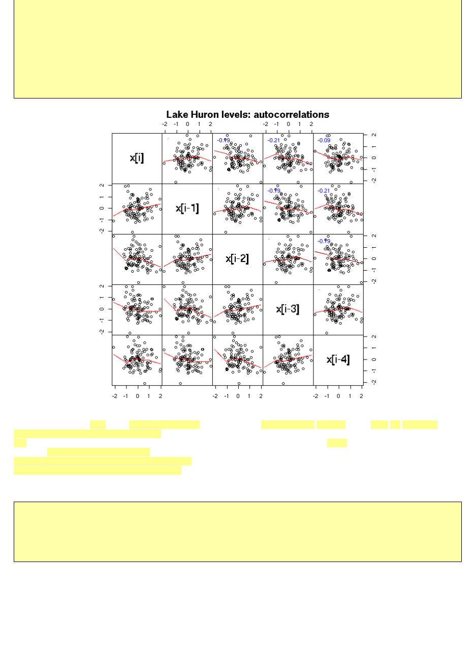
n <- length(x)

k <- 5

m <- matrix(nr=n+k-1, nc=k)

colnames(m) <- c("x[i]", "x[i-1]", "x[i-2]",

"x[i-3]", "x[i-4]")

for (i in 1:k) {

m[,i] <- c(rep(NA,i-1), x, rep(NA, k-i))

}

pairs(m,

gap = 0,

lower.panel = panel.smooth,

upper.panel = function (x,y) {

panel.smooth(x,y)

par(usr = c(0, 1, 0, 1))

a <- cor(x,y, use='pairwise.complete.obs')

text(.1,.9,

adj=c(0,1),

round(a, digits=2),

col='blue',

cex=2*a)

})

title("Lake Huron levels: autocorrelations",

line = 3)

We shall also see other , more . The first one, the (ACF)

(these are the numbers that already appeared in the previous pair plot). The second one, the (Partial AutoCorrelation

Function),

(more about this later, when we speak of AR models). The last one, the spectrogram,

tries to find periodic components, of various frequencies, in the signal and displays the importance of the various frequencies (more

about this later).

op <- par(mfrow = c(3,1),

mar = c(2,4,1,2)+.1)

acf(x, xlab = "")

pacf(x, xlab = "")

spectrum(x, xlab = "", main = "")

par(op)

plots specific to time series AutoCorrelation Function gives the correlation

between x[i] and x[i-k], for increasing values

of k PACF

contains the same information,

but gives the correlation between x[i] and x[i-k] that is

not explained by the correlations with a shorter lag

Simulations

ne (or one step)

Here are, in no particular order, a few simulated time series.

The first is just gaussian noise; the second is an integrated noise (a "random walk"). We can then build on those, integrating several

times, adding noise to the result, adding a linear or periodic trend, etc.

op <- par(mfrow = c(3,3),

mar = .1 + c(0,0,0,0))

n <- 100

k <- 5

N <- k*n

x <- (1:N)/n

plot(ts(y1),

xlab="", ylab="", main="", axes=F)

box()

plot(ts(y2),

xlab="", ylab="", main="", axes=F)

box()

)

plot(ts(y3),

xlab="", ylab="", main="", axes=F)

box()

)

plot(ts(y4),

xlab="", ylab="", main="", axes=F)

box()

plot(ts(y5),

xlab="", ylab="", main="", axes=F)

box()

# With a trend

O aim of time series analysis is to find the

"structure" of a time series, i.e., to find how it was

build, i.e., to find a simple algorithm that could produce

similar-looking data.

y1 <- rnorm(N)

y2 <- cumsum(rnorm(N))

y3 <- cumsum(rnorm(N))+rnorm(N

y4 <- cumsum(cumsum(rnorm(N))

y5 <- cumsum(cumsum(rnorm(N))+rnorm(N))+rnorm(N)

# With a trend

y6 <- 1 - x + cumsum(rnorm(N)) + .2 * rnorm(N)

plot(ts(y6),

xlab="", ylab="", main="", axes=F)

box()

y7 <- 1 - x - .2*x^2 + cumsum(rnorm(N)) +

.2 * rnorm(N)

plot(ts(y7),

xlab="", ylab="", main="", axes=F)

box()

# With a seasonnal component

y8 <- .3 + .5*cos(2*pi*x) - 1.2*sin(2*pi*x) +

.6*cos(2*2*pi*x) + .2*sin(2*2*pi*x) +

-.5*cos(3*2*pi*x) + .8*sin(3*2*pi*x)

plot(ts(y8+ .2*rnorm(N)),

xlab="", ylab="", main="", axes=F)

box()

lines(y8, type='l', lty=3, lwd=3, col='red')

y9 <- y8 + cumsum(rnorm(N)) + .2*rnorm(N)

plot(ts(y9),

xlab="", ylab="", main="", axes=F)

box()

par(op)

often called "innovations", usually by going in the other direction:

We can present this problem from another point of view: when you study a statistical phenomenon, you usually have several realizations

of it. With time series, you have a single one. Therefore, we replace the study of several realizations at a given point in time by the study

The main problem of time series analysis

In statistics, we like independent data -- the problem is

that time series contain dependent data The aim of a time

series analysis will thus be to extract this structure and

transform the initial time series into a series of

independant values by providing a recipe (a "model")

to build a series similar to the one we have with noise as only

ingredient.

of a single realization at several points in time. Depending on the statistical phenomenon, these two points of view may be equivalent or

not -- this problem is called ergodicity -- more about this later.

As the

(strictly speaking, one can consider the Sample ACF, if it is computed from a sample, or the

theoretical autocorrelation function, if it is not computed from actual data but from a model)

In order to compute it from a sample, you have to assume that it does not depend on n but only on the lag, k.

We could do it by hand

my.acf <- function (

lag.max = ceiling(5*log(length(x)))

) {

m <- matrix(

c( NA,

rep( c(rep(NA, lag.max-1), x),

lag.max ),

rep(NA,, lag.max-1)

byrow=T,

nr=lag.max)

x0 <- m[1,]

apply(m,1,cor, x0, use="complete")

}

n <- 200

x <- rnorm(n)

plot(my.acf(x),

xlab = "Lag",

type = 'h')

abline(h=0)

but there is already such a function.

op <- par(mfrow=c(2,1))

acf(x, main="ACF of white noise")

x <- LakeHuron

acf(x, main="ACF of a time series (Lake Huron)")

par(op)

Autocorrelation

observations in a time series are generally not

independant, we can first have a look at their correlation:

the AutoCorrelation Function (ACF)

at lag k

is the correlation between observation number n and

observation number n - k.

The y=0 line traditionnally added to those plots can be misleading: it can suggest that the sign of a coefficient is known, while this

coefficient is not significantly different from zero. The boundaries of the confidence interval are sufficient

op <- par(mfrow=c(2,1))

set.seed(1)

x <- rnorm(100)

# Default plot

acf(x, main = "ACF with a distracting horizontal line")

# Without the axis, with larger bars

r <- acf(x, plot = FALSE)

plot(r$lag, r$acf,

type = "h", lwd = 20, col = "grey",

xlab = "lag", ylab = "autocorrelation",

main = "Autocorrelation without the y=0 line")

ci <- .95

clim <- qnorm( (1+ci) / 2 ) / sqrt(r$n.used)

abline(h = c(-1,1) * clim,

lty = 2, col = "blue", lwd = 2)

Here are the

but the plots have been shuffled: can you put them back in the correct order? Alternatively, can you see

several groups among those time series?

op <- par(mfrow=c(3,3), mar=c(0,0,0,0))

for (y in sample(list(y1,y2,y3,y4,y5,y6,y7,y8,y9))) {

acf(y,

xlab="", ylab="", main="", axes=F)

box(lwd=2)

}

par(op)

autocorrelation functions of the simulated

examples from the introduction,

Personnally, I can see three groups:

;

A white noise is

In other words, these are iid (independant, identically distributed) random variables, to the second order. (They may be dependent, but in

non-linear ways, that cannot be seen from the correlation; they may have different distributions, as long as the mean and variance remain

the same; their distribution need not be symetric.)

For instance, a series of iid random variables is a white noise.

my.plot.ts <- function (x, main="") {

op <- par(mar=c(2,2,4,2)+.1)

layout( matrix(c(1,2),nr=1,nc=2), widths=c(3,1) )

plot(x, xlab="", ylab="")

abline(h=0, lty=3)

title(main=main)

hist(x, col="light blue", main='', ylab="", xlab="")

par(op)

}

n <- 100

x <- ts(rnorm(n))

my.plot.ts(x, "Gaussian iid noise")

when the ACF is almost

zero, the data are not correlated when the ACF is sometimes

positive sometimes negative, the data might be periodic in

the other cases, the data are correlated -- but the speed at which

the autocorrelation decreases can vary.

White noise

a series of uncorrelated random variables,

whose expectation is zero, whose variance is constant.

Quite often, we shall try to decompose our time series into

a "trend" (or anything interpretable) plus a noise term,

that should be white noise.

A series of iid random variables of mean zero is also a white noise.

n <- 100

x <- ts(runif(n,-1,1))

my.plot.ts(x, "Non gaussian iid noise")

x <- ts(rnorm(100)^3)

my.plot.ts(x, "Non gaussian iid noise")

But you can also have a series of uncorrelated random variables that are not independant: the definition just asks that they be

"independant to the second order".

n <- 100

x <- rep(0,n)

z <- rnorm(n)

for (i in 2:n) {

x[i] <- z[i] * sqrt( 1 + .5 * x[i-1]^2 )

}

my.plot.ts(x, "Non iid noise")

Some deterministic sequences look like white noise.

n <- 100

x <- rep(.7, n)

for (i in 2:n) {

x[i] <- 4 * x[i-1] * ( 1 - x[i-1] )

}

my.plot.ts(x, "A deterministic time series")

n <- 1000

tn <- cumsum(rexp(n))

# A C^infinity function defined as a sum

# of gaussian densities

f <- function (x) {

# If x is a single number: sum(dnorm(x-tn))

apply( dnorm( outer(x,rep(1,length(tn))) -

outer(rep(1,length(x)),tn) ),

sum )

}

op <- par(mfrow=c(2,1))

curve(

f(x),

xlim = c(1,500),

n = 1000,

main = "From far away, it looks random..."

)

curve(

f(x),

xlim = c(1,10),

n = 1000,

main="...but it is not: it is a C^infinity function"

)

par(op)

We have a few tests t

as we said in the introduction.

(exactly as we did with regression).

z <- rnorm(200)

op <- par(mfrow=c(2,1), mar=c(5,4,2,2)+.1)

plot(ts(z))

acf(z, main = "")

par(op)

o check if a given time series actually

is white noise.

Diagnostics: is this white noise?

The analysis of a time series mainly consists in finding out

a recipe to build it (or to build a similar-looking series)

from white noise, But to

find this recipe, we proceed in the other direction: we

start with our time series and we try to transform it into something that looks like white noise. To check if our

analysis is correct, we have to check that the residuals are

indeed white noise To

this end, we can start to have a look at the ACF (on

average, 5% of the values should be beyond the dashed lines

-- if there are much more, there might be a problem).

x <- diff(co2)

y <- diff(x,lag=12)

op <- par(mfrow=c(2,1), mar=c(5,4,2,2)+.1)

plot(ts(y))

acf(y, main="")

par(op)

To have a numerical result (a p-value), we can perform a Box--Pierce or Ljung--Box test (these are also called "portmanteau statistics"):

the idea is to consider the (weighted) sum of the first autocorrelation coefficients -- those sums (asymptotically) follow a chi^2

distribution (the Ljung-Box is a variant of the Box-Pierce one that gives a better Chi^2 approximation for small samples).

> Box.test(z) # Box-Pierce

Box-Pierce test

X-squared = 0.014, df = 1, p-value = 0.9059

> Box.test(z, type="Ljung-Box")

Box-Ljung test

X-squared = 0.0142, df = 1, p-value = 0.9051

> Box.test(y)

Box-Pierce test

X-squared = 41.5007, df = 1, p-value = 1.178e-10

> Box.test(y, type='Ljung')

Box-Ljung test

X-squared = 41.7749, df = 1, p-value = 1.024e-10

op <- par(mfrow=c(2,1))

plot.box.ljung <- function (

k = 15,

main = "p-value of the Ljung-Box test",

ylab = "p-value"

) {

p <- rep(NA, k)

for (i in 1:k) {

p[i] <- Box.test(z, i,

type = "Ljung-Box")$p.value

}

plot(p,

type = 'h',

ylim = c(0,1),

lwd = 3,

main = main,

ylab = ylab)

abline(h = c(0,.05),

lty = 3)

}

plot.box.ljung(z, main="Random data")

plot.box.ljung(y, main="diff(diff(co2),lag=12)")

par(op)

There are other such tests: McLeod-Li, Turning-point, difference-sign, rank test, etc.

We can also use the Durbin--Watson we have already mentionned when we tackled regression.

TODO: check that I actually mention it.

library(car)

?durbin.watson

library(lmtest)

?dwtest

Here (it is the same test, but it is not implemented in the same way: the results may differ):

> dwtest(LakeHuron ~ 1)

Durbin-Watson test

data: LakeHuron ~ 1

DW = 0.3195, p-value = < 2.2e-16

alternative hypothesis: true autocorrelation is greater than 0

> durbin.watson(lm(LakeHuron ~ 1))

lag Autocorrelation D-W Statistic p-value

1 0.8319112 0.3195269 0

Alternative hypothesis: rho != 0

op <- par(mfrow=c(2,1))

library(lmtest)

plot(LakeHuron,

main = "Lake Huron")

acf(

LakeHuron,

main = paste(

"Durbin-Watson: p =",

signif( dwtest( LakeHuron ~ 1 ) $ p.value, 3 )

)

par(op)

n <- 200

x <- rnorm(n)

op <- par(mfrow=c(2,1))

x <- ts(x)

plot(x, main="White noise", ylab="")

acf(

main = paste(

"Durbin-Watson: p =",

signif( dwtest( x ~ 1 ) $ p.value, 3)

)

par(op)

n <- 200

x <- rnorm(n)

op <- par(mfrow=c(2,1))

y <- filter(x,.8,method="recursive")

plot(y, main="AR(1)", ylab="")

acf(

main = paste(

"p =",

signif( dwtest( y ~ 1 ) $ p.value, 3 )

)

par(op)

But beware: the default options tests wether the autocorrelation is positive or zero -- if it is significantly negative, the result will be

misleading...

set.seed(1)

n <- 200

x <- rnorm(n)

y <- filter(x, c(0,1), method="recursive")

op <- par(mfrow=c(3,1), mar=c(2,4,2,2)+.1)

plot(

main = paste(

"one-sided DW test: p =",

signif( dwtest ( y ~ 1 ) $ p.value, 3 )

)

acf( y, main="")

pacf(y, main="")

par(op)

op <- par(mfrow=c(3,1), mar=c(2,4,2,2)+.1)

res <- dwtest( y ~ 1, alternative="two.sided")

plot(

main = paste(

"two-sided p =",

signif( res$p.value, 3 )

)

acf(y, main="")

pacf(y, main="")

par(op)

There are other tests, such as the runs test (that looks at the number of runs, a run being consecutive observations of the same sign; that

kind of test is mainly used for qualitative time series or for time series that leave you completely clueless).

library(tseries)

?runs.test

or the Cowles-Jones test

TODO

A sequence is a pair of consecutive returns of the same sign; a

reversal is a pair of consecutive returns of opposite signs.

Their ratio, the Cowles-Jones ratio,

number of sequences

CJ = ---------------------

number of reversals

should be around one IF the drift is zero.

tsdiag

Actually, there is already a function, "tsdiag", that performs some tests on a time series (plot, ACF and Ljung-Box test).

data(co2)

r <- arima(

co2,

order = c(0, 1, 1),

seasonal = list(order = c(0, 1, 1), period = 12)

)

tsdiag(r)

he class

d white noise.

In this section, we shall try to model time series from this idea, using classical statistical methods (mainly regression). Some of the

procedures we shall present will be relevant, useful, but others will not work -- they are just ideas that one might think could work but

turn out not to. Keep your eyes open!

TODO: give the structure of this section

We shall first start to model the time series to be studied with regression, as a polynomial plus a sine wave or, more generally, as a

polynomial plus a periodic signal.

We shall then present modelling techniques based on the (exponential) moving average, that assume that the series locally looks like a

constant plus noise or a linear function plus noise -- this is the Holt-Winters filter.

First attempt: regression

data(co2)

plot(co2)

Simple time series models

T ical model

Classically, one tries to decompose a time series into a sum

of three terms: a trend (often, an affine function), a

seasonal component (a perdiodic function) an

Here, we , as when we were playing with regressions. Let us first try to write the data as the sum of

an affine function and a sine function.

y <- as.vector(co2)

x <- as.vector(time(co2))

r <- lm( y ~ poly(x,1) + cos(2*pi*x) + sin(2*pi*x) )

plot(y~x, type='l', xlab="time", ylab="co2")

lines(predict(r)~x, lty=3, col='red', lwd=3)

This is actually insufficient. It might not be that clear on this plot, but if you look at the residuals, it becomes obvious.

plot( y-predict(r),

main = "The residuals are not random yet",

xlab = "Time",

ylab = "Residuals" )

consider time as a predictive variable

Let us complicate the model: a degree 2 polynomial plus a sine function (if it were not sufficient, we would replace the polynomial by

splines) (we could also transform the time series, e.g., with a logarithm -- here, it does not work).

r <- lm( y ~ poly(x,2) + cos(2*pi*x) + sin(2*pi*x) )

plot(y~x, type='l', xlab="Time", ylab="co2")

lines(predict(r)~x, lty=3, col='red', lwd=3)

That is better.

plot( y-predict(r),

main = "Better residuals -- but still not random",

xlab = "Time",

ylab = "Residuals" )

We could try to refine the periodic component, but it would not really improve things.

r <- lm( y ~ poly(x,2) + cos(2*pi*x) + sin(2*pi*x)

+ cos(4*pi*x) + sin(4*pi*x) )

plot(y~x, type='l', xlab="Time", ylab="co2")

lines(predict(r)~x, lty=3, col='red', lwd=3)

plot( y-predict(r),

type = 'l',

xlab = "Time",

ylab = "Residuals",

main = "Are those residuals any better?" )

However, the ACF suggests that those models are not as good as they seemed:

r1 <- lm( y ~ poly(x,2) +

cos(2*pi*x) +

sin(2*pi*x) )

r2 <- lm( y ~ poly(x,2) +

cos(2*pi*x) +

sin(2*pi*x) +

cos(4*pi*x) +

sin(4*pi*x) )

op <- par(mfrow=c(2,1))

acf(y - predict(r1))

acf(y - predict(r2))

par(op)

if the residuals were really white noise, we

would have very few values beyond the dashed lines...

Those plots tell us two things: first, after all, it was useful to refine the periodic component; second, we still have autocorrelation

problems.

Other attempt (apparently a bad idea)

To estimate the periodic component, we could average the january values, then the february values, etc.

m <- tapply(co2, gl(12,1,length(co2)), mean)

m <- rep(m, ceiling(length(co2)/12)) [1:length(co2)]

m <- ts(m, start=start(co2), frequency=frequency(co2))

op <- par(mfrow=c(3,1), mar=c(2,4,2,2))

plot(co2)

plot(m, ylab = "Periodic component")

plot(co2-m, ylab = "Withou the periodic component")

r <- lm(co2-m ~ poly(as.vector(time(m)),2))

lines(predict(r) ~ as.vector(time(m)), col='red')

par(op)

However, a look at the residuals tell us that the periodic component is still there...

op <- par(mfrow=c(4,1), mar=c(2,4,2,2)+.1)

plot(r$res, type = "l")

acf(r$res, main="")

pacf(r$res, main="")

spectrum(r$res, col=par('fg'), main="")

abline(v=1:6, lty=3)

par(op)

Other attempt (better than the previous)

Using the mean as above to estimate the periodic component would only work if the model were of the form

y ~ a + b x + periodic component.

But here, we have a quadratic term: averaging for each month will nt work. However, we can reuse the same idea with a single

regression, to find both the periodic component and the trend. Here, the periodic component can be anything: we have 12 coefficients to

estimate on top of those of the trend.

k <- 12

m <- matrix( as.vector(diag(k)),

nr = length(co2),

nc = k,

byrow = TRUE )

m <- cbind(m, poly(as.vector(time(co2)),2))

r <- lm(co2~m-1)

summary(r)

b <- r$coef

y1 <- m[,1:k] %*% b[1:k]

y1 <- ts(y1,

start=start(co2),

frequency=frequency(co2))

y2 <- m[,k+1:2] %*% b[k+1:2]

y2 <- ts(y2,

start=start(co2),

frequency=frequency(co2))

res <- co2 - y1 - y2

op <- par(mfrow=c(3,1), mar=c(2,4,2,2)+.1)

plot(co2)

lines(y2+mean(b[1:k]) ~ as.vector(time(co2)),

col='red')

plot(y1)

plot(res)

par(op)

Here, the analysis is not finished: we still have to study the resulting noise -- but we did get rid of the periodic component.

op <- par(mfrow=c(3,1), mar=c(2,4,2,2)+.1)

acf(res, main="")

pacf(res, main="")

spectrum(res, col=par('fg'), main="")

abline(v=1:10, lty=3)

par(op)

To pursue the example to its end, one is tempted to fit an AR(2) (an ARMA(1,1) would do, as well) to the residuals.

innovations <- arima(res, c(2,0,0))$residuals

op <- par(mfrow=c(4,1), mar=c(3,4,2,2))

plot(innovations)

acf(innovations)

pacf(innovations)

spectrum(innovations)

par(op)

Same idea, with splines

In the last example, if the period was longer, we would use splines to find a smoother periodic component -- and also to have fewer

parameters: 15 was really a lot.

Exercise left to the reader...

Finding the trend (or removing the seasonal component): Moving Average

x <- co2

n <- length(x)

k <- 12

m <- matrix( c(x, rep(NA,k)), nr=n+k-1, nc=k )

y <- apply(m, 1, mean, na.rm=T)

y <- y[1:n + round(k/2)]

y <- ts(y, start=start(x), frequency=frequency(x))

y <- y[round(k/4):(n-round(k/4))]

yt <- time(x)[ round(k/4):(n-round(k/4)) ]

plot(x, ylab="co2")

lines(y~yt, col='red')

To find the trend of a time series, you can simply "smooth"

it, e.g., with a Moving Average (MA).

The Moving average will leave invariant some functions (e.g., polynomials of degree up to three -- choose the coefficients accordingly).

The "filter" function already does this. Do not forget the "side" argument: otherwise, it will use values from the past and the future -- for

time series this is rarely desirable: it would introduce a look-ahead bias.

x <- co2

plot(x, ylab="co2")

k <- 12

lines( filter(x, rep(1/k,k), side=1), col='red')

MA: Filtering and smoothing

Actually, one should distinguish between "smoothing" with a Moving Average (to find the value at a point, one uses the whole sample,

including what happend after that point) and "filtering" with a Moving Average (to find the smoothed value at a point, one only uses the

information up to that point).

When we perform a usual regression, we are interested in the shape of our data in the whole interval. On the contrary, quite often, when

we study time series, we are interested in what happens at the end of the interval -- and try to forecast beyond.

In the first case, we use smoothing: to compute the Moving Average at time t, we average over an interval centered on t. The drawback is

that we cannot do that at the two ends of the interval: there will be missing values at the begining and the end.

In the second case, as we do want values at the end of the interval, we do not average on an interval centered on t, but on the values up to

time t. The drawback is that this introduces a lag: we have the same values as before, but t/2 units later.

The "side" argument of the filter() function lest you choose between smoothing and filtering.

x <- co2

plot(window(x, 1990, max(time(x))), ylab="co2")

k <- 12

lines( filter(x, rep(1/k,k)),

col='red', lwd=3)

lines( filter(x, rep(1/k,k), sides=1),

col='blue', lwd=3)

legend(par('usr')[1], par('usr')[4], xjust=0,

c('smoother', 'filter'),

lwd=3, lty=1,

col=c('red','blue'))

Filters are especially used in real-time systems: we want the best estimation of some quantity using all the data collected so far, and we

want to update this estimate when new data comes in.

Applications of the Moving Average

Here is a classical investment strategy (I do not claim it works): take a price time series, compute a 20-day moving average and a 50-day

one; when the two curves intersect, buy or sell (finance people call the difference between those two moving averages an "oscillator" -- it

is a time series that should wander around zero, that should revert to zero -- you can try to design you own oscillator: the strategy will be

"buy when the oscillator is low, sell when it is high").

library(fBasics) # RMetrics

x <- yahooImport("s=IBM&a=11&b=1&c=1999&d=0&q=31&f=2000&z=IBM&x=.csv")

x <- as.numeric(as.character(x@data$Close))

x20 <- filter(x, rep(1/20,20), sides=1)

x50 <- filter(x, rep(1/50,50), sides=1)

matplot(cbind(x,x20,x50), type="l", lty=1, ylab="price", log="y")

segments(1:length(x), x[-length(x)], 1:length(x), x[-1], lwd=ifelse(x20>x50,1,5)[-1], col=ifelse(x20>x50,"black","blue")[-1])

Exercise: do the same with an exponential moving average.

Exponential Moving average

The moving average has a slight problem: it uses a window with sharp edges; an observation is either in the window or not. As a result,

when large observations enter or leave the window, there is large jump in the moving average.

This is another moving average: instead of taking the N latest values, equally-weighted, we take all the preceding values and give a

higher weight to the latest values.

exponential.moving.average <-

function (x, a) {

m <- x

for (i in 2:n) {

# Definition

# Exercise: use the "filter" function instead,

# with its "recursive" argument (that should be

# much, much faster)

m[i] <- a * x[i] + (1-a)*m[i-1]

}

m <- ts(m, start=start(x), frequency=frequency(x))

}

plot.exponential.moving.average <-

function (x, a=.9, ...) {

plot(exponential.moving.average(x,a), ...)

par(usr=c(0,1,0,1))

text(.02,.9, a, adj=c(0,1), cex=3)

}

op <- par(mfrow=c(4,1), mar=c(2,2,2,2)+.1)

plot(x, main="Exponential Moving Averages")

plot.exponential.moving.average(x, main="", ylab="")

plot.exponential.moving.average(x,.1, main="", ylab="")

plot.exponential.moving.average(x,.02, main="", ylab="")

par(op)

r <- x - exponential.moving.average(x,.02)

op <- par(mfrow=c(4,1), mar=c(2,4,2,2)+.1)

plot(r, main="Residuals of an exponential moving average")

acf(r, main="")

pacf(r, main="")

spectrum(r, main="")

abline(v=1:10,lty=3)

par(op)

As with all moving average filters, there is a lag.

Actually, there is already a function to do this (it is a special case of the Holt-Winters filter -- we shall present the general case in a few

moments):

x <- co2

m <- HoltWinters(x, alpha=.1, beta=0, gamma=0)

p <- predict(m, n.ahead=240, prediction.interval=T)

plot(m, predicted.values=p)

y <- x20 > x50

op <- par(mfrow=c(5,1), mar=c(0,0,0,0), oma=.1+c(0,0,0,0))

plot(y, type="l", axes=FALSE); box()

plot(filter(y, 50/100, "recursive", sides=1), axes=FALSE); box()

plot(filter(y, 90/100, "recursive", sides=1), axes=FALSE); box()

plot(filter(y, 95/100, "recursive", sides=1), axes=FALSE); box()

plot(filter(y, 99/100, "recursive", sides=1), axes=FALSE); box()

par(op)

Other moving quantities

The "runing" function in the "gtools" package, the "rollFun" function in the "rollFun" in the "fMultivar" package (in RMetrics) and the

"rollapply" function in the "zoo" package compute a statistic (mean, standard deviation, median, quantiles, etc.) on a moving window.

library(zoo)

op <- par(mfrow=c(3,1), mar=c(0,4,0,0), oma=.1+c(0,0,0,0))

plot(rollapply(zoo(x), 10, median, align="left"),

axes = FALSE, ylab = "median")

lines(zoo(x), col="grey")

box()

plot(rollapply(zoo(x), 50, sd, align="left"),

axes = FALSE, ylab = "sd")

box()

library(robustbase)

plot(sqrt(rollapply(zoo(x), 50, Sn, align="left")),

axes = FALSE, ylab = "Sn")

box()

par(op)

Finding the trend: Fourrier Transform

One can also find the trend of a time series by performing a Fourier transform and removing the high frequencies -- indeed, the moving

averages we considered earlier are low-pass filters.

Exercise left to the reader

Finding the trend: differentiation

If a time series has a trend, if this trend is a polynomial of degree n, then you can transform this series into a trend-less one by

differentiating it (using the discrete derivative) n times.

TODO: an example

To go back to the initial time series, you just have to integrate n times ("discrete integration" is just a complicated word for "cumulated

sums" -- but, of course, you have to worry about the integration constants).

TODO: Explain the relations/confusions between trend, stationarity,

integration, derivation.

TODO: Take a couple of (real-world) time series and apply them all the methods above, in order to compare them

Local regression: loess

The "stl" function performs a "Seasonal Decomposition of a Time Series by Loess".

In case you have forgotten, the "loess" function performs a local regression, i.e., for each value of the predictive variable, we take the

neighbouring observations and perform a linear regression with them; the loess curve is the "envelope" of those regression lines.

op <- par(mfrow=c(3,1), mar=c(3,4,0,1), oma=c(0,0,2,0))

r <- stl(co2, s.window="periodic")$time.series

plot(co2)

lines(r[,2], col='blue')

lines(r[,2]+r[,1], col='red')

plot(r[,3])

acf(r[,3], main="residuals")

par(op)

mtext("STL(co2)", line=3, font=2, cex=1.2)

The "decompose" function has a similar purpose.

r <- decompose(co2)

plot(r)

op <- par(mfrow=c(2,1), mar=c(0,2,0,2), oma=c(2,0,2,0))

acf(r$random, na.action=na.pass, axes=F, ylab="")

box(lwd=3)

mtext("PACF", side=2, line=.5)

pacf(r$random, na.action=na.pass, axes=F, ylab="")

box(lwd=3)

axis(1)

mtext("PACF", side=2, line=.5)

par(op)

mtext("stl(co2): residuals", line=2.5, font=2, cex=1.2)

Holt-Winters filtering

This is a generalization of exponential filtering (which assumes there is no seasonal component). It has the same advantages: it is not

very sensible to (not too drastic) structural changes.

For exponential filtering, we had used

a(t) = alpha * Y(t) + (1-alpha) * a(t-1).

This is a good estimator of the future values of the time series if it is of the form Y(t) = Y_0 + noise, i.e., if the series is "a constant plus

noise" (or even if it is just "locally constant").

This assumed that the series was locallly constant. Here is an example.

data(LakeHuron)

x <- LakeHuron

before <- window(x, end=1935)

after <- window(x, start=1935)

a <- .2

b <- 0

g <- 0

model <- HoltWinters(

before,

alpha=a, beta=b, gamma=g)

forecast <- predict(

model,

n.ahead=37,

prediction.interval=T)

plot(model, predicted.values=forecast,

main="Holt-Winters filtering: constant model")

lines(after)

We can add a trend: we model the data as a line, from the preceding values, giving more weight to the most recent values.

data(LakeHuron)

x <- LakeHuron

before <- window(x, end=1935)

after <- window(x, start=1935)

a <- .2

b <- .2

g <- 0

model <- HoltWinters(

before,

alpha=a, beta=b, gamma=g)

forecast <- predict(

model,

n.ahead=37,

prediction.interval=T)

plot(model, predicted.values=forecast,

main="Holt-Winters filtering: trend model")

lines(after)

Depending on the choice of beta, the forecasts can be very different...

data(LakeHuron)

x <- LakeHuron

op <- par(mfrow=c(2,2),

mar=c(0,0,0,0),

oma=c(1,1,3,1))

before <- window(x, end=1935)

after <- window(x, start=1935)

a <- .2

b <- .5

g <- 0

for (b in c(.02, .04, .1, .5)) {

model <- HoltWinters(

before,

alpha=a, beta=b, gamma=g)

forecast <- predict(

model,

n.ahead=37,

prediction.interval=T)

plot(model,

predicted.values=forecast,

axes=F, xlab='', ylab='', main='')

box()

text( (4*par('usr')[1]+par('usr')[2])/5,

(par('usr')[3]+5*par('usr')[4])/6,

paste("beta =",b),

cex=2, col='blue' )

lines(after)

}

par(op)

mtext("Holt-Winters filtering: different values for beta",

line=-1.5, font=2, cex=1.2)

You can also add a seosonal component (and additive or a multiplicative one).

TODO: Example

TODO: A multiplicative example

Structural models

Before presenting general models whose interpretation may not be that straightforward (ARIMA, SARIMA), let us stop a moment to

consider structural models, that are special cases of AR, MA, ARMA, ARIMA, SARIMA.

A random walk, with noise (a special case of ARIMA(0,1,1)):

X(t) = mu(t) + noise1

mu(t+1) = mu(t) + noise2

n <- 200

plot(ts(cumsum(rnorm(n)) + rnorm(n)),

main="Noisy random walk",

ylab="")

A random walk is simply "integrated noise" (as this is a discrete integration, we use the "cumsum" function). One can add some noise to

a random walk: this is called a local level model.

We can also change the variance of those noises.

op <- par(mfrow=c(2,1),

mar=c(3,4,0,2)+.1,

oma=c(0,0,3,0))

plot(ts(cumsum(rnorm(n, sd=1))+rnorm(n,sd=.1)),

ylab="")

plot(ts(cumsum(rnorm(n, sd=.1))+rnorm(n,sd=1)),

ylab="")

par(op)

mtext("Noisy random walk", line=2, font=2, cex=1.2)

A noisy random walk, integrated, with added noise (ARIMA(0,2,2), aka local trend model):

X(t) = mu(t) + noise1

mu(t+1) = mu(t) + nu(t) + noise2 (level)

nu(t+1) = nu(t) + noise3 (slope)

n <- 200

plot(ts( cumsum( cumsum(rnorm(n))+rnorm(n) ) +

rnorm(n) ),

main = "Local trend model",

ylab="")

Here again, we can play and change the noise variances.

n <- 200

op <- par(mfrow=c(3,1),

mar=c(3,4,2,2)+.1,

oma=c(0,0,2,0))

plot(ts( cumsum( cumsum(rnorm(n,sd=1))+rnorm(n,sd=1) )

+ rnorm(n,sd=.1) ),

ylab="")

plot(ts( cumsum( cumsum(rnorm(n,sd=1))+rnorm(n,sd=.1) )

+ rnorm(n,sd=1) ),

ylab="")

plot(ts( cumsum( cumsum(rnorm(n,sd=.1))+rnorm(n,sd=1) )

+ rnorm(n,sd=1) ),

ylab="")

par(op)

mtext("Local level models", line=2, font=2, cex=1.2)

A noisy random walk, integrated, with added noise, to which we add a variable seasonal component.

X(t) = mu(t) + gamma(t) + noise1

mu(t+1) = mu(t) + nu(t) + noise2 (level)

nu(t+1) = nu(t) + noise2 (slope)

gamma(t+1) = -(gamma(t) + gamma(t-1) + gamma(t-2)) + noise4 (seasonal component)

structural.model <- function (

n=200,

sd1=1, sd2=1, sd3=1, sd4=1, sd5=200

) {

sd1 <- 1

sd2 <- 2

sd3 <- 3

sd4 <- 4

mu <- rep(rnorm(1),n)

nu <- rep(rnorm(1),n)

g <- rep(rnorm(1,sd=sd5),n)

x <- mu + g + rnorm(1,sd=sd1)

for (i in 2:n) {

if (i>3) {

g[i] <- -(g[i-1]+g[i-2]+g[i-3]) + rnorm(1,sd=sd4)

} else {

g[i] <- rnorm(1,sd=sd5)

}

nu[i] <- nu[i-1] + rnorm(1,sd=sd3)

mu[i] <- mu[i-1] + nu[i-1] + rnorm(1,sd=sd2)

x[i] <- mu[i] + g[i] + rnorm(1,sd=sd1)

}

ts(x)

}

n <- 200

op <- par(mfrow=c(3,1),

mar=c(2,2,2,2)+.1,

oma=c(0,0,2,0))

plot(structural.model(n))

par(op)

mtext("Structural models", line=2.5, font=2, cex=1.2)

Here again, we can change the noise variance. If the seasonal component is not noisy, it is constant (but arbitrary).

n <- 200

op <- par(mfrow=c(3,1),

mar=c(2,2,2,2)+.1,

oma=c(0,0,2,0))

plot(structural.model(n,sd4=0))

par(op)

mtext("Structural models", line=2.5, font=2, cex=1.2)

You can model a time series along those models with the "StructTS" function.

data(AirPassengers)

plot(AirPassengers)

plot(log(AirPassengers))

x <- log(AirPassengers)

r <- StructTS(x)

plot(x, main="AirPassengers", ylab="")

f <- apply(fitted(r), 1, sum)

f <- ts(f, frequency=frequency(x), start=start(x))

lines(f, col='red', lty=3, lwd=3)

Here, the slope seems constant.

> r

Call:

StructTS(x = x)

Variances:

level slope seas epsilon

0.0007718 0.0000000 0.0013969 0.0000000

> summary(r$fitted[,"slope"])

Min. 1st Qu. Median Mean 3rd Qu. Max.

0.000000 0.009101 0.010210 0.009420 0.010560 0.011040

matplot(

(StructTS(x-min(x)))$fitted,

type = 'l',

ylab = "",

main = "Structural model decomposition of a time series"

)

You can also try to forecast future values (but it might not be that reliable).

l <- 1956

x <- log(AirPassengers)

x1 <- window(x, end=l)

x2 <- window(x, start=l)

r <- StructTS(x1)

plot(x)

f <- apply(fitted(r), 1, sum)

f <- ts(f, frequency=frequency(x), start=start(x))

lines(f, col='red')

p <- predict(r, n.ahead=100)

lines(p$pred, col='red')

lines(p$pred + qnorm(.025) * p$se,

col='red', lty=2)

lines(p$pred + qnorm(.975) * p$se,

col='red', lty=2)

title(main="Forecasting with a structural model (StructTS)")

Examples

TODO: put this at the end of the introduction?

# A function to look at a time series

eda.ts <- function (x, bands=FALSE) {

op <- par(no.readonly = TRUE)

par(mar=c(0,0,0,0), oma=c(1,4,2,1))

# Compute the Ljung-Box p-values

# (we only display them if needed, i.e.,

# if we have any reason of

# thinking it is white noise).

p.min <- .05

k <- 15

p <- rep(NA, k)

for (i in 1:k) {

p[i] <- Box.test(

x, i, type = "Ljung-Box"

)$p.value

}

if( max(p)>p.min ) {

par(mfrow=c(5,1))

} else {

par(mfrow=c(4,1))

}

if(!is.ts(x))

x <- ts(x)

plot(x, axes=FALSE);

axis(2); axis(3); box(lwd=2)

if(bands) {

a <- time(x)

i1 <- floor(min(a))

i2 <- ceiling(max(a))

y1 <- par('usr')[3]

y2 <- par('usr')[4]

if( par("ylog") ){

y1 <- 10^y1

y2 <- 10^y2

}

for (i in seq(from=i1, to=i2-1, by=2)) {

polygon( c(i,i+1,i+1,i), c(y1,y1,y2,y2),

col='grey', border=NA )

}

lines(x)

}

acf(x, axes=FALSE)

axis(2, las=2)

box(lwd=2)

mtext("ACF", side=2, line=2.5)

pacf(x, axes=FALSE)

axis(2, las=2)

box(lwd=2)

mtext("ACF", side=2, line=2.5)

spectrum(x, col=par('fg'), log="dB",

main="", axes=FALSE )

axis(2, las=2)

box(lwd=2)

mtext("Spectrum", side=2, line=2.5)

abline(v=1, lty=2, lwd=2)

abline(v=2:10, lty=3)

abline(v=1/2:5, lty=3)

if( max(p)>p.min ) {

main <-

plot(p, type='h', ylim=c(0,1),

lwd=3, main="", axes=F)

axis(2, las=2)

box(lwd=2)

mtext("Ljung-Box p-value", side=2, line=2.5)

abline(h=c(0,.05),lty=3)

}

par(op)

}

data(co2)

eda.ts(co2, bands=T)

Transformations

TODO: Put this section somewhere above

As for the regression, we first transform the data so that ot looks "nicer" (as usual, plot the histogram, density estimation, qqplot, etc., try

a Box-Cox transformation). For instance, if you remark that the larger the value, the larger the variations, and if it is reasonable to think

that the model could be "something deterministic plus noise", you can take the logarithm.

More generally, the aim of time series analysis is actually to transform the data so that it looks gaussian; the inverse of that

transformation is then a model describing how the time series may have been produced from white noise.

Examples

data(AirPassengers)

x <- AirPassengers

plot(x)

abline(lm(x~time(x)), col='red')

The residuals or the first derivative suggest that the amplitude of the variations increase.

plot(lm(x~time(x))$res)

plot(diff(x))

Let us try with the logarithm.

x <- log(x)

plot(x)

abline(lm(x~time(x)),col='red')

plot(lm(x~time(x))$res)

plot(diff(x))

We could also have a look at the next derivatives.

op <- par(mfrow=c(3,1))

plot(diff(x,1,2))

plot(diff(x,1,3))

plot(diff(x,1,4))

par(op)

There seems to be a 12-month seasonal component.

op <- par(mfrow=c(3,1))

plot(x)

abline(h=0, v=1950:1962, lty=3)

y <- diff(x)

plot(y)

abline(h=0, v=1950:1962, lty=3)

plot(diff(y, 12,1))

abline(h=0, v=1950:1962, lty=3)

par(op)

You can also use a regression to get rid of the up-trend.

op <- par(mfrow=c(3,1))

plot(x)

abline(lm(x~time(x)), col='red', lty=2)

abline(h=0, v=1950:1962, lty=3)

y <- x - predict(lm(x~time(x)))

plot(y)

abline(h=0, v=1950:1962, lty=3)

plot(diff(y, 12,1))

abline(h=0, v=1950:1962, lty=3)

par(op)

Let us look at the residuals and differentiate.

z <- diff(y,12,1)

op <- par(mfrow=c(3,1))

plot(z)

abline(h=0,lty=3)

plot(diff(z))

abline(h=0,lty=3)

plot(diff(z,1,2))

abline(h=0,lty=3)

par(op)

How many times should we differentiate?

k <- 3

op <- par(mfrow=c(k,2))

zz <- z

for(i in 1:k) {

acf(zz, main=i-1)

pacf(zz, main=i-1)

zz <- diff(zz)

}

par(op)

TODO: What is this?

data(sunspots)

op <- par(mfrow=c(5,1))

for (i in 10+1:5) {

plot(diff(sunspots,i))

}

par(op)

ARIMA

ACF

The main difference between time series and the series of iid random variables we have been playing with up to now is the lack of

independance. Correlation is one means of measuring that lack of independance (if the variables are gaussian, it is even an accurate

means).

The AutoCorrelation Function (ACF) is the correlation between a term and the i-th preceding term

ACF(i) = Cor( X(t), X(t-i) )

If indeed this does not depend on the position t, the time series is said to be weakly stationary -- it is said to be strongly stationary if for

all t, h, the joint distributions of (X(t),X(t+1),...,X(t+n)) and (X(t+h),X(t+h+1),...,X(t+h+n)) are the same.

In the following plot, most (1/20) of the values of the ACT should be between the dashed lines -- otherwise, there might be something

else than gaussian noise in your data.

Strictly speaking, one should distinguish between the theoretical ACF, computed from a model, without any data and the Sample ACF

(SACF), computed from a sample. Here, we compute the SACF of a realization of a model.

op <- par(mfrow=c(2,1), mar=c(2,4,3,2)+.1)

x <- ts(rnorm(200))

plot(x, main="gaussian iidrv",

xlab="", ylab="")

acf(x, main="")

par(op)

A real example:

op <- par(mfrow=c(2,1), mar=c(2,4,3,2)+.1)

data(BJsales)

plot(BJsales, xlab="", ylab="", main="BJsales")

acf(BJsales, main="")

par(op)

f <- 24

x <- seq(0,10, by=1/f)

y <- sin(2*pi*x)

y <- ts(y, start=0, frequency=f)

op <- par(mfrow=c(4,1), mar=c(2,4,2,2)+.1)

plot(y, xlab="", ylab="")

acf(y, main="")

pacf(y, main="")

spectrum(y, main="", xlab="")

par(op)

f <- 24

x <- seq(0,10, by=1/f)

y <- x + sin(2*pi*x) + rnorm(10*f)

y <- ts(y, start=0, frequency=f)

op <- par(mfrow=c(4,1), mar=c(2,4,2,2)+.1)

plot(y, xlab="", ylab="")

acf(y, main="")

pacf(y, main="")

spectrum(y, main="", xlab="")

par(op)

Correlogram, variogram

The ACF plot is called an "autocorrelogram". In the case where the observations are not evenly spaced, one can plot a variogram instead:

(y(t_i)-y(t_j))^2 as a function of t_i-t_j.

TODO: plot with irregularly-spaced data

TODO: smooth this plot.

Often, these are (regular) time series with missing values, In this case, for a given value of k=t_i-t_j (on the horizontal axis), we have

several values. You can replace them by their mean.

TODO: example

Take a time series, remove some of its values, compare the

correlogram and the variogram.

(There is also an analogue of the variogram for discrete-valued time series: the lorelogram, based on the LOR -- Logarithm of Odds

Ratio.)

MA (Moving Average models)

Here is a simple way of building a time series from a white noise: just perform a Moving Average (MA) of this noise.

n <- 200

x <- rnorm(n)

y <- ( x[2:n] + x[2:n-1] ) / 2

op <- par(mfrow=c(3,1), mar=c(2,4,2,2)+.1)

plot(ts(x), xlab="", ylab="white noise")

plot(ts(y), xlab="", ylab="MA(1)")

acf(y, main="")

par(op)

n <- 200

x <- rnorm(n)

y <- ( x[1:(n-3)] + x[2:(n-2)] + x[3:(n-1)] + x[4:n] )/4

op <- par(mfrow=c(3,1), mar=c(2,4,2,2)+.1)

plot(ts(x), xlab="", ylab="white noise")

plot(ts(y), xlab="", ylab="MA(3)")

acf(y, main="")

par(op)

You can also compute the moving average with different coefficients.

n <- 200

x <- rnorm(n)

y <- x[2:n] - x[1:(n-1)]

op <- par(mfrow=c(3,1), mar=c(2,4,2,2)+.1)

plot(ts(x), xlab="", ylab="white noise")

plot(ts(y), xlab="", ylab="momentum(1)")

acf(y, main="")

par(op)

n <- 200

x <- rnorm(n)

y <- x[3:n] - 2 * x[2:(n-1)] + x[1:(n-2)]

op <- par(mfrow=c(3,1), mar=c(2,4,2,2)+.1)

plot(ts(x), xlab="", ylab="white noise")

plot(ts(y), xlab="", ylab="Momentum(2)")

acf(y, main="")

par(op)

Instead of computing the moving average by hand, you can use the "filter" function.

n <- 200

x <- rnorm(n)

y <- filter(x, c(1,-2,1))

op <- par(mfrow=c(3,1), mar=c(2,4,2,2)+.1)

plot(ts(x), xlab="", ylab="White noise")

plot(ts(y), xlab="", ylab="Momentum(2)")

acf(y, na.action=na.pass, main="")

par(op)

TODO: the "side=1" argument.

AR (Auto-Regressive models)

Another means of building a time series is to compute each term by adding noise to the preceding term: this is called a random walk.

For instance,

n <- 200

x <- rep(0,n)

for (i in 2:n) {

x[i] <- x[i-1] + rnorm(1)

}

This can be written, more simply, with the "cumsum" function.

n <- 200

x <- rnorm(n)

y <- cumsum(x)

op <- par(mfrow=c(3,1), mar=c(2,4,2,2)+.1)

plot(ts(x), xlab="", ylab="")

plot(ts(y), xlab="", ylab="AR(1)")

acf(y, main="")

par(op)

More generally, one can consider

X(n+1) = a X(n) + noise.

This is called an auto-regressive model, or AR(1), because one can estimate the coefficients by performing a regression of x against

lag(x,1).

n <- 200

a <- .7

x <- rep(0,n)

for (i in 2:n) {

x[i] <- a*x[i-1] + rnorm(1)

}

y <- x[-1]

x <- x[-n]

r <- lm( y ~ x -1)

plot(y~x)

abline(r, col='red')

abline(0, .7, lty=2)

More generally, an AR(q) process is a process in which each term is a linear combination of the q preceding terms and a white noise

(with fixed coefficients).

n <- 200

x <- rep(0,n)

for (i in 4:n) {

x[i] <- .3*x[i-1] -.7*x[i-2] + .5*x[i-3] + rnorm(1)

}

op <- par(mfrow=c(3,1), mar=c(2,4,2,2)+.1)

plot(ts(x), xlab="", ylab="AR(3)")

acf(x, main="", xlab="")

pacf(x, main="", xlab="")

par(op)

You can also simulate those models with the "arima.sim" function.

n <- 200

x <- arima.sim(list(ar=c(.3,-.7,.5)), n)

op <- par(mfrow=c(3,1), mar=c(2,4,2,2)+.1)

plot(ts(x), xlab="", ylab="AR(3)")

acf(x, xlab="", main="")

pacf(x, xlab="", main="")

par(op)

PACF

The partial AutoCorrelation Function (PACF) provides an estimation of the coefficients of an AR(infinity) model: we have already seen

it on the previous examples. It can be easily computed from the autocorrelation function with the "Yule-Walker" equations.

Yule-Walker Equations

To compute the auto-correlation function of an AR(p) process whose coefficients are known,

(1 - a1 B - a2 B^2 - ... - ap B^p) Y = Z

we just have to compute the first autocorrelations r1, r2, ..., rp, and then use the Yule-Walker equations:

r(j) = a1 r(j-1) + a2 r(j-2) + ... + ap r(j-p).

You can also use them in the other direction to compute the coefficients of an AR process from its autocorrelations.

Stationarity

A time series is said to be weakly stationary if the expectation of X(t) does not depend on t and if the covariance of X(t) and X(s) only

depends on abs(t-s).

A time series is said to be stationary if all the X(t) have the same distribution and all the joint distribution of (X(t),X(s)) (for a given

value of abs(s-t)) are the same. Thus, "weakly stationary" means "stationary up to the second order.

For instance, if your time series has a trend, i.e., if the expectation of X(t) is not constant, the series is not stationary.

n <- 200

x <- seq(0,2,length=n)

trend <- ts(sin(x))

plot(trend,

ylim=c(-.5,1.5),

lty=2, lwd=3, col='red',

ylab='')

r <- arima.sim(

list(ar = c(0.5,-.3), ma = c(.7,.1)),

sd=.1

)

lines(trend+r)

Other example: a random walk is not stationary, because the variance of X(t) increases with t -- but the expectation of X(t) remains zero.

n <- 200

k <- 10

x <- 1:n

r <- matrix(nr=n,nc=k)

for (i in 1:k) {

r[,i] <- cumsum(rnorm(n))

}

matplot(x, r,

type = 'l',

lty = 1,

col = par('fg'),

main = "A random walk is not stationnary")

abline(h=0,lty=3)

Ergodicity

Ergodicity and stationarity are two close but different notions.

Given a stochastic process X(n), (n integer), to compute the mean of X(1), we can use one of the following methods: either take several

realizations of this process, each providing a value for X(1), and average those values; or take a single realization of this process and

average X(1), X(2), X(3), etc.. The result we want is the first, but if we are lucky (if the process is ergodic), both will coincide.

Intuitively, a process is ergodic if, to get information that would require several realizations of the process, you can instead consider a

single longer realization.

The practical interest of ergodic processes is that usually, when we study time series, we have a single realization of this time series. With

an ergodic hypothesis, we can say something about it -- without it, we are helpless.

TODO: understand and explain the differences.

For instance, a stationnary process need not be ergodic.

AR and stationarity

In an autoregressive (AR) process, it is reasonable to ask that past observations have less influence than more recent ones. That is why

we ask, in the AR(1) model,

Y(t+1) = a * Y(t) + Z(t) (where Z is a white noise)

that abs(a)<1. This can also be written:

Y(t+1) - a Y(t) = Z(t)

phi(B) Y = Z (where phi(u) = 1 - a u

and B is the Backwards, operator,

aka shift, delay or lag operator)

and we ask that all the roots of phi have a modulus greater than 1.

More generally, an AR process

phi(B) Y = Z

where phi(u) = 1 - a_1 u - a_2 u^2 - ... - a_p u^p

is stationary if the modulus of all the roots of phi are greater that 1.

You can check that these stationary AR process are MA(infinity) processes (this is another meaning of the Yule--Walker equations).

MA and invertibility

TODO: understand and correct this.

Symetrically, for a Moving Average (MA) process, defined by

Y = psi(B) Z

where psi(u) = 1 + b_1 u + b_2 u^3 + ... + b_q u^q

We shall also ask that modulus of the roots of psi be greater than 1. The process is then said to be invertible. Without this hypothesis, the

autocorrelation function does not uniquely define the coefficients of the Moving Average.

For instance, for an MA(1) process,

Y(t+1) = Z(t+1) + a Z(t),

you can replace a by 1/a without changing the autocorrelation function.

n <- 200

ma <- 2

mai <- 1/ma

op <- par(mfrow=c(4,1), mar=c(2,4,1,2)+.1)

x <- arima.sim(list(ma=ma),n)

plot(x, xlab="", ylab="")

acf(x, xlab="", main="")

lines(0:n,

ARMAacf(ma=ma, lag.max=n),

lty=2, lwd=3, col='red')

x <- arima.sim(list(ma=mai),n)

plot(x, xlab="", ylab="")

acf(x, main="", xlab="")

lines(0:n,

ARMAacf(ma=mai, lag.max=n),

lty=2, lwd=3, col='red')

par(op)

TODO: an example with a higher degree polynomial (I naively thought I would just have to invert the roots of the polynomial, but

apparently it is more complicated...)

sym.poly <- function (z,k) {

# Sum of the products of k

# distinct elements of the vector z

if (k==0) {

r <- 1

} else if (k==1) {

r <- sum(z)

} else {

r <- 0

for (i in 1:length(z)) {

r <- r + z[i]*sym.poly(z[-i],k-1)

}

r <- r/k # Each term appeared k times

}

sym.poly( c(1,2,3), 1 ) # 6

sym.poly( c(1,2,3), 2 ) # 11

sym.poly( c(1,2,3), 3 ) # 6

roots.to.poly <- function (z) {

n <- length(z)

p <- rep(1,n)

for (k in 1:n) {

p[n-k+1] <- (-1)^k * sym.poly(z,k)

}

p <- c(p,1)

}

roots.to.poly(c(1,2)) # 2 -3 1

round(

Re(polyroot( roots.to.poly(c(1,2,3)) )),

digits=1

)

# After this interlude, we can finally

# construct an MA process and one of

# its inverses

n <- 200

k <- 3

ma <- runif(k,-1,1)

# The roots

z <- polyroot(c(1,-ma))

# The inverse of the roots

zi <- 1/z

# The polynomial

p <- roots.to.poly(zi)

# The result should be real, but because

# of rounding errors, it is not.

p <- Re(p)

# We want the constant term to be 1.

p <- p/p[1]

mai <- -p[-1]

op <- par(mfrow=c(4,1), mar=c(2,4,1,2)+.1)

x <- arima.sim(list(ma=ma),n)

plot(x, xlab="")

acf(x, main="", xlab="")

lines(0:n, ARMAacf(ma=ma, lag.max=n),

lty=2, lwd=3, col='red')

x <- arima.sim(list(ma=mai),n)

plot(x, xlab="")

acf(x, main="", xlab="")

lines(0:n, ARMAacf(ma=mai, lag.max=n),

lty=2, lwd=3, col='red')

par(op)

The MA(p) processes have another interesting feature: they are AR(infinity) processes.

TODO: on an example, plot the roots of those polynomials.

Unit root tests

TODO: To check if the series we are studying has unit roots.

library(tseries)

?adf.test

?pp.tests

ARMA

Of course, one can mix up MA and AR models, to get the so-called ARMA models. In the following formulas, z is a white noise and x

the series we are interested in.

MA(p): x(i) = a1 z(i-1) + a2 z(i-2) + ... + ap z(i-p)

AR(q): x(i) - b1 x(i-1) - b2 x(i-2) - ... - bq x(i-q) = z(i)

ARMA(p,q): x(i) - b1 x(i-1) - ... - bq x(i-q) = a1 z(i-1) + ... + ap z(i-p)

Remark: AR(q) processes are also MA(infinity) processes, we could replace ARMA processes by MA(infinity) processes, but we prefer

having fewer coefficients to estimate.

Remark: Wold's theorem states that any stationary process can be written as the sum of an MA(infinity) process and a deterministic one.

TODO: I have not defined what a deterministic process was.

Remark: if we let B be the shift operator, so that the derivation operator be 1-B, an ARMA process can be written as

phi(B) X(t) = theta(B) Z(t)

where theta(B) = 1 + a1 B + a2 B^2 + ... + ap B^p

phi(B) = 1 - b1 B - b2 B^2 - ... - bq B^q

Z is a white noise

ARMA processes give a good approximation to most stationary processes. As a result, you can use the estimated ARMA coefficients as

a statistical summary of a stationary process, exactly as the mean and the quantiles for univariate statistical series. They might be useful

to forecast future values, but they provide little information as the the underlying mechanisms that produced the time series.

Overfitting an ARMA process

An ARMA(p,q) process

phi(B) Y = theta(B) Z

in which phi and theta have a root in common can be written, more simply, as an ARMA(p-1,q-1).

How to get to a stationary process

To model a time series as an ARMA model, it has to be stationnary. To get a stationary series (in short, to get rid of the trend), you can

try to differentiate it.

The fact that the series is not stationary is usually obvious on the plot. You can also see it on the ACF: if the series is stationary, the ACF

should rapidly (usually exponentially) decay to zero.

data(Nile)

op <- par(mfrow=c(2,1), mar=c(2,4,3,2)+.1)

plot(Nile, main="There is no trend", xlab="")

acf(Nile, main="", xlab="")

par(op)

data(BJsales)

op <- par(mfrow=c(3,1), mar=c(2,4,3,2)+.1)

plot(BJsales, xlab="",

main="The trend disappears if we differentiate")

acf(BJsales, xlab="", main="")

acf(diff(BJsales), xlab="", main="",

ylab="ACF(diff(BJsales)")

par(op)

n <- 2000

x <- arima.sim(

model = list(

ar = c(.3,.6),

ma = c(.8,-.5,.2),

order = c(2,1,3)),

)

x <- ts(x)

op <- par(mfrow=c(3,1), mar=c(2,4,3,2)+.1)

plot(x, main="It suffices to differentiate once",

xlab="", ylab="")

acf(x, xlab="", main="")

acf(diff(x), xlab="", main="",

ylab="ACF(diff(x))")

par(op)

n <- 10000

x <- arima.sim(

model = list(

ar = c(.3,.6),

ma = c(.8,-.5,.2),

order = c(2,2,3)

)

x <- ts(x)

op <- par(mfrow=c(4,1), mar=c(2,4,3,2)+.1)

plot(x, main="One has to differentiate twice",

xlab="", ylab="")

acf(x, main="", xlab="")

acf(diff(x), main="", xlab="",

ylab="ACF(diff(x))")

acf(diff(x,differences=2), main="", xlab="",

ylab="ACF(diff(diff(x)))")

par(op)

To check more precisely if the ACF decreases exponentially, one could perform a regression (but it might be overkill).

acf.exp <- function (x, lag.max=NULL, lag.max.reg=lag.max, ...) {

a <- acf(x, lag.max=lag.max.reg, plot=F)

b <- acf(x, lag.max=lag.max, ...)

r <- lm( log(a$acf) ~ a$lag -1)

lines( exp( b$lag * r$coef[1] ) ~ b$lag, lty=2 )

}

data(BJsales)

acf.exp(BJsales,

main="Exponential decay of the ACF")

acf.exp(BJsales,

lag.max=40,

main="Exponential decay of the ACF")

data(Nile)

acf.exp(Nile, lag.max.reg=10, main="Nile")

Differentiating can also help you get rid of the seasonal component, if you differentiate with a lag: e.g., take the difference between the

value today and the same value one year ago.

x <- diff(co2, lag=12)

op <- par(mfrow=c(4,1), mar=c(2,4,3,2)+.1)

plot(x, ylab="", xlab="")

acf(x, xlab="", main="")

pacf(x, xlab="", main="")

spectrum(x, xlab="", main="",

col=par('fg'))

par(op)

y <- diff(x)

op <- par(mfrow=c(4,1), mar=c(2,4,3,2)+.1)

plot(y, xlab="", ylab="")

acf(y, xlab="", main="")

pacf(y, xlab="", main="")

spectrum(y, col=par('fg'),

xlab="", main="")

par(op)

ARIMA

ARIMA processes are just integrated ARMA processes. In other words, a process is ARIMA of order d if its d-th derivative is ARMA.

The model can be written

phi(B) (1-B)^d X(t) = theta(B) Z(t)

where B is the shift operator, Z a white noise, phi the polynomial defining the AR part, theta the polynomial defining the MA part of the

process.

ARIMA processes are not stationary processes. We have already seen it with the random walk, which is an integrated ARMA(0,0)

process, i.e., an ARIMA process of order 1: the variance of X(t) increases with t. This is the very reason why we differentiate: to get a

stationary process.

TODO: Give an example of ARIMA(0,1,0) process, show that

it is not stationary.

Recall the tests to check if it is stationary.

Quick and dirty stationarity test: cut the data into two

parts, compute Cor(X(t),X(t-1)) on each, compare.

To infer the order of an ARIMA process, you can differentiate it until its ACF rapidly decreases.

n <- 200

x <- arima.sim(

list(

order=c(2,1,2),

ar=c(.5,-.8),

ma=c(.9,.6)

)

op <- par(mfrow=c(3,1), mar=c(2,4,4,2)+.1)

acf(x, main="You will have to defferentiate once")

acf(diff(x), main="First derivative")

acf(diff(x, differences=2), main="Second derivative")

par(op)

n <- 200

x <- arima.sim(

list(

order=c(2,2,2),

ar=c(.5,-.8),

ma=c(.9,.6)

)

op <- par(mfrow=c(3,1), mar=c(2,4,4,2)+.1)

acf(x, main="You will have to differentiate twice")

acf(diff(x), main="First derivative")

acf(diff(x, differences=2), main="Second derivative")

par(op)

Here is a concrete example.

data(sunspot)

op <- par(mfrow=c(4,1), mar=c(2,4,3,2)+.1)

plot(sunspot.month, xlab="", ylab="sunspot")

acf(sunspot.month, xlab="", main="")

plot(diff(sunspot.month),

xlab="", ylab="diff(sunspot)")

acf(diff(sunspot.month), xlab="", main="")

par(op)

Same here (but actually, the differentiation discards the affine trend).

data(JohnsonJohnson)

x <- log(JohnsonJohnson)

op <- par(mfrow=c(4,1), mar=c(2,4,3,2)+.1)

plot(x, xlab="", ylab="JJ")

acf(x, main="")

plot(diff(x), ylab="diff(JJ)")

acf(diff(x), main="")

par(op)

In the following examples, you might want to differentiate twice. But beware, it might not always be a good idea: if the ACF decreases

exponentially, you can stop differentiating.

data(BJsales)

x <- BJsales

op <- par(mfrow=c(6,1), mar=c(2,4,0,2)+.1)

plot(x)

acf(x)

plot(diff(x))

acf(diff(x))

plot(diff(x, difference=2))

acf(diff(x, difference=2))

par(op)

data(austres)

x <- austres

op <- par(mfrow=c(6,1), mar=c(2,4,0,2)+.1)

plot(x)

acf(x)

plot(diff(x))

acf(diff(x))

plot(diff(x, difference=2))

acf(diff(x, difference=2))

par(op)

# In the preceding example, there was a linear trend:

# let ut remove it.

data(austres)

x <- lm(austres ~ time(austres))$res

op <- par(mfrow=c(6,1), mar=c(2,4,0,2)+.1)

plot(x)

acf(x)

plot(diff(x))

acf(diff(x))

plot(diff(x, difference=2))

acf(diff(x, difference=2))

par(op)

SARIMA

These are Seasonnal ARIMA processes (the integration, the MA or the AR parts can be seasonal). They are often denoted:

(p,d,q) \times (P,D,Q) _s

and they are described by the model:

phi(B) Phi(B^s) (1-B)^d (1-B^s)^D X(t) = theta(B) Theta(B^s) Z(t)

where s is the period

theta(B) = 1 + a1 B + a2 B^2 + ... + ap B^p is the MA polynomial

phi(B) = 1 - b1 B - b2 B^2 - ... - bq B^q is the AR polynomial

Theta(B^s) = 1 + A1 B^s + A2 B^2s + ... + AP B^(P*s) is the seasonal MA polynomial

Phi(B^s) = 1 - B1 B^s - B2 B^2s - ... - BQ B^(Q*s) is the seasonal AR polynomial

Z is a white noise

There is no function to simulate SARIMA processes -- but we can model them.

my.sarima.sim <- function (

n = 20,

period = 12,

model,

seasonal

) {

x <- arima.sim( model, n*period )

x <- x[1:(n*period)]

for (i in 1:period) {

xx <- arima.sim( seasonal, n )

xx <- xx[1:n]

x[i + period * 0:(n-1)] <-

x[i + period * 0:(n-1)] + xx

}

x <- ts(x, frequency=period)

}

op <- par(mfrow=c(3,1))

x <- my.sarima.sim(

20,

12,

list(ar=.6, ma=.3, order=c(1,0,1)),

list(ar=c(.5), ma=c(1,2), order=c(1,0,2))

)

eda.ts(x, bands=T)

x <- my.sarima.sim(

20,

12,

list(ar=c(.5,-.3), ma=c(-.8,.5,-.3), order=c(2,1,3)),

list(ar=c(.5), ma=c(1,2), order=c(1,0,2))

)

eda.ts(x, bands=T)

x <- my.sarima.sim(

20,

12,

list(ar=c(.5,-.3), ma=c(-.8,.5,-.3), order=c(2,1,3)),

list(ar=c(.5), ma=c(1,2), order=c(1,1,2))

)

eda.ts(x, bands=T)

The Box and Jenkins method

TODO

The co2 example (somewhere above) could well be modeled as an SARIMA model.

x <- co2

eda.ts(x)

First, we see that there is a trend: we differentiate once to get rid of it.

eda.ts(diff(x))

There is also a periodic component: we differentiate, with a 12-month lag, to get rid of it.

eda.ts(diff(diff(x),lag=12))

But wait! We have differentiated twice. Couldn't we get rid of both the periodic component and the trend by differentiating just once,

with the 12-month lag?

eda.ts(diff(x,lag=12))

Well, perhaps. We hesitate between

SARIMA(?,1,?)(?,1,?)

and

SARIMA(?,0,?)(?,1,?).

If we look at the ACF and the PACF:

SARIMA(1,1,1)(2,1,1)

SARIMA(1,1,2)(2,1,1)

SARIMA(2,0,0)(1,1,0)

SARIMA(2,0,0)(1,1,1)

Let us compute the coefficients of those models:

r1 <- arima(co2,

order=c(1,1,1),

list(order=c(2,1,1), period=12)

)

r2 <- arima(co2,

order=c(1,1,2),

list(order=c(2,1,1), period=12)

)

r3 <- arima(co2,

order=c(2,0,0),

list(order=c(1,1,0), period=12)

)

r4 <- arima(co2,

order=c(2,0,0),

list(order=c(1,1,1), period=12)

)

This yields:

> r1

Call:

arima(x = co2, order = c(1, 1, 1), seasonal = list(order = c(2, 1, 1), period = 12))

Coefficients:

ar1 ma1 sar1 sar2 sma1

0.2595 -0.5902 0.0113 -0.0869 -0.8369

s.e. 0.1390 0.1186 0.0558 0.0539 0.0332

sigma^2 estimated as 0.08163: log likelihood = -83.6, aic = 179.2

> r2

Call:

arima(x = co2, order = c(1, 1, 2), seasonal = list(order = c(2, 1, 1), period = 12))

Coefficients:

ar1 ma1 ma2 sar1 sar2 sma1

0.5935 -0.929 0.1412 0.0141 -0.0870 -0.8398

s.e. 0.2325 0.237 0.1084 0.0557 0.0538 0.0328

sigma^2 estimated as 0.08132: log likelihood = -82.85, aic = 179.7

> r3

Call:

arima(x = co2, order = c(2, 0, 0), seasonal = list(order = c(1, 1, 0), period = 12))

Coefficients:

ar1 ar2 sar1

0.6801 0.3087 -0.4469

s.e. 0.0446 0.0446 0.0432

sigma^2 estimated as 0.1120: log likelihood = -150.65, aic = 309.3

For r4, it was even:

Error in arima(co2, order = c(2, 0, 1), list(order = c(1, 1, 1), period = 12)) :

non-stationary AR part from CSS

The AIC of a3 is appallingly high (we want as low a value as possible): we really need to differentiate twice.

Let us look at the p-values:

> round(pnorm(-abs(r1$coef), sd=sqrt(diag(r1$var.coef))),5)

ar1 ma1 sar1 sar2 sma1

0.03094 0.00000 0.42007 0.05341 0.00000

> round(pnorm(-abs(r1$coef), sd=sqrt(diag(r1$var.coef))),5)

ar1 ma1 ma2 sar1 sar2 sma1

0.00535 0.00004 0.09635 0.39989 0.05275 0.00000

This suggests an SARIMA(1,1,1)(0,1,1) model.

r3 <- arima( co2,

order=c(1,1,1),

list(order=c(0,1,1), period=12)

)

This yields:

> r3

Call:

arima(x = co2, order = c(1, 1, 1), seasonal = list(order = c(0, 1, 1), period = 12))

Coefficients:

ar1 ma1 sma1

0.2399 -0.5710 -0.8516

s.e. 0.1430 0.1237 0.0256

sigma^2 estimated as 0.0822: log likelihood = -85.03, aic = 178.07

> round(pnorm(-abs(r3$coef), sd=sqrt(diag(r3$var.coef))),5)

ar1 ma1 sma1

0.04676 0.00000 0.00000

We now look at the residuals:

r3 <- arima(

co2,

order = c(1, 1, 1),

seasonal = list(

order = c(0, 1, 1),

period = 12

)

eda.ts(r3$res)

Good, we can now try to use this mode to predict future values. To get an idea of the quality of those forecasts, we can use the first part

of the data to estimate the model coefficients and compute the predictions and the second part to assess the quality of the predictions --

but beware, this is biased, because we chose the model by using all the data, including the data from the test sample.

x1 <- window(co2, end = 1990)

r <- arima(

x1,

order = c(1, 1, 1),

seasonal = list(

order = c(0, 1, 1),

period = 12

)

plot(co2)

p <- predict(r, n.ahead=100)

lines(p$pred, col='red')

lines(p$pred+qnorm(.025)*p$se, col='red', lty=3)

lines(p$pred+qnorm(.975)*p$se, col='red', lty=3)

# On the contrary, I do not know what to do with

# this plots (it looks like integrated noise).

eda.ts(co2-p$pred)

It is not that bad. Here are our forecasts.

r <- arima(

co2,

order = c(1, 1, 1),

seasonal = list(

order = c(0, 1, 1),

period = 12

)

p <- predict(r, n.ahead=150)

plot(co2,

xlim=c(1959,2010),

ylim=range(c(co2,p$pred)))

lines(p$pred, col='red')

lines(p$pred+qnorm(.025)*p$se, col='red', lty=3)

lines(p$pred+qnorm(.975)*p$se, col='red', lty=3)

What we have done is called the Box and Jenkins method. The general case can be a little more complicated: if the residuals do not look

like white noise, we have to get back to find another model.

0. Differentiate to get a stationary process.

If there is a trend, the process is not stationary.

If the ACF decreases slowly, try to differentiate once more.

1. Identify the model:

ARMA(1,0): ACF: exponential decrease; PACF: one peak

ARMA(2,0): ACF: exponential decrease or waves; PACF: two peaks

ARMA(0,1): ACF: one peak; PACF: exponential decrease

ARMA(0,2): ACF: two peaks; PACF: exponential decrease or waves

ARMA(1,1): ACF&PACF: exponential decrease

2. Compute the coefficients

3. Diagnostics (go to 1 if they do not look like white noise)

Computhe the p-values, remove unneeded coefficients (check on the

residuals that they are indeed unneeded).

4. Forecasts

Sample ARMA processes and their ACF and PACF

Here are a few examples of ARMA processes (in red: the theoretic ACF and PACF).

The ARMA(1,0) is characterized by the exponential decrease of the ACF and the single peak in the PACF.

op <- par(mfrow=c(4,2), mar=c(2,4,4,2))

n <- 200

for (i in 1:4) {

x <- NULL

while(is.null(x)) {

model <- list(ar=rnorm(1))

try( x <- arima.sim(model, n) )

}

acf(x,

main = paste(

"ARMA(1,0)",

"AR:",

round(model$ar, digits = 1)

))

points(0:50,

ARMAacf(ar=model$ar, lag.max=50),

col='red')

pacf(x, main="")

points(1:50,

ARMAacf(ar=model$ar, lag.max=50, pacf=T),

col='red')

}

par(op)

You can recognize an ARMA(2,0) from the two peaks in the PACF and the exponential decrease (or the waves) in the ACF.

op <- par(mfrow=c(4,2), mar=c(2,4,4,2))

n <- 200

for (i in 1:4) {

x <- NULL

while(is.null(x)) {

model <- list(ar=rnorm(2))

try( x <- arima.sim(model, n) )

}

acf(x,

main=paste("ARMA(2,0)","AR:",

round(model$ar[1],digits=1),

round(model$ar[2],digits=1)

))

points(0:50,

ARMAacf(ar=model$ar, lag.max=50),

col='red')

pacf(x, main="")

points(1:50,

ARMAacf(ar=model$ar, lag.max=50, pacf=T),

col='red')

}

par(op)

You can recognize an ARMA(0,1) process from its unique peak in the ACF and the exponential decrease of the PACF.

op <- par(mfrow=c(4,2), mar=c(2,4,4,2))

n <- 200

for (i in 1:4) {

x <- NULL

while(is.null(x)) {

model <- list(ma=rnorm(1))

try( x <- arima.sim(model, n) )

}

acf(x,

main = paste(

"ARMA(0,1)",

"MA:",

round(model$ma, digits=1)

))

points(0:50,

ARMAacf(ma=model$ma, lag.max=50),

col='red')

pacf(x, main="")

points(1:50,

ARMAacf(ma=model$ma, lag.max=50, pacf=T),

col='red')

}

par(op)

The ARMA(0,2) model has two peaks in the ACF and if PACF exponentially decreases or exhibits a pattern of waves.

op <- par(mfrow=c(4,2), mar=c(2,4,4,2))

n <- 200

for (i in 1:4) {

x <- NULL

while(is.null(x)) {

model <- list(ma=rnorm(2))

try( x <- arima.sim(model, n) )

}

acf(x, main=paste("ARMA(0,2)","MA:",

round(model$ma[1],digits=1),

round(model$ma[2],digits=1)

))

points(0:50,

ARMAacf(ma=model$ma, lag.max=50),

col='red')

pacf(x, main="")

points(1:50,

ARMAacf(ma=model$ma, lag.max=50, pacf=T),

col='red')

}

par(op)

For the ARMA(1,1), both the ACF and the PACF exponentially decrease.

op <- par(mfrow=c(4,2), mar=c(2,4,4,2))

n <- 200

for (i in 1:4) {

x <- NULL

while(is.null(x)) {

model <- list(ma=rnorm(1),ar=rnorm(1))

try( x <- arima.sim(model, n) )

}

acf(x, main=paste("ARMA(1,1)",

"AR:", round(model$ar,digits=1),

"AR:", round(model$ma,digits=1)

))

points(0:50,

ARMAacf(ar=model$ar, ma=model$ma, lag.max=50),

col='red')

pacf(x, main="")

points(1:50,

ARMAacf(ar=model$ar, ma=model$ma, lag.max=50, pacf=T),

col='red')

}

par(op)

Brute force

Instead of the stepwise procedure presented, we can proceed in a more violent way, by looking at the AIC of all thereasonably complex

models and retaining those whose AIC is the lowest. As this amounts to performing innumarable tests, we do not only take the single

model with the lowest AIC, but several -- we shall prefer a simple model whose residuals look like white noise. You can remorselessly

discard models whose AIC (or BIC: the AIC may be meaningful for nested model, but the BIC has a more general validity) is 100 units

more that the lowest one, you should have remorse if you discard those 6 to 20 units from the lowest, and you should not discard those

less than 6 units away.

a <- array(NA, dim=c(2,2,2,2,2,2))

for (p in 0:2) {

for (d in 0:2) {

for (q in 0:2) {

for (P in 0:2) {

for (D in 0:2) {

for (Q in 0:2) {

r <- list(aic=NA)

try(

r <- arima( co2,

order=c(p,d,q),

list(order=c(P,D,Q), period=12)

)

a[p,d,q,P,D,Q] <- r$aic

cat(r$aic); cat("\n")

}

# When I wrote this, I dod not know the "which.min" function.

argmin.vector <- function (v) {

(1:length(v)) [ v == min(v) ]

}

x <- sample(1:10)

argmin.vector(x)

x <- sample(1:5, 20, replace=T)

argmin.vector(x)

x <- array(x, dim=c(5,2,2))

index.from.vector <- function (i,d) {

res <- NULL

n <- prod(d)

i <- i-1

for (k in length(d):1) {

n <- n/d[k]

res <- c( i %/% n, res )

i <- i %% n

}

res+1

}

index.from.vector(7, c(2,2,2))

index.from.vector(29, c(5,3,2))

argmin <- function (a) {

a <- as.array(a)

d <- dim(a)

a <- as.vector(a)

res <- matrix(nr=0, nc=length(d))

for (i in (1:length(a))[ a == min(a) ]) {

j <- index.from.vector(i,d)

res <- rbind(res, j)

}

res

}

x <- array( sample(1:10,30, replace=T), dim=c(5,3,2) )

argmin(x)

After a couple of hours (I am starting to worry: the computer produces a strange whistling sound when I run those computations...), this

yields:

1 1 1 2 1 2

This is a rather complicated model. Let us look at models whose AIC is close to this one.

x <- as.vector(a)

d <- dim(a)

o <- order(x)

res <- matrix(nr=0, nc=6+2)

for (i in 1:30) {

p <- index.from.vector(o[i],d)

res <- rbind( res, c(p, sum(p), x[o[i]]))

}

colnames(res) <- c("p","d","q", "P","D","Q", "n", "AIC")

res

This yields:

p d q P D Q n AIC

[1,] 1 1 1 2 1 2 8 172.7083

[2,] 1 1 2 2 1 2 9 173.3215

[3,] 0 1 1 2 1 2 7 173.5009

[4,] 2 1 2 2 1 2 10 173.8748

[5,] 0 1 2 2 1 2 8 174.0323

[6,] 2 1 1 0 1 1 6 177.8278

[7,] 1 1 1 0 1 1 5 178.0672

[8,] 0 1 1 0 1 1 4 178.1557

[9,] 2 1 1 2 1 1 8 178.9373

[10,] 2 1 2 0 1 1 7 179.0768

[11,] 2 1 0 2 1 2 8 179.0776

[12,] 0 1 2 0 1 1 5 179.0924

[13,] 1 1 1 2 1 1 7 179.2043

[14,] 2 1 1 0 1 2 7 179.3557

[15,] 2 1 1 1 1 1 7 179.4335

[16,] 1 1 2 2 1 1 8 179.6950

[17,] 1 1 1 0 1 2 6 179.6995

[18,] 0 1 1 2 1 1 6 179.7224

[19,] 1 1 1 1 1 1 6 179.7612

[20,] 0 1 1 0 1 2 5 179.8808

[21,] 0 1 1 1 1 1 5 179.9235

[22,] 1 1 2 0 1 1 6 180.1146

[23,] 1 1 0 2 1 2 7 180.1713

[24,] 2 1 2 2 1 1 9 180.2019

[25,] 1 1 2 1 1 1 7 180.2686

[26,] 0 1 2 2 1 1 7 180.4483

[27,] 2 1 2 0 1 2 8 180.4797

[28,] 2 1 2 1 1 1 8 180.5757

[29,] 1 1 1 1 1 2 7 180.7777

[30,] 0 1 2 0 1 2 6 180.8024

[31,] 0 1 2 1 1 1 6 180.8495

[32,] 0 1 1 1 1 2 6 181.1830

[33,] 1 1 2 1 1 2 8 181.3127

[34,] 2 1 2 1 1 2 9 181.6425

[35,] 1 1 2 0 1 2 7 181.7322

[36,] 0 1 2 1 1 2 7 181.9859

[37,] 2 1 0 0 1 1 5 183.4687

[38,] 1 1 0 0 1 1 4 184.1817

[39,] 2 1 0 2 1 1 7 185.1404

[40,] 2 1 0 0 1 2 6 185.1918

[41,] 2 1 0 1 1 1 6 185.2337

[42,] 1 1 0 0 1 2 5 185.7290

[43,] 1 1 0 1 1 1 5 185.7909

[44,] 1 1 0 2 1 1 6 186.0117

[45,] 2 1 0 1 1 2 7 186.5521

[46,] 1 1 0 1 1 2 6 187.1703

If we look at the distribution of the AICs,

plot(sort(as.vector(a))[1:100])

we see that the first bunch of values is under 200: among those, we select the simplest ones:

p d q P D Q n AIC

0 1 1 0 1 1 4 178.1557

1 1 0 0 1 1 4 184.1817

1 1 1 0 1 1 5 178.0672

0 1 2 0 1 1 5 179.0924

0 1 1 0 1 2 5 179.8808

0 1 1 1 1 1 5 179.9235

2 1 0 0 1 1 5 183.4687

1 1 0 0 1 2 5 185.7290

1 1 0 1 1 1 5 185.7909

I would be tempted to choose the first

0 1 1 0 1 1

or the third (the one we had obtained from the Box and Jenkins method).

1 1 1 0 1 1

Let us perform the computations.

> r <- arima(co2, order=c(0,1,1), list(order=c(0,1,1), period=12 ) )

> r

Call:

arima(x = co2, order = c(0, 1, 1), seasonal = list(order = c(0, 1, 1), period = T))

Coefficients:

ma1 sma1

0.1436 0.1436

s.e. 0.1068 0.1068

sigma^2 estimated as 0.7821: log likelihood = -604.01, aic = 1214.02

> r$var.coef

ma1 sma1

ma1 0.01140545 -0.01048563

sma1 -0.01048563 0.01140545

> pnorm(-abs(r$coef), sd=sqrt(diag(r$var.coef)))

ma1 sma1

0.08940721 0.08940721

Let us look at the residuals.

r <- arima(co2, order=c(0,1,1), list(order=c(0,1,1), period=12 ) )

eda.ts(r$res)

That looks fine, we can keep the model (of the residuals had not looked like a white noise, we would have investigated another model,

until the residuals look fine).

As before, we can validate the model and forecast future values.

x1 <- window(co2,end=1990)

r <- arima(x1, order = c(0, 1, 1), seasonal = list(order = c(0, 1, 1), period = 12))

plot(co2)

p <- predict(r, n.ahead=100)

lines(p$pred, col='red')

lines(p$pred+qnorm(.025)*p$se, col='red', lty=3)

lines(p$pred+qnorm(.975)*p$se, col='red', lty=3)

eda.ts(co2-p$pred)

r <- arima(co2, order = c(0, 1, 1), seasonal = list(order = c(0, 1, 1), period = 12))

p <- predict(r, n.ahead=150)

plot(co2, xlim=c(1959,2010), ylim=range(c(co2,p$pred)))

lines(p$pred, col='red')

lines(p$pred+qnorm(.025)*p$se, col='red', lty=3)

lines(p$pred+qnorm(.975)*p$se, col='red', lty=3)

The forecasts are similar to those of the preceding model,

r1 <- arima(co2, order = c(0, 1, 1), seasonal = list(order = c(0, 1, 1), period = 12))

r2 <- arima(co2, order = c(1, 1, 1), seasonal = list(order = c(0, 1, 1), period = 12))

p1 <- predict(r1, n.ahead=150)

p2 <- predict(r2, n.ahead=150)

plot(co2, xlim=c(1959,2010), ylim=range(c(co2,p$pred)))

lines(p1$pred, col='red')

lines(p2$pred, col='green', lty=3, lwd=4)

TODO: put all this, including the study of the residuals, in a function.

Long-term memory, fractional integration

TODO

Validating a model

TODO: put this section somewhere above

TODO: cross-validation. It is a bit limoted because, a priori, we can only do one cross-validation: we select the model with all the data,

we compute the coefficients with the first half (or 90%) of the data and we check on the second half (or the remaining 10%).

TODO: bootstrap and time series (we can build a new time series by splicing pieces of the initial one: cut anywhere and splice in any

order).

library(help=boot)

http://cran.r-project.org/doc/Rnews/Rnews_2002-3.pdf

Spectral Analysis

Periodogram

Some time series have a seasonal component difficult to spot, especially if you do not know the period in advance: a periodogram, also

known as "sample spectrum" (simply a discrete Fourrier transform) can help you find the period.

In the following example, you get the period, 1 year, together with its harmonics (1/2 year, 1/3 year, 1/4 year, etc. -- recall that the

frequency is the inverse of the period); the harmonics will always be there if the periodic function is not exactly a sine wave.

spectrum(co2)

abline(v=1:10, lty=3)

Harmonics

Here are a few examples of harmonics: when the signal has a given frequency f, its spectral decomposition also displays significant

components at frequencies 2f, 3f, 4f, etc. -- unless the signal is a perfect sine wave.

signal.and.spectrum <- function (x, main="") {

op <- par(mfrow=c(2,1),

mar=c(2,4,2,2)+.1,

oma=c(0,0,2,0))

plot(x, type="l", main="", ylab="Signal")

spectrum(x, main="", xlab="")

abline(v=.1*1:10, lty=3)

par(op)

mtext(main, line=1.5, font=2, cex=1.2)

}

N <- 100

x <- 10 * (1:N / N)

signal.and.spectrum(sin(2*pi*x),

"Sine wave, period=10")

signal.and.spectrum(x - floor(x),

"sawtooth, period=10")

signal.and.spectrum(abs(x - floor(x)-.5),

"triangle, period=10")

signal.and.spectrum(x-floor(x)>.5,

"square, period=10")

Periodogram (continued)

Here is a more complicated example in which we do not know the period in advance.

data(sunspots)

plot(sunspots)

You could find the period without the periodogram:

a <- locator() # click on the local maxima

b <- a$x - a$x[1]

bb <- outer(b, 9:13, '/')

apply(abs(bb - round(bb)), 2, mean)

This yields:

[1] 0.2278710 0.1606527 0.1545937 0.1979566 0.2106840

i.e., the most probable period is 11.

However, it will be easier with a periodogram.

spectrum(sunspots)

For the moment, we cannot see anything, so we ask R to smooth the periodogram.

spectrum(sunspots, spans=10)

Now, we can see a peak close to zero. We can estimate its value with the "locator" function, as before, then zoom in on the plot.

spectrum(sunspots, spans=10, xlim=c(0,1))

abline(v=1/1:12, lty=3)

spectrum(sunspots, spans=10, xlim=c(0,1),

main="10: Not quite")

abline(v=1:3/10, lty=3)

spectrum(sunspots, spans=10, xlim=c(0,1),

main="11: Better")

abline(v=1:3/11, lty=3)

spectrum(sunspots, spans=10, xlim=c(0,1),

main="12: Not quite")

abline(v=1:3/12, lty=3)

To decompose this series, you can try to transform it (it is sometimes useful, sometime not -- here, it might not be needed).

library(car)

box.cox.powers(3+sunspots)

y <- box.cox(sunspots,.3)

spectrum(y, spans=10, xlim=c(0,1))

abline(v=1:3/11, lty=3) # A single harmonic

Once we know the period and which harmonics are important, we can try to model the time series as a sum of sine waves.

x <- as.vector(time(y))

y <- as.vector(y)

r1 <- lm( y ~ sin(2*pi*x/11) + cos(2*pi*x/11) )

r2 <- lm( y ~ sin(2*pi*x/11) + cos(2*pi*x/11)

+ sin(2* 2*pi*x/11) + cos(2* 2*pi*x/11)

+ sin(3* 2*pi*x/11) + cos(3* 2*pi*x/11)

+ sin(4* 2*pi*x/11) + cos(4* 2*pi*x/11)

)

plot(y~x, type='l')

lines(predict(r1)~x, col='red')

lines(predict(r2)~x, col='green', lty=3, lwd=3)

More terms do not add much.

> summary(r2)

...

Estimate Std. Error t value Pr(>|t|)

(Intercept) 6.854723 0.045404 150.973 < 2e-16 ***

sin(2 * pi * x/11) 1.696287 0.064100 26.463 < 2e-16 ***

cos(2 * pi * x/11) 1.213098 0.064319 18.860 < 2e-16 ***

sin(2 * 2 * pi * x/11) 0.056443 0.064238 0.879 0.380

cos(2 * 2 * pi * x/11) 0.343087 0.064182 5.346 9.74e-08 ***

sin(3 * 2 * pi * x/11) 0.025019 0.064249 0.389 0.697

cos(3 * 2 * pi * x/11) 0.003333 0.064169 0.052 0.959

sin(4 * 2 * pi * x/11) 0.039955 0.064191 0.622 0.534

cos(4 * 2 * pi * x/11) -0.046268 0.064216 -0.721 0.471

However, the analysis is far from over: the residuals do not look like white noise -- we could try an ARMA model.

z <- y - predict(r1)

op <- par(mfrow=c(2,2), mar=c(2,4,3,2)+.1)

hist(z, probability=T, col="light blue")

lines(density(z), lwd=3, col="red")

qqnorm(z)

acf(z, main="")

pacf(z, main="")

par(op)

Spectrum and Autocorrelation

They are linked: if rho(k) is the lag-k autocorrelation, then the value of the spectrum at frequency omega is

+infinity

f(omega) = Sum( rho(k) * exp(- i k omega ) )

k=-infinity

Linear filters

TODO:

A linear filter acts linearly on the spectrum.

(This is linked to why the Fourrier transform is that widely used:

it turns derivations into multiplications.)

Smoothing the raw periodogram

The raw periodogram contains a lot of noise: you have to smooth it, as we saw in the subspot example above.

Fourier transform

Let us come back in more details on the notion of periodogram. So far, we have only seen how to interpret it (what frequencies were

"important" in the signal we are studying): we shall now see how to actually compute it.

The idea of a Fourier series is to write a (periodic) function as a sum of sines and cosines.

f(t) = a0 + a1 cos(t) + b1 sin(t) + a2 cos(2t) + b2 sin(2t) + ...

It is a bit unwieldy, because we have two sequences (a and b, for cosines and sines) that do not even start at the same index (0 for

cosines, 1 for sines). It is simpler if we replace the sines and cosines by their definition in terms of complex exponentials:

f(t) = ... + c(-2) e^(-2it) + c(-1) e^-it + c(0) + c1 e^it + c2 e^2it + ...

This is not exactly what we want, because we do not start with a function, but a discrete signal, a sequence. There are actually several

flavours of Fourier "transforms", according to the nature (function or discrete signal) of the input and desired output:

Fourier series decomposition: function --> sequence

Fourier transform: function --> function

Discrete Fourier Transform (DFT): discrete signal --> sequence

If you want formulas (I am probably forgetting some "normalizing constants"):

f(x) = Sum( c(n) exp( 2 pi i n x ) )

n in Z

f(x) = Integral \hat f ( omega ) exp( 2 pi i x omega ) d omega

x_m = Sum( c(n) exp( 2 pi i / N * n m ) )

0 <= n < N

These are not the useful formulas, because we know the left-hand side and we want c(n) of \hat f in the right hand-side. Luckily, the

inversion formulas are very similar (here, I am definitely forgetting normalizing constants): the only change is the sign in the

exponential.

c(n) = Integral f ( x ) exp( - 2 pi i n x ) d x

\hat f(omega) = Integral f ( x ) exp( - 2 pi i x omega ) d x

c(n) = Sum( x(m) exp( - 2 pi i / N * n m ) )

0 <= m < N

Those formulas would be sufficient to compute the Discrete Fourier Transform (DFT) we are interested in, but they are not very

efficient: their complexity is O(n^2), where n is the signal length -- the FFT (Fast Fourier Transform) is a way of computing this DFT in

O(n log(n)).

Before presenting this algorithm, let us just play with the results.

Time domain, frequency domain

A signal can be seen as an element of a vector space. To describe it, we can choose a basis of this vector space. If we choose the basis of

"impulse signals" (i.e., the basis elements are zero everywhere except at one point), the coordinates of the signal are simply its values for

each point in time. The signal is said to be described in the "time domain".

But you can choose another basis: the coordinates in the basis of sines and cosine functions are said to describe the signal in the

"frequency domain".

You can choose other bases and describe the signal, say, in the "wavelet domain" -- more about this later.

Reading the results of a DFT

Let us consider the DFT of a few signals (we take real signals: it will be easier to interpret).

n <- 8

x <- 1:n/n*2*pi

k <- 0

y <- cbind(rep(1,n),

1 + cos(x),

1 + cos(x) + sin(x),

1 + cos(x) + sin(x) + cos(2*x),

1 + cos(x) + sin(x) + cos(2*x) + sin(2*x)

)

z <- mvfft(y)

op <- par(mfrow=c(2,1))

barplot(Re(t(z)),

beside = TRUE,

col = rainbow(dim(y)[2]),

main = "Real part of the FFT")

barplot(Im(t(z)),

beside = TRUE,

col = rainbow(dim(y)[2]),

main = "Imaginary part of the FFT")

par(op)

The first coefficient is the constant term, the second and last coefficients (they are conjugate) are the coefficients of cos(t) and sin(t), the

third and the second from the end correspond to cos(2t) and sin(2t), etc.

As the signal we are studying is real, the last coefficients are conjugate of the first ones: we need not plot them. Besides, if we are not

interested in the phase, we just have to plot the modulus of the FFT.

Here are a few examples.

x <- rep(0,256)

x[129:256] <- 1

op <- par(mfrow=c(2,1), mar=c(3,4,4,2)+.1)

plot(x, type='l', lwd=3,

main="Signal",

xlab="", ylab="")

plot(Mod(fft(x)[1: ceiling((length(x)+1)/2) ]),

type='l', lwd=3, col="blue",

xlab="", ylab="Mod(fft(x))",

main="DFT (Discrete Fourrier Transform)")

par(op)

x <- rep(0,256)

x[33:64] <- 1

x[64+33:64] <- 1

x[128+33:64] <- 1

x[128+64+33:64] <- 1

op <- par(mfrow=c(2,1), mar=c(3,4,4,2)+.1)

plot(x, type='l', lwd=3,

main="Signal", xlab="", ylab="")

plot(Mod(fft(x)[1: ceiling((length(x)+1)/2) ]),

type='l', col="blue", lwd=3,

ylab="Mof(fft(x))", xlab="",

main="DTF (Discrete Fourrier Transform)")

par(op)

x <- rep( 1:32/32, 8 )

op <- par(mfrow=c(2,1), mar=c(3,4,4,2)+.1)

plot(x, type='l', lwd=3,

main="Signal", xlab="", ylab="")

plot(Mod(fft(x)[1: ceiling((length(x)+1)/2) ]),

type='l', col="blue", lwd=3,

ylab="Mof(fft(x))", xlab="",

main="DTF (Discrete Fourrier Transform)")

par(op)

x <- 1:256/256

op <- par(mfrow=c(2,1), mar=c(3,4,4,2)+.1)

plot(x, type='l', lwd=3,

main="Signal", xlab="", ylab="")

plot(Mod(fft(x)[1: ceiling((length(x)+1)/2) ]),

type='l', col="blue", lwd=3,

ylab="Mof(fft(x))", xlab="",

main="DTF (Discrete Fourrier Transform)")

par(op)

x <- abs(1:256-128)

op <- par(mfrow=c(2,1), mar=c(3,4,4,2)+.1)

plot(x, type='l', lwd=3,

main="Signal", xlab="", ylab="")

plot(Mod(fft(x)[1: ceiling((length(x)+1)/2) ]),

type='l', col="blue", lwd=3,

ylab="Mof(fft(x))", xlab="",

main="DTF (Discrete Fourrier Transform)")

par(op)

x <- 1:256/256

x <- sin(2*pi*x) + cos(3*pi*x) + sin(4*pi*x+pi/3)

op <- par(mfrow=c(2,1), mar=c(3,4,4,2)+.1)

plot(x, type='l', lwd=3,

main="Signal", xlab="", ylab="")

plot(Mod(fft(x)[1: ceiling((length(x)+1)/2) ]),

type='l', col="blue", lwd=3,

ylab="Mof(fft(x))", xlab="",

main="DTF (Discrete Fourrier Transform)")

par(op)

x <- 1:256/256

x <- sin(16*pi*x)

op <- par(mfrow=c(2,1), mar=c(3,4,4,2)+.1)

plot(x, type='l', lwd=3,

main="Signal", xlab="", ylab="")

plot(Mod(fft(x)[1: ceiling((length(x)+1)/2) ]),

type='l', col="blue", lwd=3,

ylab="Mof(fft(x))", xlab="",

main="DTF (Discrete Fourrier Transform)")

par(op)

x <- 1:256/256

x <- sin(16*pi*x) + .3*cos(56*pi*x)

op <- par(mfrow=c(2,1), mar=c(3,4,4,2)+.1)

plot(x, type='l', lwd=3,

main="Signal", xlab="", ylab="")

plot(Mod(fft(x)[1: ceiling((length(x)+1)/2) ]),

type='l', col="blue", lwd=3,

ylab="Mof(fft(x))", xlab="",

main="DTF (Discrete Fourrier Transform)")

par(op)

FFT: Details of the algorithm

TODO

http://en.wikipedia.org/wiki/Fast_Fourier_transform

Applications of the FFT

Multiplying large integers

Multiplying polynomials

Others? PDE? DSP?

TODO

Applications of the FFT: detailed examples

We can use the FFT to filter a signal by removing the high (or the low) frequencies.

n <- 1000

x <- cumsum(rnorm(n))+rnorm(n)

y <- fft(x)

y[20:(length(y)-19)] <- 0

y <- Re(fft(y, inverse=T)/length(y))

op <- par(mfrow=c(3,1), mar=c(3,4,2,2)+.1)

plot(x, type='l',

main="FFT: Removing the high frequencies from a signal")

lines(y, col='red', lwd=3)

plot(Mod(fft(x)[1: ceiling((length(x)+1)/2) ]),

type='l', ylab="FFT")

plot(Mod(fft(y)[1: ceiling((length(y)+1)/2) ]),

type='l', ylab="Truncated FFT")

par(op)

n <- 1000

x <- cumsum(rnorm(n))+rnorm(n)

plot(x, type='l', ylab="",

main="FFT: Removing more and more high frequencies")

for (i in 1:10) {

y <- fft(x)

y[(1+i):(length(y)-i)] <- 0

y <- Re(fft(y, inverse=T)/length(y))

lines(y, col=rainbow(10)[i])

}

On those examples, you should notice that, if the transform looks fine in the middle of the interval, it looks awful at both ends of the

interval. This is due to the fact that we artificially build an infinite periodic signal by joining the end of the interval with the begining.

This introduces a singularity in the signal: what we see at the begining or the end is a desperate attempt to equate the final level of the

signal with its begining. That would be bad in its own right, but it is amplified by the "Gibbs phenomenon": the Fourier decomposition of

a discontinuous function amplifies the amplifies those singularities.

n <- 1000

x <- c(129:256,1:128)/256

y <- fft(x)

y[20:(length(y)-19)] <- 0

y <- Re(fft(y, inverse=T)/length(y))

plot(x, type='l',

ylim=c(-.2,1.2),

xlab="", ylab="",

main="Gibbs phenomenon")

lines(y, col='red', lwd=3)

Here are a few ideas to overcome this effect.

Idea 1: remove the "trend" of the signal, so that the

start and the end of the signal coincide.

Idea 2: perform the DFT in a moving window and only retain

the middle of the window (yes, this sounds like

local regression)

TODO: Do this on a real-life time series.

FFT and time series

TODO: Example. Get the trend.

x <- co2

y <- fft(x)

y[20:(length(y)-19)] <- 0

y <- Re(fft(y, inverse=T)/length(y))

plot(x, type='l')

lines(y, col='red', lwd=3)

TODO:

Problem: the result is a continuous periodic function, not

at all what we want...

TODO: We can first transform the data so that the first

and last value be close, via a linear regression.

(This is a bad idea: the trend need not be linear --

indeed, if it was, we could simply get it from a linear

regression.)

Why not simply remove a linear trend and

p <- predict(lm(co2~time(co2)))

x <- co2 - p

y <- fft(x)

y[20:(length(y)-19)] <- 0

y <- Re(fft(y, inverse=T)/length(y))

plot(x+p, type='l')

lines(y+p, col='red', lwd=3)

lines(x-y+mean(x+p), col='green', lwd=3)

TODO:

Same problem if we try to do the opposite and get the

periodic component without the trend.

x <- co2

y <- fft(x)

k <- 20

n <- length(y)

y[1:(k+1)] <- 0

y[(n-k):n] <- 0

y <- Re(fft(y, inverse=T)/length(y))

plot(x, type='l')

lines(y+mean(x), col='red', lwd=3)

And here, we have another problem with the period: it is

not the right one -- 40 years instead of 1 year.

FFT and sounds

library(sound)

x <- loadSample("sample.wav")

plot(x)

n <- length(x$sound)

n <- round(n/3)

y <- x$sound[ n:(n+2000) ]

n <- length(y)

op <- par(mfrow=c(2,1), mar=c(2,4,2,2)+.1)

plot(y, type='l')

#plot(Mod(fft(y)[1: ceiling((length(y)+1)/2) ]), type='l')

plot(Mod(fft(y)[1:100]), type='l')

TODO:

Give an example of a Fourier transform on a sound signal.

(2D plot, time on the horizontal axis, FFT in a moving

window along the vertical axis)

TODO: give examples on sound files, with the initial *.wav (or

*.ogg) file and the result.

TODO: put those sound examples in a separate part.

Wavelets

General idea

The wavelet transform is very similar to the Fourrier transform: in both cases, we replace a function by its coordinates is some basis --

the difference is only the choice of the basis.

Fourrier analysis might be fine to study periodic phenomena, but it breaks down (Gibbs phenomenon, etc.) for non-periodic ones. This is

because it expresses the characteristics of the signal only in terms of frequencies: "the signal contains this and that frequencies". On the

contrary, the wavelet transforms expresses the characteristics of the signal in terms of frequencies and location, e.g., "the signal contains

this frequency at the begining and that other at the end".

The basis used in the Fourrier transform was made of sine signals. You can hope to find a "wavelet" basis by cutting them into pieces: a

wavelet would be a single sine wave, located at a precise location -- this is the basic idea, but it will has to be modified slightly for the

basis to have good theoretical and practical properties (it has to actually be a basis; it has to be able to express most signals of interest

with a few coefficients, i.e., the series decomposition of the signals we shall study should converge quickly).

The following figure represents a wavelet transform: the curve in the first plot is the signal to be described; the rectangles (or vertical

segments) represent the coefficients; the lower left part tells us that in the left part of the interval, high frequencies dominate; the top

right part tells us that in the right part of the interval, low frequencies dominate.

N <- 1024

k <- 6

x <- ( (1:N) - N/2 ) * 2 * pi * k / N

y <- ifelse( x>0, sin(x), sin(3*x) )

plot(y, type='l',

xlab="", ylab="")

# With the "wd" function in the "wavethresh" package

library(wavethresh)

y <- ifelse( x>0, sin(x), sin(10*x) )

plot(wd(y), main="")

This is very similar to the decomposition of periodic functions into Fourier series, but we have one more dimension: the frequency

spectrum is replaced by a frequency-location plot (an other advantage is that there is almost no Gibbs effect -- very convenient when the

signals are not periodic or stationnary...)

Introduction

Fourier analysis decomposes periodic functions as sums of sine functions, each indicating what happens at a given scale.

The problem is that this assumes the signal is stationnary.

Instead, we would like to decompose the signal along two scales: first, the frequency, second, the location.

A first idea would be to cut the signal into small chunks, assume that the signal is stationnary on each chunk, and perform a Fourier

decomposition.

Wavelets provide another solution.

The idea of Fourier analysis was to start with a function (the sine function), scale it (sin(x), sin(2x), sin(3x), etc.), remark that we get an

orthonormal basis of some space of functions, and decompose the signals we wanto to study along this basis.

Similarly, we can start with a function, change its scale and localization (by applying both homotheties and translations), check if we get

an orthonormal basis of some sufficiently large space of function (this is not always the case) and, if we are lucky, decompose our signals

along this basis.

More precisely, we are looking for a function psi so that

( psi(2^j x - k), j, k \in Z )

be an orthonormal basis of L^2(R).

Here is an example:

The Haar wavelet:

H(x) = 1 if x is in [0,.5]

-1 if x is in [.5,1]

0 otherwise

TODO: Daubechies wavelets (there is a whole family of them)

There is a recipe to build such wavelets: start with a "self-similar" function, i.e., satisfying an equation of the form

phi(x) = Sum( a_k phi(2x-k) ),

then consider

psi(x) = Sum( \bar a_{1-k} phi(2x-k) )

For some values of a_k, psi fulfils our needs (convergence, orthogonality, etc.)

The irregular appearance of wavelets comes from this self-similarity condition.

Phi is called the father wavelet and psi the mother wavelet. (If you find your wavelets by other means, you can have a mother wavelet

and no father wavelet.)

DWT: Discrete Wavelet Transform

MRA: Multi-Resolution Analysis

We do not always work in L^2(R), but in smaller spaces. In particular, given a father wavelet phi, one can build a filtration of L^2(R)

(i.e., an increasing sequence of subspaces of L^2(R))

... V(-2) \subset V(-1) \subset V(0) \subset V(1) \subset V(2) ...

such that

f(x) \in V(n) \ssi f(2x) \in V(n+1)

by defining V(0) as the subspace generated by the

phi(x-k), k \in Z.

In terms of mother wavelets, V(1) is generated by the

psi(2^j x - k), j <= 1, k \in Z.

One also often considers the W(n) spaces, generated by the

psi(2^n x - k), k \in Z.

One has

V(1) = V(0) \oplus W(1)

= \bigoplus _{ j \leq 1 } W(j).

Example: decomposition in Haar wavelets of the function (7 5 1 9) with the "pyramidal algorithm".

Resolution Approximations Detail coefficients

----------------------------------------------

4 7 5 1 9

2 6 5 -1 4

1 5.5 -0.5

Haar(7 5 1 9) = (5.5, -.5, -1, 4)

Complexity:

O(n log n) for the FFT

O(n) for the wavelet decomposition

Gory technical details

The general idea is the following: find an orthonormal basis of L^2 whose elements can be interpreted in terms of ``location'' and

``frequency''. For example (this is called the Haar basis):

father <- function (x) {

ifelse( x<0 | x>1, 0, 1 )

}

mother <- function (x) {

ifelse( x<0 | x>1,

ifelse(x<.5, 1, -1))

}

jk <- function (f,x,j,k) {

f(2^j * x - k)

}

op <- par(mfrow=c(4,3), mar=c(0,0,0,0))

for (j in 1:3) {

curve(jk(father,x,0,j),

xlim=c(-.2,3.2), ylim=c(-1,1),

xlab="", ylab="",

axes=F,

lwd=3, col="blue"

)

abline(h=0,lty=3)

abline(v=0:4,lty=3)

}

for (i in 1:3) {

for (j in 1:3) {

curve(jk(mother,x,i,j),

xlim=c(-.2,3.2), ylim=c(-1,1),

xlab="", ylab="",

axes=F,

lwd=3, col="blue"

)

abline(h=0,lty=3)

abline(v=0:4,lty=3)

box()

}

This gives a decomposition

L^2 = V_0 \oplus \bigoplus_j W_j

where V_0 is generated by the father wavelet phi and its translations and the W_j are generated by the mother wavelet psi, its translations

and rescalings.

op <- par(mar=c(0,0,3,0))

curve(jk(father,x,0,1),

xlim=c(-.2,3.2),

ylim=c(-1,1),

xlab="", ylab="", axes=F,

lwd=3, col="blue",

main="phi, father wavelet")

abline(h=0,lty=3)

#abline(v=0:4,lty=3)

par(op)

op <- par(mar=c(0,0,3,0))

curve(jk(mother,x,0,1),

xlim=c(-.2,3.2),

ylim=c(-1,1),

xlab="", ylab="", axes=F, lwd=3, col="blue",

main="psi, mother wavelet")

abline(h=0,lty=3)

#abline(v=0:4,lty=3)

par(op)

The choice of the basis depends on the applications: will you be dealing with smooth ($\mathscr{C}^\infty$) functions? continuous but

non-differentiable functions, with a fractal nature? functions with jumps? The convergence speed and the parsimony of the wavelet

decomposition will depend on the adequacy of the basis and the data studied.

More technically, the construction of a basis goes as follows.

1. Choose a father wavelet phi.

2. Set phi_jk(x) = 2^{j/2} phi(2^j x - k ), for all non-negative integers j and all integers k -- this is f translated by k and shrinked j times.

3. Set V_j = Vect { phi_{jk}, k in Z } and check that

4. the phi_{0k}, k in Z, form an orthonormal system (a Hilbert basis of V_0);

5. For all j in Z, V_j is included in V_{j+1};

6. The closure of the union of the V_j is L^2;

7. Then, set W_j = V_{j+1} minus V_j so that L^2 be the sum of V_0 and the W_j.

We then want to find a mother wavelet psi in W_0 such that if we set

8. psi_{jk}(x) = 2^{j/2} psi( 2^j x - k),

9. then the psi_{jk}, k in Z, for a basis of $W_j$.

10. Then (finally), we have a basis of $L^2$:

... phi_{0,-2} phi_{0,-1} phi_{0,0} phi_{0,1} phi_{0,2} ...

... phi_{1,-2} phi_{1,-1} phi_{1,0} phi_{1,1} phi_{1,2} ...

... phi_{2,-2} phi_{2,-1} phi_{2,0} phi_{2,1} phi_{2,2} ...

... ... ... ... ...

When conditions 4, 5 and 6 are satisfied, we say that we have found a MultiResolution Analysis (MRA).

You can devise many recipes to construct wavelet bases, with various properties. For instance, with the Daubechies wavelets, father and

mother wavelets have a compact support; the first moment of the father wavelet are vanishing.

N <- 1024

k <- 6

x <- ( (1:N) - N/2 ) * 2 * pi * k / N

y <- ifelse( x>0, sin(x), sin(3*x) )

r <- wd(y)

draw(r, col="blue", lwd=3, main="")

abline(h=0, lty=3)

There are many other (families of) wavelets: Haar, Battle--Lemari\'e, Daubechies, Coiflets (the father wavelet has vanishing moments),

Symlets (more symetric than the Daubechies wavelets), etc.

Statistical applications of wavelets

Approximation of possibly irregular functions and surfaces (there is a reduced Gibbs phenomenon, but you can circumvent it by using

translation-invariant wavelets).

Smoothing.

Density estimation: just try to estimate the density as a linear combination of wavelets, then remove/threshold the wavelets whose

coefficients are too small (usually, the threshold is chosen as 0.4 to 0.8 times the maximum coefficient; we also use block thresholding:

we do not remove simgle coefficients but whole blocks of coefficients). For instance, density estimation of financial returns: we can

clearly see the fat tails. Kernel methods do not perform that well, unless they use adaptive bandwidth.

Regression: this is very similar, we try to find a function f (linear combination of wavelets, we threshold the smaller coefficients) such

that

For all i, y_i = f(x_i) + noise

If x_i = i/n

with n=2^k for some k in Z, it works out of the box

otherwise, you have to scale and bin the data.

Gaussian White Noise Estimation: find a function f such that

dY(t) = f(t) dt + epsilon dW(t) t in [0,1]

Applications:

Jump detection.

Time series.

Diffusion Models (?).

Image compression, indexing, reconstruction, etc.

Data management, with the help of the tree-like structure of the wavelet transforms, in particular to speed up the search for a trend

change in time series, without having to retrieve the whole series (TSA, Trend and Surprise Abstraction)

You can use the same idea to index images or sound files.

More simply, you can choose to keep the first k coefficients and use them to index the data.

You can also apply a Principal Component Analysis (PCA) to the coefficients of medium resolution of a set of images (we discard the

other coefficients: this speeds up the computations) in order to sort them.

One can also use wavelets to clean data (noise removal, dimension reduction) by only keeping the highest coefficients -- this is the basic

idea of image compression (JPEG works like that, with a cosine transform instead of wavelets).

WaveShrink: compute the wavelet transform, reduce the coefficients (by applying a threshold (whose choice is troublesome) or

something smoother) and compute the inverse transform.

One also uses wavelets to reduce the dimension of the data: after a wavelet transform (it is just a base change, like the Principal

Component Analysis (PCA)), only keep the most important coefficients.

Alternatively, you can separate the coefficients in several bands (say, depending on the frequency), perform a Principal Component

Analysis (PCA) in each band (you can choose to retain a different number of dimensions in each band, or even to discard some bands).

TODO: applications to regression.

Other applications, unsorted:

clustering (WaveCluster),

classification (e.g.: classifying the pixels in an image)

Wavelets are also well-suited for distributed computations -- very trendy with the spread of clusters.

http://www.acm.org/sigs/sigkdd/explorations/issue4-2/li.pdf

TODO

(read pages 13sqq)

Wavelets in R

The main packages are

wavethresh

waveslim

but you might also want to have a look at

Rwave (1-dimensional wavelets, non-free)

fields

ebayesthresh.wavelet in EbayesThresh (to select which coefficients

to zero out when smoothing a signal with wavelets)

LongMemoryModelling in fSeries

rwt (not free?)

More about wavelets

Survey on Wavelet Applications in Data Mining, SIGKDD Explorations

http://www.acm.org/sigs/sigkdd/explorations/issue4-2/li.pdf

Wavelets, Approximation and Statistical Applications

W. Hardle et al., 1997

http://www.quantlet.com/mdstat/scripts/wav/pdf/wavpdf.pdf

Pattern Recognition of Time Series Using Wavelets

E. A. Mahara j

http://www.quantlet.de/scripts/compstat2002_wh/paper/full/P_03_maharaj.pdf

Digital Signal Processing (DSP)

TODO

Sound

TODO

Hilbert transform

TODO

Modeling volatility: GARCH models (Generalized AutoRegressive Conditionnal Heteroscedasticity)

Motivation

AR(I)MA models were studying time series by modeling their autocorrelation function. (G)ARCH models do the same by modeling their

variance.

The problem GARCH models tackle is the following: even if the variance is constant over time, you can only see it if you have several

realizations of the process. Usually, you only have one: to estimate the variance, you can only take several continuous values. In the case

of ARMA models, it gives a good approximation of the variance, in GARCH models, it does not. What happens, it that for a given

realization, the apparent value of the variance will depend on time; if you had several realizations, you could consider the variance of

each realization and take the mean (at a given time, across all the realizations): this mean variance could well be constant.

This is the basic problem of time series: we only have one realization of a process.

Volatility clustering

(G)ARCH models are often used in finance, where they can model the volatility.

TODO: Somewhere in this document, present the vocabulary of finance.

Volatility is a tricky notion, never defined properly. Let us have a go at it. We consider a time series (if you work in finance, think "log-

returns") generated by the following process

X(n) is taken from a gaussian distribution of mean 0 and

variance v(n)

where we do not know anything about v(n). This v(n) (or rather, its square root) is called the volatility. That is all. As we do not know

anything about it, we cannot say much about it, let alone estimate it. So we have either to heuristically estimate it (there are many ways

of doing so, yielding different results) or to make a few hypotheses about it, to assume it evolves according to a certain model.

Thus, speaking of volatility without stating which model you use, without cheking if this model fits the data, is completely meaningless.

(G)ARCH models are such models. The basic idea leading to them is that "volatility clusters": if there is a large value, the next values are

likely to be large; conversely, if there is a small value, the next values are likely to be small. In other words, the volatility v(n) varies

slowly.

Volatility clustering and runs test

Let us consider an example

data(EuStockMarkets)

x <- EuStockMarkets[,1]

x <- diff(log(x))

i <- abs(x)>median(abs(x))

and look if high values tend to cluster.

> library(tseries)

> runs.test(factor(i))

Runs Test

data: factor(i)

Standard Normal = -2.2039, p-value = 0.02753

alternative hypothesis: two.sided

In this runs test, we look at the number of runs of sequential high values, the number of runs of sequential low values and we transform

them so that it follows a gaussian distribution. Here, we get a negative value, which means that we have fewer runs that expected, i.e.,

longer runs than expected. As the p-value is under 5%, we shall say that the difference is statistically significant.

Here is another implementation of this test:

number.of.runs <- function (x) {

1+sum(abs(diff(as.numeric(x))))

}

my.runs.test <- function (x, R=999) {

if( is.numeric(x) )

x <- factor(sign(x), levels=c(-1,1))

if( is.logical(x) )

x <- factor(x, levels=c(FALSE,TRUE))

if(!is.factor(x))

stop("x should be a factor")

# Non-parametric (permutation) test

n <- length(x)

res <- rep(NA, R)

for (i in 1:R) {

res[i] <- number.of.runs(

x[sample(1:n,n,replace=F)]

)

}

t0 <- number.of.runs(x)

n1 <- 1+sum(t0<=res)

n2 <- 1+sum(t0>=res)

p <- min( n1/R, n2/R )*2

p <- min(1,p) # If more than half the values are identical

# Parametric test, based on a formula found on the

# internet...

# People believe that Z follows a gaussian distribution

# (this is completely wrong if the events are rare -- I

# had first used it with mutations on a DNA sequence...)

n1 <- sum(x==levels(x)[1])

n2 <- sum(x==levels(x)[2])

r <- number.of.runs(x)

mr <- 2*n1*n2/(n1+n2) + 1

sr <- sqrt( 2*n1*n2*(2*n1*n2-n1-n2)/

(n1+n2)^2/(n1+n2-1) )

z <- (r-mr)/sr

pp <- 2*min(pnorm(z), 1-pnorm(z))

r <- list(t0=t0, t=res, R=R,

p.value.boot=p,

n1=n1, n2=n2, r=r, mr=mr, sr=sr, z=z,

p.value.formula=pp)

class(r) <- "nstest"

}

print.nstest <- function (d) {

cat("Runs test\n");

cat(" NS = ")

cat(d$t0)

cat("\n p-value (")

cat(d$R)

cat(" samples) = ")

cat(round(d$p.value.boot,digits=3))

cat("\n")

cat(" theoretical p-value = ")

cat(d$p.value.formula)

cat("\n")

}

plot.statistic <- function (t0, t, ...) {

xlim <- range(c(t,t0))

hist(t, col='light blue', xlim=xlim, ...)

points(t0, par("usr")[4]*.8,

type='h', col='red', lwd=5)

text(t0, par("usr")[4]*.85, signif(t0,3))

}

plot.nstest <- function (

d, main="Runs test",

ylab="effectif", ...

) {

plot.statistic(d$t0, d$t, main=main,

xlab=paste("Runs, p =",signif(d$p.value.boot,3)),

...)

}

# Example

data(EuStockMarkets)

x <- EuStockMarkets[,1]

x <- diff(log(x))

i <- abs(x)>median(abs(x))

plot(my.runs.test(i))

Here, we get the same p-value:

> my.runs.test(i)

Runs test

NS = 883

p-value (999 resamplings) = 0.024

p-value ("theoretical") = 0.02752902

We can repeat this experiment with other financial time series.

op <- par(mfrow=c(2,2))

for (k in 1:4) {

x <- EuStockMarkets[,k]

x <- diff(log(x))

i <- abs(x)>median(abs(x))

plot(my.runs.test(i))

}

par(op)

TODO: do this with many more series...

Other examples, in finance (Stochastic Differential Equations)

Here are a few models of time series.

First, a few notations (these correspond to "stochastic processes" and "stochastic differential equations", i.e., the continuous-time

analogue of time series -- but as far as intuition is concerned, you can stay with a discrete time).

S The quantity we want to model ("S" stands for "spot price")

dS The first derivative of S: think "dS = S(n) - S(n-1)"

t Time

dX Gaussian noise, with variance dt

s volatility

m trend

n a constant

A random walk:

dS = s dX

A random walk with a trend:

dS = m dt + s dX

A logarithmic random walk:

dS = m S dt + s S dX

A mean-reverting random walk (used to model a value that will not wander too far away from zero, e.g., an interest rate):

dS = (n - m S) dt + s dX

Another mean-reverting random walk:

dS = (n - m S) dt + s S^.5 dX

We can simulate them as follows:

sde.sim <- function (t, f, ...) {

n <- length(t)

S <- rep(NA,n)

S[1] <- 1

for (i in 2:n) {

S[i] <- S[i-1] + f(S[i-1], t[i]-t[i-1], sqrt(t[i]-t[i-1])*rnorm(1), ...)

}

a <- 0

b <- 10

N <- 1000

x <- sde.sim(seq(a,b,length=N),

function (S,dt,dX,m=1,s=1) { m * S * dt + s * S * dX })

x <- ts(x, start=a, end=b, freq=(N-1)/(b-a))

op <- par(mfrow=c(4,1), mar=c(2,4,2,2))

plot(x)

plot(log(x))

plot(diff(log(x)))

acf(diff(log(x)))

par(op)

Here are similations for the previous examples:

TODO: give several examples for each model

N <- 1000

a <- 0

b <- 3

op <- par(mfrow=c(3,1))

for (i in 1:3) {

x <- sde.sim(seq(a,b,length=N),

function (S,dt,dX,m=1,s=1) { s * dX })

x <- ts(x, start=a, end=b, freq=(N-1)/(b-a))

plot(x, main="Random walk")

}

par(op)

op <- par(mfrow=c(3,1))

for (i in 1:3) {

x <- sde.sim(seq(a,b,length=N),

function (S,dt,dX,m=1,s=1) { m * dt + s * dX })

x <- ts(x, start=a, end=b, freq=(N-1)/(b-a))

plot(x, main="Random walk with a trend")

}

par(op)

op <- par(mfrow=c(3,1))

for (i in 1:3) {

x <- sde.sim(seq(a,b,length=N),

function (S,dt,dX,m=1,s=1) { m * S * dt + s * S * dX })

x <- ts(x, start=a, end=b, freq=(N-1)/(b-a))

plot(x, main="Lognormal random walk")

}

par(op)

b <- 10

op <- par(mfrow=c(3,1))

for (i in 1:3) {

x <- sde.sim(seq(a,b,length=N),

function (S,dt,dX,m=3,s=1,n=3) { (n - m*S) * dt + s * dX })

x <- ts(x, start=a, end=b, freq=(N-1)/(b-a))

plot(x, main="Mean-reverting random walk")

abline(h=1,lty=3)

}

par(op)

op <- par(mfrow=c(3,1))

for (i in 1:3) {

x <- sde.sim(seq(a,b,length=N),

function (S,dt,dX,m=3,s=1,n=3) { (n - m*S) * dt + s * sqrt(S) * dX })

x <- ts(x, start=a, end=b, freq=(N-1)/(b-a))

plot(x, main="Mean-reverting random walk")

abline(h=1,lty=3)

}

par(op)

TODO:

Look at the volatility of the examples above.

op <- par(mfrow=c(2,1))

x <- sde.sim(seq(a,b,length=N),

function (S,dt,dX,m=1,s=1) { m * S * dt + s * S * dX })

x <- ts(x, start=a, end=b, freq=(N-1)/(b-a))

plot(x, main="Lognormal random walk")

return <- diff(x) / x[ -length(x) ]

y <- return^2

plot(y)

lines(predict(loess(y~time(y))) ~ as.vector(time(y)), col='red', lwd=3)

par(op)

Err... This has nothing to do in the chapter about GARCH models...

TODO: put this section somewhere else...

ARCH model

An ARCH series is a series of gaussian random variables, centered, independant, but with different variances:

u(n) ~ N(0, var=h(n))

h(n) = a0 + a1 u(n-1)^2 + a2 u(n-2)^2 + ... + aq u(n-q)^2

Example:

n <- 200

a <- c(1,.2,.8,.5)

a0 <- a[1]

a <- a[-1]

k <- length(a)

u <- rep(NA,n)

u[1:k] <- a0 * rnorm(k)

for (i in (k+1):n) {

u[i] <- sqrt( a0 + sum(a * u[(i-1):(i-k) ]^2 )) * rnorm(1)

}

u <- ts(u)

eda.ts(u)

The plots we are drawing do not allow us to spot heteroscedasticity problems; even in the most extreme casesm it really looks like iid

noise.

h <- rnorm(1000)^2

x <- filter(h, rep(1,50))

x <- x[!is.na(x)]

eda.ts(x)

y <- rnorm(length(x),0,sqrt(x))

eda.ts(y)

h <- c(rep(1,100), rep(2,100))

y <- ts(rnorm(length(h), 0, sd=h))

eda.ts(y)

How can we spot heteroscedasticity?

When it is obvious, as in the last example, we can perform a non-linear regression (splines or local regression, as you fancy) on the

absolute value of the series.

plot(abs(y))

lines(predict(loess(abs(y)~time(y))), col='red', lwd=3)

k <- 20

lines(filter(abs(y), rep(1/k,k)), col='blue', lwd=3, lty=2)

With our initial ARCH model:

plot.ma <- function (x, k=20, ...) {

plot(abs(x), ...)

a <- time(x)

b <- predict(loess(abs(x) ~ a))

lines(b ~ as.vector(a), col='red', lwd=3)

k <- 20

lines(filter(abs(x), rep(1/k,k)), col='blue', lwd=3)

}

plot.ma(u)

The ARIMA series we have seen were indeed different.

n <- 1000

op <- par(mfrow=c(4,1), mar=c(2,4,2,2))

plot.ma(ts(rnorm(n)))

plot.ma(arima.sim(list(ar = c(.8,.1)), n))

plot.ma(arima.sim(list(ma = c(.8,.1)), n))

plot.ma(arima.sim(list(ma = c(.8,.4,.1), ar = c(.8,.1)), n))

par(op)

Generalizations

In all these models, we model the variance of a series (a series that looks like noise and whose sole problem is a heteroskedasticity one:

e.g., a residuals of a regression or of an ARIMA model).

Our series is

u(n) ~ N(0, var=h(n))

and the variance, h(n) is a function if the previous u(k).

ARCH:

h(n) = a0 + a1 u(n-1)^2 + a2 u(n-2)^2 + ... + aq u(n-q)^2

For the GARCH model, we also use the previous variances:

h(n) = a0 + a1 u(n-1)^2 + a2 u(n-2)^2 + ... + aq u(n-q)^2

+ b1 h(n-1) + ... + bq h(n-q)

In those models, the sign of u is not used: GARCH models are symetric. However, for some data sets (typicall, financial data), one can

see that this sign is important; this is called the "leverage effect", and it calls for extensions of the GARCH model.

TODO: Find an example of this leverage effect (it is not visible here...)

op <- par(mfrow=c(1,4))

data(EuStockMarkets)

for (a in 1:4) {

x <- EuStockMarkets[,a]

x <- diff(log(x))

n <- length(x)

s <- rep(NA, n+1)

s[ which(x>0) + 1 ] <- "+"

s[ which(x<0) + 1 ] <- "-"

i <- which( !is.na(s) )

s <- factor(s[i])

x <- x[i]

boxplot(log(abs(x))~s, col='pink')

}

par(op)

Some models account for this asymetry (you will find many others in the literature and you can roll up your own):

AGARCH1 (The effects are symetric around A, not around 0):

h(n) = a0 + a1 (A + u(n-1))^2 + ... + aq (A + u(n-q))^2

+ b1 h(n-1) + ... + bq h(n-q)

AGARCH2 (Larger coefficients when u>0):

h(n) = a0 + a1 (abs(u(n-1)) + A*u(n-1))^2 + ... + aq (abs(u(n-q)) + A*u(n-q))^2

+ b1 h(n-1) + ... + bq h(n-q)

GJR-GARCH (idem):

h(n) = a0 + (a1 + A * (u(n-1)>0)) * u(n-1))^2 + ... + (aq + A*(u(n-q)>0)) * u(n-q))^2

+ b1 h(n-1) + ... + bq h(n-q)

EGARCH:

TODO

Regression with GARCH residuals

You can use a (G)ARCH model for the noise in a regression, when you seen that the residuals have a heteroskedasticity problem.

TODO: An example that show the effects of

heteroskedasticity (bias? wrong confidence intervals? Far

from optimal estimators?)

TODO

BEWARE: I have not (yet) understood what follows.

It is probably not entirely correct.

x(t+1) = x(t) * noise

log(noise) ~ N(0, var=v(t))

data(EuStockMarkets)

x <- EuStockMarkets[,1]

op <- par(mfrow=c(3,1))

plot(x, main="An index")

y <- diff(log(x))

plot(abs(y), main="Volatility")

k <- 30

z <- filter(abs(y),rep(1,k)/k)

plot(z, ylim=c(0,max(z,na.rm=T)), col='red', type='l',

main="smoothed volatility (30 days)")

par(op)

A simulation:

n <- 200

v <- function (t) { .1*(.5 + sin(t/50)^2) }

x <- 1:n

y <- rnorm(n) * v(x)

y <- ts(y)

op <- par(mfrow=c(3,1))

plot(ts(cumsum(y)), main="A simulation")

plot(abs(y), main="volatility")

plot(v(x)~x,

ylim=c(0,.3),

type='l', lty=2, main="smoothed volatility")

k <- c(5,10,20,50)

col <- rainbow(length(k))

for (i in 1:length(k)) {

z <- filter(abs(y),rep(1,k[i])/k[i])

lines(z, col=col[i])

}

par(op)

TODO: simple variant, EWMA (exponentially weighted moving average)

v[i] <- lambda * v[i-1] + (1-lambda) * u[i-1]^2

Easy, there is a simgle parameter...

You can choose it empirically, lambda=0.094

TODO: Simulation, model.

TODO:

My likelihood is wrong.

There should only be gausians, no chi^2.

you can try to estimate this variance v(t+1) as a weighted mean of: the mean variance V (e.g., obtained by an exponential moving

standard deviation or an exponential moving averege of v); yesterday's forecast v(t); the square of the stock price returns u(t) = (x(t)-x(t-

1))/x(t-1).

v(t+1) = gamma V + alpha v(t) + beta u(t)^2.

Rather than estimating the alpha, beta, gamma coefficients yourself, you can estimate them with the Maximum Likelihood method.

TODO: Example

ll <- function (u, gammaV, alpha, beta) {

n <- length(u)

v <- rep(NA,n)

v[1] <- u[1]^2

for (i in 2:n) {

v[i] <- gammaV + alpha * v[i-1] + beta*u[i-1]^2

}

sum(log(dchisq(u^2 / v, df=1)))

}

lll <- function (p) {

ll(y,p[1],p[2],p[3])

}

r <- nlm(lll, c(.4*mean(diff(y)^2),.3,.3))

r$estimate

res <- NULL

for (i in 1:20) {

p <- diff(c(0,sort(runif(2)),1)) *

c( mean((diff(y)/y)^2), 1, 1 )

r <- NULL

try( r <- nlm(lll, p) )

if(!is.null(r)){

res <- rbind(res, c(r$minimum, r$estimate))

print(res)

}

colnames(res) = c("minimum", "gammaV", "alpha", "beta")

res

TODO: I never get the same result.

gammaV is always negative: I do not like that...

minimum gammaV alpha beta

[1,] -473.3557 -2.489084e-05 0.31610437 0.23202868

[2,] -280.1692 -4.024827e-05 0.09674672 0.73230780

[3,] -266.3034 -5.859300e-05 0.23999115 0.59694235

[4,] -506.3229 -5.244953e-05 0.51160110 0.16128155

[5,] -228.9716 6.530461e-06 0.97200115 0.02253152

[6,] -516.4043 -5.520438e-05 0.85418375 0.06408601

[7,] -415.7290 -2.314525e-05 0.14884342 0.37617978

[8,] -291.3665 -1.223586e-04 0.50715120 0.36927627

[9,] -278.2773 -7.733857e-05 0.35255591 0.45927997

[10,] -310.3256 -5.888580e-05 0.17611217 0.69979118

[11,] -288.9966 -3.312234e-05 0.07831422 0.72978797

[12,] -259.3784 -1.318697e-04 0.43313467 0.46553856

[13,] -314.1510 -9.033081e-05 0.58692361 0.24131744

[14,] -210.2558 -1.020534e-05 0.22237139 0.77719951

[15,] -407.7668 -2.849821e-05 0.11921529 0.42430838

[16,] -505.7438 -1.841478e-05 0.27421749 0.22635609

[17,] -193.4423 -1.266605e-05 0.79456866 0.19993238

[18,] -426.6810 -3.046373e-05 0.26306608 0.29960224

[19,] -929.4232 -7.528851e-06 0.09520649 0.13700275

This was the GARCH(1,1) model. The GARCH*p,q) is its obvious generalization:

v(t+1) = gamma V + alpha1 v(t) + alpha2 v(t-1) + ... + alphaq v(t-q+1)

+ beta1 u(t) + ... + betap u(t-p+1).

TODO: other motivation:

We do not only want a forecast of the value we are

studying but also an estimation of the forecast

error. Most models assume that the variance is constant,

so the forecast error does not change much.

But this is not realistic. The variance is not constant

and we must acocunt for it.

Question:

Among the disgnostics after modeling a time series, did I

mention heteroskedasticity?

I cursorily mentionned it in the definition of a white

noise.

You can see the problem by smoothing the squared

residualsor with the tests in the "lmtest" package.

TODO: a simulation

TODO: check

garch.sim <- function (n, gammaV, p=NULL, q=NULL) {

if(gammaV<0){ stop("gammaV should be positive") }

if (any(p)<0 || any(p)>1) {

stop("The coefficients in p should be in [0,1]")

}

if (any(q)<0 || any(q)>1 ){

stop("The coefficients in q should be in [0,1]")

}

if (sum(c(p,q))>1) {

stop("The coefficients (including gamma) should sum up to 1")

}

gamma <- 1-sum(p)-sum(q)

V <- gammaV/gamma

v <- ( sqrt(V)*rnorm(n) )^2

u <- sqrt(V)*rnorm(n)

# TODO: Initialisation

k <- max(length(p),length(q)+1)

for (i in k:n) {

v[i] <- gammaV

for (j in 1:length(q)) {

v[i] <- v[i] + q[j]*v[i-j]

}

for (j in 1:length(p)) {

v[i] <- v[i] + p[j]*u[i-j]^2

}

u[i] <- sqrt(v[i]) * rnorm(1)

}

ts(u)

}

res <- NULL

for (i in 1:20) {

x <- garch.sim(200,1,c(.3,.2),c(.2,.1))

r <- garch(x, order=c(2,2))

res <- rbind(res, r$coef)

}

res

res <- NULL

for (i in 1:200) {

x <- garch.sim(200,1,.5,.3)

r <- garch(x, order=c(1,1))

res <- rbind(res, r$coef)

}

res

apply(res, 2, mean)

In R, the functions pertaining to GARCH models are in the "tseries" package.

library(tseries)

x <- EuStockMarkets[,1]

y <- diff(x)/x

r <- garch(y)

# plot(r) The plot function is only for interactive use...

op <- par(mfrow=c(2,1))

plot(y, main = r$series, ylab = "Series")

plot(r$residuals, main = "Residuals", ylab = "Series")

par(op)

op <- par(mfrow=c(2,1))

hist(y,

main = paste("Histogram of", r$series),

xlab = "Series")

hist(r$residuals,

main = "Histogram of Residuals",

xlab = "Series")

par(op)

op <- par(mfrow=c(2,1))

qqnorm(y,

main = paste("Q-Q Plot of", r$series),

xlab = "Gaussian Quantiles")

qqnorm(r$residuals,

main = "Q-Q Plot of Residuals",

xlab = "Normal Quantiles")

par(op)

op <- par(mfrow=c(2,1))

acf(y^2,

main = paste("ACF of Squared", r$series))

acf(r$residuals^2,

main = "ACF of Squared Residuals",

na.action = na.remove)

par(op)

We get (The Jacques Bera test is a gaussianity test):

> r

Call:

garch(x = y)

Coefficient(s):

a0 a1 b1

5.054e-06 6.921e-02 8.847e-01

> summary(r)

Call:

garch(x = y)

Model:

GARCH(1,1)

Residuals:

Min 1Q Median 3Q Max

-12.66546 -0.47970 0.04895 0.65193 4.39506

Coefficient(s):

Estimate Std. Error t value Pr(>|t|)

a0 5.054e-06 8.103e-07 6.237 4.45e-10 ***

a1 6.921e-02 1.151e-02 6.014 1.81e-09 ***

b1 8.847e-01 1.720e-02 51.439 < 2e-16 ***

---

Signif. codes: 0 `***' 0.001 `**' 0.01 `*' 0.05 `.' 0.1 ` ' 1

Diagnostic Tests:

Jarque Bera Test

data: Residuals

X-squared = 17279.64, df = 2, p-value = < 2.2e-16

Box-Ljung test

data: Squared.Residuals

X-squared = 0.1291, df = 1, p-value = 0.7194

TODO

TODO: diagnostics (look at the residuals: the are supposed

to have a zero mean (or, at least, a constatn mean), a

constant variance and have no autocorrelation (Ljung-Box

test, with lags up to 15 days).

TODO: diagnostics.

Autocorrelation

Autocorrelation of u/sqrt(v)

TODO: forecasting the future returns???

(With the variance, you can plot the 95% confidence intervals of the

forecast paths.)

TODO: Generalizations

TARCH (Threshold ARCH)

EGARCH

http://marshallinside.usc.edu/simrohoroglu/teaching/543/spring2002/garch101.pdf

TODO: regression with GARCH error terms ?

no (not yet in R)

Implied volatility

TODO

Multivariate time series

TODO

VAR models (Vector Auto-Regressive)

TODO

We had defined the notion of auto-regressive (AR) model for 1-dimensionnal time-series,

y_{n+1} = A y_n + noise.

For multidimensional time-series, i.e., vector-valued time-series, the formula is the same, but A is a matrix. As in the 1-dimensional case,

we can also add in earlier terms, go get a VAR(p) process and not simply a VAR(1) process.

TODO: Example.

TODO: how do we fit such a model?

?ar

library(dse1)

estVARXls(x)

TODO: VARMA

library(dse1)

x <- simulate(ARMA(...))

Other packages: MSBVAR (Bayesian VAR)

TODO: ARMA, VARMA, VARMAX???

correlogram

data(EuStockMarkets)

x <- EuStockMarkets[,1]

y <- EuStockMarkets[,2]

acf(ts.union(x,y),lag.max=100)

x <- diff(x)

y <- diff(y)

acf(ts.union(x,y),lag.max=100)

Granger causality

TODO

Risk models

TODO

Dynamic principal component analysis

Cointegration

TODO

Panel data

TODO

State-Space Models and Kalman Filtering

TODO: Write this section...

TODO: SSM and classical models

Motivation: For the classical model (trend, seasonal

component, noise), I had used a set of equations to

describe the model: this was actually a SSM.

http://www.uio.no/studier/emner/matnat/biologi/BIO4040/h03/undervisningsmateriale/Lectures/lecture10.pdf

Motivation

TODO

(The classical example with the space probe motion)

Other motivation: the notion of volatility in finance

When studying financial data, especially "return" time series (the return is the difference between today's price and yesterday's price --

some people define it as the difference of the logarithms of those prices), it is tempting to assume that the values are taken from a series

of iid random variables. The volatility is the variance of those random variables. But sometimes, the assumption that the variance, aka

"volatility", is constant is not reasonnable.

TODO: example (plot)

More recent models consider the volatility as a random variable: we model the evolution of two random variables, the price and its

volatility -- the first is directly measurable, the second is not.

We can see this as a state space model: the phenomenom we are studying lives in a 2-dimensional space whose coordinates are the

returns and the volatility. The first coordinate can be measured, the second cannot. The aim of the game is to estimate this hidden

coordinate. For instance, the model could be

TODO: give the equations

give the name of this model

give a simulation

Given such a model, given the observed variable X_n, we want to estimate the hidden variable V_n.

Other, more formal, example

Let us consider an autoregressive process S,

S(t+1) = f( S(t) ) + noise_1

that is not directly observed: we only observe a certain function of S, with noise.

X = g(S) + noise_2.

One says that

S is the unobserved state

X are the observed data

g is the transition function

f is the measure function

noise_1 is the state noise

noise_2 is the measure noise

Quite often, we shall require that f and g be linear, but we will accept that the change with time.

One can consider different problems:

1. Given f, g, the variance of both noises, the first values of X, forecast the past and future values if S -- this is the Kalman filter.

2. Given the first values of X, find f, g and the variance of both noises. For this problem, we shall assume that f and g have a simple

(linear) known form.

Examples

The following process

S(n) = a S(n-1) + u(n)

X(n) = S(n) + v(n)

is an ARMA(1,1) process.

(Exercise for the reaser: check this.)

All ARMA(1,1) processes are actually SSM: if

X(n) = a X(n-1) + u(n) + b u(n-1),

then, if we set

/ X(n-1) \

| |

S(n) = | u(n) |

| |

\ u(n-1) /

we get:

X = ( a 1 b ) * S

/ a 1 0 \ / 0 \

| | | |

S(n) = | 0 0 0 | * S(n-1) + | u(n) |

| | | |

\ 0 0 1 / \ 0 /

This can be generalized: all ARA(p,q) processes are SSM.

Scope of State Space Models

They are very general: they contain, as a special case, ARMA models, and even ARMA models with time-changing coefficients.

They also allow us to study multivariate data: it we have several time series, we can either: study them one at a time; or consider them as

independant realizations of a single process (panel data); or consider them as a single vector time series, accounting for correlations (or

more complicated relations) between them -- SSM can be used in the last case.

Kalman filter

Let us denote

x: state of the system, the hidden variables (that play a

pivotal role in the evolution of the system but cannot be

directly measured)

y: the quantities that can actually be measured

The state of the system (i.e., the hidden variables) at time n depend on the state of the system at time n-1, but it is a stochastic process:

some noise (here, epsilon) intervenes.

x_n = f ( x_{n-1}, epsilon_{n-1} )

For instance, if the model states that x is "constant except that it moves a bit", we can model it as a random walk,

x_n = x_{n-1} + epsilon_{n-1}.

If the variance of epsilon is small, x will indeed appear "not to move too much".

The quantities actually measures are a function of the state of the system, with some noise (here, eta),

y_n = g ( x_n, eta_n )

For instance, if we simply measure the state of the system, but if we can only do so with some imprecision, the equation would be

y_n = x_n + epsilon_n.

We now compute the probability density of the hidden variables x_n given the observed variables y_1, y_2, ..., y_n. We proceed in two

steps: first, the a priori estimate,

p( x_n | y_1, ..., y_{n-1} )

where we do not use (yet) the value of the observed variable at time n; and second,

p( x_n | y_1, ..., y_{n-1}, y_n ).

If you really want formulas:

p( x_n | y_1, ..., y_{n-1} ) = Integral of p(x_n|x_{n-1}) p(x_{n-1}|y1,...,y_{n-1}) d x_{n-1}

p( y_n | x_n ) p( x_n | y_1,...,y_n )

p( x_n | y_1, ..., y_n ) = ---------------------------------------

p( y_n | y_1,...,y_n)

p( y_n | x_n ) p( x_n | y_1,...,y_n )

= -----------------------------------------------

Integral of p(y_n|x_n) p(x_n|y_1,...y_n) dx_n

There are too many integrals, so we do not really use those equations (but actually, we could, if the phenomena was was sufficiently non-

linear and/or non-gaussian, with Monte Carlo simulations -- this would be called a Particle Filter). To simplify those formulas, let us

assume that the transition and measurement function f and g are linear

x_n = f ( x_{n-1}, epsilon_{n-1} )

= A x_{n-1} + W epsilon_{n-1}

y_n = g ( x_n, eta_n )

= H x_n + U eta_n

and that all the random variables are gaussian (it suffices to assume that the noises eta and epsilon are gaussian). Then, instead of

estimating the whole probability distribution function of the a priori estimate

x_n | y_1,...,y_{n-1}

and the a posteriori estimate

x_n | y_1,...,y_{n-1},y_n

it suffices to compute the expectation and the variance of those apriori

\bar x_n = E[ x_n | y_1,...,y_{n-1} ]

\bar P = Var[ x_n | y_1,...,y_{n-1} ]

and a posteriori estimates

\hat x_n = E[ x_n | y_1,...,y_n ]

\hat P = Var[ x_n | y_1,...,y_n ]

The formulas become:

\bar x_n = E[ x_n | y_1,...,y_{n-1} ]

= E[ A x_{n-1} + W epsilon_{n-1} | y_1,...,y_{n-1} ]

= A E[ x_{n-1} | y_1,...,y_{n-1} ]

= A \hat x_{n-1}

\bar P_n = Var[ x_n | y_1,...,y_{n-1} ]

= Var[ A x_{n-1} + W epsilon_{n-1} | y_1,...,y_{n-1} ]

= Var[ A x_{n-1} | y_1,...,y_{n-1} ] + Var[ W epsilon_{n-1} | y_1,...,y_{n-1} ]

= A Var[ A x_{n-1} | y_1,...,y_{n-1} ] A' + W Var[ epsilon ] W'

= A \hat P_{n-1} A' + W Q W'

where

Q = Var[ epsilon ].

For the second set of formulas, it is trickier. We first need to know a little more about conditionnal expectation and conditionnal variance,

namely

If (X,Y) is gaussian

Then

E[X|Y] = E[X] + Cov(X,Y) (Var[Y])^-1 (Y-E[Y])

Var[X|Y] = Var[X] - Cov(X,Y) (Var[Y])^-1 Cov(X,Y)'

We get

E[x1|y1] = E[x1] + Cov(x1,y1) (Var y1)^-1 (y1-E[y1])

where

y1 = H x1 + U eta

Var[eta] = R

Cov(x1,y1) = Cov( x1, H x1 + U eta )

= Cov( x1, H x1 )

= (Var x1) H'

= \bar P1 H'

Var y1 = Var[ H x1 + U eta ]

= Var[ H x1 ] + Var[ U eta ]

= H Var[x1] H' + U Var[eta] U'

= H \bar P1 H' + U R U'

E[y1] = E[ H x1 + U eta ]

= H E[x1]

= H bar x1

thus (I take n=1 for readability reasons):

E[x1|y1] = \bar x1 + \bar P1 H' (H \bar P1 H' + U R U')^-1 ( y1 - H \bar x1 )

and

Var[x1|y1] = Var[x1] - Cov(x1,y1) (Var[y1])^-1 Cov(x1,y1)'

= \bar P1 - \bar P1 H' (H \bar P1 H' + U R U')^-1 (\bar P1 H)'

= \bar P1 - \bar P1 H' (H \bar P1 H' + U R U')^-1 H \bar P1 '

In general,

\hat x_n = E[ x_n | y_1,...,y_n ]

= \bar x_n + \bar P_n H' (H \bar P_n H' + U R U')^-1 ( y_n - H \bar x_n )

\hat P_n = Var[ x_1 | y_1,...,y_n ]

= \bar P_n - \bar P_n H' (H \bar P_n H' + U R U')^-1 H \bar P_n '

TODO: check this formula

TODO: implement this

TODO: give some simple models (LLM, LTM), mention the already available implementations

TODO: CAPM regression

TODO: Extended Kalman Filter (EKF)

TODO: Unscented Kalman Filter (UKF)

TODO: Particle Filter

1-dimensional Kalman filter

The stats package contains a function StructTS that filters a 1-dimensional signal as- suming it was produced by a Local Level Model

(LLM) or a Local Trend Model (LTM).

TODO

Multi-dimensional Kalman filter: the dse1 package

The DSE package provides a Kalman filter for a general State Space Model (the model has too many parameters for them to be reliably

estimated, unless we have very long time series).

TODO: try to use it

The DSE package also contains a function to compute the likelihood of a model.

TODO: use it to estimate the parameters

Adaptive least squares

Adaptive Least Squares (ALS) Regression is a non-linear Kalman filter, defined by the following State Space Model.

beta_{t+1} = beta_t + noise (hidden variables)

x_t = noise (observed variables)

y_t = beta_t x_t + noise (observed variable)

This is simply a regression whose coefficient, beta, is a random walk. As we multiply two of the variables, this is a non-linear model.

TODO...

Extended Kalman filter

TODO

If the state space model is not linear, just linearize it.

This still assumes Gaussian, additive noise.

Particle Kalman filter

TODO

State-space models:

library(dse)

library(dse1)

library(dse2)

library(dseplus)

library(tseries)

(econometrics)

Kalman filtering

ARAR

Intervention analysis (at some moment in time, the model changes)

Transfer function models (?)

regime switching models

Non-linear time series and chaos

Power laws

A gaussian random walk (or its continuous-time equivalent, a brownian motion) is characterized by

dt is proportionnal to (dx)^2

We can use this to simulate a random walk: if we know the values of x(0) and x(N), we choose a value for x(N/2) according to a gaussian

distribution of mean (x(0) + x(N)) / 2 and standard deviation (proportionnal to) N^(1/2).

f <- function (N, alpha = 2, reverting = FALSE) {

if (N <= 1) {

res <- 0

} else {

a <- rnorm(1) * (N/2)^(1/alpha)

res <- c( seq(0, a, length = N/2) + f(N/2, reverting = TRUE),

seq(a, 0, length = N/2) + f(N/2, reverting = TRUE) )

}

if (!reverting) {

final <- rnorm(1) * N^(1/alpha)

res <- res + seq(0, final, length = length(res))

}

res

}

N <- 1024

plot( f(N),

type = "l",

xlab = "time", ylab = "x",

main = "power law random walk, alpha = 2" )

do.it <- function (alpha = 2, N=1024) {

op <- par()

layout(matrix(c(1,2,3, 1,2,4), nc=2))

par(mar=c(2,4,4,2)+.1)

x <- f(N, alpha = alpha)

plot(x,

type="l",

ylab="",

main = paste("Power law random walk, alpha =", alpha))

plot(diff(x), type="l")

par(mar=c(5,4,4,2)+.1)

hist(diff(x),

col = "light blue",

probability = TRUE)

lines(density(diff(x)),

col="red", lwd=3 )

qqnorm(diff(x))

qqline(diff(x), col="red", lwd=3)

par(op)

}

do.it()

do.it(alpha = 1.5)

do.it(alpha = 1)

do.it(alpha = 2.5)

do.it(alpha = 3)

TODO: other plots, to see the exponent...

Beta

The spectrum of a random walk is very characteristic.

N <- 10000

x <- cumsum(rnorm(N)) # Random walk

y <- spectrum(x)

On a logarithmic scale, it is linear.

plot(y$spec ~ y$freq,

xlab = "Frequency",

ylab = "Spectral density",

log = "xy")

in other words, there exists a real beta such that

spectral density is proportional to 1/frequency^beta

The exponent seems to be around 1.8.

N <- 1000

n <- 100

res <- rep(NA, n)

for (i in 1:n) {

x <- cumsum(rnorm(N))

y <- spectrum(x, plot = FALSE)

res[i] <- lm( log(y$spec) ~ log(y$freq) )$coef[2]

}

summary(res)

hist(res, col="light blue",

main = "Exponent of the spectral density decay")

TODO: Isn't it supposed to be 2?

The colours of noise

TODO: More details

Noises are often classified from the decay of their spectral density:

white noise 1

pink noise 1/f

brown noise (random walk) 1/f^2

black noise 1/f^p with p > 2

Alpha

We can do the same thing with the AutoCorrelation Function (ACF)

N <- 10000

x <- cumsum(rnorm(N)) + rnorm(N)

y <- acf(x, lag.max=N/4)

TODO...

I seem to recall that:

ACF(k) is proportional to 1/k^alpha

H (Hurst exponent)

TODO...

I seem to recall that:

the spectral density is proportional to 1/f^beta

ACF(k) is proportional to 1/k^alpha

E[ R/S ] is proportional to n^H (n = sample size)

H = (beta - 1) / 2 = 1 - alpha / 2

H = 0.5 random

H > 0.5 long-term memory

H < 0.5 mean reversion

I am confused: is this valid for something resembling a

random walk (e.g., stock prices), or its first difference

(the returns)???

Implementation:

RS <- function (x) {

diff( range( cumsum( x - mean(x)))) / sd(x)

}

hurst <- function (x) {

stopifnot( is.vector(x) )

stopifnot( is.numeric(x) )

stopifnot( length(x) >= 16 )

n <- length(x)

N <- floor( log(n/8) / log(2) ) # Number of subdivisions

size <- rep(NA, length=N)

rs <- rep(NA, length=N)

for (k in 1:N) {

l <- floor( n / 2^k ) # Subdivision length

start <- seq(1, n-l, by=floor(l/2))

y <- rep(NA, length=length(start))

for (i in seq(along=start)) {

y[i] <- RS( x[ start[i] : (start[i] + l) ] )

}

size[k] <- l

rs[k] <- mean(y)

}

size <- log(size)

rs <- log(rs)

lm(rs ~ size) $ coef [2]

}

N <- 200

n <- 100

res <- rep(NA, n)

for (i in 1:n) {

res[i] <- hurst(rnorm(N))

}

hist(res, col="light blue",

main="Hurst exponent of an iid gaussian")

%--

TODO

Look how stable its estimation is (very unstable?)

No, not that bad.

TODO: Design other examples: long-term memory, mean

reversion.

TODO: Try this with financial data (daily, weekly, monthly

returns)

Fractionnal brownian motion

TODO

Generalized Hurst exponent

TODO

( Mean abs( x(t+T) - x(t) )^q )^(1/q) ~ T ^ H_q

Persistence probability (cf survival analysis):

P(T) = P[ x(t) \not \in range( x(t+1), ..., x(t+T) ) ]

Persistence exponent:

P(T) ~ T ^ -theta

Other plots

LAG <- function (x, k = 1) {

stopifnot( is.vector(x) )

n <- length(x)

stopifnot( abs(k) < n )

if (k > 0) {

x <- c( x[ -(1:k) ], rep(NA, k) )

} else if ( k < 0 ) {

k <- -k

x <- c(rep(NA,k), x[ 1:(k-n) ])

}

x <- as.vector(sunspots)

# Delay plots

op <- par(mfrow=c(3,3))

for (k in 1:9) {

plot( LAG(x, k), x )

}

par(op)

# Principal Components plots

N <- 20

d <- x

for (k in 1:N) {

d <- cbind(d, LAG(x,k))

}

d <- d[ 1:(dim(d)[1]-N), ]

r <- prcomp(d)

plot(r$x[,1:2])

pairs(r$x[,1:4])

op <- par(mfrow=c(3,3))

for (i in 1 + 1:9) {

plot(r$x[,c(1,k)])

}

par(op)

# Recurrence plot

r <- outer(x, x, "-")

image(r)

image( abs(r) )

# Space-time separation plot

s <- tapply( as.vector(abs(r)),

as.vector(abs(row(r) - col(r))),

quantile, seq(.1, .9, by=.1)

)

s <- t(do.call(cbind, s))

matplot(s, type="l", lty=1,

xlab="time distance", ylab="signal distance",

main="Space-time separation plot")

# TODO: variants (moving quantiles, quantile regression)

Recurrence plot

The recurrence plot of a time series plots the distance between x(t1) and x(t2) as a function of t1 and t2.

recurrence_plot <- function (x, ...) {

image(outer(x, x, function (a, b) abs(a-b)), ...)

box()

}

N <- 500

recurrence_plot( sin(seq(0, 10*pi, length=N)),

main = "Recurrence plot: sine")

recurrence_plot( rnorm(100),

main = "Recurrence plot: noise" )

recurrence_plot( cumsum(rnorm(200)),

main = "Recurrence plot: random walk")

library(tseriesChaos)

recurrence_plot(lorenz.ts[100:200],

main = "Recurrence plot: Lorentz attractor")

# Thresholded recurrence plot

thresholded_recurrence_plot <- function (

threshold = 0,

FUN = function (x) x,

...

) {

image(-outer(

x, x,

function (a, b)

ifelse(FUN(a-b)>threshold,1,0)

...)

box()

}

thresholded_recurrence_plot(

lorenz.ts[1:100],

main = "Thresholded recurrence plot"

)

thresholded_recurrence_plot(

lorenz.ts[1:100],

abs,

main = "Thresholded recurrence plot"

)

This is the "1-dimensional recurrence plot": instead of taking the distance between x(t1) and x(t2), one can compute the distance between

the m-dimensional vectors (x(t1),x(t1+1),...,x(t1+m-1)) and (x(t2),x(t2+1),...,x(t2+m-1)).

# Recurrence plot

recurrence_plot <- function (x, m, ...) {

stopifnot (m >= 1, m == floor(m))

res <- outer(x, x, function (a,b) (a-b)^2)

i <- 2

LAG <- function (x, lag) {

stopifnot(lag > 0)

if (lag >= length(x)) {

rep(NA, length(x))

} else {

c(rep(NA, lag), x[1:(length(x)-lag)])

}

while (i <= m) {

res <- res + outer(LAG(x,i-1), LAG(x,i-1), function (a,b) (a-b)^2)

i <- i + 1

}

res <- sqrt(res)

if (m>1) {

res <- res[ - (1:(m-1)), ] [ , - (1:(m-1)) ]

}

image(res, ...)

box()

}

library(tseriesChaos)

recurrence_plot(lorenz.ts[1:200], m=1,

main = "1-dimensional recurrence plot")

recurrence_plot(lorenz.ts[1:200], m=2)

recurrence_plot(lorenz.ts[1:200], m=10)

# A more complete function

recurrence_plot <- function (

m=1, # Dimension of the embedding

t=1, # Lag used to define this embedding

epsilon=NULL, # If non-NULL, threshold

box=TRUE, ...

) {

stopifnot( length(m) == 1, m >= 1, m == floor(m),

length(t) == 1, t >= 1, t == floor(t),

is.null(epsilon) || (

length(epsilon) == 1 && epsilon > 0 ) )

stopifnot( length(x) > m * t )

res <- outer(x, x, function (a,b) (a-b)^2)

i <- 2

LAG <- function (x, lag) {

stopifnot(lag > 0)

if (lag >= length(x)) {

rep(NA, length(x))

} else {

c(rep(NA, lag), x[1:(length(x)-lag)])

}

while (i <= m) {

y <- LAG(x,t*(i-1))

res <- res + outer(y, y, function (a,b) (a-b)^2)

i <- i + 1

}

res <- sqrt(res)

if (!is.null(epsilon)) {

res <- res > epsilon

}

if (m>1) {

# TODO: Check this...

res <- res[ - (1:(t*(m-1))), ] [ , - (1:(t*(m-1))) ]

}

image(res, ...)

if (box) {

box()

}

library(tseriesChaos)

recurrence_plot(lorenz.ts[1:200], m=10)

title("Recurrence plot")

op <- par(mfrow=c(5,5), mar=c(0,0,0,0), oma=c(0,0,2,0))

for (i in 1:5) {

for (j in 1:5) {

recurrence_plot(lorenz.ts[1:200], m=i, t=j,

axes=FALSE)

}

par(op)

mtext("Recurrence plots", line=3, font=2, cex=1.2)

For more about recurrence plots, check

http://www.recurrence-plot.tk/

Phase plot

The phase plane plot of a time series (or, more generally, a dynamical system) is the plot of dx/dt versus x. If you use the time to select

the colour of the points, this can highlight a regime change.

phase_plane_plot <- function (

col=rainbow(length(x)-1),

xlab = "x", ylab = "dx/dt",

...) {

plot( x[-1], diff(x), col = col,

xlab = xlab, ylab = ylab, ... )

}

phase_plane_plot( sin(seq(0, 20*pi, length=200)), pch=16 )

x <- c(sin(seq(0, 5*pi, length=500)),

sin(seq(0, 5*pi, length=1000)) + .2*rnorm(1000),

sin(seq(0, 2*pi, length=500)^2))

phase_plane_plot(x)

library(tseriesChaos)

phase_plane_plot(lorenz.ts, pch=16,

main = "Phase plot")

phase_plane_plot(lorenz.ts, type="l",

main = "Phase plot")

After turning a time series into a function, one can also look into Poincare sections.

http://mathworld.wolfram.com/SurfaceofSection.html

http://www.maplesoft.com/applications/app_center_view.aspx?AID=5&CID=1&SCID=3

http://images.google.co.uk/images?q=poincare%20section

Correlation dimension

Phase space analysis, correlation dimension

number of i<j s.t. abs(xi-xj)<r

C(r) = -------------------------------

nomber of i<j (i.e., n(n-1))

in dimension d, C(r) sis proportional to r^d

We get the dimension of the attractor.

But the noise may be troublesome.

Zoom, Fish-eye

You may wish to zoom on part of the data, to highlight features hidden in a dense cloud of points. Traditional zooming would only

display a portion of the data, without any deformation, but you can devise transformations that zoom in on part of the image and out on

the rest. In the following example, some text is hidden in the cloud of points: will you be able to read it?

library(pixmap)

z <- read.pnm("2006-08-27_Hello.pgm") # Created (by hand) with The Gimp

z <- z@grey

d <- cbind(

x = col(z)[ ! z ],

y = -row(z)[ ! z ]

)

N <- 10000

d <- d[sample(1:nrow(d), N, replace = TRUE),]

d <- d + rnorm(2*N)

#plot(d)

d <- apply(d, 2, scale)

explode <- function (

FUN = function (x) { rank(x, na.last="keep") / length(x) }

) {

# Convert to polar coordinates

d <- data.frame(

rho = sqrt(d[,1]^2 + d[,2]^2),

theta = atan2(d[,2], d[,1])

)

d$rho <- FUN(d$rho)

# Convert back to cartesian coordinates

d <- cbind(

x = d$rho * cos(d$theta),

y = d$rho * sin(d$theta)

)

}

#plot(explode(d))

d <- explode(d, FUN = function (x) x^4)

d <- apply(d, 2, function (x) (x - min(x))/diff(range(x)))

d <- rbind(d, matrix(rnorm(2*N), nc=2))

# Exercice: Find the word in the following cloud of points...

op <- par(mfrow=c(2,2), mar=c(.1,.1,.1,.1))

plot(d, axes = FALSE)

box()

plot( rank(d[,1]), rank(d[,2]), axes = FALSE )

box()

plot(explode(d), axes = FALSE)

box()

plot(explode(d, atan), axes = FALSE)

box()

par(op)

This also works with a single dimension.

one_dimensional_fish_eye <- function (x1, x2, y, method="natural") {

n <- length(y)

x <- seq(min(x1), max(x1), length=n)

x3 <- splinefun(x1, x2, method = method)(x)

if (! all(x3 == sort(x3))) {

warning("Non monotonic transformation!")

}

d <- cbind(x=x3, y=y)

op1 <- par(mar=c(.1,.1,.1,.1))

plot(d, type="l", lwd=3, axes = FALSE)

box()

abline(v=d[seq(0,length(y),by=ceiling(length(y)/50)),1])

op2 <- par(fig=c(.02,.2,.8,.98), mar=c(0,0,0,0), new=TRUE)

plot(x, x3, type = "l", lwd = 3, axes = FALSE)

polygon(rep(par("usr")[1:2], 2)[c(1,2,4,3)],

rep(par("usr")[3:4], each=2),

border = NA, col = "white")

lines(x, x3, type = "l", lwd = 3, col="blue")

box(lwd=3, col="blue")

par(op2)

par(op1)

}

library(Ecdat) # Some econometric data

data(DM)

y <- DM$s

# More details in the middle

one_dimensional_fish_eye(

seq(0, 1, length = 4),

c(0, .2, .8, 1),

)

# More details on the left

one_dimensional_fish_eye(

c(0, .33, .67, 1),

c(0, .6, .9, 1),

)

# More details on the right

one_dimensional_fish_eye(

seq(0, 1, length=4),

c(0, .1, .4, 1),

)

Other times

Irregular time series

TODO

Alternate times

When plotting time series, the time variable given by the actual, clock-on-the-wall time is not always the best way of viewing your data.

If the phenomenon studied goes faster at some times of the day and slower at others, a time distortion according to this pace might be

helpful. This is the case with financial data: we can plot intraday prices with respect to clock time or market time (defined, e.g., with the

number of transactions or the cumulated volume of those transactions).

two_time_scales <- function (x1, x2, y) {

stopifnot( length(x1) == length(y),

length(x2) == length(y),

x1 == sort(x1),

x2 == sort(x2) )

op <- par(mfrow=c(2,1))

plot(x1, y, type="l", xlab="", axes=FALSE)

box()

axis(2, lwd=2)

mtext(side=1, "x1", line=2.5, col="blue", font=2)

mtext(side=3, "x2", line=2.5, col="red", font=2)

x2lab <- pretty(x2, 10)

axis(1, col="blue", lwd=2)

axis(3, at = approx(x2, x1, x2lab)$y, labels=x2lab,

col="red", lwd=2)

plot(x2, y, type="l", axes=FALSE,

xlab="")

box()

mtext(side=1, "x1", line=2.5, col="blue", font=2)

mtext(side=3, "x2", line=2.5, col="red", font=2)

x1lab <- pretty(x1, 10)

axis(1, at = approx(x1,x2,x1lab)$y, labels=x1lab,

col="blue", lwd=2)

axis(2, lwd=2)

axis(3, col="red", lwd=2)

par(op)

}

N <- 100

x1 <- seq(0, 2, length=N)

x2 <- x1^2

y <- x2

two_time_scales(x1,x2,y)

x <- read.csv(gzfile("2006-08-27_tick_data.csv.gz"))

op <- par(mfrow=c(3,1))

x$DateTime <- as.POSIXct(paste(as.character(x$Date),

as.character(x$Time)))

x <- x[!is.na(x$TradePrice),]

plot(TradePrice ~ DateTime,

data = x,

type = "l",

xlab = "Clock time",

main = "Is time a good choice for the X axis?")

plot(x$TradePrice,

type = "l",

ylab = "TradePrice",

xlab = "Transaction time")

coalesce <- function (x,y) ifelse(!is.na(x),x,y)

plot(cumsum(coalesce(x$TradeSize,0)),

x$TradePrice,

type = "l",

xlab = "Volume time",

ylab = "TradePrice")

par(op)

two_time_scales(

cumsum(coalesce(x$TradeSize,0)),

as.numeric(x$DateTime - x$DateTime[1]) / 3600,

x$TradePrice

)

This is especially useful when comparing two time series that should follow the same pattern, but one goes faster than the other or there

is a (varying) delay between the two (this idea emerged in speech recognition problems). "Dynamic Time Warping" (DTW) refers to the

algorithms used to automatically map the time of one time series to that of the other -- they were initially used in spech recognition.

http://www.cs.ucr.edu/~eamonn/

The following example is similar, but the second time is derived from the data: we want the absolute value of the slope of the curve (i.e.,

the amplitude of the variations) to be always the same.

data_driven_time_warp <- function (y) {

cbind(

x = cumsum(c(0, abs(diff(y)))),

y = y

)

}

library(Ecdat) # Some econometric data

data(DM)

y <- DM$s

i <- seq(1,length(y),by=10)

op <- par(mfrow=c(2,1), mar=c(.1,.1,.1,.1))

plot(y, type="l", axes = FALSE)

abline(v=i, col="grey")

lines(y, lwd=3)

box()

d <- data_driven_time_warp(y)

plot(d, type="l", axes=FALSE)

abline(v=d[i,1], col="grey")

lines(d, lwd=3)

box()

par(op)

Continuous time, stochastic differential equations

TODO

Discrete-valued time series: Markov chains and beyond

Markov chains are very similar to AR(n) processes, but they have discrete values.

Example, definition

TODO

(The spider example)

(already there, see below, put it here...)

Stationnary distribution

Quite often, the vector of probabilities at time t stabilizes when t increases and does not depend on the starting vector.

TODO: example

Irreducibility

Actually, the stationnary distribution is not always unique. For instance, if you can partition the states into two sets and if it is impossible

to go from one to the other: you will get a stationnary distribution for each of those sets.

TODO: Examples (plot)

In the transition matrix, it means that we can change the ordering of the states so that it be block diagonal.

TODO: Example of such a matrix.

Give an example in which we have to reorder the states.

A Markov chain is said to be irreducible if, given any two states a and b, it is always possible to go from a to b, potentially in several

steps.

Aperiodicity

A return time to a state e is an integer t such that

P( X(t)=e | X(0)=e ).

A Markov chain is aperiodic if, for any state, the gcd of its return times equals 1.

For instance, if we can partition the states into two classes and, if the transitions always go from one class to the other (i.e., the Markov

chain has the structure of a bipartite graph), the return times are always even: such a Markov chain is not aperiodic.

Ergodicity

If a Markov chain is irreducible and aperiodic, then it has a unique stationnary distribution and we can use this Markov chain to integrate

with respect to this distribution.

1/N * Sum( f(X_n), n=1..N ) ---> Integral( f * p )

Reversible Markov Chain

TODO: understand

A Markov chain with transition matrix P and stationnary distribution p is reversible if

P(y|x)p(x) = P(x|y)p(y)

Variants of Markov chains

Markov chains

A Markov chain is a sequence of random variables Xn such that

P[ X(n+1)=a | X(n)=b ]

is independant of n. This property is often refered to as "short memory": if X(n+1) is a decision taken on day n+1, it only depends on

what happened the previous day, not what happened before.

Let us imagine, for instance, a spider wandering on the edges of a tetrahedron, strolling from vertex to another. Let us call the vertices 1,

2, 3, 4, X(n) the location of the spider after n time units. If the spider selects the next vertex at random, we have:

P[ X(n+1) = a | X(n) = a ] = 0

P[ X(n+1) = a | X(n) = b ] = 1/3, if a <> b,

i.e., the probability that it stays on the same vertex is zero and the probability it goes to one of the three other vertices is 1/3 (for each

vertex).

Such a Markov chain is often represented by a transition matrix: the columns correspond to X(n), the rows to X(n+1) and the matrix

coefficients are the transition probabilities.

0 1/3 1/3 1/3

1/3 0 1/3 1/3

1/3 1/3 0 1/3

1/3 1/3 1/3 0

One can then write

P_n = M^n * P_0

where M is the transition matrix and P_k the vector containing the probability of each state (here, each vertex) at time k.

Let us make the model more interesting by adding flies on some vertices (the smell will attract the spider and entice it to stay there) or

glue (when it reaches such a vertex, the spider will be stuck).

0 1/4 1/6 0

1/4 0 1/6 0

(fly) 1/2 1/2 1/2 0

(glue) 1/4 1/4 1/6 1

A Markov chain can also be represented as an oriented graph: the vertices are the states (in our example, these are the vertices of the

tetrahedron) and the edges are the transitions (in our example, two for each edge of the tetrahedron: one in each direction); on each edge,

write the transtion probability.

TODO: plot...

(using Rgraphviz?)

Exercice: simulate the path of the spider, either with a computer, or with dice. Compare those paths: in what proportion of the paths does

the spider eat the fly? What is the life expectancy of the spider (before it gest glued)?

TODO: Perform this simulation...

You may notice that Markov chains are very similar to finite automata: the main difference between a Markov chain and a probabilistic

finite automaton is that in the latter, the labels are on the transitions, not on the states.

Markov chain example: the extinction of smokers

Smokers' children have 60% "chances" of smoking while non-smokers' children only have 20% chances of smoking. Given that half the

population currently smokes (when I wrote this, I was still living in France), can we expect that smokers will eventually disappear?

This situation can be modelled by a 2-state Markov chain, the states being "smoker" and "non-smoker" and the transitions corresponding

to generation renewal (to simplify things, we assume that each individual has exactly one child). The probability vector P_k is then the

proportion of smokers and non-smokers in generation k.

Exercise: write the transition matrix; compute P_100; what is the limit? Do smokers eventually dwindle and disappear?

Remark: this is very similar to the evolution of an animal population facing a predator, described by a (system of) differential

equation(s): Markov chains are a discrete analogue of some evolution models.

TODO: Picture?

TODO: URL?

Other Markov chain example

From an english text, one can derive transition probabilities from one word to another, e.g.,

P[ "destruction" given that the previous word was "mass" ] = 0.002,

i.e.,

P[ X(n+1) = "destruction" | X(n) = "mass" ] = 0.002

Of course, there are really many of them (if you disregard rare words and limit yourself to 2000 words, you would have 4 million

probabilities -- unless your corpus is really huge, many of them would be zero).

Exercise: write a program that computes those probabilities from a set of texts (a corpus). Write another program that uses those

probabilities to perform a simulation, i.e., that wrotes a text using that Markov chain. Modify those programs so that they use order 2

Markov chains, i.e., probabilities

P[ X(n+2) | X(n+1), X(n) ].

I think this example is detailed in the book "Programming pearls".

http://netlib.bell-labs.com/cm/cs/pearls/

Remark: if you consider letters (or pairs of letters, forgetting spaces -- these are called 2-grams) instead of words, you can easily and

reliably recognize the manguage of a text (using the proportion of letters, regardless of the order, is less reliable).

Similarly, you can design a Markov chain to recognise a family of amino-acid sequences.

# Building a Markov chain

markov <- function (x) {

x <- strsplit(x,'')[[1]]

x <- factor(x)

aa <- strsplit("ACDEFGHIKLMNPSQRTVWY01",'')[[1]]

n <- length(aa)

m <- matrix(0, nr=n, nc=n)

colnames(m) <- aa

rownames(m) <- aa

m["1","1"] <- 1

m["0", x[1]] <- m["0", x[1]] +1

for (i in 1:(length(x)-1)) {

m[ x[i], x[i+1] ] <- m[ x[i], x[i+1] ] +1

}

m[ x[length(x)], "1" ] <- m[ x[length(x)], "1" ] +1

# This is a contingency matrix, we want a probability

# matrix, where the sum of each row is 1

m <- m +.001 # Pas n

m <- m/apply(m,1,sum)

print(round(m, digits=2))

invisible(m)

}

x <-"MAKGVAVLNSSEGVTGTIFFTQEGDGVTTVSGTVSGLKPGLHGFHVHALGDTTNGCMSTGPHFNPDGKTHGAPEDANRHAGDLGNITVGDDGTATFTITDCQIPLTGPNSIVGRAVVVHADPDDLGKGGHELSLATGNAGGRVACGIIGLQG"

m <- markov(x)

image(m)

Exercise: use this Markov chain to build new sequences.

If you estimate the parameters (the transition matrix) of a Markov chain naively, by counting the number of occurrences of each

transition, this may yield null probabilities: you can avoid them with Laplace pseudocounts

n_a + 1

P(a) = --------------

sum(n_i+1)

or with "m-estimators"

n_a + m

P(a) = ----------------

sum(n_i) + m

(one then says there are m virtual instances).

Other Markov chain example

(This example is not mine)

In the Land of Oz they never have two nice days in a row. If

they have a nice day they are just as likely to have snow as

rain in the next . If they have snow (or rain) they have an

even chance of having the same in the next day. If there is

a change from snow or rain, only half of the time is this

change to a nice day.

You plan to arrive in the Land of Oz on a Monday, but

require that it did not rain on Sunday.

1. What is the probability that Monday is a nice day?

2. What is the probability that the next Saturday is a nice day?

3. When you arrive, it is snowing. What is the probability

that the next Saturday is a nice day?

4. On Tuesday, you sleep all day, and on Wednesday it is

still snowing. What is the probability that the weather

was nice when you were sleeping?

5. On a long span of time, what are the proportion of

snowy, rainy and nice days? Is this climate description

valid right away or should we wait some time for a "steady

regime" to kick in?

Markov chains are merely another presentation of the notion of conditional probability, a graphical and algorithmic one.

Exercise: another Markov chain example

TODO: Translation

On considere une population diploïde à deux allèles A et

a, à generations non recouvrantes. Il y a trois génotypes

possibles, b1=AA, b2=Aa et b3=aa. Il y a six types de

couples possibles : E1 = AA × AA, E2 = AA × Aa, E3 = Aa ×

Aa, E4 = Aa × aa, E5 = AA × aa, E6 = aa × aa.

Modéliser cette situation par une chaîne de Markov en

supposant que les accouplements se font entre frêres et

soeurs (i.e., entre enfants issus d'un même couple).

(Indication : on pourra choisir les différents types de

couples, E1, E2, ..., E6 comme états.)

Quelle est la fréquence limite des divers génotypes ?

Hidden Markov chains (or Hidden Markov Models, HMM)

A hidden Markov model (HMM) is a Markov chain whose states have probabilistic labels and whose states are not observed: only the

labels are. In other words, the states are hidden, but they emit labels or symbols, that are observed.

Let us come back to our wandering spider example. When it is stuck on the glue vertex, it screams for help with probability 0.8 (and

remains silent, frozen by fear, with probability 0.2); when it reaches the fly vertex, it is a scream of joy with probability 0.8 (and a silent

feast with probability 0.2); when it is on another vertex, there is a scream of joy with probability 0.1 (it probably dreams of the fly

vertex) and a scream for help with probability 0.1 (a nightmare) and remains silent with probability 0.8.

Those probabilities can be represented by a matrix,

silence .8 .8 .2 .2

scream for help .1 .1 0 .8

scream of joy .1 .1 .8 0

Imagine that we do not see the spider but that we can only hear it: from the sound, what can we infer about its path on the tetrahedron?

Here is a summary pf the vocabulary of HMM

tetrahedron transition matrix

voicing emission probability matrix

spider position states

spider sounds symboles, labels

Example: speech recognition. One can design a HMM for each word and, given a sequence of phonemes, one tries to find the closest

HMM, i.e., the word that most likely produced this sound. (The HMM is not entirely deterministic because of pronunciation differences

between people, regions).

Example: hand writing. The situation is the same as above: one designs a HMM for each character and then, given a scribble, one selects

the closest HMM (i.e., letter). This is a real-world example, used by postal services to automatically read postcodes and route mail, or by

PDAs, that recognize simplified letters.

TODO: In those examples, explain what the hidden states are.

Example: text analysis (the states are the PoS (parts-of-speech) of the words, the symbols are the words). This can be refined: the states

are hidden and have no a priori interpretation; the PoS are classes (or "colours") of states; the symbols are the words -- we do not really

want to predict the hidden states, but just the PoS.

Given a set of texts (a corpus) of an author (or of a given genre, or on a give subject), build a HMM describing it. Then, given a new text

(e.g., a newly discovered manuscript, whose author is to be identified), check if it is reasonable to claim it is from the same author. This

is not only yet another way of fueling the "Did Ben Johnson write Shakespeare's plays?" debate, but also a means of automatically

classifying electronic documents, e.g., web pages or research articles.

Example: predicting coding and non-coding parts of a DNA sequence. The HMM has two states (coding, non-coding) and the symbols

are the bases.

Algorithms around Markov chains

There are three of them

1. Given a HMM, find the probability of a sequence of symbols: forward algorithm.

This probability can be turned into an "alignment" score between the sequence of symbols and the HMM: if you have several HMMs,

this can help choose the "best" (in biology, you can use this to recognize coding and non-coding DNA, CpG islands, protein families,

etc.)

2. Find the most probable path (the sequence of states) given a sequence of symbols: Viterbi algorithm.

3. Find the parameters of the Markov chain (transition matrix (transition matrix, emission probability matrix -- we already know the

topology of the Markov chain: forward-backward algorithm, aka Baum--Welch algorithm, aka EM algorithm.

Forward algorithm

The problem is the following: we have a hidden Markov chain and a sequence of symbols produced by it (or not). We want to know the

probability of this sequence being generated by this HMM.

This can help us choose between several HMMs (for instance, the HMM can describe protein domains, or protein families) -- this

probability is sometimes refered to as a score, and the pairing between a sequence and an HMM as an alignment.

If we knew the sequence of states, it would be very easy -- but we only have the symbols.

The idea is to go proceed recursively, by computing the probability of observing the first t symbols given that we reach state e.

As often, to avoid numerical instability, we replace probabilities by their logarithms and products of probabilities by sums of logarithms

of probabilities.

# Not tested

# Transition matrix: mt[i,j] is P[i --> j]

mt <- matrix(c( 1/4,1/2,1/4,

1/8,3/4,1/8,

7/10,1/10,1/5),

nr=3, byrow=T)

rownames(mt) <- c('p1','p2','p3')

colnames(mt) <- rownames(mt)

# Emission probability matrix

pe <- matrix(c( 1/4,1/4,1/4,1/4,

1/3,1/6,1/6,1/3,

1/5,3/10,1/4,1/4),

nr=3, byrow=T)

rownames(pe) <- rownames(mt)

colnames(pe) <- c('A','C','G','T')

# Observed symbols

x <- "TTACGGATCGGGTATC"

x <- strsplit(x,'')[[1]]

# Forward algorithm: score of the alignment of an HMM and a sequence

forward <- function (mt,pe,x) {

if(length(x)==1) {

x <- strsplit(x,'')[[1]]

}

k <- length(x)

n <- dim(mt)[1]

m <- matrix(-Inf, nr=n, nc=k)

pe <- log(pe)

mt <- log(mt)

m[,1] <- pe[,x[1]]

for(i in 2:k) {

for (j in 1:n) {

m[j,i] <- sum( m[,i-1] + mt[,j] + pe[j,x[i]] )

}

forward(mt,pe,x)

The problem of those scores is that they depend on the length of the sequence. To facilitate comparisons, we con consider the (logarithm

of the) likelihood ration:

Probability of observing this sequence with this HMM

log -----------------------------------------------------------

Probability of observing this sequence with a trivial HMM

But there is no single best choice for this "trivial HMM": it can be built from the frequencies of the amino-acids in the species at hand,

etc.

Quite often, this is not a real problem, because we actually want to compare two models: we just have to compute the quotient of their

likelihoods.

This can be done with the Viterbi algorithm.

TODO: ???

The problem is the following: we know the Markov chain and the sequence of symbols it produced and we want the most probable

sequence of states.

The idea is to proceed recursively, computing, for each time t and each state e, the most probable sequence of states producing the first t

symbols and reaching state e.

You quickly realize that the problem is not recursive but requires dynamic programming (in pictorial terms: if you draw the graph of

function calls required to get the result, they do not form a tree): we will store, in a table, the probability that the first t symbolswere

produces by a sequence of states stopping at state e and then, once this table is filled, we just read it in the other direction to find the most

probable path.

As usual, to avoid numeric instability, we replace probabilities by their logarithms and we add them instead of multiplying them.

# Not tested

# Transition matrix: mt[i,j] = P[ i --> j ]

mt <- matrix(c( 1/4,1/2,1/4,

1/8,3/4,1/8,

7/10,1/10,1/5),

nr=3, byrow=T)

rownames(mt) <- c('p1','p2','p3')

colnames(mt) <- rownames(mt)

# Emssion probability matrix

pe <- matrix(c( 1/4,1/4,1/4,1/4,

1/3,1/6,1/6,1/3,

1/5,3/10,1/4,1/4),

nr=3, byrow=T)

rownames(pe) <- rownames(mt)

colnames(pe) <- c('A','C','G','T')

# The observed symbols

x <- "TTACGGATCGGGTATC"

x <- strsplit(x,'')[[1]]

viterbi <- function (mt,pe,x) {

if(length(x)==1) {

x <- strsplit(x,'')[[1]]

}

pe <- log(pe)

mt <- log(mt)

n <- dim(mt)[1] # Number of states

k <- length(x) # Length of the sequence of symbols

# Building the dynamic programming matrix

m <- matrix(-Inf, nr=n, nc=k)

m[,1] <- pe[,x[1]]

for (i in 2:k) {

for (j in 1:n) {

m[j,i] <- max(m[,i-1] + mt[,j] + pe[,x[i]])

}

rownames(m) <- rownames(mt)

colnames(m) <- x

print(m)

# Reconstructiong the path ("chemin" is French for "path")

chemin <- rep(NA, k)

chemin[k] <- which( m[,k] == max(m[,k]) )[1]

for (i in k:2) {

j <- chemin[i]

chemin[i-1] <- which( m[j,i] == max(m[,i-1] + mt[,j] + pe[,x[i]]) )[1]

}

ch <- rownames(pe)[chemin]

print(ch)

image(t(m))

lines( seq(0,1,length=k), seq(0,1,length=n)[chemin] )

invisible(list(matrice=m, chemin=ch))

}

r <- viterbi(mt,pe,x)

See, for instamce:

http://www.comp.leeds.ac.uk/roger/HiddenMarkovModels/html_dev/viterbi_algorithm/s1_pg1.html

Topology of Markov chains

Until now, we always assumed that we knew the topology of the Markov chain -- quite often, a clique: each state was reachable from

each stae in a single step. Easy enough, but it does not scale well.

Depending on the nature of sequences studied and on the a priori knowledge of those sequences, people suggested ad hoc topologies.

For instance, to study proteins, one aound have pairong states, insertion states, deletion states (that do not emit any symbol), an initial

state and a final state.

TODO: Picture

From a multiple protein alignment (or a PSSM), one can easily obtain the transition and emission probabilities: those Markov chains are

just another way of representing a PSSM.

TODO: THe same picture as above, with probabilities, and

the corresponding PSSM.

The fact that some of those probabilities can be sero can be a problem: it completely forbids you to recognize a sequence that would

differ by a single character. To avoid this, we ask that the probabilities be at least equal to some threshold: this is called Markov vhain

regularization.

Learning a hidden Markov model: EM (Expectation-Maximization) algorithm, Forward-Backward algorithm, Baum-Welsh algorithm.

Until now, we assumed that the Markov model was known: we shall now see how one can build it from a set of sequences and a set of

states. We need to find the initial probabilities, the transition probabilities and the emission probabilities.

The idea is the following: start with random probabilities, compute the score of the sequences for this HMM, derive better estimations of

the probabilities, iterate.

Since this is a local search, we might have a problem with local extrema: we might get stuck with suboptimal that can not be bettered by

a small modification of the probabilities, that would need a drastic change...

This algorithm computes a HMM that maximizes the likelihood of the sequences. To increase your chances of finding a global, not local

maximum, you can run the algorithm several times, with different initial guesses. Another idea would be to accept slightly suboptimal

probabilities at each iteration (the tolerance would decrease with time): this is simulated annealing instead.

Bias

There is another problem: the set of sequences used to teach the HMM might contain very similar sequences, that could lead to a biased

HMM. To correct this, one can compute a (rooted) phylogenetic tree on those sequences and assign a weight to each of them (the root

has weight 1 and at each branching, the weight is equally divided into the two branches -- this might reming you of Kirchoff's laws, in

electricity).

Another means of correcting this bias is to assign a higher weight to the sequences with a bad score -- the weights change at each

iteration. This is very similar to "boosting" (the idea is to "stabilize" an estimator by computing it on many bootstrap samples, but,

contrary to bagging, the bootstrap samples are not completely random: the mis-classified or mis-predicted observations have a higher

probability of being chosen).

There are other ways of correcting this bias, for instance, using weights computed for each column, with lower weights for more frequent

amino acids.

TODO: Dirichlet mixtures?

While learning a hidden Markov chain, instead of considering the amino acids one by one, we can group them: some are hydrophilic,

some are hydrophobic, etc. Those classes can overlap: a single amino acid can be inseveral classes. We no longer look for the probability

transitions from one aminoacid to another, but from one class to another -- aminoacid transition probabilities being a further step.x

This can also be seen as a form of regularization

HMM and multiple alignment

A multiple alignment can be computed as follows: build a HMM that recognizes the sequences at hand (using the "classical" topology

mentionned above) and find the most probable path using Viterbi's algorithm.

Beyond HMMs

I do not know anything about what follows.

Hybrids of HMMs and neural nets

dynamic Bayesian nets

factorial HMMs

Boltzmann trees

hidden Markov random fields <-- I know this one

(example: handwritten characters)

Secondary ARN structure and stochastic grammars (SCFG)

http://www.cs.tufts.edu/comp/150B/lectures/RNA2DStructureLecture.ppt

The bases of an ARN strand tend to pair, providing it with a 3-dimensional structure.

This can be described by a dotplot of the sequence with itself.

TODO (I have not presented the notion of a dotplot in this document)

You can also write the sequence on a circle and draw a chord for each pair.

TODO: picture

One usually assumes that there are no pseudo-knot, i.e., that the chords of the graphical representation do not cross.

A knot can also be represented as follows.

--------------------

| ------------------ |

|| ---------------- ||

||| -------------- |||

|||| ------------ ||||

||||| ---------- |||||

|||||| -------- ||||||

||||||| ------ |||||||

|||||||| ||||||||

GCGCGCGCATATATGCGCGCGCATATAT

|||||| ||||||

||||| -------- |||||

|||| ---------- ||||

||| ------------ |||

|| -------------- ||

| ---------------- |

------------------

Algorithms

This is still dynamic programming (I skip the details).

Ussinov-Jacobson algorithm

Zuker algorithm

Stochastic grammars

A language is a set of words (a word is a sequence of letters, a letter is a member of an aggreed on set). For instance "all the English

words" or "any sequence of a's and b's", or "all the words made from the letters a and b and starting with aaabab" or "all the words made

from the letters a and b and containing aaabab" or "all the words made from the letters a and b and containing as many a's as b's".

A grammar is a set of rules describing a language, of the form

S --> aXaab

S --> X

X --> aXa

X --> b

aX --> Xb

Here, the capitals are "non-terminal symbols", the lower case characters are the actual letters: start with the start symbol S, apply a rule,

that replaces the symbol by a sequence of letters and symbols, and continue to apply rules until you have no more non-terminal symbols.

The language described by this grammar is the set of words that can be obtained in this way.

Rules with the same left-hand side are usually regrouped as follows (the vertical bar reads "or"):

S --> aXaab | X

X --> aXa | b

aX --> Xb

Here is an example of a complete derivation of a word:

Rule Result

----------------------------------

S --> aXaab aXaab

aX --> Xb Xbaab

X --> aXa aXabaab

X --> aXa aaXaabaab

aX --> Xb aXbaabaab

X --> b abbaabaab

Thus, "abbaabaab" is in the language described by the grammar above.

N. Chomsky (not a computer scientist but a linguist) distinguishes between four classes of grammars.

A grammar is regular (it is sometimes called a "regular expression" or a rational expression" -- you probably have that somewhere in

your text processor) if its rules are of the form

W --> a V

W --> V a

where V and W are non-terminal symbols and a is one or several letters.

A regular language can be described by a finite automaton. The main counter-example is the set of well-formed parrenthesis strings --

strings of opening and closing parentheses, where each closing parenthesis corresponds to a previously openned one --, which is not

regular.

A Context-Free Grammar (CFG)is a grammar whose rules are of the form

W --> S

where W is a non-terminal symbol and S any sequence of non-terminal symbols and letters. They can be be described by stack automata.

For instance, palindromes form a CFG:

S --> a S a | b S b | aa | bb

On the other hand, the language of copies (e.g., baba) are not context-free.

There are also context-sensitive grammars

a W b --> a S b

and general grammars.

a W b --> S

Stochastic grammars

Grammars are typically used when implementing compilers: they are used to describe programming languages and, given a program, to

check if it is valid and to decompose it.

Grammars can also be used in a generative ways: start with the initial symbol, and apply rules at random, until all non-terminal symbols

have disappeared. This can be formalized by adding a probability for each rule.

For instance, the grammar

S --> aXaab | X

X --> aXa | b | Xb

can be turned into a stochastic grammar:

S --> aXaab with probability 0.7

S --> X with probability 0.3

X --> aXa with probability 0.2

X --> b with probability 0.5

X --> Xb with probability 0.3

Stochastic grammars generalize hidden Markov chains -- Markov chains are the special case of regular grammars.

Stochastic grammar and ARN secondary structure

ARN secondary structure can be described by a grammar:

S --> aS | cS | uS | gS (non-pairing)

S --> Sa | Sc | Su | Sg (non-pairing)

S --> aSu | uSa | cSg | gSc (pairing)

S --> SS (bifurcation)

We then proceed as with hidden Markov models: start with a set of sequences whose structure is known, compute the probabilities in the

model; after that learning phase, you can give a new sequence to the stochastic grammar and ask it the most probable path, i.e., the most

probable secondary structure.

The learning phase still uses an EM algorithm.

The alignment of the grammar with a sequence can use the Cocke-Younger-Kasami algorithm (CYK algorith).

(As with Markiv chains, one can also focus on a third problem: compute the score of an alignment between a sequence and a stochastic

grammar, in order to choose between several grammar the closest to the sequence studied.

http://www.dcs.kcl.ac.uk/teaching/units/csmacmb/DOC/lecture18b.pdf

http://www.imb-jena.de/RNA.html

http://scor.lbl.gov/index.html

http://www.rnabase.org/metaanalysis/

Optimization algorithms

The find the secondary structure of an ARN sequence, one can start with one and try to modify it, step by step, via "elementary moves",

with usual optimization algorithms (simulated annealing, genetic algorithms).

http://www.santafe.edu/%7Ewalter/Papers/kinfold.pdf

ARN sequence indexing

Usually, the bases in an ARN sequence are not well preserved, while the secondary structure is. Therefore, when searching in a database

of ARN sequences, we do not really want similar sequences, but sequences whose secondary structure is similar.

HMM (Hidden Markov Chains)

TODO

A Tutorial on Hidden Markov Models and selected

applications in speech recognition (L.R. Rabiner)

http://www.ece.ucsb.edu/Faculty/Rabiner/ece259/Reprints/tutorial%20on%20hmm%20and%20applications.pdf

HMM emitting continuous variables

TODO

Markov Decision Processes (MDP)

TODO

In each state, one can make a decision that leads to

different transition probabilities. "Reinforcement

learning" is the problem of finding a profitable (wrt some

reward awarded to each decision) policy to make these

decisions.

See: Reinforcement learning, a survey, by Kaelbling, Littman and Moore.

http://www.cs.cmu.edu/afs/cs/project/jair/pub/volume4/kaelbling96a.pdf

TO SORT

Markov chains

A Markov chain of order 1 is a time series with discrete values such that

P( X(n+1)=a | X(n)=b )

does not depend on n. The matrix of those probabilities is called the transition matrix. (Higher order Markov chains can be expressed as

"vector-valued" Markov chains of order 1.)

TODO: Markov chains: simulation, estimating the transition matrix.

library(help=dse1)

library(help=dse2)

library(help=VLMC) # Variable-length Markov Chains

Hidden Markov chains

Hidden Markov model

(We do not directly observe the states of the Markov

chain, but other states, probabilistically related to

them (by a "confusion matrix"))

Forward algorithm: probability of observing a given

(sequence of) state(s).

Viterbo algorithm: to get an estimation of the hidden

state transitions knowing the observable state

transitions

Forward-backward algorithm: to get an estimation of the

transition matrix, the confusion matrix, and the initial

probability vector

http://www.comp.leeds.ac.uk/roger/HiddenMarkovModels/html_dev/main.html

library(msm) # Multi-state Markov models in continuous time

library(qtl) # Tools for analyzing QTL experiments --

# Analysis of experimental crosses to

# identify genes (called quantitative trait

# loci, QTLs) contributing to variation in

# quantitative traits -- see

# http://www.biostat.jhsph.edu/~kbroman/qtl

Untackled subjects

Missing values

Rnews 2 2 (June 2002)

library(fracdiff)

Maximum likelihood estimation of the parameters of a

fractionally differenced ARIMA(p,d,q) model (Haslett and

Raftery, Applied Statistics, 1989).

TODO: Example with two periodic components whose ratio is not rational.

n <- 2000

x <- 1:n

y <- sin(x/10) + cos(pi*x/20) + rnorm(n)

op <- par(mfrow=c(4,1))

plot(ts(y))

acf(y)

pacf(y)

spectrum(y, col=par('fg'))

abline(v=c(1/40,1/20/pi), lty=3)

par(op)

TODO

# AR, MA, ARMA, ARIMA, etc.

library(nlme)

?gls

TODO: plot() on all those examples

doit <- function (d) {

name <- deparse(substitute(d))

cat(paste(name,"\n"))

png(filename=paste(name,".png",sep=''), width=600, height=600, pointsize=12, bg="white")

try(plot(d, main=name))

dev.off()

}

source("ALL.R")

find -size 0 -exec rm {} \;

find -name "*.png" -size 444c -exec rm {} \;

(

echo '<html><head><title>R</title></head><body>'

for i in *.png

echo '<p>'$i'</p>'

echo '<img src="'$i'"><hr>'

done

echo '</body></html>'

) > all.html

TODO: Plots are more informative, easier to compare, when the slope of the lines is around 45 degres.

TODO: give an example with a large unreadable plot and a smaller readable plot.

?filter

(Exercice: compute Centered Moving Averages with it)

help(filter)

filter(y,rep(1,12),method="convolution",sides=1)[-(1:11)]

Various libraries:

The "ts" package, for ARIMA models

tseries contains other models primarily of interest in

economics, and GARCH models (which are better models of

stock prices). It also has arma, which is subsumed by

arima (and arima0) in R-devel.

fracdiff handles fractionally differenced models, a very

specialized topic.

(GARCH models variance, i.e., volatility)

TODO

Replicated time series

TO SORT

Examples of time series (TO DELETE?)

see.ts <- function (name, ma=NULL, ar=NULL, d=0, n=2000) {

order=c(length(ar), d, length(ma))

x <- arima.sim(list(ma=ma, ar=ar, order=order), n)

op <- par(mfrow=c(4,1))

plot(x, main=name)

acf(x)

pacf(x)

spectrum(x, spans=10, col=par('fg'))

par(op)

}

n <- 200

see.ts("MA(1) theta_1=.9", .9)

see.ts("MA(1) theta_1=.5", .5)

see.ts("MA(1) theta_1=.1", .1)

see.ts("MA(1) theta_1=-.9", -.9)

see.ts("AR(1) phi_1=.9", 0, .9)

see.ts("AR(1) phi_1=.8", 0, .9)

see.ts("AR(1) phi_1=.5", 0, .5)

see.ts("AR(1) phi_1=.1", 0, .1)

see.ts("AR(1) phi_1=-.9", 0, -.9)

see.ts("AR(1) phi_1=-.8", 0, -.8)

see.ts("ARMA(1,1) theta_1=.9 phi_1=.9", .9, .9)

see.ts("ARMA(1,1) theta_1=.9 phi_1=-.9", .9, -.9)

see.ts("ARMA(1,1) theta_1=-.9 phi_1=.9", -.9, .9)

see.ts("ARMA(1,1) theta_1=-.9 phi_1=-.9", -.9, -.9)

Examples (TO DELETE?)

Examples from the manual.

op <- par(mfrow=c(4,1))

data(AirPassengers)

plot(AirPassengers)

acf(AirPassengers)

pacf(AirPassengers)

spectrum(AirPassengers);

par(op)

op <- par(mfrow=c(4,1))

data(austres)

plot(austres)

acf(austres)

pacf(austres)

spectrum(austres);

par(op)

op <- par(mfrow=c(4,1))

data(beavers)

plot(ts(beaver1$temp))

acf(beaver1$temp)

pacf(beaver1$temp)

spectrum(beaver1$temp);

par(op)

op <- par(mfrow=c(4,1))

data(BJsales)

plot(BJsales)

acf(BJsales)

pacf(BJsales)

spectrum(BJsales);

par(op)

op <- par(mfrow=c(4,1))

data(EuStockMarkets)

plot(EuStockMarkets[,1])

acf(EuStockMarkets[,1])

pacf(EuStockMarkets[,1])

spectrum(EuStockMarkets[,1]);

par(op)

op <- par(mfrow=c(4,1))

data(JohnsonJohnson)

plot(JohnsonJohnson)

acf(JohnsonJohnson)

pacf(JohnsonJohnson)

spectrum(JohnsonJohnson);

par(op)

op <- par(mfrow=c(4,1))

data(LakeHuron)

plot(LakeHuron)

acf(LakeHuron)

pacf(LakeHuron)

spectrum(LakeHuron);

par(op)

op <- par(mfrow=c(4,1))

data(lh)

plot(lh)

acf(lh)

pacf(lh)

spectrum(lh);

par(op)

op <- par(mfrow=c(4,1))

data(lynx)

plot(lynx)

acf(lynx)

pacf(lynx)

spectrum(lynx);

par(op)

op <- par(mfrow=c(4,1))

data(Nile)

plot(Nile)

acf(Nile)

pacf(Nile)

spectrum(Nile);

par(op)

op <- par(mfrow=c(4,1))

data(nottem)

plot(nottem)

acf(nottem)

pacf(nottem)

spectrum(nottem);

par(op)

op <- par(mfrow=c(4,1))

#data(sunspot, package=ts) # Il y en a aussi dans "boot"...

data(sunspot)

plot(sunspot.month)

acf(sunspot.month)

pacf(sunspot.month)

spectrum(sunspot.month);

par(op)

op <- par(mfrow=c(4,1))

data(treering)

plot(treering)

acf(treering)

pacf(treering)

spectrum(treering);

par(op)

op <- par(mfrow=c(4,1))

data(UKDriverDeaths)

plot(UKDriverDeaths)

acf(UKDriverDeaths)

pacf(UKDriverDeaths)

spectrum(UKDriverDeaths);

par(op)

op <- par(mfrow=c(4,1))

data(UKLungDeaths)

plot(ldeaths)

acf(ldeaths)

pacf(ldeaths)

spectrum(ldeaths);

par(op)

op <- par(mfrow=c(4,1))

data(UKgas)

plot(UKgas)

acf(UKgas)

pacf(UKgas)

spectrum(UKgas);

par(op)

op <- par(mfrow=c(4,1))

data(USAccDeaths)

plot(USAccDeaths)

acf(USAccDeaths)

pacf(USAccDeaths)

spectrum(USAccDeaths);

par(op)

op <- par(mfrow=c(4,1))

data(WWWusage)

plot(WWWusage)

acf(WWWusage)

pacf(WWWusage)

spectrum(WWWusage);

par(op)

Nyquist Frequency

Nyquist theorem: you should sample you process often enough, otherwise, you will miss the highest frequencies and you may be left

with artefacts.

Sampling frequency > 2 * maximum frequency

TODO: plots.

Phase space

Another way of ploting a time series: y(i+1)~y(i) (plot the segments)

Example: a sine wave

TODO

Example: a sum of two sine waves

TODO

Example: a deterministic time series

x(n+1) = 4 * x(n) * ( 1 - x(n) )

TODO

Examples: AR(1)

TODO

Examples: Something completely random.

TODO

etc.

Phase space

The attractor above can be written

x(n+1) = f( x(n) )

As we represent the points in a 2-dimensional space, this can be written

x(n+1) = y(n)

y(n+1) = f(y(n))

If we set X = (x,y), this becomes

X = f(X).

Thus, we can consider vector-valued time series. In some cases, we have all the coordinates, but in other cases, we think that our process

can be described in this way, but we only have a single variable, a single coordinate -- the others were not observed. We have a model

with "hidden variables" (or "latent variables").

Other packages

TODO: put this at the end of this document?

ArDec Auto-regressive decomposition

This work is licensed under a Creative Commons Attribution-NonCommercial-ShareAlike 2.5 License.

Vincent Zoonekynd

<zoonek@math.jussieu.fr>

latest modification on Sat Jan 6 10:28:25 GMT 2007

Time Series Guide

Navigation menu

Versions of this User Manual:

Views

Navigation