(Undergraduate Topics In Computer Science) Antti Laaksonen Guide To Competitive Programming Learning And%
Guide-to-Competitive-Programming-Learning-and-improving-Algorithms-through-Cons
Antti%20Laaksonen-Guide%20to%20Competitive%20Programming.%20Learning%20and%20improving%20Algorithms%20through%20Cons-Springe
User Manual:
Open the PDF directly: View PDF ![]() .
.
Page Count: 283 [warning: Documents this large are best viewed by clicking the View PDF Link!]
Antti Laaksonen
Guide to Competitive
Programming
123
Learning and Improving Algorithms
Through Contests
Antti Laaksonen
Department of Computer Science
University of Helsinki
Helsinki
Finland
ISSN 1863-7310 ISSN 2197-1781 (electronic)
Undergraduate Topics in Computer Science
ISBN 978-3-319-72546-8 ISBN 978-3-319-72547-5 (eBook)
https://doi.org/10.1007/978-3-319-72547-5
Library of Congress Control Number: 2017960923
©Springer International Publishing AG, part of Springer Nature 2017
Preface
The purpose of this book is to give you a comprehensive introduction to modern
competitive programming. It is assumed that you already know the basics of pro-
gramming, but previous background in algorithm design or programming contests
is not necessary. Since the book covers a wide range of topics of various difficulty,
it suits both for beginners and more experienced readers.
Programming contests already have a quite long history. The International
Collegiate Programming Contest for university students was started during the
1970s, and the first International Olympiad in Informatics for secondary school
students was organized in 1989. Both competitions are now established events with
a large number of participants from all around the world.
Today, competitive programming is more popular than ever. The Internet has
played a significant role in this progress. There is now an active online community
of competitive programmers, and many contests are organized every week. At the
same time, the difficulty of contests is increasing. Techniques that only the very best
participants mastered some years ago are now standard tools known by a large
number of people.
Competitive programming has its roots in the scientific study of algorithms.
However, while a computer scientist writes a proof to show that their algorithm
works, a competitive programmer implements their algorithm and submits it to a
contest system. Then, the algorithm is tested using a set of test cases, and if it passes
all of them, it is accepted. This is an essential element in competitive programming,
because it provides a way to automatically get strong evidence that an algorithm
works. In fact, competitive programming has proved to be an excellent way to learn
algorithms, because it encourages to design algorithms that really work, instead of
sketching ideas that may work or not.
Another benefit of competitive programming is that contest problems require
thinking. In particular, there are no spoilers in problem statements. This is actually a
severe problem in many algorithms courses. You are given a nice problem to solve,
but then the last sentence says, for example: “Hint: modify Dijkstra’s algorithm to
solve the problem.”After reading this, there is not much thinking needed, because
you already know how to solve the problem. This never happens in competitive
programming. Instead, you have a full set of tools available, and you have to figure
out yourself which of them to use.
Solving competitive programming problems also improves one’s programming
and debugging skills. Typically, a solution is awarded points only if it correctly
solves all test cases, so a successful competitive programmer has to be able to
implement programs that do not have bugs. This is a valuable skill in software
engineering, and it is not a coincidence that IT companies are interested in people
who have background in competitive programming.
It takes a long time to become a good competitive programmer, but it is also an
opportunity to learn a lot. You can be sure that you will get a good general
understanding of algorithms if you spend time reading the book, solving problems,
and taking part in contests.
If you have any feedback, I would like to hear it! You can always send me a
message to ahslaaks@cs.helsinki.fi.
I am very grateful to a large number of people who have sent me feedback on
draft versions of this book. This feedback has greatly improved the quality of the
book. I especially thank Mikko Ervasti, Janne Junnila, Janne Kokkala, Tuukka
Korhonen, Patric Östergård, and Roope Salmi for giving detailed feedback on the
manuscript. I also thank Simon Rees and Wayne Wheeler for excellent collabo-
ration when publishing this book with Springer.
Helsinki, Finland Antti Laaksonen
October 2017
Contents
1 Introduction ............................................. 1
1.1 What is Competitive Programming? ...................... 1
1.1.1 Programming Contests.......................... 2
1.1.2 Tips for Practicing ............................. 3
1.2 About This Book .................................... 3
1.3 CSES Problem Set ................................... 5
1.4 Other Resources ..................................... 7
2 Programming Techniques .................................. 9
2.1 Language Features ................................... 9
2.1.1 Input and Output .............................. 10
2.1.2 Working with Numbers ......................... 12
2.1.3 Shortening Code .............................. 14
2.2 Recursive Algorithms ................................. 15
2.2.1 Generating Subsets ............................ 15
2.2.2 Generating Permutations ........................ 16
2.2.3 Backtracking ................................. 18
2.3 Bit Manipulation..................................... 20
2.3.1 Bit Operations ................................ 21
2.3.2 Representing Sets ............................. 23
3Efficiency ............................................... 27
3.1 Time Complexity .................................... 27
3.1.1 Calculation Rules ............................. 27
3.1.2 Common Time Complexities ..................... 30
3.1.3 Estimating Efficiency ........................... 31
3.1.4 Formal Definitions............................. 32
3.2 Examples .......................................... 32
3.2.1 Maximum Subarray Sum........................ 32
3.2.2 Two Queens Problem .......................... 35
4 Sorting and Searching..................................... 37
4.1 Sorting Algorithms ................................... 37
4.1.1 Bubble Sort .................................. 38
4.1.2 Merge Sort .................................. 39
4.1.3 Sorting Lower Bound .......................... 40
4.1.4 Counting Sort ................................ 41
4.1.5 Sorting in Practice ............................. 41
4.2 Solving Problems by Sorting ........................... 43
4.2.1 Sweep Line Algorithms ......................... 44
4.2.2 Scheduling Events ............................. 45
4.2.3 Tasks and Deadlines ........................... 45
4.3 Binary Search ....................................... 46
4.3.1 Implementing the Search ........................ 47
4.3.2 Finding Optimal Solutions....................... 48
5 Data Structures .......................................... 51
5.1 Dynamic Arrays ..................................... 51
5.1.1 Vectors ..................................... 52
5.1.2 Iterators and Ranges ........................... 53
5.1.3 Other Structures............................... 54
5.2 Set Structures ....................................... 55
5.2.1 Sets and Multisets ............................. 55
5.2.2 Maps ....................................... 57
5.2.3 Priority Queues ............................... 58
5.2.4 Policy-Based Sets ............................. 59
5.3 Experiments ........................................ 60
5.3.1 Set Versus Sorting............................. 60
5.3.2 Map Versus Array ............................. 61
5.3.3 Priority Queue Versus Multiset ................... 62
6 Dynamic Programming .................................... 63
6.1 Basic Concepts ...................................... 63
6.1.1 When Greedy Fails ............................ 63
6.1.2 Finding an Optimal Solution ..................... 64
6.1.3 Counting Solutions ............................ 67
6.2 Further Examples .................................... 68
6.2.1 Longest Increasing Subsequence .................. 69
6.2.2 Paths in a Grid ............................... 70
6.2.3 Knapsack Problems ............................ 71
6.2.4 From Permutations to Subsets .................... 72
6.2.5 Counting Tilings .............................. 74
7 Graph Algorithms ........................................ 77
7.1 Basics of Graphs..................................... 78
7.1.1 Graph Terminology ............................ 78
7.1.2 Graph Representation .......................... 80
7.2 Graph Traversal ..................................... 83
7.2.1 Depth-First Search ............................. 83
7.2.2 Breadth-First Search ........................... 85
7.2.3 Applications ................................. 86
7.3 Shortest Paths ....................................... 87
7.3.1 Bellman–Ford Algorithm ........................ 88
7.3.2 Dijkstra’s Algorithm ........................... 89
7.3.3 Floyd–Warshall Algorithm ...................... 92
7.4 Directed Acyclic Graphs............................... 94
7.4.1 Topological Sorting ............................ 94
7.4.2 Dynamic Programming ......................... 96
7.5 Successor Graphs .................................... 97
7.5.1 Finding Successors ............................ 98
7.5.2 Cycle Detection ............................... 99
7.6 Minimum Spanning Trees.............................. 100
7.6.1 Kruskal’s Algorithm ........................... 101
7.6.2 Union-Find Structure ........................... 103
7.6.3 Prim’s Algorithm.............................. 106
8 Algorithm Design Topics................................... 107
8.1 Bit-Parallel Algorithms ................................ 107
8.1.1 Hamming Distances............................ 107
8.1.2 Counting Subgrids ............................. 108
8.1.3 Reachability in Graphs ......................... 110
8.2 Amortized Analysis .................................. 111
8.2.1 Two Pointers Method .......................... 111
8.2.2 Nearest Smaller Elements ....................... 113
8.2.3 Sliding Window Minimum ...................... 114
8.3 Finding Minimum Values .............................. 115
8.3.1 Ternary Search ............................... 115
8.3.2 Convex Functions ............................. 116
8.3.3 Minimizing Sums ............................. 117
9 Range Queries ........................................... 119
9.1 Queries on Static Arrays............................... 119
9.1.1 Sum Queries ................................. 120
9.1.2 Minimum Queries ............................. 121
9.2 Tree Structures ...................................... 122
9.2.1 Binary Indexed Trees .......................... 122
9.2.2 Segment Trees ................................ 125
9.2.3 Additional Techniques.......................... 128
10 Tree Algorithms ......................................... 131
10.1 Basic Techniques .................................... 131
10.1.1 Tree Traversal ................................ 132
10.1.2 Calculating Diameters .......................... 134
10.1.3 All Longest Paths ............................. 135
10.2 Tree Queries ........................................ 137
10.2.1 Finding Ancestors ............................. 137
10.2.2 Subtrees and Paths............................. 138
10.2.3 Lowest Common Ancestors...................... 140
10.2.4 Merging Data Structures ........................ 142
10.3 Advanced Techniques................................. 144
10.3.1 Centroid Decomposition ........................ 144
10.3.2 Heavy-Light Decomposition ..................... 145
11 Mathematics............................................. 147
11.1 Number Theory ..................................... 147
11.1.1 Primes and Factors ............................ 148
11.1.2 Sieve of Eratosthenes .......................... 150
11.1.3 Euclid’s Algorithm ............................ 151
11.1.4 Modular Exponentiation ........................ 153
11.1.5 Euler’s Theorem .............................. 153
11.1.6 Solving Equations ............................. 155
11.2 Combinatorics....................................... 156
11.2.1 Binomial Coefficients .......................... 157
11.2.2 Catalan Numbers .............................. 159
11.2.3 Inclusion-Exclusion ............................ 161
11.2.4 Burnside’s Lemma............................. 163
11.2.5 Cayley’s Formula ............................. 164
11.3 Matrices ........................................... 164
11.3.1 Matrix Operations ............................. 165
11.3.2 Linear Recurrences ............................ 167
11.3.3 Graphs and Matrices ........................... 169
11.3.4 Gaussian Elimination........................... 170
11.4 Probability ......................................... 173
11.4.1 Working with Events........................... 174
11.4.2 Random Variables ............................. 175
11.4.3 Markov Chains ............................... 178
11.4.4 Randomized Algorithms ........................ 179
11.5 Game Theory ....................................... 181
11.5.1 Game States ................................. 181
11.5.2 Nim Game................................... 182
11.5.3 Sprague–Grundy Theorem ....................... 184
12 Advanced Graph Algorithms ............................... 189
12.1 Strong Connectivity .................................. 189
12.1.1 Kosaraju’s Algorithm .......................... 190
12.1.2 2SAT Problem................................ 192
12.2 Complete Paths...................................... 193
12.2.1 Eulerian Paths ................................ 194
12.2.2 Hamiltonian Paths ............................. 195
12.2.3 Applications ................................. 196
12.3 Maximum Flows..................................... 198
12.3.1 Ford–Fulkerson Algorithm....................... 199
12.3.2 Disjoint Paths ................................ 202
12.3.3 Maximum Matchings........................... 203
12.3.4 Path Covers .................................. 205
12.4 Depth-First Search Trees .............................. 207
12.4.1 Biconnectivity ................................ 207
12.4.2 Eulerian Subgraphs ............................ 209
13 Geometry ............................................... 211
13.1 Geometric Techniques ................................ 211
13.1.1 Complex Numbers............................. 211
13.1.2 Points and Lines .............................. 213
13.1.3 Polygon Area ................................ 216
13.1.4 Distance Functions ............................ 218
13.2 Sweep Line Algorithms ............................... 220
13.2.1 Intersection Points ............................. 220
13.2.2 Closest Pair Problem ........................... 221
13.2.3 Convex Hull Problem .......................... 224
14 String Algorithms ........................................ 225
14.1 Basic Topics ........................................ 225
14.1.1 Trie Structure ................................ 226
14.1.2 Dynamic Programming ......................... 227
14.2 String Hashing ...................................... 228
14.2.1 Polynomial Hashing ........................... 228
14.2.2 Applications ................................. 229
14.2.3 Collisions and Parameters ....................... 230
14.3 Z-Algorithm ........................................ 231
14.3.1 Constructing the Z-Array........................ 232
14.3.2 Applications ................................. 233
14.4 Suffix Arrays ....................................... 234
14.4.1 Prefix Doubling Method ........................ 235
14.4.2 Finding Patterns............................... 236
14.4.3 LCP Arrays .................................. 236
15 Additional Topics ........................................ 239
15.1 Square Root Techniques ............................... 239
15.1.1 Data Structures ............................... 240
15.1.2 Subalgorithms ................................ 241
15.1.3 Integer Partitions .............................. 243
15.1.4 Mo’s Algorithm............................... 244
15.2 Segment Trees Revisited............................... 245
15.2.1 Lazy Propagation.............................. 246
15.2.2 Dynamic Trees ............................... 249
15.2.3 Data Structures in Nodes........................ 251
15.2.4 Two-Dimensional Trees......................... 253
15.3 Treaps............................................. 253
15.3.1 Splitting and Merging .......................... 253
15.3.2 Implementation ............................... 255
15.3.3 Additional Techniques.......................... 257
15.4 Dynamic Programming Optimization ..................... 258
15.4.1 Convex Hull Trick............................. 258
15.4.2 Divide and Conquer Optimization ................. 260
15.4.3 Knuth’s Optimization .......................... 261
15.5 Miscellaneous ....................................... 262
15.5.1 Meet in the Middle ............................ 263
15.5.2 Counting Subsets.............................. 263
15.5.3 Parallel Binary Search .......................... 265
15.5.4 Dynamic Connectivity .......................... 266
Appendix A: Mathematical Background .......................... 269
References .................................................. 277
Index ...................................................... 279

Introduction
This chapter shows what competitive programming is about, outlines the contents of
the book, and discusses additional learning resources.
Section 1.1 goes through the elements of competitive programming, introduces
a selection of popular programming contests, and gives advice on how to practice
competitive programming.
Section 1.2 discusses the goals and topics of this book, and briefly describes the
contents of each chapter.
Section 1.3 presents the CSES Problem Set, which contains a collection of practice
problems. Solving the problems while reading the book is a good way to learn
competitive programming.
Section 1.4 discusses other books related to competitive programming and the
design of algorithms.
1.1 What is Competitive Programming?
Competitive programming combines two topics: the design of algorithms and the
implementation of algorithms.
Design of Algorithms The core of competitive programming is about inventing
efficient algorithms that solve well-defined computational problems. The design of
algorithms requires problem solving and mathematical skills. Often a solution to a
problem is a combination of well-known methods and new insights.
Mathematics plays an important role in competitive programming. Actually, there
are no clear boundaries between algorithm design and mathematics. This book has
been written so that not much background in mathematics is needed. The appendix
of the book reviews some mathematical concepts that are used throughout the book,

2 1 Introduction
such as sets, logic, and functions, and the appendix can be used as a reference when
reading the book.
Implementation of Algorithms In competitive programming, the solutions to prob-
lems are evaluated by testing an implemented algorithm using a set of test cases.
Thus, after coming up with an algorithm that solves the problem, the next step is to
correctly implement it, which requires good programming skills. Competitive pro-
gramming greatly differs from traditional software engineering: programs are short
(usually at most some hundreds of lines), they should be written quickly, and it is
not needed to maintain them after the contest.
At the moment, the most popular programming languages used in contests are
C++, Python, and Java. For example, in Google Code Jam 2017, among the best
3,000 participants, 79% used C++, 16% used Python, and 8% used Java. Many
people regard C++ as the best choice for a competitive programmer. The benefits of
using C++ are that it is a very efficient language and its standard library contains a
large collection of data structures and algorithms.
All example programs in this book are written in C++, and the standard library’s
data structures and algorithms are often used. The programs follow the C++11 stan-
dard, which can be used in most contests nowadays. If you cannot program in C++
yet, now is a good time to start learning.
1.1.1 Programming Contests
IOI The International Olympiad in Informatics is an annual programming contest for
secondary school students. Each country is allowed to send a team of four students
to the contest. There are usually about 300 participants from 80 countries.
The IOI consists of two five-hour long contests. In both contests, the participants
are asked to solve three difficult programming tasks. The tasks are divided into
subtasks, each of which has an assigned score. While the contestants are divided into
teams, they compete as individuals.
Participants for the IOI are selected through national contests. Before the IOI,
many regional contests are organized, such as the Baltic Olympiad in Informatics
(BOI), the Central European Olympiad in Informatics (CEOI), and the Asia-Pacific
Informatics Olympiad (APIO).
ICPC The International Collegiate Programming Contest is an annual programming
contest for university students. Each team in the contest consists of three students,
and unlike in the IOI, the students work together; there is only one computer available
for each team.
The ICPC consists of several stages, and finally the best teams are invited to the
World Finals. While there are tens of thousands of participants in the contest, there
are only a small number1of final slots available, so even advancing to the finals is a
great achievement.
1The exact number of final slots varies from year to year; in 2017, there were 133 final slots.

1.1 What is Competitive Programming? 3
In each ICPC contest, the teams have five hours of time to solve about ten algorithm
problems. A solution to a problem is accepted only if it solves all test cases efficiently.
During the contest, competitors may view the results of other teams, but for the last
hour the scoreboard is frozen and it is not possible to see the results of the last
submissions.
Online Contests There are also many online contests that are open for everybody.
At the moment, the most active contest site is Codeforces, which organizes contests
about weekly. Other popular contest sites include AtCoder, CodeChef, CS Academy,
HackerRank, and Topcoder.
Some companies organize online contests with onsite finals. Examples of such
contests are Facebook Hacker Cup, Google Code Jam, and Yandex.Algorithm. Of
course, companies also use those contests for recruiting: performing well in a contest
is a good way to prove one’s skills in programming.
1.1.2 Tips for Practicing
Learning competitive programming requires a great amount of work. However, there
are many ways to practice, and some of them are better than others.
When solving problems, one should keep in mind that the number of solved
problems is not so important that the quality of the problems. It is tempting to select
problems that look nice and easy and solve them, and skip problems that look hard
and tedious. However, the way to really improve one’s skills is to focus on the latter
type of problems.
Another important observation is that most programming contest problems can
be solved using simple and short algorithms, but the difficult part is to invent the
algorithm. Competitive programming is not about learning complex and obscure
algorithms by heart, but rather about learning problem solving and ways to approach
difficult problems using simple tools.
Finally, some people despise the implementation of algorithms: it is fun to design
algorithms but boring to implement them. However, the ability to quickly and cor-
rectly implement algorithms is an important asset, and this skill can be practiced. It
is a bad idea to spend most of the contest time for writing code and finding bugs,
instead of thinking of how to solve problems.
1.2 About This Book
The IOI Syllabus [15] regulates the topics that may appear at the International
Olympiad in Informatics, and the syllabus has been a starting point when select-
ing topics for this book. However, the book also discusses some advanced topics that
are (as of 2017) excluded from the IOI but may appear in other contests. Examples
of such topics are maximum flows, nim theory, and suffix arrays.
4 1 Introduction
While many competitive programming topics are discussed in standard algorithms
textbooks, there are also differences. For example, many textbooks focus on imple-
menting sorting algorithms and fundamental data structures from scratch, but this
knowledge is not very relevant in competitive programming, because standard li-
brary functionality can be used. Then, there are topics that are well known in the
competitive programming community but rarely discussed in textbooks. An example
of such a topic is the segment tree data structure that can be used to solve a large
number of problems that would otherwise require tricky algorithms.
One of the purposes of this book has been to document competitive programming
techniques that are usually only discussed in online forums and blog posts. When-
ever possible, scientific references have been given for methods that are specific to
competitive programming. However, this has not often been possible, because many
techniques are now part of competitive programming folklore and nobody knows
who has originally discovered them.
The structure of the book is as follows:
•Chapter 2reviews features of the C++ programming language, and then discusses
recursive algorithms and bit manipulation.
•Chapter 3focuses on efficiency: how to create algorithms that can quickly process
large data sets.
•Chapter 4discusses sorting algorithms and binary search, focusing on their ap-
plications in algorithm design.
•Chapter 5goes through a selection of data structures of the C++ standard library,
such as vectors, sets, and maps.
•Chapter 6introduces an algorithm design technique called dynamic programming,
and presents examples of problems that can be solved using it.
•Chapter 7discusses elementary graph algorithms, such as finding shortest paths
and minimum spanning trees.
•Chapter 8deals with some advanced algorithm design topics, such as bit-
parallelism and amortized analysis.
•Chapter 9focuses on efficiently processing array range queries, such as calculating
sums of values and determining minimum values.
•Chapter 10 presents specialized algorithms for trees, including methods for
processing tree queries.
•Chapter 11 discusses mathematical topics that are relevant in competitive pro-
gramming.
•Chapter 12 presents advanced graph techniques, such as strongly connected com-
ponents and maximum flows.
•Chapter 13 focuses on geometric algorithms and presents techniques using which
geometric problems can be solved conveniently.
•Chapter 14 deals with string techniques, such as string hashing, the Z-algorithm,
and using suffix arrays.
•Chapter 15 discusses a selection of more advanced topics, such as square root
algorithms and dynamic programming optimization.
1.3 CSES Problem Set 5
1.3 CSES Problem Set
The CSES Problem Set provides a collection of problems that can be used to practice
competitive programming. The problems have been arranged in order of difficulty,
and all techniques needed for solving the problems are discussed in this book. The
problem set is available at the following address:
https://cses.fi/problemset/
Let us see how to solve the first problem in the problem set, called Weird Algorithm.
The problem statement is as follows:
Consider an algorithm that takes as input a positive integer n.Ifnis even, the algorithm
divides it by two, and if nis odd, the algorithm multiplies it by three and adds one. The
algorithm repeats this, until nis one. For example, the sequence for n=3 is as follows:
3→10 →5→16 →8→4→2→1
Your task is to simulate the execution of the algorithm for a given value of n.
Input
The only input line contains an integer n.
Output
Print a line that contains all values of nduring the algorithm.
Constraints
•1≤n≤106
Example
Input:
3
Output:
3105168421
This problem is connected to the famous Collatz conjecture which states that the
above algorithm terminates for every value of n. However, nobody has been able to
prove it. In this problem, however, we know that the initial value of nwill be at most
one million, which makes the problem much easier to solve.
This problem is a simple simulation problem, which does not require much think-
ing. Here is a possible way to solve the problem in C++:

6 1 Introduction
#include <iostream>
using namespace std;
int main() {
int n;
cin >> n;
while (true){
cout << n << " ";
if (n == 1) break;
if (n%2 == 0) n /= 2;
else n = n*3+1;
}
cout << "\n";
}
The code first reads in the input number n, and then simulates the algorithm and
prints the value of nafter each step. It is easy to test that the algorithm correctly
handles the example case n=3 given in the problem statement.
Now is time to submit the code to CSES. Then the code will be compiled and
tested using a set of test cases. For each test case, CSES will tell us whether our code
passed it or not, and we can also examine the input, the expected output, and the
output produced by our code.
After testing our code, CSES gives the following report:
test verdict time (s)
#1 ACCEPTED 0.06 / 1.00
#2 ACCEPTED 0.06 / 1.00
#3 ACCEPTED 0.07 / 1.00
#4 ACCEPTED 0.06 / 1.00
#5 ACCEPTED 0.06 / 1.00
#6 TIME LIMIT EXCEEDED – / 1.00
#7 TIME LIMIT EXCEEDED – / 1.00
#8 WRONG ANSWER 0.07 / 1.00
#9 TIME LIMIT EXCEEDED – / 1.00
#10 ACCEPTED 0.06 / 1.00
This means that our code passed some of the test cases (ACCEPTED), was some-
times too slow (TIME LIMIT EXCEEDED), and also produced an incorrect output
(WRONG ANSWER). This is quite surprising!
The first test case that fails has n=138367. If we test our code locally using this
input, it turns out that the code is indeed slow. In fact, it never terminates.
The reason why our code fails is that ncan become quite large during the simula-
tion. In particular, it can become larger than the upper limit of an int variable. To
1.3 CSES Problem Set 7
fix the problem, it suffices to change our code so that the type of nis long long.
Then we will get the desired result:
test verdict time (s)
#1 ACCEPTED 0.05 / 1.00
#2 ACCEPTED 0.06 / 1.00
#3 ACCEPTED 0.07 / 1.00
#4 ACCEPTED 0.06 / 1.00
#5 ACCEPTED 0.06 / 1.00
#6 ACCEPTED 0.05 / 1.00
#7 ACCEPTED 0.06 / 1.00
#8 ACCEPTED 0.05 / 1.00
#9 ACCEPTED 0.07 / 1.00
#10 ACCEPTED 0.06 / 1.00
As this example shows, even very simple algorithms may contain subtle bugs.
Competitive programming teaches how to write algorithms that really work.
1.4 Other Resources
Besides this book, there are already several other books on competitive programming.
Skiena’s and Revilla’s Programming Challenges [28] is a pioneering book in the field
published in 2003. A more recent book is Competitive Programming 3 [14] by Halim
and Halim. Both the above books are intended for readers with no background in
competitive programming.
Looking for a Challenge? [7] is an advanced book, which present a collection of
difficult problems from Polish programming contests. The most interesting feature
of the book is that it provides detailed analyses of how to solve the problems. The
book is intended for experienced competitive programmers.
Of course, general algorithms books are also good reads for competitive program-
mers. The most comprehensive of them is Introduction to Algorithms [6] written by
Cormen, Leiserson, Rivest, and Stein, also called the CLRS. This book is a good re-
source if you want to check all details concerning an algorithm and how to rigorously
prove that it is correct.
Kleinberg’s and Tardos’s Algorithm Design [19] focuses on algorithm design tech-
niques, and thoroughly discusses the divide and conquer method, greedy algorithms,
dynamic programming, and maximum flow algorithms. Skiena’s The Algorithm De-
sign Manual [27] is a more practical book which includes a large catalogue of
computational problems and describes ways how to solve them.

Programming Techniques
This chapter presents some of the features of the C++ programming language that
are useful in competitive programming, and gives examples of how to use recursion
and bit operations in programming.
Section 2.1 discusses a selection of topics related to C++, including input and
output methods, working with numbers, and how to shorten code.
Section 2.2 focuses on recursive algorithms. First we will learn an elegant way
to generate all subsets and permutations of a set using recursion. After this, we will
use backtracking to count the number of ways to place nnon-attacking queens on
an n×nchessboard.
Section 2.3 discusses the basics of bit operations and shows how to use them to
represent subsets of sets.
2.1 Language Features
A typical C++ code template for competitive programming looks like this:
#include <bits/stdc++.h>
using namespace std;
int main() {
// solution comes here
}
The #include line at the beginning of the code is a feature of the g++ compiler
that allows us to include the entire standard library. Thus, it is not needed to separately

10 2 Programming Techniques
include libraries such as iostream,vector, and algorithm, but rather they
are available automatically.
The using line declares that the classes and functions of the standard library can
be used directly in the code. Without the using line we would have to write, for
example, std::cout, but now it suffices to write cout.
The code can be compiled using the following command:
g++ -std=c++11 -O2 -Wall test.cpp -o test
This command produces a binary file test from the source code test.cpp. The
compiler follows the C++11 standard (-std=c++11), optimizes the code (-O2),
and shows warnings about possible errors (-Wall).
2.1.1 Input and Output
In most contests, standard streams are used for reading input and writing output. In
C++, the standard streams are cin for input and cout for output. Also C functions,
such as scanf and printf, can be used.
The input for the program usually consists of numbers and strings separated with
spaces and newlines. They can be read from the cin stream as follows:
int a, b;
string x;
cin>>a>>b>>x;
This kind of code always works, assuming that there is at least one space or
newline between each element in the input. For example, the above code can read
both the following inputs:
123 456 monkey
123 456
monkey
The cout stream is used for output as follows:
int a = 123, b = 456;
string x = "monkey";
cout << a <<""<<b<<""<<x<<"\n";
Input and output is sometimes a bottleneck in the program. The following lines
at the beginning of the code make input and output more efficient:

2.1 Language Features 11
ios::sync_with_stdio(0);
cin.tie(0);
Note that the newline "\n" works faster than endl, because endl always causes
a flush operation.
The C functions scanf and printf are an alternative to the C++ standard
streams. They are usually slightly faster, but also more difficult to use. The following
code reads two integers from the input:
int a, b;
scanf("%d %d", &a, &b);
The following code prints two integers:
int a = 123, b = 456;
printf("%d %d\n", a, b);
Sometimes the program should read a whole input line, possibly containing spaces.
This can be accomplished by using the getline function:
string s;
getline(cin, s);
If the amount of data is unknown, the following loop is useful:
while (cin >> x) {
// code
}
This loop reads elements from the input one after another, until there is no more
data available in the input.
In some contest systems, files are used for input and output. An easy solution for
this is to write the code as usual using standard streams, but add the following lines
to the beginning of the code:
freopen("input.txt", "r", stdin);
freopen("output.txt", "w", stdout);
After this, the program reads the input from the file “input.txt” and writes the
output to the file “output.txt”.

12 2 Programming Techniques
2.1.2 Working with Numbers
Integers The most used integer type in competitive programming is int, which is
a 32-bit type1with a value range of −231 ...231 −1 (about −2·109...2·109). If
the type int is not enough, the 64-bit type long long can be used. It has a value
range of −263 ...263 −1 (about −9·1018 ...9·1018).
The following code defines a long long variable:
long long x = 123456789123456789LL;
The suffix LL means that the type of the number is long long.
A common mistake when using the type long long is that the type int is still
used somewhere in the code. For example, the following code contains a subtle error:
int a = 123456789;
long long b = a*a;
cout << b << "\n";
// -1757895751
Even though the variable bis of type long long, both numbers in the expression
a*a are of type int, and the result is also of type int. Because of this, the variable
bwill have a wrong result. The problem can be solved by changing the type of ato
long long or by changing the expression to (long long)a*a.
Usually contest problems are set so that the type long long is enough. Still, it
is good to know that the g++ compiler also provides a 128-bit type __int128_t
with a value range of −2127 ...2127 −1 (about −1038 ...1038). However, this type
is not available in all contest systems.
Modular Arithmetic Sometimes, the answer to a problem is a very large number,
but it is enough to output it “modulo m”, i.e., the remainder when the answer is
divided by m(e.g., “modulo 109+7”). The idea is that even if the actual answer is
very large, it suffices to use the types int and long long.
We denote by xmod mthe remainder when xis divided by m. For example,
17 mod 5 =2, because 17 =3·5+2. An important property of remainders is that
the following formulas hold:
(a+b)mod m=(amod m+bmod m)mod m
(a−b)mod m=(amod m−bmod m)mod m
(a·b)mod m=(amod m·bmod m)mod m
Thus, we can take the remainder after every operation, and the numbers will never
become too large.
1In fact, the C++ standard does not exactly specify the sizes of the number types, and the bounds
depend on the compiler and platform. The sizes given in this section are those you will very likely
see when using modern systems.

2.1 Language Features 13
For example, the following code calculates n!, the factorial of n, modulo m:
long long x=1;
for (int i = 1; i <= n; i++) {
x = (x*i)%m;
}
cout << x << "\n";
Usually we want the remainder to always be between 0 ...m−1. However, in C++
and other languages, the remainder of a negative number is either zero or negative.
An easy way to make sure there are no negative remainders is to first calculate the
remainder as usual and then add mif the result is negative:
x=x%m;
if (x<0)x+=m;
However, this is only needed when there are subtractions in the code, and the
remainder may become negative.
Floating Point Numbers In most competitive programming problems, it suffices
to use integers, but sometimes floating point numbers are needed. The most useful
floating point types in C++ are the 64-bit double and, as an extension in the g++
compiler, the 80-bit long double. In most cases, double is enough, but long
double is more accurate.
The required precision of the answer is usually given in the problem statement.
An easy way to output the answer is to use the printf function and give the number
of decimal places in the formatting string. For example, the following code prints
the value of xwith 9 decimal places:
printf("%.9f\n", x);
A difficulty when using floating point numbers is that some numbers cannot be
represented accurately as floating point numbers, and there will be rounding errors.
For example, in the following code, the value of xis slightly smaller than 1, while
the correct value would be 1.
double x = 0.3*3+0.1;
printf("%.20f\n", x);
// 0.99999999999999988898
It is risky to compare floating point numbers with the == operator, because it is
possible that the values should be equal but they are not because of precision errors.
A better way to compare floating point numbers is to assume that two numbers are
equal if the difference between them is less than ε, where εis a small number. For
example, in the following code ε=10−9:

14 2 Programming Techniques
if (abs(a-b) < 1e-9) {
// a and b are equal
}
Note that while floating point numbers are inaccurate, integers up to a certain
limit can still be represented accurately. For example, using double, it is possible
to accurately represent all integers whose absolute value is at most 253.
2.1.3 Shortening Code
Type Names The command typedef can be used to give a short name to a data
type. For example, the name long long is long, so we can define a short name
ll as follows:
typedef long long ll;
After this, the code
long long a = 123456789;
long long b = 987654321;
cout << a*b << "\n";
can be shortened as follows:
ll a = 123456789;
ll b = 987654321;
cout << a*b << "\n";
The command typedef can also be used with more complex types. For example,
the following code gives the name vi for a vector of integers, and the name pi for
a pair that contains two integers.
typedef vector<int>vi;
typedef pair<int,int>pi;
Macros Another way to shorten code is to define macros. A macro specifies that
certain strings in the code will be changed before the compilation. In C++, macros
are defined using the #define keyword.
For example, we can define the following macros:
#define F first
#define S second
#define PB push_back
#define MP make_pair

2.1 Language Features 15
After this, the code
v.push_back(make_pair(y1,x1));
v.push_back(make_pair(y2,x2));
int d = v[i].first+v[i].second;
can be shortened as follows:
v.PB(MP(y1,x1));
v.PB(MP(y2,x2));
int d = v[i].F+v[i].S;
A macro can also have parameters, which makes it possible to shorten loops and
other structures. For example, we can define the following macro:
#define REP(i,a,b) for (int i=a;i<=b;i++)
After this, the code
for (int i = 1; i <= n; i++) {
search(i);
}
can be shortened as follows:
REP(i,1,n) {
search(i);
}
2.2 Recursive Algorithms
Recursion often provides an elegant way to implement an algorithm. In this section,
we discuss recursive algorithms that systematically go through candidate solutions to
a problem. First, we focus on generating subsets and permutations and then discuss
the more general backtracking technique.
2.2.1 Generating Subsets
Our first application of recursion is generating all subsets of a set of nelements. For
example, the subsets of {1,2,3}are ∅,{1},{2},{3},{1,2},{1,3},{2,3}, and {1,2,3}.
The following recursive function search can be used to generate the subsets. The
function maintains a vector
16 2 Programming Techniques
vector<int> subset;
that will contain the elements of each subset. The search begins when the function
is called with parameter 1.
void search(int k) {
if (k == n+1) {
// process subset
}else {
// include k in the subset
subset.push_back(k);
search(k+1);
subset.pop_back();
// don’t include k in the subset
search(k+1);
}
}
When the function search is called with parameter k, it decides whether to
include the element kin the subset or not, and in both cases, then calls itself with
parameter k+1. Then, if k=n+1, the function notices that all elements have been
processed and a subset has been generated.
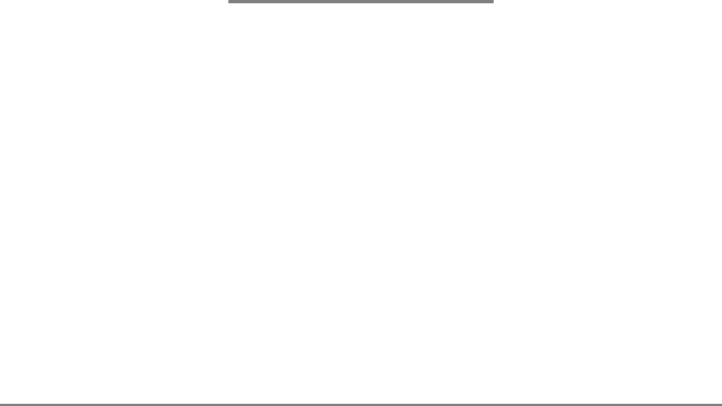
Figure 2.1 illustrates the generation of subsets when n=3. At each function call,
either the upper branch (kis included in the subset) or the lower branch (kis not
included in the subset) is chosen.
2.2.2 Generating Permutations
Next we consider the problem of generating all permutations of a set of nelements.
For example, the permutations of {1,2,3}are (1,2,3),(1,3,2),(2,1,3),(2,3,1),
(3,1,2), and (3,2,1). Again, we can use recursion to perform the search. The fol-
lowing function search maintains a vector
Fig. 2.1 The recursion tree
when generating the subsets
of the set {1,2,3}

2.2 Recursive Algorithms 17
vector<int> permutation;
that will contain each permutation, and an array
bool chosen[n+1];
which indicates for each element if it has been included in the permutation. The
search begins when the function is called without parameters.
void search() {
if (permutation.size() == n) {
// process permutation
}else {
for (int i = 1; i <= n; i++) {
if (chosen[i]) continue;
chosen[i] = true;
permutation.push_back(i);
search();
chosen[i] = false;
permutation.pop_back();
}
}
}
Each function call appends a new element to permutation and records that it
has been included in chosen. If the size of permutation equals the size of the
set, a permutation has been generated.
Note that the C++ standard library also has the function next_permutation
that can be used to generate permutations. The function is given a permutation, and
it produces the next permutation in lexicographic order. The following code goes
through the permutations of {1,2,...,n}:
for (int i = 1; i <= n; i++) {
permutation.push_back(i);
}
do {
// process permutation
}while (next_permutation(permutation.begin(),
permutation.end()));
18 2 Programming Techniques
2.2.3 Backtracking
Abacktracking algorithm begins with an empty solution and extends the solution
step by step. The search recursively goes through all different ways how a solution
can be constructed.
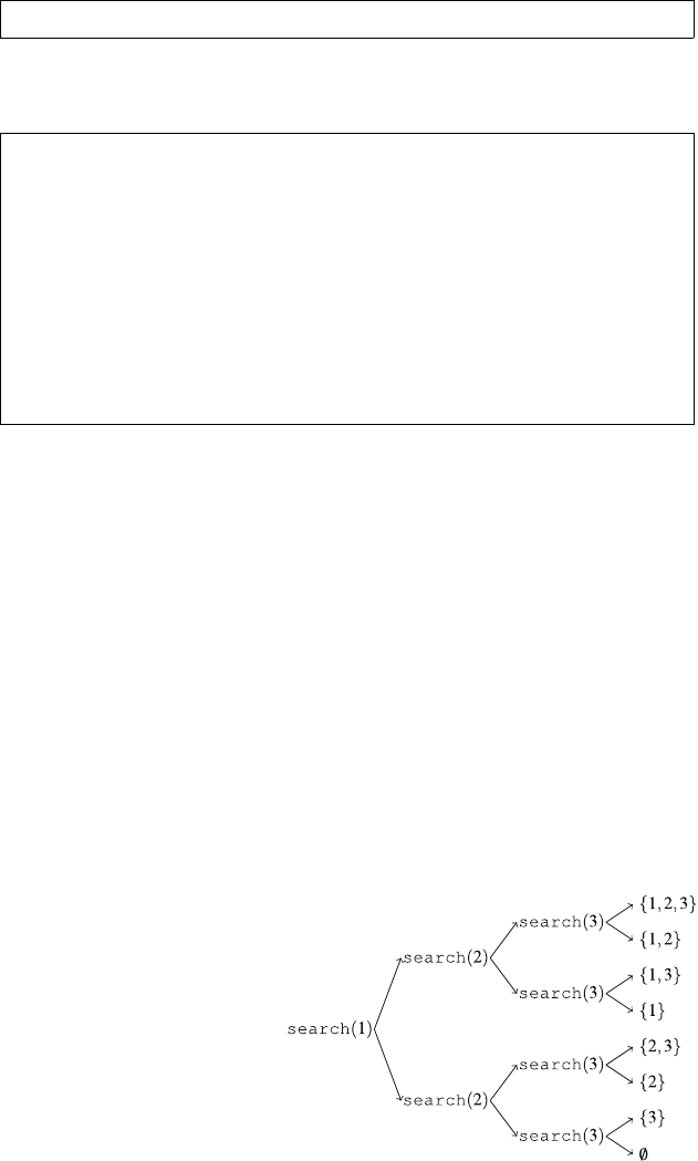
As an example, consider the problem of calculating the number of ways nqueens
can be placed on an n×nchessboard so that no two queens attack each other. For
example, Fig. 2.2 shows the two possible solutions for n=4.
The problem can be solved using backtracking by placing queens on the board
row by row. More precisely, exactly one queen will be placed on each row so that no
queen attacks any of the queens placed before. A solution has been found when all
nqueens have been placed on the board.
For example, Fig. 2.3 shows some partial solutions generated by the backtracking
algorithm when n=4. At the bottom level, the three first configurations are illegal,
because the queens attack each other. However, the fourth configuration is valid, and
it can be extended to a complete solution by placing two more queens on the board.
There is only one way to place the two remaining queens.
Fig. 2.2 The possible ways to place 4 queens on a 4 ×4 chessboard
Fig. 2.3 Partial solutions to the queen problem using backtracking
2.2 Recursive Algorithms 19
The algorithm can be implemented as follows:
void search(int y) {
if (y == n) {
count++;
return;
}
for (int x=0;x<n;x++) {
if (col[x] || diag1[x+y] || diag2[x-y+n-1]) continue;
col[x] = diag1[x+y] = diag2[x-y+n-1] = 1;
search(y+1);
col[x] = diag1[x+y] = diag2[x-y+n-1] = 0;
}
}
The search begins by calling search(0). The size of the board is n, and the
code calculates the number of solutions to count. The code assumes that the rows
and columns of the board are numbered from 0 to n−1. When search is called
with parameter y, it places a queen on row yand then calls itself with parameter
y+1. Then, if y=n, a solution has been found, and the value of count is increased
by one.
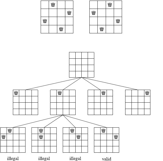
The array col keeps track of the columns that contain a queen, and the arrays
diag1 and diag2 keep track of the diagonals. It is not allowed to add another
queen to a column or diagonal that already contains a queen. For example, Fig. 2.4
shows the numbering of columns and diagonals of the 4 ×4 board.
The above backtracking algorithm tells us that there are 92 ways to place 8 queens
on the 8 ×8 board. When nincreases, the search quickly becomes slow, because
the number of solutions grows exponentially. For example, it takes already about a
minute on a modern computer to calculate that there are 14772512 ways to place 16
queens on the 16 ×16 board.
In fact, nobody knows an efficient way to count the number of queen combinations
for larger values of n. Currently, the largest value of nfor which the result is known is
27: there are 234907967154122528 combinations in this case. This was discovered
in 2016 by a group of researchers who used a cluster of computers to calculate the
result [25].
Fig. 2.4 Numbering of the
arrays when counting the
combinations on the 4 ×4
board
20 2 Programming Techniques
2.3 Bit Manipulation
In programming, an n-bit integer is internally stored as a binary number that consists
of nbits. For example, the C++ type int is a 32-bit type, which means that every
int number consists of 32 bits. For example, the bit representation of the int
number 43 is
00000000000000000000000000101011.
The bits in the representation are indexed from right to left. To convert a bit repre-
sentation bk...b2b1b0into a number, the formula
bk2k+···+b222+b121+b020.
can be used. For example,
1·25+1·23+1·21+1·20=43.
The bit representation of a number is either signed or unsigned. Usually a signed
representation is used, which means that both negative and positive numbers can be
represented. A signed variable of nbits can contain any integer between −2n−1and
2n−1−1. For example, the int type in C++ is a signed type, so an int variable
can contain any integer between −231 and 231 −1.
The first bit in a signed representation is the sign of the number (0 for nonnegative
numbers and 1 for negative numbers), and the remaining n−1 bits contain the
magnitude of the number. Two’s complement is used, which means that the opposite
number of a number is calculated by first inverting all the bits in the number and
then increasing the number by one. For example, the bit representation of the int
number −43 is
11111111111111111111111111010101.
In an unsigned representation, only nonnegative numbers can be used, but the
upper bound for the values is larger. An unsigned variable of nbits can contain any
integer between 0 and 2n−1. For example, in C++, an unsigned int variable
can contain any integer between 0 and 232 −1.
There is a connection between the representations: a signed number −xequals
an unsigned number 2n−x. For example, the following code shows that the signed
number x=−43 equals the unsigned number y=232 −43:
int x = -43;
unsigned int y=x;
cout << x << "\n";
// -43
cout << y << "\n";
// 4294967253
If a number is larger than the upper bound of the bit representation, the number
will overflow. In a signed representation, the next number after 2n−1−1is−2n−1,

2.3 Bit Manipulation 21
and in an unsigned representation, the next number after 2n−1 is 0. For example,
consider the following code:
int x = 2147483647
cout << x << "\n";
// 2147483647
x++;
cout << x << "\n";
// -2147483648
Initially, the value of xis 231 −1. This is the largest value that can be stored in
an int variable, so the next number after 231 −1is−231.
2.3.1 Bit Operations
And Operation The and operation x&yproduces a number that has one bits in
positions where both xand yhave one bits. For example, 22 & 26 =18, because
10110 (22)
& 11010 (26)
=10010 (18).
Using the and operation, we can check if a number xis even because x&1=0
if xis even, and x&1=1ifxis odd. More generally, xis divisible by 2kexactly
when x&(2k−1)=0.
Or Operation The or operation x|yproduces a number that has one bits in positions
where at least one of xand yhave one bits. For example, 22 |26 =30, because
10110 (22)
|11010 (26)
=11110 (30).
Xor Operation The xor operation xˆyproduces a number that has one bits in
positions where exactly one of xand yhave one bits. For example, 22 ˆ 26 =12,
because
10110 (22)
ˆ 11010 (26)
=01100 (12).
Not Operation The not operation ~xproduces a number where all the bits of xhave
been inverted. The formula ~x=−x−1 holds, for example, ~29 =−30. The result
of the not operation at the bit level depends on the length of the bit representation,
22 2 Programming Techniques
because the operation inverts all bits. For example, if the numbers are 32-bit int
numbers, the result is as follows:
x=29 00000000000000000000000000011101
~x=−30 11111111111111111111111111100010
Bit Shifts The left bit shift x << kappends kzero bits to the number, and the right bit
shift x >> kremoves the klast bits from the number. For example, 14 << 2=56,
because 14 and 56 correspond to 1110 and 111000. Similarly, 49 >> 3=6, because
49 and 6 correspond to 110001 and 110. Note that x<< kcorresponds to multiplying
xby 2k, and x>> kcorresponds to dividing xby 2krounded down to an integer.
Bit Masks Abit mask of the form 1 << khas a one bit in position k, and all other
bits are zero, so we can use such masks to access single bits of numbers. In particular,
the kth bit of a number is one exactly when x&(1<< k)is not zero. The following
code prints the bit representation of an int number x:
for (int k=31;k>=0;k--){
if (x&(1<<k)) cout << "1";
else cout << "0";
}
It is also possible to modify single bits of numbers using similar ideas. The formula
x|(1<< k)sets the kth bit of xto one, the formula x&~(1<< k)sets the kth bit
of xto zero, and the formula xˆ(1<< k)inverts the kth bit of x. Then, the formula
x&(x−1)sets the last one bit of xto zero, and the formula x&−xsets all the one
bits to zero, except for the last one bit. The formula x|(x−1)inverts all the bits
after the last one bit. Finally, a positive number xis a power of two exactly when x
&(x−1)=0.
One pitfall when using bit masks is that 1<<k is always an int bit mask. An
easy way to create a long long bit mask is 1LL<<k.
Additional Functions The g++ compiler also provides the following functions for
counting bits:
•__builtin_clz(x): the number of zeros at the beginning of the bit represen-
tation
•__builtin_ctz(x): the number of zeros at the end of the bit representation
•__builtin_popcount(x): the number of ones in the bit representation
•__builtin_parity(x): the parity (even or odd) of the number of ones in the
bit representation
The functions can be used as follows:

2.3 Bit Manipulation 23
int x = 5328;
// 00000000000000000001010011010000
cout << __builtin_clz(x) << "\n";
// 19
cout << __builtin_ctz(x) << "\n";
// 4
cout << __builtin_popcount(x) << "\n";
// 5
cout << __builtin_parity(x) << "\n";
// 1
Note that the above functions only support int numbers, but there are also long
long versions of the functions available with the suffix ll.
2.3.2 Representing Sets
Every subset of a set {0,1,2,...,n−1}can be represented as an nbit integer
whose one bits indicate which elements belong to the subset. This is an efficient way
to represent sets, because every element requires only one bit of memory, and set
operations can be implemented as bit operations.
For example, since int is a 32-bit type, an int number can represent any subset
of the set {0,1,2,...,31}. The bit representation of the set {1,3,4,8}is
00000000000000000000000100011010,
which corresponds to the number 28+24+23+21=282.
The following code declares an int variable xthat can contain a subset of
{0,1,2,...,31}. After this, the code adds the elements 1, 3, 4, and 8 to the set
and prints the size of the set.
int x=0;
x |= (1<<1);
x |= (1<<3);
x |= (1<<4);
x |= (1<<8);
cout << __builtin_popcount(x) << "\n";
// 4
Then, the following code prints all elements that belong to the set:
for (int i = 0; i < 32; i++) {
if (x&(1<<i)) cout << i << " ";
}
// output:1348
Set Operations Table 2.1 shows how set operations can be implemented as bit
operations. For example, the following code first constructs the sets x={1,3,4,8}
and y={3,6,8,9}and then constructs the set z=x∪y={1,3,4,6,8,9}:

24 2 Programming Techniques
Table 2.1 Implementing set operations as bit operations
Operation Set syntax Bit syntax
Intersection a∩b a &b
Union a∪b a |b
Complement ¯a~a
Difference a\b a &(
~b)
int x = (1<<1)|(1<<3)|(1<<4)|(1<<8);
int y = (1<<3)|(1<<6)|(1<<8)|(1<<9);
int z=x|y;
cout << __builtin_popcount(z) << "\n";
// 6
The following code goes through the subsets of {0,1,...,n−1}:
for (int b = 0; b < (1<<n); b++) {
// process subset b
}
Then, the following code goes through the subsets with exactly kelements:
for (int b = 0; b < (1<<n); b++) {
if (__builtin_popcount(b) == k) {
// process subset b
}
}
Finally, the following code goes through the subsets of a set x:
int b=0;
do {
// process subset b
}while (b=(b-x)&x);
C++ Bitsets The C++ standard library also provides the bitset structure, which
corresponds to an array whose each value is either 0 or 1. For example, the following
code creates a bitset of 10 elements:
2.3 Bit Manipulation 25
bitset<10> s;
s[1] = 1;
s[3] = 1;
s[4] = 1;
s[7] = 1;
cout << s[4] << "\n";
// 1
cout << s[5] << "\n";
// 0
The function count returns the number of one bits in the bitset:
cout << s.count() << "\n";
// 4
Also bit operations can be directly used to manipulate bitsets:
bitset<10> a, b;
// ...
bitset<10> c = a&b;
bitset<10> d = a|b;
bitset<10> e = a^b;

Efficiency
The efficiency of algorithms plays a central role in competitive programming. In this
chapter, we learn tools that make it easier to design efficient algorithms.
Section 3.1 introduces the concept of time complexity, which allows us to estimate
running times of algorithms without implementing them. The time complexity of an
algorithm shows how quickly its running time increases when the size of the input
grows.
Section 3.2 presents two example problems which can be solved in many ways.
In both problems, we can easily design a slow brute force solution, but it turns out
that we can also create much more efficient algorithms.
3.1 Time Complexity
The time complexity of an algorithm estimates how much time the algorithm will use
for a given input. By calculating the time complexity, we can often find out whether
the algorithm is fast enough for solving a problem—without implementing it.
A time complexity is denoted O(···)where the three dots represent some func-
tion. Usually, the variable ndenotes the input size. For example, if the input is an
array of numbers, nwill be the size of the array, and if the input is a string, nwill be
the length of the string.
3.1.1 Calculation Rules
If a code consists of single commands, its time complexity is O(1). For example,
the time complexity of the following code is O(1).

28 3Efficiency
a++;
b++;
c=a+b;
The time complexity of a loop estimates the number of times the code inside the
loop is executed. For example, the time complexity of the following code is O(n),
because the code inside the loop is executed ntimes. We assume that “...” denotes
a code whose time complexity is O(1).
for (int i = 1; i <= n; i++) {
...
}
Then, the time complexity of the following code is O(n2):
for (int i = 1; i <= n; i++) {
for (int j=1;j<=n;j++){
...
}
}
In general, if there are knested loops and each loop goes through nvalues, the
time complexity is O(nk).
A time complexity does not tell us the exact number of times the code inside a
loop is executed, because it only shows the order of growth and ignores the constant
factors. In the following examples, the code inside the loop is executed 3n,n+5,
and n/2times, but the time complexity of each code is O(n).
for (int i = 1; i <= 3*n; i++) {
...
}
for (int i = 1; i <= n+5; i++) {
...
}
for (int i=1;i<=n;i+=2){
...
}
As another example, the time complexity of the following code is O(n2), because
the code inside the loop is executed 1 +2+...+n=1
2(n2+n)times.

3.1 Time Complexity 29
for (int i = 1; i <= n; i++) {
for (int j=1;j<=i;j++){
...
}
}
If an algorithm consists of consecutive phases, the total time complexity is the
largest time complexity of a single phase. The reason for this is that the slowest
phase is the bottleneck of the algorithm. For example, the following code consists
of three phases with time complexities O(n),O(n2), and O(n). Thus, the total time
complexity is O(n2).
for (int i = 1; i <= n; i++) {
...
}
for (int i = 1; i <= n; i++) {
for (int j=1;j<=n;j++){
...
}
}
for (int i = 1; i <= n; i++) {
...
}
Sometimes the time complexity depends on several factors, and the time com-
plexity formula contains several variables. For example, the time complexity of the
following code is O(nm):
for (int i = 1; i <= n; i++) {
for (int j=1;j<=m;j++){
...
}
}
The time complexity of a recursive function depends on the number of times the
function is called and the time complexity of a single call. The total time complexity
is the product of these values. For example, consider the following function:
void f(int n) {
if (n == 1) return;
f(n-1);
}
The call f(n)causes nfunction calls, and the time complexity of each call is
O(1), so the total time complexity is O(n).
As another example, consider the following function:

30 3Efficiency
void g(int n) {
if (n == 1) return;
g(n-1);
g(n-1);
}
What happens when the function is called with a parameter n? First, there are two
calls with parameter n−1, then four calls with parameter n−2, then eight calls with
parameter n−3, and so on. In general, there will be 2kcalls with parameter n−k
where k=0,1,...,n−1. Thus, the time complexity is
1+2+4+···+2n−1=2n−1=O(2n).
3.1.2 Common Time Complexities
The following list contains common time complexities of algorithms:
O(1)The running time of a constant-time algorithm does not depend on the input
size. A typical constant-time algorithm is a direct formula that calculates the
answer.
O(log n)Alogarithmic algorithm often halves the input size at each step. The
running time of such an algorithm is logarithmic, because log2nequals the number
of times nmust be divided by 2 to get 1. Note that the base of the logarithm is not
shown in the time complexity.
O(√n)Asquare root algorithm is slower than O(log n)but faster than O(n).A
special property of square roots is that √n=n/√n,sonelements can be divided
into O(√n)blocks of O(√n)elements.
O(n)Alinear algorithm goes through the input a constant number of times. This
is often the best possible time complexity, because it is usually necessary to access
each input element at least once before reporting the answer.
O(nlog n)This time complexity often indicates that the algorithm sorts the input,
because the time complexity of efficient sorting algorithms is O(nlog n). Another
possibility is that the algorithm uses a data structure where each operation takes
O(log n)time.
O(n2)Aquadratic algorithm often contains two nested loops. It is possible to go
through all pairs of the input elements in O(n2)time.
O(n3)Acubic algorithm often contains three nested loops. It is possible to go
through all triplets of the input elements in O(n3)time.
O(2n)This time complexity often indicates that the algorithm iterates through all
subsets of the input elements. For example, the subsets of {1,2,3}are ∅,{1},{2},
{3},{1,2},{1,3},{2,3}, and {1,2,3}.
O(n!)This time complexity often indicates that the algorithm iterates through all
permutations of the input elements. For example, the permutations of {1,2,3}are
(1,2,3),(1,3,2),(2,1,3),(2,3,1),(3,1,2), and (3,2,1).
3.1 Time Complexity 31
An algorithm is polynomial if its time complexity is at most O(nk)where kis a
constant. All the above time complexities except O(2n)and O(n!)are polynomial. In
practice, the constant kis usually small, and therefore a polynomial time complexity
roughly means that the algorithm can process large inputs.
Most algorithms in this book are polynomial. Still, there are many important
problems for which no polynomial algorithm is known, i.e., nobody knows how to
solve them efficiently. NP-hard problems are an important set of problems, for which
no polynomial algorithm is known.
3.1.3 Estimating Efficiency
By calculating the time complexity of an algorithm, it is possible to check, before
implementing the algorithm, that it is efficient enough for solving a problem. The
starting point for estimations is the fact that a modern computer can perform some
hundreds of millions of simple operations in a second.
For example, assume that the time limit for a problem is one second and the
input size is n=105. If the time complexity is O(n2), the algorithm will perform
about (105)2=1010 operations. This should take at least some tens of seconds, so
the algorithm seems to be too slow for solving the problem. However, if the time
complexity is O(nlog n), there will be only about 105log 105≈1.6·106operations,
and the algorithm will surely fit the time limit.
On the other hand, given the input size, we can try to guess the required time
complexity of the algorithm that solves the problem. Table 3.1 contains some useful
estimates assuming a time limit of one second.
For example, if the input size is n=105, it is probably expected that the time
complexity of the algorithm is O(n)or O(nlog n). This information makes it easier
to design the algorithm, because it rules out approaches that would yield an algorithm
with a worse time complexity.
Still, it is important to remember that a time complexity is only an estimate of
efficiency, because it hides the constant factors. For example, an algorithm that runs
in O(n)time may perform n/2or5noperations, which has an important effect on
the actual running time of the algorithm.
Table 3.1 Estimating time complexity from input size
Input size Expected time complexity
n≤10 O(n!)
n≤20 O(2n)
n≤500 O(n3)
n≤5000 O(n2)
n≤106O(nlog n)or O(n)
nis large O(1)or O(log n)
32 3Efficiency
3.1.4 Formal Definitions
What does it exactly mean that an algorithm works in O(f(n)) time? It means
that there are constants cand n0such that the algorithm performs at most c f (n)
operations for all inputs where n≥n0. Thus, the Onotation gives an upper bound
for the running time of the algorithm for sufficiently large inputs.
For example, it is technically correct to say that the time complexity of the fol-
lowing algorithm is O(n2).
for (int i = 1; i <= n; i++) {
...
}
However, a better bound is O(n), and it would be very misleading to give the
bound O(n2), because everybody actually assumes that the Onotation is used to
give an accurate estimate of the time complexity.
There are also two other common notations. The Ωnotation gives a lower bound
for the running time of an algorithm. The time complexity of an algorithm is Ω( f(n)),
if there are constants cand n0such that the algorithm performs at least c f (n)
operations for all inputs where n≥n0. Finally, the Θnotation gives an exact bound:
the time complexity of an algorithm is Θ( f(n)) if it is both O(f(n)) and Ω( f(n)).
For example, since the time complexity of the above algorithm is both O(n)and
Ω(n), it is also Θ(n).
We can use the above notations in many situations, not only for referring to time
complexities of algorithms. For example, we might say that an array contains O(n)
values, or that an algorithm consists of O(log n)rounds.
3.2 Examples
In this section we discuss two algorithm design problems that can be solved in several
different ways. We start with simple brute force algorithms, and then create more
efficient solutions by using various algorithm design ideas.
3.2.1 Maximum Subarray Sum
Given an array of nnumbers, our first task is to calculate the maximum subarray sum,
i.e., the largest possible sum of a sequence of consecutive values in the array. The
problem is interesting when there may be negative values in the array. For example,
Fig. 3.1 shows an array and its maximum-sum subarray.
3.2 Examples 33
Fig. 3.1 The maximum-sum
subarray of this array is
[2,4,−3,5,2], whose sum
is 10
O(n3)Time Solution A straightforward way to solve the problem is to go through
all possible subarrays, calculate the sum of values in each subarray and maintain the
maximum sum. The following code implements this algorithm:
int best = 0;
for (int a=0;a<n;a++){
for (int b=a;b<n;b++) {
int sum = 0;
for (int k = a; k <= b; k++) {
sum += array[k];
}
best = max(best,sum);
}
}
cout << best << "\n";
The variables aand bfix the first and last index of the subarray, and the sum of
values is calculated to the variable sum. The variable best contains the maximum
sum found during the search. The time complexity of the algorithm is O(n3), because
it consists of three nested loops that go through the input.
O(n2)Time Solution It is easy to make the algorithm more efficient by removing
one loop from it. This is possible by calculating the sum at the same time when the
right end of the subarray moves. The result is the following code:
int best = 0;
for (int a=0;a<n;a++){
int sum = 0;
for (int b=a;b<n;b++) {
sum += array[b];
best = max(best,sum);
}
}
cout << best << "\n";
After this change, the time complexity is O(n2).
O(n)Time Solution It turns out that it is possible to solve the problem in O(n)time,
which means that just one loop is enough. The idea is to calculate, for each array
position, the maximum sum of a subarray that ends at that position. After this, the
answer to the problem is the maximum of those sums.
34 3Efficiency
Consider the subproblem of finding the maximum-sum subarray that ends at posi-
tion k. There are two possibilities:
1. The subarray only contains the element at position k.
2. The subarray consists of a subarray that ends at position k−1, followed by the
element at position k.
In the latter case, since we want to find a subarray with maximum sum, the subarray
that ends at position k−1 should also have the maximum sum. Thus, we can solve
the problem efficiently by calculating the maximum subarray sum for each ending
position from left to right.
The following code implements the algorithm:
int best = 0, sum = 0;
for (int k=0;k<n;k++){
sum = max(array[k],sum+array[k]);
best = max(best,sum);
}
cout << best << "\n";
The algorithm only contains one loop that goes through the input, so the time
complexity is O(n). This is also the best possible time complexity, because any
algorithm for the problem has to examine all array elements at least once.
Efficiency Comparison How efficient are the above algorithms in practice? Table 3.2
shows the running times of the above algorithms for different values of non a modern
computer. In each test, the input was generated randomly, and the time needed for
reading the input was not measured.
The comparison shows that all algorithms work quickly when the input size is
small, but larger inputs bring out remarkable differences in the running times. The
O(n3)algorithm becomes slow when n=104, and the O(n2)algorithm becomes
slow when n=105. Only the O(n)algorithm is able to process even the largest
inputs instantly.
Table 3.2 Comparing running times of the maximum subarray sum algorithms
Array size n O(n3)(s) O(n2)(s) O(n)(s)
1020.0 0.0 0.0
1030.1 0.0 0.0
104>10.0 0.1 0.0
105>10.0 5.3 0.0
106>10.0>10.0 0.0
107>10.0>10.0 0.0
3.2 Examples 35
3.2.2 Two Queens Problem
Given an n×nchessboard, our next problem is to count the number of ways we can
place two queens on the board in such a way that they do not attack each other. For
example, as Fig. 3.2 shows, there are eight ways to place two queens on the 3 ×3
board. Let q(n)denote the number of valid combinations for an n×nboard. For
example, q(3)=8, and Table 3.3 shows the values of q(n)for 1 ≤n≤10.
To start with, a simple way to solve the problem is to go through all possible ways
to place two queens on the board and count the combinations where the queens do
not attack each other. Such an algorithm works in O(n4)time, because there are n2
ways to choose the position of the first queen, and for each such position, there are
n2−1 ways to choose the position of the second queen.
Since the number of combinations grows fast, an algorithm that counts combina-
tions one by one will certainly be too slow for processing larger values of n. Thus, to
create an efficient algorithm, we need to find a way to count combinations in groups.
One useful observation is that it is quite easy to calculate the number of squares that
a single queen attacks (Fig. 3.3). First, it always attacks n−1 squares horizontally
and n−1 squares vertically. Then, for both diagonals, it attacks d−1 squares where
dis the number of squares on the diagonal. Using this information, we can calculate
Fig. 3.2 All possible ways
to place two non-attacking
queens on the 3 ×3
chessboard
Table 3.3 First values of the
function q(n): the number of
ways to place two
non-attacking queens on an
n×nchessboard
Board size nNumber of ways q(n)
1 0
2 0
3 8
444
5140
6340
7700
81288
92184
10 3480
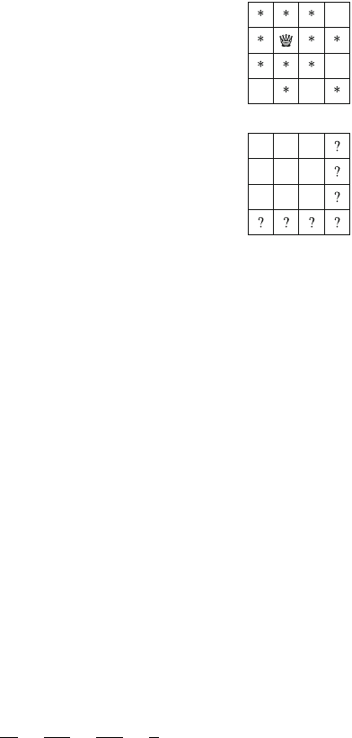
36 3Efficiency
Fig. 3.3 The queen attacks
all squares marked with “*”
on the board
Fig. 3.4 Possible positions
for queens on the last row
and column
in O(1)time the number of squares where the other queen can be placed, which
yields an O(n2)time algorithm.
Another way to approach the problem is to try to formulate a recursive function
that counts the number of combinations. The question is: if we know the value of
q(n), how can we use it to calculate the value of q(n+1)?
To get a recursive solution, we may focus on the last row and last column of the n×
nboard (Fig. 3.4). First, if there are no queens on the last row or column, the number
of combinations is simply q(n−1). Then, there are 2n−1 positions for a queen on
the last row or column. It attacks 3(n−1)squares, so there are n2−3(n−1)−1
positions for the other queen. Finally, there are (n−1)(n−2)combinations where
both queens are on the last row or column. Since we counted those combinations
twice, we have to remove this number from the result. By combining all this, we get
a recursive formula
q(n)=q(n−1)+(2n−1)(n2−3(n−1)−1)−(n−1)(n−2)
=q(n−1)+2(n−1)2(n−2),
which provides an O(n)solution to the problem.
Finally, it turns out that there is also a closed-form formula
q(n)=n4
2−5n3
3+3n2
2−n
3,
which can be proved using induction and the recursive formula. Using this formula,
we can solve the problem in O(1)time.

Sorting and Searching
Many efficient algorithms are based on sorting the input data, because sorting often
makes solving the problem easier. This chapter discusses the theory and practice of
sorting as an algorithm design tool.
Section 4.1 first discusses three important sorting algorithms: bubble sort, merge
sort, and counting sort. After this, we will learn how to use the sorting algorithm
available in the C++ standard library.
Section 4.2 shows how sorting can be used as a subroutine to create efficient
algorithms. For example, to quickly determine if all array elements are unique, we
can first sort the array and then simply check all pairs of consecutive elements.
Section 4.3 presents the binary search algorithm, which is another important build-
ing block of efficient algorithms.
4.1 Sorting Algorithms
The basic problem in sorting is as follows: Given an array that contains nelements,
sort the elements in increasing order. For example, Fig. 4.1 shows an array before
and after sorting.
In this section we will go through some fundamental sorting algorithms and exam-
ine their properties. It is easy to design an O(n2)time sorting algorithm, but there
are also more efficient algorithms. After discussing the theory of sorting, we will
focus on using sorting in practice in C++.
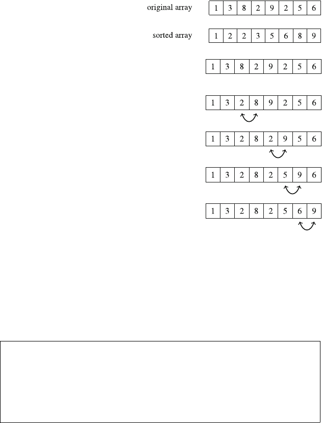
38 4 Sorting and Searching
Fig. 4.1 An array before and
after sorting
Fig. 4.2 The first round of
bubble sort
4.1.1 Bubble Sort
Bubble sort is a simple sorting algorithm that works in O(n2)time. The algorithm
consists of nrounds, and on each round, it iterates through the elements of the array.
Whenever two consecutive elements are found that are in wrong order, the algorithm
swaps them. The algorithm can be implemented as follows:
for (int i=0;i<n;i++){
for (int j = 0; j < n-1; j++) {
if (array[j] > array[j+1]) {
swap(array[j],array[j+1]);
}
}
}
After the first round of bubble sort, the largest element will be in the correct
position, and more generally, after krounds, the klargest elements will be in the
correct positions. Thus, after nrounds, the whole array will be sorted.
For example, Fig. 4.2 shows the first round of swaps when bubble sort is used to
sort an array.
Bubble sort is an example of a sorting algorithm that always swaps consecutive
elements in the array. It turns out that the time complexity of such an algorithm
is always at least O(n2), because in the worst case, O(n2)swaps are required for
sorting the array.
4.1 Sorting Algorithms 39
Fig. 4.3 This array has three
inversions: (3,4),(3,5),and
(6,7)
Inversions A useful concept when analyzing sorting algorithms is an inversion:a
pair of array indices (a,b)such that a<band array[a]>array[b], i.e., the
elements are in wrong order. For example, the array in Fig. 4.3 has three inversions:
(3,4),(3,5), and (6,7).
The number of inversions indicates how much work is needed to sort the array.
An array is completely sorted when there are no inversions. On the other hand, if the
array elements are in the reverse order, the number of inversions is
1+2+···+(n−1)=n(n−1)
2=O(n2),
which is the largest possible.
Swapping a pair of consecutive elements that are in the wrong order removes
exactly one inversion from the array. Hence, if a sorting algorithm can only swap
consecutive elements, each swap removes at most one inversion, and the time com-
plexity of the algorithm is at least O(n2).
4.1.2 Merge Sort
If we want to create an efficient sorting algorithm, we have to be able to reorder
elements that are in different parts of the array. There are several such sorting algo-
rithms that work in O(nlog n)time. One of them is merge sort, which is based on
recursion. Merge sort sorts a subarray array[a...b]as follows:
1. If a=b, do not do anything, because a subarray that only contains one element
is already sorted.
2. Calculate the position of the middle element: k=(a+b)/2.
3. Recursively sort the subarray array[a...k].
4. Recursively sort the subarray array[k+1...b].
5. Merge the sorted subarrays array[a...k]and array[k+1...b]into a sorted
subarray array[a...b].
For example, Fig. 4.4 shows how merge sort sorts an array of eight elements. First,
the algorithm divides the array into two subarrays of four elements. Then, it sorts
these subarrays recursively by calling itself. Finally, it merges the sorted subarrays
into a sorted array of eight elements.
Merge sort is an efficient algorithm, because it halves the size of the subarray at
each step. Then, merging the sorted subarrays is possible in linear time, because they
are already sorted. Since there are O(log n)recursive levels, and processing each
level takes a total of O(n)time, the algorithm works in O(nlog n)time.
40 4 Sorting and Searching
Fig. 4.4 Sorting an array
using merge sort
Fig. 4.5 The progress of a
sorting algorithm that
compares array elements
4.1.3 Sorting Lower Bound
Is it possible to sort an array faster than in O(nlog n)time? It turns out that this
is not possible when we restrict ourselves to sorting algorithms that are based on
comparing array elements.
The lower bound for the time complexity can be proved by considering sorting as
a process where each comparison of two elements gives more information about the
contents of the array. Figure 4.5 illustrates the tree created in this process.
Here “x<y?” means that some elements xand yare compared. If x<y, the
process continues to the left, and otherwise to the right. The results of the process
are the possible ways to sort the array, a total of n!ways. For this reason, the height
of the tree must be at least
log2(n!)=log2(1)+log2(2)+···+log2(n).
We get a lower bound for this sum by choosing the last n/2 elements and changing
the value of each element to log2(n/2). This yields an estimate
log2(n!)≥(n/2)·log2(n/2),
so the height of the tree and the worst-case number of steps in a sorting algorithm is
Ω(nlog n).
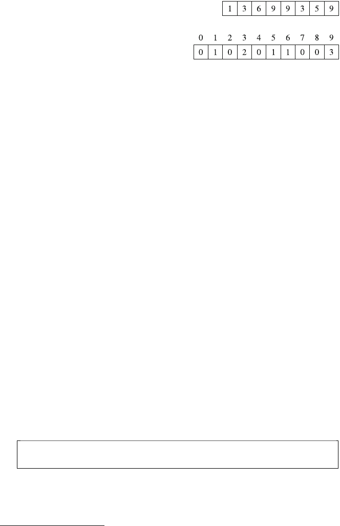
4.1 Sorting Algorithms 41
Fig. 4.6 Sorting an array
using counting sort
4.1.4 Counting Sort
The lower bound Ω(nlog n)does not apply to algorithms that do not compare array
elements but use some other information. An example of such an algorithm is count-
ing sort that sorts an array in O(n)time assuming that every element in the array is
an integer between 0 ...cand c=O(n).
The algorithm creates a bookkeeping array, whose indices are elements of the
original array. The algorithm iterates through the original array and calculates how
many times each element appears in the array. As an example, Fig. 4.6 shows an
array and the corresponding bookkeeping array. For example, the value at position
3 is 2, because the value 3 appears 2 times in the original array.
The construction of the bookkeeping array takes O(n)time. After this, the sorted
array can be created in O(n)time, because the number of occurrences of each element
can be retrieved from the bookkeeping array. Thus, the total time complexity of
counting sort is O(n).
Counting sort is a very efficient algorithm but it can only be used when the constant
cis small enough, so that the array elements can be used as indices in the bookkeeping
array.
4.1.5 Sorting in Practice
In practice, it is almost never a good idea to implement a home-made sorting algo-
rithm, because all modern programming languages have good sorting algorithms
in their standard libraries. There are many reasons to use a library function: it is
certainly correct and efficient, and also easy to use.
In C++, the function sort efficiently1sorts the contents of a data structure. For
example, the following code sorts the elements of a vector in increasing order:
vector<int> v = {4,2,5,3,5,8,3};
sort(v.begin(),v.end());
After the sorting, the contents of the vector will be [2,3,3,4,5,5,8]. The default
sorting order is increasing, but a reverse order is possible as follows:
1The C++11 standard requires that the sort function works in O(nlog n)time; the exact imple-
mentation depends on the compiler.

42 4 Sorting and Searching
sort(v.rbegin(),v.rend());
An ordinary array can be sorted as follows:
int n=7;
// array size
int a[] = {4,2,5,3,5,8,3};
sort(a,a+n);
Then, the following code sorts the string s:
string s = "monkey";
sort(s.begin(), s.end());
Sorting a string means that the characters of the string are sorted. For example,
the string “monkey” becomes “ekmnoy”.
Comparison Operators The sort function requires that a comparison operator is
defined for the data type of the elements to be sorted. When sorting, this operator
will be used whenever it is necessary to find out the order of two elements.
Most C++ data types have a built-in comparison operator, and elements of those
types can be sorted automatically. Numbers are sorted according to their values, and
strings are sorted in alphabetical order. Pairs are sorted primarily according to their
first elements and secondarily according to their second elements:
vector<pair<int,int>> v;
v.push_back({1,5});
v.push_back({2,3});
v.push_back({1,2});
sort(v.begin(), v.end());
// result: [(1,2),(1,5),(2,3)]
In a similar way, tuples are sorted primarily by the first element, secondarily by
the second element, etc.2:
vector<tuple<int,int,int>> v;
v.push_back({2,1,4});
v.push_back({1,5,3});
v.push_back({2,1,3});
sort(v.begin(), v.end());
// result: [(1,5,3),(2,1,3),(2,1,4)]
User-defined structs do not have a comparison operator automatically. The opera-
tor should be defined inside the struct as a function operator<, whose parameter
2Note that in some older compilers, the function make_tuple has to be used to create a tuple
instead of braces (for example, make_tuple(2,1,4) instead of {2,1,4}).

4.1 Sorting Algorithms 43
is another element of the same type. The operator should return true if the element
is smaller than the parameter, and false otherwise.
For example, the following struct point contains the x and y coordinates of a
point. The comparison operator is defined so that the points are sorted primarily by
the x coordinate and secondarily by the y coordinate.
struct point {
int x, y;
bool operator<(const point &p) {
if (x == p.x) return y < p.y;
else return x < p.x;
}
};
Comparison Functions It is also possible to give an external comparison function
to the sort function as a callback function. For example, the following comparison
function comp sorts strings primarily by length and secondarily by alphabetical
order:
bool comp(string a, string b) {
if (a.size() == b.size()) return a<b;
else return a.size() < b.size();
}
Now a vector of strings can be sorted as follows:
sort(v.begin(), v.end(), comp);
4.2 Solving Problems by Sorting
Often, we can easily solve a problem in O(n2)time using a brute force algorithm,
but such an algorithm is too slow if the input size is large. In fact, a frequent goal
in algorithm design is to find O(n)or O(nlog n)time algorithms for problems that
can be trivially solved in O(n2)time. Sorting is one way to achieve this goal.
For example, suppose that we want to check if all elements in an array are unique.
A brute force algorithm goes through all pairs of elements in O(n2)time:
bool ok = true;
for (int i=0;i<n;i++){
for (int j = i+1; j < n; j++) {
if (array[i] == array[j]) ok = false;
}
}
44 4 Sorting and Searching
However, we can solve the problem in O(nlog n)time by first sorting the array.
Then, if there are equal elements, they are next to each other in the sorted array, so
they are easy to find in O(n)time:
bool ok = true;
sort(array, array+n);
for (int i=0;i<n-1;i++){
if (array[i] == array[i+1]) ok = false;
}
Several other problems can be solved in a similar way in O(nlog n)time, such
as counting the number of distinct elements, finding the most frequent element, and
finding two elements whose difference is minimum.
4.2.1 Sweep Line Algorithms
Asweep line algorithm models a problem as a set of events that are processed in
a sorted order. For example, suppose that there is a restaurant and we know the
arriving and leaving times of all customers on a certain day. Our task is to find out
the maximum number of customers who visited the restaurant at the same time.
For example, Fig. 4.7 shows an instance of the problem where there are four
customers A,B,C, and D. In this case, the maximum number of simultaneous
customers is three between A’s arrival and B’s leaving.
To solve the problem, we create two events for each customer: one event for
arrival and another event for leaving. Then, we sort the events and go through them
according to their times. To find the maximum number of customers, we maintain
a counter whose value increases when a customer arrives and decreases when a
customer leaves. The largest value of the counter is the answer to the problem.
Figure 4.8 shows the events in our example scenario. Each customer is assigned
two events: “+” denotes an arriving customer and “−” denotes a leaving customer.
The resulting algorithm works in O(nlog n)time, because sorting the events takes
O(nlog n)time and the sweep line part takes O(n)time.
Fig. 4.7 An instance of the
restaurant problem
Fig. 4.8 Solving the
restaurant problem using a
sweep line algorithm
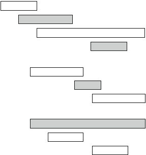
4.2 Solving Problems by Sorting 45
Fig. 4.9 An instance of the
scheduling problem and an
optimal solution with two
events
Fig. 4.10 If we select the
short event, we can only
select one event, but we
could select both long events
Fig. 4.11 If we select the
first event, we cannot select
any other events, but we
could to select the other two
events
4.2.2 Scheduling Events
Many scheduling problems can be solved by sorting the input data and then using a
greedy strategy to construct a solution. A greedy algorithm always makes a choice
that looks the best at the moment and never takes back its choices.
As an example, consider the following problem: Given nevents with their starting
and ending times, find a schedule that includes as many events as possible. For
example, Fig. 4.9 shows an instance of the problem where an optimal solution is to
select two events.
In this problem, there are several ways how we could sort the input data. One
strategy is to sort the events according to their lengths and select as short events as
possible. However, this strategy does not always work, as shown in Fig. 4.10. Then,
another idea is to sort the events according to their starting times and always select
the next possible event that begins as early as possible. However, we can find a
counterexample also for this strategy, shown in Fig. 4.11.
A third idea is to sort the events according to their ending times and always select
the next possible event that ends as early as possible. It turns out that this algorithm
always produces an optimal solution. To justify this, consider what happens if we
first select an event that ends later than the event that ends as early as possible. Now,
we will have at most an equal number of choices left how we can select the next
event. Hence, selecting an event that ends later can never yield a better solution, and
the greedy algorithm is correct.
4.2.3 Tasks and Deadlines
Finally, consider a problem where we are given ntasks with durations and deadlines
and our task is to choose an order to perform the tasks. For each task, we earn d−x
points where dis the task’s deadline and xis the moment when we finish the task.
What is the largest possible total score we can obtain?
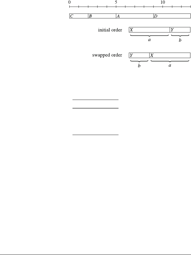
46 4 Sorting and Searching
Fig. 4.12 An optimal
schedule for the tasks
Fig. 4.13 Improving the
solution by swapping tasks
Xand Y
For example, suppose that the tasks are as follows:
task duration deadline
A42
B310
C28
D415
Figure 4.12 shows an optimal schedule for the tasks in our example scenario.
Using this schedule, Cyields 6 points, Byields 5 points, Ayields −7 points, and D
yields 2 points, so the total score is 6.
It turns out that the optimal solution to the problem does not depend on the
deadlines at all, but a correct greedy strategy is to simply perform the tasks sorted
by their durations in increasing order. The reason for this is that if we ever perform
two tasks one after another such that the first task takes longer than the second task,
we can obtain a better solution if we swap the tasks.
For example, in Fig. 4.13, there are two tasks Xand Ywith durations aand
b. Initially, Xis scheduled before Y. However, since a>b, the tasks should be
swapped. Now Xgives bpoints less and Ygives apoints more, so the total score
increases by a−b>0. Thus, in an optimal solution, a shorter task must always
come before a longer task, and the tasks must be sorted by their durations.
4.3 Binary Search
Binary search is an O(log n)time algorithm that can be used, for example, to effi-
ciently check whether a sorted array contains a given element. In this section, we
first focus on the implementation of binary search, and after that, we will see how
binary search can be used to find optimal solutions for problems.
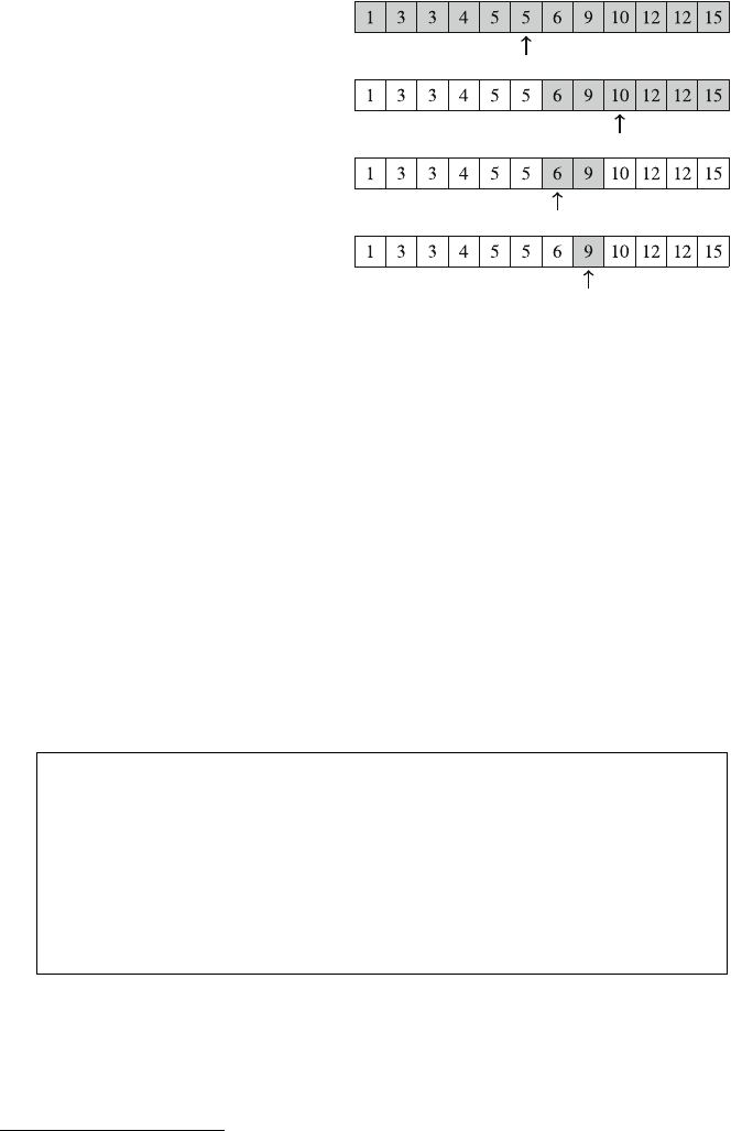
4.3 Binary Search 47
Fig. 4.14 The traditional
way to implement binary
search. At each step we
check the middle element of
the active subarray and
proceed to the left or right
part
4.3.1 Implementing the Search
Suppose that we are given a sorted array of nelements and we want to check if
the array contains an element with a target value x. Next we discuss two ways to
implement a binary search algorithm for this problem.
First Method The most common way to implement binary search resembles looking
for a word in a dictionary.3The search maintains an active subarray in the array, which
initially contains all array elements. Then, a number of steps are performed, each of
which halves the search range. At each step, the search checks the middle element of
the active subarray. If the middle element has the target value, the search terminates.
Otherwise, the search recursively continues to the left or right half of the subarray,
depending on the value of the middle element. For example, Fig. 4.14 shows how an
element with value 9 is found in the array.
The search can be implemented as follows:
int a = 0, b = n-1;
while (a <= b) {
int k = (a+b)/2;
if (array[k] == x) {
// x found at index k
}
if (array[k] < x) a = k+1;
else b = k-1;
}
In this implementation, the range of the active subarray is a...b, and the initial
range is 0 ...n−1. The algorithm halves the size of the subarray at each step, so
the time complexity is O(log n).
3Some people, including the author of this book, still use printed dictionaries. Another example is
finding a phone number in a printed phone book, which is even more obsolete.
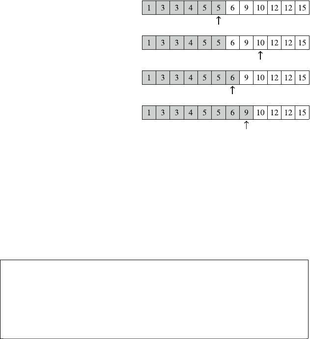
48 4 Sorting and Searching
Fig. 4.15 An alternative
way to implement binary
search. We scan the array
from left to right jumping
over elements
Second Method Another way to implement binary search is to go through the array
from left to right making jumps. The initial jump length is n/2, and the jump length
is halved on each round: first n/4, then n/8, then n/16, etc., until finally the length
is 1. On each round, we make jumps until we would end up outside the array or in
an element whose value exceeds the target value. After the jumps, either the desired
element has been found or we know that it does not appear in the array. Figure 4.15
illustrates the technique in our example scenario.
The following code implements the search:
int k=0;
for (int b = n/2; b >= 1; b /= 2) {
while (k+b < n && array[k+b] <= x) k += b;
}
if (array[k] == x) {
// x found at index k
}
During the search, the variable bcontains the current jump length. The time
complexity of the algorithm is O(log n), because the code in the while loop is
performed at most twice for each jump length.
4.3.2 Finding Optimal Solutions
Suppose that we are solving a problem and have a function valid(x)that returns
true if xis a valid solution and false otherwise. In addition, we know that
valid(x)is false when x<kand true when x≥k. In this situation, we can
use binary search to efficiently find the value of k.
The idea is to binary search for the largest value of xfor which valid(x)is
false. Thus, the next value k=x+1 is the smallest possible value for which
valid(k)is true. The search can be implemented as follows:
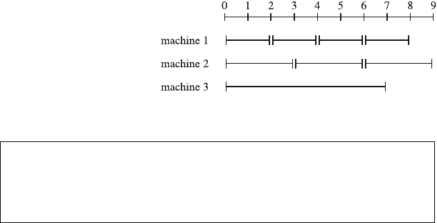
4.3 Binary Search 49
Fig. 4.16 An optimal
processing schedule:
machine 1 processes four
jobs, machine 2 processes
three jobs, and machine 3
processes one job
int x = -1;
for (int b=z;b>=1;b/=2){
while (!valid(x+b)) x += b;
}
int k = x+1;
The initial jump length zhas to be an upper bound for the answer, i.e., any value
for which we surely know that valid(z)is true. The algorithm calls the function
valid O(log z)times, so the running time depends on the function valid.For
example, if the function works in O(n)time, the running time is O(nlog z).
Example Consider a problem where our task is to process kjobs using nmachines.
Each machine iis assigned an integer pi: the time to process a single job. What is
the minimum time to process all the jobs?
For example, suppose that k=8, n=3 and the processing times are p1=2,
p2=3, and p3=7. In this case, the minimum total processing time is 9, by following
the schedule in Fig. 4.16.
Let valid(x)be a function that finds out whether it is possible to process all
the jobs using at most xunits of time. In our example scenario, clearly valid(9)is
true, because we can follow the schedule in Fig. 4.16. On the other hand, valid(8)
must be false, because the minimum processing time is 9.
Calculating the value of valid(x)is easy, because each machine ican process
at most x/pijobs in xunits of time. Thus, if the sum of all x/pivalues is k
or more, xis a valid solution. Then, we can use binary search to find the minimum
value of xfor which valid(x)is true.
How efficient is the resulting algorithm? The function valid takes O(n)time,
so the algorithm works in O(nlog z)time, where zis an upper bound for the answer.
One possible value for zis kp1which corresponds to a solution where only the first
machine is used to process all the jobs. This is surely a valid upper bound.
Data Structures
This chapter introduces the most important data structures of the C++ standard
library. In competitive programming, it is crucial to know which data structures
are available in the standard library and how to use them. This often saves a large
amount of time when implementing an algorithm.
Section 5.1 first describes the vector structure which is an efficient dynamic array.
After this, we will focus on using iterators and ranges with data structures, and briefly
discuss deques, stacks, and queues.
Section 5.2 discusses sets, maps and priority queues. Those data structures are
often used as building blocks of efficient algorithms, because they allow us to main-
tain dynamic structures that support both efficient searches and updates.
Section 5.3 shows some results about the efficiency of data structures in practice.
As we will see, there are important performance differences that cannot be detected
by only looking at time complexities.
5.1 Dynamic Arrays
In C++, ordinary arrays are fixed-size structures, and it is not possible to change the
size of an array after creating it. For example, the following code creates an array
which contains ninteger values:
int array[n];
Adynamic array is an array whose size can be changed during the execution of
the program. The C++ standard library provides several dynamic arrays, most useful
of them being the vector structure.

52 5 Data Structures
5.1.1 Vectors
Avector is a dynamic array that allows us to efficiently add and remove elements
at the end of the structure. For example, the following code creates an empty vector
and adds three elements to it:
vector<int>v;
v.push_back(3);
// [3]
v.push_back(2);
// [3,2]
v.push_back(5);
// [3,2,5]
Then, the elements can be accessed like in an ordinary array:
cout << v[0] << "\n";
// 3
cout << v[1] << "\n";
// 2
cout << v[2] << "\n";
// 5
Another way to create a vector is to give a list of its elements:
vector<int> v = {2,4,2,5,1};
We can also give the number of elements and their initial values:
vector<int> a(8);
// size 8, initial value 0
vector<int> b(8,2);
// size 8, initial value 2
The function size returns the number of elements in the vector. For example,
the following code iterates through the vector and prints its elements:
for (int i=0;i<v.size(); i++) {
cout << v[i] << "\n";
}
A shorter way to iterate through a vector is as follows:
for (auto x:v){
cout << x << "\n";
}
The function back returns the last element of a vector, and the function
pop_back removes the last element:
vector<int> v = {2,4,2,5,1};
cout << v.back() << "\n";
// 1
v.pop_back();
cout << v.back() << "\n";
// 5
5.1 Dynamic Arrays 53
Vectors are implemented so that the push_back and pop_back operations
work in O(1)time on average. In practice, using a vector is almost as fast as using
an ordinary array.
5.1.2 Iterators and Ranges
An iterator is a variable that points to an element of a data structure. The iterator
begin points to the first element of a data structure, and the iterator end points to
the position after the last element. For example, the situation can look as follows in
a vector vthat consists of eight elements:
[5,2,3,1,2,5,7,1]
↑↑
v.begin() v.end()
Note the asymmetry in the iterators: begin() points to an element in the data
structure, while end() points outside the data structure.
Arange is a sequence of consecutive elements in a data structure. The usual way
to specify a range is to give iterators to its first element and the position after its
last element. In particular, the iterators begin() and end() define a range that
contains all elements in a data structure.
The C++ standard library functions typically operate with ranges. For example,
the following code first sorts a vector, then reverses the order of its elements, and
finally shuffles its elements.
sort(v.begin(),v.end());
reverse(v.begin(),v.end());
random_shuffle(v.begin(),v.end());
The element to which an iterator points can be accessed using the *syntax. For
example, the following code prints the first element of a vector:
cout << *v.begin() << "\n";
To give a more useful example, lower_bound gives an iterator to the first
element in a sorted range whose value is at least x, and upper_bound gives an
iterator to the first element whose value is larger than x:
vector<int> v = {2,3,3,5,7,8,8,8};
auto a = lower_bound(v.begin(),v.end(),5);
auto b = upper_bound(v.begin(),v.end(),5);
cout << *a <<""<<*b<<"\n";
//57
Note that the above functions only work correctly when the given range is sorted.
The functions use binary search and find the requested element in logarithmic time.

54 5 Data Structures
If there is no such element, the functions return an iterator to the element after the
last element in the range.
The C++ standard library contains a large number of useful functions that are
worth exploring. For example, the following code creates a vector that contains the
unique elements of the original vector in a sorted order:
sort(v.begin(),v.end());
v.erase(unique(v.begin(),v.end()),v.end());
5.1.3 Other Structures
Adeque is a dynamic array that can be efficiently manipulated at both ends of
the structure. Like a vector, a deque provides the functions push_back and
pop_back, but it also provides the functions push_front and pop_front
which are not available in a vector. A deque can be used as follows:
deque<int>d;
d.push_back(5);
// [5]
d.push_back(2);
// [5,2]
d.push_front(3);
// [3,5,2]
d.pop_back();
// [3,5]
d.pop_front();
// [5]
The operations of a deque also work in O(1)average time. However, deques have
larger constant factors than vectors, so deques should be used only if there is a need
to manipulate both ends of the array.
C++ also provides two specialized data structures that are, by default, based on a
deque. A stack has the functions push and pop for inserting and removing elements
at the end of the structure and the function top that retrieves the last element:
stack<int>s;
s.push(2);
// [2]
s.push(5);
// [2,5]
cout << s.top() << "\n";
// 5
s.pop();
// [2]
cout << s.top() << "\n";
// 2
Then, in a queue, elements are inserted at the end of the structure and removed
from the front of the structure. Both the functions front and back are provided
for accessing the first and last element.

5.1 Dynamic Arrays 55
queue<int>q;
q.push(2);
// [2]
q.push(5);
// [2,5]
cout << q.front() << "\n";
// 2
q.pop();
// [5]
cout << q.back() << "\n";
// 5
5.2 Set Structures
Aset is a data structure that maintains a collection of elements. The basic operations
of sets are element insertion, search, and removal. Sets are implemented so that all
the above operations are efficient, which often allows us to improve on running times
of algorithms using sets.
5.2.1 Sets and Multisets
The C++ standard library contains two set structures:
•set is based on a balanced binary search tree and its operations work in O(log n)
time.
•unordered_set is based on a hash table and its operations work, on average,1
in O(1)time.
Both structures are efficient, and often either of them can be used. Since they are
used in the same way, we focus on the set structure in the following examples.
The following code creates a set that contains integers and shows some of its
operations. The function insert adds an element to the set, the function count
returns the number of occurrences of an element in the set, and the function erase
removes an element from the set.
1The worst-case time complexity of the operations is O(n), but this is very unlikely to occur.

56 5 Data Structures
set<int>s;
s.insert(3);
s.insert(2);
s.insert(5);
cout << s.count(3) << "\n";
// 1
cout << s.count(4) << "\n";
// 0
s.erase(3);
s.insert(4);
cout << s.count(3) << "\n";
// 0
cout << s.count(4) << "\n";
// 1
An important property of sets is that all their elements are distinct. Thus, the
function count always returns either 0 (the element is not in the set) or 1 (the
element is in the set), and the function insert never adds an element to the set if
it is already there. The following code illustrates this:
set<int>s;
s.insert(3);
s.insert(3);
s.insert(3);
cout << s.count(3) << "\n";
// 1
A set can be used mostly like a vector, but it is not possible to access the elements
using the [] notation. The following code prints the number of elements in a set and
then iterates through the elements:
cout << s.size() << "\n";
for (auto x:s){
cout << x << "\n";
}
The function find(x)returns an iterator that points to an element whose value
is x. However, if the set does not contain x, the iterator will be end().
auto it = s.find(x);
if (it == s.end()) {
// x is not found
}
Ordered Sets The main difference between the two C++ set structures is that set
is ordered, while unordered_set is not. Thus, if we want to maintain the order
of the elements, we have to use the set structure.
For example, consider the problem of finding the smallest and largest value in a
set. To do this efficiently, we need to use the set structure. Since the elements are
sorted, we can find the smallest and largest value as follows:

5.2 Set Structures 57
auto first = s.begin();
auto last = s.end(); last--;
cout << *first <<""<<*last << "\n";
Note that since end() points to an element after the last element, we have to
decrease the iterator by one.
The set structure also provides the functions lower_bound(x)and
upper_bound(x)that return an iterator to the smallest element in a set whose
value is at least or larger than x, respectively. In both the functions, if the requested
element does not exist, the return value is end().
cout << *s.lower_bound(x) << "\n";
cout << *s.upper_bound(x) << "\n";
Multisets Amultiset is a set that can have several copies of the same value. C++ has
the structures multiset and unordered_multiset that resemble set and
unordered_set. For example, the following code adds three copies of the value
5 to a multiset.
multiset<int>s;
s.insert(5);
s.insert(5);
s.insert(5);
cout << s.count(5) << "\n";
// 3
The function erase removes all copies of a value from a multiset:
s.erase(5);
cout << s.count(5) << "\n";
// 0
Often, only one value should be removed, which can be done as follows:
s.erase(s.find(5));
cout << s.count(5) << "\n";
// 2
Note that the functions count and erase have an additional O(k)factor where
kis the number of elements counted/removed. In particular, it is not efficient to count
the number of copies of a value in a multiset using the count function.
5.2.2 Maps
Amap is a set that consists of key-value pairs. A map can also be seen as a gen-
eralized array. While the keys in an ordinary array are always consecutive integers
0,1,...,n−1, where nis the size of the array, the keys in a map can be of any data
type and they do not have to be consecutive values.
58 5 Data Structures
The C++ standard library contains two map structures that correspond to the set
structures: map is based on a balanced binary search tree and accessing elements
takes O(log n)time, while unordered_map uses hashing and accessing elements
takes O(1)time on average.
The following code creates a map whose keys are strings and values are integers:
map<string,int>m;
m["monkey"] = 4;
m["banana"] = 3;
m["harpsichord"] = 9;
cout << m["banana"] << "\n";
// 3
If the value of a key is requested but the map does not contain it, the key is
automatically added to the map with a default value. For example, in the following
code, the key “aybabtu” with value 0 is added to the map.
map<string,int>m;
cout << m["aybabtu"] << "\n";
// 0
The function count checks if a key exists in a map:
if (m.count("aybabtu")) {
// key exists
}
Then, the following code prints all keys and values in a map:
for (auto x:m){
cout << x.first <<""<<x.second << "\n";
}
5.2.3 Priority Queues
Apriority queue is a multiset that supports element insertion and, depending on the
type of the queue, retrieval and removal of either the minimum or maximum element.
Insertion and removal take O(log n)time, and retrieval takes O(1)time.
A priority queue is usually based on a heap structure, which is a special binary
tree. While a multiset provides all the operations of a priority queue and more,
the benefit of using a priority queue is that it has smaller constant factors. Thus, if
we only need to efficiently find minimum or maximum elements, it is a good idea to
use a priority queue instead of a set or multiset.

5.2 Set Structures 59
By default, the elements in a C++ priority queue are sorted in decreasing order,
and it is possible to find and remove the largest element in the queue. The following
code illustrates this:
priority_queue<int>q;
q.push(3);
q.push(5);
q.push(7);
q.push(2);
cout << q.top() << "\n";
// 7
q.pop();
cout << q.top() << "\n";
// 5
q.pop();
q.push(6);
cout << q.top() << "\n";
// 6
q.pop();
If we want to create a priority queue that supports finding and removing the
smallest element, we can do it as follows:
priority_queue<int,vector<int>,greater<int>> q;
5.2.4 Policy-Based Sets
The g++ compiler also provides some data structures that are not part of the C++
standard library. Such structures are called policy-based structures. To use these
structures, the following lines must be added to the code:
#include <ext/pb_ds/assoc_container.hpp>
using namespace __gnu_pbds;
After this, we can define a data structure indexed_set that is like set but can
be indexed like an array. The definition for int values is as follows:
typedef tree<int,null_type,less<int>,rb_tree_tag,
tree_order_statistics_node_update> indexed_set;
Then, we can create a set as follows:
indexed_set s;
s.insert(2);
s.insert(3);
s.insert(7);
s.insert(9);

60 5 Data Structures
The speciality of this set is that we have access to the indices that the elements
would have in a sorted array. The function find_by_order returns an iterator to
the element at a given position:
auto x = s.find_by_order(2);
cout << *x << "\n";
// 7
Then, the function order_of_key returns the position of a given element:
cout << s.order_of_key(7) << "\n";
// 2
If the element does not appear in the set, we get the position that the element
would have in the set:
cout << s.order_of_key(6) << "\n";
// 2
cout << s.order_of_key(8) << "\n";
// 3
Both the functions work in logarithmic time.
5.3 Experiments
In this section, we present some results concerning the practical efficiency of the
data structures presented in this chapter. While time complexities are a great tool,
they do not always tell the whole truth about the efficiency, so it is worthwhile to
also do experiments with real implementations and data sets.
5.3.1 Set Versus Sorting
Many problems can be solved using either sets or sorting. It is important to realize
that algorithms that use sorting are usually much faster, even if this is not evident by
just looking at the time complexities.
As an example, consider the problem of calculating the number of unique elements
in a vector. One way to solve the problem is to add all the elements to a set and return
the size of the set. Since it is not needed to maintain the order of the elements, we
may use either a set or an unordered_set. Then, another way to solve the
problem is to first sort the vector and then go through its elements. It is easy to count
the number of unique elements after sorting the vector.
Table 5.1 shows the results of an experiment where the above algorithms were
tested using random vectors of int values. It turns out that the unordered_set

5.3 Experiments 61
Table 5.1 The results of an experiment where the number of unique elements in a vector was
calculated. The first two algorithms insert the elements to a set structure, while the last algorithm
sorts the vector and inspects consecutive elements
Input size nset (s) unordered_set (s) Sorting (s)
1060.65 0.34 0.11
2·1061.50 0.76 0.18
4·1063.38 1.63 0.33
8·1067.57 3.45 0.68
16 ·10617.35 7.18 1.38
Table 5.2 The results of an experiment where the most frequent value in a vector was determined.
The two first algorithms use map structures, and the last algorithm uses an ordinary array
Input size nmap (s) unordered_map (s) Array (s)
1060.55 0.23 0.01
2·1061.14 0.39 0.02
4·1062.34 0.73 0.03
8·1064.68 1.46 0.06
16 ·1069.57 2.83 0.11
algorithm is about two times faster than the set algorithm, and the sorting algorithm
is more than ten times faster than the set algorithm. Note that both the set algorithm
and the sorting algorithm work in O(nlog n)time; still the latter is much faster. The
reason for this is that sorting is a simple operation, while the balanced binary search
tree used in set is a complex data structure.
5.3.2 Map Versus Array
Maps are convenient structures compared to arrays, because any indices can be used,
but they also have large constant factors. In our next experiment, we created a vector
of nrandom integers between 1 and 106and then determined the most frequent value
by counting the number of each element. First we used maps, but since the upper
bound 106is quite small, we were also able to use arrays.
Table 5.2 shows the results of the experiment. While unordered_map is about
three times faster than map, an array is almost a hundred times faster. Thus, arrays
should be used whenever possible instead of maps. Especially, note that while
unordered_map provides O(1)time operations, there are large constant factors
hidden in the data structure.
62 5 Data Structures
Table 5.3 The results of an experiment where elements were added and removed using a multiset
and a priority queue
Input size nmultiset (s) priority_queue (s)
1061.17 0.19
2·1062.77 0.41
4·1066.10 1.05
8·10613.96 2.52
16 ·10630.93 5.95
5.3.3 Priority Queue Versus Multiset
Are priority queues really faster than multisets? To find out this, we conducted
another experiment where we created two vectors of nrandom int numbers. First,
we added all elements of the first vector to a data structure. Then, we went through the
second vector and repeatedly removed the smallest element from the data structure
and added the new element to it.
Table 5.3 shows the results of the experiment. It turns out that in this problem a
priority queue is about five times faster than a multiset.

Dynamic Programming
Dynamic programming is an algorithm design technique that can be used to find
optimal solutions to problems and to count the number of solutions. This chapter
is an introduction to dynamic programming, and the technique will be used many
times later in the book when designing algorithms.
Section 6.1 discusses the basic elements of dynamic programming in the context
of a coin change problem. In this problem we are given a set of coin values and our
task is to construct a sum of money using as few coins as possible. There is a simple
greedy algorithm for the problem, but as we will see, it does not always produce an
optimal solution. However, using dynamic programming, we can create an efficient
algorithm that always finds an optimal solution.
Section 6.2 presents a selection of problems that show some of the possibilities
of dynamic programming. The problems include determining the longest increasing
subsequence in an array, finding an optimal path in a two-dimensional grid, and
generating all possible weight sums in a knapsack problem.
6.1 Basic Concepts
In this section, we go through the basic concepts of dynamic programming in the
context of a coin change problem. First we present a greedy algorithm for the problem,
which does not always produce an optimal solution. After this, we show how the
problem can be efficiently solved using dynamic programming.
6.1.1 When Greedy Fails
Suppose that we are given a set of coin values coins ={c1,c2,...,ck}and a
target sum of money n, and we are asked to construct the sum nusing as few coins as

64 6 Dynamic Programming
possible. There are no restrictions on how many times we can use each coin value. For
example, if coins ={1,2,5}and n=12, the optimal solution is 5 +5+2=12,
which requires three coins.
There is a natural greedy algorithm for solving the problem: always select the
largest possible coin so that the sum of coin values does not exceed the target sum.
For example, if n=12, we first select two coins of value 5, and then one coin of
value 2, which completes the solution. This looks like a reasonable strategy, but is it
always optimal?
It turns out that this strategy does not always work. For example, if coins =
{1,3,4}and n=6, the optimal solution has only two coins (3 +3=6) but the
greedy strategy produces a solution with three coins (4 +1+1=6). This simple
counterexample shows that the greedy algorithm is not correct.1
How could we solve the problem, then? Of course, we could try to find another
greedy algorithm, but there are no other obvious strategies that we could consider.
Another possibility would be to create a brute force algorithm that goes through all
possible ways to select coins. Such an algorithm would surely give correct results,
but it would be very slow on large inputs.
However, using dynamic programming, we can create an algorithm that is almost
like a brute force algorithm but it is also efficient. Thus, we can both be sure that the
algorithm is correct and use it for processing large inputs. Furthermore, we can use
the same technique for solving a large number of other problems.
6.1.2 Finding an Optimal Solution
To use dynamic programming, we should formulate the problem recursively so that
the solution to the problem can be calculated from solutions to smaller subproblems.
In the coin problem, a natural recursive problem is to calculate values of a function
solve(x): what is the minimum number of coins required to form a sum x? Clearly,
the values of the function depend on the values of the coins. For example, if coins =
{1,3,4}, the first values of the function are as follows:
solve(0)=0
solve(1)=1
solve(2)=2
solve(3)=1
solve(4)=1
solve(5)=2
solve(6)=2
solve(7)=2
solve(8)=2
solve(9)=3
solve(10)=3
1It is an interesting question when exactly does the greedy algorithm work. Pearson [24] describes
an efficient algorithm for testing this.

6.1 Basic Concepts 65
For example, solve(10)=3, because at least 3 coins are needed to form the
sum 10. The optimal solution is 3 +3+4=10.
The essential property of solve is that its values can be recursively calculated
from its smaller values. The idea is to focus on the first coin that we choose for the
sum. For example, in the above scenario, the first coin can be either 1, 3 or 4. If
we first choose coin 1, the remaining task is to form the sum 9 using the minimum
number of coins, which is a subproblem of the original problem. Of course, the
same applies to coins 3 and 4. Thus, we can use the following recursive formula to
calculate the minimum number of coins:
solve(x)=min(solve(x−1)+1,
solve(x−3)+1,
solve(x−4)+1).
The base case of the recursion is solve(0)=0, because no coins are needed to
form an empty sum. For example,
solve(10)=solve(7)+1=solve(4)+2=solve(0)+3=3.
Now we are ready to give a general recursive function that calculates the minimum
number of coins needed to form a sum x:
solve(x)=⎧
⎪
⎨
⎪
⎩
∞x<0
0x=0
minc∈coins solve(x−c)+1x>0
First, if x<0, the value is infinite, because it is impossible to form a negative
sum of money. Then, if x=0, the value is zero, because no coins are needed to form
an empty sum. Finally, if x>0, the variable cgoes through all possibilities how to
choose the first coin of the sum.
Once a recursive function that solves the problem has been found, we can directly
implement a solution in C++ (the constant INF denotes infinity):
int solve(int x) {
if (x<0)return INF;
if (x == 0) return 0;
int best = INF;
for (auto c : coins) {
best = min(best, solve(x-c)+1);
}
return best;
}
Still, this function is not efficient, because there may be a large number of ways to
construct the sum and the function checks all of them. Fortunately, it turns out that
there is a simple way to make the function efficient.

66 6 Dynamic Programming
Memoization The key idea in dynamic programming is memoization, which means
that we store each function value in an array directly after calculating it. Then, when
the value is needed again, it can be retrieved from the array without recursive calls.
To do this, we create arrays
bool ready[N];
int value[N];
where ready[x]indicates whether the value of solve(x)has been calculated, and
if it is, value[x]contains this value. The constant Nhas been chosen so that all
required values fit in the arrays.
After this, the function can be efficiently implemented as follows:
int solve(int x) {
if (x<0)return INF;
if (x == 0) return 0;
if (ready[x]) return value[x];
int best = INF;
for (auto c : coins) {
best = min(best, solve(x-c)+1);
}
ready[x] = true;
value[x] = best;
return best;
}
The function handles the base cases x<0 and x=0 as previously. Then it
checks from ready[x]if solve(x)has already been stored in value[x], and if
it is, the function directly returns it. Otherwise the function calculates the value of
solve(x)recursively and stores it in value[x].
This function works efficiently, because the answer for each parameter xis calcu-
lated recursively only once. After a value of solve(x)has been stored in value[x],
it can be efficiently retrieved whenever the function will be called again with the para-
meter x. The time complexity of the algorithm is O(nk), where nis the target sum
and kis the number of coins.
Iterative Implementation Note that we can also iteratively construct the array
value using a loop as follows:
value[0] = 0;
for (int x = 1; x <= n; x++) {
value[x] = INF;
for (auto c : coins) {
if (x-c >= 0) {
value[x] = min(value[x], value[x-c]+1);
}
}
}

6.1 Basic Concepts 67
In fact, most competitive programmers prefer this implementation, because it
is shorter and has smaller constant factors. From now on, we also use iterative
implementations in our examples. Still, it is often easier to think about dynamic
programming solutions in terms of recursive functions.
Constructing a Solution Sometimes we are asked both to find the value of an optimal
solution and to give an example how such a solution can be constructed. To construct
an optimal solution in our coin problem, we can declare a new array that indicates
for each sum of money the first coin in an optimal solution:
int first[N];
Then, we can modify the algorithm as follows:
value[0] = 0;
for (int x = 1; x <= n; x++) {
value[x] = INF;
for (auto c : coins) {
if (x-c >= 0 && value[x-c]+1 < value[x]) {
value[x] = value[x-c]+1;
first[x] = c;
}
}
}
After this, the following code prints the coins that appear in an optimal solution
for the sum n:
while (n>0){
cout << first[n] << "\n";
n -= first[n];
}
6.1.3 Counting Solutions
Let us now consider another variant of the coin problem where our task is to calcu-
late the total number of ways to produce a sum xusing the coins. For example, if
coins ={1,3,4}and x=5, there are a total of 6 ways:
•1+1+1+1+1
•1+1+3
•1+3+1
•3+1+1
•1+4
•4+1
Again, we can solve the problem recursively. Let solve(x)denote the number of
ways we can form the sum x. For example, if coins ={1,3,4}, then solve(5)=6
and the recursive formula is

68 6 Dynamic Programming
solve(x)=solve(x−1)+
solve(x−3)+
solve(x−4).
Then, the general recursive function is as follows:
solve(x)=⎧
⎪
⎨
⎪
⎩
0x<0
1x=0
c∈coins solve(x−c)x>0
If x<0, the value is zero, because there are no solutions. If x=0, the value is
one, because there is only one way to form an empty sum. Otherwise we calculate
the sum of all values of the form solve(x−c)where cis in coins.
The following code constructs an array count such that count[x]equals the
value of solve(x)for 0 ≤x≤n:
count[0] = 1;
for (int x = 1; x <= n; x++) {
for (auto c : coins) {
if (x-c >= 0) {
count[x] += count[x-c];
}
}
}
Often the number of solutions is so large that it is not required to calculate the
exact number but it is enough to give the answer modulo mwhere, for example,
m=109+7. This can be done by changing the code so that all calculations are
done modulo m. In the above code, it suffices to add the line
count[x] %= m;
after the line
count[x] += count[x-c];
6.2 Further Examples
After having discussed the basic concepts of dynamic programming, we are now
ready to go through a set of problems that can be efficiently solved using dynamic
programming. As we will see, dynamic programming is a versatile technique that
has many applications in algorithm design.
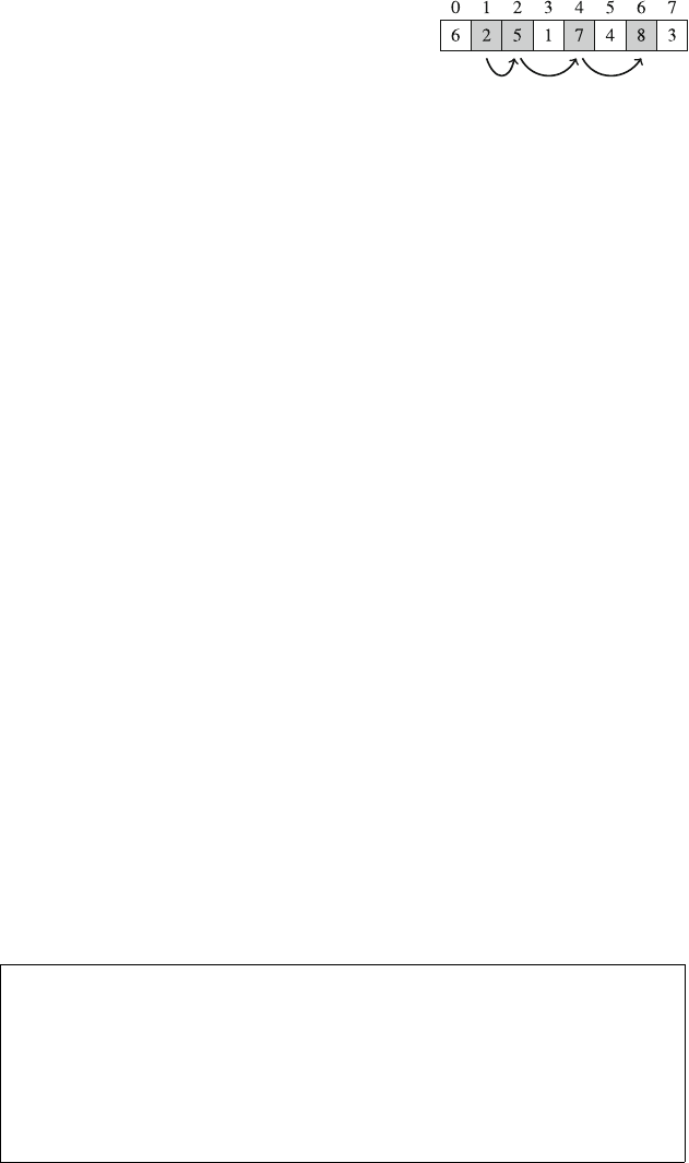
6.2 Further Examples 69
Fig. 6.1 The longest
increasing subsequence of
this array is [2,5,7,8]
6.2.1 Longest Increasing Subsequence
The longest increasing subsequence in an array of nelements is a maximum-length
sequence of array elements that goes from left to right, and each element in the
sequence is larger than the previous element. For example, Fig. 6.1 shows the longest
increasing subsequence in an array of eight elements.
We can efficiently find the longest increasing subsequence in an array using
dynamic programming. Let length(k)denote the length of the longest increasing
subsequence that ends at position k. Then, if we calculate all values of length(k)
where 0 ≤k≤n−1, we will find out the length of the longest increasing subse-
quence. The values of the function for our example array are as follows:
length(0)=1
length(1)=1
length(2)=2
length(3)=1
length(4)=3
length(5)=2
length(6)=4
length(7)=2
For example, length(6)=4, because the longest increasing subsequence that
ends at position 6 consists of 4 elements.
To calculate a value of length(k), we should find a position i<kfor which
array[i]<array[k]and length(i)is as large as possible. Then we know that
length(k)=length(i)+1, because this is an optimal way to append array[k]
to a subsequence. However, if there is no such position i, then length(k)=1,
which means that the subsequence only contains array[k].
Since all values of the function can be calculated from its smaller values, we can
use dynamic programming to calculate the values. In the following code, the values
of the function will be stored in an array length.
for (int k=0;k<n;k++){
length[k] = 1;
for (int i=0;i<k;i++) {
if (array[i] < array[k]) {
length[k] = max(length[k],length[i]+1);
}
}
}
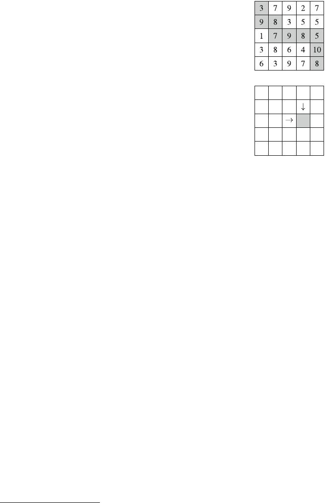
70 6 Dynamic Programming
Fig. 6.2 An optimal path
from the upper-left corner to
the lower-right corner
Fig. 6.3 Two possible ways
to reach a square on a path
The resulting algorithm clearly works in O(n2)time.2
6.2.2 Paths in a Grid
Our next problem is to find a path from the upper-left corner to the lower-right corner
of an n×ngrid, with the restriction that we may only move down and right. Each
square contains an integer, and the path should be constructed so that the sum of the
values along the path is as large as possible.
As an example, Fig. 6.2 shows an optimal path in a 5 ×5 grid. The sum of the
values on the path is 67, and this is the largest possible sum on a path from the
upper-left corner to the lower-right corner.
Assume that the rows and columns of the grid are numbered from 1 to n, and
value[y][x]equals the value of square (y,x). Let sum(y,x)denote the maximum
sum on a path from the upper-left corner to square (y,x). Then, sum(n,n)tells us
the maximum sum from the upper-left corner to the lower-right corner. For example,
in the above grid, sum(5,5)=67. Now we can use the formula
sum(y,x)=max(sum(y,x−1), sum(y−1,x)) +value[y][x],
which is based on the observation that a path that ends at square (y,x)can come
either from square (y,x−1)or from square (y−1,x)(Fig. 6.3). Thus, we select
the direction that maximizes the sum. We assume that sum(y,x)=0ify=0or
x=0, so the recursive formula also works for leftmost and topmost squares.
Since the function sum has two parameters, the dynamic programming array also
has two dimensions. For example, we can use an array
2In this problem, it is also possible to calculate the dynamic programming values more efficiently
in O(nlog n)time. Can you find a way to do this?
6.2 Further Examples 71
int sum[N][N];
and calculate the sums as follows:
for (int y = 1; y <= n; y++) {
for (int x=1;x<=n;x++){
sum[y][x] = max(sum[y][x-1],sum[y-1][x])+value[y][x];
}
}
The time complexity of the algorithm is O(n2).
6.2.3 Knapsack Problems
The term knapsack refers to problems where a set of objects is given, and subsets
with some properties have to be found. Knapsack problems can often be solved using
dynamic programming.
In this section, we focus on the following problem: Given a list of weights
[w1,w2,...,wn], determine all sums that can be constructed using the weights.
For example, Fig. 6.4 shows the possible sums for weights [1,3,3,5]. In this case,
all sums between 0 ...12 are possible, except 2 and 10. For example, the sum 7 is
possible because we can choose the weights [1,3,3].
To solve the problem, we focus on subproblems where we only use the first k
weights to construct sums. Let possible(x,k)=true if we can construct a sum
xusing the first kweights, and otherwise possible(x,k)=false. The values
of the function can be recursively calculated using the formula
possible(x,k)=possible(x−wk,k−1)or possible(x,k−1),
which is based on the fact that we can either use or not use the weight wkin the
sum. If we use wk, the remaining task is to form the sum x−wkusing the first k−1
weights, and if we do not use wk, the remaining task is to form the sum xusing the
first k−1 weights. The base cases are
possible(x,0)=true x=0
false x= 0,
because if no weights are used, we can only form the sum 0. Finally, possible(x,n)
tells us whether we can construct a sum xusing all weights.
Fig. 6.4 Constructing sums
using the weights [1,3,3,5]
72 6 Dynamic Programming
Fig. 6.5 Solving the
knapsack problem for the
weights [1,3,3,5]using
dynamic programming
Figure 6.5 shows all values of the function for the weights [1,3,3,5](the symbol
“” indicates the true values). For example, the row k=2 tells us that we can
construct the sums [0,1,3,4]using the weights [1,3].
Let mdenote the total sum of the weights. The following O(nm)time dynamic
programming solution corresponds to the recursive function:
possible[0][0] = true;
for (int k = 1; k <= n; k++) {
for (int x=0;x<=m;x++){
if (x-w[k] >= 0) {
possible[x][k] |= possible[x-w[k]][k-1];
}
possible[x][k] |= possible[x][k-1];
}
}
It turns out that there is also a more compact way to implement the dynamic
programming calculation, using only a one-dimensional array possible[x]that
indicates whether we can construct a subset with sum x. The trick is to update the
array from right to left for each new weight:
possible[0] = true;
for (int k = 1; k <= n; k++) {
for (int x = m-w[k]; x >= 0; x--) {
possible[x+w[k]] |= possible[x];
}
}
Note that the general dynamic programming idea presented in this section can
also be used in other knapsack problems, such as in a situation where objects have
weights and values and we have to find a maximum-value subset whose weight does
not exceed a given limit.
6.2.4 From Permutations to Subsets
Using dynamic programming, it is often possible to change an iteration over per-
mutations into an iteration over subsets. The benefit of this is that n!, the number of

6.2 Further Examples 73
permutations, is much larger than 2n, the number of subsets. For example, if n=20,
n!≈2.4·1018 and 2n≈106. Thus, for certain values of n, we can efficiently go
through the subsets but not through the permutations.
As an example, consider the following problem: There is an elevator with maxi-
mum weight x, and npeople who want to get from the ground floor to the top floor.
The people are numbered 0,1,...,n−1, and the weight of person iis weight[i].
What is the minimum number of rides needed to get everybody to the top floor?
For example, suppose that x=12, n=5, and the weights are as follows:
•weight[0]=2
•weight[1]=3
•weight[2]=4
•weight[3]=5
•weight[4]=9
In this scenario, the minimum number of rides is two. One optimal solution is as
follows: first, people 0, 2, and 3 take the elevator (total weight 11), and then, people
1 and 4 take the elevator (total weight 12).
The problem can be easily solved in O(n!n)time by testing all possible permu-
tations of npeople. However, we can use dynamic programming to create a more
efficient O(2nn)time algorithm. The idea is to calculate for each subset of people
two values: the minimum number of rides needed and the minimum weight of people
who ride in the last group.
Let rides(S)denote the minimum number of rides for a subset S, and let
last(S)denote the minimum weight of the last ride in a solution where the number
of rides is minimum. For example, in the above scenario
rides({3,4})=2 and last({3,4})=5,
because the optimal way for people 3 and 4 to get to the top floor is that they take
two separate rides and person 4 goes first, which minimizes the weight of the second
ride. Of course, our final goal is to calculate the value of rides({0...n−1}).
We can calculate the values of the functions recursively and then apply dynamic
programming. To calculate the values for a subset S, we go through all people who
belong to Sand optimally choose the last person pwho enters the elevator. Each
such choice yields a subproblem for a smaller subset of people. If last(S\p)+
weight[p]≤x, we can add pto the last ride. Otherwise, we have to reserve a new
ride that only contains p.
A convenient way to implement the dynamic programming calculation is to use
bit operations. First, we declare an array
pair<int,int> best[1<<N];
that contains for each subset Sa pair (rides(S), last(S)). For an empty subset,
no rides are needed:
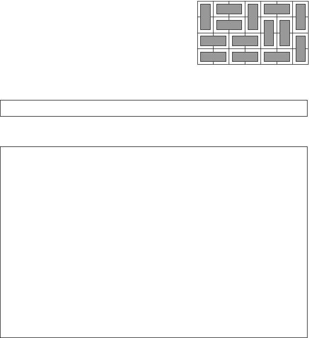
74 6 Dynamic Programming
Fig. 6.6 One way to fill the
4×7gridusing1×2and
2×1tiles
best[0] = {0,0};
Then, we can fill the array as follows:
for (int s = 1; s < (1<<n); s++) {
// initial value: n+1 rides are needed
best[s] = {n+1,0};
for (int p=0;p<n;p++) {
if (s&(1<<p)) {
auto option = best[s^(1<<p)];
if (option.second+weight[p] <= x) {
// add p to an existing ride
option.second += weight[p];
}else {
// reserve a new ride for p
option.first++;
option.second = weight[p];
}
best[s] = min(best[s], option);
}
}
}
Note that the above loop guarantees that for any two subsets S1and S2such
that S1⊂S2, we process S1before S2. Thus, the dynamic programming values are
calculated in the correct order.
6.2.5 Counting Tilings
Sometimes the states of a dynamic programming solution are more complex than
fixed combinations of values. As an example, consider the problem of calculating
the number of distinct ways to fill an n×mgrid using 1 ×2 and 2 ×1 size tiles. For
example, there are a total of 781 ways to fill the 4 ×7 grid, one of them being the
solution shown in Fig. 6.6.
The problem can be solved using dynamic programming by going through the
grid row by row. Each row in a solution can be represented as a string that contains

6.2 Further Examples 75
mcharacters from the set {,,,}. For example, the solution in Fig. 6.6 consists
of four rows that correspond to the following strings:
•
•
•
•
Suppose that the rows of the grid are indexed from 1 to n. Let count(k,x)
denote the number of ways to construct a solution for rows 1 ...ksuch that string x
corresponds to row k. It is possible to use dynamic programming here, because the
state of a row is constrained only by the state of the previous row.
A solution is valid if row 1 does not contain the character ,rowndoes not
contain the character , and all consecutive rows are compatible. For example, the
rows and are compatible, while the rows
and are not compatible.
Since a row consists of mcharacters and there are four choices for each character,
the number of distinct rows is at most 4m. We can go through the O(4m)possible
states for each row, and for each state, there are O(4m)possible states for the previous
row, so the time complexity of the solution is O(n42m). In practice, it is a good idea to
rotate the grid so that the shorter side has length m, because the factor 42mdominates
the time complexity.
It is possible to make the solution more efficient by using a more compact rep-
resentation for the rows. It turns out that it suffices to know which columns of the
previous row contain the upper square of a vertical tile. Thus, we can represent a
row using only the characters and , where is a combination of the characters
,, and . Using this representation, there are only 2mdistinct rows, and the time
complexity is O(n22m).
As a final note, there is also a direct formula for calculating the number of tilings:
n/2
a=1
m/2
b=1
4·cos2πa
n+1+cos2πb
m+1
This formula is very efficient, because it calculates the number of tilings in O(nm)
time, but since the answer is a product of real numbers, a problem when using the
formula is how to store the intermediate results accurately.
Graph Algorithms
Many programming problems can be solved by considering the situation as a graph
and using an appropriate graph algorithm. In this chapter, we will learn the basics of
graphs and a selection of important graph algorithms.
Section 7.1 discusses graph terminology and data structures that can be used to
represent graphs in algorithms.
Section 7.2 introduces two fundamental graph traversal algorithms. Depth-first
search is a simple way to visit all nodes that can be reached from a starting node,
and breadth-first search visits the nodes in increasing order of their distance from
the starting node.
Section 7.3 presents algorithms for finding shortest paths in weighted graphs.
The Bellman–Ford algorithm is a simple algorithm that finds shortest paths from a
starting node to all other nodes. Dijkstra’s algorithm is a more efficient algorithm
which requires that all edge weights are nonnegative. The Floyd–Warshall algorithm
determines shortest paths between all node pairs of a graph.
Section 7.4 explores special properties of directed acyclic graphs. We will learn
how to construct a topological sort and how to use dynamic programming to effi-
ciently process such graphs.
Section 7.5 focuses on successor graphs where each node has a unique successor.
We will discuss an efficient way to find successors of nodes and Floyd’s algorithm
for cycle detection.
Section 7.6 presents Kruskal’s and Prim’s algorithms for constructing minimum
spanning trees. Kruskal’s algorithm is based on an efficient union-find structure
which has also other uses in algorithm design.
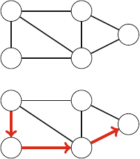
78 7 Graph Algorithms
7.1 Basics of Graphs
In this section, we first go through terminology which is used when discussing
graphs and their properties. After this, we focus on data structures that can be used
to represent graphs in algorithm programming.
7.1.1 Graph Terminology
Agraph consists of nodes (also called vertices) that are connected with edges.In
this book, the variable ndenotes the number of nodes in a graph, and the variable
mdenotes the number of edges. The nodes are numbered using integers 1,2,...,n.
For example, Fig. 7.1 shows a graph with 5 nodes and 7 edges.
Apath leads from a node to another node through the edges of the graph. The
length of a path is the number of edges in it. For example, Fig. 7.2 shows a path
1→3→4→5 of length 3 from node 1 to node 5. A cycle is a path where the first
and last node is the same. For example, Fig. 7.3 shows a cycle 1 →3→4→1.
A graph is connected if there is a path between any two nodes. In Fig. 7.4, the left
graph is connected, but the right graph is not connected, because it is not possible to
get from node 4 to any other node.
The connected parts of a graph are called its components. For example, the graph
in Fig. 7.5 has three components: {1,2,3},{4,5,6,7}, and {8}.
Atree is a connected graph that does not contain cycles. Figure 7.6 shows an
example of a graph that is a tree.
In a directed graph, the edges can be traversed in one direction only. Figure 7.7
shows an example of a directed graph. This graph contains a path 3 →1→2→5
from node 3 to node 5, but there is no path from node 5 to node 3.
In a weighted graph, each edge is assigned a weight. The weights are often inter-
preted as edge lengths, and the length of a path is the sum of its edge weights. For
example, the graph in Fig. 7.8 is weighted, and the length of the path 1 →3→4→5
is 1 +7+3=11. This is the shortest path from node 1 to node 5.
Two nodes are neighbors or adjacent if there is an edge between them. The degree
of a node is the number of its neighbors. Figure 7.9 shows the degree of each node
Fig. 7.1 Agraphwith5
nodes and 7 edges 1 2
34
5
Fig. 7.2 A path from node 1
to node 5 1 2
34
5
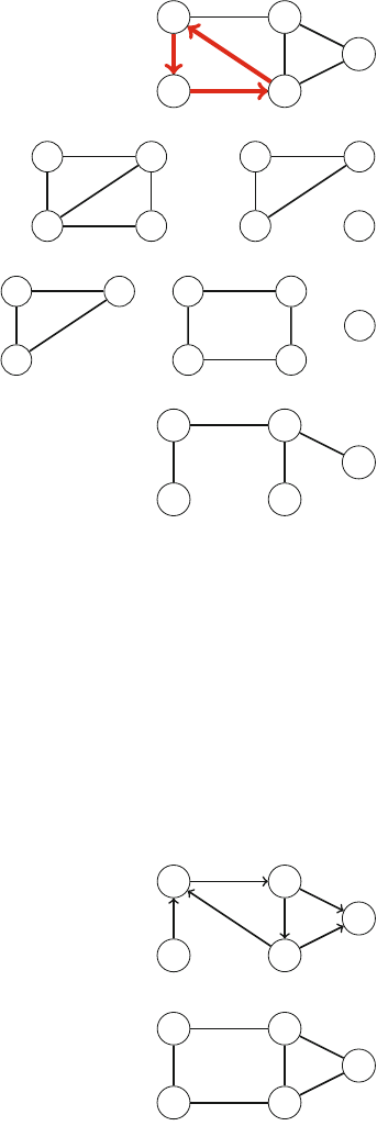
7.1 Basics of Graphs 79
Fig. 7.3 A cycle of three
nodes 1 2
34
5
Fig. 7.4 The left graph is
connected, the right graph is
not
1 2
34
1 2
34
Fig. 7.5 A graph with three
components 1 2
367
45
8
Fig. 7.6 Atree 1 2
34
5
of a graph. For example, the degree of node 2 is 3, because its neighbors are 1, 4,
and 5.
The sum of degrees in a graph is always 2m, where mis the number of edges,
because each edge increases the degree of exactly two nodes by one. For this reason,
the sum of degrees is always even. A graph is regular if the degree of every node is
a constant d. A graph is complete if the degree of every node is n−1, i.e., the graph
contains all possible edges between the nodes.
In a directed graph, the indegree of a node is the number of edges that end at
the node, and the outdegree of a node is the number of edges that start at the node.
Fig. 7.7 A directed graph 1 2
34
5
Fig. 7.8 A weighted graph 1 2
34
5
5
1
7
6
7
3
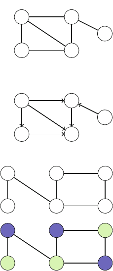
80 7 Graph Algorithms
Fig. 7.9 Degrees of nodes
1 2
34
5
23
33
1
Fig. 7.10 Indegrees and
outdegrees 1 2
34
5
1/13/0
0/32/1
0/1
Fig. 7.11 A bipartite graph
and its coloring 23
5 6
4
1
23
5 6
4
1
Figure 7.10 shows the indegree and outdegree of each node of a graph. For example,
node 2 has indegree 2 and outdegree 1.
A graph is bipartite if it is possible to color its nodes using two colors in such a
way that no adjacent nodes have the same color. It turns out that a graph is bipartite
exactly when it does not have a cycle with an odd number of edges. For example,
Fig. 7.11 shows a bipartite graph and its coloring.
7.1.2 Graph Representation
There are several ways to represent graphs in algorithms. The choice of a data struc-
ture depends on the size of the graph and the way the algorithm processes it. Next
we will go through three popular representations.
Adjacency Lists In the adjacency list representation, each node xof the graph is
assigned an adjacency list that consists of nodes to which there is an edge from x.
Adjacency lists are the most popular way to represent graphs, and most algorithms
can be efficiently implemented using them.
A convenient way to store the adjacency lists is to declare an array of vectors as
follows:
7.1 Basics of Graphs 81
Fig. 7.12 Example graphs
1 2 3
4
(a)
1 2 3
4
57
65
2
(b)
vector<int> adj[N];
The constant Nis chosen so that all adjacency lists can be stored. For example,
the graph in Fig. 7.12a can be stored as follows:
adj[1].push_back(2);
adj[2].push_back(3);
adj[2].push_back(4);
adj[3].push_back(4);
adj[4].push_back(1);
If the graph is undirected, it can be stored in a similar way, but each edge is added
in both directions.
For a weighted graph, the structure can be extended as follows:
vector<pair<int,int>> adj[N];
In this case, the adjacency list of node acontains the pair (b,w)always when
there is an edge from node ato node bwith weight w. For example, the graph in Fig.
7.12b can be stored as follows:
adj[1].push_back({2,5});
adj[2].push_back({3,7});
adj[2].push_back({4,6});
adj[3].push_back({4,5});
adj[4].push_back({1,2});
Using adjacency lists, we can efficiently find the nodes to which we can move
from a given node through an edge. For example, the following loop goes through
all nodes to which we can move from node s:
for (auto u : adj[s]) {
// process node u
}
Adjacency Matrix An adjacency matrix indicates the edges that a graph contains.
We can efficiently check from an adjacency matrix if there is an edge between two
nodes. The matrix can be stored as an array

82 7 Graph Algorithms
int adj[N][N];
where each value adj[a][b]indicates whether the graph contains an edge from node
ato node b. If the edge is included in the graph, then adj[a][b]=1, and otherwise
adj[a][b]=0. For example, the adjacency matrix for the graph in Fig. 7.12ais
⎡
⎢
⎢
⎣
0100
0011
0001
1000
⎤
⎥
⎥
⎦
.
If the graph is weighted, the adjacency matrix representation can be extended
so that the matrix contains the weight of the edge if the edge exists. Using this
representation, the graph in Fig. 7.12b corresponds to the following matrix:
⎡
⎢
⎢
⎣
0500
0076
0005
2000
⎤
⎥
⎥
⎦
The drawback of the adjacency matrix representation is that an adjacency matrix
contains n2elements, and usually most of them are zero. For this reason, the repre-
sentation cannot be used if the graph is large.
Edge List An edge list contains all edges of a graph in some order. This is a convenient
way to represent a graph if the algorithm processes all its edges, and it is not needed
to find edges that start at a given node.
The edge list can be stored in a vector
vector<pair<int,int>> edges;
where each pair (a,b)denotes that there is an edge from node ato node b. Thus, the
graph in Fig. 7.12a can be represented as follows:
edges.push_back({1,2});
edges.push_back({2,3});
edges.push_back({2,4});
edges.push_back({3,4});
edges.push_back({4,1});
If the graph is weighted, the structure can be extended as follows:
vector<tuple<int,int,int>> edges;

7.1 Basics of Graphs 83
Each element in this list is of the form (a,b,w), which means that there is an edge
from node ato node bwith weight w. For example, the graph in Fig. 7.12b can be
represented as follows1:
edges.push_back({1,2,5});
edges.push_back({2,3,7});
edges.push_back({2,4,6});
edges.push_back({3,4,5});
edges.push_back({4,1,2});
7.2 Graph Traversal
This section discusses two fundamental graph algorithms: depth-first search and
breadth-first search. Both algorithms are given a starting node in the graph, and they
visit all nodes that can be reached from the starting node. The difference in the
algorithms is the order in which they visit the nodes.
7.2.1 Depth-First Search
Depth-first search (DFS) is a straightforward graph traversal technique. The algo-
rithm begins at a starting node and proceeds to all other nodes that are reachable
from the starting node using the edges of the graph.
Depth-first search always follows a single path in the graph as long as it finds new
nodes. After this, it returns to previous nodes and begins to explore other parts of
the graph. The algorithm keeps track of visited nodes, so that it processes each node
only once.
Figure 7.13 shows how depth-first search processes a graph. The search can begin
at any node of the graph; in this example we begin the search at node 1. First the
search explores the path 1 →2→3→5, then returns back to node 1 and visits
the remaining node 4.
Implementation Depth-first search can be conveniently implemented using recur-
sion. The following function dfs begins a depth-first search at a given node. The
function assumes that the graph is stored as adjacency lists in an array
vector<int> adj[N];
and also maintains an array
1In some older compilers, the function make_tuple must be used instead of the braces (e.g.,
make_tuple(1,2,5) instead of {1,2,5}).
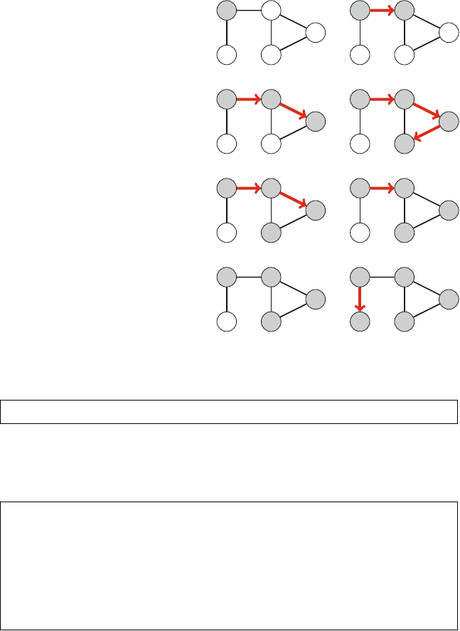
84 7 Graph Algorithms
Fig. 7.13 Depth-first search 1 2
3
45
step 1
1 2
3
45
step 2
1 2
3
45
step 3
1 2
3
45
step 4
1 2
3
45
step 5
1 2
3
45
step 6
1 2
3
45
step 7
1 2
3
45
step 8
bool visited[N];
that keeps track of the visited nodes. Initially, each array value is false, and when
the search arrives at node s, the value of visited[s] becomes true. The function
can be implemented as follows:
void dfs(int s) {
if (visited[s]) return;
visited[s] = true;
// process node s
for (auto u: adj[s]) {
dfs(u);
}
}
The time complexity of depth-first search is O(n+m)where nis the number of
nodes and mis the number of edges, because the algorithm processes each node and
edge once.
7.2 Graph Traversal 85
Fig. 7.14 Breadth-first
search 1 2 3
45 6
step 1
1 2 3
45 6
step 2
1 2 3
45 6
step 3
1 2 3
45 6
step 4
7.2.2 Breadth-First Search
Breadth-first search (BFS) visits the nodes of a graph in increasing order of their
distance from the starting node. Thus, we can calculate the distance from the starting
node to all other nodes using breadth-first search. However, breadth-first search is
more difficult to implement than depth-first search.
Breadth-first search goes through the nodes one level after another. First the search
explores the nodes whose distance from the starting node is 1, then the nodes whose
distance is 2, and so on. This process continues until all nodes have been visited.
Figure 7.14 shows how breadth-first search processes a graph. Suppose that the
search begins at node 1. First the search visits nodes 2 and 4 with distance 1, then
nodes 3 and 5 with distance 2, and finally node 6 with distance 3.
Implementation Breadth-first search is more difficult to implement than depth-first
search, because the algorithm visits nodes in different parts of the graph. A typical
implementation is based on a queue that contains nodes. At each step, the next node
in the queue will be processed.
The following code assumes that the graph is stored as adjacency lists and main-
tains the following data structures:
queue<int>q;
bool visited[N];
int distance[N];
The queue qcontains nodes to be processed in increasing order of their distance.
New nodes are always added to the end of the queue, and the node at the beginning
of the queue is the next node to be processed. The array visited indicates which
nodes the search has already visited, and the array distance will contain the
distances from the starting node to all nodes of the graph.
The search can be implemented as follows, starting at node x:
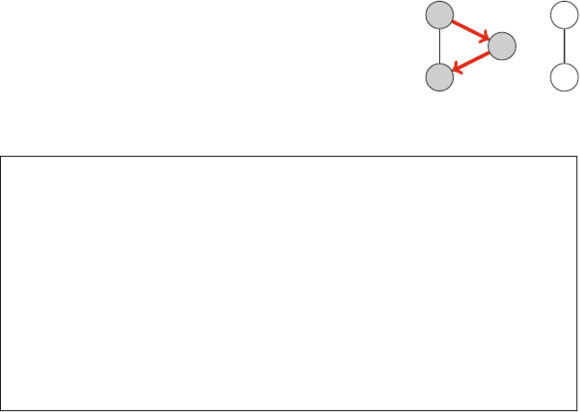
86 7 Graph Algorithms
Fig. 7.15 Checking the
connectivity of a graph 21
3
5
4
visited[x] = true;
distance[x] = 0;
q.push(x);
while (!q.empty()) {
int s = q.front(); q.pop();
// process node s
for (auto u : adj[s]) {
if (visited[u]) continue;
visited[u] = true;
distance[u] = distance[s]+1;
q.push(u);
}
}
Like in depth-first search, the time complexity of breadth-first search is O(n+m),
where nis the number of nodes and mis the number of edges.
7.2.3 Applications
Using the graph traversal algorithms, we can check many properties of graphs. Usu-
ally, both depth-first search and breadth-first search may be used, but in practice,
depth-first search is a better choice, because it is easier to implement. In the appli-
cations described below we will assume that the graph is undirected.
Connectivity Check A graph is connected if there is a path between any two nodes
of the graph. Thus, we can check if a graph is connected by starting at an arbitrary
node and finding out if we can reach all other nodes.
For example, in Fig. 7.15, since a depth-first search from node 1 does not visit all
the nodes, we can conclude that the graph is not connected. In a similar way, we can
also find all connected components of a graph by iterating through the nodes and
always starting a new depth-first search if the current node does not belong to any
component yet.
Cycle Detection A graph contains a cycle if during a graph traversal, we find a
node whose neighbor (other than the previous node in the current path) has already
been visited. For example, in Fig. 7.16, a depth-first search from node 1 reveals that
the graph contains a cycle. After moving from node 2 to node 5 we notice that the
neighbor 3 of node 5 has already been visited. Thus, the graph contains a cycle that
goes through node 3, for example, 3 →2→5→3.

7.2 Graph Traversal 87
Fig. 7.16 Finding a cycle in
agraph 21
3
5
4
Fig. 7.17 A conflict when
checking bipartiteness 21
3
5
4
Another way to determine if a graph contains a cycle is to simply calculate the
number of nodes and edges in every component. If a component contains cnodes
and no cycle, it must contain exactly c−1 edges (so it has to be a tree). If there are
cor more edges, the component surely contains a cycle.
Bipartiteness Check A graph is bipartite if its nodes can be colored using two colors
so that there are no adjacent nodes with the same color. It is surprisingly easy to check
if a graph is bipartite using graph traversal algorithms.
The idea is to pick two colors Xand Y, color the starting node X, all its neighbors
Y, all their neighbors X, and so on. If at some point of the search we notice that
two adjacent nodes have the same color, this means that the graph is not bipartite.
Otherwise the graph is bipartite and one coloring has been found.
For example, in Fig. 7.17, a depth-first search from node 1 shows that the graph is
not bipartite, because we notice that both nodes 2 and 5 should have the same color,
while they are adjacent nodes in the graph.
This algorithm always works, because when there are only two colors available,
the color of the starting node in a component determines the colors of all other nodes
in the component. It does not make any difference what the colors are.
Note that in the general case it is difficult to find out if the nodes in a graph can be
colored using kcolors so that no adjacent nodes have the same color. The problem
is NP-hard already for k=3.
7.3 Shortest Paths
Finding a shortest path between two nodes of a graph is an important problem that
has many practical applications. For example, a natural problem related to a road
network is to calculate the shortest possible length of a route between two cities,
given the lengths of the roads.
In an unweighted graph, the length of a path equals the number of its edges, and
we can simply use breadth-first search to find a shortest path. However, in this section
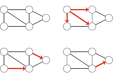
88 7 Graph Algorithms
Fig. 7.18 The
Bellman–Ford algorithm 1 2
34
5
0∞
∞∞
∞
2
3
−2
3
5
2
7
step 1
1 2
34
5
02
37
∞
2
3
−2
3
5
2
7
step 2
1 2
34
5
02
31
7
2
3
−2
3
5
2
7
step 3
1 2
34
5
02
31
3
2
3
−2
3
5
2
7
step 4
we focus on weighted graphs where more sophisticated algorithms are needed for
finding shortest paths.
7.3.1 Bellman–Ford Algorithm
The Bellman–Ford algorithm finds shortest paths from a starting node to all nodes
of the graph. The algorithm can process all kinds of graphs, provided that the graph
does not contain a cycle with negative length. If the graph contains a negative cycle,
the algorithm can detect this.
The algorithm keeps track of distances from the starting node to all nodes of the
graph. Initially, the distance to the starting node is 0 and the distance to any other node
is infinite. The algorithm then reduces the distances by finding edges that shorten the
paths until it is not possible to reduce any distance.
Figure 7.18 shows how the Bellman–Ford algorithm processes a graph. First, the
algorithm reduces distances using the edges 1 →2, 1 →3 and 1 →4, then using
the edges 2 →5 and 3 →4, and finally using the edge 4 →5. After this, no edge
can be used to reduce distances, which means that the distances are final.
Implementation The implementation of the Bellman–Ford algorithm below deter-
mines the shortest distances from a node xto all nodes of the graph. The code
assumes that the graph is stored as an edge list edges that consists of tuples of the
form (a,b,w), meaning that there is an edge from node ato node bwith weight w.
The algorithm consists of n−1 rounds, and on each round the algorithm goes
through all edges of the graph and attempts to reduce the distances. The algorithm
constructs an array distance that will contain the distances from node xto all
nodes. The constant INF denotes an infinite distance.
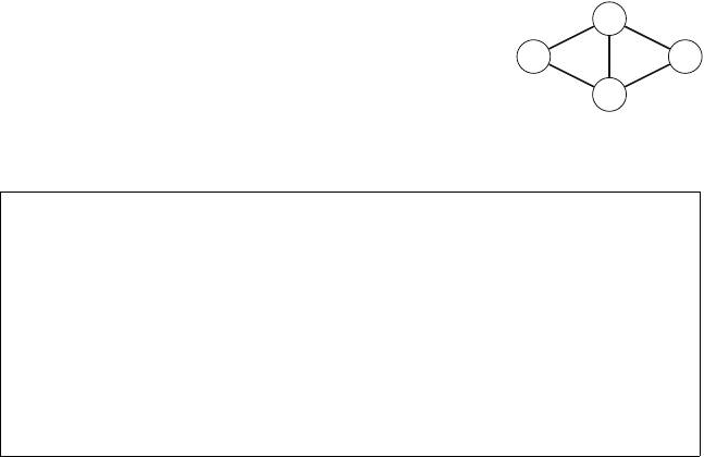
7.3 Shortest Paths 89
Fig. 7.19 Agraphwitha
negative cycle
1
2
3
4
31
5−7
2
for (int i=1;i<=n;i++){
distance[i] = INF;
}
distance[x] = 0;
for (int i = 1; i <= n-1; i++) {
for (auto e : edges) {
int a, b, w;
tie(a,b,w)=e;
distance[b] = min(distance[b], distance[a]+w);
}
}
The time complexity of the algorithm is O(nm), because the algorithm consists of
n−1 rounds and iterates through all medges during a round. If there are no negative
cycles in the graph, all distances are final after n−1 rounds, because each shortest
path can contain at most n−1 edges.
There are several ways to optimize the algorithm in practice. First, the final dis-
tances can usually be found earlier than after n−1 rounds, so we can simply stop the
algorithm if no distance can be reduced during a round. A more advanced variant is
the SPFA algorithm (“Shortest Path Faster Algorithm” [8]) which maintains a queue
of nodes that might be used for reducing the distances. Only the nodes in the queue
will be processed, which often yields a more efficient search.
Negative Cycles The Bellman–Ford algorithm can also be used to check if the graph
contains a cycle with negative length. In this case, any path that contains the cycle can
be shortened infinitely many times, so the concept of a shortest path is not meaningful.
For example, the graph in Fig. 7.19 contains a negative cycle 2 →3→4→2 with
length −4.
A negative cycle can be detected using the Bellman–Ford algorithm by running
the algorithm for nrounds. If the last round reduces any distance, the graph contains
a negative cycle. Note that this algorithm can be used to search for a negative cycle
in the entire graph regardless of the starting node.
7.3.2 Dijkstra’s Algorithm
Dijkstra’s algorithm finds shortest paths from the starting node to all nodes of the
graph, like the Bellman–Ford algorithm. The benefit of Dijkstra’s algorithm is that it
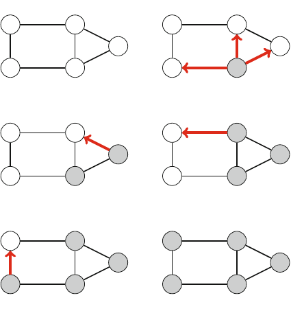
90 7 Graph Algorithms
Fig. 7.20 Dijkstra’s
algorithm 34
2 1
5
∞∞
∞0
∞
6
2
5
9
2
1
step 1
34
2 1
5
∞9
50
1
6
2
5
9
2
1
step 2
34
2 1
5
∞3
50
1
6
2
5
9
2
1
step 3
34
2 1
5
93
50
1
6
2
5
9
2
1
step 4
34
2 1
5
73
50
1
6
2
5
9
2
1
step 5
34
2 1
5
73
50
1
6
2
5
9
2
1
step 6
is more efficient and can be used for processing large graphs. However, the algorithm
requires that there are no negative weight edges in the graph.
Like the Bellman–Ford algorithm, Dijkstra’s algorithm maintains distances to the
nodes and reduces them during the search. At each step, Dijkstra’s algorithm selects a
node that has not been processed yet and whose distance is as small as possible. Then,
the algorithm goes through all edges that start at the node and reduces the distances
using them. Dijkstra’s algorithm is efficient, because it only processes each edge in
the graph once, using the fact that there are no negative edges.
Figure 7.20 shows how Dijkstra’s algorithm processes a graph. Like in the
Bellman–Ford algorithm, the initial distance to all nodes, except for the starting
node, is infinite. The algorithm processes the nodes in the order 1, 5, 4, 2, 3, and at
each node reduces distances using edges that start at the node. Note that the distance
to a node never changes after processing the node.
Implementation An efficient implementation of Dijkstra’s algorithm requires that
we can efficiently find the minimum-distance node that has not been processed. An
appropriate data structure for this is a priority queue that contains the remaining nodes
ordered by their distances. Using a priority queue, the next node to be processed can
be retrieved in logarithmic time.
A typical textbook implementation of Dijkstra’s algorithm uses a priority queue
that has an operation for modifying a value in the queue. This allows us to have
a single instance of each node in the queue and update its distance when needed.
However, standard library priority queues do not provide such an operation, and
a somewhat different implementation is usually used in competitive programming.

7.3 Shortest Paths 91
The idea is to add a new instance of a node to the priority queue always when its
distance changes.
Our implementation of Dijkstra’s algorithm calculates the minimum distances
from a node xto all other nodes of the graph. The graph is stored as adjacency lists
so that adj[a]contains a pair (b,w)always when there is an edge from node ato
node bwith weight w. The priority queue
priority_queue<pair<int,int>> q;
contains pairs of the form (−d,x), meaning that the current distance to node xis d.
The array distance contains the distance to each node, and the array processed
indicates whether a node has been processed.
Note that the priority queue contains negative distances to nodes. The reason for
this is that the default version of the C++ priority queue finds maximum elements,
while we want to find minimum elements. By exploiting negative distances, we can
directly use the default priority queue.2Also note that while there may be several
instances of a node in the priority queue, only the instance with the minimum distance
will be processed.
The implementation is as follows:
for (int i=1;i<=n;i++){
distance[i] = INF;
}
distance[x] = 0;
q.push({0,x});
while (!q.empty()) {
int a = q.top().second; q.pop();
if (processed[a]) continue;
processed[a] = true;
for (auto u : adj[a]) {
int b = u.first, w = u.second;
if (distance[a]+w < distance[b]) {
distance[b] = distance[a]+w;
q.push({-distance[b],b});
}
}
}
The time complexity of the above implementation is O(n+mlog m), because
the algorithm goes through all nodes of the graph and adds for each edge at most
one distance to the priority queue.
Negative Edges The efficiency of Dijkstra’s algorithm is based on the fact that the
graph does not have negative edges. However, if the graph has a negative edge, the
2Of course, we could also declare the priority queue as in Sect. 5.2.3 and use positive distances, but
the implementation would be longer.
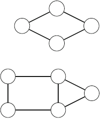
92 7 Graph Algorithms
Fig. 7.21 Agraphwhere
Dijkstra’s algorithm fails
1
2
3
4
23
6−5
Fig. 7.22 An input for the
Floyd–Warshall algorithm 34
2 1
5
7
2
5
9
2
1
algorithm may give incorrect results. As an example, consider the graph in Fig. 7.21.
The shortest path from node 1 to node 4 is 1 →3→4 and its length is 1. However,
Dijkstra’s algorithm incorrectly finds the path 1 →2→4 by greedily following
minimum weight edges.
7.3.3 Floyd–Warshall Algorithm
The Floyd–Warshall algorithm provides an alternative way to approach the problem
of finding shortest paths. Unlike the other algorithms in this chapter, it finds shortest
paths between all node pairs of the graph in a single run.
The algorithm maintains a matrix that contains distances between the nodes. The
initial matrix is directly constructed based on the adjacency matrix of the graph.
Then, the algorithm consists of consecutive rounds, and on each round, it selects a
new node that can act as an intermediate node in paths from now on, and reduces
distances using this node.
Let us simulate the Floyd–Warshall algorithm for the graph in Fig. 7.22. In this
case, the initial matrix is as follows:
⎡
⎢
⎢
⎢
⎢
⎣
05∞91
502∞∞
∞207∞
9∞702
1∞∞ 20
⎤
⎥
⎥
⎥
⎥
⎦
On the first round, node 1 is the new intermediate node. There is a new path
between nodes 2 and 4 with length 14, because node 1 connects them. There is also
a new path between nodes 2 and 5 with length 6.
⎡
⎢
⎢
⎢
⎢
⎣
05∞91
50214 6
∞207∞
914 702
16∞20
⎤
⎥
⎥
⎥
⎥
⎦
7.3 Shortest Paths 93
Fig. 7.23 A shortest path
from node 2 to node 4 34
2 1
5
7
2
5
9
2
1
On the second round, node 2 is the new intermediate node. This creates new paths
between nodes 1 and 3 and between nodes 3 and 5:
⎡
⎢
⎢
⎢
⎢
⎣
05791
502146
72078
9147 0 2
16820
⎤
⎥
⎥
⎥
⎥
⎦
The algorithm continues like this, until all nodes have been appointed intermediate
nodes. After the algorithm has finished, the matrix contains the minimum distances
between any two nodes:
⎡
⎢
⎢
⎢
⎢
⎣
05731
50286
72078
38702
16820
⎤
⎥
⎥
⎥
⎥
⎦
For example, the matrix tells us that the shortest distance between nodes 2 and 4
is 8. This corresponds to the path in Fig. 7.23.
Implementation The Floyd–Warshall algorithm is particularly easy to implement.
The implementation below constructs a distance matrix where dist[a][b]denotes
the shortest distance between nodes aand b. First, the algorithm initializes dist
using the adjacency matrix adj of the graph:
for (int i=1;i<=n;i++){
for (int j=1;j<=n;j++){
if (i == j) dist[i][j] = 0;
else if (adj[i][j]) dist[i][j] = adj[i][j];
else dist[i][j] = INF;
}
}
After this, the shortest distances can be found as follows:
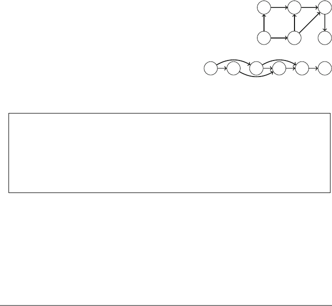
94 7 Graph Algorithms
Fig. 7.24 Agraphanda
topological sort 1 2 3
45 6
1 2 3
45 6
for (int k=1;k<=n;k++){
for (int i=1;i<=n;i++){
for (int j = 1; j <= n; j++) {
dist[i][j] = min(dist[i][j],dist[i][k]+dist[k][j]);
}
}
}
The time complexity of the algorithm is O(n3), because it contains three nested
loops that go through the nodes of the graph.
Since the implementation of the Floyd–Warshall algorithm is simple, the algorithm
can be a good choice even if it is only needed to find a single shortest path in the
graph. However, the algorithm can only be used when the graph is so small that a
cubic time complexity is fast enough.
7.4 Directed Acyclic Graphs
An important class of graphs are directed acyclic graphs, also called DAGs. Such
graphs do not contain cycles, and many problems are easier to solve if we may assume
that this is the case. In particular, we can always construct a topological sort for the
graph and then apply dynamic programming.
7.4.1 Topological Sorting
Atopological sort is an ordering of the nodes of a directed graph such that if there
is a path from node ato node b, then node aappears before node bin the ordering.
For example, in Fig. 7.24, one possible topological sort is [4,1,5,2,3,6].
A directed graph has a topological sort exactly when it is acyclic. If the graph
contains a cycle, it is not possible to form a topological sort, because no node of the
cycle can appear before the other nodes of the cycle in the ordering. It turns out that
depth-first search can be used to both check if a directed graph contains a cycle and,
if it does not, to construct a topological sort.
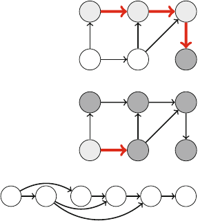
7.4 Directed Acyclic Graphs 95
Fig. 7.25 The first search
adds nodes 6, 3, 2, and 1 to
the list
1 2 3
45 6
Fig. 7.26 The second search
adds nodes 5 and 4 to the list 1 2 3
45 6
Fig. 7.27 The final
topological sort 1 2 3
45 6
The idea is to go through the nodes of the graph and always begin a depth-first
search at the current node if it has not been processed yet. During the searches, the
nodes have three possible states:
•state 0: the node has not been processed (white)
•state 1: the node is under processing (light gray)
•state 2: the node has been processed (dark gray)
Initially, the state of each node is 0. When a search reaches a node for the first
time, its state becomes 1. Finally, after all edges from the node have been processed,
its state becomes 2.
If the graph contains a cycle, we will discover this during the search, because
sooner or later we will arrive at a node whose state is 1. In this case, it is not possible
to construct a topological sort. If the graph does not contain a cycle, we can construct
a topological sort by adding each node to a list when its state becomes 2. Finally, we
reverse the list and get a topological sort for the graph.
Now we are ready to construct a topological sort for our example graph. The first
search (Fig. 7.25) proceeds from node 1 to node 6, and adds nodes 6, 3, 2, and 1 to
the list. Then, the second search (Fig. 7.26) proceeds from node 4 to node 5 and adds
nodes 5 and 4 to the list. The final reversed list is [4,5,1,2,3,6], which corresponds
to a topological sort (Fig. 7.27). Note that a topological sort is not unique; there can
be several topological sorts for a graph.
Figure 7.28 shows a graph that does not have a topological sort. During the search,
we reach node 2 whose state is 1, which means that the graph contains a cycle. Indeed,
there is a cycle 2 →3→5→2.
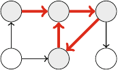
96 7 Graph Algorithms
Fig. 7.28 This graph does
not have a topological sort,
because it contains a cycle
1 2 3
45 6
7.4.2 Dynamic Programming
Using dynamic programming, we can efficiently answer many questions regarding
paths in directed acyclic graphs. Examples of such questions are:
•What is the shortest/longest path from node ato node b?
•How many different paths are there?
•What is the minimum/maximum number of edges in a path?
•Which nodes appear in every possible path?
Note that many of the above problems are difficult to solve or not well-defined
for general graphs.
As an example, consider the problem of calculating the number of paths from
node ato node b. Let paths(x)denote the number of paths from node ato node
x. As a base case, paths(a)=1. Then, to calculate other values of paths(x),we
can use the recursive formula
paths(x)=paths(s1)+paths(s2)+···+paths(sk),
where s1,s2,...,skare the nodes from which there is an edge to x. Since the graph
is acyclic, the values of paths can be calculated in the order of a topological sort.
Figure 7.29 shows the values of paths in an example scenario where we want
to calculate the number of paths from node 1 to node 6. For example,
paths(6)=paths(2)+paths(3),
because the edges that end at node 6 are 2 →6 and 3 →6. Since paths(2)=2
and paths(3)=2, we conclude that paths(6)=4. The paths are as follows:
•1→2→3→6
•1→2→6
•1→4→5→2→3→6
•1→4→5→2→6
Processing Shortest Paths Dynamic programming can also be used to answer ques-
tions regarding shortest paths in general (not necessarily acyclic) graphs. Namely,
if we know minimum distances from a starting node to other nodes (e.g., after using
Dijkstra’s algorithm), we can easily create a directed acyclic shortest paths graph
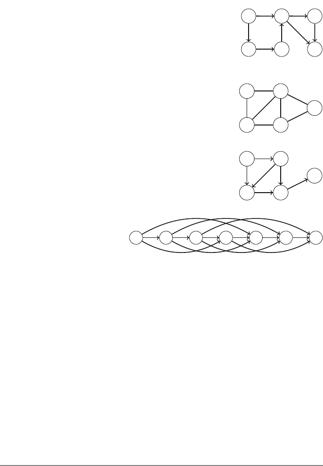
7.4 Directed Acyclic Graphs 97
Fig. 7.29 Calculating the
number of paths from node 1
to node 6
1 2 3
45 6
114
122
Fig. 7.30 Agraphandits
shortest paths graph 1 2
34
5
3
54
8
2
1
2
1 2
34
5
3
54
2
1
2
Fig. 7.31 Coin problem as a
directed acyclic graph 01 2 345 6
that indicates for each node the possible ways to reach the node using a shortest path
from the starting node. For example, Fig. 7.30 shows a graph and the corresponding
shortest paths graph.
Coin Problem Revisited In fact, any dynamic programming problem can be rep-
resented as a directed acyclic graph where each node corresponds to a dynamic
programming state and the edges indicate how the states depend on each other.
For example, consider the problem of forming a sum of money nusing coins
{c1,c2,...,ck}(Sect. 6.1.1). In this scenario, we can construct a graph where each
node corresponds to a sum of money, and the edges show how the coins can be
chosen. For example, Fig. 7.31 shows the graph for the coins {1,3,4}and n=6.
Using this representation, the shortest path from node 0 to node ncorresponds to
a solution with the minimum number of coins, and the total number of paths from
node 0 to node nequals the total number of solutions.
7.5 Successor Graphs
Another special class of directed graphs are successor graphs. In those graphs, the
outdegree of each node is 1, i.e., each node has a unique successor. A successor
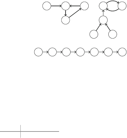
98 7 Graph Algorithms
Fig. 7.32 A successor graph 1 2
3
4
5
6
7
8
9
Fig. 7.33 Walking in a
successor graph 4625252
graph consists of one or more components, each of which contains one cycle and
some paths that lead to it.
Successor graphs are sometimes called functional graphs, because any successor
graph corresponds to a function succ(x)that defines the edges of the graph. The
parameter xis a node of the graph, and the function gives the successor of the node.
For example, the function
x123456789
succ(x)357622163
defines the graph in Fig. 7.32.
7.5.1 Finding Successors
Since each node of a successor graph has a unique successor, we can also define a
function succ(x,k)that gives the node that we will reach if we begin at node xand
walk ksteps forward. For example, in our example graph succ(4,6)=2, because
we will reach node 2 by walking 6 steps from node 4 (Fig. 7.33).
A straightforward way to calculate a value of succ(x,k)is to start at node xand
walk ksteps forward, which takes O(k)time. However, using preprocessing, any
value of succ(x,k)can be calculated in only O(log k)time.
Let udenote the maximum number of steps we will ever walk. The idea is to
precalculate all values of succ(x,k)where kis a power of two and at most u. This
can be efficiently done, because we can use the following recurrence:
succ(x,k)=succ(x)k=1
succ(succ(x,k/2), k/2)k>1
The idea is that a path of length kthat begins at node xcan be divided into two
paths of length k/2. Precalculating all values of succ(x,k)where kis a power of
two and at most utakes O(nlog u)time, because O(log u)values are calculated for
each node. In our example graph, the first values are as follows:
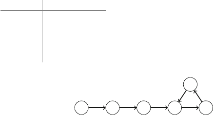
7.5 Successor Graphs 99
x123456789
succ(x,1)357622163
succ(x,2)721255327
succ(x,4)327255123
succ(x,8)721255327
···
Fig. 7.34 A cycle in a
successor graph
5
4
6
3
21
After the precalculation, any value of succ(x,k)can be calculated by presenting
kas a sum of powers of two. Such a representation always consists of O(log k)parts,
so calculating a value of succ(x,k)takes O(log k)time. For example, if we want
to calculate the value of succ(x,11), we use the formula
succ(x,11)=succ(succ(succ(x,8), 2), 1).
In our example graph,
succ(4,11)=succ(succ(succ(4,8), 2), 1)=5.
7.5.2 Cycle Detection
Consider a successor graph that only contains a path that ends in a cycle. We may
ask the following questions: if we begin our walk at the starting node, what is the
first node in the cycle and how many nodes does the cycle contain? For example,
in Fig. 7.34, we begin our walk at node 1, the first node that belongs to the cycle is
node 4, and the cycle consists of three nodes (4, 5, and 6).
A simple way to detect the cycle is to walk in the graph and keep track of all nodes
that have been visited. Once a node is visited for the second time, we can conclude
that the node is the first node in the cycle. This method works in O(n)time and also
uses O(n)memory. However, there are better algorithms for cycle detection. The
time complexity of such algorithms is still O(n), but they only use O(1)memory,
which may be an important improvement if nis large.
One such algorithm is Floyd’s algorithm, which walks in the graph using two
pointers aand b. Both pointers begin at the starting node x. Then, on each turn, the
pointer awalks one step forward and the pointer bwalks two steps forward. The
process continues until the pointers meet each other:

100 7 Graph Algorithms
a = succ(x);
b = succ(succ(x));
while (a != b) {
a = succ(a);
b = succ(succ(b));
}
At this point, the pointer ahas walked ksteps and the pointer bhas walked 2k
steps, so the length of the cycle divides k. Thus, the first node that belongs to the
cycle can be found by moving the pointer ato node xand advancing the pointers
step by step until they meet again.
a=x;
while (a != b) {
a = succ(a);
b = succ(b);
}
first = a;
After this, the length of the cycle can be calculated as follows:
b = succ(a);
length = 1;
while (a != b) {
b = succ(b);
length++;
}
7.6 Minimum Spanning Trees
Aspanning tree contains all nodes of a graph and some of its edges so that there is a
path between any two nodes. Like trees in general, spanning trees are connected and
acyclic. The weight of a spanning tree is the sum of its edge weights. For example,
Fig. 7.35 shows a graph and one of its spanning tree. The weight of this spanning
tree is 3 +5+9+3+2=22.
Aminimum spanning tree is a spanning tree whose weight is as small as possible.
Figure 7.36 shows a minimum spanning tree for our example graph with weight 20.
In a similar way, a maximum spanning tree is a spanning tree whose weight is as large
as possible. Figure 7.37 shows a maximum spanning tree for our example graph with
weight 32. Note that a graph may have several minimum and maximum spanning
trees, so the trees are not unique.
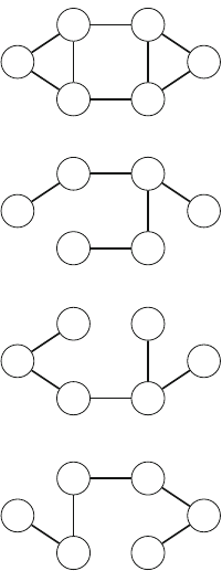
7.6 Minimum Spanning Trees 101
Fig. 7.35 Agraphanda
spanning tree
1
23
4
5 6
3
5
9
5
2
7
63
1
23
4
5 6
3
5
9
2
3
Fig. 7.36 A minimum
spanning tree with weight 20
1
23
4
5 6
3
5
2
7
3
Fig. 7.37 Amaximum
spanning tree with weight 32
1
23
4
5 6
5
9
57
6
It turns out that several greedy methods can be used to construct minimum and
maximum spanning trees. This section discusses two algorithms that process the
edges of the graph ordered by their weights. We focus on finding minimum spanning
trees, but the same algorithms can also find maximum spanning trees by processing
the edges in reverse order.
7.6.1 Kruskal’s Algorithm
Kruskal’s algorithm builds a minimum spanning tree by greedily adding edges to
the graph. The initial spanning tree only contains the nodes of the graph and does
not contain any edges. Then the algorithm goes through the edges ordered by their
weights and always adds an edge to the graph if it does not create a cycle.
The algorithm maintains the components of the graph. Initially, each node of the
graph belongs to a separate component. Always when an edge is added to the graph,
two components are joined. Finally, all nodes belong to the same component, and a
minimum spanning tree has been found.
As an example, let us construct a minimum spanning tree for our example graph
(Fig. 7.35). The first step is to sort the edges in increasing order of their weights:
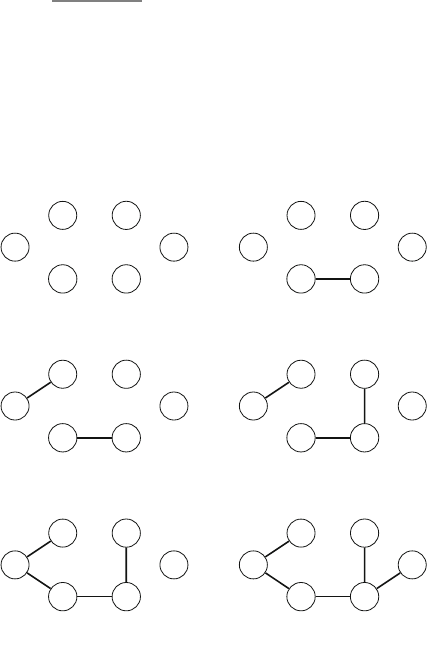
102 7 Graph Algorithms
edge weight
5–6 2
1–2 3
3–6 3
1–5 5
2–3 5
2–5 6
4–6 7
3–4 9
Fig. 7.38 Kruskal’s
algorithm
1
23
4
5 6
step 1
1
23
4
5 6
2
step 2
1
23
4
5 6
3
2
step 3
1
23
4
5 6
3
2
3
step 4
1
23
4
5 6
3
5
2
3
step 5
1
23
4
5 6
3
5
2
7
3
step 6
Then, we go through the list and add each edge to the graph if it joins two separate
components. Figure 7.38 shows the steps of the algorithm. Initially, each node belongs
to its own component. Then, the first edges on the list (5–6, 1–2, 3–6, and 1–5) are
added to the graph. After this, the next edge would be 2–3, but this edge is not added,
because it would create a cycle. The same applies to edge 2–5. Finally, the edge 4–6
is added, and the minimum spanning tree is ready.
Why Does This Work? It is a good question why Kruskal’s algorithm works. Why
does the greedy strategy guarantee that we will find a minimum spanning tree?
Let us see what happens if the minimum weight edge of the graph is not included
in the spanning tree. For example, suppose that a minimum spanning tree of our
example graph would not contain the minimum weight edge 5–6. We do not know
the exact structure of such a spanning tree, but in any case it has to contain some
edges. Assume that the tree would look like the tree in Fig. 7.39.
However, it is not possible that the tree in Fig. 7.39 would be a minimum spanning
tree, because we can remove an edge from the tree and replace it with the minimum
7.6 Minimum Spanning Trees 103
Fig. 7.39 A hypothetical
minimum spanning tree
1
23
4
5 6
Fig. 7.40 Including the edge
5–6 reduces the weight of the
spanning tree 1
23
4
5 6
2
weight edge 5–6. This produces a spanning tree whose weight is smaller, shown in
Fig. 7.40.
For this reason, it is always optimal to include the minimum weight edge in the
tree to produce a minimum spanning tree. Using a similar argument, we can show
that it is also optimal to add the next edge in weight order to the tree, and so on.
Hence, Kruskal’s algorithm always produces a minimum spanning tree.
Implementation When implementing Kruskal’s algorithm, it is convenient to use
the edge list representation of the graph. The first phase of the algorithm sorts the
edges in the list in O(mlog m)time. After this, the second phase of the algorithm
builds the minimum spanning tree as follows:
for (...) {
if (!same(a,b)) unite(a,b);
}
The loop goes through the edges in the list and always processes an edge (a,b)
where aand bare two nodes. Two functions are needed: the function same deter-
mines if aand bare in the same component, and the function unite joins the
components that contain aand b.
The problem is how to efficiently implement the functions same and unite.
One possibility is to implement the function same as a graph traversal and check if
we can get from node ato node b. However, the time complexity of such a function
would be O(n+m)and the resulting algorithm would be slow, because the function
same will be called for each edge in the graph.
We will solve the problem using a union-find structure that implements both
functions in O(log n)time. Thus, the time complexity of Kruskal’s algorithm will
be O(mlog n)after sorting the edge list.
7.6.2 Union-Find Structure
Aunion-find structure maintains a collection of sets. The sets are disjoint, so no
element belongs to more than one set. Two O(log n)time operations are supported:
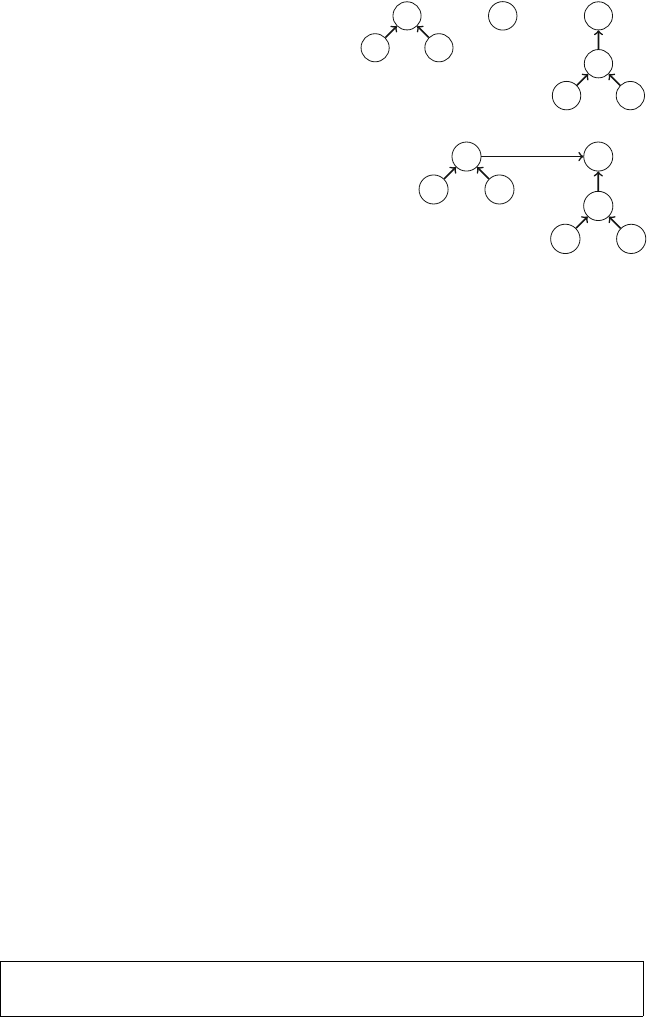
104 7 Graph Algorithms
Fig. 7.41 A union-find
structure with three sets
1
2
3
45
6
7
8
Fig. 7.42 Joining two sets
into a single set
1
2
3
4
6
7
8
the unite operation joins two sets, and the find operation finds the representative
of the set that contains a given element.
In a union-find structure, one element in each set is the representative of the
set, and there is a path from any other element of the set to the representative. For
example, assume that the sets are {1,4,7},{5}and {2,3,6,8}. Figure 7.41 shows
one way to represent these sets.
In this case the representatives of the sets are 4, 5, and 2. We can find the represen-
tative of any element by following the path that begins at the element. For example,
the element 2 is the representative for the element 6, because we follow the path
6→3→2. Two elements belong to the same set exactly when their representatives
are the same.
To join two sets, the representative of one set is connected to the representative of
the other set. For example, Fig. 7.42 shows a possible way to join the sets {1,4,7}
and {2,3,6,8}. From this on, the element 2 is the representative for the entire set
and the old representative 4 points to the element 2.
The efficiency of the union-find structure depends on how the sets are joined. It
turns out that we can follow a simple strategy: always connect the representative of
the smaller set to the representative of the larger set (or if the sets are of equal size,
we can make an arbitrary choice). Using this strategy, the length of any path will be
O(log n), so we can find the representative of any element efficiently by following
the corresponding path.
Implementation The union-find structure can be conveniently implemented using
arrays. In the following implementation, the array link indicates for each element
the next element in the path, or the element itself if it is a representative, and the
array size indicates for each representative the size of the corresponding set.
Initially, each element belongs to a separate set:
for (int i=1;i<=n;i++)link[i]=i;
for (int i=1;i<=n;i++)size[i]=1;
The function find returns the representative for an element x. The representative
can be found by following the path that begins at x.

7.6 Minimum Spanning Trees 105
int find(int x) {
while (x != link[x]) x = link[x];
return x;
}
The function same checks whether elements aand bbelong to the same set. This
can easily be done by using the function find:
bool same(int a, int b) {
return find(a) == find(b);
}
The function unite joins the sets that contain elements aand b(the elements
have to be in different sets). The function first finds the representatives of the sets
and then connects the smaller set to the larger set.
void unite(int a, int b) {
a = find(a);
b = find(b);
if (size[a] < size[b]) swap(a,b);
size[a] += size[b];
link[b] = a;
}
The time complexity of the function find is O(log n)assuming that the length
of each path is O(log n). In this case, the functions same and unite also work
in O(log n)time. The function unite makes sure that the length of each path is
O(log n)by connecting the smaller set to the larger set.
Path Compression Here is an alternative way to implement the find operation:
int find(int x) {
if (x == link[x]) return x;
return link[x] = find(link[x]);
}
This function uses path compression: each element in the path will directly point
to its representative after the operation. It can be shown that using this function, the
union-find operations work in amortized O(α(n)) time, where α(n)is the inverse
Ackermann function which grows very slowly (it is almost a constant). However,
path compression cannot be used in some applications of the union-find structure,
such as in the dynamic connectivity algorithm (Sect. 15.5.4).
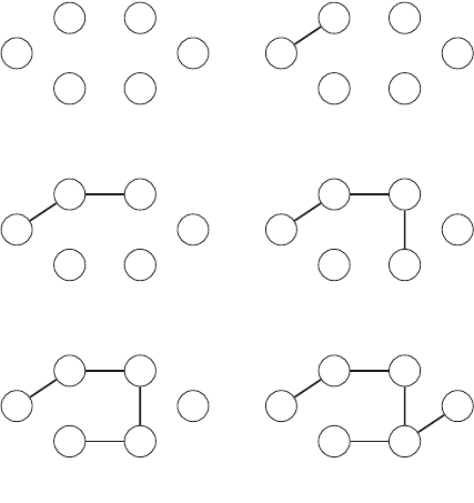
106 7 Graph Algorithms
Fig. 7.43 Prim’s algorithm
1
23
4
5 6
step 1
1
23
4
5 6
3
step 2
1
23
4
5 6
3
5
step 3
1
23
4
5 6
3
5
3
step 4
1
23
4
5 6
3
5
2
3
step 5
1
23
4
5 6
3
5
2
7
3
step 6
7.6.3 Prim’s Algorithm
Prim’s algorithm is an alternative method for constructing minimum spanning trees.
The algorithm first adds an arbitrary node to the tree, and then always chooses a
minimum weight edge that adds a new node to the tree. Finally, all nodes have been
added and a minimum spanning tree has been found.
Prim’s algorithm resembles Dijkstra’s algorithm. The difference is that Dijkstra’s
algorithm always selects a node whose distance from the starting node is minimum,
but Prim’s algorithm simply selects a node that can be added to the tree using a
minimum weight edge.
As an example, Fig. 7.43 shows how Prim’s algorithm constructs a minimum
spanning tree for our example graph, assuming that the starting node is node 1.
Like Dijkstra’s algorithm, Prim’s algorithm can be efficiently implemented using
a priority queue. The priority queue should contain all nodes that can be connected
to the current component using a single edge, in increasing order of the weights of
the corresponding edges.
The time complexity of Prim’s algorithm is O(n+mlog m)that equals the time
complexity of Dijkstra’s algorithm. In practice, Prim’s and Kruskal’s algorithms
are both efficient, and the choice of the algorithm is a matter of taste. Still, most
competitive programmers use Kruskal’s algorithm.

Algorithm Design Topics
This chapter discusses a selection of algorithm design topics.
Section 8.1 focuses on bit-parallel algorithms that use bit operations to efficiently
process data. Typically, we can replace a for loop with bit operations, which may
remarkably improve the running time of the algorithm.
Section 8.2 presents the amortized analysis technique, which can be used to
estimate the time needed for a sequence of operations in an algorithm. Using the
technique, we can analyze algorithms for determining nearest smaller elements and
sliding window minima.
Section 8.3 discusses ternary search and other techniques for efficiently calculating
minimum values of certain functions.
8.1 Bit-Parallel Algorithms
Bit-parallel algorithms are based on the fact that individual bits of numbers can
be manipulated in parallel using bit operations. Thus, a way to design an efficient
algorithm is to represent the steps of the algorithm so that they can be efficiently
implemented using bit operations.
8.1.1 Hamming Distances
The Hamming distance hamming(a,b)between two strings aand bof equal length
is the number of positions where the strings differ. For example,
hamming(01101,11001)=2.

108 8 Algorithm Design Topics
Consider the following problem: Given nbit strings, each of length k, calculate
the minimum Hamming distance between two strings. For example, the answer for
[00111,01101,11110]is 2, because
•hamming(00111,01101)=2,
•hamming(00111,11110)=3, and
•hamming(01101,11110)=3.
A straightforward way to solve the problem is to go through all pairs of strings
and calculate their Hamming distances, which yields an O(n2k)time algorithm. The
following function calculates the distance between strings aand b:
int hamming(string a, string b) {
int d=0;
for (int i=0;i<k;i++) {
if (a[i] != b[i]) d++;
}
return d;
}
However, since the strings consist of bits, we can optimize the solution by storing
the strings as integers and calculating distances using bit operations. In particular, if
k≤32, we can just store the strings as int values and use the following function
to calculate distances:
int hamming(int a, int b) {
return __builtin_popcount(a^b);
}
In the above function, the xor operation constructs a string that has one bits in
positions where aand bdiffer. Then, the number of one bits is calculated using the
__builtin_popcount function.
Table 8.1 shows a comparison of running times of the original algorithm and
the bit-parallel algorithm on a modern computer. In this problem, the bit-parallel
algorithm is about 20 times faster than the original algorithm.
8.1.2 Counting Subgrids
As another example, consider the following problem: Given an n×ngrid whose
each square is either black (1) or white (0), calculate the number of subgrids whose
all corners are black. For example, Fig. 8.1 shows two such subgrids in a grid.
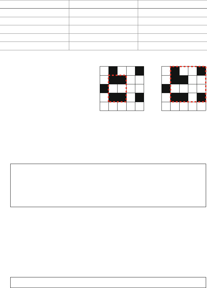
8.1 Bit-Parallel Algorithms 109
Table 8.1 The running times of the algorithms when calculating minimum Hamming distances of
nbit strings of length k=30
Size nOriginal algorithm (s) Bit-parallel algorithm (s)
5000 0.84 0.06
10000 3.24 0.18
15000 7.23 0.37
20000 12.79 0.63
25000 19.99 0.97
Fig. 8.1 This grid contains
two subgrids with black
corners
There is an O(n3)time algorithm for solving the problem: go through all O(n2)
pairs of rows, and for each pair (a,b)calculate, in O(n)time, the number of columns
that contain a black square in both rows aand b. The following code assumes that
color[y][x]denotes the color in row yand column x:
int count = 0;
for (int i=0;i<n;i++){
if (color[a][i] == 1 && color[b][i] == 1) {
count++;
}
}
Then, after finding out that there are count columns where both squares are
black, we can use the formula count(count −1)/2 to calculate the number of
subgrids whose first row is aand last row is b.
To create a bit-parallel algorithm, we represent each row kas an n-bit bitset row[k]
where one bits denote black squares. Then, we can calculate the number of columns
where rows aand bboth have black squares using an and operation and counting
the number of one bits. This can be conveniently done as follows using bitset
structures:
int count = (row[a]&row[b]).count();
Table 8.2 shows a comparison of the original algorithm and the bit-parallel algo-
rithm for different grid sizes. The comparison shows that the bit-parallel algorithm
can be up to 30 times faster than the original algorithm.
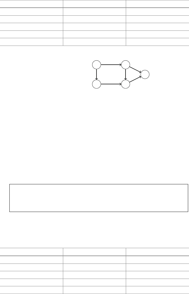
110 8 Algorithm Design Topics
Table 8.2 The running times of the algorithms for counting the subgrids
Grid size nOriginal algorithm (s) Bit-parallel algorithm (s)
1000 0.65 0.05
1500 2.17 0.14
2000 5.51 0.30
2500 12.67 0.52
3000 26.36 0.87
Fig. 8.2 Agraphandits
reach values. For example,
reach(2)=3, because
nodes 2, 4, and 5 can be
reached from node 2
1 2
34
5
reach(1)=5
reach(2)=3
reach(3)=3
reach(4)=2
reach(5)=1
8.1.3 Reachability in Graphs
Given a directed acyclic graph of nnodes, consider the problem of calculating for
each node xa value reach(x): the number of nodes that can be reached from node
x. For example, Fig. 8.2 shows a graph and its reach values.
The problem can be solved using dynamic programming in O(n2)time by con-
structing for each node a list of nodes that can be reached from it. Then, to create
a bit-parallel algorithm, we represent each list as a bitset of nbits. This permits us
to efficiently calculate the union of two such lists using an or operation. Assuming
that reach is an array of bitset structures and the graph is stored as adjacency
lists in adj, the calculation for node xcan be done as follows:
reach[x][x] = 1;
for (auto u : adj[x]) {
reach[x] |= reach[u];
}
Table 8.3 shows some running times for the bit-parallel algorithm. In each test,
the graph has nnodes and 2nrandom edges a→bwhere a<b. Note that the
Table 8.3 The running times of the algorithms when counting reachable nodes in a graph
Graph size nRunning time (s) Memory usage (MB)
2·1040.06 50
4·1040.17 200
6·1040.32 450
8·1040.51 800
1050.78 1250
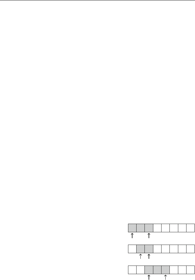
8.1 Bit-Parallel Algorithms 111
algorithm uses a great amount of memory for large values of n. In many contests,
the memory limit may be 512 MB or lower.
8.2 Amortized Analysis
The structure of an algorithm often directly tells us its time complexity, but sometimes
a straightforward analysis does not give a true picture of the efficiency. Amortized
analysis can be used to analyze a sequence of operations whose time complexity
varies. The idea is to estimate the total time used to all such operations during the
algorithm, instead of focusing on individual operations.
8.2.1 Two Pointers Method
In the two pointers method, two pointers walk through an array. Both pointers move
to one direction only, which ensures that the algorithm works efficiently. As a first
example of how to apply the technique, consider a problem where we are given an
array of npositive integers and a target sum x, and we want to find a subarray whose
sum is xor report that there is no such subarray.
The problem can be solved in O(n)time by using the two pointers method. The
idea is to maintain pointers that point to the first and last value of a subarray. On each
turn, the left pointer moves one step to the right, and the right pointer moves to the
right as long as the resulting subarray sum is at most x. If the sum becomes exactly
x, a solution has been found.
For example, Fig. 8.3 shows how the algorithm processes an array when the target
sum is x=8. The initial subarray contains the values 1, 3, and 2, whose sum is
6. Then, the left pointer moves one step right, and the right pointer does not move,
because otherwise the sum would exceed x. Finally, the left pointer moves one
step right, and the right pointer moves two steps right. The sum of the subarray is
2+5+1=8, so the desired subarray has been found.
The running time of the algorithm depends on the number of steps the right pointer
moves. While there is no useful upper bound on how many steps the pointer can move
Fig. 8.3 Finding a subarray
with sum 8 using the two
pointers method
13251123
13251123
13251123
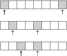
112 8 Algorithm Design Topics
Fig. 8.4 Solving the 2SUM
problem using the two
pointers method
1456799
10
1456799
10
1456799
10
on a single turn, we know that the pointer moves a total of O(n)steps during the
algorithm, because it only moves to the right. Since both the left and right pointer
move O(n)steps, the algorithm works in O(n)time.
2SUM Problem Another problem that can be solved using the two pointers
method is the 2SUM problem: given an array of nnumbers and a target sum x,
find two array values such that their sum is x, or report that no such values exist.
To solve the problem, we first sort the array values in increasing order. After that,
we iterate through the array using two pointers. The left pointer starts at the first
value and moves one step to the right on each turn. The right pointer starts at the last
value and always moves to the left until the sum of the left and right value is at most
x. If the sum is exactly x, a solution has been found.
For example, Fig. 8.4 shows how the algorithm processes an array when the target
sum is x=12. In the initial position, the sum of the values is 1 +10 =11 which is
smaller than x. Then the left pointer moves one step right, and the right pointer moves
three steps left, and the sum becomes 4 +7=11. After this, the left pointer moves
one step right again. The right pointer does not move, and a solution 5 +7=12 has
been found.
The running time of the algorithm is O(nlog n), because it first sorts the array in
O(nlog n)time, and then both pointers move O(n)steps.
Note that it is also possible to solve the problem in another way in O(nlog n)time
using binary search. In such a solution, we first sort the array and then iterate through
the array values and for each value binary search for another value that yields the sum
x. In fact, many problems that can be solved using the two pointers method can also
be solved using sorting or set structures, sometimes with an additional logarithmic
factor.
The more general kSUM problem is also interesting. In this problem we have to
find kelements such that their sum is x. It turns out that we can solve the 3SUM
problem in O(n2)time by extending the above 2SUM algorithm. Can you see how
we can do it? For a long time, it was actually thought that O(n2)would be the best
possible time complexity for the 3SUM problem. However, in 2014, Grønlund and
Pettie [12] showed that this is not the case.
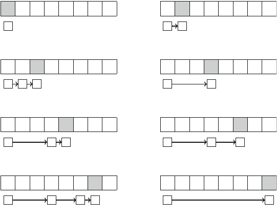
8.2 Amortized Analysis 113
8.2.2 Nearest Smaller Elements
Amortized analysis is often used to estimate the number of operations performed on
a data structure. The operations may be distributed unevenly so that most operations
occur during a certain phase of the algorithm, but the total number of the operations
is limited.
As an example, suppose that we want to find for each array element the nearest
smaller element, i.e., the first smaller element that precedes the element in the array.
It is possible that no such element exists, in which case the algorithm should report
this. Next we will efficiently solve the problem using a stack structure.
We go through the array from left to right and maintain a stack of array elements.
At each array position, we remove elements from the stack until the top element is
smaller than the current element, or the stack is empty. Then, we report that the top
element is the nearest smaller element of the current element, or if the stack is empty,
there is no such element. Finally, we add the current element to the stack.
Figure 8.5 shows how the algorithm processes an array. First, the element 1 is
added to the stack. Since it is the first element in the array, it clearly does not have a
nearest smaller element. After this, the elements 3 and 4 are added to the stack. The
nearest smaller element of 4 is 3, and the nearest smaller element of 3 is 1. Then, the
next element 2 is smaller than the two top elements in the stack, so the elements 3
and 4 are removed from the stack. Thus, the nearest smaller element of 2 is 1. After
this, the element 2 is added to the stack. The algorithm continues like this, until the
entire array has been processed.
13425342
1
step 1
13425342
13
step 2
13425342
134
step 3
13425342
12
step 4
13425342
12
5
step 5
13425342
12
3
step 6
13425342
12
34
step 7
13425342
12
step 8
Fig. 8.5 Finding the nearest smaller elements in linear time using a stack
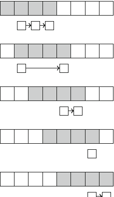
114 8 Algorithm Design Topics
The efficiency of the algorithm depends on the total number of stack operations.
If the current element is larger than the top element in the stack, it is directly added to
the stack, which is efficient. However, sometimes the stack can contain several larger
elements and it takes time to remove them. Still, each element is added exactly once
to the stack and removed at most once from the stack. Thus, each element causes
O(1)stack operations, and the algorithm works in O(n)time.
8.2.3 Sliding Window Minimum
Asliding window is a constant-size subarray that moves from left to right through
an array. At each window position, we want to calculate some information about the
elements inside the window. Next we will focus on the problem of maintaining the
sliding window minimum, which means that we want to report the smallest value
inside each window.
The sliding window minima can be calculated using a similar idea that we used
to calculate the nearest smaller elements. This time we maintain a queue where each
element is larger than the previous element, and the first element always corresponds
to the minimum element inside the window. After each window move, we remove
elements from the end of the queue until the last queue element is smaller than the
new window element, or the queue becomes empty. We also remove the first queue
element if it is not inside the window anymore. Finally, we add the new window
element to the queue.
Figure 8.6 shows how the algorithm processes an array when the sliding window
size is 4. At the first window position, the smallest value is 1. Then the window
moves one step right. The new element 3 is smaller than the elements 4 and 5 in
the queue, so the elements 4 and 5 are removed from the queue and the element 3
Fig. 8.6 Finding sliding
window minima in linear
time
21453412
145
21453412
13
21453412
34
21453412
1
21453412
12
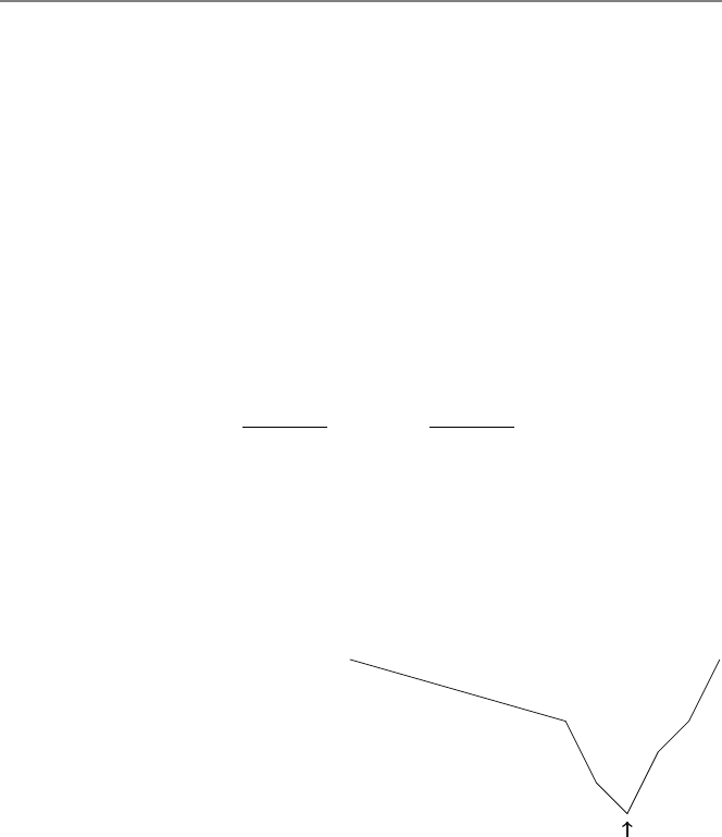
8.2 Amortized Analysis 115
is added to the queue. The smallest value is still 1. After this, the window moves
again, and the smallest element 1 does not belong to the window anymore. Thus, it
is removed from the queue, and the smallest value is now 3. Also the new element
4 is added to the queue. The next new element 1 is smaller than all elements in the
queue, so all elements are removed from the queue, and it only contains the element
1. Finally, the window reaches its last position. The element 2 is added to the queue,
but the smallest value inside the window is still 1.
Since each array element is added to the queue exactly once and removed from
the queue at most once, the algorithm works in O(n)time.
8.3 Finding Minimum Values
Suppose that there is a function f(x)that first only decreases, then attains its min-
imum value, and then only increases. For example, Fig. 8.7 shows such a function
whose minimum value is marked with an arrow. If we know that our function has
this property, we can efficiently find its minimum value.
8.3.1 Ternary Search
Ternary search provides an efficient way to find the minimum value of a function
that first decreases and then increases. Assume that we know that the value of xthat
minimizes f(x)is in a range [xL,xR]. The idea is to divide the range into three
equal-size parts [xL,a],[a,b], and [b,xR]by choosing
a=2xL+xR
3and b=xL+2xR
3.
Then, if f(a)< f(b), we conclude that the minimum must be in range [xL,b], and
otherwise it must be in range [a,xR]. After this, we recursively continue the search,
until the size of the active range is small enough.
As an example, Fig. 8.8 shows the first step of ternary search in our example
scenario. Since f(a)> f(b), the new range becomes [a,xR].
Fig. 8.7 A function and its
minimum value
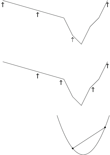
116 8 Algorithm Design Topics
Fig. 8.8 Searching for the
minimum using ternary
search
x
L
a
b
xR
xL
a
b
xR
Fig. 8.9 Example of a
convex function: f(x)=x2
a
b
In practice, we often consider functions whose parameters are integers, and the
search is terminated when the range only contains one element. Since the size of
the new range is always 2/3 of the previous range, the algorithm works in O(log n)
time, where nis the number of elements in the original range.
Note that when working with integer parameters, we can also use binary search
instead of ternary search, because it suffices to find the first position xfor which
f(x)≤f(x+1).
8.3.2 Convex Functions
A function is convex if a line segment between any two points on the graph of the
function always lies above or on the graph. For example, Fig.8.9 shows the graph of
f(x)=x2, which is a convex function. Indeed, the line segment between points a
and blies above the graph.
If we know that the minimum value of a convex function is in range [xL,xR],
we can use ternary search to find it. However, note that several points of a convex
function may have the minimum value. For example, f(x)=0 is convex and its
minimum value is 0.
Convex functions have some useful properties: if f(x)and g(x)are convex func-
tions, then also f(x)+g(x)and max(f(x), g(x)) are convex functions. For example,
8.3 Finding Minimum Values 117
if we have nconvex functions f1,f2,..., fn, we immediately know that also the
function f1+f2+...+fnhas to be convex and we can use ternary search to find
its minimum value.
8.3.3 Minimizing Sums
Given nnumbers a1,a2,...,an, consider the problem of finding a value of xthat
minimizes the sum
|a1−x|+|a2−x|+···+|an−x|.
For example, if the numbers are [1,2,9,2,6], the optimal solution is to choose
x=2, which produces the sum
|1−2|+|2−2|+|9−2|+|2−2|+|6−2|=12.
Since each function |ak−x|is convex, the sum is also convex, so we could
use ternary search to find the optimal value of x. However, there is also an easier
solution. It turns out that the optimal choice for xis always the median of the
numbers, i.e., the middle element after sorting. For example, the list [1,2,9,2,6]
becomes [1,2,2,6,9]after sorting, so the median is 2.
The median is always optimal, because if xis smaller than the median, the sum
becomes smaller by increasing x, and if xis larger then the median, the sum becomes
smaller by decreasing x.Ifnis even and there are two medians, both medians and
all values between them are optimal choices.
Then, consider the problem of minimizing the function
(a1−x)2+(a2−x)2+···+(an−x)2.
For example, if the numbers are [1,2,9,2,6], the best solution is to choose x=4,
which produces the sum
(1−4)2+(2−4)2+(9−4)2+(2−4)2+(6−4)2=46.
Again, this function is convex and we could use ternary search to solve the prob-
lem, but there is also a simple solution: the optimal choice for xis the average of
the numbers. In the example the average is (1+2+9+2+6)/5=4. This can be
proved by presenting the sum as follows:
nx2−2x(a1+a2+···+an)+(a2
1+a2
2+···+a2
n)
The last part does not depend on x, so we can ignore it. The remaining parts form
a function nx2−2xs where s=a1+a2+···+an. This is a parabola opening
upwards with roots x=0 and x=2s/n, and the minimum value is the average of
the roots x=s/n, i.e., the average of the numbers a1,a2,...,an.

Range Queries
In this chapter, we discuss data structures for efficiently processing range queries on
arrays. Typical queries are range sum queries (calculating the sum of values) and
range minimum queries (finding the minimum value).
Section 9.1 focuses on a simple situation where the array values are not modified
between the queries. In this case it suffices to preprocess the array so that we can
efficiently determine the answer for any possible query. We will first learn to process
sum queries using a prefix sum array, and then we will discuss the sparse table
algorithm for processing minimum queries.
Section 9.2 presents two tree structures that allow us to both process queries and
update array values efficiently. A binary indexed tree supports sum queries and can
be seen as a dynamic version of a prefix sum array. A segment tree is a more versatile
structure that supports sum queries, minimum queries, and several other queries. The
operations of both the structures work in logarithmic time.
9.1 Queries on Static Arrays
In this section, we focus on a situation where the array is static, i.e., the array values
are never updated between the queries. In this case, it suffices to preprocess the array
so that we can efficiently answer range queries.
First we will discuss a simple way to process sum queries using a prefix sum
array, which can also be generalized to higher dimensions. After this, we will learn
the sparse table algorithm for processing minimum queries, which is somewhat more
difficult. Note that while we focus on processing minimum queries, we can always
also process maximum queries using similar methods.
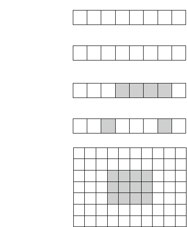
120 9 Range Queries
9.1.1 Sum Queries
Let sumq(a,b)(“range sum query”) denote the sum of array values in a range [a,b].
We can efficiently process any sum query by first constructing a prefix sum array.
Each value in the prefix sum array equals the sum of values in the original array up to
the corresponding position, i.e., the value at position kis sumq(0,k). For example,
Fig. 9.1 shows an array and its prefix sum array.
The prefix sum array can be constructed in O(n)time. Then, since the prefix sum
array contains all values of sumq(0,k), we can calculate any value of sumq(a,b)in
O(1)time using the formula
sumq(a,b)=sumq(0,b)−sumq(0,a−1).
By defining sumq(0,−1)=0, the above formula also holds when a=0.
As an example, Fig. 9.2 shows how to calculate the sum of values in the range
[3,6]using the prefix sum array. We can see in the original array that sumq(3,6)=
8+6+1+4=19. Using the prefix sum array, we need to examine only two values:
sumq(3,6)=sumq(0,6)−sumq(0,2)=27 −8=19.
Higher Dimensions It is also possible to generalize this idea to higher dimensions.
For example, Fig. 9.3 shows a two-dimensional prefix sum array that can be used to
calculate the sum of any rectangular subarray in O(1)time. Each sum in this array
Fig. 9.1 An array and its
prefix sum array 13486142
01234567
original array
14816 22 23 27 29
01234567
prefix sum array
Fig. 9.2 Calculating a range
sum using the prefix sum
array 13486142
01234567
original array
14816 22 23 27 29
01234567
prefix sum array
Fig. 9.3 Calculating a
two-dimensional range sum
A
B
C
D
9.1 Queries on Static Arrays 121
Fig. 9.4 Preprocessing for
minimum queries 13486142
01234567
original array
1346112–
01234567
range size 2
13111–––
01234567
range size 4
1–––––––
01234567
range size 8
corresponds to a subarray that begins at the upper-left corner of the array. The sum
of the gray subarray can be calculated using the formula
S(A)−S(B)−S(C)+S(D),
where S(X)denotes the sum of values in a rectangular subarray from the upper-left
corner to the position of X.
9.1.2 Minimum Queries
Let minq(a,b)(“range minimum query”) denote the minimum array value in a range
[a,b]. We will next discuss a technique using which we can process any minimum
query in O(1)time after an O(nlog n)time preprocessing. The method is due to
Bender and Farach-Colton [3] and often called the sparse table algorithm.
The idea is to precalculate all values of minq(a,b)where b−a+1 (the length
of the range) is a power of two. For example, Fig. 9.4 shows the precalculated values
for an array of eight elements.
The number of precalculated values is O(nlog n), because there are O(log n)
range lengths that are powers of two. The values can be calculated efficiently using
the recursive formula
minq(a,b)=min(minq(a,a+w−1), minq(a+w,b)),
where b−a+1 is a power of two and w=(b−a+1)/2. Calculating all those
values takes O(nlog n)time.
After this, any value of minq(a,b)can be calculated in O(1)time as a minimum
of two precalculated values. Let kbe the largest power of two that does not exceed
b−a+1. We can calculate the value of minq(a,b)using the formula
minq(a,b)=min(minq(a,a+k−1), minq(b−k+1,b)).
122 9 Range Queries
Fig. 9.5 Calculating a range
minimum using two
overlapping ranges 13486142
01234567
range size 6
13486142
01234567
range size 4
13486142
01234567
range size 4
In the above formula, the range [a,b]is represented as the union of the ranges
[a,a+k−1]and [b−k+1,b], both of length k.
As an example, consider the range [1,6]in Fig. 9.5. The length of the range is 6,
and the largest power of two that does not exceed 6 is 4. Thus the range [1,6]is the
union of the ranges [1,4]and [3,6]. Since minq(1,4)=3 and minq(3,6)=1, we
conclude that minq(1,6)=1.
Note that there are also sophisticated techniques using which we can process
range minimum queries in O(1)time after an only O(n)time preprocessing (see,
e.g., Fischer and Heun [10]), but they are beyond the scope of this book.
9.2 Tree Structures
This section presents two tree structures, using which we can both process range
queries and update array values in logarithmic time. First, we discuss binary indexed
trees that support sum queries, and after that, we focus on segment trees that also
support several other queries.
9.2.1 Binary Indexed Trees
Abinary indexed tree (or a Fenwick tree)[9] can be seen as a dynamic variant of a
prefix sum array. It provides two O(log n)time operations: processing a range sum
query and updating a value. Even if the name of the structure is a binary indexed tree,
the structure is usually represented as an array. When discussing binary indexed trees,
we assume that all arrays are one-indexed, because it makes the implementation of
the structure easier.
Let p(k)denote the largest power of two that divides k. We store a binary indexed
tree as an array tree such that
tree[k]=sumq(k−p(k)+1,k),
i.e., each position kcontains the sum of values in a range of the original array whose
length is p(k)and that ends at position k. For example, since p(6)=2, tree[6]
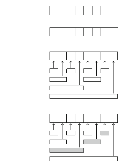
9.2 Tree Structures 123
Fig. 9.6 An array and its
binary indexed tree 13486142
12345678
original array
144
16 6 7429
12345678
binary indexed tree
Fig. 9.7 Ranges in a binary
indexed tree 144
16 6 7429
12345678
Fig. 9.8 Processing a range
sum query using a binary
indexed tree 144
16 6 7429
12345678
contains the value of sumq(5,6). Figure 9.6 shows an array and the corresponding
binary indexed tree. Figure 9.7 shows more clearly how each value in the binary
indexed tree corresponds to a range in the original array.
Using a binary indexed tree, any value of sumq(1,k)can be calculated in O(log n)
time, because a range [1,k]can always be divided into O(log n)subranges whose
sums have been stored in the tree. For example, to calculate the value of sumq(1,7),
we divide the range [1,7]into three subranges [1,4],[5,6], and [7,7](Fig. 9.8).
Since the sums of those subranges are available in the tree, we can calculate the sum
of the entire range using the formula
sumq(1,7)=sumq(1,4)+sumq(5,6)+sumq(7,7)=16 +7+4=27.
Then, to calculate the value of sumq(a,b)where a>1, we can use the same trick
that we used with prefix sum arrays:
sumq(a,b)=sumq(1,b)−sumq(1,a−1)
We can calculate both sumq(1,b)and sumq(1,a−1)in O(log n)time, so the total
time complexity is O(log n).
After updating an array value, several values in the binary indexed tree should
be updated. For example, when the value at position 3 changes, we should update
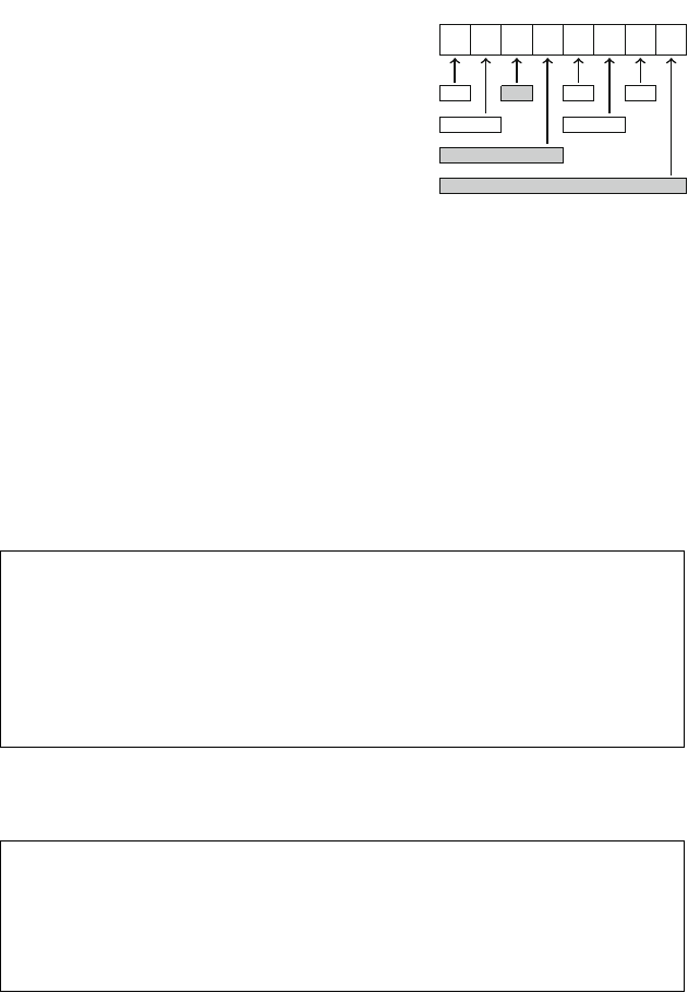
124 9 Range Queries
Fig. 9.9 Updating a value in
abinaryindexedtree 144
16 6 7429
12345678
the subranges [3,3],[1,4], and [1,8](Fig. 9.9). Since each array element belongs to
O(log n)subranges, it suffices to update O(log n)tree values.
Implementation The operations of a binary indexed tree can be efficiently imple-
mented using bit operations. The key fact needed is that we can easily calculate any
value of p(k)using the bit formula
p(k)=k&−k,
which isolates the least significant one bit of k.
First, the following function calculates the value of sumq(1,k):
int sum(int k) {
int s=0;
while (k >= 1) {
s += tree[k];
k -= k&-k;
}
return s;
}
Then, the following function increases the array value at position kby x(xcan
be positive or negative):
void add(int k, int x) {
while (k <= n) {
tree[k] += x;
k += k&-k;
}
}
The time complexity of both the functions is O(log n), because the functions
access O(log n)values in the binary indexed tree, and each move to the next position
takes O(1)time.
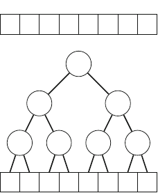
9.2 Tree Structures 125
Fig. 9.10 An array and the
corresponding segment tree
for sum queries 58632726
01234567
58632726
13 9 9 8
22 17
39
9.2.2 Segment Trees
Asegment tree is a data structure that provides two O(log n)time operations: process-
ing a range query and updating an array value. Segment trees support sum queries,
minimum queries, and many other queries. Segment trees have their origins in geo-
metric algorithms (see, e.g., Bentley and Wood [4]), and the elegant bottom-up imple-
mentation presented in this section follows the textbook by Sta´nczyk [30].
A segment tree is a binary tree whose bottom level nodes correspond to the array
elements, and the other nodes contain information needed for processing range
queries. When discussing segment trees, we assume that the size of the array is
a power of two, and zero-based indexing is used, because it is convenient to build a
segment tree for such an array. If the size of the array is not a power of two, we can
always append extra elements to it.
We will first discuss segment trees that support sum queries. As an example,
Fig. 9.10 shows an array and the corresponding segment tree for sum queries. Each
internal tree node corresponds to an array range whose size is a power of two. When
a segment tree supports sum queries, the value of each internal node is the sum of
the corresponding array values, and it can be calculated as the sum of the values of
its left and right child node.
It turns out that any range [a,b]can be divided into O(log n)subranges whose
values are stored in tree nodes. For example, Fig. 9.11 shows the range [2,7]in the
original array and in the segment tree. In this case, two tree nodes correspond to
the range, and sumq(2,7)=9+17 =26. When the sum is calculated using nodes
located as high as possible in the tree, at most two nodes on each level of the tree are
needed. Hence, the total number of nodes is O(log n).
After an array update, we should update all nodes whose value depends on the
updated value. This can be done by traversing the path from the updated array element
to the top node and updating the nodes along the path. For example, Fig. 9.12 shows
the nodes that change when the value at position 5 changes. The path from bottom
to top always consists of O(log n)nodes, so each update changes O(log n)nodes in
the tree.
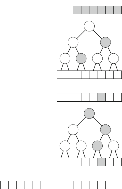
126 9 Range Queries
Fig. 9.11 Processing a range
sum query using a segment
tree 58632726
01234567
58632726
13 9 9 8
22 17
39
Fig. 9.12 Updating an array
value in a segment tree 58632726
01234567
58632726
13 9 9 8
22 17
39
Fig. 9.13 Contents of a
segment tree in an array 39 22 17 13 99858632726
12345678910 11 12 13 14 15
Implementation A convenient way to store the contents of a segment tree is to use
an array of 2nelements where nis the size of the original array. The tree nodes are
stored from top to bottom: tree[1]is the top node, tree[2]and tree[3]are its
children, and so on. Finally, the values from tree[n]to tree[2n−1]correspond
to the bottom level of the tree, which contains the values of the original array. Note
that the element tree[0]is not used.
For example, Fig. 9.13 shows how our example tree is stored. Note that the par-
ent of tree[k]is tree[k/2], its left child is tree[2k], and its right child is
tree[2k+1]. In addition, the position of a node (other than the top node) is even
if it is a left child and odd if it is a right child.

9.2 Tree Structures 127
The following function calculates the value of sumq(a,b):
int sum(int a, int b) {
a+=n;b+=n;
int s=0;
while (a <= b) {
if (a%2 == 1) s += tree[a++];
if (b%2 == 0) s += tree[b--];
a/=2;b/=2;
}
return s;
}
The function maintains a range in the segment tree array. Initially, the range is
[a+n,b+n]. At each step, the range is moved one level higher in the tree, and the
values of the nodes that do not belong to the higher range are added to the sum.
The following function increases the array value at position kby x:
void add(int k, int x) {
k+=n;
tree[k] += x;
for (k/=2;k>=1;k/=2){
tree[k] = tree[2*k]+tree[2*k+1];
}
}
First the value at the bottom level of the tree is updated. After this, the values of
all internal tree nodes are updated, until the top node of the tree is reached.
Both the above functions work in O(log n)time, because a segment tree of n
elements consists of O(log n)levels and the functions move one level higher in the
tree at each step.
Other Queries Segment trees can support any range queries where we can divide
a range into two parts, calculate the answer separately for both parts, and then effi-
ciently combine the answers. Examples of such queries are minimum and maximum,
greatest common divisor, and bit operations and, or, and xor.
For example, the segment tree in Fig.9.14 supports minimum queries. In this tree,
every node contains the smallest value in the corresponding array range. The top
node of the tree contains the smallest value in the whole array. The operations can
be implemented like previously, but instead of sums, minima are calculated.
The structure of a segment tree also allows us to use a binary search style method
for locating array elements. For example, if the tree supports minimum queries, we
can find the position of an element with the smallest value in O(log n)time. For
example, Fig. 9.15 shows how the element with the smallest value 1 can be found by
traversing a path downwards from the top node.
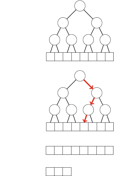
128 9 Range Queries
Fig. 9.14 A segment tree for
processing range minimum
queries
58631726
5 3 1 2
31
1
Fig. 9.15 Using binary
search to find the minimum
element
58631726
5 3 1 2
31
1
Fig. 9.16 Compressing an
array using index
compression 00500304
01234567
original array
534
012
compressed array
9.2.3 Additional Techniques
Index Compression A limitation in data structures that are built upon arrays is that
the elements are indexed using consecutive integers. Difficulties arise when large
indices are needed. For example, if we want to use the index 109, the array should
contain 109elements which would require too much memory.
However, if we know all the indices needed during the algorithm beforehand, we
can bypass this limitation by using index compression. The idea is to replace the
original indices with consecutive integers 0,1,2, and so on. To do this, we define
a function cthat compresses the indices. The function gives each original index ia
compressed index c(i)in such a way that if aand bare two indices and a<b, then
c(a)<c(b). After compressing the indices, we can conveniently perform queries
using them.
Figure 9.16 shows a simple example of index compression. Here only indices 2, 5,
and 7 are actually used, and all other array values are zeros. The compressed indices
are c(2)=0, c(5)=1, and c(7)=2, which allows us to create a compressed array
that only contains three elements.
9.2 Tree Structures 129
Fig. 9.17 An array and its
difference array 33111522
01234567
original array
30
−2004−30
01234567
difference array
Fig. 9.18 Updating an array
range using the difference
array 36444522
01234567
original array
33
−2001−30
01234567
difference array
After index compression, we can, for example, build a segment tree for the com-
pressed array and perform queries. The only modification needed is that we have to
compress the indices before queries: a range [a,b]in the original array corresponds
to the range [c(a), c(b)]in the compressed array.
Range Updates So far, we have implemented data structures that support range
queries and updates of single values. Let us now consider an opposite situation,
where we should update ranges and retrieve single values. We focus on an operation
that increases all elements in a range [a,b]by x.
It turns out that we can use the data structures presented in this chapter also in this
situation. To do this, we build a difference array whose values indicate the differences
between consecutive values in the original array. The original array is the prefix sum
array of the difference array. Figure 9.17 shows an array and its difference array.
For example, the value 2 at position 6 in the original array corresponds to the sum
3−2+4−3=2 in the difference array.
The advantage of the difference array is that we can update a range in the origi-
nal array by changing just two elements in the difference array. More precisely, to
increase the values in range [a,b]by x, we increase the value at position aby x
and decrease the value at position b+1byx. For example, to increase the original
array values between positions 1 and 4 by 3, we increase the difference array value
at position 1 by 3 and decrease the value at position 5 by 3 (Fig.9.18).
Thus, we only update single values and process sum queries in the difference
array, so we can use a binary indexed tree or a segment tree. A more difficult task
is to create a data structure that supports both range queries and range updates. In
Sect. 15.2.1, we will see that also this is possible using a lazy segment tree.

Tree Algorithms
The special properties of trees allow us to create algorithms that are specialized for
trees and work more efficiently than general graph algorithms. This chapter presents
a selection of such algorithms.
Section 10.1 introduces basic concepts and algorithms related to trees. A central
problem is finding the diameter of a tree, i.e., the maximum distance between two
nodes. We will learn two linear time algorithms for solving the problem.
Section 10.2 focuses on processing queries on trees. We will learn to use a tree
traversal array to process various queries related to subtrees and paths. After this,
we will discuss methods for determining lowest common ancestors, and an offline
algorithm which is based on merging data structures.
Section 10.3 presents two advanced tree processing techniques: centroid decom-
position and heavy-light decomposition.
10.1 Basic Techniques
Atree is a connected acyclic graph that consists of nnodes and n−1 edges. Remov-
ing any edge from a tree divides it into two components, and adding any edge creates
a cycle. There is always a unique path between any two nodes of a tree. The leaves
of a tree are the nodes with only one neighbor.
As an example, consider the tree in Fig.10.1. This tree consists of 8 nodes and 7
edges, and its leaves are nodes 3, 5, 7, and 8.
In a rooted tree, one of the nodes is appointed the root of the tree, and all other
nodes are placed underneath the root. The lower neighbors of a node are called its
children, and the upper neighbor of a node is called its parent. Each node has exactly
one parent, except for the root that does not have a parent. The structure of a rooted
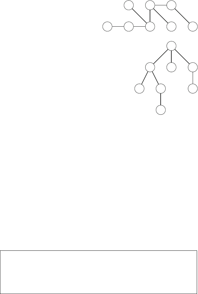
132 10 Tree Algorithms
Fig. 10.1 Atreethat
consists of 8 nodes and 7
edges
1 4
237
5
6
8
Fig. 10.2 A rooted tree
where node 1 is the root
node
1
42 3
7
5 6
8
tree is recursive: each node of the tree acts as the root of a subtree that contains the
node itself and all nodes that are in the subtrees of its children.
For example, Fig. 10.2 shows a rooted tree where node 1 is the root of the tree.
The children of node 2 are nodes 5 and 6, and the parent of node 2 is node 1. The
subtree of node 2 consists of nodes 2, 5, 6, and 8.
10.1.1 Tree Traversal
General graph traversal algorithms can be used to traverse the nodes of a tree. How-
ever, the traversal of a tree is easier to implement than that of a general graph, because
there are no cycles in the tree, and it is not possible to reach a node from more than
one direction.
A typical way to traverse a tree is to start a depth-first search at an arbitrary node.
The following recursive function can be used:
void dfs(int s, int e) {
// process node s
for (auto u : adj[s]) {
if (u != e) dfs(u, s);
}
}
The function is given two parameters: the current node sand the previous node e.
The purpose of the parameter eis to make sure that the search only moves to nodes
that have not been visited yet.
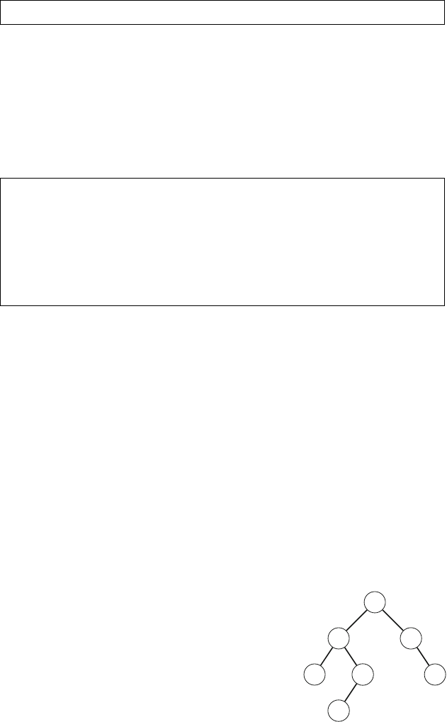
10.1 Basic Techniques 133
The following function call starts the search at node x:
dfs(x, 0);
In the first call e=0, because there is no previous node, and it is allowed to
proceed to any direction in the tree.
Dynamic Programming Dynamic programming can be used to calculate some infor-
mation during a tree traversal. For example, the following code calculates for each
node sa value count[s]: the number of nodes in its subtree. The subtree contains
the node itself and all nodes in the subtrees of its children, so we can calculate the
number of nodes recursively as follows:
void dfs(int s, int e) {
count[s] = 1;
for (auto u : adj[s]) {
if (u == e) continue;
dfs(u, s);
count[s] += count[u];
}
}
Binary Tree Traversals In a binary tree, each node has a left and right subtree (which
may be empty), and there are three popular tree traversal orderings:
•pre-order: first process the root node, then traverse the left subtree, then traverse
the right subtree
•in-order: first traverse the left subtree, then process the root node, then traverse
the right subtree
•post-order: first traverse the left subtree, then traverse the right subtree, then
process the root node
For example, in Fig. 10.3, the pre-order is [1,2,4,5,6,3,7], the in-order is
[4,2,6,5,1,3,7], and the post-order is [4,6,5,2,7,3,1].
If we know the pre-order and in-order of a tree, we can reconstruct its exact
structure. For example, the only possible tree with pre-order [1,2,4,5,6,3,7]and
Fig. 10.3 Abinarytree 1
23
45
6
7
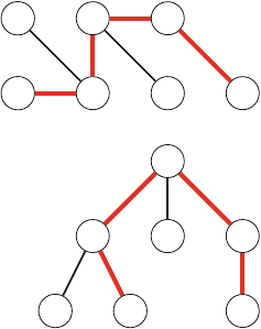
134 10 Tree Algorithms
Fig. 10.4 A tree whose
diameter is 4 1 4
237
5
6
Fig. 10.5 Node 1 is the
highest point on the diameter
path
1
42 3
7
5 6
in-order [4,2,6,5,1,3,7]is shown in Fig. 10.3. The post-order and in-order also
uniquely determine the structure of a tree. However, if we only know the pre-order
and post-order, there may be more than one tree that matches the orderings.
10.1.2 Calculating Diameters
The diameter of a tree is the maximum length of a path between two nodes. For
example, Fig. 10.4 shows a tree whose diameter is 4 that corresponds to a path of
length 4 between nodes 6 and 7. Note that the tree also has another path of length 4
between nodes 5 and 7.
Next we will discuss two O(n)time algorithms for calculating the diameter of a
tree. The first algorithm is based on dynamic programming, and the second algorithm
uses depth-first searches.
First Algorithm A general way to approach tree problems is to first root the tree
arbitrarily and then solve the problem separately for each subtree. Our first algorithm
for calculating diameters is based on this idea.
An important observation is that every path in a rooted tree has a highest point:
the highest node that belongs to the path. Thus, we can calculate for each node xthe
length of the longest path whose highest point is x. One of those paths corresponds
to the diameter of the tree. For example, in Fig. 10.5, node 1 is the highest point on
the path that corresponds to the diameter.
We calculate for each node xtwo values:
•toLeaf(x): the maximum length of a path from xto any leaf
•maxLength(x): the maximum length of a path whose highest point is x
For example, in Fig. 10.5,toLeaf(1)=2, because there is a path 1 →2→6, and
maxLength(1)=4, because there is a path 6 →2→1→4→7. In this case,
maxLength(1)equals the diameter.
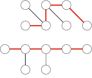
10.1 Basic Techniques 135
Fig. 10.6 Nodes a,b,andc
when calculating the
diameter
1 4
237
5
6
a
bc
Fig. 10.7 Why does the
algorithm work? 1 42
3
7
5
6
a
bcx
Dynamic programming can be used to calculate the above values for all nodes
in O(n)time. First, to calculate toLeaf(x), we go through the children of x,
choose a child cwith the maximum toLeaf(c), and add one to this value. Then,
to calculate maxLength(x), we choose two distinct children aand bsuch that the
sum toLeaf(a)+toLeaf(b)is maximum and add two to this sum. (The cases
where xhas less than two children are easy special cases.)
Second Algorithm Another efficient way to calculate the diameter of a tree is based
on two depth-first searches. First, we choose an arbitrary node ain the tree and find
the farthest node bfrom a. Then, we find the farthest node cfrom b. The diameter
of the tree is the distance between band c.
For example, Fig. 10.6 shows a possible way to select nodes a,b, and cwhen
calculating the diameter for our example tree.
This is an elegant method, but why does it work? It helps to draw the tree so that
the path that corresponds to the diameter is horizontal and all other nodes hang from
it (Fig. 10.7). Node xindicates the place where the path from node ajoins the path
that corresponds to the diameter. The farthest node from ais node b, node c, or some
other node that is at least as far from node x. Thus, this node is always a valid choice
for an endpoint of a path that corresponds to the diameter.
10.1.3 All Longest Paths
Our next problem is to calculate for every tree node xa value maxLength(x): the
maximum length of a path that begins at node x. For example, Fig.10.8 shows a tree
and its maxLength values. This can be seen as a generalization of the tree diameter
problem, because the largest of those lengths equals the diameter of the tree. Also,
this problem can be solved in O(n)time.
Once again, a good starting point is to root the tree arbitrarily. The first part of
the problem is to calculate for every node xthe maximum length of a path that goes
downwards through a child of x. For example, the longest path from node 1 goes
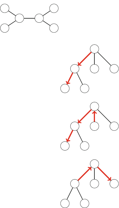
136 10 Tree Algorithms
Fig. 10.8 Calculating
maximum path lengths
1
4
2
3
6
5
maxLength(1)=2
maxLength(2)=2
maxLength(3)=3
maxLength(4)=3
maxLength(5)=3
maxLength
(
6
)
=3
Fig. 10.9 The longest path
that starts at node 1 1
42 3
5 6
Fig. 10.10 The longest path
from node 3 goes through its
parent
1
42 3
5 6
Fig. 10.11 In this case, the
second longest path from the
parent should be chosen
1
42 3
5 6
through its child 2 (Fig. 10.9). This part is easy to solve in O(n)time, because we
can use dynamic programming as we have done previously.
Then, the second part of the problem is to calculate for every node xthe maximum
length of a path upwards through its parent p. For example, the longest path from
node 3 goes through its parent 1 (Fig. 10.10). At first glance, it seems that we should
first move to pand then choose the longest path (upwards or downwards) from
p. However, this does not always work, because such a path may go through x
(Fig. 10.11). Still, we can solve the second part in O(n)time by storing the maximum
lengths of two paths for each node x:
•maxLength1(x): the maximum length of a path from xto a leaf
•maxLength2(x)the maximum length of a path from xto a leaf, in another
direction than the first path
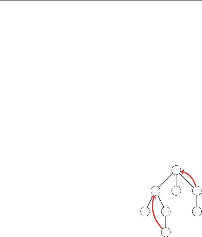
10.1 Basic Techniques 137
For example, in Fig. 10.11,maxLength1(1)=2 using the path 1 →2→5, and
maxLength2(1)=1 using the path 1 →3.
Finally, to determine the maximum-length path from node xupwards through its
parent p, we consider two cases: if the path that corresponds to maxLength1(p)
goes through x, the maximum length is maxLength2(p)+1 and otherwise the
maximum length is maxLength1(p)+1.
10.2 Tree Queries
In this section we focus on processing queries on rooted trees. Such queries are
typically related to subtrees and paths of the tree, and they can be processed in
constant or logarithmic time.
10.2.1 Finding Ancestors
The kth ancestor of a node xin a rooted tree is the node that we will reach if we move
klevels up from x. Let ancestor(x,k)denote the kth ancestor of a node x(or 0 if
there is no such an ancestor). For example, in Fig. 10.12,ancestor(2,1)=1 and
ancestor(8,2)=4.
An easy way to calculate any value of ancestor(x,k)is to perform a sequence
of kmoves in the tree. However, the time complexity of this method is O(k), which
may be slow, because a tree of nnodes may have a path of nnodes.
Fortunately, we can efficiently calculate any value of ancestor(x,k)in O(log k)
time after preprocessing. As in Sect. 7.5.1, the idea is to first precalculate all values
of ancestor(x,k)where kis a power of two. For example, the values for the tree
in Fig. 10.12 are as follows:
Fig. 10.12 Finding
ancestors of nodes 1
24 5
6
37
8

138 10 Tree Algorithms
x12345678
ancestor(x,1)01411247
ancestor(x,2)00100114
ancestor(x,4)00000000
···
Since we know that a node always has less than nancestors, it suffices to calculate
O(log n)values for each node and the preprocessing takes O(nlog n)time. After this,
any value of ancestor(x,k)can be calculated in O(log k)time by representing k
as a sum where each term is a power of two.
10.2.2 Subtrees and Paths
Atree traversal array contains the nodes of a rooted tree in the order in which a
depth-first search from the root node visits them. For example, Fig. 10.13 shows a
tree and the corresponding tree traversal array.
An important property of tree traversal arrays is that each subtree of a tree cor-
responds to a subarray in the tree traversal array such that the first element of the
subarray is the root node. For example, Fig. 10.14 shows the subarray that corre-
sponds to the subtree of node 4.
Subtree Queries Suppose that each node in the tree is assigned a value and our task
is to process two types of queries: updating the value of a node and calculating the
sum of values in the subtree of a node. To solve the problem, we construct a tree
traversal array that contains three values for each node: the identifier of the node, the
size of the subtree, and the value of the node. For example, Fig. 10.15 shows a tree
and the corresponding array.
1
2345
6789
126347895
Fig. 10.13 A tree and its tree traversal array
126347895
Fig. 10.14 The subtree of node 4 in the tree traversal array
10.2 Tree Queries 139
Fig. 10.15 A tree traversal
array for calculating subtree
sums
1
2345
6789
2
35 31
44
31
node id
subtree size
node value
126347895
921141111
234534311
Fig. 10.16 Calculating the
sum of values in the subtree
of node 4
node id
subtree size
node value
126347895
921141111
234534311
Using this array, we can calculate the sum of values in any subtree by first deter-
mining the size of the subtree and then summing up the values of the corresponding
nodes. For example, Fig. 10.16 shows the values that we access when calculating the
sum of values in the subtree of node 4. The last row of the array tells us that the sum
of values is 3 +4+3+1=11.
To answer queries efficiently, it suffices to store the last row of the array in a
binary indexed or segment tree. After this, we can both update a value and calculate
the sum of values in O(log n)time.
Path Queries Using a tree traversal array, we can also efficiently calculate sums of
values on paths from the root node to any node of the tree. As an example, consider
a problem where our task is to process two types of queries: updating the value of a
node and calculating the sum of values on a path from the root to a node.
To solve the problem, we construct a tree traversal array that contains for each
node its identifier, the size of its subtree, and the sum of values on a path from the
root to the node (Fig. 10.17). When the value of a node increases by x, the sums of
all nodes in its subtree increase by x. For example, Fig.10.18 shows the array after
increasing the value of node 4 by 1.
To support both the operations, we need to be able to increase all values in a range
and retrieve a single value. This can be done in O(log n)time using a binary indexed
or segment tree and a difference array (see Sect. 9.2.3).
140 10 Tree Algorithms
Fig. 10.17 A tree traversal
array for calculating path
sums
1
2345
6789
4
53 52
353
1
node id
subtree size
path sum
126347895
921141111
4912 7914 12 10 6
Fig. 10.18 Increasing the
value of node 4 by 1 node id
subtree size
path sum
126347895
921141111
4912 710 15 13 11 6
Fig. 10.19 The lowest
common ancestor of nodes 5
and 8 is node 2
1
42 3
7
5 6
8
10.2.3 Lowest Common Ancestors
The lowest common ancestor of two nodes of a rooted tree is the lowest node whose
subtree contains both the nodes. For example, in Fig. 10.19 the lowest common
ancestor of nodes 5 and 8 is node 2.
A typical problem is to efficiently process queries that require us to find the lowest
common ancestor of two nodes. Next we will discuss two efficient techniques for
processing such queries.
First Method Since we can efficiently find the kth ancestor of any node in the tree,
we can use this fact to divide the problem into two parts. We use two pointers that
initially point to the two nodes whose lowest common ancestor we should find.
First, we make sure that the pointers point to nodes at the same level in the tree.
If this is not the case initially, we move one of the pointers upwards. After this, we
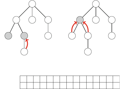
10.2 Tree Queries 141
1
42 3
7
5 6
8
1
42 3
7
5 6
8
Fig. 10.20 Two steps to find the lowest common ancestor of nodes 5 and 8
node id
depth
125268621314741
123234321212321
012345678910 11 12 13 14
Fig. 10.21 An extended tree traversal array for processing lowest common ancestor queries
determine the minimum number of steps needed to move both pointers upwards so
that they will point to the same node. The node to which the pointers point after this
is the lowest common ancestor. Since both parts of the algorithm can be performed
in O(log n)time using precomputed information, we can find the lowest common
ancestor of any two nodes in O(log n)time.
Figure 10.20 shows how we can find the lowest common ancestor of nodes 5 and
8 in our example scenario. First, we move the second pointer one level up so that it
points to node 6 which is at the same level with node 5. Then, we move both pointers
one step upwards to node 2, which is the lowest common ancestor.
Second Method Another way to solve the problem, proposed by Bender and Farach-
Colton [3], is based on an extended tree traversal array, sometimes called an Euler
tour tree. To construct the array, we go through the tree nodes using depth-first search
and add each node to the array always when the depth-first search walks through
the node (not only at the first visit). Hence, a node that has kchildren appears k+1
times in the array, and there are a total of 2n−1 nodes in the array. We store two
values in the array: the identifier of the node and the depth of the node in the tree.
Figure 10.21 shows the resulting array in our example scenario.
Now we can find the lowest common ancestor of nodes aand bby finding the node
with the minimum depth between nodes aand bin the array. For example, Fig. 10.22
shows how to find the lowest common ancestor of nodes 5 and 8. The minimum-
depth node between them is node 2 whose depth is 2, so the lowest common ancestor
of nodes 5 and 8 is node 2.
Note that since a node may appear several times in the array, there may be mul-
tiple ways to choose the positions of nodes aand b. However, any choice correctly
determines the lowest common ancestor of the nodes.
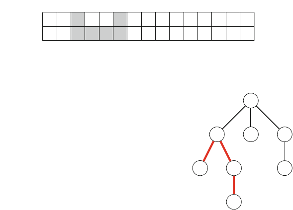
142 10 Tree Algorithms
node id
depth
↑
125268621314741
123234321212321
012345678910 11 12 13 14
Fig. 10.22 Finding the lowest common ancestor of nodes 5 and 8
Fig. 10.23 Calculating the
distance between nodes 5
and 8
1
42 3
7
5 6
8
Using this technique, to find the lowest common ancestor of two nodes, it suffices
to process a range minimum query. A usual way is to use a segment tree to process
such queries in O(log n)time. However, since the array is static, we can also process
queries in O(1)time after an O(nlog n)time preprocessing.
Calculating Distances Finally, consider the problem of processing queries where
we need to calculate the distance between nodes aand b(i.e., the length of the path
between aand b). It turns out that this problem reduces to finding the lowest common
ancestor of the nodes. First, we root the tree arbitrarily. After this, the distance of
nodes aand bcan be calculated using the formula
depth(a)+depth(b)−2·depth(c),
where cis the lowest common ancestor of aand b.
For example, to calculate the distance between nodes 5 and 8 in Fig. 10.23,we
first determine that the lowest common ancestor of the nodes is node 2. Then, since
the depths of the nodes are depth(5)=3, depth(8)=4, and depth(2)=2, we
conclude that the distance between nodes 5 and 8 is 3 +4−2·2=3.
10.2.4 Merging Data Structures
So far, we have discussed online algorithms for tree queries. Those algorithms are
able to process queries one after another in such a way that each query is answered
before receiving the next query. However, in many problems, the online property
is not necessary, and we may use offline algorithms to solve them. Such algorithms
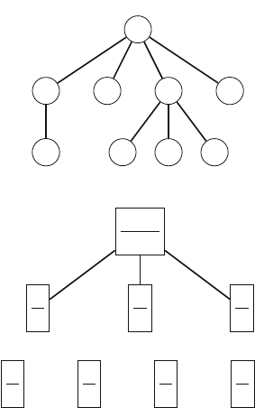
10.2 Tree Queries 143
Fig. 10.24 The subtree of
node 4 contains two nodes
whose value is 3
1
2345
6789
2
35 31
44
31
Fig. 10.25 Processing
queries using map structures
4
1
3
1
1
1
134
121
Fig. 10.26 Merging map
structures at a node
4
1
3
1
1
1
3
1
are given a complete set of queries which can be answered in any order. Offline
algorithms are often easier to design than online algorithms.
One method to construct an offline algorithm is to perform a depth-first tree
traversal and maintain data structures in nodes. At each node s, we create a data
structure d[s]that is based on the data structures of the children of s. Then, using
this data structure, all queries related to sare processed.
As an example, consider the following problem: We are given a rooted tree where
each node has some value. Our task is to process queries that ask to calculate the
number of nodes with value xin the subtree of node s. For example, in Fig. 10.24,
the subtree of node 4 contains two nodes whose value is 3.
In this problem, we can use map structures to answer the queries. For example,
Fig. 10.25 shows the maps for node 4 and its children. If we create such a data
structure for each node, we can easily process all given queries, because we can
handle all queries related to a node immediately after creating its data structure.
However, it would be too slow to create all data structures from scratch. Instead,
at each node s, we create an initial data structure d[s]that only contains the value of
s. After this, we go through the children of sand merge d[s]and all data structures
d[u]where uis a child of s. For example, in the above tree, the map for node 4
is created by merging the maps in Fig. 10.26. Here the first map is the initial data
structure for node 4, and the other three maps correspond to nodes 7, 8, and 9.
The merging at node scan be done as follows: We go through the children of s
and at each child umerge d[s]and d[u]. We always copy the contents from d[u]to
d[s]. However, before this, we swap the contents of d[s]and d[u]if d[s]is smaller
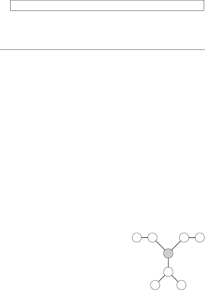
144 10 Tree Algorithms
than d[u]. By doing this, each value is copied only O(log n)times during the tree
traversal, which ensures that the algorithm is efficient.
To swap the contents of two data structures aand befficiently, we can just use
the following code:
swap(a,b);
It is guaranteed that the above code works in constant time when aand bare C++
standard library data structures.
10.3 Advanced Techniques
In this section, we discuss two advanced tree processing techniques. Centroid decom-
position divides a tree into smaller subtrees and processes them recursively. Heavy-
light decomposition represents a tree as a set of special paths, which allows us to
efficiently process path queries.
10.3.1 Centroid Decomposition
Acentroid of a tree of nnodes is a node whose removal divides the tree into subtrees
each of which contains at most n/2nodes. Every tree has a centroid, and it can be
found by rooting the tree arbitrarily and always moving to the subtree that has the
maximum number of nodes, until the current node is a centroid.
In the centroid decomposition technique, we first locate a centroid of the tree and
process all paths that go through the centroid. After this, we remove the centroid
from the tree and process the remaining subtrees recursively. Since removing the
centroid always creates subtrees whose size is at most half of the size of the original
tree, the time complexity of such an algorithm is O(nlog n), provided that we can
process each subtree in linear time.
For example, Fig. 10.27 shows the first step of a centroid decomposition algorithm.
In this tree, node 5 is the only centroid, so we first process all paths that go through
Fig. 10.27 Centroid
decomposition 1 2 34
5
6
78
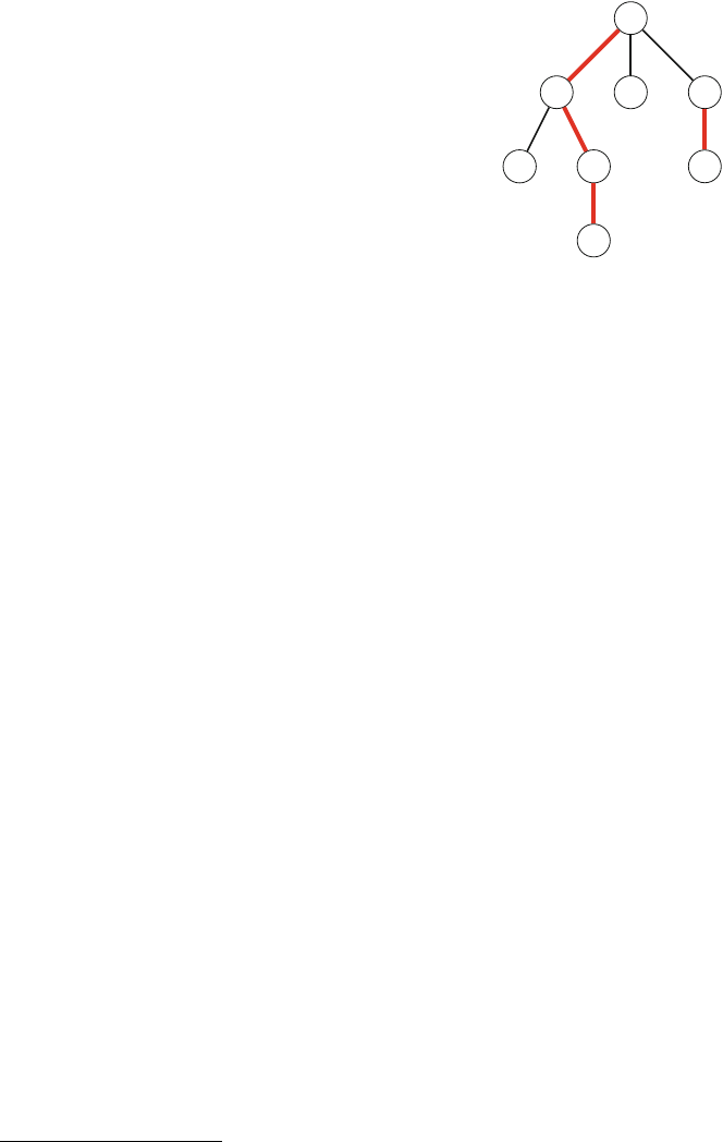
10.3 Advanced Techniques 145
Fig. 10.28 Heavy-light
decomposition 1
42 3
7
5 6
8
node 5. After this, node 5 is removed from the tree, and we process the three subtrees
{1,2},{3,4}, and {6,7,8}recursively.
Using centroid decomposition, we can, for example, efficiently calculate the num-
ber of paths of length xin a tree. When processing a tree, we first find a centroid
and calculate the number of paths that go through it, which can be done in linear
time. After this, we remove the centroid and recursively process the smaller trees.
The resulting algorithm works in O(nlog n)time.
10.3.2 Heavy-Light Decomposition
Heavy-light decomposition1divides the nodes of a tree into a set of paths that are
called heavy paths. The heavy paths are created so that a path between any two tree
nodes can be represented as O(log n)subpaths of heavy paths. Using the technique,
we can manipulate nodes on paths between tree nodes almost like elements in an
array, with only an additional O(log n)factor.
To construct the heavy paths, we first root the tree arbitrarily. Then, we start the
first heavy path at the root of the tree and always move to a node that has a maximum-
size subtree. After this, we recursively process the remaining subtrees. For example,
in Fig. 10.28, there are four heavy paths: 1–2–6–8, 3, 4–7, and 5 (note that two of
the paths only have one node).
Now, consider any path between two nodes in the tree. Since we always chose the
maximum-size subtree when creating heavy paths, this guarantees that we can divide
the path into O(log n)subpaths so that each of them is a subpath of a single heavy
path. For example, in Fig. 10.28, the path between nodes 7 and 8 can be divided into
two heavy subpaths: first 7–4, then 1–2–6–8.
The benefit of heavy-light decomposition is that each heavy path can be treated
like an array of nodes. For example, we can assign a segment tree for each heavy
path and support sophisticated path queries, such as calculating the minimum node
value in a path or increasing the value of every node in a path. Such queries can be
1Sleator and Tarjan [29] introduced the idea in the context of their link/cut tree data structure.

146 10 Tree Algorithms
processed in O(log2n)time,2because each path consists of O(log n)heavy paths
and each heavy path can be processed in O(log n)time.
While many problems can be solved using heavy-light decomposition, it is good
to keep in mind that there is often another solution that is easier to implement.
In particular, the techniques presented in Sect. 10.2.2 can often be used instead of
heavy-light decomposition.
2The notation logkncorresponds to (log n)k.

Mathematics
This chapter deals with mathematical topics that are recurrent in competitive pro-
gramming. We will both discuss theoretical results and learn how to use them in
practice in algorithms.
Section 11.1 discusses number-theoretical topics. We will learn algorithms for
finding prime factors of numbers, techniques related to modular arithmetic, and
efficient methods for solving integer equations.
Section 11.2 explores ways to approach combinatorial problems: how to efficiently
count all valid combinations of objects. The topics of this section include binomial
coefficients, Catalan numbers, and inclusion-exclusion.
Section 11.3 shows how to use matrices in algorithm programming. For example,
we will learn how to make a dynamic programming algorithm more efficient by
exploiting an efficient way to calculate matrix powers.
Section 11.4 first discusses basic techniques for calculating probabilities of events
and the concept of Markov chains. After this, we will see examples of algorithms
that are based on randomness.
Section 11.5 focuses on game theory. First, we will learn to optimally play a simple
stick game using nim theory, and after this, we will generalize the strategy to a wide
range of other games.
11.1 Number Theory
Number theory is a branch of mathematics that studies integers. In this section, we
will discuss a selection of number-theoretical topics and algorithms, such as finding
prime numbers and factors, and solving integer equations.
148 11 Mathematics
11.1.1 Primes and Factors
An integer ais called a factor or a divisor of an integer bif adivides b.Ifais a
factor of b, we write a|b, and otherwise we write ab. For example, the factors of
24 are 1, 2, 3, 4, 6, 8, 12, and 24.
An integer n>1isaprime if its only positive factors are 1 and n. For example,
7, 19, and 41 are primes, but 35 is not a prime, because 5 ·7=35. For every integer
n>1, there is a unique prime factorization
n=pα1
1pα2
2···pαk
k,
where p1,p2,..., pkare distinct primes and α1,α
2,...,α
kare positive integers.
For example, the prime factorization for 84 is
84 =22·31·71.
Let τ(n)denote the number of factors of an integer n. For example, τ(12)=6,
because the factors of 12 are 1, 2, 3, 4, 6, and 12. To calculate the value of τ(n),we
can use the formula
τ(n)=
k
i=1
(αi+1),
because for each prime pi, there are αi+1 ways to choose how many times it appears
in the factor. For example, since 12 =22·3, τ(12)=3·2=6.
Then, let σ(n)denote the sum of factors of an integer n. For example, σ(12)=28,
because 1 +2+3+4+6+12 =28. To calculate the value of σ(n), we can use
the formula
σ(n)=
k
i=1
(1+pi+···+pαi
i)=
k
i=1
pαi+1
i−1
pi−1,
where the latter form is based on the geometric progression formula. For example,
σ(12)=(23−1)/(2−1)·(32−1)/(3−1)=28.
Basic Algorithms If an integer nis not prime, it can be represented as a product
a·b, where a≤√nor b≤√n, so it certainly has a factor between 2 and √n.
Using this observation, we can both test if an integer is prime and find its prime
factorization in O(√n)time.
The following function prime checks if a given integer nis prime. The function
attempts to divide nby all integers between 2 and √n, and if none of them divides
n, then nis prime.

11.1 Number Theory 149
bool prime(int n) {
if (n<2)return false;
for (int x = 2; x*x <= n; x++) {
if (n%x == 0) return false;
}
return true;
}
Then, the following function factors constructs a vector that contains the prime
factorization of n. The function divides nby its prime factors and adds them to the
vector. The process ends when the remaining number nhas no factors between 2 and
√n.Ifn>1, it is prime and the last factor.
vector<int> factors(int n) {
vector<int>f;
for (int x = 2; x*x <= n; x++) {
while (n%x == 0) {
f.push_back(x);
n/=x;
}
}
if (n > 1) f.push_back(n);
return f;
}
Note that each prime factor appears in the vector as many times as it divides the
number. For example, 12 =22·3, so the result of the function is [2,2,3].
Properties of Primes It is easy to show that there is an infinite number of primes. If
the number of primes would be finite, we could construct a set P={p1,p2,..., pn}
that would contain all the primes. For example, p1=2, p2=3, p3=5, and so on.
However, using such a set P, we could form a new prime
p1p2···pn+1
that would be larger than all elements in P. This is a contradiction, and the number
of primes has to be infinite.
The prime-counting function π(n)gives the number of primes up to n. For exam-
ple, π(10)=4, because the primes up to 10 are 2, 3, 5, and 7. It is possible to show
that
π(n)≈n
ln n,
which means that primes are quite frequent. For example, an approximation for
π(106)is 106/ln 106≈72382, and the exact value is 78498.
150 11 Mathematics
0010101110101110101
2345678910 11 12 13 14 15 16 17 18 19 20
Fig. 11.1 Outcome of the sieve of Eratosthenes for n=20
23252723211213 23217 219 2
2345678910 11 12 13 14 15 16 17 18 19 20
Fig. 11.2 An extended sieve of Eratosthenes that contains the smallest prime factor of each number
11.1.2 Sieve of Eratosthenes
The sieve of Eratosthenes is a preprocessing algorithm that constructs an array
sieve from which we can efficiently check if any integer xbetween 2 ...nis
prime. If xis prime, then sieve[x]=0, and otherwise sieve[x]=1. For exam-
ple, Fig. 11.1 shows the contents of sieve for n=20.
To construct the array, the algorithm iterates through the integers 2 ...none by
one. Always when a new prime xis found, the algorithm records that the num-
bers 2x,3x,4x, etc., are not primes. The algorithm can be implemented as follows,
assuming that every element of sieve is initially zero:
for (int x = 2; x <= n; x++) {
if (sieve[x]) continue;
for (int u=2*x;u<=n;u+=x){
sieve[u] = 1;
}
}
The inner loop of the algorithm is executed n/xtimes for each value of x. Thus,
an upper bound for the running time of the algorithm is the harmonic sum
n
x=2n/x=n/2+n/3+n/4+···=O(nlog n).
In fact, the algorithm is more efficient, because the inner loop will be executed
only if the number xis prime. It can be shown that the running time of the algorithm
is only O(nlog log n), a complexity very near to O(n). In practice, the sieve of
Eratosthenes is very efficient; Table 11.1 shows some real running times.
There are several ways to extend the sieve of Eratosthenes. For example, we can
calculate for each number kits smallest prime factor (Fig. 11.2). After this, we can
efficiently factorize any number between 2 ...nusing the sieve. (Note that a number
nhas O(log n)prime factors.)

11.1 Number Theory 151
Table 11.1 Running times of
the sieve of Eratosthenes Upper bound nRunning time (s)
1060.01
2·1060.03
4·1060.07
8·1060.14
16 ·1060.28
32 ·1060.57
64 ·1061.16
128 ·1062.35
11.1.3 Euclid’s Algorithm
The greatest common divisor of integers aand b, denoted gcd(a,b), is the largest
integer that divides both aand b. For example, gcd(30,12)=6. A related concept
is the lowest common multiple, denoted lcm(a,b), which is the smallest integer that
is divisible by both aand b. The formula
lcm(a,b)=ab
gcd(a,b)
can be used to calculate lowest common multiples. For example, lcm(30,12)=
360/gcd(30,12)=60.
One way to find gcd(a,b)is to divide aand binto prime factors, and then choose
for each prime the largest power that appears in both factorizations. For example,
to calculate gcd(30,12), we can construct the factorizations 30 =2·3·5 and
12 =22·3, and conclude that gcd(30,12)=2·3=6. However, this technique is
not efficient if aand bare large numbers.
Euclid’s algorithm provides an efficient way to calculate the value of gcd(a,b).
The algorithm is based on the formula
gcd(a,b)=ab=0
gcd(b,amod b)b= 0.
For example,
gcd(30,12)=gcd(12,6)=gcd(6,0)=6.
The algorithm can be implemented as follows:
int gcd(int a, int b) {
if (b == 0) return a;
return gcd(b, a%b);
}
152 11 Mathematics
Fig. 11.3 Why does
Euclid’s algorithm work?
a
bbamod b
xxxxxxxx
Why does the algorithm work? To understand this, consider Fig. 11.3. where
x=gcd(a,b). Since xdivides both aand b, it must also divide amod b, which
shows why the recursive formula holds.
It can be proved that Euclid’s algorithm works in O(log n)time, where n=
min(a,b).
Extended Euclid’s Algorithm Euclid’s algorithm can also be extended so that it
gives integers xand yfor which
ax +by =gcd(a,b).
For example, when a=30 and b=12,
30 ·1+12 ·(−2)=6.
We can solve also this problem using the formula gcd(a,b)=gcd(b,amod b).
Suppose that we have already solved the problem for gcd(b,amod b), and we know
values xand yfor which
bx+(amod b)y=gcd(a,b).
Then, since amod b=a−a/b·b,
bx+(a−a/b·b)y=gcd(a,b),
which equals
ay+b(x−a/b·y)=gcd(a,b).
Thus, we can choose x=yand y=x−a/b·y. Using this idea, the following
function returns a tuple (x,y,gcd(a,b)) that satisfies the equation.
tuple<int,int,int> gcd(int a, int b) {
if (b == 0) {
return {1,0,a};
}else {
int x,y,g;
tie(x,y,g) = gcd(b,a%b);
return {y,x-(a/b)*y,g};
}
}

11.1 Number Theory 153
We can use the function as follows:
int x,y,g;
tie(x,y,g) = gcd(30,12);
cout << x <<""<<y<<""<<g<<"\n";
//1-26
11.1.4 Modular Exponentiation
There is often a need to efficiently calculate the value of xnmod m. This can be done
in O(log n)time using the following recursive formula:
xn=⎧
⎪
⎨
⎪
⎩
1n=0
xn/2·xn/2nis even
xn−1·xnis odd
For example, to calculate the value of x100, we first calculate the value of x50 and
then use the formula x100 =x50 ·x50. Then, to calculate the value of x50, we first
calculate the value of x25 and so on. Since nalways halves when it is even, the
calculation takes only O(log n)time.
The algorithm can be implemented as follows:
int modpow(int x, int n, int m) {
if (n == 0) return 1%m;
long long u = modpow(x,n/2,m);
u = (u*u)%m;
if (n%2==1)u=(u*x)%m;
return u;
}
11.1.5 Euler’s Theorem
Two integers aand bare called coprime if gcd(a,b)=1. Euler’s totient function
ϕ(n)gives the number of integers between 1 ...nthat are coprime to n. For example,
ϕ(10)=4, because 1, 3, 7, and 9 are coprime to 10.
Any value of ϕ(n)can be calculated from the prime factorization of nusing the
formula
ϕ(n)=
k
i=1
pαi−1
i(pi−1).
For example, since 10 =2·5, ϕ(10)=20·(2−1)·50·(5−1)=4.
154 11 Mathematics
Euler’s theorem states that
xϕ(m)mod m=1
for all positive coprime integers xand m. For example, Euler’s theorem tells us that
74mod 10 =1, because 7 and 10 are coprime and ϕ(10)=4.
If mis prime, ϕ(m)=m−1, so the formula becomes
xm−1mod m=1,
which is known as Fermat’s little theorem. This also implies that
xnmod m=xnmod (m−1)mod m,
which can be used to calculate values of xnif nis very large.
Modular Multiplicative Inverses The modular multiplicative inverse of xwith
respect to mis a value invm(x)such that
x·invm(x)mod m=1.
For example, inv17(6)=3, because 6 ·3 mod 17 =1.
Using modular multiplicative inverses, we can divide numbers modulo m, because
division by xcorresponds to multiplication by invm(x). For example, since we know
that inv17(6)=3, we can calculate the value of 36/6 mod 17 in another way using
the formula 36 ·3 mod 17.
A modular multiplicative inverse exists exactly when xand mare coprime. In this
case, it can be calculated using the formula
invm(x)=xϕ(m)−1,
which is based on Euler’s theorem. In particular, if mis prime, ϕ(m)=m−1 and
the formula becomes
invm(x)=xm−2.
For example,
inv17(6)mod 17 =617−2mod 17 =3.
The above formula allows us to efficiently calculate modular multiplicative
inverses using the modular exponentiation algorithm (Sect. 11.1.4).

11.1 Number Theory 155
11.1.6 Solving Equations
Diophantine Equations ADiophantine equation is an equation of the form
ax +by =c,
where a,b, and care constants and the values of xand yshould be found. Each
number in the equation has to be an integer. For example, one solution to the equation
5x+2y=11
is x=3 and y=−2.
We can efficiently solve a Diophantine equation by using the extended Euclid’s
algorithm (Sect. 11.1.3) which gives integers xand ythat satisfy the equation
ax +by =gcd(a,b).
A Diophantine equation can be solved exactly when cis divisible by gcd(a,b).
As an example, let us find integers xand ythat satisfy the equation
39x+15y=12.
The equation can be solved, because gcd(39,15)=3 and 3 |12. The extended
Euclid’s algorithm gives us
39 ·2+15 ·(−5)=3,
and by multiplying this by 4, the equation becomes
39 ·8+15 ·(−20)=12,
so a solution to the equation is x=8 and y=−20.
A solution to a Diophantine equation is not unique, because we can form an infinite
number of solutions if we know one solution. If a pair (x,y)is a solution, then also
all pairs
x+kb
gcd(a,b),y−ka
gcd(a,b)
are solutions, where kis any integer.
Chinese Remainder Theorem The Chinese remainder theorem solves a group of
equations of the form
x=a1mod m1
x=a2mod m2
···
x=anmod mn

156 11 Mathematics
where all pairs of m1,m2,...,mnare coprime.
It turns out that a solution to the equations is
x=a1X1invm1(X1)+a2X2invm2(X2)+···+anXninvmn(Xn),
where
Xk=m1m2···mn
mk
.
In this solution, for each k=1,2,...,n,
akXkinvmk(Xk)mod mk=ak,
because
Xkinvmk(Xk)mod mk=1.
Since all other terms in the sum are divisible by mk, they have no effect on the
remainder and xmod mk=ak.
For example, a solution for
x=3 mod 5
x=4 mod 7
x=2 mod 3
is
3·21 ·1+4·15 ·1+2·35 ·2=263.
Once we have found a solution x, we can create an infinite number of other
solutions, because all numbers of the form
x+m1m2···mn
are solutions.
11.2 Combinatorics
Combinatorics studies methods for counting combinations of objects. Usually, the
goal is to find a way to count the combinations efficiently without generating each
combination separately. In this section, we discuss a selection of combinatorial tech-
niques that can be applied to a large number of problems.

11.2 Combinatorics 157
11.2.1 Binomial Coefficients
The binomial coefficient n
kgives the number of ways we can choose a subset
of kelements from a set of nelements. For example, 5
3=10, because the set
{1,2,3,4,5}has 10 subsets of 3 elements:
{1,2,3},{1,2,4},{1,2,5},{1,3,4},{1,3,5},
{1,4,5},{2,3,4},{2,3,5},{2,4,5},{3,4,5}
Binomial coefficients can be recursively calculated using the formula
n
k=n−1
k−1+n−1
k.
with the base cases
n
0=n
n=1.
To see why this formula works, consider an arbitrary element xin the set. If we
decide to include xin our subset, the remaining task is to choose k−1 elements
from n−1 elements. Then, if we do not include xin our subset, we have to choose
kelements from n−1 elements.
Another way to calculate binomial coefficients is to use the formula
n
k=n!
k!(n−k)!
which is based on the following reasoning: There are n!permutations of nelements.
We go through all permutations and always include the first kelements of the per-
mutation in the subset. Since the order of the elements in the subset and outside the
subset does not matter, the result is divided by k!and (n−k)!
For binomial coefficients,
n
k=n
n−k,
because we actually divide a set of nelements into two subsets: the first contains k
elements and the second contains n−kelements.
The sum of binomial coefficients is
n
0+n
1+n
2+···+n
n=2n.
The reason for the name “binomial coefficient” can be seen when the binomial
(a+b)is raised to the nth power:
(a+b)n=n
0anb0+n
1an−1b1+···+n
n−1a1bn−1+n
na0bn.
158 11 Mathematics
Fig. 11.4 First 5 rows of
Pascal’s triangle
1
11
121
1331
14641
... ... ... ... ...
Fig. 11.5 Scenario 1: Each
box contains at most one ball
Binomial coefficients also appear in Pascal’s triangle (Fig. 11.4) where each value
equals the sum of two above values.
Multinomial Coefficients The multinomial coefficient
n
k1,k2,...,km=n!
k1!k2!···km!,
gives the number of ways a set of nelements can be divided into subsets of sizes
k1,k2,...,km, where k1+k2+···+km=n. Multinomial coefficients can be seen
as a generalization of binomial coefficients; if m=2, the above formula corresponds
to the binomial coefficient formula.
Boxes and Balls “Boxes and balls” is a useful model, where we count the ways to
place kballs in nboxes. Let us consider three scenarios:
Scenario 1: Each box can contain at most one ball. For example, when n=5
and k=2, there are 10 combinations (Fig. 11.5). In this scenario, the number of
combinations is directly the binomial coefficient n
k.
Scenario 2: A box can contain multiple balls. For example, when n=5 and
k=2, there are 15 combinations (Fig. 11.6). In this scenario, the process of placing
the balls in the boxes can be represented as a string that consists of symbols “o”
and “→.” Initially, assume that we are standing at the leftmost box. The symbol “o”
means that we place a ball in the current box, and the symbol “→” means that we
move to the next box to the right. Now each solution is a string of length k+n−1
that contains ksymbols “o” and n−1 symbols “→.” For example, the upper-right
solution in Fig. 11.6 corresponds to the string “→→o→o→.” Thus, we can
conclude that the number of combinations is k+n−1
k.
Scenario 3: Each box may contain at most one ball, and in addition, no two adjacent
boxes may both contain a ball. For example, when n=5 and k=2, there are 6
combinations (Fig. 11.7). In this scenario, we can assume that kballs are initially
placed in the boxes and there is an empty box between each two adjacent boxes. The
11.2 Combinatorics 159
Fig. 11.6 Scenario 2: A box
may contain multiple balls
Fig. 11.7 Scenario 3: Each
box contains at most one ball
and no two adjacent boxes
contain a ball
remaining task is to choose the positions for the remaining empty boxes. There are
n−2k+1 such boxes and k+1 positions for them. Thus, using the formula of
Scenario 2, the number of solutions is n−k+1
n−2k+1.
11.2.2 Catalan Numbers
The Catalan number Cngives the number of valid parenthesis expressions that
consist of nleft parentheses and nright parentheses. For example, C3=5, because
we can construct a total of five parenthesis expressions using three left parentheses
and three right parentheses:
•()()()
•(())()
•()(())
•((()))
•(()())
What is exactly a valid parenthesis expression? The following rules precisely
define all valid parenthesis expressions:
•An empty parenthesis expression is valid.
•If an expression Ais valid, then also the expression (A)is valid.
•If expressions Aand Bare valid, then also the expression AB is valid.
Another way to characterize valid parenthesis expressions is that if we choose
any prefix of such an expression, it has to contain at least as many left parentheses
as right parentheses, and the complete expression has to contain an equal number of
left and right parentheses.

160 11 Mathematics
Catalan numbers can be calculated using the formula
Cn=
n−1
i=0
CiCn−i−1
where we consider the ways to divide the parenthesis expression into two parts that
are both valid parenthesis expressions, and the first part is as short as possible but not
empty. For each i, the first part contains i+1 pairs of parentheses and the number
of valid expressions is the product of the following values:
•Ci: the number of ways to construct a parenthesis expression using the parentheses
of the first part, not counting the outermost parentheses
•Cn−i−1: the number of ways to construct a parenthesis expression using the paren-
theses of the second part
The base case is C0=1, because we can construct an empty parenthesis expres-
sion using zero pairs of parentheses.
Catalan numbers can also be calculated using the formula
Cn=1
n+12n
n,
which can be explained as follows:
There are a total of 2n
nways to construct a (not necessarily valid) parenthesis
expression that contains nleft parentheses and nright parentheses. Let us calculate
the number of such expressions that are not valid.
If a parenthesis expression is not valid, it has to contain a prefix where the number
of right parentheses exceeds the number of left parentheses. The idea is to pick the
shortest such prefix and reverse each parenthesis in the prefix. For example, the
expression ())()( has the prefix ()), and after reversing the parentheses, the
expression becomes )((()(. The resulting expression consists of n+1 left and
n−1 right parentheses. In fact, there is a unique way to produce any expression
of n+1 left and n−1 right parentheses in the above manner. The number of such
expressions is 2n
n+1, which equals the number of nonvalid parenthesis expressions.
Thus, the number of valid parenthesis expressions can be calculated using the formula
2n
n−2n
n+1=2n
n−n
n+12n
n=1
n+12n
n.
Counting Trees We can also count certain tree structures using Catalan numbers.
First, Cnequals the number of binary trees of nnodes, assuming that left and right
children are distinguished. For example, since C3=5, there are 5 binary trees of 3
nodes (Fig. 11.8). Then, Cnalso equals the number of general rooted trees of n+1
nodes. For example, there are 5 rooted trees of 4 nodes (Fig. 11.9).
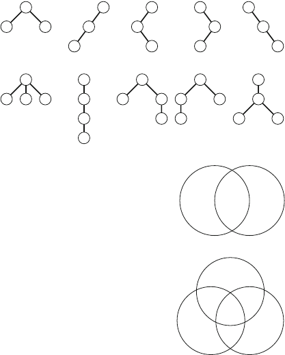
11.2 Combinatorics 161
Fig. 11.8 There are 5 binary
trees of 3 nodes
Fig. 11.9 There are 5 rooted
trees of 4 nodes
Fig. 11.10
Inclusion-exclusion principle
for two sets AB
A∩B
Fig. 11.11
Inclusion-exclusion principle
for three sets
AB
C
A∩B
A∩CB∩C
A∩B∩C
11.2.3 Inclusion-Exclusion
Inclusion-exclusion is a technique that can be used for counting the size of a union of
sets when the sizes of the intersections are known, and vice versa. A simple example
of the technique is the formula
|A∪B|=|A|+|B|−|A∩B|,
where Aand Bare sets and |X|denotes the size of X. Figure 11.10 illustrates the
formula. In this case, we want to calculate the size of the union A∪Bthat corresponds
to the area of the region that belongs to at least one circle in Fig.11.10. We can
calculate the area of A∪Bby first summing up the areas of Aand Band then
subtracting the area of A∩Bfrom the result.
The same idea can be applied when the number of sets is larger. When there are
three sets, the inclusion-exclusion formula is
|A∪B∪C|=|A|+|B|+|C|−|A∩B|−|A∩C|−|B∩C|+|A∩B∩C|,
which corresponds to Fig. 11.11.
In the general case, the size of the union X1∪X2∪···∪Xncan be calculated by
going through all possible intersections that contain some of the sets X1,X2,...,Xn.
162 11 Mathematics
If an intersection contains an odd number of sets, its size is added to the answer, and
otherwise its size is subtracted from the answer.
Note that there are similar formulas for calculating the size of an intersection from
the sizes of unions. For example,
|A∩B|=|A|+|B|−|A∪B|
and
|A∩B∩C|=|A|+|B|+|C|−|A∪B|−|A∪C|−|B∪C|+|A∪B∪C|.
Counting Derangements As an example, let us count the number of derangements
of {1,2,...,n}, i.e., permutations where no element remains in its original place.
For example, when n=3, there are two derangements: (2,3,1)and (3,1,2).
One approach for solving the problem is to use inclusion-exclusion. Let Xkbe
the set of permutations that contain the element kat position k. For example, when
n=3, the sets are as follows:
X1={(1,2,3), (1,3,2)}
X2={(1,2,3), (3,2,1)}
X3={(1,2,3), (2,1,3)}
The number of derangements equals
n!−|X1∪X2∪···∪Xn|,
so it suffices to calculate |X1∪X2∪···∪Xn|. Using inclusion-exclusion, this reduces
to calculating sizes of intersections. Moreover, an intersection of cdistinct sets Xk
has (n−c)!elements, because such an intersection consists of all permutations that
contain celements in their original places. Thus, we can efficiently calculate the
sizes of the intersections. For example, when n=3,
|X1∪X2∪X3|=|X1|+|X2|+|X3|
−|X1∩X2|−|X1∩X3|−|X2∩X3|
+|X1∩X2∩X3|
=2+2+2−1−1−1+1
=4,
so the number of derangements is 3!−4=2.
It turns out that the problem can also be solved without using inclusion-exclusion.
Let f(n)denote the number of derangements for {1,2,...,n}. We can use the
following recursive formula:
f(n)=⎧
⎪
⎨
⎪
⎩
0n=1
1n=2
(n−1)( f(n−2)+f(n−1)) n>2
11.2 Combinatorics 163
Fig. 11.12 Four symmetric
necklaces
The formula can be proved by considering the possibilities how the element 1
changes in the derangement. There are n−1 ways to choose an element xthat
replaces the element 1. In each such choice, there are two options:
Option 1: We also replace the element xwith the element 1. After this, the remain-
ing task is to construct a derangement of n−2 elements.
Option 2: We replace the element xwith some other element than 1. Now we
have to construct a derangement of n−1 element, because we cannot replace the
element xwith the element 1, and all other elements must be changed.
11.2.4 Burnside’s Lemma
Burnside’s lemma can be used to count the number of distinct combinations so that
symmetric combinations are counted only once. Burnside’s lemma states that the
number of combinations is
1
n
n
k=1
c(k),
where there are nways to change the position of a combination, and there are c(k)
combinations that remain unchanged when the kth way is applied.
As an example, let us calculate the number of necklaces of npearls, where
each pearl has mpossible colors. Two necklaces are symmetric if they are simi-
lar after rotating them. For example, Fig. 11.12 shows four symmetric necklaces,
which should be counted as a single combination.
There are nways to change the position of a necklace, because it can be rotated
k=0,1,...,n−1 steps clockwise. For example, if k=0, all mnnecklaces remain
the same, and if k=1, only the mnecklaces where each pearl has the same color
remain the same. In the general case, a total of mgcd(k,n)necklaces remain the same,
because blocks of pearls of size gcd(k,n)will replace each other. Thus, according
to Burnside’s lemma, the number of distinct necklaces is
1
n
n−1
k=0
mgcd(k,n).
For example, the number of distinct necklaces of 4 pearls and 3 colors is
34+3+32+3
4=24.
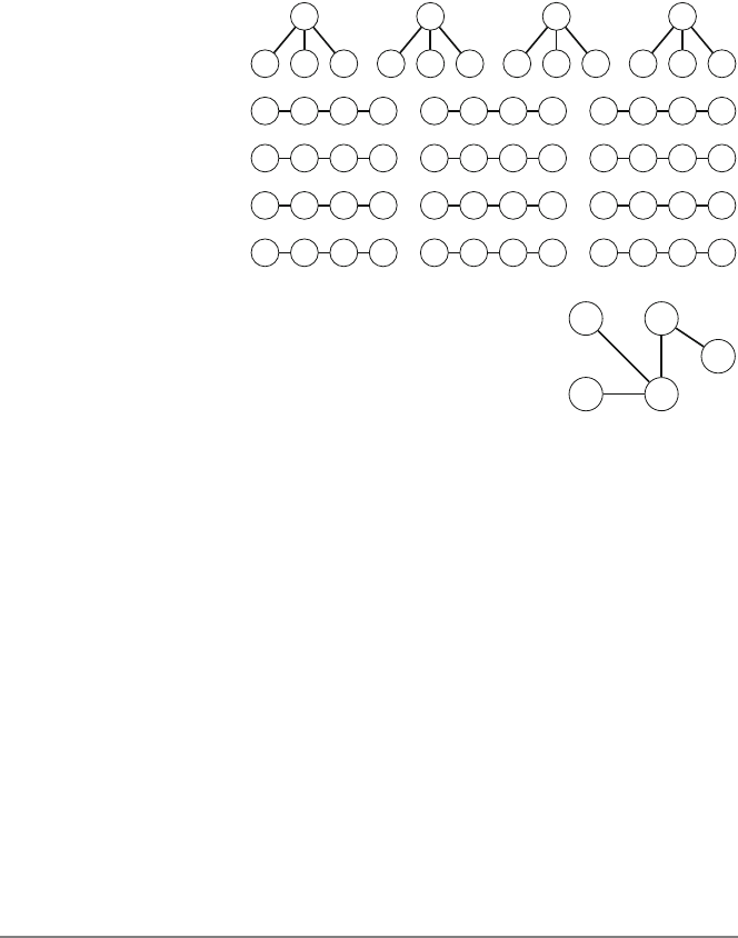
164 11 Mathematics
Fig. 11.13 There are 16
distinct labeled trees of 4
nodes
1
234
2
134
3
1 2 4
4
1 2 3
1 2 34 1 2 4 3132 4
134 2 1 4 2 31 4 32
2 1 34 2 1 4 3231 4
2 4 1 3 3 1 2 4 32 1 4
Fig. 11.14 Prüfer code of
this tree is [4,4,2]1 2
34
5
11.2.5 Cayley’s Formula
Cayley’s formula states that there are a total of nn−2distinct labeled trees of nnodes.
The nodes are labeled 1,2,...,n, and two trees are considered distinct if either their
structure or labeling is different. For example, when n=4, there are 44−2=16
labeled trees, shown in Fig. 11.13.
Cayley’s formula can be proved using Prüfer codes. A Prüfer code is a sequence
of n−2 numbers that describes a labeled tree. The code is constructed by following
a process that removes n−2 leaves from the tree. At each step, the leaf with the
smallest label is removed, and the label of its only neighbor is added to the code.
For example, the Prüfer code of the tree in Fig. 11.14 is [4,4,2], because we remove
leaves 1, 3, and 4.
We can construct a Prüfer code for any tree, and more importantly, the original
tree can be reconstructed from a Prüfer code. Hence, the number of labeled trees of
nnodes equals nn−2, the number of Prüfer codes of length n.
11.3 Matrices
Amatrix is a mathematical concept that corresponds to a two-dimensional array in
programming. For example,
A=⎡
⎣
6137 4
7082
95418
⎤
⎦
11.3 Matrices 165
is a matrix of size 3 ×4, i.e., it has 3 rows and 4 columns. The notation [i,j]refers
to the element in row iand column jin a matrix. For example, in the above matrix,
A[2,3]=8 and A[3,1]=9.
A special case of a matrix is a vector that is a one-dimensional matrix of size
n×1. For example,
V=⎡
⎣
4
7
5⎤
⎦
is a vector that contains three elements.
The transpose ATof a matrix Ais obtained when the rows and columns of Aare
swapped, i.e., AT[i,j]=A[j,i]:
AT=⎡
⎢
⎢
⎣
679
13 0 5
784
4218
⎤
⎥
⎥
⎦
A matrix is a square matrix if it has the same number of rows and columns. For
example, the following matrix is a square matrix:
S=⎡
⎣
312 4
5915
02 4
⎤
⎦
11.3.1 Matrix Operations
The sum A+Bof matrices Aand Bis defined if the matrices are of the same size.
The result is a matrix where each element has the sum of the corresponding elements
in Aand B. For example,
614
392
+493
813
=6+41+94+3
3+89+12+3=10 10 7
11 10 5.
Multiplying a matrix Aby a value xmeans that each element of Ais multiplied
by x. For example,
2·614
392
=2·62·12·4
2·32·92·2=12 2 8
6184
.
The product AB of matrices Aand Bis defined if Ais of size a×nand Bis of
size n×b, i.e., the width of Aequals the height of B. The result is a matrix of size
a×bwhose elements are calculated using the formula
AB[i,j]=
n
k=1
(A[i,k]·B[k,j]).
166 11 Mathematics
Fig. 11.15 Intuition behind
the matrix multiplication
formula
AAB
B
The idea is that each element of AB is a sum of products of elements of Aand B
according to Fig. 11.15. For example,
⎡
⎣
14
39
86
⎤
⎦·16
29
=⎡
⎣
1·1+4·21·6+4·9
3·1+9·23·6+9·9
8·1+6·28·6+6·9⎤
⎦=⎡
⎣
942
21 99
20 102⎤
⎦.
We can directly use the above formula to calculate the product Cof two n×n
matrices Aand Bin O(n3)time1:
for (int i = 1; i <= n; i++) {
for (int j=1;j<=n;j++){
for (int k = 1; k <= n; k++) {
C[i][j] += A[i][k]*B[k][j];
}
}
}
Matrix multiplication is associative, so A(BC)=(AB)Cholds, but it is not
commutative, so usually AB = BA.
An identity matrix is a square matrix where each element on the diagonal is 1
and all other elements are 0. For example, the following matrix is the 3 ×3 identity
matrix:
I=⎡
⎣
100
010
001
⎤
⎦
Multiplying a matrix by an identity matrix does not change it. For example,
⎡
⎣
100
010
001
⎤
⎦·⎡
⎣
14
39
86
⎤
⎦=⎡
⎣
14
39
86
⎤
⎦and ⎡
⎣
14
39
86
⎤
⎦·10
01
=⎡
⎣
14
39
86
⎤
⎦.
1While the straightforward O(n3)time algorithm is sufficient in competitive programming, there are
theoretically more efficient algorithms. In 1969, Strassen [31] discovered the first such algorithm,
now called Strassen’s algorithm, whose time complexity is O(n2.81). The best current algorithm,
proposed by Le Gall [11] in 2014, works in O(n2.37)time.

11.3 Matrices 167
The power Akof a matrix Ais defined if Ais a square matrix. The definition is
based on matrix multiplication:
Ak=A·A·A···A
ktimes
For example,
25
14
3
=25
14
·25
14
·25
14
=48 165
33 114.
In addition, A0is an identity matrix. For example,
25
14
0
=10
01
.
The matrix Akcan be efficiently calculated in O(n3log k)time using the algorithm
in Sect. 11.1.4. For example,
25
14
8
=25
14
4
·25
14
4
.
11.3.2 Linear Recurrences
Alinear recurrence is a function f(n)whose initial values are f(0), f(1),..., f(k−
1)and larger values are calculated recursively using the formula
f(n)=c1f(n−1)+c2f(n−2)+···+ckf(n−k),
where c1,c2,...,ckare constant coefficients.
Dynamic programming can be used to calculate any value of f(n)in O(kn)time
by calculating all values of f(0), f(1),..., f(n)one after another. However, as
we will see next, we can also calculate the value of f(n)in O(k3log n)time using
matrix operations. This is an important improvement if kis small and nis large.
Fibonacci Numbers A simple example of a linear recurrence is the following func-
tion that defines the Fibonacci numbers:
f(0)=0
f(1)=1
f(n)=f(n−1)+f(n−2)
In this case, k=2 and c1=c2=1.
168 11 Mathematics
To efficiently calculate Fibonacci numbers, we represent the Fibonacci formula
as a square matrix Xof size 2 ×2, for which the following holds:
X·f(i)
f(i+1)=f(i+1)
f(i+2)
Thus, values f(i)and f(i+1)are given as “input” for X, and Xcalculates values
f(i+1)and f(i+2)from them. It turns out that such a matrix is
X=01
11
.
For example,
01
11
·f(5)
f(6)=01
11
·5
8=8
13=f(6)
f(7).
Thus, we can calculate f(n)using the formula
f(n)
f(n+1)=Xn·f(0)
f(1)=01
11
n
·0
1.
The value of Xncan be calculated in O(log n)time, so the value of f(n)can also
be calculated in O(log n)time.
General Case Let us now consider the general case where f(n)is any linear recur-
rence. Again, our goal is to construct a matrix Xfor which
X·⎡
⎢
⎢
⎢
⎣
f(i)
f(i+1)
.
.
.
f(i+k−1)
⎤
⎥
⎥
⎥
⎦=⎡
⎢
⎢
⎢
⎣
f(i+1)
f(i+2)
.
.
.
f(i+k)
⎤
⎥
⎥
⎥
⎦
.
Such a matrix is
X=⎡
⎢
⎢
⎢
⎢
⎢
⎣
01 0··· 0
00 1··· 0
.
.
..
.
..
.
.....
.
.
00 0··· 1
ckck−1ck−2···c1
⎤
⎥
⎥
⎥
⎥
⎥
⎦
.
In the first k−1 rows, each element is 0 except that one element is 1. These rows
replace f(i)with f(i+1),f(i+1)with f(i+2), and so on. Then, the last row
contains the coefficients of the recurrence to calculate the new value f(i+k).
11.3 Matrices 169
Fig. 11.16 Example graphs
for matrix operations 1
4
23
5 6
(a)
1
4
23
5 6
4 1
2 4
123
2
(b)
Now, f(n)can be calculated in O(k3log n)time using the formula
⎡
⎢
⎢
⎢
⎣
f(n)
f(n+1)
.
.
.
f(n+k−1)
⎤
⎥
⎥
⎥
⎦=Xn·⎡
⎢
⎢
⎢
⎣
f(0)
f(1)
.
.
.
f(k−1)
⎤
⎥
⎥
⎥
⎦
.
11.3.3 Graphs and Matrices
The powers of adjacency matrices of graphs have interesting properties. When Mis
an adjacency matrix of an unweighted graph, the matrix Mngives for each node pair
(a,b)the number of paths that begin at node a, end at node b, and contain exactly
nedges. It is allowed that a node appears on a path several times.
As an example, consider the graph in Fig. 11.16a. The adjacency matrix of this
graph is
M=
⎡
⎢
⎢
⎢
⎢
⎢
⎢
⎣
000100
100011
010000
010000
000000
001010
⎤
⎥
⎥
⎥
⎥
⎥
⎥
⎦
.
Then, the matrix
M4=
⎡
⎢
⎢
⎢
⎢
⎢
⎢
⎣
001110
200022
020000
020000
000000
001110
⎤
⎥
⎥
⎥
⎥
⎥
⎥
⎦
gives the number of paths that contain exactly 4 edges. For example, M4[2,5]=2,
because there are two paths of 4 edges from node 2 to node 5: 2 →1→4→2→5
and 2 →6→3→2→5.
Using a similar idea in a weighted graph, we can calculate for each node pair
(a,b)the shortest length of a path that goes from ato band contains exactly n
170 11 Mathematics
edges. To calculate this, we define matrix multiplication in a new way, so that we do
not calculate numbers of paths but minimize lengths of paths.
As an example, consider the graph in Fig.11.16b. Let us construct an adjacency
matrix where ∞means that an edge does not exist, and other values correspond to
edge weights. The matrix is
M=
⎡
⎢
⎢
⎢
⎢
⎢
⎢
⎣
∞∞∞ 4∞∞
2∞∞∞ 12
∞4∞∞∞∞
∞1∞∞∞∞
∞∞∞∞∞∞
∞∞ 3∞2∞
⎤
⎥
⎥
⎥
⎥
⎥
⎥
⎦
.
Instead of the formula
AB[i,j]=
n
k=1
(A[i,k]·B[k,j])
we now use the formula
AB[i,j]=
n
min
k=1(A[i,k]+B[k,j])
for matrix multiplication, so we calculate minima instead of sums, and sums of
elements instead of products. After this modification, matrix powers minimize path
lengths in the graph. For example, as
M4=
⎡
⎢
⎢
⎢
⎢
⎢
⎢
⎣
∞∞10 11 9 ∞
9∞∞∞ 89
∞11 ∞∞∞∞
∞8∞∞∞∞
∞∞∞∞∞∞
∞∞12 13 11 ∞
⎤
⎥
⎥
⎥
⎥
⎥
⎥
⎦
,
we can conclude that the minimum length of a path of 4 edges from node 2 to node
5 is 8. Such a path is 2 →1→4→2→5.
11.3.4 Gaussian Elimination
Gaussian elimination is a systematic way to solve a group of linear equations. The
idea is to represent the equations as a matrix and then apply a sequence of sim-
ple matrix row operations that both preserve the information of the equations and
determine a value for each variable.
11.3 Matrices 171
Suppose that we are given a group of nlinear equations, each of which contains
nvariables:
a1,1x1+a1,2x2+···+a1,nxn=b1
a2,1x1+a2,2x2+···+a2,nxn=b2
···
an,1x1+an,2x2+···+an,nxn=bn
We represent the equations as a matrix as follows:
⎡
⎢
⎢
⎢
⎣
a1,1a1,2···a1,nb1
a2,1a2,2···a2,nb2
.
.
..
.
.....
.
..
.
.
an,1an,2···an,nbn
⎤
⎥
⎥
⎥
⎦
To solve the equations, we want to transform the matrix to
⎡
⎢
⎢
⎢
⎣
10··· 0c1
01··· 0c2
.
.
..
.
.....
.
..
.
.
00··· 1cn
⎤
⎥
⎥
⎥
⎦
,
which tells us that the solution is x1=c1,x2=c2,...,xn=cn. To do this, we use
three types of matrix row operations:
1. Swap the values of two rows.
2. Multiply each value in a row by a nonnegative constant.
3. Add a row, multiplied by a constant, to another row.
Each above operation preserves the information of the equations, which guarantees
that the final solution agrees with the original equations. We can systematically
process each matrix column so that the resulting algorithm works in O(n3)time.
As an example, consider the following group of equations:
2x1+4x2+x3=16
x1+2x2+5x3=17
3x1+x2+x3=8
In this case the matrix is as follows:
⎡
⎣
24116
12517
311 8
⎤
⎦
172 11 Mathematics
We process the matrix column by column. At each step, we make sure that the
current column has a one in the correct position and all other values are zeros. To
process the first column, we first multiply the first row by 1
2:
⎡
⎣
12 1
28
12517
311 8
⎤
⎦
Then we add the first row to the second row (multiplied by −1) and the first row to
the third row (multiplied by −3):
⎡
⎢
⎣
12 1
28
00 9
29
0−5−1
2−16
⎤
⎥
⎦
After this, we process the second column. Since the second value in the second
row is zero, we first swap the second and third row:
⎡
⎢
⎣
12 1
28
0−5−1
2−16
00 9
29
⎤
⎥
⎦
Then we multiply the second row by −1
5and add it to the first row (multiplied by
−2):
⎡
⎢
⎢
⎣
10 3
10
8
5
01 1
10
16
5
00 9
29
⎤
⎥
⎥
⎦
Finally, we process the third column by first multiplying it by 2
9and then adding
it to the first row (multiplied by −3
10 ) and to the second row (multiplied by −1
10 ):
⎡
⎣
1001
0103
0012
⎤
⎦
Now the last column of the matrix tells us that the solution to the original group
of equations is x1=1,x2=3,x3=2.
Note that Gaussian elimination only works if the group of equations has a unique
solution. For example, the group
x1+x2=2
2x1+2x2=4
11.3 Matrices 173
has an infinite number of solutions, because both the equations contain the same
information. On the other hand, the group
x1+x2=5
x1+x2=7
cannot be solved, because the equations are contradictory. If there is no unique
solution, we will notice this during the algorithm, because at some point we will not
be able to successfully process a column.
11.4 Probability
Aprobability is a real number between 0 and 1 that indicates how probable an event
is. If an event is certain to happen, its probability is 1, and if an event is impossible,
its probability is 0. The probability of an event is denoted P(···)where the three
dots describe the event. For example, when throwing a dice, there are six possible
outcomes 1,2,...,6, and P(“the outcome is even”) =1/2.
To calculate the probability of an event, we can either use combinatorics or sim-
ulate the process that generates the event. As an example, consider an experiment
where we draw the three top cards from a shuffled deck of cards.2What is the
probability that each card has the same value (e.g., ♠8, ♣8, and ♦8)?
One way to calculate the probability is to use the formula
number of desired outcomes
total number of outcomes .
In our example, the desired outcomes are those in which the value of each card is
the same. There are 134
3such outcomes, because there are 13 possibilities for the
value of the cards and 4
3ways to choose 3 suits from 4 possible suits. Then, there
are a total of 52
3outcomes, because we choose 3 cards from 52 cards. Thus, the
probability of the event is
134
3
52
3=1
425 .
Another way to calculate the probability is to simulate the process that generates
the event. In our example, we draw three cards, so the process consists of three steps.
We require that each step of the process is successful.
Drawing the first card certainly succeeds, because any card is fine. The second
step succeeds with probability 3/51, because there are 51 cards left and 3 of them
2A deck of cards consists of 52 cards. Each card has a suit (spade ♠, diamond ♦,club♣, or heart
♥) and a value (an integer between 1 and 13).

174 11 Mathematics
have the same value as the first card. In a similar way, the third step succeeds with
probability 2/50. Thus, the probability that the entire process succeeds is
1·3
51 ·2
50 =1
425 .
11.4.1 Working with Events
A convenient way to represent events is to use sets. For example, the possible out-
comes when throwing a dice are {1,2,3,4,5,6}, and any subset of this set is an
event. The event “the outcome is even” corresponds to the set {2,4,6}.
Each outcome xis assigned a probability p(x), and the probability P(X)of an
event Xcan be calculated using the formula
P(X)=
x∈X
p(x).
For example, when throwing a dice, p(x)=1/6 for each outcome x, so the proba-
bility of the event “the outcome is even” is
p(2)+p(4)+p(6)=1/2.
Since the events are represented as sets, we can manipulate them using standard
set operations:
•The complement ¯
Ameans “Adoes not happen.” For example, when throwing a
dice, the complement of A={2,4,6}is ¯
A={1,3,5}.
•The union A ∪Bmeans “ Aor Bhappen.” For example, the union of A={2,5}
and B={4,5,6}is A∪B={2,4,5,6}.
•The intersection A ∩Bmeans “ Aand Bhappen.” For example, the intersection
of A={2,5}and B={4,5,6}is A∩B={5}.
Complement The probability of ¯
Ais calculated using the formula
P(¯
A)=1−P(A).
Sometimes, we can solve a problem easily using complements by solving the
opposite problem. For example, the probability of getting at least one six when
throwing a dice ten times is
1−(5/6)10.
Here 5/6 is the probability that the outcome of a single throw is not six, and (5/6)10
is the probability that none of the ten throws is a six. The complement of this is the
answer to the problem.
11.4 Probability 175
Union The probability of A∪Bis calculated using the formula
P(A∪B)=P(A)+P(B)−P(A∩B).
For example, consider the events A=“the outcome is even” and B=“the outcome
is less than 4” when throwing a dice. In this case, the event A∪Bmeans “the outcome
is even or less than 4,” and its probability is
P(A∪B)=P(A)+P(B)−P(A∩B)=1/2+1/2−1/6=5/6.
If the events Aand Bare disjoint, i.e., A∩Bis empty, the probability of the event
A∪Bis simply
P(A∪B)=P(A)+P(B).
Intersection The probability of A∩Bcan be calculated using the formula
P(A∩B)=P(A)P(B|A),
where P(B|A)is the conditional probability that Bhappens assuming that we know
that Ahappens. For example, using the events of our previous example, P(B|A)=
1/3, because we know that the outcome belongs to the set {2,4,6}, and one of the
outcomes is less than 4. Thus,
P(A∩B)=P(A)P(B|A)=1/2·1/3=1/6.
Events Aand Bare independent if
P(A|B)=P(A)and P(B|A)=P(B),
which means that the fact that Bhappens does not change the probability of A, and
vice versa. In this case, the probability of the intersection is
P(A∩B)=P(A)P(B).
11.4.2 Random Variables
Arandom variable is a value that is generated by a random process. For example,
when throwing two dice, a possible random variable is
X=“the sum of the outcomes”.
For example, if the outcomes are [4,6](meaning that we first throw a four and then
a six), then the value of Xis 10.
We denote by P(X=x)the probability that the value of a random variable X
is x. For example, when throwing two dice, P(X=10)=3/36, because the total
176 11 Mathematics
Fig. 11.17 Possible ways to
place two balls in four boxes
number of outcomes is 36 and there are three possible ways to obtain the sum 10:
[4,6],[5,5], and [6,4].
Expected Values The expected value E[X]indicates the average value of a random
variable X. The expected value can be calculated as a sum
x
P(X=x)x,
where xgoes through all possible values of X.
For example, when throwing a dice, the expected outcome is
1/6·1+1/6·2+1/6·3+1/6·4+1/6·5+1/6·6=7/2.
A useful property of expected values is linearity. It means that the sum E[X1+
X2+···+Xn]always equals the sum E[X1]+E[X2]+···+E[Xn]. This holds
even if random variables depend on each other. For example, when throwing two
dice, the expected sum of their values is
E[X1+X2]=E[X1]+E[X2]=7/2+7/2=7.
Let us now consider a problem where nballs are randomly placed in nboxes, and
our task is to calculate the expected number of empty boxes. Each ball has an equal
probability to be placed in any of the boxes.
For example, Fig. 11.17 shows the possibilities when n=2. In this case, the
expected number of empty boxes is
0+0+1+1
4=1
2.
Then, in the general case, the probability that a single box is empty is
n−1
nn
,
because no ball should be placed in it. Hence, using linearity, the expected number
of empty boxes is
n·n−1
nn
.
11.4 Probability 177
Distributions The distribution of a random variable Xshows the probability of each
value that Xmay have. The distribution consists of values P(X=x). For example,
when throwing two dice, the distribution for their sum is:
x23456789101112
P(X=x)1/36 2/36 3/36 4/36 5/36 6/36 5/36 4/36 3/36 2/36 1/36
In a uniform distribution, the random variable Xhas npossible values a,a+
1,...,band the probability of each value is 1/n. For example, when throwing a
dice, a=1, b=6, and P(X=x)=1/6 for each value x.
The expected value of Xin a uniform distribution is
E[X]=a+b
2.
In a binomial distribution,nattempts are made and the probability that a single
attempt succeeds is p. The random variable Xcounts the number of successful
attempts, and the probability of a value xis
P(X=x)=px(1−p)n−xn
x,
where pxand (1−p)n−xcorrespond to successful and unsuccessful attempts, and
n
xis the number of ways we can choose the order of the attempts.
For example, when throwing a dice ten times, the probability of throwing a six
exactly three times is (1/6)3(5/6)710
3.
The expected value of Xin a binomial distribution is
E[X]=pn.
In a geometric distribution, the probability that an attempt succeeds is p, and we
continue until the first success happens. The random variable Xcounts the number
of attempts needed, and the probability of a value xis
P(X=x)=(1−p)x−1p,
where (1−p)x−1corresponds to the unsuccessful attempts and pcorresponds to
the first successful attempt.
For example, if we throw a dice until we get a six, the probability that the number
of throws is exactly 4 is (5/6)31/6.
The expected value of Xin a geometric distribution is
E[X]=1
p.

178 11 Mathematics
Fig. 11.18 AMarkovchain
for a building that consists of
five floors 1 2 345
11/2 1/21/2
1
1/21/2
1/2
11.4.3 Markov Chains
AMarkov chain is a random process that consists of states and transitions between
them. For each state, we know the probabilities of moving to other states. A Markov
chain can be represented as a graph whose nodes correspond to the states and edges
describe the transitions.
As an example, consider a problem where we are in floor 1 in an nfloor building.
At each step, we randomly walk either one floor up or one floor down, except that
we always walk one floor up from floor 1 and one floor down from floor n. What is
the probability of being in floor mafter ksteps?
In this problem, each floor of the building corresponds to a state in a Markov
chain. For example, Fig. 11.18 shows the chain when n=5.
The probability distribution of a Markov chain is a vector [p1,p2,..., pn], where
pkis the probability that the current state is k. The formula p1+p2+···+pn=1
always holds.
In the above scenario, the initial distribution is [1,0,0,0,0], because we always
begin in floor 1. The next distribution is [0,1,0,0,0], because we can only move
from floor 1 to floor 2. After this, we can either move one floor up or one floor down,
so the next distribution is [1/2,0,1/2,0,0], and so on.
An efficient way to simulate the walk in a Markov chain is to use dynamic pro-
gramming. The idea is to maintain the probability distribution, and at each step go
through all possibilities how we can move. Using this method, we can simulate a
walk of msteps in O(n2m)time.
The transitions of a Markov chain can also be represented as a matrix that updates
the probability distribution. In the above scenario, the matrix is
⎡
⎢
⎢
⎢
⎢
⎣
01/20 00
101/200
01/201/20
001/201
00 01/20
⎤
⎥
⎥
⎥
⎥
⎦
.
When we multiply a probability distribution by this matrix, we get the new dis-
tribution after moving one step. For example, we can move from the distribution
11.4 Probability 179
[1,0,0,0,0]to the distribution [0,1,0,0,0]as follows:
⎡
⎢
⎢
⎢
⎢
⎣
01/20 00
101/200
01/201/20
001/201
00 01/20
⎤
⎥
⎥
⎥
⎥
⎦
⎡
⎢
⎢
⎢
⎢
⎣
1
0
0
0
0
⎤
⎥
⎥
⎥
⎥
⎦=⎡
⎢
⎢
⎢
⎢
⎣
0
1
0
0
0
⎤
⎥
⎥
⎥
⎥
⎦
.
By calculating matrix powers efficiently, we can calculate the distribution after m
steps in O(n3log m)time.
11.4.4 Randomized Algorithms
Sometimes we can use randomness for solving a problem, even if the problem is
not related to probabilities. A randomized algorithm is an algorithm that is based on
randomness. There are two popular types of randomized algorithms:
•AMonte Carlo algorithm is an algorithm that may sometimes give a wrong
answer. For such an algorithm to be useful, the probability of a wrong answer
should be small.
•ALas Vegas algorithm is an algorithm that always gives the correct answer, but its
running time varies randomly. The goal is to design an algorithm that is efficient
with high probability.
Next we will go through three example problems that can be solved using such
algorithms.
Order Statistics The kth order statistic of an array is the element at position k
after sorting the array in increasing order. It is easy to calculate any order statistic
in O(nlog n)time by first sorting the array, but is it really needed to sort the entire
array just to find one element?
It turns out that we can find order statistics using a Las Vegas algorithm, whose
expected running time is O(n). The algorithm chooses a random element xfrom
the array and moves elements smaller than xto the left part of the array, and all
other elements to the right part of the array. This takes O(n)time when there are n
elements.
Assume that the left part contains aelements and the right part contains belements.
If a=k, element xis the kth order statistic. Otherwise, if a>k, we recursively find
the kth order statistic for the left part, and if a<k, we recursively find the rth order
statistic for the right part where r=k−a−1. The search continues in a similar
way, until the desired element has been found.
When each element xis randomly chosen, the size of the array about halves at
each step, so the time complexity for finding the kth order statistic is about
n+n/2+n/4+n/8+···=O(n).
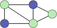
180 11 Mathematics
Fig. 11.19 A valid coloring
of a graph 1 2
34
5
Note that the worst case of the algorithm requires O(n2)time, because it is possible
that xis always chosen in such a way that it is one of the smallest or largest elements
in the array and O(n)steps are needed. However, the probability of this is so small
that we may assume that this never happens in practice.
Verifying Matrix Multiplication Given matrices A,B, and C, each of size n×n,
our next problem is to verify if AB =Cholds. Of course, we can solve the problem
by just calculating the product AB in O(n3)time, but one could hope that verifying
the answer would be easier than to calculate it from scratch.
It turns out that we can solve the problem using a Monte Carlo algorithm whose
time complexity is only O(n2). The idea is simple: we choose a random vector Xof
nelements and calculate the matrices ABX and CX.If ABX =CX, we report that
AB =C, and otherwise we report that AB = C.
The time complexity of the algorithm is O(n2), because we can calculate the
matrices ABX and CX in O(n2)time. We can calculate the matrix ABX efficiently
by using the representation A(BX), so only two multiplications of n×nand n×1
size matrices are needed.
The drawback of the algorithm is that there is a small chance that the algorithm
makes a mistake when it reports that AB =C. For example,
68
13
= 87
32
,
but
68
13
3
6=87
32
3
6.
However, in practice, the probability that the algorithm makes a mistake is small,
and we can decrease the probability by verifying the result using multiple random
vectors Xbefore reporting that AB =C.
Graph Coloring Given a graph that contains nnodes and medges, our final problem
is to find a way to color the nodes using two colors so that for at least m/2 edges,
the endpoints have different colors. For example, Fig. 11.19 shows a valid coloring
of a graph. In this case the graph contains seven edges, and the endpoints of five of
them have different colors in the coloring.
The problem can be solved using a Las Vegas algorithm that generates random
colorings until a valid coloring has been found. In a random coloring, the color of
each node is independently chosen so that the probability of both colors is 1/2.
Hence, the expected number of edges whose endpoints have different colors is m/2.

11.4 Probability 181
Since it is expected that a random coloring is valid, we will quickly find a valid
coloring in practice.
11.5 Game Theory
In this section, we focus on two-player games where the players move alternately
and have the same set of moves available, and there are no random elements. Our
goal is to find a strategy that we can follow to win the game no matter what the
opponent does, if such a strategy exists.
It turns out that there is a general strategy for such games, and we can analyze the
games using nim theory. First, we will analyze simple games where players remove
sticks from heaps, and after this, we will generalize the strategy used in those games
to other games.
11.5.1 Game States
Let us consider a game that starts with a heap of nsticks. Two players move alter-
nately, and on each move, the player has to remove 1, 2, or 3 sticks from the heap.
Finally, the player who removes the last stick wins the game.
For example, if n=10, the game may proceed as follows:
•Player Aremoves 2 sticks (8 sticks left).
•Player Bremoves 3 sticks (5 sticks left).
•Player Aremoves 1 stick (4 sticks left).
•Player Bremoves 2 sticks (2 sticks left).
•Player Aremoves 2 sticks and wins.
This game consists of states 0,1,2,...,n, where the number of the state corre-
sponds to the number of sticks left.
Awinning state is a state where the player will win the game if they play optimally,
and a losing state is a state where the player will lose the game if the opponent plays
optimally. It turns out that we can classify all states of a game so that each state is
either a winning state or a losing state.
In the above game, state 0 is clearly a losing state, because the player cannot make
any moves. States 1, 2, and 3 are winning states, because the player can remove 1,
2, or 3 sticks and win the game. State 4, in turn, is a losing state, because any move
leads to a state that is a winning state for the opponent.
More generally, if there is a move that leads from the current state to a losing state,
it is a winning state, and otherwise it is a losing state. Using this observation, we can
classify all states of a game starting with losing states where there are no possible
moves. Figure 11.20 shows the classification of states 0 ...15 (Wdenotes a winning
state and Ldenotes a losing state).
182 11 Mathematics
LWWW LWWW LWWW LWWW
012345678910 11 12 13 14 15
Fig. 11.20 Classification of states 0 ...15 in the stick game
Fig. 11.21 State graph of
the divisibility game 1 2
3
4
5
6
7
8
9
Fig. 11.22 Classification of
states 1 ...9inthe
divisibility game LWLWLWLWL
123456789
It is easy to analyze this game: a state kis a losing state if kis divisible by 4, and
otherwise it is a winning state. An optimal way to play the game is to always choose
a move after which the number of sticks in the heap is divisible by 4. Finally, there
are no sticks left and the opponent has lost. Of course, this strategy requires that the
number of sticks is not divisible by 4 when it is our move. If it is, there is nothing
we can do, and the opponent will win the game if they play optimally.
Let us then consider another stick game, where in each state k, it is allowed to
remove any number xof sticks such that xis smaller than kand divides k.For
example, in state 8 we may remove 1, 2, or 4 sticks, but in state 7 the only allowed
move is to remove 1 stick. Figure 11.21 shows the states 1 ...9 of the game as a state
graph, whose nodes are the states and edges are the moves between them:
The final state in this game is always state 1, which is a losing state, because there
are no valid moves. Figure 11.22 shows the classification of states 1 ...9. It turns out
that in this game, all even-numbered states are winning states, and all odd-numbered
states are losing states.
11.5.2 Nim Game
The nim game is a simple game that has an important role in game theory, because
many other games can be played using the same strategy. First, we focus on nim,
and after this, we generalize the strategy to other games.
There are nheaps in nim, and each heap contains some number of sticks. The
players move alternately, and on each turn, the player chooses a heap that still contains
sticks and removes any number of sticks from it. The winner is the player who
removes the last stick.
11.5 Game Theory 183
The states in nim are of the form [x1,x2,...,xn], where xidenotes the number
of sticks in heap i. For example, [10,12,5]is a state where there are three heaps
with 10, 12, and 5 sticks. The state [0,0,...,0]is a losing state, because it is not
possible to remove any sticks, and this is always the final state.
Analysis It turns out that we can easily classify any nim state by calculating the nim
sum s =x1⊕x2⊕···⊕xn, where ⊕denotes the xor operation. The states whose
nim sum is 0 are losing states, and all other states are winning states. For example,
the nim sum of [10,12,5]is 10 ⊕12 ⊕5=3, so the state is a winning state.
But how is the nim sum related to the nim game? We can explain this by looking
at how the nim sum changes when the nim state changes.
Losing states: The final state [0,0,...,0]is a losing state, and its nim sum is 0, as
expected. In other losing states, any move leads to a winning state, because when a
single value xichanges, the nim sum also changes, so the nim sum is different from
0 after the move.
Winning states: We can move to a losing state if there is any heap ifor which
xi⊕s<xi. In this case, we can remove sticks from heap iso that it will contain
xi⊕ssticks, which will lead to a losing state. There is always such a heap, where
xihas a one bit at the position of the leftmost one bit of s.
Example As an example, consider the state [10,12,5]. This state is a winning state,
because its nim sum is 3. Thus, there has to be a move which leads to a losing state.
Next we will find out such a move.
The nim sum of the state is as follows:
10 1010
12 1100
50101
30011
In this case, the heap with 10 sticks is the only heap that has a one bit at the
position of the leftmost one bit of the nim sum:
10 1010
12 1100
50101
30011
The new size of the heap has to be 10 ⊕3=9, so we will remove just one stick.
After this, the state will be [9,12,5], which is a losing state:
91001
12 1100
50101
00000
Misère Game In a misère nim game, the goal of the game is opposite, so the player
who removes the last stick loses the game. It turns out that the misère nim game can
be optimally played almost like the standard nim game.
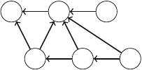
184 11 Mathematics
Fig. 11.23 Grundy numbers
of game states 010
202
The idea is to first play the misère game like the standard game, but change the
strategy at the end of the game. The new strategy will be introduced in a situation
where each heap would contain at most one stick after the next move. In the standard
game, we should choose a move after which there is an even number of heaps with
one stick. However, in the misère game, we choose a move so that there is an odd
number of heaps with one stick.
This strategy works because a state where the strategy changes always appears in
the game, and this state is a winning state, because it contains exactly one heap that
has more than one stick so the nim sum is not 0.
11.5.3 Sprague–Grundy Theorem
The Sprague–Grundy theorem generalizes the strategy used in nim to all games that
fulfill the following requirements:
•There are two players who move alternately.
•The game consists of states, and the possible moves in a state do not depend on
whose turn it is.
•The game ends when a player cannot make a move.
•The game surely ends sooner or later.
•The players have complete information about the states and allowed moves, and
there is no randomness in the game.
Grundy Numbers The idea is to calculate for each game state a Grundy number
that corresponds to the number of sticks in a nim heap. When we know the Grundy
numbers of all states, we can play the game like the nim game.
The Grundy number of a game state is calculated using the formula
mex({g1,g2,...,gn}),
where g1,g2,...,gnare the Grundy numbers of the states to which we can move
from the state, and the mex function gives the smallest nonnegative number that is
not in the set. For example, mex({0,1,3})=2. If a state has no possible moves, its
Grundy number is 0, because mex(∅)=0.
For example, Fig. 11.23 shows a state graph of a game where each state is assigned
its Grundy number. The Grundy number of a losing state is 0, and the Grundy number
of a winning state is a positive number.
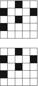
11.5 Game Theory 185
Fig. 11.24 Possible moves
on the first turn
@
****
*
*
Fig. 11.25 Grundy numbers
of game states 0101
012
021
0
3041
04132
Consider a state whose Grundy number is x. We can think that it corresponds to
a nim heap that has xsticks. In particular, if x>0, we can move to states whose
Grundy numbers are 0,1,...,x−1, which simulates removing sticks from a nim
heap. There is one difference, though it may be possible to move to a state whose
Grundy number is larger than xand “add” sticks to a heap. However, the opponent
can always cancel any such move, so this does not change the strategy.
As an example, consider a game where the players move a figure in a maze. Each
square of the maze is either floor or wall. On each turn, the player has to move the
figure some number of steps left or up. The winner of the game is the player who
makes the last move. Figure 11.24 shows a possible initial configuration of the game,
where @ denotes the figure and * denotes a square where it can move. The states of
the game are all floor squares of the maze. Figure 11.25 shows the Grundy numbers
of the states in this configuration.
According to the Sprague–Grundy theorem, each state of the maze game corre-
sponds to a heap in the nim game. For example, the Grundy number of the lower-right
square is 2, so it is a winning state. We can reach a losing state and win the game by
moving either four steps left or two steps up.
Subgames Assume that our game consists of subgames, and on each turn, the player
first chooses a subgame and then a move in the subgame. The game ends when it is
not possible to make any move in any subgame. In this case, the Grundy number of
a game equals the nim sum of the Grundy numbers of the subgames. The game can
then be played like a nim game by calculating all Grundy numbers for subgames and
then their nim sum.
As an example, consider a game that consists of three mazes. On each turn, the
player chooses one of the mazes and then moves the figure in the maze. Figure 11.26
shows an initial configuration of the game, and Fig. 11.27 shows the corresponding
Grundy numbers. In this configuration, the nim sum of the Grundy numbers is 2 ⊕
3⊕3=2, so the first player can win the game. One optimal move is to move two
steps up in the first maze, which produces the nim sum 0 ⊕3⊕3=0.
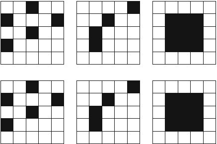
186 11 Mathematics
Fig. 11.26 Agamethat
consists of three subgames
@@@
Fig. 11.27 Grundy numbers
in subgames 0101
012
021
0
3041
04132
0123
100
1
2012
3120
40253
01234
10
21
32
40123
Grundy’s Game Sometimes a move in a game divides the game into subgames that
are independent of each other. In this case, the Grundy number of a game state is
mex({g1,g2,...,gn}),
where there are npossible moves and
gk=ak,1⊕ak,2⊕...⊕ak,m,
meaning that move kdivides the game into msubgames whose Grundy numbers are
ak,1,ak,2,...,ak,m.
An example of such a game is Grundy’s game. Initially, there is a single heap
that has nsticks. On each turn, the player chooses a heap and divides it into two
nonempty heaps such that the heaps are of different size. The player who makes the
last move wins the game.
Let g(n)denote the Grundy number of a heap of size n. The Grundy number
can be calculated by going through all ways to divide the heap into two heaps. For
example, when n=8, the possibilities are 1 +7, 2 +6, and 3 +5, so
g(8)=mex({g(1)⊕g(7), g(2)⊕g(6), g(3)⊕g(5)}).
In this game, the value of g(n)is based on the values of g(1),...,g(n−1). The
base cases are g(1)=g(2)=0, because it is not possible to divide the heaps of 1
and 2 sticks into smaller heaps. The first Grundy numbers are:
g(1)=0
g(2)=0
g(3)=1
g(4)=0
11.5 Game Theory 187
g(5)=2
g(6)=1
g(7)=0
g(8)=2
The Grundy number for n=8 is 2, so it is possible to win the game. The winning
move is to create heaps 1 +7, because g(1)⊕g(7)=0.

Advanced Graph Algorithms
This chapter discusses a selection of advanced graph algorithms.
Section 12.1 presents an algorithm for finding the strongly connected components
of a graph. After this, we will learn how to efficiently solve the 2SAT problem using
the algorithm.
Section 12.2 focuses on Eulerian and Hamiltonian paths. An Eulerian path goes
through each edge of the graph exactly once, and a Hamiltonian path visits each node
exactly once. While the concepts look quite similar at first glance, the computational
problems related to them are very different.
Section 12.3 first shows how we can determine the maximum flow from a source
to a sink in a graph. After this, we will see how to reduce several other graph problems
to the maximum flow problem.
Section 12.4 discusses properties of depth-first search and problems related to
biconnected graphs.
12.1 Strong Connectivity
A directed graph is called strongly connected if there is a path from any node to all
other nodes in the graph. For example, the left graph in Fig. 12.1 is strongly connected
while the right graph is not. The right graph is not strongly connected, because, for
example, there is no path from node 2 to node 1.
A directed graph can always be divided into strongly connected components. Each
such component contains a maximal set of nodes such that there is a path from any
node to all other nodes, and the components form an acyclic component graph that
represents the deep structure of the original graph. For example, Fig. 12.2 shows a
graph, its strongly connected components and the corresponding component graph.
The components are A={1,2},B={3,6,7},C={4}, and D={5}.
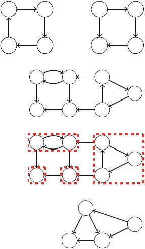
190 12 Advanced Graph Algorithms
Fig. 12.1 The left graph is
strongly connected, the right
graph is not
1 2
34
1 2
34
Fig. 12.2 A graph, its
strongly connected
components and the
component graph
7
3
21
65
4
7
3
21
65
4
B
A
D
C
A component graph is a directed acyclic graph, so it is easier to process than the
original graph. Since the graph does not contain cycles, we can always construct a
topological sort and use dynamic programming to process it.
12.1.1 Kosaraju’s Algorithm
Kosaraju’s algorithm is an efficient method for finding the strongly connected com-
ponents of a graph. The algorithm performs two depth-first searches: the first search
constructs a list of nodes according to the structure of the graph, and the second
search forms the strongly connected components.
The first phase of Kosaraju’s algorithm constructs a list of nodes in the order in
which depth-first search processes them. The algorithm goes through the nodes and
begins a depth-first search at each unprocessed node. Each node will be added to the
list after it has been processed.
For example, Fig. 12.3 shows the processing order of the nodes in our example
graph. The notation x/ymeans that processing the node started at time xand finished
at time y. The resulting list is [4,5,2,1,6,7,3]
The second phase of Kosaraju’s algorithm forms the strongly connected compo-
nents. First, the algorithm reverses every edge of the graph. This guarantees that
during the second search, we will always find valid strongly connected components.
Figure 12.4 shows the graph in our example after reversing the edges.
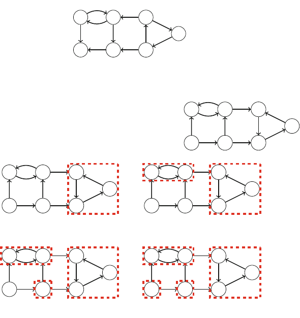
12.1 Strong Connectivity 191
7
3
21
65
4
1/82/79/14
4/53/611/12
10/13
Fig. 12.3 The processing order of the nodes
Fig. 12.4 Agraphwith
reversed edges
7
3
21
65
4
7
3
21
65
4
step 1
7
3
21
65
4
step 2
7
3
21
65
4
step 3
7
3
21
65
4
step 4
Fig. 12.5 Constructing the strongly connected components
After this, the algorithm goes through the list of nodes created by the first search, in
reverse order. If a node does not belong to a component, the algorithm creates a new
component by starting a depth-first search that adds all new nodes found during the
search to the new component. Note that since all edges are reversed, the components
do not “leak” to other parts of the graph.
Figure 12.5 shows how the algorithm processes our example graph. The process-
ing order of the nodes is [3,7,6,1,2,5,4]. First, node 3 generates the component
{3,6,7}. Then, nodes 7 and 6 are skipped, because they already belong to a com-
ponent. After this, node 1 generates the component {1,2}, and node 2 is skipped.
Finally, nodes 5 and 4 generate the components {5}and {4}.
The time complexity of the algorithm is O(n+m), because the algorithm performs
two depth-first searches.
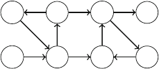
192 12 Advanced Graph Algorithms
12.1.2 2SAT Problem
In the 2SAT problem, we are given a logical formula
(a1∨b1)∧(a2∨b2)∧···∧(am∨bm),
where each aiand biis either a logical variable (x1,x2,...,xn) or a negation of
a logical variable (¬x1,¬x2,...,¬xn). The symbols “∧” and “∨” denote logical
operators “and” and “or.” Our task is to assign each variable a value so that the
formula is true, or state that this is not possible.
For example, the formula
L1=(x2∨¬x1)∧(¬x1∨¬x2)∧(x1∨x3)∧(¬x2∨¬x3)∧(x1∨x4)
is true when the variables are assigned as follows:
⎧
⎪
⎪
⎪
⎨
⎪
⎪
⎪
⎩
x1=false
x2=false
x3=true
x4=true
However, the formula
L2=(x1∨x2)∧(x1∨¬x2)∧(¬x1∨x3)∧(¬x1∨¬x3)
is always false, regardless of how we assign the values. The reason for this is that
we cannot choose a value for x1without creating a contradiction. If x1is false, both
x2and ¬x2should be true which is impossible, and if x1is true, both x3and ¬x3
should be true which is also impossible.
An instance of the 2SAT problem can be represented as an implication graph
whose nodes correspond to variables xiand negations ¬xi, and edges determine
the connections between the variables. Each pair (ai∨bi)generates two edges:
¬ai→biand ¬bi→ai. This means that if aidoes not hold, bimust hold, and
vice versa. For example, Fig. 12.6 shows the implication graph of L1, and Fig. 12.7
shows the implication graph of L2.
The structure of the implication graph tells us whether it is possible to assign the
values of the variables so that the formula is true. This can be done exactly when
there are no nodes xiand ¬xisuch that both nodes belong to the same strongly
Fig. 12.6 The implication
graph of L1
¬x3x2
¬x4x1
¬x1x4
¬x2x3
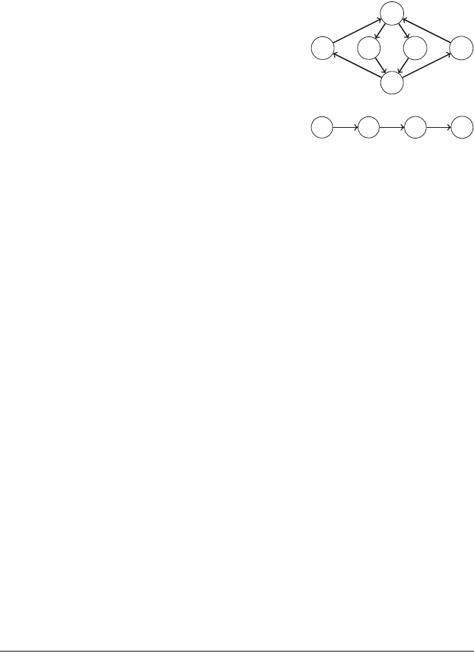
12.1 Strong Connectivity 193
Fig. 12.7 The implication
graph of L2
x3x2¬x2¬x3
¬x1
x1
Fig. 12.8 The component
graph of L1
ABCD
connected component. If there are such nodes, the graph contains a path from xito
¬xiand also a path from ¬xito xi, so both xiand ¬xishould be true which is not
possible. For example, the implication graph of L1does not have nodes xiand ¬xi
such that both nodes belong to the same strongly connected component, so there is a
solution. Then, in the implication graph of L2all nodes belong to the same strongly
connected component, so there are no solutions.
If a solution exists, the values for the variables can be found by going through
the nodes of the component graph in a reverse topological sort order. At each step,
we process a component that does not contain edges that lead to an unprocessed
component. If the variables in the component have not been assigned values, their
values will be determined according to the values in the component, and if they
already have values, the values remain unchanged. The process continues until each
variable has been assigned a value.
Figure 12.8 shows the component graph of L1. The components are A={¬x4},
B={x1,x2,¬x3},C={¬x1,¬x2,x3}, and D={x4}. When constructing the
solution, we first process the component Dwhere x4becomes true. After this, we
process the component Cwhere x1and x2become false and x3becomes true. All
variables have been assigned values, so the remaining components Aand Bdo not
change the values of the variables.
Note that this method works, because the implication graph has a special structure:
if there is a path from node xito node xjand from node xjto node ¬xj, then node
xinever becomes true. The reason for this is that there is also a path from node ¬xj
to node ¬xi, and both xiand xjbecome false.
A more difficult problem is the 3SAT problem, where each part of the formula is
of the form (ai∨bi∨ci). This problem is NP-hard, so no efficient algorithm for
solving the problem is known.
12.2 Complete Paths
In this section we discuss two special types of paths in graphs: an Eulerian path is a
path that goes through each edge exactly once, and a Hamiltonian path is a path that
visits each node exactly once. While such paths look quite similar at first glance, the
computational problems related to them are very different.
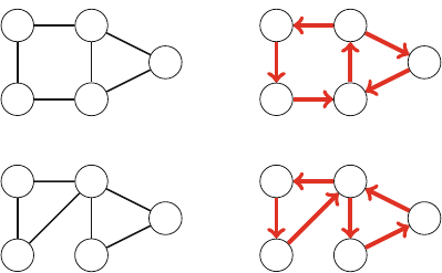
194 12 Advanced Graph Algorithms
Fig. 12.9 Agraphandan
Eulerian path 1 2
3
45
1 2
3
45
1.
2.
3.
4.
5.
6.
Fig. 12.10 Agraphandan
Eulerian circuit 1 2
3
45
1 2
3
45
1. 2. 3.
4.
5.
6.
12.2.1 Eulerian Paths
An Eulerian path is a path that goes exactly once through each edge of a graph.
Furthermore, if such a path starts and ends at the same node, it is called an Eulerian
circuit. Figure 12.9 shows an Eulerian path from node 2 to node 5, and Fig.12.10
shows an Eulerian circuit that starts and ends at node 1.
The existence of Eulerian paths and circuits depends on the degrees of the nodes.
First, an undirected graph has an Eulerian path exactly when all the edges belong to
the same connected component and
•the degree of each node is even, or
•the degree of exactly two nodes is odd, and the degree of all other nodes is even.
In the first case, each Eulerian path is also an Eulerian circuit. In the second case,
the odd-degree nodes are the endpoints of an Eulerian path, which is not an Eulerian
circuit. In Fig. 12.9, nodes 1, 3, and 4 have degree 2, and nodes 2 and 5 have degree
3. Exactly two nodes have an odd degree, so there is an Eulerian path between nodes
2 and 5, but the graph does not have an Eulerian circuit. In Fig. 12.10, all nodes have
an even degree, so the graph has an Eulerian circuit.
To determine whether a directed graph has Eulerian paths, we focus on indegrees
and outdegrees of the nodes. A directed graph contains an Eulerian path exactly
when all the edges belong to the same strongly connected component and
•in each node, the indegree equals the outdegree, or
•in one node, the indegree is one larger than the outdegree, in another node, the
outdegree is one larger than the indegree, and in all other nodes, the indegree
equals the outdegree.
In the first case, each Eulerian path is also an Eulerian circuit, and in the second
case, the graph has an Eulerian path that begins at the node whose outdegree is larger
and ends at the node whose indegree is larger. For example, in Fig. 12.11, nodes 1,
3, and 4 have both indegree 1 and outdegree 1, node 2 has indegree 1 and outdegree
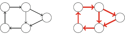
12.2 Complete Paths 195
Fig. 12.11 A directed graph
and an Eulerian path 1 2
3
45
1 2
3
45
1.
2.
3.
4.
5.
6.
2, and node 5 has indegree 2 and outdegree 1. Hence, the graph contains an Eulerian
path from node 2 to node 5.
Construction Hierholzer’s algorithm is an efficient method for constructing an
Eulerian circuit for a graph. The algorithm consists of several rounds, each of which
adds new edges to the circuit. Of course, we assume that the graph contains an
Eulerian circuit; otherwise Hierholzer’s algorithm cannot find it.
The algorithm begins with an empty circuit that contains only a single node and
then extends the circuit step by step by adding subcircuits to it. The process continues
until all edges have been added to the circuit. The circuit is extended by finding a
node xthat belongs to the circuit but has an outgoing edge that is not included in the
circuit. Then, a new path from node xthat only contains edges that are not yet in the
circuit is constructed. Sooner or later, the path will return to node x, which creates
a subcircuit.
If a graph does not have an Eulerian circuit but has an Eulerian path, we can still
use Hierholzer’s algorithm to find the path by adding an extra edge to the graph
and removing the edge after the circuit has been constructed. For example, in an
undirected graph, we add the extra edge between the two odd-degree nodes.
As an example, Fig. 12.12 shows how Hierholzer’s algorithm constructs an
Eulerian circuit in an undirected graph. First, the algorithm adds a subcircuit
1→2→3→1, then a subcircuit 2 →5→6→2, and finally a subcircuit
6→3→4→7→6. After this, since all edges have been added to the circuit, we
have successfully constructed an Eulerian circuit.
12.2.2 Hamiltonian Paths
AHamiltonian path is a path that visits each node of a graph exactly once. Further-
more, if a such a path begins and ends at the same node, it is called a Hamiltonian
circuit. For example, Fig. 12.13 shows a graph that has both a Hamiltonian path and
a Hamiltonian circuit.
Problems related to Hamiltonian paths are NP-hard: nobody knows a general
way to efficiently check if a graph has a Hamiltonian path or circuit. Of course, in
some special cases we can be certain that a graph contains a Hamiltonian path. For
example, if the graph is complete, i.e., there is an edge between all pairs of nodes, it
surely contains a Hamiltonian path.
A simple way to search for a Hamiltonian path is to use a backtracking algorithm
that goes through all possible ways to construct a path. The time complexity of such
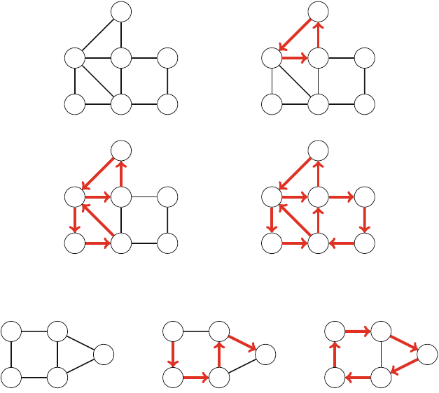
196 12 Advanced Graph Algorithms
1
234
5 6 7
step 1
1
234
5 6 7
1.
2.
3.
step 2
1
234
5 6 7
1.
2.
3.
4.
5.
6.
step 3
1
234
5 6 7
1.
2.
3.
4.
5.
6.
7.
8.
9.
10.
step 4
Fig. 12.12 Hierholzer’s algorithm
1 2
3
45
1 2
3
45
1.
2.
3.
4. 1 2
3
45
1.
2.
3.
4.
5.
Fig. 12.13 A graph, a Hamiltonian path and a Hamiltonian circuit
an algorithm is at least O(n!), because there are n!different ways to choose the
order of nnodes. Then, using dynamic programming, we can create a more efficient
O(2nn2)time solution, which determines for each subset of nodes Sand each node
x∈Sif there is a path that visits all nodes of Sexactly once and ends at node x.
12.2.3 Applications
De Bruijn Sequences ADe Bruijn sequence is a string that contains every string of
length nexactly once as a substring, for a fixed alphabet of kcharacters. The length
of such a string is kn+n−1 characters. For example, when n=3 and k=2, an
example of a De Bruijn sequence is
0001011100.
The substrings of this string are all combinations of three bits: 000, 001, 010, 011,
100, 101, 110, and 111.
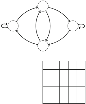
12.2 Complete Paths 197
Fig. 12.14 Constructing a
De Bruijn sequence from an
Eulerian path
00 11
01
10
11
0
0
0
1
0 1
Fig. 12.15 An open knight’s
tour on a 5 ×5 board 1411
16 25
12 17 2510
320724 15
18 13 22 96
21 819 14 23
A De Bruijn sequence always corresponds to an Eulerian path in a graph where
each node contains a string of n−1 characters, and each edge adds one character
to the string. For example, the graph in Fig. 12.14 corresponds to the scenario where
n=3 and k=2. To create a De Bruijn sequence, we start at an arbitrary node and
follow an Eulerian path that visits each edge exactly once. When the characters in the
starting node and on the edges are added together, the resulting string has kn+n−1
characters and is a valid De Bruijn sequence.
Knight’s Tours Aknight’s tour is a sequence of moves of a knight on an n×n
chessboard following the rules of chess such that the knight visits each square exactly
once. A knight’s tour is called closed if the knight finally returns to the starting square
and otherwise it is called open. For example, Fig. 12.15 shows an open knight’s tour
ona5×5 board.
A knight’s tour corresponds to a Hamiltonian path in a graph whose nodes repre-
sent the squares of the board, and two nodes are connected with an edge if a knight
can move between the squares according to the rules of chess. A natural way to con-
struct a knight’s tour is to use backtracking. Since there is a large number of possible
moves, the search can be made more efficient by using heuristics that attempt to
guide the knight so that a complete tour will be found quickly.
Warnsdorf’s rule is a simple and effective heuristic for finding a knight’s tour.
Using the rule, it is possible to efficiently construct a tour even on a large board. The
idea is to always move the knight so that it ends up in a square where the number of
possible follow-up moves is as small as possible. For example, in Fig. 12.16, there are
five possible squares to which the knight can move (squares a...e). In this situation,
Warnsdorf’s rule moves the knight to square a, because after this choice, there is
only a single possible move. The other choices would move the knight to squares
where there would be three moves available.
198 12 Advanced Graph Algorithms
Fig. 12.16 Using
Warndorf’s rule to construct
a knight’s tour
1
2
a
be
cd
12.3 Maximum Flows
In the maximum flow problem, we are given a directed weighted graph that contains
two special nodes: a source is a node with no incoming edges, and a sink is a node
with no outgoing edges. Our task is to send as much flow as possible from the source
to the sink. Each edge has a capacity that restricts the flow that can go through the
edge, and in each intermediate node, the incoming and outgoing flow has to be equal.
As an example, consider the graph in Fig. 12.17, where node 1 is the source and
node 6 is the sink. The maximum flow in this graph is 7, shown in Fig. 12.18. The
notation v/kmeans that a flow of vunits is routed through an edge whose capacity
is kunits. The size of the flow is 7, because the source sends 3 +4 units of flow
and the sink receives 5 +2 units of flow. It is easy to see that this flow is maximum,
because the total capacity of the edges leading to the sink is 7.
It turns out that the maximum flow problem is connected to another graph problem,
the minimum cut problem, where our task is to remove a set of edges from the graph
such that there will be no path from the source to the sink after the removal and the
total weight of the removed edges is minimum.
For example, consider again the graph in Fig. 12.17. The minimum cut size is 7,
because it suffices to remove the edges 2 →3 and 4 →5, as shown in Fig. 12.19.
After removing the edges, there will be no path from the source to the sink. The size
of the cut is 6 +1=7, and the cut is minimum, because there is no valid cut whose
weight would be less than 7.
Fig. 12.17 A graph with
source 1 and sink 6
1
23
6
45
5
6
5
4
1
2
38
Fig. 12.18 The maximum
flow of the graph is 7
1
23
6
45
3/5
6/6
5/5
4/4
1/1
2/2
3/3 1/8
12.3 Maximum Flows 199
Fig. 12.19 The minimum
cut of the graph is 7
1
23
6
45
5
6
5
4
1
2
38
Fig. 12.20 Graph
representation in the
Ford–Fulkerson algorithm
1
23
6
45
5
0
6
05
0
4
01
0
2
0
3 0 80
It is not a coincidence that the maximum flow and minimum cut are equal in our
example graph. Rather, it turns out that they are always equal, so the concepts are
two sides of the same coin. Next we will discuss the Ford–Fulkerson algorithm that
can be used to find the maximum flow and minimum cut of a graph. The algorithm
also helps us to understand why they are equal.
12.3.1 Ford–Fulkerson Algorithm
The Ford–Fulkerson algorithm finds the maximum flow in a graph. The algorithm
begins with an empty flow, and at each step finds a path from the source to the
sink that generates more flow. Finally, when the algorithm cannot increase the flow
anymore, the maximum flow has been found.
The algorithm uses a special graph representation where each original edge has
a reverse edge in another direction. The weight of each edge indicates how much
more flow we could route through it. At the beginning of the algorithm, the weight
of each original edge equals the capacity of the edge, and the weight of each reverse
edge is zero. Figure 12.20 shows the new representation for our example graph.
The Ford–Fulkerson algorithm consists of several rounds. On each round, the
algorithm finds a path from the source to the sink such that each edge on the path
has a positive weight. If there is more than one possible path available, any of them
can be chosen. After choosing the path, the flow increases by xunits, where xis the
smallest edge weight on the path. In addition, the weight of each edge on the path
decreases by x, and the weight of each reverse edge increases by x.
The idea is that increasing the flow decreases the amount of flow that can go
through the edges in the future. On the other hand, it is possible to cancel flow later
using the reverse edges if it turns out that it would be beneficial to route the flow
in another way. The algorithm increases the flow as long as there is a path from the
source to the sink through positive-weight edges. Then, if there are no such paths,
the algorithm terminates and the maximum flow has been found.
Figure 12.21 shows how the Ford–Fulkerson algorithm finds the maximum flow
for our example graph. In this case, there are four rounds. On the first round, the

200 12 Advanced Graph Algorithms
step 1
step 2
step 3
step 4
1
23
6
45
5
0
6
05
0
4
01
0
2
0
3 0 80 1
23
6
45
3
2
4
25
0
4
01
0
0
2
3 0 6
2
1
23
6
45
3
2
4
25
0
4
01
0
0
2
3 0 6
21
23
6
45
3
2
1
52
3
1
31
0
0
2
0 3 6
2
1
23
6
45
3
2
1
52
3
1
31
0
0
2
0 3 6
21
23
6
45
3
2
1
51
4
0
40
1
0
2
0 3 7
1
1
23
6
45
3
2
1
51
4
0
40
1
0
2
0 3 7
11
23
6
45
2
3
0
60
5
0
40
1
0
2
0 3 7
1
Fig. 12.21 The Ford–Fulkerson algorithm
algorithm chooses the path 1 →2→3→5→6. The minimum edge weight on
this path is 2, so the flow increases by 2 units. Then, the algorithm chooses three
other paths that increase the flow by 3, 1, and 1 units. After this, there is no path with
positive-weight edges, so the maximum flow is 2 +3+1+1=7.
Finding Paths The Ford–Fulkerson algorithm does not specify how we should
choose the paths that increase the flow. In any case, the algorithm will terminate
sooner or later and correctly find the maximum flow. However, the efficiency of the
algorithm depends on how the paths are chosen. A simple way to find paths is to
use depth-first search. Usually this works well, but in the worst case, each path only
increases the flow by one unit, and the algorithm is slow. Fortunately, we can avoid
this situation by using one of the following techniques:
The Edmonds–Karp algorithm chooses each path so that the number of edges on
the path is as small as possible. This can be done by using breadth-first search instead
12.3 Maximum Flows 201
Fig. 12.22 Nodes 1, 2, and
4 belong to the set A
1
23
6
45
2
3
0
60
5
0
40
1
0
2
0 3 7
1
of depth-first search for finding paths. It can be proved that this guarantees that the
flow increases quickly, and the time complexity of the algorithm is O(m2n).
The capacity scaling algorithm1uses depth-first search to find paths where each
edge weight is at least an integer threshold value. Initially, the threshold value is
some large number, for example, the sum of all edge weights of the graph. Always
when a path cannot be found, the threshold value is divided by 2. The algorithm
terminates when the threshold value becomes 0. The time complexity of the algorithm
is O(m2log c), where cis the initial threshold value.
In practice, the capacity scaling algorithm is easier to implement, because depth-
first search can be used for finding paths. Both algorithms are efficient enough for
problems that typically appear in programming contests.
Minimum Cuts It turns out that once the Ford–Fulkerson algorithm has found a
maximum flow, it has also determined a minimum cut. Consider the graph produced
by the algorithm, and let Abe the set of nodes that can be reached from the source
using positive-weight edges. Now the minimum cut consists of the edges of the
original graph that start at some node in A, end at some node outside A, and whose
capacity is fully used in the maximum flow. For example, in Fig. 12.22,Aconsists of
nodes 1, 2, and 4, and the minimum cut edges are 2 →3 and 4 →5, whose weight
is 6 +1=7.
Why is the flow produced by the algorithm maximum and why is the cut minimum?
The reason is that a graph cannot contain a flow whose size is larger than the weight
of any cut of the graph. Hence, always when a flow and a cut are equal, they are a
maximum flow and a minimum cut.
To see why the above holds, consider any cut of the graph such that the source
belongs to A, the sink belongs to B, and there are some edges between the sets
(Fig. 12.23). The size of the cut is the sum of the weights of the edges that go from
Ato B. This is an upper bound for the flow in the graph, because the flow has to
proceed from Ato B. Thus, the size of a maximum flow is smaller than or equal to
the size of any cut in the graph. On the other hand, the Ford–Fulkerson algorithm
produces a flow whose size is exactly as large as the size of a cut in the graph. Thus,
the flow has to be a maximum flow, and the cut has to be a minimum cut.
1This elegant algorithm is not very well known; a detailed description can be found in a textbook
by Ahuja, Magnanti, and Orlin [1].
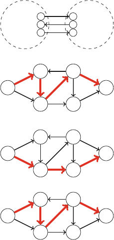
202 12 Advanced Graph Algorithms
Fig. 12.23 Routing the flow
from Ato B
AB
Fig. 12.24 Two
edge-disjoint paths from
node 1 to node 6 1
23
45
6
1
23
45
6
Fig. 12.25 A node-disjoint
path from node 1 to node 6
1
23
45
6
12.3.2 Disjoint Paths
Many graph problems can be solved by reducing them to the maximum flow problem.
Our first example of such a problem is as follows: we are given a directed graph with
a source and a sink, and our task is to find the maximum number of disjoint paths
from the source to the sink.
Edge-Disjoint Paths We first focus on the problem of finding the maximum number
of edge-disjoint paths from the source to the sink. This means that each edge may
appear in at most one path. For example, in Fig. 12.24, the maximum number of
edge-disjoint paths is 2 (1 →2→4→3→6 and 1 →4→5→6).
It turns out that the maximum number of edge-disjoint paths always equals the
maximum flow of the graph where the capacity of each edge is one. After the max-
imum flow has been constructed, the edge-disjoint paths can be found greedily by
following paths from the source to the sink.
Node-Disjoint Paths Then, consider the problem of finding the maximum number
of node-disjoint paths from the source to the sink. In this case, every node, except for
the source and sink, may appear in at most one path, which may reduce the maximum
number of disjoint paths. Indeed, in our example graph, the maximum number of
node-disjoint paths is 1 (Fig. 12.25).
We can reduce also this problem to the maximum flow problem. Since each node
can appear in at most one path, we have to limit the flow that goes through the nodes.
A standard construction for this is to divide each node into two nodes such that
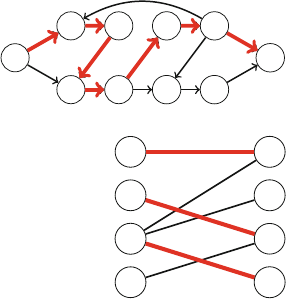
12.3 Maximum Flows 203
Fig. 12.26 A construction
that limits the flow through
the nodes 1
23
45
23
45
6
Fig. 12.27 Maximum
matching 1
2
3
4
5
6
7
8
the first node has the incoming edges of the original node, the second node has the
outgoing edges of the original node, and there is a new edge from the first node to
the second node. Figure 12.26 shows the resulting graph and its maximum flow in
our example.
12.3.3 Maximum Matchings
Amaximum matching of a graph is a maximum-size set of node pairs where each pair
is connected with an edge and each node belongs to at most one pair. While solving
the maximum matching problem in a general graph requires tricky algorithms, the
problem is much easier to solve if we assume that the graph is bipartite. In this case
we can reduce the problem to the maximum flow problem.
The nodes of a bipartite graph can always be divided into two groups such that all
edges of the graph go from the left group to the right group. For example, Fig. 12.27
shows a maximum matching of a bipartite graph whose left group is {1,2,3,4}and
right group is {5,6,7,8}.
We can reduce the bipartite maximum matching problem to the maximum flow
problem by adding two new nodes to the graph: a source and a sink. We also add
edges from the source to each left node and from each right node to the sink. After
this, the size of a maximum flow in the resulting graph equals the size of a maximum
matching in the original graph. For example, Fig. 12.28 shows the reduction and the
maximum flow for our example graph.
Hall’s Theorem Hall’s theorem can be used to find out whether a bipartite graph has
a matching that contains all left or right nodes. If the number of left and right nodes
is the same, Hall’s theorem tells us if it is possible to construct a perfect matching
that contains all nodes of the graph.
Assume that we want to find a matching that contains all left nodes. Let Xbe
any set of left nodes and let f(X)be the set of their neighbors. According to Hall’s
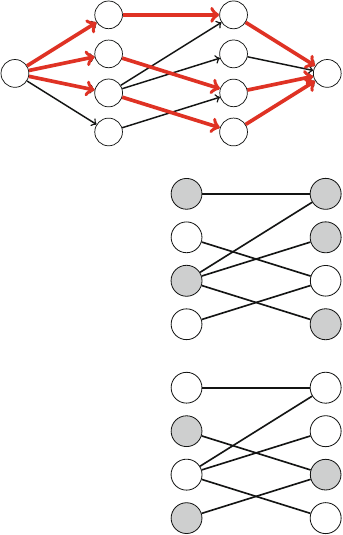
204 12 Advanced Graph Algorithms
Fig. 12.28 Maximum
matching as a maximum flow 1
2
3
4
5
6
7
8
Fig. 12.29 X={1,3}and
f(X)={5,6,8}1
2
3
4
5
6
7
8
Fig. 12.30 X={2,4}and
f(X)={7}1
2
3
4
5
6
7
8
theorem, a matching that contains all left nodes exists exactly when for every possible
set X, the condition |X|≤|f(X)|holds.
Let us study Hall’s theorem in our example graph. First, let X={1,3}which
yields f(X)={5,6,8}(Fig. 12.29). The condition of Hall’s theorem holds, because
|X|=2 and |f(X)|=3. Then, let X={2,4}which yields f(X)={7}(Fig. 12.30).
In this case, |X|=2 and |f(X)|=1, so the condition of Hall’s theorem does not
hold. This means that it is not possible to form a perfect matching for the graph. This
result is not surprising, because we already know that the maximum matching of the
graph is 3 and not 4.
If the condition of Hall’s theorem does not hold, the set Xexplains why we cannot
form such a matching. Since Xcontains more nodes than f(X), there are no pairs for
all nodes in X. For example, in Fig. 12.30, both nodes 2 and 4 should be connected
with node 7, which is not possible.
K˝onig’s Theorem Aminimum node cover of a graph is a minimum set of nodes
such that each edge of the graph has at least one endpoint in the set. In a general
graph, finding a minimum node cover is a NP-hard problem. However, if the graph
is bipartite, K˝onig’s theorem tells us that the size of a minimum node cover always
equals the size of a maximum matching. Thus, we can calculate the size of a minimum
node cover using a maximum flow algorithm.
12.3 Maximum Flows 205
Fig. 12.31 Aminimum
node cover 1
2
3
4
5
6
7
8
Fig. 12.32 Amaximum
independent set 1
2
3
4
5
6
7
8
Fig. 12.33 An example
graph for constructing path
covers
1 2 34
5 6 7
For example, since the maximum matching of our example graph is 3, K˝onig’s
theorem tells us that the size of a minimum node cover is also 3. Figure 12.31 shows
how such a cover can be constructed.
The nodes that do not belong to a minimum node cover form a maximum inde-
pendent set. This is the largest possible set of nodes such that no two nodes in the set
are connected with an edge. Again, finding a maximum independent set in a general
graph is a NP-hard problem, but in a bipartite graph we can use K˝onig’s theorem
to solve the problem efficiently. Figure 12.32 shows a maximum independent set for
our example graph.
12.3.4 Path Covers
Apath cover is a set of paths in a graph such that each node of the graph belongs
to at least one path. It turns out that in directed acyclic graphs, we can reduce the
problem of finding a minimum path cover to the problem of finding a maximum flow
in another graph.
Node-Disjoint Path Covers In a node-disjoint path cover, each node belongs to
exactly one path. As an example, consider the graph in Fig. 12.33. A minimum
node-disjoint path cover of this graph consists of three paths (Fig. 12.34).
We can find a minimum node-disjoint path cover by constructing a matching graph
where each node of the original graph is represented by two nodes: a left node and a
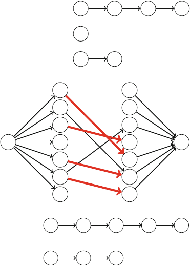
206 12 Advanced Graph Algorithms
Fig. 12.34 Aminimum
node-disjoint path cover 15 6 7
2
34
Fig. 12.35 A matching
graph for finding a minimum
node-disjoint path cover
1
2
3
4
5
6
7
1
2
3
4
5
6
7
Fig. 12.36 Aminimum
general path cover 15 6 3 4
267
right node. There is an edge from a left node to a right node if there is such an edge
in the original graph. In addition, the matching graph contains a source and a sink,
and there are edges from the source to all left nodes and from all right nodes to the
sink. Each edge in the maximum matching of the matching graph corresponds to an
edge in the minimum node-disjoint path cover of the original graph. Thus, the size
of the minimum node-disjoint path cover is n−c, where nis the number of nodes
in the original graph, and cis the size of the maximum matching.
For example, Fig. 12.35 shows the matching graph for the graph in Fig. 12.33.
The maximum matching is 4, so the minimum node-disjoint path cover consists of
7−4=3 paths.
General Path Covers Ageneral path cover is a path cover where a node can belong to
more than one path. A minimum general path cover may be smaller than a minimum
node-disjoint path cover, because a node can be used multiple times in paths. Consider
again the graph in Fig. 12.33. The minimum general path cover of this graph consists
of two paths (Fig. 12.36).
A minimum general path cover can be found almost like a minimum node-disjoint
path cover. It suffices to add some new edges to the matching graph so that there
is an edge a→balways when there is a path from ato bin the original graph
(possibly through several nodes). Figure 12.37 shows the resulting matching graph
for our example graph.
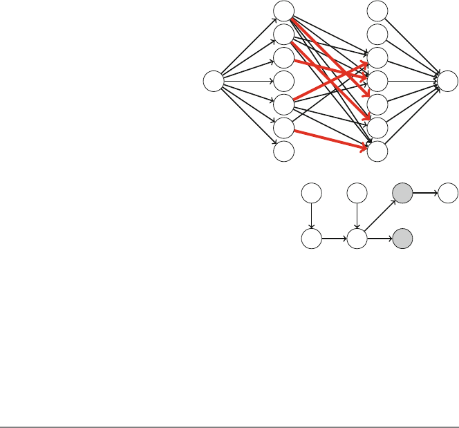
12.3 Maximum Flows 207
Fig. 12.37 A matching
graph for finding a minimum
general path cover
1
2
3
4
5
6
7
1
2
3
4
5
6
7
Fig. 12.38 Nodes 3 and 7
form a maximum antichain 1 2 34
5 6 7
Dilworth’s Theorem An antichain is a set of nodes in a graph such that there is
no path from any node to another node using the edges of the graph. Dilworth’s
theorem states that in a directed acyclic graph, the size of a minimum general path
cover equals the size of a maximum antichain. For example, in Fig. 12.38, nodes
3 and 7 form an antichain of two nodes. This is a maximum antichain, because a
minimum general path cover of this graph has two paths (Fig. 12.36).
12.4 Depth-First Search Trees
When depth-first search processes a connected graph, it also creates a rooted directed
spanning tree that can be called a depth-first search tree. Then, the edges of the graph
can be classified according to their roles during the search. In an undirected graph,
there will be two types of edges: tree edges that belong to the depth-first search tree
and back edges that point to already visited nodes. Note that a back edge always
points to an ancestor of a node.
For example, Fig. 12.39 shows a graph and its depth-first search tree. The solid
edges are tree edges, and the dashed edges are back edges.
In this section, we will discuss some applications for depth-first search trees in
graph processing.
12.4.1 Biconnectivity
A connected graph is called biconnected if it remains connected after removing
any single node (and its edges) from the graph. For example, in Fig. 12.40, the left
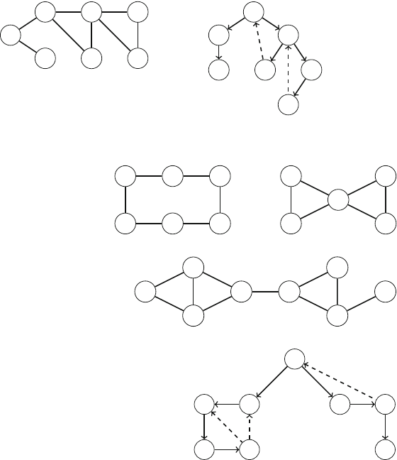
208 12 Advanced Graph Algorithms
1
2
3
45
67
1
2
3
4
56
7
Fig. 12.39 A graph and its depth-first search tree
Fig. 12.40 The left graph is
biconnected, the right graph
is not
1 2 3
45 6
1 2
3
45
Fig. 12.41 A graph with
three articulation points and
two bridges 1
2
3
45
6
7
8
Fig. 12.42 Finding bridges
and articulation points using
depth-first search
1
2
3
4
5
67
8
graph is biconnected, but the right graph is not. The right graph is not biconnected,
because removing node 3 from the graph disconnects the graph by dividing it into
two components {1,4}and {2,5}.
A node is called an articulation point if removing the node from the graph dis-
connects the graph. Thus, a biconnected graph does not have articulation points.
In a similar way, an edge is called a bridge if removing the edge from the graph
disconnects the graph. For example, in Fig. 12.41, nodes 4, 5, and 7 are articulation
points, and edges 4–5 and 7–8 are bridges.
We can use depth-first search to efficiently find all articulation points and bridges
in a graph. First, to find bridges, we begin a depth-first search at an arbitrary node,
which builds a depth-first search tree. For example, Fig. 12.42 shows a depth-first
search tree for our example graph.
An edge a→bcorresponds to a bridge exactly when it is a tree edge, and
there is no back edge from the subtree of bto aor any ancestor of a. For example,
in Fig. 12.42, edge 5 →4 is a bridge, because there is no back edge from nodes
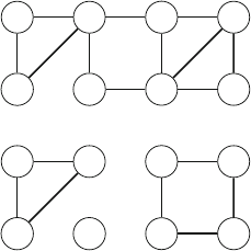
12.4 Depth-First Search Trees 209
Fig. 12.43 Agraphandan
Eulerian subgraph 1 2 34
5 6 78
1 2 34
5 6 78
{1,2,3,4}to node 5. However, edge 6 →7 is not a bridge, because there is a back
edge 7 →5, and node 5 is an ancestor of node 6.
Finding articulation points is a bit more difficult, but we can again use the depth-
first search tree. First, if a node xis the root of the tree, it is an articulation point
exactly when it has two or more children. Then, if xis not the root, it is an articulation
point exactly when it has a child whose subtree does not contain a back edge to an
ancestor of x.
For example, in Fig.12.42, node 5 is an articulation point, because it is the root
and has two children, and node 7 is an articulation point, because the subtree of its
child 8 does not contain a back edge to an ancestor of 7. However, node 2 is not
an articulation point, because there is a back edge 3 →4, and node 8 is not an
articulation point, because it does not have any children.
12.4.2 Eulerian Subgraphs
An Eulerian subgraph of a graph contains the nodes of the graph and a subset of
the edges such that the degree of each node is even. For example, Fig. 12.43 shows
a graph and its Eulerian subgraph.
Consider the problem of calculating the total number of Eulerian subgraphs for a
connected graph. It turns out that there is a simple formula for this: there are always
2kEulerian subgraphs were kis the number of back edges in the depth-first search
tree of the graph. Note that k=m−(n−1)where nis the number of nodes and m
is the number of edges.
The depth-first search tree helps to understand why this formula holds. Consider
any fixed subset of back edges in the depth-first search tree. To create an Eulerian
subgraph that contains these edges, we need to choose a subset of the tree edges so
that each node has an even degree. To do this, we process the tree from bottom to
top and always include a tree edge in the subgraph exactly when it points to a node
whose degree is even with the edge. Then, since the sum of degrees is even, also the
degree of the root node will be even.

Geometry
This chapter discusses algorithm techniques related to geometry. The general goal
of the chapter is to find ways to conveniently solve geometric problems, avoiding
special cases and tricky implementations.
Section 13.1 introduces the C++ complex number class which has useful tools for
geometric problems. After this, we will learn to use cross products to solve various
problems, such as testing whether two line segments intersect and calculating the
distance from a point to a line. Finally, we discuss ways to calculate polygon areas
and explore special properties of Manhattan distances.
Section 13.2 focuses on sweep line algorithms which play an important role in
computational geometry. We will see how to use such algorithms for counting inter-
section points, finding closest points, and constructing convex hulls.
13.1 Geometric Techniques
A challenge when solving geometric problems is how to approach the problem so
that the number of special cases is as small as possible and there is a convenient way
to implement the solution. In this section, we will go through a set of tools that make
solving geometric problems easier.
13.1.1 Complex Numbers
Acomplex number is a number of the form x+yi, where i=√−1istheimaginary
unit. A geometric interpretation of a complex number is that it represents a two-
dimensional point (x,y)or a vector from the origin to a point (x,y). For example,
Fig. 13.1 illustrates the complex number 4 +2i.
212 13 Geometry
Fig. 13.1 Complex number
4+2iinterpreted as a point
and a vector (4,2)
The C++ complex number class complex is useful when solving geometric
problems. Using the class we can represent points and vectors as complex numbers,
and use the features of the class to manipulate them. To do this, let us first define
a coordinate type C. Depending on the situation, a suitable type is long long or
long double. As a general rule, it is good to use integer coordinates whenever
possible, because calculations with integers are exact.
Here are possible coordinate type definitions:
typedef long long C;
typedef long double C;
After this, we can define a complex type Pthat represents a point or a vector:
typedef complex<C> P;
Finally, the following macros refer to x and y coordinates:
#define X real()
#define Y imag()
For example, the following code creates a point p=(4,2)and prints its x and y
coordinates:
P p = {4,2};
cout << p.X << "" << p.Y << "\n";
// 4 2
Then, the following code creates vectors v=(3,1)and u=(2,2), and after that
calculates the sum s=v+u.
P v = {3,1};
P u = {2,2};
Ps=v+u;
cout << s.X << "" << s.Y << "\n";
// 5 3
13.1 Geometric Techniques 213
Functions The complex class also has functions that are useful in geometric prob-
lems. The following functions should only be used when the coordinate type is long
double (or another floating point type).
The function abs(v)calculates the length |v|of a vector v=(x,y)using the
formula x2+y2. The function can also be used for calculating the distance between
points (x1,y1)and (x2,y2), because that distance equals the length of the vector
(x2−x1,y2−y1). For example, the following code calculates the distance between
points (4,2)and (3,−1)
P a = {4,2};
P b = {3,-1};
cout << abs(b-a) << "\n";
// 3.16228
The function arg(v)calculates the angle of a vector v=(x,y)with respect to
the x-axis. The function gives the angle in radians, where rradians equals 180r/π
degrees. The angle of a vector that points to the right is 0, and angles decrease
clockwise and increase counterclockwise.
The function polar(s,a)constructs a vector whose length is sand that points
to an angle a, given in radians. A vector can be rotated by an angle aby multiplying
it by a vector with length 1 and angle a.
The following code calculates the angle of the vector (4,2), rotates it 1/2 radians
counterclockwise, and then calculates the angle again:
P v = {4,2};
cout << arg(v) << "\n";
// 0.463648
v *= polar(1.0,0.5);
cout << arg(v) << "\n";
// 0.963648
13.1.2 Points and Lines
The cross product a ×bof vectors a=(x1,y1)and b=(x2,y2)is defined to be
x1y2−x2y1. It tells us the direction to which bturns when it is placed directly after
a. There are three cases illustrated in Fig. 13.2:
a
b
a×b>0
a
b
a×b=0
a
b
a×b<0
Fig. 13.2 Interpretation of cross products
214 13 Geometry
Fig. 13.3 Testing the
location of a point
s1
s2
p
•a×b>0: bturns left
•a×b=0: bdoes not turn (or turns 180 degrees)
•a×b<0: bturns right
For example, the cross product of vectors a=(4,2)and b=(1,2)is 4 ·2−2·
1=6, which corresponds to the first scenario of Fig. 13.2. The cross product can be
calculated using the following code:
P a = {4,2};
P b = {1,2};
C p = (conj(a)*b).Y;
// 6
The above code works, because the function conj negates the y coordinate of
a vector, and when the vectors (x1,−y1)and (x2,y2)are multiplied together, the y
coordinate of the result is x1y2−x2y1.
Next we will go through some applications of cross products.
Testing Point Location Cross products can be used to test whether a point is located
on the left or right side of a line. Assume that the line goes through points s1and
s2, we are looking from s1to s2and the point is p. For example, in Fig. 13.3,pis
located on the left side of the line.
The cross product (p−s1)×(p−s2)tells us the location of the point p. If the
cross product is positive, pis located on the left side, and if the cross product is
negative, pis located on the right side. Finally, if the cross product is zero, the points
s1,s2, and pare on the same line.
Line Segment Intersection Next, consider the problem of testing whether two line
segments ab and cd intersect. It turns out that if the line segments intersect, there
are three possible cases:
Case 1: The line segments are on the same line and they overlap each other. In
this case, there is an infinite number of intersection points. For example, in Fig.13.4,
all points between cand bare intersection points. To detect this case, we can use
cross products to test if all points are on the same line. If they are, we can then sort
them and check whether the line segments overlap each other.
Case 2: The line segments have a common vertex that is the only intersection
point. For example, in Fig. 13.5 the intersection point is b=c. This case is easy
to check, because there are only four possibilities for the intersection point: a=c,
a=d,b=c, and b=d.
13.1 Geometric Techniques 215
Fig. 13.4 Case 1: the line
segments are on the same
line and overlap each other
a
d
c
b
Fig. 13.5 Case 2: the line
segments have a common
vertex
a
b=c
d
Fig. 13.6 Case 3: the line
segments have an
intersection point that is not
avertex
c
d
a
b
p
Fig. 13.7 Calculating the
distance from pto the line
s1
s2
p
d
Case 3: There is exactly one intersection point that is not a vertex of any line
segment. In Fig. 13.6, the point pis the intersection point. In this case, the line
segments intersect exactly when both points cand dare on different sides of a line
through aand b, and points aand bare on different sides of a line through cand d.
We can use cross products to check this.
Distance from a Point to a Line Another property of cross products is that the area
of a triangle can be calculated using the formula
|(a−c)×(b−c)|
2,
where a,b, and care the vertices of the triangle. Using this fact, we can derive a
formula for calculating the shortest distance between a point and a line. For example,
in Fig. 13.7,dis the shortest distance between the point pand the line that is defined
by the points s1and s2.
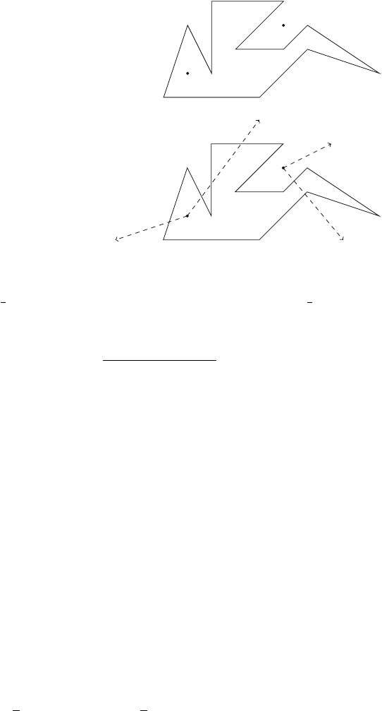
216 13 Geometry
Fig. 13.8 Point ais inside
and point bis outside the
polygon
a
b
Fig. 13.9 Sending rays from
points aand b
a
b
The area of a triangle whose vertices are s1,s2, and pcan be calculated in two
ways: it is both 1
2|s2−s1|d(the standard formula taught in school) and 1
2((s1−p)×
(s2−p)) (the cross product formula). Thus, the shortest distance is
d=(s1−p)×(s2−p)
|s2−s1|.
Point in a Polygon Finally, consider the problem of testing whether a point is located
inside or outside a polygon. For example, in Fig. 13.8, point ais inside the polygon
and point bis outside the polygon.
A convenient way to solve the problem is to send a ray from the point to an
arbitrary direction and calculate the number of times it touches the boundary of the
polygon. If the number is odd, the point is inside the polygon, and if the number is
even, the point is outside the polygon.
For example, in Fig. 13.9, the rays from atouch 1 and 3 times the boundary of the
polygon, so ais inside the polygon. In a similar way, the rays from btouch 0 and 2
times the boundary of the polygon, so bis outside the polygon.
13.1.3 Polygon Area
A general formula for calculating the area of a polygon, sometimes called the
shoelace formula, is as follows:
1
2|
n−1
i=1
(pi×pi+1)|=1
2|
n−1
i=1
(xiyi+1−xi+1yi)|.
13.1 Geometric Techniques 217
Fig. 13.10 A polygon
whose area is 17/2
(4,1)
(7,3)
(5,5)
(2,4)
(4,3)
Fig. 13.11 Calculating the
area of the polygon using
trapezoids
(4,1)
(7,3)
(5,5)
(2,4)
(4,3)
Here the vertices are p1=(x1,y1),p2=(x2,y2),..., pn=(xn,yn)in such an
order that piand pi+1are adjacent vertices on the boundary of the polygon, and the
first and last vertex is the same, i.e., p1=pn.
For example, the area of the polygon in Fig. 13.10 is
|(2·5−5·4)+(5·3−7·5)+(7·1−4·3)+(4·3−4·1)+(4·4−2·3)|
2=17/2.
The idea behind the formula is to go through trapezoids whose one side is a side
of the polygon, and another side lies on the horizontal line y=0. For example,
Fig. 13.11 shows one such trapezoid. The area of each trapezoid is
(xi+1−xi)yi+yi+1
2,
where the vertices of the polygon are piand pi+1.Ifxi+1>xi, the area is positive,
and if xi+1<xi, the area is negative. Then, the area of the polygon is the sum of
areas of all such trapezoids, which yields the formula
n−1
i=1
(xi+1−xi)yi+yi+1
2
=1
2
n−1
i=1
(xiyi+1−xi+1yi)
.
Note that the absolute value of the sum is taken, because the value of the sum may
be positive or negative, depending on whether we walk clockwise or counterclock-
wise along the boundary of the polygon.
218 13 Geometry
Fig. 13.12 Calculating the
polygon area using Pick’s
theorem
(4,1)
(7,3)
(5,5)
(2,4)
(4,3)
Pick’s Theorem Pick’s theorem provides another way to calculate the area of a
polygon, assuming that all vertices of the polygon have integer coordinates. Pick’s
theorem tells us that the area of the polygon is
a+b/2−1,
where ais the number of integer points inside the polygon and bis the number of
integer points on the boundary of the polygon. For example, the area of the polygon
in Fig. 13.12 is
6+7/2−1=17/2.
13.1.4 Distance Functions
Adistance function defines the distance between two points. The usual distance
function is the Euclidean distance where the distance between points (x1,y1)and
(x2,y2)is
(x2−x1)2+(y2−y1)2.
An alternative distance function is the Manhattan distance where the distance
between points (x1,y1)and (x2,y2)is
|x1−x2|+|y1−y2|.
For example, in Fig. 13.13, the Euclidean distance between the points is
(5−2)2+(2−1)2=√10
and the Manhattan distance is
|5−2|+|2−1|=4.
13.1 Geometric Techniques 219
(2,1)
(5,2)
(2,1)
(5,2)
Euclidean distance Manhattan distance
Fig. 13.13 Two distance functions
Fig. 13.14 Regions within a
distance of 1
Euclidean distance Manhattan distance
Fig. 13.15 Points Band C
have the maximum
Manhattan distance
A
C
B
D
Fig. 13.16 Maximum
Manhattan distance after
transforming the coordinates A
C
B
D
Figure 13.14 shows regions that are within a distance of 1 from the center point,
using the Euclidean and Manhattan distances.
Some problems are easier to solve if Manhattan distances are used instead of
Euclidean distances. As an example, given a set of points in the two-dimensional
plane, consider the problem of finding two points whose Manhattan distance is maxi-
mum. For example, in Fig. 13.15, we should select points Band Cto get the maximum
Manhattan distance 5.
A useful technique related to Manhattan distances is to transform the coordinates
so that a point (x,y)becomes (x+y,y−x). This rotates the point set 45◦and scales
it. For example, Fig. 13.16 shows the result of the transformation in our example
scenario.
220 13 Geometry
Then, consider two points p1=(x1,y1)and p2=(x2,y2)whose transformed
coordinates are p
1=(x
1,y
1)and p
2=(x
2,y
2). Now there are two ways to express
the Manhattan distance between p1and p2:
|x1−x2|+|y1−y2|=max(|x
1−x
2|,|y
1−y
2|)
For example, if p1=(1,0)and p2=(3,3), the transformed coordinates are
p
1=(1,−1)and p
2=(6,0)and the Manhattan distance is
|1−3|+|0−3|=max(|1−6|,|−1−0|)=5.
The transformed coordinates provide a simple way to operate with Manhattan
distances, because we can consider x and y coordinates separately. In particular, to
maximize the Manhattan distance, we should find two points whose transformed
coordinates maximize the value of
max(|x
1−x
2|,|y
1−y
2|).
This is easy, because either the horizontal or vertical difference of the transformed
coordinates has to be maximum.
13.2 Sweep Line Algorithms
Many geometric problems can be solved using sweep line algorithms. The idea in
such algorithms is to represent an instance of the problem as a set of events that
correspond to points in the plane. Then, the events are processed in increasing order
according to their x or y coordinates.
13.2.1 Intersection Points
Given a set of nline segments, each of them being either horizontal or vertical,
consider the problem of counting the total number of intersection points. For example,
in Fig. 13.17, there are five line segments and three intersection points.
Fig. 13.17 Five line
segments with three
intersection points
13.2 Sweep Line Algorithms 221
Fig. 13.18 Events that
correspond to the line
segments
12
12
12
33
It is easy to solve the problem in O(n2)time, because we can go through all
possible pairs of line segments and check if they intersect. However, we can solve
the problem more efficiently in O(nlog n)time using a sweep line algorithm and a
range query data structure. The idea is to process the endpoints of the line segments
from left to right and focus on three types of events:
(1) horizontal segment begins
(2) horizontal segment ends
(3) vertical segment
Figure 13.18 shows the events in our example scenario.
After creating the events, we go through them from left to right and use a data
structure that maintains the y coordinates of the active horizontal segments. At event
1, we add the y coordinate of the segment to the structure, and at event 2, we remove
the y coordinate from the structure. Intersection points are calculated at event 3:
when processing a vertical segment between points y1and y2, we count the number
of active horizontal segments whose y coordinate is between y1and y2, and add this
number to the total number of intersection points.
To store y coordinates of horizontal segments, we can use a binary indexed or
segment tree, possibly with index compression. Processing each event takes O(log n)
time, so the algorithm works in O(nlog n)time.
13.2.2 Closest Pair Problem
Given a set of npoints, our next problem is to find two points whose Euclidean
distance is minimum. For example, Fig. 13.19 shows a set of points, where the closest
pair is painted black.
This is another example of a problem that can be solved in O(nlog n)time using
a sweep line algorithm.1We go through the points from left to right and maintain
1Creating an efficient algorithm for the closest pair problem was once an important open problem in
computational geometry. Finally, Shamos and Hoey [26] discovered a divide and conquer algorithm
that works in O(nlog n)time. The sweep line algorithm presented here has common elements with
their algorithm, but it is easier to implement.
222 13 Geometry
Fig. 13.19 An instance of the closest pair problem
d
d
Fig. 13.20 Region where the closest point must lie
Fig. 13.21 Closest point
region contains O(1)points
d
d
a value d: the minimum distance between two points seen so far. At each point, we
find its nearest point to the left. If the distance is less than d, it is the new minimum
distance and we update the value of d.
If the current point is (x,y)and there is a point to the left within a distance of
less than d, the x coordinate of such a point must be between [x−d,x]and the y
coordinate must be between [y−d,y+d]. Thus, it suffices to only consider points
that are located in those ranges, which makes the algorithm efficient. For example,
in Fig. 13.20, the region marked with dashed lines contains the points that can be
within a distance of dfrom the active point.
The efficiency of the algorithm is based on the fact that the region always contains
only O(1)points. To see why this holds, consider Fig. 13.21. Since the current
minimum distance between two points is d, each d/2×d/2 square may contain at
most one point. Thus, there are at most eight points in the region.
13.2 Sweep Line Algorithms 223
Fig. 13.22 Convex hull of a point set
step 1 step 2 step 3 step 4
step 5 step 6 step 7 step 8
step 9 step 10 step 11 step 12
step 13 step 14 step 15 step 16
step 17 step 18 step 19 step 20
Fig. 13.23 Constructing the upper part of the convex hull using Andrew’s algorithm
224 13 Geometry
We can go through the points in the region in O(log n)time by maintaining a set
of points whose x coordinates are between [x−d,x]so that the points are sorted
in increasing order according to their y coordinates. The time complexity of the
algorithm is O(nlog n), because we go through npoints and determine for each
point its nearest point to the left in O(log n)time.
13.2.3 Convex Hull Problem
Aconvex hull is the smallest convex polygon that contains all points of a given
point set. Here convexity means that a line segment between any two vertices of the
polygon is completely inside the polygon. For example, Fig. 13.22 shows the convex
hull of a point set.
There are many efficient algorithms for constructing convex hulls. Perhaps the
simplest among them is Andrew’s algorithm [2], which we will describe next. The
algorithm first determines the leftmost and rightmost points in the set, and then
constructs the convex hull in two parts: first the upper hull and then the lower hull.
Both parts are similar, so we can focus on constructing the upper hull.
First, we sort the points primarily according to x coordinates and secondarily
according to y coordinates. After this, we go through the points and add each point
to the hull. Always after adding a point to the hull, we make sure that the last line
segment in the hull does not turn left. As long as it turns left, we repeatedly remove
the second last point from the hull. Figure 13.23 shows how Andrew’s algorithm
creates the upper hull for our example point set.

String Algorithms
This chapter deals with topics related to string processing.
Section 14.1 presents the trie structure which maintains a set of strings. After this,
dynamic programming algorithms for determining longest common subsequences
and edit distances are discussed.
Section 14.2 discusses the string hashing technique which is a general tool for
creating efficient string algorithms. The idea is to compare hash values of strings
instead of their characters, which allows us to compare strings in constant time.
Section 14.3 introduces the Z-algorithm which determines for each string position
the longest substring which is also a prefix of the string. The Z-algorithm is an
alternative for many string problems that can also be solved using hashing.
Section 14.4 discusses the suffix array structure, which can be used to solve some
more advanced string problems.
14.1 Basic Topics
Throughout the chapter, we assume that all strings are zero indexed. For example, a
string sof length nconsists of characters s[0],s[1],...,s[n−1].
Asubstring is a sequence of consecutive characters in a string. We use the notation
s[a...b]to refer to a substring of sthat starts at position aand ends at position b.
Aprefix is a substring that contains the first character of a string, and a suffix is a
substring that contains the last character of a string.
Asubsequence is any sequence of characters in a string in their original order. All
substrings are subsequences, but the converse is not true (Fig.14.1).
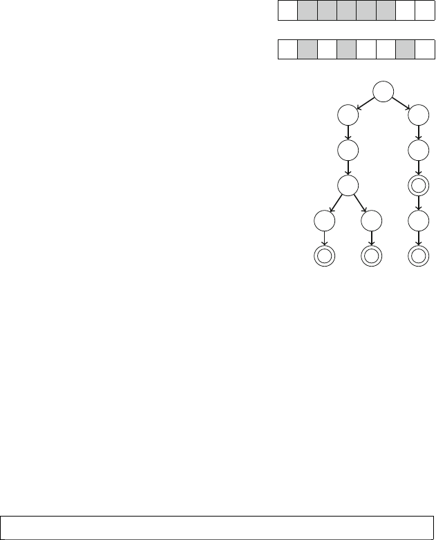
226 14 String Algorithms
Fig. 14.1 NVELO is a
substring, NEP is a
subsequence
ENVELOPE
asubstring
ENVELOPE
asubsequence
Fig. 14.2 Atriethat
contains the strings CANAL,
CANDY,THE,andTHERE
CT
A
N
A D
L Y
H
E
R
E
14.1.1 Trie Structure
Atrie is a rooted tree that maintains a set of strings. Each string in the set is stored as a
character chain that starts at the root node. If two strings have a common prefix, they
also have a common chain in the tree. As an example, the trie in Fig. 14.2 corresponds
to the set {CANAL,CANDY,THE,THERE}. A circle in a node means that a string in
the set ends at the node.
After constructing a trie, we can easily check whether it contains a given string
by following the chain that starts at the root node. We can also add a new string to
the trie by first following the chain and then adding new nodes if necessary. Both the
operations work in O(n)time where nis the length of the string.
A trie can be stored in an array
int trie[N][A];
where Nis the maximum number of nodes (the maximum total length of the strings
in the set) and Ais the size of the alphabet. The trie nodes are numbered 0,1,2,...
in such a way that the number of the root is 0, and trie[s][c]specifies the next
node in the chain when we move from node susing character c.
There are several ways how we can extend the trie structure. For example, suppose
that we are given queries that require us to calculate the number of strings in the set
that have a certain prefix. We can do this efficiently by storing for each trie node the
number of strings whose chain goes through the node.
14.1 Basic Topics 227
Fig. 14.3 The values of the
lcs function for
determining the longest
common subsequence of
TOUR and OPERA
T
O
U
R
OPERA
0
1
1
1
0
1
1
1
0
1
1
1
0
1
1
2
0
1
1
2
14.1.2 Dynamic Programming
Dynamic programming can be used to solve many string problems. Next we will
discuss two examples of such problems.
Longest Common Subsequence The longest common subsequence of two strings
is the longest string that appears as a subsequence in both strings. For example, the
longest common subsequence of TOUR and OPERA is OR.
Using dynamic programming, we can determine the longest common subsequence
of two strings xand yin O(nm)time, where nand mdenote the lengths of the strings.
To do this, we define a function lcs(i,j)that gives the length of the longest common
subsequence of the prefixes x[0...i]and y[0... j]. Then, we can use the recurrence
lcs(i,j)=lcs(i−1,j−1)+1x[i]=y[j]
max(lcs(i,j−1), lcs(i−1,j)) otherwise.
The idea is that if characters x[i]and y[j]are equal, we match them and increase
the length of the longest common subsequence by one. Otherwise, we remove the
last character from either xor y, depending on which choice is optimal.
For example, Fig. 14.3 shows the values of the lcs function in our example
scenario.
Edit Distances The edit distance (or Levenshtein distance) between two strings
denotes the minimum number of editing operations that transform the first string
into the second string. The allowed editing operations are as follows:
•insert a character (e.g., ABC →ABCA)
•remove a character (e.g., ABC →AC)
•modify a character (e.g., ABC →ADC)
For example, the edit distance between LOVE and MOVIE is 2, because we can
first perform the operation LOVE →MOVE (modify) and then the operation MOVE
→MOVIE (insert).
We can calculate the edit distance between two strings xand yin O(nm)time,
where nand mare the lengths of the strings. Let edit(i,j)denote the edit distance
between the prefixes x[0...i]and y[0... j]. The values of the function can be
calculated using the recurrence
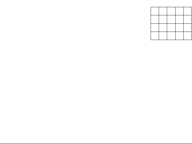
228 14 String Algorithms
Fig. 14.4 The values of the
edit function for
determining the edit distance
between LOVE and MOVIE
L
O
V
E
MOVIE
1
2
3
4
2
1
2
3
3
2
1
2
4
3
2
2
5
4
3
2
edit(a,b)=min(edit(a,b−1)+1,
edit(a−1,b)+1,
edit(a−1,b−1)+cost(a,b)),
where cost(a,b)=0ifx[a]=y[b], and otherwise cost(a,b)=1. The formula
considers three ways to edit the string x: insert a character at the end of x, remove
the last character from x, or match/modify the last character of x. In the last case, if
x[a]=y[b], we can match the last characters without editing.
For example, Fig. 14.4 shows the values of the edit function in our example
scenario.
14.2 String Hashing
Using string hashing we can efficiently check whether two strings are equal by
comparing their hash values. A hash value is an integer that is calculated from the
characters of the string. If two strings are equal, their hash values are also equal,
which makes it possible to compare strings based on their hash values.
14.2.1 Polynomial Hashing
A usual way to implement string hashing is polynomial hashing, which means that
the hash value of a string sof length nis
(s[0]An−1+s[1]An−2+···+s[n−1]A0)mod B,
where s[0],s[1],...,s[n−1]are interpreted as character codes, and Aand Bare
prechosen constants.
For example, let us calculate the hash value of the string ABACB. The character
codes of A,B, and Care 65, 66, and 67. Then, we need to fix the constants; suppose
that A=3 and B=97. Thus, the hash value is
(65 ·34+66 ·33+65 ·32+66 ·31+67 ·30)mod 97 =40.
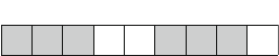
14.2 String Hashing 229
When polynomial hashing is used, we can calculate the hash value of any substring
of a string sin O(1)time after an O(n)time preprocessing. The idea is to construct
an array hsuch that h[k]contains the hash value of the prefix s[0...k]. The array
values can be recursively calculated as follows:
h[0]=s[0]
h[k]=(h[k−1]A+s[k])mod B
In addition, we construct an array pwhere p[k]=Akmod B:
p[0]=1
p[k]=(p[k−1]A)mod B.
Constructing the above arrays takes O(n)time. After this, the hash value of any
substring s[a...b]can be calculated in O(1)time using the formula
(h[b]−h[a−1]p[b−a+1])mod B
assuming that a>0. If a=0, the hash value is simply h[b].
14.2.2 Applications
We can efficiently solve many string problems using hashing, because it allows us
to compare arbitrary substrings of strings in O(1)time. In fact, we can often simply
take a brute force algorithm and make it efficient by using hashing.
Pattern Matching A fundamental string problem is the pattern matching problem:
given a string sand a pattern p, find the positions where poccurs in s. For example,
the pattern ABC occurs at positions 0 and 5 in the string ABCABABCA (Fig. 14.5).
We can solve the pattern matching problem in O(n2)time using a brute force
algorithm that goes through all positions where pmay occur in sand compares
strings character by character. Then, we can make the brute force algorithm efficient
using hashing, because each comparison of strings then only takes O(1)time. This
results in an O(n)time algorithm.
Distinct Substrings Consider the problem of counting the number of distinct sub-
strings of length kin a string. For example, the string ABABAB has two distinct
substrings of length 3: ABA and BAB. Using hashing, we can calculate the hash
value of each substring and reduce the problem to counting the number of distinct
integers in a list, which can be done in O(nlog n)time.
Fig. 14.5 The pattern ABC
appears two times in the
string ABCABABCA
ABCABABCA
012345678

230 14 String Algorithms
Minimal Rotation Arotation of a string can be created by repeatedly moving the
first character of the string to the end of the string. For example, the rotations of
ATLAS are ATLAS,TLASA,LASAT,ASATL, and SATLA. Next we will consider the
problem of finding the lexicographically minimal rotation of a string. For example,
the minimal rotation of ATLAS is ASATL.
We can efficiently solve the problem by combining string hashing and binary
search. The key idea is that we can find out the lexicographic order of two strings in
logarithmic time. First, we calculate the length of the common prefix of the strings
using binary search. Here hashing allows us to check in O(1)time whether two
prefixes of a certain length match. After this, we check the next character after the
common prefix, which determines the order of the strings.
Then, to solve the problem, we construct a string that contains two copies of
the original string (e.g., ATLASATLAS) and go through its substrings of length n
maintaining the minimal substring. Since each comparison can be done in O(log n)
time, the algorithm works in O(nlog n)time.
14.2.3 Collisions and Parameters
An evident risk when comparing hash values is a collision, which means that two
strings have different contents but equal hash values. In this case, an algorithm that
relies on the hash values concludes that the strings are equal, but in reality they are
not, and the algorithm may give incorrect results.
Collisions are always possible, because the number of different strings is larger
than the number of different hash values. However, the probability of a collision is
small if the constants Aand Bare carefully chosen. A usual way is to choose random
constants near 109, for example, as follows:
A=911382323
B=972663749
Using such constants, the long long type can be used when calculating hash
values, because the products AB and BB will fit in long long. But is it enough to
have about 109different hash values?
Let us consider three scenarios where hashing can be used:
Scenario 1: Strings xand yare compared with each other. The probability of a
collision is 1/Bassuming that all hash values are equally probable.
Scenario 2: A string xis compared with strings y1,y2,...,yn. The probability
of one or more collisions is
1−(1−1/B)n.
Scenario 3: All pairs of strings x1,x2,...,xnare compared with each other. The
probability of one or more collisions is
1−B·(B−1)·(B−2)···(B−n+1)
Bn.

14.2 String Hashing 231
Table 14.1 Collision probabilities in hashing scenarios when n=106
Constant BScenario 1 Scenario 2 Scenario 3
1030.00 1.00 1.00
1060.00 0.63 1.00
1090.00 0.00 1.00
1012 0.00 0.00 0.39
1015 0.00 0.00 0.00
1018 0.00 0.00 0.00
Table 14.1 shows the collision probabilities for different values of Bwhen n=
106. The table shows that in Scenarios 1 and 2, the probability of a collision is
negligible when B≈109. However, in Scenario 3 the situation is very different: a
collision will almost always happen when B≈109.
The phenomenon in Scenario 3 is known as the birthday paradox: if there are n
people in a room, the probability that some two people have the same birthday is
large even if nis quite small. In hashing, correspondingly, when all hash values are
compared with each other, the probability that some two hash values are equal is
large.
We can make the probability of a collision smaller by calculating multiple hash
values using different parameters. It is unlikely that a collision would occur in all
hash values at the same time. For example, two hash values with parameter B≈109
correspond to one hash value with parameter B≈1018, which makes the probability
of a collision very small.
Some people use constants B=232 and B=264, which is convenient, because
operations with 32- and 64-bit integers are calculated modulo 232 and 264. However,
this is not a good choice, because it is possible to construct inputs that always generate
collisions when constants of the form 2xare used [23].
14.3 Z-Algorithm
The Z-array zof a string sof length ncontains for each k=0,1,...,n−1 the
length of the longest substring of sthat begins at position kand is a prefix of s.
Thus, z[k]= ptells us that s[0... p−1]equals s[k...k+p−1],buts[p]and
s[k+p]are different characters (or the length of the string is k+p).
For example, Fig. 14.6 shows the Z-array of ABCABCABAB. In the array, for
example, z[3]=5, because the substring ABCAB of length 5 is a prefix of s, but the
substring ABCABA of length 6 is not a prefix of s.
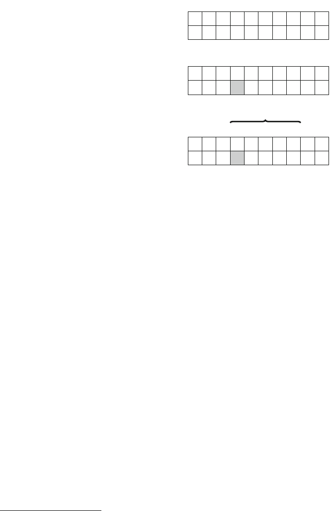
232 14 String Algorithms
Fig. 14.6 The Z-array of
ABCABCABAB ABCABCABAB
–005002020
0123456789
Fig. 14.7 Scenario 1:
Calculating the value of z[3]ABCABCABAB
–00???????
0123456789
ABCABCABAB
–005??????
0123456789
xy
14.3.1 Constructing the Z-Array
Next we describe an algorithm, called the Z-algorithm which efficiently constructs
the Z-array in O(n)time.1The algorithm calculates the Z-array values from left
to right by both using information already stored in the array and by comparing
substrings character by character.
To efficiently calculate the Z-array values, the algorithm maintains a range [x,y]
such that s[x...y]is a prefix of s, the value of z[x]has been determined, and yis
as large as possible. Since we know that s[0...y−x]and s[x...y]are equal, we
can use this information when calculating subsequent array values. Suppose that we
have calculated the values of z[0],z[1],...,z[k−1]and we want to calculate the
value of z[k]. There are three possible scenarios:
Scenario 1:y<k. In this case, we do not have information about the position k,
so we calculate the value of z[k]by comparing substrings character by character.
For example, in Fig. 14.7, there is no [x,y]range yet, so we compare the substrings
starting at positions 0 and 3 character by character. Since z[3]=5, the new [x,y]
range becomes [3,7].
Scenario 2:y≥kand k+z[k−x]≤y. In this case we know that z[k]=z[k−
x], because s[0...y−x]and s[x...y]are equal and we stay inside the [x,y]
range. For example, in Fig. 14.8, we conclude that z[4]=z[1]=0.
Scenario 3:y≥kand k+z[k−x]>y. In this case we know that z[k]≥y−
k+1. However, since we do not have information after the position y,wehaveto
compare substrings character by character starting at positions y−k+1 and y+1.
For example, in Fig. 14.9, we know that z[6]≥2. Then, since s[2] = s[8], it turns
out that, in fact, z[6]=2.
1Gusfield [13] presents the Z-algorithm as the simplest known method for linear-time pattern match-
ing and attributes the original idea to Main and Lorentz [22].
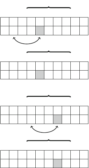
14.3 Z-Algorithm 233
Fig. 14.8 Scenario 2:
Calculating the value of z[4]
ABCABCABAB
–005??????
0123456789
xy
ABCABCABAB
–0050?????
0123456789
xy
Fig. 14.9 Scenario 3:
Calculating the value of z[6]
ABCABCABAB
–00500????
0123456789
xy
ABCABCABAB
–005002???
0123456789
xy
The resulting algorithm works in O(n)time, because always when two characters
match when comparing substrings character by character, the value of yincreases.
Thus, the total work needed for comparing substrings is only O(n).
14.3.2 Applications
The Z-algorithm provides an alternative way to solve many string problems that
can be also solved using hashing. However, unlike hashing, the Z-algorithm always
works and there is no risk of collisions. In practice, it is often a matter of taste whether
to use hashing or the Z-algorithm.
Pattern Matching Consider again the pattern matching problem, where our task is
to find the occurrences of a pattern pin a string s. We already solved the problem
using hashing, but now we will see how the Z-algorithm handles the problem.
A recurrent idea in string processing is to construct a string that consists of multiple
individual parts separated by special characters. In this problem, we can construct a
string p#s, where pand sare separated by a special character #that does not occur
in the strings. Then, the Z-array of p#stells us the positions where poccurs in s,
because such positions contain the length of p.
234 14 String Algorithms
Fig. 14.10 Pattern matching
using the Z-algorithm ABC#ABCABABCA
–000300203001
012345678910 11 12
Fig. 14.11 Finding borders
using the Z-algorithm ABACABACABA
–0107010301
012345678910
Fig. 14.12 The suffix array
of the string ABAACBAB 26037154
01234567
Fig. 14.13 Another way to
represent the suffix array 2
6
0
3
7
1
5
4
AACBAB
AB
ABAACBAB
ACBAB
B
BAACBAB
BAB
CBAB
0
1
2
3
4
5
6
7
Figure 14.10 shows the Z-array for s=ABCABABCA and p=ABC. Positions 4
and 9 contain the value 3, which means that poccurs in positions 0 and 5 in s.
Finding Borders Aborder is a string that is both a prefix and a suffix of a string, but
not the entire string. For example, the borders of ABACABACABA are A,ABA, and
ABACABA. All borders of a string can be efficiently found using the Z-algorithm,
because a suffix at position kis a border exactly when k+z[k]=nwhere nis the
length of the string. For example, in Fig. 14.11,4+z[4]=11, which means that
ABACABA is a border of the string.
14.4 Suffix Arrays
The suffix array of a string describes the lexicographic order of its suffixes. Each
value in the suffix array is a starting position of a suffix. For example, Fig.14.12
shows the suffix array of the string ABAACBAB.
It is often convenient to represent the suffix array vertically and also show the
corresponding suffixes (Fig. 14.13). However, note that the suffix array itself only
contains the starting positions of the suffixes and not their characters.
14.4 Suffix Arrays 235
–––––––– 12113212
initial labels final labels
round 0
length 1
1, 2 2, 1 1, 1 1, 3 3, 2 2, 1 1, 2 2, 0 25136524
initial labels final labels
round 1
length 2
2, 1 5, 3 1, 6 3, 5 6, 2 5, 4 2, 0 4, 0 36148725
initial labels final labels
round 2
length 4
3, 8 6, 7 1, 2 4, 5 8, 0 7, 0 2, 0 5, 0 36148725
initial labels final labels
round 3
len
g
th 8
Fig. 14.14 Constructing the labels for the string ABAACBAB
14.4.1 Prefix Doubling Method
A simple and efficient way to create the suffix array of a string is to use a prefix dou-
bling construction, which works in O(nlog2n)or O(nlog n)time, depending on
the implementation.2The algorithm consists of rounds numbered 0,1,...,log2n,
and round igoes through substrings whose length is 2i. During a round, each sub-
string xof length 2iis given an integer label l(x)such that l(a)=l(b)exactly when
a=band l(a)<l(b)exactly when a<b.
On round 0, each substring consists of only one character, and we can, for example,
use labels A=1,B=2, and so on. Then, on round i, where i>0, we use the labels
for substrings of length 2i−1to construct labels for substrings of length 2i.Togivea
label l(x)for a substring xof length 2i, we divide xinto two halves aand bof length
2i−1whose labels are l(a)and l(b). (If the second half begins outside the string, we
assume that its label is 0.) First, we give xan initial label that is a pair (l(a), l(b)).
Then, after all substrings of length 2ihave been given initial labels, we sort the initial
labels and give final labels that are consecutive integers 1,2,3, etc. The purpose of
giving the labels is that after the last round, each substring has a unique label, and the
labels show the lexicographic order of the substrings. Then, we can easily construct
the suffix array based on the labels.
Figure 14.14 shows the construction of the labels for ABAACBAB. For example,
after round 1, we know that l(AB)=2 and l(AA)=1. Then, on round 2, the initial
label for ABAA is (2,1). Since there are two smaller initial labels ((1,6)and (2,0)),
the final label is l(ABAA)=3. Note that in this example, each label is unique already
2The idea of prefix doubling is due to Karp, Miller, and Rosenberg [17]. There are also more
advanced O(n)time algorithms for constructing suffix arrays; Kärkkäinen and Sanders [16] provide
a quite simple such algorithm.
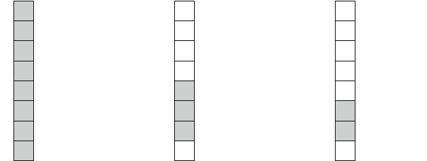
236 14 String Algorithms
2
6
0
3
7
1
5
4
AACBAB
AB
ABAACBAB
ACBAB
B
BAACBAB
BAB
CBAB
0
1
2
3
4
5
6
7
2
6
0
3
7
1
5
4
AACBAB
AB
ABAACBAB
ACBAB
B
BAACBAB
BAB
CBAB
0
1
2
3
4
5
6
7
2
6
0
3
7
1
5
4
AACBAB
AB
ABAACBAB
ACBAB
B
BA ACBAB
BAB
CBAB
0
1
2
3
4
5
6
7
Fig. 14.15 Finding the occurrences of BA in ABAACBAB using a suffix array
after round 2, because the first four characters of the substrings completely determine
their lexicographical order.
The resulting algorithm works in O(nlog2n)time, because there are O(log n)
rounds and we sort a list of npairs on each round. In fact, an O(nlog n)implemen-
tation is also possible, because we can use a linear-time sorting algorithm to sort the
pairs. Still, a straightforward O(nlog2n)time implementation just using the C++
sort function is usually efficient enough.
14.4.2 Finding Patterns
After constructing the suffix array, we can efficiently find the occurrences of any
given pattern in the string. This can be done in O(klog n)time, where nis the length
of the string and kis the length of the pattern. The idea is to process the pattern
character by character and maintain a range in the suffix array that corresponds to
the prefix of the pattern processed so far. Using binary search, we can efficiently
update the range after each new character.
For example, consider finding the occurrences of the pattern BA in the string
ABAACBAB (Fig. 14.15). First, our search range is [0,7], which spans the entire
suffix array. Then, after processing the character B, the range becomes [4,6]. Finally,
after processing the character A, the range becomes [5,6]. Thus, we conclude that
BA has two occurrences in ABAACBAB in positions 1 and 5.
Compared to string hashing and the Z-algorithm discussed earlier, the advantage
of the suffix array is that we can efficiently process several queries that are related
to different patterns, and it is not necessary to know the patterns beforehand when
constructing the suffix array.
14.4.3 LCP Arrays
The LCP array of a string gives for its each suffix a LCP value: the length of the
longest common prefix of the suffix and the next suffix in the suffix array. Figure 14.16
14.4 Suffix Arrays 237
Fig. 14.16 The LCP array
of the string ABAACBAB 1
2
1
0
1
2
0
–
AACBAB
AB
ABAACBAB
ACBAB
B
BAACBAB
BAB
CBAB
0
1
2
3
4
5
6
7
shows the LCP array for the string ABAACBAB. For example, the LCP value of the
suffix BAACBAB is 2, because the longest common prefix of BAACBAB and BAB is
BA. Note that the last suffix in the suffix array does not have a LCP value.
Next we present an efficient algorithm, due to Kasai et al. [18], for constructing
the LCP array of a string, provided that we have already constructed its suffix array.
The algorithm is based on the following observation: Consider a suffix whose LCP
value is x. If we remove the first character from the suffix and get another suffix,
we immediately know that its LCP value has to be at least x−1. For example, in
Fig. 14.16, the LCP value of the suffix BAACBAB is 2, so we know that the LCP
value of the suffix AACBAB has to be at least 1. In fact, it happens to be exactly 1.
We can use the above observation to efficiently construct the LCP array by calcu-
lating the LCP values in decreasing order of suffix length. At each suffix, we calculate
its LCP value by comparing the suffix and the next suffix in the suffix array character
by character. Now we can use the fact that we know the LCP value of the suffix
that has one more character. Thus, the current LCP value has to be at least x−1,
where xis the previous LCP value, and we do not need to compare the first x−1
characters of the suffixes. The resulting algorithm works in O(n)time, because only
O(n)comparisons are done during the algorithm.
Using the LCP array, we can efficiently solve some advanced string problems.
For example, to calculate the number of distinct substrings in a string, we can simply
subtract the sum of all values in the LCP array from the total number of substrings,
i.e., the answer to the problem is
n(n+1)
2−c,
where nis the length of the string and cis the sum of all values in the LCP array.
For example, the string ABAACBAB has
8·9
2−7=29
distinct substrings.
Additional Topics
This final chapter presents a selection of advanced algorithms and data structures.
Mastering the techniques of this chapter may sometimes help you to solve the most
difficult problem in a programming contest.
Section 15.1 discusses square root techniques for creating data structures and
algorithms. Such solutions are often based on the idea of dividing a sequence of n
elements into O(√n)blocks, each of which consists of O(√n)elements.
Section 15.2 further explores the possibilities of segment trees. For example, we
will see how to create a segment tree that supports both range queries and range
updates at the same time.
Section 15.3 presents the treap data structure which allows us to efficiently split
an array into two parts and combine two arrays into a single array.
Section 15.4 focuses on optimizing dynamic programming solutions. First we will
learn the convex hull trick which is used with linear functions, and after this we will
discuss the divide and conquer optimization and Knuth’s optimization.
Section 15.5 deals with miscellaneous algorithm design techniques, such as meet
in the middle and parallel binary search.
15.1 Square Root Techniques
A square root can be seen as a “poor man’s logarithm”: the complexity O(√n)is
better than O(n)but worse than O(log n). In any case, many data structures and
algorithms involving square roots are fast and usable in practice. This section shows
some examples of how square roots can be used in algorithm design.
240 15 Additional Topics
15.1.1 Data Structures
Sometimes we can create an efficient data structure by dividing an array into blocks
of size √nand maintaining information about array values inside each block. For
example, suppose that we should process two types of queries: modifying array values
and finding minimum values in ranges. We have previously seen that a segment tree
can support both operations in O(log n)time, but next we will solve the problem in
another simpler way where the operations take O(√n)time.
We divide the array into blocks of √nelements, and maintain for each block the
minimum value inside it. For example, Fig. 15.1 shows an array of 16 elements that
is divided into blocks of 4 elements. When an array value changes, the corresponding
block needs to be updated. This can be done in O(√n)time by going through the
values inside the block, as shown in Fig.15.2. Then, to calculate the minimum value
in a range, we divide the range into three parts such that the range consists of single
values and blocks between them. Figure 15.3 shows an example of such a division.
The answer to the query is either a single value or the minimum value inside a block.
Since the number of single elements is O(√n)and the number of blocks is also
O(√n), the query takes O(√n)time.
How efficient is the resulting structure in practice? To find this out, we conducted
an experiment where we created an array of nrandom int values and then processed
nrandom minimum queries. We implemented three data structures: a segment tree
with O(log n)time queries, the square root structure described above with O(√n)
time queries, and a plain array with O(n)time queries. Table 15.1 shows the results
of the experiment. It turns out that in this problem, the square root structure is quite
efficient up to n=218; however, after this, it requires clearly more time than a
segment tree.
5863472671756232
3212
Fig. 15.1 A square root structure for finding minimum values in ranges
5863475671756232
3412
Fig. 15.2 When an array value is updated, the value in the corresponding block has to be also
updated
5863472671756232
3212
Fig. 15.3 To determine the minimum value in a range, the range is divided into single values and
blocks
15.1 Square Root Techniques 241
Table 15.1 The running times of three data structures for range minimum queries: a segment tree
(O(log n)), a square root structure (O(√n)), and a plain array (O(n))
Input size n O(log n)Queries (s) O(√n)Queries (s) O(n)Queries (s)
216 0.02 0.05 1.50
217 0.03 0.16 6.02
218 0.07 0.28 24.82
219 0.14 1.14 >60
220 0.31 2.11 >60
221 0.66 9.27 >60
Fig. 15.4 An instance of the
letter distance problem ACEA
BDFD
EABC
CFEA
15.1.2 Subalgorithms
Next we discuss two problems that can be efficiently solved by creating two subal-
gorithms that are specialized for different kinds of situations during the algorithm.
While either of the subalgorithms could be used to solve the problem without the
other, we get an efficient algorithm by combining them.
Letter Distances Our first problem is as follows: We are given an n×ngrid whose
each square is assigned a letter. What is the minimum Manhattan distance between
two squares that have the same letter? For example, in Fig. 15.4 the minimum distance
is 2 between the two squares with letter “D.”
To solve the problem, we can go through all letters that appear in the grid, and
for each letter c, determine the minimum distance between two squares with letter
c. Consider two algorithms for processing a fixed letter c:
Algorithm 1: Go through all pairs of squares that contain the letter cand determine
the minimum distance pair among them. This algorithm works in O(k2)time, where
kis the number of squares with letter c.
Algorithm 2: Perform a breadth-first search that simultaneously begins at each
square with letter c. The search takes O(n2)time.
Both algorithms have certain worst-case situations. The worst case for Algorithm
1 is a grid where each square has the same color, in which case k=n2and the
algorithm takes O(n4)time. Then, the worst case for Algorithm 2 is a grid where
each square has a distinct color. In this case, the algorithm is performed O(n2)times,
which takes O(n4)time.
242 15 Additional Topics
Fig. 15.5 A turn in the black
squares game. The minimum
distance from Xto a black
square is 3
X
However, we can combine the algorithms so that they function as subalgorithms of
a single algorithm. The idea is to decide for each color cseparately which algorithm
to use. Clearly, Algorithm 1 works well if kis small, and Algorithm 2 is best suited
for cases where kis large. Thus, we can fix a constant xand use Algorithm 1 if kis
at most x, and otherwise use Algorithm 2.
In particular, by choosing x=√n2=n, we get an algorithm that works in O(n3)
time. First, each square that is processed using Algorithm 1 is compared with at most
nother squares, so processing those squares takes O(n3)time. Then, since there are
at most ncolors that appear in more than nsquares, Algorithm 2 is performed at
most ntimes, and its total running time is also O(n3).
Black Squares As another example, consider the following game: We are given an
n×ngrid where exactly one square is black and all other squares are white. On each
turn, one white square is chosen, and we should calculate the minimum Manhattan
distance between this square and a black square. After this, the white square is
painted black. This process continues for n2−1 turns, after which all squares have
been painted black.
For example, Fig. 15.5 shows a turn in the game. The minimum distance from the
chosen square Xto a black square is 3 (by going two steps down and one step right).
After this, the square is painted black.
We can solve the problem by processing the turns in batches of kturns. Before
each batch, we calculate for each square of the grid the minimum distance to a
black square. This can be done in O(n2)time using breadth-first search. Then,
when processing a batch, we keep a list of all squares that have been painted black
during the current batch. Thus, the minimum distance to a black square is either the
precalculated distance or a distance to one of the squares on the list. Since the list
contains at most kvalues, it takes O(k)time to go through the list.
Then, by choosing k=√n2=n, we get an algorithm that works in O(n3)time.
First, there are O(n)batches, so the total time used for breadth-first searches is O(n3).
Then, the list of squares in a batch contains O(n)values, so calculating minimum
distances for O(n2)squares also takes O(n3)time.
Tuning Parameters In practice, it is not necessary to use the exact square root
value as the parameter, but rather we can fine-tune the performance of an algorithm
by experimenting with different parameters and choosing the parameter that works
best. Of course, the optimal parameter depends on the algorithm and also on the
properties of the test data.
15.1 Square Root Techniques 243
Table 15.2 Optimizing the value of the parameter kin the black squares algorithm
Parameter kRunning time (s)
200 5.74
500 2.41
1000 1.32
2000 1.02
5000 1.28
10000 2.13
20000 3.97
Fig. 15.6 Some integer
partitions of a stick of
length 7
7
34
131 2
Table 15.2 shows the results of an experiment where the O(n3)time algorithm for
the black squares game was performed for different values of kwhen n=500. The
order in which the squares were painted black was randomly selected. In this case,
the optimal parameter seems to be about k=2000.
15.1.3 Integer Partitions
Suppose that there is a stick whose length is n, and it is divided into some parts
whose lengths are integers. For example, Fig.15.6 shows some possible partitions
for n=7. What is the maximum number of distinct lengths in such a partition?
It turns out that there are at most O(√n)distinct lengths. Namely an optimal
way to produce as many distinct lengths as possible is to include lengths 1,2,...,k.
Then, since
1+2+···+k=k(k+1)
2,
we can conclude that kcan be at most O(√n). Next, we will see how this observation
can be used when designing algorithms.
Knapsack Problem Consider a knapsack problem where we are given a list of
integer weights [w1,w2,...,wk]such that w1+w2+···+wk=n, and our task
is to determine all possible weight sums that can be created. For example, Fig. 15.7
shows the possible sums using the weights [3,3,4].
244 15 Additional Topics
Fig. 15.7 The possible sums
using the weights [3,3,4]
012345678910
Using a standard knapsack algorithm (Sect. 6.2.3), we can solve the problem in
O(nk)time, so if k=O(n), the time complexity becomes O(n2). However, since
there are at most O(√n)distinct weights, we can actually solve the problem more
efficiently by simultaneously processing all weights of a certain value. For example,
if the weights are [3,3,4], we first process the two weights of value 3 and then the
weight of value 4. It is not difficult to modify the standard knapsack algorithm so
that processing each group of equal weights only takes O(n)time, which yields an
O(n√n)time algorithm.
String Construction As another example, suppose that we are given a string of
length nand a dictionary of words whose total length is m. Our task is to count the
number of ways we can construct the string using the words. For example, there are
four ways to construct the string ABAB using the words {A,B,AB}:
•A+B+A+B
•AB +A+B
•A+B+AB
•AB +AB
Using dynamic programming, we can calculate for each k=0,1,...,nthe num-
ber of ways to construct a prefix of length kof the string. One way to do this is to
use a trie that contains reverses of all the words in the dictionary, which yields an
O(n2+m)time algorithm. However, another approach is to use string hashing and
the fact that there are at most O(√m)distinct word lengths. Thus, we can restrict
ourselves to word lengths that actually exist. This can be done by creating a set that
contains all hash values of words, which results in an algorithm whose running time
is O(n√m+m)(using unordered_set).
15.1.4 Mo’s Algorithm
Mo’s algorithm1processes a set of range queries on a static array (i.e., the array values
do not change between the queries). Each query requires us to calculate something
based on the array values in a range [a,b]. Since the array is static, the queries can
be processed in any order, and the trick in Mo’s algorithm is to use a special order
which guarantees that the algorithm works efficiently.
The algorithm maintains an active range in the array, and the answer to a query
concerning the active range is known at each moment. The algorithm processes the
1According to [5], Mo’s algorithm is named after Mo Tao, a Chinese competitive programmer.
15.1 Square Root Techniques 245
Fig. 15.8 Moving between
two ranges in Mo’s
algorithm
425424334
425424334
queries one by one and always moves the endpoints of the active range by inserting
and removing elements. The array is divided into blocks of k=O(√n)elements,
and a query [a1,b1]is always processed before a query [a2,b2]if
•a1/k<a2/kor
•a1/k=a2/kand b1<b2.
Thus, all queries whose left endpoints are in a certain block are processed one after
another sorted according to their right endpoints. Using this order, the algorithm only
performs O(n√n)operations, because the left endpoint moves O(n)times O(√n)
steps, and the right endpoint moves O(√n)times O(n)steps. Thus, both endpoints
move a total of O(n√n)steps during the algorithm.
Example Consider a problem where we are given a set of array ranges, and we are
asked to calculate the number of distinct values in each range. In Mo’s algorithm,
the queries are always sorted in the same way, but the way the answer to the query
is maintained depends on the problem.
To solve the problem, we maintain an array count where count[x]indicates
the number of times an element xoccurs in the active range. When we move from
one query to another query, the active range changes. For example, consider the two
ranges in Fig. 15.8. When we move from the first range to the second range, there will
be three steps: the left endpoint moves one step to the right, and the right endpoint
moves two steps to the right.
After each step, the array count needs to be updated. After adding an element
x, we increase the value of count[x]by 1, and if count[x]=1 after this, we
also increase the answer to the query by 1. Similarly, after removing an element
x, we decrease the value of count[x]by 1, and if count[x]=0 after this, we
also decrease the answer to the query by 1. Since each step requires O(1)time, the
algorithm works in O(n√n)time.
15.2 Segment Trees Revisited
A segment tree is a versatile data structure that can be used to solve a large number
of problems. However, so far we have only seen a small part of the possibilities of
segment trees. Now is time to discuss some more advanced variants of segment trees
that allow us to solve more advanced problems.

246 15 Additional Topics
Until now, we have implemented the operations of a segment tree by walking
from bottom to top in the tree. For example, we have used the following function
(Sect. 9.2.2) to calculate the sum of values in a range [a,b]:
int sum(int a, int b) {
a+=n;b+=n;
int s=0;
while (a <= b) {
if (a%2 == 1) s += tree[a++];
if (b%2 == 0) s += tree[b--];
a/=2;b/=2;
}
return s;
}
However, in advanced segment trees, it is often necessary to implement the oper-
ations from top to bottom as follows:
int sum(int a, int b, int k, int x, int y) {
if (b<x||a>y)return 0;
if (a<=x&&y<=b)return tree[k];
int d = (x+y)/2;
return sum(a,b,2*k,x,d) + sum(a,b,2*k+1,d+1,y);
}
Using this function, we can calculate the sum in a range [a,b]as follows:
int s = sum(a,b,1,0,n-1);
The parameter kindicates the current position in tree. Initially kequals 1,
because we begin at the root of the tree. The range [x,y]corresponds to kand is
initially [0,n−1]. When calculating the sum, if [x,y]is outside [a,b], the sum is
0, and if [x,y]is completely inside [a,b], the sum can be found in tree.If[x,y]
is partially inside [a,b], the search continues recursively to the left and right half of
[x,y]. The left half is [x,d], and the right half is [d+1,y], where d=x+y
2.
Figure 15.9 shows how the search proceeds when calculating the value of
sumq(a,b). The gray nodes indicate nodes where the recursion stops and the sum
can be found in tree. Also in this implementation, operations take O(log n)time,
because the total number of visited nodes is O(log n).
15.2.1 Lazy Propagation
Using lazy propagation, we can build a segment tree that supports both range updates
and range queries in O(log n)time. The idea is to perform updates and queries from
top to bottom and perform updates lazily so that they are propagated down the tree
only when it is necessary.

15.2 Segment Trees Revisited 247
5863272671756232
13 9 9 8 8 12 8 5
22 17 20 13
39 33
72
ab
Fig. 15.9 Traversing a segment tree from top to bottom
5863272671756232
13/0 9/0 9/0 8/0 8/0 12/0 8/0 5/0
22/0 17/0 20/0 13/0
39/0 33/0
72/0
Fig. 15.10 A lazy segment tree for range updates and queries
The nodes of a lazy segment tree contain two types of information. Like in an
ordinary segment tree, each node contains the sum, minimum value, or some other
value related to the corresponding subarray. In addition, a node may contain informa-
tion about a lazy update which has not been propagated to its children. Lazy segment
trees can support two types of range updates: each array value in the range is either
increased by some value or assigned some value. Both operations can be imple-
mented using similar ideas, and it is even possible to construct a tree that supports
both operations at the same time.
Let us consider an example where our goal is to construct a segment tree that
supports two operations: increasing each value in [a,b]by a constant and calculating
the sum of values in [a,b]. To achieve this goal, we construct a tree where each node
has two values s/z:sdenotes the sum of values in the range, and zdenotes the value
of a lazy update, which means that all values in the range should be increased by z.
Figure 15.10 shows an example of such a tree, where z=0 in all nodes, meaning
that there are no ongoing lazy updates.
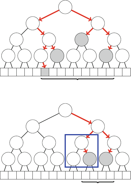
248 15 Additional Topics
5863292671756232
13/0 9/0 11/0 8/2 8/0 12/0 8/2 5/0
22/0 23/0 20/2 17/0
45/0 45/0
90/0
ab
Fig. 15.11 Increasing the values in the range [a,b]by 2
5863292671756232
13/0 9/0 11/0 8/2 8/2 12/2 8/2 5/0
22/0 23/0 28/0 17/0
45/0 45/0
90/0
ab
Fig. 15.12 Calculating the sum of values in the range [a,b]
We implement the tree operations from top to bottom. To increase the values in
a range [a,b]by u, we modify the nodes as follows: If the range [x,y]of a node is
completely inside [a,b], we increase the zvalue of the node by uand stop. Then, if
[x,y]partially belongs to [a,b], we continue our walk recursively in the tree, and
after this calculate the new svalue for the node. As an example, Fig. 15.11 shows
our tree after increasing the range [a,b]by 2.
In both updates and queries, lazy updates are propagated downwards when we
move in the tree. Always before accessing a node, we check if it has an ongoing
lazy update. If it has, we update its svalue, propagate the update to its children, and
then clear its zvalue. For example, Fig. 15.12 shows how our tree changes when we
calculate the value of suma(a,b). The rectangle contains the nodes whose values
change when a lazy update is propagated downwards.
15.2 Segment Trees Revisited 249
Polynomial Updates We can generalize the above segment tree so that it is possible
to update ranges using polynomials of the form
p(u)=tkuk+tk−1uk−1+···+t0.
In this case, the update for a value at position iin [a,b]is p(i−a). For example,
adding the polynomial p(u)=u+1to[a,b]means that the value at position a
increases by 1, the value at position a+1 increases by 2, and so on.
To support polynomial updates, each node is assigned k+2 values, where kequals
the degree of the polynomial. The value sis the sum of the elements in the range,
and the values z0,z1,...,zkare the coefficients of a polynomial that corresponds to
a lazy update. Now, the sum of values in a range [x,y]equals
s+
y−x
u=0
(zkuk+zk−1uk−1+···+z1u+z0),
and the value of such a sum can be efficiently calculated using sum formulas. For
example, the term z0corresponds to the sum z0(y−x+1), and the term z1ucorre-
sponds to the sum
z1(0+1+···+y−x)=z1
(y−x)(y−x+1)
2.
When propagating an update in the tree, the indices of p(u)change, because in
each range [x,y], the values are calculated for u=0,1,...,y−x. However, we
can easily handle this, because p(u)=p(u+h)is a polynomial of equal degree as
p(u). For example, if p(u)=t2u2+t1u+t0, then
p(u)=t2(u+h)2+t1(u+h)+t0=t2u2+(2ht2+t1)u+t2h2+t1h+t0.
15.2.2 Dynamic Trees
An ordinary segment tree is static, which means that each node has a fixed position
in the segment tree array and the structure requires a fixed amount of memory. In a
dynamic segment tree, memory is allocated only for nodes that are actually accessed
during the algorithm, which can save a large amount of memory.
The nodes of a dynamic tree can be represented as structs:
struct node {
int value;
int x, y;
node *left, *right;
node(int v, int x, int y) : value(v), x(x), y(y) {}
};
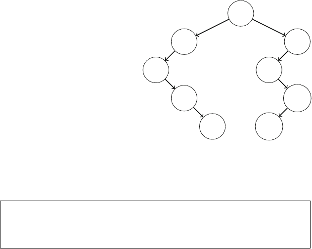
250 15 Additional Topics
Fig. 15.13 Asparse
segment tree where the
elements at positions 3 and
10 have been modified
[0,15]
[0,7]
[0,3]
[2,3]
[3,3]
[8,15]
[8,11]
[10,11]
[10,10]
Here value is the value of the node, [x,y]is the corresponding range, and left
and right point to the left and right subtree. Nodes can be created as follows:
// create a node with value 2 and range [0,7]
node *x = new node(2,0,7);
// change value
x->value = 5;
Sparse Segment Trees A dynamic segment tree is a useful structure when the under-
lying array is sparse, i.e., the range [0,n−1]of allowed indices is large, but most
array values are zeros. While an ordinary segment tree would use O(n)memory,
a dynamic segment tree only uses O(klog n)memory, where kis the number of
operations performed.
Asparse segment tree initially has only one node [0,n−1]whose value is zero,
which means that every array value is zero. After updates, new nodes are dynamically
added to the tree. Any path from the root node to a leaf contains O(log n)nodes, so
each segment tree operation adds at most O(log n)new nodes to the tree. Thus, after
koperations, the tree contains O(klog n)nodes. For example, Fig.15.13 shows a
sparse segment tree where n=16, and the elements at positions 3 and 10 have been
modified.
Note that if we know all elements that will be updated during the algorithm
beforehand, a dynamic segment tree is not necessary, because we can use an ordinary
segment tree with index compression (Sect. 9.2.3). However, this is not possible when
the indices are generated during the algorithm.
Persistent Segment Trees Using a dynamic implementation, we can also create a
persistent segment tree that stores the modification history of the tree. In such an
implementation, we can efficiently access all versions of the tree that have existed
during the algorithm. When the modification history is available, we can perform
queries in any previous tree like in an ordinary segment tree, because the full structure
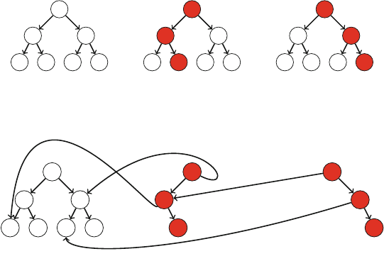
15.2 Segment Trees Revisited 251
step 1 step 2 step 3
Fig. 15.14 A modification history of a segment tree: the initial tree and two updates
step 1 step 2 step 3
Fig. 15.15 A compact way to store the modification history
of each tree is stored. We can also create new trees based on previous trees and modify
them independently.
Consider the sequence of updates in Fig. 15.14, where marked nodes change and
other nodes remain the same. After each update, most nodes of the tree remain the
same, so a compact way to store the modification history is to represent each historical
tree as a combination of new nodes and subtrees of previous trees. Figure 15.15 shows
how the modification history can be stored. The structure of each previous tree can
be reconstructed by following the pointers starting at the corresponding root node.
Since each operation adds only O(log n)new nodes to the tree, it is possible to store
the full modification history of the tree.
15.2.3 Data Structures in Nodes
Instead of single values, the nodes of a segment tree can also contain data structures
that maintain information about the corresponding ranges. As an example, suppose
that we should be able to efficiently count the number of occurrences of an element
xin a range [a,b]. To do this, we can create a segment tree where each node is
assigned a data structure that can be asked how many times any element xappears
in the corresponding range. After this, the answer to a query can be calculated by
combining the results from nodes that belong to the range.
The remaining task is to choose a suitable data structure for the problem. A good
choice is a map structure whose keys are array elements and values indicate how
many times each element occurs in a range. Figure15.16 shows an array and the
corresponding segment tree. For example, the root node of the tree tells us that
element 1 appears 4 times in the array.
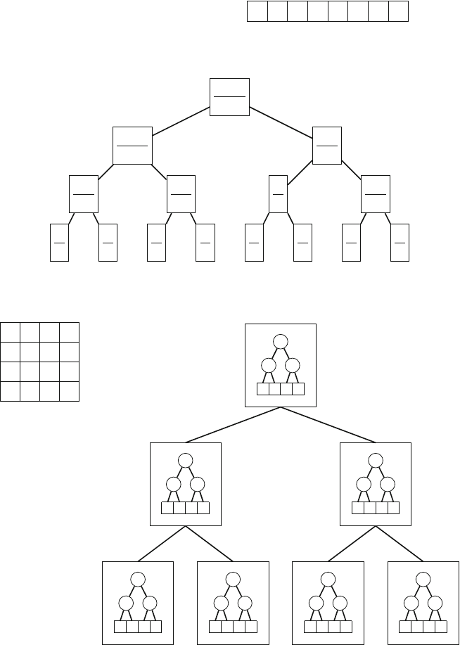
252 15 Additional Topics
31231112
3
1
1
1
2
1
3
1
1
1
1
1
1
1
2
1
13
11
23
11
1
2
12
11
123
112
12
31
123
422
Fig. 15.16 A segment tree for calculating the number of occurrences of an element in an array
range
7
6
1
6
8
7
5
2
3
9
7
1
8
5
3
8
7616
13 7
20
8752
15 7
22
3971
12 8
20
8538
13 11
24
15 13 6 8
28 14
42
11 14 10 9
25 19
44
26 27 16 17
53 33
86
Fig. 15.17 A two-dimensional array and the corresponding segment tree for calculating sums of
rectangular subarrays

15.2 Segment Trees Revisited 253
Each query in the above segment tree works in O(log2n)time, because each node
has a map structure whose operations take O(log n)time. The tree uses O(nlog n)
memory, because it has O(log n)levels, and each level contains nelements that have
been distributed in the map structures.
15.2.4 Two-Dimensional Trees
Atwo-dimensional segment tree allows us to process queries related to rectangular
subarrays on a two-dimensional array. The idea is to create a segment tree that
corresponds to the columns of the array and then assign each node of this structure
a segment tree that corresponds to the rows of the array.
For example, Fig. 15.17 shows a two-dimensional segment tree that supports two
queries: calculating the sum of values in a subarray and updating a single array value.
Both the queries take O(log2n)time, because O(log n)nodes in the main segment
tree are accessed, and processing each node takes O(log n)time. The structure uses
a total of O(n2)memory, because the main segment tree has O(n)nodes, and each
node has a segment tree of O(n)nodes.
15.3 Treaps
Atreap is a binary tree that can store the contents of an array in such a way that we
can efficiently split an array into two arrays and merge two arrays into an array. Each
node in a treap has two values: a weight and a value. Each node’s weight is smaller
or equal than the weights of its children, and the node is located in the array after all
nodes in its left subtree and before all nodes in its right subtree.
Figure 15.18 shows an example of an array and the corresponding treap. For
example, the root node has weight 1 and value D. Since its left subtree contains three
nodes, this means that the array element at position 3 has value D.
15.3.1 Splitting and Merging
When a new node is added to the treap, it is assigned a random weight. This guar-
antees that the tree is balanced (its height is O(log n)) with high probability, and its
operations can be performed efficiently.
Splitting The splitting operation of a treap creates two treaps which divide the array
into two arrays so that the first kelements belong to the first array and the rest of
the elements belong to the second array. To do this, we create two new treaps that
are initially empty and traverse the original treap starting at the root node. At each
254 15 Additional Topics
Fig. 15.18 An array and the
corresponding treap SANDWICH
01234567
9S
3A
6N
1D
8W
9I
4C
5H
Fig. 15.19 Splitting an array
into two arrays SANDWICH
01234012
9S
3A
6N
1D
8W9I
4C
5H
step, if the current node belongs to the left treap, the node and its left subtree are
added to the left treap and we recursively process its right subtree. Similarly, if the
current node belongs to the right treap, the node and its right subtree are added to the
right treap and we recursively process its left subtree. Since the height of the treap
is O(log n), this operation works in O(log n)time.
For example, Fig. 15.19 shows how to divide our example array into two arrays so
that the first array contains the first five elements of the original array and the second
array contains the last three elements. First, node D belongs to the left treap, so we
add node D and its left subtree to the left treap. Then, node C belongs to the right
treap, and we add node C and its right subtree to the right treap. Finally, we add node
W to the left treap and node I to the right treap.
Merging The merging operation of two treaps creates a single treap that concatenates
the arrays. The two treaps are processed simultaneously, and at each step, the treap
whose root has the smallest weight is selected. If the root of the left treap has the
smallest weight, the root and its left subtree are moved to the new treap and its right
subtree becomes the new root of the left treap. Similarly, if the root of the right treap
15.3 Treaps 255
Fig. 15.20 Merging two
arrays into an array, before
merging
ICH SA
NDW
012 01234
9S
3A
6N
1D
8W
9I
4C
5H
Fig. 15.21 Merging two
arrays into an array, after
merging
I CHSANDW
01234567
9S
3A
6N
1D
8W
9I
4C
5H
has the smallest weight, the root and its right subtree are moved to the new treap and
its left subtree becomes the new root of the right treap. Since the height of the treap
is O(log n), this operation works in O(log n)time.
For example, we may now swap the order of the two arrays in our example scenario
and then concatenate the arrays again. Figure 15.20 shows the arrays before merging,
and Fig. 15.21 shows the final result. First, node D and its right subtree is added to
the new treap. Then, node A and its right subtree become the left subtree of node
D. After this, node C and its left subtree become the left subtree of node A. Finally,
node H and node S are added to the new treap.
15.3.2 Implementation
Next we will learn a convenient way to implement a treap. First, here is a struct that
stores a treap node:

256 15 Additional Topics
struct node {
node *left, *right;
int weight, size, value;
node(int v) {
left = right = NULL;
weight = rand();
size = 1;
value = v;
}
};
The field size contains the size of the subtree of the node. Since a node can be
NULL, the following function is useful:
int size(node *treap) {
if (treap == NULL) return 0;
return treap->size;
}
The following function split implements the splitting operation. The function
recursively splits the treap treap into treaps left and right so that the left treap
contains the first knodes and the right treap contains the remaining nodes.
void split(node *treap, node *&left, node *&right, int k) {
if (treap == NULL) {
left = right = NULL;
}else {
if (size(treap->left) < k) {
split(treap->right, treap->right, right,
k-size(treap->left)-1);
left = treap;
}else {
split(treap->left, left, treap->left, k);
right = treap;
}
treap->size = size(treap->left)+size(treap->right)+1;
}
}
Then, the following function merge implements the merging operation. This
function creates a treap treap that contains first the nodes of the treap left and
then the nodes of the treap right.

15.3 Treaps 257
void merge(node *&treap, node *left, node *right) {
if (left == NULL) treap = right;
else if(right == NULL) treap = left;
else {
if (left->weight < right->weight) {
merge(left->right, left->right, right);
treap = left;
}else {
merge(right->left, left, right->left);
treap = right;
}
treap->size = size(treap->left)+size(treap->right)+1;
}
}
For example, the following code creates a treap that corresponds to the array
[1,2,3,4]. Then it divides it into two treaps of size 2 and swaps their order to create
a new treap that corresponds to the array [3,4,1,2].
node *treap = NULL;
merge(treap, treap, new node(1));
merge(treap, treap, new node(2));
merge(treap, treap, new node(3));
merge(treap, treap, new node(4));
node *left, *right;
split(treap, left, right, 2);
merge(treap, right, left);
15.3.3 Additional Techniques
The splitting and merging operations of treaps are very powerful, because we can
freely “cut and paste” arrays in logarithmic time using them. Treaps can be also
extended so that they work almost like segment trees. For example, in addition to
maintaining the size of each subtree, we can also maintain the sum of its values, the
minimum value, and so on.
One special trick related to treaps is that we can efficiently reverse an array. This
can be done by swapping the left and right child of each node in the treap. For
example, Fig. 15.22 shows the result after reversing the array in Fig. 15.18.Todo
this efficiently, we can introduce a field that indicates if we should reverse the subtree
of the node, and process swapping operations lazily.
258 15 Additional Topics
Fig. 15.22 Reversing an
array using a treap HC IWDNAS
01234567
9S
3A
6N
1D
8W
9I
4C
5H
Fig. 15.23 The minimum
function value at point x=4
is f2(4)=16/3
f
1
f
2
f
3
f
4
x=4
15.4 Dynamic Programming Optimization
This section discusses techniques for optimizing dynamic programming solutions.
First, we focus on the convex hull trick, which can be used to efficiently find minimum
values of linear functions. After this, we discuss two other techniques that are based
on properties of cost functions.
15.4.1 Convex Hull Trick
The convex hull trick allows us to efficiently find the minimum function value at a
given point xamong a set of nlinear functions of the form f(x)=ax +b. For exam-
ple, Fig. 15.23 shows functions f1(x)=x+2, f2(x)=x/3+4, f3(x)=x/6+5,
and f4(x)=−x/4+7. The minimum value at point x=4is f2(4)=16/3.
The idea is to divide the x-axis into ranges where a certain function has the
minimum value. It turns out that each function will have at most one range, and we
can store the ranges in a sorted list that will contain at most nranges. For example,
15.4 Dynamic Programming Optimization 259
Fig. 15.24 The ranges
where f1,f2,and f4have
the minimum value
f
1
f
2
f
3
f
4
f1f2f4
Fig. 15.24 shows the ranges in our example scenario. First, f1has the minimum
value, then f2has the minimum value, and finally f4has the minimum value. Note
that f3never has the minimum value.
Given a list of ranges, we can find the minimum function value at point xin
O(log n)time using binary search. For example, since point x=4 belongs to the
range of f2in Fig. 15.24, we immediately know that the minimum function value at
point x=4is f2(4)=16/3. Thus, we can process a set of kqueries in O(klog n)
time. Moreover, if the queries are given in increasing order, we can process them in
O(k)time by just iterating through the ranges from left to right.
Then, how to determine the ranges? If the functions are given in decreasing order
of their slopes, we can easily find the ranges, because we can maintain a stack that
contains the ranges, and the amortized cost for processing each function is O(1).If
the functions are given in an arbitrary order, we need to use a more sophisticated set
structure and processing each function takes O(log n)time.
Example Suppose that there are nconsecutive concerts. The ticket for concert i
costs pieuros, and if we attend the concert, we get a discount coupon whose value
is di(0 <di<1). We can later use the coupon to buy a ticket for dipeuros where
pis the original price. It is also known that di≥di+1for all consecutive concerts i
and i+1. We definitely want to attend the last concert, and we can also attend other
concerts. What is the minimum total price for this?
We can easily solve the problem using dynamic programming by calculating for
each concert ia value ui: the minimum price for attending concert iand possibly
some previous concerts. A simple way to find the optimal choice for the previous
concert is to go through all previous concerts in O(n)time, which results in an O(n2)
time algorithm. However, we can use the convex hull trick to find the optimal choice
in O(log n)time and get an O(nlog n)time algorithm.
The idea is to maintain a set of linear functions, which initially only contains the
function f(x)=x, which means that we do not have a discount coupon. To calculate
the value uifor a concert, we find a function fin our set that minimizes the value of
f(pi), which can be done in O(log n)time using the convex hull trick. Then, we add
a function f(x)=dix+uito our set, and we can use it to attend another concert
later. The resulting algorithm works in O(nlog n)time.
260 15 Additional Topics
Fig. 15.25 An optimal way
to divide a sequence into
three blocks 23122341
12345678
Note that if it is additionally known that pi≤pi+1for all consecutive concerts
iand i+1, we can solve the problem more efficiently in O(n)time, because we
can process the ranges from left to right and find each optimal choice in amortized
constant time instead of using binary search.
15.4.2 Divide and Conquer Optimization
The divide and conquer optimization can be applied to certain dynamic programming
problems where a sequence s1,s2,...,snof nelements has to be divided into k
subsequences of consecutive elements. A cost function cost(a,b)is given, which
determines the cost of creating a subsequence sa,sa+1,...,sb. The total cost of a
division is the sum of the individual costs of the subsequences, and our task is to find
a division that minimizes the total cost.
As an example, suppose that we have a sequence of positive integers and
cost(a,b)=(sa+sa+1+···+sb)2. Figure 15.25 shows an optimal way to divide
a sequence into three subsequences using this cost function. The total cost of the divi-
sion is (2+3+1)2+(2+2+3)2+(4+1)2=110.
We can solve the problem by defining a function solve(i,j)which gives the
minimum total cost of dividing the first ielements s1,s2,...,siinto jsubsequences.
Clearly, solve(n,k)equals the answer to the problem. To calculate a value of
solve(i,j), we have to find a position 1 ≤p≤ithat minimizes the value of
solve(p−1,j−1)+cost(p,i).
For example, in Fig. 15.25, an optimal choice for solve(8,3)is p=7. A simple
way to find an optimal position is to check all positions 1,2,...,i, which takes
O(n)time. By calculating all values of solve(i,j)like this, we get a dynamic
programming algorithm that works in O(n2k)time. However, using the divide and
conquer optimization, we can improve the time complexity to O(nk log n).
The divide and conquer optimization can be used if the cost function satisfies the
quadrangle inequality
cost(a,c)+cost(b,d)≤cost(a,d)+cost(b,c)
for all a≤b≤c≤d. Let pos(i,j)denote the smallest position pthat minimizes
the cost of a division for solve(i,j). If the above inequality holds, it is guaranteed
that pos(i,j)≤pos(i+1,j)for all values of iand j, which allows us to calculate
the values of solve(i,j)more efficiently.

15.4 Dynamic Programming Optimization 261
The idea is to create a function calc(j,a,b,x,y)that calculates all values of
solve(i,j)for a≤i≤band a fixed jusing the information that x≤pos(i,j)≤
y. The function first calculates the value of solve(z,j)where z=(a+b)/2.
Then it performs recursive calls calc(j,a,z−1,x,p)and calc(j,z+1,b,p,y)
where p=pos(z,j). Here the fact that pos(i,j)≤pos(i+1,j)is used to limit
the search range. To calculate all values of solve(i,j), we perform a function call
calc(j,1,n,1,n)for each j=1,2,...,k. Since each such function call takes
O(nlog n)time, the resulting algorithm works in O(nk log n)time.
Finally, let us prove that the squared sum cost function in our example satisfies the
quadrangle inequality. Let sum(a,b)denote the sum of values in range [a,b], and
let x=sum(b,c),y=sum(a,c)−sum(b,c), and z=sum(b,d)−sum(b,c).
Using this notation, the quadrangle inequality becomes
(x+y)2+(x+z)2≤(x+y+z)2+x2,
which is equal to
0≤2yz.
Since yand zare nonnegative values, this completes the proof.
15.4.3 Knuth’s Optimization
Knuth’s optimization2can be used in certain dynamic programming problems where
we are asked to divide a sequence s1,s2,...,snof nelements into single elements
using splitting operations. A cost function cost(a,b)gives the cost of processing a
sequence sa,sa+1,...,sb, and our task is to find a solution that minimizes the total
sum of the splitting costs.
For example, suppose that cost(a,b)=sa+sa+1+···+sb. Figure 15.26
shows an optimal way to process a sequence in this case. The total cost of this
solution is 19 +9+10 +5=43.
We can solve the problem by defining a function solve(i,j)which gives the
minimum cost of dividing the sequence si,si+1,...,sjinto single elements. Then,
solve(1,n)gives the answer to the problem. To determine a value of solve(i,j),
we have to find a position i≤p<jthat minimizes the value of
cost(i,j)+solve(i,p)+solve(p+1,j).
If we check all positions between iand j, we get a dynamic programming algorithm
that works in O(n3)time. However, using Knuth’s optimization, we can calculate
the values of solve(i,j)more efficiently in O(n2)time.
2Knuth [20] used his optimization to construct optimal binary search trees; later, Yao [32] general-
ized the optimization to other similar problems.
262 15 Additional Topics
Fig. 15.26 An optimal way
to divide an array into single
elements
27325
cost: 19
27325
cost: 9
27325
cost: 10
27325
cost: 5
27325
Knuth’s optimization is applicable if
cost(b,c)≤cost(a,d)
and
cost(a,c)+cost(b,d)≤cost(a,d)+cost(b,c)
for all values of a≤b≤c≤d. Note that the latter inequality is the quadrangle
inequality that was also used in the divide and conquer optimization. Let pos(i,j)
denote the smallest position pthat minimizes the cost for solve(i,j). If the above
inequalities hold, we know that
pos(i,j−1)≤pos(i,j)≤pos(i+1,j).
Now we can perform nrounds 1,2,...,n, and on round kcalculate the values of
solve(i,j)where j−i+1=k, i.e., we process the subsequences in increasing
order of length. Since we know that pos(i,j)has to be between pos(i,j−1)
and pos(i+1,j), we can perform each round in O(n)time, and the total time
complexity of the algorithm becomes O(n2).
15.5 Miscellaneous
This section presents a selection of miscellaneous algorithm design techniques. We
discuss the meet in the middle technique, a dynamic programming algorithm for
counting subsets, the parallel binary search technique, and an offline solution to the
dynamic connectivity problem.

15.5 Miscellaneous 263
15.5.1 Meet in the Middle
The meet in the middle technique divides the search space into two parts of about
equal size, performs a separate search for both of the parts, and finally combines the
results of the searches. Meet in the middle allows us to speed up certain O(2n)time
algorithms so that they work in only O(2n/2)time. Note that O(2n/2)is much faster
than O(2n), because 2n/2=√2n. Using an O(2n)algorithm we can process inputs
where n≈20, but using an O(2n/2)algorithm the bound is n≈40.
Suppose that we are given a set of nintegers and our task is to determine whether
the set has a subset with sum x. For example, given the set {2,4,5,9}and x=15,
we can choose the subset {2,4,9}, because 2 +4+9=15. We can easily solve the
problem in O(2n)time by going through every possible subset, but next we will
solve the problem more efficiently in O(2n/2)time using meet in the middle.
The idea is to divide our set into two sets Aand Bsuch that both sets contain about
half of the numbers. We perform two searches: the first search generates all subsets
of Aand stores their sums to a list SA, and the second search creates a similar list
SBfor B. After this, it suffices to check if we can choose one element from SAand
another element from SBsuch that their sum is x, which is possible exactly when
the original set contains a subset with sum x.
For example, let us see how the set {2,4,5,9}is processed. First, we divide the
set into sets A={2,4}and B={5,9}. After this, we create lists SA=[0,2,4,6]
and SB=[0,5,9,14]. Since SAcontains the sum 6 and SBcontains the sum 9, we
conclude that the original set has a subset with sum 6 +9=15.
With a good implementation, we can create the lists SAand SBin O(2n/2)time
in such a way that the lists are sorted. After this, we can use a two pointers algorithm
to check in O(2n/2)time if the sum xcan be created from SAand SB. Thus, the total
time complexity of the algorithm is O(2n/2).
15.5.2 Counting Subsets
Let X={0...n−1}, and each subset S⊂Xis assigned an integer value[S]. Our
task is to calculate for each S
sum(S)=
A⊂S
value[A],
i.e., the sum of values of subsets of S.
For example, suppose that n=3 and the values are as follows:
•value[∅] = 3
•value[{0}] = 1
•value[{1}] = 4
•value[{0,1}] = 5
•value[{2}] = 5
•value[{0,2}] = 1
•value[{1,2}] = 3
•value[{0,1,2}] = 3
264 15 Additional Topics
In this case, for example,
sum({0,2})=value[∅] + value[{0}] + value[{2}] + value[{0,2}]
=3+1+5+1=10.
Next we will see how to solve the problem in O(2nn)time using dynamic pro-
gramming and bit operations. The idea is to consider subproblems where it is limited
which elements may be removed from S.
Let partial(S,k)denote the sum of values of subsets of Swith the restriction
that only elements 0 ...kmay be removed from S. For example,
partial({0,2},1)=value[{2}] + value[{0,2}],
because we only may remove elements 0 ...1. Note that we can calculate any value
of sum(S)using partial, because
sum(S)=partial(S,n−1).
To use dynamic programming, we have to find a recurrence for partial. First,
the base cases are
partial(S,−1)=value[S],
because no elements can be removed from S. Then, in the general case we can
calculate the values as follows:
partial(S,k)=partial(S,k−1)k/∈S
partial(S,k−1)+partial(S\{k},k−1)k∈S
Here we focus on the element k.Ifk∈S, there are two options: we can either keep
kin the subset or remove it from the subset.
Implementation There is a particularly clever way to implement a dynamic pro-
gramming solution using bit operations. Namely we can declare an array
int sum[1<<N];
that will contain the sum of each subset. The array is initialized as follows:
for (int s = 0; s < (1<<n); s++) {
sum[s] = value[s];
}
15.5 Miscellaneous 265
Fig. 15.27 An instance of
the road building problem 1 2
34
day 1
1 2
34
day 2
1 2
34
day 3
1 2
34
day 4
Then, we can fill the array as follows:
for (int k=0;k<n;k++){
for (int s=0;s<(1<<n);s++){
if (s&(1<<k)) sum[s] += sum[s^(1<<k)];
}
}
This code calculates the values of partial(S,k)for k=0...n−1 to the array
sum. Since partial(S,k)is always based on partial(S,k−1), we can reuse
the array sum, which yields a very efficient implementation.
15.5.3 Parallel Binary Search
Parallel binary search is a technique that allows us to make some binary search based
algorithms more efficient. The general idea is to perform several binary searches
simultaneously, instead of doing the searches separately.
As an example, consider the following problem: There are ncities numbered
1,2,...,n. Initially there are no roads between the cities. Then, during mdays, each
day a new road is built between two cities. Finally, we are given kqueries of the form
(a,b), and our task is to determine for each query the earliest moment when cities a
and bare connected. We can assume that all requested pairs of cities are connected
after mdays.
Figure 15.27 shows an example scenario where there are four cities. Suppose that
the queries are q1=(1,4)and q2=(2,3). The answer for q1is 2, because cities 1
and 4 are connected after day 2, and the answer for q2is 4, because cities 2 and 3
are connected after day 4.
266 15 Additional Topics
Let us first consider an easier problem where we have only one query (a,b).In
this case, we can use a union-find structure to simulate the process of adding roads
to the network. After each new road, we check if cities aand bare connected and
stop the search if they are. Both adding a road and checking if cities are connected
take O(log n)time, so the algorithm works in O(mlog n)time.
How could we generalize this solution to kqueries? Of course we could process
each query separately, but such an algorithm would take O(km log n)time, which
would be slow if both kand mare large. Next we will see how we can solve the
problem more efficiently using parallel binary search.
The idea is to assign each query a range [x,y]which means that the cities are
connected for the first time no earlier than after xdays and no later than after y
days. Initially, each range is [1,m]. Then, we simulate log mtimes the process of
adding all roads to the network using a union-find structure. For each query, we check
at moment u=(x+y)/2if the cities are connected. If they are, the new range
becomes [x,u], and otherwise the range becomes [u+1,y]. After log mrounds,
each range only contains a single moment which is the answer to the query.
During each round, we add mroads to the network in O(mlog n)time and check
whether kpairs of cities are connected in O(klog n)time. Thus, since there are log m
rounds, the resulting algorithm works in O((m+k)log nlog m)time.
15.5.4 Dynamic Connectivity
Suppose that there is a graph of nnodes and medges. Then, we are given qqueries,
each of which is either “add an edge between nodes aand b” or “remove the edge
between nodes aand b.” Our task is to efficiently report the number of connected
components in the graph after each query.
Figure 15.28 shows an example of the process. Initially, the graph has three com-
ponents. Then, the edge 2–4 is added, which joins two components. After this, the
edge 4–5 is added and the edge 2–5 is removed, but the number of components
remains the same. Then, the edge 1–3 is added, which joins two components, and
finally, the edge 2–4 is removed, which divides a component into two components.
If edges would only be added to the graph, the problem would be easy to solve
using a union-find data structure, but the removal operations make the problem much
more difficult. Next we will discuss a divide and conquer algorithm for solving the
offline version of the problem where all queries are known beforehand, and we are
allowed to report the results in any order. The algorithm presented here is based on
the work by Kopeliovich [21].
The idea is to create a timeline where each edge is represented by an interval
that shows the insertion and removal time of the edge. The timeline spans a range
[0,q+1], and an edge that is added on step aand removed on step bis represented
by an interval [a,b]. If an edge belongs to the initial graph, a=0, and if an edge is
never removed, b=q+1. Figure 15.29 shows the timeline in our example scenario.
To process the intervals, we create a graph that has nnodes and no edges, and
use a recursive function that is called with range [0,q+1]. The function works as
15.5 Miscellaneous 267
1 2
34
5
the initial graph
number of components: 3
1 2
34
5
step 1: add edge2–4
number of components: 2
1 2
34
5
step 2: add edge4–5
number of components: 2
1 2
34
5
step 3: remove edge2–5
number of components: 2
1 2
34
5
step 4: add edge1–3
number of components: 1
1 2
34
5
step 5: remove edge2–4
number of components: 2
Fig. 15.28 The dynamic connectivity problem
Fig. 15.29 Timeline of edge
insertions and removals
0123456
1–2
2–5
2–4
4–5
1–3
follows for a range [a,b]: First, if [a,b]is completely inside the interval of an edge,
and the edge does not belong to the graph, it is added to the graph. Then, if the
size of [a,b] is 1, we report the number of connected components, and otherwise
we recursively process ranges [a,k]and [k,b]where k=(a+b)/2. Finally, we
remove all edges that were added at the beginning of processing the range [a,b].
Always when an edge is added or removed, we also update the number of com-
ponents. This can be done using a union-find data structure, because we always
remove the edge that was added last. Thus, it suffices to implement an undo oper-
268 15 Additional Topics
ation for the union-find structure, which is possible by storing information about
operations in a stack. Since each edge is added and removed at most O(log q)times
and each operation works in O(log n)time, the total running time of the algorithm
is O((m+q)log qlog n).
Note that in addition to counting the number of components, we may maintain
any information that can combined with the union-find data structure. For example,
we may maintain the number of nodes in the largest component or the bipartiteness
of each component. The technique can also be generalized to other data structures
that support insertion and undo operations.

Sum Formulas
Each sum of the form
n
x=1
xk=1k+2k+3k+···+nk,
where kis a positive integer has a closed-form formula that is a polynomial of degree
k+1. For example,1
n
x=1
x=1+2+3+···+n=n(n+1)
2
and
n
x=1
x2=12+22+32+...+n2=n(n+1)(2n+1)
6.
An arithmetic progression is a sequence of numbers where the difference between
any two consecutive numbers is constant. For example,
3,7,11,15
is an arithmetic progression with constant 4. The sum of an arithmetic progression
can be calculated using the formula
a+···+b
nnumbers =n(a+b)
2
1There is even a general formula for such sums, called Faulhaber’s formula, but it is too complex
to be presented here.
Mathematical Background

270 Appendix A: Mathematical Background
where ais the first number, bis the last number, and nis the amount of numbers.
For example,
3+7+11 +15 =4·(3+15)
2=36.
The formula is based on the fact that the sum consists of nnumbers and the value of
each number is (a+b)/2 on average.
Ageometric progression is a sequence of numbers where the ratio between any
two consecutive numbers is constant. For example,
3,6,12,24
is a geometric progression with constant 2. The sum of a geometric progression can
be calculated using the formula
a+ak +ak2+···+b=bk −a
k−1
where ais the first number, bis the last number, and the ratio between consecutive
numbers is k. For example,
3+6+12 +24 =24 ·2−3
2−1=45.
This formula can be derived as follows. Let
S=a+ak +ak2+···+b.
By multiplying both sides by k, we get
kS =ak +ak2+ak3+···+bk,
and solving the equation
kS −S=bk −a
yields the formula.
A special case of a sum of a geometric progression is the formula
1+2+4+8+···+2n−1=2n−1.
Aharmonic sum is a sum of the form
n
x=1
1
x=1+1
2+1
3+···+1
n.

Appendix A: Mathematical Background 271
An upper bound for a harmonic sum is log2(n)+1. Namely, we can modify each
term 1/kso that kbecomes the nearest power of two that does not exceed k.For
example, when n=6, we can estimate the sum as follows:
1+1
2+1
3+1
4+1
5+1
6≤1+1
2+1
2+1
4+1
4+1
4.
This upper bound consists of log2(n)+1 parts (1, 2 ·1/2, 4 ·1/4, etc.), and the value
of each part is at most 1.
Sets
Aset is a collection of elements. For example, the set
X={2,4,7}
contains elements 2, 4, and 7. The symbol ∅denotes an empty set, and |S|denotes
the size of a set S, i.e., the number of elements in the set. For example, in the above
set, |X|=3. If a set Scontains an element x, we write x∈S, and otherwise we
write x/∈S. For example, in the above set, 4 ∈Xand 5 /∈X.
New sets can be constructed using set operations:
•The intersection A∩Bconsists of elements that are in both Aand B. For example,
if A={1,2,5}and B={2,4}, then A∩B={2}.
•The union A ∪Bconsists of elements that are in Aor Bor both. For example, if
A={3,7}and B={
2,3,8}, then A∪B={2,3,7,8}.
•The complement ¯
Aconsists of elements that are not in A. The interpretation of a
complement depends on the universal set, which contains all possible elements.
For example, if A={1,2,5,7}and the universal set is {1,2,...,10}, then
¯
A={3,4,6,8,9,10}.
•The difference A \B=A∩¯
Bconsists of elements that are in Abut not in B. Note
that Bcan contain elements that are not in A. For example, if A={2,3,7,8}
and B={3,5,8}, then A\B={2,7}.
If each element of Aalso belongs to S, we say that Ais a subset of S, denoted by
A⊂S. A set Salways has 2|S|subsets, including the empty set. For example, the
subsets of the set {2,4,7}are
∅,{2},{4},{7},{2,4},{2,7},{4,7}and {2,4,7}.
Some often used sets are N(natural numbers), Z(integers), Q(rational numbers),
and R(real numbers). The set Ncan be defined in two ways, depending on the
situation: either N={0,1,2,...}or N={1,2,3, ...}.
272 Appendix A: Mathematical Background
Table A.1 Logical operators
A B ¬A¬B A ∧B A ∨B A ⇒B A ⇔B
0 0 1 1 0 0 1 1
01 1 0 0 1 1 0
10 0 1 0 1 0 0
11 0 0 1 1 1 1
There are several notations for defining sets. For example,
A={2n:n∈Z}
consists of all even integers, and
B={x∈R:x>2}
consists of all real numbers that are greater than two.
Logic
The value of a logical expression is either true (1) or false (0). The most important
logical operators are ¬(negation), ∧(conjunction), ∨(disjunction), ⇒(implication),
and ⇔(equivalence). Table A.1 shows the meanings of these operators.
The expression ¬Ahas the opposite value of A. The expression A∧Bis true if
both Aand Bare true, and the expression A∨Bis true if Aor Bor both are true.
The expression A⇒Bis true if whenever Ais true, also Bis true. The expression
A⇔Bis true if Aand Bare both true or both false.
Apredicate is an expression that is true or false depending on its parameters.
Predicates are usually denoted by capital letters. For example, we can define a pred-
icate P(x)that is true exactly when xis a prime number. Using this definition, P(7)
is true but P(8)is false.
Aquantifier connects a logical expression to the elements of a set. The most
important quantifiers are ∀(for all) and ∃(there is). For example,
∀x(∃y(y<x))
means that for each element xin the set, there is an element yin the set such that
yis smaller than x. This is true in the set of integers, but false in the set of natural
numbers.
Using the notation described above, we can express many kinds of logical propo-
sitions. For example,
∀x((x>1∧¬P(x)) ⇒(∃a(∃b(a>1∧b>1∧x=ab))))
Appendix A: Mathematical Background 273
means that if a number xis larger than 1 and not a prime number, then there are
numbers aand bthat are larger than 1 and whose product is x. This proposition is
true in the set of integers.
Functions
The function xrounds the number xdown to an integer, and the function x
rounds the number xup to an integer. For example,
3/2=1 and 3/2=2.
The functions min(x1,x2,...,xn)and max(x1,x2,...,xn)give the smallest and
largest of values x1,x2,...,xn. For example,
min(1,2,3)=1 and max(1,2,3)=3.
The factorial n!can be defined by
n
x=1
x=1·2·3·...·n
or recursively
0!=1
n!=n·(n−1)!
The Fibonacci numbers arise in many situations. They can be defined recursively
as follows:
f(0)=0
f(1)=1
f(n)=f(n−1)+f(n−2)
The first Fibonacci numbers are
0,1,1,2,3,5,8,13,21,34,55,...
There is also a closed-form formula for calculating Fibonacci numbers, which is
sometimes called Binet’s formula:
f(n)=(1+√5)n−(1−√5)n
2n√5.
274 Appendix A: Mathematical Background
Logarithms
The logarithm of a number xis denoted logb(x), where bis the base of the logarithm.
It is defined so that logb(x)=aexactly when ba=x. The natural logarithm ln(x)
of a number xis a logarithm whose base is e≈2.71828.
A useful property of logarithms is that logb(x)equals the number of times we
have to divide xby bbefore we reach the number 1. For example, log2(32)=5
because 5 divisions by 2 are needed:
32 →16 →8→4→2→1
The logarithm of a product is
logb(xy)=logb(x)+logb(y),
and consequently,
logb(xn)=n·logb(x).
In addition, the logarithm of a quotient is
logbx
y=logb(x)−logb(y).
Another useful formula is
logu(x)=logb(x)
logb(u),
using which it is possible to calculate logarithms to any base if there is a way to
calculate logarithms to some fixed base.
Number Systems
Usually, numbers are written in base 10, which means that the digits 0,1,...,9 are
used. However, there are also other number systems, like the base 2 binary system that
has only two digits 0 and 1. In general, in a base bsystem, the integers 0,1,...,b−1
are used as digits.
We can convert a base 10 number to base bby dividing the number by buntil it
becomes zero. The remainders in reverse order correspond to the digits in base b.
For example, let us convert the number 17 to base 3:
•17/3=5 (remainder 2)
•5/3=1 (remainder 2)
•1/3=0 (remainder 1)
Appendix A: Mathematical Background 275
Thus, the number 17in base 3 is 122. Then, to convert a base bnumber to base 10,
it suffices to multiply each digit by bk, where kis the zero-based position of the digit
starting from the right, and sum the results together. For example, we can convert
the base 3 number 122 back to base 10 as follows:
1·32+2·31+2·30=17
The number of digits of an integer xin base bcan be calculated using the formula
logb(x)+1. For example, log3(17)+1=3.
References
1. R. K. Ahuja, T. L. Magnanti, and J. B. Orlin. Network Flows: Theory, Algorithms, and Appli-
cations, Pearson, 1993.
2. A. M. Andrew. Another efficient algorithm for convex hulls in two dimensions. Information
Processing Letters, 9(5):216–219, 1979.
3. M. A. Bender and M. Farach-Colton. The LCA problem revisited. Latin American Symposium
on Theoretical Informatics, 88–94, 2000.
4. J. Bentley and D. Wood. An optimal worst case algorithm for reporting intersections of rectan-
gles. IEEE Transactions on Computers, C-29(7):571–577, 1980.
5. Codeforces: On ”Mo’s algorithm”, http://codeforces.com/blog/entry/20032
6. T. H. Cormen, C. E. Leiserson, R. L. Rivest, and C. Stein. Introduction to Algorithms,MIT
Press, 2009 (3rd edition).
7. K. Diks et al. Looking for a Challenge? The Ultimate Problem Set from the University of Warsaw
Programming Competitions, University of Warsaw, 2012.
8. D. Fanding. A faster algorithm for shortest-path – SPFA. Journal of Southwest Jiaotong Uni-
versity, 2, 1994.
9. P. M. Fenwick. A new data structure for cumulative frequency tables. Software: Practice and
Experience, 24(3):327–336, 1994.
10. J. Fischer and V. Heun. Theoretical and practical improvements on the RMQ-problem, with
applications to LCA and LCE. Annual Symposium on Combinatorial Pattern Matching, 36–48,
2006.
11. F. Le Gall. Powers of tensors and fast matrix multiplication. International Symposium on Sym-
bolic and Algebraic Computation, 296–303, 2014.
12. A. Grønlund and S. Pettie. Threesomes, degenerates, and love triangles. Annual Symposium on
Foundations of Computer Science, 621–630, 2014.
13. D. Gusfield. Algorithms on Strings, Trees and Sequences: Computer Science and Computational
Biology, Cambridge University Press, 1997.
14. S. Halim and F. Halim. Competitive Programming 3: The New Lower Bound of Programming
Contests, 2013.
15. The International Olympiad in Informatics Syllabus, https://people.ksp.sk/~misof/ioi-syllabus/
278 References
16. J. Kärkkäinen and P. Sanders. Simple linear work suffix array construction. International Col-
loquium on Automata, Languages, and Programming, 943–955, 2003.
17. R. M. Karp, R. E. Miller, and A. L. Rosenberg. Rapid identification of repeated patterns in
strings, trees and arrays. Annual ACM Symposium on Theory of Computing, 125–135, 1972.
18. T. Kasai, G. Lee, H. Arimura, S. Arikawa, and K. Park. Linear-time longest-common-prefix
computation in suffix arrays and its applications. Annual Symposium on Combinatorial Pattern
Matching, 181–192, 2001.
19. J. Kleinberg and É. Tardos. Algorithm Design, Pearson, 2005.
20. D. E. Knuth. Optimum binary search trees. Acta Informatica 1(1):14–25, 1971.
21. S. Kopeliovich. Offline solution of connectivity and 2-edge-connectivity problems for fully
dynamic graphs. MSc thesis, Saint Petersburg State University, 2012.
22. M. G. Main and R. J. Lorentz. An O(nlog n)algorithm for finding all repetitions in a string.
Journal of Algorithms, 5(3):422–432, 1984.
23. J. Pachocki and J. Radoszewski. Where to use and how not to use polynomial string hashing.
Olympiads in Informatics, 7(1):90–100, 2013.
24. D. Pearson. A polynomial-time algorithm for the change-making problem. Operations Research
Letters, 33(3):231–234, 2005.
25. 27-Queens Puzzle: Massively Parallel Enumeration and Solution Counting. https://github.com/
preusser/q27
26. M. I. Shamos and D. Hoey. Closest-point problems. Annual Symposium on Foundations of
Computer Science, 151–162, 1975.
27. S. S. Skiena. The Algorithm Design Manual, Springer, 2008 (2nd edition).
28. S. S. Skiena and M. A. Revilla. Programming Challenges: The Programming Contest Training
Manual, Springer, 2003.
29. D. D. Sleator and R. E. Tarjan. A data structure for dynamic trees. Journal of Computer and
System Sciences, 26(3):362–391, 1983.
30. P. Sta´nczyk. Algorytmika praktyczna w konkursach Informatycznych. MSc thesis, University
of Warsaw, 2006.
31. V. Strassen. Gaussian elimination is not optimal. Numerische Mathematik, 13(4):354–356,
1969.
32. F. F. Yao. Efficient dynamic programming using quadrangle inequalities. Annual ACM Sympo-
sium on Theory of Computing, 429–435, 1980.
Index
Symbols
2SAT problem, 192
2SUM problem, 112
3SAT problem, 193
A
Adjacency list, 80
Adjacency matrix, 81
Amortized analysis, 111
Ancestor, 137
And operation, 21
Andrew’s algorithm, 224
Antichain, 207
Arithmetic progression, 1,269
Articulation point, 208
B
Backtracking, 18
Bellman–Ford algorithm, 88
Biconnected graph, 207
Biconnectivity, 207
Binary indexed tree, 122
Binary search, 46
Binary search tree, 55
Binet’s formula, 5,273
Binomial coefficient, 157
Binomial distribution, 177
Bipartite graph, 80
Bipartiteness check, 87
Birthday paradox, 231
Bit mask, 22
Bit representation, 20
Bit shift, 22
Bit-parallel algorithm, 107
Bitset, 24
Border, 234
Breadth-First Search (BFS), 85
Bridge, 208
Bubble sort, 38
Burnside’s lemma, 163
C
Catalan number, 159
Cayley’s formula, 164
Centroid, 144
Centroid decomposition, 144
Child, 131
Chinese remainder theorem, 155
Closest pair, 221
Coin change problem, 63
Collatz conjecture, 5
Collision, 230
Combinatorics, 156
Comparison function, 43
Comparison operator, 42
Complement, 3,271
Complete graph, 79
Complex number, 211
Component, 78
Component graph, 189
Conditional probability, 175
Conjunction, 4,272
Connected graph, 78
Connectivity check, 86
Constant factor, 31
Constant-time algorithm, 30
Convex function, 116
Convex hull, 224
Convex hull trick, 258
Coprime, 153
Counting sort, 41
Cross product, 213
280 Index
Cubic algorithm, 30
Cut, 198
Cycle, 78
Cycle detection, 86,94,99
D
Data structure, 51
De Bruijn sequence, 196
Degree, 78
Depth-First Search (DFS), 83
Depth-first search tree, 207
Deque, 54
Derangement, 162
Diameter, 134
Difference, 3,271
Difference array, 129
Dijkstra’s algorithm, 89
Dilworth’s theorem, 207
Diophantine equation, 155
Directed Acyclic Graph (DAG) 94
Directed graph, 78
Disjoint paths, 202
Disjunction, 4,272
Distance function, 218
Distribution, 177
Divide and conquer optimization, 260
Divisibility, 148
Divisor, 148
Dynamic array, 51
Dynamic connectivity, 266
Dynamic programming, 63
Dynamic programming optimization, 258
Dynamic segment tree, 249
E
Edge, 78
Edge list, 82
Edit distance, 227
Edmonds–Karp algorithm, 200
Equivalence, 4,272
Euclid’s algorithm, 151
Euclidean distance, 218
Euler tour tree, 141
Euler’s theorem, 154
Euler’s totient function, 153
Eulerian circuit, 194
Eulerian path, 194
Eulerian subgraph, 209
Expected value, 176
Extended Euclid’s algorithm, 152
F
Factor, 148
Factorial, 5,273
Faulhaber’s formula, 1,269
Fenwick tree, 122
Fermat’s little theorem, 154
Fibonacci number, 5,167,273
Floating point number, 13
Flow, 198
Floyd’s algorithm, 99
Floyd–Warshall algorithm, 92
Ford–Fulkerson algorithm, 199
Functional graph, 97
G
Game state, 181
Game theory, 181
Geometric distribution, 177
Geometric progression, 2,270
Geometry, 211
Graph, 78
Graph coloring, 180
Greatest common divisor, 151
Greedy algorithm, 45
Grundy number, 184
Grundy’s game, 186
H
Hall’s theorem, 203
Hamiltonian circuit, 195
Hamiltonian path, 195
Hamming distance, 107
Harmonic sum, 2,150,270
Hash table, 55
Hash value, 228
Hashing, 228
Heap, 58
Heavy-Light decomposition, 145
Hierholzer’s algorithm, 195
I
Identity matrix, 166
Implication, 4,272
In-order, 133
Inclusion-exclusion, 161
Indegree, 79
Independence, 175
Independent set, 205
Index compression, 128
Input and output, 10
Integer, 12
Index 281
Integer partition, 243
Intersection, 3,271
Intersection point, 220
Inversion, 38
Iterator, 53
K
K˝onig’s theorem, 204
Knapsack, 71,243
Knight’s tour, 197
Knuth’s optimization, 261
Kosaraju’s algorithm, 190
Kruskal’s algorithm, 101
L
Las Vegas algorithm, 179
Lazy propagation, 246
Lazy segment tree, 246
LCP array, 236
Leaf, 131
Levenshtein distance, 227
Line segment intersection, 214
Linear algorithm, 30
Linear recurrence, 167
Logarithm, 6,274
Logarithmic algorithm, 30
Logic, 4,272
Longest border, 234
Longest common subsequence, 227
Longest increasing subsequence, 69
Losing state, 181
Lowest common ancestor, 140
Lowest common multiple, 151
M
Macro, 14
Manhattan distance, 218
Map, 57
Markov chain, 178
Matching, 203
Matrix, 164
Matrix exponentiation, 167
Matrix multiplication, 165,180
Matrix sum, 165
Maximum flow, 198
Maximum independent set, 205
Maximum matching, 203
Maximum spanning tree, 100
Maximum subarray sum, 32
Meet in the middle, 263
Memoization, 66
Merge sort, 39
Mex function, 184
Minimal rotation, 230
Minimum cut, 198,201
Minimum node cover, 204
Minimum spanning tree, 100
Misère game, 183
Mo’s algorithm, 244
Modular arithmetic, 12
Modular exponentiation, 153
Modular multiplicative inverse, 154
Monte Carlo algorithm, 179
Multinomial coefficient, 158
Multiset, 57
N
Natural logarithm, 6,274
Nearest smaller elements, 113
Negation, 4,272
Negative cycle, 89
Neighbor, 78
Nim game, 182
Nim sum, 183
Nim theory, 181
Node, 78
Node cover, 204
Not operation, 21
NP-hard problem, 31
Number theory, 147
O
Or operation, 21
Order statistic, 179
Outdegree, 79
P
Parallel binary search, 265
Parent, 131
Parenthesis expression, 159
Pascal’s triangle, 157
Path, 78
Path compression, 105
Path cover, 205
Pattern matching, 229,233
Perfect matching, 203
Permutation, 16
Persistent segment tree, 250
Pick’s theorem, 218
Point, 211
Point in a polygon, 216
Point location, 214
282 Index
Point-line distance, 215
Policy-based set, 59
Polygon area, 216
Polynomial algorithm, 31
Polynomial hashing, 228
Post-order, 133
Prüfer code, 164
Pre-order, 133
Predicate, 4,272
Prefix, 225
Prefix doubling method, 235
Prefix sum array, 120
Prim’s algorithm, 106
Primality test, 148
Prime, 148
Prime decomposition, 148
Priority queue, 58
Probability, 173
Probability event, 174
Q
Quadrangle inequality, 260
Quadratic algorithm, 30
Quantifier, 4,272
Queen problem, 18,35
Queue, 54
R
Random variable, 175
Randomized algorithm, 179
Range, 53
Range query, 119
Range update, 129
Reachability, 110
Recursion, 15
Regular graph, 79
Remainder, 12
Root, 131
Rooted tree, 131
Rotating coordinates, 219
Rotation, 230
S
Scaling algorithm, 201
Segment tree, 125,245
Set, 3,55,271
Shoelace formula, 216
Shortest path, 87
Sieve of Eratosthenes, 150
Signed number, 20
Sliding window, 114
Sliding window minimum, 114
Sorting, 37
Sorting algorithm, 37
Spanning tree, 100
Sparse segment tree, 250
Sparse table algorithm, 121
SPFA algorithm, 89
Sprague–Grundy theorem, 184
Square matrix, 165
Square root algorithm, 239
Stack, 54
Strassen’s algorithm, 166
String hashing, 228
Strongly connected component, 189
Strongly connected graph, 189
Subalgorithm, 241
Subsequence, 225
Subset, 3,15,271
Substring, 225
Subtree, 131
Successor, 97
Successor graph, 97
Suffix, 225
Suffix array, 234
Sweep line algorithm, 44,220
T
Ternary search, 115
Tiling, 74
Time complexity, 27
Topological sorting, 94
Transpose, 165
Treap, 253
Tree, 78,131
Tree query, 137
Tree traversal array, 138
Trie, 226
Two pointers method, 111
Two-dimensional segment tree, 253
U
Uniform distribution, 177
Union, 3,271
Union-find structure, 103
Universal set, 3,271
Unsigned number, 20
