Turing Machine Simulator User Manual
User Manual:
Open the PDF directly: View PDF ![]() .
.
Page Count: 14

Turing Machine Simulator User Manual
Brian Ward and David Kocen
December 13, 2018
1
Contents
1 About Turing Machines 3
2 Using the Simulator 4
2.1 Overview .............................. 4
2.2 Running the Program ....................... 4
2.3 The Editor ............................. 5
2.3.1 Writing a .tm file ..................... 5
2.3.2 Saving a .tm file ...................... 6
2.3.3 Loading a .tm file ..................... 6
2.4 The Simulator ........................... 7
2.4.1 Reading the Simulator .................. 7
2.4.2 Running a Turing Machine ................ 8
2.4.3 Going Step by Step Through a Run ........... 9
2.4.4 Encountering the Halting Problem ........... 9
3 Using Grapher 10
4 Technical Overview 11
4.1 Functional Limitations ...................... 11
4.2 Known Issues ........................... 12
A Sample .tm file 13
B Sample Grapher Output 14
2
1 About Turing Machines
Originally proposed by Alan Turing in 1936, a Turing Machine is an abstract
machine that allows for the simulation of any computational algorithm. The
machine works on an infinite tape made up of discrete cells. When started,
the machine head first looks at the starting cell and reads the symbol in
that cell. Then, based on user defined instructions the machine replaces the
symbol in the cell with a symbol from the machine’s alphabet (it can be the
same symbol) and then moves the head either left or right. This process
continues until the machine reaches a predefined halt state. The user can
then read the contents of the tape to get the output of the program.
Despite their simplicity, Turing Machines are believed to be capable of com-
puting any paper and pen algorithm performed by a human, as stated in
the Church-Turing Thesis. As such, anything that can be performed on a
modern day computer can be simulated on a Turing Machine. However, that
is not to say that Turing Machines, and thus modern computing, are without
any weaknesses. Like all computational models, Turing Machines are subject
to the Halting Problem. The problem asks if there is a general algorithm for
determining if a given program will eventually halt. With the creation of
Turing Machines, Alan Turing proved that there is no general algorithm to
solve the halting problem. The implications of this a far reaching and point
out some of the fundamental limitation of computers as a whole.
Turing Machines are probably the most well known models of computation
that are capable of performing all tasks that a modern computer can perform.
However, there are a number of other equivalent models. These include
lambda calculus, counter machines, and FRACTRAN. All of these models,
including Turing Machines, are classified as Turing-Complete. From Turing
Machines came the explosive growth of computers and the field of computer
science. These simple yet powerful machines provide incredible insight into
the field of computing and what it can and cannot solve for us.
3
2 Using the Simulator
2.1 Overview
This Turing Machine simulator provides all the functionality of a bidirec-
tional, infinite tape Turing Machine with the qualifier that the simulated
machine does not actually have an infinitely long tape (though it is plently
long for all practical uses). This is due to fundamental memory limitations
in computers. In addition to simulating a Turing Machine, this program is
also capable of simulating a unidirectional, infinite tape Turing Machine and
a two-tape Turing Machine. These different machines can be viewed as both
simulated tapes and as texts providing information for each step. Within the
program itself, the user can write the various states and state changes that
the machine should follow. These can then be saved as .tm files and loaded
into the simulator for use at a later time.
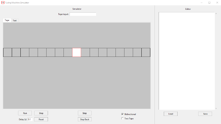
Figure 1: Simulator upon startup
2.2 Running the Program
In order to run this program you must have either Python 2.7 or 3.7 installed
on your computer. Additionally, if you are running this program on a Linux
4
machine you will need to install the TKinter library for your installation
of Python. After installing the prerequisite software, simply double click
TMGUI.py or run TMGUI.py in the command line.
2.3 The Editor
The editor window is located on the right of the program window. Here is
where you will load, write, and save .tm files that will define the functionality
of your Turing Machine.
2.3.1 Writing a .tm file
The instructions for the simulated Turing Machine are written as a .tm file.
These can be created by either using the editor within this program or cre-
ating an ordinary text file and saving it with the extension .tm. Instructions
are written in the following format:
•States are always integers with 0 being the initial state.
•-1 denotes a halt-and-accept state, -2 is a halt-and-reject state, and -3
is a general halt state. All other state number must be nonnegative.
•L tells the machine to move left and R tells it to move right. Addition-
ally, if you are writing a two tape Turing Machine, S tells the machine
to stay where it is. S can only be used for two tape Turing Machines.
•A capital ’B’ represents the blank symbol.
•For a one tape Turing Machine, each line of the .tm file takes the form
STATE SYMBOL NEW-STATE NEW-SYMBOL DIRECTION.
So the line
2b5cL
tells the machine that if it is in state 2 and is reading the symbol b,
replace the b with a c, move left, and change to state 5.
•To include comments start each comment line with a #.
5
•For a two tape Turing Machine, each line of the .tm file takes the form
STATE SYMBOL1:SYMBOL2 NEW-STATE NEW-SYMBOL1:NEW-
SYMBOL2 DIRECTION1:DIRECTION2.
So the line
0 a:b 3 B:a L:S
tells the machine that if it is in state 2 and is reading the symbol a in
tape 1 and b in tape 2, replace the a in tape 1 with a blank and the
b in tape 2 with an a, move tape 1 left but do not move tape 2, and
change to state 3.
•If there is no specification for a given state and character combination
the machine will enter a halt-and-reject state.
2.3.2 Saving a .tm file
If you have written your machine instructions within the editor window, you
can save them to your computer in order to use them at another time. To
do so:
1. Ensure that your instructions follow the exact format described above.
While anything you write in the editor window can be saved as a .tm
file, if it does not follow the proper format the simulator will be unable
to run.
2. Click the save button located at the bottom right of the editor section.
3. Choose the directory you wish to save the file in, provide a file name,
and then click save.
This will create a .tm file in the given directory that can be used at a later
date.
2.3.3 Loading a .tm file
To load a previously used .tm file:
1. Click the load button located at the bottom left of the editor section.
2. Navigate to your file, select it, and click open.
6
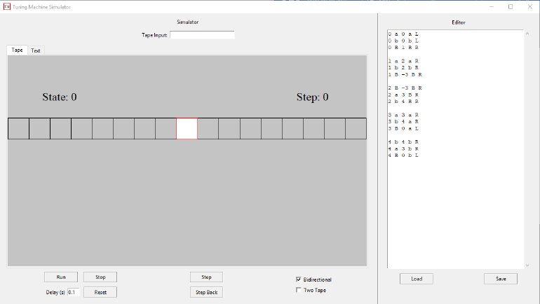
Figure 2: Simulator with loaded .tm file
You should now see the list of instructions for your Turing Machine in the
editor window. You can then edit them as you see fit and save them just like
anything else that is written in the editor window.
2.4 The Simulator
The simulator window is located on the left side of the program window.
Here is where you can see a visualization of your Turing Machine running
both graphically and as text.
2.4.1 Reading the Simulator
In this program there are two ways you can simulate the Turing Machine.
This is either as a graphical representation of the tape or as text. At any
time in the machines run you can go between seeing the machine simulated
as an actual tape and seeing it as text. This is done by toggling between the
“tape” and “text” tabs located at the top left of the simulator window.
When simulating the machine as a tape:
7

•The current state and step are located above the tape itself.
•The cell currently being read by the machine is the white cell
When simulating the machine as text:
•Each step is written as a chunk of text with the current step, the current
state, and what is currently written on the tape.
•The letter with a caret beneath it is the one being read by the machine
While the “tape” tab is useful for getting a visual understanding of how your
Turing Machine runs, we recommend doing any actual analysis in the “text”
tab since you are limited to only ever seeing a section of the entire tape in
the “tape” tab whereas you can easily scroll through all the steps when in
the “text” tab.
2.4.2 Running a Turing Machine
In order to run a Turing Machine do the following:
1. Either load a .tm file into the editor or save what you have written
to your machine. Whenever a machine is loaded in the simulator, you
will then see a “state” and “step” label appear in the tape and text
window.
2. If your .tm file is written for a unidirectional Turing Machine, uncheck
the “Bidirectional” box located at the bottom right of simulator win-
dow. If your .tm file is written for a two tape Turing Machine, check
the “Two Tape” box located directly below the “Bidirectional” box.
If you do not check off the proper boxes the simulator will likely halt
and reject any input, but could also attempt1to run forever. Note that
these options are mutually exclusive, the simulator does not support
two tape unidirectional Turing Machines.
3. Type in the textbox labeled “Tape Input” located in the top center of
the simulator window what you want the initial tape input to be.
4. Enter the delay you want between each step in the textbox labeled “De-
lay” located in the bottom left of the simulator window. The default
delay is 0.1s
1See Section 2.4.4
8
5. Click the run button located directly above the “Delay” textbox.
6. If you wish to stop the run at any time press the “Stop” button located
to the right of the “Run” button. If you wish to reset the machine click
the “Reset” button located directly below the “Stop” button.
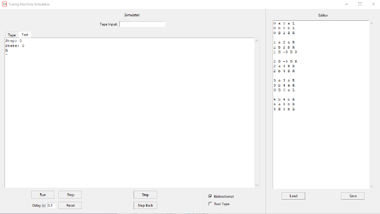
Figure 3: Simulator in text tab
2.4.3 Going Step by Step Through a Run
If you wish to have more control over the run of your Turing Machine, you can
go through step by step using the “Step” and “Step Back” buttons located
at the bottom center of the simulator window. Note that if you press the
“Step Back” button at step 0 nothing will occur. If you press the “Step”
button after the machine has halted you will be adding additional steps but
the machine will stay in a halt state. These functionalities can be used in
conjunction with the “Run” and “Stop” functionality, as expected.
2.4.4 Encountering the Halting Problem
Because of fundamental limitations to Turing Machines and computation,
it is impossible to know if your Turing Machine will ever halt. This is the
9

Halting Problem and is discussed in the “About Turing Machines” section.
If you run a Turing Machine that never halts the program will likely be-
come unresponsive. At this point we recommend closing and restarting the
program. Alternatively, to help deal with this problem we have set the max-
imum number of steps allowed for any given run to be 200,000 steps. After
the program has determined all of these steps it should respond again and
show the run for 200,000 steps. This may take a while so restarting the
program is probably your best option.
3 Using Grapher
In addition to simulating a Turing Machine, we have included a program
that automatically converts a .tm file into an easy to follow directed graph.
This is useful if the user wishes to have a visual representation of the Turing
Machine without actually having to test various input strings. To use the
grapher do the following:
1. Install the graphviz Python library using the command pip install
graphviz.
2. Download the Graphviz program here. Make sure that you follow all
installation instructions (Including adding this program to your PATH
on Windows systems) or else the grapher will not be able to work.
3. Open the grapher by running grapher.py.
4. Click the graph button and select the .tm file you wish to graph. The
program will automatically make a .png of the Turing Machine and save
it in a directory titled img within the same directory that grapher.py
is located in.
The Grapher was developed with the sole intent of graphing the .tm files
associated with one-tape Turing Machines. It will function with two-tape
files, but the output may not be as readable or look as expected.
4 Technical Overview
The simulator code is divided into two classes. The first of these classes is
turing machines.py. This class serves as the backend for the simulator,
10

Figure 4: Grapher upon startup
housing objects which model the Turing Machines. It is here that the actual
code for simulating a Turing Machine is contained. The code in this class is
adapted from the simulator created by Howard Straubing. The other class
is TMGUI.py. This class is a GUI built using the Python library TKinter
and allows for the user to actually interact with the program. Additional
documentation can be found within these classes.
The grapher code uses GraphViz, a program for generating directed graphs,
in order to convert a .tm file into a directed graph of the state transitions.
This code was initially developed in order to provide a nice animation for
Turing Machines to be included within the simulator itself. However, to pro-
vide this functionality would require additional libraries and is particularly
slow. As such, we decided to devote most of our efforts on exploring two tape
Turing Machines and included the grapher as a standalone ‘bonus’ program.
4.1 Functional Limitations
There are a number of different functional limitations to the simulator pro-
gram.
•We have capped the maximum number of steps at 200,000 in order to
help deal with the Halting Problem. We feel this is more than enough
steps for most simulations though if more are needed the user can edit
the MAX STEPS variable in turing machines.py.
•Because of limitations in computer memory the tape used is not actu-
ally infinite. Each tape is limited to 20,000 spaces. The simulator will
not let you move past either end of the tape – attempting to do so will
simply keep the head position the same. This is particularly important
to keep in mind when simulating one-way ‘infinite’ tapes, as the head
starts at the left end of the tape.
11
•Unidirectional tapes are not an option when using a two tape Turing
Machine despite theoretically being possible. This decision was made
mainly because this model does not seem to provide any more value or
insight – it would be rather trivial to adapt the existing code to handle
it if truly desired.
•Due to how the TKinter Canvas object works, it is not possible to scroll
through what is written on the tape when in the “tape” tab. You are
limited to only a section of the entire tape, centered on the reading
head. As stated earlier, we recommend using the “text” tab if a fuller
view is desired.
4.2 Known Issues
The only known issue right now is the program begins to lag if too large of
a tape input is entered, or if the program is run for a long time on many
machines or on many different inputs. It is unclear if this is due to a memory
leak within our program or a limitation on the part of Python, though con-
siderable effort was put in to mitigate this problem. Restarting the program
resolves this lag.
12

A Sample .tm file
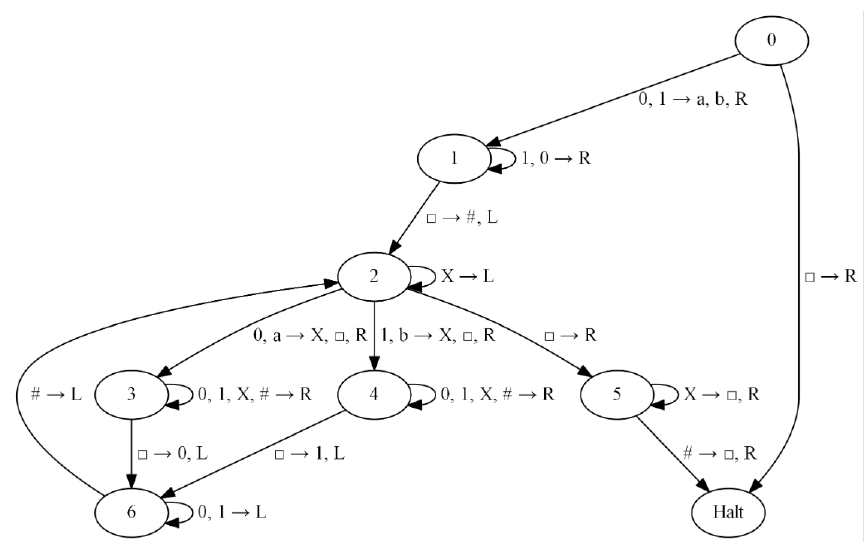
A .tm file defining a unidirectional Turing Machine for reversing tape input.
#Phase 0: Mark the first entry. a is 0, b is 1
0 0 1 a R
0 1 1 b R
0 B -3 B R
#Phase 1: Move forward to first blank and write #
1 1 1 1 R
1 0 1 0 R
1 B 2 # L
#Phase 2: Move left until you find 0, 1 or blank
2 0 3 X R
2 1 4 X R
2 B 5 B R
2 X 2 X L
# 2.1: If you found the first character, replace with a blank
2 a 3 B R
2 b 4 B R
#Phase 3a: Found 0, move right to blank, then left to #
3 0 3 0 R
3 1 3 1 R
3 X 3 X R
3 # 3 # R
3 B 6 0 L
6 0 6 0 L
6 1 6 1 L
6 # 2 # L
#Phase 3b, Found 1
4 0 4 0 R
4 1 4 1 R
4 X 4 X R
4 # 4 # R
4 B 6 1 L
#Cleanup phase
5 X 5 B R
5 # -3 B R
13