User Manual
User Manual:
Open the PDF directly: View PDF ![]() .
.
Page Count: 108 [warning: Documents this large are best viewed by clicking the View PDF Link!]


Guide
1. Introduction ⇲
2. The message box ⇲
3. Setting options ⇲
4. Project definition ⇲
5. Simulation of point localizations ⇲
6. Identification of structures ⇲
7. Geometrical analysis of structures ⇲
8. Classifier training ⇲
9. Classification of structures ⇲
10. Cluster analysis ⇲
11. Statistical and visual analysis ⇲
12. Montage construction ⇲


Introduction
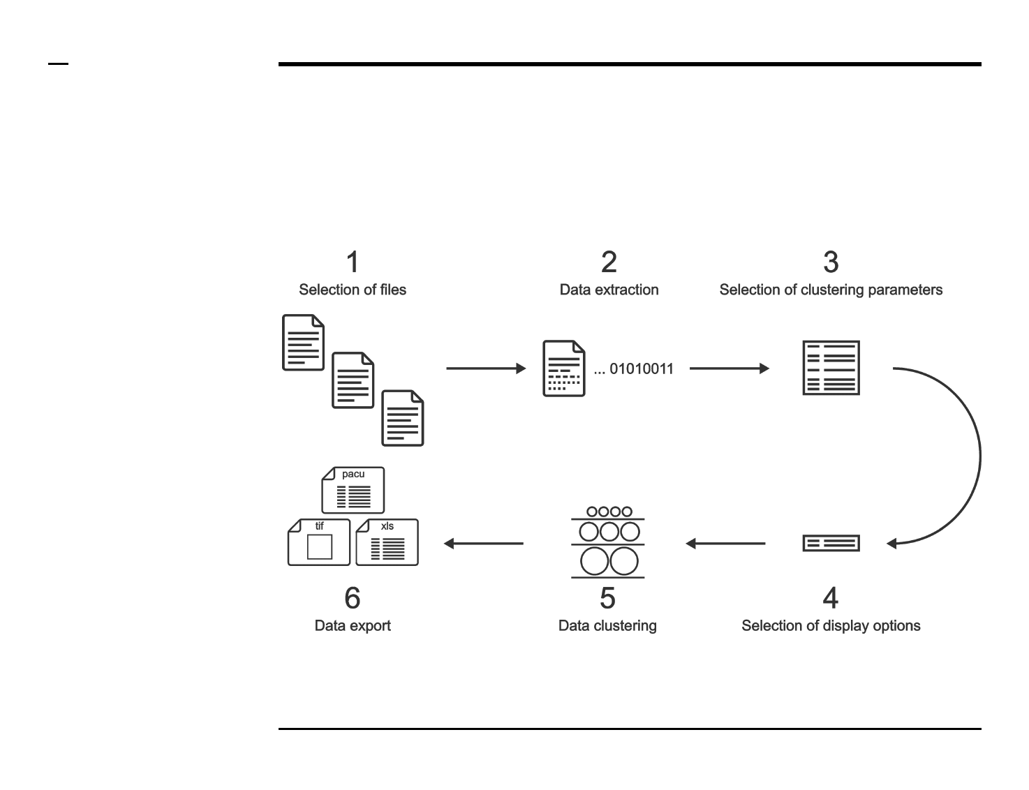
What is ASAP?
Determining the architecture of nanoscopic structures in the cell is now possible,
but requires the quantitative, statistical analysis of many thousands of subcellular
assemblies. Manually classifying and analyzing the varied morphologies of those
structures is very time consuming and imprecise, thereby limiting statistical
inference across scales and the understanding of biological function at the
molecular level. There is a strong need for a simple tool that enables rapid and
unbiased detection, classification and analysis of nanoscopic biological structures
from microscopy images. To fill this gap, we developed ASAP (Automated
Structures Analysis Program); a novel, interactive and freely-available toolkit that
permits automated, rapid and robust detection, classification and quantitative
analysis of macromolecular structures.
Guide ⇲

Introduction
Why ASAP?
●Freely-available.
●Image based (i.e. compatible with all super-resolved microscopy methods).
●GPU- and parallel- computing accelerated image analysis.
●A variety of methods for segmentation and geometrical analysis.
●Machine learning based classification of structures.
●Geometrical-based cluster analysis.
●In situ statistical visualization (high quality publication-ready figures),
analysis and modelling.
●Customizable easily-generable gallery of structures.
Guide ⇲


Introduction
License
MIT License
Copyright (c) 2018 John S H Danial & Ana J Garcia-Saez
Permission is hereby granted, free of charge, to any person obtaining a copy
of this software and associated documentation files (the "Software"), to deal
in the Software without restriction, including without limitation the rights
to use, copy, modify, merge, publish, distribute, sublicense, and/or sell
copies of the Software, and to permit persons to whom the Software is
furnished to do so, subject to the following conditions:
The above copyright notice and this permission notice shall be included in all
copies or substantial portions of the Software.
THE SOFTWARE IS PROVIDED "AS IS", WITHOUT WARRANTY OF ANY KIND, EXPRESS OR IMPLIED,
INCLUDING BUT NOT LIMITED TO THE WARRANTIES OF MERCHANTABILITY, FITNESS FOR A
PARTICULAR PURPOSE AND NON INFRINGEMENT. IN NO EVENT SHALL THE AUTHORS OR
COPYRIGHT HOLDERS BE LIABLE FOR ANY CLAIM, DAMAGES OR OTHER LIABILITY, WHETHER IN AN
ACTION OF CONTRACT, TORT OR OTHERWISE, ARISING FROM, OUT OF OR IN CONNECTION WITH
THE SOFTWARE OR THE USE OR OTHER DEALINGS IN THE SOFTWARE.
Guide ⇲
The message box
Instructions
/ All messages indicating errors,
warnings and progress are
displayed on the message box
located underneath the main
window.
/ The user is advised to refer to the
ASAP guide: description of error
and warning messages
accompanying this user manual.
§ Note 1:
The message box has been clipped
from all the consequent images of
the ASAP window for clarity.
Guide ⇲

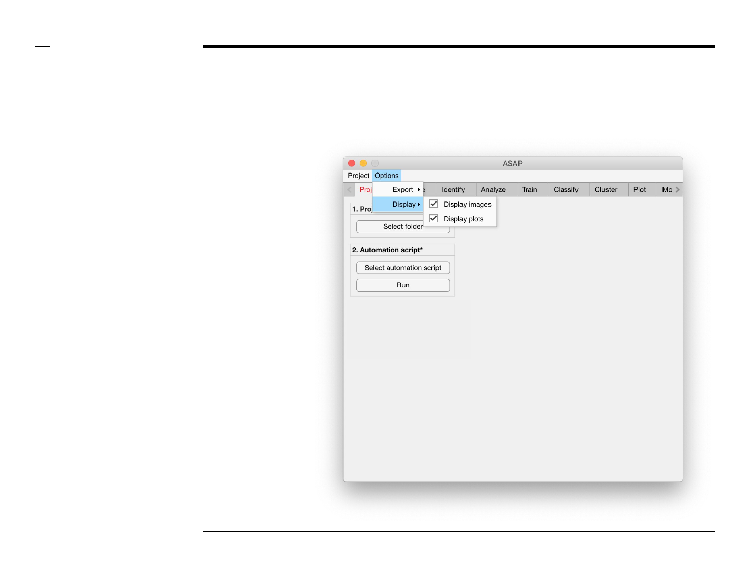
Setting options
Changing export settings
Instructions
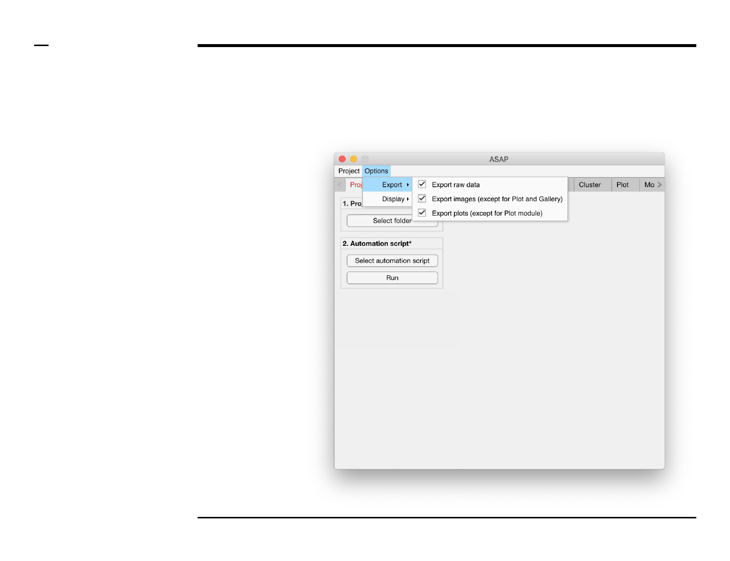
The export process can take a long
time if ASAP is exporting all raw
data (as excel files), images and
plots. To speed the analysis process
we recommend to disable the
export of the mentioned files. Files
native to ASAP are always exported
and do not constitute a large
duration of the whole process.
Guide ⇲
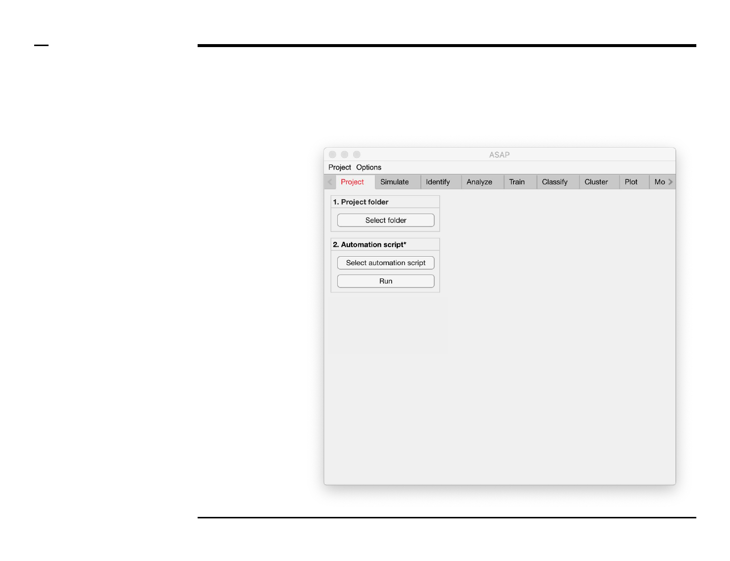
Project definition
Instructions
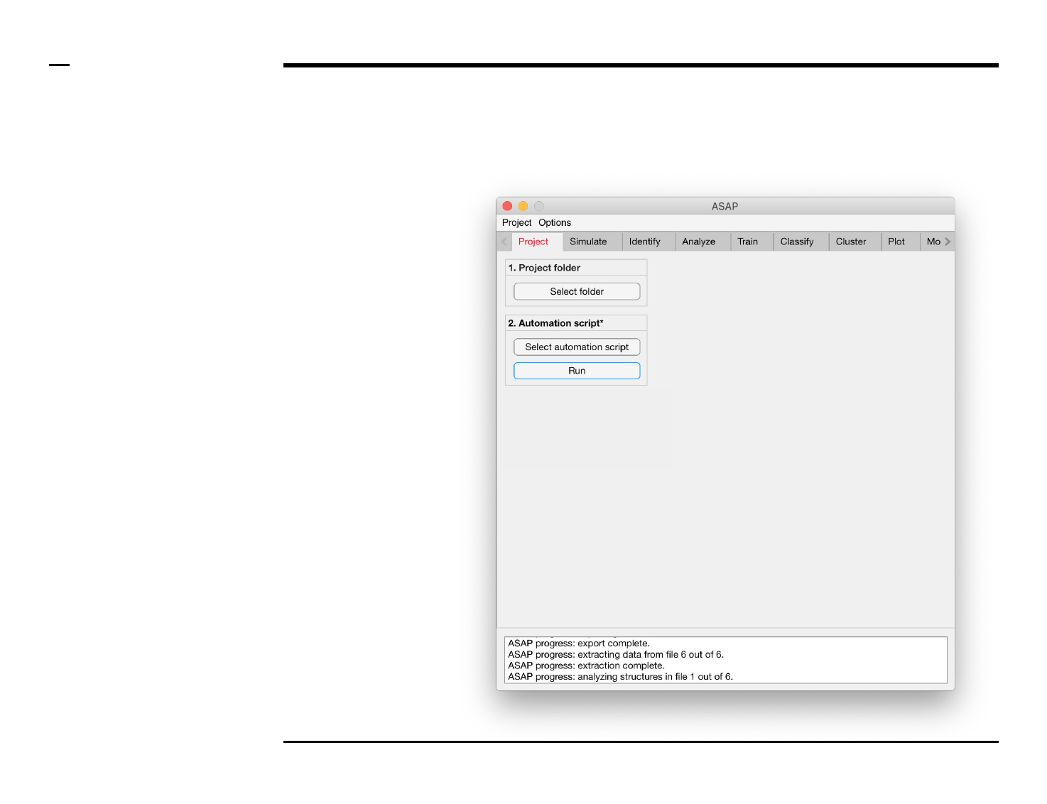
/ Select the ‘Project’ tab from the
tabs’ bar.
/ Select a project folder containing
the images to be processed by
pressing the ‘Select folder’ button
in the panel titled ‘1. Project folder’.
The name of the folder will be
shown in the text beneath.
/ The workflow of ASAP can be
automated through the automation
script; a single text file containing
all parameters required by ASAP.
To automate ASAP select an
automation script (.txt) file by
pressing the ‘Select automation
script’ button. When the
automation automation script is
successfully loaded, automation is
executed when the ‘Run’ button is
pressed.
Guide ⇲

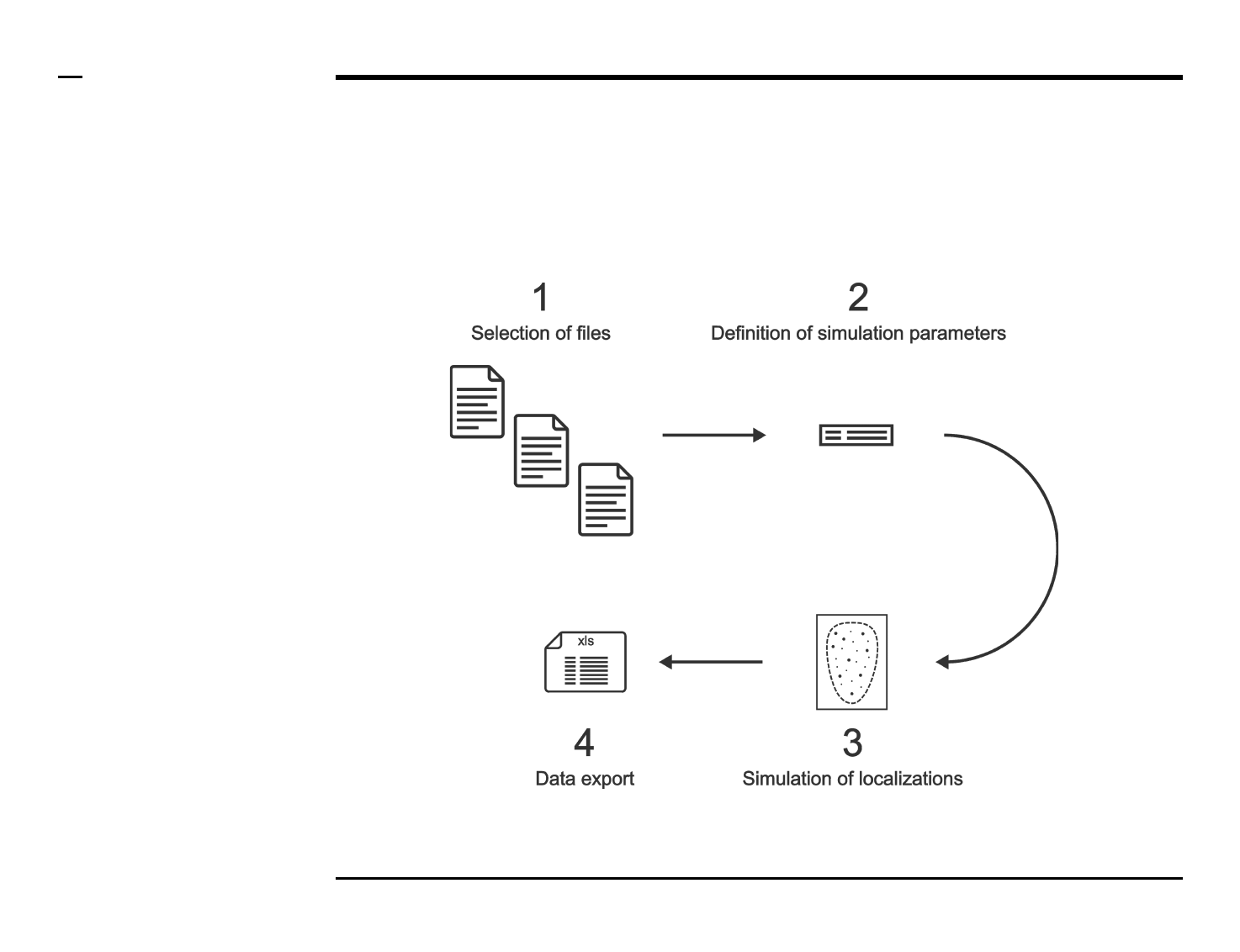

Simulation of point localizations
Selection of files
Instructions
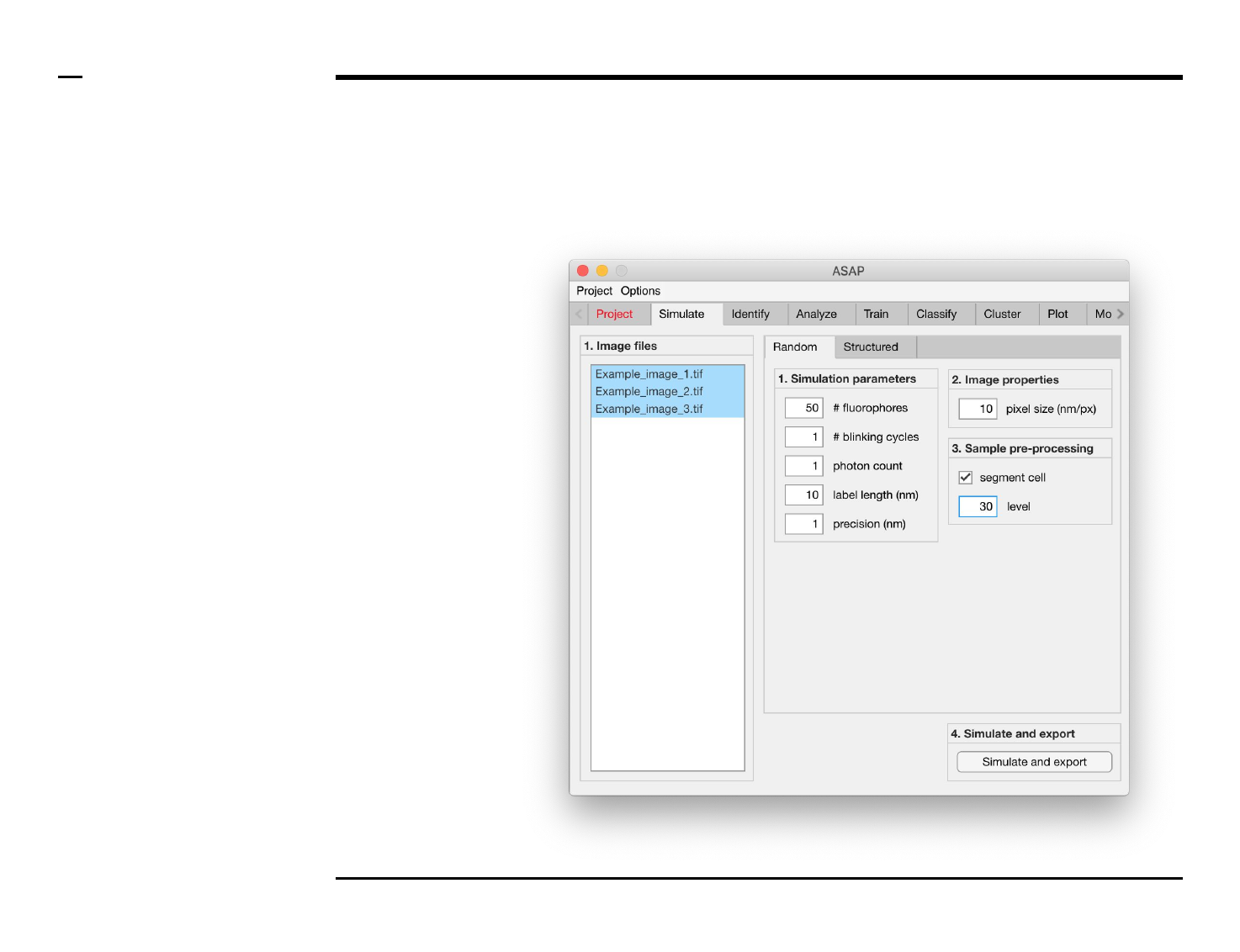
/ Select the ‘Simulate’ tab from the
tabs’ bar.
/ The listbox in the panel titled ‘1.
Image files’ will be populated with
the names of png, jpg and tiff
images located in the input folder
previously selected ⇲.
/ Select files by holding the CTRL
key and right-clicking the desired
files in the listbox in the panel titled
‘1. Image files’. Selected files will be
highlighted as shown in the figure
on the right.
§ Warning 1:
Only images with the extensions
png, jpg and tiff will be shown in the
listbox.
Guide ⇲

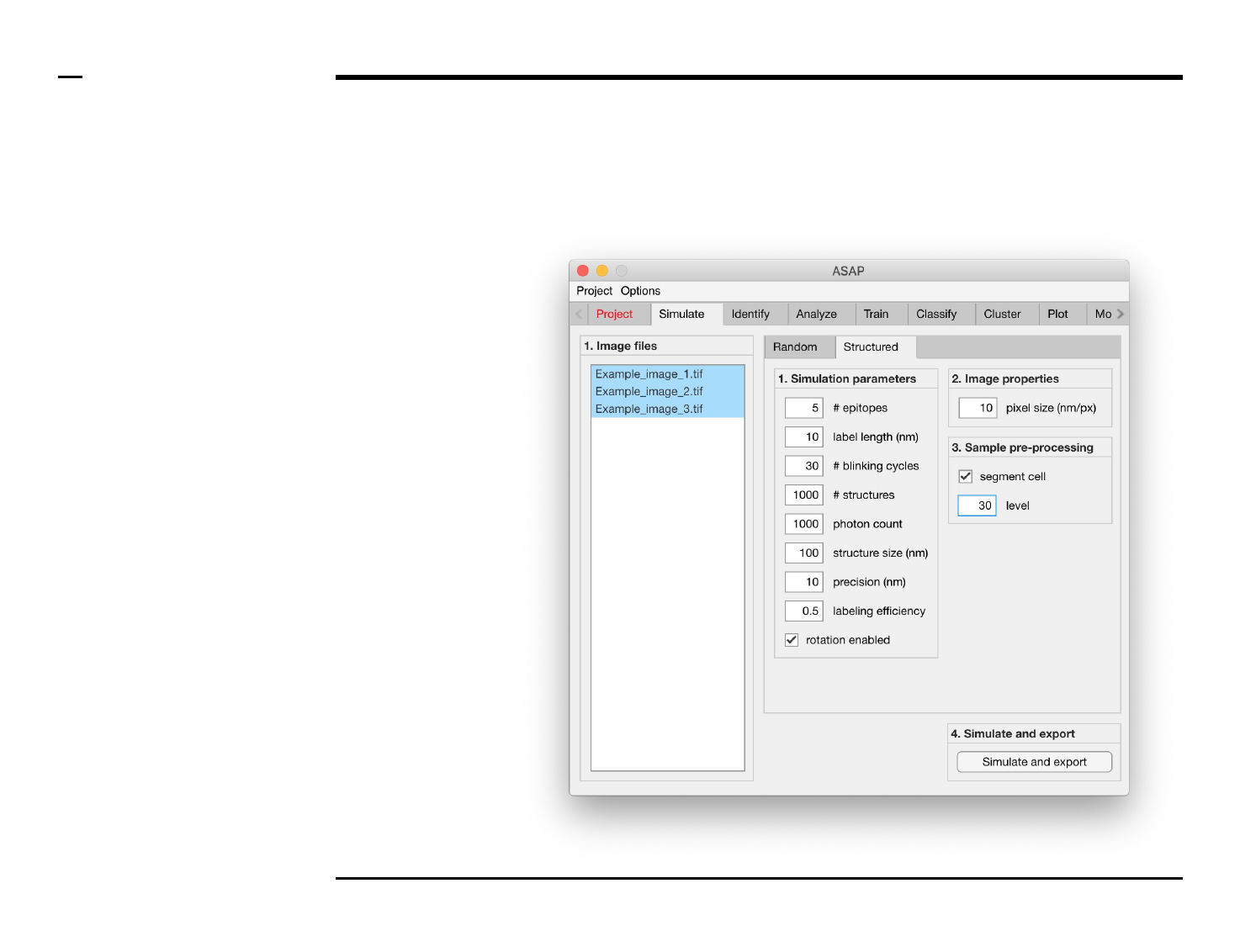
Simulation of point localizations
Definition of simulation parameters (1/2)
Instructions
/ Random or Structured localiations
can selected to be simulated by
pressing either on the Tab group
labeled ‘Random’ and ‘Structured’.
/ If Random is selected, the panel
titled ‘1. Simulation parameters’
contains 5 simulation parameters
which have to be defined:
1. # fluorophores (1000):
total number of
fluorophores in an field of
view. Please note that this
does not correspond to the
number of localizations.
2. # blinking cycles: average
number of blinking cycles
per fluorophore.
3. # photon count: number of
photons emitted per
emission cycle.
4. label length (nm): length of
fluorescent label from
protein..
5. precision (nm): expected
localization precision.
Guide ⇲
Simulation of point localizations
Definition of simulation parameters (2/2)
Guide ⇲
Instructions (contd.)
/ If Structured is selected, the panel
titled ‘1. Simulation parameters’
contains 9 simulation parameters
which have to be defined:
1. # epitopes: number of
discrete positions across a
ring-like structure.
2. label length (nm): length of
fluorescent label from
protein.
3. # blinking cycles: average
number of blinking cycles
per fluorophore.
4. # structures: number of
ring-link structures in field
of view.
5. # photon count: number of
photons emitted per
emission cycle.
6. structure size (nm):
diameter of ring-like
structure in nanometers.
7. precision (nm): expected
localization precision.
8. labeling efficiency:
average ratio of epitopes
which are labeled.
9. rotation enabled: to be
checked if ring-link
structures are to have
different orientations.


Identification of structures
Selection of files
Instructions
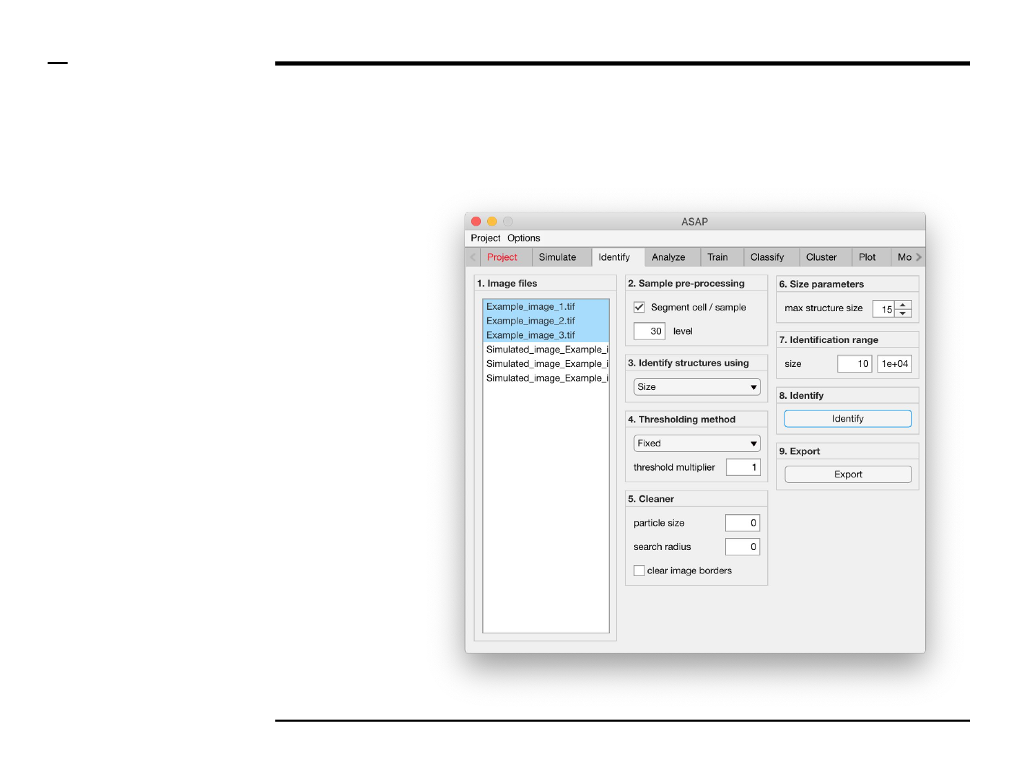
/ Select the ‘Identify’ tab from the
tabs’ bar.
/ The listbox in the panel titled ‘1.
Image files’ will be populated with
the names of png, jpg and tiff
images located in the input folder
previously selected ⇲.
/ Select files by holding the CTRL
key and right-clicking the desired
files in the listbox in the same panel.
Selected files will be highlighted as
shown in the figure on the right.
§ Note 1:
Only images with the extensions
png, jpg and tiff will be shown in the
listbox.
Guide ⇲


Identification of structures
Definition of segmentation parameters (2/3)
Instructions (contd.)
The panel titled ‘3. Identify
structures using’ contains 1
parameter which has to be defined:
1. Connectivity / Size: if
connectivity is selected,
structures are segmented
(identified) based on their
pixel-to-pixel connectivity
(best used when the
imaged structures are
aggregates). If size is
selected, structures are
segmented based on
regional density (best used
when the imaged
structures are sparse).
Guide ⇲

Identification of structures
Definition of segmentation parameters (3/3)
Instructions (contd.)
The panel titled ‘4. Thresholding
method’ contains 2 parameters
which have to be defined:
1. Fixed / Relative: if fixed is
selected, the software only
considers those pixels
whose intensities are
higher than a global
uniform threshold (best
used when illumination is
uniform and structures are
located within a thin optical
section). If relative is
selected, the software only
considers those pixels
whose intensities are
higher than a threshold
value that is modulated
depending on average
regional intensity (best
used when illumination is
non-uniform and / or
structures are not located
within a thin optical
section).
2. Threshold multiplier: a
constant multiplier for
modulating the output of
the relative thresholding
algorithm (best used when
intensity histogram is
strongly skewed).
Guide ⇲

Identification of structures
Definition of image clean-up parameters
Instructions
The panel titled ‘5. Cleaner’
contains 3 optional parameters:
1. Particle size (px):
maximum number of
post-thresholding pixels to
be contained in a structure
for it to be discarded.
2. Search radius (px): the
maximum radius of a
structures for it to be
discarded.
3. Clear image borders:
discards all structures
which touch the borders of
an image (true / false).
Guide ⇲


Identification of structures
Definition of filter parameters (2/2)
Instructions (contd.)
The panel titled ‘7. Identification
range’ contains 2 parameters which
have to be defined:
1. Size (px) - left box: lower
size bound (minimum area)
of structures to be filtered.
Structures smaller than
this value are discarded.
2. Size (px) - right box: upper
size bound (maximum area)
of structures to be filtered.
Structures larger than this
value are discarded.
Guide ⇲

Identification of structures
Identification of structures (2/2)
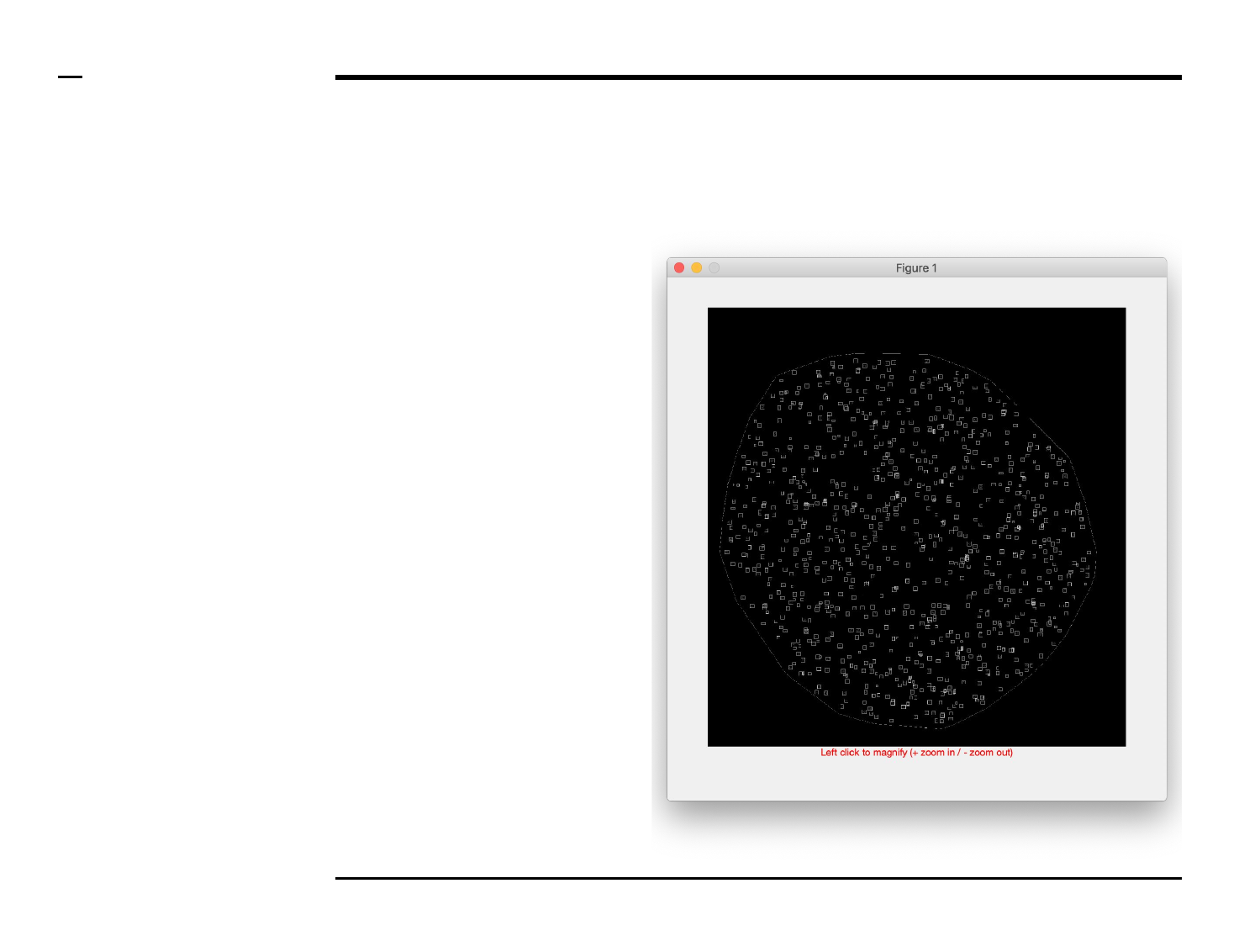
Instructions (contd.)
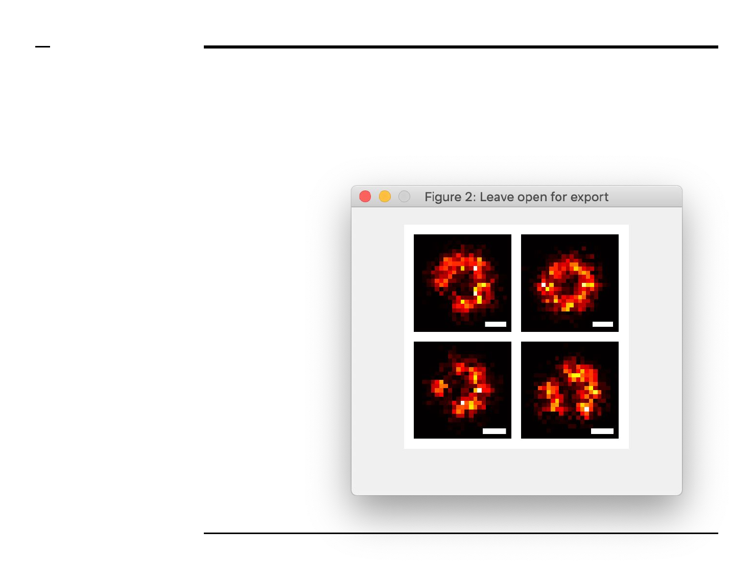
/ A number of figures will appear
equal to the number of images
being processed. A figure will
similar to the one shown on the
right.
/ In the figure(s), the processed
image(s) will be shown with the
structures identified bound within
white rectangles.
/ To magnify into the image hold the
left click of the mouse at any point
on the image and press the + or - to
zoom in and out respectively.
/By hovering the pointer across the
image the user can access the
different parts magnified in real
time.
Guide ⇲

Identification of structures
Data export (2/2)
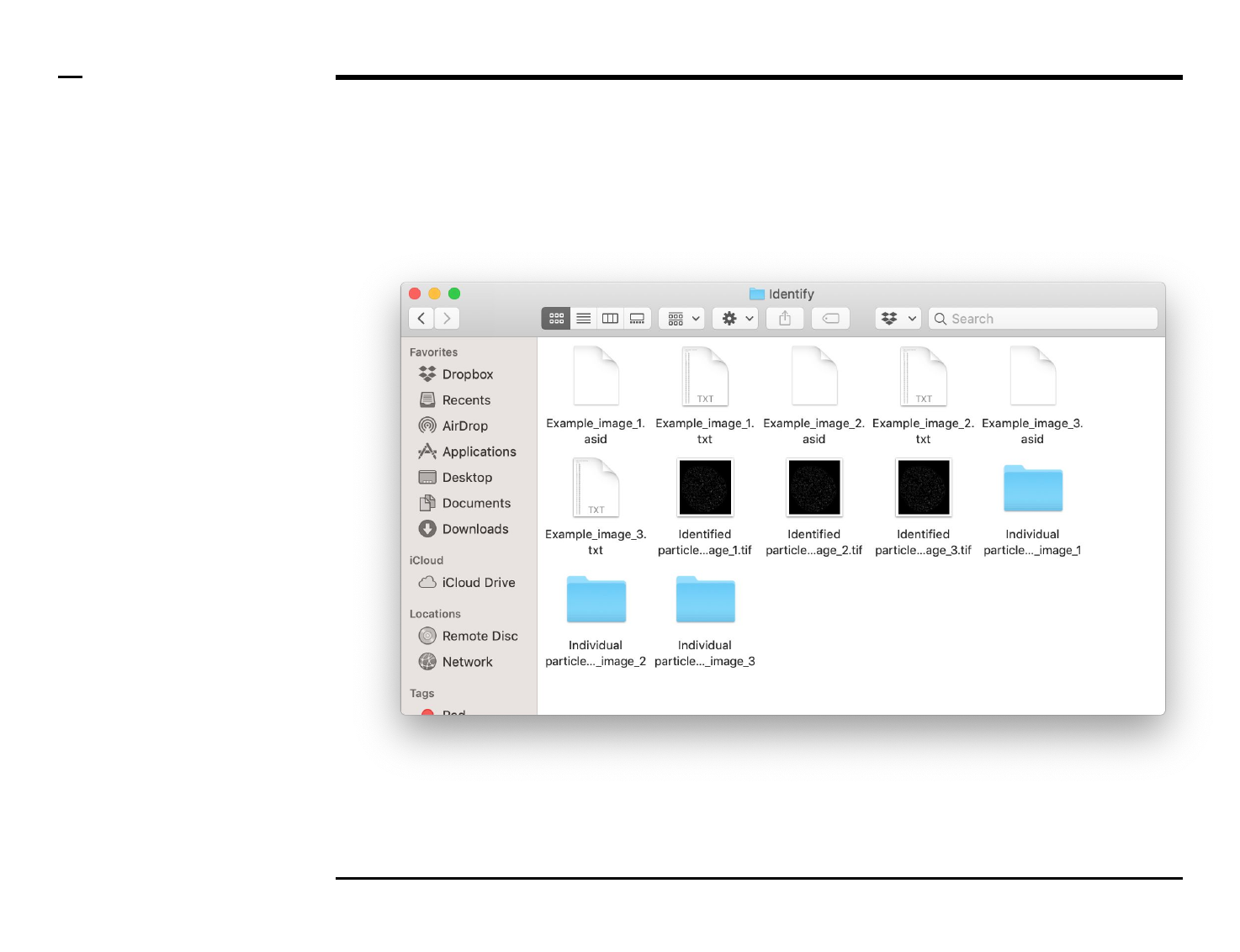
Instructions (contd.)
A folder named ‘Identify’ will be
created in the output folder and the
following 1 output folder + 3 output
files (per processed image) will be
placed in the folder:
1. ‘Individual particles_xx’ -
folder: a folder containing
tiff images of all identified
structures in an image.
2. ‘xx.asid’ - file: a ASAP file
containing processing
details used by the
program for later analysis.
3. ‘Identified particles_xx.tif’
- file: a grayscale tiff image
of the processed image
with identified particles
shown bound within white
rectangles.
4. ‘xx.txt’ - file: text file
containing a summary of
the structures identified as
well as their coordinates in
the original image.
Guide ⇲

Geometrical analysis of structures
Selection of files
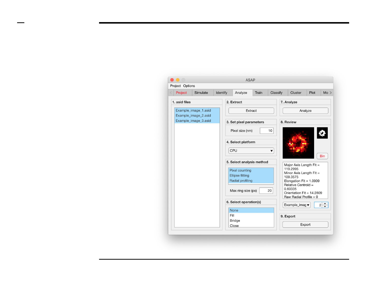
Instructions
/ Select the ‘Analyze’ tab from the
tabs’ bar.
/ The listbox in the panel titled ‘1.
asid files’ will be populated with the
names of asid files located in the
input folder previously selected ⇲.
/ Select files by holding the CTRL
key and right-clicking the desired
files in the listbox in the same panel.
Selected files will be highlighted as
shown in the figure on the right.
Guide ⇲


Geometrical analysis of structures
Definition of pixel size
Instructions
The panel titled ‘3. Set pixel
parameters’ contains 1 parameter
which has to be defined:
Pixel size (nm): the size of 1 pixel (in
nanometers) depends on several
factors, including: the actual size of
1 camera pixel and the
magnification factor. A size of 10
nm is typically reported, however,
consult your microscopy
administrator for a precise value.
Guide ⇲

Geometrical analysis of structures
Selection of computation platform
Instructions
The panel titled ‘4. Select platform’
contains 1 parameter which has to
be defined:
CPU / GPU*: if GPU computing was
previously enabled, the drop down
menu will contain a GPU item which
can be selected by the user.
Otherwise, the CPU is
automatically selected.
Guide ⇲

Geometrical analysis of structures
Selection of analysis method (1/3)
Instructions
The panel titled ‘5. Select analysis
method’ contains 1 parameter
which has to be defined:
Pixel counting / Ellipse fitting /
Radial profiling: dictates the
analysis method(s) to be used. if
‘Ellipse fitting’ is selected, the
identified structures are fitted with
an ellipse and the following
descriptors are reported:
1. Major axis length
2. Minor axis length
3. Orientation
If ‘Radial profiling’ is selected, the
number and intensity of pixels lying
within a pixel-sized ring of
increasing radii is counted and
reported as follows:
1. Raw radial profile
2. Intensity normalized radial
profile
3. Area normalized radial
profile
4. Raw radial density profile
5. Intensity normalized radial
density profile
6. Area normalized radial
density profile
Please turn over
Guide ⇲

Geometrical analysis of structures
Selection of analysis method (2/3)
Instructions (contd.)
If ‘Pixel counting’ is selected, the
following descriptors are reported:
1. Area
2. Filled area
3. Convex area
4. Perimeter
5. Euler number
6. Eccentricity
7. Solidity
8. Orientation
9. Extent
10. Major axis length
11. Minor axis length
12. Form factor
13. Roundness
14. Elongation
15. Fill ratio
16. Mean intensity
17. Number of minimas
18. Minima intensity
19. Minima eccentricity
20. Minima area
21. Minima convex area
22. Number of maximas
23. Maxima intensity
24. Maxima eccentricity
25. Maxima area
26. Maxima convex area
27. Segment total length
28. Number of intersections
Guide ⇲

Geometrical analysis of structures
Selection of analysis method (3/3)
Instructions (contd.)
/ The numeric field labeled ‘Max
Ring Size (px)’ will be enabled if
‘Radial profile was selected’. A
maximum radius of the ring used for
radial profiling has to be entered in
this field.
§ Note: it is advised that the Max
ring size be 5 pixels larger than the
average radius of the underlying
structures.
Guide ⇲

Geometrical analysis of structures
Selection of image operation(s)
Instructions
The panel titled ‘6. Select
operation(s)’ contains 1 optional
parameter:
Listbox with multiple selections:
1. None: no operation is
performed on the
identified structures.
2. Fill: dark pixels in the
thresholded images of the
identified structures are
filled if surrounded with
bright pixels.
3. Bridge: bridges
unconnected pixels, that is,
sets dark pixels to bright if
it has 2 bright unconnected
pixels as neighbours
4. Close: dilates then erodes a
thresholded image
5. Open: erodes then dilates a
threshold image
6. Clear: removes isolated
pixels (1 bright pixel that is
surrounded by dark pixels)
7. Rotate: rotates a structure
to align its major axis with
the x axis.
8. Center: centers a structure
in the field of view.
9. Resize: resizes and pads a
structure to fill a 30 x 30
square pixels area.
Guide ⇲


Geometrical analysis of structures
Analysis and revision (2/2)
Instructions (contd.)
/ Grayscale images of the identified
structures will be displayed in the
large in-app figure in the panel
titled ‘8. Review’.
/ Binary images of the identified
structures will be displayed in the
small in-app figure in the same
panel.
/ The analyzed parameters will be
displayed in the large text box in
the same panel.
/ The drop down menu in same
panel can be used to access the
analyzed files. Selecting a different
file from the drop down menu will
result in the text box and large &
small in-app figures updating
accordingly.
/ The numeric spinner in the same
panel contains the IDs of the
structures belonging to the file
selected in the drop down menu.
Scrolling the spinner will result in
the text box and large & small
in-app figures updating accordingly.
/ To bin a structure press the
button labeled ‘Bin’ in the same
panel.
Guide ⇲

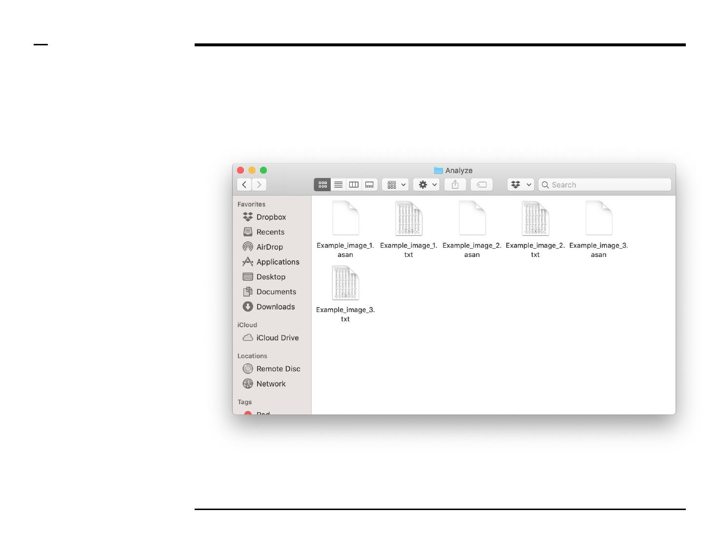
Geometrical analysis of structures
Data export (2/2)
Instructions (contd.)
A folder named ‘Analyze’ will be
created in the output folder and the
following 2 output files (per
processed image) will be placed in
the folder:
1. ‘xx.txt’ - file: text file
containing a summary of
the structures analyzed as
well as their parameters.
2. ‘xx.asan’ - file: a ASAP file
containing processing
details used by the
program for later analysis.
Guide ⇲


Classifier training
Selection of files
Instructions
/ Select the ‘Train’ tab from the
tabs’ bar.
/ The listbox in the panel titled ‘1.
asan files’ will be populated with
the names of asan files located in
the input folder previously selected
⇲.
/ Select files by holding the CTRL
key and right-clicking the desired
files in the listbox in the same panel.
Selected files will be highlighted as
shown in the figure on the right.
Guide ⇲


Classifier training
Structure annotation
Instructions
/ Grayscale images of the identified
structures will be displayed in the
large in-app figure in the panel
titled ‘4. Manual classification’.
/ Binary images of the identified
structures will be displayed in the
small in-app figure in the same
panel.
/ The names of the shapes will be
displayed in the text box in the
same panel.
/ The drop down menu in the same
panel can be used to access the
analyzed files. Selecting a different
file from the drop down menu will
result in the large & small in-app
figures updating accordingly.
/ The numeric spinner in the same
panel contains the IDs of the
structures belonging to the file
selected in the drop down menu.
Scrolling the spinner will result in
the large & small in-app figures
updating accordingly.
/ Annotate the currently displayed
structure by selecting the shape it
corresponds to in the listbox.
Display next structure by scrolling
the spinner and selecting the
corresponding shape accordingly.
Guide ⇲
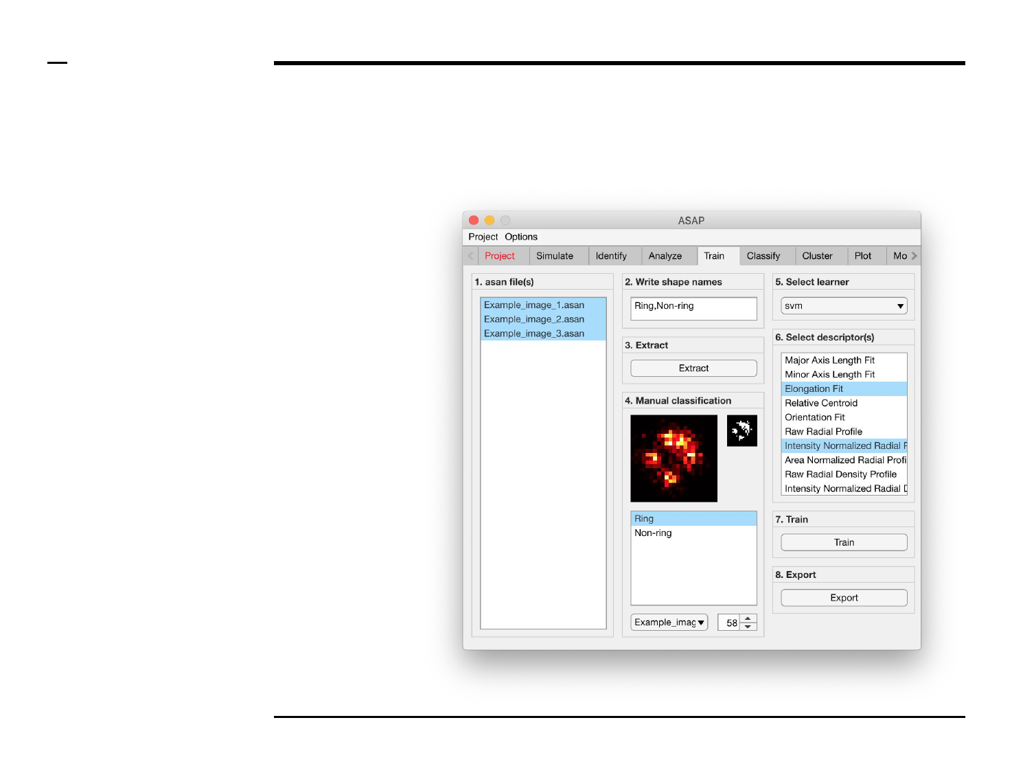
Classifier training
Selection of learner and features
Instructions
/ Select a learner from the drop
down menu in the located in the
panel titled ‘5. Select learner’. More
information on the different
learners can be found here ⇲.
/ Select the most important
features that discriminates
between the different shapes from
the listbox in the panel titled ‘6.
Select descriptor(s)’. We advise to
select as few features as possible
then expand the set of features for
improvement.
Guide ⇲

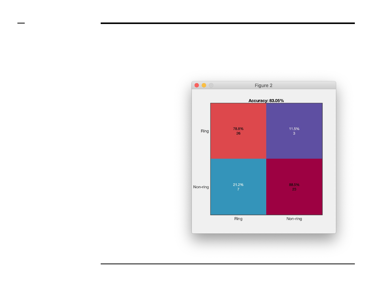
Classifier training
Classifier training (2/2)
Instructions (contd.)
/ A figure similar to the one shown
on the right will be displayed.
/ The shown matrix is known as the
confusion matrix. The confusion
matrix visually represents the
proportion of structures belonging
to a certain group of shapes is being
classified as to belonging to the
same group or groups.
/ A diagonal value (i.e. one that is
shared between the same
annotated group and the classified
group) should be the highest
amongst all values in the
intersecting row and column.
/ The overall accuracy of the
trained classifier can be assessed by
comparing the accuracy value
shown on top of the matrix with the
desired accuracy.
/ If the displayed accuracy is lower
than expected, the user can:
1. Increase the number of
annotated structures ⇲.
2. Select another learner ⇲.
3. Modify or expand the set of
features used for
discrimination ⇲.
and, re-run the classifier.
Guide ⇲

Classifier training
Data export (2/2)
Instructions (contd.)
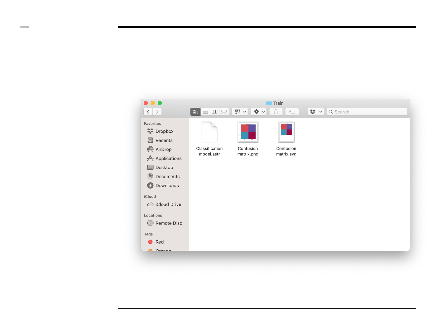
A folder named ‘Train’ will be
created in the output folder and the
following 3 output files will be
placed in the folder:
1. ‘Confusion matrix.png’ -
file: png file of the
confusion matrix.
2. ‘Confusion matrix.svg’ -
file: svg file of the confusion
matrix.
3. ‘Confusion matrix.astr’ -
file: a ASAP file containing
the classifier details used
by the program for later
analysis.
Guide ⇲


Classification of structures
Selection of files
Instructions
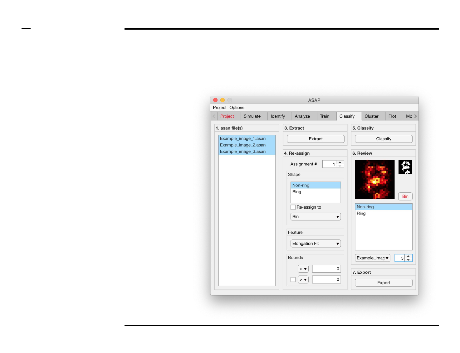
/ Select the ‘Classify’ tab from the
tabs’ bar.
/ The listbox in the panel titled ‘1.
asan files’ will be populated with
the names of asan files located in
the input folder previously selected
⇲.
/ Select files by holding the CTRL
key and right-clicking the desired
files in the listbox in the same panel.
Selected files will be highlighted as
shown in the figure on the right.
§ Note1:
A classification model .astr file
located in the project folder will be
automatically read..
Guide ⇲


Classification of structures
Structure reassignment
Instructions
To re-assign shapes based on hard
limits imposed on the extracted
features:
1. Select an assignment
number by changing the
spinner value labeled
‘Assignment #’.
2. Select 1 or more shape(s)
from the listbox located in
the subpanel titled ‘Shape’
to be assigned from.
3. Check the checkbox
labeled ‘Re-assign to’ to
activate the current
assignment.
4. Select a shape, or bin, from
the dropdown menu
located in the subpanel
titled ‘Shape’ to be assign
to.
5. Select a feature from the
dropdown menu located in
the subpanel titled
‘Feature’.
6. Select bounds for the
selected feature. Within
those bounds a structure is
re-assigned, otherwise not.
7. At least 1 bound has to be
assigned, using an equality
and number in the
subpanel titled Bounds. To
assign a second bound,
check the checkbox in the
same panel and assign the
parameters accordingly.
Guide ⇲

Classification of structures
Structure classification and revision (2/2)
Instructions (contd.)
/ Grayscale images of the classified
structures will be displayed in the
large in-app figure in the panel
titled ‘6. Review’.
/ Binary images of the classified
structures will be displayed in the
small in-app figure in the same
panel.
/ The names of the shapes will be
displayed in the text box in the
same panel.
/ The drop down menu in the same
panel can be used to access the
classified files. Selecting a different
file from the drop down menu will
result in the large & small in-app
figures updating accordingly.
/ The numeric spinner in the same
panel contains the IDs of the
structures belonging to the file
selected in the drop down menu.
Scrolling the spinner will result in
the large & small in-app figures
updating accordingly.
/ Review the currently displayed
structure by selecting the shape it
corresponds to in the listbox if the
highlighted shape is incorrect.
Display next structure by scrolling
the spinner and repeating process.
Guide ⇲

Classification of structures
Data export (2/2)
Instructions (contd.)
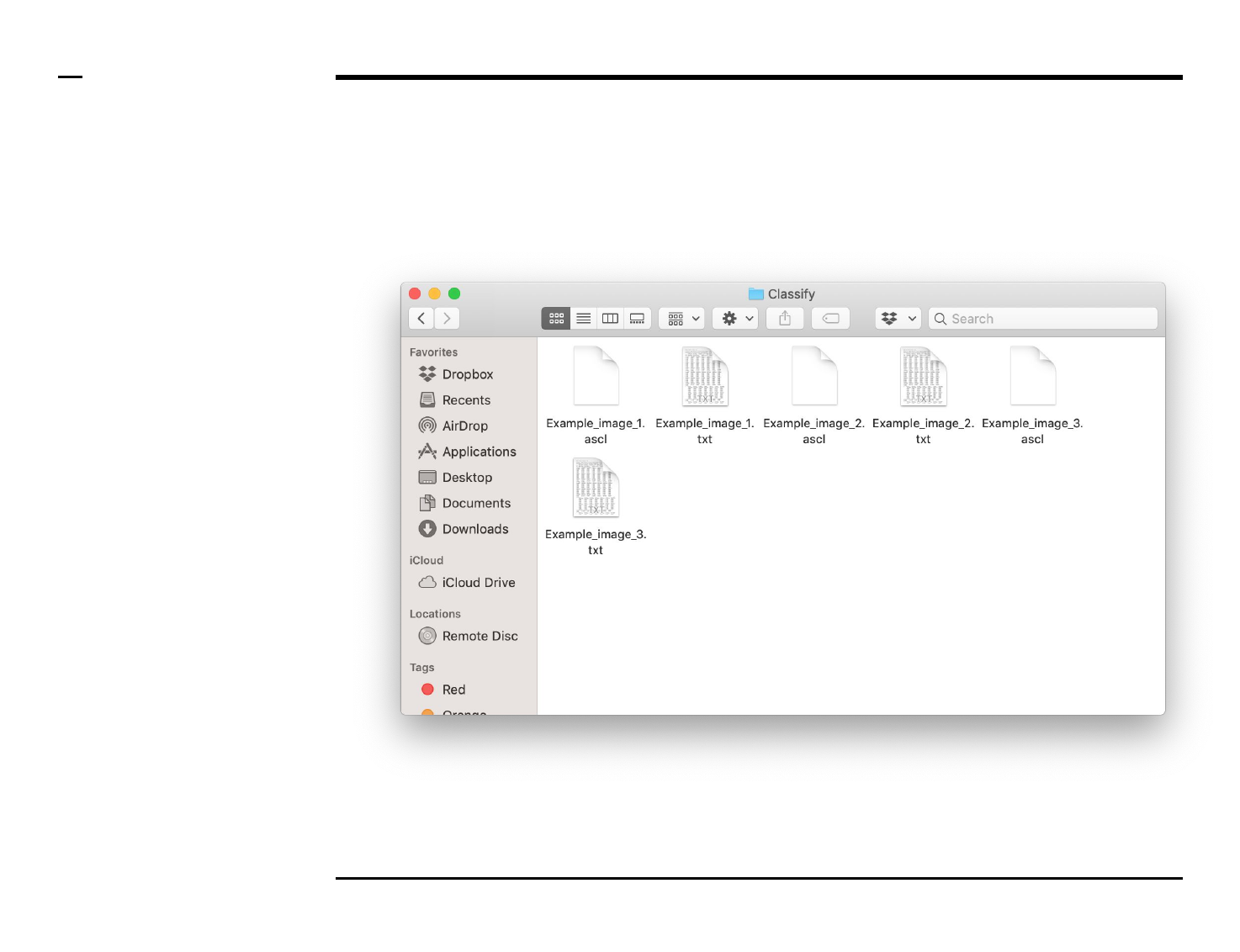
A folder named ‘Classify’ will be
created in the output folder and the
following 2 output files (per
processed image) will be placed in
the folder:
1. ‘xx.txt’ - file: text file
containing a summary of
the structures classified as
well as their parameters.
2. ‘xx.ascl’ - file: a ASAP file
containing classification
details used by the
program for later analysis.
Guide ⇲


Cluster analysis
Selection of files
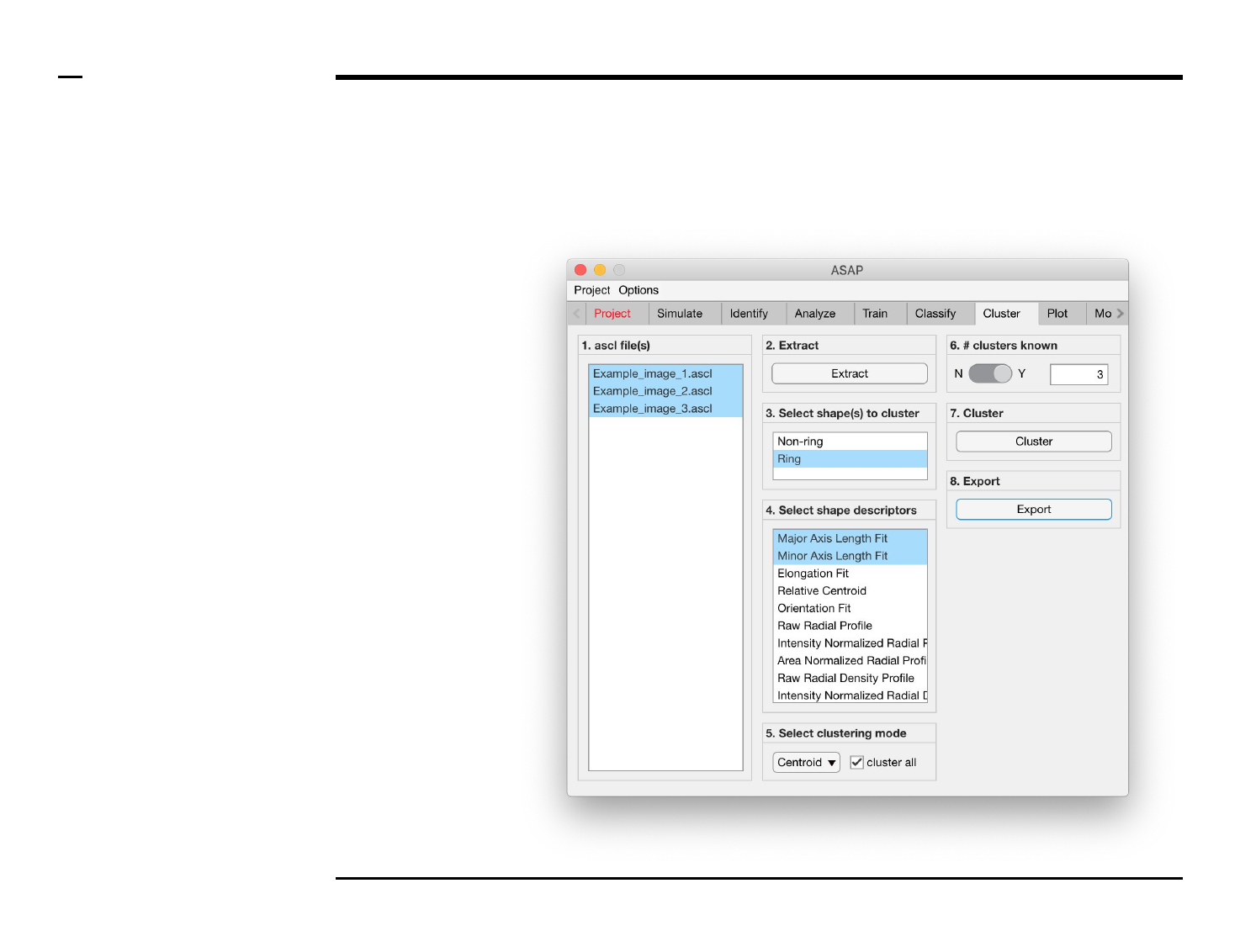
Instructions
/ Select the ‘Cluster’ tab from the
tabs’ bar.
/ The listbox in the panel titled ‘1.
ascl files’ will be populated with the
names of ascl files located in the
input folder previously selected ⇲.
/ Select files by holding the CTRL
key and right-clicking the desired
files in the listbox in the same panel.
Selected files will be highlighted as
shown in the figure on the right.
Guide ⇲


Cluster analysis
Selection of clustering parameters (3/4)
Instructions (contd.)
/ Choose a clustering mode from
the drop menu in the panel titled ‘5.
Select clustering mode’. The
following modes (algorithms) are
available:
1. Centroid: deploys a
k-means algorithm ⇲ for
data clustering.
2. Gaussian mixture model:
deploys an expectation
maximization algorithm ⇲
for data clustering.
/ To use data from all the selected
files in the clustering process, check
the checkbox labeled ‘cluster all’ in
the same panel.
Guide ⇲

Cluster analysis
Selection of clustering parameters (4/4)
Instructions (contd.)
/ If the number of clusters is known
a priori, pull the switch in the panel
titled ‘6. # clusters known’ to the
position labeled ‘Y’. If otherwise,
pull the switch to the position
labeled ‘N’.
/ If the number of clusters is known,
a numeric edit field will be enabled
on the right side where the user can
enter the known number of
clusters.
/ If the number of clusters is
unknown, an optimal number of
clusters will be automatically
calculated.
Guide ⇲
Cluster analysis
Data clustering (2/3)
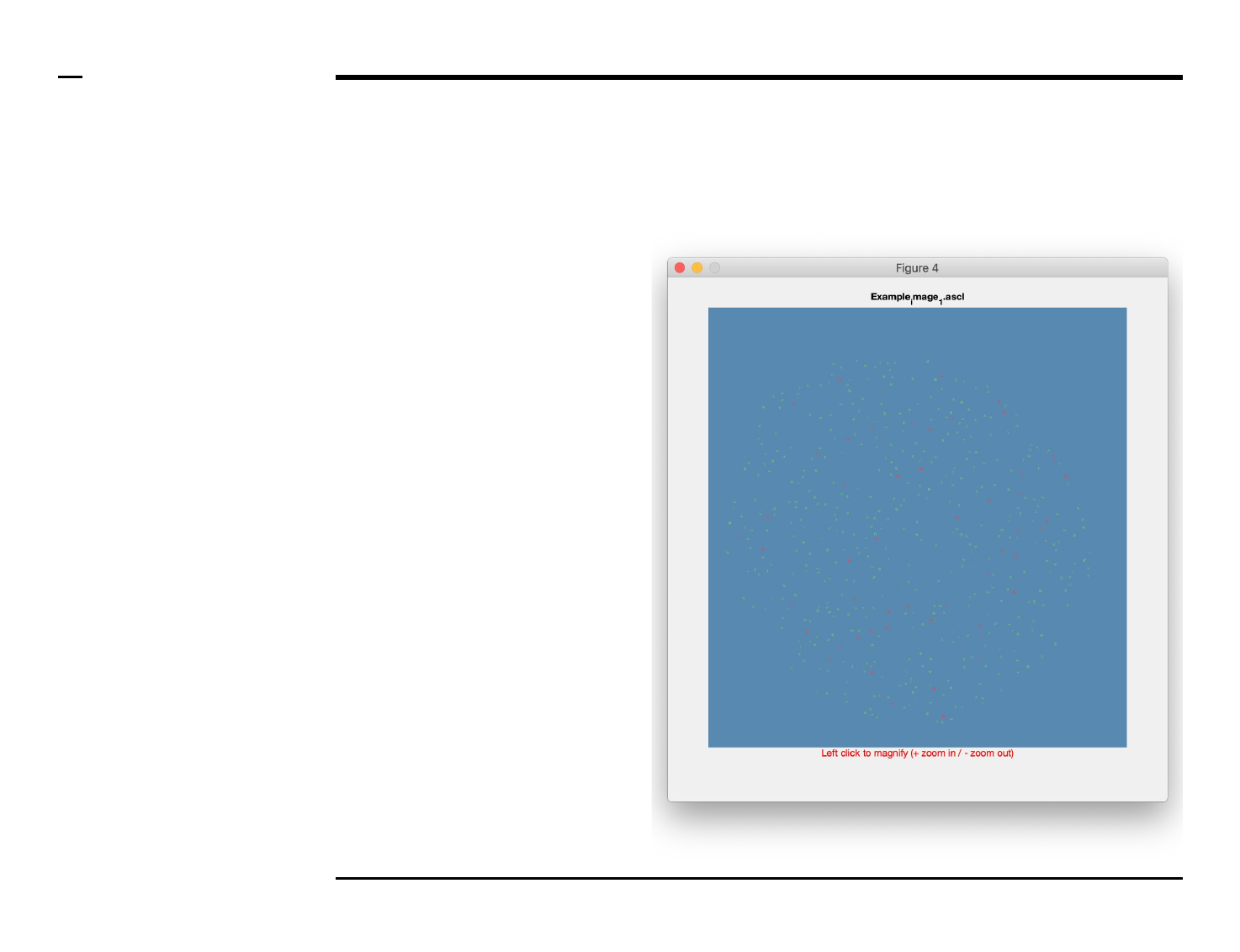
Instructions (contd.)
/ If the user selects to show the
clustered images, a number of
figures equal to the number of
processed files and similar to the
one shown on the right will be
displayed.
/ Figures are titled with the name of
the processed file.
/ Each structure is color-coded
according to its cluster affiliation.
/ To magnify into the image hold
the left click of the mouse at any
point on the image and press the +
or - to zoom in and out respectively.
/ By hovering the pointer across the
image the user can access the
different parts magnified in real
time.
Please turn over
Guide ⇲
Cluster analysis
Data clustering (3/3)
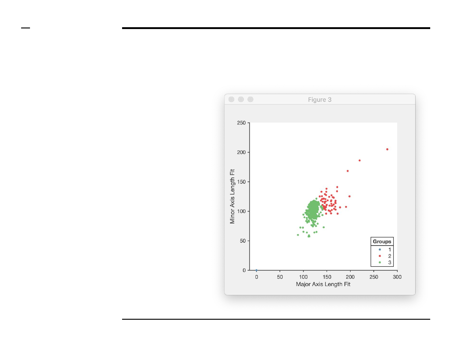
Instructions (contd.)
/ If the user selects to cluster all
data, 1 plot similar to the one
shown on the right will be
displayed. The clustering plot maps
structures across 2 similar or
different dimensions (i.e. shape
descriptors) and groups them into
different clusters according to the
chosen clustering mode.
/ Plots are titled with the name of
the processed file.
/ If the user does not select to
cluster all data, a number of plots
equal to the number of processed
files and similar to the plot shown
on the right will be displayed.
Guide ⇲

Cluster analysis
Data export (2/2)
Instructions (contd.)
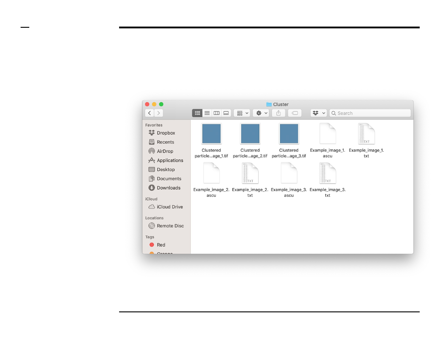
A folder named ‘Cluster’ will be
created in the output folder and the
following 3 output files (per
processed image) will be placed in
the folder:
1. ‘xx.txt’ - file: text file
containing a summary of
the structures clustered as
well as their parameters.
2. ‘xx.ascu’ - file: a ASAP file
containing clustering
details used by the
program for later analysis.
3. ‘Clustered particles_xx.tif’
- file: tiff file of the
clustered image.
Guide ⇲


Statistical and visual analysis
Selection of files
Instructions
/ Select the ‘Plot’ tab from the tabs’
bar.
/ The listbox in the panel titled ‘1.
ascl files’ will be populated with the
names of ascl files located in the
input folder previously selected ⇲.
/ Select files by holding the CTRL
key and right-clicking the desired
files in the listbox in the same panel.
Selected files will be highlighted as
shown in the figure on the right.
Guide ⇲


Statistical and visual analysis
Definition of plot properties
Instructions
/ The length, width and text size of
the figure plot can be defined by
setting numeric edit fields labeled
‘L/W’ and ‘Font’ respectively.
/ The units of the length and width
are in centimeters.
/ The unit of the font size is in
pixels.
Guide ⇲

Statistical and visual analysis
Selection of graph properties (1/6)
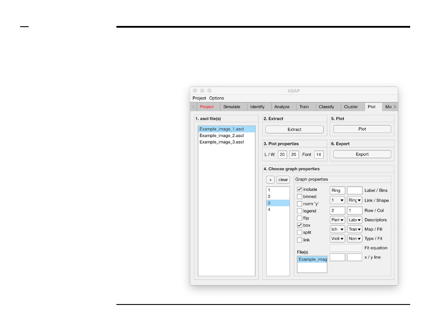
Instructions
/ Each plot (figure) is composed of
smaller subplots positioned at
specific rows and columns.
/ Each subplot is composed of 1 or
more graphs visually representing
numeric data.
/ To create a graph press the button
labeled ‘+’ located on the top-left
corner in the panel titled ‘4. Choose
graph properties’.
/ The large listbox located
underneath in the same panel will
be populated with the name of the
created graph as shown in the
figure on the right.
/ Multiple graphs can be created at
once by pressing the ‘+’ button
multiple times.
/ To clear (remove) all graphs and
start from scratch press the button
labeled ‘clear’ in the same panel.
Guide ⇲

Statistical and visual analysis
Selection of graph properties (2/6)
Instructions (contd.)
/ To define what is represented by
one graph, select the graph name
from the listbox earlier referred to.
Once selected the graph name will
be highlighted.
/ For each graph / plot, the
following properties can be
modified, defined or selected:
1. Graph property: to include
the selected graph in a plot,
check the checkbox labeled
‘include’.
2. Graph property: to include
structures previously
binned during analysis and
classification in the
selected graph, check the
checkbox labeled ‘binned’.
3. Plot property: to normalize
the y - axis (i.e. plot the
probability instead of the
number of counts), check
the checkbox labeled ‘norm
’y’’.
4. Plot property: to include a
legend for 1 or more
graphs, check the checkbox
labeled ‘legend’.
5. Plot property: to flip the x -
and y - axes, check the
checkbox labeled ‘flip’.
Please turn over
Guide ⇲

Statistical and visual analysis
Selection of graph properties (3/6)
Instructions (contd.)
6. Plot property: to include a
bounding box around a
plot, check the checkbox
labeled ‘box’.
7. Plot property: to split
graphs belonging to the
same subplot into different
sub subplots, check the
checkbox labeled ‘split’.
8. Graph property: to link one
graph to another graph (i.e.
include two graphs in the
same plot) select the graph
name of the mother graph
to which the selected child
graph should be linked to
from the drop down menu
labeled ‘Link’ and check the
checkbox labeled ‘link’.
Once the checkbox is
checked, the name of the
mother graph will be
modified to include an (*).
§ Warning 1:
Do not link a mother graph
to a child / mother graph.
Only child to mother graph
linking is permitted.
§ Warning 2:
Do not check the ‘link’
checkbox prior to selecting
the linked to graph.
Please turn over
Guide ⇲

Statistical and visual analysis
Selection of graph properties (4/6)
Instructions (contd.)
9. Graph property: select 1 or
more file(s) from the
listbox labeled ‘File(s)’.
10. Graph property: to include
a sample label type a label
in the text edit field labeled
‘Label’.
11. Graph property: to
manually set the number of
bins of a histogram, type
the number of bins in the
text edit field labeled ‘Bins’.
The input number will only
be processed when the
plotted graph is a
histogram.
12. Graph property: select a
shape from the dropdown
menu labeled ‘Shape’.
13. Graph properties: enter
the row and column
numbers of the plot to
which the currently
selected graph belongs.
Please turn over
Guide ⇲

Statistical and visual analysis
Selection of graph properties (5/6)
Instructions (contd.)
15. Graph properties: select
the 2 descriptors to be
plotted from the 2
dropdown menus labeled
‘Descriptors’.
16. Plot property: to change
the set of colors used for
plotting a plot, select a color
map from the drop down
menu labeled ‘Map’.
17. Plot property: to change
the filling for histogram(s),
bar plot(s) and box plot(s)
select a filling from the
dropdown menu labeled
‘Fill’.
18. Plot property: select a plot
type from the dropdown
menu labeled ‘Type’.
Please turn over
Guide ⇲

Statistical and visual analysis
Selection of graph properties (6/6)
Instructions (contd.)
19. Plot property: select a
fitting curve from the
dropdown menu labeled
‘Fit’. If ‘custom’ is selected,
the edit field labeled ‘Fit
equation’ will be enabled.
20. Plot property: type a fitting
equation and starting
points between rectangular
brackets in the text edit
field labeled ‘Fit equation’
if enabled:
a. a * x + b [1 1]
b. ln(x / sqrt(2))
c. a * x ^ 3 + x ^ 2 + x
[10]
d. x / ((x ^ 2) + m) [3]
e. erf((x + d - s) / l * 2)
[0.1 10 100]
21. Plot properties: to draw a
vertical dashed line at a
specific x - and / or y -
value(s), type the x - and /
or y - values in the text edit
fields labeled x / y line.
Guide ⇲


Statistical and visual analysis
Data export (2/2)
Guide ⇲
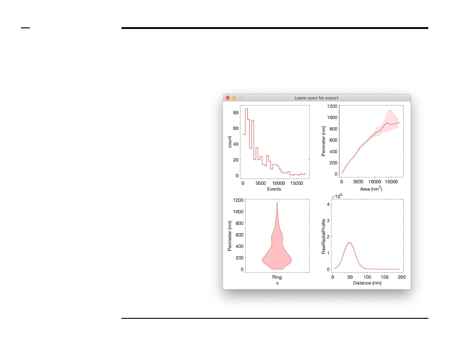
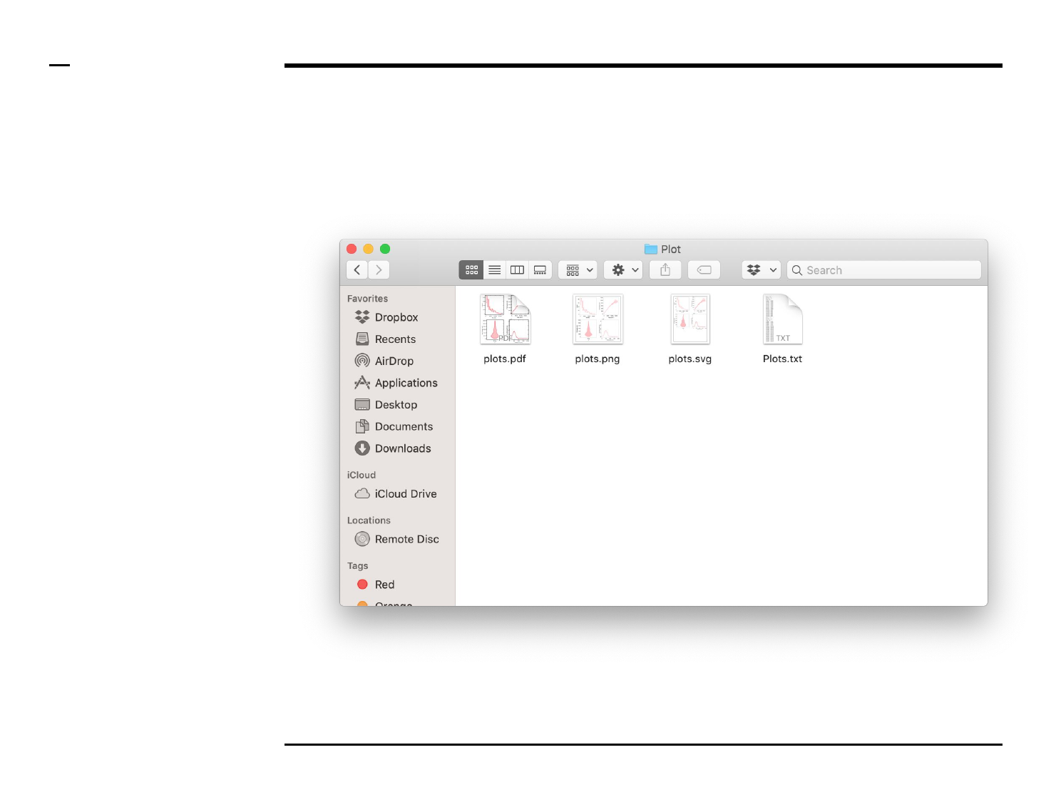
Instructions (contd.)
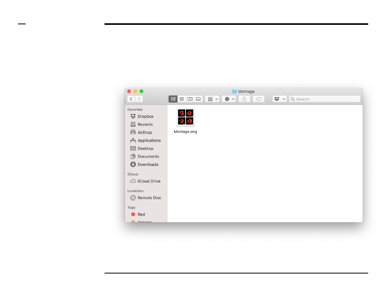
A folder named ‘Plot’ will be
created in the output folder and the
following 4 output files will be
placed in the folder:
1. ‘plots.png’ - file: png file of
the plot.
2. ‘plots.pdf’ - file: pdf file of
the plot.
3. ‘plots.svg’ - file: svg file of
the plot.
4. ‘xx.txt’ - file: text file
containing a summary of
the graphs including
relevant parameters.

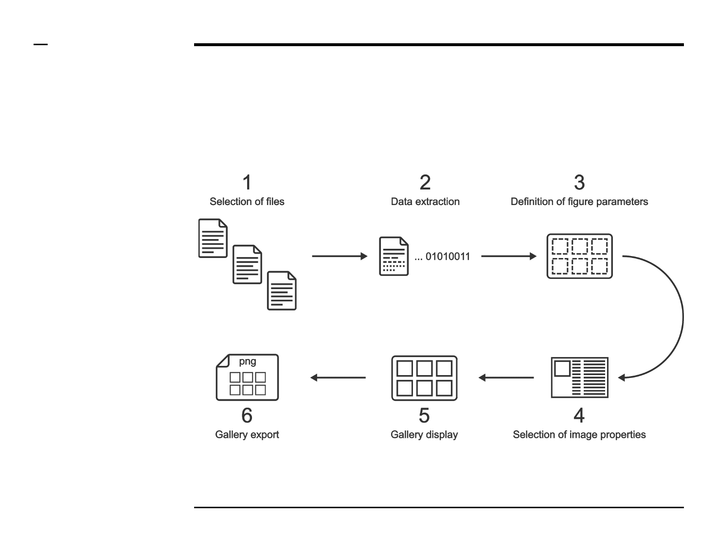
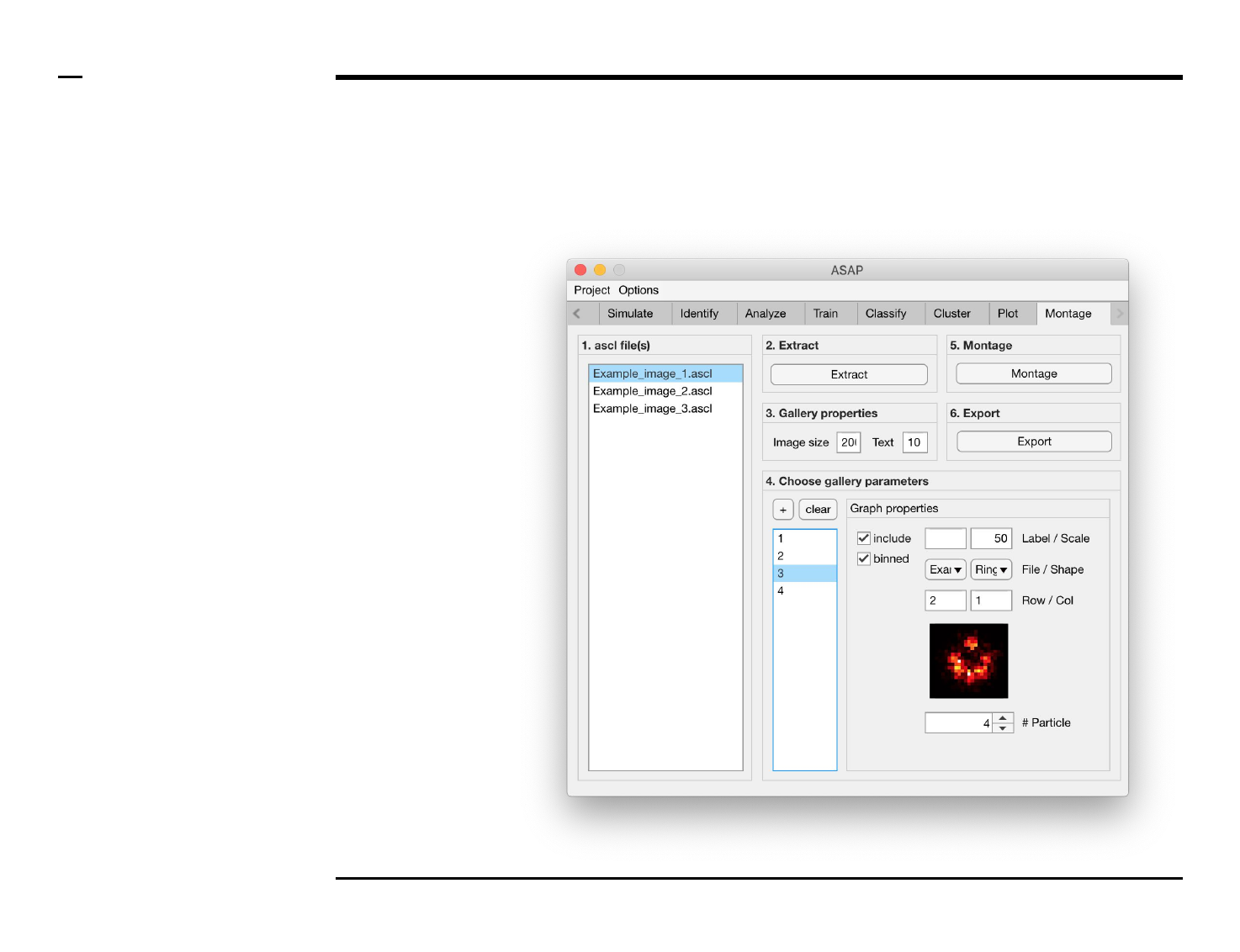
Montage construction
Selection of files
Instructions
/ Select the ‘Montage’ tab from the
tabs’ bar.
/ The listbox in the panel titled ‘1.
ascl files’ will be populated with the
names of ascl files located in the
input folder previously selected ⇲.
/ Select files by holding the CTRL
key and right-clicking the desired
files in the listbox in the same panel.
Selected files will be highlighted as
shown in the figure on the right.
Guide ⇲


Montage construction
Definition of montage properties
Instructions
/ The size of single image and text
size in the gallery can be defined by
setting the numeric edit fields
labeled ‘Image size’ and ‘Text’
respectively in the panel titled ‘3.
Gallery properties’.
/ The units of the text size is in
pixels.
Guide ⇲

Montage construction
Selection of montage parameters (1/3)
Instructions
/ Each gallery (figure) is composed
of smaller images positioned at
specific rows and columns.
/ To add images press the button
labeled ‘+’ located on the top-left
corner in the panel titled ‘4. Choose
gallery parameters’.
/ The large listbox located
underneath in the same panel will
be populated with the name(s) of
the add images, or particles, as
shown in the figure on the right.
/ Multiple images can be added at
once by pressing the ‘+’ button
multiple times.
/ To clear (remove) all graphs and
start from scratch press the button
labeled ‘clear’ in the same panel.
Guide ⇲

Montage construction
Selection of montage parameters (2/3)
Instructions (contd.)
/ To define what is represented by
one image, select the image name
from the listbox earlier referred to.
Once selected the image name will
be highlighted.
/ For each image, the following
parameters can be modified,
defined or selected:
1. Image property: to include
the selected image in the
gallery, check the checkbox
labeled ‘include’.
2. Image property: to include
binned structures in the
gallery, check the checkbox
labeled ‘binned’.
3. Image property: to label
the selected image in the
gallery, type a label in the
text edit field labeled
‘Label’.
4. Image property: to add a
scale bar to the selected
image in the gallery, type
the length of the scale bar
(in nanometers) in the text
edit field labeled ‘Scale’.
Please turn over
Guide ⇲

Montage construction
Selection of montage parameters (3/3)
Instructions (contd.)
5. Image property: select a
file from the dropdown
menu labeled ‘File’.
6. Image property: select a
shape from the dropdown
menu labeled ‘Shape’.
7. Image properties: select
the row and column to
which the selected image
belongs from the
dropdown menus labeled
‘Row’ and ‘Col’
respectively.
8. Image property: scroll
through the structures in
the selected file and of the
selected shape by
modifying the value of the
spinner labeled ‘# Particle’.
The in-app figure located
above the spinner will be
updated to show the
selected structure.
§ Warning 1:
The row and column values of one
image should not coincide with the
row and column values of another.
Ensure this condition is satisfied to
prevent error propagation.
Guide ⇲