User Guide
User Manual:
Open the PDF directly: View PDF ![]() .
.
Page Count: 23
Path-Flyer:
A Benchmark of Quadrotor Path Following Algorithms
USER GUIDE
Authors:
Bartomeu Rub´ı, Adri´an Ruiz, Bernardo Morcego, Ramon P´erez
Specific Center of Research CS2AC at Universitat Polit`ecnica de Catalunya (UPC).
Rbla Sant Nebridi 22, Terrassa (Spain). (email: tomeu.rubi, adrian.ruiz, bernardo.morcego,
ramon.perez at upc.edu)
November 2018
Contents
1 Introduction 1
2 Installing the Benchmark 2
3 User Interface 3
4 Modifying Parameters 5
4.1 ModelParameters ................................. 5
4.2 InitialConditions.................................. 7
4.3 WindDisturbance ................................. 10
4.4 MeasurementNoise................................. 12
5 Implement Your Own Algorithm 14
6 Program a New Reference Path 19
ii

Introduction
This document is the user guide of the Path-Flyer simulator: a benchmark platform for
testing path following algorithms on a quadrotor vehicle.
The benchmark has been build upon the Quad-Sim1platform, a quadrotor simulation
tool developed on the Drexdel University for simulation and control of quadrotors. That is,
it has been improved and modified to have a realistic mathematical and dynamic model of the
quadrotor and its environment, to implement a proper structure to solve the path following
problem and include various PF algorithms, and to incorporate new functionalities suited for
the present benchmark.
Some key features of Path-Flyer are:
•It has a complete and experimentally validated model of the Asctec Hummingbird
Quadrotor.
•Wind disturbance and noise on the measured states are modeled and can be customized.
•Two path following algorithms, Non-linear Guidance Law (NLGL) and Carrot-Chasing,
and its adaptive versions have been implemented.
•Path following algorithms can be tested in diverse simulation scenarios.
•A user interface helps the user to modify test conditions and to explore simulation
results.
•It is modular and programmable, meaning that new path following algorithms and/or
reference paths can be incorporated with ease.
In this user guide it is found how to install the benchmark, how to use the user interface,
how to modify parameters such as wind disturbance or noise, how to program a new algo-
rithm and how to incorporate new path references.
Hope you find it useful. If you have any doubts do not hesitate to contact us.
Note: More information about the mathematical model of the quadrotor and its environ-
ment, the implemented path following algorithms and control structure, and the validation
process of the Path-Flyer platform in the following publication:
Rub´ı, B., Ruiz, A., Morcego, B., and P´erez, R. (2019). Path-Flyer: A Benchmark of Quadro-
tor Path Following Algorithms. In 2019 15th IEEE International Conference on Control and
Automation (ICCA).
1https://github.com/dch33/Quad-Sim
1
Installing the Benchmark
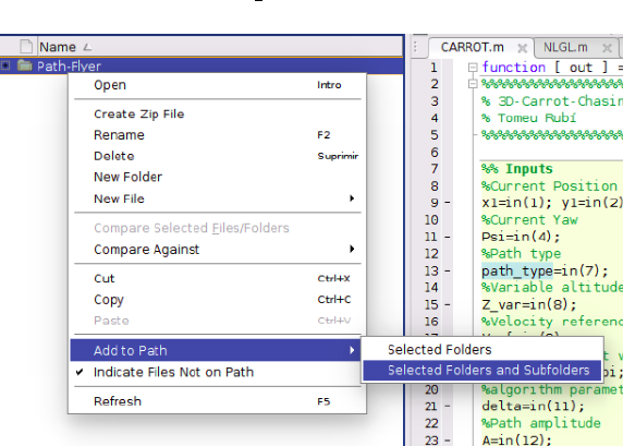
Installing the Benchmark is very simple: just copy the Path-Flyer folder provided within the
benchmark files into the MATLAB work path. Make sure to add all folders and subfolders
as shown in Fig. 1. Then open the Path Flyer.slx Simulink model, and simulate!
Figure 1: Add Folders and Subfolders.
Note: This benchmark has been developed with MATLAB R2017b version.
2
User Interface
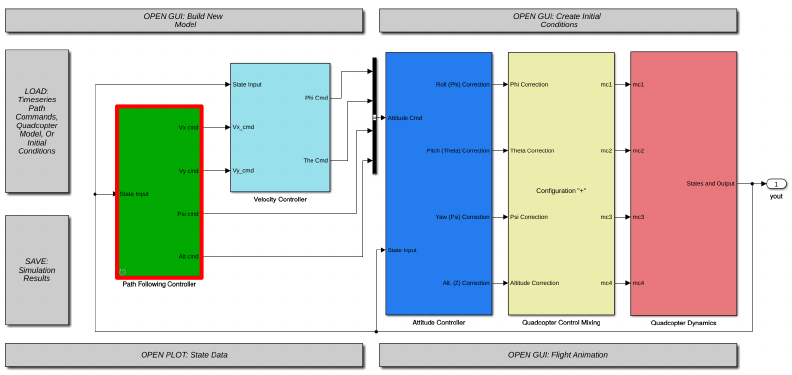
In addition to the functionalities of the original Quad-Sim platform (grey blocks) this bench-
mark also presents a user interface to help the user to modify the path following simulation
scenarios and explore simulation results. This user interface can be opened by double-clicking
the Path Following Controller block in the Simulink model (Fig. 2).
Figure 2: Double-click Path Following Controller to open the user interface.
The user interface (Fig. 3) is divided in two parts: the Path Following Control (red) and
the Path Following Evaluation (blue).
In the Path Following Control part the user can:
1. Choose the path following algorithm from a drop-down list. In this version the available
algorithms are NLGL and Carrot-Chasing, and its adaptive versions.
2. Specify the value of the control parameter of the algorithm (Lfor the NLGL and δfor
the Carrot-Chasing). Some path following algorithms only have one parameter to tune
(i.e. NLGL and Carrot-Chasing), however, if the algorithm has more than one control
parameter, the other parameters will have to be declared inside the algorithm code.
3. Select the adaptive version of the chosen algorithm. That is, the control parameter
or parameters of the algorithm are selected automatically. Note that if this option is
active, the value of the control parameter specified previously is ignored. However, if
there is not implemented an adaptive version of the algorithm, the simulator will run
the standard version of it.
3
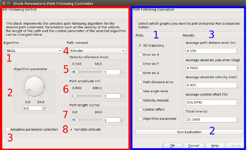
4. Choose the reference path from a drop-down list. In this version, four paths are avail-
able: a circle, a lemniscata (eight-shaped), a spiral and a line plus a circle path.
5. Specify the velocity reference of the Quadrotor.
6. Select amplitude of the path. That is, the radius of the circle (in the circular and
line+circular paths), the radius of the small circle of the lemniscata and the growth rate
of the spiral.
7. Select the number of turns on the path to be performed by the vehicle.
8. Select if the altitude of the path is variable or not. If this selector is not active the path
reference is defined on the xy plane at 3 mof altitude. If it is active, the path’s altitude
will be increasing constantly upon the evolution of the γparameter, starting at 3 m.
Figure 3: User interface.
In the Path Following Evaluation part the user can:
1. Choose which graphs want to plot.
2. Run an Evaluation that will plot the selected graphs and display relevant results of the
previous performed simulation.
3. View relevant values of the last performed simulation, once the evaluation has been
run.
4
Modifying Parameters
In this platform, diverse parameters can be modified: this section explains how to do it.
Model Parameters
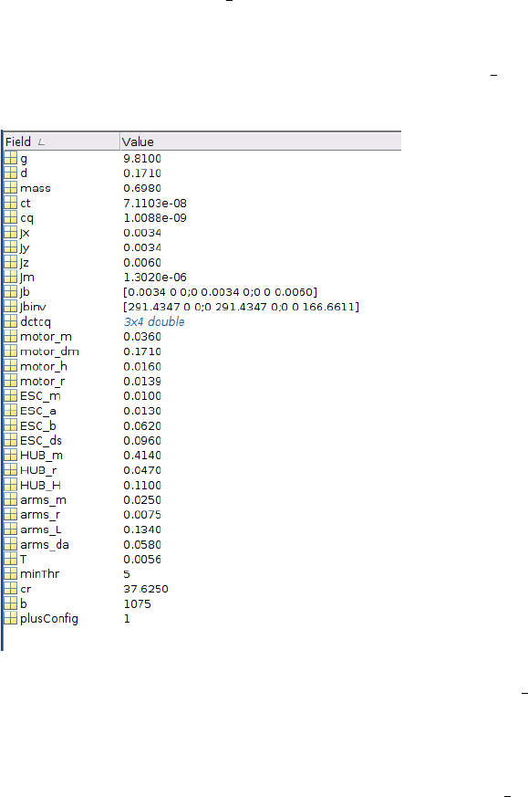
The parameters of the quadrotor vehicle are stored in a .mat MATLAB structure, which
is loaded at the time the Simulink model (Path Flyer.slx) is opened. The structures are
located in the /Quadcopter Structure Files/ folder. The fields of the model parameters
structure are described in detail in the Quad-Sim documentation.
The user can modify the value of the parameters stored in the Hummingbird +.mat struc-
ture, which contains the parameters of the Asctec Hummingbird Quadrotor (Fig. 4).
Figure 4: Parameter structure of the Asctec Hummingbird vehicle (Hummingbird +.mat).
Alternatively, the user can create a new structure file and complete it with the parameters
of other quadrotor vehicle. It is important to note this structure must contain the same fields
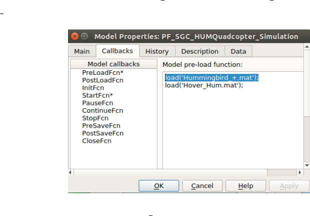
as the original structure. Then, the structure file that is pre-load on the Path Flyer.slx
must be modified. To do so, follow in the Simulink model:
File →Model Properties →Model Properties →Callbacks →PreLoad
5
Initial Conditions
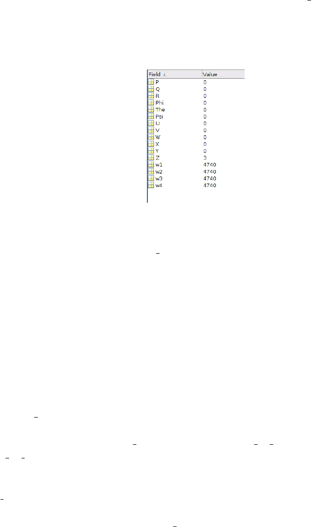
The initial conditions (IC) vector is stored in a .mat MATLAB structure, which, as the model
parameter structure, is loaded at the time the Simulink model (Path Flyer.slx) is opened.
The IC structures are located in the /Initial Conditions/ folder. This structure is formed by
the angular velocities (3, in deg
/s), the Euler angles (3, in deg), the linear body velocities (3,
in m
/s), the position (3, in m) and the angular velocity of the motors (4, in rpm), as shown
in Fig. 6.
Figure 6: Initial Conditions vector.
The original IC structure, Hover Hum.mat, defines an initial altitude of 3 meters, and
the initial angular velocity of the motors at the hover state of Hummingbird vehicle. It is
important to mention that an initial position of (x = 0, y = 0, z = 0) implies that the vehicle
will start on the initial point of the reference path. Meaning that it will not necessarily start
at the origin point on the space. Similarly, a value of 0 on the Psi angle means that the
vehicle starts with the correct orientation to follow the path. Changing the value of the IC
vector will represent an increment over this point and orientation.
As with the Model Parameters structure, the user can either modify the original IC vector
file, or create a new structure following the same fields. We recommend to keep the orig-
inal file, as creating a new one implies modifying more than one thing on the Simulink model.
If a new IC vector file is created, it will be necessary to change the preloaded IC structure
on the Path Flyer.slx Simulink model. To this end, follow this:
File →Model Properties →Model Properties →Callbacks →PreLoad
and replace the line load(Hover Hum.mat) by load(YOUR IC STRUCTURE.mat) where
”YOUR IC STRUCTURE” is the name of the structure you have created (Fig. 7).
Also, the user will need to modify a callback code on the Path Following Controller
block user interface. To do this, right-click on Path Following Controller block on the
Path Flyer.slx Simulink model, and follow:
Mask →Edit Mask →Parameters & Dialog
and then, open the callback of the ”Path type” mask item as denoted in Fig. 9.
7
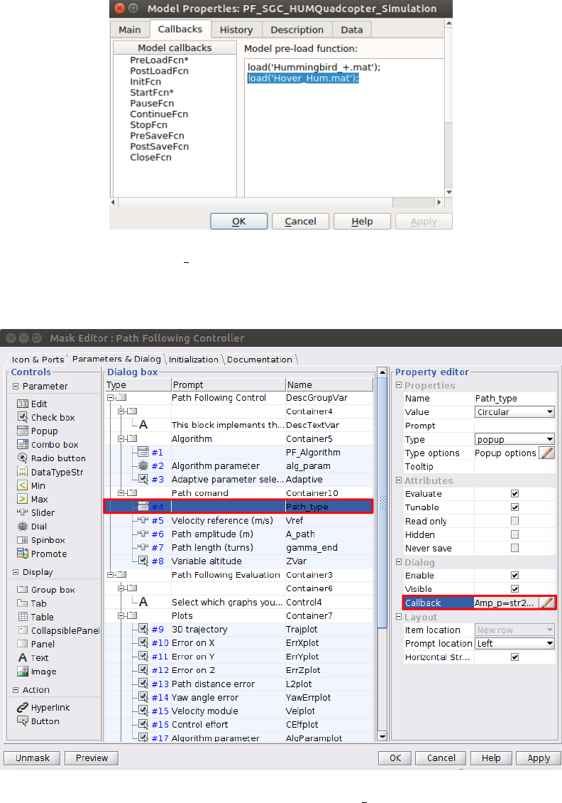
Figure 7: Modify load(Hover Hum.mat) to add your IC structure name on the pre-load
callback.
Figure 8: Open the callback of the Path type mask item.
8
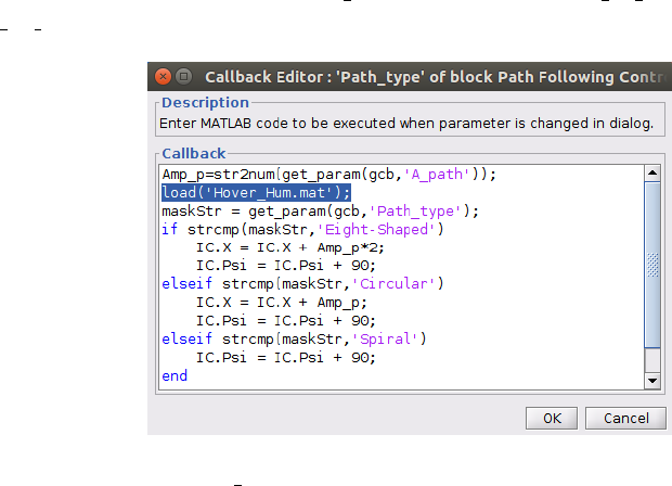
Finally, replace the line load(Hover Hum.mat) by load(YOUR IC STRUCTURE.mat), where
”YOUR IC STRUCTURE” is the name of the structure you have created.
Figure 9: Modify load(Hover Hum.mat) to add your IC structure name on the mask callbak.
9
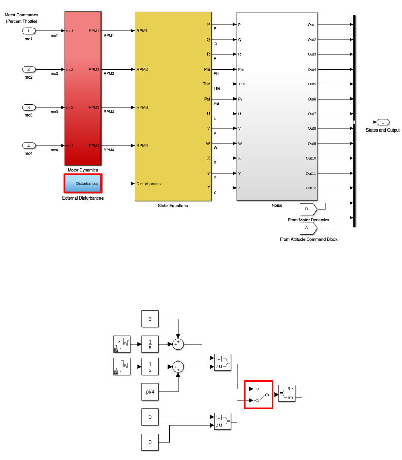
Wind Disturbance
The wind disturbance section is found inside the Quadcopter Dynamics block on a block
named External Disturbances, as shown in Fig. 10. In this block the user can generate
any desired wind disturbance profile on each of the 3 axis. Wind disturbance signals are
interpreted as wind velocities.
Figure 10: External Disturbance block is found inside the Quadcopter Dynamics block.
Figure 11: Wind disturbance velocities defined on the benchmark.
10
By default, there is not any active wind disturbance. Nevertheless, we defined a wind
disturbance profile that can be activated anytime before or during a simulation by clicking
on a selector, as shown in Fig. 11. The defined wind disturbance is a random walk signal on
the xand yaxis. This random walk is generated by integrating the signal of the Band-limited
white noise simulink block to a constant value. This process is performed with the velocity
module and direction of the wind, being 3 m
/sand π
/2rad the constant values, respectively.
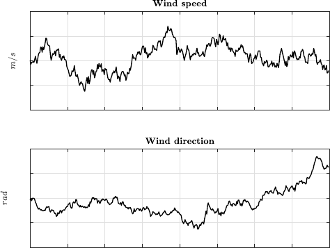
The resultant wind disturbance signal is shown in Fig. 12.
0 5 10 15 20 25 30 35 40
1
2
3
4
5
0 5 10 15 20 25 30 35 40
0.4
0.6
0.8
1
1.2
Figure 12: Wind disturbance generated with a random walk.
The user can modify the constant values of this random walk as well as the parameters
of the Band-limited white noise block which are the seed of the random value generator, and
other two values related to the frequency and amplitude of the signal. Alternatively, the user
can create its own wind disturbance profile.
11
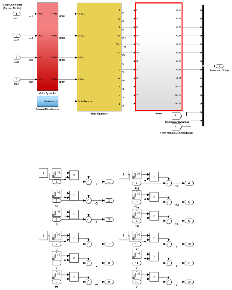
In this block (Fig. 14) the user can choose which of the twelve measured states (position,
velocity, orientation or angular velocity) must present noise. That is, if the value of the
Constant simulink block related to each set of states is set to 1 noise will be introduced, and
if constant is 0 it is disabled. Noise is generated by adding the signal of a Band-limited white
noise block to the corresponding state. The user can customize the amplitude and frequency
of the noise inside each of these blocks. In this benchmark noise signals have been set as
those that resemble more the behavior of sensors of the real Asctec Hummingbird platform.
13

Implement Your Own Algorithm
In the /Functions/Path following/ folder (within the benchmark files) there exist a template
function named NEW ALGORITHM FILE.m that the user can use to program a new path following
algorithm in the benchmark. In this template, the inputs and outputs of the function and the
initialization of the path are already defined. Note that those fields can not be modified. Ad-
ditionally, there is an empty "TO DO" space where the user must implement its own algorithm.
Here are some considerations to care about when implementing a new algorithm:
•The inputs and outputs of the path following algorithm function are shown in Table 1.
The user is free to use any of the stated inputs, but must fill all the outputs, with special
attention to the velocities, altitude and orientation command references. The errors
(ErrX, ErrY and ErrZ) must contain the distance between the vehicle and the closer
point to the path on each axis. Remember to put a simulation ending condition
(when vehicle completes the path) that set the variable End Path to 1.
•The reference path is discrete and is stored in three vectors, one for each component
(P x,P y and P z). The path is created with a parametric function that depends on
parameter γ(Px(γ), Py(γ) and Pz(γ)). The γparameter is defined from 0to g end.
The value of g end is obtained by multiplying the number of path ”turns” (defined
in the user interface) by 2π. Thus, it can be considered that γis given in radians.
Nevertheless, paths are defined with a precision of 1
/1000 rads, meaning that
P x(1000) corresponds to the value of the component xof the path at γ= 1 rad.
•When performing a simulation, the algorithm function is called continuously in the
Path Flyer simulink model. Thus, we recommend to use persistent variables to ini-
tialize constants in such a way that they are only defined on the first execution of the
function.
14

Table 1: Parameters of algorithm template.
Name Description
INPUTS
x, y, z Position of the vehicle in the three coordinates (in meters).
psi ψ- yaw orientation (in radians).
u, v Body velocities (in m
/s) on the xand ydirection, respec-
tively.
Path type Variable the indicates which path must be created (circle,
line, lemniscata, ...).
z var Variable that indicates if the created path must vary the
altitude or not.
Vref Desired velocity (in m
/s).
g end Last value of γof the path (needed to create the path).
ALG PARAMTER
Parameter of the programmed algorithm that can be tunned
in the user interface (Change the name to the corresponding
parameter, if desired).
AVariable that indicates the amplitude of the path.
OUTPUTS
u cmd, v cmd Command for the body velocities on the xand ydirection,
respectively, sent to the velocity controller.
psi cmd ψcmd - yaw orientation command sent to the attitude con-
troller.
z cmd Altitude command sent to the altitude controller.
ErrX, ErrY, ErrZ Instant distance error between the vehicle and the path on
the x,yand zaxis, respectively.
End Path Boolean variable. If this variable is set to 1, simulation is
stopped.
out(9) Output that can be used for debugging (currently linked to
the algorithm parameter value).
15
Once the algorithm is programed in the provided template and the name of the template
file is changed with the algorithm’s name, the following steps must be followed to include the
algorithm in the benchmark:
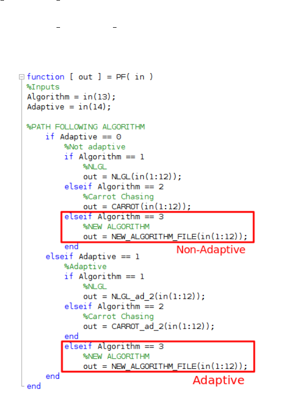
First, open the PF.m file, found in the /Functions/Path following/ path, and add a call
to the algorithm’s function as shown in Fig. 15. That is, include the line
out = NEW ALGORITHM FILE(in(1:12));
inside an ”elseif” statement of variable Algorithm, which indicates which algorithm must
be executed. Again, ”NEW ALGORITHM FILE” represents the name of your algorithm file. In
this example, the incorporated algorithm is the third one, thus, the algorithm is called inside
the a ”Algorithm == 3”if statement.
Figure 15: Add a call to the algorithm’s function inside the Algorithm - if statement.
Note that there is another variable named Adaptive, which indicates if the executed
algorithm is adaptive of not. If both adaptive and non-adaptive versions of the algorithm
have been implemented, add a call to the non-adaptive version inside the ”Adaptive == 0”
16

statement as shown:
if Adaptive == 0
if Algorithm == 1
...
elseif Algorithm == 3
out = NEW ALGORITHM FILE(in(1:12));
end
...
And add a call to the Adaptive version of it, inside the ”Adaptive == 1” statement, as
follows:
...
elseif Adaptive == 1
if Algorithm == 1
...
elseif Algorithm == 3
out = NEW ADAPTIVE ALGORITHM FILE(in(1:12));
...
end
end
where ”NEW ADAPTIVE ALGORITHM FILE” is the name of the file wherein the adaptive version
of the algorithm is implemented.
If only the non-adaptive version of the algorithm has been implemented, add
a call to this function on both sides (when Adaptive == 0 and when Adaptive == 1),
in such a way that the algorithm will be executed without taking into account the value of
the ”adaptive parameter selection” button on the user interface (Fig. 3).
After adding a call of the algorithm on the PF.m file, the user must add a new field on
the user interface algorithm list, in order to include it in the set of algorithms that can be
simulated in the benchmark. To do so, right-click on Path Following Controller block on the
Path Flyer.slx Simulink model, and open the list of parameters of the mask:
Mask →Edit Mask →Parameters & Dialog
and then, open the ”popup options” of the ”PF Algorithm” mask item as denoted in Fig. 16.
17
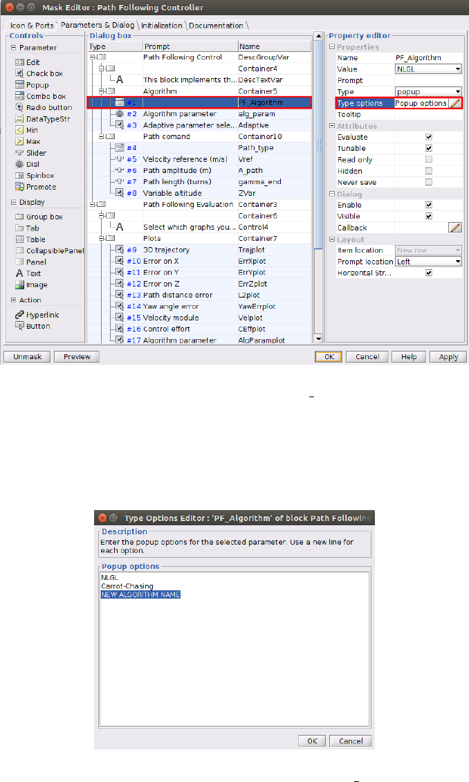
Figure 16: Open the popup options of the PF Algorithm mask item.
Then, add the name of the implemented algorithm in the pop-up list (as it is desired that
it appears in the user interface algorithm’s list) as denoted in Fig. 17. It is important that the
order of the algorithm names is preserved, since it is related to the value of the Algorithm
parameter found in the PF.m file.
Figure 17: Add the name of the algorithm in list of the PF Algorithm mask item.
18
Program a New Reference Path
In the /Functions/Path following/ folder (within the benchmark files) there is a function,
named CreatePath.m, in which the reference paths are defined. To create a new reference
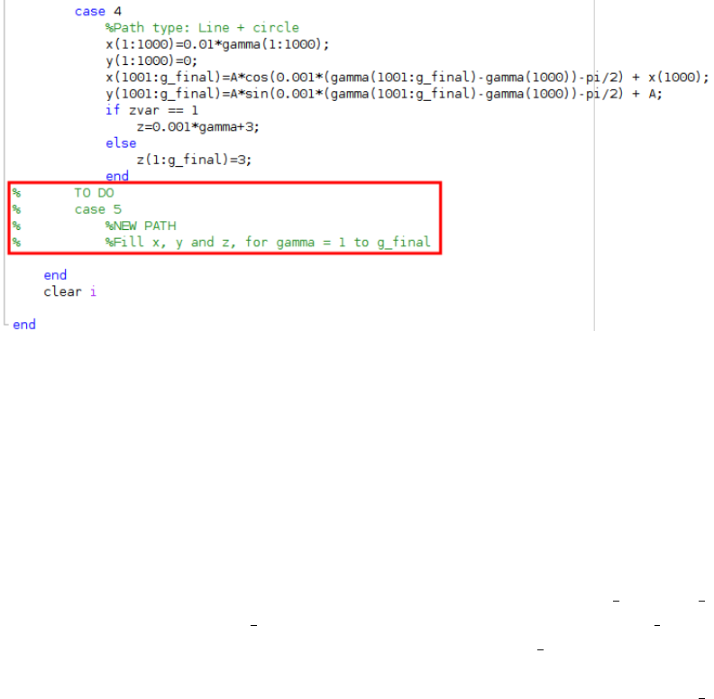
path the user must program it inside a swith-case statement, as denoted by a "TO DO"
inside the file (Fig. 18). The variable of the swith-case statement is named type and it is
used to defined which path must be performed on each simulation (for instance, type = 1
means that an eight-shaped path will be simulated).
Figure 18: Create the path inside the swith-case statement on the CreatePath.m function.
The reference path is discrete and is stored in three vectors, one for each component (x,y
and z). The path is programmed with a parametric function that depends on parameter gamma
(x(gamma),y(gamma) and z(gamma)). Note that gamma is different from the γparameter
stated in the previous section. That is, γis the arc length parameter used to define the
path mathematically (given in radians), while gamma is a parameter used to discretize and
program the path. A value of γ= 1 rad corresponds to a value of 1000 of the parameter
gamma, meaning that paths are defined with a precision of 1
/1000 rad.
In the CreatePath.m function, parameter gamma is defined from 0to g final.g final
parameter is different from the g end stated in the previous section. That is, g end defines
the last point of the path that is being simulated (in rad), while g final is the total length
of the defined path (in 1
/1000 rad) and is usually longer than the simulated path (note that in
a simulation, the traveled path length is not necessary the total length of the path). g final
is pre-defined to 100000, but its value can be modified to change the total path length if
desired. Note that paths are created in such a way that a value of gamma of 6283 (2 ·π·1000)
represents a full lap on the path. This condition must be taken into account when creating
a new path.
19
Summarizing, to create a new path the user must fill all the three vectors components
of the path (x,yand z) for each value of gamma, from 0to g final, assuring that a gamma
= 6283 is when a lap is completed (if path is circular). This must be included inside an
swith-case statement of the type variable on the CreatePath.m function.
After defining the path on the CreatePath.m file, the user must add a new field on the
user interface path list, in order to include it in the set of paths that can be simulated in the
benchmark. To do so, right-click on Path Following Controller block on the Path Flyer.slx
Simulink model, and open the list of parameters of the mask:
Mask →Edit Mask →Parameters & Dialog
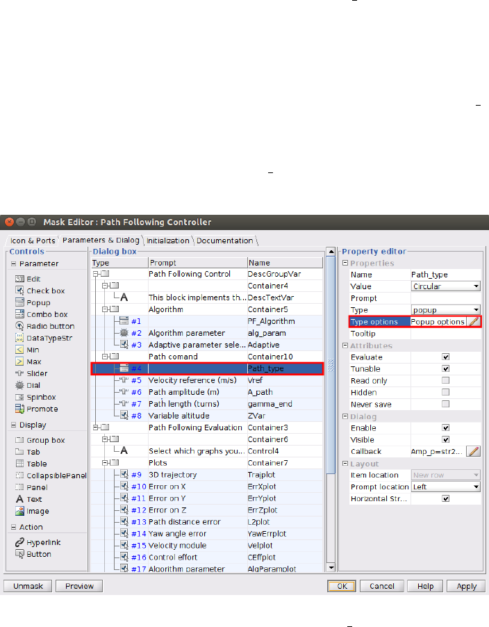
and then, open the ”popup options” of the ”Path type” mask item as denoted in Fig. 19.
Figure 19: Open the popup options of the Path type mask item.
Then, add the name of the created path in the pop-up list (as it is desired that it appears
in the user interface path’s list) as denoted in Fig. 20. It is important that the order of the
paths names is preserved, since it is related to the value of the type parameter found in the
CreatePath.m file.
20
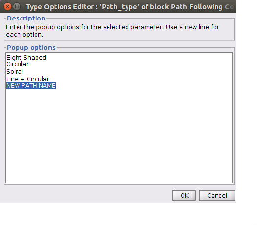
Figure 20: Add the name of the implemented algorithm in list of the Path type mask item.
21
