User Guide

User Manual:

Open the PDF directly: View PDF .
Page Count: 45

PyVASCO

User guide

Patricia Ribes Metidieri

Ida Aichinger

Christina Yin Vallgren

TE-VSC

CERN - Geneva, Switzerland

Contents

Contents 2

1 About PyVASCO 3

1.1 Getting started . . . . . . . . . . . . . . . . . . . . . . . . . . . . . 3

1.2 Authors and contributors . . . . . . . . . . . . . . . . . . . . . . . 4

1.3 Contact . . . . . . . . . . . . . . . . . . . . . . . . . . . . . . . . . 4

2 Basic concepts 5

2.1 Motivation and main advantages with respect to VASCO . . . . 5

2.2 Dynamic vacuum model . . . . . . . . . . . . . . . . . . . . . . . 5

2.3 Electron stimulated desorption . . . . . . . . . . . . . . . . . . . 6

2.4 Treatment of cryogenic surfaces . . . . . . . . . . . . . . . . . . . 9

3 Inputs of PyVASCO 12

3.1 ’Old’ Input format . . . . . . . . . . . . . . . . . . . . . . . . . . . 12

3.2 ’New’ Input format . . . . . . . . . . . . . . . . . . . . . . . . . . 12

3.3 ESD curves format . . . . . . . . . . . . . . . . . . . . . . . . . . . 18

4 Layout and functionality 20

4.1 Menus . . . . . . . . . . . . . . . . . . . . . . . . . . . . . . . . . . 20

4.2 Tabs . . . . . . . . . . . . . . . . . . . . . . . . . . . . . . . . . . . 28

5 Extracting results with PyVASCO 39

5.1 Management and plot options . . . . . . . . . . . . . . . . . . . . 39

5.2 Exporting plots in different formats . . . . . . . . . . . . . . . . . 41

6 Benchmark with VASCO and Molﬂow+ 43

Bibliography 45

Chapter 1

About PyVASCO

PyVASCO (VAcuum Stability COde written in Python) is a code integrally de-

veloped at CERN for the simulation of pressure proﬁles in cylindrical geome-

tries considering beam induced effects.

The ﬁrst version of this program was distributed under the name IdaVac.

This program constitutes an update of VASCO (presented in [1]) and seeks to

optimize the performance of the original code for large geometries [2].

This program has been integrally developed in Python 2.7 and tested on

Windows 10.

1.1 Getting started

Installation

This version of PyVASCO includes an installer, called ’setup.exe’. In order to

install PyVASCO in your machine, launch the installer and follow the spec-

iﬁed instructions. Even if recommended, the installation using the setup is

not compulsory in order to launch PyVASCO. To launch the application with-

out installing, enter in the folder PyVASCO and double-click on the applica-

tion (’PyVASCO.exe’).

Developer tools

This version of PyVASCO is distributed together with its source code (in PyVASCO/

PyVASCO_Code/) and a portable python interpreter

PyVASCO/WinPython-64bit-2.7.6.4 with all the required dependencies al-

ready installed.

There’s also an API documentation available in web format in the direc-

tory docs/ under the name ’API.html’ or opening the program and selecting

the option ’Documentation’ in the menu Help or pressing the keyboard key

combination Ctrl+U.

4CHAPTER 1. ABOUT PYVASCO

To build a stand-alone python application from the source code:

•Make sure that Pyinstaller is installed in your computer:

–Open a command prompt and type pyinstaller.

–If you don’t have pyinstaller in your computer, in the same com-

mand prompt, type:

pip i n s t a l l p y i n s t a l l e r

•Enter in the directory containing the source code (PyVASCO_Code/) and

open the ﬁle ’PyVASCO.spec’. Paste the full path of the location of the

directory PyVASCO_Code in the tag pathex and save the changes.

•Open a command prompt in this directory and type:

p y i n s t a l l e r PyVASCO . spec

1.2 Authors and contributors

List of authors:

•Ida Aichinger

•Patricia Ribes Metidieri

List of contributors:

•Christina Yin Vallgren

•Giuseppe Bregliozzi

•Simone Callegari

1.3 Contact

In case of problems,if a bug is detected or if you have suggestions for further

development, please send an emalil to the following addresses:

•patricia.ribes.metidieri@cern.ch

Chapter 2

Basic concepts

2.1 Motivation and main advantages with respect

to VASCO

PyVASCO is an upgrade of a preexisting program at CERN: VASCO [1], and

it solves the same vacuum model. Even though this program is not as pre-

cise as other simulations tools for ultra high vacuum (UHV) based on Mon-

tecarlo techniques, its main advantages to are twofold: ﬁrst, PyVASCO can

easily simulate several gas species at a time and cross-desorption between

gas species. Second, it solves the vacuum model in Eq. 2.1 analytically, which

allows to simulate large portions of an accelerator in minutes.

The original VASCO, however, didn’t allow for simulations with more than

around 40 segments. The reason is that, in order to solve a system of Nsegments

it holds in memory matrices of dimension 8·Ngas ·Nsegments ×8·Ngas ·Nsegments.

PyVASCO takes advantage of the sparse structure of the solving matrices to

store the information of the system in arrays of dimension 8·Ngas ·Nsegments ×

17. Thus, the memory storage is reduced from O(N2) to O(N). This step is

fundamental in order to simulate large geometries.

For more information on the computer implementation of PyVASCO, see

Ref. [2].

2.2 Dynamic vacuum model

PyVASCO uses the same vacuum model as presented in Ref. [1] and, as in Ref.

[1], PyVASCO solves the equations of the model analytically. The purpose of

this section is to give a fast overview of the equations solved by PyVASCO and

to present some of the limitations of this vacuum model.

The model used in PyVASCO assumes the the rate of change of molecules

per unit volume depends uniquely on:

6CHAPTER 2. BASIC CONCEPTS

• molecular diffusion due to a density gradient;

• beam induced effects such as ion, photon and electron stimulated des-

orption;

• gas pumping through a distributed pumping (NEG of cryo-pumping)

or through lumped pumps located in the interconnection of segments;

• addition of gas to the system through lumped leaks and through ther-

mal outgassing.

PyVASCO assumes that the simulated vacuum system is made of cylin-

drical ﬁnite elements characterized with constant, time invariant parame-

ters (material properties, radius, pumps...), and it can take into account the

cross- desorption of gas of one specie by ions of other gas species (mu. Py-

VASCO considers four gas species: H2, CH4, CO and CO2, since these are the

dominant gas species in a backed ultra-high vacuum (UHV) system.

These assumptions allow to solve analytically the stationary equations

presented in 2.1 in 1-dimension.

As presented in Refs. [1] and [2], the main equation governing the station-

ary behavior of the vector volume density ~

n=(nH2,nC H4,nCO,nCO2) is

0=~

cspec

∂2~

∂x2+~

ηi~

σi−I

n−~

σi−I~

n−(~

Swal l +~

Cdi s)~

n−~

Scr yo(~

n−~

ne)+(2.1)

ηph ˙

Γph +~

ηe˙

Ne+a~

qth

The deﬁnition, dimension and units of the quantities in Eq. 2.1 are de-

ﬁned in Tab.

2.3 Electron stimulated desorption

The electron-stimulated desorption (ESD), the desorption process initiated

by electronic excitation, of atoms and molecules is an important factor in

determining the pressure proﬁle under beam induced effects.

In order to empirically characterize this effect for different gases, the so-

called ESD yield, ηeis deﬁned as:

ηe=Ni

(2.2)

where Niis the number of desorbed molecules of a given gas specie and Ne

is the number of incident electrons.

2.3. ELECTRON STIMULATED DESORPTION 7

Magnitude Units Dimension Deﬁnition

nm−34×1 Molecular density of the different gas species

cspec m4/s 4×4 Speciﬁc conductance. (Diagonal matrix)

ηi- 4×4 Ion stimulated desorption yield

σi−Im24×4 Ionization cross section of the gas-proton interaction

Swal l m2

s4×4 Distributed pumping speed per unit length due to NEG Si

wal l =α(T)a·¯

Cdi s m2

s4×4 Distributed pumping through holes per unit length

Scr yo m2

s4×4 Cryogenic pumping due to cryo-condensation, per unit length

nem−34×1 Thermal equilibrium density

ηph - 4×4 Photon stimulated desorption yield (diagonal matrix)

Γph 1

m s 1×1 Photon ﬂux to the wall per unit length

ηe- 4 ×4 Electron stimulated desorption yield (diagonal matrix)

Ne1

ms 1×1 Electron ﬂux to the walls per unit length

am Surface area per unit length

qth 1

m2s4×1 Thermal outgassing. (The user introduces the thermal outgassing in mbar l/s)

I A 1 ×1 Proton beam current

e C 1 ×1 Charge of the electron

Table 2.1: Symbol, units and description of the magnitudes used in Py-

VASCO’s model.

8CHAPTER 2. BASIC CONCEPTS

Figure 2.1: ESD curve for backed copper.

The ESD yields of different gases depend on the properties of the surface

where the molecules of the studied gases are adsorbed, on the temperature

and on gas specie.

The curve representing the ESD yields for a material as a function of the

accumulated electron dose is the ESD curve for that material, and it has been

observed that the ESD yields for different gases on materials relevant for UHV

systems decrease with the accumulation of incident electron dose (in electrons/cm2),

as presented in Fig. 2.1 for backed copper.

This phenomenon of decrease of the ESD with the accumulated electron

dose received in the walls is typically called conditioning effect (or scrubbing

effect).

This phenomenon is relevant for the vacuum performance of UHV sys-

tems under electron bombardment due to beam induced effects, like the

LHC, which performs dedicated scrubbing runs at the beginning of opera-

tion periods [3].

2.4. TREATMENT OF CRYOGENIC SURFACES 9

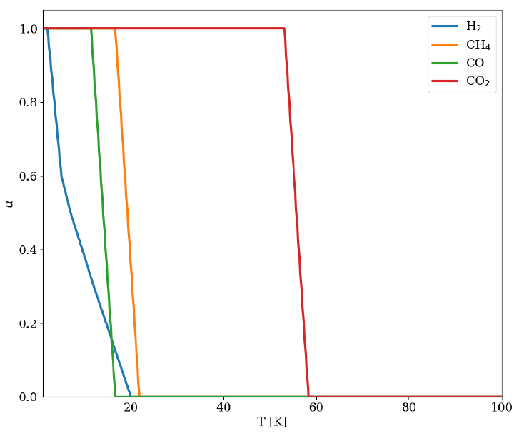
Figure 2.2: Equilibrium vapor pressure for different gases relevant in UHV.

2.4 Treatment of cryogenic surfaces

Basics concepts

The molecules of the gas species present in an UHV system mainly interact

with the surfaces of vacuum chambers through van der Waals forces.

The binding energies between the surface and the gas molecules increases

when the temperature of the system decreases, increasing the number of

adsorbed molecules. For sufﬁciently low temperatures, the surface cover-

age increases sufﬁciently for the van der Waals forces to start acting between

the molecules themselves. This regime is called cryocondensation. Once in

the cryocondensation regime at a ﬁxed temperature, a dynamic equilibrium

might be reached between the adsorbed and desorbed molecules of a given

gas specie, which translates to an equilibrium pressure of the gas over its con-

densed phase, called the equilibrium vapor pressure (Fig. . 2.2).

The sticking coefﬁcient for cryosorption and cryocondensation is deﬁned

α=Number of molecules "sticking" on a surface

Total number of molecules impinging on the surface (2.3)

The sticking coefﬁcient ignores the effects of the vapor pressure and it is

close to unity at sufﬁciently low temperatures.

A cold surface acts as a pump with the characteristic pumping speed pre-

10 CHAPTER 2. BASIC CONCEPTS

sented in Eq. 2.4:

Scr yo

i=αi

4¯

vi, (2.4)

where the αiis the sticking coefﬁcient for the gas specie i,Ais the area of the

cold surface and ¯

viis the average molecular speed of the gas specie i.

Cryogenic surfaces in PyVASCO

As explained in Sec. 3.2, PyVASCO divides a simulation in a main input de-

scribing the geometry and in basic components of a vacuum system, i.e., Ma-

terials,Pumps and Gasources. In order to avoid confusion, the properties of

all materials are deﬁned at room temperature and a cryogenic behavior is set

by default. In order to change the cryogenic behavior of a given material, see

...

IMPORTANT!: For temperatures below 100 K, PyVASCO doesn’t consider

thermal outgassing (it is set to zero). However, the value of the thermal out-

gassing is not changed with temperature. Therefore, in order to simulate a

system at a temperature considerably larger than room temperature, the user

has to modify the outgassing in the deﬁnition of the material or to deﬁne an-

other material with the correct outgassing for the temperature of interest.

Below 100 K, PyVASCO computes the distributed pumping speed of the

cryogenic surfaces as in Eq. 2.4, using for the sticking factor the correspond-

ing value as a function of the temperature set for the corresponding material

(in ...) . If this information is not provided, the following default options are

assumed:

• The dependence of the sticking factor with temperature for CH4, CO

and CO2are assumed to be the step functions presented in Fig.

• At temperatures below 20 K, the values of the sticking factor for H2as a

function of the temperature are taken from Ref. [4]. Due to the scarce

experimental data concerning the sticking coefﬁcient of H2on techni-

cal surfaces at cryogenic temperatures, the choice of the reference has

been arbitrary.

As can be seen in Eq. , the cryogenic pumping speed used in the vacuum

model implemented in PyVASCO is modulated by the equilibrium density,

ne. This term takes into account the reduction of the efﬁciency of the cryo-

genic pumping due to the desorption of molecules from the considered sur-

face. This term also implies that the cryogenic pumping becomes null when

2.4. TREATMENT OF CRYOGENIC SURFACES 11

Figure 2.3: Default dependence of the sticking coefﬁcient with temperature

at low temperatures.

the computed gas density in the considered segment equals the equilibrium

density for the temperature of the segment.

For a given temperature, PyVASCO estimates the values of the equilib-

rium density for the considered gas species for using the curves of Fig. 2.2,

truncated at a certain pressure to ensure that neis always smaller than the

computed density.

Chapter 3

Inputs of PyVASCO

3.1 ’Old’ Input format

As already mentioned, PyVASCO is based in VASCO, thus ’old’ input format

refers to VASCO’s input format, detailed in [1].

To ease the comparison between VASCO and PyVASCO, PyVASCO can ac-

cept CSV ﬁles written with the format of the ﬁrst program, as mentioned in

Subsection 4.2 and transform this ﬁles to the native format of PyVASCO.

3.2 ’New’ Input format

Writing input simulation ﬁles with a large number of segments in VASCO’s

input format might be tedious and the it might be difﬁcult to detect mistakes.

For this reason, PyVASCO uses a new input format, which seeks to make an

input ﬁle more readable.

A simulation in PyVASCO is built through a main simulation table plus

three different constituents: Materials,Pumps and Gas sources. These three

components are deﬁned and stored as independent building blocks, making

it possible to reuse them in different simulations.

Main input ﬁle

A geometric model in PyVASCO is built by cylindrical segments stuck to-

gether. An example of input ﬁle with the new format is shown in Tab. 3.1.

Input ﬁles in this format can be written using the integrated Input edi-

tor (in the menu Add →Input ﬁle or by pressing Ctrl+I) or in spreadsheet

programs (like Excel) or in a plain text editor (like WordPad or Notepad). An

example of how a simple input ﬁle would look like when using the integrated

editor is shown in Fig. 3.1.

The new input format consists in:

3.2. ’NEW’ INPUT FORMAT 13

Figure 3.1: Input example written in the integrated editor.

Table 3.1: Example of input ﬁle written in the ’new’ format.

14 CHAPTER 3. INPUTS OF PYVASCO

•Name of the simulation:

The name of the simulation must be written in the dedicated line edit

when using the integrated editor or, when using external editors like

Excel, it must be written in the ﬁrst row, ﬁrst column of the input ﬁle.

•Columns, labeled S1...SN, for the deﬁned segments:

Each column labeled S1...SNin the input ﬁle represents a segment in

the simulated geometry. For each segment the following information

has to be provided:

– d[mm]: The diameter of the segment (in mm), assumed to be

cylindrical.

– L[mm]: The length of the segment (in mm).

– T[k]: The average temperature of the segment.

– Material: Name of the material of the segment. The list of regis-

tered materials can be visualized in the menu File →Show Com-

ponents or pressing Ctrl+S. (See Show components in Section 4.1

and Materials in Section 3.2 for more details).

– Pump: The pumps speciﬁed in the main input ﬁle are lumped

pumps located on the left side of the segment where they are indi-

cated. The list of registered pumps can be visualized in the menu

File →Show Components or pressing Ctrl+S. In order to simulate

the union of two segments without a lumped pump in between,

P0 has to be written in the corresponding cell.

–Gas source: The gas sources in the main input ﬁle represent local-

ized leaks in the interconnections between segments and, in par-

ticular, located on the left side of the segment where they are indi-

cated.The list of registered pumps can be visualized in the menu

File →Show Components or pressing Ctrl+S. In order indicate to

PyVASCO that no leak exists in a certain location, G0 has to be

written in the corresponding cell.

– Photon ﬂux: PyVASCO accepts an homogeneous, constant pho-

ton ﬂux (in photons/m/s) impinging the walls of every segment.

– Electron ﬂux An homogeneous, constant electron ﬂux (in elec-

trons/m/s) can be added to the different simulated segments.

•End column:

This column is exclusively used to indicate the lumped pump and the

gas source located at the right side of the last simulated segment.

3.2. ’NEW’ INPUT FORMAT 15

Figure 3.2: 3D model of the simulated geometry presented in Tab. 3.1. (For

aesthetic reasons, the geometry has been shrinked in the longitudinal direc-

tion).

Thus, the example of Fig. 3.1 and Tab. 3.1, is composed by 3 copper segments

of the same same length and increasing diameters of 10, 20 and 40 mm, re-

spectively. The three segments are hold at room temperature and two lumped

pumps (called P16) are connected at the beginning of the ﬁrst segment (left

side) and at the end of the third segment (right side). There are no lumped

pumps connected nor on the right side of the ﬁrst segment nor on the right

side of the second segment, and there are no leaks along the geometry. A 3D

model of the described system can be seen in Fig. 3.2.

IMPORTANT!: If the user writes the main input in an external editor, the same

format as shown in Tab. 3.1 has to be used. The input ﬁle has to be saved in

CSV format.

Materials

The materials used in the main input ﬁle for the PyVASCO simulations have

to be deﬁned previously to their usage. PyVASCO offers the possibility of

deﬁning new materials in the dedicated Material editor, but the user can also

import a CSV ﬁle with the format shown in Tab. 3.2.

A material ﬁle deﬁned in PyVASCO consists in:

•Name of the material

The name with which this material will be called in the main input ﬁles.

16 CHAPTER 3. INPUTS OF PYVASCO

•Colums:

A material ﬁle always have 4 data columns, corresponding to the be-

havior of the deﬁned material with respect to the main dominant gases

in UHV, i.e. H2, CH4CO and CO2.

•Rows:

The different rows speciﬁed in the a materials ﬁle are:

– alpha: Sticking factor or sticking coefﬁcient (adimensional).This

quantity represents the probability which each of the deﬁned gases

have of sticking onto the surface of the segment. In the case of the

LHC, this parameter is used to represent the pumping due to NEG

in the warm sections and to physisorption (cryopumping) in the

cold sections.

IMPORTANT!: The sticking coefﬁcient deﬁned in this section

is always deﬁned at room temperature! PyVASCO scales the

sticking coefﬁcient with the temperature for the deﬁned cryo-

genic behavior of the material (See , for more information).

– eta_ion: Ion stimulated desorption yields ~

ηI(in molecules/inci-

dent ion) at a chosen ion impact energy (4×4 matrix, occupying

from row 2 to row 5).

– eta_e: Electron stimulated desorption yields (in molecules/ inci-

dent electron) at a chosen impact energy.

– eta_ph: Photon stimulated desorption yields (in molecules/inci-

dent photon) at a chosen photon energy.

– Cbs: distributed pumping speed per unit length (in l·s−1·m−1). In

the case of the LHC, this input parameter can be used to simulate

the pumping through pumping slots.

– Qth_total: Thermal outgassing rate per unit area at a chosen tem-

perature (in mbar·l·s−1·cm−2).

IMPORTANT!: If the user writes a material ﬁle in an external editor (Excel, for

example) the name of the material written in the ﬁrst row and column of the

material table has to match the name of the ﬁle. Moreover, the material ﬁle

has to be saved in CSV format.

3.2. ’NEW’ INPUT FORMAT 17

Table 3.2: Example of deﬁned material in PyVASCO.

IMPORTANT!: All the properties deﬁned for a certain material depend on the

temperature! For this reason it is important to register the same material held

at different temperatures as different entries by including the temperature in

the deﬁnition name. For example: use Cu@RT and Cu@5K to deﬁne copper

at room temperature and at 5 K, respectively.

IMPORTANT!: The outgassing rate of a given material is internally converted

to total outgassing by multiplying this quantity by the surface area of the

cylindrical segment considered. If you are trying to simulate a geometry

which considerably differs from a cylinder, it might turn out that the real out-

gassing area is much bigger than the computed area, and you should scale

the outgassing rate accordingly to give the real total outgassing when multi-

plied by the computed area.

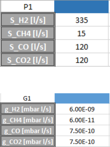
Pumps

The lumped pumps used in the main input ﬁle for the PyVASCO simulations

have to be deﬁned previously to their usage. The same pump in PyVASCO can

present different pumping speeds for different pressure ranges. PyVASCO

offers the possibility of deﬁning new pumps in the dedicated Pump editor,

but the user can also import a CSV ﬁle with the format shown in Tab. 3.3.

However, in the later case only simple pumps (with pumping speeds for the

different considered gas species independent of the pressure range) can be

deﬁned.

The pumping speed for each of the gas species has to be in l/s.

18 CHAPTER 3. INPUTS OF PYVASCO

Table 3.3: Example of a deﬁned simple pump in PYVASCO.

Table 3.4: Example of a deﬁned local gas release (gas source) in PyVASCO.

Gas sources

The gas sources used in the main input ﬁle for the PyVASCO simulations have

to be deﬁned previously to their usage. PyVASCO offers the possibility of

deﬁning new gas sources in the dedicated Gas source editor, but the user can

also import a CSV ﬁle with the format shown in Tab. 3.4.

The gas release for each of the gas species has to be in mbar l/s.

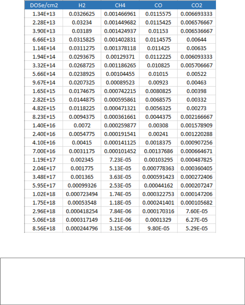
3.3 ESD curves format

In order to easily quantify the impact of the reduction of the ESD yields with

the accumulated electron dose, PyVASCO offers the possibility of solving the

dynamic vacuum model for different accumulated electron doses. (See Dy-

namic pressure due to ESD in Section 4.2, for more details on the simulation).

The ESD input ﬁles for PyVASCO must be CSV ﬁles containing 5 columns:

•The ﬁrst column must be labeled DOSe/cm2, and contain the accumu-

lated electron dose (in electrons/cm2).

•The second to ﬁfth columns must include the ESD yields of H2, CH4,

CO and CO2, respectively.

An example of the format for a ESD curve in PyVASCO can be seen in

Tab. 3.5

3.3. ESD CURVES FORMAT 19

Table 3.5: Example of the format for an ESD curve required by PyVASCO.

IMPORTANT!: In order to properly run this simulation, all the materials used

in the geometry model must have an associated ESD curve. To associate an

ESD curve to a given material, select the option Add →ESD curve in PyVASCO

menus or press Ctrl+D. See ESD curve in Subsection 4.1 for more details on

how to use this option.

Chapter 4

Layout and functionality

4.1 Menus

The current version of PyVASCO (2.0) presents 4 menus, named: File,Add,

Analysis and Help. In this section, a detailed description of the different

menus in PyVASCO and their functionality is provided.

File

The File menu of PyVASCO contains 4 options:

•Load...:

This option reloads all the registered materials, pumps and gas sources

when selecting it or pressing the keyboard key combination Ctr+L.

•Properties:

When selected or on pressing the keyboard key combination Ctr+P, this

option will launch the Properties window, shown in Fig. ??. The prop-

erties window allows to select the pressure unit (mbar or torr) of the

input. The native pressure unit of PyVASCO is mbar, while the input

pressure unit in VASCO is torr. This option was added in order to ease

the benchmark between both programs.

IMPORTANT! : Please note that changing the pressure unit in the Properties

window won’t change the pressure unit in the output of the simulation (the

results will still be given in mbar). Changing this value will only affect the

interpreted units of all the gas sources and the thermal outgassing and the

linear pumping of all materials.

Add and Edit

The Add menu of PyVASCO contains 5 options:

4.1. MENUS 21

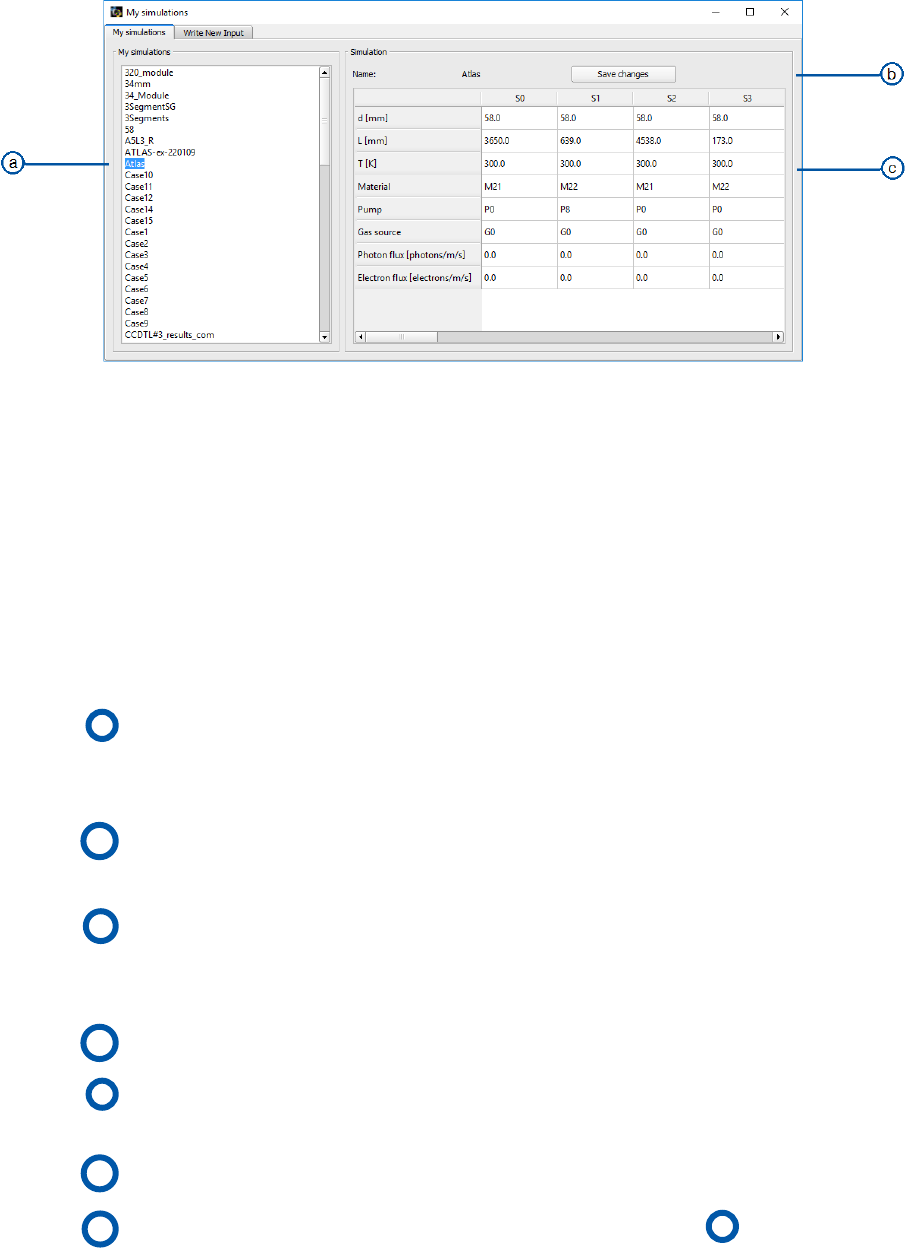
Figure 4.1: Tab 1 of "My Simulations" window.

•Simulation:

When this option is selected or the keyboard key combination Ctrl+I

is pressed, the My simualtions window will be launched. This window

allows the user to view and edit the preexisting simulations in the ﬁrst

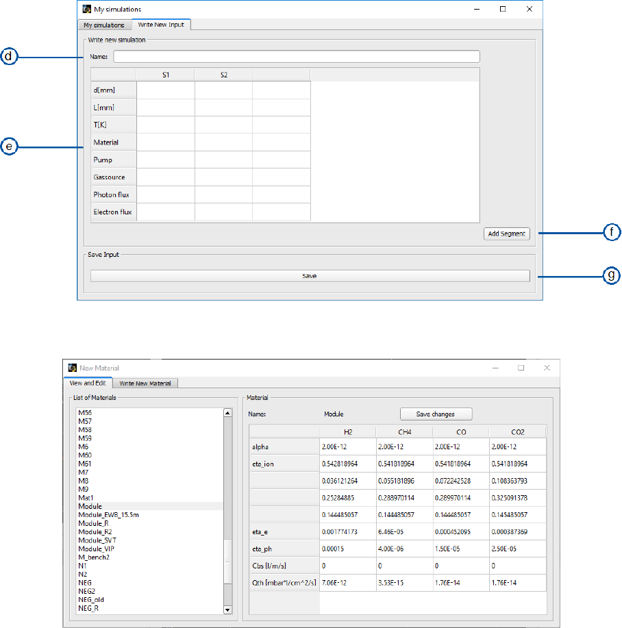
tab (Fig. 4.1 ) and to write a new input model in the second tab (Fig.

4.2).

aList of the existing simulations. A single click on a list elements

makes that it appears in the table on the right. A double click on a

name makes it possible to rename a simulation.

bPressing the "button save changes" save the modiﬁcations done

in the simulation.

c Table showing the components of the simulation selected on the

right. The elements of the table can be manually edited and the

changes saved by pressing the Save button.

dDeﬁnes the name of the simulation

eSimulation components in the ’New format’ (see Section 3.2 for a

detailed explanation).

f Allows to add a segment to the model.

gSaves the new input under the name speciﬁed in aplus the sufﬁx

"_New" .

•Material:

When this option is selected or the keyboard key combination Ctrl+M

is pressed, the New Material window is launched. This window allows

22 CHAPTER 4. LAYOUT AND FUNCTIONALITY

Figure 4.2: Tab 2 of "My Simulations" window.

Figure 4.3: Tab 1 of the "New Material" window

the user to view the preexisting materials and to deﬁne a new material.

It contains 2 tabs:

– View and Edit: (Fig. 4.3) with this tab, the user can see all the

deﬁned materials by selecting them in the list on the left, edit their

names by double-clicking them in the list and edit their properties

in the table. To save the changes done in a material, the user has

to press the button "Save changes".

– Write New Material: (Fig. 4.4) with this tab, the user can deﬁne a

new material in PyVASCO, which will be available for all the sim-

ulations once saved (pressing the ’Save’ button).

4.1. MENUS 23

Figure 4.4: Tab 2 of the "New Material" window

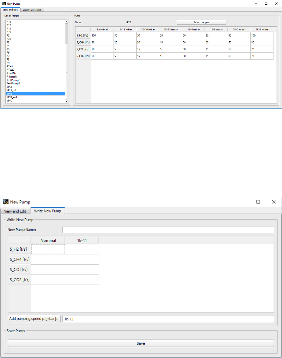
•Pump:

When this option is selected or the keyboard key combination Alt+P is

pressed, the New Pump window will be launched. This window allows

the user to deﬁne a new pump. It contains 2 tabs:

– View and Edit: (Fig. 4.5) with this tab, the user can see all the

deﬁned pumps by selecting them in the list on the left, edit their

names by double-clicking them in the list and edit their properties

in the table. To save the changes done in a material, the user has

to press the button "Save changes".

– Write New Pump: (Fig. 4.6) with this tab, the user can deﬁne a

new pump in PyVASCO, which will be available for all the simula-

tions once saved (pressing the ’Save’ button). Different pumping

speeds can be associated to the same pumps for different pressure

ranges by writing a pressure value (in mbar) in the second line edit

and pressing the button ’Add pumping speed p [mbar]:’.

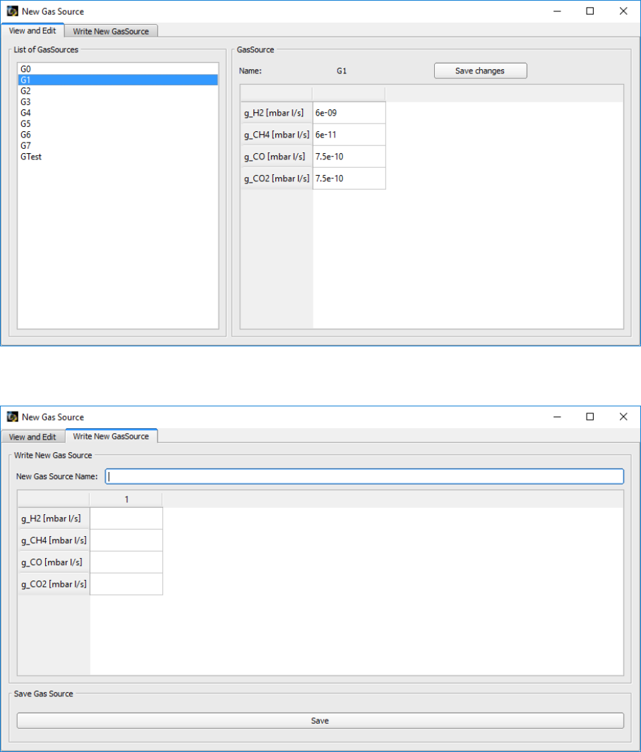
•Gas source:

When this option is selected or the keyboard key combination Ctrl+G

is pressed, the New Gas Source window will be launched. This window

allows the user to view and edit preexisting gas sources and to deﬁne a

new gas source. It contains 2 tabs:

– Data: View and Edit: (Fig. 4.7) with this tab, the user can see all the

deﬁned pumps by selecting them in the list on the left, edit their

names by double-clicking them in the list, and edit their proper-

24 CHAPTER 4. LAYOUT AND FUNCTIONALITY

Figure 4.5: Tab 1 of the "New Pump" window.

Figure 4.6: Tab 1 of the "New Pump" window.

4.1. MENUS 25

Figure 4.7: Tab 1 of the "New Gas SOurce" window.

Figure 4.8: Tab 2 of the "New Gas SOurce" window.

ties in the table. To save the changes done in a material, the user

has to press the button "Save changes".

– Write New Gas Source: (Fig. 4.8) with this tab, the user can deﬁne

a new gas source in PyVASCO, which will be available for all the

simulations once saved (pressing the ’Save’ button).

•ESD curve:

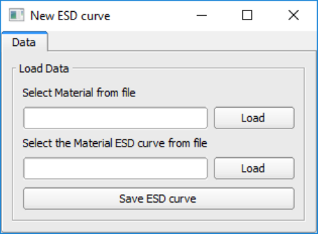
26 CHAPTER 4. LAYOUT AND FUNCTIONALITY

Figure 4.9: New ESD curve window.

When this option is selected or the keyboard key combination Ctrl+D

is pressed, the New ESD curve window will be launched. This window,

shown in Fig. 4.9 links an existing material with the experimental data

of its corresponding ESD curve. See Section 3.3 for more information

on the format of this ﬁle.

Analysis

The Analysis menu of PYVASCO launches the Analysis menu window. This

window contains 3 tabs:

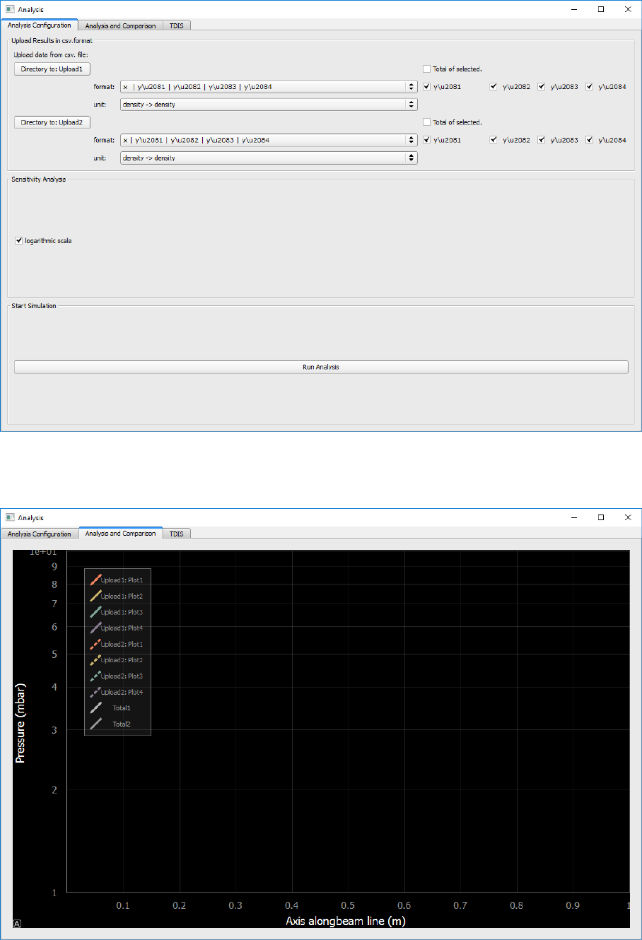
•Analysis Conﬁguration (Fig. 4.10) and Analysis and Comparison (Fig.

4.11):

These two tabs allow the user to upload two different simulation results

in CSV format and plot them together in the Analysis and Comparison

tab. In the Analysis Conﬁguration tab, the user can select the result

ﬁles clicking on the buttons ’Directory to Upload...’, and has to man-

ually indicate the format and units in those ﬁles using the format and

unit dopdowns, and pressing ’Run Analysis’.

•TDIS:

This tab was used to carry out the study on the TDIS presented in [5],

and has been kept in order to ease the generation of the this results.

Help

The Help menu of PyVASCO contains 2 options:

•User’s guide:

When this option is selected or the keyboard key combination Ctrl+H

4.1. MENUS 27

Figure 4.10: Analysis window, Analysis Conﬁguration tab.

Figure 4.11: Analysis window, Analysis and Comparison tab.

28 CHAPTER 4. LAYOUT AND FUNCTIONALITY

Figure 4.12: Analysis window, TDIS tab.

is pressed, the current document (PyVASCO User’s guide) is launched

and shown in the default web browser.

•Documentation:

When this option is selected or the keyboard key combination Ctrl+U is

pressed, the API documentation is launched in the default web browser.

4.2 Tabs

The current version of PyVASCO (2.0) contains 4 tabs, named: Data,Simu-

lation,Critical Current and Dynamic pressure due to ESD, respectively. In

this section, a detailed description of the different tabs in PyVASCO and their

functionality is provided.

4.2. TABS 29

Data

Figure 4.13: Data tab of PyVASCO.

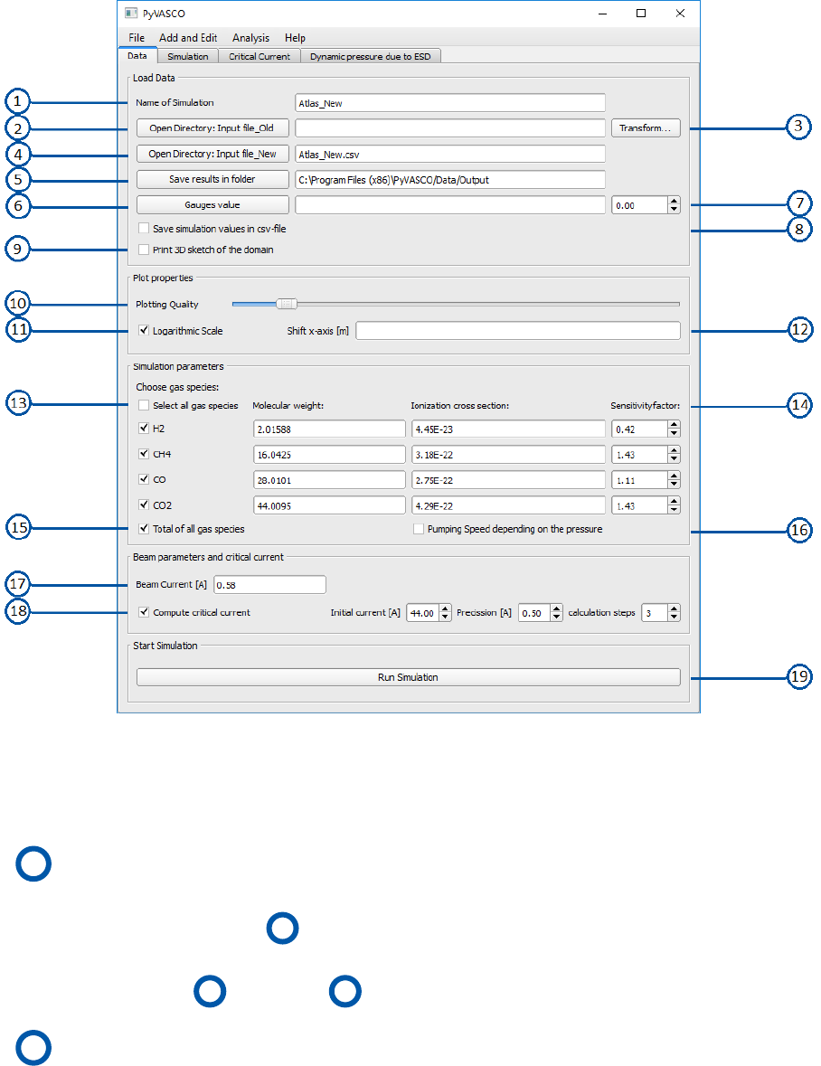
The numbers in Fig. 4.13 represent:

1Name of the simulation:

The name of the simulation is automatically set to the name of the in-

put ﬁle selected in 4, and can be manually modiﬁed by the user. This

name is used for the automatic saving in CSV format in the directory

speciﬁed in 5if option 8is selected.

2’Old’ format input ﬁle:

As mentioned in Chapter 1 and Chapter 3, PyVASCO is based in VASCO,

but the format of the input ﬁles has been changed in order to ease the

writing of the input ﬁles for large simulations. However, it is still possi-

ble to upload a CSV input ﬁle written in the same format as the input

in VASCO [1] with this option.

30 CHAPTER 4. LAYOUT AND FUNCTIONALITY

3Transform to new format:

After selecting an input ﬁle written with the same format as used in

VASCO (see [1] and Chapter 3 for more details) in 2, this option allows

to generate a new input ﬁle written in the native PyVASCO format con-

taining the same information as the one previously selected and named

as the old ﬁle with the sufﬁx "_New". The new input ﬁle is saved in the

default input directory of PyVASCO, i.e., Data/Input/.

4’New’ format input ﬁle:

Upload an input ﬁle in the native format of PyVASCO (see Chapter 3 for

more details).

5Default output directory:

If option 8is selected, the result of the simulation will be automati-

cally saved in the directory selected using this option under the name

speciﬁed in 1.

6Upload data from gauges:

This option allows to upload experimental data from different gauges

and plot it together with the simulation results in Simulation (see for

more details on the format of the gauges data).

7Shift the data from gauges:

Typically, PyVASCO assumes that the geometry starts in x=0 m, while

the data from gauges extracted from, for example, the LHC, might start

at a longitudinal coordinate (s) different from 0 m, depending on the

reference point used. In order to effectively compare the simulation

results with the experimental data in the tab Simulation, his option al-

lows to shift horizontally the experimental data uploaded in 6. The

number indicated in this slot corresponds to the shift in meters to the

right (if the value is positive) or to the left (if the value is negative).

8Save results in CSV format:

If this option is selected, the results of the simulation, i.e., the molecu-

lar density of the different considered gas species considered (in m−3)

will be automatically saved in CSV format in the directory indicated in

5under the name indicated in 1.

9Print a 3D sketch of the geometry:

If this option is selected, a 3D sketch of the simulated geometry will be

saved in PNG format under the name indicated in 1in the directory

Data/.

4.2. TABS 31

10 Plotting quality:

This option speciﬁes the number of points with which the density pro-

ﬁle for the different gas species is calculated and presented in tab Sim-

ulation.

11 Logarithmic scale:

If selected, the Y axis of the density proﬁle plot in tab Simulation is set

to logarithmic scale.

12 Move horizontally:

Similarly to 7, this option shifts horizontally the simulated density

proﬁle and the geometry. Thus, if a value different than 0 m is indi-

cated, the geometry and the simulated density proﬁle will be assumed

to start at the indicated x coordinate (in m).

13 Gas species:

This option allows to select the gas species to simulate and their ion-

ization cross section (in m2). The default values indicated for the ion-

ization cross sections of the different gas species correspond to those

calculated in [6] for a proton beam at 7 TeV.

14 Sensitivity factor:

If option 15 is selected, the total pressure is computed using the spec-

iﬁed sensitivity factors for each gas specie.

15 Total of all gas species:

If this option is selected, the total pressure is computed using the sen-

sitivity factors speciﬁed in 14 and plotted in the tab Simulation.

16 Variable pumping speed: If this option is selected, the change in pump-

ing speed of ion pumps for different pressure ranges will be taken into

account. After performing an initial simulation with the nominal (max-

imum after saturation) pumping speed for the different gases, the pump-

ing speed of the ion pumps located along the geometry is recalculated

and the gas density is recomputed.

17 Beam current:

Current of the circulating proton beam (in A). The default value is 0.582 A,

which corresponds to the nominal average beam current in the LHC

[7].

32 CHAPTER 4. LAYOUT AND FUNCTIONALITY

Figure 4.14: Simulation tab of PyVASCO.

18 Compute critical current :

If selected, the critical current for the selected model will be computed

and plotted in the tab Critical Current. PyVASCO looks for a divergence

in the gas density as a function of the beam current from the indicated

initial current and increases the test beam current as indicated by pre-

cision for the indicated number of steps.

19 Start simulation:

Pressing this button will launch the simulation with the setup speciﬁed

above. The results of the simulation are shown in the tabs Simulation

and Critical Current (if option 18 has been selected).

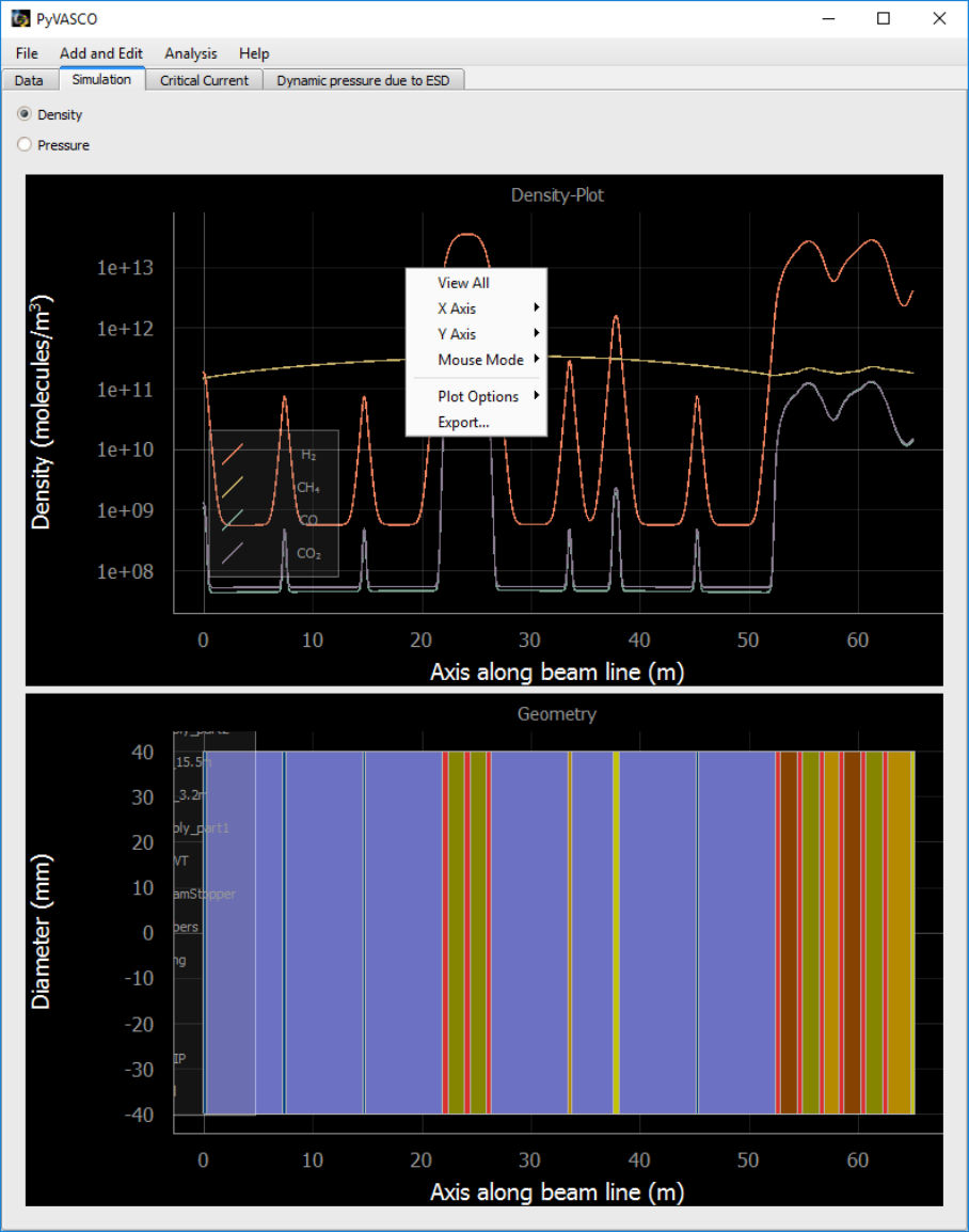
Simulation

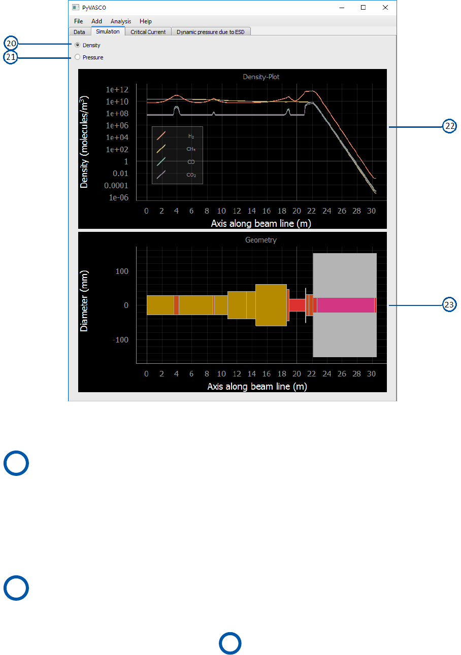
The numbers in Fig. 4.14 represent:

4.2. TABS 33

20 Density:

If selected, the plot in 22 will show the density proﬁle of the different

gas species selected in the tab Data in molecules/m3.

21 Pressure:

If selected, the plot in 22 will show the pressure proﬁle of the different

gas species selected in the tab Data in mbar and the total pressure com-

puted using the sensitivity factors in 14 (if the option 15 is selected).

22 Density/Pressure plot:

This plot shows the simulated density or pressure proﬁle, if the option

20 or 21 is selected, respectively.

23 Geometry plot:

This plot shows a block diagram of the simulated system. Different col-

ors correspond to different materials.

Critical Current

Ion stimulated desorption in the presence of a high intensity proton beam

can lead to the so-called ion induced pressure instability [8]. Above a certain

beam current, the so called the critical current, IC, the pressure in the system

diverges. PyVASCO allows to simulate the evolution of the pressure for dif-

ferent beam currents, and to estimate the value of the critical current when a

divergence in the pressure of the system is found.

The numbers in Fig. 4.15 represent:

24 Critical current value:

Computed value of critical current for the simulated system.

25 Total density proﬁle plot:

This plot shows the total molecular density proﬁle for the different com-

puted beam currents.

26 Dynamic current plot :

This plot shows the maximum density of the different gas species as a

function of the beam current.

In order to compute the critical current for the simulated system for an

explanation on the critical current), the dynamic vacuum model presented

34 CHAPTER 4. LAYOUT AND FUNCTIONALITY

Figure 4.15: Critical Current tab of PyVASCO.

in [1,2] and summarized in Section 2.2 is solved for different tested beam

currents. The ﬁrst value of the beam current used for the computation is the

value set in the box ’Initial current [A]’ in 18 . The subsequent used values of

current are computed by repeatedly increasing the initial value by the indi-

cated precision until the number of steps entered by the user is reached. If a

divergence in the density has been found for a given beam current, this value

±the precision are set as the critical current. If the divergence is found in the

ﬁrst step of the computation (the current set in ’Initial current [A]’ in 18 ),

the shown critical current value will be ≤Initial current. On the opposite, if

a divergence in the density is not found after the indicated number of steps,

the value of critical current shown in this tag will be ≥than the last tried beam

current.

4.2. TABS 35

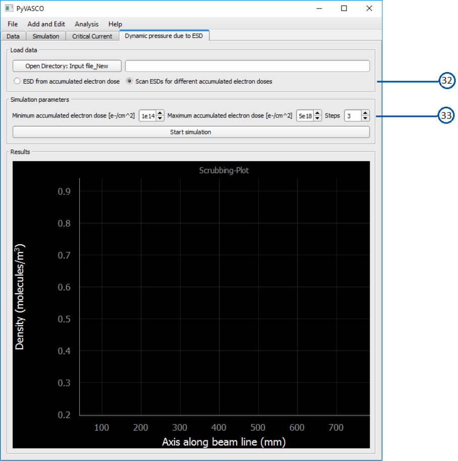
Dynamic pressure due to ESD

The tab Dynamic pressure due to ESD of PyVASCO allows to perform two dif-

ferent simulations varying the ESD of the materials used in the simulation.

The different setups of this tab are shown in Figs. 4.16 and 4.17, and the num-

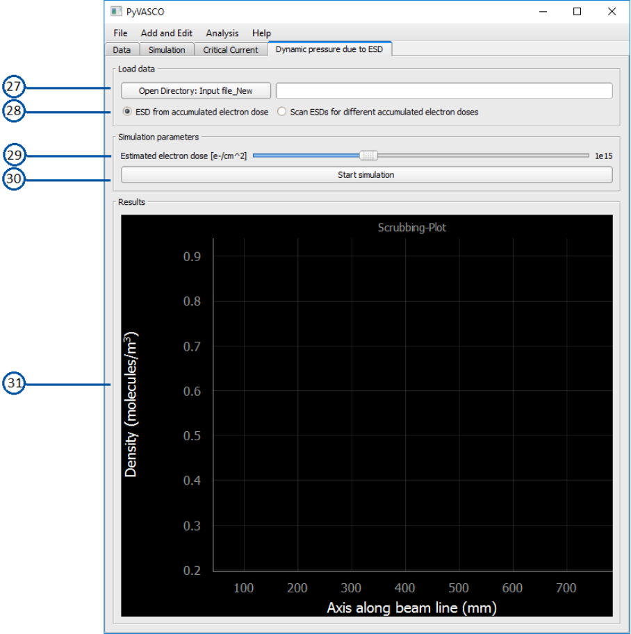
bers in these ﬁgures indicate:

27 Open Directory:

Select the input ﬁle (in the native PyVASCO format).

28 ESD from accumulated electron dose:

This option uses the ESD yields of the different UHV gas species for the

selected accumulated electron dose while solving the dynamic vacuum

model for the input ﬁle selected in 27 . If option 28 is selected, the

slider 29 will appear in the box ’Simulation parameters’.

29 Estimated electron dose:

This slider allows the user to set the accumulated electron dose re-

ceived homogeneously along the simulated geometry.

30 Start simulation:

Launches the simulation.

31 Scrubbing Plot:

This plot shows the density proﬁle of the different selected gas species

for the accumulated electron dose selected in 29 if option 28 is se-

lected. On the contrary, if option 32 is selected, the plot will show the

total density proﬁle for the different accumulated electron doses set in

33 .

32 Scan ESD for different accumulated electron doses:

This option solves the dynamic vacuum model presented in Section 2.2

for a range of accumulated electron doses speciﬁed in 33 .

33 Electron dose values:

These 3 boxes allow the user to introduce the range of accumulated

electron doses of interest for the simulation.

36 CHAPTER 4. LAYOUT AND FUNCTIONALITY

Figure 4.16: Dynamic pressure due to ESD tab of PyVASCO, layout for the sim-

ulation after receiving a ﬁx accumulated electron doses.

4.2. TABS 37

Figure 4.17: Dynamic pressure due to ESD tab of PyVASCO, layout for the sim-

ulation of the conditioning effect.

38 CHAPTER 4. LAYOUT AND FUNCTIONALITY

IMPORTANT! : Please note that this simulation will be properly performed

if an ESD curve for each of the materials used in the simulation has already

been deﬁned. If this is not the case, please link the concerned materials with

an ESD curve pressing on the menu Add →ESD curve.

Chapter 5

Extracting results with PyVASCO

By right-clicking on any plot of PyVASCO, the menu in Fig. 5.1 will appear.

This menu allows the user to directly modify some properties of the pre-

sented plot and to export it in several formats. In this chapter, a fast overview

of the relevant options available for the extraction of data from PyVASCO will

be given.

5.1 Management and plot options

The plot menu contains the following options:

•View All : This option centers the plotted data and adjusts the axis

scale to optimize the occupied space in the plot. Selecting this option

is equivalent to press the A which appears in the left-down corner in

every plot.

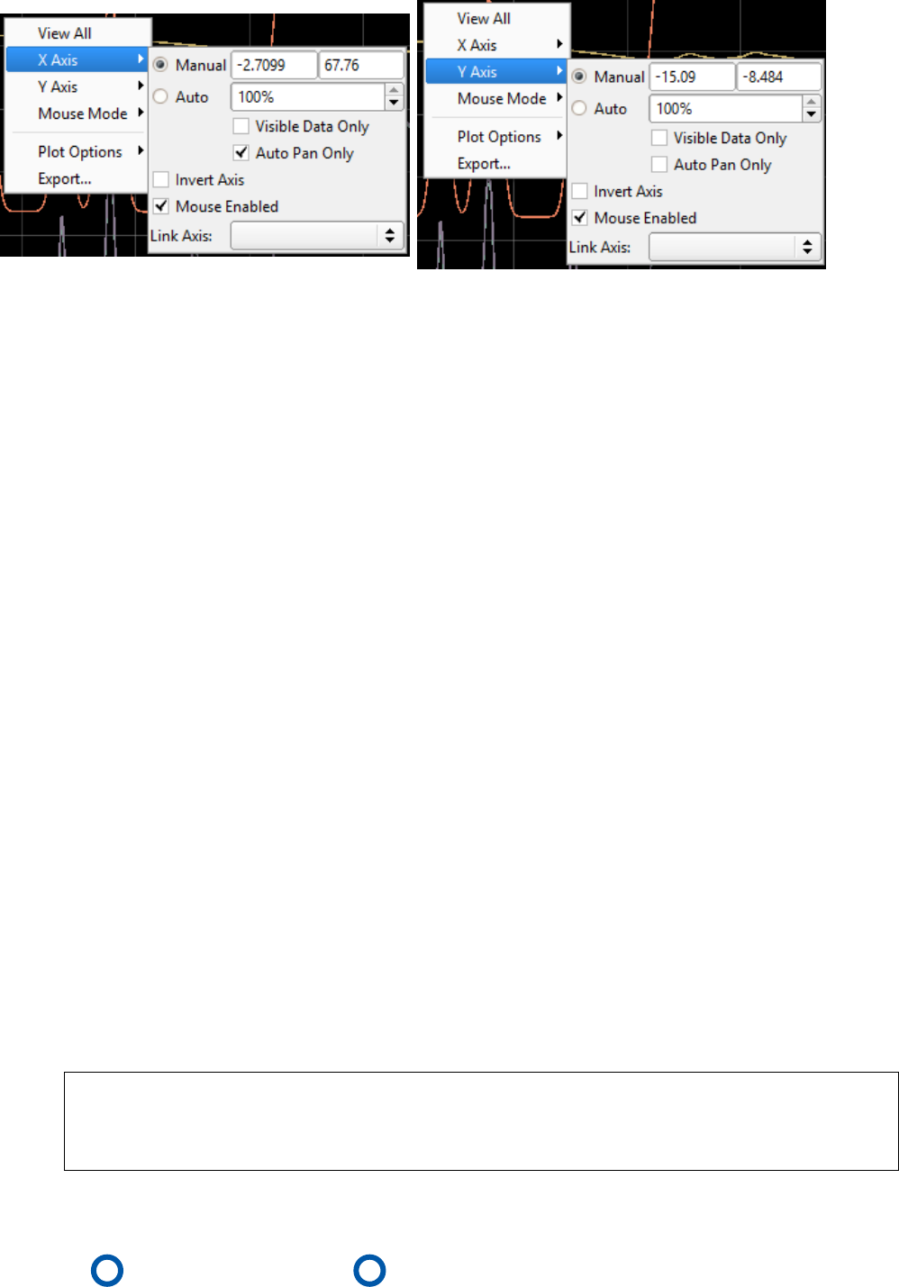
•XAxis and YAxis: Selecting these option will open the menus in Figs.

5.2a and 5.2b, respectively. The ﬁrst and second cell under the option

Manual allow to set the minimum and maximum values in the x and y

axis, respectively.

•Mouse Mode: In 3 button, the left mouse button pans the view and the

right button scales. In 1 button mode, the left button draws a rectangle

which updates the visible region (this mode is more suitable for single-

button mice).

•Plot options: Several options are available. The most relevant are Log

Xand Log Y (under the Plot options > Transforms), which allows to

change the scales in both the X and Y axis from linear to log and vice

versa, andGrid, which allows to show, hide and modulate the intensity

of the plot grid in both x and y axes.

40 CHAPTER 5. EXTRACTING RESULTS WITH PYVASCO

Figure 5.1: Plot menu (by right-clicking anywhere in the plot).

5.2. EXPORTING PLOTS IN DIFFERENT FORMATS 41

(a) (b)

Figure 5.2: Options XAxis and YAxis in the plot menu.

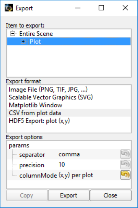
5.2 Exporting plots in different formats

Pressing the option Export in the plot menu of Fig. 5.1 will launch the menu

in Fig. 5.3.

The Export menu allows the user to save the plots in PyVASCO in differ-

ent formats, listed in the frame Export format in Fig. 5.3. It is interesting to

mention the following formats:

•Image File: The user can export any plot in PyVASCO as an image ﬁle.

This options allows for the manual modiﬁcation of the size of the re-

sulting ﬁle and the background color.

•Scalable Vector Graphics: The advantage of this option is that the re-

sulting plot can be opened and edited directly in programs like InkScape.

•Matplotlib Window: Matplotlib is one of the most used plotting li-

braries in Python. This option allows the user to further customize the

plot changing, for instance, the width, shape and markers of the lines,

the labels in both axis, etc.

•CSV: The data from all PyVASCO plots can be exported to CSV format

with this option.

IMPORTANT!: If the X or Y scale in the plot to export to CSV data is in loga-

rithmic scale, only the logarithm of the real value will be exported. The real

values can be recovered by doing 10exported values.

Alternatively, the data of the pressure proﬁle in the Tab Simulation of

PyVASCO is automatically saved in CSV format in the directory selected

in 5of Tab Data if option 8in the same tab is selected.

42 CHAPTER 5. EXTRACTING RESULTS WITH PYVASCO

Figure 5.3: Export menu.

Chapter 6

Benchmark with VASCO and Molﬂow+

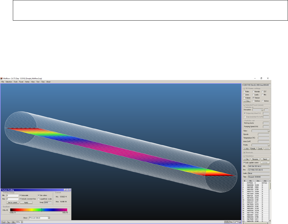
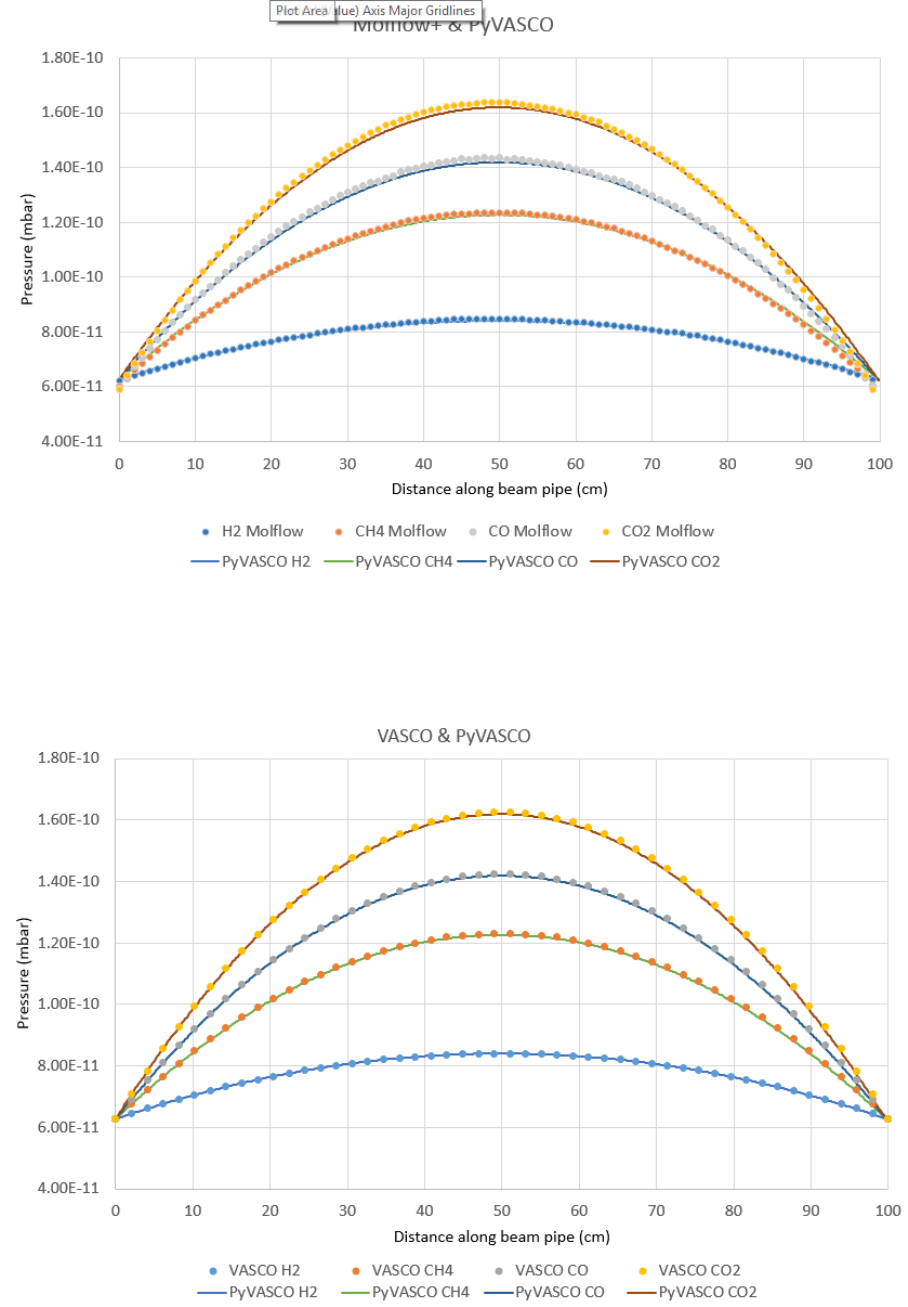
We have benchmarked PyVASCO with two other programs: VASCO and Molﬂow+

[9] for the simple case of a single segment of length 100 cm and a radius of

1 cm, with lumped pumps of 5 l/s connected in the extremes. Fig. 6.1 shows

the 3D model built in Molﬂow+ for this simulation and Figs. 6.2 and 6.3 show

a comparison between the results of PyVASCO and Molﬂow+ and PyVASCO

and VASCO, respectively, for this simple model.

IMPORTANT! : Please note that more complex tests for comparing PyVASCO

with other simulation tools have not been done due to lack of time.

Figure 6.1: Molﬂow+ model for benchmark with PyVASCO.

44 CHAPTER 6. BENCHMARK WITH VASCO AND MOLFLOW+

Figure 6.2: Comparison between the results obtained with Molﬂow+ and Py-

VASCO.

Figure 6.3: Comparison between the results obtained with VASCO and Py-

VASCO.

Bibliography

[1] A. Rossi, “VASCO (VAcuum Stability COde): multi-gas code to calculate

gas density proﬁle in a UHV system,” Tech. Rep. LHC-Project-Note-341.

CERN-LHC-Project-Note-341, CERN, Geneva, Mar 2004.

[2] I. Aichinger, G. Larcher, and R. Kersevan, “Vacuum Simulations in High

Energy Accelerators and Distribution Properties of Continuous and Dis-

crete Particle Motions,” 2017. Presented 2017.

[3] O. Bruning, F. Caspers, I. R. Collins, O. Grobner, B. Henrist, N. Hilleret, J. .

Laurent, M. Morvillo, M. Pivi, F. Ruggiero, and X. Zhang, “Electron cloud

and beam scrubbing in the lhc,” in Proceedings of the 1999 Particle Accel-

erator Conference (Cat. No.99CH36366), vol. 4, pp. 2629–2631 vol.4, March

1999.

[4] C. Day, “Basics and applications of cryopumps,” 01 2006.

[5] P. Ribes Metidieri, C. Yin Vallgren, G. Skripka, G. Iadarola, and

G. Bregliozzi, “TDIS pressure proﬁle simulations after LS2,” tech. rep.,

CERN, Geneva, 2018.

[6] A. G. Mathewson and S. Zhang, “Beam-gas ionisation cross sections at 7.0

TeV,” Tech. Rep. LHC-VAC/AGM. Vacuum-Technical-Note-96-01, CERN,

Geneva, Jan 1996.

[7] Brüning, Oliver Sim and Collier, Paul and Lebrun, P and Myers, Stephen

and Ostojic, Ranko and Poole, John and Proudlock, Paul, LHC Design Re-

port. CERN Yellow Reports: Monographs, Geneva: CERN, 2004.

[8] E. Fischer and K. Zankel, “The stability of the residual gas density in the

ISR in presence of high density proton beams,” Tech. Rep. CERN-ISR-VA-

73-52. ISR-VA-73-52, CERN, Geneva, Nov 1973.

[9] M. Ady and R. Kersevan, “Molﬂow+ user guide,” tech. rep., CERN, Geneva,

June 2014.

User Guide

Navigation menu

Versions of this User Manual:

Views

Navigation