User Guide
User Manual:
Open the PDF directly: View PDF ![]() .
.
Page Count: 4

1/4
FARMCA User Guide
The code FARMCA has been developed for modelling the permeability using the well
log data. The methodology is describe in the paper:
Uma Vadapalli, Ajay Malkoti, Harini Guruhappa, Nimisha Vedanti, Vijay Prasad Dimri
(2018) Fractal theory based Acceptance Rejection Monte-Carlo Algorithm (FARMCA)
for permeability modeling of sandstone reservoirs, submitted to Computers &
Geosciences.
Using the code:
The modeling of permeability using Fractal theory based Acceptance Rejection
Monte-Carlo Algorithm (FARMCA) can be started by executing the following
program in MATLAB:
>> GUI.m
The algorithm is divided into following three important steps for the Graphical User
Interface (GUI) implementation as described below:
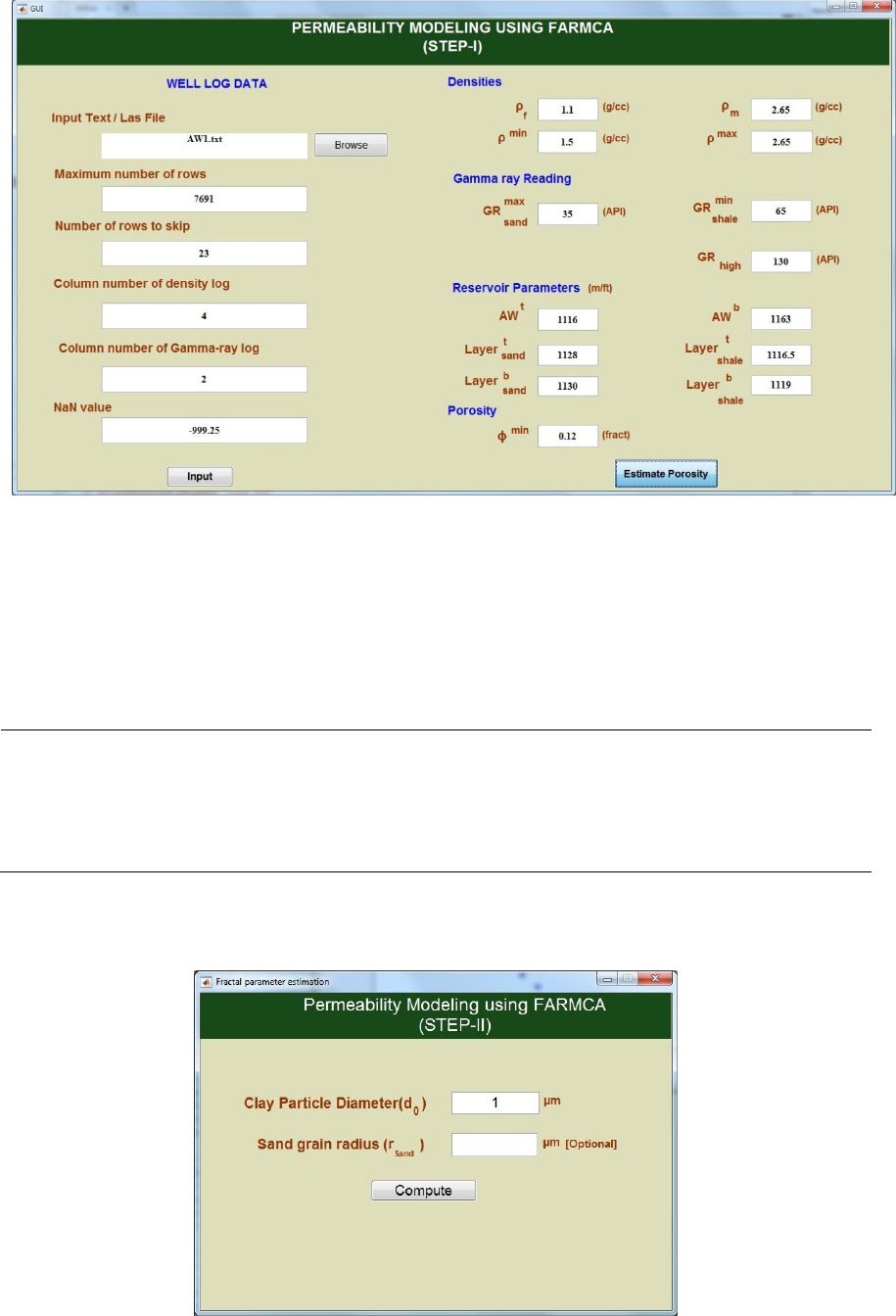
Step I : Data input and estimation of useful porosity
The program reads the density and gamma ray logs from well log data file (in LAS or
TEXT format). The required input parameters for reading the file are given:
Input text/las file - The well log data either in text or las format
Maximum number of rows - The maximum number of rows in the input file
Number of rows to skip - The number of rows of text, which have to be
skipped while reading the input file
Column number of density - The column number of the density log in input
file
Column number of density - The column number of Gamma-ray log in input
File
NAN value - The NAN value in the input file

2/4
The parameters to run the FARMCA on well log data are following:
-
Matrix density (Default = 2.65 g/cc, density of Quartz matrix) in g/cc
-
Fluid density (Default = 1.1 g/cc, density of saline formation water)
in g/cc
-
Maximum acceptable density ( ) in the analysis window in g/cc
-
Minimum acceptable density in the analysis window in g/cc
-
The API gamma ray reading above which can be ignored from the
analysis
-
The API gamma ray reading below which the litho-facies can be
characterized as pure-sandstone
-
The API gamma ray reading above which the litho-facies can be
characterized as pure-shale
-
The top of the analysis window (m or ft)
-
The bottom of the analysis window (m or ft)
-
The top of pure sand layer for determining
(m or ft)
-
The bottom of pure sand layer for determining
(m or ft)
-
The top of pure shale layer for determining
(m or ft)
-
The bottom of pure shale layer for determining
(m or ft)
-
The porosity values below which are ignored from the computation
(in fraction) since that block is considered as predominantly shale
(*note: If there is no pure-shale block between top and bottom of reservoir zone, the
Analysis Window (AW) can be slightly extended to include at least one pure-shale
block, since pure-shale density is required for the estimation of effective porosity)
Based on the above mentioned parameters the program interprets litho-facies,
divides the reservoir into blocks and estimates the average values of & ,
, and in each block. The completion of STEP I execution displays a plot of
porosity versus shale volume. The GUI window and input parameters of the demo
data for implementation of STEP I are shown in Fig. 1.

3/4
Fig 1. The inputs values used for execution of step 1.
Step II: Estimation of fractal parameters
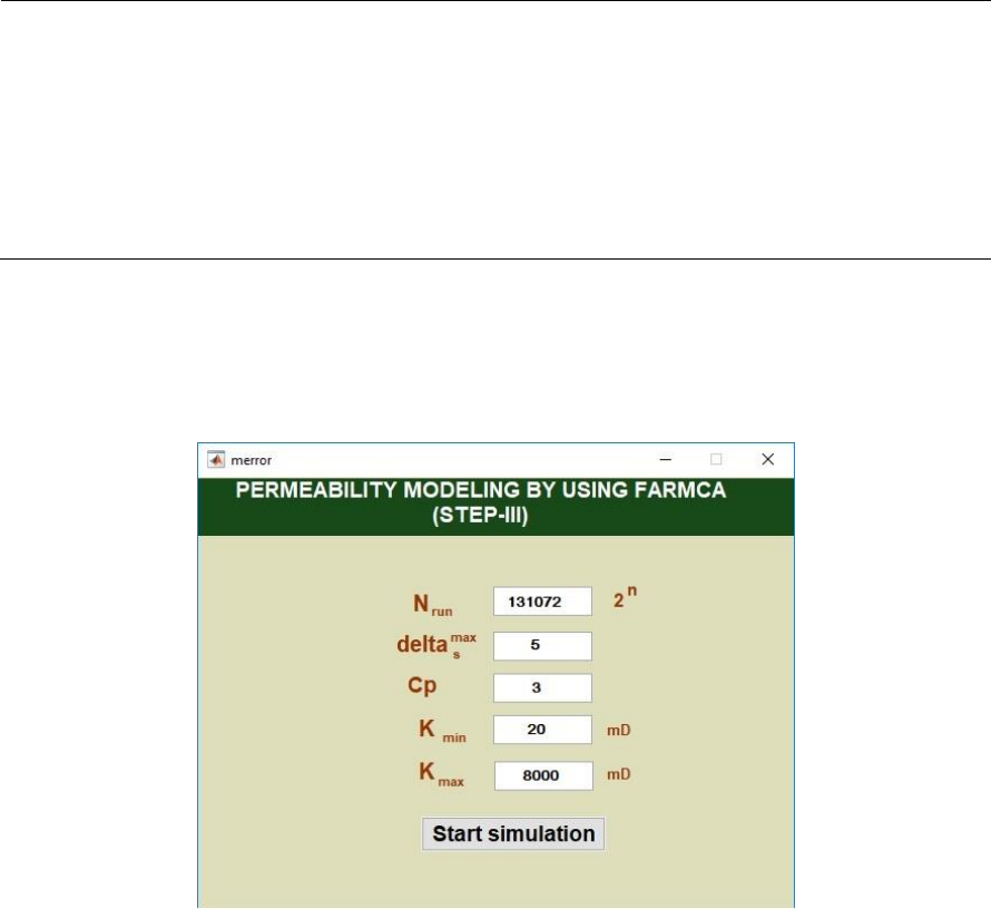
In Step II, the program estimates the fractal and pore structural parameters. The
parameters required in this step are:
–
Clay particle diameter (in µm) which can be chosen based on type of clay
minerals present in the formation
–
Sand grain radius (in µm) (optional). If left blank, program estimates it
automatically
The GUI window and input parameters of the demo data for implementation of STEP
II are shown in Fig. 2.
Fig 2. The inputs values used for execution of step 2.

4/4
Step III: Error analysis and permeability estimation
In this step the program performs the error analysis and models the permeability of
each lithological block of the reservoir. The parameters required for implementation
of STEP III are:
-
Initial number of runs (= , e.g. ) to start with the error
analysis
-
Maximum allowable error to check for error convergence
CP
-
Number of converging points of error
-
Minimum value of permeability permissible in the reservoir zone (mD)
-
Maximum value of permeability permissible in the reservoir zone (mD)
Completion of STEP III displays permeability versus, grain radius, pore diameter,
useful porosity and blocked logs of useful porosity and permeability. The GUI
window and input parameters of the demo data for implementation of STEP III are
shown in Fig. 3.
Fig 3. The inputs values used for execution of step 3.
The computation time can be reduced by increasing error (
) and reducing
number of convergence points (CP).
Directory Structure:
/FARMAC_GUI/ : Main program
/FARMAC_GUI/OUTPUT : Contains all the results
/FARMAC_GUI/OUTPUT/FIGURES : Contains all the final figures
/FARMAC_GUI/OUTPUT/PERMEABILITY : All output files related to permeability
calculation
/FARMAC_GUI/OUTPUT/PHI : All output files related to porosity calculation