User Guide
User Manual:
Open the PDF directly: View PDF ![]() .
.
Page Count: 26
Visualization of electron structures
LiTH
2019-05-25
USER GUIDE
Linda Le, Abdullatif Ismail, Anton Hjert,
Lloyd Kizito, Jesper Ericsson
Version 1.0
Parts of chapter 1 and 2 are based on the 2018 user guide for ENVISIoN, see appendix B.
Status
Granskad
Godkänd
User guide TFYA75
Visualization of electron structures
LiTH
2019-05-25
PROJECT IDENTITY
2019/Spring,
Linköpings Tekniska Högskola, IFM
Group members
Name Role Phone nr. E-mail
Linda Le Project leader (PL) 076-2249926 linle336@student.liu.se
Abdullatif Ismail Document manager(DOK) 072-0355455 abdis077@student.liu.se
Anton Hjert Anton Hjert (AH) 070-5728891 anthj975@student.liu.se
Jesper Ericsson Jesper Ericsson (JE) 070-8772630 jeser991@student.liu.se
Lloyd Kizito Lloyd Kizito (LK) 070-8230589 lloki004@student.liu.se
Website: https://liuonline.sharepoint.com/sites/TFYA75/TFYA75_2019VT_7Z/62340
Client: Rickard Armiento, IFM, Linköpings universitet, 581 83 Linköping
Contact person of client: Rickard Armiento, rickard.armiento@liu.se
Course examintor: Per Sandström, per.sandstrom@liu.se
Main supervisor: Johan Jönsson, johan.jonsson@liu.se
User guide i TFYA75

Visualization of electron structures
LiTH
2019-05-25
Contents
Document history iii
Licens iv
1 Introduction 1
2 How to build Inviwo with ENVISIoN on Ubuntu 18.04 LTS 2
2.1 Installgit ..................................... 2
2.2 DownloadENVISIoN............................... 2
2.3 Prepare Inviwo using the ENVISIoN install script . . . . . . . . . . . . . . . . 2
3 How to build Inviwo with ENVISIoN on other OS 3
3.1 Installgit ..................................... 3
3.2 DownloadENVISIoN............................... 3
3.3 PrepareInviwoforbuild ............................. 3
4 Start ENVISIoN 4
5 Start Inviwo and run ENVISIoN scripts 5
6 Graphical user interface 6
6.1 Start-up ...................................... 6
6.2 Parsermenu.................................... 6
6.2.1 Quick Step-by-Step Guide . . . . . . . . . . . . . . . . . . . . . . . . 8
6.3 Visualizationmenu ................................ 8
6.3.1 Common controls - Charge Density, ELF, and Partial Charge Density . 8
6.3.2 ChargeDensity.............................. 11
6.3.3 ELF - Electron Localization Function . . . . . . . . . . . . . . . . . . 11
6.3.4 Partial charge density . . . . . . . . . . . . . . . . . . . . . . . . . . . 12
6.3.5 Bandstructure............................... 13
6.3.6 DoS - Density of States . . . . . . . . . . . . . . . . . . . . . . . . . . 14
6.3.7 PCF - Pair Correlation Function . . . . . . . . . . . . . . . . . . . . . 15
7 Common errors during installation 17
7.1 Qt ......................................... 17
Appendix A Licens 19
Appendix B Projekt group 2018 20
User guide ii TFYA75
Visualization of electron structures
LiTH
2019-05-25
Document history
Version Date Changes Done by Reviewed
0.1 2019-05-21 First draft. DOK, AH, JE Projektgruppen
1.0 2019-05-25 Second draft. Rewritten based on com-
ments from the client.
DOK, AH, JE
User guide iii TFYA75

Visualization of electron structures
LiTH
2019-05-25
Licens
This documet is licensed as BSD, see appendix A.
User guide iv TFYA75

Visualization of electron structures
LiTH
2019-05-25
1 Introduction
ENVISIoN is an open source toolkit for electron visualization, developed as a part of the course
TFYA75: Applied Physics - Bachelor’s Project, given at Linköpings universitet, LiU. It’s im-
plemented by using a modified verision of the Inviwo visualization framework, developed at the
Scientific Visualization Group at Linköpings universitet, LIU.
The present version was developed during the spring term of 2019 by a project group consisting
of: Linda Le, Abdullatif Ismail, Anton Hjert, Lloyd Kizito and Jesper Ericsson. Supervisor:
Johan Jönsson; Requisitioner and co-supervisor: Rickard Armiento; Visualization expert: Peter
Steneteg; and Course examiner: Per Sandström. The work is based on a previous version by the
project group taking the course in the spring term of 2018 consisting of: Anders Rehult, Marian
Brännvall, Andreas Kempe and Viktor Bernholtz. Supervisor: Johan Jönsson; Requisitioner
and co-supervisor: Rickard Armiento; Visualization expert: Rickard Englund; and Course ex-
aminer: Per Sandström. That work was is based on the work by the project group taking the
course in the spring term of 2017 consisting of: Josef Adamsson, Robert Cranston, David Hart-
man, Denise Härnström, Fredrik Segerhammar. Supervisor: Johan Jönsson; Requisitioner and
co-supervisor: Rickard Armiento; Visualization expert: Peter Steneteg; and Course examiner:
Per Sandström.
ENVISIoN provides a graphical user interface and a set of Python scripts that allow the user to:
•Read and parse output from electronic structure calculations made by the program VASP
and storing the result in a structured HDF5 file.
•Generate Inviwo visualizations for common tasks when analyzing electronic structure
calculations. Presently there is support for visualizing the crystal structure of the unit
cell of a material, electron localization function (ELF)-data, electronic charge density,
electronic band structure, radial Distribution Function and density of states - both total
and partial. The system also provides the ability to interconnect some of the networks
mentioned above.
User guide 1 TFYA75
Visualization of electron structures
LiTH
2019-05-25
2 How to build Inviwo with ENVISIoN on Ubuntu 18.04 LTS
These instructions show how to build Inviwo and ENVISIoN on Ubuntu 18.04 LTS.
2.1 Install git
Start by installing git, which will be used to fetch ENVISIoN in the next step.
sudo apt install git
2.2 Download ENVISIoN
Go to your home folder and clone ENVISIoN from Github. This guide will assume that both
ENVISIoN and Inviwo will be placed directly under the home folder.
cd
git clone https://github.com/rartino/ENVISIoN
2.3 Prepare Inviwo using the ENVISIoN install script
ENVISIoN provides an install script for Ubuntu 18.04 LTS. Executing the installation script will
install all required dependencies, clone Inviwo from Github and configure the Inviwo build.
The script should NOT be run as root, but as your own user and it will ask for your password
when it needs root rights. It is possible that the script will ask for other user input during the
process, if that’s the case, just accept the default.
cd ~/ENVISIoN/scripts
./install.sh /home/$USER/ENVISIoN /home/$USER/inviwo
Once the installation script has run, it prints build instructions. Follow the instructions and start
the build. The instructions will tell you to cd to the build directory and execute make.
An easy way to modify the build settings, if needed, is to install the cmake curses gui and run it
in the build directory.
To install the cmake gui:
sudo apt install cmake-curses-gui
Running cmake in the build directory:
cd ~/inviwo/build
ccmake .
When in the GUI, press cto apply the current configuration, gto generate build files and qto
quit. If settings have changed, it is possible that you will need to press cmore than once before
the goption becomes available.
After having generated the build files, the project can now be rebuilt with the new settings by
executing make like earlier.
User guide 2 TFYA75
Visualization of electron structures
LiTH
2019-05-25
3 How to build Inviwo with ENVISIoN on other OS
3.1 Install git
Start by installing git, which will be used to fetch ENVISIoN in the next step. Git can be
downloaded from the website below.
https://git-scm.com/downloads
3.2 Download ENVISIoN
Change the working directory to the home folder and clone ENVISIoN from Github. This
guide will assume that both ENVISIoN and Inviwo will be placed directly under the home
folder. Clone the ENVISIoN repository be executing the command below.
git clone https://github.com/rartino/ENVISIoN
3.3 Prepare Inviwo for build
To be able to install Inviwo, all required dependencies needs to installed:
•gcc
•hdf5
•cmake
•qt
•python3
•numpy
•h5py
•regex
•wxPython
•pybind11
Make sure to install the latest version of all the softwares mentioned above. Clone the Inviwo
repository into the home folder and make it your working directory. Clone the Inviwo repository
be executing the command below.
git clone https://github.com/inviwo/inviwo.git
ENVISIoN isn’t compatible with the newest version of Inviwo due to a reconstruction in the
Inviwo file system on April 15, 2019. To make ENVISIoN compatible with Inviwo that just got
cloned, a checkout of a compatible version is needed.
git checkout d20199dfd37c80559ce687243d296f6ce3e41c71
Some minor alterations has been made on the Inviwo source code by the ENVISIoN project
group that need to be patched.
User guide 3 TFYA75
Visualization of electron structures
LiTH
2019-05-25
git apply < "~/ENVISIoN/inviwo/patches/2019/envisionTransferFuncFix2019
.patch"
git apply < "~/ENVISIoN/inviwo/patches/2019/paneProperty2019.patch"
The only remaining change in the Inviwo repository is an update of its submodules.
git submodule init
Create a build directory in the home folder and configure the ENVISIoN module and project
path using cmake. Execute the command below when standing in the build directory.
cmake .. -DIVW_EXTERNAL_PROJECTS="~/ENVISIoN/inviwo/app" \
-DIVW_EXTERNAL_MODULES="$~/ENVISIoN/inviwo/modules" \
-DIVW_MODULE_CRYSTALVISUALIZATION=ON \
-DIVW_MODULE_FERMI=OFF \
-DIVW_MODULE_GRAPH2D=ON \
-DIVW_MODULE_PYTHON3=ON \
-DIVW_MODULE_PYTHON3QT=ON \
-DIVW_MODULE_QTWIDGETS=ON \
-DIVW_MODULE_HDF5=ON
Inviwo is now ready to be installed with the ENVISIoN modules added. Add the -j extension to
use multiple cores while installing.
make -j5
4 Start ENVISIoN
After the Inviwo build is done, an application named inviwo_envisionminimum will be available
in the bin files in the build directory. The commands in this section are only compatible with
Ubuntu 18.04 LTS and other UNIX based operating systems. To make the application start
the graphical user interface, it needs the path to the interface source files located in the same
directory. The file containing these files can be copied from ∼/ENVISIoN/scripts and is named
ENVISIoNimport.py. Execute the command below to copy the file to the correct directory.
cp ~/ENVISIoN/scripts/ENVISIoNimport.py ~/build/bin/ENVISIoNimport.py
The application can now be started by standing in the build directory and executing the com-
mand below.
./bin/inviwo_envisionminimum
User guide 4 TFYA75
Visualization of electron structures
LiTH
2019-05-25
5 Start Inviwo and run ENVISIoN scripts
If the user wishes to run Inviwo with its own graphical user interface, it’s possible and still have
access to the visualizations provided by ENVISIoN. These visualizations are stored in the form
of Python scripts that can be compiled through the Inviwo user interface.
To run Inviwo in an UNIX environment, execute the commands below.
cd ~/build
./bin/inviwo
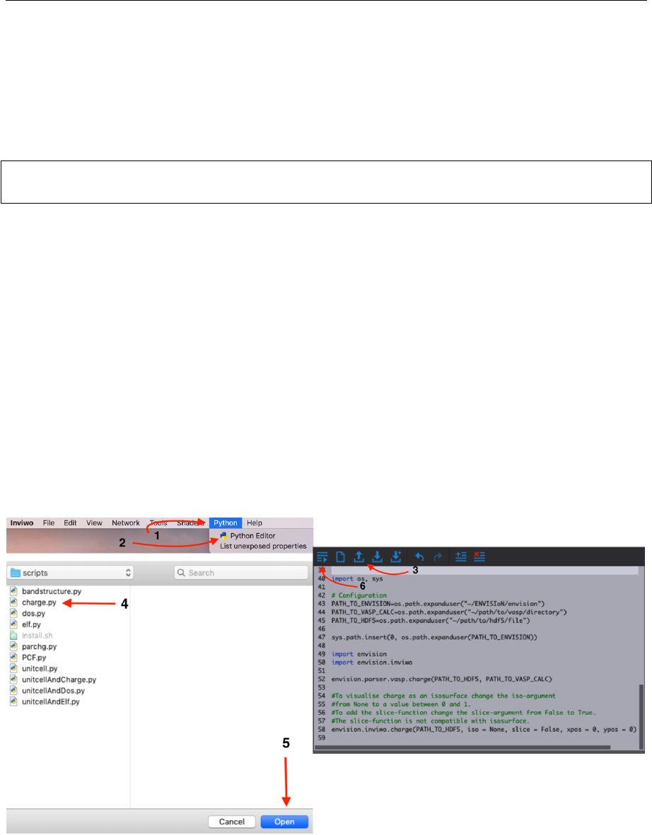
When the Inviwo interface has opened, follow the instructions given in figure 1 and in the list
below to run a visualization script.
1. Locate and press the Python menu in the Inviwo bar.
2. Open the Python editor by pressing it.
3. In the Python editor, click Open Script.
4. Select one of the scripts. The ENVISIoN scripts can be located in ∼/ENVISIoN/scripts.
5. Click open.
6. Click the button in the top left corner to run.
Figure 1: Cutout from Inviwo with instructions on how to run a ENVISIoN visualization script
in numeric order.
User guide 5 TFYA75
Visualization of electron structures
LiTH
2019-05-25
6 Graphical user interface
The purpose of the graphical user interface is to simplify the usage of ENVISIoN.
6.1 Start-up
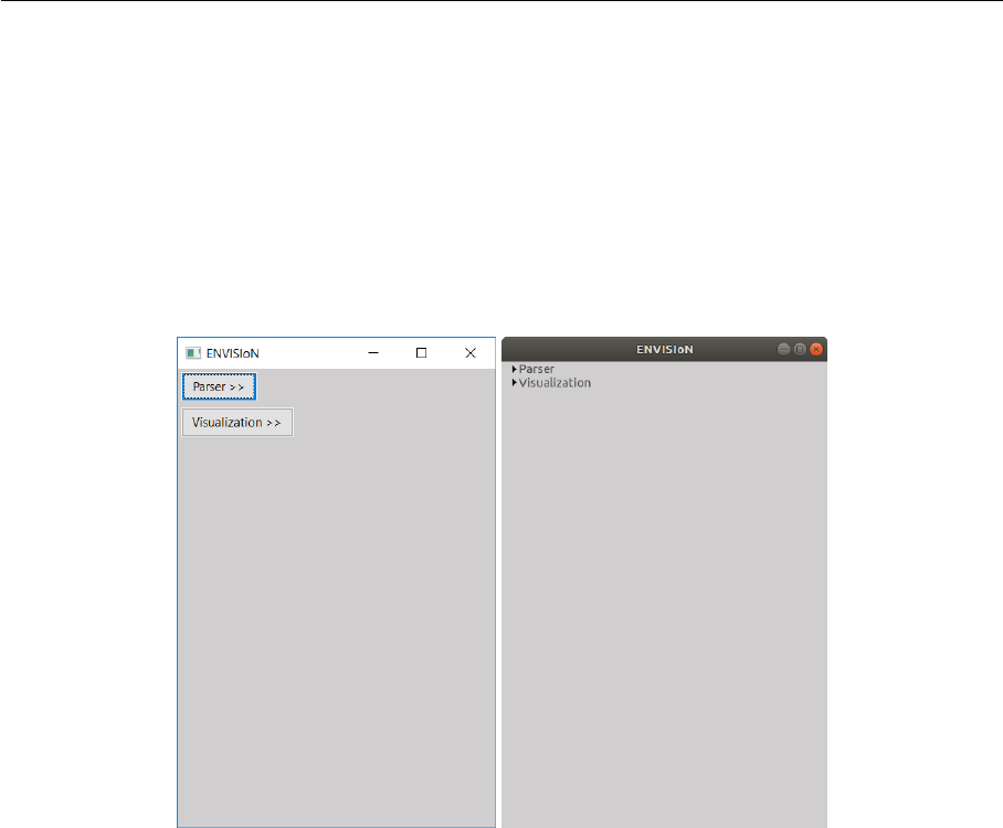
When the user run the application a window opens, see figure 2. After ENVISIoN has been
opened, two possible menu-choices appear, “Parser” and “Visualization”.
Figure 2: ENVISIoN start up-window, for Windows on the left and Linux on the right.
6.2 Parser menu
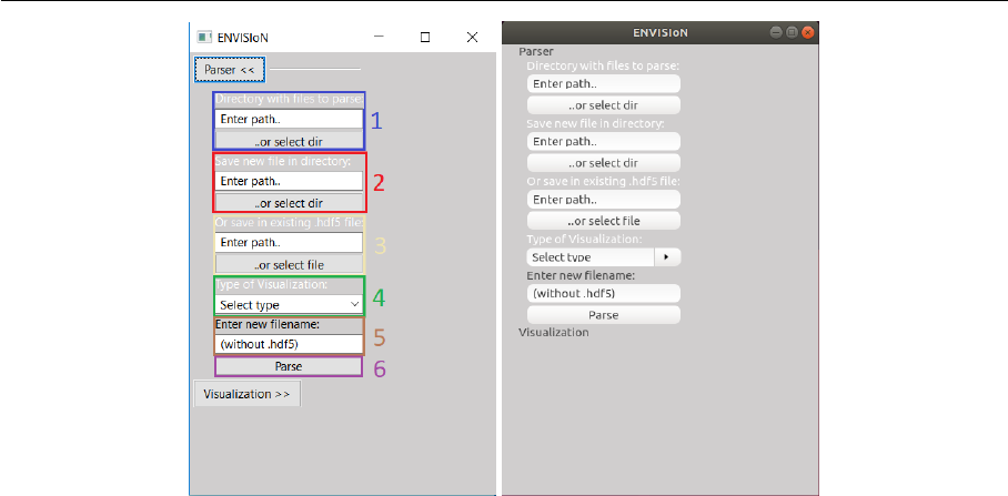
The parser menu is localized on top in the interface. To access its content, press the fold out
button to expand the menu. The result will be that of figure 3, depending on the system running
the software.
For quick step-by-step guide, scroll down to last segment of this subsection.
In the blue box, labeled “1”, the path to the directory of VASP-files to parse is selected. There
are two options, either the path can be entered as a string in the text field or the “..or select dir”-
button can be pressed. This button will reveal the file explorer and allow to select the desired
folder.
In the red box, labeled “2”, the path to the desired saving directory for the new hdf5-files is
selected. This path-selection has the same two options as the previous.
In the yellow box, labeled “3”, the path to an existing hdf5-file can be selected. Here, there
are two options as well, which are similar to those above. The difference is that the button will
open a file explorer where an hdf5-file shall be selected.
In the green box, labeled “4”, the type of the parsing for certain visualizations can be picked. If
one type of visualization is desired, there can be of advantage to pick that in the drop-down list
User guide 6 TFYA75
Visualization of electron structures
LiTH
2019-05-25
Figure 3: Parser menu expanded, for Windows on the left and Linux on the right.
to enhance performance of the parser. If not changed or if “All” is selected, the parser will run
all possible types of parsing. The available choices for types are:
•All
•Bandstructure
•Charge
•DoS - Density of States
•ELF - Electron Localization Function
•Fermi Energy
•MD - Molecular Dynamics
•Parchg - Partial Charge
•PCF - Pair Correlation Function
•Unitcell
In the brown box, labeled “5”, if a new hdf5-file is to created, the name of the new file is entered
here without file extension.
In the purple box, labeled “6”, is the execution-button of the parser. When pressing this button
the parser tries to run. Afterwards, a message box will appear on the screen with the status of
the parsing. If the parsing was successful the message box will show for which data the parsing
was done. If it failed, the message box will tell where it failed. If no message box appear, then
something went wrong that wasn’t detected, an exception that wasn’t caught.
User guide 7 TFYA75

Visualization of electron structures
LiTH
2019-05-25
6.2.1 Quick Step-by-Step Guide
For new *.hdf5 file:
1. Enter path to directory in “1”.
2. Enter path to directory in “2”.
3. Select type in “4”.
4. Enter new file name in “5”.
5. Press “Parse” in “6”.
6. Message whether the parsing was successful or not will appear.
For existing *.hdf5 file:
1. Enter path to directory in “1”.
2. Enter path to file in “3”.
3. Select type in “4”.
4. Press ’Parse’ in “6”.
5. Message weather the parsing was successful or not will appear.
6.3 Visualization menu
6.3.1 Common controls - Charge Density, ELF, and Partial Charge Density
Because of the strong similarity between these three menues the interface share many elements.
The common elements will be described here.
When opening any of the visualization main menues four sub-menues will be visible. Volume
Rendering,Volume Slice,Atom Rendering and Background. All those control different aspects
of the visualization.
Volume Rendering menu
User guide 8 TFYA75
Visualization of electron structures
LiTH
2019-05-25
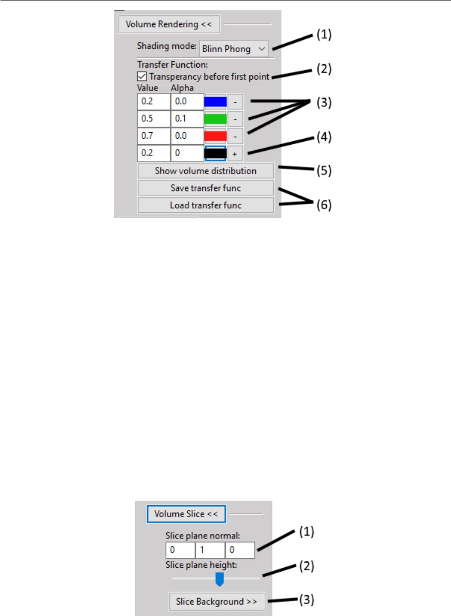
Figure 4: Volume Rendering menu.
(1) Drop-down menu to choose volume shading mode. Affects how the volume is lighted.
(2) Toggle full transparency for volume densities lower than the lowest transfer function
point.
(3) Edit existing transfer function points by editing text fields or picking color. Remove point
by pressing “-” button.
(4) Add new transfer function point with specified value, alpha, and color by pressing “+”
button.
(5) Click button to show volume density distribution histogram. Histogram will open in a
new window.
(6) Click to save or load active transfer function.
Volume Slice menu
Figure 5: Slice menu.
(1) Text fields specify (x, y, z)-components of the normal vector of slice plane.
(2) Slider controls the height of the slice plane.
User guide 9 TFYA75
Visualization of electron structures
LiTH
2019-05-25
(3) Expandable menu to control the background of the slice image.
Atom Rendering menu
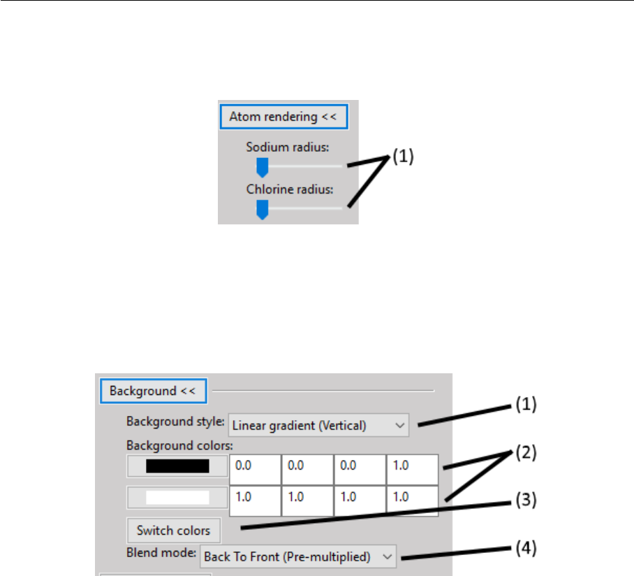
Figure 6: Atom Rendering menu.
(1) Sliders to choose the radius of each atom type.
Background menu
Figure 7: Background menu.
(1) Drop-down menu to choose the background pattern style.
(2) Select the two colors of the background. Either use the color picker on the left, or specify
a RGBA-color via the text fields
(3) Button to swap positions of the colors.
(4) Drop-down menu to choose the blend mode of the background.
User guide 10 TFYA75
Visualization of electron structures
LiTH
2019-05-25
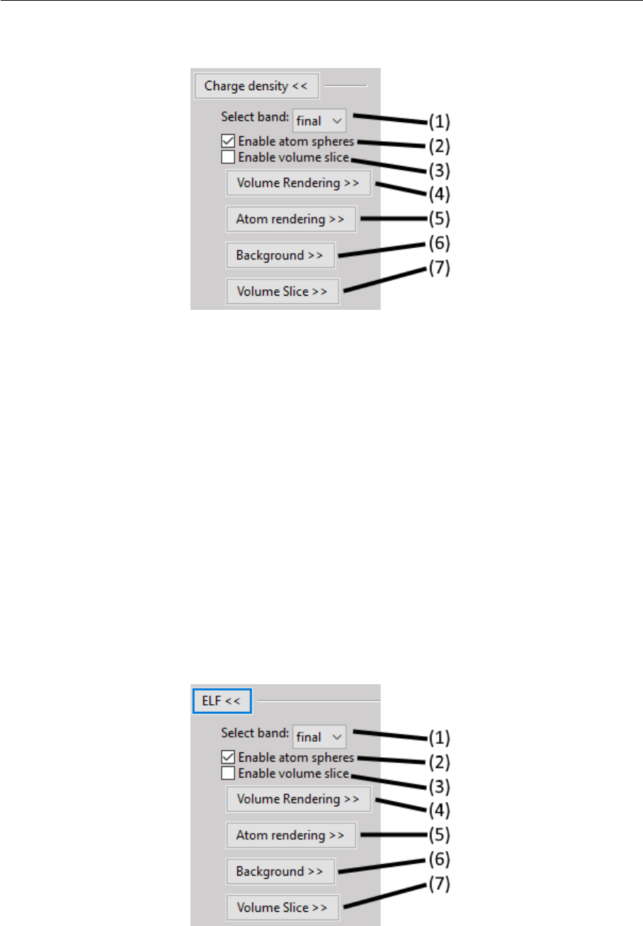
6.3.2 Charge Density
Figure 8: Charge Density menu.
(1) Drop-down menu to select which band to visualize. Each band has its own volume data.
(2) Toggle the atom sphere rendering.
(3) Toggle the volume slice visualization.
(4) Expand the Volume Rendering menu.
(5) Expand the Atom Rendering menu.
(6) Expand the Background menu.
(7) Expand the Volume Slice menu.
6.3.3 ELF - Electron Localization Function
Figure 9: ELF menu.
(1) Drop-down menu to select which band to visualize. Each band has its own volume data.
User guide 11 TFYA75
Visualization of electron structures
LiTH
2019-05-25
(2) Toggle the atom sphere rendering.
(3) Toggle the volume slice visualization.
(4) Expand the Volume Rendering menu.
(5) Expand the Atom Rendering menu.
(6) Expand the Background menu.
(7) Expand the Volume Slice menu.
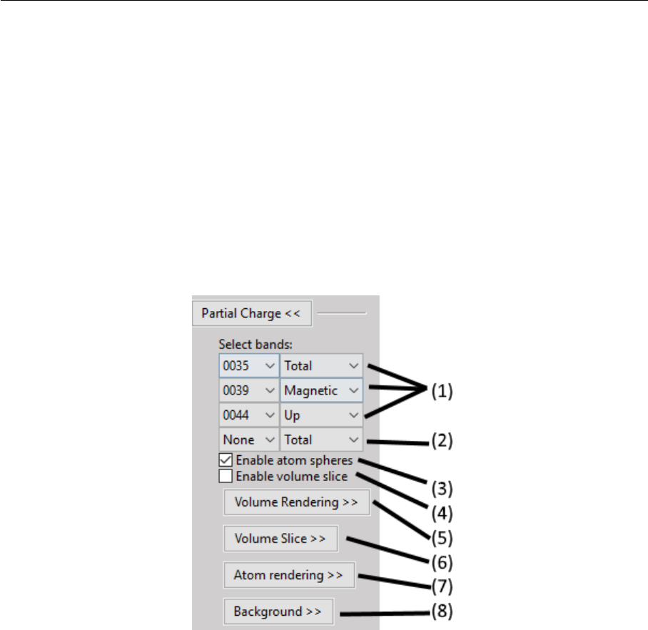
6.3.4 Partial charge density
Figure 10: Partial charge density menu.
(1) Manage selected bands and modes. Band selections and modes can be changed. Select
“None” to remove band from visualization.
(2) Add new band selection with selected mode. Select any other opetion than ”None” to add
new band to visualization.
(3) Toggle the atom sphere rendering.
(4) Toggle the volume slice visualization.
(5) Expand the Volume Rendering menu.
(6) Expand the Atom Rendering menu.
(7) Expand the Background menu.
(8) Expand the Volume Slice menu.
User guide 12 TFYA75
Visualization of electron structures
LiTH
2019-05-25
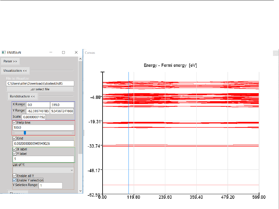
6.3.5 Bandstructure
When expanding the bandstructure visualization menu the visualization starts and a control
panel appears. This menu is shown in figure 11.
Figure 11: Bandstructure visualization menu expanded
The bandstructure visualization menu contains a number of possibilities to control parameters.
Range and Scale: In the first (blue) box, controls for scaling and changing the visible interval
appears. The range boxes sets minimum and maximum values for the axes to show. The scale
box sets the scaling for the entire graph with maximum one and minimum at one over a hundred.
Help line: The help line, the blue line in the graph, is controlled by the red box in the graphical
interface. By checking and unchecking the box, the help line is enabled and disabled. When the
line is enabled, it is possible to move around to check which X-values corresponds to what part
of the curve in the graph.
Grid: When grid is checked (yellow box) the visible mesh in figure 11 appears. The frequency
of the grid lines is in direct relations to number of labels, covered in the next paragraph. The
thickness of the lines is controlled from the text entry below the checkbox for the grid.
Labels: In the green box, the option of labels concerns if labels should be visible on the axes
or not and the number of labels appearing along the axes. There is one option for each axis to
show or hide the labels. The text entry is for number of labels apart from lowest value.
User guide 13 TFYA75
Visualization of electron structures
LiTH
2019-05-25
List of Y: Below the label “List of Y” in the brown box are controls for choosing lines to show
and a list of all possible choices.The drop down list is not a control, it’s a list of the possible
bands to show. The tick box for “Enable all Y” enables all Y-values to be visualized or not.
When enabled, the option to visualize some or one of the bands is disabled. The tick box for
enabling y selection reveals a hidden text entry. Here it’s possible to choose one or more band
to visualize. The options of how to choose the lines are; “n”, “n:N”, “n,N” or some combination
of these, where n and N are arbitrary integers corresponding to list indices.
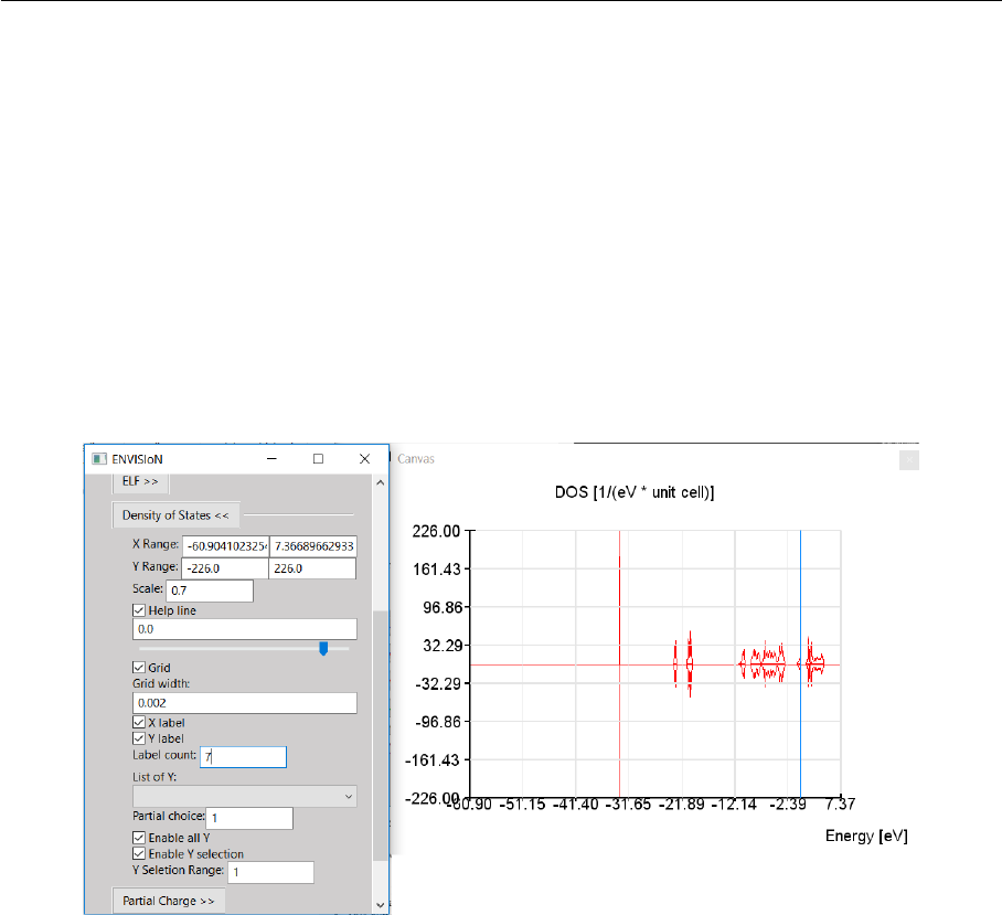
6.3.6 DoS - Density of States
When expanding the density of states visualization menu the visualization starts and a control
panel appears. The menu is shown in figure 12.
Figure 12: Density of stats visualization menu expanded
Range and Scale: In the first, controls for scaling and changing the visible interval appears.
The range boxes sets minimum and maximum values for the axes to show. The scale box sets
the scaling for the entire graph with maximum one and minimum at one over a hundred.
Help line: The help line is controlled by the red box in the graphical interface. By checking
and unchecking the box, the help line is enabled and disabled. When the line is enabled, it is
possible to move around to check which X-values corresponds to what part of the curve in the
graph.
Grid: When grid is checked the visible mesh in figure 11 appears. The frequency of the grid
lines is in direct relations to number of labels, covered in the next paragraph. The thickness of
the lines is controlled from the text entry below the checkbox for the grid.
Labels: The option of labels concerns if labels should be visible on the axes or not and the
number of labels appearing along the axes. There is one option for each axis to show or hide
the labels. The text entry is for number of labels apart from lowest value.
User guide 14 TFYA75
Visualization of electron structures
LiTH
2019-05-25
List of Y: Below the label ’List of Y’ are controls for choosing lines to show and a list of all
possible choices. Here, the drop down list is a control, which can select what line to show in
the graph. The tick box for “Enable all Y” enables all Y-values to be visualized or not. When
enabled, the option to visualize some or one of the bands is disabled. The tick box for enabling y
selection reveals a hidden text entry. Here it’s possible to choose one or more band to visualize.
The options of how to choose the lines are; “n”, “n:N”, “n,N” or some combination of these,
where n and N are arbitrary integers corresponding to list indices.
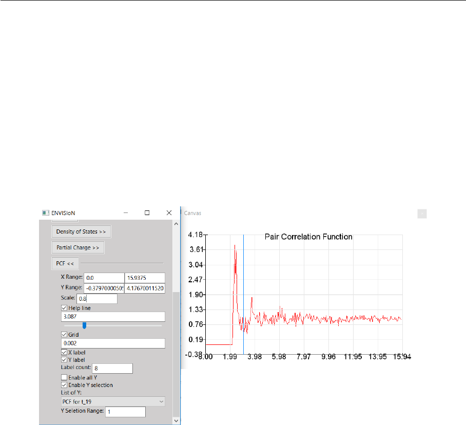
6.3.7 PCF - Pair Correlation Function
When expanding the PCF visualization menu the visualization starts and a control panel ap-
pears. In figure 13, this menu is visible.
Figure 13: Pair correlation function visualization menu expanded
Range and Scale: In the first, controls for scaling and changing the visible interval appears.
The range boxes sets minimum and maximum values for the axes to show. The scale box sets
the scaling for the entire graph with maximum one and minimum at one over a hundred.
Help line: The help line is controlled by the red box in the graphical interface. By checking
and unchecking the box, the help line is enabled and disabled. When the line is enabled, it is
possible to move around the line to check which X-values corresponds to what part of the curve
in the graph.
Grid: When grid is checked the visible mesh in figure 11 appears. The frequency of the grid
lines is in direct relations to number of labels, covered in the next paragraph. The thickness of
the lines is controlled from the text entry below the checkbox for the grid.
Labels: The option of labels concerns if labels should be visible on the axes or not and the
number of labels appearing along the axes. There is one option for each axis to show or hide
the labels. The text entry is for number of labels apart from lowest value.
User guide 15 TFYA75

Visualization of electron structures
LiTH
2019-05-25
List of Y: Below the label “List of Y” are controls for choosing lines to show and a list of all
possible choices. Here, the drop down list is a control, which can select what line to show in
the graph. The tick box for “Enable all Y” enables all Y-values to be visualized or not. When
enabled, the option to visualize some or one of the bands is disabled. The tick box for enabling
y selection reveals a hidden text entry. Here it’s possible to choose one or several bands to
visualize. The options of how to choose the lines are; “n”, “n:N”, “n,N” or some combination
of these, where n and N are arbitrary integers corresponding to list indices.
User guide 16 TFYA75
Visualization of electron structures
LiTH
2019-05-25
7 Common errors during installation
7.1 Qt
Inviwo uses the graphics library Qt which isn’t always installed properly. These instructions
show how to download and install the latest version of Qt on Ubuntu 10.04 LTS. That is, in the
moment of writing this user guide, version 5.12.3.
To download the installation file into the /Downloads directory, simply execute the commands
below.
cd ~/Downloads
wget http://download.qt.io/official_releases/qt/5.12/5.12.3/qt-
opensource-linux-x64-5.12.3.run
When the installation file has finished downloading, the user won’t have permission to run the
file. To change permissions and run the file by executing the commands below and enter your
superuser password immediately after.
chmod +x qt-opensource-linux-x64-5.12.3.run
sudo ./qt-opensource-linux-x64-5.12.3.run
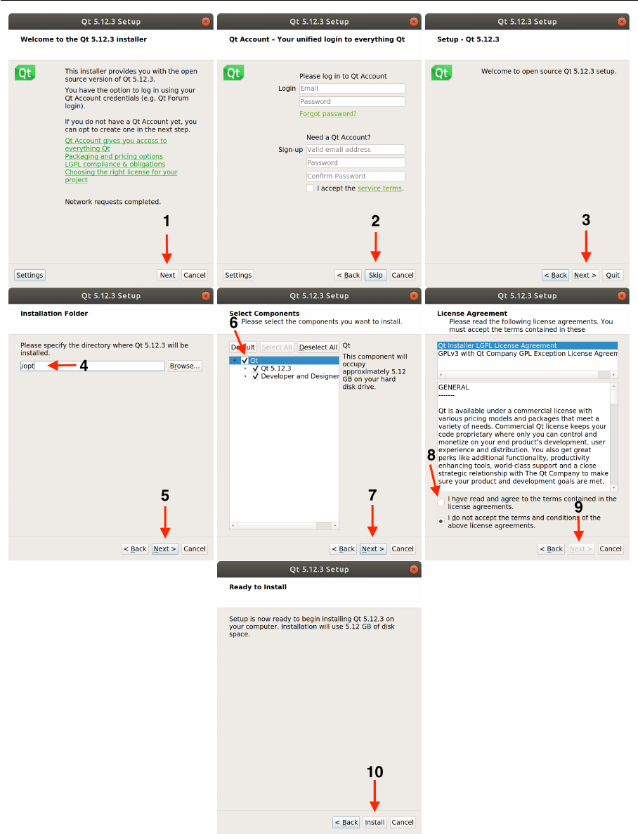
An Qt installer is now shown on the screen. Notice that the manual installation will force a
installation of the Qt editor as shown in step 6. The entire installation will occupy approximately
5.12 GB. Follow the instructions in figure 14 to complete the installation.
After the installation is done, the path to Qt needs to be added to the system. Add the necessary
paths by executing the commands below.
cd /usr/lib/x86_64-linux-gnu/qtchooser
sudo echo "/opt/Qt5.12.3/5.12.3/gcc_64/bin" | sudo tee -a default.conf
sudo echo "/opt/Qt5.12.3/5.12.3/gcc_64/lib" | sudo tee -a default.conf
The system is now ready for an Inviwo installation.
User guide 17 TFYA75
Visualization of electron structures
LiTH
2019-05-25
Figure 14: Instructions for installation of Qt 5.12.3.
User guide 18 TFYA75

Visualization of electron structures
LiTH
2019-05-25
A Licens
Copyright (c) 2019: Abdullatif Ismail, Anton Hjert, Jesper Ericsson, Lloyd Kizito, Linda Le
All rights reserved.
Redistribution and use in source and binary forms, with or without modification, are permitted
provided that the following conditions are met:
1. Redistributions of source code must retain the above copyright notice, this list of conditions
and the following disclaimer. 2. Redistributions in binary form must reproduce the above
copyright notice, this list of conditions and the following disclaimer in the documentation and/or
other materials provided with the distribution.
THIS SOFTWARE IS PROVIDED BY THE COPYRIGHT HOLDERS AND CONTRIBU-
TORS "AS IS" AND ANY EXPRESS OR IMPLIED WARRANTIES, INCLUDING, BUT
NOT LIMITED TO, THE IMPLIED WARRANTIES OF MERCHANTABILITY AND FIT-
NESS FOR A PARTICULAR PURPOSE ARE DISCLAIMED. IN NO EVENT SHALL THE
COPYRIGHT OWNER OR CONTRIBUTORS BE LIABLE FOR ANY DIRECT, INDIRECT,
INCIDENTAL, SPECIAL, EXEMPLARY, OR CONSEQUENTIAL DAMAGES (INCLUD-
ING, BUT NOT LIMITED TO, PROCUREMENT OF SUBSTITUTE GOODS OR SERVICES;
LOSS OF USE, DATA, OR PROFITS; OR BUSINESS INTERRUPTION) HOWEVER CAUSED
AND ON ANY THEORY OF LIABILITY, WHETHER IN CONTRACT, STRICT LIABIL-
ITY, OR TORT (INCLUDING NEGLIGENCE OR OTHERWISE) ARISING IN ANY WAY
OUT OF THE USE OF THIS SOFTWARE, EVEN IF ADVISED OF THE POSSIBILITY OF
SUCH DAMAGE.
User guide 19 TFYA75
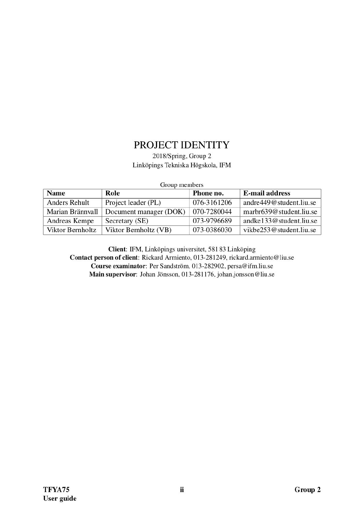
B Projekt group 2018