OpenFOAM User Guide
User Manual:
Open the PDF directly: View PDF ![]() .
.
Page Count: 228 [warning: Documents this large are best viewed by clicking the View PDF Link!]
- Copyright Notice
- Trademarks
- Contents
- 1 Introduction
- 2 Tutorials
- 2.1 Lid-driven cavity flow
- 2.1.1 Pre-processing
- 2.1.2 Viewing the mesh
- 2.1.3 Running an application
- 2.1.4 Post-processing
- 2.1.5 Increasing the mesh resolution
- 2.1.6 Introducing mesh grading
- 2.1.7 Increasing the Reynolds number
- 2.1.8 High Reynolds number flow
- 2.1.9 Changing the case geometry
- 2.1.10 Post-processing the modified geometry
- 2.2 Stress analysis of a plate with a hole
- 2.3 Breaking of a dam
- 2.3.1 Mesh generation
- 2.3.2 Boundary conditions
- 2.3.3 Setting initial field
- 2.3.4 Fluid properties
- 2.3.5 Turbulence modelling
- 2.3.6 Time step control
- 2.3.7 Discretisation schemes
- 2.3.8 Linear-solver control
- 2.3.9 Running the code
- 2.3.10 Post-processing
- 2.3.11 Running in parallel
- 2.3.12 Post-processing a case run in parallel
- 2.1 Lid-driven cavity flow
- 3 Applications and libraries
- 3.1 The programming language of OpenFOAM
- 3.2 Compiling applications and libraries
- 3.3 Running applications
- 3.4 Running applications in parallel
- 3.5 Standard solvers
- 3.6 Standard utilities
- 3.7 Standard libraries
- 4 OpenFOAM cases
- 5 Mesh generation and conversion
- 6 Post-processing
- 6.1 paraFoam
- 6.2 Function Objects
- 6.3 Post-processing with Fluent
- 6.4 Post-processing with Fieldview
- 6.5 Post-processing with EnSight
- 6.6 Sampling data
- 6.7 Monitoring and managing jobs
- 7 Models and physical properties
- Index

OpenFOAM
The Open Source CFD Toolbox
User Guide
Version 2.4.0
21st May 2015

U-2
Copyright c
°2011-2015 OpenFOAM Foundation Ltd.
Author: Christopher J. Greenshields, CFD Direct Ltd.
This work is licensed under a
Creative Commons Attribution-NonCommercial-NoDerivs 3.0 Unported License.
Typeset in L
A
T
EX.
License
THE WORK (AS DEFINED BELOW) IS PROVIDED UNDER THE TERMS OF THIS CRE-
ATIVE COMMONS PUBLIC LICENSE (“CCPL” OR “LICENSE”). THE WORK IS PRO-
TECTED BY COPYRIGHT AND/OR OTHER APPLICABLE LAW. ANY USE OF THE WORK
OTHER THAN AS AUTHORIZED UNDER THIS LICENSE OR COPYRIGHT LAW IS PRO-
HIBITED.
BY EXERCISING ANY RIGHTS TO THE WORK PROVIDED HERE, YOU ACCEPT AND
AGREE TO BE BOUND BY THE TERMS OF THIS LICENSE. TO THE EXTENT THIS LI-
CENSE MAY BE CONSIDERED TO BE A CONTRACT, THE LICENSOR GRANTS YOU THE
RIGHTS CONTAINED HERE IN CONSIDERATION OF YOUR ACCEPTANCE OF SUCH
TERMS AND CONDITIONS.
1. Definitions
a. “Adaptation” means a work based upon the Work, or upon the Work and other pre-existing
works, such as a translation, adaptation, derivative work, arrangement of music or other
alterations of a literary or artistic work, or phonogram or performance and includes cine-
matographic adaptations or any other form in which the Work may be recast, transformed, or
adapted including in any form recognizably derived from the original, except that a work that
constitutes a Collection will not be considered an Adaptation for the purpose of this License.
For the avoidance of doubt, where the Work is a musical work, performance or phonogram,
the synchronization of the Work in timed-relation with a moving image (“synching”) will be
considered an Adaptation for the purpose of this License.
b. “Collection” means a collection of literary or artistic works, such as encyclopedias and an-
thologies, or performances, phonograms or broadcasts, or other works or subject matter
other than works listed in Section 1(f) below, which, by reason of the selection and arrange-
ment of their contents, constitute intellectual creations, in which the Work is included in its
entirety in unmodified form along with one or more other contributions, each constituting
separate and independent works in themselves, which together are assembled into a collec-
tive whole. A work that constitutes a Collection will not be considered an Adaptation (as
defined above) for the purposes of this License.
c. “Distribute” means to make available to the public the original and copies of the Work
through sale or other transfer of ownership.
d. “Licensor” means the individual, individuals, entity or entities that offer(s) the Work under
the terms of this License.
e. “Original Author” means, in the case of a literary or artistic work, the individual, individuals,
entity or entities who created the Work or if no individual or entity can be identified, the
OpenFOAM-2.4.0

U-3
publisher; and in addition (i) in the case of a performance the actors, singers, musicians,
dancers, and other persons who act, sing, deliver, declaim, play in, interpret or otherwise
perform literary or artistic works or expressions of folklore; (ii) in the case of a phonogram
the producer being the person or legal entity who first fixes the sounds of a performance
or other sounds; and, (iii) in the case of broadcasts, the organization that transmits the
broadcast.
f. “Work” means the literary and/or artistic work offered under the terms of this License
including without limitation any production in the literary, scientific and artistic domain,
whatever may be the mode or form of its expression including digital form, such as a book,
pamphlet and other writing; a lecture, address, sermon or other work of the same nature;
a dramatic or dramatico-musical work; a choreographic work or entertainment in dumb
show; a musical composition with or without words; a cinematographic work to which are
assimilated works expressed by a process analogous to cinematography; a work of drawing,
painting, architecture, sculpture, engraving or lithography; a photographic work to which are
assimilated works expressed by a process analogous to photography; a work of applied art; an
illustration, map, plan, sketch or three-dimensional work relative to geography, topography,
architecture or science; a performance; a broadcast; a phonogram; a compilation of data to
the extent it is protected as a copyrightable work; or a work performed by a variety or circus
performer to the extent it is not otherwise considered a literary or artistic work.
g. “You” means an individual or entity exercising rights under this License who has not pre-
viously violated the terms of this License with respect to the Work, or who has received
express permission from the Licensor to exercise rights under this License despite a previous
violation.
h. “Publicly Perform” means to perform public recitations of the Work and to communicate to
the public those public recitations, by any means or process, including by wire or wireless
means or public digital performances; to make available to the public Works in such a way
that members of the public may access these Works from a place and at a place individu-
ally chosen by them; to perform the Work to the public by any means or process and the
communication to the public of the performances of the Work, including by public digital
performance; to broadcast and rebroadcast the Work by any means including signs, sounds
or images.
i. “Reproduce” means to make copies of the Work by any means including without limitation
by sound or visual recordings and the right of fixation and reproducing fixations of the Work,
including storage of a protected performance or phonogram in digital form or other electronic
medium.
2. Fair Dealing Rights.
Nothing in this License is intended to reduce, limit, or restrict any uses free from copyright or
rights arising from limitations or exceptions that are provided for in connection with the copyright
protection under copyright law or other applicable laws.
3. License Grant.
Subject to the terms and conditions of this License, Licensor hereby grants You a worldwide,
royalty-free, non-exclusive, perpetual (for the duration of the applicable copyright) license to ex-
ercise the rights in the Work as stated below:
a. to Reproduce the Work, to incorporate the Work into one or more Collections, and to
Reproduce the Work as incorporated in the Collections;
OpenFOAM-2.4.0

U-4
b. and, to Distribute and Publicly Perform the Work including as incorporated in Collections.
The above rights may be exercised in all media and formats whether now known or hereafter
devised. The above rights include the right to make such modifications as are technically necessary
to exercise the rights in other media and formats, but otherwise you have no rights to make
Adaptations. Subject to 8(f), all rights not expressly granted by Licensor are hereby reserved,
including but not limited to the rights set forth in Section 4(d).
4. Restrictions.
The license granted in Section 3 above is expressly made subject to and limited by the following
restrictions:
a. You may Distribute or Publicly Perform the Work only under the terms of this License. You
must include a copy of, or the Uniform Resource Identifier (URI) for, this License with every
copy of the Work You Distribute or Publicly Perform. You may not offer or impose any terms
on the Work that restrict the terms of this License or the ability of the recipient of the Work
to exercise the rights granted to that recipient under the terms of the License. You may not
sublicense the Work. You must keep intact all notices that refer to this License and to the
disclaimer of warranties with every copy of the Work You Distribute or Publicly Perform.
When You Distribute or Publicly Perform the Work, You may not impose any effective
technological measures on the Work that restrict the ability of a recipient of the Work from
You to exercise the rights granted to that recipient under the terms of the License. This
Section 4(a) applies to the Work as incorporated in a Collection, but this does not require
the Collection apart from the Work itself to be made subject to the terms of this License. If
You create a Collection, upon notice from any Licensor You must, to the extent practicable,
remove from the Collection any credit as required by Section 4(c), as requested.
b. You may not exercise any of the rights granted to You in Section 3 above in any manner
that is primarily intended for or directed toward commercial advantage or private monetary
compensation. The exchange of the Work for other copyrighted works by means of digital file-
sharing or otherwise shall not be considered to be intended for or directed toward commercial
advantage or private monetary compensation, provided there is no payment of any monetary
compensation in connection with the exchange of copyrighted works.
c. If You Distribute, or Publicly Perform the Work or Collections, You must, unless a request
has been made pursuant to Section 4(a), keep intact all copyright notices for the Work
and provide, reasonable to the medium or means You are utilizing: (i) the name of the
Original Author (or pseudonym, if applicable) if supplied, and/or if the Original Author
and/or Licensor designate another party or parties (e.g., a sponsor institute, publishing
entity, journal) for attribution (“Attribution Parties”) in Licensor’s copyright notice, terms
of service or by other reasonable means, the name of such party or parties; (ii) the title of
the Work if supplied; (iii) to the extent reasonably practicable, the URI, if any, that Licensor
specifies to be associated with the Work, unless such URI does not refer to the copyright
notice or licensing information for the Work. The credit required by this Section 4(c) may be
implemented in any reasonable manner; provided, however, that in the case of a Collection,
at a minimum such credit will appear, if a credit for all contributing authors of Collection
appears, then as part of these credits and in a manner at least as prominent as the credits
for the other contributing authors. For the avoidance of doubt, You may only use the credit
required by this Section for the purpose of attribution in the manner set out above and, by
exercising Your rights under this License, You may not implicitly or explicitly assert or imply
any connection with, sponsorship or endorsement by the Original Author, Licensor and/or
OpenFOAM-2.4.0

U-5
Attribution Parties, as appropriate, of You or Your use of the Work, without the separate,
express prior written permission of the Original Author, Licensor and/or Attribution Parties.
d. For the avoidance of doubt:
i. Non-waivable Compulsory License Schemes. In those jurisdictions in which the
right to collect royalties through any statutory or compulsory licensing scheme cannot
be waived, the Licensor reserves the exclusive right to collect such royalties for any
exercise by You of the rights granted under this License;
ii. Waivable Compulsory License Schemes. In those jurisdictions in which the right
to collect royalties through any statutory or compulsory licensing scheme can be waived,
the Licensor reserves the exclusive right to collect such royalties for any exercise by You
of the rights granted under this License if Your exercise of such rights is for a purpose
or use which is otherwise than noncommercial as permitted under Section 4(b) and
otherwise waives the right to collect royalties through any statutory or compulsory
licensing scheme; and,
iii. Voluntary License Schemes. The Licensor reserves the right to collect royalties,
whether individually or, in the event that the Licensor is a member of a collecting
society that administers voluntary licensing schemes, via that society, from any exercise
by You of the rights granted under this License that is for a purpose or use which is
otherwise than noncommercial as permitted under Section 4(b).
e. Except as otherwise agreed in writing by the Licensor or as may be otherwise permitted by
applicable law, if You Reproduce, Distribute or Publicly Perform the Work either by itself or
as part of any Collections, You must not distort, mutilate, modify or take other derogatory
action in relation to the Work which would be prejudicial to the Original Author’s honor or
reputation.
5. Representations, Warranties and Disclaimer
UNLESS OTHERWISE MUTUALLY AGREED BY THE PARTIES IN WRITING, LICENSOR
OFFERS THE WORK AS-IS AND MAKES NO REPRESENTATIONS OR WARRANTIES OF
ANY KIND CONCERNING THE WORK, EXPRESS, IMPLIED, STATUTORY OR OTHER-
WISE, INCLUDING, WITHOUT LIMITATION, WARRANTIES OF TITLE, MERCHANTIBIL-
ITY, FITNESS FOR A PARTICULAR PURPOSE, NONINFRINGEMENT, OR THE ABSENCE
OF LATENT OR OTHER DEFECTS, ACCURACY, OR THE PRESENCE OF ABSENCE OF
ERRORS, WHETHER OR NOT DISCOVERABLE. SOME JURISDICTIONS DO NOT ALLOW
THE EXCLUSION OF IMPLIED WARRANTIES, SO SUCH EXCLUSION MAY NOT APPLY
TO YOU.
6. Limitation on Liability.
EXCEPT TO THE EXTENT REQUIRED BY APPLICABLE LAW, IN NO EVENT WILL LI-
CENSOR BE LIABLE TO YOU ON ANY LEGAL THEORY FOR ANY SPECIAL, INCIDEN-
TAL, CONSEQUENTIAL, PUNITIVE OR EXEMPLARY DAMAGES ARISING OUT OF THIS
LICENSE OR THE USE OF THE WORK, EVEN IF LICENSOR HAS BEEN ADVISED OF
THE POSSIBILITY OF SUCH DAMAGES.
7. Termination
a. This License and the rights granted hereunder will terminate automatically upon any breach
by You of the terms of this License. Individuals or entities who have received Collections
OpenFOAM-2.4.0

U-6
from You under this License, however, will not have their licenses terminated provided such
individuals or entities remain in full compliance with those licenses. Sections 1, 2, 5, 6, 7,
and 8 will survive any termination of this License.
b. Subject to the above terms and conditions, the license granted here is perpetual (for the
duration of the applicable copyright in the Work). Notwithstanding the above, Licensor
reserves the right to release the Work under different license terms or to stop distributing
the Work at any time; provided, however that any such election will not serve to withdraw
this License (or any other license that has been, or is required to be, granted under the terms
of this License), and this License will continue in full force and effect unless terminated as
stated above.
8. Miscellaneous
a. Each time You Distribute or Publicly Perform the Work or a Collection, the Licensor offers
to the recipient a license to the Work on the same terms and conditions as the license granted
to You under this License.
b. If any provision of this License is invalid or unenforceable under applicable law, it shall
not affect the validity or enforceability of the remainder of the terms of this License, and
without further action by the parties to this agreement, such provision shall be reformed to
the minimum extent necessary to make such provision valid and enforceable.
c. No term or provision of this License shall be deemed waived and no breach consented to
unless such waiver or consent shall be in writing and signed by the party to be charged with
such waiver or consent.
d. This License constitutes the entire agreement between the parties with respect to the Work
licensed here. There are no understandings, agreements or representations with respect to
the Work not specified here. Licensor shall not be bound by any additional provisions that
may appear in any communication from You.
e. This License may not be modified without the mutual written agreement of the Licensor
and You. The rights granted under, and the subject matter referenced, in this License were
drafted utilizing the terminology of the Berne Convention for the Protection of Literary
and Artistic Works (as amended on September 28, 1979), the Rome Convention of 1961,
the WIPO Copyright Treaty of 1996, the WIPO Performances and Phonograms Treaty of
1996 and the Universal Copyright Convention (as revised on July 24, 1971). These rights
and subject matter take effect in the relevant jurisdiction in which the License terms are
sought to be enforced according to the corresponding provisions of the implementation of
those treaty provisions in the applicable national law. If the standard suite of rights granted
under applicable copyright law includes additional rights not granted under this License,
such additional rights are deemed to be included in the License; this License is not intended
to restrict the license of any rights under applicable law.
OpenFOAM-2.4.0

U-7
Trademarks
ANSYS is a registered trademark of ANSYS Inc.
CFX is a registered trademark of Ansys Inc.
CHEMKIN is a registered trademark of Reaction Design Corporation
EnSight is a registered trademark of Computational Engineering International Ltd.
Fieldview is a registered trademark of Intelligent Light
Fluent is a registered trademark of Ansys Inc.
GAMBIT is a registered trademark of Ansys Inc.
Icem-CFD is a registered trademark of Ansys Inc.
I-DEAS is a registered trademark of Structural Dynamics Research Corporation
JAVA is a registered trademark of Sun Microsystems Inc.
Linux is a registered trademark of Linus Torvalds
OpenFOAM is a registered trademark of ESI Group
ParaView is a registered trademark of Kitware
STAR-CD is a registered trademark of Computational Dynamics Ltd.
UNIX is a registered trademark of The Open Group
OpenFOAM-2.4.0

U-8
OpenFOAM-2.4.0
Contents
Copyright Notice U-2
1. Definitions . . . . . . . . . . . . . . . . . . . . . . . . . . . . . . . . . . . U-2
2. Fair Dealing Rights. . . . . . . . . . . . . . . . . . . . . . . . . . . . . . . U-3
3. License Grant. . . . . . . . . . . . . . . . . . . . . . . . . . . . . . . . . . U-3
4. Restrictions. . . . . . . . . . . . . . . . . . . . . . . . . . . . . . . . . . . U-4
5. Representations, Warranties and Disclaimer . . . . . . . . . . . . . . . . . U-5
6. Limitation on Liability. . . . . . . . . . . . . . . . . . . . . . . . . . . . . U-5
7. Termination . . . . . . . . . . . . . . . . . . . . . . . . . . . . . . . . . . U-5
8. Miscellaneous . . . . . . . . . . . . . . . . . . . . . . . . . . . . . . . . . U-6
Trademarks U-7
Contents U-9
1 Introduction U-15
2 Tutorials U-17
2.1 Lid-driven cavity flow . . . . . . . . . . . . . . . . . . . . . . . . . . . . U-17
2.1.1 Pre-processing . . . . . . . . . . . . . . . . . . . . . . . . . . . . U-18
2.1.1.1 Mesh generation . . . . . . . . . . . . . . . . . . . . . U-18
2.1.1.2 Boundary and initial conditions . . . . . . . . . . . . . U-20
2.1.1.3 Physical properties . . . . . . . . . . . . . . . . . . . . U-21
2.1.1.4 Control . . . . . . . . . . . . . . . . . . . . . . . . . . U-22
2.1.1.5 Discretisation and linear-solver settings . . . . . . . . . U-23
2.1.2 Viewing the mesh . . . . . . . . . . . . . . . . . . . . . . . . . . U-23
2.1.3 Running an application . . . . . . . . . . . . . . . . . . . . . . . U-25
2.1.4 Post-processing . . . . . . . . . . . . . . . . . . . . . . . . . . . U-25
2.1.4.1 Isosurface and contour plots . . . . . . . . . . . . . . . U-25
2.1.4.2 Vector plots . . . . . . . . . . . . . . . . . . . . . . . . U-27
2.1.4.3 Streamline plots . . . . . . . . . . . . . . . . . . . . . U-29
2.1.5 Increasing the mesh resolution . . . . . . . . . . . . . . . . . . . U-29
2.1.5.1 Creating a new case using an existing case . . . . . . . U-29
2.1.5.2 Creating the finer mesh . . . . . . . . . . . . . . . . . U-31
2.1.5.3 Mapping the coarse mesh results onto the fine mesh . . U-31
2.1.5.4 Control adjustments . . . . . . . . . . . . . . . . . . . U-32
2.1.5.5 Running the code as a background process . . . . . . . U-32
2.1.5.6 Vector plot with the refined mesh . . . . . . . . . . . . U-32
2.1.5.7 Plotting graphs . . . . . . . . . . . . . . . . . . . . . . U-32

U-10 Contents
2.1.6 Introducing mesh grading . . . . . . . . . . . . . . . . . . . . . U-35
2.1.6.1 Creating the graded mesh . . . . . . . . . . . . . . . . U-36
2.1.6.2 Changing time and time step . . . . . . . . . . . . . . U-37
2.1.6.3 Mapping fields . . . . . . . . . . . . . . . . . . . . . . U-38
2.1.7 Increasing the Reynolds number . . . . . . . . . . . . . . . . . . U-38
2.1.7.1 Pre-processing . . . . . . . . . . . . . . . . . . . . . . U-38
2.1.7.2 Running the code . . . . . . . . . . . . . . . . . . . . . U-39
2.1.8 High Reynolds number flow . . . . . . . . . . . . . . . . . . . . U-39
2.1.8.1 Pre-processing . . . . . . . . . . . . . . . . . . . . . . U-40
2.1.8.2 Running the code . . . . . . . . . . . . . . . . . . . . . U-42
2.1.9 Changing the case geometry . . . . . . . . . . . . . . . . . . . . U-42
2.1.10 Post-processing the modified geometry . . . . . . . . . . . . . . U-44
2.2 Stress analysis of a plate with a hole . . . . . . . . . . . . . . . . . . . U-44
2.2.1 Mesh generation . . . . . . . . . . . . . . . . . . . . . . . . . . U-47
2.2.1.1 Boundary and initial conditions . . . . . . . . . . . . . U-49
2.2.1.2 Mechanical properties . . . . . . . . . . . . . . . . . . U-51
2.2.1.3 Thermal properties . . . . . . . . . . . . . . . . . . . . U-51
2.2.1.4 Control . . . . . . . . . . . . . . . . . . . . . . . . . . U-51
2.2.1.5 Discretisation schemes and linear-solver control . . . . U-52
2.2.2 Running the code . . . . . . . . . . . . . . . . . . . . . . . . . . U-54
2.2.3 Post-processing . . . . . . . . . . . . . . . . . . . . . . . . . . . U-54
2.2.4 Exercises . . . . . . . . . . . . . . . . . . . . . . . . . . . . . . . U-55
2.2.4.1 Increasing mesh resolution . . . . . . . . . . . . . . . . U-55
2.2.4.2 Introducing mesh grading . . . . . . . . . . . . . . . . U-55
2.2.4.3 Changing the plate size . . . . . . . . . . . . . . . . . U-56
2.3 Breaking of a dam . . . . . . . . . . . . . . . . . . . . . . . . . . . . . U-56
2.3.1 Mesh generation . . . . . . . . . . . . . . . . . . . . . . . . . . U-57
2.3.2 Boundary conditions . . . . . . . . . . . . . . . . . . . . . . . . U-58
2.3.3 Setting initial field . . . . . . . . . . . . . . . . . . . . . . . . . U-59
2.3.4 Fluid properties . . . . . . . . . . . . . . . . . . . . . . . . . . . U-60
2.3.5 Turbulence modelling . . . . . . . . . . . . . . . . . . . . . . . . U-61
2.3.6 Time step control . . . . . . . . . . . . . . . . . . . . . . . . . . U-61
2.3.7 Discretisation schemes . . . . . . . . . . . . . . . . . . . . . . . U-62
2.3.8 Linear-solver control . . . . . . . . . . . . . . . . . . . . . . . . U-63
2.3.9 Running the code . . . . . . . . . . . . . . . . . . . . . . . . . . U-64
2.3.10 Post-processing . . . . . . . . . . . . . . . . . . . . . . . . . . . U-64
2.3.11 Running in parallel . . . . . . . . . . . . . . . . . . . . . . . . . U-64
2.3.12 Post-processing a case run in parallel . . . . . . . . . . . . . . . U-67
3 Applications and libraries U-69
3.1 The programming language of OpenFOAM . . . . . . . . . . . . . . . . U-69
3.1.1 Language in general . . . . . . . . . . . . . . . . . . . . . . . . U-69
3.1.2 Object-orientation and C++ . . . . . . . . . . . . . . . . . . . . U-70
3.1.3 Equation representation . . . . . . . . . . . . . . . . . . . . . . U-70
3.1.4 Solver codes . . . . . . . . . . . . . . . . . . . . . . . . . . . . . U-71
3.2 Compiling applications and libraries . . . . . . . . . . . . . . . . . . . . U-71
3.2.1 Header .H files . . . . . . . . . . . . . . . . . . . . . . . . . . . . U-71
3.2.2 Compiling with wmake . . . . . . . . . . . . . . . . . . . . . . . U-73
OpenFOAM-2.4.0

Contents U-11
3.2.2.1 Including headers . . . . . . . . . . . . . . . . . . . . . U-73
3.2.2.2 Linking to libraries . . . . . . . . . . . . . . . . . . . . U-74
3.2.2.3 Source files to be compiled . . . . . . . . . . . . . . . . U-75
3.2.2.4 Running wmake . . . . . . . . . . . . . . . . . . . . . . U-75
3.2.2.5 wmake environment variables . . . . . . . . . . . . . . U-76
3.2.3 Removing dependency lists: wclean and rmdepall . . . . . . . . . U-76
3.2.4 Compilation example: the pisoFoam application . . . . . . . . . U-77
3.2.5 Debug messaging and optimisation switches . . . . . . . . . . . U-80
3.2.6 Linking new user-defined libraries to existing applications . . . . U-81
3.3 Running applications . . . . . . . . . . . . . . . . . . . . . . . . . . . . U-81
3.4 Running applications in parallel . . . . . . . . . . . . . . . . . . . . . . U-82
3.4.1 Decomposition of mesh and initial field data . . . . . . . . . . . U-82
3.4.2 Running a decomposed case . . . . . . . . . . . . . . . . . . . . U-84
3.4.3 Distributing data across several disks . . . . . . . . . . . . . . . U-85
3.4.4 Post-processing parallel processed cases . . . . . . . . . . . . . . U-86
3.4.4.1 Reconstructing mesh and data . . . . . . . . . . . . . U-86
3.4.4.2 Post-processing decomposed cases . . . . . . . . . . . . U-86
3.5 Standard solvers . . . . . . . . . . . . . . . . . . . . . . . . . . . . . . . U-86
3.6 Standard utilities . . . . . . . . . . . . . . . . . . . . . . . . . . . . . . U-91
3.7 Standard libraries . . . . . . . . . . . . . . . . . . . . . . . . . . . . . . U-99
4 OpenFOAM cases U-107
4.1 File structure of OpenFOAM cases . . . . . . . . . . . . . . . . . . . . U-107
4.2 Basic input/output file format . . . . . . . . . . . . . . . . . . . . . . . U-108
4.2.1 General syntax rules . . . . . . . . . . . . . . . . . . . . . . . . U-108
4.2.2 Dictionaries . . . . . . . . . . . . . . . . . . . . . . . . . . . . . U-109
4.2.3 The data file header . . . . . . . . . . . . . . . . . . . . . . . . U-109
4.2.4 Lists . . . . . . . . . . . . . . . . . . . . . . . . . . . . . . . . . U-110
4.2.5 Scalars, vectors and tensors . . . . . . . . . . . . . . . . . . . . U-111
4.2.6 Dimensional units . . . . . . . . . . . . . . . . . . . . . . . . . . U-111
4.2.7 Dimensioned types . . . . . . . . . . . . . . . . . . . . . . . . . U-112
4.2.8 Fields . . . . . . . . . . . . . . . . . . . . . . . . . . . . . . . . U-112
4.2.9 Directives and macro substitutions . . . . . . . . . . . . . . . . U-113
4.2.10 The #include and #inputMode directives . . . . . . . . . . . . U-114
4.2.11 The #codeStream directive . . . . . . . . . . . . . . . . . . . . U-114
4.3 Time and data input/output control . . . . . . . . . . . . . . . . . . . U-115
4.4 Numerical schemes . . . . . . . . . . . . . . . . . . . . . . . . . . . . . U-118
4.4.1 Interpolation schemes . . . . . . . . . . . . . . . . . . . . . . . . U-119
4.4.1.1 Schemes for strictly bounded scalar fields . . . . . . . U-120
4.4.1.2 Schemes for vector fields . . . . . . . . . . . . . . . . . U-121
4.4.2 Surface normal gradient schemes . . . . . . . . . . . . . . . . . U-121
4.4.3 Gradient schemes . . . . . . . . . . . . . . . . . . . . . . . . . . U-122
4.4.4 Laplacian schemes . . . . . . . . . . . . . . . . . . . . . . . . . U-123
4.4.5 Divergence schemes . . . . . . . . . . . . . . . . . . . . . . . . . U-123
4.4.6 Time schemes . . . . . . . . . . . . . . . . . . . . . . . . . . . . U-124
4.4.7 Flux calculation . . . . . . . . . . . . . . . . . . . . . . . . . . . U-125
4.5 Solution and algorithm control . . . . . . . . . . . . . . . . . . . . . . . U-125
4.5.1 Linear solver control . . . . . . . . . . . . . . . . . . . . . . . . U-125
OpenFOAM-2.4.0

U-12 Contents
4.5.1.1 Solution tolerances . . . . . . . . . . . . . . . . . . . . U-126
4.5.1.2 Preconditioned conjugate gradient solvers . . . . . . . U-127
4.5.1.3 Smooth solvers . . . . . . . . . . . . . . . . . . . . . . U-127
4.5.1.4 Geometric-algebraic multi-grid solvers . . . . . . . . . U-127
4.5.2 Solution under-relaxation . . . . . . . . . . . . . . . . . . . . . U-128
4.5.3 PISO and SIMPLE algorithms . . . . . . . . . . . . . . . . . . . U-129
4.5.3.1 Pressure referencing . . . . . . . . . . . . . . . . . . . U-130
4.5.4 Other parameters . . . . . . . . . . . . . . . . . . . . . . . . . . U-130
5 Mesh generation and conversion U-131
5.1 Mesh description . . . . . . . . . . . . . . . . . . . . . . . . . . . . . . U-131
5.1.1 Mesh specification and validity constraints . . . . . . . . . . . . U-131
5.1.1.1 Points . . . . . . . . . . . . . . . . . . . . . . . . . . . U-132
5.1.1.2 Faces . . . . . . . . . . . . . . . . . . . . . . . . . . . U-132
5.1.1.3 Cells . . . . . . . . . . . . . . . . . . . . . . . . . . . . U-133
5.1.1.4 Boundary . . . . . . . . . . . . . . . . . . . . . . . . . U-133
5.1.2 The polyMesh description . . . . . . . . . . . . . . . . . . . . . . U-133
5.1.3 The cellShape tools . . . . . . . . . . . . . . . . . . . . . . . . . U-134
5.1.4 1- and 2-dimensional and axi-symmetric problems . . . . . . . . U-135
5.2 Boundaries . . . . . . . . . . . . . . . . . . . . . . . . . . . . . . . . . U-135
5.2.1 Specification of patch types in OpenFOAM . . . . . . . . . . . . U-135
5.2.2 Base types . . . . . . . . . . . . . . . . . . . . . . . . . . . . . . U-139
5.2.3 Primitive types . . . . . . . . . . . . . . . . . . . . . . . . . . . U-140
5.2.4 Derived types . . . . . . . . . . . . . . . . . . . . . . . . . . . . U-140
5.3 Mesh generation with the blockMesh utility . . . . . . . . . . . . . . . . U-141
5.3.1 Writing a blockMeshDict file . . . . . . . . . . . . . . . . . . . . U-143
5.3.1.1 The vertices . . . . . . . . . . . . . . . . . . . . . . U-144
5.3.1.2 The edges . . . . . . . . . . . . . . . . . . . . . . . . U-144
5.3.1.3 The blocks . . . . . . . . . . . . . . . . . . . . . . . . U-145
5.3.1.4 Multi-grading of a block . . . . . . . . . . . . . . . . . U-146
5.3.1.5 The boundary . . . . . . . . . . . . . . . . . . . . . . U-147
5.3.2 Multiple blocks . . . . . . . . . . . . . . . . . . . . . . . . . . . U-149
5.3.3 Creating blocks with fewer than 8 vertices . . . . . . . . . . . . U-151
5.3.4 Running blockMesh . . . . . . . . . . . . . . . . . . . . . . . . . U-151
5.4 Mesh generation with the snappyHexMesh utility . . . . . . . . . . . . . U-151
5.4.1 The mesh generation process of snappyHexMesh . . . . . . . . . U-152
5.4.2 Creating the background hex mesh . . . . . . . . . . . . . . . . U-153
5.4.3 Cell splitting at feature edges and surfaces . . . . . . . . . . . . U-154
5.4.4 Cell removal . . . . . . . . . . . . . . . . . . . . . . . . . . . . . U-156
5.4.5 Cell splitting in specified regions . . . . . . . . . . . . . . . . . . U-156
5.4.6 Snapping to surfaces . . . . . . . . . . . . . . . . . . . . . . . . U-157
5.4.7 Mesh layers . . . . . . . . . . . . . . . . . . . . . . . . . . . . . U-157
5.4.8 Mesh quality controls . . . . . . . . . . . . . . . . . . . . . . . . U-159
5.5 Mesh conversion . . . . . . . . . . . . . . . . . . . . . . . . . . . . . . . U-160
5.5.1 fluentMeshToFoam . . . . . . . . . . . . . . . . . . . . . . . . . U-161
5.5.2 starToFoam . . . . . . . . . . . . . . . . . . . . . . . . . . . . . U-162
5.5.2.1 General advice on conversion . . . . . . . . . . . . . . U-162
5.5.2.2 Eliminating extraneous data . . . . . . . . . . . . . . . U-163
OpenFOAM-2.4.0

Contents U-13
5.5.2.3 Removing default boundary conditions . . . . . . . . . U-164
5.5.2.4 Renumbering the model . . . . . . . . . . . . . . . . . U-164
5.5.2.5 Writing out the mesh data . . . . . . . . . . . . . . . . U-165
5.5.2.6 Problems with the .vrt file . . . . . . . . . . . . . . . . U-166
5.5.2.7 Converting the mesh to OpenFOAM format . . . . . . U-166
5.5.3 gambitToFoam . . . . . . . . . . . . . . . . . . . . . . . . . . . . U-167
5.5.4 ideasToFoam . . . . . . . . . . . . . . . . . . . . . . . . . . . . . U-167
5.5.5 cfx4ToFoam . . . . . . . . . . . . . . . . . . . . . . . . . . . . . U-167
5.6 Mapping fields between different geometries . . . . . . . . . . . . . . . U-168
5.6.1 Mapping consistent fields . . . . . . . . . . . . . . . . . . . . . . U-168
5.6.2 Mapping inconsistent fields . . . . . . . . . . . . . . . . . . . . . U-168
5.6.3 Mapping parallel cases . . . . . . . . . . . . . . . . . . . . . . . U-169
6 Post-processing U-171
6.1 paraFoam . . . . . . . . . . . . . . . . . . . . . . . . . . . . . . . . . . U-171
6.1.1 Overview of paraFoam . . . . . . . . . . . . . . . . . . . . . . . U-171
6.1.2 The Properties panel . . . . . . . . . . . . . . . . . . . . . . . . U-173
6.1.3 The Display panel . . . . . . . . . . . . . . . . . . . . . . . . . . U-173
6.1.4 The button toolbars . . . . . . . . . . . . . . . . . . . . . . . . U-175
6.1.5 Manipulating the view . . . . . . . . . . . . . . . . . . . . . . . U-175
6.1.5.1 View settings . . . . . . . . . . . . . . . . . . . . . . . U-175
6.1.5.2 General settings . . . . . . . . . . . . . . . . . . . . . U-176
6.1.6 Contour plots . . . . . . . . . . . . . . . . . . . . . . . . . . . . U-176
6.1.6.1 Introducing a cutting plane . . . . . . . . . . . . . . . U-176
6.1.7 Vector plots . . . . . . . . . . . . . . . . . . . . . . . . . . . . . U-176
6.1.7.1 Plotting at cell centres . . . . . . . . . . . . . . . . . . U-177
6.1.8 Streamlines . . . . . . . . . . . . . . . . . . . . . . . . . . . . . U-177
6.1.9 Image output . . . . . . . . . . . . . . . . . . . . . . . . . . . . U-177
6.1.10 Animation output . . . . . . . . . . . . . . . . . . . . . . . . . . U-177
6.2 Function Objects . . . . . . . . . . . . . . . . . . . . . . . . . . . . . . U-178
6.2.1 Using function objects . . . . . . . . . . . . . . . . . . . . . . . U-180
6.2.2 Packaged function objects . . . . . . . . . . . . . . . . . . . . . U-181
6.3 Post-processing with Fluent . . . . . . . . . . . . . . . . . . . . . . . . U-183
6.4 Post-processing with Fieldview . . . . . . . . . . . . . . . . . . . . . . . U-184
6.5 Post-processing with EnSight . . . . . . . . . . . . . . . . . . . . . . . . U-185
6.5.1 Converting data to EnSight format . . . . . . . . . . . . . . . . U-185
6.5.2 The ensight74FoamExec reader module . . . . . . . . . . . . . . U-185
6.5.2.1 Configuration of EnSight for the reader module . . . . U-185
6.5.2.2 Using the reader module . . . . . . . . . . . . . . . . . U-186
6.6 Sampling data . . . . . . . . . . . . . . . . . . . . . . . . . . . . . . . . U-186
6.7 Monitoring and managing jobs . . . . . . . . . . . . . . . . . . . . . . . U-188
6.7.1 The foamJob script for running jobs . . . . . . . . . . . . . . . . U-190
6.7.2 The foamLog script for monitoring jobs . . . . . . . . . . . . . . U-190
7 Models and physical properties U-193
7.1 Thermophysical models . . . . . . . . . . . . . . . . . . . . . . . . . . . U-193
7.1.1 Thermophysical property data . . . . . . . . . . . . . . . . . . . U-195
7.2 Turbulence models . . . . . . . . . . . . . . . . . . . . . . . . . . . . . U-198
OpenFOAM-2.4.0

Chapter 1
Introduction
This guide accompanies the release of version 2.4.0 of the Open Source Field Operation and
Manipulation (OpenFOAM) C++ libraries. It provides a description of the basic operation
of OpenFOAM, first through a set of tutorial exercises in chapter 2and later by a more
detailed description of the individual components that make up OpenFOAM.
OpenFOAM is first and foremost a C++ library, used primarily to create executables,
known as applications. The applications fall into two categories: solvers, that are each
designed to solve a specific problem in continuum mechanics; and utilities, that are designed
to perform tasks that involve data manipulation. The OpenFOAM distribution contains
numerous solvers and utilities covering a wide range of problems, as described in chapter 3.
One of the strengths of OpenFOAM is that new solvers and utilities can be created by its
users with some pre-requisite knowledge of the underlying method, physics and programming
techniques involved.
OpenFOAM is supplied with pre- and post-processing environments. The interface to the
pre- and post-processing are themselves OpenFOAM utilities, thereby ensuring consistent
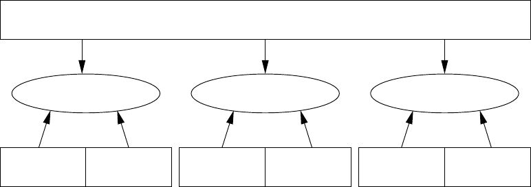
data handling across all environments. The overall structure of OpenFOAM is shown in
Figure 1.1. The pre-processing and running of OpenFOAM cases is described in chapter 4.
Applications
User
Tools
Meshing
Utilities Standard
Applications Others
e.g.EnSight
Post-processingSolvingPre-processing
Open Source Field Operation and Manipulation (OpenFOAM) C++ Library
ParaView
Figure 1.1: Overview of OpenFOAM structure.
In chapter 5, we cover both the generation of meshes using the mesh generator supplied
with OpenFOAM and conversion of mesh data generated by third-party products. Post-
processing is described in chapter 6.

U-16 Introduction
OpenFOAM-2.4.0

Chapter 2
Tutorials
In this chapter we shall describe in detail the process of setup, simulation and post-processing
for some OpenFOAM test cases, with the principal aim of introducing a user to the basic
procedures of running OpenFOAM. The $FOAM TUTORIALS directory contains many more
cases that demonstrate the use of all the solvers and many utilities supplied with Open-
FOAM. Before attempting to run the tutorials, the user must first make sure that they have
installed OpenFOAM correctly.
The tutorial cases describe the use of the blockMesh pre-processing tool, case setup and
running OpenFOAM solvers and post-processing using paraFoam. Those users with access to
third-party post-processing tools supported in OpenFOAM have an option: either they can
follow the tutorials using paraFoam; or refer to the description of the use of the third-party
product in chapter 6when post-processing is required.
Copies of all tutorials are available from the tutorials directory of the OpenFOAM instal-
lation. The tutorials are organised into a set of directories according to the type of flow and
then subdirectories according to solver. For example, all the icoFoam cases are stored within
a subdirectory incompressible/icoFoam, where incompressible indicates the type of flow. If
the user wishes to run a range of example cases, it is recommended that the user copy the
tutorials directory into their local run directory. They can be easily copied by typing:
mkdir -p $FOAM RUN
cp -r $FOAM TUTORIALS $FOAM RUN
2.1 Lid-driven cavity flow
This tutorial will describe how to pre-process, run and post-process a case involving isother-
mal, incompressible flow in a two-dimensional square domain. The geometry is shown in
Figure 2.1 in which all the boundaries of the square are walls. The top wall moves in the
x-direction at a speed of 1 m/s while the other 3 are stationary. Initially, the flow will be
assumed laminar and will be solved on a uniform mesh using the icoFoam solver for laminar,
isothermal, incompressible flow. During the course of the tutorial, the effect of increased
mesh resolution and mesh grading towards the walls will be investigated. Finally, the flow
Reynolds number will be increased and the pisoFoam solver will be used for turbulent,
isothermal, incompressible flow.
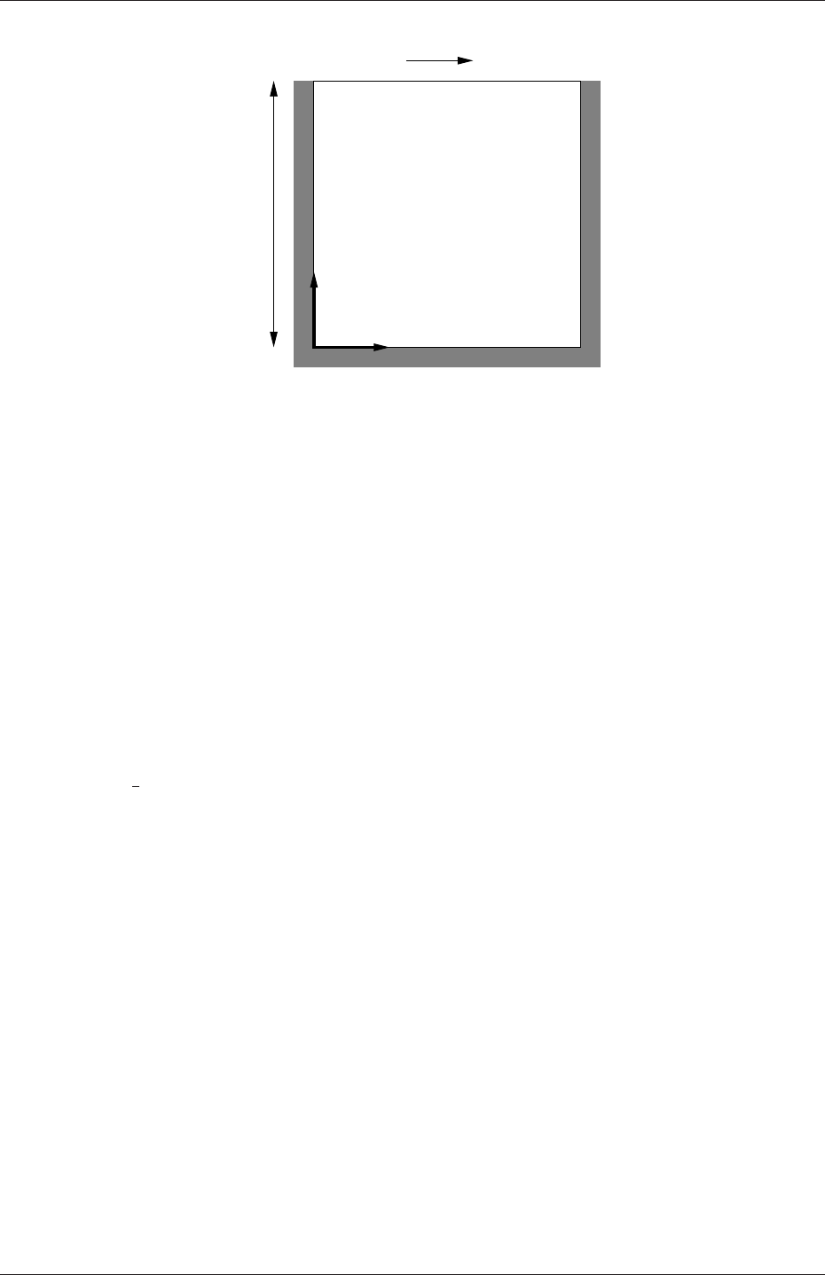
U-18 Tutorials
x
Ux= 1 m/s
d= 0.1 m
y
Figure 2.1: Geometry of the lid driven cavity.
2.1.1 Pre-processing
Cases are setup in OpenFOAM by editing case files. Users should select an xeditor of choice
with which to do this, such as emacs,vi,gedit,kate,nedit,etc. Editing files is possible in
OpenFOAM because the I/O uses a dictionary format with keywords that convey sufficient
meaning to be understood by even the least experienced users.
A case being simulated involves data for mesh, fields, properties, control parameters,
etc. As described in section 4.1, in OpenFOAM this data is stored in a set of files within a
case directory rather than in a single case file, as in many other CFD packages. The case
directory is given a suitably descriptive name, e.g. the first example case for this tutorial is
simply named cavity. In preparation of editing case files and running the first cavity case,
the user should change to the case directory
cd $FOAM RUN/tutorials/incompressible/icoFoam/cavity
2.1.1.1 Mesh generation
OpenFOAM always operates in a 3 dimensional Cartesian coordinate system and all geome-
tries are generated in 3 dimensions. OpenFOAM solves the case in 3 dimensions by default
but can be instructed to solve in 2 dimensions by specifying a ‘special’ empty boundary
condition on boundaries normal to the (3rd) dimension for which no solution is required.
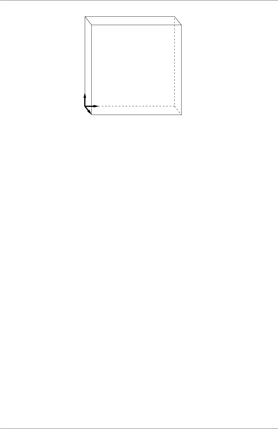
The cavity domain consists of a square of side length d= 0.1 m in the x-yplane. A
uniform mesh of 20 by 20 cells will be used initially. The block structure is shown in Fig-
ure 2.2. The mesh generator supplied with OpenFOAM, blockMesh, generates meshes from a
description specified in an input dictionary, blockMeshDict located in the constant/polyMesh
directory for a given case. The blockMeshDict entries for this case are as follows:
1/*--------------------------------*- C++ -*----------------------------------*\
2| ========= | |
3| \\ / F ield | OpenFOAM: The Open Source CFD Toolbox |
4| \\ / O peration | Version: 2.4.0 |
5| \\ / A nd | Web: www.OpenFOAM.org |
6| \\/ M anipulation | |
7\*---------------------------------------------------------------------------*/
8FoamFile
OpenFOAM-2.4.0
2.1 Lid-driven cavity flow U-19
3 2
4 5
7 6
0
z
x1
y
Figure 2.2: Block structure of the mesh for the cavity.
9{
10 version 2.0;
11 format ascii;
12 class dictionary;
13 object blockMeshDict;
14 }
15 // * * * * * * * * * * * * * * * * * * * * * * * * * * * * * * * * * * * * * //
16
17 convertToMeters 0.1;
18
19 vertices
20 (
21 (0 0 0)
22 (1 0 0)
23 (1 1 0)
24 (0 1 0)
25 (0 0 0.1)
26 (1 0 0.1)
27 (1 1 0.1)
28 (0 1 0.1)
29 );
30
31 blocks
32 (
33 hex (0 1 2 3 4 5 6 7) (20 20 1) simpleGrading (1 1 1)
34 );
35
36 edges
37 (
38 );
39
40 boundary
41 (
42 movingWall
43 {
44 type wall;
45 faces
46 (
47 (3 7 6 2)
48 );
49 }
50 fixedWalls
51 {
52 type wall;
53 faces
54 (
55 (0 4 7 3)
56 (2 6 5 1)
57 (1 5 4 0)
58 );
59 }
60 frontAndBack
61 {
OpenFOAM-2.4.0

U-20 Tutorials
62 type empty;
63 faces
64 (
65 (0 3 2 1)
66 (4 5 6 7)
67 );
68 }
69 );
70
71 mergePatchPairs
72 (
73 );
74
75 // ************************************************************************* //
The file first contains header information in the form of a banner (lines 1-7), then file
information contained in a FoamFile sub-dictionary, delimited by curly braces ({...}).
For the remainder of the manual:
For the sake of clarity and to save space, file headers, including the banner and
FoamFile sub-dictionary, will be removed from verbatim quoting of case files
The file first specifies coordinates of the block vertices; it then defines the blocks
(here, only 1) from the vertex labels and the number of cells within it; and finally, it defines
the boundary patches. The user is encouraged to consult section 5.3 to understand the
meaning of the entries in the blockMeshDict file.
The mesh is generated by running blockMesh on this blockMeshDict file. From within
the case directory, this is done, simply by typing in the terminal:
blockMesh
The running status of blockMesh is reported in the terminal window. Any mistakes in the
blockMeshDict file are picked up by blockMesh and the resulting error message directs the
user to the line in the file where the problem occurred. There should be no error messages
at this stage.
2.1.1.2 Boundary and initial conditions
Once the mesh generation is complete, the user can look at this initial fields set up for this
case. The case is set up to start at time t= 0 s, so the initial field data is stored in a 0
sub-directory of the cavity directory. The 0sub-directory contains 2 files, pand U, one for
each of the pressure (p) and velocity (U) fields whose initial values and boundary conditions
must be set. Let us examine file p:
17 dimensions [0 2 -2 0 0 0 0];
18
19 internalField uniform 0;
20
21 boundaryField
22 {
23 movingWall
24 {
25 type zeroGradient;
26 }
27
28 fixedWalls
29 {
30 type zeroGradient;
31 }
32
33 frontAndBack
OpenFOAM-2.4.0

2.1 Lid-driven cavity flow U-21
34 {
35 type empty;
36 }
37 }
38
39 // ************************************************************************* //
There are 3 principal entries in field data files:
dimensions specifies the dimensions of the field, here kinematic pressure, i.e. m2s−2(see
section 4.2.6 for more information);
internalField the internal field data which can be uniform, described by a single value;
or nonuniform, where all the values of the field must be specified (see section 4.2.8
for more information);
boundaryField the boundary field data that includes boundary conditions and data for all
the boundary patches (see section 4.2.8 for more information).
For this case cavity, the boundary consists of walls only, split into 2 patches named: (1)
fixedWalls for the fixed sides and base of the cavity; (2) movingWall for the moving top
of the cavity. As walls, both are given a zeroGradient boundary condition for p, meaning
“the normal gradient of pressure is zero”. The frontAndBack patch represents the front
and back planes of the 2D case and therefore must be set as empty.
In this case, as in most we encounter, the initial fields are set to be uniform. Here the
pressure is kinematic, and as an incompressible case, its absolute value is not relevant, so is
set to uniform 0 for convenience.
The user can similarly examine the velocity field in the 0/U file. The dimensions are
those expected for velocity, the internal field is initialised as uniform zero, which in the case of
velocity must be expressed by 3 vector components, i.e.uniform (0 0 0) (see section 4.2.5
for more information).
The boundary field for velocity requires the same boundary condition for the frontAnd-
Back patch. The other patches are walls: a no-slip condition is assumed on the fixedWalls,
hence a fixedValue condition with a value of uniform (0 0 0). The top surface moves at
a speed of 1 m/s in the x-direction so requires a fixedValue condition also but with uniform
(1 0 0).
2.1.1.3 Physical properties
The physical properties for the case are stored in dictionaries whose names are given the
suffix . . . Properties, located in the Dictionaries directory tree. For an icoFoam case,
the only property that must be specified is the kinematic viscosity which is stored from
the transportProperties dictionary. The user can check that the kinematic viscosity is set
correctly by opening the transportProperties dictionary to view/edit its entries. The keyword
for kinematic viscosity is nu, the phonetic label for the Greek symbol νby which it is
represented in equations. Initially this case will be run with a Reynolds number of 10,
where the Reynolds number is defined as:
Re =d|U|
ν(2.1)
where dand |U|are the characteristic length and velocity respectively and νis the kinematic
viscosity. Here d= 0.1 m, |U|= 1 m s−1, so that for Re = 10, ν= 0.01 m2s−1. The correct
file entry for kinematic viscosity is thus specified below:
OpenFOAM-2.4.0

U-22 Tutorials
17
18 nu nu [ 0 2 -1 0 0 0 0 ] 0.01;
19
20
21 // ************************************************************************* //
2.1.1.4 Control
Input data relating to the control of time and reading and writing of the solution data are
read in from the controlDict dictionary. The user should view this file; as a case control file,
it is located in the system directory.
The start/stop times and the time step for the run must be set. OpenFOAM offers great
flexibility with time control which is described in full in section 4.3. In this tutorial we
wish to start the run at time t= 0 which means that OpenFOAM needs to read field data
from a directory named 0— see section 4.1 for more information of the case file structure.
Therefore we set the startFrom keyword to startTime and then specify the startTime
keyword to be 0.
For the end time, we wish to reach the steady state solution where the flow is circulating
around the cavity. As a general rule, the fluid should pass through the domain 10 times to
reach steady state in laminar flow. In this case the flow does not pass through this domain
as there is no inlet or outlet, so instead the end time can be set to the time taken for the
lid to travel ten times across the cavity, i.e. 1 s; in fact, with hindsight, we discover that
0.5 s is sufficient so we shall adopt this value. To specify this end time, we must specify the
stopAt keyword as endTime and then set the endTime keyword to 0.5.
Now we need to set the time step, represented by the keyword deltaT. To achieve
temporal accuracy and numerical stability when running icoFoam, a Courant number of less
than 1 is required. The Courant number is defined for one cell as:
Co =δt|U|
δx (2.2)
where δt is the time step, |U|is the magnitude of the velocity through that cell and δx is
the cell size in the direction of the velocity. The flow velocity varies across the domain and
we must ensure Co < 1 everywhere. We therefore choose δt based on the worst case: the
maximum Co corresponding to the combined effect of a large flow velocity and small cell
size. Here, the cell size is fixed across the domain so the maximum Co will occur next to
the lid where the velocity approaches 1 m s−1. The cell size is:
δx =d
n=0.1
20 = 0.005 m (2.3)
Therefore to achieve a Courant number less than or equal to 1 throughout the domain the
time step deltaT must be set to less than or equal to:
δt =Co δx
|U|=1×0.005
1= 0.005 s (2.4)
As the simulation progresses we wish to write results at certain intervals of time that we
can later view with a post-processing package. The writeControl keyword presents several
options for setting the time at which the results are written; here we select the timeStep
option which specifies that results are written every nth time step where the value nis
specified under the writeInterval keyword. Let us decide that we wish to write our
OpenFOAM-2.4.0

2.1 Lid-driven cavity flow U-23
results at times 0.1, 0.2,. . . , 0.5 s. With a time step of 0.005 s, we therefore need to output
results at every 20th time time step and so we set writeInterval to 20.
OpenFOAM creates a new directory named after the current time,e.g. 0.1 s, on each
occasion that it writes a set of data, as discussed in full in section 4.1. In the icoFoam solver,
it writes out the results for each field, Uand p, into the time directories. For this case, the
entries in the controlDict are shown below:
17
18 application icoFoam;
19
20 startFrom startTime;
21
22 startTime 0;
23
24 stopAt endTime;
25
26 endTime 0.5;
27
28 deltaT 0.005;
29
30 writeControl timeStep;
31
32 writeInterval 20;
33
34 purgeWrite 0;
35
36 writeFormat ascii;
37
38 writePrecision 6;
39
40 writeCompression off;
41
42 timeFormat general;
43
44 timePrecision 6;
45
46 runTimeModifiable true;
47
48
49 // ************************************************************************* //
2.1.1.5 Discretisation and linear-solver settings
The user specifies the choice of finite volume discretisation schemes in the fvSchemes dictio-
nary in the system directory. The specification of the linear equation solvers and tolerances
and other algorithm controls is made in the fvSolution dictionary, similarly in the system
directory. The user is free to view these dictionaries but we do not need to discuss all their
entries at this stage except for pRefCell and pRefValue in the PISO sub-dictionary of the
fvSolution dictionary. In a closed incompressible system such as the cavity, pressure is rel-
ative: it is the pressure range that matters not the absolute values. In cases such as this,
the solver sets a reference level by pRefValue in cell pRefCell. In this example both are
set to 0. Changing either of these values will change the absolute pressure field, but not, of
course, the relative pressures or velocity field.
2.1.2 Viewing the mesh
Before the case is run it is a good idea to view the mesh to check for any errors. The mesh
is viewed in paraFoam, the post-processing tool supplied with OpenFOAM. The paraFoam
post-processing is started by typing in the terminal from within the case directory
paraFoam
OpenFOAM-2.4.0
U-24 Tutorials
Alternatively, it can be launched from another directory location with an optional -case
argument giving the case directory, e.g.
paraFoam -case $FOAM RUN/tutorials/incompressible/icoFoam/cavity
This launches the ParaView window as shown in Figure 6.1. In the Pipeline Browser,
the user can see that ParaView has opened cavity.OpenFOAM, the module for the cavity
case. Before clicking the Apply button, the user needs to select some geometry from the
Mesh Parts panel. Because the case is small, it is easiest to select all the data by checking
the box adjacent to the Mesh Parts panel title, which automatically checks all individual
components within the respective panel. The user should then click the Apply button to
load the geometry into ParaView.
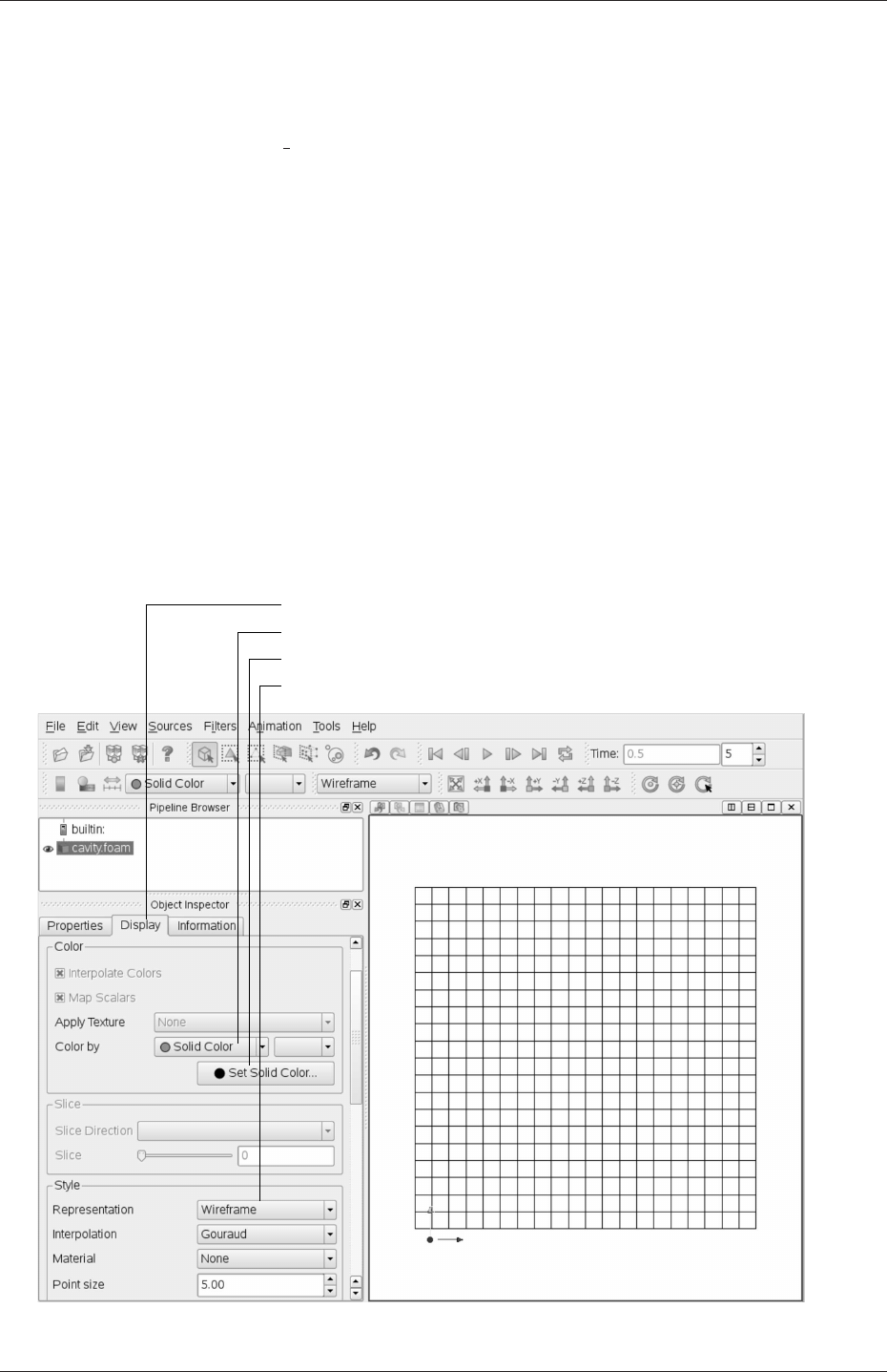
The user should then open the Display panel that controls the visual representation of the
selected module. Within the Display panel the user should do the following as shown in Fig-
ure 2.3: (1) set Color By Solid Color; (2) click Set Ambient Color and select an appropriate
colour e.g. black (for a white background); (3) in the Style panel, select Wireframe from the
Representation menu. The background colour can be set by selecting View Settings...
from Edit in the top menu panel.
Open Display panel
Select Color by Solid Color
Set Solid Color,e.g. black
Select Wireframe
Figure 2.3: Viewing the mesh in paraFoam.
OpenFOAM-2.4.0

2.1 Lid-driven cavity flow U-25
Especially the first time the user starts ParaView,it is recommended that they ma-
nipulate the view as described in section 6.1.5. In particular, since this is a 2D case, it is
recommended that Use Parallel Projection is selected in the General panel of View Settings
window selected from the Edit menu. The Orientation Axes can be toggled on and off in the
Annotation window or moved by drag and drop with the mouse.
2.1.3 Running an application
Like any UNIX/Linux executable, OpenFOAM applications can be run in two ways: as
a foreground process, i.e. one in which the shell waits until the command has finished
before giving a command prompt; as a background process, one which does not have to be
completed before the shell accepts additional commands.
On this occasion, we will run icoFoam in the foreground. The icoFoam solver is executed
either by entering the case directory and typing
icoFoam
at the command prompt, or with the optional -case argument giving the case directory,
e.g.
icoFoam -case $FOAM RUN/tutorials/incompressible/icoFoam/cavity
The progress of the job is written to the terminal window. It tells the user the current
time, maximum Courant number, initial and final residuals for all fields.
2.1.4 Post-processing
As soon as results are written to time directories, they can be viewed using paraFoam.
Return to the paraFoam window and select the Properties panel for the cavity.OpenFOAM
case module. If the correct window panels for the case module do not seem to be present at
any time, please ensure that: cavity.OpenFOAM is highlighted in blue; eye button alongside
it is switched on to show the graphics are enabled;
To prepare paraFoam to display the data of interest, we must first load the data at the
required run time of 0.5 s. If the case was run while ParaView was open, the output data
in time directories will not be automatically loaded within ParaView. To load the data the
user should click Refresh Times in the Properties window. The time data will be loaded into
ParaView.
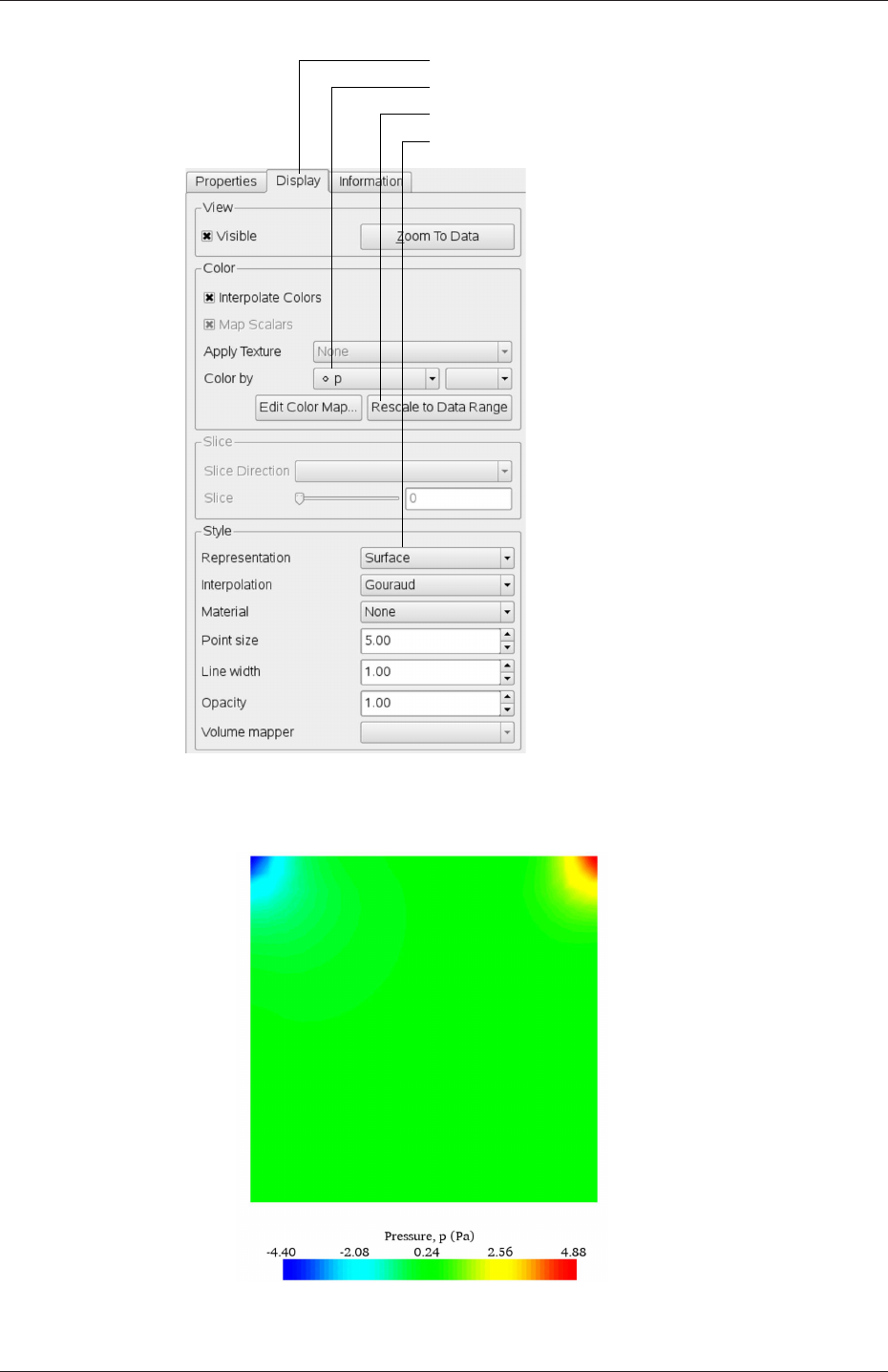
2.1.4.1 Isosurface and contour plots
To view pressure, the user should open the Display panel since it controls the visual repre-
sentation of the selected module. To make a simple plot of pressure, the user should select
the following, as described in detail in Figure 2.4: in the Style panel, select Surface from
the Representation menu; in the Color panel, select Color by and Rescale to Data
Range. Now in order to view the solution at t= 0.5 s, the user can use the VCR Controls
or Current Time Controls to change the current time to 0.5. These are located in the
toolbars below the menus at the top of the ParaView window, as shown in Figure 6.4. The
OpenFOAM-2.4.0
U-26 Tutorials
Open Display panel
Rescale to Data Range
Select Surface
Select Color by interpolated p
Figure 2.4: Displaying pressure contours for the cavity case.
Figure 2.5: Pressures in the cavity case.
OpenFOAM-2.4.0

2.1 Lid-driven cavity flow U-27
pressure field solution has, as expected, a region of low pressure at the top left of the cavity
and one of high pressure at the top right of the cavity as shown in Figure 2.5.
With the point icon ( ) the pressure field is interpolated across each cell to give a
continuous appearance. Instead if the user selects the cell icon, , from the Color by
menu, a single value for pressure will be attributed to each cell so that each cell will be
denoted by a single colour with no grading.
A colour bar can be included by either by clicking the Toggle Color Legend Visibility button
in the Active Variable Controls toolbar, or by selecting Show Color Legend from the
View menu. Clicking the Edit Color Map button, either in the Active Variable Controls
toolbar or in the Color panel of the Display window, the user can set a range of attributes
of the colour bar, such as text size, font selection and numbering format for the scale. The
colour bar can be located in the image window by drag and drop with the mouse.
New versions of ParaView default to using a colour scale of blue to white to red rather
than the more common blue to green to red (rainbow). Therefore the first time that the
user executes ParaView, they may wish to change the colour scale. This can be done by
selecting Choose Preset in the Color Scale Editor and selecting Blue to Red Rainbow. After
clicking the OK confirmation button, the user can click the Make Default button so that
ParaView will always adopt this type of colour bar.
If the user rotates the image, they can see that they have now coloured the complete
geometry surface by the pressure. In order to produce a genuine contour plot the user
should first create a cutting plane, or ‘slice’, through the geometry using the Slice filter as
described in section 6.1.6.1. The cutting plane should be centred at (0.05,0.05,0.005) and its
normal should be set to (0,0,1) (click the Z Normal button). Having generated the cutting
plane, the contours can be created using by the Contour filter described in section 6.1.6.
2.1.4.2 Vector plots
Before we start to plot the vectors of the flow velocity, it may be useful to remove other
modules that have been created, e.g. using the Slice and Contour filters described above.
These can: either be deleted entirely, by highlighting the relevant module in the Pipeline
Browser and clicking Delete in their respective Properties panel; or, be disabled by toggling
the eye button for the relevant module in the Pipeline Browser.
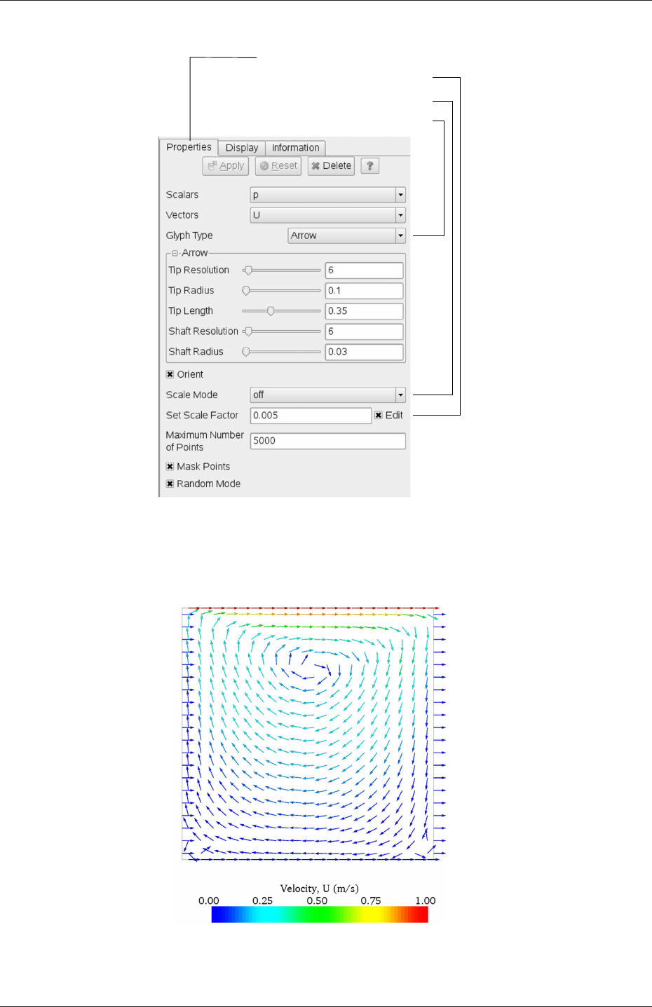
We now wish to generate a vector glyph for velocity at the centre of each cell. We first
need to filter the data to cell centres as described in section 6.1.7.1. With the cavity.OpenFOAM
module highlighted in the Pipeline Browser, the user should select Cell Centers from the
Filter->Alphabetical menu and then click Apply.
With these Centers highlighted in the Pipeline Browser, the user should then select
Glyph from the Filter->Alphabetical menu. The Properties window panel should appear
as shown in Figure 2.6. In the resulting Properties panel, the velocity field, U, is automatically
selected in the vectors menu, since it is the only vector field present. By default the Scale
Mode for the glyphs will be Vector Magnitude of velocity but, since the we may wish to
view the velocities throughout the domain, the user should instead select off and Set Scale
Factor to 0.005. On clicking Apply, the glyphs appear but, probably as a single colour,
e.g. white. The user should colour the glyphs by velocity magnitude which, as usual, is
controlled by setting Color by U in the Display panel. The user should also select Show
Color Legend in Edit Color Map. The output is shown in Figure 2.7, in which uppercase
Times Roman fonts are selected for the Color Legend headings and the labels are specified
to 2 fixed significant figures by deselecting Automatic Label Format and entering %-#6.2f in
OpenFOAM-2.4.0
U-28 Tutorials
Open Parameters panel
Select Scale Mode off
Select Glyph Type Arrow
Specify Set Scale Factor 0.005
Figure 2.6: Properties panel for the Glyph filter.
Figure 2.7: Velocities in the cavity case.
OpenFOAM-2.4.0

2.1 Lid-driven cavity flow U-29
the Label Format text box. The background colour is set to white in the General panel of
View Settings as described in section 6.1.5.1.
Note that at the left and right walls, glyphs appear to indicate flow through the walls.
On closer examination, however, the user can see that while the flow direction is normal
to the wall, its magnitude is 0. This slightly confusing situation is caused by ParaView
choosing to orientate the glyphs in the x-direction when the glyph scaling off and the
velocity magnitude is 0.
2.1.4.3 Streamline plots
Again, before the user continues to post-process in ParaView, they should disable modules
such as those for the vector plot described above. We now wish to plot streamlines of
velocity as described in section 6.1.8.
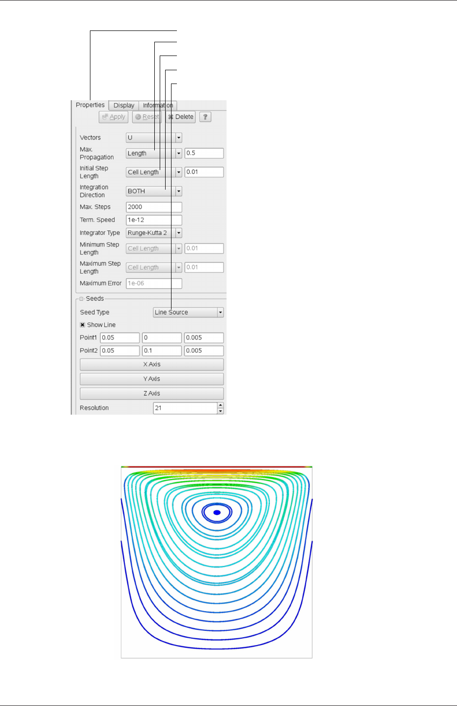
With the cavity.OpenFOAM module highlighted in the Pipeline Browser, the user should
then select Stream Tracer from the Filter menu and then click Apply. The Properties
window panel should appear as shown in Figure 2.8. The Seed points should be speci-
fied along a Line Source running vertically through the centre of the geometry, i.e. from
(0.05,0,0.005) to (0.05,0.1,0.005). For the image in this guide we used: a point Resolu-
tion of 21; Max Propagation by Length 0.5; Initial Step Length by Cell Length 0.01; and,
Integration Direction BOTH. The Runge-Kutta 2 IntegratorType was used with default
parameters.
On clicking Apply the tracer is generated. The user should then select Tube from the
Filter menu to produce high quality streamline images. For the image in this report, we
used: Num. sides 6; Radius 0.0003; and, Radius factor 10. The streamtubes are coloured by
velocity magnitude. On clicking Apply the image in Figure 2.9 should be produced.
2.1.5 Increasing the mesh resolution
The mesh resolution will now be increased by a factor of two in each direction. The results
from the coarser mesh will be mapped onto the finer mesh to use as initial conditions for
the problem. The solution from the finer mesh will then be compared with those from the
coarser mesh.
2.1.5.1 Creating a new case using an existing case
We now wish to create a new case named cavityFine that is created from cavity. The user
should therefore clone the cavity case and edit the necessary files. First the user should
create a new case directory at the same directory level as the cavity case, e.g.
cd $FOAM RUN/tutorials/incompressible/icoFoam
mkdir cavityFine
The user should then copy the base directories from the cavity case into cavityFine, and then
enter the cavityFine case.
cp -r cavity/constant cavityFine
cp -r cavity/system cavityFine
cd cavityFine
OpenFOAM-2.4.0
U-30 Tutorials
Open Parameters panel
Set Integration Direction to BOTH
Set Max Propagation to Length 0.5
Set Initial Step Length to Cell Length 0.01
Specify Line Source and set points and resolution
Figure 2.8: Properties panel for the Stream Tracer filter.
Figure 2.9: Streamlines in the cavity case.
OpenFOAM-2.4.0

2.1 Lid-driven cavity flow U-31
2.1.5.2 Creating the finer mesh
We now wish to increase the number of cells in the mesh by using blockMesh. The user
should open the blockMeshDict file in an editor and edit the block specification. The blocks
are specified in a list under the blocks keyword. The syntax of the block definitions is
described fully in section 5.3.1.3; at this stage it is sufficient to know that following hex
is first the list of vertices in the block, then a list (or vector) of numbers of cells in each
direction. This was originally set to (20 20 1) for the cavity case. The user should now
change this to (40 40 1) and save the file. The new refined mesh should then be created
by running blockMesh as before.
2.1.5.3 Mapping the coarse mesh results onto the fine mesh
The mapFields utility maps one or more fields relating to a given geometry onto the cor-
responding fields for another geometry. In our example, the fields are deemed ‘consistent’
because the geometry and the boundary types, or conditions, of both source and target fields
are identical. We use the -consistent command line option when executing mapFields in
this example.
The field data that mapFields maps is read from the time directory specified by startFrom/startTime
in the controlDict of the target case, i.e. those into which the results are being mapped. In
this example, we wish to map the final results of the coarser mesh from case cavity onto the
finer mesh of case cavityFine. Therefore, since these results are stored in the 0.5 directory
of cavity, the startTime should be set to 0.5 s in the controlDict dictionary and startFrom
should be set to startTime.
The case is ready to run mapFields. Typing mapFields -help quickly shows that map-
Fields requires the source case directory as an argument. We are using the -consistent
option, so the utility is executed from withing the cavityFine directory by
mapFields ../cavity -consistent
The utility should run with output to the terminal including:
Source: ".." "cavity"
Target: "." "cavityFine"
Create databases as time
Case : ../cavity
nProcs : 1
Source time: 0.5
Target time: 0.5
Create meshes
Source mesh size: 400 Target mesh size: 1600
Consistently creating and mapping fields for time 0.5
Creating mesh-to-mesh addressing ...
Overlap volume: 0.0001
Creating AMI between source patch movingWall and target patch movingWall ...
interpolating p
interpolating U
End
OpenFOAM-2.4.0

U-32 Tutorials
2.1.5.4 Control adjustments
To maintain a Courant number of less that 1, as discussed in section 2.1.1.4, the time step
must now be halved since the size of all cells has halved. Therefore deltaT should be set to
to 0.0025 s in the controlDict dictionary. Field data is currently written out at an interval
of a fixed number of time steps. Here we demonstrate how to specify data output at fixed
intervals of time. Under the writeControl keyword in controlDict, instead of requesting
output by a fixed number of time steps with the timeStep entry, a fixed amount of run time
can be specified between the writing of results using the runTime entry. In this case the
user should specify output every 0.1 and therefore should set writeInterval to 0.1 and
writeControl to runTime. Finally, since the case is starting with a the solution obtained on
the coarse mesh we only need to run it for a short period to achieve reasonable convergence
to steady-state. Therefore the endTime should be set to 0.7 s. Make sure these settings are
correct and then save the file.
2.1.5.5 Running the code as a background process
The user should experience running icoFoam as a background process, redirecting the ter-
minal output to a log file that can be viewed later. From the cavityFine directory, the user
should execute:
icoFoam > log &
cat log
2.1.5.6 Vector plot with the refined mesh
The user can open multiple cases simultaneously in ParaView; essentially because each new
case is simply another module that appears in the Pipeline Browser. There is one minor
inconvenience when opening a new case in ParaView because there is a prerequisite that the
selected data is a file with a name that has an extension. However, in OpenFOAM, each
case is stored in a multitude of files with no extensions within a specific directory structure.
The solution, that the paraFoam script performs automatically, is to create a dummy file
with the extension .OpenFOAM — hence, the cavity case module is called cavity.OpenFOAM.
However, if the user wishes to open another case directly from within ParaView, they
need to create such a dummy file. For example, to load the cavityFine case the file would be
created by typing at the command prompt:
cd $FOAM RUN/tutorials/incompressible/icoFoam
touch cavityFine/cavityFine.OpenFOAM
Now the cavityFine case can be loaded into ParaView by selecting Open from the File
menu, and having navigated the directory tree, selecting cavityFine.OpenFOAM. The user
can now make a vector plot of the results from the refined mesh in ParaView. The plot can
be compared with the cavity case by enabling glyph images for both case simultaneously.
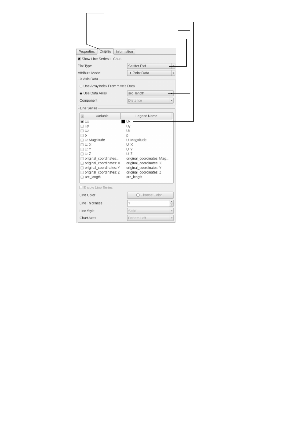
2.1.5.7 Plotting graphs
The user may wish to visualise the results by extracting some scalar measure of velocity and
plotting 2-dimensional graphs along lines through the domain. OpenFOAM is well equipped
OpenFOAM-2.4.0
2.1 Lid-driven cavity flow U-33
Open Display panel
Select Scatter Plot
Select Ux from Line Series
Select arc length
Figure 2.10: Selecting fields for graph plotting.
for this kind of data manipulation. There are numerous utilities that do specialised data
manipulations, and some, simpler calculations are incorporated into a single utility foamCalc.
As a utility, it is unique in that it is executed by
foamCalc <calcType> <fieldName1 ... fieldNameN>
The calculator operation is specified in <calcType>; at the time of writing, the following
operations are implemented: addSubtract;randomise;div;components;mag;magGrad;
magSqr;interpolate. The user can obtain the list of <calcType>by deliberately calling
one that does not exist, so that foamCalc throws up an error message and lists the types
available, e.g.
>> foamCalc xxxx
Selecting calcType xxxx
unknown calcType type xxxx, constructor not in hash table
Valid calcType selections are:
8
(
randomise
magSqr
magGrad
addSubtract
div
mag
interpolate
OpenFOAM-2.4.0

U-34 Tutorials
components
)
The components and mag calcTypes provide useful scalar measures of velocity. When
“foamCalc components U” is run on a case, say cavity, it reads in the velocity vector field
from each time directory and, in the corresponding time directories, writes scalar fields Ux,
Uy and Uz representing the x,yand zcomponents of velocity. Similarly “foamCalc mag U”
writes a scalar field magU to each time directory representing the magnitude of velocity.
The user can run foamCalc with the components calcType on both cavity and cavityFine
cases. For example, for the cavity case the user should do into the cavity directory and
execute foamCalc as follows:
cd $FOAM RUN/tutorials/incompressible/icoFoam/cavity
foamCalc components U
The individual components can be plotted as a graph in ParaView. It is quick, convenient
and has reasonably good control over labelling and formatting, so the printed output is a
fairly good standard. However, to produce graphs for publication, users may prefer to write
raw data and plot it with a dedicated graphing tool, such as gnuplot or Grace/xmgr. To do
this, we recommend using the sample utility, described in section 6.6 and section 2.2.3.
Before commencing plotting, the user needs to load the newly generated Ux,Uy and
Uz fields into ParaView. To do this, the user should click the Refresh Times at the top
of the Properties panel for the cavity.OpenFOAM module which will cause the new fields
to be loaded into ParaView and appear in the Volume Fields window. Ensure the new
fields are selected and the changes are applied, i.e. click Apply again if necessary. Also,
data is interpolated incorrectly at boundaries if the boundary regions are selected in the
Mesh Parts panel. Therefore the user should deselect the patches in the Mesh Parts panel,
i.e.movingWall,fixedWall and frontAndBack, and apply the changes.
Now, in order to display a graph in ParaView the user should select the module of
interest, e.g.cavity.OpenFOAM and apply the Plot Over Line filter from the Filter->Data
Analysis menu. This opens up a new XY Plot window below or beside the existing 3D View
window. A PlotOverLine module is created in which the user can specify the end points of
the line in the Properties panel. In this example, the user should position the line vertically
up the centre of the domain, i.e. from (0.05,0,0.005) to (0.05,0.1,0.005), in the Point1 and
Point2 text boxes. The Resolution can be set to 100.
On clicking Apply, a graph is generated in the XY Plot window. In the Display panel,
the user should set Attribute Mode to Point Data. The Use Data Array option can be
selected for the X Axis Data, taking the arc length option so that the x-axis of the graph
represents distance from the base of the cavity.
The user can choose the fields to be displayed in the Line Series panel of the Display
window. From the list of scalar fields to be displayed, it can be seen that the magnitude
and components of vector fields are available by default, e.g. displayed as U:X, so that it
was not necessary to create Ux using foamCalc. Nevertheless, the user should deselect all
series except Ux (or U:x). A square colour box in the adjacent column to the selected series
indicates the line colour. The user can edit this most easily by a double click of the mouse
over that selection.
In order to format the graph, the user should modify the settings below the Line Series
panel, namely Line Color,Line Thickness,Line Style,Marker Style and Chart Axes.
OpenFOAM-2.4.0
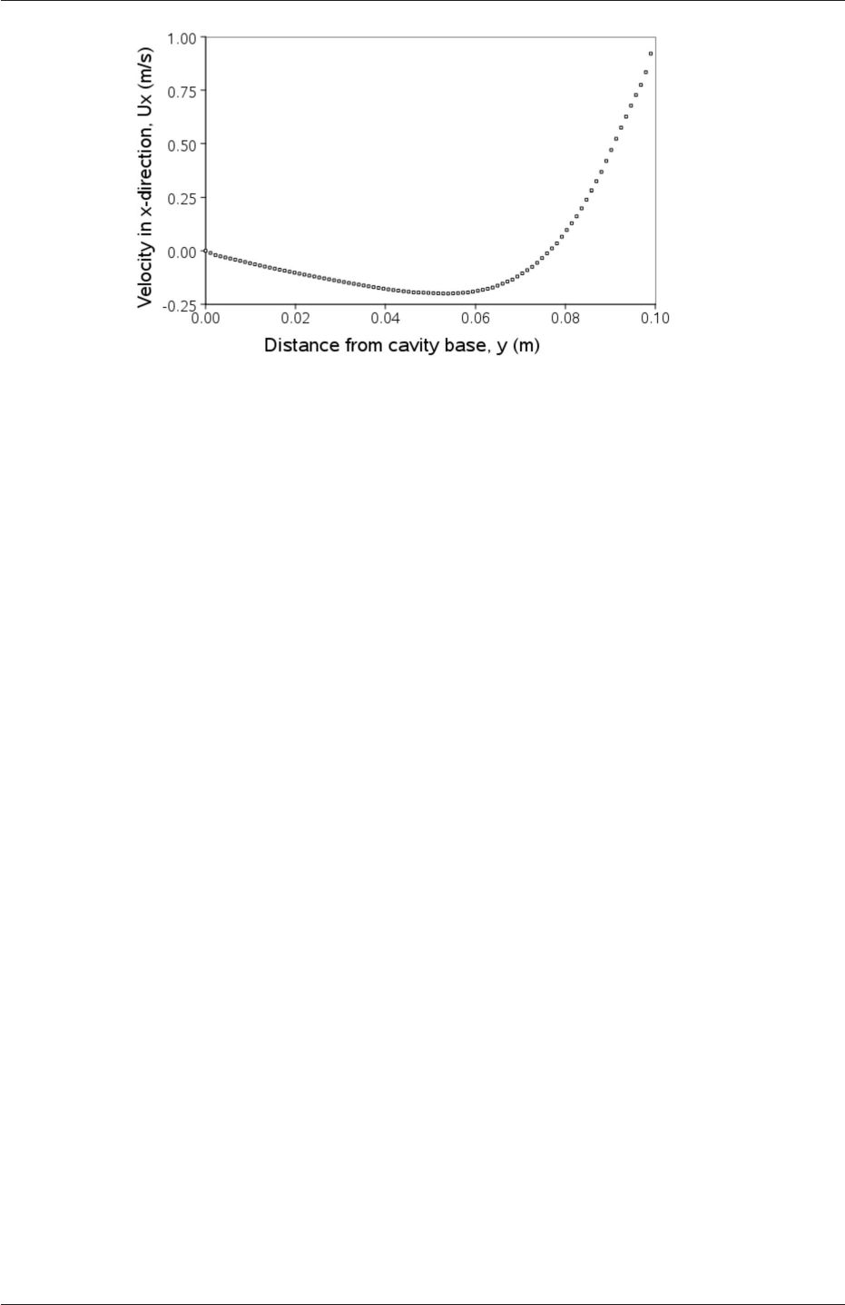
2.1 Lid-driven cavity flow U-35
Figure 2.11: Plotting graphs in paraFoam.
Also the user can click one of the buttons above the top left corner of the XY Plot. The
third button, for example, allows the user to control View Settings in which the user can set
title and legend for each axis, for example. Also, the user can set font, colour and alignment
of the axes titles, and has several options for axis range and labels in linear or logarithmic
scales.
Figure 2.11 is a graph produced using ParaView. The user can produce a graph however
he/she wishes. For information, the graph in Figure 2.11 was produced with the options for
axes of: Standard type of Notation;Specify Axis Range selected; titles in Sans Serif 12
font. The graph is displayed as a set of points rather than a line by activating the Enable
Line Series button in the Display window. Note: if this button appears to be inactive by
being “greyed out”, it can be made active by selecting and deselecting the sets of variables
in the Line Series panel. Once the Enable Line Series button is selected, the Line Style and
Marker Style can be adjusted to the user’s preference.
2.1.6 Introducing mesh grading
The error in any solution will be more pronounced in regions where the form of the true
solution differ widely from the form assumed in the chosen numerical schemes. For example
a numerical scheme based on linear variations of variables over cells can only generate an
exact solution if the true solution is itself linear in form. The error is largest in regions
where the true solution deviates greatest from linear form, i.e. where the change in gradient
is largest. Error decreases with cell size.
It is useful to have an intuitive appreciation of the form of the solution before setting
up any problem. It is then possible to anticipate where the errors will be largest and to
grade the mesh so that the smallest cells are in these regions. In the cavity case the large
variations in velocity can be expected near a wall and so in this part of the tutorial the
mesh will be graded to be smaller in this region. By using the same number of cells, greater
accuracy can be achieved without a significant increase in computational cost.
A mesh of 20 ×20 cells with grading towards the walls will be created for the lid-driven
cavity problem and the results from the finer mesh of section 2.1.5.2 will then be mapped
onto the graded mesh to use as an initial condition. The results from the graded mesh will
be compared with those from the previous meshes. Since the changes to the blockMeshDict
OpenFOAM-2.4.0
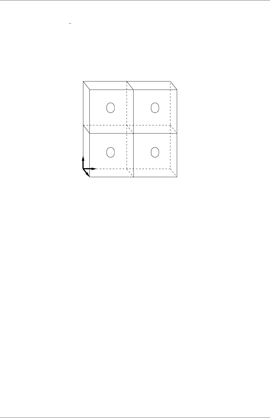
U-36 Tutorials
dictionary are fairly substantial, the case used for this part of the tutorial, cavityGrade, is
supplied in the $FOAM RUN/tutorials/incompressible/icoFoam directory.
2.1.6.1 Creating the graded mesh
The mesh now needs 4 blocks as different mesh grading is needed on the left and right and top
and bottom of the domain. The block structure for this mesh is shown in Figure 2.12. The
0
z
x
y
3 4 5
6 87
1 2
1715
911
10
16
12 13 14
0 1
2 3
Figure 2.12: Block structure of the graded mesh for the cavity (block numbers encircled).
user can view the blockMeshDict file in the constant/polyMesh subdirectory of cavityGrade;
for completeness the key elements of the blockMeshDict file are also reproduced below. Each
block now has 10 cells in the xand ydirections and the ratio between largest and smallest
cells is 2.
17 convertToMeters 0.1;
18
19 vertices
20 (
21 (0 0 0)
22 (0.5 0 0)
23 (1 0 0)
24 (0 0.5 0)
25 (0.5 0.5 0)
26 (1 0.5 0)
27 (0 1 0)
28 (0.5 1 0)
29 (1 1 0)
30 (0 0 0.1)
31 (0.5 0 0.1)
32 (1 0 0.1)
33 (0 0.5 0.1)
34 (0.5 0.5 0.1)
35 (1 0.5 0.1)
36 (0 1 0.1)
37 (0.5 1 0.1)
38 (1 1 0.1)
39 );
40
41 blocks
42 (
43 hex (0 1 4 3 9 10 13 12) (10 10 1) simpleGrading (2 2 1)
44 hex (1 2 5 4 10 11 14 13) (10 10 1) simpleGrading (0.5 2 1)
45 hex (3 4 7 6 12 13 16 15) (10 10 1) simpleGrading (2 0.5 1)
46 hex (4 5 8 7 13 14 17 16) (10 10 1) simpleGrading (0.5 0.5 1)
47 );
48
49 edges
OpenFOAM-2.4.0

2.1 Lid-driven cavity flow U-37
50 (
51 );
52
53 boundary
54 (
55 movingWall
56 {
57 type wall;
58 faces
59 (
60 (6 15 16 7)
61 (7 16 17 8)
62 );
63 }
64 fixedWalls
65 {
66 type wall;
67 faces
68 (
69 (3 12 15 6)
70 (0 9 12 3)
71 (0 1 10 9)
72 (1 2 11 10)
73 (2 5 14 11)
74 (5 8 17 14)
75 );
76 }
77 frontAndBack
78 {
79 type empty;
80 faces
81 (
82 (0 3 4 1)
83 (1 4 5 2)
84 (3 6 7 4)
85 (4 7 8 5)
86 (9 10 13 12)
87 (10 11 14 13)
88 (12 13 16 15)
89 (13 14 17 16)
90 );
91 }
92 );
93
94 mergePatchPairs
95 (
96 );
97
98 // ************************************************************************* //
Once familiar with the blockMeshDict file for this case, the user can execute blockMesh from
the command line. The graded mesh can be viewed as before using paraFoam as described
in section 2.1.2.
2.1.6.2 Changing time and time step
The highest velocities and smallest cells are next to the lid, therefore the highest Courant
number will be generated next to the lid, for reasons given in section 2.1.1.4. It is therefore
useful to estimate the size of the cells next to the lid to calculate an appropriate time step
for this case.
When a nonuniform mesh grading is used, blockMesh calculates the cell sizes using a
geometric progression. Along a length l, if ncells are requested with a ratio of Rbetween
the last and first cells, the size of the smallest cell, δxs, is given by:
δxs=lr−1
αr −1(2.5)
where ris the ratio between one cell size and the next which is given by:
r=R1
n−1(2.6)
OpenFOAM-2.4.0

U-38 Tutorials
and
α=(Rfor R > 1,
1−r−n+r−1for R < 1.(2.7)
For the cavityGrade case the number of cells in each direction in a block is 10, the ratio
between largest and smallest cells is 2 and the block height and width is 0.05 m. Therefore
the smallest cell length is 3.45 mm. From Equation 2.2, the time step should be less than 3.45
ms to maintain a Courant of less than 1. To ensure that results are written out at convenient
time intervals, the time step deltaT should be reduced to 2.5 ms and the writeInterval
set to 40 so that results are written out every 0.1 s. These settings can be viewed in the
cavityGrade/system/controlDict file.
The startTime needs to be set to that of the final conditions of the case cavityFine,
i.e.0.7. Since cavity and cavityFine converged well within the prescribed run time, we can
set the run time for case cavityGrade to 0.1 s, i.e. the endTime should be 0.8.
2.1.6.3 Mapping fields
As in section 2.1.5.3, use mapFields to map the final results from case cavityFine onto the
mesh for case cavityGrade. Enter the cavityGrade directory and execute mapFields by:
cd $FOAM RUN/tutorials/incompressible/icoFoam/cavityGrade
mapFields ../cavityFine -consistent
Now run icoFoam from the case directory and monitor the run time information. View
the converged results for this case and compare with other results using post-processing
tools described previously in section 2.1.5.6 and section 2.1.5.7.
2.1.7 Increasing the Reynolds number
The cases solved so far have had a Reynolds number of 10. This is very low and leads to
a stable solution quickly with only small secondary vortices at the bottom corners of the
cavity. We will now increase the Reynolds number to 100, at which point the solution takes
a noticeably longer time to converge. The coarsest mesh in case cavity will be used initially.
The user should make a copy of the cavity case and name it cavityHighRe by typing:
cd $FOAM_RUN/tutorials/incompressible/icoFoam
cp -r cavity cavityHighRe
2.1.7.1 Pre-processing
Enter the cavityHighRe case and edit the transportProperties dictionary. Since the Reynolds
number is required to be increased by a factor of 10, decrease the kinematic viscosity by a
factor of 10, i.e. to 1×10⁻³m2s−1. We can now run this case by restarting from the solution
at the end of the cavity case run. To do this we can use the option of setting the startFrom
keyword to latestTime so that icoFoam takes as its initial data the values stored in the
directory corresponding to the most recent time, i.e. 0.5. The endTime should be set to 2 s.
OpenFOAM-2.4.0

2.1 Lid-driven cavity flow U-39
2.1.7.2 Running the code
Run icoFoam for this case from the case directory and view the run time information. When
running a job in the background, the following UNIX commands can be useful:
nohup enables a command to keep running after the user who issues the command has
logged out;
nice changes the priority of the job in the kernel’s scheduler; a niceness of -20 is the highest
priority and 19 is the lowest priority.
This is useful, for example, if a user wishes to set a case running on a remote machine and
does not wish to monitor it heavily, in which case they may wish to give it low priority
on the machine. In that case the nohup command allows the user to log out of a remote
machine he/she is running on and the job continues running, while nice can set the priority
to 19. For our case of interest, we can execute the command in this manner as follows:
cd $FOAM RUN/tutorials/incompressible/icoFoam/cavityHighRe
nohup nice -n 19 icoFoam > log &
cat log
In previous runs you may have noticed that icoFoam stops solving for velocity Uquite quickly
but continues solving for pressure pfor a lot longer or until the end of the run. In practice,
once icoFoam stops solving for Uand the initial residual of pis less than the tolerance set
in the fvSolution dictionary (typically 10−6), the run has effectively converged and can be
stopped once the field data has been written out to a time directory. For example, at
convergence a sample of the log file from the run on the cavityHighRe case appears as follows
in which the velocity has already converged after 1.395 s and initial pressure residuals are
small; No Iterations 0 indicates that the solution of Uhas stopped:
1Time = 1.43
2
3Courant Number mean: 0.221921 max: 0.839902
4smoothSolver: Solving for Ux, Initial residual = 8.73381e-06, Final residual = 8.73381e-06, No Iterations 0
5smoothSolver: Solving for Uy, Initial residual = 9.89679e-06, Final residual = 9.89679e-06, No Iterations 0
6DICPCG: Solving for p, Initial residual = 3.67506e-06, Final residual = 8.62986e-07, No Iterations 4
7time step continuity errors : sum local = 6.57947e-09, global = -6.6679e-19, cumulative = -6.2539e-18
8DICPCG: Solving for p, Initial residual = 2.60898e-06, Final residual = 7.92532e-07, No Iterations 3
9time step continuity errors : sum local = 6.26199e-09, global = -1.02984e-18, cumulative = -7.28374e-18
10 ExecutionTime = 0.37 s ClockTime = 0 s
11
12 Time = 1.435
13
14 Courant Number mean: 0.221923 max: 0.839903
15 smoothSolver: Solving for Ux, Initial residual = 8.53935e-06, Final residual = 8.53935e-06, No Iterations 0
16 smoothSolver: Solving for Uy, Initial residual = 9.71405e-06, Final residual = 9.71405e-06, No Iterations 0
17 DICPCG: Solving for p, Initial residual = 4.0223e-06, Final residual = 9.89693e-07, No Iterations 3
18 time step continuity errors : sum local = 8.15199e-09, global = 5.33614e-19, cumulative = -6.75012e-18
19 DICPCG: Solving for p, Initial residual = 2.38807e-06, Final residual = 8.44595e-07, No Iterations 3
20 time step continuity errors : sum local = 7.48751e-09, global = -4.42707e-19, cumulative = -7.19283e-18
21 ExecutionTime = 0.37 s ClockTime = 0 s
2.1.8 High Reynolds number flow
View the results in paraFoam and display the velocity vectors. The secondary vortices in
the corners have increased in size somewhat. The user can then increase the Reynolds
number further by decreasing the viscosity and then rerun the case. The number of vortices
increases so the mesh resolution around them will need to increase in order to resolve
the more complicated flow patterns. In addition, as the Reynolds number increases the
OpenFOAM-2.4.0

U-40 Tutorials
time to convergence increases. The user should monitor residuals and extend the endTime
accordingly to ensure convergence.
The need to increase spatial and temporal resolution then becomes impractical as the
flow moves into the turbulent regime, where problems of solution stability may also occur. Of
course, many engineering problems have very high Reynolds numbers and it is infeasible to
bear the huge cost of solving the turbulent behaviour directly. Instead Reynolds-averaged
simulation (RAS) turbulence models are used to solve for the mean flow behaviour and
calculate the statistics of the fluctuations. The standard k−εmodel with wall functions
will be used in this tutorial to solve the lid-driven cavity case with a Reynolds number of 104.
Two extra variables are solved for: k, the turbulent kinetic energy; and, ε, the turbulent
dissipation rate. The additional equations and models for turbulent flow are implemented
into a OpenFOAM solver called pisoFoam.
2.1.8.1 Pre-processing
Change directory to the cavity case in the $FOAM RUN/tutorials/incompressible/pisoFoam/-
ras directory (N.B: the pisoFoam/ras directory). Generate the mesh by running blockMesh
as before. Mesh grading towards the wall is not necessary when using the standard k−ε
model with wall functions since the flow in the near wall cell is modelled, rather than having
to be resolved.
A range of wall function models is available in OpenFOAM that are applied as boundary
conditions on individual patches. This enables different wall function models to be applied to
different wall regions. The choice of wall function models are specified through the turbulent
viscosity field, νtin the 0/nut file:
17
18 dimensions [0 2 -1 0 0 0 0];
19
20 internalField uniform 0;
21
22 boundaryField
23 {
24 movingWall
25 {
26 type nutkWallFunction;
27 value uniform 0;
28 }
29 fixedWalls
30 {
31 type nutkWallFunction;
32 value uniform 0;
33 }
34 frontAndBack
35 {
36 type empty;
37 }
38 }
39
40
41 // ************************************************************************* //
This case uses standard wall functions, specified by the nutWallFunction type on the
movingWall and fixedWalls patches. Other wall function models include the rough wall
functions, specified though the nutRoughWallFunction keyword.
The user should now open the field files for kand ε(0/k and 0/epsilon) and examine
their boundary conditions. For a wall boundary condition, εis assigned a epsilonWallFunction
boundary condition and a kqRwallFunction boundary condition is assigned to k. The latter
is a generic boundary condition that can be applied to any field that are of a turbulent
kinetic energy type, e.g. k,qor Reynolds Stress R. The initial values for kand εare set
OpenFOAM-2.4.0

2.1 Lid-driven cavity flow U-41
using an estimated fluctuating component of velocity U′and a turbulent length scale, l.k
and εare defined in terms of these parameters as follows:
k=1
2U′•U′(2.8)
ε=C0.75
µk1.5
l(2.9)
where Cµis a constant of the k−εmodel equal to 0.09. For a Cartesian coordinate system,
kis given by:
k=1
2(U′2
x+U′2
y+U′2
z) (2.10)
where U′2
x,U′2
yand U′2
zare the fluctuating components of velocity in the x,yand z
directions respectively. Let us assume the initial turbulence is isotropic, i.e. U′2
x=U′2
y=
U′2
z, and equal to 5% of the lid velocity and that l, is equal to 5% of the box width, 0.1 m,
then kand εare given by:
U′
x=U′
y=U′
z=5
1001 m s−1(2.11)
⇒k=3
2µ5
100¶2
m2s−2= 3.75 ×10⁻³m2s−2(2.12)
ε=C0.75
µk1.5
l≈7.54 ×10⁻³m2s−3(2.13)
These form the initial conditions for kand ε. The initial conditions for Uand pare (0,0,0)
and 0 respectively as before.
Turbulence modelling includes a range of methods, e.g. RAS or large-eddy simulation
(LES), that are provided in OpenFOAM. In most transient solvers, the choice of turbu-
lence modelling method is selectable at run-time through the simulationType keyword in
turbulenceProperties dictionary. The user can view this file in the constant directory:
17
18 simulationType RASModel;
19
20
21 // ************************************************************************* //
The options for simulationType are laminar,RASModel and LESModel. With RASModel
selected in this case, the choice of RAS modelling is specified in a RASProperties file, also
in the constant directory. The turbulence model is selected by the RASModel entry from a
long list of available models that are listed in Table 3.9. The kEpsilon model should be
selected which is is the standard k−εmodel; the user should also ensure that turbulence
calculation is switched on.
The coefficients for each turbulence model are stored within the respective code with a
set of default values. Setting the optional switch called printCoeffs to on will make the
default values be printed to standard output, i.e. the terminal, when the model is called
at run time. The coefficients are printed out as a sub-dictionary whose name is that of
the model name with the word Coeffs appended, e.g. kEpsilonCoeffs in the case of the
kEpsilon model. The coefficients of the model, e.g. kEpsilon, can be modified by optionally
including (copying and pasting) that sub-dictionary within the RASProperties dictionary
and adjusting values accordingly.
OpenFOAM-2.4.0

U-42 Tutorials
The user should next set the laminar kinematic viscosity in the transportProperties dic-
tionary. To achieve a Reynolds number of 104, a kinematic viscosity of 10−5m is required
based on the Reynolds number definition given in Equation 2.1.
Finally the user should set the startTime,stopTime,deltaT and the writeInterval
in the controlDict. Set deltaT to 0.005 s to satisfy the Courant number restriction and the
endTime to 10 s.
2.1.8.2 Running the code
Execute pisoFoam by entering the case directory and typing “pisoFoam” in a terminal. In
this case, where the viscosity is low, the boundary layer next to the moving lid is very thin
and the cells next to the lid are comparatively large so the velocity at their centres are
much less than the lid velocity. In fact, after ≈100 time steps it becomes apparent that
the velocity in the cells adjacent to the lid reaches an upper limit of around 0.2 m s−1hence
the maximum Courant number does not rise much above 0.2. It is sensible to increase the
solution time by increasing the time step to a level where the Courant number is much closer
to 1. Therefore reset deltaT to 0.02 s and, on this occasion, set startFrom to latestTime.
This instructs pisoFoam to read the start data from the latest time directory, i.e.10.0. The
endTime should be set to 20 s since the run converges a lot slower than the laminar case.
Restart the run as before and monitor the convergence of the solution. View the results at
consecutive time steps as the solution progresses to see if the solution converges to a steady-
state or perhaps reaches some periodically oscillating state. In the latter case, convergence
may never occur but this does not mean the results are inaccurate.
2.1.9 Changing the case geometry
A user may wish to make changes to the geometry of a case and perform a new simulation.
It may be useful to retain some or all of the original solution as the starting conditions for
the new simulation. This is a little complex because the fields of the original solution are
not consistent with the fields of the new case. However the mapFields utility can map fields
that are inconsistent, either in terms of geometry or boundary types or both.
As an example, let us go to the cavityClipped case in the icoFoam directory which consists
of the standard cavity geometry but with a square of length 0.04 m removed from the bottom
right of the cavity, according to the blockMeshDict below:
17 convertToMeters 0.1;
18
19 vertices
20 (
21 (0 0 0)
22 (0.6 0 0)
23 (0 0.4 0)
24 (0.6 0.4 0)
25 (1 0.4 0)
26 (0 1 0)
27 (0.6 1 0)
28 (1 1 0)
29
30 (0 0 0.1)
31 (0.6 0 0.1)
32 (0 0.4 0.1)
33 (0.6 0.4 0.1)
34 (1 0.4 0.1)
35 (0 1 0.1)
36 (0.6 1 0.1)
37 (1 1 0.1)
38
39 );
OpenFOAM-2.4.0

2.1 Lid-driven cavity flow U-43
40
41 blocks
42 (
43 hex (0 1 3 2 8 9 11 10) (12 8 1) simpleGrading (1 1 1)
44 hex (2 3 6 5 10 11 14 13) (12 12 1) simpleGrading (1 1 1)
45 hex (3 4 7 6 11 12 15 14) (8 12 1) simpleGrading (1 1 1)
46 );
47
48 edges
49 (
50 );
51
52 boundary
53 (
54 lid
55 {
56 type wall;
57 faces
58 (
59 (5 13 14 6)
60 (6 14 15 7)
61 );
62 }
63 fixedWalls
64 {
65 type wall;
66 faces
67 (
68 (0 8 10 2)
69 (2 10 13 5)
70 (7 15 12 4)
71 (4 12 11 3)
72 (3 11 9 1)
73 (1 9 8 0)
74 );
75 }
76 frontAndBack
77 {
78 type empty;
79 faces
80 (
81 (0 2 3 1)
82 (2 5 6 3)
83 (3 6 7 4)
84 (8 9 11 10)
85 (10 11 14 13)
86 (11 12 15 14)
87 );
88 }
89 );
90
91 mergePatchPairs
92 (
93 );
94
95 // ************************************************************************* //
Generate the mesh with blockMesh. The patches are set accordingly as in previous cavity
cases. For the sake of clarity in describing the field mapping process, the upper wall patch
is renamed lid, previously the movingWall patch of the original cavity.
In an inconsistent mapping, there is no guarantee that all the field data can be mapped
from the source case. The remaining data must come from field files in the target case itself.
Therefore field data must exist in the time directory of the target case before mapping
takes place. In the cavityClipped case the mapping is set to occur at time 0.5 s, since the
startTime is set to 0.5 s in the controlDict. Therefore the user needs to copy initial field
data to that directory, e.g. from time 0:
cd $FOAM RUN/tutorials/incompressible/icoFoam/cavityClipped
cp -r 0 0.5
Before mapping the data, the user should view the geometry and fields at 0.5 s.
OpenFOAM-2.4.0

U-44 Tutorials
Now we wish to map the velocity and pressure fields from cavity onto the new fields of
cavityClipped. Since the mapping is inconsistent, we need to edit the mapFieldsDict dictio-
nary, located in the system directory. The dictionary contains 2 keyword entries: patchMap
and cuttingPatches. The patchMap list contains a mapping of patches from the source
fields to the target fields. It is used if the user wishes a patch in the target field to inherit
values from a corresponding patch in the source field. In cavityClipped, we wish to inherit the
boundary values on the lid patch from movingWall in cavity so we must set the patchMap
as:
patchMap
(
lid movingWall
);
The cuttingPatches list contains names of target patches whose values are to be
mapped from the source internal field through which the target patch cuts. In this case
we will include the fixedWalls to demonstrate the interpolation process.
cuttingPatches
(
fixedWalls
);
Now the user should run mapFields, from within the cavityClipped directory:
mapFields ../cavity
The user can view the mapped field as shown in Figure 2.13. The boundary patches have
inherited values from the source case as we expected. Having demonstrated this, however,
we actually wish to reset the velocity on the fixedWalls patch to (0,0,0). Edit the Ufield,
go to the fixedWalls patch and change the field from nonuniform to uniform (0,0,0). The
nonuniform field is a list of values that requires deleting in its entirety. Now run the case
with icoFoam.
2.1.10 Post-processing the modified geometry
Velocity glyphs can be generated for the case as normal, first at time 0.5 s and later at
time 0.6 s, to compare the initial and final solutions. In addition, we provide an outline of
the geometry which requires some care to generate for a 2D case. The user should select
Extract Block from the Filter menu and, in the Parameter panel, highlight the patches
of interest, namely the lid and fixedWalls. On clicking Apply, these items of geometry can be
displayed by selecting Wireframe in the Display panel. Figure 2.14 displays the patches in
black and shows vortices forming in the bottom corners of the modified geometry.
2.2 Stress analysis of a plate with a hole
This tutorial describes how to pre-process, run and post-process a case involving linear-
elastic, steady-state stress analysis on a square plate with a circular hole at its centre. The
OpenFOAM-2.4.0
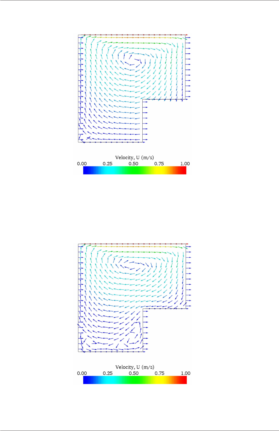
2.2 Stress analysis of a plate with a hole U-45
Figure 2.13: cavity solution velocity field mapped onto cavityClipped.
Figure 2.14: cavityClipped solution for velocity field.
OpenFOAM-2.4.0
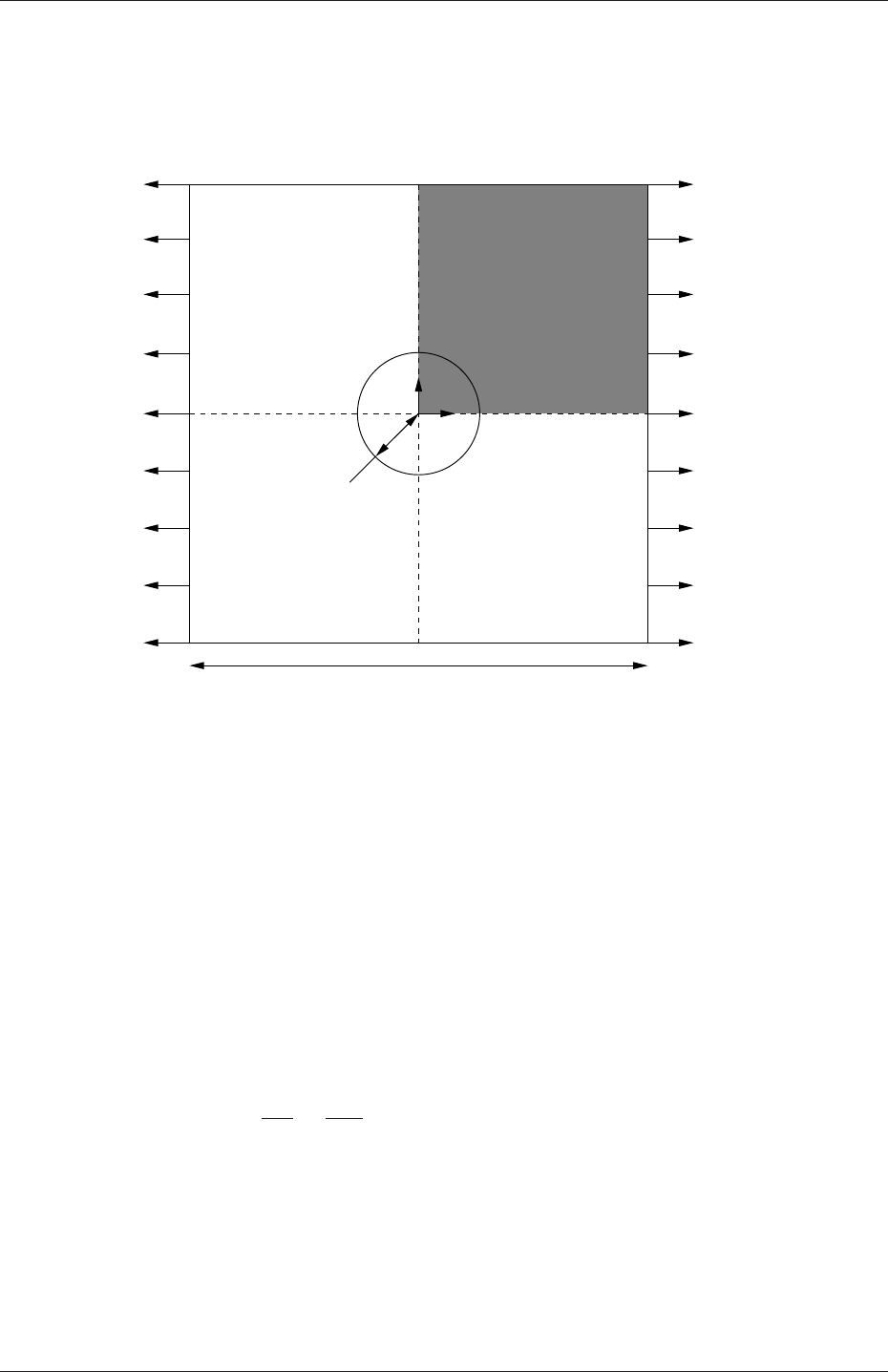
U-46 Tutorials
plate dimensions are: side length 4 m and radius R= 0.5 m. It is loaded with a uniform
traction of σ= 10 kPa over its left and right faces as shown in Figure 2.15. Two symmetry
planes can be identified for this geometry and therefore the solution domain need only cover
a quarter of the geometry, shown by the shaded area in Figure 2.15.
xsymmetry plane
4.0 m
y
σ= 10 kPa
σ= 10 kPa
R= 0.5 m
symmetry plane
Figure 2.15: Geometry of the plate with a hole.
The problem can be approximated as 2-dimensional since the load is applied in the plane
of the plate. In a Cartesian coordinate system there are two possible assumptions to take
in regard to the behaviour of the structure in the third dimension: (1) the plane stress
condition, in which the stress components acting out of the 2D plane are assumed to be
negligible; (2) the plane strain condition, in which the strain components out of the 2D
plane are assumed negligible. The plane stress condition is appropriate for solids whose
third dimension is thin as in this case; the plane strain condition is applicable for solids
where the third dimension is thick.
An analytical solution exists for loading of an infinitely large, thin plate with a circular
hole. The solution for the stress normal to the vertical plane of symmetry is
(σxx)x=0 =
σµ1 + R2
2y2+3R4
2y4¶for |y| ≥ R
0 for |y|< R
(2.14)
Results from the simulation will be compared with this solution. At the end of the tutorial,
the user can: investigate the sensitivity of the solution to mesh resolution and mesh grading;
and, increase the size of the plate in comparison to the hole to try to estimate the error in
comparing the analytical solution for an infinite plate to the solution of this problem of a
finite plate.
OpenFOAM-2.4.0
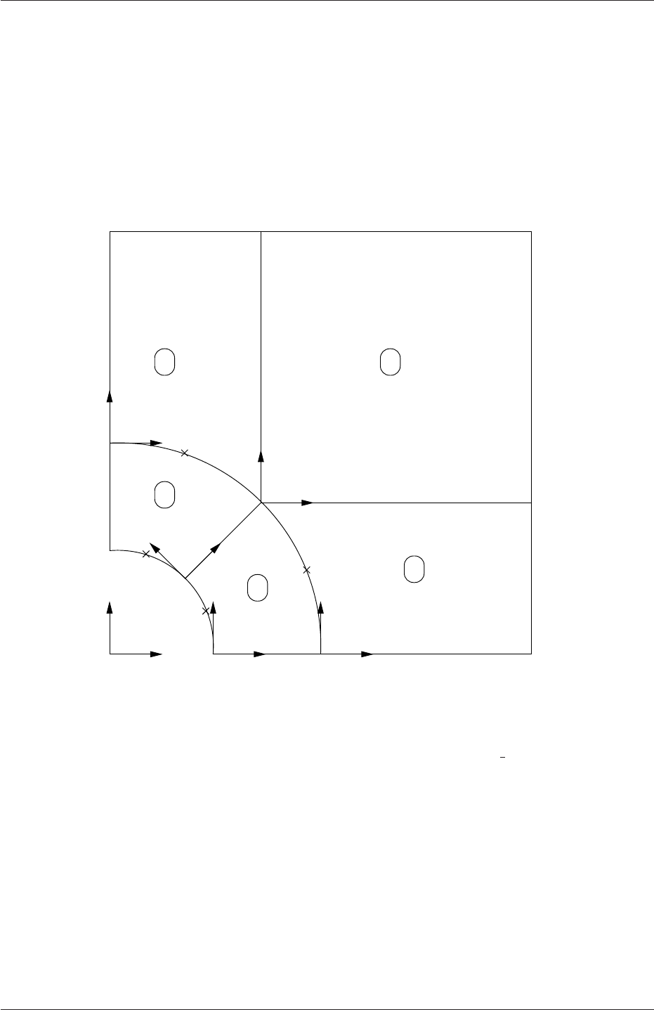
2.2 Stress analysis of a plate with a hole U-47
2.2.1 Mesh generation
The domain consists of four blocks, some of which have arc-shaped edges. The block struc-
ture for the part of the mesh in the x−yplane is shown in Figure 2.16. As already mentioned
in section 2.1.1.1, all geometries are generated in 3 dimensions in OpenFOAM even if the
case is to be as a 2 dimensional problem. Therefore a dimension of the block in the z
direction has to be chosen; here, 0.5 m is selected. It does not affect the solution since the
traction boundary condition is specified as a stress rather than a force, thereby making the
solution independent of the cross-sectional area.
x
y x2
x1x1
x2
x2
x1
x1
x2
x2
x1
left
left
up 7up
right
3
down
hole
0
down
right
6
9
8
4
10
10 2
5
2
1
4 3
Figure 2.16: Block structure of the mesh for the plate with a hole.
The user should change into the plateHole case in the $FOAM RUN/tutorials/stress-
Analysis/solidDisplacementFoam directory and open the constant/polyMesh/blockMeshDict
file in an editor, as listed below
17 convertToMeters 1;
18
19 vertices
20 (
21 (0.5 0 0)
22 (1 0 0)
23 (2 0 0)
24 (2 0.707107 0)
25 (0.707107 0.707107 0)
26 (0.353553 0.353553 0)
27 (2 2 0)
28 (0.707107 2 0)
29 (0 2 0)
30 (0 1 0)
31 (0 0.5 0)
OpenFOAM-2.4.0

U-48 Tutorials
32 (0.5 0 0.5)
33 (1 0 0.5)
34 (2 0 0.5)
35 (2 0.707107 0.5)
36 (0.707107 0.707107 0.5)
37 (0.353553 0.353553 0.5)
38 (2 2 0.5)
39 (0.707107 2 0.5)
40 (0 2 0.5)
41 (0 1 0.5)
42 (0 0.5 0.5)
43 );
44
45 blocks
46 (
47 hex (5 4 9 10 16 15 20 21) (10 10 1) simpleGrading (1 1 1)
48 hex (0 1 4 5 11 12 15 16) (10 10 1) simpleGrading (1 1 1)
49 hex (1 2 3 4 12 13 14 15) (20 10 1) simpleGrading (1 1 1)
50 hex (4 3 6 7 15 14 17 18) (20 20 1) simpleGrading (1 1 1)
51 hex (9 4 7 8 20 15 18 19) (10 20 1) simpleGrading (1 1 1)
52 );
53
54 edges
55 (
56 arc 0 5 (0.469846 0.17101 0)
57 arc 5 10 (0.17101 0.469846 0)
58 arc 1 4 (0.939693 0.34202 0)
59 arc 4 9 (0.34202 0.939693 0)
60 arc 11 16 (0.469846 0.17101 0.5)
61 arc 16 21 (0.17101 0.469846 0.5)
62 arc 12 15 (0.939693 0.34202 0.5)
63 arc 15 20 (0.34202 0.939693 0.5)
64 );
65
66 boundary
67 (
68 left
69 {
70 type symmetryPlane;
71 faces
72 (
73 (8 9 20 19)
74 (9 10 21 20)
75 );
76 }
77 right
78 {
79 type patch;
80 faces
81 (
82 (2 3 14 13)
83 (3 6 17 14)
84 );
85 }
86 down
87 {
88 type symmetryPlane;
89 faces
90 (
91 (0 1 12 11)
92 (1 2 13 12)
93 );
94 }
95 up
96 {
97 type patch;
98 faces
99 (
100 (7 8 19 18)
101 (6 7 18 17)
102 );
103 }
104 hole
105 {
106 type patch;
107 faces
108 (
109 (10 5 16 21)
110 (5 0 11 16)
111 );
OpenFOAM-2.4.0

2.2 Stress analysis of a plate with a hole U-49
112 }
113 frontAndBack
114 {
115 type empty;
116 faces
117 (
118 (10 9 4 5)
119 (5 4 1 0)
120 (1 4 3 2)
121 (4 7 6 3)
122 (4 9 8 7)
123 (21 16 15 20)
124 (16 11 12 15)
125 (12 13 14 15)
126 (15 14 17 18)
127 (15 18 19 20)
128 );
129 }
130 );
131
132 mergePatchPairs
133 (
134 );
135
136 // ************************************************************************* //
Until now, we have only specified straight edges in the geometries of previous tutorials but
here we need to specify curved edges. These are specified under the edges keyword entry
which is a list of non-straight edges. The syntax of each list entry begins with the type of
curve, including arc,simpleSpline,polyLine etc., described further in section 5.3.1. In
this example, all the edges are circular and so can be specified by the arc keyword entry.
The following entries are the labels of the start and end vertices of the arc and a point vector
through which the circular arc passes.
The blocks in this blockMeshDict do not all have the same orientation. As can be seen in
Figure 2.16 the x2direction of block 0 is equivalent to the −x1direction for block 4. This
means care must be taken when defining the number and distribution of cells in each block
so that the cells match up at the block faces.
6 patches are defined: one for each side of the plate, one for the hole and one for the
front and back planes. The left and down patches are both a symmetry plane. Since this is
ageometric constraint, it is included in the definition of the mesh, rather than being purely
a specification on the boundary condition of the fields. Therefore they are defined as such
using a special symmetryPlane type as shown in the blockMeshDict.
The frontAndBack patch represents the plane which is ignored in a 2D case. Again this
is a geometric constraint so is defined within the mesh, using the empty type as shown in the
blockMeshDict. For further details of boundary types and geometric constraints, the user
should refer to section 5.2.1.
The remaining patches are of the regular patch type. The mesh should be generated
using blockMesh and can be viewed in paraFoam as described in section 2.1.2. It should
appear as in Figure 2.17.
2.2.1.1 Boundary and initial conditions
Once the mesh generation is complete, the initial field with boundary conditions must be
set. For a stress analysis case without thermal stresses, only displacement Dneeds to be set.
The 0/D is as follows:
17 dimensions [0 1 0 0 0 0 0];
18
19 internalField uniform (0 0 0);
20
OpenFOAM-2.4.0
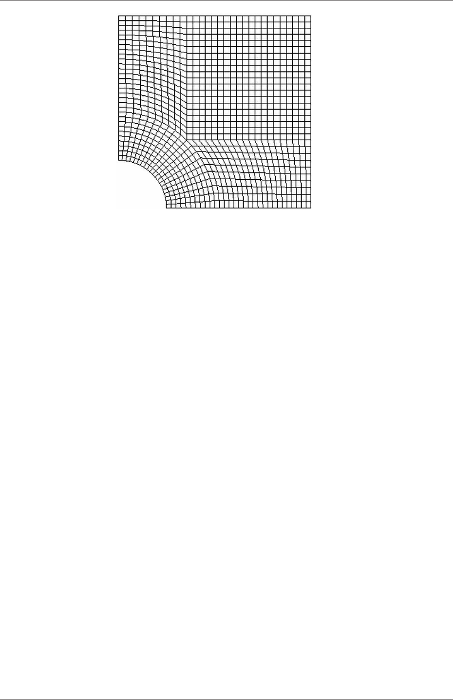
U-50 Tutorials
Figure 2.17: Mesh of the hole in a plate problem.
21 boundaryField
22 {
23 left
24 {
25 type symmetryPlane;
26 }
27 right
28 {
29 type tractionDisplacement;
30 traction uniform ( 10000 0 0 );
31 pressure uniform 0;
32 value uniform (0 0 0);
33 }
34 down
35 {
36 type symmetryPlane;
37 }
38 up
39 {
40 type tractionDisplacement;
41 traction uniform ( 0 0 0 );
42 pressure uniform 0;
43 value uniform (0 0 0);
44 }
45 hole
46 {
47 type tractionDisplacement;
48 traction uniform ( 0 0 0 );
49 pressure uniform 0;
50 value uniform (0 0 0);
51 }
52 frontAndBack
53 {
54 type empty;
55 }
56 }
57
58 // ************************************************************************* //
Firstly, it can be seen that the displacement initial conditions are set to (0,0,0) m. The
left and down patches must be both of symmetryPlane type since they are specified as such
in the mesh description in the constant/polyMesh/boundary file. Similarly the frontAndBack
patch is declared empty.
The other patches are traction boundary conditions, set by a specialist traction bound-
ary type. The traction boundary conditions are specified by a linear combination of: (1) a
OpenFOAM-2.4.0

2.2 Stress analysis of a plate with a hole U-51
boundary traction vector under keyword traction; (2) a pressure that produces a traction
normal to the boundary surface that is defined as negative when pointing out of the surface,
under keyword pressure. The up and hole patches are zero traction so the boundary trac-
tion and pressure are set to zero. For the right patch the traction should be (1e4,0,0) Pa
and the pressure should be 0 Pa.
2.2.1.2 Mechanical properties
The physical properties for the case are set in the mechanicalProperties dictionary in the con-
stant directory. For this problem, we need to specify the mechanical properties of steel given
in Table 2.1. In the mechanical properties dictionary, the user must also set planeStress
to yes.
Property Units Keyword Value
Density kg m−3rho 7854
Young’s modulus Pa E2×1011
Poisson’s ratio — nu 0.3
Table 2.1: Mechanical properties for steel
2.2.1.3 Thermal properties
The temperature field variable Tis present in the solidDisplacementFoam solver since the user
may opt to solve a thermal equation that is coupled with the momentum equation through
the thermal stresses that are generated. The user specifies at run time whether OpenFOAM
should solve the thermal equation by the thermalStress switch in the thermalProperties
dictionary. This dictionary also sets the thermal properties for the case, e.g. for steel as
listed in Table 2.2.
Property Units Keyword Value
Specific heat capacity Jkg−1K−1C434
Thermal conductivity Wm−1K−1k60.5
Thermal expansion coeff. K−1alpha 1.1×10⁻⁵
Table 2.2: Thermal properties for steel
In this case we do not want to solve for the thermal equation. Therefore we must set
the thermalStress keyword entry to no in the thermalProperties dictionary.
2.2.1.4 Control
As before, the information relating to the control of the solution procedure are read in
from the controlDict dictionary. For this case, the startTime is 0 s. The time step is not
important since this is a steady state case; in this situation it is best to set the time step
deltaT to 1 so it simply acts as an iteration counter for the steady-state case. The endTime,
set to 100, then acts as a limit on the number of iterations. The writeInterval can be set
to 20.
The controlDict entries are as follows:
OpenFOAM-2.4.0

U-52 Tutorials
17
18 application solidDisplacementFoam;
19
20 startFrom startTime;
21
22 startTime 0;
23
24 stopAt endTime;
25
26 endTime 100;
27
28 deltaT 1;
29
30 writeControl timeStep;
31
32 writeInterval 20;
33
34 purgeWrite 0;
35
36 writeFormat ascii;
37
38 writePrecision 6;
39
40 writeCompression off;
41
42 timeFormat general;
43
44 timePrecision 6;
45
46 graphFormat raw;
47
48 runTimeModifiable true;
49
50
51 // ************************************************************************* //
2.2.1.5 Discretisation schemes and linear-solver control
Let us turn our attention to the fvSchemes dictionary. Firstly, the problem we are analysing
is steady-state so the user should select SteadyState for the time derivatives in timeScheme.
This essentially switches off the time derivative terms. Not all solvers, especially in fluid
dynamics, work for both steady-state and transient problems but solidDisplacementFoam
does work, since the base algorithm is the same for both types of simulation.
The momentum equation in linear-elastic stress analysis includes several explicit terms
containing the gradient of displacement. The calculations benefit from accurate and smooth
evaluation of the gradient. Normally, in the finite volume method the discretisation is based
on Gauss’s theorem The Gauss method is sufficiently accurate for most purposes but, in this
case, the least squares method will be used. The user should therefore open the fvSchemes
dictionary in the system directory and ensure the leastSquares method is selected for the
grad(U) gradient discretisation scheme in the gradSchemes sub-dictionary:
17
18 d2dt2Schemes
19 {
20 default steadyState;
21 }
22
23 ddtSchemes
24 {
25 default Euler;
26 }
27
28 gradSchemes
29 {
30 default leastSquares;
31 grad(D) leastSquares;
32 grad(T) leastSquares;
33 }
34
35 divSchemes
OpenFOAM-2.4.0

2.2 Stress analysis of a plate with a hole U-53
36 {
37 default none;
38 div(sigmaD) Gauss linear;
39 }
40
41 laplacianSchemes
42 {
43 default none;
44 laplacian(DD,D) Gauss linear corrected;
45 laplacian(DT,T) Gauss linear corrected;
46 }
47
48 interpolationSchemes
49 {
50 default linear;
51 }
52
53 snGradSchemes
54 {
55 default none;
56 }
57
58 fluxRequired
59 {
60 default no;
61 D yes;
62 T no;
63 }
64
65
66 // ************************************************************************* //
The fvSolution dictionary in the system directory controls the linear equation solvers and
algorithms used in the solution. The user should first look at the solvers sub-dictionary
and notice that the choice of solver for Dis GAMG. The solver tolerance should be set to
10−6for this problem. The solver relative tolerance, denoted by relTol, sets the required
reduction in the residuals within each iteration. It is uneconomical to set a tight (low)
relative tolerance within each iteration since a lot of terms in each equation are explicit and
are updated as part of the segregated iterative procedure. Therefore a reasonable value for
the relative tolerance is 0.01, or possibly even higher, say 0.1, or in some cases even 0.9 (as
in this case).
17
18 solvers
19 {
20 "(D|T)"
21 {
22 solver GAMG;
23 tolerance 1e-06;
24 relTol 0.9;
25 smoother GaussSeidel;
26 cacheAgglomeration true;
27 nCellsInCoarsestLevel 20;
28 agglomerator faceAreaPair;
29 mergeLevels 1;
30 }
31 }
32
33 stressAnalysis
34 {
35 compactNormalStress yes;
36 nCorrectors 1;
37 D 1e-06;
38 }
39
40
41 // ************************************************************************* //
The fvSolution dictionary contains a sub-dictionary, stressAnalysis that contains some control
parameters specific to the application solver. Firstly there is nCorrectors which specifies
the number of outer loops around the complete system of equations, including traction
OpenFOAM-2.4.0

U-54 Tutorials
boundary conditions within each time step. Since this problem is steady-state, we are
performing a set of iterations towards a converged solution with the ’time step’ acting as an
iteration counter. We can therefore set nCorrectors to 1.
The Dkeyword specifies a convergence tolerance for the outer iteration loop, i.e. sets a
level of initial residual below which solving will cease. It should be set to the desired solver
tolerance specified earlier, 10−6for this problem.
2.2.2 Running the code
The user should run the code here in the background from the command line as specified
below, so he/she can look at convergence information in the log file afterwards.
cd $FOAM RUN/tutorials/stressAnalysis/solidDisplacementFoam/plateHole
solidDisplacementFoam > log &
The user should check the convergence information by viewing the generated log file which
shows the number of iterations and the initial and final residuals of the displacement in each
direction being solved. The final residual should always be less than 0.9 times the initial
residual as this iteration tolerance set. Once both initial residuals have dropped below the
convergence tolerance of 10−6the run has converged and can be stopped by killing the batch
job.
2.2.3 Post-processing
Post processing can be performed as in section 2.1.4. The solidDisplacementFoam solver
outputs the stress field σas a symmetric tensor field sigma. This is consistent with the way
variables are usually represented in OpenFOAM solvers by the mathematical symbol by
which they are represented; in the case of Greek symbols, the variable is named phonetically.
For post-processing individual scalar field components, σxx,σxy etc., can be generated
by running the foamCalc utility as before in section 2.1.5.7, this time on sigma:
foamCalc components sigma
Components named sigmaxx,sigmaxy etc. are written to time directories of the case. The
σxx stresses can be viewed in paraFoam as shown in Figure 2.18.
We would like to compare the analytical solution of Equation 2.14 to our solution. We
therefore must output a set of data of σxx along the left edge symmetry plane of our domain.
The user may generate the required graph data using the sample utility. The utility uses
asampleDict dictionary located in the system directory, whose entries are summarised in
Table 6.8. The sample line specified in sets is set between (0.0,0.5,0.25) and (0.0,2.0,0.25),
and the fields are specified in the fields list:
17
18 interpolationScheme cellPoint;
19
20 setFormat raw;
21
22 sets
23 (
24 leftPatch
25 {
26 type uniform;
27 axis y;
OpenFOAM-2.4.0
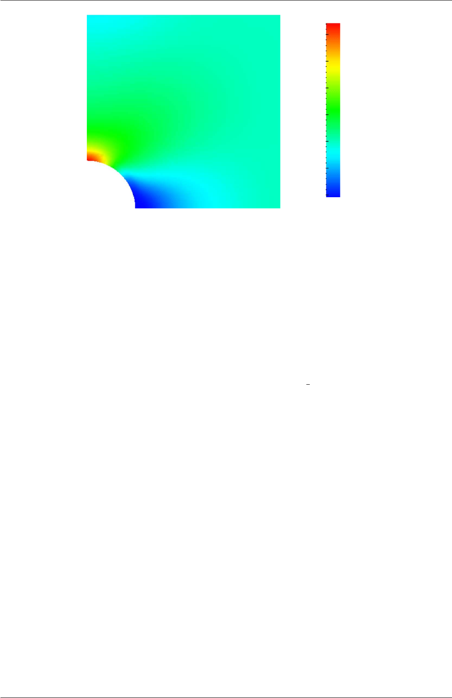
2.2 Stress analysis of a plate with a hole U-55
0
5
10
15
20
25
30
σxx (kPa)
Figure 2.18: σxx stress field in the plate with hole.
28 start ( 0 0.5 0.25 );
29 end ( 0 2 0.25 );
30 nPoints 100;
31 }
32 );
33
34 fields ( sigmaEq );
35
36
37 // ************************************************************************* //
The user should execute sample as normal. The writeFormat is raw 2 column format. The
data is written into files within time subdirectories of a postProcessing/sets directory, e.g.
the data at t= 100 s is found within the file sets/100/leftPatch sigmaxx.xy. In an application
such as GnuPlot, one could type the following at the command prompt would be sufficient
to plot both the numerical data and analytical solution:
plot [0.5:2] [0:] 'postProcessing/sets/100/leftPatch sigmaxx.xy',
1e4*(1+(0.125/(x**2))+(0.09375/(x**4)))
An example plot is shown in Figure 2.19.
2.2.4 Exercises
The user may wish to experiment with solidDisplacementFoam by trying the following exer-
cises:
2.2.4.1 Increasing mesh resolution
Increase the mesh resolution in each of the xand ydirections. Use mapFields to map the
final coarse mesh results from section 2.2.3 to the initial conditions for the fine mesh.
2.2.4.2 Introducing mesh grading
Grade the mesh so that the cells near the hole are finer than those away from the hole.
Design the mesh so that the ratio of sizes between adjacent cells is no more than 1.1 and so
OpenFOAM-2.4.0
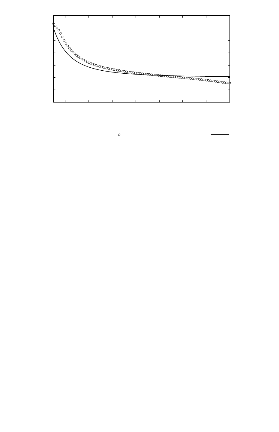
U-56 Tutorials
0
5
10
15
20
25
30
35
0.6 0.8 1.0 1.2 1.4 1.6 1.8 2.0
Stress (σxx)x=0 (kPa)
Distance, y(m)
Numerical prediction Analytical solution
Figure 2.19: Normal stress along the vertical symmetry (σxx)x=0
that the ratio of cell sizes between blocks is similar to the ratios within blocks. Mesh grading
is described in section 2.1.6. Again use mapFields to map the final coarse mesh results from
section 2.2.3 to the initial conditions for the graded mesh. Compare the results with those
from the analytical solution and previous calculations. Can this solution be improved upon
using the same number of cells with a different solution?
2.2.4.3 Changing the plate size
The analytical solution is for an infinitely large plate with a finite sized hole in it. Therefore
this solution is not completely accurate for a finite sized plate. To estimate the error,
increase the plate size while maintaining the hole size at the same value.
2.3 Breaking of a dam
In this tutorial we shall solve a problem of simplified dam break in 2 dimensions using the
interFoam.The feature of the problem is a transient flow of two fluids separated by a sharp
interface, or free surface. The two-phase algorithm in interFoam is based on the volume of
fluid (VOF) method in which a specie transport equation is used to determine the relative
volume fraction of the two phases, or phase fraction α, in each computational cell. Physical
properties are calculated as weighted averages based on this fraction. The nature of the
VOF method means that an interface between the species is not explicitly computed, but
rather emerges as a property of the phase fraction field. Since the phase fraction can have
any value between 0 and 1, the interface is never sharply defined, but occupies a volume
around the region where a sharp interface should exist.
The test setup consists of a column of water at rest located behind a membrane on the
left side of a tank. At time t= 0 s, the membrane is removed and the column of water
collapses. During the collapse, the water impacts an obstacle at the bottom of the tank
and creates a complicated flow structure, including several captured pockets of air. The
geometry and the initial setup is shown in Figure 2.20.
OpenFOAM-2.4.0
2.3 Breaking of a dam U-57
0.584 m
0.048 m
0.024 m
0.584 m
0.292 m
0.1459 m0.1461 m
water column
Figure 2.20: Geometry of the dam break.
2.3.1 Mesh generation
The user should go to the damBreak case in their $FOAM RUN/tutorials/multiphase/inter-
Foam/laminar directory. Generate the mesh running blockMesh as described previously. The
damBreak mesh consist of 5 blocks; the blockMeshDict entries are given below.
17 convertToMeters 0.146;
18
19 vertices
20 (
21 (0 0 0)
22 (2 0 0)
23 (2.16438 0 0)
24 (4 0 0)
25 (0 0.32876 0)
26 (2 0.32876 0)
27 (2.16438 0.32876 0)
28 (4 0.32876 0)
29 (0 4 0)
30 (2 4 0)
31 (2.16438 4 0)
32 (4 4 0)
33 (0 0 0.1)
34 (2 0 0.1)
35 (2.16438 0 0.1)
36 (4 0 0.1)
37 (0 0.32876 0.1)
38 (2 0.32876 0.1)
39 (2.16438 0.32876 0.1)
40 (4 0.32876 0.1)
41 (0 4 0.1)
42 (2 4 0.1)
43 (2.16438 4 0.1)
44 (4 4 0.1)
45 );
46
47 blocks
48 (
49 hex (0 1 5 4 12 13 17 16) (23 8 1) simpleGrading (1 1 1)
50 hex (2 3 7 6 14 15 19 18) (19 8 1) simpleGrading (1 1 1)
51 hex (4 5 9 8 16 17 21 20) (23 42 1) simpleGrading (1 1 1)
52 hex (5 6 10 9 17 18 22 21) (4 42 1) simpleGrading (1 1 1)
OpenFOAM-2.4.0

U-58 Tutorials
53 hex (6 7 11 10 18 19 23 22) (19 42 1) simpleGrading (1 1 1)
54 );
55
56 edges
57 (
58 );
59
60 boundary
61 (
62 leftWall
63 {
64 type wall;
65 faces
66 (
67 (0 12 16 4)
68 (4 16 20 8)
69 );
70 }
71 rightWall
72 {
73 type wall;
74 faces
75 (
76 (7 19 15 3)
77 (11 23 19 7)
78 );
79 }
80 lowerWall
81 {
82 type wall;
83 faces
84 (
85 (0 1 13 12)
86 (1 5 17 13)
87 (5 6 18 17)
88 (2 14 18 6)
89 (2 3 15 14)
90 );
91 }
92 atmosphere
93 {
94 type patch;
95 faces
96 (
97 (8 20 21 9)
98 (9 21 22 10)
99 (10 22 23 11)
100 );
101 }
102 );
103
104 mergePatchPairs
105 (
106 );
107
108 // ************************************************************************* //
2.3.2 Boundary conditions
The user can examine the boundary geometry generated by blockMesh by viewing the bound-
ary file in the constant/polyMesh directory. The file contains a list of 5 boundary patches:
leftWall,rightWall,lowerWall,atmosphere and defaultFaces. The user should notice
the type of the patches. The atmosphere is a standard patch,i.e. has no special attributes,
merely an entity on which boundary conditions can be specified. The defaultFaces patch
is empty since the patch normal is in the direction we will not solve in this 2D case. The
leftWall,rightWall and lowerWall patches are each a wall. Like the plain patch, the wall
type contains no geometric or topological information about the mesh and only differs from
the plain patch in that it identifies the patch as a wall, should an application need to know,
e.g. to apply special wall surface modelling.
A good example is that the interFoam solver includes modelling of surface tension at the
OpenFOAM-2.4.0

2.3 Breaking of a dam U-59
contact point between the interface and wall surface. The models are applied by specifying
the alphaContactAngle boundary condition on the alpha (α) field. With it, the user must
specify the following: a static contact angle, theta0 θ0; leading and trailing edge dynamic
contact angles, thetaA θAand thetaR θRrespectively; and a velocity scaling function for
dynamic contact angle, uTheta.
In this tutorial we would like to ignore surface tension effects between the wall and
interface. We can do this by setting the static contact angle, θ0= 90◦and the velocity
scaling function to 0. However, the simpler option which we shall choose here is to specify
azeroGradient type on alpha, rather than use the alphaContactAngle boundary condition.
The top boundary is free to the atmosphere so needs to permit both outflow and inflow
according to the internal flow. We therefore use a combination of boundary conditions for
pressure and velocity that does this while maintaining stability. They are:
•totalPressure which is a fixedValue condition calculated from specified total pressure
p0 and local velocity U;
•pressureInletOutletVelocity, which applies zeroGradient on all components, except where
there is inflow, in which case a fixedValue condition is applied to the tangential com-
ponent;
•inletOutlet, which is a zeroGradient condition when flow outwards, fixedValue when flow
is inwards.
At all wall boundaries, the fixedFluxPressure boundary condition is applied to the pressure
field, which adjusts the pressure gradient so that the boundary flux matches the velocity
boundary condition.
The defaultFaces patch representing the front and back planes of the 2D problem, is,
as usual, an empty type.
2.3.3 Setting initial field
Unlike the previous cases, we shall now specify a non-uniform initial condition for the phase
fraction αwater where
αwater =(1 for the water phase
0 for the air phase (2.15)
This will be done by running the setFields utility. It requires a setFieldsDict dictionary,
located in the system directory, whose entries for this case are shown below.
17
18 defaultFieldValues
19 (
20 volScalarFieldValue alpha.water 0
21 );
22
23 regions
24 (
25 boxToCell
26 {
27 box (0 0 -1) (0.1461 0.292 1);
28 fieldValues
29 (
30 volScalarFieldValue alpha.water 1
31 );
32 }
OpenFOAM-2.4.0
U-60 Tutorials
33 );
34
35
36 // ************************************************************************* //
The defaultFieldValues sets the default value of the fields, i.e. the value the field takes
unless specified otherwise in the regions sub-dictionary. That sub-dictionary contains a list
of subdictionaries containing fieldValues that override the defaults in a specified region.
The region is expressed in terms of a topoSetSource that creates a set of points, cells or
faces based on some topological constraint. Here, boxToCell creates a bounding box within
a vector minimum and maximum to define the set of cells of the water region. The phase
fraction αwater is defined as 1 in this region.
The setFields utility reads fields from file and, after re-calculating those fields, will write
them back to file. Because the files are then overridden, it is recommended that a backup
is made before setFields is executed. In the damBreak tutorial, the alpha.water field is
initially stored as a backup only, named alpha.water.org. Before running setFields, the
user first needs to copy alpha.water.org to alpha.water,e.g. by typing:
cp 0/alpha.water.org 0/alpha.water
The user should then execute setFields as any other utility is executed. Using paraFoam,
check that the initial alpha.water field corresponds to the desired distribution as in Fig-
ure 2.21.
0.0
0.1
0.2
0.3
0.4
0.5
0.6
0.7
0.8
0.9
1.0
Phase fraction, α1
Figure 2.21: Initial conditions for phase fraction alpha.water.
2.3.4 Fluid properties
Let us examine the transportProperties file in the constant directory. The dictionary contains
the material properties for each fluid, separated into two dictionaries water and air. The
transport model for each phase is selected by the transportModel keyword. The user should
select Newtonian in which case the kinematic viscosity is single valued and specified under
the keyword nu. The viscosity parameters for the other models, e.g.CrossPowerLaw, are
OpenFOAM-2.4.0

2.3 Breaking of a dam U-61
specified within subdictionaries with the generic name <model>Coeffs,i.e.CrossPowerLawCoeffs
in this example. The density is specified under the keyword rho.
The surface tension between the two phases is specified under the keyword sigma. The
values used in this tutorial are listed in Table 2.3.
water properties
Kinematic viscosity m2s−1nu 1.0×10⁻⁶
Density kg m−3rho 1.0×10³
air properties
Kinematic viscosity m2s−1nu 1.48 ×10⁻⁵
Density kg m−3rho 1.0
Properties of both phases
Surface tension N m−1sigma 0.07
Table 2.3: Fluid properties for the damBreak tutorial
Gravitational acceleration is uniform across the domain and is specified in a file named
gin the constant directory. Unlike a normal field file, e.g. Uand p,gis a uniformDimen-
sionedVectorField and so simply contains a set of dimensions and a value that represents
(0,9.81,0) m s−2for this tutorial:
17
18 dimensions [0 1 -2 0 0 0 0];
19 value ( 0 -9.81 0 );
20
21
22 // ************************************************************************* //
2.3.5 Turbulence modelling
As in the cavity example, the choice of turbulence modelling method is selectable at run-time
through the simulationType keyword in turbulenceProperties dictionary. In this example,
we wish to run without turbulence modelling so we set laminar:
17
18 simulationType laminar;
19
20
21 // ************************************************************************* //
2.3.6 Time step control
Time step control is an important issue in free surface tracking since the surface-tracking
algorithm is considerably more sensitive to the Courant number Co than in standard fluid
flow calculations. Ideally, we should not exceed an upper limit Co ≈0.5 in the region of
the interface. In some cases, where the propagation velocity is easy to predict, the user
should specify a fixed time-step to satisfy the Co criterion. For more complex cases, this
is considerably more difficult. interFoam therefore offers automatic adjustment of the time
step as standard in the controlDict. The user should specify adjustTimeStep to be on and
the the maximum Co for the phase fields, maxAlphaCo, and other fields, maxCo, to be 1.0.
OpenFOAM-2.4.0

U-62 Tutorials
The upper limit on time step maxDeltaT can be set to a value that will not be exceeded in
this simulation, e.g. 1.0.
By using automatic time step control, the steps themselves are never rounded to a
convenient value. Consequently if we request that OpenFOAM saves results at a fixed
number of time step intervals, the times at which results are saved are somewhat arbitrary.
However even with automatic time step adjustment, OpenFOAM allows the user to specify
that results are written at fixed times; in this case OpenFOAM forces the automatic time
stepping procedure to adjust time steps so that it ‘hits’ on the exact times specified for
write output. The user selects this with the adjustableRunTime option for writeControl
in the controlDict dictionary. The controlDict dictionary entries should be:
17
18 application interFoam;
19
20 startFrom startTime;
21
22 startTime 0;
23
24 stopAt endTime;
25
26 endTime 1;
27
28 deltaT 0.001;
29
30 writeControl adjustableRunTime;
31
32 writeInterval 0.05;
33
34 purgeWrite 0;
35
36 writeFormat ascii;
37
38 writePrecision 6;
39
40 writeCompression uncompressed;
41
42 timeFormat general;
43
44 timePrecision 6;
45
46 runTimeModifiable yes;
47
48 adjustTimeStep yes;
49
50 maxCo 1;
51 maxAlphaCo 1;
52
53 maxDeltaT 1;
54
55
56 // ************************************************************************* //
2.3.7 Discretisation schemes
The interFoam solver uses the multidimensional universal limiter for explicit solution (MULES)
method, created by OpenCFD, to maintain boundedness of the phase fraction independent
of underlying numerical scheme, mesh structure, etc. The choice of schemes for convec-
tion are therfore not restricted to those that are strongly stable or bounded, e.g. upwind
differencing.
The convection schemes settings are made in the divSchemes sub-dictionary of the
fvSchemes dictionary. In this example, the convection term in the momentum equation
(∇•(ρUU)), denoted by the div(rho*phi,U) keyword, uses Gauss linearUpwind grad(U)
to produce good accuracy. The limited linear schemes require a coefficient φas described
in section 4.4.1. Here, we have opted for best stability with φ= 1.0. The ∇•(Uα1) term,
represented by the div(phi,alpha) keyword uses the vanLeer scheme. The ∇•(Urbα1)
OpenFOAM-2.4.0

2.3 Breaking of a dam U-63
term, represented by the div(phirb,alpha) keyword, can use second order linear (central)
differencing as boundedness is assured by the MULES algorithm.
The other discretised terms use commonly employed schemes so that the fvSchemes
dictionary entries should therefore be:
17
18 ddtSchemes
19 {
20 default Euler;
21 }
22
23 gradSchemes
24 {
25 default Gauss linear;
26 }
27
28 divSchemes
29 {
30 div(rhoPhi,U) Gauss linearUpwind grad(U);
31 div(phi,alpha) Gauss vanLeer;
32 div(phirb,alpha) Gauss linear;
33 div((muEff*dev(T(grad(U))))) Gauss linear;
34 }
35
36 laplacianSchemes
37 {
38 default Gauss linear corrected;
39 }
40
41 interpolationSchemes
42 {
43 default linear;
44 }
45
46 snGradSchemes
47 {
48 default corrected;
49 }
50
51 fluxRequired
52 {
53 default no;
54 p_rgh;
55 pcorr;
56 alpha.water;
57 }
58
59
60 // ************************************************************************* //
2.3.8 Linear-solver control
In the fvSolution, the PIMPLE sub-dictionary contains elements that are specific to interFoam.
There are the usual correctors to the momentum equation but also correctors to a PISO loop
around the αphase equation. Of particular interest are the nAlphaSubCycles and cAlpha
keywords. nAlphaSubCycles represents the number of sub-cycles within the αequation;
sub-cycles are additional solutions to an equation within a given time step. It is used to
enable the solution to be stable without reducing the time step and vastly increasing the
solution time. Here we specify 2 sub-cycles, which means that the αequation is solved in
2×half length time steps within each actual time step.
The cAlpha keyword is a factor that controls the compression of the interface where: 0
corresponds to no compression; 1 corresponds to conservative compression; and, anything
larger than 1, relates to enhanced compression of the interface. We generally recommend a
value of 1.0 which is employed in this example.
OpenFOAM-2.4.0

U-64 Tutorials
2.3.9 Running the code
Running of the code has been described in detail in previous tutorials. Try the following,
that uses tee, a command that enables output to be written to both standard output and
files:
cd $FOAM RUN/tutorials/multiphase/interFoam/laminar/damBreak
interFoam | tee log
The code will now be run interactively, with a copy of output stored in the log file.
2.3.10 Post-processing
Post-processing of the results can now be done in the usual way. The user can monitor the
development of the phase fraction alpha.water in time, e.g. see Figure 2.22.
2.3.11 Running in parallel
The results from the previous example are generated using a fairly coarse mesh. We now
wish to increase the mesh resolution and re-run the case. The new case will typically take
a few hours to run with a single processor so, should the user have access to multiple
processors, we can demonstrate the parallel processing capability of OpenFOAM.
The user should first make a copy of the damBreak case, e.g. by
cd $FOAM RUN/tutorials/multiphase/interFoam/laminar
mkdir damBreakFine
cp -r damBreak/0 damBreakFine
cp -r damBreak/system damBreakFine
cp -r damBreak/constant damBreakFine
Enter the new case directory and change the blocks description in the blockMeshDict dic-
tionary to
blocks
(
hex (0 1 5 4 12 13 17 16) (46 10 1) simpleGrading (1 1 1)
hex (2 3 7 6 14 15 19 18) (40 10 1) simpleGrading (1 1 1)
hex (4 5 9 8 16 17 21 20) (46 76 1) simpleGrading (1 2 1)
hex (5 6 10 9 17 18 22 21) (4 76 1) simpleGrading (1 2 1)
hex (6 7 11 10 18 19 23 22) (40 76 1) simpleGrading (1 2 1)
);
Here, the entry is presented as printed from the blockMeshDict file; in short the user must
change the mesh densities, e.g. the 46 10 1 entry, and some of the mesh grading entries to
1 2 1. Once the dictionary is correct, generate the mesh.
As the mesh has now changed from the damBreak example, the user must re-initialise the
phase field alpha.water in the 0time directory since it contains a number of elements that
is inconsistent with the new mesh. Note that there is no need to change the Uand prgh
OpenFOAM-2.4.0
2.3 Breaking of a dam U-65
0.0
0.1
0.2
0.3
0.4
0.5
0.6
0.7
0.8
0.9
1.0
Phase fraction, α1
(a) At t= 0.25 s.
0.0
0.1
0.2
0.3
0.4
0.5
0.6
0.7
0.8
0.9
1.0
Phase fraction, α1
(b) At t= 0.50 s.
Figure 2.22: Snapshots of phase α.
OpenFOAM-2.4.0

U-66 Tutorials
fields since they are specified as uniform which is independent of the number of elements
in the field. We wish to initialise the field with a sharp interface, i.e. it elements would
have α= 1 or α= 0. Updating the field with mapFields may produce interpolated values
0< α < 1 at the interface, so it is better to rerun the setFields utility. There is a backup
copy of the initial uniform αfield named 0/alpha.water.org that the user should copy to
0/alpha.water before running setFields:
cd $FOAM RUN/tutorials/multiphase/interFoam/laminar/damBreakFine
cp -r 0/alpha.water.org 0/alpha.water
setFields
The method of parallel computing used by OpenFOAM is known as domain decomposi-
tion, in which the geometry and associated fields are broken into pieces and allocated to sep-
arate processors for solution. The first step required to run a parallel case is therefore to de-
compose the domain using the decomposePar utility. There is a dictionary associated with de-
composePar named decomposeParDict which is located in the system directory of the tutorial
case; also, like with many utilities, a default dictionary can be found in the directory of the
source code of the specific utility, i.e. in $FOAM UTILITIES/parallelProcessing/decomposePar
for this case.
The first entry is numberOfSubdomains which specifies the number of subdomains into
which the case will be decomposed, usually corresponding to the number of processors
available for the case.
In this tutorial, the method of decomposition should be simple and the corresponding
simpleCoeffs should be edited according to the following criteria. The domain is split
into pieces, or subdomains, in the x,yand zdirections, the number of subdomains in each
direction being given by the vector n. As this geometry is 2 dimensional, the 3rd direction,
z, cannot be split, hence nzmust equal 1. The nxand nycomponents of nsplit the domain
in the xand ydirections and must be specified so that the number of subdomains specified
by nxand nyequals the specified numberOfSubdomains,i.e. nxny=numberOfSubdomains.
It is beneficial to keep the number of cell faces adjoining the subdomains to a minimum so,
for a square geometry, it is best to keep the split between the xand ydirections should be
fairly even. The delta keyword should be set to 0.001.
For example, let us assume we wish to run on 4 processors. We would set numberOfSub-
domains to 4 and n= (2,2,1). When running decomposePar, we can see from the screen
messages that the decomposition is distributed fairly even between the processors.
The user should consult section 3.4 for details of how to run a case in parallel; in
this tutorial we merely present an example of running in parallel. We use the openMPI
implementation of the standard message-passing interface (MPI). As a test here, the user
can run in parallel on a single node, the local host only, by typing:
mpirun -np 4 interFoam -parallel >log &
The user may run on more nodes over a network by creating a file that lists the host
names of the machines on which the case is to be run as described in section 3.4.2. The case
should run in the background and the user can follow its progress by monitoring the log file
as usual.
OpenFOAM-2.4.0
2.3 Breaking of a dam U-67
Figure 2.23: Mesh of processor 2 in parallel processed case.
2.3.12 Post-processing a case run in parallel
Once the case has completed running, the decomposed fields and mesh must be reassembled
for post-processing using the reconstructPar utility. Simply execute it from the command
line. The results from the fine mesh are shown in Figure 2.24. The user can see that the
resolution of interface has improved significantly compared to the coarse mesh.
The user may also post-process a segment of the decomposed domain individually by
simply treating the individual processor directory as a case in its own right. For example if
the user starts paraFoam by
paraFoam -case processor1
then processor1 will appear as a case module in ParaView. Figure 2.23 shows the mesh from
processor 1 following the decomposition of the domain using the simple method.
OpenFOAM-2.4.0
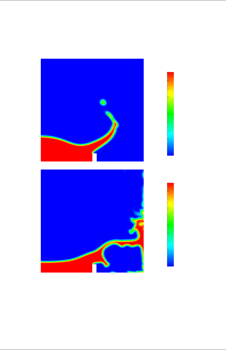
U-68 Tutorials
0.0
0.1
0.2
0.3
0.4
0.5
0.6
0.7
0.8
0.9
1.0
Phase fraction, α1
(a) At t= 0.25 s.
0.0
0.1
0.2
0.3
0.4
0.5
0.6
0.7
0.8
0.9
1.0
Phase fraction, α1
(b) At t= 0.50 s.
Figure 2.24: Snapshots of phase αwith refined mesh.
OpenFOAM-2.4.0
Chapter 3
Applications and libraries
We should reiterate from the outset that OpenFOAM is a C++ library used primarily to
create executables, known as applications. OpenFOAM is distributed with a large set of
precompiled applications but users also have the freedom to create their own or modify
existing ones. Applications are split into two main categories:
solvers that are each designed to solve a specific problem in computational continuum
mechanics;
utilities that perform simple pre-and post-processing tasks, mainly involving data manip-
ulation and algebraic calculations.
OpenFOAM is divided into a set of precompiled libraries that are dynamically linked during
compilation of the solvers and utilities. Libraries such as those for physical models are
supplied as source code so that users may conveniently add their own models to the libraries.
This chapter gives an overview of solvers, utilities and libraries, their creation, modification,
compilation and execution.
3.1 The programming language of OpenFOAM
In order to understand the way in which the OpenFOAM library works, some background
knowledge of C++, the base language of OpenFOAM, is required; the necessary information
will be presented in this chapter. Before doing so, it is worthwhile addressing the concept of
language in general terms to explain some of the ideas behind object-oriented programming
and our choice of C++ as the main programming language of OpenFOAM.
3.1.1 Language in general
The success of verbal language and mathematics is based on efficiency, especially in express-
ing abstract concepts. For example, in fluid flow, we use the term “velocity field”, which has
meaning without any reference to the nature of the flow or any specific velocity data. The
term encapsulates the idea of movement with direction and magnitude and relates to other
physical properties. In mathematics, we can represent velocity field by a single symbol, e.g.
U, and express certain concepts using symbols, e.g. “the field of velocity magnitude” by
|U|. The advantage of mathematics over verbal language is its greater efficiency, making it
possible to express complex concepts with extreme clarity.

U-70 Applications and libraries
The problems that we wish to solve in continuum mechanics are not presented in terms of
intrinsic entities, or types, known to a computer, e.g. bits, bytes, integers. They are usually
presented first in verbal language, then as partial differential equations in 3 dimensions of
space and time. The equations contain the following concepts: scalars, vectors, tensors,
and fields thereof; tensor algebra; tensor calculus; dimensional units. The solution to these
equations involves discretisation procedures, matrices, solvers, and solution algorithms.
3.1.2 Object-orientation and C++
Progamming languages that are object-oriented, such as C++, provide the mechanism —
classes — to declare types and associated operations that are part of the verbal and math-
ematical languages used in science and engineering. Our velocity field introduced earlier
can be represented in programming code by the symbol Uand “the field of velocity mag-
nitude” can be mag(U). The velocity is a vector field for which there should exist, in an
object-oriented code, a vectorField class. The velocity field Uwould then be an instance, or
object, of the vectorField class; hence the term object-oriented.
The clarity of having objects in programming that represent physical objects and abstract
entities should not be underestimated. The class structure concentrates code development
to contained regions of the code, i.e. the classes themselves, thereby making the code easier
to manage. New classes can be derived or inherit properties from other classes, e.g. the
vectorField can be derived from a vector class and a Field class. C++ provides the mechanism
of template classes such that the template class Field<Type>can represent a field of any
<Type>,e.g.scalar,vector,tensor. The general features of the template class are passed on
to any class created from the template. Templating and inheritance reduce duplication of
code and create class hierarchies that impose an overall structure on the code.
3.1.3 Equation representation
A central theme of the OpenFOAM design is that the solver applications, written using the
OpenFOAM classes, have a syntax that closely resembles the partial differential equations
being solved. For example the equation
∂ρU
∂t +∇•φU− ∇ •µ∇U=−∇p
is represented by the code
solve
(
fvm::ddt(rho, U)
+ fvm::div(phi, U)
- fvm::laplacian(mu, U)
==
- fvc::grad(p)
);
This and other requirements demand that the principal programming language of Open-
FOAM has object-oriented features such as inheritance, template classes, virtual functions
and operator overloading. These features are not available in many languages that purport
OpenFOAM-2.4.0

3.2 Compiling applications and libraries U-71
to be object-orientated but actually have very limited object-orientated capability, such
as FORTRAN-90. C++, however, possesses all these features while having the additional
advantage that it is widely used with a standard specification so that reliable compilers
are available that produce efficient executables. It is therefore the primary language of
OpenFOAM.
3.1.4 Solver codes
Solver codes are largely procedural since they are a close representation of solution algo-
rithms and equations, which are themselves procedural in nature. Users do not need a deep
knowledge of object-orientation and C++ programming to write a solver but should know
the principles behind object-orientation and classes, and to have a basic knowledge of some
C++ code syntax. An understanding of the underlying equations, models and solution
method and algorithms is far more important.
There is often little need for a user to immerse themselves in the code of any of the
OpenFOAM classes. The essence of object-orientation is that the user should not have
to; merely the knowledge of the class’ existence and its functionality are sufficient to use
the class. A description of each class, its functions etc. is supplied with the OpenFOAM
distribution in HTML documentation generated with Doxygen at $WM PROJECT DIR/-
doc/Doxygen/html/index.html.
3.2 Compiling applications and libraries
Compilation is an integral part of application development that requires careful management
since every piece of code requires its own set instructions to access dependent components
of the OpenFOAM library. In UNIX/Linux systems these instructions are often organised
and delivered to the compiler using the standard UNIXmake utility. OpenFOAM, however,
is supplied with the wmake compilation script that is based on make but is considerably
more versatile and easier to use; wmake can, in fact, be used on any code, not simply the
OpenFOAM library. To understand the compilation process, we first need to explain certain
aspects of C++ and its file structure, shown schematically in Figure 3.1. A class is defined
through a set of instructions such as object construction, data storage and class member
functions. The file containing the class definition takes a .C extension, e.g. a class nc would
be written in the file nc.C. This file can be compiled independently of other code into a binary
executable library file known as a shared object library with the .so file extension, i.e.nc.so.
When compiling a piece of code, say newApp.C, that uses the nc class, nc.C need not be
recompiled, rather newApp.C calls nc.so at runtime. This is known as dynamic linking.
3.2.1 Header .H files
As a means of checking errors, the piece of code being compiled must know that the classes
it uses and the operations they perform actually exist. Therefore each class requires a class
declaration, contained in a header file with a .H file extension, e.g.nc.H, that includes the
names of the class and its functions. This file is included at the beginning of any piece
of code using the class, including the class declaration code itself. Any piece of .C code
can resource any number of classes and must begin with all the .H files required to declare
these classes. The classes in turn can resource other classes and begin with the relevant .H
OpenFOAM-2.4.0
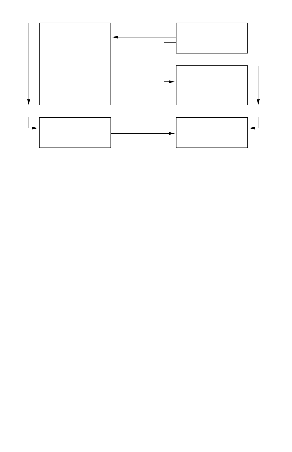
U-72 Applications and libraries
int main()
...
...
return(0);
{
}
nc.so
Library
option-I
#include "nc.H"
Main code
Code...
Compiled
nc.H
nc.C
#include "nc.H"
nc class
Definition...
Compiled
Executable
Header file
Linked
option-l
newApp.C
newApp
Figure 3.1: Header files, source files, compilation and linking
files. By searching recursively down the class hierarchy we can produce a complete list of
header files for all the classes on which the top level .C code ultimately depends; these .H
files are known as the dependencies. With a dependency list, a compiler can check whether
the source files have been updated since their last compilation and selectively compile only
those that need to be.
Header files are included in the code using # include statements, e.g.
# include "otherHeader.H";
causes the compiler to suspend reading from the current file to read the file specified. Any
self-contained piece of code can be put into a header file and included at the relevant location
in the main code in order to improve code readability. For example, in most OpenFOAM
applications the code for creating fields and reading field input data is included in a file
createFields.H which is called at the beginning of the code. In this way, header files are
not solely used as class declarations. It is wmake that performs the task of maintaining file
dependency lists amongst other functions listed below.
•Automatic generation and maintenance of file dependency lists, i.e. lists of files which
are included in the source files and hence on which they depend.
•Multi-platform compilation and linkage, handled through appropriate directory struc-
ture.
•Multi-language compilation and linkage, e.g. C, C++, Java.
•Multi-option compilation and linkage, e.g. debug, optimised, parallel and profiling.
•Support for source code generation programs, e.g. lex, yacc, IDL, MOC.
•Simple syntax for source file lists.
•Automatic creation of source file lists for new codes.
OpenFOAM-2.4.0
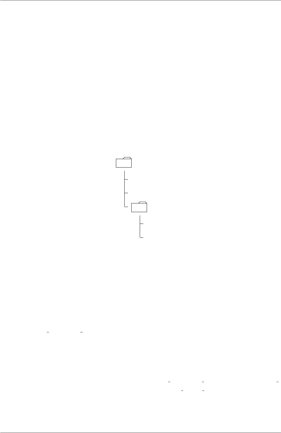
3.2 Compiling applications and libraries U-73
•Simple handling of multiple shared or static libraries.
•Extensible to new machine types.
•Extremely portable, works on any machine with: make;sh,ksh or csh;lex,cc.
•Has been tested on Apollo, SUN, SGI, HP (HPUX), Compaq (DEC), IBM (AIX),
Cray, Ardent, Stardent, PC Linux, PPC Linux, NEC, SX4, Fujitsu VP1000.
3.2.2 Compiling with wmake
OpenFOAM applications are organised using a standard convention that the source code
of each application is placed in a directory whose name is that of the application. The top
level source file takes the application name with the .C extension. For example, the source
code for an application called newApp would reside is a directory newApp and the top level
file would be newApp.C as shown in Figure 3.2. The directory must also contain a Make
newApp
newApp.C
otherHeader.H
Make
files
options
Figure 3.2: Directory structure for an application
subdirectory containing 2 files, options and files, that are described in the following sections.
3.2.2.1 Including headers
The compiler searches for the included header files in the following order, specified with the
-I option in wmake:
1. the $WM PROJECT DIR/src/OpenFOAM/lnInclude directory;
2. a local lnInclude directory, i.e.newApp/lnInclude;
3. the local directory, i.e.newApp;
4. platform dependent paths set in files in the $WM PROJECT DIR/wmake/rules/$WM -
ARCH/ directory, e.g./usr/X11/include and $(MPICH ARCH PATH)/include;
5. other directories specified explicitly in the Make/options file with the -I option.
The Make/options file contains the full directory paths to locate header files using the syntax:
OpenFOAM-2.4.0

U-74 Applications and libraries
EXE INC = \
-I<directoryPath1>\
-I<directoryPath2>\
... \
-I<directoryPathN>
Notice first that the directory names are preceeded by the -I flag and that the syntax uses
the \to continue the EXE INC across several lines, with no \after the final entry.
3.2.2.2 Linking to libraries
The compiler links to shared object library files in the following directory paths, specified
with the -L option in wmake:
1. the $FOAM LIBBIN directory;
2. platform dependent paths set in files in the $WM DIR/rules/$WM ARCH/ directory,
e.g./usr/X11/lib and $(MPICH ARCH PATH)/lib;
3. other directories specified in the Make/options file.
The actual library files to be linked must be specified using the -l option and removing
the lib prefix and .so extension from the library file name, e.g.libnew.so is included with
the flag -lnew. By default, wmake loads the following libraries:
1. the libOpenFOAM.so library from the $FOAM LIBBIN directory;
2. platform dependent libraries specified in set in files in the $WM DIR/rules/$WM ARCH/
directory, e.g.libm.so from /usr/X11/lib and liblam.so from $(LAM ARCH PATH)/lib;
3. other libraries specified in the Make/options file.
The Make/options file contains the full directory paths and library names using the syntax:
EXE LIBS = \
-L<libraryPath1>\
-L<libraryPath2>\
... \
-L<libraryPathN>\
-l<library1>\
-l<library2>\
... \
-l<libraryN>
Let us reiterate that the directory paths are preceeded by the -L flag, the library names are
preceeded by the -l flag.
OpenFOAM-2.4.0

3.2 Compiling applications and libraries U-75
3.2.2.3 Source files to be compiled
The compiler requires a list of .C source files that must be compiled. The list must contain
the main .C file but also any other source files that are created for the specific application
but are not included in a class library. For example, users may create a new class or some
new functionality to an existing class for a particular application. The full list of .C source
files must be included in the Make/files file. As might be expected, for many applications
the list only includes the name of the main .C file, e.g.newApp.C in the case of our earlier
example.
The Make/files file also includes a full path and name of the compiled executable, specified
by the EXE = syntax. Standard convention stipulates the name is that of the application,
i.e.newApp in our example. The OpenFOAM release offers two useful choices for path:
standard release applications are stored in $FOAM APPBIN; applications developed by the
user are stored in $FOAM USER APPBIN.
If the user is developing their own applications, we recommend they create an applica-
tions subdirectory in their $WM PROJECT USER DIR directory containing the source code
for personal OpenFOAM applications. As with standard applications, the source code for
each OpenFOAM application should be stored within its own directory. The only differ-
ence between a user application and one from the standard release is that the Make/files
file should specify that the user’s executables are written into their $FOAM USER APPBIN
directory. The Make/files file for our example would appear as follows:
newApp.C
EXE = $(FOAM_USER_APPBIN)/newApp
3.2.2.4 Running wmake
The wmake script is executed by typing:
wmake <optionalArguments> <optionalDirectory>
The <optionalDirectory>is the directory path of the application that is being compiled.
Typically, wmake is executed from within the directory of the application being compiled,
in which case <optionalDirectory>can be omitted.
If a user wishes to build an application executable, then no <optionalArguments>are
required. However <optionalArguments>may be specified for building libraries etc. as
described in Table 3.1.
Argument Type of compilation
lib Build a statically-linked library
libso Build a dynamically-linked library
libo Build a statically-linked object file library
jar Build a JAVA archive
exe Build an application independent of the specified project
Table 3.1: Optional compilation arguments to wmake.
OpenFOAM-2.4.0

U-76 Applications and libraries
3.2.2.5 wmake environment variables
For information, the environment variable settings used by wmake are listed in Table 3.2.
Main paths
$WM PROJECT INST DIR Full path to installation directory,
e.g.$HOME/OpenFOAM
$WM PROJECT Name of the project being compiled: OpenFOAM
$WM PROJECT VERSION Version of the project being compiled: 2.4.0
$WM PROJECT DIR Full path to locate binary executables of OpenFOAM
release, e.g.$HOME/OpenFOAM/OpenFOAM-2.4.0
$WM PROJECT USER DIR Full path to locate binary executables of the user
e.g.$HOME/OpenFOAM/${USER}-2.4.0
Other paths/settings
$WM ARCH Machine architecture: Linux,SunOS
$WM ARCH OPTION 32 or 64 bit architecture
$WM COMPILER Compiler being used: Gcc43 -gcc 4.5+, ICC - Intel
$WM COMPILER DIR Compiler installation directory
$WM COMPILER BIN Compiler installation binaries $WM COMPILER BIN/bin
$WM COMPILER LIB Compiler installation libraries $WM COMPILER BIN/lib
$WM COMPILE OPTION Compilation option: Debug - debugging, Opt optimisa-
tion.
$WM DIR Full path of the wmake directory
$WM MPLIB Parallel communications library: LAM,MPI,MPICH,PVM
$WM OPTIONS =$WM ARCH$WM COMPILER...
...$WM COMPILE OPTION$WM MPLIB
e.g.linuxGcc3OptMPICH
$WM PRECISION OPTION Precision of the compiled binares, SP, single precision or
DP, double precision
Table 3.2: Environment variable settings for wmake.
3.2.3 Removing dependency lists: wclean and rmdepall
On execution, wmake builds a dependency list file with a .dep file extension, e.g.newApp.dep
in our example, and a list of files in a Make/$WM OPTIONS directory. If the user wishes
to remove these files, perhaps after making code changes, the user can run the wclean script
by typing:
wclean <optionalArguments> <optionalDirectory>
Again, the <optionalDirectory>is a path to the directory of the application that is being
compiled. Typically, wclean is executed from within the directory of the application, in
which case the path can be omitted.
OpenFOAM-2.4.0

3.2 Compiling applications and libraries U-77
If a user wishes to remove the dependency files and files from the Make directory, then no
<optionalArguments>are required. However if lib is specified in <optionalArguments>
a local lnInclude directory will be deleted also.
An additional script, rmdepall removes all dependency .dep files recursively down the
directory tree from the point at which it is executed. This can be useful when updating
OpenFOAM libraries.
3.2.4 Compilation example: the pisoFoam application
The source code for application pisoFoam is in the $FOAM APP/solvers/incompressible/pisoFoam
directory and the top level source file is named pisoFoam.C. The pisoFoam.C source code is:
1/*---------------------------------------------------------------------------*\
2========= |
3\\ / F ield | OpenFOAM: The Open Source CFD Toolbox
4\\ / O peration |
5\\ / A nd | Copyright (C) 2011-2013 OpenFOAM Foundation
6\\/ M anipulation |
7-------------------------------------------------------------------------------
8License
9This file is part of OpenFOAM.
10
11 OpenFOAM is free software: you can redistribute it and/or modify it
12 under the terms of the GNU General Public License as published by
13 the Free Software Foundation, either version 3 of the License, or
14 (at your option) any later version.
15
16 OpenFOAM is distributed in the hope that it will be useful, but WITHOUT
17 ANY WARRANTY; without even the implied warranty of MERCHANTABILITY or
18 FITNESS FOR A PARTICULAR PURPOSE. See the GNU General Public License
19 for more details.
20
21 You should have received a copy of the GNU General Public License
22 along with OpenFOAM. If not, see <http://www.gnu.org/licenses/>.
23
24 Application
25 pisoFoam
26
27 Description
28 Transient solver for incompressible flow.
29
30 Turbulence modelling is generic, i.e. laminar, RAS or LES may be selected.
31
32 \*---------------------------------------------------------------------------*/
33
34 #include "fvCFD.H"
35 #include "singlePhaseTransportModel.H"
36 #include "turbulenceModel.H"
37
38 // * * * * * * * * * * * * * * * * * * * * * * * * * * * * * * * * * * * * * //
39
40 int main(int argc, char *argv[])
41 {
42 #include "setRootCase.H"
43
44 #include "createTime.H"
45 #include "createMesh.H"
46 #include "createFields.H"
47 #include "initContinuityErrs.H"
48
49 // * * * * * * * * * * * * * * * * * * * * * * * * * * * * * * * * * * * //
50
51 Info<< "\nStarting time loop\n" << endl;
52
53 while (runTime.loop())
54 {
55 Info<< "Time = " << runTime.timeName() << nl << endl;
56
57 #include "readPISOControls.H"
58 #include "CourantNo.H"
59
60 // Pressure-velocity PISO corrector
61 {
OpenFOAM-2.4.0

U-78 Applications and libraries
62 // Momentum predictor
63
64 fvVectorMatrix UEqn
65 (
66 fvm::ddt(U)
67 + fvm::div(phi, U)
68 + turbulence->divDevReff(U)
69 );
70
71 UEqn.relax();
72
73 if (momentumPredictor)
74 {
75 solve(UEqn == -fvc::grad(p));
76 }
77
78 // --- PISO loop
79
80 for (int corr=0; corr<nCorr; corr++)
81 {
82 volScalarField rAU(1.0/UEqn.A());
83
84 volVectorField HbyA("HbyA", U);
85 HbyA = rAU*UEqn.H();
86 surfaceScalarField phiHbyA
87 (
88 "phiHbyA",
89 (fvc::interpolate(HbyA) & mesh.Sf())
90 + fvc::interpolate(rAU)*fvc::ddtCorr(U, phi)
91 );
92
93 adjustPhi(phiHbyA, U, p);
94
95 // Non-orthogonal pressure corrector loop
96 for (int nonOrth=0; nonOrth<=nNonOrthCorr; nonOrth++)
97 {
98 // Pressure corrector
99
100 fvScalarMatrix pEqn
101 (
102 fvm::laplacian(rAU, p) == fvc::div(phiHbyA)
103 );
104
105 pEqn.setReference(pRefCell, pRefValue);
106
107 if
108 (
109 corr == nCorr-1
110 && nonOrth == nNonOrthCorr
111 )
112 {
113 pEqn.solve(mesh.solver("pFinal"));
114 }
115 else
116 {
117 pEqn.solve();
118 }
119
120 if (nonOrth == nNonOrthCorr)
121 {
122 phi = phiHbyA - pEqn.flux();
123 }
124 }
125
126 #include "continuityErrs.H"
127
128 U = HbyA - rAU*fvc::grad(p);
129 U.correctBoundaryConditions();
130 }
131 }
132
133 turbulence->correct();
134
135 runTime.write();
136
137 Info<< "ExecutionTime = " << runTime.elapsedCpuTime() << " s"
138 << " ClockTime = " << runTime.elapsedClockTime() << " s"
139 << nl << endl;
OpenFOAM-2.4.0

3.2 Compiling applications and libraries U-79
140 }
141
142 Info<< "End\n" << endl;
143
144 return 0;
145 }
146
147
148 // ************************************************************************* //
The code begins with a brief description of the application contained within comments over 1
line (//) and multiple lines (/*...*/). Following that, the code contains several # include
statements, e.g.# include "fvCFD.H", which causes the compiler to suspend reading from
the current file, pisoFoam.C to read the fvCFD.H.
pisoFoam resources the incompressibleRASModels,incompressibleLESModels and incom-
pressibleTransportModels libraries and therefore requires the necessary header files, specified
by the EXE INC = -I... option, and links to the libraries with the EXE LIBS = -l...
option. The Make/options therefore contains the following:
1EXE_INC = \
2-I$(LIB_SRC)/turbulenceModels/incompressible/turbulenceModel \
3-I$(LIB_SRC)/transportModels \
4-I$(LIB_SRC)/transportModels/incompressible/singlePhaseTransportModel \
5-I$(LIB_SRC)/finiteVolume/lnInclude \
6-I$(LIB_SRC)/meshTools/lnInclude
7
8EXE_LIBS = \
9-lincompressibleTurbulenceModel \
10 -lincompressibleRASModels \
11 -lincompressibleLESModels \
12 -lincompressibleTransportModels \
13 -lfiniteVolume \
14 -lmeshTools
pisoFoam contains only the pisoFoam.C source and the executable is written to the $FOAM -
APPBIN directory as all standard applications are. The Make/files therefore contains:
1pisoFoam.C
2
3EXE = $(FOAM_APPBIN)/pisoFoam
Following the recommendations of section 3.2.2.3, the user can compile a separate version
of pisoFoam into their local $FOAM USER DIR directory by the following:
•copying the pisoFoam source code to a local directory, e.g. $FOAM RUN;
cd $FOAM RUN
cp -r $FOAM SOLVERS/incompressible/pisoFoam .
cd pisoFoam
•editing the Make/files file as follows;
1pisoFoam.C
2
3EXE = $(FOAM_USER_LIBBIN)/pisoFoam
•executing wmake.
wmake
The code should compile and produce a message similar to the following
OpenFOAM-2.4.0

U-80 Applications and libraries
Making dependency list for source file pisoFoam.C
SOURCE DIR=.
SOURCE=pisoFoam.C ;
g++ -DFOAM EXCEPTION -Dlinux -DlinuxGccDPOpt
-DscalarMachine -DoptSolvers -DPARALLEL -DUSEMPI -Wall -O2 -DNoRepository
-ftemplate-depth-17 -I.../OpenFOAM/OpenFOAM-2.4.0/src/OpenFOAM/lnInclude
-IlnInclude
-I.
......
-lmpich -L/usr/X11/lib -lm
-o ... platforms/bin/linuxGccDPOpt/pisoFoam
The user can now try recompiling and will receive a message similar to the following to say
that the executable is up to date and compiling is not necessary:
make: Nothing to be done for `allFiles'.
make: `Make/linuxGccDPOpt/dependencies' is up to date.
make: `... platforms/linuxGccDPOpt/bin/pisoFoam'
is up to date.
The user can compile the application from scratch by removing the dependency list with
wclean
and running wmake.
3.2.5 Debug messaging and optimisation switches
OpenFOAM provides a system of messaging that is written during runtime, most of which
are to help debugging problems encountered during running of a OpenFOAM case. The
switches are listed in the $WM PROJECT DIR/etc/controlDict file; should the user wish
to change the settings they should make a copy to their $HOME directory, i.e.$HOME/-
.OpenFOAM/2.4.0/controlDict file. The list of possible switches is extensive and can be
viewed by running the foamDebugSwitches application. Most of the switches correspond to a
class or range of functionality and can be switched on by their inclusion in the controlDict file,
and by being set to 1. For example, OpenFOAM can perform the checking of dimensional
units in all calculations by setting the dimensionSet switch to 1. There are some switches
that control messaging at a higher level than most, listed in Table 3.3.
In addition, there are some switches that control certain operational and optimisa-
tion issues. These switches are also listed in Table 3.3. Of particular importance is
fileModificationSkew. OpenFOAM scans the write time of data files to check for mod-
ification. When running over a NFS with some disparity in the clock settings on different
machines, field data files appear to be modified ahead of time. This can cause a problem
if OpenFOAM views the files as newly modified and attempting to re-read this data. The
fileModificationSkew keyword is the time in seconds that OpenFOAM will subtract from
the file write time when assessing whether the file has been newly modified.
OpenFOAM-2.4.0

3.3 Running applications U-81
High level debugging switches - sub-dictionary DebugSwitches
level Overall level of debugging messaging for OpenFOAM- - 3 levels 0,
1,2
lduMatrix Messaging for solver convergence during a run - 3 levels 0,1,2
Optimisation switches - sub-dictionary OptimisationSwitches
fileModific-
ationSkew
A time in seconds that should be set higher than the maximum
delay in NFS updates and clock difference for running OpenFOAM
over a NFS.
fileModific-
ationChecking
Method of checking whether files have been modified during a
simulation, either reading the timeStamp or using inotify; ver-
sions that read only master-node data exist, timeStampMaster,
inotifyMaster.
commsType Parallel communications type: nonBlocking,scheduled,
blocking.
floatTransfer If 1, will compact numbers to float precision before transfer; de-
fault is 0
nProcsSimpleSum Optimises global sum for parallel processing; sets number of pro-
cessors above which hierarchical sum is performed rather than a
linear sum (default 16)
Table 3.3: Runtime message switches.
3.2.6 Linking new user-defined libraries to existing applications
The situation may arise that a user creates a new library, say new, and wishes the features
within that library to be available across a range of applications. For example, the user
may create a new boundary condition, compiled into new, that would need to be recognised
by a range of solver applications, pre- and post-processing utilities, mesh tools, etc. Under
normal circumstances, the user would need to recompile every application with the new
linked to it.
Instead there is a simple mechanism to link one or more shared object libraries dy-
namically at run-time in OpenFOAM. Simply add the optional keyword entry libs to the
controlDict file for a case and enter the full names of the libraries within a list (as quoted
string entries). For example, if a user wished to link the libraries new1 and new2 at run-time,
they would simply need to add the following to the case controlDict file:
libs
(
"libnew1.so"
"libnew2.so"
);
3.3 Running applications
Each application is designed to be executed from a terminal command line, typically reading
and writing a set of data files associated with a particular case. The data files for a case are
OpenFOAM-2.4.0

U-82 Applications and libraries
stored in a directory named after the case as described in section 4.1; the directory name
with full path is here given the generic name <caseDir>.
For any application, the form of the command line entry for any can be found by simply
entering the application name at the command line with the -help option, e.g. typing
blockMesh -help
returns the usage
Usage: blockMesh [-region region name] [-case dir] [-blockTopology]
[-help] [-doc] [-srcDoc]
The arguments in square brackets, [ ], are optional flags. If the application is executed from
within a case directory, it will operate on that case. Alternatively, the -case <caseDir>
option allows the case to be specified directly so that the application can be executed from
anywhere in the filing system.
Like any UNIX/Linux executable, applications can be run as a background process, i.e.
one which does not have to be completed before the user can give the shell additional
commands. If the user wished to run the blockMesh example as a background process and
output the case progress to a log file, they could enter:
blockMesh > log &
3.4 Running applications in parallel
This section describes how to run OpenFOAM in parallel on distributed processors. The
method of parallel computing used by OpenFOAM is known as domain decomposition, in
which the geometry and associated fields are broken into pieces and allocated to separate
processors for solution. The process of parallel computation involves: decomposition of
mesh and fields; running the application in parallel; and, post-processing the decomposed
case as described in the following sections. The parallel running uses the public domain
openMPI implementation of the standard message passing interface (MPI).
3.4.1 Decomposition of mesh and initial field data
The mesh and fields are decomposed using the decomposePar utility. The underlying aim
is to break up the domain with minimal effort but in such a way to guarantee a fairly eco-
nomic solution. The geometry and fields are broken up according to a set of parameters
specified in a dictionary named decomposeParDict that must be located in the system direc-
tory of the case of interest. An example decomposeParDict dictionary can be copied from
the interFoam/damBreak tutorial if the user requires one; the dictionary entries within it are
reproduced below:
17
18 numberOfSubdomains 4;
19
20 method simple;
21
22 simpleCoeffs
23 {
OpenFOAM-2.4.0

3.4 Running applications in parallel U-83
24 n ( 2 2 1 );
25 delta 0.001;
26 }
27
28 hierarchicalCoeffs
29 {
30 n ( 1 1 1 );
31 delta 0.001;
32 order xyz;
33 }
34
35 manualCoeffs
36 {
37 dataFile "";
38 }
39
40 distributed no;
41
42 roots ( );
43
44
45 // ************************************************************************* //
The user has a choice of four methods of decomposition, specified by the method keyword
as described below.
simple Simple geometric decomposition in which the domain is split into pieces by direction,
e.g. 2 pieces in the xdirection, 1 in yetc.
hierarchical Hierarchical geometric decomposition which is the same as simple except
the user specifies the order in which the directional split is done, e.g. first in the
y-direction, then the x-direction etc.
scotch Scotch decomposition which requires no geometric input from the user and attempts
to minimise the number of processor boundaries. The user can specify a weighting
for the decomposition between processors, through an optional processorWeights
keyword which can be useful on machines with differing performance between proces-
sors. There is also an optional keyword entry strategy that controls the decompo-
sition strategy through a complex string supplied to Scotch. For more information,
see the source code file: $FOAM SRC/decompositionMethods/decompositionMethods/-
scotchDecomp/scotchDecomp.C
manual Manual decomposition, where the user directly specifies the allocation of each cell
to a particular processor.
For each method there are a set of coefficients specified in a sub-dictionary of decomposi-
tionDict, named <method>Coeffs as shown in the dictionary listing. The full set of keyword
entries in the decomposeParDict dictionary are explained in Table 3.4.
The decomposePar utility is executed in the normal manner by typing
decomposePar
On completion, a set of subdirectories will have been created, one for each processor, in the
case directory. The directories are named processorNwhere N= 0,1,... represents a pro-
cessor number and contains a time directory, containing the decomposed field descriptions,
and a constant/polyMesh directory containing the decomposed mesh description.
OpenFOAM-2.4.0

U-84 Applications and libraries
Compulsory entries
numberOfSubdomains Total number of subdomains N
method Method of decomposition simple/
hierarchical/
scotch/metis/
manual/
simpleCoeffs entries
nNumber of subdomains in x,y,z(nxnynz)
delta Cell skew factor Typically, 10−3
hierarchicalCoeffs entries
nNumber of subdomains in x,y,z(nxnynz)
delta Cell skew factor Typically, 10−3
order Order of decomposition xyz/xzy/yxz...
scotchCoeffs entries
processorWeights
(optional)
List of weighting factors for allocation
of cells to processors; <wt1>is the
weighting factor for processor 1, etc.;
weights are normalised so can take any
range of values.
(<wt1>...<wtN>)
strategy Decomposition strategy (optional); de-
faults to "b"
manualCoeffs entries
dataFile Name of file containing data of alloca-
tion of cells to processors
"<fileName>"
Distributed data entries (optional) — see section 3.4.3
distributed Is the data distributed across several
disks?
yes/no
roots Root paths to case directories; <rt1>
is the root path for node 1, etc.
(<rt1>...<rtN>)
Table 3.4: Keywords in decompositionDict dictionary.
3.4.2 Running a decomposed case
A decomposed OpenFOAM case is run in parallel using the openMPI implementation of
MPI.
openMPI can be run on a local multiprocessor machine very simply but when running
on machines across a network, a file must be created that contains the host names of
the machines. The file can be given any name and located at any path. In the following
description we shall refer to such a file by the generic name, including full path, <machines>.
The <machines>file contains the names of the machines listed one machine per line. The
names must correspond to a fully resolved hostname in the /etc/hosts file of the machine
OpenFOAM-2.4.0

3.4 Running applications in parallel U-85
on which the openMPI is run. The list must contain the name of the machine running the
openMPI. Where a machine node contains more than one processor, the node name may be
followed by the entry cpu=nwhere nis the number of processors openMPI should run on
that node.
For example, let us imagine a user wishes to run openMPI from machine aaa on the
following machines: aaa;bbb, which has 2 processors; and ccc. The <machines>would
contain:
aaa
bbb cpu=2
ccc
An application is run in parallel using mpirun.
mpirun --hostfile <machines>-np <nProcs>
<foamExec> <otherArgs>-parallel > log &
where: <nProcs>is the number of processors; <foamExec>is the executable, e.g.icoFoam;
and, the output is redirected to a file named log. For example, if icoFoam is run on 4 nodes,
specified in a file named machines, on the cavity tutorial in the $FOAM RUN/tutorials/-
incompressible/icoFoam directory, then the following command should be executed:
mpirun --hostfile machines -np 4 icoFoam -parallel > log &
3.4.3 Distributing data across several disks
Data files may need to be distributed if, for example, if only local disks are used in order to
improve performance. In this case, the user may find that the root path to the case directory
may differ between machines. The paths must then be specified in the decomposeParDict
dictionary using distributed and roots keywords. The distributed entry should read
distributed yes;
and the roots entry is a list of root paths, <root0>,<root1>, . . . , for each node
roots
<nRoots>
(
"<root0>"
"<root1>"
...
);
where <nRoots>is the number of roots.
Each of the processorNdirectories should be placed in the case directory at each of
the root paths specified in the decomposeParDict dictionary. The system directory and files
within the constant directory must also be present in each case directory. Note: the files in
the constant directory are needed, but the polyMesh directory is not.
OpenFOAM-2.4.0

U-86 Applications and libraries
3.4.4 Post-processing parallel processed cases
When post-processing cases that have been run in parallel the user has two options:
•reconstruction of the mesh and field data to recreate the complete domain and fields,
which can be post-processed as normal;
•post-processing each segment of decomposed domain individually.
3.4.4.1 Reconstructing mesh and data
After a case has been run in parallel, it can be reconstructed for post-processing. The case
is reconstructed by merging the sets of time directories from each processorNdirectory into
a single set of time directories. The reconstructPar utility performs such a reconstruction by
executing the command:
reconstructPar
When the data is distributed across several disks, it must be first copied to the local case
directory for reconstruction.
3.4.4.2 Post-processing decomposed cases
The user may post-process decomposed cases using the paraFoam post-processor, described
in section 6.1. The whole simulation can be post-processed by reconstructing the case or
alternatively it is possible to post-process a segment of the decomposed domain individually
by simply treating the individual processor directory as a case in its own right.
3.5 Standard solvers
The solvers with the OpenFOAM distribution are in the $FOAM SOLVERS directory, reached
quickly by typing sol at the command line. This directory is further subdivided into several
directories by category of continuum mechanics, e.g. incompressible flow, combustion and
solid body stress analysis. Each solver is given a name that is reasonably descriptive,
e.g.icoFoam solves incompressible, laminar flow. The current list of solvers distributed with
OpenFOAM is given in Table 3.5.
‘Basic’ CFD codes
laplacianFoam Solves a simple Laplace equation, e.g. for thermal diffusion
in a solid
potentialFoam Simple potential flow solver which can be used to generate
starting fields for full Navier-Stokes codes
scalarTransportFoam Solves a transport equation for a passive scalar
Incompressible flow
Continued on next page
OpenFOAM-2.4.0

3.5 Standard solvers U-87
Continued from previous page
adjointShapeOptimiz-
ationFoam
Steady-state solver for incompressible, turbulent flow of non-
Newtonian fluids with optimisation of duct shape by applying
”blockage” in regions causing pressure loss as estimated using
an adjoint formulation
boundaryFoam Steady-state solver for incompressible, 1D turbulent flow, typ-
ically to generate boundary layer conditions at an inlet, for
use in a simulation
icoFoam Transient solver for incompressible, laminar flow of Newtonian
fluids
nonNewtonianIcoFoam Transient solver for incompressible, laminar flow of non-
Newtonian fluids
pimpleDyMFoam Transient solver for incompressible, flow of Newtonian flu-
ids on a moving mesh using the PIMPLE (merged PISO-
SIMPLE) algorithm
pimpleFoam Large time-step transient solver for incompressible, flow using
the PIMPLE (merged PISO-SIMPLE) algorithm
pisoFoam Transient solver for incompressible flow
porousSimpleFoam Steady-state solver for incompressible, turbulent flow with im-
plicit or explicit porosity treatment
shallowWaterFoam Transient solver for inviscid shallow-water equations with ro-
tation
simpleFoam Steady-state solver for incompressible, turbulent flow
SRFSimpleFoam Steady-state solver for incompressible, turbulent flow of non-
Newtonian fluids in a single rotating frame
SRFPimpleFoam Large time-step transient solver for incompressible, flow in
a single rotating frame using the PIMPLE (merged PISO-
SIMPLE) algorithm.
Compressible flow
rhoCentralDyMFoam Density-based compressible flow solver based on central-
upwind schemes of Kurganov and Tadmor with moving mesh
capability and turbulence modelling
rhoCentralFoam Density-based compressible flow solver based on central-
upwind schemes of Kurganov and Tadmor
rhoLTSPimpleFoam Transient solver for laminar or turbulent flow of compress-
ible fluids with support for run-time selectable finite volume
options, e.g. MRF, explicit porosity
rhoPimplecFoam Transient solver for laminar or turbulent flow of compressible
fluids for HVAC and similar applications
rhoPimpleFoam Transient solver for laminar or turbulent flow of compressible
fluids for HVAC and similar applications
rhoPorousSimpleFoam Steady-state solver for turbulent flow of compressible fluids
with RANS turbulence modelling, implicit or explicit porosity
treatment and run-time selectable finite volume sources
rhoSimplecFoam Steady-state SIMPLEC solver for laminar or turbulent RANS
flow of compressible fluids
Continued on next page
OpenFOAM-2.4.0

U-88 Applications and libraries
Continued from previous page
rhoSimpleFoam Steady-state SIMPLE solver for laminar or turbulent RANS
flow of compressible fluids
sonicDyMFoam Transient solver for trans-sonic/supersonic, laminar or turbu-
lent flow of a compressible gas with mesh motion
sonicFoam Transient solver for trans-sonic/supersonic, laminar or turbu-
lent flow of a compressible gas
sonicLiquidFoam Transient solver for trans-sonic/supersonic, laminar flow of a
compressible liquid
Multiphase flow
cavitatingDyMFoam Transient cavitation code based on the homogeneous equi-
librium model from which the compressibility of the liq-
uid/vapour ”mixture” is obtained, with optional mesh motion
and mesh topology changes including adaptive re-meshing
cavitatingFoam Transient cavitation code based on the homogeneous equi-
librium model from which the compressibility of the liq-
uid/vapour ”mixture” is obtained
compressibleInterDyM-
Foam
Solver for 2 compressible, non-isothermal immiscible fluids us-
ing a VOF (volume of fluid) phase-fraction based interface
capturing approach, with optional mesh motion and mesh
topology changes including adaptive re-meshing
compressibleInterFoam Solver for 2 compressible, isothermal immiscible fluids using
a VOF (volume of fluid) phase-fraction based interface cap-
turing approach
compressibleMulti-
phaseInterFoam
Solver for n compressible, non-isothermal immiscible fluids
using a VOF (volume of fluid) phase-fraction based interface
capturing approach
interFoam Solver for 2 incompressible, isothermal immiscible fluids us-
ing a VOF (volume of fluid) phase-fraction based interface
capturing approach
interDyMFoam Solver for 2 incompressible, isothermal immiscible fluids using
a VOF (volume of fluid) phase-fraction based interface captur-
ing approach, with optional mesh motion and mesh topology
changes including adaptive re-meshing.
interMixingFoam Solver for 3 incompressible fluids, two of which are miscible,
using a VOF method to capture the interface
interPhaseChange-
Foam
Solver for 2 incompressible, isothermal immiscible fluids with
phase-change (e.g. cavitation). Uses a VOF (volume of fluid)
phase-fraction based interface capturing approach
interPhaseChange-
DyMFoam
Solver for 2 incompressible, isothermal immiscible fluids with
phase-change (e.g. cavitation). Uses a VOF (volume of fluid)
phase-fraction based interface capturing approach, with op-
tional mesh motion and mesh topology changes including
adaptive re-meshing
Continued on next page
OpenFOAM-2.4.0

3.5 Standard solvers U-89
Continued from previous page
LTSInterFoam Local time stepping (LTS, steady-state) solver for 2 incom-
pressible, isothermal immiscible fluids using a VOF (volume
of fluid) phase-fraction based interface capturing approach
MRFInterFoam Multiple reference frame (MRF) solver for 2 incompressible,
isothermal immiscible fluids using a VOF (volume of fluid)
phase-fraction based interface capturing approach
MRFMultiphaseInter-
Foam
Multiple reference frame (MRF) solver for nincompressible
fluids which captures the interfaces and includes surface-
tension and contact-angle effects for each phase
multiphaseEulerFoam Solver for a system of many compressible fluid phases includ-
ing heat-transfer
multiphaseInterFoam Solver for nincompressible fluids which captures the interfaces
and includes surface-tension and contact-angle effects for each
phase
porousInterFoam Solver for 2 incompressible, isothermal immiscible fluids us-
ing a VOF (volume of fluid) phase-fraction based interface
capturing approach, with explicit handling of porous zones
potentialFreeSurface-
Foam
Incompressible Navier-Stokes solver with inclusion of a wave
height field to enable single-phase free-surface approximations
settlingFoam Solver for 2 incompressible fluids for simulating the settling
of the dispersed phase
twoLiquidMixingFoam Solver for mixing 2 incompressible fluids
twoPhaseEulerFoam Solver for a system of 2 incompressible fluid phases with one
phase dispersed, e.g. gas bubbles in a liquid
Direct numerical simulation (DNS)
dnsFoam Direct numerical simulation solver for boxes of isotropic tur-
bulence
Combustion
chemFoam Solver for chemistry problems - designed for use on single cell
cases to provide comparison against other chemistry solvers -
single cell mesh created on-the-fly - fields created on the fly
from the initial conditions
coldEngineFoam Solver for cold-flow in internal combustion engines
engineFoam Solver for internal combustion engines
fireFoam Transient Solver for Fires and turbulent diffusion flames
LTSReactingFoam Local time stepping (LTS) solver for steady, compressible,
laminar or turbulent reacting and non-reacting flow
PDRFoam Solver for compressible premixed/partially-premixed combus-
tion with turbulence modelling
reactingFoam Solver for combustion with chemical reactions
rhoReactingBuoyant-
Foam
Solver for combustion with chemical reactions using density
based thermodynamics package, using enahanced buoyancy
treatment
Continued on next page
OpenFOAM-2.4.0

U-90 Applications and libraries
Continued from previous page
rhoReactingFoam Solver for combustion with chemical reactions using density
based thermodynamics package
XiFoam Solver for compressible premixed/partially-premixed combus-
tion with turbulence modelling
Heat transfer and buoyancy-driven flows
buoyantBoussinesqPim-
pleFoam
Transient solver for buoyant, turbulent flow of incompressible
fluids
buoyantBoussinesqSim-
pleFoam
Steady-state solver for buoyant, turbulent flow of incompress-
ible fluids
buoyantPimpleFoam Transient solver for buoyant, turbulent flow of compressible
fluids for ventilation and heat-transfer
buoyantSimpleFoam Steady-state solver for buoyant, turbulent flow of compressible
fluids
chtMultiRegionFoam Combination of heatConductionFoam and buoyantFoam for
conjugate heat transfer between a solid region and fluid re-
gion
chtMultiRegionSimple-
Foam
Steady-state version of chtMultiRegionFoam
thermoFoam Evolves the thermodynamics on a frozen flow field
Particle-tracking flows
coalChemistryFoam Transient solver for: - compressible, - turbulent flow, with -
coal and limestone parcel injections, - energy source, and -
combustion
DPMFoam Transient solver for the coupled transport of a single kinematic
particle cloud including the effect of the volume fraction of
particles on the continuous phase
icoUncoupledKinem-
aticParcelDyMFoam
Transient solver for the passive transport of a single kinematic
particle could
icoUncoupledKinem-
aticParcelFoam
Transient solver for the passive transport of a single kinematic
particle could
LTSReactingParcelFoam Local time stepping (LTS) solver for steady, compressible,
laminar or turbulent reacting and non-reacting flow with mul-
tiphase Lagrangian parcels and porous media, including ex-
plicit sources for mass, momentum and energy
reactingParcelFilmFoam Transient PISO solver for compressible, laminar or turbulent
flow with reacting Lagrangian parcels, and surface film mod-
elling
reactingParcelFoam Transient PIMPLE solver for compressible, laminar or tur-
bulent flow with reacting multiphase Lagrangian parcels, in-
cluding run-time selectable finite volume options, e.g. sources,
constraints
Continued on next page
OpenFOAM-2.4.0

3.6 Standard utilities U-91
Continued from previous page
simpleReactingParcel-
Foam
Steady state SIMPLE solver for compressible, laminar or tur-
bulent flow with reacting multiphase Lagrangian parcels, in-
cluding run-time selectable finite volume options, e.g. sources,
constraints
sprayEngineFoam Transient PIMPLE solver for compressible, laminar or turbu-
lent engine flow swith spray parcels
sprayFoam Transient PIMPLE solver for compressible, laminar or turbu-
lent flow with spray parcels
uncoupledKinematic-
ParcelFoam
Transient solver for the passive transport of a single kinematic
particle could
Molecular dynamics methods
mdEquilibrationFoam Equilibrates and/or preconditions molecular dynamics sys-
tems
mdFoam Molecular dynamics solver for fluid dynamics
Direct simulation Monte Carlo methods
dsmcFoam Direct simulation Monte Carlo (DSMC) solver for 3D, tran-
sient, multi- species flows
Electromagnetics
electrostaticFoam Solver for electrostatics
magneticFoam Solver for the magnetic field generated by permanent magnets
mhdFoam Solver for magnetohydrodynamics (MHD): incompressible,
laminar flow of a conducting fluid under the influence of a
magnetic field
Stress analysis of solids
solidDisplacement-
Foam
Transient segregated finite-volume solver of linear-elastic,
small-strain deformation of a solid body, with optional ther-
mal diffusion and thermal stresses
solidEquilibriumDis-
placementFoam
Steady-state segregated finite-volume solver of linear-elastic,
small-strain deformation of a solid body, with optional ther-
mal diffusion and thermal stresses
Finance
financialFoam Solves the Black-Scholes equation to price commodities
Table 3.5: Standard library solvers.
3.6 Standard utilities
The utilities with the OpenFOAM distribution are in the $FOAM UTILITIES directory,
reached quickly by typing util at the command line. Again the names are reasonably
descriptive, e.g.ideasToFoam converts mesh data from the format written by I-DEAS to the
OpenFOAM-2.4.0

U-92 Applications and libraries
OpenFOAM format. The current list of utilities distributed with OpenFOAM is given in
Table 3.6.
Pre-processing
applyBoundaryLayer Apply a simplified boundary-layer model to the velocity and
turbulence fields based on the 1/7th power-law
applyWallFunction-
BoundaryConditions
Updates OpenFOAM RAS cases to use the new (v1.6) wall
function framework
boxTurb Makes a box of turbulence which conforms to a given energy
spectrum and is divergence free
changeDictionary Utility to change dictionary entries, e.g. can be used to change
the patch type in the field and polyMesh/boundary files
createExternalCoupled-
PatchGeometry
Application to generate the patch geometry (points and faces)
for use with the externalCoupled boundary condition
dsmcInitialise Initialise a case for dsmcFoam by reading the initialisation
dictionary system/dsmcInitialise
engineSwirl Generates a swirling flow for engine calulations
faceAgglomerate Agglomerate boundary faces for use with the view factor ra-
diation model. Writes a map from the fine to the coarse grid.
foamUpgradeCyclics Tool to upgrade mesh and fields for split cyclics
foamUpgradeFvSolution Simple tool to upgrade the syntax of system/fvSolution::solvers
mapFields Maps volume fields from one mesh to another, reading and
interpolating all fields present in the time directory of both
cases. Parallel and non-parallel cases are handled without the
need to reconstruct them first
mdInitialise Initialises fields for a molecular dynamics (MD) simulation
setFields Set values on a selected set of cells/patchfaces through a dic-
tionary
viewFactorsGen Calculates view factors based on agglomerated faces (faceAg-
glomerat) for view factor radiation model.
wallFunctionTable Generates a table suitable for use by tabulated wall functions
Mesh generation
blockMesh A multi-block mesh generator
extrudeMesh Extrude mesh from existing patch (by default outwards facing
normals; optional flips faces) or from patch read from file.
extrude2DMesh Takes 2D mesh (all faces 2 points only, no front and back
faces) and creates a 3D mesh by extruding with specified
thickness
extrudeToRegionMesh Extrude faceZones into separate mesh (as a different region),
e.g. for creating liquid film regions
foamyHexMesh Conformal Voronoi automatic mesh generator
foamyHexMeshBack-
groundMesh
Writes out background mesh as constructed by foamyHexMesh
and constructs distanceSurface
foamyHexMeshSurf-
aceSimplify
Simplifies surfaces by resampling
Continued on next page
OpenFOAM-2.4.0

3.6 Standard utilities U-93
Continued from previous page
foamyQuadMesh Conformal-Voronoi 2D extruding automatic mesher
snappyHexMesh Automatic split hex mesher. Refines and snaps to surface
Mesh conversion
ansysToFoam Converts an ANSYS input mesh file, exported from I-DEAS,
to OpenFOAM format
ccm26ToFoam Converts a CCM mesh to OpenFOAM format
cfx4ToFoam Converts a CFX 4 mesh to OpenFOAM format
datToFoam Reads in a datToFoam (.dat) mesh file and outputs a points
file. Used in conjunction with blockMesh
fluent3DMeshToFoam Converts a Fluent mesh to OpenFOAM format
fluentMeshToFoam Converts a Fluent mesh to OpenFOAM format including mul-
tiple region and region boundary handling
foamMeshToFluent Writes out the OpenFOAM mesh in Fluent mesh format
foamToStarMesh Reads an OpenFOAM mesh and writes a PROSTAR (v4)
bnd/cel/vrt format
foamToSurface Reads an OpenFOAM mesh and writes the boundaries in a
surface format
gambitToFoam Converts a GAMBIT mesh to OpenFOAM format
gmshToFoam Reads .msh file as written by Gmsh
ideasUnvToFoam I-Deas unv format mesh conversion
kivaToFoam Converts a KIVA grid to OpenFOAM format
mshToFoam Converts .msh file generated by the Adventure system
netgenNeutralToFoam Converts neutral file format as written by Netgen v4.4
plot3dToFoam Plot3d mesh (ascii/formatted format) converter
sammToFoam Converts a STAR-CD (v3) SAMM mesh to OpenFOAM format
star3ToFoam Converts a STAR-CD (v3) PROSTAR mesh into OpenFOAM
format
star4ToFoam Converts a STAR-CD (v4) PROSTAR mesh into OpenFOAM
format
tetgenToFoam Converts .ele and .node and .face files, written by tetgen
vtkUnstructuredToFoam Converts ascii .vtk (legacy format) file generated by
vtk/paraview
writeMeshObj For mesh debugging: writes mesh as three separate OBJ files
which can be viewed with e.g. javaview
Mesh manipulation
attachMesh Attach topologically detached mesh using prescribed mesh
modifiers
autoPatch Divides external faces into patches based on (user supplied)
feature angle
checkMesh Checks validity of a mesh
createBaffles Makes internal faces into boundary faces. Does not duplicate
points, unlike mergeOrSplitBaffles
createPatch Utility to create patches out of selected boundary faces. Faces
come either from existing patches or from a faceSet
Continued on next page
OpenFOAM-2.4.0

U-94 Applications and libraries
Continued from previous page
deformedGeom Deforms a polyMesh using a displacement field Uand a scaling
factor supplied as an argument
flattenMesh Flattens the front and back planes of a 2D cartesian mesh
insideCells Picks up cells with cell centre ’inside’ of surface. Requires
surface to be closed and singly connected
mergeMeshes Merges two meshes
mergeOrSplitBaffles Detects faces that share points (baffles). Either merge them
or duplicate the points
mirrorMesh Mirrors a mesh around a given plane
moveDynamicMesh Mesh motion and topological mesh changes utility
moveEngineMesh Solver for moving meshes for engine calculations
moveMesh Solver for moving meshes
objToVTK Read obj line (not surface!) file and convert into vtk
orientFaceZone Corrects orientation of faceZone
polyDualMesh Calculates the dual of a polyMesh. Adheres to all the feature
and patch edges
refineMesh Utility to refine cells in multiple directions
renumberMesh Renumbers the cell list in order to reduce the bandwidth,
reading and renumbering all fields from all the time directories
rotateMesh Rotates the mesh and fields from the direcion n1to the direc-
tion n2
setSet Manipulate a cell/face/point/ set or zone interactively
setsToZones Add pointZones/faceZones/cellZones to the mesh from similar
named pointSets/faceSets/cellSets
singleCellMesh Reads all fields and maps them to a mesh with all internal
faces removed (singleCellFvMesh) which gets written to region
singleMesh. Used to generate mesh and fields that can be
used for boundary-only data. Might easily result in illegal
mesh though so only look at boundaries in paraview
splitMesh Splits mesh by making internal faces external. Uses attachDe-
tach
splitMeshRegions Splits mesh into multiple regions
stitchMesh ’Stitches’ a mesh
subsetMesh Selects a section of mesh based on a cellSet
topoSet Operates on cellSets/faceSets/pointSets through a dictionary
transformPoints Transforms the mesh points in the polyMesh directory accord-
ing to the translate, rotate and scale options
zipUpMesh Reads in a mesh with hanging vertices and zips up the cells
to guarantee that all polyhedral cells of valid shape are closed
Other mesh tools
autoRefineMesh Utility to refine cells near to a surface
collapseEdges Collapses short edges and combines edges that are in line
Continued on next page
OpenFOAM-2.4.0

3.6 Standard utilities U-95
Continued from previous page
combinePatchFaces Checks for multiple patch faces on same cell and combines
them. Multiple patch faces can result from e.g. removal of
refined neighbouring cells, leaving 4 exposed faces with same
owner.
modifyMesh Manipulates mesh elements
PDRMesh Mesh and field preparation utility for PDR type simulations
refineHexMesh Refines a hex mesh by 2x2x2 cell splitting
refinementLevel Tries to figure out what the refinement level is on refined
cartesian meshes. Run before snapping
refineWallLayer Utility to refine cells next to patches
removeFaces Utility to remove faces (combines cells on both sides)
selectCells Select cells in relation to surface
splitCells Utility to split cells with flat faces
Post-processing graphics
ensightFoamReader EnSight library module to read OpenFOAM data directly
without translation
Post-processing data converters
foamDataToFluent Translates OpenFOAM data to Fluent format
foamToEnsight Translates OpenFOAM data to EnSight format
foamToEnsightParts Translates OpenFOAM data to Ensight format. An Ensight
part is created for each cellZone and patch
foamToGMV Translates foam output to GMV readable files
foamToTecplot360 Tecplot binary file format writer
foamToVTK Legacy VTK file format writer
smapToFoam Translates a STAR-CD SMAP data file into OpenFOAM field
format
Post-processing velocity fields
Co Calculates and writes the Courant number obtained from field
phi as a volScalarField.
enstrophy Calculates and writes the enstrophy of the velocity field U
flowType Calculates and writes the flowType of velocity field U
Lambda2 Calculates and writes the second largest eigenvalue of the sum
of the square of the symmetrical and anti-symmetrical parts
of the velocity gradient tensor
Mach Calculates and optionally writes the local Mach number from
the velocity field Uat each time
Pe Calculates and writes the Pe number as a surfaceScalar-
Field obtained from field phi
QCalculates and writes the second invariant of the velocity gra-
dient tensor
streamFunction Calculates and writes the stream function of velocity field U
at each time
uprime Calculates and writes the scalar field of uprime (p2k/3)
Continued on next page
OpenFOAM-2.4.0

U-96 Applications and libraries
Continued from previous page
vorticity Calculates and writes the vorticity of velocity field U
Post-processing stress fields
stressComponents Calculates and writes the scalar fields of the six components
of the stress tensor sigma for each time
Post-processing scalar fields
pPrime2 Calculates and writes the scalar field of pPrime2 ([p−p]2) at
each time
Post-processing at walls
wallGradU Calculates and writes the gradient of Uat the wall.
wallHeatFlux Calculates and writes the heat flux for all patches as the
boundary field of a volScalarField and also prints the inte-
grated flux for all wall patches.
wallShearStress Calculates and writes the wall shear stress, for the specified
times when using RAS turbulence models.
yPlusLES Calculates and reports yPlus for all wall patches, for the spec-
ified times when using LES turbulence models.
yPlusRAS Calculates and reports yPlus for all wall patches, for the spec-
ified times when using RAS turbulence models.
Post-processing turbulence
createTurbulenceFields Creates a full set of turbulence fields
RCalculates and writes the Reynolds stress Rfor the current
time step
Post-processing patch data
patchAverage Calculates the average of the specified field over the specified
patch
patchIntegrate Calculates the integral of the specified field over the specified
patch
Post-processing Lagrangian simulation
particleTracks Generates a VTK file of particle tracks for cases that were
computed using a tracked-parcel-type cloud
steadyParticleTracks Generates a VTK file of particle tracks for cases that were
computed using a steady-state cloud NOTE: case must be
re-constructed (if running in parallel) before use
Sampling post-processing
probeLocations Probe locations
sample Sample field data with a choice of interpolation schemes, sam-
pling options and write formats
Continued on next page
OpenFOAM-2.4.0

3.6 Standard utilities U-97
Continued from previous page
Miscellaneous post-processing
dsmcFieldsCalc Calculate intensive fields (Uand T) from averaged extensive
fields from a DSMC calculation
engineCompRatio Calculate the geometric compression ratio. Note that if you
have valves and/or extra volumes it will not work, since it
calculates the volume at BDC and TCD
execFlowFunctionObjects Execute the set of functionObjects specified in the selected
dictionary (which defaults to system/controlDict) for the se-
lected set of times. Alternative dictionaries should be placed
in the system/ folder
foamCalc Generic utility for simple field calculations at specified times
foamListTimes List times using timeSelector
pdfPlot Generates a graph of a probability distribution function
postChannel Post-processes data from channel flow calculations
ptot For each time: calculate the total pressure
temporalInterpolate Interpolate fields between time-steps, e.g. for animation
wdot Calculates and writes wdot for each time
writeCellCentres Write the three components of the cell centres as volScalar-
Fields so they can be used in postprocessing in thresholding
Surface mesh (e.g. STL) tools
surfaceAdd Add two surfaces. Does geometric merge on points. Does not
check for overlapping/intersecting triangles
surfaceAutoPatch Patches surface according to feature angle. Like autoPatch
surfaceBooleanFeatures Generates the extendedFeatureEdgeMesh for the interface be-
tween a boolean operation on two surfaces
surfaceCheck Checking geometric and topological quality of a surface
surfaceClean - removes baffles - collapses small edges, removing triangles.
- converts sliver triangles into split edges by projecting point
onto base of triangle
surfaceCoarsen Surface coarsening using ’bunnylod’.
surfaceConvert Converts from one surface mesh format to another
surfaceFeatureConvert Convert between edgeMesh formats
surfaceFeatureExtract Extracts and writes surface features to file
surfaceFind Finds nearest face and vertex
surfaceHookUp Find close open edges and stitches the surface along them
surfaceInertia Calculates the inertia tensor, principal axes and moments of
a command line specified triSurface. Inertia can either be of
the solid body or of a thin shell
surfaceLambdaMu-
Smooth
Smooths a surface using lambda/mu smoothing. To get
laplacian smoothing (previous surfaceSmooth behavior), set
lambda to the relaxation factor and mu to zero
surfaceMeshConvert Converts between surface formats with optional scaling or
transformations (rotate/translate) on a coordinateSystem
surfaceMeshConvert-
Testing
Converts from one surface mesh format to another, but pri-
marily used for testing functionality
Continued on next page
OpenFOAM-2.4.0

U-98 Applications and libraries
Continued from previous page
surfaceMeshExport Export from surfMesh to various third-party surface formats
with optional scaling or transformations (rotate/translate) on
a coordinateSystem
surfaceMeshImport Import from various third-party surface formats into surfMesh
with optional scaling or transformations (rotate/translate) on
a coordinateSystem
surfaceMeshInfo Miscellaneous information about surface meshes
surfaceMeshTriangulate Extracts triSurface from a polyMesh. Depending on output
surface format triangulates faces. Region numbers on trian-
gles are the patch numbers of the polyMesh. Optionally only
triangulates named patches
surfaceOrient Set normal consistent with respect to a user provided ’outside’
point. If the -inside is used the point is considered inside.
surfacePointMerge Merges points on surface if they are within absolute distance.
Since absolute distance use with care!
surfaceRedistributePar (Re)distribution of triSurface. Either takes an undecomposed
surface or an already decomposed surface and redistributes it
so that each processor has all triangles that overlap its mesh.
surfaceRefineRedGreen Refine by splitting all three edges of triangle (’red’ refine-
ment). Neighbouring triangles (which are not marked for re-
finement get split in half (’green’ refinement). (R. Verfuerth,
”A review of a posteriori error estimation and adaptive mesh
refinement techniques”, Wiley-Teubner, 1996)
surfaceSplitByPatch Writes regions of triSurface to separate files
surfaceSplitByTopology Strips any baffle parts of a surface
surfaceSplitNonMani-
folds
Takes multiply connected surface and tries to split surface at
multiply connected edges by duplicating points. Introduces
concept of - borderEdge. Edge with 4 faces connected to it.
- borderPoint. Point connected to exactly 2 borderEdges. -
borderLine. Connected list of borderEdges
surfaceSubset A surface analysis tool which sub-sets the triSurface to choose
only a part of interest. Based on subsetMesh
surfaceToPatch Reads surface and applies surface regioning to a mesh. Uses
boundaryMesh to do the hard work
surfaceTransformPoints Transform (scale/rotate) a surface. Like transformPoints but
for surfaces
Parallel processing
decomposePar Automatically decomposes a mesh and fields of a case for
parallel execution of OpenFOAM.
redistributePar Redistributes existing decomposed mesh and fields according
to the current settings in the decomposeParDict file
reconstructParMesh Reconstructs a mesh using geometric information only.
Thermophysical-related utilities
Continued on next page
OpenFOAM-2.4.0

3.7 Standard libraries U-99
Continued from previous page
adiabaticFlameT Calculates the adiabatic flame temperature for a given fuel
over a range of unburnt temperatures and equivalence ratios
chemkinToFoam Converts CHEMKIN 3 thermodynamics and reaction data files
into OpenFOAM format
equilibriumCO Calculates the equilibrium level of carbon monoxide
equilibriumFlameT Calculates the equilibrium flame temperature for a given fuel
and pressure for a range of unburnt gas temperatures and
equivalence ratios; the effects of dissociation on O2, H2O and
CO2are included
mixtureAdiabaticFlameT Calculates the adiabatic flame temperature for a given mix-
ture at a given temperature
Miscellaneous utilities
expandDictionary Read the dictionary provided as an argument, expand the
macros etc. and write the resulting dictionary to standard
output
foamDebugSwitches Write out all library debug switches
foamFormatConvert Converts all IOobjects associated with a case into the format
specified in the controlDict
foamHelp Top level wrapper utility around foam help utilities
foamInfoExec Interrogates a case and prints information to stdout
patchSummary Writes fields and boundary condition info for each patch at
each requested time instance
Table 3.6: Standard library utilities.
3.7 Standard libraries
The libraries with the OpenFOAM distribution are in the $FOAM LIB/$WM OPTIONS
directory, reached quickly by typing lib at the command line. Again, the names are prefixed
by lib and reasonably descriptive, e.g. incompressibleTransportModels contains the library of
incompressible transport models. For ease of presentation, the libraries are separated into
two types:
General libraries those that provide general classes and associated functions listed in
Table 3.7;
Model libraries those that specify models used in computational continuum mechanics,
listed in Table 3.8, Table 3.9 and Table 3.10.
Library of basic OpenFOAM tools —OpenFOAM
algorithms Algorithms
containers Container classes
db Database classes
Continued on next page
OpenFOAM-2.4.0

U-100 Applications and libraries
Continued from previous page
dimensionedTypes dimensioned<Type>class and derivatives
dimensionSet dimensionSet class
fields Field classes
global Global settings
graph graph class
interpolations Interpolation schemes
matrices Matrix classes
memory Memory management tools
meshes Mesh classes
primitives Primitive classes
Finite volume method library —finiteVolume
cfdTools CFD tools
fields Volume, surface and patch field classes; includes boundary
conditions
finiteVolume Finite volume discretisation
fvMatrices Matrices for finite volume solution
fvMesh Meshes for finite volume discretisation
interpolation Field interpolation and mapping
surfaceMesh Mesh surface data for finite volume discretisation
volMesh Mesh volume (cell) data for finite volume discretisation
Post-processing libraries
cloudFunctionObjects Function object outputs Lagrangian cloud information to a
file
fieldFunctionObjects Field function objects including field averaging, min/max, etc.
foamCalcFunctions Functions for the foamCalc utility
forces Tools for post-processing force/lift/drag data with function
objects
FVFunctionObjects Tools for calculating fvcDiv, fvcGrad etc with a function ob-
ject
jobControl Tools for controlling job running with a function object
postCalc For using functionality of a function object as a post-
processing activity
sampling Tools for sampling field data at prescribed locations in a do-
main
systemCall General function object for making system calls while running
a case
utilityFunctionObjects Utility function objects
Solution and mesh manipulation libraries
autoMesh Library of functionality for the snappyHexMesh utility
blockMesh Library of functionality for the blockMesh utility
dynamicMesh For solving systems with moving meshes
dynamicFvMesh Library for a finite volume mesh that can move and undergo
topological changes
Continued on next page
OpenFOAM-2.4.0

3.7 Standard libraries U-101
Continued from previous page
edgeMesh For handling edge-based mesh descriptions
fvMotionSolvers Finite volume mesh motion solvers
ODE Solvers for ordinary differential equations
meshTools Tools for handling a OpenFOAM mesh
surfMesh Library for handling surface meshes of different formats
triSurface For handling standard triangulated surface-based mesh de-
scriptions
topoChangerFvMesh Topological changes functionality (largely redundant)
Lagrangian particle tracking libraries
coalCombustion Coal dust combustion modelling
distributionModels Particle distribution function modelling
dsmc Direct simulation Monte Carlo method modelling
lagrangian Basic Lagrangian, or particle-tracking, solution scheme
lagrangianIntermediate Particle-tracking kinematics, thermodynamics, multispecies
reactions, particle forces, etc.
potential Intermolecular potentials for molecular dynamics
molecule Molecule classes for molecular dynamics
molecularMeasurements For making measurements in molecular dynamics
solidParticle Solid particle implementation
spray Spray and injection modelling
turbulence Particle dispersion and Brownian motion based on turbulence
Miscellaneous libraries
conversion Tools for mesh and data conversions
decompositionMethods Tools for domain decomposition
engine Tools for engine calculations
fileFormats Core routines for reading/writing data in some third-party
formats
genericFvPatchField A generic patch field
MGridGenGAMG-
Agglomeration
Library for cell agglomeration using the MGridGen algorithm
pairPatchAgglom-
eration
Primitive pair patch agglomeration method
OSspecific Operating system specific functions
randomProcesses Tools for analysing and generating random processes
Parallel libraries
decompose General mesh/field decomposition library
distributed Tools for searching and IO on distributed surfaces
metisDecomp Metis domain decomposition library
reconstruct Mesh/field reconstruction library
scotchDecomp Scotch domain decomposition library
ptsotchDecomp PTScotch domain decomposition library
Continued on next page
OpenFOAM-2.4.0

U-102 Applications and libraries
Continued from previous page
Table 3.7: Shared object libraries for general use.
Basic thermophysical models —basicThermophysicalModels
hePsiThermo General thermophysical model calculation based on com-
pressibility ψ
heRhoThermo General thermophysical model calculation based on density
ρ
pureMixture General thermophysical model calculation for passive gas
mixtures
Reaction models —reactionThermophysicalModels
psiReactionThermo Calculates enthalpy for combustion mixture based on ψ
psiuReactionThermo Calculates enthalpy for combustion mixture based on ψu
rhoReactionThermo Calculates enthalpy for combustion mixture based on ρ
heheupsiReactionThermo Calculates enthalpy for unburnt gas and combustion mix-
ture
homogeneousMixture Combustion mixture based on normalised fuel mass frac-
tion b
inhomogeneousMixture Combustion mixture based on band total fuel mass fraction
ft
veryInhomogeneousMixture Combustion mixture based on b,ftand unburnt fuel mass
fraction fu
basicMultiComponent-
Mixture
Basic mixture based on multiple components
multiComponentMixture Derived mixture based on multiple components
reactingMixture Combustion mixture using thermodynamics and reaction
schemes
egrMixture Exhaust gas recirculation mixture
singleStepReactingMixture Single step reacting mixture
Radiation models —radiationModels
P1 P1 model
fvDOM Finite volume discrete ordinate method
opaqueSolid Radiation for solid opaque solids; does nothing to energy
equation source terms (returns zeros) but creates absorp-
tionEmissionModel and scatterModel
viewFactor View factor radiation model
Laminar flame speed models —laminarFlameSpeedModels
constant Constant laminar flame speed
GuldersLaminarFlameSpeed Gulder’s laminar flame speed model
Continued on next page
OpenFOAM-2.4.0

3.7 Standard libraries U-103
Continued from previous page
GuldersEGRLaminar-
FlameSpeed
Gulder’s laminar flame speed model with exhaust gas re-
circulation modelling
RaviPetersen Laminar flame speed obtained from Ravi and Petersen’s
correlation
Barotropic compressibility models —barotropicCompressibilityModels
linear Linear compressibility model
Chung Chung compressibility model
Wallis Wallis compressibility model
Thermophysical properties of gaseous species —specie
adiabaticPerfectFluid Adiabatic perfect gas equation of state
icoPolynomial Incompressible polynomial equation of state, e.g. for liquids
perfectFluid Perfect gas equation of state
incompressiblePerfectGas Incompressible gas equation of state using a constant ref-
erence pressure. Density only varies with temperature and
composition
rhoConst Constant density equation of state
eConstThermo Constant specific heat cpmodel with evaluation of internal
energy eand entropy s
hConstThermo Constant specific heat cpmodel with evaluation of enthalpy
hand entropy s
hPolynomialThermo cpevaluated by a function with coefficients from polynomi-
als, from which h,sare evaluated
janafThermo cpevaluated by a function with coefficients from JANAF
thermodynamic tables, from which h,sare evaluated
specieThermo Thermophysical properties of species, derived from cp,h
and/or s
constTransport Constant transport properties
polynomialTransport Polynomial based temperature-dependent transport prop-
erties
sutherlandTransport Sutherland’s formula for temperature-dependent transport
properties
Functions/tables of thermophysical properties —thermophysicalFunctions
NSRDSfunctions National Standard Reference Data System (NSRDS) -
American Institute of Chemical Engineers (AICHE) data
compilation tables
APIfunctions American Petroleum Institute (API) function for vapour
mass diffusivity
Chemistry model —chemistryModel
chemistryModel Chemical reaction model
chemistrySolver Chemical reaction solver
Continued on next page
OpenFOAM-2.4.0

U-104 Applications and libraries
Continued from previous page
Other libraries
liquidProperties Thermophysical properties of liquids
liquidMixtureProperties Thermophysical properties of liquid mixtures
basicSolidThermo Thermophysical models of solids
hExponentialThermo Exponential properties thermodynamics package tem-
plated into the equationOfState
SLGThermo Thermodynamic package for solids, liquids and gases
solidChemistryModel Thermodynamic model of solid chemsitry including pyrol-
ysis
solidProperties Thermophysical properties of solids
solidMixtureProperties Thermophysical properties of solid mixtures
solidSpecie Solid reaction rates and transport models
solidThermo Solid energy modelling
Table 3.8: Libraries of thermophysical models.
RAS turbulence models for incompressible fluids —incompressibleRASModels
laminar Dummy turbulence model for laminar flow
kEpsilon Standard high-Re k −εmodel
kOmega Standard high-Re k −ωmodel
kOmegaSST k−ω-SST model
RNGkEpsilon RNG k−εmodel
NonlinearKEShih Non-linear Shih k−εmodel
LienCubicKE Lien cubic k−εmodel
qZeta q−ζmodel
kkLOmega Low Reynolds-number k-kl-omega turbulence model for in-
compressible flows
LaunderSharmaKE Launder-Sharma low-Re k −εmodel
LamBremhorstKE Lam-Bremhorst low-Re k −εmodel
LienCubicKELowRe Lien cubic low-Re k −εmodel
LienLeschzinerLowRe Lien-Leschziner low-Re k −εmodel
LRR Launder-Reece-Rodi RSTM
LaunderGibsonRSTM Launder-Gibson RSTM with wall-reflection terms
realizableKE Realizable k−εmodel
SpalartAllmaras Spalart-Allmaras 1-eqn mixing-length model
v2f Lien and Kalitzin’s v2-f turbulence model for incompress-
ible flows
RAS turbulence models for compressible fluids —compressibleRASModels
laminar Dummy turbulence model for laminar flow
kEpsilon Standard k−εmodel
kOmegaSST k−ω−SST model
RNGkEpsilon RNG k−εmodel
LaunderSharmaKE Launder-Sharma low-Re k −εmodel
LRR Launder-Reece-Rodi RSTM
Continued on next page
OpenFOAM-2.4.0

3.7 Standard libraries U-105
Continued from previous page
LaunderGibsonRSTM Launder-Gibson RSTM
realizableKE Realizable k−εmodel
SpalartAllmaras Spalart-Allmaras 1-eqn mixing-length model
v2f Lien and Kalitzin’s v2-f turbulence model for incompress-
ible flows
Large-eddy simulation (LES) filters —LESfilters
laplaceFilter Laplace filters
simpleFilter Simple filter
anisotropicFilter Anisotropic filter
Large-eddy simulation deltas —LESdeltas
PrandtlDelta Prandtl delta
cubeRootVolDelta Cube root of cell volume delta
maxDeltaxyz Maximum of x, y and z; for structured hex cells only
smoothDelta Smoothing of delta
Incompressible LES turbulence models —incompressibleLESModels
Smagorinsky Smagorinsky model
Smagorinsky2 Smagorinsky model with 3-D filter
homogenousDynSmag-
orinsky
Homogeneous dynamic Smagorinsky model
dynLagrangian Lagrangian two equation eddy-viscosity model
scaleSimilarity Scale similarity model
mixedSmagorinsky Mixed Smagorinsky/scale similarity model
homogenousDynOneEq-
Eddy
One Equation Eddy Viscosity Model for incompressible
flows
laminar Simply returns laminar properties
kOmegaSSTSAS k−ω-SST scale adaptive simulation (SAS) model
oneEqEddy k-equation eddy-viscosity model
dynOneEqEddy Dynamic k-equation eddy-viscosity model
spectEddyVisc Spectral eddy viscosity model
LRDDiffStress LRR differential stress model
DeardorffDiffStress Deardorff differential stress model
SpalartAllmaras Spalart-Allmaras model
SpalartAllmarasDDES Spalart-Allmaras delayed detached eddy simulation
(DDES) model
SpalartAllmarasIDDES Spalart-Allmaras improved DDES (IDDES) model
vanDriestDelta Simple cube-root of cell volume delta used in incompress-
ible LES models
Compressible LES turbulence models —compressibleLESModels
Smagorinsky Smagorinsky model
oneEqEddy k-equation eddy-viscosity model
lowReOneEqEddy Low-Re k-equation eddy-viscosity model
Continued on next page
OpenFOAM-2.4.0

U-106 Applications and libraries
Continued from previous page
homogenousDynOneEq-
Eddy
One Equation Eddy Viscosity Model for incompressible
flows
DeardorffDiffStress Deardorff differential stress model
SpalartAllmaras Spalart-Allmaras 1-eqn mixing-length model
vanDriestDelta Simple cube-root of cell volume delta used in incompress-
ible LES models
Table 3.9: Libraries of RAS and LES turbulence models.
Transport models for incompressible fluids —incompressibleTransportModels
Newtonian Linear viscous fluid model
CrossPowerLaw Cross Power law nonlinear viscous model
BirdCarreau Bird-Carreau nonlinear viscous model
HerschelBulkley Herschel-Bulkley nonlinear viscous model
powerLaw Power-law nonlinear viscous model
interfaceProperties Models for the interface, e.g. contact angle, in multiphase
simulations
Miscellaneous transport modelling libraries
interfaceProperties Calculation of interface properties
twoPhaseProperties Two phase properties models, including boundary condi-
tions
surfaceFilmModels Surface film models
Table 3.10: Shared object libraries of transport models.
OpenFOAM-2.4.0

Chapter 4
OpenFOAM cases
This chapter deals with the file structure and organisation of OpenFOAM cases. Nor-
mally, a user would assign a name to a case, e.g. the tutorial case of flow in a cavity
is simply named cavity. This name becomes the name of a directory in which all the
case files and subdirectories are stored. The case directories themselves can be located
anywhere but we recommend they are within a run subdirectory of the user’s project
directory, i.e.$HOME/OpenFOAM/${USER}-2.4.0 as described at the beginning of chap-
ter 2. One advantage of this is that the $FOAM RUN environment variable is set to
$HOME/OpenFOAM/${USER}-2.4.0/run by default; the user can quickly move to that di-
rectory by executing a preset alias, run, at the command line.
The tutorial cases that accompany the OpenFOAM distribution provide useful exam-
ples of the case directory structures. The tutorials are located in the $FOAM TUTORIALS
directory, reached quickly by executing the tut alias at the command line. Users can view
tutorial examples at their leisure while reading this chapter.
4.1 File structure of OpenFOAM cases
The basic directory structure for a OpenFOAM case, that contains the minimum set of files
required to run an application, is shown in Figure 4.1 and described as follows:
Aconstant directory that contains a full description of the case mesh in a subdirec-
tory polyMesh and files specifying physical properties for the application concerned,
e.g.transportProperties.
Asystem directory for setting parameters associated with the solution procedure itself.
It contains at least the following 3 files: controlDict where run control parameters are
set including start/end time, time step and parameters for data output; fvSchemes
where discretisation schemes used in the solution may be selected at run-time; and,
fvSolution where the equation solvers, tolerances and other algorithm controls are set
for the run.
The ‘time’ directories containing individual files of data for particular fields. The data
can be: either, initial values and boundary conditions that the user must specify to de-
fine the problem; or, results written to file by OpenFOAM. Note that the OpenFOAM
fields must always be initialised, even when the solution does not strictly require it, as
in steady-state problems. The name of each time directory is based on the simulated
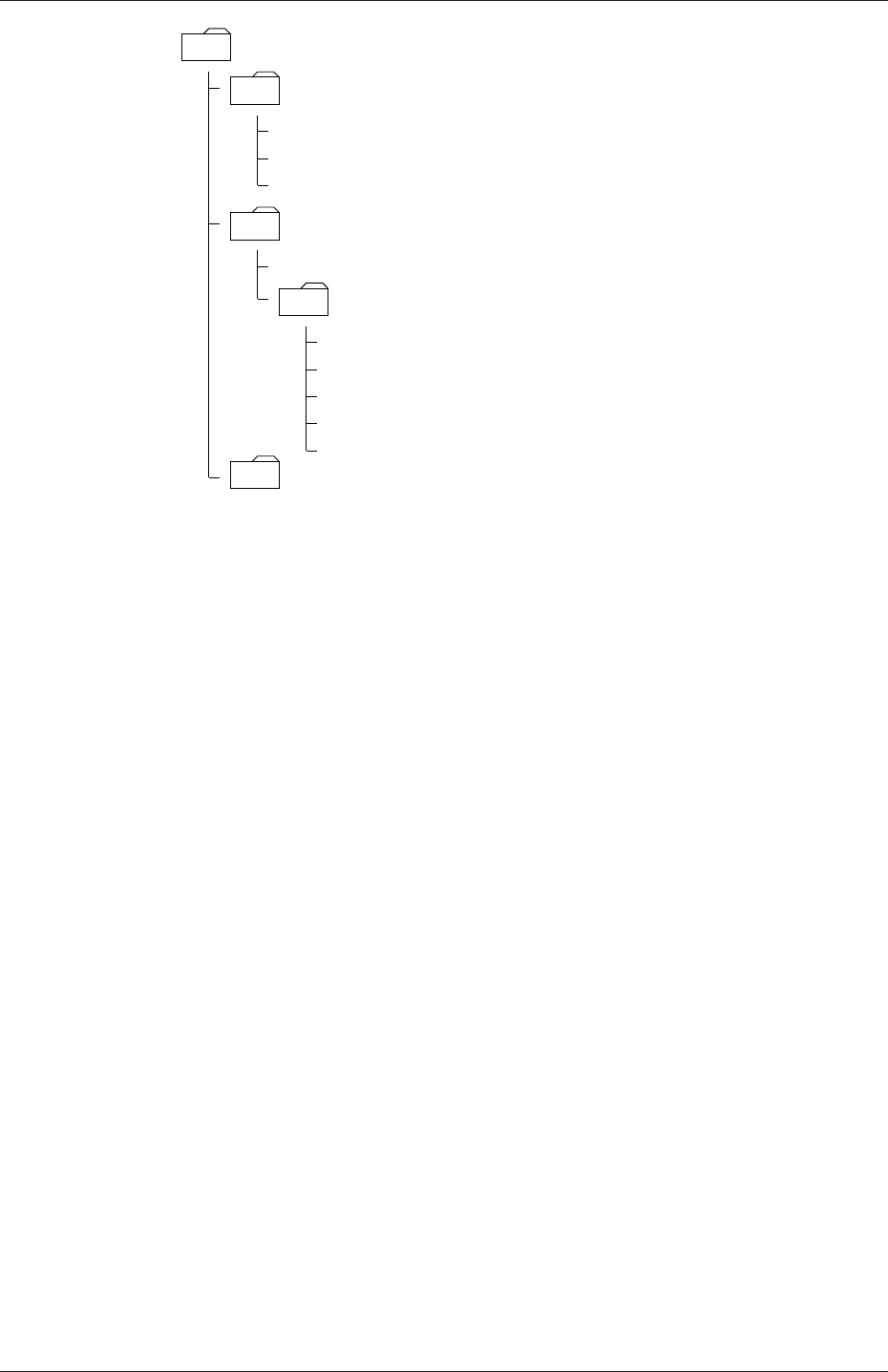
U-108 OpenFOAM cases
<case>
system
controlDict
fvSchemes
polyMesh
points
. . . Properties
constant
fvSolution
see section 4.3
see section 4.4
see section 4.5
see section 5.1.2
see chapter 7
boundary
time directories see section 4.2.8
faces
owner
neighbour
Figure 4.1: Case directory structure
time at which the data is written and is described fully in section 4.3. It is sufficient to
say now that since we usually start our simulations at time t= 0, the initial conditions
are usually stored in a directory named 0or 0.000000e+00, depending on the name
format specified. For example, in the cavity tutorial, the velocity field Uand pressure
field pare initialised from files 0/U and 0/p respectively.
4.2 Basic input/output file format
OpenFOAM needs to read a range of data structures such as strings, scalars, vectors, tensors,
lists and fields. The input/output (I/O) format of files is designed to be extremely flexible
to enable the user to modify the I/O in OpenFOAM applications as easily as possible.
The I/O follows a simple set of rules that make the files extremely easy to understand, in
contrast to many software packages whose file format may not only be difficult to understand
intuitively but also not be published anywhere. The OpenFOAM file format is described in
the following sections.
4.2.1 General syntax rules
The format follows some general principles of C++ source code.
•Files have free form, with no particular meaning assigned to any column and no need
to indicate continuation across lines.
•Lines have no particular meaning except to a // comment delimiter which makes
OpenFOAM ignore any text that follows it until the end of line.
•A comment over multiple lines is done by enclosing the text between /* and */ de-
limiters.
OpenFOAM-2.4.0

4.2 Basic input/output file format U-109
4.2.2 Dictionaries
OpenFOAM uses dictionaries as the most common means of specifying data. A dictionary
is an entity that contains data entries that can be retrieved by the I/O by means of keywords.
The keyword entries follow the general format
<keyword> <dataEntry1>... <dataEntryN>;
Most entries are single data entries of the form:
<keyword> <dataEntry>;
Most OpenFOAM data files are themselves dictionaries containing a set of keyword entries.
Dictionaries provide the means for organising entries into logical categories and can be
specified hierarchically so that any dictionary can itself contain one or more dictionary
entries. The format for a dictionary is to specify the dictionary name followed by keyword
entries enclosed in curly braces {} as follows
<dictionaryName>
{... keyword entries ...
}
4.2.3 The data file header
All data files that are read and written by OpenFOAM begin with a dictionary named
FoamFile containing a standard set of keyword entries, listed in Table 4.1. The table
Keyword Description Entry
version I/O format version 2.0
format Data format ascii /binary
location Path to the file, in "..." (optional)
class OpenFOAM class constructed from the
data file concerned
typically dictionary or a
field, e.g.volVectorField
object Filename e.g.controlDict
Table 4.1: Header keywords entries for data files.
provides brief descriptions of each entry, which is probably sufficient for most entries with
the notable exception of class. The class entry is the name of the C++ class in the
OpenFOAM library that will be constructed from the data in the file. Without knowledge
of the underlying code which calls the file to be read, and knowledge of the OpenFOAM
classes, the user will probably be unable to surmise the class entry correctly. However,
most data files with simple keyword entries are read into an internal dictionary class and
therefore the class entry is dictionary in those cases.
The following example shows the use of keywords to provide data for a case using the
types of entry described so far. The extract, from an fvSolution dictionary file, contains
2 dictionaries, solvers and PISO. The solvers dictionary contains multiple data entries for
OpenFOAM-2.4.0

U-110 OpenFOAM cases
solver and tolerances for each of the pressure and velocity equations, represented by the p
and Ukeywords respectively; the PISO dictionary contains algorithm controls.
17
18 solvers
19 {
20 p
21 {
22 solver PCG;
23 preconditioner DIC;
24 tolerance 1e-06;
25 relTol 0;
26 }
27
28 U
29 {
30 solver smoothSolver;
31 smoother symGaussSeidel;
32 tolerance 1e-05;
33 relTol 0;
34 }
35 }
36
37 PISO
38 {
39 nCorrectors 2;
40 nNonOrthogonalCorrectors 0;
41 pRefCell 0;
42 pRefValue 0;
43 }
44
45
46 // ************************************************************************* //
4.2.4 Lists
OpenFOAM applications contain lists, e.g. a list of vertex coordinates for a mesh description.
Lists are commonly found in I/O and have a format of their own in which the entries are
contained within round braces ( ). There is also a choice of format preceeding the round
braces:
simple the keyword is followed immediately by round braces
<listName>
(
... entries ...
);
numbered the keyword is followed by the number of elements <n>in the list
<listName>
<n>
(
... entries ...
);
token identifier the keyword is followed by a class name identifier Label<Type>where
<Type>states what the list contains, e.g. for a list of scalar elements is
<listName>
List<scalar>
OpenFOAM-2.4.0

4.2 Basic input/output file format U-111
<n>// optional
(
... entries ...
);
Note that <scalar>in List<scalar>is not a generic name but the actual text that should
be entered.
The simple format is a convenient way of writing a list. The other formats allow the
code to read the data faster since the size of the list can be allocated to memory in advance
of reading the data. The simple format is therefore preferred for short lists, where read time
is minimal, and the other formats are preferred for long lists.
4.2.5 Scalars, vectors and tensors
A scalar is a single number represented as such in a data file. A vector is a VectorSpace of
rank 1 and dimension 3, and since the number of elements is always fixed to 3, the simple
List format is used. Therefore a vector (1.0,1.1,1.2) is written:
(1.0 1.1 1.2)
In OpenFOAM, a tensor is a VectorSpace of rank 2 and dimension 3 and therefore the data
entries are always fixed to 9 real numbers. Therefore the identity tensor can be written:
(
1 0 0
0 1 0
0 0 1
)
This example demonstrates the way in which OpenFOAM ignores the line return is so that
the entry can be written over multiple lines. It is treated no differently to listing the numbers
on a single line:
(100010001)
4.2.6 Dimensional units
In continuum mechanics, properties are represented in some chosen units, e.g. mass in
kilograms (kg), volume in cubic metres (m3), pressure in Pascals (kg m−1s−2). Algebraic
operations must be performed on these properties using consistent units of measurement; in
particular, addition, subtraction and equality are only physically meaningful for properties
of the same dimensional units. As a safeguard against implementing a meaningless opera-
tion, OpenFOAM attaches dimensions to field data and physical properties and performs
dimension checking on any tensor operation.
The I/O format for a dimensionSet is 7 scalars delimited by square brackets, e.g.
[0 2 -1 0 0 0 0]
OpenFOAM-2.4.0

U-112 OpenFOAM cases
No. Property SI unit USCS unit
1 Mass kilogram (kg) pound-mass (lbm)
2 Length metre (m) foot (ft)
3 Time — — — — second (s) — — — —
4 Temperature Kelvin (K) degree Rankine (◦R)
5 Quantity — — — — mole (mol) — — — —
6 Current — — — — ampere (A) — — — —
7 Luminous intensity — — — — candela (cd) — — — —
Table 4.2: Base units for SI and USCS
where each of the values corresponds to the power of each of the base units of measurement
listed in Table 4.2. The table gives the base units for the Syst`eme International (SI) and the
United States Customary System (USCS) but OpenFOAM can be used with any system of
units. All that is required is that the input data is correct for the chosen set of units. It is par-
ticularly important to recognise that OpenFOAM requires some dimensioned physical con-
stants, e.g. the Universal Gas Constant R, for certain calculations, e.g. thermophysical mod-
elling. These dimensioned constants are specified in a DimensionedConstant sub-dictionary of
main controlDict file of the OpenFOAM installation ($WM PROJECT DIR/etc/controlDict).
By default these constants are set in SI units. Those wishing to use the USCS or any other
system of units should modify these constants to their chosen set of units accordingly.
4.2.7 Dimensioned types
Physical properties are typically specified with their associated dimensions. These entries
have the format that the following example of a dimensionedScalar demonstrates:
nu nu [0 2 -1 0 0 0 0] 1;
The first nu is the keyword; the second nu is the word name stored in class word, usually
chosen to be the same as the keyword; the next entry is the dimensionSet and the final entry
is the scalar value.
4.2.8 Fields
Much of the I/O data in OpenFOAM are tensor fields, e.g. velocity, pressure data, that
are read from and written into the time directories. OpenFOAM writes field data using
keyword entries as described in Table 4.3.
Keyword Description Example
dimensions Dimensions of field [1 1 -2 0 0 0 0]
internalField Value of internal field uniform (1 0 0)
boundaryField Boundary field see file listing in section 4.2.8
Table 4.3: Main keywords used in field dictionaries.
The data begins with an entry for its dimensions. Following that, is the internalField,
described in one of the following ways.
OpenFOAM-2.4.0

4.2 Basic input/output file format U-113
Uniform field a single value is assigned to all elements within the field, taking the form:
internalField uniform <entry>;
Nonuniform field each field element is assigned a unique value from a list, taking the
following form where the token identifier form of list is recommended:
internalField nonuniform <List>;
The boundaryField is a dictionary containing a set of entries whose names correspond
to each of the names of the boundary patches listed in the boundary file in the polyMesh
directory. Each patch entry is itself a dictionary containing a list of keyword entries. The
compulsory entry, type, describes the patch field condition specified for the field. The
remaining entries correspond to the type of patch field condition selected and can typically
include field data specifying initial conditions on patch faces. A selection of patch field
conditions available in OpenFOAM are listed in Table 5.3 and Table 5.4 with a description
and the data that must be specified with it. Example field dictionary entries for velocity U
are shown below:
17 dimensions [0 1 -1 0 0 0 0];
18
19 internalField uniform (0 0 0);
20
21 boundaryField
22 {
23 movingWall
24 {
25 type fixedValue;
26 value uniform (1 0 0);
27 }
28
29 fixedWalls
30 {
31 type fixedValue;
32 value uniform (0 0 0);
33 }
34
35 frontAndBack
36 {
37 type empty;
38 }
39 }
40
41 // ************************************************************************* //
4.2.9 Directives and macro substitutions
There is additional file syntax that offers great flexibility for the setting up of OpenFOAM
case files, namely directives and macro substitutions. Directives are commands that can be
contained within case files that begin with the hash (#) symbol. Macro substitutions begin
with the dollar ($) symbol.
At present there are 4 directive commands available in OpenFOAM:
#include "<fileName>"(or #includeIfPresent "<fileName>"reads the file of name
<fileName>;
#inputMode has two options: merge, which merges keyword entries in successive dictio-
naries, so that a keyword entry specified in one place will be overridden by a later
specification of the same keyword entry; overwrite, which overwrites the contents of
an entire dictionary; generally, use merge;
OpenFOAM-2.4.0

U-114 OpenFOAM cases
#remove <keywordEntry>removes any included keyword entry; can take a word or regular
expression;
#codeStream followed by verbatim C++ code, compiles, loads and executes the code on-
the-fly to generate the entry.
4.2.10 The #include and #inputMode directives
For example, let us say a user wishes to set an initial value of pressure once to be used
as the internal field and initial value at a boundary. We could create a file, e.g. named
initialConditions, which contains the following entries:
pressure 1e+05;
#inputMode merge
In order to use this pressure for both the internal and initial boundary fields, the user
would simply include the following macro substitutions in the pressure field file p:
#include "initialConditions"
internalField uniform $pressure;
boundaryField
{patch1
{type fixedValue;
value $internalField;
}
}
This is a fairly trivial example that simply demonstrates how this functionality works.
However, the functionality can be used in many, more powerful ways particularly as a means
of generalising case data to suit the user’s needs. For example, if a user has a set of cases
that require the same RAS turbulence model settings, a single file can be created with those
settings which is simply included in the RASProperties file of each case. Macro substitutions
can extend well beyond a single value so that, for example, sets of boundary conditions can
be predefined and called by a single macro. The extent to which such functionality can be
used is almost endless.
4.2.11 The #codeStream directive
The #codeStream directive takes C++ code which is compiled and executed to deliver the
dictionary entry. The code and compilation instructions are specified through the following
keywords.
•code: specifies the code, called with arguments OStream& os and const dictionary&
dict which the user can use in the code, e.g. to lookup keyword entries from within
the current case dictionary (file).
OpenFOAM-2.4.0

4.3 Time and data input/output control U-115
•codeInclude (optional): specifies additional C++ #include statements to include
OpenFOAM files.
•codeOptions (optional): specifies any extra compilation flags to be added to EXE INC
in Make/options.
•codeLibs (optional): specifies any extra compilation flags to be added to LIB LIBS in
Make/options.
Code, like any string, can be written across multiple lines by enclosing it within hash-bracket
delimiters, i.e. #{...#}. Anything in between these two delimiters becomes a string with
all newlines, quotes, etc. preserved.
An example of #codeStream is given below. The code in the controlDict file looks up
dictionary entries and does a simple calculation for the write interval:
startTime 0;
endTime 100;
...
writeInterval #codeStream
{
code
#{
scalar start = readScalar(dict.lookup("startTime"));
scalar end = readScalar(dict.lookup("endTime"));
label nDumps = 5;
os << ((end - start)/nDumps);
#};
};
4.3 Time and data input/output control
The OpenFOAM solvers begin all runs by setting up a database. The database controls
I/O and, since output of data is usually requested at intervals of time during the run, time
is an inextricable part of the database. The controlDict dictionary sets input parameters
essential for the creation of the database. The keyword entries in controlDict are listed in
Table 4.4. Only the time control and writeInterval entries are truly compulsory, with the
database taking default values indicated by †in Table 4.4 for any of the optional entries
that are omitted.
Time control
startFrom Controls the start time of the simulation.
-firstTime Earliest time step from the set of time directories.
-startTime Time specified by the startTime keyword entry.
-latestTime Most recent time step from the set of time directories.
startTime Start time for the simulation with startFrom startTime;
stopAt Controls the end time of the simulation.
-endTime Time specified by the endTime keyword entry.
-writeNow Stops simulation on completion of current time step and writes
data.
Continued on next page
OpenFOAM-2.4.0

U-116 OpenFOAM cases
Continued from previous page
-noWriteNow Stops simulation on completion of current time step and does not
write out data.
-nextWrite Stops simulation on completion of next scheduled write time, spec-
ified by writeControl.
endTime End time for the simulation when stopAt endTime; is specified.
deltaT Time step of the simulation.
Data writing
writeControl Controls the timing of write output to file.
-timeStep†Writes data every writeInterval time steps.
-runTime Writes data every writeInterval seconds of simulated time.
-adjustableRunTime Writes data every writeInterval seconds of simulated time,
adjusting the time steps to coincide with the writeInterval if
necessary — used in cases with automatic time step adjustment.
-cpuTime Writes data every writeInterval seconds of CPU time.
-clockTime Writes data out every writeInterval seconds of real time.
writeInterval Scalar used in conjunction with writeControl described above.
purgeWrite Integer representing a limit on the number of time directories that
are stored by overwriting time directories on a cyclic basis. Exam-
ple of t0= 5s, ∆t= 1s and purgeWrite 2;: data written into 2
directories, 6and 7, before returning to write the data at 8 s in 6,
data at 9 s into 7,etc.
To disable the time directory limit, specify purgeWrite 0;†
For steady-state solutions, results from previous iterations can be
continuously overwritten by specifying purgeWrite 1;
writeFormat Specifies the format of the data files.
-ascii†ASCII format, written to writePrecision significant figures.
-binary Binary format.
writePrecision Integer used in conjunction with writeFormat described above, 6†
by default
writeCompression Specifies the compression of the data files.
-uncompressed No compression.†
-compressed gzip compression.
timeFormat Choice of format of the naming of the time directories.
-fixed ±m.dddddd where the number of ds is set by timePrecision.
-scientific ±m.dddddde±xx where the number of ds is set by timePrecision.
-general†Specifies scientific format if the exponent is less than -4 or
greater than or equal to that specified by timePrecision.
Continued on next page
OpenFOAM-2.4.0

4.3 Time and data input/output control U-117
Continued from previous page
timePrecision Integer used in conjunction with timeFormat described above, 6†
by default
graphFormat Format for graph data written by an application.
-raw†Raw ASCII format in columns.
-gnuplot Data in gnuplot format.
-xmgr Data in Grace/xmgr format.
-jplot Data in jPlot format.
Adjustable time step
adjustTimeStep yes†/no switch for OpenFOAM to adjust the time step during
the simulation, usually according to. . .
maxCo Maximum Courant number, e.g. 0.5
Data reading
runTimeModifiable yes†/no switch for whether dictionaries, e.g.controlDict, are re-
read by OpenFOAM at the beginning of each time step.
Run-time loadable functionality
libs List of additional libraries (on $LD LIBRARY PATH) to be loaded
at run-time, e.g.( "libUser1.so" "libUser2.so" )
functions List of functions, e.g. probes to be loaded at run-time; see examples
in $FOAM TUTORIALS
†denotes default entry if associated keyword is omitted.
Table 4.4: Keyword entries in the controlDict dictionary.
Example entries from a controlDict dictionary are given below:
17
18 application icoFoam;
19
20 startFrom startTime;
21
22 startTime 0;
23
24 stopAt endTime;
25
26 endTime 0.5;
27
28 deltaT 0.005;
29
30 writeControl timeStep;
31
32 writeInterval 20;
33
34 purgeWrite 0;
35
36 writeFormat ascii;
37
38 writePrecision 6;
39
40 writeCompression off;
41
42 timeFormat general;
OpenFOAM-2.4.0

U-118 OpenFOAM cases
43
44 timePrecision 6;
45
46 runTimeModifiable true;
47
48
49 // ************************************************************************* //
4.4 Numerical schemes
The fvSchemes dictionary in the system directory sets the numerical schemes for terms, such
as derivatives in equations, that appear in applications being run. This section describes
how to specify the schemes in the fvSchemes dictionary.
The terms that must typically be assigned a numerical scheme in fvSchemes range from
derivatives, e.g. gradient ∇, and interpolations of values from one set of points to another.
The aim in OpenFOAM is to offer an unrestricted choice to the user. For example, while
linear interpolation is effective in many cases, OpenFOAM offers complete freedom to choose
from a wide selection of interpolation schemes for all interpolation terms.
The derivative terms further exemplify this freedom of choice. The user first has a choice
of discretisation practice where standard Gaussian finite volume integration is the common
choice. Gaussian integration is based on summing values on cell faces, which must be
interpolated from cell centres. The user again has a completely free choice of interpolation
scheme, with certain schemes being specifically designed for particular derivative terms,
especially the convection divergence ∇•terms.
The set of terms, for which numerical schemes must be specified, are subdivided within
the fvSchemes dictionary into the categories listed in Table 4.5. Each keyword in Table 4.5
is the name of a sub-dictionary which contains terms of a particular type, e.g.gradSchemes
contains all the gradient derivative terms such as grad(p) (which represents ∇p). Further
examples can be seen in the extract from an fvSchemes dictionary below:
Keyword Category of mathematical terms
interpolationSchemes Point-to-point interpolations of values
snGradSchemes Component of gradient normal to a cell face
gradSchemes Gradient ∇
divSchemes Divergence ∇•
laplacianSchemes Laplacian ∇2
timeScheme First and second time derivatives ∂/∂t, ∂2/∂2t
fluxRequired Fields which require the generation of a flux
Table 4.5: Main keywords used in fvSchemes.
17
18 ddtSchemes
19 {
20 default Euler;
21 }
22
23 gradSchemes
24 {
25 default Gauss linear;
26 grad(p) Gauss linear;
27 }
28
29 divSchemes
OpenFOAM-2.4.0

4.4 Numerical schemes U-119
30 {
31 default none;
32 div(phi,U) Gauss linear;
33 }
34
35 laplacianSchemes
36 {
37 default Gauss linear orthogonal;
38 }
39
40 interpolationSchemes
41 {
42 default linear;
43 }
44
45 snGradSchemes
46 {
47 default orthogonal;
48 }
49
50 fluxRequired
51 {
52 default no;
53 p ;
54 }
55
56
57 // ************************************************************************* //
The example shows that the fvSchemes dictionary contains the following:
•6. . . Schemes subdictionaries containing keyword entries for each term specified within
including: a default entry; other entries whose names correspond to a word identifier
for the particular term specified, e.g.grad(p) for ∇p
•afluxRequired sub-dictionary containing fields for which the flux is generated in the
application, e.g.pin the example.
If a default scheme is specified in a particular . . . Schemes sub-dictionary, it is assigned to
all of the terms to which the sub-dictionary refers, e.g. specifying a default in gradSchemes
sets the scheme for all gradient terms in the application, e.g. ∇p,∇U. When a default
is specified, it is not necessary to specify each specific term itself in that sub-dictionary,
i.e. the entries for grad(p),grad(U) in this example. However, if any of these terms are
included, the specified scheme overrides the default scheme for that term.
Alternatively the user may insist on no default scheme by the none entry. In this
instance the user is obliged to specify all terms in that sub-dictionary individually. Setting
default to none may appear superfluous since default can be overridden. However, spec-
ifying none forces the user to specify all terms individually which can be useful to remind
the user which terms are actually present in the application.
The following sections describe the choice of schemes for each of the categories of terms
in Table 4.5.
4.4.1 Interpolation schemes
The interpolationSchemes sub-dictionary contains terms that are interpolations of values typ-
ically from cell centres to face centres. A selection of interpolation schemes in OpenFOAM
are listed in Table 4.6, being divided into 4 categories: 1 category of general schemes; and,
3 categories of schemes used primarily in conjunction with Gaussian discretisation of con-
vection (divergence) terms in fluid flow, described in section 4.4.5. It is highly unlikely that
the user would adopt any of the convection-specific schemes for general field interpolations
OpenFOAM-2.4.0

U-120 OpenFOAM cases
in the interpolationSchemes sub-dictionary, but, as valid interpolation schemes, they are de-
scribed here rather than in section 4.4.5. Note that additional schemes such as UMIST are
available in OpenFOAM but only those schemes that are generally recommended are listed
in Table 4.6.
A general scheme is simply specified by quoting the keyword and entry, e.g. alinear
scheme is specified as default by:
default linear;
The convection-specific schemes calculate the interpolation based on the flux of the flow
velocity. The specification of these schemes requires the name of the flux field on which the
interpolation is based; in most OpenFOAM applications this is phi, the name commonly
adopted for the surfaceScalarField velocity flux φ. The 3 categories of convection-specific
schemes are referred to in this text as: general convection; normalised variable (NV); and,
total variation diminishing (TVD). With the exception of the blended scheme, the general
convection and TVD schemes are specified by the scheme and flux, e.g. an upwind scheme
based on a flux phi is specified as default by:
default upwind phi;
Some TVD/NVD schemes require a coefficient ψ, 0≤ψ≤1 where ψ= 1 corresponds to
TVD conformance, usually giving best convergence and ψ= 0 corresponds to best accuracy.
Running with ψ= 1 is generally recommended. A limitedLinear scheme based on a flux
phi with ψ= 1.0 is specified as default by:
default limitedLinear phi 1.0;
4.4.1.1 Schemes for strictly bounded scalar fields
There are enhanced versions of some of the limited schemes for scalars that need to be strictly
bounded. To bound between user-specified limits, the scheme name should be preceded by
the word limited and followed by the lower and upper limits respectively. For example, to
bound the vanLeer scheme strictly between -2 and 3, the user would specify:
default limitedVanLeer -2.0 3.0;
There are specialised versions of these schemes for scalar fields that are commonly bounded
between 0 and 1. These are selected by adding 01 to the name of the scheme. For example,
to bound the vanLeer scheme strictly between 0 and 1, the user would specify:
default vanLeer01;
Strictly bounded versions are available for the following schemes: limitedLinear,vanLeer,
Gamma,limitedCubic,MUSCL and SuperBee.
OpenFOAM-2.4.0

4.4 Numerical schemes U-121
4.4.1.2 Schemes for vector fields
There are improved versions of some of the limited schemes for vector fields in which the lim-
iter is formulated to take into account the direction of the field. These schemes are selected
by adding Vto the name of the general scheme, e.g.limitedLinearV for limitedLinear.
‘V’ versions are available for the following schemes: limitedLinearV,vanLeerV,GammaV,
limitedCubicV and SFCDV.
Centred schemes
linear Linear interpolation (central differencing)
cubicCorrection Cubic scheme
midPoint Linear interpolation with symmetric weighting
Upwinded convection schemes
upwind Upwind differencing
linearUpwind Linear upwind differencing
skewLinear Linear with skewness correction
filteredLinear2 Linear with filtering for high-frequency ringing
TVD schemes
limitedLinear limited linear differencing
vanLeer van Leer limiter
MUSCL MUSCL limiter
limitedCubic Cubic limiter
NVD schemes
SFCD Self-filtered central differencing
Gamma ψGamma differencing
Table 4.6: Interpolation schemes.
4.4.2 Surface normal gradient schemes
The snGradSchemes sub-dictionary contains surface normal gradient terms. A surface normal
gradient is evaluated at a cell face; it is the component, normal to the face, of the gradient
of values at the centres of the 2 cells that the face connects. A surface normal gradient
may be specified in its own right and is also required to evaluate a Laplacian term using
Gaussian integration.
The available schemes are listed in Table 4.7 and are specified by simply quoting the
keyword and entry, with the exception of limited which requires a coefficient ψ, 0≤ψ≤1
OpenFOAM-2.4.0

U-122 OpenFOAM cases
where
ψ=
0 corresponds to uncorrected,
0.333 non-orthogonal correction ≤0.5×orthogonal part,
0.5 non-orthogonal correction ≤orthogonal part,
1 corresponds to corrected.
(4.1)
Alimited scheme with ψ= 0.5 is therefore specified as default by:
default limited 0.5;
Scheme Description
corrected Explicit non-orthogonal correction
uncorrected No non-orthogonal correction
limited ψLimited non-orthogonal correction
bounded Bounded correction for positive scalars
fourth Fourth order
Table 4.7: Surface normal gradient schemes.
4.4.3 Gradient schemes
The gradSchemes sub-dictionary contains gradient terms. The discretisation scheme for each
term can be selected from those listed in Table 4.8.
Discretisation scheme Description
Gauss <interpolationScheme>Second order, Gaussian integration
leastSquares Second order, least squares
fourth Fourth order, least squares
cellLimited <gradScheme>Cell limited version of one of the above schemes
faceLimited <gradScheme>Face limited version of one of the above schemes
Table 4.8: Discretisation schemes available in gradSchemes.
The discretisation scheme is sufficient to specify the scheme completely in the cases of
leastSquares and fourth,e.g.
grad(p) leastSquares;
The Gauss keyword specifies the standard finite volume discretisation of Gaussian inte-
gration which requires the interpolation of values from cell centres to face centres. Therefore,
the Gauss entry must be followed by the choice of interpolation scheme from Table 4.6. It
would be extremely unusual to select anything other than general interpolation schemes and
in most cases the linear scheme is an effective choice, e.g.
grad(p) Gauss linear;
OpenFOAM-2.4.0

4.4 Numerical schemes U-123
Limited versions of any of the 3 base gradient schemes — Gauss,leastSquares and fourth
— can be selected by preceding the discretisation scheme by cellLimited (or faceLimited),
e.g. a cell limited Gauss scheme
grad(p) cellLimited Gauss linear 1;
4.4.4 Laplacian schemes
The laplacianSchemes sub-dictionary contains Laplacian terms. Let us discuss the syntax of
the entry in reference to a typical Laplacian term found in fluid dynamics, ∇•(ν∇U), given
the word identifier laplacian(nu,U). The Gauss scheme is the only choice of discretisation
and requires a selection of both an interpolation scheme for the diffusion coefficient, i.e. ν
in our example, and a surface normal gradient scheme, i.e. ∇U. To summarise, the entries
required are:
Gauss <interpolationScheme> <snGradScheme>
The interpolation scheme is selected from Table 4.6, the typical choices being from the
general schemes and, in most cases, linear. The surface normal gradient scheme is se-
lected from Table 4.7; the choice of scheme determines numerical behaviour as described in
Table 4.9. A typical entry for our example Laplacian term would be:
laplacian(nu,U) Gauss linear corrected;
Scheme Numerical behaviour
corrected Unbounded, second order, conservative
uncorrected Bounded, first order, non-conservative
limited ψBlend of corrected and uncorrected
bounded First order for bounded scalars
fourth Unbounded, fourth order, conservative
Table 4.9: Behaviour of surface normal schemes used in laplacianSchemes.
4.4.5 Divergence schemes
The divSchemes sub-dictionary contains divergence terms. Let us discuss the syntax of the
entry in reference to a typical convection term found in fluid dynamics ∇•(ρUU), which
in OpenFOAM applications is commonly given the identifier div(phi,U), where phi refers
to the flux φ=ρU.
The Gauss scheme is the only choice of discretisation and requires a selection of the
interpolation scheme for the dependent field, i.e. Uin our example. To summarise, the
entries required are:
Gauss <interpolationScheme>
OpenFOAM-2.4.0

U-124 OpenFOAM cases
The interpolation scheme is selected from the full range of schemes in Table 4.6, both general
and convection-specific. The choice critically determines numerical behaviour as described
in Table 4.10. The syntax here for specifying convection-specific interpolation schemes does
not include the flux as it is already known for the particular term, i.e. for div(phi,U),
we know the flux is phi so specifying it in the interpolation scheme would only invite an
inconsistency. Specification of upwind interpolation in our example would therefore be:
div(phi,U) Gauss upwind;
Scheme Numerical behaviour
linear Second order, unbounded
skewLinear Second order, (more) unbounded, skewness correction
cubicCorrected Fourth order, unbounded
upwind First order, bounded
linearUpwind First/second order, bounded
QUICK First/second order, bounded
TVD schemes First/second order, bounded
SFCD Second order, bounded
NVD schemes First/second order, bounded
Table 4.10: Behaviour of interpolation schemes used in divSchemes.
4.4.6 Time schemes
The first time derivative (∂/∂t) terms are specified in the ddtSchemes sub-dictionary. The
discretisation scheme for each term can be selected from those listed in Table 4.11.
There is an off-centering coefficient ψwith the CrankNicolson scheme that blends it
with the Euler scheme. A coefficient of ψ= 1 corresponds to pure CrankNicolson and and
ψ= 0 corresponds to pure Euler. The blending coefficient can help to improve stability in
cases where pure CrankNicolson are unstable.
Scheme Description
Euler First order, bounded, implicit
localEuler Local-time step, first order, bounded, implicit
CrankNicolson ψSecond order, bounded, implicit
backward Second order, implicit
steadyState Does not solve for time derivatives
Table 4.11: Discretisation schemes available in ddtSchemes.
When specifying a time scheme it must be noted that an application designed for tran-
sient problems will not necessarily run as steady-state and visa versa. For example the
solution will not converge if steadyState is specified when running icoFoam, the transient,
laminar incompressible flow code; rather, simpleFoam should be used for steady-state, in-
compressible flow.
Any second time derivative (∂2/∂t2) terms are specified in the d2dt2Schemes sub-dictionary.
Only the Euler scheme is available for d2dt2Schemes.
OpenFOAM-2.4.0

4.5 Solution and algorithm control U-125
4.4.7 Flux calculation
The fluxRequired sub-dictionary lists the fields for which the flux is generated in the appli-
cation. For example, in many fluid dynamics applications the flux is generated after solving
a pressure equation, in which case the fluxRequired sub-dictionary would simply be entered
as follows, pbeing the word identifier for pressure:
fluxRequired
{p;
}
4.5 Solution and algorithm control
The equation solvers, tolerances and algorithms are controlled from the fvSolution dictionary
in the system directory. Below is an example set of entries from the fvSolution dictionary
required for the icoFoam solver.
17
18 solvers
19 {
20 p
21 {
22 solver PCG;
23 preconditioner DIC;
24 tolerance 1e-06;
25 relTol 0;
26 }
27
28 U
29 {
30 solver smoothSolver;
31 smoother symGaussSeidel;
32 tolerance 1e-05;
33 relTol 0;
34 }
35 }
36
37 PISO
38 {
39 nCorrectors 2;
40 nNonOrthogonalCorrectors 0;
41 pRefCell 0;
42 pRefValue 0;
43 }
44
45
46 // ************************************************************************* //
fvSolution contains a set of subdictionaries that are specific to the solver being run. However,
there is a small set of standard subdictionaries that cover most of those used by the standard
solvers. These subdictionaries include solvers,relaxationFactors,PISO and SIMPLE which are
described in the remainder of this section.
4.5.1 Linear solver control
The first sub-dictionary in our example, and one that appears in all solver applications,
is solvers. It specifies each linear-solver that is used for each discretised equation; it is
emphasised that the term linear-solver refers to the method of number-crunching to solve the
set of linear equations, as opposed to application solver which describes the set of equations
OpenFOAM-2.4.0

U-126 OpenFOAM cases
and algorithms to solve a particular problem. The term ‘linear-solver’ is abbreviated to
‘solver’ in much of the following discussion; we hope the context of the term avoids any
ambiguity.
The syntax for each entry within solvers uses a keyword that is the word relating to the
variable being solved in the particular equation. For example, icoFoam solves equations
for velocity Uand pressure p, hence the entries for Uand p. The keyword is followed
by a dictionary containing the type of solver and the parameters that the solver uses.
The solver is selected through the solver keyword from the choice in OpenFOAM, listed
in Table 4.12. The parameters, including tolerance,relTol,preconditioner,etc. are
described in following sections.
Solver Keyword
Preconditioned (bi-)conjugate gradient PCG/PBiCG†
Solver using a smoother smoothSolver
Generalised geometric-algebraic multi-grid GAMG
Diagonal solver for explicit systems diagonal
†PCG for symmetric matrices, PBiCG for asymmetric
Table 4.12: Linear solvers.
The solvers distinguish between symmetric matrices and asymmetric matrices. The
symmetry of the matrix depends on the structure of the equation being solved and, while
the user may be able to determine this, it is not essential since OpenFOAM will produce an
error message to advise the user if an inappropriate solver has been selected, e.g.
--> FOAM FATAL IO ERROR : Unknown asymmetric matrix solver PCG
Valid asymmetric matrix solvers are :
3
(
PBiCG
smoothSolver
GAMG
)
4.5.1.1 Solution tolerances
The sparse matrix solvers are iterative, i.e. they are based on reducing the equation residual
over a succession of solutions. The residual is ostensibly a measure of the error in the
solution so that the smaller it is, the more accurate the solution. More precisely, the
residual is evaluated by substituting the current solution into the equation and taking the
magnitude of the difference between the left and right hand sides; it is also normalised to
make it independent of the scale of the problem being analysed.
Before solving an equation for a particular field, the initial residual is evaluated based
on the current values of the field. After each solver iteration the residual is re-evaluated.
The solver stops if either of the following conditions are reached:
•the residual falls below the solver tolerance,tolerance;
•the ratio of current to initial residuals falls below the solver relative tolerance,relTol;
OpenFOAM-2.4.0

4.5 Solution and algorithm control U-127
•the number of iterations exceeds a maximum number of iterations,maxIter;
The solver tolerance should represent the level at which the residual is small enough that
the solution can be deemed sufficiently accurate. The solver relative tolerance limits the
relative improvement from initial to final solution. In transient simulations, it is usual to set
the solver relative tolerance to 0 to force the solution to converge to the solver tolerance in
each time step. The tolerances, tolerance and relTol must be specified in the dictionaries
for all solvers; maxIter is optional.
4.5.1.2 Preconditioned conjugate gradient solvers
There are a range of options for preconditioning of matrices in the conjugate gradient solvers,
represented by the preconditioner keyword in the solver dictionary. The preconditioners
are listed in Table 4.13.
Preconditioner Keyword
Diagonal incomplete-Cholesky (symmetric) DIC
Faster diagonal incomplete-Cholesky (DIC with caching) FDIC
Diagonal incomplete-LU (asymmetric) DILU
Diagonal diagonal
Geometric-algebraic multi-grid GAMG
No preconditioning none
Table 4.13: Preconditioner options.
4.5.1.3 Smooth solvers
The solvers that use a smoother require the smoother to be specified. The smoother options
are listed in Table 4.14. Generally GaussSeidel is the most reliable option, but for bad
matrices DIC can offer better convergence. In some cases, additional post-smoothing using
GaussSeidel is further beneficial, i.e. the method denoted as DICGaussSeidel
Smoother Keyword
Gauss-Seidel GaussSeidel
Diagonal incomplete-Cholesky (symmetric) DIC
Diagonal incomplete-Cholesky with Gauss-Seidel (symmetric) DICGaussSeidel
Table 4.14: Smoother options.
The user must also pecify the number of sweeps, by the nSweeps keyword, before the
residual is recalculated, following the tolerance parameters.
4.5.1.4 Geometric-algebraic multi-grid solvers
The generalised method of geometric-algebraic multi-grid (GAMG) uses the principle of:
generating a quick solution on a mesh with a small number of cells; mapping this solution
onto a finer mesh; using it as an initial guess to obtain an accurate solution on the fine
mesh. GAMG is faster than standard methods when the increase in speed by solving first
OpenFOAM-2.4.0

U-128 OpenFOAM cases
on coarser meshes outweighs the additional costs of mesh refinement and mapping of field
data. In practice, GAMG starts with the mesh specified by the user and coarsens/refines
the mesh in stages. The user is only required to specify an approximate mesh size at the
most coarse level in terms of the number of cells nCoarsestCells.
The agglomeration of cells is performed by the algorithm specified by the agglomerator
keyword. Presently we recommend the faceAreaPair method. It is worth noting there is
an MGridGen option that requires an additional entry specifying the shared object library
for MGridGen:
geometricGamgAgglomerationLibs ("libMGridGenGamgAgglomeration.so");
In the experience of OpenCFD, the MGridGen method offers no obvious benefit over the
faceAreaPair method. For all methods, agglomeration can be optionally cached by the
cacheAgglomeration switch.
Smoothing is specified by the smoother as described in section 4.5.1.3. The number
of sweeps used by the smoother at different levels of mesh density are specified by the
nPreSweeps,nPostSweeps and nFinestSweeps keywords. The nPreSweeps entry is used
as the algorithm is coarsening the mesh, nPostSweeps is used as the algorithm is refining,
and nFinestSweeps is used when the solution is at its finest level.
The mergeLevels keyword controls the speed at which coarsening or refinement levels
is performed. It is often best to do so only at one level at a time, i.e. set mergeLevels
1. In some cases, particularly for simple meshes, the solution can be safely speeded up by
coarsening/refining two levels at a time, i.e. setting mergeLevels 2.
4.5.2 Solution under-relaxation
A second sub-dictionary of fvSolution that is often used in OpenFOAM is relaxationFactors
which controls under-relaxation, a technique used for improving stability of a computa-
tion, particularly in solving steady-state problems. Under-relaxation works by limiting the
amount which a variable changes from one iteration to the next, either by modifying the
solution matrix and source prior to solving for a field or by modifying the field directly. An
under-relaxation factor α, 0< α ≤1 specifies the amount of under-relaxation, as described
below.
•No specified α: no under-relaxation.
•α= 1: guaranteed matrix diagonal equality/dominance.
•αdecreases, under-relaxation increases.
•α= 0: solution does not change with successive iterations.
An optimum choice of αis one that is small enough to ensure stable computation but large
enough to move the iterative process forward quickly; values of αas high as 0.9 can ensure
stability in some cases and anything much below, say, 0.2 are prohibitively restrictive in
slowing the iterative process.
The user can specify the relaxation factor for a particular field by specifying first the
word associated with the field, then the factor. The user can view the relaxation factors
used in a tutorial example of simpleFoam for incompressible, laminar, steady-state flows.
OpenFOAM-2.4.0

4.5 Solution and algorithm control U-129
17
18 solvers
19 {
20 p
21 {
22 solver GAMG;
23 tolerance 1e-06;
24 relTol 0.1;
25 smoother GaussSeidel;
26 nPreSweeps 0;
27 nPostSweeps 2;
28 cacheAgglomeration on;
29 agglomerator faceAreaPair;
30 nCellsInCoarsestLevel 10;
31 mergeLevels 1;
32 }
33
34 "(U|k|epsilon|R|nuTilda)"
35 {
36 solver smoothSolver;
37 smoother symGaussSeidel;
38 tolerance 1e-05;
39 relTol 0.1;
40 }
41 }
42
43 SIMPLE
44 {
45 nNonOrthogonalCorrectors 0;
46
47 residualControl
48 {
49 p 1e-2;
50 U 1e-3;
51 "(k|epsilon|omega)" 1e-3;
52 }
53 }
54
55 relaxationFactors
56 {
57 fields
58 {
59 p 0.3;
60 }
61 equations
62 {
63 U 0.7;
64 k 0.7;
65 epsilon 0.7;
66 R 0.7;
67 nuTilda 0.7;
68 }
69 }
70
71
72 // ************************************************************************* //
4.5.3 PISO and SIMPLE algorithms
Most fluid dynamics solver applications in OpenFOAM use the pressure-implicit split-
operator (PISO) or semi-implicit method for pressure-linked equations (SIMPLE) algo-
rithms. These algorithms are iterative procedures for solving equations for velocity and
pressure, PISO being used for transient problems and SIMPLE for steady-state.
Both algorithms are based on evaluating some initial solutions and then correcting them.
SIMPLE only makes 1 correction whereas PISO requires more than 1, but typically not more
than 4. The user must therefore specify the number of correctors in the PISO dictionary by
the nCorrectors keyword as shown in the example on page U-125.
An additional correction to account for mesh non-orthogonality is available in both
SIMPLE and PISO in the standard OpenFOAM solver applications. A mesh is orthogonal
if, for each face within it, the face normal is parallel to the vector between the centres of the
OpenFOAM-2.4.0

U-130 OpenFOAM cases
cells that the face connects, e.g. a mesh of hexahedral cells whose faces are aligned with a
Cartesian coordinate system. The number of non-orthogonal correctors is specified by the
nNonOrthogonalCorrectors keyword as shown in the examples above and on page U-125.
The number of non-orthogonal correctors should correspond to the mesh for the case being
solved, i.e. 0 for an orthogonal mesh and increasing with the degree of non-orthogonality
up to, say, 20 for the most non-orthogonal meshes.
4.5.3.1 Pressure referencing
In a closed incompressible system, pressure is relative: it is the pressure range that matters
not the absolute values. In these cases, the solver sets a reference level of pRefValue in cell
pRefCell where pis the name of the pressure solution variable. Where the pressure is prgh,
the names are prhgRefValue and p rhgRefCell respectively. These entries are generally
stored in the PISO/SIMPLE sub-dictionary and are used by those solvers that require them
when the case demands it. If ommitted, the solver will not run, but give a message to alert
the user to the problem.
4.5.4 Other parameters
The fvSolutions dictionaries in the majority of standard OpenFOAM solver applications
contain no other entries than those described so far in this section. However, in general the
fvSolution dictionary may contain any parameters to control the solvers, algorithms, or in
fact anything. For a given solver, the user can look at the source code to find the parameters
required. Ultimately, if any parameter or sub-dictionary is missing when an solver is run, it
will terminate, printing a detailed error message. The user can then add missing parameters
accordingly.
OpenFOAM-2.4.0
Chapter 5
Mesh generation and conversion
This chapter describes all topics relating to the creation of meshes in OpenFOAM: section 5.1
gives an overview of the ways a mesh may be described in OpenFOAM; section 5.3 covers
the blockMesh utility for generating simple meshes of blocks of hexahedral cells; section 5.4
covers the snappyHexMesh utility for generating complex meshes of hexahedral and split-
hexahedral cells automatically from triangulated surface geometries; section 5.5 describes
the options available for conversion of a mesh that has been generated by a third-party
product into a format that OpenFOAM can read.
5.1 Mesh description
This section provides a specification of the way the OpenFOAM C++ classes handle a mesh.
The mesh is an integral part of the numerical solution and must satisfy certain criteria to
ensure a valid, and hence accurate, solution. During any run, OpenFOAM checks that
the mesh satisfies a fairly stringent set of validity constraints and will cease running if the
constraints are not satisfied. The consequence is that a user may experience some frustration
in ‘correcting’ a large mesh generated by third-party mesh generators before OpenFOAM
will run using it. This is unfortunate but we make no apology for OpenFOAM simply
adopting good practice to ensure the mesh is valid; otherwise, the solution is flawed before
the run has even begun.
By default OpenFOAM defines a mesh of arbitrary polyhedral cells in 3-D, bounded by
arbitrary polygonal faces, i.e. the cells can have an unlimited number of faces where, for
each face, there is no limit on the number of edges nor any restriction on its alignment. A
mesh with this general structure is known in OpenFOAM as a polyMesh. This type of mesh
offers great freedom in mesh generation and manipulation in particular when the geometry
of the domain is complex or changes over time. The price of absolute mesh generality is,
however, that it can be difficult to convert meshes generated using conventional tools. The
OpenFOAM library therefore provides cellShape tools to manage conventional mesh formats
based on sets of pre-defined cell shapes.
5.1.1 Mesh specification and validity constraints
Before describing the OpenFOAM mesh format, polyMesh, and the cellShape tools, we will
first set out the validity constraints used in OpenFOAM. The conditions that a mesh must
satisfy are:
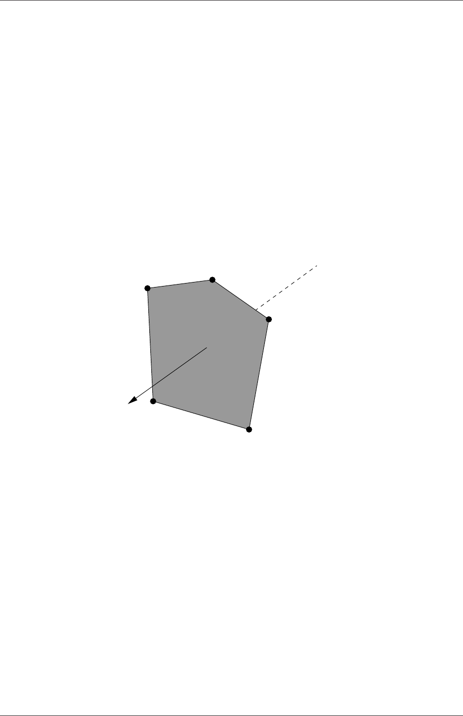
U-132 Mesh generation and conversion
5.1.1.1 Points
A point is a location in 3-D space, defined by a vector in units of metres (m). The points are
compiled into a list and each point is referred to by a label, which represents its position in
the list, starting from zero. The point list cannot contain two different points at an exactly
identical position nor any point that is not part at least one face.
5.1.1.2 Faces
A face is an ordered list of points, where a point is referred to by its label. The ordering of
point labels in a face is such that each two neighbouring points are connected by an edge,
i.e. you follow points as you travel around the circumference of the face. Faces are compiled
into a list and each face is referred to by its label, representing its position in the list. The
direction of the face normal vector is defined by the right-hand rule, i.e. looking towards a
face, if the numbering of the points follows an anti-clockwise path, the normal vector points
towards you, as shown in Figure 5.1.
4
3
0
2
1
Sf
Figure 5.1: Face area vector from point numbering on the face
There are two types of face:
Internal faces Those faces that connect two cells (and it can never be more than two).
For each internal face, the ordering of the point labels is such that the face normal
points into the cell with the larger label, i.e. for cells 2 and 5, the normal points into
5;
Boundary faces Those belonging to one cell since they coincide with the boundary of the
domain. A boundary face is therefore addressed by one cell(only) and a boundary
patch. The ordering of the point labels is such that the face normal points outside of
the computational domain.
Faces are generally expected to be convex; at the very least the face centre needs to be
inside the face. Faces are allowed to be warped, i.e. not all points of the face need to be
coplanar.
OpenFOAM-2.4.0

5.1 Mesh description U-133
5.1.1.3 Cells
A cell is a list of faces in arbitrary order. Cells must have the properties listed below.
Contiguous The cells must completely cover the computational domain and must not
overlap one another.
Convex Every cell must be convex and its cell centre inside the cell.
Closed Every cell must be closed, both geometrically and topologically where:
•geometrical closedness requires that when all face area vectors are oriented to
point outwards of the cell, their sum should equal the zero vector to machine
accuracy;
•topological closedness requires that all the edges in a cell are used by exactly two
faces of the cell in question.
Orthogonality For all internal faces of the mesh, we define the centre-to-centre vector as
that connecting the centres of the 2 cells that it adjoins oriented from the centre of
the cell with smaller label to the centre of the cell with larger label. The orthogonality
constraint requires that for each internal face, the angle between the face area vector,
oriented as described above, and the centre-to-centre vector must always be less than
90◦.
5.1.1.4 Boundary
A boundary is a list of patches, each of which is associated with a boundary condition. A
patch is a list of face labels which clearly must contain only boundary faces and no internal
faces. The boundary is required to be closed, i.e. the sum all boundary face area vectors
equates to zero to machine tolerance.
5.1.2 The polyMesh description
The constant directory contains a full description of the case polyMesh in a subdirectory
polyMesh. The polyMesh description is based around faces and, as already discussed, internal
faces connect 2 cells and boundary faces address a cell and a boundary patch. Each face
is therefore assigned an ‘owner’ cell and ‘neighbour’ cell so that the connectivity across a
given face can simply be described by the owner and neighbour cell labels. In the case of
boundaries, the connected cell is the owner and the neighbour is assigned the label ‘-1’.
With this in mind, the I/O specification consists of the following files:
points a list of vectors describing the cell vertices, where the first vector in the list represents
vertex 0, the second vector represents vertex 1, etc.;
faces a list of faces, each face being a list of indices to vertices in the points list, where
again, the first entry in the list represents face 0, etc.;
owner a list of owner cell labels, the index of entry relating directly to the index of the face,
so that the first entry in the list is the owner label for face 0, the second entry is the
owner label for face 1, etc;
OpenFOAM-2.4.0

U-134 Mesh generation and conversion
neighbour a list of neighbour cell labels;
boundary a list of patches, containing a dictionary entry for each patch, declared using the
patch name, e.g.
movingWall
{type patch;
nFaces 20;
startFace 760;
}
The startFace is the index into the face list of the first face in the patch, and nFaces
is the number of faces in the patch.
Note that if the user wishes to know how many cells are in their domain, there is a note
in the FoamFile header of the owner file that contains an entry for nCells.
5.1.3 The cellShape tools
We shall describe the alternative cellShape tools that may be used particularly when con-
verting some standard (simpler) mesh formats for the use with OpenFOAM library.
The vast majority of mesh generators and post-processing systems support only a fraction
of the possible polyhedral cell shapes in existence. They define a mesh in terms of a limited
set of 3D cell geometries, referred to as cell shapes. The OpenFOAM library contains
definitions of these standard shapes, to enable a conversion of such a mesh into the polyMesh
format described in the previous section.
The cellShape models supported by OpenFOAM are shown in Table 5.1. The shape is
defined by the ordering of point labels in accordance with the numbering scheme contained
in the shape model. The ordering schemes for points, faces and edges are shown in Table 5.1.
The numbering of the points must not be such that the shape becomes twisted or degenerate
into other geometries, i.e. the same point label cannot be used more that once is a single
shape. Moreover it is unnecessary to use duplicate points in OpenFOAM since the available
shapes in OpenFOAM cover the full set of degenerate hexahedra.
The cell description consists of two parts: the name of a cell model and the ordered list
of labels. Thus, using the following list of points
8
(
(0 0 0)
(1 0 0)
(1 1 0)
(0 1 0)
(0 0 0.5)
(1 0 0.5)
(1 1 0.5)
(0 1 0.5)
)
A hexahedral cell would be written as:
OpenFOAM-2.4.0

5.2 Boundaries U-135
(hex 8(0 1 2 3 4 5 6 7))
Here the hexahedral cell shape is declared using the keyword hex. Other shapes are described
by the keywords listed in Table 5.1.
5.1.4 1- and 2-dimensional and axi-symmetric problems
OpenFOAM is designed as a code for 3-dimensional space and defines all meshes as such.
However, 1- and 2- dimensional and axi-symmetric problems can be simulated in Open-
FOAM by generating a mesh in 3 dimensions and applying special boundary conditions on
any patch in the plane(s) normal to the direction(s) of interest. More specifically, 1- and 2-
dimensional problems use the empty patch type and axi-symmetric problems use the wedge
type. The use of both are described in section 5.2.2 and the generation of wedge geometries
for axi-symmetric problems is discussed in section 5.3.3.
5.2 Boundaries
In this section we discuss the way in which boundaries are treated in OpenFOAM. The
subject of boundaries is a little involved because their role in modelling is not simply that
of a geometric entity but an integral part of the solution and numerics through boundary
conditions or inter-boundary ‘connections’. A discussion of boundaries sits uncomfortably
between a discussion on meshes, fields, discretisation, computational processing etc. Its
placement in this Chapter on meshes is a choice of convenience.
We first need to consider that, for the purpose of applying boundary conditions, a bound-
ary is generally broken up into a set of patches. One patch may include one or more enclosed
areas of the boundary surface which do not necessarily need to be physically connected.
There are three attributes associated with a patch that are described below in their
natural hierarchy and Figure 5.2 shows the names of different patch types introduced at
each level of the hierarchy. The hierarchy described below is very similar, but not identical,
to the class hierarchy used in the OpenFOAM library.
Base type The type of patch described purely in terms of geometry or a data ‘communi-
cation link’.
Primitive type The base numerical patch condition assigned to a field variable on the
patch.
Derived type A complex patch condition, derived from the primitive type, assigned to a
field variable on the patch.
5.2.1 Specification of patch types in OpenFOAM
The patch types are specified in the mesh and field files of a OpenFOAM case. More
precisely:
•the base type is specified under the type keyword for each patch in the boundary file,
located in the constant/polyMesh directory;
OpenFOAM-2.4.0
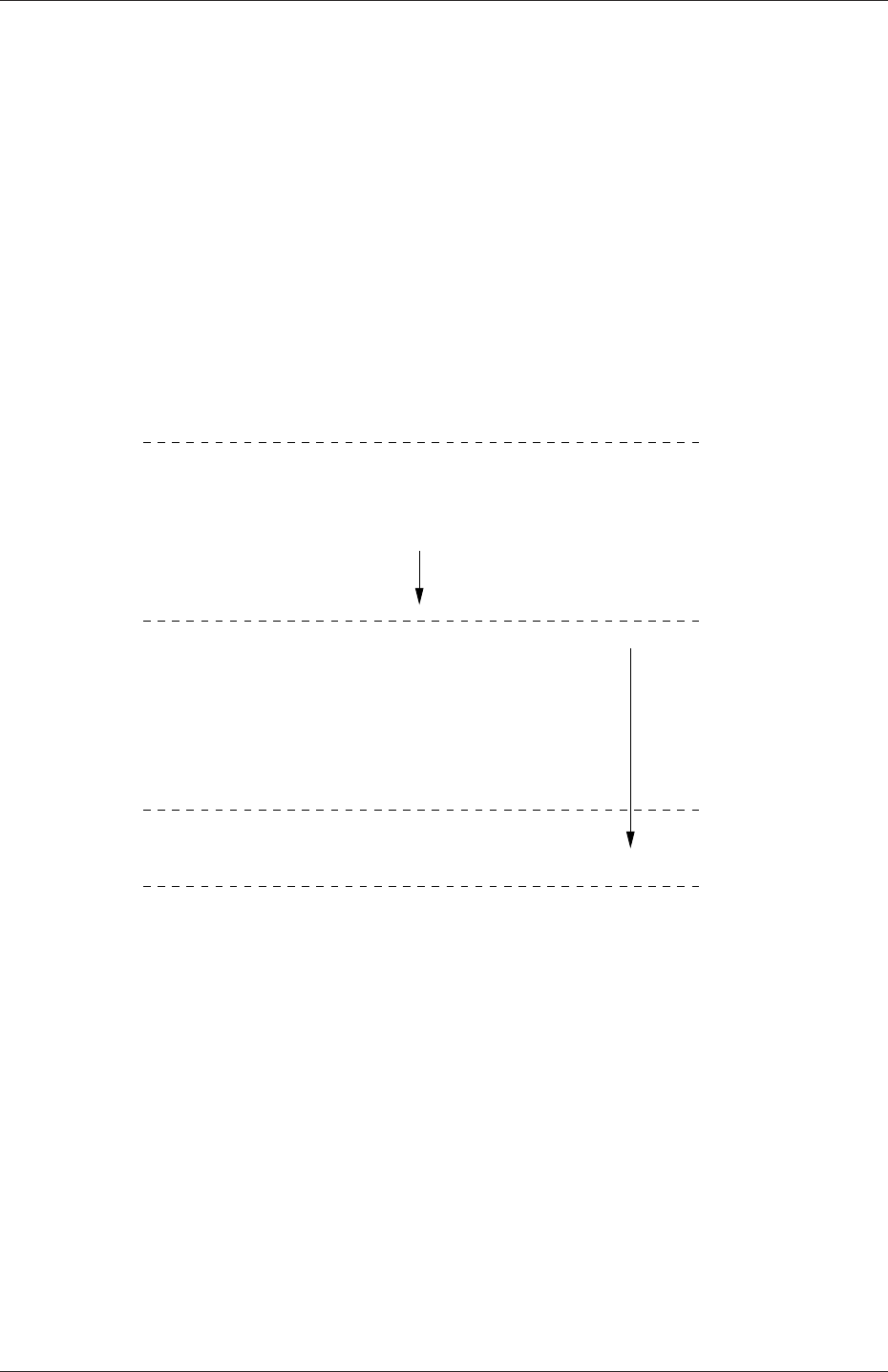
U-136 Mesh generation and conversion
Derived type
fixedGradient
fixedValue
Primitive type
calculated
mixed
directionMixed
zeroGradient
symmetry
empty
wedge
cyclic
Base type
processor
patch
wall
e.g. inletOutlet
Figure 5.2: Patch attributes
OpenFOAM-2.4.0
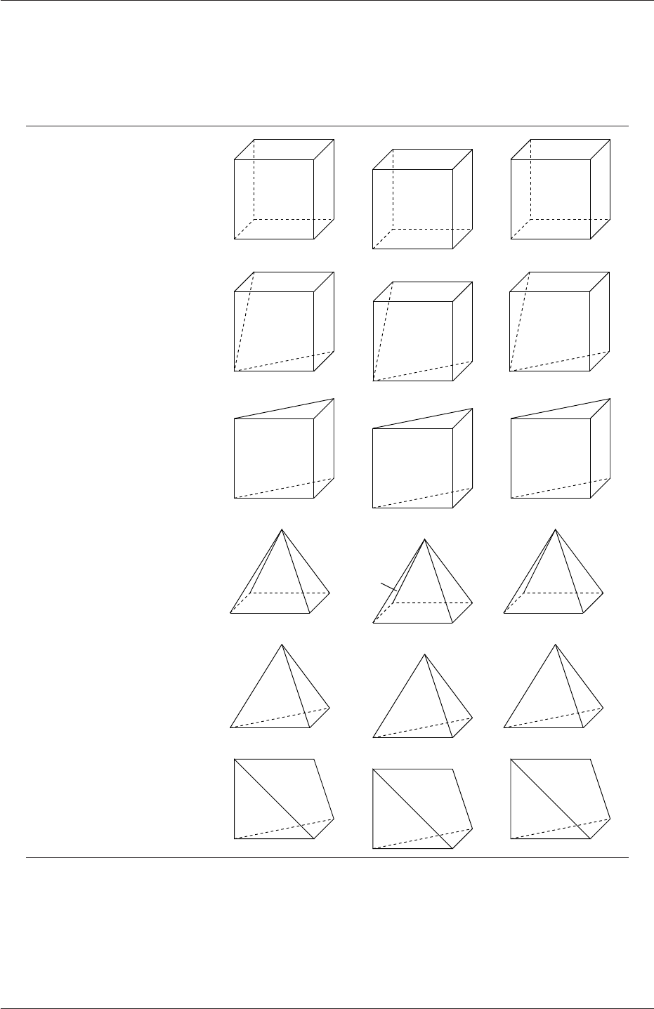
5.2 Boundaries U-137
Cell type Keyword Vertex numbering Face numbering Edge numbering
Hexahedron hex
2
7
3
10
4
6
5
01
2
3
5
40
1
2
3
45
6
7
89
10
11
Wedge wedge
2
10
34
56
0
1
23
5
4
01
2
3
5
6
7
8
9
10
4
Prism prism
2
10
34
5
0
1
3
42
0
12
3
4
5
6 7
8
Pyramid pyr
2
10
4
3
0
23
4
1
01
2
3
4 5 6
7
Tetrahedron tet 0 1
2
3
1
2
3
0
0
1
23
4
5
Tet-wedge tetWedge
2
10
34
0
13
2
01
2
3
456
Table 5.1: Vertex, face and edge numbering for cellShapes.
OpenFOAM-2.4.0

U-138 Mesh generation and conversion
•the numerical patch type, be it a primitive or derived type, is specified under the type
keyword for each patch in a field file.
An example boundary file is shown below for a sonicFoam case, followed by a pressure
field file, p, for the same case:
17
18 6
19 (
20 inlet
21 {
22 type patch;
23 nFaces 50;
24 startFace 10325;
25 }
26 outlet
27 {
28 type patch;
29 nFaces 40;
30 startFace 10375;
31 }
32 bottom
33 {
34 type symmetryPlane;
35 inGroups 1(symmetryPlane);
36 nFaces 25;
37 startFace 10415;
38 }
39 top
40 {
41 type symmetryPlane;
42 inGroups 1(symmetryPlane);
43 nFaces 125;
44 startFace 10440;
45 }
46 obstacle
47 {
48 type patch;
49 nFaces 110;
50 startFace 10565;
51 }
52 defaultFaces
53 {
54 type empty;
55 inGroups 1(empty);
56 nFaces 10500;
57 startFace 10675;
58 }
59 )
60
61 // ************************************************************************* //
17 dimensions [1 -1 -2 0 0 0 0];
18
19 internalField uniform 1;
20
21 boundaryField
22 {
23 inlet
24 {
25 type fixedValue;
26 value uniform 1;
27 }
28
29 outlet
30 {
31 type waveTransmissive;
32 field p;
33 phi phi;
34 rho rho;
35 psi thermo:psi;
36 gamma 1.4;
37 fieldInf 1;
38 lInf 3;
39 value uniform 1;
40 }
41
42 bottom
OpenFOAM-2.4.0
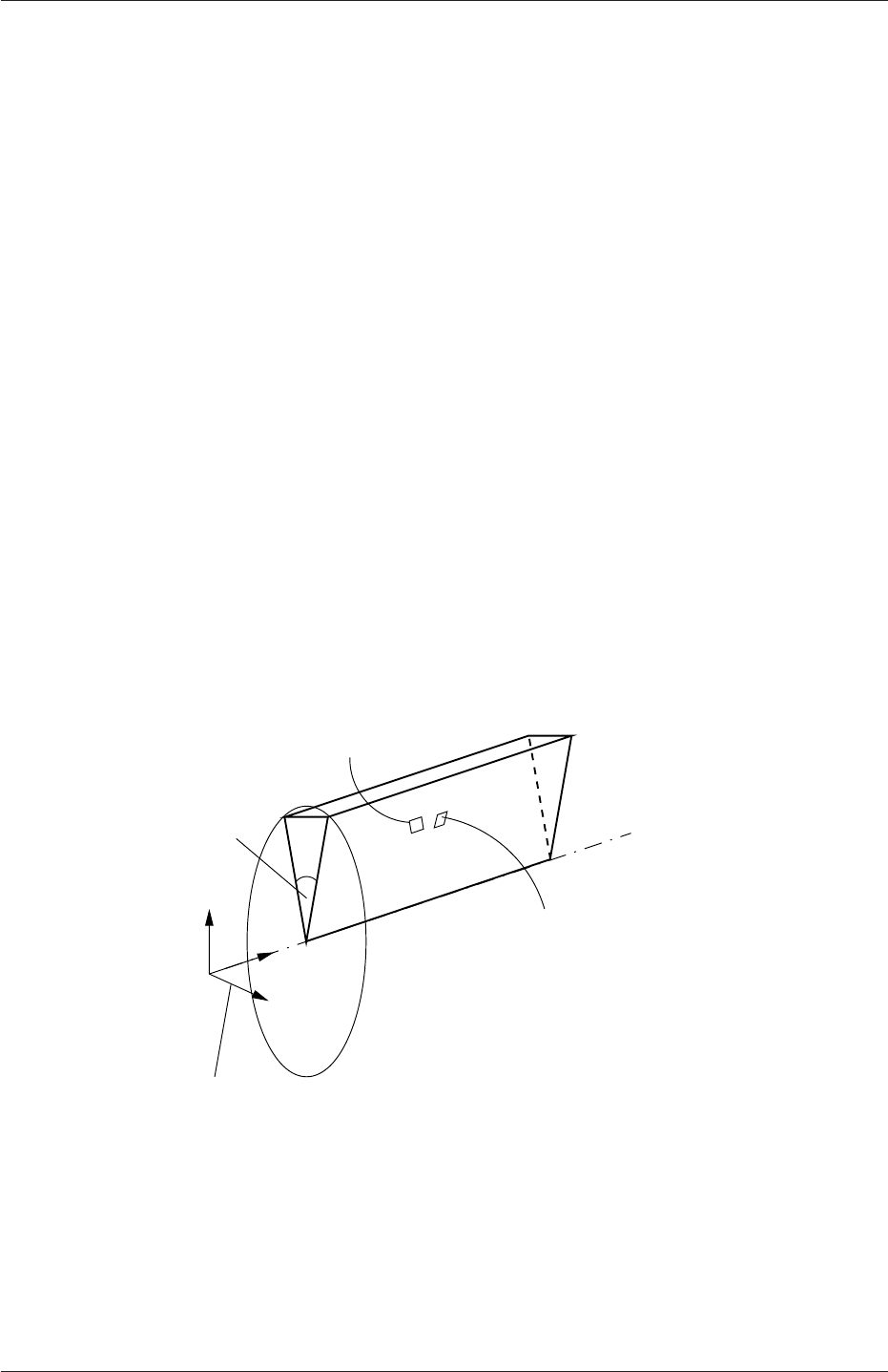
5.2 Boundaries U-139
43 {
44 type symmetryPlane;
45 }
46
47 top
48 {
49 type symmetryPlane;
50 }
51
52 obstacle
53 {
54 type zeroGradient;
55 }
56
57 defaultFaces
58 {
59 type empty;
60 }
61 }
62
63 // ************************************************************************* //
The type in the boundary file is patch for all patches except those that have some geo-
metrical constraint applied to them, i.e. the symmetryPlane and empty patches. The pfile
includes primitive types applied to the inlet and bottom faces, and a more complex derived
type applied to the outlet. Comparison of the two files shows that the base and numerical
types are consistent where the base type is not a simple patch,i.e. for the symmetryPlane
and empty patches.
5.2.2 Base types
The base and geometric types are described below; the keywords used for specifying these
types in OpenFOAM are summarised in Table 5.2.
wedge aligned along
coordinate plane
<5◦Axis of symmetry
wedge patch 1
wedge patch 2
Figure 5.3: Axi-symmetric geometry using the wedge patch type.
patch The basic patch type for a patch condition that contains no geometric or topological
information about the mesh (with the exception of wall), e.g. an inlet or an outlet.
wall There are instances where a patch that coincides with a wall needs to be identifiable
as such, particularly where specialist modelling is applied at wall boundaries. A good
OpenFOAM-2.4.0

U-140 Mesh generation and conversion
Selection Key Description
patch generic patch
symmetryPlane plane of symmetry
empty front and back planes of a 2D geometry
wedge wedge front and back for an axi-symmetric geometry
cyclic cyclic plane
wall wall — used for wall functions in turbulent flows
processor inter-processor boundary
Table 5.2: Basic patch types.
example is wall turbulence modelling where a wall must be specified with a wall patch
type, so that the distance from the wall to the cell centres next to the wall are stored
as part of the patch.
symmetryPlane For a symmetry plane.
empty While OpenFOAM always generates geometries in 3 dimensions, it can be instructed
to solve in 2 (or 1) dimensions by specifying a special empty condition on each patch
whose plane is normal to the 3rd (and 2nd) dimension for which no solution is required.
wedge For 2 dimensional axi-symmetric cases, e.g. a cylinder, the geometry is specified as a
wedge of small angle (e.g. <5◦) and 1 cell thick running along the plane of symmetry,
straddling one of the coordinate planes, as shown in Figure 5.3. The axi-symmetric
wedge planes must be specified as separate patches of wedge type. The details of
generating wedge-shaped geometries using blockMesh are described in section 5.3.3.
cyclic Enables two patches to be treated as if they are physically connected; used for repeated
geometries, e.g. heat exchanger tube bundles. One cyclic patch is linked to another
through a neighbourPatch keyword in the boundary file. Each pair of connecting faces
must have similar area to within a tolerance given by the matchTolerance keyword
in the boundary file. Faces do not need to be of the same orientation.
processor If a code is being run in parallel, on a number of processors, then the mesh must be
divided up so that each processor computes on roughly the same number of cells. The
boundaries between the different parts of the mesh are called processor boundaries.
5.2.3 Primitive types
The primitive types are listed in Table 5.3.
5.2.4 Derived types
There are numerous derived types of boundary conditions in OpenFOAM, too many to list
here. Instead a small selection is listed in Table 5.4. If the user wishes to obtain a list of
all available models, they should consult the OpenFOAM source code. Derived boundary
condition source code can be found at the following locations:
•in $FOAM SRC/finiteVolume/fields/fvPatchFields/derived
OpenFOAM-2.4.0

5.3 Mesh generation with the blockMesh utility U-141
Type Description of condition for patch field φData to specify
fixedValue Value of φis specified value
fixedGradient Normal gradient of φis specified gradient
zeroGradient Normal gradient of φis zero —
calculated Boundary field φderived from other fields —
mixed Mixed fixedValue/fixedGradient condition depend-
ing on the value in valueFraction
refValue,
refGradient,
valueFraction,
value
directionMixed Amixed condition with tensorial valueFraction,
e.g. for different levels of mixing in normal and
tangential directions
refValue,
refGradient,
valueFraction,
value
Table 5.3: Primitive patch field types.
•within certain model libraries, that can be located by typing the following command
in a terminal window
find $FOAM SRC -name "*derivedFvPatch*"
•within certain solvers, that can be located by typing the following command in a
terminal window
find $FOAM SOLVERS -name "*fvPatch*"
5.3 Mesh generation with the blockMesh utility
This section describes the mesh generation utility, blockMesh, supplied with OpenFOAM.
The blockMesh utility creates parametric meshes with grading and curved edges.
The mesh is generated from a dictionary file named blockMeshDict located in the con-
stant/polyMesh directory of a case. blockMesh reads this dictionary, generates the mesh and
writes out the mesh data to points and faces,cells and boundary files in the same directory.
The principle behind blockMesh is to decompose the domain geometry into a set of 1 or
more three dimensional, hexahedral blocks. Edges of the blocks can be straight lines, arcs
or splines. The mesh is ostensibly specified as a number of cells in each direction of the
block, sufficient information for blockMesh to generate the mesh data.
Each block of the geometry is defined by 8 vertices, one at each corner of a hexahedron.
The vertices are written in a list so that each vertex can be accessed using its label, remem-
bering that OpenFOAM always uses the C++ convention that the first element of the list
has label ‘0’. An example block is shown in Figure 5.4 with each vertex numbered according
to the list. The edge connecting vertices 1 and 5 is curved to remind the reader that curved
edges can be specified in blockMesh.
It is possible to generate blocks with less than 8 vertices by collapsing one or more pairs
of vertices on top of each other, as described in section 5.3.3.
OpenFOAM-2.4.0

U-142 Mesh generation and conversion
Types derived from fixedValue Data to specify
movingWallVelocity Replaces the normal of the patch value so the flux across the patch is
zero
value
pressureInletVelocity When pis known at inlet, Uis evaluated from the flux, normal to the
patch
value
pressureDirectedInletVelocity When pis known at inlet, Uis calculated from the flux in the
inletDirection
value,
inletDirection
surfaceNormalFixedValue Specifies a vector boundary condition, normal to the patch, by its mag-
nitude; +ve for vectors pointing out of the domain
value
totalPressure Total pressure p0=p+1
2ρ|U|2is fixed; when Uchanges, pis adjusted
accordingly
p0
turbulentInlet Calculates a fluctuating variable based on a scale of a mean value referenceField,
fluctuationScale
Types derived from fixedGradient/zeroGradient
fluxCorrectedVelocity Calculates normal component of Uat inlet from flux value
buoyantPressure Sets fixedGradient pressure based on the atmospheric pressure gradient —
Types derived from mixed
inletOutlet Switches Uand pbetween fixedValue and zeroGradient depending on di-
rection of U
inletValue,value
outletInlet Switches Uand pbetween fixedValue and zeroGradient depending on di-
rection of U
outletValue,
value
pressureInletOutletVelocity Combination of pressureInletVelocity and inletOutlet value
pressureDirected-
InletOutletVelocity
Combination of pressureDirectedInletVelocity and inletOutlet value,
inletDirection
pressureTransmissive Transmits supersonic pressure waves to surrounding pressure p∞pInf
supersonicFreeStream Transmits oblique shocks to surroundings at p∞,T∞,U∞pInf,TInf,UInf
Other types
slip zeroGradient if φis a scalar; if φis a vector, normal component is fixed-
Value zero, tangential components are zeroGradient
—
partialSlip Mixed zeroGradient/slip condition depending on the valueFraction; =
0 for slip
valueFraction
Note: pis pressure, Uis velocity
Table 5.4: Derived patch field types.
OpenFOAM-2.4.0
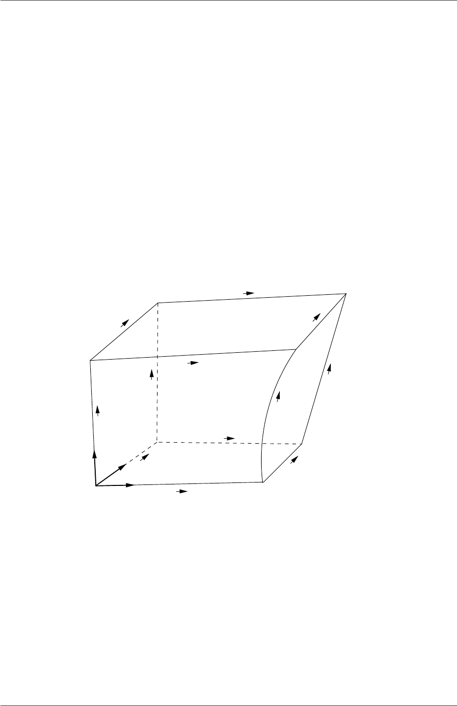
5.3 Mesh generation with the blockMesh utility U-143
Each block has a local coordinate system (x1, x2, x3) that must be right-handed. A right-
handed set of axes is defined such that to an observer looking down the Oz axis, with O
nearest them, the arc from a point on the Ox axis to a point on the Oy axis is in a clockwise
sense.
The local coordinate system is defined by the order in which the vertices are presented
in the block definition according to:
•the axis origin is the first entry in the block definition, vertex 0 in our example;
•the x1direction is described by moving from vertex 0 to vertex 1;
•the x2direction is described by moving from vertex 1 to vertex 2;
•vertices 0, 1, 2, 3 define the plane x3= 0;
•vertex 4 is found by moving from vertex 0 in the x3direction;
•vertices 5,6 and 7 are similarly found by moving in the x3direction from vertices 1,2
and 3 respectively.
3
9
1
2
x2
x3
x1
0
3
4
5
76
0
2
1
45
6
7
10
8
11
Figure 5.4: A single block
5.3.1 Writing a blockMeshDict file
The blockMeshDict file is a dictionary using keywords described in Table 5.5. The convertToMeters
keyword specifies a scaling factor by which all vertex coordinates in the mesh description
are multiplied. For example,
convertToMeters 0.001;
means that all coordinates are multiplied by 0.001, i.e. the values quoted in the blockMesh-
Dict file are in mm.
OpenFOAM-2.4.0

U-144 Mesh generation and conversion
Keyword Description Example/selection
convertToMeters Scaling factor for the vertex
coordinates
0.001 scales to mm
vertices List of vertex coordinates (0 0 0)
edges Used to describe arc or
spline edges
arc 1 4 (0.939 0.342 -0.5)
block Ordered list of vertex labels
and mesh size
hex (0 1 2 3 4 5 6 7)
(10 10 1)
simpleGrading (1.0 1.0 1.0)
patches List of patches symmetryPlane base
( (0 1 2 3) )
mergePatchPairs List of patches to be merged see section 5.3.2
Table 5.5: Keywords used in blockMeshDict.
5.3.1.1 The vertices
The vertices of the blocks of the mesh are given next as a standard list named vertices,
e.g. for our example block in Figure 5.4, the vertices are:
vertices
(
( 0 0 0 ) // vertex number 0
( 1 0 0.1) // vertex number 1
( 1.1 1 0.1) // vertex number 2
( 0 1 0.1) // vertex number 3
(-0.1 -0.1 1 ) // vertex number 4
( 1.3 0 1.2) // vertex number 5
( 1.4 1.1 1.3) // vertex number 6
( 0 1 1.1) // vertex number 7
);
5.3.1.2 The edges
Each edge joining 2 vertex points is assumed to be straight by default. However any edge
may be specified to be curved by entries in a list named edges. The list is optional; if the
geometry contains no curved edges, it may be omitted.
Each entry for a curved edge begins with a keyword specifying the type of curve from
those listed in Table 5.6.
The keyword is then followed by the labels of the 2 vertices that the edge connects.
Following that, interpolation points must be specified through which the edge passes. For
aarc, a single interpolation point is required, which the circular arc will intersect. For
simpleSpline,polyLine and polySpline, a list of interpolation points is required. The
line edge is directly equivalent to the option executed by default, and requires no inter-
polation points. Note that there is no need to use the line edge but it is included for
completeness. For our example block in Figure 5.4 we specify an arc edge connecting
vertices 1 and 5 as follows through the interpolation point (1.1,0.0,0.5):
OpenFOAM-2.4.0

5.3 Mesh generation with the blockMesh utility U-145
Keyword selection Description Additional entries
arc Circular arc Single interpolation point
simpleSpline Spline curve List of interpolation points
polyLine Set of lines List of interpolation points
polySpline Set of splines List of interpolation points
line Straight line —
Table 5.6: Edge types available in the blockMeshDict dictionary.
edges
(
arc 1 5 (1.1 0.0 0.5)
);
5.3.1.3 The blocks
The block definitions are contained in a list named blocks. Each block definition is a
compound entry consisting of a list of vertex labels whose order is described in section 5.3,
a vector giving the number of cells required in each direction, the type and list of cell
expansion ratio in each direction.
Then the blocks are defined as follows:
blocks
(
hex (0 1 2 3 4 5 6 7) // vertex numbers
(10 10 10) // numbers of cells in each direction
simpleGrading (1 2 3) // cell expansion ratios
);
The definition of each block is as follows:
Vertex numbering The first entry is the shape identifier of the block, as defined in the
.OpenFOAM-2.4.0/cellModels file. The shape is always hex since the blocks are always
hexahedra. There follows a list of vertex numbers, ordered in the manner described
on page U-143.
Number of cells The second entry gives the number of cells in each of the x1x2and x3
directions for that block.
Cell expansion ratios The third entry gives the cell expansion ratios for each direction in
the block. The expansion ratio enables the mesh to be graded, or refined, in specified
directions. The ratio is that of the width of the end cell δealong one edge of a block
to the width of the start cell δsalong that edge, as shown in Figure 5.5. Each of
the following keywords specify one of two types of grading specification available in
blockMesh.
simpleGrading The simple description specifies uniform expansions in the local x1,
x2and x3directions respectively with only 3 expansion ratios, e.g.
OpenFOAM-2.4.0
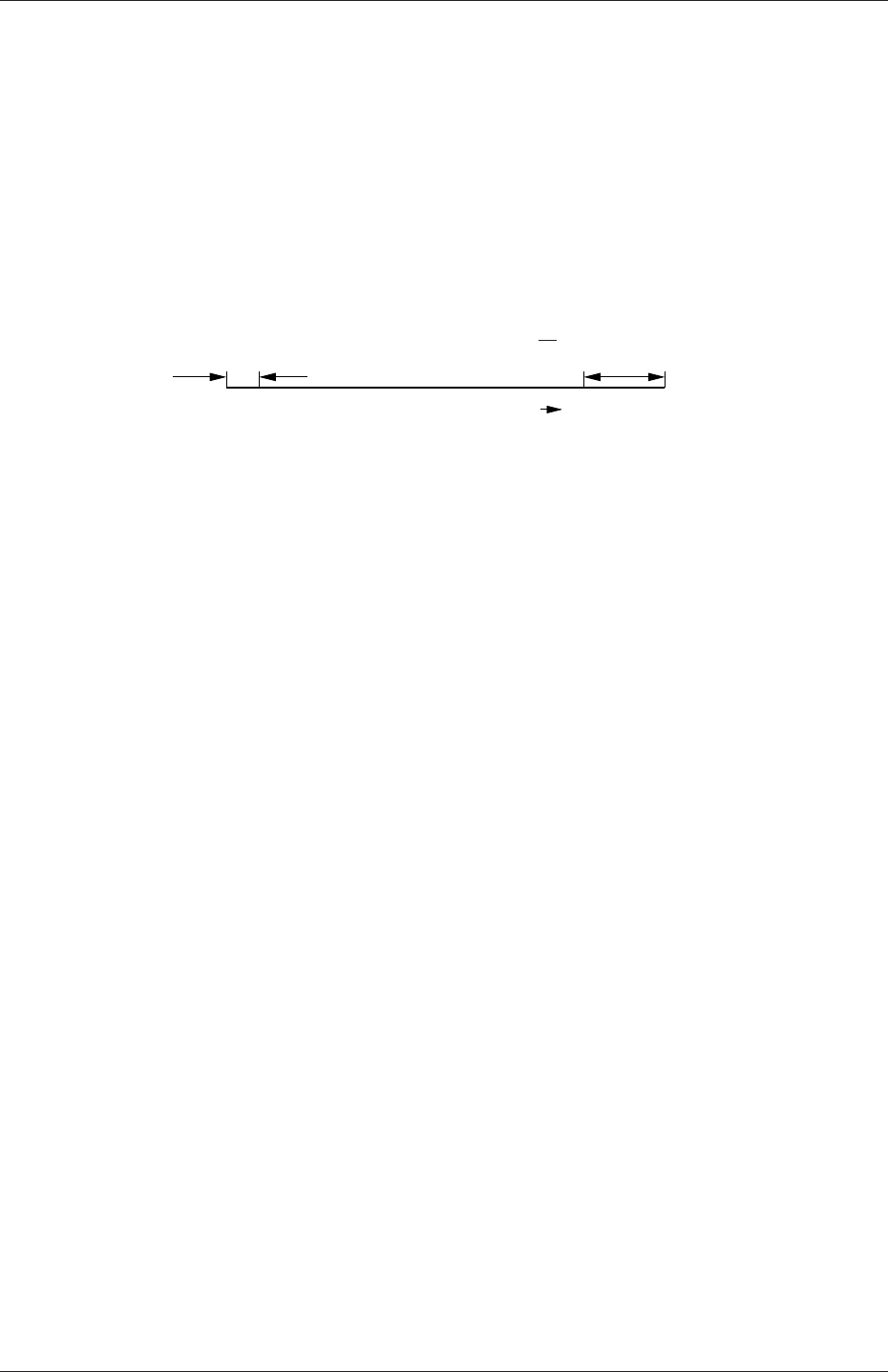
U-146 Mesh generation and conversion
simpleGrading (1 2 3)
edgeGrading The full cell expansion description gives a ratio for each edge of the
block, numbered according to the scheme shown in Figure 5.4 with the arrows
representing the direction ‘from first cell. . . to last cell’ e.g. something like
edgeGrading (1 1 1 1 2 2 2 2 3 3 3 3)
This means the ratio of cell widths along edges 0-3 is 1, along edges 4-7 is 2 and
along 8-11 is 3 and is directly equivalent to the simpleGrading example given
above.
δsExpansion ratio = δe
δsδe
Expansion direction
Figure 5.5: Mesh grading along a block edge
5.3.1.4 Multi-grading of a block
Using a single expansion ratio to describe mesh grading permits only “one-way” grading
within a mesh block. In some cases, it reduces complexity and effort to be able to control
grading within separate divisions of a single block, rather than have to define several blocks
with one grading per block. For example, to mesh a channel with two opposing walls and
grade the mesh towards the walls requires three regions: two with grading to the wall with
one in the middle without grading.
OpenFOAM v2.4+ includes multi-grading functionality that can divide a block in an
given direction and apply different grading within each division. This multi-grading is
specified by replacing any single value expansion ratio in the grading specification of the
block, e.g. “1”, “2”, “3” in
blocks
(
hex (0 1 2 3 4 5 6 7) (100 300 100)
simpleGrading (1 2 3);
);
We will present multi-grading for the following example:
•split the block into 3 divisions in the y-direction, representing 20%, 60% and 20% of
the block length;
•include 30% of the total cells in the y-direction (300) in each divisions 1 and 3 and
the remaining 40% in division 2;
•apply 1:4 expansion in divisions 1 and 3, and zero expansion in division 2.
We can specify this by replacing the y-direction expansion ratio “2” in the example above
with the following:
OpenFOAM-2.4.0

5.3 Mesh generation with the blockMesh utility U-147
blocks
(
hex (0 1 2 3 4 5 6 7) (100 300 100)
simpleGrading
(
1 // x-direction expansion ratio
(
(0.2 0.3 4) // 20% y-dir, 30% cells, expansion = 4
(0.6 0.4 1) // 60% y-dir, 40% cells, expansion = 1
(0.2 0.3 0.25) // 20% y-dir, 30% cells, expansion = 0.25 (1/4)
)
3 // z-direction expansion ratio
);
);
Both the fraction of the block and the fraction of the cells are normalized automatically.
They can be specified as percentages, fractions, absolute lengths, etc. and do not need to
sum to 100, 1, etc. The example above can be specified using percentages, e.g.
blocks
(
hex (0 1 2 3 4 5 6 7) (100 300 100)
simpleGrading
(
1
(
(20 30 4) // 20%, 30%...
(60 40 1)
(20 30 0.25)
)
3
);
);
5.3.1.5 The boundary
The boundary of the mesh is given in a list named boundary. The boundary is broken into
patches (regions), where each patch in the list has its name as the keyword, which is the
choice of the user, although we recommend something that conveniently identifies the patch,
e.g.inlet; the name is used as an identifier for setting boundary conditions in the field data
files. The patch information is then contained in sub-dictionary with:
•type: the patch type, either a generic patch on which some boundary conditions are
applied or a particular geometric condition, as listed in Table 5.2 and described in
section 5.2.2;
•faces: a list of block faces that make up the patch and whose name is the choice of
the user, although we recommend something that conveniently identifies the patch,
OpenFOAM-2.4.0

U-148 Mesh generation and conversion
e.g.inlet; the name is used as an identifier for setting boundary conditions in the field
data files.
blockMesh collects faces from any boundary patch that is omitted from the boundary
list and assigns them to a default patch named defaultFaces of type empty. This means
that for a 2 dimensional geometry, the user has the option to omit block faces lying in the
2D plane, knowing that they will be collected into an empty patch as required.
Returning to the example block in Figure 5.4, if it has an inlet on the left face, an output
on the right face and the four other faces are walls then the patches could be defined as
follows:
boundary // keyword
(
inlet // patch name
{type patch; // patch type for patch 0
faces
(
(0 4 7 3); // block face in this patch
);
}// end of 0th patch definition
outlet // patch name
{type patch; // patch type for patch 1
faces
(
(1 2 6 5)
);
}
walls
{type wall;
faces
(
(0 1 5 4)
(0 3 2 1)
(3 7 6 2)
(4 5 6 7)
);
}
);
Each block face is defined by a list of 4 vertex numbers. The order in which the vertices are
given must be such that, looking from inside the block and starting with any vertex, the
face must be traversed in a clockwise direction to define the other vertices.
OpenFOAM-2.4.0

5.3 Mesh generation with the blockMesh utility U-149
When specifying a cyclic patch in blockMesh, the user must specify the name of the
related cyclic patch through the neighbourPatch keyword. For example, a pair of cyclic
patches might be specified as follows:
left
{type cyclic;
neighbourPatch right;
faces ((0 4 7 3));
}
right
{type cyclic;
neighbourPatch left;
faces ((1 5 6 2));
}
5.3.2 Multiple blocks
A mesh can be created using more than 1 block. In such circumstances, the mesh is created
as has been described in the preceeding text; the only additional issue is the connection
between blocks, in which there are two distinct possibilities:
face matching the set of faces that comprise a patch from one block are formed from the
same set of vertices as a set of faces patch that comprise a patch from another block;
face merging a group of faces from a patch from one block are connected to another
group of faces from a patch from another block, to create a new set of internal faces
connecting the two blocks.
To connect two blocks with face matching, the two patches that form the connection
should simply be ignored from the patches list. blockMesh then identifies that the faces
do not form an external boundary and combines each collocated pair into a single internal
faces that connects cells from the two blocks.
The alternative, face merging, requires that the block patches to be merged are first
defined in the patches list. Each pair of patches whose faces are to be merged must then
be included in an optional list named mergePatchPairs. The format of mergePatchPairs
is:
mergePatchPairs
(
(<masterPatch> <slavePatch>) // merge patch pair 0
(<masterPatch> <slavePatch>) // merge patch pair 1
...
)
The pairs of patches are interpreted such that the first patch becomes the master and the
second becomes the slave. The rules for merging are as follows:
OpenFOAM-2.4.0
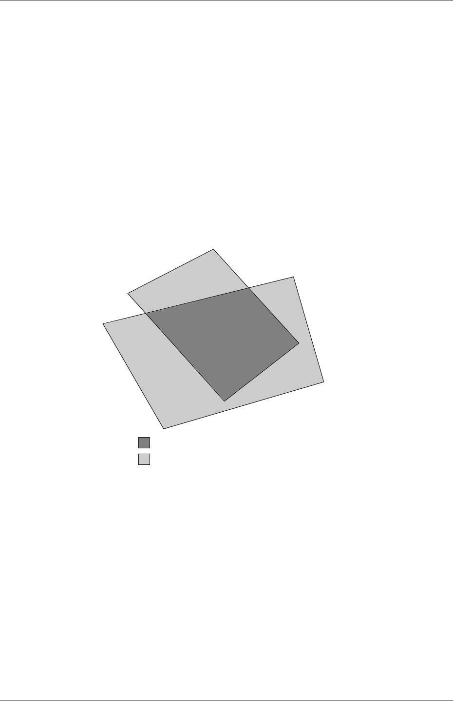
U-150 Mesh generation and conversion
•the faces of the master patch remain as originally defined, with all vertices in their
original location;
•the faces of the slave patch are projected onto the master patch where there is some
separation between slave and master patch;
•the location of any vertex of a slave face might be adjusted by blockMesh to eliminate
any face edge that is shorter than a minimum tolerance;
•if patches overlap as shown in Figure 5.6, each face that does not merge remains as
an external face of the original patch, on which boundary conditions must then be
applied;
•if all the faces of a patch are merged, then the patch itself will contain no faces and is
removed.
patch 1
patch 2
region of internal connecting faces
region of external boundary faces
Figure 5.6: Merging overlapping patches
The consequence is that the original geometry of the slave patch will not necessarily be
completely preserved during merging. Therefore in a case, say, where a cylindrical block
is being connected to a larger block, it would be wise to the assign the master patch to
the cylinder, so that its cylindrical shape is correctly preserved. There are some additional
recommendations to ensure successful merge procedures:
•in 2 dimensional geometries, the size of the cells in the third dimension, i.e. out of the
2D plane, should be similar to the width/height of cells in the 2D plane;
•it is inadvisable to merge a patch twice, i.e. include it twice in mergePatchPairs;
•where a patch to be merged shares a common edge with another patch to be merged,
both should be declared as a master patch.
OpenFOAM-2.4.0
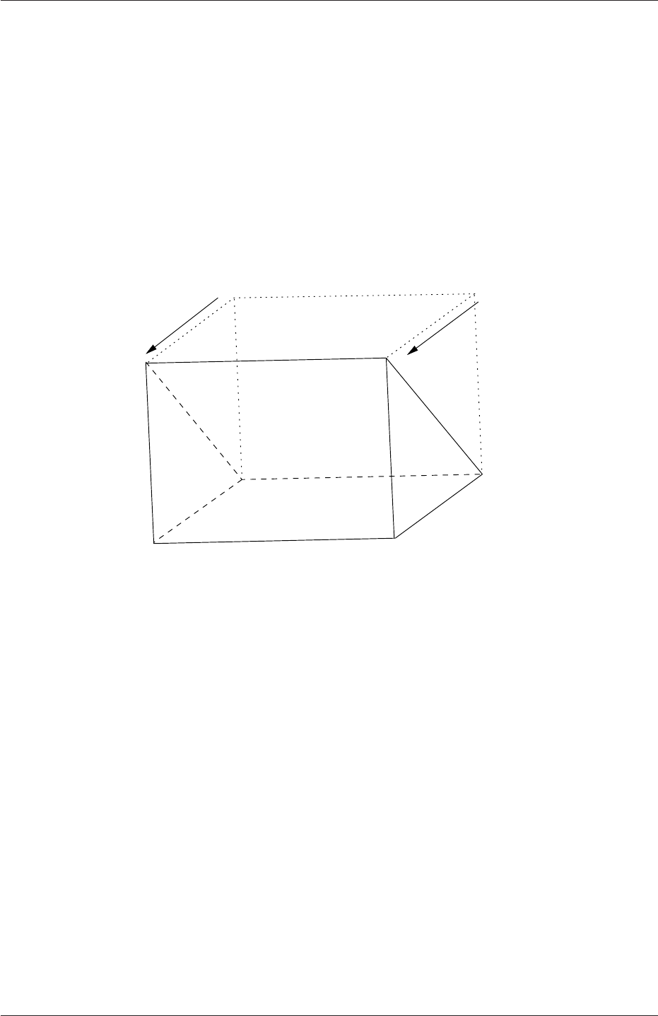
5.4 Mesh generation with the snappyHexMesh utility U-151
5.3.3 Creating blocks with fewer than 8 vertices
It is possible to collapse one or more pair(s) of vertices onto each other in order to create
a block with fewer than 8 vertices. The most common example of collapsing vertices is
when creating a 6-sided wedge shaped block for 2-dimensional axi-symmetric cases that use
the wedge patch type described in section 5.2.2. The process is best illustrated by using a
simplified version of our example block shown in Figure 5.7. Let us say we wished to create
a wedge shaped block by collapsing vertex 7 onto 4 and 6 onto 5. This is simply done by
exchanging the vertex number 7 by 4 and 6 by 5 respectively so that the block numbering
would become:
hex (0 1 2 3 4 5 5 4)
0
3
4
76
5
1
2
Figure 5.7: Creating a wedge shaped block with 6 vertices
The same applies to the patches with the main consideration that the block face contain-
ing the collapsed vertices, previously (4 5 6 7) now becomes (4 5 5 4). This is a block
face of zero area which creates a patch with no faces in the polyMesh, as the user can see in
aboundary file for such a case. The patch should be specified as empty in the blockMeshDict
and the boundary condition for any fields should consequently be empty also.
5.3.4 Running blockMesh
As described in section 3.3, the following can be executed at the command line to run
blockMesh for a case in the <case>directory:
blockMesh -case <case>
The blockMeshDict file must exist in subdirectory constant/polyMesh.
5.4 Mesh generation with the snappyHexMesh utility
This section describes the mesh generation utility, snappyHexMesh, supplied with Open-
FOAM. The snappyHexMesh utility generates 3-dimensional meshes containing hexahedra
OpenFOAM-2.4.0
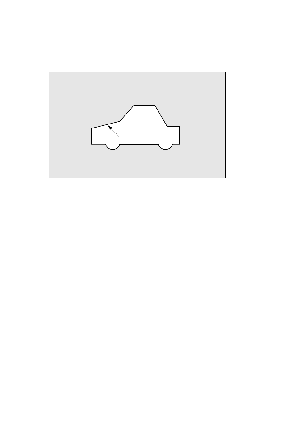
U-152 Mesh generation and conversion
(hex) and split-hexahedra (split-hex) automatically from triangulated surface geometries in
Stereolithography (STL) format. The mesh approximately conforms to the surface by itera-
tively refining a starting mesh and morphing the resulting split-hex mesh to the surface. An
optional phase will shrink back the resulting mesh and insert cell layers. The specification of
mesh refinement level is very flexible and the surface handling is robust with a pre-specified
final mesh quality. It runs in parallel with a load balancing step every iteration.
STL surface
Figure 5.8: Schematic 2D meshing problem for snappyHexMesh
5.4.1 The mesh generation process of snappyHexMesh
The process of generating a mesh using snappyHexMesh will be described using the schematic
in Figure 5.8. The objective is to mesh a rectangular shaped region (shaded grey in the
figure) surrounding an object described by and STL surface, e.g. typical for an external
aerodynamics simulation. Note that the schematic is 2-dimensional to make it easier to
understand, even though the snappyHexMesh is a 3D meshing tool.
In order to run snappyHexMesh, the user requires the following:
•surface data files in STL format, either binary or ASCII, located in a constant/triSurface
sub-directory of the case directory;
•a background hex mesh which defines the extent of the computational domain and a
base level mesh density; typically generated using blockMesh, discussed in section 5.4.2.
•asnappyHexMeshDict dictionary, with appropriate entries, located in the system sub-
directory of the case.
The snappyHexMeshDict dictionary includes: switches at the top level that control the
various stages of the meshing process; and, individual sub-directories for each process. The
entries are listed in Table 5.7.
All the geometry used by snappyHexMesh is specified in a geometry sub-dictionary in the
snappyHexMeshDict dictionary. The geometry can be specified through an STL surface or
bounding geometry entities in OpenFOAM. An example is given below:
geometry
{
sphere.stl // STL filename
OpenFOAM-2.4.0

5.4 Mesh generation with the snappyHexMesh utility U-153
Keyword Description Example
castellatedMesh Create the castellated mesh? true
snap Do the surface snapping stage? true
doLayers Add surface layers? true
mergeTolerance Merge tolerance as fraction of bounding box
of initial mesh
1e-06
debug Controls writing of intermediate meshes and
screen printing
— Write final mesh only 0
— Write intermediate meshes 1
— Write volScalarField with cellLevel for
post-processing
2
— Write current intersections as .obj files 4
geometry Sub-dictionary of all surface geometry used
castellatedMeshControls Sub-dictionary of controls for castellated mesh
snapControls Sub-dictionary of controls for surface snapping
addLayersControls Sub-dictionary of controls for layer addition
meshQualityControls Sub-dictionary of controls for mesh quality
Table 5.7: Keywords at the top level of snappyHexMeshDict.
{
type triSurfaceMesh;
regions
{
secondSolid // Named region in the STL file
{
name mySecondPatch; // User-defined patch name
} // otherwise given sphere.stl_secondSolid
}
}
box1x1x1 // User defined region name
{
type searchableBox; // region defined by bounding box
min (1.5 1 -0.5);
max (3.5 2 0.5);
}
sphere2 // User defined region name
{
type searchableSphere; // region defined by bounding sphere
centre (1.5 1.5 1.5);
radius 1.03;
}
};
5.4.2 Creating the background hex mesh
Before snappyHexMesh is executed the user must create a background mesh of hexahedral
cells that fills the entire region within by the external boundary as shown in Figure 5.9.
This can be done simply using blockMesh. The following criteria must be observed when
creating the background mesh:
•the mesh must consist purely of hexes;
OpenFOAM-2.4.0
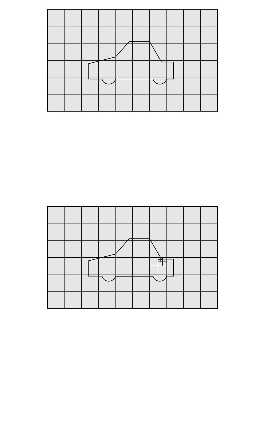
U-154 Mesh generation and conversion
Figure 5.9: Initial mesh generation in snappyHexMesh meshing process
•the cell aspect ratio should be approximately 1, at least near surfaces at which the
subsequent snapping procedure is applied, otherwise the convergence of the snapping
procedure is slow, possibly to the point of failure;
•there must be at least one intersection of a cell edge with the STL surface, i.e. a mesh
of one cell will not work.
Figure 5.10: Cell splitting by feature edge in snappyHexMesh meshing process
5.4.3 Cell splitting at feature edges and surfaces
Cell splitting is performed according to the specification supplied by the user in the castellat-
edMeshControls sub-dictionary in the snappyHexMeshDict. The entries for castellatedMesh-
Controls are presented in Table 5.8.
The splitting process begins with cells being selected according to specified edge features
first within the domain as illustrated in Figure 5.10. The features list in the castellat-
edMeshControls sub-dictionary permits dictionary entries containing a name of an edgeMesh
file and the level of refinement, e.g.:
OpenFOAM-2.4.0

5.4 Mesh generation with the snappyHexMesh utility U-155
Keyword Description Example
locationInMesh Location vector inside the region to be meshed (5 0 0)
N.B. vector must not coincide with a cell face
either before or during refinement
maxLocalCells Max number of cells per processor during re-
finement
1e+06
maxGlobalCells Overall cell limit during refinement (i.e. before
removal)
2e+06
minRefinementCells If ≥number of cells to be refined, surface re-
finement stops
0
nCellsBetweenLevels Number of buffer layers of cells between dif-
ferent levels of refinement
1
resolveFeatureAngle Applies maximum level of refinement to cells
that can see intersections whose angle exceeds
this
30
features List of features for refinement
refinementSurfaces Dictionary of surfaces for refinement
refinementRegions Dictionary of regions for refinement
Table 5.8: Keywords in the castellatedMeshControls sub-dictionary of snappyHexMeshDict.
features
(
{
file "features.eMesh"; // file containing edge mesh
level 2; // level of refinement
}
);
The edgeMesh containing the features can be extracted from the STL geometry file using
surfaceFeatureExtract,e.g.
surfaceFeatureExtract -includedAngle 150 surface.stl features
Following feature refinement, cells are selected for splitting in the locality of specified sur-
faces as illustrated in Figure 5.11. The refinementSurfaces dictionary in castellatedMesh-
Controls requires dictionary entries for each STL surface and a default level specification of
the minimum and maximum refinement in the form (<min> <max>). The minimum level
is applied generally across the surface; the maximum level is applied to cells that can see
intersections that form an angle in excess of that specified by resolveFeatureAngle.
The refinement can optionally be overridden on one or more specific region of an STL
surface. The region entries are collected in a regions sub-dictionary. The keyword for each
region entry is the name of the region itself and the refinement level is contained within a
further sub-dictionary. An example is given below:
refinementSurfaces
{
sphere.stl
{
level (2 2); // default (min max) refinement for whole surface
regions
{
OpenFOAM-2.4.0
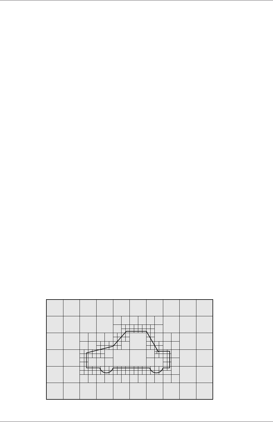
U-156 Mesh generation and conversion
secondSolid
{
level (3 3); // optional refinement for secondSolid region
}
}
}
}
5.4.4 Cell removal
Once the feature and surface splitting is complete a process of cell removal begins. Cell
removal requires one or more regions enclosed entirely by a bounding surface within the
domain. The region in which cells are retained are simply identified by a location vector
within that region, specified by the locationInMesh keyword in castellatedMeshControls.
Cells are retained if, approximately speaking, 50% or more of their volume lies within the
region. The remaining cells are removed accordingly as illustrated in Figure 5.12.
5.4.5 Cell splitting in specified regions
Those cells that lie within one or more specified volume regions can be further split as
illustrated in Figure 5.13 by a rectangular region shown by dark shading. The refinement-
Regions sub-dictionary in castellatedMeshControls contains entries for refinement of the
volume regions specified in the geometry sub-dictionary. A refinement mode is applied to
each region which can be:
•inside refines inside the volume region;
•outside refines outside the volume region
•distance refines according to distance to the surface; and can accommodate different
levels at multiple distances with the levels keyword.
For the refinementRegions, the refinement level is specified by the levels list of entries
with the format(<distance> <level>). In the case of inside and outside refinement,
the <distance>is not required so is ignored (but it must be specified). Examples are shown
below:
Figure 5.11: Cell splitting by surface in snappyHexMesh meshing process
OpenFOAM-2.4.0
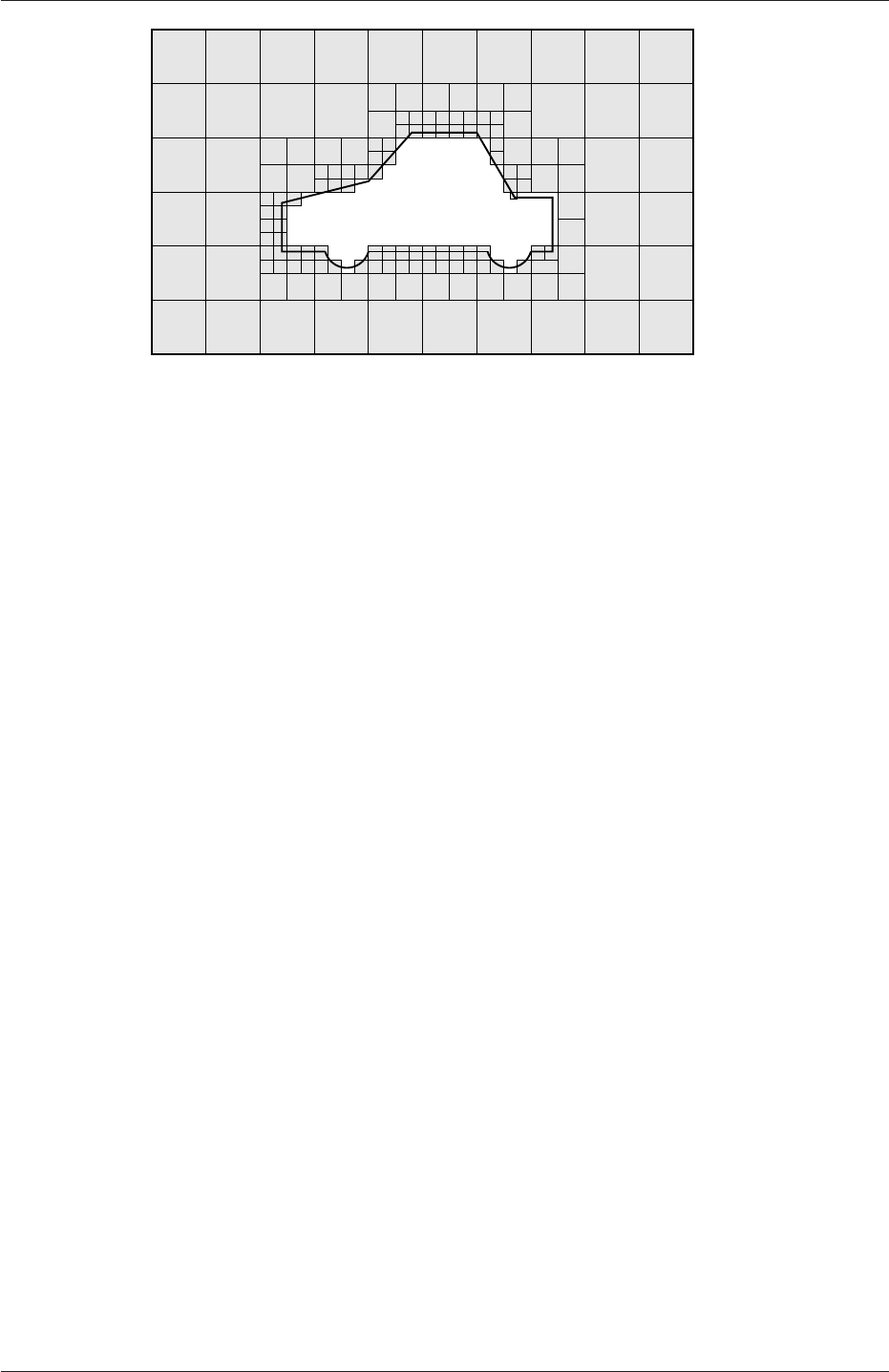
5.4 Mesh generation with the snappyHexMesh utility U-157
Figure 5.12: Cell removal in snappyHexMesh meshing process
refinementRegions
{
box1x1x1
{
mode inside;
levels ((1.0 4)); // refinement level 4 (1.0 entry ignored)
}
sphere.stl
{ // refinement level 5 within 1.0 m
mode distance; // refinement level 3 within 2.0 m
levels ((1.0 5) (2.0 3)); // levels must be ordered nearest first
}
}
5.4.6 Snapping to surfaces
The next stage of the meshing process involves moving cell vertex points onto surface ge-
ometry to remove the jagged castellated surface from the mesh. The process is:
1. displace the vertices in the castellated boundary onto the STL surface;
2. solve for relaxation of the internal mesh with the latest displaced boundary vertices;
3. find the vertices that cause mesh quality parameters to be violated;
4. reduce the displacement of those vertices from their initial value (at 1) and repeat
from 2 until mesh quality is satisfied.
The method uses the settings in the snapControls sub-dictionary in snappyHexMeshDict,
listed in Table 5.9. An example is illustrated in the schematic in Figure 5.14 (albeit with
mesh motion that looks slightly unrealistic).
5.4.7 Mesh layers
The mesh output from the snapping stage may be suitable for the purpose, although it
can produce some irregular cells along boundary surfaces. There is an optional stage of
the meshing process which introduces additional layers of hexahedral cells aligned to the
boundary surface as illustrated by the dark shaded cells in Figure 5.15.
OpenFOAM-2.4.0
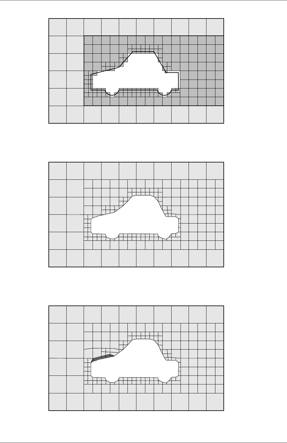
U-158 Mesh generation and conversion
Figure 5.13: Cell splitting by region in snappyHexMesh meshing process
Figure 5.14: Surface snapping in snappyHexMesh meshing process
Figure 5.15: Layer addition in snappyHexMesh meshing process
OpenFOAM-2.4.0

5.4 Mesh generation with the snappyHexMesh utility U-159
Keyword Description Example
nSmoothPatch Number of patch smoothing iterations before
finding correspondence to surface
3
tolerance Ratio of distance for points to be attracted
by surface feature point or edge, to local
maximum edge length
4.0
nSolveIter Number of mesh displacement relaxation it-
erations
30
nRelaxIter Maximum number of snapping relaxation it-
erations
5
Table 5.9: Keywords in the snapControls dictionary of snappyHexMeshDict.
The process of mesh layer addition involves shrinking the existing mesh from the bound-
ary and inserting layers of cells, broadly as follows:
1. the mesh is projected back from the surface by a specified thickness in the direction
normal to the surface;
2. solve for relaxation of the internal mesh with the latest projected boundary vertices;
3. check if validation criteria are satisfied otherwise reduce the projected thickness and
return to 2; if validation cannot be satisfied for any thickness, do not insert layers;
4. if the validation criteria can be satisfied, insert mesh layers;
5. the mesh is checked again; if the checks fail, layers are removed and we return to 2.
The layer addition procedure uses the settings in the addLayersControls sub-dictionary
in snappyHexMeshDict; entries are listed in Table 5.10. The layers sub-dictionary contains
entries for each patch on which the layers are to be applied and the number of surface
layers required. The patch name is used because the layers addition relates to the existing
mesh, not the surface geometry; hence applied to a patch, not a surface region. An example
layers entry is as follows:
layers
{
sphere.stl_firstSolid
{
nSurfaceLayers 1;
}
maxY
{
nSurfaceLayers 1;
}
}
5.4.8 Mesh quality controls
The mesh quality is controlled by the entries in the meshQualityControls sub-dictionary in
snappyHexMeshDict; entries are listed in Table 5.11.
OpenFOAM-2.4.0

U-160 Mesh generation and conversion
Keyword Description Example
layers Dictionary of layers
relativeSizes Are layer thicknesses relative to undistorted cell
size outside layer or absolute?
true/false
expansionRatio Expansion factor for layer mesh 1.0
finalLayerThickness Thickness of layer furthest from the wall, ei-
ther relative or absolute according to the
relativeSizes entry
0.3
minThickness Minimum thickness of cell layer, either relative
or absolute (as above)
0.25
nGrow Number of layers of connected faces that are not
grown if points get not extruded; helps conver-
gence of layer addition close to features
1
featureAngle Angle above which surface is not extruded 60
nRelaxIter Maximum number of snapping relaxation itera-
tions
5
nSmoothSurfaceNormals Number of smoothing iterations of surface nor-
mals
1
nSmoothNormals Number of smoothing iterations of interior mesh
movement direction
3
nSmoothThickness Smooth layer thickness over surface patches 10
maxFaceThicknessRatio Stop layer growth on highly warped cells 0.5
maxThicknessTo-
MedialRatio
Reduce layer growth where ratio thickness to me-
dial distance is large
0.3
minMedianAxisAngle Angle used to pick up medial axis points 130
nBufferCellsNoExtrude Create buffer region for new layer terminations 0
nLayerIter Overall max number of layer addition iterations 50
nRelaxedIter Max number of iterations after which the
controls in the relaxed sub dictionary of
meshQuality are used
20
Table 5.10: Keywords in the addLayersControls sub-dictionary of snappyHexMeshDict.
5.5 Mesh conversion
The user can generate meshes using other packages and convert them into the format that
OpenFOAM uses. There are numerous mesh conversion utilities listed in Table 3.6. Some of
the more popular mesh converters are listed below and their use is presented in this section.
fluentMeshToFoam reads a Fluent.msh mesh file, working for both 2-D and 3-D cases;
starToFoam reads STAR-CD/PROSTAR mesh files.
gambitToFoam reads a GAMBIT.neu neutral file;
ideasToFoam reads an I-DEAS mesh written in ANSYS.ans format;
cfx4ToFoam reads a CFX mesh written in .geo format;
OpenFOAM-2.4.0

5.5 Mesh conversion U-161
Keyword Description Example
maxNonOrtho Maximum non-orthogonality allowed; 180 dis-
ables
65
maxBoundarySkewness Max boundary face skewness allowed; <0dis-
ables
20
maxInternalSkewness Max internal face skewness allowed; <0disables 4
maxConcave Max concaveness allowed; 180 disables 80
minFlatness Ratio of minimum projected area to actual area;
-1 disables
0.5
minVol Minimum pyramid volume; large negative num-
ber, e.g.-1e30 disables
1e-13
minArea Minimum face area; <0disables -1
minTwist Minimum face twist; <-1 disables 0.05
minDeterminant Minimum normalised cell determinant; 1= hex;
≤0 illegal cell
0.001
minFaceWeight 0→0.5 0.05
minVolRatio 0→1.0 0.01
minTriangleTwist >0for Fluent compatability -1
nSmoothScale Number of error distribution iterations 4
errorReduction Amount to scale back displacement at error
points
0.75
relaxed Sub-dictionary that can include modified values
for the above keyword entries to be used when
nRelaxedIter is exceeded in the layer addition
process
relaxed
{
...
}
Table 5.11: Keywords in the meshQualityControls sub-dictionary of snappyHexMeshDict.
5.5.1 fluentMeshToFoam
Fluent writes mesh data to a single file with a .msh extension. The file must be writ-
ten in ASCII format, which is not the default option in Fluent. It is possible to convert
single-stream Fluent meshes, including the 2 dimensional geometries. In OpenFOAM, 2
dimensional geometries are currently treated by defining a mesh in 3 dimensions, where
the front and back plane are defined as the empty boundary patch type. When reading
a 2 dimensional Fluent mesh, the converter automatically extrudes the mesh in the third
direction and adds the empty patch, naming it frontAndBackPlanes.
The following features should also be observed.
•The OpenFOAM converter will attempt to capture the Fluent boundary condition
definition as much as possible; however, since there is no clear, direct correspondence
between the OpenFOAM and Fluent boundary conditions, the user should check the
boundary conditions before running a case.
•Creation of axi-symmetric meshes from a 2 dimensional mesh is currently not sup-
ported but can be implemented on request.
•Multiple material meshes are not permitted. If multiple fluid materials exist, they
will be converted into a single OpenFOAM mesh; if a solid region is detected, the
OpenFOAM-2.4.0

U-162 Mesh generation and conversion
converter will attempt to filter it out.
•Fluent allows the user to define a patch which is internal to the mesh, i.e. consists of
the faces with cells on both sides. Such patches are not allowed in OpenFOAM and
the converter will attempt to filter them out.
•There is currently no support for embedded interfaces and refinement trees.
The procedure of converting a Fluent.msh file is first to create a new OpenFOAM case
by creating the necessary directories/files: the case directory containing a controlDict file in
asystem subdirectory. Then at a command prompt the user should execute:
fluentMeshToFoam <meshFile>
where <meshFile>is the name of the .msh file, including the full or relative path.
5.5.2 starToFoam
This section describes how to convert a mesh generated on the STAR-CD code into a form
that can be read by OpenFOAM mesh classes. The mesh can be generated by any of the
packages supplied with STAR-CD,i.e.PROSTAR,SAMM,ProAM and their derivatives. The
converter accepts any single-stream mesh including integral and arbitrary couple matching
and all cell types are supported. The features that the converter does not support are:
•multi-stream mesh specification;
•baffles, i.e. zero-thickness walls inserted into the domain;
•partial boundaries, where an uncovered part of a couple match is considered to be a
boundary face;
•sliding interfaces.
For multi-stream meshes, mesh conversion can be achieved by writing each individual stream
as a separate mesh and reassemble them in OpenFOAM.
OpenFOAM adopts a policy of only accepting input meshes that conform to the fairly
stringent validity criteria specified in section 5.1. It will simply not run using invalid meshes
and cannot convert a mesh that is itself invalid. The following sections describe steps that
must be taken when generating a mesh using a mesh generating package supplied with
STAR-CD to ensure that it can be converted to OpenFOAM format. To avoid repetition
in the remainder of the section, the mesh generation tools supplied with STAR-CD will be
referred to by the collective name STAR-CD.
5.5.2.1 General advice on conversion
We strongly recommend that the user run the STAR-CD mesh checking tools before attempt-
ing a starToFoam conversion and, after conversion, the checkMesh utility should be run on
the newly converted mesh. Alternatively, starToFoam may itself issue warnings containing
PROSTAR commands that will enable the user to take a closer look at cells with problems.
Problematic cells and matches should be checked and fixed before attempting to use the
OpenFOAM-2.4.0

5.5 Mesh conversion U-163
mesh with OpenFOAM. Remember that an invalid mesh will not run with OpenFOAM, but
it may run in another environment that does not impose the validity criteria.
Some problems of tolerance matching can be overcome by the use of a matching tolerance
in the converter. However, there is a limit to its effectiveness and an apparent need to
increase the matching tolerance from its default level indicates that the original mesh suffers
from inaccuracies.
5.5.2.2 Eliminating extraneous data
When mesh generation in is completed, remove any extraneous vertices and compress the
cells boundary and vertex numbering, assuming that fluid cells have been created and all
other cells are discarded. This is done with the following PROSTAR commands:
CSET NEWS FLUID
CSET INVE
The CSET should be empty. If this is not the case, examine the cells in CSET and adjust
the model. If the cells are genuinely not desired, they can be removed using the PROSTAR
command:
CDEL CSET
Similarly, vertices will need to be discarded as well:
CSET NEWS FLUID
VSET NEWS CSET
VSET INVE
Before discarding these unwanted vertices, the unwanted boundary faces have to be collected
before purging:
CSET NEWS FLUID
VSET NEWS CSET
BSET NEWS VSET ALL
BSET INVE
If the BSET is not empty, the unwanted boundary faces can be deleted using:
BDEL BSET
At this time, the model should contain only the fluid cells and the supporting vertices,
as well as the defined boundary faces. All boundary faces should be fully supported by the
vertices of the cells, if this is not the case, carry on cleaning the geometry until everything
is clean.
OpenFOAM-2.4.0

U-164 Mesh generation and conversion
5.5.2.3 Removing default boundary conditions
By default, STAR-CD assigns wall boundaries to any boundary faces not explicitly associated
with a boundary region. The remaining boundary faces are collected into a default bound-
ary region, with the assigned boundary type 0. OpenFOAM deliberately does not have
a concept of a default boundary condition for undefined boundary faces since it invites
human error, e.g. there is no means of checking that we meant to give all the unassociated
faces the default condition.
Therefore all boundaries for each OpenFOAM mesh must be specified for a mesh to
be successfully converted. The default boundary needs to be transformed into a real one
using the procedure described below:
1. Plot the geometry with Wire Surface option.
2. Define an extra boundary region with the same parameters as the default region 0
and add all visible faces into the new region, say 10, by selecting a zone option in the
boundary tool and drawing a polygon around the entire screen draw of the model.
This can be done by issuing the following commands in PROSTAR:
RDEF 10 WALL
BZON 10 ALL
3. We shall remove all previously defined boundary types from the set. Go through the
boundary regions:
BSET NEWS REGI 1
BSET NEWS REGI 2
... 3, 4, ...
Collect the vertices associated with the boundary set and then the boundary faces
associated with the vertices (there will be twice as many of them as in the original
set).
BSET NEWS REGI 1
VSET NEWS BSET
BSET NEWS VSET ALL
BSET DELE REGI 1
REPL
This should give the faces of boundary Region 10 which have been defined on top of
boundary Region 1. Delete them with BDEL BSET. Repeat these for all regions.
5.5.2.4 Renumbering the model
Renumber and check the model using the commands:
CSET NEW FLUID
CCOM CSET
VSET NEWS CSET
OpenFOAM-2.4.0

5.5 Mesh conversion U-165
VSET INVE (Should be empty!)
VSET INVE
VCOM VSET
BSET NEWS VSET ALL
BSET INVE (Should be empty also!)
BSET INVE
BCOM BSET
CHECK ALL
GEOM
Internal PROSTAR checking is performed by the last two commands, which may reveal
some other unforeseeable error(s). Also, take note of the scaling factor because PROSTAR
only applies the factor for STAR-CD and not the geometry. If the factor is not 1, use the
scalePoints utility in OpenFOAM.
5.5.2.5 Writing out the mesh data
Once the mesh is completed, place all the integral matches of the model into the couple
type 1. All other types will be used to indicate arbitrary matches.
CPSET NEWS TYPE INTEGRAL
CPMOD CPSET 1
The components of the computational grid must then be written to their own files. This is
done using PROSTAR for boundaries by issuing the command
BWRITE
by default, this writes to a .23 file (versions prior to 3.0) or a .bnd file (versions 3.0 and
higher). For cells, the command
CWRITE
outputs the cells to a .14 or .cel file and for vertices, the command
VWRITE
outputs to file a .15 or .vrt file. The current default setting writes the files in ASCII format.
If couples are present, an additional couple file with the extension .cpl needs to be written
out by typing:
CPWRITE
OpenFOAM-2.4.0

U-166 Mesh generation and conversion
After outputting to the three files, exit PROSTAR or close the files. Look through the
panels and take note of all STAR-CD sub-models, material and fluid properties used – the
material properties and mathematical model will need to be set up by creating and editing
OpenFOAM dictionary files.
The procedure of converting the PROSTAR files is first to create a new OpenFOAM
case by creating the necessary directories. The PROSTAR files must be stored within the
same directory and the user must change the file extensions: from .23,.14 and .15 (below
STAR-CD version 3.0), or .pcs,.cls and .vtx (STAR-CD version 3.0 and above); to .bnd,.cel
and .vrt respectively.
5.5.2.6 Problems with the .vrt file
The .vrt file is written in columns of data of specified width, rather than free format. A
typical line of data might be as follows, giving a vertex number followed by the coordinates:
19422 -0.105988957 -0.413711881E-02 0.000000000E+00
If the ordinates are written in scientific notation and are negative, there may be no space
between values, e.g.:
19423 -0.953953117E-01-0.338810333E-02 0.000000000E+00
The starToFoam converter reads the data using spaces to delimit the ordinate values and
will therefore object when reading the previous example. Therefore, OpenFOAM includes a
simple script, foamCorrectVrt to insert a space between values where necessary, i.e. it would
convert the previous example to:
19423 -0.953953117E-01 -0.338810333E-02 0.000000000E+00
The foamCorrectVrt script should therefore be executed if necessary before running the
starToFoam converter, by typing:
foamCorrectVrt <file>.vrt
5.5.2.7 Converting the mesh to OpenFOAM format
The translator utility starToFoam can now be run to create the boundaries, cells and points
files necessary for a OpenFOAM run:
starToFoam <meshFilePrefix>
where <meshFilePrefix>is the name of the the prefix of the mesh files, including the full
or relative path. After the utility has finished running, OpenFOAM boundary types should
be specified by editing the boundary file by hand.
OpenFOAM-2.4.0

5.5 Mesh conversion U-167
5.5.3 gambitToFoam
GAMBIT writes mesh data to a single file with a .neu extension. The procedure of converting
aGAMBIT.neu file is first to create a new OpenFOAM case, then at a command prompt,
the user should execute:
gambitToFoam <meshFile>
where <meshFile>is the name of the .neu file, including the full or relative path.
The GAMBIT file format does not provide information about type of the boundary patch,
e.g. wall, symmetry plane, cyclic. Therefore all the patches have been created as type patch.
Please reset after mesh conversion as necessary.
5.5.4 ideasToFoam
OpenFOAM can convert a mesh generated by I-DEAS but written out in ANSYS format as
a.ans file. The procedure of converting the .ans file is first to create a new OpenFOAM
case, then at a command prompt, the user should execute:
ideasToFoam <meshFile>
where <meshFile>is the name of the .ans file, including the full or relative path.
5.5.5 cfx4ToFoam
CFX writes mesh data to a single file with a .geo extension. The mesh format in CFX is
block-structured, i.e. the mesh is specified as a set of blocks with glueing information and
the vertex locations. OpenFOAM will convert the mesh and capture the CFX boundary
condition as best as possible. The 3 dimensional ‘patch’ definition in CFX, containing
information about the porous, solid regions etc. is ignored with all regions being converted
into a single OpenFOAM mesh. CFX supports the concept of a ‘default’ patch, where each
external face without a defined boundary condition is treated as a wall. These faces are
collected by the converter and put into a defaultFaces patch in the OpenFOAM mesh and
given the type wall; of course, the patch type can be subsequently changed.
Like, OpenFOAM 2 dimensional geometries in CFX are created as 3 dimensional meshes
of 1 cell thickness. If a user wishes to run a 2 dimensional case on a mesh created by CFX,
the boundary condition on the front and back planes should be set to empty; the user should
ensure that the boundary conditions on all other faces in the plane of the calculation are
set correctly. Currently there is no facility for creating an axi-symmetric geometry from a
2 dimensional CFX mesh.
The procedure of converting a CFX.geo file is first to create a new OpenFOAM case,
then at a command prompt, the user should execute:
cfx4ToFoam <meshFile>
where <meshFile>is the name of the .geo file, including the full or relative path.
OpenFOAM-2.4.0

U-168 Mesh generation and conversion
5.6 Mapping fields between different geometries
The mapFields utility maps one or more fields relating to a given geometry onto the corre-
sponding fields for another geometry. It is completely generalised in so much as there does
not need to be any similarity between the geometries to which the fields relate. However, for
cases where the geometries are consistent, mapFields can be executed with a special option
that simplifies the mapping process.
For our discussion of mapFields we need to define a few terms. First, we say that the
data is mapped from the source to the target. The fields are deemed consistent if the
geometry and boundary types, or conditions, of both source and target fields are identical.
The field data that mapFields maps are those fields within the time directory specified by
startFrom/startTime in the controlDict of the target case. The data is read from the
equivalent time directory of the source case and mapped onto the equivalent time directory
of the target case.
5.6.1 Mapping consistent fields
A mapping of consistent fields is simply performed by executing mapFields on the (target)
case using the -consistent command line option as follows:
mapFields <source dir>-consistent
5.6.2 Mapping inconsistent fields
When the fields are not consistent, as shown in Figure 5.16,mapFields requires a mapFields-
Dict dictionary in the system directory of the target case. The following rules apply to the
mapping:
•the field data is mapped from source to target wherever possible, i.e. in our example
all the field data within the target geometry is mapped from the source, except those
in the shaded region which remain unaltered;
•the patch field data is left unaltered unless specified otherwise in the mapFieldsDict
dictionary.
The mapFieldsDict dictionary contain two lists that specify mapping of patch data. The first
list is patchMap that specifies mapping of data between pairs of source and target patches
that are geometrically coincident, as shown in Figure 5.16. The list contains each pair of
names of source and target patch. The second list is cuttingPatches that contains names
of target patches whose values are to be mapped from the source internal field through which
the target patch cuts. In the situation where the target patch only cuts through part of the
source internal field, e.g. bottom left target patch in our example, those values within the
internal field are mapped and those outside remain unchanged. An example mapFieldsDict
dictionary is shown below:
17
18 patchMap ( lid movingWall );
19
20 cuttingPatches ( fixedWalls );
21
22
23 // ************************************************************************* //
OpenFOAM-2.4.0
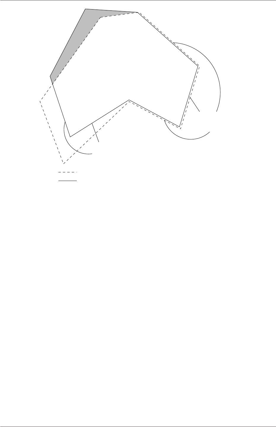
5.6 Mapping fields between different geometries U-169
Internal target patches:
can be mapped using cuttingPatches
Target field geometry
Source field geometry
can be mapped using patchMap
Coincident patches:
Figure 5.16: Mapping inconsistent fields
mapFields <source dir>
5.6.3 Mapping parallel cases
If either or both of the source and target cases are decomposed for running in parallel,
additional options must be supplied when executing mapFields:
-parallelSource if the source case is decomposed for parallel running;
-parallelTarget if the target case is decomposed for parallel running.
OpenFOAM-2.4.0

U-170 Mesh generation and conversion
OpenFOAM-2.4.0
Chapter 6
Post-processing
This chapter describes options for post-processing with OpenFOAM. OpenFOAM is supplied
with a post-processing utility paraFoam that uses ParaView, an open source visualisation
application described in section 6.1.
Other methods of post-processing using third party products are offered, including En-
Sight,Fieldview and the post-processing supplied with Fluent.
6.1 paraFoam
The main post-processing tool provided with OpenFOAM is a reader module to run with
ParaView, an open-source, visualization application. The module is compiled into 2 li-
braries, PV3FoamReader and vtkPV3Foam using version 4.1.0 of ParaView supplied with
the OpenFOAM release (PVFoamReader and vtkFoam in ParaView version 2.x). It is rec-
ommended that this version of ParaView is used, although it is possible that the lat-
est binary release of the software will run adequately. Further details about ParaView
can be found at http://www.paraview.org and further documentation is available at
http://www.kitware.com/products/paraviewguide.html.
ParaView uses the Visualisation Toolkit (VTK) as its data processing and rendering
engine and can therefore read any data in VTK format. OpenFOAM includes the foam-
ToVTK utility to convert data from its native format to VTK format, which means that any
VTK-based graphics tools can be used to post-process OpenFOAM cases. This provides
an alternative means for using ParaView with OpenFOAM. For users who wish to experi-
ment with advanced, parallel visualisation, there is also the free VisIt software, available at
http://www.llnl.gov/visit.
In summary, we recommend the reader module for ParaView as the primary post-processing
tool for OpenFOAM. Alternatively OpenFOAM data can be converted into VTK format to
be read by ParaView or any other VTK -based graphics tools.
6.1.1 Overview of paraFoam
paraFoam is strictly a script that launches ParaView using the reader module supplied with
OpenFOAM. It is executed like any of the OpenFOAM utilities either by the single command
from within the case directory or with the -case option with the case path as an argument,
e.g.:
paraFoam -case <caseDir>
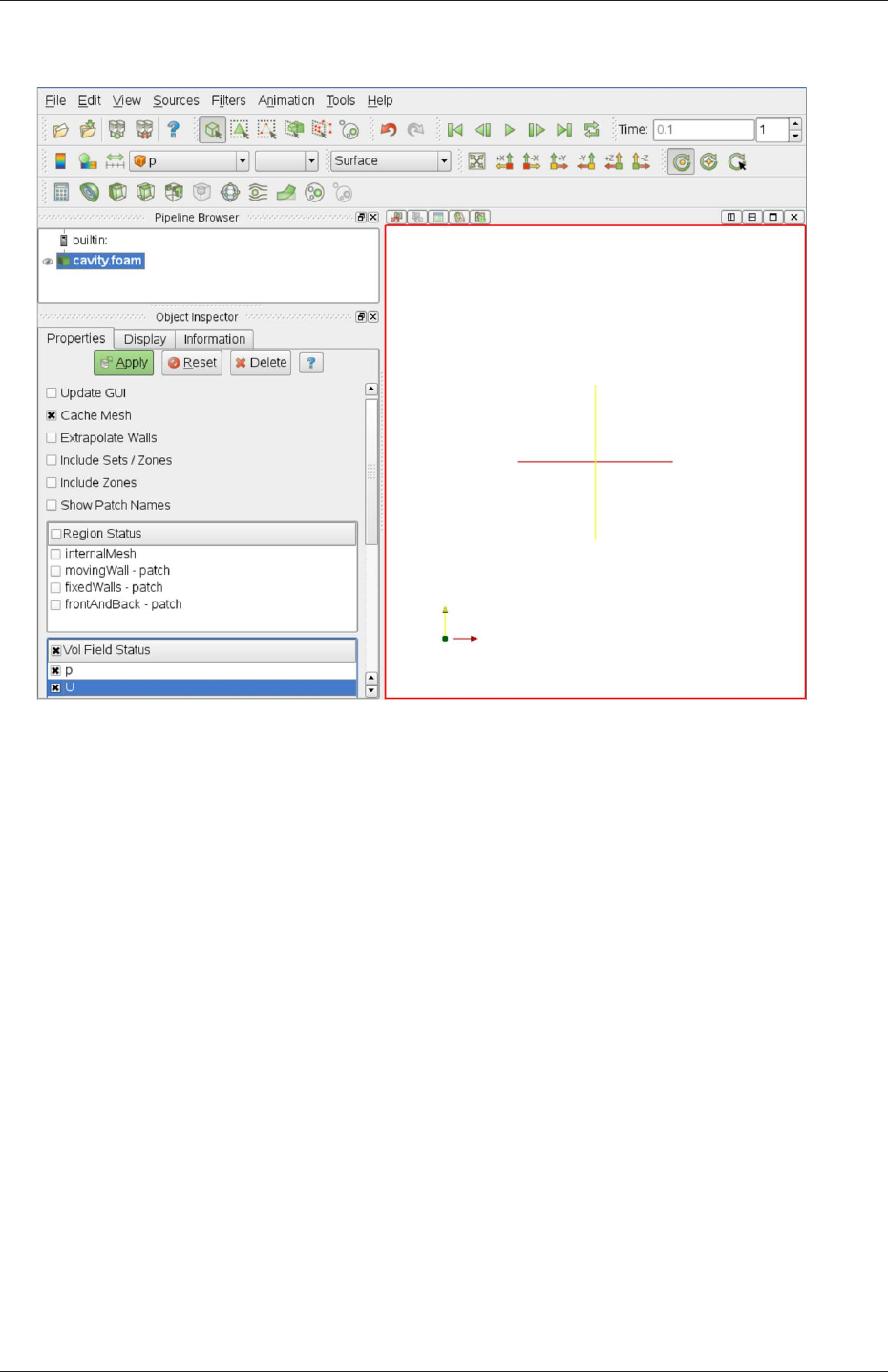
U-172 Post-processing
Figure 6.1: The paraFoam window
ParaView is launched and opens the window shown in Figure 6.1. The case is controlled
from the left panel, which contains the following:
Pipeline Browser lists the modules opened in ParaView, where the selected modules are high-
lighted in blue and the graphics for the given module can be enabled/disabled by
clicking the eye button alongside;
Properties panel contains the input selections for the case, such as times, regions and fields;
Display panel controls the visual representation of the selected module, e.g. colours;
Information panel gives case statistics such as mesh geometry and size.
ParaView operates a tree-based structure in which data can be filtered from the top-level
case module to create sets of sub-modules. For example, a contour plot of, say, pressure
could be a sub-module of the case module which contains all the pressure data. The strength
of ParaView is that the user can create a number of sub-modules and display whichever ones
they feel to create the desired image or animation. For example, they may add some solid
geometry, mesh and velocity vectors, to a contour plot of pressure, switching any of the
items on and off as necessary.
The general operation of the system is based on the user making a selection and then
clicking the green Apply button in the Properties panel. The additional buttons are: the
Reset button which can be used to reset the GUI if necessary; and, the Delete button that
will delete the active module.
OpenFOAM-2.4.0
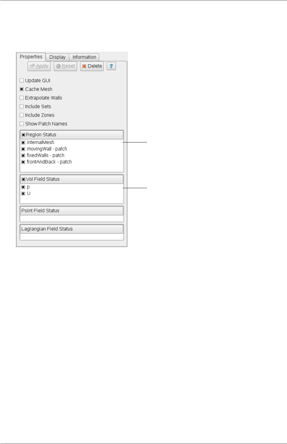
6.1 paraFoam U-173
6.1.2 The Properties panel
The Properties panel for the case module contains the settings for time step, regions and
fields. The controls are described in Figure 6.2. It is particularly worth noting that in the
The user can select internalMesh
region and/or individual patches
read into the case module
The user can select the fields
Figure 6.2: The Properties panel for the case module
current reader module, data in all time directories are loaded into ParaView (in the reader
module for ParaView 2.x, a set of check boxes controlled the time that were displayed). In
the current reader module, the buttons in the Current Time Controls and VCR Controls
toolbars select the time data to be displayed, as shown is section 6.1.4.
As with any operation in paraFoam, the user must click Apply after making any changes
to any selections. The Apply button is highlighted in green to alert the user if changes have
been made but not accepted. This method of operation has the advantage of allowing the
user to make a number of selections before accepting them, which is particularly useful in
large cases where data processing is best kept to a minimum.
There are occasions when the case data changes on file and ParaView needs to load the
changes, e.g. when field data is written into new time directories. To load the changes, the
user should check the Update GUI button at the top of the Properties panel and then apply
the changes.
6.1.3 The Display panel
The Display panel contains the settings for visualising the data for a given case module. The
following points are particularly important:
OpenFOAM-2.4.0
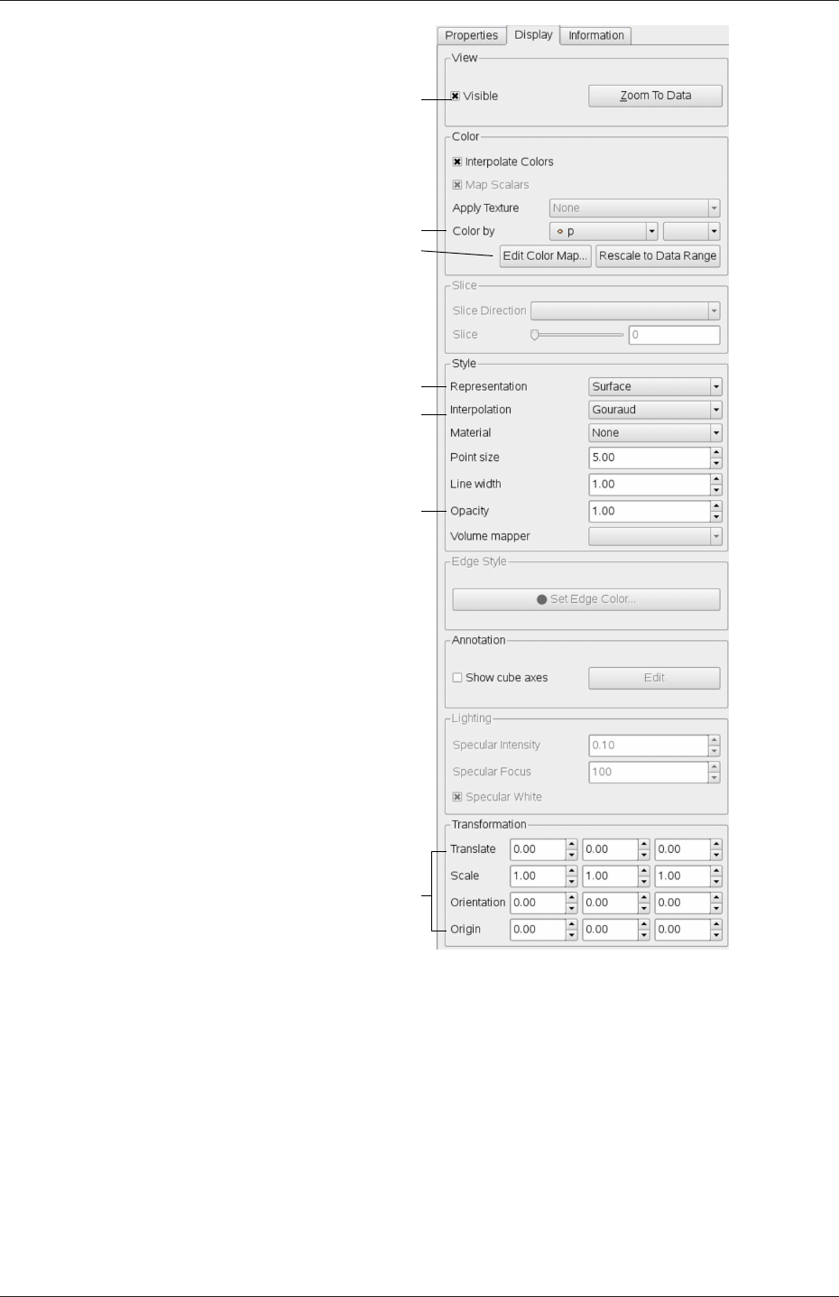
U-174 Post-processing
Outline, surface, wireframe or points
Data interpolation method
Change image opacity
e.g. to make transluscent
View case data
Colour geometry/entity by...
Set colour map range/appearance
Geometry manipulation tools
Figure 6.3: The Display panel
•the data range may not be automatically updated to the max/min limits of a field, so
the user should take care to select Rescale to Data Range at appropriate intervals, in
particular after loading the initial case module;
•clicking the Edit Color Map button, brings up a window in which there are two panels:
1. The Color Scale panel in which the colours within the scale can be chosen. The
standard blue to red colour scale for CFD can be selected by clicking Choose
Preset and selecting Blue to Red Rainbox HSV.
2. The Color Legend panel has a toggle switch for a colour bar legend and contains
OpenFOAM-2.4.0
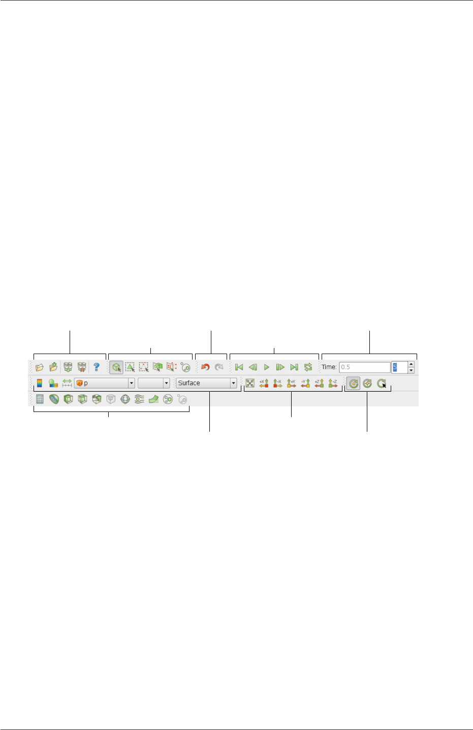
6.1 paraFoam U-175
settings for the layout of the legend, e.g. font.
•the underlying mesh can be represented by selecting Wireframe in the Representat-
ion menu of the Style panel;
•the geometry, e.g. a mesh (if Wireframe is selected), can be visualised as a single
colour by selecting Solid Color from the Color By menu and specifying the colour
in the Set Ambient Color window;
•the image can be made translucent by editing the value in the Opacity text box (1 =
solid, 0 = invisible) in the Style panel.
6.1.4 The button toolbars
ParaView duplicates functionality from pull-down menus at the top of the main window
and the major panels, within the toolbars below the main pull-down menus. The displayed
toolbars can be selected from Toolbars in the main View menu. The default layout with
all toolbars is shown in Figure 6.4 with each toolbar labelled. The function of many of the
buttons is clear from their icon and, with tooltips enabled in the Help menu, the user is
given a concise description of the function of any button.
Selection Controls VCR Controls
Common Filters Camera Controls
Centre Axes Controls
Undo/Redo ControlsMain controls Current Time Controls
Active Variable Controls |Representation
Figure 6.4: Toolbars in ParaView
6.1.5 Manipulating the view
This section describes operations for setting and manipulating the view of objects in paraFoam.
6.1.5.1 View settings
The View Settings are selected from the Edit menu, which opens a View Settings (Render
View) window with a table of 3 items: General,Lights and Annotation. The General panel
includes the following items which are often worth setting at startup:
•the background colour, where white is often a preferred choice for printed material, is
set by choosing background from the down-arrow button next to Choose Color button,
then selecting the color by clicking on the Choose Color button;
•Use parallel projection which is the usual choice for CFD, especially for 2D cases.
OpenFOAM-2.4.0

U-176 Post-processing
The Lights panel contains detailed lighting controls within the Light Kit panel. A separate
Headlight panel controls the direct lighting of the image. Checking the Headlight button with
white light colour of strength 1 seems to help produce images with strong bright colours,
e.g. with an isosurface.
The Annotation panel includes options for including annotations in the image. The
Orientation Axes feature controls an axes icon in the image window, e.g. to set the colour of
the axes labels x,yand z.
6.1.5.2 General settings
The general Settings are selected from the Edit menu, which opens a general Options
window with General,Colors,Animations,Charts and Render View menu items.
The General panel controls some default behaviour of ParaView. In particular, there is an
Auto Accept button that enables ParaView to accept changes automatically without clicking
the green Apply button in the Properties window. For larger cases, this option is generally
not recommended: the user does not generally want the image to be re-rendered between
each of a number of changes he/she selects, but be able to apply a number of changes to be
re-rendered in their entirety once.
The Render View panel contains 3 sub-items: General,Camera and Server. The General
panel includes the level of detail (LOD) which controls the rendering of the image while it
is being manipulated, e.g. translated, resized, rotated; lowering the levels set by the sliders,
allows cases with large numbers of cells to be re-rendered quickly during manipulation.
The Camera panel includes control settings for 3D and 2D movements. This presents the
user with a map of rotation, translate and zoom controls using the mouse in combination
with Shift- and Control-keys. The map can be edited to suit by the user.
6.1.6 Contour plots
A contour plot is created by selecting Contour from the Filter menu at the top menu
bar. The filter acts on a given module so that, if the module is the 3D case module itself,
the contours will be a set of 2D surfaces that represent a constant value, i.e. isosurfaces.
The Properties panel for contours contains an Isosurfaces list that the user can edit, most
conveniently by the New Range window. The chosen scalar field is selected from a pull down
menu.
6.1.6.1 Introducing a cutting plane
Very often a user will wish to create a contour plot across a plane rather than producing
isosurfaces. To do so, the user must first use the Slice filter to create the cutting plane,
on which the contours can be plotted. The Slice filter allows the user to specify a cutting
Plane,Box or Sphere in the Slice Type menu by a center and normal/radius respectively.
The user can manipulate the cutting plane like any other using the mouse.
The user can then run the Contour filter on the cut plane to generate contour lines.
6.1.7 Vector plots
Vector plots are created using the Glyph filter. The filter reads the field selected in Vectors
and offers a range of Glyph Types for which the Arrow provides a clear vector plot images.
OpenFOAM-2.4.0

6.1 paraFoam U-177
Each glyph has a selection of graphical controls in a panel which the user can manipulate
to best effect.
The remainder of the Properties panel contains mainly the Scale Mode menu for the
glyphs. The most common options are Scale Mode are: Vector, where the glyph length is
proportional to the vector magnitude; and, Off where each glyph is the same length. The
Set Scale Factor parameter controls the base length of the glyphs.
6.1.7.1 Plotting at cell centres
Vectors are by default plotted on cell vertices but, very often, we wish to plot data at cell
centres. This is done by first applying the Cell Centers filter to the case module, and then
applying the Glyph filter to the resulting cell centre data.
6.1.8 Streamlines
Streamlines are created by first creating tracer lines using the Stream Tracer filter. The
tracer Seed panel specifies a distribution of tracer points over a Line Source or Point
Cloud. The user can view the tracer source, e.g. the line, but it is displayed in white, so
they may need to change the background colour in order to see it.
The distance the tracer travels and the length of steps the tracer takes are specified in
the text boxes in the main Stream Tracer panel. The process of achieving desired tracer lines
is largely one of trial and error in which the tracer lines obviously appear smoother as the
step length is reduced but with the penalty of a longer calculation time.
Once the tracer lines have been created, the Tubes filter can be applied to the Tracer
module to produce high quality images. The tubes follow each tracer line and are not
strictly cylindrical but have a fixed number of sides and given radius. When the number of
sides is set above, say, 10, the tubes do however appear cylindrical, but again this adds a
computational cost.
6.1.9 Image output
The simplest way to output an image to file from ParaView is to select Save Screenshot
from the File menu. On selection, a window appears in which the user can select the
resolution for the image to save. There is a button that, when clicked, locks the aspect
ratio, so if the user changes the resolution in one direction, the resolution is adjusted in the
other direction automatically. After selecting the pixel resolution, the image can be saved.
To achieve high quality output, the user might try setting the pixel resolution to 1000 or
more in the x-direction so that when the image is scaled to a typical size of a figure in an
A4 or US letter document, perhaps in a PDF document, the resolution is sharp.
6.1.10 Animation output
To create an animation, the user should first select Save Animation from the File menu.
A dialogue window appears in which the user can specify a number of things including the
image resolution. The user should specify the resolution as required. The other noteworthy
setting is number of frames per timestep. While this would intuitively be set to 1, it can
be set to a larger number in order to introduce more frames into the animation artificially.
OpenFOAM-2.4.0

U-178 Post-processing
This technique can be particularly useful to produce a slower animation because some movie
players have limited speed control, particularly over mpeg movies.
On clicking the Save Animation button, another window appears in which the user spec-
ifies a file name root and file format for a set of images. On clicking OK, the set of files will
be saved according to the naming convention “<fileRoot><imageNo>.<fileExt>”, e.g.
the third image of a series with the file root “animation”, saved in jpg format would be
named “animation 0002.jpg” (<imageNo>starts at 0000).
Once the set of images are saved the user can convert them into a movie using their
software of choice. The convert utility in the ImageMagick package can do this from the
command line, e.g. by
convert animation*jpg movie.mpg
When creating an mpg movie it can be worth increasing the default quality setting, e.g. with
-quality 90%, to reduce the graininess that can occur with the default setting.
6.2 Function Objects
OpenFOAM provides functionality that can be executed during a simulation by the user at
run-time through a configuration in the controlDict file. For example, a user may wish to run
a steady-state, incompressible, turbulent flow simulation of aerodynamics around a vehicle
and from that simulation they wish to calculate the drag coefficient. While the simulation
is performed by the simpleFoam solver, the additional force calculation for drag coefficient is
included in a tool, called a function object, that can be requested by the user to be executed
at certain times during the simulation.
Function object Description
cellSource performs operations on cell values, e.g. sums, averages and integra-
tions
faceSource performs operations on face values, e.g. sums, averages and inte-
grations
fieldMinMax writes min/max values of fields
fieldValue averaging/integration across sets of faces/cells, e.g. for flux across
a plane
fieldValueDelta Provides differencing between two fieldValue function objects,
e.g. to calculate pressure drop
forces calculates pressure/viscous forces and moments
forceCoeffs calculates lift, drag and moment coefficients
regionSizeDistrib-
ution
creates a size distribution via interrogating a continuous phase frac-
tion
sampledSet data sampling along lines, e.g. for graph plotting
probes data probing at point locations
residuals writes initial residuals for selected fields
Table 6.1: Function objects writing time-value data for monitoring/plotting
OpenFOAM-2.4.0

6.2 Function Objects U-179
Function object Description
fieldAverage temporal averaging of fields
writeRegistered-
Object
writes fields that are not scheduled to be written
fieldCoordinate-
SystemTransform
transforms fields between global to local co-ordinate system
turbulenceFields stores turbulence fields on the mesh database
calcFvcDiv calculates the divergence of a field
calcFvcGrad calculates the gradient of a field
calcMag calculates the magnitude of a field
CourantNo outputs the Courant number field
Lambda2 outputs Lambda2
Peclet outputs the Peclet number field
pressureTools calculate pressure in different forms, static, total, etc.
Qsecond invariant of the velocity gradient
vorticity calculates vorticity field
processorField writes a field of the local processor ID
partialWrite allows registered objects to be written at specified times
readFields reads fields from the time directories and adds to database
blendingFactor outputs the blending factor used by the convection schemes
DESModelRegions writes out an indicator field for DES turbulence
Table 6.2: Function objects for writing/reading fields, typically writing to time directories
Function object Description
nearWallFields writes fields in cells adjacent to patches
wallShearStress evaluates and outputs the shear stress at wall patches
yPlusLES outputs turbulence y+ for LES models
yPlusRAS outputs turbulence y+ for RAS models
Table 6.3: Function objects for near wall fields
A large number of function objects exist in OpenFOAM that perform mainly a range of
post-processing calculations but also some job control activities. Function objects can be
broken down into the following categories.
•Table 6.1: write out tabulated data, typically containing time-values, usually at regular
time intervals, for plotting graphs and/or monitoring, e.g. force coefficients.
•Table 6.2: write out field data, usually at the normal time interval for writing fields
into time directories.
•Table 6.3: write out field data on boundary patches, e.g. wall shear stress, usually at
the time interval for writing fields into time directories.
•Table 6.4: write out image files, e.g. iso-surface for visualization.
•Table 6.5: function objects that manage job control, supplementary simulation, etc.
OpenFOAM-2.4.0

U-180 Post-processing
Function object Description
streamline streamline data from sampled fields
surfaces iso-surfaces, cutting planes, patch surfaces, with field data
wallBoundedStreamline streamlines constrained to a boundary patch
Table 6.4: Function objects for creating post-processing images
Function object Description
timeActivatedFile-
Update
modifies case settings at specified times in a simulation
abortCalculation aborts simulation when named file appears in the case directory
removeRegistered-
Object
removes specified registered objects in the database
setTimeStepFunct-
ionObject
enables manual over-ride of the time step
codedFunctionObject function object coded with #codeStream
cloudInfo outputs Lagrangian cloud information
scalarTransport solves a passive scalar transport equation
systemCall makes any call to the system, e.g. sends an email
Table 6.5: Miscellaneous function objects
6.2.1 Using function objects
Function objects are specified in the controlDict file of a case through a dictionary named
functions. One or more function objects can be specified, each within its own sub-
dictionary. An example of specification of 2 function objects is shown below:
functions
{pressureProbes
{type probes;
functionObjectLibs ("libsampling.so");
outputControl timeStep;
outputInterval 1;
probeLocations
(
(100)
(200)
);
fields
(
p
);
}
OpenFOAM-2.4.0

6.2 Function Objects U-181
meanVelocity
{type fieldAverage;
functionObjectLibs ( "libfieldFunctionObjects.so" );
outputControl outputTime;
fields
(
U
{mean on;
prime2Mean off;
base time;
}
);
}
}
For each function object, there are some mandatory keyword entries.
name Every function object requires a unique name, here pressureProbes and meanVelocity
are used. The names can be used for naming output files and/or directories.
type The type of function object, e.g. probes.
functionObjectLibs A list of additional libraries that may need to be dynamically linked
at run-time to access the relevant functionality. For example the forceCoeffs function
object is compiled into the libforces.so library, so force coefficients cannot be calculated
without linking that library.
outputControl Specifies when data should be calculated and output. Options are: timeStep,
when data is output each writeInterval time steps; and, outputTime when data is
written at scheduled times, i.e. when fields are written to time directories.
The remaining entries in the example above are specific to the particular function object.
For example probeLocations describes the locations where pressure values are probed. For
any other function object, how can the user find out the specific keyword entries required?
One option is to access the code C++ documentation at either http://openfoam.org/-
docs/cpp or http://openfoam.github.io/Documentation-dev/html and click the post-
processing link. This takes the user to a set of lists of function objects, the class description
of each function object providing documentation on its use.
Alternatively the user can scan the cases in $FOAM TUTORIALS directory for examples
of function objects in use. The find and grep command can help to locate relevant examples,
e.g.
find $FOAM TUTORIALS -name controlDict | xargs grep -l functions
6.2.2 Packaged function objects
From OpenFOAM v2.4, commonly used function objects are “packaged” in the distribution
in $FOAM ETC/caseDicts/postProcessing. The tools range from quite generic, e.g. minMax
OpenFOAM-2.4.0

U-182 Post-processing
to monitor min and max values of a field, to some more application-oriented, e.g. flowRate
to monitor flow rate.
The configuration of function objects includes both required input data and control
parameters for the function object. This creates a lot of input that can be confusing to
users. The packaged function objects separate the user input from control parameters.
Control parameters are pre-configured in files with .cfg extension. For each tool, required
user input is all in one file, for the users to copy into their case and set accordingly.
The tools can be used as follows, using an example of monitoring flow rate at an outlet
patch named outlet.
1. Locate the flowRatePatch tool in the flowRate directory:
$FOAM ETC/caseDicts/postProcessing/flowRate
2. Copy the flowRatePatch file into the case system directory (not flowRatePatch.cfg)
3. Edit system/flowRatePatch to set the patch name, replacing “patch <patchName>;”
with “patch outlet;”
4. Activate the function object by including the flowRatePatch file in functions sub-
dictionary in the case controlDict file, e.g.
functions
{#include "flowRatePatch"
... other function objects here ...
}
Current packaged function objects are found in the following directories:
•fields calculate specific fields, e.g. Q
•flowRate: tools to calculate flow rate
•forces: forces and force coefficients for incompressible/compressible flows
•graphs: simple sampling for graph plotting, e.g. singleGraph
•minMax: range of minimum and maximum field monitoring, e.g. cellMax
•numerical: outputs information relating to numerics, e.g. residuals
•pressure: calculates different forms of pressure, pressure drop, etc
•probes: options for probing data
•scalarTransport: for plugin scalar transport calculations
•visualization: post-processing VTK files for cutting planes, streamlines, etc.
•faceSource: configuration for some of the tools above
OpenFOAM-2.4.0

6.3 Post-processing with Fluent U-183
6.3 Post-processing with Fluent
It is possible to use Fluent as a post-processor for the cases run in OpenFOAM. Two con-
verters are supplied for the purpose: foamMeshToFluent which converts the OpenFOAM
mesh into Fluent format and writes it out as a .msh file; and, foamDataToFluent converts the
OpenFOAM results data into a .dat file readable by Fluent.foamMeshToFluent is executed
in the usual manner. The resulting mesh is written out in a fluentInterface subdirectory of
the case directory, i.e.<caseName>/fluentInterface/<caseName>.msh
foamDataToFluent converts the OpenFOAM data results into the Fluent format. The con-
version is controlled by two files. First, the controlDict dictionary specifies startTime, giving
the set of results to be converted. If you want to convert the latest result, startFrom can
be set to latestTime. The second file which specifies the translation is the foamDataToFlu-
entDict dictionary, located in the constant directory. An example foamDataToFluentDict
dictionary is given below:
1/*--------------------------------*- C++ -*----------------------------------*\
2| ========= | |
3| \\ / F ield | OpenFOAM: The Open Source CFD Toolbox |
4| \\ / O peration | Version: 2.4.0 |
5| \\ / A nd | Web: www.OpenFOAM.org |
6| \\/ M anipulation | |
7\*---------------------------------------------------------------------------*/
8FoamFile
9{
10 version 2.0;
11 format ascii;
12 class dictionary;
13 location "system";
14 object foamDataToFluentDict;
15 }
16 // * * * * * * * * * * * * * * * * * * * * * * * * * * * * * * * * * * * * * //
17
18 p 1;
19
20 U 2;
21
22 T 3;
23
24 h 4;
25
26 k 5;
27
28 epsilon 6;
29
30 alpha1 150;
31
32
33 // ************************************************************************* //
The dictionary contains entries of the form
<fieldName> <fluentUnitNumber>
The <fluentUnitNumber>is a label used by the Fluent post-processor that only recognises a
fixed set of fields. The basic set of <fluentUnitNumber>numbers are quoted in Table 6.6.
The dictionary must contain all the entries the user requires to post-process, e.g. in our
example we have entries for pressure pand velocity U. The list of default entries described
in Table 6.6. The user can run foamDataToFluent like any utility.
To view the results using Fluent, go to the fluentInterface subdirectory of the case direc-
tory and start a 3 dimensional version of Fluent with
fluent 3d
OpenFOAM-2.4.0

U-184 Post-processing
Fluent name Unit number Common OpenFOAM name
PRESSURE 1p
MOMENTUM 2U
TEMPERATURE 3T
ENTHALPY 4h
TKE 5k
TED 6epsilon
SPECIES 7 —
G8 —
XF RF DATA VOF 150 gamma
TOTAL PRESSURE 192 —
TOTAL TEMPERATURE 193 —
Table 6.6: Fluent unit numbers for post-processing.
The mesh and data files can be loaded in and the results visualised. The mesh is read by
selecting Read Case from the File menu. Support items should be selected to read certain
data types, e.g. to read turbulence data for kand epsilon, the user would select k-epsilon
from the Define->Models->Viscous menu. The data can then be read by selecting Read
Data from the File menu.
A note of caution: users MUST NOT try to use an original Fluent mesh file that has been
converted to OpenFOAM format in conjunction with the OpenFOAM solution that has been
converted to Fluent format since the alignment of zone numbering cannot be guaranteed.
6.4 Post-processing with Fieldview
OpenFOAM offers the capability for post-processing OpenFOAM cases with Fieldview. The
method involves running a post-processing utility foamToFieldview to convert case data from
OpenFOAM to Fieldview.uns file format. For a given case, foamToFieldview is executed like
any normal application. foamToFieldview creates a directory named Fieldview in the case
directory, deleting any existing Fieldview directory in the process. By default the converter
reads the data in all time directories and writes into a set of files of the form <case>nn.uns,
where nn is an incremental counter starting from 1 for the first time directory, 2 for the
second and so on. The user may specify the conversion of a single time directory with the
option -time <time>, where <time>is a time in general, scientific or fixed format.
Fieldview provides certain functions that require information about boundary conditions,
e.g. drawing streamlines that uses information about wall boundaries. The converter tries,
wherever possible, to include this information in the converted files by default. The user
can disable the inclusion of this information by using the -noWall option in the execution
command.
The data files for Fieldview have the .uns extension as mentioned already. If the original
OpenFOAM case includes a dot ‘.’, Fieldview may have problems interpreting a set of data
files as a single case with multiple time steps.
OpenFOAM-2.4.0

6.5 Post-processing with EnSight U-185
6.5 Post-processing with EnSight
OpenFOAM offers the capability for post-processing OpenFOAM cases with EnSight, with
a choice of 2 options:
•converting the OpenFOAM data to EnSight format with the foamToEnsight utility;
•reading the OpenFOAM data directly into EnSight using the ensight74FoamExec mod-
ule.
6.5.1 Converting data to EnSight format
The foamToEnsight utility converts data from OpenFOAM to EnSight file format. For a
given case, foamToEnsight is executed like any normal application. foamToEnsight creates a
directory named Ensight in the case directory, deleting any existing Ensight directory in the
process. The converter reads the data in all time directories and writes into a case file and
a set of data files. The case file is named EnSight Case and contains details of the data file
names. Each data file has a name of the form EnSight nn.ext, where nn is an incremental
counter starting from 1 for the first time directory, 2 for the second and so on and ext is
a file extension of the name of the field that the data refers to, as described in the case
file, e.g.Tfor temperature, mesh for the mesh. Once converted, the data can be read into
EnSight by the normal means:
1. from the EnSight GUI, the user should select Data (Reader) from the File menu;
2. the appropriate EnSight Case file should be highlighted in the Files box;
3. the Format selector should be set to Case, the EnSight default setting;
4. the user should click (Set) Case and Okay.
6.5.2 The ensight74FoamExec reader module
EnSight provides the capability of using a user-defined module to read data from a format
other than the standard EnSight format. OpenFOAM includes its own reader module en-
sight74FoamExec that is compiled into a library named libuserd-foam. It is this library that
EnSight needs to use which means that it must be able to locate it on the filing system as
described in the following section.
6.5.2.1 Configuration of EnSight for the reader module
In order to run the EnSight reader, it is necessary to set some environment variables correctly.
The settings are made in the bashrc (or cshrc) file in the $WM PROJECT DIR/etc/apps/-
ensightFoam directory. The environment variables associated with EnSight are prefixed by
$CEI or $ENSIGHT7 and listed in Table 6.7. With a standard user setup, only $CEI HOME
may need to be set manually, to the path of the EnSight installation.
OpenFOAM-2.4.0

U-186 Post-processing
Environment variable Description and options
$CEI HOME Path where EnSight is installed, eg /usr/local/ensight, added
to the system path by default
$CEI ARCH Machine architecture, from a choice of names cor-
responding to the machine directory names in
$CEI HOME/ensight74/machines; default settings include
linux 2.4 and sgi 6.5 n32
$ENSIGHT7 READER Path that EnSight searches for the user defined libuserd-foam
reader library, set by default to $FOAM LIBBIN
$ENSIGHT7 INPUT Set by default to dummy
Table 6.7: Environment variable settings for EnSight.
6.5.2.2 Using the reader module
The principal difficulty in using the EnSight reader lies in the fact that EnSight expects that
a case to be defined by the contents of a particular file, rather than a directory as it is
in OpenFOAM. Therefore in following the instructions for the using the reader below, the
user should pay particular attention to the details of case selection, since EnSight does not
permit selection of a directory name.
1. from the EnSight GUI, the user should select Data (Reader) from the File menu;
2. The user should now be able to select the OpenFOAM from the Format menu; if not,
there is a problem with the configuration described above.
3. The user should find their case directory from the File Selection window, highlight one
of top 2 entries in the Directories box ending in /. or /.. and click (Set) Geometry.
4. The path field should now contain an entry for the case. The (Set) Geometry text box
should contain a ‘/’.
5. The user may now click Okay and EnSight will begin reading the data.
6. When the data is read, a new Data Part Loader window will appear, asking which
part(s) are to be read. The user should select Load all.
7. When the mesh is displayed in the EnSight window the user should close the Data Part
Loader window, since some features of EnSight will not work with this window open.
6.6 Sampling data
OpenFOAM provides the sample utility to sample field data, either through a 1D line for
plotting on graphs or a 2D plane for displaying as isosurface images. The sampling locations
are specified for a case through a sampleDict dictionary in the case system directory. The
data can be written in a range of formats including well-known graphing packages such as
Grace/xmgr,gnuplot and jPlot.
The sampleDict dictionary can be generated by copying an example sampleDict from the
sample source code directory at $FOAM UTILITIES/postProcessing/sampling/sample. The
OpenFOAM-2.4.0

6.6 Sampling data U-187
plateHole tutorial case in the $FOAM TUTORIALS/solidDisplacementFoam directory also con-
tains an example for 1D line sampling:
17
18 interpolationScheme cellPoint;
19
20 setFormat raw;
21
22 sets
23 (
24 leftPatch
25 {
26 type uniform;
27 axis y;
28 start ( 0 0.5 0.25 );
29 end ( 0 2 0.25 );
30 nPoints 100;
31 }
32 );
33
34 fields ( sigmaEq );
35
36
37 // ************************************************************************* //
Keyword Options Description
interpolation-
Scheme
cell
cellPoint
cellPointFace
Cell-centre value assumed constant over cell
Linear weighted interpolation using cell values
Mixed linear weighted / cell-face interpolation
setFormat raw
gnuplot
xmgr
jplot
Raw ASCII data in columns
Data in gnuplot format
Data in Grace/xmgr format
Data in jPlot format
surfaceFormat null
foamFile
dx
vtk
raw
stl
Suppresses output
points,faces,values file
DX scalar or vector format
VTK ASCII format
xyz values for use with e.g.gnuplotsplot
ASCII STL; just surface, no values
fields List of fields to be sampled, e.g. for velocity U:
UWrites all components of U
sets List of 1D sets subdictionaries — see Table 6.9
surfaces List of 2D surfaces subdictionaries — see Table 6.10 and Table 6.11
Table 6.8: keyword entries for sampleDict.
The dictionary contains the following entries:
interpolationScheme the scheme of data interpolation;
sets the locations within the domain that the fields are line-sampled (1D).
surfaces the locations within the domain that the fields are surface-sampled (2D).
setFormat the format of line data output;
OpenFOAM-2.4.0

U-188 Post-processing
surfaceFormat the format of surface data output;
fields the fields to be sampled;
The interpolationScheme includes cellPoint and cellPointFace options in which each
polyhedral cell is decomposed into tetrahedra and the sample values are interpolated from
values at the tetrahedra vertices. With cellPoint, the tetrahedra vertices include the
polyhedron cell centre and 3 face vertices. The vertex coincident with the cell centre inherits
the cell centre field value and the other vertices take values interpolated from cell centres.
With cellPointFace, one of the tetrahedra vertices is also coincident with a face centre,
which inherits field values by conventional interpolation schemes using values at the centres
of cells that the face intersects.
The setFormat entry for line sampling includes a raw data format and formats for
gnuplot,Grace/xmgr and jPlot graph drawing packages. The data are written into a sets
directory within the case directory. The directory is split into a set of time directories and
the data files are contained therein. Each data file is given a name containing the field name,
the sample set name, and an extension relating to the output format, including .xy for raw
data, .agr for Grace/xmgr and .dat for jPlot. The gnuplot format has the data in raw form
with an additional commands file, with .gplt extension, for generating the graph. Note that
any existing sets directory is deleted when sample is run.
The surfaceFormat entry for surface sampling includes a raw data format and formats
for gnuplot,Grace/xmgr and jPlot graph drawing packages. The data are written into a
surfaces directory within the case directory. The directory is split into time directories and
files are written much as with line sampling.
The fields list contains the fields that the user wishes to sample. The sample utility
can parse the following restricted set of functions to enable the user to manipulate vector
and tensor fields, e.g. for U:
U.component(n)writes the nth component of the vector/tensor, n= 0,1...;
mag(U) writes the magnitude of the vector/tensor.
The sets list contains sub-dictionaries of locations where the data is to be sampled.
The sub-dictionary is named according to the name of the set and contains a set of entries,
also listed in Table 6.9, that describes the locations where the data is to be sampled. For
example, a uniform sampling provides a uniform distribution of nPoints sample locations
along a line specified by a start and end point. All sample sets are also given: a type; and,
means of specifying the length ordinate on a graph by the axis keyword.
The surfaces list contains sub-dictionaries of locations where the data is to be sampled.
The sub-dictionary is named according to the name of the surface and contains a set of
entries beginning with the type: either a plane, defined by point and normal direction,
with additional sub-dictionary entries specified in Table 6.10; or, a patch, coinciding with
an existing boundary patch, with additional sub-dictionary entries a specified in Table 6.11.
6.7 Monitoring and managing jobs
This section is concerned primarily with successful running of OpenFOAM jobs and extends
on the basic execution of solvers described in section 3.3. When a solver is executed, it
reports the status of equation solution to standard output, i.e. the screen, if the level
OpenFOAM-2.4.0

6.7 Monitoring and managing jobs U-189
Required entries
Sampling type Sample locations
name
axis
start
end
nPoints
points
uniform Uniformly distributed points on a line • • • • •
face Intersection of specified line and cell faces • • • •
midPoint Midpoint between line-face intersections • • • •
midPointAndFace Combination of midPoint and face • • • •
curve Specified points, tracked along a curve • • •
cloud Specified points • • •
Entries Description Options
type Sampling type see list above
axis Output of sample location xxordinate
yyordinate
zzordinate
xyz xyz coordinates
distance distance from point 0
start Start point of sample line e.g.(0.0 0.0 0.0)
end End point of sample line e.g.(0.0 2.0 0.0)
nPoints Number of sampling points e.g.200
points List of sampling points
Table 6.9: Entries within sets sub-dictionaries.
Keyword Description Options
basePoint Point on plane e.g.(0 0 0)
normalVector Normal vector to plane e.g.(1 0 0)
interpolate Interpolate data? true/false
triangulate Triangulate surface? (optional) true/false
Table 6.10: Entries for a plane in surfaces sub-dictionaries.
debug switch is set to 1 or 2 (default) in DebugSwitches in the $WM PROJECT DIR/etc/-
controlDict file. An example from the beginning of the solution of the cavity tutorial is shown
below where it can be seen that, for each equation that is solved, a report line is written
with the solver name, the variable that is solved, its initial and final residuals and number
of iterations.
Starting time loop
Time = 0.005
Max Courant Number = 0
BICCG: Solving for Ux, Initial residual = 1, Final residual = 2.96338e-06, No Iterations 8
ICCG: Solving for p, Initial residual = 1, Final residual = 4.9336e-07, No Iterations 35
time step continuity errors : sum local = 3.29376e-09, global = -6.41065e-20, cumulative = -6.41065e-20
ICCG: Solving for p, Initial residual = 0.47484, Final residual = 5.41068e-07, No Iterations 34
time step continuity errors : sum local = 6.60947e-09, global = -6.22619e-19, cumulative = -6.86725e-19
ExecutionTime = 0.14 s
OpenFOAM-2.4.0

U-190 Post-processing
Keyword Description Options
patchName Name of patch e.g.movingWall
interpolate Interpolate data? true/false
triangulate Triangulate surface? (optional) true/false
Table 6.11: Entries for a patch in surfaces sub-dictionaries.
Time = 0.01
Max Courant Number = 0.585722
BICCG: Solving for Ux, Initial residual = 0.148584, Final residual = 7.15711e-06, No Iterations 6
BICCG: Solving for Uy, Initial residual = 0.256618, Final residual = 8.94127e-06, No Iterations 6
ICCG: Solving for p, Initial residual = 0.37146, Final residual = 6.67464e-07, No Iterations 33
time step continuity errors : sum local = 6.34431e-09, global = 1.20603e-19, cumulative = -5.66122e-19
ICCG: Solving for p, Initial residual = 0.271556, Final residual = 3.69316e-07, No Iterations 33
time step continuity errors : sum local = 3.96176e-09, global = 6.9814e-20, cumulative = -4.96308e-19
ExecutionTime = 0.16 s
Time = 0.015
Max Courant Number = 0.758267
BICCG: Solving for Ux, Initial residual = 0.0448679, Final residual = 2.42301e-06, No Iterations 6
BICCG: Solving for Uy, Initial residual = 0.0782042, Final residual = 1.47009e-06, No Iterations 7
ICCG: Solving for p, Initial residual = 0.107474, Final residual = 4.8362e-07, No Iterations 32
time step continuity errors : sum local = 3.99028e-09, global = -5.69762e-19, cumulative = -1.06607e-18
ICCG: Solving for p, Initial residual = 0.0806771, Final residual = 9.47171e-07, No Iterations 31
time step continuity errors : sum local = 7.92176e-09, global = 1.07533e-19, cumulative = -9.58537e-19
ExecutionTime = 0.19 s
6.7.1 The foamJob script for running jobs
The user may be happy to monitor the residuals, iterations, Courant number etc. as report
data passes across the screen. Alternatively, the user can redirect the report to a log file
which will improve the speed of the computation. The foamJob script provides useful options
for this purpose with the following executing the specified <solver>as a background process
and redirecting the output to a file named log:
foamJob <solver>
For further options the user should execute foamJob -help. The user may monitor the log
file whenever they wish, using the UNIXtail command, typically with the -f ‘follow’ option
which appends the new data as the log file grows:
tail -f log
6.7.2 The foamLog script for monitoring jobs
There are limitations to monitoring a job by reading the log file, in particular it is difficult
to extract trends over a long period of time. The foamLog script is therefore provided to
extract data of residuals, iterations, Courant number etc. from a log file and present it in a
set of files that can be plotted graphically. The script is executed by:
OpenFOAM-2.4.0
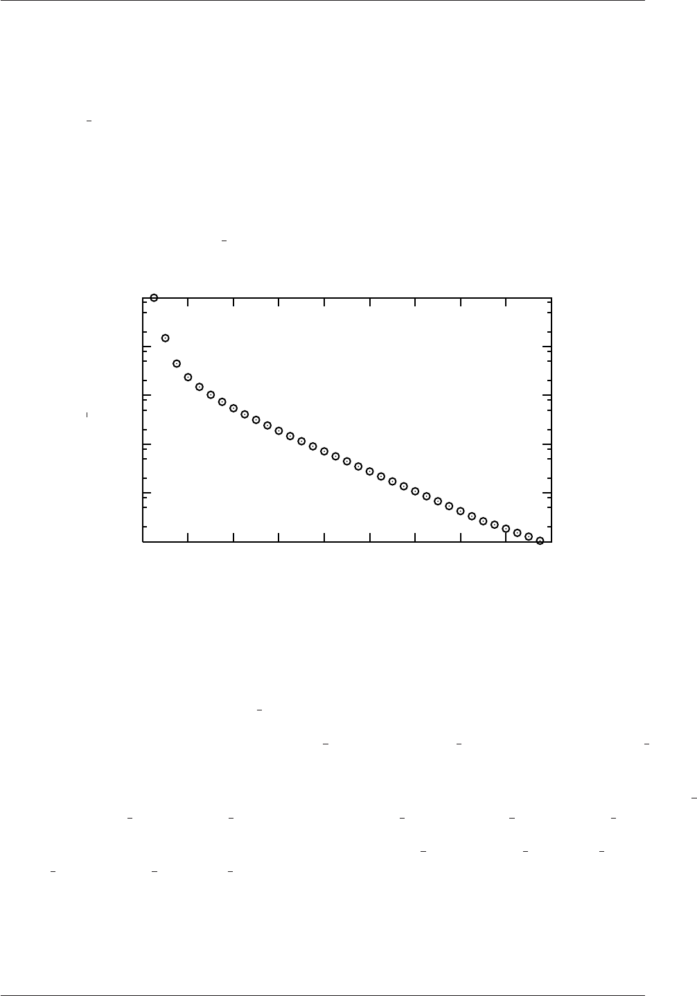
6.7 Monitoring and managing jobs U-191
foamLog <logFile>
The files are stored in a subdirectory of the case directory named logs. Each file has the
name <var><subIter>where <var>is the name of the variable specified in the log file and
<subIter>is the iteration number within the time step. Those variables that are solved for,
the initial residual takes the variable name <var>and final residual takes <var>FinalRes.
By default, the files are presented in two-column format of time and the extracted values.
For example, in the cavity tutorial we may wish to observe the initial residual of the Ux
equation to see whether the solution is converging to a steady-state. In that case, we would
plot the data from the logs/Ux 0file as shown in Figure 6.5. It can be seen here that the
residual falls monotonically until it reaches the convergence tolerance of 10−5.
Time [s]
Ux 0
0.180.160.140.120.100.080.060.040.020.00
1e+00
1e-01
1e-02
1e-03
1e-04
1e-05
Figure 6.5: Initial residual of Ux in the cavity tutorial
foamLog generates files for everything it feasibly can from the log file. In the cavity
tutorial example, this includes:
•the Courant number, Courant 0;
•Ux equation initial and final residuals, Ux 0and UxFinalRes 0, and iterations, UxIters 0
(and equivalent Uy data);
•cumulative, global and local continuity errors after each of the 2 pequations, contCumulative 0,
contGlobal 0,contLocal 0 and contCumulative 1,contGlobal 1,contLocal 1;
•residuals and iterations from the the 2 pequations p0,pFinalRes 0,pIters 0 and
p1,pFinalRes 1,pIters 1;
•and execution time, executionTime.
OpenFOAM-2.4.0

U-192 Post-processing
OpenFOAM-2.4.0

Chapter 7
Models and physical properties
OpenFOAM includes a large range of solvers each designed for a specific class of problem.
The equations and algorithms differ from one solver to another so that the selection of a
solver involves the user making some initial choices on the modelling for their particular case.
The choice of solver typically involves scanning through their descriptions in Table 3.5 to find
the one suitable for the case. It ultimately determines many of the parameters and physical
properties required to define the case but leaves the user with some modelling options that
can be specified at runtime through the entries in dictionary files in the constant directory of
a case. This chapter deals with many of the more common models and associated properties
that may be specified at runtime.
7.1 Thermophysical models
Thermophysical models are concerned with the energy, heat and physical properties.
The thermophysicalProperties dictionary is read by any solver that uses the thermophys-
ical model library. A thermophysical model is constructed in OpenFOAM as a pressure-
temperature p−Tsystem from which other properties are computed. There is one compul-
sory dictionary entry called thermoType which specifies the complete thermophysical model
that is used in the simulation. The thermophysical modelling starts with a layer that defines
the basic equation of state and then adds more layers of modelling that derive properties
from the previous layer(s). The naming of the thermoType reflects these multiple layers of
modelling as listed in Table 7.1.
Equation of State —equationOfState
adiabaticPerfectFluid Adiabatic perfect gas equation of state
icoPolynomial Incompressible polynomial equation of state, e.g. for liquids
perfectFluid Perfect gas equation of state
incompressiblePerfectGas Incompressible gas equation of state using a constant ref-
erence pressure. Density only varies with temperature and
composition
rhoConst Constant density equation of state
Basic thermophysical properties —thermo
eConstThermo Constant specific heat cpmodel with evaluation of internal
energy eand entropy s
Continued on next page

U-194 Models and physical properties
Continued from previous page
hConstThermo Constant specific heat cpmodel with evaluation of enthalpy
hand entropy s
hPolynomialThermo cpevaluated by a function with coefficients from polynomi-
als, from which h,sare evaluated
janafThermo cpevaluated by a function with coefficients from JANAF
thermodynamic tables, from which h,sare evaluated
Derived thermophysical properties —specieThermo
specieThermo Thermophysical properties of species, derived from cp,h
and/or s
Transport properties —transport
constTransport Constant transport properties
polynomialTransport Polynomial based temperature-dependent transport prop-
erties
sutherlandTransport Sutherland’s formula for temperature-dependent transport
properties
Mixture properties —mixture
pureMixture General thermophysical model calculation for passive gas
mixtures
homogeneousMixture Combustion mixture based on normalised fuel mass frac-
tion b
inhomogeneousMixture Combustion mixture based on band total fuel mass fraction
ft
veryInhomogeneousMixture Combustion mixture based on b,ftand unburnt fuel mass
fraction fu
basicMultiComponent-
Mixture
Basic mixture based on multiple components
multiComponentMixture Derived mixture based on multiple components
reactingMixture Combustion mixture using thermodynamics and reaction
schemes
egrMixture Exhaust gas recirculation mixture
singleStepReactingMixture Single step reacting mixture
Thermophysical model —thermoModel
hePsiThermo General thermophysical model calculation based on com-
pressibility ψ
heRhoThermo General thermophysical model calculation based on density
ρ
psiReactionThermo Calculates enthalpy for combustion mixture based on ψ
psiuReactionThermo Calculates enthalpy for combustion mixture based on ψu
rhoReactionThermo Calculates enthalpy for combustion mixture based on ρ
heheupsiReactionThermo Calculates enthalpy for unburnt gas and combustion mix-
ture
Continued on next page
OpenFOAM-2.4.0

7.1 Thermophysical models U-195
Continued from previous page
Table 7.1: Layers of thermophysical modelling.
The following is an example entry for thermoType:
thermoType
{type hePsiThermo;
mixture pureMixture;
transport const;
thermo hConst;
equationOfState perfectGas;
specie specie;
energy sensibleEnthalpy;
}
The keyword entries specify the choice of thermophysical models, e.g. constant transport
(constant viscosity, thermal diffusion), Perfect Gas equationOfState,etc. In addition there
is a keyword entry named energy that allows the user to specify the form of energy to be
used in the solution and thermodynamics. The energy can be internal energy or enthalpy
and in forms that include the heat of formation ∆hfor not. We refer to absolute energy
where heat of formation is included, and sensible energy where it is not. For example
absolute enthalpy his related to sensible enthalpy hsby
h=hs+X
i
ci∆hi
f(7.1)
where ciand hi
fare the molar fraction and heat of formation, respectively, of specie i. In most
cases, we use the sensible form of energy, for which it is easier to account for energy change
due to reactions. Keyword entries for energy therefore include e.g. sensibleEnthalpy,
sensibleInternalEnergy and absoluteEnthalpy.
7.1.1 Thermophysical property data
The basic thermophysical properties are specified for each species from input data. Data
entries must contain the name of the specie as the keyword, e.g. O2,H2O,mixture, followed
by sub-dictionaries of coefficients, including:
specie containing i.e. number of moles, nMoles, of the specie, and molecular weight,
molWeight in units of g/mol;
thermodynamics containing coefficients for the chosen thermodynamic model (see below);
transport containing coefficients for the chosen tranpsort model (see below).
The thermodynamic coefficients are ostensibly concerned with evaluating the specific
heat cpfrom which other properties are derived. The current thermo models are described
as follows:
OpenFOAM-2.4.0

U-196 Models and physical properties
hConstThermo assumes a constant cpand a heat of fusion Hfwhich is simply specified by
a two values cpHf, given by keywords Cp and Hf.
eConstThermo assumes a constant cvand a heat of fusion Hfwhich is simply specified by
a two values cvHf, given by keywords Cv and Hf.
janafThermo calculates cpas a function of temperature Tfrom a set of coefficients taken
from JANAF tables of thermodynamics. The ordered list of coefficients is given in
Table 7.2. The function is valid between a lower and upper limit in temperature Tl
and Threspectively. Two sets of coefficients are specified, the first set for temperatures
above a common temperature Tc(and below Th, the second for temperatures below
Tc(and above Tl). The function relating cpto temperature is:
cp=R((((a4T+a3)T+a2)T+a1)T+a0) (7.2)
In addition, there are constants of integration, a5and a6, both at high and low tem-
perature, used to evaluating hand srespectively.
hPolynomialThermo calculates Cpas a function of temperature by a polynomial of any order.
The following case provides an example of its use: $FOAM TUTORIALS/lagrangian/-
porousExplicitSourceReactingParcelFoam/filter
Description Entry Keyword
Lower temperature limit Tl(K) Tlow
Upper temperature limit Th(K) Thigh
Common temperature Tc(K) Tcommon
High temperature coefficients a0. . . a4highCpCoeffs (a0 a1 a2 a3 a4...
High temperature enthalpy offset a5a5...
High temperature entropy offset a6a6)
Low temperature coefficients a0. . . a4lowCpCoeffs (a0 a1 a2 a3 a4...
Low temperature enthalpy offset a5a5...
Low temperature entropy offset a6a6)
Table 7.2: JANAF thermodynamics coefficients.
The transport coefficients are used to to evaluate dynamic viscosity µ, thermal conduc-
tivity κand laminar thermal conductivity (for enthalpy equation) α. The current transport
models are described as follows:
constTransport assumes a constant µand Prandtl number P r =cpµ/κ which is simply
specified by a two keywords, mu and Pr, respectively.
sutherlandTransport calculates µas a function of temperature Tfrom a Sutherland coefficient
Asand Sutherland temperature Ts, specified by keywords As and Ts;µis calculated
according to:
µ=As√T
1 + Ts/T (7.3)
OpenFOAM-2.4.0

7.1 Thermophysical models U-197
polynomialTransport calculates µand κas a function of temperature Tfrom a polynomial
of any order.
The following is an example entry for a specie named fuel modelled using sutherlandTrans-
port and janafThermo:
fuel
{specie
{nMoles 1;
molWeight 16.0428;
}
thermodynamics
{Tlow 200;
Thigh 6000;
Tcommon 1000;
highCpCoeffs (1.63543 0.0100844 -3.36924e-06 5.34973e-10
-3.15528e-14 -10005.6 9.9937);
lowCpCoeffs (5.14988 -0.013671 4.91801e-05 -4.84744e-08
1.66694e-11 -10246.6 -4.64132);
}
transport
{As 1.67212e-06;
Ts 170.672;
}
}
The following is an example entry for a specie named air modelled using constTransport
and hConstThermo:
air
{specie
{nMoles 1;
molWeight 28.96;
}
thermodynamics
{Cp 1004.5;
Hf 2.544e+06;
}
transport
{mu 1.8e-05;
OpenFOAM-2.4.0

U-198 Models and physical properties
Pr 0.7;
}
}
7.2 Turbulence models
The turbulenceProperties dictionary is read by any solver that includes turbulence mod-
elling. Within that file is the simulationType keyword that controls the type of turbulence
modelling to be used, either:
laminar uses no turbulence models;
RASModel uses Reynolds-averaged stress (RAS) modelling;
LESModel uses large-eddy simulation (LES) modelling.
If RASModel is selected, the choice of RAS modelling is specified in a RASProperties file,
also in the constant directory. The RAS turbulence model is selected by the RASModel entry
from a long list of available models that are listed in Table 3.9. Similarly, if LESModel is
selected, the choice of LES modelling is specified in a LESProperties dictionary and the LES
turbulence model is selected by the LESModel entry.
The entries required in the RASProperties are listed in Table 7.3 and those for LESProp-
erties dictionaries are listed in Table 7.4.
RASModel Name of RAS turbulence model
turbulence Switch to turn turbulence modelling on/off
printCoeffs Switch to print model coeffs to terminal at simulation startup
<RASModel>Coeffs Optional dictionary of coefficients for the respective RASModel
Table 7.3: Keyword entries in the RASProperties dictionary.
LESModel Name of LES model
delta Name of delta δmodel
<LESModel>Coeffs Dictionary of coefficients for the respective LESModel
<delta>Coeffs Dictionary of coefficients for each delta model
Table 7.4: Keyword entries in the LESProperties dictionary.
The incompressible and compressible RAS turbulence models, isochoric and anisochoric
LES models and delta models are all named and described in Table 3.9. Examples of their
use can be found in the $FOAM TUTORIALS.
7.2.1 Model coefficients
The coefficients for the RAS turbulence models are given default values in their respective
source code. If the user wishes to override these default values, then they can do so by adding
a sub-dictionary entry to the RASProperties file, whose keyword name is that of the model
OpenFOAM-2.4.0

7.2 Turbulence models U-199
with Coeffs appended, e.g. kEpsilonCoeffs for the kEpsilon model. If the printCoeffs
switch is on in the RASProperties file, an example of the relevant ...Coeffs dictionary is
printed to standard output when the model is created at the beginning of a run. The user
can simply copy this into the RASProperties file and edit the entries as required.
7.2.2 Wall functions
A range of wall function models is available in OpenFOAM that are applied as boundary
conditions on individual patches. This enables different wall function models to be applied
to different wall regions. The choice of wall function model is specified through: νtin the
0/nut file for incompressible RAS; µtin the 0/mut file for compressible RAS; νsgs in the
0/nuSgs file for incompressible LES; µsgs in the 0/muSgs file for incompressible LES. For
example, a 0/nut file:
17
18 dimensions [0 2 -1 0 0 0 0];
19
20 internalField uniform 0;
21
22 boundaryField
23 {
24 movingWall
25 {
26 type nutkWallFunction;
27 value uniform 0;
28 }
29 fixedWalls
30 {
31 type nutkWallFunction;
32 value uniform 0;
33 }
34 frontAndBack
35 {
36 type empty;
37 }
38 }
39
40
41 // ************************************************************************* //
There are a number of wall function models available in the release, e.g. nutWallFunc-
tion,nutRoughWallFunction,nutSpalartAllmarasStandardRoughWallFunction,nut-
SpalartAllmarasStandardWallFunction and nutSpalartAllmarasWallFunction. The
user can consult the relevant directories for a full list of wall function models:
find $FOAM SRC/turbulenceModels -name wallFunctions
Within each wall function boundary condition the user can over-ride default settings for E,
κand Cµthrough optional E,kappa and Cmu keyword entries.
Having selected the particular wall functions on various patches in the nut/mut file,
the user should select epsilonWallFunction on corresponding patches in the epsilon field and
kqRwallFunction on corresponding patches in the turbulent fields k,qand R.
OpenFOAM-2.4.0

U-200 Models and physical properties
OpenFOAM-2.4.0

Index U-201
Index
Symbols Numbers A B C D E F G H I J K L M N O P Q R S T U V W X Z
Symbols
*
tensor member function, P-23
+
tensor member function, P-23
-
tensor member function, P-23
/
tensor member function, P-23
/*...*/
C++ syntax, U-79
//
C++ syntax, U-79
OpenFOAM file syntax, U-108
# include
C++ syntax, U-72,U-79
&
tensor member function, P-23
&&
tensor member function, P-23
^
tensor member function, P-23
<LESModel>Coeffs keyword, U-198
<RASModel>Coeffs keyword, U-198
<delta>Coeffs keyword, U-198
0.000000e+00 directory, U-108
1-dimensional mesh, U-135
1D mesh, U-135
2-dimensional mesh, U-135
2D mesh, U-135
Numbers
0directory, U-108
A
access functions, P-21
addLayersControls keyword, U-153
adiabaticFlameT utility, U-99
adiabaticPerfectFluid model, U-103,U-193
adjointShapeOptimizationFoam solver, U-87
adjustableRunTime
keyword entry, U-62,U-116
adjustTimeStep keyword, U-61,U-117
agglomerator keyword, U-128
algorithms tools, U-99
alphaContactAngle
boundary condition, U-59
analytical solution, P-43
Animations window panel, U-176
anisotropicFilter model, U-105
Annotation window panel, U-25,U-176
ansysToFoam utility, U-93
APIfunctions model, U-103
applications, U-69
Apply button, U-172,U-176
applyBoundaryLayer utility, U-92
applyWallFunctionBoundaryConditions utility,
U-92
arbitrarily unstructured, P-29
arc
keyword entry, U-145
arc keyword, U-144
As keyword, U-196
ascii
keyword entry, U-116
attachMesh utility, U-93
Auto Accept button, U-176
autoMesh
library, U-100
autoPatch utility, U-93
autoRefineMesh utility, U-94
axes
right-handed, U-143
right-handed rectangular Cartesian, P-13,
U-18
axi-symmetric cases, U-140,U-151
axi-symmetric mesh, U-135
OpenFOAM-2.4.0

U-202 Index
B
background
process, U-25,U-82
backward
keyword entry, U-124
Backward differencing, P-37
barotropicCompressibilityModels
library, U-103
basicMultiComponentMixture model, U-102,
U-194
basicSolidThermo
library, U-104
basicThermophysicalModels
library, U-102
binary
keyword entry, U-116
BirdCarreau model, U-106
blended differencing, P-36
block
expansion ratio, U-145
block keyword, U-144
blocking
keyword entry, U-81
blockMesh
library, U-100
blockMesh solver, P-45
blockMesh utility, U-37,U-92,U-141
blockMesh executable
vertex numbering, U-145
blockMeshDict
dictionary, U-18,U-20,U-36,U-49,U-141,
U-151
blocks keyword, U-20,U-31,U-145
boundaries, U-135
boundary, U-135
boundary
dictionary, U-134,U-141
boundary keyword, U-147, U-148
boundary condition
alphaContactAngle,U-59
buoyantPressure,U-142
calculated,U-141
cyclic,U-140,U-149
directionMixed,U-141
empty,P-63,P-69,U-18,U-135,U-140
fixedGradient,U-141
fixedValue,U-141
fluxCorrectedVelocity,U-142
inlet,P-69
inletOutlet,U-142
mixed,U-141
movingWallVelocity,U-142
outlet,P-69
outletInlet,U-142
partialSlip,U-142
patch,U-139
pressureDirectedInletVelocity,U-142
pressureInletVelocity,U-142
pressureOutlet,P-63
pressureTransmissive,U-142
processor,U-140
setup, U-20
slip,U-142
supersonicFreeStream,U-142
surfaceNormalFixedValue,U-142
symmetryPlane,P-63,U-140
totalPressure,U-142
turbulentInlet,U-142
wall, U-40
wall,P-63,P-69,U-58,U-139, U-140
wedge,U-135,U-140,U-151
zeroGradient,U-141
boundary conditions, P-41
Dirichlet, P-41
inlet, P-42
Neumann, P-41
no-slip impermeable wall, P-42
outlet, P-42
physical, P-42
symmetry plane, P-42
boundaryField keyword, U-21,U-112
boundaryFoam solver, U-87
bounded
keyword entry, U-122, U-123
boxToCell keyword, U-60
boxTurb utility, U-92
breaking of a dam, U-56
buoyantBoussinesqPimpleFoam solver, U-90
buoyantBoussinesqSimpleFoam solver, U-90
buoyantPimpleFoam solver, U-90
buoyantPressure
boundary condition, U-142
buoyantSimpleFoam solver, U-90
button
Apply,U-172,U-176
Auto Accept,U-176
Choose Preset,U-174
Delete,U-172
Edit Color Map,U-174
Enable Line Series,U-35
OpenFOAM-2.4.0

Index U-203
Orientation Axes,U-25,U-176
Refresh Times,U-25
Rescale to Data Range,U-25
Reset,U-172
Set Ambient Color,U-175
Update GUI,U-173
Use Parallel Projection,U-25
Use parallel projection,U-175
C
C++ syntax
/*...*/,U-79
//,U-79
# include,U-72,U-79
cacheAgglomeration keyword, U-128
calculated
boundary condition, U-141
cAlpha keyword, U-63
cases, U-107
castellatedMesh keyword, U-153
castellatedMeshControls
dictionary, U-154–U-156
castellatedMeshControls keyword, U-153
cavitatingDyMFoam solver, U-88
cavitatingFoam solver, U-88
cavity flow, U-17
ccm26ToFoam utility, U-93
CEI ARCH
environment variable, U-186
CEI HOME
environment variable, U-186
cell
expansion ratio, U-145
cell class, P-29
cell
keyword entry, U-187
cellLimited
keyword entry, U-122
cellPoint
keyword entry, U-187
cellPointFace
keyword entry, U-187
cells
dictionary, U-141
central differencing, P-36
cfdTools tools, U-100
cfx4ToFoam utility, U-93,U-160
changeDictionary utility, U-92
Charts window panel, U-176
checkMesh utility, U-93,U-162
chemFoam solver, U-89
chemistryModel
library, U-103
chemistryModel model, U-103
chemistrySolver model, U-103
chemkinToFoam utility, U-99
Choose Preset button, U-174
chtMultiRegionSimpleFoam solver, U-90
chtMultiRegionFoam solver, U-90
Chung
library, U-103
class
cell,P-29
dimensionSet,P-24,P-30, P-31
face,P-29
finiteVolumeCalculus,P-34
finiteVolumeMethod,P-34
fvMesh,P-29
fvSchemes,P-36
fvc,P-34
fvm,P-34
pointField,P-29
polyBoundaryMesh,P-29
polyMesh,P-29,U-131,U-133
polyPatchList,P-29
polyPatch,P-29
scalarField,P-27
scalar,P-22
slice,P-29
symmTensorField,P-27
symmTensorThirdField,P-27
tensorField,P-27
tensorThirdField,P-27
tensor,P-22
vectorField,P-27
vector,P-22,U-111
word,P-24,P-29
class keyword, U-109
clockTime
keyword entry, U-116
cloud keyword, U-189
cloudFunctionObjects
library, U-100
cmptAv
tensor member function, P-23
Co utility, U-95
coalChemistryFoam solver, U-90
coalCombustion
library, U-101
cofactors
tensor member function, P-23
OpenFOAM-2.4.0

U-204 Index
coldEngineFoam solver, U-89
collapseEdges utility, U-94
Color By menu, U-175
Color Legend window, U-27
Color Legend window panel, U-174
Color Scale window panel, U-174
Colors window panel, U-176
compressibleInterDyMFoam solver, U-88
compressibleInterFoam solver, U-88
compressibleMultiphaseInterFoam solver, U-88
combinePatchFaces utility, U-95
comments, U-79
commsType keyword, U-81
compressed
keyword entry, U-116
compressibleLESModels
library, U-105
compressibleRASModels
library, U-104
constant directory, U-107,U-193
constant model, U-102
constTransport model, U-103,U-194
containers tools, U-99
continuum
mechanics, P-13
control
of time, U-115
controlDict
dictionary, P-65,U-22,U-31,U-42,U-51,
U-62,U-107,U-168
controlDict file, P-48
convection, see divergence, P-36
convergence, U-39
conversion
library, U-101
convertToMeters keyword, U-143, U-144
coordinate
system, P-13
coordinate system, U-18
corrected
keyword entry, U-122, U-123
Courant number, P-40,U-22
Cp keyword, U-196
cpuTime
keyword entry, U-116
Crank Nicolson
temporal discretisation, P-41
CrankNicolson
keyword entry, U-124
createExternalCoupledPatchGeometry utility,
U-92
createBaffles utility, U-93
createPatch utility, U-93
createTurbulenceFields utility, U-96
cross product, see tensor, vector cross product
CrossPowerLaw
keyword entry, U-60
CrossPowerLaw model, U-106
cubeRootVolDelta model, U-105
cubicCorrected
keyword entry, U-124
cubicCorrection
keyword entry, U-121
curl, P-35
curl
fvc member function, P-35
Current Time Controls menu, U-25,U-173
curve keyword, U-189
Cv keyword, U-196
cyclic
boundary condition, U-140,U-149
cyclic
keyword entry, U-140
cylinder
flow around a, P-43
D
d2dt2
fvc member function, P-35
fvm member function, P-35
dam
breaking of a, U-56
datToFoam utility, U-93
db tools, U-99
ddt
fvc member function, P-35
fvm member function, P-35
DeardorffDiffStress model, U-105, U-106
debug keyword, U-153
decompose model, U-101
decomposePar utility, U-82, U-83,U-98
decomposeParDict
dictionary, U-82
decomposition
of field, U-82
of mesh, U-82
decompositionMethods
library, U-101
decompression of a tank, P-61
defaultFieldValues keyword, U-60
OpenFOAM-2.4.0

Index U-205
deformedGeom utility, U-94
Delete button, U-172
delta keyword, U-84,U-198
deltaT keyword, U-116
dependencies, U-72
dependency lists, U-72
det
tensor member function, P-23
determinant, see tensor, determinant
dev
tensor member function, P-23
diag
tensor member function, P-23
diagonal
keyword entry, U-126, U-127
DIC
keyword entry, U-127
DICGaussSeidel
keyword entry, U-127
dictionary
LESProperties,U-198
PISO,U-23
blockMeshDict,U-18,U-20,U-36,U-49,
U-141,U-151
boundary,U-134,U-141
castellatedMeshControls,U-154–U-156
cells,U-141
controlDict,P-65,U-22,U-31,U-42,U-51,
U-62,U-107,U-168
decomposeParDict,U-82
faces,U-133,U-141
fvSchemes,U-62, U-63,U-107,U-118
fvSolution,U-107,U-125
mechanicalProperties,U-51
neighbour,U-134
owner,U-133
points,U-133,U-141
thermalProperties,U-51
thermophysicalProperties,U-193
transportProperties,U-21,U-38,U-42
turbulenceProperties,U-41,U-61,U-198
differencing
Backward, P-37
blended, P-36
central, P-36
Euler implicit, P-37
Gamma, P-36
MINMOD, P-36
SUPERBEE, P-36
upwind, P-36
van Leer, P-36
DILU
keyword entry, U-127
dimension
checking in OpenFOAM, P-24,U-111
dimensional units, U-111
dimensioned<Type>template class, P-24
dimensionedTypes tools, U-100
dimensions keyword, U-21,U-112
dimensionSet class, P-24,P-30, P-31
dimensionSet tools, U-100
directionMixed
boundary condition, U-141
directory
0.000000e+00,U-108
0,U-108
Make,U-73
constant,U-107,U-193
fluentInterface,U-183
polyMesh,U-107,U-133
processorN,U-83
run,U-107
system,P-48,U-107
tutorials,P-43,U-17
discretisation
equation, P-31
Display window panel, U-24, U-25,U-172, U-173
distance
keyword entry, U-156,U-189
distributed model, U-101
distributed keyword, U-84, U-85
distributionModels
library, U-101
div
fvc member function, P-35
fvm member function, P-35
divergence, P-35,P-37
divSchemes keyword, U-118
dnsFoam solver, U-89
doLayers keyword, U-153
double inner product, see tensor,double inner
product
DPMFoam solver, U-90
dsmc
library, U-101
dsmcFieldsCalc utility, U-97
dsmcFoam solver, U-91
dsmcInitialise utility, U-92
dx
keyword entry, U-187
OpenFOAM-2.4.0
U-206 Index
dynamicFvMesh
library, U-100
dynamicMesh
library, U-100
dynLagrangian model, U-105
dynOneEqEddy model, U-105
E
eConstThermo model, U-103,U-193
edgeGrading keyword, U-146
edgeMesh
library, U-101
edges keyword, U-144
Edit menu, U-175, U-176
Edit Color Map button, U-174
egrMixture model, U-102,U-194
electrostaticFoam solver, U-91
empty
boundary condition, P-63,P-69,U-18,
U-135,U-140
empty
keyword entry, U-140
Enable Line Series button, U-35
endTime keyword, U-22,U-115, U-116
energy keyword, U-195
engine
library, U-101
engineCompRatio utility, U-97
engineFoam solver, U-89
engineSwirl utility, U-92
ensight74FoamExec utility, U-185
ENSIGHT7 INPUT
environment variable, U-186
ENSIGHT7 READER
environment variable, U-186
ensightFoamReader utility, U-95
enstrophy utility, U-95
environment variable
CEI ARCH,U-186
CEI HOME,U-186
ENSIGHT7 INPUT,U-186
ENSIGHT7 READER,U-186
FOAM RUN,U-107
WM ARCH OPTION,U-76
WM ARCH,U-76
WM COMPILER BIN,U-76
WM COMPILER DIR,U-76
WM COMPILER LIB,U-76
WM COMPILER,U-76
WM COMPILE OPTION,U-76
WM DIR,U-76
WM MPLIB,U-76
WM OPTIONS,U-76
WM PRECISION OPTION,U-76
WM PROJECT DIR,U-76
WM PROJECT INST DIR,U-76
WM PROJECT USER DIR,U-76
WM PROJECT VERSION,U-76
WM PROJECT,U-76
wmake,U-76
equationOfState keyword, U-195
equilibriumCO utility, U-99
equilibriumFlameT utility, U-99
errorReduction keyword, U-161
Euler
keyword entry, U-124
Euler implicit
differencing, P-37
temporal discretisation, P-40
examples
decompression of a tank, P-61
flow around a cylinder, P-43
flow over backward step, P-50
Hartmann problem, P-67
supersonic flow over forward step, P-58
execFlowFunctionObjects utility, U-97
expandDictionary utility, U-99
expansionRatio keyword, U-160
explicit
temporal discretisation, P-40
extrude2DMesh utility, U-92
extrudeMesh utility, U-92
extrudeToRegionMesh utility, U-92
F
face class, P-29
face keyword, U-189
faceAgglomerate utility, U-92
faceAreaPair
keyword entry, U-128
faceLimited
keyword entry, U-122
faces
dictionary, U-133,U-141
FDIC
keyword entry, U-127
featureAngle keyword, U-160
features keyword, U-154, U-155
field
U,U-23
p,U-23
decomposition, U-82
OpenFOAM-2.4.0

Index U-207
FieldField<Type>template class, P-30
fieldFunctionObjects
library, U-100
fields, P-27
mapping, U-168
fields tools, U-100
fields keyword, U-187
Field<Type>template class, P-27
fieldValues keyword, U-60
file
Make/files,U-75
controlDict,P-48
files,U-73
g,U-61
options,U-73
snappyHexMeshDict,U-152
transportProperties,U-60
file format, U-108
fileFormats
library, U-101
fileModificationChecking keyword, U-81
fileModificationSkew keyword, U-81
files file, U-73
filteredLinear2
keyword entry, U-121
finalLayerThickness keyword, U-160
financialFoam solver, U-91
find script/alias, U-181
finite volume
discretisation, P-25
mesh, P-29
finiteVolume
library, U-100
finiteVolume tools, U-100
finiteVolumeCalculus class, P-34
finiteVolumeMethod class, P-34
fireFoam solver, U-89
firstTime keyword, U-115
fixed
keyword entry, U-116
fixedGradient
boundary condition, U-141
fixedValue
boundary condition, U-141
flattenMesh utility, U-94
floatTransfer keyword, U-81
flow
free surface, U-56
laminar, U-17
steady, turbulent, P-50
supersonic, P-58
turbulent, U-17
flow around a cylinder, P-43
flow over backward step, P-50
flowType utility, U-95
fluent3DMeshToFoam utility, U-93
fluentInterface directory, U-183
fluentMeshToFoam utility, U-93,U-160
fluxCorrectedVelocity
boundary condition, U-142
fluxRequired keyword, U-118
OpenFOAM
cases, U-107
FOAM RUN
environment variable, U-107
foamCalc utility, U-33,U-97
foamCalcFunctions
library, U-100
foamCorrectVrt script/alias, U-166
foamDataToFluent utility, U-95,U-183
foamDebugSwitches utility, U-99
FoamFile keyword, U-109
foamFile
keyword entry, U-187
foamFormatConvert utility, U-99
foamHelp utility, U-99
foamInfoExec utility, U-99
foamJob script/alias, U-190
foamListTimes utility, U-97
foamLog script/alias, U-190
foamMeshToFluent utility, U-93,U-183
foamToEnsight utility, U-95
foamToEnsightParts utility, U-95
foamToGMV utility, U-95
foamToStarMesh utility, U-93
foamToSurface utility, U-93
foamToTecplot360 utility, U-95
foamToVTK utility, U-95
foamUpgradeCyclics utility, U-92
foamUpgradeFvSolution utility, U-92
foamyHexMeshBackgroundMesh utility, U-92
foamyHexMeshSurfaceSimplify utility, U-92
foamyHexMesh utility, U-92
foamyQuadMesh utility, U-93
forces
library, U-100
foreground
process, U-25
format keyword, U-109
fourth
OpenFOAM-2.4.0

U-208 Index
keyword entry, U-122, U-123
functionObjectLibs keyword, U-181
functions keyword, U-117,U-180
fvc class, P-34
fvc member function
curl,P-35
d2dt2,P-35
ddt,P-35
div,P-35
gGrad,P-35
grad,P-35
laplacian,P-35
lsGrad,P-35
snGrad,P-35
snGradCorrection,P-35
sqrGradGrad,P-35
fvDOM
library, U-102
FVFunctionObjects
library, U-100
fvm class, P-34
fvm member function
d2dt2,P-35
ddt,P-35
div,P-35
laplacian,P-35
Su,P-35
SuSp,P-35
fvMatrices tools, U-100
fvMatrix template class, P-34
fvMesh class, P-29
fvMesh tools, U-100
fvMotionSolvers
library, U-101
fvSchemes
dictionary, U-62, U-63,U-107,U-118
fvSchemes class, P-36
fvSchemes
menu entry, U-52
fvSolution
dictionary, U-107,U-125
G
gfile, U-61
gambitToFoam utility, U-93,U-160
GAMG
keyword entry, U-53,U-126, U-127
Gamma
keyword entry, U-121
Gamma differencing, P-36
Gauss
keyword entry, U-122
Gauss’s theorem, P-34
GaussSeidel
keyword entry, U-127
General window panel, U-175, U-176
general
keyword entry, U-116
genericFvPatchField
library, U-101
geometric-algebraic multi-grid, U-127
GeometricBoundaryField template class, P-30
geometricField<Type>template class, P-30
geometry keyword, U-153
gGrad
fvc member function, P-35
global tools, U-100
gmshToFoam utility, U-93
gnuplot
keyword entry, U-117,U-187
grad
fvc member function, P-35
(Grad Grad) squared, P-35
gradient, P-35,P-38
Gauss scheme, P-38
Gauss’s theorem, U-52
least square fit, U-52
least squares method, P-38,U-52
surface normal, P-38
gradSchemes keyword, U-118
graph tools, U-100
graphFormat keyword, U-117
GuldersEGRLaminarFlameSpeed model, U-103
GuldersLaminarFlameSpeed model, U-102
H
hConstThermo model, U-103,U-194
heheupsiReactionThermo model, U-102,U-194
Help menu, U-175
hePsiThermo model, U-102,U-194
heRhoThermo model, U-102,U-194
HerschelBulkley model, U-106
hExponentialThermo
library, U-104
Hf keyword, U-196
hierarchical
keyword entry, U-83, U-84
highCpCoeffs keyword, U-196
homogenousDynOneEqEddy model, U-105, U-106
homogenousDynSmagorinsky model, U-105
homogeneousMixture model, U-102,U-194
hPolynomialThermo model, U-103,U-194
OpenFOAM-2.4.0

Index U-209
I
I
tensor member function, P-23
icoFoam solver, U-17,U-21, U-22,U-25,U-87
icoPolynomial model, U-103,U-193
icoUncoupledKinematicParcelDyMFoam solver,
U-90
icoUncoupledKinematicParcelFoam solver, U-90
ideasToFoam utility, U-160
ideasUnvToFoam utility, U-93
identities, see tensor, identities
identity, see tensor, identity
incompressibleLESModels
library, U-105
incompressiblePerfectGas model, U-103,U-193
incompressibleRASModels
library, U-104
incompressibleTransportModels
library, P-53,U-106
incompressibleTurbulenceModels
library, P-53
index
notation, P-14, P-15
Information window panel, U-172
inhomogeneousMixture model, U-102,U-194
inlet
boundary condition, P-69
inletOutlet
boundary condition, U-142
inner product, see tensor, inner product
inotify
keyword entry, U-81
inotifyMaster
keyword entry, U-81
inside
keyword entry, U-156
insideCells utility, U-94
interPhaseChangeDyMFoam solver, U-88
interPhaseChangeFoam solver, U-88
interDyMFoam solver, U-88
interfaceProperties
library, U-106
interfaceProperties model, U-106
interFoam solver, U-88
interMixingFoam solver, U-88
internalField keyword, U-21,U-112
interpolation tools, U-100
interpolationScheme keyword, U-187
interpolations tools, U-100
interpolationSchemes keyword, U-118
inv
tensor member function, P-23
iterations
maximum, U-127
J
janafThermo model, U-103,U-194
jobControl
library, U-100
jplot
keyword entry, U-117,U-187
K
kEpsilon model, U-104
keyword
As,U-196
Cp,U-196
Cv,U-196
FoamFile,U-109
Hf,U-196
LESModel,U-198
Pr,U-196
RASModel,U-198
Tcommon,U-196
Thigh,U-196
Tlow,U-196
Ts,U-196
addLayersControls,U-153
adjustTimeStep,U-61,U-117
agglomerator,U-128
arc,U-144
blocks,U-20,U-31,U-145
block,U-144
boundaryField,U-21,U-112
boundary,U-147, U-148
boxToCell,U-60
cAlpha,U-63
cacheAgglomeration,U-128
castellatedMeshControls,U-153
castellatedMesh,U-153
class,U-109
cloud,U-189
commsType,U-81
convertToMeters,U-143, U-144
curve,U-189
debug,U-153
defaultFieldValues,U-60
deltaT,U-116
delta,U-84,U-198
dimensions,U-21,U-112
distributed,U-84, U-85
OpenFOAM-2.4.0

U-210 Index
divSchemes,U-118
doLayers,U-153
edgeGrading,U-146
edges,U-144
endTime,U-22,U-115, U-116
energy,U-195
equationOfState,U-195
errorReduction,U-161
expansionRatio,U-160
face,U-189
featureAngle,U-160
features,U-154, U-155
fieldValues,U-60
fields,U-187
fileModificationChecking,U-81
fileModificationSkew,U-81
finalLayerThickness,U-160
firstTime,U-115
floatTransfer,U-81
fluxRequired,U-118
format,U-109
functionObjectLibs,U-181
functions,U-117,U-180
geometry,U-153
gradSchemes,U-118
graphFormat,U-117
highCpCoeffs,U-196
internalField,U-21,U-112
interpolationSchemes,U-118
interpolationScheme,U-187
laplacianSchemes,U-118
latestTime,U-38
layers,U-160
leastSquares,U-52
levels,U-156
libs,U-81,U-117
locationInMesh,U-155, U-156
location,U-109
lowCpCoeffs,U-196
manualCoeffs,U-84
maxAlphaCo,U-61
maxBoundarySkewness,U-161
maxConcave,U-161
maxCo,U-61,U-117
maxDeltaT,U-62
maxFaceThicknessRatio,U-160
maxGlobalCells,U-155
maxInternalSkewness,U-161
maxIter,U-127
maxLocalCells,U-155
maxNonOrtho,U-161
maxThicknessToMedialRatio,U-160
mergeLevels,U-128
mergePatchPairs,U-144
mergeTolerance,U-153
meshQualityControls,U-153
method,U-84
midPointAndFace,U-189
midPoint,U-189
minArea,U-161
minDeterminant,U-161
minFaceWeight,U-161
minFlatness,U-161
minMedianAxisAngle,U-160
minRefinementCells,U-155
minThickness,U-160
minTriangleTwist,U-161
minTwist,U-161
minVolRatio,U-161
minVol,U-161
mode,U-156
molWeight,U-195
mu,U-196
nAlphaSubCycles,U-63
nBufferCellsNoExtrude,U-160
nCellsBetweenLevels,U-155
nFaces,U-134
nFinestSweeps,U-128
nGrow,U-160
nLayerIter,U-160
nMoles,U-195
nPostSweeps,U-128
nPreSweeps,U-128
nRelaxIter,U-159, U-160
nRelaxedIter,U-160
nSmoothNormals,U-160
nSmoothPatch,U-159
nSmoothScale,U-161
nSmoothSurfaceNormals,U-160
nSmoothThickness,U-160
nSolveIter,U-159
neighbourPatch,U-149
numberOfSubdomains,U-84
n,U-84
object,U-109
order,U-84
outputControl,U-181
pRefCell,U-23,U-130
pRefValue,U-23,U-130
p rhgRefCell,U-130
OpenFOAM-2.4.0

Index U-211
p rhgRefValue,U-130
patchMap,U-168
patches,U-144
preconditioner,U-126, U-127
pressure,U-51
printCoeffs,U-41,U-198
processorWeights,U-83
processorWeights,U-84
purgeWrite,U-116
refGradient,U-141
refinementRegions,U-155, U-156
refinementSurfaces,U-155
refinementRegions,U-156
regions,U-60
relTol,U-53,U-126
relativeSizes,U-160
relaxed,U-161
resolveFeatureAngle,U-155
roots,U-84, U-85
runTimeModifiable,U-117
scotchCoeffs,U-84
setFormat,U-187
sets,U-187
simpleGrading,U-145
simulationType,U-41,U-61,U-198
smoother,U-128
snGradSchemes,U-118
snapControls,U-153
snap,U-153
solvers,U-125
solver,U-53,U-126
specie,U-195
spline,U-144
startFace,U-134
startFrom,U-22,U-115
startTime,U-22,U-115
stopAt,U-115
strategy,U-83, U-84
surfaceFormat,U-187
surfaces,U-187
thermoType,U-193
thermodynamics,U-195
timeFormat,U-116
timePrecision,U-117
timeScheme,U-118
tolerance,U-53,U-126,U-159
topoSetSource,U-60
traction,U-51
transport,U-195
turbulence,U-198
type,U-135,U-138
uniform,U-189
valueFraction,U-141
value,U-21,U-141
version,U-109
vertices,U-20,U-144
writeCompression,U-116
writeControl,U-22,U-62,U-116
writeFormat,U-55,U-116
writeInterval,U-22,U-32,U-116
writePrecision,U-116
<LESModel>Coeffs,U-198
<RASModel>Coeffs,U-198
<delta>Coeffs,U-198
keyword entry
CrankNicolson,U-124
CrossPowerLaw,U-60
DICGaussSeidel,U-127
DIC,U-127
DILU,U-127
Euler,U-124
FDIC,U-127
GAMG,U-53,U-126, U-127
Gamma,U-121
GaussSeidel,U-127
Gauss,U-122
LESModel,U-41,U-198
MGridGen,U-128
MUSCL,U-121
Newtonian,U-60
PBiCG,U-126
PCG,U-126
QUICK,U-124
RASModel,U-41,U-198
SFCD,U-121,U-124
UMIST,U-120
adjustableRunTime,U-62,U-116
arc,U-145
ascii,U-116
backward,U-124
binary,U-116
blocking,U-81
bounded,U-122, U-123
cellLimited,U-122
cellPointFace,U-187
cellPoint,U-187
cell,U-187
clockTime,U-116
compressed,U-116
corrected,U-122, U-123
OpenFOAM-2.4.0

U-212 Index
cpuTime,U-116
cubicCorrected,U-124
cubicCorrection,U-121
cyclic,U-140
diagonal,U-126, U-127
distance,U-156,U-189
dx,U-187
empty,U-140
faceAreaPair,U-128
faceLimited,U-122
filteredLinear2,U-121
fixed,U-116
foamFile,U-187
fourth,U-122, U-123
general,U-116
gnuplot,U-117,U-187
hierarchical,U-83, U-84
inotifyMaster,U-81
inotify,U-81
inside,U-156
jplot,U-117,U-187
laminar,U-41,U-198
latestTime,U-115
leastSquares,U-122
limitedCubic,U-121
limitedLinear,U-121
limited,U-122, U-123
linearUpwind,U-121,U-124
linear,U-121,U-124
line,U-145
localEuler,U-124
manual,U-83, U-84
metis,U-84
midPoint,U-121
nextWrite,U-116
noWriteNow,U-116
nonBlocking,U-81
none,U-119,U-127
null,U-187
outputTime,U-181
outside,U-156
patch,U-140,U-188
polyLine,U-145
polySpline,U-145
processor,U-140
raw,U-117,U-187
runTime,U-32,U-116
scheduled,U-81
scientific,U-116
scotch,U-83, U-84
simpleSpline,U-145
simple,U-83, U-84
skewLinear,U-121,U-124
smoothSolver,U-126
startTime,U-22,U-115
steadyState,U-124
stl,U-187
symmetryPlane,U-140
timeStampMaster,U-81
timeStamp,U-81
timeStep,U-22,U-32,U-116,U-181
uncompressed,U-116
uncorrected,U-122, U-123
upwind,U-121,U-124
vanLeer,U-121
vtk,U-187
wall,U-140
wedge,U-140
writeControl,U-116
writeInterval,U-181
writeNow,U-115
xmgr,U-117,U-187
xyz,U-189
x,U-189
y,U-189
z,U-189
kivaToFoam utility, U-93
kkLOmega model, U-104
kOmega model, U-104
kOmegaSST model, U-104
kOmegaSSTSAS model, U-105
Kronecker delta, P-19
L
lagrangian
library, U-101
lagrangianIntermediate
library, U-101
Lambda2 utility, U-95
LamBremhorstKE model, U-104
laminar model, U-104, U-105
laminar
keyword entry, U-41,U-198
laminarFlameSpeedModels
library, U-102
laplaceFilter model, U-105
Laplacian, P-36
laplacian, P-35
laplacian
fvc member function, P-35
fvm member function, P-35
OpenFOAM-2.4.0

Index U-213
laplacianFoam solver, U-86
laplacianSchemes keyword, U-118
latestTime
keyword entry, U-115
latestTime keyword, U-38
LaunderGibsonRSTM model, U-104, U-105
LaunderSharmaKE model, U-104
layers keyword, U-160
leastSquares
keyword entry, U-122
leastSquares keyword, U-52
LESdeltas
library, U-105
LESfilters
library, U-105
LESModel
keyword entry, U-41,U-198
LESModel keyword, U-198
LESProperties
dictionary, U-198
levels keyword, U-156
libraries, U-69
library
Chung,U-103
FVFunctionObjects,U-100
LESdeltas,U-105
LESfilters,U-105
MGridGenGAMGAgglomeration,U-101
ODE,U-101
OSspecific,U-101
OpenFOAM,U-99
P1,U-102
PV3FoamReader,U-171
PVFoamReader,U-171
SLGThermo,U-104
Wallis,U-103
autoMesh,U-100
barotropicCompressibilityModels,U-103
basicSolidThermo,U-104
basicThermophysicalModels,U-102
blockMesh,U-100
chemistryModel,U-103
cloudFunctionObjects,U-100
coalCombustion,U-101
compressibleLESModels,U-105
compressibleRASModels,U-104
conversion,U-101
decompositionMethods,U-101
distributionModels,U-101
dsmc,U-101
dynamicFvMesh,U-100
dynamicMesh,U-100
edgeMesh,U-101
engine,U-101
fieldFunctionObjects,U-100
fileFormats,U-101
finiteVolume,U-100
foamCalcFunctions,U-100
forces,U-100
fvDOM,U-102
fvMotionSolvers,U-101
genericFvPatchField,U-101
hExponentialThermo,U-104
incompressibleLESModels,U-105
incompressibleRASModels,U-104
incompressibleTransportModels,P-53,U-106
incompressibleTurbulenceModels,P-53
interfaceProperties,U-106
jobControl,U-100
lagrangianIntermediate,U-101
lagrangian,U-101
laminarFlameSpeedModels,U-102
linear,U-103
liquidMixtureProperties,U-104
liquidProperties,U-104
meshTools,U-101
molecularMeasurements,U-101
molecule,U-101
opaqueSolid,U-102
pairPatchAgglomeration,U-101
postCalc,U-100
potential,U-101
primitive,P-21
radiationModels,U-102
randomProcesses,U-101
reactionThermophysicalModels,U-102
sampling,U-100
solidChemistryModel,U-104
solidMixtureProperties,U-104
solidParticle,U-101
solidProperties,U-104
solidSpecie,U-104
solidThermo,U-104
specie,U-103
spray,U-101
surfMesh,U-101
surfaceFilmModels,U-106
systemCall,U-100
thermophysicalFunctions,U-103
thermophysical,U-193
OpenFOAM-2.4.0

U-214 Index
topoChangerFvMesh,U-101
triSurface,U-101
turbulence,U-101
twoPhaseProperties,U-106
utilityFunctionObjects,U-100
viewFactor,U-102
vtkFoam,U-171
vtkPV3Foam,U-171
libs keyword, U-81,U-117
lid-driven cavity flow, U-17
LienCubicKE model, U-104
LienCubicKELowRe model, U-104
LienLeschzinerLowRe model, U-104
Lights window panel, U-176
limited
keyword entry, U-122, U-123
limitedCubic
keyword entry, U-121
limitedLinear
keyword entry, U-121
line
keyword entry, U-145
Line Style menu, U-35
linear
library, U-103
linear
keyword entry, U-121,U-124
linearUpwind
keyword entry, U-121,U-124
liquid
electrically-conducting, P-67
liquidMixtureProperties
library, U-104
liquidProperties
library, U-104
lists, P-27
List<Type>template class, P-27
localEuler
keyword entry, U-124
location keyword, U-109
locationInMesh keyword, U-155, U-156
lowCpCoeffs keyword, U-196
lowReOneEqEddy model, U-105
LRDDiffStress model, U-105
LRR model, U-104
lsGrad
fvc member function, P-35
LTSInterFoam solver, U-89
LTSReactingFoam solver, U-89
LTSReactingParcelFoam solver, U-90
M
Mach utility, U-95
mag
tensor member function, P-23
magneticFoam solver, U-91
magnetohydrodynamics, P-67
magSqr
tensor member function, P-23
Make directory, U-73
make script/alias, U-71
Make/files file, U-75
manual
keyword entry, U-83, U-84
manualCoeffs keyword, U-84
mapFields utility, U-31,U-38,U-42,U-55,U-92,
U-168
mapping
fields, U-168
Marker Style menu, U-35
matrices tools, U-100
max
tensor member function, P-23
maxAlphaCo keyword, U-61
maxBoundarySkewness keyword, U-161
maxCo keyword, U-61,U-117
maxConcave keyword, U-161
maxDeltaT keyword, U-62
maxDeltaxyz model, U-105
maxFaceThicknessRatio keyword, U-160
maxGlobalCells keyword, U-155
maximum iterations, U-127
maxInternalSkewness keyword, U-161
maxIter keyword, U-127
maxLocalCells keyword, U-155
maxNonOrtho keyword, U-161
maxThicknessToMedialRatio keyword, U-160
mdEquilibrationFoam solver, U-91
mdFoam solver, U-91
mdInitialise utility, U-92
mechanicalProperties
dictionary, U-51
memory tools, U-100
menu
Color By,U-175
Current Time Controls,U-25,U-173
Edit,U-175, U-176
Help,U-175
Line Style,U-35
Marker Style,U-35
VCR Controls,U-25,U-173
OpenFOAM-2.4.0

Index U-215
View,U-175
menu entry
Plot Over Line,U-34
Save Animation,U-177
Save Screenshot,U-177
Settings,U-176
Show Color Legend,U-27
Solid Color,U-175
Toolbars,U-175
View Settings...,U-24
View Settings,U-25,U-175
Wireframe,U-175
fvSchemes,U-52
mergeLevels keyword, U-128
mergeMeshes utility, U-94
mergeOrSplitBaffles utility, U-94
mergePatchPairs keyword, U-144
mergeTolerance keyword, U-153
mesh
1-dimensional, U-135
1D, U-135
2-dimensional, U-135
2D, U-135
axi-symmetric, U-135
basic, P-29
block structured, U-141
decomposition, U-82
description, U-131
finite volume, P-29
generation, U-141,U-151
grading, U-141,U-145
grading, example of, P-50
non-orthogonal, P-43
refinement, P-61
resolution, U-29
specification, U-131
split-hex, U-152
Stereolithography (STL), U-152
surface, U-152
validity constraints, U-131
Mesh Parts window panel, U-24
meshes tools, U-100
meshQualityControls keyword, U-153
meshTools
library, U-101
message passing interface
openMPI,U-84
method keyword, U-84
metis
keyword entry, U-84
metisDecomp model, U-101
MGridGenGAMGAgglomeration
library, U-101
MGridGen
keyword entry, U-128
mhdFoam solver, P-69,U-91
midPoint
keyword entry, U-121
midPoint keyword, U-189
midPointAndFace keyword, U-189
min
tensor member function, P-23
minArea keyword, U-161
minDeterminant keyword, U-161
minFaceWeight keyword, U-161
minFlatness keyword, U-161
minMedianAxisAngle keyword, U-160
MINMOD differencing, P-36
minRefinementCells keyword, U-155
minThickness keyword, U-160
minTriangleTwist keyword, U-161
minTwist keyword, U-161
minVol keyword, U-161
minVolRatio keyword, U-161
mirrorMesh utility, U-94
mixed
boundary condition, U-141
mixedSmagorinsky model, U-105
mixtureAdiabaticFlameT utility, U-99
mode keyword, U-156
model
APIfunctions,U-103
BirdCarreau,U-106
CrossPowerLaw,U-106
DeardorffDiffStress,U-105, U-106
GuldersEGRLaminarFlameSpeed,U-103
GuldersLaminarFlameSpeed,U-102
HerschelBulkley,U-106
LRDDiffStress,U-105
LRR,U-104
LamBremhorstKE,U-104
LaunderGibsonRSTM,U-104, U-105
LaunderSharmaKE,U-104
LienCubicKELowRe,U-104
LienCubicKE,U-104
LienLeschzinerLowRe,U-104
NSRDSfunctions,U-103
Newtonian,U-106
NonlinearKEShih,U-104
PrandtlDelta,U-105
OpenFOAM-2.4.0

U-216 Index
RNGkEpsilon,U-104
RaviPetersen,U-103
Smagorinsky2,U-105
Smagorinsky,U-105
SpalartAllmarasDDES,U-105
SpalartAllmarasIDDES,U-105
SpalartAllmaras,U-104–U-106
adiabaticPerfectFluid,U-103,U-193
anisotropicFilter,U-105
basicMultiComponentMixture,U-102,U-194
chemistryModel,U-103
chemistrySolver,U-103
constTransport,U-103,U-194
constant,U-102
cubeRootVolDelta,U-105
decompose,U-101
distributed,U-101
dynLagrangian,U-105
dynOneEqEddy,U-105
eConstThermo,U-103,U-193
egrMixture,U-102,U-194
hConstThermo,U-103,U-194
hPolynomialThermo,U-103,U-194
hePsiThermo,U-102,U-194
heRhoThermo,U-102,U-194
heheupsiReactionThermo,U-102,U-194
homogenousDynOneEqEddy,U-105, U-106
homogenousDynSmagorinsky,U-105
homogeneousMixture,U-102,U-194
icoPolynomial,U-103,U-193
incompressiblePerfectGas,U-103,U-193
inhomogeneousMixture,U-102,U-194
interfaceProperties,U-106
janafThermo,U-103,U-194
kEpsilon,U-104
kOmegaSSTSAS,U-105
kOmegaSST,U-104
kOmega,U-104
kkLOmega,U-104
laminar,U-104, U-105
laplaceFilter,U-105
lowReOneEqEddy,U-105
maxDeltaxyz,U-105
metisDecomp,U-101
mixedSmagorinsky,U-105
multiComponentMixture,U-102,U-194
oneEqEddy,U-105
perfectFluid,U-103,U-193
polynomialTransport,U-103,U-194
powerLaw,U-106
psiReactionThermo,U-102,U-194
psiuReactionThermo,U-102,U-194
ptsotchDecomp,U-101
pureMixture,U-102,U-194
qZeta,U-104
reactingMixture,U-102,U-194
realizableKE,U-104, U-105
reconstruct,U-101
rhoConst,U-103,U-193
rhoReactionThermo,U-102,U-194
scaleSimilarity,U-105
scotchDecomp,U-101
simpleFilter,U-105
singleStepReactingMixture,U-102,U-194
smoothDelta,U-105
specieThermo,U-103,U-194
spectEddyVisc,U-105
sutherlandTransport,U-103,U-194
v2f,U-104, U-105
vanDriestDelta,U-105, U-106
veryInhomogeneousMixture,U-102,U-194
modifyMesh utility, U-95
molecularMeasurements
library, U-101
molecule
library, U-101
molWeight keyword, U-195
moveDynamicMesh utility, U-94
moveEngineMesh utility, U-94
moveMesh utility, U-94
movingWallVelocity
boundary condition, U-142
MPI
openMPI,U-84
MRFInterFoam solver, U-89
MRFMultiphaseInterFoam solver, U-89
mshToFoam utility, U-93
mu keyword, U-196
multiComponentMixture model, U-102,U-194
multigrid
geometric-algebraic, U-127
multiphaseEulerFoam solver, U-89
multiphaseInterFoam solver, U-89
MUSCL
keyword entry, U-121
N
nkeyword, U-84
nabla
operator, P-25
nAlphaSubCycles keyword, U-63
OpenFOAM-2.4.0

Index U-217
nBufferCellsNoExtrude keyword, U-160
nCellsBetweenLevels keyword, U-155
neighbour
dictionary, U-134
neighbourPatch keyword, U-149
netgenNeutralToFoam utility, U-93
Newtonian
keyword entry, U-60
Newtonian model, U-106
nextWrite
keyword entry, U-116
nFaces keyword, U-134
nFinestSweeps keyword, U-128
nGrow keyword, U-160
nLayerIter keyword, U-160
nMoles keyword, U-195
non-orthogonal mesh, P-43
nonBlocking
keyword entry, U-81
none
keyword entry, U-119,U-127
NonlinearKEShih model, U-104
nonNewtonianIcoFoam solver, U-87
noWriteNow
keyword entry, U-116
nPostSweeps keyword, U-128
nPreSweeps keyword, U-128
nRelaxedIter keyword, U-160
nRelaxIter keyword, U-159, U-160
nSmoothNormals keyword, U-160
nSmoothPatch keyword, U-159
nSmoothScale keyword, U-161
nSmoothSurfaceNormals keyword, U-160
nSmoothThickness keyword, U-160
nSolveIter keyword, U-159
NSRDSfunctions model, U-103
null
keyword entry, U-187
numberOfSubdomains keyword, U-84
O
object keyword, U-109
objToVTK utility, U-94
ODE
library, U-101
oneEqEddy model, U-105
Opacity text box, U-175
opaqueSolid
library, U-102
OpenFOAM
applications, U-69
file format, U-108
libraries, U-69
OpenFOAM
library, U-99
OpenFOAM file syntax
//,U-108
openMPI
message passing interface, U-84
MPI, U-84
operator
scalar, P-26
vector, P-25
Options window, U-176
options file, U-73
order keyword, U-84
Orientation Axes button, U-25,U-176
orientFaceZone utility, U-94
OSspecific
library, U-101
outer product, see tensor, outer product
outlet
boundary condition, P-69
outletInlet
boundary condition, U-142
outputControl keyword, U-181
outputTime
keyword entry, U-181
outside
keyword entry, U-156
owner
dictionary, U-133
P
pfield, U-23
P1
library, U-102
p rhgRefCell keyword, U-130
p rhgRefValue keyword, U-130
pairPatchAgglomeration
library, U-101
paraFoam,U-23,U-171
parallel
running, U-82
partialSlip
boundary condition, U-142
particleTracks utility, U-96
patch
boundary condition, U-139
patch
keyword entry, U-140,U-188
patchAverage utility, U-96
OpenFOAM-2.4.0

U-218 Index
patches keyword, U-144
patchIntegrate utility, U-96
patchMap keyword, U-168
patchSummary utility, U-99
PBiCG
keyword entry, U-126
PCG
keyword entry, U-126
pdfPlot utility, U-97
PDRFoam solver, U-89
PDRMesh utility, U-95
Pe utility, U-95
perfectFluid model, U-103,U-193
permutation symbol, P-18
pimpleDyMFoam solver, U-87
pimpleFoam solver, U-87
Pipeline Browser window, U-24,U-172
PISO
dictionary, U-23
pisoFoam solver, U-17,U-87
Plot Over Line
menu entry, U-34
plot3dToFoam utility, U-93
pointField class, P-29
pointField<Type>template class, P-31
points
dictionary, U-133,U-141
polyBoundaryMesh class, P-29
polyDualMesh utility, U-94
polyLine
keyword entry, U-145
polyMesh directory, U-107,U-133
polyMesh class, P-29,U-131,U-133
polynomialTransport model, U-103,U-194
polyPatch class, P-29
polyPatchList class, P-29
polySpline
keyword entry, U-145
porousInterFoam solver, U-89
porousSimpleFoam solver, U-87
post-processing, U-171
post-processing
paraFoam,U-171
postCalc
library, U-100
postChannel utility, U-97
potentialFreeSurfaceFoam solver, U-89
potential
library, U-101
potentialFoam solver, P-44,U-86
pow
tensor member function, P-23
powerLaw model, U-106
pPrime2 utility, U-96
Pr keyword, U-196
PrandtlDelta model, U-105
preconditioner keyword, U-126, U-127
pRefCell keyword, U-23,U-130
pRefValue keyword, U-23,U-130
pressure keyword, U-51
pressure waves
in liquids, P-62
pressureDirectedInletVelocity
boundary condition, U-142
pressureInletVelocity
boundary condition, U-142
pressureOutlet
boundary condition, P-63
pressureTransmissive
boundary condition, U-142
primitive
library, P-21
primitives tools, U-100
printCoeffs keyword, U-41,U-198
processorWeights keyword, U-83
probeLocations utility, U-96
process
background, U-25,U-82
foreground, U-25
processor
boundary condition, U-140
processor
keyword entry, U-140
processorNdirectory, U-83
processorWeights keyword, U-84
Properties window panel, U-25,U-172, U-173
psiReactionThermo model, U-102,U-194
psiuReactionThermo model, U-102,U-194
ptot utility, U-97
ptsotchDecomp model, U-101
pureMixture model, U-102,U-194
purgeWrite keyword, U-116
PV3FoamReader
library, U-171
PVFoamReader
library, U-171
Q
Qutility, U-95
QUICK
keyword entry, U-124
OpenFOAM-2.4.0

Index U-219
qZeta model, U-104
R
Rutility, U-96
radiationModels
library, U-102
randomProcesses
library, U-101
RASModel
keyword entry, U-41,U-198
RASModel keyword, U-198
RaviPetersen model, U-103
raw
keyword entry, U-117,U-187
reactingFoam solver, U-89
reactingMixture model, U-102,U-194
reactingParcelFilmFoam solver, U-90
reactingParcelFoam solver, U-90
reactionThermophysicalModels
library, U-102
realizableKE model, U-104, U-105
reconstruct model, U-101
reconstructPar utility, U-86
reconstructParMesh utility, U-98
redistributePar utility, U-98
refGradient keyword, U-141
refineHexMesh utility, U-95
refinementRegions keyword, U-156
refinementLevel utility, U-95
refinementRegions keyword, U-155, U-156
refinementSurfaces keyword, U-155
refineMesh utility, U-94
refineWallLayer utility, U-95
Refresh Times button, U-25
regions keyword, U-60
relative tolerance, U-126
relativeSizes keyword, U-160
relaxed keyword, U-161
relTol keyword, U-53,U-126
removeFaces utility, U-95
Render View window, U-176
Render View window panel, U-176
renumberMesh utility, U-94
Rescale to Data Range button, U-25
Reset button, U-172
resolveFeatureAngle keyword, U-155
restart, U-38
Reynolds number, U-17,U-21
rhoPorousSimpleFoam solver, U-87
rhoReactingBuoyantFoam solver, U-89
rhoCentralDyMFoam solver, U-87
rhoCentralFoam solver, U-87
rhoConst model, U-103,U-193
rhoLTSPimpleFoam solver, U-87
rhoPimpleFoam solver, U-87
rhoPimplecFoam solver, U-87
rhoReactingFoam solver, U-90
rhoReactionThermo model, U-102,U-194
rhoSimpleFoam solver, U-88
rhoSimplecFoam solver, U-87
rmdepall script/alias, U-77
RNGkEpsilon model, U-104
roots keyword, U-84, U-85
rotateMesh utility, U-94
run
parallel, U-82
run directory, U-107
runTime
keyword entry, U-32,U-116
runTimeModifiable keyword, U-117
S
sammToFoam utility, U-93
sample utility, U-96,U-186
sampling
library, U-100
Save Animation
menu entry, U-177
Save Screenshot
menu entry, U-177
scalar, P-14
operator, P-26
scalar class, P-22
scalarField class, P-27
scalarTransportFoam solver, U-86
scale
tensor member function, P-23
scalePoints utility, U-165
scaleSimilarity model, U-105
scheduled
keyword entry, U-81
scientific
keyword entry, U-116
scotch
keyword entry, U-83, U-84
scotchCoeffs keyword, U-84
scotchDecomp model, U-101
script/alias
find,U-181
foamCorrectVrt,U-166
foamJob,U-190
foamLog,U-190
OpenFOAM-2.4.0

U-220 Index
make,U-71
rmdepall,U-77
wclean,U-76
wmake,U-71
second time derivative, P-35
Seed window, U-177
selectCells utility, U-95
Set Ambient Color button, U-175
setFields utility, U-59, U-60,U-92
setFormat keyword, U-187
sets keyword, U-187
setSet utility, U-94
setsToZones utility, U-94
Settings
menu entry, U-176
settlingFoam solver, U-89
SFCD
keyword entry, U-121,U-124
shallowWaterFoam solver, U-87
shape, U-145
Show Color Legend
menu entry, U-27
SI units, U-112
simpleReactingParcelFoam solver, U-91
simple
keyword entry, U-83, U-84
simpleFilter model, U-105
simpleFoam solver, P-53,U-87
simpleGrading keyword, U-145
simpleSpline
keyword entry, U-145
simulationType keyword, U-41,U-61,U-198
singleCellMesh utility, U-94
singleStepReactingMixture model, U-102,U-194
skew
tensor member function, P-23
skewLinear
keyword entry, U-121,U-124
SLGThermo
library, U-104
slice class, P-29
slip
boundary condition, U-142
Smagorinsky model, U-105
Smagorinsky2 model, U-105
smapToFoam utility, U-95
smoothDelta model, U-105
smoother keyword, U-128
smoothSolver
keyword entry, U-126
snap keyword, U-153
snapControls keyword, U-153
snappyHexMesh utility
background mesh, U-153
cell removal, U-156
cell splitting, U-154
mesh layers, U-157
meshing process, U-152
snapping to surfaces, U-157
snappyHexMesh utility, U-93,U-151
snappyHexMeshDict file, U-152
snGrad
fvc member function, P-35
snGradCorrection
fvc member function, P-35
snGradSchemes keyword, U-118
Solid Color
menu entry, U-175
solidChemistryModel
library, U-104
solidDisplacementFoam solver, U-91
solidDisplacementFoam solver, U-51
solidEquilibriumDisplacementFoam solver, U-91
solidMixtureProperties
library, U-104
solidParticle
library, U-101
solidProperties
library, U-104
solidSpecie
library, U-104
solidThermo
library, U-104
solver
DPMFoam,U-90
LTSInterFoam,U-89
LTSReactingFoam,U-89
LTSReactingParcelFoam,U-90
MRFInterFoam,U-89
MRFMultiphaseInterFoam,U-89
PDRFoam,U-89
SRFPimpleFoam,U-87
SRFSimpleFoam,U-87
XiFoam,U-90
adjointShapeOptimizationFoam,U-87
blockMesh,P-45
boundaryFoam,U-87
buoyantBoussinesqPimpleFoam,U-90
buoyantBoussinesqSimpleFoam,U-90
buoyantPimpleFoam,U-90
OpenFOAM-2.4.0

Index U-221
buoyantSimpleFoam,U-90
cavitatingDyMFoam,U-88
cavitatingFoam,U-88
chemFoam,U-89
chtMultiRegionFoam,U-90
chtMultiRegionSimpleFoam,U-90
coalChemistryFoam,U-90
coldEngineFoam,U-89
compressibleInterDyMFoam,U-88
compressibleInterFoam,U-88
compressibleMultiphaseInterFoam,U-88
dnsFoam,U-89
dsmcFoam,U-91
electrostaticFoam,U-91
engineFoam,U-89
financialFoam,U-91
fireFoam,U-89
icoFoam,U-17,U-21, U-22,U-25,U-87
icoUncoupledKinematicParcelDyMFoam,
U-90
icoUncoupledKinematicParcelFoam,U-90
interDyMFoam,U-88
interFoam,U-88
interMixingFoam,U-88
interPhaseChangeDyMFoam,U-88
interPhaseChangeFoam,U-88
laplacianFoam,U-86
magneticFoam,U-91
mdEquilibrationFoam,U-91
mdFoam,U-91
mhdFoam,P-69,U-91
multiphaseEulerFoam,U-89
multiphaseInterFoam,U-89
nonNewtonianIcoFoam,U-87
pimpleDyMFoam,U-87
pimpleFoam,U-87
pisoFoam,U-17,U-87
porousInterFoam,U-89
porousSimpleFoam,U-87
potentialFreeSurfaceFoam,U-89
potentialFoam,P-44,U-86
reactingFoam,U-89
reactingParcelFilmFoam,U-90
reactingParcelFoam,U-90
rhoCentralDyMFoam,U-87
rhoCentralFoam,U-87
rhoLTSPimpleFoam,U-87
rhoPimpleFoam,U-87
rhoPimplecFoam,U-87
rhoReactingFoam,U-90
rhoSimpleFoam,U-88
rhoSimplecFoam,U-87
rhoPorousSimpleFoam,U-87
rhoReactingBuoyantFoam,U-89
scalarTransportFoam,U-86
settlingFoam,U-89
shallowWaterFoam,U-87
simpleReactingParcelFoam,U-91
simpleFoam,P-53,U-87
solidDisplacementFoam,U-91
solidDisplacementFoam,U-51
solidEquilibriumDisplacementFoam,U-91
sonicDyMFoam,U-88
sonicFoam,P-59,U-88
sonicLiquidFoam,P-63,U-88
sprayEngineFoam,U-91
sprayFoam,U-91
thermoFoam,U-90
twoLiquidMixingFoam,U-89
twoPhaseEulerFoam,U-89
uncoupledKinematicParcelFoam,U-91
solver keyword, U-53,U-126
solver relative tolerance, U-126
solver tolerance, U-126
solvers keyword, U-125
sonicDyMFoam solver, U-88
sonicFoam solver, P-59,U-88
sonicLiquidFoam solver, P-63,U-88
source, P-35
SpalartAllmaras model, U-104–U-106
SpalartAllmarasDDES model, U-105
SpalartAllmarasIDDES model, U-105
specie
library, U-103
specie keyword, U-195
specieThermo model, U-103,U-194
spectEddyVisc model, U-105
spline keyword, U-144
splitCells utility, U-95
splitMesh utility, U-94
splitMeshRegions utility, U-94
spray
library, U-101
sprayEngineFoam solver, U-91
sprayFoam solver, U-91
sqr
tensor member function, P-23
sqrGradGrad
fvc member function, P-35
SRFPimpleFoam solver, U-87
OpenFOAM-2.4.0

U-222 Index
SRFSimpleFoam solver, U-87
star3ToFoam utility, U-93
star4ToFoam utility, U-93
startFace keyword, U-134
startFrom keyword, U-22,U-115
starToFoam utility, U-160
startTime
keyword entry, U-22,U-115
startTime keyword, U-22,U-115
steady flow
turbulent, P-50
steadyParticleTracks utility, U-96
steadyState
keyword entry, U-124
Stereolithography (STL), U-152
stitchMesh utility, U-94
stl
keyword entry, U-187
stopAt keyword, U-115
strategy keyword, U-83, U-84
streamFunction utility, U-95
stress analysis of plate with hole, U-44
stressComponents utility, U-96
Style window panel, U-24,U-175
Su
fvm member function, P-35
subsetMesh utility, U-94
summation convention, P-15
SUPERBEE differencing, P-36
supersonic flow, P-58
supersonic flow over forward step, P-58
supersonicFreeStream
boundary condition, U-142
surfaceLambdaMuSmooth utility, U-97
surface mesh, U-152
surfaceAdd utility, U-97
surfaceAutoPatch utility, U-97
surfaceBooleanFeatures utility, U-97
surfaceCheck utility, U-97
surfaceClean utility, U-97
surfaceCoarsen utility, U-97
surfaceConvert utility, U-97
surfaceFeatureConvert utility, U-97
surfaceFeatureExtract utility, U-97,U-155
surfaceField<Type>template class, P-31
surfaceFilmModels
library, U-106
surfaceFind utility, U-97
surfaceFormat keyword, U-187
surfaceHookUp utility, U-97
surfaceInertia utility, U-97
surfaceMesh tools, U-100
surfaceMeshConvert utility, U-97
surfaceMeshConvertTesting utility, U-97
surfaceMeshExport utility, U-98
surfaceMeshImport utility, U-98
surfaceMeshInfo utility, U-98
surfaceMeshTriangulate utility, U-98
surfaceNormalFixedValue
boundary condition, U-142
surfaceOrient utility, U-98
surfacePointMerge utility, U-98
surfaceRedistributePar utility, U-98
surfaceRefineRedGreen utility, U-98
surfaces keyword, U-187
surfaceSplitByPatch utility, U-98
surfaceSplitByTopology utility, U-98
surfaceSplitNonManifolds utility, U-98
surfaceSubset utility, U-98
surfaceToPatch utility, U-98
surfaceTransformPoints utility, U-98
surfMesh
library, U-101
SuSp
fvm member function, P-35
sutherlandTransport model, U-103,U-194
symm
tensor member function, P-23
symmetryPlane
boundary condition, P-63,U-140
symmetryPlane
keyword entry, U-140
symmTensorField class, P-27
symmTensorThirdField class, P-27
system directory, P-48,U-107
systemCall
library, U-100
T
T()
tensor member function, P-23
Tcommon keyword, U-196
template class
GeometricBoundaryField,P-30
fvMatrix,P-34
dimensioned<Type>,P-24
FieldField<Type>,P-30
Field<Type>,P-27
geometricField<Type>,P-30
List<Type>,P-27
pointField<Type>,P-31
OpenFOAM-2.4.0

Index U-223
surfaceField<Type>,P-31
volField<Type>,P-31
temporal discretisation, P-40
Crank Nicolson, P-41
Euler implicit, P-40
explicit, P-40
in OpenFOAM, P-41
temporalInterpolate utility, U-97
tensor, P-13
addition, P-16
algebraic operations, P-16
algebraic operations in OpenFOAM, P-22
antisymmetric, see tensor, skew
calculus, P-25
classes in OpenFOAM, P-21
cofactors, P-20
component average, P-18
component maximum, P-18
component minimum, P-18
determinant, P-20
deviatoric, P-20
diagonal, P-20
dimension, P-14
double inner product, P-17
geometric transformation, P-19
Hodge dual, P-21
hydrostatic, P-20
identities, P-19
identity, P-19
inner product, P-16
inverse, P-21
magnitude, P-18
magnitude squared, P-18
mathematics, P-13
notation, P-15
nth power, P-18
outer product, P-17
rank, P-14
rank 3, P-15
scalar division, P-16
scalar multiplication, P-16
scale function, P-18
second rank, P-14
skew, P-20
square of, P-18
subtraction, P-16
symmetric, P-20
symmetric rank 2, P-14
symmetric rank 3, P-15
trace, P-20
transformation, P-19
transpose, P-14,P-20
triple inner product, P-17
vector cross product, P-18
tensor class, P-22
tensor member function
*,P-23
+,P-23
-,P-23
/,P-23
&,P-23
&&,P-23
^,P-23
cmptAv,P-23
cofactors,P-23
det,P-23
dev,P-23
diag,P-23
I,P-23
inv,P-23
mag,P-23
magSqr,P-23
max,P-23
min,P-23
pow,P-23
scale,P-23
skew,P-23
sqr,P-23
symm,P-23
T(),P-23
tr,P-23
transform,P-23
tensorField class, P-27
tensorThirdField class, P-27
tetgenToFoam utility, U-93
text box
Opacity,U-175
thermalProperties
dictionary, U-51
thermodynamics keyword, U-195
thermoFoam solver, U-90
thermophysical
library, U-193
thermophysicalFunctions
library, U-103
thermophysicalProperties
dictionary, U-193
thermoType keyword, U-193
Thigh keyword, U-196
time
OpenFOAM-2.4.0

U-224 Index
control, U-115
time derivative, P-35
first, P-37
second, P-35,P-37
time step, U-22
timeFormat keyword, U-116
timePrecision keyword, U-117
timeScheme keyword, U-118
timeStamp
keyword entry, U-81
timeStampMaster
keyword entry, U-81
timeStep
keyword entry, U-22,U-32,U-116,U-181
Tlow keyword, U-196
tolerance
solver, U-126
solver relative, U-126
tolerance keyword, U-53,U-126,U-159
Toolbars
menu entry, U-175
tools
algorithms,U-99
cfdTools,U-100
containers,U-99
db,U-99
dimensionSet,U-100
dimensionedTypes,U-100
fields,U-100
finiteVolume,U-100
fvMatrices,U-100
fvMesh,U-100
global,U-100
graph,U-100
interpolations,U-100
interpolation,U-100
matrices,U-100
memory,U-100
meshes,U-100
primitives,U-100
surfaceMesh,U-100
volMesh,U-100
topoChangerFvMesh
library, U-101
topoSet utility, U-94
topoSetSource keyword, U-60
totalPressure
boundary condition, U-142
tr
tensor member function, P-23
trace, see tensor, trace
traction keyword, U-51
transform
tensor member function, P-23
transformPoints utility, U-94
transport keyword, U-195
transportProperties
dictionary, U-21,U-38,U-42
transportProperties file, U-60
triple inner product, P-17
triSurface
library, U-101
Ts keyword, U-196
turbulence
dissipation, U-40
kinetic energy, U-40
length scale, U-41
turbulence
library, U-101
turbulence keyword, U-198
turbulence model
RAS, U-40
turbulenceProperties
dictionary, U-41,U-61,U-198
turbulent flow
steady, P-50
turbulentInlet
boundary condition, U-142
tutorials
breaking of a dam, U-56
lid-driven cavity flow, U-17
stress analysis of plate with hole, U-44
tutorials directory, P-43,U-17
twoLiquidMixingFoam solver, U-89
twoPhaseEulerFoam solver, U-89
twoPhaseProperties
library, U-106
type keyword, U-135,U-138
U
Ufield, U-23
Ucomponents utility, P-70
UMIST
keyword entry, U-120
uncompressed
keyword entry, U-116
uncorrected
keyword entry, U-122, U-123
uncoupledKinematicParcelFoam solver, U-91
uniform keyword, U-189
units
OpenFOAM-2.4.0

Index U-225
base, U-112
of measurement, P-24,U-111
S.I. base, P-24
SI, U-112
Syst`eme International, U-112
United States Customary System, U-112
USCS, U-112
Update GUI button, U-173
uprime utility, U-95
upwind
keyword entry, U-121,U-124
upwind differencing, P-36,U-62
USCS units, U-112
Use Parallel Projection button, U-25
Use parallel projection button, U-175
utility
Co,U-95
Lambda2,U-95
Mach,U-95
PDRMesh,U-95
Pe,U-95
Q,U-95
R,U-96
Ucomponents,P-70
adiabaticFlameT,U-99
ansysToFoam,U-93
applyBoundaryLayer,U-92
applyWallFunctionBoundaryConditions,U-92
attachMesh,U-93
autoPatch,U-93
autoRefineMesh,U-94
blockMesh,U-37,U-92,U-141
boxTurb,U-92
ccm26ToFoam,U-93
cfx4ToFoam,U-93,U-160
changeDictionary,U-92
checkMesh,U-93,U-162
chemkinToFoam,U-99
collapseEdges,U-94
combinePatchFaces,U-95
createBaffles,U-93
createPatch,U-93
createTurbulenceFields,U-96
createExternalCoupledPatchGeometry,U-92
datToFoam,U-93
decomposePar,U-82, U-83,U-98
deformedGeom,U-94
dsmcFieldsCalc,U-97
dsmcInitialise,U-92
engineCompRatio,U-97
engineSwirl,U-92
ensight74FoamExec,U-185
ensightFoamReader,U-95
enstrophy,U-95
equilibriumCO,U-99
equilibriumFlameT,U-99
execFlowFunctionObjects,U-97
expandDictionary,U-99
extrude2DMesh,U-92
extrudeMesh,U-92
extrudeToRegionMesh,U-92
faceAgglomerate,U-92
flattenMesh,U-94
flowType,U-95
fluent3DMeshToFoam,U-93
fluentMeshToFoam,U-93,U-160
foamCalc,U-33,U-97
foamDataToFluent,U-95,U-183
foamDebugSwitches,U-99
foamFormatConvert,U-99
foamHelp,U-99
foamInfoExec,U-99
foamListTimes,U-97
foamMeshToFluent,U-93,U-183
foamToEnsightParts,U-95
foamToEnsight,U-95
foamToGMV,U-95
foamToStarMesh,U-93
foamToSurface,U-93
foamToTecplot360,U-95
foamToVTK,U-95
foamUpgradeCyclics,U-92
foamUpgradeFvSolution,U-92
foamyHexMesh,U-92
foamyQuadMesh,U-93
foamyHexMeshBackgroundMesh,U-92
foamyHexMeshSurfaceSimplify,U-92
gambitToFoam,U-93,U-160
gmshToFoam,U-93
ideasToFoam,U-160
ideasUnvToFoam,U-93
insideCells,U-94
kivaToFoam,U-93
mapFields,U-31,U-38,U-42,U-55,U-92,
U-168
mdInitialise,U-92
mergeMeshes,U-94
mergeOrSplitBaffles,U-94
mirrorMesh,U-94
mixtureAdiabaticFlameT,U-99
OpenFOAM-2.4.0

U-226 Index
modifyMesh,U-95
moveDynamicMesh,U-94
moveEngineMesh,U-94
moveMesh,U-94
mshToFoam,U-93
netgenNeutralToFoam,U-93
objToVTK,U-94
orientFaceZone,U-94
pPrime2,U-96
particleTracks,U-96
patchAverage,U-96
patchIntegrate,U-96
patchSummary,U-99
pdfPlot,U-97
plot3dToFoam,U-93
polyDualMesh,U-94
postChannel,U-97
probeLocations,U-96
ptot,U-97
reconstructParMesh,U-98
reconstructPar,U-86
redistributePar,U-98
refineHexMesh,U-95
refineMesh,U-94
refineWallLayer,U-95
refinementLevel,U-95
removeFaces,U-95
renumberMesh,U-94
rotateMesh,U-94
sammToFoam,U-93
sample,U-96,U-186
scalePoints,U-165
selectCells,U-95
setFields,U-59, U-60,U-92
setSet,U-94
setsToZones,U-94
singleCellMesh,U-94
smapToFoam,U-95
snappyHexMesh,U-93,U-151
splitCells,U-95
splitMeshRegions,U-94
splitMesh,U-94
star3ToFoam,U-93
star4ToFoam,U-93
starToFoam,U-160
steadyParticleTracks,U-96
stitchMesh,U-94
streamFunction,U-95
stressComponents,U-96
subsetMesh,U-94
surfaceLambdaMuSmooth,U-97
surfaceAdd,U-97
surfaceAutoPatch,U-97
surfaceBooleanFeatures,U-97
surfaceCheck,U-97
surfaceClean,U-97
surfaceCoarsen,U-97
surfaceConvert,U-97
surfaceFeatureConvert,U-97
surfaceFeatureExtract,U-97,U-155
surfaceFind,U-97
surfaceHookUp,U-97
surfaceInertia,U-97
surfaceMeshConvertTesting,U-97
surfaceMeshConvert,U-97
surfaceMeshExport,U-98
surfaceMeshImport,U-98
surfaceMeshInfo,U-98
surfaceMeshTriangulate,U-98
surfaceOrient,U-98
surfacePointMerge,U-98
surfaceRedistributePar,U-98
surfaceRefineRedGreen,U-98
surfaceSplitByPatch,U-98
surfaceSplitByTopology,U-98
surfaceSplitNonManifolds,U-98
surfaceSubset,U-98
surfaceToPatch,U-98
surfaceTransformPoints,U-98
temporalInterpolate,U-97
tetgenToFoam,U-93
topoSet,U-94
transformPoints,U-94
uprime,U-95
viewFactorsGen,U-92
vorticity,U-96
vtkUnstructuredToFoam,U-93
wallFunctionTable,U-92
wallGradU,U-96
wallHeatFlux,U-96
wallShearStress,U-96
wdot,U-97
writeCellCentres,U-97
writeMeshObj,U-93
yPlusLES,U-96
yPlusRAS,U-96
zipUpMesh,U-94
utilityFunctionObjects
library, U-100
OpenFOAM-2.4.0

Index U-227
V
v2f model, U-104, U-105
value keyword, U-21,U-141
valueFraction keyword, U-141
van Leer differencing, P-36
vanDriestDelta model, U-105, U-106
vanLeer
keyword entry, U-121
VCR Controls menu, U-25,U-173
vector, P-14
operator, P-25
unit, P-18
vector class, P-22,U-111
vector product, see tensor, vector cross product
vectorField class, P-27
version keyword, U-109
vertices keyword, U-20,U-144
veryInhomogeneousMixture model, U-102,U-194
View menu, U-175
View Settings
menu entry, U-25,U-175
View Settings (Render View) window, U-175
View Settings...
menu entry, U-24
viewFactor
library, U-102
viewFactorsGen utility, U-92
viscosity
kinematic, U-21,U-42
volField<Type>template class, P-31
volMesh tools, U-100
vorticity utility, U-96
vtk
keyword entry, U-187
vtkFoam
library, U-171
vtkPV3Foam
library, U-171
vtkUnstructuredToFoam utility, U-93
W
wall
boundary condition, P-63,P-69,U-58,
U-139, U-140
wall
keyword entry, U-140
wallFunctionTable utility, U-92
wallGradU utility, U-96
wallHeatFlux utility, U-96
Wallis
library, U-103
wallShearStress utility, U-96
wclean script/alias, U-76
wdot utility, U-97
wedge
boundary condition, U-135,U-140,U-151
wedge
keyword entry, U-140
window
Color Legend,U-27
Options,U-176
Pipeline Browser,U-24,U-172
Render View,U-176
Seed,U-177
View Settings (Render View),U-175
window panel
Animations,U-176
Annotation,U-25,U-176
Charts,U-176
Color Legend,U-174
Color Scale,U-174
Colors,U-176
Display,U-24, U-25,U-172, U-173
General,U-175, U-176
Information,U-172
Lights,U-176
Mesh Parts,U-24
Properties,U-25,U-172, U-173
Render View,U-176
Style,U-24,U-175
Wireframe
menu entry, U-175
WM ARCH
environment variable, U-76
WM ARCH OPTION
environment variable, U-76
WM COMPILE OPTION
environment variable, U-76
WM COMPILER
environment variable, U-76
WM COMPILER BIN
environment variable, U-76
WM COMPILER DIR
environment variable, U-76
WM COMPILER LIB
environment variable, U-76
WM DIR
environment variable, U-76
WM MPLIB
environment variable, U-76
WM OPTIONS
OpenFOAM-2.4.0

U-228 Index
environment variable, U-76
WM PRECISION OPTION
environment variable, U-76
WM PROJECT
environment variable, U-76
WM PROJECT DIR
environment variable, U-76
WM PROJECT INST DIR
environment variable, U-76
WM PROJECT USER DIR
environment variable, U-76
WM PROJECT VERSION
environment variable, U-76
wmake
platforms, U-73
wmake script/alias, U-71
word class, P-24,P-29
writeCellCentres utility, U-97
writeCompression keyword, U-116
writeControl
keyword entry, U-116
writeControl keyword, U-22,U-62,U-116
writeFormat keyword, U-55,U-116
writeInterval
keyword entry, U-181
writeInterval keyword, U-22,U-32,U-116
writeMeshObj utility, U-93
writeNow
keyword entry, U-115
writePrecision keyword, U-116
X
x
keyword entry, U-189
XiFoam solver, U-90
xmgr
keyword entry, U-117,U-187
xyz
keyword entry, U-189
Y
y
keyword entry, U-189
yPlusLES utility, U-96
yPlusRAS utility, U-96
Z
z
keyword entry, U-189
zeroGradient
boundary condition, U-141
zipUpMesh utility, U-94
OpenFOAM-2.4.0
