User Manual Gnuplot
User Manual:
Open the PDF directly: View PDF ![]() .
.
Page Count: 13
Using Gnuplot on Linux Platform
Wadhwani Electronics Laboratory, IITB.
July 10, 2014
Contents
1 Installation 2
1.1 Using Terminal ................................. 2
1.2 Using Synaptic Package Manager ....................... 2
2 Using Gnuplot on linux Platform 3
2.1 Points to note .................................. 3
2.2 Plotting data-points from a file ........................ 3
2.2.1 Viewing Plots .............................. 3
2.2.2 Saving the Output file ......................... 4
2.2.3 Customizing plot area ......................... 5
2.2.4 Plotting multiple curves from data file ................ 6
2.3 Curve fitting ................................... 7
2.4 Plotting direct functions ............................ 9
2.4.1 Basics .................................. 9
2.4.2 Multiplots ................................ 10
A Supported functions 12
1
Chapter 1
Installation
1.1 Using Terminal
•Open Terminal.
•Type "sudo apt-get install gnuplot" and press Enter.
•Type "sudo apt-get install gnuplot-x11" and press Enter.
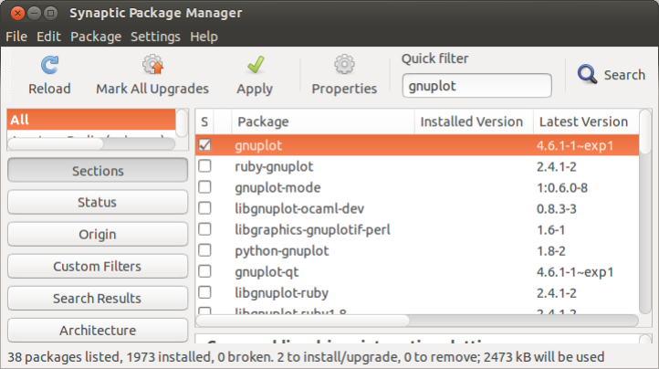
1.2 Using Synaptic Package Manager
•Open Synaptic Package Manager and type gnuplot in Quick Filter search.
•Right click on gnuplot package and click Mark for Installation.
•Similarly select gnuplot-x11 and click Mark for Installation.
•Now install packages by clicking Apply.
2

Chapter 2
Using Gnuplot on linux Platform
2.1 Points to note
•GnuPlot ignores lines starting with # (Symbol for comments).
•“**” mean exponent. e.g. “3**4” means 34.
•Any file name in command must be mentioned in double quotes. e.g. “file.txt”.
•
•
2.2 Plotting data-points from a file
2.2.1 Viewing Plots
Many Computing simulators give output in data files (with .dat extension).
Each line in data file specifies one data point which has one independent variable and one
or more dependent variable which are seperated by [space] or [Tab].
Here we will plot data points using Gnuplot.
•Open your favorite text editor (e.g. gedit), copy follwing text and save it with .dat
extension (e.g. test.dat) to the prefered directory.
#this file contais data points having two dependent variables.
#X ramdom Xsquare
0 0.1 0
1 1.1 1
2 2.1 4
3 3.2 9
4 4.3 16
5 5.5 25
•Open terminal and go to the directory (where you saved your file) using cd command.
3
Wadhwani Electronics Laboratory (WEL) IIT Bombay
•Type gnuplot and press Enter.
•When Gnuplot is launched in terminal, the last line should be “Terminal type set
to ‘wxt’ ” if not, gnuplot-x11 package is not installed properly and hence it will not
generate plots.
•Type plot "test.dat" and Enter. Plot window should pop-out.
•By default, it will plot first two columns, first on X-axis and second on Y-axis.
•Pressing ‘l’ on keyboard will change Y-axis of plot to log-scale.
•Similarely ‘a’ for autoscale, ‘r’ for ruler, ‘g’ for grid, ‘b’ for border.
2.2.2 Saving the Output file
•Type set terminal png and Enter
To get output in png format.
It can also be set to gif, jpeg and many more file types
For more information, type set terminal and press Enter.
•Type set output "out.png" and Enter
Output will be saved as out.png in the same directory after plotting.
•Type replot and Enter
You will observe that ranges for x & y axes and legend are automatially gener-
ated.
For any update or modification in plot, only replot command is needed.
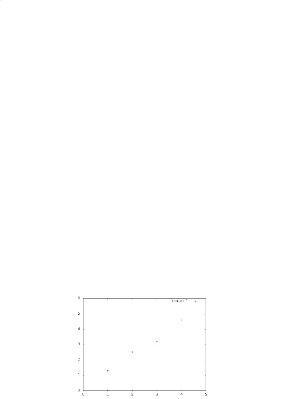
Go to the directory and see output (see Figure 2.1 for reference).
Figure 2.1: Plot of 1st dependent variable
Page 4
Wadhwani Electronics Laboratory (WEL) IIT Bombay
2.2.3 Customizing plot area
Plot area can be modified using following commands and entering replot after-
wards.
Table 2.1: Modifying plot area
Purpose Command
To add x-label set xlabel "Independent-variable"
To add y-label set ylabel "Dependent-variable"
To add Title set title "plot-title"
To set sample points set samples n
To set x or y range set xrange [x1:x2],set yrange [y1:y2]
To set grid set grid
To set x tics set xtics <start pt>, <increment>, <end pt>
To set log x scale set logscale
To set log y scale unset logscale;set logscale y
•In Figure 2.1, crosspoints are used to denote the datapoints. We can Customize it
to impulse plot or line plot or line+point plot etc. also the type of dots and its size
can be adjusted.
plot "test.dat" with lines
Replace “lines” in above command with “lines linestyle 2 linewidth 3”, “impulse”,
“linespoints”, “points pointtype 7 pointsize 2” and play around for more insight.
•To modify position of legend, Try follwing commands.
set key left box / set key right nobox / set key reverse Left outside
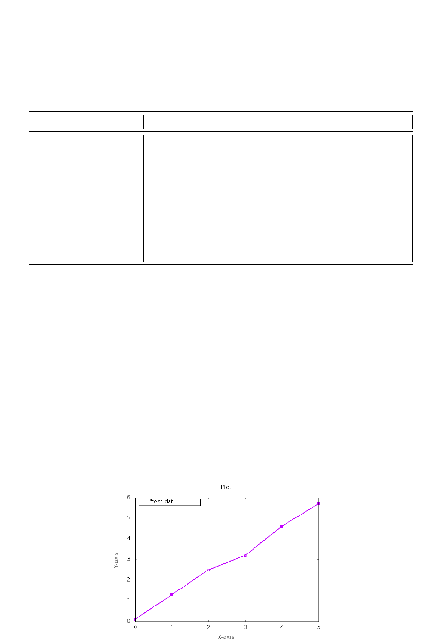
Following figure shows same plot with modified labels and legend.
Figure 2.2: Plot after modification
Page 5
Wadhwani Electronics Laboratory (WEL) IIT Bombay
2.2.4 Plotting multiple curves from data file
•Using simple plot command as used above, we were not able to plot multiple de-
pendent variables in data file.
For that we will use more specific commands as given below.
plot "test.dat" using 1:2 title ‘Random’ with linespoints pointtype 3,
"test.dat" using 1:3 title ‘Xsquared’ with line
Term “1:2” means x=1st column and y=2nd column
Term “1:3” means y=1st column and y=3nd column.
•You may have multiple data files. In this case, you may make use a command like:
plot "test1.dat" using 1:2 title ‘Test1-data’ with linespoints pointtype
3,"test2.dat" using 1:3 title ‘Test2-data’ with line
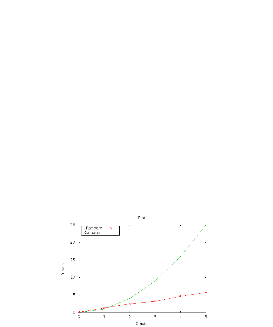
•Play with some modifications for proper understanding. See Multiple curves in
following figure which shows two dependent variables from data file.
Figure 2.3: Plot of Multiple dependent variable
Page 6

Wadhwani Electronics Laboratory (WEL) IIT Bombay
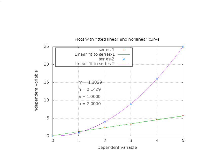
2.3 Curve fitting
•Curve fitting in data is necessory tool for any plotting software. Gnuplot supports
linear as well as nonlinear curve fits.
•Our first column data can be fitted into line f(x) = a∗x+b.
•To fit it in equation of line, follow the commands one by one:
plot "test.dat" using 1:2 title ‘Random’
f(x)=m*x+n
fit f(x) "test.dat" using 1:2 via m,n
replot f(x)
•For fitting polynomial in second data.
plot "test.dat" using 1:3 title ‘series-2’
g(x)=a*x**b
fit g(x) "test.dat" using 1:3 via a,b
replot g(x)
•After successful fitting, it will show values of m & n or a & b in the terminal.
•If it finds any singularity, then it will give error as “-nan”(it means Not A Number).
To resolve it, give initial guess of values of m and n in terminal. e.g. m=1,n=1 .
Or add some small value in f(x). e.g. f(x)=m*x+n+1e-8.
If Problem continues, Find other ways (Google :)).
•All graphs can be plotted simultaniously using following command :—>
plot "test.dat" using 1:2 title ‘series-1’, f(x) title ‘Fit to series-1’,
"test.dat" using 1:3 title ‘series-2’, g(x) title ‘Fit to series-2’
•Gnuplot support C-language syntax along with all mathematical formats.
Variable can be displayed on graph using sprint command as shown below.
set label 1 sprintf("m = %3.4f",m) at 1,15
set label 2 sprintf("n = %3.4f",n) at 1,13
set label 3 sprintf("a = %3.4f",a) at 1,11
set label 4 sprintf("b = %3.4f",b) at 1,9
replot
—>last two numbers seperated by comma shows position of label on graph.
•To save it —>
set terminal png
set output "fitted-out.png"
replot
Page 7
Wadhwani Electronics Laboratory (WEL) IIT Bombay
•Figure 2.5 shows the obtained plot.
Figure 2.4: Plot of Multiple dependent variable
Page 8
Wadhwani Electronics Laboratory (WEL) IIT Bombay
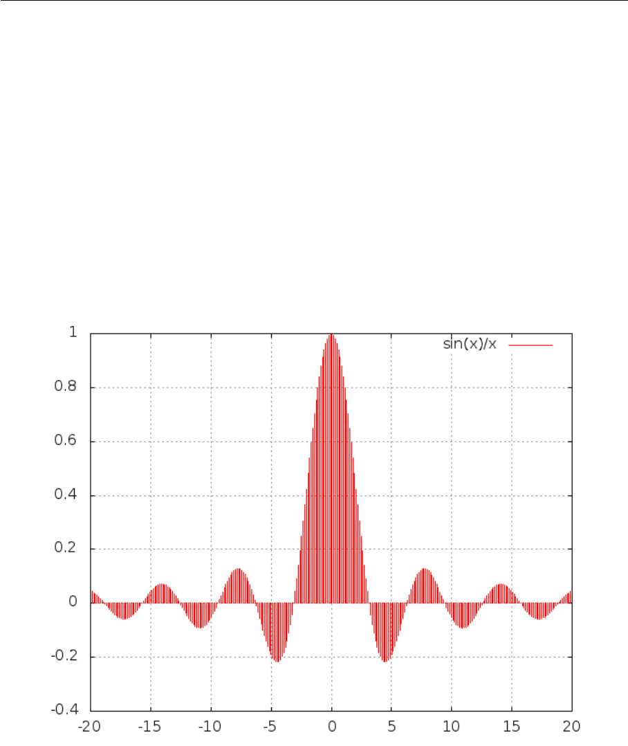
2.4 Plotting direct functions
2.4.1 Basics
•plot is used for 2D graphs and splot is used for 3D graphs.
•All standard mathematical expressions are valid for Gnuplot.
See Examples.
set samples 500
set xrange [-20:20]
plot sin(x)/x
•output will look like :—>
Figure 2.5: Sinc Functin
•For Supported functions see Appendix.
•commands like following are also acceptable.
plot [-pi/2:pi] cos(x),-(sin(x) > sin(x+1) ? sin(x) : sin(x+1))
Page 9
Wadhwani Electronics Laboratory (WEL) IIT Bombay
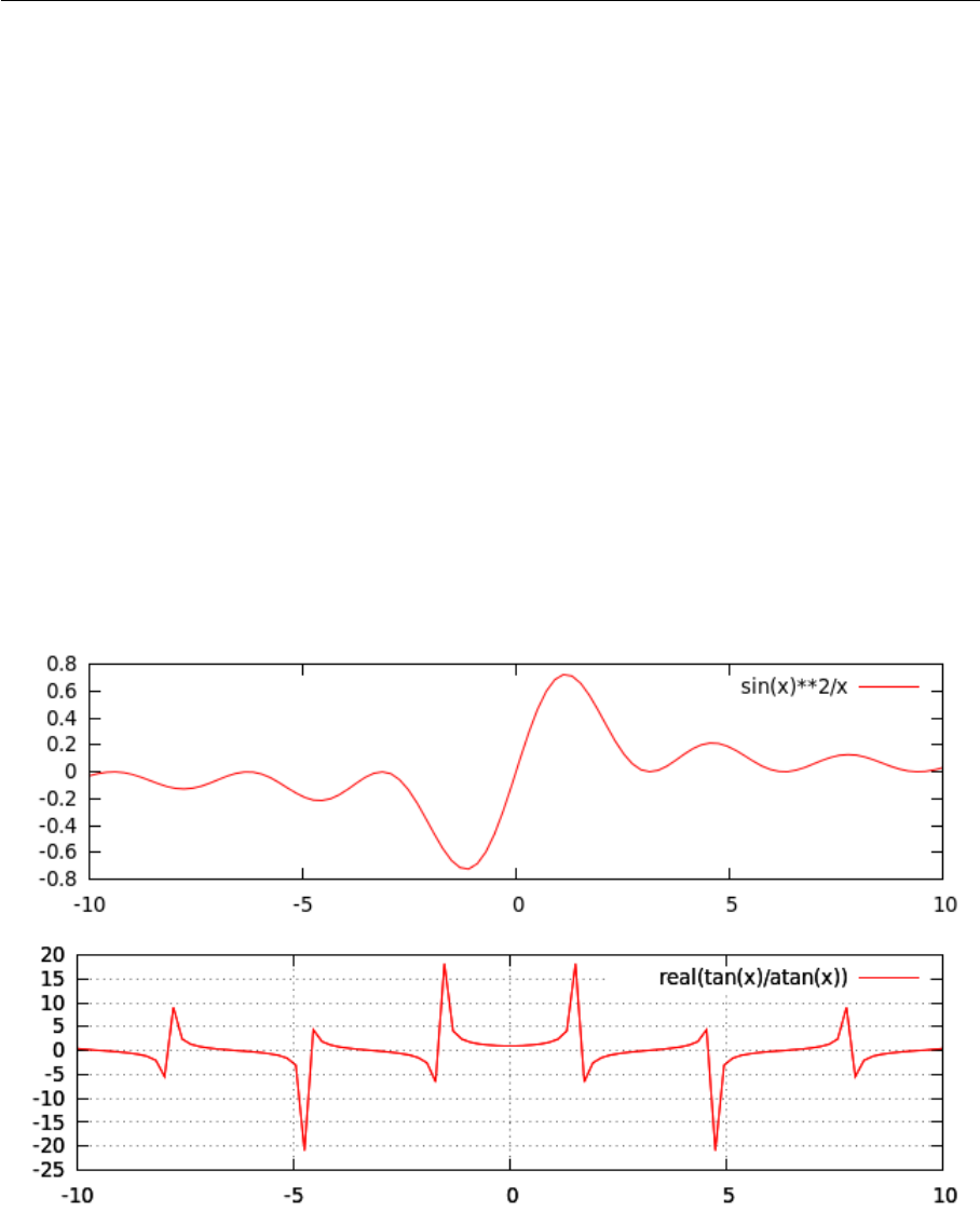
2.4.2 Multiplots
Gnuplot can plot more than one figure in same figure (like subplot in Matlab).
Try following commands in terminal one after another:
set multiplot
set size 1,0.5
set origin 0.0,0.5; plot sin(x)**2/x
set origin 0.0,0.0; plot real(tan(x)/atan(x))
set grid unset multiplot
•In second command,
(1,0.5) means row is splitted in half. (2 subplots)
(0.5,0.5) means row and column are splitted in half. (4 subplots)
(0.25,0.25) means row and column are spitted in four parts. (16 subplots)
•Obtained output is —>
Figure 2.6: Multiplots
Page 10

Appendix A
Supported functions
Table A.1: Supported Functions
Functions Return
abs(x) absolute value of x, |x|
acos(x) arc-cosine of x
asin(x) arc-sine of x
atan(x) arc-tangent of x
cos(x) cosine of x, x is in radians.
cosh(x) hyperbolic cosine of x, x is in radians
erf(x) error function of x
exp(x) exponential function of x, base e
inverf(x) inverse error function of x
invnorm(x) inverse normal distribution of x
log(x) log of x, base e
log10(x) log of x, base 10
norm(x) normal Gaussian distribution function
rand(x) pseudo-random number generator
sgn(x) 1 if x >0, -1 if x <0, 0 if x=0
sin(x) sine of x, x is in radians
sinh(x) hyperbolic sine of x, x is in radians
sqrt(x) the square root of x
tan(x) tangent of x, x is in radians
tanh(x) hyperbolic tangent of x, x is in radians
NOTE:
Bessel, gamma, ibeta, igamma, and lgamma functions are also supported.
Many functions can take complex arguments.
Binary and unary operators are also supported.
12
