User Guide
User Manual:
Open the PDF directly: View PDF ![]() .
.
Page Count: 10
User guide for FEtool.py – v1.0
1. Introduction
The program FEtool.py is designed to fully automate absolute binding free energy calculations, starting
only from a crystal structure or a docked complex. The building of the simulation boxes, generation of
all the needed parameters, set up of the various simulation windows, running the simulations, and the
final free energy analysis are all done without any manual interference. FEtool.py uses the
pmemd.cuda sofware from AMBER [1], which has shown very high performance on Graphics
Processing Units (GPUs) at a reduced cost (http://ambermd.org/gpus16/benchmarks.htm). We believe
that our implementation can be used for high-throughput search of high-affinity ligands to a given
receptor, using a rigorous physics-based free energy approach. FEtool.py can also be applied for
parameter testing and optimization, as well as the comparison between alchemical (double decoupling
-DD) and physical routes (attach-pull-release - APR) for standard binding free energy calculations.
In this user guide we will first describe the workflow of the program, then the various
components of the free energy calculation, and how the simulations are analyzed in order to obtain the
quantities of interest. All the parameters needed for the program input file, and how they apply to the
various calculation steps, will also be described in detail. Finally, we will explain how to add a new
protein system to our automated protocol.
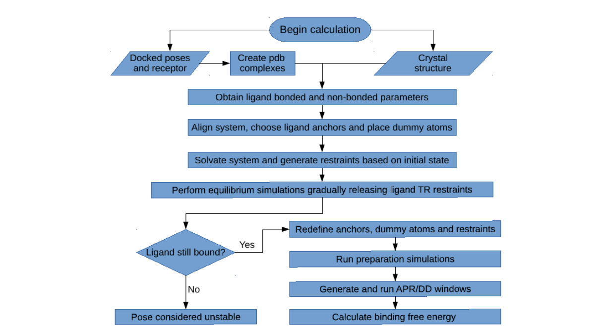
2. Workflow

The workflow above shows the equilibration, preparation and calculation procedures. It begins by first
building the initial complex, either starting from the docked receptor and ligand files or directly from
the receptor-ligand co-crystal structure. The necessary ligand parameters are obtained using
Antechamber [2], with the General Amber Force-Field (GAFF) for the bonded and LJ parameters [3],
and the AM1-BCC model for the partial atomic charges [4,5]. The system is then aligned to a reference
structure of a similar protein using the program MUSTANG [6], so that the ligand anchors and dummy
atom coordinates can be automatically assigned.
With all the coordinates of the initial system already set, the complex is then placed in a water
box with a given ion concentration, and the necessary restraints are applied. An initial equilibration is
then performed, with all the receptor restraints activated, and the translational/rotational restraints of
the ligand being gradually released in order to find a nearby energy minimum. At the end of this last
step, the ligand might still be bound or it might have left the binding site in the case of unstable binding
mode. If the latter happens, this pose is considered unstable and no further simulations are performed
for this system.
If the ligand is still bound after equilibration, which should usually be the case, then the
preparation of the system for the binding free energy calculations is performed. The preparation starts
from the last state from equilibrium, reassigning the ligand anchors, repositioning the dummy atoms,
solvating/ionizing the system and and redefining the restraints. This is necessary since the unrestrained
ligand can adopt a different binding mode in the last stage of the equilibration step, which requires a
new reference state for the free energy calculations. The preparation simulations may involve the
pulling of the ligand from the binding site to bulk, if APR is to be used, or only the simulation of the
restrained ligand in the bound state, if only DD is employed.
Starting from the last state of the preparation step, all the necessary simulation windows are
now created for the binding free energy calculation. They involve various components for the
application/removal of restraints, as well as the pulling/decoupling of the ligand, which are explained in
detail in the next section. Once the free energy simulations are concluded, they can be analyzed using
the Multistate Bennett Acceptance Ratio (MBAR) [7], Thermodynamic Integration with Gaussian
Quadrature (TI), or analytically, depending on the stage and the choice in the input file.
3. Free Energy Components
The FEtool.py expression for the calculated binding free energy is defined as follows:
−Δ Gbind
o=Δ Gp , conf ,att +Δ Gl , conf , att+ Δ Gl ,TR ,att +Δ Gtransfer + Δ Gl ,TR, rel+ Δ Gl ,conf , rel+ Δ Gp ,conf , rel
In the equation above, the att index denotes attachment of restraints in the bound state, and rel indicates
release of restraints with the ligand in bulk. The l and p indexes are for ligand and protein (receptor),
respectively, conf is for conformational restraints and TR is for translational/rotational restraints. The
ΔGtransfer term is the free energy of transferring of the ligand from the receptor binding site to bulk with
all restraints applied, using either a physical reaction coordinate (APR), or an alchemical
transformation (DD):
ΔGtransfer−APR= Δ Gpull
(APR)
ΔGtransfer−DD= Δ Gdec, elec ,site +Δ Gdec , LJ ,site− Δ Gdec, elec ,bulk −Δ Gdec , LJ , bulk
(DD)

In the case of APR, ΔGtransfer-APR is equal to the pulling free energy of the ligand from the binding site to
bulk, which is done using umbrella sampling, as in Ref [8]. For the double decoupling procedure,
ΔGtransfer-DD is equal to the sum of four terms, as shown in the equation above. The index dec stands for
decoupling, elec for electrostatic interactions and LJ for Lennard-Jones interactions, with these
calculations being performed both in the binding site or in bulk.
Table I summarizes all the free energy components from our simulations, with each identified
by a letter:
Description Letter System Free Energy Method Free energy term
Attachment of receptor
conformational restraints aComplex MBAR
ΔGp , conf ,att
Attachment of ligand
conformational restraints lComplex MBAR
ΔGl , conf ,att
Attachment of ligand TR restraints tComplex MBAR
ΔGl ,TR , att
Pulling stage (umbrella sampling) uComplex* MBAR
ΔGpull
Decoupling of ligand charge
interactions (binding site) eComplex MBAR/TI
ΔGdec , elect , site
Decoupling of ligand LJ
interactions (binding site) vComplex MBAR/TI
ΔGdec , LJ , site
Decoupling of ligand charge
interactions (bulk) fLigand only MBAR/TI
ΔGdec , elec, bulk
Decoupling of ligand LJ
interactions (bulk) wLigand only MBAR/TI
ΔGdec , LJ , bulk
Release of ligand TR restraints bLigand only Analytical
ΔGl ,TR ,rel
Release of ligand conformational
restraints cLigand only MBAR
ΔGl , conf ,rel
Release of receptor conformational
restraints rReceptor only MBAR
ΔGp , conf ,rel
* The receptor and ligand will be physically separated during the pulling simulations
When the calculations are set up, the windows from each free energy component will have their
corresponding letter followed by the window number, starting at 0. The number of windows and their
properties can be defined in the input file. The letters also identify the free energy output files, which
are stored in the ./data folder of each component, after the analysis is performed. More information on
the nature of each of the restraints, and the free energy methods we use, can be found in Refs. [8,9].
4. Input file
Various options concerning the creation of the systems, simulations and analysis, can be chosen in the
input file:
calc_type: Accepts the options “dock” or “crystal”, for a receptor ligand pair of pdb files, or a complex
co-crystal structure, respectively. The system initial pdb files should be located in the ./all-poses folder.

celpp_receptor: Sets the name of the receptor, followed by _docked. For example, choose “hiTanimoto-
5uf0_5uez” for a receptor file called hiTanimoto-5uf0_5uez_docked.pdb. The naming is based on the CELPP
challenge procedure. For a crystal structure, put the four letter identifier for the structure, for example “5uf0” for
the 5uf0.pdb crystal structure.
poses_list: The list of poses that will be used for the calculations. The list should be placed in brackets
ans separated by commas. Ex: “[0,1,2,3,4]”. The docked poses files in the ./all-poses folder must be listed
accordingly as pose0.pdb, pose1.pdb, pose2.pdb, etc. This parameter is not used for crystal structure
calculations.
ligand_name: The residue name for the ligand. This is arbitrary for docked poses (Ex: “DOK”), but is
necessary if starting the calculations from a crystal structure. In that case, put the three letter ligand identifier in
this option. Ex: “89J” for the 5uf0 crystal structure.
P1, P2 and P3: These define the anchor atoms of the receptor, which have to be determined beforehand.
The original protein sequence numbering should be used here, using AMBER masks to define each atom. Ex:
“:403@CA” for the CA atom of residue 403.
fe_type: Designates which components are to be included in the free energy calculations. For example, if all
the APR and DD calculations are to be performed, choose “all” for this option. If only double decoupling with
restraints will be performed, choose “dd-rest”, and if only APR choose “pmf-rest”. The “custom” option allows
to choose any combination of components, using the components option below.
components: If the option “custom” is set in the option above, choose the components you want to calculate,
using a list of letters separated by spaces inside a bracket. Ex: “[ c l t a ]”.
release_eq: The weights for the gradual release of the restraints in the equilibrium stage, going from 100
(fully restrained) to 0 (unrestrained). Each option will be a new simulation, and they are performed in sequence.
Use a list of letters separated by spaces inside a bracket to define these weights. Ex: “[ 5.00 2.50 1.00 0.00 ]”. A
single 0.00 inside the brackets (Ex: “[ 0.00 ]”) will run just one equilibrium simulation without any ligand
restraints.
attach_apr: List of weights for the spring constant of each window during the attaching/releasing of
restraints using MBAR (components a, l, t, c and r). The total number of windows for each of these components
will be the size of the array. Ex: “[ 0.00 2.00 4.00 16.00 64.00 100.00 ]” for a total of 6 windows.
translate_apr: Windows for the umbrella sampling (pulling) procedure of APR, identified by the letter u.
It starts from 0.00 (bound state) until the desired reference distance between the receptor and the ligand in the
unbound state. The number of windows is the size of the array. Ex: “[ 0.00 1.00 2.00 3.00 4.00 5.00 ]” for a total
of 6 windows, ending 5.00 Å away from the initial reference distance.
lambdas: Lambda values for the double decoupling procedure, going from 0.00 to 1.00. Ex: For a 12-point
Gaussian quadrature, choose “[ 0.00922 0.04794 0.11505 0.20634 0.31608 0.43738 0.56262 0.68392 0.79366
0.88495 0.95206 0.99078 ]” for the lambda array values.
pull_ligand: Choice to pull the ligand from the binding site or not during preparation. This is needed for
the APR method, but not needed for double decoupling. Choose “yes” or “no” for this option.
pull_spacing: The interval between each ligand position during the preparation simulations, if the option
above is set to yes. The final distance is the last value in the translate_apr array. Ex: “0.1” for a pulling

interval of 0.1 Å.
rec_distance_force: Distance spring constant for the receptor rigid body restraints, identified as R2 in
Ref. [8]. Use units of kcal/mol.Ų.
rec_angle_force: Angle and torsion angle spring constants for the receptor rigid body restraints,
identified as A3, A4, T4, T5 and T6 in Ref. [8]. Use units of kcal/mol.rad². The forces from
rec_distance_force and rec_angle_force are included to keep the receptor in the laboratory
reference frame.
rec_dihcf_force: Final spring constant for the protein conformational dihedral restraints, if this option is
activated (see rec_bb variable). The nature of these restraints, and how they are implemented, are explained in
Ref. [9]. Use units of kcal/mol.rad².
rec_discf_force: Final spring constant for the protein conformational distance restraints between the
anchor atoms. Use units of kcal/mol.Ų.
lig_distance_force, lig_angle_force, lig_dihcf_force and lig_discf_force:
Final spring constants for the ligand restraints, defined the same way as the receptor above. The value of
lig_distance_force also designates the spring constant used during the pulling simulations. The nature
of the ligand conformational restraints, and how they are implemented, are explained in Ref. [9].
water_model: The water model used in the calculations. Supported options are “TIP3P”, “TIP4PEW” and
“SPCE”.
num_waters: Number of waters used in the simulations of the complex and the apo protein.
buffer_x and buffer_y: Options for the water padding in the x and y axes of the system, remembering
that the pulling is done along the z coordinate. The dependent variable is the padding in the z-axis, so make sure
you have enough waters to cover the complex and allow the pulling of the ligand.
lig_box: Water padding in the three Cartesian axes for the box with only the ligand in it.
neutralize_only: Option to add ions only to neutralize the system, or to also include a chosen ion molar
concentration. Accepts options “yes” or “no”.
cation and anion: Cation and anion species to be used, accepts all ions supported by the Joung and
Cheatham monovalent ion parameters [10]. Ex: “Na+” and “Cl-”.
num_cations: Number of cations to be added after neutralization, for the desired ion concentration, for
simulations of the complex and the apo protein. The number of anions is the dependent variable, since the
systems are always neutral.
num_cations_ligbox: Number of cations to be added after neutralization, for the desired ion
concentration, for the smaller ligand box.
hmr: Use hydrogen mass repartitioning [11] with a 4 fs time step, if set to “yes”. If set to “no”, the simulations
do not use hmr, and use a 2 fs time step.

temperature: Temperature of the simulated systems, in Kelvin (K).
eq_steps1: Number of steps for each simulation of the gradual release of restraints, during the equilibration
procedure.
eq_steps2: Number of steps for the last simulation of the equilibration procedure, in which the ligand is
unrestrained.
prep_steps1: Number of steps for the first simulation of the preparation step, in which the ligand is fully
restrained in the bound state.
prep_steps2: Number of steps for each of the pulling simulations, during the preparation procedure. The
distance separation of each of these steps is defined in the pull_spacing option.
[component]_steps1: Number of steps of equilibration, for each window of the various components of
the free energy calculation, with the component letters shown in Table I. No data is collected during this
simulation.
[component]_steps2: Number of steps for the production stage of each window of the various
components of the free energy calculation, in which data is collected.
rec_bb: Choice to use or not protein (receptor) backbone dihedral restraints, accepting “yes” or “no”.
bb_start and bb_end: If the option above is activated, these variables define the residue range of the
protein backbone dihedral restraints, using the original protein sequence numbering.
l1_x: distance in the x axis between the first protein anchor atom P1 and the center of the “strike zone” for the
search of the ligand first anchor L1. More details on this procedure can be found in section 6 of this guide and
also in Ref. [9]
l1_y: Same as the previous one, but for the y axis distance.
l1_z: Minimum distance between the first protein anchor atom P1 and the first ligand anchor L1, in the z axis.
l1_range: Size of the “strike zone” for the first ligand anchor atom search, which is a square with sides
having twice the value of this parameter (2*l1_range).
min_adis and max_adis: Minimum and maximum distance between the ligand anchors.
dd_type: Type of integration method for the decoupling components of the binding free energy calculation (e,
v, f and w). If “TI” is chosen, Gaussian quadrature is applied, if “MBAR” is chosen, the latter is used to calculate
these components. Remember that the lambda values have to be suitable for either type of integration method.
weights: Weights for Gaussian quadrature calculations, in case the TI option is chosen above. These values
must correspond to the values in the lambdas array, for the procedure to be applied correctly. In the case of a
12-point Gaussian quadrature, write “[ 0.02359 0.05347 0.08004 0.10158 0.11675 0.12457 0.12457 0.11675
0.10158 0.08004 0.05347 0.02359 ]” for this variable.

blocks: Number of blocks for block data analysis. This separates the simulation data in blocks and provides
the results for each, so the temporal variation and convergence of the results can be assessed.
5. Adding new ligands to a given protein
In the example provided in the FEtool folder, binding free energy calculations are performed for the 5uf0 crystal
structure, as well as 5 docked poses of the same ligand docked to the receptor with the 5uez structure. The
protein receptor is the second bromodomain of the BRD4 protein – BRD4(2). The ./all-poses folder in this
example contains the original 5uf0.pdb file, as well as a set of pdb files for the docked poses and receptor. The
same procedure can be applied to any ligand that binds to BRD4(2), as explained below:
5.1 Docked complexes: In order to generate a set of pdb files for the docked poses and receptor, there are two
options, either do a manual docking with chosen input files, or using the CELPP challenge workflow. Both
options use AutoDockTools [12], Chimera [13], and AutoDock Vina [14] to prepare the files and run the
docking, so you must have them in your path in order to perform this stage. For the first option, the ./docking-
files/Vina-example folder has a simple docking workflow using the dock.bash script and the input files for the
5uf0 system, which already outputs the files in the right format for use with FEtool.
The docking can also be integrated into the CELPP challenge, using the procedure from the CELPPade
tutorial (ht tps://doc.google.com/document/d/1iJcPUktbdrRftAA8cuVa32Ri1TPr2XvZVqTccDja2OM h),
which the user needs to be familiarized with. The same scripts from the “internal_autodockvina_contestant”
model from this tutorial can be used for docking, except for internal_autodockvina_contestant_dock.py. To
output the docked structures suitable for use with FEtool, you should use instead the FEtool_dock.py script,
which is included inside the FEtool/CELPP-docking folder. Once you run the CELPP docking, the necessary pdb
structures for various different receptors will be inside the ./4-docking folder that was just created.
5.2 Co-crystal structure: In the case of a co-crystal structure, the calc_type, ligand_name and
celpp_receptor options in the input file have to be adjusted properly, as explained in section 4. The script
prep-crystal.tcl, inside the ./build_files folder, is used by VMD [15] to “clean” the original file and leave only a
single chain of the receptor-ligand complex. The editing of this tcl script usually not needed, but is necessary if
the original pdb file has more than one chain. Keep in mind that the “MMM” identifier will be replaced by the
ligand name, so it does not have to be changed beforehand.
6. Adding a new protein system
FEtool.py can be extended to several protein systems, by including a reference alignment file and adjusting a
few parameters in the input.in file. The ./systems-library folder contains the necessary data for a few systems,
and more can be requested by contacting the author directly. The user can also set up a new protein system, so
below we show a few good practices, using the second BRD4 bromodomain as an example.
6.1: Aligning the protein: The first step is to create the reference.pdb file, so that the complex can be aligned
relative to it using MUSTANG, before the FEtool.py simulations are performed. If using APR, the ligand pulling
direction is along the z axis and towards positive values (z+), so the ligand must have free access to the solvent
along this direction. This is not needed if only DD is to be employed. The reference file is created by rotating a
structure of the desired protein with a ligand bound, in this example the 5uf0 crystal structure of BRD4(2), and
then saving it as reference.pdb. One way of doing this is using VMD
(http://www.ks.uiuc.edu/Training/Tutorials/vmd/vmd-tutorial.pdf), but other programs such as Chimera can also
be employed for that purpose. Figure 1 shows the 5uf0 structure before (red) and after the rotation (blue), with
the ligand now having access to the solvent along the z direction. The reference.pdb file does not need to have
the same sequence as the receptor input file, so the same reference created here for for BRD4(2) can be extended
to other bromodomains that share the same fold, such as BRD4(1), CREBBP and BAZ2B.
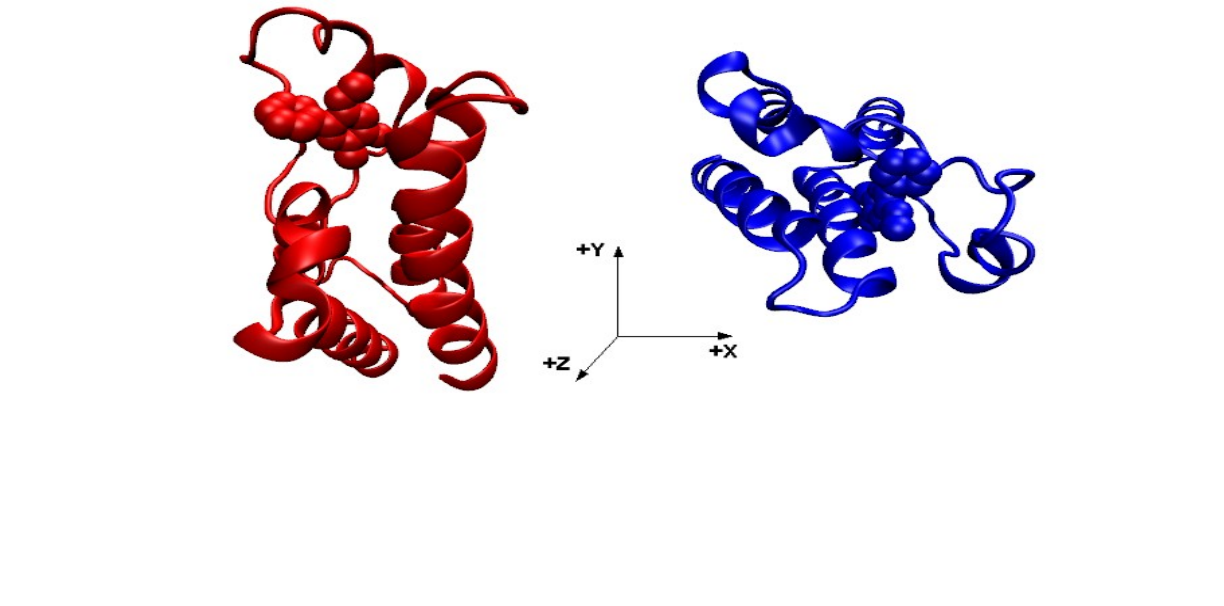
Figure 1: The 5uf0 structure before (red) and after (blue) the rotation, so that the latter has the ligand with free access
to the solvent in the +z direction.
6.2: Choosing the protein anchors: Once the reference.pdb file with the desired orientation is created, it is time
to choose the three protein anchor atoms. Starting from this file, choose a tentative ligand first anchor atom L1
[8], with the lowest or one of the lowest values for the z coordinate from all the ligand atoms, and with the x and
y coordinates not too far from the center of the binding site (Figure 2). Even though this anchor is going to be
chosen automatically when you run FEtool.py, an estimate of its location is needed to choose the protein
anchors. The protein P1 anchor is then chosen using a few rules:
1 – Should be a backbone atom (CA, C or N) and part of a stable secondary structure such as an alpha-helix or a
beta sheet, always avoiding loop regions due to their increased flexibility.
2 – Should have a distance between 10 Å and 15 Å from the chosen L1 atom in the z axis, and having an
absolute value between 5.0 Å and 10 Å in the xy plane.
In the example for the 5uf0 structure (Figure 2), the tentative L1 atom has a {x1 y1 z1} distance vector from the
CA atom from the protein 403 residue (P1) being equal to {-0.74 -6.16 13.03} , with the z1 distance being 13.03
Å and the distance in the xy plane
x12+y12
being 6.20 Å. Since it satisfies our criteria, we choose :403@CA
for the first protein anchor P1.
The choice of the other protein anchors P2 and P3 are chosen after the first one, and also follow a few
guidelines:
1 – Should also be backbone atoms part of stable secondary structures such as alpha-helix or beta sheet, always
avoiding loop regions due to their increased flexibility.
2 – The N2-P1-P2 and P1-P2-P3 angles (Figure 2) should not be close to 0 or 180 degrees (better if close to 90o),
and the distance between the protein anchors should be large (at least 10 Å) . This is to avoid large forces during
the simulations due to a gimbal lock. Like the ligand anchors, the positioning of the dummy atoms is done
automatically, with an example shown in Figure 2. More information on their location and the full restraint setup
can be found on Refs [8,9].
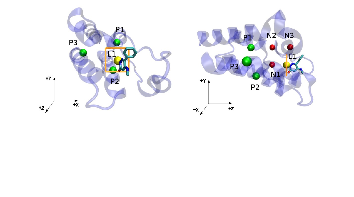
Figure 2: (left) The ligand tentative first anchor L1 (yellow) and the three protein anchors P1, P2 and P3 (green). The
strike zone for L1 search is shown in orange. (right) The same structure, but showing the the yz plane. The dummy
atoms N1, N2 and N3 (red), which are placed automatically when running FEtool.py, are shown as an example.
6.3: Determining the input values for ligand anchor search: Once P1, P2 and P3 are chosen, a few more
parameters are needed for the input file. The x1 and y1 coordinates determined above can be used for the l1_x
and l1_y parameters, and the l1_z parameter can have a safe minimum value of 8.50 Å. The l1_range
parameter defines a “strike zone” when searching for the first ligand anchor L1, and can also be safely defined as
3.0 Å (Figure 2). The min_adis and max_adis define the minimum and maximum distance between the
ligand anchors, and can usually be left with values of 4.0 Å and 8.0 Å, respectively. For smaller ligands,
min_adis might have to be reduced to 3.5 Å or even 3.0 Å, and max_adis could be increased in the case of
larger ligands.
Even though this is a heuristic approach, if applied correctly the protein and the ligand will be properly
restrained during the calculations, allowing us to obtain the absolute binding free energy of several molecules to
a given protein without any further adjustments.
7. References
[1] D.A. Case, I.Y. Ben-Shalom, S.R. Brozell, D.S. Cerutti, T.E. Cheatham, III, V.W.D. Cruzeiro, T.A. Darden,
R.E. Duke, D. Ghoreishi, M.K. Gilson, H. Gohlke, A.W. Goetz, D. Greene, R Harris, N. Homeyer, S. Izadi, A.
Kovalenko, T. Kurtzman, T.S. Lee, S. LeGrand, P. Li, C. Lin, J. Liu, T. Luchko, R. Luo, D.J. Mermelstein, K.M.
Merz, Y. Miao, G. Monard, C. Nguyen, H. Nguyen, I. Omelyan, A. Onufriev, F. Pan, R. Qi, D.R. Roe, A.
Roitberg, C. Sagui, S. Schott-Verdugo, J. Shen, C.L. Simmerling, J. Smith, R. Salomon-Ferrer, J. Swails, R.C.
Walker, J. Wang, H. Wei, R.M. Wolf, X. Wu, L. Xiao, D.M. York and P.A. Kollman (2018), AMBER 2018,
University of California, San Francisco.
[2] J. Wang, W. Wang, P.A. Kollman, and D.A. Case.. (2006) "Automatic atom type and bond type perception in
molecular mechanical calculations".Journal of Molecular Graphics and Modelling, 25, 247-260.
[3] J. Wang, R.M. Wolf, J.W. Caldwell, and P. A. Kollman, D. A. Case (2004) "Development and testing of a
general AMBER force field". Journal of Computational Chemistry, 25, 1157-1174.
[4] A. Jakalian, B. L. Bush, D. B. Jack, and C.I. Bayly (2000) "Fast, efficient generation of high‐quality atomic

charges. AM1‐BCC model: I. Method". Journal of Computational Chemistry, 21, 132-146.
[5] A. Jakalian, D. B. Jack, and C.I. Bayly (2002) "Fast, efficient generation of high‐quality atomic charges.
AM1‐BCC model: II. Parameterization and validation". Journal of Computational Chemistry, 16, 1623-1641.
[6] A. S. Konagurthu, J. Whisstock, P. J. Stuckey, and A. M. Lesk. (2006) “MUSTANG: A multiple structural
alignment algorithm”. Proteins, 64, 559-574.
[7] M. R. Shirts and J. Chodera (2008) “Statistically optimal analysis of samples from multiple equilibrium
states.” Journal of Chemical Physics, 129, 129105.
[8] G. Heinzelmann, N. M. Henriksen, and M. K. Gilson. (2017) “Attach-Pull-Release Calculations of Ligand
Binding and Conformational Changes on the First BRD4 Bromodomain” Journal of Chemical Theory and
Computation, 13, 3260-3275.
[9] G. Heinzelmann and M. K. Gilson. “FEtool.py: A fully automated tool for high-performance absolute
binding free energy calculations” . Paper in preparation.
[10] I. S. Joung and T. E. Cheatham III (2008). “Determination of Alkali and Halide Monovalent Ion Parameters
for Use in Explicitly Solvated Biomolecular Simulations”. The Journal of Physical Chemistry B, 112, 9020-
9041.
[11] C. W. Hopkins, S. Le Grand, R. C. Walker, and A. E. Roitberg. (2015) “Long-Time-Step Molecular
Dynamics through Hydrogen Mass Repartitioning”. Journal of Chemical Theory and Computation, 11, 1864-
1874.
[12] G. M. Morris, R. Huey, W. Lindstrom, M. F. Sanner, R. K. Belew, D. S. Goodsell, and A. J. Olson. (2009)
“AutoDock4 and AutoDockTools4: Automated Docking with Selective Receptor Flexibility” Journal of
Computational Chemistry, 30, 2785-2791.
[13] E. F. Pettersen, T. D. Goddard, C. C. Huang, G. S. Couch, D. M. Greenblatt, E. C. Meng, and T. E. Ferrin.
(2004). "UCSF Chimera - A Visualization System for Exploratory Research and Analysis." Journal of
Computational Chemistry, 25, 1605-1612.
[14] O. Trott and A. J. Olson. (2010) "AutoDock Vina: improving the speed and accuracy of docking with a new
scoring function, efficient optimization and multithreading," Journal of Computational Chemistry, 31, 455-461.
[15] W. Humphrey, A. Dalke and K. Schulten. (1996) "VMD - Visual Molecular Dynamics", Journal of
Molecular Graphics, 14, 33-38.
