User Manual Matlab

Multi-Imbalance: an open-source software for multi-class imbalance learning

User Manual in MATLAB

Chongsheng Zhanga, Jingjun Bia, Shixin Xua, Enislay Ramentolb, Gaojuan

Fana, Hamido Fujitac

aThe Big Data Research Center, Henan University, 475001 KaiFeng, China

bSICS Swedish ICT, Isafjordsgatan 22, Box 1263, SE-164 29 Kista, Sweden

cFaculty of Software and Information Science, Iwate Prefectural University, Iwate, Japan

This user manual presents "Multi-Imbalance", which is the first open source software

for the multi-class imbalanced learning field. It contains 18 algorithms for multi-class

imbalanced data classification.

If you have any problems, please do not hesitate to send us an email: henucs@qq.com

This software is protected by the GNU General Public License (GPL).

 
CONTENTS 
Overview of Multi-Imbalance .......................................................................................................................1 
Installation in MATLAB .................................................................................................................................1 
Usage Example for Each Algorithm ............................................................................................................2 
1 AdaBoost.M1 .........................................................................................................................................2 
2 SAMME ..................................................................................................................................................3 
3 AdaC2.M1 ...............................................................................................................................................4 
4 AdaBoost.NC .........................................................................................................................................5 
5 PIBoost ....................................................................................................................................................6 
6 DECOC ...................................................................................................................................................7 
7 DOVO ......................................................................................................................................................8 
8 FuzzyImbECOC ....................................................................................................................................9 
9 HDDTova ............................................................................................................................................. 10 
10 HDDTecoc ......................................................................................................................................... 10 
11 MCHDDT .......................................................................................................................................... 11 
12 ImECOC + sparse ............................................................................................................................ 12 
13 ImECOC + OVA .............................................................................................................................. 13 
14 ImECOC + dense ............................................................................................................................. 14 
15 Multi-IM + OVA .............................................................................................................................. 15 
16 Multi-IM + OVO ............................................................................................................................. 16 
17 Multi-IM + OAHO .......................................................................................................................... 17 
18 Multi-IM + A&O ............................................................................................................................. 18 
 
 

1

1. Overview of Multi-Imbalance

In recent years, although many researchers have proposed different algorithms and techniques to

tackle the multi-class imbalanced data classification issue, there is still no open-source software for

this specific field. To address this issue, we develop the "Multi-Imbalance" (Multi-class Imbalanced

data classification) software package and share it with the community, to boost research in this field.

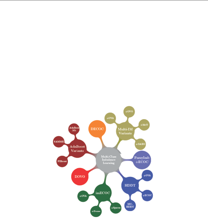
The developed Multi-Imbalance software contains 18 different algorithms for multi-class imbalance

learning, which are depicted in Figure 1, many of them were proposed in recent years. We divide

these algorithms into 7 modules (categories). We will introduce the framework and functionalities

of this software in the next sections.

Figure 1. The major modules in Multi-Imbalance

Using Multi-Imbalance, researchers can directly re-use our implementations on multi-class

imbalanced data classification, thus avoid implementing them from scratch. Hence, Multi-

Imbalance will be helpful and indispensable for researchers in the multi-class imbalance learning

field.

2. Installation in MATLAB

In order to use Multi-Imbalance, users only need to add the Multi-Imbalance software package to

the MATLAB search path.

2

Figure 2. Adding the Multi-Imbalance package to the MATLAB path

3. Usage Example for Each Algorithm

There are 7 classes (categories) of algorithms for multi-class imbalance learning, each class

consisting of one or more algorithms. In total, there are 18 major algorithms for multi-class

imbalance learning. In the following, we give the user manual of these 18 major algorithms for

multi-class imbalance learning.

If users need to test a new dataset, they only need to replace the original

“Wine_data_set_index_fixed” with the new dataset.

3.1 AdaBoost.M1

Input: the imbalanced dataset

Output: the prediction results on the dataset using the AdaBoost.M1 algorithm,

where _p.mat is the prediction results, and _c.mat is the ground truth.

Usage example:

function runAdaBoostM1

javaaddpath('weka.jar');

p = genpath(pwd);

addpath(p, '-begin');

% record = 'testall.txt';

% save record record

3

dataset_list = {'Wine_data_set_indx_fixed'};

for p = 1:length(dataset_list)%1:numel(dataset_list)

load(['data\', dataset_list{p},'.mat']);

disp([dataset_list{p}, ' - numero dataset: ',num2str(p), ]);

%AdaBoost.M1

for d=1:5

[Cost(d).adaboostcartM1tr,Cost(d).adaboostcartM1te,Pre(d).adaboostcartM1] =

adaboostcartM1(data(d).train,data(d).trainlabel,data(d).test,20);

end

save (['results/', dataset_list{p},'_', 'p', '.mat'], 'Pre');

save (['results/', dataset_list{p},'_', 'c', '.mat'], 'Cost');

clear Cost Pre Indx;

end

Reference:

Freund, Y. & Schapire, R. E. (1997). A decision-theoretic generalization of on-line learning and an

application to boosting. Journal of Computer and System Sciences, August 1997, 55(1).

3.2 SAMME

Input: the imbalanced dataset

Output: the prediction results on the dataset using the SAMME algorithm,

where _p.mat is the prediction results, and _c.mat is the ground truth.

Usage example:

function runSAMME

javaaddpath('weka.jar');

p = genpath(pwd);

addpath(p, '-begin');

% record = 'testall.txt';

% save record record

dataset_list = {'Wine_data_set_indx_fixed'};

for p = 1:length(dataset_list)%1:numel(dataset_list)

load(['data\', dataset_list{p},'.mat']);

4

disp([dataset_list{p}, ' - numero dataset: ',num2str(p), ]);

%SAMME

for d=1:5

[Cost(d).SAMMEcarttr,Cost(d).SAMMEcartte,Pre(d).SAMMEcart] =

SAMMEcart(data(d).train,data(d).trainlabel,data(d).test,20);

end

save (['results/', dataset_list{p},'_', 'p', '.mat'], 'Pre');

save (['results/', dataset_list{p},'_', 'c', '.mat'], 'Cost');

clear Cost Pre Indx;

end

Reference:

Zhu, J., Zou, H., Rosset, S., et al. (2006). Multi-class AdaBoost. Statistics & Its Interface, 2006,

2(3), 349-360.

3.3 AdaC2.M1

Input: the imbalanced dataset

Output: the prediction results on the dataset using the AdaC2.M1 algorithm,

where _p.mat is the prediction results, and _c.mat is the ground truth.

Usage example:

function runAdaC2M1

javaaddpath('weka.jar');

p = genpath(pwd);

addpath(p, '-begin');

% record = 'testall.txt';

% save record record

dataset_list = {'Wine_data_set_indx_fixed'};

for p = 1:length(dataset_list)%1:numel(dataset_list)

load(['data\', dataset_list{p},'.mat']);

disp([dataset_list{p}, ' - numero dataset: ',num2str(p), ]);

%AdaC2.M1

for d=1:5

tic;

5

C0=GAtest(data(d).train,data(d).trainlabel);

Cost(d).GA=toc;

Indx(d).GA=C0;

[Cost(d).adaC2cartM1GAtr,Cost(d).adaC2cartM1GAte,Pre(d).adaC2cartM1GA] =

adaC2cartM1(data(d).train,data(d).trainlabel,data(d).test,20,C0);

end

save (['results/', dataset_list{p},'_', 'p', '.mat'], 'Pre');

save (['results/', dataset_list{p},'_', 'c', '.mat'], 'Cost');

clear Cost Pre Indx;

end

Reference:

Sun, Y., Kamel, M. S. & Wang, Y. (2006). Boosting for learning multiple classes with imbalanced

class distribution. Proceedings of the 6th International Conference on Data Mining, 2006 (PP. 592-

602).

3.4 AdaBoost.NC

Input: the imbalanced dataset

Output: the prediction results on the dataset using the AdaBoost.NC algorithm,

where _p.mat is the prediction results, and _c.mat is the ground truth.

Usage example:

function runAdaBoostNC

javaaddpath('weka.jar');

p = genpath(pwd);

addpath(p, '-begin');

% record = 'testall.txt';

% save record record

dataset_list = {'Wine_data_set_indx_fixed'};

for p = 1:length(dataset_list)%1:numel(dataset_list)

load(['data\', dataset_list{p},'.mat']);

disp([dataset_list{p}, ' - numero dataset: ',num2str(p), ]);

%AdaBoost.NC

for d=1:5

6

[Cost(d).adaboostcartNCtr,Cost(d).adaboostcartNCte,Pre(d).adaboostcartNC] =

adaboostcartNC(data(d).train,data(d).trainlabel,data(d).test,20,2);

end

save (['results/', dataset_list{p},'_', 'p', '.mat'], 'Pre');

save (['results/', dataset_list{p},'_', 'c', '.mat'], 'Cost');

clear Cost Pre Indx;

end

Reference:

Wang, S., Chen, H. & Yao, X. Negative correlation learning for classification ensembles. Proc. Int.

Joint Conf. Neural Netw., 2010 (PP. 2893-2900).

3.5 PIBoost

Input: the imbalanced dataset

Output: the prediction results on the dataset using the PIBoost algorithm,

where _p.mat is the prediction results, and _c.mat is the ground truth.

Usage example:

function runPIBoost

javaaddpath('weka.jar');

p = genpath(pwd);

addpath(p, '-begin');

% record = 'testall.txt';

% save record record

dataset_list = {'Wine_data_set_indx_fixed'};

for p = 1:length(dataset_list)%1:numel(dataset_list)

load(['data\', dataset_list{p},'.mat']);

disp([dataset_list{p}, ' - numero dataset: ',num2str(p), ]);

%PIBoost

for d=1:5

[Cost(d).PIBoostcarttr,Cost(d).PIBoostcartte,Pre(d).PIBoostcart] =

PIBoostcart(data(d).train,data(d).trainlabel,data(d).test,20);

end

7

save (['results/', dataset_list{p},'_', 'p', '.mat'], 'Pre');

save (['results/', dataset_list{p},'_', 'c', '.mat'], 'Cost');

clear Cost Pre Indx;

end

Reference:

Fernndez, B. A. & Baumela. L. (2014). Multi-class boosting with asymmetric binary weak-learners.

Pattern Recognition, 2014, 47(5), PP. 2080-2090.

3.6 DECOC

Input: the imbalanced dataset

Output: the prediction results on the dataset using the DECOC algorithm,

where _p.mat is the prediction results, and _c.mat is the ground truth.

Usage Example

function runDECOC

javaaddpath('weka.jar');

p = genpath(pwd);

addpath(p, '-begin');

% record = 'testall.txt';

% save record record

dataset_list = {'Wine_data_set_indx_fixed'};

for p = 1:length(dataset_list)%1:numel(dataset_list)

load(['data\', dataset_list{p},'.mat']);

disp([dataset_list{p}, ' - numero dataset: ',num2str(p), ]);

%DECOC

for d=1:5

[Cost(d).imECOCDOVOs1tr,Cost(d).imECOCDOVOs1te,Pre(d).imECOCDOVOs1]

= DECOC(data(d).train,data(d).trainlabel,data(d).test, 'sparse',1);

end

save (['results/', dataset_list{p},'_', 'p', '.mat'], 'Pre');

save (['results/', dataset_list{p},'_', 'c', '.mat'], 'Cost');

clear Cost Pre Indx;

end

8

Reference:

Jingjun Bi, Chongsheng Zhang*. (2018). An Empirical Comparison on State-of-the-art Multi-class

Imbalance Learning Algorithms and A New Diversified Ensemble Learning Scheme. Knowledge-

based Systems, 2018, Vol.158, pp. 81-93.

3.7 DOVO

Input: the imbalanced dataset

Output: the prediction results on the dataset using the DOVO algorithm,

where _p.mat is the prediction results, and _c.mat is the ground truth.

Usage example:

function runDOVO

javaaddpath('weka.jar');

p = genpath(pwd);

addpath(p, '-begin');

% record = 'testall.txt';

% save record record

dataset_list = {'Wine_data_set_indx_fixed'};

for p = 1:length(dataset_list)%1:numel(dataset_list)

load(['data\', dataset_list{p},'.mat']);

disp([dataset_list{p}, ' - numero dataset: ',num2str(p), ]);

%DOVO

for d=1:5

[Cost(d).DOAOtr,Cost(d).DOAOte,Pre(d).DOAO,Indx(d).C] =

DOVO([data(d).train,data(d).trainlabel],data(d).test,data(d).testlabel,5);

end

save (['results/', dataset_list{p},'_', 'p', '.mat'], 'Pre');

save (['results/', dataset_list{p},'_', 'c', '.mat'], 'Cost');

clear Cost Pre Indx;

end

Reference:

Kang, S., Cho, S. & Kang P. (2015) Constructing a multi-class classifier using one-against-one

9

approach with different binary classifiers. Neurocomputing, 2015, Vol. 149, pp. 677-682.

3.8 FuzzyImbECOC

Input: the imbalanced dataset

Output: the prediction results on the dataset using the FuzzyImbECOC algorithm,

where _p.mat is the prediction results, and _c.mat is the ground truth.

Usage example:

function runFuzzyImbECOC

javaaddpath('weka.jar');

p = genpath(pwd);

addpath(p, '-begin');

% record = 'testall.txt';

% save record record

dataset_list = {'Wine_data_set_indx_fixed'};

for p = 1:length(dataset_list)%1:numel(dataset_list)

load(['data\', dataset_list{p},'.mat']);

disp([dataset_list{p}, ' - numero dataset: ',num2str(p), ]);

%FuzzyImb+ECOC

for d=1:5

tic;

[Pre(d).fuzzyw6] =

fuzzyImbECOC(data(d).train,data(d).trainlabel,data(d).test,data(d).testlabel, 'w6',0.1);

Cost(d).fuzzyw6=toc;

end

save (['results/', dataset_list{p},'_', 'p', '.mat'], 'Pre');

save (['results/', dataset_list{p},'_', 'c', '.mat'], 'Cost');

clear Cost Pre Indx;

end

Refrence:

E. Ramentol, S. Vluymans, N. Verbiest, et al. , IFROWANN: Imbalanced Fuzzy-Rough Ordered

Weighted Average Nearest Neighbor Classification, IEEE Transactions on Fuzzy Systems 23 (5)

(2015) 1622-1637.

10

3.9 HDDTova

Input: the imbalanced dataset

Output: the prediction results on the dataset using the HDDTova algorithm,

where _p.mat is the prediction results, and _c.mat is the ground truth.

Usage example:

function runHDDTOVA

javaaddpath('weka.jar');

p = genpath(pwd);

addpath(p, '-begin');

% record = 'testall.txt';

% save record record

dataset_list = {'Wine_data_set_indx_fixed'};

for p = 1:length(dataset_list)%1:numel(dataset_list)

load(['data\', dataset_list{p},'.mat']);

disp([dataset_list{p}, ' - numero dataset: ',num2str(p), ]);

%HDDT+OVA

for d=1:5

[Cost(d).HDDTovatr,Cost(d).HDDTovate,Pre(d).HDDTova] =

HDDTova(data(d).train,data(d).trainlabel,data(d).test,data(d).testlabel);

end

save (['results/', dataset_list{p},'_', 'p', '.mat'], 'Pre');

save (['results/', dataset_list{p},'_', 'c', '.mat'], 'Cost');

clear Cost Pre Indx;

end

Reference:

Hoens, T. R., Qian, Q., Chawla, N. V., et al. (2012). Building decision trees for the multi-class

imbalance problem. Advances in Knowledge Discovery and Data Mining. Springer Berlin

Heidelberg, 2012 (PP. 122-134).

3.10 HDDTecoc

Input: the imbalanced dataset

11

Output: the prediction results on the dataset using the HDDTecoc algorithm,

where _p.mat is the prediction results, and _c.mat is the ground truth.

Usage example:

function runHDDTECOC

javaaddpath('weka.jar');

p = genpath(pwd);

addpath(p, '-begin');

% record = 'testall.txt';

% save record record

dataset_list = {'Wine_data_set_indx_fixed'};

for p = 1:length(dataset_list)%1:numel(dataset_list)

load(['data\', dataset_list{p},'.mat']);

disp([dataset_list{p}, ' - numero dataset: ',num2str(p), ]);

%HDDT+ECOC

for d=1:5

[Cost(d).HDDTecoctr,Cost(d).HDDTecocte,Pre(d).HDDTecoc] =

HDDTecoc(data(d).train,data(d).trainlabel,data(d).test,data(d).testlabel);

end

save (['results/', dataset_list{p},'_', 'p', '.mat'], 'Pre');

save (['results/', dataset_list{p},'_', 'c', '.mat'], 'Cost');

clear Cost Pre Indx;

end

Reference：

Hoens, T. R., Qian, Q., Chawla, N. V., et al. (2012). Building decision trees for the multi-class

imbalance problem. Advances in Knowledge Discovery and Data Mining. Springer Berlin

Heidelberg, 2012 (PP. 122-134).

3.11 MCHDDT

Input: the imbalanced dataset

Output: the prediction results on the dataset using the MCHDDT algorithm,

where _p.mat is the prediction results, and _c.mat is the ground truth.

Usage example:

12

function runMCHDDT

javaaddpath('weka.jar');

p = genpath(pwd);

addpath(p, '-begin');

% record = 'testall.txt';

% save record record

dataset_list = {'Wine_data_set_indx_fixed'};

for p = 1:length(dataset_list)%1:numel(dataset_list)

load(['data\', dataset_list{p},'.mat']);

disp([dataset_list{p}, ' - numero dataset: ',num2str(p), ]);

%MC-HDDT

for d=1:5

[Cost(d).MCHDDTtr,Cost(d).MCHDDTte,Pre(d).MCHDDT] =

MCHDDT(data(d).train,data(d).trainlabel,data(d).test,data(d).testlabel);

end

save (['results/', dataset_list{p},'_', 'p', '.mat'], 'Pre');

save (['results/', dataset_list{p},'_', 'c', '.mat'], 'Cost');

clear Cost Pre Indx;

end

Reference:

Hoens, T. R., Qian, Q., Chawla, N. V., et al. (2012). Building decision trees for the multi-class

imbalance problem. Advances in Knowledge Discovery and Data Mining. Springer Berlin

Heidelberg, 2012 (PP. 122-134).

3.12 ImECOC + sparse

Input: the imbalanced dataset

Output: the prediction results on the dataset using the ImECOC sparse algorithm,

where _p.mat is the prediction results, and _c.mat is the ground truth.

Usage example:

function runImECOCsparse

javaaddpath('weka.jar');

13

p = genpath(pwd);

addpath(p, '-begin');

% record = 'testall.txt';

% save record record

dataset_list = {'Wine_data_set_indx_fixed'};

for p = 1:length(dataset_list)%1:numel(dataset_list)

load(['data\', dataset_list{p},'.mat']);

disp([dataset_list{p}, ' - numero dataset: ',num2str(p), ]);

%imECOC+sparse

for d=1:5

[Cost(d).imECOCs1tr,Cost(d).imECOCs1te,Pre(d).imECOCs1] =

imECOC(data(d).train,data(d).trainlabel,data(d).test, 'sparse',1);

end

save (['results/', dataset_list{p},'_', 'p', '.mat'], 'Pre');

save (['results/', dataset_list{p},'_', 'c', '.mat'], 'Cost');

clear Cost Pre Indx;

end

Reference:

Liu, X. Y., Li, Q. Q. & Zhou Z H. (2013). Learning imbalanced multi-class data with optimal

dichotomy weights. IEEE 13th International Conference on Data Mining (IEEE ICDM), 2013 (PP.

478-487).

3.13 ImECOC + OVA

Input: the imbalanced dataset

Output: the prediction results on the dataset using the ImECOC OVA algorithm,

where _p.mat is the prediction results, and _c.mat is the ground truth.

Usage example:

function runImECOCOVA

javaaddpath('weka.jar');

p = genpath(pwd);

addpath(p, '-begin');

% record = 'testall.txt';

% save record record

14

dataset_list = {'Wine_data_set_indx_fixed'};

for p = 1:length(dataset_list)%1:numel(dataset_list)

load(['data\', dataset_list{p},'.mat']);

disp([dataset_list{p}, ' - numero dataset: ',num2str(p), ]);

%imECOC+OVA

for d=1:5

[Cost(d).imECOCo1tr,Cost(d).imECOCo1te,Pre(d).imECOCo1] =

imECOC(data(d).train,data(d).trainlabel,data(d).test, 'OVA',1);

end

save (['results/', dataset_list{p},'_', 'p', '.mat'], 'Pre');

save (['results/', dataset_list{p},'_', 'c', '.mat'], 'Cost');

clear Cost Pre Indx;

end

Reference:

Liu, X. Y., Li, Q. Q. & Zhou Z H. (2013). Learning imbalanced multi-class data with optimal

dichotomy weights. IEEE 13th International Conference on Data Mining (IEEE ICDM), 2013 (PP.

478-487).

3.14 ImECOC + dense

Input: the imbalanced dataset

Output: the prediction results on the dataset using the ImECOC dense algorithm,

where _p.mat is the prediction results, and _c.mat is the ground truth.

Usage example:

function runImECOCdense

javaaddpath('weka.jar');

p = genpath(pwd);

addpath(p, '-begin');

% record = 'testall.txt';

% save record record

dataset_list = {'Wine_data_set_indx_fixed'};

for p = 1:length(dataset_list)%1:numel(dataset_list)

15

load(['data\', dataset_list{p},'.mat']);

disp([dataset_list{p}, ' - numero dataset: ',num2str(p), ]);

%imECOC+dense

for d=1:5

[Cost(d).imECOCd1tr,Cost(d).imECOCd1te,Pre(d).imECOCd1] =

imECOC(data(d).train,data(d).trainlabel,data(d).test, 'dense',1);

end

save (['results/', dataset_list{p},'_', 'p', '.mat'], 'Pre');

save (['results/', dataset_list{p},'_', 'c', '.mat'], 'Cost');

clear Cost Pre Indx;

end

Reference:

Liu, X. Y., Li, Q. Q. & Zhou Z H. (2013). Learning imbalanced multi-class data with optimal

dichotomy weights. IEEE 13th International Conference on Data Mining (IEEE ICDM), 2013 (PP.

478-487).

3.15 Multi-IM + OVA

Input: the imbalanced dataset

Output: the prediction results on the dataset using the Multi-IM OVA algorithm,

where _p.mat is the prediction results, and _c.mat is the ground truth.

Usage example:

function runMultiImOVA

javaaddpath('weka.jar');

p = genpath(pwd);

addpath(p, '-begin');

% record = 'testall.txt';

% save record record

dataset_list = {'Wine_data_set_indx_fixed'};

for p = 1:length(dataset_list)%1:numel(dataset_list)

load(['data\', dataset_list{p},'.mat']);

disp([dataset_list{p}, ' - numero dataset: ',num2str(p), ]);

%Multi-IM+OVA

16

for d=1:5

[Cost(d).classOVAtr,Cost(d).classOVAte,Pre(d).classOVA] =

classOVA(data(d).train,data(d).trainlabel,data(d).test);

end

save (['results/', dataset_list{p},'_', 'p', '.mat'], 'Pre');

save (['results/', dataset_list{p},'_', 'c', '.mat'], 'Cost');

clear Cost Pre Indx;

end

Reference:

Ghanem, A. S., Venkatesh, S. & West, G. (2010). Multi-class pattern classification in imbalanced

data. International Conference on Pattern Recognition (ICPR), 2010 (PP. 2881-2884).

3.16 Multi-IM + OVO

Input: the imbalanced dataset

Output: the prediction results on the dataset using the Multi-IM OVO algorithm,

where _p.mat is the prediction results, and _c.mat is the ground truth.

Usage example:

function runMultiImOVO

javaaddpath('weka.jar');

p = genpath(pwd);

addpath(p, '-begin');

% record = 'testall.txt';

% save record record

dataset_list = {'Wine_data_set_indx_fixed'};

for p = 1:length(dataset_list)%1:numel(dataset_list)

load(['data\', dataset_list{p},'.mat']);

disp([dataset_list{p}, ' - numero dataset: ',num2str(p), ]);

%Multi-IM+OVO

for d=1:5

[Cost(d).classOAOtr,Cost(d).classOAOte,Pre(d).classOAO] =

classOAO([data(d).train,data(d).trainlabel],data(d).test);

17

end

save (['results/', dataset_list{p},'_', 'p', '.mat'], 'Pre');

save (['results/', dataset_list{p},'_', 'c', '.mat'], 'Cost');

clear Cost Pre Indx;

end

Reference:

Ghanem, A. S., Venkatesh, S. & West, G. (2010). Multi-class pattern classification in imbalanced

data. International Conference on Pattern Recognition (ICPR), 2010 (PP. 2881-2884).

3.17 Multi-IM + OAHO

Input: the imbalanced dataset

Output: the prediction results on the dataset using the Multi-IM OAHO algorithm,

where _p.mat is the prediction results, and _c.mat is the ground truth.

Usage example:

function runMultiImOAHO

javaaddpath('weka.jar');

p = genpath(pwd);

addpath(p, '-begin');

% record = 'testall.txt';

% save record record

dataset_list = {'Wine_data_set_indx_fixed'};

for p = 1:length(dataset_list)%1:numel(dataset_list)

load(['data\', dataset_list{p},'.mat']);

disp([dataset_list{p}, ' - numero dataset: ',num2str(p), ]);

%Multi-IM+OAHO

for d=1:5

[Cost(d).classOAHOtr,Cost(d).classOAHOte,Pre(d).classOAHO] =

classOAHO([data(d).train,data(d).trainlabel],data(d).test);

end

save (['results/', dataset_list{p},'_', 'p', '.mat'], 'Pre');

save (['results/', dataset_list{p},'_', 'c', '.mat'], 'Cost');

18

clear Cost Pre Indx;

end

Reference:

Ghanem, A. S., Venkatesh, S. & West, G. (2010). Multi-class pattern classification in imbalanced

data. International Conference on Pattern Recognition (ICPR), 2010 (PP. 2881-2884).

3.18 Multi-IM + A&O

Input: the imbalanced dataset

Output: the prediction results on the dataset using the Multi-IM A&O algorithm,

where _p.mat is the prediction results, and _c.mat is the ground truth.

Usage example:

function runMultiImAO

javaaddpath('weka.jar');

p = genpath(pwd);

addpath(p, '-begin');

% record = 'testall.txt';

% save record record

dataset_list = {'Wine_data_set_indx_fixed'};

for p = 1:length(dataset_list)%1:numel(dataset_list)

load(['data\', dataset_list{p},'.mat']);

disp([dataset_list{p}, ' - numero dataset: ',num2str(p), ]);

%Multi-IM+A&O

for d=1:5

[Cost(d).classAandOtr,Cost(d).classAandOte,Pre(d).classAandO] =

classAandO(data(d).train,data(d).trainlabel,data(d).test);

end

save (['results/', dataset_list{p},'_', 'p', '.mat'], 'Pre');

save (['results/', dataset_list{p},'_', 'c', '.mat'], 'Cost');

clear Cost Pre Indx;

end

19

Reference:

Ghanem, A. S., Venkatesh, S. & West, G. (2010). Multi-class pattern classification in imbalanced

data. International Conference on Pattern Recognition (ICPR), 2010 (PP. 2881-2884).

User Manual Matlab

Navigation menu

Versions of this User Manual:

Views

Navigation