User's Manual 2018
User Manual:
Open the PDF directly: View PDF ![]() .
.
Page Count: 21

LIONSIMBA Toolbox – Li-ION SIMulation BAttery Toolbox
Marcello Torchio∗
, Lalo Magni†
, Bhushan Gopaluni‡
, Richard D. Braatz§
,
Davide M. Raimondo¶
and Alessio Stefanini
October 2018
Version 1.024
∗marcello.torchio01@ateneopv.it
†lalo.magni@unipv.it
‡bhushan.gopaluni@ubc.ca
§braatz@mit.edu
¶davide.raimondo@unipv.it

Contents
1 Introduction 3
1.1 Prerequisites ......................... 3
1.2 Download, Installation and Configuration of SUNDIALS . 3
1.3 Package structure . . . . . . . . . . . . . . . . . . . . . . . 4
1.4 Installation .......................... 5
1.5 Releases, bugs report and comments . . . . . . . . . . . . 5
2 Li-ion cell electrochemical model 5
2.1 Pseudo two-dimensional Model . . . . . . . . . . . . . . . 5
2.2 Numerical implementation . . . . . . . . . . . . . . . . . . 7
3 Configurable scripts and parameters 8
3.1 Configurable parameters . . . . . . . . . . . . . . . . . . . 8
3.2 Solid-phase diffusion models . . . . . . . . . . . . . . . . . 8
3.3 Battery pack simulations . . . . . . . . . . . . . . . . . . . 9
3.4 Configurable scripts . . . . . . . . . . . . . . . . . . . . . 9
3.5 Run simulations . . . . . . . . . . . . . . . . . . . . . . . 10
3.6 Rootfinding feature for discontinuities handling in the ap-
pliedcurrent ......................... 11
3.7 Feedback-based custom current profiles . . . . . . . . . . . 11
3.8 Analytical Jacobian support . . . . . . . . . . . . . . . . . 11
3.9 Outputdata.......................... 12
3.10Powerinput.......................... 12
4 Test Simulations 13
2LIONSIMBA Toolbox - User Manual

1 Introduction
1.1 Prerequisites
This manual is a brief user guide for the installation and usage of the
LIONSIMBA Toolbox developed by Torchio et al. [1]. LIONSIMBA
implements the well known theory-based pseudo two-dimensional (P2D)
model developed and validated by the authors in [2], representing the
electrochemical phenomena occurring inside a Li-ion cell. The toolbox
has been implemented using the scientific scripting language Matlab and
makes use of the Sundials suite [3] in order to solve the set of resulting
highly nonlinear and tightly coupled Differential and Algebraic Equations
(DAEs). The package is freely available and it is available at the following
link:
http://sisdin.unipv.it/labsisdin/lionsimba.php
In the following, the software requirements are listed:
•Matlab R2014b or higher (Windows, Os-X or Linux versions)
•Sundials 2.6.2 (versions of Sundials newer than 2.6.2 do not
have the Matlab interface, and therefore cannot be used
to run LIONSIMBA).
•CasADi 3.1 (Please make use of this version.)
If not available, the tools can be obtained at the following links:
•http://www.mathworks.com/ - Mathworks Matlab home page
•https://computation.llnl.gov/casc/sundials/main.html -
SUNDIALS suite home page.
•https://github.com/casadi/casadi/wiki/InstallationInstructions
- CasADi installation instructions for Matlab
1.2 Download, Installation and Configuration of SUNDIALS
The SUNDIALS suite has recently deprecated the support to the inter-
face for Matlab. To correctly run the LIONSIMBA toolbox the
SUNDIALS version 2.6.2 is needed. This is the last version of SUN-
DIALS which has the support for the Matlab interface. In the following,
a step-by-step guide is given for the correct installation of SUNDIALS
1. Download the SUNDIALS package 2.6.2 from the following URL:
http://computation.llnl.gov/projects/sundials/download/
sundials-2.6.2.tar.gz
Once downloaded, unpack the tar.gz file into a directory.
2. Start Matlab and move the working path into the sundialsTB
folder that is found among the available folders of the above un-
packed file.
3. Run the script install STB.m located in the folder. This step
will start a compilation procedure for the SUNDIALS interface for
Matlab. Note that the user needs to have Matlab compatible com-
piler to accomplish this step. Please refer to the Mathworks website
in order to figure out the compatible compilers for your version of
Matlab. When asked, answer yes for the compilation of the IDA
interface.
LIONSIMBA Toolbox - User Manual 3

4. Once the procedure issued by install STB.m has finished, add the
folder created by the installation script to the Matlab path.
5. SUNDIALS is correctly installed and configured to work with Mat-
lab and LIONSIMBA.
Information about how to install and configure the SUNDIALS suite with
Matlab can be obtained from the SUNDIALS User’s guide.
In the following a list of common problems and corresponding solutions
in the SUNDIALS installation is given.
1.2.1 SUNDIALS installation problems and solutions on Windows, Mac and Linux
If a suitable compiler is not present in Windows it is needed to installs
it, for instance:
•MinGW-w64 is freely available at the following link:
https://it.mathworks.com/matlabcentral/fileexchange/52848-matlab-support-for-mingw-w64-c-c+
+-compiler.
or selecting Add On in the Matlab home, then select MATLAB
Support for MinGW-w64 C/C++ Compiler and finally
Download. There can be problems with the download of third-
party software in Matlab 2017a or earlier. With these problems go
to Bug Report and then follow the Installation instructions.
•Compiler SDK 7.1 is freely available at the following link:
https://developer.microsoft.com/it-it/windows/downloads/
windows-10-sdk
Xcode is a suitable compiler for Mac and should be alreay installed.
However, SUNDIALS installation may require the following changes in
the script kim.c
•line 682:
if (kimData == NULL) return; →if (kimData == NULL) return NULL;
•line 810:
return; →return NULL;
1.3 Package structure
The files of LIONSIMBA are organized in different folders as follows:
LIONSIMBA Root Folder
User’s Manual
battery model files
external functions
interpolation scripts
numerical tools
P2D equations
simulator tools
example scripts
The set of parameters used for simulation are reported inside the file
Parameters init.m. Within the P2D equations folder, besides the numer-
ical schemes used to implement LIONSIMBA, the user can find all the
scripts that allow the customization of the electrochemical dynamics of
the Li-ion cell.
4LIONSIMBA Toolbox - User Manual

•electrolyteDiffusionCoefficients.m: contains the analytical formula
which provides the values of the diffusion coefficients inside the
electrolyte phase.
•electrolyteConductivity.m: contains the analytical formula which
provides the values of the electrolyte conductivity coefficients.
•openCircuitPotential.m: contains the analytical formula which pro-
vides the values of the Open Circuit Voltage (OCV) of the elec-
trodes.
•reactionRates.m: contains the code able to provide the reaction
rates coefficient for the ionic flux computation.
•solidPhaseDiffusionCoefficients.m: contains the code able to com-
pute the solid phase diffusion coefficients.
•getInputCurrent.m: contains the code which analytically describes
a variable profile of the current density. The user can implement
its own generic non-linear function.
The toolbox comes with the analytical formulae for the different coeffi-
cients related to the particular Li-ion cell chemistry presented in [4].
1.4 Installation
In order to install LIONSIMBA, the root folder and its subfolders have to
be added to the Matlab path. By setting the current working directory
of Matlab as the LIONSIMBA Root folder, perform this action from the
Matlab prompt:
% Add t he c u r r e n t c u r r e n t work in g d i r e c t o r y and i t s
s u b f o l d e r s to the Matlab path
addpath ( genpath (pwd) )
% Save the Matlab path
savepath
1.5 Releases, bugs report and comments
All new releases of LIONSIMBA will be published on the project’s web
page:
http://sisdin.unipv.it/labsisdin/lionsimba.php
For bugs report or comments on this work, please send an e-mail to
marcello.torchio01@ateneopv.it or davide.raimondo@unipv.it
2 Li-ion cell electrochemical model
In this section a brief description of numerical approach used to imple-
ment the P2D model is provided. Firstly an introduction to the set of
non-linear Partial Differential and Algebraic Equations (PDAEs) is pro-
vided. Then the numerical implementation is addressed.
2.1 Pseudo two-dimensional Model
As shown in Fig. 1, the Li-ion cell is composed of five main sections: the
positive current collector (a), the cathode (p), the separator (s), the anode
(n), and the negative current collector (v). The index z∈ {a, p, s, n, v}
is used to indicate the different sections. The thickness of each battery
LIONSIMBA Toolbox - User Manual 5
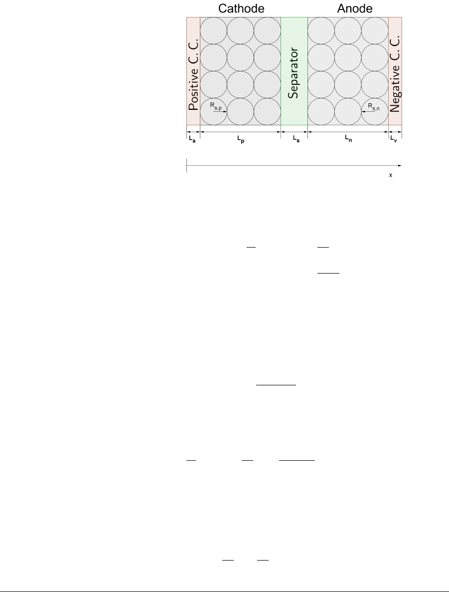
section is defined by Lzand L:= PzLzrepresents the overall battery
thickness. The electrodes and the porous separator of the Li-ion cell are
placed in contact with an electrolyte solution, facilitating the flow of ions
during charging and discharging processes. During a charging process,
the ions deintercalate from the positive electrode and, passing through
the porous media of the separator, intercalate into the negative electrode.
The inverse process occurs when discharging the cell. The diffusion of
Figure 1: 1D diagram of a Li-ion cell.
ions within the electrodes are modeled by
∂
∂t cavg
s(x, t) = −3
Rs
j(x, t) (1)
c∗
s(x, t)−cavg
s(x, t) = −Rs
5Ds
eff
j(x, t),(2)
where t∈R+represents the time, x∈Ris the one-dimensional spatial
variable, c∗
s(x, t) and cavg
s(x, t) are the surface and average concentration
of solid particles respectively, the function j(x, t) represents the ionic flux,
and Rsand Ds
eff account for the particle radius and effective diffusion
coefficients of the solid phases. The bulk State of Charge (SOC) of the
anode is defined as
SOC(t) := 1
Lncmax,n
sZLn
0
cavg
s(x, t)dx,
where cmax,n
srepresents the maximum concentration of Li-ions in the
negative electrode. The flow of ions inside the electrolyte solution is
modeled by a diffusion equation,
∂
∂t ce(x, t) = ∂
∂x Deff
∂ce(x, t)
∂x +a(1 −t+)j(x, t),(3)
where ce(x, t) represents the electrolyte concentration of ions, t+defines
the transference number, ais the particle surface area to volume ratio,
Deff accounts for the effective diffusion coefficients in the electrolyte, and
represents the material porosity. According to Ohm’s law, the conser-
vation of charge in the electrodes can be defined as
∂
∂x σeff
∂
∂x Φs(x, t)=aF j(x, t),(4)
6LIONSIMBA Toolbox - User Manual

where Φs(x, t) is the solid potential, σeff is the electrodes effective con-
ductivity, and Fis the Faraday’s constant. The potential of the Li-ion
cell is obtained as
Vout(t) := Φs(0, t)−Φs(L, t).
Similarly, a modified Ohm’s law is used to represent the charge conser-
vation within the electrolyte:
aF j(x, t) = −∂
∂x κeff
∂
∂x Φe(x, t)(5)
+∂
∂x 2κeffRT(x, t)
F(1 −t+)∂
∂x ln ce(x, t),
where Φe(x, t) is the electrolyte potential, T(x, t) represents the tem-
perature, R defines the universal gas constant, and κeff is the effective
conductivity of the liquid phase. The temperature dynamics are modeled
by an energy balance,
ρCp
∂
∂t T(x, t) = ∂
∂x λ∂
∂x T(x, t)+Qohm(x, t) (6)
+Qrxn(x, t) + Qrev(x, t),
where ρis the material density, Cpis the specific heat, λis the heat
diffusion coefficient, and the terms Qohm(x, t), Qrev(x, t), and Qrxn(x, t)
account for ohmic, reversible, and reaction heat sources as shown in [5].
The above equations are coupled by means of the ionic flux, which is
defined by the Butler-Volmer equation
jint(x, t) =2i0,int
Fsinh 0.5F
RT(x, t)ηint,(7)
where the exchange current density is given by
i0,int =F keffpce(x, t)(cmax
s−c∗
s(x, t))c∗
s(x, t).
The overpotential at the anode side is defined as
ηint := Φs(x, t)−Φe(x, t)−Un,
while at the cathode side as
ηint := Φs(x, t)−Φe(x, t)−Up
where the terms Upand Unrepresent the cathode and anode OCV re-
spectively, and keff represents the effective kinetic reaction rate. The
intercalation flux jint(x, t) is zero inside the separator.
2.2 Numerical implementation
The overall set of nonlinear and tightly coupled Partial Differential Al-
gebraic Equations (PDAEs) is used to represent all the electrochemical
phenomena occurring in the Li-ion cell. A more detailed description of the
model with the complete set of equations, numerical discretization and
the set of parameters used in this work can be found in [1]. The resulting
set of PDAEs together with the BCs is reformulated as a set of Differential
Algebraic Equations (DAEs). The spatial domain is discretized according
to the Finite Volume Method (FVM), whereas the time domain is left
continuous, according to the Method of Lines (MOL) as discussed in [6].
Therefore the spatial domain is subdivided into Na+Np+Ns+Nn+Nv
control volumes. The resulting set of DAEs is then fed to the IDA solver
from the SUNDIALS suite.
LIONSIMBA Toolbox - User Manual 7

3 Configurable scripts and parameters
3.1 Configurable parameters
As mentioned in Section 1.3, the file Parameters init.m contains param-
eters used to characterize both the Li-ion cell and the simulator settings.
By running this script a Matlab structure is returned. Note that the
returned value must be put in a cell variable. For instance:
param{1}= P a r a m e t e r s i n i t ;
This structure will contain all the parameters and their values as defined
in Parameters init.m. If the cell array would contain more than one
parameters structure, then the simulation will perform a battery pack
simulation where series-connected cells will be considered.
param{1}= P a r a m e t e r s i n i t ;
param{2}= P a r a m e t e r s i n i t ;
. . .
param{n}= P a r a m e t e r s i n i t ;
Note that the user can’t remove or add new fields to the original param-
eters list. The description of every single parameter is reported in the
Matlab source file.
3.2 Solid-phase diffusion models
LIONSIMBA allows the user to chose among three different models for
the solid-phase diffusion:
•Fick’s law diffusion equation (including the pseudo-second dimen-
sion r):
∂cs(r, t)
∂t =1
r2
∂
∂r r2Ds
eff
∂cs(r, t)
∂r
with boundary conditions
∂cs(r, t)
∂r
r=0
= 0 ∂cs(r, t)
∂r
r=Rp
=−j(x, t)
Ds
eff
•two-parameters polynomial approximation [7]:
∂cavg
s(x, t)
∂t =−3j(x, t)
Rp
c∗
s(x, t)−cavg
s(x, t) = −Rp
Ds
eff
j(x, t)
5
•higher-order polynomial approximation [7]:
∂cavg
s(x, t)
∂t =−3j(x, t)
Rp
∂q(x, t)
∂t =−30 Ds
eff
R2
p
q(x, t)−45
2
j(x, t)
R2
p
c∗
s(x, t)−cavg
s(x, t) = −j(x, t)Rp
35Ds
eff
+ 8Rpq(x, t)
8LIONSIMBA Toolbox - User Manual

The choice of the solid-phase diffusion model can be set by changing
the value of the parameters SolidPhaseDiffusion inside the Parame-
ters init.m.
Listing 1: Solid-phase diffusion model selection
param{1}= P a r a m e t e r s i n i t ;
% Two−terms model
param {1}. SolidPhaseDiffusion = 1;
% Higher−or de r model
param {1}. SolidPhaseDiffusion = 2;
% Fick ’ s law o f d i f f u s i o n
param {1}. SolidPhaseDiffusion = 3;
3.3 Battery pack simulations
LIONSIMBA allows to simulate battery packs, in particular pack where
series-connected cells are present. In order to do this just define a cell
array containing several parameters structure, e.g.:
param{1}= P a r a m e t e r s i n i t ;
param{2}= P a r a m e t e r s i n i t ;
param{3}= P a r a m e t e r s i n i t ;
Then each parameters structure can be modified, thus leading to inde-
pendent scenarios:
% Change the cathod e t h i c k n e s s o f c e l l #1
param {1}. l e n p = 5e −6;
% Reduce th e i n i t i a l anode SOC f o r c e l l #2
param {2}. c s i n i t n = 0 . 8 ∗param {2}. c s i n i t n ;
% Change the cathod e p o r o s i t y f o r c e l l #3
param {3}. eps p = 0 . 5 5 ;
In order to start a simulation of series-connected cells it is sufficient to
type:
out = s t ar tS i m u l a ti on ( 0 ,3 0 0 0 , i n i t i a l S t a t e , I , param ) ;
In this way a battery pack will be simulated from 0 to 3000 seconds,
with the initial states defined by initialState demanding (or providing) a
current density equal to I, with each cell parametrized according to the
elements of the param structure.
3.4 Configurable scripts
Besides parameters, some scripts can be modified in order to meet the
simulation needs of different scenarios.
This imply that it is possible to customize the functions used for the
computation of the diffusion coefficients in the electrolyte, the electrolyte
conductivities and so on. This leads to test different chemistries and
different types of Li-ion cells.
All the editable scripts provided in the package have an extra help text.
All the general rules that have to be followed in order to correctly imple-
ment a custom defined function are reported.
For more information about the editable scripts, type:
hel p script name
LIONSIMBA Toolbox - User Manual 9

in the Matlab command line.
3.5 Run simulations
In order to start simulations, the user must call the startSimulation script
from the Matlab command line. This script, after checking for the pres-
ence of the required tools, starts the simulation. The resulting output
will be a structure; this output will contain all the solutions of the de-
pendent variables and other parameters. Type help startSimulation from
the command line in order to get more information about the output
structure.
The startSimulation function needs four parameters:
r e s u l t s = s t a r t S i m u l a t i o n ( t0 , t f , i n i t S t a t e ,
InputDensity , param )
where:
•t0 [s]: initial integration time (Mandatory)
•tf [s]: final integration time (Mandatory)
•initState : initial state structure (Can be empty [ ] )
•InputDensity [A/m2] or [W/m2]: applied current/power density
(Mandatory for constant current/power simulation scenarios)
•param : set of parameters (Can be empty [ ] or an cell array con-
taining several parameters structure.)
The parameter initialState can be passed to the simulator in order to
define a set of initial states from which the simulations will start. It could
be useful for simulating pulse charge-discharge effects or for applying
some control-oriented algorithms. If empty, then the simulator will start
from Consistent Initial Conditions (CICs) according to the parameters
defined in the Parameters init.m script.
The applied current/power density InputDensity is used respectively by
the simulator only for simulations in galvanostatic/costant input power
conditions. Note that according to this implementation, positive cur-
rent densities make the battery charging, while negative current
densities make the battery discharging.
In the Parameters init.m script it is possible to define three operational
modes:
•Galvanostatic input current
•Costant input power
•Potentiostatic
•Variable input current
•Variable input power
If the first operational mode is chosen, the value of the parameter In-
putDensity will be used as a fixed current density applied to the battery
for the whole simulation from t0to tf. The second operational mode
set the value of the input power InputDensity and change the values
of the current and the voltage of the simulation. If the potentiostatic
mode is selected, the simulator will apply to the battery a variable cur-
rent profile which will keep the voltage at the end of the cell fixed to
10 LIONSIMBA Toolbox - User Manual

the value set in the Parameters init.m script. Like the variable current
profile, the parameter InputDensity is neglected while operating in po-
tentiostatic mode. In case of variable input profile, the simulator will
not make use of the value passed in the parameter InputDensity, but it
will get the value of the applied current density through the script get-
InputCurrent.m. Finally, the Variable input power will make use of the
power profile described in the file getInputPowerDensity.m.
3.6 Rootfinding feature for discontinuities handling in the applied current
From version 1.024 of LIONSIMBA, the software has been upgraded in
order to handle situations in which the applied current density presents
discontinuities. The application of current profiles that exhibit signifi-
cant discontinuities between two adjacent time steps, could provoke the
integrator to crash because the integration tolerances are not met. For
this reason, when the flag
AppliedCurrent
of the parameters structure is set to 2, the simulator will be able to
identify whenever a discontinuity will take place in the applied current
profile and will handle it accordingly. The car cycling example has been
extended with a second version which shows how to make use of this new
feature.
3.7 Feedback-based custom current profiles
From LIONSIMBA1.024 it is possible to define the custom profile of the
current density as a function of the battery internal states. Indeed, when
running simulations with the parameters flag AppliedCurrent set to 2,
the function used to determine the value of the current density accepts
as input also the data related to the values of the internal states at time
instant t. This extra information can be used to provide a value of Iapp
which is a function of the battery states. The example script Propor-
tional voltage control.m has been added to show this new feature.
More information can be found in the script.
3.8 Analytical Jacobian support
From version 1.022 of LIONSIMBA, an important feature has been added.
In particular, thanks to the support of the CasADitoolbox, the integra-
tion process of the P2D model has been significantly speeded up by means
of the evaluation of the analytical form of the Jacobian matrix of the en-
tire PDE model. CasADiprovides a Matlab interface for working with
symbolical variables and very efficient routines for the evaluation of an-
alytical derivatives [8]. The parameter which enables the evaluation of
the Jacobian matrix is the UseJacobian flag present in the Parame-
ters init.m file. To enable the evaluation of the Jacobian, type
param{1}= P a r a m e t e r s i n i t ;
param {1}. UseJacobian = 1;
With this flag enabled, when starting a simulation with the function
startSimulation, LIONSIMBAwill firstly evaluate the analytical Jaco-
bian of the P2D model and automatically will make use of it to provide
support to the integration process. Moreover, in order to gain the max-
imum performance, at the end of each simulation cycle the Jacobian
function is returned among the simulation results. In this way, the user
LIONSIMBA Toolbox - User Manual 11

can set the JacobianFunction field of the parameters structure to avoid
the recalculation of the analytical Jacobian matrix.
Suppose to run a simulation, and to assign the results into the variable
result. By defining
param {1}. Jaco b ianFu n ction = r e s u l t . JacobianFun ;
the Jacobian matrix will be stored and ready for future usage. In fact,
if another simulation is needed (under the assumption that no changes
have been made to the model), a new simulation can be run with the
parameters structure containing already the analytical Jacobian matrix.
Remark: The same Jacobian matrix can be reused across several simu-
lations if and only if the model structure and/or parameterization have
not been changed between one run and the next one. As soon as the
model structure (or parameterization) changes, a new Jacobian matrix
has to be evaluated otherwise the previous one would point to a wrong
model structure (or parameterization). In case of modifications of the
model it is sufficient to leave the JacobianFunction field empty, and
LIONSIMBA will automatically reevaluate the Jacobian matrix. The
CC CV charge.m example script makes use of this approach to carry
out the entire simulation.
Note: to ensure full compatibility, the CasADi matlab package is re-
quired [8]. This software is freely available at https://github.com/
casadi/casadi/wiki/InstallationInstructions
3.9 Output data
At the end of each simulation, a data structure is returned. This structure
will contain all the results related to the particular scenario defined. Each
field of the structure, moreover, is a cell array. For instance:
% D ef i n e two p a ra me t er s s t r u c t u r e to s i m u l a t e a
b a t t e r y pack
param{1}= P a r a m e t e r s i n i t ;
param{2}= P a r a m e t e r s i n i t ;
% Simul a te 1000 s at −30 A/m2
out = s t a r t S i m u l a t i o n ( 0 , 10 0 0 , [ ] , −3 0 , param ) ;
% Pl ot c e l l #1 v o l t a g e
p l o t ( out . Voltage {1})
% Hold t he f i g u r e and p l o t t he c e l l #2 v o l t a g e
p l o t ( out . Voltage {2},’−− ’)
By indexing the output structure fields, the user will access to the vari-
ables of the different cells. When a single cell is simulated, only one
element of the cell array will be present.
In order to have a full list of output fields, please type
hel p startSimulation
from the Matlab command line.
3.10 Power input
From LIONSIMBA 2.0, it is possible to set the power density as a con-
stant or variable input. To use the constant input power density in LI-
ONSIMBA, the parameter OperationMode need to be set to 2. In this
12 LIONSIMBA Toolbox - User Manual

case, the user is able to choose the power value for charge or discharge
the battery system. Instead, the user can choose the variable power den-
sity profile changing the parameter OperationMode to 5. In this case,
the user can modify the power profile described in the file getInputPow-
erDensity.m. More detailed examples can be found in Section 4.
4 Test Simulations
Simulation results were obtained using Matlab R2014b on a Windows
7@3.2GHz PC with 8 GB of RAM for the experimental battery parame-
ters in [4] with a cutoff voltage of 2.5 V and environmental temperature
of 298.15 K. For the proposed chemistry, the 1C value is ≈30 A/m2. The
effectiveness and ease of use of the proposed framework is shown.
In the first scenario (Fig. 2), −1C discharge simulations are compared for
a very wide range of heat exchange coefficient h, with high hbeing the
most challenging for retaining numerical stability in dynamic simulations.
As expected, decreasing the value of the parameter hleads to a faster
increase of the cell temperature. Moreover, due to the coupling of all
the governing equations, it is possible to note the influence of different
temperatures on the cell voltage. In the second scenario (Fig. 3), for a
fixed value of h= 1 W/(m2K), different discharge cycles are compared
at −0.5C, −1C, and −2C. According to the different applied currents, the
temperature rises in different ways; it is interesting to note the high slope
of the temperature during a −2C discharge, mainly due to the electrolyte
concentration cebeing driven to zero in the positive electrode by the high
discharge rate. In the third scenario, the framework is used to simulate a
hybrid charge-discharge cycle, emulating the throttle of a HEV. During
breaking, the battery gets charged. In Fig. 4 it is possible to analyze
the battery response under a hybrid charge-discharge cycle. The solid
potential behavior is primarily due to the different applied C rates, with
discontinuous changes producing voltage drops. Different slopes of the
voltage curve are related to the different C rates applied. Temperature
rise is recorded in the first 50 seconds of simulations, which are followed
by a slight decrease of the temperature mainly due to the exchange of
heat with the surrounding environment (h= 1 W/(m2K)) and due to
the lower current density applied. At around 250 s, temperature starts to
increase due to the −1C rate applied during moderate speed; high slope
of increase at around 410 s is due to the higher value of the discharge
current which during an overtake reaches the value of −2C. Returning
to moderate speed makes the temperature slope more gentle. During the
last 10 seconds, temperature decreases due to the significant change in
applied current and due to dissipation of heat with surrounding ambient.
In Fig. 5, the application of an ABMS is addressed. In this particular
simulation, a model predictive control algorithm [9] is adopted to drive
the SOC of the battery to a given value, while accounting for input and
output constraints. The initial SOC was around 20% and its reference
value was set to 85%. According to LIONSIMBA, the estimation of the
SOC can be easily carried out by defining a custom function. In this
particular scenario, the SOC has been computed as
SOC(t) = 1
lncmax
s,n Zln
0
cavg
s(x, t)dx
The temperature maximum bound was set to 313.5K, with the voltage
set to 4.2 V. The BMS applies a current density which is almost fixed
LIONSIMBA Toolbox - User Manual 13

at 1C value for the entire simulation, while starting to drop as the SOC
approaches its final value. The behavior of the SOC is almost linear
during the first 2500 s, while starting to change according to the current
drop, in order to approach smoothly the final stage of charge. In Fig.
6 it is possible to see that, according to the different charging stages,
the electrolyte concentration diffuses in different ways. Starting from
cinit
e= 1000 mol/m3, the input current induces a drop of concentration
within the battery sections due to the diffusion of ions from the cathode
to the anode. Approaching the final stage of charging, the concentration
starts to converge back to the initial value of 1000 mol/m3and, around
5500 s, reaches the steady value. This behavior emphasizes the property
of the FVM to conserve properties within numerical roundoff.
In Fig. 7, simulations have been run disabling the thermal dynamics lead-
ing to an isothermal environment. This particular configuration can be
exploited in order to assess the influence of different constant tempera-
tures at which the battery can operate.
In Fig. 8, it is simulated a discharge-charge cycle with the use of constant
input power density. In particular, for the temperature dynamic the
lumped thermal model has been used. For the first 1500 s the power is
set to different negative values, that increase the temperature especially
when the power density is set a higher value. Even if the power remain
negative from 1000 s and 1500 s, the temperature starts to decrease due
to the high different of power set. The current plot follows the power
cycle and the slope of this parameter is horizontal only in the resting
phase( from 1500 s and 2000 s and from 2500 s and 3000 s), while when
the power has higher values the current has an higher slope.
In Fig. 9, it is simulated a sinusoidal charge-discharge cycle of variable
input power density. The SOC decreases on every period of constant
value that is due to the phase shift put initially in the function. The
temperature has little jumps that are due to the continuously change in
the sign of the power.
All the results of the proposed simulations can be reproduced by running
the example scripts available with LIONSIMBA.
14 LIONSIMBA Toolbox - User Manual
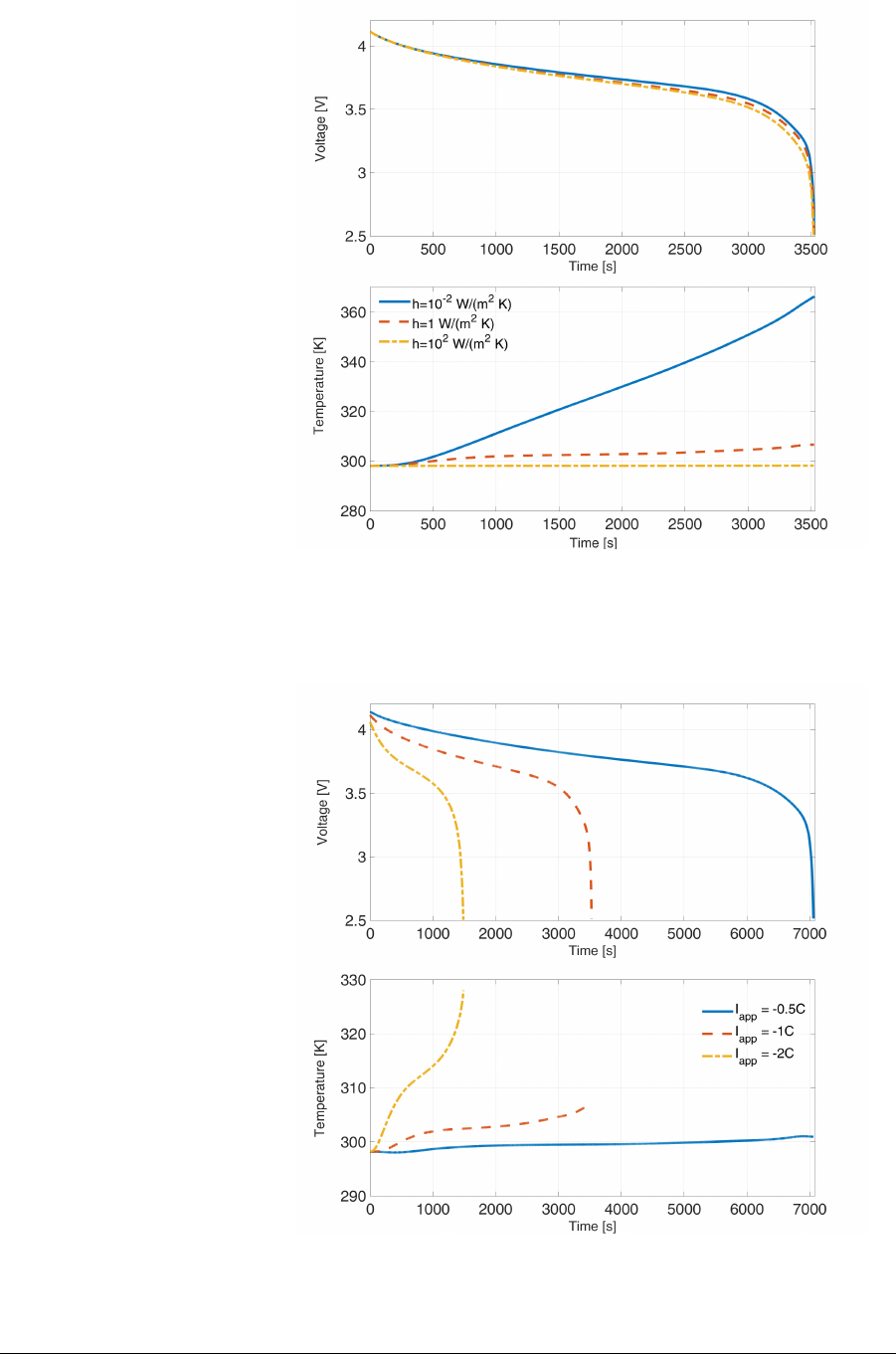
Figure 2: −1C discharge cycle run under different heat exchange param-
eters: blue line h= 0.01W/(m2K), dashed orange line h= 1 W/(m2K)
and dot-dashed yellow line h= 100 W/(m2K).
Figure 3: Full discharge cycle run under different C rates: −2C (dot-
dashed yellow), −1C (dashed orange line), and −0.5C (blue line).
LIONSIMBA Toolbox - User Manual 15
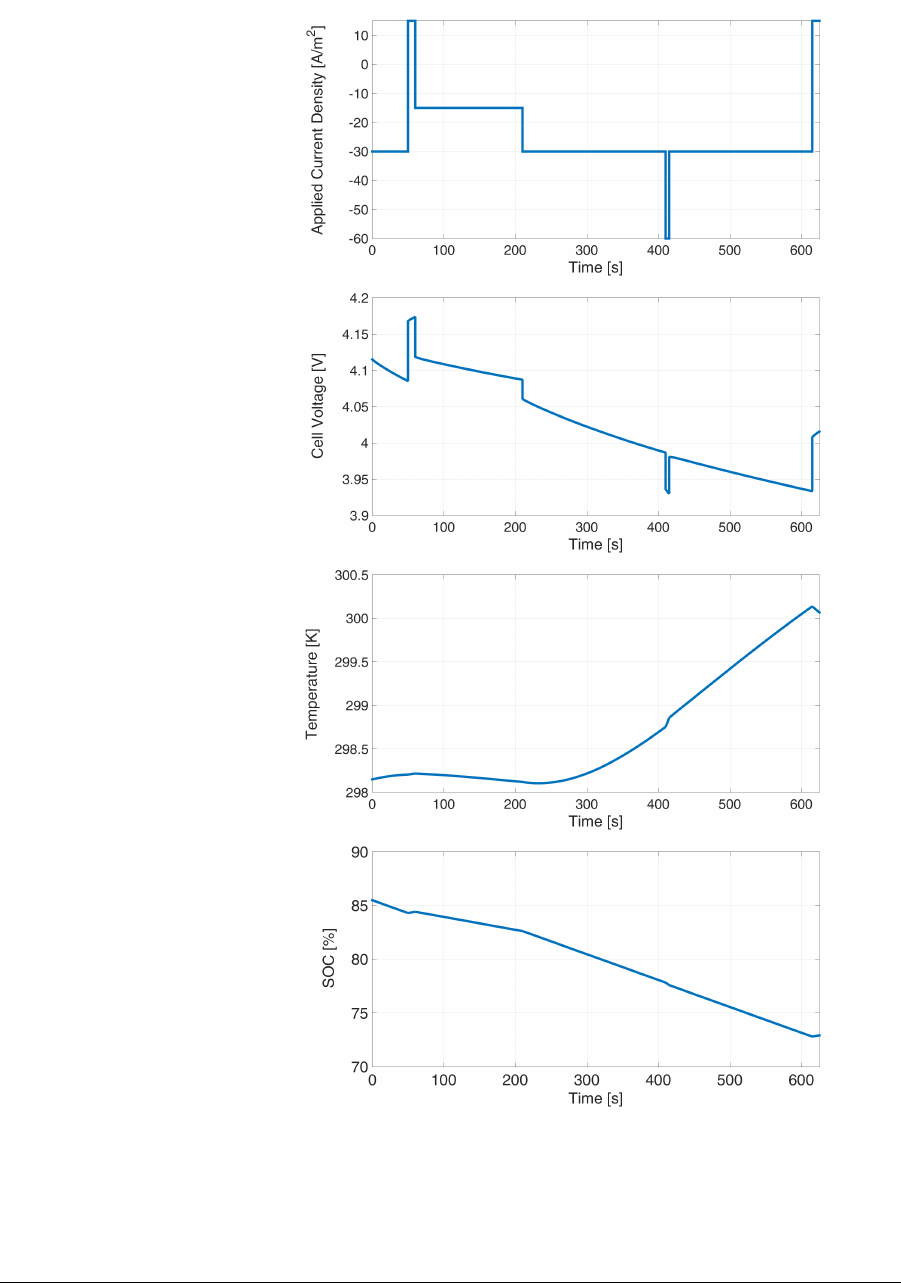
Figure 4: Hybrid charging-discharging cycle.
16 LIONSIMBA Toolbox - User Manual

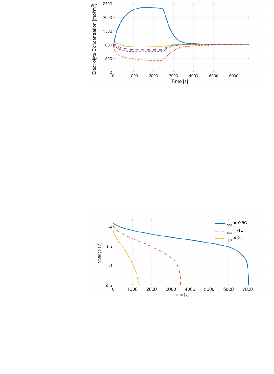
Figure 6: ABMS control – Electrolyte concentration: The behavior of the
first and last volume of each section of the battery is depicted, where the
countinous lines belong to the cathode, the dashed lines to the separator
and the dotted lines to the anode.
Figure 7: Full discharge cycle in an isothermal environment: blue line
−0.5C, dashed orange line −1C, and dot-dashed yellow line −2C.
18 LIONSIMBA Toolbox - User Manual
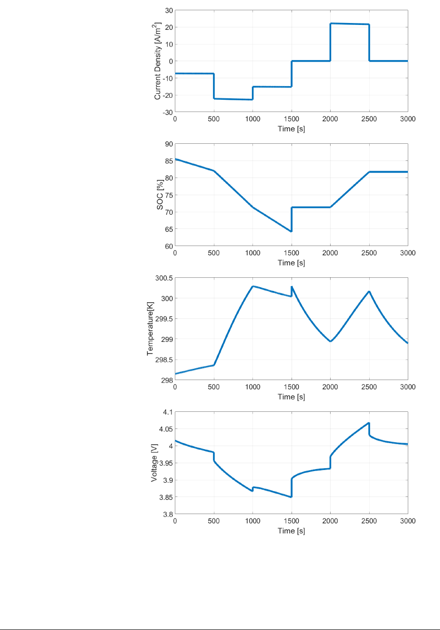
Figure 8: Charging-discharging cycle done with a constant input power
density
LIONSIMBA Toolbox - User Manual 19
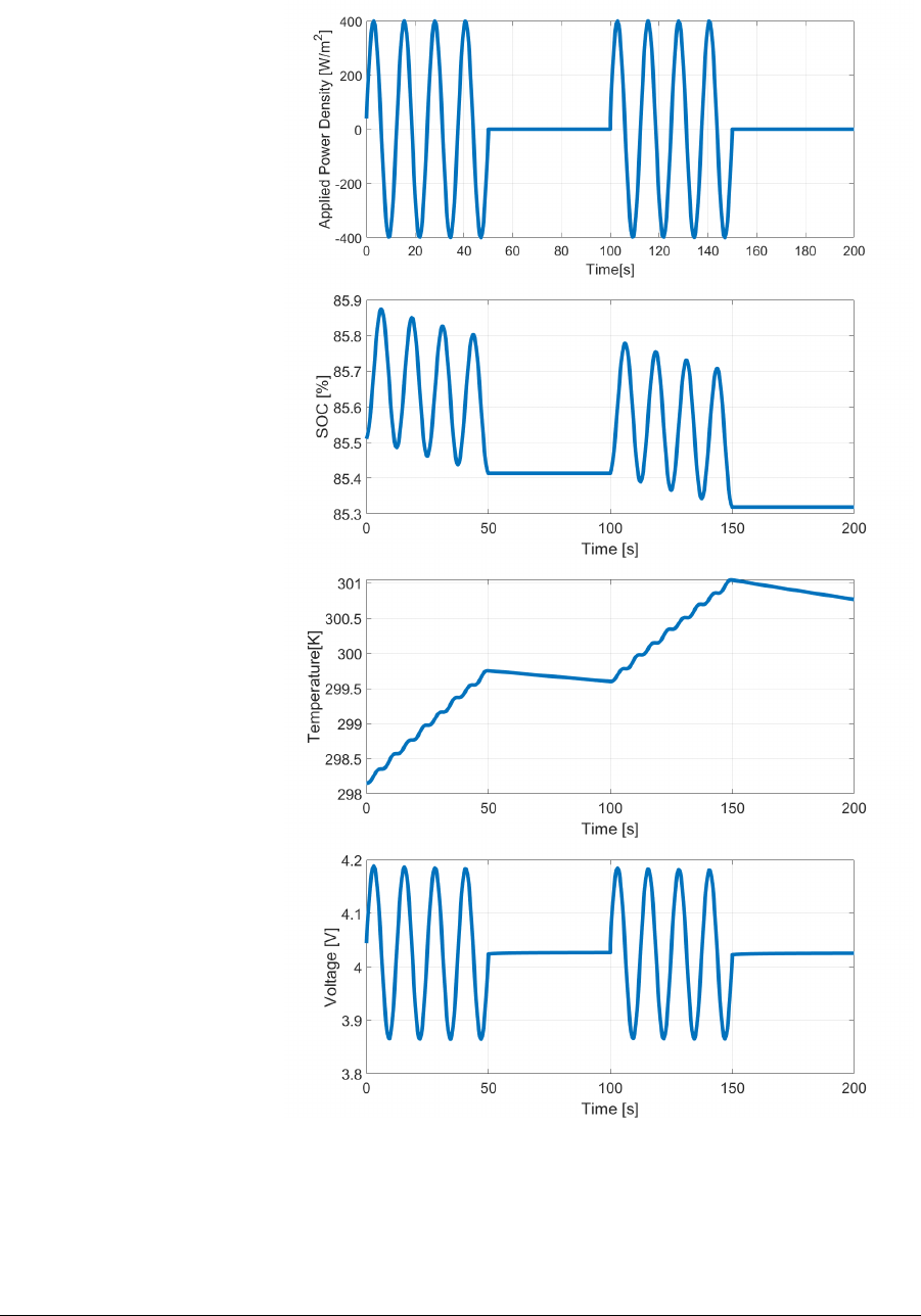
Figure 9: Sinusoidal charging-discharging cycle done with a variable input
power density
20 LIONSIMBA Toolbox - User Manual

References
[1] M. Torchio, L. Magni, R. B. Gopaluni, R. D. Braatz, and
D. M. Raimondo, “LIONSIMBA: A matlab framework based
on a finite volume model suitable for li-ion battery design,
simulation, and control,” Journal of The Electrochemical Society,
vol. 163, no. 7, pp. A1192–A1205, 2016. [Online]. Available:
http://jes.ecsdl.org/content/163/7/A1192.abstract
[2] M. Doyle, T. F. Fuller, and J. Newman, “Modeling of galvanostatic
charge and discharge of the lithium/polymer/insertion cell,” Journal
of the Electrochemical Society, vol. 140, no. 6, pp. 1526–1533, 1993.
[3] A. C. Hindmarsh, P. N. Brown, K. E. Grant, S. L. Lee, R. Serban,
D. E. Shumaker, and C. S. Woodward, “SUNDIALS: Suite of nonlin-
ear and differential/algebraic equation solvers,” ACM Trans. Math.
Softw., vol. 31, no. 3, pp. 363–396, Sep. 2005.
[4] P. W. C. Northrop, V. Ramadesigan, S. De, and V. R. Subramanian,
“Coordinate transformation, orthogonal collocation, model reformu-
lation and simulation of electrochemical-thermal behavior of lithium-
ion battery stacks,” Journal of The Electrochemical Society, vol. 158,
no. 12, pp. A1461–A1477, 2011.
[5] K. Kumaresan, G. Sikha, and R. E. White, “Thermal model for a
Li-ion cell,” Journal of the Electrochemical Society, vol. 155, no. 2,
pp. A164–A171, 2008.
[6] W. E. Schiesser, The Numerical Method of Lines. Academic Press,
1991.
[7] V. Ramadesigan, V. Boovaragavan, J. C. Pirkle, and V. R. Subrama-
nian, “Efficient reformulation of solid-phase diffusion in physics-based
lithium-ion battery models,” Journal of The Electrochemical Society,
vol. 157, no. 7, pp. A854–A860, 2010.
[8] J. Andersson, “A General-Purpose Software Framework for Dynamic
Optimization,” PhD thesis, Arenberg Doctoral School, KU Leuven,
Department of Electrical Engineering (ESAT/SCD) and Optimiza-
tion in Engineering Center, Kasteelpark Arenberg 10, 3001-Heverlee,
Belgium, October 2013.
[9] M. Torchio, N. A. Wolff, D. M. Raimondo, L. Magni, U. Krewer,
R. B. Gopaluni, J. A. Paulson, and R. D. Braatz, “Real-time model
predictive control for the optimal charging of a lithium-ion battery,”
in Proceedings of thet American Control Conference, 2015, pp. 4536–
4541.
LIONSIMBA Toolbox - User Manual 21
