VARIFORC User Manual: Chapter 8 (FORC Tutorial) Manual Chapter08 Tutorial

User Manual:

Open the PDF directly: View PDF .
Page Count: 45

VARIFORC User Manual: 8. FORC tutorial 8.1

VARIFORC User Manual

Chapter 8:

FORC tutorial

M

0

M

1

M

2

M

3

0

0

H

H

H

(M1

−

M0)′

(M2

−

M1)′

(M3

−

M2)′

µ0Hc

µ0Hb

1,1

2,1

2,2

3,1

3,2

3,3

1,1

1,1



2,1

2,1

3,1

2,2

2,2

3,2

3,3

VARIFORC User Manual: 8. FORC tutorial 8.2

© 2014 by Ramon Egli and Michael Winklhofer. Provided for non-commercial research

and educaonal use only.

VARIFORC User Manual: 8. FORC tutorial 8.3

This chapter is based on contribuons by Ramon Egli and Michael Winklhofer to the Inter-

naonal Workshop on Paleomagnesm and Rock Magnesm (Kazan Instute of Geology and

Petroleum Technology, Russia, October 7-12, 2013), summarized in the following conference

proceeding arcle:

Recent developments on processing and interpretaon aspects of

first-order reversal curves (FORC)

Ramon Egli

Central Instute for Meteorology and Geodynamics, Hohe Warte 38, 1190 Vienna, Austria

(r.egli@zamg.ac.at)

Michael Winklhofer

Department for Earth and Environmental Sciences, Munich University, Theresienstrasse 41,

80333 Munich, Germany (michael@geophysik.uni-muenchen.de)

Abstract  Several recent developments in paleo- and environmental magnesm have been based on

measurement of first-order reversal curves (FORC). Most notable examples are related to the detec-

on of fossil magnetosomes produced by magnetotacc bacteria and to absolute paleointensity es-

mates for temperature-sensive samples, such as meteorites. Future developments in these scienfic

disciplines rely on improved characterizaon of natural magnec mineral assemblages. Promising

results have been obtained in several cases with the parallel development of FORC processing proto-

cols on one hand, and models for idealized magnec systems on the others. Unl now, FORC diagrams

have been used mainly as a qualitave tool for the idenficaon of magnec domain state fingerprints,

with missing quantave links to other magnec parameters. This arcle bridges FORC measurements

and convenonal hysteresis parameters on the basis of three types of FORC-related magnezaons

and corresponding coercivity distribuons. One of them is the well-known saturaon remanence, with

corresponding coercivity distribuon derived from backfield demagnezaon data in zero-field FORC

measurements. The other two magnezaon types are related to irreversible processes occurring

along hysteresis branches and to the inversion symmetry of magnec states in isolated parcles, res-

pecvely. All together, these magnezaons provide precise informaon about magnezaon proces-

ses in single-domain, pseudo-single-domain, and muldomain parcles. Unlike hysteresis parameters

used in the so-called Day diagram, these magnezaons are unaffected by reversible processes (e.g.

superparamagnesm), and therefore well suited for reliable characterizaon of remanent magneza-

on carriers. The soware package VARIFORC has been developed with the purpose of performing

detailed FORC analyses and calculate the three types of coercivity distribuons described above. Key

examples of such analyses are presented in this arcle, and are available for download along with the

VARIFORC package.

VARIFORC User Manual: 8. FORC tutorial 8.4

VARIFORC User Manual: 8. FORC tutorial 8.5

8.1 Introducon

Several measurement protocols have been developed over the last 50 years for under-

standing complex magnezaon processes related to technological applicaons [Chikazumi,

1997; Coey, 2009], the origin and stability of rock magnezaons [Dunlop and Özdemir, 1997;

Tauxe, 2010], and environment-sensive magnec minerals in sediments [Evans and Heller,

2003; Liu et al., 2012]. First-order reversal curves (FORC) provide one of the most advanced

protocols for probing hysteresis processes and represent them in a two-dimensional parame-

ter space (i.e. coercivity field c

H and bias field b

H). The interpretaon of hysteresis has evol-

ved from mathemacal formalisms based on the superposion of elemental source contribu-

ons, called hysterons [Preisach, 1935; Mayergoyz, 1986; Hejda and Zelinka, 1990; Fabian and

Dobeneck, 1997], toward physical models of specific magnec systems, such as non-interac-

ng [Newell, 2005; Egli et al., 2010] and interacng [Woodward and Della Torre, 1960; Basso

and Berto, 1994; Pike et al., 1999; Muxworthy and Williams, 2005; Egli, 2006a] single-do-

main (SD) parcles, pseudo-single-domain (PSD) parcles [Muxworthy and Dunlop, 2002; Car-

vallo et al., 2003; Winklhofer et al., 2008], muldomain (MD) crystals [Pike et al., 2001b;

Church et al., 2011], and spin glasses [Katzgraber et al., 2002]. These models provide proto-

type signatures for specific magnezaon processes (e.g. switching, vortex nucleaon, do-

main wall pinning), which can be recognized in FORC diagrams of geologic samples [Roberts

et al., 2000, 2006]. Some of these signatures occur within a limited subset of FORC space, as

for instance along c0H» (viscosity and MD processes) or along b0H» (weakly interacng

SD parcles). Therefore, it is possible to idenfy the corresponding sources in FORC diagrams

of samples containing complex magnec mineral mixtures [e.g. Roberts et al., 2012], and, in

some cases, to esmate the abundance of magnec parcles associated with these processes

[Roberts et al., 2011; Yamazaki and Ikehara, 2012; Egli, 2013; Ludwig et al., 2013]. Up to the

few examples menoned above, FORC diagrams of geologic materials are mostly interpreted

in a qualitave manner. Furthermore, only loose connecons have been established with mo-

re common magnec parameters, such as isothermal and anhysterec remanent magneza-

ons and domain state-sensive raos, although some of these parameters can be directly

derived from FORC subsets [e.g. Fabian and Dobeneck, 1997; Winklhofer and Zimanyi, 2006;

Egli et al., 2010].

Quantave interpretaon of FORC measurements is based on the calculaon of magnec

parameters associated with specific magnezaon processes. Some of these processes pro-

duce FORC signatures that are representable only in terms of non-regular funcons, whose

appearance in the FORC diagram depends strongly on data processing. A meanwhile well-

known example of non-regular FORC signatures is represented by the so-called central ridge

produced by non-interacng SD parcles [Egli et al., 2010; Egli, 2013]. Magnec viscosity is

another example associated with a vercal ridge near c0H= [Pike et al., 2001a]. On the other

hand, most magnec processes in weakly magnec natural samples produce connuous FORC

VARIFORC User Manual: 8. FORC tutorial 8.6

contribuons with very low amplitudes, which are below the significance threshold aainable

with convenonal FORC processing [Egli, 2013]. Since the introducon of FORC measurements

to rock magnesm [Pike et al., 1999; Roberts et al., 2000], some studies have been dedicated

to selected aspects of FORC processing, such as computaonal opmizaon [Heslop and Mux-

worthy, 2005], locally weighted regression [Harrison and Feinberg, 2008], error calculaon

[Heslop and Roberts, 2012], and variable polynomial regression smoothing [Egli, 2013]. These

improvements have been merged into a single FORC processing procedure called VARIFORC

(VARIable FORC smoothing) [Egli, 2013]. The principal advantage of VARIFORC consists in the

possibility of processing FORC data containing high-amplitude, non-regular FORC signatures

as well as low-amplitude, connuous backgrounds, using a local compromise between high

resoluon and noise suppression requirements. First applicaons of this technique enabled

full characterizaon of SD signatures in pelagic carbonates [Ludwig et al., 2013].

Meanwhile, VARIFORC has been complemented with rounes for the automac separa-

on of different FORC contribuons, and the calculaon of corresponding magnezaons and

coercivity distribuons. The full VARIFORC package, including a detailed user manual, is availa-

ble at hp://www.conrad-observatory.at/cmsjoomla/en/download. VARIFORC runs on Wol-

fram MathemacaTM and Wofram PlayerProTM (see Chapter 2). Applicaon examples of quan-

tave FORC analysis performed with VARIFORC are discussed in this paper.

VARIFORC User Manual: 8. FORC tutorial 8.7

8.2 A brief introducon to FORC diagrams

8.2.1 Reversible and irreversible hysteresis processes

Ferrimagnec materials are characterized by complex magnec properes that depend on

their past magnec and thermal history. Memory of previously applied fields gives raise to the

well-known phenomenon of magnec hysteresis. The discovery magnec hysteresis is credi-

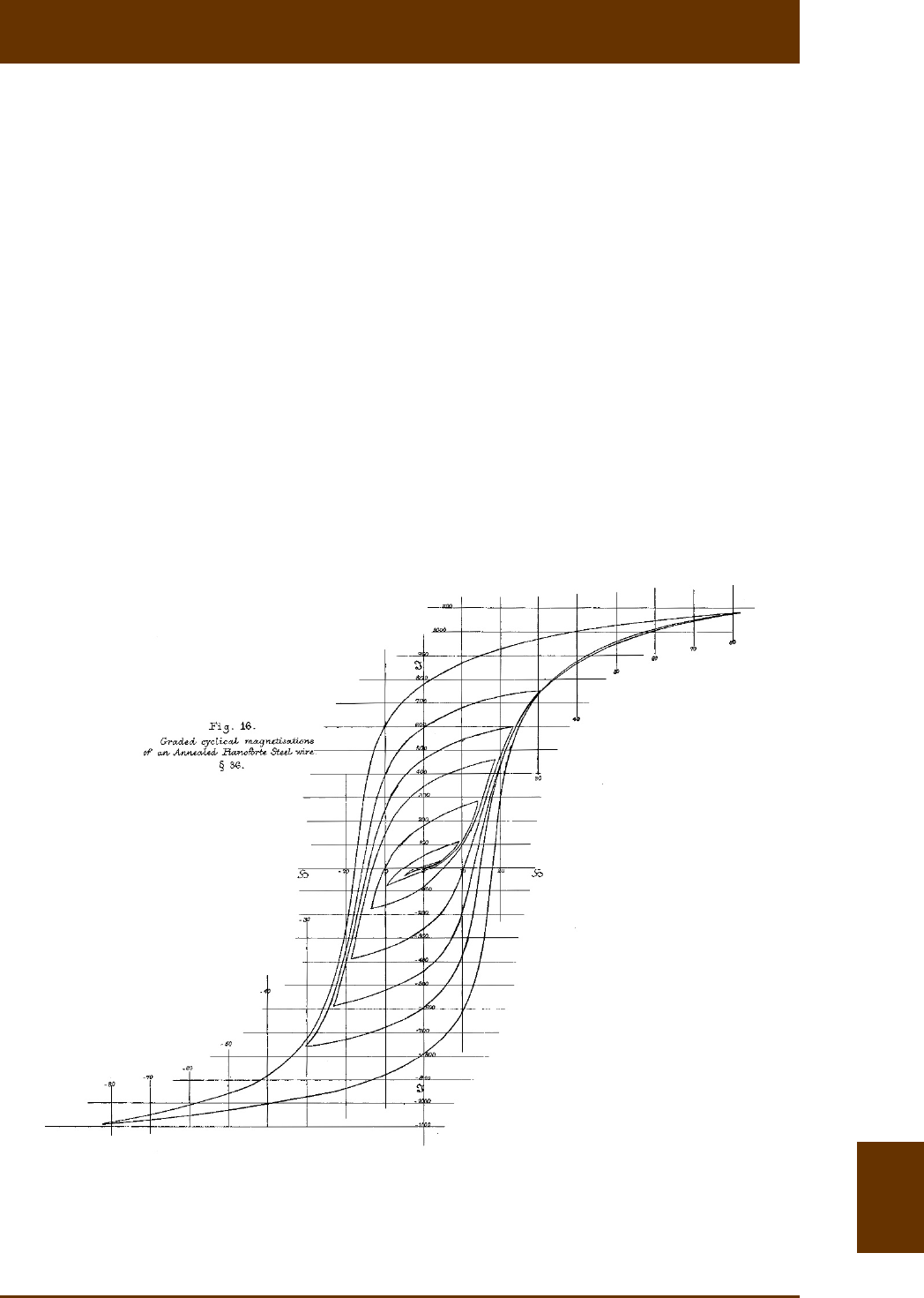
ted to Sir Alfred James Ewing (1855-1955), who measured the first hysteresis loop (Fig. 8.1)

on a piano wire [Ewing, 1885]. While the main characteriscs of a hysteresis loop are summari-

zed by four magnec parameters yielding the well-known Day diagram [Day et al., 1977;

Dunlop, 2002a,b], much more detailed informaon on magnezaon processes can be obtai-

ned by accessing the inner area of hysteresis loops. This is possible by in-field measuring pro-

tocols involving a sequence of field sweep reversals. The oldest example of such sequences is

the alternang-field (AF) demagnezaon [Chikazumi, 1997], in which the field sweep is rever-

sed at increasingly small field amplitudes, unl a demagnezed, so-called anhysterec state

0HM== is reached (Fig. 8.1).

Fig. 8.1: Original figure from Ewing [1885] showing the hysteresis measurement of a piano wire (see

the IRM Quarterly Vol. 22 for a story about Sir Alfred Ewing’s first hysteresis measurements). The

measurement shown here represents an AF demagnezaon curve, as a possible method for accessing

the inner area of hysteresis loops.

VARIFORC User Manual: 8. FORC tutorial 8.8

Other measuring protocols for accessing the inner area of a hysteresis loop are possible,

and the FORC protocol described by Pike et al. [1999] is just one of them. All protocols start

from a well-defined magnec state obtained by saturang the sample in a large field. The first

magnezaon curve obtained by sweeping the magnec field from posive or negave satu-

raon coincides with one of the two major hysteresis loop branches ()MH

. Hysteresis bran-

ches are also known as a zero-order curves, because they originate directly from a saturated

state. If the field sweep producing a zero-order curve is reversed at a reversal field r

H, before

saturaon is reached, a new magnezaon curve r

(,)MH H originates from the major hyste-

resis loop (Fig. 8.2a). This curve represents a first-order magnezaon, also known as first-

order reversal curve in case of FORC measurements. A set of first-order curves branching from

the major hysteresis loop at different reversal fields covers the enre area enclosed by the

loop, accessing a much larger number of magnezaon states that cannot be obtained with

simple hysteresis measurements. If the field sweep is reversed again while a first-order curve

is measured, a second-order curve is obtained, and so on. Within this context, AF demagne-

zaon is a sequence of nested magnezaon curves with increasing order.

When describing magnezaon curves, an important disncon is made between mag-

nezaon changes due to reversible and irreversible processes. The two types of processes

occurring along any magnezaon curve are disnguished by comparing a small poron

A

B

MM of the curve between close fields

A

H and B

H with the magnezaon

A

M* obtained

by sweeping the field from B

H back to

A

H (Fig. 8.2a). Hysteresis, known in this context as

magnec memory, ensures that BA

MM

*

 does not follow the same path as

A

B

MM , in

which case

A

A

MM

*¹ [Mayergoyz, 1986]. The difference

A

A

MM

*- is the irreversible magne-

zaon change occurring when sweeping the field from

A

H to B

H, while BA

MM

*

- is the rever-

sible change. The sum of the two contribuons gives BA

MM-, as expected.

8.2.2 Preisach diagrams

Because n-th order magnezaon curves depend on 1n+ parameters (i.e. n reversal

fields and one measuring field), interpretaon of first- and higher order curves requires a para-

meter space model. The best known bivariate hysteresis model has been implemented by

Preisach [1935] for the characterizaon of transformer steel. The Preisach model assumes that

magnezaon curves are the result of magnec switching in elemental rectangular hysteresis

loops (so-called hysterons). Hysterons are characterized by two switching fields AB

HH£ whe-

re the magnezaon jumps disconnuously from the lower to the upper branch and vice-

versa (Fig. 8.2b). Each hysteron is thus represented by a point in AB

(,)HH-space, and macro-

scopic magnec volumes or magnec parcle assemblages are described by a bivariate sta-

scal distribuon AB

(,)PH H of hysteron switching fields, known as the Preisach distribuon.

VARIFORC User Manual: 8. FORC tutorial 8.9

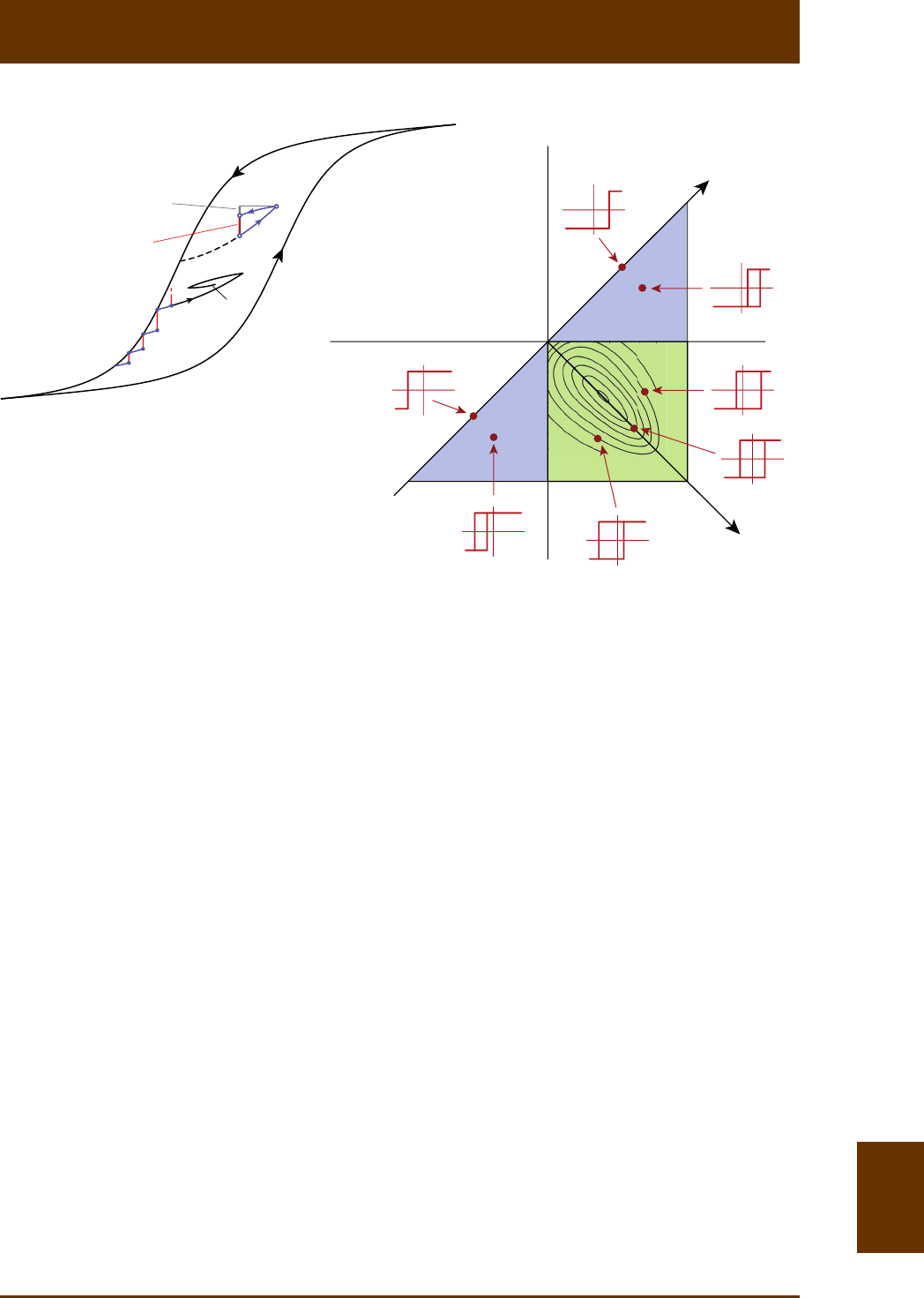
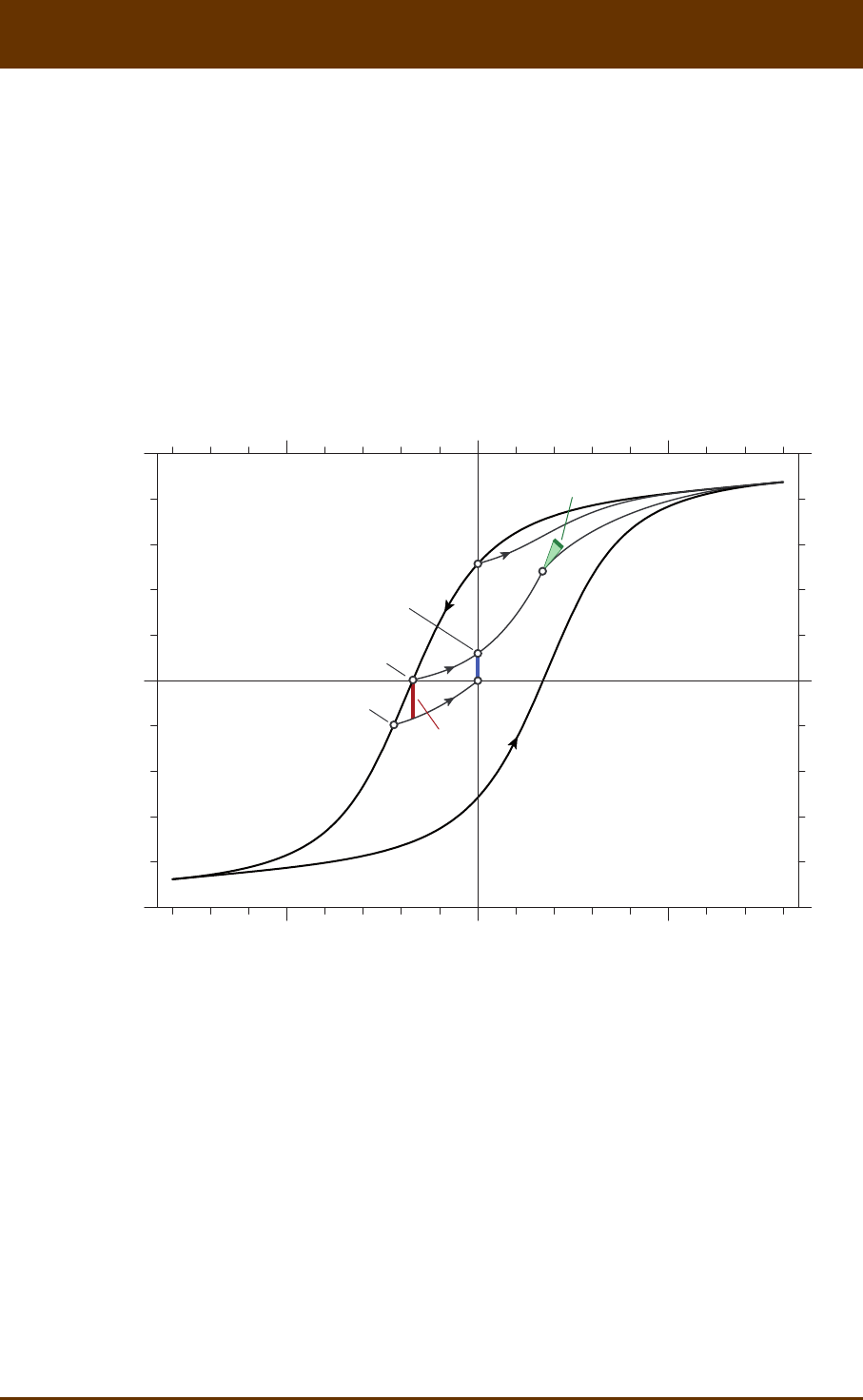
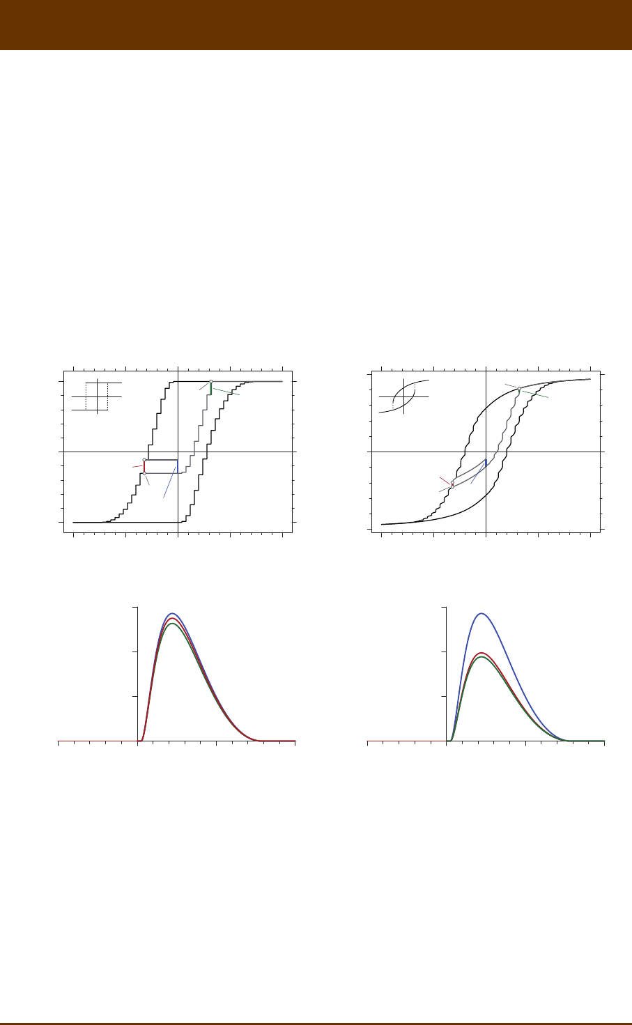
Fig. 8.2: Preisach theory in a nutshell. (a) The major hysteresis loop (black lines with large arrows) is

composed of two zero-order magnezaon curves starng from posive and negave saturaon,

respecvely. First-order magnezaon curves originate from the major hysteresis if the field sweep is

reversed (black curve labeled with 1st). Higher-order magnezaon curves (curves labeled with 2nd and

3rd) are obtained aer successive field sweep reversals. Any point inside the major hysteresis loop can

be accessed by first-order magnezaon curves (dashed black line). For any of these points (e.g. point

A at the end of the dashed line), magnezaon changes can be decomposed into a reversible ( rev

ΔM)

and an irreversible ( irr

ΔM) component by sweeping the field a lile further to point B and then back

to the original field, ending with point A*, which, because of irr

ΔM, does not coincide with A. The

inial parts of first-order curves originang from the upper hysteresis branch (blue segments) define

the irreversible component (red bars) of magnezaon changes along this branch. (b) The Preisach

diagram is a representaon of hysteresis processes as the sum of elemental contribuons from rectan-

gular hysteresis loops (hysterons, sketched in red) with switching fields A

H and B

H. Because BA

HH³

by definion, hysteron coordinates AB

(,)HH plot below the AB

HH= diagonal, over a triangular area

(colored) limited by the saturaon field sat

H above which magnec hysteresis is fully reversible.

Further disncons can be made between (1) closed hysterons with AB

HH=, (2) hysterons with only

one possible state in zero field (posive or negave saturaon, blue areas), and (3) hysterons with two

possible states in zero field (so-called magnec remanence carriers, green square). The Preisach space

can also be expressed in transformed coordinates represenng coercivity (i.e. hysteron opening

cBA

()/2HHH=- ) and the bias field (i.e. hysteron horizontal shis b

H= BA

()/2HH+). Hysteron

examples (red) are given for selected points of the Preisach space, which can be understood as samples

of the Preisach distribuon. Contour lines over the region occupied by remanence-carrying hysterons

(green) represent a Preisach distribuon obtained for interacng SD parcles by Dunlop et al. [1990].

In the Preisach-Néel model, c

H- and b

H-coordinates coincide with coercivies and interacon fields

of real SD parcles, respecvely.

1

st

2

nd

3

rd

A

B

A*

A

BA*

∆M

irr

∆M

rev

H

b

H

c

H

A

H

B

(a) (b)

−H

sat

H

sat

VARIFORC User Manual: 8. FORC tutorial 8.10

Hysterons are merely a mathemacal construct and do generally not correspond to dis-

crete parcles or sample volumes. Nevertheless, the bivariate Preisach distribuon provides

intrinsically more informaon than any one-dimensional magnezaon curve. The simplest

physical interpretaon of a Preisach distribuon has been proposed by Néel [1958] with what

is known as the Preisach-Néel model of single-domain (SD) parcles. This model relies on the

resemblance between hysteresis loops of individual SD parcles with uniaxial anisotropy [Sto-

ner and Wohlfarth, 1948] on one hand, and symmetric Preisach hysterons (i.e. AB

HH=- ) on

the other hand. Both are characterized by only two magnezaon states (one for each hyste-

resis branch) with disconnuous transions at Ac

HH=- and Bc

HH=+ . The Preisach distri-

buon of isolated SD parcles is thus concentrated along the AB

HH=- diagonal of the Prei-

sach space and coincides with the well-known coercivity or switching field distribuon.

In interacng SD parcle assemblages, magnec switching of individual parcles occur in

a total field given by the sum of the applied field and an internal, so-called interacon field

b

H, which is the sum of dipole fields produced by the magnec moments of the other par-

cles. Whenever b0H¹, elemental hysteresis loops are shied horizontally, so that magnec

switching occurs at Abc

HHH=- and B

H

=

bc

HH+. Because the interacon field is a local

variable determined by the spaal arrangement and magnezaon of neighbor parcles, the

Preisach distribuon of interacng SD parcles can be represented as the product of a coer-

civity distribuon c

()

f

H and an interacon field distribuon b

()gH :

cb

()()PfHgH= (8.1)

with cBA

()/2HHH=- and bBA

()/2HHH=+ (Fig. 8.2b). More generally, c

H and b

H are

known as the coercivity field and the bias field of hysterons. The appealing simplicity of the

Preisach-Néel model has promoted the use of the transformed coordinates cb

(,)HH (whereby

b

H is also called u

H or i

H), instead of the original Preisach fields A

H and B

H.

The Preisach space spanned by hysteresis processes that are saturated in fields sat

||HH<

is a triangular region delimited by the diagonal line BA

HH³ (by definion of hysteron swit-

ching fields), and by Asat

HH>- , Bsat

HH<+ , respecvely (Fig. 8.2b). This space can be further

subdivided into a square region with A0H< and B0H> where hysterons can have two mag-

nezaon states in zero field, and the remaining space where hysterons are negavely or posi-

vely saturated when no external fields are applied. The square region is parcularly relevant

to paleo- and rock magnesm, because remanent magnezaons originate only from hyste-

rons located within it. In parcular, the saturaon remanent magnezaon rs

M corresponds

to the integral of the Preisach funcon over this region, i.e.

sat

AsatB

0

rs A B A B

0(,)dd

H

HHH

MPHHHH

+

=- =

=òò (8.2)

On the other hand, the saturaon magnezaon s

M corresponds to the integral of the

Preisach funcon over the enre domain defined by BA

HH³.

VARIFORC User Manual: 8. FORC tutorial 8.11

8.2.3 The FORC distribuon

Several measurement protocols have been developed in order to obtain experimental

Preisach funcon esmates. What is nowadays known as the FORC protocol has been first

described by Hejda and Zelinka [1990]. With this protocol, first-order magnezaon curves

r

(,)MH H , measured upon posive sweeps of H (i.e. H increases) from reversal fields r

H, de-

fine the so-called FORC funcon

2

r

r

1

(,) 2

M

ρH H HH

=- 

 (8.3)

[Pike, 2003]. This funcon coincides with the Preisach distribuon in case of measurements

performed on samples that are correctly described by the Preisach model. Because real sam-

ples rarely sasfy this condion, empirical distribuons such as eq. (3) do generally not coin-

cide with the Preisach distribuon up to few excepons [e.g. Carvallo et al., 2005]. For exam-

ple, the Preisach distribuon is a strictly posive probability funcon, while FORC diagrams

can have negave amplitudes [Newell, 2005]. Several modificaons of the original Preisach

model have been developed in order to account for such differences. So-called moving Prei-

sach models [Vajda and Della Torre, 1991] take the effect of macroscopic magnezaon states

on the intrinsic hysteron properes into account, and are used for instance to describe mag-

nezaon-dependent interacon fields. Magnec viscosity, on the other hand, is accounted

by Preisach models with stochasc inputs simulang thermal fluctuaons of switching fields

[Mitchler et al., 1996; Borcia et al., 2002].

Modificaons of the Preisach formalism are not sufficient to explain all aspects of FORC

funcons, especially in case of non-SD magnec systems. Therefore, physical FORC models

have been developed in order to properly interpret magnec processes in isolated [Newell,

2005] and interacng [Muxworthy and Williams, 2005; Egli, 2006] SD parcles, nucleaon of

magnec vorces in PSD parcles [Carvallo et al., 2003; Winklhofer et al., 2008], domain wall

displacement in MD crystals [Pike et al., 2001b; Church et al., 2011], and magnec viscosity

[Pike et al., 2001a]. Magnec models of idealized systems yield characterisc signatures of the

FORC funcon that can be used as fingerprints for the idenficaon of magnec minerals in

geologic samples [Roberts et al., 2000]. In some cases, these signatures are precisely determi-

ned to the point that quantave analysis is possible [Winklhofer and Zimanyi, 2006; Egli et

al., 2010; Ludwig et al., 2013].

The remaining part of this secon is dedicated to the implementaon of a general FORC

model that will be used to interpret the properes of SD, PSD, and MD samples presented in

this arcle. For this purpose, a relavely simple magnec system with few magnezaon sta-

tes is considered. This system corresponds to the micromagnec hysteresis simulaon of a

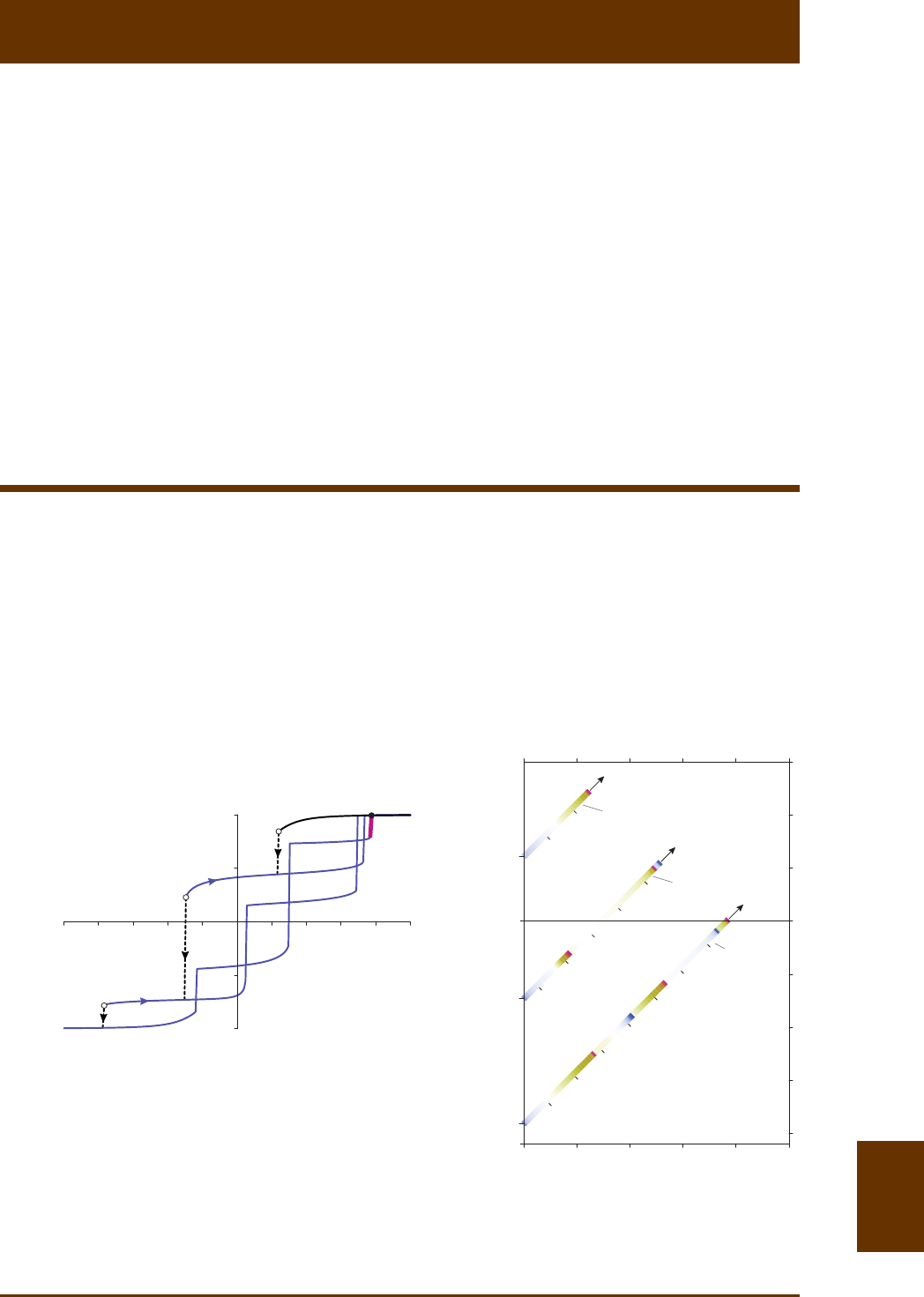
cluster of seven strongly interacng SD parcles (Fig. 8.3). The upper branch of the major hys-

teresis loop contains three magnezaon jumps produced by abrupt transions between four

VARIFORC User Manual: 8. FORC tutorial 8.12

magnec states with magnezaons 0

M, 1

M, 2

M, and 3

M. These states represent con-

nuous segments of the upper hysteresis branch.

Fig. 8.3: FORC model of a linear chain of 7 SD magnete parcles with elongaon 1.3e= and long

axes perpendicular to the chain axis. This model represents the simulaon of a collapsed magnetosome

chain according to Fig. 9a in Shcherbakov et al. [1997]. In this example, the chain axis forms an angle

of 75° with the applied field direcon. Magnezaon jumps along the upper branch of the major

hysteresis loop are indicated by dashed lines. Cursive number pairs are used to count disconnuies

of first-order curves 1

M, 2

M, and 3

M (blue lines). For example, (2,2) is the second jump (counted from

the right) occurring along 2

M. Any measurable FORC coincide with 0

M, 1

M, 2

M, or 3

M. The amplitude

of the last magnezaon jump on 3

M (magenta) defines the contribuon cr

M of the central ridge to

the FORC diagram shown in (b). (b) FORC diagram calculated from (a), consisng of three diagonal

ridges defined by first derivaves 1

()

ii

MM

-¢

- of differences between 0

M, 1

M, 2

M, and 3

M. The

ridges width is exaggerated in order to show the color coding for posive (orange to magenta) and

negave (blue) contribuons. Cursive number pairs indicate peaks of the FORC funcon produced by

magnezaon jumps with same labels as in (a). One of the peaks, labeled with CR, contributes to the

central ridge and is generated by the last magnezaon jump (i.e. 3,1) of the last FORC (i.e. 3

M). All

FORC contribuons are enclosed in a triangular region defined by verces with coordinates sat

(0, )H

and sat

(,0)H, where sat 40 mTH» is the field above which hysteresis becomes fully reversible.

02040

+50 mT−50

M

0

M

1

M

2

M

3

H

r,1

H

r,2

H

r,3

0

0

20 30

0102030−10

20

10

0

−10

−20

−30

H

H

H

(M

1

− M

0

)′

(M

2

− M

1

)′

(M

3

− M

2

)′

µ

0Hc [mT]

µ0Hb [mT]

(a) (b)

1,1

2,1

2,2

3,1

3,2

3,3

H

r,1

H

r,2

H

r,3

1,1

1,1



2,1

2,1

3,1

2,2

2,2

3,2

3,3

−H

r,3



VARIFORC User Manual: 8. FORC tutorial 8.13

If the field sweep is reversed within the posively saturated state 0

M, the resulng first-

order magnezaon curves will always coincide with 0

M. Because these curves are idencal,

r

/0MH= and no contribuon to the FORC funcon is obtained. If the reversal field is de-

creased below the first magnezaon jump at r,1

H, first-order curves will start from 1

M

in-

stead of 0

M, and connue along 1

M unl a magnezaon jump (labeled with ‘1,1’ in Fig. 8.3a)

will bring the magnezaon 1

M back to posive saturaon (i.e. 0

M). The finite difference

between the last first-order curve coinciding with 0

M and the first one coinciding with 1

M

creates a contribuon

rr,1 1 0

1()( )

2

ρ

δH H M M

H

=- -



 (8.4)

to the FORC distribuon, where rr,1

()δH H- is the Dirac impulse funcon accounng for the

magnezaon jump at r,1

H. Because rr,1

()

δ

HH- is zero everywhere, except for rr,1

HH-=

0, eq. (8.4) produces a diagonal ridge in FORC space (Fig. 8.3b). Using the coordinate transfor-

maons cr

()/2HHH=- and br

()/2HHH=+ , the ridge locaon is given by a line with equa-

on br,1c

HH H=+. FORC contribuons along this line are proporonal to the derivave of

10

MM- and are of two fundamental types. The first type occurs at points where 0

M and 1

M

are connuous, and is proporonal to differences between their slopes. Such FORC contribu-

ons are magnecally reversible, because a small change of the applied field H does not nu-

cleate magnec state transions. On the other hand, magnecally irreversible contribuons

occur at magnezaon jumps occurring along 1

M

(e.g. jump ‘1,1’ in Fig. 8.3b). In this case, the

derivave of 10

MM- is a Dirac impulse with amplitude 1,1

ΔM, contribung with a point peak

1,1 r r,1 1,1

1()()

2

ρ

MδH H δHHΔ=--

(8.5)

to the FORC distribuon. Equaons (8.4-5) can be generalized to any pair of first-order curves,

giving raise to as many diagonal ridges in FORC space, as discrete magnezaon jumps are

encountered along the upper hysteresis branch. The FORC funcon is thus fully described by

the sum of all diagonal ridges, i.e.

rr, 1

1

1()( )

2

n

iii

i

ρδHHMM

H-

=

=- -

å

 (8.6)

An important characteriscs of this FORC model is that both reversible and irreversible con-

tribuons can have posive and negave amplitudes, depending on the slopes of first-order

curves, and on whether a magnezaon jump occurs along i

M or 1i

M-.

The FORC funcon of a simple system with few magnezaon states, such as in the exam-

ple of Fig. 8.3, is given by a certain number of infinite, isolated peaks corresponding to discrete

transions between magnec states. Each peak is preceded by a sort of diagonal “shadow”

produced by the pronounced curvature of magnezaon curves in proximity of magnec state

VARIFORC User Manual: 8. FORC tutorial 8.14

transions. Peak posions define so-called switching or nucleaon fields in which magnec

state transions occur. Small modificaons of the magnec system, as for instance the intro-

ducon of an addional parcle in the SD cluster model of Fig. 8.3, modify crical fields and

eventually produce addional magnezaon states with corresponding transions. Therefore,

samples containing large numbers of heterogeneous magnec parcles generate a dense

“cloud” of peaks merging into a connuous FORC distribuon. Because individual peaks can

be posive or negave, some regions of the FORC diagram might be characterized by negave

amplitudes. In general, all FORC contribuons are contained within a triangular region defined

by verces with coordinates sat

(0, )H and sat

(,0)H.

An important characterisc of the general FORC model described above is related to the

inversion symmetry of magnec states. This symmetry ensures that the last magnezaon

jump along the upper branch (i.e. the transion from 2

M to 3

M in Fig. 8.3a) is always ac-

companied by an idencal jump along the following first-order curve, which coincides with

the lower hysteresis branch (i.e. jump ‘3,1’ in Fig. 8.3a). This jump produces an infinite peak

on the last diagonal ridge of the FORC diagram (Fig. 8.3b), which is located exactly at b0H=.

This is because the last diagonal ridge starts at a certain negave reversal field r,last

H and ends

with a jump occurring at r,last

HH=- , so that b r,last r,last 0HH H=-=. While other peaks can

occur everywhere in FORC space, the peak associated with r,last

H is always placed exactly at

b0H=.

A sample containing many isolated (i.e. non-interacng) parcles with few magnec states

will produce a corresponding number of FORC peaks along b0H=, while other peaks contri-

bute to a distributed background. The superposion of all peaks with b0H= appears as an

infinitely sharp, so-called central ridge [Egli et al., 2010]. Its existence has been first predicted

for non-interacng uniaxial SD parcles [Newell, 2005], which represent the simplest possible

case of parcles with two magnec states, and observed for a magnetofossil-bearing lake sedi-

ment [Egli et al., 2010]. Because of the theorecally infinite sharpness of the central ridge,

high-resoluon FORC measurements and proper processing are necessary for its idenfica-

on. Since its first observaon, the central ridge has been found to be a widespread signature

of freshwater and marine sediments containing magnetofossils [Roberts et al., 2012]. Two

condions must be met for the existence of a central ridge: first, magnec parcles should not

interact with each other, since the presence of an interacon field destroys the inversion sym-

metry of single parcle hysteresis loops by shiing them horizontally. Second, individual par-

cles should have only few magnezaon states, so that the lower hysteresis branch merges

directly with the upper branch, without joining any other first-order curve. For example, MD

parcles with many domain wall pinning sites produce a large number of individual FORC

peaks, none of which must forcedly occur at b0H= (Fig. 8.4).

VARIFORC User Manual: 8. FORC tutorial 8.15

In any case, the central ridge is not an exclusive feature of SD parcles, as it can occur in

ensembles of non-interacng parcles with few magnezaon states (e.g. PSD). Some exam-

ples will be provided with the discussion of PSD magnezaon processes in secon 8.4.2.

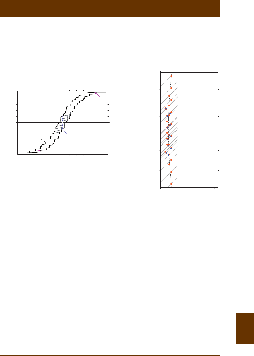
Fig. 8.4: (a) Model hysteresis loop (black) and FORCs (gray) generated by three MD parcles with

demagnezing factors of 0.1, 0.2, and 0.3, respecvely, calculated according to Pike et al. [2001b]. Only

FORCs necessary for measurement of the backfield demagnezaon curve bf

M (blue dots) are shown

for clarity. The last FORC 1n

M- that does not coincide with the lower hysteresis branch is show in

purple. It merges with the lower hysteresis branch before the last magnezaon jump Δ n

M has occur-

red, so that no central ridge contribuons are produced. (b) FORC diagram corresponding to the MD

hysteresis model shown in (a). Gray diagonal lines are individual FORC trajectories along which irrever-

sible magnezaon processes are recorded as posive (orange dots) and negave (blue dots) peaks.

The dashed line is a quadrac fit to the dots showing clustering around the crest of a ‘crescent-shaped’

distribuon as discussed in Church et al. [2011].

−100 0 +100

Mbf

+1

−1

0

µ0H [mT]

norm. magnetization

(a)

M+

Mn−1

0 +50

−50

0

+50

µ0Hc [mT]

µ0Hb [mT]

(b)

∆Mn

VARIFORC User Manual: 8. FORC tutorial 8.16

8.3 Coercivity distribuons derived from FORC measurements

FORC measurements subsets define three types of coercivity distribuons that provide a

bridge with convenonal parameters used in rock magnesm since several decades. These

coercivity distribuons originate from three parcular FORC segments (Fig. 8.5): (1) the inial

part rr

(, )MH H H of each curve and its departure from the upper hysteresis branch, (2) the

remanent magnezaon r

(,0)MH of each curve, and (3) the point r

HH=- of each curve

where the applied field equals the reversal field amplitude. These regions define magneza-

on curves that will be discussed in the following.

Fig. 8.5: Relevant magnezaon processes captured by FORCs. irr

ΔM (red bar) is the irreversible mag-

nezaon change along the upper hysteresis branch, defined by the inial difference between FORCs

originang at consecuve reversal fields r

H. In this example, r

H-values have been chosen to coincide

with the coercivity c

H and the coercivity of remanence cr

H for didacc purposes. The difference

between the same two FORCs in zero field ( 0H=, blue bar) defines a contribuon bf

ΔM to the back-

field demagnezaon curve. Finally, the abrupt slope change of FORCs at r

HH= defines the contribu-

on cr

ΔM (green) to the central ridge. The FORC starng at r0H=, where rs

MM=, is called satura-

on inial curve [Fabian, 2003]. In ensembles of non-interacng SD parcles, this curve coincides with

the upper hysteresis branch because negave fields are required to switch them from posive satura-

on.

∆M

irr

∆M

bf

H

r

=H

cr

−H

r

M

rs

−50 0 +50

0

−1

+1

field µ0H [mT]

norm. magnetization M/Ms

H=0

H

r

=H

c

∆M

bf

VARIFORC User Manual: 8. FORC tutorial 8.17

8.3.1 Backfield coercivity distribuon

Backfield or DC demagnezaon of a posively saturated sample is obtained by measuring

its remanent magnezaon aer applicaon of increasingly large negave fields [Wohlfarth,

1958]. The applied negave fields are equivalent to reversal fields r

H of the FORC protocol

(Fig. 8.6), so that the backfield demagnezaon curve is given by FORC remanent magne-

zaons r

(,0)MH . The corresponding backfield coercivity distribuon is defined as the first

derivave of r

(,0)MH , i.e.

bf

1d ( ,0)

() 2d

Mx

fx

x

-

=- (8.7)

The backfield coercivity distribuon can be determined very precisely with the same polyno-

mial regression method used to calculate FORC diagrams. The factor ½ in eq. (8.7) ensures

that the integral of bf

f

over all fields yields the saturaon remanence rs

M of the sample.

Moreover, bf

f

is defined only for posive arguments, which correspond to negave reversal

fields, because the remanent magnezaon of curves starng at r0H> cannot be measured.

Within the Preisach model, the argument of bf

f

coincides with the coercivity field c

H of hyste-

rons, and bf c c

()d

f

HH

coincides with the rs

M-contribuon of all hysterons with coercivies

comprised between c

H and cc

dHH+.

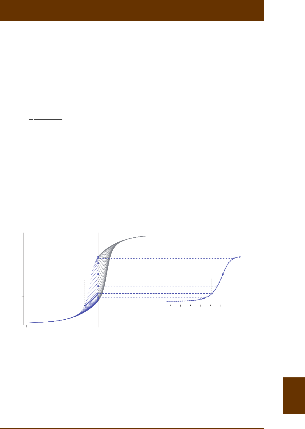
Fig. 8.6: Construcon of a backfield demagnezaon curve (right) from FORC measurements (le) of

a magnetofossil-bearing pelagic carbonate. FORC porons that are actually swept during backfield

measurements are shown in blue, and some zero-field measurements are highlighted with blue circles.

Remanent magnezaon measurements rr

(,0)MMH= on FORCs beginning at r

H- define the back-

field curve coordinates rr

(, )HM.

–100 0 +100

–2

0

+2

–60 –40 –20 0

–1

0

+1

H

, mT

M

, μAm2

Hr

, mT

M

(Hr, 0)

H

r,nH

r,n

VARIFORC User Manual: 8. FORC tutorial 8.18

8.3.2 Reversal coercivity distribuon

Inial FORC slopes can be used to calculate irreversible magnezaon changes

irr r r r r

Δ(,)(,)M MHδHHδHMHHδH=+ +- + (8.8)

along the upper hysteresis branch (Fig. 8.7), where

δ

H is the (constant) field increment used

for the measurements. The sum of all irr

ΔM’s obtained from consecuve FORCs starng at

reversal fields r

Hx£ defines a magnezaon curve irr ()Mx with the following meaning: if

reversible magnezaon processes are removed from the upper hysteresis branch, the re-

sulng ‘irreversible hysteresis’ branch would coincide with irr

M up to a constant (Fig. 8.7b).

The so-called reversal coercivity distribuon is defined by analogy with backfield demagne-

zaon as

r

irr r

irr

r

1d ( ) 1 ( , )

() 2d 2 HH x

Mx MHH

fx xH

==-

-

=- =- 

. (8.9)

The factor ½ in eq. (8.9) has been introduced to ensure that the total integral irs

M of irr

f

is a

magnezaon with the following properes: irs s

0MM<£

for any sample, and irs s

MM= in

absence of reversible processes. Unlike rs

M, the parameter irs

M includes all irreversible pro-

cesses occurring along the major hysteresis loop and shall therefore be called irreversible satu-

raon magnezaon.

A fundamental property of irs

M is that it coincides with the total integral of the FORC

funcon, because, using eq. (8.6):

r,

r

rr 1 irs

,11

11

(,)dd ( ) Δ

22

i

nn

ii i

HH

HH ii

ρ

HH H H M M M M

-=

==

=-==

åå

òò (8.10)

This important result implies that, while reversible magnezaon processes can contribute

locally to the FORC funcon, these local contribuons cancel each other out upon integraon

in FORC space.

The definions of bf

f

and irr

f

are analogous, since they both rely on differences between

consecuve FORCs evaluated at 0H= and r

HH=, respecvely, and are both related to the

FORC starng at r

Hx

=-

(Fig. 8.5). An important difference, on the other hand, is that the

argument of irr

f

can be posive as well as negave, unlike other coercivity distribuons.

Posive arguments of irr

f

correspond to measurements of the upper hysteresis branch in ne-

gave fields and vice versa. Similarly, posive arguments of bf

f

correspond to negave fields

used for DC demagnezaon. Furthermore, irr bf

(0) (0)

f

f= by the definions given with eq.

(8.7) and eq. (8.9).

VARIFORC User Manual: 8. FORC tutorial 8.19

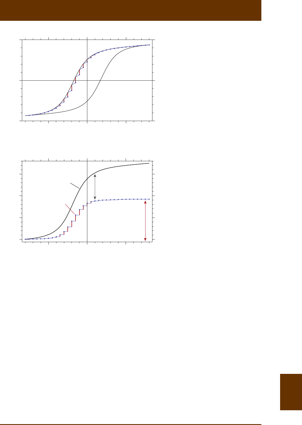
Fig. 8.7: Construcon of the magne-

zaon curve corresponding to irre-

versible processes along the upper

hysteresis branch. (a) Irreversible

magnezaon changes irr

ΔM (red)

defined by the inial parts of all

FORCs (blue). (b) Upper hysteresis

branch M+ (black curve) aer ad-

ding the saturaon magnezaon

s

M, and irreversible magnezaon

curve irr ()MH

reconstructed by in-

tegrang all magnezaon steps

irr

ΔM shown in (a). The saturaon

value irr ()MH ¥ is the total irre-

versible magnezaon irs

2M of the

hysteresis branch.

8.3.3 Central ridge coercivity distribuon

The central ridge coercivity distribuon is best explained by considering an isolated mag-

nec parcle with any domain state. A first-order curve starng from the upper hysteresis

branch just aer a magnezaon jump has occurred at r0H< will contribute to the central

ridge if another magnezaon jump is encountered at r

HH=- while sweeping the field back

towards posive values, before merging with the previous FORC. Usually, magnezaon

jumps can occur at any field and there is no parcular reason for having one exactly at H=

r

H-. In this case FORC contribuons accumulate at b0H= as over any other place in FORC

space, generang a connuous FORC distribuon. An excepon is provided by the FORC ori-

ginang from the upper hysteresis branch just aer the last magnezaon jump. This curve

coincides by definion with the lower hysteresis branch. Because of inversion symmetry, the

lower branch will contain a symmetric magnezaon jump at r

HH=- . If the lower branch

−50 0 +50

0

1

0

−1

+1

−50 0 +50

∆Mirr

µ

0

H [mT]

MM + Ms

µ

0

H [mT]

(a)

(b)

M+(H) + Ms

Mirr(H)

Mirr(H)

2Mirs

∆Mirr

M+

M−

VARIFORC User Manual: 8. FORC tutorial 8.20

merges with the previous FORC curve before r

HH=- is reached, as it is commonly the case

for MD hysteresis (Fig. 8.4a), the jump at r

HH=- will not contribute to the FORC diagram,

because the two curves are idencal and

r

/0MH= . Otherwise, there will be a contribuon

to the central ridge in form of a peak with FORC coordinates cb r

(,)( ,0)HH H=- (Fig. 8.3).

Because these contribuons are placed exactly at b0H=, they produce a ridge of the form

cr c b cr c b

1

(,) ()()

2

ρ

HH f HδH= (8.11)

where cr

f

is the so-called central ridge coercivity distribuon [Egli et al., 2010]. In FORC dia-

grams obtained from real measurements, the infinite sharpness of cr

ρ

is regularized by re-

placing the Dirac impulse with an appropriate funcon of b

H that takes the smoothing effects

of measurements performed with finite field increments into account. A rigorous treatment

of such effects is given in Egli [2013]. The central ridge coercivity distribuon is obtained from

real measurements in two steps: first, the central ridge contribuon cr

ρ

to the FORC diagram

is isolated from the connuous background produced by other processes, then cr

ρ

is integra-

ted over b

H so that

cr c cr c b b

() (, )dfH

ρ

HH H

+¥

-¥

=ò. (8.12)

While the amplitude of cr

ρ

depends on the resoluon of FORC measurements and on FORC

processing, cr

f

is independent of any measuring and processing parameter and reflects intrin-

sic magnec properes. The complex operaon of isolang the central ridge and calculang

cr

f

is performed automacally by VARIFORC with few controlling parameters described in this

user manual (Chapter 6).

The total magnezaon cr

M associated with the central ridge is obtained by integrang

cr

f

over c

H and represents the total contribuon of last magnezaon jumps in isolated

magnec parcles. Accordingly, cr irs

/MM

is the rao between the last magnezaon jump

n

ΔM of a hysteresis branch and the sum of all magnezaon jumps over the same branch. In

case of non-interacng, uniaxial SD parcles, n1

ΔΔMM= is the only magnezaon jump of

single parcle hysteresis, so that cr irs

/1MM=. As soon as addional magnec states begin to

exist in small PSD parcles, the relave amplitude of n

ΔM decreases with respect to the sum

irs

M of all magnezaon jumps, and cr irs

/1MM<, unl cr 0M= is reached in MD-like sys-

tems.

VARIFORC User Manual: 8. FORC tutorial 8.21

8.4 Examples

The physical meaning of FORC diagrams and derived coercivity distribuons is best illus-

trated with topic examples related to SD, PSD, and MD magnec parcle assemblages. The

hysteresis properes of samples discussed in this secon are summarized by the Day diagram

of Fig. 8.8.

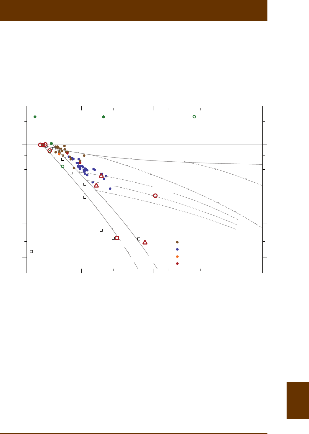
Fig. 8.8: Day diagram summarizing the hysteresis properes of samples discussed in this paper (red

circles for SD samples, red triangles for PSD samples, red squares for MD samples), compared with

properes of magnetofossil-bearing sediments (colored dots). The Day diagram with mixing curves

between domain states (gray) is drawn from Dunlop [2002b]. Cultured magnetotacc bacteria (‘cul-

tured MB’) plot exactly on the expected spot for non-interacng uniaxial SD parcles. The effect of

magnetostac interacons on such parcles is shown with models from Muxworthy et al. [2003] and

with disrupted magnetosome chains (green circle, from Li et al., 2012]). In general, interacng SD par-

cles follow the SD+MD mixing curve. Magnetofossil-bearing sediments follow a different trend with

end-members defined by CBD-extractable magnec minerals on one hand (red circle labeled as ‘CBD

extr.’, from Ludwig et al. [2013]) and the central region of the diagram on the other hand, possibly

represented by a clay mineral dispersion of SDS-treated Magnetospirillum cells (red circle labeled as

‘MS disp.’). Iron nanodots with single-vortex states (red triangle labeled as AV-109, from Winklhofer et

al. [2008]) do not plot on the expected trend line for PSD parcles.

SD+MD mixing curves

20%

40%

50%

60%

70%

80%

SP+PSD

mixing curves

SP saturation envelope

10% 20%

30%

30%

40%

50%

60%

SP+SD

mixing curves

70%

80%

10 nm

40%

50%

15 nm

1251020

1

0.5

0.2

0.1

0.05

Hcr/Hc

Mrs/Ms

interacting uniaxial

SD particles

[Muxworthy et al., 2003]

uncultured MB

(mainly cocci with double chains)

[Pan et al., 2005]

P

L

PL uncultured cocci

[Lin and Pan, 2009]

AMB-1 intact and collapsed

[Li et al., 2012]

Gehring et al., 2011

Abrajevitch and Kodama, 2011

Roberts et al., 2011

magnetofossil-rich sediments:

this study

cultured MB

MS disp.

CBD

extr.

AV-109

EF-3

volc. ash

MD-20

VARIFORC User Manual: 8. FORC tutorial 8.22

8.4.1 SD magnec assemblages

The first example is a conceptual model of a sample containing a small number of non-

interacng, uniaxial SD parcles with rectangular (Fig. 8.9a) and curved (Fig. 8.9c) single-par-

cle hysteresis loops. Reversible processes (i.e. magnec moment rotaon in the applied field)

are absent in the first case. The SD parcles have two stable magnezaon states in fields

s

HH||< , where s

H is a parcle-specific switching field. Transions from one magnezaon

state to the other in individual parcles once their specific s

H-values have been reached is

seen in Fig. 8.9 as a series of magnezaon jumps. These jumps represent irreversible magne-

zaon processes, while reversible magnec moment rotaons (Fig. 8.9c) occur along con-

nuous segments of the magnezaon curves.

Fig. 8.9: Modeled FORC properes of few uniaxial, non-interacng SD parcles. Switching of individual

parcles appears as magnezaon jumps. (a) Preisach-Néel model with rectangular single parcle hys-

teresis loops (inset). This case is characterized by irr bf cr

ΔΔΔMMM==, so that the coercivity distribu-

ons in (b) are idencal. irr

ΔM and cr

ΔM are magnezaon jumps produced by the same parcle in

r

H and r

H-, respecvely. (c) Model with Stoner-Wohlfarth single parcle hysteresis loops (inset).

Magnezaon jumps occur at same fields as in (a), but their size is smaller, because magnezaon

changes are caused in part by magnec moment rotaons over the connuous segments. Because

magnezaon jump sizes of single parcle hysteresis loops are smaller than saturaon remanent mag-

nezaons, irr cr bf

ΔΔΔMMM=<, and the backfield coercivity distribuon is larger than the other two

coercivity distribuons, as shown in (d).

−0.1 0 +0.1

∆M

irr

∆M

bf

H

r

−H

r

+0.5

−0.5

0

∆M

irr

∆M

bf

H

r

−H

r

µ

0H [T]

norm. magnetization

−0.1 0 +0.1

+1

−1

0

µ0H [T]

norm. magnetization

(a) (c)

M

+

(H)

M

+

(H)

∆M

cr

∆M

cr

µ

0H [T]

(b)

+0.1+0.050−0.05

f

bf

=

f

irr

=

f

cr

f

bf

f

irr

=

f

cr

µ

0H [T]

+0.1+0.050−0.05

(d)

VARIFORC User Manual: 8. FORC tutorial 8.23

Each magnezaon jump along the upper hysteresis branch is the starng point of a FORC

that does not coincide with the previous one, while all FORCs starng from the same con-

nuous hysteresis segment are idencal.

Non-interacng, uniaxial SD parcles have relavely simple FORC properes. First, no swit-

ching occurs when the field is reduced from posive saturaon to zero. Therefore, all FORCs

r

(0,)MH H³ starng at posive reversal fields are idencal to the upper branch M+ of the

major hysteresis loop and their shape is enrely determined by reversible magnec moment

rotaon. Departure from M+ of the FORC (0, )MH

originang at r0H= (called saturaon

inial curve si

M), can be used as a measure of how much real hysteresis loops differ from the

ideal non-interacng SD case characterized by si

MM

+

= [Fabian, 2003]. As soon as negave

fields are reached along r

()MH

+, all parcles with sr

HH>- are switched: accordingly, FORCs

starng at r0H< are produced by a mixture of switched and unswitched parcles. While the

applied field is increased from r0H< to 0H=, magnec moments rotate reversibly without

further switching. Moreover, the remanent magnezaon bf

M= r

(,0)MH obtained at 0H=

reflects the same configuraon of switched parcles created at the beginning of the corres-

ponding FORC.

In both examples of Fig. 8.9, the last magnezaon jump of each FORC contributes to the

central ridge and has the same amplitude as the magnezaon jump on ()MH

+ from which

the FORC is branching, because both jumps are produced by the two switching fields s

H of

same parcles. Therefore, the coercivity distribuons associated with r

()MH

+ and with the

central ridge are idencal, i.e. cr irr

() ()

f

xfx= over 0

x

³ and irr (0)0

f

x<= (Fig. 8.9b,d). The

backfield coercivity distribuon, on the other hand, is based on magnezaon differences

measured in zero field instead of the switching fields, and is therefore disnct from the other

two coercivity distribuons in case of SD parcles with curved elemental hysteresis loops, such

as Stoner-Wohlfarth parcles (Fig. 8.9c,d). In case of randomly oriented Stoner-Wohlfarth par-

cles, the mean size of magnezaon jumps in single-parcle hysteresis is irs rs

/SMM==

cr rs

/ 0.5436MM= [Egli et al., 2010], and rs s

/0.5MM=. Single-parcle hysteresis loops be-

come much closer to rectangular loops as soon as thermal acvaons are taken into conside-

raon, because switching occurs in smaller fields where reversible magnec moment rotaon

is less pronounced. FORC measurements yield 0.8-0.9S» for SD parcles in a pelagic carbo-

nate [Ludwig et al., 2013].

The FORC properes discussed above are important for the idenficaon of SD parcles

in geologic samples, notably magnetofossils in freshwater and marine sediment, but also well-

dispersed SD parcles in rocks. In parcular, the occurrence of sedimentary SD parcles in

isolated form or as linear chains produced by magnetotacc bacteria is the maer of an on-

going debate. For example, the unusually strong SD signature of sediments from the Paleo-

cene-Eocene thermal maximum (PETM) has been aributed to magnetofossils produced by

magnetotacc bacteria thriving in a parcularly favorable environment [Kopp et al., 2007;

VARIFORC User Manual: 8. FORC tutorial 8.24

Lippert and Zachos, 2007], as well as, at least in part, to isolated SD parcles produced by a

cometary impact [Wang et al., 2013]. In the following, some examples of FORC and coercivity

distribuon signatures of sedimentary SD parcles are discussed.

The first example is based on high-resoluon FORC measurements by Wang et al. [2013]

of a pure culture of the magnetotacc bacterium MV-1, which produces single chains of pris-

mac 3553 nm magnete crystals [Sparks et al., 1990]. The original measurements have

been reprocessed with VARIFORC and results are shown in Fig. 8.10. Isolated magnetosome

chains behave as a whole like SD parcles with uniaxial anisotropy, because the magnec

moments of individual crystal are switched in unison due to strong magnetostac coupling

[Jacobs and Bean, 1955; Egli et al., 2010]. Magnetostac interacons between chains, on the

other hand, are minimized by the good separaon naturally provided by the much larger cell

volume.

Because of intrinsic magnetosome elongaon and well-constrained dimensions, MV-1 cul-

tures provide a close analogue to random dispersions of nearly idencal, uniaxial SD parcles.

The resulng coercivity distribuons are relavely narrow with virtually no contribuons at

c0H= (Fig. 8.10f), as expected for SD parcles with minimum uniaxial anisotropy provided

by crystal elongaon and chain geometry. Hysteresis parameters (rs s

/0.496MM=, cr c

/HH=

1.19, Fig. 8.8) praccally coincide with those of randomly oriented Stoner-Wohlfarth parcles.

Lack of strong magnetostac interacons is confirmed by the negligible intrinsic vercal exten-

sion of the central ridge, as predicted by theorecal calculaons [Newell, 2005].

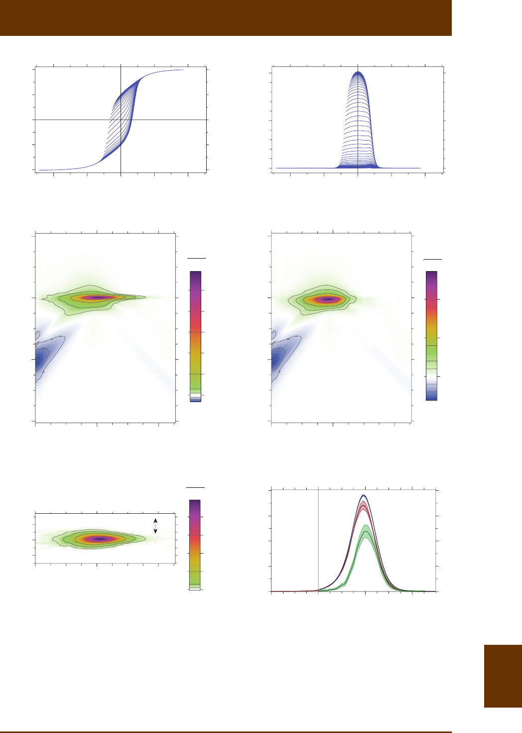
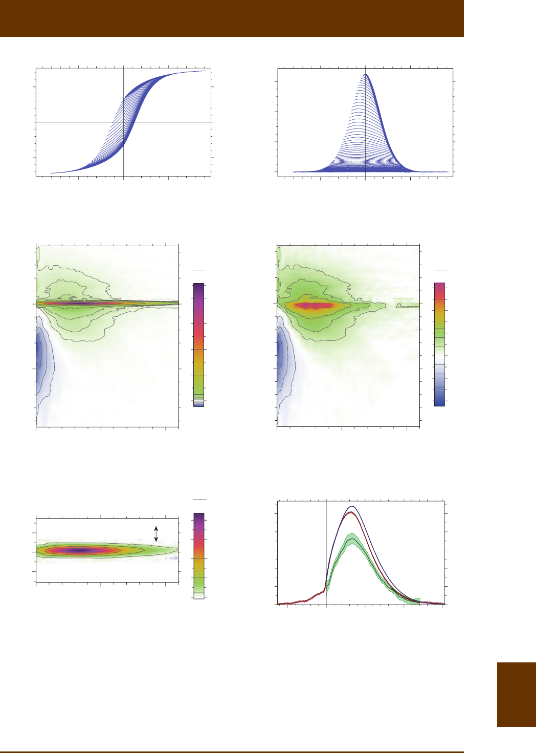
Fig. 8.10 (front page): Cultures of the magnetotacc bacterium MV-1 represent one of the best

material realizaons of non-interacng SD parcle assemblages with minimum uniaxial magnec ani-

sotropy. These bacteria contain a single chain of SD magnete crystals that switch in unison, behaving

effecvely as an equivalent SD parcle with elongaon along the chain axis. (a) Set of FORC measu-

rements where every 4th curve is ploed for clarity. (b) Same as (a), aer subtracng the lower hyste-

resis branch from each curve. Every 2nd curve is shown for clarity. The bell-shaped envelope of all

curves is the difference between upper and lower hysteresis branches, i.e. the even component

rh ()/2MMM

+-

=- of the hysteresis loop mulplied by a factor 2 [Fabian and Dobeneck, 1997]. (c)

FORC diagram calculated with VARIFORC from the measurements shown in (a). (d) Same as (c), aer

subtracon of the central ridge. Most contribuons in this diagram are due to reversible magnezaon

processes (i.e. in-field magnec moment rotaons). (e) Central ridge isolated from (c) and ploed with

a 2 vercal exaggeraon. Zero-coercivity contribuons are completely absent, as expected for a

system of parcles with intrinsic shape anisotropy along chain axes. The central ridge’s vercal exten-

sion slightly exceeds the minimum extension expected from data processing of an ideal ridge, revealing

residual magnetostac interacons between magnetosome chains. The associated interacon field

amplitudes are <0.5 mT.

VARIFORC User Manual: 8. FORC tutorial 8.25

Fig. 8.10 (connued): (f) Coercivity distribuons derived from FORC measurements and corresponding

magnezaons calculated by integraon of the distribuons over all fields. The condion irs cr

MM=

expected for these parcles is not exactly met, because of residual FORC contribuons not correspon-

ding to non-interacng, uniaxial SD parcles. On the other hand, irr (0)0fx<=, as expected from

posively saturated SD parcles that cannot be switched in posive fields. High-resoluon FORC mea-

surements have been kindly provided by Wang et al. [2013].

–2

0

+2

0

2

4

0.0

0.5

1.0

0

2

4

0

20

40

+2000

H

, mT

M

, μAm

2

0

1

–200 +2000

H

, mT

∆M, μAm

2

04080

H

c

, mT

0

–40

H

b

, mT

+40

–80

04080

H

c

, mT

0

–40

H

b

, mT

+40

–80

04080

H

c

, mT

0

–5

H

b

, mT

+5

04080

−H

r

or H

c

, mT

–40

dM/dH

, μAm

2

/T

(a) (b)

(c) (d)

(e) (f)

–200

2

2

2

mAm

T

2

2

mAm

T

2

2

mAm

T

2×

μAm

2

:

M

rs

= 1.01

M

irs

= 0.889

M

cr

= 0.568

f

bf

f

cr

f

irr

VARIFORC User Manual: 8. FORC tutorial 8.26

Ideally, the three types of coercivity distribuons shown in Fig. 8.10f should be characte-

rized by irr cr bk

f

ffº£ and irr () 0

f

x= for negave arguments, so that cr irs

/1MM=. The mea-

sured rao cr irs

/0.64MM= reflects residual FORC contribuons of unspecified nature clearly

visible over b0H>, where 0

ρ

= is expected from non-interacng SD parcles [Newell, 2005].

These contribuons are probably associated with a small fracon of collapsed magnetosome

chains (Fig. 8.10d).

The second example is also based on a magnetotacc bacteria sample, but its magnec

properes are less straighorward. The sample is a synthec sediment analogue obtained by

dispersing cultured cells of the magnetotacc bacterium Magnetospirillum magnetotaccum

MS-1 in a clay slurry (kaolinite) while dissolving the cell material with addion of 2% sodium

dodecyl sulfate (SDS) during connuous srring. The purpose of this experiment was to check

the stability of magnetosome chains in sediment once the cell material is dissolved. Analogous

experiments performed directly in aqueous soluon yielded strongly interacng magneto-

some clusters [Kobayashi et al., 2006]. FORC analysis of this sample (Fig. 8.11) poses a formi-

dable problem in terms of data processing, because of the simultaneous presence of (1) a

sharp superparamagnec (SP) overprint, and (2) a double disconnuity at r0HH==, due to

the overlap of a central ridge and a vercal ridge in the FORC diagram.

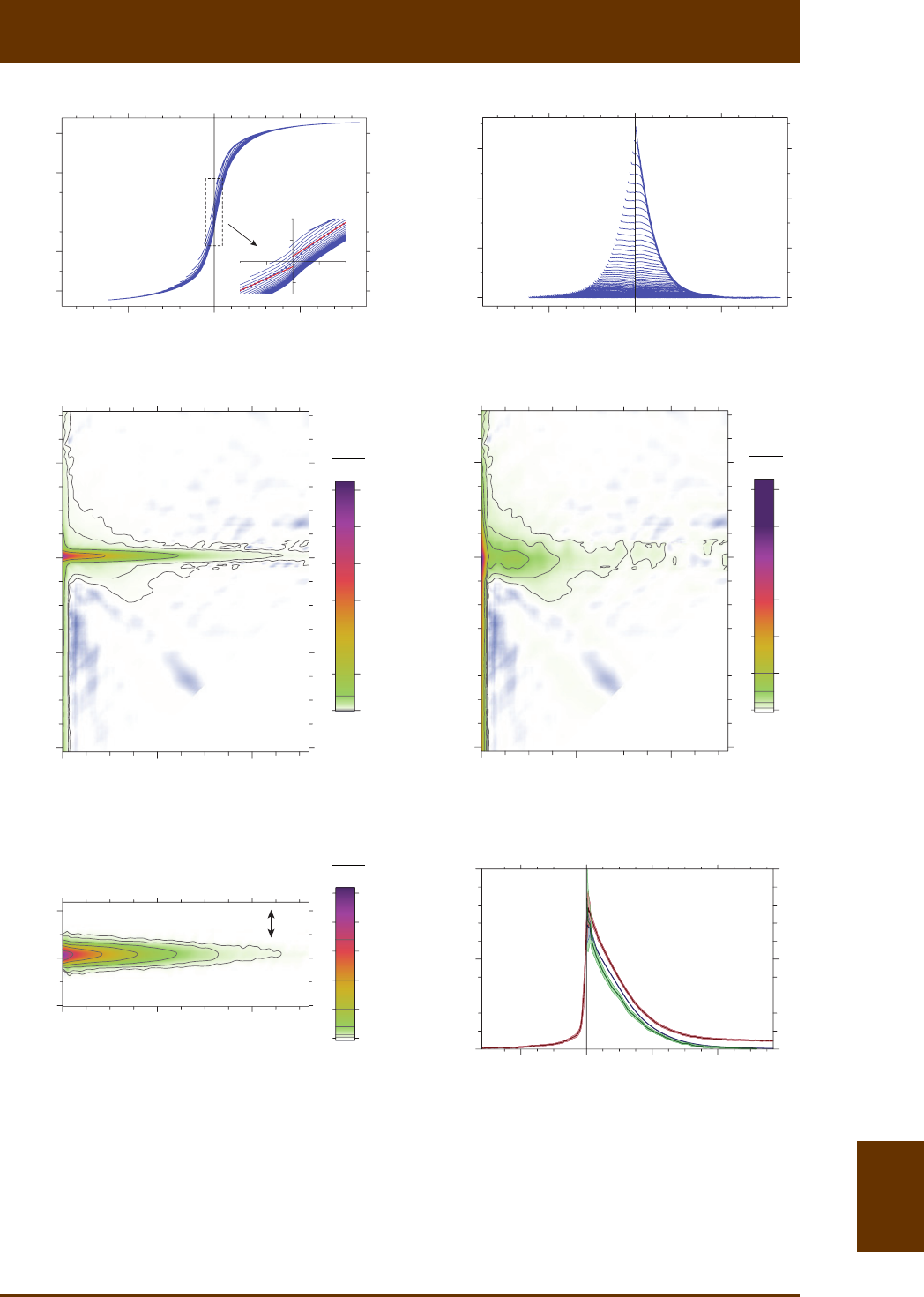
Fig. 8.11 (front page): FORC measurements of a specially prepared sample containing equidimensional

magnete magnetosomes. The sample was obtained by dispersing a Magnetospirillum culture in clay

(kaolinite) with subsequent 2% SDS addion under connuous srring. Dissoluon of cell material by

SDS is expected to produce clay-magnetosomes aggregates of some form. (a) Set of FORC measu-

rements where every 12th curve is ploed for clarity. The insert shows a zoom around the origin, where

a sigmoidal SP contribuon is recognizable. The SP signature saturates in <2 mT, and, although not

contribung to the FORC diagram, it poses a processing problem, because polynomial regression pro-

vides a correct fit only if unsuitably small smoothing factors are chosen (SF = 2 in this case). (b) Same

as (a), aer subtracng the lower hysteresis branch from each curve. Every 3rd curve is shown for cla-

rity. The exponenal-like envelope of all curves is the difference between the upper and lower hyste-

resis branches, and the cusp at 0H= denotes a system with zero-coercivity contribuons. The SP

contribuon shown in the inset of (a) is naturally eliminated from measurement differences, which

therefore no longer pose FORC processing problems. (c) FORC diagram calculated with VARIFORC from

the measurement differences shown in (b). The only significant contribuons are the central ridge,

indicave of non-interacng SD parcles, and a vercal ridge at c0H=, which is produced by magnec

viscosity. The absence of other significant FORC contribuons, and in parcular the typical signature

for reversible magnec moment rotaon, indicate that single-parcle hysteresis loops are praccally

rectangular. (d) Same as (c), aer subtracon of the central ridge. Residual contribuons around the

former central ridge locaon reveal addional magnezaon processes, which, given the SD nature of

the sample, must arise from magnetostac interacons. (e) Central ridge isolated from (c) and ploed

with a 3 vercal exaggeraon. The central ridge peak at c0H= denotes a system containing SD par-

cles with vanishing coercivity.

VARIFORC User Manual: 8. FORC tutorial 8.27

Fig. 8.11 (connued): (f) Coercivity distribuons derived from FORC measurements and corresponding

magnezaons calculated by integraon of the distribuons over all fields. The condion irs rs

MM»»

cr

M met by this sample is typical for non-interacng SD parcles with squared hysteresis loops and

represents a physical realizaon of a Preisach-Néel system. Residual irr

f-contribuons over negave

arguments are caused by non-zero FORC amplitudes over b0H> in (d).

–0.4

0

+0.4

0

1

2

3

0

0.2

0.4

0.6

0

1

2

0

5

10

–50 +500

H

, mT

M

, μAm

2

0

0.1

–50 +500

H

, mT

∆M, μAm

2

02040

H

c

, mT

0

–20

H

b

, mT

+20

–40

02040

H

c

, mT

0

–20

H

b

, mT

+20

–40

02040

H

c

, mT

0

–5

H

b

, mT

+5

02040

−H

r

or H

c

, mT

–20

dM/dH

, μAm

2

/T

(a) (b)

(c) (d)

(e) (f)

2

2

mAm

T

2

2

mAm

T

2

2

mAm

T

−4 +4

0.2

3×

μAm

2

:

M

rs

= 80

M

irs

= 120

M

cr

= 74

f

bf

f

cr

f

irr

VARIFORC User Manual: 8. FORC tutorial 8.28

Because the sigmoidal SP overprint extends only over few measurement points, saturang

in <2 mT (Fig. 8.11a), it cannot be adequately fied by polynomial regression with smoothing

factors required for adequate measurement noise suppression [Egli, 2013]. The SP overprint

is eliminated by subtracng the lower branch of the major hysteresis loop from all curves, in

which case no parcular features are seen at 0H= (Fig. 8.11b). This operaon does not affect

FORC calculaons, because the r

H-derivave of any magnezaon curve added or subtracted

to all measurements is zero. For this reason, subtracon of the lower hysteresis branch is an

opon provided by VARIFORC for processing quasi-disconnuous measurements. Moreover,

FORC measurement differences reveal details that are oen completely hidden in hysteresis

loops with rs s

/0MM and/or large paramagnec contribuons.

The hysteresis loop of this sample is clearly constricted at 0H=, in what is oen called a

‘wasp-waisted’ shape [Tauxe et al., 2006]. The interpretaon of corresponding Day diagram

parameters ( rs s

/0.177MM=,cr c

/5.12HH=, Fig. 8.8) is ambiguous, because it involves mix-

tures of SD, PSD, and SP parcles. On the other hand, the FORC diagram (Fig. 8.11c), contains

two precisely interpretable signatures, namely a central ridge, as expected for non-interacng

SD parcles, and a vercal ridge due to magnec viscosity. Addional FORC contribuons out-

side of the two ridges are very weak (Fig. 8.11d). Coercivity distribuons (Fig. 8.11f) are charac-

terized by exponenal-like funcons peaking at c0H=. Because this is also true for cr

f

, many

parcles must have vanishingly small switching fields. Such features can be explained by a

combinaon of thermal acvaon effects and the absence of chain-derived uniaxial aniso-

tropy, as expected for equidimensional MS-1 magnetosomes if their original arrangement is

destroyed. On the other hand, the presence of magnetosome clusters similar to those obtai-

ned from cell disrupon in aqueous soluons [Kobayashi et al., 2006] can be excluded, be-

cause of the absence of magnetostac interacon signatures otherwise reported with FORC

diagrams of extracted magnetosomes [e.g. Chen et al., 2007; Wang et al., 2013]. The apparent

contradicon between lack of uniaxial chain anisotropy and magnetostac interacon signa-

tures can be reconciled by assuming that magnetosomes have been individually dispersed in

the clay matrix.

The three coercivity distribuons derived from FORC measurements are almost idencal;

approaching the limit case bk cr irr

f

ff== predicted for non-interacng SD parcles with rec-

tangular single-parcle hysteresis loops. Rectangular loops can be explained by the strong

switching field reducon in thermally acvated SD parcles close to the SD/SP threshold. This

example demonstrates the level of detailed informaon that is provided by high-resoluon

FORC measurements. Results shown in Fig. 8.10 and Fig. 8.11 can be considered represen-

tave for well dispersed SD parcles with and without minimum uniaxial shape anisotropies.

The effect of shape anisotropy is much less evident with samples of interacng SD parcles,

because local interacon fields act as an addional magnec anisotropy source.

VARIFORC User Manual: 8. FORC tutorial 8.29

The third SD example is based on high-resoluon FORC measurements of a magnetofossil-

bearing pelagic carbonate from the Equatorial Pacific [Ludwig et al., 2013]. Typical sediment

magnezaons of the order of few mAm2/kg, as for this sample, yield FORC measurements

with important noise contribuons that need to be adequately suppressed in order to obtain

useful FORC diagrams. FORC processing becomes crical in such cases, as shown in Fig. 8.12.

Convenonal data processing based on constant smoothing factors yields significant values of

the FORC distribuon only over a limited region around the central ridge (Fig. 8.12a), unless

the high resoluon required in proximity of b0H= and c0H= is sacrificed. The VARIFORC

variable smoothing algorithm, on the other hand, finds a locally opmized compromise be-

tween resoluon preservaon and noise suppression. With this approach, significant domains

of the FORC distribuon are dramacally expanded (Fig. 8.12b), revealing a broad, connuous

background around the central ridge, as well as negave FORC amplitudes characterisc for

SD parcles.

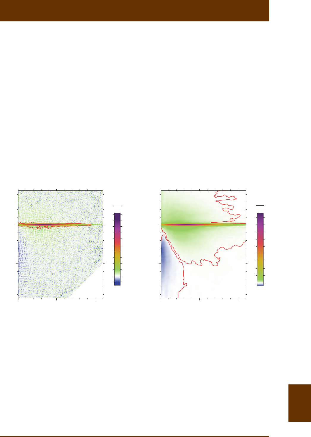
Fig. 8.12: Example showing the importance of proper FORC processing for extracng detailed infor-

maon from weak natural samples. The two FORC diagrams have been obtained from the same set of

high-resoluon measurements (field step size: 0.5 mT) of a pelagic carbonate from the Equatorial Paci-

fic [Ludwig et al., 2013]. The red contour(s) enclose significant regions of the FORC diagram, i.e. regions

where the FORC funcon is not zero at a 95% confidence level according to the error calculaon me-

thod implemented by Heslop and Roberts [2012]. (a) Convenonal FORC processing with a constant

smoothing factor SF = 4. The central ridge is the only significant FORC feature that can be resolved.

Larger smoothing factors would extend the significant region at the cost of blurring the central ridge

to the point where it can no longer be idenfied as such (see Fig. 1 in Egli [2013]). (b) VARIFORC pro-

cessing obtained with a variable smoothing factor opmized for the best compromise between noise

suppression and detail preservaon. Low-amplitude features, such as negave contribuons, are now

significant over large porons of the whole FORC space.

0

4

8

0 50 100

H

c

, mT

0

–50

H

b

, mT

2

2

Am

Tkg

0 50 100

H

c

, mT

0

–50

H

b

, mT

0

4

8

2

2

Am

Tkg

(a) (b)

SF = 4 variable smoothing

VARIFORC User Manual: 8. FORC tutorial 8.30

The last example of this secon (Fig. 8.13) is based on a special technique used to isolate

the contribuon of secondary SD magnete parcles from the same pelagic carbonate sample

of Fig. 8.12. For this purpose, idencal FORC measurements has been performed before and

aer treang homogenized sediment material with a citrate-bicarbonate-dithionite (CBD) so-

luon for selecve magnetofossil dissoluon [Ludwig et al., 2013]. Large magnete crystals,

as well as SD parcles embedded in a silicate matrix, are not affected by this treatment. There-

fore, differences shown in Fig. 8.13 between the two sets of measurements represent the

intrinsic magnec signature of CBD-extractable parcles. Hysteresis properes ( rs s

/MM=

0.44, cr c

/1.34HH=, Fig. 8.8) are close to the limit case of randomly oriented, non-interacng

SD parcles with uniaxial anisotropy, despite evident magnetostac interacon signatures

deducible from posive FORC contribuons over the upper quadrant (Fig. 8.13d). Interpreta-

on of interacon signatures in terms of collapsed magnetosome chains or authigenic SD mag-

nete clusters requires further invesgaon [Ludwig et al., 2013]. Coercivity distribuons (Fig.

8.13f) display minor contribuons near c0H=, and their overall shape is beer associable

with intact magnetotacc bacteria cultures (Fig. 8.10) than dispersed magnetosomes in clay

(Fig. 8.11). Coercivity distribuons of magnetofossil-bearing sediment are wider than those of

individual bacterial strains, because of the natural diversity of magnetosome and chain mor-

phologies. On the other hand, no systemac differences are observed between FORC-related

magnezaon raos (Table 8.1), as long as chain integrity is not evidently compromised. In

parcular, FORC properes of PETM sediment appear to be compable with those of similar

magnetofossil-bearing samples, rather than dispersions of equidimensional SD parcles.

Fig. 8.13 (front page): FORC analysis of a pelagic carbonate sample from the Equatorial Pacific, ob-

tained from differences between idencal measurements of the same material before and aer selec-

ve SD magnete dissoluon [Ludwig et al., 2013]. This approach, combined with the fact that the

main magnezaon carriers are magnetofossils, ensures that results shown here represent the uncon-

taminated signature of secondary SD minerals. (a) Set of FORC measurements where every 8th curve is

ploed for clarity. (b) Same as (a), aer subtracng the lower hysteresis branch from each curve. Every

4th curve is shown for clarity. The bell-shaped envelope of all curves is the difference between the

upper and lower hysteresis branches. Its shape is intermediate between the examples shown in Fig.

8.10-11, albeit closer to Fig. 8.10b. (c) FORC diagram calculated with VARIFORC from the measure-

ments shown in (a). The central ridge is overlaid to addional low-amplitude contribuons (<10% of

the central ridge peak), which, because of their extension over the FORC space, represent as much as

50% of the total magnezaon irs

M ‘seen’ by the measurements. (d) Same as (c), aer subtracon

of the central ridge. The lower quadrant partly coincides with the signature of reversible magnec

moment rotaons as predicted by Newell [2005]. Because non-SD contribuons are excluded by the

special preparaon procedure, posive FORC amplitudes over b0H> must represent the signature of

magnetostac interacons between SD parcles. (e) Central ridge isolated from (c) and ploed with a

3 vercal exaggeraon.

VARIFORC User Manual: 8. FORC tutorial 8.31

Fig. 8.13 (connued): (f) Coercivity distribuons derived from FORC measurements and corresponding

magnezaons calculated by integraon of the distribuons over all fields. Magnezaon raos (e.g.

irs rs

/MM

, cr irs

/MM

, Table 8.1) are similar to those of the MV-1 example in Fig. 8.10 and represen-

tave for magnetofossil-bearing sediment.

–5

0

+5

0

4

8

0

–0.4

0.4

0

4

8

0

20

–100 +1000

H , mT

M , mAm2/kg

0

2

–100 +1000

H , mT

∆M , mAm2/kg

0 50 100

Hc , mT

0

–50

Hb , mT

0 50 100

Hc , mT

0

–50

Hb , mT

0 50 100

Hc , mT

0

–5

Hb , mT

+5

0 50 100

−Hr or Hc , mT

–50

dM/dH, mAm2/(Tkg)

(a) (b)

(c) (d)

(e) (f)

4

6

150

40

2

2

Am

Tk

g

2

2

Am

Tk

g

2

2

Am

Tkg

mAm

2

/kg:

M

rs

= 3.25

M

irs

= 3.18

M

cr

= 2.12

3×

fbf

fcr

firr

VARIFORC User Manual: 8. FORC tutorial 8.32

Table 8.1: Hysteresis parameters cr c

/HH

and rs s

/MM

, and raos between FORC-derived magneza-

ons rs

M, irs

M, and cr

M, for samples described in this arcle.

Material cr c

/HH

rs s

/MM

irs rs

/MM cr rs

/MM

cr irs

/MM

Strictly SD examples

MS-1 dispersion in clay

MS-1

AMB-1 a

MV-1 b

CBD-extractable in pelagic carbonate c

Magnetofossil-rich sediments

Pelagic carbonate c

PETM b

Soppensee d

PSD examples

AV-109 e

EF-3

Volcanic ash b

MD parcles

MD20

5.12

1.233

1.267

1.190

1.340

1.690

1.677

1.503

2.578

4.489

2.421

3.147

0.177

0.494

0.500

0.496

0.442

0.399

0.418

0.411

0.267

0.069

0.219

0.075

1.397

0.928

0.893

0.879

0.815

1.011

0.953

1.066

1.856

2.500

1.976

2.873

0.885

0.510

0.698

0.561

0.651

0.569

0.550

0.387

0.598

0.097

0.024

0

0.633

0.550

0.782

0.638

0.667

0.563

0.576

0.364

0.322

0.039

0.012

0

a FORC data kindly provided by Li et al. [2012].

b FORC data kindly provided by Wang et al. [2013].

c FORC data from Ludwig et al. [2013].

d FORC data from Kind et al. [2011].

e FORC data from Winklhofer et al. [2008].

8.4.2 PSD magnec assemblages

The next two FORC examples are based on PSD parcle assemblages, starng with the

simplest case of an array of idencal, weakly interacng Fe nanoparcles with grain sizes sligh-

tly larger than the upper SD limit [Winklhofer et al., 2008]. These parcles can have two pairs

of anparallel magnec states: so-called ‘flower’ states with nearly homogenous magneza-

on and SD-like magnec moments (SD+ and SD), and single vortex states with nearly zero

magnec moments (SV+ and SV). Hysteresis properes are shaped by the transion sequen-

ces SD+  SV+  SD and SD  SV  SD+ between posive and negave saturaon. Similar

transions in magnete cubes have been modeled micromagnecally [Newell and Merrill,

2000], yielding the single-parcle hysteresis loops shown in Fig. 8.14.

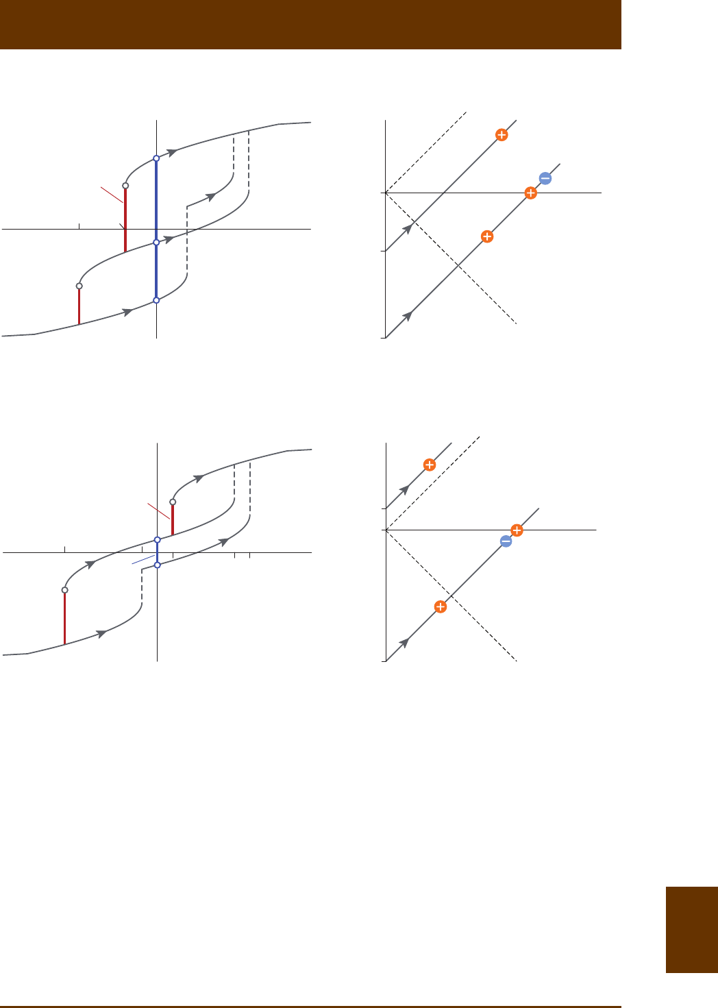
VARIFORC User Manual: 8. FORC tutorial 8.33

Fig. 8.14: Two examples of single parcle hysteresis loops (le plots) and corresponding FORC dia-

grams (right plots), generated by micromagnec simulaons of 0.1 µm (a) and 0.11 µm (c) magnete

cubes by Newell and Merrill [2000]. In both cases, the parcles have two SD-like (SD) and two vortex-

like (SV) magnezaon states. SD-like states in (c) exist only in sufficiently large applied fields and

cannot contribute to remanent magnezaons. Transions between magnec states occur at magne-

zaon jumps (dashed lines and red lines), defining three groups of idencal FORCs 0

M, 1

M and 2

M.

Magnezaon jumps relevant for FORC calculaons are labeled by number pairs like in Fig. 8.3. Corres-

ponding posive and negave peaks of the FORC funcon (b,d) are shown with ‘+’ and ‘’ symbols,

respecvely. Gray diagonal lines with arrows are the only FORC trajectories producing non-zero contri-

buons. Only peaks located to the right of the dashed lines contribute to the backfield demagnezaon

curve and thus to rs

M, determining large differences in magnec remanence properes of otherwise

similar FORC diagrams.

M

0

M

1

M

2

∆M

irr

∆M

irr

∆M

bf

∆M

bf

1,1

2,1

2,2

H

r2

SD

+

SV

+

SV

−

SD

−

(1,1)− M

0

(2,1)− M

1

M

2

−(1,1)

H

r2

H

r1

21

MM

′

(−)

0

∆M

irr

∆M

irr

∆M

bf

H

r2

H

r1

M

0

M

1

M

2

SD

+

SD

−

SV

−

SV

+

2,1

1,1

2,2

10

MM

′

(−)

21

MM

′

(−)

H

r2

H

r1

0

H

c

H

c

H

b

H

b

H

H

M

M

(a) (b)

(c) (d)

H

r1

(2,2)− M

1

(1,1)− M

0

(2,1)− M

1

M

2

−(1,1)

(2,2)− M

1

10

MM

′

(−)

VARIFORC User Manual: 8. FORC tutorial 8.34

The complex FORC signature of Fe nanoparcles (Fig. 8.15) can explained by a combinaon

of the two micromagnec models in Fig. 8.14, with individual peaks corresponding to magnec

transions between SD and SV states. The SV  SD+ transion along the lower hysteresis

branch produces a central ridge peaking at c0.15 TH». Addional pairs of posive FORC

peaks at c0.06 TH» and negave peaks just above and below the central ridge are produced

by the remaining transions, while negave FORC amplitudes peaking at b0.15 TH»- can

be explained by reversible magnezaon changes of the SV

+-state in proximity of its de-

nucleaon field. All relevant FORC contribuons occur at or in proximity of SV nucleaon in

±0.01 T and SV denucleaon in ±0.15 T (Fig. 8.15c), producing a constricted hysteresis loop

(Fig. 8.15a) and bimodal coercivity distribuons (Fig. 8.15f).

Unlike the case of isolated SD parcles, magnec state transions from posive saturaon

(i.e. SD+) occur already in posive fields. These transions (e.g. SV nucleaon) are not captured

by remanent demagnezaon measurements, therefore contribung to irr (0)

f

x<, but not to

bk

f. In the example of Fig. 8.15, SV denucleaon is the only process captured by the central

ridge, so that cr

f is characterized by a single peak at c0.15 TH», instead of two peaks, as for

the other two coercivity distribuons.

Fig. 8.15 (front page): FORC analysis of Fe nanodots [Winklhofer et al., 2008]. The arficial sample (AV-

109) is a two-dimensional, quasi-hexagonal array of polycrystalline Fe nanodots with a diameter of

6713 nm and 20 nm thickness. The nanodots center-to-center spacing is 2 dot diameters [Dumas et

al., 2007]. FORC measurements have been performed in the array plane. (a) Set of FORC measure-

ments where every 2nd curve is ploed for clarity. (b) Same as (a), aer subtracng the lower hysteresis

branch from each curve. Every 2nd curve is shown for clarity. Hysteresis loop constricon at 0H= and

the double peak of the curve envelope in (b) are produced by a bimodal distribuon of nucleaon

fields. As evident in (b), some FORCs cross each other, as well as the lower hysteresis branch. This

means that regions outside the major hysteresis loop can in principle be accessed by FORC measure-

ments (e.g. Fig. 8.14a), albeit rarely seen with natural samples and impossible with non-interacng SD

parcles. (c) FORC diagram calculated with VARIFORC from the measurements shown in (a), featuring

localized peaks typical for magnec transions between four magnec states: two SD-like states with

large magnec moments, and two states corresponding to a single magnec vortex with small net

magnec moment. Because magnec parcles in this sample are praccally idencal, magnec tran-

sions occur collecvely, appearing as disnct FORC funcon peaks. In case of less homogenous sam-

ples, FORC peaks would merge into a connuous background with triangular contour lines, as com-

monly seen with natural PSD assemblages. The dashed lines mark the rectangular domain of FORC

amplitudes associated with remanent magnezaons. Accordingly, only about half of the two peaks

at c

H» 0.06 T contribute to rs

M. (d) Same as (c), aer subtracon of the central ridge. The two

negave peaks around the central ridge in (c) now appear as a single contribuon produced by vortex

denucleaon. (e) Central ridge isolated from (c) and ploed with a 2 vercal exaggeraon, featuring

a single peak at 0.15 T.

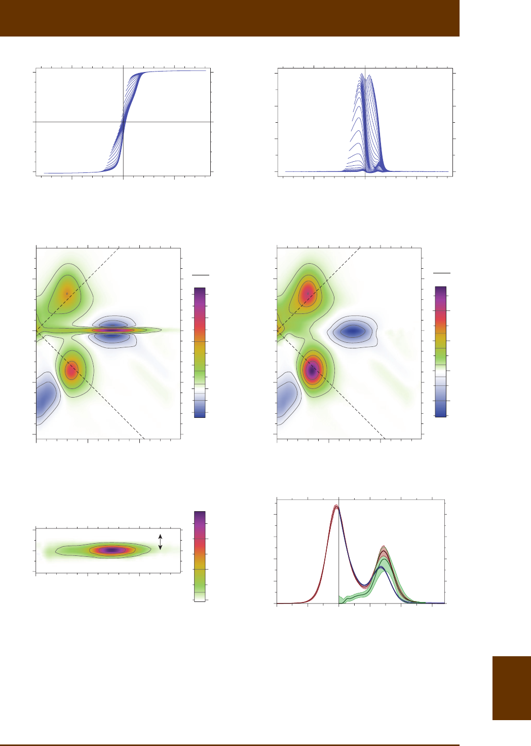
VARIFORC User Manual: 8. FORC tutorial 8.35

Fig. 8.15 (connued): (f) Coercivity distribuons derived from FORC measurements and corresponding

magnezaons calculated by integraon of the distribuons over all fields. The bimodal character of

irr

f and bf

f arises from the existence of two different fields for nucleaon (±0.01 T) and denucleaon

(±0.15 T) of vortex states, producing the constricted hysteresis loop seen in (a). Only vortex denuclea-

on is captured by the central ridge, so that cr

f consists of a single peak.

–0.1

0

+0.1

0

4

8

0

2

4

0

4

8

0

0.2

0.4

+0.50

H

, T

M

, μAm

2

0

20

–0.5 +0.50

H

, T

∆M, nAm

2

0 0.1 0.2

H

c

, T

0

–0.1

H

b

, T

+0.1

–0.2

0 0.1 0.2

H

c

, T

H

b

, T

0 0.1 0.2

H

c

, T

0

H

b

, mT

+20

00.2

−H

r

or H

c

, mT

–0.2

dM/dH

, μAm

2

/T

(a) (b)

(c) (d)

(e) (f)

–0.5

40

60

0

–0.1

+0.1

–0.2

–2

–20

2

2

μAm

T

2

2

μAm

T

2×

μAm

2

:

M

rs

= 28.8

M

irs

= 53.5

M

cr

= 17.5

f

bf

f

cr

f

irr

VARIFORC User Manual: 8. FORC tutorial 8.36

Hysteresis parameters of small PSD crystals are very sensive to vortex nucleaon fields:

if nucleaon from posive saturaon occurs in negave fields, SD-like values of rs s

/MM

are

obtained from SD states that are stable in zero fields. If, on the contrary, vortex states can

nucleate from SD+ in posive fields, rs s

/MM

drops well below 0.5, because of their small net

magnec moment. On the other hand, PSD parcles are always characterized by cr bk

MM<

irs

M<, unlike the case of non-interacng SD parcles, where bk irs

MM³.

The FORC diagram in Fig. 8.15c does not resemble the typical signature of PSD magnete

in synthec and geologic samples, which consists of a unimodal distribuon peaking near

cb

0HH==

, with triangular contour lines having their maximum vercal extension at c0H=

[Roberts et al., 2000; Muxworthy and Dunlop, 2002]. This signature is explainable on the basis

of the abovemenoned PSD processes by taking the following factors into consideraon: first,

magnec states of small PSD parcles are very sensive to grain sizes and shapes, so that

magnezaon jumps of single-parcle hysteresis generate disnct FORC peaks only in case of

exceponally homogeneous samples, such as the Fe nanoparcles discussed above. Second,

the number of possible magnec states grows rapidly with increasing grain size, along with

the number of FORC peaks, which eventually merge into a unimodal funcon. As discussed in

secon 3, the FORC funcon occupies a triangular area of the FORC space limited by verces

with coordinates sat

(0, )H and sat

(,0)H, where sat

H is the field in which the two branches of

the hysteresis loop merge. This limit is consequently imposed to the shape of contour lines.

Finally, the central ridge is broadened by magnetostac interacons, which are probably not

negligible in most synthec magnete powders.

Some natural materials, such as olivine-hosted Fe-Ni parcles in chondric meteorites

[Lappe et al., 2011], contain weakly interacng PSD parcles with sufficiently homogeneous

properes for producing FORC diagrams with disnguishable contribuons from vortex nu-

cleaon and denucleaon. In such cases, high-resoluon measurements are essenal for cap-

turing details of PSD magnezaon processes. Faint evidence of such processes persists in

FORC diagrams of many natural rocks (Fig. 8.16).

Fig. 8.16 (front page): Two FORC examples based on natural samples containing PSD parcle assembla-

ges, i.e. (a-c) basalt (sample EF-3), and (d-f) volcanic ash [Ludwig et al., 2013]. (a,d) FORC measure-

ments, with results aer lower hysteresis branch subtracon shown in the insets. (b,e) FORC diagrams

calculated with VARIFORC from the measurements shown in (a,d). Some features typical for single-

vortex PSD parcles (Fig. 8.15) can be recognized, namely the existence of a central ridge, albeit much

weaker, and the influence of localized negave FORC amplitudes (labeled with a minus sign) on the

overall shape of contour lines. Furthermore, two nearly symmetric posive peaks above and below the

central ridge are disnguishable in (b). Unlike the example of Fig. 8.15, the existence of such contri-

buons cannot be directly inferred from the hysteresis loop. The vercal ridge along c0H= in (e) is a

signature of magnec viscosity.

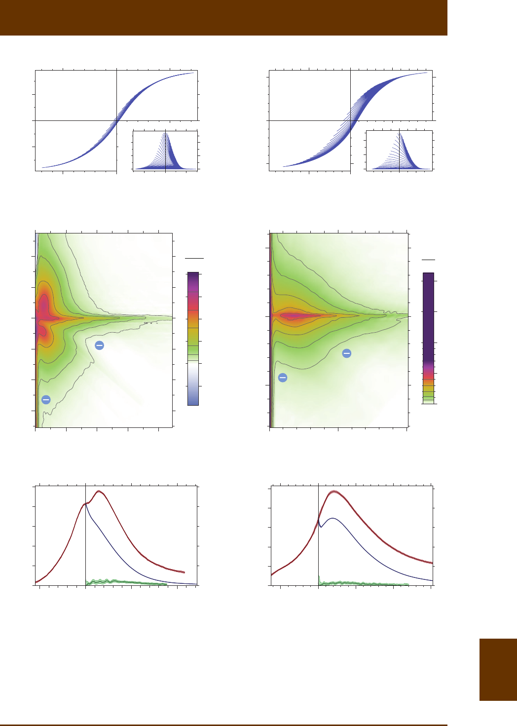
VARIFORC User Manual: 8. FORC tutorial 8.37

Fig. 8.16 (connued): (c,f) Coercivity distribuons derived from the FORC measurements shown in

(b,e). Residual bimodality is sll recognizable for irr

f and bf

f in (c). The central ridge distribuon cr

f is

much smaller than the other two, but significantly 0. Unlike the case of SD parcles, the contribuon

of irr

f over negave arguments is not negligible, as expected from large posive FORC amplitudes over

the upper quadrant.

0

10

20

0

10

20

04080

H

c

, T

0

–40

H

b

, T

+40

0 50 100

H

c

, T

0

–50

H

b

, T

+50

2

2

Am

Tkg

2

2

mAm

T

0

0.2

0.4

050

−H

r

or H

c

, mT

–50

dM/dH

, mAm

2

/T

100

0

0.2

0.4

050

−H

r

or H

c

, mT

–50

dM/dH

, mAm

2

/(Tkg)

100 150

–0.1

0

+0.1

+0.1

0

H

, T

M

, mAm2

(a)

–0.1 –0.1

0.02

0

0

H

, T

–0.1

–50

0

+50

M

, mAm2/kg

+0.1–0.1

20

0

(d)

(b) (e)

(c) (f)

μAm

2

:

Mrs = 13.5

Mirs = 33.7

Mcr = 1.3

f

bf

f

cr

f

irr

f

bf

f

cr

f

irr

mAm

2

/kg:

Mrs = 12.7

Mirs = 25.1

Mcr = 0.3

VARIFORC User Manual: 8. FORC tutorial 8.38

Because of its sharpness, the central ridge remains disnguishable even with contribuons

as low as few % of irs

M. Localized negave amplitudes over the lower quadrant, on the other

hand, produce characterisc contour line indentaons when overlaid to a posive back-

ground. Resoluon of such signatures in PSD samples can benefit paleomagnec applicaons,

where FORC analysis has been proposed as a selecon [Wehland et al., 2005; Carvallo et al.,

2006; Acton et al., 2007] and modeling [Muxworthy et al., 2011a,b] tool for paleointensity

determinaons. For example, cr irs

/MM

is a measure for the relave magnezaon of vortex

states, which probably represent the preferenal PSD contribuon to natural remanent mag-

nezaons.

8.4.3 MD parcles

Domain wall displacement models [Pike et al., 2001b; Church et al., 2011] explain the ideal

hysteresis properes and FORC signature of MD parcles (Fig. 8.4). These properes are met

by annealed magnete crystals [Pike et al., 2001b], while FORC diagrams of unannealed par-

cles (Fig. 8.17) can be explained by the superposion of MD and PSD signatures. As far as

coercivity distribuons are concerned, ideal MD properes are characterized by hysteresis

branches and corresponding irreversible contribuons being are quasi-symmetric about H=

0, which means that irr irr

() ( )

f

xf x»-

. The typical irr

f

-shape of MD parcles resembles a

Laplace (double exponenal) distribuon (Fig. 8.17c). Because the magnezaon of ideal

crystals with weak domain wall pinning is almost completely reversible, irreversible processes,

which occur in form of so-called Barkhausen magnezaon jumps, represent only a small frac-

on of the saturaon magnezaon, i.e. irs s

/1MM. For example, irs s

/0.22MM= for the

20-25 µm magnete crystals of Fig. 8.17. Only a small fracon of all Barkhausen jumps yield a

remanent magnezaon, so that rs irs

/1MM ( rs irs

/0.35MM= for the example of Fig. 8.17).

Since bk irr

(0) (0)ff=, the backfield coercivity distribuon is a funcon that decays much more

rapidly than irr

f

to zero for posive arguments. Finally, cr 0f= because of the absence of a

central ridge.

In summary, ideal MD crystals without strong domain wall pinning are characterized by

cr 0M= and rs irs s

MM M

. For comparison, PSD and SD parcles yield rs irs

MM< and

rs irs

MM³, respecvely. Therefore, the rao rs irs

/MM can be considered as a sort of domain

state indicator analogous to rs s

/MM

, with the important advantage that rs irs

/MM is insensive

to reversible magnezaon processes (e.g. SP contribuons).

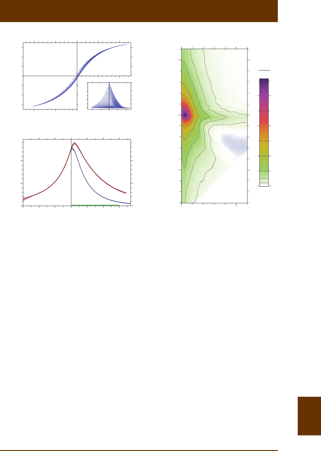
VARIFORC User Manual: 8. FORC tutorial 8.39

Fig. 8.17: FORC analysis of synthec MD magnete parcles with 20-25 µm mean grain size. (a) Set of

FORC measurements where every 8th curve is ploed for clarity. The inset shows the same set of curves

(every 4th is ploed) aer subtracon of the lower hysteresis branch. Measurement details are recog-

nizable only in this plot, because of the very small hysteresis loop opening. (b) FORC diagram obtained

with VARIFORC from the FORC measurements shown in (a). The MD nature of this sample is determi-

ned by the large vercal spread of the FORC funcon in proximity of c0H=. Addional PSD signatures

are recognizable over b0H< and along a sort of blurred central ridge. These features are typical of

unannealed MD crystals. (c) Coercivity distribuons derived from the FORC measurements shown in

(c). irr

f is a quasi-even funcon with similar contribuons over negave and posive field, as expected

for MD parcles. The central ridge does not exist, so that cr 0f=.

–0.2

0

+0.2

+0.1

0

H

, T

M

, mAm

2

(a)

–0.1 –0.1

0.04

0

0

20

40

60

050

H

c

, T

0

–50

H

b

, T

+50

2

2

mAm

T

0

0.5

1.0

020

−H

r

or H

c

, mT

–60

dM/dH

, mAm

2

/T

60

(c)

40–40 –20

(b)

f

bf

f

cr

f

irr

μAm2:

M

rs

= 28.4

M

irs

= 81.7

M

cr

≈ 0

VARIFORC User Manual: 8. FORC tutorial 8.40

8.5 Conclusions

FORC diagrams are two-dimensional parameter representaons of hysteresis processes

providing a lot more details than the convenonal bulk hysteresis parameters rs s

/MM

and

cr c

/HH

. The simplest interpretaon of FORC diagrams is based on Preisach theories, which,

however, rarely describes real magnezaon processes. Dedicated models have been develo-

ped for explaining the FORC properes of ideal SD, PSD, and MD parcle assemblages. Such

models describe ‘end-member’ FORC signatures that can be used for qualitave interpretaon

of FORC diagrams in terms of domain states. This has been the first rock magnec applicaon

of FORC measurements. Meanwhile, connuous modeling improvements and the use of high-

resoluon measurements resulted in first quantave FORC analyses of samples containing

non-interacng SD parcles.

An important forward step in FORC analysis consists in overcoming the quantave gap

with convenonal magnec parameters. As shown in this arcle, FORC measurements define

three different types of irreversible magnezaons and corresponding coercivity distribu-

ons: the first type is represented by the well-known saturaon remanence rs

M and asso-

ciated coercivity distribuon derived from backfield demagnezaon. The second magne-

zaon type defined by FORC measurements is the irreversible saturaon magnezaon irs

M,

which is the sum of all irreversible magnezaon changes occurring along the upper or lower

branch of the hysteresis loop. irs

M is also the total integral of the FORC funcon. The coercivity

distribuon associated with irs

M represents irreversible processes occurring on the upper

hysteresis branch at a given field. The third, so-called central ridge magnezaon cr

M is gene-

rated by the last magnezaon jump occurring in single parcle hysteresis loops of isolated

SD and small PSD magnec parcles. The central ridge coercivity distribuon is derived from

the corresponding signature of the FORC funcon along b0H=.

Unlike rs s

/MM

and cr c

/HH

, these magnezaons are unaffected by reversible magne-

zaons and provide more robust domain state informaon than the Day diagram. For exam-

ple, the Day diagram characteriscs of clay-dispersed, SDS-treated magnetosome chains (Fig.

8.8) suggest a mixture of SD, SP, and PSD parcles. In reality, as seen with FORC diagram mea-

surements, the whole remanent magnezaon of this sample is produced by non-interacng

SD parcles. This sample represents a possible end-member of a trend defined by magneto-

fossil-bearing sediments on the Day diagram. The magnec properes of these sediments are

therefore not necessarily interpretable as mixtures of magnetofossils on one hand, and SP and

PSD parcles on the other. Another example is represented by the Day diagram properes of

small PSD parcles (Fig. 8.15), which plots on the same trend defined by sediments, while its

purely PSD nature is clearly recognizable on the basis of irs rs

/MM

and cr irs

/MM

.

All FORC processing aspects described in this paper, including the calculaon of FORC-

related magnezaons and coercivity distribuons, have been implemented in the VARIFORC

soware package, so that they can become a roune magnec analysis tool.

VARIFORC User Manual: 8. FORC tutorial 8.41

8.6 Literature

Acton, G., Q.-Z. Yin, K.L. Verosub, L. Jovane, A. Roth, B. Jacobsen, and D.S. Ebel (2007). Micromagnec

coercivity distribuons and interacons in chondrules with implicaons for paleointensies of the

early solar system, Journal of Geophysical Research, 112, doi:10.1029/2006JB 004655.

Basso, V., and G. Berto (1994). Descripon of magnec interacons and Henkel plots by the Preisach

hysteresis model, IEEE Transacons on Magnesm, 30, 64-72.

Borcia, I.D., L. Spinu, and A. Stancu (2002). A Preisach-Néel model with thermally variable variance,

IEEE Transacons on Magnesm, 38, 2415-2417.

Carvallo, C., A.R. Muxworthy, D.J. Dunlop, and W. Williams (2003). Micromagnec modeling of first-

order reversal curve (FORC) diagrams for single-domain and pseudo-single-domain magnete,

Earth and Planetary Science Leers, 213, 375-390.

Carvallo, C., D.J. Dunlop, and Ö. Özdemir (2005). Experimental comparison of FORC and remanent

Preisach diagrams, Geophysical Journal Internaonal, 162, 747-754.

Carvallo, C., A. P. Roberts, R. Leonhardt, C. Laj, C. Kissel, M. Perrin, and P. Camps (2006). Increasing the

efficiency of paleointensity analyses by selecon of samples using first-order reversal curve dia-

grams, Journal of Geophysical Research, 111, B12103, doi:10.1029/2005JB 004126.

Chen, A.P., R. Egli, and B.M. Moskowitz (2007). First-order reversal curve (FORC) of natural and cul-

tured biogenic magnete, Journal of Geophysical Research, 112, B08S90, doi:10.1029/2006JB

004575.

Chikazumi, S. (1997). Physics of ferromagnesm, Oxford University Press, New York, 655 pp.

Church, N., J.M. Feinberg, and R. Harrison (2011). Low-temperature domain wall pinning in tanomag-

nete: Quantave modeling of muldomain first-order reversal curve diagrams and AC suscep-

bility, Geochemistry, Geophysics, Geosystems, 12, Q07Z27, doi:10.1029/GC003538.

Coey, J.M.D. (2009). Magnesm and Magnec Materials, Cambridge University Press, Cambridge, 614

pp.

Day, R., M. Fuller, and V.A. Schmidt (1977). Hysteresis properes of tanomagnetes: grain size and

composion dependence, Physics of the Earth and Planetary Interiors, 13, 260-267.

Dunlop, D.J., and Ö. Özdemir (1997). Rock Magnesm: Fundamentals and Froners, Cambridge

University Press, Cambridge, 573.

Dunlop, D.J., M.F. Wesco-Lewis, and M.E. Bailey (1990). Preisach diagrams and anhysteresis: do they

measure interacons?, Physics of the Earth and Planetary Interiors, 65, 62-77.

Dunlop, D.J. (2002a). Theory and applicaon of the Day plot (Mrs/Ms versus Hcr/Hc), 1: Theorecal cur-

ves and tests using tanomagnete data, Journal of Geophysical Research, 107, doi: 10.1029/

2001JB000486.

Dunlop, D.J. (2002b). Theory and applicaon of the Day plot (Mrs/Ms versus Hcr/Hc), 2: Applicaon to

data for rocks, sediments, and soils, Journal of Geophysical Research, 107, doi:10.1029/2001JB

000487.

Dumas, R.K., C.-P. Li, I.V. Roshchin, I.K. Schuller, and K. Liu (2007). Magnec fingerprints of sub-100 nm

Fe dots, Physical Review B, 75, 134405.

VARIFORC User Manual: 8. FORC tutorial 8.42

Egli, R. (2006). Theorecal aspects of dipolar interacons and their appearance in first-order reversal

curves of thermally acvated single-domain parcles, Journal of Geophysical Research, 111,

B12S17, doi:10.1029/2006JB004567.

Egli, R., A.P. Chen, M. Winklhofer, K.P. Kodama, and C.-S. Horng (2010). Detecon of non-interacng

single domain parcles using first-order reversal curve diagrams, Geochemistry, Geophysics, Geo-

systems, 11, Q01Z11, doi:10.1029/2009GC002916.

Egli, R. (2013). VARIFORC: an opmized protocol for the calculaon of non-regular first-order reversal

curve (FORC) diagrams, Global and Planetary Change, 110, 302-320.

Evans, M.E., and F. Heller (2003). Environmental Magnesm: Principles and Applicaons of Enviro-

magnecs, Academic Press, Elsevier, 293 pp.

Ewing, J.A. (1885). Experimental research in magnesm, Philosophical Transacons of the Royal Society

of London, 176, 523-640.

Fabian, K., and T. von Dobeneck (1997). Isothermal magnezaon of samples with stable Preisach

funcon: A survey of hysteresis, remanence, and rock magnec parameters, Journal of Geophysical

Research, 102, 17659-17677.

Fabian, K. (2003). Some addional parameters to esmate domain state from isothermal magne-

zaon measurements, Earth and Planetary Science Leers, 213, 337-345.

Harrison, R.J., and J.M. Feinberg (2008). FORCinel: An improved algorithm for calculang first-order

reversal curve distribuons using locally weighted regression smoothing, Geochemistry, Geo-

physics, Geosystems, 9, Q05016, doi:10.1029/2008GC001987.

Hejda, P., and T. Zelinka (1990). Modeling of hysteresis processes in magnec rock samples using the

Preisach diagram, Physics of the Earth and Planetary Interiors, 63, 32-40.

Heslop, D., and A. Muxworthy (2005). Aspects of calculang first-order reversal curve distribuons,

Journal of Magnesm and Magnec Materials, 288, 155-167.

Heslop, D., and A.P. Roberts (2012). Esmaon of significance levels and confidence intervals for first-

order reversal curve distribuons, Geochemistry, Geophysics, Geosystems, 13, Q12Z40, doi:

10.1029/2012GC004115.

Jacobs, I.S., and C.P. Bean (1955). An approach to elongated fine-parcle magnets, Physical Review,

100, 1060-1067.

Katzgraber, H.G., F. Pázmándi, C.R. Pike, K. Liu, R.T. Scalear, K.L. Verosub, and G.T. Zimányi (2002).

Reversal-field memory in the hysteresis of spin glasses, Physical Review Leers, 89, 257202.

Kind, K., Gehring A.U., Winklhofer, M., Hirt, A.M. (2011). Combined use of magnetometry and spectro-

scopy for idenfying magnetofossils in sediments, Geochemistry, Geophysics, Geosystems, 12,

Q08008, doi:10.1029/2011GC003633.

Kobayashi, A., J.L. Krischvink, C.Z. Nash, R.E. Kopp, D.A. Sauer, L.E. Bertani, W.F. Voorhout, and T.

Taguchi (2006). Experimental observaon of magnetosome chain collapse in magnetotacc bac-

teria: Sedimentological, paleomagnec, and evoluonary implicaons, Earth and Planetary Science

Leers, 245, 538-550.

Kopp, R.E. et al. (2007). Magnetofossil spike during the Paleocene-Eocene thermal maximum: Ferro-

magnec resonance, rock magnec, and electron microscopy evidence from Ancora, New Jersey,

United States, Paleoceanograpy, 22, PA4103, doi:10.1029/2007PA001473.

VARIFORC User Manual: 8. FORC tutorial 8.43

Lappe, S.-C., N.S. Church, T. Kasama, A. Bastos da Silva Fanta, G. Bromiley, R.E. Dunin-Borkowski, J.M.

Feinberg, S. Russell, and R.J. Harrison (2011). Mineral magnesm of dusty olivine: A credible re-

corder of pre-accreonary remanence, Geochemistry, Geophysics, Geosystems, 12, Q12Z35, doi:

10.1029/2011GC003811.

Li, J., W. Wu, Q. Liu, and Y. Pan (2012). Magnec anisotropy, magnetostac interacons, and iden-

ficaon of magnetofossils, Geochemistry, Geophysics, Geosystems, 13, Q10Z51, doi: 10.1029/

2012GC0043 84.

Lippert, P.C., and J.C. Zachos (2007). A biogenic origin for anomalous fine-grained magnec material at

the Paleocene-Eocene boundary at Wilson Lake, New Jersey, Paleoceanography, 22, PA4104,

doi:10.1029/2007PA001471.

Liu, Q., A.P. Robersts, J.C. Larrasoaña, S.K. Banerjee, Y. Guyodo, L. Tauxe, and F. Oldfield (2012).

Environmental magnesm: Principles and applicalons, Reviews of Geophysics, 50, RG4002, doi:

10.1029/ 2012RG000393.

Ludwig, P., R. Egli, S. Bishop, V. Chernenko, T. Frederichs, G. Rugel, and S. Merchel (2013). Charac-

terizaon of primary and secondary magnete in marine sediment by combining chemical and

magnec unmixing techniques, Global and Planetary Change, 110, 321-339.

Mayergoyz, I.D. (1986). Mathemacal models of hysteresis, Physical Review Leers, 56, 1518-1521.

Mitchler, P.D., E. Dan Dahlberg, E.E. Wesseling, and R.M. Roshko (1996). Henkel plots in a temperature

and me dependent Preisach model, IEEE Transacons on Magnesm, 32, 3185-3194.

Muxworthy, A.R., and D.J. Dunlop (2002). First-order reversal curve (FORC) diagrams for pseudo-single-

domain magnetes at high temperature, Earth and Planetary Science Leers, 203, 369-382.

Muxworthy, A., W. Williams, and D. Virdee (2003). Effect of magnetostac interacons on the hyste-

resis parameters of single-domain and pseudo-single-domain grains, Journal of Geophysical Re-

search, 108, 2517, doi: 10.1029/2003JB002588.

Muxworthy, A.R., and W. Williams (2005). Magnetostac interacon fields in first-order-reversal curve

diagrams, Journal of Applied Physics, 97, 063905.

Muxworthy, A.R., and D. Heslop (2011a). A Preisach method for esmang absolute paleofield inten-

sity under the constraint of using only isothermal measurements: 1. Theorecal framework, Journal

of Geophysical Research, 116, B04102, doi: 10.1029/2010JB007843.

Muxworthy, A.R., D. Heslop, G.A. Paterson, and D. Michalk (2011b). A Preisach method for esmang

absolute paleofield intensity under the constraint of using only isothermal measurements: 2. Expe-

rimental tesng, Journal of Geophysical Research, 116, B04103, doi:10.1029/2010 JB007844.

Néel, L. (1958). Sur les effets d’un couplage entre grains ferromagnéques, Comptes Rendus de l’Aca-

démie des Sciences, 246, 2313-2319.

Newell, A.J., and R.T. Merrill (2000). Nucleaon and stability of ferromagnec states, Journal of Geo-

physical Research, 105, 19377-19391.

Newell, A.J. (2005). A high-precision model of first-order reversal curve (FORC) funcons for single-

domain ferromagnets with uniaxial anisotropy, Geochemistry, Geophysics, Geosystems, 6, Q05010,

doi: 10. 1029/2004GC000877.

Pike, C.R., A.P. Roberts, and K.L. Verosub (1999). Characterizing interacons in fine magnec parcle

systems using first order reversal curves, Journal of Applied Physics, 85, 6660-6667.

VARIFORC User Manual: 8. FORC tutorial 8.44

Pike, C.R., A.P. Roberts, and K.L. Verosub (2001a). First-order reversal curve diagrams and thermal

relaxaon effects in magnec parcles, Geophysical Journal Internaonal, 145, 721-730.

Pike, C.R., A.P. Roberts, M.J. Dekkers, and K.L. Verosub (2001b). An invesgaon of mul-domain

hysteresis mechanism using FORC diagrams, Physics of the Earth and Planetary Interiors, 126, 11-

25.

Pike, C.R. (2003). First-order reversal-curve diagrams and reversible magnezaon, Physical Review B,

68, 104424.

Preisach, F. (1935). Über die magnesche Nachwirkung, Zeitschri für Physik, 94, 277-302.

Roberts, A.P., C.R. Pike, and K.L. Verosub (2000). First-order reversal curve diagrams: A new tool for

characterizing the magnec properes of natural samples, Journal of Geophysical Research, 105,

28461-28475.

Roberts, A.P., Q. Liu, C.J. Rowan, L. Chang, C. Carvallo, J. Torrent, an C.-H. Horng (2006). Characte-

rizaon of hemate (α-Fe2O3), goethite (α-FeOOH), greigite (Fe3S4), and pyrrhote (Fe

7S8) using

first-order reversal curve diagrams, Journal of Geophysical Research, 111, B12S35, doi:10.1029/

2006JB004715.

Roberts, A.P., F. Florindo, G. Villa, L. Chang, L. Jovine, S.M. Bohaty, J.C. Larrasoaña, D. Heslop, and J.D.

Fitz Gerald (2011). Magnetotacc bacterial abundance in pelagic marine environments is limited by

organic carbon flux and availability of dissolved iron, Earth and Planetary Science Leers, 310, 441-

452.

Roberts, A.P., L. Chang, D. Heslop, F. Florindo, and J.C. Larrasoaña (2012). Searching for single domain

magnete in the ‘pseudo-single-domain’ sedimentary haystack: Implicaons of biogenic magnete

preservaon for sediment magnesm and relave paleointensity determinaons, Journal of Geo-

physical Research, 117: B08104, doi: 10.1029/2012JB 009412.

Shcherbakov, V.P., M. Winklhofer, M. Hanzlik, and N. Petersen (1997). Elasc stability of chains of

magnetosomes in magnetotacc bacteria, European Biophysical Journal, 26, 319-326.

Sparks, N.H.C., S. Mann, D.A. Bazylinski, D.R. Lovley, H.W. Jannash, and R.B. Frankel (1990). Structure

and morphology of magnete anaerobically-produced by a marine magnetotacc bacterium and a

dissimilatory iron-reducing bacterium, Earth and Planetary Science Leers, 98, 14-22.

Stoner, E.C., and E.P. Wohlfarth (1948). A mechanism of magnec hysteresis in heterogeneous alloys,

Philosophical Transacons of the Royal Society of London, A240, 599-642

Tauxe, L., T.A.T. Mullender, and R. Pick (1996). Potbellies, wasp-waists, and superparamagnesm in

magnec hysteresis, Journal of Geophysical Research, 101, 571-583.

Tauxe, L. (2010). Essenals of Paleomagnesm, University of California Press, 489 pp.

Vajda F., and E. Della Torre (1991). Measurements of output-dependent Preisach funcons, IEEE

Transacons on Magnesm, 27, 4757-4762.

Wang, H., Kent, D.V., and M.J. Jackson (2013). Evidence for abundant isolated magnec nanoparcles

at the Paleocene-Eocene boundary, Proceedings of the Naonal Academy of Sciences of the United

States, 110, 425-430.

Winklhofer, M., and G.T. Zimanyi (2006). Extracng the intrinsic switching field distribuon in perpen-

dicular media: A comparave analysis, Journal of Applied Physics, 99, 08E710.

VARIFORC User Manual: 8. FORC tutorial 8.45

Winklhofer, M., Dumas, R.K., and K. Liu (2008). Idenfying reversible and irreversible magnezaon

changes in prototype paerned media using first- and second-order reversal curves, Journal of Ap-

plied Physics, 103, 07C518.

Wehland, F., R. Leonhardt, F. Vadeboin, and E. Appel (2005). Magnec interacon analysis of basalc

samples and pre-selecon for absolute paleointensity measurements, Geophysical Journal Interna-

onal, 162, 315-320.

Wohlfarth, E.P. (1958). Relaons between different modes of acquision of the remanent magne-

zaon of ferromagnec parcles, Journal of Applied Physics, 29, 595-596.

Woodward, J.G., and E. Della Torre (1960). Parcle interacon in magnec recording tapes, Journal of

Applied Physics, 31, 56-62.

Yamazaki, T., and M. Ikehara (2012). Origin of magnec mineral concentraon variaon in the Sou-

thern Ocean, Paleoceanography, 27, PA2206, doi: 10.1029/2011PA002271.