Veloview User Guide Velo View
User Manual:
Open the PDF directly: View PDF ![]() .
.
Page Count: 27

2
Contents
I- Introduction ............................................................................................................................................... 3
II- Visualize and analyze data ........................................................................................................................ 4
A- Global presentation of user interface .................................................................................................. 4
A-1 Main view ....................................................................................................................................... 4
A-2 Spreadsheet view ........................................................................................................................... 4
D-3 Sensor track view ........................................................................................................................... 4
B- Live Stream Mode ................................................................................................................................. 6
B-1- Open sensor stream and sensor configuration dialog .................................................................. 6
B-2- Visualization & Interaction ............................................................................................................ 8
C- Playback mode (.pcap files) .................................................................................................................. 9
D- VeloView toolbars ................................................................................................................................ 9
D-1 Basic controls toolbar ..................................................................................................................... 9
D-2 Display controls toolbar ............................................................................................................... 11
D-3 Color controls toolbar .................................................................................................................. 12
D-4 View Controls toolbar ................................................................................................................... 13
D-5 Tools Menu ................................................................................................................................... 15
III- Python Console ...................................................................................................................................... 17
A- Introduction ........................................................................................................................................ 17
B- Presentation of the Python Shell ........................................................................................................ 17
B-1 Introduction to python-VeloView functionalities ......................................................................... 17
B-2 Opening the python console ........................................................................................................ 17
B-3 Presentation of the python shell .................................................................................................. 18
D- VeloView and VTK glossary and datamodel ....................................................................................... 19
E- Examples ............................................................................................................................................. 20
E-1- Get data information ................................................................................................................... 20
E-2- Select points using data ............................................................................................................... 22
E-3- Manipulation of the GUI .............................................................................................................. 23
E-4- Display a 3D model in the mainview ........................................................................................... 23
E-5- Start VeloView with a 3D model loaded in the mainview with “- -script” .................................. 24
F- List of functionalities ........................................................................................................................... 25
F-1- Simple Paraview : “vv.smp.” ........................................................................................................ 25
3
F-2- Qt “vv.QtGui” ............................................................................................................................... 25
F-3- Vtk Python ................................................................................................................................... 25
F-4- VeloView functions “vv.” ............................................................................................................. 25
I- Introduction
VeloView is the software provided by Velodyne to visualize, analyze and record data from Velodyne-HDL
sensors. The software performs real-time visualization and processing of live captured 3D LiDAR data
from Velodyne's HDL sensors (HDL-64E, HDL-32E, VLP-32, VLP-16, Puck, Puck Lite, Puck HiRes). VeloView
is able to playback pre-recorded data stored in .pcap files, and can record live stream as .pcap file. In the
next sections of the manual it will be assumed that the reader is familiar with the Velodyne’s sensors.
In a first part of the manual we will focus on how to get, visualize and analyze Velodyne sensors data
using the graphical interface of VeloView. In a second part, we will show how it is possible to process the
data using python scripting with the Python shell/console
If you don’t have VeloView installed on your computer yet, you can get the installer corresponding with
your operative system or the source code here : https://www.paraview.org/Wiki/VeloView
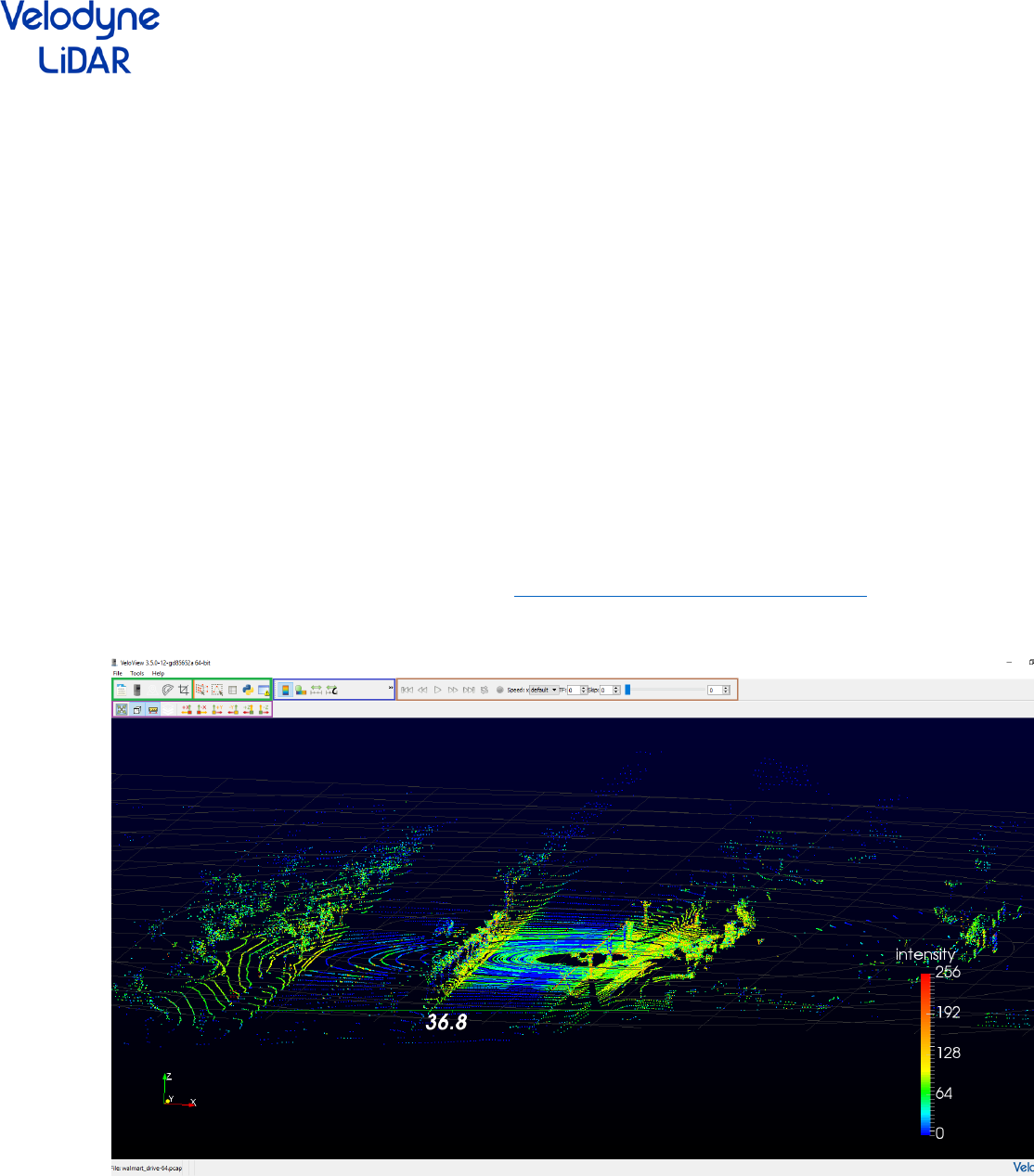
Figure 1 : Global view of VeloView : Green: Basic Control toolbar, blue: Color Control toolbar, brown:
Display toolbar, purple: View Control
4
II- Visualize and analyze data
There are two ways to visualize data in VeloView: live stream mode and playback mode. The live stream
mode corresponds to the situation where a Velodyne sensor is directly connected to the computer
running VeloView. In this case, the live stream mode permits to visualize the current output of the
sensor (just like a webcam). The playback mode corresponds to the situation where you had recorded a
live stream in .pcap format and you want to replay it.
A- Global presentation of user interface
First, we will introduce the VeloView graphical user interface (GUI). The VeloView GUI is composed of
four toolbars (introduced in section D- VeloView toolbars) and three different views which are called
main view, spreadsheet view and sensor track view.
A-1 Main view
The main view is responsible of the 3D display of the point-cloud in an interactive viewer.
A-2 Spreadsheet view
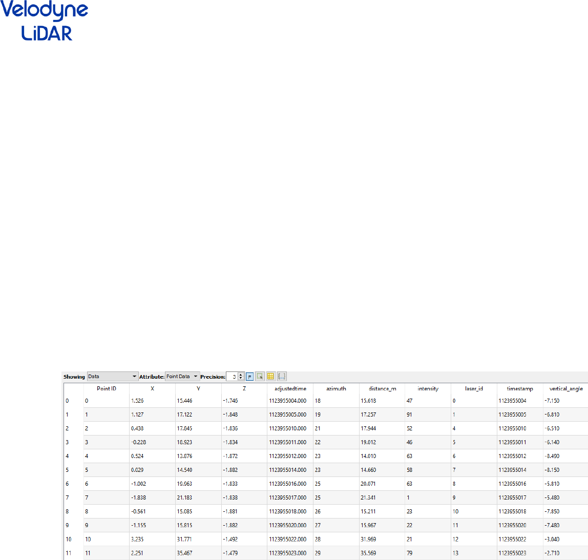
Like the main view, the spreadsheet view displays the point-cloud sensor data. However, the data are
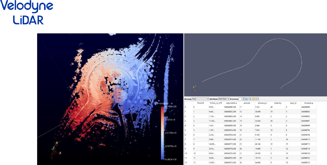
not displayed as a point cloud but as a spreadsheet (see figure 2).
Figure 2 : Spreadsheet view
In the spreadsheet view you can select the source of data to be displayed (Velodyne sensor, gps sensor,
IMU, measurement grid, …), change the digit precision, show only the selected points.
Notice that the rows are sortable if you click the column header.
D-3 Sensor track view
The Sensor track view displayed the GPS / IMU or slam position and orientation (see figure 3)
5
Figure 3 : VeloView with the 3 views shown. Left : MainView displaying the point cloud. Top right :
sensor track view displaying the gps path. Bottom right : spreadsheet view displaying the selected
points.
6
B- Live Stream Mode
B-1- Open sensor stream and sensor configuration dialog
Once a compatible (HDL-64E, HDL-32E, VLP-32, VLP-16, Puck, Puck Lite, Puck HiRes) Velodyne sensor is
connected to your computer and VeloView is running, you can display the output of the sensor using the
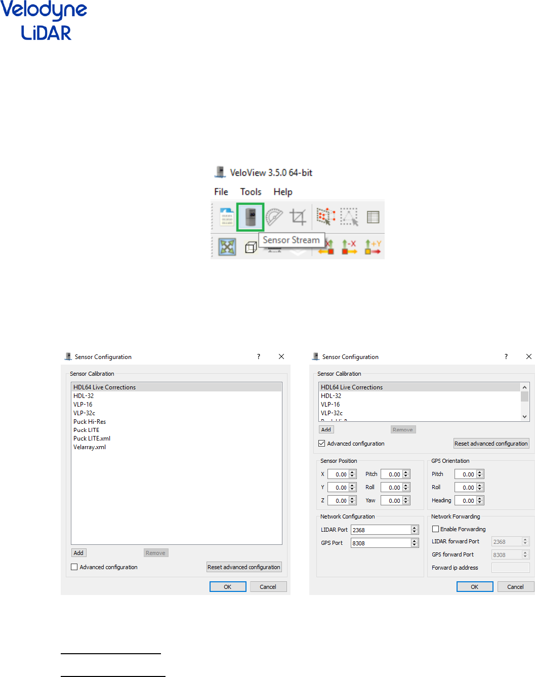
sensor stream action (see figure 4).
Figure4 : sensor stream action
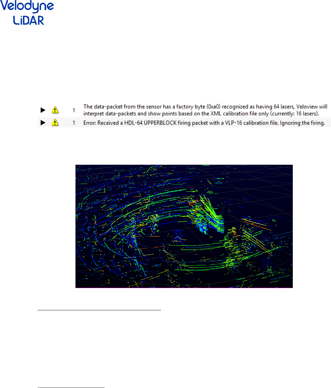
Once the Sensor Stream button has been clicked, a configuration dialog named Sensor Configuration will
pop (see Figure 5). You will be able to choose the sensor calibration file corresponding to your sensor;
and if you click on the advanced configuration checkbox you will be able to configure the GPS
parameters and the network configuration.
Figure 5 : Sensor configuration. Left : default option Right : with advanced options
Sensor Configuration:
Sensor Calibration file:
The sensor configuration file depends on the type of sensor you had connected to the computer. The
configuration file contains information about the number of lasers, the vertical angles corrections, the
7
intensity correction, distance calibration, … If you want to add a specific sensor calibration file you can
click on the “add” button and select the your calibration file.
Remark: In case you chose a wrong calibration file, here is some hints that indicate that you may have
chosen a wrong calibration file:
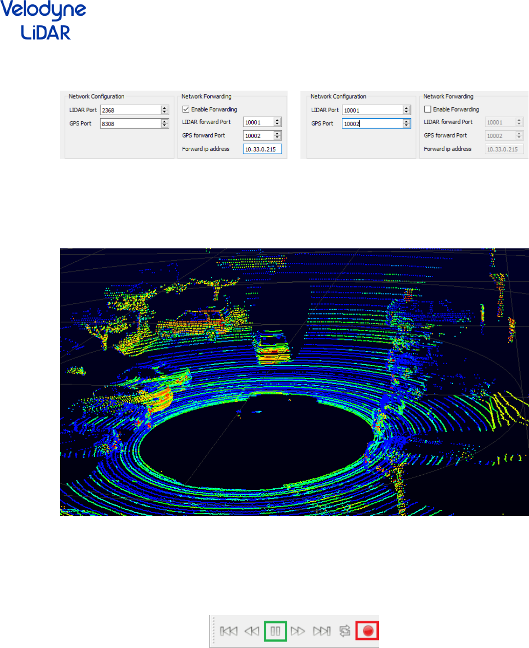
-If the number of lasers do not match between your sensor and the calibration file you should obtain an
error like in figure 6.
Figure 6 : Error message when number of lasers don’t match
- The outputted point cloud should be distorted because of the wrong vertical angles corrections like in
figure 7.
Figure 7 : Distorded point cloud due to wrong configuration file
GPS parameters (position and orientation):
In case you are using a GPS associated to the Velodyne sensor you should be careful to the Sensor
position and the GPS Orientation. Since the GPS and the Velodyne sensors may not be at the same
physical point and exactly aligned you must indicate to VeloView the position and orientation of the
Velodyne sensor according to the GPS frame. If the orientation is not indicated the point cloud will not
be georeferenced due to a rotation shift. If the position is not indicated the result may have some lever
arm issues and result in a blurred stabilization of the points clouds. The position is in meters and the
orientation in degrees.
Network configuration:
You have the possibility to forward the lidar data to another computer station. For example you can
have a first instance of VeloView which receives the sensor’s data and forwards the data to another
instance of VeloView on another computer at the address 10.33.0.215. To do so, the first instance of
VeloView will received the data on the usual ports [2368; 8308] and forward the data to the ip address
10.33.0.215 and ports [10001; 10002] (you can choose other ports here). The second instance of
8
VeloView will received the data on the ports [10001; 10002] (see figure 8). Of course, you can forward
the data received by the second instance of VeloView if you want.
Figure 8 : Left : first instance of VeloView which forwards the received data on the address 10.33.0.215
on the ports [10001; 10002]. Right : Second instance of VeloView which received the forwarded data on
the ports [10001; 10002].
Once the configuration is done, you should be able to see the point cloud outputted by your sensor (see
figure 9).
Figure 9 : Ouput of a HDL-64 correctly configured
B-2- Visualization & Interaction
While the live stream is running you can pause the stream to a specific frame or record the stream into a
.pcap file (see figure 10).
Figure 10 : green : button to pause the stream, red : button to record the stream
9
C- Playback mode (.pcap files)
If you have a .pcap file containing Velodyne sensor data (recorded from VeloView, wireshark, …) it is
possible to display the data in VeloView with the playback mode using the playback mode button (see
figure 11).
Figure 11 : playback mode action
Once the Playback Mode button has been clicked, a configuration dialog named Sensor Configuration
will pop. For more information about the Sensor Configuration dialog and how to set it, please refer to
section B-1- Open sensor stream and sensor configuration dialog.
D- VeloView toolbars
Once you are visualizing data in VeloView, many tools are available to analyze and improve
comprehension of the data.
D-1 Basic controls toolbar
The basic controls toolbar is located to the top right-hand corner of the VeloView GUI (see figure 12).
Figure 12 : Localization of the basic controls toolbar
Basic controls toolbar overview
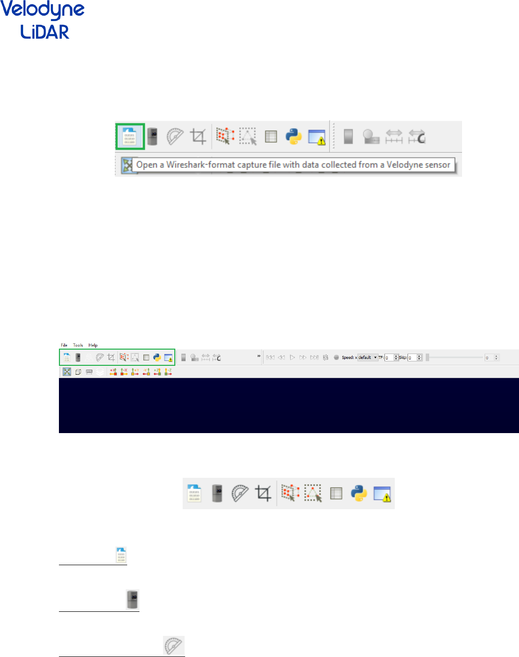
Figure 13 : Basic controls. From left to right : open .pcap, sensor stream, Choose calibration file, Crop
returns, Select all points, Select dual returns, Spreadsheet view, python console, Error console
Open .pcap:
Open a .pcap file containing recorded Velodyne sensor data
Sensor stream:
Open an UDP socket to receive the data of a connected sensor in real-time.
Change the calibration:
Open the calibration dialog to change the calibration parameters (calibration file, gps parameters and
network parameters). Note that Open .pcap and Sensor stream button will automatically open the

10
calibration dialog before displaying the point cloud. But if you did something wrong in the calibration
you can adjust it using this button.
Crop returns:
Filter points to only show those that are inside or outside a defined region. The region can be defined
using cartesian (x, y and z condition) or spherical (radius, azimuth and vertical angle condition)
coordinates (see figure 14).
Figure 14 : Left : Crop return dialog to define the crop region. Middle : a region defined in spherical
mode (condition over the radius, azimuth and vertical angle). Right : a region defined in Cartesian mode
(condition over x, y and z).
Select points:
Select points in a defined region. The region is defined with the mouse. Once drawn, the defined zone
and viewpoint is saved, and all the 3D points falling in this zone from this viewpoint will be selected. This
works even if you move the camera around or change the time-step.
Select dual returns:
Select the dual returns of each selected points. If no selection exists, this operation will return the dual
returns of all points.
Spreadsheet view:
Open the spreadsheet view.
Python console:
open the python console (python console is explained in section III- Python Console).
Error console:
open the error console
11
D-2 Display controls toolbar
You can affect the way the data are displayed in VeloView using the playback control tool bar (see figure
15).
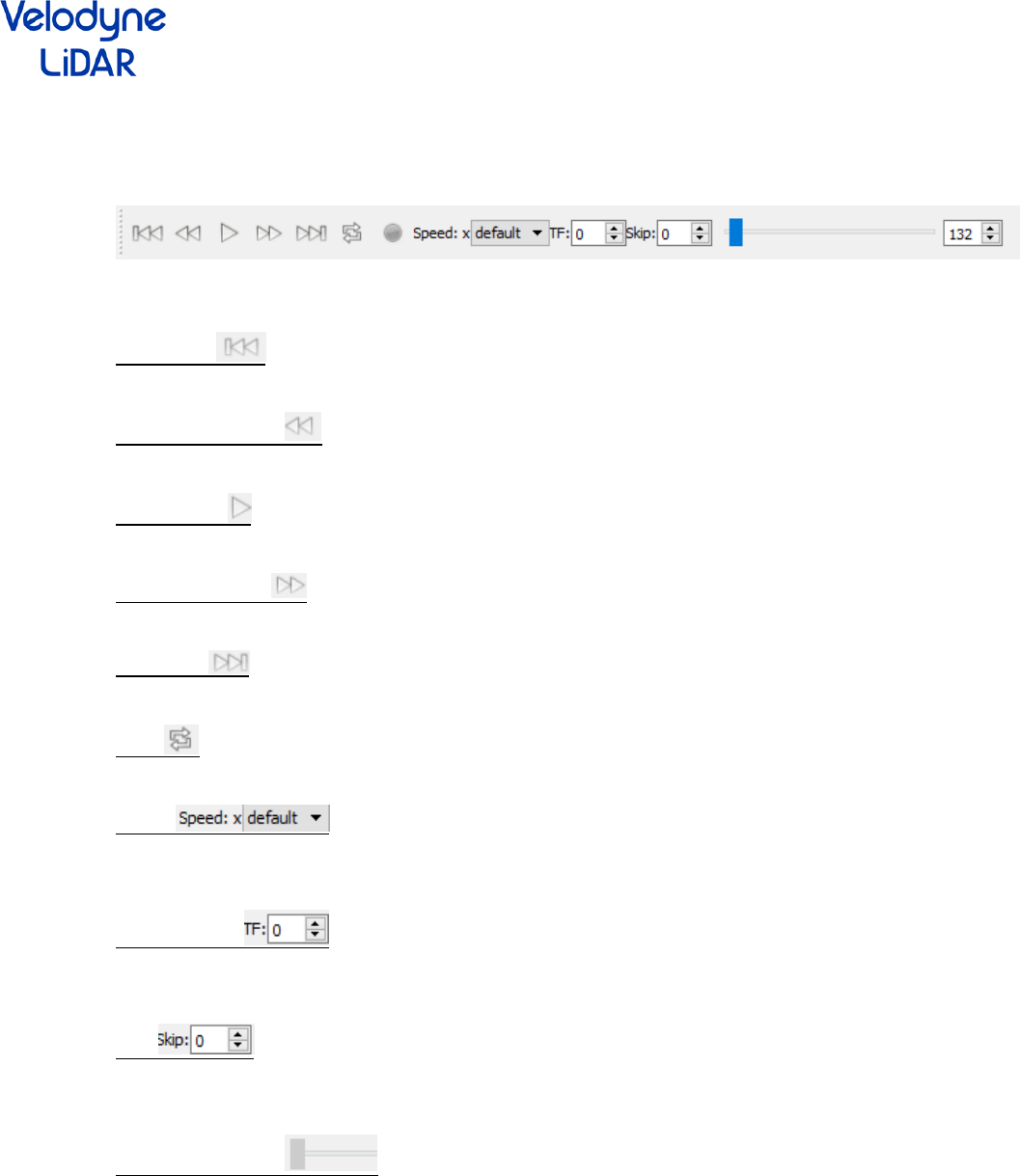
Figure 15 : playback control tool bar. From left to right : Go to start, Go previous frame, Start / Stop, Go
next frame, Go to end, Loop, speed, Trailing frame, Skip and Select frame slider.
Go to start:
Go to the first frame of the pcap
Go previous frame:
Go to the previous frame
Start / Stop:
Start or stop the playback
Go to next frame:
Go to the next frame
Go to end:
Go to the last frame of the pcap
Loop:
Enable or disable the loop mode. Loop mode replays the playback once the last frame is reached
Speed:
Control the speed of the playback. The numbers indicate the multiplicative coefficient according to the
real time
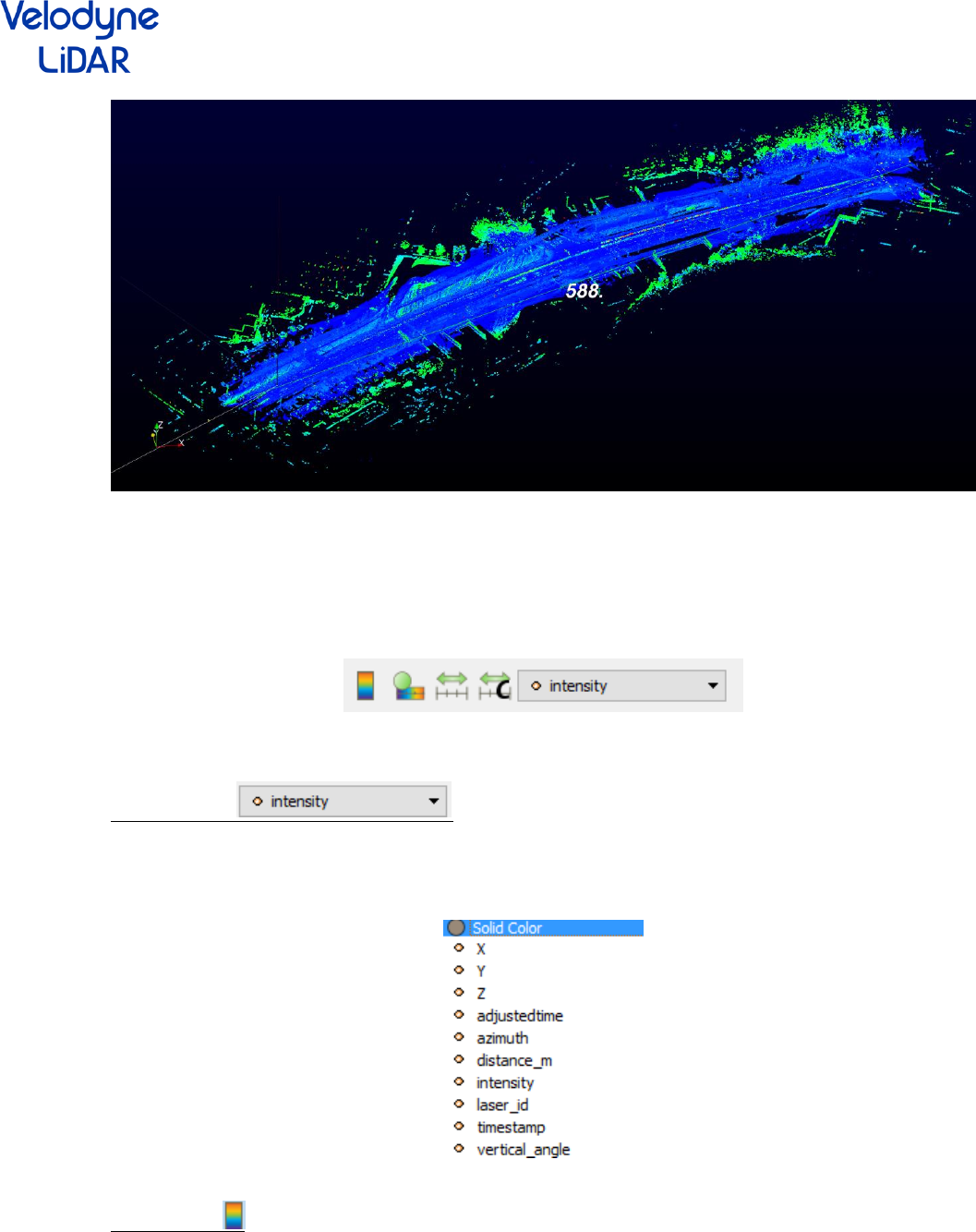
Trailing frame:
Display the last X frames at the same time. It is useful when you have stabilized data (with GPS/IMU or
slam data for example) (see figure 16).
Skip:
Subsamples the points shown by keeping only one point every X point of the point cloud. It is useful if
you are in trailing frame mode with a lot of point cloud accumulated.
Select frame slider:
Indicates the current frame. You can move to the frame you want using the slider or the spinbox.
12
Fig 16 : Road section stabilized using GPS over 588 meters visualized using trailing frame.
D-3 Color controls toolbar
The color control tool (see figure 16) is useful to display the information attached to each point. You can
choose the information you want to use for color-coding and choose the exact color map or range of
colored data.
Figure 16 : from left to right : Color legend, Edit color map, Fit color range to data, Custom color range,
color-coding data selection
Data selection:
Changes the data information used for color coding. By default the intensity of each Lidar Return is
displayed. However, you can select other information such as X, Y or Z coordinates, timestamp, laser id…
(see Figure 17).
Figure 17 : avalaible data information for color-coding
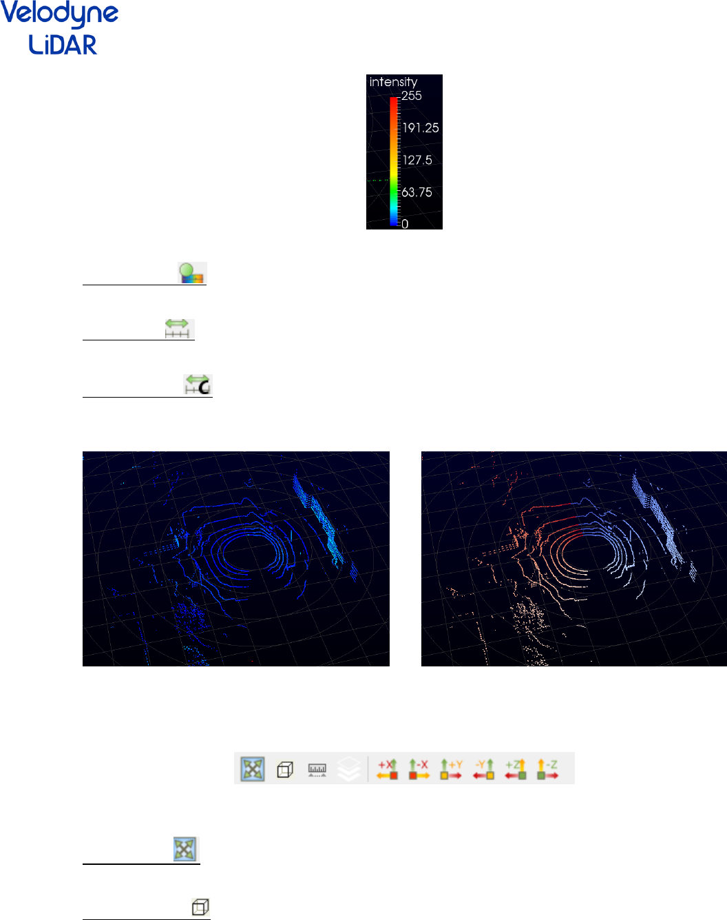
Color legend:
Display the color legend within the Main 3D View (see figure 18).
13
Figure 18 : color legend
Edit color map:
Edit and change the color mapping of the data.
Rescale data:
Rescale the color map so that the color extremities correspond to the data value extremities
Rescale custom:
Rescale the color map as you want. It is useful if you have data with a big range value but the major part
of the information is located on a subrange values.
Figure 19 : same data displayed with different data information. Left : intensity, Right : azimuth
D-4 View Controls toolbar
The view control (see figure 20) contains tools to control the camera.
Figure 20: View Control. From left to right : Reset camera, Orthogonal view, measure distances, plane fit
selection, set view direction to +x, -x, +y, -z, +z, -y
Reset Camera:
Reset the camera at its initial position and orientation
Orthogonal view:
Switch from a perspective to an orthogonal view
14
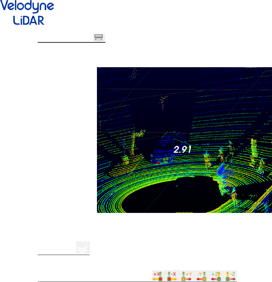
Measure distances:
Ctrl + left button of the mouse to draw a line and measure its distance. This functionality only works
when the orthogonal view is activated (see figure 21)
Figure 21: distance between car and pedestrian in meters
Plane fit tool:
Compute the plane which fits the currently selected points.
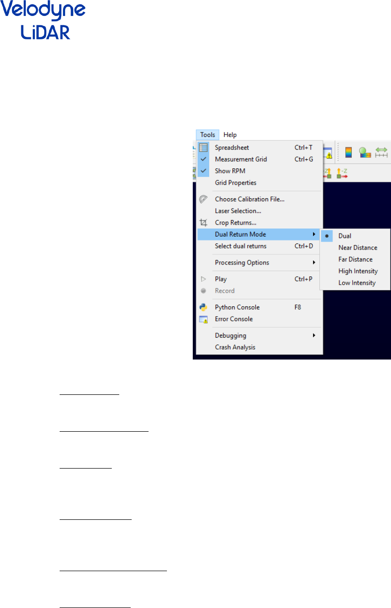
Set view direction to +x, -x, +y, -y, +z, -z:
Set the camera viewing direction to the x, y or z axis.
15
D-5 Tools Menu
The tool menu provides additional functionalities to visualize and analyze the data. Some functionalities
located in the tool menu are also available in one of the controls toolbar we just introduced.
Figure 22 : Tool Menu
Spreadsheet:
Open the spreadsheet view
Measurement Grid:
Show or hide the measurement grid on the main view
Show RPM:
Display the Rotation Per Minute (RPM) of the current frame. If the trailing frame mode is on, the RPM
displayed is the one of the last frame.
Grid Properties:
Open a dialog to change the properties of the measurement grid : number of ticks, size of the grid, size
of a tick, …
Choose Calibration File:
Open the calibration file dialog that we already introduced
Laser Selection:
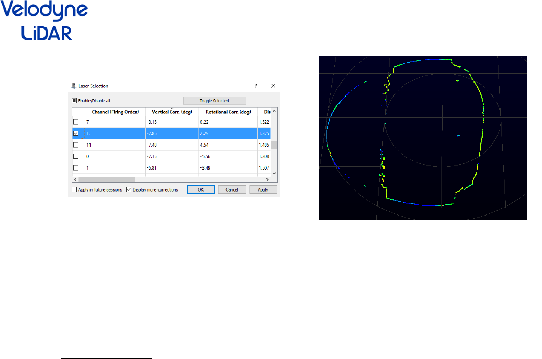
Open a dialog to select and show calibration information of the lasers (see figure 23).
This is useful to display only a subset of the lasers, or to know the internal calibration values attached to
each laser (such as vertical angle, horizontal angle, … ).
16
Figure 23 : Left laser selection dialog. Right: point cloud with only one laser selected
Crop Returns:
Open the crop return dialog ( see section D-1 Basic controls toolbar)
Dual return mode:
Choose the dual return mode that you are interested on.
Processing options:
Some options that are used to decode the raw sensor packets into 3D points:
• Apply HDL-64 intensity corrections,
• Ignore returns with distance equals to 0,
• Adjust intra firing timings and azimuth (interpolate time and azimuth between two firings, using
live computed sensor rotation speed)
• Ignore empty frames.
17
III- Python Console
A- Introduction
VeloView is the software provided by Velodyne to visualize, analyze and record data from velodyne-HDL
sensors. As with ParaView on which it is based, it is possible to create some task automation pipelines or
small filters using the Python Shell console in VeloView. Another convenient tool is the “VeloView --
script” directly derived from ParaView. It is possible to launch VeloView with the following argument
“VeloView –script path_to_my_script” to directly run a python script when VeloView is launched.
However, the automation is limited by functions which will required an user interaction such as
choosing a sensor calibration This manual goes through accessing data and programing into the python
console. Then, we will show some examples of python programming using VeloView specific functions.
Finally, we will expose a non-exhaustive list of VeloView -python functionalities.
B- Presentation of the Python Shell
B-1 Introduction to python-VeloView functionalities
The python console is a python environment available into VeloView which give you access to some
python, paraview, Qt and VeloView functionalities. The VeloView functionalities give access to the data
provided by the Velodyne-HDL sensors, and gives some basic manipulation and analysis functions.
Paraview provides lots of built-in filters to be applied on the data. Qt is in charge of the graphical user
interface (GUI), and can be controlled with python too. Finally, you get all the usual Python scripting
functionalities for task automation.
B-2 Opening the python console
Once a VeloView instance is running, the “Python Console” can be opened in three differents ways :
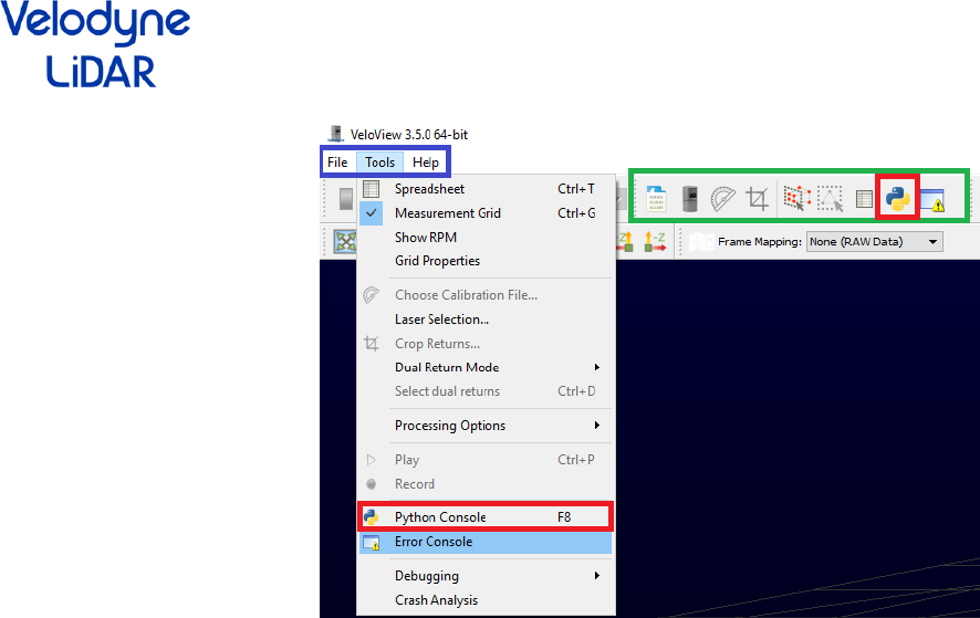
1- by clicking on the python icon in the “Basic Controls” bar (see Figure 21)
2- by clicking on the python icon in “Tools > Python Console” in the Menu Bar (see Figure 21)
3- by pressing F8 on the keyboard
18
Figure 21 : How to access the python console. Blue frame represents the Menu Bar. Green frame
represents the “Basic Controls” bar. Red frames represent the accesses to the python console
B-3 Presentation of the python shell
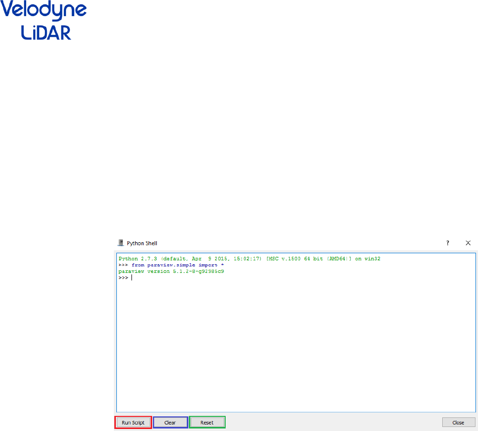
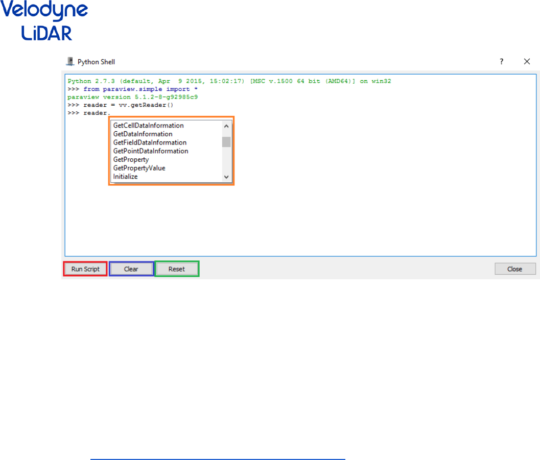
Once you opened the python console using one of the three ways presented previously, a python shell
should be opened (see figure 22). The python console / shell presents 4 differents options :
1- Run Script : Allow you to load and run a python script
2- Clear : Clear the console. The information of the console are cleared but the state remains. All your
variables and data will not be removed
3- Reset : Reset the console. All the variables and data will be removed. Nethertheless, the console
won’t be cleared. If you want to restart with a fresh new console you can Clear and Reset the console.
4- Tab : Pressing the “Tab” key the Python Shell shows you the available autocompletion.
19
Figure 22 : The Python Shell, Red: Run script option, Blue: Clear option, Green: Reset option, Orange :
Autocompletion option
D- VeloView and VTK glossary and datamodel
In VeloView the data are represented as a VTK “vtkPolyData” class. It is a dataset containing two things:
the 3D geometry (the list of 3D points provided by the velodyne sensor) and the extra data associated to
these points (intensity, timestamp, azimuth, laser ID, …). The association of the points and their
corresponding data is called the polydata or dataset.
The readers available in VeloView read the data from the network (streaming reader) or from .pcap files
(pcap reader) and provides the vtkPolyData corresponding to the data. Hence, when we get the output
of a reader in the Python Shell we get a vtkPolyData object. The structure of a vtkPolyData can be found
here : http://www.vtk.org/doc/release/5.4/html/a01260.html.
What should be retained is that the geometric points are accessible through the method “.GetPoints()”
and the extra data are stored in arrays accessible through the method “.GetPointData()”.
On the “GetClientSideObject()”:
TL;DR: You don’t need to understand the client/server paradigm: just base yourself on examples and
auto-completion.
Long story:
Usually the VeloView functions will provide a servermanager containing the object you want. It is
because VeloView is directly derived from the Paraview Client / Server architecture. When you get a
reader with the function “vv.getReader” for instance, you will get a servermanager instance on the
reader. If you want to get the output or have access to the method of the object you must use
“GetClientSideObject()” function. For instance, if you want to get the vtkPolyData output of the reader
you must write “getReader().GetClientSideObject().GetOutput()”.
20
E- Examples
E-1- Get data information
The first example will show you how to get the point cloud generated by the Velodyne-HDL sensor.
Step 1 : Open the provided .pcap example: “roundabout.pcap”
Step 2 : Open the Python Shell
Step 3 : Write these python code lines :
reader = vv.getReader() # Get the .pcap reader
cloudInfo = reader.GetClientSideObject().GetOutput() # Get the output of the reader -> dataset stored in a
vtkPolyData class
points = cloudInfo.GetPoints() # Get the 3D points list
times = cloudInfo.GetPointData().GetArray("timestamp") # Get the time information of the points
times.GetValue(10) # Value of the time information for the 10 th point
points.GetPoint(10) # Coordinates of the 10 th point
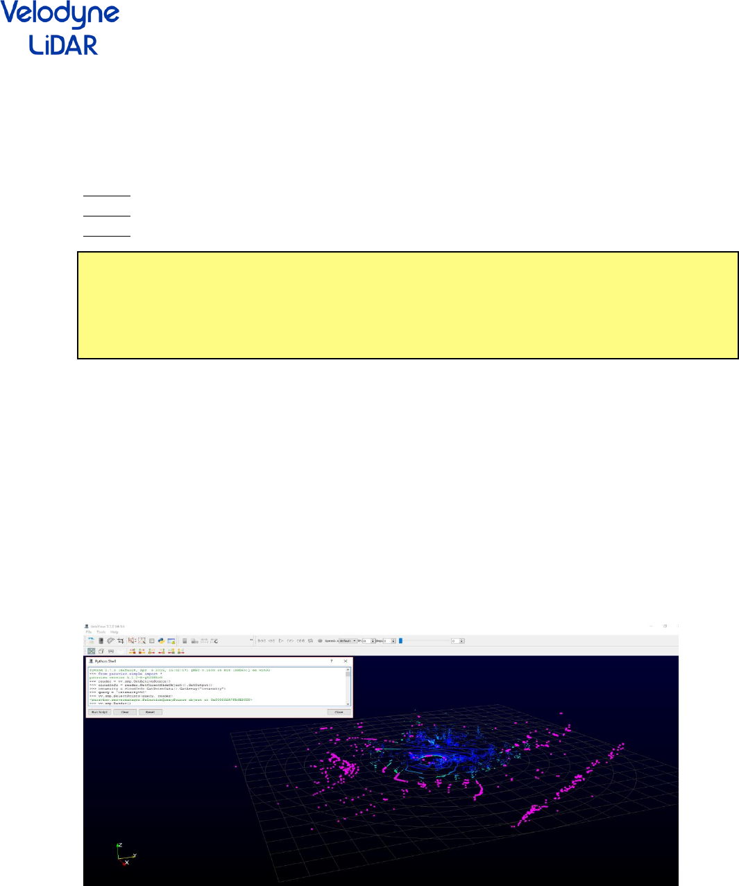
Explanation : In this example we get the point cloud associated to the first frame of the
“roundabout.pcap” data.
1- As you can see, all the function available in VeloView-python are stored in the module named “vv”.
For instance, if you want to access to the function stored in the module vtk, you must write :
vv.vtk.FunctionWanted.
2- getReader is the VeloView function which give you the .pcap reader. The .pcap reader is a vtk filter
whose output is the dataset of the current frame. The outputted dataset is stored in a vtkPolyData class.
It contains the 3D points list and the extra data associated to these points
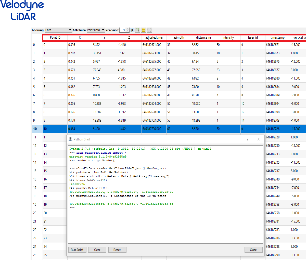
3- The method GetPointData() of the vtkPolyData class give you access to the data arrays stored in the
dataset. Using the method GetArray(“ArrayName”) you will have access to the data of the
corresponding array. The exact names of the arrays available in the point cloud are visible in the
spreadsheet view (see Figure 23). The arrays available depend on the data (Type of Velodyne sensor, if
GPS is available or not, IMU available or not, extra data, …).
21
Figure 3 : Python shell + Spreadsheet view
22
E-2- Select points using data
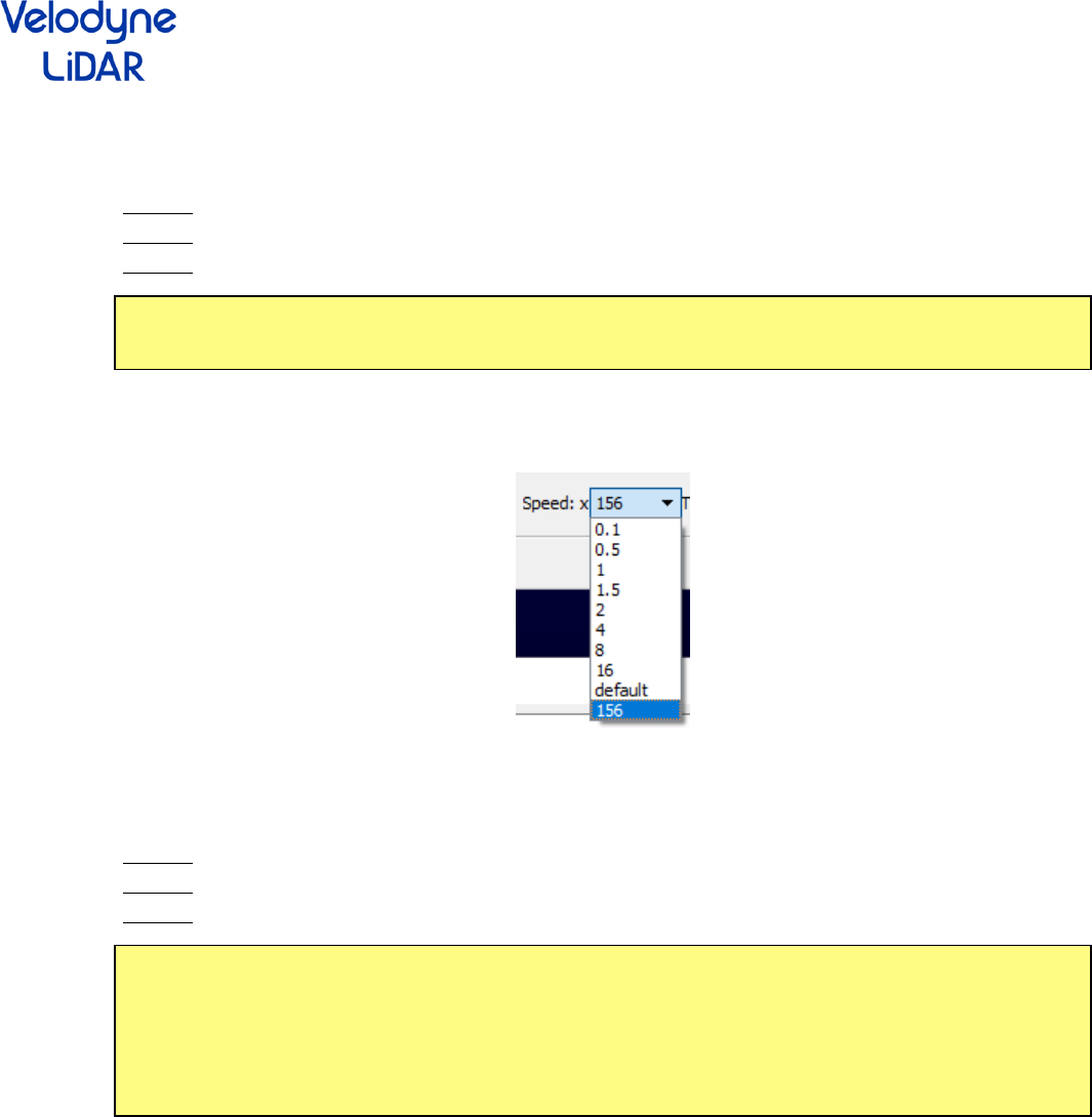
In this example we will select points with a returned intensity over a defined threshold and save the
result in a .csv file.
Step 1 : Open the provided .pcap example: “roundabout.pcap”
Step 2 : Open the Python Shell
Step 3 : Write these python code lines :
reader = vv.smp.GetActiveSource() # Get the .pcap reader
cloudInfo = reader.GetClientSideObject().GetOutput()
myintensity = cloudInfo.GetPointData().GetArray("intensity") # Get the intensity array
query = 'intensity>50' # query to select points having their intensity data array value over 50
vv.smp.SelectPoints(query, reader) # Select the points which satisfies the query
vv.smp.Render() # render the result
vv.saveCSVCurrentFrameSelection("D:\save.csv") # Save the selected points in .csv format
Explanation :
1- vv.smp.GetActiveSource() : here we get the .pcap reader with the function GetActiveSource(). As you
can see this function belong to the module “smp” which is the module “paraview.simple” where all the
paraview function are stored. GetActiveSource() returns the active source, in our example the active
source is the .pcap reader.
2- smp.Render() refresh the active source once the data process is done. If you want to refresh another
view (spreadsheet view, overhead view, Main view) you have to set the active source with
smp.SetActiveSource.
3- vv.saveCSVCurrentFrameSelection("D:\save.csv") saves the selected points in a .csv file located in the
indicated filename.
Figure 24 : Result of example #2. Pink points are the selected points
23
E-3- Manipulation of the GUI
In this example we add a new value available to the display speed button in the GUI.
Step 1 : Open the provided .pcap example: “roundabout.pcap”
Step 2 : Open the Python Shell
Step 3 : Write these python code lines :
speedButton = vv.app.PlaybackSpeed
speedButton.addItem("156")
speedButton.setCurrentIndex(speedButton.count - 1)
Figure 25 show the obtained result.
Figure 25 : New option available and setted : x156 speed
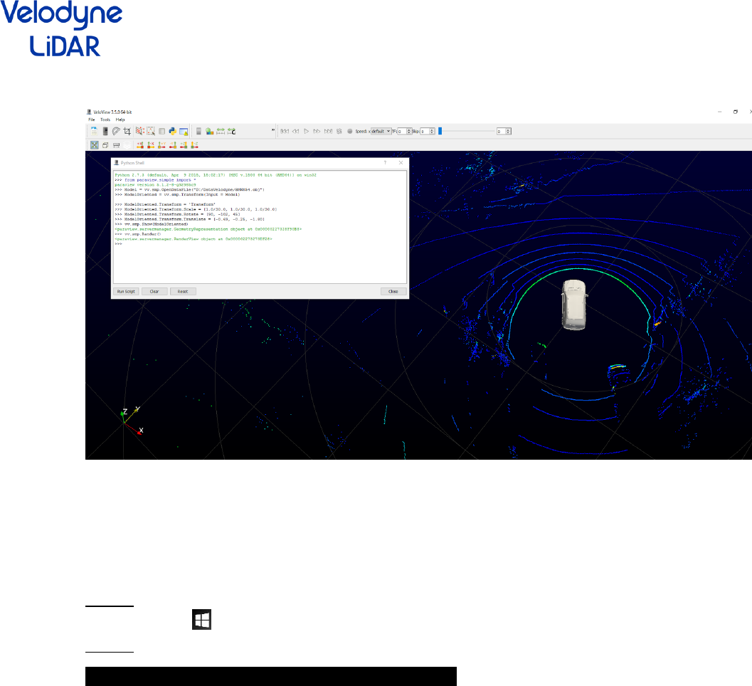
E-4- Display a 3D model in the mainview
In this example we load and display a 3D model in the main view
Step 1 : Open the provided .pcap example: “roundabout.pcap”
Step 2 : Open the Python Shell
Step 3 : Write these python code lines :
Model = vv.smp.OpenDataFile("D:/PythonManualData/BMWX54.obj")
ModelOriented = vv.smp.Transform(Input = Model)
ModelOriented.Transform = 'Transform'
ModelOriented.Transform.Scale = [1.0/30.0, 1.0/30.0, 1.0/30.0]
ModelOriented.Transform.Rotate = [90, -102, 45]
ModelOriented.Transform.Translate = [-0.69, -0.25, -1.80]
vv.smp.Show(ModelOriented)
vv.smp.Render()
Explanation :
1- smp.OpenDataFile("D:/PythonManualData/BMWX54.obj") open the .obj model.
2- Scale, Rotate, Translate : Since the model is given in an arbitrary frame, we must rescale and set the
orientation of the model to fit our data
3- Show(), Render() : We show the result in the main view and then render the result to display the
model
24
Figure 26 : The model is added in the main view
E-5- Start VeloView with a 3D model loaded in the mainview with “- -script”
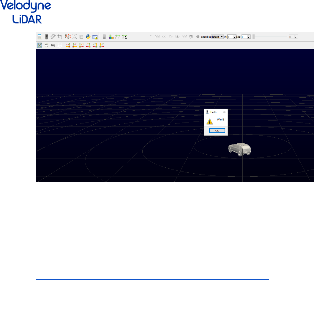
In this example we load and display a 3D model in the mainview directly when VeloView is launched
using the --script command-line option.
Step 1 : Open a terminal in the folder containing VeloView executable. You can do that on Windows by
pressing the key + R and type “cmd”.
Step 2 : launch VeloView from the terminal with the command:
./Veloview --script='D:\PythonManualData\LoadModel.py'
Of course, you must replace “D:\PythonManualData\LoadModel.py” with the path to the file
LoadModel.py. You also must replace the model filename contained in the file LoadModel.py.
25
Figure 28 : The model is loaded thanks to python script launched with --script tool
F- List of functionalities
Here we will give a non-exhaustive list of all functionalities available in Python-VeloView
F-1- Simple Paraview : “vv.smp.”
All functionalities provided by the module paraview.simple are available using “vv.smp.”. You can find
the description and documentation of the functionalities here :
https://www.paraview.org/ParaView3/Doc/Nightly/www/py-doc/paraview.simple.html
F-2- Qt “vv.QtGui”
All functionalities provided by the module QtGui are available using “vv.QtGui.”. You can find the
description and documentation of the functionalities here :
http://pyqt.sourceforge.net/Docs/PyQt4/qtgui.html
F-3- Vtk Python
All functionalities provided by the module vtk are available using “vv.vtk.”. You can find the description
and documentation of the functionalities here : http://www.vtk.org/Wiki/VTK/Examples/Python
F-4- VeloView functions “vv.”
All these functions are available on the module “vv.” :
getReader() : return the .pcap reader which contains the point cloud of the current frame
openSensor() : Instantiate a UDP socket to receive data from velodyne-HDL sensor.

26
openPCAP(filename) : Create a .pcap reader to read the data contained in the filename
hideMeasurementGrid() : Hide the measurement grid
showMeasurementGrid(): Show the measurement grid
saveCSVCurrentFrame(filename) : export the current frame into a .csv file format
saveCSVCurrentFrameSelection(filename) : export the current selection of the current frame into a .csv file format
seekForward(): move to the next frame
seekBackward() : move to the previous frame
recordFile(filename) : record the data received in live stream
stopRecording() : Stop the recording
startStream() : Start the listening of the UDP socket
stopStream() : Stop the listening of the UDP socket
gotoNext() : go to the next frame
gotoPrevious : go to the previous frame
gotoEnd() : go to the last frame
gotoStart() : go to the first frame
updatePosition() : Refresh data of the current frame (RPM, GPS transformation, …)
getSensor() : get the live streaming reader. The output of this reader is the 100 last received pointcloud
getPosition() : get the position reader. The output of this reader is the GPS / IMU information contained in the data
onCropReturns(show = True) : open the crop dialog box
resetCamera() : reset the camera
saveScreenshot(filename) : Save a screenshot
showGrid() : Show the grid
hideGrid() : Hide the grid
getMainWindow() : Get the main view (the view where the point cloud is displayed)
toggleSelectDualReturn() : Select the dual return of the current selection
setFilterToDual() : Show only the dual return
setFilterToDistanceNear() : Show nearest returns
setFilterToDistanceFar() : Show farest returns
setFilterToIntensityHigh() : Show highest intensity returns
setFilterToIntensityLow() : Show lowest intensity returns
setTransformMode(mode) : change the transform mode 0 - raw, 1 - absolute, 2 - relative
showRPM() : show the rpm
Vv.app.reader : get the .pcap reader
vv.app.sensor : get the streaming reader
vv.app.distanceResolutionM : Distance resolution of the sensor
vv.app.trailingFramesSpinBox : GUI spinbox which determines the number of trailing frame
vv.app.geolocationToolBar : GUI geolocation toolbar
vv.app.overheadView : the overhead view (the one displaying the gps trajectory)
vv.app.mainView : the main view (the one displaying the point cloud)
vv.app.gridProperties : Properties of the grid
Vv.app.grid : The gris displayed in the main view
vv.app.targetFps : the target fps in playback mode
vv.app.scene : scene displayed in the main view
vv.app.PlaybackSpeed : GUI combo box which determines the playback speed
vv.app.pointsSkipSpinBox : GUI spin box which determines the number of points to skip
