PTV Vissim 10 User Manual
User Manual:
Open the PDF directly: View PDF ![]() .
.
Page Count: 1155 [warning: Documents this large are best viewed by clicking the View PDF Link!]
- Copyright and legal agreements
- Important changes compared to previous versions
- Quick start: creating a network and starting simulation
- Typography and conventions
- 1 Introduction
- 1.1 Simulation of pedestrians with PTV Viswalk
- 1.2 PTV Vissim use cases
- 1.3 Traffic flow model and light signal control
- 1.4 How to install and start PTV Vissim
- 1.5 Technical information and requirements
- 1.6 Overview of add-on modules
- 1.7 Using a demo version
- 1.8 Using PTV Vissim Viewer
- 1.9 Using the PTV Vissim Simulation Engine
- 1.10 Using files with examples
- 1.11 Opening the Working directory
- 1.12 Documents
- 1.13 Service and support
- 2 Principles of operation of the program
- 2.1 Program start and start screen
- 2.2 Starting PTV Vissim via the command prompt
- 2.3 Using the Start page
- 2.4 Becoming familiar with the user interface
- 2.5 Using the Network object toolbar
- 2.6 Using the Level toolbar
- 2.7 Using the background image toolbar
- 2.8 Using the Quick View
- 2.9 Using the Smart Map
- 2.9.1 Displaying the Smart Map
- 2.9.2 Displaying the entire network in the Smart Map
- 2.9.3 Moving the Network Editor view
- 2.9.4 Showing all Smart Map sections
- 2.9.5 Zooming in or out on the network in the Smart Map
- 2.9.6 Redefining the display in the Smart Map
- 2.9.7 Defining a Smart Map view in a new Network Editor
- 2.9.8 Moving the Smart Map view
- 2.9.9 Copying the layout of a Network Editor into Smart Map
- 2.9.10 Displaying or hiding live map for the Smart Map
- 2.10 Using network editors
- 2.10.1 Showing Network editors
- 2.10.2 Network editor toolbar
- 2.10.3 Network editor context menu
- 2.10.4 Zooming in
- 2.10.5 Zooming out
- 2.10.6 Displaying the entire network
- 2.10.7 Moving the view
- 2.10.8 Defining a new view
- 2.10.9 Displaying previous or next sections
- 2.10.10 Zooming to network objects in the network editor
- 2.10.11 Selecting network objects in the Network editor and showing them in a list
- 2.10.12 Using named Network editor layouts
- 2.11 Selecting simple network display
- 2.12 Using the Quick Mode
- 2.13 Changing the display of windows
- 2.14 Using lists
- 2.14.1 Structure of lists
- 2.14.2 Opening lists
- 2.14.3 Selecting network objects in the Network editor and showing them in a list
- 2.14.4 List toolbar
- 2.14.5 Selecting and editing data in lists
- 2.14.6 Editing lists and data via the context menu
- 2.14.7 Selecting cells in lists
- 2.14.8 Sorting lists
- 2.14.9 Deleting data in lists
- 2.14.10 Moving column in list
- 2.14.11 Using named list layouts
- 2.14.12 Selecting attributes and subattributes for a list
- 2.14.13 Setting a filter for selection of subattributes displayed
- 2.14.14 Using coupled lists
- 2.15 Using the Menu bar
- 2.16 Using toolbars
- 2.17 Mouse functions and key combinations
- 2.18 Saving and importing a layout of the user interface
- 2.19 Information in the status bar
- 2.20 Selecting decimal separator via the control panel
- 3 Setting user preferences
- 3.1 Selecting the language of the user interface
- 3.2 Selecting the country for regional information on the start page
- 3.3 Selecting a compression program
- 3.4 Selecting the 3D mode and 3D recording settings
- 3.5 Right-click behavior and action after creating an object
- 3.6 Showing and hiding object information in the Network editor
- 3.7 Configuring command history
- 3.8 Specifying automatic saving of the layout file *.layx
- 3.9 Defining click behavior for the activation of detectors in test mode
- 3.10 Checking and selecting the network with simulation start
- 3.11 Resetting menus, toolbars, shortcuts, and dialog positions
- 3.12 Showing short or long names of attributes in column headers
- 3.13 Defining default values
- 3.14 Allowing the collection of usage data
- 4 Using 2D mode and 3D mode
- 4.1 Calling the 2D mode from the 3D mode
- 4.2 Selecting display options
- 4.2.1 Editing graphic parameters for network objects
- 4.2.2 List of graphic parameters for network objects
- 4.2.3 Editing base graphic parameters for a network editor
- 4.2.4 List of base graphic parameters for network editors
- 4.2.5 Using textures
- 4.2.6 Defining colors for vehicles and pedestrians
- 4.2.7 Assigning a color to links based on aggregated parameters
- 4.2.8 Assigning a color to areas based on aggregated parameters (LOS)
- 4.2.9 Assigning a color to ramps and stairs based on aggregated parameters (LOS)
- 4.2.10 Assigning a color to nodes based on an attribute
- 4.3 Using 3D mode and specifying the display
- 4.3.1 Calling the 3D mode from the 2D mode
- 4.3.2 Navigating in 3D mode in the network
- 4.3.3 Editing 3D graphic parameters
- 4.3.4 List of 3D graphic parameters
- 4.3.5 Flight over the network
- 4.3.6 Showing 3D perspective of a driver or a pedestrian
- 4.3.7 Changing the 3D viewing angle (focal length)
- 4.3.8 Displaying vehicles and pedestrians in the 3D mode
- 4.3.9 3D animation of PT vehicle doors
- 4.3.10 Using fog in the 3D mode
- 5 Base data for simulation
- 5.1 Selecting network settings
- 5.1.1 Selecting network settings for vehicle behavior
- 5.1.2 Selecting network settings for pedestrian behavior
- 5.1.3 Selecting network settings for units
- 5.1.4 Selecting network settings for attribute concatenation
- 5.1.5 Selecting network settings for 3D signal heads
- 5.1.6 Network settings for standard types of elevators and elevator groups
- 5.1.7 Network settings for standard type of direction change duration distribution
- 5.1.8 Showing reference points
- 5.1.9 Selecting angle towards north
- 5.1.10 Network settings for the driving simulator
- 5.2 Using user-defined attributes
- 5.3 Using aliases for attribute names
- 5.4 Using 2D/3D models
- 5.5 Defining acceleration and deceleration behavior
- 5.5.1 Default curves for maximum acceleration and deceleration
- 5.5.2 Stochastic distribution of values for maximum acceleration and deceleration
- 5.5.3 Defining acceleration and deceleration functions
- 5.5.4 Attributes of acceleration and deceleration functions
- 5.5.5 Deleting the acceleration/deceleration function
- 5.6 Using distributions
- 5.6.1 Using desired speed distributions
- 5.6.2 Using power distributions
- 5.6.3 Using weight distributions
- 5.6.4 Using time distributions
- 5.6.5 Using location distributions for boarding and alighting passengers in PT
- 5.6.6 Using distance distributions
- 5.6.7 Using occupation distributions
- 5.6.8 Using 2D/3D model distributions
- 5.6.9 Using color distributions
- 5.6.10 Editing the graph of a function or distribution
- 5.6.11 Deleting intermediate point of a graph
- 5.7 Managing vehicle types, vehicle classes and vehicle categories
- 5.8 Defining driving behavior parameter sets
- 5.8.1 Driving states in the traffic flow model according to Wiedemann
- 5.8.2 Editing the driving behavior parameter Following behavior
- 5.8.3 Applications and driving behavior parameters of lane changing
- 5.8.4 Editing the driving behavior parameter Lateral behavior
- 5.8.5 Editing the driving behavior parameter Signal Control
- 5.8.6 Editing the driving behavior parameter Meso
- 5.9 Defining link behavior types for links and connectors
- 5.10 Defining display types
- 5.11 Defining track properties
- 5.12 Defining levels
- 5.13 Using time intervals
- 5.14 Toll pricing and defining managed lanes
- 5.1 Selecting network settings
- 6 Creating and editing a network
- 6.1 Setting up a road network or PT link network
- 6.2 Copying and pasting network objects into the Network Editor
- 6.3 Editing network objects, attributes and attribute values
- 6.3.1 Inserting a new network object in a Network Editor
- 6.3.2 Editing attributes of network objects
- 6.3.3 Showing attribute values of a network object in the Network editor
- 6.3.4 Direct and indirect attributes
- 6.3.5 Duplicating network objects
- 6.3.6 Moving network objects in the Network Editor
- 6.3.7 Moving network object sections
- 6.3.8 Calling up network object specific functions in the network editor
- 6.3.9 Rotating network objects
- 6.3.10 Deleting network objects
- 6.4 Displaying and selecting network objects
- 6.4.1 Moving network objects in the Network Editor
- 6.4.2 Selecting network objects in the Network editor and showing them in a list
- 6.4.3 Showing the names of the network objects at the click position
- 6.4.4 Zooming to network objects in the network editor
- 6.4.5 Selecting a network object from superimposed network objects
- 6.4.6 Viewing and positioning label of a network object
- 6.4.7 Resetting the label position
- 6.5 Importing a network
- 6.5.1 Reading a network additionally
- 6.5.2 Importing ANM data
- 6.5.3 Selecting ANM file, configuring and starting data import
- 6.5.4 Adaptive import of ANM data
- 6.5.5 Generated network objects from the ANM import
- 6.5.6 Importing data from the add-on module Synchro 7
- 6.5.7 Adaptive import process for abstract network models
- 6.5.8 Importing Synchro 7 network adaptively
- 6.6 Exporting data
- 6.7 Rotating the network
- 6.8 Moving the network
- 6.9 Inserting a background image
- 6.10 Modeling the road network
- 6.10.1 Modeling links for vehicles and pedestrians
- 6.10.2 Modeling connectors
- 6.10.3 Editing points in links or connectors
- 6.10.4 Changing the desired speed
- 6.10.5 Modeling pavement markings
- 6.10.6 Defining data collection points
- 6.10.7 Defining vehicle travel time measurement
- 6.10.8 Attributes of vehicle travel time measurement
- 6.10.9 Modeling queue counters
- 6.11 Modeling vehicular traffic
- 6.12 Modeling short-range public transportation
- 6.12.1 Modeling PT stops
- 6.12.2 Defining PT stops
- 6.12.3 Attributes of PT stops
- 6.12.4 Generating platform edges
- 6.12.5 Generating a public transport stop bay
- 6.12.6 Modeling PT lines
- 6.12.7 Entering a public transport stop bay in a PT line path
- 6.12.8 Editing a PT line stop
- 6.12.9 Calculating the public transport dwell time for PT lines and partial PT routes
- 6.12.10 Defining partial PT routes
- 6.12.11 Attributes of PT partial routing decisions
- 6.12.12 Attributes of partial PT routes
- 6.13 Modeling right-of-way without SC
- 6.14 Modeling signal controllers
- 6.15 Using static 3D models
- 6.16 Modeling sections
- 6.17 Visualizing turn values
- 7 Using the dynamic assignment add-on module
- 7.1 Quick start dynamic assignment
- 7.2 Differences between static and dynamic assignment
- 7.3 Base for calculating the dynamic assignment
- 7.4 Flow diagram dynamic assignment
- 7.5 Building an Abstract Network Graph
- 7.6 Modeling traffic demand with origin-destination matrices or trip chain files
- 7.6.1 Modeling traffic demand with origin-destination matrices
- 7.6.2 Defining an origin-destination matrix
- 7.6.3 Selecting an origin-destination matrix
- 7.6.4 Matrix attributes
- 7.6.5 Editing OD matrices for vehicular traffic in the Matrix editor
- 7.6.6 Using OD matrices from previous versions
- 7.6.7 Modeling traffic demand with trip chain files
- 7.6.8 Selecting a trip chain file
- 7.6.9 Structure of the trip chain file *.fkt
- 7.7 Simulated travel time and generalized costs
- 7.8 Path search and path selection
- 7.8.1 Calculation of paths and costs
- 7.8.2 Path search finds only the best possible path in each interval
- 7.8.3 Method of path selection with or without path search
- 7.8.4 Equilibrium assignment – Example
- 7.8.5 Performing an alternative path search
- 7.8.6 Displaying paths in the network
- 7.8.7 Attributes of paths
- 7.9 Optional expansion for the dynamic assignment
- 7.9.1 Defining simultaneous assignment
- 7.9.2 Defining the destination parking lot selection
- 7.9.3 Using the detour factor to avoid detours
- 7.9.4 Correcting distorted demand distribution for overlapping paths
- 7.9.5 Defining dynamic routing decisions
- 7.9.6 Attributes of dynamic routing decisions
- 7.9.7 Defining route guidance for vehicles
- 7.10 Visualizing volumes on paths as flow bundles
- 7.11 Controlling dynamic assignment
- 7.11.1 Attributes for the trip chain file, matrices, path file and cost file
- 7.11.2 Attributes for calculating costs as a basis for path selection
- 7.11.3 Attributes for path search
- 7.11.4 Attributes for path selection
- 7.11.5 Attributes for achieving convergence
- 7.11.6 Checking the convergence in the evaluation file
- 7.11.7 Showing converged paths and paths that are not converged
- 7.11.8 Attributes for the guidance of vehicles
- 7.11.9 Controlling iterations of the simulation
- 7.11.10 Setting volume for paths manually
- 7.11.11 Influencing the path search by using cost surcharges or blocks
- 7.11.12 Evaluating costs and assigned traffic of paths
- 7.12 Correcting demand matrices
- 7.13 Generating static routes from assignment
- 7.14 Using an assignment from Visum for dynamic assignment
- 8 Using add-on module for mesoscopic simulation
- 8.1 Quick start guide mesoscopic simulation
- 8.2 Car following model for mesoscopic simulation
- 8.3 Mesoscopic node-edge model
- 8.4 Node control in mesoscopic simulation
- 8.5 Modeling meso network nodes
- 8.6 Rules and examples for defining meso network nodes
- 8.7 Defining meso network nodes
- 8.8 Attributes of meso nodes
- 8.9 Attributes of meso edges
- 8.10 Attributes of meso turns
- 8.11 Attributes of meso turn conflicts
- 8.12 Generating meso graphs
- 8.13 Hybrid simulation
- 8.14 Selecting sections for hybrid simulation
- 8.15 Limitations of mesoscopic simulation
- 9 Running a simulation
- 9.1 Selecting simulation method micro or meso
- 9.2 Defining simulation parameters
- 9.3 Selecting the number of simulation runs and starting simulation
- 9.4 Showing simulation run data in lists
- 9.5 Displaying vehicles in the network in a list
- 9.6 Showing pedestrians in the network in a list
- 9.7 Reading one or multiple simulation runs additionally
- 9.8 Checking the network
- 10 Pedestrian simulation
- 10.1 Movement of pedestrians in the social force model
- 10.2 Version-specific functions of pedestrian simulation
- 10.3 Modeling examples and differences of the pedestrian models
- 10.4 Internal procedure of pedestrian simulation
- 10.5 Parameters for pedestrian simulation
- 10.6 Network objects and base data for the simulation of pedestrians
- 10.7 Using pedestrian types
- 10.8 Using pedestrian classes
- 10.9 Modeling construction elements
- 10.9.1 Areas, Ramps & Stairs
- 10.9.2 Escalators and moving walkways
- 10.9.3 Obstacles
- 10.9.4 Deleting construction elements
- 10.9.5 Importing walkable areas and obstacles from AutoCAD
- 10.9.6 Importing Building Information Model files
- 10.9.7 Defining construction elements as rectangles
- 10.9.8 Defining construction elements as polygons
- 10.9.9 Editing construction elements in the Network Editor
- 10.9.10 Attributes of areas
- 10.9.11 Attributes of obstacles
- 10.9.12 Attributes of ramps, stairs, moving walkways and escalators
- 10.9.13 Modeling length, headroom and ceiling opening
- 10.9.14 Defining levels
- 10.10 Modeling links as pedestrian areas
- 10.10.1 Differences between road traffic and pedestrian flows
- 10.10.2 Differences between walkable construction elements and link-based pedestrian areas
- 10.10.3 Modeling obstacles on links
- 10.10.4 Network objects for pedestrian links
- 10.10.5 Defining pedestrian links
- 10.10.6 Modeling interaction between vehicles and pedestrians
- 10.10.7 Modeling signal controls for pedestrians
- 10.10.8 Modeling conflict areas for pedestrians
- 10.10.9 Modeling detectors for pedestrians
- 10.10.10 Modeling priority rules for pedestrians
- 10.11 Modeling pedestrian compositions
- 10.12 Modeling area-based walking behavior
- 10.13 Modeling pedestrian demand and routing of pedestrians
- 10.14 Visualizing pedestrian traffic in 2D mode
- 10.15 Modeling pedestrians as PT passengers
- 10.16 Modeling elevators
- 10.17 Defining pedestrian travel time measurement
- 11 Performing evaluations
- 11.1 Overview of evaluations
- 11.2 Comparing evaluations of PTV Vissim with evaluations according to HBS
- 11.3 Performing environmental impact assessments
- 11.4 Managing results
- 11.5 Defining and generating measurements or editing allocated objects
- 11.5.1 Defining an area measurement in lists
- 11.5.2 Generating area measurements in lists
- 11.5.3 Editing sections assigned to area measurements
- 11.5.4 Defining a data collection measurement in lists
- 11.5.5 Generating data collection measurements in lists
- 11.5.6 Editing data collection points assigned to data collection measurements
- 11.5.7 Defining delay measurement in lists
- 11.5.8 Generating delay measurements in lists
- 11.5.9 Editing vehicle and travel time measurements assigned to delay measurements
- 11.6 Showing results of measurements
- 11.7 Configuring evaluations of the result attributes for lists
- 11.8 Configuring evaluations for direct output
- 11.9 Showing evaluations in windows
- 11.10 Importing text file in a database after the simulation
- 11.11 Output options and results of individual evaluations
- 11.12 Visualizing evaluation results
- 11.13 Saving discharge record to a file
- 11.14 Displaying OD pair data in lists
- 11.15 Saving lane change data to a file
- 11.16 Saving vehicle record to a file or database
- 11.17 Evaluating pedestrian density and speed based on areas
- 11.18 Grid-based evaluation of pedestrian density and speed
- 11.19 Output attributes of area and ramp evaluation
- 11.20 Evaluating pedestrian areas with area measurements
- 11.21 Evaluating pedestrian travel time measurements
- 11.22 Saving pedestrian travel time measurements from OD data to a file
- 11.23 Saving pedestrian record to a file or database
- 11.24 Evaluating nodes
- 11.25 Showing meso edges results in lists
- 11.26 Showing meso lane results in lists
- 11.27 Saving data about the convergence of the dynamic assignment to a file
- 11.28 Evaluating SC detector records
- 11.29 Saving SC green time distribution to a file
- 11.30 Evaluating signal changes
- 11.31 Saving managed lane data to a file
- 11.32 Vehicle network performance : Displaying network performance results (vehicles) in result lists
- 11.33 Pedestrian network performance: Displaying network performance results (pedestrians) in lists
- 11.34 Saving PT waiting time data to a file
- 11.35 Evaluating data collection measurements
- 11.36 Evaluating vehicle travel time measurements
- 11.37 Showing signal times table in a window
- 11.38 Saving SSAM trajectories to a file
- 11.39 Showing data from links in lists
- 11.40 Showing results of queue counters in lists
- 11.41 Showing delay measurements in lists
- 11.42 Showing data about paths of dynamic assignment in lists
- 11.43 Saving vehicle input data to a file
- 12 Creating charts
- 12.1 Presenting data
- 12.2 Creating a chart quick-start guide
- 12.3 Charts toolbar
- 12.4 Creating charts with or without preselection
- 12.5 Configuring a created chart
- 12.6 Using named chart layouts
- 12.6.1 Generating a named chart layout
- 12.6.2 Assigning a complete chart layout
- 12.6.3 Assigning only the graphic parameters from a named chart layout
- 12.6.4 Assigning only the data selection from a named chart layout
- 12.6.5 Saving a named chart layout
- 12.6.6 Reading saved named chart layouts additionally
- 12.6.7 Deleting a named chart layout
- 12.7 Reusing a chart
- 13 Scenario management
- 13.1 Quick start scenario management
- 13.2 Using the project explorer
- 13.3 Project explorer toolbar
- 13.4 Editing the project structure
- 13.5 Placing a network under scenario management
- 13.6 Creating a new scenario
- 13.7 Creating a new modification
- 13.8 Opening and editing the base network in the network editor
- 13.9 Opening and editing scenarios in the network editor
- 13.10 Opening and editing modifications in the network editor
- 13.11 Comparing scenarios
- 13.12 Comparing and transferring networks
- 14 Testing logics without traffic flow simulation
- 15 Creating simulation presentations
- 16 Using event based script files
- 17 Runtime messages and troubleshooting
- 17.1 Editing error messages for an unexpected program state
- 17.2 Checking the runtime warnings in the file *.err
- 17.3 Showing messages and warnings
- 17.4 Using the vissim_msgs.txt log file.
- 17.5 Performing an error diagnosis with VDiagGUI.exe
- 17.6 Saving network file after losing connection to dongle
- 18 Add-on modules programming interfaces (API)
- 19 Overview of PTV Vissim files
- 20 References
- 21 Index

PTV VISSIM 10
USER MANUAL

Copyright and legal agreements
Copyright and legal agreements
Copyright
© 2018 PTV AG, Karlsruhe, Germany
All brand or product names in this document are trademarks or registered trademarks of the
corresponding companies or organizations. All rights reserved.
Legal agreements
The information contained in this documentation is subject to change without notice and
should not be construed as a commitment on the part of PTV AG.
Without the prior written permission of PTV AG, this documentation may neither be
reproduced, stored in a retrieval system, nor transmitted in any form or by any means,
electronically, mechanically, photocopying, recording, or otherwise, except for the buyer's
personal use.
Warranty restriction
The content accuracy is not warranted. Any information regarding mistakes in this manual is
greatly appreciated.
Imprint
PTV AG
Haid-und-Neu-Str. 15
76131 Karlsruhe
Germany
Phone +49 721 9651-300
info@vision.ptvgroup.com
www.ptvgroup.com
vision-traffic.ptvgroup.com
Last amended: 22.02.2018 EN
© PTV GROUP 3

Contents
Copyright and legal agreements 3
Important changes compared to previous versions 23
Quick start: creating a network and starting simulation 25
Typography and conventions 27
1 Introduction 29
1.1 Simulation of pedestrians with PTV Viswalk 29
1.2 PTV Vissim use cases 29
1.3 Traffic flow model and light signal control 31
1.3.1 Operating principles of the car following model 32
1.4 How to install and start PTV Vissim 34
1.4.1 Information on installation and deinstallation 34
1.4.2 Content of the PTV Vision program group 34
1.4.3 Specifying the behavior of the right mouse button when starting the program for
the first time 35
1.4.4 Agreeing to share diagnostics and usage data 35
1.5 Technical information and requirements 36
1.5.1 Criteria for simulation speed 36
1.5.2 Main memory recommended 37
1.5.3 Graphics card requirements 37
1.5.4 Interfaces 37
1.5.5 Number of characters of filename and path 37
1.6 Overview of add-on modules 38
1.6.1 General modules 38
1.6.2 Signal controllers: Complete procedures 39
1.6.3 Signal control: Interfaces 41
1.6.4 Programming interfaces 41
1.7 Using a demo version 41
1.8 Using PTV Vissim Viewer 42
1.8.1 Limitations of the Vissim Viewer 42
1.8.2 Vissim Viewer installation and update 42
1.9 Using the PTV Vissim Simulation Engine 43
1.10 Using files with examples 43
1.10.1 Opening the Examples Demo folder 43
1.10.2 Opening the Examples Training folder 43
1.11 Opening the Working directory 43
1.11.1 Opening the working directory from the Windows Explorer 43
1.12 Documents 44
1.12.1 Showing the user manual 44
1.12.2 Showing the PTV Vissim Help 44
1.12.3 Additional documentation 44
© PTV GROUP V

1.13 Service and support 46
1.13.1 Using the manual, Help and FAQ list 46
1.13.2 Services by the PTV GROUP 46
1.13.3 Posting a support request 48
1.13.4 Requests to the Traffic customer service 49
1.13.5 Showing program and license information 49
1.13.6 Managing licenses 49
1.13.7 Information about the PTV GROUP and contact data 52
2 Principles of operation of the program 53
2.1 Program start and start screen 53
2.2 Starting PTV Vissim via the command prompt 54
2.3 Using the Start page 56
2.4 Becoming familiar with the user interface 57
2.5 Using the Network object toolbar 60
2.5.1 Context menu in the network object toolbar 63
2.6 Using the Level toolbar 65
2.7 Using the background image toolbar 66
2.8 Using the Quick View 66
2.8.1 Showing the Quick View 67
2.8.2 Selecting attributes for the Quick view display 67
2.8.3 Editing attribute values in the Quick view 68
2.8.4 Editing attribute values in the Quick view with arithmetic operations 68
2.9 Using the Smart Map 69
2.9.1 Displaying the Smart Map 69
2.9.2 Displaying the entire network in the Smart Map 69
2.9.3 Moving the Network Editor view 70
2.9.4 Showing all Smart Map sections 70
2.9.5 Zooming in or out on the network in the Smart Map 70
2.9.6 Redefining the display in the Smart Map 71
2.9.7 Defining a Smart Map view in a new Network Editor 71
2.9.8 Moving the Smart Map view 71
2.9.9 Copying the layout of a Network Editor into Smart Map 72
2.9.10 Displaying or hiding live map for the Smart Map 72
2.10 Using network editors 72
2.10.1 Showing Network editors 73
2.10.2 Network editor toolbar 73
2.10.3 Network editor context menu 78
2.10.4 Zooming in 80
2.10.5 Zooming out 80
2.10.6 Displaying the entire network 81
2.10.7 Moving the view 81
2.10.8 Defining a new view 82
VI © PTV GROUP

2.10.9 Displaying previous or next sections 82
2.10.10 Zooming to network objects in the network editor 82
2.10.11 Selecting network objects in the Network editor and showing them in a list 83
2.10.12 Using named Network editor layouts 83
2.11 Selecting simple network display 84
2.12 Using the Quick Mode 85
2.13 Changing the display of windows 86
2.13.1 Showing program elements together 86
2.13.2 Arranging or freely positioning program elements in PTV Vissim 87
2.13.3 Anchoring windows 87
2.13.4 Releasing windows from the anchors 88
2.13.5 Restoring the display of windows 89
2.13.6 Switching between windows 89
2.14 Using lists 89
2.14.1 Structure of lists 90
2.14.2 Opening lists 92
2.14.3 Selecting network objects in the Network editor and showing them in a list 93
2.14.4 List toolbar 93
2.14.5 Selecting and editing data in lists 96
2.14.6 Editing lists and data via the context menu 99
2.14.7 Selecting cells in lists 102
2.14.8 Sorting lists 102
2.14.9 Deleting data in lists 103
2.14.10 Moving column in list 104
2.14.11 Using named list layouts 104
2.14.12 Selecting attributes and subattributes for a list 106
2.14.13 Setting a filter for selection of subattributes displayed 110
2.14.14 Using coupled lists 111
2.15 Using the Menu bar 113
2.15.1 Overview of menus 113
2.15.2 Editing menus 126
2.16 Using toolbars 127
2.16.1 Overview of toolbars 128
2.16.2 Adapting the toolbar 130
2.17 Mouse functions and key combinations 131
2.17.1 Using the mouse buttons, scroll wheel and Del key 132
2.17.2 Using key combinations 133
2.17.3 Customizing key combinations 136
2.17.4 Resetting menus, toolbars, shortcuts, and dialog positions 137
2.18 Saving and importing a layout of the user interface 138
2.18.1 Saving the user interface layout 138
2.18.2 Importing the saved user interface layout 139
2.19 Information in the status bar 139
© PTV GROUP VII

2.19.1 Specifying the simulation time format for the status bar 139
2.19.2 Switching the simulation time format for the status bar 140
2.20 Selecting decimal separator via the control panel 140
3 Setting user preferences 141
3.1 Selecting the language of the user interface 141
3.2 Selecting the country for regional information on the start page 142
3.3 Selecting a compression program 142
3.4 Selecting the 3D mode and 3D recording settings 143
3.5 Right-click behavior and action after creating an object 143
3.6 Showing and hiding object information in the Network editor 144
3.7 Configuring command history 145
3.8 Specifying automatic saving of the layout file *.layx 145
3.9 Defining click behavior for the activation of detectors in test mode 145
3.10 Checking and selecting the network with simulation start 146
3.11 Resetting menus, toolbars, shortcuts, and dialog positions 146
3.12 Showing short or long names of attributes in column headers 147
3.13 Defining default values 147
3.14 Allowing the collection of usage data 147
4 Using 2D mode and 3D mode 149
4.1 Calling the 2D mode from the 3D mode 149
4.2 Selecting display options 149
4.2.1 Editing graphic parameters for network objects 149
4.2.2 List of graphic parameters for network objects 152
4.2.3 Editing base graphic parameters for a network editor 161
4.2.4 List of base graphic parameters for network editors 161
4.2.5 Using textures 164
4.2.6 Defining colors for vehicles and pedestrians 164
4.2.7 Assigning a color to links based on aggregated parameters 169
4.2.8 Assigning a color to areas based on aggregated parameters (LOS) 172
4.2.9 Assigning a color to ramps and stairs based on aggregated parameters (LOS) 180
4.2.10 Assigning a color to nodes based on an attribute 181
4.3 Using 3D mode and specifying the display 183
4.3.1 Calling the 3D mode from the 2D mode 183
4.3.2 Navigating in 3D mode in the network 183
4.3.3 Editing 3D graphic parameters 184
4.3.4 List of 3D graphic parameters 184
4.3.5 Flight over the network 185
4.3.6 Showing 3D perspective of a driver or a pedestrian 186
4.3.7 Changing the 3D viewing angle (focal length) 188
4.3.8 Displaying vehicles and pedestrians in the 3D mode 188
4.3.9 3D animation of PT vehicle doors 188
4.3.10 Using fog in the 3D mode 190
VIII © PTV GROUP

5 Base data for simulation 192
5.1 Selecting network settings 192
5.1.1 Selecting network settings for vehicle behavior 193
5.1.2 Selecting network settings for pedestrian behavior 193
5.1.3 Selecting network settings for units 195
5.1.4 Selecting network settings for attribute concatenation 195
5.1.5 Selecting network settings for 3D signal heads 196
5.1.6 Network settings for standard types of elevators and elevator groups 196
5.1.7 Network settings for standard type of direction change duration distribution 197
5.1.8 Showing reference points 197
5.1.9 Selecting angle towards north 199
5.1.10 Network settings for the driving simulator 199
5.2 Using user-defined attributes 200
5.2.1 Creating user-defined attributes 202
5.2.2 Editing user-defined attribute values 208
5.3 Using aliases for attribute names 209
5.3.1 Defining aliases 209
5.3.2 Editing aliases in the Attribute selection list 210
5.4 Using 2D/3D models 210
5.4.1 Defining 2D/3D models 211
5.4.2 Assigning model segments to 2D/3D models 216
5.4.3 Attributes of 2D/3D model segments 218
5.4.4 Defining doors for public transport vehicles 220
5.4.5 Editing doors of public transport vehicles 221
5.5 Defining acceleration and deceleration behavior 221
5.5.1 Default curves for maximum acceleration and deceleration 222
5.5.2 Stochastic distribution of values for maximum acceleration and deceleration 223
5.5.3 Defining acceleration and deceleration functions 224
5.5.4 Attributes of acceleration and deceleration functions 226
5.5.5 Deleting the acceleration/deceleration function 227
5.6 Using distributions 227
5.6.1 Using desired speed distributions 228
5.6.2 Using power distributions 231
5.6.3 Using weight distributions 234
5.6.4 Using time distributions 237
5.6.5 Using location distributions for boarding and alighting passengers in PT 240
5.6.6 Using distance distributions 243
5.6.7 Using occupation distributions 245
5.6.8 Using 2D/3D model distributions 248
5.6.9 Using color distributions 250
5.6.10 Editing the graph of a function or distribution 252
5.6.11 Deleting intermediate point of a graph 254
© PTV GROUP IX

5.7 Managing vehicle types, vehicle classes and vehicle categories 254
5.7.1 Using vehicle types 254
5.7.2 Using vehicle categories 266
5.7.3 Using vehicle classes 267
5.8 Defining driving behavior parameter sets 268
5.8.1 Driving states in the traffic flow model according to Wiedemann 270
5.8.2 Editing the driving behavior parameter Following behavior 271
5.8.3 Applications and driving behavior parameters of lane changing 281
5.8.4 Editing the driving behavior parameter Lateral behavior 289
5.8.5 Editing the driving behavior parameter Signal Control 295
5.8.6 Editing the driving behavior parameter Meso 298
5.9 Defining link behavior types for links and connectors 299
5.10 Defining display types 300
5.11 Defining track properties 304
5.12 Defining levels 305
5.13 Using time intervals 306
5.13.1 Defining time intervals for a network object type 306
5.13.2 Calling time intervals from an attributes list 307
5.14 Toll pricing and defining managed lanes 307
5.14.1 Defining managed lane facilities 308
5.14.2 Defining toll pricing calculation models 311
6 Creating and editing a network 314
6.1 Setting up a road network or PT link network 315
6.1.1 Example for a simple network 315
6.1.2 Traffic network data 316
6.1.3 Evaluating vehicular parameters from the network 317
6.2 Copying and pasting network objects into the Network Editor 317
6.2.1 Selecting and copying network objects 320
6.2.2 Pasting network objects from the Clipboard 321
6.2.3 Copying network objects to different level 323
6.2.4 Saving a selected part of the network 324
6.3 Editing network objects, attributes and attribute values 324
6.3.1 Inserting a new network object in a Network Editor 326
6.3.2 Editing attributes of network objects 330
6.3.3 Showing attribute values of a network object in the Network editor 331
6.3.4 Direct and indirect attributes 332
6.3.5 Duplicating network objects 332
6.3.6 Moving network objects in the Network Editor 333
6.3.7 Moving network object sections 334
6.3.8 Calling up network object specific functions in the network editor 334
6.3.9 Rotating network objects 334
6.3.10 Deleting network objects 336
X© PTV GROUP

6.4 Displaying and selecting network objects 336
6.4.1 Moving network objects in the Network Editor 336
6.4.2 Selecting network objects in the Network editor and showing them in a list 339
6.4.3 Showing the names of the network objects at the click position 339
6.4.4 Zooming to network objects in the network editor 340
6.4.5 Selecting a network object from superimposed network objects 340
6.4.6 Viewing and positioning label of a network object 340
6.4.7 Resetting the label position 341
6.5 Importing a network 341
6.5.1 Reading a network additionally 341
6.5.2 Importing ANM data 345
6.5.3 Selecting ANM file, configuring and starting data import 347
6.5.4 Adaptive import of ANM data 349
6.5.5 Generated network objects from the ANM import 352
6.5.6 Importing data from the add-on module Synchro 7 357
6.5.7 Adaptive import process for abstract network models 358
6.5.8 Importing Synchro 7 network adaptively 359
6.6 Exporting data 359
6.6.1 Exporting nodes and edges for visualization in Visum 360
6.6.2 Exporting nodes and edges for assignment in Visum 361
6.6.3 Exporting PT stops and PT lines for Visum 365
6.6.4 Exporting static network data for 3ds Max 366
6.7 Rotating the network 367
6.8 Moving the network 368
6.9 Inserting a background image 369
6.9.1 Using live maps from the Internet 369
6.9.2 Using background images 373
6.10 Modeling the road network 379
6.10.1 Modeling links for vehicles and pedestrians 380
6.10.2 Modeling connectors 393
6.10.3 Editing points in links or connectors 404
6.10.4 Changing the desired speed 407
6.10.5 Modeling pavement markings 416
6.10.6 Defining data collection points 419
6.10.7 Defining vehicle travel time measurement 420
6.10.8 Attributes of vehicle travel time measurement 421
6.10.9 Modeling queue counters 423
6.11 Modeling vehicular traffic 424
6.11.1 Modeling vehicle compositions 425
6.11.2 Modeling vehicle inputs for private transportation 426
6.11.3 Modeling vehicle routes, partial vehicle routes, and routing decisions 430
6.11.4 Modeling parking lots 461
6.11.5 Modeling overtaking maneuvers on the lane of oncoming traffic 475
© PTV GROUP XI

6.12 Modeling short-range public transportation 478
6.12.1 Modeling PT stops 478
6.12.2 Defining PT stops 479
6.12.3 Attributes of PT stops 480
6.12.4 Generating platform edges 483
6.12.5 Generating a public transport stop bay 485
6.12.6 Modeling PT lines 485
6.12.7 Entering a public transport stop bay in a PT line path 491
6.12.8 Editing a PT line stop 492
6.12.9 Calculating the public transport dwell time for PT lines and partial PT routes 497
6.12.10 Defining partial PT routes 503
6.12.11 Attributes of PT partial routing decisions 504
6.12.12 Attributes of partial PT routes 505
6.13 Modeling right-of-way without SC 506
6.13.1 Modeling priority rules 506
6.13.2 Modeling conflict areas 526
6.13.3 Modeling stop signs and toll counters 536
6.13.4 Merging lanes and lane reduction 541
6.14 Modeling signal controllers 542
6.14.1 Modeling signal groups and signal heads 544
6.14.2 Modeling 3D signal heads 549
6.14.3 Using detectors 557
6.14.4 Using signal control procedures 566
6.14.5 Opening and using the SC Editor 595
6.14.6 Linking SC 636
6.14.7 Modeling railroad block signals 637
6.15 Using static 3D models 638
6.15.1 Defining static 3D models 638
6.15.2 Attributes of static 3D models 639
6.15.3 Editing static 3D models in the Network Editor 640
6.16 Modeling sections 641
6.16.1 Defining sections as a rectangle 642
6.16.2 Defining sections as a polygon 643
6.16.3 Attributes of sections 643
6.17 Visualizing turn values 645
6.17.1 Configuring turn value visualization 648
6.17.2 Activate turn value visualization 651
6.17.3 Editing the size of turn value visualization for a node 652
6.17.4 Setting active turn value diagrams to the same size 652
7 Using the dynamic assignment add-on module 653
7.1 Quick start dynamic assignment 654
7.2 Differences between static and dynamic assignment 655
XII © PTV GROUP

7.3 Base for calculating the dynamic assignment 656
7.4 Flow diagram dynamic assignment 657
7.5 Building an Abstract Network Graph 658
7.5.1 Modeling parking lots and zones 659
7.5.2 Modeling nodes 666
7.5.3 Editing edges 677
7.6 Modeling traffic demand with origin-destination matrices or trip chain files 681
7.6.1 Modeling traffic demand with origin-destination matrices 681
7.6.2 Defining an origin-destination matrix 681
7.6.3 Selecting an origin-destination matrix 682
7.6.4 Matrix attributes 683
7.6.5 Editing OD matrices for vehicular traffic in the Matrix editor 684
7.6.6 Using OD matrices from previous versions 685
7.6.7 Modeling traffic demand with trip chain files 690
7.6.8 Selecting a trip chain file 691
7.6.9 Structure of the trip chain file *.fkt 691
7.7 Simulated travel time and generalized costs 694
7.7.1 Evaluation interval duration needed to determine the travel times 694
7.7.2 Defining simulated travel times 694
7.7.3 Selecting exponential smoothing of the travel times 695
7.7.4 Selecting the MSA method for travel times 696
7.7.5 General cost, travel distances and financial cost in the path selection 697
7.8 Path search and path selection 698
7.8.1 Calculation of paths and costs 699
7.8.2 Path search finds only the best possible path in each interval 699
7.8.3 Method of path selection with or without path search 700
7.8.4 Equilibrium assignment – Example 705
7.8.5 Performing an alternative path search 709
7.8.6 Displaying paths in the network 711
7.8.7 Attributes of paths 712
7.9 Optional expansion for the dynamic assignment 713
7.9.1 Defining simultaneous assignment 714
7.9.2 Defining the destination parking lot selection 715
7.9.3 Using the detour factor to avoid detours 719
7.9.4 Correcting distorted demand distribution for overlapping paths 719
7.9.5 Defining dynamic routing decisions 721
7.9.6 Attributes of dynamic routing decisions 722
7.9.7 Defining route guidance for vehicles 724
7.10 Visualizing volumes on paths as flow bundles 726
7.10.1 Defining flow bundles and filter cross sections 727
7.10.2 Flow bundle attributes 728
7.10.3 Show flow bundle bars 729
7.11 Controlling dynamic assignment 730
© PTV GROUP XIII

7.11.1 Attributes for the trip chain file, matrices, path file and cost file 731
7.11.2 Attributes for calculating costs as a basis for path selection 735
7.11.3 Attributes for path search 736
7.11.4 Attributes for path selection 738
7.11.5 Attributes for achieving convergence 741
7.11.6 Checking the convergence in the evaluation file 744
7.11.7 Showing converged paths and paths that are not converged 744
7.11.8 Attributes for the guidance of vehicles 744
7.11.9 Controlling iterations of the simulation 744
7.11.10 Setting volume for paths manually 745
7.11.11 Influencing the path search by using cost surcharges or blocks 746
7.11.12 Evaluating costs and assigned traffic of paths 748
7.12 Correcting demand matrices 748
7.12.1 Defining and performing Matrix correction 749
7.13 Generating static routes from assignment 750
7.14 Using an assignment from Visum for dynamic assignment 752
7.14.1 Calculating a Visum assignment automatically 752
7.14.2 Stepwise Visum assignment calculation 754
8 Using add-on module for mesoscopic simulation 758
8.1 Quick start guide mesoscopic simulation 758
8.2 Car following model for mesoscopic simulation 760
8.2.1 Car following model for the meso speed model Link-based 760
8.2.2 Car following model for the meso speed model Vehicle-based 761
8.2.3 Additional bases of calculation 761
8.3 Mesoscopic node-edge model 761
8.3.1 Properties and nodes of the meso graph 761
8.3.2 Differences between meso network nodes and meso nodes 763
8.3.3 Meso edges in meso graphs 763
8.3.4 Changes to the network will delete the meso graph 764
8.4 Node control in mesoscopic simulation 764
8.5 Modeling meso network nodes 766
8.6 Rules and examples for defining meso network nodes 767
8.6.1 Rules for defining meso network nodes 767
8.6.2 Examples of applying the rules for defining meso network nodes 768
8.7 Defining meso network nodes 784
8.8 Attributes of meso nodes 785
8.9 Attributes of meso edges 788
8.10 Attributes of meso turns 789
8.11 Attributes of meso turn conflicts 790
8.12 Generating meso graphs 793
8.13 Hybrid simulation 793
8.14 Selecting sections for hybrid simulation 794
XIV © PTV GROUP

8.15 Limitations of mesoscopic simulation 795
9 Running a simulation 796
9.1 Selecting simulation method micro or meso 796
9.2 Defining simulation parameters 796
9.2.1 Special effect of simulation resolution on pedestrian simulation 801
9.3 Selecting the number of simulation runs and starting simulation 801
9.4 Showing simulation run data in lists 802
9.5 Displaying vehicles in the network in a list 803
9.6 Showing pedestrians in the network in a list 809
9.7 Reading one or multiple simulation runs additionally 811
9.7.1 Reading a simulation run additionally 811
9.7.2 Reading simulation runs additionally 811
9.8 Checking the network 812
10 Pedestrian simulation 814
10.1 Movement of pedestrians in the social force model 814
10.2 Version-specific functions of pedestrian simulation 815
10.3 Modeling examples and differences of the pedestrian models 816
10.3.1 Modeling examples: Quickest or shortest path? 816
10.3.2 Main differences between the Wiedemann and the Helbing approaches 818
10.4 Internal procedure of pedestrian simulation 819
10.4.1 Requirements for pedestrian simulation 820
10.4.2 Inputs, routing decisions and routes guide pedestrians 820
10.5 Parameters for pedestrian simulation 822
10.5.1 Defining model parameters per pedestrian type according to the social force
model 822
10.5.2 Defining global model parameters 825
10.5.3 Using desired speed distributions for pedestrians 827
10.6 Network objects and base data for the simulation of pedestrians 828
10.6.1 Displaying only network object types for pedestrians 828
10.6.2 Base data 829
10.6.3 Base data in the Traffic menu 830
10.7 Using pedestrian types 830
10.7.1 Defining pedestrian types 830
10.7.2 Attributes of pedestrian types 831
10.8 Using pedestrian classes 832
10.8.1 Defining pedestrian classes 833
10.8.2 Attributes of pedestrian classes 833
10.9 Modeling construction elements 834
10.9.1 Areas, Ramps & Stairs 834
10.9.2 Escalators and moving walkways 835
10.9.3 Obstacles 835
10.9.4 Deleting construction elements 835
© PTV GROUP XV

10.9.5 Importing walkable areas and obstacles from AutoCAD 835
10.9.6 Importing Building Information Model files 837
10.9.7 Defining construction elements as rectangles 844
10.9.8 Defining construction elements as polygons 845
10.9.9 Editing construction elements in the Network Editor 846
10.9.10 Attributes of areas 848
10.9.11 Attributes of obstacles 859
10.9.12 Attributes of ramps, stairs, moving walkways and escalators 861
10.9.13 Modeling length, headroom and ceiling opening 867
10.9.14 Defining levels 868
10.10 Modeling links as pedestrian areas 869
10.10.1 Differences between road traffic and pedestrian flows 869
10.10.2 Differences between walkable construction elements and link-based ped-
estrian areas 870
10.10.3 Modeling obstacles on links 870
10.10.4 Network objects for pedestrian links 870
10.10.5 Defining pedestrian links 870
10.10.6 Modeling interaction between vehicles and pedestrians 871
10.10.7 Modeling signal controls for pedestrians 872
10.10.8 Modeling conflict areas for pedestrians 873
10.10.9 Modeling detectors for pedestrians 876
10.10.10 Modeling priority rules for pedestrians 876
10.11 Modeling pedestrian compositions 877
10.11.1 Defining pedestrian compositions 878
10.11.2 Attributes of pedestrian compositions 878
10.12 Modeling area-based walking behavior 879
10.12.1 Defining walking behavior 879
10.12.2 Defining area behavior types 881
10.13 Modeling pedestrian demand and routing of pedestrians 883
10.13.1 Modeling pedestrian inputs 883
10.13.2 Modeling routing decisions and routes for pedestrians 886
10.13.3 Dynamic potential 910
10.13.4 Pedestrian OD matrices 918
10.14 Visualizing pedestrian traffic in 2D mode 925
10.15 Modeling pedestrians as PT passengers 925
10.15.1 Modeling PT infrastructure 925
10.15.2 Quick start: defining pedestrians as PT passengers 927
10.16 Modeling elevators 929
10.16.1 Walking behavior of pedestrians when using elevators 932
10.16.2 Defining elevators 933
10.16.3 Elevator attributes 933
10.16.4 Elevator door attributes 935
10.16.5 Defining an elevator group 936
XVI © PTV GROUP

10.16.6 Attributes of elevator groups 936
10.17 Defining pedestrian travel time measurement 939
11 Performing evaluations 941
11.1 Overview of evaluations 942
11.2 Comparing evaluations of PTV Vissim with evaluations according to HBS 945
11.3 Performing environmental impact assessments 946
11.3.1 Simplified method via node evaluation 946
11.3.2 Precise method with EnViVer Pro or EnViVer Enterprise 946
11.3.3 The COM interface or API approach with EmissionModel.dll 947
11.3.4 Noise calculation 947
11.3.5 Calculation of ambient pollution 947
11.4 Managing results 947
11.5 Defining and generating measurements or editing allocated objects 949
11.5.1 Defining an area measurement in lists 949
11.5.2 Generating area measurements in lists 950
11.5.3 Editing sections assigned to area measurements 950
11.5.4 Defining a data collection measurement in lists 951
11.5.5 Generating data collection measurements in lists 951
11.5.6 Editing data collection points assigned to data collection measurements 952
11.5.7 Defining delay measurement in lists 952
11.5.8 Generating delay measurements in lists 953
11.5.9 Editing vehicle and travel time measurements assigned to delay meas-
urements 953
11.6 Showing results of measurements 953
11.7 Configuring evaluations of the result attributes for lists 954
11.7.1 Showing result attributes in result lists 956
11.7.2 Displaying result attributes in attribute lists 957
11.8 Configuring evaluations for direct output 957
11.8.1 Using the Direct output function to save evaluation results to files 958
11.8.2 Configuring the database connection for evaluations 958
11.8.3 Saving evaluations in databases 961
11.9 Showing evaluations in windows 962
11.10 Importing text file in a database after the simulation 962
11.11 Output options and results of individual evaluations 963
11.12 Visualizing evaluation results 964
11.13 Saving discharge record to a file 964
11.14 Displaying OD pair data in lists 967
11.15 Saving lane change data to a file 968
11.16 Saving vehicle record to a file or database 971
11.17 Evaluating pedestrian density and speed based on areas 974
11.18 Grid-based evaluation of pedestrian density and speed 977
11.19 Output attributes of area and ramp evaluation 979
© PTV GROUP XVII

11.20 Evaluating pedestrian areas with area measurements 981
11.21 Evaluating pedestrian travel time measurements 986
11.22 Saving pedestrian travel time measurements from OD data to a file 988
11.23 Saving pedestrian record to a file or database 993
11.24 Evaluating nodes 997
11.25 Showing meso edges results in lists 1004
11.26 Showing meso lane results in lists 1005
11.27 Saving data about the convergence of the dynamic assignment to a file 1007
11.28 Evaluating SC detector records 1010
11.28.1 Configuring an SC detector record in SC window 1010
11.28.2 Showing a signal control detector record in a window 1012
11.28.3 Results of SC detector evaluation 1015
11.29 Saving SC green time distribution to a file 1018
11.30 Evaluating signal changes 1021
11.31 Saving managed lane data to a file 1024
11.32 Vehicle network performance : Displaying network performance results
(vehicles) in result lists 1025
11.33 Pedestrian network performance: Displaying network performance results (ped-
estrians) in lists 1030
11.34 Saving PT waiting time data to a file 1032
11.35 Evaluating data collection measurements 1033
11.36 Evaluating vehicle travel time measurements 1036
11.37 Showing signal times table in a window 1038
11.37.1 Configuring signal times table on SC 1040
11.37.2 Configuring the display settings for a signal times table 1042
11.38 Saving SSAM trajectories to a file 1042
11.39 Showing data from links in lists 1043
11.40 Showing results of queue counters in lists 1045
11.41 Showing delay measurements in lists 1047
11.42 Showing data about paths of dynamic assignment in lists 1049
11.43 Saving vehicle input data to a file 1050
12 Creating charts 1053
12.1 Presenting data 1053
12.1.1 Dimension on the x-axis 1053
12.1.2 Attribute values on the y-axis 1054
12.1.3 Presentation of data during an active simulation 1055
12.2 Creating a chart quick-start guide 1055
12.2.1 Making preselections or selecting all data 1055
12.2.2 Configuring the chart 1055
12.3 Charts toolbar 1058
12.4 Creating charts with or without preselection 1059
12.4.1 Creating charts from a network object type 1059
12.4.2 Creating charts from network objects in the network editor 1060
XVIII © PTV GROUP

12.4.3 Creating charts from data in a list 1061
12.4.4 Creating a chart without preselection 1063
12.5 Configuring a created chart 1066
12.5.1 Configuring the chart type and data 1067
12.5.2 Adjusting how the chart is displayed 1067
12.5.3 Showing a chart area enlarged 1069
12.6 Using named chart layouts 1070
12.6.1 Generating a named chart layout 1070
12.6.2 Assigning a complete chart layout 1070
12.6.3 Assigning only the graphic parameters from a named chart layout 1070
12.6.4 Assigning only the data selection from a named chart layout 1071
12.6.5 Saving a named chart layout 1071
12.6.6 Reading saved named chart layouts additionally 1071
12.6.7 Deleting a named chart layout 1071
12.7 Reusing a chart 1072
12.7.1 Saving a chart in a graphic file 1072
12.7.2 Copying a chart to the clipboard 1072
13 Scenario management 1073
13.1 Quick start scenario management 1075
13.2 Using the project explorer 1076
13.3 Project explorer toolbar 1078
13.4 Editing the project structure 1079
13.4.1 Editing basic settings 1079
13.4.2 Editing scenario properties 1080
13.4.3 Editing modification properties 1082
13.5 Placing a network under scenario management 1084
13.6 Creating a new scenario 1085
13.6.1 Creating a new scenario in the base network 1085
13.7 Creating a new modification 1086
13.7.1 Creating a new modification in the base network 1086
13.8 Opening and editing the base network in the network editor 1086
13.9 Opening and editing scenarios in the network editor 1087
13.10 Opening and editing modifications in the network editor 1087
13.11 Comparing scenarios 1088
13.11.1 Selecting scenarios for comparison 1088
13.11.2 Selecting attributes for scenario comparison 1089
13.12 Comparing and transferring networks 1091
13.12.1 Creating model transfer files 1092
13.12.2 Applying model transfer files 1093
14 Testing logics without traffic flow simulation 1094
14.1 Setting detector types interactively during a test run 1094
14.2 Using macros for test runs 1095
© PTV GROUP XIX

14.2.1 Recording a macro 1095
14.2.2 Editing a macro 1096
14.2.3 Run Macro 1097
15 Creating simulation presentations 1098
15.1 Recording a 3D simulation and saving it as an AVI file 1098
15.1.1 Saving camera positions 1098
15.1.2 Attributes of camera positions 1099
15.1.3 Using storyboards and keyframes 1100
15.1.4 Recording settings 1104
15.1.5 Starting AVI recording 1104
15.2 Recording a simulation and saving it as an ANI file 1106
15.2.1 Defining an animation recording 1107
15.2.2 Recording an animation 1108
15.2.3 Running the animation 1109
15.2.4 Displaying values during an animation run 1109
16 Using event based script files 1111
16.1 Use cases for event-based script files 1111
16.2 Impact on network files 1111
16.3 Impact on animations 1111
16.4 Impact on evaluations 1111
16.5 Defining scripts 1111
16.6 Starting a script file manually 1112
17 Runtime messages and troubleshooting 1114
17.1 Editing error messages for an unexpected program state 1114
17.2 Checking the runtime warnings in the file *.err 1115
17.2.1 Runtime warnings during a simulation 1115
17.2.2 Runtime warnings before a simulation 1115
17.2.3 Runtime warnings during multiple simulation runs 1116
17.3 Showing messages and warnings 1117
17.3.1 Opening the Messages window 1117
17.3.2 Editing messages 1118
17.4 Using the vissim_msgs.txt log file. 1119
17.5 Performing an error diagnosis with VDiagGUI.exe 1120
17.6 Saving network file after losing connection to dongle 1126
18 Add-on modules programming interfaces (API) 1127
18.1 Using the COM Interface 1127
18.1.1 Accessing attributes via the COM interface 1127
18.1.2 Selecting and executing a script file 1128
18.1.3 Using Python as the script language 1129
18.2 Activating the external SC control procedures 1129
18.3 Activating the external driver model with DriverModel.dll 1129
18.4 Accessing EmissionModel.dll for the calculation of emissions 1130
XX © PTV GROUP

18.5 Activating the external pedestrian model with PedestrianModel.dll 1130
19 Overview of PTV Vissim files 1132
19.1 Files with results of traffic flow simulation 1132
19.2 Files for test mode 1133
19.3 Files of dynamic assignment 1133
19.4 Files of the ANM import 1135
19.5 Other files 1136
20 References 1138
21 Index 1141
© PTV GROUP XXI

© PTV GROUP
XXII

Important changes compared to previous versions
Important changes compared to previous versions
With the following changes and new features, the behavior of Vissim is very different to that of
previous versions.
You can find a complete list of the new features and changes to the current version in your
Vissim installation in the directory ..\Doc\<language ID> in the file ReleaseNotes_ VISSIM_
<language ID>.pdf.
Versions before Vissim 10
In versions prior to Vissim 10, the Discontinued models directory is installed in the install-
ation directory of Vissim, under ..\Exe\3DModels\Vehicles and ..\Exe\3DModels\Pedes-
trians.
From Vissim 10, the Discontinued models directory is no longer installed. To use 3D
models of this directory in Vissim 10, save the 3D models of the version prior to Vissim 10.
Then after installing Vissim 10, copy them into the directory where the *.inpx file is saved.
Versions prior to Vissim 9.00-03
In previous versions of Vissim 9.00-03, a route location on a ramp or stairway has no dir-
ection defined for its use by pedestrians. From Vissim 9.00-03, a route location defines a
direction for several cases (see "Modeling the course of pedestrian routes using inter-
mediate points" on page 902).
Versions before Vissim 9
In versions prior to Vissim 9, the origin-destination matrix for dynamic assignment is saved
to *.fma file. From Vissim 9 on, the origin-destination matrix is saved to a matrix in Vissim, it
can be shown in the Matrices list and edited in the matrix editor.
To access the Help in versions prior to Vissim 9, from the Help menu, choose >
PTV Vissim Help. From Vissim 9, you can show the Help page (including attribute descrip-
tions) for some windows. To do so, in the respective window, press the F1 button or click
the ? symbol.
Versions prior to Vissim 8.00-14 and Vissim 9.00-03
In previous versions of Vissim, selecting the path pre-selection options Reject paths with
too high total cost and Limit number of paths meant that paths were deleted from the
path collection/path file. From Vissim 8.00-14 and Vissim 9.00-03, selecting these options
only means that the corresponding paths will not be used in the respective time interval.
Versions before Vissim 8
In previous versions of Viswalk, for pedestrians, you could select Never walk back. This
attribute is no longer available. If the attribute is still activated in older entry data, the
© PTV GROUP 23

Important changes compared to previous versions
attribute is deactivated when imported.
In previous versions, licenses could not be managed within Vissim. This is now possible
from Vissim 8 (see "Program start and start screen" on page 53).
The simulation results of Vissim 7 and Vissim 8 may differ, as e.g. the departure times from
vehicle inputs, parking lots and of PT lines were made uniform and for some special
cases, an improved driving behavior was integrated.
Versions before Vissim 7
In previous versions, the point was used as decimal separator. From Vissim 7, the decimal
separator in lists depends on the settings in the control panel of your operating system
(see "Selecting decimal separator via the control panel" on page 140).
In previous versions, the color of the vehicle status could be toggled during a simulation
run by pressing CTRL+V. From Vissim 7, this is possible with the key combination CTRL+E
(see "Dynamically assigning a color to vehicles during the simulation" on page 165).
24 © PTV GROUP

Quick start: creating a network and starting simulation
Quick start: creating a network and starting simulation
Quick start shows you the most important steps that allow you to define base data, create a
network, make the necessary settings for simulation, and start simulation.
1. Opening Vissim and saving a new network file
2. Defining simulation parameters (see "Defining simulation parameters" on page 796)
3. Defining desired speed distribution (see "Using desired speed distributions" on page 228)
4. Defining vehicle types (see "Using vehicle types" on page 254)
5. Defining vehicle compositions (see "Modeling vehicle compositions" on page 425)
6. Loading the project area map as a background image (see "Inserting a background image"
on page 369)
7. Positioning, scaling, and saving the background image (see "Positioning background
image" on page 377). Scaling as precisely as possible (see "Scaling the background
image" on page 377).
8. Drawing links and connectors for lanes and crosswalks (see "Modeling links for vehicles
and pedestrians" on page 380), (see "Modeling connectors" on page 393)
9. Entering vehicle inputs at the end points of the network (see "Modeling vehicle inputs for
private transportation" on page 426). If you are using pedestrian simulation: defining
pedestrian flows at crosswalks (see "Modeling pedestrian inputs" on page 883).
10. Entering routing decisions and the corresponding routes (see "Modeling vehicle routes,
partial vehicle routes, and routing decisions" on page 430). If you are using pedestrian
simulation, you can also specify the following for pedestrians (see "Static pedestrian routes,
partial pedestrian routes and pedestrian routing decisions" on page 887).
11. Defining changes to the desired speed (see "Using reduced speed areas to modify
desired speed" on page 408), (see "Using desired speed to modify desired speed
decisions" on page 412)
12. Editing conflict areas at non-signalized intersections (see "Modeling conflict areas" on
page 526). You may enter priority rules for special cases (see "Modeling priority rules" on
page 506).
13. Defining stop signs at non-signalized intersections (see "Modeling stop signs and toll
counters" on page 536)
14. Defining SC with signal groups, entering or selecting times for fixed time controllers, e.g.
VAP or RBC (see "Modeling signal controllers" on page 542)
15. Inserting signal heads (see "Modeling signal groups and signal heads" on page 544)
16. Creating detectors at intersections with traffic-actuated signal control (see "Using
detectors" on page 557)
© PTV GROUP 25

Quick start: creating a network and starting simulation
17. Inserting stop signs for right turning vehicles at red light (see "Using stop signs for right
turning vehicles even if red" on page 540)
18. Entering priority rules for left turning vehicles in conflict at red light and crosswalks (see
"Modeling priority rules" on page 506).
19. Defining dwell time distributions (see "Using time distributions" on page 237). Inserting PT
stops in the network (see "Modeling PT stops" on page 478)
20. Defining PT lines (see "Modeling PT lines" on page 485)
21. Activating evaluations, e.g. travel times, delays, queue counter, measurements (see
"Performing evaluations" on page 941)
22. Performing simulations (see "Selecting the number of simulation runs and starting
simulation" on page 801)
26 © PTV GROUP

Typography and conventions
Typography and conventions
To make it easier for you to identify individual GUI elements in the manual, we have used the
following typography throughout the document.
Element Description
Program elements Elements of the graphical user interface are bold-formatted:
Names of windows and tabbed pages
Entries in menus and selection lists
Names of options, window sections, buttons, input fields and
icons
Input data, output
data, Code examples
Data that is entered, output or used as a code example is format-
ted in a different font.
KEYS Keys you need to press are printed in capital letters, e.g. CTRL +
C.
Path and file name data Directory paths and file names are printed in italics, e.g. C:\Pro-
gram Files\PTV Vision\PTV Vissim <Version number>\Doc\.
Prompts for actions and results of actions
If just a single step is required to solve a task, the paraphrase is indicated by an arrow.
1. In case of multiple steps to be done, these are numbered consecutively.
If the prompt for an action is followed by a visible intermediate result this result is listed in
italic format.
Also the final result of an action appears in italic format.
Warnings, notes and tips for using the program
Warning: Warnings might indicate data loss.
Note: Notes provide either information on possible consequences caused by an action
or background information on the program logic.
Tip: Tips contain alternative methods for operating the program.
Using the mouse buttons
By default, click means left mouse click, e.g.:
1. Click the Open button.
If you need to use the right mouse button, you are explicitly asked to do so, e.g.:
© PTV GROUP 27

Typography and conventions
Right-click in the list.
Tip: In Network editors, by default a right-click opens the shortcut menu. However, you
can choose to have a network object inserted instead. The right-click was used to insert
network objects in versions prior to Vissim 6 (see "Right-click behavior and action after
creating an object" on page 143).
Names of network object attributes
The attributes of network objects that are displayed by default in the windows of the program
interface or in the attribute lists are described in tables. The first column lists the attribute name
as used in the program interface, e.g. Vehicle record. If the short or long name of the attribute
is different, these names are listed in the other columns together with a description of the
attribute, e.g. Vehicle record active (VehRecAct). In the attribute lists provided of the user
interface, you can show additional or hide existing attributes (see "Selecting attributes and
subattributes for a list" on page 106).
28 © PTV GROUP

1 Introduction
1 Introduction
PTV Vissim is the leading microscopic simulation program for modeling multimodal transport
operations and belongs to the Vision Traffic Suite software.
Realistic and accurate in every detail, Vissim creates the best conditions for you to test
different traffic scenarios before their realization.
Vissim is now being used worldwide by the public sector, consulting firms and universities.
In addition to the simulation of vehicles by default, you can also use Vissim to perform
simulations of pedestrians based on the Wiedemann model (see "Version-specific functions of
pedestrian simulation" on page 815).
1.1 Simulation of pedestrians with PTV Viswalk
PTV Viswalk is the leading software for pedestrian simulation. Based on the Social Force
Model by Prof. Dr. Dirk Helbing, it reproduces the human walking behavior realistically and
reliably. This software solution with powerful features is used when it is necessary to simulate
and analyze pedestrian flows, be it outdoors or indoors.
Viswalk is designed for all those who wish to take into account the needs of pedestrians in
their projects or studies, for example for traffic planners and traffic consultants, architects and
owners of publicly accessible properties, event managers and fire safety officers.
Using PTV Viswalk alone, however, you cannot simulate vehicle flows. To simulate vehicle
and pedestrian flows, you need Vissim and the add-on module PTV Viswalk. You can then
choose whether to use the modeling approach of Helbing or Wiedemann.
1.2 PTV Vissim use cases
Vissim is a microscopic, time step oriented, and behavior-based simulation tool for modeling
urban and rural traffic as well as pedestrian flows.
Besides private transportation (PrT), you may also model rail- and road- based public
transportation (PuT).
The traffic flow is simulated under various constraints of lane distribution, vehicle composition,
signal control, and the recording of PrT and PT vehicles.
Vissim allows you to comfortably test and analyze the interaction between systems, such as
adaptive signal controls, route recommendation in networks, and communicating vehicles
(C2X).
Simulate the interaction between pedestrian streams and local public and private transport, or
plan the evacuation of buildings and entire stadiums.
Vissim may be deployed to answer various issues. The following use cases represent a few
possible areas of application:
© PTV GROUP 29
1.2 PTV Vissim use cases
Comparison of junction geometry
Model various junction geometries
Simulate the traffic for multiple node variations
Account for the interdependency of different modes of transport (motorized, rail, cyclists,
pedestrians)
Analyze numerous planning variants regarding level of service, delays or queue length
Graphical depiction of traffic flows
Traffic development planning
Model and analyze the impact of urban development plans
Have the software support you in setting up and coordinating construction sites
Benefit from the simulation of pedestrians inside and outside buildings
Simulate parking search, the size of parking lots, and their impact on parking behavior
Capacity analysis
Realistically model traffic flows at complex intersection systems
Account for and graphically depict the impact of throngs of arriving traffic, interlacing
traffic flows between intersections, and irregular intergreen times
Traffic control systems
Investigate and visualize traffic on a microscopic level
Analyze simulations regarding numerous traffic parameters (for example speed, queue
length, travel time, delays)
Examine the impact of traffic-actuated control and variable message signs
Develop actions to speed up the traffic flow
Signal systems operations and re-timing studies
Simulate travel demand scenarios for signalized intersections
Analyze traffic-actuated control with efficient data input, even for complex algorithms
Create and simulate construction and signal plans for traffic calming before starting imple-
mentation
Vissim provides numerous test functions that allow you to check the impact of signal con-
trols
30 © PTV GROUP

1.3 Traffic flow model and light signal control
Public transit simulation
Model all details for bus, tram, subway, light rail transit, and commuter rail operations
Analyze transit specific operational improvements, by using built-in industry standard sig-
nal priority
Simulate and compare several approaches, showing different courses for special public
transport lanes and different stop locations (during preliminary draft phase)
Test and optimize switchable, traffic-actuated signal controls with public transport priority
(during implementation planning)
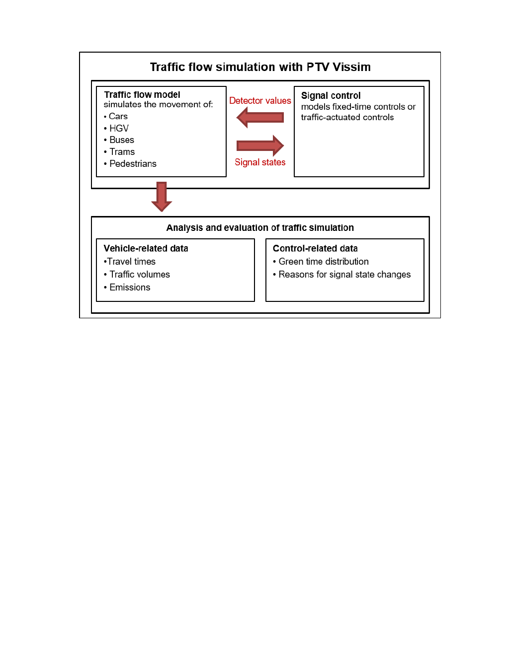
1.3 Traffic flow model and light signal control
Vissim is based on a traffic flow model and the light signal control. These exchange detector
readings and signaling status.
You can run the traffic flow simulation of vehicles or pedestrians as animation in Vissim. You
can clearly display many important vehicular parameters in windows or you can output them in
files or databases, for example, travel time distributions and delay distributions differentiated
by user groups.
The traffic flow model is based on a car-following model (for the modeling of driving in a
stream on a single lane) and on a lane changing model.
External programs for light signal control model the traffic-dependent control logic units. The
control logic units query detector readings in time steps of one to 1/10 second. You can define
the time steps for that reason and they depend on the signal control type. Using detector
readings, e.g. occupancy and time gap data, the control logic units determine the signaling
status of all signals for the next time step and deliver them back to the traffic flow simulation.
Vissim can use multiple and also diverse external signal control programs in one simulation,
for example, VAP, VSPLUS.
Communication between traffic flow model and traffic signal control:
© PTV GROUP 31
1.3.1 Operating principles of the car following model
1.3.1 Operating principles of the car following model
Vehicles are moving in the network using a traffic flow model. The quality of the traffic flow
model is essential for the quality of the simulation. In contrast to simpler models in which a
largely constant speed and a deterministic car following logic are provided, Vissim uses the
psycho-physical perception model developed by Wiedemann (1974) (see "Driving states in
the traffic flow model according to Wiedemann" on page 270). The basic concept of this model
is that the driver of a faster moving vehicle starts to decelerate as he reaches his individual
perception threshold to a slower moving vehicle. Since he cannot exactly determine the speed
of that vehicle, his speed will fall below that vehicle’s speed until he starts to slightly accelerate
again after reaching another perception threshold. There is a slight and steady acceleration
and deceleration. The different driver behavior is taken into consideration with distribution
functions of the speed and distance behavior.
32 © PTV GROUP

1.3.1 Operating principles of the car following model
Car following model (according to: Wiedemann 1974)
Legend
Axes: d: Distance, Δv: Change in speed 3: Approaching state
1: "Free flow" state 4: Braking state
2: Following state 5: Collision state
The car following model has been calibrated through multiple measurements at the Institute of
transport studies of the Karlsruhe Institute of Technology (since 2009 KIT – Karlsruhe Institute
of Technology), Germany. Recent measurements ensure that changes in driving behavior and
technical capabilities of the vehicles are accounted for.
Vissim calculates the acceleration of a vehicle during free traffic flow, below the desired
speed, based on the following:
If the desired safety distance is set to 100 percent, the vehicle drives at the same
speed as its preceding vehicle.
If the desired safety distance is set to between 100 and 110 percent, the speed is inter-
polated between the vehicle's desired speed and the speed of its preceding vehicle.
If the desired safety distance is set to greater than or equal to 110 percent, the vehicle
accelerates at its desired speed.
© PTV GROUP 33
1.4 How to install and start PTV Vissim
For multi-lane roadways a driver in the Vissim model takes into account not only the vehicles
ahead (default: 4 vehicles), but also the vehicles in the two adjacent lanes. In addition, a
signal control for about 100 meters before reaching the stop line leads to increased attention
of the driver.
Vissim simulates the traffic flow by moving driver-vehicle-units through a network. Every
driver with his specific behavior characteristics is assigned to a specific vehicle. As a
consequence, the driving behavior corresponds to the technical capabilities of his vehicle.
Attributes characterizing each driver- vehicle unit can be subdivided into following three
categories:
Technical specification of the vehicle, for example:
Vehicle length
Maximum speed
Accelerating power
and:
Actual vehicle position in the network
Actual speed and acceleration
Behavior of driver-vehicle units, for example:
Psycho-physical perception thresholds of the driver, e.g. ability to estimate, perception
of security, willingness to take risk
Driver memory
Acceleration based on current speed and driver’s desired speed
Interdependence of driver-vehicle units, for example:
Reference to vehicles in front and trailing vehicles on own and adjacent lanes
Reference to currently used network segment and next node
Reference to next traffic signal
1.4 How to install and start PTV Vissim
Vissim is provided electronically or on a DVD with demo files, examples files, its
documentation, and other license dependent files.
1.4.1 Information on installation and deinstallation
For information on program installation and deinstallation, refer to Vissim <Version> -
Installation Manual.pdf.
The installation guide is on the DVD, in the ..\OnCD\Documentation\Eng folder.
After the installation, you will find the installation guide in your Vissim installation, under
..\Doc\Eng.
1.4.2 Content of the PTV Vision program group
After you have installed Vissim, several icons are displayed in the PTV Vision program group,
depending on your license and the options chosen during the installation process. To call the
34 © PTV GROUP
1.4.3 Specifying the behavior of the right mouse button when starting the program for the first
program, from the Start menu, choose > All Programs > PTV Vision <year> > PTV Vissim
<version> (navigation of the Start menu depends on your operating system).
Element Description
Vissim
<Version>
Opens Vissim:
with an empty network, if no default network is saved.
Opens the program with this network, if a default network is
saved (see "Overview of menus" on page 113)
V3DM Opens the add-on module V3DM (Vissim 3D modeler). Using V3DM,
you can convert 3D models of the file formats DWF (Design Web
Format), 3DS (Autodesk), and SKP (Sketchup) into the Vissim 3D
format V3D. This applies to static 3D models and vehicle models (see
"Using static 3D models" on page 638).
VISVAP Opens the add on module VISVAP. VisVAP is tool that allows you to
easily create the program logic of a VAP signal control as a flow chart.
1.4.3 Specifying the behavior of the right mouse button when starting the program for
the first time
When you start Vissim for the first time, the window Right Click Behavior Definition opens. To
select the function that is carried out, right-click in the Network editor.
1. Select the desired entry.
Element Description
Context menu The context menu of the Network editor opens (see "Network editor
context menu" on page 78).
Creating a new
object
In the Network editor, insert a new network object of type selected in
the Network objects toolbar. The context menu of the Network editor
does not open. This is the behavior of Vissim versions released prior
to version 6.
2. Confirm with OK.
Tips:
If you hold down the CTRL key and right-click in the Network editor you are mod-
eling in, you can switch to another function and execute it.
You can change the right-click behavior again (see "Right-click behavior and
action after creating an object" on page 143).
1.4.4 Agreeing to share diagnostics and usage data
With the third start of Vissim, the window We need your help! opens.
© PTV GROUP 35
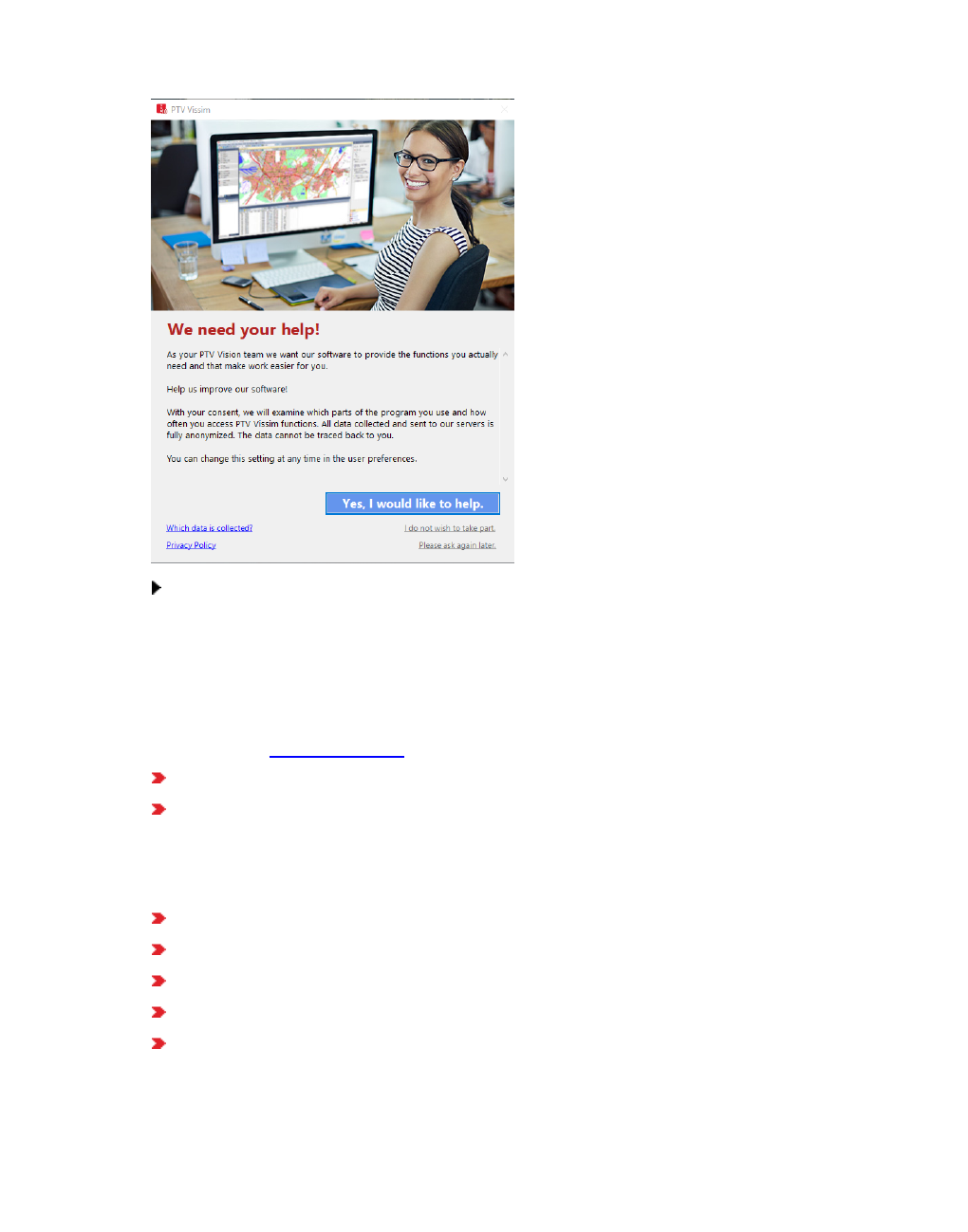
1.5 Technical information and requirements
Confirm with Yes, I would like to help.
You can deactivate the recording of diagnostics and usage data (see "Allowing the collection
of usage data" on page 147).
1.5 Technical information and requirements
Current information on the technical requirements for the current Vissim version can be found
on our website PTV Vissim FAQs. The following information, e.g., is essential:
Entry (#3): What are the hardware and software requirements for Vissim?
Entry (#6): Which graphics card has the best performance with Vissim 3D?
1.5.1 Criteria for simulation speed
The speed of a Vissim simulation primarily depends on the following criteria:
Number of vehicles and/or pedestrians used simultaneously in the network
Number of signal controls
Type of signal controls
Number of processor cores deployed
Computer performance. On a faster computer, a simulation will run faster with the same
network file.
36 © PTV GROUP

1.5.2 Main memory recommended
Tip: With the 64-bit editions of Vissim and Viswalk, you can use a larger main memory
of more than 3 GB RAM.
1.5.2 Main memory recommended
Vissim edition Main memory recommended
32-bit min. 2 GB RAM
64-bit min. 4 GB RAM
The memory requirements may be considerably higher for the following use cases:
Networks with many dynamically assigned paths
Large applications with many pedestrian areas
1.5.3 Graphics card requirements
If under User Preferences > GUI > Graphics, the graphics driver OpenGL 3.0 is selected,
make sure that your video card at least supports OpenGL 3.0.
Ensure that the latest driver update has been installed for your graphics card. This way, you
will avoid visualization problems when using the 3D mode. For many graphics adapters, you
can download update drivers from the Internet.
Note: Should any problems arise with the 3D display in Vissim, first install the latest
driver update for your graphics card before you contact PTV Vision Support.
1.5.4 Interfaces
Not all program interfaces are by default part of your Vissim license. They might be available
as add-on modules (see "Add-on modules programming interfaces (API)" on page 1127). Add-
on modules and their documentation are saved in the folder ..\Vissim<Version>\API.
1.5.5 Number of characters of filename and path
With Windows, the number of characters of a path, including drive letter and filename, is
limited to 260.
With Windows, the number of characters of a path is limited to 248.
In Scenario Management, the length of the path to the project directory is limited to 214
characters.
Make sure that your project files are not saved to any paths longer than that. This for
instance includes the following paths:
Name of *.inpx network file and path to the directory where the network file is saved.
Directories and subdirectories you create during a project Files saved to these dir-
ectories
Directories and subdirectories that Vissim creates automatically or to which Vissim
saves data, e.g. for scenario management or evaluations.
© PTV GROUP 37

1.6 Overview of add-on modules
1.6 Overview of add-on modules
Vissim is available with the following add-on modules:
1.6.1 General modules
Dynamic assignment
The module Dynamic Assignment is used to distribute the vehicles automatically among
the available paths. Users only need to specify an origin-destination matrix and the parking
lots assigned to the corresponding zones. They are not required to enter static routes
manually (see "Using the dynamic assignment add-on module" on page 653).
EnViVer Pro
EnViVer Pro is a tool used to calculate emissions based on vehicle record data.
EnViVer Enterprise
In addition to the functions of EnViVer Pro, EnViVer Enterprise allows for the modeling of
additional vehicle classes, individual time periods as well as automatic processing of
several input files.
3D packages: 3DS Max Export and V3DM
Export 3DS Max: Network data and vehicle positions are exported from Vissim as text files
and can be imported into Autodesk's 3ds Max software. The 3D packet contains a script in
the Autodesk macro language, as well as numerous vehicle model information.
Using V3DM (Vissim 3D modeler), allows users to convert 3D models of the file formats
DWF, 3DS (both by Autodesk), and SKP (Sketchup) into Vissim 3D format V3D. This works
for both static models and vehicles.
Example MAX files for vehicle models are located in the ..\API\3dsMaxExport\MAXModels
folder of your Vissim installation.
Synchro Import
Using this module, users can generate Vissim models from Synchro. The network
geometry, volumes, turns, vehicle compositions, and signalization are imported. The
module supports adaptive import. This means changes made in Vissim are not lost when
more current versions of the Synchro model are imported.
Mesoscopic simulation
The module allows for significantly faster simulation of larger networks compared to
microscopic simulation. The driving behavior is still based on individual vehicles and a
temporal resolution of, e.g., a tenth of a second. The difference is that the individual
vehicles are not looked at with each time step, but only when an event occurs. Such an
event could, for instance, be a vehicle reaching the end of a route and traversing a node, or
an SC switching to green.
The main benefits of mesoscopic simulation are increased simulation speed and less time
required for creating and calibrating the network.
38 © PTV GROUP

1.6.2 Signal controllers: Complete procedures
If an area of the network still needs to be microscopically simulated, including all the
details, hybrid simulation can be used. It allows you to select one or multiple sections for
microscopic simulation, while the rest of the network undergoes mesoscopic simulation.
(see "Using add-on module for mesoscopic simulation" on page 758).
PTV Viswalk
Viswalk Is used for professional pedestrian simulation, either as a stand-alone solution or
in combination with Vissim. The dynamic model is based on the Social Forces Model
developed in 1995, inter alia, by Prof. Dirk Helbing. It allows pedestrians to walk
independently to their destination, without a network model predefining their trajectories.
A simple pedestrian simulation, based on directed routes (instead of areas), is included in
Vissim. It is based on the car following model of Professor Wiedemann, as is the vehicle
simulation. It does not require the Viswalk module (see "Pedestrian simulation" on page
814).
BIM Import
The BIM Import module converts BIM files (Building Information Model) of the data format
IFC (Industry Foundation Class) into INPX files. These converted INPX files are meant for
use in pedestrian simulation with Viswalk.
Nearly every CAD software supports IFC export and thus provides an interface between the
CAD software and Viswalk. The Importer converts slabs into areas, walls into obstacles and
can import stairways, whilst keeping the level structure. Slabs with curves or holes are
automatically optimized for use in Viswalk during data import (see "Importing Building
Information Model files" on page 837).
1.6.2 Signal controllers: Complete procedures
Econolite ASC/3 (see "Add-on module Econolite ASC/3" on page 578)
This module enables user to simulate signal controllers that run on ASC/3 North American
controller devices by Econolite. It provides a dedicated user interface for its control
parameters.
RBC (Ring Barrier Controller) (see "Using the Ring Barrier Controller RBC add-on mod-
ule" on page 583)
This module enables PTV Vissim to simulate signal controllers that are controlled
according to the North American standard procedure "ring barrier controller". It provides a
dedicated user interface for the RBC parameters.
Signal control procedure vehicle-actuated programming (VAP) (see "Add-on module
Traffic-dependent VAP Programming" on page 590)
VAP enables Vissim to simulate programmable vehicle-actuated signal controls (SC). This
is possible for both stage or signal group based signal controls. During Vissim simulation
runs or in the test mode, VAP interprets the control logic commands and generates the
signal control commands for the signal control that become effective in the network. Vice
versa, detector parameters are retrieved from the Vissim network and processed in the
logic. The VAP program logic is described in a text file (*.vap) with a simple programming
© PTV GROUP 39

1.6.2 Signal controllers: Complete procedures
language. It can be also be exported from VisVAP. The signal data file (*.pua) can either be
comfortably exported from Vissig or generated manually in a text editor. The range of
application of VAP stretches from controls for individual nodes over PT priorities to complex
control systems for entire corridors or subnetworks. Additionally, applications in the ITS
range, e.g. variable message signs (VMS) or temporary side lane clearances are readily
possible.
VisVAP
Flow chart editor for VAP: VisVAP (short for Visual VAP) is an easy to use tool for defining
the program logic of VAP signal controllers as a flow chart. All VAP commands are listed in
a function library. The export function allows users to generate VAP files, which saves
additional changes to the VAP file. Moreover, VisVAP provides a debug functionality that
during a running simulation in Vissim allows users to go through the control logic step by
step using the control logic. It also shows the current values of all parameters used in the
logic. To start VisVap, from the Start menu, choose > PTV Vision program group.
Vissig (see "Opening and using the SC Editor" on page 595)
Vissig complements the stage-based fixed time control (which is included in any basic
Vissim version and in the Visum module "Junction editor and control") by additionally
providing stage-based fixed time signal control. Vissig contains a graphical editor for
defining stages and interstages. Interstages can also be automatically generated by Vissig.
Besides providing the usual functionality, the signal program editor allows users to easily
extend or shorten stages and interstages. Additionally, Vissig offers an interface for the
export of signal data compliant with VAP in the PUA format so that a traffic-dependent
signal control with VAP can be easily generated on the basis of the generated stages and
interstages. All signal plan information can be exported to Microsoft Excel and easily added
to reports.
Balance/Epics (see "Using Balance-Central signal controllers" on page 576), (see "Using
Epics/Balance-Local signal controllers" on page 577)
PTV Balance is a comprehensive and proven adaptive transport network control software
which is fully integrated into Vissim. Used in conjunction with the local adaptive node
control PTV Epics or on its own, it calculates new signal plans for all nodes in the
simulation network every 5 minutes based on the current detector data of the simulation.
The module balance/epics allows you to simulate PTV Balance using Vissim, just like in
the real application. The road network and transport demand data for PTV Balance are
supplied by .anm/.anmroutesfiles and require PTV Visum. The signalization related
parameters of PTV Balanceare supplied with an extended version of Vissig. PTV
Balancecomes with a web-based and user-friendly program interface. It allows for a direct
comparison of the calculated traffic parameters with the vehicles simulated in Vissim.
Moreover, this supply does not contain any formatting and can also be used in real network
control projects with PTV Balance.
PTV Epics is a local, adaptive signal control, with a special focus on public transportation. It
can be used instead of a fixed time or VAP signal control. You can simulate it using Vissim.
Every second, the mathematical optimization function in PTV Epics uses current detector
data to calculate the best signal plan for the next 100 seconds. It then transfers this signal
plan to Vissim. All parameters required by PTV Epics are supplied by an extended version
40 © PTV GROUP
1.6.3 Signal control: Interfaces
of Vissig. All modes of transport (private, public, pedestrian) are treated similarly, but can
be weighted differently. This makes it particularly easy to implement acceleration in public
transport with PTV Epics.
1.6.3 Signal control: Interfaces
External signal control SC
This module allows users to simulate signal controller procedures, which are available as a
separate executable application (*.exe) or program library (*.dll). These can be either
standard procedures supplied by PTV GROUP or other providers, or procedures
developed internally with the API module.
LISA+ OMTC
This add-on is used to simulate signal controls specified with the LISA+ procedure by
Schlothauer. The actual control DLL and the GUI for the controller parameters can be
obtained from Schlothauer.
SCATS interface
This module is used to simulate signal controllers specified according to the Australian
SCATS procedure. The actual control DLL and the GUI for entry of the control parameters
(SCATS.DLL, SCATS_GUI.DLL, WinTraff, ScatSim) must be obtained from Roads and
Maritime Services of New South Wales, Australia.
SCOOT interface
The SCOOT interface is used to simulate signal controllers that are specified according to
the British SCOOT procedure. The actual control DLL and the GUI for the control
parameters (SCOOT.DLL, SCOOT_GUI.DLL, PCScoot) can be obtained from Siemens UK.
1.6.4 Programming interfaces
API Package Application Programmer's Interface:
SignalControl, SignalGUI, DriverModel, and EmissionModel.DLL files. The API package
enables users to integrate their own or external applications in order to influence a PTV
Vissim simulation (see "Add-on modules programming interfaces (API)" on page 1127).
1.7 Using a demo version
When you open a demo version, Demo version is displayed in the title bar.
You can use an installed demo version for 30 days after it has first been opened.
You can initially open the demo version during a maximum period of 180 days from its
build.
Demo version users do not receive any technical support.
The Help and the manual can be opened via the Help menu. You can find answers to fre-
quently asked questions about Vissim on our web pages PTV Vissim FAQs.
© PTV GROUP 41

1.8 Using PTV Vissim Viewer
A demo version does not allow you to print or save any data.
The COM interface is not provided.
Simulation runs are limited to 1800 simulation seconds.
You can work with a demo version for a maximum of two hours.
In the matrix editor, you cannot copy data.
The command Save as Default Network is not available.
If the demo version is overwritten by a later version of the service pack, the 30-day trial
period starts anew.
1.8 Using PTV Vissim Viewer
Using the Vissim Viewer, you can, for instance, forward project data to your customers. The
Vissim Viewer is a limited Vissim version, which needs to be additionally installed.
1.8.1 Limitations of the Vissim Viewer
Network files cannot be saved.
Evaluation files cannot be generated.
Simulation runs are possible only for the first 1,800 s. This period cannot be extended in
order to show longer simulation runs. If it is necessary to show the visualization of vehicles
and/or pedestrians beyond the first 1,800 s, animation files *.ani can be used. For anim-
ation files there is no time limit.
The COM interface is not provided.
There are no demo examples available.
1.8.2 Vissim Viewer installation and update
You can install or update the Vissim Viewer for 32-bit versions of Vissim. To do so, download
the program from our website.
1. Open the web page PTV Vissim & PTV Viswalk Service Pack Download Area.
2. For your 32-bit version, click <product name> (32 Bit) Service Packs.
In the Available Downloads table, the entries are displayed sorted by:
Vissim Viewer Update for an update of your installation
Vissim Viewer Setup for a new installation
descending by version number
You can download updates in the EXE or ZIP file formats. Setups are downloaded in the
ZIP file format.
3. In the row of the desired Vissim viewer, click the Download button.
4. Save the downloaded file to your hard disk.
42 © PTV GROUP

1.9 Using the PTV Vissim Simulation Engine
5. If you have downloaded a ZIP file, extract it.
6. Start the setup respectively update program.
The Vissim Viewer is added to the Start menu.
The Archive.zip file downloaded also includes a viewer_readme.txt. This file describes how to
create a CD for your clients that contains this limited Vissim version and your project data.
1.9 Using the PTV Vissim Simulation Engine
The Vissim Simulation Engine is a limited version of Vissim. It allows users to perform
simulations and record the results. It does not have a graphical user interface. The Network
editor and lists are not available. The Vissim Simulation Engine needs a dongle to use license
base data, Vissim modules and signal controllers.
In a typical use case, you would model your network using a full version of Vissim and deploy
multiple computers installed with the Vissim Simulation Engine to calculate simulations of the
network that are configured differently. You can access the Vissim Simulation Engine via the
COM interface.
1.10 Using files with examples
Example data are provided in the folders Examples Demo and Examples Training.
Depending on the Microsoft Windows operating system used, they are saved to different
directories, for example:
..\Users\Public\Public Documents\PTV Vision\PTV Vissim <version number>
Tip: This directory contains the Examples Overview.pdf file with brief descriptions
available in English.
1.10.1 Opening the Examples Demo folder
From the Help menu, choose > Examples > Open Demo Directory.
1.10.2 Opening the Examples Training folder
From the Help menu, choose > Examples > Open Training Directory.
1.11 Opening the Working directory
The *.inpx network file of the network currently opened is saved to the working directory.
From the File menu, choose > Open Working Directory.
1.11.1 Opening the working directory from the Windows Explorer
To show the Vissim Working directory in the Windows Explorer, in the Windows Explorer, enter
the string of a variable.
© PTV GROUP 43

1.12 Documents
For this purpose, the variable Vissim<Version>_EXAMPLES is automatically created during
the installation process.
1. In the Windows Explorer, into the address bar, enter: %VISSIM100_EXAMPLES% or
%VISWALK100_EXAMPLES%
2. Confirm with Enter.
1.12 Documents
We provide a comprehensive manual to help you quickly become familiar with Vissim and
Viswalk:
The Help and manual describe functions and procedures. The step-by-step instruc-
tions guide you through tasks. The Help and manual are identical in content (see
"Showing the PTV Vissim Help" on page 44), (see "Showing the user manual" on page
44).
Additional documentation is available for further information (see "Additional doc-
umentation" on page 44)
1.12.1 Showing the user manual
If during the installation of Vissim the installation of the user manual is not deactivated, it is
saved as a PDF file to the ..\Doc\<language ID> folder of your Vissim installation directory.
1.12.2 Showing the PTV Vissim Help
If during the installation process of Vissim the installation of the Help was not deactivated, you
can access the Help in Vissim.
Opening the PTV Vissim Help and showing the start page
From the Help menu, choose > PTV Vissim Help.
The Help start page opens.
Showing the COM interface reference documentation
Reference documentation for the COM interface Vissim - COM is by default available as a
separate Help in the ..\exe directory of your Vissim installation.
Showing Help of the attributes in currently opened window
Press F1.
1.12.3 Additional documentation
In your Vissim installation directory, in the folder ..\Doc\Eng\ , you can find the following
documentation. These are partly also available in other languages.
44 © PTV GROUP
1.12.3 Additional documentation
Vissim <Version> - Installation Manual.pdf: Installation guide
Vissim 9 - what's new.pdf: Description of the most important changes in Vissim 9 com-
pared to Vissim 8
Vissim 10 - what's new.pdf: Description of the most important changes in Vissim 10 com-
pared to Vissim 9
ReleaseNotes_Vissim_<language ID>.pdf: Release notes
They contain information on changes, bug fixes, and new features available in the Vissim
service packs. You can access the information by keyword search. New service packs are
provided for download on a regular basis on the PTV GROUP website.
Vissim <Version> - Manual.pdf: user manual, describing functions, network objects and
attributes.
Vissim <Version> - COM Intro.pdf: Introduction into the Vissim COM interface in English
Using the Component Object Model (COM) interface and scripts, you can access data and
functions in Vissim. Via the COM interface, you can find the Vissim <Version> - COM.chm
file, by default, in the ..\PTV Vissim <Version>\Exe folder.
Overview_CodeMeter.pdf: Information on how to use the CodeMeter Runtime Kit and set
up CodeMeter as a dongle server
CodeMeter_Support.txt: Information on support for WIBU CodeMeter dongle
CodeMeterAdministratorManual6.20_en.pdf: CodeMeter Administrator manual version
6.20 - April 2016
VAP_<version>_<language ID>.pdf: User manual for VAP add-on module, which allows
you to simulate a freely programmable, stage or signal group oriented, traffic-actuated sig-
nal control
vap_chan_<version>_<language ID>.txt: upgrades and bug fixes in VAP/SIM
VisVAP <version> <language ID>.pdf: User manual VisVAP (tool that allows you to display
the program logic as a flow chart)
LISA+_OMTC.pdf: only in directory ..\Doc\Deu\: Information on VIAP LISA+ / Vissim inter-
face
LicenseAgreementGeneral.rtf: Vissim license agreement
attribute.xlsx:
List of tables for base data types and network object types
List of attributes, including ID, short name, long name, singular, plural in the lan-
guages Vissim is available in.
List of EnumStrings: enumeration types with predefined values
List of relations: base data types and network object types that have relations to other
base data types and network object types, as well as the base data types and/or net-
work object types assigned.
The directory ..\Doc\Eng\ also includes the following documentation:
© PTV GROUP 45
1.13 Service and support
Manual_RBC.pdf: Ring Barrier Controller Manual
Manual_Synchro_Import.pdf: Synchro 7 Import Manual
release_notes_RBC.txt
1.13 Service and support
With Vissim you receive extensive technical documentation and can call on the services of
PTV GROUP. PTV GROUP provides technical support in the following cases:
Program errors in the current program version
Questions about the use of Vissim
Notes: The prerequisite for technical support is participation in a basic course for Vision
Traffic Suite.
As our software is continually being improved, we regret being limited when it comes to
providing support for older program versions.
Please understand that the PTV Vision Support cannot replace a training course. PTV Vision
Support can neither impart specialist engineering knowledge which goes beyond the
functionality of the product, for example concerning demand modeling, signal control or
project-related problems. Should you require any help on these subjects, we will be happy to
offer you a project-specific training course.
1.13.1 Using the manual, Help and FAQ list
Before you make an inquiry to the technical support, please read the information about the
topic in the manual, the Help or the FAQs.
1.13.1.1 FAQs
Here you can find the answers to frequently asked questions about Vissim on our web pages:
PTV Vissim FAQs
Note: For access to the FAQ list you need access to the Internet.
From the Help menu, choose > FAQ (Online).
In your browser, the Vissim FAQ list appears.
1.13.2 Services by the PTV GROUP
1.13.2.1 Product information on the Internet
On the PTV GROUP web page you can find further product information, AVI files with
examples of various simulations as well as service packs, which you can download:
Homepage of PTV Group: PTV Vissim
46 © PTV GROUP

1.13.2 Services by the PTV GROUP
1.13.2.2 Product training sessions
PTV GROUP offers training sessions for entry-level and experienced users.
We will be glad to carry out training sessions in your own company. You can also participate in
training sessions which we hold on our own premises.
You can find the latest information on our web page:
PTV Vissim Training Courses
1.13.2.3 Maintenance Agreement
A Maintenance Agreement ensures that the current version of Vissim or Viswalk is always
available.
Advantages of a Maintenance Agreement:
Provision of the latest version of Vissim or Viswalk, as soon as it is available
Service packs for the current version for download from our web pages
Support by PTV Vision Support
Please address any inquiries about Maintenance Agreements to:
customerservice@vision.ptvgroup.com.
1.13.2.4 Downloading service packs
If you have a Maintenance Agreement you can download the service packs for the current
version of Vissim or Viswalk from the Internet.
1. Open the web page PTV Vissim & PTV Viswalk Service Pack Download Area.
2. Click on the desired version.
Depending on the product you are using, you can download files in the EXE or ZIP file
format.
3. In the Available Downloads table, click the row with the desired product. Then click the
Download <file format> button.
4. Download the file.
1.13.2.5 Being automatically informed about new service packs
You can be notified if new service packs are available for downloading.
1. Open the web page PTV Vissim & PTV Viswalk Service Pack Download Area.
2. Click on sign-up/sign-off.
3. Fill in the form.
4. Click the Submit button.
© PTV GROUP 47

1.13.3 Posting a support request
1.13.2.6 PTV Vision Support
PTV GROUP offers technical support for Viswalk and Vissim (see "Posting a support request"
on page 48).
1.13.2.7 PTV Vissim Webinars
Learn about the concepts of simulation in PTV Vissim step by step in our free webinars. For
current information on our webinars, check our Webinars site.
1.13.3 Posting a support request
You can contact PTV Vision Support with a contact form in the following cases:
Program errors in the current Vissim version. As our software is continually being
improved, we regret being limited when it comes to providing support for older program
versions.
If you have a Maintenance Agreement, you can contact us with inquiries about your pro-
ject and for modeling.
Before you contact us with questions and problems:
From the Help menu, choose Vissim Help or use the manual to try to solve the problem.
These often contain the information which you are looking for.
Read the tips and tricks on the Internet: PTV Vissim Tips & Tricks.
Read the FAQ list on the Internet. These often contain the information which you are look-
ing for. The FAQ list also contains valuable information about modeling.
In the interest of an efficient processing of your inquiry to PTV Vision Support we request that
you use the corresponding hotline contact form on the Internet:
Technical Support PTV Vissim
Technical Support PTV Viswalk
Note: The following information is necessary for the smooth processing of your inquiry:
A description of the problem
The steps which were performed immediately before the problem occurred
If necessary, screenshots of the program states
All files which are necessary for the reproduction of the error
The following data are automatically entered into the form:
The Vissim version and service pack number, e.g. 10.00-01, listed in the title line
of Vissim
Vissim edition, 32 Bit or 64 Bit
The operating system and service pack number
The PTV customer number
The dongle number
Thank you for your cooperation!
48 © PTV GROUP

1.13.4 Requests to the Traffic customer service
1.13.4 Requests to the Traffic customer service
Our Traffic customer service will respond to general requests concerning Vissim.
For inquiries about license fees, please contact:
info@vision.ptvgroup.com
Please address inquiries about Maintenance Agreements to PTV Traffic Customerservice:
customerservice@vision.ptvgroup.com
1.13.5 Showing program and license information
You can show information on the dongle, network size, installed add-ons, version number,
build number and installation directory of your Vissim installation as well as manage licenses.
From the Help menu, choose > License.
The License window opens.
The following license information is displayed:
Maximum section
Signal Controllers (SC): Maximum number of SC
Network Size: Maximum network extent in km
Link behavior types: Maximum number of link behavior types
Period: Maximum simulation duration in seconds
Pedestrians: Maximum number of pedestrians
Modules section
List of modules and add-on modules Check marks show the licensed modules and
add-on modules installed.
Signal Controllers section
List of signal control procedures supported
Version section
Customer-specific data of the installed version
Program path: Path of installation directory
Manage licenses: Opens the License Management window (see "Managing licenses" on
page 49).
Note: If your Vissim license does not include the Viswalk add-on module, you may still
perform a pedestrian simulation with up to 30 pedestrians.
1.13.6 Managing licenses
You can identify the licenses available in your network and specify which licenses you want to
use when you start the program. In the same way, you can manage the licenses for individual
modules.
1. From the Help menu, choose > License.
The License window opens.
© PTV GROUP 49
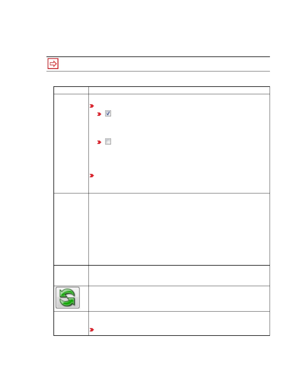
1.13.6 Managing licenses
2. Click the Manage licenses button.
The License Management - PTV Vissim window opens. PTV Vissim automatically
searches for licenses.
Tip: You can also open the License Management - PTV Vissim window from the start
menu for programs under PTV Vision <Year> > PTV Vissim License Manager.
3. Make the desired changes:
Element Description
Settings You can show or hide the section.
Check out automatically, if possible:
Select this option to have the path to the licenses in the registry
automatically loaded and started when you start PTV Vissim. The
License Management - PTV Vissim window does not open. The
option is selected by default.
If you do not select this option, the License Management - PTV
Vissim window will always open when you start PTV Vissim and
you will need to select a license. PTV Vissim starts automatically,
independently of the option, if exactly one PTV Vissim license exists
on all searched CodeMeter dongles.
Delete saved license list: Deletes all license information saved to the
following directory (example): C:\User\<User
name>\AppData\Roaming\PTV Vision\PTV Vissim 10
If you open the License Management - PTV Vissim window, initially, the
found licenses are displayed in gray because the CodeMeter servers have
not yet been searched at that time.
You can get the current status of all available licenses if you click Update
all displayed licenses below the list of found licenses.
The next time you open PTV Vissim, you can specify new settings.
If you want to save a new licenses.data file, close the License
Management - PTV Vissim window with OK.
You can find information on a central, user-independent license
management below this table.
CodeMeter
server envir-
onment
Used license servers with status on which a CodeMeter server is installed.
The list is based on the CodeMeter server search list.
Update: Search for computers in your network on which a CodeMeter
server has been installed. The list is updated.
Licenses Vissim licenses and/or Viswalk licenses that in your network have been
saved to CodeMeter servers.
Use license: Select the license with which you want to start PTV Vis-
50 © PTV GROUP

1.13.6 Managing licenses
Element Description
sim. You may select multiple licenses. The sequence in the list determ-
ines the sequence in which the licenses are reserved. If a license is
being used by another user, it cannot be selected.
Product: Shows products for which the license is valid. Use + and - to
show and hide the list of modules. You can book out individual mod-
ules.
License name: License text
Number: For a network license, the number of licenses is shown. For
single-user licenses, the text N/A is displayed.
Expiration date: If applicable, the expiration date of the license is
shown, otherwise may be used for an unlimited period.
Network size: Network size of the license is displayed
Languages: Languages supported by the licensed version
Server: License server
Box: Shows serial number of the CodeMeter stick
Move the row of selected licenses one row up
Move the row of selected licenses one row down
Moves the row of selected licenses to the top of the list
Moves the row of selected licenses to the bottom of the list
Remove
from list
Delete selected licenses from the list
Find
licenses
Start a network search for CodeMeter servers.
Update all
displayed
licenses
Search for licenses on computers that are shown in the CodeMeter server
environment list. The Found licenses list is updated.
Activate
new or
changed
license
The hyperlink opens the PTV website on which you can enter the ticket
code for the activation process. For further information on how to proceed,
refer to the installation guide in your Vissim installation folder under
..\Doc\Eng\Vissim <Version> - Installation Manual.pdf, in the chapter
"License provisioning".
© PTV GROUP 51

1.13.7 Information about the PTV GROUP and contact data
Element Description
Note: New or changed license information is transferred to the
dongle during the activation process. Each time a new license is
issued or licenses are changed, a contact person in your company
receives an e-mail with a ticket code similar to A43UT-PMXRC-
43D76-KF3AH-Y5GDQ (example). Using this ticket, you can start
the activation process, access new license information from the PTV
license server and transfer it to the dongle.
Start Open Vissim with the license selected
Note: If your Vissim license does not include the Viswalk add-on module, you may still
perform a pedestrian simulation with up to 30 pedestrians.
Centralized license management
In certain working environments, an administrator has to preset the license selection
throughout the system. In this case, a licenses.data file is stored in folder
..\ProgramData\PTV Vision\PTV Vissim <version number>. The settings in this centrally stored
file also apply if your user-specific directory C:\Users\<user name>\AppData\Roaming\PTV
Vision\PTV Vissim <version-number> contains a licenses.data file with other settings.
The icon on the button to delete the list of licenses indicates the centralized license
management.
You can only edit or delete this central file if you have administrator rights. If you delete this
file, license settings will subsequently be saved separately for each user of the computer. The
icon will no longer be displayed on the button if your license management is user-specific.
Please also refer to section System-wide license selection in the installation guide of Vissim.
1.13.7 Information about the PTV GROUP and contact data
You can find information about the PTV GROUP and contact data in Vissim and Viswalk.
Select the menu Help > About PTV Vissim.
Version number
The Internet page of PTV GROUP
Copyright details
52 © PTV GROUP

2 Principles of operation of the program
2 Principles of operation of the program
You model your network in Vissim in a network editor. The network editor shows the precise
position of the network objects. By default, you edit the data for the network objects in lists. For
editing, you can use, for example, mouse functions, context menus and key combinations.
Note: A good knowledge of Windows is assumed for the operation of the program.
Tip: For your first steps in Vissim you can use simple example data, which were
installed with Vissim. By default, the example data are stored under:
Users\Public\Public documents\PTV Vision\PTV Vissim <Version>\Examples Demo\
2.1 Program start and start screen
The simplest way to start Vissim is by double-clicking on the Vissim icon on your desktop:
Tips: Other options to start Vissim:
via the Start menu
in Microsoft Windows 8, via the Start screen
In Microsoft Windows 7 or 8 add Vissim to the taskbar
via the command prompt (see "Starting PTV Vissim via the command prompt" on
page 54)
double-click a network file (*.inpx) in the Windows Explorer
as Microsoft Windows server from session 0. Vissim can then be executed on a
Microsoft Windows HPC server without a user session.
If after the initial start more than one license is found, after you start the program the window
License management - PTV Vissim opens.
1. Select the license of your choice (see "Managing licenses" on page 49).
Vissim opens. The Start sceen shows information on the program version:
Number of Vissim version
Installation folder
Tip: You can call up further program information in Vissim:
From the Help menu, choose > About.
From the Help menu, choose > License.
If Vissim writes important messages into the Messages window when importing a network file,
a corresponding message is displayed. You can open the Messages window immediately or
later on.
© PTV GROUP 53
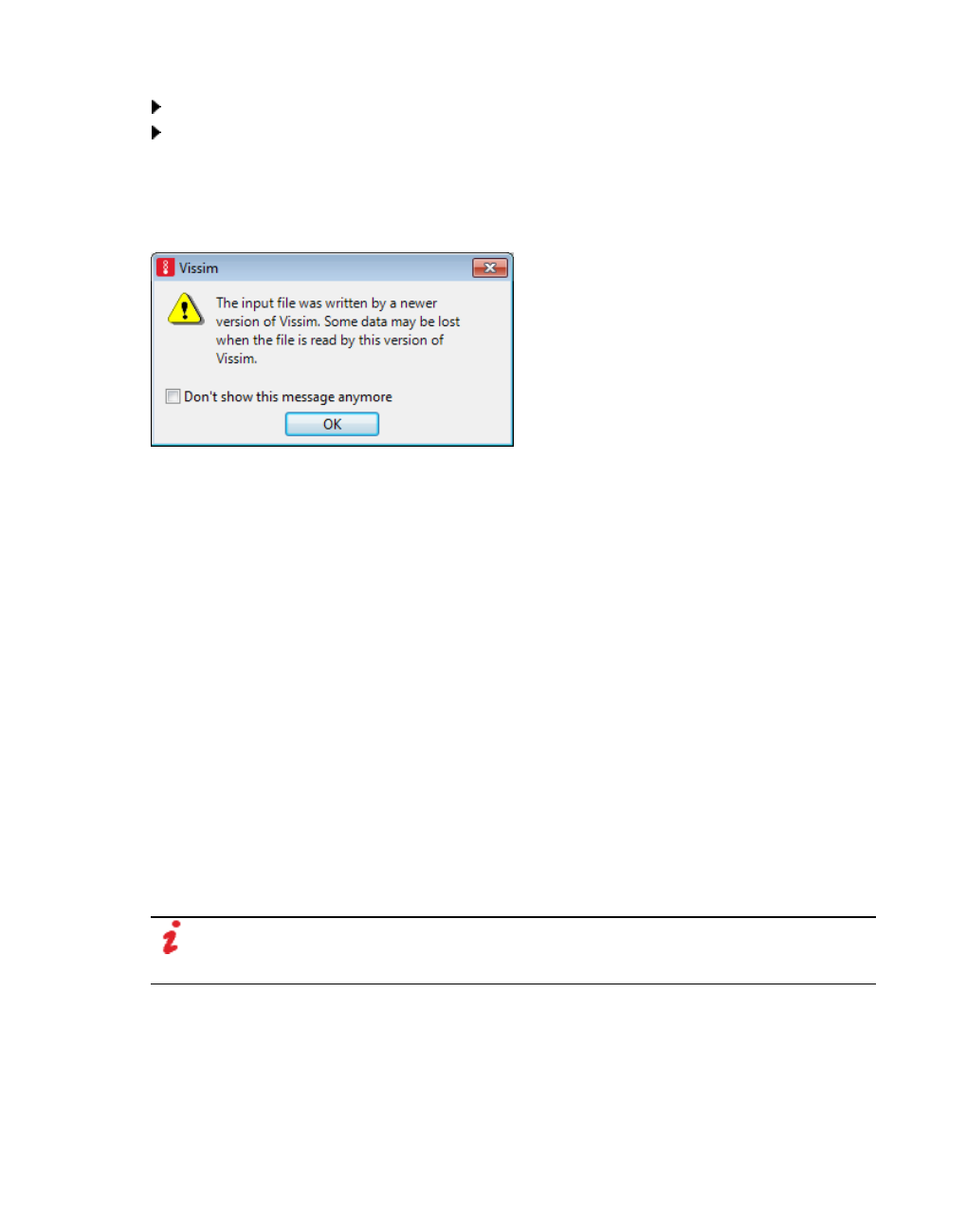
2.2 Starting PTV Vissim via the command prompt
Open immediately: In the window informing you of the messages, click the Open button.
Open later: In the window informing you of the messages, click the Open button. At a later
time of your choice, from the View menu, choose > Messages.
When you open a layout or network file that contains attributes of a more recent Vissim version
than the one you are using, you will not be able to read these attributes. The following
message is displayed:
2. Confirm with OK.
A window opens. Attributes that cannot be read are listed.
3. Confirm with OK.
If the defaults.inpx file in the ..\AppData\Roaming\PTV Vision\PTV Vissim <Version
number> directory is not readable, a corresponding message is displayed in the Messages
window.
If the ..\AppData\Roaming\PTV Vision\PTV Vissim <Version number> directory does not
contain a defaults.inpx file, the defaults.inpx file in the Exe installation directory of Vissim is
used.
When you save the Vissim network as default network (see "Overview of menus" on page
113), the defaults.inpx file is saved to the ..\AppData\Roaming\PTV Vision\PTV Vissim
<Version number> directory.
Vissim opens and shows the start page in a tab displayed in the foreground (see "Using the
Start page" on page 56).
4. If you want to go from the start page to the network editor, click the Network Editortab
below the start page.
Up to four instances of Vissim can be opened at the same time.
Note: Your user preferences are saved in the Windows registry and in the *.layx layout
file when Vissim is ended. The settings are used automatically when the program is
restarted.
2.2 Starting PTV Vissim via the command prompt
You can also start Vissim via the command prompt. Here, you can use parameters to control
various start options.
54 © PTV GROUP

2.2 Starting PTV Vissim via the command prompt
1. Press the Windows key and the r key at the same time.
The Run window opens.
2. Click the Browse button.
The Browse window opens.
3. Browse to the Exe directory of your Vissim installation. This is by default:
32-bit: C:\Program Files (x86)\PTV Vision\PTV Vissim 10Exe\
64-bit: C:\Program Files\PTV Vision\PTV Vissim 10\Exe\
4. Double-click the VISSIM 10.exe file.
The Browse window closes. The path is entered in the Start window, in the Open box.
5. Next to the ..\VISSIM 10.exe file, into the Open box, enter a space.
6. After the space, enter the desired command line parameter:
Parameter Description
-automation Provides Vissim as a COM server in the automation mode for
COM scripts that are started subsequently.
<input file> Loads the specified network file *.inpx or *.inp. If the network
file has not been saved to the Exe directory, enter the path in
front of the <input file>.
If a path contains spaces, add the character " at the beginning
and end of the path, for example "C:\Program Files\PTV
Vision\PTV Vissim 9\Exe\Vissim90.exe" Busmall.inpx
-b <layout file> Loads the specified layout file *.layx.
-flush Immediately saves any debug messages to the file
%Tmp%\VISSIM\vissim_msgs.txt, instead of waiting until a
certain number of messages has been reached. Use this
parameter to ensure that the vissim_msgs.txt file contains all
messages, e.g. when looking for a program error and you want
to send all messages in a Hotline package to support. In this
case, use the -flush parameter together with the -o
parameter: ...-o -flush
-flush has an impact on the performance of Vissim. Therefore
do not use this parameter by default. Only use it when you want
to make sure that all messages are included in the vissim_
msgs.txt file.
-force3d Deactivates the testing of the supported OpenGL version.
-o Saves debug messages in the %tmp%\VISSIM\vissim_msgs.txt
file.
-q <input file> Enables the Quick mode during simulation. If the network file
has not been saved to the Exe directory,next to the <Input
file>, enter the path. -q must be followed by a space.
© PTV GROUP 55

2.3 Using the Start page
Parameter Description
-regserver Registers Vissim as a COM server. If the registration has not
been successful, a message opens.
-s <input file> Batch operation: Vissim starts the simulation and closes after
the end of the simulation. If the network file has not been saved
to the Exe directory,next to the <Input file>, enter the path.
-s must be followed by a space.
-unregserver Deregisters Vissim as a COM server.
-version Opens the Start screen and shows information on the program
version
7. Confirm with OK.
2.3 Using the Start page
After you start the program, the start screen opens and the Vissim user interface with the Start
page tab is displayed.
The Start page allows you to have quick access to the following elements:
Recently used files
Support Services: Opens Help file, documents or web pages that provide support for
users
In the section on the right: Latest product news, interesting PTV news, information on
new service packs. This section may contain information that varies by region. Some of
it is available in different languages. Select the desired region (see "Selecting the
country for regional information on the start page" on page 142).
An Internet connection is required to make use of the full functionality of the Start page.
56 © PTV GROUP

2.4 Becoming familiar with the user interface
When you open a *.inpx network file, the tab with the Start page is closed. The program
elements are then displayed based on the settings saved to the *.layx file.
When you choose File > New or click the New button , the tab and Start page are moved to
the background and the Network editor is displayed in foreground.
Opening the Start page tab
From the View menu, choose > Start page.
2.4 Becoming familiar with the user interface
After you start the program, the start screen opens and the Vissim user interface with the Start
page tab is displayed (see "Using the Start page" on page 56).
Program elements of the user interface
The following figure shows the program interface with a *.inpx network file opened and
individually arranged program elements:
By default, the user interface contains the following elements for viewing, editing, and
controlling the network, data and simulation.
© PTV GROUP 57

2.4 Becoming familiar with the user interface
Element Description
(1) Title bar Program name
Version number including service pack number
Currently open network file and path
Demo: a demo version is opened
Uni: a student version is opened
Viewer: a Vissim Viewer is opened
(2) Menu
bar
You can call program functions via the menus (see "Overview of menus" on
page 113).
Network files used most recently in Vissim are shown in the File menu. Click
on the entry if you want to open one of these network files.
(3) Toolbars You can call program functions via the toolbars. Lists and network editors have
their own toolbars (see "Using toolbars" on page 127).
(4) Network
Editors
Show the currently open network in one or more Network Editors. You can edit
the network graphically and customize the view in each Network Editor (see
"Using network editors" on page 72).
(5) Network
objects tool-
bar
Network objects toolbar, level toolbar and background image toolbar are
shown together by default in a window on tabs.
Network objects toolbar (see "Using the Network object toolbar" on page 60):
Select the Insert mode for network object types
Select visibility for network objects
Select selectability for network objects
Editing graphic parameters for network objects
Show and hide label for network objects
Context menu for additional functions
(6) Levels
toolbar Select visibility for levels (see "Using the Level toolbar" on page 65)
Select editing option for levels
Select visibility for vehicles and pedestrians per level
(7) Back-
ground tool-
bar
Select visibility for backgrounds (see "Using the background image tool-
bar" on page 66)
(8) Project
explorer
Displays projects, base networks, scenarios and modifications of scenario
management
(9) Lists In lists, you show and edit different data, for example, attributes of network
objects. You can open multiple lists and arrange them on the screen (see
"Using lists" on page 89).
(10) Quick
View
Shows attribute values of the currently marked network object. You can
change attribute values of the marked network objects in the Quick View (see
"Using the Quick View" on page 66).
58 © PTV GROUP

2.4 Becoming familiar with the user interface
Element Description
(11) Smart
Map
Shows a small scale overview of the network. The section displayed in the Net-
work Editor is shown in the Smart Map by a rectangle or a cross-hair. You can
quickly access a specific network section via the Smart Map (see "Using the
Smart Map" on page 69).
(12) Status
bar
Shows the position of the cursor in the Network Editor. Shows the current
simulation second during a running simulation.
Arranging program elements
You can arrange the program elements of the user interface according to your requirements,
such as by moving, displaying from other program elements or hiding from available program
elements (see "Changing the display of windows" on page 86).
You can also arrange program elements on multiple screens. Thus you can edit the network
and data in a structured way, such as by opening a network and adding more network objects,
building a new network from network objects, or running a simulation.
Saving the user interface layout
The layout of the user interface is saved by default when the network is saved. The program
elements are arranged accordingly the next time you open Vissim (see "Saving and importing
a layout of the user interface" on page 138).
Without a Vissim network file loaded, the Network Editor is empty.
If no network file is open, the Network Editors show an empty Vissim network (see "Using
network editors" on page 72).
Labeling mandatory fields and invalid data formats
Vissim highlights entry fields with a red in the following cases:
Entry field is mandatory. You must enter a value or string in a valid data format.
Part of the value or string entered is in an invalid data format. For example, for the
attribute No of a link, a number must be entered. Characters are not accepted.
You must fill in all mandatory fields of a window to be able to close it with OK and make the
data available in Vissim.
Point the mouse pointer at the red triangle to open a quick info about the cause of error.
Quick info displays a description
For many program elements, a small window opens temporarily, if you point the mouse pointer
to the program element, e.g. a toolbar button or a network object type in the network object
toolbar. The window displays a brief description of the program element.
© PTV GROUP 59

2.5 Using the Network object toolbar
If in an attribute list, you point the mouse pointer to an attribute name in a column header, a
small window opens displaying a description of the attribute (see "Structure of lists" on page
90).
In some windows, the symbol is displayed next to an entry box, list box or option. If you
click the symbol, a small window opens displaying information on the program element.
2.5 Using the Network object toolbar
The network object toolbar contains a list with the network object types. In a network editor,
you can use icons and the context menu to access functions for the display, selection, and
editing of network objects. Your settings are only active in the last network editor used. If you
click another network editor to activate it, in the network objects toolbar, the settings for this
network editor are displayed.
Tip: By default, the Network object toolbar, the Level toolbar, and the Background
toolbar are displayed together. Using the tabs at the bottom of a toolbar, you can switch
to another toolbar.
60 © PTV GROUP

2.5 Using the Network object toolbar
Elements in the network objects toolbar
(1) Network object type button (visibility)
The icon (and name) of the network object type are shown in color: Network objects of this
network object type are shown in the Network editor.
The icon (and name) of the network object type are grayed out: Network objects of this net-
work object type are not shown in the Network editor.
(2) Lock button (selectability)
The icon is shown only when you position the mouse pointer before the name or on the name
of the network object type or when the lock is locked.
© PTV GROUP 61
2.5 Using the Network object toolbar
Lock unlocked: You can select and edit network objects of this network object type in
the Network editor.
Lock locked: You cannot select or edit network objects of this network object type in the
Network editor.
(3) Button with the name of the network object type (Insert mode)
Click the button with the name of the network object type to activate the Insert mode. If the
Insert mode is activated, the entire row is highlighted in orange.
You can insert new network objects of this network object type into network editors.
The network objects of this network object type are visible and selectable in all network
editors.
You can switch off visibility and selectability only for the other network object types.
(4) Selecting variants of a network object type
If you click the button of a network object type that has variants, the variant that is currently
selected is shown in brackets together with the icon . If you click the button or icon again, you
can select a different variant to add a network objects of this network object type to a network
editor.
Vehicle Routes:
Static
Partial
Partial PT
Parking Lot
Dynamic
Closure
Managed Lanes
Areas:
Polygon
Rectangle
Obstacles:
Polygon
Rectangle
Sections:
Polygon
Rectangle
62 © PTV GROUP
2.5.1 Context menu in the network object toolbar
(5) Edit graphic parameters icon: Open preview and graphic parameters
This icon shows you how network objects of this type are displayed in the Network editor. The
icons of network object types, displayed differently depending on the attribute values, consist
of several colored bars. Four gray bars indicate that the Display type is activated (see
"Defining display types" on page 300).
Click the symbol to open a list of graphic parameters of the network object type. In the list, you
can select and edit graphic parameters (see "Editing graphic parameters for network objects"
on page 149), (see "List of graphic parameters for network objects" on page 152).
(6) Label icon
This icon is shown only when you position the mouse pointer on the name or next to the name
of the network object type.
Click this icon to show or hide the label of the network objects of this network object type:
Label is hidden
Label is shown
Context menu in the network object toolbar
In the context menu, you can select functions for visibility and selectability and call the list of
network objects of the selected network object type (see "Context menu in the network object
toolbar" on page 63).
Changing the display of the network object toolbar
You can customize the position, size, and visibility of the window (see "Changing the display
of windows" on page 86).
2.5.1 Context menu in the network object toolbar
1. In the network object bar, right-click the network object type for which you want to select a
command from the short menu.
2. Choose the desired entry from the context menu.
© PTV GROUP 63

2.5.1 Context menu in the network object toolbar
Function Description
Show List If you have already opened a list of the network object type, it will be
displayed in the foreground.
If no list of the network object type has been opened, the list will be opened
and displayed in the foreground.
Open new
list
Show the list with network objects of network object type, including the net-
work objects' attributes If you have already opened a list of the network
object type, another list of the network object type will be opened.
Create
Chart
Open the Create Chart window (see "Creating charts" on page 1053). In
the Network object type list box, the object type you right-clicked is
automatically selected.
Creating a
user-
defined
attribute
Open the User-defined attribute window (see "Using user-defined
attributes" on page 200). In the Object type list box, the object type you
right-clicked is automatically selected.
Edit graphic
parameters
Show list of graphic parameters of the network object type (see "Editing
graphic parameters for network objects" on page 149)
Make All
Types Vis-
ible
Display all network objects of all network object types in the Network editor
Make No
Types Vis-
ible
Hide all network objects of all network object types in the Network editor
Make All
Types
Selectable
All network objects of all network object types can be selected in the
Network editor
Make No
Types
Selectable
Not all network objects of all network object types can be selected in the
Network editor
Selectability
Column
Show or hide the Selectability column on the network objects toolbar
Label
Column
Show or hide the Label column on the network objects toolbar
Graphic
Parameters
Column
Show or hide the Graphic parameters column on the network objects
toolbar
All Object
Types
On the network objects toolbar, show all network objects types for vehicle
and pedestrian simulation
Vehicle
Object
Types Only
On the network objects toolbar, only show network object types for vehicle
simulation and hide network object types for pedestrian simulation
Pedestrian
Object
Types Only
On the network objects toolbar, only show network object types for
pedestrian simulation and hide network object types for vehicle simulation
64 © PTV GROUP

2.6 Using the Level toolbar
2.6 Using the Level toolbar
The Level toolbar shows the defined levels.
Tip: By default, the Network object toolbar, the Level toolbar, and the Background
toolbar are displayed together. Using the tabs at the bottom of a toolbar, you can switch
to another toolbar.
(1) Visibility button
Button is colored and activated: Static objects on this level are displayed in the Network
editor. In addition, on the network objects toolbar, the visibility of the network object types
must be active.
Button is gray and deactivated: Static objects on this level are not displayed in the Network
editor.
(2) Selectability button
activated: You can edit static objects on the this level.
deactivated: You cannot edit static objects on the this level.
(3) Buttons for vehicles and pedestrians
Display or hide vehicles or pedestrians in the active Network Editor at this level.
(4) All levels
Activate or deactivate visibility and selectability of static objects for all levels.
You can customize the position, size, and visibility of the level toolbar (see "Changing the
display of windows" on page 86).
Shortcut menu of the Level toolbar
From the shortcut menu, you can choose to open the Levels list (see "Defining levels" on page
868).
© PTV GROUP 65
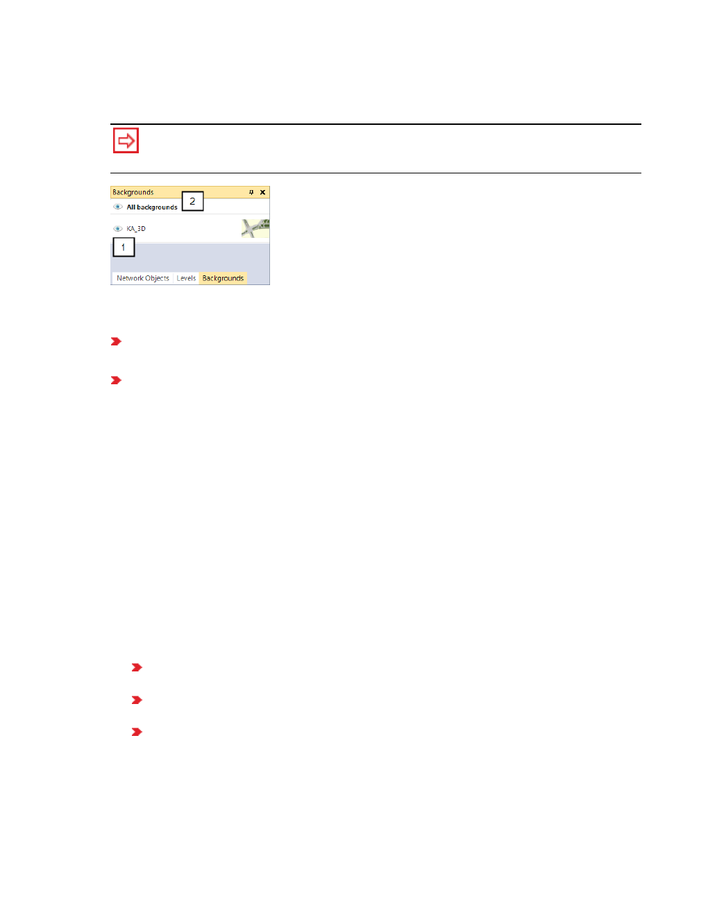
2.7 Using the background image toolbar
2.7 Using the background image toolbar
The background image toolbar shows the names of the loaded backgrounds in succession.
Tip: By default, the Network object toolbar, the Level toolbar, and the Background
toolbar are displayed together. Using the tabs at the bottom of a toolbar, you can switch
to another toolbar.
(1) Visibility button
Button is colored and open: background is displayed in the Network Editor. The visibility of
backgrounds must be activated in the network object toolbar.
Button is gray and closed: background is not displayed in the Network Editor.
(2) All backgrounds
Select or deselect visibility for all backgrounds.
You can customize the position, size, and visibility of the background image toolbar (see
"Changing the display of windows" on page 86).
Shortcut menu of Background images bar
From the shortcut menu, you can choose to open the Backgrounds list (see "Attributes of
background images" on page 378).
2.8 Using the Quick View
The Quick View contains a selection of attributes and attribute values for the network objects
currently selected. When you globally select network objects, your selection is the same in all
network editors and synchronized lists.
If several network objects of the same network object type are selected, the name of
the network object type is shown in the title bar of the Quick View.
If several network objects with different attribute values are selected, the symbol * is
shown with the different attribute values.
If several network objects of different network object types are selected, the following
message will be displayed in Quick View: Multi-type selection, no quick view avail-
able.
66 © PTV GROUP
2.8.1 Showing the Quick View
If several network objects of different network object types are selected, no attribute val-
ues are shown and no name is shown in the title bar of the Quick View.
If synchronization is activated in a list with network objects and you select network
objects in the list, these are shown in all network editors and in Quick View (see "List
toolbar" on page 93).
Data cells that you can or cannot edit are highlighted in color or hatched (see "Structure of
lists" on page 90). Hatched cells: Irrelevant attribute values that due to other attribute values
have no effect.
You can select the attributes that are displayed (see "Selecting attributes for the Quick
view display" on page 67).
Using global selection, you can change the attribute values of all network objects (see
"Editing attribute values in the Quick view" on page 68).
You can customize the position, size, and visibility of the Quick View (see "Using tool-
bars" on page 127).
Tip: The Smart Map and Quick View are displayed in the same section by default. To
switch between the Smart Map and Quick View, use the tabs.
2.8.1 Showing the Quick View
In the View menu, choose > Quick View.
The Quick View opens as a tab. The position depends on how your user interface is set up.
2.8.2 Selecting attributes for the Quick view display
You can select network objects in a Network Editor or list and specify which attributes are
shown in the quick view. When you press the CTRL key to select multiple network objects,
these may belong to diifferent network object types.
1. If you want to select network objects in the Network editor, you must ensure that visibility
and selectability have been activated for the network object type in the network object
toolbar.
2. In a network editor or list, select at least one network object.
3. Select the Quick view.
4. Click on the Attribute selection icon.
The Select Attributes window opens (see "Selecting attributes and subattributes for a list"
on page 106).
5. Select the desired attributes.
6. Deactivate the attributes that you do not want to display in the Quick view.
7. Confirm with OK.
The attributes selected and their values are displayed in the Quick view window, in the units
and sequence specified.
© PTV GROUP 67
2.8.3 Editing attribute values in the Quick view
Note: The selection of attributes in the Quick view is saved separately for all objects in
a *.layx file (see "Saving and importing a layout of the user interface" on page 138).
2.8.3 Editing attribute values in the Quick view
1. Make sure that the network objects are selected in the network whose attribute values you
want to edit.
2. In the Quick view, mark one or more cells.
Note: If several network objects with different attribute values are selected, the *
symbol is shown instead of the value of the attribute.
3. Into the field selected, enter the value of your choice.
4. Confirm with Enter.
Notes: When entering numerical attribute values with a reference to length, time,
speed and acceleration, you must take the units into account:
If you enter just one digit, the value is interpreted in the format in which the attribute
is displayed. Example: If an attribute is displayed in the minutes format, the value 5
is read as 5 minutes. You can change the format in the attribute selection window
(see "Selecting attributes and subattributes for a list" on page 106).
You can enter a number with a unit. In this case, Vissim converts the value in such
a way that it is displayed accordingly in the selected format. You can enter length
units either with metrical (m, km) or imperial (ft, mi) units. For example, if an attrib-
ute is shown in the format Minutes, you can enter 2 h. After the confirmation, the
value 120 will be displayed.
The new attribute value is shown in all highlighted fields and applied to all objects that were
selected. This also applies to fields in which the symbol * referenced different attribute values.
2.8.4 Editing attribute values in the Quick view with arithmetic operations
Make sure that the network objects are selected in the network whose attribute values you
want to edit.
1. In the Quick view, mark one or more numerical cells.
2. In a marked cell, enter one of the below arithmetic operations:
Operation Syntax
Addition =+2
Subtraction =-2
Multiplication =*2
Division =/2
Raise to power =^2
Setting the lower bound value =min2
68 © PTV GROUP
2.9 Using the Smart Map
Operation Syntax
Setting the upper bound value =max2
Use an exponential function =exp
Take logarithm =log
Form reciprocal value =1/
The operation is run for all marked cells with a numerical value. The result is entered as
attribute value.
Warning: If you have selected an alphanumerical cell, the text of the arithmetic
operation is entered in the cell!
2.9 Using the Smart Map
The Smart Map displays a small scale overview of the network. A rectangle shows the section
which is currently displayed in the Network Editor. If the zoom factor in the Network editor is so
large that the section in the Smart Map is not displayed as a rectangle, cross hairs are
displayed instead.
If a network is displayed in several Network Editors, the Smart Map uses rectangles to
indicate the different sections. The border line of the rectangle that displays the section of the
active Network Editor is formatted in bold.
Smart Map is linked to the Network editor. Modifications which are made in the Network editor
view have an effect on the Smart Map and vice-versa. For instance, if you zoom into the
network or move the current view, the position of the rectangle or cross hairs is moved in the
Smart Map as well. To change the network view, change the position or size of the colored
rectangle in the Smart Map.
Dynamic objects such as vehicles and pedestrians are not shown in the Smart Map. Network
objects selected in Network Editors are not highlighted in the Smart Map.
You can customize the position, size, and visibility of the Smart Map (see "Using toolbars" on
page 127).
Tip: The Smart Map and Quick View are displayed in the same section by default. To
switch between the Smart Map and Quick View, use the tabs.
2.9.1 Displaying the Smart Map
In the View menu, choose > Smart Map.
The Smart Map opens as a tab. The position depends on how your user interface is set up.
2.9.2 Displaying the entire network in the Smart Map
Note: If a network is displayed in several Network editors, the Smart Map uses
rectangles to indicate the different views.
1. Right-click on the Smart Map.
© PTV GROUP 69

2.9.3 Moving the Network Editor view
2. Select Display Entire Network from the context menu.
The entire network is shown in the Smart Map.
2.9.3 Moving the Network Editor view
To move the view shown in the Network Editor, in the Smart Map, move the rectangle. If the
network is greatly enlarged in the Smart Map, the rectangle may lie outside of the Smart Map
and is not shown in the Smart Map (see "Displaying the entire network in the Smart Map" on
page 69).
Note: If a network is displayed in several Network editors, the Smart Map uses
rectangles to indicate the different views.
Note: Make sure that you choose the desired rectangle in the next steps.
1. In the Smart Map, point the mouse pointer to a position inside the colored rectangle.
The mouse pointer becomes a symbol.
2. Hold down the mouse button.
3. Drag the rectangle to the position of your choice and release the mouse button.
The Network Editor view is adjusted according to the Smart Map.
2.9.4 Showing all Smart Map sections
Note: If a network is displayed in several Network editors, the Smart Map uses
rectangles to indicate the different views.
1. Right-click on the Smart Map.
2. From the shortcut menu, choose Zoom All Sections.
In the Smart Map, all colored rectangles of the Network Editors opened are displayed in
full.
2.9.5 Zooming in or out on the network in the Smart Map
1. Right-click on the Smart Map.
2. Select the entry Zoom In or Zoom Out in the context menu.
Tip: Alternatively, you can use:
the PAGE UP and PAGE DOWN keys
mouse scroll wheel
The network is adjusted in the Smart Map.
70 © PTV GROUP

2.9.6 Redefining the display in the Smart Map
2.9.6 Redefining the display in the Smart Map
You can redefine the display shown in the Network Editor in 2D mode by drawing a new
rectangle in the Smart Map.
Note: If a network is displayed in several Network editors, the Smart Map uses
rectangles to indicate the different views.
1. Click on the Network Editor.
The Network Editor is activated.
2. In the Smart Map, point the mouse pointer to a position outside of all rectangles.
Note: If you want to start drawing the rectangle within a rectangle, you also have to
hold down the SHIFT key in the next step.
3. Hold down the mouse button.
The pointer appears as magnifier.
4. Drag the rectangle to the desired size and release the mouse button.
The network window view is adjusted according to the Smart Map.
Tip: Alternatively, you can select Redefine section in the context menu and draw a
rectangle.
2.9.7 Defining a Smart Map view in a new Network Editor
In the Smart Map, you can drag open a rectangle, automatically open a new Network Editor,
and show the network in the rectangle map section.
Note: If a network is displayed in several Network editors, the Smart Map uses
rectangles to indicate the different views.
1. Right-click on the Smart Map.
2. From the shortcut menu, choose Define Section in New Network Editor.
The mouse pointer becomes a cross.
3. In the Smart Map, point the mouse pointer to a corner of the desired map section.
4. Hold down the mouse button.
5. Drag the rectangle to the desired size and release the mouse button.
A new Network editor is opened. The network window view is adjusted according to the Smart
Map.
2.9.8 Moving the Smart Map view
1. Click into the Smart Map.
2. On your keyboard, press the arrow button of your choice.
© PTV GROUP 71

2.9.9 Copying the layout of a Network Editor into Smart Map
Tip: Alternatively, you can hold down the mouse wheel.
The Smart Map view is moved.
2.9.9 Copying the layout of a Network Editor into Smart Map
The layout of the smart map is saved additionally to the layouts of the network editors in the
*.layx layout file. You can change the layout of the Smart Map by copying the layout of a
network editor.
1. Click on the Network Editor.
The Network Editor is activated.
2. Right-click into the Smart Map.
3. In the context menu, choose Apply Layout > From Current View.
The Smart Map is updated.
2.9.10 Displaying or hiding live map for the Smart Map
You can select a live map for the Smart Map and activate or deactivate it.
1. Right-click on the Smart Map.
2. From the Background Maps Configuration context menu, choose the desired entry:
Element Description
Bing Maps (aerophoto) Display Bing Maps in Smart Map
Open Street Map (Mapnik) Display Open Street Map (Mapnik) in Smart Map
Disable Background Maps Hide the currently selected live map from the Smart Map
The Smart Map is updated.
2.10 Using network editors
In Vissim you can display one or multiple network editors, e.g. to show the network in the 2D
and 3D mode or in different scales.
In each network editor you can display and edit the open network, zoom out for an overview or
zoom in to show more details. You can display the network with different graphic parameters
in the Network Editors; for example, two dimensional in one editor and three dimensional in
another.
If you run simulations, these are shown in the open Network Editors. You can control the
display of network objects for each network editor using the visibility (see "Using the Network
object toolbar" on page 60).
In Vissim, you can move and arrange Network editors to other positions on the desktop or
anchor them in other windows of Vissim (see "Changing the display of windows" on page 86).
The positions are saved in the *.layx file.
72 © PTV GROUP
2.10.1 Showing Network editors
Above each open Network Editor, a toolbar with functions that you can use to control the
appearance of the network in that Network Editor is shown.
Note: The display in the network editor is linked to the display in Smart Map (see
"Using the Smart Map" on page 69). If you change the section in the Network editor, the
position of the colored rectangle or cross hairs in Smart Map also changes and vice-
versa.
2.10.1 Showing Network editors
In Vissim, you can show one or more Network editors. In each Network editor, you can open,
show and edit the network, reduce its size for an overview or enlarge it to show more details.
You can further watch dynamic objects, e.g. vehicles, pedestrians or signal heads changing
their status, during a simulation run.
In the View menu, choose > Open New Network Editor.
The new Network Editor opens as a tab. The position depends on how your user interface is
set up.
Tip: You switch between open lists and Network Editors with CTRL+TAB.
2.10.2 Network editor toolbar
Toolbar
button
Name Description Keyboard /
mouse
Network editor layout
selection list
Save specified network editor layout (see
"Saving the user interface layout" on page
138)
Select specified network editor layout
Edit basic
graphic para-
meters
Edit basic graphic parameters (see "List of base
graphic parameters for network editors" on page
161)
© PTV GROUP 73

2.10.2 Network editor toolbar
Toolbar
button
Name Description Keyboard /
mouse
Toggle wire-
frame on
If wireframe display is enabled, disable
wireframe display.
The icon remains selected and the function
remains active, until you click the icon again.
You cannot activate or deactivate the Wireframe
view in 3D mode.
In the Wireframe view, only the middle lines are
shown for links and connectors. Standard colors:
Blue: Links
Pink: Connectors
In the Wireframe view in 3D mode, areas are
shown in the display type selected.
Toggle wire-
frame off
If wireframe display is disabled, change to
wireframe display.
The icon remains selected and the function
remains active, until you click the icon again.
Toggle back-
ground maps on
If background map display is enabled, hide the
background map.
The icon remains selected and the function
remains active, until you click the icon again.
Toggle back-
ground maps off
If the background map is hidden, display the
background map (see "Using live maps from the
Internet" on page 369).
The icon remains selected and the function
remains active, until you click the icon again.
Legend on The legend appears. The legend is displayed if
the Show legend attribute has been selected in
the graphic parameters of the network editor and
the Legend includes <Attribute > attribute has
been selected in the graphic parameters for at
least one network object type.
Legend off Legend is hidden.
74 © PTV GROUP

2.10.2 Network editor toolbar
Toolbar
button
Name Description Keyboard /
mouse
Toggle selection If network objects are overlapping each other at
the position that you clicked, select the next
network object.
For instance, for a link with the attribute Is
pedestrian area (option Use as pedestrian
area), you can then select the other respective
direction.
The icon is only active if network objects lie on
top of each other and one of the network objects
on the top is selected.
TAB
Copy selection Copy the selected network objects to the
Clipboard (see "Selecting and copying network
objects" on page 320)
Paste from clip-
board
Paste network objects from the Clipboard into the
Network Editor (see "Pasting network objects
from the Clipboard" on page 321)
Synchronization:
Auto pan on
The display of the selected network objects is
centered automatically in the Network Editor. If
you change the selection of network objects in a
different Network editor or synchronized list, the
section in the Network editor is automatically
adjusted to the new selection.
The icon remains selected and the function
remains active, until you click one of the
following icons:
the Auto pan button again
Auto zoom button
Synchronization:
Auto pan off
In the Network Editor, the section is not
automatically adjusted to the selected network
objects.
© PTV GROUP 75

2.10.2 Network editor toolbar
Toolbar
button
Name Description Keyboard /
mouse
Synchronization:
Auto zoom on
Display the selected network objects centered in
the Network Editor and select the section so
large that all the selected network objects are
displayed. If you change the selection of network
objects in a different Network editor or
synchronized list, the section in the Network
editor is automatically adjusted to the new
selection.
The icon remains selected and the function
remains active, until you click one of the
following icons:
the Auto zoom button again
Auto pan button
Synchronization:
Auto zoom off
In the Network Editor, the section is not auto-
matically adjusted.
Show entire net-
work
Choose a section size large enough to display
the entire network.
Zoom in (see "Zooming in" on page 80) PAGE DOWN or
move mouse
wheel
forward
Zoom out (see "Zooming out" on page 80) PAGE UP
or move
mouse wheel
backward
Previous view Display previous view. You must have previously
displayed views.
ALT+ left
arrow key
Next window sec-
tion
Display next view. You must have displayed
some previous views beforehand.
ALT+ right
arrow key
Pan Move entire network section. Selected and non-
selected network objects are moved.
The icon remains selected and the function
remains active, until you click the icon again.
Arrow keys or
pressed
mouse wheel
76 © PTV GROUP

2.10.2 Network editor toolbar
Toolbar
button
Name Description Keyboard /
mouse
Rotate mode
(3D) on
only in 3D mode: Tilt or rotate the network
display level vertically or horizontally (see
"Navigating in 3D mode in the network" on page
183).
The icon remains selected and the function
remains active, until you click one of the
following icons:
the Rotate mode (3D) button again
the Flight mode button
the 2D/3D button
Hold down
left mouse
button and
drag the
mouse, or
press the ALT
key + hold
mouse wheel
down
Rotate mode
(3D) off
Rotate mode is not selected
Flight mode (3D)
on
only in 3D mode: Move current camera position
over network (see "Flight over the network" on
page 185)
The icon remains selected and the function
remains active, until you click one of the
following icons:
the Flight mode button again
the Rotate mode (3D) button
the 2D/3D button
Flight mode (3D)
off
Flight mode is not selected
Export image
(Screenshot)
Opens the Save as window. You can save a
screenshot of the Network editor as a graphic file
to a folder of your choice. You can saved data in
the following file formats:
*.png
*.jpg
*.tiff
*.bmp
*.gif
© PTV GROUP 77
2.10.3 Network editor context menu
Toolbar
button
Name Description Keyboard /
mouse
2D/3D 2D mode is currently displayed. Switch to 3D
mode
The icon remains selected and the function
remains active, until you click the icon again.
2D/3D Currently shows 3D mode. Switch to 2D mode.
The icon remains selected and the function
remains active, until you click the icon again.
Edit 3D graphic
parameters
Edit 3D graphic parameters (see "Editing 3D
graphic parameters" on page 184), (see "List of
3D graphic parameters" on page 184)
The 3D graphic parameters only affect the
network objects in 3D mode.
Selection of camera
position list
only in 3D mode:
Saving camera positions
Select saved camera position
Tip: Alternatively, in the Camera Positions list, select one of the saved camera
positions. Then from the context menu, choose Apply to current Network Editor to
assign the camera position to the current Network editor.
2.10.3 Network editor context menu
The context menu in a network editor can display different features. They depend on whether
network objects have been selected, you right-click a network object, or right-click a section in
which no network object has been inserted.
2.10.3.1 Commands that do not depend on a previous selection of objects
You can always perform the following functions via the context menu, regardless of whether
you click with the right mouse button on a network object or whether network objects are
selected:
Add <network object type>: Add a network object of the type selected in the Network
objects toolbar, if the network object does not have to be added to another network object.
Possible options are links, areas or nodes.
Paste: Paste network objects that you have copied to the Clipboard.
Read Additionally Here: Read a network file *.inpx additionally.
Show List: Open the network objects list of the network object type that is selected on the
Network Objects toolbar.
Map this Point to Background Position: Specify a point in the background map as a ref-
erence point (see "Mapping Vissim network to background position" on page 371).
78 © PTV GROUP

2.10.3 Network editor context menu
2.10.3.2 Commands that depend on a previous selection of objects
The following functions are displayed in the context menu depending on whether network
objects are selected:
Network objects selected in
the network editor
Functions
No network objects selected Show List: Show the network objects list of the network
object type that is selected for the Insert mode in the network
objects toolbar.
One network object is selec-
ted The standard editing functions are shown, for example:
Zoom To Selection
Delete
Duplicate
Copy
Paste
Edit
Show In List
Reset label position
Create Chart for Selected Objects
Network object type specific functions, e.g. Split link here
Multiple network objects of a
network object type or dif-
ferent network object types
are selected
Only the standard editing functions that can be carried
out when multiple network objects are selected are
shown, for example:
Zoom To Selection
Delete
Duplicate
Copy
Paste
Show In List
Editing functions that are available for a single selected
network object are not displayed.
Only functions specific to the network object type that are
useful when multiple network objects are selected are
shown.
2.10.3.3 Deselecting all network objects
If network objects have been selected and you right-click a section (not a network object) into
which no network object has been inserted to open the shortcut menu, all network objects are
deselected.
© PTV GROUP 79

2.10.4 Zooming in
2.10.4 Zooming in
To maximize the view, on the toolbar, click the respective button or use the scroll wheel of the
mouse.
Tip: You can also change the Network editor view using the Smart Map (see "Zooming
in or out on the network in the Smart Map" on page 70).
2.10.4.1 Enlarging the view to a certain section
In 2D mode, click the Zoom in symbol to enlarge the view of a specific section. In 3D mode,
click the Zoom in symbol to gradually enlarge the view.
1. On the Network editor toolbar, click the Zoom in button.
The pointer appears as magnifier.
2. Click the position in the network from which you want to zoom into a section, and hold the
mouse button down.
3. Drag the desired section and release the mouse button.
The selected section will be zoomed in. The mouse pointer is reset to standard display.
2.10.4.2 Zooming in with a scroll wheel
1. In the Network editor, point the mouse pointer to the position you want to zoom in on.
Next, simultaneously hold down the SHIFT key. Then Vissim will enlarge the view faster.
2. Turn the scroll wheel forwards.
The view is zoomed in at the position of the mouse pointer.
If you zoom in until the maximum magnification, the contents of the Network editor are
displayed in black.
Tip: Alternatively, press the PAGE UP key to zoom in gradually.
2.10.5 Zooming out
To minimize the view, on the toolbar, click the respective button or use the scroll wheel of the
mouse.
Tip: You can also change the Network editor view using the Smart Map (see "Zooming
in or out on the network in the Smart Map" on page 70).
2.10.5.1 Zooming out using icon
In 2D mode, click the Zoom out symbol to reduce the view of a specific section. In 3D
mode, click the Zoom out symbol to gradually reduce the view.
80 © PTV GROUP

2.10.6 Displaying the entire network
On the Network editor toolbar, click the Zoom out button.
The view is reduced.
2.10.5.2 Zooming out using a scroll wheel
1. In the Network editor, point the mouse pointer to the position you want to zoom in on.
Next, simultaneously hold down the SHIFT key. Then Vissim will reduce the view faster.
2. Turn the scroll wheel backwards.
The view is zoomed out at the position of the mouse pointer.
Tip: Alternatively, you can zoom out by gradually. To do so, press the PAGE DOWN key.
2.10.6 Displaying the entire network
On the Network Editor toolbar, click the Show entire network button.
The full network is shown in the network editor.
Tip: Alternatively you can also display the entire network by pressing the HOME key.
2.10.7 Moving the view
1. On the Network editor toolbar, click the Shift mode button.
The Shift mode button is activated: . The mouse pointer becomes a symbol. This
designates the Pan mode.
2. Click any position in the network and keep the left mouse button pressed.
3. Drag the view to the desired position and release the left mouse button.
The view is shifted.
4. In the Network Editor, on the toolbar, click the Shift mode button to deactivate the 'Pan'
mode.
The Shift mode button is deactivated: . The mouse pointer is reset to the standard
depiction.
Note: Only the display is shifted, the network itself is not. Coordinates remain
unchanged.
© PTV GROUP 81

2.10.8 Defining a new view
Tips: Alternatively, you have these possibilities to shift the view:
Hold down the middle mouse button or the scroll wheel and move the view.
Press an arrow key on your keyboard. The section moves to a greater extent if you
simultaneously hold down the SHIFT key.
You can also move the view in the Smart Map (see "Moving the Network Editor
view" on page 70).
2.10.8 Defining a new view
In the Network Editor, you can specify a different network section by dragging open a
rectangle in the Smart Map (see "Using the Smart Map" on page 69).
1. In the Smart Map, click the position at which you want to set a corner of the new display
outside of a colored rectangle and hold down the left mouse button.
The mouse pointer becomes a symbol.
2. Diagonally drag open the rectangle of your choice.
3. Release the mouse button.
The Network Editor view is adjusted according to the Smart Map.
2.10.9 Displaying previous or next sections
If you have changed the section in the network editor, you can return to the previous section
and display it. If a previous section is displayed, you can go to the next section and display it.
1. In the Network editor, on the toolbar, click the Previous view button.
The previous section is displayed.
Tip: Alternatively, you can change to the previous view with the ALT + LEFT ARROW
key.
2. In the Network Editor, click on the icon Next window section in the toolbar.
The next section is displayed.
Tip: Alternatively, you can change to the previous view with the ALT + RIGHT ARROW
key.
2.10.10 Zooming to network objects in the network editor
In the network editor you can select the size of the network so that the selected network
objects are automatically completely displayed.
In the context menu, select Zoom To Selection.
82 © PTV GROUP

2.10.11 Selecting network objects in the Network editor and showing them in a list
2.10.11 Selecting network objects in the Network editor and showing them in a list
In the network editor you can select network objects of a particular network object type and
show them, together with their attributes, in a list of network objects with the particular network
type.
1. In the Network Editor, right-click the network object of your choice.
2. From the context menu, choose entry Show In List.
The list of defined network objects for the network object type opens.
The objects selected in the Network editor are marked in the list, if the list is synchronized (see
"List toolbar" on page 93).
2.10.12 Using named Network editor layouts
The layout of a Network editor is defined by graphic parameters and settings in the network
objects toolbar. You can assign the current layout of a Network editor a name, under which
you can import the layout again later on. You can save these so-called named Network editor
layouts to the *.layx file. In a Network editor, you can choose a Network editor layout from all
the named ones available, to change the graphic parameters and network object toolbar
settings of your window accordingly.
2.10.12.1 Creating a Network editor layout
1. Adapt the graphic parameters of a Network editor via its toolbar and/or the network objects
toolbar (see "Editing base graphic parameters for a network editor" on page 161), (see
"Using the Network object toolbar" on page 60).
2. On the Network editor toolbar, in the Network editor layout selection box, enter a unique
name.
3. Confirm with Enter.
On the toolbar of all Network editors, in the Select layout list box, the new network editor
layout is displayed and can be selected.
2.10.12.2 Assigning a Network editor layout
1. In the Network editor, in the NetworkEditorLayout list, click the symbol.
2. Select the Network editor layout of your choice.
The network editor layout is assigned to the network editor and the display is adjusted. The
new settings are shown on the network objects toolbar.
2.10.12.3 Saving Network editor layouts
1. In the menu, select File > Save Layout as.
2. Enter a unique name.
3. Click the Save button.
© PTV GROUP 83

2.11 Selecting simple network display
The current layout of the entire Vissim user interface, and thus all named Network editor
layouts, are saved to the *.layx layout file.
If in the User Preferences, the option Auto-save layout when network file (inpx) is saved is
selected, the layout file is saved automatically under the name of the currently loaded network
file, each time the network file is saved (see "Specifying automatic saving of the layout file
*.layx" on page 145).
2.10.12.4 Reading in saved Network editor layouts additionally
You may read all Network editor layouts, saved to a *.layx file, into your currently opened file.
Then you can apply these Network editor layouts to the Network editors in the file currently
open.
1. From the File menu, choose > Read Additionally > Named Network Editor Layouts.
2. Select the desired *.layx file of your choice.
3. Click the Open button.
The network editor layouts are read in. On the toolbar of the Network editors opened and the
Network editors you open later on, in the Select layout list, you can select the Network editor
layouts read in.
2.10.12.5 Deleting a named Network editor layout
1. On the Network editor toolbar, right-click in the Network editor layout selection list box.
2. Position the mouse pointer on the Delete entry in the context menu.
The named Network editor layouts are displayed in the context menu.
3. Click the desired Network editor layout in the context menu.
4. Confirm with Yes.
2.11 Selecting simple network display
To gain a better overview of complex networks, switch to the simple network display that hides
all network objects lying on links, areas, ramps and stairways.
1. In the View menu, select > Simple Network Display.
Tip: Alternatively, press CTRL+N or on the Edit toolbar, click Simple Network
Display.
The following network objects and their labels are hidden in the Simple Network Display. This
is also the case for network objects of the network object type selected during a simulation run
in the network objects toolbar, which allows network objects to be added:
84 © PTV GROUP

2.12 Using the Quick Mode
Desired Speed Decisions
Reduced Speed Areas
Conflict Areas
Priority Rules
Stop Signs
Signal Heads
Detectors
Vehicle Inputs
Vehicle Routes
Parking Lots
Public transport stops
Public Transport Lines
Nodes
Data Collection Points
Vehicle Travel Times
Queue Counters
Flow bundles
Pavement Markings
Elevators
Pedestrian Inputs
Pedestrian Routes
Pedestrian Travel Times
In the Simple Network Display, all other objects are displayed, if you do not individually set
them to invisible:
Links
Sections
Backgrounds
3D Traffic Signals
Static 3D Models
Vehicles In Network
Pedestrians In Network
Areas
Obstacles
Ramps & Stairs
2. To show the hidden objects again, from the View menu, choose > Simple Network Display
again.
2.12 Using the Quick Mode
In the Quick Mode, all dynamic objects (e.g. vehicles, pedestrians, dynamic labels, and colors)
are hidden in all network editors. In addition, in the Quick Mode, list windows and the Quick
view are only then updated when you scroll or click in them. The Messages window is not
updated and does not display any messages. This allows for a maximum simulation speed.
The simulation speed set is not used.
In the View menu, choose > Quick Mode.
Tip: Alternatively, press CTRL+Q or on the Edit toolbar, click Quick Mode.
You can deactivate the Quick Mode again:
Press CTRL+Q again.
From the View menu, choose Quick Mode.
Again click the Quick Mode icon.
All dynamic objects are shown again. All lists and the Quick view are updated.
© PTV GROUP 85
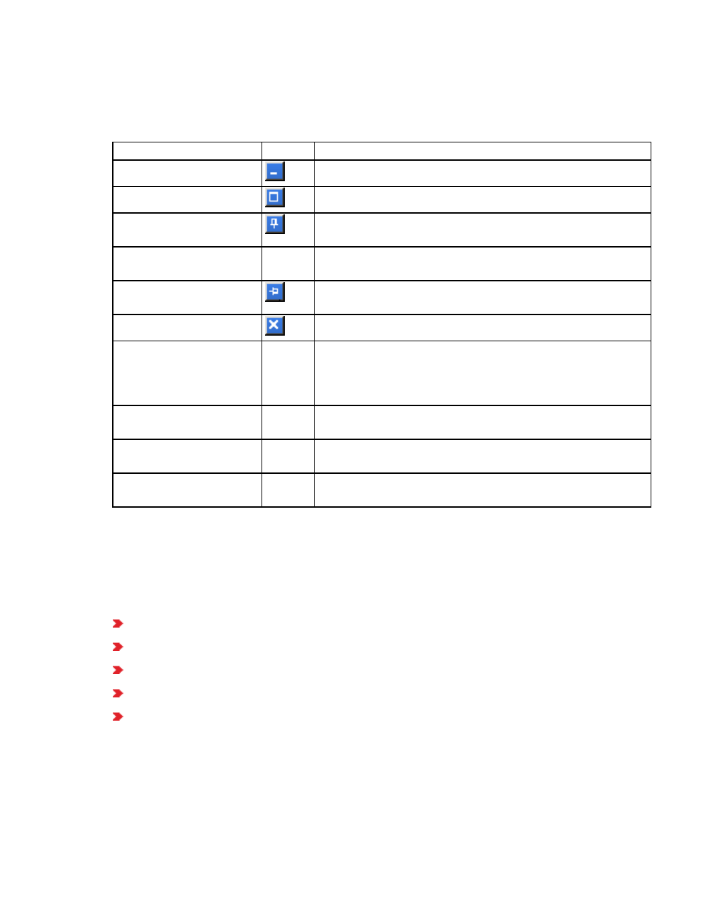
2.13 Changing the display of windows
2.13 Changing the display of windows
You can significantly change the display of windows showing network editors, lists, network
object toolbars, the Smart Map and Quick View by using standard program functions:
Name or function Symbol Description
Minimize Minimize user interface
Maximize Maximize user interface
Auto Hide: hide The window is hidden. A tab with the name of the hidden
window is displayed at the edge of the user interface.
Use Auto Hide to show
hidden window again
At the edge of the user interface, point the mouse to the
tab of the desired window.
Auto Hide: show per-
manently
The window is permanently shown.
Close The window closes.
Move Moving and rearranging a window in Vissim or arranging
a windows outside of Vissim
(see "Arranging or freely positioning program elements in
PTV Vissim" on page 87)
Anchoring Anchor windows or show them together in one section
(see "Anchoring windows" on page 87)
Releasing from
anchors
Release anchored window
(see "Releasing windows from the anchors" on page 88)
Change size Change the size of the window using the corner drag
points. The size of windows cannot always be changed.
You can restore the default settings (see "Resetting menus, toolbars, shortcuts, and dialog
positions" on page 146).
2.13.1 Showing program elements together
If you open several program elements, you can group them into one area, for example:
multiple lists
multiple network editors
one or multiple lists together with one or multiple network editors
the Smart Map together with the Quick View
network objects toolbar and level toolbar together with the background image toolbar
You cannot show lists and network editors together with the Smart Map, the Quick or a toolbar
in one area.
Tabs under each area display the program elements inside:
86 © PTV GROUP

2.13.2 Arranging or freely positioning program elements in PTV Vissim
For lists, the name of the network object types or base data type
For Network editors, numbers in the order they were opened
Smart Map and Quick View
Network object toolbar, level toolbar, background image toolbar: Network object types,
levels, background images
The name of the visible program element is highlighted in the tab. The name of the active
program element is highlighted in the title bar.
You can change the arrangement of program elements (see "Changing the display of
windows" on page 86), (see "Anchoring windows" on page 87), (see "Arranging or freely
positioning program elements in PTV Vissim" on page 87).
2.13.2 Arranging or freely positioning program elements in PTV Vissim
You can move and arrange program elements in Vissim or move them on your screen or
screens independently of Vissim. You can also group multiple program elements together, for
example, multiple lists or multiple network editors.
Note: Changing program elements or shortcut keys can make it more difficult for you to
find and use commands. The documentation and the PTV Vision Support assume that
the standard settings are used.
1. Click the title bar of the program element, keep the mouse button held down, and drag the
program element to the position of your choice.
The icon for anchoring the program element is shown until you drag the program element
out of Vissim.
2. Release the mouse button.
Outside of Vissim, the display of the program element floats freely.
You can restore the default settings (see "Resetting menus, toolbars, shortcuts, and dialog
positions" on page 146).
2.13.3 Anchoring windows
You can anchor windows such as network editors, lists, bars, Smart Map and Quick View or
display them together in one area. Vissim assists you with visual aids. An icon and a colored
shadow show you where you can anchor the window.
Note: Changing program elements or shortcut keys can make it more difficult for you to
find and use commands. The documentation and the PTV Vision Support assume that
the standard settings are used.
1. Click on the title bar or the tab for the window and hold the mouse button pressed.
If you move the mouse, an icon is displayed, which shows you the possible anchoring
positions:
© PTV GROUP 87
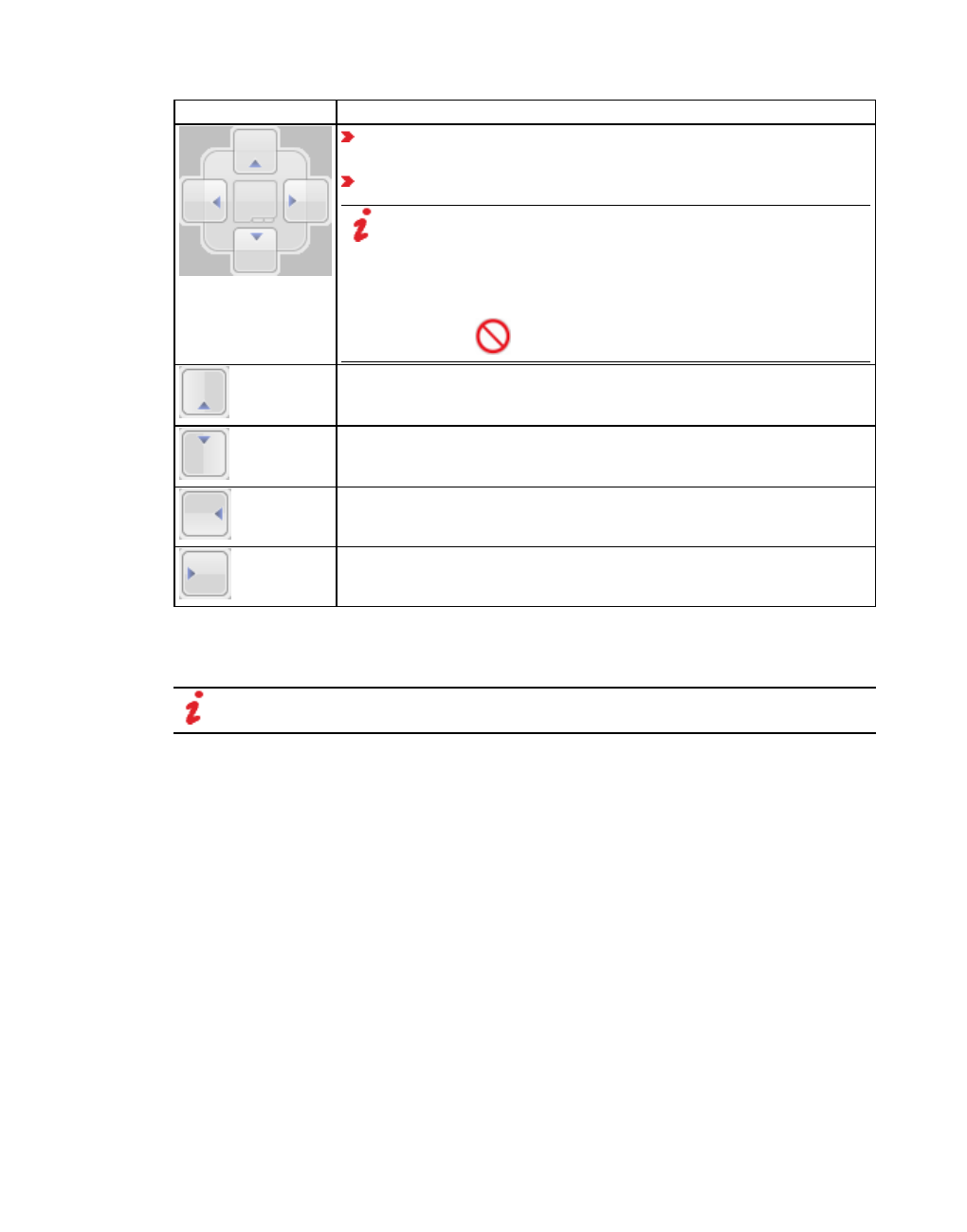
2.13.4 Releasing windows from the anchors
Element Description
Outer icons: This anchors the window in the destination area at
one of the four edges.
Icon in the middle: This anchors the window as a tab.
Note: You cannot anchor all windows with all other windows
as a tab. You cannot anchor network editors and lists with the
Quick View, Smart Map, Network objects toolbar, Levels
toolbar or the Background toolbar as a tab.
If anchoring as a tab is not possible, the following symbol is
displayed:
Anchoring the window at the top edge of the destination area
Anchoring the window at the bottom edge of the destination area
Anchoring the window at the left-hand edge of the destination area
Anchoring the window at the right-hand edge of the destination area
2. Drag the mouse pointer to the desired icon.
The desired target area is given a colored shadow.
Note: The icon which you drag with the mouse pointer is decisive, not the position of
the window.
3. Release the mouse button.
The window is anchored at the desired position.
You can restore the default settings (see "Resetting menus, toolbars, shortcuts, and dialog
positions" on page 146).
If several window are anchored together in an area, they are shown as tabs.
2.13.4 Releasing windows from the anchors
You can release anchored windows from each other.
1. If in a window, you have attached multiple tabs next to each other and want to detach them,
click the title bar and hold down the mouse button.
2. If in a window, you have attached multiple tabs next to each other and want to detach one,
click the tab window and hold down the mouse button.
3. Drag the mouse pointer to the desired area of the desktop and release the mouse button.
88 © PTV GROUP

2.13.5 Restoring the display of windows
The window is released from the anchor.
You can restore the default settings (see "Resetting menus, toolbars, shortcuts, and dialog
positions" on page 146).
2.13.5 Restoring the display of windows
1. Choose Edit > User Preferences.
The User Preferences window opens.
2. Choose the entry GUI > General.
3. Click the Reset dialog positions button.
The next time you start Vissim without a network, the default settings are used to arrange the
windows.
2.13.6 Switching between windows
If you have opened multiple windows, you can switch between them to place another window
in the foreground. This also includes the start page. The View toolbar list shows the windows
opened in Vissim.
On the View toolbar, in the Windows Selection list, click the window of your choice.
The window selected is placed in the foreground and is activated.
2.14 Using lists
In a list, you can show all objects of a type together with a selection of the object's attributes
(see "Opening lists" on page 92):
You can display input attributes, e.g. for links these are the length, name, link behavior
type, display type, etc. You can change input attributes in the list, e.g. when you create
new network objects or make changes later on (see "Editing attributes of network objects"
on page 330), (see "Selecting and editing data in lists" on page 96). This is not always pos-
sible during a simulation run. In this case, a corresponding message is displayed when
you try to do so.
You can display attributes calculated from input attributes, e.g. a distance or travel time
measurement. The values of these attributes cannot be changed in the list.
You can display result attributes, whose values are determined during a simulation run
(see "Displaying result attributes in attribute lists" on page 957). Result attributes can have
subattributes, e.g. a different value per simulation run and time interval. The values of
these attributes cannot be changed in the list.
There are two types of lists:
"Normal" attribute lists contain the attributes of network objects and base data. You can
choose these lists from the Lists menu (see "Opening lists" on page 92): A list contains a
row for each object of the respective type, e.g. for a defined link. There is one column for
© PTV GROUP 89

2.14.1 Structure of lists
each attribute, e.g. name or length of the link. There is also a column for each subattribute,
e.g. time intervals or vehicle classes. "Normal" attribute lists can be extended to coupled
lists, if the network object type has relations to other objects, e.g. a link to lanes (see
"Using coupled lists" on page 111).
To select result lists, from the Lists menu, choose > Results or from the Evaluation menu,
choose > Result Lists (see "Configuring evaluations of the result attributes for lists" on
page 954): A results list contains rows for each object of the respective type per time inter-
val of each simulation run. Moreover, you can show additional rows for static results: the
mean, the standard deviation and minimum and maximum values of all simulation runs.
You can further view the mean, the standard deviation, the minimum and maximum values
and total of all time intervals. Only the subattributes Vehicle class or Pedestrian class are
shown in the attribute columns.
2.14.1 Structure of lists
Element Description
(1) Title bar Name of list
Auto Hide: Hide and show lists
Close list
(2) Toolbar Functions for displaying and editing (see "List toolbar" on page 93)
90 © PTV GROUP

2.14.1 Structure of lists
Element Description
(3) Column
header Short name of attribute
Sort, move and mark columns
Functions are available via the context menu (see "Editing lists and data via
the context menu" on page 99)
To open a quick info with an attribute description, point the mouse pointer to
the attribute name in the column header.
Right-click the column header to select the data in the column.
(4) Data Attribute values. Functions are available via the context menu.
If you point to the first column of a list with the cursor, the row number is shown.
(5) Orange
cells
Data is selected in one or more cells, rows or columns, and can, for example,
be copied or changed.
White cells Values you can change, e.g. of input attributes
In cells for selecting values, the button is shown when you click in the
cell.
For cells that allow the direct entry of values, click the cell and enter the
data.
Gray cells Values of calculated attributes or result attributes. You cannot change them.
Hatched
cells
Values of irrelevant attributes with no impact due to the values of other attrib-
utes, e.g. a Wiedemann 74 parameter, when for a driving behavior, the type
Wiedemann 99 is selected.
(6) Red,
green, yel-
low cells
Only for conflict areas (see "Defining the right of way at conflict areas" on page
530)
(7) Cells
with list
boxes
For some attributes, in the cells, in list boxes, you can select or add attribute
values.
If you point the cursor to a cell that contains a selection list, the button is
displayed.
Click the symbol to select attribute values in the list box or click Add to
define a new attribute.
Tip: If no cell is selected, alternatively, double-click a cell. A list box
opens. Select the entry of your choice.
Note: Do not double-click a cell that is already selected! By doing so, you
add the first entry of the list box into the cell.
© PTV GROUP 91
2.14.2 Opening lists
Element Description
(8) Options Some cells of attributes contain a list of options that allows you to select or add
attribute values. Options will be displayed, if the selection of multiple entries is
allowed.
If this option is selected, the entry is considered.
(9) Tab When multiple lists are open, they are shown as tabs. You can thus quickly
show the desired list in the foreground.
Tip: Alternatively you can press CTRL+TAB. You thus switch between
open lists and Network Editors.
2.14.2 Opening lists
You can open lists using the following elements of the user interface: If a list of the same type
is open, this list will be shown in the foreground.
Element Description
Lists menu If no list of the same type has been opened yet, a list showing all objects
of the selected entry will be displayed.
Menu: Base Data,
Traffic, Signal
Control,
Evaluation,
Presentation
Opens a list with all objects of the selected entry
Context menu in
the Network
objects toolbar >
Show List
Opens a list with the network objects, attributes and attribute values to
the selected network object type
Shortcut menu of
the Level toolbar >
Show List
Opens the Levels list with the defined levels, attributes and attribute
values
Shortcut menu of
the Background
image toolbar >
Show List
Opens the Backgrounds list with the defined backgrounds, attributes
and attribute values
Shortcut menu in
Network editor >
Show In List
If no network object is selected in the Network Editor: a list of net-
work objects, attributes and attribute values of the network object
type opens, which is selected in the network object toolbar.
If one or more network objects of a network object type is selected in
the Network Editor: A list with the network objects, attributes and
attribute values to the selected network object type opens. The selec-
ted network objects are marked in the list.
92 © PTV GROUP
2.14.3 Selecting network objects in the Network editor and showing them in a list
Element Description
Tabs with list
names
If you open additional lists, these are shown as tabs at the bottom of the
first list.
Network editor For network object types, whose attributes you can only edit in the
network objects list of the respective object type: Double-click the
network object to open the list.
If you open a list with network objects, you activated synchronization in this list, and in the
Network editor, you selected the network objects of the network object type of the list, these
network objects are highlighted in the list.
Tips:
You can open multiple lists and arrange them on the user interface or on multiple
screens.
You can select which attributes are displayed in the list.
2.14.3 Selecting network objects in the Network editor and showing them in a list
In the network editor you can select network objects of a particular network object type and
show them, together with their attributes, in a list of network objects with the particular network
type.
1. In the Network Editor, right-click the network object of your choice.
2. From the context menu, choose entry Show In List.
The list of defined network objects for the network object type opens.
The objects selected in the Network editor are marked in the list, if the list is synchronized (see
"List toolbar" on page 93).
2.14.4 List toolbar
Your settings are saved to a *.layx file as soon as you save the network file.
Icon Name Description
List layout selection
list
Save named list layout (see "Using named list layouts" on page
104)
Select named list layout and apply to list
Attribute selec-
tion
Open the Select Attributes window and select attributes which are
shown column by column in the list or whose columns you want to
hide (see "Selecting attributes and subattributes for a list" on page
106).
© PTV GROUP 93

2.14.4 List toolbar
Icon Name Description
Add Adds a new row to the list to create a new object in it. If there is a win-
dow for the object in which attributes can be entered, this window
automatically opens, provided that the respective setting has been
selected under user preferences (see "Right-click behavior and
action after creating an object" on page 143).
Edit For the object selected, opens the window in which you can edit
attributes of the object. If there is no such window for the network
object type or the base data type, the symbol is not shown.
Delete object(s) Deletes selected objects from the list. If the object is a network
object, it is also deleted from the network editor. Conflict areas
cannot be deleted.
Duplicate object
(s)
Copies the object from the list. If the object is a network object, it is
also copied in the network editor. The object is inserted as a
duplicate:
In the list, in a new row, with a new unique number.
If the object is a network object, in the network editor, the
duplicate is placed on the original network object and can
then be moved.
Conflict areas cannot be duplicated.
Sort ascending Sorts a list by one or multiple columns in ascending order (see
"Sorting lists" on page 102)
Sort des-
cending
Sorts a list by one or multiple columns in descending order
Synchronization Synchronizes list with all network editors, other synchronized lists
and the Quick View. If you select or deselect network objects in the
list, these are also selected or deselected in other windows.
If the Auto pan icon is selected in a Network editor, the selected
network objects are shown automatically centered in this Network
editor. If you change the selection of network objects in a different
Network editor or synchronized list, the section in the Network editor
is automatically adjusted to your selection.
If the Auto zoom icon is selected in a Network editor, the
selected network objects are shown centered in this Network editor,
and the section is selected so large that all selected network objects
are shown. If you change the selection of network objects in a
different Network Editor or synchronized list, the section in the
Network Editor is automatically adjusted to your selection.
94 © PTV GROUP

2.14.4 List toolbar
Icon Name Description
You can synchronize the result lists of simulation runs, vehicles in
the network, pedestrians in the network, and paths. Synchronization,
however, only has an effect on the Quick View (see "Using the Quick
View" on page 66). For other result lists, the Synchronization icon is
not available.
No syn-
chronization
The list is not synchronized with other program elements.
Synchronization is not selected as standard in lists with
measurement results.
Relations list
In simple lists: Select a relation for the objects of the list with
other objects, and show the other objects in a coupled list on the
right, e.g. the lanes of a link.
In coupled lists: Select a relation for the objects of the left list with
other objects, and show these objects in the list on the right (see
"Using coupled lists" on page 111). The entry Single List only
displays the left list and hides the right list with the relation.
Copy Copy content of tab-separated rows selected to the Clipboard.
Save to data-
base
Save list as database. Opens the Evaluations (Database) window.
A database connection must be configured (see "Configuring the
database connection for evaluations" on page 958).
In the Database Connection section, select > Data Link Prop-
erties...: the database connection last set
In the Database table section, select > Table name: by default
name of current table. Avoid using spaces in a table name.
Save to file Opens a window where you can specify a file name under which the
list is saved as a Vissim attribute file *.att. In the Attribute file, the
data is output in rows and is separated by a semi-colon for each
column.
In the header of the attribute file, the legend specifies the attributes
in the attribute file, listing their short and long name. The short and
long names are displayed on the GUI in the language currently
selected under User Preferences.
Selected:
Autosave after
simulation
For the network object type of the current list, data and result
attributes of the simulation run completed are automatically saved to
the current evaluation output directory, to a file and/or database. At
the end of the simulation, the list must be open to save the data.
If under Result Management, you selected Keep result attributes
of previous simulation runs, Vissim will add the number of the
simulation run to each file name, according to the following
convention:
<File name *.inpx>_<attribute name>_<number of simulation
run>.att.
© PTV GROUP 95
2.14.5 Selecting and editing data in lists
Icon Name Description
If under Result Management, you selected Delete previous
simulation runs and only perform one simulation run, the naming
convention is as follows:
<File name *.inpx>_<attribute name>_001.att.
If under Result Management, you selected Delete previous
simulation runs and using the parameter Number of runs:, perform
several simulation runs, the data of each simulation run is saved to
a separate file. The file names then include the number of the
respective simulation run.
For automatic output into a database, the database configuration is
used that has been defined for evaluations (see "Configuring the
database connection for evaluations" on page 958).
Not selected For the network object type of the current list, do not automatically
save data and result attributes of the simulation after the expiry of
the simulation.
Show passive
conflict areas
only for conflict areas: shows also the passive, yellow (by default)
conflict areas in the list which have no effect on traffic
only for conflict areas: shows only active conflict areas (which have
no effect on traffic)
Create User-
Defined Attrib-
ute
Open the User-Defined Attribute window and create an attribute
(see "Using user-defined attributes" on page 200)
2.14.5 Selecting and editing data in lists
To a large extent, you can select the common functions and key combinations in spreadsheet
programs and subsequently edit, copy, delete or paste the data. Some attributes cannot be
changed; these cells are displayed in gray in the lists.
2.14.5.1 List sections in which you can select data
You can select the following areas in lists:
all cells
an individual cell
adjacent cells in multiple rows
adjacent cells in multiple columns
adjacent cells in multiple rows and columns
non-adjacent cells
row by row
96 © PTV GROUP

2.14.5 Selecting and editing data in lists
column by column
non-adjacent rows or columns
You edit data in lists depending on their data type. The following types of cells exist:
Cells, in which you enter text or values
Cells, in which you select one or more options or for which the selection can be can-
celed
Cells, in which you select one or multiple entries from list box .
2.14.5.2 Entering text or values in a cell
To change the text or value of cell that can be edited, you have to mark the cell.
1. Click or double-click into the desired cell.
An entry is marked.
When you click or double-click a selected cell, the cell content is marked and an insertion
marker is displayed at the end of the cell.
2. In the cell, click the position to which you want to move the insertion marker.
3. Enter the desired data.
4. To complete your entry, press ENTER.
The entry is completed.
5. If desired, click another cell.
2.14.5.3 Entering text or values in multiple cells
If you highlight multiple cells that contain similar data, changing the data in one cell will
automatically change the data in all highlighted cells.
1. Mark the desired cells in the list.
2. Enter the desired data.
3. To complete your entry, press ENTER.
4. If desired, click another cell.
2.14.5.4 Selection options in cells
Using the mouse, you can only select options for individual data sets or you can cancel the
selection.
Click in the list of the desired option:
The option is selected.
The option is not selected.
© PTV GROUP 97

2.14.5 Selecting and editing data in lists
Using the keyboard, you can also activate or deactivate options for multiple cells at the same
time.
1. Mark the desired cells in the list.
2. Press the space bar.
All options are selected.
Not all options are selected.
2.14.5.5 Selecting data in cells via list boxes
In cells with list boxes, you can click a value in the list box (which contains various values), e.g.
a reference to other objects. Cells with list boxes are marked with the button .
1. Point the cursor at the right border of the cell.
2. Click on the symbol.
A list box opens.
You have the following options to highlight the entry:
Click the desired entry.
The entry is selected.
Enter the first or the first few characters of the entry.
The first entry that begins with the characters entered is selected.
2.14.5.6 Defining data in cells with list boxes
In some cells that contain list boxes, you can create a new entry. The first entry of the list boxes
is Add.
1. If the desired cell is not selected, double-click the cell. If the desired cell is selected, click
the cell.
A list box opens.
2. In the cell, in the list box, click the first entry Add.
If there is a window for editing the attributes of this object type, and it should be shown
according to your user preferences, this window opens. You can enter attributes for the new
object. Otherwise, the new object is created with the default values.
3. If the window for editing has opened, enter the data of your choice.
4. Confirm with OK.
2.14.5.7 Opening the Edit <network object name> window from a list
If for a network object, there is an Edit <network object name> window, in the Edit <network
object name> window, you have the following options to open an attribute list:
98 © PTV GROUP
2.14.6 Editing lists and data via the context menu
Double-click the row header of the desired entry.
Double-click a non-editable cell of the desired row.
In the row of your choice, double-click a non-editable cell next to the selected option or
the deselected option .
2.14.6 Editing lists and data via the context menu
Using shortcut menus, you can edit lists and data in lists. The following elements of a list have
a shortcut menu:
column header
row header
cells
Notes:
Depending on the cells, network object type or base data you selected, some func-
tions might by grayed out or hidden and thus cannot be used.
Depending on the network object type or base data used, the context menu also
contains functions that only allow you to edit specific attributes. These functions are
described under network object types and base data (see "Creating and editing a
network" on page 314), (see "Base data for simulation" on page 192).
2.14.6.1 Functions available in the shortcut menu of the column header
If you have selected multiple columns and right-click the column header of one of these
columns, the selection remains unchanged. The context menu opens.The function you select
has an impact on the selected columns.
If you have selected multiple columns and right-click the column header of a column not yet
selected, this column will be selected and the selection of the other columns will be undone.
The context menu opens.The function you select has an impact on the selected column.
Function Description
Sort
Ascending
Sorts a list by one or multiple columns in ascending order
Sort Des-
cending
Sorts a list by one or multiple columns in descending order
Adding ali-
ases
Opens the Alias window (see "Using aliases for attribute names" on page
209). The corresponding network object type and the attribute name will be dis-
played. These entries cannot be changed. In Name field an Alias is suggested.
You can overwrite this value.
Editing
aliases
For the Alias column only: Opens an Alias window(see "Using aliases for attrib-
ute names" on page 209). You can change the name of the alias.
© PTV GROUP 99

2.14.6 Editing lists and data via the context menu
Function Description
Removing
aliases
For the Alias column only: You may remove the alias. The original attribute
name is shown in the column header.
Set
Optimum
Width for
All
Columns
Adjusts column width for each column to accommodate the longest column title
and longest cell entry
Set
Optimum
Column
Width
Adjusts column width for each selected column to accommodate the longest
column title and longest cell entry
Adjust
Column
Widths To
Window
Size
Adjusts column width for all columns to the window width.
Remove
Column
Hides the column.
Add
Column To
The Left
Opens a window that allows you to select an attribute for a column that is inser-
ted to the left of a highlighted column.
Attribute
Selection
Opens a window that allows you to select attributes for all columns.
2.14.6.2 Functions available in the shortcut menu of the row header
Function Description
Add Add a new row with a new object and selects the row. Some attribute values
are set by default. For other attribute values, a window is opened. You can
then change attribute values.
The Add command is not available for all object types.
Edit A window opens that allows you to edit the input attributes of the object.
The Edit function is not available for all object types.
Delete Deletes all objects in the rows selected.
Duplicate Copies the object and its data and inserts a copy of it into a new row. For
objects with a geographic position in the network, the copy lies exactly on the
position of the original.
Create
User-
Defined
Attribute
Opens the Create User-Defined Attribute window and automatically adopts the
object type of the list (see "Using user-defined attributes" on page 200).
100 © PTV GROUP

2.14.6 Editing lists and data via the context menu
Function Description
Zoom Sets the section in the network editor last active, so that the selected network
objects are all fully displayed.
Create
Chart
The Create Chart window opens. The network objects selected in the list are
displayed in the Create Chart window.
2.14.6.3 Functions available in the shortcut menu of cells
Function Description
Copy cells Copies the cells selected to the Clipboard. You can paste the data into Vissim
or another program.
Paste cells Pastes the content of the Clipboard to where the cursor is or to a selected
area.
Note: Make sure that the data and rows copied to the Clipboard match
the data and cells of the list you want to paste the Clipboard content to.
Sort Ascend-
ing
Sorts a list by one or multiple columns in ascending order
Sort Des-
cending
Sorts a list by one or multiple columns in descending order
Edit A window opens that allows you to edit the input attributes of the object.
The Edit function is not available for all object types.
Delete Deletes all objects in whose rows at least one cell is selected.
Duplicate Copies the object and its data and inserts a copy of it into a new row. For
objects with a geographic position in the network, the copy lies exactly on the
position of the original.
Create
User-
Defined
Attribute
Opens the Create User-Defined Attribute window and automatically adopts
the object type of the list (see "Using user-defined attributes" on page 200).
Zoom Sets the section in the network editor last active, so that the selected network
objects are all fully displayed.
Create
Chart
Create chart for selected attributes
2.14.6.4 Functions available in the shortcut menu outside of cells
1. Right-click the empty area next to or below the list.
2. Choose the desired entry from the context menu.
© PTV GROUP 101

2.14.7 Selecting cells in lists
Function Description
Opening new
list for <Net-
work object
type>
Show another list with network objects of network object type including
the network objects' attributes.
You can select the function in the shortcut menu of the list of a relation, if
the coupled list has been opened and the relation list contains network
objects of the network object type with their own list.
Creating user-
defined attrib-
utes
(see "Using user-defined attributes" on page 200)
2.14.7 Selecting cells in lists
In a list, you can use the mouse and keyboard to select cells:
Purpose Description
Selecting a cell in a list Click the cell.
Select all cells in the rows and columns
which lie between two cells, including the
latter
You have the following options:
Click in a cell, hold down the SHIFT key and
click in another cell.
Click in a cell, hold down the left mouse but-
ton and drag the mouse.
Select additional cells Click in a cell, hold down the CTRL key and click
in another cell.
Undo the selection Right-click into an empty area below or next to
the list.
Selecting all cells of a column Click the column header.
Select an additional column. Hold down the CTRL key and click another
column header.
Selecting all cells of a row Click the row header.
Selecting additional rows Hold down the CTRL key and click another row
header.
If on the toolbar you selected Synchronization, in the Network Editor, in 2D mode, the network
objects you select in the list are highlighted.
This is also the case for coupled lists, in the list on the right, for instance for the following
relations:
for Lanes, if the list on the left shows Links
for Pedestrian routes (static), if the list on the left shows Pedestrians In Network.
2.14.8 Sorting lists
You can sort a list by the data in one or multiple columns. This is also possible for lists that are
embedded in windows.
102 © PTV GROUP

2.14.9 Deleting data in lists
2.14.8.1 Sorting lists according to a column
1. Click on the column header of the desired column.
2. Click on the Sort ascending or Sort descending icon.
The entries are sorted.
2.14.8.2 Sorting lists according to several columns
1. Click on the column header of one of the desired columns
2. Press the CTRL key and click on further column headers.
3. Click on the Sort ascending or Sort descending icon.
The list is first sorted according to the entries in the selected column which is furthest to the left.
If several of these entries are identical, these rows are sorted according to the next column,
etc.
2.14.9 Deleting data in lists
You can select and delete data in lists. Some attributes cannot be changed; these cells are
displayed in gray in the lists. These attributes are deleted when the respective network object
is deleted.
1. Right-click the entry, section, column header or row header of your choice (see "List
sections in which you can select data" on page 96).
The context menu opens.
2. From the shortcut menu, choose Delete.
Tip: Alternatively, click the symbol Delete object(s) to delete a selected entry (see
"List toolbar" on page 93).
When you delete network objects, this might affect other network objects, e.g. if they lie on
top of the deleted network objects, are assigned to them or vice versa. A message is
displayed for the first network object affected.
3. When the message is shown, click the desired button:
© PTV GROUP 103

2.14.10 Moving column in list
Button Description
Continue Deletes network object according to the message. Shows the next message.
When you select Do this for all messages, then all network objects are
deleted for which afterwards corresponding messages are displayed.
The window closes.
Skip Does not delete network object according to the message. Shows the next
message.
When you select Do this for all messages, then no more network objects
are deleted.
The window closes.
Cancel Closes the window without deleting any network objects. You can then, e.g.,
assign other network objects to the network objects affected, so that they no
longer have objects assigned to them that you want to delete.
2.14.10 Moving column in list
1. In the column of your choice, click on the desired column header and keep the mouse
button pressed.
2. Move the mouse pointer to the desired position between two column headers.
Between the column headers, a blue bar is displayed, showing the position of the moved
column.
3. Release the mouse button.
2.14.11 Using named list layouts
You can adjust the columns of the list and specify a name under which the current settings are
saved, so that the list layout can be used again later. You can save the named list layouts to
the *.layx file. In a list, you can choose a list layout from all named list layouts in order to show
the columns in your list accordingly.
A list layout always refers to lists of a specific network object type. You cannot use a list layout
for lists of other network object types.
2.14.11.1 Creating a list layout
1. Open the list of your choice.
2. Adjust the list layout:
104 © PTV GROUP

2.14.11 Using named list layouts
Adjusting an
element
Description
Hiding
columns
Context menu Remove Column
Showing
columns Symbol Attribute Selection: Opens the window <Name network
object type>.
In the list on the left, double-click the desired attribute (see "Selecting
attributes and subattributes for a list" on page 106).
Sorting
columns
(see "Sorting lists" on page 102)
Moving
columns
Move column header horizontally between the columns you want to move
(see "Moving column in list" on page 104).
3. On the List toolbar, into the List layout selection box, enter a unique name.
4. Confirm with Enter.
On the toolbar of lists of the same type, in the List layout selection box, the new list layout is
displayed and can be selected.
2.14.11.2 Assigning a list layout
1. Open the list of your choice.
2. In the list, in the List layout selection list box, click the icon .
3. Select the desired list layout.
The list layout is assigned to the list. The columns of the list are adjusted.
2.14.11.3 Saving list layouts
1. In the menu, select File > Save Layout As.
2. Enter a unique name.
3. Confirm with Save.
The current layout of the entire Vissim user interface, and thus all named list layouts, are
saved to the *.layx file.
If in the User Preferences, the option Auto-save layout when network file (inpx) is saved is
selected, the layout file is saved automatically under the name of the currently loaded network
file, each time the network file is saved (see "Specifying automatic saving of the layout file
*.layx" on page 145).
2.14.11.4 Reading in saved list layouts additionally
In your currently open file, you can import all list layouts that are saved to a *.layx layout file for
the individual network object types. Then you can apply these list layouts to the list of network
© PTV GROUP 105

2.14.12 Selecting attributes and subattributes for a list
object types in the currently opened file.
1. In the File menu, choose > Read Additionally > Named List Layouts.
2. Select the desired *.layx file of your choice.
3. Click the Open button.
The list layouts are imported. When you open lists of the corresponding network object types,
on the toolbars of the lists, in the List layout selection list box, you can select the newly
imported list layouts.
2.14.11.5 Deleting a named list layout
1. On the list toolbar, right-click on the List layout selection list box.
2. Position the mouse pointer on the Delete entry in the context menu.
The named list layouts are displayed in the context menu
3. Click the desired list layout in the context menu.
4. Confirm with Yes.
2.14.12 Selecting attributes and subattributes for a list
In each list, you can specify the sequence and format in which you want to show attributes.
You can also define an alias for an attribute, change the name of the alias or delete the alias
(see "Editing aliases in the Attribute selection list" on page 210).
2.14.12.1 Select attribute or subattribute
1. On the toolbar, click the Attribute selection button.
The attribute selection window <Name Network object type>: Select Attributes opens.
On the right, the program indicates the attributes and their formats for each column in the
list.
106 © PTV GROUP

2.14.12 Selecting attributes and subattributes for a list
You can edit the data in the rows of the list on the right. The changes are accepted in the
columns of the list, when you click OK to close the <Name Network object type>: Select
Attributes window.
The attributes, which you can display as columns in the list, are displayed in an Explorer
pane on the left, in alphabetical order of the attributes' long names. Symbols indicate the
properties of the attributes:
Symbol Description
Disk Green: attribute without subattribute
Red: attribute, for which you must select at least one sub-attribute.
Black filling: user-defined attribute (see "Using user-defined attributes"
on page 200)
Blue filling: alias of an attribute (see "Using aliases for attribute names"
on page 209)
Ring Green: attribute, without subattributes, that only has values during a
simulation run
Red: attribute, for which you must chose at least one sub-attribute, and
that only has values during a simulation run
Blue: alias for an attribute that only has a value during a simulation run
Indirect attribute of a corresponding network object: The network object
has exactly one network object belonging to it in the respective category.
You can edit the indirect attribute if the target object can be edited.
Indirect attribute of a corresponding network object: The network object
either has or does not have a network object belonging to it in the respect-
ive category
© PTV GROUP 107

2.14.12 Selecting attributes and subattributes for a list
Symbol Description
Indirect attribute of a corresponding network object: The network object
has many corresponding network objects in the respective category. This
is summarized with aggregation functions.
Scenario comparison <Name Scenario> under attribute Exists in
scenario: In the scenario currently open, network objects of this type have
relations to a scenario selected for comparison whose network has been
opened in the background (see "Comparing scenarios" on page 1088).
Scenario comparison <Name Scenario>: Contains attributes, from which
you can select subattributes of scenarios for scenario comparison and add
them to the list (see "Selecting attributes for scenario comparison" on page
1089)
For 0..n relations, the following aggregate functions are provided:
Count Determine the number of associated network objects.
Min Determine the minimum value of all associated network objects for the
selected attribute.
Max Determine the maximum value of all associated network objects for the
selected attribute.
Sum Determine the total of the values of all associated network objects for the
selected attribute.
Average Determine the mean of the values of all associated network objects for the
selected attribute.
Histogram Contrary to the Concatenate aggregate function, each occurring value is
issued only once along with the frequency of its occurrence.
Concatenate String all values of the associated network objects together for the selected
attribute.
Distinct Contrary to the Histogram aggregate function, each occurring value is
issued only once regardless of the frequency of its occurrence.
2. If desired, filter the displayed subattributes (see "Setting a filter for selection of subattributes
displayed" on page 110).
3. Repeat the following steps for all attributes that you want to show in the list:
4. In the section on the left, select the attributes of your choice:
an attribute Click the desired entry.
several individual
attributes
Hold down the CTRL key and click the desired entries one
after another.
multiple adjacent
attributes
Hold down the SHIFT key and click the first and last entry.
5. Click on the icon .
108 © PTV GROUP

2.14.12 Selecting attributes and subattributes for a list
Each attribute selected on the left is listed on the right in an additional row. You cannot edit
hatched cells or the attribute name.
6. If in the section on the right, you neither want to edit a value in a cell nor change the view or
arrangement of the rows, confirm with OK.
2.14.12.2 Editing the value of a cell in the section on the right
Each attribute selected on the left is listed on the right in an additional row. You cannot edit
hatched cells or the attribute name.
1. Click the cell of your choice.
2. Make the desired changes:
Column Description
Attribute Attribute name
Decimals Number of decimal places. This is also possible with integer result attributes,
which allows you to set the desired precision of the aggregated
parameters.Mean and Standard deviation.
ShowUnits If this option is selected, in the list, next to the attribute value, the unit is
displayed that has been selected in the Format column.
Alignment vertical alignment of the attribute value in the list
Format Unit of the attribute value
3. If you do not wish to change the view or the arrangement of the rows in the section on
the right, confirm with OK.
2.14.12.3 Changing the view and the arrangement of the rows in the section on the right
1. If desired, edit the view and arrangement of the rows on the right:
Button Description
Adds the attributes selected in the Explorer on the left as rows to the section on
right and as columns to the list.
Adds the subattributes, including those from other scenario comparisons,
selected in the Explorer under Scenario comparison <Name Scenario> to
the section on the right as rows and to the list as columns.
Deletes the rows selected on the right and the corresponding columns of these
attributes from the list.
Moves rows up and moves columns in list to the left
Moves rows down and moves columns in the list to the right
2. Confirm with OK.
© PTV GROUP 109
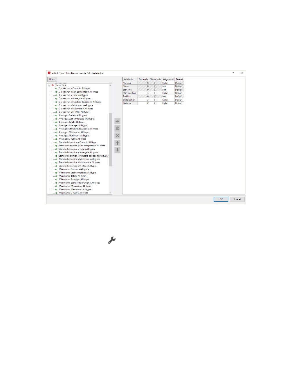
2.14.13 Setting a filter for selection of subattributes displayed
The columns are adjusted in the list.
2.14.13 Setting a filter for selection of subattributes displayed
If attributes have subattributes, the Attribute selection window might contain many entries for
selection on the left, e.g. for each time interval of the simulation runs.
If you want to transfer only certain types of subattributes to the right side, e.g. only for the
current simulation run, you can filter the entries on the left by subattributes. On the left, only the
filtered subattribute types are displayed. From these, you can choose the ones you want to
adopt into the right side. This is particularly useful for the evaluation of result attributes.
1. In the list, click the icon Attribute selection.
The Attribute selection window opens.
On the left, all attributes are shown that you can display in columns in the list (see
"Selecting attributes and subattributes for a list" on page 106).
On the right, the attributes are shown that are displayed with the current list layout.
2. Click the Filter button.
The Preselection Filter window opens.
3. Select the desired filter criteria:
110 © PTV GROUP

2.14.14 Using coupled lists
Element Description
Simulation
Runs
Setting filters for the simulation runs performed:
Current run: show only attributes of the current simulation run
Average: arithmetic and thus unweighted average of all simulation runs
Standard deviation between all simulation runs
Minimum of all simulation runs
Maximum of all simulation runs
Number of each simulation run started
Time Inter-
vals
Set filter for time intervals:
Last completed: Shows last time interval completed of the simulation run
selected
Total: Sum of all time interval values
Maximum of all time intervals
Minimum of all time intervals
Standard deviation between all time intervals
Average: arithmetic and thus unweighted average of all time intervals
x - y: specific, individual time intervals
Vehicle
Classes
Set filter for all vehicle classes or select vehicle classes. Only those vehicle
classes are displayed that were selected for the collection of separate results
during global configuration of the evaluation (see "Configuring evaluations of
the result attributes for lists" on page 954).
Pedestrian
Classes
Set filter for all pedestrian classes or select pedestrian classes. Only those
pedestrian classes are displayed that were selected for the collection of sep-
arate results during global configuration of the evaluation (see "Configuring
evaluations of the result attributes for lists" on page 954).
4. Confirm with OK.
Next to the Filter button, an entry indicates which sub-attributes are filtered. On the left, only
the selected subattribute types are displayed.
2.14.14 Using coupled lists
Many network object types and base data types have relations other network object types or
base data types. For instance, a vehicle class refers to the vehicle types it contains. For
convenient assignment and editing, Vissim automatically displays two lists next to each other:
In the list on the left, network objects of the type from which the relation begins are dis-
played together with the network objects' attribute values.
For the list on the right, you can select one of the network object types or base data types
with relations to the network object type in the left list.
© PTV GROUP 111

2.14.14 Using coupled lists
The left hand and right hand lists are linked to each other. If you select an object in the left list,
the right list automatically only shows objects with a relation to the object you selected. If there
are no such relations, only the column title is displayed. In the list, you can also select multiple
or all objects. Then the right list shows all objects that refer to the objects selected in the left
list.
You may edit attribute values in both coupled lists, with the exception of calculated attributes
and result attributes.
In the right list, you cannot add or delete objects unless they only exist within the objects in the
left list, e.g. the lanes of a link. Independent objects, to which multiple other objects might refer
(e.g. vehicle types of a vehicle class), can only be added or deleted in their own list or in the
Network editor. To add or delete such a reference, the relevant attribute must be shown in the
left list and changed there.
Synchronization with the global selection (in network windows and the Quick view) can be
activated in either of the lists on the left and on the right. If synchronization is activated on one
side , it is automatically deactivated on the other . For instance, in the coupled list
Routing Decisions/Routes , activate synchronization for routes to also display the routes
selected in the list in the Network window.
If on the toolbar you selected Synchronization, the network objects you select in the list are
highlighted in the Network Editor in 2D mode.
This is also the case for coupled lists, in the list on the right, for instance for the following
relations:
for Lanes, if the list on the left shows Links
for Pedestrian routes (static), if the list on the left shows Pedestrians In Network.
2.14.14.1 Selecting relations in coupled lists
Many network object types have relations to other network object types, such as to a link or to
multiple lanes. To show the objects of such a relation in both sections next to each other, open
the attribute list of the desired network object type. Then in the toolbar of the attribute list, in the
Relations list, click the network object type whose attributes you want to display in a list on the
right.
1. Open the list of the desired network object type.
If there is a relation, on the list toolbar, the Relations list box is displayed. By default, the
entry Single List is shown in the Relations list box.
2. Select the desired network object type in the Relations list box.
112 © PTV GROUP

2.15 Using the Menu bar
On the right, the coupled list, with the network object type to which the relation refers, is
opened. Only those objects are shown to which the objects selected in the left list refer.
By default, you can edit the list (see "Using lists" on page 89).
2.14.14.2 Showing the simple list only
When a coupled list is displayed, you can close the right list and only show the list on the left:
On the list toolbar, in the Relations list box, click Single List.
2.15 Using the Menu bar
You can call program functions via the menus in the menu bar. You can change the menu
entries. You can redo the default settings.
Note: Your user preferences are saved in the Windows registry and in the *.layx layout
file when Vissim is ended. The settings are used automatically when the program is
restarted.
2.15.1 Overview of menus
You can also move the menus to the user interface and change the sequence of entries (see
"Editing menus" on page 126).
Note: Changing program elements or shortcut keys can make it more difficult for you to
find and use commands. The documentation and the PTV Vision Support assume that
the standard settings are used.
2.15.1.1 File menu
Menu commands / key
combinations
Description
New If no network has been opened and the tab on the Start page
has been moved to the foreground, the tab is moved to the
background and the network editor is displayed in foreground.
If a network has been opened, it is closed. You can create a
new network.
If data was changed, a message is displayed asking whether
you want to save the network file before you close the network.
In any case, the user interface settings, graphic parameters of
the network editors and list settings are saved in a layout file
with the same name as the network file if this option is activated
under User Preferences (see "Specifying automatic saving of
the layout file *.layx" on page 145).
Open
CTRL+O
Import network file
You can drag an *.inpx network file from the Microsoft Win-
© PTV GROUP 113

2.15.1 Overview of menus
Menu commands / key
combinations
Description
dows Explorer to the user interface by drag&drop in order to
open the file.
In the Windows Explorer, you can also double-click a *.inpx
network file to open it.
If you open a network file containing 2D/3D model segments,
with a width that differs from the current Visum 2D/3D model
segments, a message is displayed. This message allows you to
copy the widths of the current Visum 2D/3D model segments to
all imported 2D/3D model segments.
Open Layout Select and read in the *.layx layout file, then apply it to the
elements of the user interface, the graphic parameters of
network editors, and the list settings (see "Saving and importing
a layout of the user interface" on page 138).
Open Default Layout Open and read in the defaults.layx layout file, and apply it to the
elements of the user interface, the graphic parameters of
network editors, and the settings in lists.
Read Additionally Network: Read network file *.inpx additionally (see "Read-
ing a network additionally" on page 341), (see "Importing
INPX files including building data" on page 843)
Named list layouts (see "Using named list layouts" on
page 104)
Named Network Editor layouts (see "Using named Net-
work editor layouts" on page 83)
Named chart layouts (see "Using named chart layouts" on
page 1070)
Simulation run (.sdf file, .db file) (see "Reading a sim-
ulation run additionally" on page 811)
Simulation runs (entire folder) (see "Reading simulation
runs additionally" on page 811)
Save
CTRL+S
Save network file *.inpx under the same path and name. In
addition, the settings for the user interface, graphic parameters
of the network editors, and the settings of lists are saved in a
layout file of the same name as the network file (if this option is
activated under User Preferences.
Save Base Network
Save Scenario
Save Modification
If in scenario management the base network is opened, Save
Base Network is shown, and you can only save the base net-
work. The same applies when you open a scenario or modi-
fications in scenario management.
Save as Open the Save File As window, and save the network file
under a new file name and/or to a different directory. The File
name box automatically shows the file name of the network file.
114 © PTV GROUP

2.15.1 Overview of menus
Menu commands / key
combinations
Description
If a different directory than the previous directory is chosen,
additional files needed for the network must be copied
manually to the new directory, e.g. supply files for signal
control.
If there is a ..\<Name of network file>.results directory for result
data, a query opens asking whether you want to save a copy of
the ..\<Name of network file>.results directory under the same
name as the *.inpx file. If you select No, the folder is not copied.
This way, you can avoid saving identical result data to different
directories when saving multiple versions of your network.
Save as Default Network The opened network is saved as a defaults.inpx file to the
following directory:
C:\Users\<Username>\AppData\Roaming\PTV Vision\PTV
Vissim 10
If a defaults.inpx file has been saved to this directory, it is
overwritten.
The default network is loaded when Vissim is opened and no
other network file is opened, e.g. when you double-click an
*.inpx file.
If you delete the defaults.inpx file from the
..\AppData\Roaming\.. path, the next time you open Vissim, the
defaults.inpx in your Exe installation directory of Vissim is used.
This command is not available when a scenario management
project has been opened.
Save Scenario as When in Scenario Management a scenario is opened, you can
save the scenario under a different name. The scenario saved
under another name is displayed in the project explorer under
Scenarios.
Save selection as Open the Save File As window, and save the selected network
objects to an *.inpx network file under a new file name and/or to
a different directory.
Save Layout as Save the current arrangement of user interface elements,
graphic parameters of network editors and the settings of lists to
a *.layx layout file in the following directory:
C:\Users\<Username>\AppData\Roaming\PTV Vision\PTV
Vissim 10
If a defaults.layx file has been saved to this directory, it is
overwritten.
If you delete the defaults.layx file from the path displayed, the
next time you open Vissim, the defaults.layx in your Exe
installation directory of Vissim is used.
© PTV GROUP 115
2.15.1 Overview of menus
Menu commands / key
combinations
Description
Save Layout as Default Save the following settings in the default layout file
defaults.layx:
the current arrangement of the user interface elements;
the graphic parameters of the network editor;
the current section of the background graphic and the back-
ground map, if a background graphic is loaded or a back-
ground map provider has been selected. In future Vissim
will open with the saved map section.
List settings
The defaults.layx file is normally located in the C:\Users\<user
name>\AppData\Roaming\PTV Vision\PTV Vissim 10 folder.
Vissim uses these settings for the default layout, when after
starting the program, you do not load a network, but create a
new network file.
Compare and Transfer
Networks Create Model Transfer File: (see "Creating model transfer
files" on page 1092)
Apply Model Transfer File...: (see "Applying model transfer
files" on page 1093)
Scenario Management Executing functions for scenario management:
Place under scenario management (see "Placing a net-
work under scenario management" on page 1084)
Open Base Network (see "Opening and editing the base
network in the network editor" on page 1086)
Open Scenario... (see "Opening and editing scenarios in
the network editor" on page 1087)
Open Modification... (see "Opening and editing modi-
fications in the network editor" on page 1087)
Save in highlighted scenarios (see "Project explorer tool-
bar" on page 1078)
Project Structure (see "Editing the project structure" on
page 1079)
Import ANM (Vistro)/Visum: Import ANM file (e.g. from Visum) (see
"Importing ANM data" on page 345)
ANM Adaptive... (see "Adaptive import of ANM data" on
page 349)
Import Synchro 7 data (see "Importing data from the add-on
module Synchro 7" on page 357)
Synchro 7 Adaptive (see "Importing Synchro 7 network
adaptively" on page 359)
CAD for Pedestrian Areas: Import CAD data that is used in
116 © PTV GROUP

2.15.1 Overview of menus
Menu commands / key
combinations
Description
pedestrian simulation to represent obstacles and walkable
areas (see "Importing walkable areas and obstacles from
AutoCAD" on page 835)
BIM (*.ifc) (see "Starting conversion in Viswalk" on page
839)
Export Export Visum (Nodes/Edges) (see "Exporting data" on
page 359)
Export 3ds Max data (see "Exporting static network data for
3ds Max" on page 366)
Open Working Directory Open Windows Explorer with the current working directory in
which the network file *.inpx is saved.
Show Log File Show vissim_msgs.txt log file (see "Using the vissim_msgs.txt
log file." on page 1119)
List of recently opened
files
Open one of the recently opened *.inpx network files. The list is
updated each time you open a network file *.inpx and save it
under a new file name. The update takes place before the File
menu is opened. *.inp files saved as a Vissim 6 version in any
previous program versions installed in parallel are not
displayed.
Exit Close Vissim. If data was changed, you are prompted whether
you want to save the network file. In any case, the user interface
settings, graphic parameters of the network editors and list
settings are saved in a layout file with the same name as the
network file if this option is activated under User Preferences
(see "Saving and importing a layout of the user interface" on
page 138).
2.15.1.2 Edit menu
Menu
command
Description
Undo
Undo with name of the last operation performed: discards this oper-
ation
Undo with subordinate menu, if multiple operations can be discarded: dis-
cards all operations, including the one selected
Redo
Redo with name of the last operation undone: performs this operation
again
Redo with subordinate menu, if multiple operations can be redone: per-
forms all operations undone, including the one selected
© PTV GROUP 117
2.15.1 Overview of menus
Menu
command
Description
Rotate
Network
Enter angle around which the network is rotated counterclockwise (see
"Rotating the network" on page 367)
Move
Network
Enter the distances for the x-axis, y-xis or z-axis by which the network is
moved (see "Moving the network" on page 368)
User Prefer-
ences
(see "Setting user preferences" on page 141)
2.15.1.3 View menu
Menu commands /
key combinations
Description
Open New Network
Editor
Open new Network editor. When a Network editor has been
opened, a new Network editor is added as a tab.
Start page Open start page (see "Using the Start page" on page 56)
Create Chart Open Create Chart window (see "Creating a chart without
preselection" on page 1063)
Network Objects Open network objects toolbar (see "Using the Network object
toolbar" on page 60)
Levels Open level toolbar (see "Using the Level toolbar" on page 65)
Backgrounds Open background toolbar (see "Using the background image
toolbar" on page 66)
Quick View Open Quick View (see "Using the Quick View" on page 66)
Smart Map Open Smart Map (see "Using the Smart Map" on page 69)
Project Explorer Open project explorer for scenario management (see "Using the
project explorer" on page 1076)
Messages Open window in which messages and warnings are displayed
(see "Showing messages and warnings" on page 1117).
Simulation time Switching the simulation time format for the status bar (see
"Specifying the simulation time format for the status bar" on page
139)
Simulation second
Simulation time based on start time in the simulation para-
meters. Format [hh:mm:ss,f]
Quick Mode
CTRL+Q
Activate or deactivate Quick Mode (see "Using the Quick Mode"
on page 85)
Simple Network Display
CTRL+N
Activate or deactivate Simple Network Display (see "Selecting
simple network display" on page 84)
2.15.1.4 Lists menu
The menu commands open lists with base data, network objects or result data.
118 © PTV GROUP

2.15.1 Overview of menus
Menu command Description
Base Data Lists for defining or editing the base data (see "Base data for
simulation" on page 192)
Network
Intersection Control
Private Transport
Public Transport
Pedestrian Traffic
Lists with attributes of network objects of the selected network
object type (see "Creating and editing a network" on page 314)
Graphics & Presentation Lists for defining or editing network objects and data, which are
used for the graphical preparation and realistic representation of
the network as well as the creation of presentations from
simulations.
Event-Based Scripts List of event-based scripts (see "Using event based script files" on
page 1111)
Measurements Lists for defining or editing network objects or collecting
simulation results
Results Result lists with data from evaluations of simulations (see
"Performing evaluations" on page 941)
2.15.1.5 Base Data menu
Menu items open a window for basic network settings and/or open lists with basic objects for
simulation (see "Base data for simulation" on page 192).
Menu
command
Description
Network Set-
tings
Basic network settings (see "Selecting network settings" on page 192)
User-
Defined
Attributes
List for defining or editing user-defined attributes (see "Using user-defined
attributes" on page 200)
Aliases List for defining and editing alternative attribute names (see "Using aliases for
attribute names" on page 209)
2D/3D Model
Segments
Axles, shafts, clutches, and doors of vehicle models (see "Attributes of 2D/3D
model segments" on page 218)
2D/3D
Models
2D models and 3D models for vehicles and pedestrians (see "Using 2D/3D
models" on page 210)
Functions Acceleration and deceleration behavior (see "Defining acceleration and
deceleration behavior" on page 221)
Distributions Distributions for desired speed, power, weight, time, location, distance,
occupancy, 2D/3D model, colors (see "Using distributions" on page 227)
Vehicle
Types
Combine vehicles with similar technical driving characteristics in vehicle types
(see "Using vehicle types" on page 254)
Vehicle Combine vehicle types (see "Using vehicle classes" on page 267)
© PTV GROUP 119

2.15.1 Overview of menus
Menu
command
Description
Classes
Driving
Behaviors
Driving behavior parameter sets (see "Defining driving behavior parameter
sets" on page 268)
Link Beha-
vior Types
Link behavior types for links and connectors (see "Defining link behavior
types for links and connectors" on page 299)
Pedestrian
Types
You can combine pedestrians with similar properties into pedestrian types
(see "Using pedestrian types" on page 830)
Pedestrian
Classes
Group pedestrian types and combine them into pedestrian classes (see
"Using pedestrian classes" on page 832)
Walking
Behaviors
Walking behavior parameter sets (see "Modeling area-based walking
behavior" on page 879)
Area Beha-
vior Types
Area behavior types for areas, ramps & stairs (see "Defining area behavior
types" on page 881)
Display
Types
Display for links, connectors and construction elements in the network (see
"Defining display types" on page 300)
Levels Levels for multistory buildings or bridge structures for links (see "Defining
levels" on page 868)
Time Inter-
vals
Time intervals (see "Defining time intervals for a network object type" on page
306)
2.15.1.6 Traffic menu
Menu
command
Description
Vehicle
Compositions
Define and edit vehicle compositions (see "Modeling vehicle compositions"
on page 425)
Pedestrian
Compositions
Define and edit pedestrian compositions (see "Modeling pedestrian
compositions" on page 877)
Pedestrian
OD Matrix
Define pedestrian demand on the basis of OD relations (see "Selecting
origins and destinations in the Pedestrian OD Matrix" on page 919)
Dynamic
Assignment Parameters: Defining parameters for dynamic assignment (see "Attrib-
utes for the trip chain file, matrices, path file and cost file" on page 731)
Matrices: Opening the Matrices list (see "Matrix attributes" on page 683)
Zones: open the list Zones (see "Modeling parking lots and zones" on
page 659)
OD pairs: open and display the OD Pairs list, origin zones and des-
tination zones
Edges: open the list Edges (see "Attributes of edges" on page 678)
Paths: Open the list Paths (see "Attributes of paths" on page 712)
Read Paths: Import the path file *.weg(see "Attributes of paths" on page
712), (see "Setting volume for paths manually" on page 745)
120 © PTV GROUP

2.15.1 Overview of menus
Menu
command
Description
Write Paths: Save current paths to path file *.weg
Create Static Routing from Assignment: convert the current state of the
dynamic assignment and thus also the paths found and their congestions
into a Vissim model with inputs and static routes (see "Generating static
routes from assignment" on page 750)
Calculating PTV Visum assignment (see "Using an assignment from
Visum for dynamic assignment" on page 752)
Toll Pricing
Calculation
Models
Opens the list Toll Pricing Calculation Models / Elements (see "Defining toll
pricing calculation models" on page 311)
Managed
Lanes
Facilities
Opens the list Managed Lanes Facilities / Pricing Models (see "Defining
managed lane facilities" on page 308)
2.15.1.7 Signal Control menu
Edit input data for signal control
Menu command Description
Signal
Controllers
Open the Signal Controllers list: Define or edit SC (see "Using signal
control procedures" on page 566)
Signal
Controller
Communication
Opens the SC Communication list (see "Linking SC" on page 636)
Optimize All
Fixed Time
Signal
Controllers
Start the green time optimization of all stage-based fixed time controllers
in the network (see "Performing green time optimization of stage-based
fixed time controllers" on page 573)
2.15.1.8 Simulation menu
Menu
command /
key
Description
Parameter Enter simulation parameters (see " Selecting simulation method micro or meso"
on page 796), (see "Defining simulation parameters" on page 796), (see
"Selecting the number of simulation runs and starting simulation" on page 801)
Continuous
F5
Starts continuous simulation run or switches from Simulation single step mode
to Simulation continuous mode.
Single Step
F6
Starts simulation in Simulation single step mode or switches from Simulation
continuous mode to Simulation single step mode or executes the next single
step.
Stop Quit simulation run
© PTV GROUP 121

2.15.1 Overview of menus
Menu
command /
key
Description
ESC
Check net-
work
Check Vissim network for inconsistencies (see "Checking the network" on page
812)
2.15.1.9 Evaluation menu
Activate and parameterize evaluations (see "Performing evaluations" on page 941)
Menu
command
Description
Configuration Define settings for the evaluation of simulation runs:
Result Management: (see "Managing results" on page 947)
Define output directory for evaluation files
Result Attributes: Configure data collection in result attributes: (see
"Configuring evaluations of the result attributes for lists" on page 954)
Direct Output: Configure output into files or databases (see "Configuring
evaluations for direct output" on page 957)
Database
Configuration
Configure the database connection (see "Configuring the database
connection for evaluations" on page 958)
Measurement
Definition
Show lists of network objects for measurements (see "Showing results of
measurements" on page 953)
Window Configure the display of signal times table, the SC detector record and signal
changes in windows (see "Showing evaluations in windows" on page 962)
Result Lists Open Result lists of evaluations (see "Showing result attributes in result lists"
on page 956)
2.15.1.10 Presentation menu
Create presentation (see "Creating simulation presentations" on page 1098)
Menu command Description
Camera Positions Open list Camera Positions (see "Attributes of camera
positions" on page 1099)
Storyboards Open list Storyboards / Keyframes (see "Using storyboards
and keyframes" on page 1100)
Record AVIs Only in 3D mode: Record a 3D simulation as a video file in
the file format *.avi (see "Starting AVI recording" on page
1104).
3D Anti-Aliasing Enable or disable 3D anti-aliasing (see "Selecting the 3D
mode and 3D recording settings" on page 143)
122 © PTV GROUP

2.15.1 Overview of menus
Menu command Description
Continuous Starts continuous animation run or switches from Animation
single step mode to Animation continuous mode.
Continuous (without ANI file) Starts a continuous animation run for the current simulation,
without using an ANI file.
Single Step Starts animation in single step mode or switches from
continuous animation run to single step mode or executes the
next single step.
Stop Finish animation run
Single Step Reverse Runs animation in reverse, single step mode.
Continuous Reverse Run animation reverse continuously
Animation with ANI file selected by default. Run animation with or without animation
file. If the command is not selected, only the animation of the
simulation in the network file currently open is run. Aggreg-
ated result attributes are used for visualization, e.g. for the
color of link segments or link bars (see "Running the anim-
ation" on page 1109).
Symbol Animation with ANI file is selected Animation with ANI file is not
selected
Animation
continuous
Opens a window in which you can select the
*.ani animation file of your choice. The
animation then runs continuously.
When a network file is loaded,
the animation of the simulation
runs continuously.
Animation
single step
Opens a window in which you can select the
*.ani animation file of your choice. The
animation then runs in single step mode.
When a network file is loaded,
the animation of the simulation
runs in single step mode.
While the animation is running, into the Go to second box, you can enter a simulation time of
your choice. This triggers an update of the Network editor and the result lists to the state of
the simulation, which corresponds to the specified simulation time period. Only aggregated
result attributes are used for visualization.
Animation Recordings Open list Animation Recordings (see "Defining an animation
recording" on page 1107)
Record Animations only in 3D mode: Switch recording on or off
2.15.1.11 Test menu
Perform testing of logic without simulation (see "Testing logics without traffic flow simulation"
on page 1094)
© PTV GROUP 123

2.15.1 Overview of menus
Menu
command
Description
Continuous Starts continuous test run or switches from Test run single step mode to Test
run continuous mode.
Single Step Starts simulation in Test run single step mode or switches from Test run
continuous mode to Test run single step mode or executes the next single
step.
Stop Quit test run
Record
Macros
Enabling and disabling macro creation. Enabled: A *.m_i macro file is saved to
the working directory.
Run Macro Select macro file *.m_i, enter simulation second until when you want to run
macro file, then start macro file
Edit Macro Open Macro Editor and edit macro (see "Editing a macro" on page 1096)
2.15.1.12 Scripts menu
Using the scripts, you manage script files and define the times at which you want to run the
script files during the simulation (see "Using event based script files" on page 1111)
Menu command Description
Event-Based Scripts Open list of event-based scripts
Run Script File Execute script file (see "Starting a script file manually" on page 1112)
Stop Running Script Stop initiated script file
2.15.1.13 Help menu
Access to information and documents about Vissim. For example, Help, information on current
Vissim installation, service and contact (see "Service and support" on page 46). Register
Vissim as COM server.
If during the installation of Vissim, a document was not selected for installation, the menu
command is grayed out and is not available.
Various documents are only available in English. If during the installation of Vissim, you select
the installation of documents for another language, these will still be installed in the ..\doc in
folder of the selected language.
Menu
command
Description
PTV Vissim
Help
Opens the Vissim Help located in the directory ..\exe (see "Using the manual,
Help and FAQ list" on page 46).
COM Help Opens reference documentation of the COM interface located in the ..\exe
directory.
PTV Vissim
Manual
Opens the user guide in pdf file format that is located in the ..\doc\<language>
directory.
124 © PTV GROUP
2.15.1 Overview of menus
Menu
command
Description
Introduction
to the
Vissim
COM API
Opens an Introduction to the VissimCOM interface Vissim <version> - COM
intro.pdf in English located in the ..\doc\<language> directory.
Open
document
directory
Opens the directory ..\Doc in the language selected under User Preferences >
General > Language > main language. All files saved to your computer during
the installation process are saved to this directory.
FAQ
(Online)
Show PTV Vissim FAQs on the web pages of PTV GROUP.
Service
Pack Down-
load
Show the PTV Vissim & PTV Viswalk Service Pack Download Area on the
webpages of PTV GROUP (see "Services by the PTV GROUP" on page 46).
Technical
Support
Show the support form of the Vissim Technical Hotline on the webpages of
PTV GROUP (see "Service and support" on page 46).
Examples Readme Examples: Open the file Overview of examples.pdf. The file con-
tains an overview of demo examples and training examples in the file
format *.inpx that can be installed during the installation of Vissim. By
default, the file Overview of examples.pdf is saved to the following path:
C:\Users\Public\Public Documents\PTV Vision\PTV Vissim 9
"First Steps" Tutorial: Open the file PTV Vissim - First steps.pdf. The file
contains a tutorial that provides a first insight into Vissim and practical
examples of how to use it. By default, the file is saved to a path similar to
the following: C:\Users\Public\Public Documents\PTV Vision\PTV Vissim
9\Tutorial First Steps
Open Demo Directory: Open the Windows Explorer and the directory
Examples Demo . The examples in the directories below illustrate typical
use cases of Vissim in subprojects. Each example is explained in *.pdf file.
The *.pdf file is always saved to the same directory as the example.
Open Training Directory: Open the Windows Explorer and show the dir-
ectory Examples Training. The examples in the directories below demon-
strate program functions or their combination in an easy to understand
context. Each example is explained in *.pdf file. The *.pdf file is always
saved to the same directory as the example.
License Open the License window (see "Showing program and license information" on
page 49).
Register
COM
Server
Register Vissim as COM server.
About
PTV Vissim
Open the Info about PTV Vissim window (see "Showing program and license
information" on page 49).
© PTV GROUP 125
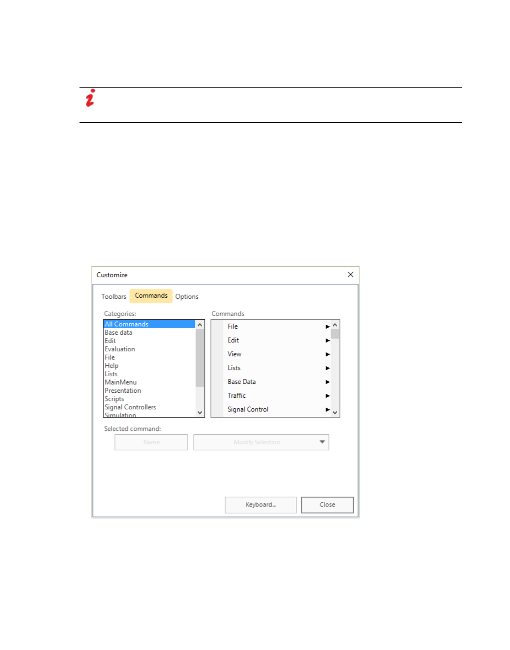
2.15.2 Editing menus
2.15.2 Editing menus
You can move or delete menus and menu entries.
Note: Changing program elements or shortcut keys can make it more difficult for you to
find and use commands. The documentation and the PTV Vision Support assume that
the standard settings are used.
You can restore the default settings (see "Resetting menus, toolbars, shortcuts, and dialog
positions" on page 146).
2.15.2.1 Showing menu entries several times
You can show menu entries in several menus or toolbars.
1. Right-click next to the menu bar.
A context menu opens.
2. Then select Customize.
The Customize window opens.
3. Select the Commands tab.
4. Under Categories, select the desired category.
5. Select the desired entry in the correspondingCommands list box.
126 © PTV GROUP

2.16 Using toolbars
6. Hold down the left mouse button and drag the entry to the position of your choice in the
Vissim menu.
7. Release the mouse button.
The entry is additionally displayed at the new position.
2.15.2.2 Deleting menu or menu entry
1. Right-click next to the menu bar.
A context menu opens.
2. Then select Customize.
The Customize window opens.
3. Hold down the left mouse button and drag the menu or menu entry from the user interface
of Vissim.
4. Release the mouse button.
The menu or menu entry is deleted from the user interface of Vissim.
2.15.2.3 Changing display of menus
1. Right-click next to the menu bar.
A context menu opens.
2. Then select Customize.
The Customize window opens.
3. Select the Options tab.
4. Make the desired changes.
2.16 Using toolbars
You can call program functions via the toolbars. You can change the position of toolbars and
edit toolbars. You can redo default settings of toolbars.
Note: Your user preferences are saved in the Windows registry and in the *.layx layout
file when Vissim is ended. The settings are used automatically when the program is
restarted.
© PTV GROUP 127

2.16.1 Overview of toolbars
2.16.1 Overview of toolbars
2.16.1.1 File toolbar
Symbol Name Description Hotkeys
New If no network has been opened and the tab on the Start page has
been moved to the foreground, the tab is moved to the
background and the network editor is displayed in foreground.
If a network has been opened, it is closed. You can create a new
network.
If you have changed data, you are prompted whether you want to
first save the network file. In any case, the user interface settings,
graphic parameters of the network editors and list settings are
saved in a layout file with the same name as the network file if this
option is activated under User Preferences (see "Specifying
automatic saving of the layout file *.layx" on page 145).
Open Open saved Vissim network. If in the same folder there is a layout
file of the same name, it is also read in.
CTRL+O
Save Save the Vissim network. In addition, the settings for the user
interface, graphic parameters of the network editors, and the
settings of lists are saved in a layout file of the same name as the
network file (if this option is activated under User Preferences.
CTRL+S
2.16.1.2 Edit toolbar
Symbol Description
Undo with the name of the last function performed: discards this func-
tion.
Undo with a list box if several functions can be discarded.
Redo with the name of the last function performed: performs this func-
tion again.
Redo with a list box if several functions can be restored.
Time interval after which the display of the current simulation is updated.
Value range: Each 0.1 simulation second (each time step) up to the entire
100 simulation seconds (all 1,000 time steps)
Toggle Quick Mode (see "Using the Quick Mode" on page 85)
Toggle Simple Network Display (see "Selecting simple network display"
on page 84)
2.16.1.3 Simulation toolbar
Start and stop simulation (see "Running a simulation" on page 796)
128 © PTV GROUP

2.16.1 Overview of toolbars
Symbol Name Description Key
Simulation
continuous
Starts continuous simulation run or switches from Simulation
single step mode to Simulation continuous mode.
F5
Simulation
single step
Starts simulation in Simulation single step mode or switches
from Simulation continuous mode to Simulation single step
mode or executes the next single step.
F6
Stop sim-
ulation
Stop started simulation run ESC
2.16.1.4 Animation toolbar
Start and stop animation (see "Running the animation" on page 1109) This toolbar is hidden in
the default layout.
To show the Animation toolbar, in the shortcut menu, right-click next to the toolbars (see
"Adapting the toolbar" on page 130).
Symbol Name Description
Animation
single step
reverse
Stops running animation and shows last step before the current sim-
ulation second.
Animation
continuous
reverse
Stops running animation and plays animation in continuous reverse
order.
Animation
continuous When no animation run is started: Opens a window in which you
can select the *.ani file of your choice. Then starts the continuous
animation run.
When the Animation single step mode is started: Lets animation
run continuously.
Animation
single step When no animation run is started: Opens a window in which you
can select the *.ani file of your choice. Then starts the animation
run and shows the step of the first simulation second.
When the Animation continuous mode is started: Stops animation
run and show next single step.
Stop anim-
ation
Finish animation run
Go to
second list
During an animation run, goes to the entered simulation second of the
animation run. Format: second [s] or time [hh:mm:ss.f], from simulation
second ZERO.
2.16.1.5 Test toolbar
Test signal control logic without simulated vehicles (see "Testing logics without traffic flow
simulation" on page 1094). This toolbar is hidden in the default layout.
© PTV GROUP 129

2.16.2 Adapting the toolbar
To show the Test toolbar, in the context menu, right-click next to the toolbars (see "Adapt-
ing the toolbar" on page 130).
Symbol Name Description
Test run
continuous
Starts continuous test run or switches from Test run single step mode
to continuous mode.
Test run
single step
Starts simulation in Test run single step mode or switches from Test
run continuous to Test run single step mode or executes the next
single step.
Stop test
run
Quit test run
2.16.1.6 View toolbar
If you have opened multiple windows, you can switch between them to place another window
in the foreground (see "Switching between windows" on page 89).
2.16.1.7 Toolbar in Network Editors
Change network display and navigate in the network (see "Network editor toolbar" on page
73)
2.16.1.8 Toolbar in lists
Change list layout and export data (see "List toolbar" on page 93)
2.16.2 Adapting the toolbar
You can position, show, hide, and adjust toolbars in the main window. The toolbars of network
editors and lists cannot be changed.
2.16.2.1 Positioning the toolbar
You can drag the toolbar to a desired position:
At the edges of the user interface of Vissim
To any position in the user interface of Vissim
1. Click the left edge of the toolbar and keep the mouse button held down.
2. Drag the toolbar to the desired position and release the mouse button.
The toolbar is shown with a title line.
2.16.2.2 Showing and hiding the toolbar
1. Click with the right mouse button on the empty area next to or below a toolbar.
The context menu opens. The selected options indicate which toolbars are shown.
130 © PTV GROUP

2.17 Mouse functions and key combinations
2. Select the desired options in the context menu.
2.16.2.3 Anchoring the toolbar
1. Click with the right mouse button on the empty area next to or below a toolbar.
The context menu opens.
2. From the context menu, choose the entry Lock the Toolbars.
You can no longer position the toolbar.
2.16.2.4 Creating your own toolbar
1. Right-click next to the menu bar.
A context menu opens.
2. Then select Customize.
The Customize window opens.
3. Select the Toolbars tab.
4. Click the New button.
5. Enter the desired data.
6. Confirm with OK.
The toolbar is shown as empty. You can integrate menu commands (see "Showing menu
entries several times" on page 126).
2.16.2.5 Deleting your own toolbar
You can delete only user-defined toolbars.
1. Right-click next to the menu bar.
A context menu opens.
2. Then select Customize.
The Customize window opens.
3. Select the Toolbars tab.
4. In the Toolbars section, click the entry you want to delete.
5. Click the Delete button.
The toolbar is deleted from the user interface of Vissim.
2.17 Mouse functions and key combinations
Many mouse functions and key combinations correspond to the default settings of your
Microsoft Windows operating system in Vissim, for example for highlighting, copying or
inserting.
© PTV GROUP 131

2.17.1 Using the mouse buttons, scroll wheel and Del key
In addition to these standards functions, you can use specific mouse functions and keyboard
combinations in Vissim (see "Using key combinations" on page 133). These are mentioned in
the description of the relevant functions in the Vissim Help and in the manual.
2.17.1 Using the mouse buttons, scroll wheel and DEL key
Key Description
Right
mouse
button
You can select the function of the right mouse button (see "Right-click behavior and
action after creating an object" on page 143).
Open context menu: Opens a context menu. Which functions are shown in the
context menu depends on the program element or the list you click on and
whether network objects are highlighted. To insert new network objects, press
CTRL and click. To insert new links, hold down the right mouse button and drag
the mouse.
Insert network object: To insert links and connectors, hold the right mouse but-
ton down and drag the mouse. To open the context menu, press the CTRL key
and right-click.
Left
mouse
button
Click in the Network editor to select a network object.
Hold the mouse button down and drag the mouse to move an object in the Net-
work editor.
Hold down the CTRL key and the mouse button to create a copy of the object in
the Network editor.
Hold down the ALT key and mouse button to rotate an object in the Network
editor. This function is only available for some network objects, for example for
areas or obstacles.
Double-click a network object in a Network editor to open a window in which you
can change the attributes of the selected network object (if there is such a win-
dow).
Double-clicking in lists:
Edit entry
If you can choose one of several attribute values, an attribute list is opened.
Middle
mouse
button
Drag the mouse to move the network section in the Network editor.
In the 3-D mode, press ALT to rotate the network display in the Network editor.
132 © PTV GROUP
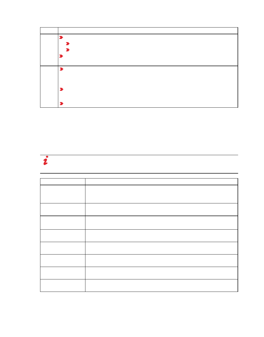
2.17.2 Using key combinations
Key Description
Scroll
wheel Rotating this changes the network display:
Rotate down: enlarge (zoom in)
Rotate up: reduce (zoom out)
Hold down the scroll wheel and drag the mouse: moves the network display in
the Network editor.
DEL Deletes all network objects currently selected in the network editor. If this means
that other objects must also be deleted, e.g. objects on a link, a message is dis-
played that you need to confirm before the network objects are deleted.
Removes a selected attribute value from a list, if you are allowed to edit or
delete the attribute.
Removes a network object from a list, if you selected the entire row.
2.17.2 Using key combinations
Normally you can use different key combinations in Vissim.
You can create and change your own key combinations for menu commands (see
"Customizing key combinations" on page 136).
Key combinations only function in activated Vissim main windows.
Note: Changing program elements or shortcut keys can make it more difficult for you to
find and use commands. The documentation and the PTV Vision Support assume that
the standard settings are used.
Hotkeys Description
CTRL+A In 2D mode: Toggle wireframe (see "Network editor toolbar" on page
73), (see "Setting up a road network or PT link network" on page 315),
(see "Moving network objects in the Network Editor" on page 336)
CTRL + B Show or hide backgrounds (see "Modeling the network for background
images" on page 379)
CTRL +C
CTRL+INS
Copy selected network objects to the Clipboard (see "Selecting and
copying network objects" on page 320)
CTRL+D Toggle 3D mode (see "Using 3D mode and specifying the display" on
page 183)
CTRL+E Only during simulation run: Toggle color of vehicle status (see "Dynam-
ically assigning a color to vehicles during the simulation" on page 165)
CTRL+N Activate or deactivate Simple Network Display (see "Selecting simple
network display" on page 84)
CTRL+O Open file. You can save the currently open network and load a saved
network file (see "Overview of menus" on page 113).
CTRL+Q Activate or deactivate Quick Mode (see "Using the Quick Mode" on
page 85)
© PTV GROUP 133

2.17.2 Using key combinations
Hotkeys Description
CTRL+S Save network file (see "Overview of menus" on page 113)
CTRL+T In 3D mode only: Switches between Rotate mode (3D) and Flight mode
(3D) (see "Navigating in 3D mode in the network" on page 183), (see
"Flight over the network" on page 185)
CTRL+U Switching the simulation time format for the status bar (see "Switching
the simulation time format for the status bar" on page 140)
CTRL+V
SHIFT+INS
Pasting network objects from the Clipboard (see "Pasting network
objects from the Clipboard" on page 321)
CTRL+Y Perform last operation undone again
CTRL+Z Undo last operation performed
TABULATOR Switches between network objects lying on top of each other at the
click position and highlights the next respective object (see "Selecting a
network object from superimposed network objects" on page 340)
CTRL+TABULATOR Switches between open lists and Network Editors (see "Structure of
lists" on page 90). Shows each of these in the foreground.
F5 Begins the continuous simulation. Switches to continuous simulation, if
simulation was started in Simulation single step mode (see "Selecting
the number of simulation runs and starting simulation" on page 801).
F6 Starts the simulation in Simulation single step mode.
Switches to single-step mode simulation, if continuous simulation
has been started.
Performs a single step, if simulation was started in Simulation
single step mode.
ESC Stop simulation (see "Selecting the number of simulation runs and
starting simulation" on page 801)
ENTER Opens the window with the network object attributes, if a network object
has been selected in the network editor.
SPACE BAR During a simulation in Simulation single step, executes the next step.
Switches to single-step mode simulation, if continuous simulation has
been started (see "Selecting the number of simulation runs and starting
simulation" on page 801).
+ If a continuous simulation has been started, increase the speed of the
simulation.
- If a continuous simulation has been started, reduce the speed of the
simulation.
* Maximum speed of the simulation.
Alternatively, press SHIFT++.
/ Go back to the last set simulation speed if this was not the maximum
speed.
Alternatively, press SHIFT+7.
134 © PTV GROUP

2.17.2 Using key combinations
Hotkeys Description
1 Simulation in real time, Simulation speed = 1.0
POS1 Show entire network (see "Displaying the entire network" on page 81)
PAGE UPZoom in (see "Zooming in" on page 80)
PAGE DOWN Zoom out (see "Zooming out" on page 80)
Arrow key Moves the observer position regarding the network to the desired
direction
A In 3D mode only: Move the current observer position horizontally to the
left. If you additionally press the SHIFT key, the speed is increased.
Alternatively for A, you can press the left arrow key.
D Only in 3D mode: Move the current observer position horizontally to the
right. If you additionally press the SHIFT key, the speed is increased.
Alternatively for D, you can press the right arrow key.
E In 3D mode only: Move current observer position vertically downwards
in terms of camera coordinates. If you additionally press the SHIFT key,
the speed is increased. It can correspond to the function of S,
depending on the orientation of the map.
F In 3D mode only: Move current observer position vertically downwards
in terms of z coordinate of the model. If you additionally press the SHIFT
key, the speed is increased. It can correspond to the function of S,
depending on the orientation of the map.
I In 3D mode only: Observer position with decreasing angle over
network
J In 3D mode only: Observer position rotating clockwise around z axis
K In 3D mode only: Observer position with increasing angle over network
L In 3D mode only: Observer position rotating counter-clockwise around
z axis
Q In 3D mode only: Move current observer position vertically upwards in
terms of camera coordinates. If you additionally press the SHIFT key, the
speed is increased. It can correspond to the function of W, depending
on the orientation of the map.
R In 3D mode only: Move current observer position vertically upwards in
terms of z coordinate of the model. If you additionally press the SHIFT
key, the speed is increased. It can correspond to the function of W,
depending on the orientation of the map.
S In 3D mode only: Zoom out.
Instead of S, if you press the PAGE DOWN key, it is zoomed out at larger
increments.
W In 3D mode only: Zoom in
Instead of W, if you press the PAGE UP key, it is zoomed in at larger
increments.
© PTV GROUP 135
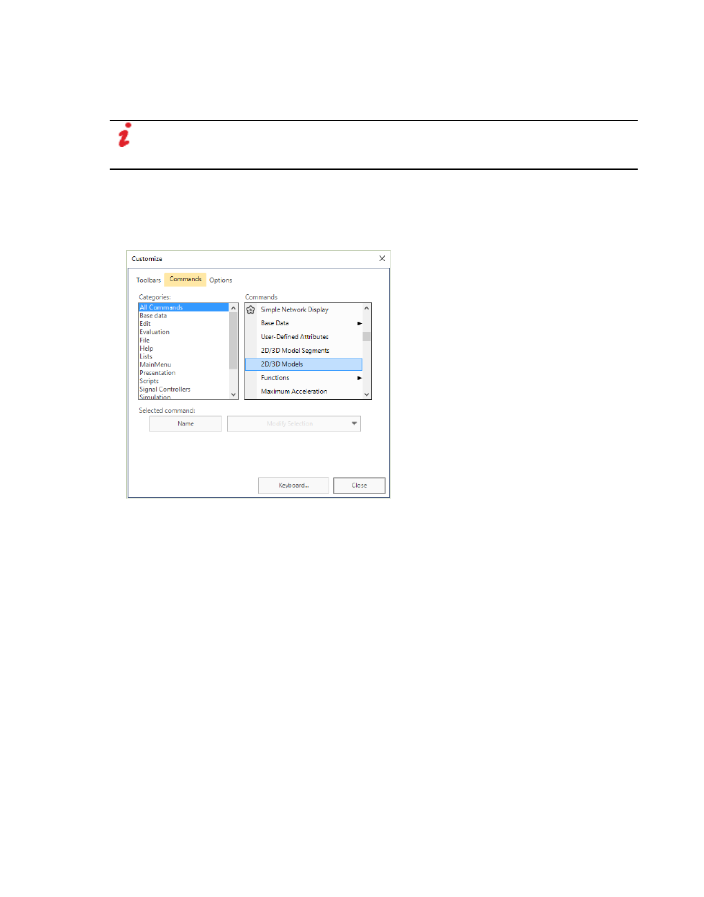
2.17.3 Customizing key combinations
2.17.3 Customizing key combinations
You can customize the keyboard mapping by specifying keyboard shortcuts.
Note: Changing program elements or shortcut keys can make it more difficult for you to
find and use commands. The documentation and the PTV Vision Support assume that
the standard settings are used.
1. Right-click under the title bar on the empty area next to the menu bar and the toolbar.
2. From the shortcut menu, choose Adapt.
The Customize window opens.
3. Click the Keyboard button.
The Customize keyboard window opens.
136 © PTV GROUP
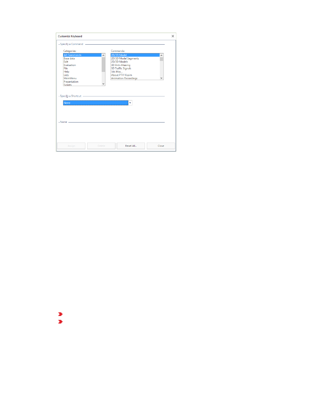
2.17.4 Resetting menus, toolbars, shortcuts, and dialog positions
4. Under Categories, select the desired menu.
5. Under Commands, select the menu command which you would like to apply for a new key
combination.
6. From the Keyboard shortcut list, select the desired key combination.
In the case that this key combination has already been used for a command, this command
is shown in the list.
7. Click Assign to confirm the selection.
If the key combination is allocated a different command, the combination is canceled.
8. Click the Close button.
9. Click the Close button.
2.17.4 Resetting menus, toolbars, shortcuts, and dialog positions
1. Choose Edit > User Preferences.
The User Preferences window opens.
2. Choose the entry GUI > General.
3. Click the button of your choice:
Reset Menu/Toolbar/Shortcuts
Reset dialog positions
A message opens confirming the reset. The next time you start Vissim, the respective interface
elements are displayed with their default settings and in their default positions.
© PTV GROUP 137

2.18 Saving and importing a layout of the user interface
2.18 Saving and importing a layout of the user interface
When you rearrange program elements, such as network editors, lists, the Quick view, the
Smart Map, toolbars, context menus, graphic parameters of network editors or column settings
of a list, you can save these settings in a *.layx file. You can re-import this layout and use it for
the user interface.
When you save a *.inpx file, the current layout is automatically saved under the same name as
the *.layx file, if this option is activated in the User Preferences (see "Specifying automatic
saving of the layout file *.layx" on page 145).
When you open a *.inpx network file, the layout is automatically imported from the *.layx file, if
it has the same file name as the network file and has been saved to the same folder.
The default network file defaults.inpx is read in and provides predefined base objects when
you start Vissim or from the File menu, choose New. The default layout file defaults.layx is read
in when you start Vissim. Both files are saved in the following directory:
C:\Users\<Username>\AppData\Roaming\PTV Vision\PTV Vissim
If the default network file and/or the default layout file are deleted, they are copied from the Exe
subfolder of the Vissim installation to the aforementioned directory when you start the
program.
In Network editors and lists, you can generate named layouts and use them again later. All
named layouts are saved in the layout file. You can also choose to only additionally read in
named Network editor layouts or list layouts from the layout file.
Note: Your user preferences are automatically saved in the registry of your computer.
These cannot be selected and imported in Vissim.
2.18.1 Saving the user interface layout
When you save a network in a *.inpx file, a *.layx file with the user interface layout is
automatically saved under the same name (if this option is activated under User Preferences
(see "Specifying automatic saving of the layout file *.layx" on page 145). You can also save the
user interface layout to a *.layx file under a different name, e.g. when you want to use the
arrangement of program elements and/or graphic parameter settings in network editors in
another network.
Note: Your user preferences are automatically saved in the registry of your computer.
These cannot be selected and imported in Vissim.
You can also save several *.layx files with different settings.
1. In the menu, select File > Save Layout as.
The Save layout file as window opens. By default the path to the opened network file is
selected. The File name box automatically shows the name of the layout file. By default, the
file type *.layx is selected.
2. Enter a unique name.
3. Click the Save button.
138 © PTV GROUP

2.18.2 Importing the saved user interface layout
The layout is saved in the *.layx file. You can reload the layout (see "Importing the saved user
interface layout" on page 139).
2.18.2 Importing the saved user interface layout
You can open a saved user interface layout to organize program elements, graphic
parameters of network editors, and the settings of list windows.
1. Select File > Open Layout in the menu.
The Load layout file window opens. By default the path to the opened network file is
selected. By default, the file type *.layx is selected.
2. Select the desired *.layx file of your choice.
3. Click the Open button.
Tip: You can also use a Drag-and-Drop operation to drag the file from the Microsoft
Windows Explorer to the user interface in order to open it.
2.19 Information in the status bar
The status bar is displayed at the bottom of the Vissim user interface interface. The status bar
is divided into the following areas. The information displayed in the areas depends on whether
or not a simulation is running:
Area Description
1st section left In 2D mode: Current coordinates of the mouse pointer (global coordin-
ates x,y in meters)
In 3D mode: fov (fieldOfView) = angle of view (FOV) of camera in
degrees from viewer's position.
2nd section Only during a simulation:
Current second or time of the simulation, followed by current cycle second
of an SC (see "Specifying the simulation time format for the status bar" on
page 139)
3rd section Only during a simulation:
Current number of vehicles in the network + current number of pedestrians in the
network
4th section Only during a simulation:
Real time factor of simulation speed
In parentheses: Number of vehicles that could be simulated close to real
time (only if in the simulation parameters, the simulation speed Max-
imum is selected)
if multiple simulations are running: Number of the current simulation run
(total of simulation runs) in the simulation parameters.
2.19.1 Specifying the simulation time format for the status bar
You can show the simulation seconds or the time.
© PTV GROUP 139

2.19.2 Switching the simulation time format for the status bar
Showing the simulation seconds
In the View menu, select > Simulation Time > Simulation Second.
Showing the time in the time format hh:mm:ss
Here the start time which is set in the simulation parameters is used (see "Defining simulation
parameters" on page 796).
From the View menu, choose > Simulation Time > Time of Day.
2.19.2 Switching the simulation time format for the status bar
During a simulation run, you may switch between the views Simulation Second and Time of
Day.
To do so, in the status bar, in the second box, double-click the simulation time.
Tip: Alternatively, press CTRL+U.
2.20 Selecting decimal separator via the control panel
Vissim shows data by default with the decimal separator that is set in the control panel of your
operating system.
1. Choose Start > Control panel.
The next step varies depending on your operating system.
2. Double-click on Time, Language and Region or Regional and Language Options.
3. If you use Microsoft Windows 7 or 8, click the Advanced Settings button in the Formats
tab.
4. In the Numbers tab, check the character in the Decimal separator list box.
5. You can change the settings if you wish.
140 © PTV GROUP

3 Setting user preferences
3 Setting user preferences
In the user preferences, you can make the following basic settings:
Select the language of the user interface of Vissim and the fallback language
Select the country for the country-specific information displayed on the start page
Restore default settings
Set the video compression for AVI recording
Settings for video compression and 3D mode
Select function for the right mouse button
Select the command you want executed after a new network object has been created.
Open the window with the attributes of the network object
Open the list with network objects of the network object type including the network
objects' attributes
None of the two commands
Check network at start of simulation
Select type of detector activation in the test mode
Specify default short name or long name for column headers
Define the number of functions last performed that are to be saved
Define the automatic saving of the layout file *.layx
Define default values for lane width, minimum gap time and minimum headway
Collect usage data
3.1 Selecting the language of the user interface
The available languages depends on the Vissim license.
1. In the Edit menu, choose > User Preferences.
2. In the navigator tree, choose GUI > General.
3. In the Main language list, click the language of your choice.
4. In the Fallback language list, click the language of your choice.
5. Confirm with OK.
The language setting is saved and is used in program elements and output files. The Main
language is used again the next time Vissim is opened.
If there is no translation available in the primary language for a text in the user interface, in the
Quick info describing an attribute or in an output file, Vissim automatically shows the text in the
fallback language. If there is no translation available in the fallback language, the text is
© PTV GROUP 141
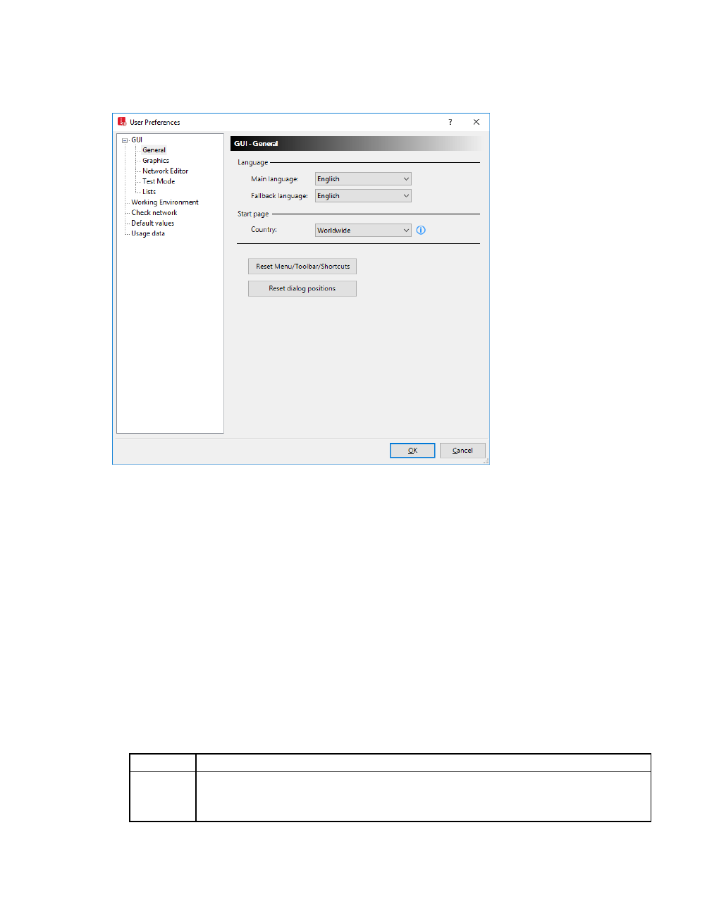
3.2 Selecting the country for regional information on the start page
displayed in English. If there is no English translation available, the text is displayed in the
original language. In most cases, the original language is German.
3.2 Selecting the country for regional information on the start page
The information on the start page may vary by region (see "Using the Start page" on page 56).
Some of it is available in different languages.
1. From the Edit menu, choose > User Preferences.
2. In the navigator tree, choose GUI > General.
3. Go to the Start page and select the desired entry in the -Country list box.
4. Confirm with OK.
3.3 Selecting a compression program
1. In the Edit menu, choose > User Preferences.
2. In the navigator tree, choose GUI > Graphics.
3. Make the desired changes:
Element Description
AVI
recording
Compression button: Open the Video compression window, and select a
default compression program for AVI recording (see "Starting AVI recording"
on page 1104).
142 © PTV GROUP

3.4 Selecting the 3D mode and 3D recording settings
4. Confirm with OK.
3.4 Selecting the 3D mode and 3D recording settings
1. In the Edit menu, choose > User Preferences.
2. In the navigator tree, choose GUI > Graphics.
3. Make the desired changes:
Section Description
3D
Mode Enable 3D mode: Select this option to show the 3D mode. After you restart
Vissim, the following icons are displayed in the toolbars of the Network editors:
2D/3D (see "Network editor toolbar" on page 73)
Edit 3D graphic parameters (see "Editing 3D graphic parameters"
on page 184)
Anti-aliasing: Select this option to reduce so-called “jaggies”, i.e. pixel
edges caused by screen resolution. Using this type of recording produces a
video of higher quality, however slows down the recording speed.
Background texture compression: Select this option to compress tex-
tures for background images. It might then take longer to load background
images. Select this option if your computer does not have sufficient video
memory.
Graphics driver: Graphics driver required for displaying objects during
simulation.
Ensure that your video card and the driver installed support the standard
selected.
Settings changes only become effective after you restart Vissim.
OpenGL 3.0: Default setting
DirectX 11: Allows access to Vissim in 3D mode via remote desktop
4. Confirm with OK.
The changes take effect after Vissim is restarted
3.5 Right-click behavior and action after creating an object
In the Network editor, you can define the right-click behavior. This means you can specify
whether a window or list for editing the attributes is automatically opened after you insert a
network object, or whether neither the list nor the window shall be opened.
1. In the Edit menu, choose > User Preferences.
2. In the navigator tree, choose GUI > Network Editor.
3. Make the desired changes:
© PTV GROUP 143

3.6 Showing and hiding object information in the Network editor
Element Description
Right click
behavior
Function, when you right-click in the network editor:
Right-click opens the context menu: The context menu of the Network
editor opens (see "Network editor context menu" on page 78)
To create new objects, press CTRL + right-click.
Right-click creates a new object: In the Network editor, a new network
object of the type selected in the Network objects toolbar is inserted.
To open the context menu, press CTRL + right-click.
Automatic
action
after
object cre-
ation
After you have added a new network object in the Network Editor, have
opened the window or list for editing the attributes, or have neither opened
the window nor the list.
For many network object types, you can not only edit the attributes in a list,
but also in a window. For some network object types, there is no window but
only the list, e.g. for vehicle inputs, pedestrian inputs, routng decisions /
routes, and conflict areas.
Show edit dialog if available, show list otherwise (default setting): If
there is a window for editing the attributes of this network object type,
open it, otherwise open the list of network objects of this type.
Show edit dialog if available, no action otherwise: If there is a window
for editing the attributes of this network object type, open it, otherwise do
not open a window or list.
Always show list: Always open the list of network objects of this type
No action: Do not open the list or window. The network object is inserted
into the Network Editor at the desired position.
4. Confirm with OK.
3.6 Showing and hiding object information in the Network editor
In the Network editor, in the Quick info, you can show Network editor attributes and attribute
values directly next to the network object. Depending on whether you insert the network
object, edit it or are point the mouse pointer towards it, different attributes and attribute values
are displayed.
You can show or hide the Quick info.
1. From the Edit menu, choose > User Preferences.
2. In the navigator tree, choose GUI > Network Editor.
3. Select or deselect Show Quick info in Network editor.
4. Confirm with OK.
144 © PTV GROUP

3.7 Configuring command history
3.7 Configuring command history
You can set that Vissim saves the recently executed functions as command history. You can
also define the number of the previously executed functions which should be saved.
From the Edit menu, choose the Undo icon to undo the maximum number of functions. To
redo them, click the Redo icon (see "Overview of menus" on page 113).
1. In the Edit menu, choose > User Preferences.
2. From the navigation tree, choose Working Environment.
3. Make the desired changes:
Element Description
Command history (Undo /
Redo) active If this option is selected, the previously executed
functions are saved.
You can use the Undo icon.
Maximum number of entries
in command history
Number of functions last performed that were saved and
shall be shown in the Edit > Undo menu.
Standard: 20
Maximum number: 49
4. Confirm with OK.
3.8 Specifying automatic saving of the layout file *.layx
1. In the Edit menu, choose > User Preferences.
2. From the navigation tree, choose Working Environment.
3. In the Auto-save layout section, make the settings of your choice.
Element Description
when network file (inpx) is saved Select this option to automatically save the
layout file *.layx when the network file *.inpx is
saved.
when network is discarded (e.g. File -
New) Select this option to automatically save the
layout file *.layx when you close the current
network.
4. Confirm with OK.
3.9 Defining click behavior for the activation of detectors in test mode
You can set whether you want to activate detectors in test mode with a single or a double click.
1. Choose Edit > User Preferences.
© PTV GROUP 145
3.10 Checking and selecting the network with simulation start
The User Preferences window opens.
2. Choose the entry GUI > Test Mode.
3. Make the desired changes:
Activate detector on double click: In the test mode, double-clicking switches the
detector call. A single click selects the detector and you can, for instance, look at the
attributes of the detector in the Quick View.D
Activate detector on single click (selection unavailable): Single click changes the
detector call. You cannot select detectors (see "Setting detector types interactively dur-
ing a test run" on page 1094).
4. Confirm with OK.
3.10 Checking and selecting the network with simulation start
When you start the simulation, Vissim automatically checks the Vissim network for certain
constraints that could prevent the simulation from starting. You can select whether you also
want Vissim to check the Vissim network for consistency when the simulation starts.
1. In the Edit menu, choose > User Preferences.
2. In the navigator tree, choose Check network.
3. Make the desired changes:
Element Description
Check network at
start of simulation If this option is selected, Vissim checks the Vissim network for
certain constraints and for consistency when the simulation is star-
ted.
If this option is not selected, Vissim only checks the Vissim net-
work for certain constraints that could prevent the simulation from
starting.
3.11 Resetting menus, toolbars, shortcuts, and dialog positions
1. Choose Edit > User Preferences.
The User Preferences window opens.
2. Choose the entry GUI > General.
3. Click the button of your choice:
Reset Menu/Toolbar/Shortcuts
Reset dialog positions
A message opens confirming the reset. The next time you start Vissim, the respective interface
elements are displayed with their default settings and in their default positions.
146 © PTV GROUP
3.12 Showing short or long names of attributes in column headers
3.12 Showing short or long names of attributes in column headers
In the column header of attribute lists, you can show the short or long name of an attribute.
1. In the Edit menu, choose > User Preferences.
2. In the navigator tree, choose GUI > Lists.
3. Select the desired option:
Short name
Long name
3.13 Defining default values
You can define default values that are assigned to links and priority rules when you add them
to your Vissim network.
1. From the Edit menu, choose > User Preferences.
2. In the navigation tree, select Default values.
3. Make the desired changes:
Element Description
Add link Use user-defined lane width: Select this option to enter the desired value
into the Lane width box. New links, with the lane width specified, are added in
the Network editor. Default 3.50 m
Add pri-
ority
rule
Use user-defined minimum gap time: Select this option to enter the
desired value into the Min. gap time box. New priority rules, with the width
specified, are added in the Network editor. Default 3.0 s
Use user-defined minimum headway: Select this option to enter the
desired value into the Min. headway box. New priority rules, with the width
specified, are added in the Network editor. Default 5.0 m
4. Confirm with OK.
3.14 Allowing the collection of usage data
As your PTV Vision team, we want Vissim to provide the functions you actually need and that
make work easier for you. To support us in this objective, activate the Collect usage data
option. We can then examine which parts of the program you prefer and how often you use
individual functions, e.g. via the number of clicks on menu items, the size of networks, the time
the Network editor is used or the duration of simulation runs. All data collected and sent to our
servers is fully anonymized. The data cannot be traced back to you or your workplace.
1. In the Edit menu, choose > User Preferences.
2. In the navigation tree, choose Usage data.
3. Make the desired changes:
© PTV GROUP 147
3.14 Allowing the collection of usage data
Element Description
Collect
usage
data
Collect and transfer usage data.
Log
usage
data loc-
ally
Only available if the option Collect usage data has been selected.
Opens the Telemetrydata_<yyyymmdd>_<hhmmss>.log file in the editor that is
installed as default on your computer. This file has been saved to the
%TEMP%\VISSIM folder. Files from the previous day are deleted when starting
Vissim.
148 © PTV GROUP

4 Using 2D mode and 3D mode
4 Using 2D mode and 3D mode
In the 2D mode, you can add, show, and edit network objects as well as run vehicle or
pedestrian simulations.
The 3D mode is used to show networks during a simulation or presentation in 3D.
4.1 Calling the 2D mode from the 3D mode
On the Network editor toolbar, click the D/3D button.
The button changes to . The Vissim network and vehicles are shown in 2D.
Tip: You can save your display options to and load them from the *.layx file.
4.2 Selecting display options
You can use Graphic Parameters to define the display of network objects in Network editors
for each network object type. In addition, you can select base graphic parameters for the
display of the network for each open Network Editor.
With 3D Graphic Parameters, you define the three-dimensional display of the network for each
open Network Editor.
For vehicles, pedestrians, links, areas, ramps and stairs, you can specify a colored display,
e.g. a dynamic display based on simulation data.
Simulations can also be run in the 3D mode (see "Using 3D mode and specifying the display"
on page 183).
Per default, they are shown in 2D.
4.2.1 Editing graphic parameters for network objects
You can set graphic parameters for the network objects of a network object type. Via graphic
parameters, you define the display of network objects in the Network editor last used.
You can also change graphic parameters during the simulation.
In the network object list, a preview button is displayed for the graphic parameter of each
network object type. The colors of the preview buttons depend on the graphic parameters
chosen.
Note: Graphic parameters can refer to attributes of network objects.
1. If several network editors are open, ensure that the network editor in which you want to
display the network objects with the modified graphic parameters is active.
© PTV GROUP 149

4.2.1 Editing graphic parameters for network objects
2. On the Network Objects toolbar, in the row of the network object type of your choice, click
the desired Edit graphic parameters button.
Icon Network object type Preview icon Graphic Parameters
(in default colors)
Links
Desired speed decisions
Reduced Speed Areas
Conflict Areas
Priority Rules
Stop Signs
Signal Heads
Detectors
Vehicle Inputs
Vehicle routes, in the list box :
Vehicle Routes (Static)
Vehicle Routes (Partial)
Vehicle Routes (Partial PT)
Vehicle Routes (Parking Lot)
Vehicle Routes (Dynamic)
Vehicle Routes (Closure)
Vehicle Routes (Managed Lanes)
Parking Lots
Public transport stops
Public Transport Lines
Nodes
150 © PTV GROUP

4.2.1 Editing graphic parameters for network objects
Icon Network object type Preview icon Graphic Parameters
(in default colors)
Data Collection Points
Vehicle Travel Times
Queue Counters
Flow bundles
Sections
Background Images No graphic parameters
Pavement Markings
3D Traffic Signals
Static 3D Models
Vehicles In Network
Pedestrians In Network
Areas:
Polygon
Rectangle
Obstacles, in the list box :
Polygon
Rectangle
Ramps & Stairs
Elevators
Pedestrian Inputs
Pedestrian routes, in the list box
Static
Partial
Pedestrian Travel Times
The list with the graphic parameters of the network object type opens (see "List of graphic
parameters for network objects" on page 152).
© PTV GROUP 151

4.2.2 List of graphic parameters for network objects
Tip: Alternatively you can also open the graphic parameters of a network object type via
the context menu.
1. On the network object toolbar, right click the network object type of your choice.
2. From the context menu, choose Edit graphic parameters.
1. Make the desired changes.
2. If you want to change colors, double-click the row of the desired graphic parameter.
3. Click next to the list when you want to close the list of the graphic parameters of a network
object type.
The list closes. The graphic parameters are assigned to the network objects of the network
object type.
4.2.2 List of graphic parameters for network objects
You can set graphic parameters for a type of network object for the network editor last used
(see "Editing graphic parameters for network objects" on page 149) . Depending on the
network object type, in addition to general graphic parameters, this may also be network
object specific parameters.
If network objects are composed of multiple components, you can assign separate colors to
some of them. For example, you can select the color for the mast and the signal arm of each
3D signal head.
You cannot define graphic parameters for backgrounds
When you display network objects in the network editor, the display type settings have priority
over the graphic parameter settings for network objects (see "Defining display types" on page
300).
4.2.2.1 General graphic parameters
You can define the following general graphic parameters for most network object types:
Graphic parameter Description
Object visibility If this option is selected, the network objects of this
network object type are displayed in a network editor
If an object of the network object type is selected, the
attribute cannot be deactivated.
If this option is not selected, the non-selected network
objects of this type are not displayed in the Network editor
when a different network object type is selected.
If this option is not selected, but Label visibility and a
label attribute have selected.
In the Network editor, only the labels of network
objects of this network object type are displayed.
152 © PTV GROUP
4.2.2 List of graphic parameters for network objects
Graphic parameter Description
In the Network editor, the network objects of this net-
work object type are not displayed.
The graphic parameters preview symbol is high-
lighted in a lighter color.
Label visibility Select this option to show a 2D label for each network
object of this type in the network editor.
By default, the label is displayed in the center of the
network object. In the Insert mode, use the mouse to move
the position of the respective network object type.
Label color Color of label
Label attribute Opens the window <Name of network object type: Select
Attribute>. Click the attribute whose value you want to
show as a label.
Label decimal places Number of decimal places in label
Label font size Font size of label in points (pt)
Use label color scheme Labeling of network objects using a color scheme based on
attribute values. Next to the margin on the right, click the
symbol to open the Edit Label Color Scheme window:
Classification by color: Attribute by whose values the
color is classified
Color for undefined value: Label color when the attrib-
ute lies outside the upper and lower limits
: Select a pre-defined color scheme that
contains class bounds and colors. The color schemes
vary in color and class bound.
Range scale factor:
Enter a factor for the upper bound and lower bound
Apply button: Multiply values of upper bounds and
lower bounds by a factor
Legend contains <parameter> The legend contains a description of the symbols and
colors of the network object types, for which under Graphic
parameters, you selected Legend contains <parameter>.
4.2.2.2 Network object specific graphic parameters
Graphic parameters for filling and outlines
The following network object types have graphic parameters for filling and outlines:
© PTV GROUP 153

4.2.2 List of graphic parameters for network objects
Reduced Speed Areas
Detectors
Parking Lots
Public transport stops
Public Transport Lines
Static 3D Models
Pedestrian Inputs
Links
Connectors in the graphic parameters of the network object type Links
Nodes and node segments
Sections
Elevators
Graphic parameter Description
Fill style
Connector fill style
Segment fill style
Solid fill: Display fill color or color scheme color in
the network object
No fill: Do not display fill color or color scheme color
in the network object. Select this option together with
the border line style No line to hide the network
object, irrespective of the attribute Object visibility.
Fill color
Connector fill color
Segment fill color
PT line fill color
Color within outline area of network object or color of
line. The graphic parameter Use display type must not
be selected.
Using the fill style Solid fill and a fill color with the Alpha
value set to 0 in the color definition, the network objects
of the network object type are transparent in 2D and 3D.
The transparent option for network object types should
only be used when absolutely necessary. This option
reduces the rendering speed and thus the display and
visualization quality of large, transparent objects.
Avoid using “Transparency” for a completely
transparent floor, for instance.
Use Transparency for windows or individual
transparent wall segments, for example. When
designing balustrades for escalators, a trans-
parent design creates a modern look. Addi-
tionally, pedestrians are more visible. The
window panes of vehicle models created as
ScetchUp files can be transparent.
Border line style Object border style:
154 © PTV GROUP

4.2.2 List of graphic parameters for network objects
Graphic parameter Description
Connector border line style
Segment border line style
Solid line
No line
Border color
Connector border color
Segment border color
Color of object border
Graphic parameters for line color
The network objects of the following network object types are displayed as a colored line that
run via a link or lane, or they contain lines. You define the line color via the graphic parameter
Line color:
Desired Speed Decisions
Stop Signs
Signal Heads
Vehicle Inputs
Queue Counters
Flow Bundles
Data Collection Points
Pavement Markings
Graphic parameters for Start line color, End line color, route course and public transport
stops.
The beginning and end of network objects of the following network object types are displayed
as a colored line that runs across a link or lane:
Priority Rules
Vehicle Travel Times
Public Transport Lines
Vehicle routes: For each type of vehicle route you may also specify the color of the route
course and of the public transport stops:
Static route color
Partial route color
Partial PT route color
Route closure color
Parking lot route color
Managed Lane general route color
Managed lane route color
Active stop color
Inactive stop color
© PTV GROUP 155

4.2.2 List of graphic parameters for network objects
Graphic parameter Description
Start line color Color of section at the beginning of network object
End line color Color of section at the end of network object
Graphic parameters for headways of priority rules
Graphic parameters Description
Headway visibility If this option and the destination section of a priority
rule are selected, the headway of the priority rule is
displayed in the 2D mode as a triangle across the lane
width. The triangle is pointing downstream. The number
of lanes is considered for which priority rules have been
defined.
Headway color Color of triangles in which headways are displayed, if
the attribute Headway visibility has been selected.
Graphic parameters for display of signal heads in 3D mode
Graphic parameter Description
Signal head display mode 3D as blocks
as stop lines: Display as stop lines on links for
vehicles and on links for which the attribute Is ped-
estrian area (option Use as pedestrian area) is
selected.
as stop lines (vehicle links only): Display as stop
lines on links for vehicles. Stop lines are not shown
in links for which the attribute Is pedestrian area
(option Use as pedestrian area) is selected.
Graphic parameters for display of 3D signal heads
You may specify the colors used in a 2D schematic diagram of the components of a 3D signal
head:
Graphic parameter Description
Signal arm color 2D Color of line that represents the arm
Outline color of circle at the end of the arm
Signal head color 2D Outline color of circle that represents the signal head
Mast color 2D Outline color of diamond that represents the mast
Streetlight color 2D Color of line that represents the street light arm
Outline color of rectangle at the end of the arm
Color 2D Outline color of 3D signal head
156 © PTV GROUP

4.2.2 List of graphic parameters for network objects
Graphic parameters for wireframe display of links and connectors
Graphic parameter Description
Wireframe color Color of links in wireframe display
Connector wireframe color Color of connectors in wireframe display
Graphic parameters for display of link bars and lanes
Dynamic attributes can only be shown as link bars, if in the graphic parameter Link bar
configuration, for the attribute Link bar representation > Segment-based is selected.
Graphic parameter Description
Link bar display type No link bars: Links are displayed without link bars.
Only link bars: Links bars are shown instead of
links.
Links and link bars: Links are displayed together
with link bars.
Link bar configuration Opens the Edit Link Bar window:
Link bar representation::
Segment-based: Link bars for individual segments
of the link
Link-based: Show link bars for entire link
Base color: Color of link bar, default RGB 190, 0, 0
Classification by width:
Attribute : The width of the link bars is based on
the values of the selected attribute and the following
settings. If the value is negative, the width is based on
the absolute value.
Width scale:
Automatic: Vissim specifies the width.
Manually: For the width, you can enter a minimum
value Scale (minimum): and a maximum value
Scale (Maximum). If the absolute value of the attrib-
ute is smaller than the specified minimum value, the
link bar is not drawn. If the absolute value of the
attribute is greater than the specified maximum
value, the link bar is drawn with its maximum width.
Scale bar width (maximum): maximum width for
link bars with automatic width
Lateral offset: Distance between links and link bars
Classification by color:
© PTV GROUP 157
4.2.2 List of graphic parameters for network objects
Graphic parameter Description
Attribute : The color of the link bars is based on the
values of the selected attribute and the following
settings:
Class bounds and colors:
Lower bound column: Value that represents the
lower bound of the selected attribute within this
value range. Based on value range after MIN, on
upper bound of the row above.
Upper bound column: Value that represents the
upper bound of the selected attribute within this
value range. The upper bound belongs the value
range.
Range scale factor:
Enter a factor for the upper bound and lower
bound
Apply button: Multiply values of upper bounds
and lower bounds by a factor
: Select a pre-defined color scheme that
contains class bounds and colors. The color schemes
vary in color and class bound.
Color of pavement markings Color of pavement markings between the lanes of links
with multiple lanes
Width of lane markings Width (in meters) of lane markings between the lanes of
links with multiple lanes, 0 = no markings.
Lane markings are no longer displayed when you zoom
far out of the Vissim network.
Graphic parameters for drawing mode of network objects
The colored display of network objects of the following network object types can be based on
graphic parameters that specify a permanent color, display type or color scheme. The colored
display of network objects can also be based on simulation data. Define the display via the
graphic parameter Drawing mode.
Links, nodes, sections, areas, obstacles, ramps & stairways:
Graphic parameter Description
Use consistent color Display network objects of the network object type in the
color of the graphic parameter Fill style.
Use display type Show network objects with display type assigned to
network object (see "Defining display types" on page
300)
158 © PTV GROUP

4.2.2 List of graphic parameters for network objects
Vehicles in network, pedestrians in network, links, nodes, areas, ramps and stairs:
Graphic parameter Description
Color scheme configuration Opens the Edit Color Scheme window: Select
classification based on attribute values of an attribute
and display network objects in this color scheme (see
"Assigning a color to vehicles based on an attribute" on
page 167), (see "Assigning a color to pedestrians based
on an attribute" on page 168), (see "Assigning a color to
links based on aggregated parameters" on page 169),
(see "Assigning a color to nodes based on an attribute"
on page 181), (see "Assigning a color to areas based
on aggregated parameters (LOS)" on page 172), (see
"Assigning a color to ramps and stairs based on
aggregated parameters (LOS)" on page 180)
The display of Vehicles In Network and Pedestrians In Network can be based on a color
distribution. The desired color distribution must be assigned to the desired vehicle type or
pedestrian type.
Graphic parameter Description
Color by color distribution During simulation, vehicles and/or pedestrians are
displayed in color according to the color distribution
assigned to your vehicle type or pedestrian type.
The display of Vehicles In Network during simulation may be based on the state of the
vehicles.
Graphic parameter Description
Color by driving state During simulation vehicles are displayed in a color that
represents their state. During a simulation run you may
switch between this view and the default view (see
"Dynamically assigning a color to vehicles during the
simulation" on page 165). You cannot edit the colors.
Graphic parameters for the display of vehicle and pedestrian shapes
Graphic
parameter
Description
Shape
(2D) Rectangle: Display vehicles and/or pedestrians as rectangles in 2D
mode. Simulations might run faster than possible with the graphic para-
meter Rounded.
Rounded: Display vehicles and/or pedestrians as rounded corners in 2D
mode. Simulations might run slower than possible with the graphic para-
meter Rectangle.
© PTV GROUP 159

4.2.2 List of graphic parameters for network objects
Graphic parameters for the display of areas and nodes based on their function
Graphic
parameter
Description
Color by
function Only for Nodes (see "Meaning of node color and line style" on page 673):
Select this option to visualize nodes based on their attribute values Use for
evaluation, Use for mesoscopic simulation and Use for dynamic
assignment:
If for the Fill style attribute, Solid fill is selected, nodes are filled with the
same color as the border.
If no node is selected, the border color depends on the node type selec-
ted:
Color and style of the bor-
der
node type selected
solid white no node type
solid green Use for evaluation
solid red Use for dynamic assignment
solid black Use for evaluation and for dynamic
assignment
white, dashed Use for mesoscopic simulation
not white, dashed Use for mesoscopic and other simulations
only for areas: This option is selected by default; the displayed area fill
color depends only on the area function:
Color Description
Magenta Platform edge is selected for the Public transport usage
attribute of the area.
Blue Waiting area is selected for the Public transport usage attribute
of the area.
Green A pedestrian input is located in the area.
Red A destination section of a pedestrian route is located in the area.
Gray All other areas
If an area has several functions, the order of the colors in the table
determines the fill color priority for displaying the area.
In wireframe display the colors are used for the edges of the areas.
Graphic parameter for turn value visualization
Visualize turn values graphically in the Network editor using result attributes of a node along
turn relations (see "Visualizing turn values" on page 645) , (see "Configuring turn value
visualization" on page 648).
160 © PTV GROUP

4.2.3 Editing base graphic parameters for a network editor
Graphic parameters for visualizing the volume on paths with flow bundles
Graphic
parameters
Description
Show flow
bundle bars
If a flow bundle or at least a filter cross section is selected, the volume on
the respective paths is displayed using flow bundle bars (see "Visualizing
volumes on paths as flow bundles" on page 726), (see "Show flow bundle
bars" on page 729).
Next to the margin on the right, click the symbol to open the Edit Flow
bundle bars window:
The classification by width is based on the flow bundle volume.
Width scale:
Automatic: Vissim specifies the width.
Manually: For the width, you can enter a minimum value Scale (min-
imum): and a maximum value Scale (Maximum). If the absolute value
of the attribute is smaller than the specified minimum value, the flow
bundle bar is not drawn. If the absolute value of the attribute is greater
than the specified maximum value, the flow bundle bar is drawn with its
maximum width.
Scale bar width (maximum): maximum width for flow bundle bars with
automatic width
Lateral offset: Distance between links and flow bundle bars
4.2.2.3 Graphic parameters with hatched cells
Hatched cells contain irrelevant attribute values that due to other attribute values have no
effect. If, for example, the Label visibility is deactivated, the graphic parameters Label color,
Label attribute, Label decimals and Label font size are shown hatched.
4.2.3 Editing base graphic parameters for a network editor
1. On the toolbar of the Network editor, click the button Edit basic graphic parameters.
The list of graphic parameters opens (see "List of base graphic parameters for network
editors" on page 161).
2. Select the desired entries.
3. If you want to change colors, double-click the row of the desired graphic parameter.
4. Click next to the list when you want to close it.
The list closes. The graphic parameters are assigned to the Network Editor.
4.2.4 List of base graphic parameters for network editors
You can set the following graphic parameters independently for every Network editor. You can
also change graphic parameters during the simulation.
© PTV GROUP 161
4.2.4 List of base graphic parameters for network editors
Long name Description
Background color Background color in 2D mode
Show map Display or hide background map in 2D mode. The desired map
must be selected in the base graphic parameter Map provider.
Map provider Select a background map from a background map provider
Map gray scale Display background map in gray tones or color
Map intensity Background map color intensity: 0 = no color, 100 = maximum
color intensity
Wireframe mode Toggle wireframe
Show scale Show or hide scale at the bottom left of the Network editor
Show grid Show 20 m grid as help to position network objects. If you zoom
out the network substantially, the grid is no longer shown.
Showing the simulation
time label
In the Network Editor, the current simulation time is displayed in
simulation seconds or as the time [hh.mm.ss]. The simulation
time is also recorded during the recording of *.avi files.
Simulation has not been started: 0.00 simulation seconds or
the time 00:00:00
Simulation in Continuous mode: Simulation time continues
to run
Simulation in Single step mode: The simulation time dis-
played is the time of the current single step. If you continue in
the Single step mode, the simulation second displayed will
only continue to run after the time intervals specified in the
simulation parameters under simulation resolution have
ended (see "Defining simulation parameters" on page 796).
Simulation time label pos-
ition
Display position of simulation time in the Network Editor
Simulation time offset Relative position of simulation time to the label position in the
Network Editor
First value: x position, default 15
Second value: y position, default 30
Simulation time label font
color
Font color of simulation time
Simulation time label font
size
Font size in pt of simulation time
Show logo Display the logo at the Logo position. The logo graphic file is
selected in the Logo filename box.
Logo position Position of logo in the network editor
Logo offset First value: Number of pixels by which the logo is moved
towards the x-axis.
Second value: Number of pixels by which the logo is moved
towards the y-axis.
162 © PTV GROUP
4.2.4 List of base graphic parameters for network editors
Long name Description
Logo file name Name of the logo graphic file Click the symbol to select the
file. Vissim supports the following file formats for logos:
Raster formats
*.bmp Windows bitmap, two-dimensional
*.jpg graphic compressed according to JPEG (Joint
Photographic Experts Group) standard
*.gif Graphics Interchange Format, compressed with no loss
in quality
*.tif Tagged Image File Format, uncompressed or packbits
compressed
*.png Portable Network Graphics, compressed with no loss in
quality
Automatic Level Trans-
parency
Select this option to draw network objects on underlying
layers with a decreasing level of transparency.
If this option is not selected, the network objects on all layers
are displayed the same way.
3D mode Toggle 3D mode
Selection color Color of selected network objects
Rubberband color Color of rectangle dragged open with the mouse for network
object selection
Show compass The compass rose to show the cardinal direction in the Network
editor Red tip = North
Compass position Display position of compass rose in the Network Editor You may
turn the compass rose.
Compass offset Relative position of compass rose in the Network Editor
First value: x position, default 0
Second value: y position, default 0
Show legend Select this option to display the legend at the legend
position. The legend contains a description of the symbols and
colors of the network object types, for which under Graphic
parameters, you selected Legend contains <parameter>.
Legend offset First value: Number of pixels by which the legend is moved
towards the x-axis. Default 10
Second value: Number of pixels by which the legend is
moved towards the y-axis. Default 10
Legend position Position in Network editor Default value Bottom right
Legend scale Factor for enlarged or reduced display of the legend. Value
range 0.01 to 100. Default 1.0
© PTV GROUP 163
4.2.5 Using textures
4.2.5 Using textures
Textures are graphic files which you can select instead of the default colors for the display of
the following elements in 3D mode:
Sky: a hemisphere is automatically displayed above the Vissim network. The texture is pro-
jected on it.
Note: A texture is displayed for the sky only if the graphics card of the computer has
at least a 16-bit Z-buffer. Otherwise, the insufficient depth resolution causes display
problems.
Land: The texture is displayed on the land area in which the Vissim network is located. If
the texture is less than the land area, it is displayed in a tiled format.
Links, connectors, areas, ramps and stairways: The texture is displayed in a tiled format on
these network objects.
You can select textures for network objects in the display types (see "Defining display types"
on page 300).
You can select textures for the sky and landscape via the 3D graphic parameters (see "Editing
3D graphic parameters" on page 184).
4.2.6 Defining colors for vehicles and pedestrians
Vissim can visualize individual vehicles and/or pedestrians as well as classified parameters
for links and areas. Visualization depends on the following graphic parameters and attributes:
Links: Links list > Show individual vehicles attribute or Link window > Display tab > Indi-
vidual vehicles option (see "Attributes of links" on page 383)
Areas: Areas list > Show individual pedestrians attribute or Pedestrian Area window >
Visualization section > Individual pedestrians option (see "Attributes of areas" on page
848)
Ramps & Stairs: Ramps & Stairs list > Show individual pedestrians attribute or
Ramps/Stairways/Escalators/Moving Walkways window > Visualization section > Indi-
vidual pedestrians option (see "Attributes of ramps, stairs, moving walkways and escal-
ators" on page 861)
Graphic parameter Use color scheme for links, vehicles in network, pedestrians in net-
work, areas, ramps & stairs (see "List of graphic parameters for network objects" on page
152).
You have the following options to visualize individual vehicles and pedestrians in color:
via colors and color distributions of classes and types of the vehicles, pedestrians or pub-
lic transport lines (see "Static colors of vehicles and pedestrians" on page 165)
for vehicles, color based on dynamic simulation data (see "Dynamically assigning a color
to vehicles during the simulation" on page 165)
164 © PTV GROUP

4.2.6 Defining colors for vehicles and pedestrians
color based on attributes (see "Assigning a color to vehicles based on an attribute" on
page 167), (see "Assigning a color to pedestrians based on an attribute" on page 168)
The status of signal heads is displayed at their position by a colored bar in addition to the
vehicles, for example red, red-amber, green.
You can assign display types to links and construction elements (see "Defining display types"
on page 300).
You can visualize links, areas, ramps, and stairs based on aggregated parameters (LOS) (see
"Assigning a color to links based on aggregated parameters" on page 169), (see "Assigning a
color to areas based on aggregated parameters (LOS)" on page 172), (see "Assigning a color
to ramps and stairs based on aggregated parameters (LOS)" on page 180).
4.2.6.1 Static colors of vehicles and pedestrians
Static colors are used for vehicles or pedestrians if neither the automatic nor the user-defined
dynamic coloring is active. Static colors are defined via the attributes of the vehicle type, the
pedestrian type, the vehicle class or the pedestrian class. For PT vehicles, the color is taken
from the respective PT line.
The table indicates which color is used, if you have defined colors for multiple objects:
Defined by
type
Defined by
class
Defined by bus line/tram
line
Display color based on
Color
distribution
- - Vehicle type, pedestrian
type
Color
distribution
Color - Vehicle class, pedestrian
class
Color
distribution
- Color PT line
Color
distribution
Color Color Vehicle class, pedestrian
class
The color of a PT line has priority over the color distribution of a vehicle type and the color of a
vehicle class or pedestrian class has priority over the color distribution of a vehicle type and a
PT line.
If a vehicle or pedestrian type belongs to multiple classes, vehicles or pedestrians of each type
are displayed in the color of the first class of these classes which has a defined color.
At the same time, you can also display the link segments in the simulation with colors based
on vehicular parameters (see "Assigning a color to links based on aggregated parameters" on
page 169).
4.2.6.2 Dynamically assigning a color to vehicles during the simulation
You can automatically assign vehicles a color based on their current status during the
simulation. Thus you obtain information about the movements of a vehicle in the simulation.
© PTV GROUP 165

4.2.6 Defining colors for vehicles and pedestrians
If the 3D models used do not only contain polygons with dedicated colors, automatic dynamic
coloring also works in 3D mode.
At the same time, you can also display the link segments in the simulation with colors based
on vehicular parameters (see "Assigning a color to links based on aggregated parameters" on
page 169).
1. Press CTRL+E in the Network Editor during the simulation.
The graphic parameter Color by driving state is selected. The following colors are used for
vehicles and are listed in descending priority. You cannot change these colors:
Color Description
White In queue: The vehicle is stuck in a traffic jam. At least one queue counter must be
defined in the network.
Light
blue
Waiting for lane change: Vehicle has been waiting more than 6s at the last
position for lane change (emergency stop distance).
Teal Ignores priority rule: Vehicle ignores priority rule to resolve a deadlock
situation.
Black In priority rule deadlock situation: Vehicle is part of a deadlock situation
caused by priority rules
Orange Wants to change lanes: Due to the vehicle route, a lane change becomes
necessary that the vehicle has not yet begun.
Light
green
Is changing lanes: Vehicle is changing lanes.
Dark
green
After lane change: Lane change was performed in the last 6 s.
Dark
red
Brakes to change lanes: Vehicle brakes, as it need to change lanes.
Amber Brakes cooperatively: Cooperative braking for an upcoming lane change
maneuver of a vehicle, from an adjacent lane to its own lane.
Red Sleep: Vehicle is currently not paying attention.
Dark
yellow
Ignores signal: Vehicle has decided in the last 3 seconds of simulation to
traverse a red signal head or a blocked section of a priority rule because its
speed was too high to come to a stop in advance.
Pink Brakes heavily: Vehicle brakes heavily (< -3.0 m/s²).
Purple Brakes moderately: Vehicle brakes moderately (-3.0 m/s² to -1.0 m/s²).
Navy
blue
Default: All other states (default)
2. Press CTRL+E again, to deactivate the graphic parameter Color by vehicle state. The
vehicle color is then no longer assigned based on simulation data.
166 © PTV GROUP
4.2.6 Defining colors for vehicles and pedestrians
4.2.6.3 Assigning a color to vehicles based on an attribute
Note: A vehicle color based on an attribute is only displayed if the colors are not
assigned automatically during the simulation (see "Dynamically assigning a color to
vehicles during the simulation" on page 165).
You may also display link segments in the simulation in colors based on traffic- related
parameters (see "Assigning a color to links based on aggregated parameters" on page 169).
1. On the Network objects toolbar, next to Vehicles In Network, click the Edit graphic
parameters button .
The list with the graphic parameters of the network object type opens (see "List of graphic
parameters for network objects" on page 152).
2. In the Drawing mode list box, click Use color scheme.
3. In the list of graphic parameters, click Color scheme configuration.
The window Edit Color Scheme for Vehicles In Network opens.
If the window does not open because the option has already been deactivated once since
program start, click the icon at the end of row to open the window.
4. Make the desired changes:
Symbol Element Description
Attribute Opens an attribute selection window. The result attributes
can be filtered (see "Setting a filter for selection of sub-
attributes displayed" on page 110).
Predefined
color
scheme
Open Select pre-defined color scheme list box: Select a
defined color scheme and show it in the Class bounds and
colors list. The color schemes vary in color and class bound.
Red-yellow-green: 11 classes, class size by default
0.500, 11 colors
Acceleration: 11 classes, 11 colors from pink to red, yel-
low, green to MAX = white
Speed: 11 classes, 11 colors from pink to red, yellow,
green to MAX = white
© PTV GROUP 167
4.2.6 Defining colors for vehicles and pedestrians
Element Description
Class
bounds and
colors list
Edit color scheme. From the shortcut menu, choose Add to add a new row to
the list and define additional class bounds and colors.
Lower bound column: Value that represents the lower bound of the
selected attribute within this value range. Based on value range after
MIN, on upper bound of the row above.
Upper bound column: Value that represents the upper bound of the
selected attribute within this value range. The upper bound belongs the
value range.
Column Color: Select the color. You may also enter RGB values.
The unit of the values depends on the attribute selected and is displayed in
the Classification section, below the attribute selected.
Range
scale
factor
Enter a factor for the upper bound and lower bound
Apply button: Multiply values of upper bounds and lower bounds by a
factor
5. If you want to change the RGB values in the Color column, double-click the desired row.
6. Select the desired colors.
7. Confirm with OK.
4.2.6.4 Assigning a color to pedestrians based on an attribute
In the 2D mode, pedestrians are displayed as colored oval shapes. You may assign individual
pedestrians a color based on attribute values.
Areas in which pedestrians move can be displayed based on LOS schemes (see "Assigning a
color to areas based on aggregated parameters (LOS)" on page 172).
1. On the Network objects toolbar, next to Pedestrians In Network, click the Edit graphic
parameters button .
The list with the graphic parameters of the network object type opens (see "List of graphic
parameters for network objects" on page 152).
2. Then select Color scheme configuration.
The window Edit Color Scheme for Pedestrians In Network opens.
If the window does not open because the option has already been deactivated once since
program start, click the icon at the end of row to open the window.
3. Make the desired changes:
168 © PTV GROUP
4.2.7 Assigning a color to links based on aggregated parameters
Symbol Element Description
Attribute Opens an attribute selection window. The result attributes
can be filtered (see "Setting a filter for selection of sub-
attributes displayed" on page 110).
Predefined
color
scheme
Select pre-defined color scheme list box: Select a defined
color scheme and show it in the Class bounds and colors
list. The color schemes vary in color and class bound.
Red-yellow-green: 11 classes, class size by default
0.500, 11 colors
Speed: 11 classes, 11 colors from pink to red, yellow,
green to MAX = white
Element Description
Class
bounds and
colors list
Edit color scheme. From the shortcut menu, choose Add to add a new row to
the list and define additional class bounds and colors.
Lower bound column: Value that represents the lower bound of the
selected attribute within this value range. Based on value range after
MIN, on upper bound of the row above.
Upper bound column: Value that represents the upper bound of the
selected attribute within this value range. The upper bound belongs the
value range.
Column Color: Select the color. You may also enter RGB values.
The unit of the values depends on the attribute selected and is displayed in
the Classification section, below the attribute selected.
Range
scale
factor
Enter a factor for the upper bound and lower bound
Apply button: Multiply values of upper bounds and lower bounds by a
factor
4. If you want to change the RGB values in the Color column, double-click the desired row.
5. Select the desired colors.
6. Confirm with OK.
4.2.7 Assigning a color to links based on aggregated parameters
During a simulation, you can display traffic-related parameters classified by color based on
link segments. For these traffic- related parameters, you can select result attributes of the
current simulation, e.g. volume, density, emissions or delay time (relative). For visualization of
the data, you can define colors or select color schemes that have been predefined, e.g. for
volume, density, emissions or delay time (relative). Thus you can easily differentiate the
vehicular parameters on the individual links during the simulation in the network, for example,
to quickly locate a hotspot in a large network.
© PTV GROUP 169
4.2.7 Assigning a color to links based on aggregated parameters
You can make similar settings for pedestrians in areas (see "Using LOS schemes for showing
aggregated pedestrian values" on page 176).
At the same time, you can also display the vehicles in the simulation in color based on their
attributes or simulation data (see "Assigning a color to vehicles based on an attribute" on page
167), (see "Dynamically assigning a color to vehicles during the simulation" on page 165).
1. Before starting the simulation, from the Evaluation menu, choose > Configuration > Result
Attributes tab > Links and make the following settings:
2. Select Collect data.
3. Into the From time and To time boxes, enter the simulation seconds during which you want
to collect data for a classified display.
4. Into the Interval box, enter the length of the time intervals for which you to aggregate data.
5. Click the More button.
6. Select how you want the data to be collected:
per lane segment: separately for each lanes
per link segment: for all lanes together
7. In the network objects toolbar, next to Links, click the Edit graphic parameters button .
The list with the graphic parameters of the network object type opens (see "List of graphic
parameters for network objects" on page 152).
8. In the Drawing mode list box, click Use color scheme.
9. In the list of graphic parameters, click Color scheme configuration.
The Edit Color Scheme for Links window opens.
If the window does not open because the option has already been deactivated once since
program start, click the icon at the end of row to open the window.
Under Classification based on, Lanes or Lane segments is selected. This depends on the
option per lane segment or per link segment of the configuration of the evaluation for links
(see "Showing data from links in lists" on page 1043).
10. In the Classification based on area, select Segments. Lanes have static attributes only.
11. Make the desired changes:
170 © PTV GROUP
4.2.7 Assigning a color to links based on aggregated parameters
Symbol Element Description
Attribute Opens an attribute selection window. The result attributes
can be filtered (see "Setting a filter for selection of
subattributes displayed" on page 110).
Predefined
color
scheme
Select pre-defined color scheme list box: Select a defined
color scheme and show it in the list below. The color
schemes vary in color and class bound:
Red-yellow-green: 11 classes, class size by default
0.500, 11 colors
Speed: 11 classes, 11 colors from pink to red, yellow,
green to MAX = white
Density: 11 classes, 11 colors from white to light blue,
blue to MAX = white
Volume: 11 classes, 11 colors from white to light blue,
blue to MAX = white
Relative delay: 11 classes, 11 colors from white to light
blue, blue to MAX = white
Element Description
List Lower bound column: Value that represents the lower bound of the selec-
ted attribute within this value range. From MIN, based on upper bound of
the row above.
Upper bound column: Value that represents the upper bound of the selec-
ted attribute within this value range. The upper bound belongs the value
range.
Column Color: Select the color. You may also enter RGB values.
The unit of the values depends on the attribute selected and is displayed in the
Classification section, below the attribute selected.
Range
scale
factor
Enter a factor for the upper bound and lower bound
Apply button: Multiply values of upper bounds and lower bounds by a
factor
12. If you want to change the RGB values in the Color column, double-click the desired row.
13. Confirm with OK.
4.2.7.1 Examples of colored links based on aggregated parameters
Speed attribute:
© PTV GROUP 171

4.2.8 Assigning a color to areas based on aggregated parameters (LOS)
Density attribute:
4.2.8 Assigning a color to areas based on aggregated parameters (LOS)
During a simulation, you can show a grid-based or area-based display of pedestrian attribute
values according to different LOS schemes (see "Using LOS schemes for showing aggregated
pedestrian values" on page 176). During simulation, this allows you to easily distinguish
between different areas in the network, e.g. in order to identify relevant differences in the
pedestrian density of a an area or different pedestrian speeds. You can set the display to 2D
or 3D mode.
When you choose Areas as a basis for classification, you can also show result attributes
during the simulation, namely the parameters Speed and Density and define classes for
them.
When as a basis for classification, you select Pedestrian Grid Cell Data, a grid is placed
over the network that is used as a basis to record its density, density of worst interval,
expected density, expected density of worst interval, speed and speed of worst pedestrian
interval. The parameter values are determined by cell and are visualized through the cell
color. For technical reasons, the 2D and 3D display might slightly differ where there is a
transition from areas to ramps and stairways.
172 © PTV GROUP

4.2.8 Assigning a color to areas based on aggregated parameters (LOS)
Note: To record these data, you need to configure the recording in the evaluation of
areas and ramps (see "Evaluating pedestrian density and speed based on areas"
on page 974). Otherwise, areas are displayed in their static colors during the
simulation.
You can, for example, show the average density in color during the last evaluation interval
of the simulation. To do so, select the attribute Density / Current run x Last completed.
Afterwards, during the simulation run, you can watch how the colors change depending on
the evaluation interval.
If the data of the attribute set is not yet available, because the time interval selected has not
begun yset, each area or cell is displayed in its static color. The latter is also used when no
color scheme has been activated.
In 2D mode, areas, ramps, and stairs defined for separate levels are displayed in different
transparent shades, depending on the height of the level they are on. This means the
colors can no longer be directly compared in the LOS display. For a comparison, open a
Network editor for each level whose objects you want to compare, and in it show the
respective level only. The objects are then shown in opaque colors and can be compared
in different Network editors.
In 3D mode, areas, ramps, and stairs on different levels are not displayed in "transparent"
in a Network. If you want to hide individual areas, ramps or stairs for comparison, in the
attributes of these objects, select a display type with the attribute invisible (see "Defining
display types" on page 300). Go to the graphic Parameters of the network object type, if you
want to select the transparent type of display for all network objects of a 2D and 3D network
object type: Fill style Solid fill and fill color with the Alpha value set to 0 in the color
definition (see "List of graphic parameters for network objects" on page 152).
You can make similar settings for links (see "Assigning a color to links based on aggregated
parameters" on page 169).
You can simultaneously show the pedestrians in color. This is based on the attributes of the
pedestrians (see "Assigning a color to pedestrians based on an attribute" on page 168).
4.2.8.1 Parameter-based area visualization - grid-based or area-based
You can choose between grid-based or area based for area visualization. You then configure
and activate visualization in the graphic parameters of the network object type Areas.
Option 1: Parameter-based area visualization - area-based
1. Before starting a simulation, make the following settings:
2. From the Evaluation menu, choose Configuration > Result Attributes tab > Areas &
ramps.
3. Select Collect data.
4. Into the From time and To time boxes, enter the simulation seconds during which you want
to collect data for a classified display.
5. Into the Interval box, enter the length of the time intervals for which you to aggregate data.
© PTV GROUP 173

4.2.8 Assigning a color to areas based on aggregated parameters (LOS)
6. Confirm with OK.
Option 2: Parameter-based area visualization - grid-based
1. Before starting a simulation, make the following settings:
2. From the Evaluation menu, choose > Configuration > Result Attributes tab.
3. In the Pedestrian Grid Cells row, select Collect data.
4. If desired, change the time and/or the interval (see "Configuring evaluations of the result
attributes for lists" on page 954).
5. Click the More button.
The Pedestrian Grid Cells window opens.
6. Make the desired changes (see "Grid-based evaluation of pedestrian density and speed"
on page 977).
7. Confirm with OK.
8. Confirm with OK.
4.2.8.2 Activating parameter-based area visualization
1. On the Network object toolbar, next to Areas, click the Edit graphic parameters button
.
The list with the graphic parameters of the network object type opens (see "List of graphic
parameters for network objects" on page 152).
2. In the Drawing mode list box, click Use color scheme.
3. In the list of graphic parameters, click Color scheme configuration.
If the window does not open because the option has already been deactivated once since
program start, click the icon at the end of row to open the window.
4. For an area-based classification, in the Classification based on section, select Areas.
5. For a grid-based classification, in the Classification based on section, select Pedestrian
Grid Cell Data.
6. Make the desired changes:
174 © PTV GROUP
4.2.8 Assigning a color to areas based on aggregated parameters (LOS)
Symbol Name Description
Attribute Opens a window that allows you to select an attribute or
subattribute.
Density
Density - duration exceeding threshold
Density (worst interval)
Level
Density experienced
Experienced density - duration exceeding threshold
Experienced density (worst interval)
Speed
Speed - duration exceeding threshold
Speed (worst interval)
Speed variance
Velocity variance - duration exceeding threshold
Ramp/Stairs
If in the evaluation configuration of pedestrian-grid cells, Only
last interval is selected, this enables the attributes Density
(worst interval), Experienced density (worst interval) and
Speed (worst interval) to display the corresponding results
aggregated.
The result attributes can be filtered (see "Setting a filter for
selection of subattributes displayed" on page 110).
Predefined
color
scheme
Open the Select pre-defined color scheme list box (see
"Using LOS schemes for showing aggregated pedestrian
values" on page 176): Show a defined color scheme in the
Class bounds and colors: list. The color schemes vary in
color and class bound.
© PTV GROUP 175
4.2.8 Assigning a color to areas based on aggregated parameters (LOS)
Name Description
Class
bounds and
colors list
Edit color scheme. From the shortcut menu, choose Add to add a new row
to the list and define additional class bounds and colors.
Lower bound column: Value that represents the lower bound of the
selected attribute within this value range. From MIN, based on upper
bound of the row above.
Upper bound column: Value that represents the upper bound of the
selected attribute within this value range. The upper bound belongs the
value range.
Column Color: Select the color. You may also enter RGB values.
The unit of the values depends on the attribute selected and is displayed in
the Classification section, below the attribute selected.
Range scale
factor Enter a factor for the upper bound and lower bound
Apply button: Multiply values of upper bounds and lower bounds by a
factor
7. If you want to change the RGB values in the Color column, double-click the desired row.
8. Select the desired colors.
9. Confirm with OK.
4.2.8.3 Using LOS schemes for showing aggregated pedestrian values
Alternatively, or in addition to displaying individual pedestrians in areas, on stairways, ramps,
moving sidewalks, and escalators, you can choose the LOS scheme to show aggregated
values in color, according to a color code. Using the LOS scheme is a quick and easy way to
gain an overview. You may also select a pre-defined red-yellow-green scheme.
Note: Areas that have reached or exceeded a capacity limit are displayed in red in all
predefined LOS schemes. This allows you to easily identify them.
You can choose to classify all areas and ramps by color, or only a user-defined square grid.
You can also choose the class boundaries for each color and the attribute, whose value
determines the class.
Predefined LOS schemes
Both subsequent tables contain predefined LOS schemes, which you can select in the Edit
color scheme window, in the graphic parameters for areas, ramps & stairs (see "Assigning a
color to areas based on aggregated parameters (LOS)" on page 172), (see "Assigning a color
to ramps and stairs based on aggregated parameters (LOS)" on page 180) . Under
Classification by color, you select a suitable attribute. When a predefined LOS-scheme is
selected, its predefined colors and class bounds are displayed in the Class bounds and
colors list. You can edit the colors and class bounds.
176 © PTV GROUP

4.2.8 Assigning a color to areas based on aggregated parameters (LOS)
Default schemes used in literature
Scheme Pedestrian
movements
Stairway Waiting
situations
Attribute
Fruin Density
[Ped/m²]
There is a different scheme for each pedestrian movement, stairs and waiting situation.
According to Fruin the breakpoints that determine the various levels-of-service have been
determined on the basis of the walking speed, pedestrian spacing, and the probabilities of
conflict at various traffic concentrations.
Numerically, these breakpoints are specified as density or flow. By defining both density and
flow limits, Fruin provides the traffic planner with the right strategy, as the level-of-service
concept is meant to assess walking quality up to a capacity limit. As soon as this limit is
exceeded, the capacity is neglected.
Weidmann Density
[Ped/m²]
Weidmann follows Pushkarev and Zupan and the HCM in stating eight criteria for
assessment of pedestrian walkway quality. Using eight further references, he describes the
level limits in words. Weidmann does not explain how his description in words is converted
into numerical limits.
HBS Density
[Ped/m²]
There is a different scheme for each pedestrian movement and waiting situation.
These level limits are similar to those of HCM (e.g. rounded values of metrical HCM data).
The importance of considering the effective width (or area) is pointed out. In addition, a factor
is given for calculation of the effective density with contraflows. Vissim calculates the level of
service based on the geometric area and does not account for contraflows.
HCM Density
[Ped/m²]
There is a different scheme for each pedestrian movement and waiting situation.
HCM refers to Fruin as originator of the LOS concept, but the breakpoints between levels are
set at considerably smaller values.
Pushkarev-Zupan Density
[Ped/m²]
Pushkarev and Zupan, along with Fruin, are credited in the HCM for having initiated and
done the principal work in developing the LOS concept.
Polus Density
[Ped/m²]
Pre-defined LOS scheme with five levels Breakpoint values are based on measurements
recorded in Haifa.
Tanaboriboon-Guyana Density
[Ped/m²]
© PTV GROUP 177
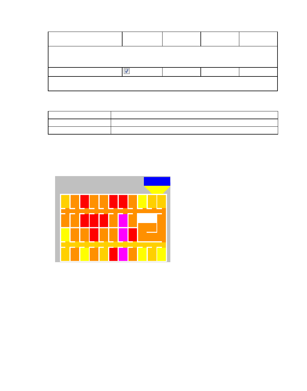
4.2.8 Assigning a color to areas based on aggregated parameters (LOS)
Scheme Pedestrian
movements
Stairway Waiting
situations
Attribute
The breakpoint values for this six-level scheme are based on measurements recorded in
Bangkok. So this is the only typically Asian scheme. It is the only LOS scheme with all
breakpoint values higher than the ones of the walkway LOS of Fruin.
Teknomo Speed [km/h]
In contrast to density-based LOS, this speed-based LOS scheme uses the opposite
sequence (starting with the worst LOS), as with increasing speed the LOS becomes better.
Schemes for user-defined classification
Scheme Attribute
Density Density in pedestrians/m²
Speed Speed in km/h
4.2.8.4 Examples of visualization of pedestrian parameters
Typical area-based visualization of essential parameters - examples
Example 1: Parameter Speed, with default settings:
Example 2: Parameter Density, with default settings:
178 © PTV GROUP

4.2.8 Assigning a color to areas based on aggregated parameters (LOS)
Typical grid-based visualization of essential parameters - examples
The parameters are depicted with the help of the simulation in the example file ..\Examples
Training\Pedestrians\Counterflow\Counterflow-2Rooms - Simple.inpx.
The image above is the result of the following configuration:
Parameter Value
Scheme LOS: User-defined: Density
Cell size 1.0 m
Range of influence 1
The image below is the result of the following configuration:
Parameter Value
Scheme LOS: User-defined: Density
Cell size 0.2 m
Range of influence 5
© PTV GROUP 179

4.2.9 Assigning a color to ramps and stairs based on aggregated parameters (LOS)
4.2.9 Assigning a color to ramps and stairs based on aggregated parameters (LOS)
During a simulation, you can visualize and classify traffic-related parameters of pedestrians on
ramps and stairs based on different LOS schemes (see "Using LOS schemes for showing
aggregated pedestrian values" on page 176) . Thus you can easily distinguish between
different traffic parameters at different positions in the network during simulation, for example,
to quickly locate a hotspot in a large network.
You can make similar settings for pedestrians in areas and vehicles on links (see "Assigning a
color to areas based on aggregated parameters (LOS)" on page 172), (see "Assigning a color
to links based on aggregated parameters" on page 169).
You can simultaneously show the pedestrians in color. This is based on the attributes of the
pedestrians (see "Assigning a color to pedestrians based on an attribute" on page 168).
1. Before starting a simulation, make the following settings:
2. From the Evaluation menu, choose Configuration > Result Attributes tab > Areas &
ramps.
3. Select Collect data.
4. Set the parameters as required.
5. Confirm with OK.
6. Confirm with OK.
7. On the Network object toolbar, next to Ramps & Stairs, click the Edit graphic parameters
button .
The list with the graphic parameters of the network object type opens (see "List of graphic
parameters for network objects" on page 152).
8. In the Drawing mode list box, click Use color scheme.
9. In the list of graphic parameters, click Color scheme configuration.
The window Edit Color Scheme for Ramps & Stairs opens.
If the window does not open because the option has already been deactivated once since
program start, click the icon at the end of row to open the window.
10. Make the desired changes:
Symbol Element Description
Attribute Opens an attribute selection window. The result attributes can
be filtered (see "Setting a filter for selection of subattributes
displayed" on page 110).
Predefined
color
scheme
Open Select pre-defined color scheme list box (see "Using
LOS schemes for showing aggregated pedestrian values" on
page 176): Select a defined color scheme and show it in the
list below. The color schemes vary in color and class bound.
180 © PTV GROUP

4.2.10 Assigning a color to nodes based on an attribute
Element Description
List UpperBound column: Enter values. The upper bound belongs the value
range.
Column Color: Select the color. You may also enter RGB values.
The unit of the values depends on the attribute selected and is displayed in
the Classification section, below the attribute selected.
Range
scale
factor
Enter a factor for the upper bound and lower bound
Apply button: Multiply values of upper bounds and lower bounds by a
factor
11. If you want to change the RGB values in the Color column, double-click the desired row.
12. Confirm with OK.
4.2.10 Assigning a color to nodes based on an attribute
You can have nodes displayed in a color based on the values of an attribute. To display nodes
in color, you can select a pre-defined color scheme or define one of your own.
1. On the Network object toolbar, next to Nodes, click the Graphic parameters button .
The list with the graphic parameters of the network object type opens (see "List of graphic
parameters for network objects" on page 152).
2. In the Drawing mode list box, click Use color scheme.
3. In the list of graphic parameters, click Color scheme configuration.
The Edit Color Scheme for Nodes window opens.
If the window does not open because the option has already been deactivated once since
program start, click the icon at the end of row to open the window.
4. Make the desired changes:
© PTV GROUP 181

4.2.10 Assigning a color to nodes based on an attribute
Symbol Name Description
Attribute Opens an attribute selection window. The result attributes
can be filtered (see "Setting a filter for selection of sub-
attributes displayed" on page 110).
Predefined
color
scheme
Open Select pre-defined color scheme list box: Select a
defined color scheme and show it in the Class bounds and
colors list. The color schemes vary in color and class bound:
Red-yellow-green: 11 classes, class size by default
0.500, 11 colors
Speed: 11 classes, 11 colors from pink to red, yellow,
green to MAX = white
Density: 11 classes, 11 colors from white to light blue,
blue to MAX = white
Volume: 11 classes, 11 colors from white to light blue,
blue to MAX = white
Relative delay: 11 classes, 11 colors from white to light
blue, blue to MAX = white
Level-of-service value: six classes, six semi-transparent
colors from blue to green and yellow to MAX = red
Name Description
Class
bounds and
colors list
Edit color scheme. From the shortcut menu, choose Add to add a new row to
the list and define additional class bounds and colors.
Lower bound column: Value that represents the lower bound of the
selected attribute within this value range. Based on value range after
MIN, on upper bound of the row above.
Upper bound column: Value that represents the upper bound of the
selected attribute within this value range. The upper bound belongs the
value range.
Column Color: Select the color. You may also enter RGB values.
The unit of the values depends on the attribute selected and is displayed in
the Classification section, below the attribute selected.
Range
scale
factor
Enter a factor for the upper bound and lower bound
Apply button: Multiply values of upper bounds and lower bounds by a
factor
5. If you want to change the RGB values in the Color column, double-click the desired row.
6. Select the desired colors.
7. Confirm with OK.
182 © PTV GROUP
4.3 Using 3D mode and specifying the display
4.3 Using 3D mode and specifying the display
The 3D mode is used to show networks during a simulation or presentation in 3D. You use the
2D mode to edit networks and network objects (see "Calling the 2D mode from the 3D mode"
on page 149).
4.3.1 Calling the 3D mode from the 2D mode
On the Network editor toolbar, click the 2D/3D button.
The button changes to . The Vissim network and vehicles are shown in 3D. The
network can be viewed from any desired perspective.
Notes:
When you load a bitmap graphic file and then call the 3D mode, the graphic file is
converted into a texture. This might delay the 3D display and require more memory.
Calculation of the size of a rectangular area accounts for static 3D models. This pre-
vents problems arising through the display of very large models and gaps from
being created between models and the area.
Tip: When you edit display options in the graphic parameters, your changes are saved
to the *.layx file as soon as you save the network file. You can also save a layout as a
*.layx file and to load it again later.
4.3.2 Navigating in 3D mode in the network
In the 3D mode, in the Network Editor toolbar, some features for navigating in the network
differ from the 2D mode:
Button Name Description
Show entire
network
Vertical and central top view on the network
Zoom out Gradually zoom out network view (see "Zooming out" on page 80)
Zoom in Gradually zoom in network view (see "Zooming in" on page 80)
Rotate
mode (3D)
Tilt or rotate the network display level vertically or horizontally.
Hold down the mouse button and drag the cursor up or down:
change height and angle of the observer position
Hold down the mouse button and drag the cursor left or right:
rotate the viewing point around the network.
Tip: Alternatively, press the ALT key and hold down the mouse
wheel, while moving the mouse.
Flight mode
(3D)
The observer position is continuously moved through the network
(see "Flight over the network" on page 185).
© PTV GROUP 183

4.3.3 Editing 3D graphic parameters
If you click the button Flight mode (3D), the button Rotate mode (3D) and the Rotate
Mode are deactivated.
If you click the button Rotate mode (3D), the button Flight mode (3D) and the Flight
Mode are deactivated.
4.3.3 Editing 3D graphic parameters
Note: Graphic parameters can be attributes of the network objects.
1. On the toolbar of the Network Editor, click the button Edit 3D graphic parameters.
The list of 3D graphic parameters opens (see "List of 3D graphic parameters" on page 184).
2. Select the desired entries.
3. If you want to change colors, double-click the row of the desired 3D graphic parameter.
4. Click next to the list when you want to close it.
The list closes. The 3D graphic parameters are assigned.
4.3.4 List of 3D graphic parameters
You can define the following 3D graphic parameters. You can also change 3D graphic
parameters during the simulation. 3D graphic parameters use the unit set for short distances
m or ft.
Base graphic parameters are taken into account (see "List of base graphic parameters for
network editors" on page 161).
Graphic
parameter
Description
Show land Shows or hides land area
Show map Display or hide background map in 3D mode. The desired map must be
selected in the base graphic parameter Map provider (see "List of base
graphic parameters for network editors" on page 161). If you zoom out of the
map view too far, Vissim no longer displays a background map. The
background is then gray.
Land texture Select graphic file for land area
Land texture
horizontal
length
Length of graphic in Network Editor
Land color Color of land area, if no texture is selected
184 © PTV GROUP

4.3.5 Flight over the network
Graphic
parameter
Description
Sky texture Allows you to select graphic file with a texture for the sky. The sky is displayed
as a hemisphere with a texture, if the 3D graphic parameter Show land is not
selected.
Sky color Color of sky, if no texture is selected
Underground
texture
Allows you to select graphic file with a texture for the underground. The
underground is displayed as a hemisphere with a texture, if the 3D graphic
parameter Show land is not selected.
Underground
color
Color of the underground, if no texture is selected The underground is
displayed in the color selected, if the 3D graphic parameter Show land is not
selected.
Fog mode Off
Linear: Define display of fog via a range. Enter distances for the 3D
graphic parameters Fog start and Fog end. The 3D graphic parameter
Fog density is disabled.
Exponential: Defines display of fog via a value for the density. The
3Dgraphics parameter Fog start and Fog end are disabled.
Fog density
(exponential
mode)
Density value, default value 6.0. With increasing value, the fog looks more
dense. The Fog mode Exponential must be selected.
Fog start (lin-
ear mode)
Distance of viewer position to the front of the fog. The default value is 0 m.
The Fog mode Linear must be selected.
Fog end (lin-
ear mode)
Distance of viewer position to the end of the fog. The default value is 250 m.
The Fog mode Linear must be selected.
Show shad-
ows
Show or hide shadows in static 3D models, for pedestrians and vehicles
Shadow
color
The default value is light gray 80, 0, 0, 0
Set the level of transparency: Double-click into the color box and use the
slider under Alpha to set the desired level of transparency.
4.3.5 Flight over the network
You can fly forward or backward over the network in 3D flight mode and change direction and
speed in the process.
1. Make sure that the icon Flight mode (3D) is selected in the toolbar of the Network
Editor.
2. Press the key of your choice or shortcut:
© PTV GROUP 185

4.3.6 Showing 3D perspective of a driver or a pedestrian
Purpose Key or shortcut
Execute flight forward
over the network
Hold down the W key.
Execute flight
backward over the
network
Hold down the S key.
Change direction of
the flight
You have the following options:
To the left: Additionally hold down the A key during flight sim-
ulation.
To the right: Additionally hold down the D. key during flight sim-
ulation.
Choose direction freely: Hold down the mouse button during
flight simulation, and drag the cursor to the desired position.
Increase speed of
flight
Additionally hold down the SHIFT button during flight simulation.
4.3.6 Showing 3D perspective of a driver or a pedestrian
You can select a vehicle or a pedestrian and show the view from their perspective in 3D mode.
You can select another vehicle or pedestrian in any opened network editor to show different
persepectives at the same time.
You can save the 3D perspective of a driver or pedestrian as a camera position. You can use
the driver perspective or pedestrian perspective for AVI recordings (see "Recording a 3D
simulation and saving it as an AVI file" on page 1098).
When you choose the camera position driver perspective, as in reality, the vehicle itself is not
visible. When you choose a camera position outside the driver perspective, parts of the vehicle
are displayed. This allows you to position the camera freely and choose a camera position
attached to a vehicle or inside a vehicle. This applies accordingly to pedestrians.
4.3.6.1 Showing 3D perspective via a Network editor
Note: If under User Preferences, you selected Right-click creates a new object, hold
down the CTRL key for the next step (see "Right-click behavior and action after creating
an object" on page 143).
1. In a Network editor, in the single-step mode, right-click the vehicle or pedestrian of your
choice.
2. From the context menu, choose the respective command.
View From Driver's Perspective
View From Pedestrian's Perspective
In the Network editor, the perspective of your choice is shown in 3D mode.
186 © PTV GROUP

4.3.6 Showing 3D perspective of a driver or a pedestrian
Note: If under User Preferences, you selected Right-click creates a new object, hold
down the CTRL key for the next step (see "Right-click behavior and action after creating
an object" on page 143).
3. If you want to exit the perspective, right-click the Network Editor.
4. From the context menu, choose the respective command.
Leave Driver's Perspective
Leave Pedestrian's Perspective
Tip: Alternatively, you can switch back to the 2D mode.
4.3.6.2 Showing 3D perspective via a result list
1. From the Evaluation menu, choose Result Lists > Vehicles In Network or Pedestrians In
Network.
The result list opens.
2. Click on the desired vehicle or pedestrian in the result list.
3. The vehicle or pedestrian is marked in the Network Editor.
The next step can be more easily executed in single-step mode or at a lower simulation
speed.
4. Double-click the marked vehicle or pedestrian in the Network Editor.
The perspective changes. When the vehicle or the pedestrian reaches its destination, the
perspective is exited automatically.
5. If you want to exit the perspective, right-click or double-click into the Network Editor.
© PTV GROUP 187

4.3.7 Changing the 3D viewing angle (focal length)
6. From the context menu, choose Leave Driver's Perspective or Leave Pedestrian's
Perspective.
The simulation continues to run in 3D mode.
4.3.7 Changing the 3D viewing angle (focal length)
You can select the viewing angle in 3D mode. This corresponds to the setting of the focal
length in photography.
The default perspective in Vissim is 45°. This corresponds to a focal length of 43mm in a
35mm system.
If you want to reduce the perspective by two degrees, press the CTRL+PAGE UP keys.
If you want to enlarge the perspective by two degrees, press the CTRL+PAGE DOWN keys.
The current perspective is displayed in the first column of the status bar during the change.
Notes:
Vissim does not save any changes to the perspective. The default perspective is set
again the next time you open Vissim.
The modification of perspective applies to Rotate mode (3D) and Flight mode (3D)
and all keyframes.
The table displays the corresponding focal lengths for different perspectives:
Perspective Focal length
(35 mm)
Perspective Focal length (35 mm)
4° 500 mm 38° 53 mm
7° 300 mm 40° 50 mm
10° 200 mm 44° 45 mm
11° 180 mm 54° 35 mm
15° 135 mm 65° 28 mm
20° 100 mm 72° 25 mm
24° 85 mm 81° 21 mm
29° 70 mm 90° 18 mm
4.3.8 Displaying vehicles and pedestrians in the 3D mode
You can assign 3D models via model distributions to any type of vehicle or pedestrian (see
"Using 2D/3D model distributions" on page 248).
4.3.9 3D animation of PT vehicle doors
Select the desired 3D model of the PT vehicle (see "Using 2D/3D model distributions" on
page 248).
The 3D model of the PT vehicle is displayed.
188 © PTV GROUP
4.3.9 3D animation of PT vehicle doors
For 3D models whose model file *.v3d includes vehicle doors as modeled areas, the opening
and closing of sliding doors or double doors at PT stops is also visualized in the 3D mode.
Tip: Under Base Data > 2D/3D Models, you can use the model Tram - GT8-2S as an
example. With the Bus - EU Standard model, the doors are not modeled as areas. This
is why the opening and closing of sliding doors is not displayed in the 3D mode.
4.3.9.1 Requirements for the animation of doors
Boarding and/or alighting via the door is permitted.
Boarding and/or alighting at the PT stop is permitted.
The door is located at a permissible platform position at the PT stop.
If there is no platform edge and there are thus no passengers, then the door must be loc-
ated at a permissible position within the PT stop length.
4.3.9.2 Temporal restrictions for opening the doors
The doors are opened for 1.5 seconds as soon as the vehicle comes to a standstill at the PT
stop.
4.3.9.3 Temporal restrictions for closing the doors
For calculated dwell times: The doors start to close 3 seconds prior to the end of the dwell
time.
For passengers in Viswalk: The doors start to close after no passenger has boarded or
alighted the vehicle for 3 seconds.
The closing of the doors always takes two seconds.
During the first of these two seconds, the doors will open again if a passenger wants to
use one of them.
During second of these two seconds, passengers behave as if the doors were already
closed.
Once the doors are closed, the vehicle waits another second before it departs.
The number of time steps depends on the simulation resolution.
4.3.9.4 Moving door polygons when doors are opened
The door is moved perpendicular to the vehicle by 6 cm (duration: 0.3 seconds)
It is further moved by its width in parallel to the vehicle element heading towards the dir-
ection with the greater distance to the next door and/or end of the vehicle.
Closing the doors corresponds to moving the door polygons in reverse order and direction.
© PTV GROUP 189
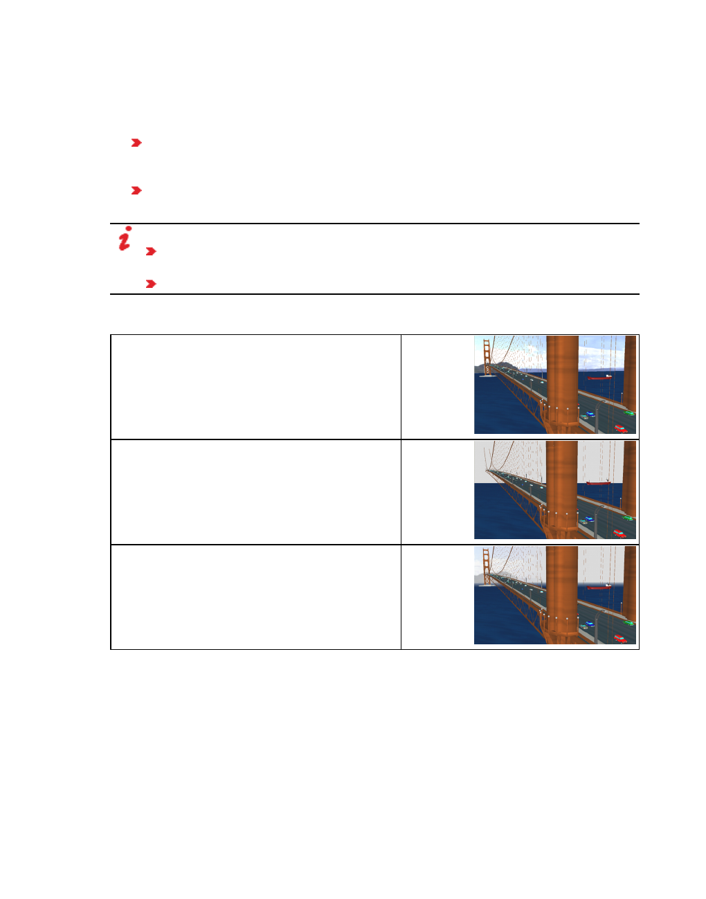
4.3.10 Using fog in the 3D mode
4.3.10 Using fog in the 3D mode
For realistic simulations in 3D mode, you can add fog (see "List of 3D graphic parameters" on
page 184).
Linear mode from Fog start to Fog end. From the observer until Fog start, visibility is
100%. The fog looks dense if you choose a short distance between Fog start and Fog
end. The fog looks less dense, the longer the distance is.
Exponential The fog begins at the location of the observer based on the Fog density
defined in the 3D graphic parameter.
Notes:
Vissim saves no settings with regard to fog. If Vissim is closed and then reopened;
the fog is switched off.
The switching on of fog applies for all keyframes.
Examples of different types of fog effects
Fog mode: Off
Fog mode: Linear
Fog start 0.0 m: Fog starts at the location of the
observer.
Fog-end 100.0 m: Visibility extends until the point
of Fog end.
Fog mode: Linear
Fog start 40.0 m: Fog starts at a distance of 40 m
from the observer.
Fog end 90.0 m: Visibility is limited from the point
of fog start at 40.0 m and extends 50.0 m far until
the point of fog end at 90.0 m.
190 © PTV GROUP

4.3.10 Using fog in the 3D mode
Fog mode Exponential: Fog starts at the position
of the viewer.
Fog density Default value 6.0: Fog density is
relatively low, visibility is not limited.
Fog mode Exponential: Fog starts at the position
of the viewer.
Fog Density: 30.0. This value is five times greater
than the default value 6.0. This means visibility is
very limited.
© PTV GROUP 191

5 Base data for simulation
5 Base data for simulation
The stochastic nature of traffic begs the necessity to provide this type of variability in Vissim
models. The heart of Vissim, Wiedemann's car- following model, accounts for this by
implementing parameters based on stochastic distribution (see "Operating principles of the car
following model" on page 32).
The base data for simulation includes the settings for the entire network and all basic objects
for modeling vehicle and pedestrian movement, e.g. distributions, functions, and behavior
parameters. Base data further contains types and classes. These allow you to group
properties that are the same for many network objects, so that you need not set them for each
individual object.
In addition to input and output attributes, you can define user-defined attributes for all objects.
User-defined attributes may be edited and managed in lists in the same way as predefined
attributes.
For each attribute, you can specify an alternative name as an alias (see "Using aliases for
attribute names" on page 209).
5.1 Selecting network settings
You can select the network default settings.
Vehicle Behavior: Determine gradient from z-coordinate, choose right-side traffic or left-
side traffic, activate Driving simulator add-on module (see "Selecting network settings for
vehicle behavior" on page 193)
Pedestrian Behavior: Define various settings for pedestrian behavior (see "Selecting net-
work settings for pedestrian behavior" on page 193)
Units: Select metric or imperial to display the units for length, speed and acceleration (see
"Selecting network settings for units" on page 195)
Attributes: Select separator and string length for indirect attributes that are linked using
the Aggregate function Concatenate (see "Selecting network settings for attribute con-
catenation" on page 195)
Display: Specify display settings for arrow of 3D traffic signals during red & amber signal,
set angle of compass rose to the north direction, show coordinates of reference points in
the background maps (see "Selecting network settings for 3D signal heads" on page 196),
(see "Showing reference points" on page 197), (see "Selecting angle towards north" on
page 199)
Standard types:
For elevators and elevator groups, specify standard types for display types and area
behavior types (see "Network settings for standard types of elevators and elevator
groups" on page 196)
192 © PTV GROUP
5.1.1 Selecting network settings for vehicle behavior
for the time a vehicle remains in standstill, between backing out of a parking space
and driving forward, after it has left the parking lot: Standard time distribution for the
attribute Direction change duration distribution of the parking lot.
Driving simulator: Activate interface to your external driving simulator. Select vehicle type
and/or pedestrian type you want to control (see "Network settings for the driving simulator"
on page 199).
5.1.1 Selecting network settings for vehicle behavior
1. Select from the menu Base Data > Network Settings.
2. Select the Vehicle Behavior tab.
3. Make the desired changes:
Element Description
Link gradi-
ent based
on
Attribute 'Gradient': For driving behavior, the static gradient entered for
the link during simulation is used. The z coordinates of the link section
are ignored.
Z-coordinates: If this option is selected, during simulation the current
gradient for driving behavior is always calculated from the z-coordinates
of the link section on which the front edge of the vehicle is located. The
given static gradient of the link is thereby ignored.
Note: When selecting the option Calculate from z coordinates, make
sure there is no connector, connecting links with a large difference in
altitude (e.g. 0.5 m) over a very short distance (e.g. 1 m).
Traffic reg-
ulations
Controls the creation of opposite lanes, bus bays, and the driving behavior
on freeways with a right/left side rule based on the selected traffic regulation:
Right-side traffic
Left-side traffic
Specific
power for
HGV
Power-to-weight ratio of vehicles of the category HGV in [kW/t], with t = metric
ton:
Minimum: Lower limit of specific power. Default: 7.00, value range 1 to
10
Maximum: Upper limit of specific power. Default 30.00, value range 11 s
to 1,000
If you change the settings, the simulation results change even if there is no
vehicle that has exceeded the upper limit or fallen below the lower limit.
Vissim uses the upper and lower limits for interpolation. Then the maximum
acceleration for all trucks can change and thus the simulation results.
5.1.2 Selecting network settings for pedestrian behavior
You can define default values for pedestrian behavior. These serve as a global model
parameters for the pedestrian routes that you define. When changing global model
© PTV GROUP 193
5.1.2 Selecting network settings for pedestrian behavior
parameters, you do not change the parameters of the pedestrian routes already defined.
1. From the menu Base Data menu, choose Network Settings.
2. Select the Pedestrian Behavior tab.
3. Make the desired changes:
Element Description (see "Defining global model parameters" on page 825)
Social force calculation
Search neigh-
borhood grid
size
Maximum distance up to which pedestrians influence each other, default
value 5.00 m
Potential cell
size of
internal des-
tinations
This parameter specifies the distances at which control points are set by
PT vehicles for calculation of the pedestrian route via stairways, ramps or
through doors. As you are not required to enter intermediate points for
pedestrian routes here, Vissim calculates the pedestrian route based on
internal routing points of the pedestrian route. Default 0.15 m (see
"Defining global model parameters" on page 825).
Default
obstacle dis-
tance
only for calculation of the static potential: Specifies the distance up to
which the nearby walls have a bearing on the distance potential. Default
0.50 m (see "Defining global model parameters" on page 825).
Element Description (see "Defining global model parameters" on page 825)
Queuing
Queue order The higher this value, the more orderly (one after the other) pedestrians get
in line in areas and elevators (see "Attributes of areas" on page 848), (see
"Elevator attributes" on page 933):
0.0: Pedestrians are standing together in groups
1.0: Queue of pedestrians lined up one behind the other
Default 0.70
Queue
straightness
The larger this value, the straighter the queue will look that pedestrians in
areas are waiting in (see "Attributes of areas" on page 848):
0.0: snake shaped queue
1.0: straight queue
Default 0.60
Element Description (see "Defining global model parameters" on page 825)
Behavior with dynamic potential (see "Dynamic potential" on page 910)
Pedestrians - dir-
ection change
clipping
Select this option to allow for the angle between the fastest and
shortest path to increase at any speed.
194 © PTV GROUP

5.1.3 Selecting network settings for units
Element Description (see "Defining global model parameters" on page 825)
Direction change
angle
Maximum permitted angle by which the angle between the quickest
and the shortest path can increase from one time step to the next,
default value 4.0°.
Element Description (see "Defining global model parameters" on page
825)
Computation of experienced Level of Service
Radius for the com-
putation of the ped-
estrians personal
area:
Radius around a pedestrian within which other pedestrians are
recorded for calculation of pedestrian-based density (see "Showing
pedestrians in the network in a list" on page 809), default value
2.00 m.
5.1.3 Selecting network settings for units
You can display the units for distance, speed and acceleration - either metric or imperial. The
selected units are displayed by default in lists and windows. Many raw data are displayed by
default with metric units.
1. From the Base Data menu, choose > Network Settings.
2. Select the Units tab.
3. Make the desired changes:
Element Description
All Imperial All parameters for lengths, speeds and accelerations are displayed in
imperial units.
All Metric All parameters for lengths, speeds and accelerations are displayed in
metric units.
Length
Speed
Acceleration
Select the desired unit for the parameter.
5.1.4 Selecting network settings for attribute concatenation
In list windows displaying indirect attributes, for the attribute selected, you can consecutively
list the values of all network objects reached via a relation using the Aggregate function
Concatenate. To do so, you can choose a separator and the maximum string length.
1. From the menu Base Data menu, choose > Network Settings.
2. Select the Attributes tab.
3. Make the desired changes:
© PTV GROUP 195

5.1.5 Selecting network settings for 3D signal heads
Element Description
Separator Separator used between multiple attribute values specified in lists. Default:
comma
Max.
string
length
Maximum number of characters listed in a row for the attribute values output.
When the maximum number is reached, the output is cut off. If no value is
specified, the output is not cut off.
Default: 255
The box may remain empty. Then the string length is unlimited.
5.1.5 Selecting network settings for 3D signal heads
In the red and amber signal fields of 3D heads, you can select how you want to show arrows.
1. From the Base Data menu, choose > Network Settings.
2. Select the Display tab.
3. Make the desired changes:
Element Description
Signal head
arrow color red
& amber (3D)
Black arrow on colored lens: If this option is selected, a black arrow
against a colored background is shown for red & amber. This is the
setting according to the regulations in Germany.
Colored arrow on black: If this option is selected, a colored arrow
against a black background is shown for red & amber.
For Green, the setting is always a colored arrow displayed against a
black background.
5.1.6 Network settings for standard types of elevators and elevator groups
The display of the cabin floor, the cabin ceiling, the shaft, and the door is based on a display
type in each case. For each of these display types, you can select a default type.
Each pedestrian in the cabin and each pedestrian alighting from the cabin uses a walking
behavior that is based on an area behavior type. You can select a default type for each of
these area behavior types.
When you open an *.inpx network file saved in a Vissim version that did not yet include
standard types, Vissim will create the standard types automatically.
1. From the Base Data menu, choose Network Settings.
2. Select the Standard types tab.
3. In the Elevators and elevator groups section, in the list boxes, click the entries of your
choice.
196 © PTV GROUP

5.1.7 Network settings for standard type of direction change duration distribution
Element Description
Display type cabin
wall
Default display type of cabin walls
Display type cabin
floor
Default display type of cabin floor
Display type cabin
ceiling
Default display type of cabin ceiling
Display type shaft Default display type of area between exterior of elevator shaft and
cabin
Display type door Default display type for the elevator door
Area behavior type
in cabin
Default area behavior type of which the pedestrian uses the walking
behavior in the cabin
Area behavior type
alighting
Area behavior type of which the pedestrian uses the walking beha-
vior when alighting from the cabin
The selected display type is used as a default for the display of the respective part of the
elevator when defining the elevator and it is displayed in the list of elevator attributes (see
"Elevator attributes" on page 933).
The selected area behavior type is used when defining an elevator group and displayed in the
list of the elevator group attributes (see "Attributes of elevator groups" on page 936).
5.1.7 Network settings for standard type of direction change duration distribution
Time during which a vehicle remains in standstill, between backing out of a parking space and
driving forward, after it has left the parking lot, based on the attribute Direction change
duration distribution of the parking lot. For this attribute, you can select a time distribution. The
default time distribution is 5 s.
When you open an *.inpx network file saved in a Vissim version that did not yet include
standard types, Vissim will create the standard types automatically.
1. From the Base Data menu, choose Network Settings.
2. Select the Standard types tab.
3. In the Parking lots section, in the list Direction change duration distribution, click the
desired time distribution.
The time distribution selected is used as a default value when you define the Direction
change duration distribution used and is displayed in the list of attributes of the parking lot
(see "Attributes of parking lots" on page 469).
5.1.8 Showing reference points
You can define a point in the live map as a reference point and assign it to the corresponding
coordinate of Vissim (see "Mapping Vissim network to background position" on page 371).
The coordinates of both reference points are shown in the network settings.
1. From the Base Data menu, choose > Network Settings.
© PTV GROUP 197

5.1.8 Showing reference points
2. Select the Display tab.
The coordinates are shown in the Background maps area. The entry No map assignment
defined is displayed, when in the Network editor, no network object has been inserted.
Element Description
Reference
point in
map
The coordinates specify the location of the Vissimnetwork geocoded on the
background map. The Reference point in network is assigned to the
Reference point in map. This means the two reference points overlap.
The coordinates of the reference point in the map are Mercator coordinates.
They refer to the point of intersection of the Equator and the international
prime meridian. The intersection has the coordinates 0.000 (x, horizontal),
0.000 (y, vertical).
Reference
point in
network
The coordinates specify where the Vissimnetwork is anchored to the
reference point on the background map. The coordinates 0.000, 0.000
indicate that the reference point in the network lies precisely on the reference
point in the map.
The Vissimnetwork is based on Cartesian coordinates, whereas the
background map is based on Mercator coordinates. This why with increasing
distance from the reference point in the network, deviations occur between
the Vissimnetwork and the background map. However, there are no area
distortions between the Vissimnetwork and the background map where the
reference point in the network and the reference point in the map overlap.
Converting Vissimcoordinates into decimal degrees
You can convert Vissimcoordinates into decimal degrees.
Thereby the following applies:
PI: 3,14159265358979
r6378137 m equatorial radius at reference object sphere
xX coordinate of the point to be converted (Cartesian Vissimsystem)
yY coordinate of the point to be converted (Cartesian Vissimsystem)
xmX coordinate of the reference point in the network (Cartesian Vissim system)
ymY coordinate of the reference point in the network (Cartesian Vissim system)
xnX coordinate of the reference point in the background map (Mercator)
ynY coordinate of the reference point in the background map (Mercator)
lon Longitude to P (by reference to sphere)
lat Latitude to P (by reference to sphere)
198 © PTV GROUP

5.1.9 Selecting angle towards north
You can find programs for the conversion of decimal degrees into other coordinate systems on
the Internet. Check the results obtained for correctness prior to using the data.
5.1.9 Selecting angle towards north
If in your Vissim network, north is not at the top, in the Network Editor, you can turn the
compass rose to have the red tip point north. When you turn the compass rose in the Network
Editor, the background map cannot be shown.
1. Make sure that no background map is displayed (see "List of base graphic parameters for
network editors" on page 161).
2. From the Base Data menu, choose > Network Settings.
3. Select the Display tab.
4. Enter the desired value.
Element Description
North Angle to north direction:: degrees, default 0.000 degrees
5.1.10 Network settings for the driving simulator
Notes:
You must have a license for the add-on module.
Verify that the connection to the driving simulator via the interface is configured cor-
rectly.
By default, information for developers in English is saved to the installation directory
of your Vissim installation: ..\API\DrivingSimulator_DLL\doc: Driving_Simulator_
Interface.pdf
You can find sample files by default in the installation directory of your Vis-
siminstallation: ..\api\driving simulator_dll\example\driving simulator text client
1. From the Base Data menu, choose > Network Settings.
2. Select the Driving simulator tab.
3. Make the desired changes:
© PTV GROUP 199

5.2 Using user-defined attributes
Element Description
Driving
simulator
active
Select this option to activate the interface to your external driving
simulator. Up to 1000 vehicles and 1000 pedestrians can be added to the
simulation using a driving simulator. You must select a vehicle type if you
wish to start a simulation.
Vehicle
type
Vehicle type which is not controlled by Vissim during the simulation, but by
your external driving simulator.
Pedestrian
type
Pedestrian type which is not controlled by Vissim during the simulation, but
by your external driving simulator.
5.2 Using user-defined attributes
For all the following network objects and base data objects, you may define further attributes in
addition to the input attributes and output attributes:
2D/3D Models
2D/3D Model Segments
2D/3D model distributions
3D signal heads
Elevators
Elevator groups
Elevator doors
Sections
Occupancy distributions
Zones
OD pairs
Display Types
Detectors
Dynamic vehicle routing decisions
Levels
Distance distributions
Lane distributions
Movements
Lanes
Driving behaviors
Vehicles In network
Vehicle classes
Vehicle network performance evaluation
Vehicle travel time measurements
Vehicle route closures
Vehicle route decisions
Vehicle route closure decisions
Vehicle routes (partial)
Partial vehicle routing decisions
Backgrounds
Camera positions
Edges
Edge closures
Nodes
Conflict areas
Reduced speed areas
Walking behavior
Power distributions
Signal controllers
Managed lane routes
Managed lane routes - routing
decisions
Managed lanes
Meso turn conflicts
Meso turns
Meso lane
Meso edges
Meso node
Data collection points
Network settings
Location distributions
Public transport lines
Public transport line stops
Partial PT routes
PT partial routing decisions
Partial PT route line stops
Parking Lots
Parking routes
200 © PTV GROUP
5.2 Using user-defined attributes
Vehicle types
Vehicle Inputs
Vehicle compositions
Areas
Area measurements
Area behavior types
Pedestrians In network
Pedestrian grid cells
Pedestrian classes
Pedestrian-network performance evaluation
Pedestrian travel time measurements
Pedestrian routing decisions
Pedestrian routes (partial)
Partial pedestrian routing decisions
Pedestrian Types
Pedestrian inputs
pedestrian compositions
Weight distributions
Public transport stops
Obstacles
Parking routing decisions
Data Collection
Priority rules
Ramps & stairs
Segments
Signal heads
Signal groups
Scripts
Flow bundles
Static 3D models
Static vehicle routes
Static vehicle routing decisions
Static pedestrian routes
Queue counters
Stop signs
Links
Link behavior types
Delay measurements
Desired speed decisions
Paths
Desired speed distributions
Time intervals
Time distributions
User- defined attributes (UDA) may be edited and managed in lists in the same way as
predefined attributes (see "Creating user-defined attributes" on page 202).
You may read in user-defined attributes additively from another Vissim network (see "Reading
a network additionally" on page 341).
When you open a *.inpx file in which a user-defined attribute is defined whose short or long
name corresponds to the name of an attribute in Vissim, Vissim adds a suffix to the name of
the user-defined attribute:
In the event of a short name: ShortName_UDA_<next higher number available>
In the event of a long name: LongName (UDA <next higher number available>)
If the short or long name contains a number in the suffix, the other name either
receives a suffix with the same number or no suffix.
Data attribute or formula attribute
For a user-defined attribute, select one of the following data source types:
Data: The user-defined attribute is based on Vissim data. You can create a default
value, minimum value and maximum value and specify the number of decimal places.
© PTV GROUP 201

5.2.1 Creating user-defined attributes
Formula: You create the desired formula using operands, operators, and/or functions.
Use parentheses to structure them. You can define TableLookup function as part of the
formula. The TableLookup function allows you to access attributes and attribute values
of other objects and use them in the formula.
Examples of use
Continue to process result attributes: You define a user-defined attribute that contains a for-
mula for the LOS calculation model of your choice. This formula for instance uses queue
length data, derived from node evaluation and emission factors.
You define user-defined attributes, for which you obtain values via the COM Interface or
DLL interfaces.
Support data calibration: You define user-defined attributes and fill them with real data.
You can show this data in Vissim in lists together with the simulation data. You can then
compare the data of your two sources.
You define user-defined attributes for vehicles or pedestrians of the simulation, add data
via the COM Interface and output this data together with the simulation results, e.g. in a
vehicle record.
You define user-defined attributes for vehicles or pedestrians of the simulation that contain
a formula. This formula contains the LOS calculation model of your choice.
User-defined attributes, predefined
Short name Long name Object type Description
NextRouteNo Next route
number
Vehicles In Net-
work
(see "User-defined and dynamic
assigning of vehicle routes" on page
458)
UseVehRouteNo Use vehicle
route num-
ber
Static vehicle
routing
decisions
Partial
vehicle rout-
ing decisions
PT partial
routing
decisions
Managed
lanes routing
decisions
(see "User-defined and dynamic
assigning of vehicle routes" on page
458)
5.2.1 Creating user-defined attributes
1. From the Base Data menu, choose > User-defined attributes.
202 © PTV GROUP

5.2.1 Creating user-defined attributes
The User-defined attributes list opens. If no user-defined attribute is defined, only the
column titles are displayed.
2. In the list, on the toolbar, click the Add button .
The User-defined attribute window opens.
Tip: Alternatively, you can also open the User-Defined Attribute window via the
following functions: When doing so, you adopt the network object type as the object
type of the user-defined attribute.
On the Network object toolbar, from the shortcut menu of the desired network
object type, choose Create User-Defined Attribute.
In the Attributes list of the desired network object type, right-click the row header of
the desired network object. Then from the shortcut menu, choose User-Defined
Attribute.
In the Attributes list of the desired network object type, on the toolbar, click the
Create User-Defined Attribute button .
Note: In lists, you can use the Attribute selection icon to show and hide attribute
values (see "Selecting attributes and subattributes for a list" on page 106).
3. Make the desired changes:
Element Description
Object
type
Object type of user-defined attribute (mandatory field)
In addition to the network object types, you can select other object types,
such as Network settings (NETPARA). For NETPARA, choose the data
source type Formula to enter a formula value that you can use as a user-
defined constant. Select TableLookup to access NETPARA.
Short
name
Abbreviated name of user-define attribute (mandatory field)
LongName Full name
Comment Optional comment
Element Description
Data type A user-defined attribute must have a data type. Select the desired
entry.
Data types allowed:
Acceleration Acceleration
Bool For logical statements, true or false. A user-defined attribute that can
only be set to 0 or 1.
© PTV GROUP 203

5.2.1 Creating user-defined attributes
Element Description
Filename Filename: Reference to a file, for example for a user-defined
attribute, which lists where to find further information.
Duration (integer) Time [s] without decimal separator
Duration (floating-
point number)
Time [s] with decimal separator
Area (km2) Square kilometers
Area (m2) Square meters
Integer Integer without decimal separators
Speed (km/h) Speed (km/h)
Speed (m/s) Speed (m/s)
Floating-point num-
ber
Floating-point number with decimal separators
Length (km) Length (km)
Length (m) Length (m)
Length (mm) Length (mm)
Text String
Currency Currency
Time Time in format hh:mm:ss (12:23:12) or hh:mm (12:23)
Element Description
Subattributes Simulation run: only for the following objects:
User-defined attributes of network objects of the data source type
Data that have evaluation attributes and can have user-defined
data attributes. The values of these attributes can only be changed
during the simulation run and are saved to the evaluation data-
base (*.db).
User-defined attributes of the data source type Formula
The values of the user-defined attribute are recorded for each
simulation run. When you show the user-defined attribute in an
attributes list, the attribute values are listed per column for each
simulation run.
Time interval: For user-defined attribute consider time intervals of net-
work object type. The network object type must be assigned time inter-
vals (see "Defining time intervals for a network object type" on page
306). When you show the user-defined attribute in an attributes list, the
attribute values are listed per column for each time interval.
4. Select the desired data source type.
Data: You can set the following attribute values and options. Depending on the data
selected, different boxes and options are displayed in the section on the right.
204 © PTV GROUP

5.2.1 Creating user-defined attributes
Default: For optional entry of a default value
Minimum value: Has Value: If this option is selected, choose the smallest pos-
sible value as default.
Maximum value: Has Value: If this option is selected, choose the largest pos-
sible value as default.
Formula: In the section on the right, you can create a formula using the following com-
mands:
Element Description
Decimals Number of decimal places for a value with decimal separator
Symbol Description
Open a window with the attributes of the network object type selected in the
Object type box and select an attribute as term. The term is added in blue.
Symbol Description
Select operator that combines one term with another. The operator is added in
black.
Symbol Description
Open the Insert function window and select a function for the
formula. The function is added in turquoise.
Possible functions:
Floor(x) Specifies the greatest integer that is smaller than or equal to x. At
the cursor position FLOOR() is inserted.
Abs(x) Absolute value of x
Truncate(x) Truncates the decimal places of x. At the cursor position TRUNCATE
() is inserted.
Ceil(x) Specifies the smallest integer that is greater than or equal to x. At
the cursor position CEIL() is inserted.
Exponential(x) Forms the exponential function of x. At the cursor position EXP() is
inserted.
© PTV GROUP 205

5.2.1 Creating user-defined attributes
Symbol Description
GEH Statistic (x; y) Calculates the GEH Statistic for x and y. At the cursor position, GEH
(;) is inserted. The GEH Statistic is a empirical formula widely
used in traffic modeling for the analysis of values. The formula is as
follows:
where:
M: modeled values
C: counted values
Reciprocal(x) Corresponds to 1/x. At the cursor position RECIPROCAL() is
inserted.
Logarithm(x) Generates the natural logarithm of x. At the cursor position LN() is
inserted.
Max(x; y) Forms the maximum of x and y
Min(x; y) Forms the minimum of x and y
Power(x; y) Corresponds to x^y. At the cursor position POW() is inserted.
Percent(x; y) Corresponds to 100*x/y. At the cursor position PERCENT() is
inserted.
Round(x; p) Rounds x to p places after the decimal point. p is optional. At the
cursor position ROUND(;) is inserted.
StringInNumberl(x) Converts a string into a floating-point number. At the cursor position
STRTONUM() is inserted.
If(b; w; f) Conditional branching. Outputs w if b is true. Outputs f if b is false.
At the cursor position IF(;;) is inserted.
Root(x) Forms the square root of x. At the cursor position SQRT() is
inserted.
NumberInString(x) Converts a floating-point number into a string. At the cursor position
NUMTOSTR() is inserted.
Symbol Description
Open the Insert TableLookup window to insert a function of the type
TableLookup into the formula. Select an attribute value of a network object type
and continue to edit it in the formula. The TableLookup function is added in
turquoise.
Network object type: In the list, click the object type you want to use as
the basis of the function. All conditions of the function that follow refer to
the object type selected.
In addition to the network object types, you can select other object types,
for instance Network settings (NETPARA) that contains a user-defined
value. To select another object type, as condition of the TableLookup
206 © PTV GROUP

5.2.1 Creating user-defined attributes
Symbol Description
command, e.g. use the value 1 for TRUE.
Variable name: Enter a variable name that starts with a letter. This name
is a so-called loop variable. In each loop, it represents another network
object of the type iterated over.
Insert explaining comments: Inserts an example of a condition and res-
ult into the input field that you can overwrite.
The TableLookup function entry box must correspond to the following scheme:
TableLookup(<object type> <variable name>;(<condition>);
(<result>)
The elements consist of:
TableLookup(<object type: English Name in capital letters>
<entered variable name>; (<condition, for example <entered
variable name>[<English attribute short name>]=<property>>);
(<result, for example <identifier>[<attribute short name>]>))
For a detailed example, see below the tables.
Symbol Description
Insert opening and closing parentheses:
Around selected part of formula
None of the formula is selected: Insert at the position of the cursor
If the attributes selected for the formula are based on dynamic data that can change during
a simulation run, the values of the user-defined attribute displayed in a results or attribute
list can also change during the simulation run.
5. Confirm with OK.
Syntax errors are highlighted in red
Vissim highlights formula syntax errors in red. Below the entry box for the formula, a message
is displayed with information on the possible cause of the syntax error.
Example of a user-defined attribute
The user-defined attribute ConflGap will calculate the gap in front for the two links of a conflict
area, if Link1 has the Status2 and Link2 has Status1.
For this example the following data are selected or entered:
Object type: Links
Short name: ConflGap
Long name: ConflAreaFrontGap
Comment: Front gap of a conflict area of this link, where vehicles
need to observe the right of way
© PTV GROUP 207

5.2.2 Editing user-defined attribute values
Data type: Entry floating point number
Data source type: Formula option
In the Insert TableLookup window:
Object type: Conflict areas
Variable name: ca
In the Formula entry box, change entry TableLookup(CONFLICTAREA ca; ; ) to:
TableLookup (CONFLICTAREA ca; ca [LINK1\NO]= [NO] & ca [STATUS]=2 | ca
[LINK2\NO]=[NO] & ca[STATUS]=1;ca[FRONTGAPDEF])
The user-defined attribute ConflGap is then available as an attribute of the network object type
Link. In the Links list, you can show ConflGap as a column. You can also show the Front gap
value for each link in the list that has conflict areas with the two statuses defined.
5.2.2 Editing user-defined attribute values
In the attribute list of the network object type selected as object type for the user-defined
attribute, you can show the attribute in a column. In the attribute list, you can edit the values of
the user-defined attribute.
1. From the Lists menu, choose the network object type selected as Object type for the user-
defined attribute.
The Attribute list opens.
2. Click on the Select attributes icon.
The window <Name Network object type>: Select Attributes opens. User-defined
attributes are highlighted with a black circle.
3. If desired, click the Filter button and filter the data (see "Setting a filter for selection of
subattributes displayed" on page 110).
4. If you have filtered data, confirm Preselection Filter window with OK.
5. Repeat the following steps for all attributes that you want to show in the attribute list.
6. In the section on the left, click the user-defined attribute.
7. Click the icon .
The attribute selected on the left is listed on the right in an additional row. You cannot edit
hatched cells or the attribute name.
8. If desired, edit the value in a cell on the right (see "Selecting attributes and subattributes for
a list" on page 106).
9. Confirm with OK.
In the attribute list, a column with the values of the user-defined attribute is displayed. A
column with attribute values is shown for each filtered sub-attribute.
208 © PTV GROUP

5.3 Using aliases for attribute names
10. Edit the desired entries.
5.3 Using aliases for attribute names
An alias is an alternative name for an attribute name. You can use aliases in particular to give
long names of indirect attributes an alternative, shorter name that meets your requirements.
The alias is displayed in the following elements:
In the attributes list: the alias replaces the standard name of the attribute. A column
must be shown for the attribute, for which you have defined the alias..
In the Attribute Selection window, the alias is displayed at the position specified by
alphabetical order. The alias is highlighted with a blue symbol (see "Selecting attrib-
utes and subattributes for a list" on page 106). The standard name of the attribute is
still displayed.
The alias is output in the following files:
Network file (*.inpx)
Attribute file (*.att)
Model transfer file (*.trax)
Pedestrian record file (*.pp)
Vehicle record file (*.ftp)
5.3.1 Defining aliases
1. From the Base Data menu, choose > Aliases.
The Aliases list opens.
2. In the list, on the toolbar, click the Add button .
The Alias window opens.
3. Make the desired changes:
Element Description
Network
object
type
ObjTypeName: In the list, click the network object type with the attribute for
which you want to enter an alternative name.
Attribute AttrName : Opens the window <Network object type>: Select attribute.
All attributes of the network object type are displayed. Click the desired network
object. You can filter the entries (see "Setting a filter for selection of
subattributes displayed" on page 110). Confirm with OK.
Name Alias name of your choice
4. Confirm with OK.
In the Aliases list, a new row is inserted. You can edit the alias in the Name column.
The alias is displayed:
© PTV GROUP 209
5.3.2 Editing aliases in the Attribute selection list
If in the attributes list of the network objects of the network object type, a column is
shown for the attribute, the alias replaces the standard attribute name.
In the Attribute Selection window, the alias is displayed at the position specified by
alphabetical order. The alias is highlighted with a blue symbol (see "Selecting attrib-
utes and subattributes for a list" on page 106). The standard name of the attribute is
still displayed.
Tip: Alternatively, define an alias in the opened list of network object attributes:
1. Right-click into the column header of the column with the desired attribute.
2. From the shortcut menu, choose Add alias.
5.3.2 Editing aliases in the Attribute selection list
You can define an alias for an attribute, change the name of the alias or delete the alias.
1. On the toolbar, click the Attribute selection button.
The attribute selection window <Name Network object type>: Select Attributes opens.
2. Make the desired changes:
Symbol Description
Add alias for selected attribute: Opens the Alias window (see "Defining aliases"
on page 209).
Edit selected alias: Opens the Alias window. You can change the name of the
alias.
Remove selected alias: Deletes the alias. The alias is no longer displayed in the
Explorer or other elements.
5.4 Using 2D/3D models
A 2D/3D model defines the visualization of static and moving objects. In the attributes of 2D/3D
models of vehicles and pedestrians, you can define their dimensions. A 2D/3D model may
consist of one or multiple 2D/3D model segments. A 2D/3D-model segment can be based on a
model file *.v3d, *.skp, *.3ds, or *.dwf.
This model file is also used for visualization in the 3D mode. For each 2D/3D model segment,
you can specify the positions of axles, shaft length and joints, if your model segment includes
these elements. In addition, you can define doors for vehicles whose position and size are
relevant for the simulation of passengers boarding and alighting from PT vehicles.
You can assign colors to certain parts of the vehicle chassis of 2D/3D models of some buses
and trains. This option is provided in addition to the color assigned to the PT vehicle based on
the PT line. For the respective vehicle type, select the desired color distribution for the
attributes Color 2 Color 3 . If these two colors are not assigned a color distribution, the
respective surfaces are assigned the same color as the PT line.
210 © PTV GROUP

5.4.1 Defining 2D/3D models
5.4.1 Defining 2D/3D models
You can define 2D/3D models for vehicles and pedestrians with or without 3D model files.
With 3D model files, the following file formats are supported:
Supported
file format
Model file
*.v3d Vissim 3D
*.skp SketchUp
Vissimoffers advanced functionality if certain naming conventions are
contained in the *.skp file before adding it to Vissim:
Functional colors: Use one of the names of the list below as a name of
the material in SketchUp to assign the corresponding functionality to all
objects or surfaces of that material:
Color group 1, Color group 2, Color group 3, Color group 4: The
color in Vissim is determined by the corresponding Vissimvehicle or
pedestrian attribute Color 1 … Color 4.
Indicator left
Indicator right
Brake lights
Animated doors: Each door object in the SketchUp model must be
grouped separately and the group named Door. Then Vissim will auto-
generate corresponding door objects upon importing the 3D model.
Note: This advanced functionality will work only for objects or surfaces
that are not part of any SketchUp Component. To ensure this, use
SketchUp’s Explode command on all referenced objects. Keep in mind
that objects may also be embedded.
For the 3D model to be used in the correct direction of travel, in Sketchup the
model orientation needs to be set in the following way:
The vehicle’s front needs to be placed at the origin of the SketchUp
coordinate system.
The vehicle needs to be centered on the red axis.
When applying the standard camera view Right, the front of the vehicle
must be directly visible.
Correct orientation of *.skp files:
To automatically determine the correct orientation in Vissim, in the Add 2D/3D
model window, in the Orientation & Position window, click the Generate
Automatically button. While in most cases this will result in the desired
orientation, it may not always do so, e.g. it the width of a vehicle is larger than
its length. In these cases, enter values for the Yaw angle, Offset X, Offset Y,
and Offset Z. In addition, also a scale factor can be defined if the original
model is out of scale. After scaling, refresh the orientation and position.
*.3ds Autodesk 3ds Max
*.dwf Autodesk Design Web Format
© PTV GROUP 211
5.4.1 Defining 2D/3D models
You can also position 3D models of static 3D objects in the Network editor, e.g. to display
buildings, plants or other static objects (see "Defining static 3D models" on page 638).
Note: When editing and saving a 3D-model file outside of Vissim that you have added
in Vissim, close and re-open Vissim for the changes to take effect in Vissim.
5.4.1.1 Defining a 2D/3D model based on a 3D model file
1. Select from the menu Base Data > 2D/3D Models.
The coupled list 2D/3D Model Segments opens.
2. In the list, on the toolbar, click the Add button .
The Open window opens. By default, 3D models are saved to the following directories and
subdirectories:
..\Exe\3DModels\Pedestrians: Pedestrian models of boys, girls, men, women, wheel-
chair users, women with child
..\exe\3DModels\vehicles: Models for vehicles:
Rail: Segments for trams and subways
Road: Bikes, motorbikes, scooters, cars, buses and segments for buses, trucks with
trailers
All files saved to the selected path are listed in the section below them. The names of the
3D models are standardized. When importing a *.inp or *.inpx network file, references to old
3D model file names are replaced automatically by the new file names. If Vissim does not
find a file, a message opens.
3. Select the desired directory.
4. Double-click the desired file *.v3d, *.skp, *.3ds or *.dwf.
The Add 2D/3D Model window opens.
212 © PTV GROUP

5.4.1 Defining 2D/3D models
The window consists of the following sections:
Section 2D/3D model segments: You can create a 2D/3D model from segments.
Large Preview window: Displays the selected 2D/3D model.
Attributes Dimensions, States, Vehicle attributes, Colors: You can adjust the values.
Section Model preview: : Show the complete 2D/3D model created from seg-
ments. Rotating the scroll wheel changes the display:
Rotate down: enlarge (zoom in)
Rotate up: reduce (zoom out)
If at the top, the 2D/3D model segments section has been expanded using the
symbol, the model is displayed in the narrow preview at the top. You can add further
models to it. This allows you to create a model from segments, e.g. a train that consists of
models for a power car and several railway cars. In the 2D/3D model segments section,
you can change the sequence of individual 2D/3D model segments and delete 2D/3D
model segments:
© PTV GROUP 213

5.4.1 Defining 2D/3D models
Element Description
Opens or closes the 2D/3D model segments section
Opens the Open window. You can select the file of a 2D/3D model and add
it as a model segment behind the last model listed in the 2D/3D model
segments section.
All model segments are displayed in the 2D/3D model segments list.
To show all model segments that belong to a 2D/3D model, In the 2D/3D
model list, select the 2D/3D model. Then, on the list toolbar, in the Relations
list box, click 2D/3D model segments (see "Assigning model segments to
2D/3D models" on page 216).
Move segment: Click the image of the model segment, hold down the
mouse button and drag the image to the desired position in the sequence of
the model segments.
Delete segment: Point the mouse pointer to the bottom right corner and click
the symbol.
Below it, a large Preview window shows the selected 2D/3D model. If the 2D/3D model
includes elements that move or change, e.g. doors or indicators, an animation is displayed
in the Preview window.
5. Make the desired settings for the attributes.
The window also provides the following commands:
Element Description
3D model
file
Path and file name of the selected 2D/3D model file
Large
Preview
window
3D display of the selected 3D model.
Zoom: Turn the mouse wheel.
Rotate the model: Left-click and keep the mouse button pressed while
moving the mouse pointer in the desired direction.
Opens the Open window for selection of a 2D/3D model file
Resets the Preview to default settings. Does not reset the attribute values.
214 © PTV GROUP

5.4.1 Defining 2D/3D models
Element Description
Adjust visualization: Show options that allow you to display additional
elements in the preview. For example, Show axles, Show joint or Show
ground plate:
If the option is selected, the element selected is displayed in the preview.
For example, in the case of Show ground plate, a gray, transparent ground
plate is displayed below the 3D model. This view supports the orientation
during rotation and tilting of the 3D model in the preview.
If this option is not selected, the element selected will not be displayed in
the preview. This view corresponds to the view provided by the Network
editor.
If various model states are available, for example for moving pedestrians or
cyclists, all states are displayed automatically one after the other.
Stops the animation of the states.
Vehicle
attributes
The default values of vehicle attributes depend on the model.
Colors Colors for the different areas of the model. These are based on the colors
selected for the vehicle type (see "Editing static data of a vehicle type" on
page 257):
Group 1: Color 1
Group 2: Color 2
Group 3: Color 3
Group 4: Color 4
6. Confirm with OK.
The model is saved. If you have grouped the elements, the vehicle length is calculated as
the sum of elements and displayed in the corresponding window of each vehicle type (see
"Using vehicle types" on page 254).
In 2D mode, the vehicle is always displayed with the data from the 2D/3D Model Seg-
ments list (see "Attributes of 2D/3D model segments" on page 218).
In 3D mode, the 3D model of the selected file is used. Changes to the data in the 2D/3D
Model Segments list result in the geometric data such as length or the axis positions of the
preselected 3D model file in the simulation being ignored. This may result in that in the 3D
visualization, vehicles overlap or seemingly hold very large distances. If the geometric
data are not suitable for the model file when loading the network file *.inpx, a warning
appears.
Selection of a new 3D model overwrites all geometric data.
If there is no reference between the 2D model and 3D model for a vehicle or pedestrian
type, vehicles and pedestrians of that type are displayed in 3D mode as a colored cuboid.
Since 3D elements have a static length, a length distribution can be defined in which you
select various models with different lengths for a distribution.
© PTV GROUP 215

5.4.2 Assigning model segments to 2D/3D models
The color of a distribution, a class or a PT line is used to assign a color to the selected sur-
faces of the 3D model. Surfaces of Vissim which are to be displayed by color can be
defined in the add-on V3DM module if the corresponding base models are available.
During the simulation, the tractrix curves of the vehicles are used for vehicle display. There-
fore, the turning behavior, in particular of the multi-part vehicles, seems more realistic; the
higher simulation resolution is selected.
2D/3D model distributions are predefined for each vehicle type. The distribution for cars
contains 7 different car models with different percentages (24 %, 16 %, 16 %, 16 %, 14 %,
20 %, 10 %). These vehicle models have been assigned as a relation 2D/3D model dis-
tribution elements of the 2D/3D model distribution Car. The other 2D/3D model dis-
tributions are also assigned as a relation 2D/3D model distribution elements.
Changes to the model file of a standard vehicle model only affect the simulation result
when the Select 3D Model window is closed with OK.
5.4.1.2 Defining 2D/3D models without a 3D model file
1. Select from the menu Base Data > 2D/3D Models.
The 2D/3D Models coupled list opens.
The attribute and attribute values of this network object type are shown in the list on the left,
which consists of two coupled lists.
2. Right-click the row header.
3. From the context menu, choose Add Without File.
A new row with default data is inserted.
Note: In lists, you can use the Attribute selection icon to show and hide attribute
values (see "Selecting attributes and subattributes for a list" on page 106).
4. Into the list, enter the desired attribute values.
In the list on the right, you can show 2D/3D model segments, assign them to a 2D/3D model,
and edit attributes (see "Assigning model segments to 2D/3D models" on page 216).
5.4.2 Assigning model segments to 2D/3D models
1. Select from the menu Base Data > 2D/3D Models.
The 2D/3D Models list opens.
The attribute and attribute values of this network object type are shown in the list on the left,
which consists of two coupled lists.
Note: In lists, you can use the Attribute selection icon to show and hide attribute
values (see "Selecting attributes and subattributes for a list" on page 106).
216 © PTV GROUP

5.4.2 Assigning model segments to 2D/3D models
2. Select the desired entry.
3. On the list toolbar, select 2D/3D model segments in the Relations list box.
If in the list on the left, the selected 2D/3D model has already been assigned model
segments, their attributes are displayed on the right, in the 2D/3D model segments list. The
2D/3D-model can be assigned only one model segment, for example a single vehicle, or
multiple model segments, for example, for a train that consists of individual model files for
the traction head and several goods wagons.
For each model selected in the list, you can add rows in the list on the right that each
contain a model segment.
4. To add a model segment to the list on the right, on the toolbar of the list, click the Add
button .
The Edit 2D/3D Model window opens.
5. At the top of the 2D/3D model segments section, click the button.
The Open window opens.
6. Open the desired folder and select the file of your choice.
7. Click the Open button.
If at the top, the 2D/3D model segments section has been expanded using the
symbol, the model is displayed in the narrow preview at the top. You can add further
models to it. This allows you to create a model from segments, e.g. a train that consists of
models for a power car and several railway cars. In the 2D/3D model segments section,
you can change the sequence of individual 2D/3D model segments and delete 2D/3D
model segments (see "Defining 2D/3D models" on page 211).
Below it, a large Preview window shows the selected 2D/3D model. If the 2D/3D model
includes elements that move or change, e.g. doors or indicators, an animation is displayed
in the Preview window.
8. Confirm with OK.
The attributes of the model segment are displayed in the 2D/3D model segments list, in a new
row.
9. To edit model segments in the list on the right, right-click into the row header.
10. Select the desired entry.
11. Enter the desired data.
The data is allocated.
Tip: You can also assign model segments to models in the Select 3D model window
(see "Defining 2D/3D models" on page 211).
© PTV GROUP 217

5.4.3 Attributes of 2D/3D model segments
5.4.3 Attributes of 2D/3D model segments
If your vehicles should be equipped with axles, shafts or clutches, you can define these
attributes in model segments.
1. From the Base Data menu, choose > 2D/3D Model Segments.
The 2D/3D Model Segments list opens.
The attribute and attribute values of this base data type are shown in the list on the left, which
consists of two coupled lists.
Note: In lists, you can use the Attribute selection icon to show and hide attribute
values (see "Selecting attributes and subattributes for a list" on page 106).
2. Click on the desired entry.
3. Into the list, enter the desired attribute values.
Element Description
Index Consecutive number of model segment
File3D 3D model file: Name of the file *.v3d *.3ds, *.dwf or *.skp, by default saved to
the directory ..\exe\3DModels\ or to one of the subdirectories in your Vissim
installation. Click on the file name to show the path to the directory.
Length Length
Width Width
Height Height
ShaftLen Shaft length
JointFront Joint position (front)
JointRear Joint position (rear)
AxleFront Axle position (front)
AxleRear Axle position (rear)
2D/3D
model
2D/3D model
218 © PTV GROUP


5.4.4 Defining doors for public transport vehicles
Doors: Display list of assigned doors and edit attribute values (see "Defining doors for
public transport vehicles" on page 220)
The data is allocated.
5.4.4 Defining doors for public transport vehicles
You can define doors for the 2D/3D model segments of the 2D/3D models of public transport
vehicles
Note: Make sure the length of PT vehicles matches the length of the PT stops. For the
Viswalk simulation, all doors need to be located in full width within the stop and within
the corresponding pedestrian area of the Platform edge type.
1. From the Base Data menu, select 2D/3D Model Segments.
The 2D/3D Model Segments list opens.
The attribute and attribute values of this base data type are shown in the list on the left, which
consists of two coupled lists.
2. Select the desired 2D/3D model segment of a PT vehicle.
3. Select Doors from the Relations field in the list toolbar.
The list on the right contains attributes and attribute values of network objects, and/or base
data allocated to the network object selected in the list on the left (see "Using coupled lists" on
page 111):
Element Meaning
Pos Position: distance between door and front of the vehicle element
Width Door width
yOffset y-offset: Distance between the door and the longitudinal axis through the
vehicle center
ZOffset ZOffset: height above the level
Side Both: The element has doors on both sides
Right: Direction of traffic right
Left: Direction of traffic left
Usage Boarding: only for boarding
Alighting: only for lighting
Both: for alighting and boarding
None
4. Right-click on the row header in the right-hand list.
5. From the shortcut menu, choose Add.
6. Enter the desired data.
You can define further doors.
220 © PTV GROUP
5.4.5 Editing doors of public transport vehicles
5.4.5 Editing doors of public transport vehicles
1. From the Base Data menu, select 2D/3D Model Segments.
The 2D/3D Model Segments list opens.
The attribute and attribute values of this network object type are shown in the list on the left,
which consists of two coupled lists.
2. Right-click the desired 2D/3D model segment of a public transport vehicle.
3. Select the Edit Doors entry in the context menu.
The Doors list opens on the right-hand side. The door attributes are displayed.
4. Edit the desired entries.
5.5 Defining acceleration and deceleration behavior
To account for differences in the driving behavior of several drivers and different vehicle
properties during acceleration and deceleration, Vissim uses functions instead of individual
acceleration or deceleration data.
Acceleration and deceleration are functions of the current speed. Thereby it is taken into
account that combustion engines reach their maximum acceleration at lower speeds, and AC
motors of trams and trains constantly accelerate over a large speed range.
In Vissim there are four types of functions: two acceleration functions and two deceleration
functions. These are illustrated as curves:
Maximum acceleration: max. acceleration technically possible. It is used to keep a cer-
tain speed on slopes, i.e. when stronger acceleration is required. The maximum accel-
eration is automatically adjusted for up and down gradients of links (see "Stochastic
distribution of values for maximum acceleration and deceleration" on page 223):
by -0.1 m/s² per gradient percent incline
by 0.1 m/s² per gradient percent downgrade
Desired acceleration: used in all situations, in which maximum acceleration is not
required.
Maximum deceleration: max. deceleration technically possible. As deceleration values
have a negative algebraic sign, the maximum deceleration is the smallest acceleration
value. Not even the desired deceleration can fall below it. Example: If the maximum decel-
eration is -5 m/s², the desired deceleration cannot be - 6m/s². The maximum deceleration
is automatically adjusted for up and down gradients of links and connectors:
by -0.1 m/s² per gradient percent incline
by 0.1 m/s² per gradient percent downgrade
Desired deceleration: Is used as the upper bound of deceleration in the following cases.
Thereby maximum deceleration is not exceeded.
based on a desired speed decision
when approaching a red light
© PTV GROUP 221

5.5.1 Default curves for maximum acceleration and deceleration
when closing up to a preceding vehicle, e.g. during stop-and-go traffic
in case of insufficient side clearance when overtaking on the same lane
when approaching an emergency stop on connectors of routes
for co-operative braking. Thereby 50% of the vehicle´s desired deceleration are used
as the max. reasonable deceleration to decide whether an indicating vehicle may
change from the neighboring lane to the vehicle´s lane.
You can assign acceleration and deceleration functions to the vehicle types of your choice. In
all other situations, the parameters of the car-following model are relevant.
Desired acceleration, maximum acceleration, desired deceleration and maximum
deceleration of a vehicle, driving at a certain speed, lie within a certain range between a
maximum and a minimum value. For each of these four functions, you can show the maximum-
minimum range in a graph for the median and limiting graphs for the upper and lower
threshold values (see "Defining acceleration and deceleration functions" on page 224). The
limiting graphs define the bandwidth. The median graph shows intermediate points as red
circles that allow you to edit the median course. The limiting graphs show the intermediate
points in green.
Modifying data points during a simulation run is possible only via the COM method
ReplaceAll, which replaces all existing data points of the function with those included in the
command call of the method. Individual data points cannot be changed during a simulation
run.
Note: Vissim provides default acceleration and deceleration functions for vehicle types
typically used in Western Europe.
5.5.1 Default curves for maximum acceleration and deceleration
The functions for maximum acceleration, provided in Vissim for passenger cars, correspond
approximately to those established in the traffic flow model Wiedemann 74 (see "Driving states
in the traffic flow model according to Wiedemann" on page 270).
For cars, these measurements which were performed in Germany before 1974 have been
slightly adapted for shorter time steps with jerk limitation and for the user-definable range
(minimum-maximum).
Jerk is the derivative of acceleration; that is, the change of acceleration with respect to time.
With more than two time steps per second, it is limited by the share that corresponds with
twice the duration of time step.
Example: With ten time steps per second (time step = 0.1 s), the limit is 20% (0.2) of the
intended change in acceleration.
The data for the acceleration from a standstill have been validated against the test vehicle
data gathered in the 2004 European research project RoTraNoMo.
For HGV, the acceleration/deceleration curves have been adapted to data from the
European research project CHAUFFEUR 2 in 1999.
222 © PTV GROUP

5.5.2 Stochastic distribution of values for maximum acceleration and deceleration
For trams and buses, the acceleration/deceleration curves have been set according to
information from the Karlsruhe Transport Authority (VBK), 1995.
Note: All functions should be adapted to local conditions. This applies especially to
your vehicle fleet data, if these are substantially different from Western European data.
5.5.2 Stochastic distribution of values for maximum acceleration and deceleration
For all vehicles, maximum acceleration is affected by gradients:
Maximum acceleration is reduced by 0.1 m/s² per 1% upward gradient.
Maximum acceleration is increased by 0.1 m/s² per 1% downward gradient.
For HGV vehicles as well, the actual acceleration is limited by the desired acceleration
function. This is why for HGV vehicles high values for maximum acceleration are only relevant
at very low speeds and with steep gradients.
A vehicle's maximum acceleration at a certain speed lies within a maximum and a minimum
value. You can show the maximum-minimum range in a graph for the median and limiting
graphs for the upper and lower threshold values (see "Defining acceleration and deceleration
functions" on page 224). The limiting graphs define the bandwidth. The median graph shows
intermediate points as red circles that allow you to edit the median course. The limiting graphs
show the intermediate points in green. The exact position within this range depends on the
following parameters:
For the maximum acceleration of vehicles of a vehicle type of the category HGV, on
power and weight (edit functions and distributions of a vehicle type).
For maximum acceleration of all other vehicles, on a random value The random value
is normally distributed with an average value of 0.5 and a standard deviation of 0.15,
but is limited to [0..1]. So the distance between the median and the min/max curves is
3.333 times the standard deviation (SD).
For desired acceleration and deceleration, the gradient is not relevant.
As a result:
Approx. 70% of the vehicles are within the inner third (-1 SD to + 1 SD) of their random
value.
95% are within the inner two thirds (-2 SD to + 2 SD).
Linear interpolation in Vissim
For random values under 0.5, Vissim interpolates between the minimum value (0.0) and
the median (0.5).
For random values above 0.5, Vissim interpolates between the median and the maximum
value (1.0).
Random values are not used for HGV vehicles. Instead, the power/weight ratio is taken into
account (see "Editing functions and distributions of a vehicle type" on page 258). In metric
© PTV GROUP 223
5.5.3 Defining acceleration and deceleration functions
units, the minimum value is 7 kW/ton and the maximum is 30 kW/ton. This means the average
is 18.5 kW/ton. Accordingly, the following applies:
For all HGV with a power/weight ratio of 7 or less, the minimum curve is used.
For all HGV with a power/weight ratio of 30 or more, the maximum curve is used.
For all HGV with a power/weight ratio of 18.5, the median is used.
For HGV with other values, linear interpolation is performed.
Example linear interpolation for maximum acceleration
Speed 40 km/h
smallest value 1m/s2
greatest value 3.5 m/s2
Median 2.2m/s2
Random value 0.6
Linear interpolation between 0.5 and 1.0:
((3.5-2.2) / (1.0-0.5)) • (0.6-0.5) + 2.2 = 2.46
After interpolation, the maximum acceleration is adapted depending on the gradient, as
described further above.
Note: If the actual power/weight ratios lie outside this range for your vehicles, you need
to use maximum acceleration curves (small spread) and separate vehicles for these
values.
5.5.3 Defining acceleration and deceleration functions
You can insert, select and edit acceleration and deceleration functions.
1. Select from the menu Base Data > Functions.
2. Select the desired entry:
Maximum Acceleration
Desired Acceleration
Maximum Deceleration
Desired Deceleration
The list of defined objects for the base data type opens.
By default, you can edit the list (see "Using lists" on page 89).
3. In the list, on the toolbar, click the Add button .
The window for the chosen function opens.
224 © PTV GROUP
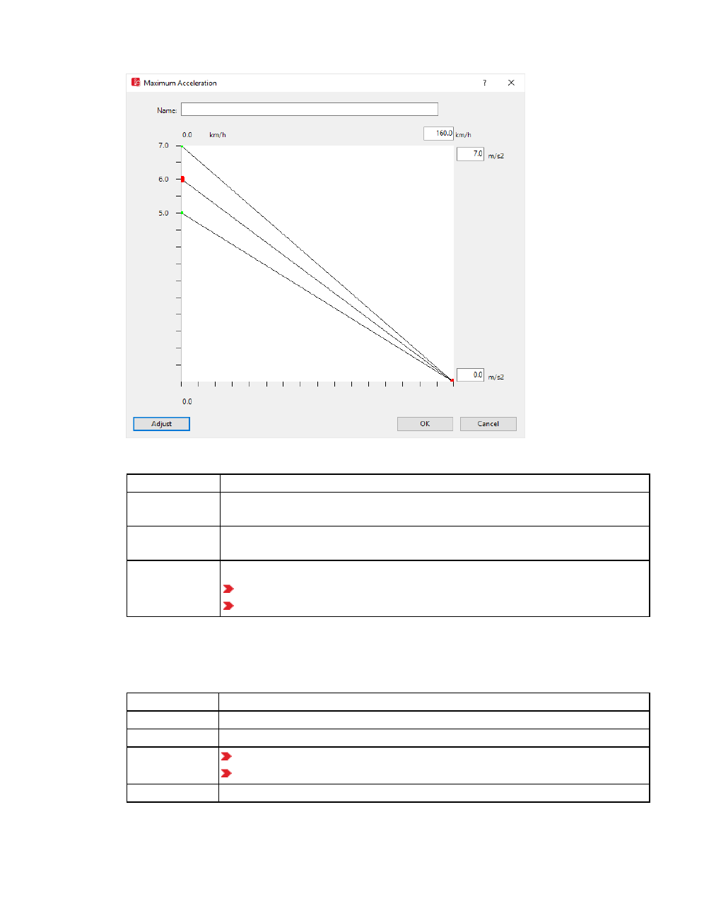
5.5.3 Defining acceleration and deceleration functions
4. Make the desired changes:
Element Description
Horizontal
abscissa
Speed
Vertical ordin-
ate
Acceleration value
Three curves describe the stochastic distribution
Median (red disks)
Two boundary curves define the bandwidth (green disks)
Vissim uses the units which are selected by default (see "Selecting network settings for
units" on page 195).
5. Make the desired changes:
Element Description
Name Name of function
km/h Max. speed of desired speed range
m/s2top box: maximum acceleration
bottom box: minimum acceleration
Adjust Show curve progression for entire value range
© PTV GROUP 225

5.5.4 Attributes of acceleration and deceleration functions
6. You can change the settings if you wish.
Element Description
Insert inter-
mediate
point
Right-click on the desired position
Move inter-
mediate
point
Click intermediate point and drag with the mouse. Progression of the three
curves changes in the value range between the limiting intermediate
points.
Delete inter-
mediate
point
Click the intermediate point and move it to the adjacent start or end point.
7. Confirm with OK.
You can show the attributes of the acceleration and deceleration functions in the respective
attributes list (see "Attributes of acceleration and deceleration functions" on page 226).
5.5.4 Attributes of acceleration and deceleration functions
1. Select from the menu Base Data > Functions.
2. Select the desired entry:
Maximum Acceleration
Desired Acceleration
Maximum Deceleration
Desired Deceleration
The list of distributions for the type selected opens.
Note: In lists, you can use the Attribute selection icon to show and hide attribute
values (see "Selecting attributes and subattributes for a list" on page 106).
The list contains the following attributes:
Element Description
No Number of acceleration or deceleration function
Name Name of acceleration or deceleration function
Showing and editing dependent objects as relation
The attribute and attribute values of this base data type are shown in the list on the left, which
consists of two coupled lists.
1. In the list on the left, click the desired entry.
The list on the right contains attributes and attribute values of base data objects allocated to
the base data object selected in the list on the left (see "Using coupled lists" on page 111):
226 © PTV GROUP

5.5.5 Deleting the acceleration/deceleration function
Acceleration function data points
Deceleration function data points
Individual data point values of the functions are:
x-coordinate and y-coordinate for the median of distribution. Data points are shown in
red in the window of the respective function.
yMin: Minimum speed of function at data point of x-coordinate and y-coordinate
yMax: Maximum speed of function at data point of x-coordinate and y-coordinate
The data points of the minimum and maximum values are shown in green in the
window of the respective function.
2. On the list toolbar, in the Relations list, click the desired entry.
3. Enter the desired data.
The data is allocated.
5.5.5 Deleting the acceleration/deceleration function
1. Select from the menu Base Data > Functions.
2. Select the desired acceleration or deceleration function.
The list of defined network objects for the network object type opens.
3. Right-click on the row number of the desired row.
4. From the shortcut menu, choose Delete.
A warning is issued.
5. Confirm with Yes.
Use this function to delete every vehicle type assigned to this function. Thus the related
vehicle categories cannot include any vehicle type anymore. The query window closes. The
deleted curve is no longer displayed.
5.6 Using distributions
There are various use cases for stochastic distributions in Vissim, for example the desired
speed of vehicles on certain network objects or the weight and power of HGVs. Using Vissim,
you can model any type of stochastic distribution.
© PTV GROUP 227

5.6.1 Using desired speed distributions
5.6.1 Using desired speed distributions
The distribution function of desired speeds is a particularly important parameter, as it has an
impact on link capacity and achievable travel times. If not hindered by other vehicles or
network objects, e.g. signal controls, a driver will travel at his desired speed. This applies
accordingly to pedestrians.
A driver, whose desired speed is higher than his current speed, will check whether he can
overtake other vehicles without endangering anyone. The more drivers' desired speed differs,
the more platoons are created.
Desired speed distributions are defined independently of vehicle type or pedestrian type.
You may use desired speed distributions for vehicle compositions, pedestrian compositions,
reduced speed zones, desired speed decisions, PT lines and parking lots.
For pedestrian simulation with Viswalk you can use desired speed distributions described in
the specialized literature (see "Using desired speed distributions for pedestrians" on page
827).
Note: Vissim provides typical default values for desired speed distributions.
5.6.1.1 Defining desired speed distributions
You can define new desired speed distributions and add intermediate points as spline points
to the course of the curve. In general, two nodes are sufficient to achieve more or less an S-
shaped distribution, and thus a concentration around the mean value.
1. Choose from the menu Base Data > Distributions > Desired Speed.
The Desired Speed Distributions list opens.
2. In the list, on the toolbar, click the Add button .
A new row with default data is inserted.
The Desired Speed Distribution window opens.
228 © PTV GROUP

5.6.1 Using desired speed distributions
3. Make the desired changes:
Element Description
Name Description
Left field with speed unit Minimum desired speed
Right field with speed unit Maximum desired speed
4. Right-click in the line.
A node is entered.
5. Click the intermediate point and keep the mouse button pressed.
6. With the mouse button pressed, drag the intermediate point to the desired position.
7. Release the mouse button.
The horizontal axis depicts the desired speed. The vertical axis depicts the proportional value
in the value range from 0.0-1.0. The course of the curve is adjusted. The labeling for the y and
x axes is adjusted. The figure shows an example in which 22 % of the vehicles drive between
80.0 and 94.50 km/h and 78% of the vehicles between 94.50 km/h and 130.00 km/h (all
equally distributed across the speed range). Due to the S-shaped distribution of the three
intermediate points at 94.50 km/h, approx. 104 km/h and 116 km/h, a concentration around the
mean value 105 km/h is achieved.
8. Confirm with OK.
© PTV GROUP 229

5.6.1 Using desired speed distributions
The desired speed distribution is displayed in the Desired Speed Distributions list (see
"Attributes of desired speed distributions" on page 230).
5.6.1.2 Attributes of desired speed distributions
1. Choose from the menu Base Data > Distributions > Desired Speed.
The Desired Speed Distributions list opens.
By default, you can edit the list (see "Using lists" on page 89).
Note: In lists, you can use the Attribute selection icon to show and hide attribute
values (see "Selecting attributes and subattributes for a list" on page 106).
The list contains the following attributes:
Element Description
No Number of desired speed distribution
Name Name of desired speed distribution
Lower
bound
Minimum desired speed
Upper
bound
Maximum desired speed
By default, the Units currently set under Network settings are used (see "Selecting network
settings for units" on page 195).
Showing and editing dependent objects as relation
The attribute and attribute values of this base data type are shown in the list on the left, which
consists of two coupled lists.
1. In the list on the left, click the desired entry.
2. On the list toolbar, in the Relations box, click > Data points.
The list on the right contains attributes and attribute values of base data objects allocated to
the base data object selected in the list on the left (see "Using coupled lists" on page 111):
Data points: Individual data point values of speed distribution. For predefined dis-
tributions, at least two points are defined by default: Data point 1 for minimum desired
speed and the last data point for maximum desired speed. You can insert additional data
points between these data points. These data points are then displayed as intermediate
points in the curve (see "Editing the graph of a function or distribution" on page 252).
x: Desired speed at data point in curve.
At data point 1: Minimum desired speed of selected desired speed distribution
Desired speed of additional data points, if defined for this curve
At last data point: Maximum desired speed of selected desired speed distribution
FX (f(x)): Probability of desired speed x at data point
At data point 1: 0
230 © PTV GROUP
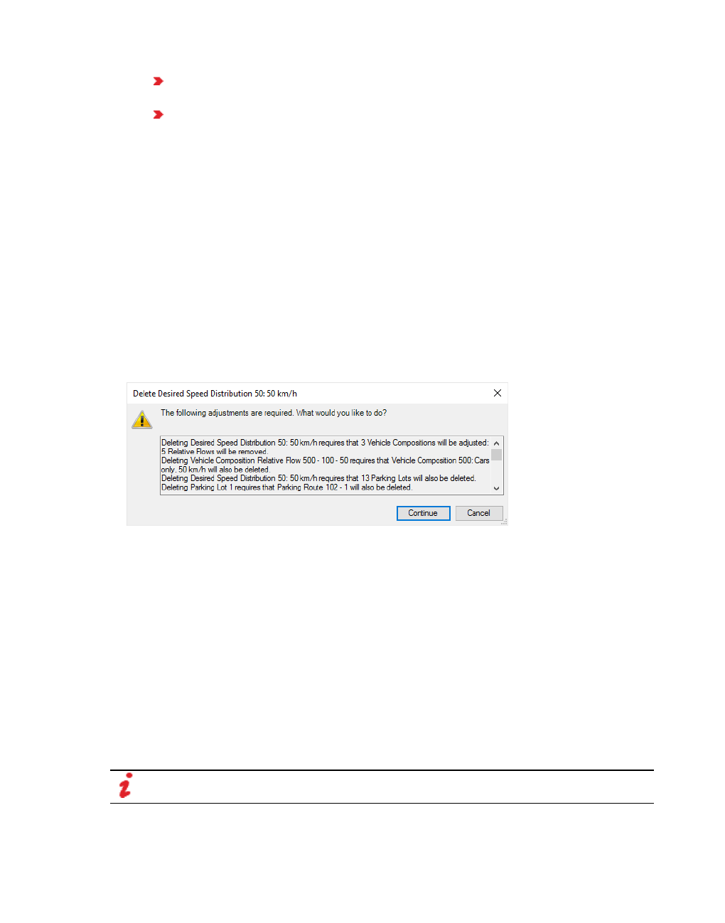
5.6.2 Using power distributions
If additional data points are defined for the curve: Probability of desired speed x at
data point
At last data point: 1
Speed distribution is monotonically increasing. This is why each FX value must be
greater than or equal to its preceding value.
3. Enter the desired data.
The data is allocated.
5.6.1.3 Deleting the desired speed distribution
1. Choose from the menu Base Data > Distributions > Desired Speed.
The Desired Speed Distributions list opens.
2. Right-click the entry of your choice.
3. From the shortcut menu, choose Delete.
If the desired speed distributions are assigned to the network objects, the window Delete
desired speed distribution opens.
4. Select from the list box an appropriate desired speed distribution for the network objects
you want to delete, to which the desired speed distribution was previously assigned.
5. Confirm with OK.
The window closes. The affected network objects are assigned the selected desired speed
distribution.
5.6.2 Using power distributions
Power refers exclusively to vehicles of vehicle category HGV and is specified via power
distribution. Power distribution is irrelevant for other vehicle categories. Power distribution is
specified independently of the vehicle type. Vissim uses power distributions and weight
distributions for HGVs (see "Using weight distributions" on page 234).
The probability increases up to the maximum power defined and then reaches the value 1.
Note: Vissim provides typical default power distributions.
© PTV GROUP 231

5.6.2 Using power distributions
5.6.2.1 Defining power distributions
You define the power through power distributions only for vehicles of HGV category. Power
distribution is irrelevant for other vehicle categories. Vissim uses power distributions together
with weight distributions (see "Using weight distributions" on page 234). Some typical power
distributions are predefined.
1. From the Base Data menu, choose Distributions > Power.
The Power Distributions list opens.
2. In the list, on the toolbar, click the Add button .
A new row with default data is inserted.
The Power Distribution window opens.
3. Make the desired changes:
Element Description
Name Description
Left field with power unit Minimum power (kW)
Right field with power unit Maximum power (kW)
4. Right-click in the line.
A node is entered.
5. Click the intermediate point and keep the mouse button pressed.
6. With the mouse button pressed, drag the intermediate point to the desired position.
7. Release the mouse button.
The labeling for the y and x axes is adjusted.
8. Confirm with OK.
The power distribution will be shown in the Power Distributions list.
5.6.2.2 Attributes of power distributions
1. From the Base Data menu, choose Distributions > Power.
The Power Distributions list opens.
Note: In lists, you can use the Attribute selection icon to show and hide attribute
values (see "Selecting attributes and subattributes for a list" on page 106).
The list contains the following attributes:
232 © PTV GROUP

5.6.2 Using power distributions
Element Description
No Number of power distribution
Name Name of the power distribution
Lower
bound
Minimum power (kW)
Upper
bound
Maximum power (kW)
Showing and editing dependent objects as relation
The attribute and attribute values of this base data type are shown in the list on the left, which
consists of two coupled lists.
1. In the list on the left, click the desired entry.
2. On the list toolbar, in the Relations box, click > Data points.
The list on the right contains attributes and attribute values of base data objects allocated to
the base data object selected in the list on the left (see "Using coupled lists" on page 111):
Data points: Individual data point values for power distribution. For predefined dis-
tributions, two points are defined by default: Data point 1 for minimum power and data
point 2 for maximum power. You can insert additional data points between these data
points. These data points are then displayed as intermediate points in the curve(see "Edit-
ing the graph of a function or distribution" on page 252).
x: Power (kW) at data point in curve
At data point 1: Minimum power of selected power distribution
Power of additional data points, if defined for the curve
At last data point: Maximum power of selected power distribution
FX (f(x)): Probability of power x at data point
At data point 1: 0
If additional data points are defined for the curve: Probability of power x at data
point
At last data point: 1
Power distribution is monotonically increasing. This is why each FX value must be
greater than or equal to its preceding value.
3. Enter the desired data.
The data is allocated.
5.6.2.3 Deleting the power distribution
1. From the Base Data menu, choose Distributions > Power.
The Power Distributions list opens.
2. Right-click the entry of your choice.
Warning: When you delete a power distribution, all vehicles types assigned to it are
deleted!
© PTV GROUP 233

5.6.3 Using weight distributions
3. From the shortcut menu, choose Delete.
If the power distribution has been assigned vehicle types, a window opens.
4. Click Delete.
5.6.3 Using weight distributions
The weight of vehicles of category HGV is defined via weight distributions. Weight distributions
are irrelevant for other vehicle categories.
You need to assign each vehicle type to a vehicle category. From the weight and power
distribution data assigned, Vissim randomly selects a value for each vehicle with a vehicle
type under vehicle category HGV. The weight and power distribution values are independent
from each other. This means Vissim may assign high power to a low-weight vehicle. Using the
weight and power data, Vissim calculates the specific power (in kW/t). The specific power is
limited to a range between 7 and 30 kW/t, so that no unrealistic weight/power combinations
are created. If a value < 7 kW/t is calculated, the specific power is set to 7 kW/t. For values
exceeding 30 kW/t, the specific power is set to 30 kW/t.
The specific power has an impact on acceleration and deceleration behavior (see "Defining
acceleration and deceleration behavior" on page 221). This is particularly important for links
with gradients. Using the specific power, Vissim calculates the percentile used to select the
relevant acceleration curve from the distribution of acceleration functions.
Weight distributions are defined independently from the vehicle type.
The probability increases up to the maximum weight defined, reaching the value 1.
Note: Vissim provides typical default values for desired distributions.
5.6.3.1 Defining weight distributions
1. Select from the menu Base Data > Distributions > Weight.
The Weight Distributions list opens.
By default, you can edit the list (see "Using lists" on page 89).
2. In the list, on the toolbar, click the Add button .
3. Right-click the row header.
234 © PTV GROUP

5.6.3 Using weight distributions
4. From the shortcut menu, choose Add.
A new row with default data is inserted.
The Weight Distribution window opens.
5. Make the desired changes:
Element Description
Name Description
Left field with weight unit Minimum weight
Right field with weight unit Maximum weight
6. Right-click in the line.
A node is entered.
7. Click the intermediate point and keep the mouse button pressed.
8. With the mouse button pressed, drag the intermediate point to the desired position.
9. Release the mouse button.
The labeling for the y and x axes is adjusted.
10. Confirm with OK.
The weight distribution will be shown in the Weight Distributions list (see "Attributes of weight
distributions" on page 235).
5.6.3.2 Attributes of weight distributions
1. From the Base Data menu, choose > Distributions > Weight.
The Weight Distributions list opens.
Note: In lists, you can use the Attribute selection icon to show and hide attribute
values (see "Selecting attributes and subattributes for a list" on page 106).
Element Description
No Number of weight distribution
Name Name of the weight distribution
Lower
bound
Minimum weight (kg)
Upper
bound
Maximum weight (kg)
Showing and editing dependent objects as relation
The attribute and attribute values of this base data type are shown in the list on the left, which
consists of two coupled lists.
1. In the list on the left, click the desired entry.
© PTV GROUP 235
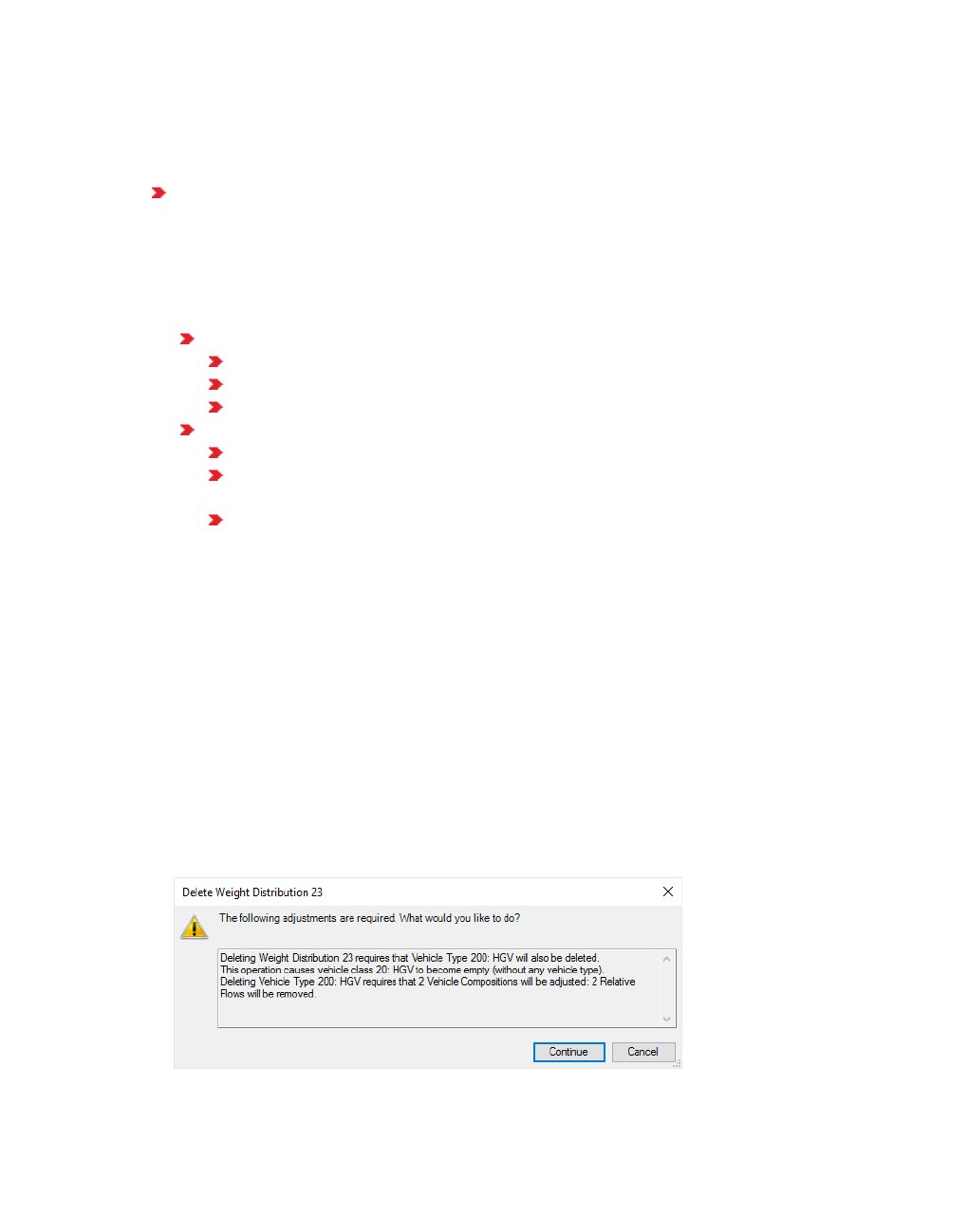
5.6.3 Using weight distributions
2. On the list toolbar, in the Relations box, click > Data points.
The list on the right contains attributes and attribute values of base data objects allocated to
the base data object selected in the list on the left (see "Using coupled lists" on page 111):
Data points: Individual data point values for weight distribution. By default, two points are
defined. The curve of weight distribution Dreyfuss F also contains an intermediate point.
Data point 1 for minimum weight and the last data point for maximum weight. You can
insert additional data points between these data points. These data points are then
displayed as intermediate points in the curve (see "Editing the graph of a function or
distribution" on page 252).
x: Weight (kg) at data point in curve.
At data point 1: Minimum weight of minimum weight distribution selected
Weight of additional data points, if defined for the curve
At last data point: Maximum weight of weight distribution selected
FX (f(x)): Value for probable weight x at data point
At data point 1: 0
If additional data points are defined for the curve: Probability of weight at data point
x
At last data point: 1
Weight distribution is monotonically increasing. This is why each FX value must be
greater than or equal to its preceding value.
3. Enter the desired data.
The data is allocated.
5.6.3.3 Deleting the weight distribution
1. Select from the menu Base Data > Distributions > Weight.
The Weight Distributions list opens.
2. Right-click the entry of your choice.
3. From the shortcut menu, choose Delete.
If the weight distribution is assigned to the network objects, the Delete weight distribution
window opens.
236 © PTV GROUP

5.6.4 Using time distributions
4. Select from the list box an appropriate weight distribution for the objects you want to delete,
to which the weight distribution was previously assigned.
5. Confirm with OK.
The window closes. The affected network objects are assigned the selected weight
distribution.
5.6.4 Using time distributions
You can use dwell time distributions for:
Standstill times on parking lots, which you specify for routing decisions of the type Parking
Lot per time interval (see "Modeling vehicle routes, partial vehicle routes, and routing
decisions" on page 430)
Waiting times at toll counters through stop signs, such as managed lanes and border
crossings
PT stops: For PT vehicles, such as bus or tram, you thereby give in this way the time
required to allow passengers to board and alight. If the method for calculating the board-
ing and alighting times is not used, the dwell time distribution in Vissim must be assigned
to every PT stop or railway station.
Set the time a vehicle remains in standstill, between backing out of a parking space and
driving forward, after it has left the parking lot. This time period is defined by the attribute
Direction change duration distribution of the parking lot (see "Attributes of parking lots"
on page 469). Default value: time distribution 5 s with lower bound 0.00, upper bound
15.00, standard deviation 1.00, average value 5.00.
The probability increases up to the maximum dwell time defined and then reaches the value 1.
5.6.4.1 Defining time distributions
1. Choose from the menu Base Data > Distributions > Time.
The Time Distributions list opens.
By default, you can edit the list (see "Using lists" on page 89).
2. Right-click the row header.
3. From the shortcut menu, choose Add.
4. Choose the desired entry from the context menu.
Empirical Distribution
Normal Distribution
A new row with default data is inserted.
5. Enter the desired values.
© PTV GROUP 237

5.6.4 Using time distributions
You can edit the curve of an empirical distribution.
6. If you would like to edit the empirical distribution of the time distribution in a graph, double-
click the entry.
The Time Distribution window opens.
7. Make the desired changes:
Element Description
Name Description
Left field with time unit s Minimum duration in seconds
Right field with time unit s Maximum duration in seconds
If you are using public transport dwell time to model public transport, a standard deviation =
0 s will result in a constant public transport dwell time (see "Calculating the public transport
dwell time for PT lines and partial PT routes" on page 497).
8. Right-click in the line.
A node is entered.
9. Click the intermediate point and keep the mouse button pressed.
10. With the mouse button pressed, drag the intermediate point to the desired position.
11. Release the mouse button.
The labeling for the y and x axes is adjusted.
12. Confirm with OK.
The time distribution will be shown in the Time Distributions list (see "Attributes of time
distributions" on page 238).
5.6.4.2 Attributes of time distributions
1. From the Base Data menu, choose > Distributions > Time.
The Time Distributions list opens.
Note: In lists, you can use the Attribute selection icon to show and hide attribute
values (see "Selecting attributes and subattributes for a list" on page 106).
The list contains the following attributes:
Long
name
Short
name
Description
Number No Number of time distribution
Name Name Name of the time distribution
238 © PTV GROUP

5.6.4 Using time distributions
Long
name
Short
name
Description
Type Type Type of distribution function:
Empirical: Cumulative frequency function. Definition between
lower limit and upper limit, with intermediate points in the curve
Normal: Normal distribution. Definition between lower limit and
upper limit, with mean value and standard deviation
Lower
bound
Lower
bound
Minimum duration in seconds
Upper
bound
Upper
bound
Maximum duration in seconds
Standard
deviation
StdDev Can only be changed for normal distribution: Dispersion of values
between lower bound and upper bound
Mean Mean Can only be changed for normal distribution: Mean of values
between lower bound and upper bound
Showing and editing dependent objects as relation
The attribute and attribute values of this base data type are shown in the list on the left, which
consists of two coupled lists.
1. In the list on the left, click the desired entry.
2. On the list toolbar, in the Relations box, click > Data points.
The list on the right contains attributes and attribute values of base data objects allocated to
the base data object selected in the list on the left (see "Using coupled lists" on page 111):
Data points: Individual data point values of time distribution. You can insert data points for
an empirical distribution. These data points are then displayed as intermediate points in
the curve (see "Editing the graph of a function or distribution" on page 252).
x: Dwell time (s) at data point in curve.
At data point 1: Minimum dwell time of selected time distribution
Dwell time of additional data points, if defined for the curve of empirical distribution
At last data point: Maximum dwell time of selected time distribution
FX (f(x)): Probability of dwell time x at data point
At data point 1: 0
If, for an empirical distribution, additional data points are defined for the curve: Val-
ues for probability of dwell time at data point x
At last data point: 1
Dwell time distribution is monotonically increasing. This is why each FX value must be
greater than or equal to its preceding value.
3. Enter the desired data.
The data is allocated.
© PTV GROUP 239

5.6.5 Using location distributions for boarding and alighting passengers in PT
5.6.4.3 Deleting the time distribution
1. Choose from the menu Base Data > Distributions > Time.
The Time Distributions list opens.
2. Right-click the entry of your choice.
3. From the shortcut menu, choose Delete.
4. Confirm with OK.
5.6.5 Using location distributions for boarding and alighting passengers in PT
A location distribution allows you to define how the total number of boarding/alighting
passengers is distributed over the entire length of the PT vehicle. For each door of a PT
vehicle that is meant for boarding and alighting passengers, the share of the vehicle length on
both its sides is calculated:
half the distance to the next door and/or
the entire distance to the start or end of the vehicle
For each share of the total vehicle length, an increase in y direction is shown on the x-axis as
a percentage of passengers for the respective door. The probability increases from NULL at
the very front of the vehicle to 1 at the very back.
5.6.5.1 Defining location distributions for boarding and alighting passengers in PT
Some typical location distributions for boarding and alighting passengers in PT vehicles are
predefined:
Element Description
Uniform Linear distribution over the full length
Center More boarding and alighting passengers in the middle
Front More boarding and alighting passengers at the front
Rear More boarding and alighting passengers at the back
Front and rear Less boarding and alighting passengers in the middle
1. Choose from the menu Base Data > Distributions > Location.
The Location Distributions list opens.
By default, you can edit the list (see "Using lists" on page 89).
2. In the list, on the toolbar, click the Add button .
A new row with default data is inserted.
The Location Distribution window opens. The x-axis defines the position:
240 © PTV GROUP

5.6.5 Using location distributions for boarding and alighting passengers in PT
0.00: maximum towards the front
1.00: maximum towards the rear
3. Enter the desired name.
4. Right-click in the line.
A node is entered.
5. Click the intermediate point and keep the mouse button pressed.
6. With the mouse button pressed, drag the intermediate point to the desired position.
7. Release the mouse button.
The labeling for the y and x axes is adjusted.
8. Confirm with OK.
The location distribution will be shown in the Location Distributions list (see "Attributes of
location distributions" on page 241).
5.6.5.2 Attributes of location distributions
1. From the Base Data, choose > Distributions > Location.
The Location Distributions list opens.
© PTV GROUP 241
5.6.5 Using location distributions for boarding and alighting passengers in PT
Note: In lists, you can use the Attribute selection icon to show and hide attribute
values (see "Selecting attributes and subattributes for a list" on page 106).
Long name Short
name
Description
Number No Number of location distribution
Name Name Name of the location distribution
Lower
bound
Lower
bound
Fixed value 0.00: maximum distance front
Upper
bound
Upper
bound
Fixed value 0.00: maximum distance rear
Showing and editing dependent objects as relation
The attribute and attribute values of this base data type are shown in the list on the left, which
consists of two coupled lists.
1. In the list on the left, click the desired entry.
2. On the list toolbar, in the Relations box, click > Data points.
The list on the right contains attributes and attribute values of base data objects allocated to
the base data object selected in the list on the left (see "Using coupled lists" on page 111):
Data points: Individual data point values of location distribution. Except for the predefined
location distribution Equally distributed, predefined distributions, by default, contain sev-
eral defined data points in order to steer boarding and alighting passengers towards the
front or rear of the PT vehicle. You can insert additional data points between these data
points. These data points are then displayed as intermediate points in the curve (see "Edit-
ing the graph of a function or distribution" on page 252).
X:Focal point of boarding and alighting passengers at data point in the curve (value
range 0.00 to 1.00)
At data point 1: for passengers boarding and alighting at the very front of the PT
vehicle
Values of additional data points, if defined for this curve
At the last data point: for passengers boarding and alighting at the very end of the
PT vehicle
FX (f(x)): Probability of passengers boarding and alighting x at data point
At data point 1: 0
If additional data points are defined for the curve: Probability of passengers board-
ing and alighting x at data point
At last data point: 1
Location distribution is monotonically increasing. This is why each FX value must be
greater than or equal to its preceding value.
3. Enter the desired data.
The data is allocated.
242 © PTV GROUP

5.6.6 Using distance distributions
5.6.5.3 Selecting alighting location distribution and boarding location distribution
Selecting alighting location distribution
A PT line with a PT stop has to be defined. When a PT line is selected, by default, the PT stop
is displayed in red.
1. Double-click the PT stop.
The PT Line Stop window opens. In the Alighting location list, the default value is No
distribution: Alighting passengers are distributed equally to all doors regardless of their
position.
2. Select the desired entry.
Selecting boarding location distribution
You can choose the boarding location distribution for every pedestrian area with PT usage
through the option Boarding location (see "Modeling construction elements" on page 834).
The standard value is the Nearest door: A boarding passenger selects the door that is
accessible on the shortest path from his location.
5.6.6 Using distance distributions
Using distance distributions, you can define the distribution between a point and a maximum
distance. To do so, you enter a maximum distance (default value 100 m). The minimum limit 0
m cannot be edited.
If you are using external software to simulate the communication between vehicles or the
communication between vehicles and suitable roadside infrastructure, you can exchange data
with Vissim via the COM interface. This type of data includes the probability of possible data
loss when the sending vehicle is at a certain distance. If the distance to the sending vehicle
(world coordinates) is NULL, the probability is NULL. The probability increases up to the
maximum distance and then reaches the value 1.
5.6.6.1 Defining distance distributions
1. From the Base Data menu, choose Distributions > Distance.
The Distance Distributions list opens.
By default, you can edit the list (see "Using lists" on page 89).
2. In the list, on the toolbar, click the Add button .
A new row with default data is inserted.
The Distance Distribution window opens.
3. Make the desired changes:
© PTV GROUP 243

5.6.6 Using distance distributions
Element Description
Name Description
Left field with distance unit Minimum distance 0.0: No change possible
Right field with distance unit Maximum distance, default value 100 m
4. Right-click in the line.
A node is entered.
5. Click the intermediate point and keep the mouse button pressed.
6. With the mouse button pressed, drag the intermediate point to the desired position.
7. Release the mouse button.
The labeling for the y and x axes is adjusted.
8. Confirm with OK.
The distance distribution is shown in the Distance Distributions list (see "Attributes of
distance distributions" on page 244).
5.6.6.2 Attributes of distance distributions
1. From the Base Data menu, choose Distributions > Distance.
The Distance Distributions list opens.
Note: In lists, you can use the Attribute selection icon to show and hide attribute
values (see "Selecting attributes and subattributes for a list" on page 106).
Long name Short
name
Description
Number No Number of distance distribution
Name Name Name of distance distribution
Lower
bound
Lower
bound
Minimum distance to assigned object
Upper
bound
Upper
bound
Maximum distance to assigned object
By default, the Units currently set under Network settings are used (see "Selecting network
settings for units" on page 195).
Showing and editing dependent objects as relation
The attribute and attribute values of this base data type are shown in the list on the left, which
consists of two coupled lists.
1. In the list on the left, click the desired entry.
2. On the list toolbar, in the Relations list, click > Data points.
244 © PTV GROUP

5.6.7 Using occupation distributions
The list on the right contains attributes and attribute values of base data objects allocated to
the base data object selected in the list on the left (see "Using coupled lists" on page 111):
Data points: Individual data point values for distance distribution. Distance distribution is
not defined by default. When you define a distance distribution, Vissim by default defines
the lower limit = 0.0 m and the upper limit = 100.0 m. You can insert additional data points
between these two data points. These data points are then displayed as intermediate
points in the curve (see "Editing the graph of a function or distribution" on page 252).
x: Distance at data point in curve.
At data point 1: Minimum distance of selected distance distribution
Distance of additional data points, if defined for the curve
At last data point: Maximum distance of selected distance distribution
FX (f(x)): Probability of distance x at data point
At data point 1: 0
If additional data points are defined for the curve: Probability of distance x at data
point
At last data point: 1
Distance distribution is monotonically increasing. This is why each FX value must be
greater than or equal to its preceding value.
3. Enter the desired data.
The data is allocated.
5.6.6.3 Deleting the distance distribution
1. From the Base Data menu, choose > Distributions > Distance.
The Distance Distributions list opens.
2. Right-click the entry of your choice.
3. From the shortcut menu, choose Delete.
4. Confirm with OK.
5.6.7 Using occupation distributions
By defining an occupancy distribution, you specify how the total number of occupants of
vehicles are distributed across the vehicles of a certain vehicle type. You can assign an
occupancy distribution to each vehicle type.
5.6.7.1 Defining occupancy distributions
1. From the Base Data menu, choose Distributions > Occupancy.
The Occupancy Distributions list opens.
By default, you can edit the list (see "Using lists" on page 89).
© PTV GROUP 245

5.6.7 Using occupation distributions
2. Right-click the row header.
3. From the shortcut menu, choose Add.
4. Choose the desired entry from the context menu.
Empirical Distribution
Normal Distribution
A new row with default data is inserted.
5. Enter the desired values.
You can edit the curve of an empirical distribution.
6. If you would like to edit the empirical distribution of the occupancy distribution, double-click
on the entry.
The Occupancy Distribution window opens.
7. Make the desired changes:
Element Description
Name Designation
Left field Minimum number of occupants
Right field Maximum number of occupants
8. Right-click in the line.
A node is entered.
9. Click the intermediate point and keep the mouse button pressed.
10. With the mouse button pressed, drag the intermediate point to the desired position.
11. Release the mouse button.
The labeling for the y and x axes is adjusted.
12. Confirm with OK.
The occupancy distribution is shown in the Occupancy Distributions list (see "Attributes of
occupancy distributions" on page 246).
5.6.7.2 Attributes of occupancy distributions
1. From the Base Data menu, choose Distributions > Occupancy.
The Occupancy Distributions list opens.
Note: In lists, you can use the Attribute selection icon to show and hide attribute
values (see "Selecting attributes and subattributes for a list" on page 106).
The list contains the following attributes:
246 © PTV GROUP
5.6.7 Using occupation distributions
Long
name
Short
name
Description
Number No Number of occupancy distribution
Name Name Name of the occupancy distribution
Type Type Type of distribution function:
Empirical: Cumulative frequency function. Definition between
lower limit and upper limit, with intermediate points in the curve
Normal: Normal distribution. Definition between lower limit and
upper limit, with mean value and standard deviation
Lower
bound
Lower
bound
Minimum occupation of vehicle
Upper
bound
Upper
bound
Maximum occupation of vehicle
Standard
deviation
StdDev Can only be changed for normal distribution: Dispersion of values
between lower bound and upper bound
Mean Mean Can only be changed for normal distribution: Mean of values
between lower bound and upper bound
Showing and editing dependent objects as relation
The attribute and attribute values of this base data type are shown in the list on the left, which
consists of two coupled lists.
1. In the list on the left, click the desired entry.
The list on the right contains attributes and attribute values of base data objects allocated to
the base data object selected in the list on the left (see "Using coupled lists" on page 111):
Data points: Individual data point values for occupancy distribution. By default, no point is
defined for the predefined distribution Individual, of the type Normal. You can insert data
points for an empirical distribution. These data points are then displayed as intermediate
points in the curve (see "Editing the graph of a function or distribution" on page 252).
x: Occupancy at data point in curve
At data point 1: Minimum occupancy of selected occupancy distribution
Occupancy of additional data points, if defined for the curve
At last data point: Maximum occupancy of selected occupancy distribution
FX (f(x)): Value for probable occupancy x at data point
At data point 1: 0
If, for an empirical distribution, additional data points are defined for the curve:
Probability of occupancy at data point x
At last data point: 1
Occupancy distribution is monotonically increasing. This is why each FX value must be
greater than or equal to its preceding value.
2. On the list toolbar, in the Relations list, click the desired entry.
3. Enter the desired data.
© PTV GROUP 247

5.6.8 Using 2D/3D model distributions
The data is allocated.
5.6.7.3 Deleting the occupancy distribution
1. From the Base Data menu, choose Distributions > Occupancy.
The Occupancy Distributions list opens.
2. Right-click the entry of your choice.
3. From the shortcut menu, choose Delete.
4. Confirm with OK.
5.6.8 Using 2D/3D model distributions
You can use a 2D/3D model distribution instead of a single model for vehicles or pedestrians
of a given type.
If you want to use only one model for all objects of a type, you must still define a 2D/3D model
distribution. You assign only one model to this 2D/3D model distribution.
In a 2D/3D model distribution you can use non-zero proportions to assign the desired 2D/3D
models. The absolute share of Vissim is calculated automatically as a ratio of the individual
relative share to the sum of all shares.
You can define a vehicle or pedestrian model by selecting a 3D model file. This automatically
defines all geometry data, such as the length and width or the positions of axles and clutches.
If you do not select a 3D model file, you can enter the geometry data manually. Models of this
sort are shown as blocks in the network.
Some typical 2D/3D model distributions are predefined.
5.6.8.1 Defining 2D/3D model distributions for 2D/3D models
1. From the Base Data menu, choose Distributions > 2D/3D Model.
The 2D/3D Model Distributions list opens.
The attribute and attribute values of this network object type are shown in the list on the left,
which consists of two coupled lists.
Note: In lists, you can use the Attribute selection icon to show and hide attribute
values (see "Selecting attributes and subattributes for a list" on page 106).
2. In the list, on the toolbar, click the Add button .
A new row with default data is inserted.
3. Into the list on the left, enter the desired number and name.
248 © PTV GROUP

5.6.8 Using 2D/3D model distributions
4. From the list toolbar, select the entry 2D/3D model distribution elements in the field
Relations.
In the next steps you select a new model distribution element from the right list and assign it
to the selected object in the left list. For each object in the left list, you can insert rows with
model distribution elements in the right list and so assign it.
A new row with default data is inserted.
5. Make the desired changes:
Element Meaning
Share 2D/3D model distribution share, by default 0.1
2D/3D
model Select a predefined model
In the list box of the cell, click the Add button to open the Select 3D
Model window (see "Defining 2D/3D models" on page 211).
The data is allocated.
6. If you want to assign other 2D/3D model distribution elements, right-click the row header in
the right list.
7. From the shortcut menu, choose Add.
8. Select the desired entry.
9. Confirm with OK.
Editing an assigned 2D/3D model
1. If you want to edit the attributes of an assigned 2D/3D model, click the model distribution
element entry in the right list.
2. From the context menu, choose Edit 2D/3D Models.
The 2D/3D Models list opens. The selected 2D/3D model is automatically highlighted.
3. Enter the desired values.
5.6.8.2 Attributes of 2D/3D model distributions
1. From the Base Data menu, choose Distributions > 2D/3D Models.
The 2D/3D Model Distributions list opens.
Note: In lists, you can use the Attribute selection icon to show and hide attribute
values (see "Selecting attributes and subattributes for a list" on page 106).
Long
name
Short
name
Description
Number No Number of 2D/3D model distribution
Name Name Name of 2D/3D model distribution
© PTV GROUP 249

5.6.9 Using color distributions
Showing and editing dependent objects as relation
The attribute and attribute values of this base data type are shown in the list on the left, which
consists of two coupled lists.
1. In the list on the left, click the desired entry.
2. On the list toolbar, in the Relations box, click > 2D/3D model segments.
The list on the right contains attributes and attribute values of base data objects allocated to
the base data object selected in the list on the left (see "Using coupled lists" on page 111):
2D/3D model distribution elements: Proportion and name of 2D/3D model assigned to
selected model distribution element
Proportion: Relative proportion of 2D/3D model (or model segment) in total value 1 of
2D/3D model distribution.
2D/3D model (Model2D3D): Name of 2D/3D model (see "Defining 2D/3D models" on
page 211). This may be a model without a file or a model based on a *.v3d file.
3. Enter the desired data.
The data is allocated.
5.6.8.3 Deleting the 2D/3D model distribution
Warning: When you delete a 2D/3D model distribution, all vehicles types assigned
to it are deleted!
1. From the Base Data menu, choose Distributions > 2D/3D Model.
The 2D/3D Model Distributions list opens.
2. Right-click the entry of your choice.
3. From the shortcut menu, choose Delete.
If the 2D/3D model distribution has been assigned vehicle types, a window opens.
4. Click Delete.
5.6.9 Using color distributions
Color distributions are relevant only for the graphical display and have no influence on the
simulation results.
The color distribution is used instead of a single color for visualization of a type of vehicle or
pedestrian. You can define a maximum of 10 colors for color distribution. By specifying a
relative share, you can specify the frequency of occurrence of each color. The absolute share
of Vissim is calculated automatically as a ratio of the individual relative share to the sum of all
shares.
If you want to use only one color for a type, you must still define a color distribution. You assign
only the desired color to this color distribution.
Some typical color distributions are predefined.
250 © PTV GROUP

5.6.9 Using color distributions
5.6.9.1 Defining color distributions
1. Choose from the menu Base Data > Distributions > Color.
The attribute and attribute values of this base data type are shown in the list on the left, which
consists of two coupled lists.
By default, you can edit the list (see "Using lists" on page 89).
2. In the list, on the toolbar, click the Add button .
A new row with default data is inserted.
3. Into the list on the left, enter the desired number and name.
4. On the list toolbar, select the Color distribution elements entry in the Relations list box.
In the next steps, set up new colors and assign them to the object selected in the left list. For
each object in the left list, you can add rows with colors to the list on the right and define
share and color distribution.
5. Right-click on the row header in the right-hand list.
A new row with default data is inserted.
6. Make the desired changes:
Element Meaning
Color Color and hexadecimal color code.
Share Color distribution share, by default 0.1
7. If you would like to edit a color, double-click in the Color box.
A color selection window opens. There are various ways to select a color.
8. Select the desired color:
Element Meaning
Color defin-
ition
Click on the desired color
RGB To select the color, use the sliders to change the values for red, yellow and
blue or enter values between 0 and 255
HSL To select the color, use the sliders to change the color value (0 to 359),
saturation (0 to 100) and relative brightness (0 to 100) or enter values
Hex Enter the color as a hexadecimal value
Alpha Use the slider to select the transparency or enter a value: 0 = transparent,
255 = opaque
Predefined
colors
Click on the desired color.
+ button: Adds the selected color to a user-defined pick list below the pre-
defined colors.
x button: Removes the selected color from the user-defined pick list.
© PTV GROUP 251

5.6.10 Editing the graph of a function or distribution
Element Meaning
Screen
color
picker
Select color with the pipette: click in the area around the pipette, keep the
mouse button pressed and drag the mouse arrow to the point on the screen
whose color you would like to copy. Release the mouse button.
New Preview of the selected color
Current Currently assigned color
9. Click next to the window when you want to close it.
The data is allocated.
5.6.9.2 Deleting the color distribution
1. Choose from the menu Base Data > Distributions > Color.
The Color Distributions list opens.
2. Right-click the entry of your choice.
3. From the shortcut menu, choose Delete.
A message is displayed if the color distribution is assigned to network objects.
4. Select from the list box an appropriate color distribution for the network objects you want to
delete, to which the color distribution was previously assigned.
5. Confirm with OK.
The window closes. The affected network objects are assigned the selected color distribution.
5.6.10 Editing the graph of a function or distribution
You can edit the values of a distribution in the list of the distribution type concerned. For the
following distributions, you can also open a window where you can define or move
intermediate points:
Desired speed
Power
Weight
Location
Distance
252 © PTV GROUP
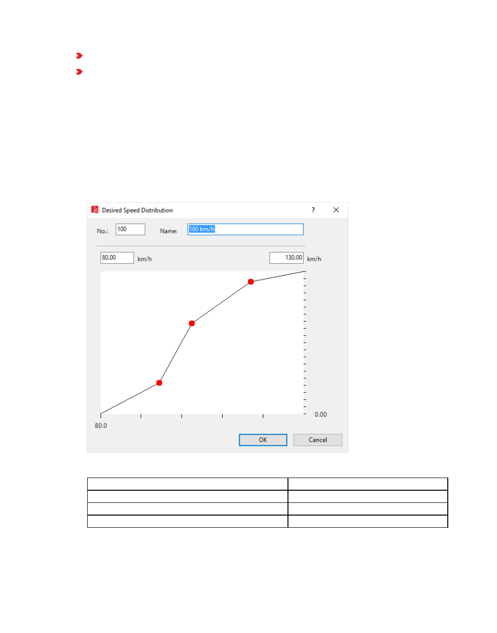
5.6.10 Editing the graph of a function or distribution
Time: Only for empirical distributions
Occupancy: Only for empirical distributions
1. Select the desired distribution from the menu Base Data > Distributions.
The list of distributions of the selected distribution type opens.
2. Select the desired entry.
3. Edit the desired entries.
4. To edit the intermediate points in the distribution curve, double-click the desired
distribution.
The <Name> Distribution window opens. Example desired speed distribution with three
intermediate points in the curve:
5. Make the desired changes:
Element Description
Name Name of distribution
Left-hand field with unit Minimum value
Right-hand field with unit Maximum value
6. To add an intermediate point, on the line, right-click the position of your choice.
© PTV GROUP 253

5.6.11 Deleting intermediate point of a graph
7. To change the shape of the curve, click the desired intermediate point, hold the mouse
button down and drag the intermediate point to the desired position.
8. Release the mouse button.
5.6.11 Deleting intermediate point of a graph
You may delete intermediate points for the following distributions:
Desired speed distributions
Power distributions
Weight distributions
Location distributions
Distance distributions
1. Choose the desired distribution type from the menu Base Data > Distributions.
The list of distributions for the distribution type opens.
2. Double-click the desired entry.
The <Name> of distribution window opens.
3. Click the intermediate point and keep the mouse button pressed.
4. Drag the intermediate point to another intermediate point.
5. If there is only one intermediate point and you want to delete it, drag the intermediate point
out of the bottom left or top right corner.
6. Release the mouse button.
7. Confirm with OK.
5.7 Managing vehicle types, vehicle classes and vehicle categories
Using Vissim, you can group vehicles with similar technical driving properties into vehicle
types and then classify vehicle types into vehicle classes. You must assign a vehicle type a
vehicle category. The Vehicle category attribute specifies the basic behavior in traffic for a
vehicle type (see "Using vehicle categories" on page 266).
5.7.1 Using vehicle types
A vehicle type allows you to form a group of vehicles with the same technical driving
characteristics. The vehicle type data is included in the emission calculation. Vissim provides
the following default vehicle types:
Car
HGV
Bus
Tram
254 © PTV GROUP

5.7.1 Using vehicle types
Man
Woman
Bike
Based on these vehicle types, you can define your own vehicle types, for example, trailer
truck, articulated truck, standard bus, articulated bus.
If vehicles in a vehicle category have different speed or acceleration behavior, you define
each vehicle type separately.
If vehicles of one type only differ in their shape, length or width, you may distinguish them by
2D/3D model distribution or color distribution and still manage them under the same vehicle
type.
Example 1: The models Car1 to Car6 represent vehicle models that differ in length, but
have a similar driving behavior. This is why they can be defined under a single vehicle
type, using 2D/3D model distribution for these 6 vehicles.
Example 2: Standard and articulated buses only differ in length. This is why you can
define them under a single vehicle type, using 2D/3D model distribution for the two vehicle
models. To distinguish between standard and articulated buses for PT lines, you need to
define standard buses and articulated buses as two separate vehicle types.
5.7.1.1 Defining vehicle types
1. From the Base Data menu, choose Vehicle Types.
The list of defined network objects for the network object type opens.
By default, you can edit the list (see "Using lists" on page 89).
You can define a new vehicle type in the list.
2. Right-click in the list.
3. From the shortcut menu, choose Add.
A new row with default data is inserted.
The Vehicle type window opens.
4. Enter the desired data.
Element Description
No. Unique identification number of the vehicle type
Name Vehicle type label
© PTV GROUP 255
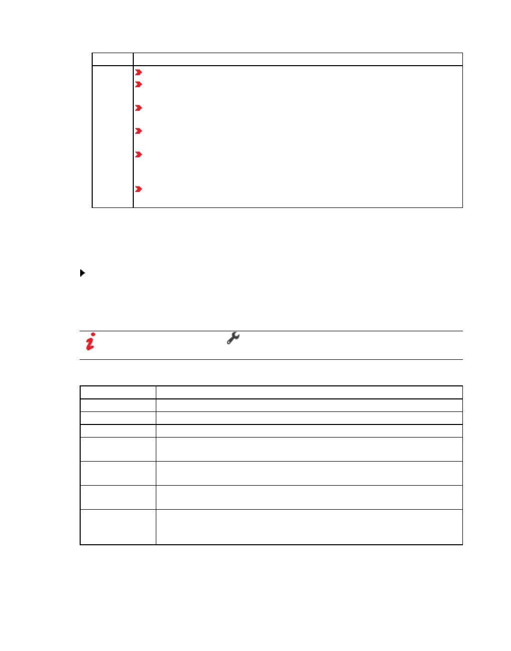
5.7.1 Using vehicle types
Element Description
Tab Static: (see "Editing static data of a vehicle type" on page 257)
Functions & Distributions: (see "Editing functions and distributions of a
vehicle type" on page 258)
Special > Section Dynamic Assignment: (see "Editing vehicle type data for
the dynamic assignment" on page 259)
Special > Others > External emission model: (see "Activating emission cal-
culation and emission model for a vehicle type" on page 261)
Special > Section Other > Vehicle Type: PT Parameters: (see "Changing
attributes for a vehicle type for the duration of boarding and alighting" on
page 262)
External Driver Model: (see "Activating the external driver model for a
vehicle type" on page 264)
The attributes are saved in the Vehicle Types list (see "Attributes of vehicle types" on page
256).
5.7.1.2 Attributes of vehicle types
From the Base Data menu, choose Vehicle Types.
The list of attributes opens.
The attribute and attribute values of this network object type are shown in the list on the left,
which consists of two coupled lists.
Note: In lists, you can use the Attribute selection icon to show and hide attribute
values (see "Selecting attributes and subattributes for a list" on page 106).
The list on the left may include the following attributes:
Column Description
No Unique identification number of the vehicle type
Name Vehicle type label
Category Vehicle category (see "Editing static data of a vehicle type" on page 257)
Model2D3DDistr 2D/3D model distribution (see "Using 2D/3D model distributions" on
page 248), (see "Editing static data of a vehicle type" on page 257)
ColorDistr1 Color distribution 1 of Color 1 (see "Editing static data of a vehicle type"
on page 257)
OccupDistr Occupancy Distribution: (see "Defining occupancy distributions" on page
245)
Capacity Capacity: PT Parameters: Maximum number of passengers permitted per
vehicle (see "Changing attributes for a vehicle type for the duration of
boarding and alighting" on page 262)
Showing and editing dependent objects as relation
1. In the list on the left, click the desired entry.
256 © PTV GROUP

5.7.1 Using vehicle types
The list on the right contains attributes and attribute values of network objects, and/or base
data allocated to the network object selected in the list on the left (see "Using coupled lists" on
page 111):
Vehicle classes (see "Defining the vehicle class" on page 267)
Parking lot selection parameters (see "Defining the destination parking lot selection" on
page 715)
2. On the list toolbar, in the Relations list, click the desired entry.
3. Enter the desired data.
5.7.1.3 Editing static data of a vehicle type
1. From the Base Data menu, choose Vehicle Types.
The list of defined objects for the base data type opens.
2. Click on the desired vehicle type.
3. Right-click in the list.
4. From the shortcut menu, choose Edit.
The Vehicle type window opens.
5. Select the Static tab.
6. Make the desired changes:
© PTV GROUP 257

5.7.1 Using vehicle types
Element Description
No. Unique number
Name Vehicle type label
Category One of the standard vehicle categories (see "Using vehicle categories" on
page 266)
Vehicle
Model
Vehicle shape and length for the vehicle type of the selected model
distribution. You need to define new vehicle models in the 2D/3D model
distribution.
Length Minimum and maximum vehicle length, depending on 2D/3D model
distribution (see "Using 2D/3D model distributions" on page 248)
Width Minimum and maximum vehicle width, depending on 2D/3D model distribution
(see "Using 2D/3D model distributions" on page 248) The width is relevant for
overtaking within the lane (see "Applications and driving behavior parameters
of lane changing" on page 281).
Colors Color distributions define the colors for the 3D representation of four vehicle
model parts of the vehicle type selected (see "Using color distributions" on
page 250). This applies for all objects of a vehicle type. When you select a
vehicle type, whose 2D/3D model color distributions have been assigned,
these are displayed in the list boxes. You can already assign your 2D/3D
models color distributions in V3DM. You may also define additional color
distributions (see "Defining color distributions" on page 251). You can choose
color distributions for each of the four colors.
Color 1: Attribute ColorDistr1
Color 2: Attribute ColorDistr2
Color 3: Attribute ColorDistr3
Color 4: Attribute ColorDistr4
The setting is ignored for PT lines in the following cases:
when a different color is selected for the vehicle class to which the PT
vehicle belongs
if a color is selected for the PT line itself
7. Confirm with OK.
5.7.1.4 Editing functions and distributions of a vehicle type
1. From the Base Data menu, choose Vehicle Types.
The list of defined network objects for the network object type opens.
2. Click on the desired vehicle type.
3. Right-click in the list.
4. From the shortcut menu, choose Edit.
The Vehicle type window opens.
5. Select the Functions & Distributions tab.
258 © PTV GROUP
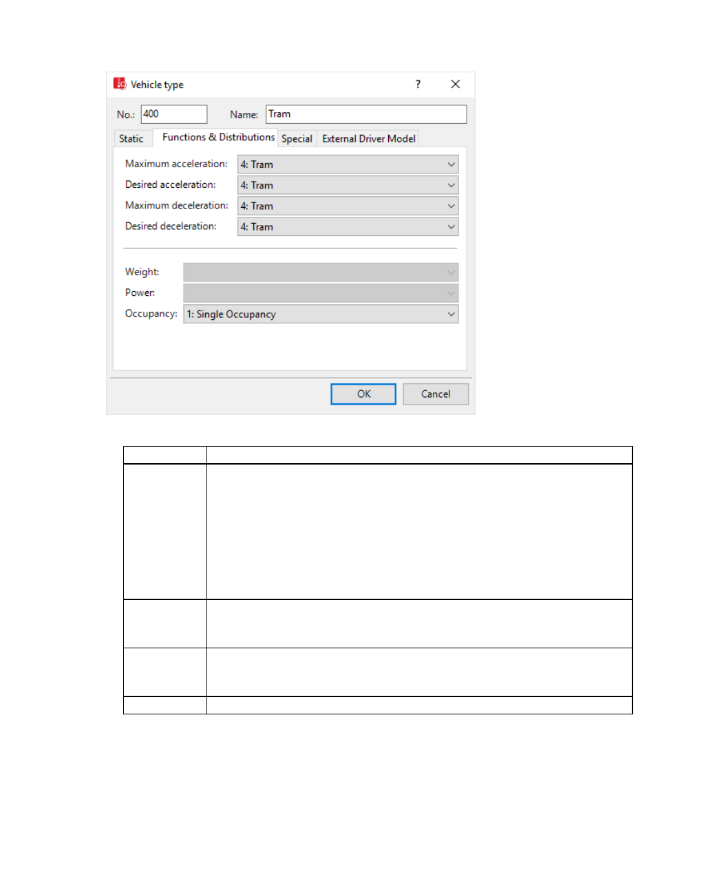
5.7.1 Using vehicle types
6. Make the desired changes:
Element Description
Maximum
Acceleration
Desired
Acceleration
Maximum
Deceleration
Desired
Deceleration
Define the accelerations and decelerations of that vehicle type (see
"Defining acceleration and deceleration functions" on page 224).
Weight The weight distributions are active only for vehicle types of Category HGV
and also, if an external model is selected (see "Using weight distributions"
on page 234)
Power The power distributions are active only for vehicle types of category HGV
and also, if an external model is selected (see "Using power distributions"
on page 231).
Occupancy Defines the number of persons (including the driver) in a vehicle
7. Confirm with OK.
5.7.1.5 Editing vehicle type data for the dynamic assignment
1. From the Base Data menu, choose Vehicle Types.
© PTV GROUP 259
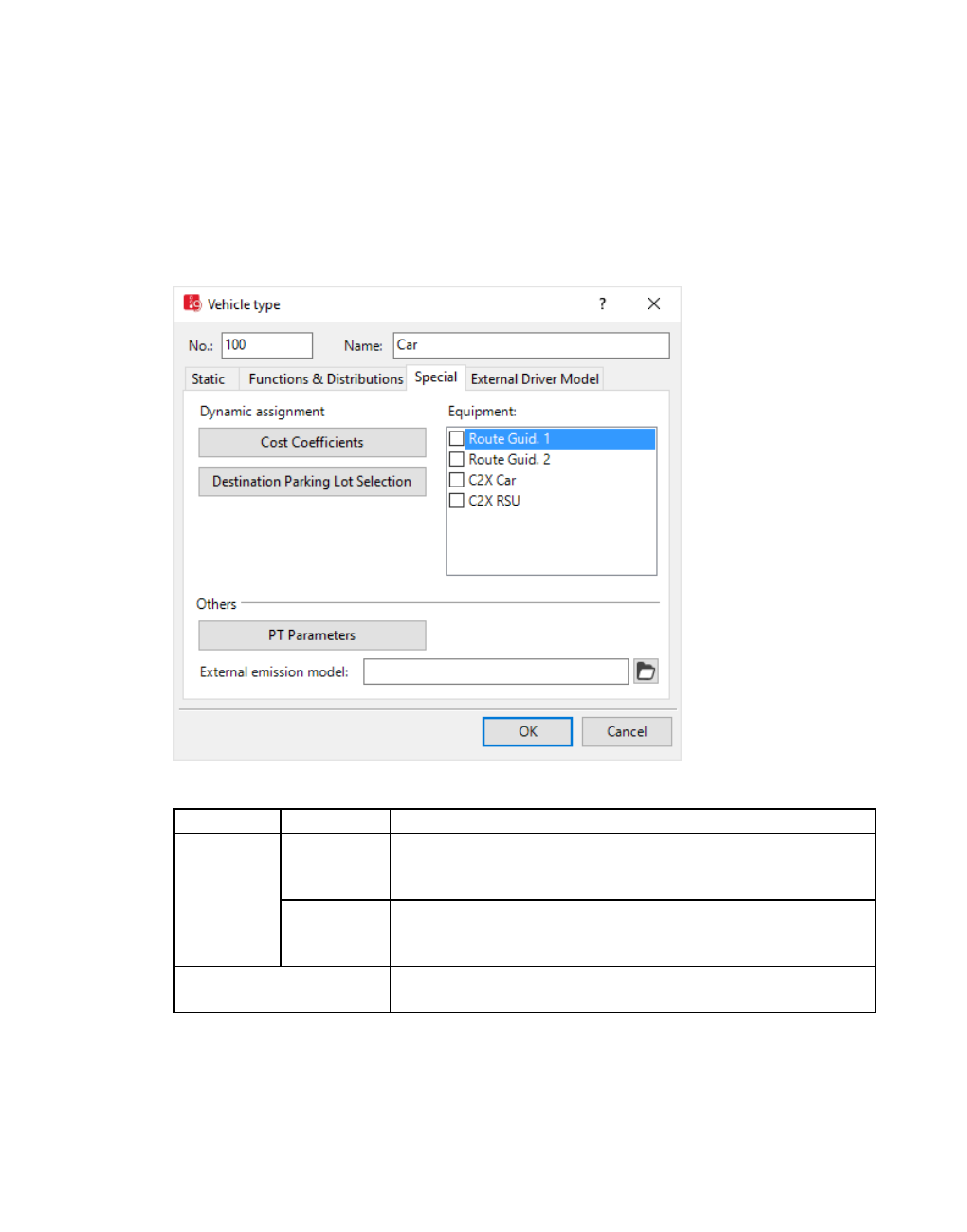
5.7.1 Using vehicle types
The list of defined network objects for the network object type opens.
2. Click on the desired vehicle type.
3. Right-click in the list.
4. From the shortcut menu, choose Edit.
The Vehicle type window opens.
5. Select the Special tab.
6. Make the desired changes:
Section Element Description
Dynamic
assignment
Cost Coef-
ficients
Defines the proportion of various factors for the path
evaluation for that type (see "Defining simulated travel times"
on page 694)
Destination
Parking Lot
Selection
The parameters are used as a decision criterion for parking
choice in a corresponding decision situation (see "Defining
the destination parking lot selection" on page 715).
Equipment Technical equipment, such as route guidance systems, for
example navigation systems for en-route re-routing.
7. Confirm with OK.
260 © PTV GROUP

5.7.1 Using vehicle types
5.7.1.6 Activating emission calculation and emission model for a vehicle type
Note: You must have a license for the add-on module.
If you have purchased the add-on module API, you can access the Emission Model.dll file for
emission calculation via an interface. You must provide the EmissionModel.dll. It is not part of
Vissim.
1. From the Base Data menu, choose Vehicle Types.
The list of defined network objects for the network object type opens.
2. Click on the desired vehicle type.
3. Right-click in the list.
4. From the shortcut menu, choose Edit.
The Vehicle type window opens.
5. Select the Special tab.
6. Make the desired changes:
Section Element Description
Others External
emission
model
Selection of an external emission model in the Emission Model.dll
file. You must provide the EmissionModel.dll. It is not part of
Vissim.
© PTV GROUP 261

5.7.1 Using vehicle types
Emission values are displayed in:
Vehicle Network Performance Evaluation (see "Vehicle network performance : Dis-
playing network performance results (vehicles) in result lists" on page 1025)
Vehicle Log (see "Saving vehicle record to a file or database" on page 971)
Evaluation Links per segment (see "Showing data from links in lists" on page 1043)
Vehicles in Network list (see "Displaying vehicles in the network in a list" on page
803)
5.7.1.7 Changing attributes for a vehicle type for the duration of boarding and alighting
You can choose to calculate the duration of boarding and alighting based on the actual
number of passengers The PT parameter definition is only applicable for PT vehicles of PT
lines.
The duration of the passenger can also change based on a stochastic distribution of the stop
time are calculated (see "Defining dwell time according to dwell time distribution" on page
497).
1. From the Base Data menu, choose Vehicle Types.
The list of defined network objects for the network object type opens.
2. Click on the desired vehicle type.
3. Right-click in the list.
4. From the shortcut menu, choose Edit.
The Vehicle type window opens.
5. Select the Special tab.
6. Click the PT Parameters button.
The PT Parameters window opens.
262 © PTV GROUP

5.7.1 Using vehicle types
7. Make the desired changes:
Element Description
Capacity Maximum permitted number of passengers per vehicle. If the maximum
capacity is reached and in the attribute Enforce capacity limit exactly,
you have not defined a larger number of passengers, no further
passengers will be able to board the vehicle.
Enforce
capacity limit
exactly
If this option is selected, no more passengers than defined in the
Capacity box will board the PT vehicle.
If this option is not selected, within one time step more passengers
could board the PT vehicle than specified in the Capacity box, in
particular if the PT-vehicle has several doors.
"Calculation”
method
Alighting
Time
Boarding
Time
Time required for a passenger to alight and board in seconds. Consider
the number of doors: For example, if the time required is 6 s / Pass and
the vehicle has 3 doors, enter the value 2 seconds.
Total Dwell
Time Sum: Sum of the boarding and alighting times
Maximum: Special doors will only be considered in the calculation for
boarding or alighting by way of using the specified maximum time for
© PTV GROUP 263
5.7.1 Using vehicle types
Element Description
each door.
Clearance
Time
The time needed for a vehicle to stop, open/close doors, and other
possible delays. Do not consider boarding and alighting times.
"Viswalk"
method & 3D
visualization
Door closure duration (DoorClosDur ): Time required for the doors to
close. Default value 2 s.
You cannot edit the time required for the doors to open. It is 1.5 s. During
this time the doors move parallel to the vehicle for 1.2 s and inwards for
0.3.s.
8. Make sure that the following data are defined:
Occupancy rate of the PT vehicles via Departure times in the PT Line window (see
"Attributes of PT lines" on page 487)
Volume by PT stop (see "Attributes of PT stops" on page 480)
Alighting percentage and Skipping possible option in PT Line Stop window (see
"Defining dwell time according to dwell time distribution" on page 497)
9. Confirm with OK.
5.7.1.8 Activating the external driver model for a vehicle type
Note: You will need the External Driver Model add-on module.
1. From the Base Data menu, choose Vehicle Types.
The list of defined network objects for the network object type opens.
2. Click on the desired vehicle type.
3. Right-click in the list.
4. From the shortcut menu, choose Edit.
The Vehicle type window opens.
5. Select the External Driver Model tab.
264 © PTV GROUP

5.7.1 Using vehicle types
6. Make the desired changes:
Element Description
External driver Only for the External Driver Model add-on module:
If this option is selected, a vehicle type is not subject to the driving
behavior models of Vissim, but is ruled by an external set of driving
behavior parameters.
Path and file-
name of driver
model DLL
Enter the path and filename of the DLL file of the external driving beha-
vior parameter set
Path and file-
name of para-
meter file
Enter the path and filename of the parameter file
7. Confirm with OK.
Vissim sends e.g. the following data to the DLL file even if 0 is returned by
DriverModelGetValue (DRIVER_DATA_SETS_XY_COORDINATES, ...):
DRIVER_DATA_VEH_REAR_X_COORDINATE
DRIVER_DATA_VEH_REAR_Y_COORDINATE
This means that global coordinates for vehicle rear ends are available in usual driver model
DLLs for vehicles on Vissim links.
© PTV GROUP 265

5.7.2 Using vehicle categories
For detailed information on all types that are managed in the files DriverModel.cpp and
DriverModel.h , please refer to the file Interface_ description.pdf in the folder
..\API\DriverModel_DLL of your Vissim installation.
5.7.2 Using vehicle categories
The Vehicle category attribute of a vehicle type specifies its basic behavior in traffic (see
"Operating principles of the car following model" on page 32). The latter varies between
individual vehicle categories. For example, the vehicle category Tram does not allow for lane
changes and the speed of vehicles of this category is not based on a desired speed. You need
to assign each vehicle type a vehicle category (see "Editing static data of a vehicle type" on
page 257). Vissim provides the following default vehicle categories:
Car
HGV
Bus
Tram
Pedestrian
Bike
The table shows the properties of vehicle categories that differ from the properties of the
vehicle category Car:
Vehicle
category
Differing property
HGV The weight distribution and the power distribution are only relevant for this
vehicle category and only for the spread in acceleration curves (see "Using
weight distributions" on page 234), (see "Using power distributions" on page
231).
In Wiedemann 99 in the FREE and FOLLOW interaction states, only accel-
erates with half the calculated acceleration (see "Driving states in the traffic
flow model according to Wiedemann" on page 270), (see "Value of the Inter-
action state attribute" on page 808)
For the right-side rule general behavior when changing lanes, has different
values for some non-user defined parameters of free lane changing.
Doesn't have an occupancy distribution, just one driver (see "Defining occu-
pancy distributions" on page 245)
Bus The properties correspond to the properties of the car vehicle category.
Tram Lange changes not allowed
In Wiedemann 74 in the FREE interaction state and in the Free driving state,
does not oscillate around the desired speed, but rather drives exactly at the
desired speed (see "Driving states in the traffic flow model according to
Wiedemann" on page 270), (see "Value of the Interaction state attribute" on
page 808)
266 © PTV GROUP
5.7.3 Using vehicle classes
Vehicle
category
Differing property
Pedestrian Always brakes at amber and red
Calculates a safety distance of 0.1 m when changing lanes (see "Editing the
driving behavior parameter Following behavior" on page 271), (see "Defin-
ing the Wiedemann 74 model parameters" on page 275)
Doesn't have a stochastic threshold that defines the speed below the desired
velocity at which a vehicle would be overtaken. Therefore a pedestrian over-
takes immediately when he cannot continue at the desired velocity.
Doesn't have an occupancy distribution, just one person (see "Defining occu-
pancy distributions" on page 245)
Has 21 motion states:
Has a state for standing pedestrians
20 states for motion sequence of two steps
Bike Doesn't have an occupancy distribution, just one person (see "Defining occu-
pancy distributions" on page 245)
Has 21 motion states:
Has a state for cyclists
20 states for motion sequence of one crank revolution
5.7.3 Using vehicle classes
You can group vehicle types into vehicle classes. A vehicle class may contain any number of
vehicle types. Vehicle classes provide the basis for speed data, evaluations, path selection
behavior and other network objects. Per default, a vehicle class contains a vehicle type of the
same name. You may assign a vehicle type to several vehicle classes. A vehicle class is, for
example, used to obtain data for specific vehicle types or to recognize and distinguish them
based on their color during simulation.
Vehicles with different technical driving properties must belong to different vehicle types.
Group vehicle types to a vehicle class in the following cases:
If for these vehicles you still want to define the same properties, for example route choice
behavior.
If you wish to collect aggregated data.
If vehicles with the same technical driving properties only differ in shape or color, they vehicles
can still be assigned to the same vehicle type. To be able to distinguish between individual
vehicles, for this vehicle type, select a suitable 2D/3D model distribution and color distribution.
5.7.3.1 Defining the vehicle class
You can define vehicle classes and assign vehicle types.
1. Select from the menu Base Data > Vehicle Classes.
The list of defined objects for the base data type opens.
By default, you can edit the list (see "Using lists" on page 89).
© PTV GROUP 267

5.8 Defining driving behavior parameter sets
You can define a new vehicle class in the list.
2. In the list, on the toolbar, click the Add button .
A new row with default data is inserted.
Enter the desired data.
Element Description
No Unique identification number of the vehicle class
Name Label of the vehicle class
Color Default color of vehicle class during simulation (see "Static colors of vehicles
and pedestrians" on page 165). Is not used in the following cases:
When for a vehicle class the attribute Use vehicle type color (UseVe-
hTypeColor) is enabled.
When for the display of vehicles in the network, from the Graphic Para-
meters menu, DrawingMode > Use color scheme is chosen, and for the
Color scheme configuration attribute, a color scheme is specified that is to
be used for classification.
Vehicle
types
VehTypes: List box with options for selecting the vehicle types you wish to
assign. Numbers and names of vehicle types.
Use
vehicle
type
color
UseVehTypeColor: If this option is selected, the vehicle color is determined
by simulation of each vehicle type (or public transport line respectively).
The Use vehicle type color attribute is not used, when for the display of
pedestrians in the network, from the Graphic Parameters menu, DrawingMode
> Use color scheme is chosen, and for the Color scheme configuration
attribute, a color scheme is specified that is to be used for classification.
Showing and editing dependent objects as relation
The attribute and attribute values of this network object type are shown in the list on the left,
which consists of two coupled lists.
1. In the list on the left, click the desired entry.
The list on the right contains attributes and attribute values of base data objects allocated to
the base data object selected in the list on the left (see "Using coupled lists" on page 111):
2. On the list toolbar, in the Relations list, click Vehicle types.
3. Enter the desired data.
The data is allocated.
5.8 Defining driving behavior parameter sets
Warning: Driving behavior parameters control the driving behavior and can
therefore lead to a considerable change in the simulation results! Change the
driving behavior parameters only if you are a very experienced user!
268 © PTV GROUP

5.8 Defining driving behavior parameter sets
In a driving behavior parameter set, you can define the driving behavior properties of a link
behavior type. In driving behavior parameter set, select properties for the following
parameters:
The following behavior and car following model according to Wiedemann
Lateral behavior
Lane change behavior
Behavior at signal controls
Parameters for mesoscopic simulation
You assign a link the desired driving behavior via the Behavior type attribute (see "Attributes
of links" on page 383).
You can change the driving behavior parameters during the simulation. However, you cannot
change Safety distance reduction factor start (signals) or Safety distance reduction factor
end (signals).
For each vehicle class, you can assign a driving behavior parameter set to a link behavior
type. You assign links the desired link behavior type via the Link behavior type attribute (see
"Defining link behavior types for links and connectors" on page 299).
1. From the Base Data menu, choose > Driving Behaviors.
The Driving Behaviors list opens. Some driving behavior parameter sets can be
predefined.
By default, you can edit the list (see "Using lists" on page 89).
You can edit all driving behavior parameters for lane change, lateral behavior and following
behavior in the list or in tabs with the following steps.
Note: In lists, you can use the Attribute selection icon to show and hide attribute
values (see "Selecting attributes and subattributes for a list" on page 106).
2. Right-click in the list.
3. From the shortcut menu, choose Add.
A new row with default data is inserted.
The Driving Behavior window opens.
4. Enter the desired data.
Element Description
No. Unique number of the driving behavior parameter set
Name Name of the link behavior type assigned
© PTV GROUP 269
5.8.1 Driving states in the traffic flow model according to Wiedemann
Element Description
Tab Following: (see "Editing the driving behavior parameter Following behavior"
on page 271)
Lane change: (see "Applications and driving behavior parameters of lane
changing" on page 281)
Lateral behavior: (see "Editing the driving behavior parameter Lateral beha-
vior" on page 289)
Signal control: (see "Editing the driving behavior parameter Signal Control"
on page 295)
Meso: (see "Editing the driving behavior parameter Meso" on page 298)
5. Confirm with OK.
5.8.1 Driving states in the traffic flow model according to Wiedemann
Vissim's traffic flow model is a stochastic, time step based, microscopic model that treats
driver-vehicle units as basic entities.
The traffic flow model contains a psycho-physical car following model for longitudinal vehicle
movement and a rule-based algorithm for lateral vehicle movement. The models deployed are
based on Wiedemann's extensive research work.
Wiedemann, R. (1974). Simulation des Straßenverkehrsflusses. Schriftenreihe des Insti-
tuts für Verkehrswesen der Universität Karlsruhe (seit 2009 KIT – Karlsruher Institut für
Technologie), Heft 8
Wiedemann, R. (1991). Modeling of RTI-Elements on multi-lane roads. In: Advanced
Telematics in Road Transport edited by the Commission of the European Community, DG
XIII, Brussels
Wiedemann's traffic flow model is based on the assumption that there are basically four
different driving states for a driver (see "Traffic flow model and light signal control" on page
31):
Free driving: No influence of preceding vehicles can be observed. In this state, the driver
seeks to reach and maintain his desired speed. In reality, the speed in free driving will
vary due to imperfect throttle control. It will always oscillate around the desired speed.
Approaching: Process of the driver adapting his speed to the lower speed of a preceding
vehicle. While approaching, the driver decelerates, so that there is no difference in speed
once he reaches the desired safety distance.
Following: The driver follows the preceding car without consciously decelerating or accel-
erating. He keeps the safety distance more or less constant. However, again due to imper-
fect throttle control, the difference in speed oscillates around zero.
Braking: Driver applies medium to high deceleration rates if distance to the preceding
vehicle falls below the desired safety distance. This can happen if the driver of the
270 © PTV GROUP

5.8.2 Editing the driving behavior parameter Following behavior
preceding vehicle abruptly changes his speed or the driver of a third vehicle changes
lanes to squeeze in between two vehicles.
For each of the four driving states, acceleration is described as a result of current speed,
speed difference, distance to the preceding vehicle as well as of individual driver and vehicle
characteristics.
Drivers switch from one state to another as soon as they reach a certain threshold that can be
described as a function of speed difference and distance. For instance, small differences in
speed can only be perceived at short distances. Whereas large differences in speed already
force drivers to react at large distances.
The perception of speed differences as well as the desired speed and safety distance kept
vary across the driver population.
As the model accounts for psychological aspects as well as for physiological restrictions of
drivers' perception , it is called psycho-physical car-following model.
5.8.2 Editing the driving behavior parameter Following behavior
1. From the Base Data menu, choose Driving Behaviors.
The Driving Behaviors list opens. Some driving behavior parameter sets can be
predefined.
By default, you can edit the list (see "Using lists" on page 89).
You can edit all driving behavior parameters for lane change, lateral behavior and following
behavior in the list or in tabs with the following steps.
Note: In lists, you can use the Attribute selection icon to show and hide attribute
values (see "Selecting attributes and subattributes for a list" on page 106).
2. Right-click the entry of your choice.
3. From the shortcut menu, choose Edit.
The Driving Behavior window opens.
4. Select the Following tab.
© PTV GROUP 271

5.8.2 Editing the driving behavior parameter Following behavior
5. Enter the desired data.
272 © PTV GROUP

5.8.2 Editing the driving behavior parameter Following behavior
Element Description
Look
ahead
distance
min., max.: Minimum and maximum distance that a vehicle can see forward in
order to react to other vehicles either in front or to the side of it (within the same
link). Vehicles take into account the minimum and maximum look-ahead
distance in addition to the entered number of preceding vehicles.
The Minimum look-ahead distance is important when modeling the lateral
behavior of vehicles.
If the minimum look ahead distance is 0.00, only the number of Observed
vehicles applies, which is specified in the attribute of Observed vehicles.
If several vehicles can overtake within a lane, this value needs to be greater
than 0.00, e.g. in urban areas, depending on the speed, the look ahead dis-
tance might be approx. 20-30m, with correspondingly larger values for out-
side of the city. This way you avoid that during the simulation the impression
is created that one vehicle is passing through another vehicle. This may
happen when there are more vehicles than specified in the Observed
vehicles attribute that want to position themselves in front of a stop line on
the same link. This applies in particular to bicycles.
If several vehicles can overtake within a lane, you can enter a greater look
ahead distance to prevent any vehicles from running a red light. When
doing so, do not change the number of Observed vehicles. This can lead
to an unrealistic simulation.
Only the Maximum look-ahead distance needs to be extended, e.g. to model
rail traffic with block signals (see "Modeling railroad block signals" on page
637).
Observed vehicles: The number of observed vehicles or number of certain net-
work objects affects how well vehicles in the link can predict other vehicles'
movements and react accordingly. In addition to the number of observed
vehicles entered, vehicles take the minimum and maximum Look ahead dis-
tance into account.
The following network objects are modeled as vehicles in in Vissim. Vehicles
treat these network objects as a preceding vehicle. These network objects act
like a red signal head. If there are several of these network objects within a very
short distance, enter a larger number for the Observed vehicles. However, this
can lead to slightly longer simulation computation times.
Red signal heads
Reduced Speed Areas
Priority rules for cases in which the minimum time gap or minimum head-
way is not kept.
Vehicles also treat the following network objects as a preceding vehicle,
when they have to stop there:
Stop Signs
Public transport stops
Parking Lots
© PTV GROUP 273
5.8.2 Editing the driving behavior parameter Following behavior
Element Description
Conflict areas behavior: A vehicle takes into consideration all conflict areas up
to the preceding vehicle, indicative of the number of Observed vehicles.
Element Description
Look back distance min., max.: The Look back distance defines the minimum and max-
imum distance that a vehicle can see backwards in order to react
to other vehicles behind (within the same link).
The minimum look-back distance is important when modeling
lateral vehicle behavior.
If several vehicles can overtake within a lane, this value needs to
be greater than 0.00, e.g. in urban areas it could be 20-30m, with
correspondingly larger values in other places. This way you make
sure the cars drive in an orderly fashion when two or more
vehicles, than specified in the Observed vehicles attribute, on the
same route want to position themselves at a stop line. This applies
in particular to bicycles.
You can reduce the maximum look-back distance in close-meshed
networks, e.g. with many connectors over a short distance. This
may positively affect the simulation speed.
Element Description
Temporary lack of
attention
Duration: The period of time when vehicles may not react to a
preceding vehicle. They do react however to emergency braking.
Probability: Frequency of the lack of attention
With increasing values, the capacity of the affected links
decreases.
Element Description
Smooth closeup
behavior If this option is checked, vehicles slow down more evenly when
approaching a stationary obstacle. At the maximum look-ahead
distance from the stationary obstacle, a following vehicle can plan
to stop there as well, because the preceding vehicle will stop there
too.
If this option is not selected, the following vehicle uses the
normal following behavior until the speed of the preceding vehicle
drops to < 1 m/s and it comes almost to a halt. Only then, the
following vehicle determines the final approach behavior. This
approach behavior can include a temporary acceleration.
274 © PTV GROUP
5.8.2 Editing the driving behavior parameter Following behavior
Element Description
Standstill distance
for static obstacles
Standstill distance (ax) upstream of static obstacles such as signal
heads, stop signs, PT stops, priority rules, conflict areas. Not valid
for stop signs in parking lots. The attribute Smooth closeup
behavior must be selected.
If this option is not selected, the vehicles use a normally
distributed random value [0.5; 0.15].
If this option is selected, the vehicles will use the given
value. The default value is 0.5 m. Activate this option for PT
vehicles at PT stops with platform screen doors and queues at
fixed positions on the platform. Enter the desired distance.
Note: From Vissim 6, the optimized modeling of driving
behavior can lead to different results than in the previous
versions.
Element Description
Car following model Car following model for the car-following behavior. Depending on
the selected car following model the Model parameters change.
No interaction: Vehicles do not recognize any other vehicles.
Use this entry to model pedestrian flows in an easy way.
Wiedemann 74: Model suitable for urban traffic and merging
areas
Wiedemann 99: Model for freeway traffic with no merging
areas
Model parameters Displays different parameters depending on the car following
model selected (see "Defining the Wiedemann 74 model para-
meters" on page 275), (see "Defining the Wiedemann 99 model
parameters" on page 277). These model parameters affect the sat-
uration flow.
5.8.2.1 Defining the Wiedemann 74 model parameters
This model is an improved version of Wiedemann’s 1974 car following model.
The following parameters are available:
© PTV GROUP 275

5.8.2 Editing the driving behavior parameter Following behavior
Parameters Description
Average
standstill dis-
tance
(ax): Defines the average desired distance between two cars. The tolerance
lies from –1.0 m to +1.0 m which is normally distributed at around 0.0 m, with
a standard deviation of 0.3 m. Default value 2.0.
Additive part
of safety dis-
tance
(bxadd): Value used for the computation of the desired safety distance d.
Allows to adjust the time requirement values. Default 2.0
Multiplicative
part of
safety dis-
tance
(bxmult): Value used for the computation of the desired safety distance d.
Allows to adjust the time requirement values. Greater value = greater dis-
tribution (standard deviation) of safety distance Default 3.0
The desired distance d is calculated from:
where:
ax: Standstill distance
v: vehicle speed [m/s]
z: is a value of range [0.1], which is normally distributed around 0.5 with a standard deviation
of 0.15
Defining the saturation flow rate with the Wiedemann 74 modeling parameters
The saturation flow rate defines the number of vehicles that can flow freely on a link for an
hour. Impacts created through signal controls or queues are not accounted for. The saturation
flow rate also depends on additional parameters, e.g. speed, share of HGV, or number of
lanes.
You define the saturation flow by combining the parameters Additive part of safety distance
and Multiplicative part of safety distance . Experienced users may want to use these
parameters to adapt their model to observation data.
Note: The graphs show the saturation flow rates calculated for examples used in
Vissim. When using a different network, you receive graphs depicting different values.
276 © PTV GROUP
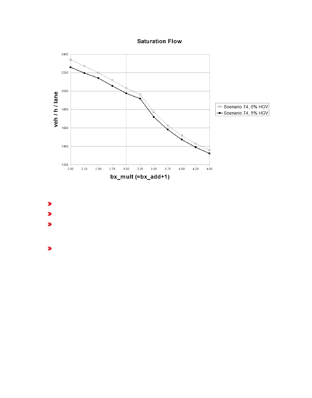
5.8.2 Editing the driving behavior parameter Following behavior
Scenario 74 was created with the following parameters:
single lane link
speed distribution between 48 and 58 km/h
Default driving behavior, with the exception of parameters bxadd (Additive part of safety
distance) and bxmult (Multiplicative part of safety distance) that vary along the x-axis. In
this example the following applies: bxadd = bxmult-1
one time step per simulation second
5.8.2.2 Defining the Wiedemann 99 model parameters
This model is based on Wiedemann’s 1999 car following model.
The following parameters are available:
© PTV GROUP 277

5.8.2 Editing the driving behavior parameter Following behavior
Parameters Unit Description
CC0 m Standstill distance: The average desired standstill distance between
two vehicles. It has no variation. You can define the behavior
upstream of static obstacles via the attribute Standstill distance for
static obstacles (see "Editing the driving behavior parameter
Following behavior" on page 271).
CC1 s Time distribution of speed-dependent part of desired safety distance
Shows number and name of time distribution Each time distribution
may be empirical or normal. Each vehicle has an individual, random
safety variable. Vissim uses this random variable as a fractile for the
selected time distribution CC1.
Based on the time distribution, the following distance for a vehicle is
calculated. This is the distance in seconds which a driver wants to
maintain at a certain speed. The higher the value, the more cautious
the driver is. The safety distance is defined in the car following model
as the minimum distance a driver will maintain while following
another vehicle. In case of high volumes this distance becomes the
value which has a determining influence on capacity.
CC2 m It restricts the distance difference (longitudinal oscillation) or how
much more distance than the desired safety distance a driver allows
before he intentionally moves closer to the car in front. If this value is
set to e.g. 10 m, the following behavior results in distances between
dxsafe and dxsafe + 10m. The default value is 4.0m which results in a
quite stable following behavior.
CC3 s It controls the start of the deceleration process, i.e. the number of
seconds before reaching the safety distance. At this stage the driver
recognizes a preceding slower vehicle.
CC4 m/s defines negative speed difference during the following process.
Low values result in a more sensitive driver reaction to the
acceleration or deceleration of the preceding vehicle.
CC5 m/s defines positive speed difference during the following process. Enter
a positive value for CC5 which corresponds to the negative value of
CC4. Low values result in a more sensitive driver reaction to the
acceleration or deceleration of the preceding vehicle.
CC6 1/(m • s) Influence of distance on speed oscillation while in following process:
Value 0: The speed oscillation is independent of the distance
Larger values: Lead to a greater speed oscillation with increasing
distance
CC7 m/s2Oscillation during acceleration
CC8 m/s2Desired acceleration when starting from standstill (limited by
maximum acceleration defined within the acceleration curves).
CC9 m/s2Desired acceleration at 80 km/h (limited by maximum acceleration
defined within the acceleration curves).
278 © PTV GROUP

5.8.2 Editing the driving behavior parameter Following behavior
Note: The units of Wiedemann 99 model parameters cannot be edited. These units are
independent of the network settings for units in the base data.
Defining the saturation flow rate with the Wiedemann 99 modeling parameters
The saturation flow rate defines the number of vehicles that can flow freely on a link for an
hour. Impacts created through signal controls or queues are not accounted for. The saturation
flow rate also depends on additional parameters, e.g. speed, share of HGV, or number of
lanes.
In the car-following model Wiedemann 99, parameter CC1 has a major impact on the safety
distance and saturation flow rate. The scenarios shown below are based on the following
assumptions:
car-following model Wiedemann 99, containing default parameters with the exception of
CC1 that varies across the x-axis
one time step per simulation second
The main properties of the following graphs are:
Scenario Right-side rule Lane Speed
cars*
Speed
HGV*
% HGV
99-1 no 2 80 n/a 0%
99-2 no 2 80 85 15%
99-3 yes 2 80 n/a 0%
99-4 yes 2 80 85 15%
99-5 yes 2** 120 n/a 0%
99-6 yes 2 120 85 15%
99-7 yes 3*** 120 n/a 0%
99-8 yes 3 120 85 15%
* Vissim default setting
** Lane 2 closed for HGV traffic
*** Lane 3 closed for HGV traffic
Note: The graphs show the saturation flow rates calculated for examples used in
Vissim. When using a different network, you receive graphs depicting different values.
© PTV GROUP 279

5.8.2 Editing the driving behavior parameter Following behavior
280 © PTV GROUP

5.8.3 Applications and driving behavior parameters of lane changing
5.8.3 Applications and driving behavior parameters of lane changing
Vissim distinguishes between the following lane changes:
Necessary lane change in order to reach the next connector of a route
For a necessary lane change, the driving behavior parameters contain the maximum
acceptable deceleration for a vehicle and its trailing vehicle on the new lane. The
deceleration depends on the distance to the emergency stop position of the next route
connector.
Free lane change if there is more space and a higher speed is required
For a free lane change, Vissim checks the desired safety distance to the trailing vehicle on
the new lane. The desired safety distance depends on the speed of the vehicle that wants
to change the lane and on the speed of the vehicle preceding it. You cannot change the
degree of "aggressiveness" for free lane changes. You can, however, influence free lane
change by changing the safety distance. Safety distances are used to specify car-following
behavior (see "Editing the driving behavior parameter Following behavior" on page 271).
For both types of lane change, you first need to find a suitable gap in the direction of travel.
The gap size depends on two speeds:
speed of the vehicle changing the lane
speed of the vehicle approaching from behind on the lane to be switched to For necessary
lane changes, the time gap also depends on drivers' "aggressiveness". Here too the max-
imum delay of the driving behavior parameters is included in the calculation of the time
gaps.
In 2D animation, a current change of lanes, as well as the desire to change lanes is visualized
via a small red line to the right or left of the vehicle (representing the indicator), from the
defined Lane change distance on. This is also the case for lane changes on connectors. In
3D animation, a current lane change and the desire to change lanes is shown via an indicator,
if this is defined for the 3D model of the vehicle. The desire to change lanes is triggered by:
the vehicle route
in the context of dynamic assignment by the path
when a desired lane is set via the COM interface
5.8.3.1 Editing the driving behavior parameter Lane change behavior
1. From the Base Data menu, choose Driving Behaviors.
The Driving Behaviors list opens. Some driving behavior parameter sets can be
predefined.
By default, you can edit the list (see "Using lists" on page 89).
You can edit all driving behavior parameters for lane change, lateral behavior and following
behavior in the list or in tabs with the following steps.
© PTV GROUP 281

5.8.3 Applications and driving behavior parameters of lane changing
Note: In lists, you can use the Attribute selection icon to show and hide attribute
values (see "Selecting attributes and subattributes for a list" on page 106).
2. Right-click the entry of your choice.
3. From the shortcut menu, choose Edit.
The Driving Behavior window opens.
4. Select the Lane Change tab.
You can edit the already defined network objects in the Driving Behaviors list or via the menu
Base Data > Driving Behaviors.
5. Make the desired changes:
282 © PTV GROUP

5.8.3 Applications and driving behavior parameters of lane changing
Element Description
General
behavior
(Lane change rule) (LnChgRule):
Free lane selection: Vehicles may overtake on each lane.
Slow lane rule, Fast lane rule: Allows overtaking on freeways or similar
links according to StVO (German Traffic Code) and to the rules in road
traffic of other countries.
Regardless of the option selected, you can model the general behavior more
realistically using the settings under Cooperative lane change.
Element Description
Necessary
lane
change
(route)
Columns Own and Trailing vehicle: Delay for changing lanes based on
the specified routes for their own overtaking vehicle and the trailing
vehicle is accepted by the driver
Maximum deceleration: Enter the maximum deceleration for changing
lanes based on the specified routes for own vehicle overtaking (MaxDe-
celOwn) and the trailing vehicle (MaxDecelTrail)
Maximum deceleration:: Upper bound of deceleration for own vehicle
and tailing vehicle for a lane change
Accepted deceleration (AccDecelTrail and AccDecelOwn): Lower
bound of deceleration for own vehicle and trailing vehicle for a lane
change
-1m/s2 per distance (DecelRedDistTrail and DecelRedDistDown): In
addition, the change of the deceleration is specified (in meters per -1
m/s2). This reduces the Maximum deceleration with increasing distance
from the emergency stop distance linearly by this value down to the
Accepted deceleration.
For example, the following parameters yield the course of the curve shown below:
© PTV GROUP 283
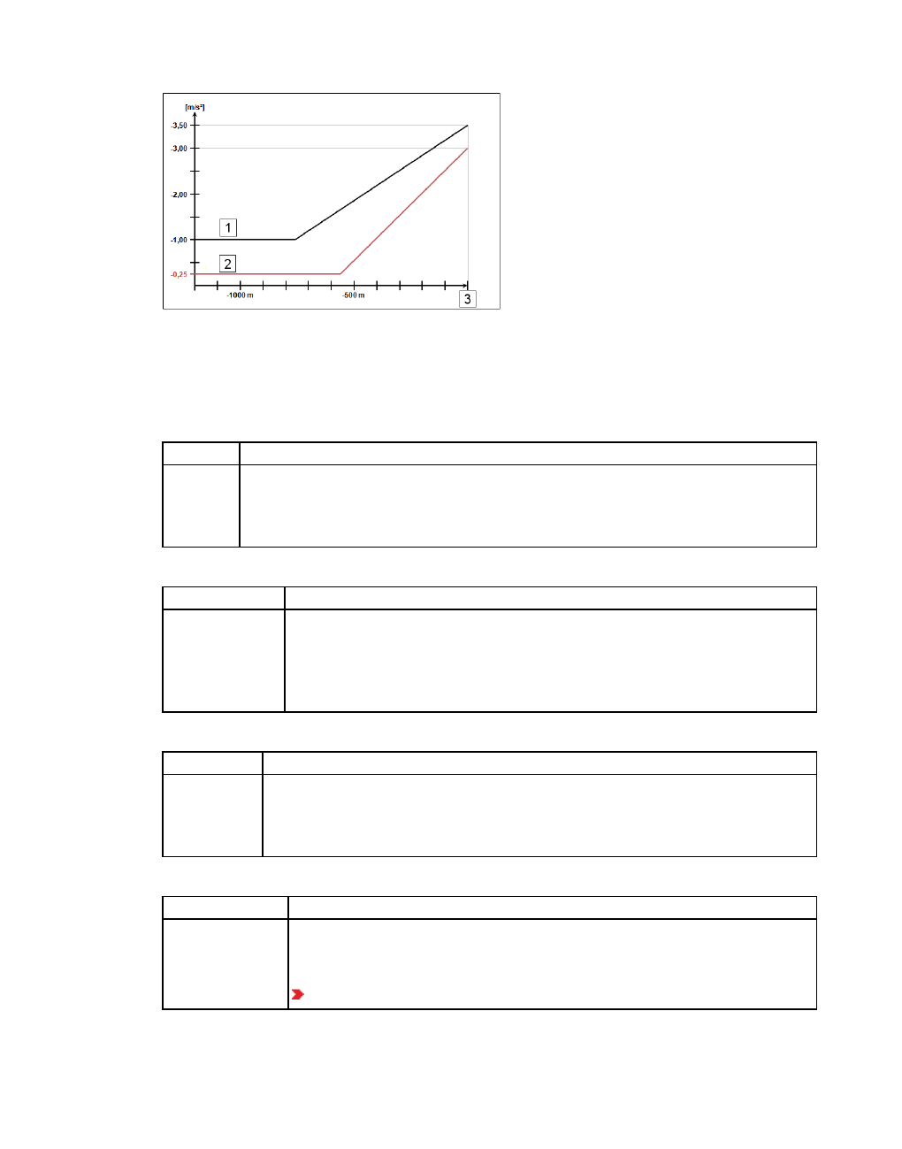
5.8.3 Applications and driving behavior parameters of lane changing
Legend:
1 black line: lane changer (own)
2 red line: trailing vehicle
3: emergency stop distance
Element Description
Diffusion
time
DiffusTm: The maximum amount of time a vehicle can wait at the emergency
stop distance for a necessary change of lanes. When this time is reached the
vehicle is removed the network, at the same time a warning is written to the
*.err file and displayed in the Messages window.
Element Description
Min. headway
(front/rear):
Minimum headway (MinHdwy):The minimum distance between two
vehicles that must be available after a lane change, so that the change
can take place (default value 0.5 m). A lane change during normal traffic
flow might require a greater minimum distance between vehicles in order
to maintain the speed-dependent safety distance.
Element Description
To slower
lane if col-
lision time
is above
Free driving time (FreeDrivTm): only for Slow lane rule or Fast lane rule:
defines the minimum distance to a vehicle in front, in seconds, which must
be present on the slower lane, so that an overtaking vehicle switches to the
slower lane.
Element Description
Safety
distance
reduction
factor:
Safety distance reduction factor (lane change), (SafeDistRedFact): is
taken into account for each lane change. It concerns the following
parameters:
The safety distance of the trailing vehicle on the new lane for determ-
284 © PTV GROUP

5.8.3 Applications and driving behavior parameters of lane changing
ining whether a lane change will be carried out
The safety distance of the lane changer itself
The distance to the preceding, slower lane changer
During the lane change Vissim reduces the safety distance to the value
that results from the following multiplication:
Original safety distance • safety distance reduction factor
The default value of 0.6 reduces the safety distance by 40%. Once a
lane change is completed, the original safety distance is taken into
account again.
Element Description
Maximum
deceleration
for cooper-
ative brak-
ing
Maximum cooperative deceleration (CoopDecel): Specifies to what
extent the trailing vehicle A is braking cooperatively, so as to allow a
preceding vehicle B to change lanes into its own lane. When the trailing
vehicle A detects that it would have to brake more heavily than what this
value indicates if the preceding vehicle B is set for lane changing, the
cooperative braking stops or is not initiated. The higher the value, the
stronger the braking and greater the probability of changing lanes. While
changing lanes, the preceding vehicle considers the factor for the reduced
safety distance and the parameters of the car-following model. Default -
3 m/s2.
During cooperative braking, a vehicle decelerates with the following
values:
0% to a maximum of 50 % of the desired deceleration, until the vehicle
in front begins to change lanes (see "Defining acceleration and decel-
eration behavior" on page 221)
Between 50% of the desired deceleration and the maximum decel-
eration (100 %) specified in the Maximum deceleration field. Typically,
the deceleration during the lane change will be considerably less than
the maximum deceleration, because the preceding vehicle, which
changes lanes, does not expect such a high deceleration from the trail-
ing vehicle.
Element Description
Overtake
reduced
Overtake reduced speed areas (OvtRedSpeedAreas): The option is not
selected by default.
© PTV GROUP 285

5.8.3 Applications and driving behavior parameters of lane changing
speed
areas If this option is selected, vehicles immediately upstream of a reduced
speed area may perform a free lane change (see "Applications and driving
behavior parameters of lane changing" on page 281). If there is also a
reduced speed area on the lane the vehicle changes to, it is accounted for.
If the option is not selected, vehicles never start a free lane change dir-
ectly upstream of a reduced speed area. They also completely ignore the
reduced speed areas on the new lane.
Element Description
Advanced
merging
Advanced merging (AdvMerg): This option is selected by default in the
driving behaviour parameter sets by newly created networks. The option is
considered for any necessary lane change towards the next connector along
the route.
If this option is selected, more vehicles can change lanes earlier. Thus,
the capacity increases and the probability, that vehicles come to a stop to
wait for a gap, is reduced.
Select the option accordingly to achieve the desired lane change
behavior:
If vehicle A has to change lanes and recognizes that the neighboring
vehicle in front B on the target lane has approximately the same speed or
is only slightly faster (-1.0 m/s < dv < 0.1 m/s), A slows down slightly (by 0.5
m/s²) to move into the gap behind B, if the option is selected.
If the option is not selected, the vehicle A slows down only when it
approaches the emergency stop distance.
If the vehicle A with vehicle in front C detects that a neighboring vehicle in
front B wants to change to the lane of A, this option can be used so that
cooperative braking of A also take place when A is downstream from C.
If this option is not selected, vehicle A leaves the cooperation to its
preceding vehicle C. In this case, C might already be too close to B, so that
286 © PTV GROUP

5.8.3 Applications and driving behavior parameters of lane changing
C overtakes B, whereby A itself is eventually too close to B for cooperative
braking.
Let us assume vehicle B is a neighboring vehicle in front of vehicle A. A
plans to let B merge, who is meanwhile driving downstream of C (in front of
vehicle A), on its own lane. In this case, vehicle A forgets that B should
have been permitted to merge. Thus, vehicle A can immediately permit
other vehicles to change into its lane.
If this option is not selected, then within the next 50 m vehicle A will not
brake for any other neighboring vehicle in front, also if vehicle B is
downstream of the vehicle in front, C (on vehicle A’s lane).
If vehicle A wanted to allow the vehicle ahead of it on the other lane, B, to
merge, but B did not change lanes and A, in the meantime, has overtaken
B, this option allows vehicle A to forget that it should have let B merge.
Thus, vehicle A can immediately permit other vehicles to change into his
lane.
If this option is not selected, then within the next 50 m vehicle A will not
brake for any other neighboring vehicle in front, also if A has meanwhile
overtaken B.
Element Description
Consider
subsequent
static rout-
ing
decisions
Vehicle routing decisions look ahead (VehRoutDecLookAhead): If this
option is selected, vehicles leaving the route identify new routing decisions
on the same link in advance and take them into account when choosing the
lane. For routing decisions further downstream that vehicles should identify
in advance, the option Combine static routing decisions must be selected
(see "Attributes of static vehicle routing decisions" on page 437).
Element Description
Cooperative
lane change
Cooperative lane change (CoopLnChg): If vehicle A observes that a
leading vehicle B on the adjacent lane wants to change to his lane A, then
vehicle A will try to change lanes itself to the next lane in order to facilitate
lane changing for vehicle B. For example, vehicle A would switch from the
right to the left lane when vehicle B would like to switch to the left from a
merging lane to the right lane.
© PTV GROUP 287

5.8.3 Applications and driving behavior parameters of lane changing
Vehicle A behaves during this lane change as if it would have to change
lanes due to a connector at a long distance. It accepts its own Maximum
deceleration and the deceleration of the trailing vehicle C on the new lane,
in accordance with the parameters for the necessary lane change.
Vehicle A does not make a cooperative lane change, when the following
conditions are true:
the new lane is less appropriate for continuing its route
if vehicle B is faster than the maximum speed difference (in the
example 10.80 km/h ( =3 m/s)
if the collision time exceeded the maximum collision time (in the
example 10 seconds), and the speed of vehicle A increased by the
maximum speed difference (in the example 10.80 km/h).
When you select Cooperative lane change, the user-defined cooper-
ative lane change rule is activated for the respective driving behavior
parameter set. For Maximum speed difference and Maximum col-
lision time the user-defined settings are used.
If this option is not selected, the user-defined cooperative lane chan-
ging behavior is not active for the particular driving behavior parameter
set.
Maximum speed difference: If option Cooperative lane change has
been selected, the user-defined value for the maximum possible speed
difference is taken into account.
Maximum collision time: If option Cooperative lane change has
been selected, the user-defined value for the maximum collision time is
taken into account.
288 © PTV GROUP

5.8.4 Editing the driving behavior parameter Lateral behavior
Element Description
Cross-cor-
rection of
the back
end
Rear correction of lateral position (RearCorr ): If a lane change takes place
at a lower speed than specified in the Maximum speed box, the vehicle's rear
end moves laterally. The rear correction compensates for this movement. This
causes the vehicle to be aligned to the middle of the lane at the end of the
lane change, instead of at angle in the original lane. The rear correction is
performed completely, even when the vehicle comes to a standstill. A rear
correction affects the capacity. Rear correction is only performed if the Keep
lateral distance to vehicles on next lane(s) option is selected for the driving
behavior parameter Lateral behavior (see "Editing the driving behavior
parameter Lateral behavior" on page 289).
Maximum speed: Speed up to which the correction of the rear end pos-
ition should take place. Default value 3 km/h. Lateral correction of the rear
end position is not performed for faster vehicles.
Active during time period from: Time after the start of the lane change at
which the lateral movement of the rear end position should start, default
value 1.0 s.
until: Time after the start of the lane change at which the lateral movement
of the rear end position should end. The value includes 3 s for the lane
change of the front end, default value 10.0.
The attributes Active during time period from and to also determine the
speed at which a rear correction is performed.
5.8.4 Editing the driving behavior parameter Lateral behavior
By default, in Vissim a vehicle uses the entire width of the lane. You can define in the driving
behavior and parameters-lateral behavior, whether the vehicles in a lane can drive on the left,
on the right or in the middle without specifying a lateral orientation. If the lane is wide enough
and the attributes in the section Default behavior when overtaking vehicles on the same
lane or on adjacent lanes allow for overtaking on the same lane, overtaking maneuvers on a
single lane are also possible. If the maximum deceleration prevents the overtaking vehicle
from braking in time, it overtakes the other vehicle if possible, even if this is not allowed by the
driving behavior parameters Consider next turning direction and Minimum lateral distance.
Improper overtaking therefore takes precedence over a collision.
Furthermore, these settings are used when the option Keep lateral distance to vehicles on
next lane(s) is selected.
1. From the Base Data menu, choose Driving Behaviors.
The Driving Behaviors list opens. Some driving behavior parameter sets can be
predefined.
You can edit all driving behavior parameters for lane change, lateral behavior and following
behavior in the list or in tabs with the following steps.
Note: In lists, you can use the Attribute selection icon to show and hide attribute
values (see "Selecting attributes and subattributes for a list" on page 106).
© PTV GROUP 289

5.8.4 Editing the driving behavior parameter Lateral behavior
By default, you can edit the list (see "Using lists" on page 89).
2. Right-click the entry of your choice.
3. From the shortcut menu, choose Edit.
The Driving Behavior window opens.
4. Select the Lateral tab.
5. Make the desired changes:
Element Description
Desired
position at
free flow
Desired position at free flow (DesLatPos): Lateral orientation of a vehicle
within its lane while it is in free traffic flow
Keep
lateral
distance to
vehicles on
next lane
(s)
Observe adjacent lanes (ObsAdjLns): If this option is selected, the
vehicles consider the position and therefore the lateral orientation of
vehicles on adjacent lanes and keep the Lateral min. distance. For this
purpose, vehicles even adjust their lateral orientation on their own lane and
swerve out of the way. The simulation also regards the actual positions of
the back ends of vehicles, which change a lane to an adjacent lane or have
already changed.
290 © PTV GROUP

5.8.4 Editing the driving behavior parameter Lateral behavior
Element Description
If this option is not selected, vehicles on adjacent lanes are ignored even
if they are wider than their lanes, except when they perform a lane change.
Note: Using this option can reduce the simulation speed significantly!
Diamond
shaped
queuing
DiamQueu: If this option is selected, queues take into account a realistic
shape of the vehicles with vehicles positioned offset, such as bikes. Vehicles
are internally represented not as a rectangle, but as a rhombus.
Consider
next
turning
direction
ConsNextTurn: In case of non-lane-bound traffic enables a lateral behavior
that accounts for another vehicle as follows: If the option has been
selected, a vehicle with this driving behavior does not pass another vehicle
on the same lane if this could cause a collision at the next turning connector.
To achieve this, attributes that enable passing on the same lane must be
selected in the section Default behavior when overtaking vehicles on the
same lane or on adjacent lanes and/or vehicle classes that may be
overtaken must be selected in the section Exceptions for overtaking
vehicles of the following vehicle classes.
Option Consider next turning direction also considers the attribute Desired
Direction of the next connector of the route of the vehicle (see "Attributes of
connectors" on page 395). If, for example, left has been selected for this
attribute, the vehicle only passes another vehicle on the right if that vehicle
turns at the same connector at the latest.
If the vehicle is within the lane change distance defined in the Lane change
attribute (Lane change distance), it moves laterally on its lane to the
respective side if there is sufficient space. Simultaneously, vehicles which
do not want to turn in the same direction on the same connector or some
time before it, do not try to overtake the vehicle on that side, since this would
cause a collision at the next intersection.
The vehicle flashes if the option Consider next turning direction is selected
and the vehicle changes lanes within the Lane change distance defined in
the Lane change attribute and the attribute Left or Right of the connector is
selected.
Note: The option Consider next turning direction has precedence
over option Desired position at free flow.
Collision
time gain
Minimum collision time gain (MinKCollTimeGain): Minimum value of the
collision time gain for the next vehicle or signal head, which must be
reached so that a change of the lateral position on the lane is worthwhile
and will be performed. The collision time is calculated based on the desired
speed of the vehicle. The default value for collision time gain is two seconds.
Smaller values lead to a livelier lateral behavior, since vehicles also have to
dodge sideways for minor improvements.
© PTV GROUP 291

5.8.4 Editing the driving behavior parameter Lateral behavior
Element Description
Minimum
longitudinal
speed
Minimum longitudinal speed for lateral movement (MinSpeedForLat):
Minimum longitudinal speed which still allows for lateral movements. The
default value of 1 km/h ensures that vehicles can also move laterally if they
have almost come to a halt already.
Time
between
direction
changes
Lateral direction change - minimum time (Lateral behavior)
(LatDirChgMinTm): Standard 0.0 s: defines the minimum simulation time
which must pass between the start of a lateral movement in one direction
and the start of a lateral movement in the reverse direction. The higher this
value, the smaller are the lateral movements of vehicles. These lateral
movements only take place if overtaking on the same lane is permitted.
Lateral movement for a lane change is not affected by this parameter.
292 © PTV GROUP

5.8.4 Editing the driving behavior parameter Lateral behavior
Element Description
Default
behavior
when over-
taking
vehicles on
the same
lane or on
adjacent
lanes
This applies for all vehicle classes, with the exception of the vehicles
classes listed under Exceptions for overtaking vehicles of the following
vehicle classes.
Overtake on same lane: When modeling traffic that is not lane-bound,
you can allow vehicles to overtake within a lane.
Left: Vehicles are allowed to overtake on a lane to the left
Right: Vehicles are allowed to overtake on a lane to the right
Minimum lateral distance: Minimum distance between vehicles when
overtaking within the lane and keeping the distance to vehicles in the
adjacent lanes, default value 1 m.
Distance standing at 0 km/h (LatDistStandDef): lateral distance of
the passing vehicle in meters. Default value: 1 m
Distance driving at 50 km/h (LatDistDrivDef): lateral distance of the
passing vehicle in meters. Default value: 1 m
The minimum distance is linearly interpolated for other speeds than at
0 km/h and 50 km/h.
If the option Keep lateral distance to vehicles on next lane(s) is not
selected, vehicles on adjacent lanes are ignored, even if they are wider than
their lanes, except when they change lanes.
Exceptions
for over-
taking
vehicles of
the fol-
lowing
vehicle
classes
Behavior for specific vehicle classes that deviates from the default behavior
when overtaking vehicles on the same lane or on adjacent lanes. When
modeling traffic that is not lane-bound, you can select vehicle classes which
may be overtaken within a lane by vehicles of this driving behavior set.
1. Right-click in the list.
2. From the shortcut menu, choose Add.
A new row with default data is inserted.
3. Make the desired changes:
VehClass: Vehicle class whose vehicles may be overtaken by
vehicles of this driving behavior parameter set within the lane.
OvtL (Overtake left): Vehicles are allowed to overtake on the left
lane
OvtR (Overtake right): Vehicles are allowed to overtake on the right
lane
LatDistStand: Minimum distance at 0 km/h
LatDistDriv: Minimum distance at 50 km/h
5.8.4.1 Example of modeling lateral behavior
The example takes into account the following guidelines:
© PTV GROUP 293

5.8.4 Editing the driving behavior parameter Lateral behavior
Bikes and cars travel on the same one-lane link.
Bikes must drive on the right side.
Bikes may be overtaken by cars only on the left.
Bikes may overtake cars only on the right.
Bikes may overtake other bikes only on the left.
For this, you define three driving behavior parameter sets:
Defining the driving behavior parameter set Urban lateral behavior
1. From the Base Data menu, choose Driving Behaviors.
The Driving Behaviors list opens. Some driving behavior parameter sets can be
predefined.
2. Right-click Urban (motorized).
3. From the shortcut menu, choose Duplicate.
4. For the new driving behavior parameter set, in the Name box, enter: Urban lateral
behavior
5. Right-click the entry.
6. From the shortcut menu, choose Edit.
The Driving Behavior Parameter Set window opens.
7. Make the desired changes:
Element Description
Following
tab
Look ahead distance:
min.: 0
max.: 30 m
Lateral tab Section Exceptions for overtaking vehicles of the following vehicle
classes:
1. From the shortcut menu, choose Add.
A new row is inserted.
2. Select the vehicle class Bike.
3. Select the option OvtL.
4. Confirm with OK.
Defining the driving behavior parameter set Urban Bike
1. In the Driving behavior list, right-click Cycle-Track (free overtaking).
2. From the shortcut menu, choose Duplicate.
3. For the new driving behavior parameter set, in the Name box, enter: Urban Bike
294 © PTV GROUP
5.8.5 Editing the driving behavior parameter Signal Control
4. Right-click the entry.
5. From the shortcut menu, choose Edit.
The Driving Behavior Parameter Set window opens.
6. Make the desired changes:
Element Description
Lateral
tab
Desired position at free flow:Right
Section Default behavior when overtaking vehicles on the same lane or on
adjacent lanes:
1. Under Overtake on same lane, deactivate the options On left and On right.
2. From the shortcut menu, choose Add.
A new row is inserted.
3. Select the vehicle class Car.
4. Select the attribute OvtR.
5. Right-click the entry.
6. From the shortcut menu, choose Add.
A new row is inserted.
7. Select the vehicle class Bike.
8. Select the attribute OvtL.
9. In the LatDistStand section, select: 0.3 m
10. Confirm with OK.
Defining the link behavior type Urban lateral behavior Bike
1. Select from the menu Base Data > Link Behavior Types.
The list Link Behavior Types opens. Some link behavior types can be predefined.
2. In the list, on the toolbar, click the Add button .
A new row with default data is inserted.
3. For the new link behavior type, in the Name column, enter: Urban lateral behavior
Bike.
4. In the column DrivBehavDef, select the driving behavior parameter set Urban Bike.
5. Assign the applicable links in the LinkBehaviorType attribute to the new Urban lateral
behavior Bike link behavior type.
5.8.5 Editing the driving behavior parameter Signal Control
For the driving behavior at signal controls, specify the following:
© PTV GROUP 295

5.8.5 Editing the driving behavior parameter Signal Control
how vehicles respond to amber signal
how vehicles respond to red-amber signal
a reduced safety distance before stop lines
a time distribution for the response time
1. From the Base Data menu, choose Driving Behaviors.
The list of defined network objects for the network object type opens.
The list shows driving behavior parameter sets. Some driving behavior parameter sets can
be predefined.
By default, you can edit the list (see "Using lists" on page 89).
You can edit all driving behavior parameters for lane change, lateral behavior and following
behavior in the list or in tabs with the following steps.
Note: In lists, you can use the Attribute selection icon to show and hide attribute
values (see "Selecting attributes and subattributes for a list" on page 106).
2. Right-click the entry of your choice.
3. From the shortcut menu, choose Edit.
The Driving Behavior window opens.
4. Select the Signal Control tab.
5. Make the desired changes:
296 © PTV GROUP
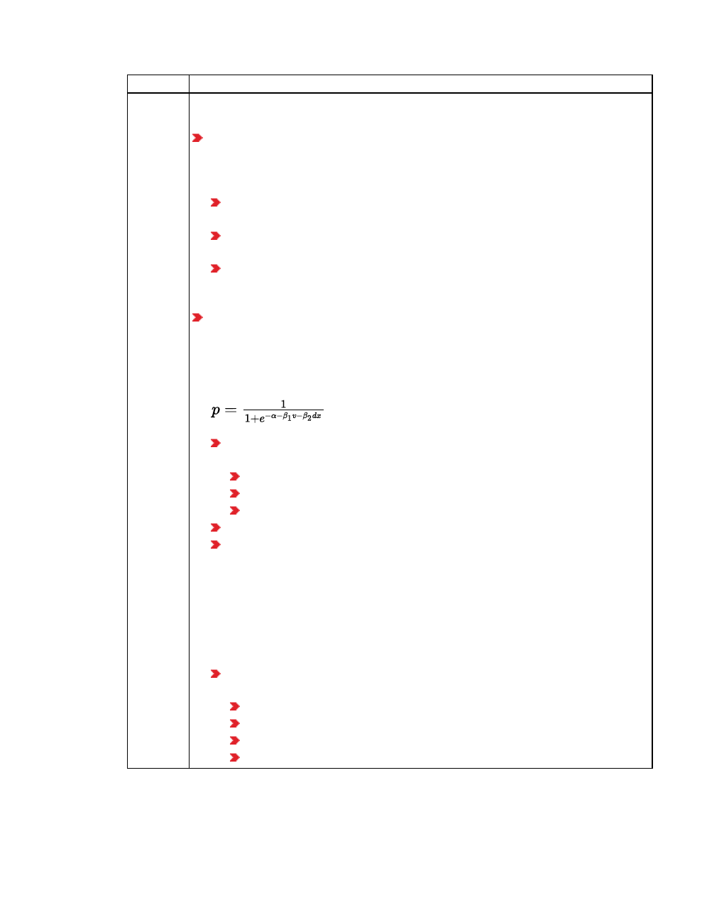
5.8.5 Editing the driving behavior parameter Signal Control
Element Description
Reaction
to amber
signal
Decision model: Defines the behavior of vehicles when they approach an
amber light.
Continuous check: Driver of vehicle continuously decides whether to con-
tinue driving or whether to stop. Vehicles assume that the amber light will
only be visible for another two seconds. They then decide continuously,
with each time step, whether they will continue to drive or stop.
A vehicle will not brake, if its maximum deceleration does not allow it to
stop at the stop line, or if it would have to brake for longer than 4.6 m/s².
The vehicle will brake, if at its current speed, it cannot drive past the sig-
nal head within two seconds.
Both braking and stopping are possible for cases that lie in between
these two scenarios. Using a normally distributed random variable, Vis-
sim decides whether or not the driver will brake.
One decision: The decision made is maintained until the vehicle crosses
the stop line. To calculate the probability p, i.e. whether a driver stops at an
amber light or not, the program uses a logistic regression function, with the
following parameters Alpha, Beta1, Beta2, vehicle speed v and distance to
stop line dx:
The default values of the Probability factors Alpha, Beta1, Beta2 are
based on empirical data:
Alpha: default 1.59
Beta1: default -0.26
Beta2: default 0.27
The decision made is maintained until the vehicle crosses the stop line.
To produce the most accurate results, select the One decision option.
To do so, adjust the number of Observed vehicles accordingly for the
look ahead distance (see "Editing the driving behavior parameter Fol-
lowing behavior" on page 271). As signal heads (and some other net-
work objects as well) are modeled internally as vehicles, they are only
recognized if the number of vehicles or network objects between the
vehicle in question and the signal head does not exceed the number of
Observed vehicles minus 1.
The following settings make a vehicle continue driving for longer when
there is an amber liight and occasionally even make it run a red light:
The One decision option is selected
Alpha is greater than the default value 1.59
Beta2 is greater than the default value -0.26 but less than 0.00.
Beta1 is greater than the default value 0.27
6. Make the desired changes:
© PTV GROUP 297
5.8.6 Editing the driving behavior parameter Meso
Element Description
Behavior
at red/am-
ber signal
Modeling country-specific or regional behavior at red/amber signal.
Stop (same as red)
Go (same as green)
Reduced
safety dis-
tance
close to a
stop line
Defining the behavior of vehicles close to a stop line.
If a vehicle is located in an area between Start upstream of stop line
and End downstream of stop line, the factor is multiplied by the safety
distance of the vehicle. The safety distance used is based on the car fol-
lowing model. The safety distance may be reduced via the Safety dis-
tance reduction factor attribute (see "Editing the driving behavior
parameter Lane change behavior" on page 281). For lane changes in
front of a stop line, the two values calculated are compared. Vissim will
use the shorter of the two distances.
Start upstream of stop line: Distance upstream of the signal head
End downstream of stop line: Distance downstream of signal head
Reaction
time dis-
tribution
Reaction time of a vehicle to the Go signal. It causes a time delay between
the time step when the signal switches to Go and the time step when the first
vehicle upstream of the corresponding stop line starts to move. The Go
signal is defined by the Behavior at red/amber signal attribute:
Stop (same as red): The Go signal is green. The response time is effect-
ive from the time step the signal changes to green.
Go (same as green): The Go signal is red-amber. The response time is
effective from the time step the signal changes to red-amber.
If no time distribution is selected, the default time is 0 s.
5.8.6 Editing the driving behavior parameter Meso
Mesoscopic simulation uses a simplified vehicle following model (see "Car following model for
mesoscopic simulation" on page 760) for modeling vehicle behavior.
1. From the Base Data menu, choose Driving Behaviors.
The list of defined network objects for the network object type opens.
The list shows driving behavior parameter sets. Some driving behavior parameter sets can
be predefined.
By default, you can edit the list (see "Using lists" on page 89).
You can edit all driving behavior parameters for lane change, lateral behavior and following
behavior in the list or in tabs with the following steps.
Note: In lists, you can use the Attribute selection icon to show and hide attribute
values (see "Selecting attributes and subattributes for a list" on page 106).
2. Right-click the entry of your choice.
3. From the shortcut menu, choose Edit.
298 © PTV GROUP

5.9 Defining link behavior types for links and connectors
The Driving Behavior window opens.
4. Select the Meso tab.
5. Make the desired changes:
Long
name
Short name Description
Meso
reaction
time
MesoReactTime Temporal safety distance [s] (response time), default
value 1.20 s
Meso
standstill
distance
MesoStandDist Meso standstill distance of vehicles, default value
2.00 m.
Meso standstill distance + vehicle length = effective
vehicle length for mesoscopic simulation
The vehicle length depends on the vehicle type.
Meso
maximum
wait time
MesoMaxWaitTime Meso maximum waiting time:: Period after which a
vehicle waiting at the node entry enters the node from a
minor flow direction, even if the time gap in the major
flow direction is too short. This way, a minimum number
of vehicles of the minor flow direction get to enter the
node, despite the heavy traffic in the major flow direction.
Default 120 s, value range 0 s to 100,000 s.
5.9 Defining link behavior types for links and connectors
Using a link behavior type, you can assign the desired type of driving behavior per vehicle
class to a link or connector. For example, you define the link behavior type Slow lane rule in
conurbations and assign it the corresponding default driving behavior Slow lane rule
(motorized). Then in the coupled list Driving behavior, you restrict the link behavior type Slow
lane rule in conurbations to the vehicle class Bus.
Note: When you open a network file of a Vissim version that is older than Vissim 5.0,
the following steps are automatically carried out:
The link types defined are used to generate link behavior types and display types
that are then assigned to links.
Connectors are assigned the link behavior type and display type of their origin link.
1. Select from the menu Base Data > Link Behavior Types.
The list Link Behavior Types opens. Some link behavior types can be predefined.
Note: Defined Vissim licenses can be limited to a maximum of two link behavior
types.
By default, you can edit the list (see "Using lists" on page 89).
© PTV GROUP 299

5.10 Defining display types
Note: In lists, you can use the Attribute selection icon to show and hide attribute
values (see "Selecting attributes and subattributes for a list" on page 106).
2. In the list, on the toolbar, click the Add button .
A new row with default data is inserted.
3. Enter the desired values.
Element Description
No Unique number of the link behavior type
Name Identification of the link behavior type
DrivBehavDef Default driving behavior: driving behavior parameter set for driving class
for the link behavior type. The vehicle classes whose vehicles use the
links of the type, can be allocated different parameter sets (see "Defining
driving behavior parameter sets" on page 268).
Showing and editing dependent objects as relation
The attribute and attribute values of this network object type are shown in the list on the left,
which consists of two coupled lists.
1. In the list on the left, click the desired entry.
The list on the right contains attributes and attribute values of network objects, and/or base
data allocated to the network object selected in the list on the left (see "Using coupled lists" on
page 111):
VehClass: Vehicle class for which the selected driving behavior applies on the link or con-
nector
Driving behavior: For the vehicle classes of your choice, select a driving behavior that dif-
fers from the default driving behavior
2. On the list toolbar, in the Relations list, click the desired entry.
3. Enter the desired data.
The data is allocated.
5.10 Defining display types
You can define display types. They specify the representation of network objects in the Vissim
network, e.g. their fill style, fill color, border line style, border line color or texture. You then
assign the desired display type to a network object in the Display Type attribute, e.g. the
display type Road gray to a link.
In Vissim, display types are defined for road, rail, pedestrian areas, obstacles and sections, as
well as for elements of escalators and elevators.
300 © PTV GROUP

5.10 Defining display types
When you display network objects in the network editor, the display type settings have priority
over the graphic parameter settings for network objects (see "List of graphic parameters for
network objects" on page 152).
The add- on module Viswalk allows you to show the following construction elements and
specify their display type: areas, obstacles, ramps and stairs, and their display types.
Note: When you open a network file of a Vissim version that is older than Vissim 5.0,
the following steps are automatically carried out:
The link types defined are used to generate link behavior types and display types
that are then assigned to links.
Connectors are assigned the link behavior type and display type of their origin link.
1. Select from the menu Base Data > Display Types.
The Display Types list opens. Some display types can be predefined.
By default, you can edit the list (see "Using lists" on page 89).
Note: In lists, you can use the Attribute selection icon to show and hide attribute
values (see "Selecting attributes and subattributes for a list" on page 106).
2. In the list, on the toolbar, click the Add button .
A new row with default data is inserted.
The Display Type window opens.
In the Display Type window, you enter attribute values. For display types already defined, you
can open this window via the Display Types list, using the following functions:
© PTV GROUP 301
5.10 Defining display types
In the Display Types list, double-click the row with the desired display type.
The display type may have additional attributes. You can show all attributes and attribute
values in the Display Types list. You can open the list via the following functions:
From the Lists menu, choose > Base Data > Display Types.
Select from the menu Base Data > Display Types.
You can edit attributes and attribute values in the lists (see "Selecting and editing data in lists"
on page 96).
Element Description
No Unique number of display type
Name Name of display type
Invisible If this option is selected, the display of links and construction
elements is limited.
In 2D mode the edge is shown as a dashed line in the color of
the display type assigned to the link or the construction ele-
ment.
in 2D mode hidden during simulation
in 3D mode hidden
If vehicles and/or pedestrians are moving on the links and
construction elements, they are shown.
Fill style No fill: show outline only. You cannot select a fill color.
Solid fill: show color between outline. Select the color in the Fill
color box.
Fill color Color between the outline of links, connectors and construction
elements in the network. The graphic parameter Use display type of
the network object type must be selected. The color is not accounted
for in the Wireframe mode.
Border line style No line: do not show outline. You cannot select an outline color.
Solid line: show outline as colored line. Select the color in the
Border color box.
Border color Color between outline border of links, connectors and construction
elements in the network. The graphic parameter Use display type of
the network object type must be selected. The color is not accounted
for in the Wireframe mode.
302 © PTV GROUP
5.10 Defining display types
Element Description
Texture Texture filename (TextureFilename) In the Texture box, select the
desired graphic file for display of the link in 3D mode. If a texture is
selected, the content of the graphic file of the texture is displayed in
the TextureFilename column in the Display Types list.
For textures, graphic files are available in the formats *.jpg and *.bmp.
By default, they are saved to the directory ..\3DModels\Textures of
your Vissim installation:
..\3DModels\Textures\Material: Surfaces of different materials
..\3DModels\Textures\roads: Surfaces of roads
..\3DModels\Textures\signs: Traffic signs
..\3DModels\Textures\Signal Head Picto grams: pictograms for
signal heads
Horizontal length Scales texture to length entered.
Alignment Follow link curvature: If required, display of the texture is adjus-
ted to the link curvature or connector along the middle line. This is
useful, for example, for labeling on the road.
Do not follow link curvature: Texture display is not adjusted.
Anisotropic filtering Only as AnisoFilt column in Display types table: If this option is
selected in the table, the display quality of textures is improved when
viewed from a very flat angle.
Make sure that in the Control Panel of your computer, in the driver
settings for your graphic card, under Anisotropic filtering, you select
Application-controlled or Use Application Settings.
Follow link curvature Curved: in 3D mode:
If the option is selected, the texture on the links of this dis-
play type is arranged along the center line of the link. This is
useful, for example, for labeling on the road.
If the option is not selected, the orientation of the texture is
the same for all links, regardless of their curvature. Thus no
edges are visible for overlapping links and overlapping con-
nectors.
Mipmapping Selected (No Mipmap) : The texture in the distance is dis-
played as more blurred. Thus for example, asphalt without mark-
ings seems more realistic.
Deselected (No Mipmap) : The texture is also displayed with
maximum resolution at a greater distance from the viewer. This is
useful, for example, for labeling on the road.
© PTV GROUP 303

5.11 Defining track properties
Element Description
Coloring / texturing
surfaces Same color / texture for all: Lateral areas are displayed in the
same texture as the top.
Color / texture only for top (default color for sides): Lateral
areas are displayed in same fill color as the top This also applies
when a texture is selected.
Shaded : If the option is selected, lateral areas are shaded.
Railroad tracks Rail: If the option is selected, on the link, tracks are displayed in 3D
mode. To define the display of tracks and ties, click the Rail
Properties button.
You can also define rail properties (see "Defining track properties" on page 304).
5.11 Defining track properties
1. Select from the menu Base Data > Display Types.
The Display Types list opens.
2. Right-click the entry of your choice.
3. From the shortcut menu, choose Edit.
The Display Type window opens.
4. Select the option Railroad tracks.
5. Click the Rail Properties button.
The Rail Properties window opens and shows a preview. If after making changes, you click
in the preview, the display is refreshed accordingly.
6. Make the desired changes:
Element Description
Rail type None: do not display tracks
Default: Show tracks in default texture
Ties type Embedded: Tracks are embedded in ties
None: do not display ties
Default: Tracks are mounted on ties
7. Enter the desired values in the Rail tab.
Element Description
Rail
gauge
Distance between inner edges of tracks, default value 1.435 m
Rail
height
Flange height + head height + web thickness calculated
304 © PTV GROUP

5.12 Defining levels
Head
width
Width of upper track portion
Head
height
Height of upper track portion
Web width Width of middle track portion
Flange
width
Width of lower track portion
Flange
height
Height of lower track portion
8. Enter the desired values in the Ties tab.
Element Description
Spacing Distance between individual ties
Length Length of sleepers (90° towards movement direction)
Width Width of ties in movement direction
Height Vertical thickness of ties type
Texture Graphic file for display of ties
Horizontal
length
Scales texture to length entered
9. Confirm with OK.
5.12 Defining levels
You may define multiple levels, e.g. for multistory buildings or bridge structures for links. For
levels, you can define links, backgrounds, static 3D models, 3D signal heads and construction
elements.
By default, Vissim already contains a level with the Height attribute = 0.0.
1. From the Base Data menu, choose Levels.
The Levels list opens.
By default, you can edit the list (see "Using lists" on page 89).
2. In the list, on the toolbar, click the Add button .
A new row with default data is inserted.
3. Make the desired changes:
Element Description
No Unique number of the level
Name Name of the level
zCoord z-coordinate: z value of layer in meters
The level is displayed in the Levels list and in the Levels toolbar.
© PTV GROUP 305

5.13 Using time intervals
Tip: Using the Levels toolbar, you can show and hide levels and activate or deactivate
their selectability (see "Using the Level toolbar" on page 65).
5.13 Using time intervals
You may define time intervals for the following network object types (see "Defining time
intervals for a network object type" on page 306):
Vehicle routes (parking)
Partial Vehicle Routes
Vehicle routes (static)
Vehicle inputs
Area behavior types
Pedestrian routes (partial)
Pedestrian routes (static)
Pedestrian inputs
Managed lanes
Partial PT routes
To define new time intervals for one of these network object types or to edit defined time
intervals, in the attribute list of network objects of this network object type, call the Time
intervals list (see "Calling time intervals from an attributes list" on page 307).
5.13.1 Defining time intervals for a network object type
In Vissim, a time interval is predefined with the default values 0.00 s up to MAX simulation
period (see "Defining simulation parameters" on page 796). This time interval is the default
used for network object types that can be assigned time intervals (see "Using time intervals"
on page 306). You may define additional time intervals for each of these network object types.
These time intervals are then only valid for the network objects of this network object type.
1. Select from the menu Base Data > Time Intervals.
The Time intervals list opens. By default the time interval 0.00 s up to MAX simulation
period is shown. If you do not add another time interval, you can only edit the start time of
this interval - not the end.
By default, you can edit the list (see "Using lists" on page 89).
On the toolbar of the Time intervals list, the Relation <network object type> list box
displays the network object types for which you can define time intervals.
2. On the list toolbar, in the Relations list, click the desired entry.
3. In the list, on the toolbar, click the Add button .
A new row with default data is inserted.
306 © PTV GROUP

5.13.2 Calling time intervals from an attributes list
Element Description
Start Start time of the time interval in seconds.
As at least one interval must be defined, the entries in the first and last row
cannot be deleted.
The limiting value must not be larger or smaller than the current highest value,
but must not be the same as an existing value. In the case of a smaller value, an
interval which has already been defined is divided.
If you change an entry which you have chosen in the list, the new value must be
greater than the preceding value and smaller than the following value in the list.
Otherwise, delete the chosen entry and add a new entry, as the sequence of the
entries cannot be changed directly.
End End of the time interval in seconds. The last time interval always ends with
MAX.
4. Enter the desired values.
5. Repeat the steps until you have defined the desired time intervals for the selected network
object type.
Tip: In the attribute list of a network object type that can be assigned time intervals, you
can access the Time intervals list and edit the respective time intervals (see "Calling
time intervals from an attributes list" on page 307).
5.13.2 Calling time intervals from an attributes list
1. Open the attributes list of the desired network object.
2. In the list, right-click the network object of your choice.
3. From the shortcut menu, choose Edit Time Intervals.
The Time intervals list opens. The Relation <Network object type> list shows the network
object type for which time intervals have been defined in the Time intervals list.
4. Edit the desired entries.
5.14 Toll pricing and defining managed lanes
You can define managed lanes in the Managed Lanes Facilities list (see "Defining managed
lane facilities" on page 308). You may assign each managed lane the following objects:
A decision model with the attributes cost coefficient, time coefficient and base
utility. In doing so, you can distinguish between individual vehicle classes. The
decision model determines the probability of a vehicle actually using the managed
lane (see "Defining decision model for managed lane facilities" on page 310).
Toll pricing calculation models for each time interval with pricing models Based on the
number of occupants, the toll pricing model determines the toll, travel time saving and
average speed (see "Defining toll pricing calculation models" on page 311).
© PTV GROUP 307

5.14.1 Defining managed lane facilities
On the desired link sequence, you define the vehicle routes Managed and General purpose
of the type Managed Lanes (see "Defining a vehicle route of the type managed lane" on page
445) . In the Managed Lanes Routing Decisions list, assign the Managed lanes routing
decision of this vehicle route the managed lanes facility of your choice (see "Attributes of
managed lanes routing decisions" on page 446).
5.14.1 Defining managed lane facilities
1. Choose Managed Lanes Facilities from the menu Traffic.
The Managed Lanes Facilities list opens.
Note: In lists, you can use the Attribute selection icon to show and hide attribute
values (see "Selecting attributes and subattributes for a list" on page 106).
The attribute and attribute values of this network object type are shown in the list on the left,
which consists of two coupled lists.
2. In the list, on the toolbar, click the Add button .
A new row with default data is inserted.
This line contains the decision model default values for the cost coefficient, the time
coefficient and base utility.
3. Enter the desired name.
4. If desired, edit further attribute values in the row.
Element Description
UpdInt The update interval specifies how often the travel times and therefore travel time
savings and average speed, as well as toll charges are recalculated. Travel
times and tolls apply to the current update interval and will only be recalculated
when a new update interval begins.
For the recalculation of the toll charge, apart from the update interval, user-
defined time can be considered: After recalculation at a user-defined time, the
update interval will be used again for the next recalculation (see "Modeling
vehicle inputs for private transportation" on page 426).
The parameters LogitA, CostCoeffDef, TmCoeffDef, BaseUtilDef are included in the Logit
model. The Logit model is used as a basis for calculating the probability of a decision to use a
managed lane (see "Defining decision model for managed lane facilities" on page 310):
308 © PTV GROUP

5.14.1 Defining managed lane facilities
Element Description
LogitA Logit alpha: default value: 0.05. This value applies to all vehicle classes
of the decision model.
Examples:
Using Logit alpha = 0.05, a difference of 20 between the two routes results
in a probabilities ratio for choosing the routes of 1:2.718 (1:e).
Using Logit alpha = 0.05, a difference of 40 between the two routes results
in a probabilities ratio for choosing the routes of 1:7.389 (1:e²).
Using Logit alpha = 0.10, a difference of 20 between the two routes results
in a probabilities ratio for choosing the routes of 1:7.389 (1:e²).
Note: Change the values LogitA, CostCoeffDef, TmCoeffDef and
BaseUtilDef depending on your use case and the length of the
managed lane route.
CostCoeffDef Cost coefficient (default): value is optional depending on vehicle class.
Use value ≤ 0 to model the impact of the charged cost. Default value -
1.00.
TmCoeffDef Time coefficient (default): value is optional depending on vehicle class.
Use value ≥ 0 to model the impact of the travel time saving. Default value
0.40.
BaseUtilDef Base utility (default): value is optional depending on vehicle class.
Default 0.0
Notes:
The ratio of the coefficients Utility Coefficient Toll and Utility Coefficient Time is
decisive for modeling real traffic conditions. With the default values Utility Coef-
ficient Toll = -1 and Utility Coefficient Time = 0.4, one monetary unit is worth as
much as a travel time saving of 2.5 min.
The default values are used for vehicles of a type, which does not belong to the spe-
cified vehicle classes. If a vehicle type belongs to several of the specified vehicle
classes, the values with the smallest number for the vehicle class the vehicle
belongs to are used.
If the travel time on the managed lane route is greater than on the general purpose
route, the result is a negative travel time saving. In this case, the travel time saving =
0 is used.
In the next steps, in the list on the left, you can select a managed lane. In the list on the
right, edit the objects assigned to it or you can assign objects depending on the relation
selected.
5. Select the desired entry from the Relations field in the list toolbar:
© PTV GROUP 309

5.14.1 Defining managed lane facilities
Decision models (see "Defining decision model for managed lane facilities" on page
310): Add desired vehicle classes, edit coefficients and base utility.
Pricing models by time interval (see "Defining toll pricing calculation models" on page
311): Edit toll and pricing models based on the number of occupants.
Edit Managed lanes routing decisions (see "Modeling vehicle routes, partial vehicle
routes, and routing decisions" on page 430): Under Managed Lanes Routing Decisions,
Managed lanes facility attribute, a managed lane facility must be assigned.
6. In the list on right, on the toolbar, click the Add button .
A new row with default data is inserted.
7. If desired, edit further attribute values in the row.
The data is allocated.
Note: When you delete a managed lane facility which is associated with a routing
decision, the routing decision is no longer complete. The routing decision will not be
deleted. However, the routing decision cannot anymore be considered in the
simulation.
5.14.1.1 Defining decision model for managed lane facilities
The decision model determines the actual probability that a vehicle uses the managed lane.
This depends on the current utility of the managed lane.
The managed lane’s utility U is calculated according to the following formula:
U(Toll) = Cost coefficient ● Toll rate + Time coefficient ● Time gain + Base utility
Thereby the time gain is the difference between the travel time on the general purpose route
and the travel time on the managed lane determined during the last update interval.
The utility of the general purpose route is always zero, since there is neither a toll, nor time
gain when compared to itself:
U(general purpose) = 0
The probability of deciding to use the managed lane is calculated according to a Logit model,
which applies the following equation:
1. Choose Managed Lanes Facilities from the menu Traffic.
The Managed Lanes Facilities list opens.
2. Select the required managed lane facility from the left list.
3. Select from the Relations field in the list toolbar > Decision models.
310 © PTV GROUP

5.14.2 Defining toll pricing calculation models
4. Right-click on the row header in the right-hand list.
5. From the shortcut menu, choose Add.
A new row with default data is inserted.
Note: In lists, you can use the Attribute selection icon to show and hide attribute
values (see "Selecting attributes and subattributes for a list" on page 106).
6. Make the desired changes (see "Defining managed lane facilities" on page 308).
The data is allocated.
5.14.1.2 Example: Using the decision model to calculate a managed lane
The ratio of the coefficients Utility Coefficient Toll and Utility Coefficient Time is decisive for
modeling real traffic conditions. With the default values Utility Coefficient Toll = -1 and Utility
Coefficient Time = 0.4, one monetary unit is worth as much as a travel time saving of 2.5 min.
If Logit alpha = 0.05: Increasing the base utility by 20 increases the ratio of probabilities for
and against the managed lane by factor e (2.718):
With Logit alpha = 0 and a base utility = 40 for HOV (heavy occupancy vehicles) vehicles,
for each minute saved by using the managed lanes, the share of HOV vehicles on the nor-
mal lane is divided by 7. For two minutes the result is 1/e^4 = about 1/55.
When you wish to model that most of the HOV vehicles already use the managed lane
though the time saving is not known yet, set the base utility accordingly: A base utility of
20, for example, results in that even with utility = 0 (unknown travel time gain) only 1/(1+e)
(about 27%) of the vehicles will travel on the normal lane.
Alpha ● Utility Managed lane probability
2 87 %
1.5 82 %
1 73 %
0.5 62 %
0 50 %
- 0.5 38 %
- 1.0 27 %
- 1.5 18 %
- 2.0 13 %
If you increase the base utility by 10, with Alpha = 0.05, the value of Alpha ● Utility increases
by 0.5. The probability increases accordingly.
5.14.2 Defining toll pricing calculation models
You can assign pricing models by time interval to managed lanes as a relation (see "Defining
managed lane facilities" on page 308).
© PTV GROUP 311

5.14.2 Defining toll pricing calculation models
Function of toll pricing calculation model
To determine toll pricing, you can use a toll pricing calculation model. The toll pricing
calculation model can determine the toll depending on the travel time saving and/or average
speed on the managed lanes.
Example:
You want the toll to be 0, if the travel time saving is less than 5 minutes.
You want the toll to be 5, if the travel time saving is greater than 5 minutes and smaller
than 15 minutes.
You want the toll to be 7, if the travel time saving is greater than 15 minutes and the
average speed on the managed lanes is slower than 80 km/h.
You want the toll to be 10, if the travel time saving is greater than 15 minutes and the
average speed on the managed lanes is faster than 80 km/h.
Pricing model of toll pricing calculation model
Each toll pricing calculation model contains a price model. The toll price model determines
when and how the managed lane facility calculates the toll charge. For this the occupancy rate
of the vehicle is also relevant.
The following occupancy rates are predefined as attributes in the pricing model by time
interval:
Occupancy rate Vehicle occupancy Vehicle occupants
TollSOV one vehicle occupant driver
TollHOV2 two vehicle occupants driver and one passenger
TollHOV3Plus three or more vehicle occupants driver and several passengers
During the simulation, the vehicle occupancy is derived from the occupancy rate of the vehicle
type.
Since the vehicle occupancy is always a whole number, the following is valid for the
calculation:
From an occupancy rate of 1 for vehicle type A is derived that all vehicles of type A are
occupied by only one person.
From an occupancy rate of 1.4 for vehicle type B, it is derived that 60% of all vehicles of
type B are occupied by only one person and 40% by two persons.
1. Select Toll Pricing Calculation Models from the menu Traffic.
The Toll Pricing Calculation Models list opens.
2. In the list, on the toolbar, click the Add button .
A new row with default data is inserted.
3. Enter a number and name.
4. Select Toll pricing calculation model elements from the Relations field in the list toolbar.
312 © PTV GROUP

5.14.2 Defining toll pricing calculation models
5. In the list on right, on the toolbar, click the Add button .
A new row with default data is inserted.
6. Make the desired changes:
Element Description
Position Position of toll pricing calculation model element in the list
TravTmSavFrom,
TravTmSavTo
Range of travel time saving with managed lanes compared to use of
toll free lanes
Operator Arithmetically connects the elements of toll pricing calculation model
(travel time saving and average speed) using AND or OR.
AvgSpeedFrom,
AvgSpeedTo
Range of average speed on managed lanes
Toll Toll costs. For fixed price = 0.0 no toll is charged. Also a user-defined
toll pricing calculation model can result in a toll fee of 0.0.
Notes:
Toll = 0.0 does not automatically mean that all vehicles choose this managed lane.
If you delete a toll pricing calculation model which is still assigned to a managed
lanes facility, a constant toll of 0.0 is used.
The toll charge is calculated according to the selected toll pricing calculation model at each
managed lanes facility for all three occupancy rates and is valid until the next update time. The
update time of the managed lane facilities on the network needs not be identical.
© PTV GROUP 313

6 Creating and editing a network
6 Creating and editing a network
In the Network editor, you model a Vissim network with network objects. The following network
object types are available for this:
Icon Network object type
Links and Connectors (see "Modeling links for vehicles and pedestrians" on page 380),
(see "Modeling connectors" on page 393)
Desired Speed Decisions (see "Modeling links for vehicles and pedestrians" on page
380)
Reduced Speed Areas (see "Using reduced speed areas to modify desired speed" on
page 408)
Conflict Areas (see "Modeling conflict areas" on page 526)
Priority Rules (see "Modeling priority rules" on page 506)
Stop Signs (see "Modeling stop signs and toll counters" on page 536)
Signal Heads (see "Modeling signal groups and signal heads" on page 544)
Detectors (see "Using detectors" on page 557)
Vehicle Inputs (see "Modeling vehicle inputs for private transportation" on page 426)
Vehicle Routes (see "Modeling vehicle routes, partial vehicle routes, and routing
decisions" on page 430)
Parking Lots (see "Modeling parking lots" on page 461)
Public Transport Stops (see "Modeling PT stops" on page 478)
Public Transport Lines (see "Modeling PT lines" on page 485)
Nodes (see "Modeling nodes" on page 666)
Data Collection Points (see "Defining data collection points" on page 419)
Vehicle Travel Times (see "Defining vehicle travel time measurement" on page 420)
Queue Counters (see "Modeling queue counters" on page 423)
Flow bundles (see "Visualizing volumes on paths as flow bundles" on page 726)
Sections (see "Modeling sections" on page 641)
Background Images (see "Inserting a background image" on page 369)
Pavement Markings (see "Modeling pavement markings" on page 416)
3D Traffic Signals (see "Modeling 3D signal heads" on page 549)
Static 3D Models (see "Using static 3D models" on page 638)
314 © PTV GROUP
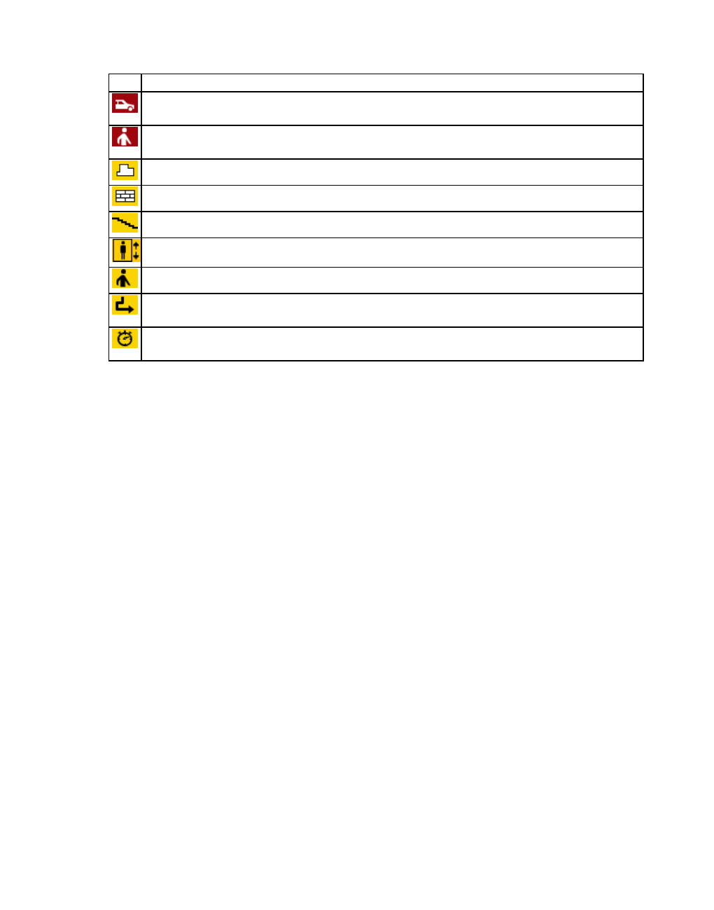
6.1 Setting up a road network or PT link network
Icon Network object type
Vehicles in the network are the result of simulation and cannot be inserted as network
objects (see "Displaying vehicles in the network in a list" on page 803).
Pedestrians in the network are the result of simulation and cannot be inserted as net-
work objects (see "Showing pedestrians in the network in a list" on page 809).
Areas (see "Modeling construction elements" on page 834)
Obstacles (see "Modeling construction elements" on page 834)
Ramps & Stairs (see "Modeling construction elements" on page 834)
Elevators (see "Modeling elevators" on page 929)
Pedestrian Inputs (see "Modeling pedestrian inputs" on page 883)
Pedestrian Routes (see "Modeling routing decisions and routes for pedestrians" on
page 886)
Pedestrian Travel Times (see "Defining pedestrian travel time measurement" on page
939)
To insert network objects in a network editor, you have to select the network object type on the
Network object toolbar (see "Using the Network object toolbar" on page 60).
Each network object has attributes and attribute values. Many attribute values are predefined
by default. When you insert a network object into a Vissimnetwork, you can edit the attribute
values. Attribute values can also be edited later on(see "Editing attributes of network objects"
on page 330).
6.1 Setting up a road network or PT link network
The basic element of a road network in Vissim is the link. Links can run in one direction over
one or more lanes. You connect links via connectors; in this way, you construct the link
network. The traffic can only flow via connectors from one link to another. It is not sufficient to
model links without connectors attached or to have them overlap.
You can also use links and connectors to create a line network for public transportation (see
"Modeling short-range public transportation" on page 478).
In the road network or line network, you can add the required network objects exactly and
define their attributes. Many network objects may lie on a link or connector, e.g. stop signs,
routing decisions, PT lines or data collection points. Vehicle inputs may be positioned on links
only. You can edit or delete network objects and attributes later on. For example, you may
move a network object lying on a link or connector to a different position on the link or
connector or copy it to a different link or connector.
6.1.1 Example for a simple network
The example shows a three-legged signalized intersection, with links, connectors, and other
network objects:
© PTV GROUP 315
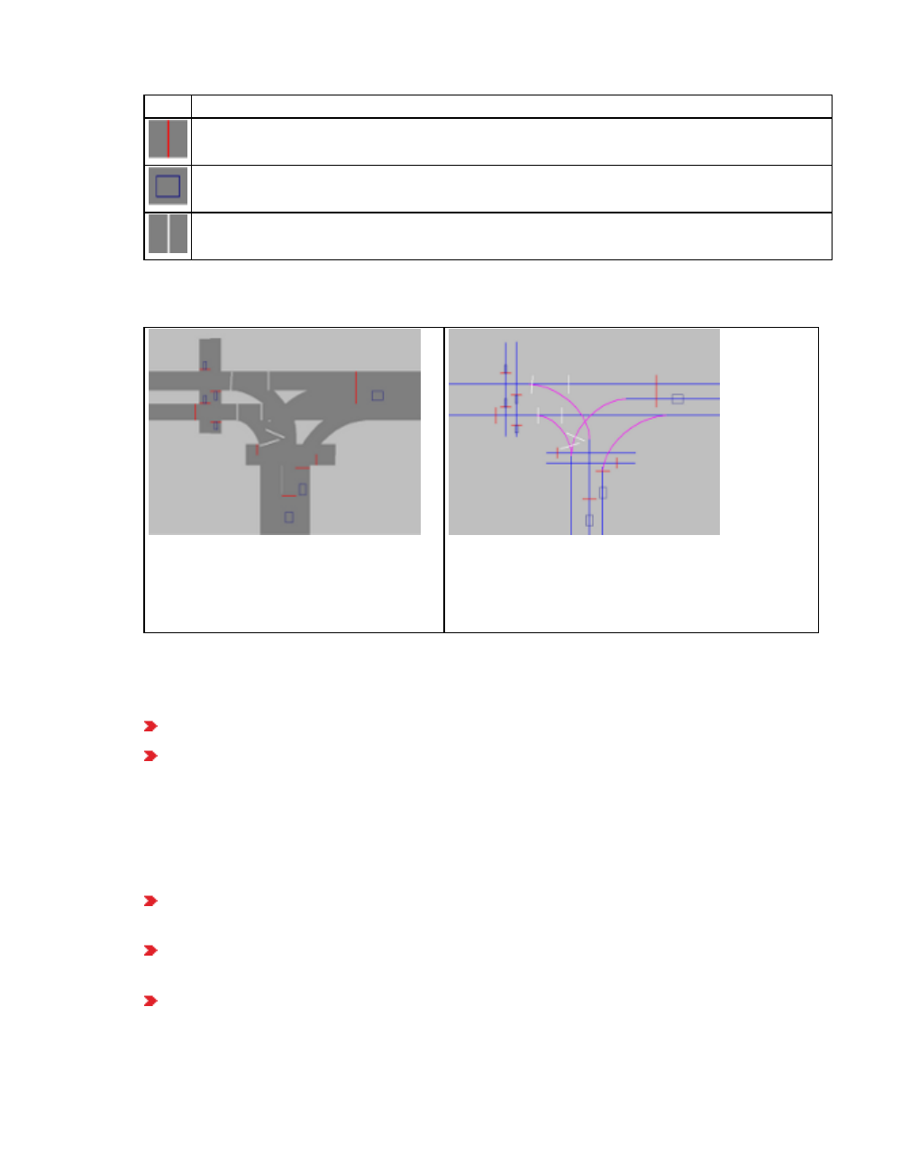
6.1.2 Traffic network data
Icon Network object
Signal Heads
Detectors
Priority Rules
You can define the colors of network objects via the graphic parameters (see "Editing graphic
parameters for network objects" on page 149).
Wireframe display disable: Three-
legged intersection with two pedestrian
crossings
Wireframe display enable: The network is
represented via the middle lines of links (straight
blue lines) and the middle lines of connectors
(pink lines in the curves).
6.1.2 Traffic network data
A Vissim traffic network is made up of the following data:
Static data, which is not changed by the simulation.
Dynamic data, which essentially includes all information that describes the simulated
traffic.
6.1.2.1 Static data
Static data illustrates the applicable traffic infrastructure. This data is necessary for simulation
and manual tests from traffic-dependent signal controls. Static data, for example, includes:
Links with starting points and end points and perhaps intermediate points. Links are dir-
ectional roadways on which traffic flows. For each link you specify a number of lanes.
Connectors between links for the modeling of possible turns and from merging and broad-
ening of lanes
Position and length from public transport stop
316 © PTV GROUP
6.1.3 Evaluating vehicular parameters from the network
Position from signal head and stop line and references to the allocated signal groups
Position and length of detectors used to record vehicles for vehicle-actuated signal con-
trol.
Position of PT calling points that record PT vehicles sending PT telegrams
6.1.2.2 Dynamic data
For the simulation, you define dynamic data, for example:
Vehicle inputs indicate congestion, including vehicle compositions, as relative shares, for
example HGV shares for all links which lead into the network.
You define link sequences via routing decisions. You define routes via temporally variable
traffic volumes that refer to vehicle classes.
The position and the values from Headway and Time Gaps from Priority Rules. Priority
Rules describe priority rules, for example, "right before left" or determines acceptable left
turn.
The curvature, departure times and boarding and alighting from public transport lines
6.1.3 Evaluating vehicular parameters from the network
You can determine from the network different vehicular parameters and subsequently
evaluate them (see "Performing evaluations" on page 941). Thereby, for example, you can
apply the following network objects:
Data collection points for user-defined local data collection measurements, for example,
measurement of the number of vehicles of particular vehicle classes, their acceleration
and average speed (see "Defining data collection points" on page 419)
Vehicle travel time measurements for the measurement of total travel times and delays
when driving on the respective network segment (see "Defining vehicle travel time meas-
urement" on page 420)
Queue counter for the measurement of average and maximum queue lengths (see "Model-
ing queue counters" on page 423)
Note: The add-on module Viswalk allows for a comparison of pedestrian traffic
evaluations.
6.2 Copying and pasting network objects into the Network Editor
In the Network editor, you may select stand-alone network objects and dependent static
network objects in 2D mode and copy them to the Clipboard (see "Selecting and copying
network objects" on page 320). Network objects copied to the Clipboard can be pasted into a
network (see "Pasting network objects from the Clipboard" on page 321).
With the copy-and-paste command you can use network objects again, whose course, form or
other attributes you have adjusted. You may also select multiple network objects to copy and
© PTV GROUP 317
6.2 Copying and pasting network objects into the Network Editor
paste the modeled parts of your Vissim network. This allows you to build your Vissim network
more quickly.
If you have defined several levels, you can copy network objects from one level into another
level (see "Copying network objects to different level" on page 323).
Stand-alone network objects
Stand-alone network objects are positioned directly in the Network Editor:
Links, areas, ramps and stairs
Obstacles
Sections
Elevators
Nodes
3D Traffic Signals
Static 3D Models
You can copy stand-alone network objects to a different position in the currently opened
Vissim network (see "Pasting network objects from the Clipboard" on page 321). You may also
open another Vissim network and insert network objects into it.
Dependent network objects
Dependent network objects are located on top of stand-alone network objects:
The connectors selected are copied, if you have also selected the origin and destination
link.
Desired Speed Decisions
Reduced Speed Areas
You may copy conflict areas, if all links have been selected that traverse conflict areas.
Priority rules may be copied from an individual link, if you have selected a From Section
and a To Section. If the From Section and To Section lie on different links, you can copy pri-
ority rules together with the links they lie on.
Stop Signs
Signal Heads
Detectors
Vehicle inputs
Vehicle routes may be copied from a link, if the From Section and To Section lie on the
same link. If the From Section and To Section lie on different links, all links of the vehicle
318 © PTV GROUP

6.2 Copying and pasting network objects into the Network Editor
routes must be selected. The From Section of a vehicle route may also be copied to
another link without the To Section.
Parking Lots
Public transport stops
Public transport lines may be copied from a link, if the From Section and the To Section lie
on the same link. If the From Section and To Section lie on different links, all links of the
public transport lines must be selected.
Data Collection Points
Vehicle travel times may be copied from a link, if the From Section and the To Section lie
on the same link. If the From Section and To Section lie on different links, you must also
select and copy the respective links.
Queue Counters
Backgrounds
Pavement Markings
Pedestrian Inputs
Pedestrian Routes: The From Section of a pedestrian route may also be copied to the
same or another area without the To Section.
Pedestrian Travel Times
You may paste dependent network objects that you have copied from a stand-alone network
object into another stand-alone network object of the same type (see "Pasting network objects
from the Clipboard" on page 321). You can also open another Vissim network and insert
copied, dependent network objects into a stand- alone network object. The stand- alone
network object must be of the same network object type as the network object copied.
Copying stand-alone network objects together with dependent network objects
To copy multiple stand-alone network objects together with their dependent network objects,
around the network objects, drag open a frame. This allows you to reuse the modeled parts of
your Vissim network.
Copying during a simulation
You may copy static network objects during a simulation in the 2D mode. Dynamic network
objects cannot be copied during a simulation.
Copying network objects with a reference to a SC
When you copy network objects with a reference to a signal control, Vissim also copies the
settings, e.g. when copying detectors, signal heads, 3D signal heads, priority rules or stop
signs. When you paste these network objects, a window opens that allows you to select
whether Vissim shall use the same SC or a new SC based on the original one.
© PTV GROUP 319

6.2.1 Selecting and copying network objects
Copying network objects with a reference to files
When copying network objects that contain file references, the references only are copied. The
files are not copied.
Copied base data
When copying the network objects, Vissim also copies base data on which the network objects
are based, for example distributions, functions, vehicle types, pedestrian types, vehicle
classes, pedestrian classes, and/or behavior parameters.
6.2.1 Selecting and copying network objects
1. Select the desired network objects in the Network Editor (see "Moving network objects in
the Network Editor" on page 336).
2. If you have selected dependent network objects with a From Section and a To Section that
both lie on stand-alone network objects, make sure that you also select the stand-alone
network objects.
3. If you have selected vehicle routes or PT lines, make sure that you also select all the links
used by the vehicle routes or PT lines.
4. If you have selected connectors, make sure that you also select the origin and destination
links.
5. If you have selected conflict areas, make sure that you also select all links that traverse the
conflict areas.
6. Right click the Network Editor.
7. From the shortcut menu, choose Copy.
Tips:
Alternatively, use the following commands to copy network objects to the Clip-
board:
Key combination CTRL+C
Key combination CTRL+INS
Network Editor toolbar > Copy selection
You can also duplicate network objects in the Network editor (see "Duplicating
network objects" on page 332)
The selected network objects are copied to the Clipboard. Together with the network
objects, base data that refers to the network objects is copied.
8. If you have copied network objects with a file reference via a relative path, before inserting
them into another Vissim network, make sure that the relative paths specified are also valid
for the other Vissim network.
9. If desired, continue to edit the Vissim network.
320 © PTV GROUP

6.2.2 Pasting network objects from the Clipboard
10. Insert the copied network objects (see "Pasting network objects from the Clipboard" on
page 321).
6.2.2 Pasting network objects from the Clipboard
If you have copied stand-alone network objects to the Clipboard, you may paste them into the
Network Editor at the position of your choice. You may then edit these network objects, for
example move or rotate them, or adjust their course, form or attributes.
You can paste network objects into the same Vissim network from which you have copied
them or into another Vissim network, for example another instance of Vissim you have
opened. If in the Vissim network, base data is missing to which the pasted network objects in
the original network refer, the respective base data is also pasted. Vissim then checks the
network for conflicts and discards duplicates (see "Reading a network additionally" on page
341). If identical base data already exists, these are used for the pasted network objects.
If together with the stand-alone network objects, you have selected and copied dependent
network objects that lie within the stand-alone network objects, these are pasted together with
the stand-alone network objects.
If you have copied dependent network objects from a stand-alone network object, you may
paste the dependent network objects into another stand-alone network object of the same
type.
You may paste connectors from the Clipboard, if they have been copied with their origin and
destination link.
You may paste conflict areas from the Clipboard, if all links were copied that traverse the
conflict areas. If after pasting a link of a conflict area, the pasted link intersects with an existing
link, a new conflict area is created.
When from the Clipboard you paste network objects that refer to files, the file references
remain intact. The files are not copied.
6.2.2.1 Pasting stand-alone or dependent network objects
1. Depending on whether you have copied stand-alone or dependent network objects to the
Clipboard, carry out the following steps:
To paste stand-alone network objects, in the Network Editor, right-click the position
where you want to paste the network objects.
To paste dependent network objects, in the Network Editor, click the stand-alone net-
work object to which you want to add the dependent network objects.
2. From the shortcut menu, choose Paste.
© PTV GROUP 321

6.2.2 Pasting network objects from the Clipboard
Tip: Alternatively, use the following commands to paste network objects from the
Clipboard:
Stand-alone network objects: In the Network Editor, move the mouse pointer to the
position of your choice and press CTRL+V or SHIFT+INS.
Dependent network objects: In the Network Editor, move the mouse pointer to the
stand-alone network object of your choice and press CTRL+V or SHIFT+INS.
Instead of using the key combinations, press the Paste from clipboard button
on the Network Editor toolbar.
When you can paste network objects from the Clipboard that contain a reference to a SC, a
window opens.
3. Click the button of your choice:
Element Description
Yes Adopt the references of inserted network objects into existing SC
No Define new SC based on the SC that contains references to the inserted net-
work objects The references of the inserted network objects are adjusted to the
new SC.
In the Network Editor, stand-alone network objects are inserted at the position of the mouse
pointer. If the mouse pointer is positioned outside the Network Editor, the network objects
are inserted at a position in the network that is shown as the middle in the active Network
Editor.
Dependent network objects are inserted into the stand-alone network object selected.
Positioning of the network object depends on several factors, for example the network
object type.
Inserted network objects have been selected. You can then move or rotate the network
objects.
In the network objects list of the network object type, a new row is added for each network
object inserted.
A new connector is assigned the attribute Number, which is a number available > 9,999.
For all other network object types, a new network object is given the next higher number
available as the Number attribute.
322 © PTV GROUP

6.2.3 Copying network objects to different level
If together with the network objects new data is inserted, the data is also assigned a new
number.
4. If desired, you can edit inserted network objects, for example move them to a different
position or adjust their attributes.
6.2.3 Copying network objects to different level
In the Network editor, you can select static network objects and copy them to a different level. If
dependent network objects have been placed on the network objects you wish to copy, and
you select those as well, you can copy the network objects together.
As long as a copyable number of objects was selected, the objects are copied and their level
attribute is changed, adding the level number offset to the previous level number. The level
number offset is the difference between the values of the number attribute of the level you
copy the objects from to the level you copy the objects to. The level number offset can be
negative when you copy from one level with a higher number to another level with a lower
number. All levels with numbers resulting from this step must already exist, otherwise the
process is canceled.
1. Select the desired network objects in the network editor (see "Moving network objects in the
Network Editor" on page 336).
2. If you have selected dependent network objects with a From Section and a To Section that
both lie on stand-alone network objects, make sure that you also select the stand-alone
network objects.
3. If you have selected vehicle routes or PT lines, make sure that you also select all the links
used by the vehicle routes or PT lines.
4. If you have selected connectors, make sure that you also select the origin and destination
links.
5. If you have selected conflict areas, make sure that you also select all links that traverse the
conflict areas.
6. Right click the Network Editor.
7. From the shortcut menu, choose Copy to level(s).
The Copy to level(s) window opens. The list box shows the levels defined. It also contains
the offset number for the respective level against the level from which the network objects
are copied.
8. In the list box, click the level to which you want to add the network objects.
9. Confirm with OK.
The network objects selected are copied to the level selected. Together with the network
objects, base data that refers to the network objects is copied.
© PTV GROUP 323

6.2.4 Saving a selected part of the network
6.2.4 Saving a selected part of the network
In a Vissim network, you may select stand- alone network objects and save them as a
subnetwork to a *.inpx network file. If on top of a stand- alone network object there are
dependent network objects you wish to save, select the dependent network objects as well.
You cannot save dependent network objects without saving the stand-alone network objects
they are placed on.
1. Select the desired network objects in the Network Editor (see "Moving network objects in
the Network Editor" on page 336).
2. From the File menu, choose > Save selection as.
The Save File As window opens.
3. Make the desired changes:
Field Description
File type File format of network file: The default setting is *.inpx.
Filename Name of file to which the subnetwork is saved
4. Select the path to the desired directory.
5. Click the Save button.
The network objects selected are saved to the *.inpx network file.
6.3 Editing network objects, attributes and attribute values
You can edit network objects, their attributes and attribute values via the following elements of
the user interface:
Element Element with editing functions
Menu com-
mands Lists menu: In a list, show the attributes and attribute values of objects of a
base data type or network object type
Base data menu: In a list, show the attributes and attribute values of objects
of a base data type
324 © PTV GROUP
6.3 Editing network objects, attributes and attribute values
Element Element with editing functions
Network
editor Graphical display and editing of network objects.
When no simulation is running, in the Network editor, you can select,
move, copy, delete and paste network objects.
Double-click the network object to open the <Name network object
type> window. Attributes and attribute values of the network object are
displayed.
Right-click the network object to open the shortcut menu. From the short-
cut menu, choose a command of your choice, e.g. show the network
object and its attributes in the list of network objects of the network object
type.
While the simulation is running, network objects, attributes and attribute
values cannot be edited or can only be edited to a very limited extent.
When, during a simulation run, you open the <Name network object
type> window to display attributes of network objects, a message is dis-
played informing you of the limited editing options.
Toolbar of the Network editor (see "Network editor toolbar" on page 73):
You can copy selected network objects to the Clipboard.
Shortcut menu in the Network Editor with and without selected network
objects (see "Network editor context menu" on page 78)
Open <Name Network object type> window (see "Showing attribute values
of a network object in the Network editor" on page 331)
Lists Show attributes and attribute values of base data and network objects in
lists (see "Selecting and editing data in lists" on page 96), (see "Editing lists
and data via the context menu" on page 99).
Toolbar of lists (see "List toolbar" on page 93)
Shortcut menu in column header, row header, cells (see "Editing lists and
data via the context menu" on page 99)
© PTV GROUP 325

6.3.1 Inserting a new network object in a Network Editor
Element Element with editing functions
Network
objects
toolbar
(see "Using the Network object toolbar" on page 60)
Button Toggle visibility in current network editor: Only if the network object
toolbar, the network object type is not selected: Shows or hides network
objects of the network object type in the active Network editor.
Lock button Toggle selectability in current network editor shows an
open lock: You can select and edit network objects of this network object
type in the Network editor.
Lock button Toggle selectability in current network editor shows a
closed lock: You cannot select and edit network objects of this network
object type in the Network editor.
Edit graphic parameters button
button Toggle label visibility in current network editor: The labeling
of the network objects of the network object type is not displayed.
button Toggle label visibility in current network editor: The labeling
of the network objects of the network object type is displayed.
Shortcut menu commands (see "Context menu in the network object tool-
bar" on page 63)
For many object types, you assign the definition of objects to other objects (see "Using
coupled lists" on page 111).
6.3.1 Inserting a new network object in a Network Editor
Notes:
You can specify that you need not press the CTRL key when adding network objects
(see "Right-click behavior and action after creating an object" on page 143).
For some network objects there are windows in which the attributes of a network
object can be defined and edited. There are lists for this, for all network objects. You
can choose whether you want to open a window, a list or neither of the two for the
definition of network objects in the Network Editor (see "Right-click behavior and
action after creating an object" on page 143).
On the network object toolbar, the desired network object type must be selected.
Network objects can be superimposed in the Network Editor. While you add a new network
object, you can select the superimposed network objects until the network object, to which you
want to add the new network object, is marked (see "Selecting a network object from
superimposed network objects" on page 340).
326 © PTV GROUP
6.3.1 Inserting a new network object in a Network Editor
6.3.1.1 Commands for inserting new network objects
If on the Network objects toolbar, you selected a network object type, you can insert network
objects into the Network editor via the following functions:
Via the context menu of the network editor If for the network object type, you inserted a
start section for the network object and afterwards need to insert one or multiple des-
tination sections, the respective function is displayed in the context menu.
depending on the user settings, using the right mouse button or normally using the right
mouse button and the CTRL key (see "Right-click behavior and action after creating an
object" on page 143)
6.3.1.2 Inserting new network objects in available positions or on other network objects
Independent from network object type, you can enter network objects in available positions or
you must place network objects on other network objects. This is described for each network
object according to the definition of the network objects (see "Creating and editing a network"
on page 314).
You can enter, for example, links or areas onto available positions in the Network Editor.
Thereby, you can cut or overlap network objects.
You must place network objects of other network object types on network objects. For
example, you can insert desired speed decisions, reduced speed areas, priority rules,
detectors, parking lots, vehicle routes, vehicle inputs, vehicle travel time measurements,
etc. onto links. Insert pedestrian inputs, sections for area measurement or pedestrian
travel time measurements onto areas.
For vehicle travel time measurements and pedestrian travel time measurements, insert a
From Section and a To Section.
You add a From Section for priority rules, vehicle routes and pedestrian routes; you can
also add one or more To Sections.
For network objects that have a start section and multiple destination sections, you can
select the start section again later on to insert additional destination sections or move
them.
6.3.1.3 Work steps during addition depend on the network object type
After you have begun to add a network object, the further steps until the network object is fully
added depend on the network object type. These steps are described in the definition of
network objects (see "Creating and editing a network" on page 314). There are the following
differences:
Network object types whose length is defined by dragging the mouse
Links: While dragging the mouse, you can use the left mouse button to set intermediate
points and change the direction there later.
Reduced Speed Areas
© PTV GROUP 327

6.3.1 Inserting a new network object in a Network Editor
Parking Lots
Detectors
Public transport stops
For these network object types, the following applies:
When the desired length is achieved by dragging the mouse, release the CTRL key and the
right mouse button.
For connectors, the following applies:
When the desired position is reached on the destination link by dragging the mouse, and
the edges of the destination link are marked by arrows along the direction of travel, release
the CTRL key and the right mouse button.
Notes:
You can specify that you need not press the CTRL key when adding network objects
(see "Right-click behavior and action after creating an object" on page 143).
For some network objects there are windows in which the attributes of a network
object can be defined and edited. There are lists for this, for all network objects. You
can choose whether you want to open a window, a list or neither of the two for the
definition of network objects in the Network Editor (see "Right-click behavior and
action after creating an object" on page 143).
Network object types with a marker
Desired Speed Decisions
Stop Signs
Signal Heads
Vehicle Inputs
Data Collection Points
Queue Counters
Pavement Markings
3D Traffic Signals
For these network object types, the following applies:
Once the network object is inserted, release the CTRL key and the right mouse button.
Network object types with a start section and a destination section
Public Transport Lines
Vehicle travel time measurements
Pedestrian Travel Time Measurement
328 © PTV GROUP

6.3.1 Inserting a new network object in a Network Editor
1. When the desired position of the destination section is achieved by dragging the mouse,
click the right mouse button.
2. Release the keys.
Network object types with a start section and several destination sections
Priority Rules
Vehicle Routes
Pedestrian Routes
For these network object types, the following applies:
1. Repeat the next two steps until all destination sections have been inserted for the network
object:
2. Move the mouse pointer to the desired destination section position.
3. Click.
4. After having inserted all destination sections for a network object, click into an empty
section of the Network Editor.
Planar network object types
You can add planar network objects as a rectangle or polygon.
Areas
Obstacles
Ramps & Stairs
Sections
For these network object types, the following applies:
for a rectangle: If you have drawn a rectangle to the desired size, double click.
for a polygon: Once you have added the desired number of the polygon points, double
click.
Graphic file of a background image
The background is inserted and selected. You can change its size via the corner drag points.
Click in an empty area of the Network Editor.
Nodes
Once you have added the desired number of the polygon points, double click.
6.3.1.4 Behavior after addition
Depending on the user settings and the network object type, a window or a list can open -
immediately after adding a network object - or none of the two (see "Right-click behavior and
© PTV GROUP 329

6.3.2 Editing attributes of network objects
action after creating an object" on page 143). In the window or the list, you can enter input
attributes for the network object.
When you insert 3D model or 3D signal head, a symbol is inserted and a window opens.
There, you can select the desired file.
When you insert a background, a window opens. There you can select the desired graphic file.
After insertion, a network object is automatically selected. This allows you, for example, to
copy it or position it exactly.
6.3.1.5 Adding a network object to a level
If you have defined levels and you add a new stand-alone object such as a link, area, stair or
ramp, an obstacle, a background graphic, a static 3D model or a 3D signal head, the network
object is added in the lowest-number level visible in the current network editor. If all levels are
invisible or no network editor is open, the network object is generated in the lowest-number
level. You can assign the network object a different level (see "Attributes of links" on page
383).
6.3.1.6 Adding a network object at the beginning or end of a connector
You can place a network object on the same link coordinates as the beginning of an outbound
connector or exactly at the end of a connector. Vehicles that change links at this position will
recognize the network object. This means that a conflict area, e.g., that ends precisely at the
end of a connector, will work as expected.
6.3.1.7 Canceling addition of network objects
You want to cancel the insertion of a network object depending on the network object type:
To cancel the insertion of a start section, in the Network Editor, move the mouse pointer to
an empty section and release the right mouse button.
To cancel the insertion of a destination section, in the Network Editor, move the mouse
pointer to an empty section and double-click.
To cancel the insertion when a window with attributes is open, release the mouse buttons
and press the ESC key.
To cancel the insert of a construction element, release the mouse buttons and press the
ESC key.
6.3.2 Editing attributes of network objects
You can edit attributes of network objects in the list of network objects of a network object type.
For some network object types, you can select attributes in the <Name network object type>
window.
The maximum value for all integer input values is 4 294 967 295.
6.3.2.1 Editing attributes in a list
1. From the Lists menu, choose the desired entry.
330 © PTV GROUP

6.3.3 Showing attribute values of a network object in the Network editor
Tip: Alternatively, you can show the list via the following functions:
On the Network objects toolbar, right-click the desired network object type and from
the shortcut menu, choose Show List.
In the Network editor, right-click a network work and from the shortcut menu, choose
Show In List.
The list with the attributes of the network objects of the network object type opens.
By default, the column titles show the short names of the attributes. The short names are
abbreviations of long names (see "Showing short or long names of attributes in column
headers" on page 147).
By default, you can edit the list (see "Using lists" on page 89).
Note: In lists, you can use the Attribute selection icon to show and hide attribute
values (see "Selecting attributes and subattributes for a list" on page 106).
2. Edit the attributes (see "Selecting and editing data in lists" on page 96):
6.3.2.2 Attributes in the Editing <Name network object type> window
For some network objects, a <Name Network object type> window is automatically opened
when you define a network object and have selected that you want the program to
automatically open the Edit dialog after object creation (see "Right-click behavior and action
after creating an object" on page 143) . You can enter entry attributes in this window. By
default, the entry attributes are also displayed in lists.
For network objects which are already defined, you can call up this window via the following
functions and edit within the attributes:
In the network objects list of the network object type (see "Functions available in the short-
cut menu of the row header" on page 100)
In the Network Editor (see "Showing attribute values of a network object in the Network
editor" on page 331)
While the simulation is running, network objects, attributes and attribute values cannot be
edited or can only be edited to a very limited extent. When, during a simulation run, you open
the <Name network object type> window to display attributes of network objects, a message
is displayed informing you of the limited editing options.
6.3.3 Showing attribute values of a network object in the Network editor
In the Network editor, you can highlight network objects and open windows for some network
object types. The windows display attribute values for the network objects. For all network
object types, you can show attributes in lists. Important entry attributes are described for the
network objects (see "Creating and editing a network" on page 314).
1. In the Network editor, double-click the network object of your choice.
The <Name network object type> window or <Name network object type> list opens.
© PTV GROUP 331

6.3.4 Direct and indirect attributes
2. You can change the settings if you wish.
3. Confirm with OK.
6.3.4 Direct and indirect attributes
A network object has attributes that allow you to save input data and output data:
Direct attribute: The data refer directly to the network object. Example: Length attribute of
a link.
Indirect attribute: The data result from the relation between two network objects. Example:
For a network object Link, you can select the network object type Display type as a rela-
tion. A direct attribute of this display type is Fill style. You can select the fill style chosen for
a link as an indirect attribute for links and show it in the Links list for each link defined. You
can edit an indirect attribute if it is an n:1 or 1:1 relation of a network object.
Direct and indirect attributes can also be used to define user-defined attributes (see "Using
user-defined attributes" on page 200).
6.3.5 Duplicating network objects
You can select and duplicate individual or multiple network objects in lists and network
editors. In the network editor, you can duplicate the following network objects:
One or more selected independent network objects, for example, from network object
type links, connectors, areas, ramps, nodes, sections, static 3D objects, 3D signal
heads, background. You can also duplicate independent network objects of different
network object types. You can move duplicate independent network objects in the net-
work editor. Dependent network objects which lie on selected, independent network
objects are not duplicated in the process, unless they are selected.
One or more selected dependent network objects which lie on an independent net-
work object. You can also duplicate dependent network objects of different network
object types. You can move duplicated dependent network objects in the network
editor to the independent network object or another independent network object of the
same network object type.
Select the desired function.
332 © PTV GROUP

6.3.6 Moving network objects in the Network Editor
Element Functions to duplicate
Lists Shortcut menu > Duplicate: You can also select more cells and therefore
duplicate more network objects. The new network object is added in the
network editor in the same position as the duplicated network object and is
selected.
Network
Editors Shortcut menu > Duplicate: The new network object is added in the network
editor in the same position as the duplicated network object and is selected.
Hold down the CTRL key, click in the network object and drag the new net-
work object to the desired position:
for independent network objects, for example, links or areas, to the
desired position in the network editor
for dependent network objects which, for example, lie on links or areas
to the desired link or area
In the list of the network objects of the network object type, a new row is added.
A new connector is assigned the attribute Number, which is a number available > 9,999.
For all other network object types, a new network object is given the next higher number
available as the Number attribute.
6.3.6 Moving network objects in the Network Editor
In the Network editor, you can move stand-alone network objects, e.g. links or areas. In doing
so, the following network objects are also moved:
Start and end points of connectors that are not selected, when their starting link and
destination link are selected and moved. If you also wish to move the connector, you
must also select this.
Dependent network objects that lie on top of stand-alone network objects that are
moved, e.g. stop signs, parking lots, start sections and destination sections of routes
and routing decisions on links, or obstacles, ramps and stairways in areas.
In the network editor, you can also move one or several dependent network objects that are on
stand-alone network objects, for example stop signs or parking lots to links. These network
objects can only be moved on a stand-alone network object or onto another stand-alone
network object. If you drag the selected network objects out of the stand-alone network object
into a free area in the network editor and release the mouse button, it is deleted.
Tip: Alternatively, in lists showing the attributes of a network object, you can change the
attribute value Position, if the network object has this attribute.
6.3.6.1 Moving stand-alone network objects
1. Select the desired network objects in the network editor (see "Moving network objects in the
Network Editor" on page 336).
2. Hold down the mouse button and move the cursor to the desired position.
3. Release the mouse button.
© PTV GROUP 333
6.3.7 Moving network object sections
Note: By moving the beginning or end of a connector or an entire connector from one
link to another link, PrT and PT routes are interrupted.
6.3.6.2 Moving dependent network objects
1. Select in the network editor the desired network objects, which are on stand-alone network
objects (see "Moving network objects in the Network Editor" on page 336).
2. Hold down the mouse button and move the cursor to the desired position.
6.3.7 Moving network object sections
In the network editor, you can move an individual start or destination section to the same link
or to another link or connector.
1. Click the header of the Network Editor.
2. In the Network editor, click the desired section and keep the mouse button pressed.
The mouse pointer becomes a symbol. The section and link or connector are
highlighted.
3. Move the start section or destination section to the desired position on the same link or
connector or to a different link or connector.
When you move the mouse pointer to a different link or connector, the latter is highlighted
and you can move the section there.
If you want to move the section to a position on a link or connector that lies under the link or
connector currently highlighted, use the TAB key to highlight the underlying link or
connector (see "Selecting a network object from superimposed network objects" on page
340).
Click into an empty section of the Network Editor to cancel the insertion.
4. Release the mouse button.
6.3.8 Calling up network object specific functions in the network editor
You can call up functions for the different network object types in the network editor via the
context menu next to the standard functions, which are only possible for the currently selected
network object types, for example, Links > Split Links. These functions are described with the
network objects.
6.3.9 Rotating network objects
You can turn an individual, independent network object or select and turn several network
objects.
334 © PTV GROUP

6.3.9 Rotating network objects
6.3.9.1 Turn individual network object
You can turn an individual network object with network object types areas, obstacles, ramps,
stairways, intersections, backgrounds, static 3D models, 3D traffic signals and sections.
1. Click on the network object type of the network object in the network object toolbar.
2. Click the desired network object.
At the corner points of the network object, curved arrows with two arrow heads are
displayed.
3. Click the desired curved arrow and hold down the mouse button.
4. To align the network object, reduce the rotation speed by moving the mouse pointer straight
away from the network object.
5. Drag the mouse pointer in circles to the desired direction.
6. Release the mouse button.
The selected network object is turned around the turning point.
7. Release the keys.
6.3.9.2 Select several network objects
You can turn several independent network objects with the network object types links,
connectors, areas, obstacles, ramps, stairways, intersections, static 3D models, 3D traffic
signals and sections. These may also be network objects with different network object types.
1. Hold down the CTRL key and click on the desired stage sequence.
A dashed line frame is drawn aground the maximum dimension of the network objects. At
the corner points of the dashed line frame, curved arrows with two arrow heads are
displayed:
Tip: Alternatively you can also hold down the left mouse button and draw a frame over
the desired network objects.
2. Point the mouse pointer to the destination area of your choice.
3. Hold down the ALT key, click in the Network Editor on the desired construction element and
circularly move it with the mouse pointer in the desired direction.
© PTV GROUP 335
6.3.10 Deleting network objects
The selected network objects are turned around their center point.
4. Release the keys.
6.3.9.3 Key combinations for turning network objects
You can use the following key combinations for turning:
Hotkeys Description
CTRL+ALT Duplicate and turn selected network objects.
CTRL+SHIFT Duplicate selected network objects and position at intervals of 22.5°.
CTRL+ALT+SHIFT Duplicate selected network objects and turn at intervals of 22.5°.
6.3.10 Deleting network objects
You can select and delete network objects. If you delete network objects that have an
assignment to other network objects or onto which other network objects have been
positioned, these may also be deleted. If you would like to keep the allocated network objects,
assign them to another network object before deleting.
Element Functions to delete
Lists Context menu > Delete
Key DEL
The network objects selected in the list are deleted. The network objects
selected in the network editor are not deleted.
Network
Editors Context menu > Delete
Key DEL
In Network Objects, drag the inserted network objects from there and release
the mouse button
The network objects selected in the network editor are deleted. The network
objects selected in a list are not deleted.
6.4 Displaying and selecting network objects
You can show and edit network objects and their attributes in lists. In Network Editors you can
add network objects in the 2D mode and position them exactly in the network. You can re-
select and re- edit network objects. In 3D mode you can view the network from different
perspectives.
You can run simulations in 2D and 3D mode. During the simulation you can select vehicles or
pedestrians, automatically display them in the Quick View and mark them in lists, for example,
in order to evaluate dynamic data from the simulation directly in the simulation.
6.4.1 Moving network objects in the Network Editor
In a Network Editor, you can select network objects in the 2D or 3D mode. You can select
network objects without having to select the network object type in the Network objects bar.
336 © PTV GROUP

6.4.1 Moving network objects in the Network Editor
You can then edit the network objects, e.g. move them in the Network Editor, change attributes
in the Quick View, or access functions via the context menu.
If in the Network Editor you point the mouse pointer to a network object, it is highlighted. This
makes it easier to select the network. You can then select the network object.
6.4.1.1 Selecting or deselecting network objects
Make the desired changes:
Purpose Description
Selecting a
network object
Click on a network object which is not selected. When you right-
click a network object, the shortcut menu of the Network Editor is
opened (see "Network editor context menu" on page 78).
If network objects have multiple sections, you can click the start
section or destination section to e.g. move it or open the context
menu.
Vehicle routes and pedestrian routes: Click the destination section
Public transport lines, vehicle travel time measurements, ped-
estrian travel time measurements: Click the start section or the
destination section
Selecting multiple
network objects in
the 2D mode
Alternatives:
Hold the left mouse button down and draw a frame
Hold down the CTRL key and click the network objects
Selecting multiple
network objects in
the 3D mode
Hold down the CTRL key and click the network objects
Undoing the selec-
tion of all network
objects
Alternatives:
Click on an area which is not selected.
Right-click in an area that is not selected.
Undoing the selec-
tion of individual
network objects
Hold down the CTRL key and click the selected network objects you
want to deselect.
The network objects selected are highlighted in the Network editor. Attribute values are
displayed in Quick View (see "Using the Quick View" on page 66)
Note: You can select a synchronization with network editors for lists and other lists.
Then network objects that you select are automatically highlighted in the list and
network editor (see "List toolbar" on page 93).
© PTV GROUP 337

6.4.1 Moving network objects in the Network Editor
6.4.1.2 Examples of visualization of network objects
Network object Not selected Mouse pointer
points to network
object
Selected
Link
Link in wireframe view
Area
Area in
wireframe view
Vehicle during
simulation
Highlights the link: Highlights the vehicle:
Pedestrian during
simulation
Highlights the
network object:
Highlights the
pedestrian:
6.4.1.3 Visualization of selected network objects that lie on a link in an area
When you select a network object that lies on a link or in an area, the network object as well as
the link or area are highlighted. This makes it easier for you to identify the network objects that
belong together, particularly if several network objects are lying on top of each other. The
highlighted link or area is displayed as shown in the diagram in the table above, in the column
Mouse pointer points to network object: The edge of a link is marked by arrows pointing in
the direction of travel. The edge of an area is marked by a bold black line.
338 © PTV GROUP
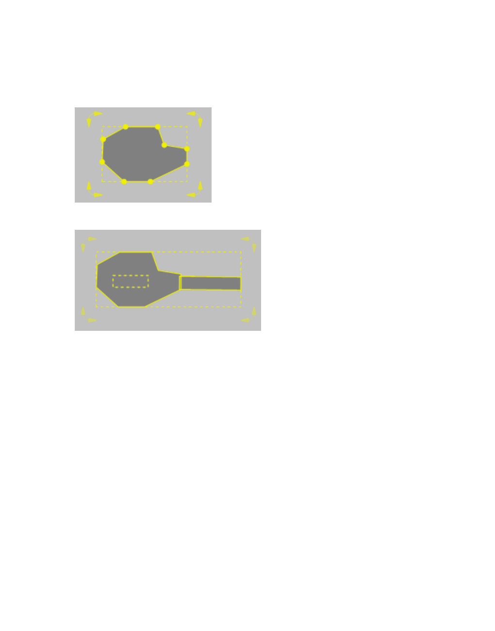
6.4.2 Selecting network objects in the Network editor and showing them in a list
6.4.1.4 Marker frame shows extension
A marker frame with a dashed line indicates the maximum horizontal and vertical extension of
a selected network object of some types, e.g. areas. Curved arrows with two arrow heads mark
points around which the network object can be rotated:
This also applies when multiple network objects are selected.
6.4.2 Selecting network objects in the Network editor and showing them in a list
In the network editor you can select network objects of a particular network object type and
show them, together with their attributes, in a list of network objects with the particular network
type.
1. In the Network Editor, right-click the network object of your choice.
2. From the context menu, choose entry Show In List.
The list of defined network objects for the network object type opens.
The objects selected in the Network editor are marked in the list, if the list is synchronized (see
"List toolbar" on page 93).
6.4.3 Showing the names of the network objects at the click position
You can show a list of network objects located at the click position. If several network objects
overlap each other, this makes it easier for you to select the desired network object.
1. In the Network Editor, right-click the network object of your choice.
2. Choose Objects At Click Position from the context menu.
© PTV GROUP 339

6.4.4 Zooming to network objects in the network editor
The network objects are shown in the context menu.
3. Click on the desired entry.
The display in the Network Editor is adjusted. The network object is selected.
6.4.4 Zooming to network objects in the network editor
In the network editor you can select the size of the network so that the selected network
objects are automatically completely displayed.
In the context menu, select Zoom To Selection.
6.4.5 Selecting a network object from superimposed network objects
If several network objects are superimposed in a Network Editor, you can select these
consecutively. This facilitates, for example, the addition of new network objects on a desired
link.
1. On the Network Editor, click on the position at which several network objects are
superimposed.
The icon is active in the network editor toolbar.
2. Click on the icon , until the desired network object is selected.
Tips:
Alternatively you can use the TAB key.
You can also press the TAB key to consecutively select the superimposed network
objects, while holding down the right mouse button and the CTRL key by default to
add a new network object on the desired network object.
6.4.6 Viewing and positioning label of a network object
In the Network Editor, you can view the attributes of the network object in a text box and
position the text box.
6.4.6.1 Showing label
1. On the Network Objects toolbar, in the row of the desired network object type,click the Edit
graphic parameters button.
The list with the graphic parameters of the network object type opens (see "List of graphic
parameters for network objects" on page 152).
2. Make sure that the option is selected for the Label visibility attribute.
3. Click the button next to the Label attribute.
The list of attributes opens.
4. Select the desired entry.
340 © PTV GROUP

6.4.7 Resetting the label position
5. Confirm with OK.
6. Click next to the list with the graphic parameters.
The label is shown in the network object.
6.4.6.2 Positioning label
1. Click on the network object type of the network object in the network object toolbar.
2. In the Network Editor, move the cursor on the label of the desired network object.
The mouse pointer becomes a symbol.
3. Hold down the left mouse button and drag the label to the position of your choice.
4. Release the mouse button.
6.4.7 Resetting the label position
In the network editor, you can reset the label position of a network object to zero.
1. On the Network objects toolbar, click the network object type.
2. In the Network Editor, right-click the network object of your choice.
3. In the context menu, select Reset label position.
6.5 Importing a network
You can import the following data:
An abstract network model from Synchro 7
An abstract network model (ANM) from Visum
Import an abstract network model from Synchro 7 adaptively into an open network.
Thereby, you can continue to edit the original network in Synchro 7 and import parts
thereof.
Import desired data additionally from a saved Vissim network file into an open network
Tip: For pedestrian areas or obstacles, you can import AutoCAD data (see "Importing
walkable areas and obstacles from AutoCAD" on page 835).
6.5.1 Reading a network additionally
You can read network objects from another Vissim network into the current network. In this
way you can select under Conflict avoidance whether Vissim the cross- overs of the
numbering between the imported and available network objects and base data should be
checked, and also in Conflict handling choose, how Vissim these conflicts should be solved in
the event of cross-overs.
© PTV GROUP 341

6.5.1 Reading a network additionally
Translating English names in the Name attribute
When reading in additional data, you normally do not want objects duplicated that are
identical in both network files. This is particularly true for base data objects, e.g. vehicle types.
If two networks mainly differ due to the different user preferences set, they also differ in terms
of the names used in the Name attribute of their base data objects, e.g. for vehicle types
(English Car, German Pkw). These names are included in several languages in the default
network file defaults.inpx that is delivered with Vissim. Even if all other attribute values are
identical, different names for the same object can cause a conflict and duplicate object data
when additional data is read in. However, you can translate the English names in the Name
attribute into the language of the network file opened into which you want to read in additional
data. Only English names in the default network file defaults.inpx delivered with Vissim will be
translated.
1. Close the network file into which you want to read in an additional network file with English
attribute values.
2. In a text editor, open the network file you want to read in.
By default, the second row contains version information, e.g. <network version="200"
vissimVersion="8.00 - 00* [55350]" >.
3. Into the row before the closing parenthesis, insert a space and the following entry:
translateStrings="true"
In the above example, this would be: <network version="200"
vissimVersion="8.00 - 00* [55350]" translateStrings="true">.
4. Save the network file.
5. Import the network file as described below.
If you save the network file after reading it in, the entry translateStrings="true" is
deleted.
Consider reference points
Vissim accounts for reference points in both networks (see "Mapping Vissim network to
background position" on page 371):
Neither of the two networks have a point on the background map that is assigned to a cor-
responding point in the network.
Vissim inserts network objects in the Network Editor at the same position they were at in the
Network Editor of the original network.
One of the networks has a point on the background map that has been assigned to a cor-
responding point in the network:
Vissim inserts network objects in the Network Editor at the same position they were at in the
Network Editor of the original network. The reference point that exists in one of the
networks is used to assign the network to a point on the background map.
342 © PTV GROUP

6.5.1 Reading a network additionally
Both networks have a point on the background map that is assigned to a corresponding
point in the network. These reference points are different in both networks:
Vissim inserts the network objects at the position in the Network Editor that corresponds
with the coordinates of the point on the background map. This might not be the same
position where the network objects were located in the Network Editor of the original
network. In the network that is read in additionally, Vissim does not change the existing
assignment of the point on the background map to the corresponding point in the network.
Importing a network
1. Ensure that the network in which you would like to import is open and saved.
2. In the File menu, choose > Read Additionally > Network.
Tip: You can also use Read Additionally Here in a Network Editor context menu to
read in a file. The center of the read-in network will be positioned at the point where
you right-clicked with the mouse.
3. Select the network file *.inpx from which data should be read additionally.
The Read Additionally window opens.
4. To sort a column, click the column header.
5. In the next steps, select for all network object types whether you want to import them and
how Vissim conflicts and duplicates should be handled.
6. Make the desired changes:
© PTV GROUP 343

6.5.1 Reading a network additionally
Element Description
Read If this option is selected, network objects of this network object type
are imported.
Network object
type
Name of the network object types which you can import
Element Description
Conflict
avoidance
Defines the behavior when network objects are imported that have the same
key as existing network objects of the same type. The key is typically a
number.
None: Keys remain unchanged. The behavior is defined in the field Con-
flict handling.
New key on conflict (default setting): Network objects with the same keys
as existing network objects are assigned a new number. In the Conflict
handling field, a number is entered that in case of a conflict is added to
the number of the network objects imported.
New key for all: all imported network objects are renumbered. In the Con-
flict handling field, a number is entered that is always added to the num-
ber of the network objects imported.
Element Description
Conflict
handling
In the Conflict avoidance field, click > None to choose from the following
options should the key of a network object you want to import be identical to the
key of an existing network object of the same type.
Ignore: The network object you wanted to import is discarded and the exist-
ing network object remains unchanged. Where all the network objects to be
imported are discarded and the Vissim network has not been changed, after
the Read Additionally, the message The network has not been changed
appears.
Overwrite object: The network object imported replaces the existing net-
work object.
Cancel: A message is opened. The import is canceled.
If in the Conflict avoidance field, New key on conflict or New key for all is
selected, Vissim suggests an Offset value, which is then added to the number
of the network objects you wish to import. You may overwrite this value. Vissim
calculates the suggested Offset values based on the following:
For numbers of the network objects to be imported, of a network object type
< 10,000: The Offset value is set to the next higher decimal power.
For numbers of the network objects to be imported, of a network object type
> 10,000: The Offset value is set to the next higher multiple of 10,000.
If all link numbers are less than1,000 and all connector numbers are less
344 © PTV GROUP

6.5.2 Importing ANM data
Element Description
than 10,000, Vissim uses a small offset. This way the numbering con-
vention, which says that link numbers are less than 1,000 and connector
numbers are less than 10,000, is maintained. Otherwise the offset is set to
the next multiple of 10,000.
Element Description
Discard
duplicates
Only for base data and network object types without geometrical positions:
If this option is not selected and you have selected the entry New key on
conflict in the field Conflict avoidance or New key for all and you have
entered an offset in the field Conflict handling, the duplicates are preserved
in the network objects.
Example: If both networks contain vehicle types with the numbers 1 to 6, the
numbers of the imported vehicle types are changed at an offset = 1,000 in
1,001 to 1,006.
If this option is selected, except for the number, the attributes of the
network objects of the network object type are compared in each network. If
the imported network object is identical to the existing network object except
for the number, the imported network object is discarded. For base data, this
option is selected by default.
Element Description
Edit
selected
The Edit Selected window opens. For the selected rows, you may edit the
settings for:
Read objects: If this option is selected, network objects of these network
object types are imported. This option is connected with the Read option in
the Read Additionally window.
Conflict avoidance: see earlier in this table
Conflict handling: see earlier in this table
7. Confirm with OK.
The network objects are read in and selected. Network Editors with Auto-Zoom
Synchronization selected choose a section that is large enough to show all selected network
objects. Backgrounds do not rotate.
6.5.2 Importing ANM data
You can export from Visum as of Visum 10 data abstracted network models (ANM files) in XML
format, or create ANM files with other programs. The abstract network models in ANM files
consist of nodes and edges. You have the following options to import ANM data:
© PTV GROUP 345

6.5.2 Importing ANM data
Select ANM file, configure data import and start data import (see "Selecting ANM file,
configuring and starting data import" on page 347)
Adaptive import of ANM data (see "Adaptive import of ANM data" on page 349)
In Visum, use the subnetwork generator to generate a subnetwork. Open Visum dir-
ectly from Vissim and import the subnetwork into Vissim. For further information, refer
to the Visum manual.
6.5.2.1 Properties of the network generated
When you import ANM files into Vissim, a new Vissim network, with the geometry of links and
connectors, is generated. Optionally, nodes can contain additional elements, for example,
lanes, lane turns, crosswalks, pockets, control types, signalizations and detectors with the
determined vehicle classes (see "Generated network objects from the ANM import" on page
352).
Notes:
The ANM import only generates segment nodes. For the editing in Vissim, you can
convert segment nodes into polygon nodes (see "Converting segment nodes" on
page 676).
You can also import files which have been exported from SITRAFFIC OFFICE.
Volumes and routing are defined in *.anmroutes files and can be imported in Vissim. This
allows you to use this data in the dynamic assignment or as static routes.
Projection in ANM data
If a projection is specified in ANM data, the ANM coordinates are converted into Cartesian
coordinates.
If no projection is specified:
A message is displayed, saying that no projection was recognized.
ANM coordinates are interpreted as Cartesian coordinates.
ANM coordinates are not converted.
Information on data for dynamic assignment
Origin-destination matrices and a Path file *.weg are generated.
346 © PTV GROUP
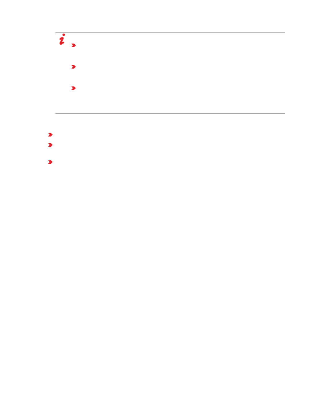
6.5.3 Selecting ANM file, configuring and starting data import
Notes:
The route volumes in a path file, which are generated via an ANM import, must
not be in whole numbers because the result of the assignment with Visum can
have decimals.
During export, the route volumes of the dynamic assignment are located in the
path file as volume per ANM time interval. During import, they are recalculated in
volumes per evaluation interval of the dynamic assignment.
For the dynamic assignment, these values are randomly rounded in Vissim. This
rounding is effected depending on the rounded share. For random rounding, the
sum of the matrix values remain somewhat constant. Example: There is a 30%
chance that 0.3 is rounded to 1 and a 70% chance it is rounded to 0.
Information on data for static routes
Vehicle inputs and routing decisions with static routes are generated.
Each routing decision for static routes contain a name, which contains the number of the
ANM origin zone.
The unique IDs of the ANM routes are taken over as routing numbers from static routing
decisions. These routes can be found in the *.anmroutes file and the respective OD rela-
tion is determined.
Information on data for mesoscopic simulation
To perform a mesoscopic simulation after ANM data import, in the ANM import window, in the
Dynamic Traffic Data section, select Dynamic assignment.
You also need to select this option when importing only one *.anm file without any routes
and/or matrices. This way you ensure that the zones and/or parking lots as well as nodes of
the network object type Node are generated.
6.5.3 Selecting ANM file, configuring and starting data import
1. From the File menu, choose > Import > ANM (Vistro/Visum).
The ANM import window opens.
© PTV GROUP 347
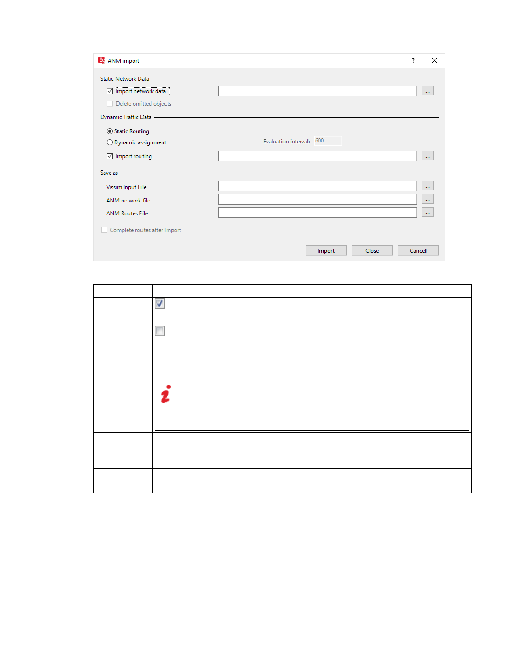
6.5.3 Selecting ANM file, configuring and starting data import
2. Make the desired changes:
Element Description
Import net-
work data If this option is selected: Enter a path and name of the *.anm file for the
import of the abstract network model.
If this option is not selected, you can force a new import of the same
routing data, which you initially imported with the abstract network model.
Select the option Import routing.
Static Rout-
ing
Import routing for static routes
Note: If you had selected the option Static Routing for the initial
import of the network data, no parking lots (zone connectors) were
created. In this case, no adaptive import of routing data is possible
for the dynamic assignment at a later time.
Dynamic
assignment
Importing data for dynamic assignment. This way you ensure that the zones
and/or parking lots as well as nodes of the network object type Node are
generated.
Evaluation
interval
Define the time interval for routing data of the dynamic assignment in which
costs are calculated and paths searched.
348 © PTV GROUP
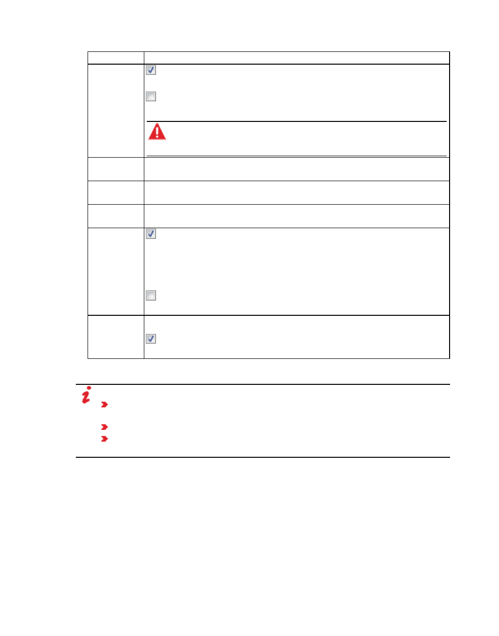
6.5.4 Adaptive import of ANM data
Element Description
Import rout-
ing If this option is selected, routing data for static routing or for the dynamic
assignment is imported.
If this option is not selected, then only the abstract network model is
imported.
Warning: An ANM import generates a network file, which refers
to the data in the *.anm file. This allows for the possibility of a
current loaded network to be overwritten or deleted.
Vissim Input
File
*.inpx network file, in which the network is saved. If you do not specify a net-
work file, adaptive import will not be possible.
ANM net-
work file
The backup file *.panm is copied to the folder in which the *.inpx network
file is saved.
ANM
Routes File
The *.panmroutes file is copied into the folder, in which the *.inpx network
file is saved.
Show warn-
ings during
Import
If this option is selected, you must confirm every warning on the screen.
The warnings are recorded in a log file and can be shown on the screen
after the import.
Note the warnings and messages in the Messages window during the
ANM import.
If this option is not selected, only the log file is generated and the list of
warnings can be shown on the screen.
Complete
routes after
Import
only for adaptive ANM import:
If this option is selected, the available Vissim routes, which have been
interrupted by the adaptive import, are automatically completed.
3. Click the Import button.
Notes:
As an alternative to the ANM import, you can drag and drop the *.anm file from the
explorer to the Vissim window.
If no network is loaded, the *.anm file is imported.
If a network is loaded, which has been initially imported as a *.anm file, you can
select whether this file should be read as adaptive or initial.
A network with network objects is generated (see "Generated network objects from the ANM
import" on page 352).
4. To show ANM import messages, from the View menu, choose > Messages.
6.5.4 Adaptive import of ANM data
You import ANM data adaptively, if the Vissim network was originally generated through an
ANM import.
© PTV GROUP 349
6.5.4 Adaptive import of ANM data
6.5.4.1 Differences to standard ANM import
When the Vissim network was generated through an ANM import, the ANM raw data were
saved by Vissim and even after being manually edited in the Network editor were not
discarded. When an edited *.anm file is imported adaptively, Vissim only adopts the changes
compared to the originally saved ANM data and adjusts the Vissim network accordingly. If a
node is changed in the *.anm file, only the node and the edges connected to it are generated
anew. This way, only manual changes made to this small part of the Vissim network are lost.
All other manual changes made to the rest of the network and the Vissim network objects
added in the Network editor are kept.
If after performing an ANM import, you define network objects on links and then select
adaptive ANM Import, the network objects of the following network object types are retained.
This applies to Vissim versions from 8.00-14 and 9.00-05.
Public transport stops
Detectors
Parking Lots
Desired Speed Decisions
Vehicle Travel Time Measurements
Data collection points
Queue Counters
Signal Heads
Stop Signs
Reduced Speed Areas
Priority rules
Pavement Markings
Conflict areas are not retained.
6.5.4.2 Use cases and properties of adaptive ANM import
Adopting changes of a Visum network into another network that a) was previously expor-
ted in Vissim and b) was edited manually after the import, without losing major changes.
Importing another demand scenario (matrix and assignment results) from Visum. The
static Vissim network remains unchanged. Only new parking lots, routing decisions, paths
and routes may be added.
6.5.4.3 Checking nodes
When you start adaptive import, an additional check is performed of the Vissim nodes. If a
Vissim node corresponds to an ANM zone, Vissim checks whether the current edge structure
matches the internal ANM attributes, e.g. the ANM zone connectors IDs of the node.
350 © PTV GROUP

6.5.4 Adaptive import of ANM data
Notes:
The node geometry cannot be restored, even if only small changes have been
made, e.g. if the driving behavior type, name of a node and/or name of a link have
changed.
In this case, restoration of the node geometry is enforced for parallel links.
6.5.4.4 Starting adaptive ANM import
1. From the File menu, choose > Import > ANM Adaptive.
The ANM Import Adaptive window opens.
Adaptive ANM import uses all parameters of the original ANM import (see "Importing ANM
data" on page 345). Adaptive ANM import also provides the following options:
© PTV GROUP 351

6.5.5 Generated network objects from the ANM import
Element Description
Delete
omitted
objects
Omitted objects might occur when after a first ANM export, the Visum network is
edited in Visum and network objects are deleted that were part of the first import
into Vissim. These network objects are not included in the *.anm file that is newly
created for adaptive import.
Select this option to delete the following network objects in the Vissim network:
Network objects missing in the *.anm file
Network objects that were automatically generated based on missing
Visum network objects
Deselect this option if you want the Vissim network to remain unchanged.in
this respect.
Complete
routes
after
Import
Select this option to complete existing Vissim routes again that were disrupted
during adaptive import.
2. Make the desired changes.
3. Click the Import button.
A network with network objects is generated (see "Generated network objects from the ANM
import" on page 352).
6.5.5 Generated network objects from the ANM import
From exported Visum network objects, the ANM import generates the following objects in
Vissim:
Visum
network
objects
Vissim network objects
Transport
system
Vehicle types and Vehicle classes
Node Nodes are generated as segment nodes (see "Modeling nodes" on page
666).
352 © PTV GROUP

6.5.5 Generated network objects from the ANM import
Visum
network
objects
Vissim network objects
Link Links can have multiple lanes, independent from the imported geometry
of the lanes. In the Messages window, the links are named as follows:
ANM-ID (from node number to node number)
One link per link section
The beginning of the widening marks a new section.
You can generate multiple connectors between two links or connectors
from or to the same lane. This can be exported as of Visum 11.
The emergency stop distance for turning-connectors in the node equals
the length of the widening minus 10 meters.
The time gap at the front for a permissive left with one parallel pedestrian
crossing equals 2.0 seconds. Thereby it is normally possible for the
oncoming right turner with a 0.5 second time gap to drive off before the
left turner after the conflict area becomes free.
Through ANM import, in a link, a link segment may be very short and in a
very wide angle to the adjacent link segment. For a uniform rep-
resentation of the link course, Vissim deletes the short link segment and
moves the adjacent link segments and their polygon points up to the
middle of the deleted link segment.
Lane Lanes with fine lane allowance or closure of vehicle types
If adjacent ANM lanes have no common vehicle type, separate Vissim
connectors are generated and not connectors with multiple lanes.
Turn Connectors with the respective angle with reduced speed areas.
Turning movement with right turn arrows are generated with stop signs,
signal heads and conflict areas.
The conflict areas of turn volumes are generated with a status.
Multiple turning lanes of a lane to different lanes on the same exit link are
allowed.
TSys closure
at turn
Closure of connectors for transport systems
The closure for a TSys from type PuT is only taken over in Vissim if a vehicle
combination is defined in Visum which allocates the TSys.
Zone and
connector for dynamic assignment: Parking lots or
for static routing: vehicle inputs and static routing decisions
If available, additional links and nodes
From connectors to Vissim links, which represent zone connectors, con-
flict areas are generated. Thereby, vehicles, which either reach or leave
the "normal" network via the connectors, do not disturb the rest of traffic.
From Visum connectors, generated links and connectors are normally
generated with a switched off option Visualization. Thereby, vehicles
which drive on these links and connectors are not visible.
© PTV GROUP 353

6.5.5 Generated network objects from the ANM import
Visum
network
objects
Vissim network objects
Link attribute
Type
A link behavior type is generated with number and name. A pre-defined
display type is assigned:
ANM standard
Pedestrian crossing (1 m before stop line)
Zone connector
A connector is assigned a link behavior type and a display type of FromLink.
Link attribute
v0 PrT
Desired speed distribution and allocation of a desired speed decision
Stop point Public transport stops
The length and the type Bay or Cap of the PT stops result from the
parameters for the stop points, which were set for the ANM export in Visum.
Vehicle
journey
(Amount in
exported
time interval)
PT lines including the optional PT telegram attributes of PT lines
If the Vehicle combination or TelegramLineSendsPTTelegram attribute
differ for two vehicle journeys in Visum, they are allocated to different Vissim
lines.
SC and
signal
groups
SC and signal groups.
SC of the type Vissig or Epics/Balance-Local with PTV Visum
SIGNALIZATIONTYPE Fixed time for the respective type: Fixed time or
Epics/Balance-Local. For Vissig SC, the program file vissig_controller.dll is
used. For Epics/Balance-Local SC, Epics_Balance-Local_Controller.dll is
used.
SG allocation
to lanes
according to
Junction
Editor
Allocation of signal groups to signal heads on lanes
Time interval Evaluation interval for the dynamic assignment
from the
control type
of the node
Signal Heads
Stop Signs
Conflict Areas
Detectors Detectors including their length and determined vehicle classes
In Visum, the position of detectors must be lane-based on lane turns.
354 © PTV GROUP

6.5.5 Generated network objects from the ANM import
Visum
network
objects
Vissim network objects
Roundabouts Vissim creates the network objects required to form roundabouts.
For dynamic assignment with mesoscopic simulation, Vissim automatically
generates meso network nodes based on approach 1 (see "Rules and
examples for defining meso network nodes" on page 767). These meso
network nodes do not require any subsequent editing.
Follow-up
gap, critical
gap
In Visum, there are follow-up gaps and critical gaps for turns. At nodes they
are only available for legs. Visum saves follow-up gap and critical gap values
to the ANM file for links and turns.
6.5.5.1 Visum zone connectors
If, as recommended, only a maximum of one origin and destination connection is available
on a Visum node with only one adjacent node, the parking lots, vehicle input and routing
decisions for these connections are placed on the available links to or from the adjacent
node.
If the connecting node has multiple adjacent nodes or if multiple zones are connected, an
additional node and an additional link with a parking lot or a vehicle input and a routing
decision are generated per connection. This link leads to a connector in the middle of the
node. Thereby, the node geometry is not taken into consideration.
6.5.5.2 Reduced speed areas on Vissim connectors
Reduced speed areas are automatically created on connectors from a specified bend of the
turn. Thereby, the coordinates of the adjacent links and the angle between the points are
used.
Normally, automatically generated reduced speed areas with a length of 2 m are placed in the
middle of the link.
From this, the resulting starting position x = Length of the connector : 2 - 1 m
If the length of the connector is < 2 m, the reduced speed area is the same length as the
connector.
The following speeds are automatically assigned:
Turns which are located on the inside (left turns in right-side traffic): 25 km/h
Turns which are located on the outside (right turns in right-side traffic): 15 km/h
The value range of the automatically generated desired speed distributions is -10% to +10 %.
Note: The deceleration is normally 2.0 ms2. If the vehicle classes contain a vehicle type
of the category HGV, bus or tram, the deceleration is 1.3 ms2.
6.5.5.3 Network objects on roundabouts
Roundabouts are imported with complete roundabout geometry.
© PTV GROUP 355

6.5.5 Generated network objects from the ANM import
For roundabouts Vissim defines reduced speed areas on the connectors that lead to a
roundabout and desired speed decisions so that the reduced speed applies to the com-
plete roundabout.
Vissim shortens links on roundabouts and links which lead to or from roundabouts as that
the display is correct.
If the roundabout has a bypass Vissim generates a partial route decision and two sub-
routes for each bypass. Vehicles then stay on the outer lane, the bypass.
If the roundabout has a bypass at which there are detectors, where appropriate, Vissim
generates multiple detectors for multiple links. You therefore have the chance to delete
unwanted detectors.
To avoid lane changes in multi-lane roundabouts for the vehicle classes HGV and Bus,
Vissim assigns the respective links and connectors the attribute Blocked vehicle classes.
Vehicles of the vehicle classes HGV and Bus stay on the outer lane.
Vissim inserts conflict areas in roundabouts at the following locations:
Entrances
Exits
Crosswalks
Bypass entrances
Bypass exits
If a link with only one lane leads into a roundabout with several lanes, this link is con-
nected to the roundabout via two connectors. One connector leads to the outer lane of the
roundabout and the other connector leads to the inner lane of the roundabout.
6.5.5.4 Network objects for mesoscopic simulation
For imported network objects of the following network object types, the following applies for
mesoscopic simulation:
356 © PTV GROUP

6.5.6 Importing data from the add-on module Synchro 7
Visum network
objects
Vissim network objects
Nodes In Vissim, nodes are generated from Visum nodes. Their use is defined
through the attributes Use for dynamic assignment (UseForDynAssign)
and Use for mesoscopic simulation (UseForMeso) (see "Attributes of
nodes" on page 669). Nodes with the attribute UseForDynAssign are
taken into account when path data is saved. Nodes with the attribute
UseForMeso are taken into account when the meso graph is created (see
"Mesoscopic node-edge model" on page 761), (see "Modeling meso
network nodes" on page 766).
Follow-up gap and critical gap at meso nodes:
The value of each critical gap at a conflict area is saved to the Meso
critical gap of the respective meso turn conflict (see "Attributes of
meso turn conflicts" on page 790).
The value of each follow-up gap at a node is saved to the Meso fol-
low-up gap of the respective defining link of the meso turn (see "Attrib-
utes of meso turns" on page 789). For channelized turns, the meso
node at the node exit is used.
By using attribute values, in mesoscopic simulation, you can influence the
behavior of vehicles at nodal points (see "Node control in mesoscopic
simulation" on page 764).
Links By default, the link attribute Meso speed model is set to Vehicle-based
(see "Attributes of links" on page 383), (see "Car following model for
mesoscopic simulation" on page 760).
The link attribute Meso speed is adopted from the v0PrT speed of the
Visum link (see "Attributes of links" on page 383).
Turns Reduced speed areas are generated on connectors. The Meso speed
attribute of these connectors is set to the minimum speed of the reduced
speed areas.
Crosswalks Crosswalks have no function in mesoscopic simulation. Consequently,
crosswalks are not integrated into meso nodes.
6.5.6 Importing data from the add-on module Synchro 7
If the add-on module Synchro 7 is contained in the Vissim license, you can import a complete
Vissim network including SC and signal times tables from Synchro 7.
Note: The import is not possible for data generated with a version before Synchro 7.
Vissim imports all elements from the Synchro 7 file, including network geometry, volumes,
turns, vehicle compositions, node control and signalization. The complete signalization is
generated during the import as individual RBC files (ring barrier control) for Vissim.
1. Save the Synchro 7 network in Synchro 7 in the data format *.csv.
2. In Vissim, from the File menu, choose > Import > Synchro 7.
© PTV GROUP 357

6.5.7 Adaptive import process for abstract network models
The Synchro 7 Import window opens.
3. Select the desired Synchro 7 file for the import.
4. Select the path for the folder in which the generated Vissim files, network files *.inpx and
*.rbc files should be saved.
5. Click the Import button.
Vissim starts the Synchro 7 Import and generates a new Vissim network.
Note: The file name of the imported *.csv file is taken over for the *.panm and *.inpx
files.
As for the ANM import, you can also edit a network generated with Synchro 7 import later on in
the source application and then import the data adaptively into Vissim.
6.5.7 Adaptive import process for abstract network models
1. Import the network into Vissim (see "Importing data from the add-on module Synchro 7" on
page 357)
2. Save the network in Vissim.
3. Edit the network in Vissim. For example, you can adjust the course of the link polygons or
define the travel time sections.
4. Define the simulation parameters.
5. Carry out the simulation.
6. Check the result of the simulation. For example, you can determine that the signal control is
not optimal. This must be adjusted in the source application Synchro 7 in the source
network.
7. Make the desired changes in Synchro 7.
8. Save the source network in Synchro 7.
9. Export the source network for the adaptive import in Vissim.
10. Import the network in Vissim adaptively (see "Importing Synchro 7 network adaptively" on
page 359)
Vissim compares the originally imported data with the new data of the abstract network model.
In the case that, for example, only the differences for the signalization exist, the data for the
358 © PTV GROUP
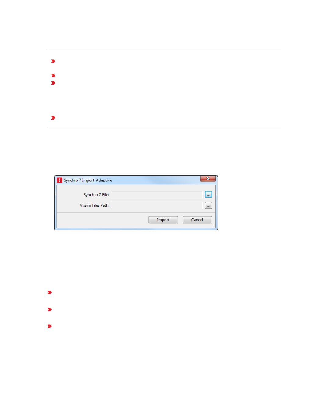
6.5.8 Importing Synchro 7 network adaptively
signalization is regenerated in Vissim. Thereby, all the manually adjusted links, connectors
and travel time sections are preserved in Vissim.
Notes:
The adaptive import is only possible if the current network is originally generated with
the same external application.
A network must be opened at the time of data import.
Contrary to a modeled network, an imported network is not displayed correctly on an
existing background map or another, file-based background. If you are using a back-
ground image, position the imported network so that it lines up with it (see "Mapping Vis-
sim network to background position" on page 371), (see "Positioning background
image" on page 377).
The quality of the imported network depends on the exactness of the imported data and
normally requires only minimal adjustments.
6.5.8 Importing Synchro 7 network adaptively
In your Vissim network, you can import a Synchro 7 network and update it. For example, after
you have changed the signalization in the source Synchro 7 network.
1. From the File menu, choose > Import > Synchro 7 Adaptive.
2. Check the path and the file name.
3. Click Import.
The Synchro 7 network is re-imported.
6.6 Exporting data
You can export the following data from Vissim:
Nodes and edges from dynamic assignment for visualization in Visum (see "Exporting
nodes and edges for visualization in Visum" on page 360)
Nodes and edges from dynamic assignment for assignment in Visum (see "Exporting
nodes and edges for assignment in Visum" on page 361)
Polygon data of the links and walkable areas for 3ds Max (see "Exporting static network
data for 3ds Max" on page 366)
© PTV GROUP 359

6.6.1 Exporting nodes and edges for visualization in Visum
Public transport stops and public transport lines (see "Exporting PT stops and PT lines for
Visum" on page 365)
Export files are saved in the folder of the currently opened file *.inpx.
During data export, all coordinates of the Sphere-Mercator projection are written to the *.net
file. The file format *.net Visum recognizes the projection.
You cannot export Vissim networks, that have been exported to Visum, from Visum and import
them in Vissim.
6.6.1 Exporting nodes and edges for visualization in Visum
After dynamic assignment, you can export the network and the paths from dynamic
assignment for visualization in Visum. You can graphically represent and analyze paths and
volume in Visum. Vissim creates the following files in the process:
Visum version file *.ver
Visum network file *.net
several Visum route files *.rim
The data of the network file and route files is also contained in the version file.
1. Open the desired network in Vissim.
2. Make sure that a dynamic assignment was performed.
3. From the menu File, choose > Export > PTV Visum (Nodes/Edges).
The PTV Visum Export window opens.
4. Select For visualization in Visum (with Vissim paths).
5. Click the button .
6. Specify a folder and a file name for the version file *.ver.
Note: You can specify only the folder and the file name for the version file. Parallel to
the file *.ver, this export creates a Visum network file *.net and several Visum route
files *.rim.
7. Confirm with OK.
360 © PTV GROUP
6.6.2 Exporting nodes and edges for assignment in Visum
Notes:
A Visum matrix file *.mtx is generated for the export from the total demand of the Vis-
sim matrices. Only the demand in the export time interval (start time of the sim-
ulation + simulation time) is taken into account for data export (see "Defining
simulation parameters" on page 796). If a Vissim matrix is not completely in the
export time interval, only the share which lies in the export time interval is exported.
The demand is combined. Thus you do not obtain separate matrices for the various
Vissim vehicle types and vehicle classes.
Route import files are exported only if the Vissim cost files and path files are avail-
able because route import files contain the resulting routes and volumes from the
dynamic assignment. A separate file *.rim is generated for each calculation interval
of the dynamic assignment.
Notes:
If no cost files and path files exist, a warning is issued and only the network data
and matrix data is exported.
Closures of edges or connectors for vehicle classes are transferred to Visum. Thus
they can be taken into account for an assignment. Visum does not use any paths by
default that are not also possible in Vissim. This excludes disjoint parallel edges
between two Vissim nodes that assume different turn relations or lead to different
turn relations. These are subsequently exported as a common edge to Visum. This
can lead the assignment in Visum to paths which cannot be used in Vissim.
Tip: You will find additional information on the subject of Importing routes in Visum in
the Visum Help, in the section Using interfaces for data exchange.
6.6.2 Exporting nodes and edges for assignment in Visum
After a dynamic assignment, you can export the network and demand from the dynamic
assignment for assignment in Visum (see "Using an assignment from Visum for dynamic
assignment" on page 752). Vissim creates the following files in the process:
Visum version file *.ver
Visum network file *.net
Visum matrix files *.mtx
The data of the network file and matrix file is also contained in the version file.
1. Open the desired network in Vissim.
2. Make sure that a dynamic assignment was performed.
3. From the File menu, choose > Export > PTV Visum (Nodes/Edges).
The PTV Visum Export window opens.
© PTV GROUP 361
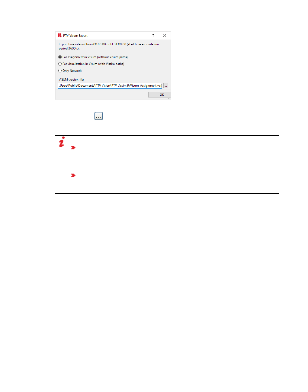
6.6.2 Exporting nodes and edges for assignment in Visum
4. Select the option For assignment in Visum (without Vissim paths).
5. Click the button .
6. Specify a folder and a file name for the version file *.ver.
Notes:
You can specify only the folder and the file name for the version file. Parallel to
the file *.ver, this export creates a Visum network file *.net and a Visum matrix file
*.mtx with the same file name as the version file. The files are saved in the folder
of the version file.
If the Vissim network contains edges which cannot be exported to Visum, these
are shown in the Messages window. You can still execute or cancel the export.
Vissim supports you when repairing the nodes and edges.
7. Confirm with OK.
The export starts. If the Vissim network contains nodes with non-unique zone connectors
(parking lot zone), a message is displayed. May you still perfom the data export or cancel it.
8. If you cancel the export, you can cancel the non-unique zone connectors (see "Canceling
non-unique zone connectors" on page 362). Then perform the export again.
6.6.2.1 Canceling non-unique zone connectors
When exporting for an assignment in Visum, the Vissim network can contain nodes with non-
unique zone connectors (parking lot zone). A message is then displayed. You can cancel the
export and the non-unique zone connectors.
Example of a Vissim network with a node with a non-unique zone connector (parking lot
zone):
362 © PTV GROUP

6.6.2 Exporting nodes and edges for assignment in Visum
Cancel the zone connector with an additional node:
6.6.2.2 Opening exported data in PTV Visum
After the export from Vissim, execute the following steps in Visum:
Open version file *.ver: see Visum Help under Using Visum > Basics of program oper-
ation > Opening and saving files
Open network file *.net: see Visum Help under Using Visum > Basics of program oper-
ation > Opening and saving files
© PTV GROUP 363
6.6.2 Exporting nodes and edges for assignment in Visum
Import routes file *.rim: see Visum Help under Using Visum > Using interfaces for data
exchange > Reading connections and routes > Importing routes
Import matrix file *.mtx: see Visum Help under Using Visum > Modeling demand >
Managing, showing and analyzing matrices > Reading an external matrix into a net-
work model
Connect matrix to demand segment: see Visum Help under Using Visum > Modeling
demand > Managing demand objects > Managing matrices > Connecting demand
matrices and demand segments
Notes:
The Visum version file created during the export contains all necessary data. It is
not necessary to open the other Visum files created during the export.
If no version file was created during the export, you can instead individually open
the other files created during the export.
A Visum network with network objects is generated (see "Network objects generated in Visum
from the Vissim export" on page 364).
6.6.2.3 Network objects generated in Visum from the Vissim export
From Vissim network objects, which were exported after a dynamic assignment, the import in
Visum generates the following network objects:
Visum
network
object or
attribute
Description
TSys,
Mode,
DSeg
Visum generates:
a PrT transport system
a PrT mode
a PrT demand segment
Vehicle types or vehicle classes from Vissim are not exported as different
transport systems, modes or demand segments.
An additional DSeg-PrT is generated for each evaluation interval of the
dynamic assignment from Vissim to Visum, when exporting routes from Vis-
sim.
Nodes Nodes are created according to the Vissim node.
The Visum node numbers correspond to the Vissim node numbers.
The maximum permitted node number in Visum is 2,147,483,647. Vissim nodes
with a higher number are renumbered. The new numbering starts with the
smallest free Vissim node number. Properties of nodes, for example, type,
geometry, signaling, orientation, etc., are neither exported nor generated.
364 © PTV GROUP

6.6.3 Exporting PT stops and PT lines for Visum
Visum
network
object or
attribute
Description
Links Links are generated according to the Vissim edges between the nodes.
Parallel edges: In Vissim several edges are possible between two adjacent
nodes. If there are several edges between two nodes, only the shortest edge is
exported. The Vissim network structure is checked in the process. If the
modeling is not suitable, a warning is issued, for example, for parallel edges.
Details are shown in the Messages window.
Link num-
ber
Link numbers start with 1.
Thus the numbering of links does not correspond to the Vissim link number or
the number of another Vissim network object.
Link type The link type is set to 0 for all links.
Thus the link type does not correspond to the behavior type of Vissim links.
Link length The length of link is calculated from the corresponding Vissim edge.
Number of
lanes
The number of lanes is set to the minimum number of lanes of all Vissim links
and connectors which belong to the edge.
Capacity
PrT
NumberVeh/h = Number of lanes • 900
Capacity = NumberVeh/h • (simulation duration/3,600)
Duration = Simulation time (see "Defining simulation parameters" on page 796)
Corresponds to "Vehicles per simulation time"
v0 PrT v0 IV is calculated based on speed distributions of Vissim origin parking lots
and the desired speed distribution per edge.
Speed for a distribution: 85 percentile
Only the default speed distribution is taken into account for parking lots.
For speed decisions, the average of all distributions is calculated: 85 per-
centile of each individual distribution
Turns Turns are generated from the Vissim edges within the node. A Visum turn is
permitted if the corresponding Vissim edge exists. The capacity is set to 99,999
for all turns. U-turns are assigned type 4, other turns are assigned type 0.
Zones Zones are created according to the Vissim zones. The zone position is
calculated from the position of the parking lot which is assigned to the zone.
Zone
connectors
(Zone –
Node)
Zone connectors are created according to the Vissim parking lots and zones.
6.6.3 Exporting PT stops and PT lines for Visum
After a dynamic assignment, you can export the network of PT stops and PT lines from
dynamic assignment for visualization in Visum. Paths and matrices are not exported. In Visum,
© PTV GROUP 365
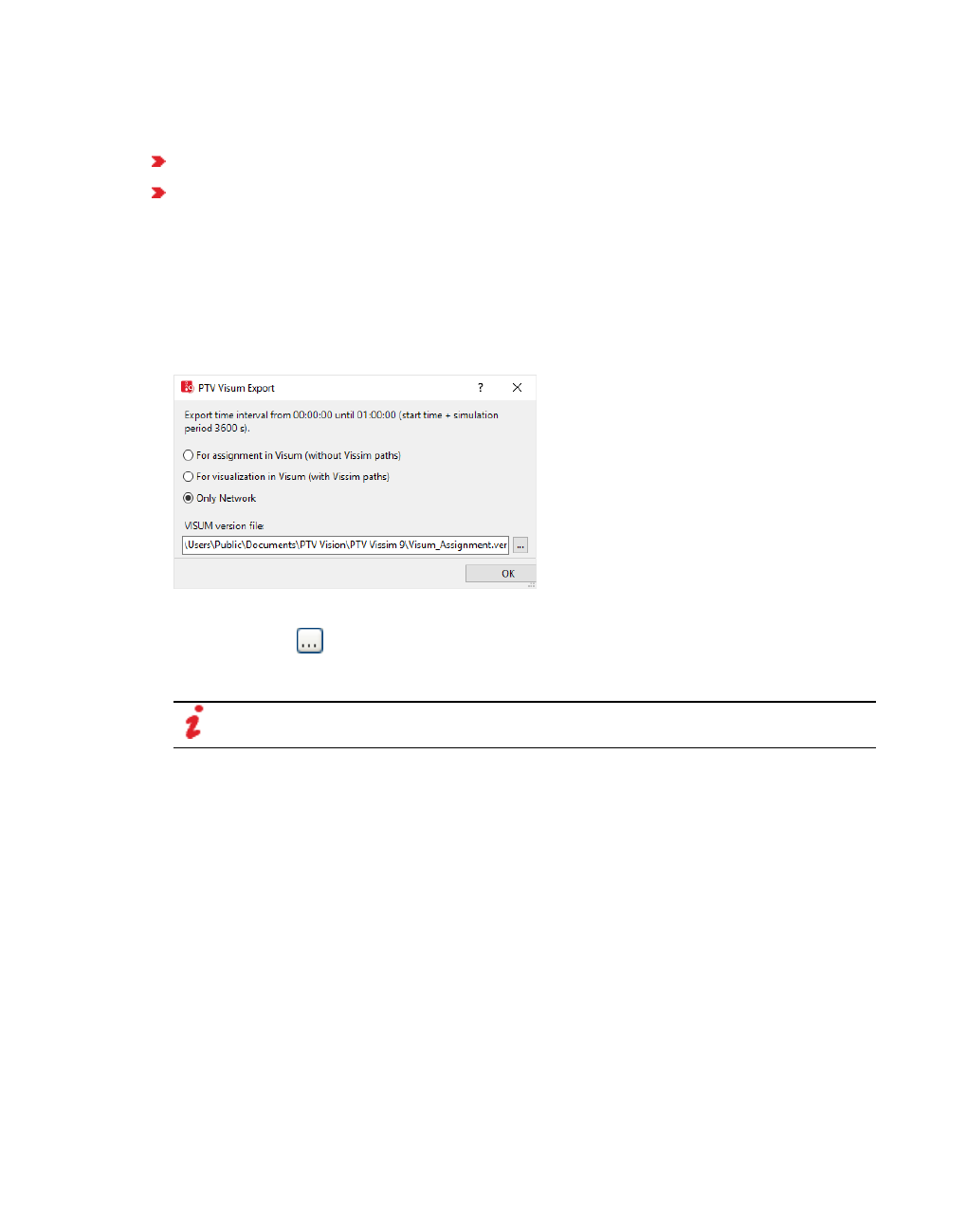
6.6.4 Exporting static network data for 3ds Max
PT stops and PT lines are displayed graphically. Vissim creates the following files in the
process:
Visum version file *.ver
Visum network file *.net
The data of the network file is also contained in the version file.
1. Open the desired network in Vissim.
2. Make sure that a dynamic assignment was performed.
3. From the menu File, choose > Export > PTV Visum (Nodes/Edges).
The PTV Visum Export window opens.
4. Select Only Network.
5. Click the button .
6. Specify a folder and a file name for the version file *.ver.
Note: You can specify only the folder and the file name for the version file. In parallel
to the *.ver file, a Visum network file *.net is created during data export.
7. Confirm with OK.
6.6.4 Exporting static network data for 3ds Max
You can export the data of polygons of links and walkable areas from your Vissim network into
a *.txt file. You can then import this file into 3ds Max.
1. From the File menu, choose > Export > 3DS MAX.
A window opens.
2. Enter the desired file name.
3. Click the Save button.
The data is saved in two data blocks to the *.txt file. There does not necessarily have to be
data in both data blocks.
366 © PTV GROUP

6.7 Rotating the network
Structure of TXT file
First row: coordinates used for later calculations of the correct position of polygon points.
Data block Links for links
Data block PedestrianAreas for pedestrian areas with coordinates of stairways/ramps
and other pedestrian areas
The data blocks consist of a data record for each network object and have the following
structure:
"Number of network object", comma-separated [list of coordinates X,Y,Z], new row: g
Example:
[870.10447,7438.97385,0.0]
Links
"10000",[49.36338,-17.03216,0.00000],[49.32021,-17.04763,0.00000],[52.51336,-
15.69895,0.00000],[52.51911,-15.69774,0.00000],[53.83595,-18.11195,0.00000],
[53.75370,-18.15874,0.00000],[50.40885,-19.84607,0.00000],[50.27076,-
19.89165,0.00000]
g
...
EndLinks
PedestrianAreas
"1:ped1",[144.64448,7536.22667,0.00000],[367.81823,7536.22667,0.00000],
[372.37280,7590.88147,0.00000],[39.88945,7595.43603,0.00000]
g
"2:ped2",[422.47302,7538.50396,0.00000],[531.78262,7533.94939,0.00000],
[529.50533,7588.60419,0.00000],[408.80933,7588.60419,0.00000]
g
EndPedestrianAreas
Tip: Information on data import into 3ds Max can be found in the directory
…\API\3dsMaxExport of your Vissim installation.
6.7 Rotating the network
In the network editor you can rotate the network and its network objects. These also include
static 3D models, 3D signal heads and keyframes (camera positions with a viewing direction)
as well as backgrounds.
Positive values rotate the network counter- clockwise. Negative values rotate the network
clockwise.
1. In the Edit menu, select > Rotate Network.
© PTV GROUP 367

6.8 Moving the network
2. Enter the desired value in degrees in the Angle field.
6.8 Moving the network
In the network editor you can move the entire network or selected network objects. These also
include backgrounds, static 3D models, 3D signal heads and keyframes (camera positions
with a viewing direction).
Background images are not moved with the network in the Z direction.
If in the Network Settings you selected imperial units, these are displayed in the Move
Network window. Vissim converts the values entered into meters.
1. In the Edit menu, select > Move Network.
2. Make the desired changes:
Element Description
Keep coordinates and move loc-
ation on background map The network coordinates remain unchanged.
The network is moved.
The reference point of the map is reset.
Corresponds to the function of mapping a Vissim
network to a background map (see "Mapping Vissim
network to background position" on page 371). Select
this option, if for example the network is not mapped
correctly to the background map. Distance Z cannot
be changed.
Adapt coordinates and keep loc-
ation on background map The network coordinates are reset.
The network is not moved.
The reference point on the map remains
unchanged.
Select this option, for example, to transfer coordinates
of a plan or ground plan. This allows you to enter
values for the distances Distance X, Distance Y,
Distance Z.
368 © PTV GROUP
6.9 Inserting a background image
Element Description
Set coordinate origin to center of
network and keep location on
background map
The network coordinates are set to the center
point 0.000,0.000.
The network is not moved.
The reference point on the map remains
unchanged.
As neither the network nor the map reference point
were moved, the distances cannot be changed.
Select this option, for example, when you have
moved the network too far, the coordinate values of
the reference point in the network are now very high
and you want to set them to 0.000,0.000.
Adapt coordinates and move loc-
ation on background map The network coordinates are reset.
The network is moved.
The reference point of the map is reset.
Corresponds to the function of moving selected,
individual network objects in the network editor.
3. If desired and if the option selected allows for the entry, into the Distance X, Distance Y,
Distance Z boxes, enter the values of your choice.
4. Confirm with OK.
6.9 Inserting a background image
You can insert true to scale digital maps as graphic files or maps from online map services as
the background for a detailed Vissim network model. You can then model your Vissim network
using the background.
6.9.1 Using live maps from the Internet
If your computer has a permanent Internet connection, you can display maps from online map
providers as a background in 2D mode and in 3D mode for a detailed Vissim network model.
Map services provide high-resolution aerial photos, satellite images and detailed city plans for
many regions. In addition to commercial offerings, such as Microsoft Bing Maps, there are
such freely available map services as OpenStreetMap whose data can be used under certain
conditions.
Notes:
The use of data from map services is subject to licensing conditions. Please obtain
information in advance about these conditions and take these into account when
working on projects and transferring results.
Backgrounds of Bing Maps are only available to customers who have maintenance
agreements.
© PTV GROUP 369

6.9.1 Using live maps from the Internet
Vissim provides some map services by default in the graphic parameters. You can select the
desired map service for each open Network Editor from these. In contrast to inserted
background graphics, the depiction is exclusively controlled via the graphics parameters in the
relevant Network Editor. There are no other administration functions for live maps.
Vissim always uses the newest map material available. The map data from Bing Maps is not
stored permanently on your hard disk as a result of the Bing Maps usage terms. The map
material is newly loaded when you start Vissim start or when you open the network again.
When Vissim has been opened, the map data is kept in the cache. This way, it can be
displayed more quickly. The data matching the current network section is loaded at the
relevant zoom level and displayed. Depending on the map service and the acceptance
conditions, the live maps have different resolutions in various areas. If the maximum resolution
is reached at a particular zoom level, the live map cannot be shown sharper; if you zoom in
closer and the pixels on the live map are shown larger.
Advantages of using live maps available on the internet
You do not need to prepare and load graphics files for backgrounds, but rather can start
the modeling directly on the live map.
The most up-to-date maps from the map service are always available.
You can switch projects between computers without having to consider that paths are
stated for the saved maps.
No storage space is required for permanently storing maps on your computer.
You can position your existing Vissim network on the corresponding position on the live
map (see "Mapping Vissim network to background position" on page 371).
You can display a particular map section and save it in the default layout file (see "Save
Layout as Default" on page 116). In future Vissim will open with the saved map section.
URL addresses for background maps
Access to background maps available on the internet may depend on the configuration of your
proxy server. For the proxy server to be able to create access rules, you might have to specify
the following URL addresses when configuring the proxy server:
BingMaps: dev.virtualearth.net/REST/V1/Imagery/Metadata/*
OpenStreetMap: *.tile.openstreetmap.org/*
For further information, please visit our webpages at: PTV Visum FAQs (#15306). > Graphics
> (#VIS15306) The display of the background map or inserting (static) Internet maps from
BING or OSM is prevented by the proxyserver.
6.9.1.1 Activating live maps from the Internet
1. Check that your computer has an active Internet connection.
2. Make sure the reference point of the live map is not identical with the reference point of the
network (see "Assigning a live map if reference points are identical" on page 372).
370 © PTV GROUP
6.9.1 Using live maps from the Internet
3. On the toolbar of the Network editor, click the button Edit basic graphic parameters.
The list of graphic parameters opens (see "List of base graphic parameters for network
editors" on page 161).
4. Select the option Show map.
A live map from the Internet is shown in the Network Editor.
5. In the Map provider list, click the desired map service.
A live map from the selected map service is shown in the Network Editor. The entry Default
map service <map service name> is used with Bing Maps (Aerial View) and
OpenStreetMap (Mapnik). If you do not have a license for Bing Maps, OpenStreetMap
(Mapnik) is used automatically.
If the map service copyright data is shown in the Network Editor but no live map is shown,
check your Internet connection.
6. Click next to the list when you want to close it.
Tip: After you select a map provider and the live map is displayed, you can use the
Toggle background maps icon on the network editor toolbar to display or hide the live
map (see "Network editor toolbar" on page 73).
6.9.1.2 Mapping Vissim network to background position
You can define a point in the live map as a reference point and assign the corresponding
coordinate from Vissim.
Assignment is possible for an existing Vissim network. Thereby you assign a point of your
Vissim network to a corresponding point in the live map. Vissim scales and moves the live
map to the corresponding position of the Vissim network. The coordinates of both reference
points are shown in the network settings.
The assignment does not change the arrangement of the network objects or their dimensions.
Note: Avoid using the Move network function to assign the background map and
Vissim network (see "Moving the network" on page 368). This will avoid wrong scaling.
Take the following steps to assign the live map:
Assigning coordinates in the live map
1. Make sure that the desired live map is shown (see "Activating live maps from the Internet"
on page 370).
By default, background maps can show a very large section of the map. It may therefore be
necessary to zoom deep into the live map and shift it a long way until your Vissim network
and the desired map section are displayed.
2. Zoom in on your Vissim network until you reach an enlargement where your Vissim network
is shown in enough detail to allow you to assign the coordinates with the desired accuracy.
© PTV GROUP 371

6.9.1 Using live maps from the Internet
3. Right-click on the reference position in your Vissim network that you want to assign to a
point on the live map.
4. Select the Map this Point to Background Position entry in the context menu.
The mouse pointer becomes a cross. A preview shows the selected network objects and
makes it easier to map them.
5. Move the mouse pointer to the desired point in the live map.
6. Click on the point.
The Vissim network is positioned over the desired location on the live map. The
coordinates of Vissim and the live map are assigned. You can also assign the coordinates
again.
7. If desired, check the coordinates in the network settings (see "Showing reference points" on
page 197).
If, for example, by moving the network the coordinates of the network's reference point are
outside the network, Vissim resets the reference point to the middle of the network.
6.9.1.3 Assigning a live map if reference points are identical
You cannot activate a live map, if the coordinates of its reference point are identical to the
coordinates of the network's reference point. The might be due to the following:
ANM import of an ANM file that does not yet contain any projection information. The ref-
erence points are assigned the coordinates (0.000, 0.000).
ANM import of an ANM file with an empty projection. The reference points are assigned
the coordinates (0.000, 0.000).
You opened an *.inp file of a Vissim version earlier than 6. The origin is set in the center of
the network.
You opened an *.inpx file of a Vissim version earlier than 6.00-06. The origin is set in the
center of the network.
If the coordinates of the reference point of the live map are identical to those of the network's
reference point and you try to activate a live map, the following message is displayed:
1. Confirm with OK.
2. Assign the reference points of the network and the live map (see "Mapping Vissim network
to background position" on page 371).
372 © PTV GROUP

6.9.2 Using background images
3. Check the coordinates in the network settings (see "Showing reference points" on page
197).
6.9.2 Using background images
You can insert true to scale digital maps as a background image for a detailed Vissim network
model as graphics files.
You can scan similar maps and save them as a graphic file. You load the graphic file of the
digital map as the background image in Vissim and display it in a Network Editor. You can
move and scale the background image in the Network Editor. You then position the network
objects on the background image.
The selection of file formats is limited in the 64-bit version of Vissim. Vector graphics in the
file formats *.dwg and *.dxf may not be displayed correctly. You can use graphics pro-
grams to convert vector graphics to raster graphics such as *.bmp or *.jpg.
The memory requirement of background images depends on:
File format and compression of the graphic file, especially with the file format *.jpg.
Screen resolution and color depth
In particular for 3D mode of the memory and graphic card memory
Thus the maximum possible file size also depends on your hardware.
A warning is issued if the graphic file is larger than the available main memory. This
provides the option of loading the file nevertheless.
If a graphic file is too large, it cannot be displayed correctly. For example, a black or white
area is displayed. Reduce the graphic file with a graphics editing program, for example, by
zooming out of the screen section or by reducing the resolution.
When a background file is read into Vissim, it is displayed in the Network Editor in tiles.
You can change the screen section during the drawing of the tiles in 3D mode. As long as
the background image is not fully loaded, the entire network is shown and then after that
the section, which was selected before the background image was imported.
6.9.2.1 Supported file formats for background graphics
Vissim supports the following file formats for graphic files:
Raster formats
*.bmp Windows bitmap, two-dimensional
*.jpg graphic compressed according to JPEG (Joint Photographic Experts Group) standard
*.png Portable Network Graphics, compressed with no loss in quality
*.tga Targa (Truevision Advanced Raster Graphics Array) image file, uncompressed or
compressed with no loss in quality. Also saves values for alpha channel, gamma
correction and text as meta-information.
*.tif Tagged Image File Format, uncompressed or packbits compressed
© PTV GROUP 373

6.9.2 Using background images
Raster formats
*.sid Mr. SID files, display with best possible resolution
*.ecw Enhanced Compressed Wavelet, for large raster graphics, e.g. aerial images. The
*.ecw file format provides the following advantages:
high compression rates
visually flawless image quality
Contrary to other file formats, it does not cause any noteworthy delays while
navigating in the Vissim network.
Compression rates recommended for Vissim:
9:1 for high quality
20:1 for good quality with shorter loading time
Vector formats
*.dwg Is updated for each new version of Autodesk AutoCADTM
*.dxf Is updated for each new version of Autodesk AutoCADTM
*.emf Windows Enhanced Metafile
*.wmf Windows Metafile
*.shp Shapefile for geodata
32-bit edition and 64-bit edition of Vissim support the file formats of *.dwg versions up to
DWG2013.
AutoCAD saves the current layout with the position, translation vector and rotation with a
*.dwg or *.dxf file, if the file is saved in AutoCAD.
These layout settings are taken into consideration by Vissim as much as possible for the
display of a loaded background graphic.
The import of pedestrian areas and obstacles of a *.dwg file do not take these layout set-
tings into consideration for the graphic display.
When you save a *.dwg or *.dxf file in AutoCAD, ensure that the current layout settings are
suitable for use of the file as a background graphic in Vissim. This applies, in particular,
before loading a *.dwg file as a background graphic, after construction elements for ped-
estrians have already been imported from this file in Vissim.
6.9.2.2 Scanning maps and site plans
The following steps outline the procedure for scanning maps and site plans:
Maps and site plans to be scanned should include a north arrow and a linear scale.
Create an overview map that shows all relevant nodes of the transport network which is to
be examined.
374 © PTV GROUP

6.9.2 Using background images
Use individual signal control plans for each intersection showing detector locations, if you
want to insert detectors in Vissim.
Ensure that the scanned plans have a high contrast.
Maps and plans should be oriented to North direction.
Use a copy machine to reduce plans in case they do not fit the available scanner.
A plan in A4 format should be scanned with 300 dpi resolution. The bigger the plan and
the higher the resolution the bigger the bitmap file size. The memory requirements of the
background file, the load time in Vissim and the network setup increase with the growing
resolution.
Save the scanned background map to one of the supported bitmap formats (for example
*.bmp, *.jpg or uncompressed *.tif).
6.9.2.3 Loading image file as background image
You can insert a true to scale digital map as a background image for a detailed Vissim network
model. Only insert graphic files, which make up the entire examination area. You load the
graphic file of the digital map as the background image in Vissim and display it in a Network
Editor. The load time is dependent upon the file size.
Load the graphics in file formats which are suitable for graphics, for example, *.bmp or *.wmf. If
a file format cannot be loaded, a message is displayed.
When loading graphic files that contain information on the size and/or position of the image,
you can specify whether or not you want Vissim to consider this data.
Vissim does not use map projection. It does not consider data obtained through map
projection, as could be included in files created with CAD software. Using a graphic file based
on map projection to model the background of your Vissimnetwork may distort your length
information and simulation results. Before loading a graphic file in Vissimthat contains data of
a map projection, in the CAD program, change the coordinate system to a metric system
without projection, e.g. to AutoCAD Map 3D.
Notes:
You can specify that you need not press the CTRL key when adding network objects
(see "Right-click behavior and action after creating an object" on page 143).
For some network objects there are windows in which the attributes of a network
object can be defined and edited. There are lists for this, for all network objects. You
can choose whether you want to open a window, a list or neither of the two for the
definition of network objects in the Network Editor (see "Right-click behavior and
action after creating an object" on page 143).
1. On the Network objects toolbar, click Background Images.
2. Hold down the CTRL key and in the Network Editor, right-click on the desired position.
The window Select Bitmap File opens.
3. Select the graphic file which should be imported.
© PTV GROUP 375

6.9.2 Using background images
4. Click the Open button.
If the graphic file contains information on the size and/or position of the image, a window
opens.
5. In the window, make the settings of your choice.
Element Description
Use position data from
image file (<name of
file>.<file format>)
only active if the graphic file selected is not a Vissim background
image file of the format *.bgr or *.hgr, but e.g. an image file in the
*.dwg format: The background is inserted at the position
specified in the image file.
Use position of selec-
ted background
only active if the graphic file selected is a Vissim background
image file of the format *.bgr or *.hgr:The background is inserted
at the position specified in the world file.
Use position you
clicked on, adjust
height
Does not account for position specified in graphic file, inserts
background in the Network editor at the position you click.
6. On the Network Editor toolbar, click the Show entire network button.
The digital map is shown in its entirety.
The name and a miniature view of the digital map is shown in the Background images
toolbar.
376 © PTV GROUP

6.9.2 Using background images
6.9.2.4 Positioning background image
You can position a background image in a Network Editor. Next, you can scale a background
image and place a network object on a background image.
1. On the Network objects toolbar, click Background Images.
2. In the Network Editor, click on the background image of your choice.
A background image is marked.
3. Hold down the left mouse button and drag the background image to the position of your
choice.
When you move, the background becomes transparent.
4. Release the mouse button.
6.9.2.5 Scaling the background image
A loaded background image is not represented according to scale even when the file has a
scale. For the precise modeling of a network, you must scale the map precisely. Use a large
distance, for example > 100 m. For the adjustment of the background image and the Vissim
units, zoom in on an object or a link with original measurements known to you. For example,
this can be the scale of the map or the edge between two corners of a building or
geographical points.
1. On the Network objects toolbar, click Background Images.
2. In the Network Editor, click on the background image of your choice.
A background image is marked.
3. Right click on the Network Editor.
4. From the context menu, select the entry Set Scale.
The mouse pointer becomes a cross.
5. Click on the desired starting point of the edge and drag it while holding down the mouse
button to the desired end point of the edge.
6. Release the mouse button.
The Scale window opens.
7. Enter the original length of the edge.
8. Confirm with OK.
Tip: Alternatively, you can point the cursor to a corner of the background in the network
editor and hold the mouse button down and drag to reduce or increase the background
to the desired size.
6.9.2.6 Hiding and showing background image
1. Select from the menu View > Backgrounds.
© PTV GROUP 377

6.9.2 Using background images
The Background Image toolbar is displayed.
2. Click on the desired icon:
Element Description
Background image is currently displayed. Hide background image.
Background image is hidden. Display background image.
6.9.2.7 Attributes of background images
1. From the Lists menu, choose > Graphics & Presentation > Background Images.
Note: In lists, you can use the Attribute selection icon to show and hide attribute
values (see "Selecting attributes and subattributes for a list" on page 106).
The Background Images list opens.
The list in the tab contains, amongst others, the following attributes:
Column Description
PathFilename Path and filename of graphic file
PosTRX Position top right (x): X coordinate
PosTRY Position top right (y): Y coordinate
PosBLX Position bottom left (x): X coordinate
PosBLY Position bottom left (y): Y coordinate
PosBLPt Position bottom left: Corner point PosBLX and PosBLY. If you change a
value, the associated value in PosTRPt changes automatically.
PosTRPt Position top right: Corner point PosTRX and PosTRY. If you change a value,
the associated value in PosBLPt changes automatically.
Level Name of level
ZOffset z-Offset: Height above the level
TileSizeHoriz Tile size horizontal: Width
The background image is loaded tile by tile. Tiles are recommended for large
networks with large background images. In 3D mode in particular, the time
for opening the graphic files depends on the file size of the graphics files.
TileSizeVert Tile size vertical: Height
378 © PTV GROUP

6.10 Modeling the road network
Column Description
Res3D Maximum 3D resolution for displaying background images in 3D for raster
graphics and vector graphics. This depends on your computer's graphics
hardware and the number of currently loaded background images.
Very low: 1,024
Low: 2,048
Average: 4,096
High: 8,192
Tiles
AnisoFilt Anisotropic filtering: If this option is selected, the display quality of tex-
tures is improved when viewed from a very flat angle.
Angle Angle in degrees, by which the background is rotated. The background is
also rotated when the Vissim network is rotated (see "Rotating the network"
on page 367). You can rotate a background in the Network editor (see "Rotat-
ing network objects" on page 334).
2. Select Level from the Relations field in the list toolbar.
The attribute and attribute values of this network object type are shown in the list on the left,
which consists of two coupled lists.
The list on the right contains attributes and attribute values of levels allocated to the network
object selected in the list on the left (see "Using coupled lists" on page 111).
3. Enter the desired data.
The data is allocated.
6.9.2.8 Modeling the network for background images
You can temporarily create Vissim links as an aid for locating the corners of buildings, in
order to place more graphic files with higher detailing correctly in the Vissim network.
Finally, model the network and intersections more carefully with regard to the detailed
graphic files.
Then delete links which are no longer needed.
To show or hide all backgrounds, in the active Network Editor, use the key combination
CTRL+B.
6.10 Modeling the road network
When modeling transport infrastructure in Vissim, you can choose between a basic test
environment and true to scale traffic flow modeling.
© PTV GROUP 379
6.10.1 Modeling links for vehicles and pedestrians
Testing environment
A less detailed model is sufficient, if you e.g, want to analyze several test cases for traffic-
actuated VAP or VS-PLUS logic by activating the detector types manually. However, if you
want to simulate traffic flows for performance analyses, you will need a more sophisticated
model.
For testing environments, it is sufficient to position approach links of intersections roughly
where you want them. Add signal heads and detectors to the approach lanes, so that you can
later easily identify these network objects. True to scale modeling is not required. So network
and nodes do not have to be based on scanned plans.
True to scale modeling
Vissim allows you to model traffic flows and real conditions true to scale. You can position the
network objects of your choice accurately to the millimeter, e.g. links and connectors, signal
groups and signal heads, individual intersections, a specific sequence or network of nodes. To
ensure true to scale modeling:
From Visum, CROSSIG, P2 or other applications that support Vissim network files, import a
true to scale network (see "Importing a network" on page 341)
You use a background map for modeling.
If you do not want to use a background map for modeling:
Import true to scale data from Synchro 7 (add-on module for optimization of signal con-
trol (see "Importing data from the add-on module Synchro 7" on page 357) and (see
"Importing Synchro 7 network adaptively" on page 359)).
Scan maps of the area.
Add the scanned maps as the background (see "Inserting a background image" on
page 369).
Your Vissim network is based on these background graphics.
6.10.1 Modeling links for vehicles and pedestrians
You can model links on which vehicles and pedestrians move. This vehicle and pedestrian
must be defined as vehicle types.
Notes:
In Viswalk, pedestrians can also move on links. These links must be defined as ped-
estrian area (see "Defining pedestrian links" on page 870).
Ensure that a background image is loaded and the scale is selected (see "Inserting
a background image" on page 369)
Within a link section, the number of lanes cannot be changed. If the number of lanes should
deviate, you must set a link for every link section. Subsequently, you can split links and
change the number of links (see "Splitting links" on page 392).
380 © PTV GROUP

6.10.1 Modeling links for vehicles and pedestrians
Deleting a link or lane: If for a link the attribute Has overtaking lane is selected, you can
delete the link. If you want to delete a lane, the corresponding link must have at least three
lanes, including the overtaking lane.
6.10.1.1 Defining sequence and modeling techniques for links
Define the links for main roads in one direction.
Add intermediate points and model the curvature of a link.
Define the opposite lane. Thereby you can generate the newly created link with a different
number of lanes. Allow the links to run corresponding to the line of a road.
If you add additional links, connect them via connectors.
Determine the number of arms per junction and add links. In the junction area, allow links
in the middle of the junction to begin and end. If the number of lanes changes, pay atten-
tion to the correct connection via connectors.
Define the number of lanes per link on the nodes.
Define the number of turning lanes in the node.
Define the possible turns, lane expansions and lane reductions at the connectors.
6.10.1.2 Defining links
Define links in the Network Editor in the movement direction. You can define straight links or
add intermediate points to change the course of the link. You can also define a circular link to
model a roundabout in the desired size and in a symmetrical, circular shape.
Tips:
Alternatively, you can define links in the Network Editor via the context menu > Add
New Link, if the network object type Links is selected in the network object toolbar.
You can set that when you enter network objects you do not have to press the CTRL
key (see "Right-click behavior and action after creating an object" on page 143).
Defining straight links
1. On the Network objects toolbar, click Links.
2. In the Network Editor, point the mouse pointer to the desired starting point of the link.
3. Press the CTRL key, hold down the right mouse button and drag the mouse to the desired
end point of the link.
4. Release the keys.
The link is shown in color in the network editor. The link contains attribute values and lane
attribute values of the link last created. If no link was created since the network was loaded
or if the previously created link was deleted, default values are used. The movement
direction is shown by arrows at the edges of the link. The Link window opens. The new link
is assigned the attribute Number, which is the next higher number available for links.
© PTV GROUP 381

6.10.1 Modeling links for vehicles and pedestrians
5. Edit the attributes (see "Attributes of links" on page 383).
6. Confirm with OK.
The attributes are saved in the Links list.
Using intermediate points to define links with a curve shape
While dragging open a link, you can set intermediate points to change the link direction. This
allows you to already model complex curves when inserting a link.
1. On the Network objects toolbar, click Links.
2. In the Network Editor, point the mouse pointer to the desired starting point of the link.
3. Hold down the CTRL key and the right mouse button, and drag the mouse to the desired first
point of a curve.
Release the CTRL key. Keep the right mouse button held down until you have inserted the
entire link. Use the left mouse button to insert intermediate points.
4. Hold down the right mouse button and click.
5. Continue to add intermediate points this way, until you have reached the final point of your
link.
6. Release the keys.
The link is shown in color in the network editor. The movement direction is shown by arrows
at the edges of the link. You can move the intermediate points, which allows you to model
the link precisely. If you zoom out too far, arrows and intermediate point cannot be fully
displayed. The Link window opens.
7. Edit the attributes (see "Attributes of links" on page 383).
8. Confirm with OK.
The attributes are saved in the Links list.
Defining a circular link
1. On the Network objects toolbar, click Links.
2. In the Network editor, right-click the desired starting point of the circular link.
3. From the shortcut menu, choose Add Circular Link.
The circular link is displayed when the mouse pointer points to the Network editor. The
movement direction is shown by arrows at the edges of the link. By default, the circular link
has 48 intermediate points. The visualization of intermediate points depends on the
diameter of the roundabout and the magnification selected for the Network editor.
4. In the Network editor,use the mouse pointer to drag the circular link in the desired direction
until the required size is reached.
The length and diameter of the circular link are displayed in the status bar, to the right of the
coordinates of the mouse pointer position.
382 © PTV GROUP

6.10.1 Modeling links for vehicles and pedestrians
5. Click.
The Link window opens. The new link is assigned the attribute Number, which is the next
higher number available.
6. Edit the attributes (see "Attributes of links" on page 383).
7. Confirm with OK.
The attributes are saved in the Links list. Vissim adds a link from the end of the circular link to
the beginning of the circular link and thus closes the circular link. The attributes of this
connector are saved to the Links list. The new connector is assigned the attribute Number,
which is the next higher number available for connectors.
You can use the same command for the roundabout that are available for links, e.g.:
Invert direction(see "Inverting direction" on page 393)
Add lane (see "Inserting lanes on the left or right" on page 392)
Add or delete points (see "Adding points to a link" on page 404)
6.10.1.3 Attributes of links
The Links window opens when you insert a network object and have selected to have the Edit
dialog opened automatically after object creation (see "Right-click behavior and action after
creating an object" on page 143). By default, only the Links list is opened.
Into the window, you enter attribute values for the network object. For network objects which
have already been defined, you can call the window using the following functions:
In the list of network objects of the network object type, double-click the row with the
desired network object.
In the Network editor, select the network object of your choice. Then, from its shortcut
menu, choose Edit.
The network object may have additional attributes. In the network objects list of the network
object type, you can show all attributes and attribute values. You can open the list via the
following functions:
In the network object toolbar, right-click the desired network object type. Then from the
shortcut menu, choose Show List (see "Context menu in the network object toolbar" on
page 63).
In the Network editor, select the network object of your choice. Then, from its shortcut
menu, choose Show In List (see "Selecting network objects in the Network editor and
showing them in a list" on page 339).
From the Lists menu, in the desired category, choose the network object type.
In the network objects list of the network object type, you can edit attributes and attribute
values of a network object (see "Selecting cells in lists" on page 102), (see "Using lists" on
page 89).
The objects of this object type may have relations to other objects. This is why the attributes list
is shown as part of a coupled list (on the left). On the Lists toolbar, in the Relations box, you
© PTV GROUP 383
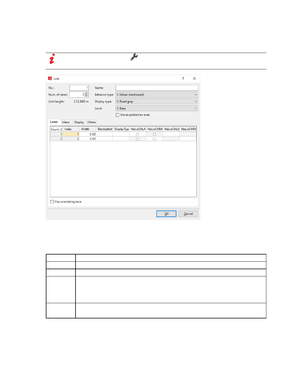
6.10.1 Modeling links for vehicles and pedestrians
can show and edit the coupled list with the attributes of the desired relation on the right (see
below Showing and editing dependent objects as relation) and (see "Using coupled lists" on
page 111).
Note: In lists, you can use the Attribute selection icon to show and hide attribute
values (see "Selecting attributes and subattributes for a list" on page 106).
Basic attributes of links
The basic attributes of the network element are shown in the upper area of the window and in
the list of network objects for the particular network object type.
Element Description
No. Unique number of the link
Name Designation of the link
Count
Lanes
Number of lanes (NumLanes). The table in the Lanes tab is automatically
adjusted. If there already is a lane and you increase the number of lanes, the
new lane is inserted in the Network editor and adopts attributes from the existing
lane.
Link
Length
Length2D: Length of the link in meters
Length3D accounts for z-offset of the link
384 © PTV GROUP

6.10.1 Modeling links for vehicles and pedestrians
Element Description
Behavior
type
Link Behavior Type (LinkBehavType): Driving behavior for the link (see
"Defining link behavior types for links and connectors" on page 299) and (see
"Defining driving behavior parameter sets" on page 268). If the Is pedestrian
area attribute (Use as pedestrian area option) is selected, the behavior type
None is automatically selected.
Display
type
Colored display of the link (see "Defining display types" on page 300).
In the coupled list Lanes, in the Display Type column, you can edit the Display
Type attribute for individual lanes of the link. The coupled list Lanes is selected
in the Links list, in the Relations box.
Level For modeling of multistory buildings or bridge structures: level on which the link
is located
Use as
pedestrian
area
Is pedestrian area (IsPedArea): Only with Viswalk: If this option is selected,
the link is defined as a pedestrian area (see "Modeling links as pedestrian
areas" on page 869).
Has
passing
lane
HasOvtLn: The inner lane may only be used for overtaking maneuvers on the
oncoming lane. This is only possible on links with at least two lanes (see
"Modeling overtaking maneuvers on the lane of oncoming traffic" on page 475).
If this option is selected, for right hand traffic, the outer left lane is displayed
as the passing lane, with hatched background. For left hand traffic, the lane on
the far right is the passing lane, displayed with hatched background.
If a passing lane and regular lane of a link of the opposite direction overlap for
long enough, the overlapping area may be used for passing.
Only select this attribute for links on which passing is actually allowed in reality.
Avoid passing lanes on which overtaking is not possible in reality, e.g. at
junctions or in traffic controlled areas.
You can also select this attribute for several, successive links that are connected
via connectors and have at least two lanes. Vehicles can then use the entire
overlapping area for overtaking maneuvers.
If the passing lane is closed for a vehicle class, the vehicles of this class cannot
use the passing lane for overtaking.
You can place other network objects, e.g. data collection points, on passing
lanes.
Passing lanes are not shown in 3D mode.
Lanes tab
The list in the tab contains, amongst others, the following attributes:
© PTV GROUP 385

6.10.1 Modeling links for vehicles and pedestrians
Column Description
Index Unique number of the lane. You cannot change this entry later on.
Width Width of the lane If several lanes are defined, several rows are
displayed. You can define different widths. The width has an effect
on:
the graphic display of a link
the possibility of whether a vehicle can overtake within a lane.
For this, overtaking within a lane must be selected in the driving
behavior parameters (see "Editing the driving behavior para-
meter Lateral behavior" on page 289). The width does not have
any effect on the speeds.
BlockedVehClasses Blocked vehicle classes on this lane.
If the link of the lane has a vehicle input, the vehicles of this
vehicle class are not used on this lane.
The vehicles of this vehicle class do not carry out a lane change
into this lane. This also applies if this would be necessary
because of their route.
Vehicles of the particular vehicle class attempt to leave the lane
as quickly as possible, if an adjacent lane is not blocked for the
vehicle class.
If all of the lanes in a link are blocked for a vehicle class, the
vehicles of this vehicle class travel along the link without chan-
ging lane.
DisplayType Color of lane (see "Defining display types" on page 300)
NoLnChLAllVehTypes,
NoLnChRAllVehTypes
No lane change left – all vehicle types and No lane change right–
all vehicle types: If this option is selected, vehicles may not
change lanes. A prohibition of lane changes is shown in the 2D and
3D mode by means of a solid line.
NoLnChLVehClasses,
NoLnChRVehClasses
No lane change left - vehicle classes and No lane change right -
vehicle classes: Vehicle classes, whose vehicles must not change
from a chosen lane to the adjacent lane in the direction of travel. A
prohibition of lane changes is shown in the 2D and 3D mode by
means of a solid line.
386 © PTV GROUP
6.10.1 Modeling links for vehicles and pedestrians
Notes:
If vehicles are to be able to overtake within a lane, you must select overtaking within
a lane in the driving behavior parameters (see "Editing the driving behavior para-
meter Lateral behavior" on page 289).
For lane changes, you must define links with multiple lanes. You cannot define lane
changes between adjacent links.
No lane change also applies for a change of lane which would have to be made
according to the route. Therefore, make sure that lane changes due to the route are
either completed before the prohibition of lane changes, or can only be made after
the prohibition of lane changes.
Cooperative lane change ignores the lane change ban (see "Editing the driving
behavior parameter Lane change behavior" on page 281).
The option All Vehicle Types is a virtual vehicle class that automatically includes all
new vehicle types and vehicle types that have not been assigned a vehicle class yet.
Meso tab
Link attributes for mesoscopic simulation:
Long
name
Short name Description
Meso
speed
model
MesoSpeedModel Specifies how the speed of vehicles on this link is determined.
Vehicle-based: Vehicles always drive at their desired
speed
Link-based: Vehicles drives at the speed defined for the
attribute Meso speed.
Meso
speed
MesoSpeed Meso speed is used exclusively in combination with the meso
speed model Link related (see "Car following model for
mesoscopic simulation" on page 760). In this case, the meso
speed defines the speed for all vehicles on the link. Default
value 50.0 km/h
Meso
follow-
up
time
MesoFollowUpGap Follow-up gap between two vehicles in the same traffic flow.
Edit this attribute in the Meso turns list or in the coupled list
Nodes - Meso turns (see "Attributes of meso turns" on page
789), (see "Attributes of nodes" on page 669).
Display tab
Attributes for the display of the link. The attributes do not influence the driving behavior.
The tab contains, amongst others, the following attributes:
Element Description
3D
© PTV GROUP 387
6.10.1 Modeling links for vehicles and pedestrians
Element Description
z-offset (start) ZOffset (zOffsetStart): Starting point of z-
coordinates of link for 3D display.
z-offset (end) z-offset (end) (zOffsetEnd): End poiont of z-
coordinates of link for 3D display.
By default, z-offset (start) and z-offset (end) do not have any impact on the driving behavior
when it comes to upward or downward gradients. If the z-coordinates in your Vissim network
have been entered correctly, you can have Vissim calculate upward and downward
gradients. In this case, the option Use gradient from z coordinates must be selected (see
"Selecting network settings for vehicle behavior" on page 193).
If you change the values of the z-offset (start) or the z-offset (end) and have inserted
intermediate points into the link, Vissim will recalculate the z-offset values of the intermediate
points. To ensure that the upward or downward gradient is harmonious, Vissim calculates a
spline for the vertical course of the link.
Thickness (3D) Thickness for display of the link in 3D mode.
Element Description
Visualization
Individual
vehicles Show individual vehicles (ShowVeh): Select this option to show vehicles in
the 2D mode.
If this option is not checked, no vehicles are indicated in the 2D mode. With
this, you can indicate underpasses or tunnel sections. This option applies for the
entire link. Therefore you must define a separate link for each underpass or for
each tunnel.
Note: Do not use this option in 3D mode, but rather model the height
details of the links correctly!
Show
classified
values
ShowClsfValues: Select this option to show classified values (not to show the
display type selected). To show classified values, in the graphic parameters for
links, select a color scheme and an attribute (see "Assigning a color to links
based on aggregated parameters" on page 169).
Label If this option is not checked, the labeling of the link is not shown.
Show link
bar
Select this option to to show links with link bars (see "List of graphic para-
meters for network objects" on page 152).
Other tab
The tab contains, amongst others, the following attributes:
388 © PTV GROUP

6.10.1 Modeling links for vehicles and pedestrians
Element Description
Gradient Uphill and downhill slopes of the link in percent. Downhill slopes have a negative
value. The value impacts the driving behavior via the maximum acceleration and
maximum deceleration on a link.
by -0.1 m/s² per gradient percent incline. The maximum accelerating power
decreases when the deceleration power increases.
by 0.1 m/s² per gradient percent downgrade. The accelerating power
increases when the deceleration power decreases.
Per default, uphill and downhill slopes in 3D mode do not affect the display (z-
coordinates) of links. You can edit z-coordinates via the z-Offset attribute. If the z-
coordinates in your Vissim network have been entered correctly, you can have
Vissim calculate uphill and downhill slopes. In this case, the option Use gradient
from z coordinates must be selected (see "Selecting network settings for vehicle
behavior" on page 193).
Overtake
only PT
OvtOnlyPT:Vehicles which travel on a route with at least two lanes may overtake
a stationary Public Transport vehicle during the change of passengers if there is
enough room ahead of it. In all other cases, overtaking is not possible.
Element Description
Evaluation
Vehicle
record Vehicle record active (VehRecAct): Select this option to record link data for
the vehicle record.
Lane
changes
record
Lane changes evaluation active (LnChgEvalAct): Select this option to
record lane data for the Lane Change evaluation.
Link Evalu-
ation Link evaluation active (LinkEvalAct): Select this option to record link data
for the link evaluation. If you selected the attribute Use as Pedestrian Record,
you can still record link data for the pedestrian record.
Segment
length
The segment length which is taken into account in the link evaluations
Element Description
Dynamic assignment
Cost distance-dependent costs per km (CostPerKm). Only relevant for Dynamic
Assignment (see "Using the dynamic assignment add-on module" on page
653)
Surcharge 1
Surcharge 2
one-time surcharges that are taken into account for path evaluation. In the
dynamic assignment, the costs for the vehicles which travel on this link are
determined.
© PTV GROUP 389

6.10.1 Modeling links for vehicles and pedestrians
Element Description
Overtaking in the opposing lane
Overtaking
speed factor:
OvtSpeedFact: Factor by which the vehicle wants to overtake, increasing
its desired speed. Default 1.30.
The following attributes are only relevant for modeling overtaking maneuvers on the oncoming
lane:
Element Description
Look
ahead dis-
tance
Look ahead distance for overtaking (LookAheadDistOvt): Distance that the
overtaking vehicle can view on this link, upstream of the oncoming lane. At this
distance oncoming traffic is perceived by drivers. At the end of this distance a
virtual, oncoming vehicle is assumed, if on this link there is a vehicle input, a PT
line or an inbound connector further upstream. The shorter the look ahead
distance for overtaking is, the smaller the likelihood of being able to overtake.
Default 250 m.
Assumed
speed of
oncoming
traffic
AssumSpeedOncom: Speed of vehicles in oncoming lane in the following
situations:
Vehicles that appear in the oncoming lane at the end of the look ahead dis-
tance of the vehicle wishing to overtake
Vehicles that may appear within the look ahead distance of the vehicle wish-
ing to overtake, e.g. due to vehicle input or a parking lot located there.
The higher the assumed speed of oncoming traffic is, the smaller the possibility of
overtaking in these situations. Default value 60 km/h.
If there is an oncoming vehicle within the look ahead distance of the vehicle
wishing to overtake, Vissim uses its current speed.
The following attribute is only relevant for matrix correction:
Element Description
Counted
data
VehClassCountedData: Shows the count data of the selected vehicle class, if con-
figured in the matrix correction procedure (see "Correcting demand matrices" on
page 748).
Showing and editing dependent objects as relation
The attribute and attribute values of this network object type are shown in the list on the left,
which consists of two coupled lists.
1. In the list on the left, click the desired entry.
The list on the right contains attributes and attribute values of network objects, and/or base
data allocated to the network object selected in the list on the left (see "Using coupled lists" on
page 111):
Dynamic vehicle routing decisions (see "Defining dynamic routing decisions" on page
721)
390 © PTV GROUP

6.10.1 Modeling links for vehicles and pedestrians
Lanes: The attributes are described further above.
Vehicles: only during running simulation: attributes of vehicles on this link
Vehicle travel time measurements (see "Defining vehicle travel time measurement" on
page 420)
Vehicle route closures (see "Attributes of route closures" on page 450)
Vehicle routes (partial) (see "Attributes of partial vehicle routes" on page 455)
Vehicle partial routing decisions (see "Attributes of partial vehicle routing decisions" on
page 454)
Vehicle inputs (see "Modeling vehicle inputs for private transportation" on page 426)
Blocked vehicle classes for dynamic assignment (see "Defining the vehicle class" on page
267)
Conflict areas (see "Modeling conflict areas" on page 526)
Managed lane routes (see "Attributes of managed lane routes" on page 447)
Managed lanes routing decisions (see "Attributes of managed lanes routing decisions" on
page 446)
Public transport lines (see "Modeling PT lines" on page 485)
Partial PT Route (see "Attributes of partial PT routes" on page 505)
PT partial routing decisions (see "Attributes of PT partial routing decisions" on page 504)
Parking lots (see "Modeling parking lots" on page 461)
Parking routes (see "Attributes of parking routes" on page 444)
Parking routing decisions (see "Attributes of parking routing decisions" on page 442)
Points 3D: Coordinates and ZOffset of start point, intermediate points and destination
point of link or connector
Static vehicle routes (see "Attributes of static vehicle routes" on page 439)
Static vehicle routing decisions (see "Attributes of static vehicle routing decisions" on page
437)
Queue counters (see "Modeling queue counters" on page 423)
Link evaluation segments: not for links for which attribute Use as pedestrian area has
been selected. Segments of link for link evaluation (see "Showing data from links in lists"
on page 1043). Start point, end point and length of each segment on the link in [m].
2. On the list toolbar, in the Relations list, click the desired entry.
3. Enter the desired data.
The data is allocated.
© PTV GROUP 391

6.10.1 Modeling links for vehicles and pedestrians
6.10.1.4 Splitting links
You can divide a link into two links.
1. On the Network objects toolbar, click Links.
2. In the network editor, right-click on the desired position in the link.
3. In the context menu, select Split Link Here.
The Split Link window opens.
4. Make the desired changes:
Element Description
Splits at Length from the start point of the link into which you have clicked.
You can change the length.
1. New Link Number and length of the first link. You cannot change this value.
2. New Link Number and length of the new, second link. You can change the
number. The link is shown in the link list.
Generate connector
automatically
If this option is checked, the links are connected with a con-
nector. The connector is shown in the link list.
5. Confirm with OK.
The link is divided. The first link is highlighted in the network editor.
6.10.1.5 Generating an opposite lane
Next to a particular link you can generate a lane with the same route which runs in the
opposite direction. For this, you enter the number of lanes. The new link is independent from
the original link.
1. Right-click the desired link.
2. In the context menu, select the entry Generate Opposite Direction.
The Generate Opposite Direction window opens.
3. Enter the number of lanes.
4. Confirm with OK.
The link is shown in the network editor and saved in the Links list.
6.10.1.6 Inserting lanes on the left or right
In the network editor you can individually insert further lanes to the left or right of the link in the
movement direction.
1. On the Network objects toolbar, click Links.
2. Right-click the desired link.
3. In the context menu, select the entry Add Lane Left or Add Lane Right.
392 © PTV GROUP

6.10.2 Modeling connectors
Tip: Alternatively, you can add further lanes in the Link window in the Lanes tab via the
lane list context menu.
The new lane is inserted into the Network editor and adopts attributes from the existing lane.
6.10.1.7 Inverting direction
You can invert the direction of travel for a link.
1. On the Network objects toolbar, click Links.
2. Right-click the desired link.
The edges of the link are marked with arrows in the movement direction.
3. Select the entry Reverse Direction in the context menu.
The movement direction for the link is reversed. The edges of the link are marked with
arrows in the movement direction.
6.10.1.8 Using nodes defined from individual link segments
The following applies if you have exported nodes from Visum which are defined by link
segments:
If you select the polygon, the segment nodes in the polygon are not highlighted.
You cannot change the two statuses belongs to selection and does not belong to selec-
tion of these segment nodes by clicking on them.
Movement of the links does not have any effect. The position of the label may change.
If you delete the node, the segment nodes in the polygon are also deleted.
6.10.2 Modeling connectors
In order for vehicles to continue their journey on the following links, you must connect these
links with connectors. You also set connectors for modeling the turn relations at nodes.
Connectors can only be inserted between two links. You cannot connect connectors to each
other. Connectors have attributes and options which are comparable to those of links (see
"Attributes of connectors" on page 395). You may move the start or end point of a connector to
a different link later on.
6.10.2.1 Defining connectors
You can insert connectors in the network editor, for example between the end of a link and the
start of another link. When dragging open a connector, you can set intermediate points and
change the direction there. This also allows you to already model complex curves when
inserting a connector.
© PTV GROUP 393

6.10.2 Modeling connectors
The connector can connect two links that have different z-coordinates. In this case, Vissim
calculates the z coordinates of the splines points of the connector for a harmonious course
with a spline.
Notes:
Overlap the link and the connector as little as possible. This avoids modeling errors.
Make sure there is no connector, connecting links with a large difference in altitude
(e.g. 0.5 m) over a very short distance (e.g. 1 m), particularly when you select the
option Use gradient from z coordinates (see "Selecting network settings for
vehicle behavior" on page 193).
When you open *.inp files of previous Vissim versions, Vissim 6 deletes the two
automatically created intermediate points that lie very close to the beginning and
end of the connector. This makes it easier for you to select the start and end point of
the connector in the Network editor.
Notes:
You can specify that you need not press the CTRL key when adding network objects
(see "Right-click behavior and action after creating an object" on page 143).
For some network objects there are windows in which the attributes of a network
object can be defined and edited. There are lists for this, for all network objects. You
can choose whether you want to open a window, a list or neither of the two for the
definition of network objects in the Network Editor (see "Right-click behavior and
action after creating an object" on page 143).
1. On the Network objects toolbar, click Links.
2. With the mouse pointer, point to the position in the link at which the connector is to begin.
The edges of the link are marked with arrows in the movement direction.
3. Press the CTRL key, hold down the right mouse button, and drag the mouse to the first
desired end point of a curve.
Until the whole connector has been inserted, keep the CTRL key and the right mouse button
held down. Use the left mouse button to insert intermediate points.
4. Hold down the CTRL key and the right mouse button and click.
5. Continue to add intermediate points until the connector reaches the position within the link
where you want it to end.
In the network editor the connector is shown in color between the two links. The number of
intermediate points of the connector just previously created is added to this one. The other
attribute values are adopted from the destination link. You can move the intermediate
points to model the connector precisely (see "Editing points in links or connectors" on page
404). The Connector window opens. A new connector is assigned the attribute Number,
which is a number available > 9,999.
6. Release the keys.
394 © PTV GROUP

6.10.2 Modeling connectors
The connector adopts the following destination link attributes:
Behavior type
Display type
Thickness (3D)
Gradient
Visualization
Show classified values
Lane change: No lane change
Lane change: Blocked vehicle classes
7. Edit the attributes (see "Attributes of connectors" on page 395).
8. Confirm with OK.
The attributes are saved in the Links list.
You can recalculate the spline and thus adjust the course of the connector, e.g. after you have
moved points (see "Recalculating the spline" on page 407).
6.10.2.2 Attributes of connectors
The Connectors window opens when you insert a network object and have selected to have
the Edit dialog automatically opened after object creation (see "Right-click behavior and action
after creating an object" on page 143). By default, only the Connectors list is opened.
Into the window, you enter attribute values for the network object. For network objects which
have already been defined, you can call the window using the following functions:
In the list of network objects of the network object type, double-click the row with the
desired network object.
In the Network editor, select the network object of your choice. Then, from its shortcut
menu, choose Edit.
The network object may have additional attributes. In the network objects list of the network
object type, you can show all attributes and attribute values. You can open the list via the
following functions:
In the network object toolbar, right-click the desired network object type. Then from the
shortcut menu, choose Show List (see "Context menu in the network object toolbar" on
page 63).
In the Network editor, select the network object of your choice. Then, from its shortcut
menu, choose Show In List (see "Selecting network objects in the Network editor and
showing them in a list" on page 339).
From the Lists menu, in the desired category, choose the network object type.
In the network objects list of the network object type, you can edit attributes and attribute
values of a network object (see "Selecting cells in lists" on page 102), (see "Using lists" on
page 89).
© PTV GROUP 395

6.10.2 Modeling connectors
The objects of this object type may have relations to other objects. This is why the attributes list
is shown as part of a coupled list (on the left). On the Lists toolbar, in the Relations box, you
can show and edit the coupled list with the attributes of the desired relation on the right (see
below Showing and editing dependent objects as relation) and (see "Using coupled lists" on
page 111).
Note: In lists, you can use the Attribute selection icon to show and hide attribute
values (see "Selecting attributes and subattributes for a list" on page 106).
Basic attributes of connectors
The basic attributes of the network element are shown in the upper area of the window and in
the list of network objects for the particular network object type.
Element Description
No. Unique number of the connector
Name Name of the connector
Behavior
type
Link Behavior Type (LinkBehavType): Driving behavior for the connector (see
"Defining link behavior types for links and connectors" on page 299) and (see
"Defining driving behavior parameter sets" on page 268).
Display
Type
Colored display of the connector (see "Defining display types" on page 300)
396 © PTV GROUP

6.10.2 Modeling connectors
Element Description
from link
to link
Lanes of the exit link (FromLink) to lanes of the next link (ToLink) between which
the connector is inserted. Always select the same number of lanes in both lists.
This assignment can also be subsequently edited.
Length Length2D of the connector in the network in meters
Length3D accounts for z-offset of the link
Spline Intermediate points for the graphical representation. Intermediate points are not
relevant for the driving behavior of vehicles driving on them. If you enter more
intermediate points, you can model the connector more precisely.
Two intermediate points are sufficient for straight connectors. Up to 15 points may
be useful for longer connectors, for example, for turns.
When you e.g. move the start or end point of a connector to a different link or
another lane, the intermediate points and the course of the connector are
recalculated.
With z-Offset, you can enter the altitude above the ground for each intermediate
point (see "Editing the z-offset of intermediate points" on page 406).
Has
passing
lane
HasOvtLn: The inner lane may only be used for overtaking maneuvers on the
oncoming lane. This is only possible on links with at least two lanes (see
"Modeling overtaking maneuvers on the lane of oncoming traffic" on page 475).
If this option is selected, for right hand traffic, the outer left lane is displayed as
the passing lane, with hatched background. For left hand traffic, the lane on the far
right is the passing lane, displayed with hatched background.
If a passing lane and regular lane of a link of the opposite direction overlap for
long enough, the overlapping area may be used for passing.
Only select this attribute for links on which passing is actually allowed in reality.
Avoid passing lanes on which overtaking is not possible in reality, e.g. at junctions
or in traffic controlled areas.
You can also select this attribute for several, successive links that are connected
via connectors and have at least two lanes. Vehicles can then use the entire
overlapping area for overtaking maneuvers.
If the passing lane is closed for a vehicle class, the vehicles of this class cannot
use the passing lane for overtaking.
You can place other network objects, e.g. data collection points, on passing lanes.
Passing lanes are not shown in 3D mode.
Lane Change tab
The tab contains, amongst others, the following attributes:
© PTV GROUP 397

6.10.2 Modeling connectors
Element Description
BlockedVehClasses Blocked vehicle classes: For each lane, you can select the vehicle
classes for which the lane is closed (see "Attributes of links" on
page 383).
NoLnChLAllVehTypes,
NoLnChRAllVehTypes
No lane change left – all vehicle types and No lane change right–
all vehicle types: If this option is selected, vehicles may not
change lanes. A prohibition of lane changes is shown in the 2D and
3D mode by means of a solid line.
Display type Color of lane (see "Defining display types" on page 300)
NoLnChLVehClasses,
NoLnChRVehClasses
No lane change left - vehicle classes and No lane change right -
vehicle classes: Vehicle classes, whose vehicles must not change
from a chosen lane to the adjacent lane in the direction of travel. A
prohibition of lane changes is shown in the 2D and 3D mode by
means of a solid line.
Emergency Stop Emergency stop distance (EmergStopDist): Is used to model the
lane change rule of vehicles that follow their route, or in dynamic
assignment their path, default value = minimum length = 5 m.
If these lanes could not be reached before the connector at the
Emergency Stop position, the vehicle stops and waits for a
sufficiently large gap. The system measures upstream starting from
the beginning of the connector. If a vehicle has to make more than
one lane change, 5 m per lane is also taken into account in each
case. If the current lane has an odd number, 2.5 m are also added
to the total length of the emergency stop distance. This prevents a
conflict from occurring due to identical positions of 2 vehicles which
are set to change lanes on neighboring lanes.
Example: A vehicle in lane 1 must change to lane 4 to follow its
route or its path. An emergency stop position of 10 m was defined
for the subsequent connector. The following relevant emergency
stop distance is obtained for lane 1:
10 + 5 + 5 + 2.5 = 22.5 m
For lane 2 accordingly: 10 + 5 = 15 m
for lane 3: 10 + 2.5 = 12.5 m
398 © PTV GROUP

6.10.2 Modeling connectors
Element Description
The actual emergency stop position is calculated as the difference
between:
Coordinate of the link where the connector starts minus the
emergency stop distance. The result is an integer. Decimal places
are not taken into account.
Example: If the connector starts at 67.2 m into the link and 12.5 m
have been specified for the emergency stop, this results in 67.2 -
12.5 = 54.7, emergency stop position: 54 m.
The emergency stop distance of a connector A can reach upstream
to another connector B. If this does not lead to a lane, from which
the connector A also departs, the vehicles cannot switch lanes. In
this case, Vissim automatically moves the emergency stop position
upstream at least 0.1 m until the first link, where the necessary lane
change is possible.
Lane change Lane change distance (LnChgDist): Is used to model the lane
change rule of vehicles that follow their route, or in dynamic
assignment their path.
Distance before the connector from which those vehicles, whose
route or path leads across this connector, try to choose the lane in
which they reach the connector without changing lanes. Standard
value: 200 m, minimum value 10 m.
The value must be >= emergency stop + 5 m.
Per lane Lane change distance is per lane (FsWechsDististProFs)
If this option is selected, the entered Lane change attribute value
is multiplied by the number of lane changes which a vehicle
requires to reach the connector.
Example: Before reaching a connector with a lane change distance
of 200 m per lane, which starts from lane 1 only, a vehicle in lane 3
already starts to look for a gap to change lanes 400 m before the
connector starts.
© PTV GROUP 399

6.10.2 Modeling connectors
Element Description
Desired Direction Direction (Direction): Shows direction-indicator blinking signal on
the vehicle during a simulation run, if the route of the vehicle leads
via this connector and there is routing information available for all
vehicles traversing this route:
All: Vehicles do not use turn signal (straight).
Right: Vehicles use right turn signal.
Left: Vehicles use left turn signal.
Vehicles without a desired direction and vehicle route always drive
on the next connector with the criterion All. If no such connector
exists at the end of the link, these vehicles are removed from the
Vissim network. The desired direction is displayed in the following
order of priority:
1. Current lane change
2. Desired lane change
3. Desired direction of current link
4. Desired direction of the next route link with the desired direction
right or left, if the vehicle is located within the value range
defined in the attribute Lane change distance (Lane change
box).
5. Turn signal direction through external driver model in the set
driver model.DLLfile
Meso tab
The attributes of the connector for mesoscopic simulation corresponds to the attributes of links
(see "Attributes of links" on page 383).
400 © PTV GROUP
6.10.2 Modeling connectors
Display tab
Element Description
Thickness
(3D)
Thickness for the display of the connector in 3D mode.
Visualization If this option is checked, the vehicles are indicated in the 2D mode.
If this option is not checked, no vehicles are indicated in the 2D mode. With
this, you can indicate underpasses or tunnel sections. This option applies for
the entire connector. Therefore you must define a separate connector for each
underpass or for each tunnel.
Note: Do not use this option in 3D mode, but rather model the height
details of the connectors correctly!
Show clas-
sified values ShowClsfValues: Select this option to show classified values (not to show
the display type selected). To show classified values, in the graphic
parameters for links, select a color scheme and an attribute (see "Assigning a
color to links based on aggregated parameters" on page 169).
Label If this option is not selected, the labeling of the connector is not displayed.
Dyn. Assignment tab
Only for the add-on module Dynamic Assignment (see "Using the dynamic assignment add-on
module" on page 653).
Element Description
Connector
closed to
Blocked vehicle classes for dynamic assignment (BlockedVe-
hClassesDynAssign): Via this list, you can model a multi-modal network
for dynamic assignment by closing the connector for one or more vehicle
classes. Thus the connector for the route selection of blocked vehicle
classes is not available.
Cost distance-dependent costs per km (CostPerKm)
Surcharge 1,
Surcharge 2
one-time surcharges that are taken into account for path evaluation. With
this data, in the dynamic assignment the costs for the vehicles which
travel on this connector are determined.
Other tab
The tab contains, amongst others, the following attributes:
© PTV GROUP 401
6.10.2 Modeling connectors
Element Description
Gradient Uphill and downhill slopes of the connector in percent.
Downhill slopes have a negative value.
The value impacts the driving behavior via the maximum acceleration
and maximum deceleration on a connector.
by -0.1 m/s² per gradient percent incline. The maximum accel-
erating power decreases when the deceleration power increases.
by 0.1 m/s² per gradient percent downgrade. The accelerating
power increases when the deceleration power decreases.
Per default, uphill and downhill slopes in 3D mode do not affect the
display (z-coordinates) of connectors. You can edit z-coordinates via
the z-Offset attribute of the connector. If the z-coordinates in your
Vissim network have been entered correctly, you can have Vissim
calculate uphill and downhill slopes. In this case, the option Use
gradient from z coordinates must be selected (see "Selecting
network settings for vehicle behavior" on page 193).
Link evaluation Link evaluation active (LinkEvalAct): Select this option to record
link data for the link evaluation. This option is only relevant, if you
selected the attribute Show classified values.
Segment length: Segment length for the link evaluation, default
value 10.0 m (see "Showing data from links in lists" on page 1043)
Overtaking speed
factor:
OvtSpeedFact: Factor by which the vehicle wants to overtake,
increasing its desired speed. Default 1.3
The following attributes are only relevant for modeling overtaking maneuvers on the oncoming
lane:
Element Description
Look ahead distance Look ahead distance for overtaking (LookAheadDistOvt): Distance
that the overtaking vehicle can view on this link, upstream of the
oncoming lane. At this distance oncoming traffic is perceived by
drivers. At the end of this distance a virtual, oncoming vehicle is
assumed, if on this connector there is a vehicle input or a PT line. The
shorter the look ahead distance for overtaking is, the smaller the
likelihood of being able to overtake. Default 250 m.
Assumed speed of
oncoming traffic
AssumSpeedOncom: Assumed speed of oncoming traffic for vehicle
that wants to overtake. The higher the assumed speed of oncoming
traffic is, the smaller the possibility of overtaking. Default value
60 km/h.
Showing and editing dependent objects as relation
The attribute and attribute values of this network object type are shown in the list on the left,
which consists of two coupled lists.
1. In the list on the left, click the desired entry.
402 © PTV GROUP

6.10.2 Modeling connectors
The list on the right contains attributes and attribute values of network objects, and/or base
data allocated to the network object selected in the list on the left (see "Using coupled lists" on
page 111). They correspond to those of links (see "Attributes of links" on page 383).
2. On the list toolbar, in the Relations list, click the desired entry.
3. Enter the desired data.
The data is allocated.
6.10.2.3 Assigning lanes between links
In the attributes and options of a connector, you can assign the lanes from the link at which the
connector begins to the lanes of the link at which the connector ends.
The Connector window opens automatically when you insert a network object and have
selected to have the Edit dialog opened automatically after object creation (see "Right-click
behavior and action after creating an object" on page 143). By default, only the Connectors list
is opened.
Into the window, you enter attribute values for the network object. For network objects which
have already been defined, you can call the window using the following functions:
In the list of network objects of the network object type, double-click the row with the
desired network object.
In the Network editor, select the network object of your choice. Then, from its shortcut
menu, choose Edit.
The network object may have additional attributes. In the network objects list of the network
object type, you can show all attributes and attribute values. You can open the list via the
following functions:
In the network object toolbar, right-click the desired network object type. Then from the
shortcut menu, choose Show List (see "Context menu in the network object toolbar" on
page 63).
In the Network editor, select the network object of your choice. Then, from its shortcut
menu, choose Show In List.(see "Selecting network objects in the Network editor and
showing them in a list" on page 339)
From the Lists menu, in the desired category, choose the network object type.
In the network objects list of the network object type, you can edit attributes and attribute
values of a network object (see "Selecting cells in lists" on page 102), (see "Using lists" on
page 89).
The objects of this object type may have relations to other objects. This is why the attributes list
is shown as part of a coupled list (on the left). On the Lists toolbar, in the Relations box, you
can show and edit the coupled list with the attributes of the desired relation on the right (see
"Using coupled lists" on page 111).
1. In the from link field, click on the desired lanes of the link in which the connector begins.
© PTV GROUP 403

6.10.3 Editing points in links or connectors
2. If you wish to select further lanes, hold down the SHIFT key and click on the other desired
lanes.
3. In the to link field, click on the desired lanes of the link in which the connector ends.
The selected lanes in the from link and the to link field are highlighted.
4. Confirm with OK.
6.10.3 Editing points in links or connectors
You can insert, move and delete points in links and connectors. This enables you to model the
course of the road.
If points lie very close to each other, they are displayed darker depending on the Zoom level
set in the Network editor.
You cannot click or edit the darker points. To edit these points, zoom in further until they are
shown in a lighter color again. If points lie so close to each other that you cannot edit a point
using the current Zoom level, all points are hidden.
If you move the mouse pointer to start point, end point or other point of a link or connector, this
point is shown enlarged. This will make it easier for you to click it.
You can also recalculate the course of a link or connector (see "Recalculating the spline" on
page 407).
6.10.3.1 Adding points to a link
You can insert points into a link to model a curve. You may define the z offset for each point
(see "Editing the z-offset of intermediate points" on page 406).
1. On the Network objects toolbar, select the network object type Links.
2. In the Network editor, zoom into the link of your choice.
3. In the Network editor, right click the desired position in the link.
The movement direction is shown by arrows at the edges of the link.
4. From the context menu, choose Add Point.
Per default, the link is inserted as a yellow intermediate point. If you zoom out very far, Vissim
arrows and intermediate points are no longer fully displayed.
404 © PTV GROUP

6.10.3 Editing points in links or connectors
If within a link, a z-offset (start), z-offset (end), and/or intermediate points with a z-offset define
of an upward or downward gradient, for a new intermediate point, a value for the z-offset is
interpolated.
6.10.3.2 Generating a spline
In the Network editor, on a link or connector, you can select spline points, insert spline points
and convert the link, connector or a section into a spline. This allows you to create a more
harmonious curve. After further changes on the curve, select Recalculate Spline to re-
establish a more harmonious curve (see "Recalculating the spline" on page 407).
Creating a spline based on the entire link
1. On the Network objects toolbar, click Links.
2. In the Network editor, right-click desired link or connector.
3. From the shortcut menu, choose Generate Spline.
The spline points are inserted into the link or connector. If the link contains multiple spline
points, several new spline points are inserted in between the existing ones. You can move the
spline points to model the course of the link.
Selecting spline points, inserting new spline points and generating a spline
1. On the Network objects toolbar, click Links.
2. In the Network editor, click the link or connector of your choice.
3. Press the ALT key and hold down the left mouse button. Drag the mouse pointer to the
spline point up to which you want to insert additional spline points or until the end point of
the link or the connector.
The spline points are highlighted. A highlighted line connects the spline points.
4. Release the keys.
The Convert section to spline window opens.
5. Make the desired changes:
Element Description
Keep current intermediate
points
Select this option to insert intermediate points in addi-
tion to the the existing points.
Number of interm. points
(per segment)
Enter the number of intermediate points.
The intermediate points are inserted into the link or connector. If you have highlighted several
successive sections of a link, new points are inserted into each section. You can move the
spline points to model the course of the link.
Only Generate Spline between Adjacent Points
1. On the Network objects toolbar, click Links.
© PTV GROUP 405

6.10.3 Editing points in links or connectors
2. In the Network editor, click the link or connector of your choice.
3. In the link, right click the desired intermediate point.
4. From the shortcut menu, choose Generate Spline For Adjacent Sections.
The Convert section to spline window opens.
5. Make the desired changes:
Element Description
Keep current intermediate
points
Select this option to insert intermediate points in addi-
tion to the the existing points.
Number of interm. points
(per segment)
Enter the number of intermediate points.
The intermediate or spline points are inserted into the link or connector between the point
selected and its adjacent point. You can move the spline points to model the course of the link.
6.10.3.3 Moving points
In the network editor, you can move the points on a link or connector in order to model the
course of a road.
1. On the Network objects toolbar, click Links.
2. In the Network editor, click on the link or the connector.
3. Click on the point and hold down the mouse button.
4. Move the mouse pointer to the desired position.
5. Release the mouse button.
You can create a harmonious curve again for the link or connector (see "Recalculating the
spline" on page 407).
6.10.3.4 Editing the z-offset of intermediate points
With z offset, you can enter the altitude above the ground for each intermediate point of a link
or connector. For links you can also do so for the start and end points.
1. On the Network objects toolbar, select the network object type Links.
2. In the Network editor, zoom into the intermediate point of your choice.
3. In the Network editor, right click the desired intermediate point.
4. From the shortcut menu, choose Edit Z-Offset Of Spline Point.
The window Spline Point opens.
5. Into the z-Offset box, enter the desired altitude above the ground.
6. Confirm with OK.
406 © PTV GROUP

6.10.4 Changing the desired speed
6.10.3.5 Recalculating the spline
In the network editor you can recalculate the course of a road or a connector on the basis of
the points, for example if you have inserted new points and wish to adjust the course of the
road. You can select whether the position and the height are to be recalculated. Vissim
calculates the distance or connector for a harmonious course with a spline.
1. On the Network objects toolbar, click Links.
2. In the network editor, right click on the desired link or connector.
3. Choose the desired entry from the context menu:
Element Description
Recalculate Spline Recalculates the x, y, z coordinates for the spline
Recalculate Spline (X/Y Only) Recalculates the x, y coordinates for the spline
Recalculate Spline (Height Only) Recalculates the z coordinates for the spline
The course of the road is adjusted.
6.10.3.6 Defining the height of a spline point
You can define the z coordinate for each point in a link or connector.
1. On the Network objects toolbar, click Links.
2. In the Network editor, click on the link or the connector.
3. Double-click on the point.
The window Spline Point opens.
4. In the Z-offset box, enter the desired value in meters.
5. Confirm with OK.
6.10.3.7 Deleting points
You can delete a single point or several points.
1. On the Network objects toolbar, click Links.
2. In the Network editor, click on the link or the connector.
3. Click on the point which you wish to delete and keep the mouse button pressed.
4. Move the mouse pointer to the point which you wish to retain as the last point.
5. Release the mouse button.
The points are deleted. The course of the road is adjusted.
6.10.4 Changing the desired speed
You can change the desired speed (DesSpeed), using the following network objects:
© PTV GROUP 407

6.10.4 Changing the desired speed
Reduced speed areas for a temporary change (see "Using reduced speed areas to modify
desired speed" on page 408).
Desired speed decisions for a permanent change, for example on motorways, for traffic
signs which limit the speed, or at the entry and exit of a town. Desired decisions are
placed at the position where the change is to begin. For multi-lane links, position a desired
speed decision on each lane and define the attributes.
With desired speed decisions, a vehicle only reduces its speed once it has entered a
desired speed decisions section. The vehicle is then assigned a new desired speed and
changes its speed accordingly. This is when its desired acceleration is used.
When entering the network, each vehicle is assigned a fractile value for speed distribution.
This value remains unchanged during the entire simulation time. If this value is 40 %, the
vehicle is always assigned a 40 percentile of the desired speed distribution for desired speed
decisions. If the fractile is 100 %, the vehicle is always assigned the highest distributed speed.
Tip: You can show the numbers of the speed distributions assigned for desired speed
decisions and reduced speed areas via the graphic parameters Label visibility and
Label attribute DesSpeedDistr<No.>.
6.10.4.1 Using reduced speed areas to modify desired speed
With reduced speed areas, vehicles automatically decelerate before entering the area and
enter it at a reduced speed. After leaving the reduced speed area, the vehicle automatically
accelerates until it reaches its desired speed again.
When entering the network, each vehicle is assigned a fractile value for speed distribution.
This value remains unchanged during the entire simulation time.
As reduced speed areas are mainly used to model curves, reduced speed areas are often
used for connectors between two links.
For multi-lane links, position a reduced speed area on each lane and specify it.
A reduced speed area may extend beyond several links or connectors. To define a larger
reduced speed area, specify multiple consecutive reduced speed areas that all lie on one link.
Note: If two reduced speed areas with identical attributes have been defined on two
consecutive links, the vehicles affected will keep the new speed, even when driving
between the two areas.
When a vehicle approaches a reduced speed area, it is assigned a new desired speed. The
new speed has been specified in the desired speed distribution of the respective vehicle
class.
A reduced speed area only applies for vehicles of the selected vehicle classes.
Note: Do not select a vehicle class for a reduced speed area whose vehicles you want
to keep a higher or lower speed when they pass the reduced speed area.
408 © PTV GROUP
6.10.4 Changing the desired speed
After leaving the reduced speed area, the vehicle automatically reaches its desired speed
again. Acceleration at the end of the reduced speed area is achieved through the technical
and driving options of the driver vehicle unit.
Assigning a reduced speed area a higher speed
You can assign a vehicle a higher than its current speed when it is approaching a reduced
speed area.
A vehicle driving faster than the vehicle class specific speed for a reduced speed area will
reduce its speed when approaching the reduced speed area. So when the vehicle
reaches it, it will be driving at the lower, vehicle class specific speed of the reduced speed
area. Braking starts, as soon as required to reach the reduced speed. The braking decel-
eration value is positive.
A vehicle driving slower than the vehicle class specific speed of the reduced speed area
will only change its speed once it has reached the reduced speed area. A reduced speed
area is not meant to cause a slower vehicle to accelerate to a certain speed until it
reaches the reduced speed area. For slower vehicles, a reduced speed area has the
effect of a higher desired speed decision and only becomes effective once the vehicle has
entered the reduced speed area.
Influence of reduced speed area on delay measurement
Preceding vehicles or different network objects located further downstream might lead to a
vehicle to go below its desired speed. Reduced speed areas are network objects. Going
below the desired speed results in a time delay that is added to the loss time. This
accumulated loss time also includes the time delay caused during braking before entering the
reduced speed area. The time delay caused through the reduced speed area is deducted from
the accumulated loss time during the time step the vehicle reaches the reduced speed area.
So during this time step, the accumulated loss time is reduced (see "Showing delay
measurements in lists" on page 1047).
6.10.4.2 Defining reduced speed areas
You can add reduced speed areas in links or connectors. At least one desired speed
distribution must be defined for the definition of a reduced speed area (see "Using desired
speed distributions" on page 228).
Notes:
You can specify that you need not press the CTRL key when adding network objects
(see "Right-click behavior and action after creating an object" on page 143).
For some network objects there are windows in which the attributes of a network
object can be defined and edited. There are lists for this, for all network objects. You
can choose whether you want to open a window, a list or neither of the two for the
definition of network objects in the Network Editor (see "Right-click behavior and
action after creating an object" on page 143).
1. On the Network objects toolbar, click Reduced Speed Areas.
© PTV GROUP 409

6.10.4 Changing the desired speed
2. Hold down the CTRL key and right-click on the desired position of the reduced speed area
in the link or the connector.
A colored bar is added. The Reduced Speed Area window opens. You can define the
desired speed distribution and the deceleration value for each vehicle class, whose speed
should be changed.
3. Edit the attributes (see "Attributes of reduced speed areas" on page 410).
4. Confirm with OK.
The attributes are saved in the Reduced Speed Areas list.
6.10.4.3 Attributes of reduced speed areas
The Reduced Speed Area window opens automatically when you insert a network object and
have selected to have the Edit dialog opened automatically after object creation (see "Right-
click behavior and action after creating an object" on page 143). By default, only the Reduced
Speed Areas list is opened.
Into the window, you enter attribute values for the network object. For network objects which
have already been defined, you can call the window using the following functions:
In the list of network objects of the network object type, double-click the row with the
desired network object.
In the Network editor, select the network object of your choice. Then, from its shortcut
menu, choose Edit.
The network object may have additional attributes. In the network objects list of the network
object type, you can show all attributes and attribute values. You can open the list via the
following functions:
In the network object toolbar, right-click the desired network object type. Then from the
shortcut menu, choose Show List (see "Context menu in the network object toolbar" on
page 63).
In the Network editor, select the network object of your choice. Then, from its shortcut
menu, choose Show In List (see "Selecting network objects in the Network editor and
showing them in a list" on page 339).
From the Lists menu, in the desired category, choose the network object type.
In the network objects list of the network object type, you can edit attributes and attribute
values of a network object (see "Selecting cells in lists" on page 102), (see "Using lists" on
page 89).
The objects of this object type may have relations to other objects. This is why the attributes list
is shown as part of a coupled list (on the left). On the Lists toolbar, in the Relations box, you
can show and edit the coupled list with the attributes of the desired relation on the right (see
below Showing and editing dependent objects as relation) and (see "Using coupled lists" on
page 111).
Note: In lists, you can use the Attribute selection icon to show and hide attribute
values (see "Selecting attributes and subattributes for a list" on page 106).
410 © PTV GROUP

6.10.4 Changing the desired speed
The basic attributes of the network element are shown in the upper area of the window and in
the list of network objects for the particular network object type.
Element Description
No. Unique number of the reduced speed area
Name Designation of the reduced speed area
Lane Ln: Number (Index) of lane on which the reduced speed area is placed.
Length Length of the reduced speed area in the network in meters
At Position (Pos): Distance from start of the link or connector
From time,
To time
TimeFrom, TimeTo: Time interval in simulation seconds for which the
reduced speed area is active
Label If the option is not selected, the label for the Reduced speed area is not dis-
played, even if the label for all reduced speed areas is selected.
The list contains, amongst others, the following attributes:
Element Description
VehClass Vehicle Classes for which the reduced speed area applies
DesSpeedDistr Desired Speed Distribution: Speed in the reduced speed area
Decel The maximum deceleration with which faster vehicles decelerate when
they approach the reduced speed area. The lower this value is, the further
away from the reduced speed area the vehicle begins to reduce its speed.
© PTV GROUP 411

6.10.4 Changing the desired speed
Notes:
A reduced speed area only applies to vehicles which enter into the reduced speed
area.
The reduced speed areas may not overlap for a particular vehicle class. If reduced
speed areas overlap, the driving behavior of the vehicle class is not defined.
Do not insert a stop line for a signal control, a priority rule, or a stop sign, within a
reduced speed area. Otherwise, not all of the vehicles may recognize the stop line.
Always insert the start of reduced speed areas behind the stop line.
The combination of vehicle classes, speed distribution and acceleration of the last
reduced speed area which was edited is used as the preset value for the new
reduced speed area.
Showing and editing dependent objects as relation
The attribute and attribute values of this network object type are shown in the list on the left,
which consists of two coupled lists.
1. In the list on the left, click the desired entry.
The list on the right contains attributes and attribute values of network objects, and/or base
data allocated to the network object selected in the list on the left (see "Using coupled lists" on
page 111):
2. On the list toolbar, in the Relations list, click > Speed reductions.
Attributes of slow driving are displayed: Slow driving defined for different vehicle types in
this reduced speed area.
The attributes are described further above.
3. Enter the desired data.
The data is allocated.
6.10.4.4 Using desired speed to modify desired speed decisions
You can permanently change desired speeds with desired speed decisions, for example on
motorways, for traffic signs which limit the speed, or at the entry and exit of a town. Desired
decisions are placed at the position in the network where the change is to begin. For multi-
lane links, position a desired speed decision on each lane and define its attributes.
With desired speed decisions, a vehicle only reduces its speed once it has entered a desired
speed decisions section. The vehicle is then assigned a new desired speed and changes its
speed accordingly. To do so, it uses the desired acceleration or desired deceleration.
When entering the network, each vehicle is assigned a fractile value for speed distribution.
This value remains unchanged during the entire simulation time. If this value is 40 %, the
vehicle is always assigned a 40 percentile of the desired speed distribution for desired speed
decisions. If the fractile is 100 %, the vehicle is always assigned the highest distributed speed.
412 © PTV GROUP
6.10.4 Changing the desired speed
Delay measurement for the desired speed decision
After the vehicle has traversed the desired speed decision, Vissim calculates a theoretical
speed over several time steps until this speed is identical with the new desired speed of the
vehicle. This theoretical speed starts at the original desired speed and ends at the new
desired speed. During the time steps the vehicle needs to reach its new, desired speed,
Vissim compares the current speed of the vehicle with the current theoretical speed calculated
- not with the new desired speed the vehicle is supposed to reach - in order to create a basis
for loss time calculation.
Note: You define speed limits over a short distance with reduced speed areas, e.g. for a
curve or tuns at intersections (see "Using reduced speed areas to modify desired
speed" on page 408). If you use a desired speed decision for this, you must define a
second desired speed decision immediately after this, so that the vehicles are given
their original desired speed.
6.10.4.5 Defining desired speed decisions
You can add Desired Speed Decisions in links or connectors.
At least one desired speed distribution must be defined for the definition of a Desired Speed
Decision (see "Using desired speed distributions" on page 228).
Vehicles change their speed exactly at the position of the desired speed decision. Thus, the
acceleration phase or the deceleration phase is only after covering this position. Depending
on the current speed, the new desired speed is reached only at a certain distance.
Notes:
You can specify that you need not press the CTRL key when adding network objects
(see "Right-click behavior and action after creating an object" on page 143).
For some network objects there are windows in which the attributes of a network
object can be defined and edited. There are lists for this, for all network objects. You
can choose whether you want to open a window, a list or neither of the two for the
definition of network objects in the Network Editor (see "Right-click behavior and
action after creating an object" on page 143).
1. On the Network objects toolbar, click Desired Speed Decisions.
2. Hold down the CTRL key and right-click on the desired position of the desired speed
decision in the link or the connector.
A colored bar is added. The Add desired speed decision window opens. You can define
the distribution of the new desired speed for the relevant vehicle classes.
3. Edit the attributes (see "Attributes of desired speed decisions" on page 414).
4. Confirm with OK.
The attributes are saved in the Desired Speed Decisions list.
© PTV GROUP 413
6.10.4 Changing the desired speed
6.10.4.6 Attributes of desired speed decisions
The Desired Speed Decision window opens automatically when you insert a network object
and have selected to have the Edit dialog opened automatically after object creation (see
"Right-click behavior and action after creating an object" on page 143). By default, only the
Desired Speed Decisions list is opened.
Into the window, you enter attribute values for the network object. For network objects which
have already been defined, you can call the window using the following functions:
In the list of network objects of the network object type, double-click the row with the
desired network object.
In the Network editor, select the network object of your choice. Then, from its shortcut
menu, choose Edit.
The network object may have additional attributes. In the network objects list of the network
object type, you can show all attributes and attribute values. You can open the list via the
following functions:
In the network object toolbar, right-click the desired network object type. Then from the
shortcut menu, choose Show List (see "Context menu in the network object toolbar" on
page 63).
In the Network editor, select the network object of your choice. Then, from its shortcut
menu, choose Show In List (see "Selecting network objects in the Network editor and
showing them in a list" on page 339).
From the Lists menu, in the desired category, choose the network object type.
In the network objects list of the network object type, you can edit attributes and attribute
values of a network object (see "Selecting cells in lists" on page 102), (see "Using lists" on
page 89).
The objects of this object type may have relations to other objects. This is why the attributes list
is shown as part of a coupled list (on the left). On the Lists toolbar, in the Relations box, you
can show and edit the coupled list with the attributes of the desired relation on the right (see
below Showing and editing dependent objects as relation) and (see "Using coupled lists" on
page 111).
Note: In lists, you can use the Attribute selection icon to show and hide attribute
values (see "Selecting attributes and subattributes for a list" on page 106).
414 © PTV GROUP

6.10.4 Changing the desired speed
The basic attributes of the network element are shown in the upper area of the window and in
the list of network objects for the particular network object type.
Element Description
No. Unique number of the desired speed decision
Name Name of desired speed decision
Lanes Ln: Number of lane
At Position (Pos): Distance from start of the link or connector
From
time,
To time
Time interval in simulation seconds for which the Desired speed decision is active
Label If the option is not selected, the label for the Desired speed decision is not dis-
played, even if the label for all Desired speed decisions is selected.
The list in the tab contains, amongst others, the following attributes:
Element Description
Vehicle class Vehicle classes for which the desired speed decision applies
DesSpeedDistr Desired Speed Distribution: Speed after the desired speed decision
© PTV GROUP 415

6.10.5 Modeling pavement markings
Notes:
The desired speed distribution does not change for vehicles in vehicle classes
which are not selected.
The combination of vehicle classes and speed distribution of the last desired speed
decision which was edited is used as the preset value for the new desired speed
decision.
You define speed limits over a short distance with reduced speed areas, e.g. for a
curve or tuns at intersections (see "Using reduced speed areas to modify desired
speed" on page 408). If you use a desired speed decision for this, you must define
a second desired speed decision immediately after this, so that the vehicles are
given their original desired speed.
If a speed change is only to apply for turning vehicles, define a reduced speed area
directly on the turning link.
Showing and editing dependent objects as relation
The attribute and attribute values of this network object type are shown in the list on the left,
which consists of two coupled lists.
1. In the list on the left, click the desired entry.
The list on the right contains attributes and attribute values of network objects, and/or base
data allocated to the network object selected in the list on the left (see "Using coupled lists" on
page 111):
2. On the list toolbar, in the Relations list, click > Desired Speed Distributions
(DesSpeedDistr).
The attributes are described further above.
3. On the list toolbar, in the Relations list, click the desired entry.
4. Enter the desired data.
The data is allocated.
6.10.5 Modeling pavement markings
You can add pavement markings and therefore model crosswalk and arrow markers. With
arrow markers you indicate the permissible movement directions in the lanes. Lanes can be
marked with diamond shapes. Especially in the USA, diamond shapes are used to show lanes
which may only be used by vehicles with a minimum number of occupants.
Note: Pavement markings do not affect the driving behavior and are not used to model
turn relations. Turning movements are modeled with vehicle routes (see "Modeling
vehicle routes, partial vehicle routes, and routing decisions" on page 430).
6.10.5.1 Defining pavement markings
You enter pavement markings on links in Network Editor.
416 © PTV GROUP

6.10.5 Modeling pavement markings
Notes:
You can specify that you need not press the CTRL key when adding network objects
(see "Right-click behavior and action after creating an object" on page 143).
For some network objects there are windows in which the attributes of a network
object can be defined and edited. There are lists for this, for all network objects. You
can choose whether you want to open a window, a list or neither of the two for the
definition of network objects in the Network Editor (see "Right-click behavior and
action after creating an object" on page 143).
1. On the Network objects toolbar, click > Pavement Markings.
2. Hold down the CTRL key and right-click the desired position of the Pavement Markings in
the link or connector.
3. Release the mouse button.
An arrow marker is added. The Pavement Marking window opens.
4. Edit the attributes of the pavement marking (see "Attributes of pavement markings" on page
417).
5. Confirm with OK.
The attributes are saved in the list of Pavement Markings.
6.10.5.2 Attributes of pavement markings
The Pavement Marking window opens automatically when you insert a network object and
have selected to automatically open the Edit dialog after object creation (see "Right-click
behavior and action after creating an object" on page 143). By default, only the Pavement
Markings list is opened.
Into the window, you enter attribute values for the network object. For network objects which
have already been defined, you can call the window using the following functions:
In the list of network objects of the network object type, double-click the row with the
desired network object.
In the Network editor, select the network object of your choice. Then, from its shortcut
menu, choose Edit.
The network object may have additional attributes. In the network objects list of the network
object type, you can show all attributes and attribute values. You can open the list via the
following functions:
In the network object toolbar, right-click the desired network object type. Then from the
shortcut menu, choose Show List (see "Context menu in the network object toolbar" on
page 63).
In the Network editor, select the network object of your choice. Then, from its shortcut
menu, choose Show In List (see "Selecting network objects in the Network editor and
© PTV GROUP 417
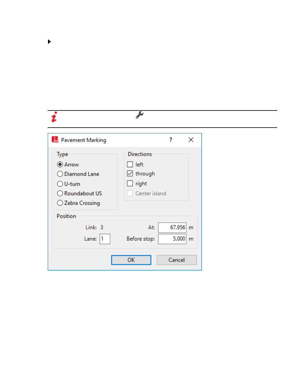
6.10.5 Modeling pavement markings
showing them in a list" on page 339).
From the Lists menu, in the desired category, choose the network object type.
In the network objects list of the network object type, you can edit attributes and attribute
values of a network object (see "Selecting cells in lists" on page 102), (see "Using lists" on
page 89).
The objects of this object type may have relations to other objects. This is why the attributes list
is shown as part of a coupled list (on the left). On the Lists toolbar, in the Relations box, you
can show and edit the coupled list with the attributes of the desired relation on the right (see
below Showing and editing dependent objects as relation) and (see "Using coupled lists" on
page 111).
Note: In lists, you can use the Attribute selection icon to show and hide attribute
values (see "Selecting attributes and subattributes for a list" on page 106).
418 © PTV GROUP
6.10.6 Defining data collection points
Element Description
Type Defines the geometric symbol shown in Vissim the network:
Arrow direction: Can be Left, Straight, Right or a combination of the lat-
ter options.
Diamond: In the USA and Canada identifies lane for high occupancy
vehicles (carpool lane)
U-rurn: Vissim displays a clockwise or anticlockwise arrow. This depends
on the settings made under Network Settings > Vehicle Behavior >
Traffic Regulations and the option selected Right-hand traffic or Left-
hand traffic.
Roundabout US: The arrow direction can be Left, Straight, Right, Center
island or a combination of these options. Center island must be com-
bined with at least one other arrow option.
Zebra Crossing is used to mark pedestrian links that are defined as ped-
estrian crossings. The option is used to indicate the width of the link which
is crossed. All traffic information must be defined for the links (see "Model-
ing links as pedestrian areas" on page 869).
Directions Arrow directions (ArrowDir): This is only relevant for the Arrow type: This
defines the geometric symbol shown in the Vissim network. If you select several
directions, these are combined in the arrow.
Links
Straight
Right
Central Island: Only relevant for US roundabout. Must be combined with
at least one other arrow option.
Position Pos: Position in the link
Before
stop:
Distance to the next downstream signal head on the same link or connector
6.10.6 Defining data collection points
Data collection points and data collection measurements based on them are similar to
induction loops that are attached to roadway tracks for the recording of traffic volume.
In Vissim data collection points can be used, in particular, for monitoring the simulated number
of vehicles. This data can be recorded in evaluations for specific vehicle classes (see
"Evaluating data collection measurements" on page 1033).
Notes:
You can specify that you need not press the CTRL key when adding network objects
(see "Right-click behavior and action after creating an object" on page 143).
For some network objects there are windows in which the attributes of a network
object can be defined and edited. There are lists for this, for all network objects. You
can choose whether you want to open a window, a list or neither of the two for the
definition of network objects in the Network Editor (see "Right-click behavior and
action after creating an object" on page 143).
© PTV GROUP 419
6.10.7 Defining vehicle travel time measurement
1. On the Network objects toolbar, click Data Collection Points.
2. Hold down the CTRL key and right-click on the desired position of the data collection point
in the link or the connector.
A colored bar is added. The Data Collection Points list opens.
3. Edit the attributes.
Element Description
No Unique identification of the data collection points
Name Data collection point name
Lane Lane
Pos Position on the link
Showing and editing dependent objects as relation
The attribute and attribute values of this network object type are shown in the list on the left,
which consists of two coupled lists.
1. In the list on the left, click the desired entry.
The list on the right contains attributes and attribute values of network objects, and/or base
data allocated to the network object selected in the list on the left (see "Using coupled lists" on
page 111):
Data collection measurements (see "Defining a data collection measurement in lists" on
page 951), (see "Generating data collection measurements in lists" on page 951)
2. Edit the desired entries.
The data is allocated.
6.10.7 Defining vehicle travel time measurement
A vehicle travel time measurement consists of a From Section and a To Section. The mean
travel time from traversing the From Section up to the traversing of the To Section is calculated,
including the waiting time and/or stop time on all lanes (see "Evaluating vehicle travel time
measurements" on page 1036).
Notes:
You can specify that you need not press the CTRL key when adding network objects
(see "Right-click behavior and action after creating an object" on page 143).
For some network objects there are windows in which the attributes of a network
object can be defined and edited. There are lists for this, for all network objects. You
can choose whether you want to open a window, a list or neither of the two for the
definition of network objects in the Network Editor (see "Right-click behavior and
action after creating an object" on page 143).
1. On the Network object toolbar, click Vehicle Travel Times.
420 © PTV GROUP

6.10.8 Attributes of vehicle travel time measurement
2. Using the mouse pointer, point to the desired position of the From Section of the Vehicle
travel time measurement in the link.
3. Hold down the CTRL key and right-click on this position.
A colored bar is added.
4. Using the mouse pointer, point to the desired position of the To Section in the link.
5. Click.
A colored bar is added. The Travel Time Measurement window opens.
6. Edit the attributes (see "Attributes of vehicle travel time measurement" on page 421):
7. Confirm with OK.
6.10.8 Attributes of vehicle travel time measurement
The Travel Time Measurement window opens automatically when you insert a network
object and have selected to automatically open the Edit dialog after object creation (see
"Right-click behavior and action after creating an object" on page 143). By default, only the
Vehicle Travel Time Measurements list is opened.
Into the window, you enter attribute values for the network object. For network objects which
have already been defined, you can call the window using the following functions:
In the list of network objects of the network object type, double-click the row with the
desired network object.
In the Network editor, select the network object of your choice. Then, from its shortcut
menu, choose Edit.
The network object may have additional attributes. In the network objects list of the network
object type, you can show all attributes and attribute values. You can open the list via the
following functions:
In the network object toolbar, right-click the desired network object type. Then from the
shortcut menu, choose Show List (see "Context menu in the network object toolbar" on
page 63).
In the Network editor, select the network object of your choice. Then, from its shortcut
menu, choose Show In List (see "Selecting network objects in the Network editor and
showing them in a list" on page 339).
From the Lists menu, in the desired category, choose the network object type.
In the network objects list of the network object type, you can edit attributes and attribute
values of a network object (see "Selecting cells in lists" on page 102), (see "Using lists" on
page 89).
The objects of this object type may have relations to other objects. This is why the attributes list
is shown as part of a coupled list (on the left). On the Lists toolbar, in the Relations box, you
can show and edit the coupled list with the attributes of the desired relation on the right (see
below Showing and editing dependent objects as relation) and (see "Using coupled lists" on
page 111).
© PTV GROUP 421
6.10.8 Attributes of vehicle travel time measurement
Note: In lists, you can use the Attribute selection icon to show and hide attribute
values (see "Selecting attributes and subattributes for a list" on page 106).
The list on the left may include the following attributes:
Element Description
No Number of travel time measurement. You can enter a different number.
Use a continuous numbering system for the Vissim network. This simplifies the
evaluations.
Name Name of travel time measurement
start sec-
tion Start link (StartLink): Number of the link of From Section
for Start position (StartPos): Distance between From Section and begin-
ning of link or connector
Label: If this option is not selected, the label for an individual vehicle
travel time measurement is hidden if the label for all vehicle travel time
measurements is selected.
destination
section End link (EndLink: Number of link of destination section
for End position ( EndPos): Distance between destination section and begin-
ning of link or connector
Label: If this option is not selected, the label for an individual vehicle
travel time measurement is hidden if the label for all vehicle travel time
measurements is selected.
Distance Dist: Length of the Vissim determined shortcut (shortest possible path) from the
From Section to the To Section.
If you change the value, the position of the To Section is automatically adjusted.
If no distance is entered, no continuous link sequence exists between both
markers. An important connector is probably missing or one of the sections
does not lie on the desired link, rather, for example, in the opposite direction.
Define a distance so large that the vehicles cannot traverse the From section
and the To Section within the same time step. Vehicles that do not traverse the
From Section and the To Section within the same time step are not accounted
for in travel time management.
Showing and editing dependent objects as relation
The attribute and attribute values of this network object type are shown in the list on the left,
which consists of two coupled lists.
1. In the list on the left, click the desired entry.
The list on the right contains attributes and attribute values of network objects, and/or base
data allocated to the network object selected in the list on the left (see "Using coupled lists" on
page 111):
2. On the list toolbar, in the Relations list, click > Delay measurements.
422 © PTV GROUP
6.10.9 Modeling queue counters
The delay measurements generated are displayed. All delay measurements can be newly
generated (see "Defining delay measurement in lists" on page 952), (see "Generating
delay measurements in lists" on page 953).
6.10.9 Modeling queue counters
Queue lengths can be determined with queue counters at any point in the Vissim network and
evaluated for any time interval. This is facilitated by stop lines of signalized intersections on
links and connectors. The following values are output (see "Showing results of queue counters
in lists" on page 1045):
Maximum queue length
Average queue length
Number of queue stops
Queues are measured from the upstream position of the queue counter up to the last vehicle
that has entered the queue conditions. You define the queue conditions when configuring the
evaluation of the queue counters. To evaluate queue lengths, you can take the adjacent lanes
of previous links into account (see "Showing results of queue counters in lists" on page 1045).
If a queue has multiple ends, queue lengths are recorded at every time step on all arms of the
queue which are upstream to the queue counter. The queue counter then returns the average
queue length of the arm, for which the longest queue was measured. At this time step
The length of a queue is detected as long as the queue has been eliminated completely, even
if vehicles have resumed driving between the queue counter and the queue end and no
longer meet the queue condition. The queue length is measured up to the last vehicle
remaining in the queue that meets the condition until the queue condition is no longer met by
any of the vehicles.
Queue lengths are output in terms of units of length, not in terms of number of vehicles.
Queues are always tracked up to their original end, even if the first vehicles are no longer in
queue.
The maximum queue length is as long as the distance to the next queue counter upstream or
as long as specified in the queue definition for the attribute Max. length. For a queue counter
that is automatically generated by Vissimfor node evaluation, the maximum queue length is
the distance to the next queue counter, upstream in the node.
6.10.9.1 Defining queue counters
Notes:
You can specify that you need not press the CTRL key when adding network objects
(see "Right-click behavior and action after creating an object" on page 143).
For some network objects there are windows in which the attributes of a network
object can be defined and edited. There are lists for this, for all network objects. You
can choose whether you want to open a window, a list or neither of the two for the
definition of network objects in the Network Editor (see "Right-click behavior and
action after creating an object" on page 143).
© PTV GROUP 423

6.11 Modeling vehicular traffic
1. On the Network objects toolbar, click Queue Counters.
2. Hold down the CTRL key and right-click on the desired position of the queue counter in the
link or the connector.
A colored bar is added. The Queue Counters list opens.
3. Edit the attributes (see "Attributes of queue counters" on page 424).
6.10.9.2 Attributes of queue counters
The Queue Counter window opens when you insert a network object and have selected to
automatically have a list opened after object creation (see "Right-click behavior and action
after creating an object" on page 143).
1. From the Lists menu, choose Measurements > Queue counters.
The Queue Counters list opens.
By default, you can edit the list (see "Using lists" on page 89).
The attribute and attribute values of this network object type are shown in the list on the left,
which consists of two coupled lists.
Tip: To open coupled lists for a network object type, from the Lists menu, choose >
<Name network object type>.
The list on the left may include the following attributes:
Element Description
No. Unique identification of the queue counter
Name Name of queue counter
Link Name of the link, on which the queue counter is defined
Pos Position on the link
6.11 Modeling vehicular traffic
Vehicular traffic can be modeled with the following variants:
Static routes: You define the routing decisions and therefore specify the paths which the
vehicles travel in the network (see "Modeling vehicle routes, partial vehicle routes, and
routing decisions" on page 430), (see "Modeling parking lots" on page 461). After this you
define the vehicle inputs. Vehicle inputs control the number of vehicles which are fed into
the Vissim network. Then run the simulation.
You use source-destination matrices with the add-on Dynamic Assignment module. For
dynamic assignment, static routes or vehicle inputs are not required (see "Using the
dynamic assignment add-on module" on page 653).
424 © PTV GROUP

6.11.1 Modeling vehicle compositions
6.11.1 Modeling vehicle compositions
You must define vehicle compositions from the vehicle type, so that the vehicle can be
generated. In general, there will be multiple vehicle compositions, e.g. cars only, cars with
5% HGV proportion or vehicle compositions for pedestrians, for which you specify relative
volumes for the vehicle types male and female.
For vehicles, which only drive in PT routes, no vehicle compositions are necessary, for
example, for public transportation by trams and city buses (see "Modeling short-range public
transportation" on page 478).
A vehicle composition contains multiple vehicle types. You allocate a relative volume and
desired speed distribution to each vehicle type (see "Using desired speed distributions" on
page 228).
For pedestrian flows you define the pedestrian compositions. Do not define vehicle
compositions for pedestrian flows, as these would then be bound to links and the model of the
flow of traffic according to Wiedemann (see "Driving states in the traffic flow model according
to Wiedemann" on page 270).
6.11.1.1 Defining vehicle compositions
You can define new vehicle compositions, assign the desired vehicle types and enter attribute
values.
1. Select Private Transport > Vehicle Compositions in the Lists menu.
The attribute and attribute values of this network object type are shown in the list on the left,
which consists of two coupled lists.
2. In the list, on the toolbar, click the Add button .
A new row with default data is inserted.
3. In the list on the left, enter a number and name (see "Attributes of vehicle compositions" on
page 426).
In the next steps, assign the desired vehicle types to the chosen vehicle compositions. For
each vehicle type you must add a row to the right hand list and you can define the attribute
values.
The right-hand list is shown. If there is no assignment, only the column titles are shown.
4. In the list on right, on the toolbar, click the Add button .
5. Select the desired entry.
6. Enter the desired attribute values in the right-hand list (see "Attributes of vehicle
compositions" on page 426).
The data is allocated.
© PTV GROUP 425
6.11.2 Modeling vehicle inputs for private transportation
6.11.1.2 Attributes of vehicle compositions
The attribute and attribute values of this network object type are shown in the list on the left,
which consists of two coupled lists.
Tip: To open coupled lists for a network object type, from the Lists menu, choose >
<Name network object type>.
Note: In lists, you can use the Attribute selection icon to show and hide attribute
values (see "Selecting attributes and subattributes for a list" on page 106).
The list on the left may include the following attributes:
Column Description
No Unique number of the vehicle composition
Name Name of vehicle composition
RelFlow Relative volumes: Taken from the right list
The list on the right contains attributes and attribute values of network objects, and/or base
data allocated to the network object selected in the list on the left (see "Using coupled lists" on
page 111):
Relative flows
Element Description
Vehicle type In the list box, select Vehicle type.
DesSpeedDistr Reference to the Desired speed distribution for the vehicle type
RelFlow Relative flow: Share of the vehicle type in the composition. The sum of
the relative volumes must not necessarily yield 1.0. As in the route
shares, the sum of all relative volumes always forms the basis of 100%;
on the basis of Vissim the absolute shares are calculated.
6.11.2 Modeling vehicle inputs for private transportation
In the network, you can define time-dependent vehicle inputs for all vehicle types. For this, at
least one vehicle composition must be defined (see "Modeling vehicle compositions" on page
425). Vehicle inputs may be positioned on links only. A vehicle input cannot be placed on a
single lane of a link.
Time intervals for vehicle inputs
You can create time intervals for vehicle inputs and thus determine the volume for each time
interval in a pedestrian input. You enter the volume for a link in vehicles per hour. When doing
so, you can choose to use the exact number of vehicles or have Vissim select a number
stochastically based on the volume entered. You must always enter the number of vehicles
per hour, even if the time interval is shorter or does not end at a full hour, e.g. after 3.5 hours.
426 © PTV GROUP

6.11.2 Modeling vehicle inputs for private transportation
Vehicle entry times
The time when the vehicles enter a link in the Vissim network is defined by Vissim
stochastically: An average time gap between two vehicles results from the hourly volume. This
average time gap is used as an average value of a negative exponential distribution. Vissim
obtains the time gaps from this distribution which relates to a Poisson distribution. In real life
scenarios, the entry time may be subject to greater variability than in Vissim on the basis of the
Poisson distribution.
If the vehicle input specified for the network during a simulation time interval is exceed by
more than two vehicles, a corresponding message is displayed.
The message and time interval per vehicle input are saved to the * .err file.
When you exit the simulation run, a window opens displaying the message. In this win-
dow, you can open the Messages window. It shows this and other messages, if there
are any.
The *.err file does not contain any messages if vehicles are not input because the
vehicle input interval is longer than the simulation time. The maximum possible traffic
volume depends on the speed and the driving behavior parameters which have been
set.
Lane selection when entering a vehicle into the Vissim network
The vehicle must be assigned to a vehicle type that is allowed in the lane of the link on which
the vehicle input is placed (see "Attributes of links" on page 383).
If a link has multiple lanes in which the vehicle can be entered, Vissim will introduce the
vehicle in the lane that provides the longest collision time for the vehicle. That is the lane in
which the vehicle can drive the longest without reaching a preceding vehicle or network object
that has an impact on its desired speed, e.g. an SC, a priority rule or a conflict area.
Vehicle speed used in network
When calculating the speed of a vehicle within the Vissim network, e.g. in an input flow or
during dynamic assignment, on a parking lot of a zone connector, Vissim accounts for the
distance between the vehicle and its preceding vehicle as well as for the maximum look
ahead distance. The look ahead distance on the respective link applies for the driving
behavior of the vehicle type the vehicle was assigned.
If the distance is greater than the maximum look ahead distance, the vehicle moves at
its desired speed.
If the distance is less than the maximum look ahead distance, but greater than the
safety distance, the following applies: v = DesSpeed - (DesSpeed - vPrecedingVehicle) * (1 -
dx / maximum look ahead distance).
If the distance is less than the safety distance, the vehicle is not used.
Demand in origin-destination matrices for dynamic assignment
For dynamic assignment, you do not need to define any vehicle inputs, as the demand is
contained in the origin-destination matrices (see "Using the dynamic assignment add- on
module" on page 653).
© PTV GROUP 427

6.11.2 Modeling vehicle inputs for private transportation
6.11.2.1 Defining vehicle inputs
Notes:
You can specify that you need not press the CTRL key when adding network objects
(see "Right-click behavior and action after creating an object" on page 143).
For some network objects there are windows in which the attributes of a network
object can be defined and edited. There are lists for this, for all network objects. You
can choose whether you want to open a window, a list or neither of the two for the
definition of network objects in the Network Editor (see "Right-click behavior and
action after creating an object" on page 143).
1. Make sure that you have defined the time intervals for which you want to enter volumes
(see "Defining time intervals for a network object type" on page 306).
2. On the Network objects toolbar, click Vehicle Inputs.
3. Hold down the CTRL key and right-click the desired link or connector.
The Vehicle input window opens.
If there is no volume yet, only the column titles are displayed.
4. Right-click in the list.
5. From the shortcut menu, choose Add.
A colored bar is shown at the start of the link. The Vehicle inputs list opens if automatic
opening of a list after object generation is selected (see "Right-click behavior and action
after creating an object" on page 143).
A new row with default data is inserted.
The default value for Volume (Volume) is 0. The default value for the Vehicle composition
(VehComp) is Default. Both default values are applied for all time intervals defined for
vehicle inputs.
The attribute and attribute values of this network object type are shown in the list on the left,
which consists of two coupled lists.
6. In the list on the left, enter the desired attribute values (see "Attributes of vehicle inputs" on
page 429).
In the next steps you assign the desired network objects to the selected vehicle input.
The list on the right contains attributes and attribute values of network objects, and/or base
data allocated to the network object selected in the list on the left (see "Using coupled lists" on
page 111):
Link: Attributes of the link (see "Attributes of links" on page 383)
Vehicle volumes by time interval: if you have entered a volume or selected a vehicle
composition and then select Vehicle volumes by time interval, the attributes of the
vehicle volumes for the first time interval are displayed (see "Defining time intervals for
a network object type" on page 306).
7. On the list toolbar, in the Relations list, click the desired entry.
428 © PTV GROUP

6.11.2 Modeling vehicle inputs for private transportation
The right-hand list is shown. If there is no assignment, only the column titles are shown.
8. Enter the desired attribute values in the right-hand list (see "Attributes of vehicle inputs" on
page 429).
9. In the right-hand list, you can add more entries for additional time intervals for which you
want to define vehicle volumes for the selected vehicle input.
The data is allocated.
6.11.2.2 Attributes of vehicle inputs
The Vehicle Inputs list opens automatically when you insert a network object and have
selected to automatically have a listed opened after object creation (see "Right-click behavior
and action after creating an object" on page 143). By default, only the Vehicle Inputs list is
opened.
1. Select Private transport > Inputs in the Lists menu.
The Vehicle inputs list opens.
By default, you can edit the list (see "Using lists" on page 89).
The attribute and attribute values of this network object type are shown in the list on the left,
which consists of two coupled lists.
Tip: To open coupled lists for a network object type, from the Lists menu, choose >
<Name network object type>.
The list on the left may include the following attributes:
Column Description
No Unique number of the vehicle input
Name Name of vehicle input
Link Name of the link to which the vehicle input was added
Volume Volume: Number of vehicles per hour - not per time interval
VehComp Vehicle composition per hour - not per time interval (see "Modeling vehicle
compositions" on page 425)
2. If you want to change the time intervals for a vehicle input, right-click the desired entry in the
Vehicle Inputs list.
3. In the context menu, select Edit Time Intervals.
The Time Intervals list opens (see "Defining time intervals for a network object type" on
page 306).
Note: In lists, you can use the Attribute selection icon to show and hide attribute
values (see "Selecting attributes and subattributes for a list" on page 106).
Showing and editing dependent objects as relation
1. In the list on the left, click the desired entry.
© PTV GROUP 429
6.11.3 Modeling vehicle routes, partial vehicle routes, and routing decisions
The list on the right contains attributes and attribute values of network objects, and/or base
data allocated to the network object selected in the list on the left (see "Using coupled lists" on
page 111):
Vehicle Volumes By Time Interval list
1. Enter the desired values.
Element Description
Cont Continued: Adopts the volume of the previous interval, if several time intervals
for vehicle inputs have been defined. The first time interval is therefore always
deactivated. The cells are white and the values are valid for this time interval
only.
The option is not selected: The cells are white and are only valid for this
interval.
The option is selected: The cells Volume, VehComp and VolTypeare
gray and are valid for the period of the combined intervals. Only the last
cell, for which the Cont attribute is not selected, can be edited. When this
option is selected, a change in volume is adopted for all the following
cells.
TimeInt Time interval: Start and end of the interval in simulation seconds (see
"Defining time intervals for a network object type" on page 306).
Volume Volume per time interval (number of vehicles per hour)
VolType Volume type:
Stochastic: Stochastic fluctuations of the traffic volume may occur. The
cells are white.
Exact: Exactly the specified number of vehicles are generated and used.
The cells are yellow. If in addition, the Continued attribute is selected, the
exact number of vehicles is generated for the entire period, which is made
up of all time intervals. If the Continued attribute is not selected, the exact
number of vehicles is generated in each time interval.
VehComp Vehicle composition (see "Modeling vehicle compositions" on page 425)
2. If you want to allocate additional volumes to other intervals for the selected vehicle input,
right-click on the Vehicle Volumes By Time Interval list.
3. From the shortcut menu, choose Add.
The next defined time interval will be added.
4. Enter the desired values.
6.11.3 Modeling vehicle routes, partial vehicle routes, and routing decisions
A route is a fixed sequence of links and connectors:
430 © PTV GROUP

6.11.3 Modeling vehicle routes, partial vehicle routes, and routing decisions
A route starts with a routing decision (From Section default color is purple)
It ends at a so-called To Section (default color is turquoise).
A routing decision point normally leads to several "to sections". Thereby the individual routes
branch out from the routing decision point to the individual "to sections".
A route may have any length. You can use a route to simply display a turning movement at a
single junction or to connect multiple nodes throughout your network. In many cases, it is
useful to deploy routes throughout the Vissim network.
A routing decision only applies to vehicles that have been assigned a vehicle class and that
are without any routing information. A vehicle already on a route may only accept new routing
information after it has passed the "to section", i.e. destination, of its route. There are
exceptions for vehicles on partial routes, PT partial routes and parking lot routes.
You may
6.11.3.1 Types of routing decisions and routes
Static: Routes vehicles from a start point (purple) to any of the To Sections specified (tur-
quoise), using a static percentage for each destination.
Static routing decisions do not apply to PT vehicles (see "Modeling short-range public
transportation" on page 478), (see "Defining PT lines" on page 485).
Partial route: Serves for local distribution of vehicles. Defines a section of one or multiple
static routes. For this section, the routes of all relevant vehicles are newly assigned accord-
ing to the partial route shares of this section. After leaving the partial route, vehicles con-
tinue with their original route.
Partial routing decisions do not apply to PT vehicles.
Partial PT route: Defines a section of one or multiple static routes. For this section, the
routes of all relevant vehicles of the PT lines selected are newly assigned according to the
partial route shares of this section. After leaving the partial route, the PT line vehicles con-
tinue with their original route.
Similar to when defining PT line stops, you can define PT stops for your PT partial route,
including attributes for dwell time (see "Modeling PT lines" on page 485):
As long as a vehicle has not completed its original line route, its Departure offset is treated
like an offset at a stop of the original route (see "Attributes of PT lines" on page 487). Once
the PT vehicle has passed the "to section" of its original line route, the Departure offset
specified for a PT partial route stop is interpreted as relative to the simulation time when the
vehicle passes the respective routing decision point.
Parking Lot, only for parking lots of the type Real parking spaces: Defines a routing
decision point used to automatically generate routes leading to each of the respective
parking lots and back to the network. You select parking lots instead of destination sec-
tions.
© PTV GROUP 431

6.11.3 Modeling vehicle routes, partial vehicle routes, and routing decisions
Managed Lanes: Routes vehicles via two parallel routes (managed lanes), from the start
section to a destination section. For a routing decision of the type Managed Lanes, you
must define a managed lanes facility with a toll pricing model and decision
model. Consequently, the following is taken into account:
occupation of vehicles with one, two or three or more persons
the time of day
the current traffic situation, including time savings and average speed
If the current Managed Lanes route is replaced with a new route at such a Managed Lanes
routing decision, it is possible that the travel times for previously begun Managed Lanes
routes continue to be counted until the vehicle passes its chosen destination.
The following conditions must be fulfilled for this to occur:
The vehicle maintains its decision for or against the toll.
The old destination is located on the new route or the new destination is on the old
route.
If the conditions are not fulfilled, the total travel time for the old route is proportionally
estimated when more than 75% of the length has been completed.
Like all other routing decisions types, only the vehicles of the selected vehicle classes will
be taken into account. Vehicles of a type, in which the classes are not selected here, use
neither the toll route nor the toll-free route. Thus, for example, HGVs can be excluded.
6.11.3.2 Routing decisions and routes for dynamic assignment
Dynamic: Defines a routing decision point, at which traffic is re-routed. For the route, you
must have defined a condition or strategy (see "Defining dynamic routing decisions" on
page 721), (see "Modeling parking lots and zones" on page 659).
Closure: Defines a route as a link sequence that will not be available for dynamic assign-
ment (see "Influencing the path search by using cost surcharges or blocks" on page 746).
You need not assign time intervals to routes of the type Closure. You do not have to enter
a relative volume.
6.11.3.3 Placing the routing decision and the mode of action in the simulation
Mode of action of routing decisions for routes
If no route is assigned to a vehicle in a simulation run, the vehicle is assigned its route as soon
as a routing decision marker traverses it. The selection of one of multiple routes to a routing
decision marker is effected according to the Monte Carlo method proportionate to the specified
"relative volumes".
On links with multiple lanes, a vehicle driving on a route attempts to independently choose a
lane for the relevant connector according to the Lane change attribute value set (Lane change
distance set (default 200 m), so that the connector can be reached without further lane
changes. Long advance links allow the vehicles a timely classification (pre- sort). In
unfavorable cases, for example, when the advance link which is selected is too short, it is
432 © PTV GROUP

6.11.3 Modeling vehicle routes, partial vehicle routes, and routing decisions
possible that many unrealistic lane changes lead to traffic disruptions, which do not exist in
reality. Most of the time such cases are preventable using suitable modeling.
In 2D animation, a current change of lanes, as well as the desire to change lanes is visualized
via a small red line to the right or left of the vehicle (representing the indicator), from the
defined Lane change distance on. This is also the case for lane changes on connectors.
In 3D animation, a current lane change and the desire to change lanes is shown via an
indicator, if this is defined for the 3D model of the vehicle.
Vehicles in the adjacent lanes decelerate partially cooperatively in order to allow the blinking
vehicle to merge (see "Applications and driving behavior parameters of lane changing" on
page 281).
Mode of action of routing decisions for partial routes
Partial routes can be used, for example, for variable message signs to model multiple
alternative routes, without having to change every single route that leads to the position of the
variable message sign. If two alternative routes are possible, only one of the partial routing
decisions with two routes must be defined, which is assigned to the total volume for each
desired share.
Positioning of routing decisions
If you define routes for links with multiple lanes, you must position the routing decision
adequately far enough from the point in which the routes separate. This will prevent unreal-
istic jams, which occurs because the decision marker assigns all vehicles a route and not
just a portion of the vehicles. This allows more lane changes to take place in the sim-
ulation than are possible in reality.
Position the routing decision section so that it is located before the end of the longest
known jam in this section.
When you insert numerous routing decisions, for example, in order to model turns per junc-
tion separately, a vehicle with an active routing decision transverses and ignores these
routing decisions until it has reached the destination section of its route. In order for a
vehicle to switch from route to route successfully and thus follow each route consecutively,
the end of the first route must be in the movement direction; only afterwards can the
second route begin. To do this, position all destination sections (turquoise) of a route on
the first connector or at the corresponding position of a link behind the last decision
marker of this route. Once you have positioned all start sections (purple) on a link behind
the junction and at the end of all connectors, ensure that all preceding routes end before
the start of a new route.
© PTV GROUP 433

6.11.3 Modeling vehicle routes, partial vehicle routes, and routing decisions
Notes:
Routing decisions are, like all other decision markers, relevant for a vehicle only
after the subsequent time step. Therefore the distance between the decision marker
and the subsequent link or connector must be defined at least large enough so that
the length of the path corresponds to the vehicle with the highest possible desired
speed within a time step. If this is not ensured, it is possible that some of the
vehicles will not be influenced by the routing decision.
If a vehicle on a route at the last possible position (emergency stop distance) is wait-
ing for an opportunity to change lanes, but this cannot occur within 60 seconds, this
vehicle is removed from the network. Otherwise unrealistic interferences and
backups will arise. In reality, one can assume that vehicles waiting to change lanes
will be compelled to "squeeze in" after a short period of time. You can adjust the
standard value of 60 s in the driving behavior parameter Diffusion time of the lane
change (see "Editing the driving behavior parameter Lane change behavior" on
page 281).
If Vissim finds no route between the start section (purple) and the destination sec-
tion (turquoise), either a connector is missing or the position of the connector is dis-
advantageous. Check the link sequence.
For partial routes or toll routes, Vissim checks at the start of the simulation run
whether all destination section, which go out from the decision section, are at a col-
lective position on the collective destination link. If this is not the case, the des-
tination link number and the position at [m] of the route with the lowest number,
which goes out from this starting marker, is taken over for all further partial routes or
Managed lanes, which begin with this starting marker.
Mode of action of routing decisions of the type Managed Lanes
In the simulation, routing decisions of the type Managed Lanes only influence the path
selection behavior of the vehicles which are already on a static route or on one of the routes,
which begins on a routing decision of the type Managed Lanes.
This does not influence vehicles on the paths of a dynamic assignment.
A lane, which is structurally separated and parallel to normal freeways which can be made up
of multiple access roads and departures, is considered to be a freeway which is subject to a
toll. Routing decisions of the type Managed Lanes serve the modeling of step-by-step use of
these parallel-guided lanes.
Positioning routing decisions of the type Managed Lanes
You can define routing decisions of the type Managed Lanes by section or add multiple
routing decisions before the managed lane starts. This choice depends on whether the driver
shall decide on how many sections to traverse before reaching the first section or whether he
shall make that decision each time before reaching one of the sections.
Positioning routing decisions of the type Managed Lanes by section
This option is useful when the toll for the next section is displayed at the routing decision:
434 © PTV GROUP

6.11.3 Modeling vehicle routes, partial vehicle routes, and routing decisions
Place a routing decision on the toll-free part of the highway, before each access from the
toll-free part of the highway to the parallel-running toll part of the highway.
For each of these routing decisions, place the destination behind the next possible exit
from the toll part to the toll-free part of the highway.
Place a routing decision on the toll road of the highway, before each access from the toll
part to the toll-free part of the highway.
On each of the toll-free parts of the highway, for each of these routing decisions, place the
destination behind the next possible exit from the toll road to the toll-free part of the high-
way.
Inserting routing decisions of the type Managed Lanes at the beginning of managed lane
This option is useful when the toll for individual sections of the total toll distance is displayed
before the first routing decision, nothing changes at the end of the first section and no other toll
is displayed there.
Using multiple, successive routing decisions, you can model various toll route options for a
driver. If you e.g. want the vehicle to be able to use one, two or three managed lane segments,
position the most expensive routing decision option on the toll-free route, so that the vehicle
has to traverse it first, then drives downstream to the next expensive routing decision option
and last to the least expensive routing decision option. Place these types of routing decisions
on toll-free routes only.
For routing decisions of the type Managed Lanes that follow upon each other at a distance of
less than10 m, the following applies: If the vehicle has selected a managed lane based on one
of these routing decisions, you cannot use another routing decision of this group that lies
further downstream to assign it a different managed lane. As soon as the vehicle has selected
a managed lane, it ignores any other managed lane routing decisions of this group that lie
further downstream.
Probability of switching to a toll road
At the first passing of a routing decision of the type Managed Lanes each vehicle receives a
random number for the probability that it will change to the toll lane. This random number is
then used for all further routing decisions of the Type Managed Lanes . This ensures that the
vehicle will only change its original decision when a completely different traffic-related state
ensues.
Two routing decisions of the type Managed Lanes should only use the same Managed lanes
facility when the following conditions are in place:
The characteristics of the toll-free routes of both routing decisions are identical for the
most part.
The course of the managed lanes of both routing decisions are identical for the most
part (see "Saving managed lane data to a file" on page 1024).
© PTV GROUP 435

6.11.3 Modeling vehicle routes, partial vehicle routes, and routing decisions
6.11.3.4 Defining static vehicle routes
To define a static vehicle route, insert a routing decision on a link and a destination section on
a destination link. You may also define multiple destination links or connectors for a routing
decision. The routing decision or the destination section may also lie on a connector.
You can assign the interval limits via the time intervals (see "Defining time intervals for a
network object type" on page 306) , (see "Calling time intervals from an attributes list" on page
307). If a distribution on a percentage basis of the traffic volume to the vehicle routes of a
routing decision varies temporally, you must define multiple time intervals which do not
overlap.
Notes:
You can specify that you need not press the CTRL key when adding network objects
(see "Right-click behavior and action after creating an object" on page 143).
For some network objects there are windows in which the attributes of a network
object can be defined and edited. There are lists for this, for all network objects. You
can choose whether you want to open a window, a list or neither of the two for the
definition of network objects in the Network Editor (see "Right-click behavior and
action after creating an object" on page 143).
1. On the Network objects toolbar, click Vehicle Routes.
The button is highlighted. The variant of the network object type is displayed in parentheses
and the button is shown.
2. Click Vehicle Routes again.
A list box opens.
3. Then select Static.
Tip: Alternatively to the following steps, to insert a routing decision, from the shortcut
menu, choose Static vehicle routing decision.
4. Hold down the CTRL key and in the Network Editor right-click the desired link or connector
on the desired position of the routing decision cross section.
5. Release the keys.
By default, a purple bar is inserted. If for this start section you want to insert multiple
destination sections, carry out the following steps accordingly. Thereby you can insert a
destination section and subsequently define each of its attributes.
If you would like to insert a destination section for this start section, execute the next steps
only once.
6. On the desired link, point the mouse pointer to the desired position of the first destination
section.
If Vissim does not find a valid link sequence, neither a yellow band nor a turquoise bar are
displayed, or the band might be interrupted. Select another destination link or a new
436 © PTV GROUP

6.11.3 Modeling vehicle routes, partial vehicle routes, and routing decisions
position for the destination section or correct the Vissim network, for example if a link is not
connected properly with a connector.
If Vissim finds a valid connection via a link sequence, between the start section and the
position the mouse pointer is pointing to, the link sequence is displayed as a yellow band
by default.
On the edge of the link, which you are pointing to with the mouse pointer, a black arrow is
shown in the direction of travel. A turquoise bar shows the possible position of the
destination section. Thereby you can select links from the different types of links, which are
added in the next step of the destination section.
7. Right-click this position.
The context menu opens.
8. If you do not wish to insert additional destination sections, from the shortcut menu, choose
Create static vehicle route: Define end.
9. To insert addition destination sections, click the desired positions.
10. If you do not want to add any additional destination sections, in the Network editor, click in
an empty area.
A turquoise bar is added for the destination section by default. The Static vehicle routing
decision list opens if automatic opening of a list after object generation is selected (see
"Right-click behavior and action after creating an object" on page 143). The attribute and
attribute values of this network object type are shown in the list on the left, which consists of
two coupled lists.
11. Edit the attributes (see "Attributes of static vehicle routing decisions" on page 437), (see
"Attributes of static vehicle routes" on page 439).
Tip: You may assign a routing decision to a destination section later on:
1. On the Network objects toolbar, click Vehicle Routes.
2. Hold down the CTRL key.
3. In the Network Editor, right-click the routing decision.
4. Release the keys.
5. Right-click the position on the link where you want to add the destination section.
6. From the shortcut menu, choose Create static vehicle route: Define end.
6.11.3.5 Attributes of static vehicle routing decisions
From the Lists menu, choose > Private Transport > Routes > Static routing decisions.
The list of attributes opens.
The attribute and attribute values of this network object type are shown in the list on the left,
which consists of two coupled lists.
© PTV GROUP 437
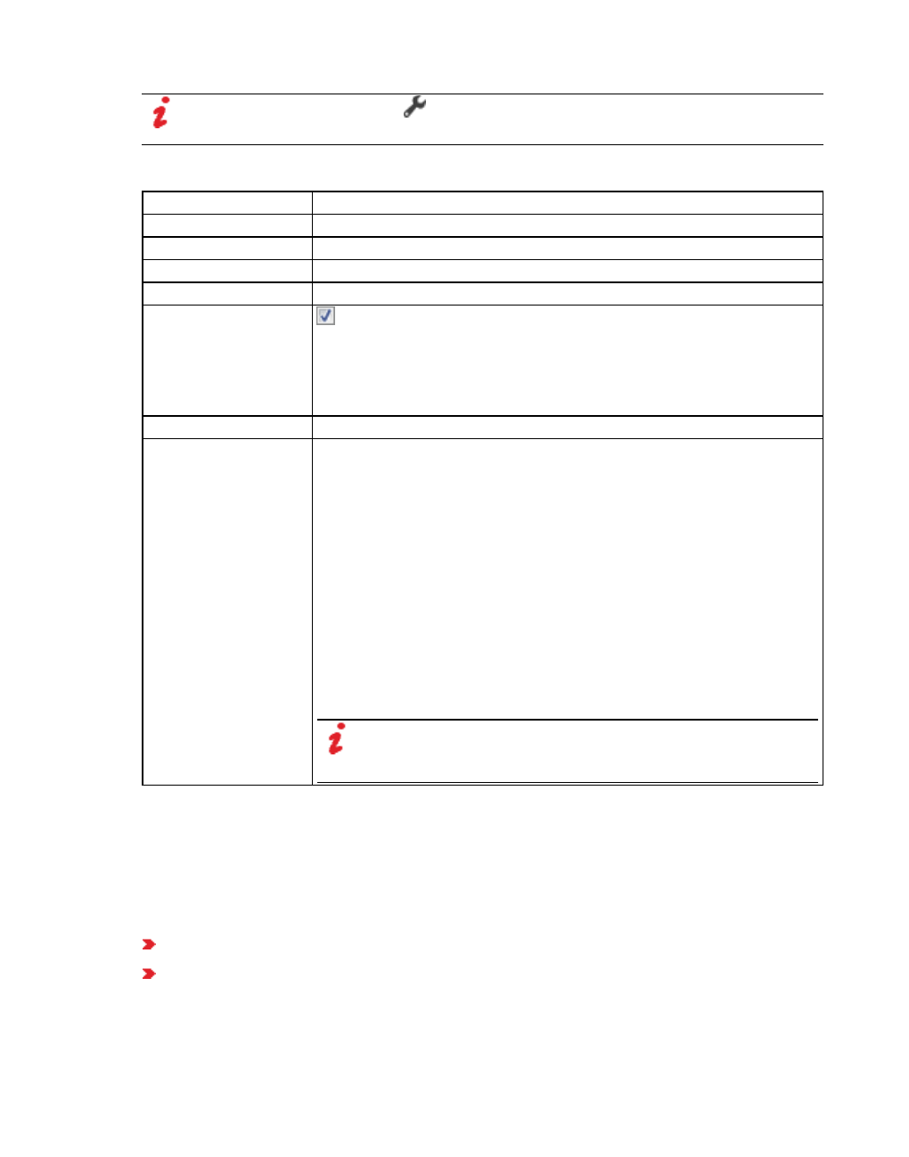
6.11.3 Modeling vehicle routes, partial vehicle routes, and routing decisions
Note: In lists, you can use the Attribute selection icon to show and hide attribute
values (see "Selecting attributes and subattributes for a list" on page 106).
The list on the left may include the following attributes:
Column Description
No Number of static vehicle routing decision
Name Name of static vehicle routing decision
Link Number of the link on which the static routing decision is located
Pos Location: Distance to the beginning of link or connector
AllVehTypes If the option is selected, all vehicle types follow the static vehicle
routing decision.
The option All Vehicle Types is a virtual vehicle class that
automatically includes all new vehicle types and vehicle types that
have not been assigned a vehicle class yet.
VehClasses Valid vehicle classes
CombineStaRoutDec Combine static routing decisions: Combines static routes which
follow one other into one route. You therefore prevent vehicles from
recognizing an imminent required change of lanes only when
passing the next routing decision and therefore artificially causing
queues.
Vissim checks at the start of the simulation for all vehicle routes,
whether on the previous link of the vehicle route there is still a further
routing decision downstream of the end of the route, for which the
option Consider subsequent static routing decisions is selected
(see "Editing the driving behavior parameter Lane change behavior"
on page 281).
If node routes are e.g. imported from PTV Vistro, ANM Import
automatically selects this attribute.
Note: Follow the instructions for the routing decision, if user-
defined route choice has been enabled (see "User-defined
and dynamic assigning of vehicle routes" on page 458).
Showing and editing dependent objects as relation
1. In the list on the left, click the desired entry.
The list on the right contains attributes and attribute values of network objects, and/or base
data allocated to the network object selected in the list on the left (see "Using coupled lists" on
page 111):
Vehicle classes (see "Defining the vehicle class" on page 267)
Static vehicle routes (see "Attributes of static vehicle routes" on page 439)
2. On the list toolbar, in the Relations list, click the desired entry.
438 © PTV GROUP

6.11.3 Modeling vehicle routes, partial vehicle routes, and routing decisions
3. Enter the desired data.
The data is allocated.
6.11.3.6 Attributes of static vehicle routes
From the Lists menu, choose > Private Transport > Routes > Static routing.
The list of attributes opens.
The attribute and attribute values of this network object type are shown in the list on the left,
which consists of two coupled lists.
Note: In lists, you can use the Attribute selection icon to show and hide attribute
values (see "Selecting attributes and subattributes for a list" on page 106).
The list on the left may include the following attributes:
Column Description
VehRoutDec Vehicle routing decision: Number and name of static vehicle routing decision
of vehicle route
No Number of static vehicle route
Name Designation
DestLink Destination link: Number and name of link on which the static vehicle route
ends
DestPos Destination position: Distance between destination section and beginning of
link or connector
RelFlow Relative volume in time interval = absolute volume in time interval: Sum of the
volumes of all time intervals
Showing and editing dependent objects as relation
1. In the list on the left, click the desired entry.
The list on the right contains attributes and attribute values of network objects, and/or base
data allocated to the network object selected in the list on the left (see "Using coupled lists" on
page 111):
2. On the list toolbar, in the Relations list, click > Link sequence.
Attributes of link sequence are displayed: Numbers of links and connectors the static
vehicle route traverses (see "Attributes of links" on page 383):
3. On the list toolbar, in the Relations list, click the desired entry.
4. Enter the desired data.
© PTV GROUP 439
6.11.3 Modeling vehicle routes, partial vehicle routes, and routing decisions
Notes:
Relative volumes: Relative volumes of a route must correspond to their absolute
volumes. However, for example, numerous turn volume calculations can deviate at
subsequent junctions. Therefore vehicles in the network are neither inserted nor
removed automatically. You must secure consistent data for modeling real scen-
arios.
Instead of absolute values, Vissim uses relative shares in order to determine the
traffic volume for destination sections of a routing decision. Thereby real volume val-
ues and percentage shares can be entered. Internally, Vissim totals the relative
volume and calculates the absolute share of each stream automatically.
6.11.3.7 Defining parking routes
If you want a vehicle to use a parking lot, define a vehicle route of the type Parking lot that
leads to the desired parking lot. To define a parking route, insert a routing decision on a link
and on a destination section located on the parking lot of your choice. For a routing decision,
you may also define multiple destination sections located on different parking lots. Your
routing decision may lie on a connector. The destination section may also lie on a connector, if
the parking lot is located on a connector.
You can assign the interval limits via the time intervals (see "Defining time intervals for a
network object type" on page 306) , (see "Calling time intervals from an attributes list" on page
307). If a distribution on a percentage basis of the traffic volume to the routes of a routing
decision varies temporally, you must define multiple time intervals which do not overlap each
other.
For parking routing decisions, time intervals assigned in the Select Attributes window, in the
list on the left, are taken into account for the subattributes Parking duration and Parking rate.
They can be selected and displayed in the Parking Routing Decisions list (see "Selecting
attributes and subattributes for a list" on page 106).
If you define a parking route to a parking lot in which the vehicle can pull out of the parking
space backwards, Vissim will create the parking route internally, using several sections: The
shortest path search defines the section of the routing decision leading to the parking lot. For
driving backwards onto the original route, Vissim defines the following sections:
A section extends up to the point where the vehicle stops driving backwards, comes to
a standstill and then continues its route driving forwards.
A section extends up to the point where a connector begins that leads to the parking
lot.
A section extends from the beginning of this connector up to the next section of the ori-
ginal route.
440 © PTV GROUP

6.11.3 Modeling vehicle routes, partial vehicle routes, and routing decisions
Notes:
You can specify that you need not press the CTRL key when adding network objects
(see "Right-click behavior and action after creating an object" on page 143).
For some network objects there are windows in which the attributes of a network
object can be defined and edited. There are lists for this, for all network objects. You
can choose whether you want to open a window, a list or neither of the two for the
definition of network objects in the Network Editor (see "Right-click behavior and
action after creating an object" on page 143).
1. On the Network objects toolbar, click Vehicle Routes.
The button is highlighted. The variant of the network object type is displayed in parentheses
and the button is shown.
2. Click Vehicle Routes again.
A list box opens.
3. Then select Parking lot.
Tip: Alternatively to the following steps, to insert a routing decision, from the shortcut
menu, choose Parking routing decision.
4. Hold down the CTRL key and in the Network Editor right-click the desired link or connector
on the desired position of the routing decision cross section.
5. Release the keys.
By default, a purple bar is inserted. If for this start section you want to insert multiple
destination sections, carry out the following steps accordingly. Thereby you can insert a
destination section into a parking lot and subsequently define each of its attributes.
If you would like to insert a destination section for this start section, execute the next steps
only once.
6. Move the cursor into the parking spaces of the desired parking lot.
If Vissim does not find a valid link sequence, neither a blue band nor a turquoise bar are
displayed, or the band might be interrupted. Select another parking lot for the destination
section or correct the Vissim network, for example if a link is not connected properly to a
connector.
If Vissim finds a valid connection via a link sequence, between the start section and the
position the mouse pointer is pointing to, the link sequence is displayed as a blue band by
default.
On the edge of the link, which you are pointing to with the mouse pointer, a black arrow is
shown in the direction of travel. A turquoise bar within the parking lot indicates the possible
position of the destination section.
7. Click this position.
© PTV GROUP 441

6.11.3 Modeling vehicle routes, partial vehicle routes, and routing decisions
8. To insert additional destination sections, in respective parking lots, click the desired
position.
9. If you do not want to add an additional destination section, in the Network editor, click in an
empty area.
A turquoise bar is added for the destination section by default. For vehicle routes of the type
Parking Lot, the route ends at the beginning of the destination parking lot. The Parking
routing decisions list opens, if automatic opening of a list after object generation is
selected (see "Right-click behavior and action after creating an object" on page 143). The
attribute and attribute values of this network object type are shown in the list on the left,
which consists of two coupled lists.
10. Edit the attributes (see "Attributes of parking routing decisions" on page 442), (see
"Attributes of parking routes" on page 444).
Tip: You may assign a routing decision to a destination section later on:
1. On the Network objects toolbar, click Vehicle Routes > Parking lot.
2. Hold down the CTRL key.
3. In the Network Editor, right-click the routing decision.
4. Release the keys.
5. In the parking lot of your choice, click the desired position of the destination section.
6. If you do not want to add an additional destination section, in the Network editor,
click in an empty area.
6.11.3.8 Attributes of parking routing decisions
From the Lists menu, choose > Private Transport > Routes > Parking Routing
Decisions.
The list of attributes opens.
The attribute and attribute values of this network object type are shown in the list on the left,
which consists of two coupled lists.
Note: In lists, you can use the Attribute selection icon to show and hide attribute
values (see "Selecting attributes and subattributes for a list" on page 106).
The list on the left may include the following attributes:
Column Description
No Number of parking routing decision
Name Name of parking routing decision
Link Number of the link, on which the parking routing decision is located
Pos Distance of the parking routing decision to the beginning of link or
connector
442 © PTV GROUP
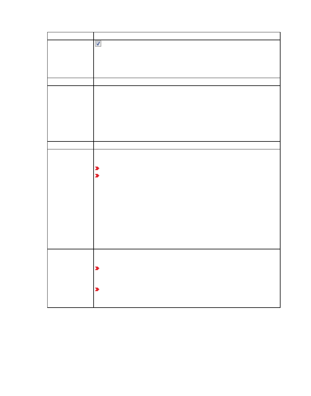
6.11.3 Modeling vehicle routes, partial vehicle routes, and routing decisions
Column Description
AllVehTypes If the option is selected, all vehicle types follow the parking routing
decision.
The option All Vehicle Types is a virtual vehicle class that automatically
includes all new vehicle types and vehicle types that have not been
assigned a vehicle class yet.
VehClasses Valid vehicle classes
ParkRate Parking rate: Share of vehicles belonging to the allocated vehicle
classes. A vehicle, which has been assigned a parking space via a
parking routing decision, carries this out on an automatically generated
route and parks for as long as the dwell time distribution specifies. This
dwell time distribution is allocated in the Parking Routing Decisions. After
the dwell time expires, the vehicle leaves the parking lot and begins on an
automatically generated route, which brings the vehicle via the shortest
path back to its original route behind the position of the routing decision.
Parking duration Parking time
GenBy Generated by: Indicates whether the parking routing decisions are user-
defined or have been generated by Vissim.
User The parking routing decision was defined by a Vissim user.
Dynamic assignment: only for parking routing decisions of dynamic
assignment: For real parking lots, Vissim automatically creates a park-
ing routing decision 50 m from a parking lot and in the attribute GenBy
box, enters Dynamic assignment. You can change the distance
between the parking routing decision and the parking lot in the attrib-
ute Routing decision distance of the parking lot. Use this distance to
ensure that the parking routing decision lies at the beginning of the
last edge before the parking lot.
After simulation has been completed, the list no longer shows
automatically generated parking routing decisions of dynamic
assignment.
FullOccupBehav Full occupancy behavior: Waiting behavior of vehicles traversing the
parking routing decision:
Waiting: If there is no parking space available, the vehicle drives to the
next parking space that will become available (a vehicle is currently
still parked there) and waits.
Drive on: If no parking space is available, the vehicle ignores the park-
ing routing decision.
By default, the attribute is not displayed in the list.
Showing and editing dependent objects as relation
1. In the list on the left, click the desired entry.
© PTV GROUP 443
6.11.3 Modeling vehicle routes, partial vehicle routes, and routing decisions
The list on the right contains attributes and attribute values of network objects, and/or base
data allocated to the network object selected in the list on the left (see "Using coupled lists" on
page 111):
Parking rate by time interval: The attribute Parking rate is described above.
Vehicle classes (see "Using vehicle classes" on page 267)
Parking routes (see "Attributes of parking routes" on page 444)
2. On the list toolbar, in the Relations list, click the desired entry.
3. Enter the desired data.
6.11.3.9 Attributes of parking routes
From the Lists menu, choose > Private Transport > Routes > Parking Routes.
The list of attributes opens.
The attribute and attribute values of this network object type are shown in the list on the left,
which consists of two coupled lists.
Note: In lists, you can use the Attribute selection icon to show and hide attribute
values (see "Selecting attributes and subattributes for a list" on page 106).
The list on the left may include the following attributes:
Column Description
VehRoutDec Vehicle routing decision: Number and name of the parking routing decision
of the parking route
No Number of parking route
ParkLot Parking lot: Name of parking lot
Additional attributes (see "Modeling parking lots" on page 461)
Showing and editing dependent objects as relation
1. In the list on the left, click the desired entry.
The list on the right contains attributes and attribute values of network objects, and/or base
data allocated to the network object selected in the list on the left (see "Using coupled lists" on
page 111):
2. On the list toolbar, in the Relations list box, click > Link sequence.
Attributes of link sequence are displayed: Numbers of links and connectors via which the
route leads. (see "Attributes of links" on page 383)
3. Enter the desired data.
444 © PTV GROUP

6.11.3 Modeling vehicle routes, partial vehicle routes, and routing decisions
6.11.3.10 Defining a vehicle route of the type managed lane
To define vehicle routes of the type Managed lanes, insert a routing decision on a link and a
destination section on a destination link. The routing decision or destination section may also
lie on connectors.
For a routing decision of the type Managed lanes, first insert a managed lane route (red by
default). Subsequently, at the destination section, insert the general purpose route (green by
default). The general purpose route, too, runs on the same link, from the routing decision of the
managed lane route to its destination section. A routing decision of the type Managed lanes
has a maximum of two routes: the managed lane route and the general purpose route. Both
routes automatically have the same destination section.
A routing decision of the type Managed lanes is only taken into account in the simulation
when it is complete: This means a route of the type Managed lanes and a general purpose
route must be defined. Then a managed lanes facility with a user-defined toll price model and
decision model must be assigned (see "Defining decision model for managed lane facilities"
on page 310), (see "Defining toll pricing calculation models" on page 311).
Notes:
You can specify that you need not press the CTRL key when adding network objects
(see "Right-click behavior and action after creating an object" on page 143).
For some network objects there are windows in which the attributes of a network
object can be defined and edited. There are lists for this, for all network objects. You
can choose whether you want to open a window, a list or neither of the two for the
definition of network objects in the Network Editor (see "Right-click behavior and
action after creating an object" on page 143).
1. On the Network objects toolbar, click Vehicle Routes.
The button is highlighted. The variant of the network object type is displayed in parentheses
and the button is shown.
2. Click Vehicle Routes again.
A list box opens.
3. Then select Managed lanes.
4. Hold down the CTRL key and in the Network Editor right-click the desired link or connector
on the desired position of the routing decision cross section.
5. Release the keys.
By default, a purple bar is inserted.
6. On the desired link, point the mouse pointer to the desired position of the destination
section.
If Vissim does not find a valid link sequence, neither a red band nor a turquoise bar are
displayed, or the band might be interrupted. Select another destination link or a new
© PTV GROUP 445

6.11.3 Modeling vehicle routes, partial vehicle routes, and routing decisions
position for the destination section or correct the Vissim network, for example if a link is not
connected properly with a connector.
If Vissim finds a valid connection via a link sequence, between the start section and the
position the mouse pointer is pointing to, the link sequence is displayed as a red band by
default.
On the edge of the link, which you are pointing to with the mouse pointer, a black arrow is
shown in the direction of travel. A turquoise bar shows the possible position of the
destination section. Thereby you can select links from the different types of links, which are
added in the next step of the destination section.
7. Right-click this position.
The context menu opens.
8. Then select Create managed lane route: Define end.
The managed lane route continues to be displayed in red. Per default, a colored bar is
inserted for the destination section. The Managed lanes routing decisions list opens, if
automatic opening of a list after object generation is selected (see "Right-click behavior and
action after creating an object" on page 143). The attribute and attribute values of this
network object type are shown in the list on the left, which consists of two coupled lists. In
the Managed Lane Routes list, a new row, with a vehicle routing decision of the type Toll, is
created. Next, in the Network editor, add the respective vehicle routing decision type
General purpose.
9. Right-click the turquoise bar of the destination section.
The context menu opens.
10. Select Add vehicle route to existing destination.
The general purpose route on the managed lanes route is highlighted in green. In the
Managed Lane Routes list, a new row, with a vehicle routing decision of the type Toll, is
inserted.
11. Edit the attributes (see "Attributes of managed lanes routing decisions" on page 446), (see
"Attributes of managed lane routes" on page 447).
6.11.3.11 Attributes of managed lanes routing decisions
From the Lists menu, choose > Private Transport > Routes > Managed lanes routing
decisions.
The list of attributes opens.
The attribute and attribute values of this network object type are shown in the list on the left,
which consists of two coupled lists.
Note: In lists, you can use the Attribute selection icon to show and hide attribute
values (see "Selecting attributes and subattributes for a list" on page 106).
The list on the left may include the following attributes:
446 © PTV GROUP

6.11.3 Modeling vehicle routes, partial vehicle routes, and routing decisions
Column Description
No Number of managed lane routing decision
Name Name of managed lane routing decision
Link Number and name of link on which the managed lane routing decision lies
Pos Location: Distance to the beginning of link or connector
AllVehTypes If the option is selected, all vehicle types follow the managed lane routing
decision.
The option All Vehicle Types is a virtual vehicle class that automatically
includes all new vehicle types and vehicle types that have not been assigned
a vehicle class yet.
VehClasses Valid vehicle classes
Managed
lanes facility
Name of assigned managed lane facility (see "Defining managed lane
facilities" on page 308)
Managed
lanes data
The result attribute lists: travel time savings / average speed / current toll for
managed lane route.
Showing and editing dependent objects as relation
1. In the list on the left, click the desired entry.
The list on the right contains attributes and attribute values of network objects, and/or base
data allocated to the network object selected in the list on the left (see "Using coupled lists" on
page 111):
Vehicle classes (see "Using vehicle classes" on page 267)
Managed lane routes (see "Attributes of managed lane routes" on page 447)
2. On the list toolbar, in the Relations list, click the desired entry.
3. Enter the desired data.
6.11.3.12 Attributes of managed lane routes
From the Lists menu, choose > Private Transport > Routes > Managed Lanes Routes.
The list of attributes opens.
The attribute and attribute values of this network object type are shown in the list on the left,
which consists of two coupled lists.
Note: In lists, you can use the Attribute selection icon to show and hide attribute
values (see "Selecting attributes and subattributes for a list" on page 106).
The list on the left may include the following attributes:
© PTV GROUP 447

6.11.3 Modeling vehicle routes, partial vehicle routes, and routing decisions
Column Description
VehRoutDec Vehicle routing decision: Number and name of managed lanes routing
decision of the managed lane route
No Number of managed lane route
Type Toll: toll route, highlighted in red by default
General purpose: toll-free route, highlighted in green by default
DestLink Destination link: Number and name of link on which the managed lane
route ends
DestPos Destination position: Distance between destination section and beginning
of link or connector
Showing and editing dependent objects as relation
1. In the list on the left, click the desired entry.
The list on the right contains attributes and attribute values of network objects, and/or base
data allocated to the network object selected in the list on the left (see "Using coupled lists" on
page 111):
2. On the list toolbar, in the Relations list, click > Link sequence.
Attributes of link sequence are displayed: Numbers of links and connectors affected by the
managed lane route (see "Attributes of links" on page 383):
3. Enter the desired data.
6.11.3.13 Defining a vehicle route of the type closure
To define a vehicle route of the type Closure , insert a routing decision on a link and a
destination section on a destination link. You may also define multiple destination links or
connectors for a routing decision. The routing decision or destination section may also lie on
connectors.
Notes:
You can specify that you need not press the CTRL key when adding network objects
(see "Right-click behavior and action after creating an object" on page 143).
For some network objects there are windows in which the attributes of a network
object can be defined and edited. There are lists for this, for all network objects. You
can choose whether you want to open a window, a list or neither of the two for the
definition of network objects in the Network Editor (see "Right-click behavior and
action after creating an object" on page 143).
1. On the Network objects toolbar, click Vehicle Routes.
The button is highlighted. The variant of the network object type is displayed in parentheses
and the button is shown.
2. Click Vehicle Routes again.
A list box opens.
448 © PTV GROUP

6.11.3 Modeling vehicle routes, partial vehicle routes, and routing decisions
3. Then select Closure.
Tip: Alternatively to the following steps, to insert a routing decision, from the shortcut
menu, choose Vehicle route closure decision.
4. Hold down the CTRL key and in the Network Editor right-click the desired link or connector
on the desired position of the routing decision cross section.
5. Release the keys.
By default, a purple bar is inserted. If for this start section you want to insert multiple
destination sections, carry out the following steps accordingly. Thereby you can insert a
destination section and subsequently define each of its attributes.
If you would like to insert a destination section for this start section, execute the next steps
only once.
6. On the desired link, point the mouse pointer to the desired position of the first destination
section.
If Vissim does not find a valid link sequence, neither a red band nor a turquoise bar are
displayed, or the band might be interrupted. Select another destination link or a new
position for the destination section or correct the Vissim network, for example if a link is not
connected properly with a connector.
If Vissim finds a valid connection via a link sequence, between the start section and the
position the mouse pointer is pointing to, the link sequence is displayed as a red band by
default.
On the edge of the link, which you are pointing to with the mouse pointer, a black arrow is
shown in the direction of travel. A turquoise bar shows the possible position of the
destination section. Thereby you can select links from the different types of links, which are
added in the next step of the destination section.
7. Right-click this position.
The context menu opens.
8. If you do not wish to insert additional destination sections, from the shortcut menu, choose
Create vehicle route closure: Define end.
9. To insert addition destination sections, click the desired positions.
10. If you do not want to add any additional destination sections, in the Network editor, click in
an empty area.
A turquoise bar is added for the destination section by default. The Vehicle route closure
decision list opens if automatic opening of a list after object generation is selected (see
"Right-click behavior and action after creating an object" on page 143). The attribute and
attribute values of this network object type are shown in the list on the left, which consists of
two coupled lists.
11. Edit the attributes (see "Attributes of route closure decisions" on page 450), (see
"Attributes of route closures" on page 450).
© PTV GROUP 449

6.11.3 Modeling vehicle routes, partial vehicle routes, and routing decisions
Tip: You may assign a routing decision to a destination section later on:
1. On the Network objects toolbar, click Vehicle Routes.
2. Hold down the CTRL key.
3. In the Network Editor, right-click the routing decision.
4. Release the keys.
5. Right-click the position on the link where you want to add the destination section.
6. From the shortcut menu, choose Create vehicle route: Define end.
6.11.3.14 Attributes of route closure decisions
From the Lists menu, choose > Private Transport > Routes > Route closure decisions.
The list of attributes opens.
The attribute and attribute values of this network object type are shown in the list on the left,
which consists of two coupled lists.
Note: In lists, you can use the Attribute selection icon to show and hide attribute
values (see "Selecting attributes and subattributes for a list" on page 106).
The list on the left may include the following attributes:
Column Description
No Number of route closure decision
Name Name of route closure decision
Link Number and name of link on which the route closure decision lies
Pos Position: Distance between route closure decision and beginning of link or con-
nector
Showing and editing dependent objects as relation
1. In the list on the left, click the desired entry.
The list on the right contains attributes and attribute values of network objects, and/or base
data allocated to the network object selected in the list on the left (see "Using coupled lists" on
page 111):
2. On the list toolbar, in the Relations list box, click > Vehicle route closures (see "Attributes
of route closures" on page 450).
3. Enter the desired data.
6.11.3.15 Attributes of route closures
From the Lists menu, choose > Private Transport > Routes > Route Closures.
The list of attributes opens.
450 © PTV GROUP

6.11.3 Modeling vehicle routes, partial vehicle routes, and routing decisions
The attribute and attribute values of this network object type are shown in the list on the left,
which consists of two coupled lists.
Note: In lists, you can use the Attribute selection icon to show and hide attribute
values (see "Selecting attributes and subattributes for a list" on page 106).
The list on the left may include the following attributes:
Column Description
VehRoutDec Vehicle routing decision: Number and name of vehicle routing decision of
route closure
No Number of route closure
DestLink Destination link: Number and name of link on which route closure ends
DestPos Destination position: Distance between destination section and beginning of
link or connector
Showing and editing dependent objects as relation
1. In the list on the left, click the desired entry.
The list on the right contains attributes and attribute values of network objects, and/or base
data allocated to the network object selected in the list on the left (see "Using coupled lists" on
page 111):
2. On the list toolbar, in the Relations list box, click > Link sequence.
Attributes of link sequence are displayed: Numbers of links and connectors affected by the
route closure (see "Attributes of links" on page 383):
3. Enter the desired data.
6.11.3.16 Defining partial vehicle routes
To define a partial vehicle route, insert a routing decision on a link and a destination section
on a destination link. The partial routing decision or the destination section may also lie on a
connector.
You can assign the interval limits via the time intervals (see "Defining time intervals for a
network object type" on page 306) , (see "Calling time intervals from an attributes list" on page
307). If a distribution on a percentage basis of the traffic volume to the routes of a routing
decision varies temporally, you must define multiple time intervals which do not overlap each
other.
© PTV GROUP 451

6.11.3 Modeling vehicle routes, partial vehicle routes, and routing decisions
Notes:
You can specify that you need not press the CTRL key when adding network objects
(see "Right-click behavior and action after creating an object" on page 143).
For some network objects there are windows in which the attributes of a network
object can be defined and edited. There are lists for this, for all network objects. You
can choose whether you want to open a window, a list or neither of the two for the
definition of network objects in the Network Editor (see "Right-click behavior and
action after creating an object" on page 143).
1. On the Network objects toolbar, click Vehicle Routes.
The button is highlighted. The variant of the network object type is displayed in parentheses
and the button is shown.
2. Click Vehicle Routes again.
A list box opens.
3. Then select Partial route.
Tip: Alternatively to the following steps, to insert a routing decision, from the shortcut
menu, choose Vehicle partial routing decision.
4. Hold down the CTRL key and in the Network Editor right-click the desired link or connector
on the desired position of the routing decision cross section.
5. Release the keys.
By default, a purple bar is inserted.
6. On the desired link, point the mouse pointer to the desired position of the destination
section.
If Vissim does not find a valid link sequence, neither a yellow band nor a turquoise bar are
displayed, or the band might be interrupted. Select another destination link or a new
position for the destination section or correct the Vissim network, for example if a link is not
connected properly with a connector.
If Vissim finds a valid connection via a link sequence, between the start section and the
position the mouse pointer is pointing to, the link sequence is displayed as a yellow band
by default.
On the edge of the link, which you are pointing to with the mouse pointer, a black arrow is
shown in the direction of travel. A turquoise bar shows the possible position of the
destination section. Thereby you can select links from the different types of links, which are
added in the next step of the destination section.
7. Right-click this position.
The context menu opens.
8. Then select Create vehicle partial route: Define end.
452 © PTV GROUP

6.11.3 Modeling vehicle routes, partial vehicle routes, and routing decisions
A turquoise bar is added for the destination section by default. The Vehicle partial routing
decision list opens if automatic opening of a list after object generation is selected (see
"Right-click behavior and action after creating an object" on page 143). The attribute and
attribute values of this network object type are shown in the list on the left, which consists of
two coupled lists.
9. Edit the attributes (see "Attributes of partial vehicle routing decisions" on page 454), (see
"Attributes of partial vehicle routes" on page 455).
6.11.3.17 Defining a partial route based on an existing partial route
If you have defined a partial route, PuT partial route, or a route of the type Managed Lanes for
a link, you can select the destination section and then insert a new partial route that starts at
the existing routing decision and ends at the current destination section.
Notes:
You can specify that you need not press the CTRL key when adding network objects
(see "Right-click behavior and action after creating an object" on page 143).
For some network objects there are windows in which the attributes of a network
object can be defined and edited. There are lists for this, for all network objects. You
can choose whether you want to open a window, a list or neither of the two for the
definition of network objects in the Network Editor (see "Right-click behavior and
action after creating an object" on page 143).
1. On the Network objects toolbar, click Vehicle Routes.
The button is highlighted. The variant of the network object type is displayed in parentheses
and the button is shown.
2. Click Vehicle Routes again.
A list box opens.
3. Select the desired entry.
Partial
Partial PT
Managed Lanes
4. In the Network editor, right-click the destination section of the partial route you want to use
as the basis of your new partial route.
5. From the context menu, choose Add Vehicle Route.
6. On the desired link, point the mouse pointer to the desired position of the new destination
section.
If Vissim does not find a valid link sequence, neither a colored band nor a turquoise bar are
displayed, or the band might be interrupted. Select another destination link or a new
© PTV GROUP 453
6.11.3 Modeling vehicle routes, partial vehicle routes, and routing decisions
position for the destination section or correct the Vissim network, for example if a link is not
connected properly with a connector.
You must select a different destination link or a new position for the destination section or
correct the Vissim network.
If Vissim finds a valid connection via a link sequence, between the start section and the
position the mouse pointer is pointing to, the link sequence is by default displayed as a
colored band.
On the edge of the link, which you are pointing to with the mouse pointer, a black arrow is
shown in the direction of travel. A colored bar shows the possible position of the destination
section. Thereby you can select links from the different types of links, which are added in
the next step of the destination section.
7. Hold down the CTRL key and right-click on this position.
8. Release the keys.
Per default, a colored bar is inserted for the destination section. The list <Variant> Vehicle
Routes opens.
9. Edit the attributes (see "Attributes of partial vehicle routing decisions" on page 454), (see
"Attributes of partial vehicle routes" on page 455)
The attributes are saved in the list.
10. In the Network editor, click into an empty section.
The attributes are saved in the lists of the partial route and the routing decision.
6.11.3.18 Attributes of partial vehicle routing decisions
1. From the Lists menu, choose > Private Transport > Routes > Partial routing decisions.
The attribute and attribute values of this network object type are shown in the list on the left,
which consists of two coupled lists.
The list on the left may include the following attributes:
Column Description
No Unique Number of vehicle partial routing decision
Name Name of partial vehicle routing decision
Link Number of the link on which the vehicle partial routing decision lies
Pos Location: Distance to the beginning of link or connector
Note: In lists, you can use the Attribute selection icon to show and hide attribute
values (see "Selecting attributes and subattributes for a list" on page 106).
The list on the right contains attributes and attribute values of network objects, and/or base
data allocated to the network object selected in the list on the left (see "Using coupled lists" on
page 111):
454 © PTV GROUP
6.11.3 Modeling vehicle routes, partial vehicle routes, and routing decisions
Vehicle classes (see "Defining the vehicle class" on page 267)
Partial vehicle routes (see "Attributes of static vehicle routes" on page 439)
Link (see "Attributes of links" on page 383)
Destination link (see "Attributes of links" on page 383)
2. On the list toolbar, in the Relations list, click the desired entry.
3. Enter the desired data.
6.11.3.19 Attributes of partial vehicle routes
1. From the Lists menu, choose > Private Transport > Routes > Partial routes.
The attribute and attribute values of this network object type are shown in the list on the left,
which consists of two coupled lists.
The list on the left may include the following attributes:
Column Description
VehRoutDec Vehicle routing decision: Number and name of partial routing decision of
partial vehicle route (see "Attributes of partial vehicle routing decisions" on
page 454)
No Unique Number of partial vehicle route
Name Name of partial vehicle route
Destination
link
Number and name of link on which partial vehicle route ends
DestPos Destination position: Distance between destination section and beginning of
link or connector
RelFlow Relative volume in time interval = absolute volume in time interval: Sum of the
volumes of all time intervals
Note: In lists, you can use the Attribute selection icon to show and hide attribute
values (see "Selecting attributes and subattributes for a list" on page 106).
The list on the right contains attributes and attribute values of network objects, and/or base
data allocated to the network object selected in the list on the left (see "Using coupled lists" on
page 111):
Vehicle routing decision(see "Attributes of partial vehicle routing decisions" on page 454)
Link sequence (see "Attributes of links" on page 383)
Destination link (see "Attributes of partial vehicle routing decisions" on page 454)
2. On the list toolbar, in the Relations list, click the desired entry.
3. Enter the desired data.
© PTV GROUP 455
6.11.3 Modeling vehicle routes, partial vehicle routes, and routing decisions
6.11.3.20 Inserting intermediate points into a vehicle route
You may insert intermediate points into a vehicle route. Subsequently, you can change the
routing process (see "Changing routing procedure via intermediate points" on page 456).
When you add a destination section, it is highlighted by default and a colored band shows the
course of the link. This identifies the following possibilities:
You can add additional destination sections for the routing decisions (see "Defining park-
ing routes" on page 440).
When you select a destination section, it is highlighted by default and a colored band indicates
the course of the road. This identifies the following possibilities:
You may move the destination section.
You can add intermediate points on the vehicle route before the marked destination sec-
tion.
Notes:
You can specify that you need not press the CTRL key when adding network objects
(see "Right-click behavior and action after creating an object" on page 143).
For some network objects there are windows in which the attributes of a network
object can be defined and edited. There are lists for this, for all network objects. You
can choose whether you want to open a window, a list or neither of the two for the
definition of network objects in the Network Editor (see "Right-click behavior and
action after creating an object" on page 143).
1. On the Network objects toolbar, select the network object type Vehicle Routes.
2. Click the destination section of the vehicle route into which you want to insert the
intermediate points.
The link sequence is shown as a colored band.
3. Keep the CTRL key pressed and right-click the desired positions for intermediate points on
the colored band of the vehicle route.
The intermediate points are added.
4. If you do not wish to add any additional intermediate points or destination sections, click on
the free space in the Network Editor.
6.11.3.21 Changing routing procedure via intermediate points
You can add temporary intermediate points in a vehicle route and move them to different links.
Vissim calculates a new link sequence or partial link sequence from the next upstream lying
intermediate point via the current new point up to the next intermediate point downstream. In
the case that no further intermediate point was set, the entire route is recalculated. You can
add intermediate points already during the definition of vehicle routes (see "Inserting
intermediate points into a vehicle route" on page 456).
1. On the Network objects toolbar, click Vehicle Routes.
456 © PTV GROUP
6.11.3 Modeling vehicle routes, partial vehicle routes, and routing decisions
2. Click in the Network Editor on the destination section of the desired route.
The link sequence is shown as a colored band.
3. Hold down the CTRL key and right-click on the desired positions of the intermediate points.
4. Release the keys.
5. Click the first intermediate point you want to move and keep the left mouse button held
down. Then drag the intermediate point to the desired position on another other link.
The new link sequence is shown as a colored band.
6. Release the keys.
7. If desired, move additional intermediate points.
8. If you would like to confirm the new link sequence and hide the yellow band, in the Network
Editor, click an empty area.
6.11.3.22 Defining a vehicle route based on an existing vehicle route
If you have defined a vehicle route of the type Static, Closure or Parking Lot for a link, you can
select the destination section and then insert a new vehicle route that starts at the existing
routing decision and ends at a new destination section.
Notes:
You can specify that you need not press the CTRL key when adding network objects
(see "Right-click behavior and action after creating an object" on page 143).
For some network objects there are windows in which the attributes of a network
object can be defined and edited. There are lists for this, for all network objects. You
can choose whether you want to open a window, a list or neither of the two for the
definition of network objects in the Network Editor (see "Right-click behavior and
action after creating an object" on page 143).
1. On the Network objects toolbar, click Vehicle Routes.
The button is highlighted. The variant of the network object type is displayed in parentheses
and the button is shown.
2. Click Vehicle Routes again.
A list box opens.
3. Select the desired entry.
Static
Closure
Parking Lot
4. In the Network editor, right-click the destination section of the vehicle route you want to use
as the basis for your new vehicle route.
5. From the context menu, choose Add Vehicle Route.
© PTV GROUP 457

6.11.3 Modeling vehicle routes, partial vehicle routes, and routing decisions
6. On the desired link, point the mouse pointer to the desired position of the new destination
section.
If Vissim does not find a valid link sequence, neither a colored band nor a turquoise bar are
displayed, or the band might be interrupted. Select another destination link or a new
position for the destination section or correct the Vissim network, for example if a link is not
connected properly with a connector.
If Vissim finds a valid connection via a link sequence, between the start section and the
position the mouse pointer is pointing to, the link sequence is by default displayed as a
colored band.
On the edge of the link, which you are pointing to with the mouse pointer, a black arrow is
shown in the direction of travel. A turquoise bar shows the possible position of the
destination section. Thereby you can select links from the different types of links, which are
added in the next step of the destination section.
7. Right-click this position.
The context menu opens.
8. To insert addition destination sections, click the desired positions.
9. If you do not wish to insert additional destination sections, from the shortcut menu, choose
Create vehicle route: Define end.
Per default, a colored bar is inserted for the destination section. The <Scenario> Vehicle
routing decisions list opens if automatic opening of a list after object generation is selected
(see "Right-click behavior and action after creating an object" on page 143). The attribute
and attribute values of this network object type are shown in the list on the left, which
consists of two coupled lists.
10. Edit the attributes (see "Attributes of static vehicle routes" on page 439), (see "Attributes of
route closures" on page 450), (see "Attributes of parking routes" on page 444).
11. Confirm with OK.
The attributes are saved in the lists of the route and routing decision.
6.11.3.23 User-defined and dynamic assigning of vehicle routes
You can assign vehicles a route at those routing decisions whose numbers have been saved
to the vehicles’ user-defined attribute UseVehRRoutNo (Use vehicle route number).
VehicleRoutingDecision
VehicleRoutingDecisionPartial
VehicleRoutingDecisionManagedLanes
PT partial routing decisions
By default, the user-defined attribute UseVehRouteNo is saved to the defaults.inpx file.
To assign the vehicle route dynamically, enable the user-defined attribute for each desired
vehicle route. Make sure that the vehicles in the network contain the desired number in the
NextRouteNo attribute:
458 © PTV GROUP

6.11.3 Modeling vehicle routes, partial vehicle routes, and routing decisions
Enabling the user-defined attribute UseVehRouteNo
1. From the Lists menu, choose > Private transport > Routes. Then select the desired
routing decision.
The list of attributes opens.
2. On list toolbar, click the Attribute selection button .
The attribute selection window <Name Routing Decision >: Select Attributes opens.
3. In the section on the left, double-click the user-defined attribute Use vehicle route number.
The attribute selected is shown in an additional row, in the section on the right.
4. Confirm with OK.
In the Attribute list of the vehicle routing decision, the column UseVehRouteNo is
displayed. By default, the option in the column is disabled.
5. Select the option for those routing decisions that need to adopt the number of the vehicle
route from the vehicle attribute UseVehRouteNo.
Note: Routing decisions for which user-defined route choice is enabled the following
applies:
Routing decisions are not suitable for combining vehicle routes (attribute Com-
bine static routing decisions combine) (see "Attributes of static vehicle routing
decisions" on page 437), since the vehicle routes can be changed any time by
changing the vehicle attribute value NextRouteNo (Next route number). This
means you cannot make any predictions about future behavior.
These routing decisions only become effective after they are traversed. So do
they do not have an indirect impact based on a combined routing decision loc-
ated upstream.
If the attribute Combine static routing decisions is selected, the subsequent
decision on the destination link of the traversed routing decision does not auto-
matically adopt the route number from the attribute NextRouteNo of the vehicle.
First, for the subsequent decision, you need to select the attribute UseVe-
hRouteNo. By default, route choice happens at the follow decision It, In par-
ticular, governs the lane choice of the vehicle up until it traverses the follow
decision.
Effect of the attribute NextRouteNo on the vehicle
Vissim checks the attribute NextRouteNo of the vehicle, when the vehicle traverses a routing
decision for which the attribute UseVehRouteNo has been selected.
If the value is empty, negative or zero, the routing decision behaves normally.
If the value of a route number corresponds to the route of a routing decision, this route
is assigned to the vehicle.
If the value is another positive number, the routing decision will have no effect.
By default, the user-defined attribute NextRouteNo is saved to the defaults.inpx file.
© PTV GROUP 459

6.11.3 Modeling vehicle routes, partial vehicle routes, and routing decisions
Setting a value for the attribute NextRouteNo
You can enter a value for the attribute via the COM interface or during the simulation run.
Entering a value for the attribute NextRouteNo during the simulation run
1. Ensure that the following requirements are met:
The attribute UseVehRouteNo is selected for the desired routing decision (see
"Enabling the user-defined attribute UseVehRouteNo" on page 459).
You have the number of the vehicle route the vehicle is supposed to follow from the
routing decision on.
2. On the network object toolbar, right-click Vehicles in network.
3. From the shortcut menu, choose Show list.
The Vehicles In Network list opens.
4. On the list toolbar, click the Attribute selection button.
The attribute selection window Vehicles In network: Select attribute opens.
5. In the section on the left, double click the user-defined attribute NextRouteNo.
The attribute selected is shown in an additional row, in the section on the right.
6. Confirm with OK.
In the Vehicles in network list, the NextRouteNo column is displayed.
Next, start the simulation run in single step mode or change to single step mode in good
time, so that you select the desired vehicle and enter the value. Switch to single step mode
before the vehicle has reached the routing decision that will adopt the number of the
vehicle route from the attribute of the vehicle.
7. Start the simulation run in the desired mode:
Symbol Name Description Key
Simulation
continuous
Starts continuous simulation run or switches from Simulation
single step mode to Simulation continuous mode.
F5
Simulation
single step
Starts simulation in Simulation single step mode or switches
from Simulation continuous mode to Simulation single step
mode or executes the next single step.
F6
Stop sim-
ulation
Stop started simulation run ESC
8. In the Network editor or the Vehicles in network list, select the desired vehicle.
9. In the Vehicles in network list, in the row of the vehicle, in the NextRouteNo column, enter
the number of the vehicle route the vehicle needs to follow from the next routing decision
on, for which the attribute UseVehRouteNo is selected.
10. Let the simulation run continue in the desired mode.
460 © PTV GROUP

6.11.4 Modeling parking lots
As soon as the vehicle reaches the routing decision, the latter adopts the route number from
the attribute of the vehicle and assigns the vehicle the respective route. The vehicle follows
this route.
6.11.3.24 Moving routing decisions or destination sections
1. Click the header of the Network Editor.
2. Click the desired routing decision or destination section and keep the mouse button
pressed.
When you move the destination section, by default the route is displayed as a yellow band.
3. Move the start section or destination section to the desired position on a link or connector.
4. Release the mouse button.
6.11.3.25 Deleting vehicle routes, partial vehicle routes and routing decisions
1. In the Network Editor, drag the by default purple From section out of the link by holding
down the mouse button.
2. Release the mouse button.
The route, partial route or routing decision is deleted. Once you have deleted a routing
decision, all of the corresponding routes are deleted.
When you remove a To Section from the link, the From Section remains intact.
Tip: Alternatively, you may also delete vehicle routes, partial vehicle routes and routing
decisions in the respective attribute list.
6.11.3.26 Checking and repairing routes
When you split or delete links and connectors that run across routes, these routes are
disconnected. Even if you then insert new links or connectors there, these routes remain
disconnected. You can have disconnected routes repaired by Vissim.
1. On the Network objects toolbar, click Vehicle Routes.
2. Right click into the Network editor.
3. From the context menu, choose Check and repair all routes.
Vissim will find new routes for disconnected routes. These may run via the added or other links
and connectors in the network.
6.11.4 Modeling parking lots
The network object Parking Lot is deployed for the following purposes:
Real parking spaces: With static routes and dynamic assignment, for modeling road-
side parking and parking on pick-up/drop-off parking spaces (see "Modeling parking
and stopping on the roadside" on page 462), (see "Defining parking lots" on page 468)
© PTV GROUP 461
6.11.4 Modeling parking lots
Abstract parking lot: For dynamic assignment to model multiple, real parking lots, e.g.
in an underground garage or parking garage (see "Modeling parking lots and zones"
on page 659)
Zone connector: For dynamic assignment to model the origins and destinations of all
trips (see "Modeling parking lots and zones" on page 659)
6.11.4.1 Modeling parking and stopping on the roadside
For parking or stopping on the roadside define:
a parking lot of the type Real parking spaces. Depending on the attributes Length
and Length of each space: the parking lot may have several parking spaces. The
parking spaces are aligned one after the other towards the lane.
a vehicle routing decision of the type Parking lot, with one or several vehicle routes.
Each vehicle route leads from the vehicle routing decision to a parking lot (see "Defin-
ing parking routes" on page 440).
Vehicle routing decisions of the type Parking Lot work similarly to vehicle partial routes (see
"Modeling vehicle routes, partial vehicle routes, and routing decisions" on page 430) .
However, instead of routes, the desired number of parking lots is assigned. In the attributes of
the vehicle routing decision type Parking lot you can specify (see "Attributes of parking lots"
on page 469):
Parking duration: the desired time distribution, how long you want the vehicle to
park
Parking rate: The percentage of vehicles that per time interval you want to assign
a parking space of the parking lots assigned.
Positioning a parking lot and vehicle routing decision of the type Parking lot
A parking lot is created in the Network editor on a lane (see "Defining parking lots" on page
468). If the lane does not continue downstream of the parking lot, the emergency stop position
of the first downstream connector must not be tangent to the parking lot (see "Attributes of
connectors" on page 395).
The beginning of a parking lot must be positioned in movement direction and at a sufficient
distance further downstream of the corresponding vehicle routing decision of the type Parking
lot. This allows vehicles enough time to slow down and safely reach the first parking space.
Otherwise, it might not be possible to allocate a vehicle to the first parking space(s), or the
vehicle might miss its assigned parking space and block the traffic flow.
If the parking lot is located on a single-lane link, vehicles parked there might hinder free traffic
flow on this link. With each time step, vehicles heading for a parking space in this parking lot
check whether there is another parking space available. The vehicle thus drives far
downstream in order to move up if possible and if the value of the Attraction attribute has
been set so high that the parking space downstream is more attractive than the parking
spaces upstream.
462 © PTV GROUP

6.11.4 Modeling parking lots
Vehicle routing decision assigns vehicle parking space
The parking space is assigned when the vehicle crosses a vehicle routing decision of the type
Parking lot. Vissim assigns a parking space to the percentage of vehicles specified in the
Parking rate attribute of the vehicle routing decision. In doing so, the vehicle classes selected,
including PT vehicles, are taken into account. The vehicles Vissim has already assigned a
parking space are not considered.
Vissim selects the parking lot and parking space depending on the following attributes (see
"Attributes of parking lots" on page 469):
Opening hours
Maximum parking time
Available parking spaces for the respective vehicle length, depending on the Length
per parking space attribute
Attraction
A parking space is only assigned if the following conditions are met:
The parking lot is open (Opening hours attribute).
The time distribution period selected in the Parking duration attribute of the vehicle
routing decision type Parking lot is shorter than the time period specified in the Max-
imum parking duration attribute of the parking lot.
There is enough parking capacity. The parking capacity of real parking spaces is
based on the length of the parking lot and the length of each parking space. To
change the parking capacity, in the Network editor, change the length of the parking
lot.
In the conditions are met, the vehicle is assigned the best suitable parking space when it
traverses the vehicle routing decision of the type Parking lot. The best suitable parking space
is determined based on the attribute Attraction. If multiple parking spaces have the same
attraction, Vissim choses one of them based on uniform distribution.
Vissim finds suitable parking space
If a parking lot only consists of a single parking space, a vehicle may park there if it is
maximally as long as the parking space.
If the vehicle is longer than a parking space, Vissim checks whether two or more adjacent
spaces are available to accommodate the vehicle. If a vehicle takes up all the parking spaces
of a parking lot, the vehicle may park there if it is maximally as long as the total length of the
parking spaces. If a vehicle does not take up all the parking spaces of a parking lot, the vehicle
may park there if the total length of the parking spaces is at least 0.5 m longer than the vehicle.
This ensures that there is sufficient space for pulling into and out of the parking space and the
other adjacent parking spaces.
Parking spaces that are only partly used by a vehicle will not be assigned to another vehicle
and are considered occupied. A vehicle always come to a standstill at the beginning of a
parking space. If there are not enough adjacent parking spaces available for the long vehicle,
it does not park, but continues on its route.
© PTV GROUP 463
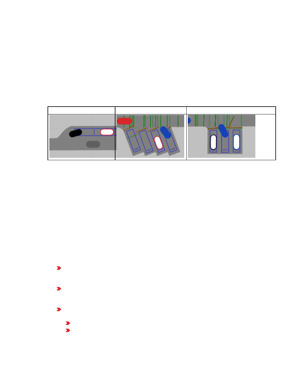
6.11.4 Modeling parking lots
Vehicle routes to parking space
Vissim automatically generates vehicle routes that lead from the vehicle routing decision of the
type Parking lot to each parking space of the corresponding parking lots. You cannot change
these internal vehicle routes.
Displaying parking and parked vehicles
During the simulation, vehicle movements are displayed realistically for vehicles pulling into
and out and in reverse of a parallel, diagonal or perpendicular parking lot. Once the vehicle
has reached its final parking position in the parking space, in 2D mode, the vehicle inside is
highlighted in white (by default). Examples:
Parallel parking lot Diagonal parking lot Perpendicular parking lot
Dwell time distribution defines parking duration
For the Parking duration attribute of the parking routing decision, you can select the desired
time distribution. The parking duration begins when the vehicle is parked in the parking space
in the direction of travel and the traffic on the adjacent lane, previously blocked, can flow
again.
Assigning the vehicle a free parking space
If a parking space has not been assigned to a vehicle and no vehicle is parked in it, it is
considered free. Vissim can then assign it to a vehicle. This is also the case, if the parking
space can currently not be reached, as it is blocked by a vehicle, e.g. because of a traffic jam.
Occupying and blocking parking spaces
A parking space is considered occupied and is not assigned to another vehicle, if:
It has already been assigned to a vehicle. The vehicle follows its route until it comes to
a stop in the parking space. From this point on, the parked vehicle blocks the parking
space.
If because of its length, a vehicle is assigned several adjacent spaces, these are con-
sidered occupied. The vehicle follows its route until it comes to a stop in the parking
spaces. From this point on, the parked vehicle blocks the parking spaces.
The parking space is considered occupied and remains assigned to a vehicle, even if
the vehicle has not yet reached it or access to it is blocked by another vehicle:
because the vehicle blocking the space is in a traffic jam
because the vehicle blocking the space is in a traffic jam adjacent to the parking
space
464 © PTV GROUP

6.11.4 Modeling parking lots
as soon as a parking space is reserved for a waiting vehicle, as all parking spaces that
can be assigned according to routing decision type Parking lot are still occupied.
Leaving the parking space
After the dwell time, the vehicle leaves the parking space via an automatically generated route
that guides it back to its original route.
Note: Vissim determines the shortest path, in terms of time, to a position downstream of
the parking lot routing decision. For generation of the route that takes the vehicle from
the parking lot back to the route network, Vissim accounts for the entire route as well as
for the current position of the vehicle on the parking lot it wants to leave. Thus, a vehicle
might travel part of its original route twice or skip part of it.
Parking direction when pulling into and out of a parking space
The vehicle drives forward into the parking space. The vehicle cannot back into a parking
space. The Parking direction attribute of the parking space defines whether the vehicle pull
outs of a parking space forward or in reverse (see "Attributes of parking lots" on page 469).
This allows the vehicle to pull into and out a parking space in the following parking directions:
Pull into and out of parking space forward: For modeling parking in a parking lot that
the vehicle can leave driving forward, e.g. a parallel parking lot, with several parking
spaces parallel to the link.
Pull into parking space forward, pull out in reverse: For modeling parking in a diagonal
or latitudinal parking lot.. A connector leads to the link with the parking lot. The link
ends downstream of the parking lot. Downstream there is no connector.
If the vehicle pulls out of the parking space in reverse, the following applies:
The car following model can be interaction-free, as when driving forward, Wiedemann
74 model or Wiedemann 99.
Visibility is based on the driving behavior parameters for forward driving. This allows
Vissim to determine the distance and number of perceived vehicles. The distance is
calculated starting from the rear edge of the vehicle. The vehicle pulling out of the park-
ing space in reverse notices other vehicles on its route. If there is an oncoming vehicle,
both vehicles can brake.
The DesSpeed of the vehicle is based on the DesSpeed specified in the Speed
(reversing) attribute of the parking lot.
The vehicle does not change lanes.
At the end of the parking duration, the vehicle pulls out of the parking lot in reverse and
drives via the first upstream connector back onto its starting link. This may be a dif-
ferent link than the one the vehicle originally came from. The vehicle drives backwards
until it has reached the link on which its route lies and on which it can continue driving
forwards. It then comes to a standstill. Once the waiting time has passed, the vehicle
continues driving forwards on its route that has been defined in the parking lot attribute
Direction change duration distribution (see "Attributes of parking lots" on page 469).
When driving forward, the vehicle drives at the DesSpeed valid before parking.
© PTV GROUP 465
6.11.4 Modeling parking lots
Vissim Internally calculates the position at which the vehicle comes to a standstill, so
that the vehicle can continue driving forward on its route from the next time step. This
calculation is also based on the standstill distance.
The Travel direction attribute of the vehicle is set to Reverse, e.g. in the Vehicles in
Network list.
The Driving state attribute of the vehicle is set to Reversing, e.g. in the Vehicles in
Network list.
The vehicle follows a route. The route uses the front edge of the vehicle as a reference
point.
Conflict areas do not respond to the vehicle, but to priority rules (see "Modeling priority
rules" on page 506).
At the start of a simulation run, Vissim generates priority rules for vehicles pulling out of
a parking space in reverse:
To make vehicles pulling out of a parking space wait for a gap in traffic flow
To ensure that vehicles that wish to pull into a parking space wait to let vehicles
pulling out of the parking space proceed. Vehicles that want to park in a parking
space on the adjacent lane wait in their lane, approximately level to the center of
the parking space, until a lane change becomes possible. This gives the vehicle
that is still parked in the parking space more room to pull out.
Parking behavior on links with several lanes and parking lots
A vehicle only selects a parking space that is not occupied or blocked by another parking
vehicle.
In the following cases, an available parking space is blocked by another vehicle that is either
parked in the space or on a lane next to an available space:
To the left and/or right of the parking space, there is a lane without a parking lot, on
which a vehicle is parked next to the available parking space.
To the left and/or right of the parking space, there is a lane with parking lots and
another lane without parking lots. A vehicle is parked in the parking space between
the available parking space and the lane without a parking lot.
To the left and/or right of the parking space, there is a lane with parking lots and
another lane without parking lots. There are two available parking spaces next to each
other, but a vehicle is parked on the lane next to the two spaces.
As soon as a vehicle traverses the section of a vehicle routing decision of the type Parking lot,
Vissim checks its vehicle routes and the corresponding parking lots. Vissim then finds and
occupies a parking space for the vehicle. With every time step, Vissim checks for all vehicles
that do not have the status Waiting, whether the occupied parking space is still accessible. If
the parking space is still accessible and lies on a link with a single lane, or if the parking space
is no longer accessible, Vissim will look for an accessible parking space that is available. This
parking space must be located on a parking lot downstream of the current parking route of the
vehicle.
If the parking space chosen for a vehicle is still available when the vehicle traverses the
decision point, but is occupied right before it arrives there, the vehicle will choose another
466 © PTV GROUP

6.11.4 Modeling parking lots
parking space. Precondition: There is still a parking space available further downstream, on
the route of the parking routing decision.
If an attractive parking space becomes available after the vehicle has traversed the decision
section, the vehicle drives towards the originally selected parking space as long as it is still
accessible.
If the vehicle cannot park on any of the parking spaces because there are not enough spaces
available and accessible, the vehicle routing decision of the type Parking lot is ignored. The
vehicle continues driving on its original route.
Parking behavior with one lane and at least one occupied parking space
If on a lane with multiple parking spaces in a row, one or several of the spaces are occupied or
reserved, the driver of a vehicle will choose a parking space further upstream that is located
before the other available parking spaces. This is also true if the Attraction attribute suggests
a parking space further downstream. With each time step, the driver of the vehicle checks
whether in the meantime a more attractive parking space has become available and changes
its destination accordingly.
Vehicle reserves parking space and waits until parking space is free
If a vehicle passes a vehicle routing decision of the type Parking lot and there is no free
parking space, you can set the attribute Full occupancy behavior to specify what you want the
vehicle to do in this case (see "Attributes of parking routing decisions" on page 442):
continue driving
drive to the next parking space that can be reserved, wait there until the parking space
frees up and then park there
Requirements for a parking space to be reserved:
The parking space is occupied, a vehicle is parked in it.
The parking space has not been reserved.
The length of the parking space is large enough to fit the length of the vehicle. If the
vehicle is longer than the parking space and multiple adjacent spaces cannot be
reserved, the vehicle continues driving.
On its way to a reserved parking space, the vehicle does not look for another free parking
space.
The vehicle continues driving in the following cases:
There is no free parking space available.
No parking space can be reserved.
All parking spaces are reserved.
For the parking route decision, in the attribute Full occupancy behavior, Drive On is
selected.
There is no parking space that is long enough for the vehicle.
Vissim Is unable to calculate the parking duration, as all parking spaces are occupied,
but no vehicles are parked there yet, e.g. because they have not yet reached their
© PTV GROUP 467
6.11.4 Modeling parking lots
assigned parking space or cannot reach it because another vehicle, stuck in a traffic
jam, is blocking it.
6.11.4.2 Defining parking lots
You can define parking lots in a network editor on a link or connector:
Parking lots with the attribute Real parking spaces, for parking or stopping on a lane (see
"Modeling parking and stopping on the roadside" on page 462).
Parking lots for dynamic assignment with the Abstract parking lots or Zone connector
attribute (see "Modeling parking lots and zones" on page 659), (see "Defining parking lots
for dynamic assignment" on page 660)
A parking lot can be modeled as a parallel, diagonal or perpendicular parking lot.
Notes:
You can specify that you need not press the CTRL key when adding network objects
(see "Right-click behavior and action after creating an object" on page 143).
For some network objects there are windows in which the attributes of a network
object can be defined and edited. There are lists for this, for all network objects. You
can choose whether you want to open a window, a list or neither of the two for the
definition of network objects in the Network Editor (see "Right-click behavior and
action after creating an object" on page 143).
1. On the Network objects toolbar, click Parking Lots.
2. With the mouse pointer, point to the position in the link at which the parking lot is to begin.
3. Hold down the CTRL key and the right mouse button, and drag the pointer to the desired
end position.
4. Release the keys.
The parking lot is inserted. The Parking Lot window opens.
The basic attributes of the network element are shown in the upper area of the window and in
the list of network objects for the particular network object type.
5. Edit the attributes (see "Attributes of parking lots" on page 469).
6. Confirm with OK.
The attributes are saved in the Parking Lots list.
For individual, adjacent parallel parking lots, accordingly define long, adjacent links and
connectors on which you can place individual parking lots of the desired length.
Note: To block traffic in a lane with parking vehicles, select the option Keep lateral
distance to vehicles on next lane(s) in the driving behavior parameter set (see
"Editing the driving behavior parameter Lateral behavior" on page 289).
468 © PTV GROUP

6.11.4 Modeling parking lots
6.11.4.3 Attributes of parking lots
The Parking Lot window opens when you insert a network object and have selected to
automatically open the Edit dialog after object creation (see "Right-click behavior and action
after creating an object" on page 143). By default, only the Parking Lots list is opened.
Into the window, you enter attribute values for the network object. For network objects which
have already been defined, you can call the window using the following functions:
In the list of network objects of the network object type, double-click the row with the
desired network object.
In the Network editor, select the network object of your choice. Then, from its shortcut
menu, choose Edit.
The network object may have additional attributes. In the network objects list of the network
object type, you can show all attributes and attribute values. You can open the list via the
following functions:
In the network object toolbar, right-click the desired network object type. Then from the
shortcut menu, choose Show List (see "Context menu in the network object toolbar" on
page 63).
In the Network editor, select the network object of your choice. Then, from its shortcut
menu, choose Show In List (see "Selecting network objects in the Network editor and
showing them in a list" on page 339).
From the Lists menu, in the desired category, choose the network object type.
In the network objects list of the network object type, you can edit attributes and attribute
values of a network object (see "Selecting cells in lists" on page 102), (see "Using lists" on
page 89).
The objects of this object type may have relations to other objects. This is why the attributes list
is shown as part of a coupled list (on the left). On the Lists toolbar, in the Relations box, you
can show and edit the coupled list with the attributes of the desired relation on the right (see
below Showing and editing dependent objects as relation) and (see "Using coupled lists" on
page 111).
Note: In lists, you can use the Attribute selection icon to show and hide attribute
values (see "Selecting attributes and subattributes for a list" on page 106).
Basic attributes of parking lots
The basic attributes of the network element are shown in the upper area of the window and in
the list of network objects for the particular network object type.
1. Make the desired changes:
Element Description
No. Unique number
Name Designation
At Position (Pos): Distance from start of the link or connector
© PTV GROUP 469
6.11.4 Modeling parking lots
Element Description
Length Length of the parking lot
Type Zone Connector: only relevant for dynamic assignment (see "Modeling park-
ing lots and zones" on page 659). Automatically creates a zone in the
Zones list, if no zone has been defined. Automatically creates an origin
zone and a destination zone in the OD Pairs list, if neither have been
defined yet.
Abstract parking lot: only relevant for dynamic assignment
Real parking spaces relevant for simulation with and without dynamic
assignment: modeling parking capacity in movement direction on one lane.
Combined with vehicle routes of the type Parking Lot, you can realistically
model parking maneuvers and stops at the roadside.
Showing
label If the option is not selected, the label for the parking lot is not displayed, even
if you selected labeling for all parking lots. For parking lot labels, the following
are available:
Number
Name
Zone No.
Group No.
Occupancy
Current parking availability
Dyn. Assignment tab
These attributes are only relevant for parking lots of dynamic assignment (see "Defining
parking lots for dynamic assignment" on page 660).
470 © PTV GROUP
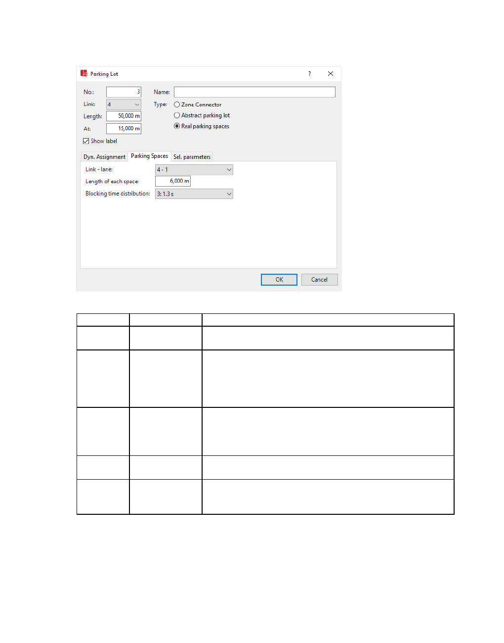
6.11.4 Modeling parking lots
Parking Spaces tab
These attributes are only relevant for Real parking spaces.
Element Short name Description
Link - lane Number of the link and lane (Ln) on which the parking lot is
located
Length per
space
LenPerSpc Length of a parking space The maximum length per space
must not exceed the length of the parking lot. If the total
length is not a multiple of the parking lot length, the remaining
length is added to the end of the parking lot, but is not used
by any vehicle.
Blocking
time dis-
tribution
BlockTmDistr Optional blocking time distribution: period during which a
parallel-parking vehicle blocks the lane until it has completed
its parking maneuver.
0: None: Blocking time is not considered for simulation.
Parking
direction
ParkDir Only for real parking spaces: Direction in which the vehicle is
driving into and out of the parking space.
Minimum
gap time
major flow
MinGapTmMajFl Minimum gap time between two vehicles of the major flow, so
that a vehicle may leave the parking space
© PTV GROUP 471

6.11.4 Modeling parking lots
Element Short name Description
Speed
(reversing)
SpeedRvs Desired speed of the vehicle for backing out of a parking
space. Default value 5 km/h, value range 0.001 to 9999 km/h.
Direction
change
duration
distribution
DirChgDurDist Only relevant if the attribute parking direction Forward >
reverse is selected: period during which the vehicle remains
in standstill after it has pulled out of parking space in reverse
until it drives forwards. Default: time distribution 5 s (see
"Using time distributions" on page 237).. If no value is
specified, the vehicle remains in standstill for the duration of a
time step.
The blocking time begins when the parking vehicle first stops while heading into a parking
space with the rear of the vehicle sticking out of the parking space, and it ends when the
vehicle finally comes to a stop in the parallel-parked position.
Blocking time distribution is considered for parking lots on the adjacent lane and thus
includes parking maneuvers in parallel to the direction of travel.
The parking lot must be longer than one length per parking space.
The time distribution may be a normal or an empirical distribution (see "Defining time dis-
tributions" on page 237).
If the parking lot is precisely as long as the parking space, the vehicle remains in parking
position during the blocking time. In this case, blocking time distribution is ignored.
Sel. parameters tab
472 © PTV GROUP

6.11.4 Modeling parking lots
Element Description
Open
hours
From (OpenFrom), to (OpenUntil): Time span during which vehicles can
enter the parking lot. Vehicles will not drive to the parking lot outside these
hours.
Maximum
parking
time
ParkTmMax:
for Real parking spaces: Vehicles with a longer parking time are not
assigned a parking space on this parking lot.
for Zone connector and Abstract parking lot:
Only relevant when using a trip chain file: time span a vehicle may use
this parking lot. If the maximum parking time is shorter than the min-
imum dwell time, the parking lot is not approached by the vehicle.
Vehicles that are assigned a route via COM and vehicles moving
based on an origin-destination matrix during dynamic assignment may
select any destination parking lot open at the time of their departure,
regardless of the attribute value Maximum parking time:. For these
vehicles, for selection of a destination parking lot, a parking time of 1 s
is assumed.
Attraction Attrac: The higher the value, the more attractive the parking lot or parking
space. This allows you to account for features of the parking lot that are not
explicitly available as an attribute. For Real parking spaces, you can create a
linear change in the attractiveness across the parking spaces by entering
different values for First and Last. If you want to create a parking lot with
attractive spaces in the middle or on the very right or left, create two
symmetrical parking lots of the type Real parking spaces, with inverse
Attraction values.
Parking
Cost
ParkFee: only relevant for Zone Connector and Abstract parking lot:
flat: fee for one-time use of the parking lot, irrespective of the dwell time.
per hour: parking costs depending on the parking time. If a trip chain file is
used, the minimum dwell time is considered. Without a trip chain file, an
hour parking time is assumed for all parking.
The network object has additional attributes that you can show in the Attributes list. Among
them are the following for example:
© PTV GROUP 473

6.11.4 Modeling parking lots
Short
name
Long
name
Description
DetBlock Detect
blockage
For real parking spaces only:
Select this option, if you want Vissim to check whether a
parking space is blocked during the simulation. Vissim
detects a vehicle blocking a parking space, without parking
in it, e.g. when the vehicle parks in a space further upstream
that lies on the same single lane link. The blocked parking
space cannot be assigned to a vehicle traversing the parking
routing decision.
If this option is not selected, Vissim will not check whether
a parking space is blocked during the simulation. Vissim
does then not recognize vehicles blocking a parking space,
unless they are parking in it. The blocked parking space can
be assigned to a vehicle traversing the parking routing
decision. This results in fewer vehicles ignoring the routing
decision due to a lack of available parking spaces.
The option is selected by default.
Zone Zone Allocation of the zone number in the OD matrix to the parking lot.
Multiple parking lots can belong to a zone.
Showing and editing dependent objects as relation
The attribute and attribute values of this network object type are shown in the list on the left,
which consists of two coupled lists.
1. In the list on the left, click the desired entry.
The list on the right contains attributes and attribute values of network objects, and/or base
data allocated to the network object selected in the list on the left (see "Using coupled lists" on
page 111):
Dyn assign des speed distributions (see "Defining parking lots for dynamic assignment"
on page 660)
Vehicles (parking): Attributes of the vehicles that are currently parked in the parking lot
Paths: Paths of path file from dynamic assignment If no paths are shown and you have per-
formed dynamic assignment, you can use its path file to read in the paths. To do so, from
the List shortcut menu, choose the respective command (see "Attributes of paths" on page
712).
2. On the list toolbar, in the Relations list, click the desired entry.
3. Enter the desired data.
The data is allocated.
474 © PTV GROUP

6.11.5 Modeling overtaking maneuvers on the lane of oncoming traffic
6.11.5 Modeling overtaking maneuvers on the lane of oncoming traffic
You can model overtaking maneuvers during which the overtaking vehicles use the lane of
oncoming traffic. This for instance allows you to simulate the overtaking of PuT vehicles
temporarily stopping in an urban area, on a link with a single lane only, or the overtaking of
slower vehicles outside of the city. You can model multiple vehicles overtaking and multiple
vehicles being overtaken. The overtaking vehicle shall only then perform the overtaking
maneuver, if there is no oncoming traffic which excludes the option of overtaking.
In Vissim a vehicle wants to overtake when it's desired speed is considerably higher than that
of vehicle preceding it (0 m/s to 4 m/s, normally distributed, around mean value 2 m/s). The
vehicle then checks the following requirements in order to be able to perform the overtaking
maneuver:
At overtaking speed, it would take the vehicle at most 4 seconds to drive into its preceding
vehicle. The overtake speed is the desired speed plus the attribute overtaking speed
factor (OvtSpeedFact).
Its link has a passing lane (see "Attributes of links" on page 383).
The passing lane must overlap with the inner lane of the oncoming lane. The width of the
overlapping area is not relevant. The z value of the oncoming lane and of the passing lane
must not deviate more than 0.5 m from each other.
The overtaking area, which consists of links and connectors that overlap with the oncom-
ing lane, must be at least long enough for a vehicle to be able to perform an overtaking
maneuver.
Downstream of the last vehicle that is to be overtaken, there must be a large enough gap
visible, so that the passing vehicle is able to change back into its previous lane after com-
pleting the overtaking maneuver. The largest gap must be at least one passing vehicle
length, plus double the safety distance from the front and rear of the vehicle, as required
during standard car following behavior.
The overtaking maneuver must be able to be completed safely, without endangering
oncoming traffic. The vehicle recognizes oncoming traffic on the opposite lane from a cer-
tain distance. This distance is defined for the link of the opposite lane in its attribute Look
ahead distance for overtaking (LookAheadDistOvt). The vehicle that wants to overtake
safely assumes that anywhere beyond this distance there will be oncoming traffic. To
assess the course of the trip of oncoming traffic, Vissim uses the attribute Assumed speed
of oncoming traffic (AssumSpeedOncom) of the oncoming lane (see "Attributes of links"
on page 383). Vissim does not account for any additional vehicles following the oncoming
vehicle.
The figure below shows the following in 2D mode:
a section of a link 1 that runs from left to right via a lane 11 and a passing lane 12
(hatched) with right-hand traffic running from left to right. Vissim displays passing lanes
with hatched lines as soon as its link has at least two lanes and the attribute Has passing
lane is selected.
© PTV GROUP 475

6.11.5 Modeling overtaking maneuvers on the lane of oncoming traffic
a section of a link 2 that has only one lane in right-hand traffic, running from right to left.
Link 2 was created as an oncoming lane of link 1 and fully overlaps with passing lane 12.
For overtaking maneuvers on link 1, vehicles driving from the left to the right use passing
lane 12.
Vehicles on link 2, driving from the right to the left, cannot be overtaken, as link 2 does not
have a passing lane.
The gray vehicle that is overtaking on passing lane 12 recognizes that there is no vehicle
in the opposite lane within the distance defined in the attribute Look ahead distance for
overtaking (LookAheadDistOvt) of link 2.
The overtaking vehicle reduces its speed to the desired speed, as soon as it leaves the
passing lane.
An overtaking vehicle may cancel its overtaking maneuver, if downstream of the vehicle it is
overtaking, the gap in its previous lane is not yet large enough to change back into it. This may
be the case when there is suddenly unexpected oncoming traffic or the vehicle that is being
overtaken accelerates. When a vehicle cancels an overtaking maneuver and wants to change
back into its lane, the vehicles behind it can reduce their speed to allow for the lane change.
The driving behavior of oncoming traffic is not influenced through the overtaking maneuver.
When the length of the overtaking areas is checked, this is done along the current route or
path of the vehicle. This way, vehicles without a current vehicle route or path cannot overtake
on the oncoming lane.
The vehicle width is not considered a criterion for the option of an overtaking maneuver. It is
generally assumed that there is not enough space on the oncoming lane for oncoming traffic
and a passing vehicle to drive next to each other .
Before an overtaking maneuver takes place, Vissim does not account for network objects on
the oncoming lane, e.g. reduced speed areas, SCs or stop signs. However, as soon as the
overtaking maneuver starts, the passing vehicle reacts to these network objects.
When a vehicle changes from a link with a passing lane to a connector without a passing lane,
the connector then has one lane less than the link with a passing lane. In this case, the
distance defined in the attribute Lane change distance ( LnChgDist ) also specifies the
minimum distance to the connector at which an overtaking maneuver may be started. Passing
on the oncoming lane is not possible within this lane change distance.
Passing on oncoming lane for both movement directions
You can model overtaking maneuvers for both movement directions. In this case, an additional
passing lane is placed on top of the inner oncoming lane. This means the passing vehicles of
476 © PTV GROUP

6.11.5 Modeling overtaking maneuvers on the lane of oncoming traffic
both movement directions use the oncoming lane and need to account for any oncoming
traffic.
The figure below shows the following in 2D mode:
a section of a link 1 that runs from left to right via a lane 11 and a passing lane 12
(hatched).
a section of a link 2 that runs from left to right via a lane 21 and a passing lane 22
(hatched).
Links 1 and 2 are placed so that their passing lanes 12 and 22 each overlap with the
lane of oncoming traffic, so that vehicles can pass in both movement directions.
6.11.5.1 Defining network objects and attributes for passing on oncoming lane
1. Make sure that the desired speed and acceleration you have defined for vehicles allows for
passing.
2. In the Network Editor, for the vehicles that shall be overtaken, define at least one link with
normal lanes, but without a passing lane (see "Defining links" on page 381).
3. Generate a link for the opposite direction (see "Generating an opposite lane" on page 392).
4. For the first link, specify the following attributes (see "Attributes of links" on page 383):
5. Increase the value for the attribute Number of lanes (NumLanes) by 1.
The number of lanes includes the passing lane.
6. Select Has passing lane (HasOvtLn).
7. Make the desired settings (see "Attributes of links" on page 383).
Overtake speed factor (OvtSpeedFact)
Look ahead distance for passing (LookAheadDistOvt)
Assumed speed of oncoming traffic (AssumSpeedOncom)
Overtake only PT (NurÖVÜberh): must be deactivated
8. Deactivate the attribute No lane change left – All vehicle types (NoLnChLAllVehTypes)
for the lane the vehicle will change back to after the overtaking maneuver.
9. Make sure that for the passing lane, the attribute Blocked vehicle classes
(BlockedVehClasses) does not contain vehicle classes that are meant to do the passing.
10. Specify the following attributes for the overlapping link(s) (see "Attributes of links" on page
383):
© PTV GROUP 477

6.12 Modeling short-range public transportation
Look ahead distance for passing (LookAheadDistOvt)
Assumed speed of oncoming traffic (AssumSpeedOncom)
11. Define vehicle inputs or create vehicles with the add-on module Dynamic Assignment
(see "Defining vehicle inputs" on page 428), (see "Using the dynamic assignment add-on
module" on page 653).
For overtaking on the lane of oncoming traffic, the vehicle must be on a vehicle route or a
path of dynamic assignment.
12. If you have defined vehicle inputs, define vehicle routes that lead via links on which
vehicles shall be overtaken (see "Modeling vehicle routes, partial vehicle routes, and
routing decisions" on page 430).
If you use dynamic assignment, Vissim will distribute the vehicles across the paths. Vissim
Saves the paths to the path file (see "Using the dynamic assignment add-on module" on
page 653), (see "Files of dynamic assignment" on page 1133).
6.12 Modeling short-range public transportation
Vehicles of short- range public transportation (PT) can use the links of the private
transportation or separate links, for example, lanes for buses or tracks for trains.
First define the stops and then the PT line that you assign a route, operated stops, PT vehicles,
and a timetable.
6.12.1 Modeling PT stops
You can construct public transport stops on a link or next to a lane.
Types of PT stops
PT stop: Stop of a PT vehicle on a lane of a link. Select the lane.
Public transport stop bay: Stop of a PT vehicle on a specific link in the movement dir-
ection to the right, next to the lane.
Behavior of vehicles on multi-lane links
For multiple-lane links, following vehicles try to overtake PT vehicles, which are stopped at a
public transport stop.
Behavior of vehicles on single-lane links
If a PT vehicle stops at a stop on a single-lane link, the vehicles behind it will wait until the PT
vehicle continues its journey. With regard to exiting the public transport stop bay, the PT
vehicle has the right of way. This is in accordance with the German Traffic Code (StVO) and
the rules in road traffic of other countries.
Behavior of PT vehicles also depends on the length of the public transport stop
While a PT vehicle is parked at a PT stop waiting for passengers to alight and board, it can
only be overtaken by another PT vehicle, moving downstream, looking for a free parking
478 © PTV GROUP

6.12.2 Defining PT stops
space at the same PT stop to also allow passengers to alight and board. The PT stop must be
sufficiently long.
Emergency stop position at PT stop
The emergency stop position depends on the number of the lane the PT stop is on:
Even lane number: 1.6 m before the end of the PT stop
Odd lane number: 2.1 m before the end of the PT stop
6.12.2 Defining PT stops
Before modeling, you must define whether or not the passengers at the public transport stop
should be taken into consideration in the simulation:
Without passengers: Select a pre-defined dwell time distribution per public transport stop
and PT line.
Boarding passenger profile: Allocate Volumes as hourly values to the lines on the public
transport stop. Select the PT parameters per vehicle type.
Viswalk for microscopic pedestrian simulations: Define at least one pedestrian area with
the attributes PT usage - Waiting area or PT usage - Platform edge at the stop.
Parameterize the public transport stops according to the method of your choice (see
"Calculating the public transport dwell time for PT lines and partial PT routes" on page 497). In
the network you can combine public transport stops of these three methods with each other.
Then the parameterization of a public transport stop applies to all lines which operate at this
public transport stop.
For each defined public transport stop, you can set specific PT line stop parameters for
each PT line and PT partial route (see "Modeling PT lines" on page 485).
For the microscopic pedestrian simulation with Viswalk, the length of the public transport
stop must correspond with at least the length of the longest PT vehicle, which operates at
this public transport stop. Doors of the vehicle, which at the time of the stop are not posi-
tioned at the platform edge, are not used by the passengers.
You can also define a public transport stop, in which boarding and alighting by multiple PT
vehicles takes place at the same time. For this to occur, the length of the public transport
stop must be correspondingly defined: at least the sum of all vehicle lengths must have
enough space, behind and between the vehicles, which operate simultaneously at the pub-
lic transport stop.
On a multiple lane link, the PT vehicles can enter or exit when there is a large enough gap.
On a single lane link, for example for bus bays, a following vehicle can only exit once the
preceding vehicle has exited.
If you move PT stops that a PT line uses, these PT stops are shown as passive, in green.
© PTV GROUP 479

6.12.3 Attributes of PT stops
Notes:
You can specify that you need not press the CTRL key when adding network objects
(see "Right-click behavior and action after creating an object" on page 143).
For some network objects there are windows in which the attributes of a network
object can be defined and edited. There are lists for this, for all network objects. You
can choose whether you want to open a window, a list or neither of the two for the
definition of network objects in the Network Editor (see "Right-click behavior and
action after creating an object" on page 143).
1. On the Network objects toolbar, click Public transport stops.
2. With the mouse pointer, point to the position in the link at which the public transport stop is
to begin.
3. Hold down the CTRL key and the right mouse button, and drag the mouse pointer to the
desired end position.
4. Release the keys.
The public transport stop is inserted. The PT Stop window opens.
The basic attributes of the network element are shown in the upper area of the window and in
the list of network objects for the particular network object type.
5. Edit the attributes (see "Attributes of PT stops" on page 480).
6. Confirm with OK.
The attributes are saved in the list Public transport stops.
6.12.3 Attributes of PT stops
The PT Stops window opens when you insert a network object and have selected to have the
Edit dialog opened automatically after object creation (see "Right-click behavior and action
after creating an object" on page 143). By default, only the PT stops list is opened.
Into the window, you enter attribute values for the network object. For network objects which
have already been defined, you can call the window using the following functions:
In the list of network objects of the network object type, double-click the row with the
desired network object.
In the Network editor, select the network object of your choice. Then, from its shortcut
menu, choose Edit.
The network object may have additional attributes. In the network objects list of the network
object type, you can show all attributes and attribute values. You can open the list via the
following functions:
In the network object toolbar, right-click the desired network object type. Then from the
shortcut menu, choose Show List (see "Context menu in the network object toolbar" on
page 63).
480 © PTV GROUP

6.12.3 Attributes of PT stops
In the Network editor, select the network object of your choice. Then, from its shortcut
menu, choose Show In List (see "Selecting network objects in the Network editor and
showing them in a list" on page 339).
From the Lists menu, in the desired category, choose the network object type.
In the network objects list of the network object type, you can edit attributes and attribute
values of a network object (see "Selecting cells in lists" on page 102), (see "Using lists" on
page 89).
The objects of this object type may have relations to other objects. This is why the attributes list
is shown as part of a coupled list (on the left). On the Lists toolbar, in the Relations box, you
can show and edit the coupled list with the attributes of the desired relation on the right (see
below Showing and editing dependent objects as relation) and (see "Using coupled lists" on
page 111).
Note: In lists, you can use the Attribute selection icon to show and hide attribute
values (see "Selecting attributes and subattributes for a list" on page 106).
6.12.3.1 Basic attributes of PT stops
The basic attributes of the network element are shown in the upper area of the window and in
the list of network objects for the particular network object type.
Element Description
No. Unique number
Name Description
© PTV GROUP 481
6.12.3 Attributes of PT stops
6.12.3.2 Base data tab
Element Description
Length Length: Length of the public transport stop [m]
Lane Ln: Lane of the link or connector on which the public transport stop is located.
At Position (Pos): Start of the public transport stop on the link or the connector
Label If the option is not selected, the label for an individual public transport stop is not
displayed when the label for all public transport stops is selected.
6.12.3.3 Boarding Passengers tab
You can set boarding passenger profiles for a public transport stop. The data is used for:
calculation of stop dwell times
proportional distribution of pedestrians on public transport lines in Viswalk
1. Right-click in the list.
2. From the shortcut menu, choose Add.
A new row with default data is inserted.
The list contains, amongst others, the following attributes:
Element Description
Volume Volume: Passenger volume of the category pedestrians per hour for all or
selected PT lines
TimeFrom Time from: Time from the start of the time interval for which this number of
boarding passengers is valid in simulation seconds.
TimeTo Time to: Time till the end of the time interval for which this number of boarding
passengers is valid in simulation seconds.
PTLines PT lines which may be used by passengers of this boarding passenger profile
AllPTLines All PT lines: If the option is selected, all PT lines take the PT stop into
consideration.
Note:
For a PT stop with Platform edge, enter the relative volume of the public transport
stop instead of the volume in [P/h].
For passengers, who are Viswalk pedestrians, defaults are generated in two cases:
For each automatically generated platform edge.
If a pedestrian area (either a Waiting area or a Platform edge) of a public trans-
port stop is allocated, for which no vehicle volume has been defined.
With regard to the defaults, each pedestrian, who reaches the waiting area in the
time interval of 0 - 99,999, boards each PT vehicle of a preferred PT line.
482 © PTV GROUP
6.12.4 Generating platform edges
Showing and editing dependent objects as relation
The attribute and attribute values of this network object type are shown in the list on the left,
which consists of two coupled lists.
1. In the list on the left, click the desired entry.
The list on the right contains attributes and attribute values of network objects, and/or base
data allocated to the network object selected in the list on the left (see "Using coupled lists" on
page 111):
Boarding volumes: The attributes are described further above.
Vehicles: Vehicles in network (see "Displaying vehicles in the network in a list" on page
803)
Areas (PT usage) (see "Attributes of areas" on page 848)
Public transport lines (active) (see "Attributes of PT lines" on page 487)
Public transport line stops (see "Editing a PT line stop" on page 492)
Partial PT routes (active) (see "Attributes of partial PT routes" on page 505)
Partial PT route line stops (see "Editing a PT line stop" on page 492)
2. On the list toolbar, in the Relations list, click the desired entry.
3. Enter the desired data.
The data is allocated.
6.12.4 Generating platform edges
Notes:
You require the add-on module Viswalk for microscopic pedestrian simulation.
Platform edges are not automatically moved along with the link or the public trans-
port stop nor are they adjusted to changes in length. Therefore, generate the plat-
form edges once the links and PT stops will no longer be changed. In this way you
prevent a transition type between the network and the PuT vehicle from being guar-
anteed.
You can define areas of the type Polygon and Rectangle as a Platform edge. For a PT stop,
you can have an area of the type Rectangle automatically generated as a Platform edge. An
automatically generated Platform edge follows the user-defined course of the road. Platform
edges are created with a width of 2 m immediately next to the link.
If boarding passengers are to board and/or alight from both sides, add platform edges to the
left and the right.
© PTV GROUP 483
6.12.4 Generating platform edges
Notes:
When generating platform edges, the volume [Pers./h] is changed in the attribute
Boarding passengers in a relative volume and existing values are taken over.
Every public transport stop with an area for Public transport usage is used by the
passengers, who are generated as pedestrians. These passengers are pro-
portionately distributed among the PT lines.
If there are no pedestrian areas with the attribute Public transport usage, the pas-
senger volume is distributed over the PT stops exactly according to the absolute val-
ues.
The Public transport usage attribute can be used to define a pedestrian area as a Plat-
form edge or a Waiting area for one or more selected stops (see "Modeling construction
elements" on page 834). Based on its type, you determine the shape of the platform edge
using the shape of a polygon or the rectangle of the pedestrian area.
A pedestrian area with the attribute Public transport usage defined as a Platform edge
must fulfill the following conditions:
The platform edge and the lane with the public transport stop must be directly adjacent
or overlap so that alighting passengers may alight on the platform edge and boarding
passengers may board the PT vehicle from the platform edge. The overlapping must
be smaller than half of the width of the pedestrian area. This means that the center line
of the platform edge, which is parallel to the lane and thus to the public transport stop,
must lie outside the lane.
The length of the pedestrian area parallel to the lane must be at least the length of the
public transport stop, so that when the public transport vehicle stops, no vehicle door
lies outside of the platform edge.
If the area for a platform edge is not automatically generated and you do not edit it later
on in the Network editor, ensure that the maximum distance between the lane on
which the PT vehicle stops and the area of the platform edge is 2 m. Otherwise, the PT
vehicle will not open its doors.
Note: When two platform edges with different parameters overlap, a warning is
displayed during the check. Even so, Vissim assigns the platform edges to the right
doors and the simulation is not interrupted.
1. On the Network objects toolbar, click Public transport stops.
2. In the Network editor, right-click the desired PT stop.
3. In the context menu, select the entry Add platform edge left or Add platform edge right.
The platform edge is displayed in the Network editor next to the link. Default color: pink. All
relevant area attributes are set automatically, e.g. for public transport usage Platform edge
and for public transport stop(s), the number of the PT stop selected. The name of the
pedestrian area includes numbers and sides of the PT stop, e.g. platform edge PT stop 1
(right). The name is not automatically adjusted when the area of the platform edge is
allocated a later point in time of another public transport stop.
484 © PTV GROUP

6.12.5 Generating a public transport stop bay
6.12.5 Generating a public transport stop bay
Note: You require the add-on module Viswalk for the microscopic pedestrian
simulation.
1. On the Network objects toolbar, click Public Transport Stops.
2. In the Network editor, right-click the desired PT stop.
3. In the context menu, select the entry Create lay-by stop.
The lay-by stop is displayed in the Network editor, next to the PT stop in the movement
direction. Connectors and conflict areas are added to the modeling for the right of way of
buses (see "Modeling PT stops" on page 478). By default, all vehicle types may use the
public transport stop bay.
6.12.6 Modeling PT lines
You can define PT lines for buses or trains, which operate in a fixed public transport stop
order. For this, they must have a timetable with departure times at the first public transport stop,
and offset times according to the time table between public transport stops and dwell times at
public transport stops.
Public transport stop dwell times are either obtained from the dwell time distribution or are
calculated on the basis of boarding passenger profiles. They may also be determined via
microscopic pedestrian simulation. Before modeling, decide whether and to what extent the
passengers in the simulation should be taken into consideration and parameterize the public
transport stops accordingly (see "Calculating the public transport dwell time for PT lines and
partial PT routes" on page 497). In the network model, you can combine public transport stops
of these three models with each other. However, the selection per public transport stop applies
to all lines which operate at this public transport stop (see "Modeling PT stops" on page 478).
For each public transport stop, you can enter specific PT stop parameters for each PT line and
partial PT route (see "Attributes of PT stops" on page 480).
A public transport line in Vissim always has a fixed route. In the case that a real PT line should
drive on different routes within the Vissim network, then multiple, separate PT lines must be
modeled in the Vissim network.
Modeling PT lines may be compared to the modeling of static routes. However, PT lines do not
distribute incoming vehicles; instead they generate them. Start points of PT lines cannot be
moved.
Note: PT vehicles drive the route, which is specified by the PT line. By default, they stay
within the Vissim network afterwards. In order that PT vehicles do not stay within the
network and therefore do not move within the network without routes, model the PT
lines in a way that they must move out of the network at the end of the link.
6.12.6.1 Defining PT lines
Define all public transport stops for the line before defining a PT line (see "Modeling PT stops"
on page 478).
© PTV GROUP 485
6.12.6 Modeling PT lines
Note: For every PT line, define a link, which will only be used from this PT line.
Notes:
You can specify that you need not press the CTRL key when adding network objects
(see "Right-click behavior and action after creating an object" on page 143).
For some network objects there are windows in which the attributes of a network
object can be defined and edited. There are lists for this, for all network objects. You
can choose whether you want to open a window, a list or neither of the two for the
definition of network objects in the Network Editor (see "Right-click behavior and
action after creating an object" on page 143).
1. On the Network objects toolbar, click Public Transport Lines.
2. Hold down the CTRL key and right-click the desired link on which the vehicles of the line are
to drive into the network.
A blue decision marker is set by default at the beginning of the link, on which the line
begins.
3. In the desired link, point with the mouse pointer at the desired position of the destination
section, at which the public transport line should end.
If no connection between the start section and the destination section exists, Vissim still
displays the line path. In this case, you must either correct the destination link and/or the
destination section or the Vissimnetwork.
If there is a connector is between a start section and a destination section, it is displayed as
a colored band in the PT line fill color over a continuous link curvature. A turquoise bar
(default color) shows the possible position of the destination section.
4. Click this position.
The PT Line window opens. The public transport line is marked in the Network Editor.
The basic attributes of the network element are shown in the upper area of the window and in
the list of network objects for the particular network object type.
5. Edit the attributes (see "Attributes of PT lines" on page 487).
6. Confirm with OK.
The attributes are saved in the list Public Transport Lines.
If in the Public Transport Lines list, on the toolbar, you click the Synchronization button,
then in the list, click a public transport line, this line is by default displayed as a colored band
in the PT line fill color, with the active stops in red and passive stops in green (default color
setting). By default, all PT public transport stops located directly on the line path are
highlighted as active in red.
486 © PTV GROUP
6.12.6 Modeling PT lines
The line path of a new PT line does not automatically include public transport stop bays. You
can change the line path of a PT line, so that it does include a public transport stop bay (see
"Entering a public transport stop bay in a PT line path" on page 491). If you modify the line
path, PT stops on the new line path are highlighted as passive, in green. Even if you move
these PT stops, they are still highlighted as passive, in green.
6.12.6.2 Attributes of PT lines
The PT Line window opens automatically when you insert a network object and have selected
to have the Edit dialog opened automatically after object creation (see "Right-click behavior
and action after creating an object" on page 143). By default, only the Public Transport Lines
list is opened.
Into the window, you enter attribute values for the network object. For network objects which
have already been defined, you can call the window using the following functions:
In the list of network objects of the network object type, double-click the row with the
desired network object.
In the Network editor, select the network object of your choice. Then, from its shortcut
menu, choose Edit.
The network object may have additional attributes. In the network objects list of the network
object type, you can show all attributes and attribute values. You can open the list via the
following functions:
In the network object toolbar, right-click the desired network object type. Then from the
shortcut menu, choose Show List (see "Context menu in the network object toolbar" on
page 63).
In the Network editor, select the network object of your choice. Then, from its shortcut
menu, choose Show In List (see "Selecting network objects in the Network editor and
showing them in a list" on page 339).
From the Lists menu, in the desired category, choose the network object type.
In the network objects list of the network object type, you can edit attributes and attribute
values of a network object (see "Selecting cells in lists" on page 102), (see "Using lists" on
page 89).
The objects of this object type may have relations to other objects. This is why the attributes list
is shown as part of a coupled list (on the left). On the Lists toolbar, in the Relations box, you
can show and edit the coupled list with the attributes of the desired relation on the right (see
below Showing and editing dependent objects as relation) and (see "Using coupled lists" on
page 111).
Note: In lists, you can use the Attribute selection icon to show and hide attribute
values (see "Selecting attributes and subattributes for a list" on page 106).
© PTV GROUP 487
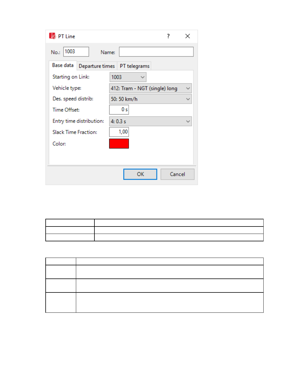
6.12.6 Modeling PT lines
Basic attributes of PT lines
The basic attributes of the network element are shown in the upper area of the window and in
the list of network objects for the particular network object type.
Element Description
No. Unique number 1 to 4294967295
Name Description
Base data tab
Element Description
Starting on
Link
Entry link EntryLink: Link on which the PT line begins
Vehicle
type
VehType: Vehicle type of PT line
Desired
speed dis-
tribution
DesSpeedDistr: Initial speed of PT vehicle
488 © PTV GROUP
6.12.6 Modeling PT lines
Element Description
Time Off-
set
Entry time offset (EntTmOffset): Time PT vehicles need to enter the network
before their scheduled departure time in order to depart punctually at the
departure times scheduled, from the first stop serviced.
This means you enter the departure times of your timetable as departure times
of the PT line. The time offset is the sum of the time the vehicle requires to get to
its first stop in the network and the average passenger interchange time at this
stop.
The resulting network entry time is always set to zero, if the departure time is
smaller than the time offset.
If the time offset is 0 s, the vehicles of the PT line enter the Vissim network
precisely at their defined departure time.
Start time
distribution
Entry time distribution (EntryTmDistr):Time distribution for variation of
departure time at which the vehicle enters the network (see "Defining time
distributions" on page 237). This value is added as a delay to the calculated
entry time. Entry time = departure time - time offset
Slack Time
Fraction
SlackTmFrac: only relevant for stops with specified departure time: factor for
wait time of PT vehicle as part of the remaining time until scheduled departure.
Value range 0.00 to 1.00.
Slack time fraction = 1: Earliest departure time is according to the timetable
(see "Attributes of PT lines" on page 487)
Slack time fraction < 1: Departure time may be earlier than fixed in the
timetable. Departure time is based solely on arrival time and dwell time.
This allows you to model earliness as well.
Color Define the color of PT vehicle of this line
Departure times tab
You may define individual trips of the line as courses. When you enter departure times,
individual trips (New) and departures based on service frequency rate (Rate) can be mixed. In
both cases, you may in addition to the time also specify a course number and occupancy rate.
The list contains, amongst others, the following attributes:
Element Description
Dep Departure time of a public transport vehicle relative to the start time of the
simulation
TeleCour PT telegram - course: Optional course number. If PT calling points are defined for
the network, the course number serves to perform evaluations of serial telegrams
in terms of the course number.
Occup Occupancy: Number of passengers
Generate start times
You may define several departure times simultaneously.
1. In the Departure Times tab, right-click into the table.
© PTV GROUP 489
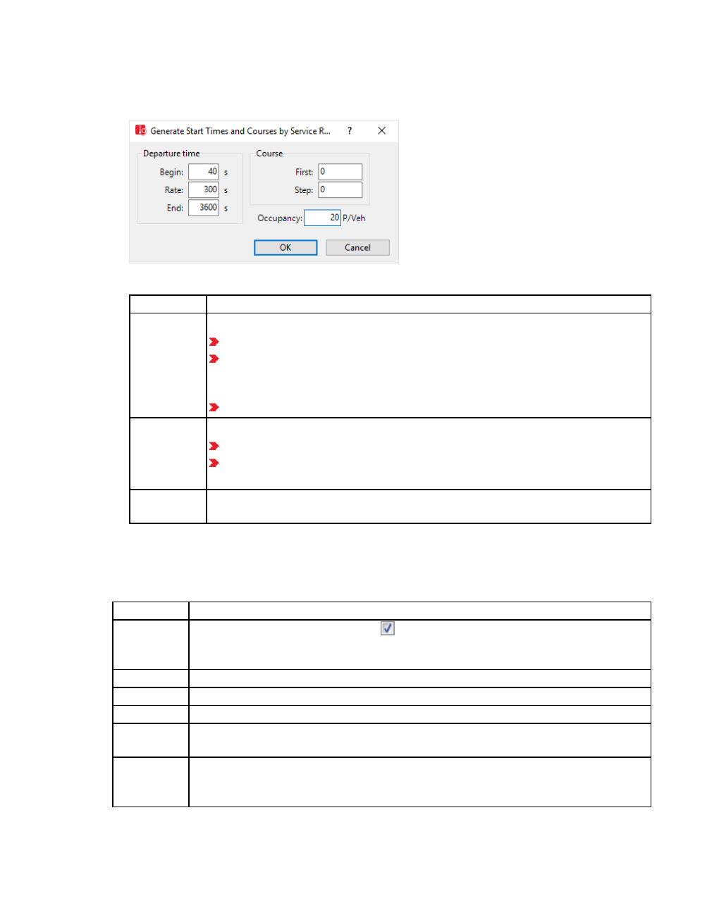
6.12.6 Modeling PT lines
2. From the shortcut menu, choose Departure Times.
The window Generate Start Times and Courses by Service Rate opens.
3. Make the desired changes:
Element Description
Departure
time
First departure in timetable of service frequency
Begin: first departure
Rate: service frequency rate. Vissim generates all departures defined
this way as individual trips. You may also define multiple service fre-
quency rates in a row.
End: last departure
Course Optional course
First: first course number. Is displayed in the Departure Times tab.
Step: increment for all following course numbers. The departure times
are sorted in chronological order.
Occupancy Number of passenger in PT vehicle when entering the Vissim network. Is dis-
played in the Departure Times tab.
PT Telegrams tab
You can define data that is transmitted via PT telegrams to control procedures, when vehicles
pass PT calling points (see "Using detectors" on page 557).
Element Description
Line sends
PT tele-
grams
Send PT telegrams (SendTele): Select this option if you want vehicles of
this PT line to be recorded by PT calling points.
Line PT Telegrams - Line (TeleLine): Number of PT line, max. 999 999 999
Route PT Telegrams - Route (TeleRout): Number of PT line path, max. 999 999 999
Priority PT telegram - priority (TelePrio): Priority of PT vehicle [1 to 7]
Tram
Length
PT telegram - tram length (TeleVehLen): Length of PT vehicle [1 to 7]
Manual Dir-
ection
PT telegram - manual direction (TeleManDir): Direction from which the vehicle
is coming, if the PT calling point cannot clearly identify this via line or route num-
ber.
490 © PTV GROUP

6.12.7 Entering a public transport stop bay in a PT line path
Showing and editing dependent objects as relation
The attribute and attribute values of this network object type are shown in the list on the left,
which consists of two coupled lists.
1. In the list on the left, click the desired entry.
The list on the right contains attributes and attribute values of network objects, and/or base
data allocated to the network object selected in the list on the left (see "Using coupled lists" on
page 111):
Departure times: The attributes are described further above.
Line stops (see "Editing a PT line stop" on page 492)
Link sequence: Numbers of links and connectors via which the PT line leads (see "Attrib-
utes of links" on page 383)
2. On the list toolbar, in the Relations list, click the desired entry.
3. Enter the desired data.
The data is allocated.
6.12.6.3 Checking and repairing PT line courses
When you split or delete links and connectors that run across PT lines, these PT lines are
disconnected. Even if you then insert new links or connectors there, these PT lines remain
disconnected. You can have disconnected PT lines repaired by Vissim.
1. On the Network objects toolbar, click Public Transport Lines.
2. Right click into the Network editor.
3. From the context menu, choose Check and repair all PT line courses.
Vissim will find new PT lines for disconnected PT lines. These may run via the added or other
links and connectors in the network.
6.12.7 Entering a public transport stop bay in a PT line path
1. Enter a public transport stop bay in the link (see "Generating a public transport stop bay" on
page 485).
2. Select Public Transport > PT Lines from the Lists menu.
3. Select the desired entry.
In the Network Editor, the selected PT line is shown as a yellow band; active public
transport stops red; passive public transport stops green. By default, all PT public transport
stops located directly on the line path are highlighted as active in red. Public transport stop
bays are not automatically in the line path of a new PT line.
© PTV GROUP 491

6.12.8 Editing a PT line stop
Notes:
You can specify that you need not press the CTRL key when adding network objects
(see "Right-click behavior and action after creating an object" on page 143).
For some network objects there are windows in which the attributes of a network
object can be defined and edited. There are lists for this, for all network objects. You
can choose whether you want to open a window, a list or neither of the two for the
definition of network objects in the Network Editor (see "Right-click behavior and
action after creating an object" on page 143).
4. Press the CTRL key, and in the Network Editor right-click next to the stop bay in the yellow
PT line.
A point is added to the PT line.
5. Click on the point, hold the mouse button down, and drag the point into the stop bay.
The line path runs over the stop.
Moving a specific PT line path section
In the section you wish to change, add three points at the following positions:
Position of the first point from which the new PT line path shall be recalculated
Position of the middle point you want to move to the public transport stop bay
Position of the third point up to which the new PT line path shall be recalculated
When you move the middle point, only the path between the two outer points is
recalculated, and the PT line path is only changed for this area.
6.12.8 Editing a PT line stop
You can edit specific attributes of PT stops for a PT line or partial PT route in the Edit PT Line
Stop window.
Note: Alternatively to in the PT Line Stop window, you may also show and edit PT line
stop attributes in the PT line stops list (as a relation of a PT stop attribute list).
1. On the Network objects toolbar, click Public Transport Stops or Public Transport Lines.
2. In the network editor, right-click the PT stop.
3. If a public transport stop is serviced by one PT line only, from the shortcut menu, choose
Edit PT Line <No. > PT Stop <No.> Pass<No.>.
4. If a public transport stop is serviced by multiple PT lines, from the shortcut menu, choose
Edit PT Line Stop. Then select the desired line stop > PT Line <No. > PT stop <No.> Pass
<No.>.
492 © PTV GROUP
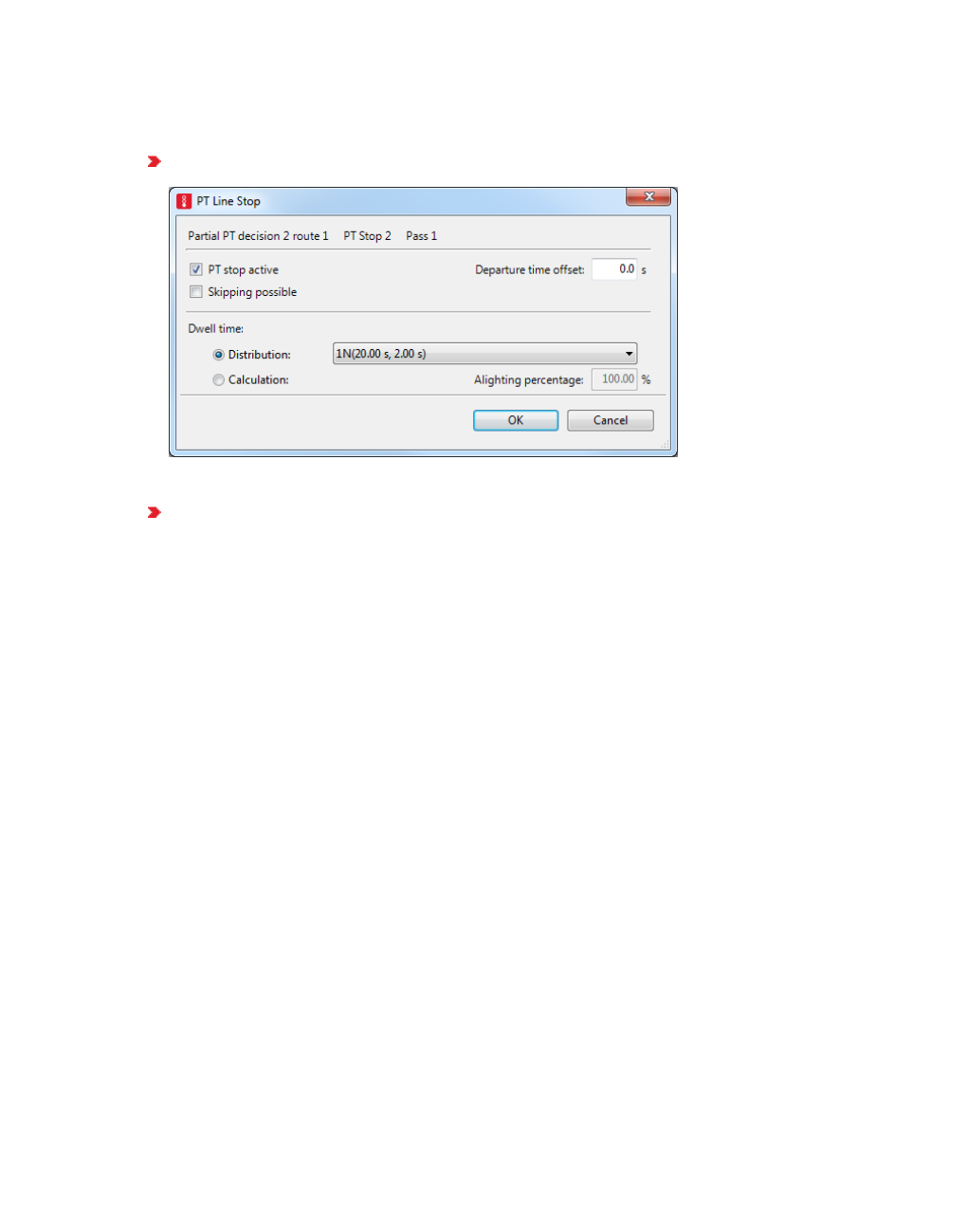
6.12.8 Editing a PT line stop
A PT Line Stop window opens with attributes that depend on the network object the PT line
stop refers to:
For PT stops of a PT line, the number of the line is shown:
For the PT stops of a partial PT route, the number of the routing decision and the number
of the route are shown:
© PTV GROUP 493

6.12.8 Editing a PT line stop
For a PT stop in Viswalk, additional attributes are displayed. These settings allow yo to sim-
ulate passengers boarding and alighting at this stop with Viswalk:
The PT stop must be selected in the For PT stop(s) attribute of the area you want to
use as a waiting area or platform edge.
In the Public Transport Usage attribute of the area, Platform edge or Waiting area
must be selected.
The attribute PT stop active must be selected.
494 © PTV GROUP
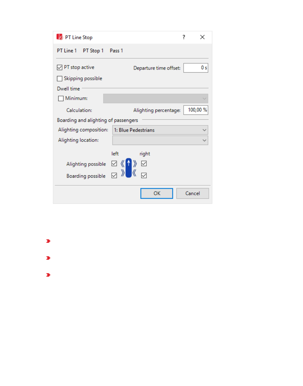
6.12.8 Editing a PT line stop
Determining public transport dwell time
The public transport dwell time for PT lines and PT routes can be determined via the following
methods:
Method Dwell time distribution: (see "Defining dwell time according to dwell time dis-
tribution" on page 497)
Method Advanced passenger model: (see "Calculating dwell time according to the
advanced passenger model" on page 498)
Method VISWALK: microscopic pedestrian simulation: (see "Calculating dwell time with
PTV Viswalk" on page 500)
You can use different methods at different PT stops. However, only one method is used for PT
lines or PT partial routes at a PT stop.
Showing PT line stop attributes as a relation of a PT stop
1. From the Lists menu, choose > Public Transport > Public transport stops.
The list with the attributes is displayed as the left list of two coupled lists (see "Using
coupled lists" on page 111).
© PTV GROUP 495

6.12.8 Editing a PT line stop
2. On the list toolbar, in the Relations list, click Public transport line stops.
The list on the right contains attributes and attribute values of network objects, and/or base
data allocated to the network object selected in the list on the left (see "Using coupled lists" on
page 111):
Column Description
PTLine Name of PT line that services the PT line stop.
Public
transport
stop
Number and name of public transport stop of the PT line stop
Active If this option is selected, the public transport stop is a PT line stop of the PT
line.
A public transport stop created in the Vissim network according to the
definition of PT lines is not automatically contained in a PT line path, even
when placed on a link that is traversed by a PT line. Non-serviced PT stops
are displayed in green and the Active attribute is disabled. You can enable
the Active attribute to include the public transport stop into the PT line path.
If a PT stop is not to be serviced by a PT line, disable its Active attribute.
SkipPoss Skipping possible: If this option is selected, the PT stop is not serviced,
depending on the method used for calculating the public transport dwell time
(see "Defining dwell time according to dwell time distribution" on page 497),
(see "Calculating dwell time according to the advanced passenger model" on
page 498), (see "Calculating dwell time with PTV Viswalk" on page 500)
DepOffset Departure time offset:: Define departure time according to timetable. The
time offset is used additionally for boarding and alighting time
(boarding/alighting). The resulting departure time is calculated as follows:
Simulation second of arrival + dwell time + max (0, ((departure time of PT line +
departure offset) - (simulation second of arrival + dwell time)) • slack time fraction of
PT line)
If the departure time, according to the time table, is later than the point in time,
which is the sum of the arrival time and dwell time, the PT vehicle waits until
the departure time, according to the time table if the Slack time fraction equals
1. For slack time fractions < 1, the vehicle correspondingly departs earlier,
value range 0.00 to 1.00.
If the Slack time fraction of the line is 0 or the Departure time offset of the
public transport stop equals 0 seconds, the time table is not considered. In
this case, the settings in the range dwell time are taken into consideration for
the calculation of the Dwell time.
For line stops in PT partial routes, the following applies:
As long as a PT vehicle has not completed its original line route, its Depar-
ture offset is treated like an offset at a line stop of the original route.
Once the PT vehicle has passed the "to section" of its original line route,
the Departure offset specified for a PT partial route stop is interpreted as
496 © PTV GROUP

6.12.9 Calculating the public transport dwell time for PT lines and partial PT routes
Column Description
relative to the simulation time when the vehicle passes the respective rout-
ing decision point.
PedsAsPass Pedestrians as passengers: Pedestrians of an area are used as passengers
for public transport. The area is a waiting area or a platform edge. The area is
assigned at least one PT stop.
DwellTmDef Dwell time definition depends on the method used for calculating public
transport dwell time (see "Defining dwell time according to dwell time
distribution" on page 497), (see "Calculating dwell time according to the
advanced passenger model" on page 498), (see "Calculating dwell time with
PTV Viswalk" on page 500)
6.12.9 Calculating the public transport dwell time for PT lines and partial PT routes
The following methods allow you to model stop dwell times for PT vehicles
Method Description
Dwell time
distribution
The dwell time is based on the dwell time distribution used (see "Defining
dwell time according to dwell time distribution" on page 497).
Define all desired dwell time distributions (see "Using time distributions" on
page 237).
You then assign the desired dwell time distribution to each stop serviced by a
PT line or partial PT route.
Advanced
passenger
model
The dwell time and number of passengers boarding and alighting are
calculated using the advanced passenger model (see "Calculating dwell time
according to the advanced passenger model" on page 498).
To model stop dwell times with the number of passengers boarding and
alighting instead of with dwell time distributions, define PT parameters for the
respective vehicle type (see "Changing attributes for a vehicle type for the
duration of boarding and alighting" on page 262).
Viswalk
(microscopic
pedestrian
simulation)
Dwell time and number of passengers boarding/alighting are calculated
during the simulation (see "Calculating dwell time with PTV Viswalk" on page
500), (see "Modeling pedestrians as PT passengers" on page 925) and (see
"Quick start: defining pedestrians as PT passengers" on page 927).
Without Viswalk, you can define the Dwell time distribution method faster than the Advanced
passenger model in Vissim. The Advanced passenger model method, however, allows you
to model the behavior at stops more precisely, e.g. the cumulation of vehicles of a PT line at a
stop caused by a delay.
6.12.9.1 Defining dwell time according to dwell time distribution
1. Define the PT line, the PT stop and at least one dwell time distribution (see "Using time
distributions" on page 237).
2. On the Network objects toolbar, click Public Transport Stops or Public Transport Lines.
© PTV GROUP 497
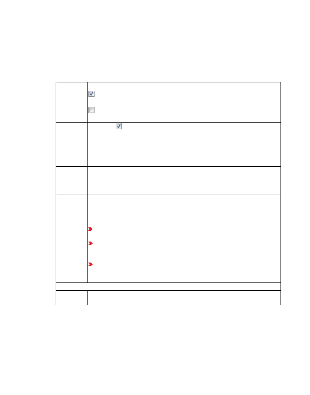
6.12.9 Calculating the public transport dwell time for PT lines and partial PT routes
3. In the network editor, right-click the PT stop.
4. From the context menu, select Edit PT Line <No. > PT Stop <No.> PT Pass <No.>.
The PT Line Stop window opens.
5. In the Dwell time section, select Distribution.
6. Make the desired changes:
Element Description
Active If the option is selected, the public transport stop for the current PT line or
PT partial route is activated.
If the option is not selected, the public transport stop is not operated and is
shown in green.
Skipping
possible SkipPoss: If the option is selected, the public transport stop is not used if
the resulting, random dwell time is < 0.1 seconds. Skipped public transport
stops are reported in the Vehicle Records file with its identifier and recorded
as having a public transport stop dwell time of 0 seconds.
Departure
time offset
DepOffset: Departure time defined according to timetable (see "Editing a PT
line stop" on page 492)
Door lock
duration
before
departure
DoorLockDurBefDep: This dwell time of the PTV vehicle is the time until
departure of the vehicle after the doors have been fully closed. Default 1.0 s
Dwell time Dwell time definition (DwellTmDef). All settings for the dwell time apply for
the line stops of a PT partial route.
Distribution and Calculation are always available if the public transport stop
is not allocated a pedestrian area with Public transport usage.
Distribution: The stop time is obtained from the selected dwell time dis-
tribution.
Calculation: Alighting percentage as percentage indication (see "Cal-
culating dwell time according to the advanced passenger model" on
page 498).
Alighting percentage: Percent of the passengers who alight on this pub-
lic transport stop. This value serves the volume-dependent calculation of
the stop time.
You can also show further attributes in the attribute list Public Transport Line Stops, e.g.:
Door clos-
ure delay
DoorClosDel: Time after which the last pedestrian has walked through doors
until the doors begin to close. Default 3.0 s
7. Confirm with OK.
6.12.9.2 Calculating dwell time according to the advanced passenger model
1. Ensure that the following parameters are defined:
498 © PTV GROUP

6.12.9 Calculating the public transport dwell time for PT lines and partial PT routes
Boarding passenger profile per PT stop and assignment to desired PT lines (see
"Attributes of PT stops" on page 480)
Specific PT parameters per vehicle type (see "Changing attributes for a vehicle type for
the duration of boarding and alighting" on page 262)
Occupancy rate per PT line (see "Attributes of PT lines" on page 487), (see "Editing
functions and distributions of a vehicle type" on page 258)
2. On the Network objects toolbar, click Public Transport Stops or Public Transport Lines.
3. In the network editor, right-click the PT stop.
4. From the context menu, select Edit PT Line <No. > PT Stop <No.> PT Pass <No.>.
The PT Line Stop window opens.
5. In the Dwell time section, select Calculation.
6. Make the desired changes:
Element Description
PT stop
active If the option is selected, the public transport stop for the current PT line or PT
partial route is activated.
If the option is not selected, the public transport stop is not operated and is
shown in green.
Skipping
possible
If the option is selected, the public transport stop is not operated if the vehicle
passes the 50 m mark before the public transport stop and no passengers would
like to board or alight. A public transport stop bay can only be fully skipped if both
of these are directly connected to the link, from which the PT vehicle is coming. If
the network structure is more complex or if the PT vehicle has already reached
the public transport stop bay or the connector, when the 50 m mark is passed,
the bay is passed without making a stop. Skipped public transport stops are
reported in the Vehicle Records file with its identifier and recorded as having a
public transport stop dwell time of 0 seconds.
Departure
time off-
set
Departure time defined according to timetable (see "Editing a PT line stop" on
page 492)
Dwell
time
All settings for the dwell time apply for the line stops of a PT partial route.
Distribution and Calculation are always available if the public transport stop is
not allocated a pedestrian area with Public transport usage.
Distribution: The stop time is obtained from the selected dwell time dis-
tribution.
Calculation: The number of boarding passengers is determined on the basis
of the boarding passenger profile at the public transport stop. The time
required for the boarding and alighting is calculated on the basis of the PT
parameters of the vehicle type.
Alighting percentage: Enter percent of passengers who alight at this public
transport stop. This value serves the volume-dependent calculation of the
stop time.
© PTV GROUP 499

6.12.9 Calculating the public transport dwell time for PT lines and partial PT routes
7. Confirm with OK.
After you have defined the PT line, PT parameters per vehicle type, and the attributes for the
PT line stop, Vissim calculates the stop dwell times of a PT vehicle as follows:
Number of alighting passengers = Number of passengers x percentage of alighting passengers
Number of boarding passengers = Number of all passengers waiting (who want or are allowed to
take the line) If the number of waiting passengers exceeds the free capacity of the PT
vehicle, the number of alighting passengers is limited to the maximum capacity of the
vehicle.
Alighting time = Number of alighting passengers x average alighting time (see "Changing attrib-
utes for a vehicle type for the duration of boarding and alighting" on page 262)
Boarding time = Number of boarding passengers x average boarding time
Passenger service time = Clearance time + alighting time + boarding time
After completion of passenger service, the PT vehicle remains at the stop until the scheduled
departure time that accounts for the respective slack time fraction.
6.12.9.3 Calculating dwell time with PTV Viswalk
You can define parameters for the calculation of the number of boarding passengers and the
dwell time, which occurs during the microscopic pedestrian simulation. Example (see
"Modeling pedestrians as PT passengers" on page 925)
Note: For this, you require PTV Viswalk.
1. Ensure that the following requirements are met:
The PT stop must have at least one pedestrian area with the Public transport usage
attribute allocated of the Waiting area or Platform edge type (see "Attributes of areas"
on page 848).
At least one location distribution must be defined for alighting passengers (see "Using
location distributions for boarding and alighting passengers in PT" on page 240).
At least one pedestrian composition has to be defined (see "Defining pedestrian com-
positions" on page 878).
2. On the Network objects toolbar, click Public Transport Stops or Public Transport Lines.
3. In the network editor, right-click the PT stop.
4. From the context menu, choose Edit PT Line <No. > PT Stop <No.> PT Pass <No.>.
The PT Line Stop window opens.
500 © PTV GROUP
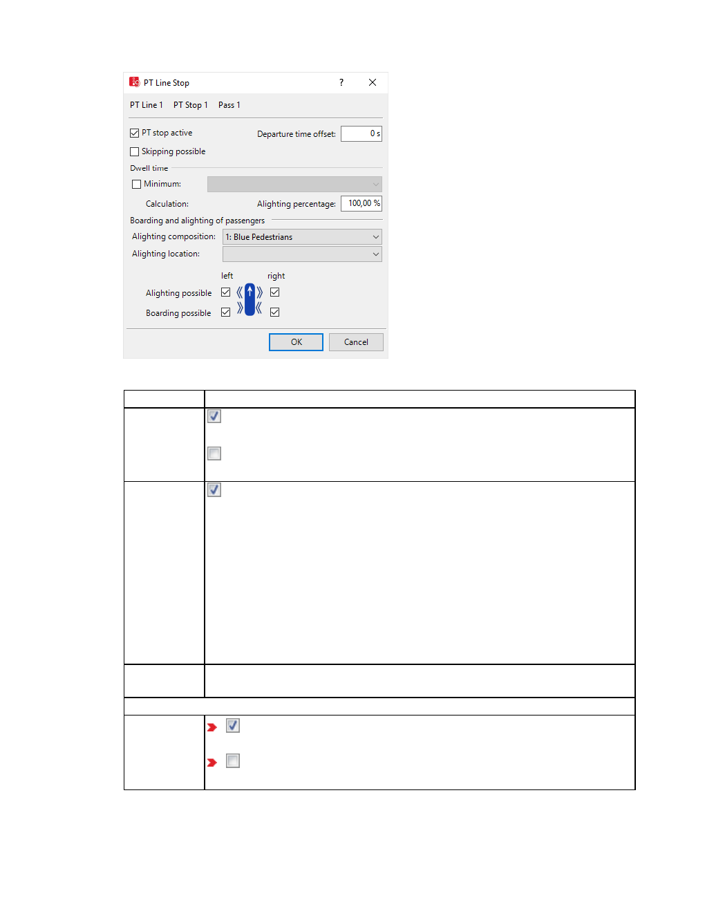
6.12.9 Calculating the public transport dwell time for PT lines and partial PT routes
5. Make the desired changes:
Element Description
PT stop
active If the option is selected, the public transport stop for the current PT line
or PT partial route is activated.
If the option is not selected, the public transport stop is not operated and
is shown in green.
Skipping
possible If the option is selected, the public transport stop is not operated if the
vehicle passes the 50 m mark before the public transport stop and no
passengers would like to board or alight.
A public transport stop bay can only be fully skipped if both of these are
directly connected to the link, from which the PT vehicle is coming. If the
network structure is more complex or if the PT vehicle has already reached
the public transport stop bay or the connector, when the 50 m mark is
passed, the bay is passed without making a stop.
Skipped public transport stops are reported in the Vehicle Records file with
its identifier and recorded as having a public transport stop dwell time of 0
seconds.
Departure
offset
Departure time defined according to timetable (see "Editing a PT line stop"
on page 492)
Dwell time section:All dwell time settings apply for the line stop of a PT partial route.
Minimum If the option is selected, the minimum dwell time on the basis of the
selected time distribution is determined.
If the option is not selected, the minimum dwell time = 0 s. If you have
neither selected Minimum nor used a timetable, you must select Late
© PTV GROUP 501
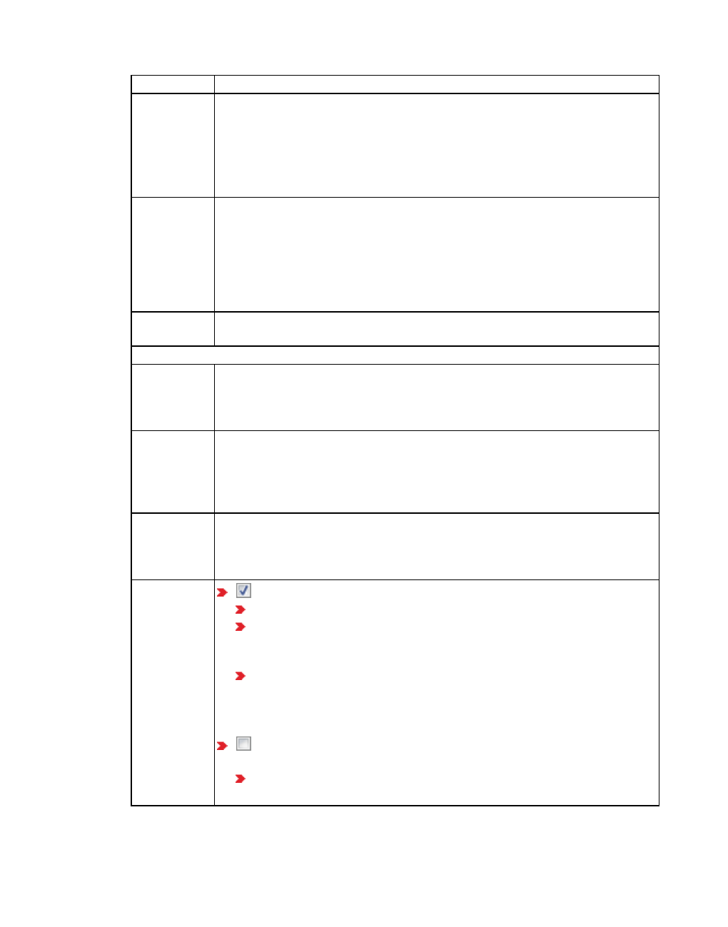
6.12.9 Calculating the public transport dwell time for PT lines and partial PT routes
Element Description
boarding possible.
PT vehicles depart once the minimum dwell time runs out. PT vehicles also
depart if the minimum dwell time = 0 seconds when all alighting
passengers have alighted.
In addition, you can select for each line stop the option Late boarding
possible
Calculation Calculation: Alighting percentage as percentage indication when the
public transport stop is allocated a pedestrian area as Platform edge or
Waiting area. Viswalk pedestrians who board or alight at a public transport
stop are modeled. The calculated public transport stop dwell time depends
on the time necessary for boarding/alighting passengers. The option Late
boarding possible is taken into consideration for the calculation of the
public transport stop dwell time.
Alighting
percentage
Percentage of the passengers, which will alight at this public transport stop.
This value serves the volume-dependent calculation of the stop time.
Boarding and alighting of passengers section
Alighting
composition
Composition of the PT-passengers (see "Defining pedestrian compositions"
on page 878). Within the PT vehicle, the Pedestrian types, corresponding to
the selected composition, are generated and the given percentage set is
used.
Alighting
location
Alighting location: Distribution of the alighting passengers at the doors of
the PT vehicle at this public transport stop (see "Using location distributions
for boarding and alighting passengers in PT" on page 240). Within the PT
vehicle, the alighting passengers at this public transport stop cor-
responding to the selected composition are distributed to the vehicle doors.
Alighting
possible,
Boarding
possible
Allow or disallow boarding and/or alighting on the right and left. An arrow
on the layout of the PT vehicle shows the movement direction.
Late
boarding
possible
If this option is selected:
the minimum dwell time is kept
the vehicle only departs after all passengers have boarded or
vehicle capacity has been reached (see "Attributes of vehicle types"
on page 256)
The doors close after three seconds have passed in which no pas-
sengers have wanted to board/alight. If you have neither selected
the option Minimum nor used a time table, you must select the
option Late boarding possible.
If the option is not selected, the minimum dwell time = maximum
dwell time.
If the Slack time fraction = 0, the PT vehicle departs immediately after
the minimum dwell time has been reached.
502 © PTV GROUP
6.12.10 Defining partial PT routes
Element Description
If the Slack time fraction > 0, the corresponding share of the remain-
ing time to the departure according to the time table adds to the
dwell time if the departure time has not yet been reached.
To ensure that the PT vehicle departs exactly at the time calculated, in case
the option is not selected, no passengers can board the PT vehicle as soon
as the doors begin to close.
The closing of the doors always begins 3 seconds before departure. The
doors also close when a passenger boards immediately before the doors
begin to close.
6. Confirm with OK.
Parameters for micro-simulation of pedestrians of previous versions
If you would like to reproduce the results of earlier Vissim versions, select the following
parameters:
Option Relevance Settings
Minimum dwell time PT line stop parameters Nothing selected
Late boarding possible PT line stop parameters selected
Slack Time Fraction Public transport line no change
Departure offset PT line stop parameters no change
6.12.10 Defining partial PT routes
To define a partial PT route, insert a routing decision on a link and a destination section on a
destination link. The partial routing decision or the destination section may also lie on a
connector.
You can assign the interval limits via the time intervals (see "Defining time intervals for a
network object type" on page 306) , (see "Calling time intervals from an attributes list" on page
307). If a distribution on a percentage basis of the traffic volume to the routes of a routing
decision varies temporally, you must define multiple time intervals which do not overlap each
other.
Notes:
You can specify that you need not press the CTRL key when adding network objects
(see "Right-click behavior and action after creating an object" on page 143).
For some network objects there are windows in which the attributes of a network
object can be defined and edited. There are lists for this, for all network objects. You
can choose whether you want to open a window, a list or neither of the two for the
definition of network objects in the Network Editor (see "Right-click behavior and
action after creating an object" on page 143).
1. On the Network objects toolbar, click Vehicle Routes.
© PTV GROUP 503

6.12.11 Attributes of PT partial routing decisions
The button is highlighted. The variant of the network object type is displayed in parentheses
and the button is shown.
2. Click Vehicle Routes again.
A list box opens.
3. Then select Partial PT route.
Tip: Alternatively to the following steps, to insert a routing decision, from the shortcut
menu, choose PT partial routing decision.
4. Hold down the CTRL key and in the Network Editor right-click the desired link or connector
on the desired position of the routing decision cross section.
5. Release the keys.
By default, a purple bar is inserted.
6. On the desired link, point the mouse pointer to the desired position of the destination
section.
If Vissim does not find a valid link sequence, neither a yellow band nor a turquoise bar are
displayed, or the band might be interrupted. Select another destination link or a new
position for the destination section or correct the Vissim network, for example if a link is not
connected properly with a connector.
If Vissim finds a valid connection via a link sequence, between the start section and the
position the mouse pointer is pointing to, the link sequence is displayed as a yellow band
by default.
On the edge of the link, which you are pointing to with the mouse pointer, a black arrow is
shown in the direction of travel. A turquoise bar shows the possible position of the
destination section. Thereby you can select links from the different types of links, which are
added in the next step of the destination section.
7. Right-click this position.
The context menu opens.
8. Then select Create partial PT route: Define end.
A turquoise bar is added for the destination section by default. The PT partial routing
decision list opens if automatic opening of a list after object generation is selected (see
"Right-click behavior and action after creating an object" on page 143). The attribute and
attribute values of this network object type are shown in the list on the left, which consists of
two coupled lists.
9. Edit the attributes (see "Attributes of PT partial routing decisions" on page 504), (see
"Attributes of partial PT routes" on page 505).
6.12.11 Attributes of PT partial routing decisions
1. From the Lists menu, choose > Public transport > PT partial routing decisions.
504 © PTV GROUP
6.12.12 Attributes of partial PT routes
The attribute and attribute values of this network object type are shown in the list on the left,
which consists of two coupled lists.
The list on the left may include the following attributes:
Column Description
No Unique Number of PT partial routing decision
Name Name of PT partial routing decision
Link Number and name of link on which the PT partial routing decision lies
Pos Location: Distance to the beginning of link or connector
Note: In lists, you can use the Attribute selection icon to show and hide attribute
values (see "Selecting attributes and subattributes for a list" on page 106).
The list on the right contains attributes and attribute values of network objects, and/or base
data allocated to the network object selected in the list on the left (see "Using coupled lists" on
page 111):
Public transport lines (see "Attributes of PT lines" on page 487)
Partial PT routes (see "Attributes of partial PT routes" on page 505)
Link (see "Attributes of links" on page 383)
Destination link of partial PT route (see "Attributes of links" on page 383)
2. On the list toolbar, in the Relations list, click the desired entry.
3. Enter the desired data.
6.12.12 Attributes of partial PT routes
1. From the Lists menu, choose > Public Transport > PT Partial Routes.
The attribute and attribute values of this network object type are shown in the list on the left,
which consists of two coupled lists.
The list on the left may include the following attributes:
Column Description
VehRoutDec Vehicle routing decision: Number and name of PT partial routing decision in
partial PT route
No Unique Number of partial PT route
Name Name of partial PT route
Destination
link
Number and name of link on which partial PT route ends
DestPos Destination position: Distance between destination section and beginning of
link or connector
RelFlow Relative volume in time interval = absolute volume in time interval: Sum of the
volumes of all time intervals If the relative load in a time interval = 0, no public
transport partial route is selected.
© PTV GROUP 505

6.13 Modeling right-of-way without SC
Note: In lists, you can use the Attribute selection icon to show and hide attribute
values (see "Selecting attributes and subattributes for a list" on page 106).
The list on the right contains attributes and attribute values of network objects, and/or base
data allocated to the network object selected in the list on the left (see "Using coupled lists" on
page 111):
Entry link (see "Attributes of PT lines" on page 487)
Vehicle routing decision (see "Attributes of PT partial routing decisions" on page 504)
Link sequence (see "Attributes of links" on page 383)
Partial line stops: Attributes of line stops in partial PT route (see "Editing a PT line stop" on
page 492)
Destination link of partial PT route (see "Attributes of links" on page 383)
2. On the list toolbar, in the Relations list, click the desired entry.
3. Enter the desired data.
6.13 Modeling right-of-way without SC
You can model the right-of-way without SC for non-signalized intersections, fork links, and
merging links. Depending on your use case, you can use priority rules, conflict areas or stop
signs in your model.
6.13.1 Modeling priority rules
You can model the priority rules for conflicting traffic flows which are not controlled by signals
by means of priority rules.
Note: Model the standard priority rules for conflicting traffic flows which are not
controlled by signals by means of conflict areas (see "Modeling conflict areas" on page
526). Only use priority rules, if conflict areas do not produce the desired results and if
you have sufficient experience in modeling with priority rules.
Priority rules for conflicting traffic flows which are not controlled by signals are required in
situations in which vehicles in different links or connectors need to consider each other. You
can also use priority rules to model keeping intersections clear.
Add a priority rule to the marker at which a vehicle or vehicles on another link have to wait.
Vehicles on the same link mutually observe each other. This also applies to links with several
lanes. Therefore you do not require any priority rules.
During simulation, Vissim automatically adds priority rules to parking lots with real parking
spaces.
506 © PTV GROUP

6.13.1 Modeling priority rules
Tip: You can also use priority rules in Viswalk:
For conflicting flows of pedestrians (see "Modeling priority rules for pedestrians" on
page 876)
For the interaction between vehicular traffic and pedestrian traffic (see "Modeling
links as pedestrian areas" on page 869)
6.13.1.1 Creating priority rules
A priority rule always consists of at least two elements:
Red bar: Stop line of the traffic which must wait, and therefore the conflicting markers, in
the image below
Green bar: One or more conflicting markers, in the top-right of the image
© PTV GROUP 507

6.13.1 Modeling priority rules
Min. Headway : The headway states the distance from the conflicting marker (green line)
against the movement direction up to the first vehicle which is moving towards the conflicting
marker. If a vehicle is still within the conflicting marker, the headway = 0.
If a vehicle travels to a stop line, Vissim checks whether the prescribed value for the minimum
headway and the minimum time gap upstream of the conflicting markers are present.
If the prescribed values are not present, the vehicle waits until both gaps are sufficiently long.
In selected priority rules, green triangles in movement direction indicate a minimum headway
> 0 as distance between the conflict marker and the green triangle:
508 © PTV GROUP

6.13.1 Modeling priority rules
The conflict marker (in figures the top green bar on the left) also detects vehicles on all
connectors, which lead upstream of the green bar onto the link. This behavior causes
problems if the waiting vehicle is also detected by the conflict marker, for example if it is in the
area of the headway of the green bar. To avoid this, always position the green bar on a link
upstream of the end points of the relevant connectors to the link.
Min. Gap Time: The available time gap is the time that the first upstream vehicle will require in
order to reach the green bar of the conflicting marker with its present speed. A vehicle which is
already on the green bar is not taken into account. In a priority rule, the limiting time gap is
specified: The vehicle must wait if the current time gap is less than the value which has been
entered.
© PTV GROUP 509

6.13.1 Modeling priority rules
Depending on the situation which is to be modeled, either the headway or the limiting time
gap is more important.
Primarily, vehicles in a flow which has to wait in order to enter a flow which has priority, or
which wish to cross such a flow, are oriented to the time gap.
The headway is used if it has to be established whether a conflicting vehicle has already
reached a certain location.
As well as this, the relevance depends on the ease of flow of the traffic in the conflicting
marker:
For a normal traffic flow, it is mainly the time gap which is relevant.
In the case of slow-moving traffic and congestion, the headway is relevant.
In order that a vehicle does not need to stop and wait at a stop line, the conditions for all of the
associated conflicting marker must be fulfilled.
For each red line (conflicting marker) Vissim takes one or several green bars (conflict markers)
into account. Because of this, several different rules may apply for a stop line (red bar).
In the attributes, you may e.g. enter the following data:
the vehicle classes of vehicles at the stop line
The vehicle classes of the conflicting marker of the vehicle
The maximum speed which a vehicle in the priority flow may still have in order for it to be
recognized as a conflicting vehicle
Red and green bars for conflicting and conflict markers can be specific to the route or to the
traffic lane.
In order to simplify the modeling, both red and green bars may apply for All lanes. With this, it
is sufficient to insert a single priority rule instead of several priority rules. If you have to use
different attribute values, which are specific to different traffic lanes, you must define the
appropriate number of green bars (conflict markers).
Note: If it appears that vehicles ignore the priority rules, this may be due to the fact that
the priority rules are so defined that vehicles have to wait for themselves or have to wait
for each other. Vissim resolves this deadlock. The vehicle with the longest waiting time
may drive off first.
Examples for behavior at a junction with priority rule
In the following figure, the blue vehicle on the left of the main road is traveling at a speed of 50
km/h (approx.14 m/s) and is 49 m upstream of the conflict marker. The current gap time is 49 m
/ 14 m/s = 3.5 s. Since the minimum gap time is 3.0 s, the yellow vehicle can pull in from the
side street below:
510 © PTV GROUP
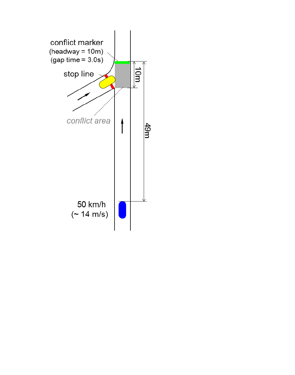
6.13.1 Modeling priority rules
In the following figure, the blue vehicle is still only 28 m from the conflicting marker. The
current gap time is 28 m / 14 m/s = 2 s. Since the minimum gap time is 3.0 s, the yellow vehicle
must wait:
© PTV GROUP 511
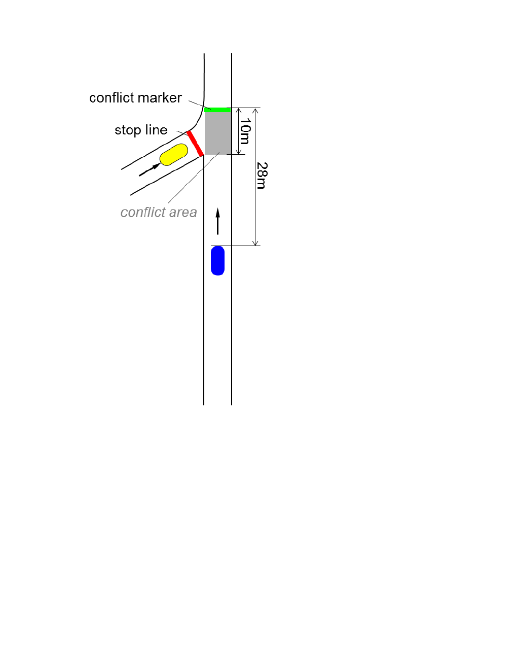
6.13.1 Modeling priority rules
In the following figure, the front end of the blue vehicle has just traversed the conflict marker.
Therefore, the present time gap is 0 sec. However, the yellow vehicle must wait until the rear
edge of the blue vehicle has completely cleared the conflict area, as the headway is greater
than 0 m.
512 © PTV GROUP

6.13.1 Modeling priority rules
6.13.1.2 Defining priority rules
Add a start section for a priority rule and one or more destination sections on the links
concerned:
Start section: a priority rule on the conflict link, on which vehicles are required to wait.
One or more destination sections (conflict markers) on the conflict link, on which vehicles
have the right of way. By default, select the position 1 to 2 m before the end of the conflict
area. The headway and time gaps must be present at the position opposite to the move-
ment direction.
© PTV GROUP 513

6.13.1 Modeling priority rules
Notes:
You can specify that you need not press the CTRL key when adding network objects
(see "Right-click behavior and action after creating an object" on page 143).
For some network objects there are windows in which the attributes of a network
object can be defined and edited. There are lists for this, for all network objects. You
can choose whether you want to open a window, a list or neither of the two for the
definition of network objects in the Network Editor (see "Right-click behavior and
action after creating an object" on page 143).
1. On the Network objects toolbar, click > Priority Rules.
2. Hold down the CTRL key and right-click on the desired position of the stop line on the
conflict link, on which vehicles should wait.
3. Release the keys.
A red bar is added by default. If for this start section you want to insert multiple destination
sections, carry out the following steps accordingly. Thereby you can insert a destination
section and subsequently define its attributes.
If you would like to insert a destination section for this start section, execute the next steps
only once.
4. On the desired link, point the mouse pointer to the desired position of the first destination
section.
On the edge of the link, which you are pointing to with the mouse pointer, a black arrow is
shown in the direction of travel. A colored bar shows the possible position of the destination
section. Thereby you can select links from the different types of links, which are added in
the next step of the destination section.
5. Hold down the CTRL key and right-click on this position.
6. Release the keys.
A green bar is added for the destination section by default. The Priority Rule window
opens.
7. Edit the attributes (see "Attributes of priority rules" on page 515).
8. Confirm with OK.
The window closes. The attributes are saved in the list Priority Rules. You can add
additional destination sections in links or stop the addition.
9. If you would like to add additional destination sections, on the desired link, point the mouse
pointer to the desired position of the next destination section, and repeat the steps.
10. If you do not want to add any additional destination sections, in the Network editor, click in
an empty area.
514 © PTV GROUP

6.13.1 Modeling priority rules
6.13.1.3 Attributes of priority rules
The Priority Rule window opens when you insert a network object and have selected to have
the Edit dialog opened automatically after object creation (see "Right-click behavior and action
after creating an object" on page 143). By default, only the Priority Rules list is opened.
Into the window, you enter attribute values for the network object. For network objects which
have already been defined, you can call the window using the following functions:
In the list of network objects of the network object type, double-click the row with the
desired network object.
In the Network editor, select the network object of your choice. Then, from its shortcut
menu, choose Edit.
The network object may have additional attributes. In the network objects list of the network
object type, you can show all attributes and attribute values. You can open the list via the
following functions:
In the network object toolbar, right-click the desired network object type. Then from the
shortcut menu, choose Show List (see "Context menu in the network object toolbar" on
page 63).
In the Network editor, select the network object of your choice. Then, from its shortcut
menu, choose Show In List (see "Selecting network objects in the Network editor and
showing them in a list" on page 339).
From the Lists menu, in the desired category, choose the network object type.
In the network objects list of the network object type, you can edit attributes and attribute
values of a network object (see "Selecting cells in lists" on page 102), (see "Using lists" on
page 89).
The objects of this object type may have relations to other objects. This is why the attributes list
is shown as part of a coupled list (on the left). On the Lists toolbar, in the Relations box, you
can show and edit the coupled list with the attributes of the desired relation on the right (see
below Showing and editing dependent objects as relation) and (see "Using coupled lists" on
page 111).
Note: In lists, you can use the Attribute selection icon to show and hide attribute
values (see "Selecting attributes and subattributes for a list" on page 106).
© PTV GROUP 515

6.13.1 Modeling priority rules
A network object may have the following attributes: These can be shown in the attributes list.
Element Description
No. Unique number
Name Description
516 © PTV GROUP

6.13.1 Modeling priority rules
Element Description
Elements under the sections Stop line and Conflict marker
Link (all
lanes)
Number of the link, in which the marker is located The marker extends over all
lanes of the link.
Link -
lane
Ln: Number of link and number of lane on which the marker is located. The
marker extends over one lanes of the link.
At Coordinate of the position of the priority rule: distance from the bus line to the
beginning of the link or connector
Affected
driving
direction
AffectDrivDir: If one of the conflict markers of the priority rule recognizes a
conflict, the stop line only causes vehicles to stop that are driving in the selected
direction.
Forward (default): Only vehicles moving forwards are recorded from the stop
line on.
Reverse: Only vehicles moving backwards are recorded from the stop line on.
These are vehicles that are pulling out of a parking space in reverse (see
"Modeling parking and stopping on the roadside" on page 462).
Vehicle
classes
VehClasses: Vehicle classes for which the marker applies. The configuration of
the vehicle class of a stop line (red bar) affects all of the associated conflict
markers. In order to define a stop line for other vehicle classes, a new (separate)
priority rule must be added, of which the stop line is at the same position.
Elements only under Stop line
Stop only
if Use signal controller condition (UseSCCond): When the option is selected,
the stop line is only active if the corresponding signal state of the chosen signal
group is active. This is useful for example when all vehicles required to wait
should not observe the vehicles located behind the stop line of a red SC. The
other conditions, e.g. Gap time, Headway are also taken into account.
Label If the option is not selected, the label for individual Priority Rules is hidden,
even when the label for all Priority Rules is selected.
Elements that are exclusively shown under Conflict marker.
Gap time Minimum gap time (MinGapTime) (in seconds) between the conflict marker and
the next vehicle driving towards it.
Headway Minimal headway (MinHdwy) (distance) between the conflict marker and the next
vehicle upstream.
Max.
Speed
Vehicles, which are traveling towards the conflict marker, are only considered for
the headway condition when their speed is ≤ max. speed.
Look bey-
ond red
signals
If this option is selected, vehicles traveling upstream of a red signal are also
observed by the conflict marker.
If the option is not selected, the time gaps and headways are only checked up
to the Red SC.
1. Confirm with OK.
© PTV GROUP 517

6.13.1 Modeling priority rules
The network object has additional attributes that you can show in the Attributes list. Among
them are the following for example:
Element Description
Slow
down
distance
SlowDownDist: Distance from stop line at which pedestrians start to reduce their
speed in order to stop at the stop line. Default 3 m.
GenBy Generated by: Indicates whether the priority rule is user-defined or has been
generated by Vissim.
Default value User: The priority rule has been defined by another Vissim
user.
Parking lot: Only during the simulation run: The priority rule has been
defined by Vissim. A conflict marker may have the following values:
<Number of priority rule>: Parking lot <number>: Vehicle pulling out
minds major flow: Priority rule that causes the vehicle pulling out of the
parking lot to stop if there is major flow traffic.
<Number of priority rule>: Parking lot <number>: Major flow minds
vehicle pulling out: Priority rule that causes major flow traffic to stop, if a
vehicle is pulling out of the parking lot.
<Number of priority rule>: Parking lot <number>: Vehicle pulling in
minds vehicle pulling out: Priority rule that causes the vehicle pulling
into the parking to stop and let the vehicle pulling out finish pulling out.
<Number of priority rule>: Parking lot <number x>: Vehicle pulling
out minds vehicle pulling out of parking lot <number y>: Priority rule
that causes the vehicle pulling out of parking lot x to stop, while a
vehicle is pulling out of parking lot y.
In the Priority rules list, double-click a priority rule to open the Priority rule window:
Only during a simulation run: For priority rules that Vissim has automatically generated,
the attributes of the stop line are displayed.
For user-defined priority rules that Vissim has automatically generated, the section on
the left displays the attributes of the stop line. The section on the right displays the attrib-
utes of the conflict marker.
Showing and editing dependent objects as relation
The attribute and attribute values of this network object type are shown in the list on the left,
which consists of two coupled lists.
1. In the list on the left, click the desired entry.
2. On the list toolbar, in the Relations list, click the desired entry.
The list on the right contains attributes and attribute values of network objects, and/or base
data allocated to the network object selected in the list on the left (see "Using coupled lists" on
page 111):
518 © PTV GROUP

6.13.1 Modeling priority rules
Vehicle classes (see "Defining the vehicle class" on page 267)
Pedestrian Classes (see "Attributes of pedestrian classes" on page 833)
Conflict markers: Attributes of conflict markers, e.g. vehicle classes, gap time, headway
(see "Attributes of links" on page 383). The attributes are described further above. Effective
driving direction (EffectDrivDir): Only vehicles driving into the chosen direction are recog-
nized by this conflict marker.
3. Enter the desired data.
The data is allocated.
6.13.1.4 Examples of priority rules
Examples of using priority rules:
Intersection with a main road, where vehicles have to wait (see "Priority rule Example 1:
Minor yielding road leading into straight main road" on page 520)
Avoiding tailbacks at a junction (see "Priority rule Example 2: Avoiding tailbacks at a junc-
tion" on page 521)
Dual-lane roundabout with dual-lane entry (see "Priority rule Example 3: Dual-lane round-
about with dual-lane entry" on page 522)
© PTV GROUP 519
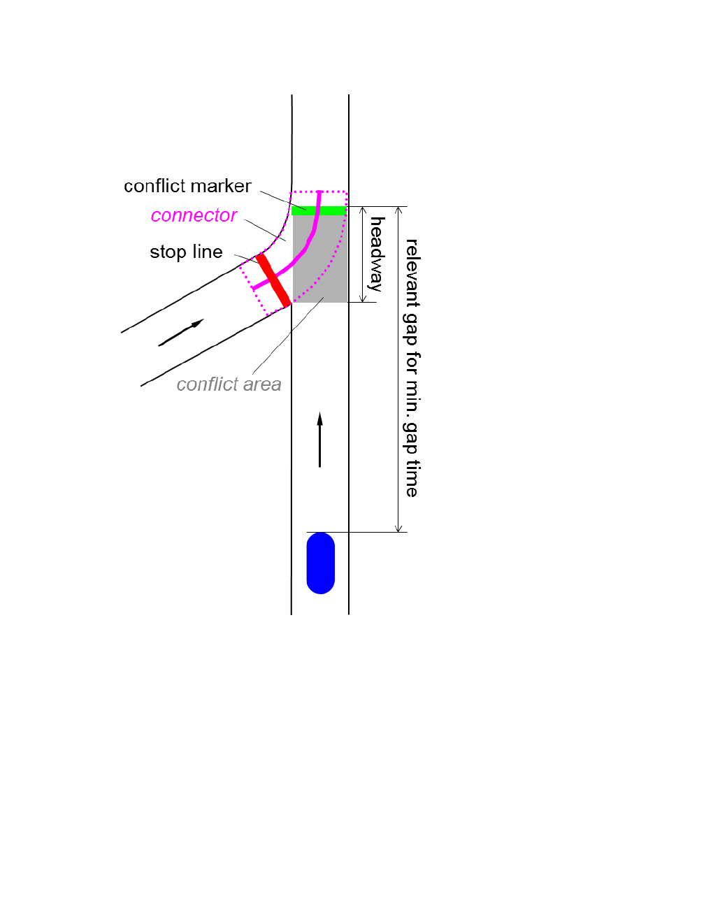
6.13.1 Modeling priority rules
Priority rule Example 1: Minor yielding road leading into straight main road
1. Position the left red bar (conflicting marker) on the stop line of the yielding road.
2. Position the top green bar (conflict marker) on the main road in movement direction,
approx. 1 m upstream of the end of the conflict area.
This makes sure that the min. headway and min. time gap are checked for the main road
only. You thereby exclude the possibility of a yielding vehicle waiting for itself. So do NOT
position the green bar (conflict marker) on the connector between minor and main road.
3. Confirm the default values: min. headway = 5 m, min. time gap = 3 s.
520 © PTV GROUP

6.13.1 Modeling priority rules
Priority rule Example 2: Avoiding tailbacks at a junction
1. Place the red bar below (conflict marker) on the stop line of the yielding link, upstream of
the junction.
2. On the same or the following link, place the top green bar (conflict marker) at a distance of
at least one vehicle length from the junction.
For a vehicle composition consisting of HGV and cars, a distance could for example be 20
m. The distance you choose should always account for the real driving behavior in such a
situation.
Cars only Additional priority rules for HGV/buses
3. The min. headway must be at least the distance between the stop line and the conflict
marker (green bar). This way, you avoid that vehicles enter the yellow hatched conflict area
as long as another vehicle is in there.
Note: The min. headway must not extend beyond the stop line. Otherwise, vehicles will
also brake even if the can cross the stop line.
4. Enter a maximum speed of 10 to 20 km/h.
This avoids possible congestion at the junction. The value defines the willingness of drivers
to keep the junction clear. With a max. speed of 20 km/h drivers are more careful and the
junction is more likely to be kept clear.
5. Enter a time gap of 0 sec.
6. Set the headway to a value which is slightly lower than the distance between the two
markers.
7. For calibration of the model, use the position of the conflict marker and thus either the min.
headway or speed.
© PTV GROUP 521

6.13.1 Modeling priority rules
Priority rule Example 3: Dual-lane roundabout with dual-lane entry
To model the entry to a roundabout, you need to specify several priority rules. They all serve
different purposes. Cars, HGV and buses are treated differently on account of their
acceleration capability and vehicle length. These vehicles thus have to be looked at
separately.
The priority rules and their purpose are depicted in the following illustrations Step 1 to Step 4.
For better understanding, you can find the numbers in the illustrations in the text. With these
you can assign the associated attributes in the text. The values specified for time gap,
headways, and max. speed have been determined through research and thus form a realistic
modeling basis for most applications.
Set the priority rules according to the following criteria:
Position the red bar (stop line) on the stop line of the yielding road. This is the typical wait-
ing position for vehicles. If more than one green bar (conflict marker) refers to this stop
line, several green bars must be set instead of separate pairs of priority rules.
Position the green bars which are used for the headways, just before the connector turns
into the roundabout lane. You thereby exclude the possibility of a yielding vehicle waiting
for itself. Because of this the capacity of the roundabout would be drastically reduced.
Position the green bars used for the time gaps at approximately the same distance from
the conflict area as the respective red bars.
Step 1: Protect lane 1
Firstly, the priority rules for vehicles entering the roundabout from lane 1 are defined.
522 © PTV GROUP

6.13.1 Modeling priority rules
All 3 priority rules listed here refer to the same stop line. So this stop line has 3 conflict
markers.
Select different positions for the min. time gap and min. headway. This allows you to model a
more realistic driving behavior: A vehicle driving at least 14 km/h on a roundabout will allow
another vehicle to accelerate into the roundabout, even if it is still in the conflict area. This
leads us to the first two priority pairs (1 and 2). They are valid for all vehicle classes.
No. 1 secures the conflict area during slow moving traffic and congestion on the roundabout
(min. headway).
No. 2 provides the conditions for a normal flow of traffic (min. gap time).
As entering vehicles on lane 1 are also affected by traffic on the inner roundabout lane, an
additional priority rule with a small gap time condition (No. 3) is needed for the inner
roundabout lane. This priority rule is also valid for all vehicle classes.
Step 2: Protect the HGVs against entering vehicles
So far, all priority rules have applied for all vehicle classes. When long vehicles on the
roundabout cross the conflict area, it is not enough to take of the vehicles that are slower than
14 km/h. To prevent vehicles entering the roundabout from laterally colliding with an HGV, an
additional priority rule (No. 4) has to be positioned at the same point as rules 1-3. This priority
© PTV GROUP 523

6.13.1 Modeling priority rules
rule must account for long, obstructive vehicles only. In our example these are HGV and
buses.
Now we only need to account for the vehicles that have a lower acceleration capability than
cars. To do so, we use priority rule No. 5. Contrary to the previous priority rules, this rule needs
a new, separate stop line, as it only applies for the vehicle classes HGV and bus. The stop line
is positioned at the same point as rule No. 2. However, a longer gap time of 3.6 s must be
specified for priority rule No. 5.
Step 3: Priority rules for the left incoming lane
As for the right lane, general priority rules are defined for all vehicle classes with help of the
min. time gap and min. headway. As in this case two lanes need to be taken into account, four
priority pair rules have to be specified: No. 6 and 7 for the outer roundabout lane and No. 8
and 9 for the inner roundabout lane. All 4 conflict markers refer to the same stop line.
Due to the greater distance to the conflict area, the minimum gap time for the inner roundabout
lane (No. 9) must be slightly higher than for the outer lane.
524 © PTV GROUP

6.13.1 Modeling priority rules
© PTV GROUP 525

6.13.2 Modeling conflict areas
Step 4: Priority rules for special vehicle classes
Finally, the priority rules for special vehicle classes are followed: as has already been carried
out for lane 1, long vehicles must first be considered, No. 10 is added additionally for the same
conflicting marker as for Nos. 6-9. HGV and buses entering the roundabout need longer gap
times: No. 11 and 12 are added to a new stop line. Here, too, the time gap for the inner
roundabout lane must be slightly longer than for the outer one.
6.13.2 Modeling conflict areas
Using conflict areas that are automatically shown, you can model conflicts between vehicles
on two links or connectors (see "Defining the right of way at conflict areas" on page 530).
Use conflict areas instead of priority rules to model the right of way at intersections. Conflict
areas are automatically displayed, are easier to edit and reflect the driving behavior better
than priority rules (see "It is better to use conflict areas than priority rules to model driving
behavior." on page 527).
6.13.2.1 Modeling conflicts with the help of conflict areas
A conflict area indicates the following cases of conflict:
526 © PTV GROUP

6.13.2 Modeling conflict areas
Crossing: two crossing links
Merging: Two connectors lead to the same link or a connector leads to a link with other
upstream traffic If the two connectors lead to the first 5 m of the link and start on two links, a
conflict between these two links is accounted for by the conflict area.
Branching: Two connectors come off the same link or one connector comes off a link that
continues further downstream for more than 0.5 m. If the two connectors lead to the first 5
m of two links, the conflict between these two links is also accounted for by the conflict
area.
6.13.2.2 Displaying conflict areas
In the Network objects toolbar, click Conflict areas to automatically show conflict areas in the
network, which is where two links or two connectors overlap. For each conflict area, you can
select the link that has the right of way. The conflict area may also remain passive and thus
without any impact on the vehicles.
Conflict areas are not inserted in the following cases:
If the height (z coordinate) of both links or both links and the connector differs more than
1.0 m in their overlapping area.
If the overlapping is less than or equal to 0.5 m
If at least one of the links ends less than 5 m after the start of the conflict area and no con-
nector begins in it. This does not apply for the following links:
Connectors
Links which are defined as pedestrian areas (see "Modeling links as pedestrian areas"
on page 869).
Links with input flows with vehicle compositions which contain vehicle types with the
category Pedestrians (see "Modeling vehicle compositions" on page 425)
6.13.2.3 It is better to use conflict areas than priority rules to model driving behavior.
Conflict areas allow you to model driving behavior better than with priority rules, as in conflict
areas, drivers plan how to traverse the conflict area:
A yielding driver watches the vehicles in the main traffic stream and then decides when to filter
in. He then plans to accelerate for the next few seconds. Acceleration allows him to pass the
conflict area. He thereby accounts for the traffic downstream from the conflict area. If he knows
that he will have to stop or drive slowly because of other vehicles, he will account for more
time to cross the conflict area or he will decide to wait for longer.
Vehicles in the main traffic stream also react to conflict areas: If a vehicle does not manage to
cross the entire conflict area because the driver has misjudged the situation, the vehicle in the
main traffic stream will brake or even stop. If a queue is forming at a signal control downstream
of the conflict area, the drivers of the vehicles in the main traffic stream try not to stop within the
conflict area in order not to block any crossing traffic. The drivers that have the right of way
carry out a comparable decision-making process for crossing the conflict area as the drivers
whose vehicles are yielding.
© PTV GROUP 527
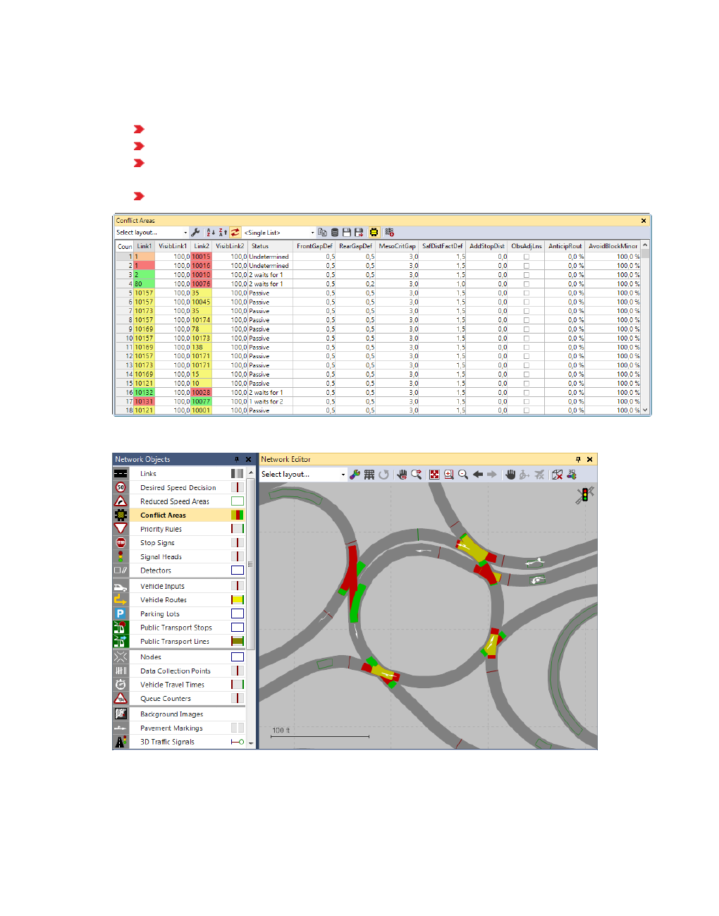
6.13.2 Modeling conflict areas
6.13.2.4 Colors indicate the status of conflict areas
The status of conflict areas is displayed in the Conflict Areas list and in the Network editor.
Green: main flow (right of way)
Red: minor flow (yield)
Both red: for branching conflicts, so that vehicles can "see" each other. There is no
right of way, as vehicles simply remain in their original sequence.
Both yellow: passive conflict area without right of way
In the Network editor:
Display of different statuses:
528 © PTV GROUP

6.13.2 Modeling conflict areas
6.13.2.5 Driving behavior at conflict areas
The driving behavior of vehicles approaching a conflict area shall produce the maximum
capacity for a minor traffic stream, without affecting vehicles of the main traffic stream. Vehicles
in the main traffic stream might be hindered by vehicles on the merge lane, the smaller the
user-defined safety distance factor is.
A vehicle in a minor traffic stream will calculate whether it will be able to filter into the main
stream with every time step while approaching the conflict area. Thereby safety distances
are taken into account (see "Defining the Wiedemann 74 model parameters" on page
275), (see "Defining the Wiedemann 99 model parameters" on page 277). If the driver
feels there is a large enough gap in the main traffic stream, he will simply continue to
drive. If the gap is too small, the vehicle will decelerate as if it had to stop in front of the con-
flict area. This calculation is repeated with the next time step. So braking is either can-
celled or the driver continues driving and might even accelerate, e.g. when finding a gap
in the traffic stream to enter.
A vehicle on the main road is careful not to collide with any vehicles on the minor road. If it
realizes that a vehicle on the minor road will still be within the conflict area when it arrives
there, it will brake in order to reach the conflict area just after the other vehicle has left it.
As decelerating causes it to arrive later, it might continue its journey without any further
braking in a later time step and pass right after the vehicle on the minor road.
A vehicle on a minor road will brake before reaching a conflict area, if there is not enough
space downstream of the conflict area to leave it. This means that particularly when there
are several adjacent conflict areas, drivers have to either pass all of them or none, if there
is not enough space for a full vehicle length.
With a conflict area of the conflict type crossing, a vehicle in the main stream will try to
keep the conflict area clear, if this vehicle belongs the percentage specified in the Avoid
blocking attribute (see "Attributes of conflict areas" on page 531).
Note: Vehicles of the main stream will not keep conflict areas of the merging or
branching conflict types clear. To make vehicles keep conflict areas of the merging
or branching type clear, you need to specify a priority rule (see "Priority rule
Example 2: Avoiding tailbacks at a junction" on page 521)
A vehicle in the minor stream will not enter a conflict area if it has to assume that it will not
be able to leave it before the next vehicle of the main stream arrives. It thereby takes the
safety distance into account (see "Attributes of conflict areas" on page 531)
A vehicle of a minor stream that has already entered a conflict area will always try to leave
it, even if this means that it has to enter another conflict area for which the Gap condition is
not or no longer met.
© PTV GROUP 529

6.13.2 Modeling conflict areas
To avoid a collision, a vehicle may temporarily stop at an intersection within a red conflict
area. If vehicle A recognizes that vehicle B is about to leave a conflict area, vehicle A can
wait within another conflict area, for which it does not have the right of way, until B leaves.
A vehicle waiting in a conflict area uses the next sufficiently large time gap to exit it. This
behavior can also occur in a yielding vehicle, when it has to yield to the vehicle with the
right of way. Example: A vehicle in a minor stream wants to turn into the major stream. It is
waiting at an intersection in a conflict area because the vehicle in the major stream has
the right of way. The vehicle in the major stream wants to turn left into the minor stream
and is yielding because of oncoming traffic in the conflict area. However, if the time gap for
the vehicle in the minor stream is sufficiently large, allowing it turn into the major stream in
spite of the two vehicles, it leaves the conflict area and turns into the major stream. If you
want a vehicle to take a headway into account, define a priority rule (see "Modeling priority
rules" on page 506).
6.13.2.6 Defining the right of way at conflict areas
You can define the priority for conflicting traffic flows at automatically generated conflict areas.
1. On the Network objects toolbar, click Conflict Areas.
The conflict areas are shown in color in the Network editor. Per default, conflict areas that
have not yet been assigned a right of way are highlighted in yellow.
Note: You can change the setting to where you do not have to press the CTRL key (see
"Right-click behavior and action after creating an object" on page 143).
2. In the Network editor, click the conflict area for which you want to define the right of way.
The conflict area is highlighted.
3. Hold down the CTRL key and right-click into the Network editor until the desired right of way
is shown.
Green: main flow (right of way)
Red: minor flow (yield)
Both red: for branching conflicts, so that vehicles can "see" each other. There is no
right of way, as vehicles simply remain in their original sequence.
Both yellow: passive conflict area without right of way
In the Network editor, the conflict area changes its color. In the Conflict Areas list, the
following attributes are automatically adjusted:
Link 1 and Link 2 are displayed in the color of the right of way
Status: right of way and colors
4. Edit the attributes (see "Attributes of conflict areas" on page 531).
The attributes are saved in the Conflict Areas list.
530 © PTV GROUP

6.13.2 Modeling conflict areas
Note: Alternatively, right-click into the Network editor and choose the desired right of
way from the shortcut menu. To do so, you need not select Conflict Areas on the
Network objects toolbar. The shortcut menu will automatically show the right of way
options available. Dependining on the current right of way of the conflict area, these
can be the following:
Set Status to 2 waits for 1:
Second link is highlighted in red: Minor flow (yield)
First link is highlighted in green: Main flow (right of way)
Set Status to 1 waits for 2:
First link is highlighted in red: Minor flow (yield)
Second link is green: Main flow (right of way)
Set Status to Undetermined: Both links turn red: For branching conflicts, so that
vehicles can "see" each other. There is no right of way, as vehicles simply remain in
their original sequence.
Set Status to Passive: Both links turn amber: No right of way specified
6.13.2.7 Attributes of conflict areas
The attributes of a conflict area influence the driving behavior of any vehicle approaching the
conflict area. This is why a vehicle may change its intention, and thus its driving behavior, in a
particular traffic situation. The situation arising thereof may differ from the attribute values
defined. This is particularly true for any resulting gaps in front of and behind two vehicles.
In the network objects list of the network object type Conflict Areas, you can edit all attributes
and attribute values of conflict areas (see "Opening lists" on page 92), (see "Selecting cells in
lists" on page 102).
Note: In lists, you can use the Attribute selection icon to show and hide attribute
values (see "Selecting attributes and subattributes for a list" on page 106).
1. Make the desired changes:
Element Description
No Unique number
Link1,
Link2
Link 1, Link 2: Number and name of link with the conflict area
VisibLink1,
VisibLink2
Visibility link 1, Visibility link 2: Maximum distance at which an
approaching vehicle can "see" the vehicles on the other link. As long
as a vehicle is on a non-priority link still far away from the conflict area,
it plans to stop as close as possible to it. Avoid values < 1 m to keep
the vehicle moving.
In the Figure, the blue vehicle at the bottom on link 2 has reached the
point from where it can fully "see" past the blue building on link 1
where the red vehicle is (on the left). This means the visibility for link 2
= dL2.
© PTV GROUP 531

6.13.2 Modeling conflict areas
Element Description
Status Identification of right of way by colors:
2 waits for 1: Link 1 green - Link 2 red
1 waits for 2: Link 1 red - Link 2 green
Undetermined: Both red for branching conflicts, so that vehicles
can "see" each other. There is no right of way, as vehicles simply
remain in their original sequence.
Passive: Both yellow: passive conflict area without right of way
FrontGapDef
FrontGap
Front gap (default):
For the types merging conflicts and crossing conflicts: Minimum
gap time in seconds between the rear end of a vehicle in the main
traffic stream and the front end of a vehicle in the minor traffic
stream. Default 0.5 seconds To adhere to the minimum gap time,
the yielding vehicle slows down as it approaches the conflict area
and stops in front it, as long as the vehicle that has priority is front
of or in the conflict area. Once the vehicle with the right of way has
left the conflict area, the yielding vehicle can enter it and no longer
takes the Front gap into account.
Into the Gaps list on the right, you can enter the minimum gap time
FrontGap per vehicle class.
The figure below shows the current situation (the non-transparent
vehicles) and the future situation (the semi-transparent vehicles). In
the future situation, the vehicle in the major stream has just left the
conflict area. Up until this time, the Front gap is considered the time
required by the vehicle in the minor stream to reach the empty conflict
area (in this case: 0.5s)
532 © PTV GROUP

6.13.2 Modeling conflict areas
Element Description
RearGapDef
RearGap
Rear gap (default): Only for type Junction:
Minimum gap time in seconds between the rear end of a
vehicle in the minor traffic stream and the front end of a vehicle
in the main traffic stream. This is the time that must be provided,
after a yielding vehicle has left the conflict area and before a
vehicle with the right of way enters it. Vehicles are perceived
within a maximum distance of up to 100 m. Default 0.5 seconds
Into the Gaps list on the right, you can enter the minimum gap
time per vehicle class.
The figure shows the current and future situation (as light, semi-
transparent vehicles), once the vehicle in the main traffic stream has
reached the conflict area. The rear gap is evaluated as the time that
has elapsed since the vehicle in the minor traffic stream has left the
conflict area (in this case: 0.7s)
© PTV GROUP 533

6.13.2 Modeling conflict areas
Element Description
MinGapBlockDef
MinGapBlock
Minimum gap blocking (default): Only applies if the attribute Avoid
blocking the major flow is not selected and thus a yielding vehicle
may enter the conflict area, blocking the major flow:
Default minimum gap time for the yielding vehicle for entry
before the vehicle with the right of way. Minimum gap blocking
(default) is used for all vehicles that are not part of a vehicle
class for which a class-specific gap time has been defined.
Default 3.0 s
Into the Gaps list on the right, you can enter the Minimum gap
blocking per vehicle class.
MesoCriticGap Meso critical gap: Edit this value in the Meso turn conflicts list or in
the coupled list Nodes - Meso turn conflicts (see "Attributes of meso
turn conflicts" on page 790), (see "Attributes of nodes" on page 669).
SafDistFactDef Safety distance factor: only for the type merging conflicts: This
factor is multiplied with the normal desired safety distance of a vehicle
in the main traffic stream in order to determine the minimum distance a
vehicle of the yielding traffic stream must keep when it is completely in
the conflict area merging conflicts.
Into the Gaps list on the right, you can enter the safety distance factor
per vehicle class.
The figure below shows identical situations, but with different factors:
top = 1.0, bottom = 0.5. This is why the blue vehicle (bottom) can still
enter the conflict area, while the red vehicle (top) has to stop.
In the figure, the relevant part of the safety distance is highlighted in
yellow.
534 © PTV GROUP

6.13.2 Modeling conflict areas
Element Description
AddStopDist Additional stop distance: only relevant for vehicles that are required
to yield: Distance in meters that moves an imaginary stop line
upstream of the conflict area. As a result, vehicles required to yield
stop further away from the conflict and thus also have to travel a longer
distance to pass the conflict area. Default 0 m.
ObsAdjLns Observe adjacent lanes: If this option is selected, at merging con-
flicts, incoming vehicles of the main traffic stream that are required to
yield will account for the vehicles in the main traffic stream that want to
change to the conflicting lane. This option reduces the simulation
speed.
AnticipRout Anticipate routes: Percentage of vehicles required to yield that
account for the routes of vehicles with the right of way. These are
approaching with the main traffic stream and will turn further upstream.
They will thus not reach the conflict area. Value between 0 and 1.
AvoidBlockMinor Avoid blocking the minor flow: If a vehicle with the right of way
belongs to the percentage rate selected, it will check the space
available downstream of the conflict area and does not drive into the
conflict area under the following conditions:
when the space available downstream of the conflict area is less
than the total of the individual vehicle length + 0.5 m and the blocking
vehicle is slower than 5 m/s and slower than 75% of its desired speed
when the obstacle is a red signal
AvoidBlockMajor Avoid blocking the major flow
If this option is selected, a yielding vehicle does not enter or
stop within the conflict area, unless it can drive through it in one
go. The option is selected by default. For the yielding vehicle, the
attribute Minimum gap blocking is not taken into account.
If this option is not selected, a yielding vehicle can enter and
stop within the conflict area, even if it cannot drive into the fol-
lowing lane conflict, as it is blocked by a vehicle that has the right
of way. In this case, the yielding vehicle might block the major flow.
For the yielding vehicle, the attribute Minimum gap blocking is
taken into account.
© PTV GROUP 535

6.13.3 Modeling stop signs and toll counters
Element Description
Example: You are modeling a long conflict area between a vehicle
route and a very wide pedestrian route with many narrow lanes and
with a priority for pedestrians. Deactivate the option to let a vehicle
successively drive into and traverse the lane conflicts without having
to wait for a time when it can drive through the entire conflict area, and
possibly other conflict areas lying close behind it, in one go.
Showing and editing dependent objects as relation
The attribute and attribute values of this network object type are shown in the list on the left,
which consists of two coupled lists.
1. In the list on the left, click the desired entry.
The list on the right contains attributes and attribute values of network objects, and/or base
data allocated to the network object selected in the list on the left (see "Using coupled lists" on
page 111):
Defining time gaps [s]
The attributes are described further above.
6.13.3 Modeling stop signs and toll counters
Model stop signs on access roads to intersections with a combination of right-of-way control
and stop sign.
Priority rules account for conflicting traffic as well as for the min. headway and min. gap time.
Stop signs, however, make vehicles stop for at least one time step, independent of whether
there is conflicting traffic or not.
Conflict areas also take desired acceleration, maximum acceleration as well as the vehicle
length of the two vehicles in both streams into account and reflect the driving behavior better
than priority rules (see "It is better to use conflict areas than priority rules to model driving
behavior." on page 527).
Toll counters are a variant of stop signs that are additionally assigned a dwell time distribution
value.
Stop signs can be used for the following modeling scenarios:
Regular stop sign: You need to define a stop sign and a priority rule. Position the stop
sign at the same position as the stop line (red) of the priority rule (see "Modeling priority
rules" on page 506).
Signal controller with turn on red: Right turns are allowed in spite of a red signal. In the
Green arrow tab, select Only on red, to enable the stop sign only when the selected sig-
nal group of the selected SC indicates red.
536 © PTV GROUP

6.13.3 Modeling stop signs and toll counters
Toll counter, e.g. customs office or toll gate: Vehicles stop according to the time dis-
tribution defined in the attribute DwellTmDistr (Dwell time distribution). On the Time Dis-
tribution tab, select Use time distribution (UsesDwellTmDistr).
6.13.3.1 Defining stop signs and toll counters
Notes:
You can specify that you need not press the CTRL key when adding network objects
(see "Right-click behavior and action after creating an object" on page 143).
For some network objects there are windows in which the attributes of a network
object can be defined and edited. There are lists for this, for all network objects. You
can choose whether you want to open a window, a list or neither of the two for the
definition of network objects in the Network Editor (see "Right-click behavior and
action after creating an object" on page 143).
1. On the Network objects toolbar, click Stop Signs.
2. Hold down the CTRL key and right-click on the desired position of the stop sign in the link or
the connector.
A colored bar is added. The window Stop Sign opens.
3. Edit the attributes (see "Attributes of stop signs and toll counters" on page 537).
4. Confirm with OK.
The attributes are saved in the list Stop Signs.
6.13.3.2 Attributes of stop signs and toll counters
The Stop Sign window opens when you insert a network object and have selected to have the
Edit dialog opened automatically after object creation (see "Right-click behavior and action
after creating an object" on page 143).
Into the window, you enter attribute values for the network object. For network objects which
have already been defined, you can call the window using the following functions:
In the list of network objects of the network object type, double-click the row with the
desired network object.
In the Network editor, select the network object of your choice. Then, from its shortcut
menu, choose Edit.
The network object may have additional attributes. In the network objects list of the network
object type, you can show all attributes and attribute values. You can open the list via the
following functions:
In the network object toolbar, right-click the desired network object type. Then from the
shortcut menu, choose Show List (see "Context menu in the network object toolbar" on
page 63).
© PTV GROUP 537

6.13.3 Modeling stop signs and toll counters
In the Network editor, select the network object of your choice. Then, from its shortcut
menu, choose Show In List (see "Selecting network objects in the Network editor and
showing them in a list" on page 339).
From the Lists menu, in the desired category, choose the network object type.
In the network objects list of the network object type, you can edit attributes and attribute
values of a network object (see "Selecting cells in lists" on page 102), (see "Using lists" on
page 89).
The objects of this object type may have relations to other objects. This is why the attributes list
is shown as part of a coupled list (on the left). On the Lists toolbar, in the Relations box, you
can show and edit the coupled list with the attributes of the desired relation on the right (see
below Showing and editing dependent objects as relation) and (see "Using coupled lists" on
page 111).
Note: In lists, you can use the Attribute selection icon to show and hide attribute
values (see "Selecting attributes and subattributes for a list" on page 106).
Basic attributes of stop signs
The basic attributes of the network element are shown in the upper area of the window and in
the list of network objects for the particular network object type.
Element Description
No. Unique number
Name Designation
538 © PTV GROUP
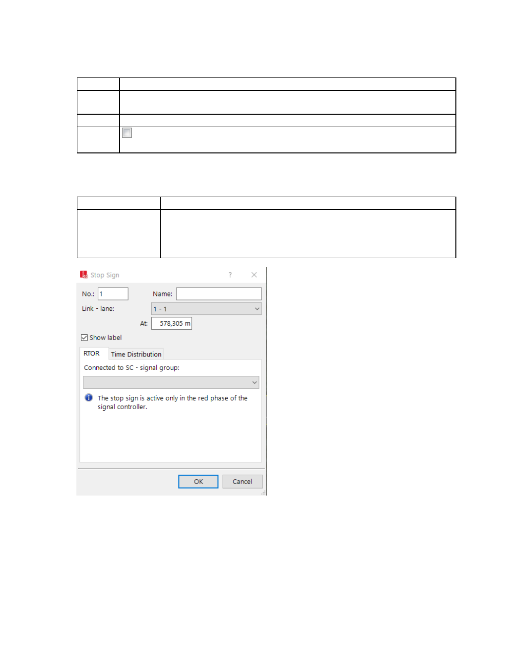
6.13.3 Modeling stop signs and toll counters
Element Description
Link -
lane
Number of the link and lane, on which the stop sign is located.
At Pos: Distance from the beginning of link or connector
Showing
label If the option is not selected, the label for the individual stop sign is hidden, even
when the label for all stop signs is selected.
RTOR tab
The tab contains, amongst others, the following attributes:
Element Description
Connected with
SC - signal group
Number of signal controller and number of signal number group in
which the green shall be displayed.
Right turn on red: defines a green arrow symbol 720 (see "Using stop
signs for right turning vehicles even if red" on page 540)
Time Distribution tab
In the Time Distribution tab, you can use dwell time distributions to define toll counters as a
variant of stop signs.
The tab contains, amongst others, the following attributes:
© PTV GROUP 539

6.13.3 Modeling stop signs and toll counters
Element Description
Use time
distribution
Uses dwell time distributions (UsesDwellTmDistr ): Select wait time at toll
counters:
If the option is selected, under each vehicle class a time distribution (see
"Using time distributions" on page 237) can be allocated in the list.
All vehicles of a vehicle class, which use a time distribution, adhere to their
corresponding, chosen time distributions.
Vehicles without allocated distributions stop for one time step.
Showing and editing dependent objects as relation
The attribute and attribute values of this network object type are shown in the list on the left,
which consists of two coupled lists.
1. In the list on the left, click the desired entry.
The list on the right contains attributes and attribute values of network objects, and/or base
data allocated to the network object selected in the list on the left (see "Using coupled lists" on
page 111):
2. On the list toolbar, in the Relations list, click > Dwell time distributions.
The attributes are described further above.
3. Enter the desired data.
The data is allocated.
6.13.3.3 Using stop signs for right turning vehicles even if red
You can also set stop signs to model the behavior for turning, even if red at sign 720 green
arrow (according to StVO German Traffic Code).
Examples:
Special right-turn only lanes: The stop sign must be placed on the right turn lanes. Addi-
tionally, a signal head can be placed on the lane and for a vehicle type, for example, a
tram or a pedestrian can be selected. Thereby the turning vehicle in the lane is not
affected, but the state of the signal is visible.
Combined right turning and straight lanes: If the option is selected, the stop sign must
be placed on the connector for right turns. This makes the stop sign only visible for turning
vehicles. The signal heads are placed at the same positions, however, it would be better
to place them on the link rather than on the connector. The signal head controls the traffic
driving straight.
The image shows:
Five signal heads: (dark) red bars at the top, on first three lanes on the left, and at the bot-
tom right
540 © PTV GROUP
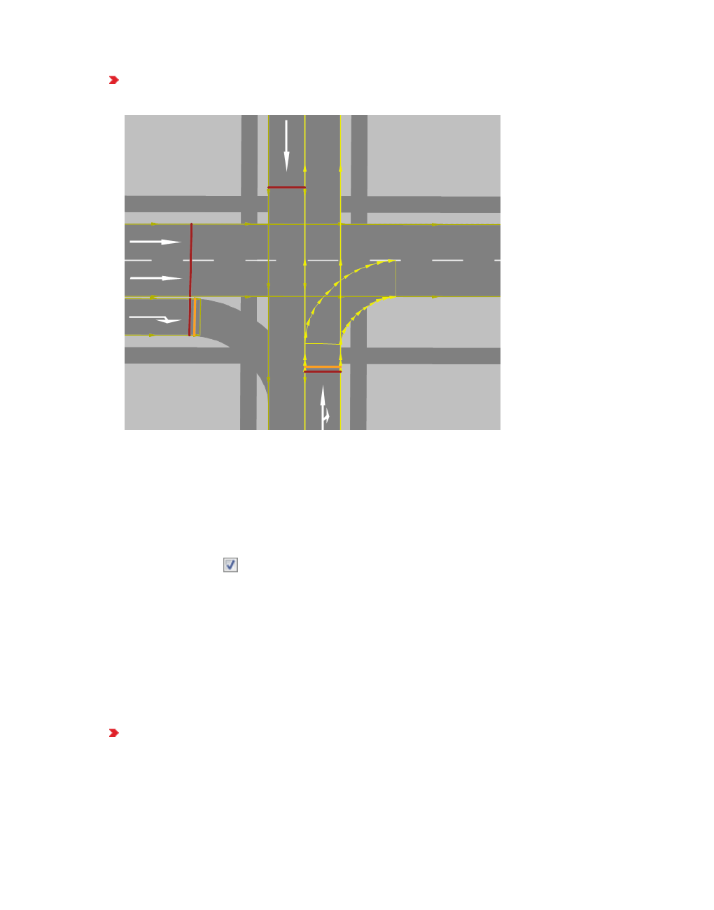
6.13.4 Merging lanes and lane reduction
Two stop signs: bright (orange) bars on the left, separate turning lane and on the bottom,
right combined turning lane
1. On the Network objects toolbar, click Stop Signs.
2. In the Network Editor, right click on the desired position of the link.
3. From the context menu, select the entry Add New Stop Sign.
The window Stop Sign opens.
4. Select the RTOR tab.
5. Select the option Only on Red.
6. Select the SC and the signal group.
7. Confirm with OK.
The stop sign is only active during the red phase of the allocated signal control.
6.13.4 Merging lanes and lane reduction
To model driving behavior at acceleration lanes and lane reduction, it is best to define links as
merging lanes.
Make sure the weaving section is a link with the following properties:
Number of lanes = Number of lanes on main link + number of merging lanes
© PTV GROUP 541
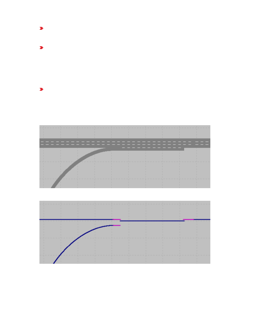
6.14 Modeling signal controllers
Make sure that after the weaving section there is only one connector to the main link. For a
realistic graphical representation, add a dummy link at the end of the merging lane. This
will make reduction of the lanes less abrupt. Do not use a connector for this link.
Make sure the through traffic is following a route, so that it does not switch to an accel-
eration lane. This route must end no sooner than on the link after the merging lane. Down-
stream of the merging lane, the value of the Lane change attribute (Lane change
distance) of the connector must be larger than the weaving section length (see "Attributes
of connectors" on page 395). If this is not the case, a vehicle on the main link may change
to the acceleration lane and thus to the weaving section. It will then need to change back
to the main link. This kind of behavior produces unrealistic lane changes.
The routes of the merging traffic must not end at the weaving section, but extend beyond it.
If not, the interweaving traffic will not know that it needs to change lanes before the end of
the merging lane in order to get on the main link.
Example of a one-lane link merging into a three-lane link.
Merging section in normal display mode:
Merging section in wireframe display mode:
6.14 Modeling signal controllers
You can define signal controllers (SCs) for the following signal control procedures:
542 © PTV GROUP

6.14 Modeling signal controllers
Use signal controller Balance-Central (see "Using Balance-Central signal controllers" on
page 576)
Econolite ASC/3 (for North America only) (see "Add-on module Econolite ASC/3" on page
578)
Use signal controller Epics/Balance-Local (see "Using Epics/Balance-Local signal con-
trollers" on page 577)
The SC type External allows you to access dialog DLL files and user-defined program
DLL files for control (see "Add-on module external signal control SC" on page 579)
Fixed time, with add-on module Vissig (see "Using SC type Fixed time" on page 571)
Fourth Dimension D4 (for North America only) (see "Add-on module Fourth Dimension"
on page 581)
LISA+ OMTC (see "Add-on module LISA+ OMTC" on page 582)
McCain 2033 (for North America only) (see "Add-on module McCain 2033" on page 582)
Ring Barrier Controller (for North America only) (see "Using the Ring Barrier Controller
RBC add-on module" on page 583)
SCATS (Australia) (see "Add-on module SCATS" on page 585)
SCOOT (see "Add-on module SCOOT" on page 586)
Siemens VA (Siemens-VS-PLUS, TL, PDM-C by Siemens AG, Munich) (see "Add-on mod-
ule Siemens VA (TL / Siemens VS-PLUS)" on page 588)
TRENDS (see "Using add-on module TRENDS" on page 588)
VAP (vehicle-actuated signal control, freely programmable logic according to RiLSA 1992,
guidelines for signal controllers in Germany) (see "Add-on module Traffic-dependent VAP
Programming" on page 590)
VS-Plus (Rudolf Keller AG, Basel) (see "Add-on module VS-Plus" on page 592)
For the signal control procedures Fixed time control, Epics Balance/Local and External, you
can use the add-on module Vissig to define and configure signal groups. The Network editor
allows you to add signal heads to the Vissim network. You assign each signal head a signal
group of your choice.
Notes: DLL files for external control procedures are provided to you together with your
Vissim version as 32-bit or 64-bit version, depending on the license purchased.
If your license includes the SC type External, you need to compile the DLL files
according to your 32- or 64-bit Vissim version.
Vissim only allows you to access data of an external signal controller, if you have saved
the network file. This way, it is made sure that the controller files and the network
file*.inpx are saved to the same directory.
© PTV GROUP 543

6.14.1 Modeling signal groups and signal heads
6.14.1 Modeling signal groups and signal heads
Signal groups are the smallest control unit belonging to a controller device assigned a unique
SC number in Vissim. You can assign an LSA up to 125 signal groups, depending on its
control logic. As signal groups are not visible in reality, Vissim also distinguishes between
signal heads and signal groups. A signal group can be assigned to several signal heads that
always show the same picture.
Vehicles approaching a red signal will stop at a standstill distance in front of the signal
controller (see "Editing the driving behavior parameter Following behavior" on page 271).. The
default standstill distance is 0.5 m.
Vehicles approaching an amber signal will cross the intersection if they cannot come to a safe
standstill at the stop line.
Optionally, you can select a method that calculates the probability of the vehicle stopping or
continuing. For this calculation, three driving behavior parameters are required (see "Defining
driving behavior parameter sets" on page 268).
By default, signal groups and thus all signal heads are updated at the end of every simulation
second. If you have specified more than 1 time step per simulation second, signal groups are
not switched at each time step. This means that in the network display, each signal header will
show a picture that vehicles on its link will respond to in the next time step. Depending on the
signal header type, switching is also possible every 1/10 s.
Signal headers allow you to model all common situations with precision. This includes
different types of signal groups for several vehicle types on one lane. For instance, for a bus
with its separate signal phases, driving on a mixed lane, select the vehicle class of your choice
for each signal head.
Note: For any SC with conflicting traffic that is allowed to drive at the same time, you
need to define priority rules (see "Creating priority rules" on page 507).
6.14.1.1 Defining signal heads
In the network, you may position signal heads at the stop line accurate to lane level. In Vissim,
signal heads are displayed as red lines per default. To model 3D signal heads realistically for
a simulation, including the display options for mast, arm, signal head, sign and light, define 3D
signal heads (see "Modeling 3D signal heads" on page 549).
1. Ensure that a SC with signal groups is defined (see "Defining SC and signal control
procedures" on page 567).
Notes:
You can specify that you need not press the CTRL key when adding network objects
(see "Right-click behavior and action after creating an object" on page 143).
For some network objects there are windows in which the attributes of a network
object can be defined and edited. There are lists for this, for all network objects. You
can choose whether you want to open a window, a list or neither of the two for the
definition of network objects in the Network Editor (see "Right-click behavior and
action after creating an object" on page 143).
544 © PTV GROUP

6.14.1 Modeling signal groups and signal heads
2. On the Network objects toolbar, click Signal Heads.
3. Hold down the CTRL key and right-click on the desired position of the signal head in the
link.
A colored bar is added. The Signal Head window opens.
4. Edit the attributes (see "Attributes of signal heads" on page 545).
5. Confirm with OK.
The attributes are saved in the list Signal Heads.
6.14.1.2 Attributes of signal heads
The Signal Heads window opens when you insert a network object and have selected to have
the Edit dialog automatically opened after object creation (see "Right-click behavior and action
after creating an object" on page 143). By default, only the Signal Heads list is opened.
Into the window, you enter attribute values for the network object. For network objects which
have already been defined, you can call the window using the following functions:
In the list of network objects of the network object type, double-click the row with the
desired network object.
In the Network editor, select the network object of your choice. Then, from its shortcut
menu, choose Edit.
The network object may have additional attributes. In the network objects list of the network
object type, you can show all attributes and attribute values. You can open the list via the
following functions:
In the network object toolbar, right-click the desired network object type. Then from the
shortcut menu, choose Show List (see "Context menu in the network object toolbar" on
page 63).
In the Network editor, select the network object of your choice. Then, from its shortcut
menu, choose Show In List (see "Selecting network objects in the Network editor and
showing them in a list" on page 339).
From the Lists menu, in the desired category, choose the network object type.
In the network objects list of the network object type, you can edit attributes and attribute
values of a network object (see "Selecting cells in lists" on page 102), (see "Using lists" on
page 89).
The objects of this object type may have relations to other objects. This is why the attributes list
is shown as part of a coupled list (on the left). On the Lists toolbar, in the Relations box, you
can show and edit the coupled list with the attributes of the desired relation on the right (see
below Showing and editing dependent objects as relation) and (see "Using coupled lists" on
page 111).
Note: In lists, you can use the Attribute selection icon to show and hide attribute
values (see "Selecting attributes and subattributes for a list" on page 106).
© PTV GROUP 545

6.14.1 Modeling signal groups and signal heads
1. Make the desired changes:
Element Description
No. Unique number
Name Designation
Link Link onto which the signal head has been inserted
Lane Ln: Number of lane to which you have added the signal head.
At Position (Pos): Distance from start of the link or connector
SC - signal
group
Number and name of respective signal controller SC and respective signal
group SG
Type Display of the signal head in 3D animation during a simulation run or test
run:
Circular
Left arrow
Right arrow
Invisible: Hides the signal heads (in 2D mode as well).
546 © PTV GROUP

6.14.1 Modeling signal groups and signal heads
Element Description
If the normal signal group of an arrow signal head has the signal state Red
or Off and an Or signal group is defined for this signal head, the signal state
or the Or signal group is shown as a bar without an arrow. This also applies
if the normal signal group is yellow and the Or signal group is red-amber or
reversed.
Or signal
group OrSG: Is the Or Sig.gr. option: Second signal group which shall influence
this signal head. Such a signal head shows exactly in green if at least one
or both signal groups are green. Shows the first signal group in red, shows
the signal group the picture of the second signal group, also in amber or
red-amber. For the display of signal states of both individual signal groups,
a short link with a signal head on both signal groups can be created next to
the link.
SC: Number of SC or the Or signal group
Signal group: Number of Or signal goup
You can use the Or signal group to model vehicles turning right with green
right arrows, which are indicated by their own signal group before and
afterwards and by a circular symbol during the actual phase as contractually
stipulated. Define two signal heads on different links:
a signal head for vehicles traveling straight ahead;
a signal head for vehicles turning right. This must be located on a con-
nector not used by vehicles traveling straight ahead. In the signal group
of the green arrow for vehicles turning right, enter the signal group of the
vehicles traveling straight ahead as an Or signal group.
Compliance
rate
ComplRate: Every vehicle and every pedestrian has an individual random
number. This number is between 0.0 (0%) and 1.0 (100%) and is evenly
distributed. If this random number is greater than the compliance rate of a
signal head, the vehicle or the pedestrian will ignore the respective signal
head.
Minimum value: 0.0 = 0%
Maximum value: 1.0 (default value) = 100%
If the compliance rate is below 100%, use conflict areas to model
intersection control (see "Modeling conflict areas" on page 526).
Discharge
record
active
DischRecAct: If this option is selected, the vehicles of this signal head
area are taken into account in the discharge record (see "Saving discharge
record to a file" on page 964).
Block
signal Is block signal (IsBlocksig): Selecting this option defines the signal
head as a block signal (see "Modeling railroad block signals" on page 637).
The fields SC, Signal group and Or signal group are deactivated.
Amber
speed
Block signal amber speed (vAmberBlock): Speed assigned to a train
when it travels past the block signal and the state of the block signal is
Amber (see "Modeling railroad block signals" on page 637).
© PTV GROUP 547

6.14.1 Modeling signal groups and signal heads
Element Description
The Block signal option must be selected.
Label If this option is not selected, the label for the signal head is hidden if the
label for all signal heads is selected.
Vehicle
classes
VehClasses: Vehicle classes for which the signal head is valid. For
example, you can define a separate signal for buses on a link, which should
be ignored by private transportation.
The option All Vehicle Types is a virtual vehicle class that automatically
includes all new vehicle types and vehicle types that have not been
assigned a vehicle class yet.
Pedestrian
classes
PedClasses: If the signal head is defined on a link for which the attribute Is
pedestrian area (option Use as pedestrian area) is selected: For
pedestrian simulation, the Pedestrian classes for which the signal head is
valid.
Slow down
distance
SlowDownDist: In list only: Distance from stop line at which pedestrians
start to reduce their speed in order to stop at the stop line. Default 3 m.
2. Confirm with OK.
Showing and editing dependent objects as relation
The attribute and attribute values of this network object type are shown in the list on the left,
which consists of two coupled lists.
1. In the list on the left, click the desired entry.
The list on the right contains attributes and attribute values of network objects, and/or base
data allocated to the network object selected in the list on the left (see "Using coupled lists" on
page 111):
Vehicle classes (see "Defining the vehicle class" on page 267)
Pedestrian Classes (see "Attributes of pedestrian classes" on page 833)
The attributes are described further above.
2. On the list toolbar, in the Relations list, click the desired entry.
3. Enter the desired data.
The data is allocated.
6.14.1.3 Zooming into signal heads and detectors of an SC
In the Network Editor you can enlarge an area that contains signal heads and detectors of an
SC.
1. From the Signal Control menu, choose > Signal Controllers.
The Signal Controllers table is opened.
2. Right-click the entry of your choice.
548 © PTV GROUP
6.14.2 Modeling 3D signal heads
3. From the shortcut menu, choose Zoom.
6.14.2 Modeling 3D signal heads
In a 3D simulation, you can model 3D signal heads realistically due to the extensive display
options for mast, signal arm, signal head, sign and light.
6.14.2.1 Defining 3D signal heads
Note: You can define network objects of the network object type 3D Signal Heads in 2D
mode and in 3D mode. Other signal heads may only be defined in 2D mode (see
"Defining signal heads" on page 544).
1. On the Network objects toolbar, click 3D Signal Heads.
Notes:
You can specify that you need not press the CTRL key when adding network objects
(see "Right-click behavior and action after creating an object" on page 143).
For some network objects there are windows in which the attributes of a network
object can be defined and edited. There are lists for this, for all network objects. You
can choose whether you want to open a window, a list or neither of the two for the
definition of network objects in the Network Editor (see "Right-click behavior and
action after creating an object" on page 143).
2. In the Network Editor, hold down the CTRL key and right-click the desired position in the link
where you want to add the 3D signal head.
The 3D Traffic Signal window opens. In the window, add an arm, a signal head, a sign
and/or light to the signal mast. Then arrange the objects and edit their attributes (see
"Attributes of 3D signal heads" on page 552). The 3D signal head window contains the
following sections:
Section on the left: default entry Signal mast. If you have added an arm, signal head, sign,
or light to the signal mast, this is indicated below it. The number added to the name facil-
itates the identification of the element.
3D view in the middle: displays a preview of the signal mast with the elements added.
Above the 3D view, there is a toolbar with functions that allow you to edit the elements.
Section on the right: If an element has been selected in the section on the left or in the pre-
view, the attributes of this element are displayed here (see "Attributes of 3D signal heads"
on page 552).
The figure shows the 3D Signal Head window, displaying a signal mast with an arm, three
signal heads and a traffic sign. Several attributes of these elements were edited.
© PTV GROUP 549

6.14.2 Modeling 3D signal heads
Adding arms, signal heads, signs, or street lights
You can align one or several of these elements with the signal mast and edit their attributes. If
you add an arm, you can align one or multiple elements with it.
1. In the section on the left, click Signal mast.
2. If you have already added an arm and would like to align an element with it, in the section
on the left, below the Signal mast <No>, click the SignalArm <No>.
3. On the toolbar, below 3D signal head parts, click the desired toolbar button:
Arm
Signal head
Sign
Street light
4. Confirm with OK.
The attributes are saved in the 3D signal heads list.
In the 2D mode, in the Network Editor, the contour or outline of the 3D model is displayed.
550 © PTV GROUP
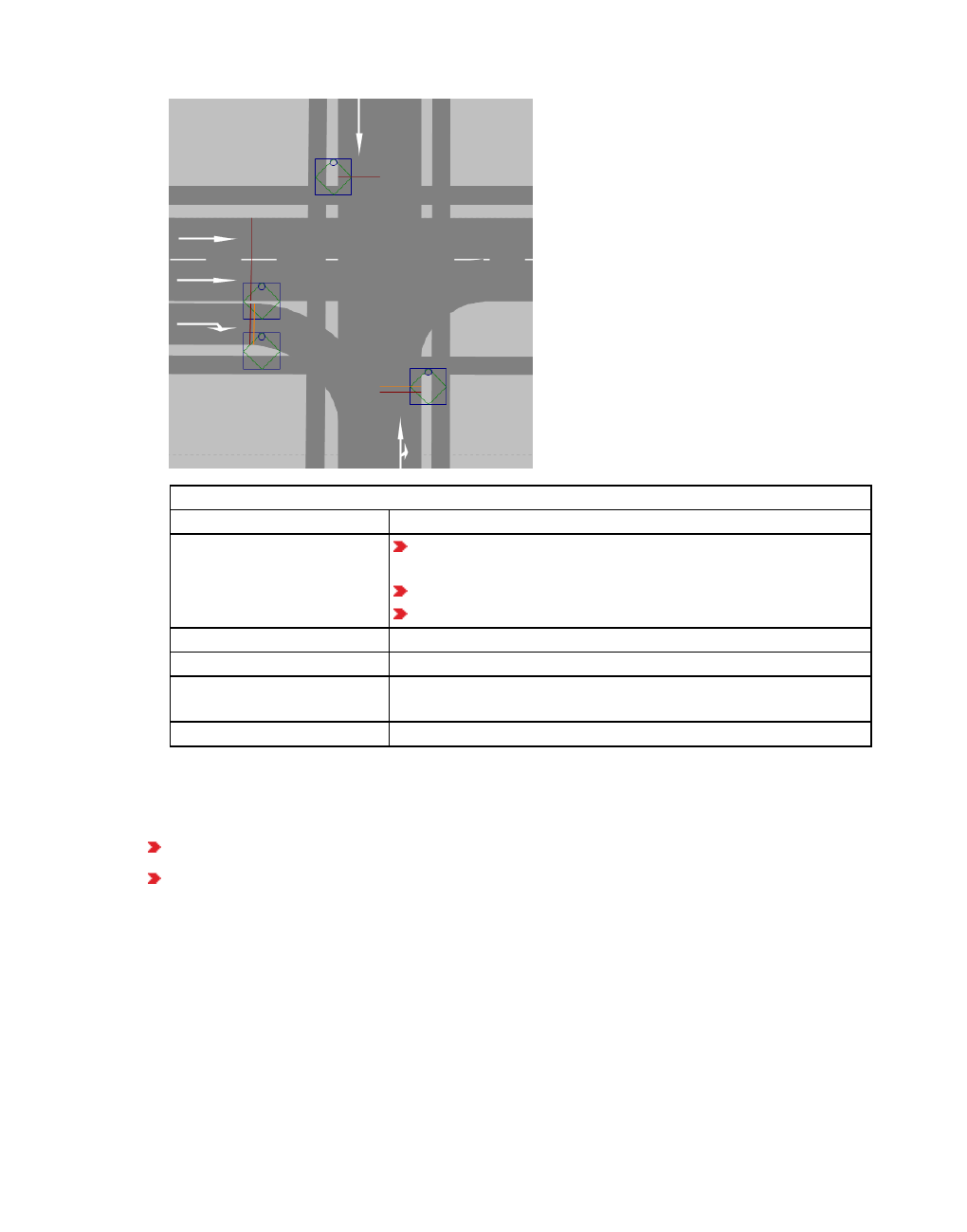
6.14.2 Modeling 3D signal heads
Legend
Element Description
Square 3D signal head not selected: green with a red circle in the
inner square
3D signal head selected: dark blue in 2D mode
3D signal head selected: light blue in 3D mode
Circle Mast
Red line Direction and length of signal arm
Blue arrows on the signal
arm
Signal Heads
Navy blue circles In 2D mode: Signal head directly on the mast
In the 3D mode, in the Network Editor, the 3D model is displayed and selected.
Zooming into the 3D view
Enlarging the view: Rotate the mouse wheel forward.
Minimizing the view: Rotate the mouse wheel backward.
Editing elements in the 3D view
Functions available on the toolbar:
© PTV GROUP 551

6.14.2 Modeling 3D signal heads
Select You can click an element to select it. The attributes of the selected
element are displayed.
Move Colored arrows are displayed next to the element. They indicate
movement towards the x-axis, y-axis and z-axis.
Click an arrow, hold the mouse button down and move the
element.
Rotate The element selected is circled with colored rings in vertical and
horizontal direction.
Click a ring, hold the mouse button down and rotate the element.
Scale For the element selected , lines and cuboids are displayed along
the x-axis, y-axis and z-axis.
Click a cuboid, hold the mouse button down and enlarge or
reduce the size of the element.
Reset view After you have zoomed in or out and wish to center the entire
signal header and show its maximum view.
Zoom to selec-
ted element
Enlarge the view of the selected element.
Deleting arms, signal heads, signs, or street lights
1. In the section on the left, under Signal mast, click the SigalArm <No>, Signal head <No>,
Traffic sign <No>, or Street light <No> of the element you want to delete.
2. On the toolbar, click the button.
3. Confirm with OK.
6.14.2.2 Attributes of 3D signal heads
The 3D signal head window opens automatically when you insert a network object and have
selected to automatically open the Edit dialog after object creation (see "Right-click behavior
and action after creating an object" on page 143). By default, only the 3D Signal Heads list is
opened.
Into the window, you enter attribute values for the network object. For network objects which
have already been defined, you can call the window using the following functions:
In the list of network objects of the network object type, double-click the row with the
desired network object.
In the Network editor, select the network object of your choice. Then, from its shortcut
menu, choose Edit.
The network object may have additional attributes. In the network objects list of the network
object type, you can show all attributes and attribute values. You can open the list via the
following functions:
552 © PTV GROUP

6.14.2 Modeling 3D signal heads
In the network object toolbar, right-click the desired network object type. Then from the
shortcut menu, choose Show List (see "Context menu in the network object toolbar" on
page 63).
In the Network editor, select the network object of your choice. Then, from its shortcut
menu, choose Show In List (see "Selecting network objects in the Network editor and
showing them in a list" on page 339).
From the Lists menu, in the desired category, choose the network object type.
In the network objects list of the network object type, you can edit attributes and attribute
values of a network object (see "Selecting cells in lists" on page 102), (see "Using lists" on
page 89).
The objects of this object type may have relations to other objects. This is why the attributes list
is shown as part of a coupled list (on the left). On the Lists toolbar, in the Relations box, you
can show and edit the coupled list with the attributes of the desired relation on the right (see
below Showing and editing dependent objects as relation) and (see "Using coupled lists" on
page 111).
Note: In lists, you can use the Attribute selection icon to show and hide attribute
values (see "Selecting attributes and subattributes for a list" on page 106).
In the preview, click the desired element or in the section on the left, click the desired entry
Signal mast., SigArms <No>, Signal head <No>, Sign <No>, or Light <No>.
In the preview, the element is selected. In the section on the right, the Properties are
displayed.
1. Make the desired changes:
Mast
properties
Description
Type Mast style (MastStyle): Surface of the mast
Height Vertical length of the mast, default 3,000 m
Diameter MastDiam: Mast diameter, default 0.14 m
Color Click in the box to define or select a color.
Relative
position (x)
Moves mast towards the x axis of the insert position. Negative values move
the mast to the left. The value used is expressed in the Network Editor, in 2D,
by the extent to which the green diamond is moved from the blue square.
Relative
position (y)
Moves mast towards the y axis of the insert position. Negative values move
the mast downwards. The value used is expressed in the Network Editor, in
2D, by the extent to which the green diamond is moved from the blue
square.
Relative
position (z)
Moves the mast vertically. Negative values move the mast downwards.
PosZOffset Position (z-offset): Base height of the mast foot, for example, > 0 for a mast
on a bridge
Scale Zooms in or out of the 3D model in the Network Editor, default value 1000
© PTV GROUP 553

6.14.2 Modeling 3D signal heads
Arm
properties
Description
Type Basic: vertical tube without diagonal frame
Double framed (down): vertical tube with diagonal frame that runs from
the end of the arm, diagonally downward to the signal mast
Double framed (up): vertical tube with diagonal frame that runs from the
end of the arm, diagonally upward to the signal mast
Flipped Select this option if you want the arm to face right.
Deselect this option if you want the arm to face left.
Length Default 5,000 m
Signal properties Description
Type Traffic (vertical)
Traffic (horizontal)
Pedestrian/Bike
Public Transport
Depending on the Type, in the Layout list, you can select different
layouts for signal heads.
Associated con-
troller data
From a list of defined signal groups, select a signal group for the
desired direction of travel
Traffic sign
properties
Description
Shape Geometric shape
Width Length of the longest horizontal expansion of the shape, default 1000
m
Height Length of the longest vertical expansion of the shape, default 5000 m
Inner area width For traffic signs with a frame: horizontal expansion of the inner area
width, default 0.950 m
Inner area height For traffic signs with a frame: vertical expansion of the inner area
width, default 0.950 m
Inner area pos-
ition (x)
Moves inner areas towards the x-axis, default 0.025 m
Inner area pos-
ition (y)
Moves inner areas towards the y-axis, default 0.025 m
Inner area pos-
ition (z)
Moves inner areas vertically, default 0.025 m
Texture Select a graphics file with texture for display
554 © PTV GROUP

6.14.2 Modeling 3D signal heads
Traffic sign
properties
Description
Border Color Click in the box to define or select a color.
Background
color
Click in the box to define or select a color for the inner area.
Street light properties Description
Length Default 3,000 m
Flipped Select this option if you want the streetl ights to face right.
Deselect this option if you want the street lights to face left.
Showing and editing dependent objects as relation
The attribute and attribute values of this network object type are shown in the list on the left,
which consists of two coupled lists.
1. In the list on the left, click the desired entry.
The list on the right contains attributes and attribute values of network objects, and/or base
data allocated to the network object selected in the list on the left (see "Using coupled lists" on
page 111):
Signal arms: Signal arms assigned using the Add Arm button
Signal heads: Signal heads assigned using the Add Signal button
Streetlights: Streetlights assigned using the Add Light button
Traffic signs: Traffic signs assigned using the Add Sign button
The attributes are described further above.
2. On the list toolbar, in the Relations list, click the desired entry.
3. Enter the desired data.
The data is allocated.
6.14.2.3 Editing 3D signal heads in the Network editor
You can move and rotate 3D signal heads in 2D mode in Network Editors.
You can edit 3D signal heads in 2D mode and 3D mode in the 3D Traffic Signal window.
Editing 3D signal heads in 2D Mode
In 2D mode, the mast, signal arm, signal head, sign and light are represented by various
symbols (see "Modeling 3D signal heads" on page 549). You can select and move these
symbols in the Network Editor.
1. In the Network Editor, click with your mouse on the symbol of the component, hold down the
mouse button and drag the cursor to the desired position.
© PTV GROUP 555

6.14.2 Modeling 3D signal heads
2. Release the mouse button.
Editing 3D signal heads in the 3D Traffic Signal window
1. In the Network editor, double-click the desired 3D signal head.
The 3D Traffic Signal window opens. The selected component of the 3D signal head is
displayed in the 3D Traffic Signal window.
2. Make the desired changes:
Element Additional
key
Function Key
Rotate view – Click in the background, hold down mouse
button and drag cursor
Arrow keys or
E,D,S,F
Rotate
component
CTRL Click on component, hold down mouse
button and drag cursor
–
Zoom 3D
Signal Head
– Turn the scroll wheel of the mouse PAGE UP
PAGE DOWN
The changes are displayed in the 3D Traffic Signal window.
3. To edit one of the components, double-click the desired component in the 3D Traffic Signal
window.
4. The <Name component> window opens (Attribute von 3D-Signalgebern).
5. Make the desired changes:
Function Additional
key
Action with the mouse
Move component SHIFT Click and drag object
Rotate component around
center
CTRL Click and drag object
Scale component – Select object, then turn scroll wheel of
mouse
If you want to move or rotate other components, arrows indicate the direction in which you
can execute a function:
556 © PTV GROUP

6.14.3 Using detectors
Move:
Rotate:
6.14.3 Using detectors
You can use detectors to record vehicles or pedestrians for vehicle-actuated signal controls.
A detector must be assigned to the desired SC and can be limited to the PT lines of your
choice (see "Attributes of detectors" on page 558).
To record traffic volumes in your Vissim network, use data collection points and evaluate them
with data collection measurements (see "Defining data collection points" on page 419), (see
"Evaluating data collection measurements" on page 1033).
6.14.3.1 Using detectors to record vehicles
In order to record vehicles for traffic-actuated signal control, various types of detectors are
deployed, such as induction loops, infra-red sensors, pedestrian push buttons, overhead wire
© PTV GROUP 557

6.14.3 Using detectors
contacts, point-blocking circuits or reporting points for radiotelegrams.
In Vissim, you model detectors as network objects on links for which you enter a length. A
message impulse is then transmitted to the signal controller as soon as the front of a vehicle
reaches the detector. Another impulse is transmitted as soon as the tail of the vehicle leaves
the detector. These message impulses are interpreted by signal control logic and converted
into appropriate switching signals for control.
6.14.3.2 Using detectors to record pedestrians
Vissim recognizes pedestrians on pedestrian links by means of detectors. If a pedestrian
leaves a pedestrian link or enters a free pedestrian link, Vissim detects this at the end of a SC
time step. The change from occupied to vacant or vacant to occupied are transmitted to the
control logic as the front ends and rear ends. If you have selected a sound file, it is started
when the first pedestrian arrives at an empty detector.
6.14.3.3 Defining detectors
You must have defined at least one SC (see "Defining SC and signal control procedures" on
page 567).
1. On the Network objects toolbar, click Detectors.
2. With the mouse pointer, point to the position in the link at which the detector is to begin.
3. Hold down the CTRL key and the right mouse button, and drag the pointer to the desired
end position.
4. Release the keys.
The detector is added. The Detector window opens.
5. Edit the attributes (see "Attributes of detectors" on page 558).
6. Confirm with OK.
The attributes are saved in the Detectors list.
6.14.3.4 Attributes of detectors
The Detectors window opens automatically when you insert a network object and have
selected to automatically open the Edit dialog after object creation (see "Right-click behavior
and action after creating an object" on page 143). By default, only the Detectors list is opened.
Into the window, you enter attribute values for the network object. For network objects which
have already been defined, you can call the window using the following functions:
In the list of network objects of the network object type, double-click the row with the
desired network object.
In the Network editor, select the network object of your choice. Then, from its shortcut
menu, choose Edit.
558 © PTV GROUP

6.14.3 Using detectors
The network object may have additional attributes. In the network objects list of the network
object type, you can show all attributes and attribute values. You can open the list via the
following functions:
In the network object toolbar, right-click the desired network object type. Then from the
shortcut menu, choose Show List (see "Context menu in the network object toolbar" on
page 63).
In the Network editor, select the network object of your choice. Then, from its shortcut
menu, choose Show In List (see "Selecting network objects in the Network editor and
showing them in a list" on page 339).
From the Lists menu, in the desired category, choose the network object type.
In the network objects list of the network object type, you can edit attributes and attribute
values of a network object (see "Selecting cells in lists" on page 102), (see "Using lists" on
page 89).
The objects of this object type may have relations to other objects. This is why the attributes list
is shown as part of a coupled list (on the left). On the Lists toolbar, in the Relations box, you
can show and edit the coupled list with the attributes of the desired relation on the right (see
below Showing and editing dependent objects as relation) and (see "Using coupled lists" on
page 111).
Note: In lists, you can use the Attribute selection icon to show and hide attribute
values (see "Selecting attributes and subattributes for a list" on page 106).
The basic attributes of the network element are shown in the upper area of the window and in
the list of network objects for the particular network object type.
Element Description
Port no. Physical Port number (PortNo) of the detector, which identifies the detector in the
control procedures. If multiple detectors of SC (signal control) are available via the
same number, they behave as if they are connected in parallel to one entry port of
the control device (logical OR-operation).
Name Designation
Length Length of the detection range of a detector. The value 0.000 is e.g. permissible and
useful for modeling trolley wire contacts and pedestrian sensors. These are rep-
resented in the network as thin horizontal lines.
SC SC to which detector is assigned. If in the Type box, > PT Calling Pt. is selected,
the SC box is deactivated. PT calling points do not belong to a specific SC.
Type Type: Select detector type (see "Modeling PT lines" on page 485):
Standard: Standard detectors detect vehicles, including PT vehicles.
Pulse: Impulse detectors do not send information regarding occupancy to the
control procedures.
Presence: does not send information regarding the impulse via the front end or
back end of the vehicle to the control procedures.
PT calling pt (PT calling point): only records PT vehicles that send PT tele-
grams.
© PTV GROUP 559

6.14.3 Using detectors
Location tab
The list in the tab contains, amongst others, the following attributes:
Element Description
Link Link, in which the detector is located
Lane Ln: Number of lane on which the detector is installed.
At Position (Pos) Distance from start of the link or connector
Before
stop
if a signal head exists: Distance of the front end of the detector to the next signal
head of the SC (signal control) on its lane
560 © PTV GROUP
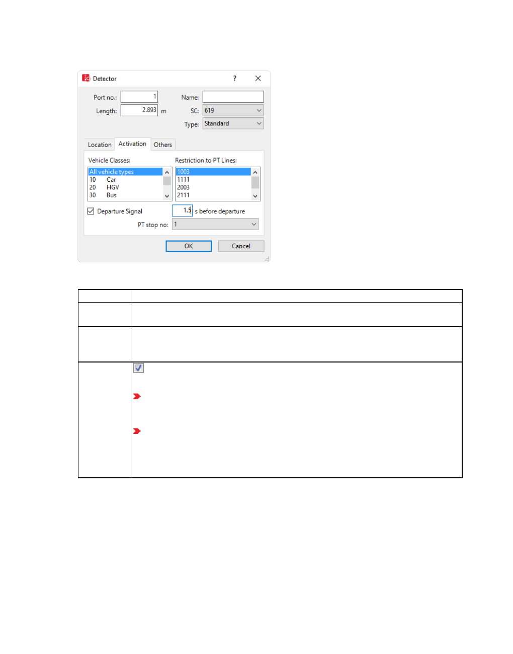
6.14.3 Using detectors
Activation tab for vehicles
The list in the tab contains, amongst others, the following attributes:
Element Description
Vehicle
Classes
VehClasses: Vehicle classes detected by detector
Restriction
to PT
Lines:
PTLines: One or multiple PT lines, for which the detector shall be relevant. Thus
vehicles of these PT lines are only detected if their vehicle class is selected.
Departure
Signal If this option is selected, the detector triggers an impulse for closing the doors
of the PT vehicle under the following conditions:
If a PT vehicle is located on a detector and stops at the stop specified in the
PT stop box, plus the boarding and alighting is completed in the first time
step after the time defined in the s before departure box or before then.
When a PT vehicle is located on a detector that has already decided to omit
the PT stop selected in the PT stop box. The impulse is then triggered upon
reaching the detector.
The time the door is closed can thus be determined via the detector.
Activation tab for pedestrians
If the detector is defined for a link whose attribute is Is pedestrian area (option Use as
pedestrian area), the detector serves for modeling calls via a pedestrian crossing button and
pedestrian classes are displayed.
© PTV GROUP 561
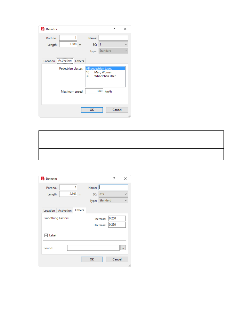
6.14.3 Using detectors
1. Make the desired changes:
Element Description
Pedestrian
Classes
Pedestrian classes detected by detector. A pedestrian is recognized by the
detector only if the pedestrian type belongs to a selected pedestrian class.
Maximum
speed
The detector recognizes pedestrians walking slower than this speed as
pedestrians requesting a green light.
Others tab
1. Make the desired changes:
562 © PTV GROUP

6.14.3 Using detectors
Element Description
Smoothing
Factors
SmthFactDecr, SmthFactIncr: Factors for the exponential smoothing of
occupancy values, which is conducted for individual control procedures. (see
"Exponential smoothing of detector occupancy rates" on page 565).
Smoothing factor decrease: Factor used whien the detector is not occu-
pied (attribute Presence = Passive).
Smoothing factor increase: Factor used when the detector is occupied
(attribute Presence = Active).
Label If the option is not selected, the label for the detector is not displayed,
even if the label for all detectors is selected.
Sound file
(Sound)
SoundFile: Wavetable sound file *.wav, which is played each time a vehicle
is detected by the detector. This file is saved in the same folder as the
network file *.inpx. A sound card or suitable Microsoft Windows driver must
be installed.
2. Confirm with OK.
The network object has additional attributes that you can show in the Attributes list. Among
them are the following for example:
© PTV GROUP 563

6.14.3 Using detectors
Element Description
Presence Presence state:
Active: A vehicle is located on the detector and is detected. This also
applies for pedestrians.
Always Passive for detectors of the type Impulse and PT Calling Pt..
A vehicle is located on a detector, if the following conditions apply:
The vehicle is located on the same link as the detector.
The front edge of the vehicle has passed the start section of the detector:
The Position (Pos) attribute of the vehicle is greater than the Position
(Pos) attribute of the detector.
The rear edge of the vehicle has not yet passed the end section of the
detector: The Position (Pos) attribute of the vehicle, minus the length of
the vehicle (rear edge), is smaller than the Position (POS) attribute of the
detector, plus the length of the detector (end position).
A pedestrian is considered on a detector, if the center of the pedestrian is
located within the rectangle that defines the length of the detector and the
width of the lane on which the detector is located.
Ensure that the detector is at least as long as the distance a pedestrian can
walk within a simulation time step back. In addition, account for the
maximum possible speed of the pedestrian at this position. If the detector
dimensions are too short, meaning that in one time step, the center of the
pedestrian will be in front of the detector and in the the next time step, the
pedestrian will be behind it (having already passed it), the detector will not
be able to detect the pedestrian. In front of and behind refer to the visually
assessed walking direction on the pedestrian link. As pedestrians have no
link coordinate, Vissim cannot determine whether the walking direction is
towards or away from the detector.
Detection Detection state:
Active for detectors of the types Standard and Occupancy, as long as
the Presence attribute is active.
Active for detectors of the types Standard and Impulse after a vehicle or
pedestrian occupies or leaves a detector, until the signal controller
resets the detection state to Passive.
A fixed time control resets the value of the Detection attribute after each
SC-time step.
Always Passive for detectors of the type PT Calling Pt.
564 © PTV GROUP

6.14.3 Using detectors
Element Description
Impulse Impulse state:
Active, as soon as a vehicle or pedestrian reaches a detector that is not
occupied. The impulse state remains Active until the signal controller
resets the impulse state back to Passive.
A fixed time control resets the value of the Impulse attribute after each
SC-time step.
Always Passive for detectors of the type Occupancy and PT Calling Pt..
Gap time Time: Period [s] after the attribute Presence (Presence state) had the value
Active. 0 = Presence attribute is Active.
Occupancy Occ: Period [s] that has passed since occupancy of the detector. 0 = The
detector is not occupied (Presence attribute = Passive). Always 0 for
detectors of the type PT Calling Pt.
Occupancy
rate
OccupRate: Proportion of time the detector was occupied during the last
simulation second. The occupancy rate is exponentially smoothed based on
each simulation second. Value range 0 to 100 %
Showing and editing dependent objects as relation
The attribute and attribute values of this network object type are shown in the list on the left,
which consists of two coupled lists.
1. In the list on the left, click the desired entry.
The list on the right contains attributes and attribute values of network objects, and/or base
data allocated to the network object selected in the list on the left (see "Using coupled lists" on
page 111):
Vehicle classes (see "Using vehicle classes" on page 267)
Pedestrian classes (see "Using pedestrian classes" on page 832)
Public transport lines (see "Modeling PT lines" on page 485)
The attributes are described further above.
2. On the list toolbar, in the Relations list, click the desired entry.
3. Enter the desired data.
The data is allocated.
6.14.3.5 Exponential smoothing of detector occupancy rates
You can use exponential smoothing to smooth the occupancy rate of a detector. This is
necessary as detectors are either fully occupied or not occupied and thus do not provide
sufficient information for signal control decisions. Exponential smoothing allows you to
calculate the occupancy rate with help of the following equation, using the last t seconds:
Thereby the following applies:
© PTV GROUP 565
6.14.4 Using signal control procedures
s(t) new, exponentially smoothed value
s(t-1) old, exponentially smoothed value (1 second ago)
xnew detector value
αSmoothing factor [0 to 1]
This means the new, exponentially smoothed value is the weighted average of the new,
detected value and the exponentially smoothed value after the last simulation second.
The new detector occupancy rate is weighted with alpha.
The old, smoothed value is weighted with (1 - α).
In Vissim, you can use the following attributes to enter different values for alpha (see
"Attributes of detectors" on page 558):
Increase: For increasing x values (x > s(t-1))
Decrease: For decreasing x values (x < s(t-1))
The exponentially smoothed occupancy rate represents a kind of a floating average of the
detected values of all previous time steps. Thereby the most current values are weighted the
strongest. With α = 1, there is no smoothing. The equation then equals the new detector value
x.
In the Vissim network, in the attribute list Detectors, you can show values of the attributes
Occupancy rate (OccupRate) in % and Occupancy (Occup) i (see "Editing attributes in a list"
on page 330).
6.14.4 Using signal control procedures
You can define new SCs with your signal groups. To do so, for the control procedure, select a
type. This e.g. specifies whether you want the SC to be fixed-time controlled or controlled via a
control procedure. Depending on your Vissim license, you can access add-on modules with
external signal control procedures (see "Showing licensed signal control procedures" on page
571).
Determining the cycle second for a fixed cycle time
Vissig determines the current cycle second for the SC type Fixed time.
For the SC types VAP, TRENDS, VS-PLUS and Siemens VA, Vissim determines the current
cycle second.
In Vissim, the first cycle starts at 00:00:00. At the simulation start, the cycle second is
calculated based on this start time.
If the start time specified in the simulation parameters is 00:00:00, the cycle and sim-
ulation start at the same time.
If the start time specified in the simulation parameters is not 00:00:00, at the simulation
start, the current cycle second may have a different value than 0, as the first cycle was
started at 00:00:00.
566 © PTV GROUP

6.14.4 Using signal control procedures
Some control procedures expect the supply file to be saved in the same directory that contains
the *.inpx file. If a control file is saved to a directory that does not meet the requirements of the
control procedure, this can cause the program to crash. The supply files of the control
procedures Fixed time/Vissig, VAP and RBC can be saved to any directory Vissim can access.
Vissim does not need the supply files to be saved to a specific directory. Should you have any
questions regarding supply files, please contact the company that developed the control
procedure.
6.14.4.1 Defining SC and signal control procedures
1. From the Signal Control menu, choose > Signal Controllers.
The Signal Controllers list opens.
The attribute and attribute values of this network object type are shown in the list on the left,
which consists of two coupled lists.
2. In the list, on the toolbar, click the Add button .
A new row with default data is inserted.
The Signal Controller window opens.
© PTV GROUP 567

6.14.4 Using signal control procedures
3. In the Signal Controller window, in the upper section, enter the desired basic attributes
(see "Attributes of SC" on page 568).
4. Depending on the signal controller selected in the Type list, in the Controller configuration
tab, make the desired settings. These vary depending on the type selected. For further
information, read the following sections:
Using the SC type Fixed time (see "Using SC type Fixed time" on page 571).
In the description of the signal control procedure selected (see "Modeling signal con-
trollers" on page 542), (see "Overview of add-on modules" on page 38).
5. If for the types Fixed time, Epics/Balance-Central or External you want to create or edit
signal programs using Vissig, click the Edit SC button (see "Opening and using the SC
Editor" on page 595).
6. To evaluate simulation data, in the tabs Signal Times Table Config. or SC Detector
Record Config., make the settings of your choice depending on the control procedure (see
"Showing signal times table in a window" on page 1038), (see "Evaluating SC detector
records" on page 1010).
7. Enter the desired data.
8. Confirm with OK.
9. Save the network file *.inpx.
You can edit the attributes in the attributes list (see "Attributes of SC" on page 568).
6.14.4.2 Attributes of SC
The Signal Controller window opens when you define an SC and have selected that you want
the program to automatically open the Edit dialog after object creation (see "Right- click
behavior and action after creating an object" on page 143) . By default, only the Signal
controllers list is opened.
Into the Signal Controller window, you enter attribute values for the signal controller. For a
signal controller which has already been defined, you can call the window using the following
function:
In the Signal Controllers list, double-click the row with the desired SC.
The network object may have additional attributes. You can show all attributes and attribute
values of a network object in the Signal Controllers list. You can open the list via the following
function:
From the Lists menu, choose > Intersection Control > Signal Controllers.
In the network objects list of the network object type, you can edit attributes and attribute
values of a network object (see "Selecting cells in lists" on page 102), (see "Using lists" on
page 89).
Every signal controller can have relations to other objects. This is why the attributes list is
shown as part of a coupled list (on the left). On the Lists toolbar, in the Relations box, you can
show and edit the coupled list with the attributes of the desired relation on the right (see below
568 © PTV GROUP

6.14.4 Using signal control procedures
Showing and editing dependent objects as relation) and (see "Using coupled lists" on page
111).
Note: In lists, you can use the Attribute selection icon to show and hide attribute
values (see "Selecting attributes and subattributes for a list" on page 106).
Basic attributes of SC
The basic attributes of the network element are shown in the upper area of the window and in
the list of network objects for the particular network object type.
Element Description
No. Unique number of the SC
Name Description
Active Enables or disables the SC during simulation
Cycle
time
Optional cycle time (CycTm). Duration in seconds. Only for control procedures
Siemens VA, TRENDS, VAP, VS Plus, as for these the cycle time is not set
externally.
variable The cycle time is variable (CycTmIsVar)
Type Control procedures for SC
Offset The times of the first cycle and all others are moved back by the offset time in [s].
© PTV GROUP 569

6.14.4 Using signal control procedures
Under them, the following tabs are displayed:
Controller configuration: Select a procedure-dependent control file
Signal Times Table Config.: Configure signal times table that runs during the simulation
(see "Showing signal times table in a window" on page 1038).
SC Detector Record Config.: Configure SC detector record for SC with external control
procedure (see "Evaluating SC detector records" on page 1010).
For the control procedures Siemens VA, TRENDS, VAP AND VS-Plus, the Signal groups tab
is displayed, as for them the signal groups are not set externally (see "Defining signal groups
for Siemens VA, TRENDS, VAP, VS-Plus" on page 594).
Showing and editing dependent objects as relation
The Signal Controllers list is displayed as the left of two coupled lists.
In the list on the left, you can select an SC. In the list on the right, you can show the objects
assigned to it. Depending on the procedure type (Type attribute) used, there are the following
restrictions:
Relations are not available for all procedure types.
Relations cannot be edited as attribute values with all procedure types.
1. On the list toolbar, in the Relations list, click the desired entry.
Detector attributes (see "Attributes of detectors" on page 558)
Attributes of SC detector record configuration (see "Evaluating SC detector records" on
page 1010)
Attributes of signal groups: Select Normal, Flashing, or Green arrow
Attributes of the signal times table configuration (see "Configuring signal times table on
SC" on page 1040)
WTT file assigned (see "Other files" on page 1136)
The right-hand list is shown. If there is no assignment, only the column titles are shown.
6.14.4.3 Changing control procedures for SC type
You can choose between a traffic-dependent procedure and Fixed time for the SC type.
Depending on the type, parameters such as amber time, red amber time, start of green may be
missing. Add these after changing the control procedure.
Parameters of the old type which are no longer required are deleted. If you switch back to the
old type, you must re-enter these parameters.
1. From the Signal Control menu, choose > Signal Controllers.
The Signal Controllers list opens.
2. Right-click the entry of your choice.
3. From the shortcut menu, choose Edit....
570 © PTV GROUP

6.14.4 Using signal control procedures
The Signal Controller window opens.
4. In the Type list box, click the control procedure of your choice.
5. Add the missing data in the tabs.
6.14.4.4 Showing licensed signal control procedures
From the Help menu, choose > License.
The licensed signal control procedures are highlighted in the Signal Controllers section.
6.14.4.5 Using SC type Fixed time
The SC type Fixed time allows you to define fixed time signal controllers. To edit the signal
plan, you use the graphical SC editor. Depending on the Vissim license, you have add-on
functions in the SC editor with Vissig, which deviate from the standard version of Vissim (see
"Opening and using the SC Editor" on page 595).
Vissig determines the current cycle second for a fixed cycle time
In Vissim, the first cycle starts at 00:00:00. At the simulation start, the cycle second is
calculated based on this start time.
If the start time specified in the simulation parameters is 00:00:00, the cycle and sim-
ulation start at the same time.
If the start time specified in the simulation parameters is not 00:00:00, at the simulation
start, the current cycle second may have a different value than 0, as the first cycle was
started at 00:00:00.
1. From the Signal Control menu, choose > Signal Controllers.
The Signal Controllers list opens.
2. Right-click the entry of your choice.
3. From the shortcut menu, choose Edit.
The Signal Controller window opens.
© PTV GROUP 571

6.14.4 Using signal control procedures
4. In the Type field, select > Fixed time.
Note:
The Cycle time section is not enabled. You cannot edit the base attributes Cycle
time and Offset in the Signal controller window. To change these attributes, click
the Edit Signal Control button. Then in the navigator, select Signal programs. In
the table, you can edit Cycle time, Offset, and Switch point (see "Opening and
using the SC Editor" on page 595).
The current cycle second (determined by Vissim for a fixed cycle time) is calculated
based on the start of the first cycle at midnight. This makes no difference when
00:00:00 is set as the start time.
5. Open the Controller configuration tab.
6. Make the desired changes:
572 © PTV GROUP
6.14.4 Using signal control procedures
Element Description
VISSIG
supply
file
Signal control file *.sig in XML format.
Notes:
When importing older Vissim network files, the files *.sig are auto-
matically created and stored in the directory in which the network file
*.inpx is stored.
When you duplicate a SC, the original SC and the duplicate both
use the same signal control file *.sig. This means the changes you
make to a SC affect all SCs that use the same signal control file
*.sig.
Program
no.
ProgNo.: The signal program or daily signal program list that you want to
simulate (see "Defining and editing daily signal program lists" on page 628). A
change of program is possible if the simulation run is in single-step mode. If the
new signal program number is confirmed with OK, the changeover is triggered
in the next simulation second.
Edit Sig-
nal Con-
trol
button
The signal program editor opens (see "Opening and using the SC Editor" on
page 595). The signal groups must be created or deleted in the SC Editor.
Changes in the channel number of existing signal groups are detected in
Vissim and adjusted accordingly in the corresponding signal heads.
Note: The SC frequency is loaded from the external data of the
controller.
Internally, the SC frequency is the smallest integer multiple of all SC
frequencies. The value may not exceed 10 because Vissim allows a
maximum of ten simulation steps per second.
The control procedure additionally uses the following files:
Element Description
Program
file
ProgFile: File with control logic, VISSIG_controller.dll by default
Dialog
DLL file
GUIFile: File name of supply interface, VISSIG_GUI.DLL by default
Supply
file 1
SupplyFile1: Configuration file, vissig.config by default.
Note: If the supply files are stored in the Exe directory of your Vissim
installation, they are automatically loaded.
WTT
files
WTTFile: Value type tables: Contain the data types of the control logic and the
type of display in the SC detector record or in the Signal times table window.
VISSIG.wtt by default.
Performing green time optimization of stage-based fixed time controllers
Note: You will need the add-on module Vissig.
© PTV GROUP 573
6.14.4 Using signal control procedures
You can improve the quality of the signal times table of a selected Vissig SC or all Vissig SCs
with the green time optimization of stage-based fixed time controllers.
To this end, Vissim repeatedly calculates simulations of the entire network. All controllers are
disabled in the process, except the SCs selected. Thus upstream SCs have no effect. The
simulations are continued as long as changes in green times of the stages lead to an increase
in the flow (volume) or to a reduction in the average vehicle delay. You can also cancel the
iteration. The stage lengths with the best result have the highest flow and the lowest average
vehicle delay and are stored in the *.sig file after the optimization.
Sequence of optimization in Vissim
Vissim determines the average delay of all vehicles that have passed through the nodes
on the lanes with signal heads of the signal group, using an automatically created node
evaluation for each signal group over the entire simulation run.
For optimizing, the signal group in which the vehicles have the highest delay is determ-
ined for each stage.
The stage with the lowest maximum average delay is selected as the best stage.
The stage with the highest maximum average delay is selected as the worst stage.
A second of green time is deducted from the best stage.
A second of green time is added to the worst stage.
If a second can no longer be deducted from the best stage, the second best stage is used.
If this can no longer be shortened, the next worst stage is always taken iteratively. If no
other stage can be shortened, the optimization is terminated.
A signal program is considered to be better than another if one of the following criteria is
met:
If the flow formed by the total number of vehicles driven through the node during the
simulation run has increased significantly by at least 25 vehicles or by 10% if this is
less.
If the flow has not significantly decreased by 25 vehicles or by 10% and the average
delay across all vehicles has decreased.
If a signal program is better than the best rated, it replaces this as the best. The optim-
ization is continued with the next step.
The optimization is terminated if one of the following criteria is met:
Once the signal program does not improve within 10 simulation runs.
Once the flow decreases by more than 25% compared to the best signal program.
Once the average delay increases by more than 25%.
Requirements for the green time optimization of stage-based fixed time controllers
Ensure that the following requirements are met:
574 © PTV GROUP

6.14.4 Using signal control procedures
The following must be defined in Vissig:
Signal groups (see "Defining signal groups in the SC editor" on page 603)
Intergreen matrix (see "Defining an intergreen matrix" on page 606)
Stages (see "Defining and editing stages" on page 609)
Stage based signal program (see "Defining signal programs" on page 617)
The following must be defined in Vissim:
Signal heads (see "Defining signal heads" on page 544)
a surrounding node that contains the junction with the SC for node evaluation (see
"Defining nodes" on page 668), (see "Evaluating nodes" on page 997)
Adjacent nodes for legs of junction
The interstages must include the minimum green times and relevant intergreens because
the length of a stage can be reduced to zero by optimizing. The signal program must be
consistent even if all stages have zero duration.
The stage-based signal program has a user-defined cycle time and stages of any length.
You can use the stage length that was proposed in Vissig when generating the signal pro-
gram from interstages, for example, an equal distribution across all. You can use the pro-
posed stage length because the original stage lengths are changed by optimizing.
The demand and the path selection must be defined in the Vissim network. The following
must thus be defined:
Vehicle inputs and routing decisions (see "Defining vehicle inputs" on page 428), (see
"Modeling vehicle routes, partial vehicle routes, and routing decisions" on page 430)
or for dynamic assignment, parking lots or parking lots and a trip chain file (see "Defin-
ing parking lots for dynamic assignment" on page 660), (see "Modeling traffic demand
with origin-destination matrices" on page 681), (see "Modeling traffic demand with trip
chain files" on page 690)
a path file (see "Attributes for the trip chain file, matrices, path file and cost file" on page
731), (see "Path search and path selection" on page 698)
The route choice does not necessarily have to be defined by static node flow routes. You
can also use the dynamic assignment or static routes across multiple nodes because it is
only required that the vehicles drive through the nodes of the SC.
Other signal controls are not considered.
Starting green time optimization for an SC
1. From the Signal Control menu, choose > Signal Controllers.
The Signal Controllers list opens.
2. Right-click the entry of your choice.
3. From the shortcut menu, choose Optimize Signal Control.
© PTV GROUP 575

6.14.4 Using signal control procedures
Starting green time optimization for all SCs
From the Signal Control menu, select Optimize All Fixed Time Signal Controllers.
6.14.4.6 Using Balance-Central signal controllers
Note: You need a license for the signal controller.
The Balance-Central signal controller allows you to simulate adaptive light signal control
using real time traffic data and thus also enables you to simulate adaptive network control.
An example and information on Balance-Central in English can be found in the directory
..\Examples\Examples Training\Signal Control\UTC - Workflow PTV Balance PTV Epics.
1. When you define an SC, in the Type list, click Balance-Central.
2. Open the Controller configuration tab.
3. Make the desired changes.
Element Description
Parameters
button
Showing Balance Central-parameters. You can change the parameters and
save them to the Balance.ini file. After making changes, you can save the
file to the default directory ..\Users\Public\Public
Documents\PTV Vision\PTV Vissim or another directory of your choice.
Network
data
*.anm file with abstracted network model data
576 © PTV GROUP
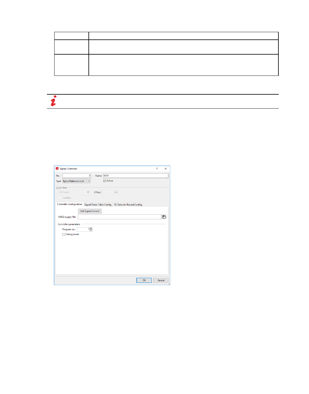
6.14.4 Using signal control procedures
Element Description
Demand
data
*.anmroutes file with volumes and routes
Balance
Central
parameters
Specify path to an *.ini file that contains Balance-Central parameters. Click
the Parameters button to display the parameters in the file.
6.14.4.7 Using Epics/Balance-Local signal controllers
Note: You need a license for the signal controller.
The Epics signal control allows you to simulate adaptive light signal control for an individual
node using real time traffic data.
Examples and information on Balance- Central in English can be found in the directory
..\Examples\Examples Training\Signal Control\UTC - Workflow PTV Balance PTV Epic and
..\Tram Priority.PTV Epics.
1. When you define an SC, in the Type list, click Epics/Balance-Local.
2. Open the Controller configuration tab.
3. Make the desired changes:
© PTV GROUP 577
6.14.4 Using signal control procedures
Element Description
Program
no.
ProgNo: The signal program which is to be simulated. A change of program is
possible if the simulation run is in single-step mode. If the new signal program
number is confirmed with OK, the changeover is triggered in the next sim-
ulation second.
Debug
mode Debug mode enabled (Debug): If this option is selected, the signal flow can
be followed during simulation in debug mode.
6.14.4.8 Add-on module Econolite ASC/3
Note: You must have a license for the add-on module.
Econolite ASC/3 is a control procedure used in North America. For further information, please
visit:
http://www.econolite.com/index.php/products/controllers/software/#software
Some control procedures expect the supply file to be saved in the same directory that contains
the *.inpx file. If a control file is saved to a directory that does not meet the requirements of the
control procedure, this can cause the program to crash. The supply files of the control
procedures Fixed time/Vissig, VAP and RBC can be saved to any directory Vissim can access.
Vissim does not need the supply files to be saved to a specific directory. Should you have any
questions regarding supply files, please contact the company that developed the control
procedure.
You are provided with the asc3gui.dll files and the asc3.dll program file for your 32-bit or 64-bit
Vissim version licensed.
Note: Current versions of ASC/3 use the asc3gui.dll file. In old projects, replace the old
file name asc3_gui.dll by the new file name asc3gui.dll.
The control procedure additionally uses the following files:
When you add an SC of the type Econolite ASC/3, the respective files are automatically saved
to the Exe directory of your Vissiminstallation:
Data file *.db
Program file asc3.dll
Dialog DLL file asc3gui.dll
File with value type tables ASC3.wtt
1. If desired, click the Parameters button.
The Econolite database editor opens.
2. Make the desired changes.
3. If desired, click the Edit Mapping button.
The ASC3 I/O mapper opens.
4. Make the desired changes.
578 © PTV GROUP

6.14.4 Using signal control procedures
6.14.4.9 Add-on module external signal control SC
Note: You must have a license for the add-on module.
You can simulate with the add-on module Signal Controllers. This is available as a separate
executable program (*.exe) or program library (*.dll). These can either be standard procedures
supplied by PTV GROUP or other providers, or procedures that users have developed
themselves (using the API add-on).
The files must be in the programming language C or C++.
Note: The DLL files must be compiled appropriately for the Vissim 32-bit version or 64-
bit version in use.
Some control procedures expect the supply file to be saved in the same directory that contains
the *.inpx file. If a control file is saved to a directory that does not meet the requirements of the
control procedure, this can cause the program to crash. The supply files of the control
procedures Fixed time/Vissig, VAP and RBC can be saved to any directory Vissim can access.
Vissim does not need the supply files to be saved to a specific directory. Should you have any
questions regarding supply files, please contact the company that developed the control
procedure.
If you have a license which includes the SC type External, the API source code modules and
the documentation can be found in the API folder of your Vissim installation.
1. From the Signal Control menu, choose > Signal Controllers.
The Signal Controllers list opens.
2. Right-click the entry of your choice.
3. From the shortcut menu, choose Edit.
The Signal Controller window opens.
© PTV GROUP 579

6.14.4 Using signal control procedures
4. In the Type field, select > External.
5. Make the desired changes:
Element Description
Program file ProgFile: User-defined DLL file with control logic
Dialog DLL file GUIFile: User-defined DLL file of supply interface
Data file 1 SupplyFile1: Data for the control logic
Note: The supply files are only necessary if you do not
want to include the data of the control logic in the
program text of your user-defined DLL file.
Data file 2 SupplyFile2: Data for the control logic
Controller parameters ProgNo (Program number):The signal program you want to
simulate. The signal program number can be specified for an
SC of type External. This is also possible during the
simulation run.
580 © PTV GROUP

6.14.4 Using signal control procedures
Element Description
Debug mode Debug mode enabled (Debug): If this option is selected,
the signal flow can be followed during simulation.
WTT files WTTFile: Value type tables: The tables contain the data types
of the control logic and the type of display in the SC detector
record or in the Signal times table window. By default, a
vissig.wtt file is saved to the Exe folder of your Vissim
installation. A WTT file must not necessarily be specified.
File names with a path for the program file, the dialog DLL and the *.wtt files can be transferred
to external signal controllers. The paths are saved as relative paths that contain the current
data directory, in which the network file *.inpx is stored, or the program directory, in which the
file VISSIM<version number>.exe is stored. Thus these can still work even after the data
directory is moved or copied to another computer.
Note: The signal program number for an SC of type External can also be specified
during the simulation run. The signal program is then changed during the next switch
point.
Documentation in English
..\<VISSIM Version>\API\SignalControl_DLLs\SC_DLL\SC_DLL_Interface.doc
Examples
..\<VISSIM Version>\API\SignalControl_DLLs\Examples\
6.14.4.10 Add-on module Fourth Dimension
Note: You must have a license for the add-on module.
This control procedure is deployed in North America.
Depending on the Vissim edition purchased, you are provided with the dialog file D4gui.dll
and the program file D4.dll files for the 32-bit or 64-bit version.
Some control procedures expect the supply file to be saved in the same directory that contains
the *.inpx file. If a control file is saved to a directory that does not meet the requirements of the
control procedure, this can cause the program to crash. The supply files of the control
procedures Fixed time/Vissig, VAP and RBC can be saved to any directory Vissim can access.
Vissim does not need the supply files to be saved to a specific directory. Should you have any
questions regarding supply files, please contact the company that developed the control
procedure.
1. When you define an SC, in the Type list, click Fourth Dimension D4.
2. Select the desired data file.
3. Make the desired changes:
© PTV GROUP 581

6.14.4 Using signal control procedures
Element Description
Data file ProgDat: Supply file of control logic
Program
no.
ProgNo: The signal program which is to be simulated. A change of program is
possible if the simulation run is in single-step mode. If the new signal program
number is confirmed with OK, the changeover is triggered in the next sim-
ulation second.
The control procedure also uses a WTT-file, e.g. D4.wtt.
6.14.4.11 Add-on module LISA+ OMTC
Note: You must have a license for the add-on module.
Some control procedures expect the supply file to be saved in the same directory that contains
the *.inpx file. If a control file is saved to a directory that does not meet the requirements of the
control procedure, this can cause the program to crash. The supply files of the control
procedures Fixed time/Vissig, VAP and RBC can be saved to any directory Vissim can access.
Vissim does not need the supply files to be saved to a specific directory. Should you have any
questions regarding supply files, please contact the company that developed the control
procedure.
LISA+ OMTC is a control procedure developed by SCHLOTHAUER & WAUER, a traffic
engineering company in Berlin, Germany.
1. Ensure that you have a dialog.dll file and a *.wtt file, e.g. VISSIM2LisaDlg.dll and Lisa_
Vissim.wtt.
2. When you define an SC, in the Type list, click LISA+ OMTC.
3. In the Data file box, select the file of your choice.
4. To open LISA+ configuration, click the LISA+ Configuration button.
5. To edit the settings for the signal groups, click the Edit signal groups button.
6. Make the desired changes.
6.14.4.12 Add-on module McCain 2033
Note: You must have a license for the add-on module.
McCain 2033 is a control procedure deployed in North America.
Some control procedures expect the supply file to be saved in the same directory that contains
the *.inpx file. If a control file is saved to a directory that does not meet the requirements of the
control procedure, this can cause the program to crash. The supply files of the control
procedures Fixed time/Vissig, VAP and RBC can be saved to any directory Vissim can access.
Vissim does not need the supply files to be saved to a specific directory. Should you have any
582 © PTV GROUP

6.14.4 Using signal control procedures
questions regarding supply files, please contact the company that developed the control
procedure.
Note: The GUI file McCaingui.dll and the program file McCain2033.dll are only
provided for 32-bit versions of Vissim.
When you define an SC, in the Type list, click McCain 2033.
Element Description
Supply file 1 SupplyFile1: Supply file of control logic. The files must be saved in
the same folder as the Vissim data.
Controller para-
meters
ProgNo (Program number):The signal program you want to
simulate. A change of program is possible if the simulation run is in
single-step mode. If the new signal program number is confirmed
with OK, the changeover is triggered in the next simulation second.
The control procedure also uses the WTT-file mccain2033.wtt.
6.14.4.13 Using the Ring Barrier Controller RBC add-on module
Note: You must have a license for the add-on module.
The Ring Barrier Controller control procedure is used in North America and has superseded
NEMA.
Note: If a network file with NEMA type controls is read in, these controls are
automatically converted to controls of the RBC type.
In Vissim, the external SC type Ring Barrier Controller has a graphic user interface and
additional functions.
In Vissim the settings are saved as an external file with the file extension *.rbc.
The English version of the RBC manual, Manual_ RBC.pdf , can be found in the folder
Doc\ENG of the Vissim installation.
1. From the Signal Control menu, choose > Signal Controllers.
The Signal Controllers list opens.
By default, you can edit the list (see "Using lists" on page 89).
2. Right-click the entry of your choice.
3. From the shortcut menu, choose Edit.
The Signal Controller window opens.
© PTV GROUP 583

6.14.4 Using signal control procedures
4. Select field Type > Ring Barrier Controller.
5. In the Data file box, select the file of your choice.
6. Make the desired changes:
The control procedure additionally uses the following files:
Element Description
Program file ProgFile: rbc_controller.dll file: program file of the control logic with
which the node is to be controlled. Your license is provided as a 32 Bit or
a 64 Bit version. By default, the file is saved in the exe folder of your
Vissim installation.
Dialog DLL file GUIFile: rbc.dll file: is provided as a 32-bit or a 64-bit version according
to your license. By default, the file is saved in the exe folder of your
Vissim installation.
WTT files WTTFiles: Value type tables: These contain the data types of the control
logic which are to be shown in the Signal Control Detector Record or in
the Signal Times Table window, as well as the display type. If the control
consists of several TL modules, you must specify the associated *.wtt file
for each module. By default, the file is saved in the exe folder of your Vis-
sim installation.
7. Click Edit signal groups.
584 © PTV GROUP

6.14.4 Using signal control procedures
The Ring Barrier Controller window opens.
8. Proceed as described in the manual Manual RBC.pdf, in the DOC\ENG folder of your
Vissim installation.
6.14.4.14 Add-on module SCATS
Note: You must have a license for the add-on module.
Some control procedures expect the supply file to be saved in the same directory that contains
the *.inpx file. If a control file is saved to a directory that does not meet the requirements of the
control procedure, this can cause the program to crash. The supply files of the control
procedures Fixed time/Vissig, VAP and RBC can be saved to any directory Vissim can access.
Vissim does not need the supply files to be saved to a specific directory. Should you have any
questions regarding supply files, please contact the company that developed the control
procedure.
When you define an SC, in the Type list, click SCATSl.
The control procedure additionally uses the following files:
scats.dll
scats_gui.dll
the programs WinTraff and ScatSim developed by the Roads and Traffic Authority of New
South Wales, Australia,
© PTV GROUP 585

6.14.4 Using signal control procedures
the program SimHub by Roads and Traffic Authority of New South Wales, Australia, if
required.
You are provided with the DLL files for the 32-bit or 64-bit Vissim version licensed.
6.14.4.15 Add-on module SCOOT
Note: You must have a license for the add-on module.
The control procedure additionally uses the following files:
SCOOT_LOGIC.dll
SCOOT_GUI.dll
The Siemens program PCScoot www.scoot-utc.com
Some control procedures expect the supply file to be saved in the same directory that contains
the *.inpx file. If a control file is saved to a directory that does not meet the requirements of the
control procedure, this can cause the program to crash. The supply files of the control
procedures Fixed time/Vissig, VAP and RBC can be saved to any directory Vissim can access.
Vissim does not need the supply files to be saved to a specific directory. Should you have any
questions regarding supply files, please contact the company that developed the control
procedure.
1. From the Signal Control menu, choose > Signal Controllers.
The Signal Controllers list opens.
By default, you can edit the list (see "Using lists" on page 89).
2. Right-click the entry of your choice.
3. From the shortcut menu, choose Edit.
The Signal Controller window opens.
586 © PTV GROUP

6.14.4 Using signal control procedures
4. In the Type field, select > SCOOT.
5. Make the desired changes:
Element Description
Data file SupplyFile: supply file
IP address Data file of fixed time control *.sig
Controller para-
meters Log information: Select this option to write data required for UTC
communication to the LOG file:
Debugging information
Log information
The control procedure additionally uses the following files:
Element Description
Program
file
ProgDat: File SCOOT_Logic.dll. Program file of control logic that shall be used
to control the intersection. Your license is provided as a 32 Bit or a 64 Bit
version.
Dialog
DLL file
GuiFile: File SCOOT_gui.dll. Your license is provided as a 32 Bit or a 64 Bit
version.
© PTV GROUP 587

6.14.4 Using signal control procedures
Element Description
WTT
files
WTTDat: Value type-tables. They contain the data types of the control logic that
shall be displayed in the SC Detector Record or in the Signal Times Table
window, as well as the display type.
6.14.4.16 Using add-on module TRENDS
Note: You must have a license for the add-on module.
Some control procedures expect the supply file to be saved in the same directory that contains
the *.inpx file. If a control file is saved to a directory that does not meet the requirements of the
control procedure, this can cause the program to crash. The supply files of the control
procedures Fixed time/Vissig, VAP and RBC can be saved to any directory Vissim can access.
Vissim does not need the supply files to be saved to a specific directory. Should you have any
questions regarding supply files, please contact the company that developed the control
procedure.
When you define an SC, in the Type list, click TRENDS.
You can simulate signal controls that internally use the TRENDS core of the company GEVAS,
Munich.
The control procedure additionally uses the following files:
Program file: Control program *.EXE, default TREND429.exe
STG file: ASCII supply file
VXB file: Binary supply file
WTT file: Value type table, by default trend429.WTT
6.14.4.17 Add-on module Siemens VA (TL / Siemens VS-PLUS)
Note: You must have a license for the add-on module.
At intervals of one second, Vissim calls up a separate control program for each signal
controller. To do this, select the supply files PW1 for the control of each signal controller.
Some control procedures expect the supply file to be saved in the same directory that contains
the *.inpx file. If a control file is saved to a directory that does not meet the requirements of the
control procedure, this can cause the program to crash. The supply files of the control
procedures Fixed time/Vissig, VAP and RBC can be saved to any directory Vissim can access.
Vissim does not need the supply files to be saved to a specific directory. Should you have any
questions regarding supply files, please contact the company that developed the control
procedure.
1. From the Signal Control menu, choose > Signal Controllers.
The Signal Controllers list opens.
588 © PTV GROUP

6.14.4 Using signal control procedures
By default, you can edit the list (see "Using lists" on page 89).
2. Right-click the entry of your choice.
3. From the shortcut menu, choose Edit.
The Signal Controller window opens.
4. In the Type box, select > Siemens VA.
5. Open the Controller configuration tab.
6. Make the desired changes:
© PTV GROUP 589
6.14.4 Using signal control procedures
Element Description
Program file ProgFile *.dll file: Program file of the control logic for more
modern Siemens control units that you want to use to control the
intersection. In addition, in the Node Executable box. choose an
*.exe file.
This is the file *.exe: the program file of the control logic for older
Siemens control units, with which the nodes are to be controlled.
Supply file 1,
Data file 2
SupplyFile1, SupplyFile2: Supply files of the control logic The
files must be saved in the same folder as the Vissim data.
Import file 1: Siemens VS-PLUS requires the logic in PW1
format.
Import file 2: This is specific to the particular device. For
example, it contains the smoothing parameters for the detect-
ors. In general the file which is supplied with the Siemens VS-
PLUS can be used for this, e.g. VSP0400G.pw1 for version
4.00.
Node Executable This is only necessary if a DLL file and no EXE file are selected in
the Program file field. This is an EXE file with a control logic
which is specific to the node. The field is ignored if an EXE file is
chosen as the program file.
Controller
parameters
ProgNo (Program number):The signal program you want to
simulate. A change of program is possible if the simulation run is
in single-step mode. If the new signal program number is
confirmed with OK, the changeover is triggered in the next
simulation second.
WTT files WTTFiles: Value type tables: These contain the data types of the
control logic which are to be shown in the Signal Control Detector
Record or in the Signal Times Table window, as well as the
display type. If the control consists of several TL modules, you
must specify the associated *.wtt file for each module.
: Select WTT file
: Delete WTT file from list
6.14.4.18 Add-on module Traffic-dependent VAP Programming
Note: You must have a license for the add-on module.
With the add-on module VAP you can model programmable control logics in the description
language VAP. These must be created in the display type A or B according to RiLSA 1992 or
2010.
590 © PTV GROUP

6.14.4 Using signal control procedures
In contrast with VS-PLUS or TrafficLanguage (TL, Siemens) VAP is not a control procedure
which can run in an identical form on devices from different signal manufacturers. However,
you can emulate almost all control procedures with VAP.
The *.dll files for VAP are provided with your Vissim edition. They are available as a 32 Bit or a
64 Bit version.
In the Doc folder of your Vissim installation, you can find a description of the VAP description
language in the file VAP_<Version>_<Language>.pdf.
1. From the Signal Control menu, choose > Signal Controllers.
The Signal Controllers list opens.
By default, you can edit the list (see "Using lists" on page 89).
2. Right-click the entry of your choice.
3. From the shortcut menu, choose Edit.
The Signal Controller window opens.
4. In the Type field, select > VAP.
5. Make the desired changes:
© PTV GROUP 591
6.14.4 Using signal control procedures
Element Description
Program
file
ProgFile:This is the *.dll or *.exe file of the control logic with which the nodes
are to be controlled. By default vap216.dll.
Interstages
file
Select the file *.pua with interstages
Logic file The *.vap file with the SC program logic for a VAP control
Program
no.
ProgNo: The signal program which is to be simulated. A change of program
is possible if the simulation run is in single-step mode. If the new signal pro-
gram number is confirmed with OK, the changeover is triggered in the next
simulation second.
Debug
mode
(VisVAP)
Debug mode enabled (Debug): If this option is selected, the signal flow
can be followed during simulation in debug mode. VisVAP must be open.
The *.vv file must be loaded.
Graphic display and editing of flow diagrams with VisVAP
VisVAP is a convenient platform for creating signal programs without knowledge of
programming. VisVAP is available in addition to VAP. VisVAP provides the following functions:
Graphic display and editing of flow diagrams
Conversion of VAP flow diagrams into VAP source text
Tracking of the sequence of the signal flow during the simulation.
Specifying relative flows for pedestrian routes (static) and pedestrian routes (partial
route)
You can find information about VisVAP in the file VisVAP_<Version>_<Language>.pdf in the
Doc folder of your Vissim installation.
6.14.4.19 Add-on module VS-Plus
Note: You must have a license for the add-on module.
At intervals of one second, Vissim calls up a separate VS-Plus program for each signal
controller. In the program name, the number behind VSP states the version number.
For each SC in Vissim, you must select the supply file *.VCE or *.PW1 for the VS-PLUS control.
You can create these files with the planning and supply interface visual VS-Plus.
Some control procedures expect the supply file to be saved in the same directory that contains
the *.inpx file. If a control file is saved to a directory that does not meet the requirements of the
control procedure, this can cause the program to crash. The supply files of the control
procedures Fixed time/Vissig, VAP and RBC can be saved to any directory Vissim can access.
Vissim does not need the supply files to be saved to a specific directory. Should you have any
questions regarding supply files, please contact the company that developed the control
procedure.
592 © PTV GROUP
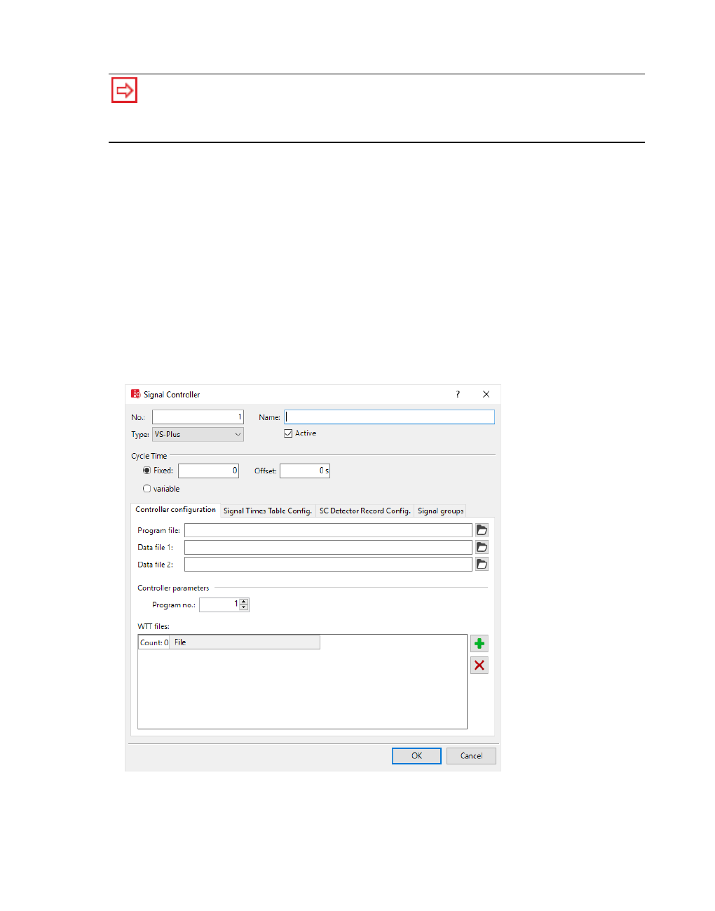
6.14.4 Using signal control procedures
Tips: You can obtain information about the program versions of VS-Plus from the
manufacturers, VS-PLUS AG and Siemens AG.
Information for the use of VS-PLUS (see "Add-on module Siemens VA (TL / Siemens
VS-PLUS)" on page 588).
1. From the Signal Control menu, choose > Signal Controllers.
The Signal Controllers list opens.
By default, you can edit the list (see "Using lists" on page 89).
2. Right-click the entry of your choice.
3. From the shortcut menu, choose Edit.
The Signal Controller window opens.
4. In the Type field, select > VS-Plus.
5. Open the Controller configuration tab.
6. Make the desired changes:
© PTV GROUP 593

6.14.4 Using signal control procedures
Element Description
Program
file
ProgFile: This is the VS-PLUS version with which the node is to be
controlled.
Always use the same VS-PLUS version to create the supply file with Visual
VS-PLUS in the simulation and for the application on the actual control
device.
Data file 1
Data file 2
SupplyFile1, SupplyFile2: Interface file and parameter file. The files must be
saved in the same folder as the Vissim data.
If the VS-PLUS supply is carried out with Visual VS-PLUS, only one VS-
PLUS input file *.vce is generated. Enter their file names in the field Import
file 1.
Import file 1: This is an interface file, e.g. GEO_I.VCE if this was gen-
erated by IVA or by the VS-PLUS input file *.vce.
Import file 2: This is a parameter file, if this was generated by IVA.
Controller
parameters
ProgNo (Program number):The signal program you want to simulate. A
change of program is possible if the simulation run is in single-step mode. If
the new signal program number is confirmed with OK, the changeover is
triggered in the next simulation second.
WTT files WTTFiles: Value type tables: These contain the data types of the control
logic which are to be shown in the Signal Control Detector Record or in the
Signal Times Table window, as well as the display type. If the control
consists of several modules, you must specify the associated *.wtt file for
each module.
: Select WTT file
: Delete WTT file from list
6.14.4.20 Defining signal groups for Siemens VA, TRENDS, VAP, VS-Plus
In the Signal Controller window or the Signal groups list, you can define signal groups for the
signal control procedures Siemens VA, TRENDS, VAP and VS Plus.
Defining signal groups in the Signal Controller window
1. From the Signal Control menu, choose > Signal Controllers.
The Signal Controllers list opens. The SCs defined are displayed (see "Defining SC and
signal control procedures" on page 567).
2. Double-click the SC of your choice (Siemens VA, TRENDS, VAP or VS-Plus).
The Signal Controller window opens.
3. Ensure that the Signal Groups tab is shown in the foreground.
A list of the attributes of signal groups is displayed.
4. Right-click in the list.
594 © PTV GROUP

6.14.5 Opening and using the SC Editor
5. From the shortcut menu, choose Add.
A new row with default data is inserted.
6. Edit the desired entries.
7. Confirm with OK.
Defining signal groups in the Signal Groups list
1. From the Signal Control menu, choose > Signal Controllers.
The Signal Controllers list opens. The SCs defined are displayed (see "Defining SC and
signal control procedures" on page 567).
2. Select the SC of your choice (Siemens VA, TRENDS, VAP or VS-Plus).
3. On the list toolbar, in the Relations list box, click Signal Groups.
4. On the toolbar of the Signal Groups list on the right, click the New ... button .
A new row with default data is inserted.
5. Edit the desired entries.
6.14.5 Opening and using the SC Editor
In the SC editor, you configure new SCs of the type Fixed time and Epics/Balance Local or
edit existing SCs of this type. To do so, you can make the following settings:
Defining SC with frequency (see "Defining SC with frequency" on page 602)
Defining signal groups of SC (see "Defining signal groups in the SC editor" on page 603)
Editing default signal sequences and signal states of signal groups (see "Editing signal
groups" on page 604)
Defining intergreens (see "Defining an intergreen matrix" on page 606)
Editing intergreens (see "Editing intergreen matrices" on page 607)
Defining and editing stages (see "Defining and editing stages" on page 609)
Assigning stages to signal groups and selecting a default intergreen matrix (see "Editing
stage assignment" on page 611)
Creating stage sequences, interstages, and signal group based signal programs (see
"Editing stage sequence" on page 613). Using the Vissig add-on module, you may also
define stage-based signal programs.
Defining signal programs (see "Defining signal programs" on page 617)
Editing signal programs (see "Editing signal programs" on page 618)
Editing the interstages created (see "Editing interstages" on page 625)
© PTV GROUP 595
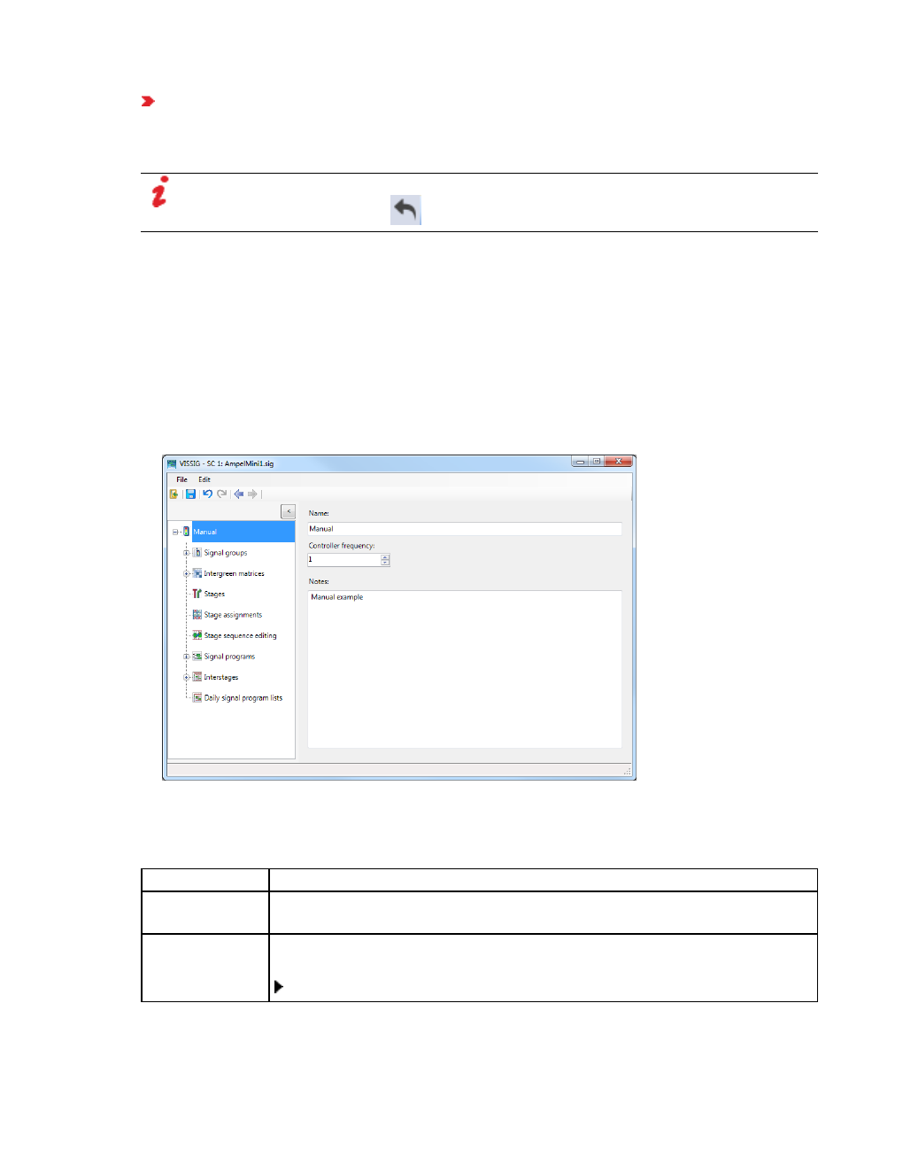
6.14.5 Opening and using the SC Editor
Defining daily signal program lists (see "Defining and editing daily signal program lists" on
page 628)
If you have added an SC, you must save the network file *.inpx to open the SC editor.
Note: When in Vissim you edit data that is saved to external files, for example *.sig files,
Vissim does not provide the Undo function for any previously selected commands.
6.14.5.1 Opening the SC Editor
1. From the Signal Control menu, choose > Signal Controllers.
The Signal Controllers list opens. The SCs defined are displayed (see "Defining SC and
signal control procedures" on page 567).
2. Right-click the entry of your choice.
3. From the context menu, choose Edit Signal Control.
The SC Editor opens.
6.14.5.2 User interface of the SC Editor
The user interface of the SC Editor is divided into the following areas:
Element Description
Title bar Program name, number of the selected signal control and currently loaded
signal control file *.sig.
Menu bar It is operated using the mouse or key combinations. Menu entries contain
graphic notes on submenus or windows:
The symbol indicates a subordinate submenu.
596 © PTV GROUP

6.14.5 Opening and using the SC Editor
Element Description
" ..." Three points stand for a subordinate window.
Toolbar Control elements for control and editing
Scroll bars Scroll window content horizontally or vertically
Navigator in
section on the
left
List of available parameter pages for the currently selected SC. With the
Vissig add-on module, you can also edit stages and daily signal program
lists.
Button < above the Navigator: Closes the pane with the view of the tree
structure. A vertical label opens which specifies the parameter page on
which the cursor was when it was closed.
Button >: Opens the Navigator again on the specified parameter page.
Parameters in
section on the
right
Parameters for defining and editing the SC (see "Defining SC with
frequency" on page 602)
6.14.5.3 Menus in the SC Editor
File menu
Element Description Hotkeys
Open *.sig configuration file
Export Export Excel Workbook or *.pua file with interstages in text format for
VAP
Save Save Vissig configuration file *.sig with same path and name CTRL+S
Save
as…
Save Vissig configuration file *.sig under a new path or name, may
contain Unicode characters.
Check Check for inconsistent planning (see "Detecting inconsistent planning"
on page 631)
Exit Close the SC Editor ALT+X
Edit menu
Element Description Hotkeys
Undo Cancels the last action. Each executed step can be undone. CTRL+Z
Redo Redoes the last undone action. Each step can be restored. CTRL+Y
Options… General Settings (Common, Optimizations, View and Export) (see
"Making global settings in the SC Editor" on page 599)
6.14.5.4 Toolbar in the SC Editor
Depending on the entry in the Navigator and the selected editing view, you can execute
functions with the following icons:
© PTV GROUP 597
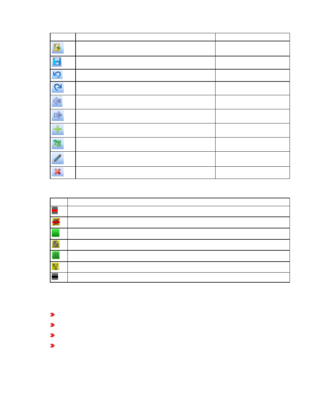
6.14.5 Opening and using the SC Editor
Icon Description Hotkeys
Back to the Signal Controller window
Save CTRL+S
Undo CTRL+Z
Redo CTRL+Y
Back in View
Forward in View
New
Duplicate
Edit
Delete
6.14.5.5 Signal states
State Signal state
Red
Red-amber
Green
Amber
Flashing Green
Flashing Amber
Dark
6.14.5.6 Signal state sequences
The signal state sequence defines the following for each signal state:
Permitted state or blocked state
Fixed or variable duration
Time horizon
Minimum duration of the signal state in the default sequence. The minimum duration is pre-
defined and can be changed for each signal group.
598 © PTV GROUP

6.14.5 Opening and using the SC Editor
State Signal state sequence Green Fixed
Duration
Minimum
Duration
Permanent Red
Permanent Green x
Red-Red/Amber-Green-Amber 1
1
x 5
3
Red-Green 1
x 5
Red-Red/Amber-Green-Flashing Green-
Amber
1
1
x 5
x 4
3
Red-Green-Flashing Green 1
x 5
x 4
Red-Green-Amber 1
x 5
3
Off (Flashing Amber)
Off (Off)
6.14.5.7 Making global settings in the SC Editor
Note: The following tabs are only available with the add-on module Vissig.
1. Open the SC Editor (see "Opening and using the SC Editor" on page 595).
2. In the menu, choose Edit > Options.
The Options window opens.
3. Make the desired changes:
© PTV GROUP 599
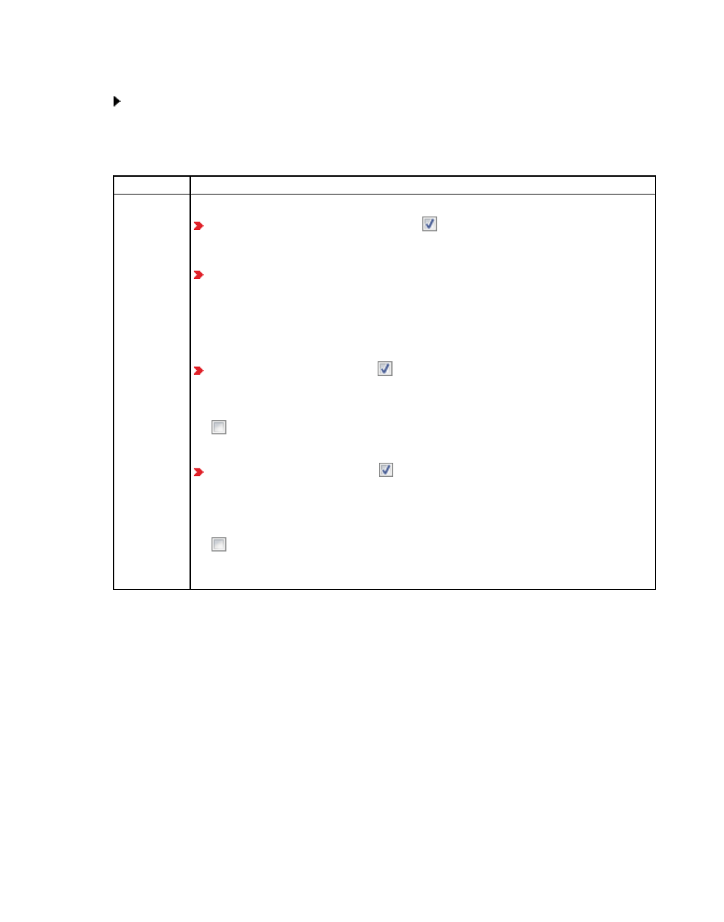
6.14.5 Opening and using the SC Editor
Common tab
Select the desired language.
The selected language is used as the default language.
Optimizations tab
Element Description
Interstages Interstages:
Add minimum times in interstage: If this option is selected, the target
signal states of the individual signal groups have at least the minimum
period specified in the signal groups.
(Setting can be changed in the SC settings): Alternatively, in the SC set-
tings with the option Check minimum times in signal programs, select or
deactivate the option Add minimum times in interstage(see "Defining SC
with frequency" on page 602).
Optimizes green time duration:
Use optimal length in front: If the option is selected, the green is ended
at the start of the interstage when changing from green to red. Green starts
as early as possible.
If the option is not selected, the green is ended at the start of the
interstage when changing from green to red.
Use optimal length in back: If the option is selected, the green does not
only start at the end of the interstage or at the end of the interstage minus
the minimum period when changing from green to red. Green ends as late
as possible.
If the option is not selected, the green only starts at the end of the
interstage or at the end of the interstage minus the minimum period when
changing from green to red.
600 © PTV GROUP

6.14.5 Opening and using the SC Editor
View tab
Element Description
Stages Stages:
Show signal group ids: Signal group numbers are shown in the
stage diagram.
Use compact view: A schematic rather than a topographic display
is shown in the stage diagram.
Signal programs
and interstages Appearance: You can select from the following display options:
Classic
3d tubes
3d boxes
Resize automatically: By changing the window size, the row
height automatically adjusts to the window height.
Show full interstage name in the stage based signal programs:
The names are displayed instead of the numbers of the interstages.
Export tab
© PTV GROUP 601

6.14.5 Opening and using the SC Editor
Element Description
Common Render mode
Fixed width: Width of export graphic based on Picture width
Fixed scale (pixels per second) in pixel per second: Width of export
graphic based on Pixel per second entered below.
Signal group height: Signal group height in pixels globally for all graphic
exports
Signal pro-
grams Picture width: Width of the export graphic in pixels. The given value is
taken into account if the Fixed width option is selected as the Render
mode.
Pixel per second: Number of pixels that represent a second in the export
graphic. The given value is taken into account if the option Fixed scale
(pixel per second) is selected as the Render mode.
Interstages Picture width: Width of the export graphic in pixels. The given value is
taken into account if the Fixed width option is selected as the Render
mode.
Pixel per second: Specify the number of pixels that represent a second in
the export graphic. The given value is taken into account if the option Fixed
scale (pixel per second) is selected as the Render mode.
Stage
sequence
Stage width: Width of the stage in pixels for the export. The given value is taken
into account if the Fixed width option is selected as the Render mode.
6.14.5.8 Defining SC with frequency
1. Open the SC Editor (see "Opening and using the SC Editor" on page 595).
2. Click on the top entry in the Navigator.
The base data of the SC opens.
602 © PTV GROUP

6.14.5 Opening and using the SC Editor
You can define a new signal control or change the settings for the selected SC.
Element Description
Name Label for the top entry in the navigator:
no name: My signal control is displayed by default in the
Navigator and the SC number is added to it.
The SC number is generated automatically.
Controller frequency Number of calls of the SC per simulation second, value range 1-
10.
The SC frequency controls the frequency of light signal controls
during the simulation.
A warning is displayed if the SC frequency is incompatible with the
simulation parameter Simulation resolution.
The least common multiple of the frequencies of all SCs must be a
factor of the simulation resolution.
Check minimum times
in interstage programs
If this option is selected, the target signal states of the individual
signal groups have at least the minimum period specified in the
signal groups.
Notes optional entry of text
3. Click the Save button.
6.14.5.9 Defining signal groups in the SC editor
You can open the SC editor to define signal groups for the following SC types:
Fixed time
Epics/Balance Local
For signal controllers of the type Siemens VA, TRENDS, VAP and VS Plus, you do not define
signal groups in the SC editor (see "Defining signal groups for Siemens VA, TRENDS, VAP,
VS-Plus" on page 594).
1. Open the SC Editor (see "Opening and using the SC Editor" on page 595).
2. In the Navigator, click Signal groups.
The signal groups list opens.
If no signal group has been defined yet, only the column titles are displayed.
© PTV GROUP 603

6.14.5 Opening and using the SC Editor
3. Right-click in the list.
The context menu opens.
4. Click on the desired entry.
Element Description
Add Add new signal group with the first port number available.
By default, the signal state sequence Red-Red/Amber-Green-Amber is
assigned. To keep data input to a minimum, create a signal group for each
signal group type you need. Then supply their standard signal sequence and
duplicate the template created as often as required.
Duplicate Copy signal group and insert with a new number
Edit Change data of the selected signal group
Delete Delete selected signal group
By default, you can edit the list (see "Using lists" on page 89).
5. Click the Save button.
6. Edit the signal group (see "Editing signal groups" on page 604).
6.14.5.10 Editing signal groups
You can change the signal state sequence and its minimum durations. For signal states that in
the signal sequence possess a variable duration, the value entered is interpreted as the
minimum duration. For any other signal states, the value entered is interpreted as the duration.
This, for instance, allows you to supply 2 seconds red-amber, 5 seconds amber for 70 km/h
(speed limit in Germany) or 15 seconds minimum green for a heavily loaded straight flow.
1. Open the SC Editor (see "Opening and using the SC Editor" on page 595).
2. In the Navigator, click Signal groups.
The signal groups list opens.
3. Right-click the entry of your choice.
604 © PTV GROUP

6.14.5 Opening and using the SC Editor
4. From the shortcut menu, choose Edit.
In the window, the name, default signal sequence, signal duration, and a description are
displayed.
Tip: Alternatively, you can show the window via the following functions:
In the Navigator, click the signal group.
In the signal groups list, in the signal group row of your choice, double-click the
Notes field.
5. Make the desired changes:
Element Description
Name Name of signal group, may contain Unicode characters.
Default
sequence
With the exception of permanent signal sequences, you can choose any of
the signal state sequences defined (see "Performing green time optimization
of stage-based fixed time controllers" on page 573):
red > red/amber > green > amber
red > green
red > red/amber > green > flashing green > amber
red > green > flashing green
red > green > amber
© PTV GROUP 605
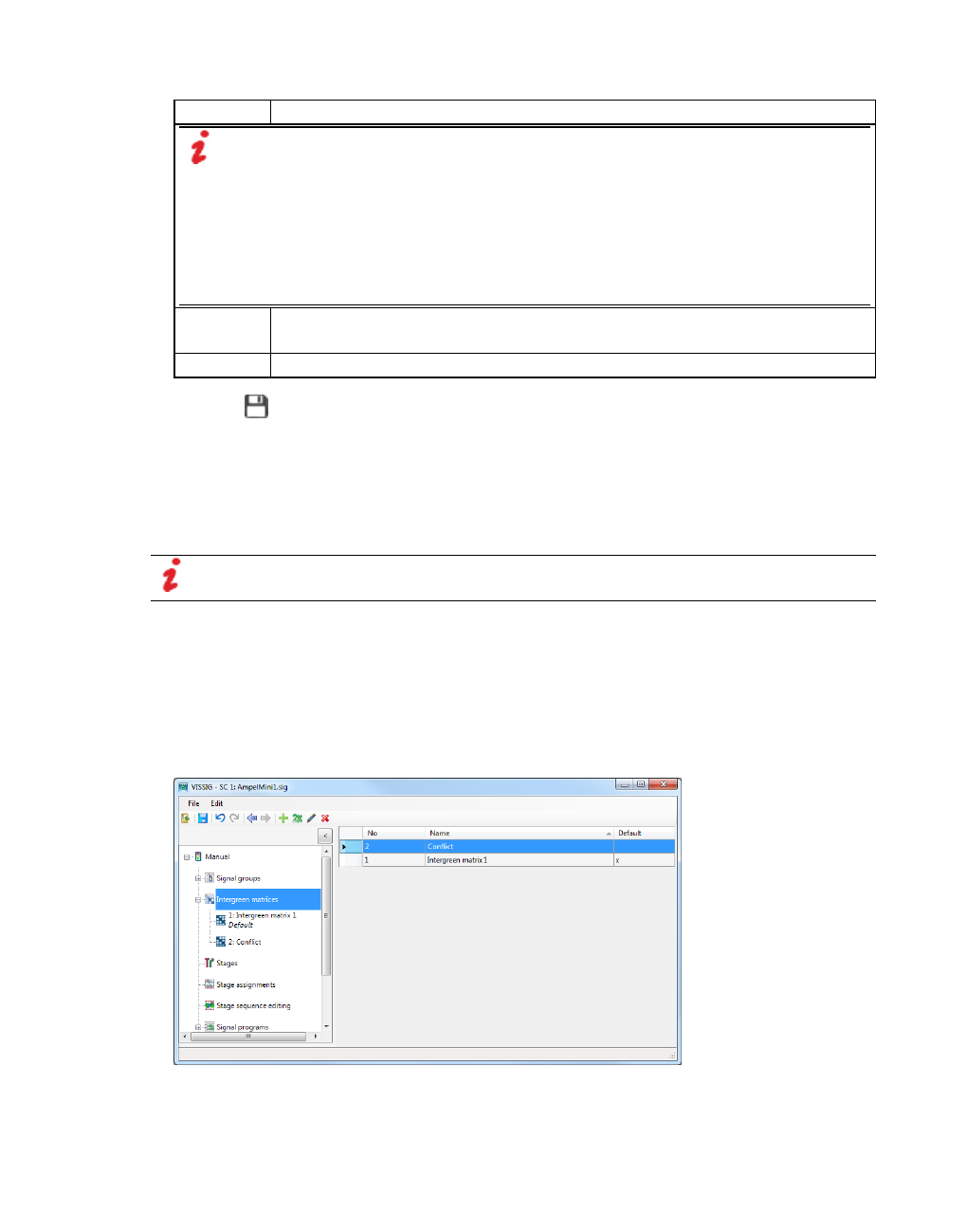
6.14.5 Opening and using the SC Editor
Element Description
Note: If in the SC editor, in the Edit menu, you choose Options > Optimizations
and then click Add minimum times in interstage, the increase in the minimum
green time or transition time might mean that individual interstages have to be
recalculated. This is why before changes are accepted, Vissim checks whether the
interstages need to be recalculated due to these changes. If required, a message
is then displayed, asking whether you still want the changes to be carried out.
Within this context, changes made in the meantime to optimization settings or
stages might also require recalculations, which are not due to the actual change.
(Minimum)
durations
Symbol for signal state sequence and minimum durations in seconds of the
signal state
Notes optional entry of text
6. Click the Save button.
6.14.5.11 Defining an intergreen matrix
Intergreen is the time required to elapse between the green end of a clearing flow and the
green start of an entering flow. By keeping the intergreen, you ensure that the clearing flow
does not conflict with the entering flow.
Note: Conflicting flows and intergreens cannot be calculated. When intergreen data is
entered, there are no checks, e.g. for the symmetry of intergreen matrices.
1. Open the SC Editor (see "Opening and using the SC Editor" on page 595).
2. Double-click the desired SC in the Navigator.
3. In the Navigator, click Intergreen matrices.
The intergreen matrices list opens.
If no intergreen matrix has been defined yet, only the column titles are displayed.
4. Right-click in the list.
606 © PTV GROUP

6.14.5 Opening and using the SC Editor
The context menu opens.
5. Click on the desired entry.
Element Description
Add Add new intergreen matrix
Duplicate Copy intergreen matrix and insert with a new number
Edit Change data of the selected intergreen matrix
Delete Delete selected intergreen matrix
To sort a column of the list, click the column header.
6. Make the desired changes:
Element Description
No Number of the intergreen matrix
Name Name of the intergreen matrix
Default The default intergreen matrix selected under Stage assignment is marked with
an x. Double-click into the Default column to open the respective editing view.
You can assign an intergreen matrix individually to each signal group-based signal program.
In the Navigator, under Stage assignments, you can choose an intergreen matrix as default
(see "Editing stage assignment" on page 611). The program then takes the intergreen matrix
into account to create stages, stage transitions, and stage-based signal programs.
7. Click the Save button.
8. Edit the intergreen matrix (see "Editing intergreen matrices" on page 607).
6.14.5.12 Editing intergreen matrices
1. Open the SC Editor (see "Opening and using the SC Editor" on page 595).
2. Click Intergreen matrices in the Navigator.
The intergreen matrices list opens.
3. Right-click the entry of your choice.
4. From the shortcut menu, choose Edit.
Tip: Alternatively, you can display the window by clicking the intergreen matrix in the
Navigator.
© PTV GROUP 607

6.14.5 Opening and using the SC Editor
5. Make the desired changes:
Element Description
Name Name of the intergreen matrix
White fields Enter intergreen values
Gray fields Editing not possible
When a cell is activated, the corresponding cell in the opposite triangle is also highlighted.
6.14.5.13 Importing intergreen values from Excel
You can import intergreen values from Microsoft™ Excel™. If, for example, you have exported
an Excel workbook, you can insert the data of the intergreen matrices into a new or existing
matrix using Copy & Paste.
Inserting Excel data in a new empty matrix
1. Open the SC Editor (see "Opening and using the SC Editor" on page 595).
2. Click Intergreen matrices in the Navigator.
The intergreen matrices list opens.
3. Right-click in the list.
4. From the shortcut menu, choose Add.
5. Right-click the new entry.
6. From the shortcut menu, choose Edit.
An empty matrix named Intergreen matrix is created.
7. Change the name and number of the intergreen matrix if necessary.
8. Switch to your Excel file.
9. Open the worksheet of the intergreen matrix from which you want to extract the data.
608 © PTV GROUP

6.14.5 Opening and using the SC Editor
10. Hold down the left mouse button and highlight only the rows and columns that contain
values.
11. Press the key combination CTRL+C.
12. Switch to the editing view of the new intergreen matrix.
13. Click in the upper left field of the matrix.
The entire matrix is highlighted in blue.
14. Press the key combination CTRL+V.
The values are inserted in the matrix.
Notes:
You can insert parts of the Excel spreadsheet in the intergreen matrix. Correctly pos-
ition columns and rows of the source area and the destination area.
No values may be in the gray fields. The process is canceled if you insert data in
these fields.
6.14.5.14 Defining and editing stages
Note: You will need the add-on module Vissig.
1. Open the SC Editor (see "Opening and using the SC Editor" on page 595).
2. Double-click the desired SC in the Navigator.
3. Click Stages in the Navigator.
© PTV GROUP 609

6.14.5 Opening and using the SC Editor
The stages list opens.
If no stage is defined, only the column titles are shown.
4. Right-click in the list.
The context menu opens.
5. Click on the desired entry.
Element Description
Add Add new stage with the first free number
Duplicate Copy stage and insert with a new number
Delete Delete selected stages
6. Click the Save button.
7. Make the desired changes:
Element Description
No. Number of stage
Name Name of stage
Pseudo
stage If the option is selected, the stage duration is not changed during green time
optimization. The duration of a pseudo stage is zero seconds in all stage-based
signal programs. This option acts as a "stage transition divider" to handle the
special case when more than one switching command is received during a
stage transition of a signal group. In this case, the stage transition is divided into
two stage transitions, each linked to a pseudo stage.
The Pseudo Stage option can only be selected if no stage transition has been
defined for this stage.
Stage
diagram
Graphical representation of stage
610 © PTV GROUP
6.14.5 Opening and using the SC Editor
8. Click the Save button.
Note: To display pavement markers in Vissim, the following nodes are required:
A node for the relevant node
A node for each neighboring node
For these nodes, the attribute Use for evaluation must be selected.
6.14.5.15 Editing stage assignment
Note: You will need the add-on module Vissig.
You can permit or block individual signal groups or classify their state as not relevant.
In the Default intergreen matrix box, select the entry of your choice.
By default, the selected intergreen matrix is marked with an x in the overview table of the
Intergreen matrices.
Switching state of signal group
1. Open the SC Editor (see "Opening and using the SC Editor" on page 595).
2. Double-click the desired SC in the Navigator.
3. Click Stage assignments in the Navigator.
The stage assignment list opens.
4. Double click on the desired cell.
Tip: Alternatively, you can click the number in the graphical representation of the stage.
The state of the signal group in the stage is switched. The system switches between the two
states in cycles:
Signal group is in the Permitted stage
Signal group is in the Blocked stage
State of signal group is in the Not Relevant stage, for example, for partial node
control
If an intergreen matrix is selected as default, the conflicts (conflict traffic streams) are tested
during the creation of the stages. When conflicting signal groups are permitted in the same
stage, these are highlighted in red in the table.
© PTV GROUP 611

6.14.5 Opening and using the SC Editor
Tip: You may change the width of the two window sections.
Displaying selected or all stages
You can switch between the display of all stages or a magnified display of the selected stage.
1. Right-click in the graphic.
2. From the context menu, choose the function of your choice.
Defining display of pavement markers
You can define the display of the pavement markers with or without displaying the signal
group number.
1. Right-click in the graphic.
2. Select the desired function.
3. Confirm with OK.
612 © PTV GROUP

6.14.5 Opening and using the SC Editor
6.14.5.16 Editing stage sequence
Note: You will need the add-on module Vissig.
You can form stage sequences from the stages defined and create the interstages.
1. Open the SC Editor (see "Opening and using the SC Editor" on page 595).
2. Double-click the desired SC in the Navigator.
3. In the navigator, click Stage sequence editing.
The existing stages are displayed in the upper pane. The currently selected stage
sequence is displayed in the lower pane.
In the upper pane, you define individual interstages and stage sequences.
Tip: You can change the ratio between the upper and lower pane using the horizontal
divider.
Defining interstages
1. Click on the From stage.
The From stage is marked.
2. Hold down the CTRL key and click on the To stage.
The stages are called 1 and 2.
3. Right-click in the window.
4. From the context menu, choose Create an interstage.
The interstage is created and graphically displayed.
© PTV GROUP 613

6.14.5 Opening and using the SC Editor
Tip: You can define several interstages, for example, with and without minimum
duration, between two stages.
Notes:
In Vissig, a signal group in an interstage can be switched once at most: The signal
group can change from Free to Blocked or from Blocked to Free.
If you model an interstage in which a signal group is switched twice, in Vissig you
must define a pseudo stage and two interstages, one directly before the pseudost-
age and the other one following the pseudostage.
Defining stage sequence
You can define a stage sequence for calculating the signal program in the upper pane.
1. Hold down the CTRL key and click on the desired stage sequence.
2. Right-click in the window.
3. In the context menu, select the entry Create sequence.
The new stage sequence is displayed in the lower view.
4. To add an additional stage to the already defined stage sequence, mark an individual
stage and choose Add to sequence in the context menu or double-click the stage.
Deleting stage and stage sequences
To delete a selected stage from the stage sequence, choose Remove stage in the context
menu.
To delete the entire stage sequence, choose Clear sequence in the context menu.
Exporting stage sequence as graphic file
1. In the menu, choose Edit > Options Export tab.
614 © PTV GROUP

6.14.5 Opening and using the SC Editor
2. Make the desired settings for formatting the graphic.
3. From the context menu, choose Export entry.
Creating signal program with fixed cycle time
You can create a signal program with a fixed cycle time via the following functions from the
stage sequences:
Enter the cycle duration in seconds in the Cycle time field.
Click on the Create stage based signal program button.
A stage-based signal program with a prescribed cycle duration is calculated. The editing
view of the signal programs is opened for further processing of your signal program.
Click on the Create signal group based signal program button.
A signal group based signal program with a prescribed cycle duration is calculated. The
editing view of the signal programs is opened for further processing of your signal program.
Manually defining interstages
You can manually define the interstages that you want to use to calculate the signal program.
1. Right-click the gray area between the two desired stages.
2. In the context menu, select the entry Interstages > Create or an existing interstage.
If the interstages are not manually selected, the system checks whether a suitable interstage
already exists for each stage change of the stage sequence.
If a suitable interstage exists, the first suitable interstage is used for the calculation.
If a suitable interstage does not exist, a new interstage is created. The new interstage is
saved for stage-based signal programs.
The interstage is deleted again for signal group-based signal programs after the calculation of
the signal program.
© PTV GROUP 615

6.14.5 Opening and using the SC Editor
Editing interstage
1. Double-click on the interstage.
The editing view of the interstage opens.
2. Make the desired changes.
3. Click on the icon .
The Stage sequence editing window opens.
4. Click the Save button.
616 © PTV GROUP

6.14.5 Opening and using the SC Editor
6.14.5.17 Defining signal programs
You may also automatically create signal programs with a fixed cycle time after editing the
stage sequence (see "Editing stage sequence" on page 613).
Signal programs have the following data:
Element Description
Number Unique number
Name Description of signal program
Intergreens Intergreen matrix assigned under Stage assignments
Cycle time Cycle time defined under Stage sequence
Offset Offset for the synchronization, for example, within a green wave
Switch
point
Switch point at which the system can switch to another signal program, for
example, to a daily signal program list
If an intergreen matrix is assigned to a signal program, the adherence to the intergreens can
be checked while editing the signal program. The intergreen time violations are displayed
automatically.
1. Open the SC Editor (see "Opening and using the SC Editor" on page 595).
2. Double-click the desired SC in the Navigator.
3. Double-click Signal programs in the Navigator.
The signal programs list opens.
The Signal programs entry in the Navigator can contain the following types of signal
programs:
Signal group-based signal programs. These can be created in the overview table.
Stage-based signal programs created from stage sequences
The type of signal program is displayed in italics in the Navigator tree below the name of the
signal program.
© PTV GROUP 617

6.14.5 Opening and using the SC Editor
4. Right-click the desired entry in the list of signal programs.
The context menu opens.
5. Click on the desired entry.
Element Description
Add Add a new row to a new signal program
Duplicate Copy signal program and insert with a new number
Edit Change data of the selected signal program
Delete Delete selected signal program
Export Export graphical display of the signal program
To sort a column of the list, click the column header.
6. Make the desired changes:
Element Description
No. Number of the signal program
Name Name of the signal program
Intergreens Used intergreen matrix
Cycle time Cycle duration in seconds
Offset Stage scheduling is postponed by this time. For the synchronization, for
example, within a green wave.
Switch
point
The system can change between two signal programs at this point. Both
signal programs must display the same signal states for all signal groups at
this point. In the signal program display, a vertical blue line indicates the
switch point.
7. Click the Save button.
8. Edit the signal program (see "Editing signal programs" on page 618).
6.14.5.18 Editing signal programs
Signal group- based signal programs allow individual editing of individual signal groups
and/or switching times. You can edit these graphically and in the time table. You can change
the display type of the table columns and the signal states via the context menu.
1. Open the SC Editor (see "Opening and using the SC Editor" on page 595).
2. Double-click the desired SC in the Navigator.
3. Double-click Signal programs in the Navigator.
The signal programs list opens.
4. Click on the desired entry.
The signal program is displayed.
618 © PTV GROUP
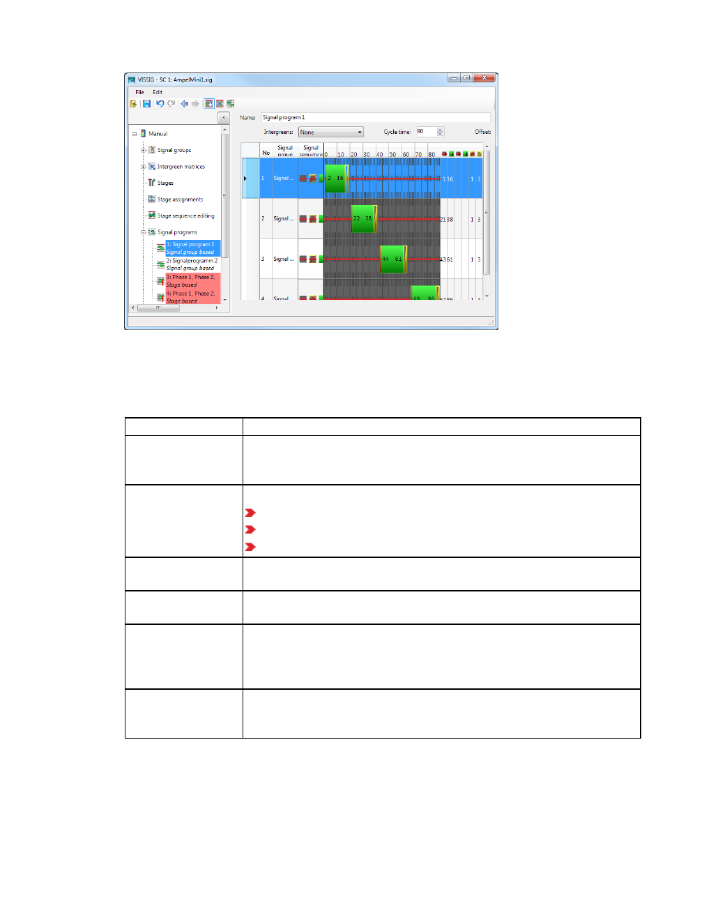
6.14.5 Opening and using the SC Editor
Functions in the context menu
1. Right-click the entry of your choice.
2. Make the desired changes:
Element Description
Export From Vissig, you can export stage sequences, signal programs, and
interstages as graphic files (see "Exporting data from the SC Editor"
on page 633).
Display View of Signal Programs:
Classic
3D tubes
3D boxes
Resize auto-
matically
The row height is automatically adjusted if you change the window
size
Show entire signal
program
Redraws the signal program and adjusts the row height to the win-
dow height
Signal group
based editing,
stage based
editing
Select a row and move a starting point or end point of a signal state
of variable duration with the mouse button held down. You can also
select the editing mode via the toolbar.
Stretch/Compress Select a row and expand or compress the signal state in the time
axis labeling with the mouse button held down. You can also select
the editing mode via the toolbar.
© PTV GROUP 619

6.14.5 Opening and using the SC Editor
Element Description
Extract interstage In Vissig, in the graphical view, you may cut out an interstage of your
choice for signal group based signal programs. After selecting this
function, the cursor changes into a cross in the Cycle Times column
above the graph. With the mouse held down, drag the area that you
want to extract. The editing view of the selected interstage opens
(see "Editing interstages" on page 625). You can also select the edit-
ing mode via the toolbar.
Second green
time
Only in signal group-based signal programs: Create additional green
time. A second green time (double throw) can be created only via the
context menu.
Time axis labeling
absolute (offset
considered)
Labeling of the time axis starts with the offset time set, not with 0.
620 © PTV GROUP

6.14.5 Opening and using the SC Editor
Element Description
Edit columns… Only in signal group-based signal programs: the Select time
columns to be displayed window opens. The settings are saved to
the registry of your computer and may change depending on the
user.
You can select entries and display them as columns via the arrow
symbols or remove the columns.
A column is added for table entries of signal states with a fixed
duration, as the amber time e.g. is identical for each green time. A
double column is added for table entries of signal states with a
variable duration, as there can be two green times within one cycle
which can have different durations, start and end times.
The columns for stage-based signal programs with signal states with
a fixed duration are not displayed, even when selected. For stage-
based signal programs, the fixed durations of the definition of signal
groups are used that cannot be changed.
Changing row height
1. Click on the desired row.
2. Point with the cursor to the line between two rows in the first gray column.
The cursor changes into a bidirectional arrow.
3. With the left mouse button held down, drag the line up or down.
© PTV GROUP 621

6.14.5 Opening and using the SC Editor
Functions in the toolbar
You can select the editing mode
Symbol Description
Edit signal states
Stretch/Compress
Extract interstage
Defining formatting of graphical representation
In the menu, choose Edit > Options tab View (see "Performing green time optimization of
stage-based fixed time controllers" on page 573).
Editing switching times graphically
1. Click on the Edit signal states icon.
2. Click on the desired entry.
3. If you move the cursor over the switching time view, you can select one of the following
options:
View Description
Move signal state with variable duration with the mouse button held down.
Only for signal group based signal programs: Drag starting time or end time of a
signal state with variable duration with the mouse button held down.
You cannot directly move signal states with a fixed duration (transition states).
Only for stage-based signal programs: When a signal state is being shifted, the
reserve times are indicated by a green background. Intergreen time violations are
indicated by an orange background. Violations of minimum durations are indicated
by a red background. In front of rows with intergreen time violations or violations of
minimum durations, the symbol is displayed.
Within the time axis labeling, you can move the entire signal program or the zero
point of the signal program.
Note: Keep the cursor in the selected area. Otherwise, the move is canceled.
You can change the durations of the transition states individually in the table for the currently
edited signal program, if they differ from the default durations defined in the signal group, for
example higher amber times in bad weather programs for signal group based signal
programs.
622 © PTV GROUP

6.14.5 Opening and using the SC Editor
Stretching or compressing signal programs
1. Click on the Stretch/Compress icon.
2. If you move the cursor over the time axis labeling, you can select one of the following
options:
View Description
Compressing a signal program: Hold the mouse button down and drag the cursor to
the left. The area highlighted in red is extracted.
Stretching the signal program: Hold the mouse button down and drag the cursor to
the right within the time axis labeling. The duration of the area highlighted in green
is inserted at the start of this area.
The highlighted area is displayed with a gray background: Compress/Stretch is not
possible (violation of minimum durations).
3. If you want to cancel Stretch/Compress, release the mouse button outside the time axis
labeling.
Extracting and saving interstage
Only for signal group based signal programs:
1. Click on the Extract interstage icon.
2. Hold the mouse button down and drag the cursor to the right within the time axis labeling.
View Description
Valid interstage: The background is displayed in green. After you have released the
mouse button within the time axis labeling, the system automatically changes to the
editing view of the interstage and saves this interstage.
If the From stage and the To stage of the interstage do not exist, these are also
created for the extracted interstage. You can edit From stage and To stage (see
"Editing interstages" on page 625).
Invalid interstage: The background is displayed in gray if a amber stage was not
completely highlighted. The interstage cannot be saved.
Only one status change per signal group: If you highlight a second green time at the
same time, the background is displayed in gray. No interstage can be saved.
3. If you want to cancel Extract interstage, release the mouse button outside the time axis
labeling.
Editing stage-based signal programs
You can change the position of the stages within the signal program.
In stage-based signal programs, it is not possible to
© PTV GROUP 623

6.14.5 Opening and using the SC Editor
edit every switching time individually
extract interstage
1. Make sure:
you have defined an intergreen matrix as default (see "Editing stage assignment" on
page 611)
you have defined stages (see "Defining and editing stages" on page 609)
you have defined a stage assignment (see "Editing stage assignment" on page 611)
you have edited the stage sequence and created the signal program (see "Editing
stage sequence" on page 613)
On the toolbar, you have enabled the Stage based editing button.
2. Make the desired changes:
View Description
Move the start markings or end markings of interstages
Move the name of interstages
Move the interstages within the signal program. This is possible only for interstages
with a duration greater than 0 seconds.
The duration of the transition states for interstages are set by default to the default values from
the definitions of the signal groups.
3. If desired, compress or stretch the individual stages.
Zooming in on the graphical representation of the signal program
You can enlarge a specific area of the graphical signal programs. Thus you can edit individual
switching times more precisely, for example, with a switch point every 1/10 seconds if SC cycle
= 10.
1. Click on the desired entry.
624 © PTV GROUP

6.14.5 Opening and using the SC Editor
The row is highlighted.
2. Click in the graphics area of the row.
The cursor changes to the following symbol:
3. If you want to stretch the time range, click the scroll wheel in the graphics area of the row.
4. If you want to reset the time range again, click the scroll wheel again in the graphics area of
the row.
6.14.5.19 Editing interstages
Note: You will need the add-on module Vissig.
1. Open the SC Editor (see "Opening and using the SC Editor" on page 595).
2. Double-click the desired SC in the Navigator.
3. Make sure that stage sequences are defined with interstages (see "Editing stage
sequence" on page 613).
4. Click Interstages in the Navigator.
The interstages are displayed.
5. Right-click the entry of your choice.
6. Choose the desired entry from the context menu.
Element Description
Duplicate Copy interstage and insert with a new number
Edit Change data of the selected interstage
Delete Delete selected interstage
Export Export graphic of the selected interstage
7. Edit the interstage:
Element Description
No. Number of interstage
Name Name of interstage. The name is taken from the stage sequences in Stage
sequence editing in the Navigator (see "Editing stage sequence" on page
613).
From stage Source stage of Interstage
To stage Target stage of Interstage
Recalculate After changing a stage, recalculate the stage sequence and update the dis-
play.
© PTV GROUP 625

6.14.5 Opening and using the SC Editor
8. To edit an interstage, double-click the row with the No. and Name of the interstage.
The editing of switching times is done like the editing of signal group-based signal programs
(see "Editing signal programs" on page 618).
Functions in the context menu of interstages
1. Right-click in the right panel of the graphic.
The context menu opens.
2. Make the desired changes:
Element Description
Export Save interstages as a graphic file (see "Exporting data from the SC
Editor" on page 633).
Appearance Select display:
Classic
3d tubes
3d boxes
Resize automatically The row height is automatically adjusted if you change the window
size
Show entire signal
program
Redraws the signal program and adjusts the row height to the win-
dow height.
Note: You can export interstages in the menu File > Export > PUA in PUA format. This
format is required, for example, for VAP control procedures.
626 © PTV GROUP

6.14.5 Opening and using the SC Editor
Editing attributes of the selected interstage
1. Select the desired interstage.
2. Make the desired settings in the two areas From stage and To stage.
3. If you move the cursor over a stage, the possible source stages and target stages are
indicated in color in the list box. The selection of a different source stage or target stage
automatically starts a recalculation of the interstage.
Blue background: Indicates the selected stage.
Purple background: Interstage with red background selected.
The selection leads to an automatic recalculation of the
interstage.
White background: This selection does not lead to an
automatic recalculation of the interstage.
© PTV GROUP 627
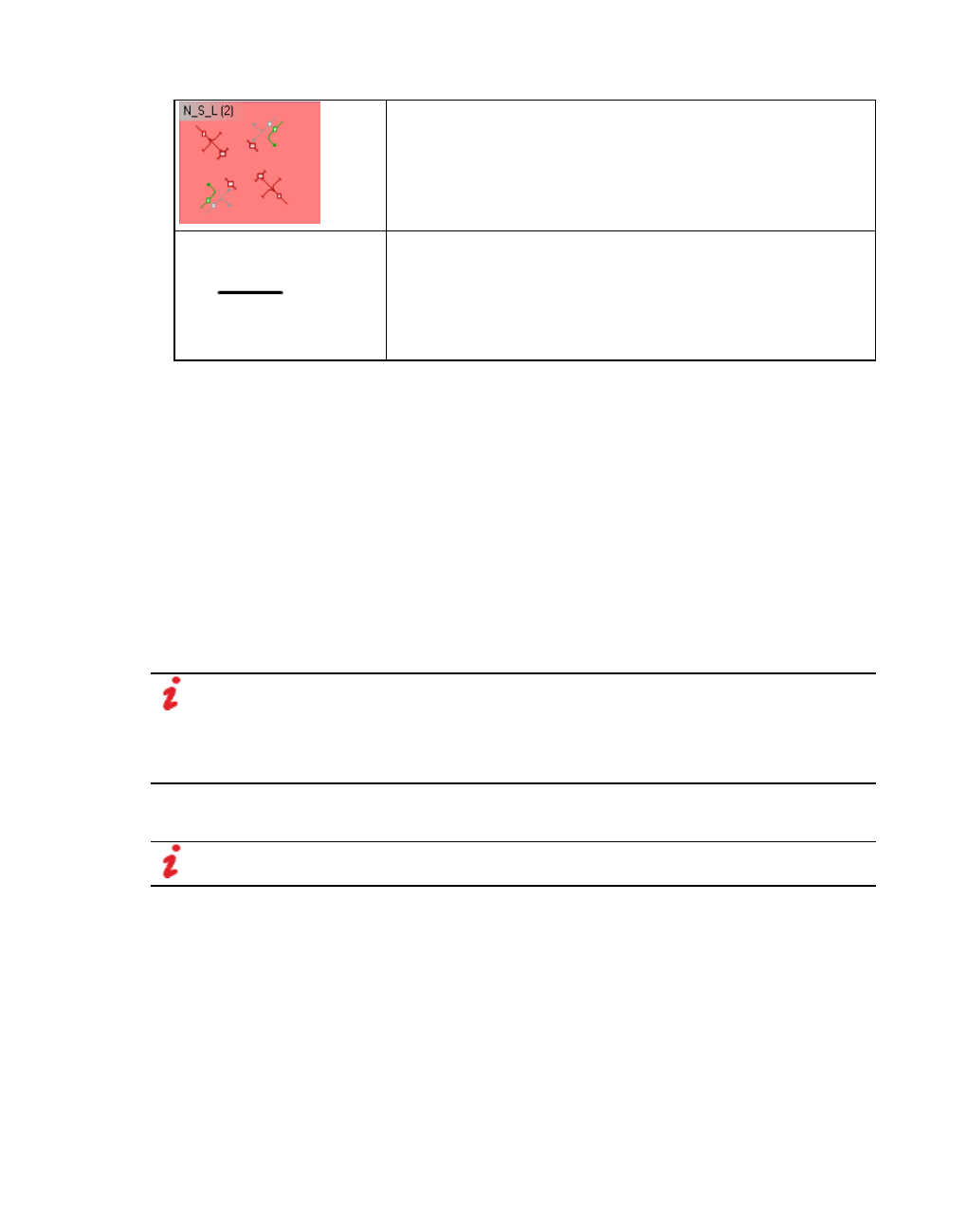
6.14.5 Opening and using the SC Editor
Red background: Indicates a stage which is unsuitable for the
interstage. The selection leads to an automatic recalculation
of the interstage. An interstage is calculated for an initial state
(From stage) and a destination state (To stage). If another
initial state or destination state is selected, the interstage must
be be redefined.
White background: This selection does not lead to an
automatic recalculation of the interstage.
Black line: The stage is not relevant.
4. Double-click in the desired stage area of a signal group.
The state of this signal group in the stage is switched. The interstage is automatically
recalculated.
With the next steps, you can move the initial state to the left (begin < 0) and the destination
state to the right (end > duration of interstage). You can move the initial state to the right
until the first state change within the interstage. You can move the destination state to the
left until the final state change within the interstage. Switching points are not moved.
5. Select the desired value for the start of the interstage in the Begin field.
6. Select the desired value for the end of the interstage in the End field.
A reduction is possible only to the duration of the longest transition state (Amber/Red-
Amber).
Note: If the state of a signal group in the source stage or target stage is not relevant
when calculating an interstage, no signal switch occurs for this signal group. The same
signaling state is displayed within the interstage as in the relevant stage. If the state of a
signal group is neither relevant in the source stage nor in the target stage, the signaling
state is also displayed as not relevant within the interstage.
6.14.5.20 Defining and editing daily signal program lists
Note: You will need the add-on module Vissig.
You can create variants of a chronological sequence of signal programs for your time
intervals. You can save these variants as daily signal program lists.
You can use the daily signal program lists to switch between various signal programs in the
simulation. In this case, enter the number of a daily signal program list rather than the number
of a signal program as the program number.
1. Open the SC Editor (see "Opening and using the SC Editor" on page 595).
2. Double-click the desired SC in the Navigator.
628 © PTV GROUP

6.14.5 Opening and using the SC Editor
3. Click Daily signal program lists in the Navigator.
The Daily signal program lists list opens.
If no daily signal program list is defined, only the column titles are displayed.
4. Right-click in the list.
The context menu opens.
5. Click on the desired entry.
Element Description
New Add new daily signal program list with the first free number
Duplicate Copy daily signal program list and insert with a new number
Edit Change data of the selected daily signal program list
Delete Delete selected daily signal program list
Note: Signal times tables and daily signal program lists follow a common numbering
system. When you create a daily signal program list, the numbering starts with the first
free number. You can overwrite this with a number that is not already used for a signal
times table.
6. Click the Save button.
7. Right-click the new entry.
The daily signal program list opens.
© PTV GROUP 629

6.14.5 Opening and using the SC Editor
8. Right-click in the list.
9. From the shortcut menu, choose Add.
10. Enter the desired data.
Element Description
Name Optional name for the daily signal program list
Time Time at which the time interval begins in which the assigned signal program
applies, format hh:mm:ss
Highlight hh or mm or ss. Set the time with the arrow keys:
upwards: forward on the time axis
downwards: back on the time axis
If the daily signal program list does not cover the 24 hours of a day, insert the
start of the interval for No signal program as the last time. Vissim automatically
accepts No signal program for the interval from 0:00:00 to the first user-defined
time. In this case the signal controls remain black.
Signal
Program
Select the signal program that applies in the respective time interval. You can
use signal group-based or stage-based signal programs for daily signal pro-
gram lists.
Notes optional entry of text
11. Click the Save button.
Note: If in daily signal list Vissim marks a signal program with the symbol , the states
of this signal program and the next signal program have not been coordinated. Edit one
or both signal programs so that the states of the two signal programs are coordinated
for the change (see "Editing interstages" on page 625).
630 © PTV GROUP

6.14.5 Opening and using the SC Editor
6.14.5.21 Detecting inconsistent planning
Due to the dependencies between the individual data objects, changing an object can lead to
inconsistencies in objects which are dependent on it. These inconsistencies are permitted
expressly so that you can make settings as flexible as possible and test them. To support
consistent planning, the following tests and mechanisms are implemented:
A change in the intergreens can lead to intergreen violations occurring in the associated
signal programs and/or interstages. These are displayed graphically when you open the
object.
If additional conflicts are added, it can lead to invalid stages. In the Stage assignments
area, conflicting green is highlighted by red cells:
A change in the stages may cause interstages to become invalid because the initial state
or target state of a signal group has changed. The following cases can be distinguished:
If the state of a signal group is changed from Permitted or Blocked to Not relevant,
the related interstages remain consistent. Since the interstage is consistent, it is not
recalculated when you select the modified stage again. To recalculate the interstage,
you must first select an arbitrary stage and then the modified stage. In the figure, in
stage 2, the state was changed from Blocked to not relevant for N RS and S RS:
If the state of a signal group is changed to Permitted or Blocked, the associated inter-
stages are usually inconsistent. This is indicated by the names of the inconsistent inter-
stages highlighted in red in the navigator tree. In the figure, in stage 2, the state was
changed from Blocked to Permitted for S RS:
© PTV GROUP 631

6.14.5 Opening and using the SC Editor
In the editing view of an inconsistent interstage, the schematic display of the responsible
stage is highlighted in red and the different stage states in the rows are also highlighted in
red. The explicit selection of the stage highlighted in red starts a recalculation of the inter-
stage so that this is now consistent with the modified stage.
A change of interstages can cause the associated stage-oriented signal programs to be
inconsistent. This is indicated by the names of the inconsistent signal programs high-
lighted in red in the navigator tree.
Rows that have an inconsistent signal sequence due to the change of interstages are
marked in the editing view as incorrect and the inconsistent area is highlighted in red. Inter-
stage 2 was recalculated after the above change of stage 2 by the explicit selection of
stage 2:
You can check the signal program for inconsistencies:
1. From the File menu, choose > Check.
If in the signal program, errors are found in elements, a treeview opens with these elements
highlighted in red.
2. Correct these elements.
632 © PTV GROUP
6.14.5 Opening and using the SC Editor
6.14.5.22 Exporting data from the SC Editor
You can export the following data:
Graphic files
Stage sequences
Signal programs
Interstages
*.pua file
Export to Microsoft™ Excel™ only with Vissig
Include graphic files in Microsoft™ Word™
Exporting graphic files
You can export stage sequences, signal programs and interstages as graphic files. You can
format graphics in the SC Editor. From the Edit menu, choose Options. Then click the Export
tab.
You can export the following file formats:
*.bmp
*.gif
*.jpg
*.png
*.svg
*.tif
Exporting a stage sequence
You can export the graphical representation of a stage sequence.
1. Generate a stage sequence (see "Editing stage sequence" on page 613).
2. Right-click the lower part of the Stage sequence editing area.
3. From the context menu, choose Export entry.
The Save as window opens.
4. Choose the desired folder.
5. Specify a File name for the graphic file.
6. Select a File type.
7. Click on Save.
Exporting signal programs
1. Choose Signal programs in the Navigator.
© PTV GROUP 633

6.14.5 Opening and using the SC Editor
2. Select a program in the list.
3. Right-click it.
4. From the context menu, choose Export entry.
The Save as window opens.
5. Choose the desired folder.
6. Specify a File name for the graphic file.
7. Select a File type.
8. Click on Save.
Exporting interstages
1. Choose Interstages in the Navigator and select an interstage in the list.
2. Right-click it.
The context menu opens.
3. Choose Export in the context menu.
The Save as window opens.
4. Choose the desired folder.
5. Specify a File name for the graphic file.
6. Select a File type.
7. Click on Save.
Exporting *.pua file
Note: You will need the add-on module Vissig.
634 © PTV GROUP

6.14.5 Opening and using the SC Editor
The *.pua file is an output file of Vissig and an input file for a VAP control logic. Interstages can
be exported in the *.pua file format.
1. Choose the menu File > Export > PUA.
The VISSIG PUA export window opens.
Note: Settings that do not correspond to the conventions of the *.pua file format are
displayed in the Export window, for example, spaces in the file name of a signal group.
The correction is made in accordance with the conventions. The details are displayed
in the Export window. If you close the Export window, the export will be continued.
2. In the VISSIG PUA export window, click the button next to Save as.
The Save as window opens.
3. Choose the desired folder.
4. Specify a file name.
5. Click on Save.
6. Select the Start stages in the VISSIG PUA export window.
7. Click on Export.
The *.pua file is generated and saved in the selected folder.
Export to Microsoft™ Excel™ (only with Vissig)
All information of the fixed time controller can be exported in an Excel workbook.
1. Choose the menu File > Export > Excel workbook.
The Save as window opens.
2. Choose the desired folder.
© PTV GROUP 635

6.14.6 Linking SC
3. Specify a File name for the Excel file.
4. Click on Save.
Note: The Excel file is saved as an *.xlsx file, the format of Microsoft™ Excel™ 2007.
The file can also be opened with Microsoft™ Excel™ 2003, but must be converted to
the older format for this purpose. You must install the Microsoft Office Compatibility
Pack in this case. You can download this in the Microsoft™ Download Center
(www.microsoft.com).
Tip: You can also open the *.xlsx file with the program Calc (OpenOffice.org). Before
you make changes to the file in Calc, save the file under a new name in the Calc
format.
6.14.6 Linking SC
You can link SCs, which support communication with other control devices. In each case, an
output of an SC is linked to an input of another SC. Depending on the control procedures, for
example, marks can thus be exchanged between several SCs. The number of links between
two light signal controls is unlimited.
1. From the Signal Control menu, choose Signal Controller Communication.
The SC Communication list opens. If there is no link, only the column titles are shown.
By default, you can edit the list (see "Using lists" on page 89).
2. In the list, on the toolbar, click the Add button .
A new row with default data is inserted.
Note: In lists, you can use the Attribute selection icon to show and hide attribute
values (see "Selecting attributes and subattributes for a list" on page 106).
3. Make the desired changes:
Element Description
FromSC SC from which an output is linked
FromChn Number of the output channel of the SC
ToSC SC from which an input is linked
ToChn Number of the input channel of the SC
In the next time step, the data that was written from the signal controller to the output channel
is transmitted to the linked input channel, where it can be read by its control.
Example with VAP control procedures
Definition of SC Communication from SC 1, output 7, to SC 3, input 5. In control logic, the
following commands can be used for transmitting and receiving data:
636 © PTV GROUP

6.14.7 Modeling railroad block signals
Within the control logic of SC 1, the following command sets the output value of output 7 to
1:
Marker_Put( 7, 1 )
In the next time step of the simulation, the control logic of SC 3 can read this value from
input 5 using the following command. The variable for the input must be numeric:
Value := Marker_Get( 5 )
The user-defined variable Value is set to 1 and can be used in the subsequent program
run.
6.14.7 Modeling railroad block signals
You can use Vissim to model the operation of railroad block signals and railway traffic,
including train protection systems according to the German regulations for tram construction
and operation (BOStrab).
Trains are not driven "on sight". The drivers rely on signals and may only drive within blocks
released for passage. A block is defined as the area between two block signals. Only after a
block has been left by one train is the next train allowed to enter it. Entry to the blocks is
controlled via block signaling.
In Vissim you model blocks via signal heads. Signal heads defined as block signals do not
belong to a signal group or signal control.
1. Place the signal heads on the link at the desired block distance (see "Defining signal
heads" on page 544).
2. For the signal heads, select the Block signal option (see "Attributes of signal heads" on
page 545).
3. Into the Amber speed box, enter the desired speed (see "Attributes of signal heads" on
page 545).
Every second, block signals identify the status of their adjacent two blocks downstream:
If a vehicle is identified in the next block, the signal switches to red. The block is closed for
entry.
If a vehicle is identified two blocks away, the signal switches to amber: A vehicle passing
the amber signal (reduced speed area), is allowed the "desired speed". This speed is kept
until the vehicle passes a green block signal further downstream.
If no vehicle is identified in either of the blocks, the signal shows green: i.e. free passage
at the desired speed specified.
If, by default, signal heads are assigned to a signal control, block signals treat them as
delimiters. They are, however, not controlled via block signals.
© PTV GROUP 637
6.15 Using static 3D models
6.15 Using static 3D models
A static 3D model is a realistic model of a building, a plant or another static object. In the
Network editor, you can insert and edit static 3D models in 2D and 3D mode.
By default, Vissim saves 3D models to the ..\exe\3DModels directory during the installation.
The depiction of 3D models requires more computation time. This is why switching to the 3D
mode might take a few seconds.
You can add 3D models of the following file formats:
Supported
file format
Model file
*.v3d Vissim-3D
*.skp SketchUp- files *.skp can be imported, edited and loaded into the network.
SketchUp files need not be converted via V3DM into a *.v3d file.
In Vissim 7, in the 32-bit version only, you can add Sketchup models up to
and including version 2014.
From Vissim 8, in the 32-bit version, Sketchup models up to version 2014
can be added. In the 64-bit version, Sketchup models up to version 2015
may be added.
From Vissim 10, in the 32-bit version, Sketchup models up to version 2014
can be added. In the 64-bit version, Sketchup models up to version 2017
may be added.
*.3ds Autodesk 3ds Max
*.dwf Autodesk Design Web Format
You can use the add-on module V3DM (Vissim 3D Modeler) to convert static 3D models in the
Autodesk 3ds Max format *.3ds into the Vissim 3D format *.v3d. V3DM also enables you to
create simple 3D models, e.g. buildings. Using textures for the faces, allows you to give them a
realistic design.
6.15.1 Defining static 3D models
You can insert static 3D models in the 2D and 3D mode.
1. In the Network Objects toolbar, click on the button for Static 3D Models.
2. In the Network Editor, right-click the position in which you want to insert the 3D model.
3. From the context menu, choose the entry Add New Static 3D Model.
The Open window opens.
4. Select the desired directory, for example the installation directory of your Vissiminstallation
..\exe\3DModels\Static.
By default, static 3D models are saved to the ..\Static directory. For example models of
benches, traffic cones, plants, buildings, overhead lines, tracks, road block equipment, sky
texture, stop lights, stops, garbage cans.
638 © PTV GROUP

6.15.2 Attributes of static 3D models
5. Double-click the desired file: *.v3d, *.skp, *.3ds or *.dwf.
A symbol for the 3D model is displayed in the Network Editor.
The Add static 3D model window opens. In the section on the left, a preview of the 3D
model is displayed.
6. Make the desired settings for the attributes (see "Attributes of static 3D models" on page
639).
The window also provides the following commands:
Element Description
Preview in
section on
the left
3D display of the selected 3D model.
Zoom: Turn the mouse wheel.
Rotate the model: Left-click and keep the mouse button pressed
while moving the mouse pointer in the desired direction.
3D model
file
Path and file name of the selected 3D model file
Opens the Open window for selection of a file with a static 3D model
Resets the Preview to default settings. Does not reset the values of attrib-
utes in the Angle section.
Adjust visualization: Show options that allow you to display additional
elements in the preview. For example, Show ground plate:
Select this option to display a gray, transparent ground plate below the
3D model. This view supports the orientation during rotation and tilting of
the 3D model in the preview.
If you do not select this option, no ground plate is displayed. This view
corresponds to the view provided by the Network editor.
Angle Angle of rotation around the three axes (see "Attributes of static 3D models"
on page 639)
In the 2D mode, in the Network Editor, the contour or outline of the 3D model is displayed and
selected.
In the 3D mode, in the Network Editor, the 3D model is displayed and selected.
You can edit the static 3D model (see "Editing static 3D models in the Network Editor" on page
640).
6.15.2 Attributes of static 3D models
Attributes of static 3D models may also be changed during a simulation run.
1. Under the Lists menu, select Graphics & Presentation > Static 3D Models.
The Static 3D Models list opens.
By default, you can edit the list (see "Using lists" on page 89).
© PTV GROUP 639

6.15.3 Editing static 3D models in the Network Editor
Note: In lists, you can use the Attribute selection icon to show and hide attribute
values (see "Selecting attributes and subattributes for a list" on page 106).
The list contains, amongst others, the following attributes:
Short name Long
name
Description
ModelFilename Model
filename
Name of *.v3d file of the static 3D model
Level Level Level at which the static 3D model lies
PosX Position
(x)
X coordinate of the position in the network
PosY Position
(y)
Y coordinate of the position in the network
PosZOffset Position
(z-off-
set)
Base height of the static 3D model across the level
Scale Scale Zoom in or out of the static 3D model in the Network editor,
default value 1
YawAngle Yaw
angle
Yaw angle: angle of rotation around z axis
PitchAngle Pitch
angle
Angle of rotation around the y-axis
RollAngle Roll
angle
Angle of rotation around the x-axis
State State Number of the desired state in which the static 3D model should
be displayed, if the static model has different states (see
"Defining 2D/3D models" on page 211).
6.15.3 Editing static 3D models in the Network Editor
You can edit static 3D models in Network Editors.
6.15.3.1 Moving 3D model in network level
You can move 3D models in 2D or 3D mode incrementally in steps of 22.5 degrees. This may
simplify positioning.
1. Click the 3D model in the Network Editor, hold the mouse button and the SHIFT key
pressed, and drag the 3D model to the desired position.
2. Release the keys.
6.15.3.2 Rotating 3D model around its own axis
You can rotate 3D models in 2D or 3D mode.
640 © PTV GROUP

6.16 Modeling sections
1. Click the 3D model in the Network Editor, hold the mouse button and the ALT key pressed,
and rotate the 3D model.
2. Release the keys.
6.15.3.3 Scaling 3D model
You can scale 3D models in 3D mode. In the Network Editor toolbar, the icon 2D/3D must
be shown (not ).
1. Select the 3D model in the Network Editor.
2. Press and hold the SHIFT key, right-click the 3D model in the Network Editor, and hold the
right mouse button pressed.
3. Drag the mouse to the right if you want to make the 3D model smaller.
4. Drag the mouse to the left if you want to make the 3D model larger.
5. Release the keys.
6.15.3.4 Changing the vertical position of a 3D model
You can change the Z offset of 3D models in 3D mode. In the Network Editor toolbar, the icon
2D/3D must be shown (not ).
1. Select the 3D model in the Network Editor.
2. Press and hold the ALT key, right-click the 3D model in the Network Editor, and hold the
right mouse button pressed.
3. Drag the mouse upward if you want to raise the position of the 3D model.
4. Drag the mouse downward if you want to lower the position of the 3D model.
5. Release the keys.
6.16 Modeling sections
Using sections, you can record data of network objects during a simulation, e.g. of pedestrians
on pedestrian areas or of vehicles on links. You can save this data to animation recordings
and save the pedestrian data to an evaluation. (see "Recording a simulation and saving it as
an ANI file" on page 1106), (see "Evaluating pedestrian areas with area measurements" on
page 981). A section lies on a level and can extend over parts of the Vissim, e.g. over several
network objects links, connectors and construction elements.
Areas which are not covered by construction elements do not become walkable areas due to
sections. The measurement includes only pedestrians from the part of the pedestrian area that
is covered by the section.
© PTV GROUP 641

6.16.1 Defining sections as a rectangle
When the size of the walkable pedestrian area is used in a measured value, for example, the
density, the percentage of the walkable area of Vissim is calculated: Thus covered areas and
areas without a construction element are deducted as obstacles.
You can define sections as polygons or rectangles (see "Defining sections as a rectangle" on
page 642), (see "Defining sections as a polygon" on page 643).
If during hybrid simulation of your Vissim network, you want to choose microscopic simulation
for parts of the network, you will need to define sections for those parts (see "Using add-on
module for mesoscopic simulation" on page 758). You select these sections in the simulation
parameters for mesoscopic simulation (see "Selecting sections for hybrid simulation" on page
794).
The following applies for modeling sections in mesoscopic simulation:
The borders of these sections must not lead through a meso node.
The borders of these sections must not intersect with certain network objects. These e.g.
include parking lots, conflict areas, priority rules, public transport stops and reduced speed
areas.
Ensure that the section borders are at a sufficient distance from existing meso nodes,
including those automatically generated, in order to avoid artifacts in the behavior of
vehicles in the transition area.
6.16.1 Defining sections as a rectangle
1. On the Network objects toolbar, click Sections.
The button is highlighted. The variant of the network object type is displayed in parentheses
and the button is shown.
2. Click Sections again.
3. Select Rectangle.
4. In the Network editor, using the mouse pointer, point to the desired position of the first
corner point of the section.
Notes:
You can specify that you need not press the CTRL key when adding network objects
(see "Right-click behavior and action after creating an object" on page 143).
For some network objects there are windows in which the attributes of a network
object can be defined and edited. There are lists for this, for all network objects. You
can choose whether you want to open a window, a list or neither of the two for the
definition of network objects in the Network Editor (see "Right-click behavior and
action after creating an object" on page 143).
5. Press the CTRL key, hold down the right mouse button and drag the mouse to the desired
end point of the link.
6. Release the keys.
642 © PTV GROUP

6.16.2 Defining sections as a polygon
7. Drag the mouse pointer sideways to the desired width.
8. Double click.
The section is shown in color in the Network editor. The Sections list opens.
The attribute and attribute values of this network object type are shown in the list on the left,
which consists of two coupled lists.
A new row with default data is inserted.
9. Edit the attributes of the section (see "Attributes of sections" on page 643).
6.16.2 Defining sections as a polygon
1. On the Network objects toolbar, click Sections.
The button is highlighted. The variant of the network object type is displayed in parentheses
and the button is shown.
2. Click Sections again.
3. Select Polygon.
4. Press the CTRL key and right-click the start point of your choice.
5. In order to insert multiple polygon points, repeat the next two steps.
6. Press the CTRL key and drag the mouse pointer in the direction of your choice.
7. Right-click the next desired point.
8. If you do not wish to insert a further polygon point, double-click the left mouse button.
9. Release the keys.
The last polygon point is connected with the first polygon point. The polygon is closed.
The section is shown in color in the Network editor. The Sections list opens. A new row
with default data is inserted.
10. Edit the attributes of the section (see "Attributes of sections" on page 643).
6.16.3 Attributes of sections
The Sections list opens automatically when you insert a network object and have selected to
automatically open a list after object creation (see "Right-click behavior and action after
creating an object" on page 143). By default, only the Sections list is opened.
The attribute and attribute values of this network object type are shown in the list on the left,
which consists of two coupled lists.
Note: In lists, you can use the Attribute selection icon to show and hide attribute
values (see "Selecting attributes and subattributes for a list" on page 106).
1. Make the desired changes:
© PTV GROUP 643

6.16.3 Attributes of sections
Element Description
No Unique number of the section
Name Name of the section
Display type Color of section (see "Defining display types" on page 300)
Level For modeling of multistory buildings: level at which the section lies.
AddLvl Additional Level: If an additional level is selected, only vehicles on those
connectors and/or pedestrians those on ramps are recoded that connect
the level with the additional level of the section. The same applies when
the level and additional level of the section are identical. Vehicles on
links and pedestrians in areas are not recorded when an additional level
is set.
The selection of an additional level affects:
Animation recordings (see "Recording a simulation and saving it as
an ANI file" on page 1106)
Area measurements (see "Defining an area measurement in lists" on
page 949), (see "Generating area measurements in lists" on page
950), (see "Evaluating pedestrian areas with area measurements" on
page 981)
Vehicle record (see "Saving vehicle record to a file or database" on
page 971)
Pedestrian record (see "Saving pedestrian record to a file or data-
base" on page 993)
Mesoscopic simulation (see "Using add-on module for mesoscopic
simulation" on page 758)
If no layer is selected in the attribute Additional Level, no vehicles on
connectors and/or pedestrians on ramps are recorded that connect the
two levels.
If no additional level is selected, the section recording also includes
ramps and connectors whose beginning and end lie on the level of the
section. Those whose do not, meaning those who have only one end or
none lying on the level of the section, are not recorded.
GeometryType Geometry type: rectangle or polygon:
Rectangle
Polygon
Showing and editing dependent objects as relation
1. In the list on the left, click the desired entry.
The list on the right contains attributes and attribute values of network objects, and/or base
data allocated to the network object selected in the list on the left (see "Using coupled lists" on
page 111):
644 © PTV GROUP

6.17 Visualizing turn values
Area measurements (see "Defining an area measurement in lists" on page 949), (see
"Generating area measurements in lists" on page 950)
Points: edit coordinates of the corners
2. On the list toolbar, in the Relations list, click the desired entry.
3. Enter the desired data.
The data is allocated.
6.17 Visualizing turn values
You can visualize turn values in 2D mode. Turn values represent the values of result attributes
or user-defined attributes along the turn relations in a node. In the Network editor, you can
visually compare turn values that arise in one or multiple nodes.
Selecting attributes for visualization
In the graphic parameters of the network object type Node, when you configure the display
settings for turn values, you select two attributes (see "Configuring turn value visualization" on
page 648):
An attribute whose value Vissim is visualized using the color of the turn value. Each
color is assigned to a class. You can select the value range for each class.
An attribute whose value Vissim visualizes using the width of the turn value. You can
select the scaling of the width. Vissim can also display the attribute value numerically,
at the beginning and end of each turn value. In this case, th following elements must
be selected large enough. Otherwise not all or no numerical values are displayed:
the section of turn value visualization
the value for Turn value bar width (maximum):
the magnification in the Network editor
In addition to numeric attribute values, you can show total values (see "Configuring
turn value visualization" on page 648). Circular segmental arches separate the total
values from the numeric attribute values.
Activate turn value visualization
To visualize turn values in the Network editor, in the graphic parameters of the network object
typeNode, select Turn value visualization.
The node attribute Object visibility also controls the visibility of turn values.
In addition, you can activate turn value visualization for each node of your choice (see
"Activate turn value visualization" on page 651). This allows you to compare turn values that
arise in one or multiple nodes during or after a simulation run. During the simulation run, turn
values are visualized based on the interval set for the evaluation of the node.
© PTV GROUP 645

6.17 Visualizing turn values
Selecting node evaluation
To perform a Node evaluation, first select the attribute Collect dataa (see "Evaluating nodes"
on page 997). For each node whose turn values you want to visualize, select the Use for
evaluation attribute.
The evaluation graph must have been generated (see "Generating a node-edge graph" on
page 678).
Graphical display of turn value visualization
Elements from outwards tow inwards:
Light
blue
circle
with
blue
outline
Defines the range of the turn value visualization. You can enlarge or reduce this
area (see "Editing the size of turn value visualization for a node" on page 652).
Arrow
tip
Shows the direction of travel.
Value
next to
the
arrow tip
If the light blue circle is sufficiently large: Sum of the attribute values of turn value
bands for each input and output
Circle
segment
arc
Separates arrow tips and sums from attribute values.
Circle
segment
Dark gray: highlights turn values of turn relations that lead into the node.
Light gray: highlights turn values of turn relations that lead out of the node.
Value
between
circle
segment
and turn
value
band
If the light blue circle is sufficiently large: numeric attribute value at the beginning
and end of each turn value band.
Turn
value
band
Each turn relation in the node, from entry to exit, is represented by a turn value
band. The width at the beginning and end and the color are based on the
configuration of turn value visualization and the values of the selected attributes
(see "Configuring turn value visualization" on page 648). In order to avoid
overlapping turn value bands during visualization, their width is reduced in the
middle. The width of that part of the band is not used to visualize any values.
Width and color of the turn values displayed already change during simulation, as
they are based on values determined using the interval set for node evaluation.
646 © PTV GROUP

6.17 Visualizing turn values
Example:
The graphic shows a turn value visualization with the following settings:
Color of turn values: The values of the attribute Vehicle delay (VehDelay) have been
classified based on the color scheme Relative lost time.
Width of turn values: Used to visualize the values of the attribute Vehicles (Veh).
The number at the beginning of a turn value shows the attribute value Vehicles (Veh)
that Vissim determines at the beginning of a turn relation in the node. Accordingly, the
number at the end shows the attribute value that Vissim determines at the end of the
turn relation in the node. Vissim automatically shows or hides the figures depending
on the selected enlargement of the network in the Network editor.
© PTV GROUP 647

6.17.1 Configuring turn value visualization
6.17.1 Configuring turn value visualization
1. On the Network object toolbar, next to Nodes, click the Edit graphic parameters button
(see "Editing graphic parameters for network objects" on page 149).
2. Select the option Turn value visualization.
3. Next to Turn value visualization, click the symbol.
The Turn value visualization window opens.
648 © PTV GROUP

6.17.1 Configuring turn value visualization
4. Make the desired changes:
Element Description
© PTV GROUP 649

6.17.1 Configuring turn value visualization
Base color Line color of turn relations in the node, if for the node, Show turn value
visualization is selected, there are movements, but no values available yet
that could be visualized as turn values. This may for instance be the case, if
no vehicle in the simulation has reached the end of turn relation yet.
Decimals Indicates the numeric attribute values, with the selected number of decimal
places.
Show sum Displays the total of values of the attribute selected for Classification by
width at the beginning and end of each movement. For Vissim to be able to
show numeric attribute values and sums, several elements of the program
interface must be set large enough (see "Visualizing turn values" on page
645).
Classification
by width Attribute : The width of the turn value bar and the numeric attribute
values displayed at the beginning and end of it are based on the values of
the attribute selected and the following settings:
Width scale:
Automatic: Vissim specifies the width.
Manually: For the width, you can enter a minimum value Scale (min-
imum): and a maximum value Scale (Maximum). If the value of the
attribute is smaller than the specified minimum value, the turn value
bar is not drawn. If the value of the attribute is greater than the spe-
cified maximum value, the turn value bar is drawn with its maximum
width.
Turn value bar width (maximum)::Maximum width for turn value bars
with automatically adjusted width. If the message Visualization is not
possible because of overlapping. is displayed, the turn value bars
take up too much space to be displayed next to each other. Reduce
the width of turn value bar.
Classification
by color Attribute : The color of the turn value bars is based on the values of the
selected attribute and the following settings:
Class bounds and colors:
Lower bound column: Value that represents the lower bound of the
selected attribute within this value range. Based on value range after
MIN, on upper bound of the row above.
Upper bound column: Value that represents the upper bound of the
selected attribute within this value range. The upper bound belongs
the value range.
Range scale factor:
Enter a factor for the upper bound and lower bound
Apply button: Multiply values of upper bounds and lower bounds by a
factor
650 © PTV GROUP

6.17.2 Activate turn value visualization
: Select a pre-defined color scheme that contains class bounds
and colors. The color schemes vary in color and class bound:
Red-yellow-green: 11 classes, class size by default 0.500, 11 colors
Speed: 11 classes, 11 colors from pink to red, yellow, green to MAX =
white
Density: 11 classes, 11 colors from white to light blue, blue to MAX =
white
Volume: 11 classes, 11 colors from white to light blue, blue to MAX =
white
Relative delay: 11 classes, 11 colors from white to light blue, blue to
MAX = white
Level-of-service value: six classes, six semi-transparent colors from
blue to green and yellow to MAX = red
5. Confirm with OK.
To visualize turn values, first make the following settings:
Activate turn value visualization for the node of your choice (see "Activate turn value
visualization" on page 651).
For the Nodes evaluation, select Collect data (see "Evaluating nodes" on page 997).
For each node whose turn values you want to visualize, select the Use for evaluation
attribute (see "Attributes of nodes" on page 669).
The simulation parameters are set and the simulation can be started (see "Defining
simulation parameters" on page 796), (see "Selecting the number of simulation runs
and starting simulation" on page 801).
6.17.2 Activate turn value visualization
1. Repeat the following steps for all nodes for which you want to visualize turn values
2. In the Network editor, right-click the node.
3. From the shortcut menu, choose Activate turn value visualization.
Tip: Alternatively, in the Nodes list, click the attribute Show turn value visualization
(ShowTurnValVisual) (see "Attributes of nodes" on page 669).
To visualize turn values, first select all the desired nodes. Then make the following settings:
For the Nodes evaluation, select Collect data (see "Evaluating nodes" on page 997).
For each node whose turn values you want to visualize, select the Use for evaluation
attribute (see "Attributes of nodes" on page 669).
Turn value visualization must be configured according to your requirements (see "Con-
figuring turn value visualization" on page 648).
© PTV GROUP 651

6.17.3 Editing the size of turn value visualization for a node
The simulation parameters are set and the simulation can be started (see "Defining
simulation parameters" on page 796), (see "Selecting the number of simulation runs
and starting simulation" on page 801).
6.17.3 Editing the size of turn value visualization for a node
1. On the Network objects toolbar, select the network object type Node.
2. In the Network editor, click the node whose turn value visualization size you want to
change.
The polyline of the node turns yellow. The corner points are displayed.
3. Point the mouse pointer to the blue circle line of turn value visualization.
The mouse pointer changes to a double arrow.
4. Click the blue circle line and hold down the mouse button.
5. While holding down the mouse button, drag the mouse in the desired direction.
6. Once the desired size is reached, release the mouse button.
You can use the size of the current turn value visualization for all other turn value
visualizations (see "Setting active turn value diagrams to the same size" on page 652).
6.17.4 Setting active turn value diagrams to the same size
You can adopt the size of one turn value diagram of a node for all other turn value diagrams
displayed.
1. In the Network editor, right-click the node.
2. From the shortcut menu, choose Set all active turn value diagrams to this size.
652 © PTV GROUP

7 Using the dynamic assignment add-on module
7 Using the dynamic assignment add-on module
Note: You must have a license for the add-on module.
When using dynamic assignment traffic demand is not specified by using vehicle inputs on
selected links with a given traffic volume but in the form of one or more origin-destination
matrix/matrices. Thus you can simulate a road network without having to manually create
routes and vehicle inputs. In origin-destination matrices, you specify the starting and end
points of trips and the number of trips between these locations. Thus the dimension of an
origin-destination matrix is the squared number of zones.
In Vissim, the dynamic assignment is done by an iterated application of the traffic flow
simulation.
Dynamic assignment glossary
The following terms are used in relation to the dynamic assignment:
Routes: manually entered static link sequences
Paths: edge sequences computed using dynamic assignment
Costs: the exact financial costs. This is the component of the general cost that is neither
travel time nor travel distance. The term "costs" is also used for general costs if the context
precludes any chance of confusion.
General cost: is the weighted sum of travel time, travel distance and financial cost. The
general cost serves as a basis for the utility function of path selection in the decision
model.
Travel time: the average time the vehicles needs for passing a path or an edge in the cur-
rent simulation.
Smoothed travel time: is computed by exponential smoothing of the travel times meas-
ured in the course of iterations. The smoothed travel time is the one that is used in the gen-
eral cost function.
Expected travel time: is used if we want to express the difference between the travel time
that is actually measured in the simulation run and the travel time that is expected in the
path selection decision.
During dynamic assignment, you can use microscopic or mesoscopic simulation to simulate
the entire network (see "Using add-on module for mesoscopic simulation" on page 758). If you
choose to use dynamic assignment with mesoscopic simulation, you can also simulate one or
multiple sections of your Vissim network microscopically (see "Hybrid simulation" on page
793).
Examples
You will find a simple use case of dynamic assignment in the 3 Paths.inpx file, in the dir-
ectory:
© PTV GROUP 653

7.1 Quick start dynamic assignment
..\Examples Training\Dynamic Assignment\3 Paths
You will find a simple use case of dynamic assignment with a detour in the detour.inp file,
in the directory:
..\Examples Training\Dynamic Assignment\Detour
You will find a simple use case of dynamic assignment for a drop-off zone at an airport ter-
minal or a railway station in the file Drop-off zone.inpx, in the directory:
..\Examples Training\Dynamic Assignment\Drop-off Zone.Trip Chains.inpx
You will find a use case of dynamic assignment with real parking lots in the file Parking
Search - Real Parking Spaces.inpx, in the directory:
..\Examples Training\Dynamic Assignment\Parking Search - Real Parking Spaces.inpx
7.1 Quick start dynamic assignment
The Quick Start- contains the most important steps and settings required for dynamic
assignment, after you have modeled the Vissimnetwork. The principle of dynamic assignment
is illustrated in a flow chart (see "Flow diagram dynamic assignment" on page 657).
1. Define the nodes required for dynamic assignment (see "Modeling nodes" on page 666),
(see "Defining nodes" on page 668):
in the areas whose dynamic assignment data you want to evaluate or whose turn val-
ues you want to visualize
at the beginning and end of edges on which there are parking lots for zone connectors
2. Ensure that for these nodes, the attribute Use for dynamic assignment is selected.
3. Define the zones between which you want the vehicles to drive in the Vissimnetwork (see
"Defining zones" on page 664).
The number of zones defines the dimensions of the OD matrix.
4. Define the OD matrix (see "Modeling traffic demand with origin-destination matrices" on
page 681), (see "Defining an origin-destination matrix" on page 681).
5. For the OD matrix, select the attributes Time from and Time to.
6. In the matrix edtior, for the OD matrix, enter the volumes for each zone (see "Editing OD
matrices for vehicular traffic in the Matrix editor" on page 684).
7. In your Vissim network, define the parking lots for zone connectors.
Vehicles drive from and to the these parking lots (see "Defining parking lots for dynamic
assignment" on page 660).
8. Assign each of these parking lots a zone of your choice (see "Defining parking lots for
dynamic assignment" on page 660).
9. In the parameters of dynamic assignment, select the desired matrix or matrices (see
"Attributes for the trip chain file, matrices, path file and cost file" on page 731).
10. Generate the node-edge graph (see "Generating a node-edge graph" on page 678).
654 © PTV GROUP

7.2 Differences between static and dynamic assignment
11. If desired, configure evaluations (see "Performing evaluations" on page 941), (see
"Overview of evaluations" on page 942).
12. If desired, visualize turn values.
13. Ensure that the desired simulation parameters have been set (see "Defining simulation
parameters" on page 796).
14. Start the simulation (see "Selecting the number of simulation runs and starting simulation"
on page 801).
7.2 Differences between static and dynamic assignment
In the static assignment, the vehicles follow routes in the road network which you have
manually defined. Therefore, the drivers in the simulation have no choice which path to follow
from their start point to their destination. For a lot of traffic flow simulation applications this is an
appropriate way of modeling.
When the simulated road network grows, there are usually several options the drivers can
choose to go from one point in the road network to another. The simulated traffic must be
realistically distributed among these alternatives. Using the traffic assignment a given traffic
demand is distributed among the various paths in the road network. Traffic assignment is one
of the basic tasks in the transport planning process. It is essentially a path selection model of
transport users, for example drivers of motorized and non-motorized vehicles.
For such a model, first a set of possible paths is determined. These alternatives must be
assessed appropriately. A representation follows on how the drivers decide on the basis of
this assessment. This path selection decision model is a special case of the general problem
of decision based on discrete alternatives (discrete choice). A lot of theory behind traffic
assignment models originates from the discrete decision theory.
The most common assignment processes in transport planning belong to the class of static
assignments. Static thereby means that neither the traffic demand, indicating how many trips
should be made in the network, nor the road network changes. This does not correspond to
reality. The traffic demand can vary significantly during the day. The road network can have
time-dependent characteristics, such as when different signal programs run throughout the
day at the signalized nodes and thus create time-dependent capacities for the individual flows.
Dynamic assignment takes these temporal fluctuations into account.
The motivations to model the path selection in a Vissim simulation model:
With the increasing size of the simulated road network, it will become more and more dif-
ficult to enter all paths from sources to destinations by hand, even if no alternative paths
are considered.
The path selection behavior can itself be the subject of your investigation, if the effects of
measures are to be judged. This would also affect the path selection.
© PTV GROUP 655

7.3 Base for calculating the dynamic assignment
7.3 Base for calculating the dynamic assignment
The principle of dynamic assignment is illustrated in a flow chart (see "Flow diagram dynamic
assignment" on page 657).
The Quick Start- contains the most important steps and settings required for dynamic
assignment, after you have modeled the Vissimnetwork (see "Quick start dynamic assignment"
on page 654).
The dynamic assignment is calculated in Vissim based on the iterated simulation. Thereby the
modeled road network is simulated not only once but repetitively. The drivers choose thereby
their paths through the network based on their experiences from the preceding simulations.
The modeling of this "learning process" consists of the following subtasks:
Vissim takes into consideration in searching for the paths from sources to destinations,
that not every driver chooses the best path. Some drivers will use less attractive paths.
That means that not only the best paths must be known for each origin-destination relation
but also a set of paths. Ideally, the number of the k best paths would be used. Since there
is no efficient method for direct calculation of this quantity, which would be useful for traffic
assignment, the following approach is used in Vissim:
In each iteration of the simulation, the best paths are calculated respectively. More than
one optimal path would be found, because traffic conditions change from iteration to
iteration. In the course of the iterations the number of different paths and the archive of
known paths, from which the drivers can choose, increases (see "Path search and path
selection" on page 698).
For the paths found an evaluation must be calculated, on which the drivers base their
choice. In Vissim, the so-called generalized costs are computed for the paths. These com-
prise travel time, travel distance and other costs (for example, tolls) are calculated. Travel
distance and costs are defined directly in the network model whereas the travel time can
be determined only with the help of the simulation. Therefore travel times will be meas-
ured in individual parts of the network during a simulation run in Vissim, and can be con-
sidered for the path selection in subsequent simulations.
The selection of a path from a set of possible paths is a special case of the discrete
decision problem (discrete choice problem). From the set of paths and their generalized
costs, the percentage of drivers that choose the path is calculated. The mathematical func-
tion which is by far the most commonly used to represent this type of selection is the Logit
function. Also Vissim uses a variant of the Logit model for the path selection (see "Method
of path selection with or without path search" on page 700).
The road network is modeled in Vissim in great detail to provide a reproduction of the traffic
flow as precisely as possible, in high temporal and spatial resolution. However, this detailed
modeling is not necessary for any of the three subtasks listed above. For example, the
decision which path through a city is chosen does not depend on which lanes the vehicles
travel, or how the junctions on the path look like exactly. For the assignment it is enough to
reference an abstract description of the road network, where the junctions are nodes and the
links between the junctions are edges of an abstract network graph. On this abstract network
graph, the assignment procedures can work much more efficiently. The abstract network graph
656 © PTV GROUP

7.4 Flow diagram dynamic assignment
also correlates with the human understanding: For example, to describe a path to someone, it
is sufficient to mention the sequence of junctions and to add if he must turn there; a detailed
description is not necessary.
In Vissim an abstract network is built for dynamic assignment. To do so, in the detailed model,
highlight the parts you want to use as abstract nodes by drawing in network objects of the type
node. For dynamic assignment with microsimulation, these will normally be network sections
that correspond to real intersections (see "Building an Abstract Network Graph" on page 658).
The simulation is iterated until there are no more significant changes from one iteration to the
next in the congestions and travel times in the network. This situation is called in Vissim as
convergence. You can set the criteria for convergence (see "Attributes for the trip chain file,
matrices, path file and cost file" on page 731).
7.4 Flow diagram dynamic assignment
The following flow diagram illustrates the principle of the dynamic assignment:
© PTV GROUP 657

7.5 Building an Abstract Network Graph
7.5 Building an Abstract Network Graph
The dynamic assignment creates an abstract network graph as a basis for the calculation. An
abstract network graph links the network objects relevant for the dynamic assignment. This
includes the parking lots, from which the vehicles enter the network, or which are the
658 © PTV GROUP

7.5.1 Modeling parking lots and zones
destination of the vehicles, as well as nodes and edges. When you start dynamic assignment,
Vissim generates an abstract network graph based on these network objects. When you
perform dynamic assignment with mesoscopic simulation, Vissim additionally generates a
meso-specific network graph (see "Mesoscopic node-edge model" on page 761).
7.5.1 Modeling parking lots and zones
In the dynamic assignment the start and destination points of the vehicles must be located in
parking lots. One parking lot is always assigned to one zone only. Trips originating from this
zone or ending in this zone can begin or end at this parking lot. A zone can have more than
one parking lot. You define the originating traffic with a distribution to the desired parking lots.
The distribution of destination traffic across multiple parking lots of a zone is computed by a
parking lot choice model (see "Defining the destination parking lot selection" on page 715). As
the start and destination points of vehicles lie on parking lots that are allocated to zones,
Vissim distinguishes between origin and destination zones. You can show the relation
between an origin zone and a destination zone in the OD Pairs list (see "Attributes of OD
pairs" on page 665). Result attributes that are created between origin and destination zones
during a simulation run can be entered in the evaluation OD pairs and displayed in the list OD
Pair Results (see "Displaying OD pair data in lists" on page 967).
If you want vehicles to drive from a parking lot of a certain district to another parking lot of the
same district and Vissim finds a path, the simulation includes the district’s entire traffic for this
OD relation. If there is no other parking lot the same district, vehicles do not drive back to their
start parking lot.
Traffic starting at a parking lot behaves similarly to the traffic generated by vehicle inputs (see
"Modeling vehicle inputs for private transportation" on page 426) . However, the vehicle
composition is not specified at the parking lot, but arises from the vehicle compositions of the
source-destination matrices that produce traffic in this parking lot.
The desired vehicles speeds are not taken from the distribution specified with the vehicle
composition in the matrix, but from the default desired speed distributions which you choose
from the parking lot attributes. In addition, you can assign individual vehicle classes a defined
desired speed distribution.
With desired speeds at parking lots you can take into account different speed limits in the
parking lot area.
Vissim uses vehicles in the network from simulation start. This allows you to assign a vehicle a
path via the COM interface when it leaves its origin parking lot. The choice of an origin parking
lot is based on the attribute Rel. demand of the parking lots of the zone the vehicle starts from.
If the origin parking lot is of the type Real parking spaces and the capacity of the parking lot
has been reached, the vehicle will not be added to the network.
7.5.1.1 Using parking lot types
You can use the following parking lot types in the dynamic assignment. Parking lot types differ
in the behavior of the vehicle when driving in and driving out.
© PTV GROUP 659

7.5.1 Modeling parking lots and zones
Zone connector: Vehicles drive in without delay and are taken out of the simulation in the
middle of the parking lot without stopping. The entry capacity is non-limited and cor-
responds to the capacity of the links to be driven. Use the zone connector in order to
model the vehicle origins (origin parking lots) and destinations (destination parking lots) in
the network. This is often useful on the edges of the modeled networks. Do not map real
parking lots with zone connectors.
Abstract parking lot: A vehicle decelerates when it approaches a parking lot and comes
to a stop in the middle of the parking lot. It is then parked and is deleted. The next vehicle
can drive in. Use abstract parking lots if the network model is detailed enough to model
many realistic parking lots together, e.g. in an underground garage or parking garage.
Due to the modeling of stoppage processes when driving in, the entry capacity of an
abstract parking lot is limited to approximately 700 vehicles per hour and lane.
Real parking spaces: For real parking spaces, Vissim by default creates a parking routing
decision 50 m before the parking lot. If the graphic parameter Object visibility is selected
for vehicle routes of the type Parking lot, the parking routing decision is displayed in the
Network editor during the simulation. If the Parking routing decision list is opened during
a simulation run, it lists the parking routing decision.
The calculated routes of the dynamic assignment may also go via parking lots of the Real
parking spaces type.
7.5.1.2 Defining parking lots for dynamic assignment
You can define different parking lot types for dynamic assignment (see "Using parking lot
types" on page 659).
Conditions for placing parking lots and calculating paths
Parking lots must always be placed on an edge between two nodes or within a node.
Parking lots whose entire length does not lie on an edge cannot use the same edge as a start
edge for departing vehicles or a destination edge for arriving vehicles.
An edge or turn relation might run via a link with adjacent, real parking spaces on several
lanes. Within a node, parking lots may be located on several turn relations. Vissim can
calculate paths based on these edges.
A route cannot lead via an edge with a parking lot that vehicles cannot drive past. This is the
case in the following situations:
if on an edge, there is a zone connector or abstract parking lot
if on the edge, on a link with only one lane, there is a parking lot with real parking
spaces
The origin parking lot and/or destination parking lie on such an edge.
No additional parking lot may lie on an edge with a zone connector, or on an abstract parking
lot, or on a parking lot with real parking spaces on a link with only one lane.
660 © PTV GROUP

7.5.1 Modeling parking lots and zones
If a parking lot is only placed on a link for destination traffic, which leads out of the network, so
that from this link no other parking lot can be reached, the relative volume for this parking lot
must be set to 0. Even these parking lots must be located between two nodes.
The costs of an edge, on which a parking lot is located, is determined as the average of the
costs of all vehicles, which drive in and out of the parking lot.
When the parking space decision is traversed and all destination parking lots only contain
blocked parking spaces, the most attractive blocked parking space is chosen, if it is not
occupied.
When a vehicle is on a route, it can only choose a parking space at a parking space routing
decision that allows it to continue its route downstream of the parking space decision.
Otherwise the parking space routing decision is ignored. If a vehicle is not on a route, it will
generally choose a parking space when one is available.
1. Define the parking lot of your choice (see "Defining parking lots" on page 468).
The Parking Lot window opens.
2. Select the tab Dyn. Assignment.
3. If the parking lot is meant to serve as an origin parking lot or destination parking lot with a
zone connector, as Type, select Zone Connector.
4. Make the desired changes:
© PTV GROUP 661

7.5.1 Modeling parking lots and zones
Element Description
Rel. flow RelFlow: only relevant when a zone has multiple parking lots: Share of
zone flow.
Example value 0 = no originating traffic for a parking lot on a link, which
departs the network. For multiple parking lots, the sum of the value of a
zone = 100 %. From this, the percentage share per zone is determined.
You can set the relative volumes of all parking lots to the volume totals (see
"Setting relative volumes from all parking lots on the volume totals" on page
664)
Capacity Only relevant for parking lots with the Abstract parking lot attribute:
Maximum number of vehicles.
For Real parking spaces the value is yielded from the length of the parking
lot and the length per parking space. The capacity cannot be changed.
Zone Zone number from origin-destination matrix for the parking lot. Multiple
parking lots can belong to a zone. The number of zones defines the
dimensions of the OD matrix (see "Editing OD matrices for vehicular traffic
in the Matrix editor" on page 684).
: Open Add zone window and define a new zone (see "Defining zones"
on page 664):
Number: Number of the zone. Vissim shows the next number avail-
able.
Name : Desired name of the zone
Group Only relevant for parking lots with the Real parking spaces attribute:
number of the parking lot group to which the parking lot shall be allocated.
Without the number, the parking lot does not belong to a group. An
allocated parking lot is allocated to all parking space decisions of a parking
lot group. Thereby, the parking space decisions are not located any further
from the allocated parking lot than the total of the distance to the parking
space decision and the maximum distance allowed for grouping parking
space decisions (by default 50 m + 50 m).
For the parking lots of a group, the automatically generated parking space
decisions are automatically combined, if they are distanced less than 50 m
from each other. If a vehicle's destination is a parking lot of the group, it can
select any parking lot in the group. Accordingly, the criterion for which a
routing decision from type Dynamic selected also applies to all parking lots
of the group to which the parking lot belongs to, for example, parking lot
full = All parking lots of the group are occupied.
Parking space decisions are automatically generated at the start of the
simulation (see "Using parking lot types" on page 659). Parking space
decisions cannot be displayed in lists or edited.
662 © PTV GROUP
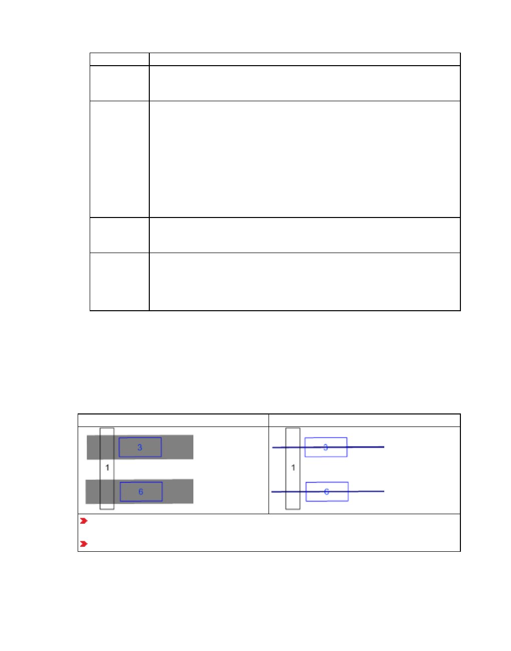
7.5.1 Modeling parking lots and zones
Element Description
Routing
decision dis-
tance
RoutDecDist: Distance of the parking space decision to the parking lot
Initial occu-
pancy
InitOccup: only relevant for Abstract parking lots and Real parking
spaces.
Initial occupancy in vehicles specifies which occupancy of the parking lot
should be calculated at the beginning of the simulation for the destination
parking lot selection. This also applies for dynamic routing decisions. The
initial occupancy serves to determine the time when the capacity of the
parking lot has been reached. Do not enter the number of vehicles which
arrive at the parking lot and then later drive away during a simulation.
These can be included in the origin-destination matrices. For Real parking
spaces, enter the composition of the initial occupancy.
Composition InitOccupComp: only relevant for Real parking spaces: Choose the
appropriate vehicle composition for the Initial occupancy (see "Modeling
vehicle compositions" on page 425).
Default
Desired
Speed
Desired speed distribution default (DesSpeedDistrDef): allocated
desired speed distribution and desired speed per vehicle class. The
default-desired speed distribution and desired speed are used for all
vehicles whose type does not belong to any of the vehicle classes dis-
played in the list below.
5. Confirm with OK.
The attributes are saved in the list of Parking Lots (see "Attributes of parking lots" on page
469).
Example for the modeling of a zone connector on the edge of a network
The figure shows a zone connector of the example file ..\dynamic assignment\Drop- Off
zone.Trip Chains\Drop-Off Zone inpx:
Toggle wireframe off Toggle wireframe on
The node is placed at the beginning of the upper link at the end of the lower link. The
beginning and end could also lie in the node.
Origin parking lot 3 and destination parking lot 6 are placed outside of the node.
© PTV GROUP 663

7.5.1 Modeling parking lots and zones
Setting relative volumes from all parking lots on the volume totals
If you have exported a network from Visum and are using a different volume scenario with a
new matrix file and a new path file, the relative volumes of the output parking lot are more
suitable.
Press the key combination CTRL+SHIFT+C.
The relative volumes of all of the parking lots are set to the volume totals of their paths in
the current path file *.weg.
Avoiding errors when modeling parking lots
An error message such as The origin parking lot 1 is part of several
different edges can mean that at least one node is missing or not positioned correctly.
Thereby multiple paths can be found between both nodes between which the parking lot is
located. For each of these paths, separate costs are determined. This can lead to different link
costs for a link sequence (in reality, a street) and therefore cause an incorrect vehicle
distribution.
In order to avoid this problem, when positioning the parking lots in the Vissim network, ensure
the following:
In the movement direction, the starting point of the path must be located before the parking
lot part of the node.
In the movement direction, the end point of the path must be located behind the parking lot
part of the node.
Both of these nodes, between which the parking lot is located, must be correctly modeled
and the beginning and end points of the path must be located between two nodes.
7.5.1.3 Defining zones
1. From the Lists menu, choose > Network > Zones.
The list of defined network objects for the network object type opens.
By default, you can edit the list (see "Using lists" on page 89).
In the list, you can define a new zone.
2. Right-click in the list.
3. From the shortcut menu, choose Add.
A new row with default data is inserted.
4. Enter the desired data.
Element Description
No Unique identification number of the zone
Name Name of zone
664 © PTV GROUP

7.5.1 Modeling parking lots and zones
You can assign the zone to a parking lot (see "Defining parking lots for dynamic assignment"
on page 660).
Tip: Alternatively, add a zone in the Parking lot window > Dyn. Assignment tab >
Zone box (see "Defining parking lots for dynamic assignment" on page 660).
7.5.1.4 Attributes of zones
1. From the Traffic menu, choose > Dynamic Assignment > Zones.
The Zones list opens.
The list on the left may include the following attributes:
Element Description
No Unique number
Name Name of zone
Center Location of a zone calculated from the mean of the coordinates of zone parking
lots
ParkLot Parking lot: Numbers of the zone parking lots
Showing and editing dependent objects as relation
1. In the list on the left, click the desired entry.
The list on the right contains attributes and attribute values of network objects, and/or base
data allocated to the network object selected in the list on the left (see "Using coupled lists" on
page 111):
OD pairs (see "Attributes of OD pairs" on page 665)
Parking lots: (see "Attributes of parking lots" on page 469)
2. On the list toolbar, in the Relations list, click the desired entry.
3. Enter the desired data.
The data is allocated.
7.5.1.5 Attributes of OD pairs
1. From the Traffic menu, choose > Dynamic Assignment > OD pairs.
The OD Pairs list opens. All relations between origin zones and destination zones are
displayed. This also includes relations within a zone.
The list on the left may include the following attributes:
Element Description
OrigZone Origin zone: Number and name
DestZone Destination zone: Number and name
© PTV GROUP 665

7.5.2 Modeling nodes
7.5.2 Modeling nodes
The geometry of the road network is modeled in a very detailed manner in Vissim. This
exactness is not necessary for the decision of a driver for a specific path through the network.
The exact traffic routing at the node is not relevant; instead, the directions on the nodes which
can be turned are relevant.
In order to reduce the complexity of the network model and therefore also the calculation time
and memory required, you can identify parts of the network as nodes. These positions are at
the minimum the positions in which the paths merge together, or the positions which branch
out in different directions. Normally these are the network sections which represent a real
junction. Do not group larger network sections, containing multiple intersections, into a node.
Nodes for evaluations, dynamic assignment and mesoscopic simulation
In the attributes of the node, you select whether you want to use the node for evaluations
and/or dynamic assignment and/or mesoscopic simulation. Depending on the particularities of
the network, a node can be used for evaluations, dynamic assignment and mesoscopic
simulation. However, certain particularities of a network might require you to model additional
nodes for mesoscopic simulation (see "Mesoscopic node-edge model" on page 761).
To perform dynamic assignment, you only need one node for each roundabout or complex
intersection. For these nodes, select the attribute Use for dynamic assignment. It is not
necessary to define a separate node for each conflict of two movements. Example file
..\Examples Demo\Roundabout Schenectady.US\Roundabout Schenectady.inpx:
Nodes at the boundary of a network
For dynamic assignment, nodes are required at the boundaries of the network where links in
the Network editor begin or end. Example file ..\Examples Training\Dynamic Assignment
\Detour\Detour.inpx:
666 © PTV GROUP

7.5.2 Modeling nodes
Notes:
Meso network nodes may intersect with nodes of dynamic assignment.
Nodes of dynamic assignment must not intersect with each other.
Meso network nodes must not intersect with each other.
If you open a network file *.inpx with an overlapping node or you add a node which
overlaps the adjacent node, an error message appears. The error message and the
numbers of the overlapping nodes are shown in the Messages window (see "Show-
ing messages and warnings" on page 1117).
Mesoscopic simulation distinguishes between different node types (see "Meso-
scopic node-edge model" on page 761).
7.5.2.1 Using polygon nodes and segment nodes
Vissim distinguishes between polygon nodes and segment nodes:
Polygon nodes: in figure, node 70. By default, polygon nodes are used in Vissim because
they can be easily defined and edited. You always add a node as a polygon node in Vissim
(see "Defining nodes" on page 668).
Segment nodes consist of link segments, as shown in figure node 69.
A polygon node can be converted into a segment node and vice versa (see "Converting
polygon nodes" on page 675), (see "Converting segment nodes" on page 676).
During the ANM import of external data, nodes in Vissim are always generated as link
segments (see "Importing ANM data" on page 345).
The definition of nodes as link segments allows a more detailed editing of the node (see
"Selecting nodes, polygons or segments" on page 674).
Examples:
© PTV GROUP 667

7.5.2 Modeling nodes
If you have defined a node manually and in a node polygon, a fast road e.g. continues as
a bridge above the node, you can convert the polygon node into segments and remove all
segments on the fast road from the node so that the fast road is no longer part of the node.
If you have imported a node as a link segment, you can convert it to a polygon, in order to
change its spatial extent at the polygon level to the segment level.
Notes:
Attributes of the polygon nodes and segment nodes are identical.
The colors from polygon nodes and segment nodes are identical.
In the dynamic assignment, the polygon nodes and segment nodes are considered
in the same manner.
7.5.2.2 Defining nodes
Notes:
You can specify that you need not press the CTRL key when adding network objects
(see "Right-click behavior and action after creating an object" on page 143).
For some network objects there are windows in which the attributes of a network
object can be defined and edited. There are lists for this, for all network objects. You
can choose whether you want to open a window, a list or neither of the two for the
definition of network objects in the Network Editor (see "Right-click behavior and
action after creating an object" on page 143).
1. On the Network objects toolbar, click Nodes.
2. Hold down the CTRL key and right click on the network editor on the desired corners of the
polygons in the area of the node.
Note: Alternatively you can select Add New Node from the context menu in the network
editor. A node with four corners is added. The Nodes window opens, if you have
selected that you want the program to open the Edit dialog automatically after object
creation (see "Right-click behavior and action after creating an object" on page 143).
3. Once you have added all of the corners of the polygon, double click.
4. Release the keys.
The node has been added. The window Node opens.
5. Edit the attributes (see "Attributes of nodes" on page 669).
6. Confirm with OK.
The attributes are saved in the list Nodes.
668 © PTV GROUP

7.5.2 Modeling nodes
Notes:
Do not define overlapping nodes.
A polygon node can be converted into a segment node and vice versa (see "Con-
verting polygon nodes" on page 675), (see "Converting segment nodes" on page
676). For each conversion the definition of the node is adjusted correspondingly.
You can edit the node definition.
Tip: Alternatively, you can import nodes via ANM import (see "Importing ANM data" on
page 345). Nodes are always imported as segment nodes.
7.5.2.3 Attributes of nodes
The Nodes window opens when you insert a network object and have selected to have the
Edit dialog automatically opened after object creation (see "Right-click behavior and action
after creating an object" on page 143). By default, only the Nodes list is opened.
Into the window, you enter attribute values for the network object. For network objects which
have already been defined, you can call the window using the following functions:
In the list of network objects of the network object type, double-click the row with the
desired network object.
In the Network editor, select the network object of your choice. Then, from its shortcut
menu, choose Edit.
The network object may have additional attributes. In the network objects list of the network
object type, you can show all attributes and attribute values. You can open the list via the
following functions:
In the network object toolbar, right-click the desired network object type. Then from the
shortcut menu, choose Show List (see "Context menu in the network object toolbar" on
page 63).
In the Network editor, select the network object of your choice. Then, from its shortcut
menu, choose Show In List (see "Selecting network objects in the Network editor and
showing them in a list" on page 339).
From the Lists menu, in the desired category, choose the network object type.
In the network objects list of the network object type, you can edit attributes and attribute
values of a network object (see "Selecting cells in lists" on page 102), (see "Using lists" on
page 89).
The objects of this object type may have relations to other objects. This is why the attributes list
is shown as part of a coupled list (on the left). On the Lists toolbar, in the Relations box, you
can show and edit the coupled list with the attributes of the desired relation on the right (see
below Showing and editing dependent objects as relation) and (see "Using coupled lists" on
page 111).
Note: In lists, you can use the Attribute selection icon to show and hide attribute
values (see "Selecting attributes and subattributes for a list" on page 106).
© PTV GROUP 669
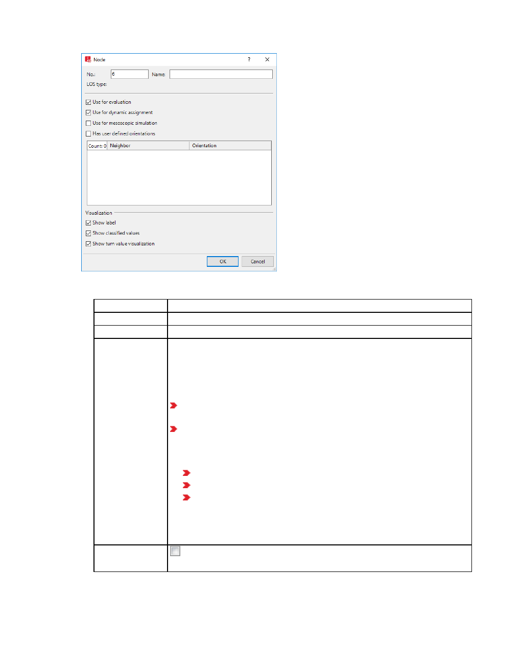
7.5.2 Modeling nodes
1. Make the desired changes:
Element Description
No. Unique node number
Name Designation of the node
LOSType Level-of-service scheme type: Basis for determining the appropriate
LOS scheme for result attributes LOS(All) and LOSVal(All) in node
evaluation (see "Evaluating nodes" on page 997). The LOSTyp is
defined Vissim based on the node type when the simulation run is first
started:
Signalized: If at least one signal head of an active SC has been
defined for at least one movement
Non-signalized: If no signal head has been defined or the SC is
inactive
The LOSType is only calculated in the following cases:
For nodes, whose Use for evaluation attribute is selected
For movements with the direction Total
For evaluation edges that are entry edges into the node
When you edit a node or insert a new node, Vissim defines the LOSTyp
for all nodes based on the node type the next time you start a
simulation.
Showing label If this option is not selected, the label for the respective node is
hidden when label for all nodes is selected.
670 © PTV GROUP
7.5.2 Modeling nodes
Element Description
Dynamic
assignment Use for dynamic assignment (UseForDynAssign): If the option is
selected, the nodes for the network graphs are taken into consideration
in the dynamic assignment. When starting a simulation from COM, the
node-edge graph is always constructed because it is not possible to
determine at the start of the simulation whether the curvature of the
simulation should add another path to the vehicle, which originates at
the COM script. Even without COM the construction of the node-edge
graph takes time if you call up the list Edges because there are many
edges between two nodes, particularly for low node density. In the list
Edges, only the nodes are shown in which the option Dyn. Assignment
is selected (see "Editing edges" on page 677).
If the option is not selected, the nodes for the network graphs are
ignored in the dynamic assignment. If you select the attribute Use for
evaluation, the node can still be considered for node evaluation (see
"Evaluating nodes" on page 997).
If the nodes are not used for the dynamic assignment, deactivate the
option. This saves you calculation time.
Use for
mesoscopic
simulation
UseForMeso:
If this option is selected, the meso network node is taken into account
for generation of the meso graph (see "Modeling meso network nodes"
on page 766).
If this option is not selected, the node in not taken into account for
mesoscopic simulation.
Note: This setting is ignored for the microscopically simulated
sections during hybrid simulation.
User defined
orientations Has user defined orientations (HasUserDefOrient): Select this
option to enable the Orientations list. The list displays the determined
orientation of the intersection between the polygon of the node and the
edge to the adjacent node. You can overwrite these in the list when they
do not correspond with the real orientation.
Column Neighbor: List of nodes adjacent to the edited node in the
network.
Column Orientation: Select a direction for this adjacent node: N, NE,
E, SE, S, SW, W, NW
Select a direction in particular when multiple edges lead to an adjacent
node and Vissim has determined an unrealistic direction. By default, in
the case of multiple edges, Vissim uses the direction which occurs the
most often; in the case of only two edges, it uses the direction which, in
the list of available directions, occurs first (at the top, in clockwise
direction).
© PTV GROUP 671

7.5.2 Modeling nodes
Element Description
Note: The evaluation graph for the calculation of orientations based on the current
direction North in the network. The evaluation graph only considers the nodes
which fulfill the following conditions:
For both adjacent nodes, you must select Use for evaluation. If this is not the
case for all network nodes, the graph is not complete.
The adjacent nodes cannot be more than 500 m from each other. In the case of
larger distances, an additional node can be inserted.
Use for
evaluation UseForEval: If the option is selected, the node is considered for the
node evaluation, if the node evaluation is selected (see "Evaluating
nodes" on page 997).
Show classified
values Show classified values (ShowClsfValues): Select this option to
show classified values, not to show the display type selected. To show
classified values, in the graphic parameters for nodes, select a color
scheme and an attribute (see "Assigning a color to nodes based on an
attribute" on page 181).
Show turn
value
visualization
(ShowTurnValVisual: Select this option to graphically show, in the
node, along the turn relations, the values of the attribute selected for
turn value visualization (see "Visualizing turn values" on page 645).
Tip: Alternatively, in the Network editor, right-click the node. Then
from the shortcut menu, choose Activate turn value
visualization.
2. Confirm with OK.
The network object has additional attributes that you can show in the Attributes list. In the
Attributes lits, the following is displayed by default:
Element Description
TurnValVisualSize Turn value visualization size: Radius [m] of the outer circle of the the
turn value visualization
Showing and editing dependent objects as relation
The attribute and attribute values of this network object type are shown in the list on the left,
which consists of two coupled lists.
1. In the list on the left, click the desired entry.
The list on the right contains attributes and attribute values of network objects, and/or base
data allocated to the network object selected in the list on the left (see "Using coupled lists" on
page 111):
Turns (evaluation): Attributes of edges in the node that are turn relations in the node-edge
graph of node evaluation (see "Generating a node-edge graph" on page 678)
672 © PTV GROUP

7.5.2 Modeling nodes
Turns (dynamic assignment): Attributes of edges in the node that are turn relations in the
node-edge graph of dynamic assignment (see "Generating a node-edge graph" on page
678)
User defined orientations
Movements (see "Evaluating nodes" on page 997). To show result attributes of move-
ments, you first need to generate the node-edge graph for evaluations (see "Generating a
node-edge graph" on page 678).
Edges (evaluation) (see "Generating a node-edge graph" on page 678), (see "Attributes of
edges" on page 678)
Edges (evaluation, entering): All edges of the evaluation node that enter the node and/or
end at the node
Edges (dynamic assignment) (see "Generating a node-edge graph" on page 678), (see
"Attributes of edges" on page 678)
Conflict areas (see "Attributes of conflict areas" on page 531)
Meso turn conflicts (see "Attributes of meso turn conflicts" on page 790)
Meso turns (see "Attributes of meso turns" on page 789)
Points: edit coordinates of the corners
Link segments: Attributes of the link segments in segment nodes
2. On the list toolbar, in the Relations list, click the desired entry.
3. Enter the desired data.
The data is allocated.
7.5.2.4 Meaning of node color and line style
In the graphic parameters of the network object type Nodes, you can define a fill style, fill color,
border line style and border line color for nodes (see "List of graphic parameters for network
objects" on page 152).
How visualization is implemented also depends on the following settings and factors:
A node is selected.
The border of the selected polygon node or segment node is a solid yellow line. Filled circles
are displayed at the corner points of the polygon node.
Multiple nodes are selected.
The border of each node selected is a solid yellow line. There are no filled circles are
displayed at the corner points of the polygon node.
No node is not selected.
The Drawing mode attribute of the network object type Node defines the color:
© PTV GROUP 673
7.5.2 Modeling nodes
Use constant colors: The border of a polygon node or segment node is drawn as a solid
line. The color depends on the node type:
Polygon node: The Border color attribute defines the color of the border.
Segment node: The color of the border is dark gray.
Color by function: For polygon nodes and segment nodes, the border and color depend
on the node type:
Color and style of the border node type selected
solid white no node type
solid green Use for evaluation
solid red Use for dynamic assignment
solid black Use for evaluation and for dynamic assignment
white, dashed Use for mesoscopic simulation
not white, dashed Use for mesoscopic and other simulations
7.5.2.5 Selecting nodes, polygons or segments
You can select and edit nodes in a Network editor. For a single node, you can open the Node
window and edit the attributes. For multiple nodes, you can edit the attributes in the Nodes list
(see "Attributes of nodes" on page 669). The Nodes list contains all nodes, regardless of
whether they are currently represented as a polygon or displayed in the segment definition.
You can select and delete single or multiple nodes.
1. On the Network objects toolbar, click Nodes.
Note: Do not define overlapping nodes.
2. In the Network Editor, click the network object:
in the desired node
in the desired polygon
on one of the segments
in the hidden rectangle around the segments
The selected node is highlighted (see "Meaning of node color and line style" on page 673).
Tip: You can select multiple nodes in a Network Editor by drawing a rectangle or by
holding down the CTRL key and clicking the node.
7.5.2.6 Editing node polygons
You can move a node polygon in a network editor and call up different functions for editing via
the context menu.
674 © PTV GROUP

7.5.2 Modeling nodes
Moving polygon
Click on the network editor on the desired polygon, hold down the mouse button and move
the polygon.
The courses of the road in the network remain unchanged.
Inserting polygon point
1. On the Network objects toolbar, click Nodes.
2. In the Network editor, right-click the desired position of the new polygon point on the line of
the polygon.
The polygon point is displayed.
Moving the polygon point
1. On the Network objects toolbar, click Nodes.
2. In the Network editor, click the polygon point, hold down the mouse button and move the
polygon point to the desired position.
3. Release the mouse button.
Deleting the polygon point
1. On the Network objects toolbar, click Nodes.
2. In the Network editor, click the polygon point, hold down the mouse button and move the
polygon point onto an adjacent polygon point.
3. Release the mouse button.
7.5.2.7 Converting polygon nodes
You can convert polygon nodes to segment nodes. When you convert nodes several times,
the expansion of the node polygon may increase. Additional segments are added to the
display of segments or the size of the segments is adjusted.
Note: Do not define overlapping nodes.
1. On the Network objects toolbar, click Nodes.
2. In the Network Editor, right-click the polygon node.
The polygon node is marked.
© PTV GROUP 675
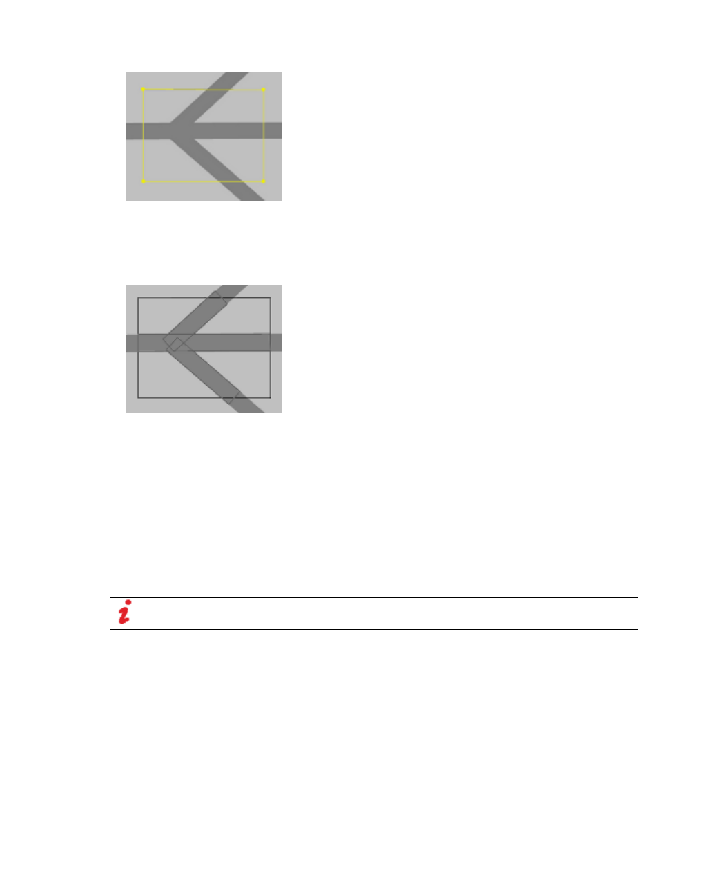
7.5.2 Modeling nodes
3. In the context menu, choose the entry Convert Node.
The segments of the node are shown. The segments are arranged according to the
expansion of the original node polygon on the links. When you convert a polygon node to a
segment node, only the segments which include the polygon are generated.
7.5.2.8 Converting segment nodes
When you convert a segment node to a polygon node, a rectangular polygon is generated. Its
location and size result from the location and size of the segments. The polygon includes all
segments. The lower horizontal line is drawn directly under the lowest point of the segments.
The right line is drawn immediately to the right of the right-most point of the segments. The
segments within this polygon do not necessarily correspond to the original segments.
When you convert nodes several times, the expansion of the node polygon may increase.
Additional segments are added to the display of segments or the size of the segments is
adjusted.
Note: Do not define overlapping nodes.
1. On the Network objects toolbar, click Nodes.
2. In the Network Editor, right-click the segment node.
The segment node is marked.
3. In the context menu, choose the entry Convert Node.
Frame and polygon points of the node are shown. The area of the polygon increases.
676 © PTV GROUP

7.5.3 Editing edges
7.5.2.9 Creating nodes per level
From a segment node on one level you can create additional segment nodes lying on other
levels. This can be useful when you convert a polygon node, with a multi-story parking garage
including links and connectors, into a segment node, but you need segment nodes for each
level of the parking garage. Vissim will then only generate segment nodes for the levels that
had network objects in the the original node.
1. Make sure that in the network editor, you have selected the segment node of your choice
(see "Moving network objects in the Network Editor" on page 336).
2. In the Network Editor, right-click the segment node.
The segment node is marked.
3. From the shortcut menu, choose Create nodes per level.
The segment node is duplicated for each level that has network objects in the segment
node. The new segment nodes are listed in the Nodes list.
7.5.2.10 Deleting nodes
You can delete an individual node in a network editor or in the Nodes list (see "Deleting
network objects" on page 336). You can also delete multiple nodes.
1. On the Network objects toolbar, click Nodes.
2. Press the CTRL key and click the nodes.
3. Press the DEL key.
7.5.3 Editing edges
At the start of the dynamic assignment, Vissim automatically generates an abstract network
graph based on the user-defined node. You can also generate this node-edge graph via a
function (see "Generating a node-edge graph" on page 678). The node-edge graph may
consist of the following edges:
Turn relations: edges within a node
Edges from node to node. An edge starts at the border of node and ends at the border of a
node.
7.5.3.1 Differences from standard network graph
The topology of the node-edge graph is only slightly different from the standard network graph
in traffic flow models:
There may be more than one edge between two Vissim nodes.
The turn relations within nodes are not just abstract entities, but are represented by edges
which have a real length in Vissim.
© PTV GROUP 677

7.5.3 Editing edges
7.5.3.2 Use of edges
Edges are the elementary components of the path search because paths are sequences of
edges. At the edge level, travel times and costs are recorded in the simulation and made
available for the path selection in the next iteration.
If for the attribute Blocked vehicle classes for dynamic assignment(Connector closed to) of
a connector, the number of vehicle classes selected results in all vehicle types being closed to
the connector, this connector is not used by network graph edges.
7.5.3.3 Generating a node-edge graph
You can create a node-edge graph for nodes:
For dynamic assignment: The nodes must have been activated for dynamic assignment
(see "Attributes of nodes" on page 669).
For node evaluation and thus for the relation movements of nodes (see "Evaluating
nodes" on page 997), (see "Attributes of nodes" on page 669). Vissim automatically gen-
erates the nodes-edges graph for evaluations when the Node evaluation results list is
opened.
1. Select Network > Edges in the Lists menu.
The list Edges opens. If no node-edge graphs were generated, only the column titles are
shown.
2. Right-click in the list.
3. From the shortcut menu, choose the desired entry:
Create Dynamic Assignment Graph
Create Evaluation Graph
The edges and their attributes are shown in the Edges list (see "Attributes of edges" on
page 678).
When you delete network objects that affect edges, Vissim updates the Edges list. You then
might have to create a new graph.
7.5.3.4 Attributes of edges
Edges and their attributes are generated with node-edge graphs (see "Generating a node-
edge graph" on page 678).
1. Select Network > Edges in the Lists menu.
The list Edges opens. If no node-edge graphs were generated, only the column titles are
shown and you must generate node-edge graphs (see "Generating a node-edge graph" on
page 678).
Note: In lists, you can use the Attribute selection icon to show and hide attribute
values (see "Selecting attributes and subattributes for a list" on page 106).
678 © PTV GROUP
7.5.3 Editing edges
The list on the left may include the following attributes:
Element Description
No Unique edge number
FromNode From node: Name of the node, on which the edge begins
ToNode To node: Name of the node, on which the edge ends
Type Type of edge is either Dynamic assignment or Evaluation
IsTurn Is turn: If this option is selected, the edge is a turn relation.
Closed Closed: If this option is selected, the edge is closed. The edge is not taken
into consideration in the dynamic assignment.
The edge is highlighted in red in network editors if the Synchronization icon
has been selected in the Edges list:
Length Length of the edge in the network in meters
ConvTravTm Converged (travel time): If this option is selected, the travel time is
converged. The edge fulfills the convergence criterion Travel time on edges
for all completed time intervals (see "Attributes for achieving convergence" on
page 741).
ConvVol Converged (volume): If this option is selected, the volume is converged.
The edge fulfills the convergence criterion Volume on edges for all completed
time intervals (see "Attributes for achieving convergence" on page 741).
Notes:
The results of the last iteration are only shown in the list Edges when the cost file
and the path file were saved in this iteration.
An edge between nodes is ignored in the dynamic assignment when the vehicle is
cycled through more than three outbound connections from one link to the same
link (more than three loops). Path files and cost files from older Vissim versions,
which contain such edges, can no longer be used.
An edge in the dynamic assignment is ignored when it does not contain a parking
lot which spans over all of the lanes, i.e. zone connectors and abstract parking lots
on all links and real parking spaces only on links with one lane (see "Modeling park-
ing lots and zones" on page 659). Path files and cost files from older Vissim ver-
sions, which contain such edges, can no longer be used.
Showing and editing dependent objects as relation
The attribute and attribute values of this network object type are shown in the list on the left,
which consists of two coupled lists.
1. In the list on the left, click the desired entry.
© PTV GROUP 679

7.5.3 Editing edges
The list on the right contains attributes and attribute values of network objects, and/or base
data allocated to the network object selected in the list on the left (see "Using coupled lists" on
page 111):
To edges
Link sequence: Numbers of links and connectors via which the edge leads.
From edges
2. On the list toolbar, in the Relations list, click the desired entry.
3. Enter the desired data.
The data is allocated.
7.5.3.5 Excluding edges from dynamic assignment
If you have generated node-edge graphs, you can block edges and therewith exclude them
from the dynamic assignment.
1. Select Network > Edges in the Lists menu.
The list Edges opens.
2. Activate the option Closed (Closed).
The edge is not taken into consideration in the dynamic assignment. The edge is marked red
in the network editor.
7.5.3.6 Visualizing edges
Edges are represented in network editors in the following colors:
Yellow: open for dynamic assignment (in figure above)
Red: blocked for dynamic assignment
Displayed values based on the last iteration in which the path file was updated.
Displayed costs based on the last saved cost file.
7.5.3.7 Deleting segments of an edge from segment nodes
1. Ensure that the relevant node is a segment node and not a polygon node.
680 © PTV GROUP

7.6 Modeling traffic demand with origin-destination matrices or trip chain files
2. Select Network > Edges in the Lists menu.
The list Edges opens.
3. Ensure that a node-edge graph has been generated (see "Generating a node-edge graph"
on page 678).
In the Edges list, the edges of the segments nodes are displayed in the Vissimnetwork.
4. Right-click the entry of your choice.
5. From the context menu, choose Delete node segments.
All segments of the turn edge are deleted from the Edges list and the network editor.
7.6 Modeling traffic demand with origin-destination matrices or trip
chain files
The traffic demand for the dynamic assignment is modeled with origin-destination matrices.
Beyond that it is also possible to model the traffic demand with a trip chain file. You can also
combine both options.
You can use both options in combination with input flows and static routes, for example for
pedestrian flows. In this process, static traffic cannot be taken into account by the dynamic
assignment.
7.6.1 Modeling traffic demand with origin-destination matrices
An OD matrix defines the travel demand based on the number of trips between the zones (see
"Defining an origin-destination matrix" on page 681). The zones are the starting points and
end points of the trips. The number of trips applies to each pair of districts for a given time
interval. You define the time interval in the matrix attributes (see "Matrix attributes" on page
683). You edit the number of trips of the OD matrix in the matrix editor (see "Editing OD
matrices for vehicular traffic in the Matrix editor" on page 684). Origin-destination matrices are
also called OD matrices, demand matrices or trip matrices.
You can specify multiple origin-destination matrices for a simulation with dynamic assignment.
Each origin- destination matrix can contain a different vehicle composition or apply to a
different time interval. The time intervals can overlap arbitrarily because the traffic generated at
any time is always the result of the total traffic from all matrices that include this point in their
validity interval.
7.6.2 Defining an origin-destination matrix
You can define an OD matrix in the parameters of dynamic assignment or in the Matrices list.
Matrices are saved to the *.inpx file. In the Matrix editor, you enter traffic demand data into the
OD matrix (see "Editing OD matrices for vehicular traffic in the Matrix editor" on page 684).
Defining an OD matrix in the parameters section of dynamic assignment
1. From the Traffic menu, choose > Dynamic Assignment > Parameters.
The Dynamic Assignment: Parameters window opens.
© PTV GROUP 681

7.6.3 Selecting an origin-destination matrix
2. Select the option Matrices.
3. Right-click in the list.
4. From the shortcut menu, choose Add.
5. Move the mouse pointer to the new cell and click the symbol.
Depending on the matrices already defined, the box contains the next consecutive number
available for the new matrix.
6. In the VehComp column, select the desired vehicle composition.
7. Edit the attributes of matrix (see "Matrix attributes" on page 683).
8. Edit the number of trips in the matrix editor (see "Editing OD matrices for vehicular traffic in
the Matrix editor" on page 684).
Defining an OD matrix in the Matrices list
1. From the Traffic menu, choose > Dynamic Assignment > Matrices.
2. In the list, on the toolbar, click the Add button .
A new row with default data is inserted.
The Matrix editor is opened. The matrix dimension automatically depends on the number of
zones defined. The dimension is displayed in the top left box.
3. Edit the attributes of matrix (see "Matrix attributes" on page 683).
4. Edit the number of trips in the matrix editor (see "Editing OD matrices for vehicular traffic in
the Matrix editor" on page 684).
7.6.3 Selecting an origin-destination matrix
You can select one or multiple OD matrices for the dynamic assignment. And you can select a
vehicle composition for each matrix. The vehicles of this vehicle composition operate between
the zones that are defined in the OD matrix. The selection of vehicles is effected randomly.
The desired speed of the vehicle is not taken from the desired speed distribution which is
defined for the vehicle composition; instead, it is taken from the desired speed distribution
which is defined for the parking lot, from which the vehicle begins its trip (see "Attributes of
parking lots" on page 469).
682 © PTV GROUP

7.6.4 Matrix attributes
In Vissim, you can edit OD matrices in the Matrix editor (see "Editing OD matrices for vehicular
traffic in the Matrix editor" on page 684)
Matrices are exchanged between Vissim and Visum via Visum data export from Vissim and
ANM export from Visum.
1. Ensure that an OD matrix has been defined (see "Defining an origin-destination matrix" on
page 681).
2. From the Traffic menu, choose > Dynamic Assignment > Parameters.
The Dynamic Assignment: Parameters window opens.
3. Select the option Matrices.
4. Move the mouse pointer to the Matrix column and click the symbol.
5. Select the desired matrix.
In the Matrix column, number and name of the matrix are displayed.
6. In the VehComp column, select the desired vehicle composition (see "Modeling vehicle
compositions" on page 425).
You can edit additional attributes of dynamic assignment (see "Attributes for the trip chain file,
matrices, path file and cost file" on page 731).
7.6.4 Matrix attributes
1. From the Traffic menu, choose > Dynamic Assignment > Matrices.
The Matrices list opens.
Note: In lists, you can use the Attribute selection icon to show and hide attribute
values (see "Selecting attributes and subattributes for a list" on page 106).
The list contains the following attributes:
Element Description
No Unique number of the matrix
Name Name of matrix
FromTime Start of the time interval from 0:00 o’clock for which the matrix applies
ToTime End of the time interval from 0:00 o’clock for which the matrix applies
© PTV GROUP 683
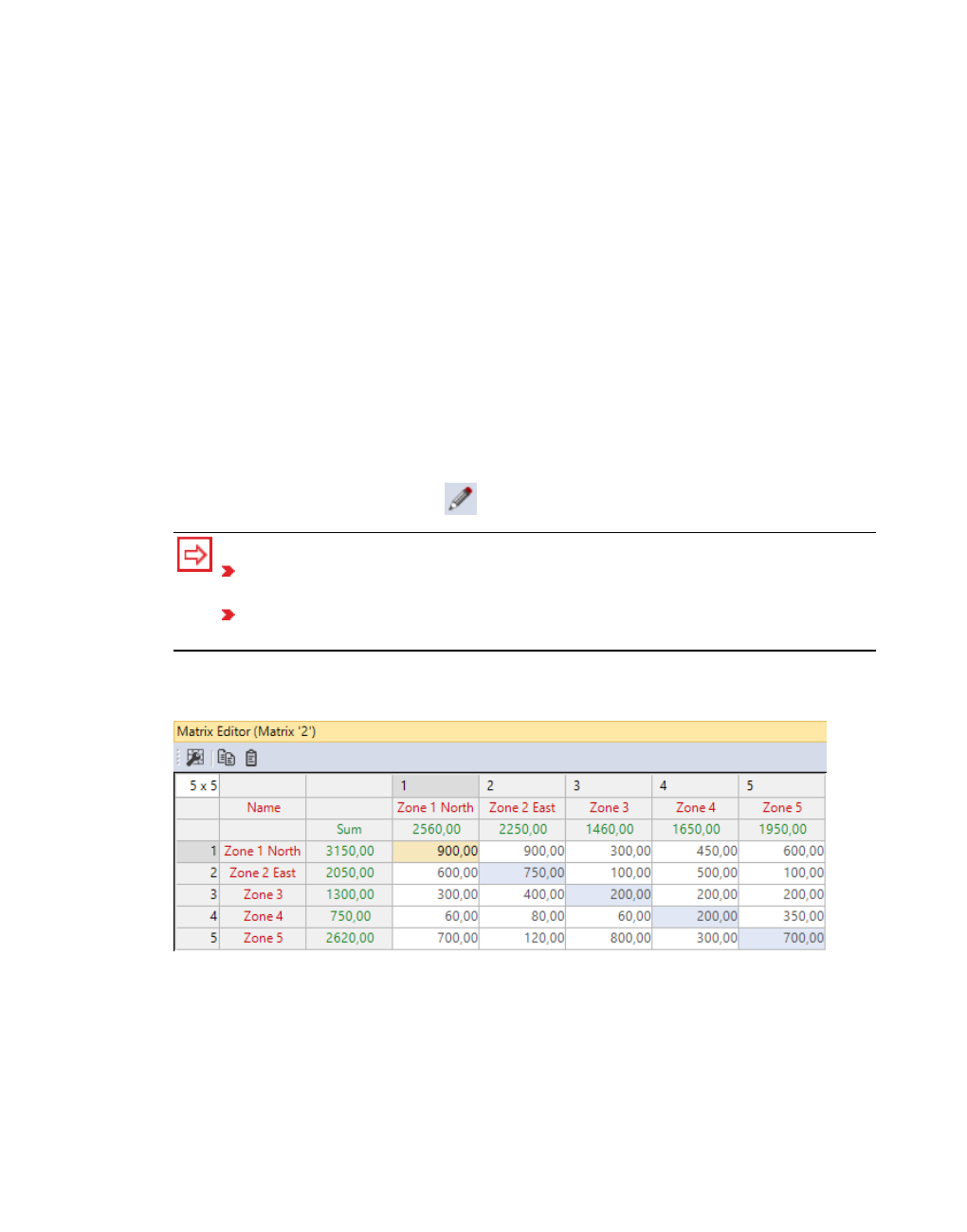
7.6.5 Editing OD matrices for vehicular traffic in the Matrix editor
7.6.5 Editing OD matrices for vehicular traffic in the Matrix editor
In the matrix editor, enter the number of journeys for the vehicle traffic between the zones for
an OD matrix. You can open multiple Matrix editors to edit their values.
In Viswalk, you edit OD matrices for pedestrians in the Pedestrian OD Matrix (see "Pedestrian
OD matrices" on page 918).
7.6.5.1 Opening the Matrix editor and entering the number of trips
1. Ensure that at least one matrix has been defined (see "Defining an origin-destination
matrix" on page 681).
2. Make sure that the parking lots of the type Zone connector are defined and that they are
allocated to a zone (see "Defining parking lots for dynamic assignment" on page 660).
3. From the Traffic menu, choose > Dynamic Assignment > Matrices.
The Matrices list opens.
4. Select the desired entry.
5. On the list toolbar, click Edit object .
Tip:
Alternatively, in the Matrices list, in the row of the desired matrix, double-click
the header.
Alternatively, in the Matrices list, double-click the row of the desired matrix and
select Edit in the context menu.
The Matrix editor is opened. The matrix, the name of the zones (red) and the sum (green) of
trips between zones are displayed.
The matrix dimension automatically depends on the number of zones defined. The
dimension is displayed in the top left box.
In the next step, you can also define several fields and enter values.
6. Into the white and blue boxes, enter the number of trips between zones.
684 © PTV GROUP
7.6.6 Using OD matrices from previous versions
7.6.5.2 Copying and pasting the number of trips
In the Matrix editor, you can select one or multiple cells, copy the values and paste them into
other cells. If you copy values of multiple cells, they must be selected according to one of the
following patterns:
The cells or rows are immediately next to each other
The cells or columns are immediately under each other
2 x 2 cells or multiple thereof
1. Select the desired cells.
2. On the Matrix editor toolbar, click .
In the next step, to paste the cells, follow the same pattern used to copy them.
3. Select the desired target cells.
4. On the Matrix editor toolbar, click .
7.6.5.3 Editing graphic parameters
1. To edit graphic parameters in the matrix, on the Matrix editor toolbar, click Matrix editor
graphic parameters .
2. Make the desired changes:
Element Description
Column width Column width for all columns in pixels
Decimals Number of decimal places, default value 2
Row height Row height in pixels for all rows, default value 20
7.6.5.4 Defining column width
1. Right-click the column header of the Matrix editor.
2. Choose the desired entry from the context menu.
Element Description
Set Optimum Width for
All Columns
Adjusts column width for alls column to accommodate the
longest column title and longest cell entry
Adjust Column Widths
To Window Size
Adjusts column width for all columns to the window width
7.6.6 Using OD matrices from previous versions
From version 9 and later, Vissim manages OD matrices in the Matrices list (see "Matrix
attributes" on page 683), (see "Modeling traffic demand with origin-destination matrices" on
© PTV GROUP 685

7.6.6 Using OD matrices from previous versions
page 681). You can view and edit the matrix content in the matrix editor (see "Editing OD
matrices for vehicular traffic in the Matrix editor" on page 684).
For the dynamic assignment, Vissim up to version 8 requires at least one OD matrix that is
saved to an *.fma file. You can choose the *.fma file from the dynamic assignment parameters
in Vissim up to version 8.
You cannot copy the OD matrix from the *.fma file and paste it immediately into the matrix
editor in Vissim.
You can export an OD matrix from a previous version to Vissim version 9 and higher. The
following applications and solutions are distinguished:
In the matrix editor, Read from file
In the Matrices list > Read from file
Open the *.inpx file from Vissim 6,7 or 8, in Vissim 9 or higher.
Copy OD matrix and paste it into Vissim version 9 or higher.
7.6.6.1 Reading from file in the matrix editor
1. In the matrix editor, make sure that the origin-source matrix of the desired matrix in the
Matrices list is displayed.
2. Make sure that the dimensions of the OD matrix in the matrix editor correspond to the
dimensions that result from the number of zones in the *.fma file.
3. In the matrix editor, click the Read from file icon.
The Read matrix from file window opens.
4. Select the *.fma file of your choice.
5. Click the Open button.
The data is inserted into the matrix editor. In the Matrices table, the values of the TimeFrom
andTimeUntil attributes are adjusted on the basis of the values of the *.fma file.
7.6.6.2 Reading from file in the Matrices list
1. Make sure that the dimensions of the OD matrix in the matrix editor correspond to the
dimensions that result from the number of zones in the *.fma file.
2. In the Matrices table, right-click the matrix of your choice.
3. Choose Read from file from the shortcut menu.
The Read matrix from file window opens.
4. Select the *.fma file of your choice.
5. Click the Open button.
The data is inserted into the matrix editor. In the Matrices table, the values of the TimeFrom
andTimeUntil attributes are adjusted on the basis of the values of the *.fma file.
686 © PTV GROUP
7.6.6 Using OD matrices from previous versions
7.6.6.3 Open the *.inpx file from Vissim 6,7 or 8, in Vissim 9 or higher.
If you have access to the following files, to the Vissim versions and meet the requirements, you
can open an older network file in Vissim 9 or higher and create an OD matrix:
*.fma file selected in another *.inpx network file
You have so far used the *.inpx network file in Vissim 6, 7 or 8. You can also open an
*.inp network file from Vissim 5.40 in subsequent versions and save it as *.inpx file. Net-
work files used in Vissim 5.40 and previous versions cannot be opened in
Vissim version 6 or above.
Vissim from version 9
You have the following options:
Open the *.inpx network file in Vissim 9 or higher and save it.
Only for *.inpx files from Vissim version 9 and higher: Additionally read the *.inpx file into
Vissim. In the Read additionally window, choose only the Matrices entry from (see "Read-
ing a network additionally" on page 341).
Vissim creates the matrices in the Matrices list (see "Matrix attributes" on page 683). They
are saved to the *.inpx file. The *.fma files are thus no longer required. You can edit the
content of any matrix in the matrix editor (see "Editing OD matrices for vehicular traffic in the
Matrix editor" on page 684).
1. In the attributes of the parking lots of the Zone connector type that you need for the
dynamic assignment, make sure that you have selected the desired zones.
2. In the list Matrices, make sure that in the TimeFrom attribute the desired start time of the
interval and in the TimeUntil attribute the desired end time of the interval are defined(see
"Matrix attributes" on page 683).
3. Before starting the simulation, make sure that the dynamic assignment parameters are as
follows:
On the Files tab, the Matrices option is selected.
The desired matrix is selected in the list below.
7.6.6.4 Copy OD matrix and paste it into Vissim version 9 or higher.
If you have access to the following files and to Vissim version 9 or higher and meet the
requirements, but do not have Vissim version 6, 7 or 8, you can copy the data from the *.fma
file and paste it into a spreadsheet program or a similar program:
*.fma file with OD matrix
Vissim version 9 and higher
Spreadsheet program or similar program
*.inpx network file with or without Vissim network and with or without defined zones
Copy the data from the spreadsheet program or similar program to the clipboard and paste it
into Vissim version 9 or higher, in the open network file, into the fields of the matrix editor.
© PTV GROUP 687

7.6.6 Using OD matrices from previous versions
Making sure that the zones of your choice are defined
From Vissim version 9 and higher, the number of zones defines the dimensions of the OD
matrix. Therefore, before copying the data, make sure that in Vissim the zones are defined
which match the copied data:
1. To open Vissim version 9 or higher.
2. If you want to paste the copied data into an existing network file, open this *.inpx network
file.
3. From the Traffic menu, choose > Dynamic Assignment > Zones.
The number of necessary zones depends, for example, on your planning targets, the
parking lots of the Zone connector type and/or the OD matrix that you want to insert.
4. Make sure that the number of defined districts corresponds to the desired dimension of the
OD matrix (see "Defining zones" on page 664).
5. From the Traffic menu, choose > Dynamic Assignment > Matrices.
The Matrices list and the matrix editor open.
6. If no matrix is defined in the Matrices list, define a matrix(see "Defining an origin-
destination matrix" on page 681).
7. If matrices are defined in the Matrices list, make sure that the matrix attributes, that you
want to copy to the trips, meet your requirements(see "Matrix attributes" on page 683).
8. In the Matrices list, double-click the matrix whose dimension you want to check and which
you want to use at a later point in time in order to insert data.
In the matrix editor, the associated OD matrix is displayed and selected. The dimension of
the OD matrix is automatically based on the number of zones defined. The dimension is
displayed in the top left box (see "Editing OD matrices for vehicular traffic in the Matrix
editor" on page 684).
9. If you want to change the dimension of the OD matrix, change the number of zones (see
"Defining zones" on page 664).
10. From the File menu, choose > Save.
11. In Vissim, keep the network file and matrix editor open, so that you can insert the data after
the next steps.
Copying an OD matrix
1. Open the *.fma file in a spreadsheet program.
Some spreadsheet programs are supported by a wizard through which you can configure
the distribution of the copied data across the individual cells.
2. Make sure that each value, that indicates a number of trips, appears in a cell.
3. If desired, save the file.
688 © PTV GROUP

7.6.6 Using OD matrices from previous versions
If you then select data in the spreadsheet program, you can select one or more cells. If you
select multiple cells, these must cover a regular range of contiguous cells, for example 1 x
4, 5 x 3, or 6 x 6 cells.
If you select more than one cell, make sure that the range you selected corresponds to the
dimension of the OD matrix in the matrix editor of Vissim that you want to copy the data to.
4. In the spreadsheet program, select the desired range.
5. Press CTRL+C.
Inserting an OD matrix
1. Switch to Vissim.
2. Make sure that:
The network file of your choice is open.
In the matrix editor, the OD matrix is displayed for the desired matrix.
The OD matrix in the matrix editor has the desired dimension.
In the next step, make sure that you select a range in the matrix editor, which can include
the range from the clipboard:
The range you copied must not be larger than the dimension of the OD matrix in the
matrix editor.
If you select more than one cell in the matrix editor, the range you selected must not be
smaller than the range you copied.
If you select a single cell, the range you copied must not be larger than the range avail-
able based on the cell you selected.
3. In the matrix editor, select the desired number of cells.
4. Press CTRL+V.
The data is inserted into the matrix editor based on its volume and the number of selected
cells. If the selected range is larger than the range you copied, the data will be inserted
multiple times.
5. In the attributes of the parking lots of the Zone connector type that you need for the
dynamic assignment, make sure that you have selected the desired zones (see "Defining
parking lots for dynamic assignment" on page 660).
6. In the Matrices list, make sure that in the TimeFrom attribute the desired start time of the
interval and in the TimeUntil attribute the desired end time of the interval are defined(see
"Matrix attributes" on page 683).
7. In the menu Traffic > Dynamic assignment > Parameters, go to the Files tab and select
the Matrices option (see "Attributes for the trip chain file, matrices, path file and cost file"
on page 731).
8. In the list below, in the Matrix column, select the matrix of your choice.
© PTV GROUP 689
7.6.7 Modeling traffic demand with trip chain files
7.6.7 Modeling traffic demand with trip chain files
In addition to origin-destination matrices, the traffic demand can also exist in trip chain files
*.fkt for dynamic assignment. A trip chain is defined as a result of a trip. In contrast to origin-
destination matrices, a trip chain file delivers detailed data regarding trips of individual
vehicles for the simulation. Therefore the generation of trip chain files is more complex
compared to that of origin- destination matrices (see "Modeling traffic demand with origin-
destination matrices" on page 681).
Trip chains are only used internally in Vissim. Trip chains are generated from origin-
destination matrices. Therefore demand data in the form of origin-destination matrices and trip
chains can be combined for a simulation run.
A trip chain file contains information regarding trips per vehicle (trip chain).
A trip chain is made up of one or more trips.
A trip chain is allocated a vehicle and is defined by the following:
Number of the vehicle
Type of the vehicle
Number of the origin zone
One or more trips result from the number and the type. A trip is defined by a group of numbers:
four numbers for the data format 1.1. or five numbers for the data format 2.1:
Departure time
Number of the destination zone
World coordinates of the destination (only for format version 2.1)
Number of the activity
Minimum dwell time
The departure time of the next trip is calculated from the arrival time in the zone and the
minimum dwell time for the activity. The specified departure time of the next trip is only
considered when the minimum dwell time is provided for: if the vehicle reaches the zone too
late, the departure time is moved accordingly. The minimum dwell time is then added to the
current arrival time.
Example trip chain file of a vehicle
07:00 departure from zone 1 (home)
to zone 2 (work)
dwell time 9 hours
17:45 departure from zone 2 (work)
to zone 3 (supermarket)
dwell time 30 minutes
690 © PTV GROUP

7.6.8 Selecting a trip chain file
6:30 PM departure from zone 3 (work)
to zone 1 (home)
dwell time 11 hours
7.6.8 Selecting a trip chain file
1. From the Traffic menu, choose > Dynamic Assignment > Parameters.
The Dynamic Assignment: Parameters window opens.
2. Select the option Trip chain file.
3. Click on the icon Select file.
4. Select the desired folder.
5. Select the desired trip chain file.
6. Click the Open button.
The trip chain file is displayed. You can edit the attributes of the dynamic assignment (see
"Attributes for the trip chain file, matrices, path file and cost file" on page 731).
7.6.9 Structure of the trip chain file *.fkt
Each row of the trip chain file contains a trip chain from a series of trips. You have to separate
columns with a semicolon.
The first row of a trip chain file must contain the number of the format version used, for
example 1.1.
Each subsequent row contains trip chains:
Column 1: Vehicle number
Column 2: Vehicle type
Column 3: Origin zone number
In the data format version 1.1 every trip is described by four columns, starting from column
4.
In the data format version 2.1 every trip is described by five columns, starting from column
4. Between destination zone number in column 5 and activity number in column 7 it con-
tains the destination global coordinates:
© PTV GROUP 691

7.6.9 Structure of the trip chain file *.fkt
If you do not want to use the center of the destination zone for the determination of the
value of "distance from desired zone”, enter the global coordinates of the destination in
parentheses.
If you want to use the coordinates of the center, enter an empty pair of brackets [] in
data format version 2.1.
The format description in BNF (Backus Naur Form)
Specific format version 2.1 entries are highlighted in bold.
<trip chain file> ::= <version> {<trip chain>}
<version> ::= <real> <nl>
<trip chain> ::= <vehicle> <vehicle type> <origin> {<trip>} <nl>
<trip> ::= <departure> <destination><coordinates><activity> <minimum dwell time>
<vehicle> ::= <cardinal> <semicolon>
<vehicle type> ::= <cardinal> <semicolon>
<origin> ::= <cardinal> <semicolon>
<departure> ::= <cardinal> <semicolon>
<destination> ::= <cardinal> <semicolon>
<coordinates> = <left parenthesis> <x coordinate> <comma><y coordinate> <right parenthesis>
<semicolon>
| <opening square bracket> <closing square bracket> <semicolon>
<x-coordinate> = <real>
<y-coordinate> = <real>
<comma> = ","
<left parenthesis> = "("
<right parenthesis> = ")"
<opening square bracket> = "["
<closing square bracket> = "]"
<activity> ::= <cardinal> <semicolon>
<minimum dwell time> ::= <cardinal> <semicolon>
<nl> ::= new line
<semicolon> ::= semicolon (;)
<cardinal> ::= positive integer (example: 23)
692 © PTV GROUP

7.6.9 Structure of the trip chain file *.fkt
<real> ::= floating-point number (example: 3.14)
Example of a *.fkt file in version 1.1 format
Example of trip chain file with 12 trip chains:
1.1
1;1;10; 1; 20; 101; 117; 211; 30; 101; 169; 732; 20; 101; 171;
2;1;10; 4; 20; 101; 255; 334; 30; 101; 147; 815; 20; 101; 124;
3;1;10; 8; 20; 101; 202; 395; 30; 101; 178; 832; 20; 101; 175;
4;1;10; 12; 20; 101; 216; 703; 30; 101; 162; 533; 20; 101; 208;
5;1;10; 16; 20; 101; 164; 601; 30; 101; 251;1134; 20; 101; 159;
6;1;10; 20; 20; 101; 295; 529; 30; 101; 133; 846; 20; 101; 114;
7;1;10; 25; 20; 101; 248; 262; 30; 101; 256; 987; 20; 101; 117;
8;1;10; 29; 20; 101; 169; 322; 30; 101; 164; 463; 20; 101; 141;
9;1;10; 31; 20; 101; 138; 543; 30; 101; 212; 405; 20; 101; 252;
10;1;10; 35; 20; 101; 296; 205; 30; 101; 160; 802; 20; 101; 221;
11;1;10; 40; 20; 101; 270; 622; 30; 101; 244; 604; 20; 101; 175;
12;1;10; 44; 20; 101; 189; 151; 30; 101; 185; 419; 20; 101; 227;
Example of a *.fkt file in version 2.1 format
Example of trip chain file with 11 trip chains. The global coordinates for the destination are
specified for zone 20 only:
2.1
1; 1; 10; 1; 20; (113.0,157.0); 101; 117; 211; 30; []; 101; 169; 732; 20;
(105.0,159.0); 101; 171;
2; 1; 10; 4; 20; (102.0,160.0); 101; 255; 334; 30; []; 101; 147; 815; 20;
(128.0,153.0); 101; 124;
3; 1; 10; 8; 20; (126.0,163.0); 101; 202; 395; 30; []; 101; 178; 832; 20;
(117.0,182.0); 101; 175;
4; 1; 10; 12; 20; (128.0,153.0); 101; 216; 703; 30; []; 101; 162; 533; 20;
(103.0,155.0); 101; 208;
5; 1; 10; 16; 20; (114.0,174.0); 101; 164; 601; 30; []; 101; 251;1134; 20;
(113.0,157.0); 101; 159;
6; 1; 10; 20; 20; (105.0,159.0); 101; 295; 529; 30; []; 101; 133; 846; 20;
(120.0,172.0); 101; 114;
7; 1; 10; 25; 20; (117.0,182.0); 101; 248; 262; 30; []; 101; 256; 987; 20;
(102.0,160.0); 101; 117;
8; 1; 10; 29; 20; (119.0,157.0); 101; 169; 322; 30; []; 101; 164; 463; 20;
(121.0,160.0); 101; 141;
9; 1; 10; 31; 20; (121.0,160.0); 101; 138; 543; 30; []; 101; 212; 405; 20;
(119.0,157.0); 101; 252;
10; 1; 10; 35; 20; (120.0,172.0); 101; 296; 205; 30; []; 101; 160; 802; 20;
(126.0,163.0); 101; 221;
11; 1; 10; 40; 20; (103.0,155.0); 101; 270; 622; 30; []; 101; 244; 604; 20;
(114.0,174.0); 101; 175;
© PTV GROUP 693

7.7 Simulated travel time and generalized costs
7.7 Simulated travel time and generalized costs
The simulation of the traffic flow is used during the dynamic assignment to determine travel
times in the network. The travel times are measured for every edge and every evaluation
interval. In contrast to travel times, the spatial lengths of the paths and the financial costs do
not depend on the traffic conditions. Thus the spatial lengths of the paths and the financial
costs do not need to be determined by simulation but can be read directly from the network
model.
7.7.1 Evaluation interval duration needed to determine the travel times
The simulation of the traffic flow is used during the dynamic assignment to determine travel
times in the network. The travel times are measured for every edge and every evaluation
interval (see "Attributes for the trip chain file, matrices, path file and cost file" on page 731).
In dynamic assignment, as opposed to static assignment process, traffic demand and
infrastructure are not assumed to be constant over time. Therefore the traffic condition in the
network and as a result the travel times will change during the assignment time period.
Therefore to cover these changes the total simulation time is divided into smaller evaluation
intervals in which travel times are observed separately. An evaluation interval also specifies
the point in time after which the path selection of vehicles changes The appropriate duration of
the evaluation interval depends on the dynamics of the traffic demand. Select a time period
during which the traffic situation is expected to change significantly. In doing so, take the entire
simulation period into account, including possible evaluation intervals.
Evaluation intervals of less than 15 minutes rarely make sense, as fluctuations of the
measured values increase with shorter intervals. In many cases, evaluation intervals from 15
to 60 minutes are appropriate.
Especially when signal controls are used the evaluation interval must be significantly longer
than the cycle times used.
7.7.2 Defining simulated travel times
During a simulation, travel times are measured for each edge in the abstract network graph.
All vehicles that have passed through an edge, report the time they have spent on it on
leaving. All travel times delivered on an edge during an evaluation interval are averaged and
thus yield the travel time for this edge in this evaluation interval.
When an edge is congested and vehicles have spent more than one evaluation interval on an
edge, these vehicles report it at the end of the evaluation interval. The vehicles report this
even if they have not managed to leave the edge until the end of the evaluation interval. Thus
Vissim gets information also from heavily congested edges, even if due to the congestion no
vehicle reaches the end to report about the congestion.
The travel times measured in the current iteration are not used directly for path selection in the
same iteration, but are adopted only in the following iterations. This behavior is useful
because, for example, for a path selection on a Tuesday between 9:00 to 10:00 the relevant
travel time is not on the same day between 8:00 to 9:00, but rather the travel time between
9:00 to 10:00 on the Monday before.
694 © PTV GROUP
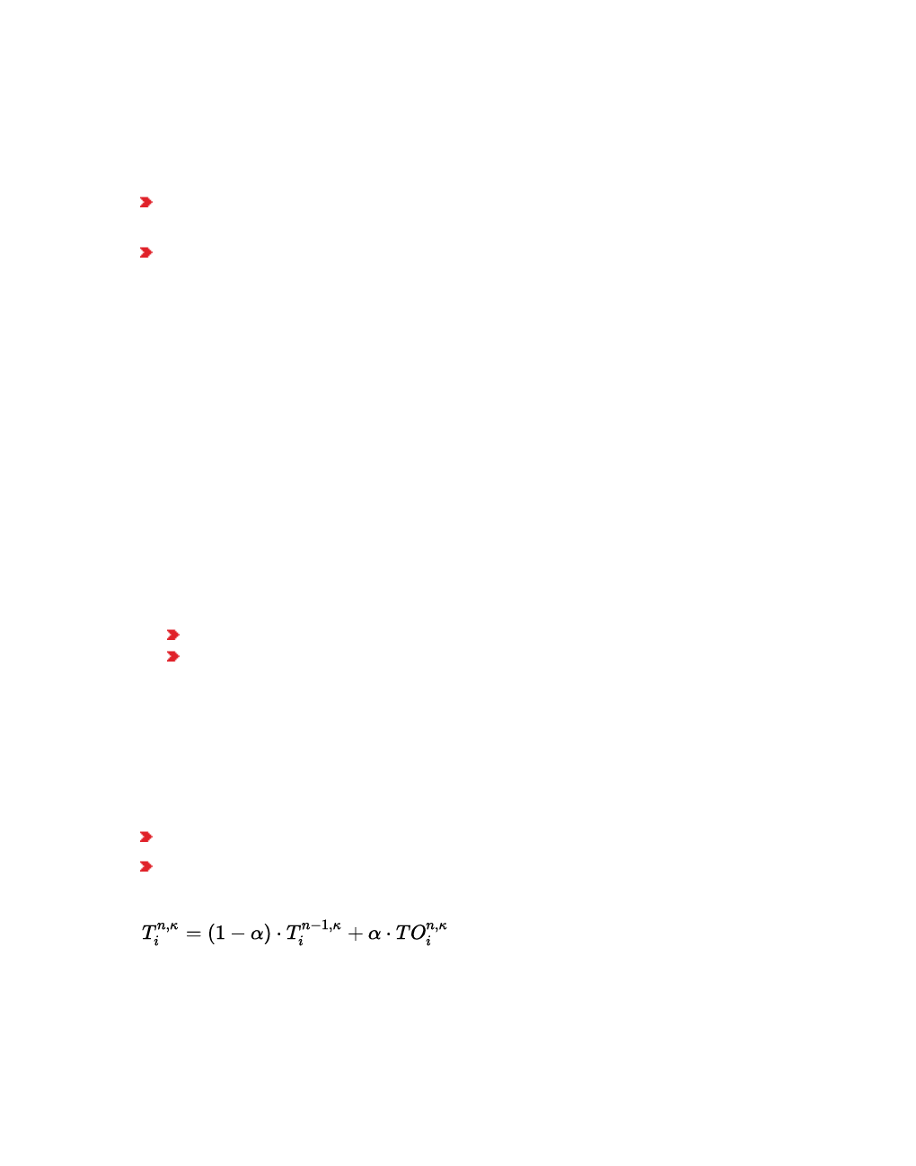
7.7.3 Selecting exponential smoothing of the travel times
For the simulation of the experience growing with time, not only the travel time of the previous
iteration is taken into account, but in particular the travel times of all previous iterations.
You can set the more distant measurements to have less influence. For this the following
methods can be used:
exponential smoothing of the travel times (see "Selecting exponential smoothing of the
travel times" on page 695)
MSA (Method of successive averages) (see "Selecting the MSA method for travel times"
on page 696)
7.7.3 Selecting exponential smoothing of the travel times
You can set the more distant measurements to have less importance compared to the recent
iterations. With a smoothing factor you set the relative weight of the respective recent iteration.
You can assign less importance to the more distant measurements, using the Method of
Successive Averages (MSA) (see "Selecting the MSA method for travel times" on page 696).
1. From the Traffic menu, choose > Dynamic Assignment > Parameters (see "Attributes for
the trip chain file, matrices, path file and cost file" on page 731).
The Dynamic Assignment: Parameters window opens.
2. Select the Cost tab.
3. Then, in the Smoothing method section, select Exponential smoothing with smoothing
factor.
4. Enter the desired smoothing factor:
for the equilibrium assignment 1.0
for the stochastic assignment according to Kirchhoff, the default value is 0.2
5. Confirm with OK.
If the option Store costs is selected in the Files tab, the expected travel times are saved after
every iteration for the next iteration in the Vissim cost file *.bew, from where they are entered
into the path selection model.
After measurement of the new travel times, the smoothed travel time is computed for each
edge as the weighted sum of the following:
the old smoothed travel time from previous iterations
the newly measured travel time from the current iteration
The new smoothed value represents the travel time that we expect in the next iteration.
Where:
K = index of the evaluation interval within the simulation time
n = index of the iteration
© PTV GROUP 695

7.7.4 Selecting the MSA method for travel times
i = index of the edge
= measured (observed) travel time on edge i for interval k in iteration n
= smoothed travel time on edge i for interval k in iteration n
α
= the given constant smoothing factor
This kind of smoothed average contains the information from all preceding iterations. The
older an iteration, the less influence has the measured value derived from it. With a smoothing
factor of for example 0.5, the current iteration n has a weight of 50 %, iteration (n-1) has a
weight of 25 %, and iteration (n-2) has a weight of 12.5 % and so on.
7.7.4 Selecting the MSA method for travel times
With the Method of Successive Averages (MSA), you give each preceding iteration as much
weight as the current iteration. This results in the arithmetic mean from all iterations. In this
way, the influence of any further iteration becomes increasingly smaller.
The MSA method parameter depends on the cost file *.bew:
If you select the option MSA (Method of Successive Averages) and there is no cost file
*.bew saved yet by the dynamic assignment, the parameter of the MSA method will be set
automatically by Vissim.
If you have already performed a dynamic assignment and a cost file *.bew is stored, enter
the number of iterations with which the file *.bew was created. If you enter a smaller value
than the actual number of iterations, the subsequent iterations will be weighted higher.
Enter a smaller value when the path evaluation shows that the measured travel times devi-
ate significantly from the expected travel times (see "Showing data about paths of dynamic
assignment in lists" on page 1049).
You can assign less importance to more distant measurements using exponential smoothing
with smoothing factor for the travel times (see "Selecting exponential smoothing of the travel
times" on page 695).
1. From the Traffic menu, choose > Dynamic Assignment > Parameters (see "Attributes for
the trip chain file, matrices, path file and cost file" on page 731).
The Dynamic Assignment: Parameters window opens.
2. Select the Cost tab.
3. In the Smoothing method section, select MSA (Method of Successive Averages), so far.
4. When a dynamic assignment was performed and thereby a cost file *.bew has been stored,
enter the number of iterations with which the *.bew file was created in the field Iterations.
5. Confirm with OK.
If the option Store costs is selected in the Files tab, the expected travel times are saved after
every iteration for the next iteration in the Vissim cost file *.bew, from where they are entered
into the path selection model.
696 © PTV GROUP

7.7.5 General cost, travel distances and financial cost in the path selection
After measurement of the new travel times, the smoothed travel time is computed for each
edge as the weighted sum of the following:
the old smoothed travel time from previous iterations
the newly measured travel time from the current iteration
The new smoothed value represents the travel time that we expect in the next iteration.
Where:
N = user-defined value for number of existing iterations that shall be considered
K = index of the evaluation interval within the simulation time
n = index of the iteration
i = index of the edge
= measured (observed) travel time on edge i for interval k in iteration n
= smoothed travel time on edge i for interval k in iteration n
= variable smoothing factor from parameter N and the iteration index
7.7.5 General cost, travel distances and financial cost in the path selection
The path selection depends on the following factors:
Travel time
spatial length of the paths
financial cost on the paths, for example for toll
In contrast to travel times, the spatial lengths of the paths and the financial costs do not
depend on the traffic conditions. Thus the spatial lengths of the paths and the financial costs
do not need to be determined by simulation but can be read directly from the network model.
To account for these three factors in path selection, for each edge the so called general cost is
computed as a weighted sum:
General cost = a • travel time + b • travel distance + g • financial cost + Σ cost surcharge 2
Where:
The Cost Coefficients are entered in the attributes of the vehicle type (see "Defining path
selection behavior with general cost function" on page 714):
α for travel time
β fortravel distance
γ for link costs
© PTV GROUP 697

7.8 Path search and path selection
Cost coefficients are specific to vehicle types. This allows the modeling of driver groups
with different path selection behaviors, with different time, path and money determinants
(see "Defining simultaneous assignment" on page 714).
The travel distances are determined from the geometry of the links.
The financial cost of an edge is the sum of the costs of all links that are contained in that
edge.
The cost is computed by multiplying the cost rate per kilometer specified in the link by the
length of the route which is contained in the edge. If for a link the attribute Surch1 contains
a value, it is added (see "Attributes of links" on page 383).
Link attribute Surcharge 2:: Additional surcharge for the link. Is added to general link
costs without weighting (see "Attributes of links" on page 383).
7.8 Path search and path selection
In the dynamic assignment, several paths are mostly found for an OD pair that a vehicle can
take. The decision for one of the paths found via path selection is based on the generalized
costs of the paths. The generalized costs consist of the travel time, distance, and link costs
(see "General cost, travel distances and financial cost in the path selection" on page 697).
The distribution of demand data to the paths can be done according to the following
distribution models:
Use volume (old): Base path search exclusively on volumes of previous simulation
runs. These may stem from a previous simulation run or an ANM import.
Stochastic assignment (Kirchhoff): The distribution is carried out in each iteration
according to Kirchhoff based on the smoothed generalized costs of the previous iter-
ation. Less vehicles use paths with higher costs than paths with lower costs. Paths with
the same cost get the same volume, regardless of their capacity. The result of the
assignment is the following distribution to the paths:
Paths with higher volumes have lower costs
Paths with lower volumes have higher costs
Paths with identical volumes have identical costs
Equilibrium assignment: Redistributes demand across paths proportionally to costs,
from expensive to inexpensive paths, for each OD pair in each iteration: The volume of
paths that are more expensive than the average is reduced. The height of the specified
volume is proportional to the additional costs of the path. All paths that are cheaper
than the average path costs are assigned additional volume. The additional volume is
proportional to the cost saving compared with the average path costs (see "Method of
path selection with or without path search" on page 700). The result of the assignment
are identical generalized costs on all paths of a parking lot OD pair, possibly with very
different volumes, dependent on the respective capacity of the path.
Choose whether you want path selection to be based on the travel time measured on paths or
on the total of travel times on edges. In doing so, you define the calculation of generalized
costs. The desired method of cost calculation can be selected in the parameters of dynamic
698 © PTV GROUP

7.8.1 Calculation of paths and costs
assignment Cost for path distribution with Kirchhoff: (see "Attributes for calculating costs as
a basis for path selection" on page 735).
7.8.1 Calculation of paths and costs
A path is a sequence of edges on which a vehicle can move through the road network. In the
dynamic assignment, paths start at an origin parking lot and end at a destination parking lot.
Since there are usually several different paths between an origin parking lot and a destination
parking lot, Vissim must also model the decision of the driver as to the path he selects. In
dynamic assignment, during path selection, Vissim identifies the number of paths available
between an origin parking lot and a destination parking lot. The software then performs a path
search for the path selection methods Sum of edge travel times and Measured path travel
times according to Kirchhoff. The path selection is a special case of discrete selection
because the selection probabilities must be calculated for a set of discrete alternatives. To do
so, a utility function for evaluating the individual paths as well as a decision function are
defined in the traffic assignment, which are based on these evaluations.
The evaluation is calculated in the form of generalized costs from expected travel time, travel
distance and financial costs for all edges. The generalized costs of a path are defined as the
total cost of edges from which the path is composed:
These include:
C = the generalized costs
R = a path
a = an edge that occurs in R
7.8.2 Path search finds only the best possible path in each interval
In Vissim it is assumed that not all drivers use only the best route from one parking lot to
another, but that traffic is distributed across all known paths. For this, it would be useful to
know the n best paths for each origin-destination relation. There are, however, no efficient
methods to directly calculate the n best paths in context of a traffic assignment in a useful way.
The shortest path search finds the best path for each origin-destination pair.
Therefore, in each iteration of a simulation, the shortest path search of Vissim searches for the
best path for each origin-destination relation. Due to the fact that over the course of an iteration
the traffic situation and therefore the travel time on the edges changes until convergence is
reached, different best paths can result in the iterations. As long as Alternative path search is
not activated, the shortest path search carried out by Vissim never results in more than one
best path for an OD pair.
Path file *.weg saves each best path.
All found paths, which qualify as the best paths in an iteration, are collected in Vissim and
saved in the path file *.weg. These paths are then available for the following iterations.
© PTV GROUP 699

7.8.3 Method of path selection with or without path search
Best path based on generalized costs
The criteria for the "best" path are the generalized costs. Due to the fact that the weighted
coefficient for the generalized costs depends on the vehicle type, different best paths can be
found for different vehicle types.
Path search at the beginning of each evaluation interval
The path search takes place at the beginning of the evaluation interval and uses the expected
generalized costs which were determined for this evaluation interval in the previous iterations.
First simulation run uses path length
Because the first iteration does not yield any travel time information from the previous
simulation, the length of the path [m] is used.
Default travel times for edges not yet used
For the following iterations, Vissim no longer uses path lengths, but enters a fictitious travel
time of 0.1 seconds for edges not yet used by vehicles. This results in the use of paths with
unused edges to appear attractive when searching according to route. It may be possible that
only a few useful paths are found in the initial iterations. However, the collection of known
paths (for which travel times were measured and generalized costs calculated) will grow more
quickly in the path collection, if drivers are encouraged to try out unknown paths.
Weighting of travel distance helps avoid detours
This "Eagerness to experiment" of the driver may be influenced by a weighting of the distance
traveled in the generalized cost functions. This results in long detours being avoided.
Generally it is an advantage to find as many paths as possible. When unrealistic paths are
found, these can be discarded in a later iteration. This can be defined in the options for path
searches (see "Influencing the path search by using cost surcharges or blocks" on page 746).
7.8.2.1 Alternative path search
Optionally, you can carry out an additional search for Alternative path search with stochastic
modifications of the edge evaluations or shortest path price increases (see "Performing an
alternative path search" on page 709).
7.8.3 Method of path selection with or without path search
You can choose from different procedures for path selection (see "Path search and path
selection" on page 698):
In the parameters of dynamic assignment, in the Choice tab, select the procedure Use
old volumes (no path search) to select a path without carrying out a path search. In
this case, the probability of a path being used corresponds to its attribute value
Volume (old) share in the total of attribute values Volume (old), of all paths of the same
OD pair. These attribute values stem from an ANM import or the path file of a previous
simulation run.
700 © PTV GROUP

7.8.3 Method of path selection with or without path search
If in the parameters of dynamic assignment, on the Choice tab, you selected the path
choice model Stochastic assignment (Kirchhoff) or Equilibrium assignment, your
path search is followed by path selection. The vehicles are then distributed across the
paths depending on the distribution model and based on the distribution formula
according to Kirchhoff or for equilibrium assignment.
The following descriptions require that the destination parking lot and potential routes to it are
already known. Path search finds only the best possible path in each interval for each OD pair,
but all found paths can be used in all intervals (see "Path search finds only the best possible
path in each interval" on page 699). For the dynamic assignment, the drivers select the route
at the time they depart from the origin parking lot.
7.8.3.1 Calculating utility
One of the basic assumptions in path selection according to Kirchhoff is that not all drivers use
the best path, but that all known paths are used and have different costs. However, a large
percentage of the traffic should be distributed across the better paths. The quality of paths is
evaluated using the generalized costs. Generalized costs are contrary to the "benefit" involved
in the theory of discrete decisions. Thus the benefit is defined as the reciprocal of the
generalized costs:
Where
Uj = the benefit of path j
Cj = the generalized costs of path j
7.8.3.2 Calculating the decision behavior using the Logit function
The most frequently used and thus also the most theoretically analyzed function for mapping
the decision behavior is the Logit function:
Where
Uj = the benefit of path j
p(Rj) = the probability that path j is selected
μ = the sensitivity parameter of the model (>0), Logit scaling factor for destination parking
lot selection
The sensitivity parameter determines how strongly the distribution responds to benefit
differences. A low value would result in a quite similar distribution without any major influence
of the benefit, and a high value would result in virtually every driver selecting the best path.
© PTV GROUP 701
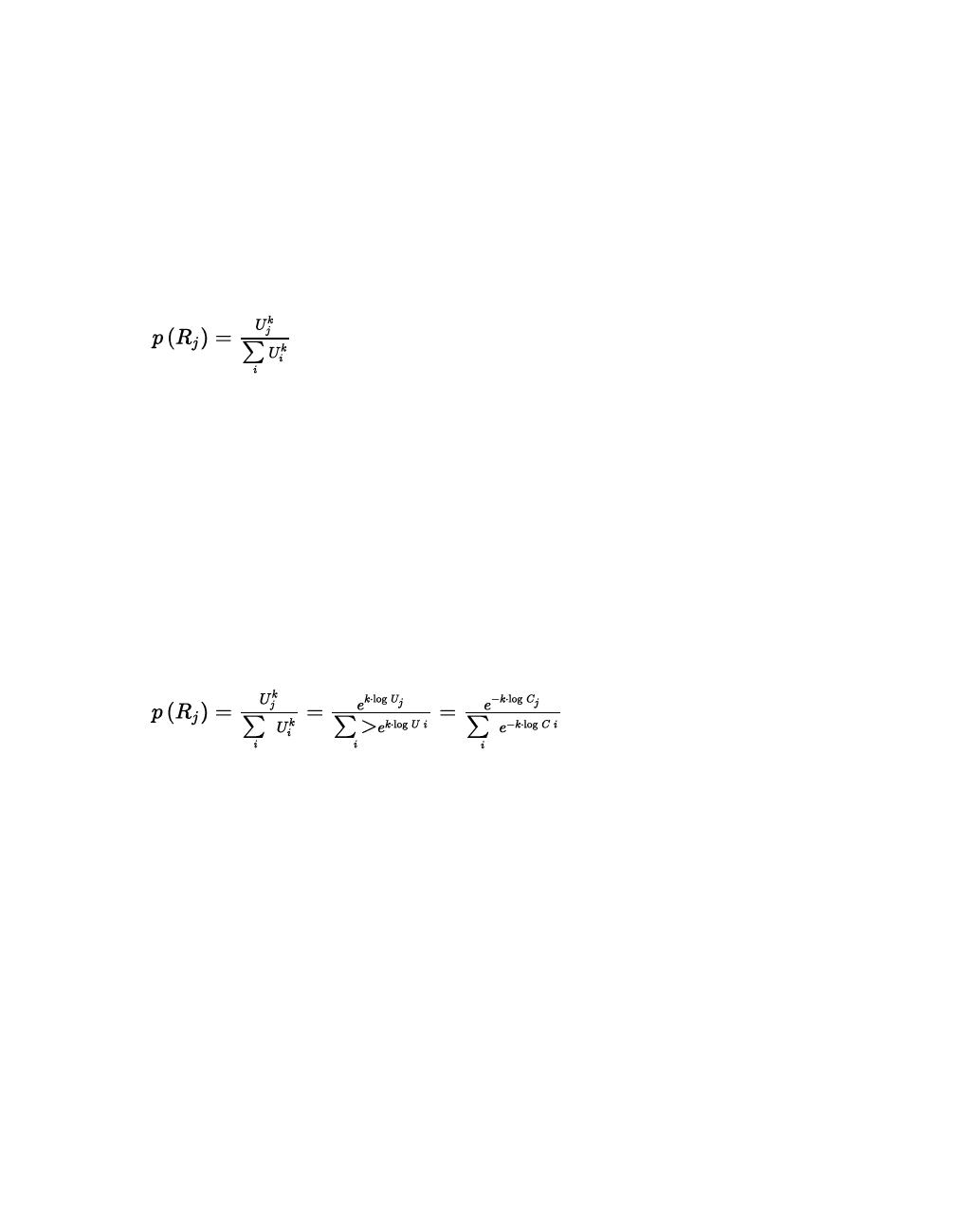
7.8.3 Method of path selection with or without path search
7.8.3.3 Distribution according to Kirchhoff
If the logit function is applied with the cost function defined above, this leads the model to
attach the same importance to the difference between 5 and 10 minutes of travel time as the
difference between 105 and 110 minutes of travel time because the logit function is
translationally invariant and thus considers only the absolute difference of benefits. Obviously,
this modeling is not particularly appropriate, because in reality two paths which have a travel
time of 105 and 110 minutes are basically considered equally good, whereas paths of 5 and
10 minutes are perceived as significantly different. To approximate the real assessment, the
distribution formula according to Kirchhoff is used in Vissim:
Where
Uj = the benefit of path j
p(Rj) = the probability that path j is selected
k = the sensitivity parameter of the model
The sensitivity parameter also determines here how sensitively the model responds to
differences in the benefits. For Kirchhoff, the ratio of benefits determines the distribution and
not the absolute difference of benefits, thus only slight variations arise in the paths with 105
and 110 minutes of travel time, whereas the path with 5 minutes of travel time receives much
more traffic than the path with 10 minutes of travel time.
In fact, the Kirchhoff function is also a logit model. It arises from the logit function described
above if the logarithmic benefit is used as a utility function:
Cj are the generalized costs of path j in this case.
7.8.3.4 Distribution with the equilibrium assignment
The equilibrium assignment redistributes demand across paths proportionally to costs, from
expensive to inexpensive paths, for each parking lot OD pair.
The volume of paths that are more expensive than the average is reduced. The volume of
these less expensive paths is also reduced and part of it assigned to cheaper paths. All paths
that are cheaper than the average path costs are assigned additional volume. The cheaper
the path, the more volume it is assigned (see "Equilibrium assignment – Example" on page
705).
702 © PTV GROUP
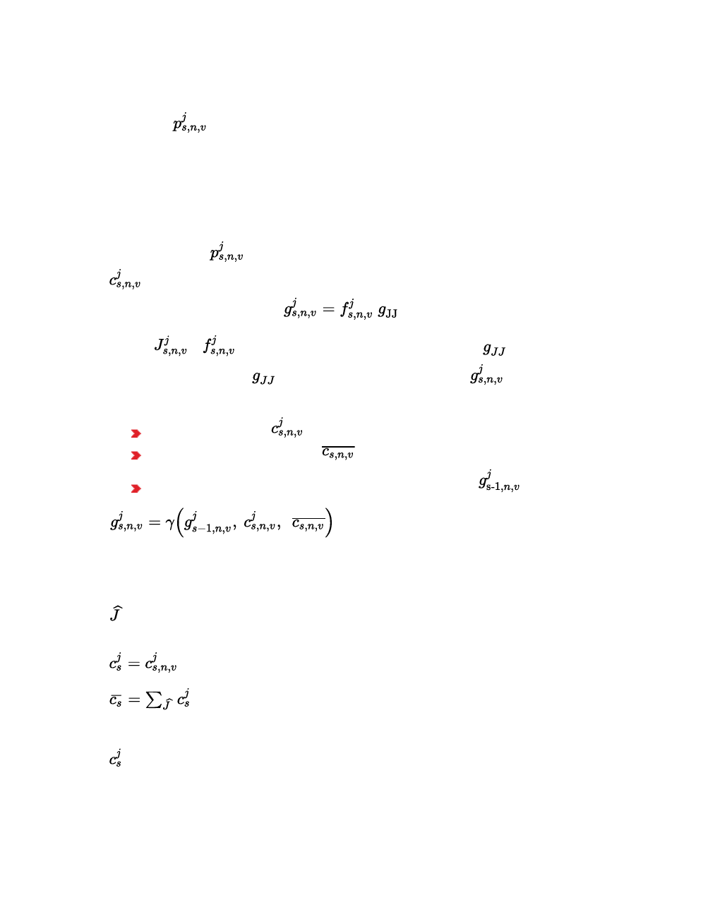
7.8.3 Method of path selection with or without path search
Assign normalized probability for path selection
As with the procedure according to Kirchhoff, each path j is a assigned a normalized
probability .
where:
s: simulation run
n: time interval
v: vehicle class
The probabilities are calculated before each time interval n from the generalized costs
. In equilibrium assignment, the target volume is determined, which is different from the
method according to Kirchhoff .
Where: = the Target volume (relative) attribute and is the total volume of the
OD parking lot relation. is iteratively calculated, so that is a function γ with the
following variables:
the generalized cost of the corresponding path
the average generalized cost
the relative target volumes of the previous simulation run
Redistributing volumes proportionally to costs
In the following
: is the number of paths at the beginning of a new time interval for each OD parking lot
relation, including newly found paths and excluding previously deleted paths.
This includes:
: the costs of path j
© PTV GROUP 703
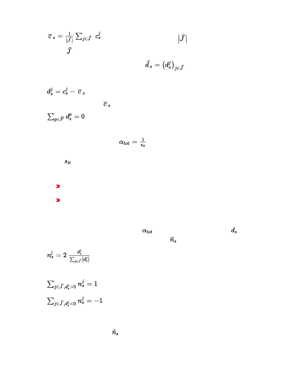
7.8.3 Method of path selection with or without path search
: the average path costs, with the number of paths with the OD
relation .
The demand is shifted towards the vector
with
Due to the definition of the following applies:
The volume is thus redistributed an no additional volume generated.
In iteration s the proportion of the total demand for a parking lot relation is
redistributed:
Where is the content of CurIterIdx (Current iteration index attribute: index of the current
iteration of an equilibrium assignment). The CurIterIdx index is incremented at the end of a
simulation run, under the following conditions:
A dynamic assignment has been carried out and matrices or trip chain files have been
referenced, and
the distribution model Equilibrium assignment has been selected.
CurIterIdx is saved to the path file *.weg.
CurIterId is restored when a simulation run is started without a path file.
To redistribute only the desired share of the total volume, the vector has yet to be
scaled. For this purpose the scaled direction vector is calculated.
Thus the following conditions are met:
This means that, just as much volume is taken from paths that are more expensive than the
average as is added to paths that are less expensive than the average.
Demand is shifted towards so that no negative demand is created on any of the paths:
704 © PTV GROUP
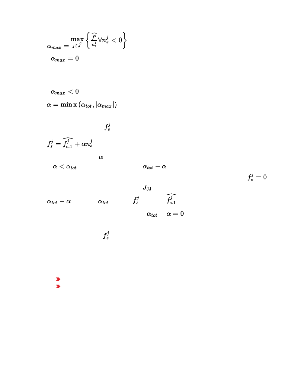
7.8.4 Equilibrium assignment – Example
If the algorithm implies that volume is taken from paths which have a volume of 0
already. To carry out the redistribution, these paths are temporarily taken from the set of paths,
the OD pair. Volume balancing is restarted and only the temporarily reduced path set is taken
into account.
If the following is set:
The new target volume is then given by:
Thus, a proportion of in the total demand for the parking lot relation is shifted.
If the remaining share of must be shifted. The remaining share is
redistributed iteratively. For this purpose, paths with a relative target volume are
temporarily removed from the path set . The volume balancing is restarted, however with
instead of and with instead of .
The iterative procedure is stopped when is reached.
The new final volume is then saved and used for the new time interval, down to vehicle
class level, in the new attribute Target volume (relative) (see "Attributes of paths" on page
712). Target volume (relative) is saved to the path file *.weg.
If during assignment a path file is read in that does not contain the Target volume (relative)
and Current iteration index, the following values are set:
Current iteration index: 1
Target volume (relative): empty for all vehicle classes and time intervals
7.8.4 Equilibrium assignment – Example
The example explains the redistribution of relative target volumes in equilibrium assignment
based on a single OD pair with only four paths.
© PTV GROUP 705
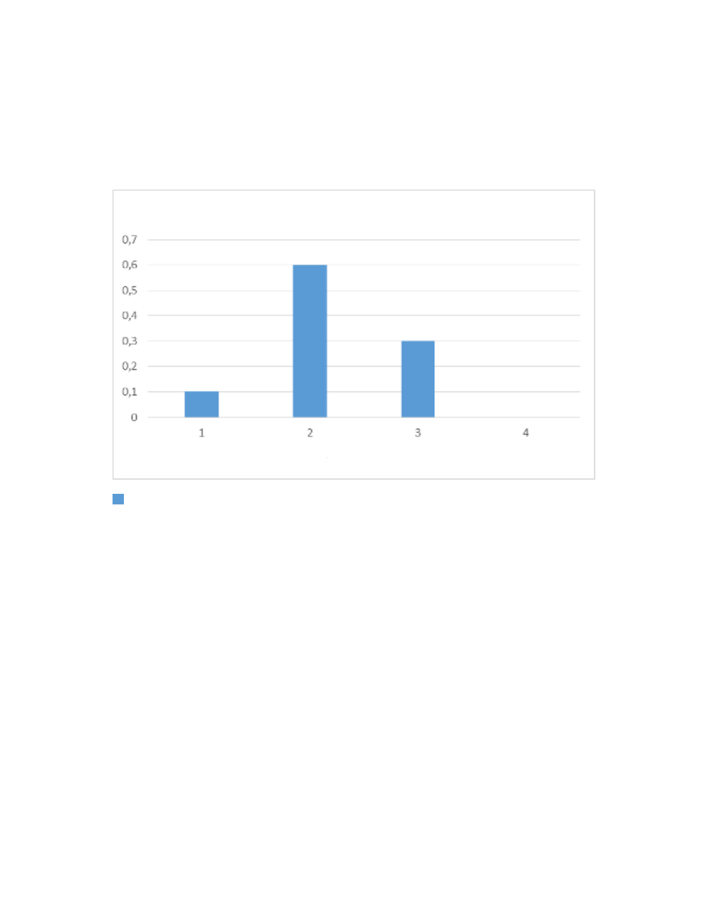
7.8.4 Equilibrium assignment – Example
Target volumes on the basis of previous simulation runs
The illustration below shows the relative target volumes on the basis of previous simulation
runs with equilibrium assignment. Most volumes were distributed to path 2 in the last
simulation run completed, followed by path 3 and path 1. Path 4 had no volumes in the
previous simulation run.
Relative target volume of previous simulation runs path 1 to 4:
: Relative target volume before
Cost measured in previous simulation run
The illustration below shows the cost measured in the previous simulation run. Path 3 was by
far the most expensive path and also the only path that was more expensive than the average
cost. Path 2 was closest to the average cost. Path 4 was slightly less expensive and path 1
was the least expensive.
Cost of path 1 to 4:
706 © PTV GROUP

7.8.4 Equilibrium assignment – Example
Cost
Average cost
Redistribution of the volume
The volume can be redistributed by means of this data (see "Method of path selection with or
without path search" on page 700). From the calculation of the formulas it follows that a share
of the total volume, which shall be redistributed, is distributed to the individual paths. This is
shown by the illustration below. The entire share of the total volume, which shall be
redistributed, is taken from path 3 because path 3 was the only path whose cost was higher
than the average cost. The least volume is added to path 2 because the costs of path 2 were
closest below the average cost. The most volume is added to path 1, because path 1 was the
least expensive path.
Redistribution path 1 to 4:
© PTV GROUP 707

7.8.4 Equilibrium assignment – Example
Result and comparison of the relative target volume before and after
If the last completed simulation run was the fourth simulation run of this assignment, as in the
example, a quarter of the total volume must be redistributed for the OD pair according to the
redistribution algorithm. The new target volumes are determined by adding a quarter of the
values from the Redistribution illustration above to the values from the first illustration above
Relative target volume of previous simulation runs. The following illustration shows the new
relative target volumes. The relative target volume of path 3 has dropped considerably, while
the target volume of path 1 has increased significantly. Path 4 now also has volumes. The
relative target volume of path 2, by contrast, is nearly unchanged.
Comparison relative target volume path 1 to 4 before and after:
708 © PTV GROUP

7.8.5 Performing an alternative path search
: Relative target volume before, left bar
: Relative target volume after, right bar
7.8.5 Performing an alternative path search
You can search via the following functions according to Alternative Path Search:
Stochastic edge evaluation with maximum dispersion share for each OD relation between
all zones and the number of passes
Shortest path price increase for paths from zones, which you select
Shortest path price increase for paths from dynamic routing decisions, which you select
Multiple passes of the shortest path algorithm with only slightly modified edge evaluations
increase the probability of finding more Alternative Paths. These may have higher total costs
than the best path, however, they should still be used.
7.8.5.1 Stochastic edge evaluation with maximum dispersion share
1. From the Traffic menu, choose > Dynamic Assignment > Parameters.
The Dynamic Assignment: Parameters window opens.
2. Select the Search tab.
3. Select Search alternative paths.
4. Click the Alternative path search button.
The Alternative path search window opens.
5. Make the desired changes:
© PTV GROUP 709

7.8.5 Performing an alternative path search
Element Description
Search alternative paths with
stochastic edge penalization If the option is selected, the specified number
from stochastic passes is carried out at the
beginning of an evaluation interval of the
dynamic assignment after each normal shortest
path search. Before each pass, the calculation of
each edge in the network is multiplied by a
random factor between (1-x) and (1+x). x is the
maximum dispersion share for each OD relation
between zones, which you have entered into the
Spread field.
Spread Dispersion share for each OD relation between
zones
Passes Number of the stochastic passes
6. Confirm with OK.
7.8.5.2 Penalization of the shortest path per zone/OD pair
Vissim runs according to the normal shortest path search as long as additional passes with
altered edge evaluations are running until a new path without a route closure is found or the
specified maximum number of passes is reached (see "Influencing the path search by using
cost surcharges or blocks" on page 746).
Thereby before each pass, the evaluations for all edges of the currently best path are
multiplied with the edge cost penalization factor (EdgCostPenFact).
1. From the Traffic menu, choose > Dynamic Assignment > Parameters.
The Dynamic Assignment: Parameters window opens.
2. Select the Search tab.
3. Select Search alternative paths.
4. Click the Alternative path search button.
The Alternative path search window opens.
5. In the Penalization of the shortest path per zone/OD pair section, right-click in the row
header.
6. From the shortcut menu, choose Add.
The list of attributes opens.
7. Make the desired changes:
Element Description
FromZone From zone: Number of the origin zone
ToZone To zone: Number of the destination zone
710 © PTV GROUP
7.8.6 Displaying paths in the network
Element Description
EdgeCostPenFact Edge cost penalization factor
MaxNumPass Maximum number of passes: Maximum number of stochastic
passes
8. Confirm with OK.
7.8.5.3 Penalization of the shortest path per dynamic routing decision/OD pair
To use this function, you must have inserted dynamic routing decisions into the Vissim network
(see "Defining dynamic routing decisions" on page 721). Vissim runs according to the normal
shortest path search as long as additional passes with altered edge evaluations are running
until a new path without a route closure is found or the specified maximum number of passes
is reached (see "Influencing the path search by using cost surcharges or blocks" on page
746).
Before each search, the evaluation of each edge of the currently best path is multiplied with
the value of the attribute Edge costs evaluation factor.
1. From the Traffic menu, choose > Dynamic Assignment > Parameters.
The Dynamic Assignment: Parameters window opens.
2. Select the Search tab.
3. Select Search alternative paths.
4. Click the Alternative path search button.
The Alternative path search window opens.
5. In the Penalization of the shortest path per dynamic routing decision/OD pair section,
right-click in the row header.
6. From the shortcut menu, choose Add.
The list of attributes opens.
7. Make the desired changes:
Element Description
FromRoutingDecision From routing decision: Number of the origin routing decision
ToZone To zone: Number of the destination zone
EdgeCostPenFact Edge cost penalization factor
MaxNumPass Maximum number of passes: Maximum number of stochastic
passes
8. Confirm with OK.
7.8.6 Displaying paths in the network
You can mark each path in color that was found during the iterations of the dynamic
assignment.
© PTV GROUP 711

7.8.7 Attributes of paths
1. Select in the menu Lists > Results > Paths.
The list Paths opens.
2. Open the network editor.
3. Ensure that the icon Synchronization is selected in the Paths list.
4. Click in the list on the desired path.
5. If you want to select additional paths, press the CTRL key and click the desired entries.
The paths are displayed in yellow in the network display. If in the Paths list, synchronization is
selected, detours are shown in red in the network display.
Note: The paths result from the last iteration in which the path file was updated. The
costs displayed are taken from the previously saved cost file. Hence the results of the
last iteration are displayed only if the cost and path files were saved during that
iteration.
7.8.7 Attributes of paths
1. Select in the menu Lists > Results > Paths.
The list Paths opens. When a *.weg file is saved to the directory specified in the parameters
of dynamic assignment, in the Files tab, in the Path file box, it is automatically read in.
Depending on the size of the file, this may take a while. A window opens, indicating the
loading progress. You can also cancel this process.
Note: In lists, you can use the Attribute selection icon to show and hide attribute
values (see "Selecting attributes and subattributes for a list" on page 106).
2. Make the desired changes:
Long name Short name Description
Is detour IsDetour If the option is selected and the option Avoid long detours
is selected, the detours are displayed (see "Using the detour
factor to avoid detours" on page 719). Paths are not
displayed.
Converged Conv If this option is selected, the travel time of the path is
converged. The path fulfills the convergence criterion Travel
time on paths for all completed time intervals (see "Attributes
for achieving convergence" on page 741). The average
journey time of all vehicles is taken into account. This
corresponds to the weighted average journey times of all
vehicle classes.
From park-
ing lot
FromParkLot Number of the origin parking lot
712 © PTV GROUP

7.9 Optional expansion for the dynamic assignment
Long name Short name Description
To parking
lot
ToParkLot Number of the destination parking lot
Volume
(old)
VolOld Number of vehicles that used the path saved to the path file
(*.weg) during the last simulation run. For blocked edges or
blocked connectors in edges, the values are in parentheses.
The volume is always output as the sum of all vehicle types.
Therefore the value does not change if you select different
vehicle types.
In the column, vehicles are displayed which have paths that
run through a connector, which are blocked only for specific
vehicle classes and not for all classes.
If the path file is generated via the ANM import, the volumes
can also have decimal positions from the assignment with
Visum.
Volume
(new)
VolNew Number of vehicles using the path during the current
simulation run
Volume tar-
get (rel-
ative)
VolTarRel only for equilibrium assignment: share of the target volume of
the path in the total volume of the parking lot OD pair (see
"Method of path selection with or without path search" on
page 700)
In the network editor, you can display all paths which are found during the iterations of the
dynamic assignment (see "Displaying paths in the network" on page 711).
Showing and editing dependent objects as relation
The attribute and attribute values of this network object type are shown in the list on the left,
which consists of two coupled lists.
1. In the list on the left, click the desired entry.
The list on the right contains attributes and attribute values of network objects, and/or base
data allocated to the network object selected in the list on the left (see "Using coupled lists" on
page 111):
2. On the list toolbar, in the Relations list, click > Edge sequence (see "Attributes of edges" on
page 678).
3. Enter the desired data.
The data is allocated.
7.9 Optional expansion for the dynamic assignment
Vissim allows for the following optional expansions:
© PTV GROUP 713

7.9.1 Defining simultaneous assignment
Simultaneous assignment: simultaneous assignment for different classes of road users
Parking lot selection: find one out of multiple destination parking lots in a zone
Detour recognition: recognize a detour factor for newly calculated legs, which lengthen
newly found paths
Correcting distorted demand distribution for overlapping paths
Dynamic routing decisions: Arrange vehicles on a new path selection
Route guidance: While driving, vehicles search for new paths to a destination parking lot.
7.9.1 Defining simultaneous assignment
You can perform an assignment for different classes of road users, who have an effect upon
each other in the road network. Examples of user classes are commuters, business travelers,
local drivers, out-of-town drivers etc. These classes differ in the following points:
in their path selection behavior
in their access to different parts of the road network
7.9.1.1 Defining path selection behavior with general cost function
To model different path selection behavior, in the attributes of the vehicle type, you can enter
Cost Coefficients of the general cost function separately for each vehicle type.
α for travel time
β fortravel distance
γ for link costs
Thus you can model e.g. drivers who are willing to pay tolls to gain time, and other drivers that
do not want to pay and accept longer paths in exchange.
1. From the Base Data menu, choose Vehicle Types.
The Vehicle Types list opens.
2. Right-click the vehicle type of your choice.
The context menu opens.
3. Select the Edit entry.
The Vehicle Type window opens.
4. Select the Special tab.
5. Click the Cost Coefficients button.
The Cost Coefficients window opens.
714 © PTV GROUP

7.9.2 Defining the destination parking lot selection
The summands must be of the same magnitude as the cost components. Pay attention to the
units:
Travel times in seconds
Travel distances in meters
Costs have no implicit unit. You define the unit. So if for example cost unit is Euro per kilo-
meter, choose the corresponding coefficient so that the product amounts to the same
order of magnitude as the travel time in seconds.
6. Enter the desired values.
7.9.1.2 Defining access to different parts of the road network
The second aspect of simultaneous assignment, besides the different cost sensitivity, is the
selective usability of the road network. It allows you to restrict parts of the network for vehicle
classes. It allows you to model, for example, that local drivers have a solid knowledge of the
network, while out-of-town drivers know only the main road network.
For this connectors are used in Vissim. You can block a connector for vehicle classes. The
path search will not use paths with blocked connectors for the vehicles from these vehicle
classes (see "Modeling connectors" on page 393). The blocks for the selected vehicle classes
are only relevant for the dynamic assignment.
7.9.2 Defining the destination parking lot selection
The traffic demand in the origin- destination matrices refer to the zones for origins and
destinations. Zones are represented in Vissim via one or more parking lots. If more than one
parking lot is located in the destination zone of a driver, the driver must choose the destination
parking lot before choosing his/her path.
Thereby, the destination parking lot selection is an additional example of the problem class
Discrete Selection (see "Differences between static and dynamic assignment" on page 655).
The reason for this is there are many alternatives: a utility function and a decision function (see
"Base for calculating the dynamic assignment" on page 656)(see "Calculation of paths and
costs" on page 699). For the vehicle type used by the driver, you may enter a utility function
coefficient for each of three decision situations that trigger a parking lot search (see "Entering
© PTV GROUP 715

7.9.2 Defining the destination parking lot selection
coefficients for utility function of parking lot" on page 717). Calculation of the utility function is
also based on the attributes Parking fee and Attraction of the parking lots (see "Attributes of
parking lots" on page 469).
For destination parking lot selection a Logit formula is used (see "Method of path selection
with or without path search" on page 700). The Logit forumula contains a scaling factor that
you can specify (see "Defining the Logit function scaling factor" on page 718).
Destination parking lot selection depends on the following settings made in the parameters of
dynamic assignment, on the Cost tab, in the section Cost for path distribution with
Kirchhoff. This also applies for destination parking lot selection for dynamic routing decisions
(see "Defining dynamic routing decisions" on page 721):
If Measured path travel times is selected, destination parking lot selection uses gen-
eralized costs of paths from the second simulation run. For the first simulation run, the
total of edge lengths is used, as there is still no data available on the travel time. From
the start of the edge, the distance from the end of the origin parking lot to the first node
border is taken into account. From the end of edge, only the distance from the last
node border to the beginning of the destination parking lot is considered.
If the Sum of edge travel times is selected, the entire length of all edges is used.
7.9.2.1 Definition of the utility function of a parking lot
Coefficient Formula
symbol
Description Description
CParking
Parking Cost Parking fee listed as Parking fee attribute of the
parking lot
Attraction Attraction Attraction listed as Attraction attribute of the parking
lot
D
Destination
Distance from
desired zone
Straight-line distance between the position of the
parking lot and the center of the destination zone
DVeh Distance from
current
position
Generalized costs of the cheapest path from the
current location (vehicle position)
fs Current
parking
availability
Availability of free parking spaces
k Index of Vehicle type
s Index of Decision Situation, Departure, Routing
Decisions, RouteGuidance cycle 1 or
RouteGuidance cycle 2
For the utility function the following applies:
716 © PTV GROUP

7.9.2 Defining the destination parking lot selection
positive coefficient for Attraction and for Current parking availability
negative coefficient for Parking Cost, Distance from desired zone and Distance from
current position
7.9.2.2 Entering coefficients for utility function of parking lot
You may enter individual utility function coefficients for each vehicle type and each of the three
following decision situations. Coefficients are weighting factors for the smallest possible
generalized cost of a path, from the current vehcile position to the destination parking lot. You
can show the coefficient values entered in the Vehicle types list, in the GenCost (generalized
costs) attribute.
Departure from Parking lot: when a vehicle begins its trip in the origin parking lot
Dynamic routing decision: when a vehicle passes a dynamic routing decision
Route Guidance Tactic 1, Route Guidance Tactic 2: when a vehicle with a route guid-
ance system receives new information
The number of the permissible destination parking lots to the time of the departure is the
number of parking lots which belong to the destination zone and are open at the time of the
departure. For decisions, which are triggered by a dynamic routing decision or a route
guidance system, the selected quantity depends on the set strategy (see "Attributes for the trip
chain file, matrices, path file and cost file" on page 731).
1. From the Base Data menu, choose Vehicle Types.
The Vehicle Types list opens.
2. Right-click the vehicle type of your choice.
3. From the shortcut menu, choose Edit.
The Vehicle Type window opens.
4. Select the Special tab.
5. Click the Destination Parking Lot Selection button.
The Destination Parking Lot Selection window opens. In the next step, to select multiple
entries, hold down the CTRL key.
6. In the list, click the desired decision situation (DecSituation).
7. Into the list boxes, enter the desired coefficients.
Note: After multiplication by the Logit scaling factor, the difference of the largest and
smallest utility function value should be no larger than 4. If the difference of the utility
value is 4, the probability of the selection of a better parking lot is 55 times as much
as the probability that a worse parking lot will be selected.
© PTV GROUP 717

7.9.2 Defining the destination parking lot selection
Warnings:
For very large utility values, an overflow of numbers can occur.
Very high negative values can lead to inaccuracy in the calculation because the
percentage of e yields a value too close to zero.
In both cases, a warning is saved to the *.err file and the Messages window.
When the use of all parking lots has been defined in the selected quantity, the selection
probability is calculated with the Logit function.
8. Confirm with OK.
7.9.2.3 Calculation of parking spaces currently available
The ratio of available parking spaces of considered parking lots to the largest number of
available spaces in the entire selection of parking lots equals the number of parking spaces
currently available.
7.9.2.4 Distance from other destination zone
Although parking lots lie in zones, the information distance from destination zone is required,
for example when all parking spaces of the destination zone are occupied. In such decision
situations, parking lots that do not belong to the destination zone may become potential
destination parking lots. Then Vissim shall choose a parking lot in a different zone as
destination parking lot, preferably one which is close by.
The location of a zone is calculated from the mean of the coordinates of the parking lot of the
zone and can be displayed as an attribute Center in the list of Zones (see "Traffic menu" on
page 120).
7.9.2.5 Defining the Logit function scaling factor
1. From the Traffic menu, choose > Dynamic Assignment > Parameters.
The Dynamic Assignment: Parameters window opens.
2. Select the Choice tab.
3. In the section Destination Parking Lot Selection, enter the desired values:
718 © PTV GROUP

7.9.3 Using the detour factor to avoid detours
Element Description
Logit
scaling
factor
The Logit scaling factor μ determines how strongly the distribution responds to
utility differences (see "Method of path selection with or without path search" on
page 700).
Logit
lower
limit
If the selection probability of a parking lot lies below this value, the parking lot is
not selected as destination parking lot. This increases the selection probability
for the remaining parking lots.
7.9.3 Using the detour factor to avoid detours
In the iterations of the dynamic assignment the drivers are encouraged to try out new paths,
which contain links or partial routes that have not yet been traveled (see "Path search finds
only the best possible path in each interval" on page 699). This may lead to useless paths in
the path collection. A path is considered useless if it is an obvious detour. An obvious detour is
a path that can be generated from another, already known path by replacing a section by a
much longer section. For this purpose, Vissim calculates the total length of nodes and turn
relations, from the position in the node entrance or node exit where the paths differ to the
position in the node entrance or node exit where the paths are the same again.
You can define how much longer the leg must be compared to the original leg to qualify as a
useless path. For example, Vissim checks with a detour factor of 2 for all paths, whether they
are just copies of other paths, in which a section has been replaced by a section which is more
than twice as long.
If two paths only differ within a node where two parallel turn relations are used (one from each
path), the detour factor is still not fulfilled, even if the two turn relations differ more in length
than the detour factor. The paths must differ in at least one edge between two nodes for the
detour to be recognized by the software.
1. From the Traffic menu, choose > Dynamic Assignment > Parameters.
The Dynamic Assignment: Parameters window opens.
2. Select the Choice tab.
3. In the Path pre-selection section select Avoid long detours.
4. Enter the desired value in the field Avoid long detours. The default value is 2.50.
From now the detour factor is taken into account in the iterations. Detours are shown in the
Paths list without travel time or volume data (see "Attributes of paths" on page 712). If in the
Paths list, synchronization is selected, detours are shown in red in the network display.
7.9.4 Correcting distorted demand distribution for overlapping paths
For every origin-destination relation the whole traffic demand will be distributed to all available
paths. The distribution considers the general path costs, calculated from the measured
variables and the configured weighting coefficients. A path consists of a sequence of edges.
Two paths are different if their sequences of edges are not exactly the same. Two paths may
also be considered to be different if they differ only by a small section. In such a case both
paths would have about the same weight in the distribution of the traffic volume. This would
© PTV GROUP 719
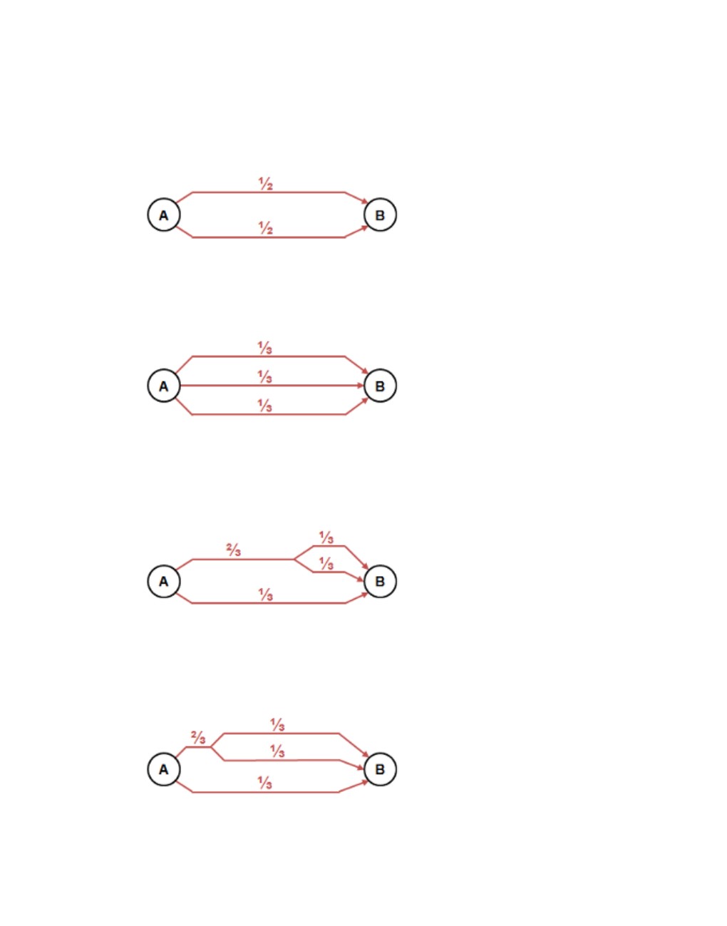
7.9.4 Correcting distorted demand distribution for overlapping paths
lead to an overall biased distribution. This problem occurs in all assignment tasks and is
called the blue/red bus paradox. This is depicted in the following figures:
Case 1: Two paths with identical cost
The distribution of trips 50:50 is unproblematic:
Case 2: Three paths with identical cost
The distribution of traffic on three paths is unproblematic. Each path receives one third of the
demand:
Case 3: A slight variation results in 3 optional paths
Problem: Actually, there are only two quite dissimilar paths. Because of the slight variation in
the end, the path search finds three different paths. Result: It is distributed amongst three
paths. The overlapping part of the two similar paths receives too much traffic.
Case 4: Common stretches leads to three possible paths
The opposite of case 3: Actually there are 3 different paths but two of them have a small stretch
in common. As in case 3, every path gets about one third of the demand. This is much more
realistic compared to case 3.
720 © PTV GROUP

7.9.5 Defining dynamic routing decisions
7.9.4.1 Selecting the correction
You can correct the biased distribution of overlapping paths. Thus, the path selection model
calculates a degree of commonality for the paths (commonality factor) The commonality factor
expresses how much of a path is shared with other paths:
Higher value: A path has many edges in common with other paths.
Lower value: A path is largely independent from other paths.
Using this value the distribution function reduces the selection probability of paths with high
commonality factor.
Notes: In certain network constellations, the correction of the biased distribution tends
to spread traffic over longer paths if these paths have little in common with other paths.
This can lead to unexpected results.
In general, the correction of a biased distribution improves the result of the assignment.
Use the correction of a biased distribution only in combination with restricting the cost
difference between the paths.
1. From the Traffic menu, choose > Dynamic Assignment > Parameters.
The Dynamic Assignment: Parameters window opens.
2. Select the Choice tab.
3. In the Path choice model section, select Correction of overlapping paths.
7.9.5 Defining dynamic routing decisions
Vehicles that are routed by the dynamic assignment ignore all static routing decisions along
their way. With dynamic routing decisions you can trigger a new path selection for these
vehicles.
On a dynamic routing decision, a vehicle decides if a specific condition has been fulfilled, for
example, if its destination parking lot is full. If the condition is fulfilled, a new parking lot
selection and a new path selection are carried out according to the given strategy. The
strategy also determines the parking lots which are available for selection.
Path selection for dynamic routing decisions uses the same generalized costs of the edges as
path selection of dynamic assignment in the current evaluation interval.
Destination parking lot selection depends on the following settings made in the parameters of
dynamic assignment, on the Cost tab, in the section Cost for path distribution with Kirchhoff:
If Measured path travel times is selected, destination parking lot selection uses gen-
eralized costs of paths from the second simulation run. For the first simulation run, the
total of edge lengths is used, as there is still no data available on the travel time. From
the start of the edge, the distance from the end of the origin parking lot to the first node
border is taken into account. From the end of edge, only the distance from the last
node border to the beginning of the destination parking lot is considered.
If the Sum of edge travel times is selected, the entire length of all edges is used.
© PTV GROUP 721
7.9.6 Attributes of dynamic routing decisions
Note: Do not position the dynamic routing decision on an edge which contains a
parking lot that cannot be passed.
1. In the Network objects toolbar, click the Vehicle Routes button.
The button is highlighted. The variant of the network object type is displayed in parentheses
and the button is shown.
2. Re-click the button Vehicle Routes.
A list box with the variants of the network object type opens.
3. Select the entry Dynamic.
4. In the Network Editor, right-click the desired position of the Routing decision section in the
desired link or connector.
5. From the context menu, choose Add New Dynamic Vehicle Routing Decision.
A red purple is shown at that position.
6. Edit the attributes (see "Attributes of dynamic routing decisions" on page 722).
7.9.6 Attributes of dynamic routing decisions
In the Lists menu, select Private Transport > Routes > Dynamic Routing Decisions.
The list of attributes opens.
The attribute and attribute values of this network object type are shown in the list on the left,
which consists of two coupled lists.
Note: In lists, you can use the Attribute selection icon to show and hide attribute
values (see "Selecting attributes and subattributes for a list" on page 106).
The list on the left may include the following attributes:
Column Description
No Number of dynamic routing decision
Name Name of dynamic routing decision
Link Number of the link, on which the dynamic routing decision is located
Pos Distance of dynamic routing decision to the beginning of link or connector
AllVehTypes If the option is selected, all vehicle types follow the vehicle routing
decision or partial routing decision
The option All Vehicle Types is a virtual vehicle class that automatically
includes all new vehicle types and vehicle types that have not been
assigned a vehicle class yet.
VehClasses Valid vehicle classes
722 © PTV GROUP
7.9.6 Attributes of dynamic routing decisions
Column Description
Condition Condition for new parking lot selection and new path selection:
Destination is zone of parking lot
Destination parking lot full
Destination parking lot fewer than: accounts for the number of free
parking spaces
Parking lot full
Destination parking lot fewer than: accounts for the number of free
parking spaces
Always
CondParkLot Condition parking lot: Name of parking lot specified in the attribute
Destination is zone of parking lot.
AvailSpaces Available spaces: Enter number of free parking spaces for the conditions
Destination parking lot fewer than and Parking lot fewer than
Strategy If the condition has been fulfilled: strategy according to which the new
path selection is performed:
Same zone, different parking lot (random): Parking lot is selected
evenly from all the parking lots of the zone.
Same zone, parking lot by benefit function
Same zone, different parking lot by benefit function
Any zone, parking lot by benefit function
Any zone, different parking lot by benefit function
New route to destination parking lot
Specified parking lot
With the strategies for benefit, parking lot search is based on a choice
model (see "Defining the destination parking lot selection" on page 715)
Closed parking lots are not taken into account.
StratParkLot Strategy parking lot: Name of parking lot specified in the Strategy attrib-
ute.
ExclFullParkLots Exclude full parking lots: Full parking lots are not considered for route
choice
Showing and editing dependent objects as relation
The list on the right contains attributes and attribute values of network objects allocated to the
network object selected in the list on the left (see "Using coupled lists" on page 111).
Among others, these may include the following attributes:
Vehicle classes (see "Defining the vehicle class" on page 267)
Paths: Paths of path file from dynamic assignment If no paths are shown and you have per-
formed dynamic assignment, you can read in the paths from their path file. To do so, read
in the paths via the Paths list shortcut menu (see "Attributes of paths" on page 712).
1. On the list toolbar, in the Relations list, click the desired entry.
© PTV GROUP 723

7.9.7 Defining route guidance for vehicles
2. Enter the desired data.
The data is allocated.
7.9.7 Defining route guidance for vehicles
With the route guidance you can make the vehicles search for new paths to a destination
parking lot while driving. This allows you to model the mode of action of the route guidance
systems.
By default, in the dynamic assignment the vehicles choose the path to their destination parking
lots at the moment of departure from the origin parking lot. Thereby the path selection is based
on the general cost from the preceding iterations of the simulation (see "Method of path
selection with or without path search" on page 700). In the route guidance, the path selection
is based on the current traffic situation in the current simulation iteration. The travel time from
the last completed time interval is therefore used.
While you need to place dynamic routing decisions at a desired position in the network, the
vehicles with route guidance search for new paths with a route guidance interval from their
current position. You set the Route guidance interval. Thereby the route guidance triggers the
search for the best path to the destination parking lot.
You assign the route guidance system to vehicle types (see "Using vehicle types" on page
254).
1. From the Traffic menu, choose > Dynamic Assignment > Parameters.
The Dynamic Assignment: Parameters window opens.
2. Select the Route guidance tab.
724 © PTV GROUP
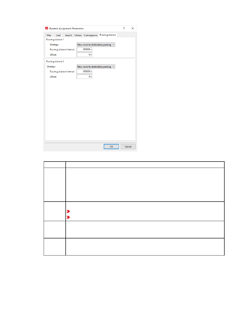
7.9.7 Defining route guidance for vehicles
3. Make the desired changes:
Element Description
Route
guidance
1
Route
guidance
2
You can model two different route guidance systems. For each route guidance
system, you can set the strategy, the route guidance interval and the offset
time.
Strategy Select destination:
New route to destination parking lot
New destination parking lot in same zone
Route
guidance
interval
Time interval for the new path search in seconds
Offset Duration of processing times and run times of messages in real route guidance
systems. This can cause the travel times of the route guidance to deviate from
the travel times of the current evaluation interval.
4. Confirm with OK.
© PTV GROUP 725
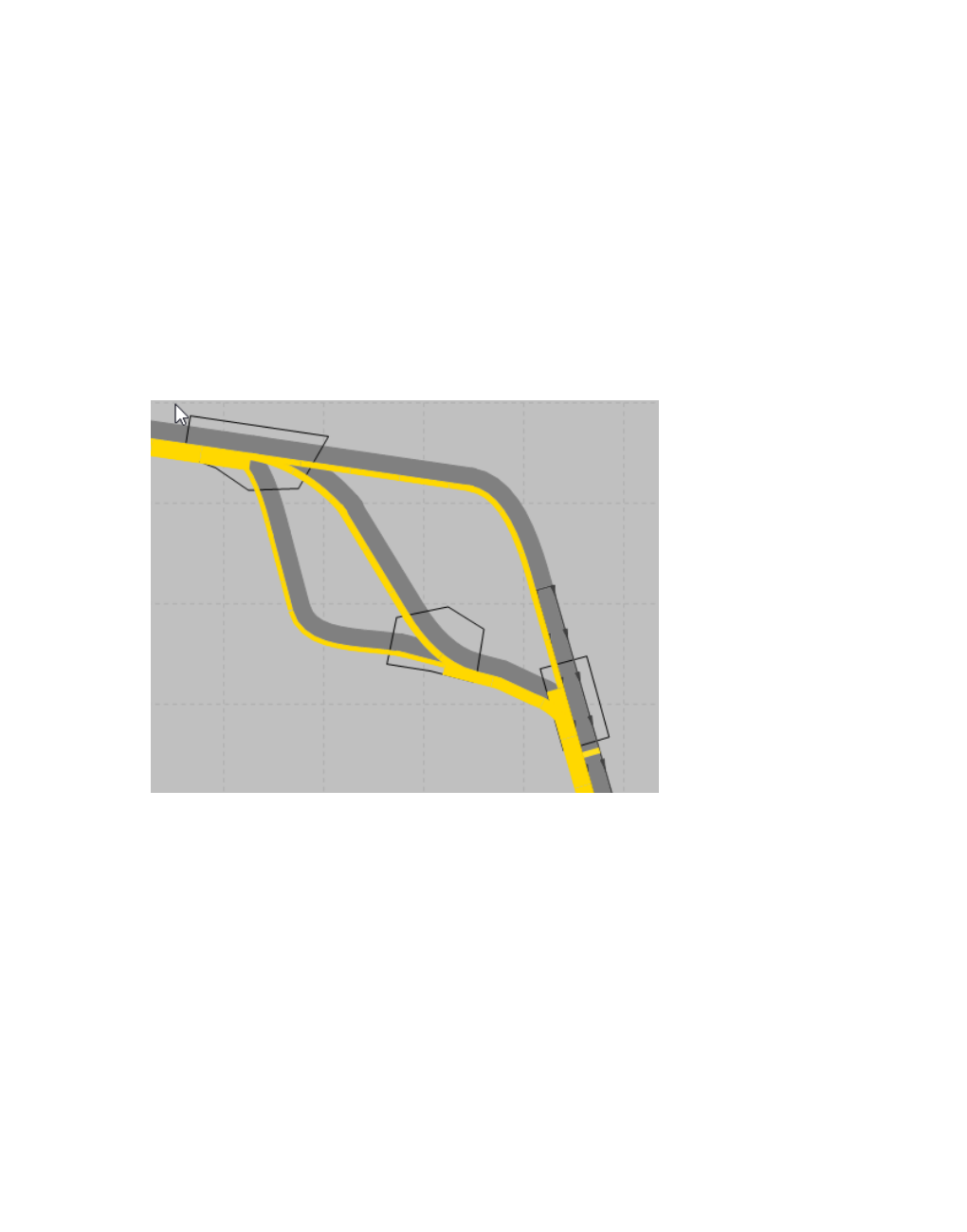
7.10 Visualizing volumes on paths as flow bundles
7.10 Visualizing volumes on paths as flow bundles
You can visualize the volume on paths generated through dynamic assignment as a flow
bundle. To do so, in the Network editor, add filter cross sections of the network object Flow
bundles to the links or connectors of the paths whose volume you want visualize (see
"Defining flow bundles and filter cross sections" on page 727). The flow bundle visualizes the
volumes of the last simulation run.
Examples
The figure shows a section of a Vissim network, with path volumes visualized as a flow bundle.
The yellow filter cross section of the flow bundle has been placed and selected at the bottom
right of the node. Parallel to it, the path volumes on the link are visualized as yellow flow
bundle bars. The width varies depending on the path volume.
The figure below shows the same section. This time, the filter cross section of the flow bundle
has been placed and selected on the left of the connector. There is only one path that
traverses this connector.
726 © PTV GROUP
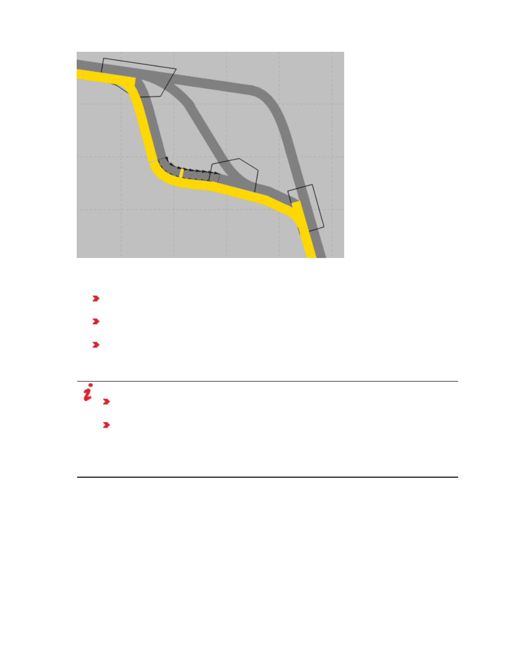
7.10.1 Defining flow bundles and filter cross sections
Additional options to visualize evaluation results
Color schemes for links (see "Assigning a color to nodes based on an attribute" on
page 181)
Link bars (see "List of graphic parameters for network objects" on page 152), (see
"Attributes of links" on page 383)
Turn value visualization (see "Visualizing turn values" on page 645)
7.10.1 Defining flow bundles and filter cross sections
Notes:
You can specify that you need not press the CTRL key when adding network objects
(see "Right-click behavior and action after creating an object" on page 143).
For some network objects there are windows in which the attributes of a network
object can be defined and edited. There are lists for this, for all network objects. You
can choose whether you want to open a window, a list or neither of the two for the
definition of network objects in the Network Editor (see "Right-click behavior and
action after creating an object" on page 143).
1. Ensure that for the Vissim network, at least one simulation run for a dynamic assignment
has been completed for which is a path file available.
2. On the Network objects toolbar, click Flow bundles.
3. Hold down the CTRL key and in the Network editor, right-click the link or connector for which
you want to visualize the volume of its entire path.
© PTV GROUP 727

7.10.2 Flow bundle attributes
By default, a yellow filter cross section is then inserted and selected at this position. By
default, parallel to the path, yellow flow bundle bars depict the volume. The width of the flow
bundle bar varies depending on the volume. You can show and hide the flow bundle bars.
4. To insert additional filter cross sections for this flow bundle, repeat the last step.
5. After having inserted the desired number of filter cross sections, in the Network editor, click
an empty space.
6. Release the keys.
The Flow bundles list opens if automatic opening of a list after object generation has been
selected (see "Right-click behavior and action after creating an object" on page 143). The
attribute and attribute values of this network object type are shown in the list on the left, which
consists of two coupled lists.
7. Edit the attributes (see "Flow bundle attributes" on page 728).
The attributes are saved to the Flow bundles list.
7.10.2 Flow bundle attributes
1. From the Lists menu, choose Measurements > Flow bundles.
The Flow bundles list opens.
Note: In lists, you can use the Attribute selection icon to show and hide attribute
values (see "Selecting attributes and subattributes for a list" on page 106).
2. Make the desired changes:
Short name Long name Description
No. Number Unique number of the flow bundle
Name Name Name of flow bundle
Cross
section
relevance
CroSecRelev Method how the relevant paths for the flow bundle are
determined from the filter cross sections, if multiple filter
cross sections are inserted:
All:The path must traverse all filter cross-sections of
the flow bundle selected in the Flow bundles list for it
to be considered for the flow bundle.
At leas one:The path must traverse at least one filter
cross-section of the flow bundle selected in the Flow
bundles list for it to be considered for the flow
bundle.
AllVehTypes All vehicle
types If this option is selected, the volume of flow bundles is
calculated for all vehicle types.
The option All Vehicle Types is a virtual vehicle class that
automatically includes all new vehicle types and vehicle
types that have not been assigned a vehicle class yet.
728 © PTV GROUP
7.10.3 Show flow bundle bars
Short name Long name Description
VehClass Vehicle class Vehicle class as an additional filter for which the volume of
the flow bundle is calculated. Make the following settings for
the simulation run during which the flow bundle relevant
path file is generated:
Select the vehicle class in the parameters of dynamic
assignment, on the Files tab, below Vehicle
classes.
Select Store paths (and volumes).
TimeInt Time interval Start and end of the interval in simulation seconds (see
"Defining time distributions" on page 237). The time interval
refers to the start time of the selected vehicles.
Showing and editing dependent objects as relation
The attribute and attribute values of this network object type are shown in the list on the left,
which consists of two coupled lists.
1. In the list on the left, click the desired entry.
The list on the right contains attributes and attribute values of network objects, and/or base
data allocated to the network object selected in the list on the left (see "Using coupled lists" on
page 111):
Filter cross sections:
Link: Number of the link or connector on which the filter cross section is positioned
Pos: Distance from the beginning of the link or connector to the position of the filter
cross section
Paths (see "Attributes of paths" on page 712)
2. On the list toolbar, in the Relations list, click the desired entry.
3. Enter the desired data.
The data is allocated.
7.10.3 Show flow bundle bars
To show flow bundle bars, ensure that the following requirements are met:
At least one filter cross section must be defined for a link or connector (see "Defining flow
bundles and filter cross sections" on page 727).
The graphic parameter Show flow bundle bars of the network object flow bundle must be
selected (see "Graphic parameters for visualizing the volume on paths with flow bundles"
on page 161).
For each link at which flow bundles are shown, select the Link evaluation active attribute.
© PTV GROUP 729

7.11 Controlling dynamic assignment
The Segment length: attribute of the link defines the subdivision of the link into segments
with their own flow bundle volumes. If you change the segment length, you must update
the flow bundle volumes. To do so, read in the path file again:
From the Traffic menu, choose > Dynamic Assignment > Read Paths.
Selecting a flow bundle or filter cross-section
You have the following options to select a flow bundle or filter cross sections and show the
corresponding flow bundle bars:
Select filter cross-section in the Network editor
Select filter cross-section in the Attribute list:
In the Attribute list Flow bundles in the Relations list, click Filter cross sections.
Make sure synchronization for the Relations list Filter cross sections is selected.
Select flow bundle in Attribute list: Make sure synchronization for the Flow bundles list
is selected.
Defining the display of flow bundle bars
By default, the display of flow bundle bars is based on the graphic parameters of the flow
bundle.
Alternatively, you can display flow bundle bars based on a color scheme for link bars:
1. Open the graphic parameters for links (see "Editing graphic parameters for network objects"
on page 149).
2. For the graphic parameter Link bar drawing mode, select Link bars only or Links and link
bars.
3. Click Link bar configuration.
The Edit Link Bar window opens.
4. As Link bar drawing mode, select Segment-based is selected.
5. Depending on your display requirements, under the Flow bundle volume attribute, select
the entry of your choice for Classification by color.
6. In the Class bounds and colors section, specfiy the desired color scheme.
7.11 Controlling dynamic assignment
You must parameterize the dynamic assignment and the files for the control and for saving. In
doing so, you e.g. specify parameters for costs, path search and selection as well as
convergence criteria.
You can also define the Alternative Path Search and simulate the effectiveness of route
guidance systems.
730 © PTV GROUP

7.11.1 Attributes for the trip chain file, matrices, path file and cost file
Resetting dynamic assignment
When you perform simulation runs during dynamic assignment, Vissim saves the path file
*.weg and the cost file *.bew together with the results of dynamic assignment. The path file
*.weg and cost file *.bew can have an impact on the dynamic assignment of subsequent
simulation runs. To reset dynamic assignment, delete the path file *.weg and cost file *.bew.
Then carry out the simulation runs again without any impact of the results obtained until then
on dynamic assignment.
Note: When you delete the path file *.weg and cost file *.bew, the results of dynamic
assignment from previous simulation runs are lost. If you need these results, e.g. for a
comparison with the results of other simulation runs, select Create archive files.
Vissim then saves the path file *.weg and evaluation file *.bew under new files names,
when you run additional simulations (see "Attributes for the trip chain file, matrices, path
file and cost file" on page 731).
7.11.1 Attributes for the trip chain file, matrices, path file and cost file
1. From the Traffic menu, choose > Dynamic Assignment > Parameters.
The Dynamic Assignment: Parameters window opens.
2. Select the Files tab.
3. Make the desired changes:
© PTV GROUP 731

7.11.1 Attributes for the trip chain file, matrices, path file and cost file
Element Description
Use trip
chain
file
If this option is selected, Vissim performs dynamic assignment based on a
trip chain file *.fkt (see "Modeling traffic demand with trip chain files" on page
690)
Trip
chain
file
*.fkt file with trip chains from a sequence of trips
Element Description
Matrices If this option is selected, Vissim performs dynamic assignment based on one
or multiple OD matrices.
Matrix column: Select number and name of origin-destination matrix (see
"Modeling traffic demand with origin-destination matrices" on page 681)
VehComp column: Selecting vehicle composition (see "Modeling vehicle
compositions" on page 425)
Scale
total
volume
to
Reduce total demand in all origin-destination matrices to the percentage
specified in [%] This value is used as a starting point for scaling the total
demand of origin-destination matrices by the value Scale total volume to (see
"Defining simulation parameters" on page 796). This starting point value of the
reduced total demand increases with each simulation run defined in the
simulation parameters (in the Number of runs box) by the Dynamic
assignment volume increment until 100 % of the total demand has been
reached (see "Defining simulation parameters" on page 796).
Element Description
Evaluation interval Time interval in which costs are calculated and paths are searched.
The path selection of vehicles can change at these intervals. Can
be changed, as long as no *.bew file has been created (see
"Evaluation interval duration needed to determine the travel times"
on page 694).
Cost file File with a current list of the costs for the current paths, plus edge
times and volumes of the edges of the abstract network graph from
the two previous simulation runs (see "Files of dynamic
assignment" on page 1133)
Check edges: If you edit the Vissim network, numbers of links
and edges may change. If the option has been selected,
when reading paths, Vissim checks if the edges from the cost
file match the edges in the open Vissim network and tries to
replace the edges from the cost file with the current edges in
the Vissim network. The check criteria are described in this
table at the bottom of section Check criteria for the cost file
732 © PTV GROUP
7.11.1 Attributes for the trip chain file, matrices, path file and cost file
Element Description
and path file.
Path file File with the path archive (see "Files of dynamic assignment" on
page 1133)
Check edges: If you edit the Vissim network, numbers of links
and edges may change. Select this option to have Vissim
check, based on the following criteria, if the edges from the path
file match the edges in the open Vissim network and try to
replace the edges from the path file with the current edges in
the Vissim network.
Vissim criteria to be checked for the cost file and path file:
Vehicle class or vehicle type not available
Parking lot not available
Dynamic dynamic routing decision not available
Edge not available
Table Linksanzahl does not contain the origin parking lot
Table Linksanzahl does not contain the destination parking
lot
Attribute list Edges: attribute Link sequence has no values
Attribute list Edges: contains nodes that do not exist in the
path file or cost file
Time interval not available
Values cannot be read because they contain letters instead
of numbers
Not enough entries in a row
The origin parking lot is not located on the first edge.
The destination parking lot is not located on the last edge.
The edges of a path are not connected.
Create archive files If this option is selected:
Before the start of the simulation, Vissim checks whether the fol-
lowing output files are saved in the directory in which the net-
work file *.inpx is saved:
Path file *.weg
Cost file *.bew
Before new output files are generated, Vissim renames the
existing output files *.bew and *.weg. When doing so, Vissim
adds an underscore and the three-digit number of the sim-
ulation run to the file name, for example, Routing_001.weg. If
the first simulation run is stared without a path file, there will not
be a path file Routing_001.bew.
Based on the archived files, the changes during dynamic
© PTV GROUP 733
7.11.1 Attributes for the trip chain file, matrices, path file and cost file
Element Description
assignment remain traceable. If necessary, you can reset a pre-
vious result of an assignment. To do so, replace both the cur-
rent path file *.weg and the current evaluation file *.bew with a
version of these files that contains the desired, previous results
you want to use to run a new simulation. Rename the files, so
that Vissim can access them.
For a simulation with multiple runs, the system checks whether
the path file and evaluation file exist before the start of the first
simulation and for every other simulation run (see "Defining sim-
ulation parameters" on page 796).
If multiple simulation runs have been defined for the simulation
parameter Number of runs, Vissim adds *.bew and *.weg files
between the individual simulation runs.
If this option is not selected and in the simulation parameters, in
the Number of runs attribute, you have chosen to perform only one
simulation run, the existing *.bew and *.weg files are overwritten
when the simulation run is performed. If multiple simulation runs
have been defined for the simulation parameter Number of runs,
Vissim adds the *.bew and *.weg files after the last simulation run
and not in between them.
Element Description
Store
costs If this option is selected, the specified file *.bew is saved.
You may select Vehicle classes for which additional vehicle class data,
namely travel times and volumes, are saved to the evaluation file. You can
access these data via the edge attributes and path attributes Travel time
(old), Travel time (new), Volume (old) and Volume (new). Then select the
subattributes Time Interval and Vehicle Class. The subattribute Vehicle
Class is based on the vehicle classes selected. For each vehicle with a
vehicle type that belongs to a selected vehicle class, vehicle class specific
values are used for path search and path selection. Combined with the
option Use volume (old) (in the Choice tab), class-independent assignment
results of an *.anmroutes file, e.g. exported from PTV Visum, can be
reproduced with only one stochastic deviation.
Travel times are smoothed based on the smoothing method selected in the
Cost tab.
Store
paths
(and
volumes)
If this option is selected, paths and volumes are saved in the *.weg path file.
Next to it, In the Vehicle Classes section, you can select vehicle classes for
which additional data, apart from the data for all vehicle classes, is saved to
the path file.
4. Confirm with OK.
734 © PTV GROUP

7.11.2 Attributes for calculating costs as a basis for path selection
7.11.2 Attributes for calculating costs as a basis for path selection
1. From the Traffic menu, choose > Dynamic Assignment > Parameters.
The Dynamic Assignment: Parameters window opens.
2. Select the Cost tab.
3. Make the desired changes:
Element Description
Time interval
for edge
travel times
in path
search
Time interval of which the smoothed edge travel times shall be used:
Same time interval, previous simulation run: Select this option for
equilibrium assignment or for stochastic assignment (according to
Kirchhoff). Always select this option when using equilibrium assign-
ment (see "Attributes for path selection" on page 738).
Previous time interval, same simulation run: May result in less iter-
ations to find paths in dynamic assignment and can thus speed up
dynamic assignment. Vehicles respond faster to temporary queues. Do
not select this option when using equilibrium assignment.
Element Description
Cost for
path dis-
tribution
with Kirch-
hoff
Calculation procedure used as a basis to calculate costs for path selection if
you have selected Stochastic assignment (Kirchhoff) or Equilibrium
assignment for the distribution model. Existing volumes Volume (old) are
not taken into account:
Sum of edge travel times: The cost calculation is based on the
smoothed travel times of the edges.
Measured path travel times: The cost calculation is based on the
smoothed travel times of the paths. If a path has no travel times yet, the
sum of the edge travel times is used for this path.
For links with multiple lanes, the Measured path travel times option
produces more accurate results than the Sum of edge travel times
option: In both cases, Vissim determines the average travel times on the
edges of the paths. However, the average edge travel time is less
significant when travel times on an edge before a node strongly differ for
different following edges, e.g. because right turn traffic in the node is
congested but straight-on traffic is flowing. Therefore, Vissim does not use
the sum of the average edge travel times when using option Measured
path travel times, but the smoothed total travel time of all vehicles that
reach the destination parking lot if at least one path travel time is
available from a previous simulation run. In an overloaded network, it
makes sense to use measured path travel times only, as the total of
estimated edge travel times in congested areas may result in completely
unrealistic total times.
© PTV GROUP 735
7.11.3 Attributes for path search
Element Description
Smoothing
method
Selecting smoothing method for travel times:
Exponential smoothing with smoothing factor: Value range 0.01 to 1,
1.0 = no smoothing, default value 0.20. If on the Choice tab, for Path
choice model, you selected Equilibrium assignment, enter 1.0 (see
"Selecting exponential smoothing of the travel times" on page 695), (see
"Attributes for path selection" on page 738).
MSA-method (method of successive averages), so far: If a dynamic
assignment has been performed and as a result the evaluation file *.bew
is saved, enter the number of iterations used to create the *.bew file.
Default 1 (see "Selecting the MSA method for travel times" on page 696)
In the Files tab, the Store costs option must be selected. If the Write
evaluations option is not selected, the smoothing of travel times is not
performed. Instead, for each simulation run, the evaluations listed in the
evaluation file *.bew are used.
The smoothing method is not relevant if you have selected equilibrium
assignment (see "Attributes for path selection" on page 738).
4. Confirm with OK.
7.11.3 Attributes for path search
1. From the Traffic menu, choose > Dynamic Assignment > Parameters.
The Dynamic Assignment: Parameters window opens.
2. Select the Search tab.
3. Make the desired changes:
736 © PTV GROUP

7.11.3 Attributes for path search
Element Description
Path
search
On the Choice tab, in the Path choice model section, select the Stochastic
assignment (Kirchhoff) option or Equilibrium assignment.
Search new paths: Before path selection, Vissim performs a path search
(see "Path search finds only the best possible path in each interval" on page
699).
Search for alternative paths (see "Performing an alternative path search"
on page 709)
Search path for O-D pairs with zero volume: A parking lot-parking lot rela-
tion is without volumes, if none of the OD matrices contain a demand for this
relation.
If this option is selected, all paths for O-D pairs with zero volume will
remain unchanged when starting the simulation. If you have also selected
the Search new paths option, paths for O-D pairs with zero volume and new
paths will be searched for.
If this option is deselected, all paths for O-D pairs with zero volume will be
discarded upon simulation start.
The option will be ignored, if in the Choice tab, in the Distribution model for
paths, the Use volume (old) option is selected. No paths will be searched
for. All paths will remain unchanged upon simulation start.
If in the Path selection type section, the Decide repeatedly option is
selected, no new paths for O-D pairs with zero volume will be searched for.
© PTV GROUP 737
7.11.4 Attributes for path selection
Element Description
Path
selection
type
If there are several paths a vehicle can use to get from the origin parking lot to
the destination parking lot, the vehicle can decide on the path it wants to take
at the following times:
Decide at start only: The vehicle chooses its path to the destination park-
ing lot at the origin parking lot or at a dynamic vehicle routing decision.
Decide repeatedly: On the Choice tab, in the Path choice model section,
the option Stochastic assignment (Kirchhoff) or Equilibrium assignment
must be selected. The vehicle chooses its path dynamically while on the
road. Before a vehicle reaches a node, Vissim determines the best route to
the vehicle's destination parking lot for each turn relation of the node.
Based on the Kirchhoff model for generalized costs, the vehicle randomly
chooses one of these routes. This procedure is repeated at every node,
until the vehicle has reached its destination parking lot. When it comes to
lane change, the vehicle accounts for the driving behavior attribute Look
ahead distance and at least the next three nodes. As soon as the vehicle
has reached its destination parking lot, the path used is saved to the path
collection.
Select this option, and in the Costs tab, click Previous time interval, same
simulation run to perform dynamic assignment with a single simulation run,
without any additional iterations. In this simulation run, all possible paths
(without loops) can theoretically be used.
4. Confirm with OK.
7.11.4 Attributes for path selection
1. From the Traffic menu, choose > Dynamic Assignment > Parameters.
The Dynamic Assignment: Parameters window opens.
2. Select the Choice tab.
3. Make the desired changes:
Element Description
Destination parking lot selection
Logit
scaling
factor
Sensitivity parameter of the Logit function for the parking lot selection model
Logit
lower
limit
Lowest selection probability which is still taken into account when choosing a
parking lot. Parking lots with lower selection probability are not selected.
738 © PTV GROUP

7.11.4 Attributes for path selection
Element Description
Path pre-selection
Reject
paths with
too high
total cost
When this option is selected, the Max. extra cost compared to the best
path: box is selected. Vehicles avoid paths identified as too expensive Paths
are too expensive if the generalized costs exceed the costs of the best path of
the corresponding parking lot relation by the specified factor (in %).
Max.
extra cost
compared
to the
best path
Threshold in % for the cost difference as a criterion for path selection.
Limit num-
ber of
paths
If this option is selected, the option below it Max. number of paths per
parking lot relation: is activated. Vehicles consider the specified number of
paths at most for a parking lot relation. This attribute is only effective during
dynamic assignment and not when you read paths (see "Setting volume for
paths manually" on page 745).
Max. num-
ber of
paths per
parking
lot rela-
tion
Maximum number of paths per parking lot relation as a criterion for path
selection. Default 999.
Avoid
long
detours
If the option has been selected, vehicles avoid paths that they identify as
detours. A path is a detour if it replaces a section of an existing path with a
section which is longer by at least the specified factor (see "Using the detour
factor to avoid detours" on page 719). The option Stochastic assignment
(Kirchhoff) or Equilibrium assignment must be selected.
4. In the Path choice model section, select the desired procedure:
© PTV GROUP 739
7.11.4 Attributes for path selection
Element Description
Use volume (old) The path is selected without a path search for new paths
being carried out.
The probability of a path being used corresponds to its
attribute value Volume (old) share in the total of attribute
values Volume (old), of all paths of the same parking lot
relation. This volume data for all intervals is read in from the
Path file at the beginning of each simulation run. It is then
moved to the Paths list, to the Volume (old) attribute. With the
Volume (new) attribute, the vehicles are counted that use the
respective path during the simulation run.
You can set the volume to the paths of a time interval that has
not yet started during the simulation interval or to a time
interval prior to the simulation run (see "Setting volume for
paths manually" on page 745).
If ANM routes are imported as paths for dynamic assignment,
the ANM import function automatically selects the attribute
Use volume (old).
Stochastic assignment
(Kirchhoff)
The path is selected based on path search for new paths and
an evaluation of the costs according to Kirchhoff. In the Costs
tab, select the calculation procedure used as a basis to
calculate the costs for path selection according to Kirchhoff.
Kirchhoff exponent:: Sensitivity parameter of the dis-
tribution function for path selection model. Default
3.50.
Correction of overlapping paths: If this option is
selected, it activates the correction of the distribution
of traffic on paths which have legs in common (see
"Correcting distorted demand distribution for over-
lapping paths" on page 719). The attribute Kirchhoff
(edge travel times) must be selected.
Equilibrium assignment Redistributes demand across paths proportionally to costs,
from expensive to inexpensive paths, for each OD pair in each
iteration: The volume of paths that are more expensive than
the average is reduced. The amount of the transferred volume
is proportional to the additional costs of the path. All paths that
are cheaper than the average path costs are assigned
additional volume. The additional volume is proportional to
the cost saving compared with the average path costs (see
"Method of path selection with or without path search" on
page 700). The result of the assignment are identical
generalized costs on all paths of a parking lot OD pair,
possibly with very different volumes, dependent on the
respective capacity of the path.
740 © PTV GROUP
7.11.5 Attributes for achieving convergence
Element Description
Current Iteration: Number of simulation runs per-
formed
On the Cost tab, in the section Time interval for edge
travel times in path search, select Same time interval,
previous simulation run (see "Attributes for calculating
costs as a basis for path selection" on page 735).
If you select Equilibrium assignment, the smoothing method
is not relevant (see "Attributes for calculating costs as a basis
for path selection" on page 735). Vissim then uses the
smoothing factor 1.0. This means no smoothing.is performed.
On the Search tab, below Path selection type, select
Decide at start only. Ensure that the option Decide
repeatedly is deselected (see "Attributes for path search"
on page 736).
5. Confirm with OK.
7.11.5 Attributes for achieving convergence
The iteration of the simulation for the calculation of the dynamic assignment can be ended
once a stable state has been reached. This is the case when from one iteration to the next the
travel time and corresponding congestion on the edge no longer changes significantly. This
stability must be reached for all evaluation intervals. The situation does not change within one
evaluation interval from iteration to iteration. The situation can, however, change within an
iteration from one interval to the next because the demand and the network control is time
dependent.
1. From the Traffic menu, choose > Dynamic Assignment > Parameters.
The Dynamic Assignment: Parameters window opens.
2. Select the Convergence tab.
3. Make the desired changes:
© PTV GROUP 741

7.11.5 Attributes for achieving convergence
Element Description
Travel time on paths If the option is selected, the change of travel time for
all paths is considered in comparison to the previous
simulation iteration. This convergence criterion is fulfilled
if the percentage change for all paths in all evaluation
intervals is smaller than the specified threshold. Default
value of 15 %.
Required share of converged paths: weakens the
convergence condition. Share of the paths in % which
must at least have converged for the convergence
criterion to be fulfilled. Default value 95 %, default value
when loading network files which do not contain this
attribute yet: 100 %. To exclude the impact of particularly
short paths, slightly reduce the value of this attribute to
approx. 90 to 95 percent.
Travel time of edges If the option is selected, the change of the travel time
for all edges is considered in comparison to the previous
simulation iteration. This convergence criterion is fulfilled
if the percentage change for all edges in all evaluation
intervals is smaller than the specified threshold. Default
value of 15 %.
Not for edges shorter than: Length in meters is a
criterion for edges, which is not checked for convergence
Default 20 m.
Required share of converged edges: weakens the
convergence condition. Share of the edges in % which
must at least have converged for the convergence
criterion to be fulfilled. Default value 95 %, default value
when loading network files which do not contain this
attribute yet: 100 %.
742 © PTV GROUP
7.11.5 Attributes for achieving convergence
Element Description
Volume on edges If the option is selected, the convergence criterion is
fulfilled if, on all edges, the absolute number of vehicles
(traffic volume) in all evaluation intervals in comparison to
the previous iteration has not changed more than the
specified number of vehicles. Default 15 vehicles.
Required share of converged paths/edges: weakens
the convergence condition. Share of the paths/edges in
% which must at least have converged for the
convergence criterion to be fulfilled. Default value 95 %,
default value when loading network files which do not
contain this attribute yet: 100%.
To exclude the impact of particularly short edges, slightly
reduce the value of this attribute to approx. 90 to 95
percent.
Required number of con-
secutive converged sim-
ulation runs
Number of converged simulation runs after which Vissim
is to end the simulation runs even if a higher Number of
runs has been specified in the Simulation parameters.
Behavior upon convergence: Convergence may already be reached before the
number of simulation runs is completed that has been
defined in the simulation parameters, in the Number of
runs box. In this case, you can choose how to want
Vissim to behave.
Exit: Do not perform another simulation run
Ask (default): Continue to perform simulation runs. If
after another simulation run, convergence is reached,
a window opens, allowing you to select one of three
options.
Complete all runs: Perform the defined number of
simulation runs. When convergence is reached, do
not open a window with behavior options.
4. Confirm with OK.
Note: In order for the convergence to be reached, note the following points:
Select only one of the three convergence criterion.
Preferably, choose Travel time on paths.
If you select multiple convergence criteria, there is a chance that convergence will
never be reached because due to the increasing requirements the convergence cri-
teria could become too strict.
In particular, if you select the convergence criterion Volume on edges, there is a
chance that convergence will never be reached because the absolute number of
vehicles on the highest volume links fluctuate more than on links with less volume
although the percentage deviation is the same.
© PTV GROUP 743

7.11.6 Checking the convergence in the evaluation file
The test for convergence is carried out at the end of each evaluation interval. When
convergence occurs with several simulation runs in a row, the following message opens: All
selected convergence conditions are true. Cancel further simulation runs? You can select
Cancel if you do not want to perform any further simulation runs or a specified number of
simulation runs. Before the start of the simulation runs, you can specify the number of
converged simulation runs after which Vissim shall not run simulations any more using the
attribute Required number of consecutive converged simulation runs.
7.11.6 Checking the convergence in the evaluation file
You can also check the behavior of the convergence during the iteration in the convergence
evaluation file. The convergence evaluation file contains a statistical evaluation of the
changes from travel time and volume on the edges/paths from one iteration to the next
evaluation (see "Saving data about the convergence of the dynamic assignment to a file" on
page 1007).
7.11.7 Showing converged paths and paths that are not converged
In the Paths list, you can show if a path converged or not using the attribute Converged
(Conv ). The convergence criterion is fulfilled if the percentage change for all paths in all
evaluation intervals is smaller than the specified threshold for the selected convergence
criterion.
7.11.8 Attributes for the guidance of vehicles
1. From the Traffic menu, choose > Dynamic Assignment > Parameters.
The Dynamic Assignment: Parameters window opens.
2. Select the Route guidance tab.
3. Make the desired changes (see "Defining route guidance for vehicles" on page 724).
4. Confirm with OK.
7.11.9 Controlling iterations of the simulation
For the calculation of the dynamic assignment, the modeled network is simulated again.
7.11.9.1 Saving data in the path file and cost file
During the iterations, information regarding paths in the network and travel times at the edges
in the network is collected. This information is saved in the following files:
Path file *.weg
Cost file *.bew
These files represent the current state of the assignment. The names of these files can be
entered (see "Attributes for the trip chain file, matrices, path file and cost file" on page 731).
Thereby you can save the different states of the assignment.
744 © PTV GROUP

7.11.10 Setting volume for paths manually
7.11.9.2 Not saving data in the path file and cost file
You can deactivate the output of evaluations and paths during the simulation. This makes
sense, for example, when the assignment is converged and the path selection should no
longer be changed for the following simulations.
1. From the Traffic menu, choose > Dynamic Assignment > Parameters.
The Dynamic Assignment: Parameters window opens.
2. Select the Files tab.
3. Deactivate the options Store costs and Store paths (and volumes).
7.11.9.3 Preventing unrealistic congestion of paths
During iteration, the number of known paths increases. In the first iterations, only a small
number of paths are available for each origin-destination relation. This can lead to unrealistic
congestion of these paths because the traffic demand cannot be distributed to enough paths.
These congestion jams disappear again in the following iterations when more paths are
found. Due to exponential smoothing of the travel times, the congestion jams continue to have
an effect on some of the iterations, slowing down the convergence of the processes.
In order to prevent these initial congestion jams, it may be necessary in the first iteration to
send only a part of the demand to the network. The traffic volume can increase with every
iteration until the entire demand is allocated. For the modeling of this procedure, Vissim offers
a global scale of all specified demand matrices.
1. From the Traffic menu, choose > Dynamic Assignment > Parameters.
The Dynamic Assignment: Parameters window opens.
2. Select the Files tab.
3. Enter the desired value in the field Scale total volume to.
7.11.10 Setting volume for paths manually
In the parameters of dynamic assignment, on the Choice tab, select Use volume (old) to set
the distribution of vehicles across the paths during a simulation run or prior to a simulation run.
7.11.10.1 Setting the distribution of vehicles during a simulation run
To set the distribution of vehicles across the paths of a time interval that has not begun yet, use
the Volume (old) attribute.
1. Start the simulation (see "Running a simulation" on page 796).
2. From the Traffic menu, choose > Dynamic Assignment > Paths.
The list Paths opens.
3. Verify that in the list, the column for the Volume (old) attribute shows the time intervals for
which you want to set volumes.
© PTV GROUP 745

7.11.11 Influencing the path search by using cost surcharges or blocks
4. Under Volume (old), enter the values of your choice for the desired time intervals that have
not begun yet.
7.11.10.2 Setting the distribution of vehicles prior to a simulation run
When in the attributes of dynamic assignment, in the Files tab, in the Path file box, a *.weg file
is selected, you can read in the paths from this file and set the volume before starting the
simulation.
1. From the Traffic menu, choose > Dynamic Assignment > Read Paths.
Tip: Alternatively, to read paths, in the Paths list, right-click them and from the shortcut
menu, choose Read Paths.
The Paths list is updated.
2. Verify that in the list, the column for the Volume (new) attribute shows the time intervals for
which you want to set volumes.
3. Under Volume (new), enter the values of your choice.
4. From the Traffic menu, choose > Dynamic Assignment > Write Path File.
7.11.11 Influencing the path search by using cost surcharges or blocks
Despite ample exact modeling of the road network, the traffic control and the demand, the
result of the dynamic assignment can deviate from the situation which is observed in reality.
This can result from the fact that the decision model in Vissim cannot account for all influences,
due to their abstractness, which affect the driver in reality. In these cases, the use of parts of
road networks are changed during the path selection of the dynamic assignment.
7.11.11.1 Modeling cost surcharges
If sections of the road network experience more or less traffic than expected, these can be
modeled via the use of cost surcharges. Put cost surcharges on the respective links or
connectors. A cost surcharge is added to the total costs of the link every time a path uses a
link, independent of the length of the used section of the link. For example, for a link which cuts
through two nodes, the surcharge is added three times when the vehicle traverses through the
entire link (see "Attributes of links" on page 383).
7.11.11.2 Blocking edges
You can block edges for the path search of the dynamic assignment and thereby displace
traffic from specific network sections (see "Excluding edges from dynamic assignment" on
page 680). Blocked edges are shown in red.
7.11.11.3 Limiting the number of paths
In principle, the number of paths which are found in the iterations are not limited. By default, all
paths which are found are collected in the path archive. The paths are thereby available for
the path selection. A consequence of this can be that from a few attractive paths only a few
746 © PTV GROUP

7.11.11 Influencing the path search by using cost surcharges or blocks
vehicles will be distributed, even when much better paths are found in later iterations and the
use of old paths is very unlikely in reality. These paths use up memory space and calculation
time. You can enter one of the two following values and thereby limit the number of applied
paths per OD relation (see "Attributes for the trip chain file, matrices, path file and cost file" on
page 731):
Element Description
Reject paths with too high total cost
Max. extra cost compared to the best path
Threshold in % for the cost difference as a
criterion for the path search
Limit number of paths
Max. number of paths per parking lot
relation
Maximum number of paths per parking lot
relation as a criterion for the path search
The limiting of the absolute number of paths can be unsuitable in the network if there is an
alternative path for some origin areas to destination areas, which also should be used and for
other relationships for which few paths are possible. In this case the limiting of the cost
difference between the best and worst path can be the suitable solution. Thereby the paths
which are discarded are those which, via a preallocation of unused edges at 0.1 seconds,
appear particularly attractive. If it is later realized, after a number of vehicles have driven there,
that these paths are much more expensive than others, they can be discarded again without
any adverse consequence.
By default, the path file is recorded at the beginning of every iteration. Within the respective
time interval, for each OD relation, none of the paths are used for which a cost difference in
comparison to the cheapest path for all evaluation intervals is larger than the specified value.
This means these paths can be used in later time intervals and/or iterations, without having to
search for them again as a shortest path.
7.11.11.4 Closing paths with vehicle routes of the type Closure
You can also confine the path search for dynamic assignment by marking a specific sequence
of links as vehicle routes of the type Closure in the network. To do so, in the Network Editor,
define a route closure like a static route with a routing decision marker of the type Closure for
a destination section (see "Defining parking routes" on page 440).
For the dynamic assignment, a path which contains a route closure is only used when it is the
only path which is found as a result of the shortest path search for a parking lot OD relation. In
the event that no better paths are found, which correspond to a lower generalized cost,
vehicles of the dynamic assignment can use a path which contains a route closure.
If in principle a specific sequence of links should not be used, a complete edge or complete
turn relation in the node is blocked (see "Editing edges" on page 677). You can change the
node polygon and determine the desired link sequence from a complete turn relation from the
node entrance up to the node departure or block all turn relations which contain this sequence
of links.
© PTV GROUP 747
7.11.12 Evaluating costs and assigned traffic of paths
Notes:
Block paths only as a last resort. Instead, define high costs or add reduced speed
areas.
To block turn relations, block the edge of a node.
Before you block paths or parts of paths, check to make sure there is no other mod-
eling possibility available. Often it is sufficient to block a turn relation when the bor-
der of the node is defined.
7.11.12 Evaluating costs and assigned traffic of paths
To evaluate the result of a dynamic assignment, we recommend in particular using the
following result lists and files:
Result list Paths (see "Showing data about paths of dynamic assignment in lists" on
page 1049)
Result list OD pairs (see "Displaying OD pair data in lists" on page 967)
Cost file *.bew (see "Files of dynamic assignment" on page 1133)
Path file (see "Files of dynamic assignment" on page 1133)
7.12 Correcting demand matrices
Using Matrix correction, you can adjust the demand in the origin-destination matrix to the
count data available in numeric link attributes, vehicle class- specific subattributes of the
attribute Count data or user-defined attributes. The results of an assignment must be saved to
a Path file.
Examples of Matrix correction use cases:
You have one OD-matrix and assignment results of dynamic assignment that include
paths and their volumes as well as a set of count data in link attributes. Using Matrix
correction, you automatically adjust the OD-matrix to the new path volumes, creating
values that are closer to the count data. The count data cover an integer multiple of the
evaluation interval. The OD-matrix does not change when count data is collected.
You receive an assignment result that includes multiple vehicle classes and the
respective OD-matrices. The count data is listed separately by vehicle class. You use
Matrix correction successively for the individual OD-matrices.
Alternatively, you can perform Matrix correction via the COM interface.
Method used
Vissim uses the least squares method. The total of squares of the differences between count
data and volumes and the total of squares of the differences between the original and
corrected matrix values is minimized. The number of iterations is set to 1000. OD relations with
a volume of ZERO are not adjusted. The values in the other cells of the matrix can be edited.
748 © PTV GROUP
7.12.1 Defining and performing Matrix correction
Using matrices with realistic values
The matrix correction is not suitable for generating a matrix with realistic values from a
"dummy" with unrealistic values. You need a matrix from a demand model, for example from
Visum. Use this matrix in Vissim for simulation runs with dynamic assignment until the model
converges. Then you will have current paths. Alternatively, adopt the paths from a Visum
assignment. Then run the matrix correction with your count data. From a mathematical point of
view, the matrix correction always provides a result based on the method of least squares.
However, this result is not automatically meaningful and realistic. Make sure you save
meaningful matrix values and count data.
Notes:
Avoid correcting demand matrices in a Vissim network that also uses trip chain files
to model transport demand.
Avoid correcting demand matrices in a Vissim network with vehicles that have been
added to the Vissim network via the COM interface.
You cannot undo Matrix correction. Before using Matrix correction, save a backup of
the OD-matrix you want to use as a basis for matrix correction.
The assignment result may become inconsistent when you use the following ele-
ments:
dynamic routing decisions
real parking lots
route guidance vehicles
Matrix correction can calculate values that are not integer.
The OD-matrix must contain integer values. These correspond to the values of the
assignment results in the Path file.
7.12.1 Defining and performing Matrix correction
For Matrix correction, select the desired origin-destination matrix, the count data source and
the path attributes. The count data must be available as numeric link attributes, vehicle class
specific subattributes of the attribute count data or as user-defined attributes.
1. Ensure that at least one OD matrix containing demand data has been defined (see
"Modeling traffic demand with origin-destination matrices" on page 681).
2. Ensure that dynamic assignment has been performed and a Path file is available.
3. Specify the source of your count data:
To use the count data of a numeric link attribute (default setting), make sure that the
desired data is available in the link attribute.
To enter count data for a specific link and access it via the Count data attribute, in the
Links list, show the vehicle class-specific subattribute of the Count data attribute.
Then, in the row of the respective link, enter the values.
To access count data via a user-defined attribute, define the attribute according to your
requirements (see "Using user-defined attributes" on page 200).
4. From the Traffic menu, choose > Dynamic Assignment > Matrix correction.
© PTV GROUP 749
7.13 Generating static routes from assignment
The Matrix correction window opens.
5. Make the desired changes:
Element Description
Input
and out-
put mat-
rix
Number and name of OD-matrix whose values you want Matrix correction to
correct based on selected count data and volumes.
Counts
for links:
Shows the link attributes selected. The count data of a link is made up of the total
of the selected attributes.
Opens the window Links: Select attribute: Select the desired numeric link
attributes and/or subattribute of the Counted data attribute. The data of the
selected attributes are used as target values during Matrix correction.
Under the Counted data attribute, you can select the desired vehicle class. If you
have created user-defined attributes, you can select them as well.
Volumes
on
paths:
Shows the path attributes selected. The volume of a path is made up of the total of
the selected attributes.
Opens the Paths: Select attribute: Select the desired numeric path attributes, for
example Volume (new).
6. Click the Execute button.
If no paths are available, Vissim will read in the Path file. Based on OD-matrix data, selected
count data of links and paths and scaling factors, Vissim calculates new values for the OD-
matrix. The scaling factors cannot be changed.
7.13 Generating static routes from assignment
You can convert the current state of the dynamic assignment and thereby also the paths found
and their congestions into a Vissim model with static routes. This Vissim model can be used
without the dynamic assignment module.
Vehicle inputs and routing decisions are generated based on the contents of the path file
*.weg, the cost file *.bew and the total demand of matrices.
Note: Ensure that for the dynamic assignment, the simulation time is a whole number,
frequently the evaluation interval. Otherwise the path and cost files can be incomplete
because you save data per evaluation interval.
To generate routing decisions and vehicle inputs the following data is used:
The path volumes last saved to the path file (Volume (new) attribute, vehicles that depar-
ted within the time interval)
The total origin volume of zones in the OD matrices
Where:
750 © PTV GROUP

7.13 Generating static routes from assignment
For each origin parking lot, one vehicle input is generated for each time interval resulting
from it whose traffic volume corresponds to the total of path volumes in the path file.
Next, the traffic volumes of all origin parking lots of a zone are multiplied with a common
factor. Their sum then corresponds to the total origin volume of this zone in the matrix or
matrices.
For each parking lot a static routing decision per group of vehicle types is generated,
which has an identical path selection behavior in the dynamic assignment, e.g. with the
same weighted parameters for the costs, the same accessible road network and the same
parking lot selection parameters. The relative volume for each route corresponds to the
route volumes from the path file.
Vissim selects the next higher number available, respectively, for the numbers of the gen-
erated vehicle input and the generated routing decisions.
The vehicle compositions are generated from the overlapping of all vehicle compositions
allocated to matrices. Vehicle compositions (combination of vehicle type - desired speed) with
a relative share < 0.001 (0.1 %) pare not taken into consideration.
If in your Vissim network, the link on which a destination parking lot is placed is connected to
additional links via connectors, vehicles will use the connectors and links after static routes
have been generated and will remain in the Vissim network.
1. Select from the menu Traffic > Dynamic Assignment > Create Static Routing from
Assignment.
The Create Static Routing window opens. The settings are only available during the run
time of Vissim and are not saved.
2. Make the desired changes:
Element Description
Limit number of
routes
All paths are converted to static routes. All path volumes are
defined based on the relative distribution of routes. For each
decision section, the absolute and the relative minimum volume as
well as the number of routes per destination section are compared
with the set parameters. Thereby the number of generated static
routes is reduced.
All routes, which do not fulfill the criteria, are deleted with their
volumes.
Decision sections are not deleted, even when all routes on a
decision section are deleted.
© PTV GROUP 751

7.14 Using an assignment from Visum for dynamic assignment
Element Description
rel. min. Volume The static route is deleted if the following applies for the relative
volume:
Relative volume in each time interval < current relative minimum volume
Value range [0.00 to 1.00], Default: 0.05, two decimals
If the rel. min. Volume = 0.00, no static routes are generated
because this criterion is discarded.
Relative volume in time interval = absolute volume in time interval /Sum of
volumes from all time intervals
If in a time interval the volumes of all routes of a routing decision =
0, the relative minimum volume has not been defined. The time
interval is not evaluated.
Abs. Min. Volume The static route is deleted if the following applies for the absolute
volume:
Absolute volume in each time interval < current absolute minimum volume
Value range [0 to 999 999 999], Default value: 2, integer
If the Abs. Min. Volume = 0, no static route generated is discarded
because of this criterion.
max. number of
routes (per des-
tination)
All the routes from the start section to the destination section are
taken into consideration. For each decision section, the number of
routes to destination sections is specified. Multiple destination
sections of a routing decision, which are located closely to each
other on a link (tolerance ± 1 m), are regarded as one single
destination section. If the number of routes per destination section
is > current Max. no. of routes, then the routes with the smallest
time interval volume sums are removed. If a very unlikely value is
entered, for example, 999,999, no static routes are generated
because this criterion is discarded.
Value range [0 to 999 999 999], Default value: 10, integer
3. Click on OK.
Create static routing is started.
7.14 Using an assignment from Visum for dynamic assignment
For the dynamic assignment, you can use the results of a static assignment from Visum in
Vissim. The goal is to reduce the number of iterations, which are necessary to reach
convergence in Vissim. On the basis of the assignment from Visum, the dynamic assignment is
carried out by Vissim. You can calculate this dynamic assignment automatically or manually.
7.14.1 Calculating a Visum assignment automatically
You can automatically calculate the dynamic assignment based on a static assignment from
Visum. You can then use it to perform simulations.
752 © PTV GROUP
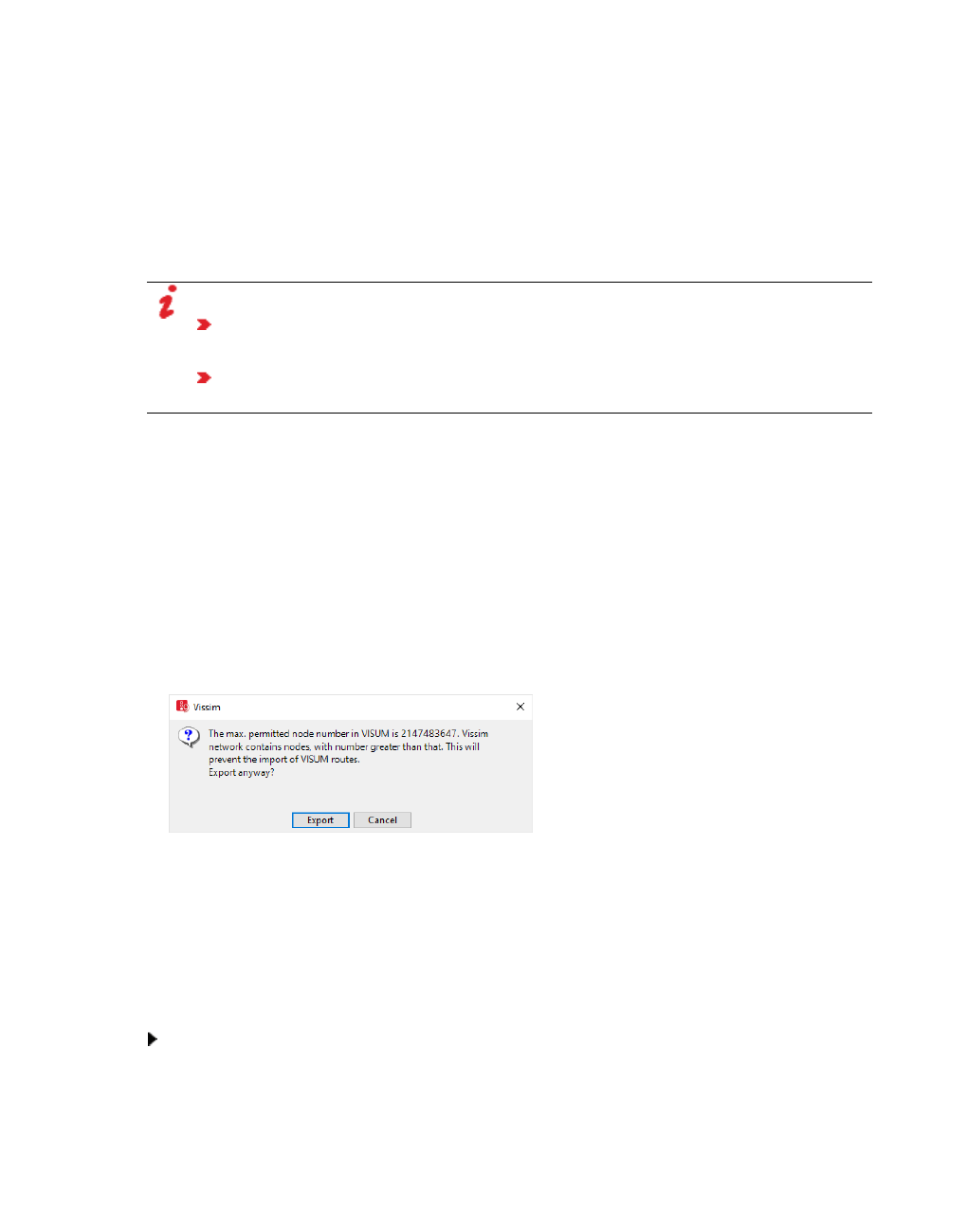
7.14.1 Calculating a Visum assignment automatically
7.14.1.1 Starting automatic calculation
In Vissim, from the Traffic menu, choose > Dynamic Assignment > PTV Visum Assignment.
The Visum assignment is calculated with the Visum converter. The Visum converter is a
standard part of your Vissim installation. The Visum converter stores the routes from Visum in
the Vissim path file *.weg. If a path file with the same name has already been saved, Vissim
saves a backup file *.bak. You can change the name of the path file (see "Attributes for the trip
chain file, matrices, path file and cost file" on page 731).
Notes:
If you run the dynamic assignment multiple times, the files *.weg and *.bak are over-
written.
A static assignment from Visum in Vissim takes place in much less time than a
microscopic Vissim simulation of individual vehicles.
7.14.1.2 Running a simulation
After the automatic calculation, you can start the simulation in Vissim without further steps (see
"Running a simulation" on page 796). You can also perform several simulation runs (see
"Defining simulation parameters" on page 796). In the first iteration the paths computed by
Visum are used. After the first iteration, the path files and cost files generated by Vissim are
used. The file names are kept.
If the Vissim network contains nodes whose numbers are greater than the maximum allowed
Visum node number 2,147,483,647, the assignment cannot be calculated. The PTV Visum
Export window opens.
1. Change the Vissim node numbers so that they are less than the maximum allowed Visum
node number.
2. Select from the menu Traffic > Dynamic Assignment > PTV Visum assignment.
7.14.1.3 Displaying warnings, notes and debug messages for the calculation
In the automatic calculation of the assignment the warnings, notes and debug messages are
displayed in the Message window.
In the View menu, choose > Messages.
© PTV GROUP 753
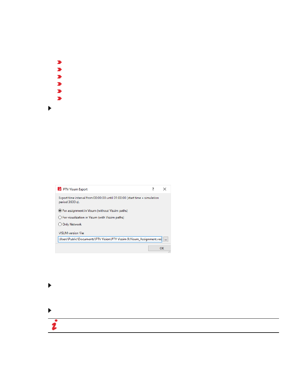
7.14.2 Stepwise Visum assignment calculation
7.14.2 Stepwise Visum assignment calculation
You can perform the dynamic assignment from Visum also based on a static assignment step-
by-step:
Export network from Vissim
Load network data in Visum
Edit the network in Visum
Calculate assignment in Visum
Export routes from Visum
Import routes into Vissim
Perform simulation run in Vissim.
This ensures that for all origin-destination relations with demand> 0 the paths throughout
the Vissimnetwork are available.
7.14.2.1 Exporting network data from Vissim
1. From the File menu, choose > Export > PTV Visum (Nodes/Edges).
2. Export network data and matrix for the assignment in Visum (see "Exporting data" on page
359).
3. Copy the Export time interval shown during export. You will need the data later in Visum.
A version file *.ver will be saved.
7.14.2.2 Loading the version file in Visum
Load the version file *.ver.
7.14.2.3 Modifying network in Visum
Make the desired changes in the network.
Note: Changes in the network topology can cause the import of routes to fail in Vissim.
The network topology in Visum is not affected by the following modifications:
754 © PTV GROUP

7.14.2 Stepwise Visum assignment calculation
Change link attributes (Type, Length, Capacity PrT, v0 PrT)
Change link polygons
Change node attributes (Type, Capacity PrT, t0 PrT, Control type)
Change node geometry
Change link orientations
Change node coordinates
Add signalization using the Node editor
The following modifications in Visum could cause the route import in Vissim to fail:
Insert and delete nodes
Edit node number
Insert and delete links
Open blocked links (change TSys of links)
Open blocked turns (change TSys of turns)
Insert and delete connectors
Open blocked connectors (change TSys of connectors)
Insert and delete TSys/Modes/DSegs
7.14.2.4 Calculating assignment in Visum
You can find further information in the Visum Help.
7.14.2.5 Exporting assignment routes into Visum
For information on ANM Export from Visum, please refer to the section Using interfaces to
exchange data of the Visum Help.
Note: Please make sure that only routes *.anmroutes are exported. Do not export
network data *.anm or matrices.
1. Enter the Export time interval which you have noted when exporting from Vissim into the
ANM export parameters window in the Further settings tab in the field From and To in
Visum.
© PTV GROUP 755

7.14.2 Stepwise Visum assignment calculation
2. Export the data from Visum.
7.14.2.6 Importing routes for dynamic assignment into Vissim
1. From the File menu, choose > Import> ANM (Vistro/Visum).
2. In the ANM Import window, deselect Import network data.
3. Select option Dynamic Assignment.
756 © PTV GROUP
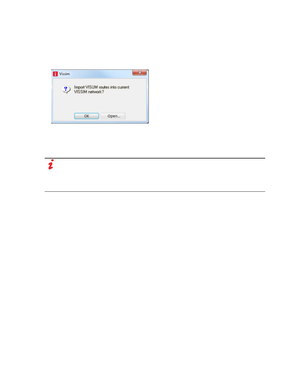
7.14.2 Stepwise Visum assignment calculation
4. Select option Import routing.
5. Select the *.anmroutes file that was exported from Visum.
6. Click Import.
The following message indicates that no errors occurred during the import:
7. Confirm with OK.
Vissim saves the calculated routes in a path file *.weg. If a path file with the same name has
already been saved, Vissim saves a backup file *.bak. You can change the name of the path
file (see "Attributes for the trip chain file, matrices, path file and cost file" on page 731).
Note: The distribution of the source volume of a zone to its parking lots in Vissim is
based on the entered relative loads and does not depend on the distribution to the
source zone connections in the assignment in Visum. The result of the assignment in
Visum is only used for the distribution of vehicles from parking lots from Vissim to the
paths Visum has found to the chosen destination parking lot.
© PTV GROUP 757

8 Using add-on module for mesoscopic simulation
8 Using add-on module for mesoscopic simulation
Note: You must have a license for the add-on module.
Mesoscopic simulation is a vehicle simulation that provides faster run speed when compared
to microscopic simulated models. Mesoscopic simulation uses a simplified vehicle following
model (see "Car following model for mesoscopic simulation" on page 760) for modeling
vehicle behavior. It allows for the fast simulation of large networks during dynamic assignment.
Mesoscopic simulation is event based. Therefore, in contrast to microscopic simulation,
vehicle data is not updated with every time step but only at times when changes occur in the
network or vehicle behavior. These so-called events may be triggered by different situations,
e.g.:
Vehicle entering the network
Change in traffic signal state
Vehicle entering a node
Vehicle entering a microscopically simulated area
Vehicle exiting a microscopically simulated area
Mesoscopic and microscopic simulations can be combined to form a hybrid simulation. To do
so, network sections where vehicles and their behavior are required to be simulated
microscopically need to be defined. This can be particularly useful when:
detailed evaluations are only needed for certain parts of the network, but a large net-
work is required to model route choice.
for parts of the network mesoscopic simulation is not precise enough and conflicts can-
not be modeled realistically, e.g. in turbo roundabouts or complex intersections.
For the mesoscopic simulation of your network, the factors dealt with in detail in the following
sections need to be considered.
You can find examples of mesoscopic simulation in the directory ..\Examples\Examples
Training\Meso.
8.1 Quick start guide mesoscopic simulation
The quick start guide demonstrates the key steps and settings required for mesoscopic
simulation.
Note: When you import a network via ANM import, all network objects required for
mesoscopic simulation are created and the parameters are set for mesoscopic
simulation (see "Importing ANM data" on page 345), (see "Generated network objects
from the ANM import" on page 352). In this case, make sure that the values and settings
meet your requirements, e.g. the meso follow-up gap and the meso critical gap (see
"Attributes of meso turns" on page 789), (see "Attributes of meso turn conflicts" on page
790).
758 © PTV GROUP

8.1 Quick start guide mesoscopic simulation
1. Prepare your Vissim network according to the requirements for dynamic assignment (see
"Using the dynamic assignment add-on module" on page 653), (see "Defining parking lots
for dynamic assignment" on page 660), (see "Defining zones" on page 664).
2. Select the desired matrix or matrices (see "Attributes for the trip chain file, matrices, path file
and cost file" on page 731).
3. Make sure the simulation duration specified in the matrix and in the simulation parameters
is the same (see "Attributes for the trip chain file, matrices, path file and cost file" on page
731).
4. Ensure that the numbers of the zones in the matrix and the numbers of the zones in the
Vissim network are the same (see "Attributes of zones" on page 665).
5. Ensure that the settings for dynamic assignment meet your requirements (see "Attributes for
the trip chain file, matrices, path file and cost file" on page 731).
6. Insert nodes for mesoscopic simulation (see "Defining nodes" on page 668). When doing
so, make sure that the modeling rules for meso graphs are applied (see "Modeling meso
network nodes" on page 766), (see "Mesoscopic node-edge model" on page 761).
7. For these nodes, select the attributes UseForDynAssign and UseForMeso (see "Attributes
of nodes" on page 669), (see "Attributes of meso nodes" on page 785), (see "Attributes of
meso edges" on page 788).
8. Create the meso graph (see "Generating meso graphs" on page 793).
9. To simulate parts of your Vissim network microscopically, make sure they lie in sections
(see "Modeling sections" on page 641), (see "Hybrid simulation" on page 793).
10. Select the Meso simulation method (see " Selecting simulation method micro or meso" on
page 796).
11. If you have defined sections in which you want Vissim to perform microscopic simulation,
select the desired sections (see "Selecting sections for hybrid simulation" on page 794).
12. Make sure that the driving behavior parameters in the Meso tab meet your requirements
(see "Editing the driving behavior parameter Meso" on page 298):
13. Make sure that for links you have selected the Meso speed model according to your
requirements (see "Attributes of links" on page 383).
14. Make sure that for links, for which you selected the Meso speed model attribute link
related, the Meso speed attribute meets your requirements (see "Attributes of links" on
page 383).
15. Define the status of conflict areas In the Conflict areas list or in the coupled list Nodes -
Conflict areas (see "Attributes of conflict areas" on page 531), (see "Attributes of nodes" on
page 669).
16. Model node control (see "Node control in mesoscopic simulation" on page 764). For
intersection control, define a critical gap, using the Meso critical gap attribute in the Meso
turn conflicts list (see "Attributes of meso turn conflicts" on page 790) and a follow-up gap
in the Meso turns list (see "Attributes of meso turns" on page 789).
© PTV GROUP 759

8.2 Car following model for mesoscopic simulation
17. To perform evaluations for mesoscopic and/or hybrid simulation, configure the following
evaluations:
Network performance (see "Vehicle network performance : Displaying network per-
formance results (vehicles) in result lists" on page 1025)
Link evaluation (see "Showing data from links in lists" on page 1043)
Meso edge evaluation (see "Showing meso edges results in lists" on page 1004)
Meso lane evaluation (see "Showing meso lane results in lists" on page 1005)
18. Ensure that the desired simulation parameters have been set (see "Defining simulation
parameters" on page 796).
19. Start the simulation (see "Selecting the number of simulation runs and starting simulation"
on page 801).
8.2 Car following model for mesoscopic simulation
Mesoscopic simulation uses a simplified car following model based on the work of M. Mahut
(see "References" on page 1138) . The main difference to car following models used in
microscopic simulation is that braking and accelerating are not included. A vehicle changes its
speed immediately and has only two statuses:
The vehicle is driving at maximum speed.
A temporal distance is kept to the rear end of the preceding vehicle. This temporal dis-
tance corresponds to the response time.
The precise formulation of a car following model depends on the meso speed model selected.
You may select a meso speed model for each link (see "Attributes of links" on page 383):
Link-based: less detailed. Can therefore lead to an improvement in simulation speed.
Vehicle-based (default setting): high level of detail. Vehicles attempt to drive at their
individual desired speed.
8.2.1 Car following model for the meso speed model Link-based
The car following model uses fixed link speeds:
These include:
xFollower: Front end position of trailing vehicle on current link
xLeader: Front end position of preceding vehicle on current link
VLink: Meso link speed
τFollower: Response time of trailing vehicle
λLeader : Effective vehicle length of preceding vehicle, calculated from the individual vehicle
length and the meso standstill distance.
760 © PTV GROUP
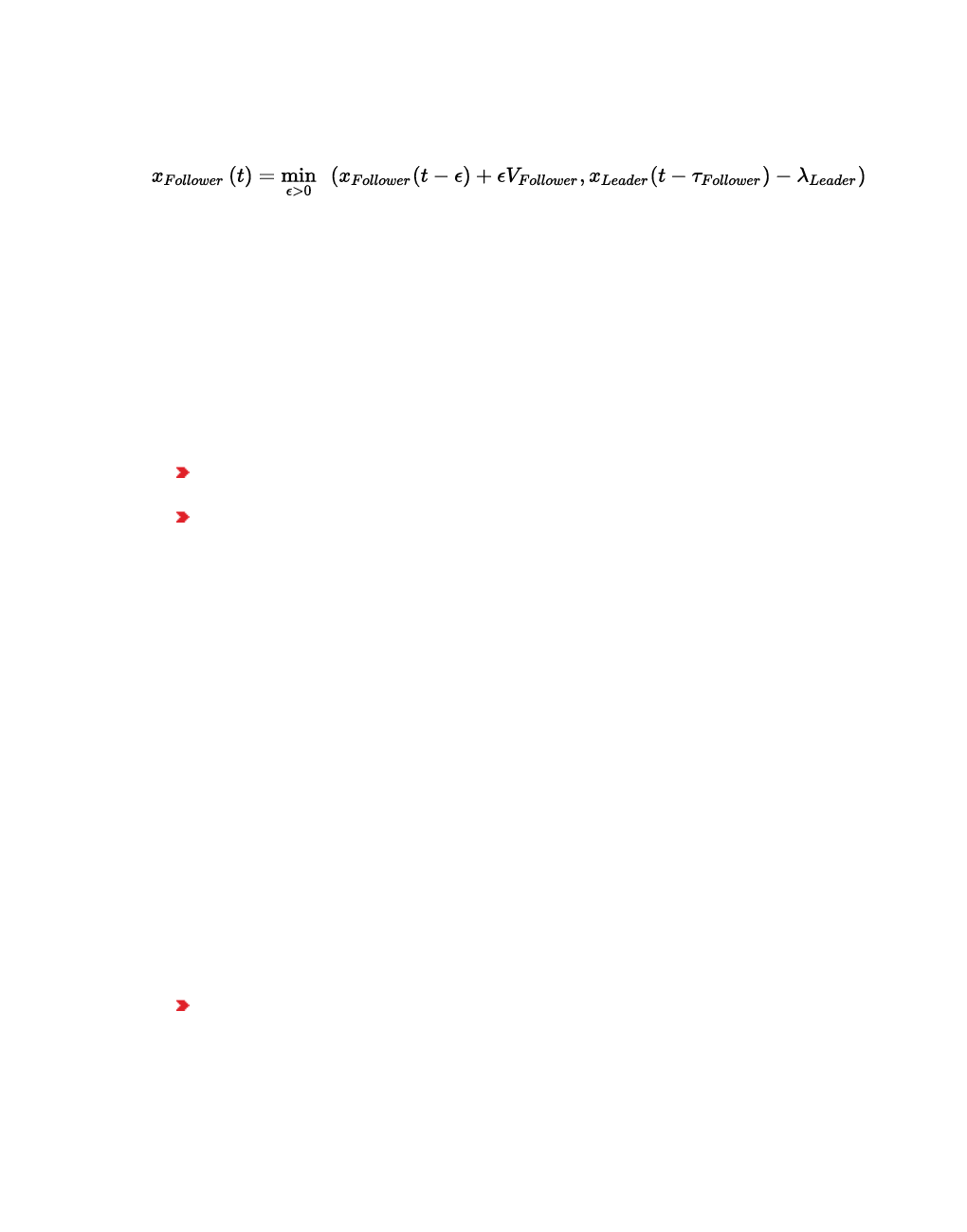
8.2.2 Car following model for the meso speed model Vehicle-based
8.2.2 Car following model for the meso speed model Vehicle-based
The car following model uses individual vehicle speeds:
In this formulation, VLink is replaced by VFollower : Each vehicle tries to drive at its individual
desired speed VFollower.
8.2.3 Additional bases of calculation
Both car following models use individual vehicle lengths and response times that are based
on driving behavior parameters.
By default, the meso speed model is set to Vehicle-based. Vehicles therefore drive at their
individual desired speed in free flowing traffic. Desired speed decisions and reduced speed
areas result in changes to the vehicle’s desired speed. When used the following limitations
apply:
Reduced speed areas and desired speed decisions apply per lane and extend over
the entire meso edge (see "Mesoscopic node-edge model" on page 761).
Multiple reduced speed areas and/or desired speed decisions cannot be used on the
same lane within the same meso edge as they are considered to overlap. In this
instance Vissim displays a message when the meso graph is created and uses the
information of only the object that is furthest downstream.
For the Link-based meso speed model the following applies:
Desired speed decisions and reduced speed areas are ignored. Differences in the desired
speed of vehicle classes cannot be modeled. This means that different speed limits on
different lanes can only be modeled with the vehicle-based model. However, in a city center
network, the Link-based meso speed model might be sufficient. Use of the Link-based meso
speed model in most parts of the network can lead to enhanced simulation speed.
8.3 Mesoscopic node-edge model
Mesoscopic simulation requires a special node- edge model also called a meso graph.
Creating a meso graph is a prerequisite for mesoscopic simulation (see "Generating meso
graphs" on page 793). Based on the meso graph and evaluations, you can generate meso
edge results and meso lane results (see "Performing evaluations" on page 941).
8.3.1 Properties and nodes of the meso graph
The meso graph is different from the abstract network graph for dynamic assignment. It is a
combination of all meso nodes and meso edges that are relevant for mesoscopic simulation:
The meso graph is created based on nodes where the attribute Use for mesoscopic
simulation has been selected. These nodes are referred to as Meso network nodes
and displayed in the Nodes list (see "Modeling nodes" on page 666). By default, meso
network nodes can be edited the same way as other nodes.
© PTV GROUP 761

8.3.1 Properties and nodes of the meso graph
The modeling of meso network nodes must comply with the rules for defining meso net-
work nodes in mesoscopic simulation (see "Modeling meso network nodes" on page
766).
In meso graphs, Vissim does not use the modeled meso network nodes, but auto-
matically generates corresponding meso nodes when it creates the meso graph.
Thus, for each meso node modeled, there is a corresponding meso network node.
Vissim assigns this meso node the value Node in the Type attribute, when it gen-
erates the meso graph. This is because the meso node is based on a modeled net-
work object of the type Node.
However, the meso nodes are not shown in the Nodes list, but in the Meso nodes list
(see "Attributes of meso nodes" on page 785).
A meso node cannot be edited like a network object node. Only the respective meso
network node that Vissim used to generate the meso node can be edited. You can
show the Meso nodes list as a relation of the Nodes list, to list each meso network
node together with its corresponding meso node.
In addition, when creating the meso graph, Vissim automatically generates additional
meso nodes, e.g. for parking lots or dynamic routing decisions. It further generates
additional nodes where, for mesoscopic simulation, relevant link attributes change,
e.g. the number of lanes or the meso speed model. Accordingly, in the Type attribute,
Vissim assigns each of these meso nodes their corresponding value, e.g. Parking lot,
Routing decision or Other (see "Attributes of meso nodes" on page 785).
This allows for a distinction between meso network nodes and meso nodes during
mesoscopic simulation. The table shows the relationships and order in which you define a
node, you mark it as a meso network node, Vissim then generates the meso network node at
the start of the simulation and the meso node for the meso network node.
Element Description
Nodes Models network object Node in the Network editor (see "Modeling nodes" on page
666), (see "Modeling meso network nodes" on page 766).
Marks
node as
meso
network
node
Selects the attribute Use for mesoscopic simulation for the modeled node.
The node is displayed in the Nodes list (see "Attributes of nodes" on page 669).
The Nodes list contains all nodes of the network object type Node. At the meso
network nodes, the attribute UseForMeso (Use for mesoscopic simulation) is
selected.
Meso
node
When after modeling the network and configuring the simulation, you start the
simulation, Vissim generates the meso graph. When generating the meso graph,
Vissim automatically generates a meso node for each meso network node
modeled. As this meso node is not the meso network node, it is not displayed in
the Nodes list, but in the meso nodes list. You can show the Meso nodes list as a
relation in the Nodes list (see "Attributes of meso nodes" on page 785).
762 © PTV GROUP

8.3.2 Differences between meso network nodes and meso nodes
8.3.2 Differences between meso network nodes and meso nodes
Meso network nodes
A meso network node is a network object of the type Node for which the attribute Use
for mesoscopic simulation (UseForMeso) has been selected.
A meso network node can be defined and edited in the same way as any other node of
the network object type Node. You may define polygon nodes and segment nodes
(see "Modeling nodes" on page 666).
Meso network nodes are shown in the Nodes list (see "Attributes of nodes" on page
669).
However, meso network nodes are not shown in the Meso nodes list (see "Attributes
of meso nodes" on page 785).
Meso nodes based on meso network nodes
Meso nodes cannot be edited in the Network editor.
Meso nodes that are automatically generated based on meso network nodes during
creation of the meso graph are shown in the Meso nodes list. In the Type attribute,
they have the value Node. The Node attribute also contains the number of the cor-
responding meso network node.
Meso nodes automatically generated by Vissim
Besides the meso nodes that Vissim generates for the modeled meso network nodes,
Vissim generates additional meso nodes when creating the meso graph. For these meso
nodes the following applies:
Meso nodes have no longitudinal extension.
Meso nodes cannot be edited.
Meso nodes are only displayed in the Meso nodes list (not in the Nodes) list.
The Type attribute value of these meso nodes is different than for Nodes, e.g. Parking
lot, Routing decision or Other.
8.3.3 Meso edges in meso graphs
The meso graph consists of meso nodes and meso edges. The following meso edges are
distinguished:
A link meso node connects two meso nodes via links and connectors that lie between the
two meso nodes (see "Attributes of meso edges" on page 788).
Within a meso node, a meso turn edge connects meso edges that lead into the meso
node with meso edges that lead out of the meso node. The number of lanes and speed of
links and connectors where a meso turn edge begins may be different for the meso turn
edge itself. For instance, the meso turn edge may start at a double-lane link, but then lead
via a single-lane connector and link to another double-lane link:
© PTV GROUP 763

8.3.4 Changes to the network will delete the meso graph
The attributes of the Defining links of the respective meso turn, however, must not change.
If in the meso node, a meso turn edge leads from a double-lane link via a link sequence,
consisting of multiple connectors and links that begin with a single-lane connector, the fol-
lowing links and connectors of the meso edge must also be single-lane. This is described
in Rule 3 (see "Rules and examples for defining meso network nodes" on page 767).
Connector meso edges are origin connector edges that lie within parking lots. An origin
connector meso edge does not have a preceding edge. A destination connector meso
edge does not have a successive edge.
A PT line connector is an edge leading from a meso node of the type PT line origin to a
meso node of the type Node or Input.
A micro-meso transition is an edge leading from a meso node of the type Micro-meso
transition to a meso node of the type Micro-meso.
8.3.4 Changes to the network will delete the meso graph
If changes are made to the network that affect the structure of the meso graph, the graph is
deleted. The attributes list of meso-specific network objects then no longer displays any data.
By creating a new meso graph, you can fill the attributes list with data again.
8.4 Node control in mesoscopic simulation
In mesoscopic simulation there are some rules for modeling signalized and non signalized
intersections that differ from the rules that apply for microscopic simulation.
For signalized intersections note that the decisive factors are the stop position and storage
capacity. The vehicle always stops at the meso network node. If the real situation cannot be
modeled with one meso network node only, model several nodes, e.g. for a separately led
right turn. For conflict control at intersections, in mesoscopic simulation, Vissim only looks at
the vehicles on the edges that lead into the node.
764 © PTV GROUP
8.4 Node control in mesoscopic simulation
Signalized intersections
As detectors cannot be used in mesoscopic simulation, no data is transferred to dynamic
controls. As a result, mesoscopic simulation only considers fixed time signal control. This type
of control only distinguishes between the statuses stop and drive. The signal state sequences
of signal groups either cause vehicles to wait at the entry of the meso network node or enter
the node:
The signal states Red and Red flashing are interpreted as stops.
Red/amber is evaluated with the driving behavior based on the settings made in the Beha-
vior at red/amber signal attribute (see "Editing the driving behavior parameter Signal Con-
trol" on page 295).
Vehicles may drive at any of the other signal states. When green times overlap, e.g. for
conditionally compatible left turns, conflict areas and attribute values take effect that are rel-
evant for mesoscopic simulation (see "Attributes of meso turn conflicts" on page 790).
Non signalized intersections
In mesoscopic simulation intersection control is modeled only using conflict areas and their
status. The network object type Priority Rule is not taken into account in mesoscopic
simulation. Priority rules should not be used in mesoscopic simulation. As different algorithms
are used to model movement of the vehicles, meso-specific attributes with individual value
ranges are required. The following parameters apply for the behavior of vehicles in conflicting
flows:
Critical gap (see "Attributes of meso turn conflicts" on page 790)
Follow-up gap (see "Attributes of meso turns" on page 789)
Maximum wait time (see "Editing the driving behavior parameter Meso" on page 298)
Default values for critical gap and follow-up gap
During ANM import, Vissim sets the following default values. When modeling nodes, you can
use these default values for orientation.
For intersection controlled nodes and u-turns the following applies:
Direction Critical gap [s] Follow-up gap [s]
left major - minor 3.5 2.2
right minor - major 5.5 3.3
minor intersects major 6.0 4.4
left minor - major 6.5 3.5
U-turn major 3.5 Same as left major - minor 3.5 Same as left minor - major
U-turn minor 6.5 Same as left minor - major 3.5 Same as left minor - major
Channel island (at the end) 5.5 Same as right minor - major 3.3 Same as right minor - major
For uncontrolled nodes the following applies (priority to right):
© PTV GROUP 765
8.5 Modeling meso network nodes
Direction Critical gap [s] Follow-up gap [s]
right minor - minor 5.5 Same as right minor - major 3.3 Same as right minor - major
straight minor - minor 5.5 Same as right minor - major 3.3 Same as right minor - major
left minor - minor 6.5 Same as left minor - major 3.5 Same as left minor - major
For controlled nodes the following applies:
Direction Critical gap [s] Follow-up gap [s]
Left turns with counter flow 3.5 Same as left major - minor 2.2 Same as left major - minor
Right turn on red 5.5 Same as right minor - major 3.3 Same as right minor - major
For roundabouts the following applies:
Direction Critical gap [s] Follow-up gap [s]
Entry into roundabout 3.5 3.2
Bypass (at the end) 3.5 (as for entry) 3.2 (as for entry)
8.5 Modeling meso network nodes
You may exclusively define and edit meso network nodes (see "Mesoscopic node- edge
model" on page 761) . You cannot define or edit meso nodes that were automatically
generated by Vissim.
Comparable to nodes for dynamic assignment in microsimulation, meso network nodes must
be defined where paths come together or significantly branch out.
For dynamic assignment with microsimulation, it is sufficient to use one node per real
intersection. This node may contain multiple conflict areas that are independent from each
other. These conflict areas only impact vehicles located precisely within their area.
In mesoscopic simulation, vehicles generally wait outside the meso network node due to
conflict areas and then traverse the entire meso network node without stopping. This is why a
meso network node must start at every position vehicles are meant to wait. If vehicles heading
different turning directions are meant to stop at different positions of an intersection entry, you
will need to create multiple separate meso network nodes. A single meso node for the entire
intersection will not be sufficient.
In mesoscopic simulation you often need more meso network nodes to model intersections
than nodes in dynamic assignment with microsimulation, even if the intersections are of similar
complexity. This is particularly true when it comes to roundabouts, non- signalized
intersections, intersections with bypasses, etc.
Each meso edge leading into a meso network node must be long enough to create a travel
time on the node which is greater than the meso critical gaps of the conflict areas for the
following turn relations. Otherwise, instead of the critical gap value defined, the travel time on
the edge is used as the critical gap. Therefore it is necessary to define small meso network
nodes and make sure the edges are sufficiently long enough. Follow the rules and examples
given for defining meso network nodes (see "Rules and examples for defining meso network
nodes" on page 767).
766 © PTV GROUP
8.6 Rules and examples for defining meso network nodes
8.6 Rules and examples for defining meso network nodes
Meso network nodes must be modeled correctly for Vissim to be able to model conflicts
realistically in mesoscopic simulation. The level of correctness has a decisive impact on the
result of dynamic assignment in mesoscopic simulation. Therefore, the rules for modeling
meso network nodes strictly need to be followed accurately. Before starting to model meso
network nodes it is necessary to look at the examples and read the descriptions of correct and
incorrect definitions for meso network nodes.
8.6.1 Rules for defining meso network nodes
Rule 1: Meso network nodes must be defined everywhere on a link where more than one
connector begins or ends.
Rule 2: For each intersection, at least one meso network node must be defined. Depend-
ing on the node geometry, several meso network nodes may be defined.
For non-signalized intersections the following applies: All conflict areas must be defined. In
order to decide which conflict areas shall lie within a separate meso network node, check
the following:
Where is the vehicle supposed to stop? For all turn conflicts, the vehicle stops at the
meso network node. Model the meso network node so that its edge roughly cor-
responds to a stopping position of the vehicle in reality, e.g. a stop line.
Are the incoming meso edges used by vehicles with the right of way to reach the meso
network node relevant for all turn conflicts in the meso network node? The size and
positioning of the node determine which meso edges are perceived as edges with
vehicles that have the right of way (see "Meso conflict relevant and non-relevant
edges" on page 770).
How long is the travel time on the incoming meso edge used by vehicles with the right
of way to reach to meso network node? This travel time should be longer then the
meso critical gap of the subordinate flow.
For signalized intersections note that the decisive factors are the stop position and storage
capacity. The vehicle always stops at the meso network node. If the real situation cannot be
modeled with one meso network node only, model several nodes, e.g. for a separately led
right turn.
Rule 3: On turn meso edges, the following properties must not change:
the number of lanes
the link behavior type
the meso speed, if the meso speed model Link-related is selected (see "Car following
model for mesoscopic simulation" on page 760)
This means the Defining links of the meso turn must each have the same value (see
"Attributes of meso turns" on page 789).
Note: Please note the limitations and information that apply for defining meso network
nodes (see "Defining meso network nodes" on page 784).
© PTV GROUP 767

8.6.2 Examples of applying the rules for defining meso network nodes
8.6.2 Examples of applying the rules for defining meso network nodes
The following examples show how the rules are applied when you model intersections. First,
you are shown how the position of a meso network node impacts where at the conflict area a
vehicle stops and which edges it perceives as relevant:
Consequences of correct and incorrect positioning of meso network nodes
Meso conflict relevant and non-relevant edges
Then, you are given an explanation of how the rules impact the modeling of different types of
intersections. For different network objects, the impact of rules on the meso graph structure
and on simulation is demonstrated:
Nodes in areas where the number of lanes changes
Modeling connectors in meso network nodes
Modeling a signalized intersection
Modeling intersections with lane widening
Modeling intersections with bypass and channelized turn
Modeling roundabouts
Modeling reduced speed areas on links
Modeling SCs on links
8.6.2.1 Consequences of correct and incorrect positioning of meso network nodes
The following example describes the meaning of travel time as a meso critical gap on an edge
for a 3-leg intersection with nine turn conflicts. Nine meso network nodes have been manually
defined at the nine turn conflicts (1 to 9):
768 © PTV GROUP

8.6.2 Examples of applying the rules for defining meso network nodes
This type of modeling is not recommended if the travel time on the edge leading into the meso
network node is shorter than the meso critical gap of the conflict in the meso network node.
This leads to incorrect modeling of the conflicts in mesoscopic simulation. It is illustrated in the
following figure and explained in the description given below it.
Situation: The vehicle is coming from below and turns upward left.
The conflicts are not modeled correctly in mesoscopic simulation:
Cause: The travel times on some edges leading into the nodes are too short.
Effect: Vehicle also stops at wrong positions.
The vehicle stops for the conflict at node 9, position a, as it should.
The vehicle stops for the conflict at node 6, position b, and only pays attention to the edge
between node 5 and 6. The travel time at the edge between nodes 5 and 6 acts as a crit-
ical gap, if it is shorter than the meso critical gap entered for the conflict. The same
applies for the subsequent nodes:
The vehicle stops for the conflict at node 3, position c, and only pays attention to the edge
between node 3 and 2. The travel time at the edge between nodes 3 and 2 acts as a crit-
ical gap, if it is shorter than the meso critical gap entered for the conflict.
The vehicle stops for the conflict at node 1, position d, and only pays attention to the edge
between node 1 and 2. The travel time at the edge between nodes 1 and 2 acts as a crit-
ical gap, if it is shorter than the meso critical gap entered for the conflict.
If the vehicle stops at a wrong position and the travel time at the edge leading into the meso
network node is very short, the travel time acts as a critical gap. Vissim is then unable to model
the conflicts in mesoscopic simulation realistically (as illustrated in the figure above).
© PTV GROUP 769

8.6.2 Examples of applying the rules for defining meso network nodes
If, for instance, no meso network node is defined for node 3 (at top of figure), Vissim does not
recognize the conflict there and the conflict is ignored in mesoscopic simulation.
Solution: If for these types of intersections, with short edges between conflicts, only one meso
network node is defined, Vissim is able to model conflicts realistically in mesoscopic
simulation. With one meso network node only, the left-turning vehicle has only one stop
position in all subsequent conflicts. The travel times at the incoming edges are long enough
and the vehicle stops at the correct position. This is illustrated in the following figure and
explained in the description given below it.
Correct modeling: The travel times at all edges leading into the node at conflict points are
long enough. This ensures that the vehicle stops at the correct positions:
With conflict 11 in the black dot, the vehicle is aware of the edge leading from node 1
into node 2. If the travel time on this edge is longer than the meso critical gap for the
conflict, the specified value is used as critical gap, e.g. 3.5 s.
With conflicts 22 and 33 in the red dots, the vehicle is aware of the incoming edge
between nodes 3 and 2. If the travel time on this edge is longer than the meso critical
gap for the conflict, the specified value is used as critical gap, e.g. 3.5 s.
8.6.2.2 Meso conflict relevant and non-relevant edges
This example shows a roundabout (right-hand traffic) for which multiple meso network nodes
have been correctly positioned, in the figure on the left. In the figure on the right, only one
meso network node has been positioned across the roundabout. The following two figures
show the meso edges the vehicle is aware of when it stops at the meso network node:
Correctly modeled: The modeling in the figure on the left ensures that the vehicle is
aware of the relevant meso edge (yellow between the two meso network nodes), lead-
ing directly into the correctly positioned meso network node at which the vehicle stops.
The correct meso critical gap is used.
Incorrectly modeled: The modeling in the figure on the right does not allow the
vehicle to become aware of the relevant meso node. For conflicts in the meso network
node, e.g. the entry of the vehicle into the roundabout, the vehicle is only aware of
non-relevant meso edges (the three meso edges highlighted in yellow that lead into
the meso network node from the left, top and right). The vehicle cannot become aware
of the relevant node as shown in the figure on the left. Thus, it cannot take a correct
meso critical gap into account. The vehicle stops at the meso network mode and gives
770 © PTV GROUP

8.6.2 Examples of applying the rules for defining meso network nodes
priority to the vehicles coming from the right, top and left, as it is only aware of their
meso nodes.
Correct: Vehicle is aware of relevant meso
edge (yellow between the two bottom meso
network nodes)
Incorrect: Vehicle is only aware of non-
relevant meso nodes (yellow)
: Vehicle is coming from below and wants to turn right into roundabout
8.6.2.3 Nodes in areas where the number of lanes changes
There are different ways to model areas in which the number of lanes changes. These impact
dynamic assignment in mesoscopic simulation in different ways. This is illustrated in the
following figure and explained in the table listed below it.
Connector connects a double-lane link with a single-lane link:
The vehicle may only change lane at the end of a meso node. This applies for meso nodes
generated automatically by Vissim and for modeled meso network nodes (see "Mesoscopic
node-edge model" on page 761).
© PTV GROUP 771
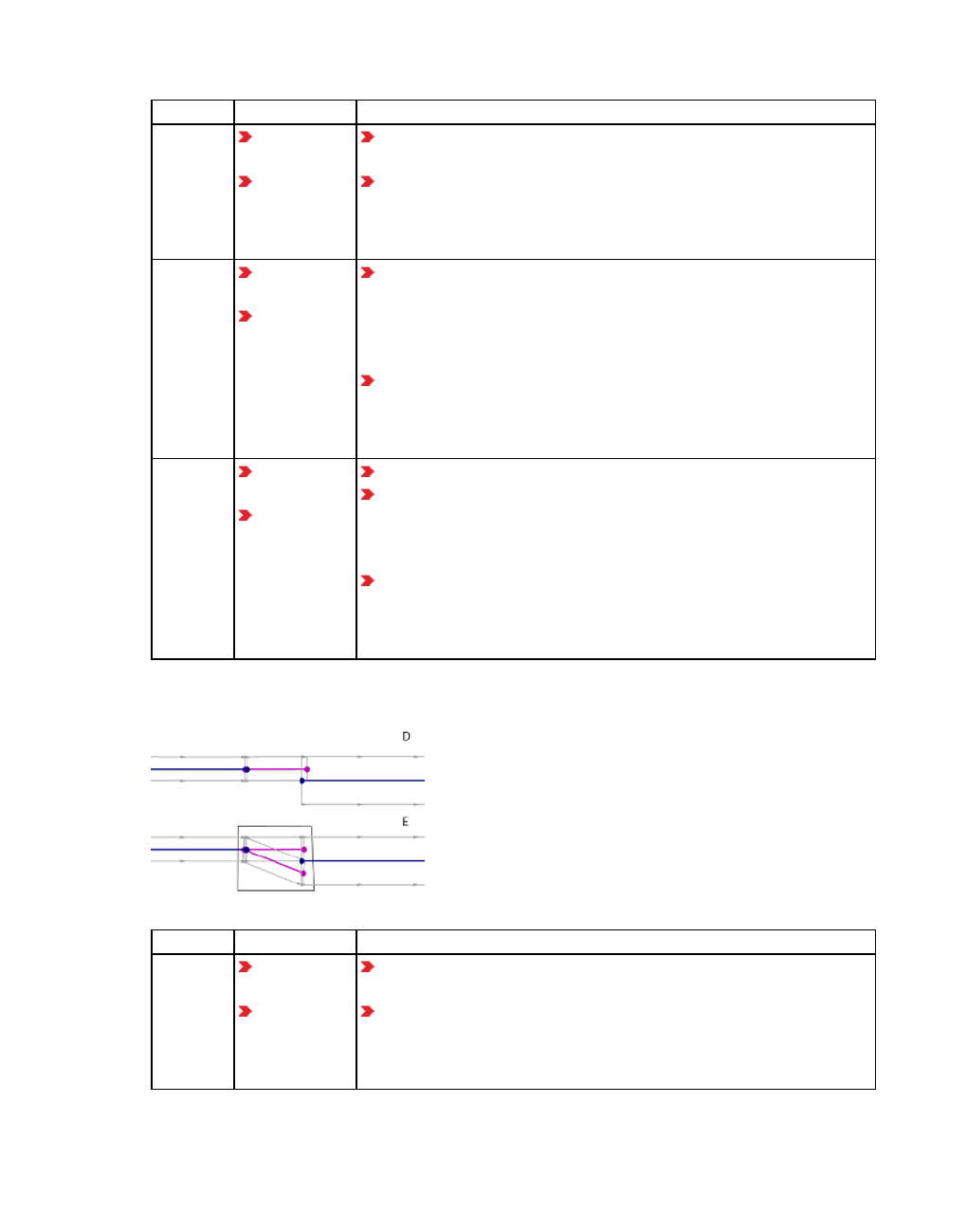
8.6.2 Examples of applying the rules for defining meso network nodes
Modeling Situation Mesoscopic simulation
Aa con-
nector
not a
modeled
meso net-
work node
Vissim automatically generates a meso node at the beginning
of the connector.
On the double-lane link, vehicles may use the right lane only
which is unrealistic.
Ba con-
nector
a modeled
meso net-
work node
Vissim automatically generates a meso node at the beginning
of a connector. In this case, you need not manually define the
meso network node. This meso network node is defined manu-
ally, so that contrary to A, both lanes may be used and lane
changes are possible.
On the double-lane link, vehicles may use both lanes.
Vehicles may use the left lane up until the modeled meso net-
work node. At the end of this meso network node, all vehicles
must change from the left lane to the right lane.
Ctwo con-
nectors
a modeled
meso net-
work node
On the double-lane link, vehicles may use both lanes.
For dynamic assignment when one of the connectors is closed
then only one connector is available for the path search.
However for mesoscopic simulation both connectors remain
available.
Apply an edge closure to one of the edges for dynamic assign-
ment. This way you can avoid parallel edges in dynamic
assignment. Parallel edges multiply the number of possible
paths significantly.
Connector connects a single-lane link with a double-lane link:
Modeling Situation Mesoscopic simulation
Da con-
nector
not a
modeled
meso net-
work node
Vissim automatically generates a meso node at the end of the
connector.
Vehicles can use both lanes of the double-lane link. To use
the lane on the right, the vehicle must change lanes. Lane
changes are penalized during lane selection. This is why the
left lane is preferred.
772 © PTV GROUP

8.6.2 Examples of applying the rules for defining meso network nodes
Etwo con-
nectors
a modeled
meso net-
work node
On the double-lane link, vehicles may use both lanes. As both
lanes can be easily reached, no lane change is required and
the vehicles are distributed evenly across the lanes, if both
lanes are permitted for the vehicle route.
Apply an edge closure to one of the edges for dynamic assign-
ment. This way you can avoid parallel edges in dynamic
assignment. Parallel edges multiply the number of possible
paths significantly.
8.6.2.4 Modeling connectors in meso network nodes
Rule Description
1Meso network nodes must be defined everywhere on a link where more than one
connector begins or ends.
A link leads into a node.
Two connectors lead out of the node.
The connectors do not have to lie entirely within the node.
The connectors must begin within the node.
Correct False
© PTV GROUP 773

8.6.2 Examples of applying the rules for defining meso network nodes
Rule Description
1Meso network nodes must be defined everywhere on a link where more than one
connector begins or ends.
The connectors do not have to lie entirely within the node.
Left meso node: Two connectors lead into node. The connectors must end within
the node.
Right meso node: Two connectors lead out of node. The connectors must begin
within the node.
Correct False
Rule Description
1Meso network nodes must be defined everywhere on a link where more than one
connector begins or ends.
If the transition from a one-lane link to a two-lane link is modeled across two
connectors, these must lie entirely within the node.
Correct False
774 © PTV GROUP

8.6.2 Examples of applying the rules for defining meso network nodes
Rule Description
3On turn meso edges, the following properties must not change:
the number of lanes
the link behavior type
the meso speed, if the meso speed model Link-related is selected (see "Car fol-
lowing model for mesoscopic simulation" on page 760)
The number of lanes must be the same for each defining link contained within the
meso network node.
However, the number of lanes of the inbound meso edge and the number of lanes
of the outbound meso edge may differ.
Correct False
© PTV GROUP 775
8.6.2 Examples of applying the rules for defining meso network nodes
8.6.2.5 Modeling a signalized intersection
Rule Description
2For each intersection, at least one meso network node must be defined. Depending on
the node geometry, several meso network nodes may be defined.
A signal head may be defined on links or connectors.
Position signal heads within a meso network node.
If a signal head is less than 5 m away from the border of the node, the software will
not automatically generate another meso node. Vissim then assumes that the
vehicle stops at the node border and the signal head belongs to the node.
If a signal head is more than 5 m away from the border of a node, Vissim auto-
matically generates an additional meso node.
If meso nodes are positioned too close to each other, the edge between them
might become so short that, in certain situations, Vissim cannot not model the driv-
ing behavior realistically. Vissim only accounts for the vehicles at the edge leading
into the node, not any other nodes further downstream.
In the figure at the bottom right this means:
If the signal heads are 10 m from the meso network node of the intersection, Vissim
automatically generates a meso node at the signal heads. The edge between the
two nodes is then 10 m long. The travel time of a vehicle driving at 10 m/s on this
edge is 1 s. This second acts as a critical gap for the vehicle approaching from the
right and turning left, regardless of the actual meso critical gap defined, as the
vehicle cannot tell whether, beyond the meso node, there is a vehicle approaching
from the left that it must yield to. A critical gap of 1 s does not give the vehicle
enough time to yield.
Solutions: a) Position the signal heads within the meso network node or b) reduce
the distance between signal heads and meso network nodes to below 5 m or c)
ensure that the length of the edge leading into the node is long enough to create a
travel time on the edge that is longer than the meso critical gap of the turn conflict in
the node.
Correct: The signal heads are positioned
within the meso network node or at a
maximum of 5 m from it
Not recommended: The signal heads are
positioned at a distance of more than 5
m from the meso network node
776 © PTV GROUP
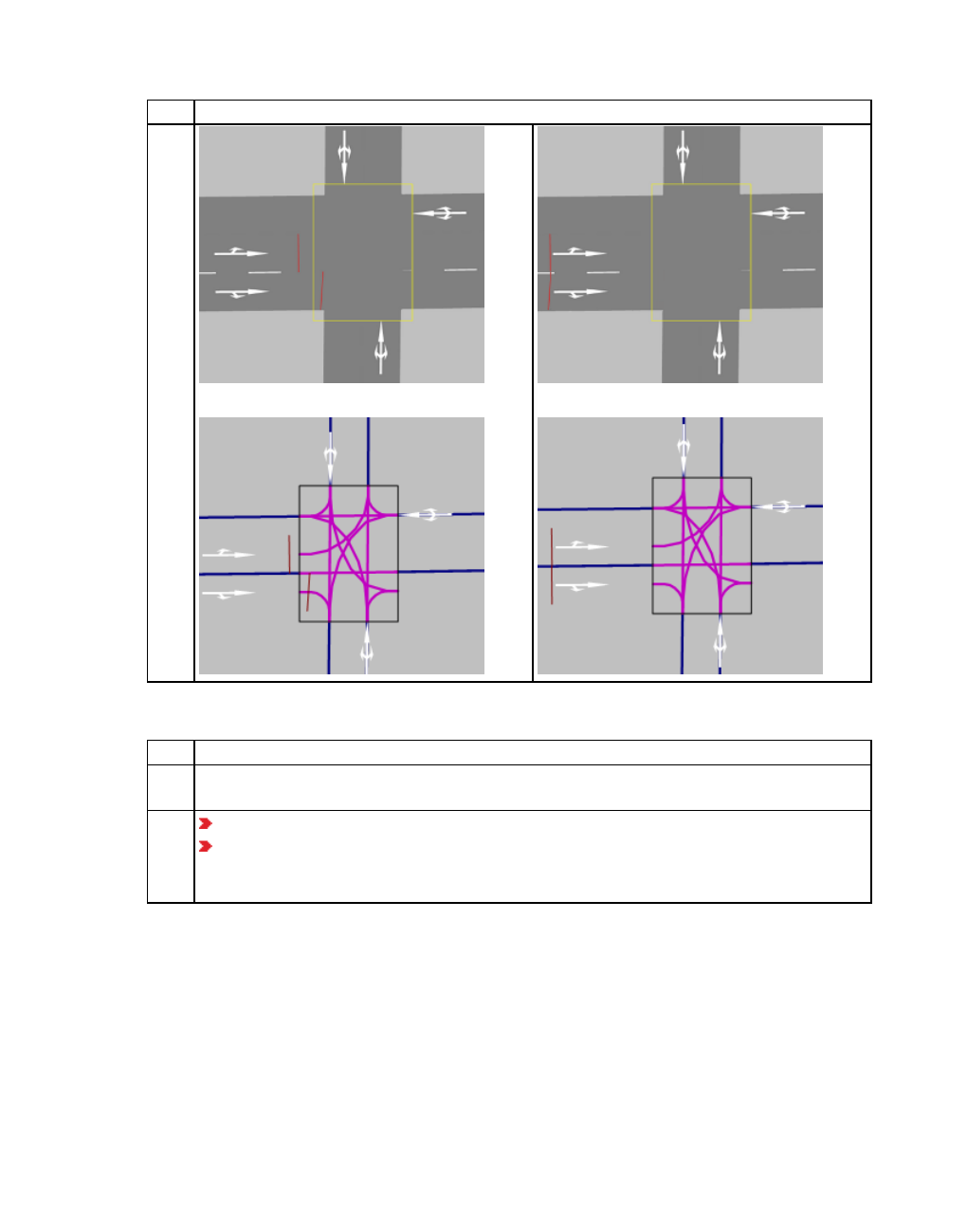
8.6.2 Examples of applying the rules for defining meso network nodes
Rule Description
8.6.2.6 Modeling intersections with lane widening
Rule Description
2For each intersection, at least one meso network node must be defined. Depending on
the node geometry, several meso network nodes may be defined.
Lane widening must not lie within the node.
When creating a meso graph, Vissim automatically generates a meso node of the
type Other where the lane widening begins (see "Attributes of meso nodes" on
page 785).
© PTV GROUP 777

8.6.2 Examples of applying the rules for defining meso network nodes
Rule Description
Correct False
8.6.2.7 Modeling intersections with bypass and channelized turn
Rule Description
2For each intersection, at least one meso network node must be defined. Depending on
the node geometry, several meso network nodes may be defined.
According to Rule 1 meso network nodes must be placed at the branchings where
the bypass begins and ends. These nodes must have the attribute Use for meso-
scopic simulation. In the figure on right, the vehicle approaching from the left and
turning to the right (downwards), already waits at the beginning of the right turn
lane, at the large node that represents the entire intersection. This is not recom-
mended. In the figure on the left, the vehicle waits at the end of the right turn lane,
at the small meso network node modeled for this purpose.
In addition, the intersection itself must lie within a meso network node.
778 © PTV GROUP

8.6.2 Examples of applying the rules for defining meso network nodes
Rule Description
Correct Not recommended
8.6.2.8 Modeling roundabouts
Note: The following tips refer to the modeling of simple roundabouts, e.g. those with a
single lane, with no or only one bypass and few entries and exits. To model more
complex roundabouts or roundabouts whose conflicts cannot be modeled correctly in
mesoscopic simulation, define sections and perform a hybrid simulation (see "Hybrid
simulation" on page 793).
Rule Description
2For each intersection, at least one meso network node must be defined. Depending on
the node geometry, several meso network nodes may be defined.
Each branching and thus each entry and exit must lie within a meso network node.
The connectors do not have to lie entirely within the node.
If there is a bypass, meso network nodes must be placed at the branchings where
the bypass begins and ends. These nodes must have the attribute Use for meso-
scopic simulation.
© PTV GROUP 779
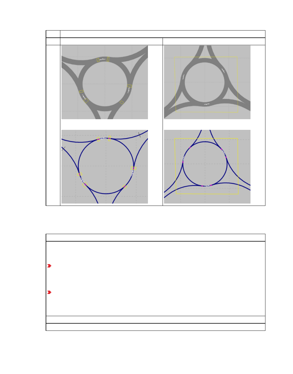
8.6.2 Examples of applying the rules for defining meso network nodes
Rule Description
Correct False
Model meso network nodes for a roundabout depending on the distance between the exit and
the next entry and according to approach A or approach B. This is illustrated in the following
figures and explained in the descriptions given below them.
Description of approach A
If the distance between the exit and next entry downstream is large enough, define a meso
network node for the exit and another one for the entry. This is the case in the following
situations:
Condition 1: The travel time on the roundabout between exit x and the next entry down-
stream y is equal to or larger than the meso critical gap for the conflict in y: txy > tCG(y). If
this condition is not met, but the following one is, you can still use approach A to model
the roundabout:
Condition 2 (for right-hand traffic): The travel time on the roundabout between exit x and
the next entry downstream y is equal to or larger than the travel time on the lane between
upstream entry b and the next downstream exit x: tbx < txy. For the conflict in y, the critical
gap is the travel time on the roundabout between exit x and the next entry downstream y.
Correct
780 © PTV GROUP
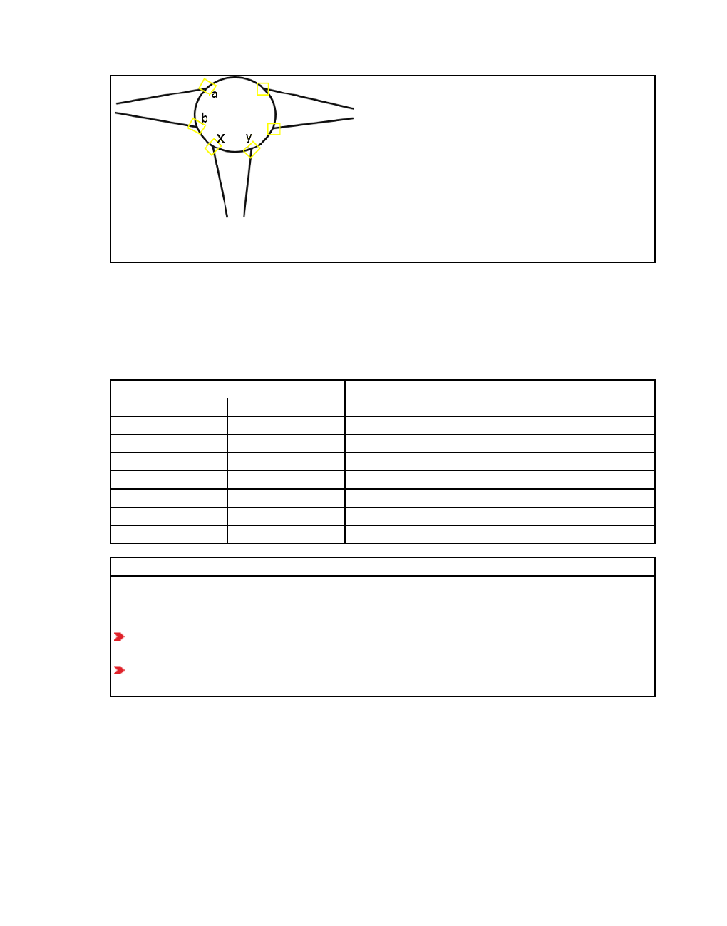
8.6.2 Examples of applying the rules for defining meso network nodes
txy > tCG(y) or tbx < txy
When you export a network from Visum and import it into Vissim via ANM import, Vissim
automatically generates meso network nodes based on approach A. These nodes do not
require any subsequent editing (see "Generated network objects from the ANM import" on
page 352). The table lists different speeds to illustrate the minimum distance between exit x
and the next downstream entry y with a critical cap of 3.5 s, in order for approach A to meet
condition 1:
Veh speed on roundabout lane min. distance [m] x-y to meet condition 1
m/s km/h
1 3.6 3.5
2 7.2 7.0
3 10.8 10.5
5 18 17.5
7 25.2 24.5
10 36 35.0
14 50.4 49
Description of approach B
If the distance between the exit and next entry downstream is not large enough, define a
common meso network node for both the exit and entry. This is the case, when the two
following situations happen at the same time:
The travel time on the roundabout lane between entry b and the next downstream exit x
is larger than the travel time between exit x and the next exit downstream y: tbx > txy and
the travel time on the roundabout lane between exit x and the next entry downstream y is
smaller than the meso critical gap for the conflict in y: txy < tCG(y)
© PTV GROUP 781
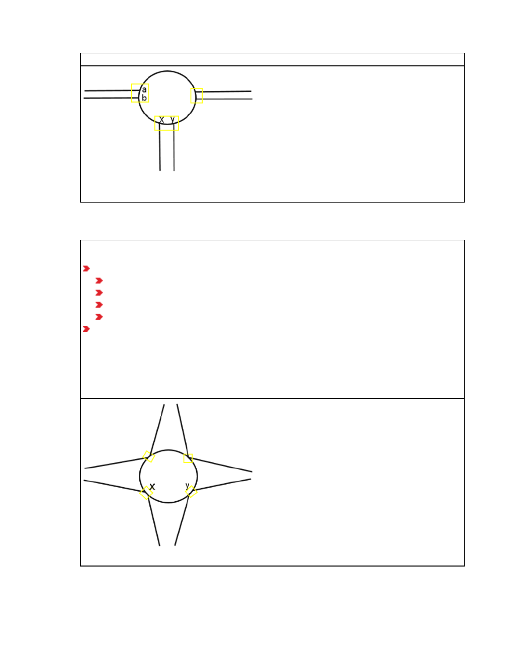
8.6.2 Examples of applying the rules for defining meso network nodes
Correct
tbx > txy and txy < tCG(y)
The two following figures show wrong approaches to define meso network nodes: These
approaches produce incorrect results when used to model conflicts in mesoscopic simulation:
Incorrect approach 1: The distance between the entry and the next exit downstream is not
large enough. As a result, too many conflicts arise at each of the nodes:
4 meso turn edges:
from roundabout
from entry
into roundabout
into exit
6 meso turn conflicts
Solution: If the entry and the next exit downstream are very close to each other, use
approach A, even if this results in short edges between the meso network nodes. In that
case, at each of the two meso network nodes, there will be only one merging or branching
conflict. At the branching conflict, the short edge leading out of the meso network node does
not pose a problem.
782 © PTV GROUP

8.6.2 Examples of applying the rules for defining meso network nodes
Figure below Incorrect approach 2: Only a single meso network node has been defined for
all conflicts in the roundabout. Effect: Conflicts are not modeled realistically, vehicles stop at
wrong positions and for conflicts, the time gap is based on non-relevant edges.
8.6.2.9 Modeling reduced speed areas on links
Description
Reduced speed areas on links are only taken into account when the vehicle-based meso
speed model is used on links.
In the top figure, the speed distribution specified for the reduced speed area has an
impact on the entire meso node for vehicles heading from west (left) to east (right) on the
right lane.
If you want the reduced speed area to have only a local impact, you need to insert a
meso network node (see "Defining nodes" on page 668). The reduced speed area must
lie entirely within the node. The meso edge within the node is a turn meso edge that is
impacted by the speed distribution of the reduced speed area.
Desired speed decisions are treated the same way in mesoscopic simulation.
© PTV GROUP 783

8.7 Defining meso network nodes
8.6.2.10 Modeling SCs on links
Description
You do not have to create nodes for signal heads on links.
In this case, a meso node of the type Other is automatically generated on the link (see
"Attributes of meso nodes" on page 785). When doing so, Vissim automatically generates
two meso edges.
8.7 Defining meso network nodes
Please note the rules and examples for defining nodes and meso network nodes (see
"Modeling meso network nodes" on page 766). In addition, consider the following limitations
and information:
Limit the extent of a meso network node to the necessary maximum extent. Conflict areas
in particular do not have to lie entirely within the node.
Ensure that there is a sufficient distance between the meso nodes. This includes the dis-
tance between automatically generated meso nodes that are not of the type A Node (see
"Attributes of meso nodes" on page 785).
Meso network nodes must not overlap.
When modeling meso network nodes, please note that during dynamic assignment, path
search and path selection are performed based on the generalized costs of edges and/or
paths of dynamic assignment. When creating networks for mesoscopic simulation in Vis-
sim, you therefore generally select the UseForDynAssign attribute (see "Defining nodes"
on page 668).
In networks imported via ANM import, for some intersections (e.g. roundabouts or inter-
sections with lane widening) nodes are created with either the UseForDynAssign attrib-
ute or the UseforMeso attribute selected. Nodes with the UseForDynAssign attribute are
exclusively used for calculations performed within dynamic assignment and the path file.
These nodes must also not overlap. In principle, the attributes UseForDynAssign and
UseForMeso may be selected independently from each other.
You can use nodes of dynamic assignment to control the path selection based on edge
closures (in the figure below, the outer node) and meso network nodes (in the figure
below, the eight node in the roundabout), as described in the respective rules (see "Rules
and examples for defining meso network nodes" on page 767):
784 © PTV GROUP

8.8 Attributes of meso nodes
1. Define the desired meso network nodes according to the definition of nodes (see "Modeling
nodes" on page 666), (see "Defining nodes" on page 668).
The Nodes window opens.
2. In the Nodes window, select Use for mesoscopic simulation.
The node then becomes a meso node. When creating a meso graph, Vissim automatically
generates a meso node for each meso network node modeled and assigns it the attribute
Node (see "Attributes of meso nodes" on page 785).
8.8 Attributes of meso nodes
Vissim automatically generates a meso node when a meso graph is generated (see
"Generating meso graphs" on page 793), (see "Mesoscopic node-edge model" on page 761).
You can display these meso nodes and their attributes in the Meso nodes list.
When generating a meso graph, Vissim assigns each meso node in the Type attribute a value.
This value is based on the network object type of the network object Vissim is generating the
meso node for.
Example:
In the Network editor, you define a node that you need for mesoscopic simulation. For this
node, you consequently select the Use for mesoscopic simulation attribute. The node then
becomes a meso network node. You can show the meso network node, like all models nodes,
in the Nodes list (see "Attributes of nodes" on page 669). When generating the meso graph,
Vissim generates a meso node for the meso network node. Vissim then assigns the meso
node the value Node in the Type attribute. The generated meso node is displayed in the Meso
nodes list., but the modeled meso network is not.
From the Lists menu, choose > Network > Meso nodes.
© PTV GROUP 785

8.8 Attributes of meso nodes
The Meso nodes list opens.
Note: In lists, you can use the Attribute selection icon to show and hide attribute
values (see "Selecting attributes and subattributes for a list" on page 106).
The list on the left may include the following attributes:
Long name Short name Description
Number No Unique number
Type Type Vissim assigns the type, while
generating the meso node, based on
the network object type for which it is
generating the meso node. The length
of automatically generated meso
nodes that are not of the type Node is
0.000 m.
Vissim can create the following types:
PT stop lay-by entry: Meso nodes at the beginning of connector that lead to the link
with the PT stop lay-by
PT stop lay-by exit: Meso nodes at the beginning of connector that lead away from
the link with the PT stop lay-by
PT lines origin: Meso node at the beginning of a PT line, leads to a meso edge of the
type PT input connector.
Parking lot: Meso node within a parking lot of teh type Zone connector
Vehicle input origin: Meso node at the beginning of a link on which vehicles are
deployed into the network, leads to a meso edge
Origin zone: Meso node for assigned origin zone in parking lot
Routing decision: Meso node of a dynamic routing decision
Node: Meso node located at a node of the network object type Node, for which the
attribute Use for mesoscopic simulation is selected
Other: Other automatically generated meso nodes for signal heads on links or where
link attributes change that are relevant for mesoscopic simulation (e.g. number of
lanes)
Transition meso-micro: Meso node at the border of a section where transition from
mesoscopic to microscopic simulation takes place
Transition micro-meso: Meso node at the border of a section where transition from
microscopic to mesoscopic simulation takes place (end point of meso edge of the type
Micro-meso transition)
Public transport stop: Meso node within a PT stop. When a PT vehicle is on a meso
turn with a PT stop, no other vehicle may enter the same meso turn. A vehicle may,
however, pass the stopping PT vehicle on the adjacent lane, if its use is permitted for
the vehicle.
786 © PTV GROUP

8.8 Attributes of meso nodes
Long name Short name Description
Transition micro-meso (virtual): Virtual meso node at the border of a section where
transition from microscopic to mesoscopic simulation takes place (start point of meso
edge of the type Micro-meso transition)
Destination zone: Meso node for assigned destination zone in parking lot
Input: Meso node where PT vehicles are deployed in the network
Long name Short name Description
Nodes Nodes Number of respective node of the network object
type Node
Parking Lot ParkLot Number of parking lot in which the meso turn lies
Public transport
stop
Public transport
stop
Number of public transport stop
Turn meso edges TurnMesoEdge Numbers of turn meso edges
PT lines (inputs) PTLinInput List of PT lines that begin at the meso node
Inbound meso
edges
InbMesoEdge Numbers of the meso edges that lead to a meso
edge of the meso node
Outbound meso
edges
OutbMesoEdge Numbers of meso edges that exit the meso edge of
the meso node
Dynamic vehicle
routing decision
VehRoutDecDyn Numbers of the dynamic vehicle routing decisions
at meso edges of the type Routing decision
Showing and editing dependent objects as relation
1. In the list on the left, click the desired entry.
The list on the right contains attributes and attribute values of network objects, and/or base
data allocated to the network object selected in the list on the left (see "Using coupled lists" on
page 111):
Turn meso edges: These are meso edges of the type Turn (see "Attributes of meso edges"
on page 788)
Outbound meso edges: List of meso edges, leading out of the meso node (see "Attributes
of meso edges" on page 788)
Inbound meso edges: List of preceding meso edges that lead into the meso node (see
"Attributes of meso edges" on page 788)
Meso turn conflicts: (see "Attributes of meso turn conflicts" on page 790)
Meso turns: Meant for entry of follow-up gap (see "Attributes of meso turns" on page 789)
PT lines (inputs): List of PT lines that begin at the meso node (see "Attributes of PT lines"
on page 487)
© PTV GROUP 787

8.9 Attributes of meso edges
Signal head: List of signal heads in meso node (see "Attributes of signal heads" on page
545)
2. On the list toolbar, in the Relations list, click the desired entry.
3. Enter the desired data.
The data is allocated.
8.9 Attributes of meso edges
From the Lists menu, choose > Network > Meso edges.
The Meso edges list opens.
The list on the left may include the following attributes:
Long name Short name Description
Number No Unique meso edge number
From meso node FromMesoNode Number of meso node at which
the meso edge begins
To meso node ToMesoNode Number of meso node at which
the meso edge ends
Length Len Length of meso edge [m]
Meso lane MesoLn Meso-specific lane numbers
Type Type Vissim distinguishes between the
following types of meso edges:
Micro-meso transition: Meso edge lies at the border of a section where transition
from microscopic to mesoscopic simulation takes place. The length is 0.000 m.
Meso link: The meso edge lies between two meso nodes. This includes between two
meso nodes of the type PT stop lay-by entry and PT stop lay-by exit.
Turn: The meso edge lies within a meso node.
Origin connector: Origin connector meso edge in parking lot. An origin connector
meso edge does not have a preceding edge.
Destination connector: Destination connector meso edge in parking lot. A destination
connector meso edge does not have a successive edge.
PT input connector: Meso edge at start section of public transport line
Vehicle input connector: Meso edge at vehicle input
Showing and editing dependent objects as relation
1. In the list on the left, click the desired entry.
The list on the right contains attributes and attribute values of network objects, and/or base
data allocated to the network object selected in the list on the left (see "Using coupled lists" on
page 111):
788 © PTV GROUP

8.10 Attributes of meso turns
Outbound meso nodes: List of the successive meso nodes
Inbound meso nodes: List of the preceding meso nodes
Reduced speed areas (see "Attributes of reduced speed areas" on page 410)
Meso lanes: Meso-specific lane numbers of meso edge
Signal heads: Numbers of the signal heads at meso edge
Link sequence: Numbers of links and connectors that lead via meso edge (see "Attributes
of links" on page 383)
Desired speed decisions (see "Attributes of desired speed decisions" on page 414)
2. On the list toolbar, in the Relations list, click the desired entry.
3. Enter the desired data.
The data is allocated.
8.10 Attributes of meso turns
From the Lists menu, choose > Intersection control > Meso turns.
The Meso turns list opens.
Note: In lists, you can use the Attribute selection icon to show and hide attribute
values (see "Selecting attributes and subattributes for a list" on page 106).
The list on the left may include the following attributes:
Long
name
Short name Description
Defining
links
DefLink Links and connectors of the meso turn. The defining links
are specified depending on the number of links in the link
sequence. If a link sequence contains only one link, it is the
defining link. If a link sequence contains two links, the
connector is the defining link. If a link sequence contains
three or more links, all links and connectors included in their
entity are defining links.
Nodes Nodes Number of node in which the meso turn lies
Meso
edge
MesoEdge Number of meso edge
Meso
node
MesoNode Number of meso node in which the meso turn lies
From link FromLink Number of link or connector at which the meso turn begins
To link ToLink Number of link or connector the meso turn leads to
© PTV GROUP 789
8.11 Attributes of meso turn conflicts
Long
name
Short name Description
Link
sequence
LinkSeq Number of links or connectors via which the meso turn
leads. Contrary to the defining links, this also includes the
From link and To link.
Meso fol-
low-up
time
MesoFollowUpGap The meso follow-up gap determines the maximum capacity
(3,600 s / meso follow-up gap) of a subordinate flow within a
node, as long as there is no traffic on a route that leads to
conflict. The follow-up gap only becomes effective, if it is
greater than the temporal distance between two successive
vehicles that has been defined in the car following model.
The meso follow-up gap is a link attribute (see "Attributes of
links" on page 383). The meso follow-up gap only has an
impact on simulation, if it is greater than the temporal
distance specified in the car following model. Only then is
the capacity reduced. When defining values for the follow-
up gap, you can refer to established manuals such as HBS
or HCM. Edit this attribute in the Meso turns list or in the
coupled list Nodes - Meso turns (see "Attributes of nodes"
on page 669). The values are saved to the defining links as
Meso follow-up gap. The default value is 0.0 s: When you
use the default value, only the car following model takes
effect (see "Car following model for mesoscopic simulation"
on page 760). Value range 0 - 1,000 s.
Showing and editing dependent objects as relation
1. In the list on the left, click the desired entry.
The list on the right contains attributes and attribute values of network objects, and/or base
data allocated to the network object selected in the list on the left (see "Using coupled lists" on
page 111):
Defining links: List of the meso turn links and connectors that are significant for the beha-
vior of vehicles in mesoscopic simulation (see "Attributes of links" on page 383)
Link sequence: List of all links and connectors of the meso turn (see "Attributes of links" on
page 383)
2. On the list toolbar, in the Relations list, click the desired entry.
3. Enter the desired data.
The data is allocated.
8.11 Attributes of meso turn conflicts
The Meso Turn Conflicts list lists the conflicts relevant for mesoscopic simulation.
From the Lists menu, choose > Intersection control > Meso turn conflicts.
790 © PTV GROUP

8.11 Attributes of meso turn conflicts
The Meso turn conflicts list opens.
Note: In lists, you can use the Attribute selection icon to show and hide attribute
values (see "Selecting attributes and subattributes for a list" on page 106).
The list on the left may include the following attributes:
Long
name
Short name Description
Nodes Nodes Number of network node in which the turn conflict lies
Meso
node
MesoNode Number of meso node in which the turn conflict lies
Turn
meso
edge 1
TurnMesoEdge1 Number of first turn meso edge
From
link 1
FromLink1 Number of FromLink of first meso turn
To
link 1
ToLink1 Number of ToLink of first meso turn
Turn
meso
edge 2
TurnMesoEdge2 Number of second turn meso edge
From
link 2
FromLink2 Number of FromLink of second meso turn
To
link 2
ToLink2 Number of ToLink of second meso turn
Conflict
areas
ConflictArea Numbers of respective conflict areas
© PTV GROUP 791
8.11 Attributes of meso turn conflicts
Long
name
Short name Description
Status Status (see "Attributes of conflict areas" on page 531). When changes
are made to the status, the value of the respective conflict areas
is saved.
Meso
critical
gap
MesoCriticGap Meso critical gap: The meso critical gap defines the temporal
distance between two successive vehicles in the main flow that a
vehicle in a subordinate flow needs to enter the node. The meso
critical gap extends from the back edge of the preceding vehicle
to the front edge of the tailing vehicle. The time required for the
effective length of the preceding vehicle is not included. This
allows you to also model realistic behavior when dealing with a
large share of overlong vehicles. When defining values for the
meso critical gap, you can refer to established manuals such as
the HBS or HCM. In deviation from the definition used here, in
the manuals, the meso critical gap is defined for between the
front edges of successive vehicles.
The meso critical gap is a conflict area attribute (see "Attributes
of conflict areas" on page 531). Edit this attribute in the Meso
Turn Conflicts list or in the coupled list Nodes - Meso Turn
Conflicts (see "Attributes of nodes" on page 669). The values
are saved with the respective conflict areas as the attribute meso
critical gap (see "Attributes of conflict areas" on page 531).
Default 3.5 s, value range 0 s to 1,000 s.
Showing and editing dependent objects as relation
1. In the list on the left, click the desired entry.
The list on the right contains attributes and attribute values of network objects, and/or base
data allocated to the network object selected in the list on the left (see "Using coupled lists" on
page 111):
Conflict areas: List of respective conflict areas (see "Attributes of conflict areas" on page
531)
Link sequence 1: List of links of the first meso turn (see "Attributes of links" on page 383)
Link sequence 2: List of links of the second meso turn (see "Attributes of links" on page
383)
2. On the list toolbar, in the Relations list, click the desired entry.
3. Enter the desired data.
The data is allocated.
792 © PTV GROUP
8.12 Generating meso graphs
8.12 Generating meso graphs
A meso graph is automatically calculated when you start mesoscopic simulation. You may
also create this graph interactively to show the data of meso-specific network objects in the
attribute lists. When changes are made to the network that affect the meso graph, it is
automatically deleted and the results are discarded. The results lists and attribute lists of
meso-specific network objects then no longer list any data.
1. From the Lists menu, choose > Network. Then select the entry of your choice:
Meso edges (see "Attributes of meso edges" on page 788)
Meso nodes (see "Attributes of meso nodes" on page 785)
Meso turns (see "Attributes of meso turns" on page 789)
Meso turn conflicts (see "Attributes of meso turn conflicts" on page 790)
If the meso graph has not been created yet, the list will display the message No <Name
Meso network object> available. Please use the shortcut menu to create the meso
graph.
2. Right-click in the list.
3. From the shortcut menu, choose Create Meso Graph.
Vissim calculates the meso graph and shows the attribute values in the attributes list. Attribute
values are also available in the the lists of other network objects that are relevant for
mesoscopic simulation.
8.13 Hybrid simulation
During dynamic assignment, you can use mesoscopic simulation to simulate your entire
network. At the same time, you may also use microscopic simulation to simulate one or several
areas of your Vissim network. This combination allows you to create a Vissim network of the
size required for your particular use case and perform a detailed analysis for the results of the
relevant network parts based on microscopic simulation.
To define the areas you want to simulate microscopically, you define sections (see "Modeling
sections" on page 641) . You select these sections in the simulation parameters for
mesoscopic simulation (see "Selecting sections for hybrid simulation" on page 794). Within the
sections, vehicles are moved according to the algorithms of microscopic simulation. The
settings of mesoscopic simulation do not apply for these sections. For vehicles traversing
between the two areas, the mesoscopic simulation settings continue to apply. Accordingly,
properties such as the desired speed are kept.
Please note the information on how to define sections (see "Modeling sections" on page 641).
As the calculation basis for vehicle movement changes significantly at these transition areas,
unrealistic vehicle behavior may occur, particularly if the edges are very short.
The following figure shows a schematic drawing of the transition area from micro- to
mesoscopic simulation.
© PTV GROUP 793
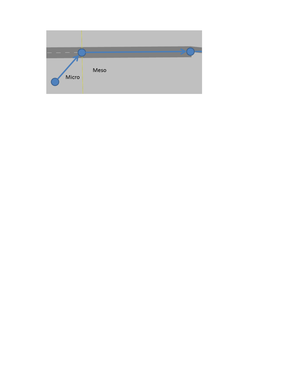
8.14 Selecting sections for hybrid simulation
At the transition point, additional meso nodes and meso edges are created. For vehicles
entering the meso area, the macroscopic speed specified for the first edge after transition is
used. If this edge is very short, significant fluctuations occur that in turn impact vehicle inputs
from the microscopic area. As a consequence, there might be unrealistically high wait times on
the micro-meso transition edge, as vehicles are not able to leave it.
At the transition point from meso- to microscopic simulation, vehicles are introduced similarly
to vehicle inputs. Here, too, you need to ensure that signal heads, desired speed decisions,
reduced speed areas, etc. are not too close to the transition point, otherwise they might be
ignored by the vehicles.
For a comprehensive analysis of the entire network, use the network performance and link
evaluation (see "Vehicle network performance : Displaying network performance results
(vehicles) in result lists" on page 1025), (see "Showing data from links in lists" on page 1043).
You can record data using node evaluation (see "Evaluating nodes" on page 997).
8.14 Selecting sections for hybrid simulation
If during hybrid simulation of your Vissim network, you want to microscopically simulate parts
of the network, you must define sections for these parts (see "Modeling sections" on page
641). The desired sections must then be selected for mesoscopic simulation.
1. From the Simulation menu, choose > Parameters.
The Simulation parameters window opens.
2. Select the Meso tab.
3. Select the Meso simulation method.
In the Sections for microscopic simulation area, all sections are displayed. Vissim only
performs microscopic simulation for the sections selected.
4. Hold down the CTRL key and click the desired sections.
When you start the simulation, the desired sections of the Vissim network are microscopically
simulated. Outside of these sections, the Vissim network is mesoscopically simulated, but
vehicles are not shown. For the selected sections, Vissim chooses the attribute Meso - use as
section for microsimulation (MesoUseForMicrosim).
794 © PTV GROUP

8.15 Limitations of mesoscopic simulation
8.15 Limitations of mesoscopic simulation
The following functions are available in microscopic simulation. These functions cannot be
used in mesoscopic simulation:
Vehicle inputs and static routing
Pedestrians
Cyclists
In dynamic assignment:
Parking lots of the type Real parking spaces as origin and destination of demand
Route guidance
Path selection type Decide repeatedly
For signal control and intersection control:
Priority rules
Stop signs
Vehicle-actuated controls
Detectors
For public transport:
Partial PT routes
PT telegrams
PT vehicles only drive up to the last PT stop of your PT line and not to the end of the PT
line, if the latter continues on a link.
Block control
For evaluations:
Data collection points
Travel time measurements can be performed in sections selected for microscopic sim-
ulation (see "Selecting sections for hybrid simulation" on page 794)
Queue counters
Should your use cases require any of the functions listed, simulate the relevant parts of the
network microscopically (see "Hybrid simulation" on page 793).
© PTV GROUP 795

9 Running a simulation
9 Running a simulation
You must set simulation parameters before you can start the simulation or a test run (see
"Defining simulation parameters" on page 796), (see "Selecting the number of simulation runs
and starting simulation" on page 801). You can also start a simulation without a Network editor
open.
The parameters for the vehicle simulation also apply to the pedestrian simulation. However,
there are additional parameters available for pedestrian simulation (see "Pedestrian
simulation" on page 814).
Via the COM Interface, you can also access network object attributes during the simulation
(see "Using the COM Interface" on page 1127).
9.1 Selecting simulation method micro or meso
You need to choose between microscopic and mesoscopic simulation of your Vissim network.
1. From the Simulation menu, choose > Parameters.
The Simulation Parameters window opens.
2. Select the Meso tab.
3. Select the desired simulation method:
Micro: When you start a simulation, the Vissim network is simulated microscopically.
The Sections for microscopic simulation are not relevant for the Micro simulation
method. They are only relevant for the Meso simulation method. Sections under Sec-
tions for microscopic simulation are displayed as deactivated.
Meso: When you start a simulation, the Vissim network is simulated mesoscopically
(see "Using add-on module for mesoscopic simulation" on page 758). In this case, Vis-
sim can simulate parts of your network microscopically, in a so-called hybrid sim-
ulation. These parts must lie within sections. You must select the sections you want
Vissim to simulate microscopically (see "Selecting sections for hybrid simulation" on
page 794).
9.2 Defining simulation parameters
Before you start your simulation, you can set general simulation parameters.
In doing so, you can enter the number of simulation runs you want to do. The following are
typical use cases of simulation runs:
Variation of the random seed for stochastic saving of results
Performing iterations of a dynamic assignment
Successive increase of total demand for dynamic assignment
The difference to a simple simulation is that depending on the use case, the corresponding
parameter, e.g, the random seed, is automatically changed with each simulation run.
796 © PTV GROUP
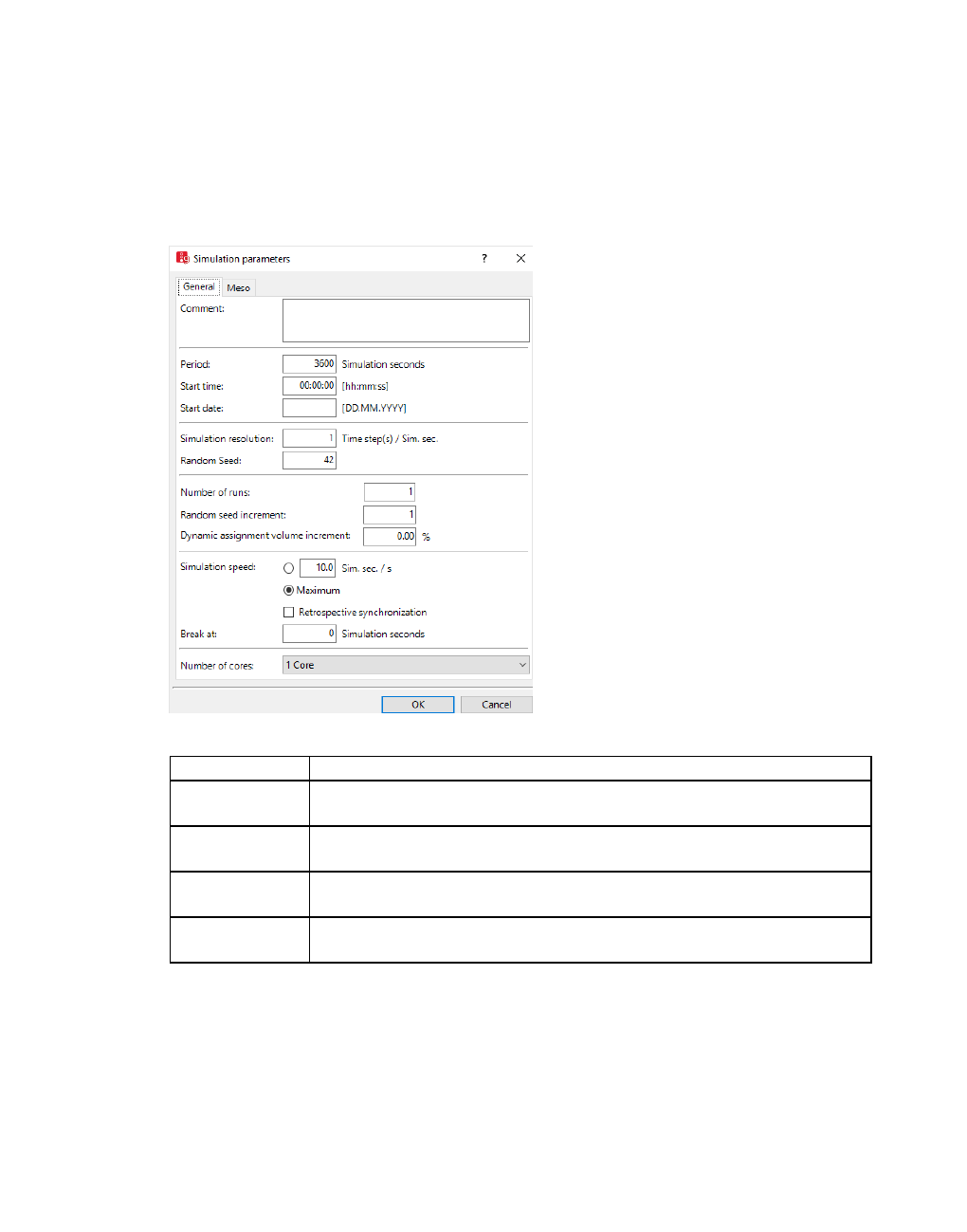
9.2 Defining simulation parameters
1. Make sure that the desired simulation method has been selected (see " Selecting
simulation method micro or meso" on page 796).
2. From the Simulation menu, choose > Parameters.
The Simulation parameters window opens.
3. Select the General tab.
4. Make the desired changes:
Element Description
Comment ID of simulation run. Is added at the beginning of output file. To save the
comment to the network file *.inpx, from the File menu, choose > Save.
Period Simulation time in simulation seconds. You also need to account for
lead times of signal controls.
Start time The simulation start time is at simulation second 0 (see "Information in
the status bar" on page 139).
Start date For signal control procedures with a date-dependent logic, the start
date is transferred to the controller DLL. Format: DD.MM.YYYY
© PTV GROUP 797
9.2 Defining simulation parameters
Element Description
Simulation resolution
Note:
The simulation resolution has an impact on the behavior of vehicles, pedestrians,
and the way they interact. This is why simulations, using different simulation
resolutions, produce different results.
Number of time steps per simulation second: specifies how often
vehicles and pedestrian are move in a simulation second.
The position of vehicles is recalculated in a simulation second with
each time step. The simulation resolution specifies the number of
time steps.
The position of pedestrians is calculated 20 times per simulation
second. This is also the case when the simulation resolution spe-
cifies less time steps. The simulation resolution then defines the fol-
lowing functions for pedestrians:
how often pedestrian movement is updated per simulation
second
how often pedestrians can be reintroduced into the simulation
per simulation second
how often pedestrians can make routing decisions per sim-
ulation second
how often evaluations may be performed per simulation second
Value range: integers from 1 to 20
Values < 5 lead to jerky movements. This is why this value range is
less suitable for production of the final simulation results. As lower
values accelerate the simulation, the use of lower values during
setup of the network model can be helpful.
Values between 5 and 10 lead to a more realistic demonstration.
This value range is suitable for the production of the final simulation
results.
Values between 10 and 20 lead to smoother movements. This value
range is suitable for high-quality simulation animations.
Random Seed This value initializes a random number generator. Two simulation runs
using the same network file and random start number look the same. If
you vary the random seed, the stochastic functions in Vissim are
assigned a different value sequence and the traffic flow changes. This,
e.g., allows you to simulate stochastic variations of vehicle arrivals in
the network. This can lead to different simulation results. A comparison
of these simulation results allows you to compare the effect of stochastic
variations. For this purpose, Vissim calculates additional, meaningful
values for various result attributes during its evaluations, e.g. minimum
value, maximum value and mean.
798 © PTV GROUP
9.2 Defining simulation parameters
Element Description
Notes:
For the model to converge during dynamic assignment,
use the same random seed. Using different random
seeds for dynamic assignment can cause a so-called
seesaw effect.
Once the model has converged and you want to obtain dif-
ferent evaluation results, use different random seeds.
Number of runs Number of simulation runs performed in a row. Logical value range:
depends on use case 5 - 20.
For dynamic assignment, more than 20 simulation runs may be
necessary.
Note: Before starting multiple simulation runs for dynamic
assignment, select the attributes of your choice (see "Attributes
for the trip chain file, matrices, path file and cost file" on page
731).
Random seed
increment
Difference between random seeds when you perform multiple
simulation runs. This number is irrelevant for stochastic distribution.
For the model to converge during dynamic assignment, enter 0.
When you perform multiple simulation runs using different random
seeds, the number of the respective simulation run is added to the
name of the evaluation file *.ldp.
Dynamic
assignment
volume incre-
ment
For dynamic assignment only: Increases total demand of the origin-
destination matrix with each simulation run defined (in the Number of
runs box) by the value specified.
The start value used is the parameter Scale total volume to of dynamic
assignment (see "Attributes for the trip chain file, matrices, path file and
cost file" on page 731). For each iteration, the demand is automatically
increased by this value until 100% of the total demand is reached. Once
100 % of the total demand is reached, any additional simulation runs
(as specified in the Number of runs box) will be performed using
100 % of the total demand. Avoid using a start value larger than 100%
of the total demand.
If due to the Number of runs specified you do not perform enough
simulation runs to reach 100 % of the total demand and you then save
the Vissim network, the current value of the total demand is saved to the
parameter Scale total volume to of dynamic assignment. The next time
you open Vissim, this value will be used as the new start value.
Simulation
speed
Corresponds to a time lapse factor: Indicates simulation seconds per
real-time second
Value 1.0: The simulation is run in real-time.
Value 2.0: The simulation is run at double real-time speed.
© PTV GROUP 799

9.2 Defining simulation parameters
Element Description
Maximum option: Select this option to run the simulation at the
maximum speed.
The simulation speed does not affect the simulation results. You can
change the simulation speed during the simulation run.
The desired simulation speed might not be reached, if you are using a
large networks or a slower computer.
Retrospective
synchronization Select this option if at the end of a time interval, you do not want
Vissim to wait until the real-time set for this interval has elapsed.
Instead, Vissim will wait until the real-time for all time intervals, since
continuous simulation was last started, has elapsed. This allows
VISSIM to make up for the time lost through slower, individual time
intervals, e.g. due to external signal control or other external factors.
With the help of external controller hardware, the synchronization
function ensures that the time lost is regained.
If you open a window during a continuous simulation run in Vissim, this
can cause a delay. After you close the window, the delay is made up for
through maximum simulation speed, until the simulation second divided
by the simulation speed equals the total real-time elapsed.
When the simulation speed of a continuous simulation run is reduced
through retrospective synchronization, Vissim waits until the total real-
time (since simulation start) equals the current simulation second
divided by the simulation speed, before it executes the next time
interval.
Break at Simulation second after which the program automatically switches to
Simulation single step mode. You can use this option to view the traffic
conditions at a specific simulation time.
Number of
cores
Number of processor cores used during simulation. The maximum
number of cores used depends on your computer. Your setting remains
selected when you start the next simulation run.
Default: Use all cores
The number of cores selected is saved to the network file *.inpx. You
cannot change this setting during the simulation run.
Note: If at least one dynamic potential is used to simulate
pedestrians, all available processor cores are used and not the
number stated in this field.
5. Confirm with OK.
The Simulation Parameters window closes Your settings are saved to the network file. The
simulation runs are started with your current settings. The status bar shows the number of the
current simulation run and the total number of simulation runs performed in brackets.
Evaluation files are saved to the folder selected.
The simulation parameters specified are taken into account for the next simulation or test run.
800 © PTV GROUP

9.2.1 Special effect of simulation resolution on pedestrian simulation
9.2.1 Special effect of simulation resolution on pedestrian simulation
From a mathematical point of view, this type of simulation basically represents a numerical
integration of a system of coupled differential equations. Smaller time steps allow for solutions
approaching the exact solution. A larger number of time steps, however, requires more
computation. Vissim calculates pedestrians with a time step of 0.05 seconds, i.e. 20 times per
second. This value only slightly diminishes the accuracy compared to the exact solution. By
comparison, in many projects the impact of uncertain external factors is probably greater, e.g.
the real number of pedestrians and their speed.
Vissim's program module for pedestrian movement internally communicates with other
modules. These modules for instance generate pedestrians or remove them during simulation,
calculate route choice or control the output of evaluations. The modules communicate at a
simulation resolution specified in the simulation parameters. These other modules have less
impact on pedestrian movement than the program module responsible, but still display some
effect. For example, with a low simulation resolution, a pedestrian could skip a very narrow
area on which a pedestrian routing decision lies. The routing decision would then have no
effect on the pedestrian. The simulation resolution also has an impact on pedestrians that
enter escalators: with each time step of simulation resolution, only one pedestrian may enter
the escalator.
Suitable simulation resolution
When still creating your model and not performing any evaluations yet, you can use a
simulation resolution of 1 or 2 steps per second.
Depending on your use case, simulation resolutions of 1 or 2 steps per second may
change the simulation runs performed for testing purposes during the setup phase in a
non-desired manner. You should then increase the simulation resolution. If you want
to evaluate simulations at the end of a setup phase, use simulation resolutions of at
least 5, better 10 or 20, steps per second.
For AVI recordings that you can use for presentations of your simulation to external
audiences, use a simulation resolution of 20 steps per second.
9.3 Selecting the number of simulation runs and starting simulation
Tip: To gain an impression of the stochastic distribution of results, run multiple
simulations using different random seeds and compare the results (see "Defining
simulation parameters" on page 796).
Notes:
When using the 64-bit Vissim version, with large networks and numerous vehicles,
you might obtain different simulation results than with the 32-bit program version
due to its different rounding behavior.
Opened lists might reduce the simulation speed. When you close opened lists, this
may increase the simulation speed.
© PTV GROUP 801
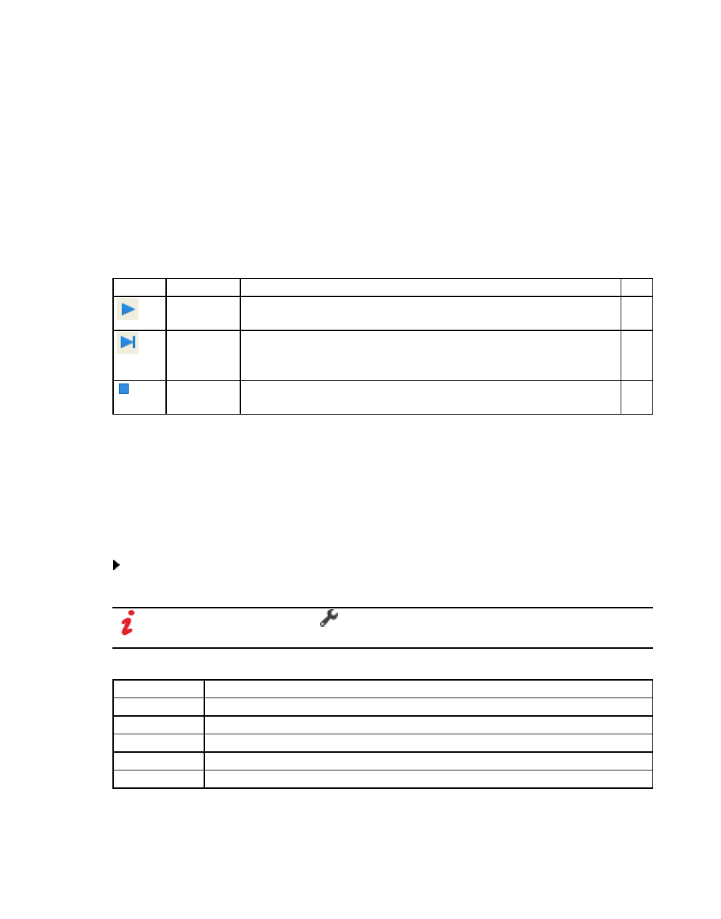
9.4 Showing simulation run data in lists
Set the simulation parameters before you start a simulation run (see "Defining simulation
parameters" on page 796). You can then run a simulation in the Simulation single step or
Simulation continuous mode.
1. From the Simulation menu, choose > Continuous or Single Step.
Vissim initializes the simulation. Initialization might take a while, if you are using a large
network. In this case, a window opens displaying the progress of initialization.
2. When this window is displayed, but you wish to cancel initialization, click the Cancel button.
3. If messages are shown during the simulation, follow the instructions and make the settings
required.
You can use the Simulation toolbar to control simulation runs:
Symbol Name Description Key
Simulation
continuous
Starts continuous simulation run or switches from Simulation
single step mode to Simulation continuous mode.
F5
Simulation
single step
Starts simulation in Simulation single step mode or switches
from Simulation continuous mode to Simulation single step
mode or executes the next single step.
F6
Stop sim-
ulation
Stop started simulation run ESC
Convergence may already be reached before the number of simulation runs is completed that
has been defined in the simulation parameters, in the Number of runs box. In this case, you
can select the Behavior upon convergence: (see "Attributes for achieving convergence" on
page 741).
9.4 Showing simulation run data in lists
You can show data of the simulation runs in a results list.
From the Lists menu, choose Results > Simulation Runs.
The Simulation Runs list opens.
Note: In lists, you can use the Attribute selection icon to show and hide attribute
values (see "Selecting attributes and subattributes for a list" on page 106).
Element Description
No. Consecutive number of simulation run
Timestamp Date and time the simulation starts
Comment Comment on simulation
SimPeriod Simulation time in seconds specified in the simulation parameters
SimEnd Time in seconds after the start at which the simulation was ended
802 © PTV GROUP

9.5 Displaying vehicles in the network in a list
Element Description
Start Date Start date specified in the simulation parameters
StartTime Start time specified in the simulation parameters
RandSeed Random seed specified in the simulation parameters
VissimVers Program version installed
Tip: In the Simulation runs list, you can delete the simulation runs that are no longer
required. This will accelerate loading the network file *.inpx.
9.5 Displaying vehicles in the network in a list
During a simulation run, you can show vehicle data for each vehicle in the network in the
Vehicles In Network list.
1. Start the simulation (see "Running a simulation" on page 796).
2. From the Lists menu, choose > Results > Vehicles in Network.
The Vehicles In Network list opens.
Note: In lists, you can use the Attribute selection icon to show and hide attribute
values (see "Selecting attributes and subattributes for a list" on page 106).
Element Description
No Number of the vehicle
VehType Vehicle type: Vehicle type assigned to the vehicle
Lane Lane: Number of lane on which the vehicle is located
Pos Position: Distance covered on the link from the beginning of the link
Speed Speed: Speed of the vehicle at the end of the time step
DesSpeed Desired Speed: Desired speed distribution of the vehicle
Acceleration Acceleration during the time step.
Positive value: Current speed of vehicle
Negative value: Current reduction of vehicle speed
LnChg Lane Change: Direction in which the vehicle changes the lane:
Links
Right
None
DestLane Destination lane: Number of lane to which vehicle changes
PTLine Public transport line: Number of PT line of PT vehicle
PTDwellTmCur Public transport - dwell time (current): Total dwell time at the current PT
stop, including slack time fraction
© PTV GROUP 803

9.5 Displaying vehicles in the network in a list
The vehicle has additional attributes that you can view in the Vehicles In network list and
save as a vehicle log to a file or database (see "Saving vehicle record to a file or database" on
page 971). Among them are the following for example:
Attribute Description
2D/3D model 3D model file of the vehicle
Indicating Current state of vehicle turn signal. Corresponds to current
visualization during simulation:
No: Vehicle is not indicating
Links
Right
Following distance Distance to the interaction vehicle in [m] before the time step
Number of stops Number of stops (cumulated): All situations in which a vehicle
comes to a standstill (speed = 0), except stops at PT stops and
in parking lots.
Dwell time Dwell time [s] at a stop sign or at a PT stop.
For PT stops: Actual dwell time according to PT line-specific
attributes (see "Calculating dwell time according to the
advanced passenger model" on page 498).
Occupancy Defines the number of persons or passengers in a vehicle. This
value is output before and after boarding and alighting.
Emissions For add-on module API package only: Results of emission
calculation for selected file EmissionModel.dll (see "Activating
emission calculation and emission model for a vehicle type" on
page 261). Emission values are also displayed in:
Vehicle network performance evaluation(see "Vehicle net-
work performance : Displaying network performance results
(vehicles) in result lists" on page 1025)
Evaluation Links per segment(see "Showing data from
links in lists" on page 1043)
Vehicles in Network list (see "Displaying vehicles in the
network in a list" on page 803)
804 © PTV GROUP

9.5 Displaying vehicles in the network in a list
Attribute Description
Motion state
Default: Default state, if none of the following states are true.
In queue: The vehicle is stuck in a traffic jam. At least one queue counter must be defined
in the network.
Waiting for lane change: Vehicle has been waiting more than 6s at the last position for
lane change (emergency stop distance).
Ignores priority rule: Vehicle ignores priority rule to resolve a deadlock situation.
In priority rule deadlock situation: Vehicle is part of a deadlock situation caused by pri-
ority rules
Wants to change lanes: Due to the vehicle route, a lane change becomes necessary
that the vehicle has not yet begun.
Is changing lanes: Vehicle is changing lanes.
After lane change: Lane change was performed in the last 6 s.
Brakes to change lanes: Vehicle brakes, as it need to change lanes.
Brakes cooperatively: Cooperative braking for an upcoming lane change maneuver of
a vehicle, from an adjacent lane to its own lane.
Sleep: Vehicle is currently not paying attention.
Ignores signal: Vehicle has decided in the last 3 seconds of simulation to traverse a red
signal head or a blocked section of a priority rule because its speed was too high to
come to a stop in advance.
Brakes heavily: Vehicle brakes heavily (< -3.0 m/s²).
Brakes moderately: Vehicle brakes moderately (-3.0 m/s² to -1.0 m/s²).
Next trip departure time Departure time from parking lot (simulation second)
Next trip activity Number of the activity
Next trip activity minimum
duration
Minimum duration of activity
Next route number Number of the next route that the vehicle should use (see
"User-defined and dynamic assigning of vehicle routes" on
page 458)
Origin parking lot Number of the origin parking lot
Origin zone Number of zone
Destination zone Number of destination parking zone
Number Number of the vehicle
Vehicle type Number of vehicle type
Name Name of vehicle type
Headway Distance to the preceding vehicle before the time step
Distance traveled (total) Total distance traveled so far
© PTV GROUP 805

9.5 Displaying vehicles in the network in a list
Attribute Description
Time in network (total) The total time which a vehicle is in the network. The value is
saved only in the last second before the vehicle leaves the
network. Also record the Delay time for the vehicle in this time
step.
For vehicles that are still in the network at the end of the
simulation, you can determine the total time on the basis of
their utilization time.
The vehicle record contains the total time = 0.00, as long as the
vehicle is still in the network.
Speed difference Relative to the preceding vehicle in the time step (>0 = faster)
Interaction state Short identifier for the state in the interaction procedure via
which the acceleration or deceleration of the vehicle in the
previous time step was determined (see "Driving states in the
traffic flow model according to Wiedemann" on page 270).
List of possible interaction states see below (see "Value of the
Interaction state attribute" on page 808)
Cost (total) Costs accrued so far
Power Power [kW]
Length Length
Weight Weight [t]
Position (lateral) Lateral position at the end of the time step. Value range 0 - 1:
0: at the right lane edge
0.5: middle of the lane
1: at the left lane edge
Route number Number of route
Routing decision no. Number of routing decision
Start time Network entry time [simulation second ss,f], where f (fraction) is
a two-digit number
Start time Start time as time of day [hh:mm:ss,f], where f (fraction) is a two-
digit number
Simulation time (time of
day)
Simulation time as time of day [hh:mm:ss,f], where f (fraction) is
a two-digit number
Simulation second Simulation time in seconds [ss,f], where f (fraction) is a two-digit
number
In queue + = Vehicle in queue
- = Vehicle not in queue
Speed (theoretical) Theoretical speed without hindrance
Delay time Difference between optimal (ideal, theoretical) driving time
Leading target number Number of the relevant preceding vehicle
806 © PTV GROUP
9.5 Displaying vehicles in the network in a list
Attribute Description
Coordinate rear Coordinate of rear end position of vehicle at the end of the time
step
Coordinate front Coordinate of front end of vehicle at the end of the time step
Desired speed Desired speed
Safety distance Safety distance during the time step
Destination parking lot Number of the destination parking lot
Public transport - course
number
Number of course
Public transport - dwell
time (total)
Total of all stop dwell times
The following applies for the following PT attributes:
Before and after boarding and alighting, the values are zero. Values are only displayed,
when the PT vehicle is stationary at the PT stop.
During boarding and alighting, the values are current for each time step, with the excep-
tion of the attributes Public transport - waiting passengers and Public transport - wait-
ing time (average).
For real passengers, the attribute values Public transport - waiting passengers and
Public transport - waiting time (average) are evaluated when the vehicle stops at the
waiting area. These values do not change while the PT vehicle is stationary.
Public transport - alighting
passengers
Number of alighting passengers at the current PT stop
Public transport - boarding
passengers
Number of boarding passengers at the current PT stop
Public transport -
passenger service time
Total passenger service time [s] at the current stop.
The Public transport - passenger service time is counted
up during the dwell time.
Per default, the Public transport - passenger service time
is one time step at the beginning of the dwell time. This
ensures that at the end of boarding and alighting, the
Public transport - passenger service time includes the
entire Public transport - dwell time (current).
Public transport stop Number of current stop
Public transport - dwell
time (current)
Expected remaining dwell time at current PT stop. Slack time
fraction is taken into account.
Public transport - waiting
time (average)
Average waiting time of boarding passengers at the current PT
stop. For real pedestrians the waiting time is evaluated with the
time step of arrival.
© PTV GROUP 807

9.5 Displaying vehicles in the network in a list
Attribute Description
Public transport - lateness Lateness in departing from the current PT stop (>0 = late)
Public transport - waiting
passengers
Number of waiting passengers at the current PT stop.
For real pedestrians: The number is only evaluated with the
time step of arrival and displayed during time steps in
which the PT vehicle is stationary.
For calculated boarding and alighting passengers: The
number calculated is displayed with the time step of PT
vehicle arrival and is displayed in the time steps during
which the PT vehicle is stationary.
Value of the Interaction state attribute
Status Description
Free Vehicle is not affected by any relevant preceding vehicle. It tries to drive at
desired speed, free driving (see "Driving states in the traffic flow model
according to Wiedemann" on page 270).
Follow Vehicle tries to follow a leading vehicle at its speed (see "Driving states in the
traffic flow model according to Wiedemann" on page 270).
Brake BX Braking at the desired safety distance (before reaching the safety distance),
approaching (see "Driving states in the traffic flow model according to
Wiedemann" on page 270).
Brake AX Braking at the desired safety distance (after reaching the safety distance) (see
"Driving states in the traffic flow model according to Wiedemann" on page 270).
Close up The vehicle slowly closes in the following cases:
There is a stationary vehicle in front of it
It is pulling out of a parking space in reverse onto its original link and
upstream there is a stationary vehicle or a vehicle approaching
until it reaches an obstacle, for example, a signal head, a stop sign, pri-
ority rule, conflict area.
Brake ZX Target deceleration to an emergency stop distance for a lane change or a
reduced speed area.
Brake LCH Slight deceleration for a lane change in order to wait for the next upstream gap
in the adjacent lane.
Brake
cooperative
Cooperative braking to allow another vehicle to change lanes (setting via
parameter Maximum deceleration for cooperative braking) (see "Editing the
driving behavior parameter Lane change behavior" on page 281).
External Acceleration/deceleration is controlled by an external driver model DLL.
Loss of
attention
The parameter Temporary lack of attention is currently active, there is neither
acceleration nor braking except for an emergency braking.
Pass Acceleration/deceleration to reach a permitted speed depending on the lateral
distance for passing another vehicle in the same lane or an adjacent lane.
Stop The vehicle stops.
808 © PTV GROUP
9.6 Showing pedestrians in the network in a list
9.6 Showing pedestrians in the network in a list
During a simulation run, you can show pedestrian data for each pedestrian in the network in
the Pedestrians In Network list.
1. Start the simulation (see "Running a simulation" on page 796).
2. From the Lists menu, choose > Results > Pedestrians in Network.
The Pedestrians In Network list opens.
Note: In lists, you can use the Attribute selection icon to show and hide attribute
values (see "Selecting attributes and subattributes for a list" on page 106).
The list contains, amongst others, the following attributes:
Element Description
No Pedestrian number
PedType Pedestrian type: Pedestrian type assigned to pedestrian
Length Pedestrian length in 2D/3D model distribution
Width Pedestrian width in 2D/3D model distribution
Height Pedestrian size in 2D/3D model distribution
Level Level on which the pedestrian moves
ConstrElNo Construction element number of area, ramp or stairway on which the
pedestrian moves
ConstrElType Area, ramp or stairway on which the pedestrian moves
Pos Position: Distance covered on construction element, from the beginning of
construction element
DesSpeed Desired speed of pedestrian
Speed Pedestrian's current velocity
StaRoutDecNo Static routing decision number
StaRoutNo Static route number
PTState Public transport state: Is the pedestrian waiting, is he alighting from the PT
vehicle or walking towards it:
None
Waiting
Approaching
Alighting
MotionState Motion state: The current motion state of a pedestrian shows for how long
the pedestrian does a certain activity:
Approaching PT vehicle: The pedestrian is on the way from the waiting
area to the PT vehicle.
Alighting from PT vehicle: The pedestrian leaves the PT vehicle.
© PTV GROUP 809

9.6 Showing pedestrians in the network in a list
Element Description
Waiting for PT vehicle: The pedestrian waits for PT vehicle on a waiting
area.
Walking upwards on escalator: The pedestrian is walking upwards on an
escalator.
Walking downwards on escalator: The pedestrian is walking downwards
on an escalator.
Standing on escalator: The pedestrian is on an escalator and is not
walking.
Walking on moving walkway: The pedestrian is walking on a moving
walkway.
Standing on moving walkway: The pedestrian is standing on a moving
walkway.
Waiting at queue head: The pedestrian is first in a queue. The pedestrian is
waiting in accordance with the dwell time distribution specified.
Waiting in queue: The pedestrian is waiting in a queue and is not first in
line.
Walking upstairs: The pedestrian is on a stairway or ramp and is walking
upwards. The pedestrian does not necessarily have to access another
level.
Walking downstairs: The pedestrian is on a stairway or ramp and is
walking downwards.
Approaching elevator: The pedestrian is walking from the waiting area to
the elevator.
Alighting from elevator: The pedestrian is exiting the elevator.
Waiting for elevator: The pedestrian is waiting for an elevator.
Riding elevator: The pedestrian is in an elevator and not exiting it.
Waiting: The pedestrian is waiting on an area for which the attribute
Queuing has not been selected.
Walking on level: The pedestrian is walking on a level, e.g. on flat stairs or
a ramp. None of these other motion states apply
ExperDens Experienced density within the perception radius of a pedestrian: Density
of pedestrians in the same area, measurement area or on the same ramp of
a pedestrian. Based on the pedestrians that at the end of an evaluation
interval are located within a radius around a pedestrian. In the network
settings, you can specify the radius (see "Selecting network settings for
pedestrian behavior" on page 193).
ExperVelVar Experienced velocity variance: Vectorial speed differences of all
pedestrians within the environment radiuses of their individual speed (see
"Selecting network settings for pedestrian behavior" on page 193)
810 © PTV GROUP

9.7 Reading one or multiple simulation runs additionally
9.7 Reading one or multiple simulation runs additionally
You can select a *.db or *.sdf file to which the result attributes of a simulation run are saved, or
choose a directory to which multiple *.db or *.sdf files are saved and then import these files.
This allows you to compare simulation runs that were originally generated on different
computers or saved to different evaluation output directories. The files are copied to the
evaluation output directory .results of the network currently loaded. If the evaluation output
directory .results does not exist yet, Vissim will create the directory before it reads the file/s
additionally.
9.7.1 Reading a simulation run additionally
You can select a *.db ir *.sdf file, to which result attributes of a simulation run are saved, and
copy it to the evaluation output directory of the currently loaded network.
File *.sdf up to Vissim8: SQL Server Compact Edition
File *.db from Vissim9: SQLite database
1. From the File menu, choose > Read Additionally > Simulation run (.sdf file, .db file).
The Import Simulation Run window opens. The file formats Simulation run results *.sdf;
*.db are selected by default.
2. Select the path to the directory in which the desired *.db or *.sdf file has been saved.
3. Select the desired file.
4. Click the Open button.
The simulation run is saved to the directory ..\<Name of network file>.results of the currently
loaded network. The next higher number available is assigned to the file name of the
simulation run *.db or *.sdf.
You can show simulation runs in the Simulation Runs list (see "Showing simulation run data
in lists" on page 802).
9.7.2 Reading simulation runs additionally
You can select a directory to which multiple simulation runs have been saved in *.db or *.sdf
files and then copy these files to the evaluation output directory of the currently loaded
network.
1. From the File menu, choose > Read Additionally > Simulation runs (entire folder).
The Find folder window opens.
2. Select the path and desired directory to which the *.db or *.sdf files have been saved.
3. Confirm with OK.
The simulation runs are saved to the directory ..\<Name of network file>.results of the currently
loaded network. The next higher number available is assigned to the file name of the
simulation runs *.db or *.sdf.
© PTV GROUP 811
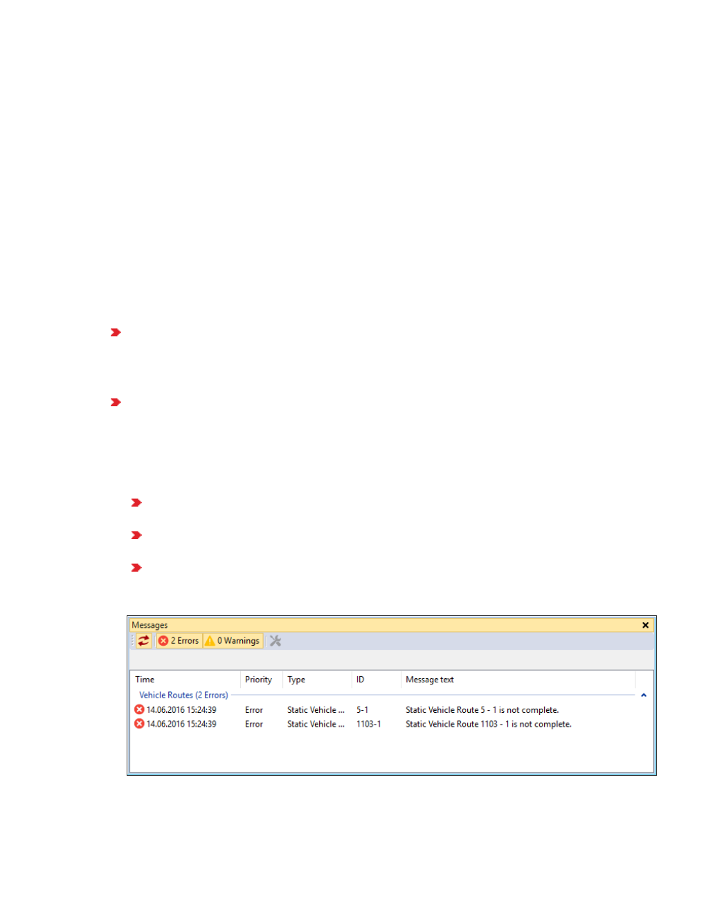
9.8 Checking the network
You can show simulation runs in the Simulation Runs list (see "Showing simulation run data
in lists" on page 802).
9.8 Checking the network
Errors in the network impact calculations and evaluations. Use the Check network command
to check the Vissim network for consistency after editing it. The command Check network can
identify errors in the Vissim network and allows you to fix some of the errors immediately.
Check network finds inconsistencies, e.g. incorrectly entered attribute values. However, it
cannot identify missing attribute values. Check network also finds network objects with
attribute values that Vissim cannot unambiguously assign to a vehicle type: A vehicle type can
be assigned to more than one vehicle class. Several of these vehicle classes can be assigned
to a network object, e.g. in the case of Conflict areas , for Gaps By Vehicle Class . If for
different vehicle classes, different attribute values are selected, unambiguous assignment to a
vehicle type that has been assigned multiple vehicle classes is no longer possible. This also
applies for pedestrian types that are assigned to multiple pedestrian classes.
When you start the simulation, Vissim automatically checks the Vissim for certain con-
straints that could prevent the simulation start and performs the Check network function, if
it has been selected under User Preferences (see "Checking and selecting the network
with simulation start" on page 146).
When you call the Check network command without starting simulation, Vissim checks
the Vissim network for consistency, but not for any constraints.
1. From the Simulation menu, select > Check network.
If the Messages window is open and contains entries, these are deleted. Vissim checks the
network.
If Vissim cannot identify any errors, a window is opened and a corresponding mes-
sage is displayed.
Should Check network detect that the simulation cannot be started, the Messages
window opens, showing the errors.
Should Check network detect that the simulation can be started, but that there are
inconsistencies, the Messages window opens, showing warnings(see "Showing mes-
sages and warnings" on page 1117).
812 © PTV GROUP
9.8 Checking the network
In the Messages window, Vissim groups errors by categories. These groups, for example,
inlcude:
Driving simulator
Scripts
Vehicle simulation
Vehicle classes
Pedestrian simulation
Pedestrian classes
PT pedestrian simulation
Evaluations
Presentation
External driver model
Dynamic assignment
Vehicle Routes
Mesoscopic simulation
Scenario Management
The entries of a group can be edited or deleted together (see "Showing messages and
warnings" on page 1117).
Errors listed in the groups Vehicle routes and 2D/3D model segments can be repaired
interactively, after you have corrected their network objects. During an interactive repair,
Vissim for instance reconnects interrupted vehicle routes, after you have corrected the
corresponding links and connectors (see "Showing messages and warnings" on page
1117). Errors of other categories must be corrected manually.
You can correct individual entries or an entire group (see "Showing messages and
warnings" on page 1117).
2. Use the messages displayed to correct your Vissim network.
3. If you correct errors in the groups Vehicle routes and 2D/3D model segments, repair these
objects afterwards using the Fix command (see "Showing messages and warnings" on
page 1117).
© PTV GROUP 813
10 Pedestrian simulation
10 Pedestrian simulation
In addition to the simulation of vehicles by default, you can also use Vissim to perform
simulations of pedestrians based on the Wiedemann model (see "Version-specific functions of
pedestrian simulation" on page 815).
However, with the stand-alone product PTV Viswalk, you can simulate pedestrians based on
Helbing but no vehicles. You can simulate vehicles and pedestrians only with Vissim and the
add-on module PTV Viswalk. You can then choose whether to use the modeling approach of
Helbing or Wiedemann.
10.1 Movement of pedestrians in the social force model
The movement of pedestrians in Vissim respectively Viswalk is based on the Social Force
Model (Helbing and Molnár, 1995). The basic principle of the Social Force Model is to model
the elementary impetus for motion of the pedestrians analogous to Newtonian mechanics.
From the social, psychological, and physical forces results a total force, which eventually
results in an entirely physical parameter Acceleration. These forces arise from the desire of the
pedestrian to reach a goal, from the influence of other pedestrians and obstacles in his
environment.
814 © PTV GROUP

10.2 Version-specific functions of pedestrian simulation
Prof. Dr. Dirk Helbing is a scientific advisor for PTV GROUP. Together with PTV GROUP he
specially expanded the Social Force Model for the use in Viswalk. This simulation model was
validated in three different ways:
Firstly, macroscopic parameters were calculated and adjusted to empirical data. Secondly it
was assured that microscopic effects like lane formation (counterflow) and stripe formation
(crossing) are reproduced. The resulting animation should be represented as realistically as
possible.
The behavior of pedestrians can be divided into three hierarchical levels (Hoogendoorn et al.
2002):
On the strategic level of minutes to hours, a pedestrian plans his route, generating a list of
destinations.
On the tactical level of seconds to minutes, a pedestrian chooses the route between the
destinations. Thereby he takes the network into account.
On the operational level of milliseconds to seconds, the pedestrian performs the actual
movement. He avoids thereby oncoming pedestrians, navigates through a dense crowd,
or simply continues the movement toward his destination.
The Social Force Model controls the operational level and parts of the tactical level. You
define the settings of the strategic level.
10.2 Version-specific functions of pedestrian simulation
The Vissim license for vehicular traffic may optionally include the Viswalk add-on module for
pedestrian simulation.
If your Vissim license does not include the Viswalk add-on module, you still have access
to the following functions:
You can import files containing elements for pedestrian modeling in *.inpx format.
They may also contain several levels and more than 30 pedestrians.
You can perform a simulation that also includes pedestrians. You can model up to 30
pedestrians in the network at the same time. If the imported network file does not con-
tain pedestrian data, Vissim generates default data for pedestrian types, pedestrian
classes and pedestrian compositions.
Pedestrian modeling can be performed using the Wiedemann or Helbing modeling
approach. This is possible for up to 30 pedestrians in the network.
If your Vissim license includes the Viswalk add-on module, the number of pedestrians is
limited by the license size of Viswalk.
You can choose whether to use the modeling approach of Helbing or Wiedemann with the
Viswalk add-on module.
When you start the Viswalk program, the following default data is generated:
Pedestrian types, e.g. Man and Woman
Pedestrian classes, e.g. People
Pedestrian compositions, e.g. Pedestrians
© PTV GROUP 815
10.3 Modeling examples and differences of the pedestrian models
The Viswalk product without vehicle simulation can only be used to simulate pedestrians.
During the installation of Viswalk, a specific default defaults.inpx network file for the ped-
estrian simulation is installed which does not contain any vehicle-specific objects (see
"Saving and importing a layout of the user interface" on page 138).
If you have a maintenance agreement for Viswalk, you can contact PTV Vision Support
(see "Service and support" on page 46).
10.3 Modeling examples and differences of the pedestrian models
The modeling examples show animations of various scenarios which are typical for pedestrian
traffic. The various scenarios require different model data according to Wiedemann or Helbing.
10.3.1 Modeling examples: Quickest or shortest path?
On YouTube, you can find a very complex animation of various scenarios for modeling
pedestrian traffic: http://www.youtube.com/watch?v=8SmRBTJ-jeU.
This animation demonstrates the principle of how simulated pedestrians in Vissim are made to
walk along the path of estimated least remaining travel time in due consideration of other
pedestrians and obstacles. The animation demonstrates as well the effect of the Dynamic
Potential method. It compares pedestrians who select the quickest path with those who
choose the shortest one (beginning at 01:42).
Much like vehicle drivers, pedestrians try to minimize their travel times to the destination. This
desire can in some situations superimpose over all other aspects. Moreover, the walking
direction for the quickest path cannot always be determined without problems.
Details of the method were published in an article in Advances in Complex Systems:
http://dx.doi.org/10.1142/S0219525911003281
Available at arXiv:
http://arxiv.org/abs/1107.2004
10.3.1.1 List of scenarios in the demo video
The following list shows at what time in the video which scenario begins.
Notes:
The various scenarios run with different time lapse factors.
The efficiency of the dynamic potential is always 100 %.
In all situations, the pedestrians move with approximately the same speed.
816 © PTV GROUP

10.3.1 Modeling examples: Quickest or shortest path?
mm:ss Description
01:42 About 800 passengers alight from two trains arriving simultaneously at the station at
the south entrance of Berlin's congress center (ICC).
To create a model of a large group of pedestrians walking realistically and efficiently
around a corner, mainly the Dynamic Potential method is used.
With only a small group of pedestrians the trajectories of both the quickest and the
shortest path would be almost identical, because both paths would have
approximately the same course.
03:18 Here a large group of pedestrians has to take an almost complete U-turn in the
course of their path.
This is more difficult and therefore the difference between the two methods (left and
right) is even more distinct.
04:48 In this scenario two large pedestrian groups meet as opposing flows. This is a
situation where the use of the dynamic potential does not necessarily produce better
results. However, it provides an alternative pedestrian behavior that becomes clear
after a few seconds. The behavior on the left side is more realistic if the pedestrians
assume that the counterflow will persist only for a short time, for example during the
green phase at the pedestrian crossing, the behavior on the right side is more
realistic, if the pedestrians assume that the constellation will persist longer, for
example when visiting a public event.
06:18 If counterflow occurs at a 90° corner, the dynamic potential (right side) is able to
better reproduce the fact, that the pedestrians move more efficiently in such
situations and most of them are able to resolve the situation. However, with
extremely high pedestrian traffic in reality it can also come to such a jam as
visualized on the left.
07:48 Counterflow at a 180° turn (U-turn).
09:18 Some passengers (red) are urgently rushing for their train, some (green) have just
alighted from a train and are heading towards exit whereas some others (blue) have
arrived at the station before departure and now spend their waiting time standing or
strolling around. (Easily recognizable, the group is quite large and behaves
strangely; thereby the effect of the method can be better demonstrated.) The red and
green pedestrians in the upper left video follow the shortest path. However, they are
increasingly being blocked by the numerically growing blue group.
The upper right video and the two scenarios below were simulated with the quickest
path but with different values for parameter h. For details of parameter h please refer
to the publication linked above.
Note that in the two scenarios below the red and green pedestrian groups manage
respectively to establish a separate walking direction or to form lanes
spontaneously, whereas they fail to do so with parameter h = 0 in the example at top
right.
© PTV GROUP 817
10.3.2 Main differences between the Wiedemann and the Helbing approaches
mm:ss Description
10:08 This is a theoretical model that does not even remotely occur in reality: However, it
demonstrates very clearly and precisely the effect of the "quickest path" approach or
alternatively of the dynamic potential.
10:48 So far all routing decisions were continuous. Thus, the pedestrian had always more
path options to their destinations to choose from. This is the first example with
discrete alternatives. The pedestrians have to choose if they want to use the left or
the right corridor. The method of dynamic potential has not been developed for such
situations. Other methods might be more helpful. In Vissim for example the partial
routes are used. The Dynamic Potential method is however suited also in this case.
12:43 A grandstand: The interesting aspect of this example is that the grandstand for the
pedestrians consists of a sequence of one-dimensional objects (links). Therefore
the directions of the shortest and the quickest path can differ by 180 degrees. In this
video it is very obvious when pedestrians prefer to take a detour to reduce the walk
time.
10.3.2 Main differences between the Wiedemann and the Helbing approaches
When pedestrians are modeled as a vehicle type according to Wiedemann model, they do not
move around freely but along user-defined links in the network. The spatial characteristics of
their trajectories are thus formed by the input data for the model and they do not result from the
simulation. Only the time at which a pedestrian crosses a link at a particular point is calculated
and a result formed.
In Helbing's model the pedestrians can move freely in two spatial dimensions. Their
trajectories are thus not defined in advance, but are calculated by the model. Therefore this
approach for pedestrian simulation is more flexible, detailed and realistic.
However, there are situations, in which the essential elements of the dynamics are produced
by the Wiedemann model. Examples are projects, where pedestrians have no role other than
to cause interruptions to vehicular traffic at signalized junctions.
10.3.2.1 Options for pedestrian modeling in the Wiedemann model
The add-on module Viswalk is not required.
Levels of Interaction for pedestrians Elements of the Vissim
network
Pedestrians using pedestrian crossings in the road network Links
Pedestrians as a vehicle
type
PT passengers Public transport stops
PT lines as vehicle type
Stop dwell time dis-
tribution or number of
boarding volumes
818 © PTV GROUP
10.4 Internal procedure of pedestrian simulation
10.3.2.2 Options for pedestrian modeling in the Helbing model
The add-on module Viswalk is necessary.
Levels of Interaction for
pedestrians
Elements of the pedestrian module Elements of the
Vissim network
Only pedestrian flows, for
example
Emergency situations
Airport, hotel etc.
walkable construction elements
(ramps/stairs and areas)
multilevel, if applicable
pedestrians as type/class of ped-
estrians
pedestrian compositions
area behavior types, if applicable
walking behavior parameters, if
applicable
location distributions, if applicable
None
pedestrians using pedestrian
crossings in the road network
pedestrians as type/class of ped-
estrians
pedestrian compositions
area behavior types, if applicable
walking behavior parameters, if
applicable
links as walk-
able areas
Signal control
Conflict areas
Detectors
Pedestrians as PT passengers
in the network
walkable areas, including platform
edges and waiting areas, if applic-
able
multilevel, if applicable
pedestrians as type/class of ped-
estrians
pedestrian compositions
area behavior types, if applicable
walking behavior parameters, if
applicable
location distributions, if applicable
Public trans-
port stops
PT lines as
vehicle type
with doors
10.4 Internal procedure of pedestrian simulation
For the simulation of pedestrians, several requirements must be met, for example, you need to
define different base data. In areas where pedestrians are supposed to start, you insert
pedestrian inputs and define routing decisions. Based on the routing decisions, you define
routes for pedestrians that lead via areas, ramps and stairways to other routing decisions,
where the routes then end. You may add intermediate points to areas, ramps and stairways.
© PTV GROUP 819
10.4.1 Requirements for pedestrian simulation
10.4.1 Requirements for pedestrian simulation
At least one pedestrian type has to be defined.
At least one pedestrian composition has to be defined.
At least one pedestrian input, yielding pedestrians, must be defined.
Tip: As an alternative to pedestrian inputs, you can use a pedestrian OD matrix that
contains demand data (see "Pedestrian OD matrices" on page 918). Based on the
OD matrix, pedestrian inputs, routing decisions and routes for pedestrians are
automatically generated.
Pedestrian routing decisions must contain at least one route per pedestrian type that
belongs to the pedestrian composition. The pedestrian composition must be defined in the
pedestrian input. The pedestrian input must lie within the same area as the pedestrian rout-
ing decision.
In each area that contains one or more pedestrian inputs, there must be at least one ped-
estrian routing decision.
The area of the pedestrian input, all areas with intermediate points and the area of the
route destination must be connected to each other via areas or ramps & stairways.
10.4.2 Inputs, routing decisions and routes guide pedestrians
When pedestrians are added to the network via pedestrian inputs, they are guided to their
destination via routes obtained through routing decisions.
10.4.2.1 Using pedestrian inputs to add pedestrians to a network
You can define pedestrian inputs on pedestrian areas or have them automatically generated
from an OD matrix. In doing so, you also generate routing decisions and routes to destinations
(see "Pedestrian OD matrices" on page 918).
If you define pedestrian inputs for pedestrian areas, you also need to define routing
decisions for pedestrians.
At least one route per pedestrian is required that is included in a time interval of the ped-
estrian input and belongs to the pedestrian composition of the input. This is automatically
the case, when for the routing decision, you specify the attribute AllPedTypes (All ped-
estrian types). However, if you choose a pedestrian class that only includes some of the
pedestrian types, a pedestrian type might be used at the pedestrian input, but no route will
be defined for it. In this case, the simulation would be canceled and an error message dis-
played. A routing decision, for which the relative volumes of all routes are set to NULL for
a time interval, is treated as if it did not exist.
A routing decision assigns each newly generated pedestrian a route that has been
defined for his pedestrian type or pedestrian class. If there is more than one route for a spe-
cific pedestrian type, a route is chosen randomly according to the relative volumes of indi-
820 © PTV GROUP

10.4.2 Inputs, routing decisions and routes guide pedestrians
vidual routes.
Each route leads via a sequence of areas and ramps, which form the route locations.
10.4.2.2 Strategic routes guide pedestrians throughout the network
A pedestrian always walks towards his next routing point.
When a pedestrian reaches a route location which has been assigned a time distribution
in the attribute TmDistr (Time Distribution), he waits for the period defined.
If this was not the pedestrian's last route location, he walks on to the next route loc-
ation.
However, if this was the last route location of his route and if the area of the route loc-
ation contains a routing decision with routes for this pedestrian type or class, he is
assigned a new route that he will continue to follow.
If there is no route for the pedestrian, he is removed from the network.
If the area with the last route location contains a pedestrian input, the pedestrian is
removed from the route, as it is assumed that routing decisions on areas that contain a
pedestrian input are specifically meant for new pedestrians coming from this input.
If the last route location lies in an area that has been assigned the attribute PTUsage >
Waiting area, the pedestrian remains in the network, if there is no routing decision for
this area. He waits for a suitable public transport vehicle to board (see "Attributes of
areas" on page 848) and (see "Modeling pedestrians as PT passengers" on page
925).
There may be several "tactical" options for pedestrians to get from one route location to the
next. For example, they can pass by obstacles, keeping left or right or use stairways and
ramps to get to their destination. Moreover, pedestrians must be able to sidestep each
other. Viswalk automatically performs the calculations and makes the decisions for such
actions during the simulation. In multi-level scenarios, Viswalk internally computes a rout-
ing graph. The routing graph consists of the route locations you defined and additionally
contains a route location for both ends of each stairway and ramp on the route. The rout-
ing graph thus includes relevant information on all routing variants that lead via the same
level or via different levels that are connected via stairways or ramps. Based on the routing
graph, Viswalk determines the shortest path between two route locations. The shortest
path is used for the pedestrian's tactic movement. In Viswalk, pedestrians prefer routes
without stairways or ramps, even if these are shorter. If instead you would like pedestrians
to use stairways or ramps, place your route locations on the desired ramps.
10.4.2.3 Requirements for assigning routing decisions
The following requirements must be fulfilled for a pedestrian to be assigned a new route.
A routing decision has been defined for this area.
A routing decision becomes effective for its pedestrian type through class dependency.
The pedestrian currently has no route. The might be due to the following:
The pedestrian was newly generated.
© PTV GROUP 821

10.5 Parameters for pedestrian simulation
In this time step, the pedestrian has reached the final route location of his current or
previous route.
The pedestrian has alighted from a public transport vehicle and is entering an area
that has been assigned the attribute PTUsage > Platform edge (see "Attributes of
areas" on page 848) and (see "Modeling pedestrians as PT passengers" on page
925)..
10.5 Parameters for pedestrian simulation
The parameters of the model can be categorized into the following groups:
Parameters of the original model (by pedestrian type)
Parameters of the model extensions for Vissim (by pedestrian type)
Implementation-specific global parameters include all discretization parameters, which
are necessary, for example, for models formulated using a continuous time. As analytical
approaches to solve the differential equations are only possible in scenarios of limited
size from every point of view, time needs to be discretized in some way to make a sim-
ulation on a computer possible.
10.5.1 Defining model parameters per pedestrian type according to the social force
model
You can set parameters for each pedestrian type derived from the original model. In addition,
you can set Vissim-specific parameters for each pedestrian type.
tau (τ) (see "Defining walking behavior" on page 879)
Tau represents the relaxation time or inertia that can be related to a response time, as it
couples the difference between desired speed and desired direction v_0 with the current
speed and direction v for acceleration .
Tip: Your Vissim installation provides example data and a description for testing with
these parameters.
..\Examples Training\Pedestrians\Parameter Demonstration\01 - Tau
lambda_mean (λ_mean) (see "Defining walking behavior" on page 879)
Lambda governs the amount of anisotropy of the forces from the fact that events and
phenomena in the back of a pedestrian do not influence him (psychologically and socially)
as much as if they were in his sight. Based on lambda and the angle φ between the current
direction of a pedestrian and the source of a force a, factor w is calculated for all social (e.g.
non-physical) forces that suppress the force, if:
and
Based on the above, then and yields
822 © PTV GROUP

10.5.1 Defining model parameters per pedestrian type according to the social force model
Tip: Your Vissim installation provides example data and a description for testing with
these parameters.
..\Examples Training\Pedestrians\Parameter Demonstration\06 - Lambda
A_soc_isotropic and B_soc_isotropic (see "Defining walking behavior" on page 879)
These two parameters and λ govern one of the two forces between pedestrians:
with d as distance between the pedestrians (body surface to body surface) and n as unit
vector, pointing from one to the other.
A_soc_mean, B_soc_mean and VD (see "Defining walking behavior" on page 879)
These parameters define strength (A) and the typical range (B) of the social force between
two pedestrians. The social force between pedestrians is calculated according to the
following formula, if the influencing pedestrian is in front of the one being influenced (180°)
and exerts his influence from the front (+/- 90°), otherwise it is zero:
Thereby the following applies:
d, in the simplest case of VD = 0, is the distance between two pedestrians (body surface to
body surface).
n is the unity vector, pointing from the influencing to the influenced pedestrian.
Note: In addition, the relative velocities of the pedestrians are considered, if
parameter VD > 0.
If parameter VD > 0, distance d is generalized and replaced by:
Where
: current distance between two pedestrians 0 and 1
: expected distance between two pedestrians on the basis of VD in seconds, if
both pedestrians keep their speed:
Apart from the last term below the root, the geometric mean between the current and
expected distance is calculated and applied.
© PTV GROUP 823

10.5.1 Defining model parameters per pedestrian type according to the social force model
d points from the influencing to the influenced pedestrian, wit . The force is
calculated for the "influenced pedestrian".
Tip: Your Vissim installation provides example data and a description for testing with
these parameters.
..\Examples Training\Pedestrians\Parameter Demonstration\09 - VD
noise (see "Defining walking behavior" on page 879)
The greater this parameter value, the stronger the random force that is added to the
systematically calculated forces if a pedestrian remains below his desired speed for a
certain time.
Checking the noise value effect:
Have a group of pedestrians pass a narrow alleyway of approx. 70 cm width.
With noise = 0, so called pedestrian "arches" will form and remain stable. If the noise value
lies within the range [0.8 to 1.4], one of the pedestrians will step back after a while and
another one will pass through. Default 1.2
Tip: Your Vissim installation provides example data and a description for testing with
these parameters.
You can find further information in the following folder:
..\Examples Training\Pedestrians\Parameter Demonstration\10 - Noise
react_to_n (see "Defining walking behavior" on page 879)
During calculation of the total force for a pedestrian, only the influence exerted by the n
closest pedestrians is taken into account. Default 8.
Tip: Your Vissim installation provides example data and a description for testing with
these parameters.
..\Examples Training\Pedestrians\Parameter Demonstration\03 - React to N
queue_order: degree of orderliness of a queue and queue_straightness: degree of
straightness of a queue (see "Selecting network settings for pedestrian behavior" on
page 193), (see "Attributes of areas" on page 848)
These two parameters specify the shape of queues. Their value range is 0.0 - 1.0. The
greater these parameter values, the more straight the queue will look.
side_preference (see "Defining walking behavior" on page 879)
This parameter defines whether opposing pedestrian flows prefer using the right or the left
side when passing each other:
-1: for preference of the right side
1: for preference of the left side
Default 0: no preference, behavior as before: pedestrians do not shun each other
824 © PTV GROUP
10.5.2 Defining global model parameters
Tip: Your Vissim installation provides example data and a description for testing with
these parameters.
..\Examples Training\Pedestrians\Parameter Demonstration\ 25 - Side Preference
10.5.2 Defining global model parameters
For each type of pedestrians, global model parameters can be set, apart from model
parameters. Global model parameters are used as default values when you define pedestrian
routes. When changing global model parameters, you do not change the parameters of the
pedestrian routes already defined.
grid_size: Search neighborhood grid size (see "Selecting network settings for pedestrian
behavior" on page 193)
With this parameter you can define the maximum distance at which pedestrians have an
effect upon each other. Default 5 m.
The pedestrians are stored in a grid with cells of size grid_size x grid_size square meters.
A pedestrian in a cell interacts with pedestrians from the following 8 cells only:
the 4 adjoining cells
the 4 cells which hit a pedestrian's cell with one of their corners.
Tip: Your Vissim installation provides example data and a description for testing with
these parameters.
..\Examples Training\Pedestrians\Parameter Demonstration\02 - Grid Size
routing_obstacle_dist: Default obstacle distance (see "Selecting network settings for
pedestrian behavior" on page 193)
This parameter only has an effect on the calculation of the static potential. It is not
considered in the calculation of the dynamic potential. The static potential is also called
distance potential or distance look-up table. When calculating the value of the static
potential the value of grid cells which are close to a wall increases, in addition to the value
resulting from the distance from the exit. This ensures that the pedestrians choose a wide
corridor rather than a narrow passage when they have both options on their way from A to
B, and neither option is shorter than the other. Generally, the pedestrians maintain a certain
distance to the walls. This parameter specifies the distance, up to which the nearby walls
have a bearing on the distance potential. Default 0.50 m.
Tip: Your Vissim installation provides example data and a description for testing with
these parameters.
..\Examples Training\Pedestrians\Parameter Demonstration\02 - Grid Size
cell_size: Cell size (see "Attributes of pedestrian route locations" on page 904)
This parameter defines the distances of control points to be set for the calculation of
distances to a destination area. Default 0.15 m.
© PTV GROUP 825

10.5.2 Defining global model parameters
never_walk_back: Option Never walk backwards (see "Selecting network settings for
pedestrian behavior" on page 193)
Use this parameter to define whether pedestrians should stop, if the direction of movement
and the desired direction differ by more than 90° (1 = on, 0 = off):
No calculation, if the default value is 0.
With parameter value 1, the scalar product is derived from the desired direction and
the calculated speed: With a negative value, the pedestrian will stop.
Tip: In the following directory you will find sample files, which illustrate the mode of
action of these parameters, as well as a description of the mode of action of the
parameters in the modeling of the dynamic potential:
..\Examples Training\Pedestrians\Enhanced Routing\Dynamic Potential
Dynamic_potential_g: g (general strength) (see "Defining dynamic potential" on page
911)
This parameter defines how in general the loss time for an occupied grid cell is estimated
in relation to an unoccupied one. Default 1.5
Dynamic_potential_h: h (direction impact) (see "Defining dynamic potential" on page
911)
With this parameter you can define the influence of speed on the estimated travel time of a
cell. Default 1.5
If parameter value is 0, there is no influence.
Parameter value of 1.0 means that the influence of a pedestrian with a typical desired
speed can either double, when he goes in the opposite direction, or can drop to zero,
when he is heading towards the destination.
Dynamic_potential_direction_change_clipping: Limit direction change (see "Selecting
network settings for pedestrian behavior" on page 193)
Use this parameter to determine whether the angle between the fastest and the shortest
route can increase at any speed, i.e. whether it can increase randomly from one time step
to the next.
Default value of 1 specifies the allowable degree of deviation with the parameter Dir-
ection change angle Dynamic_potential_ direction_change_p.
If parameter value is 0, no test is made.
Dynamic_potential_direction_change_p: Direction change angle (see "Selecting net-
work settings for pedestrian behavior" on page 193)
With this parameter you can define the maximum permitted angle, by which the angle
between the quickest and the shortest path can increase from one time step to the next. If a
larger deviation results for a position from the dynamic potential, the direction of the
quickest path is determined from the direction of the quickest path from the last turn plus
this angle. Default 4 degrees
826 © PTV GROUP

10.5.3 Using desired speed distributions for pedestrians
This parameter value is only considered if for Dynamic_potential_direction_change_
clipping (Limit direction change), you have entered the value 1.
10.5.3 Using desired speed distributions for pedestrians
You can use desired speed distributions for pedestrians that are described in the specialized
literature. You can allocate desired speed distributions for pedestrians to the following types of
base data:
The desired pedestrian types in pedestrian compositions (see "Attributes of pedestrian
compositions" on page 878)
The desired pedestrian classes in area behavior types (see "Defining area behavior
types" on page 881)
The walking behavior of pedestrians and the simulation results are strongly affected by the
various desired speed distributions. Upper and lower limits for pedestrian speed and
intermediate points, which mark the changes in speed, are defined in the desired speed
distributions for pedestrians.
Viswalk contains the following desired speed distributions for pedestrians that are described
in the specialized literature (see "Attributes of desired speed distributions" on page 230):
No. Name Description
1020 IMO-M <30 Speed distribution for male pedestrians on ships, age class under 30
International Maritime Organization: Guidelines for evacuation analysis
for new and existing passenger ships (as IMO below)
1021 IMO-F <30 Same as IMO-M <30, but for females
1022 IMO-M 30-
50
Speed distribution for male pedestrians on ships, age class 30 to 50.
International Maritime Organization
1023 IMO-F >30-
50
Same as IMO-M 30-50, but for females
1024 IMO-M >50 Speed distribution for male pedestrians on ships, age class over 50.
International Maritime Organization
1025 IMO-F >50 Same as IMO-F >50, but for females
1026 IMO-M M1 Speed distribution for male pedestrians on ships with reduced mobility,
age class over 50. International Maritime Organization
1027 IMO-F M1 Same as IMO-F >50, but for females
1028 IMO-M M2 Speed distribution for male pedestrians on ships with severely reduced
mobility, age class over 50. International Maritime Organization
1029 IMO-F M2 Same as IMO-F >50, but for females
1040 Fruin 1 Speed distribution according to Fruin, J.J.: In: Pedestrian Planning and
Design, 1971, PEDESTRIAN PLANNING AND DESIGN
1041 Fruin 2 Speed distribution according to Fruin, J.J.: In: Pedestrian Planning and
Design, 1971, PEDESTRIAN PLANNING AND DESIGN
© PTV GROUP 827

10.6 Network objects and base data for the simulation of pedestrians
No. Name Description
1042 Predt-Mil-
inski
Speed distribution for pedestrians in buildings. Predtechenski, V.;
Milinski, A.: Planning for Foot Traffic Flow in Buildings. Amerino
Publishing Co., New Delhi, 1978
1043 Stairs Kretz
1
Speed distribution based on measurements of the upward speed of
pedestrians at the top end of long stairs. Kretz, T.; Grünebohm, A.;
Kessel, A.; Klüpfel, H.; Meyer-König, T. and Schreckenberg, M.:
Upstairs walking speed distributions on a long stairway. In: Safety
Science 46(1) p. 72-78. 2008.
1044 Stairs Kretz
2
Speed distribution based on measurements of the upward speed of
pedestrians at the top end of long stairs. Kretz, T.; Grünebohm, A.;
Kessel, A.; Klüpfel, H.; Meyer-König, T. and Schreckenberg, M.:
Upstairs walking speed distributions on a long stairway. In: Safety
Science 46(1) p. 72-78. 2008.
1045 Airport -
S.B. Young
Speed distribution for pedestrians in airports. Young, S.B.: journal
article: Evaluation of Pedestrian Walking Speeds in Airport Terminals
and full papers: Evaluation of Pedestrian Walking Speeds in Airport
Terminals.
1046 Airport -
S.B. Young
Speed distribution for pedestrians on moving walkways in airports. The
speeds of pedestrians on the moving walkway are given relative to the
speed of the walkway, so the speeds of some pedestrians are close to
ZERO.
Young and Viswalk define the speed distribution differently:
Young includes pedestrians who are standing on the moving walk-
way, in their speed distribution.
In Viswalk, you enter a value for the attribute Walking percentage
(WalkPerc) of the relevant moving walkway. The difference is taken
into consideration in Viswalk:
In Viswalk, the speed difference 1009 of Young begins at 0.77 km/h.
Therefore enter 74.5 % for the attribute Walking percentage
(WalkPerc).
Young, S.B.: journal article: Evaluation of Pedestrian Walking Speeds in
Airport Terminals and Evaluation of Pedestrian Walking Speeds in
Airport Terminals.
10.6 Network objects and base data for the simulation of pedestrians
The following network objects and base data are of particular importance for the modeling of
pedestrians. Using the network objects toolbar, you can hide network object types for vehicles
that are only relevant for vehicles and show network object types that you need for pedestrian
simulation.
10.6.1 Displaying only network object types for pedestrians
1. Right-click in the Network Objects toolbar.
828 © PTV GROUP

10.6.2 Base data
2. From the context menu, select the entry Pedestrian Object Types Only.
Symbol Network object type
Areas
Obstacles
Ramps & Stairs
Elevators
Pedestrian Inputs
Pedestrian Routes
Pedestrian Travel Times
Pedestrians In Network
Links
Priority Rules
Signal Heads
Detectors
Sections
Backgrounds
3D Traffic Signals
Static 3D Models
10.6.2 Base data
In addition to functions and distributions, the following base data is of particular importance:
Pedestrian Types (see "Using pedestrian types" on page 830)
Pedestrian Classes (see "Using pedestrian classes" on page 832)
Walking Behaviors (see "Modeling area-based walking behavior" on page 879)
Area Behavior Types (see "Defining area behavior types" on page 881)
Display Types of areas and links (see "Defining display types" on page 300)
Levels for multistory models (see "Defining levels" on page 868)
© PTV GROUP 829
10.6.3 Base data in the Traffic menu
10.6.3 Base data in the Traffic menu
Pedestrian Compositions (see "Modeling pedestrian compositions" on page 877)
Pedestrian OD matrix (see "Pedestrian OD matrices" on page 918)
10.7 Using pedestrian types
You can combine pedestrians with similar properties in pedestrian types. You may also
change pedestrian types during the simulation run, for example via the COM interface.
By default, the following pedestrian types are available:
Man
Woman
Woman & Child
Wheelchair User
10.7.1 Defining pedestrian types
1. Select from the menu Base Data > Pedestrian Types.
The list of defined network objects for the network object type opens.
By default, you can edit the list (see "Using lists" on page 89).
You can define a new pedestrian type in the list.
2. Right-click in the list.
3. From the shortcut menu, choose Add.
A new row with default data is inserted.
The Pedestrian Type window opens.
830 © PTV GROUP

10.7.2 Attributes of pedestrian types
4. Edit the attributes (see "Attributes of pedestrian types" on page 831).
5. Confirm with OK.
The attributes are saved in the Pedestrian Types list.
10.7.2 Attributes of pedestrian types
The Pedestrian Type window opens when you define a new pedestrian type and have
selected to have the Edit dialog opened automatically after object creation (see "Right-click
behavior and action after creating an object" on page 143). Into the window, you enter attribute
values for the network object. For already-defined network objects, you can call this window
via the list of network objects of the network object type (see "Functions available in the
shortcut menu of the row header" on page 100).
In the network objects list of the network object type, you can edit all attributes and attribute
values of a network object (see "Opening lists" on page 92), (see "Selecting cells in lists" on
page 102).
Note: In lists, you can use the Attribute selection icon to show and hide attribute
values (see "Selecting attributes and subattributes for a list" on page 106).
Element Description
No. Unique number of pedestrian type
Name Name of pedestrian type
© PTV GROUP 831

10.8 Using pedestrian classes
Element Description
Walking beha-
vior
WalkBehav: Name of walking behavior (see "Defining walking behavior" on
page 879)
Model lengths Model distribution (2D/3D model distribution, 2D3DModVert): Defines
appearance, length, width and height of pedestrians of this pedestrian
type (see "Using 2D/3D models" on page 210).
Model length: Shows length of 2D/3D model with minimum length and
maximum length based on 2D/3D model distribution
Dimension
variance Length (Length variance, LngVar): Scaling range for the object length
(3D model length, for example, step length from the tip of the toe of the
front foot to the heel of the rear foot)
Width (Width varianceWidVar): Scaling range for the object width (3D
model width, for example, shoulder width)
Height (Height variance, HgtVar): Scaling range for the object height
(3D model height, for example, only adults or adults and children)
Colors Color distributions define the colors of the 3D display for the following
attributes for pedestrians of the selected pedestrian type (see "Using color
distributions" on page 250):
Shirt: Shirt color distribution (ShirtColorDistr)
Hair: Hair color distribution (HairColorDistr)
Trousers: Trousers color distribution (TrousersColorDistr)
Shoes: Shoes color distribution (ShoesColorDistr)
This applies for all objects of a pedestrian type. The attribute Use
pedestrian type color (UsePedTypeColor) must be selected for pedestrian
classes.
Showing and editing dependent objects as relation
The attribute and attribute values of this network object type are shown in the list on the left,
which consists of two coupled lists.
1. In the list on the left, click the desired entry.
The list on the right contains attributes and attribute values of network objects, and/or base
data allocated to the network object selected in the list on the left (see "Using coupled lists" on
page 111):
2. On the list toolbar, in the Relations list, click > Pedestrian Classes (see "Defining
pedestrian classes" on page 833).
3. Enter the desired data.
The data is allocated.
10.8 Using pedestrian classes
You can group pedestrian types and combine them into pedestrian classes. This can facilitate
the modeling of certain scenarios.
832 © PTV GROUP
10.8.1 Defining pedestrian classes
Pedestrian classes are optional. A pedestrian type can belong to several pedestrian classes,
but does not have to belong to a pedestrian class.
10.8.1 Defining pedestrian classes
You can define pedestrian classes and assign pedestrian types to the attributes.
1. Select from the menu Base Data > Pedestrian Classes.
The list of defined network objects for the network object type opens.
By default, you can edit the list (see "Using lists" on page 89).
You can define a new pedestrian class in the list.
2. In the list, on the toolbar, click the Add button .
A new row with default data is inserted.
3. Edit the attributes (see "Attributes of pedestrian classes" on page 833).
10.8.2 Attributes of pedestrian classes
In the Pedestrian Classes list, you can edit all attributes and attribute values of a pedestrian
class (see "Opening lists" on page 92), (see "Selecting cells in lists" on page 102).
1. Select from the menu Base Data > Pedestrian Classes.
The list of defined network objects for the network object type opens.
By default, you can edit the list (see "Using lists" on page 89).
2. Click on the desired entry.
3. Make the desired changes:
Element Description
No Unique identification number of the pedestrian class
Name Name of pedestrian class
Color Default color of pedestrian class during simulation (see "Static colors
of vehicles and pedestrians" on page 165). Is not used in the
following cases:
When for a pedstrian class the attribute attribute Use pedestrian
type color (UsePedTypeColor) is enabled.
When for the display of pedestrians in the network, from the
Graphic Parameters menu, DrawingMode > Use color scheme
is chosen, and for the Color scheme configuration attribute, a
color scheme is specified that is to be used for classification.
© PTV GROUP 833

10.9 Modeling construction elements
Element Description
PedTypes Pedestrian types: list box with options for selecting the pedestrian
types which you want to assign. Numbers and names of pedestrian
types.
UsePedTypeColor Use pedestrian type color: If this option is selected, the colors of
the color distribution are used for shirt, hair, trousers, and shoes of
the assigned pedestrian type. (see "Attributes of pedestrian types" on
page 831).
If this option is not selected, the Color attribute of the pedestrian
class is used for all pedestrians whose pedestrian type is assigned to
the pedestrian class. If a pedestrian type is assigned to two
pedestrian classes, the color distribution is used for the shirt of
pedestrians of the pedestrian type that is assigned to the pedestrian
class with the lower number.
The Use pedestrian type color attribute is not used, when for the
display of pedestrians in the network, from the Graphic Parameters
menu, DrawingMode > Use color scheme is chosen, and for the
Color scheme configuration attribute, a color scheme is specified
that is to be used for classification.
Note: In lists, you can use the Attribute selection icon to show and hide attribute
values (see "Selecting attributes and subattributes for a list" on page 106).
10.9 Modeling construction elements
Construction elements are the following network objects:
Areas
Obstacles
Ramps, stairways, escalators, moving walkways
10.9.1 Areas, Ramps & Stairs
All construction elements except obstacles are accessible to pedestrians. Ramps can
therefore be the generic term for construction elements, which connect areas of different levels
with each other: Ramps, stairways, escalators, moving walkways.
Areas are defined as rectangles or polygons. Areas do not have a specific direction. You can
import areas from AutoCAD. Ramps and stairways are defined as rectangles.
Areas and ramps may optionally include additional information for pedestrians, e.g. routing
decisions (see "Modeling routing decisions and routes for pedestrians" on page 886).
You can define public transport stop areas as waiting areas or platform edges (see "Modeling
PT stops" on page 478), (see "Attributes of areas" on page 848).
834 © PTV GROUP

10.9.2 Escalators and moving walkways
Construction elements are automatically connected where they are directly adjacent or
overlap. Where accessible elements overlap, pedestrians may walk from one element into the
next one. Pedestrians do not require any connectors.
Before information on walkable areas is transferred to the pedestrian model, Vissim groups
areas touching or overlapping each other into the largest possible walkable polygons. The
original edges of these areas are not treated as obstacles. They are pedestrian accessible. So
when you split an area during network editing, this does not affect pedestrian simulation in the
network.
To model a complex area containing numerous corners, define several polygons in a row that
overlap.
Note: Add pedestrian inputs to pedestrian areas as a source of pedestrian flows (see
"Modeling pedestrian inputs" on page 883).
Whereas links defined with the attribute Is pedestrian area (option Use as pedestrian
area) are accessible elements, on which you can place signal heads, detectors or
conflict areas. They are meant for modeling the interaction of pedestrians with vehicular
traffic or other pedestrian flows (see "Modeling links as pedestrian areas" on page
869).
10.9.2 Escalators and moving walkways
Pedestrians may use escalators and moving sidewalks for automated transport. Escalators
and moving walkways have a direction and are defined as rectangles.
10.9.3 Obstacles
Obstacles are not accessible. An obstacle has the same effect on pedestrian dynamics as if
you were to model a hole in an otherwise accessible area. Obstacles are defined as
rectangles or polygons. You can import obstacles from AutoCAD (see "Importing walkable
areas and obstacles from AutoCAD" on page 835).
If obstacles intersect ramps, a message is displayed when you start the simulation. The
message shows the number of the obstacle, starting with the smallest number, that intersects a
ramp and the number of the ramp. Click the Continue button to show the next message. Click
the Cancel button to cancel the start of the simulation, e.g. in order to edit an obstacle.
10.9.4 Deleting construction elements
By default, you may delete construction elements in lists or network editors (see "Deleting
network objects" on page 336).
10.9.5 Importing walkable areas and obstacles from AutoCAD
You can import AutoCAD data into Viswalk. Using AutoCAD data, you can create walkable
areas and obstacles for pedestrians.
With the help of maps of the area, you create the geometry required for pedestrian flow
simulation.
© PTV GROUP 835

10.9.5 Importing walkable areas and obstacles from AutoCAD
To complete an existing network or create a new one, import polylines in the data format *.dwg
and convert them.
Depending on the parameter settings you select for data import, all objects of an AutoCAD
layer are converted into areas or obstacles.
Objects of the type line or polyline are imported as long as they do not belong to AutoCAD
blocks or AutoCAD groups.
Lines and polylines that have a common point are connected to form a single polyline.
Closed polylines are converted into polygons that you can import as obstacles or areas.
Open polylines are not imported.
Overlapping polygons and enclosed polygons are imported as overlapping construction
elements. They are not interpreted as "holes" in areas or obstacles.
In the CAD Import - Configuration window, you may select several attributes for the
objects generated. For some attributes, default values are assigned.
In Vissim, object names are derived from the concatenation of "Level <x>:" and the respect-
ive object name, where available. If there is no object name, a consecutive number is
added.
Notes: In the *.dwg file, the x- and y-coordinates must be specified in meters.
During import of the *.dwg file, z-coordinates are ignored.
1. From the File menu, choose > Import > CAD for Pedestrian Areas.
The Import CAD File window opens.
2. Select the *.dwg file of your choice.
3. Click the Open button.
The CAD Import - Configuration window opens. A level is displayed for each row.
836 © PTV GROUP

10.9.6 Importing Building Information Model files
4. In the columns, select the attributes of your choice.
Column Description
Import Select this option to import the respective level.
Layer Name of the CAD level from the *.dwg file
Import as Network object type for the level:
Obstacle: Creates the level as an obstacle
Area: Creates the level as an area
Display type Select the Display type
Display types have to be defined (see "Defining display types" on
page 300).
Level Select Level from Vissim for the CAD levels from the *.dwg file. The
level has to be defined in Vissim (see "Defining levels" on page 868).
Z-Offset
top/bottom
Offset above: Positive value for the distance between the ground and
the top edge of the area or the obstacle.
Offset below: Negative value for the distance between the ground
and the bottom edge of the area or the obstacle.
Thickness/Height Thickness: for areas (see "Attributes of areas" on page 848)
Height: for obstacles (see "Attributes of obstacles" on page 859)
Select all In the Import column, selects all layers from the *.dwg file for import.
Deselect all Deselects all selected options in the Import column.
Notes: The unit used in the window for all lengths corresponds to the unit of length for
the smallest unit of length selected, for example [m]. Check this setting before import in
the menu Base data > Network settings > Units tab.
5. Confirm with OK.
The CAD Import - Configuration window closes.
The imported polygons are displayed as construction elements in the network editor and in
lists. You can edit or delete the construction elements.
10.9.6 Importing Building Information Model files
Building Information Model data is used for building data modeling. The BIM principle is
implemented via Industry Foundation Classes (IFC) (IFC - Industry Foundation Classes). IFC is
an open data format used to describe building and construction models. IFC provides 3D
geometry representation and additional data on other project elements such as doors, walls,
ceilings or other building objects). Viswalk can import IFC-based building data for pedestrian
simulation. Viswalk converts individual objects into construction elements. Viswalk supports
version IFC2x3 (TC1) of the IFC standard (IFC2x Edition 3 Technical Corrigendum 1).
© PTV GROUP 837
10.9.6 Importing Building Information Model files
Relevant subcomponents
In the IFC format, all components of the building model are based on a hierarchical structure.
For the import to Viswalk the following simplified hierarchy applies to the subcomponents:
IfcProject: the hierarchy's root node
IfcSite: the base area, e.g. the building site. IfcSite may include a number of buildings.
IfcBuilding: a single building
IfcBuildingStorey: a single level of a building Stories are used to create the levels
for the pedestrian areas.
IfcSlab: Ceiling or floor. An IfcSlab is imported as pedestrian area. An obstacle is
created on the basis of a hole in the floor.
IfcWall: Wall. An obstacle is created on the basis of an IfcWall.
IfcWindow: Window. An obstacle is generated on the basis of an IfcWindow.
IfcPlate: A panoramic window or a non-load bearing wall. An obstacle is created
on the basis of an IfcPlate.
IfcStair: Stairway
IfcRamp: Ramp
Further building model components (e.g. elevators or roofs) cannot be imported when using
the IFC format.
Steps of BIM import
1. Convert your *.ifc file to an *.inpx file using the IFC2INPX.exe converter (see "Converting
IFC files to INPX files" on page 838).
2. Import the *.inpx file you created into Viswalk (see "Importing INPX files including building
data" on page 843).
Steps in Viswalk
1. Use the network editor to check the location, height and display of the construction
elements .
2. Use the network editor and/or Level list to check the level data.
3. Remodel your Viswalk, if required.
10.9.6.1 Converting IFC files to INPX files
If you want to use your Building Information Model data from an *.ifc file in Viswalk, you will
have to convert the *.ifc file to an *.inpx network file. You can then import the network file (see
"Importing INPX files including building data" on page 843).
You may start the conversion process via Viswalk or a *.bat batch file (see "Starting conversion
in Viswalk" on page 839), (see "Starting conversion via a batch file" on page 841).
838 © PTV GROUP
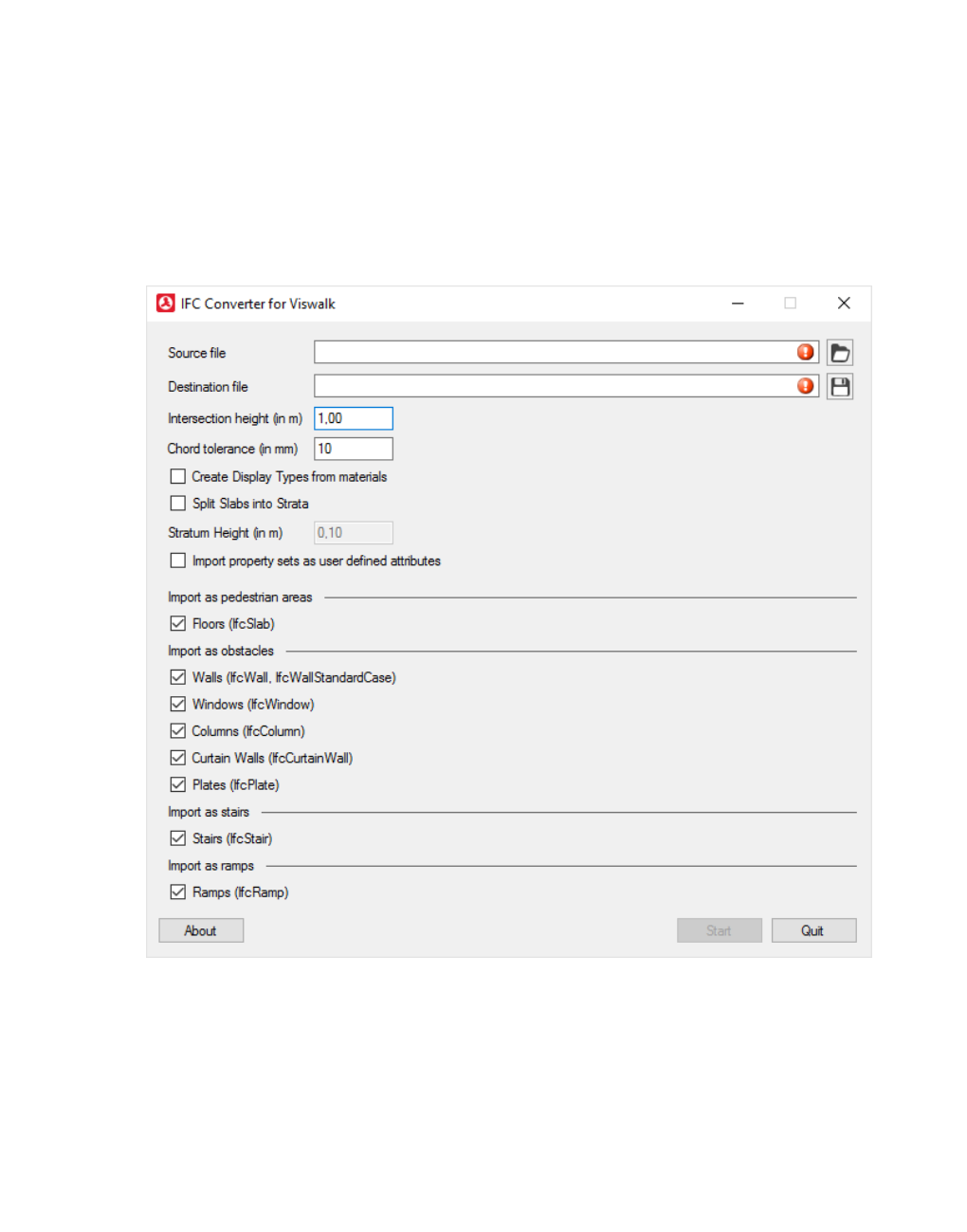
10.9.6 Importing Building Information Model files
Starting conversion in Viswalk
The conversion process may take a few minutes, depending on the data volume. The
conversion is run in the external IFC2INPX_GUI.exe application. It is not run in Viswalk. This
allows you to continue to work in Viswalk during the conversion process. IFC2INPX_GUI.exe
is stored to the ..\exe\IFC2INPX directory of your Viswalk installation.
1. From the File menu, choose > Import > BIM converter (*.ifc).
The IFC Converter window opens.
2. Make the desired changes:
© PTV GROUP 839

10.9.6 Importing Building Information Model files
Element Description
Source file *.ifc file that is to be converted to an *.inpx file.
Target file *.inpx file that is created by a conversion
Intersection
height (in m)
The height above each imported level that runs in parallel to the base
area in which Viswalk checks the building model's vertical
subcomponents in terms of openings in order to identify window/door
openings and obstacles. Default 1.00 m
Chord tol-
erance
(in mm)
Viswalk uses polygons for modeling circular objects in IFC. The chord
tolerance value specifies the maximum distance between the edges of
the polygon and the actual circle before creating an additional corner
point. Default 10.00 mm
Creating dis-
play types
using mater-
ials
Creating a display type using each material imported.
Stratifying
slabs
Modeling sloped ceilings or floors based on the BIM by stratifying the
resultant pedestrian areas. Multiple pedestrian areas with different Z-
coordinates are created. The attribute Stratum height (in m) defines the
vertical distance.
Stratum
height (in m)
Indicates height of the terrace. For floors above the base area. Default
0.10 m
Imported prop-
erty sets as
user-defined
attributes
Creating user-defined attributes based on the IFC property sets.
Import as ped-
estrian areas
Floors (IfcSlab): Selecting floors to create construction elements based
on the network object type pedestrian area.
Import as
obstacles
Selecting the following subcomponents to create construction elements
based on the network object type Obstacles:
Walls (IfcWall, IfcWallStandardCase):
Windows (IfcWindow):
Columns (IfcColumn):
Curtain Walls (IfcCurtainWall):
Plates (IfcPlate):
Import as
stairs
Stairways (IfcStair): Selecting stairs to create construction elements
based on the network object type Stairs.
Import as
ramps
Ramps (IfcRamp): Selecting ramps to create construction elements
based on the network object type ramps.
About Information on IFC2INPX, the software used and contact details
Start Starting conversion to the *.inpx file
3. Import the network file (see "Importing INPX files including building data" on page 843).
840 © PTV GROUP

10.9.6 Importing Building Information Model files
Starting conversion via a batch file
You must create a batch file for the conversion of an *.ifc file to an *.inpx network file. Here you
will have to enter the conversion parameters.
The conversion may take a few minutes, depending on the data volume. The conversion runs
on the external IFC2INPX.exe application. IFC2INPX.exe is stored to the ..\exe\IFC2INPX
directory of your Viswalk installation.
1. Create a blank *.txt file in a directory of your choice.
2. Name the *.txt file according to your requirements.
3. Rename *.txt file with a *.bat file extension.
In the *.bat file, the conversion parameters have to follow the following scheme:
ifc2inpx [inputfile[outputfile]] [/IntersectionHeight=h] [/Bogentoleranz=c] [/IfcEle-
ments=e] [/ImportPropertySets] [/DefaultStairWidth=w] [/ImportMaterials] [/SplitSlab-
sIntoStrata] [/StratumHeight=s]
Parameter Description
inputfile Input file: Path to the *.ifc file to be converted.
outputfile Output file: Path to the *.inpx file which the network created by
conversion should be saved to.
IntersectionHeight Intersection height (see "Starting conversion in Viswalk" on
page 839): At intersection height, Ifc elements are intersected
above each imported level (in parallel to the base area) in
order to find out whether network file elements need to be
stored as obstacles.
Without this parameter the default value is 1.00 m.
hIntersection height in meters, decimals > 0
ChordTolerance Chord tolerance (see "Starting conversion in Viswalk" on page
839): The chord tolerance value specifies the maximum
distance between the edges of the polygon and the actual
circle before generating an additional corner point in the
polygon. Without this parameter the default value is 10.00 mm.
cChord tolerance in millimeters, decimals from 0 to 1,000
IfcElements List of Ifc elements to be converted during import. All elements
enabled for conversion will be converted by default.
eList of Ifc elements to be converted during import (separated by
commas) such as Slabs, Walls, Windows, Columns,
CurtainWalls, Plates, Stairs, Ramps
ImportPropertySets Create user-defined attributes based on the IFC property sets.
Without this parameter the property sets will not be imported.
© PTV GROUP 841

10.9.6 Importing Building Information Model files
Parameter Description
DefaultStairWidth Default value for the width of stairways, if the width cannot be
specified on the basis of the geometry. Without this parameter
the default value is 2.0 meters.
wDefault value for the width of stairways in meters, decimals > 0
ImportMaterials Creating a display type that belongs to an imported element,
using each imported material Material is imported by default.
StratifySlabs Stratifying slabs: Modeling sloped ceilings and floors by
stratifying the resultant pedestrian areas. Multiple pedestrian
areas with different Z-coordinates are created. Without this
parameter, slabs will not be stratified.
StratumHeight If the StratifySlabs parameter is set: Defines the stratum height
at which slabs are intersected. Without this parameter the
default value is 0.1 meter.
sStratum height in meters, decimals > 0
4. Enter the conversion parameters of your choice in the *.bat file.
5. Save the *.bat file.
You can run the *.bat file at the time of your choice and thus start conversion of an *.ifc file
to an *.inpx network file:
6. Double-click the *.bat file.
The batch process initiates the conversion and stores an *.inpx network file.
An example of two project conversions
Two projects are converted to two *.inpx files:
ifc2inpx c:\projects\project1.ifc c:\projects\Viswalk\project1.inpx
ifc2inpx c:\projects\project2.ifc c:\projects\Viswalk\project2.inpx
An example of a project conversion with different intersection heights
A project with different intersection heights is converted to six *.inpx files. Default values will be
used, if parameters are not specified.
ifc2inpx c:\projects\projectX.ifc c:\projects\Viswalk\projectX-ISH-01.inpx /In-
tersectionHeight: 0.1
ifc2inpx c:\projects\projectX.ifc c:\projects\Viswalk\projectX-ISH-05.inpx /In-
tersectionHeight: 0.5
ifc2inpx c:\projects\projectX.ifc c:\projects\Viswalk\projectX-ISH-10.inpx /In-
tersectionHeight: 1.0
ifc2inpx c:\projects\projectX.ifc c:\projects\Viswalk\projectX-ISH-15.inpx /In-
tersectionHeight: 1.5
ifc2inpx c:\projects\projectX.ifc c:\projects\Viswalk\projectX-ISH-20.inpx /In-
tersectionHeight: 2.0
ifc2inpx c:\projects\projectX.ifc c:\projects\Viswalk\projectX-ISH-25.inpx /In-
tersectionHeight: 2.5
842 © PTV GROUP

10.9.6 Importing Building Information Model files
Example of a project conversion using the fcElements parameter
If six projects mentioned in the example above contain areas and ramps, you may use the
fcElements as follows:
ifc2inpx c:\projects\projectX.ifc c:\projects\Viswalk\projectX-ISH-01.inpx /In-
tersectionHeight: 0.1
ifc2inpx c:\projects\projectX.ifc c:\projects\Viswalk\projectX-ISH-05.inpx /In-
tersectionHeight: 0.5 /IfcElements: Walls,Windows,Columns,CurtainWalls,Plates
ifc2inpx c:\projects\projectX.ifc c:\projects\Viswalk\projectX-ISH-10.inpx /In-
tersectionHeight: 1.0 /IfcElements: Walls,Windows,Columns,CurtainWalls,Plates
ifc2inpx c:\projects\projectX.ifc c:\projects\Viswalk\projectX-ISH-15.inpx /In-
tersectionHeight: 1.5 /IfcElements: Walls,Windows,Columns,CurtainWalls,Plates
ifc2inpx c:\projects\projectX.ifc c:\projects\Viswalk\projectX-ISH-20.inpx /In-
tersectionHeight: 2.0 /IfcElements: Walls,Windows,Columns,CurtainWalls,Plates
ifc2inpx c:\projects\projectX.ifc c:\projects\Viswalk\projectX-ISH-25.inpx /In-
tersectionHeight: 2.5 /IfcElements: Walls,Windows,Columns,CurtainWalls,Plates
In this case, areas and ramps are only included in the first *.inpx file you created. Using the
Read Additionally feature in Viswalk allows you to combine this data with the conversion
results you get from other *.inpx files.
Show list of possible parameters
Enter ifc2inpx without further parameters in the Windows command line prompt.
The list of possible parameters is displayed.
10.9.6.2 Importing INPX files including building data
Once you have converted an *.ifc file to an *.inpx network file, you can import it into Viswalk.
1. From the File menu, choose > Read Additionally > Network.
2. The window Select file to read additionally opens.
3. Select the *.inpx network file you converted.
4. Click on Open.
Network objects such as levels and construction elements are created. The following colors
are assigned to the elements:
Gray: Walkable pedestrian area
Green: Walls
Orange: Holes in accessible pedestrian areas
Red: Elements with ambiguous IFC data or files that do not comply with the openBIM
standard.
5. Use the network editor to check and correct the red elements
6. and check the location, height and display of the other construction elements.
7. Go to the network editor and/or Level list to check the level data.
8. Correct and remodel your Viswalk network, if required.
© PTV GROUP 843

10.9.7 Defining construction elements as rectangles
10.9.7 Defining construction elements as rectangles
You can define all types of construction elements as rectangles:
Icon Network object type of the construction element
Areas
You may also define areas as polygons (see "Defining construction elements as
polygons" on page 845)
Obstacles
You may also define obstacles as polygons.
Ramps and stairs, moving walkways and escalators
For technical reasons, a 10 cm wide obstacle is automatically added on both sides of a
ramp. This reduces the accessible area to the surrounding areas.
1. Click on the network object toolbar on the desired network object type of the construction
element Areas, Obstacles or Ramps & Stairs.
The button is highlighted. The variant of the network object type is displayed in parentheses
and the button is shown.
2. Click again Areas, Obstacles or Ramps & Stairs.
3. Select Rectangle.
When you insert a ramp, stairway, a moving walkway or an escalator, drag the network
object towards the construction element that the pedestrian should use.
4. Using the mouse pointer, point to the desired position of the first corner point of the
construction element.
Notes:
You can specify that you need not press the CTRL key when adding network objects
(see "Right-click behavior and action after creating an object" on page 143).
For some network objects there are windows in which the attributes of a network
object can be defined and edited. There are lists for this, for all network objects. You
can choose whether you want to open a window, a list or neither of the two for the
definition of network objects in the Network Editor (see "Right-click behavior and
action after creating an object" on page 143).
5. Press the CTRL key, hold down the right mouse button and drag the mouse to the desired
end point of the link.
6. Release the keys.
7. Drag the mouse pointer sideways to the desired width.
8. Double click.
The construction element is shown in color in the Network Editor. In ramps and stairways,
escalators and moving walkways, the tip of a triangle shows in the direction towards which
844 © PTV GROUP

10.9.8 Defining construction elements as polygons
pedestrians can use the construction element. The <Name Construction element type>
window opens.
9. Edit the attributes of the inserted construction element type:
Attribute of areas (see "Attributes of areas" on page 848)
Attribute of obstacles (see "Attributes of obstacles" on page 859)
Attribute of ramps, stairways, moving walkways and escalators (see "Attributes of
ramps, stairs, moving walkways and escalators" on page 861)
10. Confirm with OK.
The attributes are saved in the list of the construction element type. Independent of the
individual type of construction element, all construction elements are numbered in sequence.
Notes:
If two levels should be connected via a ramp, stairway, moving walkway or escal-
ator, both levels must be defined (see "Defining levels" on page 868).
Alternatively, you can define construction elements in the Network Editor via the
context menu > Add New <Name Construction element type> when a network
object type is selected in the network object toolbar.
10.9.8 Defining construction elements as polygons
You can define areas and obstacles as polygons or rectangles. All other types of construction
elements can be defined solely as rectangles (see "Defining construction elements as
rectangles" on page 844).
Notes:
You can specify that you need not press the CTRL key when adding network objects
(see "Right-click behavior and action after creating an object" on page 143).
For some network objects there are windows in which the attributes of a network
object can be defined and edited. There are lists for this, for all network objects. You
can choose whether you want to open a window, a list or neither of the two for the
definition of network objects in the Network Editor (see "Right-click behavior and
action after creating an object" on page 143).
1. Click on the network object toolbar on the desired network object type of the construction
element Areas or Obstacles.
The button is highlighted. The variant of the network object type is displayed in parentheses
and the button is shown.
2. Click again Areas or Obstacles.
3. Select Polygon.
4. Using the mouse pointer, point to the desired position of the first corner point of the
construction element.
© PTV GROUP 845

10.9.9 Editing construction elements in the Network Editor
5. Press the CTRL key and right-click on the desired starting point of construction element and
keep the mouse button pressed.
6. In order to insert multiple polygon points, repeat the next two steps.
7. Drag the mouse pointer in the desired direction.
8. Right-click the next desired point.
9. Double-click, when you no longer wish to insert additional polygon points.
The last polygon point is connected with the first polygon point. The polygon is closed.
The construction element is shown in color in the Network Editor. The <Name
Construction element type> window opens.
10. Edit the attributes of the inserted construction element type:
Attribute of areas (see "Attributes of areas" on page 848)
Attribute of obstacles (see "Attributes of obstacles" on page 859)
The attributes are saved in the list of the construction element type. Independent of the
individual type of construction element, all construction elements are numbered in sequence.
11. Confirm with OK.
Tips:
You can define areas and obstacles, in which you import CAD data from files in file
format *.dwg (see "Importing walkable areas and obstacles from AutoCAD" on page
835). Thereby, you can complete an available network for pedestrians or generate
a new network.
Alternatively, you can define construction elements in the Network Editor via the
context menu > Add New <Name Construction element type> when a network
object type is selected in the network object toolbar.
10.9.9 Editing construction elements in the Network Editor
Unlike other network objects, you can edit the polygons and rectangles of construction
elements with additional functions. The level, on which the construction element is located,
may not be blocked (see "Defining levels" on page 868).
10.9.9.1 Inserting another point on the border line of a polygon
1. Click on the network object toolbar on the network object type of the construction element
Areas or Obstacles.
2. In the Network Editor, right click on the desired position on the border of the area or the
obstacle.
3. From the shortcut menu, choose Add Point.
The point is inserted. You can move the point in order to model the shape of the polygon.
846 © PTV GROUP

10.9.9 Editing construction elements in the Network Editor
10.9.9.2 Moving the polygon point
1. Click on the network object toolbar on the network object type of the construction element
Areas or Obstacles.
2. Click in the Network Editor on the polygon point, hold down the mouse button and drag the
mouse pointer to the desired position.
3. Release the mouse button.
10.9.9.3 Deleting the polygon point
1. Click on the network object toolbar on the network object type of the construction element
Areas or Obstacles.
2. In the Network Editor, click on the polygon point, hold down the mouse button and move the
polygon point to an adjacent polygon point of the construction element.
3. Release the mouse button.
10.9.9.4 Rotating the construction element
You can rotate construction elements like other network objects (see "Rotating network
objects" on page 334)
10.9.9.5 Zooming the rectangle in or out
1. Click on the network object toolbar on the network object type of the construction element
Areas or Obstacles.
2. Click in the Network Editor on a corner of the area, obstacle, ramp or stairway; hold down
the mouse button and move the mouse pointer to the desired position.
3. Release the mouse button.
If the area contains colored dots for pedestrian inputs, pedestrian routes, or pedestrian travel
times that would lie outside the area if you changed its shape, Vissim automatically moves
them back into the area.
10.9.9.6 Moving one side of the construction element
You may move any side between two corner points of a rectangle or polygon, both vertically
and horizontally. Adjacent sides are thus extended or shortened.
1. Point the mouse pointer to the side of your choice.
The mouse pointer appears as double arrow.
2. Hold the mouse button down and drag the mouse horizontally or vertically to move the side
of the construction element to the position of your choice.
3. Release the mouse button.
© PTV GROUP 847
10.9.10 Attributes of areas
10.9.10 Attributes of areas
The Pedestrian Area window opens when you insert an area, if the automatic opening of the
Edit dialog after object creation is selected (see "Right-click behavior and action after creating
an object" on page 143).
Into the window, you enter attribute values for the network object. For network objects which
have already been defined, you can call the window using the following functions:
In the list of network objects of the network object type, double-click the row with the
desired network object.
In the Network editor, select the network object of your choice. Then, from its shortcut
menu, choose Edit.
The network object may have additional attributes. In the network objects list of the network
object type, you can show all attributes and attribute values. You can open the list via the
following functions:
In the network object toolbar, right-click the desired network object type. Then from the
shortcut menu, choose Show List (see "Context menu in the network object toolbar" on
page 63).
In the Network editor, select the network object of your choice. Then, from its shortcut
menu, choose Show In List (see "Selecting network objects in the Network editor and
showing them in a list" on page 339).
From the Lists menu, in the desired category, choose the network object type.
In the network objects list of the network object type, you can edit attributes and attribute
values of a network object (see "Selecting cells in lists" on page 102), (see "Using lists" on
page 89).
The objects of this object type may have relations to other objects. This is why the attributes list
is shown as part of a coupled list (on the left). On the Lists toolbar, in the Relations box, you
can show and edit the coupled list with the attributes of the desired relation on the right (see
below Showing and editing dependent objects as relation) and (see "Using coupled lists" on
page 111).
Note: In lists, you can use the Attribute selection icon to show and hide attribute
values (see "Selecting attributes and subattributes for a list" on page 106).
848 © PTV GROUP

10.9.10 Attributes of areas
A network object may have the following attributes: These can be shown in the attributes list.
Element Description
No. Unique number of the area
Name Name of area
Level Level if the area for the modeling of multistory buildings is to be on one level
(see "Defining levels" on page 868)
Offset z-Offset (ZOffset) > 0.000 along the Z axis up to the specified edge for the 3D
display of the area. z = 0 is the floor on which the pedestrians walk (A in the
figure below)
If Thickness > offset, the floor rises in 3D from below 0
If Thickness < offset, the floor seems to float in 3D
© PTV GROUP 849

10.9.10 Attributes of areas
Element Description
Thickness Thickness of area for the 3D display (B in the figure below). Not relevant for the
simulation.
Thickness > 0 for an area reduces the clearance displayed below the area in the
3D view because the thickness of the ceiling is not considered when calculating
the length of the opening or the ramp foot from the clearance height.
Area left (green): A = offset top, B = thickness
Obstacle right (red): C = offset bottom, D = height
Display
type
Display type for the colored display of the area (see "Defining display types" on
page 300)
The options can be used, for example, for modeling tunnels and underpasses in 2D because
the option selected during the simulation is considered only if it corresponds to the relevant
selected pedestrian attribute Show individual pedestrians or Show classified values.
Element Description
Individual
pedestrians
Individual pedestrians: This option is considered if the pedestrian
attribute Show individual pedestrians is selected.
Select this option to show individual pedestrians in the area during
the simulation. If for a coordinate there is contradictory data on multiple
areas, the area setting with the smallest surface area is applied.
If this option is not selected, aggregated data is shown in the
simulation.
Show classified
values
ShowClsfValue: This option is considered if the pedestrian attribute
Show classified values is selected. Then the global LOS scheme for
this area can be ignored during the area-based LOS display (see
"Using LOS schemes for showing aggregated pedestrian values" on
page 176).
If the option is selected, classified values are displayed in the area
during the simulation (see "Assigning a color to areas based on
aggregated parameters (LOS)" on page 172)
If the option is not selected, no classified values are displayed in the
area during the simulation.
Always use as
origin area
Always use as origin area: Origin areas are considered to be origins
(rows) in the pedestrian OD matrix (see "Selecting origins and
destinations in the Pedestrian OD Matrix" on page 919).
850 © PTV GROUP

10.9.10 Attributes of areas
If the option is selected, the area is displayed as the origin in the
Pedestrian OD matrix.
If the option is not selected, the area is included in the matrix as an
origin if at least one pedestrian input and at most one static routing
decision are specified for it.
Always use as
destination area
Always use as destination area: Destination areas are taken into
account as destinations (columns) in the pedestrian OD matrix (see
"Selecting origins and destinations in the Pedestrian OD Matrix" on
page 919).
If this option is selected, the area in the Pedestrian OD matrix is
shown as a destination.
If this option is not selected, the area in the Pedestrian OD matrix is
included as a destination if a static route from an origin area ends on it.
Pedestrian record Pedestrian record active (PedRecAct): If this option is selected,
the pedestrians in this area are taken into consideration in the ped-
estrian record (see "Saving pedestrian record to a file or database" on
page 993).
1. Select the desired tab.
2. Make the desired changes:
10.9.10.1 Area Behavior tab
Element Description
Behavior
type
Optionally, select an area behavior type (AreaBehavType). Is used to model
occasional changes to the speed or other parameter (see "Modeling area-
based walking behavior" on page 879). If no area behavior type is selected or
if an area behavior type has not been assigned a walking behavior, the walk-
ing behavior assigned to the pedestrian type is used.
Time dis-
tribution
TmDistr: Optionally, select a time distribution, which is allocated to
pedestrians who enter the area according to their strategic routes. Time
distribution on input areas have no effect on pedestrians which are used on
this area of the network.
For pedestrian areas with PT usage of the type Platform edge or Waiting
area, you can define a minimum dwell time via the allocation of a time
distribution. PT vehicles depart once the minimum dwell time runs out. The PT
vehicles depart once all alighting passengers have exited. This also applies
for a minimum dwell time = 0. Optionally you can activate the option Late
boarding possible for each line stop (see "Calculating dwell time with PTV
Viswalk" on page 500).
© PTV GROUP 851
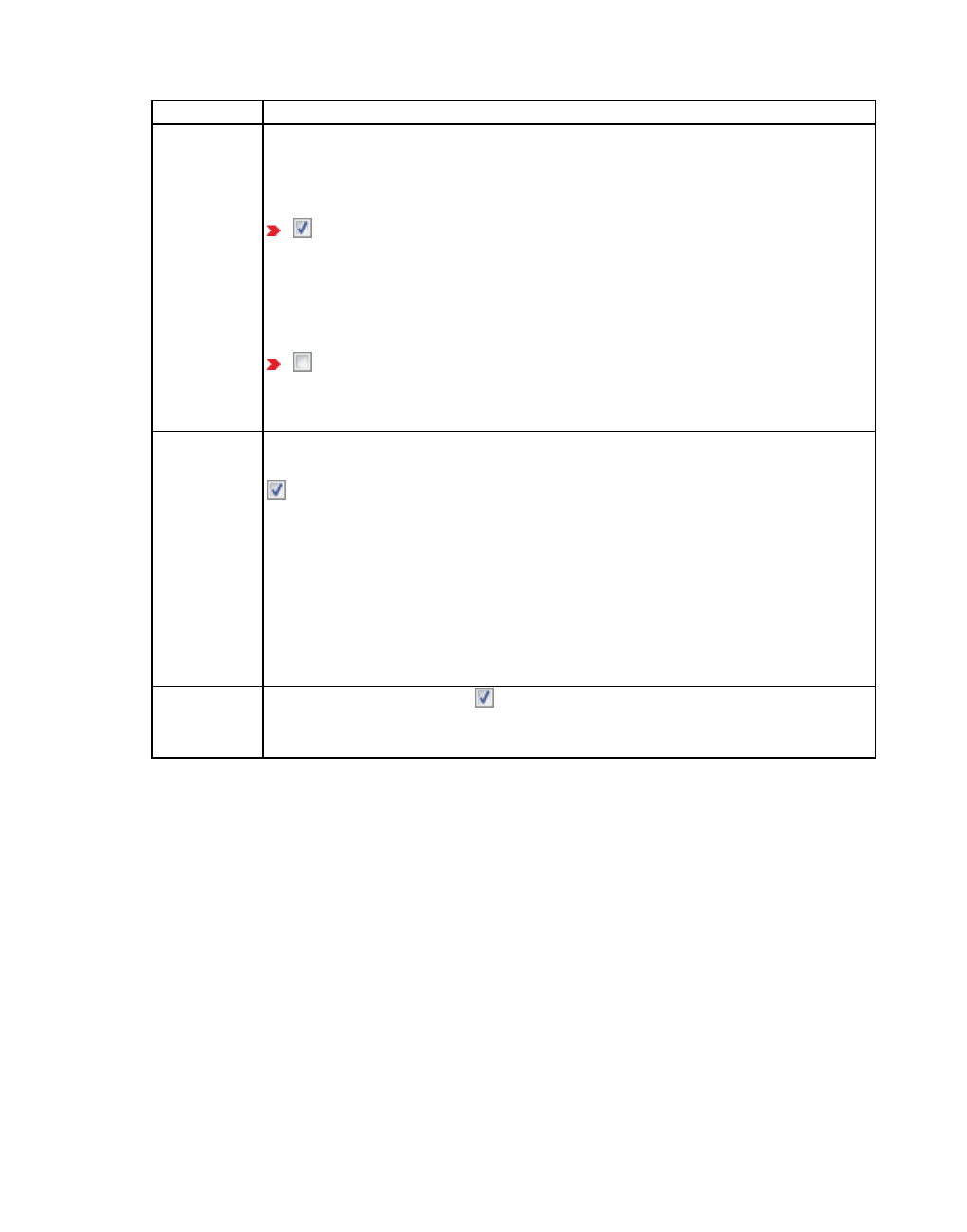
10.9.10 Attributes of areas
Element Description
Waiting time
is relative to
the start of
simulation
WaitTimeIsRelToStartSim: If a time distribution is selected for the area and
the pedestrian route has a route location within the area, the pedestrian will be
allocated a waiting period from the time distribution as soon as he/she enters
the area. The waiting period can refer to the following points in time:
If this option is selected, the waiting time refers to the simulation start.
The pedestrian continues on his/her route as soon as the simulation
second corresponds to the time of the time distribution. If the simulation
second has already exceeded the time of the time distribution when the
pedestrian enters the area, the pedestrian immediately continues on
his/her pedestrian route.
If this option is not selected, the waiting time refers to time when the ped-
estrian enters the area.
This option cannot be selected, if the Queuing attribute is selected.
Queuing Is queue (IsQueue): Attribute for the waiting behavior on pedestrian areas
which are the destination or intermediate point of a route.
If this option is selected, queuing pedestrians build a queue during their
dwell time. If no time distribution is allocated, the positioning only occurs for a
few seconds. The positioning is effected according to the orientation vector
during generation of the area. In wireframe view, the vector is displayed as a
dashed line with an arrowhead.
Define the desired queue behavior in the list on the Area Behavior tab for the
queue and assign the desired pedestrian class.
This option cannot be selected if the Waiting time is relative to the start of
simulation attribute is selected.
Queue eval-
uation act-
ive
Queue Evaluation Active: If this option and the option Is queue are selec-
ted, you may output result attributes for the queue (see "Evaluating pedestrian
density and speed based on areas" on page 974).
852 © PTV GROUP

10.9.10 Attributes of areas
Element Description
Queue
approaching
method
Method used to calculate how pedestrians approach the end of a queue.
Direct line: Pedestrians approach the end of the queue in a direct line.
This method requires only minimal computing time. However, pedestrians
may be permanently blocked by obstacles.
Static potential: Pedestrians approach the end of the queue up to the dis-
tance defined in the attribute Queue approaching direct line radius based
on a static potential. This allows pedestrians to circumvent the obstacles,
taking the shortest path possible. Within this radius, they walk the remain-
ing distance to the end of the queue in a direct line. The static potential is
calculated based on the position of the pedestrian standing at the end of
the queue. Viswalk checks this position with each time step. If the position
changes, the static potential is re-calculated. This method allows ped-
estrians to pass through obstacles.
Queue approaching direct line radius
(QueueApproachingDirectLineRadius): Radius around the current end of the
queue within which the method Direct line is used. Outside this radius, the
selected queue approaching method is used. Default 2.0 m
In queues that Viswalk automatically generates next to PT vehicles and
elevators, pedestrians always approach the end of the queue in direct line.
Queue eval-
uation act-
ive
Queue Evaluation Active: If this option and the option Is queue are selec-
ted, you may output result attributes for the queue (see "Evaluating pedestrian
density and speed based on areas" on page 974).
Behavior within the queue
By default, pedestrians move to the position of the person in front them when they leave their
position. For each queue selected for the queue approaching method Static potential,
Viswalk calculates an additional potential as soon as the simulation is started. This potential
shows at the beginning of the queue. It becomes effective each time you update the queue.
The distance to the person in front of each pedestrian in the queue is calculated. If the
distance is greater than 2 meters, pedestrians do not move up in the queue in direct line, but in
walk mode according to the new potential. This mode ends as soon as the pedestrians are
closer than 2 meters to the person in front of them. Then pedestrians move up in the queue in
direct line again. This procedure allows for a more realistic moving up in line of the
pedestrians, particularly when queues are angled, for example in front of a desk at the airport,
where shut-off systems are used to create a zigzag queue.
Define queue behavior and assign pedestrian class
1. In the Area Behavior tab, activate the Queuing option.
2. Right-click in the list.
3. From the shortcut menu, choose Add.
A new line for the pedestrian class with the lowest number is added.
© PTV GROUP 853

10.9.10 Attributes of areas
4. Make the desired changes:
Element Description
PedClass Select the pedestrian class for which the queue order and/or the queue
straightness needs to be defined
QueueStraight The Queue straightness defines the shape of the queue, with values
between 0.0 and 1.0. The greater the value, the more straight the queue
will look:
0.0: snake shaped queue
1.0: straight queue
If no waiting behavior is defined for this waiting area, the attribute applies
to all elevators of the elevator group, to all floors and all pedestrian
classes. Default values are defined in the network settings (see
"Selecting network settings for pedestrian behavior" on page 193). They
are used if this attribute is not defined for the elevator group.
Using the coupled list Queuing behavior, you can limit the shape of the
queue to the desired pedestrian classes, and for the selected pedestrian
classes, define the queue shape.
The Is queue attribute of the area must be selected.
QueueOrder The Queue order defines the orderliness of the queue formed by
pedestrians, with values between 0.0 and 1.0. The higher this value, the
more orderly pedestrians line up one behind the other:
0.0: Pedestrians are standing together in groups
1.0: Queue of pedestrians lined up one behind the other
If no waiting behavior is defined for this waiting area, the attribute applies
to all elevators of the elevator group, to all floors and all pedestrian
classes. Default values are defined in the network settings (see
"Selecting network settings for pedestrian behavior" on page 193). They
are used if this attribute is not defined for the elevator group.
Using the coupled list Queuing behavior, you can limit the orderliness of
the queue to the desired pedestrian classes, and for the selected
pedestrian classes, define the orderliness.
The Is queue attribute of the area must be selected.
854 © PTV GROUP
10.9.10 Attributes of areas
10.9.10.2 PT & Elevators tab
PT section Description
Usage Usage of area in PT:
None: Area not used for PT
Waiting area: Location, in which the pedestrians wait, in order to
board at the allocated public transport stop in the desired PT trans-
port line. When the area is allocated at least one public transport
stop, select for the pedestrians an arbitrary point in the waiting area
where they are waiting for the next PT vehicle. Default color for the
waiting area: blue.
Platform edge: Location, to which pedestrians go, when they alight
from their PT line to the allocated public transport stop. Alighting pas-
sengers will always use the nearest platform edge. Afterwards, they
follow the routing decision, which is placed on this area. If there is no
routing decision defined for this area, the pedestrians are removed
from the network. For a platform edge, a width of at least 2 m is
required. An area of the type Polygon, which serves as a platform
edge, can be generated automatically with a public transport stop
(see "Generating platform edges" on page 483). You can select the
side and thus specify on which side of the PT stop boarding is
allowed (see "Attributes of PT stops" on page 480). A platform edge
can be allocated to multiple PT stops. Default color for the platform
edge: pink.
As soon as you allocate public transport usage with the attribute Waiting
area or Platform edge and a public transport stop with the attribute for
public transport stop(s) to the area, Vissim checks whether boarding
volumes are defined for this stop. If no boarding volumes are defined,
Vissim enters default data in the Public transport stop window on the
Boarding volumes tab.
for PT stop(s) Allocating one or more public transport stops to the area. The area must
be a Waiting area or a Platform edge.
As soon as you select a PT stop and confirm the entries with OK, Vissim
changes the following data of the PT stops affected (see "Attributes of PT
stops" on page 480):
For the Areas attribute, the number of areas with the selected
attribute Public transport usage is entered.
For the Pedestrians as passengers attribute, the option is selec-
ted.
In the Boarding Passengers tab, a line with data is created.
© PTV GROUP 855

10.9.10 Attributes of areas
PT section Description
Boarding loc-
ation
As a standard, for pedestrian areas with Public transport usage for the
Boarding location the option Nearest door is used. Alternatively, for the
door selection when boarding, you can allocate a location distribution
after the queuing boarding passengers have distributed for the boarding
at the doors of the PT vehicle (see "Using location distributions for
boarding and alighting passengers in PT" on page 240).
Elevators
section
Description
Waiting
area for
elevator
group
ElevGrp: Elevator groups whose elevators take the area into account. When a
pedestrian enters an area that includes a route location of his route, an elevator
is requested depending on the following route location.
856 © PTV GROUP

10.9.10 Attributes of areas
PT & Elevators
section
Description
Waiting beha-
vior
PTWaitBehav: Waiting behavior of pedestrians in public transport waiting
area and elevators:
Wait at fixed location: Prevents pedestrians from waiting outside the
waiting area. Each pedestrian attempts to reach his randomly determ-
ined waiting position in the waiting area before he stops to wait for the
next public transport vehicle or the next elevator. If, in the case of a
boarding passenger, a relevant PT vehicle has already arrived at the
public transport stop or the next elevator has already arrived, this ped-
estrian is no longer routed to a randomly determined position at the wait-
ing area. Instead, the pedestrian tries to go directly to the PT vehicle or
elevator as soon as he reaches the waiting area, provided that the PT
vehicle or elevator has an additional dwell time of at least two more
seconds.
Wait if held up: If pedestrians whose destination is a waiting area are
closer than 5 m to the waiting area and who are walking more slowly
than 0.4 m/s for 3 time steps, Vissim consider these pedestrians as
"arrived at the waiting area". In this case, the pedestrians remain stand-
ing and waiting, even if they are not yet at the waiting area. This can
cause unrealistic jams in the simulation because queuing pedestrians
create a permanent obstacle. In order to avoid this, you can select the
Wait at fixed location attribute or define a sufficiently large boarding
capacity for each waiting area. From a larger waiting area, you can build
multiple small waiting areas to reach a better area distribution for the
waiting pedestrians. Alternatively, you can define an intermediate des-
tination in a large waiting area, in which the pedestrians can be dis-
tributed in the waiting area. In addition, for destinations on waiting
areas, use the dynamic potential (see "Dynamic potential" on page
910). This causes pedestrians who are already queuing to be more
aware of the incoming pedestrians and to choose their paths respect-
ively. The dynamic potential can extend the calculation time.
© PTV GROUP 857
10.9.10 Attributes of areas
PT & Elevators
section
Description
Queue
approaching
method
Method according to which pedestrians in a waiting area move towards a
waiting position
Direct line: Pedestrians approach the waiting position in a waiting area
in a direct line. This method requires only minimal computing time.
However, pedestrians may be permanently blocked by obstacles.
Static potential: Pedestrians approach a waiting position in a waiting
area based on a static potential. The potential is calculated as soon as
pedestrians reach the waiting area. Then they move along the potential
gradient to the waiting position, up to a certain distance that is cal-
culated based on the cell size. This allows pedestrians to circumvent
the obstacles, taking the shortest path possible. If the distance of the
pedestrians to the waiting position is less than the diagonal of the cell
size, they move to the waiting position in a direct line. If they are pushed
back from this distance, they start moving again based on the static
potential. If an elevator door opens or a PuT vehicle stops, pedestrians
will move directly towards them.
Cell size: Edge length of a grid mesh used for the calculation of distances
to the destination area with the static or dynamic potential (see "Defining
global model parameters" on page 825). Default 0.15 m.
Obstacle distance:: Distance up to which the nearby walls have a bearing
on the distance potential (see "Defining global model parameters" on page
825). Default 0.5 m.
Note: If, at a public transport stop at least one pedestrian area is defined as a Waiting
area or Platform edge, Vissim assumes that the boarding/alighting at this public
transport stop is calculated during the simulation and that the dwell time should not
only be determined numerically regarding the number of boarding/alighting
passengers.
The difference becomes visible in the window PT Line Stop: The content of the window
changes as soon as a pedestrian area is defined as a Waiting area or Platform edge
(see "Editing a PT line stop" on page 492).
Showing and editing dependent objects as relation
The attribute and attribute values of this network object type are shown in the list on the left,
which consists of two coupled lists.
1. In the list on the left, click the desired entry.
The list on the right contains attributes and attribute values of network objects, and/or base
data allocated to the network object selected in the list on the left (see "Using coupled lists" on
page 111):
858 © PTV GROUP

10.9.11 Attributes of obstacles
Pedestrians: Pedestrians within the area. The evaluation may reduce simulation speed.
Pedestrian routing decision (static) (see "Attributes of static routing decisions for ped-
estrian routes" on page 906)
Static pedestrian route locations (see "Attributes of pedestrian route locations" on page
904)
Static pedestrian route destinations (see "Attributes of pedestrian route locations" on page
904)
Pedestrian routing decision (partial) (see "Attributes of pedestrian partial routing
decisions" on page 908)
Partial pedestrian route locations (see "Attributes of pedestrian route locations" on page
904)
Partial pedestrian route destinations (see "Attributes of pedestrian route locations" on
page 904)
Pedestrian inputs (see "Attributes of pedestrian inputs" on page 884)
Public transport stops (see "Attributes of PT stops" on page 480)
Points: edit coordinates of the corners
Queuing behavior: The Public transport waiting behavior is described further above.
2. On the list toolbar, in the Relations list, click the desired entry.
3. Enter the desired data.
The data is allocated.
10.9.11 Attributes of obstacles
The Obstacles window opens when you insert an obstacle, if automatic opening of the Edit
dialog after object creation is selected (see "Right-click behavior and action after creating an
object" on page 143).
Into the window, you enter attribute values for the network object. For network objects which
have already been defined, you can call the window using the following functions:
In the list of network objects of the network object type, double-click the row with the
desired network object.
In the Network editor, select the network object of your choice. Then, from its shortcut
menu, choose Edit.
The network object may have additional attributes. In the network objects list of the network
object type, you can show all attributes and attribute values. You can open the list via the
following functions:
In the network object toolbar, right-click the desired network object type. Then from the
shortcut menu, choose Show List (see "Context menu in the network object toolbar" on
page 63).
© PTV GROUP 859

10.9.11 Attributes of obstacles
In the Network editor, select the network object of your choice. Then, from its shortcut
menu, choose Show In List (see "Selecting network objects in the Network editor and
showing them in a list" on page 339).
From the Lists menu, in the desired category, choose the network object type.
In the network objects list of the network object type, you can edit attributes and attribute
values of a network object (see "Selecting cells in lists" on page 102), (see "Using lists" on
page 89).
The objects of this object type may have relations to other objects. This is why the attributes list
is shown as part of a coupled list (on the left). On the Lists toolbar, in the Relations box, you
can show and edit the coupled list with the attributes of the desired relation on the right (see
below Showing and editing dependent objects as relation) and (see "Using coupled lists" on
page 111).
Note: In lists, you can use the Attribute selection icon to show and hide attribute
values (see "Selecting attributes and subattributes for a list" on page 106).
1. Make the desired changes:
Element Description
No. Unique number of the obstacle
Name Name of the obstacle
Level Level, if when modeling multistory buildings, you want to place the obstacle on
a level (see "Defining levels" on page 868)
z-Offset zOffsetB:Offset > 0.000 along the z-axis up to the edge specified for 3D display
of the obstacle (C in the figure below)
Height Height of obstacle for 3D display(D in the figure below)
Area left (green): A = offset top, B = thickness
Obstacle right (red): C = offset bottom, D = height
Display
type
Display type for colored display of the obstacle (see "Defining display types" on
page 300)
860 © PTV GROUP
10.9.12 Attributes of ramps, stairs, moving walkways and escalators
A network object may have the following attributes: These can be shown in the attributes list.
Long
name
Short
name
Description
Created
by
CreatedBy Indicates whether the obstacle is user-defined or has been generated
by Vissim.
User: The obstacle was defined by a Vissim user (see "Defining
construction elements as rectangles" on page 844), (see "Defining
construction elements as polygons" on page 845)
3D traffic signal: The obstacle is the mast of a 3D traffic signal.
This obstacle was defined by Vissim during a simulation run (see
"Attributes of 3D signal heads" on page 552).
Showing and editing dependent objects as relation
The attribute and attribute values of this network object type are shown in the list on the left,
which consists of two coupled lists.
1. In the list on the left, click the desired entry.
The list on the right contains attributes and attribute values of network objects, and/or base
data allocated to the network object selected in the list on the left (see "Using coupled lists" on
page 111):
2. On the list toolbar, in the Relations box, click > Points.
3. Edit the coordinates of the vertices.
The data is allocated.
10.9.12 Attributes of ramps, stairs, moving walkways and escalators
The window Ramps/Stairways/Escalators/Moving Walkways opens when a ramp, stairway,
escalator or moving walkway is inserted, if automatic opening of the Edit dialog after object
creation is selected (see "Right-click behavior and action after creating an object" on page
143).
Into the window, you enter attribute values for the network object. For network objects which
have already been defined, you can call the window using the following functions:
In the list of network objects of the network object type, double-click the row with the
desired network object.
In the Network editor, select the network object of your choice. Then, from its shortcut
menu, choose Edit.
The network object may have additional attributes. In the network objects list of the network
object type, you can show all attributes and attribute values. You can open the list via the
following functions:
In the network object toolbar, right-click the desired network object type. Then from the
shortcut menu, choose Show List (see "Context menu in the network object toolbar" on
© PTV GROUP 861

10.9.12 Attributes of ramps, stairs, moving walkways and escalators
page 63).
In the Network editor, select the network object of your choice. Then, from its shortcut
menu, choose Show In List (see "Selecting network objects in the Network editor and
showing them in a list" on page 339).
From the Lists menu, in the desired category, choose the network object type.
In the network objects list of the network object type, you can edit attributes and attribute
values of a network object (see "Selecting cells in lists" on page 102), (see "Using lists" on
page 89).
The objects of this object type may have relations to other objects. This is why the attributes list
is shown as part of a coupled list (on the left). On the Lists toolbar, in the Relations box, you
can show and edit the coupled list with the attributes of the desired relation on the right (see
below Showing and editing dependent objects as relation) and (see "Using coupled lists" on
page 111).
Note: In lists, you can use the Attribute selection icon to show and hide attribute
values (see "Selecting attributes and subattributes for a list" on page 106).
1. Make the desired changes:
862 © PTV GROUP

10.9.12 Attributes of ramps, stairs, moving walkways and escalators
Element Description
No. Unique identification of the construction element (ramp, stairway,
moving walkway or escalator)
Name Name of the construction element
Level (start) Start level (StartLvl): Level, on which you can begin the definition of
the construction element. A ramp, stairway, moving walkway or
escalator can be located within a level, or the two levels Level (start)
and Level (end) can be linked together. You can end the definition of a
level when the construction element for the modeling of multistory
buildings begins on one level and ends on another (see "Defining
levels" on page 868).
z-offset (start) Start z-offset (StartZOffset): Offset > 0.000 of the Level (start) along
the Z axis to the given edge for the 3D graphics mode of the
construction element. This is the floor on which the pedestrians walk (A
in the figure below)
If Thickness > offset, the floor rises in 3D from below 0
If Thickness < offset, the floor seems to float in 3D
Level (end) End level (EndLvl): Level, on which you can end the definition of the
construction element.
z-offset (end) End z-offset (EndZOffset): Offset > 0.000 of the Level (end) along the Z
axis to the given edge for the 3D graphics mode of the construction
element.
If Thickness > offset, the floor rises in 3D from below 0
If Thickness < offset, the floor seems to float in 3D
For a Stairway or Escalator, the Z-offset (start) and Z-offset (end)
must be different. The value of the z-coordinates are calculated from the
height of the respective Level and the corresponding Offset.
Length Length2D: Length of the construction element for the definition of the
construction element in the Network Editor
Length3D accounts for the z-Offset of the link.
Height Height of the construction element from the height of the level and the
Offset.
Width Width of the construction element
Thickness Thickness of the construction element for 3D representation Not
relevant for the simulation.
The thickness > 0 for the construction element reduces the clearance
shown in 3D under the construction element because the thickness of
the construction element is not considered when the length of the
opening or the ramp foot of the clearance is calculated.
Display type Display type for color display of the construction element (see "Defining
display types" on page 300)
© PTV GROUP 863

10.9.12 Attributes of ramps, stairs, moving walkways and escalators
Element Description
Visualization The options can be used, for example, for modeling tunnels and
underpasses in 2D because the option selected during the simulation is
considered only if it corresponds to the relevant selected pedestrian
attribute Show individual pedestrians or Show classified values.
Individual pedestrians (ShowIndivPeds): This option is considered
if the pedestrian attribute Show individual pedestrians is selected.
If the option is selected, pedestrians are shown on the construction
element during the simulation.
If the option is not selected, no pedestrians are shown on the
construction element then during the simulation.
Show classified values (ShowClsfValues): This option is con-
sidered if the pedestrian attribute Show classified values is selec-
ted. Then the global LOS scheme for this construction element can
be ignored during the area-based LOS display (see "Examples of
visualization of pedestrian parameters" on page 178).
If the option is not selected, classified values are shown on the
construction element during the simulation (see "Assigning a color to
ramps and stairs based on aggregated parameters (LOS)" on page
180).
If the option is not selected, no classified values are shown on the
construction element then during the simulation.
Pedestrian Record (Pedestrian record active)) (PedRecAct): cre-
ates pedestrian record
Note the following for area behavior types: If no area behavior type is selected or if an
area behavior type has not been assigned a walking behavior, the walking behavior
assigned to the pedestrian type is used.
Behavior type Optionally, select an area behavior type (AreaBehavType). Is used to
model occasional changes to the speed or other parameter (see
"Modeling area-based walking behavior" on page 879)
Behavior type
(flat)
Optionally, select an area behavior type (AreaBehavType). Is used to
model occasional changes to speed or other parameters on a flat
construction element, e.g. a moving walkway (see "Modeling area-
based walking behavior" on page 879)
Behavior type
(up)
Optionally, select an area behavior type (AreaBehavType). Is used to
model occasional changes to speed or other parameters on a ramp,
stairway or escalator going upwards. It can be used to model the
walking behavior of elderly people or wheelchair users (see "Modeling
area-based walking behavior" on page 879).
864 © PTV GROUP

10.9.12 Attributes of ramps, stairs, moving walkways and escalators
Element Description
Behavior type
(down)
Optionally, select an area behavior type (AreaBehavType). Is used to
model occasional changes to speed or other parameters on a ramp,
stairway or escalator going downwards. It can be used to model the
walking behavior of elderly people or wheelchair users (see "Modeling
area-based walking behavior" on page 879).
Type Select desired construction element:
Ramp: Define the attributes of the ramp in the Installation tab.
Moving walkway: Define the attributes of the moving walkway in the
tabs Installation, Design, Width & Balustrade and Movement.
Stairway: Two levels must be defined. Define the attributes of the
stairway in the tabs Installation and Design.
Escalator: Two levels must be defined. Define the attributes of the
escalator in the tabs Installation, Design, Width & Balustrade and
Movement.
You can model the length, headroom, ceiling opening and other
attributes of the construction element (see "Modeling length, headroom
and ceiling opening" on page 867). You can define these attributes in
the tabs Installation, Design, Width & Balustrade and Movement.
2. Select the desired tab.
3. Make the desired changes:
10.9.12.1 Installation tab
Area over and under the construction element.
Element Description
Define ceiling
opening by Headroom (OpenHeadr): head clearance
Length (OpenLen): length of the ceiling opening
Solid ramp foot Up to (FootHeadr): up to the height of the headroom
Length (FootLen) Length of the ramp foot
Show solid
obstacle (3D) FootVisible): If this option is selected, the ramp foot is shown full in 3D
mode.
If this option is not selected, the ramp foot is not shown full in 3D mode.
© PTV GROUP 865
10.9.12 Attributes of ramps, stairs, moving walkways and escalators
10.9.12.2 Design tab
Element Description
Define stair-
way by Total steps (TreadsDefBy): Number of steps defined, height of the
steps
Rise: Height of steps defined, length of the steps
Going: Length of steps defined, height of the steps
Landing plat-
forms
Horizontal, flat, immovable area before and after the construction element:
Entry Length (EntryLandLen): in front of the construction element
Exit Length (ExitLandLen): after the construction element
Display type (LandingDisplType): Select display types for the landing
platforms (see "Defining display types" on page 300)
Horiz. Runout area (EntryRunLen), (ExitRunLen), Horizontal runout
area: Length from Entry and Exit, so that the steps continue horizontally
with any slope in order to avoid accidents in the transition to and from
the walking areas.
In the wireframe view, triangles mark the landing platforms before and after
the construction element in the direction of movement:
The Horiz. Runout area is not displayed.
10.9.12.3 Width & Balustrade tab
Display and measurement of the handrail and the balustrade.
Element Description
Usable
width
Width (UsableWid), pedestrians can walk on. Base for the socket width. Value
range 600 to 1,200 mm. Alternatively, a warning opens at the start of the
simulation.
Handrail
Balustrade
Socket
Width and display type of handrail (HandrWid), (HandrDisplType), balustrade
(BalustrWid), (BalustrDisplType), and socket (SocketWid),
(SocketDisplType).
The socket width must be larger than the width of the balustrade and the
handrail.
Socket width = (Total width - usable width) / 2
Show bal-
ustrade
(3D)
ShowBalustr: If this option is selected, the balustrade is shown in 3D mode.
The balustrade does not move.
866 © PTV GROUP

10.9.13 Modeling length, headroom and ceiling opening
10.9.12.4 Movement tab
The movement of the construction element has an influence on the result of the simulation.
Element Description
Treads Direction of travel (MovDir): Movement direction, in which the moving
walkway or escalator is moving forwards = Direction according to the defin-
ition.
Speed (OpSpeed): of the moving walkway or escalator. Default 0,500 m/s
Pedestrians Standing location: Side in the direction of travel, on which the pedestrians
are located
Walking percentage (WalkPerc): Share of the pedestrians who are mov-
ing on a moving walkway or escalator
Pedestrian classes: Moving pedestrians of a pedestrian class. Pedes-
trians of other pedestrian classes are not moving. All pedestrian types
also include pedestrian types, which are not allocated a pedestrian class.
Showing and editing dependent objects as relation
The attribute and attribute values of this network object type are shown in the list on the left,
which consists of two coupled lists.
1. In the list on the left, click the desired entry.
The list on the right contains attributes and attribute values of network objects, and/or base
data allocated to the network object selected in the list on the left (see "Using coupled lists" on
page 111):
Pedestrians: Pedestrians within the area. The evaluation may reduce simulation speed.
Area behavior type (upwards)
Area behavior type (downwards)
Area behavior type (flat)
Walking - Pedestrian Classes
Points: edit coordinates of the corners
The attributes are described further above.
2. On the list toolbar, in the Relations list, click the desired entry.
3. Enter the desired data.
The data is allocated.
10.9.13 Modeling length, headroom and ceiling opening
You can model the length, head room and ceiling opening for ramps, stairways, moving
walkways and escalators. You can define these attributes in the tabs Installation, Design,
© PTV GROUP 867

10.9.14 Defining levels
Width & Balustrade and Movement (see "Attributes of ramps, stairs, moving walkways and
escalators" on page 861).
The length, headroom and ceiling opening are marked by lines in the following figure:
Length (1) and head clearance (2) on the ramp foot of the stairway are used for the cal-
culation of available space on the floors.
The ceiling opening at the top of the stairway is determined either by the length attribute
(3) or the headroom attribute (4).
The length, headroom and ceiling opening do not affect the pedestrian flows which use
the element.
For the lower floor, the size of the area built is produced from the dimensions of the
obstacle.
Note: Define sufficient head clearance. Otherwise the heads of the pedestrians
"overrun" the underside of the element.
The thickness > 0 for the construction element, which connects two levels with each other,
reduces the height shown in 3D under the construction element because the thickness of the
ceiling or the ramp is not considered when the length of the opening or the ramp foot of the
clearance is calculated.
10.9.14 Defining levels
You may define multiple levels, e.g. for multistory buildings or bridge structures for links. For
levels, you can define links, backgrounds, static 3D models, 3D signal heads and construction
elements.
By default, Vissim already contains a level with the Height attribute = 0.0.
1. From the Base Data menu, choose Levels.
The Levels list opens.
By default, you can edit the list (see "Using lists" on page 89).
868 © PTV GROUP

10.10 Modeling links as pedestrian areas
2. In the list, on the toolbar, click the Add button .
A new row with default data is inserted.
3. Make the desired changes:
Element Description
No Unique number of the level
Name Name of the level
zCoord z-coordinate: z value of layer in meters
The level is displayed in the Levels list and in the Levels toolbar.
Tip: Using the Levels toolbar, you can show and hide levels and activate or deactivate
their selectability (see "Using the Level toolbar" on page 65).
10.10 Modeling links as pedestrian areas
You can define links as pedestrian areas and thus model the interaction between vehicles and
pedestrians. Pedestrians become part of the network via pedestrian inputs that you position in
areas (see "Modeling pedestrian inputs" on page 883). These areas must overlap the links
that are used as pedestrian area so that pedestrians can use these links.
In addition, you can define additional construction elements for pedestrian flows, e.g. areas,
ramps or obstacles (see "Modeling construction elements" on page 834).
Using the default settings, you can edit and delete pedestrian areas. When you delete a
pedestrian area, the pedestrian link generated for the opposite direction is also automatically
deleted.
For pedestrians on links that serve as a pedestrian area, the same mechanisms are used as
for vehicles: At a junction where a vehicle path and a pedestrian path intersect, a Vissim link
forms the basis for the automatically generated pedestrian area.
In contrast to walkable pedestrian areas, on pedestrian links, pedestrian flows can be
controlled via link-based Vissim network objects.
10.10.1 Differences between road traffic and pedestrian flows
For links used as pedestrian areas the following applies:
They are not directional.
They cannot be split.
They cannot contain any intermediate points.
They have no pedestrian inputs.
They cannot be the start or end of a connector.
Using the default settings, you can define links as pedestrian areas and edit them (see
"Modeling links for vehicles and pedestrians" on page 380).
© PTV GROUP 869

10.10.2 Differences between walkable construction elements and link-based pedestrian areas
10.10.2 Differences between walkable construction elements and link-based pedestrian
areas
The differences between walkable construction elements (e.g. areas, ramps) and links used
as pedestrian areas are as follows:
For links used as pedestrian areas the following applies:
They cannot be edited as an area.
They cannot be a ramp.
The links cannot be the start, end or intermediate point of a pedestrian route.
A pedestrian area can be positioned on a pedestrian link. There you can define start, des-
tination and intermediate points of pedestrian routes.
10.10.3 Modeling obstacles on links
An obstacle cannot only be added to an area, but also to a link that serves as a pedestrian
area. The option Use as pedestrian area (Attribute Is pedestrian area (IsPedArea)) must be
selected for this link (see "Attributes of links" on page 383). The steps for adding an obstacle
as a polygon or rectangle to a link correspond to the steps for adding an obstacle to an area
(see "Defining construction elements as polygons" on page 845), (see "Defining construction
elements as rectangles" on page 844).
10.10.4 Network objects for pedestrian links
You can define the following Vissim network objects for a pedestrian link and model the
interaction between vehicles and pedestrians or pedestrian flows:
Conflict areas with road traffic (see "Defining the right of way at conflict areas" on page
530), (see "Modeling conflict areas for pedestrians" on page 873)
Signal Heads (see "Defining signal groups in the SC editor" on page 603), (see "Modeling
signal controls for pedestrians" on page 872)
Detectors (see "Defining detectors" on page 558), (see "Modeling detectors for ped-
estrians" on page 876)
Priority Rules (see "Defining priority rules" on page 513), (see "Modeling priority rules for
pedestrians" on page 876)
10.10.5 Defining pedestrian links
You can define existing links as pedestrian links or create new pedestrian links. On the
pedestrian links, you can position signal heads, detectors, priority rules or conflict areas for
pedestrians. You cannot insert intermediate points in pedestrian links.
1. To insert a new pedestrian link, define the link (see "Defining links" on page 381).
870 © PTV GROUP

10.10.6 Modeling interaction between vehicles and pedestrians
2. After you have added the new link, or when you want to define an existing link as a
pedestrian link, display the link attributes in the Link window or the Links list (see
"Attributes of links" on page 383).
3. For the link, select the IsPedArea attribute (Is pedestrian area and the Use as pedestrian
area option.
Vissim generates the following pedestrian links with identical coordinates. Both pedestrian
links overlap. Then the pedestrian link can be used in both directions. Vehicles cannot use
a pedestrian link.
Pedestrian link no. 1, with the direction you dragged the link open in the Network
editor.
Pedestrian link no. 2, with the opposite direction.
4. For the Level attribute, select the level of your choice (see "Attributes of links" on page 383),
(see "Defining levels" on page 868).
5. If desired, edit the other attributes (see "Attributes of links" on page 383).
6. Confirm with OK.
10.10.6 Modeling interaction between vehicles and pedestrians
Model the interaction of vehicles and pedestrians or pedestrian flows with the following
network objects:
Signal control : in the figure, the red bar (1), (2) (see "Modeling signal controls for ped-
estrians" on page 872)
Conflict areas: in the figure, the eight yellow areas (see "Modeling conflict areas for ped-
estrians" on page 873)
Detectors: in the figure, the four orange lines (see "Modeling detectors for pedestrians" on
page 876)
Priority rules (see "Modeling priority rules for pedestrians" on page 876): (11) to (18) stop
lines, (1234) and (5678) conflict markers
Links for vehicles (A)
Links for pedestrians (B)
© PTV GROUP 871

10.10.7 Modeling signal controls for pedestrians
10.10.7 Modeling signal controls for pedestrians
1. Ensure that the following network objects are defined:
Links for pedestrians in which the attribute Use as pedestrian area is selected (see
"Defining pedestrian links" on page 870). (B) in the figure.
Signal control with signal groups on the links (see "Defining signal groups in the SC
editor" on page 603). (1), (2) in the figure.
2. Select the desired pedestrian classes in the attribute PedClasses of the signal heads
which lie in the pedestrian link (see "Attributes of signal heads" on page 545). A pedestrian
observes a signal head only if it belongs to a pedestrian type whose pedestrian class is
selected in the attribute of the signal head.
The figure shows a modeling example:
872 © PTV GROUP

10.10.8 Modeling conflict areas for pedestrians
The signal head works exclusively in the direction of the pedestrian link at the time when the
signal head is inserted on the pedestrian link. The signal head does not work for the opposite
direction. The direction of the pedestrian link is indicated by yellow arrows on the edge of the
pedestrian link. These are arrows are displayed when you mark the pedestrian link.
When the signal head is inserted in the direction of the pedestrian link, it is either open or
closed for pedestrians walking in this direction. This depends on the dynamic state of the
assigned signal group:
Red and amber: The signal head is closed. Pedestrians stop at the signal head until it
no longer shows red or amber.
Other cases: The signal head is open, pedestrians can continue walking on the ped-
estrian link.
Pedestrians can always pass the signal head when walking In the opposite direction of
the pedestrian link, regardless of its condition. To supply these pedestrians with data via
signal heads, reverse the direction of the pedestrian link and insert another signal head.
You can then switch back to the original direction of the pedestrian link. This means there
are two signal heads on the pedestrian link that have an impact on different directions.
3. To reverse the direction of the link, click the link and hold down the TAB key.
The dynamic state (for example red or green) of the signal head is linked to the dynamic state
of the respective signal group to which the signal head belongs.
10.10.8 Modeling conflict areas for pedestrians
1. Ensure that the following network objects are defined:
Links for pedestrians in which the attribute Use as pedestrian area is selected (see
"Defining pedestrian links" on page 870): B in the figure.
Links for vehicles in which the attribute Use as pedestrian area is deactivated (see
"Attributes of links" on page 383): A1, A2 in the figure.
2. On the Network objects toolbar, click Conflict Areas.
Passive conflict areas are marked yellow by default.
3. Repeat the following steps until the desired priority rule is shown.
4. Right-click the desired conflict area.
5. In the context menu, select the entry Change conflict area status.
The figure shows a modeling example:
© PTV GROUP 873
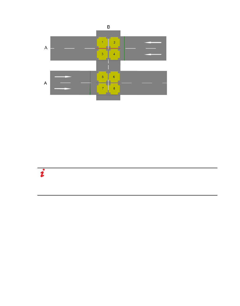
10.10.8 Modeling conflict areas for pedestrians
Vissim creates passive conflict areas in the two opposite directions of pedestrian links. You
may change the priority rules for the conflict areas (see "Modeling conflict areas" on page
526). Conflict areas on a link for pedestrians always have the same priority rule: pedestrians
have the right of way or must give the right of way. Based on the current priority rule and the
current speed as well as desired speed, pedestrians and vehicles decide when they can pass
a conflict area.
A conflict area has a stop line distance. The stop line distance describes the upstream position
on the link at which the pedestrians or vehicles have to wait if they have to grant the right of
way. At a default value of NULL, the stop line position in the direction of travel is immediately
before the start of the conflict area. You can position the stop line upstream from the regular
stop line of the conflict area.
Note: If the two links intersect at an acute angle, the distance for crossing the road is
greater. This also increases the time required by pedestrians to cross the link. Since
there is no geometric analysis of the relative position of the two links related by the
conflict area, a pedestrian may not have yet left the lane when he reaches the next
vehicle.
10.10.8.1 Case 1: Pedestrians yield to vehicles
Pedestrians who want to cross the vehicle link (A1) and enter the conflict area on the left lanes
of (A1) in the figure above have to consider the minimum speed that is calculated on the stop
lines where the arrows end.
874 © PTV GROUP

10.10.8 Modeling conflict areas for pedestrians
Minimum speeds are calculated dynamically at stop lines: pedestrians using minimum speed
or a higher speed can pass the stop line, but other pedestrians have to wait before the stop
line.
Pedestrians enter a conflict area with a vehicle link only if they can cross the entire link (in
stages) so that they never are on a lane on which a vehicle is just passing through the conflict
area. The desired speed of the pedestrian and the current speed of the vehicle are assumed
here. Vehicles that are not yet in the network are not taken into account here. Vehicles that are
more than 75 m times the number of lanes of the link from the conflict area are also not taken
into account. This condition can no longer be fulfilled after entering the conflict area if, for
example, a vehicle accelerates or enters the network at a relatively short distance. In this case,
the pedestrian waits before the first lane of the vehicle link which he probably cannot cross
completely before the arrival of the vehicle.
10.10.8.2 Case 2: Vehicles have to wait
On the pedestrian link, the area 3 m upstream from the conflict area to the start of the conflict
area is used as a "detector area" for the pedestrians approaching the conflict area (see
"Modeling detectors for pedestrians" on page 876). Pedestrians within the conflict area are
always taken into account:
© PTV GROUP 875

10.10.9 Modeling detectors for pedestrians
If no pedestrian is expected to enter the conflict area, the gaps between pedestrians or groups
of pedestrians are transferred to the approaching vehicles. Thus they can respond
accordingly.
10.10.9 Modeling detectors for pedestrians
Detector areas are used to model push buttons for pedestrian signals.
Detectors are also used as SC detectors for pedestrians. In this case, the detector must be
placed on the pedestrian link with the signal head (see "Activation tab for pedestrians" on
page 561).
10.10.10 Modeling priority rules for pedestrians
You can define priority rules of the vehicular traffic accordingly for conflicting pedestrian
streams or for the interaction between vehicular and pedestrian traffic.
Note: Model the standard priority rules for conflicting traffic flows which are not
controlled by signals by means of conflict areas. Only use priority rules, if conflict areas
do not produce the desired results and if you have sufficient experience in modeling
with priority rules.
Priority rules for pedestrians must lie on a pedestrian link (see "Modeling links as pedestrian
areas" on page 869). Pedestrians may be both the conflict marker and the stop line. With
priority rules for pedestrians, the following combinations are possible:
Pedestrians x Vehicles
Vehicles x Pedestrians
Pedestrians x Pedestrians
876 © PTV GROUP

10.11 Modeling pedestrian compositions
For these combinations and depending on the link attribute Use as a pedestrian area, you
can select the vehicle classes and pedestrian classes for the conflict marker and the stop line.
1. Make sure that the attribute Use as a pedestrian area is selected in the attributes of the
desired links for pedestrians (see "Defining pedestrian links" on page 870).
2. Make sure that the attribute Use as a pedestrian area is deactivated in the attributes of the
desired links for pedestrians (see "Attributes of links" on page 383).
3. Add the first priority rule (see "Defining priority rules" on page 513).
4. Edit the attributes of the priority rule (see "Attributes of priority rules" on page 515).
The Priority Rule window opens. The vehicle classes or pedestrian classes are shown in
the areas Stop line and Conflict marker depending on the link attribute Use as a
pedestrian area.
5. Select the desired entries.
6. Confirm with OK.
10.11 Modeling pedestrian compositions
For pedestrian flows you define the pedestrian compositions. Pedestrian compositions consist
of pedestrian types (see "Defining pedestrian compositions" on page 878). The definition is
comparable to the definition of vehicle compositions (see "Modeling vehicle compositions" on
page 425). Pedestrian compositions are based on pedestrian types (see "Using pedestrian
types" on page 830). Assign pedestrian compositions to pedestrian inputs.
Do not define vehicle compositions for pedestrian flows because they are bound to links and
follow the traffic flow model by Wiedemann (see "Driving states in the traffic flow model
according to Wiedemann" on page 270).
© PTV GROUP 877
10.11.1 Defining pedestrian compositions
10.11.1 Defining pedestrian compositions
You can define new pedestrian compositions, assign the desired pedestrian types and enter
attribute values.
1. Choose Pedestrian Compositions from the Traffic menu.
The attribute and attribute values of this network object type are shown in the list on the left,
which consists of two coupled lists.
2. In the list, on the toolbar, click the Add button .
A new row with default data is inserted.
3. Enter the desired attribute values in the right hand list (see "Attributes of pedestrian
compositions" on page 878).
In the next steps, assign the desired pedestrian types to the chosen pedestrian
compositions. For each pedestrian type you must add a row to the right hand list and you
can define the attribute values.
The right-hand list is shown. If there is no assignment, only the column titles are shown.
4. In the list on right, on the toolbar, click the Add button .
5. Select the desired entry.
6. Enter the desired attribute values in the right-hand list (see "Attributes of pedestrian
compositions" on page 878).
The data is allocated.
10.11.2 Attributes of pedestrian compositions
The attribute and attribute values of this network object type are shown in the list on the left,
which consists of two coupled lists.
Tip: To open coupled lists for a network object type, from the Lists menu, choose >
<Name network object type>.
Note: In lists, you can use the Attribute selection icon to show and hide attribute
values (see "Selecting attributes and subattributes for a list" on page 106).
The list on the left may include the following attributes:
Column Description
No Unique number of the vehicle composition
Name Designation of the vehicle composition
RelFlow Relative volumes: Taken from the right list
878 © PTV GROUP

10.12 Modeling area-based walking behavior
The list on the right contains attributes and attribute values of network objects, and/or base
data allocated to the network object selected in the list on the left (see "Using coupled lists" on
page 111):
Pedestrian composition relative flows
Element Description
PedType In the list box, select pedestrian type
RelFlow Relative flow: Share of this pedestrian type in the composition. The sum
of the relative volumes must not necessarily yield 1.0. As in the route
shares, the sum of all relative volumes always forms the basis of 100%;
on the basis of Vissim the absolute shares are calculated.
DesSpeedDistr Reference to the Desired speed distribution for the pedestrian type
10.12 Modeling area-based walking behavior
In their attributes, you can assign the following objects an area-based walking behavior:
For elevators: area-based behavior in an elevator car and area-based behavior that
sets in when the elevator car of defined elevator groups is exited (see "Attributes of
elevator groups" on page 936)
Areas (see "Attributes of areas" on page 848)
Ramps & Stairs (see "Attributes of ramps, stairs, moving walkways and escalators" on
page 861)
A walking behavior type consists of (see "Defining walking behavior" on page 879):
desired speed that you assign with the pedestrian compositions
parameters for the model of pedestrian dynamics, which you assign to the walking
behavior and that are assigned to the pedestrian type
An area behavior type consists of (see "Defining area behavior types" on page 881):
one or more types of walking behavior
the assigned pedestrian class per walking behavior
the time interval
the desired speed distribution
10.12.1 Defining walking behavior
You can define different walking behaviors and assign them to an area behavior type and to
the pedestrians of a pedestrian type. Walking behavior is comparable to driving behavior (see
"Defining driving behavior parameter sets" on page 268).
To link the walking behavior to a construction element, assign the area behavior type selected
for it to the desired walking behavior. You select the area behavior type via the Behavior type
attribute of the construction element. In area behavior type, you can define a special walking
behavior for each pedestrian class (see "Defining area behavior types" on page 881). You can
also assign several walking behaviors to one area behavior type.
© PTV GROUP 879

10.12.1 Defining walking behavior
If no area behavior type is selected for an area, ramp or stairs or if an area behavior type has
not been assigned a walking behavior, the walking behavior assigned to the pedestrian type
is used.
The following default walking behaviors can be predefined:
Element Description
Elevator (in cab) Walking behavior of pedestrians in an elevator cab The default
walking behavior differs from the Noise parameter = 0.3 (walking
behavior default = 1.2). This means the pedestrians in the elevator
cab are not moving much.
Elevator (alighting) Walking behavior of pedestrians alighting from an elevator car to
continue their route in the area in front of the elevator. The following
parameters differ from the default walking behavior:
Tau = 0.2 (walking behavior default = 0.4)
ASocIso = 2.04 (walking behavior default = 2.72)
BSocIso = 0.3 (walking behavior default = 0.2)
These values allow passengers alighting from the elevator cab to
easily pass other passengers.
1. From the Base Data menu, choose > Walking Behaviors.
The Walking Behaviors list opens. The columns in the list also contain model parameters
per pedestrian type according to the social force model (see "Defining model parameters
per pedestrian type according to the social force model" on page 822).
By default, you can edit the list (see "Using lists" on page 89).
Note: In lists, you can use the Attribute selection icon to show and hide attribute
values (see "Selecting attributes and subattributes for a list" on page 106).
2. Right-click in the list.
3. From the shortcut menu, choose Add.
A new row with default data is inserted.
4. Enter the desired data.
Element Description
No Unique number of walking behavior
Name Name of walking behavior
880 © PTV GROUP

10.12.2 Defining area behavior types
The following columns contain model parameter values (see "Defining model
parameters per pedestrian type according to the social force model" on page 822):
Tau Relaxation time or inertia that can be related to a reaction time
Default value 0.4 s
Tau will be set to 0.8 s for pedestrians that wait in front of a red
signal head. This allows for realistic passing of approaching
pedestrians and calm waiting behavior of pedestrians in stationary
state. As soon as the signal head turns green, Tau is reset to the
default value.
ReactToN React to n: During calculation of the total force for a pedestrian,
considers only the influence exerted by the n closest pedestrians.
ASocIso A social (isotropic) and B social (isotropic) govern the force
between pedestrians.
BSocIso B social (isotropic) and A social (isotropic) govern the force
between pedestrians.
Lambda Lambda governs the degree of anisotropy of the forces.
ASocMean A social (mean) governs the strength (A) of the social force between
two pedestrians.
BSocMean B social (mean) governs the range (B) of the social force between
two pedestrians.
VD Parameter VD in seconds
Noise The greater this value, the stronger the random force that is added to
the systematically calculated forces if a pedestrian remains below
his desired speed for a certain time.
Noise is set to 0 for pedestrians waiting in front of a red signal head.
This allows for realistic passing of approaching pedestrians and
calm waiting behavior of pedestrians in stationary state. As soon as
the signal head turns green, Noise is reset to the default value.
Side preference Specifies whether opposing pedestrian flows prefer using the right
or the left side when passing each other.
10.12.2 Defining area behavior types
You can define, edit and delete area behavior types. These allow you to group properties that
influence the walking behavior of pedestrian classes on areas, ramps and stairs. Assign the
desired time interval, pedestrian class, their desired speed and the walking behavior to an
area behavior type via area behavior type elements. You assign the desired area behavior
type in the attributes of the area, ramp or stairs (see "Attributes of areas" on page 848), (see
"Attributes of ramps, stairs, moving walkways and escalators" on page 861).
1. From the Base Data menu, choose > Area Behavior Types.
The Area Behavior Types list opens.
By default, you can edit the list (see "Using lists" on page 89).
© PTV GROUP 881

10.12.2 Defining area behavior types
Note: In lists, you can use the Attribute selection icon to show and hide attribute
values (see "Selecting attributes and subattributes for a list" on page 106).
In the Attributes list, you can define new objects and edit attribute values.
The objects of this object type may have relations to other objects. This is why the attributes list
is shown as part of a coupled list (on the left). In the Relations list box, to the right of the list on
the left, you can show the coupled list with the attributes of the relation of your choice (see
"Using coupled lists" on page 111).
2. Right-click in the list.
3. From the shortcut menu, choose Add.
A new row with default data is inserted.
4. Enter the desired data.
Element Description
No. Unique number of the area behavior type
Name Name of area behavior type
Allocating area behavior type elements via relation
The attribute and attribute values of this base data type are shown in the list on the left, which
consists of two coupled lists.
1. In the list on the left, click the desired entry.
2. On the list toolbar, in the Relations list box, click Area behavior type elements.
The list on the right contains attributes and attribute values of the area behavior type
elements.
3. Right-click on the row header in the right-hand list.
4. From the shortcut menu, choose Add.
A new row with default data is inserted.
By default, you can edit the list (see "Using lists" on page 89).
5. Enter the desired data.
Element Description
AreaBehaviorType The area behavior type selected in the list on the left
PedClass Pedestrian classes (see "Using pedestrian classes" on page 832)
TimeInt Time interval (see "Using time distributions" on page 237)
DesSpeedDistr Desired speed distribution (see "Using desired speed distributions"
on page 228)
WalkBehav Walking behavior (see "Defining walking behavior" on page 879)
The data is allocated.
882 © PTV GROUP

10.13 Modeling pedestrian demand and routing of pedestrians
10.13 Modeling pedestrian demand and routing of pedestrians
You can model the pedestrian demand by defining the pedestrian inputs for the areas,
inserting routing decisions in the walkable areas and defining routes to the destination areas.
As this can be very time-consuming in big networks with many pedestrian inputs and route
destinations, you can define pedestrian demand in an origin- destination matrix with less
detail, based on flows between origin and destination areas.
You can combine the two approaches in your network model.
10.13.1 Modeling pedestrian inputs
You can define pedestrian inputs for pedestrian areas. Select the attributes to enter the
pedestrian inputs and select a pedestrian composition. During the simulation period,Vissim
generates single pedestrians for pedestrian inputs at a random point of time based on
pedestrian compositions and the volumes entered.
You can create time intervals for pedestrian inputs and thus determine the volume for each
time interval in a pedestrian input. You enter the volume for a pedestrian input as pedestrians
per hour. Here you can select whether the exact number of pedestrians is entered or Vissim
selects the number stochastically based on the volume entered. You must always enter the
number of pedestrians per hour, even if the time interval is shorter or is 3.5 hours, for example.
The time when the pedestrian enters an area in the Vissim network is defined by Vissim
stochastically: An average time gap between two pedestrians results from the hourly volume.
This average time gap is used as an average value of a negative exponential distribution.
Vissim obtains the time gaps from this distribution which relates to a Poisson distribution. In
real life scenarios, the entry time may be subject to greater variability than in Vissim on the
basis of the Poisson distribution.
10.13.1.1 Defining pedestrian inputs
Pedestrian inputs are positioned on areas. The pedestrians in the pedestrian input are not
generated at this point, but are generated randomly at different positions in the area. This way,
you can use the shape and size of this area to determine whether Vissim should create
pedestrians for selected spots or large areas.
Notes:
You can specify that you need not press the CTRL key when adding network objects
(see "Right-click behavior and action after creating an object" on page 143).
For some network objects there are windows in which the attributes of a network
object can be defined and edited. There are lists for this, for all network objects. You
can choose whether you want to open a window, a list or neither of the two for the
definition of network objects in the Network Editor (see "Right-click behavior and
action after creating an object" on page 143).
1. On the Network objects toolbar, select Pedestrian Inputs.
© PTV GROUP 883

10.13.1 Modeling pedestrian inputs
2. Hold down the CTRL key and right-click on the desired position of the pedestrian input in the
pedestrian area.
The pedestrian input is defined. Per default, the pedestrian area displays a black circle with
a blue outline. The pedestrian area is displayed in green. The Pedestrian Inputs list opens
if automatic opening of a list after object generation is selected (see "Right-click behavior
and action after creating an object" on page 143).
A new row with default data is inserted.
The default value for the Volume (Volume) is 0. The default value for the Pedestrian
composition (PedComp) is Pedestrian. Both default values are valid for all time intervals
defined for pedestrian inputs.
The attribute and attribute values of this network object type are shown in the list on the left,
which consists of two coupled lists.
3. Enter the desired attribute values in the left-hand list (see "Attributes of pedestrian inputs"
on page 884).
In the next steps, you assign the desired network objects to the selected pedestrian input.
The list on the right contains attributes and attribute values of network objects, and/or base
data allocated to the network object selected in the list on the left (see "Using coupled lists" on
page 111):
Area: Area attributes
Pedestrian volumes by time interval: If you have entered a volume or selected a ped-
estrian composition and then select Pedestrian volumes by time interval, the attrib-
utes of the pedestrian volumes for the first time interval are displayed.
4. On the list toolbar, in the Relations list, click the desired entry.
The right-hand list is shown. If there is no assignment, only the column titles are shown.
5. Enter the desired attribute values in the right-hand list (see "Attributes of pedestrian inputs"
on page 884).
6. If you wish to define more pedestrian volumes for the selected pedestrian input, enter more
time intervals in the right-hand list.
The data is allocated.
10.13.1.2 Attributes of pedestrian inputs
The Pedestrian Inputs list opens when you insert the network object, if automatic opening of a
list after object creation is enabled (see "Right-click behavior and action after creating an
object" on page 143).
1. From the Lists menu, choose Pedestrian traffic > Inputs.
The Pedestrian inputs list opens.
By default, you can edit the list (see "Using lists" on page 89).
884 © PTV GROUP

10.13.1 Modeling pedestrian inputs
The attribute and attribute values of this network object type are shown in the list on the left,
which consists of two coupled lists.
Tip: To open coupled lists for a network object type, from the Lists menu, choose >
<Name network object type>.
The list on the left may include the following attributes:
Column Description
No Unique number of the pedestrian input
Name Name of the pedestrian input
Area Name of the area to which the pedestrian input was added
Volume(0) Volume: number of pedestrians per hour and not per time interval
Pt Coordinates of the circle of the pedestrian input
ShowLabel Show label: If this option is not selected, the label for the pedestrian input is
not displayed, even if the label for all pedestrian inputs is selected.
2. If you want to change the time interval for a pedestrian input, right-click the desired entry in
the Pedestrian Inputs list.
3. In the context menu, select Edit Time Intervals.
The Time Intervals list opens (see "Defining time intervals for a network object type" on
page 306).
Note: In lists, you can use the Attribute selection icon to show and hide attribute
values (see "Selecting attributes and subattributes for a list" on page 106).
Showing and editing dependent objects as relation
1. In the list on the left, click the desired entry.
The list on the right contains attributes and attribute values of network objects, and/or base
data allocated to the network object selected in the list on the left (see "Using coupled lists" on
page 111):
Pedestrian Volumes By Time Interval list
2. Enter the desired values.
© PTV GROUP 885

10.13.2 Modeling routing decisions and routes for pedestrians
Column Description
Cont Continued: Adopts the volume of the previous interval, if several time intervals
for pedestrian inputs have been defined. The first time interval is therefore
always deactivated.
The option is not selected: The cells are white and are only valid for this
interval.
The option is selected: The cells are gray and are valid for the period of
the combined intervals. Only the last cell, for which the Cont attribute is not
selected, can be edited. When this option is selected, a change in volume
is adopted for all the following cells.
TimeInt Time interval: Start and end of the interval in simulation seconds (see
"Defining time intervals for a network object type" on page 306).
PedComp Pedestrian composition (see "Defining pedestrian compositions" on page
878)
Volume Volume: number of pedestrians per hour and not per time interval
VolType Volume type:
Stochastic: Stochastic variations of the number of pedestrians may occur.
The cells are white.
Exact: Exactly the specified number of pedestrians are generated and
used. The cells are yellow.
3. If you want to allocate additional volumes to other time intervals for the selected pedestrian
input, right-click on the Pedestrian Volumes By Time Interval list.
4. From the shortcut menu, choose Add.
The next defined time interval will be added.
5. Enter the desired values.
10.13.2 Modeling routing decisions and routes for pedestrians
The definition and editing of pedestrian routing decisions, static pedestrian routes and partial
pedestrian routes is mostly similar to that for vehicles (see "Modeling vehicle routes, partial
vehicle routes, and routing decisions" on page 430).
Static pedestrian routes and partial pedestrian routes are edited in the same way. Therefore,
descriptions relating to pedestrian routing decisions and pedestrian routes will always refer to
both types, unless explicit distinction is made between static pedestrian routes and partial
pedestrian routes in the following sections.
A pedestrian route is a defined sequence of areas and ramps:
A pedestrian route starts with routing decision in an area. The routing decision is a rout-
ing point which is displayed as a red circle by default. The routing decision and its rout-
ing point must be located in an area.
The last routing point of a pedestrian route is referred to as destination. The des-
tination is a routing point which is displayed as a turquoise circle by default. The
886 © PTV GROUP

10.13.2 Modeling routing decisions and routes for pedestrians
destination can be located in an area or a ramp . If a pedestrian has reached his des-
tination area and the area does not contain any additional routing decisions he can
use, he is removed from the simulation.
The other routing points are intermediate destinations. They can be located as inter-
mediate points in an area or a ramp .
Several pedestrian routes to different destinations can start from the first routing point.
The destinations of static pedestrian routes which start from one routing point can be
located in different areas. A static pedestrian route can also run back to the area from
where it started.
The destinations of partial pedestrian routes which start from one routing point must be
located in one area.
If you delete a routing decision, the corresponding routes are deleted.
Note: Start points, intermediate points or the destination of a pedestrian route must not
be placed on a link defined as a pedestrian area. (see "Attributes of links" on page
383), (see "Modeling links as pedestrian areas" on page 869). You can specify an Area
construction element on the link and then position the first routing point, intermediate
point or destination of your pedestrian route in this area.
Consideration of a routing decision by pedestrians
A routing decision only applies to pedestrians that have been assigned a pedestrian class and
that are without any routing information. A pedestrian already on a route may only accept new
routing information after he has reached the destination area of his route. There must be no
pedestrian input to this area. Partial routing decisions (static) lead to a different behavior (see
"Static pedestrian routes, partial pedestrian routes and pedestrian routing decisions" on page
887).
10.13.2.1 Static pedestrian routes, partial pedestrian routes and pedestrian routing
decisions
A pedestrian route starts with routing decision in an area. A pedestrian route may be static or
partial. A static pedestrian route starts at a routing decision of the type Pedestrian routes
(static). A partial pedestrian route starts at a routing decision of the type Pedestrian route
(partial) . You select the type in the Network objects toolbar, when inserting the routing
decision.
Differences between static pedestrian routes and partial pedestrian routes
Pedestrian routes (static): Static pedestrian routes lead pedestrians from an area with a
pedestrian input and the first routing point of a pedestrian route (a red circle by default) to
an area with the destination of the pedestrian route (a turquoise circle by default). Several
pedestrian routes may run from the first routing point of a static pedestrian route to different
areas. The number of pedestrians (static) is defined by the Relative volume attribute. It
does not depend on the dynamic status in the simulation.
© PTV GROUP 887
10.13.2 Modeling routing decisions and routes for pedestrians
In Viswalk, pedestrian inputs, static pedestrian routing decisions and static pedestrian
routes define a pedestrian OD matrix that is adhered to. Therefore, pedestrians arrive at the
destination of their static pedestrian route and are not influenced by other routing decisions
in areas that they pass in the course of their pedestrian route. Only if there is a routing point
of a static pedestrian route and a first routing point of one or several partial pedestrian
routes in one of these areas, this may have an impact on the pedestrian's remaining route.
Pedestrian routes (partial): Partial pedestrian routes serve the local distribution of ped-
estrians without changing the pedestrian OD matrix. If several partial pedestrian routes
start at the same routing point, their destinations must be located in the same area.
If the pedestrians fulfills the following conditions, he is assigned a new role:
The pedestrian enters an area which has the following properties:
a routing point of his original static pedestrian route or partial pedestrian route is
located in this area.
the first routing point of another partial pedestrian route is located in this area. If the
pedestrian is already on a partial pedestrian route, he can choose the other ped-
estrian partial route.
The destination of the new, partial pedestrian route is located in an area which also
includes the routing point of his original route.
The pedestrian belongs to a pedestrian class which the partial routing decision
applies to.
The pedestrians follow the partial pedestrian route depending on the route choice method
selected (see "Defining partial routing decisions of a pedestrian" on page 895). From the
destination of the partial pedestrian route, the pedestrians continue to follow their previous,
static pedestrian route.
Replacing, creating and adding routing points
Replace route points: Effect of a partial pedestrian route, if its destination is the second
next or later routing point of the pedestrian's static route. This also applies for multiple par-
tial pedestrian routes.
Inserting routing points: Effect of a partial pedestrian route, if its destination is the next
routing point of a pedestrian's static route. This also applies for multiple partial pedestrian
routes.
Add routing point at the end of pedestrian route: Effect of a static pedestrian route. A rout-
ing point can only be added when a pedestrian is added to the network or has reached
the destination of his former pedestrian route in an area that carries a new routing
decision. If his former pedestrian route ends in the area of a new routing decision, this
area must not contain a pedestrian input. Otherwise, the routing decision is ignored and
the pedestrian is removed from the simulation.
10.13.2.2 Modeling partial routes for pedestrians
A pedestrian routing decision (partial) is either static or dynamic. For dynamic pedestrian
routing decisions (partial) you can also select a route choice method.
888 © PTV GROUP

10.13.2 Modeling routing decisions and routes for pedestrians
Static method
Route
choice
method
Description
Static Fixed user-defined ratios per partial route for each user-defined time interval
(see "Defining partial routing decisions of a pedestrian" on page 895).
For static partial routes the decision process is the same as for static routes
(main routes).
Dynamic method
Route
choice
method
Description
Travel
time
Dependence of choice ratios on the travel time of pedestrians who have already
finished the partial route (see "Route choice method with the criterion Travel
Time" on page 898)
Service
point
selection
For modeling the route choice when confronted with a set of parallel queues, e.g.
in front of several counters where the shortest queue should be selected (see
"Route choice method - service point selection" on page 914).
Quantity Proportion depends on the number of pedestrians in that area (see "Route choice
method with the criterion Quantity" on page 899):
Combination method: Calculation of the number of pedestrians from the route
choice areas
Density Proportion depends on the density of pedestrians in that area (see "Route choice
method with the criterion Density" on page 900):
Combination method: Calculation of the number of pedestrians from the route
choice areas
The partial routing decision only affects pedestrians whose current pedestrian route (static or
partial) includes an intermediate point or destination in the area that the partial routes,
belonging to the respective partial routing decision, have their destination.
A partial routing decision function applies as soon as the pedestrian enters the area where the
partial routing decision is made. The area does not have to include an intermediate point of
the pedestrian's route.
All partial pedestrian routes starting at the same partial routing decision lead to the same
destination area. This does not only apply to partial pedestrian routes whose routing point is
located in an area with the Queuing attribute. In this case, this routing point is required in order
to allow pedestrians to join the queue.
10.13.2.3 Use cases for static partial routes of pedestrians
You can for instance use static partial routes for the following use cases:
© PTV GROUP 889

10.13.2 Modeling routing decisions and routes for pedestrians
Use case 1 distributes the pedestrians with a long static pedestrian route locally, using
static partial routes on different paths, but with the same destination. Then the pedestrians
continue their route, taking the original, static pedestrian route to their original destination.
This way, you do not have to define several similar, static pedestrian routes that differ in
just a few route elements.
Use case 2 benefits from an attribute of the static partial routing decision. This attribute spe-
cifies the obligatory inclusion of all pedestrians that enter the area without their inter-
mediate or final destination there. Thanks to this attribute, pedestrians are spatially better
distributed if their current position already suggests their next routing variant. In this case,
the routing decision often provides one route only. You will find an example of the Static -
Ticket Gates.inpx file in the directory:
..\Examples Training\Pedestrians\Enhanced Routing\Partial Routes\
A partial routing decision with the Decision model attribute and the Entering the area entry
may apply to a pedestrian in one of the following cases:
when entering an area for which a partial routing decision has been specified
when selecting a new static pedestrian route
There are the following cases in which a partial routing decision is ignored, although you
might expect it to be applied:
Areas A and B have been assigned the partial routing decisionsa and b. The decision
model attribute and the Entering the area have been selected for both partial routing
decisions. Area B is located completely within area A. A pedestrian first enters area A
before he might enter area B. The main route and partial routes have been defined so that
partial routing decision b applies to the pedestrian, partial routing decision a, however,
does not. Partial routing decision a would, however, become applicable if the main route
was replaced by partial route b. All the same, partial routing decision a is not applied
immediately after partial routing decision b or when the pedestrian leaves area B and
enters area A .
In the simulation, one pedestrian is added to the pedestrian input and is assigned a static
pedestrian route. At his starting position, however in other areas, there are two partial rout-
ing decisions a and b. The decision model attribute and the Entering the area have been
selected for both partial routing decisions. Partial route a ends in an area in which the
main route includes an intermediate destination, but the partial route b does not. Partial
route b, however, does end in an area in which partial route a includes an intermediate
destination. Even so, only partial routing decision a is carried out. Partial routing decision
b is ignored, as the condition "check for existing partial routing decisions" requires that a
normal routing decision was carried out. If the partial routing decision b is not positioned in
the area which contains the pedestrian input through which the pedestrian is added, but in
an area that the pedestrian will enter in the following time step, the partial routing decision
b is still carried out.
These restrictions prevent endless loops that could occur within a single time step.
890 © PTV GROUP

10.13.2 Modeling routing decisions and routes for pedestrians
Use case 1
Use case 1 includes pedestrians coming from different origins located relatively far away and
following routes with many intermediate points. All these pedestrians will pass through a
specific area. This area provides alternative routes, irrespective of the pedestrians' origins or
destinations. After having passed through this area, the pedestrians continue their routes,
based on their origins, to their distant destinations. On their respective routes, they account for
numerous intermediate points.
In this case, it is useful to model the route choice in their common through area with special
partial routes. These should only change the route locally, not all the way.
The following two figures show examples of sections of long pedestrian routes, including the
section that can be modeled with partial routes. The following figure shows the static
pedestrian route through the red area below to the green area above, with the destination of
the pedestrian route:
In the following figure, the static pedestrian route is highlighted by a light yellow line that runs
horizontally from the red area on the outer left to the destination in the green area on the right.
Both partial pedestrian routes are marked by darker, orange lines. They start in the dark red
area and run to the destinations in the right area via the areas with the blue intermediate
points.
© PTV GROUP 891

10.13.2 Modeling routing decisions and routes for pedestrians
In this example, the static partial route choice function is applied because the destinations of
the partial pedestrian routes are located in the same green area to the right as the
intermediate point of the static pedestrian route.
Without static partial routes, each long static route would have to be defined as often as there
are spatially limited alternative options in the common area.
Use case 2
The problem with ticket gates is that the simulated pedestrians will mostly choose the shortest
path. They will not take a detour to save time - not even if the detour is as quick as in the case
of this ticket gate example. If pedestrians do not approach the ticket gates orthogonally, they
might cram at one or two of them and ignore the other ticket gates. This would not be realistic
behavior. To avoid this, use dynamic partial routing decisions.
As the pedestrian's exact position, which is located a few meters away from the ticket gates,
specifies to a certain extent the gate he is likely to use in reality, you can use the so-called
“catch all” feature of static partial routing decisions to guide him to a particular gate. This is
depicted in the following figures:
892 © PTV GROUP

10.13.2 Modeling routing decisions and routes for pedestrians
In this case, routing decisions are actually not real decisions regarding alternative routes, as
each decision is assigned one route only. This again reflects the advantage of the “catch all”
feature.
You can also use the dynamic potential method to model similar situations in which the
shortest or quickest route are relevant (see "Dynamic potential" on page 910).
The dynamic potential method is particularly suited for the following cases:
when alternative routes show minor differences only, e.g. with the service point selection
route choice method (see "Route choice method - service point selection" on page 914)
when alternative routes are not fully discrete, e.g. when a large crowd has to make a 90°
turn or a U-turn at a specific point.
© PTV GROUP 893

10.13.2 Modeling routing decisions and routes for pedestrians
10.13.2.4 Defining static pedestrian routes
Add the first routing point as starting point for a pedestrian route (static) to the area of your
choice. Define one or several pedestrian routes (static) from this routing point to other areas.
Using intermediate points in areas and ramps allows you to model the course of the route
realistically.
Notes:
You can specify that you need not press the CTRL key when adding network objects
(see "Right-click behavior and action after creating an object" on page 143).
For some network objects there are windows in which the attributes of a network
object can be defined and edited. There are lists for this, for all network objects. You
can choose whether you want to open a window, a list or neither of the two for the
definition of network objects in the Network Editor (see "Right-click behavior and
action after creating an object" on page 143).
1. On the Network objects toolbar, click Pedestrian Routes.
The button is highlighted. The variant of the network object type is displayed in parentheses
and the button is shown.
2. Click Pedestrian Routes again.
A list box opens.
3. Then click Static.
4. Press the CTRL key and in the Network editor, right-click the area of your choice.
5. Release the keys.
A red circle is added by default. During simulation, the pedestrians are not generated
exactly at a circle, but within an area. If for this first routing point you want to insert multiple
destinations, carry out the following steps accordingly. By carrying out these steps, you
insert one destination.
6. Point the mouse pointer to the destination area of your choice.
The border of the destination area is highlighted.
7. Click into the destination area.
A turquoise dot is inserted by default. The pedestrian area is displayed in red. A yellow
band is shown between the first routing point of the pedestrian route and the destination by
default.
8. Release the keys.
The Pedestrian routing decision (static) list opens, if automatic opening of a list after
object creation is selected (see "Right-click behavior and action after creating an object" on
page 143). You can add additional destinations to areas or stop the addition.
894 © PTV GROUP
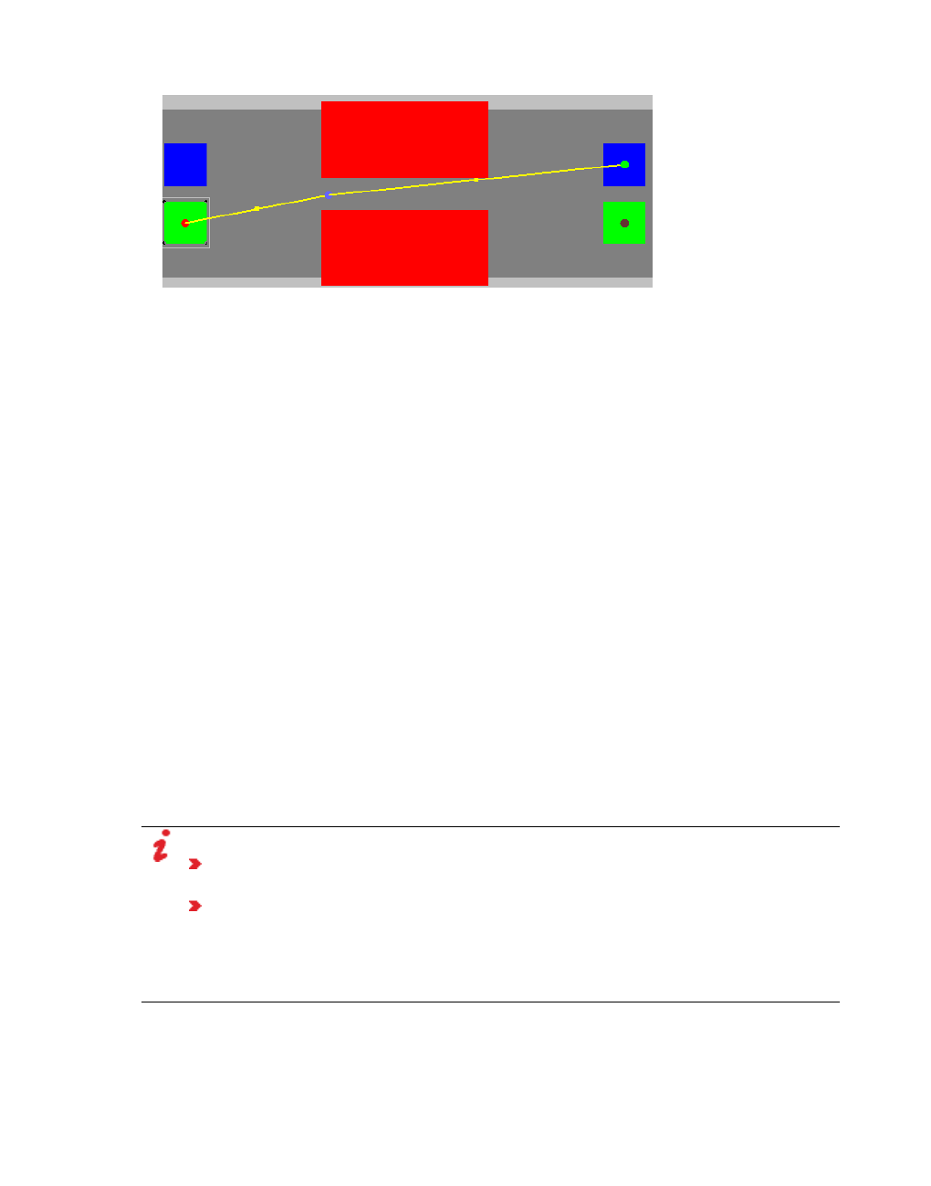
10.13.2 Modeling routing decisions and routes for pedestrians
9. To insert additional destinations, point the mouse pointer to the desired area of your next
destination and carry out the steps again.
When you point the mouse pointer to a destination, a yellow line will appear by default
between the first routing point of the pedestrian route and the destination.
10. If you do not want to add any additional destinations, in the Network editor, click in an
empty area.
Especially when defining several pedestrian routes from the first routing point of a
pedestrian route, use intermediate points in areas and on ramps to model the course of a
route (see "Modeling the course of pedestrian routes using intermediate points" on page
902).
11. You can edit the attributes of a pedestrian route (see "Attributes of static routing decisions
for pedestrian routes" on page 906), (see "Attributes of static pedestrian routes" on page
907).
The attributes are saved to the respective list.
10.13.2.5 Defining partial routing decisions of a pedestrian
Add the first routing point as starting point for a partial pedestrian route to the area of your
choice. You may select attributes, such as the decision model, the pedestrian class and the
route choice method. From this routing point, define one or several partial pedestrian routes
which run through other areas or over other ramps. Using intermediate points in areas and on
ramps allows you to model the course of the route realistically. If several partial pedestrian
routes start at the same routing point, their destinations must be located in the same area.
Notes:
You can specify that you need not press the CTRL key when adding network objects
(see "Right-click behavior and action after creating an object" on page 143).
For some network objects there are windows in which the attributes of a network
object can be defined and edited. There are lists for this, for all network objects. You
can choose whether you want to open a window, a list or neither of the two for the
definition of network objects in the Network Editor (see "Right-click behavior and
action after creating an object" on page 143).
1. On the Network objects toolbar, click Pedestrian Routes.
© PTV GROUP 895

10.13.2 Modeling routing decisions and routes for pedestrians
The button is highlighted. The variant of the network object type is displayed in parentheses
and the button is shown.
2. Click Pedestrian Routes again.
A list box opens.
3. Then click Partial.
4. Press the CTRL key and in the Network editor, right-click the area of your choice.
5. Release the keys.
For the first routing point, a red circle is inserted by default. If you want to insert multiple
pedestrian routes for this first routing point, carry out the following steps accordingly. This
allows you to add a destination and pedestrian partial route.
The window Pedestrian Routing Decision (Partial) opens.
6. Make the desired changes:
Element Description
Decision Number of partial routing decision
Start area Name of area for which the partial routing system has been defined. In the
list box, you can select another area as your start area.
Destination
area
is empty before you insert the partial routing decision. Afterwards, it shows
the name of the destination area.
Destination
ramp
is empty before you insert the partial routing decision. Afterwards, it shows
the name of the destination ramp.
Decision
models
Select option:
Entering the area: This partial routing decision function applies as soon
as the pedestrian enters the area. Select this option when decision-rel-
evant criteria are likely to change rather quickly, e.g. when you select the
Static route choice method which has the same number of route choices
for the pedestrian routes.
Every time step: The partial routing decision function applies in each
time step when the pedestrian is in the area. Select this option when
there are only minor or no changes to the decision-relevant criteria, e.g.
when you select the Density route choice method in order to find an
area with the lowest density.
896 © PTV GROUP

10.13.2 Modeling routing decisions and routes for pedestrians
Element Description
Pedestrian
classes
Select option:
All pedestrian types of pedestrian class
individual pedestrian classes
Route
choice
method
Select static or dynamic route choice method (see "Modeling partial routes
for pedestrians" on page 888):
Static (see "Defining static pedestrian routes" on page 894)
Travel time (see "Route choice method with the criterion Travel Time" on
page 898)
Service point selection (see "Route choice method - service point selec-
tion" on page 914)
Quantity (see "Route choice method with the criterion Quantity" on page
899)
Density (see "Route choice method with the criterion Density" on page
900)
7. Point the mouse pointer to the destination area of your choice.
The border of the destination area is highlighted.
8. Press the CTRL key and right-click in the destination area.
9. Release the keys.
By default, a turquoise circle is inserted. By default, a yellow band is shown between red
circle of the first routing point of the partial pedestrian route and the destination. The Partial
Pedestrian Routing Decisions list opens if automatic opening of a list after object
generation is selected (see "Right-click behavior and action after creating an object" on
page 143). You may add further partial pedestrian routes to areas on the basis of the
routing point or stop the addition.
10. To insert additional partial pedestrian routes, point the mouse pointer to the desired area
of your next destination and carry out the steps again.
When you point the mouse pointer to an area, a yellow line will appear by default to the first
routing point of the partial pedestrian route.
11. If you do not want to add any partial pedestrian routes, in the Network editor, click in an
empty area.
Especially when defining several pedestrian routes from the first routing point of a
pedestrian route, use intermediate points in areas and on ramps to model the course of a
route (see "Modeling the course of pedestrian routes using intermediate points" on page
902).
12. You can edit the attributes (see "Attributes of pedestrian partial routes" on page 909), (see
"Attributes of pedestrian partial routing decisions" on page 908).
The attributes are saved to the respective list.
© PTV GROUP 897
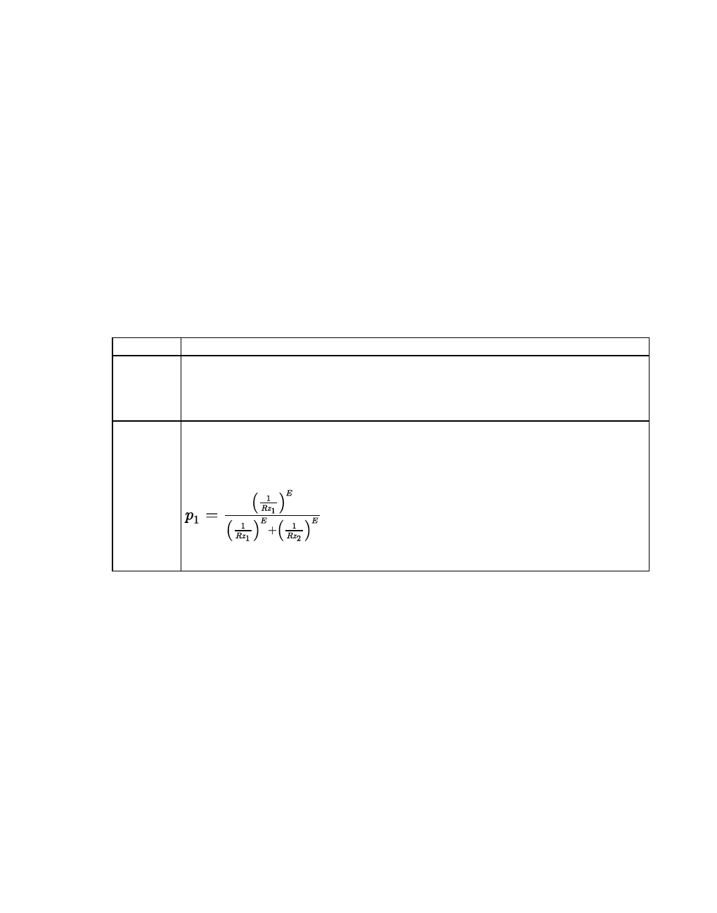
10.13.2 Modeling routing decisions and routes for pedestrians
13. Define route choice areas for the route choice methods Quantity and Density or generate
this automatically (see "Selecting route choice areas" on page 901).
Route choice method with the criterion Travel Time
The following steps are performed:
1. The pedestrians are equally distributed across all pedestrian routes of the routing decision.
2. Vissim evaluates the travel times of the pedestrians who have finished this pedestrian
route. You can enter the number of these pedestrians in the field Average of the last
<number> pedestrians. The default value is 10. If the number of pedestrians is < 10, an
even distribution is taken as a basis.
3. Travel time of route i = Ti is the average travel times of the last user-defined number of
pedestrians who have finished a route. It can also be the average of travel times of
pedestrians who have so far arrived at the route destination.
You can select the following Route choice parameters:
Option Meaning
Best
Route
The user-defined percentage of pedestrians uses the best route. That is the route
with the least travel time. If there are two best routes, the volumes are distributed
equally on both routes. The remaining pedestrians are distributed randomly
across the other routes. Default value of 90.00%.
Kirchhoff Kirchhoff exponent: The probability of a route choice is calculated as the
reciprocal of the travel time RZ to the power of Kirchhoff exponent E) divided by
the sum of these powers for all routes, default value 3.5. For two partial routes,
the relative volume pi for partial route 1 is:
898 © PTV GROUP
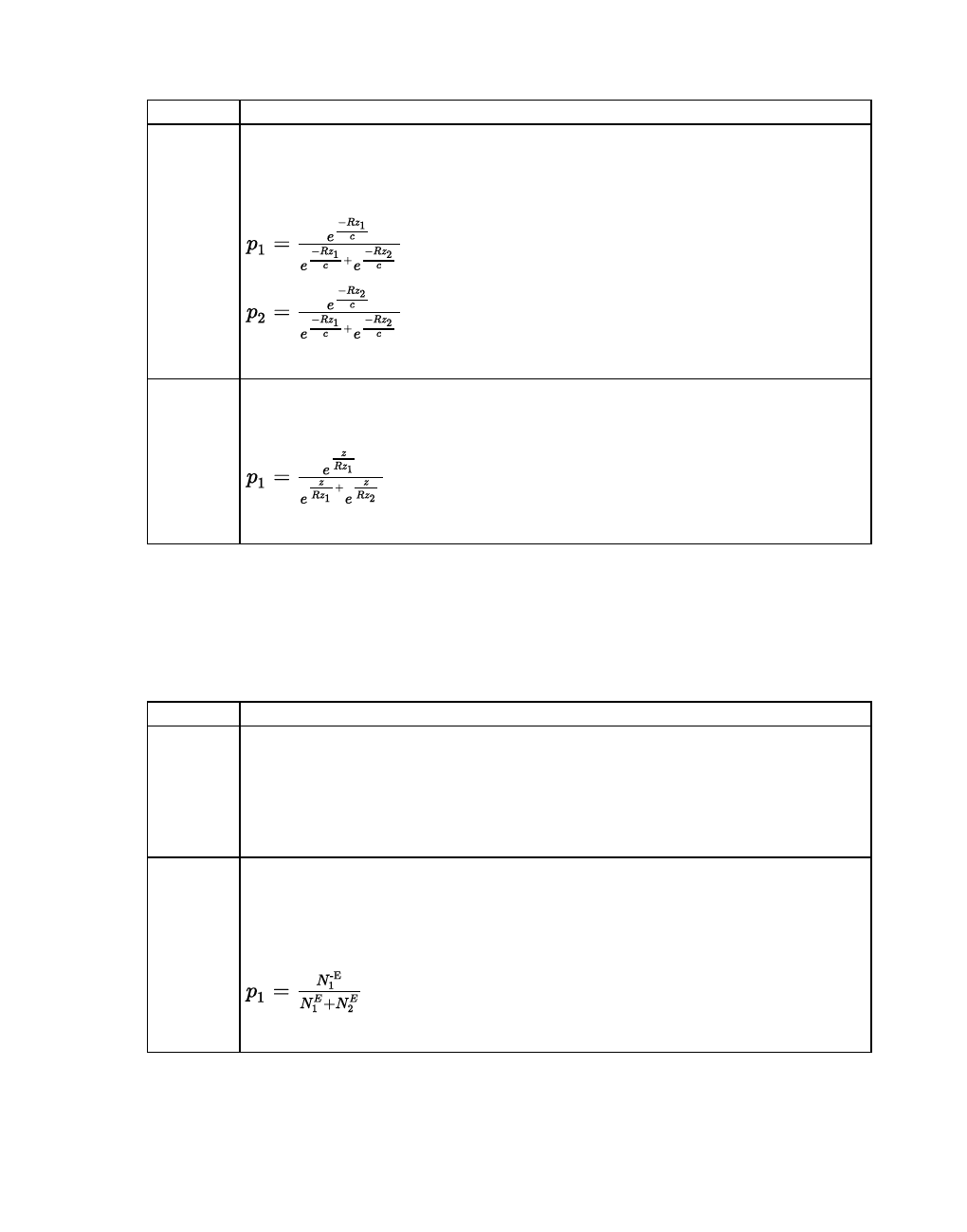
10.13.2 Modeling routing decisions and routes for pedestrians
Option Meaning
Logit Logit - denominator: The probability of a route choice is calculated as exponent e
to the power of (the negative travel time-RZ divided by the user-defined
denominator c), divided by the sum of these powers for all routes, default value
10 seconds:
Logit of
reciprocal
Logit of reciprocal - numerator z: the probability of a route choice is calculated as
exponent e, to the power of (the numerator z divided by the travel timeRZ),
divided by the sum of these powers for all routes, default value 10 seconds:
Route choice method with the criterion Quantity
Vissim calculates the number of pedestrians in the areas of the pedestrian partial routing
decisions. Then Vissim calculates the number of pedestrians in areas with the pedestrians'
relevant partial routing decisions.
You can select the following Route choice parameters:
Option Meaning
Best
route
The user-defined percentage of pedestrians uses the best route. It follows the
pedestrian route whose areas have the lowest number of pedestrians. These
areas include the pedestrians' relevant partial routing decisions. If there are
multiple best routes, the volumes are distributed equally across them. The
remaining pedestrians are distributed randomly across the other routes. Default
value of 90.00 %.
Kirchhoff Kirchhoff exponent E: The probability pi of a route choice is calculated as the
quotient reciprocal of the number N of the relative volumes, to the power of
negative Kirchhoff exponent -E, divided by the sum of these powers for all routes,
default value 3.5. For two partial routes, the relative volume pi for partial route 1
is:
© PTV GROUP 899

10.13.2 Modeling routing decisions and routes for pedestrians
Option Meaning
Logit Logit - denominator c: The probability of a route choice is calculated as exponent
e to the power of (the negative quantity -N divided by the user-defined
denominator) c, divided by the sum of these powers for all routes, default value
1.00:
Logit of
reciprocal
Logit of reciprocal - numerator z: the probability of a route choice is calculated as
exponent e, to the power of (the numerator z divided by the quantityN), divided by
the sum of these powers for all routes, default value 1.00:
Combination method: Calculation of the number of pedestrians from the route choice areas
Total: Total number from all route choice areas. When route choice areas overlap,
these areas and the pedestrians there are each taken into account only simply.
Average: Average number from all route choice areas
Maximum: Maximum number from all route choice areas
Minimum: Minimum number from all route choice areas
Applies to average, maximumand minimum: When route choice areas overlap, these areas
and the pedestrians there are taken into account several times, and so the number of
pedestrians for each area is determined separately.
Route choice method with the criterion Density
Vissim calculates the number of pedestrians in the areas of the pedestrian partial routing
decisions. Then Vissim calculates the volume of pedestrians in areas with the pedestrians'
relevant partial routing decisions on the basis of the route choice parameters.
You can select the following Route choice parameters:
Option Meaning
Best
route
The user-defined percentage of pedestrians uses the best route. It traverses the
area with the lowest pedestrian density. If there are multiple best routes, the
volumes are distributed equally across them. The remaining pedestrians are
distributed randomly across the other routes. Default value of 90.00%.
900 © PTV GROUP
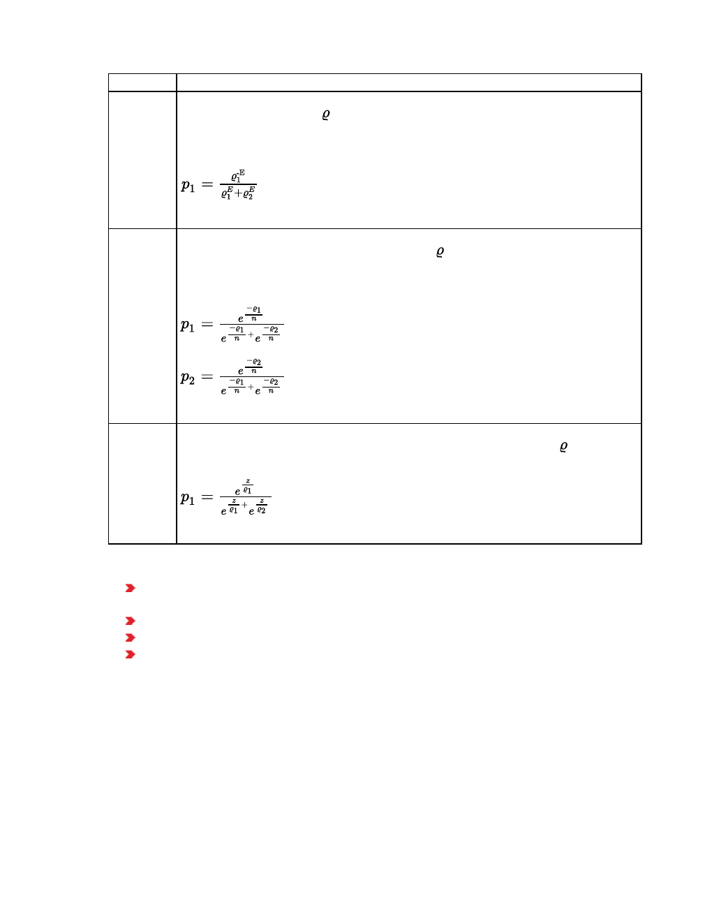
10.13.2 Modeling routing decisions and routes for pedestrians
Option Meaning
Kirchhoff Kirchhoff exponent E: The probability of a route choice is calculated as the
reciprocal of the density, to the power of negative Kirchhoff exponent -E
divided by the sum of these powers for all routes, default value 3.5. For two
partial routes, the relative volume pi for partial route 1 is:
Logit Logit - denominator n: The probability of a route choice is calculated as
exponente to the power of (negative density - divided by the user-defined
denominatorn) divided by the sum of these powers for all routes, default value
1.33 pedestrian/m2:
Logit of
reciprocal
Logit of reciprocal - numerator z: the probability of a route choice is calculated as
exponent : e to the power of (the numeratorz divided by the density ) divided by
the sum of these powers for all routes, default value 1.33 pedestrian/m2:
Combination method: Calculation of the number of pedestrians from the route choice areas
Total: Total density from all route choice areas. When route choice areas overlap, these
areas and the pedestrians there are each taken into account only simply.
Average: Average density from all route choice areas
Maximum: Maximum density from all route choice areas
Minimum: Minimum density from all route choice areas
Applies to average, maximum and minimum: When route choice areas overlap, these areas
and the pedestrians there are taken into account several times, and so the density of
pedestrians for each area is determined separately.
Selecting route choice areas
Through route choice areas Vissim collects the density and number of pedestrians as the
basis for the calculation of relative volumes when selecting a route.
© PTV GROUP 901

10.13.2 Modeling routing decisions and routes for pedestrians
You may take into account all areas or ramps in your Vissim network as route choice areas
which include intermediate points of the pedestrian route. Or you may select individual areas
or ramps to be used as route choice areas.
When you change the course of a partial route and therefore position intermediate points in
other areas, repeat the steps.
Select areas with intermediate points as route choice areas
1. Under the Lists menu, choose Pedestrian traffic > Partial routes.
2. Right-click the entry of your choice.
3. In the context menu, select the entry Automatically generate route choice areas.
All areas where the intermediate points of the pedestrian partial route are situated are used
as route choice areas. You can select the combination method through which the number
or density of the pedestrians on the route choice areas is calculated (see "Modeling partial
routes for pedestrians" on page 888).
Tips:
Alternatively, you can also right-click the desired partial route in the network editor
and choose the entry Generate route choice areas automatically in the context
menu.
You can also select multiple partial routes and choose the entry Generate route
choice areas automatically in the context menu.
Select an individual area as route choice area
1. Under the Lists menu, choose Pedestrian traffic > Partial routes.
2. Right-click the entry of your choice.
3. Select Relations > Pedestrian route choice areas.
The right-hand list is shown. If there is no assignment, only the column titles are shown.
4. Repeat the next steps until you have selected all desired areas or ramps in the list.
5. From the shortcut menu, choose Add.
6. In the list on the right, right-click a free area.
A new row with default data is inserted.
7. Select the desired area or ramp.
10.13.2.6 Modeling the course of pedestrian routes using intermediate points
After you insert intermediate points, a pedestrian route, by default, has the following objects
and is displayed as a line:
a routing decision in the start area
the destination pedestrian route location in the area where the pedestrian route ends
902 © PTV GROUP

10.13.2 Modeling routing decisions and routes for pedestrians
The route course is shown as a yellow line.
The yellow line contains a yellow dot in the middle.
You can insert an intermediate point of the route into each area you want the pedestrian route
to traverse. You can move a pedestrian route location to a different area. Examples of use:
You want the pedestrian route to traverse certain areas. You e.g. want to add addi-
tional destinations for the pedestrian route or partial pedestrian routes.
You want to edit attributes that have an impact on the pedestrian route of an area, e.g.
Cell size, Obstacle distance, Potential calculation method, attributes for dynamic
potential.
You want to assign the pedestrian route location to another area or ramp
In the following cases, a route location on a ramp or stairway defines the direction that the
pedestrian takes on the ramp or stairway. In these cases, the pedestrian uses the entire ramp
or stairway:
The previous pedestrian route location of the pedestrian route or the pedestrian’s rout-
ing decision must be on the same level of the ramp or stairway. This is the start or end
level of the ramp or stairway.
The previous pedestrian route location of the pedestrian route must no be part of an
area for which the Waiting area for elevators attribute is selected. Near these waiting
areas, the pedestrian always uses the ramp or stairway towards the start - end level.
You can edit the attributes for each pedestrian route location (intermediate point or
destination) (see "Attributes of pedestrian route locations" on page 904).
1. On the Network objects toolbar, click Pedestrian Routes.
2. In the Network editor, click the destination of the desired pedestrian route.
A yellow band is shown between the first routing point of the pedestrian route and the
destination, including an intermediate point in the middle.
3. Click the intermediate point, hold the mouse button down, and drag the point to the ramp,
stairway or area of your choice.
4. Release the mouse button.
The course of the pedestrian route is adjusted. The intermediate point is larger and displayed
as a blue circle by default (in the figure in the middle of the upper area). Additional yellow
points are displayed (in the figure on the left and right lower margin of the upper area). Using
these points, you can model the pedestrian routes in more detail.
Note: Within a pedestrian area, there must not be two adjacent intermediate points of a
static pedestrian route or a partial pedestrian route.
© PTV GROUP 903
10.13.2 Modeling routing decisions and routes for pedestrians
10.13.2.7 Attributes of pedestrian route locations
You can edit attributes of pedestrian route locations:
Destination: A pedestrian route location in a destination area, by default displayed as a tur-
quoise circle. If you are using dynamic potential, it is displayed as a turquoise square.
Route location: A pedestrian route location in an area the pedestrian route traverses, by
default displayed as a blue circle. If you are using dynamic potential, it is displayed as a
blue square.
Editing attributes of the destination
The turquoise dot or turquoise square, representing the destination of a pedestrian route, is
also shown when the pedestrian route is not selected.
1. In the Network editor, double-click the turquoise point of the pedestrian route.
The Pedestrian Route Location window opens.
2. Edit the entries of your choice, see table below.
Editing the attributes of a pedestrian route location
The blue intermediate points of a pedestrian route are displayed when the pedestrian route is
selected.
1. On the Network objects toolbar, click Pedestrian Routes.
2. In the desired pedestrian route, click the turquoise point of the destination.
The pedestrian route is displayed as a yellow line with blue route locations.
3. Double-click the desired route location.
The Pedestrian Route Location window opens.
4. Make the desired changes:
Column Description
Decision Number of routing decision of pedestrian route
Route Number of routing decision and number of pedestrian route
Area Area in which the routing point is located In the list box, in the areas list, you
can click another route location the pedestrian route runs through.
Ramp Ramp that lies on the routing point. In the list box, in the ramps list, you can
click another ramp for the route location the pedestrian route runs through.
Cell size Edge length of a grid mesh used for the calculation of distances to the
destination area with the static or dynamic potential (see "Defining global
model parameters" on page 825). Default value 0.15 m. Avoid values > object
radius.
904 © PTV GROUP

10.13.2 Modeling routing decisions and routes for pedestrians
Column Description
Obstacle
distance
Distance up to which the nearby walls have a bearing on the distance potential
(see "Defining global model parameters" on page 825). Default 0.5 m.
Dynamic
potential
UseDynPot: Routing takes place along the path with the lowest estimated
travel time that pedestrians can take within a single level. Enables the input
boxes for the parameters of dynamic potential (see "Dynamic potential" on
page 910), (see "Defining dynamic potential" on page 911).
5. Confirm with OK.
Tips:
Alternatively, open the Pedestrian Route Location window for a route location that is
an intermediate point or destination. To do so, in the Network editor, right-click the route
location of your choice. Then from the shortcut menu, choose Edit.
Editing additional attributes in the attribute list Route locations
In the attribute list Route locations, you can edit additional attributes of route locations.
1. From the Lists menu, choose Pedestrian Traffic > Static Routes.
The list of attributes opens.
The attribute and attribute values of this network object type are shown in the list on the left,
which consists of two coupled lists.
2. In the Static Pedestrian Routes list, on the toolbar, in the Relations list box, click Route
locations.
The Route locations list is displayed on the right. By default, you can edit the list (see
"Using lists" on page 89).
Note: In lists, you can use the Attribute selection icon to show and hide attribute
values (see "Selecting attributes and subattributes for a list" on page 106).
In the Route locations list, in addition to the attributes described above, you can show and
edit the following attributes:
© PTV GROUP 905

10.13.2 Modeling routing decisions and routes for pedestrians
Column Description
Dynamic potential - cal-
culation interval
Dynamic potential - g
(general strength)
Dynamic potential - h (dir-
ection impact)
Dynamic potential -
impact
(see "Defining dynamic potential" on page 911)
Ban elevator use If a route location of a pedestrian route or partial pedestrian
route lies on a ramp or stairs and you selected the attribute
Ban elevator use for it, the pedestrian will not use the
elevator until he has reached the next route location for
which this attribute has not been selected.
Point x and y coordinates of route location
WKT point x and y coordinates of the route location in the Well-known
text format
xx coordinate of route location
yy coordinate of route location
10.13.2.8 Attributes of static routing decisions for pedestrian routes
You may edit the attributes of different variants.
1. From the Lists menu, choose Pedestrian Traffic > Static Routing Decisions.
The list of attributes opens.
The attribute and attribute values of this network object type are shown in the list on the left,
which consists of two coupled lists.
Note: In lists, you can use the Attribute selection icon to show and hide attribute
values (see "Selecting attributes and subattributes for a list" on page 106).
The list on the left may include the following attributes:
Column Description
No Number
Name Designation
Area Name of the area for which a routing decision has been defined.
PedClasses Pedestrian classes
Showing and editing dependent objects as relation
The attribute and attribute values of this network object type are shown in the list on the left,
which consists of two coupled lists.
1. In the list on the left, click the desired entry.
906 © PTV GROUP

10.13.2 Modeling routing decisions and routes for pedestrians
The list on the right contains attributes and attribute values of network objects, and/or base
data allocated to the network object selected in the list on the left (see "Using coupled lists" on
page 111):
Pedestrian Classes (see "Attributes of pedestrian classes" on page 833)
Pedestrian routes (static)
2. On the list toolbar, in the Relations list, click the desired entry.
3. Enter the desired data.
The data is allocated.
10.13.2.9 Attributes of static pedestrian routes
You may edit the attributes of different variants.
1. From the Lists menu, choose Pedestrian Traffic > Static Routes.
The list of attributes opens.
The attribute and attribute values of this network object type are shown in the list on the left,
which consists of two coupled lists.
Note: In lists, you can use the Attribute selection icon to show and hide attribute
values (see "Selecting attributes and subattributes for a list" on page 106).
The list on the left may include the following attributes:
Column Description
No Number
Name Designation
RelFlow (0) relative volume
PedRoutDecSta Pedestrian Routing Decisions (Static )
Showing and editing dependent objects as relation
The attribute and attribute values of this network object type are shown in the list on the left,
which consists of two coupled lists.
1. In the list on the left, click the desired entry.
The list on the right contains attributes and attribute values of network objects, and/or base
data allocated to the network object selected in the list on the left (see "Using coupled lists" on
page 111):
Route locations
2. On the list toolbar, in the Relations list, click the desired entry.
3. Enter the desired data.
The data is allocated.
© PTV GROUP 907

10.13.2 Modeling routing decisions and routes for pedestrians
10.13.2.10 Attributes of pedestrian partial routing decisions
You may edit the attributes of different variants.
1. From the Lists menu, choose Pedestrian Traffic > Partial Routing Decisions.
The list of attributes opens.
The attribute and attribute values of this network object type are shown in the list on the left,
which consists of two coupled lists.
Note: In lists, you can use the Attribute selection icon to show and hide attribute
values (see "Selecting attributes and subattributes for a list" on page 106).
The list on the left may include the following attributes:
Column Description
No Number
Name Designation
Area Name of area for which the partial routing decision has been
defined.
AllPedTypes Select this option if you want the partial routing decision to
be valid for all pedestrian types of the pedestrian class.
NumPedsForAvg Number of pedestrians (for calculation of average)
NumPedsInQueue Number of pedestrians in queue
PedClasses Pedestrian classes
BestRoutPerc Best route percentage for dynamic route choice with the
Travel time criterion (see "Route choice method with the
criterion Travel Time" on page 898)
DecModel Decision model: Defines when the route choice affects
pedestrians of the pedestrian routing decision area.
Area walked on: The route choice affects passengers only
in the time step during which the passenger walks in the
partial routing decision area.
Each time step: The route choice affects passengers from
the time step in which they step into the partial routing
decision area until the time step when they leave the area.
KirchExp Kirchhoff exponent for dynamic route choice with the criterion
Travel time
LogitDenom Logit - Denominator for dynamic route choice with the criterion
Count, Density or Travel time
LogitRecipNum Logit of reciprocal - numerator for dynamic route choice with
the criterion Count, Density or Travel time
908 © PTV GROUP

10.13.2 Modeling routing decisions and routes for pedestrians
Column Description
RouteChoiceMeth Route choice method for pedestrian routes (partial) (see
"Defining partial routing decisions of a pedestrian" on page
895)
RoutChoiceAreaCombMeth Combination method for the route choice methods with the
criteria of Count and Density (see "Route choice method with
the criterion Quantity" on page 899), (see "Route choice
method with the criterion Density" on page 900)
Showing and editing dependent objects as relation
The attribute and attribute values of this network object type are shown in the list on the left,
which consists of two coupled lists.
1. In the list on the left, click the desired entry.
The list on the right contains attributes and attribute values of network objects, and/or base
data allocated to the network object selected in the list on the left (see "Using coupled lists" on
page 111):
Pedestrian Classes (see "Attributes of pedestrian classes" on page 833)
Pedestrian routes (partial)
2. On the list toolbar, in the Relations list, click the desired entry.
3. Enter the desired data.
The data is allocated.
10.13.2.11 Attributes of pedestrian partial routes
You may edit the attributes of different variants.
1. From the Lists menu, choose Pedestrian Traffic > Partial routes.
The list of attributes opens.
The attribute and attribute values of this network object type are shown in the list on the left,
which consists of two coupled lists.
Note: In lists, you can use the Attribute selection icon to show and hide attribute
values (see "Selecting attributes and subattributes for a list" on page 106).
The list on the left may include the following attributes:
Column Description
No Number
Name Designation
RelFlow (0) relative volume
PedRoutDecPart Pedestrian routing decision (partial)
© PTV GROUP 909

10.13.3 Dynamic potential
Showing and editing dependent objects as relation
The attribute and attribute values of this network object type are shown in the list on the left,
which consists of two coupled lists.
1. In the list on the left, click the desired entry.
The list on the right contains attributes and attribute values of network objects, and/or base
data allocated to the network object selected in the list on the left (see "Using coupled lists" on
page 111):
Pedestrian route choice areas
Route locations
2. On the list toolbar, in the Relations list, click the desired entry.
3. Enter the desired data.
The data is allocated.
10.13.3 Dynamic potential
Dynamic potential is a route-based method used to control the search for the best route that
pedestrians can take within a level. Thereby pedestrians are not meant to take the shortest
distance path, but the path with the least estimated travel time to their destination or
intermediate destination.
The dynamic potential method is spatially continuous and complements the pedestrians'
dynamic partial route which takes the number, volume or travel time of pedestrians into
account.
For both the dynamic potential and partial route method, the travel time reduction is the
determining factor for walking behavior. Travel time based partial routes that are based on the
dynamic potential method, however, provide pedestrians with a discrete choice of different
routes at a certain time. If the dynamic potential is active for a destination or an intermediate
destination, pedestrians will try to take the route they currently believe is the quickest. This
means pedestrians want to move in a direction that according to a heuristic mathematical
method is considered the shortest walking time to the next destination or intermediate
destination.
Even this rather simplified description of the dynamic potential methods shows its continuous
character. There is no specific decision point. Pedestrians continuously aim at optimizing their
travel time. This is limited by the simulation time step only. Pedestrians do not try to take the
path with the shortest travel time out of a limited number of user-defined routes. With the
dynamic potential method, pedestrians choose their trajectory automatically, and thus their
route from a continuously unlimited and uncountable number of possible trajectories.
Calculation of the dynamic route potential is very computation time consuming. The dynamic
potential field for a specific route is only calculated as long as there are pedestrians that
actually use the route.
910 © PTV GROUP

10.13.3 Dynamic potential
10.13.3.1 Dynamic potential use cases
The dynamic potential is limited to the level you have specified it for. The dynamic potential
method cannot be applied to multiple levels and is not meant to find the fastest route across
multiple levels. This is where you use partial routes.
Using dynamic potential or travel time based partial routes for a level
There are many use cases where you can apply both methods. Experience has shown that in
some cases partial routes may be the better method, whereas in other cases dynamic
potential should be preferred. There are use cases for which both methods lead equally to the
results desired and others in which neither do.
When modeling scenarios, partial routes can be used for discrete choices. Partial routes
are discrete, whereas the dynamic potential is continuous in several respects.
When modeling continuous choices, you should opt for the dynamic potential method.
Example:
You are modeling a large number of pedestrians at, for example, a 90° corner, using the
dynamic potential method. If there are also several service points in the corner, the selected
quantity becomes discrete. For these routes, you can use partial routes because the distance
from the starting point to the individual service points is different.
Modeling effort and computation time
In general, there is less modeling effort required for the dynamic potential method than for
partial routes. Even so, you should avoid modeling use cases with the dynamic potential
method that are better suited for the partial routes method. In spite of the higher modeling effort
required for partial routes, by default the simulation speed is faster than when you apply the
dynamic potential method.
10.13.3.2 Defining dynamic potential
You define the dynamic potential on the destination of a pedestrian route (static).
1. On the Network objects toolbar, click Pedestrian Routes.
2. In the Network Editor, click on the destination point (default color: turquoise) of the desired
static route.
The course of the static route is shown as a yellow line by default. The routing decision, the
destination point, auxiliary points and intermediate points are shown in color.
3. Double-click the destination.
The Pedestrian Route Location window opens.
4. Select the option Use dynamic potential.
5. Enter the desired values.
© PTV GROUP 911

10.13.3 Dynamic potential
Element Description
Impact Deviation from the static potential. Factor influencing ealpha ffor weighting
when calculating the path selection (see "Description of the method
Dynamic Potential" on page 913).
Standard value 100 % = Pedestrians follow the direction which is cal-
culated on the basis of the Dynamic Potential.
0 % = Pedestrians follow the direction which is calculated on the basis of
the Static Potential.
The angles inbetween are obtained from the values inbetween. A useful
impact depends on the value of the general strength g.
Calculation
interval
Time interval after which the potential in each case should be updated.
As the dynamic potential requires a lot of calculation time, an extension of
the calculation interval can ensure an acceptable simulation speed with a
slow computer and many active dynamic potentials.
However, a shorter calculation interval improves the results.
g (basic
force)
Defines how the loss time for occupied grid cells is estimated in relation to
unoccupied ones, when a pedestrian must walk around a group of
pedestrians, forming a circle or square, and there are no obstacles that
could extend the path (see "Defining global model parameters" on page
825). Default value for g = 1.5.
Basic force g = 1.5 and impact 100%: Pedestrians no longer want to use
the fastest path and only react to other pedestrians in order to avoid col-
lisions.
g > 3 and impact of approximately 100% or only slightly below can lead
to unrealistic behavior of pedestrians, for example, to zig-zag move-
ments or stopping short.
If the effect of the dynamic potential with an impact of 100% also appears
too weak, increase the value of the parameter g. Do not enter any impact
over 100%.
General strength g = 0: estimated loss time = 0. Impacts simulation as if
the dynamic potential was switched off. The estimated travel time is pro-
portional to the remaining path distance. Thus, routing is more likely to
take place along the shortest path. Pedestrians only react to other ped-
estrians in order to avoid collisions.
General strength g = 1: the estimated loss time is as long as the time it
takes to cross this cell in the unoccupied state, i.e. the required time is
doubled.
912 © PTV GROUP

10.13.3 Dynamic potential
Element Description
h (direction
impact)
Influence of the direction of movement of a pedestrian on the calculation of
the dynamic potential (see "Defining global model parameters" on page
825).
Default = 0.7
h = 0.0: There is no influence.
h = 1.0: Pedestrians, moving at a free walking speed, are evaluated
depending on the direction of the geographically shortest path to the
route destination for which the dynamic potential is activated:
not evaluated if they move in the exact direction of the route des-
tination
evaluated twice if they move in the exact opposite direction to the
route destination
evaluated once if they move in the exact orthogonal direction to the
route destination
Slower pedestrians in the direction of the destination are graded less
than once accordingly.
Slower pedestrians away from the destination are graded between
once and twice.
h > 1.0: only useful in exceptional cases. Thus a negative value cannot
be achieved.
6. Confirm with OK.
The window closes. The destination point and the intermediate points of the pedestrian route,
for which a dynamic potential is defined, are shown as squares.
10.13.3.3 Description of the method Dynamic Potential
An important basis for the dynamic potential is the method in which pedestrians generally find
their next destination area in a simulation. This is achieved because the driving force of the
social force model points towards the next destination as long as the pedestrian does not walk
in this direction:
Where:
: pedestrians current velocity
: desired speed of the pedestrian based on the user-defined distribution
: Direction of the desired speed (unit vector): from which the multiplication of the desired
walking speed results in the current desired walking speed. is obtained from the Static
Potential or Dynamic Potential or a linear combination of both values.
© PTV GROUP 913
10.13.3 Dynamic potential
Using the Static Potential in Vissim always points in the direction of the path with the
shortest distance.
Using the Dynamic Potential points in the direction of the path with shortest time according
to the current estimation. This may not be the absolutely right direction of the path with the
shortest time in terms of analytics. Due to the fact that in reality pedestrians are often confused
regarding which direction at the current time can lead them to their destination the quickest, it
is not a big problem that the actual direction of the quickest path cannot be precisely
calculated. Therefore, the hypothetical assumption that the direction of the path with the
shortest time is known in the simulation and hence the behavior of each pedestrian is optimal,
is probably not realistic.
Parameter Impact (see "Defining dynamic potential" on page 911): The value s for the
direction of the path with the shortest distance and the value q for the direction of the path
with the shortest time. The value is derived therefrom. s and q are included in
accordance with the value of the impact parameter as a weighting.
Tip: You will find further information in the document Quickest Paths in Simulations of
Pedestrians, Kretz T., Große A. u.a., Karlsruhe, 2011
Regardless of whether points in the direction of the path with the shortest distance (Static
Potential is used, the Dynamic Potential is not used) or in the direction of the path with the
shortest time (the Dynamic Potential is used at 100 %), when calculating the first step is to
determine the values for the points of the grid which indicate either the distance or the
estimated remaining travel time from the respective point to the relevant distance area. The
grid is consistent with the potential. Since the distance from a grid point to the destination does
not change during the simulation run, the potential that provides the distance values, referred
to as static potential, acts as a "Look- up" table. In contrast, with the consideration of all
pedestrians in the network at the same time, the estimated remaining travel time to the
destination changes continuously for each grid point. Thus this potential is referred to as
dynamic potential. If you imagine the values of this potential as rising or increasing values,
points in the direction of the descent, which mathematically represents the (negative) gradient.
As soon as has been calculated based on the static or dynamic potential, the value is
applied in the driving force term. The total of the driving force and the social forces is included
for acceleration of the pedestrian in the respective time step.
10.13.3.4 Route choice method - service point selection
You can use the service point selection route choice method to perform dynamic pedestrian
routing.
Tip: Network files, including examples, can be found in the folder ..\Documents\PTV
Vision\PTV Viswalk <Version>\Queuing:
04 Service Points.inpx
04 Service Points 2.inpx
914 © PTV GROUP

10.13.3 Dynamic potential
Use cases for the service point selection method
The route choice method service point selection is suited for the following use cases:
Central queue
To model a single joint queue for multiple service points. In reality, the "first come – first
served" principle is practiced in post offices, at train stations or airports. Pedestrians are not
only queuing in front of the service points, but they may also wait in areas in front of these
points. The Queue attribute of the area which relates to the partial route decision must be
selected. The area is thus turned into a queue area.
Immediate service point allocation
A simple decision model for multiple service points. The pedestrians wait at each service
point with a separate queue. The pedestrian has to decide which queue to join. Normally,
pedestrians will choose the queue with the shortest waiting time. However, it is not easy to
tell which one that is, particularly when there is a large number of service points and/or
queues, e.g. at supermarket checkouts or ticket gates. The Queue attribute of the area in
front of the service points must be selected. The areas are thus turned into queue areas.
Survey/interview
Individual pedestrians walking by are asked to stop for a minute, e.g. to answer a few
questions in a questionnaire. Afterwards, they continue their route.
You can also model pedestrians who wait in a central area and then go to the service
points where queues may occur.
Effects on routing
Pedestrians affected by this partial routing decision can be influenced in their routing behavior
as follows:
Routing to a central queue in the area containing a partial routing decision. This area must
be a queue area. The waiting time refers to the area containing a partial routing decision.
Direct routing to a queue in a queue area. The area where the partial routing decision is
made must not be a queue area. At least one of the service points should not have
reached its maximum number of waiting pedestrians in order to allow pedestrians to join
the queue. You can enter them as Proceed to service point if no more than __ people
are queuing there parameter of the partial routing decision. If all queues are longer, the
partial routing decision is ignored and the pedestrian ignores the service points.
The service point is the first queue area on the course of the route that includes an
intermediate point of the partial route.
Modeling suggestions for these use cases
Tip: Your Vissim installation provides modeling examples for test applications:
..\Examples Training\Pedestrians\Queuing\08 - Service Desk Partial Routes - Use
Cases.inpx
In all figures below, the pedestrian streams go from left to right.
© PTV GROUP 915

10.13.3 Dynamic potential
Symbol Name Description
Pedestrian
area
The Queue option is selected.
Pedestrian
area
The Queue option is not selected.
Static rout-
ing decision
Route point where a pedestrian route starts (static).
In the pictures below, in the left areas in which pedestrian inputs are
defined as well.
Partial rout-
ing decision
Partial routing decision with route choice method Service point
selection In the pictures below, in the waiting areas.
Use case 1: Central queue, the Queue option s selected
Typically, the queue threshold nis as follows: Proceed to service point if no more than __
people are queuing there = 0.
This ensures that there is no queue at the service point.
Use case 2: Immediate service point allocation Queue option is not selected
Typically, the queue threshold nis as follows: Proceed to service point if no more than __
people are queuing there = 99.
This ensures that all pedestrians join a queue.
916 © PTV GROUP

10.13.3 Dynamic potential
Scenario 3: Survey/interview
Typically, the queue threshold nis as follows: Proceed to service point if no more than __
people are queuing there = 0.
This ensures that there is no queue at the service point.
10.13.3.5 Prerequisites and requirements of the service point selection method
The main difference between partial routing decisions with the service point selection
method and other partial routing decisions:
For a pedestrian to be able to see the partial route, an intermediate point of the pedestrian's
original route must be positioned in the area where the partial routing decision is made.
This area is therefore a decision area. It is not necessary to select the Queue attribute for
this area (see "Attributes of areas" on page 848).
Pedestrians on a route without an intermediate point in the decision area are not affected
by a partial routing decision. These pedestrians are not going to a service point.
If pedestrians are supposed to go to the service points, each partial route must have an
intermediate point in the area for which the Queue attribute (queue area) was selected.
This way, a queue can be built in this area.
For a central queue, the partial routing decision must be made in a queue area.
For immediate service point allocation, the partial routing decision must not be made in a
queue area.
Each queue area must be assigned a wait time distribution via the Time distribution attrib-
ute (see "Attributes of areas" on page 848).
10.13.3.6 The service point selection method
If the decision area is a queue area with dwell time distribution, the following applies:
The first pedestrian waits until his waiting time at the decision area has expired. In this
case, a wait time distribution must be defined via the Time distribution attribute (see
"Attributes of areas" on page 848).
The first pedestrian waiting continues his way. If there are service points where queues
may occur, he will continue his way toward the "best" queue, which is the shortest one. At
least at one of the service points should have a queue with no more than n waiting
© PTV GROUP 917

10.13.4 Pedestrian OD matrices
pedestrians. You define this number in the attribute Proceed to service point if no more
than __ people are queuing there.. If all the queues are full, the pedestrian waits until
queue space at one of the service points opens up.
If people are queuing on or after a while in front of a decision area, pedestrians, whose
pedestrian class is not affected by the partial routing, are also affected by the queuing, if
an intermediate point of their pedestrian route is part of the decision area. These ped-
estrians also wait in the same queue until they have reached the decision area, wait the
wait time defined in the time distribution, however, do not go to a service point but con-
tinue with their original route.
If the decision area is a queue area without dwell time distribution, the following applies:
If people are queuing on or after a while in front of a decision area, pedestrians, pedestrians
only queue until they have reached the decision area. They then continue with their original
route.
If the decision area is not a queue area, but a time distribution is defined, the following
applies:
A pedestrian of an affected pedestrian class waits until his dwell time has expired and
then continues his way.
Calculation method for finding the best queue
Of all waiting areas the one is selected with no more than n pedestrians waiting in its
queue.
If there is more than one of these queues, the queue with the fewest pedestrians is selec-
ted. It is the shortest queue.
If there is more than one shortest queue, the one with the shortest direct distance to the
end of the routing decision that is closest to the pedestrian's coordinates is selected.
Pedestrians on their way to the service point or ready to join the queue are treated as if they
already were in the queue.
Note: For each partial route, only the first waiting area after the routing decision is taken
into account. Additional waiting areas on the course of the partial route are ignored.
10.13.4 Pedestrian OD matrices
You can enter the pedestrian travel demand for origin-destination relations, i.e. the demand
from origin areas to destination areas. This way, you need not define pedestrian inputs and
pedestrian routes in the network. The origin-destination relations between pedestrian areas
are displayed in a matrix. In the matrix, you enter the hourly pedestrian volume for each origin-
destination relation.
Based on a pedestrian OD matrix, you can save origin-destination data to a file during the
simulation run (see "Saving pedestrian travel time measurements from OD data to a file" on
page 988).
918 © PTV GROUP

10.13.4 Pedestrian OD matrices
Note: Viswalk then internally generates the pedestrian inputs and routing decisions
including static pedestrian routes, if these are not available for the origin-destination
relation. Thereby the volumes entered are taken into account.
10.13.4.1 Conditions for origin areas and destination areas
Areas, which you select as an origin or a destination for an origin-destination matrix, must
meet the following conditions.
Conditions for origin areas in the origin-destination matrix
An area is shown as a row in the origin-destination matrix, if the Always use as origin area
attribute is selected or if the area contains a pedestrian input for any time interval. The area
contains no more than one pedestrian decision. There is no route from this pedestrian routing
decision to a stairway/ramp. If the area contains more than one pedestrian routing decision,
the Always use as origin area attribute has no effect.
Conditions for destination areas in the origin-destination matrix
An area is shown as a column in the origin-destination matrix, if it fulfills at least one of the
conditions:
For the area, the Always use as a destination area attribute is selected.
At least one pedestrian route ends in an area in which an origin area begins.
Notes regarding further network objects
The pedestrian OD matrix only takes into account areas as origins and destinations of
pedestrian flows, because pedestrian inputs and routing decisions can only be included in
areas.
Pedestrian routing decisions (partial) and destinations of partial routes in areas are not rel-
evant to the pedestrian OD matrix.
Stairways, ramps, moving walkways and escalators cannot be the destination of a route in
the pedestrian OD matrix, even though the destination of a static pedestrian route can be
defined for them.
10.13.4.2 Selecting origins and destinations in the Pedestrian OD Matrix
You can select a pedestrian area as origin or destination of pedestrians in the Pedestrian OD
Matrix. Specific conditions must be fulfilled for this to occur (see "Conditions for origin areas
and destination areas" on page 919) . You can also copy and edit existing origins and
destinations.
Tip: Alternatively you can select Always use as origin area and/or Always use as
destination area for an area (see "Attributes of areas" on page 848). Thus the area in
the Pedestrian OD Matrix is shown as an origin area and/or destination area.
1. From the Traffic menu, choose Pedestrian OD Matrix.
© PTV GROUP 919

10.13.4 Pedestrian OD matrices
The Pedestrian OD Matrix window opens.
2. Right-click in the window.
3. From the context menu, select the desired entry: Add Origin or Add Destination.
A window opens and displays the areas from your network in a list box, which do not
contain origins or destinations in the Pedestrian OD Matrix.
4. Select the desired entry.
5. Confirm with OK.
If you have added the area as an origin, it is shown as a new row in the Pedestrian OD
Matrix. The attribute Always use as origin area is activated for this area (see "Attributes of
areas" on page 848).
If you have added the area as a destination, it is shown as a new column in the Pedestrian
OD Matrix. The attribute Always use as destination area is activated for this area (see
"Attributes of areas" on page 848).
Notes:
Vissim does not check if a pedestrian input and a routing decision are in the area.
In the area, neither a pedestrian input nor a routing decision is generated.
6. If desired, repeat these steps for further areas.
7. Enter the desired volumes in pedestrian/h in the fields (see "Defining the pedestrian
demand in the Pedestrian OD Matrix" on page 922).
Tip: You can copy and paste the entries and the matrix via the context menu (see
"Defining the pedestrian demand in the Pedestrian OD Matrix" on page 922).
10.13.4.3 Time intervals in the pedestrian OD matrix
The matrix values specified in the pedestrian OD matrix are hourly values referring the
respective time intervals. The time intervals of a pedestrian OD matrix are predefined through
the time intervals of the following network objects used in the current network:
Pedestrian Inputs (see "Modeling pedestrian inputs" on page 883)
Static pedestrian routes (see "Static pedestrian routes, partial pedestrian routes and ped-
estrian routing decisions" on page 887)
920 © PTV GROUP

10.13.4 Pedestrian OD matrices
If identical time intervals have been defined for pedestrian inputs and pedestrian routes, you
can enter, show, and edit the demand data for each time interval (see "Defining the pedestrian
demand in the Pedestrian OD Matrix" on page 922).
You can, e.g., use the Copy-and-Paste command to adopt interval values for another set of
time intervals.
If the time intervals are not the same, the first pedestrian input interval and the first pedestrian
route are listed above the matrix, in the Pedestrian OD matrix window. You cannot edit the
time intervals of the other matrix values.
10.13.4.4 Using the matrix values in the pedestrian OD matrix
In a pedestrian OD matrix, the hourly pedestrian demand for each OD relation is displayed in
the cells where the Origin column and Destination row overlap.
Each cell value represents the pedestrian volume expected for an origin area to a destination
area in the respective time interval.
Demand data in pedestrian OD matrices in [pedestrians/h]
When pedestrian inputs and static pedestrian routes are defined for a network, matrix data is
created:
Total input volume of origin area during input time interval
Relative volume of static routes to destination area during routing time interval
If no pedestrian inputs or static pedestrian routes have been defined, the program bases the
input volume of the origin area for a time interval on user-defined cell data and then generates
relative volumes for static routes to the destination for a time interval.
If you position two routing decisions for different pedestrian classes on a origin area,
the origin area is deleted from the origin-destination matrix. If you open the Pedestrian
OD matrix window, a message is displayed.
The total input volume is the total of all input volumes of an origin area for a time inter-
val. The pedestrian inputs of an area may consist of different pedestrian compositions
(see "Modeling pedestrian inputs" on page 883). The program does not distinguish
between different pedestrian types or pedestrian compositions for the total of ped-
estrian inputs.
The routing decision of the origin area applies to selected pedestrian classes and/or
all pedestrian types (see "Static pedestrian routes, partial pedestrian routes and ped-
estrian routing decisions" on page 887). For each OD relation there may be several
routes from the routing decision to a destination area. The relative volumes of such par-
allel routes are added in the pedestrian OD matrix.
The matrix value of a cell includes:
© PTV GROUP 921

10.13.4 Pedestrian OD matrices
Note: You can perform a simulation if one of the following conditions is met:
The matrix cell value is = 0 as the input value for the origin area in a time interval is
0.
The matrix cell is empty as there is no pedestrian input or pedestrian routing
decision in the origin area, but the option Always use as origin area has been
selected for the area (see "Defining construction elements as rectangles" on page
844).
10.13.4.5 Defining the pedestrian demand in the Pedestrian OD Matrix
Once you have entered the origins and the destinations, you can define the demand per time
interval in the pedestrian OD matrix for all origin-destination relations in the network.
For origin-destination relations, for which up to now no pedestrian inputs, routing
decisions, and/or static pedestrian routes have been defined, pedestrian inputs, routes
and routing decisions are generated in Vissim. The entered volume is applied.
For origin-destination relations, for which pedestrian inputs, pedestrian routing decisions
and static pedestrian routes are already defined, the input values and the relevant routing
volumes are adjusted respectively. The relationship between unchanged routing volumes
is retained.
Notes:
Matrices must not be symmetrical.
The dimensions of a matrix are the same for all time intervals.
1. From the Traffic menu, choose Pedestrian OD Matrix.
The Pedestrian OD Matrix window opens. Normally you can edit fields and copy, paste
and delete values.
You may enter values or paste values (e.g. from Microsoft Excel tables used in other
programs) from the Clipboard.
Notes:
The volume per OD relation applies only for the currently selected time interval of
the matrix.
An input value cannot be allocated multiple marked OD relations.
922 © PTV GROUP

10.13.4 Pedestrian OD matrices
Entering values
1. Enter the desired volumes in pedestrian/h.
2. If you would like to copy values, mark the desired cells.
3. Right-click in the window.
4. Choose the desired entry from the context menu.
Element Description
Copy
matrix
Copy the matrix data of the entire matrix onto the clipboard in order to be able
to add it into another time interval or document. The table structure is applied.
The labels of the rows and columns are not applied.
Copy
matrix
incl.
headers
Copy the entire matrix onto the clipboard in order to be able to add it to a
document. This contains all matrix data including the labels of rows and
columns as well as the grid structure.
The value for this relation is applied only for the currently shown time interval.
If for this relation no values have been entered in another time interval, the value zero is
automatically entered for this time interval.
If values are entered for this relation in other time intervals, the values remain unchanged.
Pasting values from the clipboard
Values from the clipboard are moved from the cell you selected to the cells below and to the
right via copy & paste. The number of columns and/or cells from the clipboard must not be
higher than the number of columns and/or cells for the origin and destination data used in the
pedestrian OD matrix.
Since an area cannot be simultaneously used as an origin and destination, no values are
entered in these areas. These areas are gray.
1. Make sure that you have copied the correct values of your choice to the clipboard.
2. In the pedestrian OD matrix, right-click the cell used to copy & paste the values to the cell
below and to the right.
3. In the context menu, select Insert.
10.13.4.6 Deleting origins, destinations or values in the Pedestrian OD Matrix
You have the option to delete the following data:
Delete origins line-by-line and destinations column-by-column
Mark values in multiple cells and delete simultaneously
normally individual values in fields
Deleting origins or destinations
1. From the Traffic menu, choose Pedestrian OD Matrix.
© PTV GROUP 923
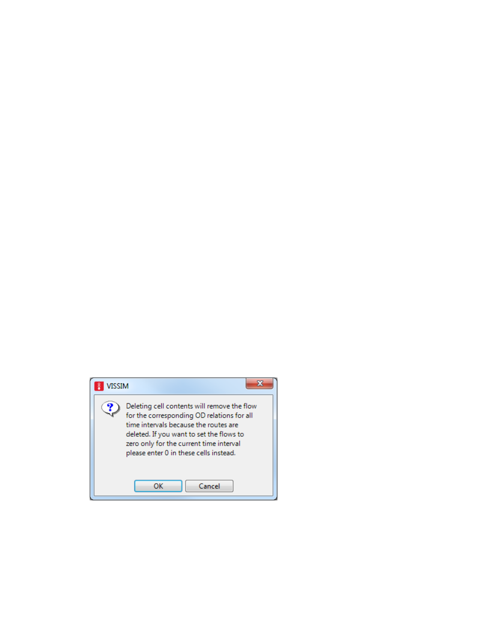
10.13.4 Pedestrian OD matrices
The Pedestrian OD Matrix window opens.
2. Click on the column header of the destination or the row header of the origin which you
would like to delete.
3. Right-click in the list.
4. In the context menu, select Delete Origin(s) or Delete Destination(s).
The marked columns or rows and all OD relations and other pedestrian areas are deleted
from the Pedestrian OD Matrix.
For the applicable areas, the attributes Always use as destination area and Always use
as origin area are deactivated (see "Attributes of areas" on page 848).
Pedestrian inputs and pedestrian routing decisions, including routes on a deleted origin
area, are deleted. Pedestrian routes to a deleted destination area and its relative volumes
are deleted. The input volumes on the areas with routing decisions of the deleted
pedestrian routes are correspondingly reduced. These changes are immediately applied
for Pedestrian inputs and Pedestrian routes (see "Modeling pedestrian inputs" on page
883), (see "Modeling routing decisions and routes for pedestrians" on page 886).
Marking values in multiple cells and deleting simultaneously
1. From the Traffic menu, choose Pedestrian OD Matrix.
The Pedestrian OD Matrix window opens.
2. Mark the cells of the desired OD relations.
3. Press the DEL key.
A warning is issued. If the content of the selected cells are deleted, the demand data of all
other time intervals of these OD relations are also deleted. If for the selected OD relation
you would only like to delete the volume for the current time interval, enter 0 in the cell.
4. Confirm with OK.
The demand data of the marked relation for all time intervals are deleted. The cells are empty.
924 © PTV GROUP

10.14 Visualizing pedestrian traffic in 2D mode
10.14 Visualizing pedestrian traffic in 2D mode
You also have the following options for representing the individual pedestrians in color:
using the default colors (see "Static colors of vehicles and pedestrians" on page 165)
based on attributes (see "Assigning a color to pedestrians based on an attribute" on page
168)
You can assign display types to the construction elements (see "Defining display types" on
page 300).
You can display areas, ramps and stairways on the basis of aggregated values (LOS) (see
"Assigning a color to areas based on aggregated parameters (LOS)" on page 172), (see
"Assigning a color to ramps and stairs based on aggregated parameters (LOS)" on page 180).
10.15 Modeling pedestrians as PT passengers
You can model pedestrians as boarding/alighting passengers in PT. The boarding and
alighting passengers use PT-vehicles based on PT-specific vehicle types. In the network
objects that pedestrians should use as boarding and alighting passengers, select the relevant
options for public transport. For example, you may define areas as platform edges or as
waiting areas and specify the number of passengers boarding at public transport stops. You
may also determine the number of passengers alighting at public transport line stops and
define the doors in 2D vehicle models (see "Modeling PT infrastructure" on page 925).
10.15.1 Modeling PT infrastructure
If you model pedestrians as passengers boarding or alighting in PT, they can be going to the
station, waiting there for the PT vehicle and boarding once the alighting passengers have left
the vehicle. Alighting passengers follow the routes which are assigned to them as soon as
they leave a train or a bus. You can easily model such a scenario with waiting areas, platform
edges and definitions of the number of boarding and alighting passengers. (see "Quick start:
defining pedestrians as PT passengers" on page 927).
You model public transport stops, PT vehicles as well as the associated PT lines by default
using the relevant network objects (see "Modeling PT stops" on page 478) , (see "Using
vehicle types" on page 254), (see "Modeling PT lines" on page 485).
10.15.1.1 Modeling waiting areas and platform edges
Pedestrians wait in waiting areas of a public transport stop for a PT vehicle of the PT line
which they want to use. To define waiting areas for a public transport stop, you must create
a pedestrian area and assign the entry Waiting area to the attribute PT usage (see "Attrib-
utes of areas" on page 848). You can also assign multiple public transport stops to a wait-
ing area.
To define a platform edge, you must create a pedestrian area and assign the entry Plat-
form edge to the attribute Public transport usage (see "Attributes of areas" on page 848).
You can also assign multiple public transport stops to a platform edge.
© PTV GROUP 925
10.15.1 Modeling PT infrastructure
Alighting passengers go to the nearest platform edge which they can reach. This depends
on the door via which they leave the PT vehicle. If a routing decision is placed on the
platform edge, the passenger continues his walk. If no routing decision is placed on the
platform edge, the passenger is removed from the network.
The platform edge and the lane with the public transport stop must be directly adjacent or
overlap so that alighting passengers may alight on the platform edge and boarding
passengers may board the PT vehicle from the platform edge. You can add a platform edge
along a public transport stop in the Network Editor via the context menu (see "Generating
platform edges" on page 483). The attributes Left and Right specify the location of the
platform edge parallel to the direction in which you have defined the public transport stop
on the link. The number of the platform edge is shown in the attribute Areas of the public
transport stop.
If a pedestrian is assigned to be at a platform edge or waiting area of a public transport stop for
which no boarding passengers are defined, default values are generated.
These defaults are also generated if a platform edge is added via a context menu.
Through these default values, each pedestrian who arrives in the waiting area, in the time
interval 0 to 99,999, boards a PT vehicle once a PT line serves the public transport stop.
10.15.1.2 Adding alighting passengers
Alighting passengers are added using the setting in the PT Line Stop window (see "Editing a
PT line stop" on page 492).
You specify the percentage of alighting passengers per line for each PT line stop.
You must select the pedestrian composition for the Alighting composition according to
which the pedestrian types are added to the vehicle.
10.15.1.3 Behavior of boarding and alighting passengers
For each PT stop, you can specify whether pedestrians may board or alight on the right or left
side or on both sides (see "Editing a PT line stop" on page 492). By default, all doors on both
sides can be used. Boarding passengers wait in the waiting area of the relevant public
transport stop. For this waiting area to be reached by the passenger, the destination of a
pedestrian route must lie on it.
The boarding passenger numbers per PT stop result in the PT line with which the waiting
passengers want to travel. Once a vehicle from one of these PT lines stops at the PT stop,
the passengers walk directly to the nearest door. The pedestrians start to board once all
alighting passengers have left the vehicle.
Passengers can enter until the door is half closed.
If, depending on the attributes Door lock duration before departure and Door closure
delay of the PT line stop and the Door closure duration of the vehicle type, nobody has
entered the vehicle, it will leave the PT stop as soon as the departure time is reached. The
926 © PTV GROUP
10.15.2 Quick start: defining pedestrians as PT passengers
departure time is based on the timetable or the predefined layover. The degree of Slack
time fraction of the PT line is taken into account for the scheduled departure time.
You can select the distribution among the doors in the attribute Boarding location of ped-
estrian area for boarding passengers, and in the PT line stop parameters for alighting pas-
sengers (see "Editing a PT line stop" on page 492). Therein, you specify with the option
Late boarding possible, how a PT vehicle, whose departure time is either prescribed by a
schedule or a predetermined time, should respond to a never-ending stream of boarding
passengers.
If a pedestrian is unable to board a PT vehicle, for example for vehicle capacity reasons,
the pedestrian returns to a waiting area.
Default settings are generated for boarding passengers if a public transport stop is
assigned to a waiting area or a platform edge for which no boarding passenger share is
specified. Due to these default settings, each pedestrian who comes to a waiting area of
this public transport stop boards the next PT vehicle that stops.
10.15.1.4 Defining doors for public transport vehicles
A door of a 2D vehicle model has the following properties (see "Defining doors for public
transport vehicles" on page 220):
Position, measured from the front
Width
one of the two sides of the vehicle
For each door, you can specify whether it can be used only for boarding or only for alight-
ing or for both.
If you use a 3D model, the properties of the door are derived from it.
You can add or remove doors via the context menu and change the data directly in the
base data (see "Defining doors for public transport vehicles" on page 220).
A warning is issued if changes do not suit the 3D model. You can still confirm these
changes. The values in the window are used for the simulation and the values of the 3D
model are used only in 3D mode to show the opening and closing of doors.
If you have not created a door for a vehicle, a door is added temporarily in the middle of
the vehicle. Thus pedestrians can still board and alight. They are informed of this via a
warning in the trace file.
10.15.2 Quick start: defining pedestrians as PT passengers
The Quick Start uses the example of the definition of a public transport stop to show you the
most important steps to define the necessary network objects and to make the necessary
settings. The following figure shows a modeling example in wireframe display.
The numbers in the figure correspond to the number of the step:
© PTV GROUP 927

10.15.2 Quick start: defining pedestrians as PT passengers
1. Add a Link (in the figure, amber with arrows) (see "Defining links" on page 381).
2. Add a Public transport stop (in the figure, with a red outline) (see "Defining PT stops" on
page 479).
3. Add an area next to the Public transport stop and select the attribute Platform edge or
create a Platform edge for the public transport stop in the network editor (see "Generating
platform edges" on page 483).
If there is more than one level, Viswalk tries to determine the correct level according to the
height of the link.
When defining the platform edge, the attribute Public transport usage > Platform edge is
selected for the network object Area of the platform edge, and the number of PT stops is
entered for the attribute for PT stops. As a result, Viswalk calculates the occupancy level of
the vehicle which departs from the stop from the number of passengers which have
actually boarded the vehicle during the pedestrian simulation, and not from the number of
boarding passengers.
4. Define a Public transport line (in the figure, the blue line) (see "Defining PT lines" on page
485)
5. Edit the PT Line Stop Parameters (see "Editing a PT line stop" on page 492):
Select the attribute PT stop active.
Alighting percentage:: Specify the total ratio of alighting passengers/passengers.
Alighting location: Distribute the alighting passengers among the doors available for
this purpose.
Select which sides of the line vehicles should be available for boarding and alighting.
If desired, enter a scheduled departure time as a fixed value and/or a minimum dwell
time as a distribution. Scheduled departure time, minimum dwell time and slack time
fraction collectively specify for how long at least a PT vehicle stops.
A departure time according to schedule is derived from scheduled departure time and
slack time fraction.
928 © PTV GROUP

10.16 Modeling elevators
The PT vehicle departs at the earliest at the later time from this time and the time
calculated from the minimum dwell time.
If the option Late boarding possible is selected, the PT vehicle also remains stopped
beyond this calculated time in case pedestrians willing to board stream in.
Other than stemming this flow, the standstill time is limited upwards only by the
capacity of the PT vehicle which is defined in the PT parameters window (see
"Changing attributes for a vehicle type for the duration of boarding and alighting" on
page 262).
6. Select a suitable 3D model or the PT vehicle(see "Defining 2D/3D models" on page 211).
7. Define the attributes of doors of the PT vehicle (see "Defining doors for public transport
vehicles" on page 220).
8. Define the geometry of the entire stop using the desired construction elements such as
areas, ramps, stairways and obstacles (in the figure, two areas with a black outline and one
obstacle with a dark-red outline) (see "Modeling construction elements" on page 834).
9. Define a Pedestrian routing decision (in the figure, the upper red circle) in the area of the
platform edge. Define at least one Pedestrian route which leads to the location that the
alighting passengers are supposed to go to (in the figure, from the upper red circle to the
lower turquoise circle) (see "Modeling routing decisions and routes for pedestrians" on
page 886).
10. Define an area with a waiting area where boarding passengers should wait for the PT
vehicle (see "Attributes of areas" on page 848).
11. For the boarding passengers, define a Pedestrian input as an origin (in the figure, the
black circle)(see "Defining pedestrian inputs" on page 883).
12. Define a Pedestrian routing decision in the area of the pedestrian input and a pedestrian
route to the waiting area (in the figure, from the lower red circle to the upper turquoise
circle) (see "Modeling routing decisions and routes for pedestrians" on page 886).
13. Enter the Capacity of the PT vehicle (see "Changing attributes for a vehicle type for the
duration of boarding and alighting" on page 262).
10.16 Modeling elevators
You can define elevators for vertical transportation of pedestrians. The modeling and
simulation of elevators is based on the following elements:
Elevator
The elevator is a network object that in the 2D mode is defined and displayed as a
rectangular network object (1) (see "Defining elevators" on page 933). The rectangle contains
a shaft and a cab (2). The elevator cab moves in the shaft. There is a distance of 30 cm (brown
area) between the exterior wall of the shaft and the cab. This area is displayed based on the
attribute Shaft display type of the elevator.
© PTV GROUP 929
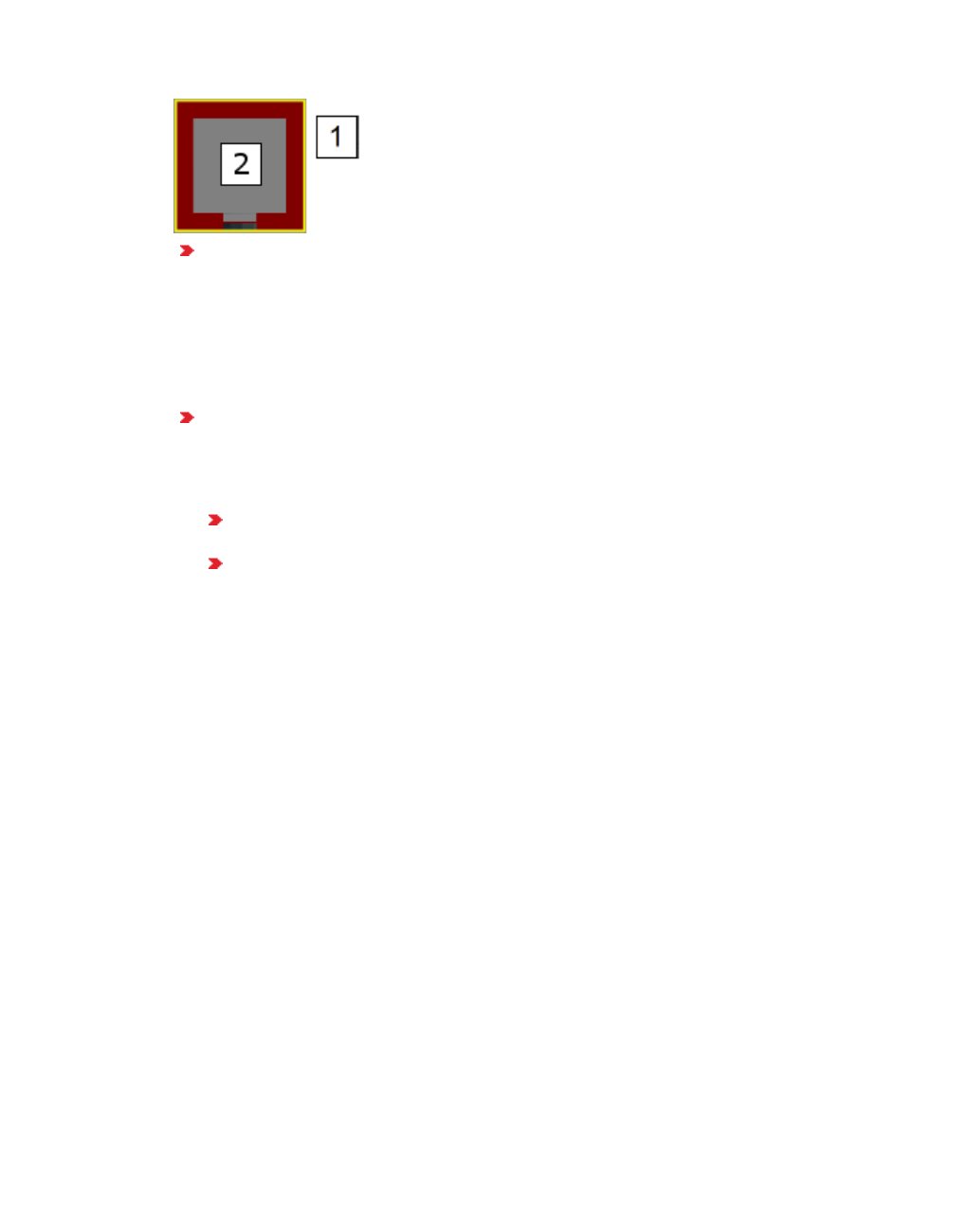
10.16 Modeling elevators
Cab
The elevator cab holds passengers. The cab is part of the elevator, not a separate
network object. You can use the following elevator attributes to define the display of the
cab: Floor display type, Ceiling display type, Wall display type (see "Elevator
attributes" on page 933). The elevator attributes contain additional attributes for the
cab, e.g. cab height or capacity. In the cab, a specific walking behavior prevails (see
"Walking behavior of pedestrians when using elevators" on page 932).
Door
The door is part of the elevator. It is not a separate network object. You can define a
door for each of the four cab walls (in image, on bottom wall). The door is displayed as
a thin line in the middle of the wall. The door is positioned automatically:
within the first wall of the elevator, when in the Network editor, you create the rect-
angle for the elevator (see "Defining elevators" on page 933).
within the bottom wall of the elevator, when in the Network editor, from the shortcut
menu, you choose Add New Elevator. By default, the elevator is square.
You can define the display of the door through the Door display type attribute of the
elevator (see "Elevator attributes" on page 933). Width and horizontal position of the
door within the elevator wall can be defined via the door attributes Width and Center
offset (horizontal)(see "Elevator door attributes" on page 935).
In the attribute Active levels (ActLvls), you can assign the elevator door the levels you
want it to stop on and open the door (see "Elevator attributes" on page 933). The door
only opens on the levels you have selected.
During simulation, the animated door is opened and closed based on the elevator
attribute Motion state. Shaft door and cab door are displayed as one single door.
Elevator group
An Elevator group consists of elevators that you can call (see "Defining an elevator group" on
page 936). Each elevator must be assigned to an Elevator group (see "Attributes of elevator
groups" on page 936). To do so, select the desired elevator group for the elevator attribute
Elevator group (ElevGrp) (see "Elevator attributes" on page 933).
All elevators of an elevator group must be able to stop on the same level. To enable this, in the
attribute Active levels (ActLvls), you can assign the door of each elevator the levels you want
it to stop on and open the door (see "Elevator attributes" on page 933). Each level assigned
must have a Waiting area.
930 © PTV GROUP

10.16 Modeling elevators
Waiting area
Pedestrians need an area in which they can wait for the elevator. For this area, in the attribute
Waiting area for elevator group, select the number of the elevator group with the elevators
the pedestrians are waiting for (see "Attributes of areas" on page 848). The waiting area can
be an area the pedestrians use to enter or exit the elevator or another area they can reach via
areas, ramps & stairs. This area must not contain a pedestrian input.
Walkable area
The door must be located at or within a walkable area, so that pedestrians can enter and exit
the elevator cab. Otherwise, the simulation will not start. There must be a walkable area on
each level the elevator can stop at and pedestrians are supposed to enter or exit the elevator
cab.
Pedestrian routes and partial pedestrian routes
Pedestrians use an elevator when their pedestrian route or partial pedestrian route leads from
an area on one level to an area on a different level or ends there and using the elevator gets
them there quicker. Pedestrians also use an elevator that e.g. only connects levels 2 and 3,
even though their route connects levels 1 and 4 without any intermediate points. Pedestrians
must be able to reach the elevator and their destination via areas and/or walkable construction
elements. For pedestrians to be able to enter and exit the elevator, in the elevator attribute
Active levels (ActLvls), you must assign the elevator door the levels it is supposed to stop on
and open the door (see "Elevator attributes" on page 933). These levels must contain areas in
which pedestrians can wait for the elevator, enter and exit it and reach their destination. Using
intermediate points, you can influence the course of the pedestrian route or partial pedestrian
route (see "Modeling the course of pedestrian routes using intermediate points" on page 902).
If a route location of a pedestrian route or partial pedestrian route lies within a waiting area on
a level where an elevator can stop, the pedestrian must use its elevator group, even if other
elevator groups or ramps & stairs were available.
If a route location of a pedestrian route or partial pedestrian route lies on a ramp or stairs and
for this route location you selected the attribute Ban elevator use, the pedestrian will not use
the elevator until he has reached the next route location for which this attribute has not been
selected (see "Attributes of pedestrian route locations" on page 904). This means you can use
this option to force pedestrians to use the stairs to reach multiple levels, without having them
use the elevator in between. When doing so, you do not have to set a lot of route locations in
the stairway.
Level
An elevator must service at least two levels. All elevators of an elevator group must be able to
stop on the same level. To enable this, in the attribute Active levels (ActLvls), you can assign
the door of the elevator the levels you want it to stop on and open the door (see "Elevator
attributes" on page 933). The door only opens on the levels you have selected.
An elevator stops at a level in the following cases:
© PTV GROUP 931

10.16.1 Walking behavior of pedestrians when using elevators
when pedestrians wish to alight: The pedestrian route or partial pedestrian route leads
via an area on this level or ends there.
when pedestrians wish to board: The pedestrian route or partial pedestrian route leads
to an area on another level where this elevator stops and can open the door. A waiting
area must be defined for the level the pedestrians are waiting on.
10.16.1 Walking behavior of pedestrians when using elevators
Pedestrians use area-based walking behavior that in turn is based on a social force model
and walkable construction elements (see "Modeling area-based walking behavior" on page
879), (see "Pedestrian simulation" on page 814).
10.16.1.1 Walking behavior of pedestrians when entering an elevator cab
Pedestrians enter the cab as soon as the door opens and the pedestrians wanting to continue
their route on this level have exited the cab. When the elevator capacity has been reached,
pedestrians stop entering the cab and wait in the waiting area for the next elevator of the
elevator group or until the elevator stops again (see "Elevator attributes" on page 933).
When entering the cab, pedestrians use the walking behavior specified in the area behavior
type for the area from which they enter the elevator.
10.16.1.2 Walking behavior of pedestrians in an elevator cab
In reality, persons in elevators are willing to accept less space than in other situations where
more space is available. In an elevator cab, pedestrians use the walking behavior Area
behavior type (in cab) (AreaBehavTypInCab) of the elevator group the elevator is assigned
to. The default walking behavior in this case is Elevator (in Cab).
10.16.1.3 Walking behavior of pedestrians when exiting an elevator cab
Pedestrians exit the elevator as soon as it reaches the floor on which they want to continue
with their route and the door opens. If pedestrians cannot alight, e.g. because there are too
many pedestrians standing in front of the door or because the door closes too soon, the
elevator continues to operate. The stop request for the same floor still exists and the elevator
services this floor again as per the control request.
When exiting an elevator, pedestrians use the walking behavior Area behavior type
(alighting) ( AreaBehavTypAlight ) of the elevator group the elevator is assigned to. The
default walking behavior in this case is Elevator (Alighting).
The pedestrians that are not alighting (because they do not have to continue with their route)
leave enough space in front of the door for other pedestrians to exit the cab and continue with
their route on the respective floor. The doors exercise a “repellent force” on those pedestrians
using the walking behavior Elevator (in the cab). This “repellent force” is not exercised on
pedestrians with the walking behavior Elevator (Alighting).
932 © PTV GROUP

10.16.2 Defining elevators
10.16.2 Defining elevators
Notes:
You can specify that you need not press the CTRL key when adding network objects
(see "Right-click behavior and action after creating an object" on page 143).
For some network objects there are windows in which the attributes of a network
object can be defined and edited. There are lists for this, for all network objects. You
can choose whether you want to open a window, a list or neither of the two for the
definition of network objects in the Network Editor (see "Right-click behavior and
action after creating an object" on page 143).
When you create an elevator, the cab area and area between the exterior of the shaft and cab
are automatically created. The elevator can be inserted into an area or next to it, with the door
adjacent to the area.
1. On the Network objects toolbar, click Elevators.
2. In the Network editor, point the mouse pointer to the desired position of the first corner point
of the elevator.
In a next step, you define the first wall of the elevator. A door is automatically added to the
first wall you define. The size of the elevator must be at least twice the wall thickness. Make
sure that the elevator is sufficiently large.
3. Press the CTRL key, hold down the right mouse button and drag the mouse pointer to
second corner point of your choice.
4. Release the keys.
5. Drag the corner point open to the desired width or vertically to the desired depth.
6. Double-click.
Elevator, shaft and doors are displayed in the Network editor. The elevator is selected.
Tip: Alternatively, in the Network editor, from the shortcut menu, choose Add New
Elevator. By default, a square elevator is added and selected. Using the anchor points,
you can drag the elevator open the desired size.
The elevator is automatically assigned to the elevator group with the lowest number. If no
elevator group has been defined, Vissim will create one.
7. Edit the attributes of the elevator (see "Elevator attributes" on page 933).
8. Edit the attributes of the area that is meant to be the elevator waiting area (see "Attributes of
areas" on page 848).
9. Confirm with OK.
The attributes are saved to the elevator list.
10.16.3 Elevator attributes
1. From the Lists menu, choose > Pedestrian Traffic > Elevators.
© PTV GROUP 933

10.16.3 Elevator attributes
The attribute and attribute values of this network object type are shown in the list on the left,
which consists of two coupled lists.
The list on the left may include the following attributes:
Long name Short name Description
Number No Unique number of the elevator
Name Name Name of elevator
Elevator
group
ElevGrp Elevator group to which this elevator belongs (see "Attributes of
elevator groups" on page 936)
Queue
order
QueueOrder (see "Attributes of areas" on page 848), (see "Selecting network
settings for pedestrian behavior" on page 193)
Cab height CabHeight Inner height of elevator cab [m]. This value defines whether the
floor located above the highest floor serviced by the elevator is
“broken through”. This way, an obstacle is created there.
Shaft
display
type
ShaftDisplTyp Display type of area between exterior of elevator shaft and cab
Floor
display
type
FloorDisplTyp Display type of cab floor
Wall dis-
play type
WallDisplTyp Display type of cab walls
Ceiling dis-
play type
CeilDisplTyp Display type of cab ceiling
Door dis-
play type
DoorDisplTyp Display type of cab door
Capacity Capacity Maximum permitted number of pedestrians per elevator cab.
Once the capacity is reached, no additional pedestrians can
enter the elevator.
Motion
state
MotionState Result attribute with current cab movement:
Stopping: Cab comes to a halt
Going Up: Cab moves upward
Going Down: Cab moves downward
Destination
level
Destlvl Next floor the elevator cab stops at. If the elevator is called from
outside, the destination level can change.
Travel dir-
ection
TravDir Direction in which the elevator is currently moving. When the
cab has come to a halt, the direction of the next ride is indic-
ated.
Current
level
CurLvl Level the elevator cab is currently on.
By default, the display types are based on the display types selected as default in the network
settings (see "Network settings for standard types of elevators and elevator groups" on page
196).
934 © PTV GROUP

10.16.4 Elevator door attributes
Note: In lists, you can use the Attribute selection icon to show and hide attribute
values (see "Selecting attributes and subattributes for a list" on page 106).
The list on the right contains attributes and attribute values of network objects, and/or base
data allocated to the network object selected in the list on the left (see "Using coupled lists" on
page 111):
Points: edit coordinates of the corners
Doors (see "Elevator door attributes" on page 935)
The attributes are described further above.
2. On the list toolbar, in the Relations list, click the desired entry.
3. Enter the desired data.
10.16.4 Elevator door attributes
1. From the Lists menu, choose > Pedestrian Traffic > Elevators.
The attribute and attribute values of this network object type are shown in the list on the left,
which consists of two coupled lists.
2. On the list toolbar, in the Relations list box, click > Doors.
The list on the right contains attributes and attribute values of network objects, and/or base
data allocated to the network object selected in the list on the left (see "Using coupled lists" on
page 111):
Long name Short
name
Description
Edge index EdgeIdx Position of elevator door as edge index of rectangle that defines
the shaft. The edge indices 1 to 4 are counted counterclockwise. 1
= First edge modeled in the Network editor when the elevator was
defined. If the elevator is created in the Network editor via shortcut
menu command Add New Elevator, this is the bottom elevator
wall.
Active
levels
ActLvls Number of levels on which the door opens. Select at least two
levels. The Main landing level of the elevator group must be
selected to which the elevator is assigned.
Avoid making the total of width and center offset larger than the width of the elevator wall with
the door:
Center off-
set (hori-
zontal)
CentOffset Horizontal offset of the door’s center line to the cab wall’s center
line [m]. In the Network editor, in the top view, negative values
move the door to the left. In the Network editor, in the top view,
positive values move the door to the right.
Width Width Entire door width [m]. With the door open this is the width of its
opening. Default value 0.9 m, if permitted by the width of the wall.
© PTV GROUP 935

10.16.5 Defining an elevator group
Note: In lists, you can use the Attribute selection icon to show and hide attribute
values (see "Selecting attributes and subattributes for a list" on page 106).
10.16.5 Defining an elevator group
In the Elevator group attribute list, you can define new elevator groups and assign elevators
to them.
1. Make sure that the desired elevators have been defined (see "Defining elevators" on page
933).
2. From the Lists menu, choose > Pedestrian Traffic > Elevator groups.
The Elevator group attribute list opens. If no elevator groups have been defined yet, only
the column headings are shown.
By default, you can edit the list (see "Using lists" on page 89).
In the list, you can define a new elevator group.
3. In the list, on the toolbar, click the Add button .
A new row with default data is inserted.
4. Edit the attributes (see "Attributes of elevator groups" on page 936).
10.16.6 Attributes of elevator groups
1. From the Lists menu, choose > Pedestrian Traffic > Elevator groups.
Tips: The Elevator groups list may also be displayed via the following functions:
Call it from the Elevators list: Right-click an elevator in theElevators list and
choose Show Elevator Group List from the shortcut menu. If Synchronization is
activated in the toolbar of the Elevators list , the elevator group that the elev-
ator is allocated to will be chosen from Elevator groups list.
Call it from the network editor, if an elevator is defined in the network editor:
Right-click an elevator and choose Show Elevator Group List from the shortcut
menu. If Synchronization is activated in the toolbar of the Elevator groups list
, the elevator group that the elevator is allocated to will be chosen from Elev-
ator groups list.
The attribute and attribute values of this network object type are shown in the list on the left,
which consists of two coupled lists.
The list on the left may include the following attributes:
Long name Short name Description
Number No Unique number of the elevator group
936 © PTV GROUP
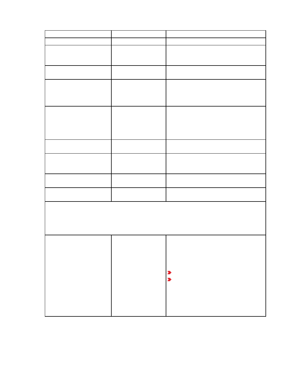
10.16.6 Attributes of elevator groups
Long name Short name Description
Name Name Name of elevator group
Acceleration Accel Value for acceleration and deceleration
of elevator cabs in shaft [m/s²] assigned
to this elevator group
Maximum speed MaxSpeed Maximum speed of elevator cab
assigned to this elevator group [m/s]
Door motion duration DoorMotionDur Time [s] to open the elevator doors of
cabs assigned to this elevator group.
This also applies for the closing of elev-
ator doors.
Door closure delay DoorClosDel Time [s] after which a pedestrian must
have cleared the elevator door and the
door begins to close. In reality, the time
after which the light barrier is no longer
interrupted.
Door hold time (min-
imum)
DoorHoldTmMin Minimum time [s] the door must remain
open when cab stops at a level.
Main landing level MainLvl Number of level on which the elevator
cabs assigned to this elevator group are
when the simulation is started
Area behavior type (in
cab)
AreaBehavTypInCab Area behavior type used by pedestrians
in the cab
Area behavior type
(alighting)
AreaBehavTypAlight Area behavior type used by pedestrians
when alighting from the cab
Pedestrians who wish to board the elevator may form queues in front of the elevator door
and let the pedestrians pass who want to alight the elevator. These queues are formed to the
left and the right of the elevator door, on a Vissim-internal area. Pedestrians alighting the
elevator move between these two queues. The shape and orderliness of queues are based
on the following attributes:
Queue straightness QueueStraight The Queues straightness defines the
shape of the queue. Value range
between 0.0 and 1.0. The greater the
value, the more straight the queue will
look:
0.0: snake shaped queue
1.0: straight queue
Default values are defined in the network
settings (see "Selecting network settings
for pedestrian behavior" on page 193).
These are used if this attribute is not
defined for this elevator group.
© PTV GROUP 937

10.16.6 Attributes of elevator groups
Long name Short name Description
If no waiting behavior is defined for the
waiting areas, the attribute affects all
elevators of this elevator group on all
floors and for all pedestrian classes.
Queue order QueueOrder The Queue order defines how orderly
the pedestrians line up in the queue.
Value range between 0.0 and 1.0. The
higher this value, the more orderly
pedestrians line up one behind the other:
0.0: Pedestrians are standing
together in groups
1.0: Queue of pedestrians lined up
one behind the other
Default values are defined in the network
settings (see "Selecting network settings
for pedestrian behavior" on page 193).
These are used if this attribute is not
defined for this elevator group.
If no waiting behavior is defined for the
waiting areas, the attribute affects all
elevators of this elevator group on all
floors and for all pedestrian classes.
By default, the area behavior types are based on the area behavior types selected as default
in the network settings (see "Network settings for standard types of elevators and elevator
groups" on page 196).
Note: In lists, you can use the Attribute selection icon to show and hide attribute
values (see "Selecting attributes and subattributes for a list" on page 106).
The list on the right contains attributes and attribute values of network objects, and/or base
data allocated to the network object selected in the list on the left (see "Using coupled lists" on
page 111):
Elevators: attributes of the elevators assigned to this elevator group (see "Elevator attrib-
utes" on page 933)
Waiting areas: areas for which the attribute Waiting area for elevator group has been
selected (see "Attributes of areas" on page 848)
2. On the list toolbar, in the Relations list, click the desired entry.
3. Enter the desired data.
938 © PTV GROUP

10.17 Defining pedestrian travel time measurement
10.17 Defining pedestrian travel time measurement
Pedestrian travel time measurement is based on a start point (in a start area) and a destination
point (in a destination area). The travel time is determined from entering the start area where
the start point is located until entering the destination area where the destination point is
located, including wait times. You can show this data in an evaluation (see "Evaluating
pedestrian travel time measurements" on page 986).
Travel time measurements are not shown in 3D mode.
If you define travel time measurements in multistory buildings on levels, for example, check
whether the respective level is correct for each pedestrian travel time measurement. Go to the
list Pedestrian Travel Time Measurements and select the attributes Start area > level and
End area > level. Check the correct position on the various levels in 2D mode by selecting the
visibility for the desired level and hiding the other levels (see "Using the Level toolbar" on
page 65).
Notes:
You can specify that you need not press the CTRL key when adding network objects
(see "Right-click behavior and action after creating an object" on page 143).
For some network objects there are windows in which the attributes of a network
object can be defined and edited. There are lists for this, for all network objects. You
can choose whether you want to open a window, a list or neither of the two for the
definition of network objects in the Network Editor (see "Right-click behavior and
action after creating an object" on page 143).
1. On the Network objects toolbar, click Pedestrian Travel Times.
In the next step, you may choose the position of the start point in the start area.
2. Press the CTRL key and right-click in the destination area.
Per default, a pink circle is inserted.
3. Drag the cursor to the destination area.
4. Click.
Per default, a green dot is inserted. The Pedestrian Travel Time Measurements list
opens.
Note: In lists, you can use the Attribute selection icon to show and hide attribute
values (see "Selecting attributes and subattributes for a list" on page 106).
5. Edit the attributes:
© PTV GROUP 939

10.17 Defining pedestrian travel time measurement
Element Description
No Number of travel time measurement. You can enter a different
number.
Use a continuous numbering system for the Vissim network. This
simplifies the evaluations.
Name Name of travel time measurement
StartArea Start area: Number and name of the area where the start point is
located
EndArea Destination area: Number and name of the area where the
destination point is located
StartPt Start point: Position of the start point based on the coordinates of
start point (x) and start point (y)
StartX Start point (x): coordinate
StartY Start point (y): coordinate
StartShowLabel Start - show label: If this option is not selected, the label on the
start point for an individual pedestrian travel time measurement is
hidden if the label for all pedestrian travel time measurements is
selected.
StartLabPosRelPt Start label position relative: Coordinates of the label position when
the label on the start section is offset
StartLabPosRelX Start label position relative (x): X-coordinate of the label position
when the label on the start point is offset
StartLabPosRelY Start label position relative (y): Y-coordinate of the label position
when the label on the start point is offset
Endpt End point: Position of the end point based on the coordinates of end
point (x) and end point (y)
EndShowLabel End - show label: If this option is not selected, the label on the
destination point for an individual pedestrian travel time
measurement is hidden if the label for all pedestrian travel time
measurements is selected.
EndLabPosRelX End label position relative (x): X-coordinate of the label position
when the label on the destination point is offset
EndLabPosRelY End label position relative (y): Y-coordinate of the label position
when the label on the destination point is offset
EndLabPosRelPt End label position relative: Coordinates of the label position when
the label on the destination point is offset
940 © PTV GROUP
11 Performing evaluations
11 Performing evaluations
Depending on the network objects used, various data is produced during simulations, e.g.
information on vehicles, links, areas, nodes, traffic jams, green time distribution or PT waiting
times (see "Overview of evaluations" on page 942). This may be raw data or aggregated data.
Depending on the type of data and the desired further use, you can show evaluations in lists
and/or windows and save them to text files and/or database files. To do so, select the desired
evaluations before the start of the simulation and configure them.
Note: Some output options and individual evaluation results may only be available with
add-on modules. You need a license to use the add-on modules.
If you wish to display the result data of evaluations in a database, you must configure the
database connection (see "Configuring the database connection for evaluations" on page
958), (see "Saving evaluations in databases" on page 961).
Tip: You can also show simulation data in diagrams (see "Creating charts" on page
1053).
1. Define basic settings for the management of the result data: overwrite previous results,
configure columns, file or database as location of automatic saving, define percentiles (see
"Managing results" on page 947).
2. From the Evaluation menu, choose the desired entry:
Configuration: Opens the Evaluation Configuration window with the following tabs
that allow you to make basic settings for result data management and evaluations:
Evaluation output directory box: By default, the path to the evaluation output dir-
ectory, the directory to which the currently opened network file *.inpx is saved. If
you are using Scenario Management and a scenario has been opened, you can
view the path to the directory in which the scenario is saved.
Result Management tab: Under Result Management, make the basic settings for
managing result data before you configure Result Attributes or the Direct Output
and start the simulation.
Result Attributes tab: Select evaluations which you wish to display in attribute lists
or result lists (see "Configuring evaluations of the result attributes for lists" on page
954)
Direct Output tab: Select evaluations which you wish to save to a file or database
(see "Configuring evaluations for direct output" on page 957)
3. Confirm with OK.
Measurement Definition: Opens a respective list with static attributes for the definition
of the following measurements:
In the Data Collection Measurements list, select Data Collection Points (see
"Defining a data collection measurement in lists" on page 951), (see "Generating
data collection measurements in lists" on page 951).
© PTV GROUP 941
11.1 Overview of evaluations
In the Delay Measurements list, select Vehicle travel time measurements (see
"Defining delay measurement in lists" on page 952), (see "Generating delay meas-
urements in lists" on page 953).
In the Area measurements list, select sections (see "Defining an area meas-
urement in lists" on page 949), (see "Generating area measurements in lists" on
page 950).
4. If you have configured evaluations and wish to create result data from a simulation, start the
simulation (see "Running a simulation" on page 796).
The evaluations are generated and, depending on your settings in the selected program
elements, they can be shown or saved to files or databases.
5. If you have configured evaluations for network objects, whose results can be displayed in
windows or result lists, from the Evaluation menu, select the entry of your choice:
Window: Opens a window with result attributes of the simulation for the chosen eval-
uation Signal Times Table, SC detector record or Signal changes (see "Showing
evaluations in windows" on page 962)
Result lists: opens a list with result attributes from the simulation for the selected eval-
uation (see "Showing result attributes in result lists" on page 956)
Notes:
By default, the currently selected units for distances, speeds, accelerations, decel-
erations are taken into account for the evaluation (see "Selecting network settings
for units" on page 195). You can also choose the unit for attribute values in the attrib-
ute selection list in the Format column (see "Selecting attributes and subattributes
for a list" on page 106).
Some parameters use different units. These are specified in the evaluation.
If the script files change attributes that are used in evaluations, the changed values
are saved to the evaluations.
11.1 Overview of evaluations
Depending on the selected evaluation, the type of data and the desired further use, you can
show evaluations in lists and/or windows and save them to text files and/or database files:
Direct Output: The data of the evaluation is saved as text files. In text files, semicolons are
used as a separator. Thus you can import text files into spreadsheet programs, e.g.
Microsoft™ Excel™, and use them for calculations, analyses or graphical display.
You can also save the data of the following evaluations to database files:
Vehicle record
Vehicle travel times (raw data)
Pedestrian record
Nodes (raw data)
Signal changes
942 © PTV GROUP
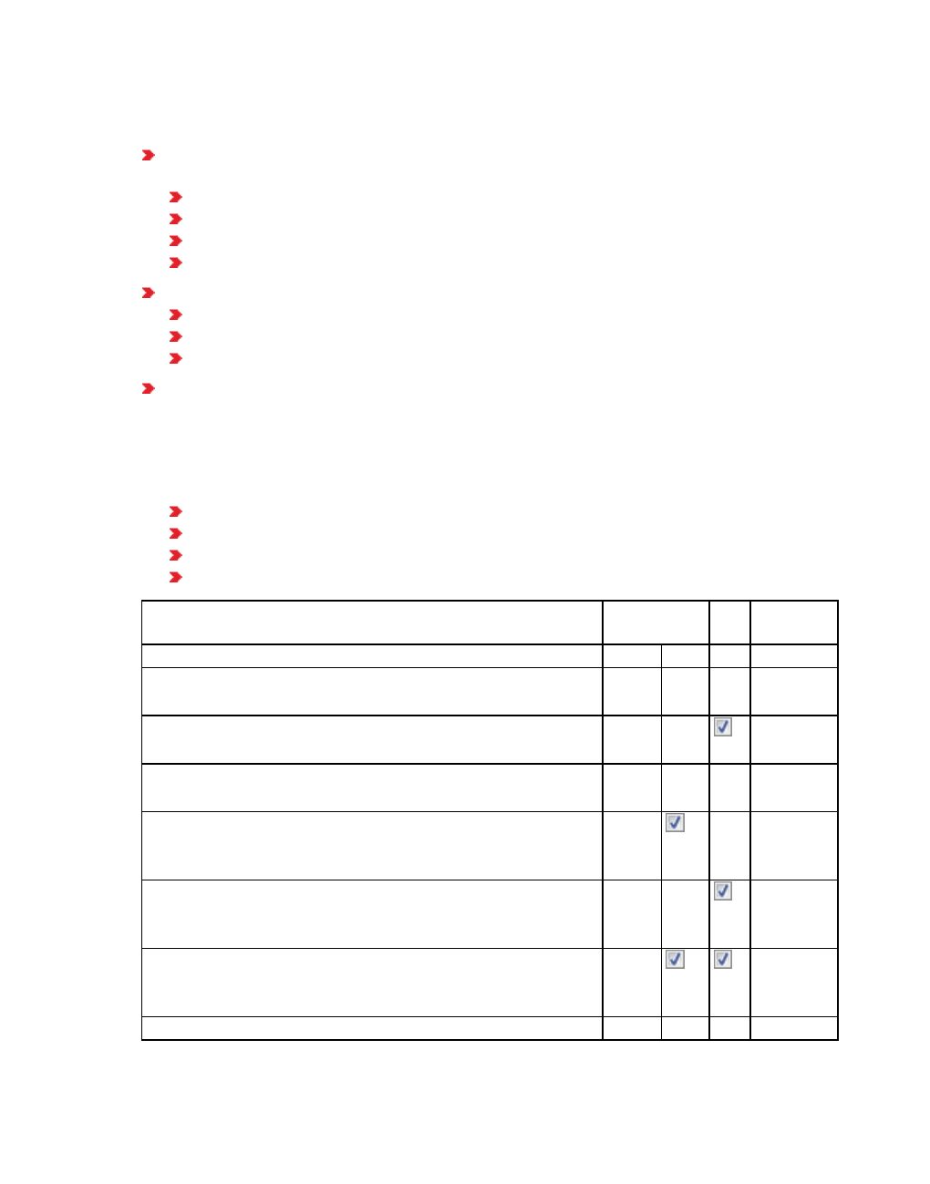
11.1 Overview of evaluations
Some evaluations contain raw data. These are already written during the simulation, while
the data of other evaluations are written after the simulation.
Result Attributes: Data is aggregated to result attributes during the simulation. You can
show the result attributes like static attributes in the following program elements:
in result lists
in the attribute lists of network objects
in the quick view
in Network Editors as labeling of network objects
Windows: You may show the data of the following evaluations in windows:
SC detector record
Signal changes
Signal times table
Result Lists: Result lists contain the values of the attributes Simulation run and Time
interval as well as the data of network object-specific attributes. You can save a result list
to an attribute file *.att.
The table under the following list shows the output options for the result data of each
evaluation:
TXT: save directly to *.txt file
MDB: save directly to *.db file
ATT: Show result attributes in lists and if desired, save to *.att file
Window: display in a window in Vissim
Direct
output
ATT Window
Evaluation TXT MDB
Discharge record
(see "Saving discharge record to a file" on page 964)
*.dis
OD pairs
(see "Displaying OD pair data in lists" on page 967)
Lane changes
(see "Saving lane change data to a file" on page 968)
*.spw
Vehicle record
(see "Saving vehicle record to a file or database" on page
971)
*.fzp
Vehicle network performance
(see "Vehicle network performance : Displaying network
performance results (vehicles) in result lists" on page 1025)
Vehicle &Travel Times and Vehicle travel times (raw data)
(see "Evaluating vehicle travel time measurements" on page
1036)
*.rsr
Vehicle input data *.fhz
© PTV GROUP 943

11.1 Overview of evaluations
Direct
output
ATT Window
Evaluation TXT MDB
(see "Saving vehicle input data to a file" on page 1050)
Areas & Ramps
(see "Evaluating pedestrian density and speed based on
areas" on page 974)
Pedestrian grid cells
(see "Grid-based evaluation of pedestrian density and
speed" on page 977)
Pedestrian network performance
(see "Pedestrian network performance: Displaying network
performance results (pedestrians) in lists" on page 1030)
Area measurements and Area measurements (raw data)
(see "Evaluating pedestrian areas with area measurements"
on page 981)
*.merp
Pedestrian record
(see "Saving pedestrian record to a file or database" on page
993)
*.pp
Pedestrian travel times and Pedestrian travel times (raw
data)
(see "Evaluating pedestrian travel time measurements" on
page 986)
*.rsrp
Pedestrian travel times (OD data)
(see "Saving pedestrian travel time measurements from OD
data to a file" on page 988)
*.rsmp
Green time distribution
(see "Saving SC green time distribution to a file" on page
1018)
*.lzv
Nodes and Nodes (raw data)
(see "Evaluating nodes" on page 997)
*.knr
Convergence
(see "Saving data about the convergence of the dynamic
assignment to a file" on page 1007)
*.cva
SC detector record
(see "Evaluating SC detector records" on page 1010)
*.ldp
Signal changes
(see "Evaluating signal changes" on page 1021)
*.lsa
Managed Lanes
(see "Saving managed lane data to a file" on page 1024)
*.mle
944 © PTV GROUP

11.2 Comparing evaluations of PTV Vissim with evaluations according to HBS
Direct
output
ATT Window
Evaluation TXT MDB
Vehicle network performance
(see "Vehicle network performance : Displaying network
performance results (vehicles) in result lists" on page 1025)
Meso edges
(see "Showing meso edges results in lists" on page 1004)
Public transport waiting times
(see "Saving PT waiting time data to a file" on page 1032)
*.ovw
Data &Collection Measurements and Data &Collection
Measurements (raw data)
(see "Evaluating data collection measurements" on page
1033)
*.mer
Signal times table
(see "Showing signal times table in a window" on page
1038)
SSAM
(see "Saving SSAM trajectories to a file" on page 1042)
*.trj
Queue Counters
(see "Showing results of queue counters in lists" on page
1045)
Links
(see "Showing data from links in lists" on page 1043)
Delays
(see "Showing delay measurements in lists" on page 1047)
Paths
(see "Showing data about paths of dynamic assignment in
lists" on page 1049)
11.2 Comparing evaluations of PTV Vissim with evaluations according
to HBS
Using the evaluation results obtained with Vissim, you can carry out an evaluation according
to HBS (Handbuch für die Bemessung von Straßenverkehrsanlagen, Manual for Road
Infrastructure Evaluation), a system of rules applied for economic construction of road
infrastructure in Germany.
Thereby, a systematic deviation between the simulation results and the parameters
analytically calculated according to HBS might occur:
The HBS calculation is based on a model of traffic and nodes that is abstract to a certain
degree. It cannot always include local particularities, as is possible with the detailed
© PTV GROUP 945

11.3 Performing environmental impact assessments
modeling of microscopic simulation in Vissim.
The evaluation parameters of the HBS refer to a static and thus long-term case, e.g. to wait
times. They analytically account for the wait time shares of all vehicles passing the node.
During simulation, the recording is limited to the section for which modeled travel time
measurements or delay measurements are available. In case of congestion according to
HBS calculation, there is a much steeper increase in wait times than shown in the sim-
ulation with Vissim. Make sure you account for this when evaluating the results.
Note: Due to the stochastic nature of the simulation, random fluctuations occur in the
results of the individual simulation runs. A more reliable assertion is only reached
through averaging the results of a sufficient number of simulation runs with different
random seeds.
11.3 Performing environmental impact assessments
To perform environmental impact assessments, you may need vehicle emission data. Using
Vissim, you have the following options to calculate the exhaust emission of vehicles.
11.3.1 Simplified method via node evaluation
Node evaluation also determines exhaust emissions (see "Evaluating nodes" on page 997).
The basis for these are formed by standard formulas for consumption values of vehicles from
TRANSYT 7-F, a program for optimizing signal times, as well as data on emissions of the Oak
Ridge National Laboratory of the U.S. Department of energy. The data refers to a typical North
American vehicle fleet and does not differentiate between individual vehicle types. This allows
you to use node evaluation for a more simple comparison of the emissions produced during
different scenarios.
11.3.2 Precise method with EnViVer Pro or EnViVer Enterprise
EnViVer Pro is a program used to calculate exhaust emissions based on detailed vehicle
record data from Vissim. Using this add-on module, you can determine the exhaust emissions
for individual vehicle types.
The statistical emissions model in EnViVer Pro and EnViVer Enterprise calculates realistic
values for CO2, NOx and PM10 emissions of different vehicle categories. The calculated
emissions are based on speed-time profiles of vehicles. The emission models are updated
annually and are kept for future calculations. With the update, new emission models are
added and existing models, if available, are updated. EnViVer Pro and EnViVer Enterprise
thus provide both current and previous emission models, which allow you to easily compare or
recalculate values (see "Overview of add-on modules" on page 38). For questions regarding
the purchase of EnViVer Pro and EnViVer Enterprise for Vissim, please contact PTV GROUP
under the following e-mail address: traffic.info@ptvgroup.com. For information on the products,
please refer to the website of the provider TNO (www.tno.nl).
946 © PTV GROUP

11.3.3 The COM interface or API approach with EmissionModel.dll
11.3.3 The COM interface or API approach with EmissionModel.dll
This approach requires programming knowledge, as you must create the EmissionModel.dll
file or write your own scripts for using the COM interface. It allows you to use your own
calculation algorithms and simulation data as input.
11.3.3.1 EmissionModel.dll
For the calculation of emissions, you can access the file EmissionModel.dll (see "Accessing
EmissionModel.dll for the calculation of emissions" on page 1130). You must provide the
EmissionModel.dll. It is not part of Vissim. The following data is transferred via the interface for
all vehicles and each simulation time step:
Accelerations
Speeds
Weights
ID numbers
Vehicle types
Gradients
11.3.3.2 COM interface
To calculate emissions, you can create your own scripts and/or integrate your own
applications into Vissim. Using the COM interface, for each time step, you can access all
Vissim attributes, e.g. position, speed and acceleration of the vehicles (see "Using the COM
Interface" on page 1127).
11.3.4 Noise calculation
Noise calculations are carried out using specialized external software, e.g. CADNA or
SoundPLAN. Vissim can provide specific input data for these programs. Alternatively, you can
use the COM port, write your own script or embed your own application into Vissim for noise
emission calculation (see "Using the COM Interface" on page 1127).
11.3.5 Calculation of ambient pollution
Concentration values determine the impact of environmental interference factors affecting
human health and the natural environment. Concentration values are not calculated in Vissim,
but in external software programs that specialize in concentration value calculation. Vissim
can provide specific input data for these programs.
11.4 Managing results
Before configuring the desired result data and starting the simulation, you can set the following
basic settings for managing the result data:
Keep or delete data from previous simulation runs
Configure columns to undertake new simulation runs
© PTV GROUP 947

11.4 Managing results
For results which are automatically saved, select as destination Database or File
Define percentiles
Notes: Evaluation data of previous simulation runs are deleted:
When you select the option Delete previous simulation runs
When you change the configuration of the evaluation
When you edit or delete network objects the evaluation is based on
Before Vissim deletes the data, a message is displayed.
1. From the Evaluation menu, choose > Configuration > Result Management tab.
2. Make the desired changes:
Element Description
Keep pre-
vious sim-
ulation
runs
None: Select this option to delete the following data:
The evaluation file *.bew is overwritten.
The path file *.weg is overwritten.
The entries of the simulation runs in the Simulation Runs results list
are deleted.
The files in the folder ..\<Name of network file>.results are deleted.
If under Simulation Parameters you selected Number of runs > 1, the
simulation run objects are deleted between the simulation runs.
However, the direct output files and automatic list export files of the
individual simulation runs remain intact.
Only of current (multiple) simulation: Select this option to save all
simulation run data of the current multiple simulation. Data of previous
simulation runs is deleted.
Of all simulation runs: Select this option to save all simulation run
data of the current multiple simulation. Data of previous simulation runs
is also kept.
Add new
columns in
lists
only if the result attributes of previous simulation runs are kept. The option
Only of current (multiple) simulation or Of all simulation runs must be
selected: If this option is selected, in the results list of the evaluation, the
column settings are adopted for each new simulation run. The results of the
new simulation run are displayed in the new lines.
Destination
for auto-
matic list
export
File: If in a list you selected the Autosave after simulation symbol,
the results are saved to an Vissim attribute file *.att at the end of the sim-
ulation run (see "List toolbar" on page 93).
Database: If in a list you selected the Autosave after simulation
symbol, the results are saved to a database at the end of the simulation
run (see "List toolbar" on page 93).
948 © PTV GROUP

11.5 Defining and generating measurements or editing allocated objects
Element Description
Available
percentiles
Define percentiles which specify a share of each of the values of the total
results as an aggregated value over all the simulation runs and time
intervals, such as 95% of the queue length in queue counters and turn
relations in nodes. One value will be considered for each interval. The value
range for a percentile is from 0 to 100%.
3. When you wish to define percentiles, repeat the following steps for each percentile:
4. Right-click in the Available aggregation percentiles table.
5. From the shortcut menu, choose Add.
6. In the Value column, enter the desired value for the percentile as a percentage.
Once the result attributes and/or the direct output has been defined and the simulation runs
performed, the results of the percentiles will be calculated for the attributes and displayed
chronologically in the result list for each percentile.
7. Confirm with OK.
8. Define the desired result attributes and/or the direct output (see "Configuring evaluations of
the result attributes for lists" on page 954), (see "Configuring evaluations of the result
attributes for lists" on page 954).
11.5 Defining and generating measurements or editing allocated objects
You can define the following measurements in your attribute list. You can define data
collection measurements and area measurements or generate them based on existing
objects:
Data collection measurements (see "Defining a data collection measurement in lists"
on page 951), (see "Generating data collection measurements in lists" on page 951)
Delay measurements (see "Defining delay measurement in lists" on page 952), (see
"Generating delay measurements in lists" on page 953),
Area measurements (see "Defining an area measurement in lists" on page 949), (see
"Generating area measurements in lists" on page 950)
If you select the measurement in the Evaluation Configuration window, you can start your
simulation and display the result attributes:
Data collection measurements (see "Evaluating data collection measurements" on
page 1033)
Delay measurements (see "Showing delay measurements in lists" on page 1047)
Area measurements (see "Evaluating pedestrian areas with area measurements" on
page 981)
11.5.1 Defining an area measurement in lists
In the Area Measurement attribute list you can define new area measurements and assign
defined sections to them.
© PTV GROUP 949
11.5.2 Generating area measurements in lists
Tip: Alternatively, you can generate area measurements from the defined sections (see
"Generating area measurements in lists" on page 950).
1. From the Lists menu, choose Measurements > Area Measurements.
The Area Measurements attribute list opens. If no area measurement has been generated
or added yet, only the column headings are shown.
2. Right-click in the list.
3. From the shortcut menu, choose Add.
A new row with default data is inserted.
Note: In lists, you can use the Attribute selection icon to show and hide attribute
values (see "Selecting attributes and subattributes for a list" on page 106).
4. Make the desired changes:
Element Description
No Unique number of the area measurement
Name Designation of the area measurement
Sections If this option is selected, the section is entered into the box and taken into
account for area measurement.
11.5.2 Generating area measurements in lists
You can generate area measurements in the Area Measurements attribute list from the
defined sections.
Tip: Alternatively, you can define a new area measurement and select the desired
sections for it (see "Defining an area measurement in lists" on page 949).
1. From the Evaluation menu, choose Measurement Definition > Area Measurements.
The Area Measurements attribute list opens. If no area measurement has been generated
or added yet, only the column headings are shown.
2. Right-click in the list.
3. Select the entry Generate all (1:1).
Area measurements are generated from the defined sections and shown in the list.
4. If desired, in the Sections column, activate or deactivate sections for area measurement.
11.5.3 Editing sections assigned to area measurements
When the area measurements attribute list is open, you can display and edit the attributes of
the assigned sections in the list on the right.
1. From the Evaluation menu, choose Measurement Definition > Area Measurements.
2. In the list on the left, click the desired area measurement.
950 © PTV GROUP
11.5.4 Defining a data collection measurement in lists
3. On the toolbar in the Relations list box, choose > Sections.
Note: In lists, you can use the Attribute selection icon to show and hide attribute
values (see "Selecting attributes and subattributes for a list" on page 106).
4. Click on the desired entry.
5. Enter the desired data.
11.5.4 Defining a data collection measurement in lists
In the Data Collection Measurements attribute list you can define new data collection
measurements and assign defined data collection points to them.
Tip: Alternatively, you can generate data collection measurements from the defined
data collection points (see "Generating data collection measurements in lists" on page
951).
1. From the Evaluation menu, choose Measurement Definition > Data Collection
Measurements.
The Data Collection Measurements attribute list opens. If no data collection measurement
has been generated or added yet, only the column titles are displayed.
2. Right-click in the list.
3. From the shortcut menu, choose Add.
A new row with default data is inserted.
4. Make the desired changes:
Element Description
No Unique number of the data collection measurement
Name Designation of the data collection measurement
DataCollectionPoints Data Collection Points list: If this option is selected, the data
collection point is entered into the box and taken into account for
data collection measurement.
11.5.5 Generating data collection measurements in lists
In the Data Collection Measurements attribute list you can generate data collection
measurements from the defined data collection points.
Tip: Alternatively, you can define a new data collection measurement and select the
desired data collection points for it (see "Defining a data collection measurement in
lists" on page 951).
1. From the Evaluation menu, choose Measurement Definition > Data Collection
Measurements.
© PTV GROUP 951

11.5.6 Editing data collection points assigned to data collection measurements
The Data Collection Measurements attribute list opens. If no data collection measurement
has been generated or added yet, only the column titles are displayed.
2. Right-click in the list.
3. Choose the desired entry from the context menu:
Generate all (grouped): Generates the data collection measurements and shows them
sorted by the links on which the data collection points are defined.
Generate all (1:1): Generates the data collection measurements and shows them sor-
ted by data collection point number.
11.5.6 Editing data collection points assigned to data collection measurements
When the data collection attribute list is open, you can display and edit the attributes of the
allocated data collection points in the list on the right.
1. From the Evaluation menu, choose Measurement Definition > Data Collection
Measurements.
2. In the list on the left, click the data collection point of your choice.
3. On the toolbar in the Relations list box, select Data collection points.
Note: In lists, you can use the Attribute selection icon to show and hide attribute
values (see "Selecting attributes and subattributes for a list" on page 106).
4. Click on the desired entry.
5. Enter the desired data.
11.5.7 Defining delay measurement in lists
In the Delay Measurement attribute list, you can define a new delay measurements and
allocate defined vehicle travel time measurements to them.
1. From the Evaluation menu, choose Measurement Definition > Delay Measurements.
The attribute list Delay Measurements opens. If no delay measurement has been
generated or added yet, only the column headings are shown.
2. Right-click in the list.
3. From the shortcut menu, choose Add.
A new row with default data is inserted.
4. Make the desired changes:
Element Description
No Unique number of the delay measurement
Name Designation of the delay measurement
952 © PTV GROUP
11.5.8 Generating delay measurements in lists
Element Description
VehTravTmMeas Vehicle Travel Time Measurement: When this option is selected,
vehicle travel time measurement is specified in the entry box and
accounted for during delay measurement.
11.5.8 Generating delay measurements in lists
In the attribute list Delay measurements, you can generate delay measurements from the
vehicle travel time measurements defined.
Tip: Alternatively, you can define a new delay measurement and select the desired
sections for it (see "Defining delay measurement in lists" on page 952).
1. From the Evaluation menu, choose Measurement Definition > Delay Measurements.
The attribute list Delay Measurements opens. If no delay measurement has been
generated or added yet, only the column headings are shown.
2. Right-click in the list.
3. Select the entry Generate all (1:1).
Delay measurements are generated from the defined vehicle travel time measurements
and displayed in the list.
4. If desired, in the VehTravTmMeas column, you can activate or deactivate vehicle travel
time measurements for delay measurement.
11.5.9 Editing vehicle and travel time measurements assigned to delay measurements
When the attribute list Delay measurements is open, in the list on the right, you can show and
edit the attributes of the vehicle travel time measurements allocated.
1. From the Evaluation menu, choose Measurement Definition > Delay Measurements.
2. In the list on the left, click the desired delay measurement.
3. On the toolbar, in the Relations list box, click > Vehicle travel time measurements.
Note: In lists, you can use the Attribute selection icon to show and hide attribute
values (see "Selecting attributes and subattributes for a list" on page 106).
4. Click on the desired entry.
5. Enter the desired data.
11.6 Showing results of measurements
You can show the result attributes of the following evaluations as a list:
Data collection measurements derived from data collection points
Delay measurements derived from vehicle travel time measurements
© PTV GROUP 953

11.7 Configuring evaluations of the result attributes for lists
Area measurements derived from sections
The result attributes can have sub-attributes. You can then filter the display of data in the list.
1. From the Lists menu, choose Results and then select the desired result list:
Data Collection Results (see "Evaluating data collection measurements" on page
1033)
Delay Results (see "Showing delay measurements in lists" on page 1047)
Area Measurement Results (see "Evaluating pedestrian areas with area meas-
urements" on page 981)
The result list opens.
2. Click on the Attribute selection icon (see "Selecting attributes and subattributes for a
list" on page 106).
3. Choose the desired attributes in the tree structure to the left (see "Selecting attributes and
subattributes for a list" on page 106).
4. If desired, click the Filter button and filter the data (see "Setting a filter for selection of
subattributes displayed" on page 110).
5. If you have filtered data, confirm Preselection Filter window with OK.
The result attributes from the simulation are shown in the results list (see "Evaluating
pedestrian areas with area measurements" on page 981), (see "Evaluating data collection
measurements" on page 1033), (see "Showing delay measurements in lists" on page 1047). A
column with result attributes is shown for each filtered sub-attribute. If you start the simulation
again, the average, standard deviation, minimum and maximum values of the simulation data
are also shown. You can save the result list to an attribute file *.att (see "List toolbar" on page
93).
11.7 Configuring evaluations of the result attributes for lists
You can select and configure evaluations whose result attributes you want to show in attribute
lists or result lists. The configuration is saved to the file *.inpx.
Notes: Evaluation data of previous simulation runs are deleted:
When you select the Delete previous simulation runs option from the Result Man-
agement tab, (see "Managing results" on page 947)
When you change the configuration of the evaluation
When you edit or delete network objects the evaluation is based on
Before Vissim deletes the data, a message is displayed.
1. Ensure that the desired settings are defined for managing the result data (see "Managing
results" on page 947)
2. From the Evaluation menu, choose > Configuration > Result Attributes tab.
3. Select the desired evaluations in the Collect data column.
954 © PTV GROUP

11.7 Configuring evaluations of the result attributes for lists
4. Make the desired changes:
Element Description
Additionally
collect data for
these classes
Vehicle classes
Pedestrian Classes
By default, the data for all vehicle classes and pedestrian classes is
entered together. You can also show the data for certain vehicle classes
and/or pedestrian classes separately in the evaluation.
Collect data Select the desired evaluations before the simulation starts
From time Simulation seconds in which the evaluation is started
To time Simulation seconds in which the evaluation is finished
Interval Duration of the evaluation intervals in which the data is aggregated
More Evaluation-specific parameters. These are described in the individual
evaluations:
Vehicle travel times (see "Evaluating vehicle travel time meas-
urements" on page 1036)
Areas & Ramps (see "Evaluating pedestrian density and speed
based on areas" on page 974)
Nodes (see "Evaluating nodes" on page 997)
Links (see "Showing data from links in lists" on page 1043)
Queue counters (see "Showing results of queue counters in lists" on
page 1045)
5. Confirm with OK.
6. Open the desired program elements in which you want to show the result attributes, for
example, attribute lists or result lists of network object types (see "Displaying result
attributes in attribute lists" on page 957), (see "Showing result attributes in result lists" on
page 956).
7. If desired, show further columns for the desired attributes in the list.
Notes:
In lists, you can use the Attribute selection icon to show and hide attribute val-
ues (see "Selecting attributes and subattributes for a list" on page 106).
By default, the currently selected units for lengths, speeds, accelerations, decel-
erations are taken into account for the evaluation (see "Selecting network settings
for units" on page 195). You can also choose the unit for attribute values in the attrib-
ute selection list in the Format column (see "Selecting attributes and subattributes
for a list" on page 106).
Coordinates are always specified in [m].
Units that are shown in the list box or in the column header with the respective attrib-
ute cannot be changed.
8. Start the simulation (see "Running a simulation" on page 796).
© PTV GROUP 955
11.7.1 Showing result attributes in result lists
The data from the simulation is shown in the attribute lists or result lists.
Tip: After the simulation, you can save lists manually or automatically to an attribute file
.att (see "List toolbar" on page 93).
11.7.1 Showing result attributes in result lists
Result lists show the values of the attributes Simulation run and Time interval as well as
network object-specific attributes from the simulation. You can save result lists to an attribute
file *.att (see "List toolbar" on page 93).
If you perform multiple simulation runs, these are shown in succession in the result lists.
1. Configure the desired evaluation of result attributes (see "Configuring evaluations of the
result attributes for lists" on page 954).
2. Choose the desired entry from the menu Evaluation > Result Lists.
The result list opens.
3. If you wish to change the selection of the attributes in the list, click on the Attribute
selection icon (see "Selecting attributes and subattributes for a list" on page 106).
4. Choose the desired attributes in the tree structure to the left (see "Selecting attributes and
subattributes for a list" on page 106).
5. If desired, click the Filter button and filter the data (see "Setting a filter for selection of
subattributes displayed" on page 110).
6. If you have filtered data, confirm Preselection Filter window with OK.
7. Start the simulation (see "Running a simulation" on page 796).
The data from the simulation is shown in the result list. You can switch between the open
program elements, for example, between various lists and network editors. You can show
result attributes in result lists after a simulation, provided that you selected and configured
the corresponding evaluation before the start.
8. Make the desired changes (see "List toolbar" on page 93).
Element Name Description
Show Sim-
ulation Run
Aggregates
Shows the following aggregated values for some network
object types in the result list or hides them:
Mean
Minimum
Maximum
Standard deviation
Percentile
Show Time
Interval
Aggregates
Shows the aggregated values across all time intervals for some
network object types in the result list or hides them, if several
time intervals are defined.
956 © PTV GROUP
11.7.2 Displaying result attributes in attribute lists
11.7.2 Displaying result attributes in attribute lists
In the attribute list of a network object type, in one of the columns, you can display result
attributes. The column lists the attribute values of the result attribute. For example, in the
Vehicles In Network list, in the Speed column, you can display the current speed of the
individual vehicles. The result attributes can have sub-attributes. You can then filter the display
of data in the list. You can save lists to an attribute file *.att (see "List toolbar" on page 93).
1. Configure the desired evaluation of result attributes (see "Configuring evaluations of the
result attributes for lists" on page 954).
2. From the Lists menu, choose the desired network object type in whose attribute list you
want to show the result attributes.
The Attribute list opens.
3. Click on the Attribute selection icon.
The window <Name Network object type>: Select Attributes opens.
4. If desired, click the Filter button and filter the data (see "Setting a filter for selection of
subattributes displayed" on page 110).
5. If you have filtered data, confirm Preselection Filter window with OK.
6. Repeat the following steps for all attributes that you want to show in the attribute list.
7. In the section on the left, click the desired result attribute.
8. Click the icon .
The attribute selected on the left is listed on the right in an additional row. You cannot edit
hatched cells or the attribute name.
9. If desired, edit the value in a cell on the right (see "Selecting attributes and subattributes for
a list" on page 106).
10. Confirm with OK.
11. Start the simulation (see "Running a simulation" on page 796).
The data from the simulation is shown in the list. A column with result attributes is shown for
each filtered sub-attribute. You can switch between the open program elements, for example,
between various lists and network editors.
11.8 Configuring evaluations for direct output
You can select and configure evaluations which you want to save directly to a file or database.
The configuration is saved to the file *.inpx . Evaluations of raw data always include all
attributes. You cannot select individual attributes.
© PTV GROUP 957
11.8.1 Using the Direct output function to save evaluation results to files
11.8.1 Using the Direct output function to save evaluation results to files
Using Direct output, you can save evaluations to text files. The file format depends on the
evaluation (see "Overview of evaluations" on page 942). If you perform several simulation runs
with evaluations in succession, text files are saved for the selected evaluations for each
simulation run.
1. From the Evaluation menu, choose > Configuration > Direct Output tab.
2. For the desired evaluation, select the option Write to file.
3. Make the desired changes:
Element Description
From
time
Simulation second in which the evaluation is started
To time Simulation second in which the evaluation is finished
More Evaluation-specific parameters. These are described in the individual eval-
uations.
4. Confirm with OK.
5. Start the simulation (see "Running a simulation" on page 796).
The data from the simulation is saved in the files (see "Output options and results of individual
evaluations" on page 963).
11.8.2 Configuring the database connection for evaluations
You must configure the database connection before you save evaluations in a database.
11.8.2.1 System prerequisites for database connections
For data export to Microsoft™ Access™, you need to install an appropriate OLE DB driver:
Jet 4.0 OLE DB provider: driver for database files of the type (*.mdb) for Access 2003.
ACE 12 provider (Microsoft Access Database Engine 2010 Redistributable): driver for
database files of the type (*.accdb) for Access 2007 and subsequent versions.
The installation of Microsoft™ Access™ itself is not absolutely necessary for the export.
All SQL 2003-compliant databases are supported.
The database connection to SQL is suitable and has been tested for the 32-bit and 64-bit
editions of Vissim.
The database outputs have been tested with Microsoft™ Access™ and Oracle™.
You can use the free MS SQL Server 2008 Express Edition. You require administrator
rights for the installation:
11.8.2.2 Downlaoding Microsoft® SQL Server® 2008 Express
1. Open the website: http://www.microsoft.com.
958 © PTV GROUP

11.8.2 Configuring the database connection for evaluations
2. Search for SQL Server 2008 Express.
3. Follow the instructions on the Internet page.
11.8.2.3 Creating new Access database
This is only necessary, if you want to create a new Access database. This creates a new
database in the Microsoft Access format *.mdb. If you select a saved file with the same name,
the file is overwritten.
1. From the Evaluation menu, choose > Database Configuration.
The Evaluations (Database) window opens.
2. Check the version of Microsoft™ Access™ that is installed on your computer:
Access 2003: Install a JET 4.0 driver for database files of the type (*.mdb).
Access from 2007: Install an ACE 12 driver (Microsoft Access Database Engine 2010
Redistributable) for database files of the type (*.accdb).
3. Click the button Create New Access Database....
A window opens.
4. Enter the name of the desired Access™ database.
5. Click the Save button.
© PTV GROUP 959
11.8.2 Configuring the database connection for evaluations
The Data Link Properties window opens. On the Connection tab, in the Data source box,
the name of the Access™ database is displayed.
6. Click the Test connection button.
7. Confirm with OK.
In the Evaluations (Database) window, the OLE DB Provider is displayed.
11.8.2.4 Configuring data link properties
A database link string is created using the Data link properties. This establishes a database
connection before the start of the simulation. A database connection can be established only
to an existing database. The database connection string is saved encrypted to the *.inpx file.
1. From the Evaluation menu, choose > Database Configuration.
The Evaluations (Database) window opens.
2. Click the button Data Link Properties.
The Data Link Properties window opens.
3. Define the settings in the tabs:
Tab Description
Provider Select desired provider from the list of installed database providers.
Jet Provider and Oracle Provider, etc., were tested with Vissim.
Connection The connection properties depend on the selected provider. Examples:
Access 2003 (Jet Provider):
Database name: Name of output file *.mdb
User name: If no other name is required, you can accept the default
entry.
Access 2007 (Access Database Engine OLE DB Provider):
Data source: Name of data source *.Accdb
Storage location: name of data storage location
Oracle:
Server name: establishes connection to the Oracle server
User name: You user name
Password: the specified password is saved unencrypted with the
Vissim network file.
Select option Allow saving of password
Advanced Provider-specific properties. You can accept the default entries.
All Provider-specific properties. You can accept the default entries.
960 © PTV GROUP
11.8.3 Saving evaluations in databases
Notes: Vissim transfers SQL statements with column identifiers in double quotation
marks to the database.
Some ODBC drivers provide the database connection with the option Use ANSI
quotes (double quotation marks). If this option does not exist for a database
connection, you can use a database that is configured to accept double quotation
marks.
Examples:
SQL Server (Microsoft SQL Server ODBC Driver Version 6.01): Select the option
Use ANSI-quoted identifiers.
MySql: Enter the parameter sql_mode in ANSI_QUOTES either as a start para-
meter or in the configuration file.
4. Confirm with OK.
11.8.3 Saving evaluations in databases
You can use the direct output to save the following evaluations in the *.mdb file format of
SQLite databases (see "Overview of evaluations" on page 942):
Vehicle record (see "Saving vehicle record to a file or database" on page 971)
Vehicle travel times (raw data) (see "Evaluating vehicle travel time measurements" on
page 1036)
Pedestrian record (see "Saving pedestrian record to a file or database" on page 993)
Nodes (raw data) (see "Evaluating nodes" on page 997)
Signal changes (see "Evaluating signal changes" on page 1021)
1. Ensure that the database connection is configured (see "Configuring the database
connection for evaluations" on page 958).
2. From the Evaluation menu, choose > Configuration > Direct Output tab.
3. For the desired evaluation, select the option Write database.
4. Make the desired changes:
Element Description
From
time
Simulation second in which the evaluation is started
To time Simulation second in which the evaluation is finished
More Evaluation-specific parameters. These are described in the individual eval-
uations.
5. Confirm with OK.
6. Start the simulation (see "Running a simulation" on page 796).
The *.mdb file is saved. A table EvalInfo is created for the evaluations in the database. The
table contains the evaluations with the user-defined name of the table in the Table name
© PTV GROUP 961
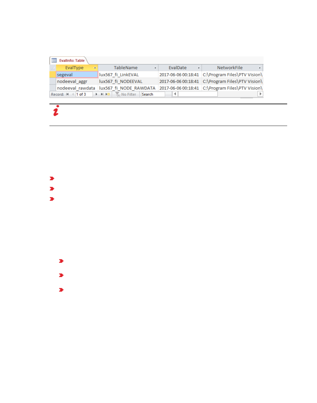
11.9 Showing evaluations in windows
column. If you wish to execute multiple simulation runs, the data from the simulation runs is
saved only in a database table. In the attribute list, multiple columns with the same title name
are merged to one column.
Note: If you wish to execute multiple simulation runs and to save the results in a
database table, avoid switching the selection of attributes between simulation runs.
Otherwise, the table with the previous data simulation runs will be deleted.
Data from the simulation run are saved after the simulation end to the directory ..\<Name of
network file>.results in the default data format *.db.
11.9 Showing evaluations in windows
You can show the following evaluation windows (see "Overview of evaluations" on page 942):
Signal times table
SC detector record
Signal changes
SCs must be defined in the network (see "Modeling signal controllers" on page 542).
1. From the Evaluation menu, choose > Windows.
2. Select the desired evaluation.
A window opens.
3. Make the desired changes:
Signal times table: Specifying display settings for signal times table (see "Showing sig-
nal times table in a window" on page 1038)
SC detector record: Showing the evaluation of an SC detector record in a window (see
"Evaluating SC detector records" on page 1010)
Signal changes (see "Evaluating signal changes" on page 1021)
4. Start the simulation (see "Running a simulation" on page 796).
11.10 Importing text file in a database after the simulation
You can use the direct output to save data to a text file during the simulation. You can import
this text file in a database after the simulation.
Saving data in a database during the simulation can affect the speed of the simulation.
962 © PTV GROUP

11.11 Output options and results of individual evaluations
Example: Importing a *.fzp file into MS Access 2007
1. Configure the direct output for the vehicle record and select Write to file.
2. Open the file *.fzp using a text editor.
3. Delete all the data above the data block in the file.
4. Save the file with the extension *.txt.
5. In Access, choose the menu File > New.
6. Create an empty database.
7. Import the text file using the menu File > Import External Data.
Note: Make sure that you have selected Text files in the Import file type window.
8. Click on Import.
The Text import Wizard opens.
9. Select the option With Separators.
10. Click on Next.
11. Select the option Semicolon.
12. Select the option First row contains field names.
13. Click on Next.
14. Select the option In a new table.
15. Click on Next.
16. From the list box for each column, select the correct data type double, integer or text.
17. Click on Next.
18. Select the option No primary key.
19. Click on Next.
20. Click on Finish.
11.11 Output options and results of individual evaluations
Depending on the selected evaluation, the type of data and the desired further use, you can
show evaluations in list and/or windows and save them to text files and/or database files (see
"Overview of evaluations" on page 942).
Note: Some output options and individual evaluation results may only be available with
add-on modules. You need a license to use the add-on modules.
© PTV GROUP 963

11.12 Visualizing evaluation results
11.12 Visualizing evaluation results
You have additional options for visualizing evaluation results:
Color schemes for links (see "Assigning a color to nodes based on an attribute" on
page 181)
Link bars (see "List of graphic parameters for network objects" on page 152), (see
"Attributes of links" on page 383)
Turn value visualization (see "Visualizing turn values" on page 645)
Path volume visualization using flow bundles (see "Visualizing volumes on paths as
flow bundles" on page 726)
11.13 Saving discharge record to a file
The discharge record shows the time intervals between vehicles driving away from signal
heads. You can use it for purposes such as determining time needs for your SC or calibrating
actual measured saturation flow values. Links, vehicle inputs and signal heads must be
defined in the network.
In order to determine meaningful time needs, the measured flows should be saturated. You
should therefore ensure that the number of vehicles queued behind the stop line is at least as
many as can pass during a green phase.
You can output the following data and data formats:
Output ASCII file MDB file Attribute file from attribute list
Aggregated data - - -
Raw data *.dis - -
Defining evaluation of the discharge record results
1. Make sure that the attribute Discharge record active is selected in the attributes of the
desired signal head.
2. From the Evaluation menu, choose > Configuration > Direct Output tab.
3. In the Discharge record row, select the option Write to file.
4. You can change the time if you wish (see "Using the Direct output function to save
evaluation results to files" on page 958).
5. Confirm with OK.
6. Start the simulation (see "Running a simulation" on page 796).
A *.dis file is saved.
Result of discharge record evaluation
A *.dis discharge record may contain the following data:
964 © PTV GROUP

11.13 Saving discharge record to a file
Element Description
File Path and name of network file
Comment Comment on simulation
Date Time of evaluation
PTV Vissim Version number, service pack number, build number
Table Discharge at SC with its number, signal group with its number, and in
parentheses data collection point with number
Data block One line for each SC cycle
Column 1: Simulation seconds at start of green time
Column 2: Time difference between start of green time and arrival
of first vehicle at measuring point
Column 3: Time need: time gap between the front end of vehicle 1
(the first vehicle in the queue) and the front end of vehicle 2
All other columns contain the time needs of all subsequent
vehicles according to their positions in the queue.
The end of the green phase is shown by the position of the par-
entheses. The numbers in parentheses show:
the number of vehicles passing the measuring point during the
green phase
the average time needs of these vehicles. Both values are
determined without taking vehicle 1 into account, because its
time needs depend on the distance between the stop line and
the measuring point.
Values after the parentheses were measured for vehicles that
crossed the stop line after the green phase (during yellow or red).
Fourth-to-last line: vehicle position number in the queue (index
number) for each cycle
Third-to-last line: average time need for the vehicle position con-
cerned
Next-to-last line: measured number of vehicles at this position. If
saturation is not present for some green phases, smaller numbers
are measured for higher index numbers.
Last line: total number of vehicles (except those in the first position)
and their time needs (measured over all cycles).
Discharge record example: file *.dis
Discharge record
File: C:\Users\Public\Documents\PTV Vision\PTV Vissim 10\Examples Demo\3D - Com-
plex Intersection Karlsruhe.DE\Karlsruhe 3D.inpx
Comment: Karlsruhe 3D example
Date: Friday, June 16, 2017 10:20:30 AM
PTV Vissim 10.00-00* [66098]
Discharge at SC 619, signal group 14, signal head 3
1 (0: 0.0)
© PTV GROUP 965

11.13 Saving discharge record to a file
80 1.11 1.16 (1: 1.16)
170 1.01 (0: 0.0)
260 (0: 0.0)
350 0.95 0.70 (1: 0.70)
440 1.07 1.31 (1: 1.31)
530 1.09 (0: 0.0)
620 1.05 (0: 0.0)
710 1.17 (0: 0.0)
800 1.15 1.45 (1: 1.45)
890 1.09 (0: 0.0)
980 1.11 (0: 0.0)
1070 (0: 0.0)
1160 0.99 0.25 0.88 (2: 0.56)
1250 (0: 0.0)
1340 1.07 (0: 0.0)
1430 (0: 0.0)
1520 6.95 (0: 0.0)
1610 1.18 1.35 (1: 1.35)
1700 1.18 0.98 (1: 0.98)
1790 1.07 (0: 0.0)
1880 1.06 0.05 1.00 0.11 1.05 1.18 (5: 0.68)
1970 1.11 (0: 0.0)
2060 1.06 1.09 (1: 1.09)
2150 1.08 (0: 0.0)
2240 1.10 1.10 1.08 3.49 (3: 1.89)
2330 1.04 (0: 0.0)
2420 1.09 0.99 (1: 0.99)
2510 1.04 (0: 0.0)
2600 1.13 1.11 (1: 1.11)
2690 (0: 0.0)
2780 (0: 0.0)
2870 1.07 (0: 0.0)
2960 (0: 0.0)
3050 (0: 0.0)
3140 (0: 0.0)
3230 (0: 0.0)
3320 1.11 0.00 1.09 0.18 0.75 0.83 (5: 0.57)
3410 1.06 (0: 0.0)
3500 (0: 0.0)
3590 (0: 0.0)
3680 1.17 (0: 0.0)
3770 1.07 1.47 (1: 1.47)
3860 1.22 (0: 0.0)
3950 1.03 6.26 (1: 6.26)
4040 1.13 (0: 0.0)
4130 1.19 1.16
----- 1 2 3 4 5 6
----- 1.26 1.28 1.01 1.26 0.90 1.00
----- 34 16 4 3 2 2
[27: 1.19]
966 © PTV GROUP

11.14 Displaying OD pair data in lists
11.14 Displaying OD pair data in lists
In lists, you can show result attributes that are created from traffic data between the origin
zones and destination zones of dynamic assignment.
by default, the data for all vehicle classes is entered together. You can also show the data for
certain vehicle classes separately in the evaluation (see "Configuring evaluations of the result
attributes for lists" on page 954).
You can save the following data and data formats:
Output ASCII file MDB table Attribute file from attribute list
Aggregated data - -
Raw data - - -
Show result attributes in attribute lists (see "Displaying result attributes in attribute lists" on
page 957)
Show result attributes in a result list (see "Showing result attributes in result lists" on page
956)
Results of the evaluation of OD pairs
The results list OD Pair Results contains the following attributes:
Result attribute
Long name
Short name Description
Simulation run SimRun Number of simulation run
Time interval TimeInt Duration of the evaluation intervals in which the data is
aggregated
ODPair OD pair Zone numbers specify the OD pairs between origin
zones, destination zones and origin and destination
zones.
Aggregated by departure time:
TravTmDep Travel time
(departure)
Average travel time = Total of travel times / number of
vehicles
DelayTmDep Delay time
(departure)
Average delay time = Total of delay times / number of
vehicles
DelayRelDep Delay (rel-
ative) (depar-
ture)
Average relative delay = Average delay time / average travel
time
VolumeDep Volume (depar-
ture)
Number of vehicles
DistTravDep Distance
traveled
(departure)
Total distance traveled / number of vehicles
© PTV GROUP 967

11.15 Saving lane change data to a file
Result attribute
Long name
Short name Description
Aggregated by arrival time:
TravTmArr Travel time
(arrival)
Total travel time / number of vehicles
DelayTmArr Delay time
(arrival)
Total of delay times / number of vehicles
DelayRelArr Delay (rel-
ative) (arrival)
Average delay time / average travel time
VolArr Volume
(arrival)
Number of vehicles
DistTravArr Distance
traveled
(arrival)
Total distance traveled / number of vehicles
The result attributes are based on the destination parking lot and thus on the destination zone
that a vehicle reaches during simulation and where it is then removed from the network. The
result attributes are not based on the destination parking lot that is the vehicle's destination at
the beginning of the simulation.
11.15 Saving lane change data to a file
You can record the time and place of the lane change that was made. You can restrict the
evaluation to vehicle classes and individual vehicles.
You can save the following data and data formats:
Output ASCII file MDB table Attribute file from attribute list
Aggregated data - - -
Raw data *.spw - -
Note: This evaluation always uses metric units.
1. From the Evaluation menu, choose > Configuration > Direct Output tab.
2. In the Lane changes row select the option Write to file.
3. You can change the time if you wish (see "Using the Direct output function to save
evaluation results to files" on page 958).
4. Click the More button.
The Lane changes window opens.
5. Make the desired changes:
968 © PTV GROUP

11.15 Saving lane change data to a file
Element Description
Vehicle
filter All vehicles: takes all vehicles into account in the evaluation
Filter by classes: takes only the selected vehicle classes into account
Filter by sections: takes only the selected sections into account Sections have
to be defined (see "Modeling sections" on page 641). The level with the section
and the the level on which vehicles move are the same. The middle of the
vehicle's front edge lies outside the section.
Filter by individual vehicles: If this option is selected, you can right-click the
list and select vehicles by their number. Only the selected vehicles are taken
into account.
6. Confirm with OK.
7. Start the simulation (see "Running a simulation" on page 796).
A *.spw file is saved.
Result of lane change evaluation
The lane change file *.spw contains the following data:
Element Description
File title Name of evaluation
File Path and name of network file
Comment Comment on simulation
Date Time of evaluation
PTV Vissim Version number, service pack number, build number
Data Data block with the attributes for each recorded vehicle
The data block of the evaluation file contains the following parameters:
Column Description
tStarting time of the lane change. t is the end of the time step in which
the lane change starts. If you simulate with only one time step per
simulation second, the lane change is already running for a second at
this time.
VehNr Vehicle number
v [m/s] Speed [m/s]
Link No. Link number
Lane Number of the old lane
New Lane Number of the new lane
VF Vehicle number of old leading vehicle (0 = not available)
v VF Speed [m/s] of old leading vehicle
dv VF Speed difference [m/s] of old leading vehicle
© PTV GROUP 969

11.15 Saving lane change data to a file
Column Description
dx VF old leading vehicle: distance [m] between rear end position of the
preceding vehicle and front end of the trailing vehicle
VB Vehicle number of old trailing vehicle (0 = not available)
v VB Speed [m/s] of old trailing vehicle
dv VB Speed difference [m/s] of old trailing vehicle
dx VB old trailing vehicle: distance [m] between rear end position of the
preceding vehicle and front end of the trailing vehicle
new VF Vehicle number of new leading vehicle (0 = not available)
v new VF Speed [m/s] of leading vehicle
dv new VF Speed difference [m/s] of new leading vehicle
dx new VF new leading vehicle: distance [m] between rear end position of the
preceding vehicle and front end of the trailing vehicle
new VB Vehicle number of new trailing vehicle (0 = not available)
v new VB Speed [m/s] of new trailing vehicle
dv new VB Speed difference [m/s] of new trailing vehicle
dx new VB new trailing vehicle: distance [m] between rear end position of the
preceding vehicle and front end of the trailing vehicle
Example of evaluation of lane change file *.spw
Lane changes record
File: C:\Users\Public\Documents\PTV Vision\PTV Vissim 10\Examples Demo\3D - Com-
plex Intersection Karlsruhe.DE\Karlsruhe 3D.inpx
Comment: Example, SC 3-10
Date: Friday, June 16, 2017 12:23:33 PM
PTV Vissim 10.00-00* [66098]
t; VehNr; v [m/s]; Link No.; Lane; New Lane;
VF; v VF [m/s]; dv VF [m/s]; dx VF[m]; VB; v VB; dv VB [m/s]; dx VB;
new VF; v new VF; dv new VF; dx new VF; new VB; v new VB; dv new VB; dx new VB
115.10; 203; 9.55; 7;2; 1;
175; 0.00; 9.55; 164.28; 0; -1.00; -1.00; -1.00;
198; 12.43; -2.89; 22.37; 0; -1.00; -1.00; -1.00;
128.50; 39; 13.30; 9;3; 2;
48; 12.77; 0.53; 11.31; 0; -1.00; -1.00; -1.00;
10; 12.66; 0.64; 9.11; 98; 9.19; 4.10; 0.58;
130.70; 40; 13.56; 9;3; 2;
48; 13.11; 0.45; 34.45; 47; 13.02; 0.54; 13.28;
98; 11.51; 2.05; 6.39; 57; 9.53; 4.03; 0.58;
136.50; 180; 12.04; 9;2; 1;
68; 10.39; 1.65; 34.99; 0; -1.00; -1.00; -1.00;
102; 12.56; -0.52; 31.48; 105; 15.16; -3.13; 26.58;
141.80; 88; 12.00; 9;3; 2;
970 © PTV GROUP

11.16 Saving vehicle record to a file or database
66; 12.20; -0.19; 18.24; 0; -1.00; -1.00; -1.00;
58; 10.29; 1.71; 8.42; 115; 12.52; -0.52; 17.11;
144.20; 115; 11.25; 9;2; 1;
88; 9.80; 1.46; 15.14; 134; 12.27; -1.02; 2.95;
117; 10.61; 0.64; 25.67; 140; 14.61; -3.36; 105.09;
144.70; 134; 11.73; 9;2; 1;
115; 11.06; 0.66; 2.51; 0; -1.00; -1.00; -1.00;
117; 10.20; 1.53; 31.93; 140; 14.53; -2.80; 96.74;
152.20; 272; 8.64; 7;1; 2;
203; 0.00; 8.64; 156.60; 0; -1.00; -1.00; -1.00;
265; 12.84; -4.19; 41.51; 0; -1.00; -1.00; -1.00;
164.90; 293; 8.70; 7;1; 2;
203; 0.00; 8.70; 156.69; 0; -1.00; -1.00; -1.00;
272; 7.72; 0.99; 131.91; 0; -1.00; -1.00; -1.00;
174.80; 293; 11.48; 7;2; 1;
272; 0.00; 11.48; 28.49; 0; -1.00; -1.00; -1.00;
203; 0.00; 11.48; 39.70; 296; 12.99; -1.51; 17.72;
215.20; 183; 10.61; 9;3; 2;
194; 13.61; -2.99; 21.95; 0; -1.00; -1.00; -1.00;
204; 12.34; -1.73; 0.64; 165; 10.61; 0.00; 9.79;
…
…
11.16 Saving vehicle record to a file or database
The vehicle record outputs the attribute values for each vehicle as raw data in one row per
time step. You can restrict the evaluation to vehicle classes and individual vehicles. Links and
vehicle inputs must be defined in the network (see "Modeling links for vehicles and
pedestrians" on page 380), (see "Modeling vehicle inputs for private transportation" on page
426).
The vehicle record includes link data, if for links the attribute vehicle record has been
selected (see "Attributes of links" on page 383).
You can output the following data and data formats:
Output ASCII file MDB file Attribute file from attribute list
Aggregated data - -
Raw data *.fzp - -
Tip: You can show many output attributes of the Vehicle record in parallel, also during
the simulation, as a result list Vehicles In Network (see "Displaying vehicles in the
network in a list" on page 803).
1. From the Evaluation menu, choose > Configuration > Direct Output tab.
2. In the Vehicle record row, select the option Write to file.
3. You can change the time if you wish (see "Using the Direct output function to save
evaluation results to files" on page 958).
© PTV GROUP 971
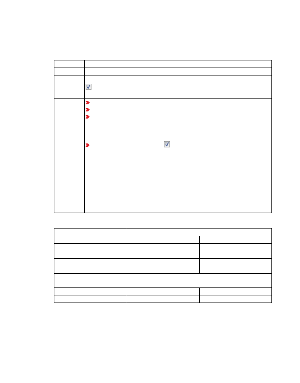
11.16 Saving vehicle record to a file or database
4. Click the More button.
The Vehicle record window opens.
5. Make the desired changes:
Element Description
Resolution Simulation resolution of time steps
Including
parked
vehicles
Only with the add-on module Dynamic Assignment.
If this option is selected, vehicles in parking lots are also taken into
account in the evaluation.
Vehicle fil-
ter All vehicles: takes all vehicles into account in the evaluation
Filter by classes: takes only the selected vehicle classes into account
Filter by sections: takes only the selected sections into account Sections
have to be defined (see "Modeling sections" on page 641). The level with
the section and the level on which vehicles move are the same. The
middle of the vehicle's front edge lies outside the section.
Filter by individual vehicles: If this option is selected, you can right-
click the list and select vehicles by their number. Only the selected
vehicles are taken into account.
Attribute
selection
The Vehicles In Network: Select Attributes window opens. You can select
attributes for the evaluation (see "Selecting attributes and subattributes for a
list" on page 106).
For import of the * .fzp file into the Autodesk 3DS MAX plug-in Civil View, the
attributes and subattributes in the following table are relevant.
Do not change the default settings specified in the Decimals column and the
Format column, if you choose to import these attributes and subattributes.
Relevant attributes and subattributes for Autodesk 3DS MAX plug-in Civil View:
Attribute\subattribute Default value of column
Decimals Format
Simulation second 2Default
Coordinate front 3Default
Coordinate rear 3Default
Vehicle type\Name 0Default
if Vehicle type\Name does not exist, Autodesk 3DS MAX Civil View looks for Vehicle
type\Number and then Vehicle type:
Vehicle type\Number 0Default
Vehicle type 0Default
6. Confirm with OK.
7. Start the simulation (see "Running a simulation" on page 796).
A *.fzp file is saved.
972 © PTV GROUP

11.16 Saving vehicle record to a file or database
Notes:
Stops at PT stops and in parking lots are not counted as stops for the Number of
stops and Delay time in the vehicle record.
You can filter and record the data of all vehicles to determine the total values of
delays or travel time in the network. This is the maximum per vehicle before leaving
the network. At the same time, the data of the vehicles that remain after the sim-
ulation in the network must be recorded.
Result of vehicle record evaluation
A vehicle record *.fzp may contain the following data:
Element Description
File Path and name of network file
Comment Comment on simulation
Date Time of evaluation
PTV Vissim Version number, service pack number, build number
Table Vehicles In network (see "Displaying vehicles in the network in a list"
on page 803)
Column names Column headers and units
Data block One row for each vehicle number.
The columns correspond to the sequence of the attributes in the
selection.
The corresponding add-on module must be installed for some of the
listed attributes so that correct values can be recorded, for example,
the add-on module Dynamic Assignment.
Notes:
By default, the currently selected units for lengths, speeds, accelerations, decel-
erations are taken into account for the evaluation (see "Selecting network settings
for units" on page 195). You can also choose the unit for attribute values in the attrib-
ute selection list in the Format column (see "Selecting attributes and subattributes
for a list" on page 106).
Coordinates are always specified in [m].
Units that are shown in the list box or in the column header with the respective attrib-
ute cannot be changed.
Your selection of attributes determines which attribute values are included. You may also
display these result attributes in the Vehicles In Network list (see "Displaying vehicles in the
network in a list" on page 803).
Vehicle record example: file *.fzp
© PTV GROUP 973
11.17 Evaluating pedestrian density and speed based on areas
$VISION
* File: C:\Users\Public\Documents\PTV Vision\PTV Vissim 10\Examples Demo\3D - Complex
Intersection Karlsruhe.DE\Karlsruhe 3D.inpx
* Comment:
*
Date: Friday, June 16, 2017 12:23:33 PM
PTV Vissim 10.00-00* [66098]
*
*Table: Vehicles In Network
* SIMSEC: SimSec, simulation second (simulation time [s]) [s]
* NO: No, Number
* LANE\LINK\NO: Lane\Link\Number
* LANE\INDEX: Lane\Index
* POS: Position [m]
* POSLAT: Position (lateral)
*
$VEHICLE:SIMSEC;NO;LANE\LINK\NO;LANE\INDEX;POS;POSLAT
0.20;1;1;1;2.57;0.50
0.40;1;1;1;5.71;0.50
0.40;3;2;1;0.22;0.50
0.60;1;1;1;8.86;0.50
0.60;3;2;1;3.25;0.50
0.80;1;1;1;12.02;0.50
0.80;3;2;1;6.29;0.50
1.00;1;1;1;15.18;0.50
1.00;3;2;1;9.33;0.50
...
11.17 Evaluating pedestrian density and speed based on areas
You can determine the density and speed of pedestrians and show them, together with other
attributes, in the result lists Area Results and Ramps Results.
In addition, you have the following options to evaluate pedestrian density and speed:
grid-based (see "Grid-based evaluation of pedestrian density and speed" on page 977).
for each individual pedestrian In this case, density is based on the pedestrians that at the
end of an evaluation interval are located within a radius around a pedestrian (see "Show-
ing pedestrians in the network in a list" on page 809).
Density and speed are determined for the following network objects:
Pedestrian Areas
Ramps & Stairs
Links, whose attribute Is pedestrian area (option Use as pedestrian area) is selected
by default, the data for all pedestrian classes is entered together. You can also show the data
for certain pedestrian classes separately in the evaluation (see "Configuring evaluations of the
result attributes for lists" on page 954).
You can save the following data and data formats:
974 © PTV GROUP

11.17 Evaluating pedestrian density and speed based on areas
Output ASCII file MDB table Attribute file from attribute list
Aggregated data - -
Raw data - - -
Show result attributes in attribute lists (see "Displaying result attributes in attribute lists" on
page 957)
Show result attributes in a result list (see "Showing result attributes in result lists" on page
956)
1. From the Evaluation menu, choose > Configuration > Result Attributes tab.
2. In the Areas & ramps row, select Collect data.
3. If desired, change the time and/or the interval (see "Configuring evaluations of the result
attributes for lists" on page 954).
4. Confirm with OK.
5. Start the simulation (see "Running a simulation" on page 796).
6. If desired, from the Evaluation menu, choose > Result Lists > Area Results or Ramp
Results (see "Output attributes of area and ramp evaluation" on page 979).
Attributes of aggregated data output
Result attribute
Long name
Short name Description
Number of
pedestrians
(maximum)
NumPedsMax Maximum number of pedestrians that were in
the area, on ramp or stairs
Number of
pedestrians
(minimum)
NumPedsMin Minimum number of pedestrians that were in the
area, on ramp or stairs
Number of
pedestrians
(average)
NumPedsAvg Average number of pedestrians that were in the
area, on ramp or stairs
Number of
pedestrians
waiting for PT
(maximum)
NumPedsWaitingPTMax Maximum number of pedestrians who were wait-
ing for a PT vehicle in the area, on the ramp or
stairs
Number of
pedestrians
waiting for PT
(minimum)
NumPedsWaitingPTMin Minimum number of pedestrians who were wait-
ing for a PT vehicle in the area, on the ramp or
stairs
© PTV GROUP 975

11.17 Evaluating pedestrian density and speed based on areas
Result attribute
Long name
Short name Description
Number of
pedestrians
waiting for PT
(average)
NumPedsWaitingPTAvg Average number of pedestrians who were wait-
ing for a PT vehicle in the area, on the ramp or
stairs
Walk-out count WalkOutCnt Number of pedestrians leaving the construction
element Pedestrians from pedestrian inputs and
pedestrians alighting from PT vehicles are not
counted.
Density Density Pedestrian density in area, on ramp or stairs
Walk-in count WalkInCnt Number of pedestrians walking on construction
element Pedestrians from inputs and ped-
estrians alighting from PT vehicles are not coun-
ted.
Density
experienced
DensityExp Pedestrian density experienced within the
perception radius of a pedestrian: Number of
other pedestrians within a radius around the
pedestrian.
Area Area in Area evaluation results list only: area
number
Speed
All types
Speed(All) average pedestrian speed, all pedestrian types,
is calculated as the harmonic mean
Speed
variance
SpeedVar Vectorial speed differences of all pedestrians
within the personal environment radius of their
own speed (see "Selecting network settings for
pedestrian behavior" on page 193)
Ramp/Stairs Ramp in Ramp evaluation results list only: ramp or
stairs number
Simulation run SimRun Number of simulation run
Time interval TimeInt Duration of the evaluation intervals in which the
data is aggregated
If for areas, you selected the Queues attribute, you may additionally output the following
result attributes via queues:
976 © PTV GROUP

11.18 Grid-based evaluation of pedestrian density and speed
Result attribute
Long name
Short name Description
Queue length
(maximum)
QueueLenMax Length and time information on the queues
Queue length
(minimum)
QueueLenMin
Queue length
(average)
QueueLenAvg
Time in queue
(maximum)
TmInQueueMax
Time in queue
(minimum)
TmInQueueMin
Time in queue
(average)
TmInQueueAvg
11.18 Grid-based evaluation of pedestrian density and speed
Note: Grid-based evaluations requires a lot of memory. Make sure that approximately
1 GB of memory space is available.
You can determine the density and speed of pedestrians based on grid cells and show them,
together with other attributes, in the result lists Area Results and Ramps Results. This way,
the result data for grid-based visualization of aggregated parameters of pedestrian simulation
can also be used after a simulation run. It, for instance, allows you to calculate, show and save
an average level-of-service image of multiple simulation runs. Density and speed data form
the basis of the LOS color scheme (see "Using LOS schemes for showing aggregated
pedestrian values" on page 176), (see "Assigning a color to areas based on aggregated
parameters (LOS)" on page 172) , (see "Assigning a color to ramps and stairs based on
aggregated parameters (LOS)" on page 180). In addition, you have the following options to
evaluate pedestrian density and speed.
area-based (see "Evaluating pedestrian density and speed based on areas" on page
974).
for each individual pedestrian In this case, density is based on the pedestrians that at the
end of an evaluation interval are located within a radius around a pedestrian (see "Show-
ing pedestrians in the network in a list" on page 809).
Density and speed are determined for the following network objects:
Pedestrian Areas
Ramps & Stairs
Links, whose attribute Is pedestrian area (option Use as pedestrian area) is selected
by default, the data for all pedestrian classes is entered together. You can also show the data
for certain pedestrian classes separately in the evaluation (see "Configuring evaluations of the
result attributes for lists" on page 954).
© PTV GROUP 977
11.18 Grid-based evaluation of pedestrian density and speed
You can save the following data and data formats:
Output ASCII file MDB table Attribute file from attribute list
Aggregated data - -
Raw data - - -
Show result attributes in attribute lists (see "Displaying result attributes in attribute lists" on
page 957)
Show result attributes in a result list (see "Showing result attributes in result lists" on page
956)
1. From the Evaluation menu, choose > Configuration > Result Attributes tab.
2. In the Pedestrian Grid Cells row, select Collect data.
Select the Collect data option to enable the recording of result attributes. If your next steps
are to click the More button, open the Pedestrian Grid Cells window and select Only last
interval, the data will not be saved and will therefore not be available outside of the
simulation run, but only during the simulation run for visualization of the data in a color
scheme.
3. If desired, change the time and/or the interval (see "Configuring evaluations of the result
attributes for lists" on page 954).
4. Click the More button.
The Pedestrian Grid Cells window opens.
5. Make the desired changes:
Element Description
Only last
interval If the option is selected, evaluation of the pedestrian-grid cells is performed
exclusively based on the last time interval completed. The values of the result
attributes obtained from the last time interval can be visualized in a color
scheme for areas and/or ramps & stairs. The values are not stored and will
therefore not be available outside of the simulation.
Cell size Edge length of a grid mesh. Value range 0.01 to max [m], default value 1.00 m
Range of
influence
Number of pedestrian-grid cells in each direction (up, down, left, right,
diagonal) up until which pedestrians are considered for density measurement.
The resulting area created around each pedestrian-grid cell is used by Vissim
for the calculation of average LOS. Value range 1 - 5
978 © PTV GROUP

11.19 Output attributes of area and ramp evaluation
Element Description
Threshold For the following attributes, Vissim records for how long they exceed the
threshold. You can enter a threshold value for each attribute. For each
attribute, you can show the duration recorded during the simulation
graphically in a color scheme of the area or the ramp. This is also possible for
a link, if the attribute Is pedestrian area is selected for it (see "Assigning a
color to areas based on aggregated parameters (LOS)" on page 172), (see
"Assigning a color to ramps and stairs based on aggregated parameters
(LOS)" on page 180), (see "Assigning a color to links based on aggregated
parameters" on page 169).
Density (DensThresh): Threshold value for evaluation attribute Density -
duration exceeding threshold
Experienced density (ExperDensThresh): Threshold value for evaluation
attribute Experienced density - duration exceeding threshold
Speed (SpeedThresh): Threshold value for evaluation attribute Speed -
duration exceeding threshold
Velocity variance: (VelVarThresh): Threshold value for evaluation attribute
Velocity variance - duration exceeding threshold
Filter by
sections:
Select the sections for which you want to collect data. If no sections are
selected, data is collected for the entire network. Select sections when you
want to record and save grid-based evaluations.for large models, small grid
cells and many time intervals. Otherwise, if data is then collected for the entire
network, your evaluation file will be very large. If a cell is only partly located
within a section, the actual area of the cell is used for the calculation of area-
based evaluations (density).
6. Confirm with OK.
7. Configure the visualization of grid-based data (see "Assigning a color to areas based on
aggregated parameters (LOS)" on page 172) (see "Assigning a color to ramps and stairs
based on aggregated parameters (LOS)" on page 180)
8. Start the simulation (see "Running a simulation" on page 796).
9. If desired, from the Evaluation menu, choose > Result Lists > Area Results or Ramp
Results (see "Output attributes of area and ramp evaluation" on page 979).
11.19 Output attributes of area and ramp evaluation
1. From the Evaluation menu, choose > Result Lists > Area Results or Ramp Results.
© PTV GROUP 979

11.19 Output attributes of area and ramp evaluation
Result attribute
Long name
Short name Description
Number of
pedestrians
(maximum)
NumPedsMax Maximum number of pedestrians that were in
the area, on ramp or stairs
Number of
pedestrians
(minimum)
NumPedsMin Minimum number of pedestrians that were in the
area, on ramp or stairs
Number of
pedestrians
(average)
NumPedsAvg Average number of pedestrians that were in the
area, on ramp or stairs
Number of
pedestrians
waiting for PT
(maximum)
NumPedsWaitingPTMax Maximum number of pedestrians who were wait-
ing for a PT vehicle in the area, on the ramp or
stairs
Number of
pedestrians
waiting for PT
(minimum)
NumPedsWaitingPTMin Minimum number of pedestrians who were wait-
ing for a PT vehicle in the area, on the ramp or
stairs
Number of
pedestrians
waiting for PT
(average)
NumPedsWaitingPTAvg Average number of pedestrians who were wait-
ing for a PT vehicle in the area, on the ramp or
stairs
Walk-out count WalkOutCnt Number of pedestrians leaving the construction
element Pedestrians from pedestrian inputs and
pedestrians alighting from PT vehicles are not
counted.
Density Density Pedestrian density in area, on ramp or stairs
Walk-in count WalkInCnt Number of pedestrians walking on construction
element Pedestrians from inputs and ped-
estrians alighting from PT vehicles are not coun-
ted.
Density
experienced
DensityExp Pedestrian density experienced within the
perception radius of a pedestrian: Number of
other pedestrians within a radius around the
pedestrian.
Area Area in Area evaluation results list only: area
number
Speed
All types
Speed(All) average pedestrian speed, all pedestrian types,
is calculated as the harmonic mean
980 © PTV GROUP

11.20 Evaluating pedestrian areas with area measurements
Result attribute
Long name
Short name Description
Speed
variance
SpeedVar Vectorial speed differences of all pedestrians
within the personal environment radius of their
own speed (see "Selecting network settings for
pedestrian behavior" on page 193)
Ramp/Stairs Ramp in Ramp evaluation results list only: ramp or
stairs number
Simulation run SimRun Number of simulation run
Time interval TimeInt Duration of the evaluation intervals in which the
data is aggregated
If for areas, you selected the Queues attribute, you may additionally output the following
result attributes via queues:
Queue length
(maximum)
QueueLenMax Length and time information on the queues
Queue length
(minimum)
QueueLenMin
Queue length
(average)
QueueLenAvg
Time in queue
(maximum)
TmInQueueMax
Time in queue
(minimum)
TmInQueueMin
Time in queue
(average)
TmInQueueAvg
11.20 Evaluating pedestrian areas with area measurements
You can define or generate area measurements that record data of pedestrian areas with
sections. You can display and store result attributes in evaluations and lists. To allow an area
measurement to record data, the following conditions must be satisfied:
At least one section must be defined in the network (see "Modeling sections" on page
641). If sections are placed on top of pedestrian areas, they can record pedestrian area
data.
At least one area measurement must be defined or generated and assigned to at least
one section (see "Defining an area measurement in lists" on page 949), (see "Generating
area measurements in lists" on page 950).
At least one pedestrian input and one pedestrian route must be defined in the pedestrian
area (see "Modeling pedestrian inputs" on page 883), (see "Modeling routing decisions
and routes for pedestrians" on page 886).
On a ramp, you can collect data from an area measurement with a section. To do so, in the
Additional Level ( AddLvl ) attribute of the section, you must select the level leading to the
ramp (see "Attributes of sections" on page 643).
© PTV GROUP 981
11.20 Evaluating pedestrian areas with area measurements
by default, the data for all pedestrian classes is entered together. You can also show the data
for certain pedestrian classes separately in the evaluation (see "Configuring evaluations of the
result attributes for lists" on page 954).
Saving results of area measurements
You can save the following data and data formats:
Output ASCII file MDB table Attribute file from attribute list
Aggregated data - -
Raw data *.merP - -
Show result attributes in attribute lists (see "Displaying result attributes in attribute lists" on
page 957)
Show result attributes in a result list (see "Showing result attributes in result lists" on page
956)
Save result attributes to files (see "Using the Direct output function to save evaluation res-
ults to files" on page 958)
Show result attributes of area measurements in list (see "Showing results of meas-
urements" on page 953)
Attributes of aggregated data output
Maximum, minimum, average all refer to time interval values.
Result attribute
Long name
Short name Description
Leave time (max-
imum), (minimum),
(average)
tLeavMax, tLeavMin,
tLeavAvg
first, last, and average point in time all ped-
estrians leave the sections [simulation
second]
Orientation x OrientXAvg Average of the x component of the orientation
vectors
Orientation y OrientYAvg Average of the y component of the orientation
vectors
Walk-out count WalkOutCnt Number of pedestrians who have left sections
This does not include passengers boarding
PT vehicles.
Density
(maximum),
(minimum),
(average)
DensMax, DensMin,
DensAvg
Pedestrian density in sections
982 © PTV GROUP

11.20 Evaluating pedestrian areas with area measurements
Result attribute
Long name
Short name Description
Density exper-
ienced (maximum),
(minimum), (aver-
age)
DensityExp Pedestrian density experienced within the per-
ception radius of a pedestrian
Entry time (max-
imum), (minimum),
(average)
tEntMax, tEntMin,
tEntAvg
first, last, and average point in time all ped-
estrians reach the sections [simulation
second]
Walk-in count WalkInCnt Number of pedestrians walking in the sec-
tions. Pedestrians from inputs and pedestrians
alighting from PT vehicles are not counted.
Area meas-
urements
AreaMeasurement Name and number of area measurement
Pedestrians
(maximum),
(minimum),
(average)
PedsMax, PedsMin,
PedsAvg
maximum, minimum number of vehicles in
section, average number
Total distance
(maximum),
(minimum),
(average)
TotDistMax,
TotDistMin,TotDistAvg
maximum, minimum and average total
distance traveled in sections of all pedestrians
who have left the sections during the
aggregation interval
Total time gain
(average)
TotTmGainAvg average total time delay in sections for
pedestrians who have left the sections during
the aggregation interval
Total delay
(maximum),
(minimum),
(average)
TotalDelay maximum, minimum and average total time
delay in sections for pedestrians who have left
the sections during the aggregation interval
Total dwell time
(maximum),
(minimum),
(average)
TotDwlTmMax,
TotDwlTmMin,
TotDwlTmAvg
maximum, minimum and average total dwell
time in sections of all pedestrians who have
left the sections during the aggregation
interval
Speed (maximum),
(minimum),
(average)
SpeedMax, SpeedMin,
SpeedAvg
maximum, minimum and average speed
Speed x-
component
(maximum),
(minimum),
(average)
SpeedXMax,
SpeedXMin,
SpeedXAvg
maximum, minimum, and average speed of x-
component of speed vector
© PTV GROUP 983

11.20 Evaluating pedestrian areas with area measurements
Result attribute
Long name
Short name Description
Speed y-
component
(maximum),
(minimum),
(average)
SpeedYMax,
SpeedYMin,
SpeedYAvg
maximum, minimum, and average speed of y-
component of speed vector
Speed deviation
(average)
SpeedDevAvg average deviation of pedestrian speeds
Source quantity SourceQu Number of pedestrians walking in the sec-
tions. This also includes pedestrians from
inputs and pedestrians alighting from PT
vehicles.
Desired speed
(average)
DesSpeedAvg average desired speed of all pedestrians
World coordinate x
(maximum),
(minimum),
(average)
WorldXMax,
WorldXMin
WorldXAvg,
maximum, minimum and average world
coordinate x
World coordinate y
(maximum),
(minimum),
(average)
WorldYMax,
WorldYMin,
WorldYAvg
maximum, minimum and average world
coordinate y
World coordinate z
(maximum),
(minimum),
(average)
WorldZMax,
WorldZMin,
WorldZAvg
maximum, minimum and average world
coordinate z
Time interval TimeInt Duration of the evaluation intervals in which
the data is aggregated
Destination count DestCnt Number of pedestrians that will not be leaving
the sections, e.g. because their route ends in
one of them or they are alighting a PT vehicle.
Output file of pedestrian area result
Structure of output file:
Element Description
File title
File Path and name of network file
Comment Comment on simulation
Date Time of evaluation
PTV Vissim Version number, service pack number, build number
984 © PTV GROUP

11.20 Evaluating pedestrian areas with area measurements
Element Description
List List of evaluated areas
Column names Column headers and units
Data block Data block with measurement data
Column Meaning
MeasurementAreaNo Number of section
tEnter Time pedestrian entered the section [simulation second]
tLeave Time pedestrian left the section [simulation second]
PedNo Pedestrian number
PedType Pedestrian type
DwellTime Dwell time [s] pedestrians spent in section
vDes Desired speed in the currently selected unit for the speed: average,
minimum and maximum
vSpeed in the currently selected unit for the speed: average, minimum
and maximum
DevSpeed Deviation of pedestrian speed in the currently selected unit for the
speed
Density Pedestrian density in the sections [ped/m²] or [ped/ft²], depending on
the unit set for short distances
AvgXOri Average of x values of orientation vector
AvgYOri Average of y values of orientation vector
WorldX
WorldY
WorldZ
World coordinate X
World coordinate Y
World coordinate Z
TimeGain Time gain [s]: Total time gain is determined based on the delay time.
The total time gain is determined only if the pedestrian is faster than
desired.
TimeDelay Time delay [s]: Total time delay is determined from the "time lost" per
time step. This is determined from the difference between actual
speed and desired speed if the pedestrian is slower than desired.
Delays through using a detour are not taken into account in the
delay.
Dist Distance traveled so far in the sections, in the current unit set for
short distances
DistNetwork Total distance traveled so far in the network in currently selected unit
for short distances
Example of raw data *.merP
The data blocks below the file header contain the area results and all column identifiers.
Area Measurement (raw data)
© PTV GROUP 985

11.21 Evaluating pedestrian travel time measurements
File: C:\Dokumente und Einstellungen\All Users\Dokumente\PTV Vision\PTV Vissim
10\Examples Demo\KAmerP2013.inpx
Comment:
Date: Sunday, June 18, 2017 12:23:33 PM
PTV Vissim 10.00-00* [66098]
Section No. : Section number
tEnter : Time pedestrians enter the section [simulation second]
tLeave : Time pedestrians leave the section [simulation second]
PedNo : Pedestrian number
PedType : Pedestrian type
Dwelltime : Dwell time [s] in section
vDes : Desired speed [km/h]
vX : X component of the speed vector [km/h]
vY : Y component of the speed vector [km/h]
v : Speed [km/h]
DevSpeed : Deviation of pedestrian speed [km/h]
Density : Pedestrian density in section [ped/m²]
AvgXOri : Average of x values of orientation vector
AvgYOri : Average of y values of orientation vector
WorldX : World coordinate x
WorldY : World coordinate y
WorldZ : World coordinate z
TimeDelay : Time delay [s]
TimeGain : Time gain [s]
Dist : Distance [m] pedestrians traveled in sections
DistNetwork : Distance [m] pedestrian traveled in networt so far
MeasurementAreaNo; tEnter; tLeave; PedNo; PedType; Dwell time;
2; 9.0; 28.8; 19; 100; 19.8;
vDes; vDes; vDes; vX; vX; vX; vY;
Average; Min; Max; Average; Min; Max; Average;
5.1; 5.1; 5.1; 4.8; 0.0; 5.0; -1.2;
vY; vY; v; v; v; DevSpeed; Density;
Min; Max; Average; Min; Max; ;Average;
-1.3; -0.0; 4.9; 0.0; 5.1; 0.15; 0.00;
Density; Density; AvgXOri; AvgYOri; WorldX; WorldX; WorldX;
Min; Max; Average; Min; Max;
0.00; 0.00; 0.9703; -0.2413; -1178.1; 0.9703; -0.2413;
WorldY; WorldY; WorldY; WorldZ; WorldZ; WorldZ;Time delay;
Average; Min; Max;Average; Min; Max; ;
115.3; 111.9; 118.6; 0.0; 0.0; 0.0; 0.6;
TimeGain; TravDist; DistNetwork;
0.0; 27.5; 27.5;
11.21 Evaluating pedestrian travel time measurements
With the evaluation of the pedestrian travel time, you record pedestrians when they are added
in the start areas until they enter the associated destination areas.
Note: Pedestrian travel time measurements must be defined in the network (see
"Defining pedestrian travel time measurement" on page 939).
986 © PTV GROUP
11.21 Evaluating pedestrian travel time measurements
by default, the data for all pedestrian classes is entered together. You can also show the data
for certain pedestrian classes separately in the evaluation (see "Configuring evaluations of the
result attributes for lists" on page 954).
You can save the following data and data formats:
Output ASCII file MDB table Attribute file from attribute list
Aggregated data - -
Raw data *.rsrP - -
Show result attributes in attribute lists (see "Displaying result attributes in attribute lists" on
page 957)
Show result attributes in result lists (see "Showing result attributes in result lists" on page
956)
Save result attributes to a file (see "Using the Direct output function to save evaluation res-
ults to files" on page 958)
Result of pedestrian travel time measurements
The file with pedestrian travel times *.rsrp contains the following data:
Element Description
File title Name of evaluation
File Path and name of network file
Comment Comment on simulation
Date Time of evaluation
Vissim Version number, service pack number, build number
Attribute names Description of evaluated data
Data block Measurement data
Tip: You can also create an evaluation based on the pedestrian origin-destination
matrix (see "Saving pedestrian travel time measurements from OD data to a file" on
page 988).
Example of pedestrian travel time sections: raw data *.rsrP
Pedestrian travel time measurement (raw data)
File: C:\Users\Public\Documents\PTV Vision\PTV Vissim 10\Examples Train-
ing\Pedestrians\HR.inpx
Comment:
Date: Friday, June 16, 2017 12:23:33 PM
PTV Vissim 10.00-00* [66098]
t : Time ped. entered dest. area of travel time measurement [sim.second]
No. : Travel time measurement number
PedNo : Pedestrian number
PedType : Pedestrian type
© PTV GROUP 987

11.22 Saving pedestrian travel time measurements from OD data to a file
TravDist : Distance traveled from start to destination area [m]
TravTime : Time traveled from start to destination are [s]
TimeDelay : Time delay [s] while traveling from start to destination area
TimeGain : Time delay [s] while traveling from start to destination area
DevSpeed : Differences [km/h] between actuel speed and v_des
t; No.; PedNo; PedType; TravDist; TravTime; TimeDelay; TimeGain; DevSpeed;
17.1; 30; 414; 100; 14.7; 16.1; 5.0; 0.0; 2.7;
18.4; 29; 56; 100; 17.3; 18.2; 6.3; 0.0; 3.4;
19.5; 29; 99; 200; 18.0; 19.2; 7.1; 0.0; 3.0;
....
Column Description
tTime pedestrian entered destination area of travel time measurement
[simulation second]
No. Travel time measurement number
PedNo Pedestrian number
PedType Pedestrian type
Dist Distance traveled from the start area to the destination area
TravTime Travel time from the start area to the destination area [s]
TimeDelay Delay [s] from the start area to the destination area:
The total TimeDelay when traveling this distance results from the "lost time" per
time step. This is determined from the difference between actual speed and
desired speed if the pedestrian is slower than desired. Pedestrians might walk
slower than desired when they have to slow down because of other pedestrians,
for instance when pedestrian density increases.
Delays through using a detour are not taken into account in the delay.
TimeGain Time gain [s] from the start area to the destination area:
The total TimeGain when traveling this distance is determined accordingly like
the delay. The total "time gain" is determined only if the pedestrian is faster than
desired. Pedestrians might walk faster than desired when they are required to
do so because of other pedestrians.
DevSpeed Difference in [km/h] between the actual speed and desired speed while walking
from the start to the end of the section.
11.22 Saving pedestrian travel time measurements from OD data to a file
If you manage the pedestrian demand of the OD relations between the pedestrian areas as a
pedestrian origin-destination matrix, you do not need to define pedestrian inputs or pedestrian
routing decisions with pedestrian routes to destination areas (see "Pedestrian OD matrices" on
page 918). From a simulation based on a pedestrian origin-destination matrix, you can save
the following aggregated data to an *.rsmp file:
Travel time
Delay
988 © PTV GROUP

11.22 Saving pedestrian travel time measurements from OD data to a file
Relative delay
Volume
Note: You do not need to define any travel time measurements. Vissim defines travel
time measurements automatically at the start of the simulation. A temporary travel time
measurement is generated for each OD relation in the pedestrian origin-destination
matrix:
The temporary travel time measurement starts at the start area.
The temporary travel time measurement ends at the destination area.
The output data results from the pedestrian volume per OD relation and aggregation
interval.
Further routes of a pedestrian in the network are ignored.
Relevant pedestrians for the evaluation
Pedestrians who are generated in the origin area according to the pedestrian input are
taken into account.
Pedestrians who reach the destination area at the end of their current static route (which
began at one of the origin areas) are taken into account.
Pedestrians who enter an origin area when they leave a PT vehicle are not taken into
account.
Pedestrians who get to the origin area from another area are not taken into account.
This also includes pedestrians who traveled a partial route between origin and destination,
and pedestrians who are located in the current destination area, but are continuing their
walk according to a further routing decision, i.e. these pedestrians are also taken into
account.
The arrival time of a pedestrian at the destination area must be in the evaluation period.
Thus only the end of the evaluation period belongs to the interval, and not the start of the
evaluation period.
The start time of the pedestrian in the origin area is not relevant.
Pedestrians who use different static routes for their path from the same origin area to the
same destination area are not differentiated. The following thus applies:
For each OD relation, the output data results from all relevant pedestrians.
There may be multiple static routes for an OD relation.
A pedestrian who has completed his route from the origin area to the destination area is
no longer recorded.
Examples:
The pedestrian is no longer relevant if, in the course of his other routes, he once again
takes his original static route from the original origin area to the same destination area.
© PTV GROUP 989
11.22 Saving pedestrian travel time measurements from OD data to a file
The pedestrian is also no longer relevant if his next destination area could also be
reached from his original origin area via another static route.
A pedestrian who enters an area on his static route to his destination, which is the des-
tination area of another static route and which also starts at the routing decision of the
pedestrian in his origin area, is also not recorded. This pedestrian is only included in
the evaluation when he has reached the destination area of his static route.
Pedestrians with circular routes, which start in area X and also end in this area X, are
included in the evaluation. Since pedestrians within an area are not considered, a cir-
cular route requires at least one route intermediate point in an area outside area X,
which is the origin and destination of the static route. Even area X, which is the origin
and destination of a circular route, can be an intermediate point of the circular route if
another intermediate point then exists in another area in the circular route before the
route destination is reached in area X.
Configuring direct output of the pedestrian travel times (OD data)
1. From the Evaluation menu, choose > Configuration > Direct Output tab.
2. In the Pedestrian travel time (OD data) row, select the option Write to file.
3. You can change the time if you wish (see "Using the Direct output function to save
evaluation results to files" on page 958).
4. Click the More button.
The Pedestrian travel time (OD data) window opens.
5. If desired, change the aggregation interval.
6. Confirm with OK.
7. Start the simulation (see "Running a simulation" on page 796).
The *.rsmp file is saved. If the simulation ends before the specified end of the evaluation, the
evaluation also ends with the simulation. Thus the last time interval may be incomplete. The
corresponding result values for the remaining time interval are still saved.
Results of the evaluation of pedestrian travel times (OD data)
The output file *.rsmp contains the following data:
Element Description
File title Name of evaluation
File Path and name of network file
Comment Comment on simulation
Date Time of evaluation
990 © PTV GROUP

11.22 Saving pedestrian travel time measurements from OD data to a file
Element Description
PTV
Vissim
Version number, service pack number, build number
Data Data blocks with the attributes for each OD relation:
for the entire evaluation period
separately for each evaluation interval
Header data (one row):
Parameter
Valid time interval in simulation seconds
List of destination areas
Output data:
One row per origin area with the output values per attribute and OD relation
For each time interval: separate data block with measurement data per OD
relation
Each data block contains the following evaluation data:
Output
data
Description
Travel
time
Average of all travel times of relevant pedestrians per OD relation.
Delay Average of all total delay values per OD relation.
For each pedestrian, the delay in each simulation step results from:
Example:
The delay is 25% of the length of the time step for a pedestrian at 75% of his
desired speed.
These values are added up over the entire measured distance of the
pedestrian.
Note: Negative values reduce the total delay value.
Relative
delay
Average of all relative delays per OD relation
This value is determined separately for each pedestrian as a percentage of the
delay in the travel time.
Volume Number of pedestrians on the basis of which the other result attributes were
determined.
Example: Output file *.rsmp
An output file is generated for the following matrix:
© PTV GROUP 991

11.22 Saving pedestrian travel time measurements from OD data to a file
In the example, line breaks in the data block (0s-360s) facilitate readability:
Pedestrian travel time measurement (OD data)
File: C:\Users\Public\Documents\PTV Vision\PTV Vissim 10\Examples Train-
ing\Pedestrian OD Matrix.inpx
Comment:
Date: Friday, June 16, 2017 12:23:33 PM
PTV Vissim 10.00-00* [66098]
Travel time:0s-360s;3;4;5;6;
Delay:0s-360s;3;4;5;6;
Relative delay:0s-360s;3;4;5;6;
Volume:0s-360s;3;4;5;6
1;0.0;0.0;53.5;61.0;
1;0.0;0.0;4.5;4.4;
1;0.00;0.00;0.09;0.07;
1;0;0;166;85
2;31.7;0.0;0.0;73.4;
2;4.1;0.0;0.0;6.0;
2;0.13;0.00;0.00;0.08;
2;97;0;0;97
4;33.2;0.0;0.0;0.0;
4;5.3;0.0;0.0;0.0;
4;0.17;0.00;0.00;0.00;
4;87;0;0;0
8;0.0;77.3;0.0;0.0;
8;0.0;7.4;0.0;0.0;
8;0.00;0.10;0.00;0.00;
8;0;108;0;0
Travel time:0s-180s;3;4;5;6;Delay:0s-180s;3;4;5;6;Relative delay:0s-
180s;3;4;5;6;Volume:0s-180s;3;4;5;6
1;0.0;0.0;51.7;58.0;1;0.0;0.0;4.2;4.0;1;0.00;0.00;0.08;0.07;1;0;0;106;53
2;31.5;0.0;0.0;0.0;2;4.0;0.0;0.0;0.0;2;0.13;0.00;0.00;0.00;2;80;0;0;0
992 © PTV GROUP
11.23 Saving pedestrian record to a file or database
4;33.1;0.0;0.0;0.0;4;5.6;0.0;0.0;0.0;4;0.17;0.00;0.00;0.00;4;74;0;0;0
8;0.0;0.0;0.0;0.0;8;0.0;0.0;0.0;0.0;8;0.00;0.00;0.00;0.00;8;0;0;0;0
Travel time:180s-360s;3;4;5;6;Delay:180s-360s;3;4;5;6;Relative delay:180s-
360s;3;4;5;6;Volume:180s-360s;3;4;5;6
1;0.0;0.0;56.6;66.0;1;0.0;0.0;5.0;4.9;1;0.00;0.00;0.09;0.07;1;0;0;60;32
2;32.5;0.0;0.0;73.4;2;4.8;0.0;0.0;6.0;2;0.15;0.00;0.00;0.08;2;17;0;0;97
4;33.7;0.0;0.0;0.0;4;3.9;0.0;0.0;0.0;4;0.12;0.00;0.00;0.00;4;13;0;0;0
8;0.0;77.3;0.0;0.0;8;0.0;7.4;0.0;0.0;8;0.00;0.10;0.00;0.00;8;0;108;0;0
11.23 Saving pedestrian record to a file or database
Note: You will need the add-on module Viswalk.
The pedestrian record outputs the attribute values for each pedestrian in one row per time
step. You can restrict the evaluation to pedestrian classes and individual pedestrians.
Pedestrian areas and pedestrian inputs must be defined in the network (see "Modeling
construction elements" on page 834), (see "Modeling pedestrian inputs" on page 883). In
areas where pedestrians are to be recorded, the Pedestrian record active option must be
selected (see "Attributes of areas" on page 848).
If under Links, you selected the attribute Is pedestrian area (option Use as pedestrian area)
and want to save the link data in the Pedestrian record, select Vehicle record active (see
"Attributes of links" on page 383).
You can output the following data and data formats:
Output ASCII file MDB file Attribute file from attribute list
Aggregated data - -
Raw data *.pp - -
Tip: You can show many output attributes of the Pedestrian record in parallel, also
during the simulation, as a result list Pedestrians in network.
1. From the Evaluation menu, choose > Configuration > Direct Output tab.
2. In the Pedestrian record row, select the option Write to file.
3. You can change the time if you wish (see "Using the Direct output function to save
evaluation results to files" on page 958).
4. Click the More button.
The Pedestrian record window opens.
5. Make the desired changes:
© PTV GROUP 993
11.23 Saving pedestrian record to a file or database
Element Description
Resolution Simulation resolution of time steps
Pedestrian
filter All pedestrians: takes all pedestrians into account in the evaluation
Filter by classes: takes only the selected pedestrian classes into account
Filter by sections: takes only the selected sections into account Sections
have to be defined (see "Modeling sections" on page 641). The level with
the section and the the level on which pedestrians move are the same. The
pedestrians' center lies within the section.
Filter by individual pedestrians: If this option is selected, you can right-
click the list and select pedestrians by their number. Only the selected ped-
estrians are taken into account.
Attribute
selection
The Pedestrians in Network: Select Attributes window opens. You can select
attributes for the evaluation (see "Selecting attributes and subattributes for a list"
on page 106).
6. Confirm with OK.
7. Start the simulation (see "Running a simulation" on page 796).
A *.pp file is saved.
Result of pedestrian record
A pedestrian record *.pp may contain the following data:
Element Description
File Path and name of network file
Comment Comment on simulation
Date Time of evaluation
PTV Vissim Version number, service pack number, build number
Table Pedestrians In Network
Column names Column headers and units
Data block A row for each pedestrian number and simulation step
The columns correspond to the sequence of the attributes in the selection.
Notes:
By default, the currently selected units for lengths, speeds, accelerations, decel-
erations are taken into account for the evaluation (see "Selecting network settings
for units" on page 195). You can also choose the unit for attribute values in the attrib-
ute selection list in the Format column (see "Selecting attributes and subattributes
for a list" on page 106).
Coordinates are always specified in [m].
Units that are shown in the list box or in the column header with the respective attrib-
ute cannot be changed.
994 © PTV GROUP

11.23 Saving pedestrian record to a file or database
Your selection of attributes determines which attribute values are included. You may also
display these result attributes in the Pedestrians In Network list. For example, the following
attributes may be included:
Attribute Definition
Current
walking
behavior
Walking behavior of the pedestrian type When the walking behavior is area-
based, it refers to the walking behavior of the area.
Current
destination
number
Number of construction element which is the destination
Current
destination
type
Type of construction element which is the destination
Width Width of the pedestrian
Level Number of level
Pedestrian
type
Number of pedestrian type
Distance
traveled
(total)
Total distance traveled so far
Time in
network
(total)
Total time in network [s]
The pedestrian record contains the total time = 0.00, as long as the pedestrian
is still in the network.
Speed Speed at the end of the time step
Height Size of pedestrian [m]
Construction
element
number
Number of construction element
Construction
element type
Type of construction element
Length Height of pedestrian [m]
Number Pedestrian number
Start time Network entry time [simulation second ss,f], where f (fraction) is a two-digit
number
Start time Start time as time of day [hh:mm:ss,f], where f (fraction) is a two-digit number
Simulation
time (time of
day)
Simulation time as time of day [hh:mm:ss,f], where f (fraction) is a two-digit
number
Simulation
second
Simulation time in seconds [ss,f], where f (fraction) is a two-digit number
Static route
number
Number of static pedestrian route
© PTV GROUP 995

11.23 Saving pedestrian record to a file or database
Attribute Definition
Static
routing
decision
number
Number of static pedestrian routing decision
Partial route
number
Number of pedestrian route (partial)
Partial
routing
decision
number
Number of pedestrian partial routing decision
Remaining
distance
Remaining distance (short length) to the next internal destination.
If the next destination or intermediate destination is at the current level of the
pedestrian, this is the distance to this destination or intermediate destination.
If the next destination or intermediate destination is at another level, the value
specifies the distance to the foot of the targeted stairways.
Previous
destination
number
Number of construction element that was the previous destination
Distance to
queue start
Direct distance (short length) to the start of the current queue
Queuing
area number
Number of the area in which the current queue is located.
0 = pedestrian is not in a queue
Time in
queues
(total)
Total waiting time of pedestrian in queues [s]
Time in
queue
Waiting time in the last queue [s] in the time step when the pedestrian leaves
the queue
Coordinate
rear
Coordinate of back of pedestrian at the end of the time step
Coordinate
front
Coordinate of front of pedestrian at the end of the time step
Desired
speed
Desired speed [km/h]
Time gains Time gain [s]: Total time gain is determined based on the delay time. The total
time gain is determined only if the pedestrian is faster than desired.
Time delays Time delay [s]: Total time delay is determined from the "time lost" per time
step. This is determined from the difference between actual speed and
desired speed if the pedestrian is slower than desired.
Delays through using a detour are not taken into account in the delay.
996 © PTV GROUP
11.24 Evaluating nodes
Attribute Definition
Public
transport
state
Is the pedestrian waiting, is he alighting from the PT vehicle or walking
towards it:
None
Waiting
Approaching
Alighting
Instead of the attribute PT status, use the attribute Motion state, which allows
you to record more motion states of pedestrians. You can continue to use
existing data with the attribute PT status.
Motion state MotionState: The current motion state of a pedestrian shows for how long the
pedestrian does a certain activity (see "Showing pedestrians in the network in
a list" on page 809).
Pedestrian record example: file *.pp
$VISION
* File: C:\Users\Public\Documents\PTV Vision\PTV Vissim 10\Examples Train-
ing\Pedestrians\RiMEA\Rimea 0.inpx
* Comment:
*
Date: Friday, June 16, 2017 12:23:33 PM
PTV Vissim 10.00-00* [66098]
*
* Table: Pedestrians In Network
*
* NO: Number
* CONSTRELNO: Construction element number
* CURDESTNO: Current destination number
* DESSPEED: Desired speed [km/h]
* SPEED: Speed [km/h]
*
$PEDESTRIAN:NO;CONSTRELNO;CURDESTNO;DESSPEED;SPEED
1;1;2;5.03;0.00
1;1;2;5.03;0.54
1;1;2;5.03;2.49
1;1;2;5.03;3.54
1;1;2;5.03;4.20
1;3;2;5.03;4.56
…
…
11.24 Evaluating nodes
Using the node evaluation, you can record data from nodes of microscopic and mesoscopic
simulation in the Vissim network (see "Modeling nodes" on page 666). Node evaluation is
© PTV GROUP 997

11.24 Evaluating nodes
used especially to determine specific data from intersections without first having to define all
sections manually in order to determine the data.
by default, the data for all vehicle classes is entered together. You can also show the data for
certain vehicle classes separately in the evaluation (see "Configuring evaluations of the result
attributes for lists" on page 954).
Node evaluation also determines exhaust emissions. The basis for these are formed by
standard formulas for consumption values of vehicles from TRANSYT 7-F, a program for
optimizing signal times, as well as data on emissions of the Oak Ridge National Laboratory of
the U.S. Department of energy. The data refers to a typical North American vehicle fleet and
does not differentiate between individual vehicle types. Thus node evaluation is used to
compare the emissions of different scenarios. To determine emissions for individual vehicle
types, use the add-on module EnViVer Pro or EnViVer Enterprise.
Node evaluation accounts for orientations that are not user-defined (see "Attributes of nodes"
on page 669).
Queue lengths in the node are recorded by queue counters for each movement and every
time step. The queue counters are located at the first signal head or first conflict marker (red) of
a priority rule on the link sequence of the turn relation. Queue counters are generated by
Vissim. If there is neither a signal head nor a conflict marker (red), Vissim will add the queue
counter at the node entrance. Vissim does not record queue lengths of conflict areas with the
status red-red or amber-amber.
Delay measurements record the number of vehicles, average delays, average stop delays and
the number of stops of a turn relation. Delay measurements consist of one or several travel
time measurements. Vissim generates these delay and travel time measurements.
For travel time measurement the following applies:
Begins upstream of the specified distance before the node entry. For travel time meas-
urements, the result attribute Start of delay segment before the node specifies this
distance.
Starts immediately after the closest node, if there are no more than four junctions
between the two nodes.
Ends at node exit
PT stops at public transport stops are not counted as PT stops. Passenger service times of PT
vehicles and the waiting time at stop signs are not accounted for in delay times. However,
delays caused through braking just before a PT stop and accelerating again afterwards are
included in delay times.
If an edge between nodes leads via more than three junctions, it is ignored during node
evaluation. Here a junction is any connector that branches off a link upstream of the beginning
of another connector.
If two or more nodes have an identical FromLink and ToLink , only one queue length is
reported.
You can save the following data and data formats:
998 © PTV GROUP
11.24 Evaluating nodes
Output ASCII file MDB table Attribute file from attribute list
Aggregated data - -
Raw data *.knr -
Show result attributes in attribute lists (see "Displaying result attributes in attribute lists" on
page 957)
Show result attributes in a result list (see "Showing result attributes in result lists" on page
956)
Save raw data to a file or database (see "Configuring evaluations for direct output" on
page 957)
Notes:
Make sure:
The attribute UseForEval (Use for evaluation) of nodes that you want to evaluate,
is selected (see "Attributes of nodes" on page 669). Nodes with the selected option
UseForEval are active nodes, while they are passive nodes if the option is deac-
tivated.
Generate a node-edge graph (see "Generating a node-edge graph" on page 678).
Do not group larger network sections, containing multiple intersections, into a node.
Restrictions for nodes of mesoscopic simulation
Only the number of vehicles and persons, the loss time per vehicle and per person,
and the level of service attributes are recorded and output.
The values of queue lengths, stop delays, stops and emissions are empty or zero.
The start section for each internal travel time measurement is placed at the beginning
of the first meso edge. The latter must start at least as far upstream of the node as spe-
cified in the configuration of the node evaluation, in the Start of delay segment attrib-
ute.
Defining evaluation of the node evaluation results
1. From the Evaluation menu, choose > Configuration > Result Attributes tab.
2. In the Nodes row, select Collect data.
3. If desired, change the time and interval (see "Configuring evaluations of the result attributes
for lists" on page 954).
4. Click the More button.
The window Node opens.
© PTV GROUP 999

11.24 Evaluating nodes
Element Description
Delay segment start
before the node (for node
results and node raw data
evaluation)
Distance [m] before node, from which delay time is measured
Queue definiton (for queues and node results): Define queue condition
Begin A vehicle is in queue if its speed is less than the value v <
that was entered for the Begin.
End A vehicle remains in queue as long as its speed has not yet
exceeded the value v > that was entered for the End.
Max. headway Maximum net distance which can occur between two
vehicles in queue. The queue is considered to be interrupted
if there are larger gaps. Values between 10 and 20m are
usual.
Max. length Maximum queue length. Longer queues may still occur. This
attribute is useful if longer queues occur at the next node in
the network, but the queues are to be evaluated separately
for each junction.
When a large value, for example, 4 km, allows a long queue
to form, the simulation speed decreases.
Consider adjacent lanes Select this option to consider adjacent lanes when
calculating the queue length for evaluation (see "Showing
results of queue counters in lists" on page 1045).
Defining direct output of node evaluation
1. From the Evaluation menu, choose > Configuration > Direct Output tab.
2. In the Nodes (raw data) row, click the option of your choice: Write to file and/or Write
database.
3. If desired, change the time and interval (see "Configuring evaluations of the result attributes
for lists" on page 954).
4. Click the More button.
The window Nodes (raw data) opens.
5. Make the desired changes:
Element Description
Start of delay segment before
node
Distance [m] before node, from which delay time is
measured
Result of node evaluation
The *.knr file contains the following data:
1000 © PTV GROUP
11.24 Evaluating nodes
Attribute Definition
VehNo Vehicle number
VehType Number of vehicle type
TStart Simulation second at which the vehicle enters the node
TEnd Simulation second at which the vehicle exits the node
StartLink Link number from which vehicle arrives at node
StartLane Lane number from which vehicle arrives at node
StartPos Position from the beginning of the link from which vehicle arrives at node
NodeNo Node number
Movement Cardinal points from-to, in which the vehicle moves through the node
FromLink Number of link that leads to the node
Note: This is the link with the shortest path to the node. This does
not have to be the link via which the vehicle enters the node.
ToLink Number of link that leads out of the node. The vehicle has left the node
via this link.
ToLane Number of lane that leads out of the node. The vehicle has left the node
via this lane.
ToPos Position of the node exit on the link which leads out from the node
Delay Delay time in seconds that it takes to leave the node starting from
crossing the start section
StopDelay StopDelay in seconds within the node, starting from crossing the start
section
Stops Number of stops within the node, starting from crossing the start section
No_Pers Number of persons in the vehicle
Defining direct output of node evaluation
1. From the Evaluation menu, choose > Configuration > Result Attributes tab.
2. In the Nodes row, select Collect data.
3. If desired, change the time and interval (see "Configuring evaluations of the result attributes
for lists" on page 954).
4. Click the More button.
The window Node opens.
Example of node evaluation of raw data *.knr
Node Evaluation (Raw data)
File: C:\Users\Public\Documents\PTV Vision\PTV Vissim 10\Examples
Demo\example.inpx
Comment: Example, SC 3-10
Date: Friday, June 16, 2017 12:23:33 PM
PTV Vissim 10.00-00* [66098]
© PTV GROUP 1001

11.24 Evaluating nodes
VehNo; VehType; TStart; TEnd; StartLink; StartLane; StartPos; NodeNo; Movement;
FromLink; ToLink; ToLane; ToPos; Delay; StopDelay; Stops; No_Pers;
2; 100; 1.7; 7.0; 4; 1; 0.000; 1;
S-N; 4; 4; 1; 77.268; 0.0; 0.0; 0; 1;
3; 100; 3.0; 8.2; 4; 1; 0.000; 1;
S-N; 4; 4; 1; 77.268; 0.0; 0.0; 0; 1;
1; 100; 1.1; 9.5; 1; 1; 11.013; 1;
SW-NE; 1; 1; 1; 144.237; 0.0; 0.0; 0;
1;
...
Results list Node results
The results list Node Results may contain the following data in addition to the above
described result attributes of the *.knr file:
Attribute Definition
EmissionsCO Emissions CO: Quantity of carbon monoxide [grams]
EmissionsNOx Emissions NOx: Quantity of nitrogen oxides [grams]
EmissionsVOC Emissions VOC: Quantity of volatile organic compounds [grams]
Movement Movement: Number of connectors of a specific inbound link to a
specific outbound link of a node. A movement may contain multiple
link sequences, for example via parallel connectors. In Node
evaluation, various result attributes are automatically calculated for
the individual movements.
Number and name of node
Number and name of the FromLink, which leads to the node
Position of FromLink, at which it passes into the node.
Number and name of the ToLink, which leads from the node
Position of ToLink, at which it leaves the node.
Movements are created for all possible pair options of inbound and
outbound links. The Total movement contains all movements of each
node. The last row of a node movement always contains the Total
movement. It is only listed specifying the node name and number.
To show result attributes of movements, you first need to generate the
node-edge graph for evaluations (see "Generating a node-edge
graph" on page 678).
Vehs Number of vehicles
FuelConsumption Fuel consumption [US liquid gallon]
VehDelay Vehicle delay (see "Showing delay measurements in lists" on page
1047)
PersDelay Person delay (see "Showing delay measurements in lists" on page
1047)
1002 © PTV GROUP

11.24 Evaluating nodes
Attribute Definition
LOS(All) Level of service (transport quality): The levels of transport quality A
to F for movements and edges, a density value (vehicle
units/mile/lane). It is based on the result attribute Vehicle delay
(average). The current value range of vehicle delay depends on the
Level of service scheme type of the node Signalized or Non-
signalized (see "Attributes of nodes" on page 669). The LOS in Vissim
is comparable to the LOS defined in the American Highway Capacity
Manual of 2010.
Signalized intersection Non-signalized intersection
LOS_
A
Loss time < 10 s or no volume, as no vehicle is moving, also
due to traffic jam
LOS_
B
> 10 s to 20 s > 10 s to 15 s
LOS_
C
> 20 s to 35 s > 15 s to 25 s
LOS_
D
> 35 s to 55 s > 25 s to 35 s
LOS_
E
> 55 s to 80 s > 35 s to 50 s
LOS_
F
> 80 s > 50 s
LOSVal(All) Level-of-service value: Level of transport quality as numbers from 1
to 6 according to the LOS scheme assigned.
No value = no volume.
1 corresponds to LOS_A < 10 s, up to 6 corresponds to LOS_F.
The level-of-service value is more suitable for user-defined formula
attributes and color schemes.
Simulation run Number of simulation run
Queue length Mean of all average queue lengths in a node. Vissim automatically
generates queue counters in a node to detect queue lengths. Vissim
calculates the average queue length detected by queue counters in a
node and then calculates their mean.
Queue length (max-
imum)
Maximum queue length. The result depends on the attribute Consider
adjacent lanes.
The attributes will be shown line-by-line for each simulation run and every movement in the
node.
For each node, the total results in a later row will show:
Calculation of the total for vehicles, persons, emissions, fuel consumption
Calculation of total average for vehicle delay, person delay, stopped delay, queue
© PTV GROUP 1003

11.25 Showing meso edges results in lists
length, stops
Calculation of the maximum queue length (maximum)
11.25 Showing meso edges results in lists
You can display result attributes in lists based on data from the traffic on meso edges during
mesoscopic assignment. The delays in the evaluation depend on the meso speed model
selected (see "Attributes of links" on page 383). If the Meso speed model Vehicle-based is
selected, the delays are based on the vehicles' desired speed.
by default, the data for all vehicle classes is entered together. You can also show the data for
certain vehicle classes separately in the evaluation (see "Configuring evaluations of the result
attributes for lists" on page 954).
You can save the following data and data formats:
Output ASCII file MDB table Attribute file from attribute list
Aggregated data - -
Raw data - - -
Show result attributes in attribute lists (see "Displaying result attributes in attribute lists" on
page 957)
Show result attributes in a result list (see "Showing result attributes in result lists" on page
956)
Results of Meso edges evaluation
The results list Meso edges results contains the following attributes:
Result attribute
Long name
Short name Description
Simulation run SimRun Number of simulation run
Time interval TimeInt Time interval within which the data are
aggregated
Meso edge MesoEdge Number of meso edge
Volume input VolInput Number of vehicles driving on the edge during
the time interval [Veh/h]
Volume dis-
charge
VolDisch Number of vehicles exiting the edge during the
time interval [Veh/h]
Travel time TravTm Average travel time on the edge
Delay time Delay Tm Average delay time based on the difference
between actual travel time and travel time at
desired speed
Density Density Vehicle density
Speed Speed Average speed
1004 © PTV GROUP

11.26 Showing meso lane results in lists
Result attribute
Long name
Short name Description
Travel time on
inbound meso
link
TravTmInbMesoLink Average travel time on inbound link meso edge
(output only available for turn meso edges)
Speed on
inbound meso
link
SpeedInbMesoLink Average speed on inbound link meso edge
(output only available for turn meso edges)
Delay time on
inbound meso
link
DelayTmInbMesoLink Average delay time on inbound link meso edge
(output only available for turn meso edges)
Vehicles
(entered)
VehEnter Number of vehicles driving on the edge during
the time interval
Vehicles
(removed)
VehRemov Number of vehicles exiting the edge during the
time interval
Demand (latent) DemandLatent Number of vehicles that could not be deployed
in the network (output only available for origin
connector meso edges)
Delay (latent) DelayLatent Total waiting time for vehicles that, since the
beginning of the simulation, were not able to
enter the network from the origin zone at the
time of deployment. (Output only available for
origin connector meso edges)
11.26 Showing meso lane results in lists
You can display result attributes in lists that are created from traffic data on meso lanes during
mesoscopic simulation. The delays in the evaluation depend on the meso speed model
selected (see "Attributes of links" on page 383). If the Meso speed model Vehicle-based is
selected, the delays are based on the vehicles' desired speed.
You can save the following data and data formats:
Output ASCII file MDB table Attribute file from attribute list
Aggregated data - -
Raw data - - -
Show result attributes in attribute lists (see "Displaying result attributes in attribute lists" on
page 957)
Show result attributes in a result list (see "Showing result attributes in result lists" on page
956)
Results of meso lane evaluation
The results list Meso lanes results contains the following attributes:
© PTV GROUP 1005

11.26 Showing meso lane results in lists
Result attribute
Long name
Short name Description
Simulation run SimRun Number of simulation run
Time interval TimeInt Time interval within which the data are
aggregated
Meso lanes MesoLn Number of meso lanes
Volume input VolInput Number of vehicles driving on the lanes during
the time interval [Veh/h]
Volume dis-
charge
VolDisch Number of vehicles exiting the lane during the
time interval [Veh/h]
Travel time TravTm Average travel time on a lane
Delay time Delay Tm Average delay time based on the difference
between actual travel time and travel time at
desired speed
Density Density Vehicle density
Speed Speed Average speed
Queue length QLen Average queue length: In each time step, the cur-
rent queue length is measured and the arith-
metic mean is calculated per time interval.
Travel time on
inbound meso
link
TravTmInbMesoLink Average travel time on inbound link meso edge
(output only available for turn meso edges)
Speed on
inbound meso
link
SpeedInbMesoLink Average speed on inbound link meso edge
(output only available for turn meso edges)
Delay time on
inbound meso
link
DelayTmInbMesoLink Average delay time on inbound link meso edge
(output only available for turn meso edges)
Vehicles
(entered)
VehEnter Number of vehicles driving on the lanes during
the time interval
Vehicles
(removed)
VehRemov Number of vehicles exiting the lane during the
time interval
Demand (latent) DemandLatent Number of vehicles that could not be deployed
in the network (output only available for origin
connector meso edges)
Delay (latent) DelayLatent Total waiting time for vehicles that, since the
beginning of the simulation, were not able to
enter the network from the origin zone at the
time of deployment. (Output only available for
origin connector meso edges)
1006 © PTV GROUP

11.27 Saving data about the convergence of the dynamic assignment to a file
11.27 Saving data about the convergence of the dynamic assignment to
a file
You can save the results of a dynamic assignment in a convergence evaluation file *.cva.
Note: The evaluation can be performed only with the add-on module Dynamic
Assignment.
The file contains, for each time interval, the distribution of changes in volume and travel time
for all edges and paths, the number of edges/paths that were traversed in this iteration for the
first time, the share of edges/paths in percent that met the convergence criterion as well as the
info whether the simulation run has converged or not.
Volume changes and travel time changes are divided into classes:
10 volume classes for volume changes
14 travel time classes for travel time changes
The number of paths and edges is output for each class for which changes have arisen in
terms of volume or travel time. This data can be used to determine whether the dynamic
assignment has converged (see "Using the dynamic assignment add-on module" on page
653).
You can save only aggregated data in ASCII format as a file *.cva.
Note: The name of the evaluation file contains the index of the simulation run in the
following cases:
if Vissim is started with the command line parameter -s <n>
if the simulation run is started via COM and RunIndex is set to a value > 0
1. From the Evaluation menu, choose > Configuration > Direct Output tab.
2. In the Convergence row, select the option Write to file.
3. Confirm with OK.
4. Start the simulation (see "Running a simulation" on page 796).
A *.cva file is saved.
Result of convergence evaluation
A convergence evaluation file *.cva contains the following data:
Element Description
File title Name of evaluation
File Path and name of network file
Comment Comment on simulation
Date Time of evaluation
© PTV GROUP 1007
11.27 Saving data about the convergence of the dynamic assignment to a file
Element Description
Vissim Version number, service pack number, build number
Data
block
The results of the convergence evaluation are displayed in a table which
compares the volumes and travel times of all edges and paths for each iteration.
The table is divided into the following blocks:
Volume difference
All edges, except closed edges
All paths, except detours
Travel time difference:
Edges
Paths: Only the paths used during the last simulation run.
Shares: Shares in percent:
of the converged paths ShrConvPathTT
of the converged edges (after travel time) ShrConvEdgeTT
of the converged edges (after volume) ShrConvEdgeVol
The fulfilment of the convergence condition AssignConv is indicated by a
+ or -.
Each row of the evaluation blocks refers to a time interval:
For example, 600.0; 1,200.0; means the interval from simulation second 600 to
1,200.
For each column, each row contains the number of edges and/or number of
paths that are contained in the respective class (intervals of volume difference
and intervals of travel time difference).
The class boundaries Class from and Class to are contained in the header of
a block. Class to belongs to the interval. For example, Class from 3 to 5
for edges means: all edges with volume changes greater than 3 vehicles and up
to and including 5 vehicles are contained in this class. In the example below, the
value 7 is for the time interval 0-600.
ShrConvPathTT: The share of the paths in percent that has met the con-
vergence criterion if the convergence criterion Travel time on paths has
been selected. The percentage weighted by volume is specified in par-
entheses: Total volume (across all time intervals) of all converged paths / total
volume of all paths used
ShrConvEdgeTT: The share of the edges in percent that has met the con-
vergence criterion if the convergence criterion Travel time of edges has
been selected. The percentage weighted by volume is specified in par-
entheses: Total volume (across all time intervals) of all converged paths / total
volume of all paths used
ShrConvEdgeVol: The share of the edges in percent that has met the con-
vergence criterion if the convergence criterion Volume on edges has
been selected.
AssignConv: The simulation run has converged (+), has not converged (-)
Column New: edges/paths entered for the first time in this iteration
1008 © PTV GROUP

11.27 Saving data about the convergence of the dynamic assignment to a file
Example of convergence evaluation: file *.cva
Convergence evaluation
File:C:\Users\Public\Documents\PTV Vision\10\Examples Training\Dynamic Assign-
ment\Detour\Detour.inpx
ID: Dynamic Assignment routing example
Date: Monday, September 4, 2017 10:33:29 AM
PTV Vissim 10.00-02* (64 bit) [66871]
From time; To time; Volume difference;
(Class from) ;; 0; 1; 3; 6; 11; 26; 51; 101; 251; 501;
(Class to) ;; 0; 2; 5; 10; 25; 50; 100; 250; 500; ~;
Edges:
0.0; 300.0; 1; 3; 5; 9; 5; 0; 0; 0; 0; 0;
300.0; 600.0; 0; 2; 4; 8; 8; 1; 0; 0; 0; 0;
600.0; 900.0; 3; 6; 8; 4; 2; 0; 0; 0; 0; 0;
900.0; 1200.0; 23; 0; 0; 0; 0; 0; 0; 0; 0; 0;
1200.0; 1500.0; 23; 0; 0; 0; 0; 0; 0; 0; 0; 0;
1500.0; 1800.0; 23; 0; 0; 0; 0; 0; 0; 0; 0; 0;
1800.0; 2100.0; 23; 0; 0; 0; 0; 0; 0; 0; 0; 0;
2100.0; 2400.0; 23; 0; 0; 0; 0; 0; 0; 0; 0; 0;
2400.0; 2700.0; 23; 0; 0; 0; 0; 0; 0; 0; 0; 0;
2700.0; 3000.0; 23; 0; 0; 0; 0; 0; 0; 0; 0; 0;
3000.0; 3300.0; 23; 0; 0; 0; 0; 0; 0; 0; 0; 0;
3300.0; 3600.0; 23; 0; 0; 0; 0; 0; 0; 0; 0; 0;
Paths:
0.0; 300.0; 0; 1; 4; 7; 0; 0; 0; 0; 0; 0;
300.0; 600.0; 2; 3; 2; 3; 2; 0; 0; 0; 0; 0;
600.0; 900.0; 12; 0; 0; 0; 0; 0; 0; 0; 0; 0;
900.0; 1200.0; 12; 0; 0; 0; 0; 0; 0; 0; 0; 0;
1200.0; 1500.0; 12; 0; 0; 0; 0; 0; 0; 0; 0; 0;
1500.0; 1800.0; 12; 0; 0; 0; 0; 0; 0; 0; 0; 0;
1800.0; 2100.0; 12; 0; 0; 0; 0; 0; 0; 0; 0; 0;
2100.0; 2400.0; 12; 0; 0; 0; 0; 0; 0; 0; 0; 0;
2400.0; 2700.0; 12; 0; 0; 0; 0; 0; 0; 0; 0; 0;
2700.0; 3000.0; 12; 0; 0; 0; 0; 0; 0; 0; 0; 0;
3000.0; 3300.0; 12; 0; 0; 0; 0; 0; 0; 0; 0; 0;
3300.0; 3600.0; 12; 0; 0; 0; 0; 0; 0; 0; 0; 0;
From time; To time; Travel time difference;
(Class from);;0%; 5%;10%;15%; 20%; 30%; 40%; 50%; 60%; 70%; 80%; 90%; 100%; 200%;
(Class to);;5%;10%;15% 20%; 30%; 40%; 50%; 60%; 70%; 80%; 90%; 100%; 200%; ~; New;
Edges:
0.0; 300.0; 8; 6; 6; 0; 3; 0; 0; 0; 0; 0; 0; 0; 0; 0; 0;
300.0; 600.0; 5; 2; 6; 4; 3; 1; 0; 1; 1; 0; 0; 0; 0; 0; 0;
600.0; 900.0; 8; 5; 2; 2; 2; 1; 2; 0; 0; 1; 0; 0; 0; 0; 0;
900.0; 1200.0; 0; 0; 0; 0; 0; 0; 0; 0; 0; 0; 0; 0; 0; 0; 0;
1200.0; 1500.0; 0; 0; 0; 0; 0; 0; 0; 0; 0; 0; 0; 0; 0; 0; 0;
1500.0; 1800.0; 0; 0; 0; 0; 0; 0; 0; 0; 0; 0; 0; 0; 0; 0; 0;
1800.0; 2100.0; 0; 0; 0; 0; 0; 0; 0; 0; 0; 0; 0; 0; 0; 0; 0;
2100.0; 2400.0; 0; 0; 0; 0; 0; 0; 0; 0; 0; 0; 0; 0; 0; 0; 0;
2400.0; 2700.0; 0; 0; 0; 0; 0; 0; 0; 0; 0; 0; 0; 0; 0; 0; 0;
2700.0; 3000.0; 0; 0; 0; 0; 0; 0; 0; 0; 0; 0; 0; 0; 0; 0; 0;
3000.0; 3300.0; 0; 0; 0; 0; 0; 0; 0; 0; 0; 0; 0; 0; 0; 0; 0;
3300.0; 3600.0; 0; 0; 0; 0; 0; 0; 0; 0; 0; 0; 0; 0; 0; 0; 0;
© PTV GROUP 1009
11.28 Evaluating SC detector records
Paths:
0.0; 300.0; 6; 2; 3; 1; 0; 0; 0; 0; 0; 0; 0; 0; 0; 0; 0;
300.0; 600.0; 4; 2; 3; 0; 2; 1; 0; 0; 0; 0; 0; 0; 0; 0; 0;
600.0; 900.0; 0; 0; 0; 0; 0; 0; 0; 0; 0; 0; 0; 0; 0; 0; 0;
900.0; 1200.0; 0; 0; 0; 0; 0; 0; 0; 0; 0; 0; 0; 0; 0; 0; 0;
1200.0; 1500.0; 0; 0; 0; 0; 0; 0; 0; 0; 0; 0; 0; 0; 0; 0; 0;
1500.0; 1800.0; 0; 0; 0; 0; 0; 0; 0; 0; 0; 0; 0; 0; 0; 0; 0;
1800.0; 2100.0; 0; 0; 0; 0; 0; 0; 0; 0; 0; 0; 0; 0; 0; 0; 0;
2100.0; 2400.0; 0; 0; 0; 0; 0; 0; 0; 0; 0; 0; 0; 0; 0; 0; 0;
2400.0; 2700.0; 0; 0; 0; 0; 0; 0; 0; 0; 0; 0; 0; 0; 0; 0; 0;
2700.0; 3000.0; 0; 0; 0; 0; 0; 0; 0; 0; 0; 0; 0; 0; 0; 0; 0;
3000.0; 3300.0; 0; 0; 0; 0; 0; 0; 0; 0; 0; 0; 0; 0; 0; 0; 0;
3300.0; 3600.0; 0; 0; 0; 0; 0; 0; 0; 0; 0; 0; 0; 0; 0; 0; 0;
ShrConvPathTT; ShrConvEdgeTT; ShrConvEdgeVol; AssignConv;
75.00%(weighted: 75.63%); 43.48%(weighted: 43.88%); 65.22%; -;
11.28 Evaluating SC detector records
You can use the SC detector record to check control logic of external control procedures,
especially VS-PLUS and TL-PDM/C. For each SC, you can show a freely configurable, precise
record of the SC values and detector values as well as internal parameters of the control
procedure.
The record can be generated for simulation runs and test runs. Detector requirements or
macros must be created for test runs.
SCs must be defined in the network (see "Modeling signal controllers" on page 542). You can
configure the SC detector record for these SCs (see "Configuring an SC detector record in SC
window" on page 1010).
You can save the following data and data formats:
Output ASCII file MDB table Window
Aggregated data - -
Raw data *.ldp -
Save data to *.ldp file (see "Using the Direct output function to save evaluation results to
files" on page 958)
Show data in a window (see "Showing a signal control detector record in a window" on
page 1012)
All essential values of the parameters and variables of the control procedure are recorded
precisely.
11.28.1 Configuring an SC detector record in SC window
1. From the Signal Control menu, choose > Signal Controllers.
The Signal Controllers list opens.
2. Right-click the desired SC.
3. From the shortcut menu, choose Edit.
1010 © PTV GROUP

11.28.1 Configuring an SC detector record in SC window
The Signal Controller window opens.
4. Select the SC Detector Record Config. tab.
Tip: For external control procedures, more information such as, for example, stage
states can be shown in addition to signal groups and detectors. For further details on
displaying additional data, refer to the documentation for the respective control
program.
5. Make the desired changes:
Element Description
List on the
left
Type
(Category)
Select the Type whose data you want to show in the detector log. Click the
symbol to add the type to the section on the right. The list box contains all
types listed in the *.wtt files that are available for an evaluation.
For some types, you must choose a corresponding object number. The object
number is listed in the box next to them, SG No., Port No. or CP No.. The
heading of the list box depends on the type you have selected, e.g. SG No..
List in the
middle
SG No.,
Det No.,
CP No.
If there are several numbers available, from both sections on the right, select
a type-specific number, e.g. a detector no. or signal group no. To select
entries in long lists, use the PAGE UP, PAGE DOWN, POS1, END and arrow keys.
Click the corresponding button to add the selected entry to the list on the right
and specify which data is shown in the detector log.
List on
right
Shows all objects selected in the defined sequence for output in the
evaluations window, chosen in both sections on the right, under Type
(categorie) .
Short title Abbreviate column title in the SC detector record file *.ldp
Signal
group
label:
Labeling of the rows in the detector log for signal groups:
Number: By default, the number for labeling signal groups is used.
Name: In the evaluation windows, signal groups of the selected SC are
labeled with a name.
Detector
label:
Labeling of the rows in the detector log for detectors.
Port number: By default, the number for labeling detectors is used.
Name: In the evaluation windows, detectors of the selected SC are
labeled with a name.
6. Confirm with OK.
7. Start the simulation (see "Running a simulation" on page 796).
For each SC selected, you can open an SC Detector Record window. The SC number is
displayed in the window title bar (see "Showing a signal control detector record in a window"
on page 1012).
© PTV GROUP 1011

11.28.2 Showing a signal control detector record in a window
11.28.2 Showing a signal control detector record in a window
The SC detector record contains data of the last 100 seconds of a simulation run or tests.
Before showing the SC detector record, configure the SC detector record of the SC (see
"Configuring an SC detector record in SC window" on page 1010).
Tip: Alternatively to the next step, you can open the SC detector record for a specific
SC. In doing so, you are skipping the next step and are not selecting any settings for
labeling. In the Signal Controllers list, right-click the desired signal control and from the
shortcut menu, choose Show SC Detector Record.
1. From the Evaluation menu, choose > Window > SC Detector Record.
The SC Detector Record - Windows opens.
2. Make the desired changes:
Element Description
Selected SC Select SC
All Select all defined SCs. The evaluation for each SC is shown in a window.
None Cancel selection of all SCs
3. Confirm with OK.
The SC Detector Record - window closes. The SC<Number> Detector Record - window for
the selected SC opens. When you start the simulation, the SC detector record is displayed
depending on the settings made in the SC Detector Record Config. tab.
Results of SC detector evaluation
During a simulation or during a test run, the values of all data specified in the configuration in
the last 100 simulation seconds are shown in the SC Detector Record window.
1012 © PTV GROUP

11.28.2 Showing a signal control detector record in a window
The type of values which can be recorded depends on the control procedures of each SC. You
can refer to the documentation of the control program in this case.
If in the Direct Output tab you selected SC Detector Record and the simulation or test run
have been completed, the *.ldp file contains the following data: The SC detector record is
constructed as a table with one row per simulation second and one column per selected type
of values. The record can show up to 1,000 values and up to 3,000 characters per row.
Element Description
Row 1 Name of evaluation with time of evaluation
Row 2 Comment on simulation
Row 3 SC number, control files, program number, simulation run or test
Other
rows
Evaluation data. The columns correspond to the sequence of values in the Con-
figuration window.
Note: The values are saved after the run of the control logic.
When you perform multiple simulation runs using different random seeds, the number of the
respective simulation run is added to the name of the evaluation file *.ldp.
For VS-PLUS, you may also output the following value types in the SC detector record (SG =
signal group; VS = Verkehrsstrom - German for traffic volume):
Value type Meaning
Active flag of
traffic
volume
Active flag of traffic volume, VS-Plus specific
GreenMax of
traffic
volume
GreenMax of traffic volume, VS-Plus specific
Main
indicator PE
Next traffic volume of main sequence of the relevant priority element (1-6) to
be processed
Control time
of traffic
volume
Control time of traffic volume, VS-Plus specific
Empty
column
Distance from a space
Priority class
of traffic
volume
By default: 1: PrT, 2: PT, 3: Emergency vehicles
Priority level
of traffic
volume
Priority level of traffic volume:
1: normal
2: maximum reasonable waiting time exceeded
© PTV GROUP 1013

11.28.2 Showing a signal control detector record in a window
Value type Meaning
Priority value
of traffic
volume
Priority level of traffic volume, VS-Plus specific
Signal state
of SG . Red
= Red/Amber
| Green
/ Amber
Simul.second Simulation second between 1 and 999,999,999
Separator vertical line between two columns
Cycle
second
Tx second between 1 and cycle time
DET waiting
time
Counter which adds up the time from the first passing of a detector to the next
release
Waiting time
of traffic
volume
Time in seconds since detection of the traffic volume (such as DET waiting
time - deceleration time)
State of DET +: within a simulation second, a vehicle has either completely passed the
detector or a vehicle has left the detector and another has reached it
(rising and falling edge in one time step)
|: at the end of the time step there is a vehicle on the detector and no
vehicle has left the detector within this time step.
.: The detector is not occupied during the time step.
State of
calling point
State of a calling point
State of
traffic
volume
Coded state of the traffic volume, for example:
1: detected
9: Green command given
10: Switched to green
21: Red command given
Example of SC detector record file *.ldp
Signal control detector record [6/6/2016 14:56:45]
Luxembourg, SC 3-10
SC 5; program file: vap216.dll; import files: l05_11hp.VAP, l05.pua; program no.
1; simulations run
1014 © PTV GROUP
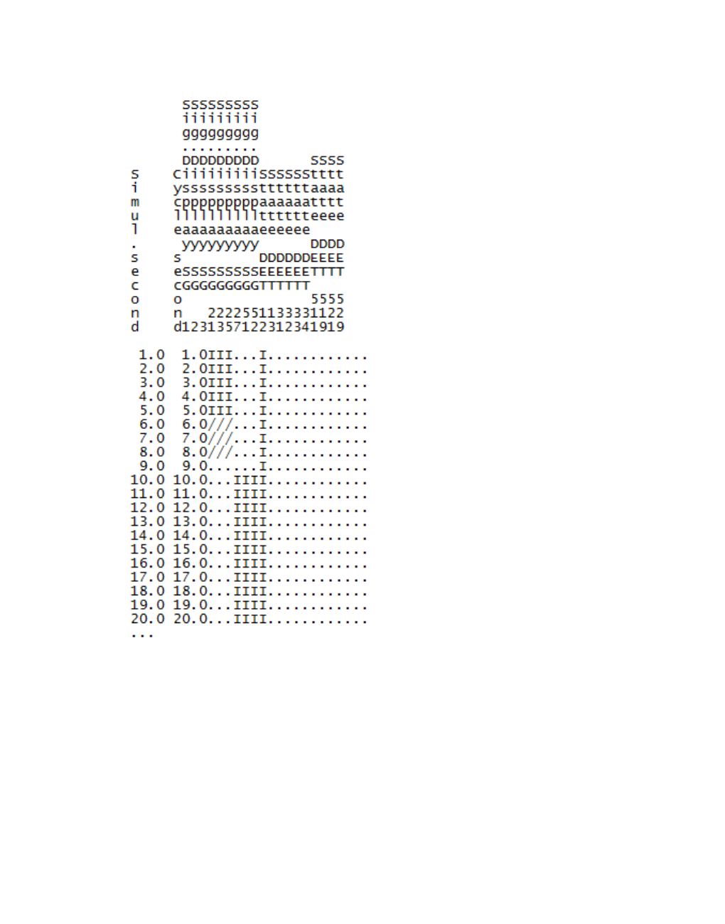
11.28.3 Results of SC detector evaluation
11.28.3 Results of SC detector evaluation
During a simulation or during a test run, the values of all data specified in the configuration in
the last 100 simulation seconds are shown in the SC Detector Record window.
The type of values which can be recorded depends on the control procedures of each SC. You
can refer to the documentation of the control program in this case.
If in the Direct Output tab, you selected SC Detector Record and the simulation or test run
have been completed, the *.ldp file contains the following data: The SC detector record is
© PTV GROUP 1015

11.28.3 Results of SC detector evaluation
constructed as a table with one row per simulation second and one column per selected type
of values. The record can show up to 1,000 values and up to 3,000 characters per row.
Element Description
Row 1 Name of evaluation with time of evaluation
Row 2 Comment on simulation
Row 3 SC number, control files, program number, simulation run or test
Other
rows
Evaluation data. The columns correspond to the sequence of values in the Con-
figuration window.
Note: The values are saved after the run of the control logic.
If simulations run several times, the respective Random Seed is attached as an index of the
simulation run to the name of the evaluation file *.ldp.
For VS-PLUS, you may also output the following value types in the SC detector record (SG =
signal group; VS = Verkehrsstrom - German for traffic volume):
Value type Meaning
Active flag of
traffic
volume
Active flag of traffic volume, VS-Plus specific
GreenMax of
traffic
volume
GreenMax of traffic volume, VS-Plus specific
Main
indicator PE
Next traffic volume of main sequence of the relevant priority element (1-6) to
be processed
Control time
of traffic
volume
Control time of traffic volume, VS-Plus specific
Empty
column
Distance from a space
Priority class
of traffic
volume
By default: 1: PrT, 2: PT, 3: Emergency vehicles
Priority level
of traffic
volume
Priority level of traffic volume:
1: normal
2: maximum reasonable waiting time exceeded
Priority value
of traffic
volume
Priority level of traffic volume, VS-Plus specific
1016 © PTV GROUP

11.28.3 Results of SC detector evaluation
Value type Meaning
Signal state
of SG . Red
= Red/Amber
| Green
/ Amber
Simul.second Simulation second between 1 and 999,999,999
Separator vertical line between two columns
Cycle
second
Tx second between 1 and cycle time
DET waiting
time
Counter which adds up the time from the first passing of a detector to the next
release
Waiting time
of traffic
volume
Time in seconds since detection of the traffic volume (such as DET waiting
time - deceleration time)
State of DET +: within a simulation second, a vehicle has either completely passed the
detector or a vehicle has left the detector and another has reached it
(rising and falling edge in one time step)
|: at the end of the time step there is a vehicle on the detector and no
vehicle has left the detector within this time step.
.: The detector is not occupied during the time step.
State of
calling point
State of a calling point
State of
traffic
volume
Coded state of the traffic volume, for example:
1: detected
9: Green command given
10: Switched to green
21: Red command given
Example of SC detector record file *.ldp
Signal control detector record [6/6/2016 14:56:45]
Luxembourg, SC 3-10
SC 5; program file: vap216.dll; import files: l05_11hp.VAP, l05.pua; program no.
1; simulations run
© PTV GROUP 1017

11.29 Saving SC green time distribution to a file
11.29 Saving SC green time distribution to a file
You can evaluate the absolute frequencies of the occurrence of green durations and red
durations for each signal group. The evaluation also includes the calculated averages of both.
SCs must be defined in the network (see "Modeling signal controllers" on page 542).
You can save the following data and data formats:
1018 © PTV GROUP

11.29 Saving SC green time distribution to a file
Output ASCII file MDB table
Aggregated data *.lzv -
Raw data
Save data to file (see "Configuring evaluations for direct output" on page 957)
1. From the Evaluation menu, choose > Configuration > Direct Output tab.
2. In the Green time distribution row, select the option Write to file.
3. Confirm with OK.
4. Start the simulation (see "Running a simulation" on page 796).
After the simulation run, an *.lzv file is saved.
Result of evaluation of SC green time distribution
The file of the SC green time distribution *.lzv contains the following data:
Element Description
File title Name of evaluation
File Path and name of network file
Comment Comment on simulation
Date Time of evaluation
Vissim Version number, service pack number, build number
Data The evaluation contains the following data blocks:
Data block with average green times for each SC
Separate data blocks with green times and red times for each SC:
The columns contain the individual signal groups j
The rows contain the green times and red times i (to 120 s)
Each table entry ij indicates how often the signal group j received a release
duration of i seconds.
Separate data blocks of all green times and red times with information about
their frequency and average for each SC and each signal group.
In addition, the frequencies are represented graphically in a simple form.
Note: For the graphic representation of green time distribution, you can import the file
*.lzv into a spreadsheet program, e.g. Microsoft™ Excel. The block with the tabular
green times is particularly suitable in this case.
Example of SC green time distribution file *.lzv
Distribution of Signal Times
Datei: C:\Users\Public\Documents\PTV Vision\PTV Vissim 10\Examples
Demo\example.inpx
© PTV GROUP 1019

11.29 Saving SC green time distribution to a file
Comment: Example, SC 3-10
Date: Friday, June 16, 2017 12:23:33 PM
PTV Vissim 10.00-00* [66098]
Time: 0.0 - 300.0
SC 7, Average Green Times:
Signal group; t;
1; 8.5;
2; 42.9;
3; 41.9;
21; 17.5;
23; 17.0;
25; 22.1;
27; 73.6;
SC 6, Average Green Times:
Signal group; t;
1; 70.3;
2; 12.0;
...
SC 7, Green Times:
t|SG; 1; 2; 3; 21; 23; 25; 27;
0; 0; 0; 0; 0; 3; 2; 0;
1; 0; 0; 0; 0; 0; 0; 0;
2; 0; 0; 0; 0; 0; 0; 0;
3; 0; 0; 0; 0; 0; 0; 0;
4; 1; 1; 1; 0; 0; 0; 0;
5; 67; 0; 2; 7; 3; 0; 1;
...
118; 0; 0; 0; 0; 0; 0; 0;
119; 0; 0; 0; 0; 0; 0; 0;
120; 0; 0; 0; 0; 0; 0; 15;
SC 7, Red Times:
t|SG; 1; 2; 3; 21; 23; 25; 27;
0; 0; 0; 0; 0; 0; 0; 20;
1; 0; 0; 0; 0; 0; 0; 0;
...
12; 13; 0; 0; 0; 0; 0; 0;
13; 10; 0; 0; 67; 0; 0; 0;
...
118; 0; 0; 0; 0; 0; 0; 0;
119; 0; 0; 0; 0; 0; 0; 0;
120; 0; 0; 0; 0; 0; 0; 0;
SC 6, Green Times:
t|Sg; 1; 2; 4; 5; 6; 11; 21; 22; 23; 24; 25; 26; 27; 28; 31;
0; 0; 0; 0; 0; 0; 0; 10; 10; 0; 0; 0; 0; 0; 0; 9;
1020 © PTV GROUP

11.30 Evaluating signal changes
1; 0; 0; 0; 0; 0; 0; 0; 0; 0; 0; 0; 0; 0; 0; 0;
2; 1; 0; 0; 0; 0; 0; 0; 0; 0; 0; 0; 0; 0; 0; 0;
...
SC 7, Signal group 1, Green Times: (Mean: 8.5)
4 1 *
5 67 *******************************************************************
6 8 ********
...
22 1 *
31 1 *
SC 7, Signal group 1, Red Times: (Mean: 22.3)
1 1 *
10 7 *******
11 9 *********
...
65 1 *
79 1 *
SC 7, Signal group 2, Green Times: (Mean: 42.9)
4 1 *
6 2 **
...
SC 6, Signal group 1, Green Times: (Mean: 70.3)
2 1 *
5 1 *
...
11.30 Evaluating signal changes
You can record all changes of the individual signal groups from all light signal controls. SCs
must be defined in the network (see "Modeling signal controllers" on page 542).
You can save the following data and data formats:
Output ASCII file MDB table Window
Aggregated data - -
Raw data *.lsa
Save raw data to a file or database (see "Configuring evaluations for direct output" on
page 957)
Show data in a window (see "Showing evaluations in windows" on page 962)
Showing evaluation of signal changes in a window
1. From the Evaluation menu, choose > Windows > Signal Changes.
The Signal changes window opens in a tab.
© PTV GROUP 1021
11.30 Evaluating signal changes
2. Start the simulation (see "Running a simulation" on page 796).
In the Signal changes window, the current values of the following data is displayed:
Element Description
SimSec Simulation second [s]
CycSec Cycle time [s]
SC SC number
SG Signal group number
State New signal state
old Time since the last signal state change (= duration of the previous signal state)
Crit SC type
bcSG Signal group which has caused the current signal change. This is supported only
by certain controllers for vehicle actuated signals.
A *.lsa file is saved.
Result of evaluation of signal changes
The record file of signal changes *.lsa contains the following information:
Element Description
File title Name of evaluation
File Path and name of network file
Comment Comment on simulation
Date Time of evaluation
Vissim Version number, service pack number, build number
SC block All signal groups
Data
block
A row is output for each change process of each signal group.
The columns contain the following data (from left to right):
Simulation second [s]
Cycle time [s]
SC number
Signal group number
New signal state
Time since the last signal state change (= duration of the previous signal
state)
SC type
Signal group which has caused the current signal change. This is supported
only by certain controllers for vehicle actuated signals.
Example of evaluation of signal changes file *.lsa
Signal Changes Protocol
1022 © PTV GROUP

11.30 Evaluating signal changes
File: C:\Users\Public\Documents\PTV Vision\PTV Vissim 10\Examples
Demo\example.inpx
Comment: Example, SC 3-10
Date: Friday, June 16, 2017 12:23:33 PM
PTV Vissim: 10.00 [66098*]
SC 6 SGroup 1 Link 10283 Lane 1 At 18.0
SC 6 SGroup 2 Link 277 Lane 1 At 300.2
SC 6 SGroup 4 Link 10279 Lane 1 At 9.8
SC 6 SGroup 4 Link 10279 Lane 2 At 3.5
SC 6 SGroup 5 Link 272 Lane 1 At 245.6
SC 6 SGroup 6 Link 273 Lane 1 At 154.0
SC 6 SGroup 11 Link 249 Lane 2 At 66.8
SC 6 SGroup 11 Link 249 Lane 3 At 66.9
SC 6 SGroup 11 Link 249 Lane 1 At 66.8
SC 6 SGroup 21 Link 280 Lane 1 At 2.1
SC 6 SGroup 22 Link 281 Lane 1 At 2.8
SC 6 SGroup 23 Link 285 Lane 1 At 1.0
SC 6 SGroup 24 Link 284 Lane 1 At 3.6
SC 6 SGroup 25 Link 287 Lane 1 At 1.4
SC 6 SGroup 26 Link 286 Lane 1 At 2.0
SC 6 SGroup 27 Link 283 Lane 1 At 2.9
SC 6 SGroup 28 Link 282 Lane 1 At 2.9
SC 6 SGroup 31 Link 73 Lane 1 At 2.8
SC 6 SGroup 31 Link 406 Lane 1 At 2.1
SC 10 SGroup 1 Link 10305 Lane 1 At 8.7
SC 10 SGroup 2 Link 4 Lane 2 At 16.7
...
1.0; 1.0; 6; 11; green; 1.0; VAP; 0;
1.0; 1.0; 6; 1; green; 1.0; VAP; 0;
1.0; 1.0; 10; 32; green; 1.0; VAP; 0;
1.0; 1.0; 10; 31; green; 1.0; VAP; 0;
1.0; 1.0; 10; 25; green; 1.0; VAP; 0;
1.0; 1.0; 10; 3; green; 1.0; VAP; 0;
1.0; 1.0; 10; 2; green; 1.0; VAP; 0;
1.0; 1.0; 10; 1; green; 1.0; VAP; 0;
1.0; 1.0; 9; 53; red/amber; 1.0; VAP; 0;
1.0; 1.0; 9; 52; red/amber; 1.0; VAP; 0;
1.0; 1.0; 9; 51; red/amber; 1.0; VAP; 0;
1.0; 1.0; 9; 25; green; 1.0; VAP; 0;
1.0; 1.0; 9; 22; green; 1.0; VAP; 0;
1.0; 1.0; 9; 11; green; 1.0; VAP; 0;
1.0; 1.0; 9; 10; green; 1.0; VAP; 0;
1.0; 1.0; 9; 1; green; 1.0; VAP; 0;
1.0; 1.0; 8; 52; red/amber; 1.0; VAP; 0;
...
© PTV GROUP 1023

11.31 Saving managed lane data to a file
11.31 Saving managed lane data to a file
During a simulation run, you can save attribute values of managed lanes, general purpose
lanes and other attribute values of managed lane facilities in the Vissim network to an *.mle
file. The following must be defined:
Managed lanes routing decision (see "Modeling vehicle routes, partial vehicle routes, and
routing decisions" on page 430)
Toll pricing calculation model (see "Defining toll pricing calculation models" on page 311)
Decision model for managed lanes facilities (see "Defining decision model for managed
lane facilities" on page 310)
Managed lanes facility (see "Defining managed lane facilities" on page 308)
You can save the following data and data formats:
Output ASCII file MDB table
Aggregated data - -
Raw data *.mle -
Save data to file (see "Using the Direct output function to save evaluation results to files"
on page 958)
Result of managed lanes evaluation
The managed lanes evaluation file *.mle contains the following data:
Element Description
File title Name of evaluation
File Path and name of network file
Comment Comment on simulation
Date Time of evaluation
Vissim Version number, service pack number, build number
Managed lanes facility Name and number of the Managed Lanes
Data block Data block with a column for each attribute
Example of managed lanes evaluation file *.mle
Managed Lanes Evaluation
File: C:\Users\Public\Documents\PTV Vision\PTV Vissim 10\Examples
Demo\example.inpx
Comment: Example, SC 3-10
Date: Friday, June 16, 2017 12:23:33 PM
PTV Vissim 10.00-00* [66098]
Managed lanes facility 1: Main Road
1024 © PTV GROUP
11.32 Vehicle network performance : Displaying network performance results (vehicles) in
Managed lanes decision 2: MLD Main
Time : Simulation Time [s]
FacilityNo : Managed lanes facility number
TTS : TTS [seconds]
AvsML : Average speed on managed lanes route [mph]
AvsGP : Average speed on general purpose route [mph]
SOV : Toll user class SOV
HOV2 : Toll user class HOV2
HOV3+ : Toll user class HOV3+
Revenues : Total toll revenue (at routing decision)
VehML(All) : Number of vehicles at end of managed lanes route, All vehicle types
VehGP(All) : Number of vehicles at end of general purpose route, All vehicle
types
Time; FacilityNo; TTS; AvsML; AvsGP; SOV; HOV2; HOV3+; Revenues; VehML(All); VehGP
(All);
0.0; 1; 0; 96.56; 96.56; 3.00; 2.00; 0.00; 0.00; 0; 0;
60.0; 1; 0; 96.56; 96.56; 3.00; 2.00; 0.00; 21.00; 0; 0;
120.0; 1; 0; 51.14; 53.18; 3.00; 2.00; 0.00; 36.00; 8; 14;
180.0; 1; 0; 50.37; 52.50; 3.00; 2.00; 0.00; 33.00; 12; 17;
240.0; 1; 0; 51.02; 52.85; 3.00; 2.00; 0.00; 36.00; 10; 19;
300.0; 1; 0; 50.06; 28.78; 3.00; 2.00; 1.00; 39.00; 14; 7;
Total; 1; 0; 50.56; 49.87; 3.00; 2.00; 0.00; 165.00; 44; 57;
11.32 Vehicle network performance : Displaying network performance
results (vehicles) in result lists
You can show vehicle specific attributes of the entire network compiled in lists.
In microscopic simulation, the network performance is updated with every time step. In
mesoscopic simulation, the network performance is updated at the end of the evaluation
interval.
Via the COM Interface, you can show and access user-defined attributes in the Network
Performance (Vehicles) Results list. User-defined formula attributes are shown, if you use the
subattribute Simulation run. User-defined attributes are saved when you save the network file.
by default, the data for all vehicle classes is entered together. You can also show the data for
certain vehicle classes separately in the evaluation (see "Configuring evaluations of the result
attributes for lists" on page 954).
You can save the following data and data formats:
Output ASCII file MDB table Attribute file from attribute list
Aggregated data - -
Raw data - - -
Show result attributes in attribute lists (see "Displaying result attributes in attribute lists" on
page 957)
© PTV GROUP 1025

11.32 Vehicle network performance : Displaying network performance results (vehicles) in result lists
Show result attributes in a result list (see "Showing result attributes in result lists" on page
956)
Result of vehicle network performance
All attributes take into account the vehicles which have already left the network or reached
their destination parking lot and the vehicles that are still in the network at the end of the
evaluation interval.
The total demand of the input flows and origin-destination matrices during the simulation time
results from:
Total = Vehicles In Network + vehicles which have left + vehicles which could not be used (immediately)
The results list Vehicle network performance results contains the following attributes.
Emissions are specified in grams:
Result attribute
Long name
Short name Description
Emissions (evap-
oration) HC
EmissionsEvaporationHC Evaporated hydrocarbons
Emissions 1,3-
Butadiene
Emissions13BUT 1,3-Butadiene (also vinyl ethylene)
Emissions 2,2,4-
trimethylpentane
Emissions224 2,2,4-trimethylpentane
Emissions
Acetaldehyde
EmissionsAcetaldehyde Acetaldehyde (ethanal)
Benzene emis-
sions
EmissionsBenzene Benzol (benzene)
Emissions CH4 EmissionsCH4 CH4 (methane)
Emissions CO EmissionsCO Carbon monoxide
Emissions CO2 EmissionsCO2 Carbon dioxide
Emissions ethyl
benzene
EmissionsEthylBenzene Ethylbenzene (ethyl benzene, phenyl
ethane)
Emissions
Formaldehyde
Emissions13Formaldhyde Formaldehyde (methanal)
Emissions HC EmissionsHC Burned hydrocarbons
Emissions Hex-
ane
EmissionsHexane Hexane
Emissions ele-
mental carbon
EmissionsElementalCarbon Elemental carbon
Emissions
methyl tert-butyl
ether
EmissionsMTBE 2-methoxy-2-methyl propane
Emissions N2O EmissionsN2O Nitrous oxide
1026 © PTV GROUP

11.32 Vehicle network performance : Displaying network performance results (vehicles) in
Result attribute
Long name
Short name Description
Emissions
Naphtalene gas
EmissionsNaphtaleneGas Naphthalene
Emissions NH3 EmissionsNH3 NH3 ammonia
Emissions
NMHC
EmissionsNMHC Non-methane hydrocarbons without
oxygen compounds
Emissions
NMOG
EmissionsNMOG Non-methane hydrocarbons with oxygen
compounds
Emissions NO3 EmissionsNO3 Nitrates
Emissions NOx EmissionsNOx Nitrogen oxides
Emissions par-
ticulates
EmissionsParticulates Particulate matter
Emissions PM10
brakes
EmissionsPM10brakes Brake abrasion according to standard
PM10
Emissions PM10
total
EmissionsPM10total Total quantity of emissions according to
standard PM10
Emissions PM10
tires
EmissionsPM10tires Tire abrasion according to standard
PM10
Emissions
PM2.5 brakes
Emissions PM2.5 brakes Brake abrasion according to standard
PM2.5
Emissions
PM2.5 total
EmissionsPM2.5total Total quantity of emissions according to
standard PM2.5
Emissions
PM2.5 tires
EmissionsPM25tires Tire abrasion according to standard
PM2.5
Emissions soot EmissionsSoot Soot particles
Emissions SO2 EmissionsSO2 Sulfur dioxide
Emissions
sulfate par-
ticulates
EmissionsSulfateParticulates Sulfates
Emissions total
organic gases
EmissionsTOG Organic gases
Emissions tolu-
ene
EmissionsToluene Toluene (toluene, methyl benzene,
phenyl methane, methyl benzene)
Emissions VOC EmissionsVOC Volatile organic compounds
Emissions
xylene
EmissionsXylene Xylene
Further result attributes of result list Vehicle network evaluation results:
© PTV GROUP 1027

11.32 Vehicle network performance : Displaying network performance results (vehicles) in result lists
Result attribute
Long name
Short name Description
Vehicles (act-
ive)
VehAct Total number of vehicles in the network at the end of
the simulation.
Vehicles arrived VehArr (Vehicles (arrived)) and
vehicles not being used are not included in the
attribute Vehicles (active).
Mesoscopic simulation does not include vehicles on
zone connector edges.
Vehicles
(arrived)
VehArr Vehicles arrived: Total number of vehicles which have
already reached their destination and have been
removed from the network before the end of the
simulation. In dynamic assignment and mesoscopic
simulation, this also includes vehicles that have
reached their destination parking lot.
Speed (average) SpeedAvg Average speed [km/h] or [mph]
Total distance DistTot / Total travel time TravTmTot
Stops (total) StopsTot Total number of stops of all vehicles that are in the
network or have already arrived.
The following stops are not included in the attribute
Stops (total):
Scheduled stop times of buses and trains at public
transport stops
Parking times in parking lots
The attribute does not contain any values in
mesoscopic simulation.
A stop is counted if the speed of the vehicle at the end
of the previous time step was greater than 0 and is 0
at the end of the current time step.
Stops (average) StopsAvg Average number of stops per vehicle:
Total number of stops / (Number of veh in network +
number of veh that have arrived)
The attribute does not contain any values in
mesoscopic simulation.
Fuel con-
sumption
FuelConsumption Fuel consumption [US liquid gallon]
1028 © PTV GROUP

11.32 Vehicle network performance : Displaying network performance results (vehicles) in
Result attribute
Long name
Short name Description
Demand (latent) DemandLatent Number of vehicles from meso origin connector
edges, vehicle inputs and parking lots that could not
be used.
Number of vehicles that were not allowed to enter the
network from vehicle inputs and parking lots until the
end of the simulation. These vehicles are not counted
as vehicles in the VehAct network.
Travel time
(total)
TravTmTot Total travel time of vehicles traveling within the
network or that have already left the network.
Simulation run SimRun Number of simulation run
Delay (total) DelayTot Total delay: Total delay of all vehicles in the network
or of those that have already exited it.
The delay of a vehicle in a time step is the part of the
time step that must also be used because the actual
speed is less than the desired speed. For the
calculation, the quotient is obtained by subtracting the
actual distance traveled in this time step and desired
speed from the duration of the time step.
Loss time, for instance, includes stop times at stop
signs.
The following times are not included in the attribute
Loss time (total):
Scheduled stop times of buses and trains at public
transport stops
Passenger service times
Parking times in parking lots
Delay (latent) DelayLatent Total delay of vehicles that cannot be used
(immediately)
Total waiting time of vehicles from input flows and
parking lots that were not used at their actual start
time in the network. This value may also include the
waiting time of vehicles that enter the network before
the end of the simulation.
Delay (average) DelayAvg Average delay per vehicle:
Total delay / (Number of veh in the network + number of veh
that have arrived)
© PTV GROUP 1029
11.33 Pedestrian network performance: Displaying network performance results (pedestrians) in lists
Result attribute
Long name
Short name Description
Delay stopped
(total)
DelayStopTot Total standstill time of all vehicles that are in the
network or have already arrived.
Standstill time = time in which the vehicle is stationary
(speed = 0)
The following times are not included in the attribute
Loss time continuous (total):
Scheduled stop times of buses and trains at public
transport stops
Parking times, regardless of parking lot type
The attribute does not contain any values in
mesoscopic simulation.
Delay stopped
(average)
DelayStopAvg Average standstill time per vehicle:
Total standstill time / (Number of veh in network + number
of vehicles that have arrived)
The attribute does not contain any values in
mesoscopic simulation.
Distance (total) DistTot Total distance of all vehicles in the network or of those
that have already exited it.
11.33 Pedestrian network performance: Displaying network performance
results (pedestrians) in lists
You can show pedestrian specific attributes of the entire network compiled in lists.
Via the COM Interface, you can show and access user-defined attributes in the Network
Performance (Pedestrians) Results list. User-defined formula attributes are shown, if you use
the subattribute Simulation run. User-defined attributes are saved when you save the network
file.
by default, the data for all pedestrian classes is entered together. You can also show the data
for certain pedestrian classes separately in the evaluation (see "Configuring evaluations of the
result attributes for lists" on page 954).
You can save the following data and data formats:
Output ASCII file MDB table Attribute file from attribute list
Aggregated data - -
Raw data - - -
Show result attributes in attribute lists (see "Displaying result attributes in attribute lists" on
page 957)
Show result attributes in a result list (see "Showing result attributes in result lists" on page
956)
1030 © PTV GROUP

11.33 Pedestrian network performance: Displaying network performance results (pedestrians)
Network performance results for pedestrians
All attributes take into account the pedestrians who have already left the network or reached
their destination and the pedestrians who are still in the network at the end of the evaluation
interval.
The results list Network performance results for pedestrians contains the following
attributes:
Result attribute
Long name
Short name Description
Simulation run SimRun Number of simulation run
Time interval TimeInt Duration of the evaluation intervals in which the data
is aggregated
Pedestrians
(added)
PedEnt Pedestrians that have newly been inserted into the
network
Pedestrians
(arrived)
PedArr Pedestrians arrived: Total number of pedestrians who
have already reached their destination and have been
removed from the network before the end of the
simulation.
Pedestrians (act-
ive)
FgAct Total number of pedestrians in the network at the end
of the simulation.
Pedestrians arriving PedArr (Pedestrians (arrived))
and pedestrians not used in the network are not
included in the attribute Pedestrians (active).
DichDensity
(average)
DensAvg Average pedestrian density: ratio of pedestrians in the
network to walkable areas.
Speed (average) SpeedAvg Average speed [km/h] or [mph]
Total distance DistTot / Total travel time TravTmTot
Flow (average) FlowAvg Product of current speed, averaged over all
pedestrians and the current density
Travel time
(average)
TravTmAvg Average travel time of pedestrians traveling within the
network or who have already been removed from the
network.
Flow towards
destination
(average)
FlowToDestAvg Product of current speed, averaged over pedestrians
and current density, accounting for static potential and
position of each pedestrian.
Speed towards
destination
(average)
SpeedToDestAvg Average speed [km/h] or [mph]
Total distance DistTot / Total travel time TravTmTot
accounting for the static potential and position of each
pedestrian
Stops (average) StopsAvg Average number of stops per pedestrian:
Total number of stops / (Number of ped in the network +
number of ped that have arrived)
© PTV GROUP 1031
11.34 Saving PT waiting time data to a file
Result attribute
Long name
Short name Description
Delay stopped
(average)
DelayStopAvg Average time of stop
Normalized
Speed (average)
NormSpeedAvg Ratio of actual speed over desired speed, averaged
over pedestrians and time steps.
11.34 Saving PT waiting time data to a file
This record contains the duration of each stop, which is not due to boarding and alighting or
due to a stop sign, for each PT vehicle. The evaluation is performed in chronological order.
You can further edit the evaluation, for example, in a spreadsheet program.
You can save the following data and data formats:
Output ASCII file MDB table
Aggregated data - -
Raw data *.ovw -
Note: This evaluation always uses metric units.
Save raw data to a file (see "Using the Direct output function to save evaluation results to
files" on page 958)
Result of evaluation of PT waiting times
A PT waiting time evaluation *.ovw contains the following information:
Element Description
File title Name of evaluation
File Path and name of network file
Comment Comment on simulation
Date Time of evaluation
Vissim Version number, service pack number, build number
Data The data block includes:
one column per attribute
one row per PT vehicle stop which is not used for boarding and alighting or
caused by a stop sign.
The data block of the evaluation file always shows the following attributes in this sequence:
Column Description
Time Simulation second at the end of wait time
VehNo Number of the vehicle
1032 © PTV GROUP

11.35 Evaluating data collection measurements
Line Number of PT line
Link Number of link
At Exact position on the link in [m]
Duration Wait time [s]
Example of PT evaluation file *.ovw
Table of PT waiting times
File: C:\Users\Public\Documents\PTV Vision\PTV Vissim 10\Examples
Demo\example.inpx
Comment: Example, SC 3-10
Date: Friday, June 16, 2017 12:23:33 PM
PTV Vissim 10.00-00* [66098]
Time VehNo Line Link At Duration
55 72 206 2006 92.20 2
96 2 218 103 320.78 16
98 72 206 103 254.35 8
122 3 101 110 537.28 5
140 1 1110 104 10.66 3
142 72 206 103 320.79 26
180 72 206 102 91.89 15
203 72 206 102 93.38 20
233 2 218 106 82.44 1
259 221 1103 220 250.52 80
260 219 1109 220 236.18 64
265 325 12121 220 203.25 7
265 220 1105 201 56.41 40
271 315 106 107 216.91 8
275 2 218 109 69.59 15
290 326 2105 346 9.22 51
291 220 1105 9 29.68 13
11.35 Evaluating data collection measurements
At least one data collection point on a link must be defined in the network (see "Defining
data collection points" on page 419).
At least one data collection measurement must be defined, and at least one data col-
lection point must be assigned to it (see "Defining a data collection measurement in lists"
on page 951), (see "Generating data collection measurements in lists" on page 951).
At least one vehicle input and one vehicle route must be defined on the link (see "Defining
vehicle inputs" on page 428), (see "Modeling vehicle routes, partial vehicle routes, and
routing decisions" on page 430).
by default, the data for all vehicle classes is entered together. You can also show the data for
certain vehicle classes separately in the evaluation (see "Configuring evaluations of the result
attributes for lists" on page 954).
© PTV GROUP 1033
11.35 Evaluating data collection measurements
Saving results of data collection measurements
You can save the following data and data formats:
Output ASCII file MDB table Attribute file from attribute list
Aggregated data - -
Raw data *.mer - -
Show result attributes in attribute lists (see "Displaying result attributes in attribute lists" on
page 957)
Show result attributes in a result list (see "Showing result attributes in result lists" on page
956)
Save raw data to a file (see "Using the Direct output function to save evaluation results to
files" on page 958)
Show result attributes of measurements in list (see "Showing results of measurements" on
page 953)
Result of evaluation of Data collection measurements
The results list Data Collection Results contains the following attributes:
Result
attribute Long
name
Short name Description
Simulation run SimRun Number of simulation run
Time interval TimeInt Duration of the evaluation intervals in which the data is
aggregated
Data Col-
lection Meas-
urement
DataCollMeas Number of data collection measurement and name of its
data collection point
The following result attributes refer to all vehicles in the network that have been recorded
during data collection measurement:
Acceleration Acceleration Average acceleration of the vehicles
Distance Dist Distance covered [m] by the vehicles
Length Length Average length [m] of the vehicles
Vehicles Vehs Total number of vehicles
Persons Pers Total number of occupants of the vehicles
Queue delay QueueDelay Total time in [s] that the vehicles have spent so far stuck in
a queue, if the queue conditions are met.
Speed Speed Average speed of the vehicle at the data collection point
Speed (arith-
metic mean)
SpeedAvgArith Arithmetic mean of speed of the vehicles
1034 © PTV GROUP

11.35 Evaluating data collection measurements
Result
attribute Long
name
Short name Description
Speed (har-
monic mean)
SpeedAvgHarm Harmonic mean of speed of the vehicles
Occupancy
rate
OccupRate Share of time [0% bis 100%] in the last simulation step,
during which at least one data collection point of this data
collection measurement was busy.
The *.mer file contains the following data:
Value Description
t(enter) Time at which the front end of the vehicle has passed the data collection point.
Time - 1.00: The front end has already passed the section in a previous time
step.
t(leave) Time at which the rear end of the vehicle has passed the data collection point.
Time -1.00: The rear end of the vehicle has not yet reached the data collection
point.
VehNo Internal number of the vehicle
Type Vehicle type, for example, 100 = car
Line PT line, only for PT vehicle types, otherwise = 0
v[km/h] Speed
b[m/s²] Acceleration
Occ Occupancy: Time in s that the vehicle has spent above data collection point in
this simulation second
Pers Number of persons in the vehicle
tQueue Queue time: Total time in [s] which the vehicles have spent so far stuck in a
queue, if the queue conditions are met.
VehLength
[m]
Vehicle length in [m]
Example: file *.mer
Data Collection (Raw Data)
File: C:\Users\Public\Documents\PTV Vision\PTV Vissim 10\Examples Demo\lux3_
10.inpx
Comment: Luxembourg, SC 3-10
Date: Friday, June 16, 2017 12:23:33 PM
PTV Vissim 10.00-00* [66098]
Data collection point 3131: Link 46 Lane 1 at 179.168.
Data Collection Point 3151: Link 10065 Lane 1 at 2.568 m.
Data Collection Point 3211: Link 42 Lane 1 at 197.590 m.
Data Collection Point 3231: Link 49 Lane 1 at 197.617 m.
Data Collection Point 3311: Link 10063 Lane 1 at 6.208 m.
Data Collection Point 3321: Link 10062 Lane 1 at 5.514 m.
Data Collection Point 3351: Link 10064 Lane 1 at 3.096 m.
© PTV GROUP 1035
11.36 Evaluating vehicle travel time measurements
…
Measurement; t(enter); t(leave); VehNo; Type; Line; v[km/h]; a[m/s2]; Occ; Pers;
tQueue; VehLength[m];
6311 16.95 -1.00 10 17 0 7.9 -2.83 0.05 1 0.0 4.55
6311 -1.00 17.60 10 17 0 6.0 -2.83 0.00 1 0.0 4.55
6312 19.90 -1.00 15 11 0 5.3 -2.68 0.10 1 0.0 4.11
6321 20.03 -1.00 14 14 0 13.5 -0.99 0.07 1 0.0 4.11
6321 -1.00 20.34 14 14 0 13.2 -0.99 0.04 1 0.0 4.11
6312 -1.00 20.94 15 11 0 2.6 -2.68 0.04 1 0.0 4.11
…
11.36 Evaluating vehicle travel time measurements
A vehicle travel time measurement consists of a From Section and a To Section. The mean
travel time from traversing the From Section up to traversing the To Section, including the
waiting time and/or holding time, is calculated as well as the distance traveled between the
start section and destination section.
by default, the data for all vehicle classes is entered together. You can also show the data for
certain vehicle classes separately in the evaluation (see "Configuring evaluations of the result
attributes for lists" on page 954).
You can also evaluate delays with travel time measurements (see "Showing delay
measurements in lists" on page 1047).
Note: Vehicle travel time measurements must be defined in the network (see "Defining
vehicle travel time measurement" on page 420).
You can save the following data and data formats:
Output ASCII file MDB table Attribute file from attribute list
Aggregated data - -
Raw data *.rsr -
Show result attributes in attribute lists (see "Displaying result attributes in attribute lists" on
page 957)
Show result attributes in result lists (see "Showing result attributes in result lists" on page
956)
Save result attributes to files or databases (see "Configuring evaluations for direct output"
on page 957)
Result of evaluation of travel time measurements
The results list Vehicle Travel Time Results contains the following attributes:
1036 © PTV GROUP

11.36 Evaluating vehicle travel time measurements
Result
attribute Long
name
Short name Description
Vehicles Vehs Number of vehicles recorded
Vehicle travel
time meas-
urement
VehTravTmMeas Name of vehicle travel time measurement
Travel time TravTm Average travel time [s] of vehicles in the network
Simulation
run
SimRun Number of simulation run
Distance
traveled
Dist Average distance traveled [m] between the start section
and destination section of travel time measurement. If
there is only one path leading from the start section to the
destination section, its value corresponds to attribute
Distance value of travel time measurement (see "Attrib-
utes of vehicle travel time measurement" on page 421).
Time interval TimeInt Duration of the evaluation intervals in which the data is
aggregated
The travel time file *.rsr contains the following data:
Element Description
File title Name of evaluation
File Path and name of network file
Comment Comment on simulation
Date Time of evaluation
Vissim Version number, service pack number, build number
Data block One row for each travel time measurement:
Time: simulation second
No.: number of simulation run
Veh: number of vehicle
VehType: number of vehicle type
TravTm: travel time in [s]
Dist: distance in [m]
Delay: delay time in [s], difference to optimal (ideal, theoretical) travel time
Example of travel time measurement file *.rsr
Table of Travel Times
File: C:\Program Files\PTV Vision\PTV Vissim 10\Examples Demo\Manual\lux3_10.inpx
Comment: Manual, SC 3-10
Date: Friday, June 16, 2017 12:23:33 PM
PTV Vissim 10.00-00* [66098]
© PTV GROUP 1037

11.37 Showing signal times table in a window
Time; No.; Veh; VehType; TravTm; Delay;
75.7; 4031; 3; 402; 4.8; 0.0;
99.2; 4102; 2; 402; 39.2; 0.0;
106.0; 4041; 3; 402; 18.5; 0.0;
118.8; 4092; 2; 402; 13.1; 0.0;
124.2;9063035; 15; 11; 113.8; 0.0;
126.4; 4051; 3; 402; 19.9; 1.3;
127.6;9063035; 23; 16; 112.5; 0.6;
137.2;4035051; 3; 402; 65.1; 1.1;
140.3;9063035; 94; 15; 81.4; 1.7;
145.2; 4102; 72; 401; 73.2; 1.3;
..
11.37 Showing signal times table in a window
You can show the current signal states and detector states during a simulation or during
interactive tests of signal control logic in a window. Therein, the green times, yellow times and
red times are represented graphically along a horizontal time axis for each selected signal
control.
SCs must be defined in the network (see "Modeling signal controllers" on page 542).
1. Ensure that the signal times table is configured according to your requirements (see
"Configuring signal times table on SC" on page 1040), (see "Configuring the display
settings for a signal times table" on page 1042)
2. From the Signal Control menu, choose > Signal Controllers.
3. Right-click the desired SC.
4. From the shortcut menu, choose Show signal times table.
The Signal Times Table Windows window closes. The SC <no.> Signal times table window
opens.
When you start the simulation, colors indicate the current status of the respective signal group.
The signal times table is processed from right to left. The processing speed depends on your
simulation speed (see "Defining simulation parameters" on page 796). The state of the current
time step is represented at the right edge of the window. The numbers specify the start time
and end time of signal states.
1038 © PTV GROUP
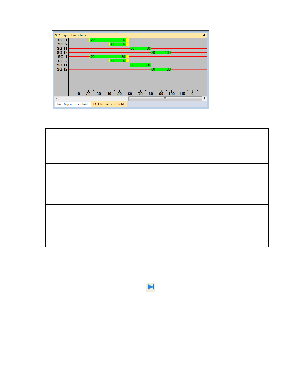
11.37 Showing signal times table in a window
If the signal times table also contains detectors, the color of the detector indicates the
occupancy state:
Detector color Description of occupancy state
Change from
black line
(empty) to light
blue
A vehicle passes the loop within a time step, rising and falling pulse edge
within a simulation second.
Change from
navy blue to light
blue
A vehicle leaves the loop, and another vehicle enters the loop within the
same time step, rising and falling pulse edge within the same simulation
second.
Light blue
(several
seconds)
Several vehicles pass the loop within a time step, rising and falling pulse
edge within a simulation second.
Navy blue A vehicle is located on the detector at the end of the time step. Thus
another vehicle enters the loop in the relevant second, but does not leave
it again within the same second.
A long navy blue bar means that a vehicle is on the detector. This
corresponds to the character ‘|’ in the SC detector record (see "Evaluating
SC detector records" on page 1010).
Displaying the time difference
Thus you can determine, for example, the length of time from a detector call to the release of a
signal group.
1. Click the Simulation single step button .
2. Click a time, and keep the mouse button pressed.
3. Click a another time, and keep the mouse button pressed.
At the bottom left of the window, the time difference between these two times is displayed.
© PTV GROUP 1039

11.37.1 Configuring signal times table on SC
Using the Signal times table window
In the window, an SC time step is four pixels wide at one call/simulation second. If the
controller is updated twice per simulation second, a time step is only two pixels wide, the width
is only one pixel if it is updated three times or more.
For a fixed time controller, you enter the number of SC time steps per simulation second as an
SC frequency (see "Defining SC with frequency" on page 602). For external controllers, see
the further information of the documentation on the respective control program.
The label of the time axis indicates the cycle second every ten simulation seconds. In addition,
a tick mark indicates each 5 seconds. The time axis remains unchanged when the controller
runs with multiple time steps per second.
If the controller DLL or the *.exe file indicate the same simulation second multiple times in
succession, only the first simulation second is used for the axis label.
A maximum of 5,000 time steps of the controller can be shown.
11.37.1 Configuring signal times table on SC
1. From the Signal Control menu, choose > Signal Controllers.
The Signal Controllers list opens.
2. Right-click the desired SC.
3. From the shortcut menu, choose Edit.
The Signal Controller window opens.
4. Select the Signal Times Table Config. tab:
Tip: For external control procedures, more information such as, for example, stage states
can be shown in addition to signal groups and detectors. For further details on displaying
additional data, refer to the documentation for the respective control program.
5. Make the desired changes:
1040 © PTV GROUP

11.37.1 Configuring signal times table on SC
Element Description
Automatic
signal times
table con-
figuration
The option is selected automatically if no user-defined configuration for
the SC is available. In this case, the configuration contains all signal
groups and detectors listed in the *.wtt files and cannot be modified.
Deselect this option to configure the signal times table manually. The
following areas are shown. Then in the sections Type (category) and the
list next to it, you can select entries and organize them in the section on
the right. This allows you to specify the data you want to show in the signal
times table.
List on the
left
Type
(Category)
Select the Type whose data you want to show in the signal times table.
Click the symbol to add the type to the section on the right. The list box
contains all types listed in the *.wttfiles that are available for the
evaluation.
For some types, you must choose a corresponding object number from the
list box on the right SG No., Port No. or CP No.. The heading of the list box
depends on the type you have selected, e.g. SG No..
List in the
middle
SG No., Det
No., CP No.
If there are several numbers available, select a type-specific number, e.g.
a detector no. or signal group no. To select entries in long lists, use the
PAGE UP, PAGE DOWN, POS1, END and arrow keys.
Click the corresponding button to add the selected entry to the list on the
right and specify which data is shown in the signal times table.
List on right Shows all objects selected in the defined sequence for output in the
evaluations window, chosen under Type (category).
Signal group
label:
Labeling of the rows in the signal times table for signal groups:
Number: By default, the number for labeling signal groups is used.
Name: In the evaluation windows, signal groups of the selected SC
are labeled with a name.
Detector
label:
Labeling of the rows in the signal times table for detectors:
Port number: By default, the number for labeling detectors is used.
Name: In the evaluation windows, detectors of the selected SC are
labeled with a name.
6. Configure the display of the signal times table (see "Configuring the display settings for a
signal times table" on page 1042).
7. Confirm with OK.
8. Start the simulation (see "Running a simulation" on page 796).
For each selected SC, an SC Signal Times Table window opens with the SC no. in the
window title (see "Showing signal times table in a window" on page 1038). Signal states
and detector states are displayed dynamically.
© PTV GROUP 1041
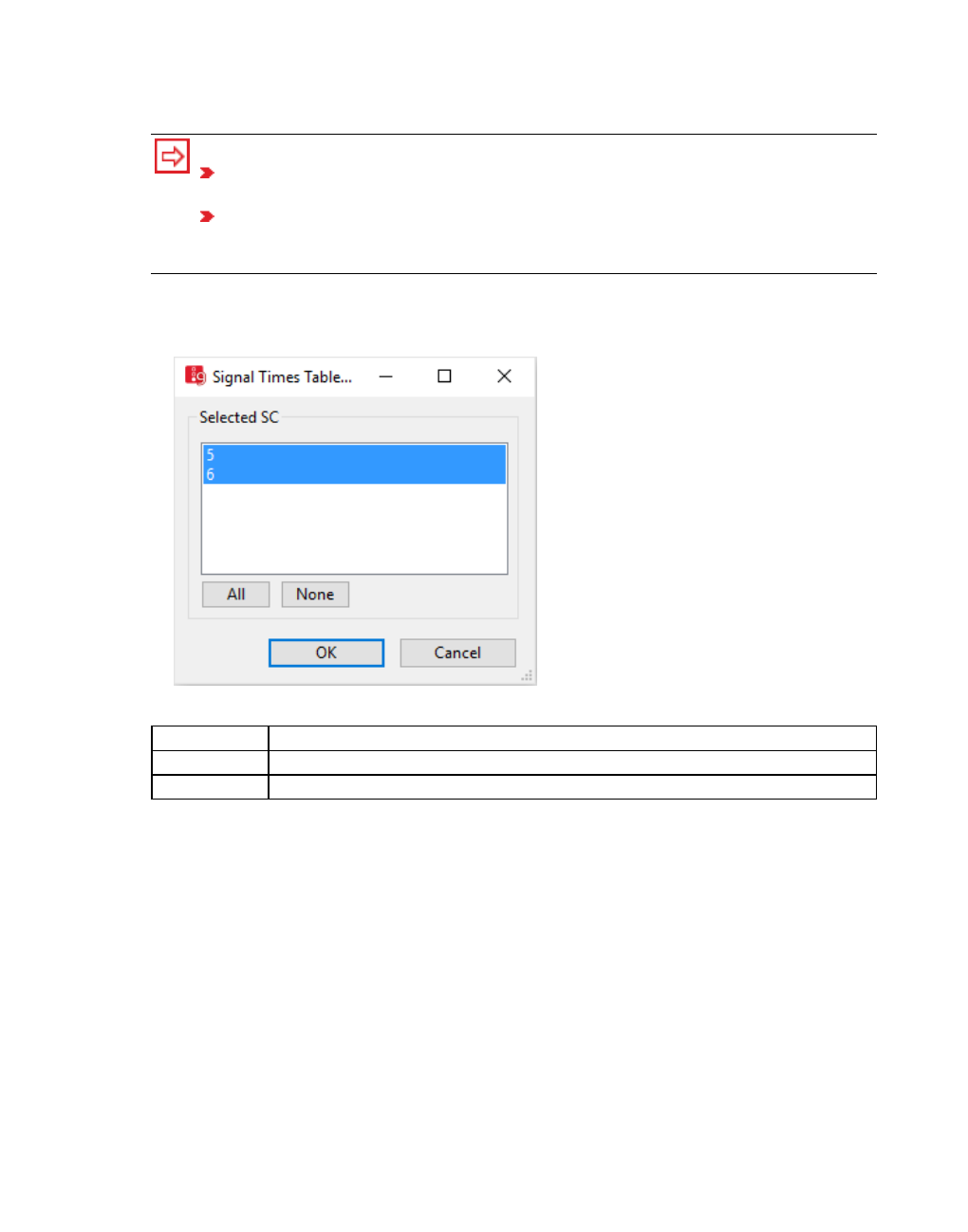
11.37.2 Configuring the display settings for a signal times table
11.37.2 Configuring the display settings for a signal times table
Tips:
You can save signal times tables with the SC detector record to a file (see "Evalu-
ating SC detector records" on page 1010).
Alternatively, for the next step, open the signal times table for a specific SC without
opening the Signal Times Table Windows: In the Signal Controllers list, right-click
the desired SC. Then, from the shortcut menu, choose Show Signal Times Table.
1. From the Evaluation menu, choose > Windows > Signal Times Table.
The Signal Times Table Windows window opens.
2. Make the desired changes:
Element Description
Selected SC Select SC
All Select all defined SCs. The evaluation for each SC is shown in a window.
3. Confirm with OK.
The Signal Times Table Windows window closes. The SC <no.> Signal times table window
opens (see "Showing signal times table in a window" on page 1038).
11.38 Saving SSAM trajectories to a file
You can save a binary file *.trj that contains trajectories. Trajectories describe the course of
vehicle positions through the network. This includes the z coordinates of a vehicle. You can
upload the file *.trj to the Surrogate Safety Assessment Model (SSAM) of the Federal Highway
Administration Research and Technology of the U.S. Department of Transportation. SSAM is
used to evaluate the road safety of transport routes. The content of a binary file *.trj cannot be
interpreted in a text editor.
1042 © PTV GROUP

11.39 Showing data from links in lists
You can save the following data and data formats:
Output ASCII file MDB table Attribute file from attribute list
Aggregated data - - -
Raw data *.trj - -
1. From the Evaluation menu, choose > Configuration > Direct Output tab.
2. In the SSAM row, select the option Write to file.
3. Confirm with OK.
4. Start the simulation (see "Running a simulation" on page 796).
A file *.trj is saved.
11.39 Showing data from links in lists
Using the Link evaluation, you can record the result attributes of vehicles based on segments
or lanes of links and connectors for the defined time interval. You can restrict the evaluation to
vehicle classes and individual vehicles. The following must be defined in the network:
Links (see "Modeling links for vehicles and pedestrians" on page 380)
Connectors (see "Modeling connectors" on page 393)
Vehicle inputs (see "Modeling vehicle inputs for private transportation" on page 426)
Note: Ensure that the attribute Link evaluation of links and connectors - which you want
to evaluate - is selected (see "Attributes of links" on page 383).
If you assign links a color based on aggregated parameters, for the Links evaluation, select
Collect data (see "Assigning a color to links based on aggregated parameters" on page 169).
by default, the data for all vehicle classes is entered together. You can also show the data for
certain vehicle classes separately in the evaluation (see "Configuring evaluations of the result
attributes for lists" on page 954).
You can save the following data and data formats:
Output ASCII file MDB table Attribute file from attribute list
Aggregated data - -
Raw data - - -
Show result attributes in attribute lists (see "Displaying result attributes in attribute lists" on
page 957)
Show result attributes in a result list (see "Showing result attributes in result lists" on page
956)
1. From the Evaluation menu, choose > Configuration > Result Attributes tab.
2. In the Links row, select the option Collect data.
© PTV GROUP 1043
11.39 Showing data from links in lists
3. If desired, change the time and/or the interval (see "Configuring evaluations of the result
attributes for lists" on page 954).
4. Click the More button.
The Links window opens.
5. Make the desired changes:
Element Description
Collect link results per link segment: the data is entered in the segments for all lanes
per lane segment: the data is entered in the segments for each
lane
6. Confirm with OK.
7. Start the simulation (see "Running a simulation" on page 796).
Result of evaluation of links
From the Evaluation menu, choose > Result Lists > Link Segment Results.
A link evaluation contains the following data:
Attribute Definition
Volume Volume [veh/h]
In mesoscopic simulation, for link segments outside the sections of
microscopic simulation, the average number of vehicles is displayed that
have entered and exited the sections on the meso edge.
Density Vehicle density
Speed Average speed
Emissions For add-on module API package only: Results of emission calculation for
selected file EmissionModel.dll (see "Activating emission calculation and
emission model for a vehicle type" on page 261). Emission values are also
displayed in:
Vehicle Network Performance Evaluation (see "Vehicle network
performance : Displaying network performance results (vehicles) in
result lists" on page 1025)
Vehicle Log (see "Saving vehicle record to a file or database" on
page 971)
Vehicles in Network list (see "Displaying vehicles in the network in a
list" on page 803)
SimRun Simulation run: Number of simulation run
LinkEvalSegs Link evaluation segment: Number of link evaluation segment
DelayRel Delay (relative): Total delay divided by total travel time of all vehicles in this
link segment during this time interval
TimeInt Time Interval: Duration of the evaluation intervals during which the data is
aggregated
1044 © PTV GROUP
11.40 Showing results of queue counters in lists
You can also show the following attributes of the Cartesian world coordinates in the list as
indirect attributes of link evaluation segments:
Attribute Definition
StartCoord Start coordinate: x, y, and z value of the position at which the link evaluation
segment begins
StartCoordX Start coordinate (x): x value of the start coordinate
StartCoordY Start coordinate (y): y value of the start coordinate
StartCoordZ Start coordinate (z): z value of the start coordinate
EndCoord End coordinate: x, y, and z value of the position at which the link evaluation
segment ends
EndCoordX End coordinate (x): x value of the end coordinate
EndCoordY End coordinate (y): y value of the end coordinate
EndCoordZ End coordinate (z): z value of the end coordinate
Link Number of the link on which the link evaluation segment is located
StartPos Start position: Position in meters at which the link evaluation segment on the
link begins
EndPos End position: Position in meters at which the link evaluation segment on the
link ends
11.40 Showing results of queue counters in lists
Queue counters must be defined in the network (see "Defining queue counters" on page 423).
by default, the data for all vehicle classes is entered together. You can also show the data for
certain vehicle classes separately in the evaluation (see "Configuring evaluations of the result
attributes for lists" on page 954).
You can save the following data and data formats:
Output ASCII file MDB file Attribute file from attribute list
Aggregated data - -
Raw data - - -
Show result attributes in attribute lists (see "Displaying result attributes in attribute lists" on
page 957)
Show result attributes in a result list (see "Showing result attributes in result lists" on page
956)
1. From the Evaluation menu, choose > Configuration > Result Attributes tab.
2. In the Queue counters row, select the option Collect data.
3. If desired, change the time and interval (see "Configuring evaluations of the result attributes
for lists" on page 954).
4. Click the More button.
The Queue counters window opens.
© PTV GROUP 1045
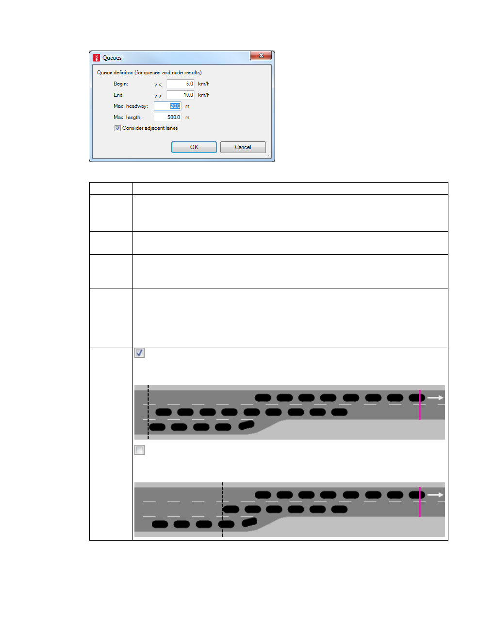
11.40 Showing results of queue counters in lists
5. Define the settings for the desired output.
Element Description
Begin Define queue condition:
A vehicle is in queue if its speed is less than the value v < that was entered for
the Begin.
End A vehicle remains in queue as long as its speed has not yet exceeded the
value v > that was entered for the End.
Max.
headway
Maximum net distance which can occur between two vehicles in queue. The
queue is considered to be interrupted if there are larger gaps. Values between
10 and 20m are usual.
Max.
length
Maximum queue length. Longer queues may still occur. This attribute is useful
if longer queues occur at the next node in the network, but the queues are to
be evaluated separately for each junction.
When a large value, for example, 4 km, allows a long queue to form, the
simulation speed decreases.
Consider
adjacent
lanes
Select this option to also take adjacent lanes of the previous link into
account for calculation of the queue end. In the figure, the dashed line on the
left indicates the position of the queue end:
If this option is not selected, the adjacent lanes of the previous link are not
taken into account for calculation of the queue end. In the figure, the dashed
line indicates the position of the queue end:
6. Confirm with OK.
1046 © PTV GROUP
11.41 Showing delay measurements in lists
7. Start the simulation (see "Running a simulation" on page 796).
8. If you wish, choose in the Evaluation menu Result Lists > Queue Results.
Result of the evaluation of queue counters
Column Description
QLen Maximum distance between the traffic counter and the vehicle that meets the
queue conditions defined. The queue length is specified as average queue
length: With each time step, the current queue length is measured upstream by
the queue counter and the arithmetic mean is thus calculated per time interval.
This also includes zero values, if there is no vehicle that meets the queue
condition. The queue length is the maximum distance between the traffic counter
and the vehicle that meets the queue conditions defined.
QLenMax Queue length (maximum): In each time step, the current queue length is
measured upstream by the queue counter and the maximum is thus calculated
per time interval.
QStops Number of queue stops. A queue stop is where one vehicle that is directly
upstream or within the queue length exceeds the speed of the Begin attribute
defined for the queue condition.
11.41 Showing delay measurements in lists
In a delay measurement, the average delay is calculated for all observed vehicles compared
to a trip without any other vehicles, signal controls or other required stops.
At least one vehicle travel time measurement on a link must be defined in the network (see
"Defining vehicle travel time measurement" on page 420).
At least one delay measurement must be defined and at least one vehicle travel time
measurement must be assigned to it (see "Defining delay measurement in lists" on page
952).
At least one vehicle input and one vehicle route must be defined on the link (see "Defining
vehicle inputs" on page 428), (see "Modeling vehicle routes, partial vehicle routes, and
routing decisions" on page 430).
All vehicles that pass the vehicle travel time measurements are recorded by delay
measurement.
Note: If a vehicle is recorded by several travel time measurements, it is correspondingly
often entered in the delay measurement.
by default, the data for all vehicle classes is entered together. You can also show the data for
certain vehicle classes separately in the evaluation (see "Configuring evaluations of the result
attributes for lists" on page 954).
You can save the following data and data formats:
© PTV GROUP 1047

11.41 Showing delay measurements in lists
Output ASCII file MDB table Attribute file from attribute list
Aggregated data - -
Raw data - - -
Show result attributes in attribute lists (see "Displaying result attributes in attribute lists" on
page 957)
Show result attributes in result lists (see "Showing result attributes in result lists" on page
956)
Result of evaluation of delay measurements
A delay measurement may include the following attribute values:
Column Description
SimRun Simulation run: Number of simulation run
TimeInt Time Interval: Duration of the evaluation intervals during which the
data is aggregated
DelayMeasurement Delay measurement: Number and name of delay measurement
StopDelay Average stopped delay per vehicle in seconds without stops at PT
stops and in parking lots
VehDelay Vehicle delay: Average delay of all vehicles
The delay of a vehicle in leaving a travel time measurement is
obtained by subtracting the theoretical (ideal) travel time from the
actual travel time.
The theoretical travel time is the travel time which could be achieved if
there were no other vehicles and/or no signal controls or other reasons
for stops. Delay time does not account for deceleration in reduced
speed areas (see "Using reduced speed areas to modify desired
speed" on page 408). To calculate the loss time caused by a desired
speed decision, Vissim calculates a theoretical speed and compares it
with the current speed (see "Using desired speed to modify desired
speed decisions" on page 412).
The actual travel time does not include any passenger service times of
PT vehicles at stops and no parking time in real parking lots.
The delay due to braking before a PT stop and/or the subsequent
acceleration after a PT stop are part of the delay.
Stops Average number of vehicle stops per vehicle without stops at PT stops
and in parking lots
Vehs Number of vehicles
PersDelay Person delay: Average delay [s] of all occupants of the vehicles
Pers Number of occupants in the vehicles: number of vehicles * average
occupancy rate
1048 © PTV GROUP
11.42 Showing data about paths of dynamic assignment in lists
11.42 Showing data about paths of dynamic assignment in lists
You can show data about paths from dynamic assignment in lists.
Note: The Paths list can only be displayed using the add-on module Dynamic
Assignment (see "Using the dynamic assignment add-on module" on page 653).
You can save the following data and data formats:
Output ASCII file MDB table Attribute file from attribute list
Aggregated data - -
Raw data - - -
Show result attributes in attribute lists (see "Displaying result attributes in attribute lists" on
page 957)
Show result attributes in a result list (see "Showing result attributes in result lists" on page
956)
Results of path evaluation
The Paths results list contains the following attributes:
Result
attribute
Long name
Short name Definition
Volume
(old)
VolOld Number of vehicles started on the path, including all
vehicle types and/or each vehicle type selected during
the last iteration for which the Path file was updated.
Volume
(new)
VolNew Number of vehicles started on the path, including all
vehicle types and/or each vehicle type selected during
the current iteration for which the Path file was updated.
Distance Dist Distance
Is detour Is detour Path is a detour
Edge
sequence
EdgeSeq Number of edges in sequence
Edge
travel time
(old)
EdgeTravTmOld Travel Time on the edges of the last iteration for which
the Path file was updated.
Edge
travel time
(new)
EdgeTravTmNew Travel Time on the edges of the current iteration for
which the Path file was updated.
Converged Conv Path converged
To parking
lot
ToParkLot Number of To parking lot
Number No Number of path
© PTV GROUP 1049

11.43 Saving vehicle input data to a file
Result
attribute
Long name
Short name Definition
Static cost StaticCost Static cost
Path travel
time (new)
PathTravTmNew Determined average travel time of path:
prior to a simulation run: smoothed travel time,
aggregated from path file by departure time
during a simulation run: changing, incomplete,
newly recorded average travel time
after a simulation run: travel time smoothed again
with the average newly recorded travel time of all
vehicles on this path and aggregated by departure
time.
Path-travel
time (old)
PathTravTmOld From the start of simulation run, travel time from
previous simulation run. This value can be used for
path search, if in the Dynamic assignment:
Parameters window, in the Choice tab, you selected
Use volume (old) (see "Attributes for the trip chain file,
matrices, path file and cost file" on page 731).
From
dynamic
vehicle
routing
decision
FromDynVehRoutDec Number of last dynamic routing decision of path
From
parking lot
FromParkLot Number of From parking lot
Route
guidance
vehicle
DestinationVeh Number of route guidance vehicle
11.43 Saving vehicle input data to a file
You can record the vehicles that are used with vehicle inputs in the network. Links and vehicle
inputs must be defined in the network (see "Modeling links for vehicles and pedestrians" on
page 380), (see "Modeling vehicle inputs for private transportation" on page 426).
You can save the following data and data formats:
Output ASCII file MDB table
Aggregated data - -
Raw data *.fhz -
Save raw data to a file (see "Using the Direct output function to save evaluation results to
files" on page 958)
1050 © PTV GROUP
11.43 Saving vehicle input data to a file
Result of vehicle input data evaluation
A vehicle input evaluation *.fhz contains the following data:
Element Description
File title Name of evaluation
File Path and name of network file
Comment Comment on simulation
Date Time of evaluation
Vissim Version number, service pack number, build number
Data block Data block with the following information:
one row per vehicle that enters the Vissim network
one column per attribute
The data block of the evaluation file contains the following attributes in this sequence:
Column Description
Time Simulation second
Link Number of link on which the vehicle is used.
Lane Number of lane on which the vehicle is used.
If a vehicle in the dynamic assignment drives away from a parking lot, the value
0 is output in the Lane column.
VehNo Number of the vehicle
VehType Number of vehicle type
Line Number of PT line. No PT line: value 0
DesSpeed Desired speed of vehicle
Example evaluation of the vehicle input data file *.fhz
Table of vehicles entered
File: C:\Users\Public\Documents\PTV Vision\PTV Vissim 10\Examples
Demo\example.inpx
Comment: Example, SC 3-10
Date: Friday, June 16, 2017 12:23:33 PM
PTV Vissim 10.00-00* [66098]
Time; Link; Lane; VehNo; VehType; Line; DesSpeed;
0.1; 1110; 1; 1; 32; 1110; 51.6;
0.1; 2008; 1; 2; 402; 218; 50.0;
0.1; 1001; 1; 3; 402; 101; 50.0;
1.6; 277; 1; 4; 10; 0; 46.3;
1.8; 267; 1; 5; 10; 0; 46.2;
2.4; 8; 1; 6; 10; 0; 45.7;
2.8; 272; 1; 7; 10; 0; 45.6;
2.9; 70; 1; 8; 17; 0; 54.2;
3.1; 69; 2; 9; 17; 0; 53.5;
© PTV GROUP 1051

11.43 Saving vehicle input data to a file
3.4; 274; 1; 10; 17; 0; 53.6;
…
1052 © PTV GROUP

12 Creating charts
12 Creating charts
You can show data graphically in charts, which are convenient for comparison, analysis or use
in reports or presentations.
In Vissim you can show the following data in bar charts or line charts:
Data containing the characteristics of your Vissim network, such as base data or attributes
of network objects. This includes data from user-defined attributes.
Data arising from simulations, such as result attributes from result lists
12.1 Presenting data
Depending on your requirements for data comparison or data analysis, you can create a line
chart or a bar chart. As the basis for the chart, select the desired network object type, base
data type or result data type as well as at least one object of the selected type and one
attribute of the object. The attribute values are plotted on the vertical y-axis.
You can also combine a line chart with a bar chart by using the data series graphic
parameters (see "Adjusting how the chart is displayed" on page 1067).
12.1.1 Dimension on the x-axis
The objects from one of the following dimensions are plotted on the x-axis. Select the desired
dimension, which for the chosen network object type, base data type or result data type
determines whether network objects, attributes, simulation runs, time intervals, vehicle types or
pedestrian types are plotted on the x-axis. Then choose the objects in this category to be
plotted on the x-axis.
You can choose from the following dimensions and objects in these dimension:
Network objects: You must choose at least one object of the selected network object type,
base data type or result data type. You can select an option to choose all objects of the
selected network object type, base data type or result data type.
Attributes: You must choose at least one attribute for the selected object or objects.
© PTV GROUP 1053
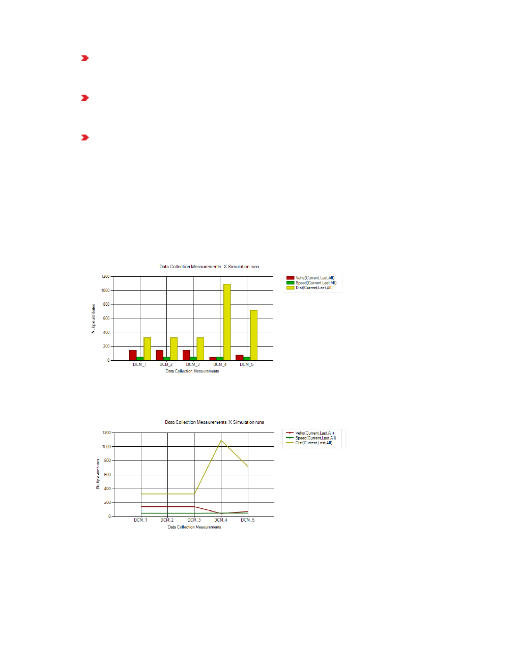
12.1.2 Attribute values on the y-axis
Simulation runs: If you have performed simulation runs, you can choose the desired sim-
ulation runs to be used as data sources for the chosen objects and chosen attributes in the
chart. You can also select an option to use the data from all simulation runs.
Time intervals: If time intervals are available, you can choose the intervals to be used as
data sources for the chosen network objects and attributes in the chart. You can also
select an option to use data from all time intervals.
Vehicle classes or Pedestrian classes: You can choose vehicle classes or pedestrian
classes to be used as data sources for the chosen network objects and attributes in the
chart. You can also select an option to use data from all vehicle classes or pedestrian
classes.
12.1.2 Attribute values on the y-axis
On a bar chart the height of the bar corresponds to the attribute value of the object plotted on
the x-axis. If you have chosen several attributes for the objects on the x-axis, a bar for each
attribute is shown on the bar chart. The bars are distinguished by a different color for each
attribute.
On a line chart the vertical position of the data point corresponds to the attribute value of the
object plotted on the x-axis. The data points of multiple objects are connected by a line.
For data in percentages, Vissim divides the y-axis into segments from 0 to 100. If the data of
only one attribute is shown in percentages, the unit [%] is added to the y-axis labeling.
1054 © PTV GROUP

12.1.3 Presentation of data during an active simulation
12.1.3 Presentation of data during an active simulation
If a chart containing dynamic data is displayed during an active simulation, the chart shows the
data at each time step. As a result, the chart can change continuously as long as the
simulation is running.
12.2 Creating a chart quick-start guide
The quick-start guide shows you the key steps for selecting the desired chart type and data
you want to display.
12.2.1 Making preselections or selecting all data
You can choose from the following options for creating a chart:
You want a chart based on a network object type selected from the network objects tool-
bar
(see "Creating charts from a network object type" on page 1059)
1. On the network object toolbar, right click the network object type of your choice.
2. From the context menu, choose Create Chart.
The Create Chart window opens. You can select data and configure the chart.
You want a chart based on data from network objects shown in a list
(see "Creating charts from data in a list" on page 1061)
1. Open the desired list of network objects, base data or result attributes.
2. Select the desired entries.
3. From the context menu, choose Create Chart > for this attribute.
If you have selected enough attribute values in list cells to create a chart, the chart is
displayed. The Create Chart window does not open.
You want to select all the data for a chart yourself
(see "Creating a chart without preselection" on page 1063)
From the View menu, choose > Create Chart.
The Create Chart window opens. You can select data and configure the chart.
12.2.2 Configuring the chart
In the Create Chart window, select more data so that the chart can be created.
© PTV GROUP 1055
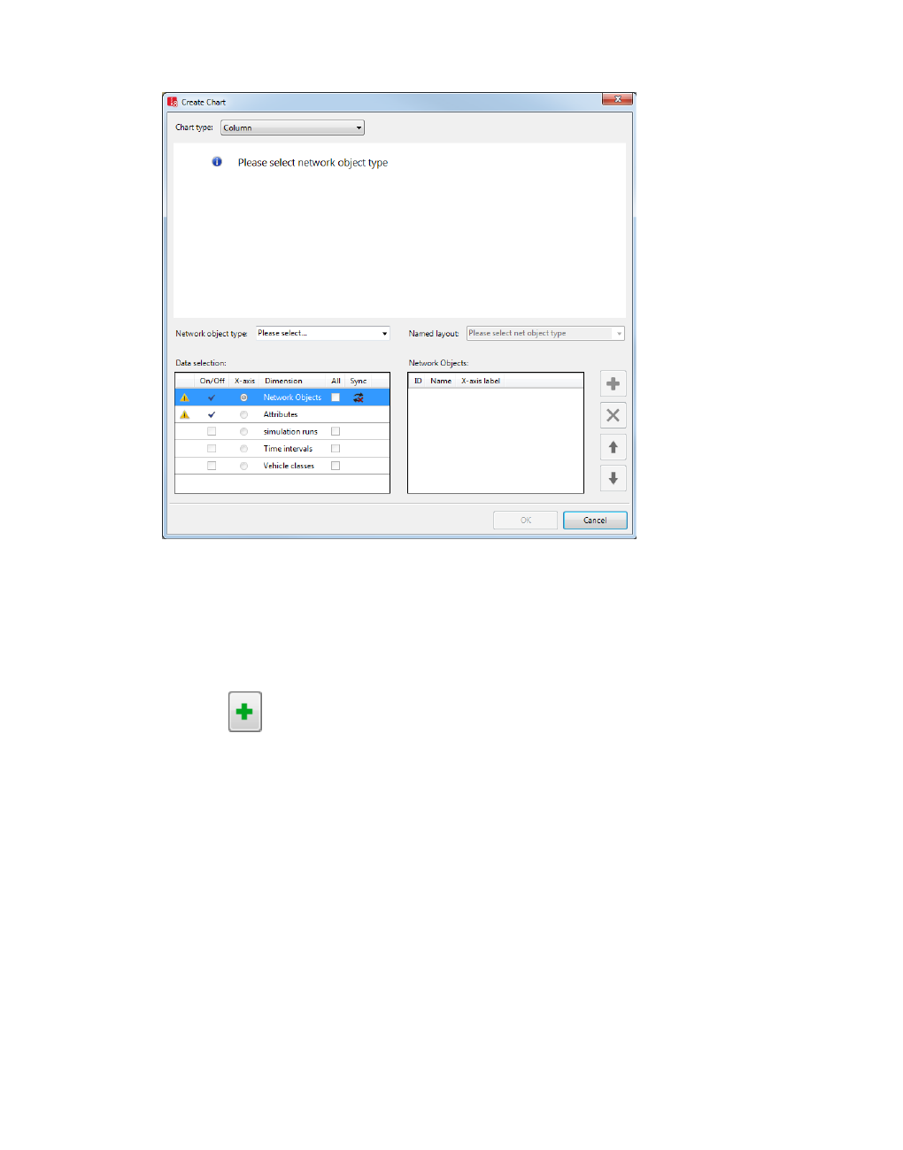
12.2.2 Configuring the chart
1. Select the desired entry in the Chart type list box.
2. Make sure that the desired entry has been selected in the Network object type list box.
3. If you want to add objects in the Network objects dimension for the selected network object
type in the area on the right, perform the following four steps:
4. Click the Network objects dimension.
5. Click the button.
A selection window opens.
6. Select the desired objects.
7. Confirm with OK.
The selected objects are shown in the area on the right.
8. If you do not wish the x-axis to be labeled with the object name, in the X-axis label column,
enter the name of your choice.
9. Repeat the last steps for the Attributes dimension.
The selected attributes are shown in the area on the right. A chart preview is displayed.
Next you can limit the selected objects and attributes to the desired simulation runs, time
intervals, vehicle classes or pedestrian classes. You can only select these if the selected
1056 © PTV GROUP
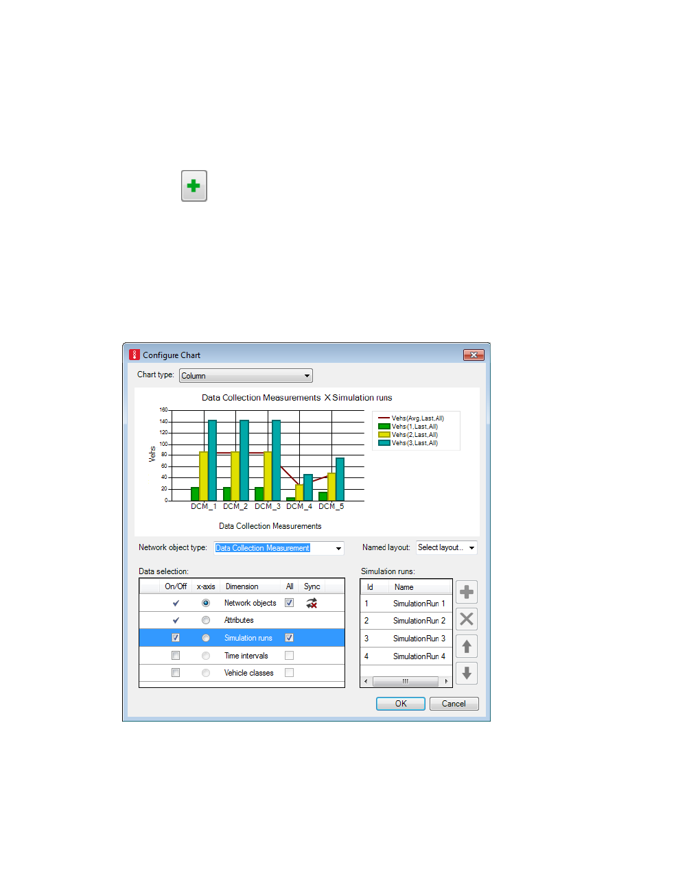
12.2.2 Configuring the chart
network object type, base data type or result data type has attributes related to the desired
dimension.
10. Repeat the following four steps for the desired dimensions:
11. Make sure that the On/Off option is selected for the dimension in the Data selection list
box.
12. Click the button.
A selection window opens.
13. Select the desired objects.
14. Confirm with OK.
15. In the Data selection list, select x-axis for the dimension, whose objects you want to plot
on the x-axis.
The selected objects are shown in the area on the right. A chart preview is displayed.
16. Confirm with OK.
The chart is displayed.
© PTV GROUP 1057

12.3 Charts toolbar
17. Edit the chart if you so wish (see "Configuring a created chart" on page 1066).
18. Reuse the chart if you so wish (see "Reusing a chart" on page 1072).
12.3 Charts toolbar
Element Name Description
Select layout
list box
Chart layout
selection Save named chart layout (see "Using named chart
layouts" on page 1070)
Select named chart layout
Configure Chart Open the Create Chart window and select data (see
"Configuring the chart type and data" on page 1067)
Edit window
graphic
parameters
Use graphic parameters to define how the various
elements of the chart are displayed (see "Adjusting
how the chart is displayed" on page 1067)
Edit title graphic
parameters
Edit legend
graphic
parameters
Edit drawing area
graphic
parameters
Edit x-axis
graphic
parameters
Edit y-axis
graphic
parameters
Edit data series
graphic
parameters
1058 © PTV GROUP

12.4 Creating charts with or without preselection
Element Name Description
Synchronization The chart is synchronized with all network editors and
synchronized lists. When you select or deselect bars
or network objects in the chart, they are also selected
or deselected in other windows, and vice versa.
The Sync option in the Create Chart window is linked
to Synchronization. The Sync option is therefore
selected when Synchronization is selected, and vice
versa.
No
synchronization
The chart is not synchronized with other program ele-
ments. The Sync option in the Create Chart window is
not selected.
Copying an image
to the clipboard
(see "Reusing a chart" on page 1072)
Export image
(Screenshot)
(see "Reusing a chart" on page 1072)
12.4 Creating charts with or without preselection
In the following program elements you can select objects to be used to generate a chart:
Network objects toolbar (see "Creating charts from a network object type" on page 1059)
Network editor (see "Creating charts from network objects in the network editor" on page
1060)
Lists, such as the attribute list of the network object of a network object type, results lists or
base data lists (see "Creating charts from data in a list" on page 1061)
You can also generate a chart without using these program elements for preselection. In that
case, select all the desired data in the Create Chart window (see "Creating a chart without
preselection" on page 1063).
12.4.1 Creating charts from a network object type
On the network object toolbar you can select a network object type and use it to configure the
data for the chart.
1. On the network object toolbar, right click the network object type of your choice.
2. In the context menu, choose Create Chart.
The Create Chart window opens. The network object type is automatically entered in the
Network object type list box.
3. Select the x-axis option for Network objects in the Data selection area.
4. Click the button.
A selection window opens.
© PTV GROUP 1059

12.4.2 Creating charts from network objects in the network editor
5. Select the desired network objects.
6. Confirm with OK.
The selected objects are shown in the area on the right.
7. Select the x-axis option for Attributes in the Data selection area.
8. Click the button.
A selection window opens.
9. Select the desired attributes.
10. Confirm with OK.
The selected objects are shown in the area on the right. A chart preview is displayed if the
data selection is valid.
11. If you do not wish the x-axis to be labeled with the object name, in the X-axis label
column, enter the name of your choice.
12. If you wish, repeat the data selection procedure for simulation runs, time intervals, vehicle
classes or pedestrian classes. You can only select these if the selected network object type,
base data type or result data type has attributes related to the desired dimension.
A chart preview is displayed if the data selection is valid.
13. Confirm with OK.
In the Vissim graphical user interface, the Chart <Chart title> window opens. The chart is
displayed.
14. Edit the chart if you so wish (see "Configuring a created chart" on page 1066).
15. Reuse the chart if you so wish (see "Reusing a chart" on page 1072).
12.4.2 Creating charts from network objects in the network editor
In the network editor you can select one or more network objects and use them to configure
other data for the chart.
1. In the network editor, select the desired network objects of a particular network object type.
2. In the context menu, choose Create Chart for Selected Objects.
The Create Chart window opens. The network object type of the selected network object is
automatically shown and selected in the Network object type list box.
The x-axis option for Network objects is automatically selected in the Data selection area.
The network objects you selected in the network editor are automatically shown in the
Network objects area on the right.
3. Select the x-axis option for Attributes in the Data selection area.
1060 © PTV GROUP

12.4.3 Creating charts from data in a list
4. Click the button.
A selection window opens.
5. Select the desired attributes.
6. Confirm with OK.
The selected objects are shown in the area on the right. A chart preview is displayed if the
data selection is valid.
7. If you do not wish the x-axis to be labeled with the object name, in the X-axis label column,
enter the name of your choice.
8. If you wish, repeat the data selection procedure for simulation runs, time intervals, vehicle
classes or pedestrian classes. You can only select these if the selected network object type,
base data type or result data type has attributes related to the desired dimension.
A chart preview is displayed if the data selection is valid.
9. Confirm with OK.
In the Vissim graphical user interface, the Chart <Chart title> window opens. The chart is
displayed.
10. Edit the chart if you so wish (see "Configuring a created chart" on page 1066).
11. Reuse the chart if you so wish (see "Reusing a chart" on page 1072).
12.4.3 Creating charts from data in a list
You can select data in a list and use it to create a chart. Depending on whether you select
columns, rows or cells in the list, different menu options are shown in the context menu for
creating the chart and different data is copied.
1. Open the desired list of network objects, base data or result attributes.
Note: If you select data in the next step that cannot be displayed in a chart, the Create
Chart option in the context menu will not be active and you cannot create a chart.
2. Select the desired data:
Data selection Description
Click the column header Selects the values of the attribute of all objects in the list
Press CTRL and click the head-
ers of several columns
Selects the values of the attributes of all objects in the
list that are located in the clicked columns
Click a row header Selects the objects in the row
Press CTRL and click the head-
ers of several rows
Selects the objects located in the clicked rows
© PTV GROUP 1061

12.4.3 Creating charts from data in a list
Data selection Description
Press CTRL and click several
cells in a column
Selects only the value of the attribute of the object in the
clicked cell
Press CTRL and click several
cells in various columns
Selects only the values of the attributes of the objects in
the clicked cells
3. Right-click on one of the selected cells.
4. Choose the desired entry from the context menu:
Context menu Description
Create Chart Only active when objects have been selected by row.
Opens the Create Chart window The selected objects are copied and
are displayed in the Network objects area on the right.
In Data selection, select Attributes and then select the desired
attributes on the right.
You can select options for the dimensions in Data selection (see
"Presenting data" on page 1053).
Create Chart >
for this attribute If you have selected attribute values by column, the Create Chart
window opens. The selected attributes and their objects are
copied. You can create the chart or continue with configuration,
such as selecting additional attributes or selecting options for the
dimensions.
If you have selected enough attribute values in list cells to create a
chart, the chart is displayed.
Create Chart >
generate for
selected attrib-
utes over sim-
ulation runs
Displayed for every subattribute of the selected attributes that has a
non-aggregated value for a simulation run.
Opens the Create Chart window The subattribute is plotted on the x-
axis and all instances are used.
Create Chart >
generate for
selected attrib-
utes over inter-
vals
Displayed for every subattribute of the selected attributes that has a
non-aggregated value for a time interval.
Opens the Create Chart window The subattribute is plotted on the x-
axis and all instances are used.
Create Chart >
Generate for
selected attrib-
utes over vehicle
classes
Displayed for every subattribute of the selected attributes that has a
non-aggregated value for a vehicle class.
Opens the Create Chart window The subattribute is plotted on the x-
axis and all instances are used.
The Chart – <Name Network object type> window opens. The chart shows the data
depending on the selected cells in the attributes list:
1062 © PTV GROUP

12.4.4 Creating a chart without preselection
Selected
cells
Displayed data
In a
column
of an
attribute
If only the values of an attribute in a column have been selected for objects in
several rows or in all rows, each object for which a value was selected in its
row is plotted on the X axis.
For each of these objects, the attribute value is plotted in the chart on the y-axis
above the associated object on the x-axis:
In a line chart the data points of the attribute values of the successive
objects are joined by a line.
In a bar chart the attribute value is indicated by a bar above each object.
In dif-
ferent
columns
If attribute values for objects in several cells or all cells in several columns have
been selected, which means that values of several attributes have been
selected, each object for which a value has been selected in its row is plotted
on the X axis.
For each of these objects, the attribute values are plotted in the chart on the Y
axis above the associated object on the X axis:
In a line chart the data points of the attribute values of each attribute of the
successive objects are joined by a line. Each column in which attribute val-
ues are selected is thus represented by a line. Each line that connects the
values of a particular attribute has its own color.
In a bar chart each attribute value is indicated by a bar. Each column in
which attribute values are selected is represented by a bar above the asso-
ciated object on the X axis. The number of bars above an object on the X
axis corresponds to the number of columns in which you have selected
attribute values. All of the bars that represent the values of a particular attrib-
ute have the same color.
5. Edit the chart if you so wish (see "Configuring a created chart" on page 1066).
6. If desired, continue to use the chart in another program (see "Reusing a chart" on page
1072).
12.4.4 Creating a chart without preselection
You can manually select all the data for a chart.
1. From the View menu, choose Create Chart.
The Create Chart window opens.
© PTV GROUP 1063

12.4.4 Creating a chart without preselection
2. Select the desired entry in the Chart type list box:
Bar chart
Line chart
Original: Resets the chart display to the original data series graphic parameters. Only
shown when data for different attributes is displayed in bar charts and line charts, for
example after you have changed the Data series graphic parameters (see "Adjusting
how the chart is displayed" on page 1067).
3. Select the desired network object type, base data type or result data type as the basis for
further data selections in the Network object type list box.
In the next steps, in the left-hand Data selection area, configure the dimension, whose
objects you can select in the right-hand area.
4. In the Data selection area, please note the symbols:
No attribute references are selected yet. Please add attribute references.: In the
right-hand area, no objects have been selected yet for this dimension. You cannot close
the window with OK. Select objects for the dimension or select another dimension.
This net object type does not have any attributes which depend on simulation runs:
The objects of the selected object type Simulation runs, Time intervals, Vehicle classes
or Pedestrian classes do not have attributes which depend upon this dimension. You can
only select simulation runs, time intervals, vehicle classes or pedestrian classes if the
1064 © PTV GROUP

12.4.4 Creating a chart without preselection
selected network object type, base data type or result data type has attributes that depend
on this dimension.
5. In the Data selection area, set the desired settings:
Column Description
On/Off Enable selection of objects for this dimension.
If this option is selected, you can select objects for this dimension with the (+)
button and add them to the area to the right.
This option is always selected for Network objects and Attributes because you
always have to select at least one network object and one attribute.
X-axis Select a dimension whose selected objects will be plotted on the X axis.
If the This net object type does not have any attributes which depend on
simulation runs symbol is not displayed, you can select the x-axis option for
Simulation runs, Time Intervals, Vehicle types or Pedestrian types and use
the (+) button to select at least one object and add it to the area to the right.
The selected dimension is shown above the area to the right as a title.
All If this option is selected, all objects of the selected object type are selected. The
objects are displayed in the area to the right. If you define new network objects
in the Vissim network, they are automatically added to the chart. This option is
not possible for attributes.
Regarding simulation runs, Vissim only shows the simulation runs for which
data is available.
Regarding time intervals, Vissim only shows the MAX time intervals, if in the
Evaluation Configuration window, in the Result Attributes tab, in the
columns Time from and Time to no other values are selected (see "Con-
figuring evaluations of the result attributes for lists" on page 954).
Regarding vehicle classes or pedestrian classes, Vissim only shows the
vehicle classes or pedestrian classes selected in the Evaluation Con-
figuration window, in the Result Attributes tab, under Additionally collect
data for these classes (see "Configuring evaluations of the result attributes
for lists" on page 954).
Sync Synchronized object selection:
If this option is selected and objects displayed in the chart are selected in a
network editor or a list, the chart also shows this data as selected.
The title of the area on the right shows the dimension chosen in the Data Selection area on
the left.
In the next steps, in the section to the right, select the objects which you want to plot on the
x-axis and for which you activated the option in the Data Selection area to the left in the x-
axis column.
Network Objects: Select the network objects of the network object type which you
selected in the Network object type list box. If you selected a network object type from
which only objects are available, e.g. Network performance, you cannot select, sort
© PTV GROUP 1065

12.5 Configuring a created chart
or delete any individual objects in the the right-hand section.
Attribute: Select the attribute of the selected network objects.
Simulation Runs: If desired, select simulation runs to be used as sources for the attrib-
ute values.
Time Intervals: If desired, select time intervals to be used as sources for the attribute
values.
Vehicle Classes or Pedestrian Classes: If desired, select classes to be used as
sources for the attribute values.
6. Select in the right-hand area the objects you want:
Element Description
Open the <Name Object type>: Select Object(s) window, in which you can
select the objects you want.
For attributes, you can select numeric attributes that are directly related to
the selected object type.
For attributes, you can also select attributes that are linked to the object type
by a relation.
For subattributes, all non-aggregated entries are merged in the window and
the symbol * is shown as a placeholder instead of the individual entries. If
you select an entry containing the * symbol and copy it to the list of selected
attributes on the right, the merged results will be deleted and the individual
entries will be displayed again. Attributes that are linked to the object types
by relations are not merged and are not displayed with the * symbol. You
can only select the entries one at a time.
Move selected objects downwards in the right-hand list
Move selected objects upwards in the right-hand list
Delete selected objects in the list on the right
A chart preview is displayed when data has been selected in the area on the right and the
data selection is valid. The selected objects are plotted on the X axis.
7. If you do not wish the x-axis to be labeled with the object name, in the X-axis label column,
enter the name of your choice.
8. If you want to apply a named chart layout in the chart, select from the Named layout list box
the entry desired (see "Using named chart layouts" on page 1070).
9. Confirm with OK.
The Create Chart window closes The Chart <title> window opens in the Vissim GUI. The
chart is displayed.
12.5 Configuring a created chart
After you create a chart, you can edit it and show it again.
1066 © PTV GROUP

12.5.1 Configuring the chart type and data
Select the chart type and/or edit the data (see "Configuring the chart type and data" on
page 1067).
Use graphic parameters to adjust the chart view (see "Adjusting how the chart is dis-
played" on page 1067).
Enlarge part of the chart in the chart itself or in the Configure Chart window (see "Show-
ing a chart area enlarged" on page 1069)
12.5.1 Configuring the chart type and data
You can reconfigure and redisplay a created chart. You have the same settings available for
this as for the creation of a new chart.
1. Click the Configure Chart icon on the chart toolbar.
The Configure Chart window opens.
2. Make the desired changes (see "Creating a chart without preselection" on page 1063).
12.5.2 Adjusting how the chart is displayed
You can use graphic parameters to adjust how the chart is displayed.
1. Click the desired icon on the chart toolbar.
2. Make the desired changes:
Toolbar
button
Name Description
Edit window
graphic para-
meters
Choose the background color for the chart window
Edit title
graphic para-
meters
Chart title: the chart title is shown above the chart. If you do
not enter a chart title, Vissim generates a chart title based on
the objects selected. You can change the title.
Chart title font size: font size in points
Chart title visibility: If this option is selected, the chart title
is displayed above the chart.
Edit legend
graphic para-
meters
Legend visibility: If this option is selected, the legend is
displayed at the position selected in the Legend position
attribute.
Legend position: Choose the desired position for the legend
Legend font size: Font size in points
© PTV GROUP 1067

12.5.2 Adjusting how the chart is displayed
Toolbar
button
Name Description
Edit drawing
area graphic
parameters
Grid visibility: If this option is selected, vertical and hori-
zontal grid lines are shown in the chart.
Activate automatic zoom:
Select this option to have Vissim automatically show
the entire digram.
If this option is not selected, you can zoom:
Point the mouse pointer to the diagram and rotate the
mouse wheel.
Hold down the left mouse button and use the mouse
pointer to drag open a frame over the section with the
diagram that want to show enlarged. Release the
mouse button.
Edit x-axis
graphic para-
meters
Show or hide elements on the X axis:
Axis title: Name of x-axis which is displayed under x-axis
Axis title visibility: Select this option to show the x-axis
title below the chart.
Axis title font size: Font size in points
Axis label visibility: Select this option to show the x-axis
label below the chart.
Axis label font size: Font size in points
Axis label interval: Show label of data series only for every
n-th position. 1 = Label for each data series, 2 = Label for
every second data series, etc.
Axis unit visibility: Select this option to show the units of
the x-axis below the chart.
Edit y-axis
graphic para-
meters
Show or hide elements on the X axis:
Axis title: Name of y-axis displayed to the left of y-axis
Axis title visibility: Select this option to show the y-axis
title to the left of the chart.
Axis title font size: Font size in points
Axis label visibility: Select this option to show the y-axis
label next to the chart.
Axis label font size: Font size in points
Axis label interval: Show label of data series only for every
n-th position. 1 = Label for each data series, 2 = Label for
every second data series, etc.
Axis unit visibility: Select this option to show the units of
the y-axis next to the chart.
1068 © PTV GROUP

12.5.3 Showing a chart area enlarged
Toolbar
button
Name Description
Editing data
series
graphic para-
meters
Opens a list box for selection of the attribute whose graphic
parameters you want to select. After you have selected the
desired attribute in the list box, the graphic parameters list
opens:
Series type: Chart type
Name: Data series name for legend. Default: Long name of
the attribute.
Line: Line chart
Column: Bar chart
Line style:
Solid line
Dashed line
No line
Line color:
With a bar chart: color of the bar outline
With a line chart: color of the line connecting the data
points of the attribute values
Fill style:
Solid fill: the Fill color attribute is used
No fill
Fill color: Only with bar charts: fill color for the bars
Marker style: If you create a line chart, select the shape of
the symbol that represents the attribute value in the chart.
Disk
Diamond
Square
None
Marker size: Symbol size in points
3. Confirm with OK.
The chart is shown with the changes.
12.5.3 Showing a chart area enlarged
You can show part of a chart at an enlarged scale. In the enlarged view, you can use the scroll
bars to see other parts of the chart. You can also return the chart to its original scale.
These functions can be performed in the chart and in the Create Chart window.
1. With the mouse button pressed, drag a frame over the desired section of the chart.
2. Release the mouse button.
© PTV GROUP 1069

12.6 Using named chart layouts
This area will be shown as enlarged, and the other parts of the chart in the drawing area
will not be visible. In the enlarged view, scroll bars and the button are shown along the
axes.
3. If you want to show the chart at its original size in the x-axis or y-axis direction, click the
button on the respective axis.
12.6 Using named chart layouts
You can adjust how charts are displayed and assign a name to the current settings, which can
be used to retrieve the chart layout later on. You can save these named chart layouts in the
*.layx file. In a chart you can choose a layout from all the named chart layouts to display the
chart accordingly.
12.6.1 Generating a named chart layout
1. Open the desired chart.
2. Adjust the chart layout (see "Adjusting how the chart is displayed" on page 1067).
3. On the chart toolbar, enter a unique name in the Chart layout selection list box.
4. Confirm with Enter.
On the chart toolbar the new chart layout is shown in the Chart layout selection box and can
be selected.
12.6.2 Assigning a complete chart layout
You can assign the data selection and the graphic parameters saved in a named chart layout
to a chart.
1. Open the desired chart.
2. On the Chart toolbar, in the Chart layout selection list, click the icon.
3. Select the desired chart layout.
The chart layout is assigned to the chart.
12.6.3 Assigning only the graphic parameters from a named chart layout
1. Open the desired chart.
2. Right-click on the Chart layout selection list box.
3. Position the mouse pointer on the Apply only graphic parameters entry in the context
menu.
The named chart layouts are displayed in the context menu.
4. Click the desired chart layout in the context menu.
1070 © PTV GROUP

12.6.4 Assigning only the data selection from a named chart layout
Only the graphic parameters of the named chart layout are assigned to the chart. The data
selection from the chart layout is not assigned.
12.6.4 Assigning only the data selection from a named chart layout
1. Open the desired chart.
2. Right-click on the Chart layout selection list box.
3. Position the mouse pointer on the Apply only data selection entry in the context menu.
The named chart layouts are displayed in the context menu.
4. Click the desired chart layout in the context menu.
Only the data selection from the chart layout is assigned to the chart. The graphic parameters
from the chart layout are not assigned.
12.6.5 Saving a named chart layout
1. In the menu, select File > Save Layout As.
2. Enter a unique name.
3. Confirm with Save.
The entire current layout of the Vissim GUI, and thus all named chart layouts, is saved in the
*.layx layout file.
If in the User Preferences, the option Auto-save layout when network file (inpx) is saved is
selected, the layout file is saved automatically under the name of the currently loaded network
file, each time the network file is saved (see "Specifying automatic saving of the layout file
*.layx" on page 145).
12.6.6 Reading saved named chart layouts additionally
You can import all chart layouts saved in a *.layx layout file into your currently opened file.
Then you can apply these chart layouts to a chart in the currently opened file.
1. From the File menu, choose > Read Additionally > Named Chart Layouts.
2. Select the desired *.layx file.
3. Click the Open button.
The chart layouts are imported. When you open a chart, you can select the added chart
layouts on the toolbar of the chart window in the Chart layout selection list box.
12.6.7 Deleting a named chart layout
1. On the chart toolbar, right-click on the Chart layout selection list box.
2. Position the mouse pointer on the Delete entry in the context menu.
The named chart layouts are displayed in the context menu.
3. Click the desired chart layout in the context menu.
© PTV GROUP 1071

12.7 Reusing a chart
4. Confirm with Yes.
12.7 Reusing a chart
You can save a chart in a graphic file or copy it to the clipboard. This allows you to use the
chart in other programs, for example for presentations.
12.7.1 Saving a chart in a graphic file
You can save a chart in a graphic file in one of the following formats:
bmp
jpeg
png
gif
tiff
1. On the toolbar of the Chart - <network object type> window, click the Export image
(Screenshot) button .
2. To use the chart in another program, copy the graphic file to the clipboard and paste it in
the target program.
12.7.2 Copying a chart to the clipboard
You can save a chart to the clipboard as an image in the *.jpeg file format.
1. On the toolbar of the Chart - <network object type> window, click the Copy image to
clipboard button .
2. To use the chart in another program, paste it from the clipboard in the target program.
1072 © PTV GROUP
13 Scenario management
13 Scenario management
Scenario management allows you to manage related networks in a single project. The aim is
to model comparable cases in these networks and then compare their simulation results. For
each case within a project, you create a separate network that is saved as a scenario. You
then change each scenario according to the requirements of the respective case. Then you
configure the desired evaluations and perform simulation runs for the scenarios whose
simulation results you want to compare.
Scenario Management is primarily based on the following elements:
Base network: The original network from which you want to derive scenarios (see "Pla-
cing a network under scenario management" on page 1084). The base network may
already contain a modeled network or be empty (see "Opening and editing the base net-
work in the network editor" on page 1086). You cannot use the base network to perform
simulation runs. Vissim automatically adopts changes made to the base network into all
scenarios of the project, as these have been derived from the base network. Make sure
that the entire base network has been modeled and simulation runs trouble-free before
you derive a scenario. Do not change the base network once you have derived a scenario
from it. If you need to change the base network, from the base network, derive a new scen-
ario without modifications. Then export the scenario from the project structure into a new
*.inpx file and save it under another name. You can now edit this new base file, belonging
to a new project ,until you derive a scenario from it.
Scenario: A changed version of the base network or of another scenario within a project
(see "Opening and editing scenarios in the network editor" on page 1087). A scenario con-
tains the changes you made in the form of modifications. You can use a scenario to per-
form simulation runs.
Modification: Changes made to a scenario, with the aim of creating different requirements
for a simulation run than those in the scenarios whose simulation results you want to com-
pare. Within a project, scenarios differ from the base network through one or multiple modi-
fications. The scenarios of a project differ from each other through several modifications
(see "Opening and editing modifications in the network editor" on page 1087). Within a pro-
ject, you can assign a modification to different scenarios or deactivate the assignments
made. Do not make changes to the base network. Edit the scenarios only.
Project allows you to manage the following elements:
Base network
Scenarios based on the base network
Modifications that distinguish the base network from its scenarios as well as the scen-
arios from each other.
You always create a project based on a network file *.inpx. This network then becomes
the base network of the project and the network file is managed under scenario
management (see "Placing a network under scenario management" on page 1084). A
project and its scenarios and modifications are displayed in the project explorer (see
"Using the project explorer" on page 1076). In Scenario Management, the length of the
© PTV GROUP 1073

13 Scenario management
path to the project directory is limited to 214 characters (see "Technical information and
requirements" on page 36).
Example of use 1
In your Vissim network, you want to compare the impact of different volumes of an area of
investigation during rush hour times in the morning and evening.
You create a new project based on your Vissim network. Vissim saves your network to the
project as a base network and automatically creates a copy of the base network called
scenario 1. In scenario 1, you define the traffic volumes for the morning. You then duplicate
scenario 1 and rename it to scenario 2. In scenario 2, you define the traffic volumes for the
evening. You configure the desired evaluations, perform simulation runs for both scenarios
and compare the results.
After evaluating the simulation results, you can make changes to the base network and
scenarios, duplicate or delete scenarios and perform simulation runs.
Example of use 2
For several PT lines, you want to compare the impact of changes to their route and their time
distribution. To do so, you want to change base data, the location of network objects in the
network and various attributes of network objects.
You create a new project based on your Vissim network that includes the initial situation of the
PT lines. Vissim saves your network to the project as a base network and automatically
creates a copy of the base network called scenario 1. In scenario 1, you change the
requirements of your use case, namely the route, distribution times, network objects and base
data. You then duplicate scenario 1 for all other use cases. You can rename these duplicates.
In each duplicate, you change the requirements according to the respective use case, i.e. the
route, additional network objects and base data. You then configure the desired evaluations,
perform simulation runs for the individual scenarios and compare the simulation results.
After evaluating the simulation results, you can make changes to the base network and
scenarios, duplicate or delete scenarios and perform simulation runs.
Managing the project and editing attributes and elements
You manage the base network, scenarios and modifications in the project explorer and the
project structure (see "Using the project explorer" on page 1076) , (see "Project explorer
toolbar" on page 1078) , (see "Editing the project structure" on page 1079) . The project
structure also allows you to edit attributes of the elements. You cannot undo a function
executed in scenario management. By default, an undo function is available when you model
Vissim networks.
Editing elements in the network editor
In the network editor, you can open and edit all scenarios and modifications (see "Opening
and editing the base network in the network editor" on page 1086), (see "Opening and editing
scenarios in the network editor" on page 1087), (see "Opening and editing modifications in the
network editor" on page 1087). In the File menu, in the list of files last opened, you can select
1074 © PTV GROUP

13.1 Quick start scenario management
the base networks and scenarios last opened in the network editor (if the file path has not
been changed).
Tip: Alternatively, in the project explorer, right-click Base network, Scenario or
Modification, and from the shortcut menu, choose Open.
Numbering network objects
In various scenarios of project, the values of the Number attribute of network objects of a
network object type may be identical. This allows you to easily identify the same network
objects in different scenarios and compare simulation results referring to these network
objects. When you define a new network object in a scenario, by default Vissim suggests a
value for the Number attribute that is not used in any other scenario for a network object of this
network object type. You can accept the value suggested or enter a different value.
Comparing scenarios
You can compare the attributes and attribute values of network objects of an opened scenario
with those of other scenarios (see "Comparing scenarios" on page 1088).
Calculate multiple scenarios automatically in a row
You can select multiple scenarios and have them automatically calculated one after the other
(see "Project explorer toolbar" on page 1078). You can do the same for all scenarios.
13.1 Quick start scenario management
This quick start info describes a simple use case, illustrating the most important steps of how to
place a Vissim network under scenario management: A project with a base network and a
scenario is created. From this scenario, another scenario is derived. The scenario is edited
and saved. You can then start a simulation run for both scenarios to compare their simulation
results.
1. Save the *.inpx network file that contains the original network and shall serve as the base
file.
2. Create a project (see "Placing a network under scenario management" on page 1084).
Vissim generates the project and automatically creates the base network and scenario 1
based on the *.inpx network file currently open and saved.
3. Open scenario 1, edit the network and then save scenario 1 (see "Opening and editing
scenarios in the network editor" on page 1087).
Vissim automatically creates one or several modifications for scenario 1 based on the
changes made.
4. Duplicate scenario 1 (see "Project explorer toolbar" on page 1078).
5. In the network editor, open the duplicate, edit the network and then save the duplicate (see
"Opening and editing scenarios in the network editor" on page 1087).
© PTV GROUP 1075

13.2 Using the project explorer
6. Configure the evaluations you want to perform for the simulation runs of scenario 1 and the
duplicate (see "Performing evaluations" on page 941).
7. Start a simulation run for scenario 1 (see "Running a simulation" on page 796).
8. Start a simulation run for the duplicate.
9. Compare the results of the two simulation runs.
10. If desired, compare the scenarios (see "Comparing scenarios" on page 1088).
13.2 Using the project explorer
In the project explorer, a treeview structures the base network, scenarios and modifications of
the current project. The functions on the toolbar and in the shortcut menu of the Project
explorer allow you to manage scenarios and modifications and open the base network, a
scenario or modification in the Network editor (see "Project explorer toolbar" on page 1078).
You may also select multiple entries and edit them using the toolbar buttons and the shortcut
menu.
Open the project file of your choice. This may be:
an *.inpx file placed under scenario management
a base network (see "Opening and editing the base network in the network editor" on
page 1086)
a scenario (see "Opening and editing scenarios in the network editor" on page 1087)
In the network editor, the network is displayed. The project explorer opens. In the project
explorer, a treeview of the following elements is displayed:
Element Description
<Project name> Folder and name of the project under which the base network and
first scenario are displayed. Vissim adopts the name from the
Project name box, in the Place Under Scenario Management
window.
Base network The original network placed under scenario management. In the
base network, you can open and edit the base network (see "Open-
ing and editing the base network in the network editor" on page
1086).
Scenarios Scenarios folder under which the scenarios of the projects are
displayed.
1076 © PTV GROUP

13.2 Using the project explorer
Element Description
1 Scenario 1 Number and name of the project scenarios. You cannot change
the number. For a scenario, you can execute the following
functions:
Open and edit a scenario in the network editor (see "Open-
ing and editing scenarios in the network editor" on page
1087)
Duplicate or delete a scenario (see "Project explorer tool-
bar" on page 1078)
Copy a scenario into one or several other scenarios (see
"Project explorer toolbar" on page 1078)
Rename the scenario (see "Editing the project structure" on
page 1079)
Modifications Modifications folder under which all modifications of a project are
saved that were performed in scenarios. In the project explorer,
under Modifications, modifications are only shown after you have
changed and saved a scenario. Each modification is saved to a
*.trax model transfer file. In the project structure, you can show the
name of the model transfer file of a modification (see "Editing the
project structure" on page 1079).
<Name of modi-
fication>
Name of a modification. A modification may be listed under the
following elements:
under a scenario in which it was created (see "Opening and
editing scenarios in the network editor" on page 1087)
under a scenario it was saved to from another scenario or
the list of modifications (see "Project explorer toolbar" on
page 1078)
under the Modifications folder, as soon as you change and
save a scenario (see "Opening and editing scenarios in the
network editor" on page 1087)
under the Modifications folder, when you create a new
modification under it (see "Creating a new modification" on
page 1086)
For a modification, you can execute the following functions:
Open and edit the modification in the network editor (see
"Opening and editing modifications in the network editor" on
page 1087)
Duplicate or delete the modification (see "Project explorer
toolbar" on page 1078)
Copy the modification into one or several scenarios (see
"Project explorer toolbar" on page 1078)
Rename the modification (see "Editing the project structure"
on page 1079)
© PTV GROUP 1077

13.3 Project explorer toolbar
13.3 Project explorer toolbar
You can use the project explorer toolbar functions to manage the base network, scenarios and
modifications of your project:
Element Name Description
Project
Structure
Opens the Project Structure window (see "Editing the project
structure" on page 1079).
Open In the network editor, opens the base network, scenario or
modification selected in the project explorer (see "Opening and
editing the base network in the network editor" on page 1086), (see
"Opening and editing scenarios in the network editor" on page 1087),
(see "Opening and editing modifications in the network editor" on
page 1087).
Save in
highlighted
scenarios
For a selected modification: Open the Select scenario window. Select
at least the current scenario and other scenarios. Then assign the
modification to the scenarios selected. Vissim adds the modification
under Scenarios, under the selected scenarios.
Add Creates a new scenario or modification:
If Scenarios is selected, Vissim adds a new scenario that is
based on the base network under the previous ones.
If Modifications is selected, Vissim adds a new modification
that is based on the base network under the previous ones.
Duplicate Copies the selected scenario or modification.
Vissim adds a copied scenario under Scenarios. The number
is incremented to the next available number. The name is adopted
and extended with the extension - Copy.
Vissim adds a copied modification under Modifications. The
number is incremented to the next available number. The name is
adopted and extended with the extension - Copy.
Delete Deletes the selected scenario or modification.
1078 © PTV GROUP

13.4 Editing the project structure
Element Name Description
Calculate
selected
scenarios
The scenarios selected are simulated in succession. In the Project
explorer, next to each scenario, the current status is displayed:
The simulation run has been started for the scenario.
The scenario is selected for a simulation run. The simulation
run will be started as soon as the previously performed
simulation run is completed.
The simulation run for the scenario has been completed.
The simulation run was canceled.
Once a simulation run for a scenario has been started, in the Project
explorer, you will not be able to carry out certain commands, for
example Open, Save, Add, Duplicate, Delete, or start another
simulation run.
Calculate
all scen-
arios
All scenarios listed the Project explorer are simulated in succession.
In the Project explorer, next to the scenarios, their current status is dis-
played.
Cancel
scenario
simulation
The simulation run started is stopped. The simulation run for the
respective scenario is not completed. No other scenarios are sim-
ulated.
Tip: Alternatively, you can call this function in the shortcut menu of the project explorer.
To do so, in the project explorer, right-click the element of your choice.
13.4 Editing the project structure
In the project structure, you may edit the project's basic settings, including the properties of
scenarios and modifications.
13.4.1 Editing basic settings
In the basic settings, you may edit, create and delete log entries manually. Log entries that
were created automatically by Vissim contain data on the scenarios and modifications created.
You may add a log entry to the list and thus document a process step manually.
1. From the File menu, select > Scenario Management > Project Structure.
The Project Structure window opens.
2. Select the Basic settings tab.
Data on the creation of scenarios and modifications as well as manual log entries (if
applicable) will be displayed.
The tab contains the following attributes:
© PTV GROUP 1079

13.4.2 Editing scenario properties
Element Description
Project
name
Name of the project
Log Overview of log entries. Vissim creates a log entry whenever a scenario or
modification is created.
The list contains the following attributes:
Number: Total number of log entries
No: Consecutive numbers created by Vissim based on the order in which the
log entries were created by Vissim or added manually.
Date: Date and time of creation
Entry: Description which includes the number and name of the created scen-
ario or modification, for example.
3. If desired, edit the project name, date, time and description in the Entry column.
Use the buttons shown to the right of the list to execute the following functions:
Element Name Description
Add log
entry
Document an individual process step: adds a new row to the Log
list and enters the current date and time. Enter a description in the
Entry column.
Delete
selected log
entries
Selecting and deleting one or more rows
13.4.2 Editing scenario properties
1. From the File menu, select > Scenario Management > Project Structure.
The Project Structure window opens.
2. Select the Scenarios tab.
All project-related scenarios are displayed, including their attributes.
The list contains the following attributes:
Element Description
Count Total number of project-related scenarios
No Consecutive numbers created by Vissim
based on the order in which the scenarios
were added.
Name Name of the scenario. You may rename
the scenario.
Description Optional description of the scenario
Directory Path that the file of the scenario is stored
to
1080 © PTV GROUP
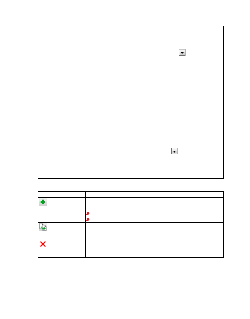
13.4.2 Editing scenario properties
Element Description
Modifications Number of modifications allocated to the
scenario. If you want to allocate or undo a
modification, go to the Modifications
column and click the button. In the list,
click the modification for the scenario of
your choice.
Concatenate:ModifComplete\No Concatenate:Modifications
(complete)\Number: Consecutive
numbers created by Vissim based on the
order in which the modifications were
added.
Concatenate:ModifCompleteByLoadOrder\No Concatenate:Modifications (complete)
by load order\Number: Consecutive
numbers created by Vissim based on the
order in which the modifications were
added.
ScenToComp Numbers and names of scenarios whose
attribute values you want to compare with
those of the current scenario. To select or
deselect a scenario, in the ScenToComp
column, click the button. Then in the
list, click the scenarios you want to load
into the background (see "Comparing
scenarios" on page 1088), (see "Selecting
scenarios for comparison" on page 1088).
Use the buttons shown to the right of the list to execute the following functions:
Element Name Description
Add new
scenario
A new row is added to the Scenarios list and the current date and
time are entered.
In the Name column, enter the name of the new scenario.
In the Description column, enter the description of the scenario.
Duplicate
selected
scenarios
A duplicate of the selected scenario is created in the Scenarios list.
Rename the new scenario in Name column, if desired. The name is
adopted for the duplicate and extended with the extension - Copy.
Delete
selected
scenarios
Selecting and deleting one or more rows
© PTV GROUP 1081
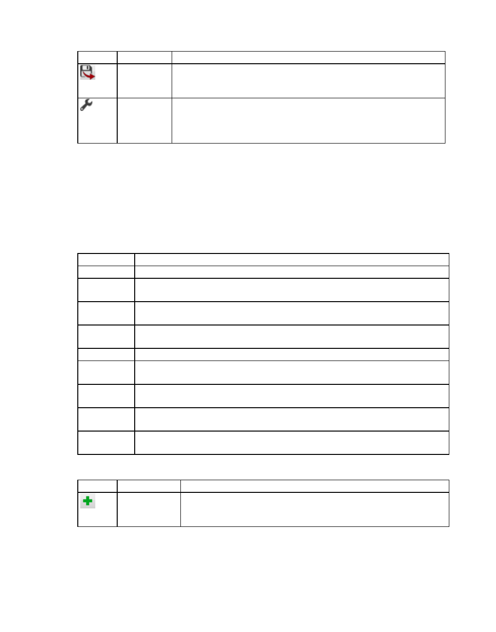
13.4.3 Editing modification properties
Element Name Description
Export
selected
scenarios
A window opens. Here you can select the desired directory path
where you can store the scenario as *.inpx file. This *.inpx file is not
part of the project and is not listed under the scenario management.
Select
attributes
to display in
the grid
Columns with attributes are shown and hidden in the Scenarios list
13.4.3 Editing modification properties
1. From the File menu, select > Scenario Management > Project Structure.
The Project Structure window opens.
2. Select the Modifications tab.
All project-related modifications are displayed together with their attributes.
The list contains the following attributes:
Element Description
Count Total number of modifications within the project
No Consecutive numbers created by Vissim based on the order in which the
modifications were added.
LoadIndex Load index: Consecutive numbers created by Vissim based on the order in
which the modifications were added.
Name Name of the modification. You can rename the default entry <generated
automatically> or an entered name.
Description Optional description of the modification
Group Name of a group of related modifications. It is used to identify modifications in
a list. To do so, you can sort the (see "Sorting lists" on page 102) column.
TraFilename Model transfer file name: Name of the *.trax file storing the changes that are
part of the modification.
Exclusions Modifications which exclude each other cannot be allocated to the same
scenario.
DependOn Dependent on: Once a modification is created, this modification is related to
the modifications which have already been allocated to the base network.
Use the buttons shown to the right of the list to execute the following functions:
Element Name Description
Add new modi-
fication
A new model transfer file is created. A new row is added to the
Modifications list. Edit the fields in the Name, Description,
Exclusions and DependOn columns.
1082 © PTV GROUP

13.4.3 Editing modification properties
Element Name Description
Duplicate
selected modi-
fications
A duplicate of the selected modification is created in the
Modifications list. Edit the fields in the Name, Description,
Exclusions and DependOn columns.
Delete selec-
ted modi-
fications
Selecting and deleting one or more rows
Move selec-
ted modi-
fications
upwards in
loading
sequence
Moving selected modifications upwards in loading sequence and
adjusting the number in the LoadIndex column.
Move selec-
ted modi-
fications
downwards in
loading
sequence
Moving selected modifications downwards in loading sequence
and adjusting the number in the LoadIndex column.
Check com-
binability of
selected modi-
fications
Vissim checks whether a batch of selected modifications can be
uploaded to a scenario or whether this is excluded in terms of
functionality. A message is displayed and shows the results of the
check made.
Check inde-
pendence of
selected modi-
fications
Vissim checks whether the selected modifications result in
networks that are modeled in different ways when changing their
loading sequence.
If changing the loading sequence does not result in networks
that are modeled in different ways, the modifications do not
relate to each other. This means entries in the DependOn
column have no effect. A message is opened. You can choose
to delete the relations entered in the DependOn column.
If changing the loading sequence result in networks that are
modeled in different ways, the modifications relate to each
other. A message is displayed and shows the results of the
check made. You may reselect the relations between the modi-
fications. The matrix file is shown in the DependOn column.
Selecting
attributes to
be displayed
in the grid
Columns with attributes are shown and hidden in the
Modifications list.
© PTV GROUP 1083

13.5 Placing a network under scenario management
13.5 Placing a network under scenario management
Warnings:
Do not change the names or structure of the files and directories generated by Vis-
sim.
Do not save the files of a project to the directory of another project.
In both cases, scenario management cannot work properly, which may lead to loss of
data!
Place your network as a base network under scenario management to derive other networks
from it, save these as scenarios and make further changes to them. The base network may
already contain a modeled network or be empty. You cannot use the base network to perform
simulation runs.
1. Ensure that the network of your choice has been modeled according to your requirements
and has been saved as a *.inpx network file.
2. Ensure that the network file is not saved to a folder that already contains a project or part of
a project.
3. From the File menu, choose > Scenario Management > Place Under Scenario
Management.
The Place Under Scenario Management window opens.
4. Enter the desired data.
Element Description
Project name Name of the project to which the base network and first scenario are
saved.
First
scenario
Name of the first scenario saved as a copy of the base network to the
project.
5. Confirm with OK.
In the network editor, the first scenario is displayed. The title bars and frames of non-
selected elements of the program interface, e.g. of the network editor, project explorer or
quick view are no longer displayed in blue (default color), but in a different color, now green
by default, as a scenario has been opened.
The title bar of Vissim displays the name of the project and the first scenario. The project
explorer opens (see "Using the project explorer" on page 1076). In the directory that
contains the *.inpx network file, Vissim creates the following directories and files for
scenario management.
Warning: Avoid deleting, moving, editing or other changes to these directories and
files. Otherwise, scenario management cannot work properly, which may lead to
loss of data!
1084 © PTV GROUP

13.6 Creating a new scenario
Backups: used internally by Vissim
Modifications: contains *.trax model transfer files of the modifications
Scenarios: When a scenario is simulated and direct output is selected for evaluations,
Vissim saves the direct output files to subfolders of this directory.
Temp: contains backup files
If you have generated files using Direct Output of Evaluations, these files remain saved in
your directory and are not automatically moved before you place the network file under
Scenario Management.
If when editing the network file, you have saved or generated the following files within
Vissim before placing the network file under Scenario Management, these files are not
automatically moved by Vissim when you place the network file under Scenario
Management:
SC control files
Fixed time control files *.sig
Animation files *.ani
Video files *.avi
When you place a network file that contains evaluation results, path files *.way, trip chain
files *.fct or cost files *.bew under scenario management, these are assigned to an
automatically created Scenario 1 and are saved to its folder under the Scenarios directory.
If when editing the network file, you have created a results database, this database is
automatically moved by Vissim to the Scenarios directory before you place the network file
under Scenario management.
13.6 Creating a new scenario
You have the following options for creating a new scenario:
In the base network: You adopt all settings, network objects and base data from the
base network into the new scenario.
In the project structure: Here you can edit the attributes of the scenario and select the
modifications of your choice (see "Editing the project structure" on page 1079).
As a duplicate of a scenario in the project explorer or project structure (see "Project
explorer toolbar" on page 1078), (see "Editing the project structure" on page 1079)
13.6.1 Creating a new scenario in the base network
1. In the project explorer, open the project of your choice.
2. In the project explorer, right-click Scenarios.
3. From the shortcut menu, choose Add.
The new scenario is shown in the project explorer, in the Scenarios folder (see "Using the
project explorer" on page 1076). In the network editor, you can open and edit the scenario
(see "Opening and editing scenarios in the network editor" on page 1087). You can rename
© PTV GROUP 1085
13.7 Creating a new modification
the scenario, enter a description for it and assign it modifications (see "Editing the project
structure" on page 1079).
13.7 Creating a new modification
You have the following options for creating a new modification:
In the base network: Adopt all settings, network objects and base data from the base
network into the new modification.
In the project structure: Vissim creates a model transfer file (*.trax) for changes to the
modification and you can edit the attributes of scenarios (see "Editing the project struc-
ture" on page 1079).
As a duplicate of a modification in the project explorer or project structure (see "Project
explorer toolbar" on page 1078), (see "Editing the project structure" on page 1079)
13.7.1 Creating a new modification in the base network
1. In the project explorer, open the project of your choice.
2. In the project explorer, right-click Modifications.
3. From the shortcut menu, choose Add.
The new modification is shown in the project explorer, in the Modifications folder (see "Using
the project explorer" on page 1076). You can open and edit the modification in the network
editor and copy it into one or multiple scenarios (see "Opening and editing scenarios in the
network editor" on page 1087), (see "Using the project explorer" on page 1076). You can
rename the modification, enter a description and make additional settings (see "Editing the
project structure" on page 1079).
Tip: Alternatively, you can create a new modification in the project structure (see
"Editing the project structure" on page 1079).
13.8 Opening and editing the base network in the network editor
In the network editor, you can open and edit the base network of a project. In the base network
you cannot perform simulation runs. Vissim automatically adopts changes made to the base
network as modifications into all scenarios of the project, as these have been derived from the
base network. In the project explorer, under Scenarios and under Modifications , the
modifications are displayed.
1. From the File menu, choose > Scenario Management > Open Base Network.
Tip: Alternatively, in the project explorer, right-click Base network. Then click Open. If
under the File menu, in the list of files last opened, the file is shown and the path has
not been changed, you can select the file there and show it in the network editor.
In the network editor, the base network is opened. The title bars and frames of non-selected
elements of the program interface, e.g. of the network editor, project explorer or quick view
are no longer displayed in blue (default color), but in olive green by default.
1086 © PTV GROUP

13.9 Opening and editing scenarios in the network editor
2. Edit the base network.
3. Use one of the following options to save the base network:
Press CTRL+S.
On the File toolbar, click Save.
Your changes are adopted in all scenarios of the project.
13.9 Opening and editing scenarios in the network editor
In the network editor, you can open and edit scenarios of a project. In a scenario, you can
perform simulation runs. If multiple scenarios have been saved under a project and you edit
and save one of them, Vissim will add it as a modification under the edited scenario and under
Modifications.
1. From the File menu, choose > Scenario Management > Open Scenario.
Tips: Alternatively, in the Project Explorer, open a scenario as follows:
Double-click the desired scenario.
Right-click the desired scenario and from the shortcut menu, choose Open.
If under the File menu, in the list of files last opened, the file is shown and the path
has not been changed, you can select the file there and show it in the network
editor.
The Open Scenario window opens.
2. Click on the desired entry.
3. Confirm with OK.
If the Messages window opens, check the messages and correct the errors reported.
Messages regarding modifications are listed under Modification.
In the network editor, the scenario is opened. The title bars and frames of non-selected
elements of the program interface, e.g. of the network editor, project explorer or quick view
are no longer displayed in blue (default color), but in green by default.
4. Edit the scenario.
5. Use one of the following options to save the scenario:
Press CTRL+S.
On the File toolbar, click Save.
Changes are saved to the scenario and displayed in the project explorer as a modification
under Scenarios and under Modifications.
13.10 Opening and editing modifications in the network editor
In the network editor, you can open and edit modifications of a project. When you edit and
save a modification, all changes become effective in the scenarios that access the edited
© PTV GROUP 1087
13.11 Comparing scenarios
modification.
1. From the File menu, choose > Scenario Management > Open Modification.
Tip: In the project explorer, right-click the scenario of your choice to open the Vissim
network in the network editor.
The Open Modification window opens.
2. Click on the desired entry.
3. Confirm with OK.
In the network editor, the modification is opened. The title bars and frames of non-selected
elements of the program interface, e.g. of the network editor, project explorer or quick view
are no longer displayed in blue (default color), but in maroon by default.
4. Edit the modification.
5. Use one of the following options to save the modification:
Press CTRL+S.
On the File toolbar, click Save.
The changes are saved to the modification. The modification then becomes effective in all
scenarios that reference the modification.
13.11 Comparing scenarios
You can compare the attributes and attribute values of network objects of an opened scenario
with those of one or multiple other scenarios (comparison scenarios) (see "Selecting
scenarios for comparison" on page 1088).
In the currently opened scenario, in the attribute list of each network object type, you can show
the scenarios in which the network objects of this network object type were used (see
"Selecting attributes and subattributes for a list" on page 106). To do so, select at least one
scenario for comparison with the opened scenario (see "Selecting scenarios for comparison"
on page 1088).
13.11.1 Selecting scenarios for comparison
In the project structure, for each scenario, you can select one or multiple scenarios for
comparison from the same scenario management project. This way you have one base
scenario that is assigned to one or multiple comparison scenarios.
The network of the comparison scenario selected loads Vissim into the background. Based on
the network of the base scenario, relations to networks loaded into the background are
generated. When you open the base scenario, in the Attribute selection window, you can
select attributes and attribute values of network objects or comparison scenarios and display
them in the attribute lists of network objects of the base scenario to compare them (see
"Selecting attributes for scenario comparison" on page 1089).
1. From the File menu, select > Scenario Management > Project Structure.
1088 © PTV GROUP
13.11.2 Selecting attributes for scenario comparison
2. Select the Scenarios tab.
3. Click into the row of the scenario you want to compare with other scenarios. Then in the
ScenToComp column, click the button.
4. In the list, click the scenarios you want to use for comparison.
5. Click the Close button.
The scenarios selected (comparison scenarios) are loaded into the background.
6. Open the base scenario.
7. Open the attribute list of the network object type whose attributes you want to compare (see
"Opening lists" on page 92).
8. Select the attributes you want to compare (see "Selecting attributes for scenario
comparison" on page 1089).
13.11.2 Selecting attributes for scenario comparison
For network objects that exist in the current as well as in comparison scenarios you can: a) in
the Attribute selection window, select attributes of the network objects of scenarios b) in the
attribute lists of the network objects of the current scenario, show and easily compare them.
You have the following options to select subattributes:
select and apply individual subattributes from one or multiple scenarios
selecting individual subattributes from one or multiple scenarios and apply them from
other scenario comparisons
13.11.2.1 Select individual subattributes and apply them in the attributes list
1. Open the base scenario you want to compare with another scenario (see "Opening and
editing scenarios in the network editor" on page 1087).
2. For the base scenario opened, select the desired comparison scenarios (see "Selecting
scenarios for comparison" on page 1088).
3. Open the attribute list of the network object type whose attributes you want to compare (see
"Opening lists" on page 92).
4. In the attribute list, click the Attribute selection symbol .
The <Network object type>: Select Attributes window opens. In the section on the left, the
attributes of the network object type are displayed. The scenarios are marked with the
symbol and sorted by their number.
5. In the section on the left, in front of the desired entry Scenario comparison <Name of
base scenario> <Name of comparison scenario>, click the + symbol.
© PTV GROUP 1089

13.11.2 Selecting attributes for scenario comparison
The following attributes are displayed under scenario comparison. The attributes are
highlighted with a red circle. You must select at least one subattribute. They cannot be
edited.
Attribute Description
Value Attribute value of network object in comparison
scenario
<Name of base scenario> minus
<Name of comparison scenario>
Difference of attribute values between base scen-
ario and comparison scenario
<Name of comparison scenario>
minus <Name of base scenario>
Difference of attribute values between com-
parison scenario and base scenario
<Name of base scenario> minus
<Name of comparison scenario> %
Difference of attribute values between base scen-
ario and comparison scenario in percent
<Name of comparison scenario>
minus <Name of base scenario> %
Difference of attribute values between com-
parison scenario and base scenario in percent
Minimum Smallest attribute value of network object in com-
parison scenario
Maximum Largest attribute value of network object in com-
parison scenario
6. Under scenario comparison, in front of the attribute of your choice, click the + symbol.
All attributes of the network object type are displayed.
7. Select the desired attributes whose values you want to compare with the values of the
same attributes in the base scenario.
If under an attribute, you select the subattribute Current run, Current run will show the
following the simulation run:
In a comparison scenario, the last simulation run completed
in the currently loaded base scenario, the active, current simulation run
If no simulation is run in the base scenario, the last simulation run completed.
If simulations were run in the comparison scenarios, you can select subattributes from the
desired simulation runs for the comparison. The subattributes begin with the number of the
respective simulation run, e.g. 4 x current x All types.
8. Click the symbol.
The attributes are displayed on the right in additional rows.
9. Confirm with OK.
The attributes are displayed in the attribute list of the network object type.
13.11.2.2 Also applying subattributes selected from all scenario comparisons
1. Select the desired subattributes as described above.
1090 © PTV GROUP

13.12 Comparing and transferring networks
2. Click the Add from all scenario comparisons button.
13.11.2.3 Showing comparison scenarios in which the selected network object is used
In an opened scenario, in the attribute list of a network object type, you can show the
scenarios assigned for comparison that use network objects of the same network object type.
To do so, in the Attribute selection window, on the left, select the desired comparison scenario
and add it to the right side (see "Selecting attributes and subattributes for a list" on page 106).
This is also possible in the result lists Simulation Runs, Vehicles In Network, Pedestrians In
Network, and for dynamic assignment, in the Paths list.
1. Opens the attribute list of the network object type in which you want to show the columns
with scenarios that include the network object type (see "Opening lists" on page 92).
2. In the attribute list, click the Attribute selection symbol .
The <Network object type>: Select Attributes window opens. In the section on the left, the
attributes of the network object type are displayed.
3. In the section to the left of Exists in scenario, click the + symbol.
All comparison scenarios with a network object of the network object type are displayed.
The scenarios to compare are marked with the symbol and sorted by number:
Scenario comparison <Name Scenario>.
4. Select the desired comparison scenario.
5. Click the symbol.
The selected scenarios to compare are listed on the right in an additional row. You cannot
edit hatched cells or the attribute name.
6. Confirm with OK.
In the attribute list, an ExistsInScen, <Number> column is displayed for each comparison
scenario selected. In this column, in each row and for each network object that exists in the
respective comparison scenario, the option is selected.
13.12 Comparing and transferring networks
You can save the differences between two networks.to a model transfer file (*.trax). Generally,
one network models the base, while the other network models the target. One of the networks
can be the one currently opened.
You apply the model transfer file (*.trax) to a network file. The network file must be opened in
the Network editor. When applying the model transfer file (*.trax), you transfer its network data
(*.trax) to the network opened in the Network editor.
© PTV GROUP 1091

13.12.1 Creating model transfer files
Application example for Scenario management
You can transfer two network variants to Scenario management: The network with the base is
placed under Scenario management. You then apply the model transfer file to this network.
This is how the second network selected is created:
1. Generate the model transfer file (*.trax) based on network A and B (see "Creating model
transfer files" on page 1092).
2. Then you place network A under Scenario management as scenario 1 (see "Placing a
network under scenario management" on page 1084)..
3. Copy Scenario 1.
4. Rename the copied scenario to Scenario 2.
5. Open scenario 2 in the Network editor.
6. Apply the model transfer file to scenario 2 (see "Applying model transfer files" on page
1093).
13.12.1 Creating model transfer files
1. Open the network file you want to use as base file to create the model transfer file.
2. From the File menu, choose > Compare and Transfer Networks > Create Model Transfer
File.
The Create Model Transfer File window opens.
3. Make the desired changes:
Element Description
Define net-
work com-
parison
Base:
Use currently loaded network: Select this option to use the network
currently opened as the basis for the model transfer file.
Read from file: Click the symbol to choose another file as the basis
for the model transfer file you want to create.
Target:
Use currently loaded network: Select this option if the currently
opened network is the desired target you want to create with the help of
the model transfer file to be created. Both files must use the same
coordinate system.
Read from file: Click the symbol to select the file of your choice.
The model transfer file created is used to transfer the base network into
the selected network.
1092 © PTV GROUP

13.12.2 Applying model transfer files
Swap base and target: The entries made and options selected in the Base
and in the Target are swapped
Result of
the com-
parison
Write model transfer file to: Click the symbol, enter the filename of the
model transfer file (*.trax), select the folder of your choice and save the
model transfer file to it (*.trax).
4. Click the Create Model Transfer File button.
13.12.2 Applying model transfer files
You can apply a saved model transfer file (*.trax) to the network file currently opened. In doing
so, you transfer the network data to the network opened in the Network editor.
1. Open the network file to which you want to apply the model transfer file.
2. From the File menu, choose > Compare and Transfer Networks > Apply Model Transfer
File.
The Choose model transfer file window opens.
3. Select the desired file.
4. Click the Open button.
5. Check any messages displayed by Vissim.
© PTV GROUP 1093
14 Testing logics without traffic flow simulation
14 Testing logics without traffic flow simulation
You can test the response of a signal control logic to several detector type constellations,
without actually modeling traffic flows.
You have the following options to generate detector types:
Add types to the detectors.
Run recorded or created macros.
The Test function is useful, if you want to check for bugs in newly developed signal control
logics. This is particularly true when they contain functions that are used only sporadically.
The following detector types are distinguished:
Detector type Description
Single
actuation
Increasing impulse (front end of vehicle) and decreasing impulse (rear end
of vehicle) within one second
Repeated
actuation
Increasing and decreasing impulse every second, equivalent to a single
actuation every time step.
Continuous
actuation
Single impulse increase, impulse decrease only after explicit termination of
actuation.
14.1 Setting detector types interactively during a test run
1. On the Network objects toolbar, click Vehicles In Network. Then click the Edit graphic
parameters icon.
The list with the graphic parameters of the network object type opens (see "List of graphic
parameters for network objects" on page 152).
2. Select Object visibility.
3. Ensure that neither the Use color scheme option nor a classification are selected.
4. On the Network objects toolbar, click Detectors. Then click the Graphic parameters
icon.
The list with the graphic parameters of the network object type opens (see "List of graphic
parameters for network objects" on page 152).
5. Select Object visibility.
Tips:
You can save a Signal Control Detector Record as a file or display it in a window
(see "Evaluating SC detector records" on page 1010).
You may record an event for comparison with another control logic (see "Using mac-
ros for test runs" on page 1095).
6. From the Test menu, choose > Continuous or Single Step.
1094 © PTV GROUP
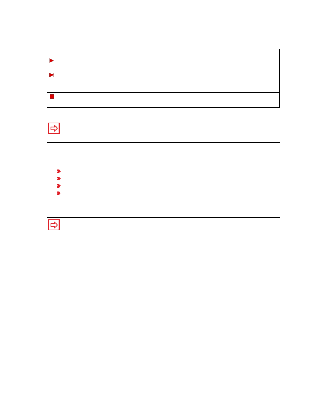
14.2 Using macros for test runs
The test run is started. During the test run, you can switch back to the Test run single step
mode, e.g. the simulation second during which startup of the SC program ends.
Symbol Name Description
Test run
continuous
Starts continuous test run or switches from Test run single step mode
to continuous mode.
Test run
single step
Starts simulation in Test run single step mode or switches from Test
run continuous to Test run single step mode or executes the next
single step.
Stop test
run
Quit test run
Tip: You can set whether you want to activate detectors in test mode with a single or a
double click (see "Defining click behavior for the activation of detectors in test mode" on
page 145).
7. In the Single Step mode, in the Network Editor, double-click a detector type.
With each click, you switch to the next requirement:
No actuation: no fill color
Single actuation: blue
Repeated actuation: turquoise
Continuous occupancy: pink
If you double-click on Continuous occupancy, the detector call switches back to No
actuation.
Tip: Alternatively, right-click the detector and from the shortcut menu, choose Edit
Actuation. Then click the state of your choice.
14.2 Using macros for test runs
You do not need to manually and interactively set each individual detector call in the Network
Editor in each test run (see "Setting detector types interactively during a test run" on page
1094). You can perform test runs with macros for which you use different parameter settings of
logic in each case. The desired detector types are saved to *.m_i macro files.
14.2.1 Recording a macro
You can record a macro file for identical test runs of several control scenarios.
1. From the Test menu, choose > Macro Recording.
The entry is marked with a checkmark the next time you open the menu.
2. From the Test menu, choose > Continuous or Single Step.
© PTV GROUP 1095
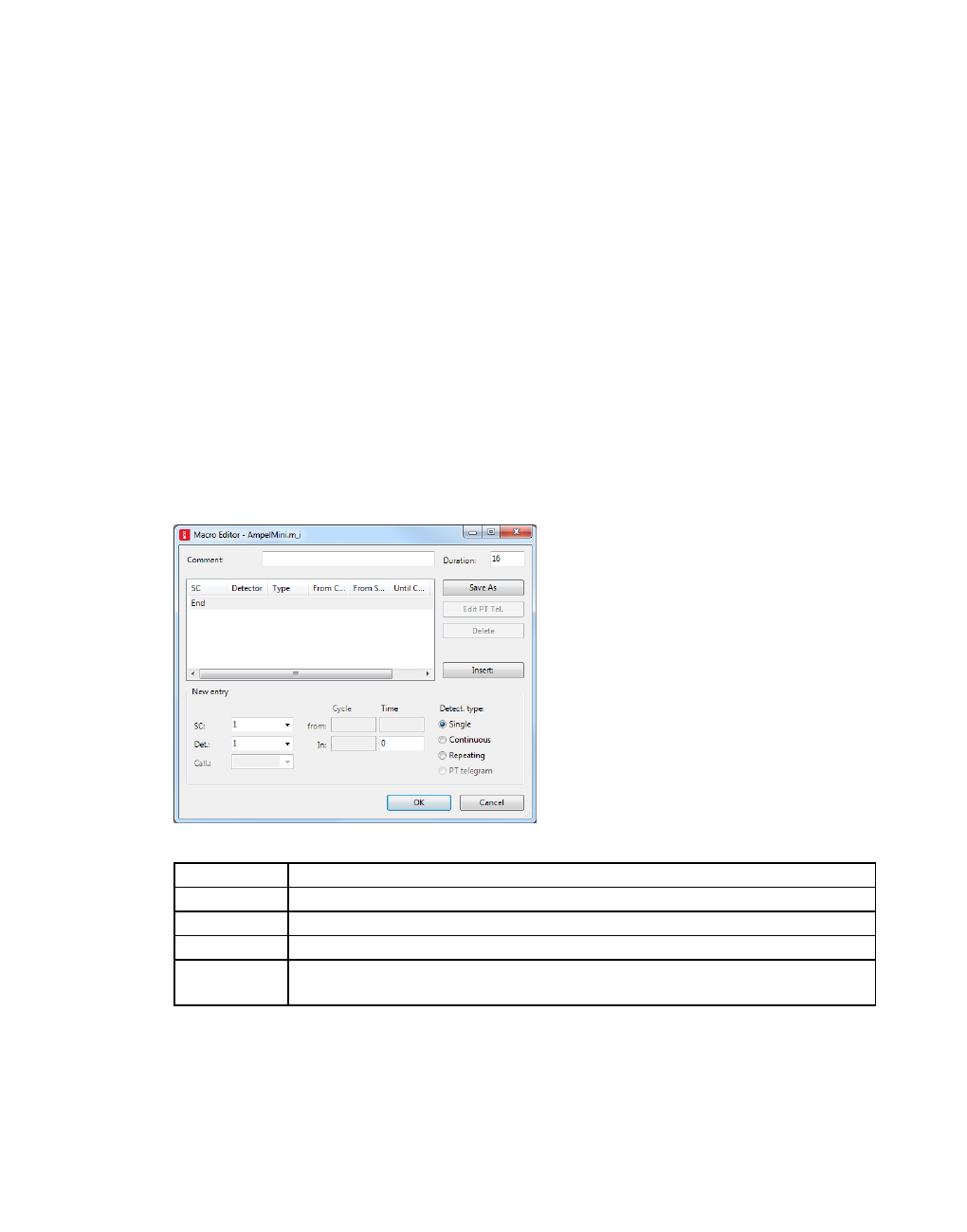
14.2.2 Editing a macro
3. Set the desired detector types in the Network Editor (see "Setting detector types
interactively during a test run" on page 1094).
4. From the Test menu, choose > Stop.
The test run is completed. A macro file <name of network file>.M_I is saved.
5. Change the parameters of the control logic for the next recording.
6. From the Test menu, choose > Run Macro.
The repetition of the same calls starts.
14.2.2 Editing a macro
To evaluate a control logic with similar test runs, you can create macro files in the Macro
Editor. If you want to edit an existing call, for example, change the time interval, you must
delete the call and add a new call.
1. From the Test menu, choose > Edit Macro.
2. Select the macro file *.m_i.
The Macro Editor opens. The existing calls are shown in the table.
3. Make the desired changes:
Element Description
SC Signal controller of the call
Det. Detector of the call
Call. PT calling pt: only records PT vehicles that send PT telegrams.
Cycle from,
to
Number of cycle
1096 © PTV GROUP

14.2.3 Run Macro
Element Description
Time from,
to
Time interval
Detect. type Single: single calls work only within a second. You can thus only spe-
cify the time in.
Continuous: permanent occupancy
Repeating: one crossing per second
4. If you have defined a new entry, click Insert.
The new call is added before the currently marked call. Automatic sorting does not take
place.
5. Enter another file name for the new test case.
6. Confirm with OK.
Note: If the current control supports PT calling points, PT telegrams can be recorded in
the macro as special calls for detectors of type PT telegram.
14.2.3 Run Macro
Perform the following steps for each test run.
1. Record the macro file.
2. If desired, edit the macro file.
3. Adjust the parameters of the control logic for the test case.
4. If desired, activate evaluations (see "Evaluating SC detector records" on page 1010).
5. From the Test menu, choose > Run Macro.
The Run Macro File window opens.
6. If desired, into the To second box, enter the simulation second up to which you want to
macro to run.
7. If you have enabled evaluations, save and analyze the evaluations.
Notes:
Vissim does not automatically name the files of different test cases. This gives you flex-
ibility when naming. Give the files useful and unique file names, for example, include the
test case number.
If different test cases are examined when testing VS-PLUS logics, an SC detector record
is created in a file *.ldp for each test case. Give this file the name of the *.m_i macro file
which was used to generate the *.ldp file. This improves the clarity and makes it easier to
find the files.
© PTV GROUP 1097

15 Creating simulation presentations
15 Creating simulation presentations
You can record simulations for presentations in the following data formats and save them in
files:
3D video files *.avi (see "Recording a 3D simulation and saving it as an AVI file" on page
1098)
Animation files *.ani (see "Recording a simulation and saving it as an ANI file" on page
1106)
15.1 Recording a 3D simulation and saving it as an AVI file
Vissim can be used to save a 3D simulation as a video file in the *.avi format. You need to
specify camera positions in order to assign them to keyframes in a storyboard (see "Saving
camera positions" on page 1098), (see "Using storyboards and keyframes" on page 1100).
You can also save the 3D perspective of a driver or a pedestrian as camera position (see
"Showing 3D perspective of a driver or a pedestrian" on page 186).
You can also start the recording in the Quick Mode (see "Using the Quick Mode" on page 85).
The Quick Mode is ignored during the recording.
Note: Video files require a lot of memory. Make sure that depending on the recording
planned, sufficient memory space is available.
15.1.1 Saving camera positions
To record a simulation as an AVI file, you need to save the camera positions with the network
view of your choice. You then assign keyframes to the camera positions.
You can also save a camera position during a simulation run. When doing so, you can save
the 3D perspective of a driver or a pedestrian as camera position as well (see "Showing 3D
perspective of a driver or a pedestrian" on page 186).
1. Make sure you have selected the 3D mode.
The symbol is selected. The network is displayed in 3D. You do not need to perform
the next step if you want to save the camera position during a simulation run, e.g., to save a
3D perspective of a driver or a pedestrian as camera positions.
2. To set the desired camera position, click the Rotate mode (3D) symbol or use the
mouse or keyboard.
3. On the Network editor toolbar, in the Selection of camera position list, enter the name of
your choice.
4. Confirm with Enter.
Tip: You can edit the attributes in the Camera Positions list (see "Attributes of camera
positions" on page 1099).
1098 © PTV GROUP

15.1.2 Attributes of camera positions
15.1.2 Attributes of camera positions
1. From the Presentation menu, choose Camera Positions.
The Camera Positions list opens.
By default, you can edit the list (see "Using lists" on page 89).
Note: In lists, you can use the Attribute selection icon to show and hide attribute
values (see "Selecting attributes and subattributes for a list" on page 106).
2. A network object may have the following attributes: These can be shown in the attributes
list.
Element Description
No Number of camera position
Name Name of camera position. Changing the name of a camera position auto-
matically changes the name of the keyframes assigned to it, if the keyframes
have the same name as the camera position.
PosX Position (x): horizontal camera position on the x-axis
PosY Position (y): horizontal camera position on the y-axis
PosZOffset Position (z-offset): vertical camera position on the z-axis. Showing 3D
perspective of a driver or a pedestrian, this is at eye level. The eye level
depends on the model:
Vehicles, with the exception of HGVs, buses and trains: default 1.5 m
HGVs, buses and trains: default 2.5 m
Vehicle types, man, woman: default 1.75 m
Pedestrians: 92.5 % of height of 3D model
PosPt Location: coordinates of the camera position Position (x), Position (y) and
Position (z-offset). Showing the 3D perspective of a driver or a pedestrian:
0, 0, eye level.
YawAngle Yaw angle: angle of rotation around z axis. Showing 3D perspective of a
driver or a pedestrian: 0°
PitchAngle Pitch angle: angle of rotation around y axis. Showing 3D perspective of a
driver or a pedestrian: 10°
RollAngle Roll angle: angle of rotation around x axis. Showing 3D perspective of a
driver or a pedestrian: 0°
FOV Aperture angle of the camera in degrees from viewer's position
FocLen Focal length in mm
VehNo Vehicle number: Number of vehicle selected for camera position
PedNo Pedestrian number: Number of pedestrian selected for camera position
3. If during editing you have changed the display of the Vissim network and want to show the
entire Vissim network again, on the Network Editor toolbar, click the Show entire network
button .
© PTV GROUP 1099

15.1.3 Using storyboards and keyframes
15.1.3 Using storyboards and keyframes
A storyboard allows you to define basic settings for the recording of a simulation. These, e.g.,
include the resolution, framerate and the option of saving the recording to an *.avi file. You
assign at least one keyframe to your storyboard. In a storyboard, you can combine multiple
keyframes that then elapse in sequence. You assign a camera position to each keyframe. This
allows you to specify the order of the camera positions used during simulation. The camera
dwells on the keyframes for the dwell time specified. It moves between the keyframes on a
linear guide, with a constant or gliding motion, for the transition time specified.
You are basically using keyframes as a “script" for the AVI recording. During the AVI recording,
the keyframes elapse in the sequence specified in the Start time attribute. The recording
begins with the first start time. It does not have to be the start time of the simulation. As soon as
the AVI recording is started, the view switches to the camera position of the first keyframe. To
record *.avi files, you must define at least one keyframe with a camera position and a dwell
time and assign it to a storyboard.
During a simulation run you can:
Editing attributes of keyframes (see "Defining a storyboard with keyframes" on page
1100)
add new camera positions (see "Saving camera positions" on page 1098)
Editing attributes of camera positions (see "Attributes of camera positions" on page
1099)
Showing a preview of the movie in a window in simulation speed (see "Showing a pre-
view of camera movement" on page 1104)
Tip: You can additionally read Storyboards like other network objects and base data
from other Vissim *.inpx network files (see "Reading a network additionally" on page
341).
15.1.3.1 Defining a storyboard with keyframes
1. Make sure you have selected the 3D mode.
The symbol is selected. The network is displayed in 3D.
2. Set the desired camera position, for example, using the icon Rotate mode (3D) and
the mouse.
3. From the Presentation menu, choose Storyboards.
The Storyboards list opens. In the Relations list box, the entry <Single List> is shown.
By default, you can edit the list (see "Using lists" on page 89).
4. In the list, on the toolbar, click the Add button .
A new row with default data is inserted.
1100 © PTV GROUP

15.1.3 Using storyboards and keyframes
Note: In lists, you can use the Attribute selection icon to show and hide attribute
values (see "Selecting attributes and subattributes for a list" on page 106).
5. Make the desired changes:
Element Description
Resolution Resolution in pixels Resolution (x) x Resolution (y), e.g. 1,280 x 780
ResX Horizontal resolution (x), e.g. 1,280
ResY Vertical resolution (y), e,g, 780
RecAVI Record AVI: Select this option to create an AVI recording for the story-
board.
Framerate Frame rate (fps), default 20 images per second
Filename Path and file name of AVI file
RealTmFact Real time factor = Framerate / Simulation resolution (see "Defining sim-
ulation parameters" on page 796). Default 2.0
NetLayout Net layout file
Name Name of storyboard
No Storyboard number
ShowPrev Show preview: While recording a simulation, you can show a preview of
the film in a window.
PrevZoomFact Preview zoom factor for film preview (default value 1)
You can define keyframes for the storyboard.
6. In the Relations list box, click Keyframes.
The right-hand list is shown. If there is no assignment, only the column titles are shown.
7. In the list on the left, click the storyboard for which you want to define keyframes.
8. In the list on right, on the toolbar, click the Add button .
A new row with default data is inserted.
The Keyframe window opens.
© PTV GROUP 1101
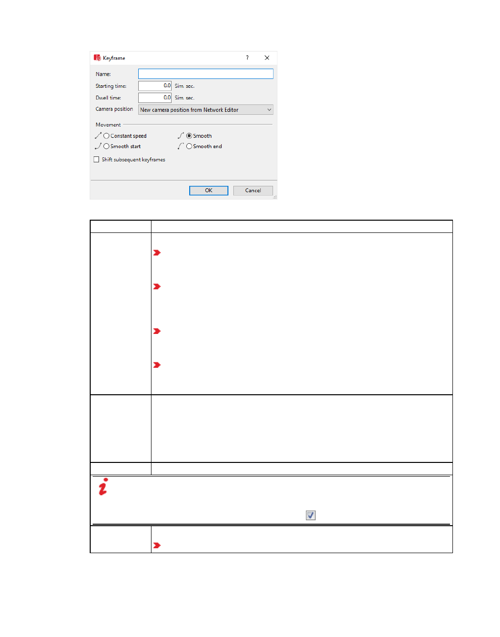
15.1.3 Using storyboards and keyframes
9. Make the desired changes:
Element Description
Name Name of keyframe.
When you define a keyframe without specifying a name for it and then
select a camera position, the name of the camera position is entered
as the keyframe name in the Keyframes list.
If the name of the keyframe and the name of the assigned camera pos-
ition are the same and you decide to change the name of the camera
position, the name of the respective keyframe is automatically changed
in the Keyframes list.
If no name is entered for the keyframe and you change the name of the
assigned camera position, the new camera position name is auto-
matically entered as the keyframe name in the Keyframes list.
Changing the name of a camera position automatically changes the
name of the keyframes assigned to it, if the keyframes have the same
name as the camera position.
StartTime Simulation second during which the keyframe is started Start time = 0:
Keyframe starts when from the Presentation menu, you choose > AVI
Recording. If Start time = 0 is not defined for any keyframe, but instead
start times > 0 are defined for all keyframes, the AVI recording starts with
the keyframe for which the shortest start time has been defined. Changing
the StartTime also allows you to move the order of the keyframe in the list.
DwellTime Time period during which simulation is viewed from this keyframe position.
Note: Vissim uses the StartTime and DwellTime to check whether the current
keyframe fits into the existing keyframe list. You must not enter a StartTime or
DwellTime for a keyframe that overlaps with the DwellTime of another keyframe.
To move any of the following keyframes, select Shift subsequent keyframes.
CamPos Camera position (see "Attributes of camera positions" on page 1099)
Adopt new camera position from the active Network editor
1102 © PTV GROUP

15.1.3 Using storyboards and keyframes
Element Description
Select saved camera position
TransTime Transition time between two keyframes, which is automatically calculated
as the difference of StartTime and DwellTime of the current keyframe and
the StartTime of the next keyframe. Overlapping keyframes cannot be
added to the list.
TransType Transition types, in the Movement section, define the motion between the
current and next camera position of the keyframe.
Constant speed: Position change at constant speed
Smooth: Motion close to keyframe positions is slower, but becomes
faster between them.
Smooth start: Keyframe position starts with increasing speed and con-
tinues with constant speed toward the next keyframe.
Smooth end: Keyframe position starts with a constant speed and
gradually slows down towards the next keyframe position.
You can use the latter two options to define a keyframe without
DwellTime as "intermediate point" between a movement of keyframes,
e.g. in order to create an effect on the distance.
Example transition types Smooth start, Smooth end: If keyframe 2 is an
intermediate keyframe with a DwellTime of 0 s, then the movements could
be defined as follows:
Keyframe 1: Smooth start
Keyframe 2: Smooth
Keyframe 3: Smooth end
Shift
subsequent
Keyframes
If this option is selected, the start times of all subsequent keyframes
according to the current settings made for the keyframe selected are
moved:
When you insert a new keyframe between two defined keyframes, Vis-
sim checks whether the start time of the new keyframe lies after the
DwellTime of the preceding value. If so, then Vissim changes the start
times of all subsequent keyframes:
∆t = start time of new KF + DwellTime of new KF + movement time of previous
KF - start time of next KF
By adjusting the start time of the next keyframe accordingly, Vissim
ensures that the (calculated) movement time is retained until the
keyframe following the added keyframe is reached. It thus remains the
same as before the new keyframe was inserted.
When you edit an existing keyframe, all subsequent keyframes are
moved according to the new start time and/or DwellTime. The start
times of all subsequent keyframes are moved by:
© PTV GROUP 1103

15.1.4 Recording settings
Element Description
∆t = new start time – old start time + new DwellTime – old DwellTime
Note: If you select this option, a defined keyframe cannot be
moved before any of its previous keyframes.
10. On the File toolbar, click Save.
15.1.3.2 Showing a preview of camera movement
You can show a preview of the camera movement at the AVI default rate of 20 frames per
second or at maximum speed.
1. Open the Storyboards list.
2. Make sure that Keyframes is selected in the Relations list box.
3. In the list on the right, right-click the keyframe of your choice.
4. From the context menu, choose Preview with AVI speed or Preview with simulation
speed.
The movement shown when recording the *.avi file is simulated using the speed currently
selected.
5. To cancel and close the preview, in the top right corner of the preview, click the X.
At the end of the AVI recording, the preview is closed.
15.1.4 Recording settings
Vissim generates *.avi video files that are played at a default rate of 20 frames per second. As
each simulation time step generates exactly one picture, the playback speed depends on the
number of time steps per simulation second: With a simulation resolution of 10 time steps,
which is recommended, the playback speed is twice as fast as real time. If you choose to use
only one time step per simulation second, the playback speed is 20 times faster than real time.
Note: Please note that changing the simulation resolution has an impact on the
behavior of vehicles and pedestrians and thus might lead to different simulation results.
Besides standard recording, you have the following options:
Anti-aliasing (see "Selecting the 3D mode and 3D recording settings" on page 143)
Double-sided lighting (see "Selecting the 3D mode and 3D recording settings" on page
143)
15.1.5 Starting AVI recording
1. Ensure that the following requirements are met:
You have saved at least one camera position (see "Saving camera positions" on page
1098)
1104 © PTV GROUP

15.1.5 Starting AVI recording
You have saved at least one storyboard (see "Using storyboards and keyframes" on
page 1100).
The storyboard has been assigned at least one keyframe.
In the keyframe, the attributes Start time, Dwell time, Transition type and Transition
time are defined and have been assigned a camera position.
2. In the Storyboards list, click the storyboards of your choice and select RecAVI (Record
AVI).
3. From the Presentation menu, choose > Record AVIs.
In the Presentation menu, Record AVIs is marked with .
4. Start the simulation (see "Running a simulation" on page 796).
If you have not started AVI recording for the current network files yet, the window Video
Compression opens. An *.avi file requires approx. 20 MB/s. On your computer there may
be several compression programs installed by default (see "Selecting a compression
program" on page 142).
Codec x264 provides an excellent quality for smaller files x264vfw.sourceforge.net. For
further information, please visit our webpages at: PTV Vissim FAQs (#91).
Notes:
Not all compression programs displayed might be suitable for recording an *.avi file.
This depends on the system configuration. Test the compression program you want to
use with a short Vissim example.
The compression program used for the original video recording must be available on the
computer you are using to show the *.avi file.
5. For a minimum file size, in the Compressor list, click a compression program.
6. In the Compression Quality box, enter a value of your choice.
7. If the compression program can be configured, the Configure button is activated and you
can make additional settings.
8. Confirm with OK.
© PTV GROUP 1105

15.2 Recording a simulation and saving it as an ANI file
Tip: You may specify a default compression program (see "Selecting a compression
program" on page 142).
The simulation starts. If the Preview option has been selected for the storyboard, a window
opens in which the movie is shown. The *.avi file is recorded during the simulation run. At
the end of the simulation, the *.avi file is saved in the same folder as the *.inpx network file.
9. To stop AVI recording before the end of the simulation run, from the Presentation menu,
choose > Record AVIs.
In the Presentation menu, Record to AVI is deactivated. The attribute RecToAVI (AVI
recording ) of the storyboard is deactivated.
10. To stop the simulation, on the Simulation toolbar, click the Stop button .
Note: The recording of an *.avi file may take considerably longer than a simulation in 3D
mode, particularly if from the Presentation menu, you chose > 3D-Anti-Aliasing. This option
corresponds to the Anti-aliasing option under User Preferences (see "Selecting a
compression program" on page 142).
15.2 Recording a simulation and saving it as an ANI file
You can save simulation runs for vehicles and pedestrians in animation files (*.ani). After this
you can use the animation files for presentations in Vissim. Since an animation file only
contains the graphical representation of the simulated vehicles or pedestrians, the animation
runs considerably faster than the actual simulation. Evaluations are not available in the
animations.
When defining sections, you can chose whether you want to record the simulation for the
sections defined or for the entire network.
You can also record simulation runs with the following settings:
Pedestrian simulations that use the LOS schema (see "Using LOS schemes for show-
ing aggregated pedestrian values" on page 176).
The wireframe view can be enabled or disabled (see "Network editor toolbar" on page
73)
Links may be hidden if their display type is set to Invisible (see "Defining display
types" on page 300).
Elevators, elevator doors and cab
You can enter the desired simulation time interval for the recording.
Playback is possible at any speed supported by Vissim and your hardware.
Unlike simulation mode, you can play animations both forward and backward for the selected
time sequences and network sections. This allows you to quickly reach the desired network
status in an animation.
Animations record attribute values of network objects that are required for animation display:
1106 © PTV GROUP
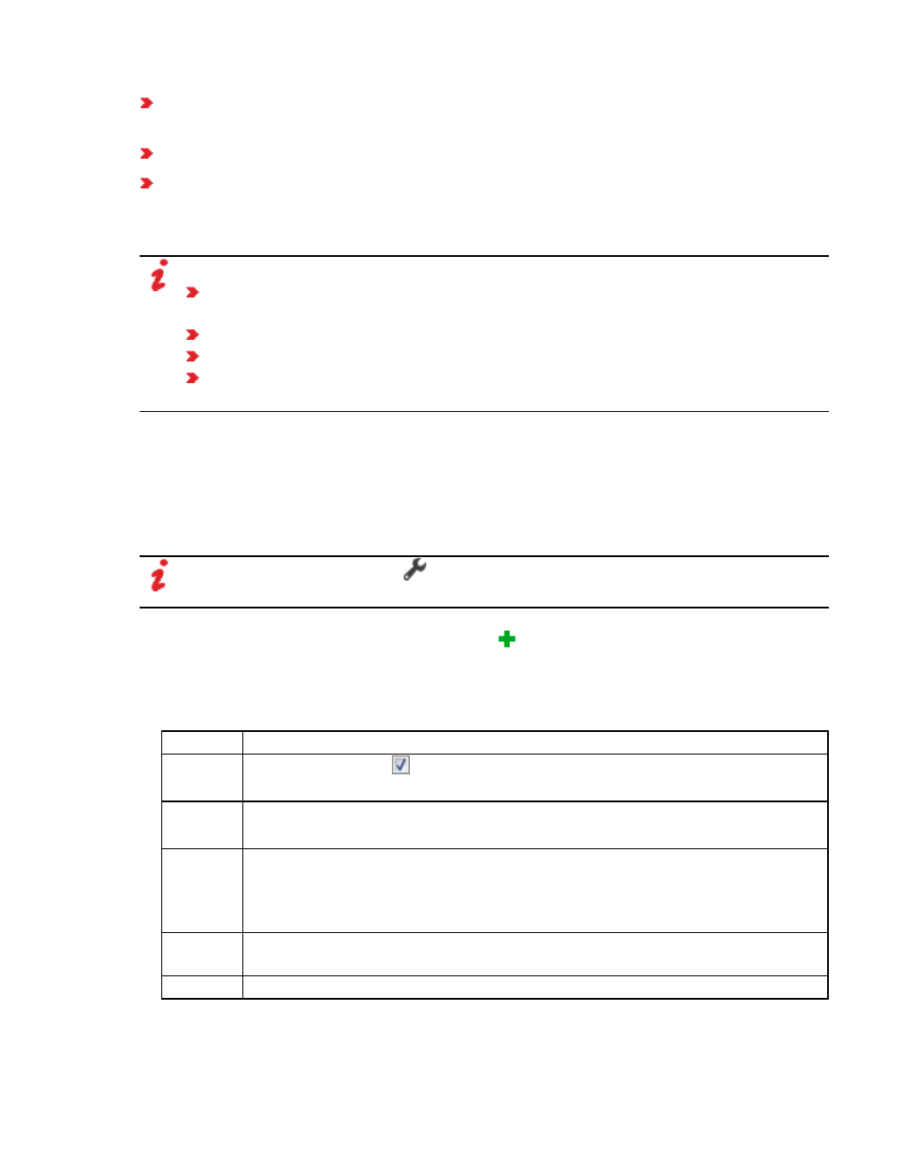
15.2.1 Defining an animation recording
Vehicles: position, turn signal, color, 3D model, state. The animation recording accounts
for the graphic parameter setting Color by vehicle state under Vehicles In Network.
Pedestrians: position,3D status, color, 3D model
Signal head: state
You can edit these attribute values using script files. Attribute values of other network objects
are not recorded and cannot be edited via script files.
Notes:
If the script files change attributes in the simulation while an animation is recorded,
the changed values are saved to the animations.
When you run animations, the changes become effective through the script files.
When you run animations, the script files are not called again.
Animation files require a lot of memory. Make sure that depending on the recording
planned, sufficient memory space is available.
15.2.1 Defining an animation recording
1. From the Presentation menu, choose > Animation Recordings.
The Animation Recordings list opens.
By default, you can edit the list (see "Using lists" on page 89).
Note: In lists, you can use the Attribute selection icon to show and hide attribute
values (see "Selecting attributes and subattributes for a list" on page 106).
2. In the list, on the toolbar, click the Add button .
A new row with default data is inserted.
3. Make the desired changes:
Element Description
RecAnim Record animation: If this option is selected, the animation is recorded when
you select Record Animation in the Presentation menu.
Sections Number of sections to be recorded.
No number: The entire network is recorded.
Filename Name of the *.ani or *.ani.txt file to which the simulation is saved as an
animation. Depending on the selection available in the Type attribute, make
sure that after the filename, the extension of your choice is displayed, *.ani or
*.ani.txt.
End Simulation second when recording ends If you define multiple animation
recordings, avoid creating overlaps between the time intervals.
No Unique number
© PTV GROUP 1107
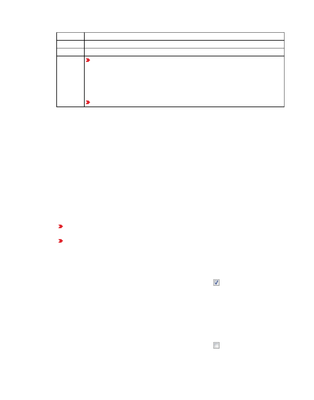
15.2.2 Recording an animation
Element Description
Name Animation name
Start Simulation second when recording starts
Type For Export (*.ani.txt): Saves the animation to a text file. Simulation time,
various vehicle data and/or pedestrian data, vehicle position and ped-
estrian position as well as the statuses of signal heads and detectors are
saved to the text file in rows The text file can be imported into Autodesk
3DS MAX. For further information, refer to the API\3dsMaxExport\HowTo
folder in your Vissim installation directory.
For Replay (*.ani): Saves the animation to a ANI file that you can replay.
Showing and editing dependent objects as relation
The attribute and attribute values of this network object type are shown in the list on the left,
which consists of two coupled lists.
1. In the list on the left, click the desired entry.
The list on the right contains attributes and attribute values of sections allocated to the network
object selected in the list on the left (see "Using coupled lists" on page 111).
2. On the list toolbar, in the Relations list box, click > Sections.
3. Enter the desired data.
The data is allocated.
15.2.2 Recording an animation
1. Ensure that the following requirements are met:
At least one animation recording is defined (see "Defining an animation recording" on
page 1107)
To record parts of the network, you need to define sections that contain these parts
(see "Modeling sections" on page 641). The desired sections must be selected in the
Sections attribute of the animation recording (see "Defining an animation recording"
on page 1107).
2. From the Presentation menu, choose > Record Animations.
In the Presentation menu, Record Animations is marked with .
3. Start the simulation (see "Running a simulation" on page 796).
The simulation starts and the data is recorded in the *.ani or *.ani.txt file while the
simulation is running. The *.ani or *.ani.txt file is saved at the end of a simulation to the
directory and under the name defined in the Filename attribute of the animation recording.
4. To stop the animation recording, from the Presentation menu, choose > Record
Animations.
In the Presentation menu, Record Animations is marked with .
1108 © PTV GROUP
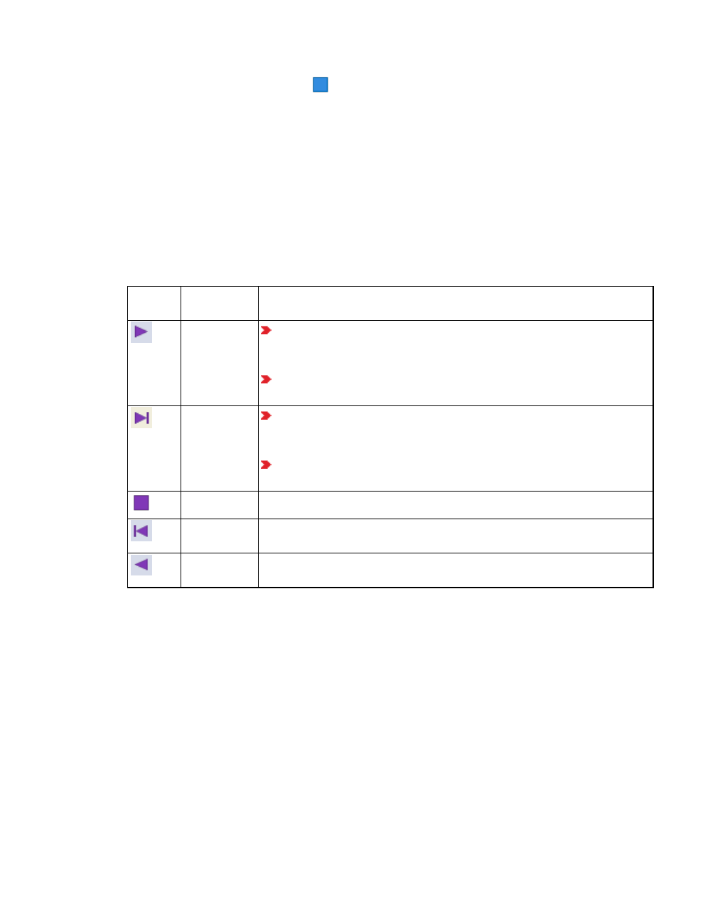
15.2.3 Running the animation
5. To stop the simulation, click the Stop button.
15.2.3 Running the animation
You can run an animation of the simulation with or without an animation file (*.ani).
When playing back an animation file (*.ani) in Vissim, you first need to open the corresponding
Vissim network.
15.2.3.1 Running the animation with an animation file (*.ani)
1. From the Presentation menu, choose Animation with ANI file.
2. From the Presentation menu, choose the desired entry:
Toolbar
button
Name Description
Continuous When no animation run is started: Opens a window in which
you can select the *.ani file of your choice. Then starts the con-
tinuous animation run.
When the Animation single step mode is started: Let anim-
ation run continuously.
Single Step When no animation run is started: Opens a window in which
you can select the *.ani file of your choice. Then starts the anim-
ation run and shows the step of the first simulation second.
When the Animation continuous mode is started: Stops anim-
ation run and show next single step.
Stop Finish animation run
Single Step
Reverse
Stops running animation and shows last step before the current
simulation second.
Continuous
Reverse
Stops running animation and plays animation in continuous
reverse order.
Creating model transfer files
15.2.3.2 Running the animation without an animation file (*.ani)
Aggregated result attributes are used for visualization, e.g. for the color of link segments or link
bars.
1. In the Presentation menu, deselect Animation with ANI file.
2. Then, from the Presentation menu, choose the desired command.
The animation of the simulation is run without an animation file.
15.2.4 Displaying values during an animation run
While running an animation, you can show time-based aggregated values.
© PTV GROUP 1109

15.2.4 Displaying values during an animation run
1. Before you run the animation, make sure the following requirements are met:
2. Under Evaluation Configuration, specify that you want to collect result attributes for links
and/or areas (see "Configuring evaluations of the result attributes for lists" on page 954).
3. For vehicles on links, click in the network objects toolbar next to Links on Edit graphic
parameters; for pedestrians in areas, click in the network objects toolbar next to Areas on
Edit graphic parameters.
4. Select the option Use color scheme.
The Edit color scheme for <network object type> window opens.
If the window does not open because the option has already been deactivated once since
program start, click the icon at the end of row to open the window.
5. For vehicles, select the classification of your choice Lanes or Segments; for pedestrians,
select the classification of your choice Areas or Pedestrian Grid Cell Data.
6. Click the Attribute button .
7. Select the desired result attribute.
8. Click the Filter button.
The Preselection Filter window opens.
9. If desired, under Simulation Runs, select the option of your choice.
10. Under Time Intervals, select Show only selected time intervals.
11. Then select Last completed.
12. If under Evaluation Configuration you selected the desired vehicle classes, under Vehicle
Classes you can now select the desired vehicle class.
13. If under Evaluation Configuration you selected Pedestrian Classes, under Pedestrian
Classes you can now select the desired pedestrian class.
14. Confirm with OK.
15. Click the icon .
16. In the list, click the color scheme of your choice.
17. Confirm with OK.
18. Start the animation (see "Running the animation" on page 1109).
The time interval results produced during the selected simulation run are used for the color
scheme of the animation run.
1110 © PTV GROUP

16 Using event based script files
16 Using event based script files
You can define scripts in a network file. Using the scripts, you manage script files and define
the times at which you want to run the script files during the simulation. This allows you to
simulate systems that respond to different simulation states and/or influence the simulation.
16.1 Use cases for event-based script files
You are modeling a traffic management system that depending on a certain amount of
traffic, at the beginning of a time step, uses a script file to change the volumes for partial
routes and to allow the use of emergency lanes.
Opening and closing barriers
Changing the display state of variable message signs
Changing the color of vehicles once they have reached their destination parking lot
16.2 Impact on network files
When script files change attributes and you then save the network file, the latter will also
contain the changed data.
16.3 Impact on animations
When script files change attributes during a simulation and animation recording, these
changes also become effective when the animation is replayed.
When you replay animations, the script files are not called again.
16.4 Impact on evaluations
Script files allow you to access evaluations, e.g. in order to activate evaluations before ini-
tialization.
If the script files change attributes that are used in evaluations, the changed values are
saved to the results of the evaluations.
16.5 Defining scripts
1. From the Scripts menu, choose > Event-Based Scripts.
The Scripts table is opened.
2. Make the desired changes:
Short
name
Long
name
Description
No Number Unique number
Name Name Name of script
© PTV GROUP 1111

16.6 Starting a script file manually
Short
name
Long
name
Description
RunType Type of
execution
Run type: Time at which the script is to be called and executed. If
you define several scripts to be run at the same time, the scripts
are executed in the sequence of their numbering.
Manually: The script is not automatically called during the sim-
ulation. You call the script at the time of your choice (see "Start-
ing a script file manually" on page 1112).
Before simulation start
After simulation start
At time step start
At time step end
Before simulation end
After simulation end
FromTime From
time
Selecting a time step of simulation: Time at which the script is
executed for the first time
ToTime To time Selecting a time step of simulation: Time at which the script is
executed for the last time
Period Period Selecting the length of time intervals (number of time steps) for
simulation
Scope Scope Time period during which the script remains active and is not
automatically deactivated:
Simulation run: Leave script open during the entire simulation
run and in it, call user-defined functions, depending on the
Function name attribute
Single call: Always run the entire script
ScriptFile Script file Selecting a script file for the script from a directory
FctName Function
name
Name of the function or subprogram executed. This option is
enabled when for the Scope attribute, the time range Simulation
run is selected.
If you have selected the run type Manually, run the script at the time of your choice (see
"Starting a script file manually" on page 1112). If you have defined other run types, the scripts
are run automatically.
16.6 Starting a script file manually
You may run script files manually that have been selected in the attributes of scripts. This also
applies to scripts that run script files automatically and have the following attribute values:
Before simulation start
After simulation start
At time step start
1112 © PTV GROUP

16.6 Starting a script file manually
At time step end
Before simulation end
After simulation end
Scripts with the Run type attribute Manually can only be started manually, not automatically.
1. Ensure that the following requirements are met:
The Vissim network model is complete, so that a simulation can be started.
The simulation parameters have been defined (see "Defining simulation parameters"
on page 796).
The script file of your choice has been defined and saved to the desired directory.
At least one script has been defined for the desired script file (see "Defining scripts" on
page 1111).
In the script, in the Script file attribute, the script file is selected.
2. From the Scripts menu, choose > Event-Based Scripts.
The Scripts table is opened.
You can either start the script immediately or at a chose time during the simulation. To run
the script file at the time of your choice, perform the simulation in Simulation single step
mode.
3. If desired, start the simulation (see "Selecting the number of simulation runs and starting
simulation" on page 801).
4. In the Scripts table, right-click the entry of your choice.
5. From the shortcut menu, choose Run script.
6. If you want to stop the script file, from the Scripts menu, choose > Stop running script.
© PTV GROUP 1113

17 Runtime messages and troubleshooting
17 Runtime messages and troubleshooting
Runtime messages, such as process messages, error messages, and warnings are shown in
the Messages window. Messages regarding test runs are also displayed in the Messages
window (see "Showing messages and warnings" on page 1117).
In addition, Vissim opens separate windows for error messages about unexpected program
states.
Vissim saves errors to error files (*.err) (see "Checking the runtime warnings in the file *.err" on
page 1115).
You can use the VDiagGUI.exe program to perform an error diagnosis (see "Performing an
error diagnosis with VDiagGUI.exe" on page 1120).
17.1 Editing error messages for an unexpected program state
An error message opens in case of an unexpected program state:
1. Follow the instructions in the error message.
This prevents loss of data and consequential errors.
2. Please forward the errors to us, so that we can correct them:
3. Click Report Error.
The PTV Vision Support contact form opens. The necessary data, including the error report,
are automatically copied into the form.
If you call up the contact form with the menu Help > Technical Support or the Internet page
Technical Support PTV Vissim or Technical Support PTV Viswalk, the data are not entered
automatically.
4. Save the network file *.inpx under a different name.
5. Close Vissim.
6. Open Vissim.
1114 © PTV GROUP

17.2 Checking the runtime warnings in the file *.err
Vissim always copies the network file and saves the copy in the file format *.inp0.
7. Compare the *.inp0 file with the network file *.inpx which was saved under a different name.
8. Make sure that the data is complete.
9. If the data in the network file *.inpx are not complete, copy the file *.inp0.
10. Name the copy of the *.inp0 file into a *.inpx file.
11. Continue work with this version.
17.2 Checking the runtime warnings in the file *.err
1. Vissim shows errors and messages in the Messages window (see "Showing messages
and warnings" on page 1117). In addition, by default, Vissim saves errors to the *.err files
and the vissim_msgs.txt file (see "Using the vissim_msgs.txt log file." on page 1119). These
files are saved in the folder in which the network file *.inpx is saved.
If in the simulation parameters, only one run is defined, the simulation is started, errors occur
and an error file (*.err) is saved, the name of the error file will not include the simulation run
number. If then another simulation run is started, the error file ( *.err ) from the previous
simulation run will be overwritten.
17.2.1 Runtime warnings during a simulation
If Vissim detects problematic situations during a simulation run which do not prevent the
continuation of the simulation, runtime warnings are displayed in the Messages window and
written to an *.err file. Except for the file extension *.err, the name of this file corresponds to the
name of the network file.
If runtime warnings have occurred, the Messages window opens after the simulation run.
Correct the causes of warnings and errors.
17.2.2 Runtime warnings before a simulation
If the Vissimnetwork contains errors and you start the simulation, runtime warnings will be
displayed before the simulation is started.
© PTV GROUP 1115
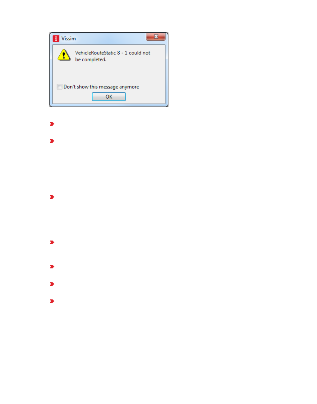
17.2.3 Runtime warnings during multiple simulation runs
All errors are saved to the *.err file. For example, this may be due to the following errors:
Private Transport: Too little distance between a routing decision and the first connector of
the route.
Private Transport: A vehicle traverses a routing decision and within the same time step
exits the link on which the routing decision is located.
Public Transport: Too little distance between an entry link and the first connector of the
route. Because of this, the Private Transport vehicle or the Public Transport vehicle have
left their route. Either the vehicle did not stop in time in order to wait for an opportunity for a
lane change, or within the same time step, the vehicle has traversed the routing decision
and another connector.
Too little distance between the desired speed decision and the first connector. This mes-
sage is displayed if, within a time step, a vehicle with the highest speed which is possible
within a defined desired speed distribution could traverse both the desired speed decision
as well as the start of a connector. For example, this would be possible at 205 km/h and 10
time steps per simulation second, at a maximum distance of 5.70 m. If this actually occurs
during the simulation run, the relevant vehicle ignores this desired speed decision.
An input volume which has not been completely processed, for example due to insufficient
capacity of the entry link, because of which there is congestion outside of the network at
the end of a defined time interval.
A vehicle, which has been removed from the network after the maximum lane change wait-
ing time has elapsed (default value 60 sec)
For some signal controls: Infringements of the minimum green period and interim time
infringements during the simulation (see "Detecting inconsistent planning" on page 631).
For pedestrian simulation: too high density within area per simulation second
17.2.3 Runtime warnings during multiple simulation runs
If the error file (*.err) is written during multiple simulation runs, Vissim enters the number of the
respective simulation run into the error file (*.err). The number of simulation runs is defined in
the simulation parameters (see "Defining simulation parameters" on page 796).
1116 © PTV GROUP

17.3 Showing messages and warnings
17.3 Showing messages and warnings
The Messages window displays process messages, error messages and warnings, e.g. after
you have chosen the Check network command (see "Checking the network" on page 812),
but during scenario management, simulation and reading and writing of model transfer files.
Related messages are combined in a group. The name of each group and the number of
errors are listed in blue font above the group.
In Scenario management the name of a group can include different information, for example
the name and number of the scenario, the name of the calculation performed and the number
of the simulation run. The information included in the group name is separated by colons.
Example: Scenario 1: Calculate Scenario 1': Load scenario: Read in network
Vissim opens different significant messages in a separate window that allow you to open the
Messages window and view all messages. For example, Vissim opens the Check network
window, showing errors, after you have selected the Check network command. Click the
Show button to open the Messages window.
Before a pedestrian simulation is started, c also automatically checks the network for
consistency and displays error messages and warnings in the Messages window.
The Messages window is not updated and does not display messages when the Quick mode
is activated and the simulation is running. This allows for a maximum simulation speed.
The Messages window can be freely positioned or docked (see "Arranging or freely
positioning program elements in PTV Vissim" on page 87). The Messages window cannot be
anchored in a section together with a list or a Network editor, but only across the entire width
or height of the user interface.
17.3.1 Opening the Messages window
In the View menu, choose > Messages.
The Messages window opens.
© PTV GROUP 1117

17.3.2 Editing messages
Element Description
Time Time at which the message was generated
Priority Debug messages, error messages or warnings
Type Network object type, e.g. Nodes
ID Number of the network objects
Message text Description of error message or warning
Syn-
chronization
Zoom on network object: Network objects of the rows selected are
selected in the Network editor. This may also be a number of network
objects of the same network object type.
Network objects of the rows selected are not selected in the Network
editor.
<Number>
Errors
Show all errors found
<Number>
Warnings
Show all warnings found
Fix Only for errors of the category Vehicle routes and 2D/3D model
segments: Start interactive repairs. If, e.g., a vehicle route is interrupted
because a connector was deleted, you can identify this error in the
Messages window, define the missing connector in the Network editor
and then click the Fix button . Vissim will complete the vehicle
route.
Then select Check network. Error messages are no longer displayed
for the repaired objects.
17.3.2 Editing messages
Sorting messages
To sort a column, click the column header.
An arrow in the column header indicates whether the entries are sorted in ascending or
descending order.
Expanding or collapsing groups
To close a group, double-click the row with the group name highlighted in blue.
Editing individual messages or groups
To edit an individual entry, right-click the row of your choice.
To edit a group, right-click the row with the group name highlighted in blue.
1118 © PTV GROUP

17.4 Using the vissim_msgs.txt log file.
If Synchronization is selected, objects or groups selected in the Messages window
are also selected in the Network editor.
The context menu opens.
1. Choose the desired entry from the context menu.
Element Description
Delete
message
Delete individual rows
Fix The Fix command is described further above.
Fix group Repair all errors or messages of the current category. The program
continues to display the errors. Then select Check network. Error
messages are no longer displayed for the repaired objects.
Delete all
messages
in this group
Delete all errors or messages of the current category.
Discard
sorting
Only active if at least one column is sorted: Resets column sorting to default
sorting.
Toast notification shows number of messages
When the Messages window is open, a simulation ends or is terminated and Vissim shows
messages in the Messages window, a toast message opens at the bottom right border of the
screen, showing the number of messages displayed.
17.4 Using the vissim_msgs.txt log file.
The vissim_msgs.txt log file is automatically saved to:
C:\Users\<username>\AppData\Local\Temp\VISSIM\vissim_msgs.txt
From the File menu, choose > Show Log File.
17.4.0.1 Naming the log files of multiple instances
Each time an instance of Vissim is opened, a log file is saved. These log files are named
consecutively according to the following convention: vissim_msgs_ 0.txt, vissim_ msgs_1.txt,
etc.
17.4.0.2 Structure of the log file
The log file consists of an upper and lower section. Upper section: System entries which were
generated at the start of Vissim. Example:
2017-05-11 9:43:18 System set VISSIM localization part I...
2017-05-11 9:43:18 Initialize system licensing...
2017-05-11 9:43:20 System certified date: 2017-05-11 (server: ptv-dxx-
xxxxx.ptvag.ptv.de, Box: x-xxxxxxx)
© PTV GROUP 1119

17.5 Performing an error diagnosis with VDiagGUI.exe
2017-05-11 9:43:20 System certified time period: 25 (server: ptv-dxx-
xxxxx.ptvag.ptv.de, Box: x-xxxxxxx)
2017-05-11 9:43:20 System system date: 2017-05-11 (server: ptv-dxx-
xxxxx.ptvag.ptv.de, Box: x-xxxxxxx)
2017-05-11 9:43:20 System certified date: 2017-05-11 (server: ptv-dxx-
xxxxx.ptvag.ptv.de, Box: x-xxxxxxx)
2017-05-11 9:43:20 System certified time period: 25 (server: ptv-dxx-
xxxxx.ptvag.ptv.de, Box: x-xxxxxxx)
2017-05-11 9:43:20 System system date: 2017-05-11 (server: ptv-dxx-
xxxxx.ptvag.ptv.de, Box: x-xxxxxxx)
2017-05-11 9:43:20 System set VISSIM localization part II...
2017-05-11 9:43:21 Start system licensing 2017-05-11 09:43:19.
2017-05-11 9:43:21 System certified time successfully updated (server: ptv-dxx-
xxxxx.ptvag.ptv.de, Box-Serial Number: x-xxxxxxx)
2017-05-11 9:43:21 System licensing completed 2017-05-11 9:43:20.
2017-05-11 9:43:21 System initialization of core components completed...
2017-05-11 9:43:21 System version 10.00 - 00* [65780] , filename C:\Program
Files\PTV Vision\PTV Vissim 10\Exe\VISSIM100.exe
2017-05-11 9:43:21 System initializing Vissim...
2017-05-11 9:43:21 System starting Vissim...
2017-05-11 9:43:21 System read settings...
2017-05-11 9:43:21 System initialization completed.
...
Lower section: Detailed messages about the functions of Vissim, e.g. warnings or messages,
which were shown during the ANM import and the creation of the Vissim network:
...
2017-05-11 9:56:57 System [ANM] import started (initial).
2017-05-11 9:56:57 System [ANM] import network data.
2017-05-11 9:56:57 Warning ANM link 4A: SPEED: (from 20 to 40) This attribute is 0
and is set to the default value.
2017-05-11 9:56:57 Warning ANM link 4B: SPEED: (from 40 to 20) This attribute is 0
and is set to the default value.
2017-05-11 9:56:57 System This ANM file does not provide a projection definition.
Coordinates are assumed to be cartesian values.
2017-05-11 9:56:57 Warning ANM node 10: Multi-leg node has additionally ANM zones
attached. Dummy link stubs are generated ignoring node geometry.
2017-05-11 9:56:57 Warning ANM node 40: Multi-leg node has additionally ANM zones
attached. Dummy link stubs are generated ignoring node geometry.
2017-05-11 9:56:57 Warning ANM node 20: This node contains lanes that do not have
any movements defined to or from.
2017-05-11 9:56:57 Warning ANM node 40: This node contains lanes that do not have
any movements defined to or from.
2017-05-11 9:56:57 Copy system [ANM] file C:\Test\PTV Vissim\ANM_Import\ANM_Import_
Test.anm to C:\Test\PTV Vissim\ANM_Import\ANM_Import_net3.panm.
2017-05-11 9:56:57 System [ANM] Remove obsolete objects.
2017-05-11 9:56:57 System [ANM] import end.
...
17.5 Performing an error diagnosis with VDiagGUI.exe
In certain cases PTV Vision Support can ask you to run the file VDiagGUI.exe.
1120 © PTV GROUP

17.5 Performing an error diagnosis with VDiagGUI.exe
1. Start Windows Explorer.
2. Open the Vissim installation directory.
3. Open the Exe directory.
4. Double-click the VDiagGUI.exe file.
The VDiagProGUI window opens. The Actions tab is shown by default.
5. Follow the instructions from PTV Vision Support.
6. Open the desired tab.
Actions tab
© PTV GROUP 1121

17.5 Performing an error diagnosis with VDiagGUI.exe
Button Description
Reset Menu/Tool-
bar/Shortcuts
Reset toolbars and menus
Note: You can also reset toolbars and menus in Vissim
(see "Resetting menus, toolbars, shortcuts, and dialog
positions" on page 146).
Reset Dialog Positions Reset window positions
Note: You can also reset window positions in Vissim (see
"Restoring the display of windows" on page 89).
Start Vissim in Dia-
gnostics Mode
Only click the button if instructed to do so by PTV Vision Support
and follow the instructions from PTV Vision Support.
Disable 3D Mode Disable 3D mode. This may be necessary if Vissim cannot be
started in 3D mode. Further information can be found in the
installation instructions Vissim <Version> - Installation Manual.pdf
in the Doc directory of your Vissim installation.
If you would like to see information on the tab, please click the ? button.
Versions tab
PTV Vision Support may ask you to check in this tab whether certain files are present.
1122 © PTV GROUP

17.5 Performing an error diagnosis with VDiagGUI.exe
If you would like to see information on the tab, please click the ? button.
© PTV GROUP 1123

17.5 Performing an error diagnosis with VDiagGUI.exe
Hotline Package tab
In the Hotline Package tab you can combine all desired data for PTV Vision Support, pack into
a file and send to PTV Vision Support.
Section Description
Custom
files Add files: Add files to the package
Remove: Remove selected files
Diagnostic
files
Check the desired options. For more information about the data provided by
the respective options, move the mouse pointer over the option text.
Save path Select the path and file name. In the list box, click the desired file format.
Create Hot-
line Pack-
age
Create the file for PTV Vision Support.
If you would like to see information on the tab, please click the ? button.
1124 © PTV GROUP

17.5 Performing an error diagnosis with VDiagGUI.exe
Log tab
PTV Vision Support may ask you to create a log file in this tab.
Click the Save Log button.
© PTV GROUP 1125

17.6 Saving network file after losing connection to dongle
If you would like to see information on the tab, please click the ? button.
17.6 Saving network file after losing connection to dongle
If there are problems with the connection between Vissim and the dongle, a message is
displayed.
Click Cancel to open another message and save the *.inpx network file, if you made
changes to the Vissim network since you last saved it.
If you then click OK, Vissim will wait until the connection to the dongle has been re-estab-
lished.
1126 © PTV GROUP

18 Add-on modules programming interfaces (API)
18 Add-on modules programming interfaces (API)
Vissim provides various APIs as an add-on module. With this, you can integrate your own
applications into Vissim. Not all add-on modules are by default part of your Vissim license.
Add-on modules and their documentation are saved in the folder ..\Vissim<Version>\API.
18.1 Using the COM Interface
Note: The following Vissim versions do not have a COM interface:
Demo versions of Vissim
Vissim Viewer
You can use the add-on COM interface module (Component Object Model) for:
Preparation and postprocessing of data
Efficiently controlling the sequence for the examination of scenarios
Including control algorithms which you have defined
Access to all network object attributes
Via the COM interface you can start Vissim from other applications or scripts or you can access
Vissim objects.
You can use various programming environments, e.g. VisualBasic for Applications in Microsoft
Excel™, Visual C++ or Visual J++ and use simple script languages, for example, VB Script or
Python.
Script files from the COM interface can be executed in Vissim (see "Selecting and executing a
script file" on page 1128).
COM Help
Information about the functions of the COM interface and associated commands can be found
in the COM Help.
From the Help menu, choose > COM Help.
You can find examples in the following default directory:
..\Users\Public\Public documents\PTV Vision\PTV Vissim <Version number>\Examples
Training\COM\
18.1.1 Accessing attributes via the COM interface
Using the AttValue method, you have read access to all network object attributes. Write
access is not available for all attributes. In the COM Help, the Editable row of each attribute
specifies a True or False value, indicating whether or not the attribute can be write-accessed.
© PTV GROUP 1127

18.1.2 Selecting and executing a script file
18.1.2 Selecting and executing a script file
In Vissim you can select and execute external script files. The following scripting languages
are supported:
Visual Basic *.vbs
Javascript *.js
Python *.py, *.pys (see "Using Python as the script language" on page 1129)
Tip: You may also manage scripts, which are executed during a simulation at a chosen
time, to the network file (see "Using event based script files" on page 1111).
The global variable Vissim can be used without initialization in the script and always refers to
the running Vissim, from which the script has been started. Additionally, you can use the
variable CurrentScript to create a reference to the current script, e.g. in order to access user-
defined attributes there.
You need not create a Vissim object, using CreateObject, as Vissim has already been started.
If additional instances of Vissim are required in the script, you can use CreateObject.
Scripts may include any command of the scripting language, e.g. loop, branch, entry, and
output commands.
Scripts must not contain any global declarations.
18.1.2.1 Executing script files
1. From the Scripts menu, choose > Run Script File.
A window opens.
2. Select the folder to which the script file has been saved.
3. Select the desired script file.
4. Click the Open button.
The script file is executed in Vissim.
18.1.2.2 Examples of script files
The following directory contains a Vissim network that uses script files: ..\Examples
Training\COM\Drop- off Zone . This example is available for Visual Basic Script (VBS) and
Python.
The following scripts are used to halve the volume of the first time interval for each input.
Example 1 of a *.vbs script file
For each flow in all_flows
For i = 1 To all_flows.Count
flow.AttValue("Volume(1)") = 0.5 * flow.AttValue("Volume(1)")
Next
1128 © PTV GROUP

18.1.3 Using Python as the script language
Example 2 of a *.vbs script file
all_flows = Vissim.Net.VehicleInputs.GetAll
For i = 0 To UBound (all_flows)
all_flows(i).AttValue("Volume(1)") = 0.5 * all_flows(i).AttValue("Volume(1)")
Next
18.1.3 Using Python as the script language
A distinguishing feature of Python is its clear and understandable syntax. With this you can
conveniently set up a prompt which is tailored to your project.
Python and all of the additional libraries are open source programs without usage restrictions.
Notes:
You must install Python 2.7 or a higher version and the appropriate extension
PythonWin, which provides Python with the COM functionality.
Python 2.7 and the appropriate extension PythonWin must correspond to your Vis-
sim version, e.g. python-2.7.6.amd64.msi and pywin32-218.win-amd64-py2.7.exe
for the 64-bit edition of Vissim.
wxPython is not supported.
Example of a *.pys script file
all_flows = Vissim.Net.VehicleInputs.GetAll()
for i in range(len(all_flows)):
all_flows[i].SetAttValue("Volume(1)", 0.5 * all_flows[i].AttValue("Volume(1)"))
18.2 Activating the external SC control procedures
You can use external, user-defined signal control procedures in Vissim (see "Add-on module
external signal control SC" on page 579). For this, you must provide an external program DLL
for the control and a specific dialog DLL. The DLL files must be programmed in C or C++. The
files are integrated with the interfaces SignalControl.DLL and SignalGUI.DLL.
18.3 Activating the external driver model with DriverModel.dll
You can replace the driver model with an external, user-defined driver model using Vissim.
The external driver model can be used for all or part of the vehicles in a simulation.
During the simulation, the DLL file is called up in each time step for each vehicle for which an
external driver model is available. The DLL file then controls the behavior of the vehicle.
Vissim transfers data to the DLL file:
the current state of the vehicle
the current state of the vehicle environment, e.g. the number and state of priority rule (1
= blocked, 3 = free), if closer to current vehicle than the next signal head downstream.
World coordinate of the front edge and rear edge of neighboring vehicles
© PTV GROUP 1129

18.4 Accessing EmissionModel.dll for the calculation of emissions
Spline of the middle line of the lane the Ego vehicle is using on its route or path within
the line of sight
Values of user-defined vehicle attributes can be transferred to the DLL and changed
by it.
The acceleration, deceleration and lane changing behavior are calculated in the DLL file. The
result is returned to Vissim.
You activate the external driver model for the desired vehicle type (see "Using vehicle types"
on page 254).
The external driver model must be implemented as a DLL file in the programming language C
or C++. The structure is described in the documentation.
Documentation in English
..\Program Files\PTV Vision\PTV Vissim <Version number>\API\DriverModel_DLL\In-
terface_Description.pdf
Example file
..\Program Files\PTV Vision\PTV Vissim <Version number>\API\DriverModel_DLL\Driver-
Model.cpp
18.4 Accessing EmissionModel.dll for the calculation of emissions
For the calculation of emissions, you can access the file EmissionModel.dll. You must provide
the EmissionModel.dll. It is not part of Vissim.
You activate the external emission model for the desired vehicle type (see "Activating
emission calculation and emission model for a vehicle type" on page 261). In each time step
Vissim calls up the functions in the file EmissionModel.dll for the calculation of the emission
values. The emission values can be output into the vehicle log and the link evaluations.
If no EmissionModel.dll is available, you can use the EnViVer Pro add-on module or EnViVer
Enterprise to calculate the emissions for individual vehicle types.
Documentation in English
..\Program Files\PTV Vision\PTV Vissim <Version number>\API\EmissionModel_DLL\E-
missionModel.txt
Files
..\Program Files\PTV Vision\PTV Vissim <Version number>\API\EmissionModel_DLL\
18.5 Activating the external pedestrian model with PedestrianModel.dll
Instead of the default file PedestrianModel.dll you can also use external pedestrian DLL files
(see "Requirements for pedestrian simulation" on page 820).
1130 © PTV GROUP

18.5 Activating the external pedestrian model with PedestrianModel.dll
With an external pedestrian DLL file, you can optionally also generate pedestrian inputs.
Please contact us if you wish to create your own pedestrian DLL files.
Directory of PedestrianModel.dll file
..\Program Files\PTV Vision\PTV Vissim <Version number>\\Exe\PedestrianModel.dll
© PTV GROUP 1131

19 Overview of PTV Vissim files
19 Overview of PTV Vissim files
The following tables describe the files which are used in Vissim.
19.1 Files with results of traffic flow simulation
Extension Name Description
*.att Attribute file Output file with static attributes and/or result attributes (see "List
toolbar" on page 93), (see "Performing evaluations" on page
941).
*.err Runtime
warnings
Error messages and warnings from the last simulation run. If
several simulation runs have been performed, multiple files
whose names each contain a simulation run number (see
"Checking the runtime warnings in the file *.err" on page 1115).
*.fhz Vehicles List of all vehicles with information on when and where they
were used at what speed in the network (see "Saving vehicle
input data to a file" on page 1050)
*.fzp Vehicle record Evaluation of vehicle data (see "Saving vehicle record to a file or
database" on page 971)
*.knr Node
evaluation
(raw data)
Output of raw data of node evaluation (see "Evaluating nodes"
on page 997)
*.ldp SC detector
record
Evaluation file for a VS-PLUS SC (see "Evaluating SC detector
records" on page 1010)
*.lsa Signal
changes
Chronologically sorted file of the signal state changes of all SCs
(see "Evaluating signal changes" on page 1021)
*.lzv SC time
distributions
Release durations and closure periods of signal groups of all
SCs (see "Saving SC green time distribution to a file" on page
1018)
*.mdb Database out-
put
Database outputs (see "Saving evaluations in databases" on
page 961)
*.mer Data collection
(raw data)
Raw data of data collections (see "Evaluating data collection
measurements" on page 1033)
*.merP Area
measurements
(raw data)
Raw data of area measurements of pedestrian simulation (see
"Evaluating pedestrian areas with area measurements" on page
981)
*.mle Managed
lanes
evaluation
Vehicles on managed lane route and general purpose route,
with aggregated data (see "Saving managed lane data to a file"
on page 1024)
*.ovw Public
transport
waiting times
Waiting times of PT vehicles not due to own boarding and
alighting, for example, waiting on SC or behind other PT
vehicles (see "Saving PT waiting time data to a file" on page
1032)
1132 © PTV GROUP

19.2 Files for test mode
Extension Name Description
*.pp Pedestrian
record
Result attributes of pedestrian movements (see "Saving
pedestrian record to a file or database" on page 993)
*.rsr Travel times
(raw data)
Record of completed travel time measurements in chronological
order (see "Evaluating vehicle travel time measurements" on
page 1036)
*.rsrP Pedestrian
travel time
(raw data)
Record of completed travel time measurements in chronological
order from the pedestrian simulation (see "Evaluating pedestrian
travel time measurements" on page 986)
*.spw Lane changes Record lane change location and time (see "Saving lane change
data to a file" on page 968)
*.trc Trace Trace outputs which were created by VAP logic (see "Add-on
module Traffic-dependent VAP Programming" on page 590)
19.2 Files for test mode
Extension Name Description
*.m_i Macro
input
Manually set or edited detector types. Input file for macro test runs (see
"Using macros for test runs" on page 1095).
*.m_o Macro
output
Manually set detector types. The file is saved when the test run is
selected and subsequently renamed in m_i.
19.3 Files of dynamic assignment
Extension Name Description
*.bew Cost file Up-to-date list of costs for current paths, edge times and volumes
of two previous simulation runs (see "Attributes for the trip chain
file, matrices, path file and cost file" on page 731). See example
below this table
*.cva Evaluation of
convergence
Volumes and travel times for the current and prior dynamic
assignment (see "Saving data about the convergence of the
dynamic assignment to a file" on page 1007)
*.weg Path file List of edges and paths currently found in network that were part of
the last simulation run (see "Attributes for the trip chain file,
matrices, path file and cost file" on page 731), (see "Path search
and path selection" on page 698): The structure and an example
are listed below the table.
*.fkt Trip chain
file
Traffic demand for dynamic assignment in a trip chain file (see
"Modeling traffic demand with trip chain files" on page 690)
Example of a cost file *.bew
Linksanzahl 8
1 1 2 3 10001 3 10002
2 1 2 3 10000 4 10003
© PTV GROUP 1133

19.3 Files of dynamic assignment
5 1 1 2 1 10000
6 1 1 2 1 10001
3 2 4 1 2
7 2 2 2 10003 2
8 2 2 2 10002 2
4 3 1 1 1
Zeitintervall 600
Bewertung 600
81.048 83.471 23
82.961 84.429 29
13.156 12.689 33
15.120 14.489 27
68.310 67.738 39
33.009 33.265 26
35.372 34.924 22
63.459 64.338 62
Bewertung 1200
75.230 75.581 32
80.033 79.773 35
...
Bewertung 1800
74.375 73.992 39
80.966 81.139 30
...
Bewertung 2400
75.571 75.098 34
80.303 80.746 33
...
Bewertung 3000
75.580 74.725 39
82.810 84.059 26
...
Bewertung 3600
75.531 75.013 40
83.375 84.735 30
...
Structure of path file *.weg
Linksanzahl: Number of edges found
One row for each edge. It contains the numbers of the Vissim objects:
<Edge number>, <FromNode number>, <ToNode number>, <Number of segments>,
<Segment 1> to <Segment n>
Parking lot paths:
<FromParkingLot number>, <ToParkingLot number>, <Number of edges>, <Edge
1> to <Edge n>, <Number of time intervals of dynamic assignment>, <Time
interval 1> to <Time interval n>, <Last travel time in time interval 1> to
<Last travel time in time interval n>
Routing decision paths:
1134 © PTV GROUP

19.4 Files of the ANM import
<Number of dynamic routing decision>, <ToParkingLot number>, <Number of
edges>, <Edge 1> to <Edge n>, <Number of time intervals of dynamic
assignment>, <Time interval 1> to <Time interval n>, <Last travel time in
time interval 1> to <Last travel time in time interval n>
Example of a path file *.weg
Linksanzahl 11
1 1 2 3 10001 3 10002
2 1 2 3 10000 4 10003
5 1 1 2 1 10000
6 1 1 2 1 10001
3 2 4 1 2
7 2 2 2 10003 2
8 2 2 2 10002 2
4 3 1 1 1
Parkplatzwege
1 2 5 4 5 2 7 3 6 39.0 34.0 30.0 32.0 26.0 32.0 260.8 265.1 266.8 270.1
268.4 272.5
1 2 5 4 6 1 8 3 6 30.0 34.0 37.0 38.0 39.0 37.0 258.0 268.5 267.7 267.2
270.6 262.3
Routenentscheidungswege
1 2 5 4 5 2 7 3 6 0.0 0.0 0.0 0.0 0.0 0.0 -1.0 -1.0 -1.0 -1.0 -1.0 -1.0
1 2 5 4 6 1 8 3 6 0.0 0.0 0.0 0.0 0.0 0.0 -1.0 -1.0 -1.0 -1.0 -1.0 -1.0
19.4 Files of the ANM import
Extension Name Description
*.anm Abstract
network model
Input file in *.xml format. Network export from Visum (see
"Importing ANM data" on page 345)
*.anmroutes Routes file Input file in *.xml format. Export of paths and path volumes
from Visum (see "Importing ANM data" on page 345)
*.panm Backup copy of an *.anm imported file (see "Importing ANM
data" on page 345)
*.panmroutes Backup copy of an *.anmroutes imported file (see "Importing
ANM data" on page 345)
*.inpx Input: Network
file (input file)
The output of ANM import may be a Vissim network file with
the extension *.inpx.
*.weg Path file Output file of ANM import for dynamic assignment (see "Files
of dynamic assignment" on page 1133)
© PTV GROUP 1135

19.5 Other files
19.5 Other files
Extension Name Description
*.layx Layout
settings
file
Initializes the Vissim session with position and size of the screen
windows and settings of the display options (see "Saving and
importing a layout of the user interface" on page 138)
*.inpx Input:
Network
file (input
file)
Description of the entire Vissim traffic network with all elements
which belong to it
*.inp Input:
Network
file (input
file)
File format of network file until Vissim 5.40. *.inp network files saved
in Vissim 5.40 can also be opened in Vissim from version 6 and
above. Network files from older versions cannot be opened in
Vissim version 6 or above.
*.inp0 Network
backup
copy
Automatically generated copy of the input file
*.pua Interstages
(ASCII)
Output file of Vissig/CROSSIG/P2, input file for a VAP control logic
with stages and interstages (see "Exporting data from the SC Editor"
on page 633), (see "Add-on module Traffic-dependent VAP
Programming" on page 590)
*.pw1 Parameter
file
VS-PLUS parameter settings (see "Add-on module VS-Plus" on
page 592)
*.sig Fixed time
controller
file
Supply file of the fixed time controllers in XML format (see "Opening
and using the SC Editor" on page 595), (see "Using SC type Fixed
time" on page 571)
*.stg TRENDS
supply
ASCII supply file for the TRENDS control procedure (see "Using
add-on module TRENDS" on page 588)
*.trax Model
transfer file
File to which the modification changes are saved (see "Editing the
project structure" on page 1079)
*.v3d Vissim 3D
file
3D model file for vehicles, pedestrians or static objects (see "Using
2D/3D models" on page 210), (see "Using static 3D models" on
page 638) A *.v3d file may include movement statuses that are
relevant for animation of the model, e.g. for the opening and closing
of doors or the pedaling movement of a cyclist.
*.vap VAP logic File with signal control program logic of a VAP controller (see "Add-
on module Traffic-dependent VAP Programming" on page 590)
*.vce VS-PLUS
C format
VS-PLUS parameter settings in C format (see "Add-on module VS-
Plus" on page 592)
1136 © PTV GROUP

19.5 Other files
Extension Name Description
*.wtt Value type
table
Internal interface description of data types and their formats
transferred by an external control procedure in the Signal Times
Table window and/or the SC detector record (see "Defining SC and
signal control procedures" on page 567), (see "Using SC type Fixed
time" on page 571)
*.vxb TRENDS
supply
Binary supply file for the TRENDS control procedure (see "Using
add-on module TRENDS" on page 588)
© PTV GROUP 1137

20 References
20 References
References for traffic planning and engineering
Böttger, R. : Moderne Steuerungsverfahren mit dezentraler Wirkungsweise. Grünlicht,
Ausgabe 27, pages 5-11, Siemens AG, München, 1989 (State-of-the art control procedures)
Fellendorf, M.: VISSIM: Ein Instrument zur Beurteilung verkehrsabhängiger Steuerungen. In:
Tagungsband zum Kolloquium „Verkehrsabhängige Steuerung am Knotenpunkt",
Forschungsgesellschaft für Strassen- und Verkehrswesen, Köln, 1994 (VISSIM: A tool for
assessment of traffic-actuated controls)
Forschungsgesellschaft für Straßen- und Verkehrswesen : Richtlinien für
Lichtsignalanlagen - RiLSA, Ausgaben 1992, 2010, Köln (Guidelines for signal control)
Hubschneider, H.: Mikroskopisches Simulationssystem für Individualverkehr und Öffentlichen
Personennahverkehr. Schriftenreihe des Instituts für Verkehrswesen, Heft 26, Universität
(TH),Karlsruhe, 1983 (Microscopic simulation systems for private and public transportation)
Hoefs, D.H. : Untersuchung des Fahrverhaltens in Fahrzeugkolonnen. Straßenbau und
Straßenverkehrstechnik Heft 140, Bonn, 1972 (Analysis of driving behavior in groups of
vehicles)
Hurrle, R.: Das ÖPNV-System Freiburg. DER Nahverkehr, Heft 7/8, pages 56-60, 1993
Kaul, H.: VS-PLUS: Ein neuer Weg zur Realisierung verkehrsabhängiger Steuerungen. In:
Tagungsband zum Kolloquium „Verkehrsabhängige Steuerung am Knotenpunkt“,
Forschungsgesellschaft für Strassen- und Verkehrswesen, Köln, 1994 (A new way of
implementing traffic-actuated signal controls)
Kohoutek, P.; Nagel, C.; Fellendorf, M.; Vortisch, P.; Brosthaus, J.: ADVANCE - integrierte
Simulation von Verkehrsnachfrage, Verkehrsfluß und Kfz-Emissionen. In: Tagungsbericht zur
HEUREKA ´99, Forschungsgesellschaft für Straßen- und Verkehrswesen, Köln, pages 359-
368, 1999 (ADVANCE - integrated simulation of transport demand, traffic flow and car
emissions)
Mahut, M. : Discrete flow model for dynamic network loading, PhD Thesis, Département
d'informatique et de recherche opérationelle, Université de Montréal 2001
Wiedemann, R. : Simulation des Verkehrsflusses. Schriftenreihe des Instituts für
Verkehrswesen, Heft 8, Universität (TH) Karlsruhe (seit 2009 KIT – Karlsruher Institut für
Technologie), 1974 (Traffic flow simulation)
Wulffius, H.; Bormet, J.: Projektierung verkehrsabhängiger Lichtsignalsteuerungen. Verkehr
und Technik, Heft 2, pages 49-53, 1994 (Project planning for traffic-actuated signal controls)
References for pedestrian simulation and the social force model
For a an excellent overview of the social force model: Helbing, D.; Johansson, A.: Pedestrian,
Crowd and Evacuation Dynamics. In: R.A. Meyers (Editor). Encyclopedia of Complexity and
System Science. Volume 16, p. 6476. Springer, Berlin Heidelberg New York, 2009
1138 © PTV GROUP

20 References
Galea E.R. (Editor): Pedestrian and Evacuation Dynamics: 2nd International Conference, Old
Royal Naval College, University of Greenwich, London, CMS Press, 2003
Helbing, D.; Molnár, P.: Social force model for pedestrian dynamics. In: Physical Review E 51
(5), pages 4282-4286, 1995
Helbing, D.; Farkas, I.; Vicsek, T.: Simulating dynamical features of escape panic. In: Nature,
407, pages 487–490, 2000
Helbing, D.; Farkas, I.; Molnár, P.; Vicsek, T.: Simulation of Pedestrian Crowds in Normal and
Evacuation Situations. In: Schreckenberg and Sharma (Editors) Pedestrian and Evacuation
Dynamics, Duisburg 2001. Springer Berlin Heidelberg, 2002
Hoogendoorn S.P. ; Bovy P.H.L. ; W. Daamen: Microscopic Pedestrian Wayfinding and
Dynamics Modelling. In: Schreckenberg and Sharma, pages 123-154, 2002
Johansson, A.; Helbing, D.; Shukla, P.K.: Specification of the Social Force Pedestrian Model
by Evolutionary Adjustment to Video Tracking Data. In: Advances in Complex Systems 10(4),
pages 271–288, 2007
Schreckenberg M.; Sharma S. D. (Editors): Pedestrian and Evacuation Dynamics, Duisburg,
Januar 2002. Springer Berlin Heidelberg, 2002
Schadschneider, A.; Klingsch, W.; Klüpfel, H.; Kretz, T.; Rogsch, C.; Seyfried, A. :
Evacuation Dynamics: Empirical Results, Modeling and Applications. In: R.A. Meyers (Editor),
Encyclopedia of Complexity and System Science. Part 5, p. 3142. Springer, Berlin Heidelberg
New York, 2009
Werner; Helbing, D.: The Social Force Pedestrian Model Applied to Real Life Scenarios. In:
Galea (Editor) Proceedings of the 2nd Conference on Pedestrian and Evacuation Dynamics,
Greenwich. CMS Press Greenwich, 2003
© PTV GROUP 1139

© PTV GROUP
20 References
1140

21 Index
© PTV GROUP 1141
21 Index
2
2D mode 149
2D/3D mode
2D mode 149
3D mode 183
2D/3D model 210-211
2D/3D model distribution 248-250
2D/3D model distributions 248
2D/3D model segment 218
3
3D animation of doors 188
3D graphic parameters 143, 184
overview 184
3D mode 149, 163, 188
activating 143
3D perspective driver / pedestrian 186
3D signal head 549, 552, 555
3D viewing angle 188
3ds file 210
3ds Max export 366
A
Abstract network graph 658
Abstract network model 358
Acceleration behavior 221
Acceleration function 226-227
Activating the detector 146
Add-on modules 38
Alias
defining 209
for attribute names 209
in Attribute selection list 210
Alighting location 243
Alternative path search 709
Ambiguous zone connectors 362
Animation 1109
recording 1107-1108
running 1109
ANM data
adaptive importing 349
importing 345
ANM file 347
ANM import
adaptive 345, 349
generated network objects 352
Anti-aliasing 143
Area 848
Area-based walking behavior 879
Area behavior type 881
Area evaluation 979
Area measurement 949-950, 981
Area visualization
parameter-based 172
Assignment
from Visum 754
static and dynamic 655
Visum 752
Assignment from Visum 752
Attribute
direct 332
editing 324
editing it 330
filtering 110
indirect 332
Attribute selection 106

21 Index
Attribute value
editing 324
showing 331
AutoCAD
data import 835
Automatic action after object creation 144
AVI file 1098
AVI recording 1104
B
Background
map from Internet 369-370
Background color 162
Background image 369, 373, 375, 377-379
Background image toolbar 66
Background map 162, 184, 372
for Smart Map 72
Background texture compression 143
Balance-Central 576
Base data 192
Base graphic parameters 161
for network editors 161
Base network 1086
BehaviorType 299
BIM converter 839
Block control 637
Boarding location 243
Building Information Model (BIM) 837
C
Camera movement
preview 1104
Camera position 1098-1099
Car following model 32
mesoscopic simulation 760
Ceiling opening 867
Cell
in lists 102
Changes compared to previous versions 23
Chart 1053, 1059-1061, 1063
configuring 1066
creating 1055
display 1067
enlarging an area 1069
quick start 1055
reusing 1072
toolbar 1058
x-axis 1053
y-axis 1053
Chart type 1067
Closure 448
CodeMeter 50
Color 164-165, 251
Color distribution 250-252
Column in list 104
COM interface 1127
Command history 145
Command prompt 54
Compass 163
Compression program
in user preferences 142
Conflict area 531
overview 526
pedestrians 873
right of way 530
Connector 393, 395, 403
lane 403
Construction element 834, 844-845, 861
editing 846
1142 © PTV GROUP

21 Index
© PTV GROUP 1143
Contex menu
Network editor 78
Context menu
Network editor 35
Control procedures 570
Convergence 741
Convergence evaluation 1007
Copyright and legal agreements 3
Correcting demand matrices 748
Cost
as basis for path selection 735
Cost coefficient 697
Cost file 744
Costs
calculating 699
Country
regional information on the start
page 142
Coupled list 111
Creating a new object 35
D
Daily signal program list 628
Data
exporting 359
importing 341
Data Collection Measurement 951-952,
1033
Data collection point 419
Data export
edges 359-361
from SC Editor 633
generated network objects 364
nodes 359-361
opening data in PTV Visum 363
polygon data 359
PT lines 359, 365
PT stops 359, 365
zone connectors 362
Data import
abstract network model adaptive 358
additive network 341
ANM data adaptive 349
ANM file 345
from ANM import generated network
objects 352
network 341
simulation run 811
Synchro 357
synchro adaptive 359
Database connection 958
Deceleration behavior 221
Deceleration function 227
Decimal separators 140
Decision models 310-311
Default values 147
Delay measurement 952-953, 1047
Demo examples 43
Demo version 41
Desired Acceleration 224
Desired Deceleration 224
Desired speed 407
Desired speed decision 412-414
Desired speed distribution
pedestrians 827
Desired Speed distribution 228, 230-231
Destination area 919
Destination parking lot selection 715

21 Index
Destination section
moving 461
Detector 548, 557-558, 565
pedestrians 876
Detour
avoiding 719
Detour factor 719
Dialog position
resetting 89, 137, 146
Direct output 957-958
Direction change duration distribution 197
DirectX 11 143
Discharge record 964
Display Types 300, 304
Distance distribution 243-245
distribution 252
Distribution 227
dkp file 210
Documentation 44
additional 44
Dongle 49, 1126
Door 220
3D animation 188
of public transport vehicles 221
Double-sided lighting 143
DriverModel.dll 1129
Driving behavior parameters 268
following behavior 271
lane change 281
lateral behavior 289
Meso 298
signal controller 295
Driving conditions 270
Dwell time 497
advanced passenger model 498
dwell time distribution 497
PTV Viswalk 500
Dwell time at stops 497
dwf file 210
Dynamic assignment 653, 730
assignment from Visum 752
basics 656
Evaluating it 748
flow diagram 657
Quick start 654
Dynamic potential 910-911, 913
Dynamic routing decision 721-722
E
Econolite ASC/3 578
Edge 677-678
excluding 680
Visualization 680
Elevator 929, 933
walking behavior pedestrians 932
Elevator door 935
Elevator group 936
Emission calculation 261, 1130
Emission model 261
EmissionModel.dll 1130
enlarging 80
Environmental impact assessment 946
Epics/Balance-Local 577
Equilibrium assignment 705
err file 1115
Error message 1114
Escalator 861
1144 © PTV GROUP

21 Index
© PTV GROUP 1145
Evaluating grid cells 977
Evaluating meso edges 1004
Evaluating meso lanes 1005
Evaluating pedestrian density and
speed 974
Evaluation 941, 963
databases 961
direct output 957-958
overview 942
Vissim, HBS 945
Evaluation file 731
Evaluation interval
for travel times 694
Evaluation results 964
Example files networks 43
Exponential smoothing of travel
times 695
Export
3ds Max 366
External driver model 264, 1129
External emission model 261
External pedestrian model 1130
External SC control procedures 1129
External signal control 579
F
FAQ 46
Files
ANM import 1135
dynamic assignment 1133
other 1136
overview 1132
results of traffic flow simulation 1132
test mode 1133
Filter
for attributes 110
Filter cross section 727
Fixed time SC type 571
fkt file 691
Flight mode 183, 185
Flow bundle 726-727
flow bundle bars 729
Flow bundles 728
focal length 188
Fog density 185
Fog end 185
Fog in the 3D mode 190
Fog mode 185
Fog start 185
Following behavior 271
Fourth Dimension D4 581
Frequency 602
function 252
G
Generalized cost 697
Global model parameters 825
Graph 252
Graphic card 37
Graphic parameters 149
3D 184
for network objects 152
network objects 149
Graphics driver 143
Graphics file 375
Green time optimization 573
Grid-based area visualization 172
GUI
language 141

21 Index
H
Helbing 29, 815
model 818
Help 44
Hotkeys 133, 136
Hybrid simulation 793
I
IFC file 838-839, 841
IFC2INPX_GUI.exe 839
Import
from AutoCAD 835
Importing a text file into a database 962
INPX file
including building data 843
Installation 34
Installation guide 45
Interface 37
Intergreen matrix 606-607
Intergreen values 608
Intermediate point 254, 456
in vehicle route 456
pedestrian route 902
z-offset 406
Intersection control 506
Interstages 625
Inverting direction 393
Iteration 744
K
Key combinations 131
keyframe 1100
Keyframe 1100
L
Label position 341
Labeling network object 340
Land color 184
Land texture 184
Lane 392
connector 403
Lane change 281, 968
driving behavior 281
Lane reduction 541
Language of user interface 141
Lateral behavior 289, 293
Layout
applying to Smart Map 72
automatic saving 145
importing 138
Opening it 139
saving 138
Legend 163
Level 305, 868
Level toolbar 65
Level transparency 163
License 571
License information 49
Light signal control 31
Line
spline point 404
Link 380-381, 383
adding point 404
as pedestrian area 869
color based on aggregated
parameters 169
editing point 404
inverting direction 393
1146 © PTV GROUP

21 Index
© PTV GROUP 1147
splitting 392
Link evaluation 1043
LISA+ OMTC 582
List
column headers 147
coupled 111
deleting data 103
editing data 96
moving columns 104
opening 92
Relation 111
selecting attributes 106
selecting cells 102
selecting data 96
shortcut menu 99
showing relations in coupled
lists 112
showing the simple list on the left 113
sorting 102
structure 90
toolbar 93
using 89
List layout 104
Local distribution 240-241, 243
Log file vissim_msgs.txt 1119
Logo 162
Long name as column header 147
LOS scheme 176
LSA_Editor
Phasenzuordnung 611
M
Macro 1095
editing 1096
recording 1095
running 1097
Main memory 37
managed lane 307
Managed lane
evaluating 1024
Managed lane route 311, 447
Managed lanes facility 308
Managed lanes routing decision 446
Managing licenses 49
Manual 44
Map gray scale 162
Map intensity 162
Map provider 162
Mapping point to background
position 371
Matrix 683, 731
Matrix correction 748-749
Matrix editor 684
Maximum acceleration 222-223
Maximum Acceleration 224
Maximum deceleration 222-223
Maximum Deceleration 224
Maximum number of entries for command
history 145
McCain 2033 582
Measurements 949, 953
menu 113
Menu
Editing it 126
overview 113
resetting 137, 146
Using the menu bar 113
Merging lane 541
Meso
driving behavior 298

21 Index
simulation method 796
Meso edge 788
Meso graph 793
Meso network nodes 766-767, 784
Meso node 785
Meso turn conflicts 790
Meso turns 789
Mesoscopic node-edge model 761
Mesoscopic simulation 758
car following model 760
quick start 758
restrictions 795
Mesoscopic Simulation
node control 764
Messages 1117
Micro simulation method 796
minimizing 80
Model distributions 248
Model parameters
per pedestrian type 822
Wiedemann 74 275
Wiedemann 99 277
Model segments 216
Model transfer file 1091-1093
Modeling examples Pedestrians 816
Modification 1086-1087
Molnár 814
Monetary cost for path selection 697
Mouse button 132
left 27
right 27, 35
Mouse functions 131
Moving section 334
Moving walkway 861
MSA method for travel times 696
N
Named chart layout 1070
Named list layout 104
Named network editor layout 83
Network
checking 812
checking at start of simulation 146
comparing 1091
creating 314
creating and starting simulation, quick
start 25
importing 341
mapping point to background
position 371
moving 368
reading additively 341
rotating 367
saving subnetwork 324
scenario management 1084
setting up 315
showing entire 183
transferring 1091
Network editor 72
construction element 846
context menu 78
opening new 73
Smart Map sections 70
toolbar 73
Network Editor
selecting network object 336
zooming in on network object 82, 340
Network editor layout
using named 83
1148 © PTV GROUP

21 Index
© PTV GROUP 1149
Network editor layout selection 83
Network graph 658
Network object
attribute value 331
commands 334
copying 317, 320
copying to different level 323
deleting 336
duplicating 332
editing 324
inserting new 326
labeling 340
moving in Network Editor 333
moving section 334
pasting from Clipboard 321
rotating 334
selecting 336, 340
selecting and showing in list 83, 93,
339
selecting in Network Editor 336
showing name 339
zooming 82, 340
Network object toolbar
Context menu 63
Network object type 314
Network objects toolbar 60
Network performance pedestrians 1030
Network settings 192
3D signal head 196
angle towards north 199
concatenating attributes 195
direction change duration
distribution 197
elevators and elevator group 196
pedestrian behavior 193
reference points background
map 197
units 195
vehicle behavior 193, 199
Next section 82
Node 666, 668-669, 673-674, 677
Node-edge graph 678
Node evaluation 997
Node polygon 674
Nodes
attribute-based color 181
evaluating 997
from PTV Visum 393
Non-signalized intersection 506
O
Obstacle 859
Occupancy rate 565
Occupation distribution 245-246, 248
OD matrix 681-685
pedestrians 918-923
OD pair 665, 967
OpenGL 143
Operation of the program 53
Opposite lane 392
Optional expansions 713
Origin area 919
Overtaking maneuvers on oncoming lane
overview 475
Overtaking on oncoming lane
network objects and attributes 477
P
Parameter-based area visualization 172
Parameters
Pedestrian simulation 822

21 Index
Parking and stopping on the roadside 462
Parking lot 659
for dynamic assignment 660
overview 461
types 659
Parking Lot 468-469
Parking route
defining 440
Parking routing decision 442
Partial pedestrian route 887-888
Partial PT route 503, 505
Partial PT routing decision 504
Partial route
using as a basis 453
Partial route of pedestrians 909
Partial routes of pedestrians 889
Partial routing decision of pedestrian 908
Partial routing decisions of a
pedestrian 895
Partial vehicle route 455, 461
defining 451
overview 430
Partial vehicle routing decision 454
Passenger changes
duration 262
Patch search 698
Path evaluation 1049
Path file 731, 744
Path search 699, 736, 746
Path selection 698, 700, 738
monetary cost 697
Paths 711-712
calculating 699
manual setting of volumes 745
overlapping 719
Pavement marking 416-417
PDF user manual 44
Pedestrian class 832-833
Pedestrian composition 877-878
Pedestrian demand 883
Pedestrian input 820, 883-884
Pedestrian link 870
Pedestrian network performance 1030
Pedestrian OD matrix 918-923
Pedestrian record 993
Pedestrian route
intermediate point 902
partial routing decision 895
static 894, 907
Pedestrian route location 904
Pedestrian routing 883
Pedestrian routing decision 886-887
Pedestrian simulation 29, 814, 819
base data 828
conflict area 873
dynamic potential 911
functions 815
global model parameters 825
input 820
model parameters per pedestrian
type 822
network objects 828
Parameter 822
requirements 820
simulation resolution 801
Pedestrian travel time measurement 939,
986, 988
Pedestrian type 830-831
1150 © PTV GROUP

21 Index
© PTV GROUP 1151
PedestrianModel.dll 1130
Pedestrians
as PT passengers 927
attribute-based color 168
color 164
PT passengers 925
visualizing 925
Pedestrians in the network 809
Perception model 32
Phasenzuordnung 611
Platform edge 483
Point 406-407
editing 404
of link 404
z-offset 406
Polygon 674, 845
Polygon node 667, 675
Position of label 341
Power 232
Power distribution 231-233
Presentation 1098
Previous section 82
previous versions 23
Priority rule 506, 513, 515
creating 507
examples 519
pedestrians 876
Program element 86-87
Program start 53
Programming interfaces (API) 1127
Project explorer 1076
toolbar 1078
Project structure 1079
PT infrastructure 925
PT line 485, 487
checking and repairing line
courses 491
PT line stop 492
PT link network 315
PT passenger 925
PT short range public transportation 478
Public transport stop 478-480
Public transport stop bay 485, 491
Public transport vehicle
door 220
doors 221
Public transport waiting times 1032
Python script language 1129
Q
Queue counter 423-424
Queue counters 1045
Quick Mode 85
Quick start
PT passenger 927
Quick View 66-68
R
Ramp 861
Ramp evalution 979
Ramps & stairs
LOS-based color 180
Recording settings 1104
Reduced speed area 408-410
Reference point 372
References 1138
Release notes 45
Resetting
menus and other elements 137, 146
Result attribute 954, 957

21 Index
Result list 956
Result management 947
Right-click behavior 143-144
Right click behavior 35
Right turn despite red light 540
Ring Barrier Controller RBC 583
Road network 315
Rotate mode (3D) 183
Route
checking and repairing 461
Route choice area 901
Route choice method
for pedestrians 898-900
Route closure 450
Route closure decision 450
Route guidance 724, 744
Routing decision 461
moving 461
pedestrians 886
placing 432
Rubberband color 163
Runtime message 1114
Runtime warning
*.err file 1115
S
Sales request 49
Saving subnetwork 324
SC 542
attributes 568
defining 567
linking 636
SC communication 636
SC control procedures 567, 570
external 1129
SC detector record 962, 1010, 1012, 1015
SC Editor 595
detecting inconsistencies 631
exporting 633
frequency 602
global Settings 599
intergreen matrix 606-607
interstages 625
signal group 603-604
signal program 617-618
stage sequence 613
stages 609
SC green time distribution 1018
Scale 162
SCATS 585
Scenario 1085, 1087
Scenario comparison 1088
attributes 1089
Scenario management
network 1084
project explorer 1076
project structure 1079
quick start 1075
Scenario Management 1073
SCOOT 586
ScriptFile 1111-1112, 1128
Scroll wheel 132
Section 641-643
hybrid simulation 794
Segment 674
deleting 680
Segment node 667
1152 © PTV GROUP

21 Index
© PTV GROUP 1153
Segment nodes 676
Selection color 163
Service point selection 914, 917
Services 46
Setting detector types interactively 1094
Shadow color 185
Shift mode 81
Short-range public transportation 478
Short name as column header 147
Shortcuts
resetting 137, 146
Show entire network 183
Show grid 162
Show land 184
Show shadows 185
Showing the entire network 81
Siemens VA (TL / Siemens VS-
PLUS) 588
Signal change 962, 1021
Signal control
pedestrians 872
Signal control procedures 566
Signal controller
driving behavior 295
overview 542
Signal group 544, 594, 603-604
Signal head 544-545, 548
Signal program 617-618
Signal times table 962, 1038, 1040,
1042
Simple network display 84
Simulated travel time and generalized
costs 694
Simulated travel times 694
Simulation 796
criteria for speed 36
iteration 744
of pedestrians 814
recording 1106
Simulation method 796
Simulation parameter 796
Simulation resolution
pedestrian simulation 801
Simulation run
number of runs 801
reading additionally 811
Simulation runs 802
Simulation time 139-140
Simulation time label 162
Simultaneous assignment 714
Sky color 185
Sky texture 185
Smart Map
applying layout 72
background map 72
defining view in new Network
Editor 71
displaying 69
entire network 69
moving the Network Editor view 70
moving view 71
Network editor sections 70
new view 82
redefining the display 71
using 69
zooming in/out 70
Smoothing method 736
Social force model 814

21 Index
Spline 405, 407
Spline point 406-407
SSAM trajectories 1042
Stage sequence 613
Stages 609
Stairway 861
Start page 56
Country for regional information 142
Static 3D model 638-640
Static 3D models 638
Static partial route of pedestrians 889
Static pedestrian route 887, 894, 907
Static routes
from assignment 750
Static routing decision
pedestrian route 906
Static vehicle route 439
defining 436
Static vehicle routing decision 437
Status bar 139-140
Stop sign 536-537, 540
Storyboard 1100
Support 46, 48
Synchro 357
T
Technical information 36
Testing environment 380
Testing signal control logic 1094
Time distribution 237-238, 240
Time distributions 237
Time format 139-140
Time interval 306-307
defining 306
pedestrian OD matrix 920
Toll counter 536-537, 540
Toll pricing 307
Toll pricing calculation model 311
Toolbar 127, 130
of lists 93
overview of all 128
resetting 137, 146
Toolbars 130
Traffic-dependent VAP programming 590
Traffic flow model 29, 31-32
driving conditions by Wiedemann 270
Training 43
Training examples 43
Travel distance 697
Travel time
edges 742
MSA method 696
paths 742
Travel times
evaluation interval 694
exponential smoothing 695
trax file 1091
TRENDS 588
Trip chain file 681, 690-691, 731
Turn value visualization 645, 648, 651
node size 652
same size 652
Typography and conventions 27
U
Underground color 185
Underground texture 185
Usage data 147-148
1154 © PTV GROUP

21 Index
© PTV GROUP 1155
User-defined attribute 202, 208
User-Defined Attributes 200
User-defined lane width 147
User-defined minimum gap time 147
User-defined minimum headway 147
User interface 57
language 141
User manual 44
User preferences
3D mode 143
anti-aliasing 143
automatic action 144
automatic saving of layout 145
AVI recording 142
background texture compression 143
command history 145
default values 147
detectors in test mode 145
dialog positions 89
double-sided lighting 143
graphics 142
graphics driver 143
if network file is discarded 145
if network file is saved
automatically 145
overview 141
resetting menus and other
elements 137, 146
right-click behavior 144
test mode 145
working environment 145
User Preferences
Checking network 146
Using textures 164
V
v3d file 210
VDiagGUI.exe 1120
Vehicle
assigning a color during
simulation 165
attribute-based color 167
color 164
Vehicle category 254, 266
Vehicle class 267
Vehicle Class 254
Vehicle composition 425-426
Vehicle input 426, 428-429
Vehicle input data 1050
Vehicle network performance 1025
Vehicle record 971
Vehicle route 461
changing routing procedure 456
checking and repairing 461
closing 448
defining static 436
intermediate point 456
managed lanes facility 445
overview 430
static 439
user-defined and dynamic 458
using existing one as a basis 457
Vehicle route parking 444
Vehicle routing decision
static 437
Vehicle travel time 1036
Vehicle travel time measurement 420-
421

21 Index
Vehicle type 254-256
dynamic assignment 259
emission model, emission
calculation 261
functions and distributions 258
passenger changes 262
static data 257
using 254
Vehicles
in the network 803
Vehicular traffic 424
Version number 52
View
enlarging 80
minimizing 80
moving it 81
View from Driver's Perspective 186
View from Pedestrian's Perspective 186
Viewer 42
Vissim
demo version 41
Simulation Engine 43
starting 53
use cases 29
Viewer 42
vissim_msgs.txt 1119
Visum
assignment 754
VS-Plus 592
W
Walking behavior 879
area-based 879
Weight 235
Weight distribution 234-236
Weight distributions 234
What is new document 45
Wiedemann 32
driving conditions in traffic flow
model 270
model 818
Wiedemann 74 model parameters 275
Wiedemann 99 model parameters 277
Window 86-89
Wireframe mode 162
Working directory 43
Z
Zone 659, 664-665
Zoom in 183
Zoom out 183
Zooming in 80
Zooming out 80
1156 © PTV GROUP