Print Preview C:\TEMP\Apdf_2541_3068\home\AppData\Local\PTC\Arbortext\Editor\.aptcache\ae2pwflg/tf2pwjc4 Wavelet Toolbox User's Guide
User Manual:
Open the PDF directly: View PDF ![]() .
.
Page Count: 593 [warning: Documents this large are best viewed by clicking the View PDF Link!]
- toc
- Acknowledgments
- Wavelets, Scaling Functions, and Conjugate Quadrature Mirror Fil
- Wavelet Families
- Daubechies Wavelets: dbN
- Symlet Wavelets: symN
- Coiflet Wavelets: coifN
- Biorthogonal Wavelet Pairs: biorNr.Nd
- Meyer Wavelet: meyr
- Gaussian Derivatives Family: gaus
- Mexican Hat Wavelet: mexh
- Morlet Wavelet: morl
- Additional Real Wavelets
- Complex Wavelets
- Wavelet Families and Associated Properties — I
- Wavelet Families and Associated Properties — II
- Adding Your Own Wavelets
- Lifting Method for Constructing Wavelets
- Wavelet Families
- Continuous Wavelet Analysis
- Discrete Wavelet Analysis
- 1-D Decimated Wavelet Transforms
- Fast Wavelet Transform (FWT) Algorithm
- Border Effects
- Discrete Stationary Wavelet Transform (SWT)
- One-Dimensional Discrete Stationary Wavelet Analysis
- One-Dimensional Multisignal Analysis
- Two-Dimensional Discrete Wavelet Analysis
- Two-Dimensional Discrete Stationary Wavelet Analysis
- Three-Dimensional Discrete Wavelet Analysis
- Wavelet Packets
- About Wavelet Packet Analysis
- One-Dimensional Wavelet Packet Analysis
- Two-Dimensional Wavelet Packet Analysis
- Importing and Exporting from Graphical Tools
- Wavelet Packets
- Introduction to Object-Oriented Features
- Objects in the Wavelet Toolbox Software
- Examples Using Objects
- Description of Objects in the Wavelet Toolbox Software
- Advanced Use of Objects
- Denoising, Nonparametric Function Estimation, and Compression
- Matching Pursuit
- Generating MATLAB Code from Wavelet Toolbox GUI
- Generating MATLAB Code for 1-D Decimated Wavelet Denoising and C
- Generating MATLAB Code for 2-D Decimated Wavelet Denoising and C
- Generating MATLAB Code for 1-D Stationary Wavelet Denoising
- Generating MATLAB Code for 2-D Stationary Wavelet Denoising
- Generating MATLAB Code for 1-D Wavelet Packet Denoising and Comp
- Generating MATLAB Code for 2-D Wavelet Packet Denoising and Comp
- GUI Reference
- Index
- tables

Wavelet Toolbox™
User’s Guide
R2012b
Michel Misiti
Yves Misiti
Georges Oppenheim
Jean-Michel Poggi

How to Contact MathWorks
www.mathworks.com Web
comp.soft-sys.matlab Newsgroup
www.mathworks.com/contact_TS.html Technical Support
suggest@mathworks.com Product enhancement suggestions
bugs@mathworks.com Bug reports
doc@mathworks.com Documentation error reports
service@mathworks.com Order status, license renewals, passcodes
info@mathworks.com Sales, pricing, and general information
508-647-7000 (Phone)
508-647-7001 (Fax)
The MathWorks, Inc.
3 Apple Hill Drive
Natick, MA 01760-2098
For contact information about worldwide offices, see the MathWorks Web site.
Wavelet Toolbox™ User’s Guide
© COPYRIGHT 1997–2012 by The MathWorks, Inc.
The software described in this document is furnished under a license agreement. The software may be used
or copied only under the terms of the license agreement. No part of this manual may be photocopied or
reproduced in any form without prior written consent from The MathWorks, Inc.
FEDERAL ACQUISITION: This provision applies to all acquisitions of the Program and Documentation
by, for, or through the federal government of the United States. By accepting delivery of the Program
or Documentation, the government hereby agrees that this software or documentation qualifies as
commercial computer software or commercial computer software documentation as such terms are used
or defined in FAR 12.212, DFARS Part 227.72, and DFARS 252.227-7014. Accordingly, the terms and
conditions of this Agreement and only those rights specified in this Agreement, shall pertain to and govern
theuse,modification,reproduction,release,performance,display,anddisclosureoftheProgramand
Documentation by the federal government (or other entity acquiring for or through the federal government)
and shall supersede any conflicting contractual terms or conditions. If this License fails to meet the
government’s needs or is inconsistent in any respect with federal procurement law, the government agrees
to return the Program and Documentation, unused, to The MathWorks, Inc.
Trademarks
MATLAB and Simulink are registered trademarks of The MathWorks, Inc. See
www.mathworks.com/trademarks for a list of additional trademarks. Other product or brand
names may be trademarks or registered trademarks of their respective holders.
Patents
MathWorks products are protected by one or more U.S. patents. Please see
www.mathworks.com/patents for more information.
Revision History
March 1997 First printing New for Version 1.0
September 2000 Second printing Revised for Version 2.0 (Release 12)
June 2001 Online only Revised for Version 2.1 (Release 12.1)
July 2002 Online only Revised for Version 2.2 (Release 13)
June 2004 Online only Revised for Version 3.0 (Release 14)
July 2004 Third printing Revised for Version 3.0
October 2004 Online only Revised for Version 3.0.1 (Release 14SP1)
March 2005 Online only Revised for Version 3.0.2 (Release 14SP2)
June 2005 Fourth printing Minor revision for Version 3.0.2
September 2005 Online only Minor revision for Version 3.0.3 (Release R14SP3)
March 2006 Online only Minor revision for Version 3.0.4 (Release 2006a)
September 2006 Online only Revised for Version 3.1 (Release 2006b)
March 2007 Online only Revised for Version 4.0 (Release 2007a)
September 2007 Online only Revised for Version 4.1 (Release 2007b)
October 2007 Fifth printing Revised for Version 4.1
March 2008 Online only Revised for Version 4.2 (Release 2008a)
October 2008 Online only Revised for Version 4.3 (Release 2008b)
March 2009 Online only Revised for Version 4.4 (Release 2009a)
September 2009 Online only Minor revision for Version 4.4.1 (Release 2009b)
March 2010 Online only Revised for Version 4.5 (Release 2010a)
September 2010 Online only Revised for Version 4.6 (Release 2010b)
April 2011 Online only Revised for Version 4.7 (Release 2011a)
September 2011 Online only Revised for Version 4.8 (Release 2011b)
March 2012 Online only Revised for Version 4.9 (Release 2012a)
September 2012 Online only Revised for Version 4.10 (Release 2012b)

Contents
Acknowledgments
Wavelets, Scaling Functions, and Conjugate
Quadrature Mirror Filters
1
Wavelet Families .................................. 1-2
Daubechies Wavelets: dbN .......................... 1-7
Symlet Wavelets: symN ............................ 1-8
Coiflet Wavelets: coifN ............................. 1-9
Biorthogonal Wavelet Pairs: biorNr.Nd ............... 1-10
Meyer Wavelet: meyr .............................. 1-12
Gaussian Derivatives Family: gaus ................... 1-14
Mexican Hat Wavelet: mexh ........................ 1-15
Morlet Wavelet: morl .............................. 1-16
Additional Real Wavelets ........................... 1-17
Complex Wavelets ................................. 1-18
Wavelet Families and Associated Properties — I ........ 1-22
Wavelet Families and Associated Properties — II ....... 1-23
Adding Your Own Wavelets ......................... 1-26
Preparing to Add a New Wavelet Family .............. 1-26
Adding a New Wavelet Family ....................... 1-32
After Adding a New Wavelet Family .................. 1-40
Lifting Method for Constructing Wavelets ........... 1-41
Lifting Background ................................ 1-42
Polyphase Representation .......................... 1-44
Split, Predict, and Update .......................... 1-46
Haar Wavelet Via Lifting ........................... 1-46
Bior2.2 Wavelet Via Lifting ......................... 1-48
Lifting Functions .................................. 1-49
Primal Lifting from Haar ........................... 1-51
Integer-to-Integer Wavelet Transform ................. 1-52
v

Continuous Wavelet Analysis
2
1-D Continuous Wavelet Analysis ................... 2-2
Command Line Continuous Wavelet Analysis .......... 2-4
Continuous Analysis Using the Graphical Interface ..... 2-8
Importing and Exporting Information from the Graphical
Interface ...................................... 2-18
One-Dimensional Complex Continuous Wavelet
Analysis ........................................ 2-21
Complex Continuous Analysis Using the Command
Line .......................................... 2-22
Complex Continuous Analysis Using the Graphical
Interface ...................................... 2-24
Importing and Exporting Information from the Graphical
Interface ...................................... 2-29
DFT-Based Continuous Wavelet Analysis — Command
Line ............................................ 2-30
CWT of Sum of Disjoint Sinusoids .................... 2-30
Approximate Scale-Frequency Conversions ............ 2-33
Signal Reconstruction from CWT Coefficients .......... 2-37
Signal Approximation with Modified CWT Coefficients ... 2-38
Interactive DFT-Based Continuous Wavelet
Analysis ........................................ 2-41
Manual Selection of CWT Coefficients ................. 2-46
Discrete Wavelet Analysis
3
1-D Decimated Wavelet Transforms ................. 3-2
One-Dimensional Analysis Using the Command Line .... 3-4
One-Dimensional Analysis Using the Graphical
Interface ...................................... 3-13
Importing and Exporting Information from the Graphical
Interface ...................................... 3-28
vi Contents
Fast Wavelet Transform (FWT) Algorithm ............ 3-37
Filters Used to Calculate the DWT and IDWT .......... 3-37
Algorithms ....................................... 3-40
WhyDoesSuchanAlgorithmExist? .................. 3-45
One-Dimensional Wavelet Capabilities ................ 3-49
Two-Dimensional Wavelet Capabilities ................ 3-50
Border Effects ..................................... 3-52
Signal Extensions: Zero-Padding, Symmetrization, and
Smooth Padding ................................ 3-52
Discrete Stationary Wavelet Transform (SWT) ....... 3-62
ε
-Decimated DWT ................................ 3-62
How to Calculate the
ε
-Decimated DWT: SWT ......... 3-63
Inverse Discrete Stationary Wavelet Transform (ISWT) .. 3-67
More About SWT .................................. 3-68
One-Dimensional Discrete Stationary Wavelet
Analysis ........................................ 3-69
One-Dimensional Analysis Using the Command Line .... 3-70
Interactive 1-D Stationary Wavelet Transform
Denoising ...................................... 3-80
Importing and Exporting from the GUI ................ 3-84
One-Dimensional Multisignal Analysis ............... 3-86
One-Dimensional Multisignal Analysis — Command
Line .......................................... 3-87
Interactive One-Dimensional Multisignal Analysis ...... 3-95
Importing and Exporting Information from the Graphical
Interface ...................................... 3-129
Two-Dimensional Discrete Wavelet Analysis ......... 3-137
Two-Dimensional Analysis — Command Line .......... 3-138
Interactive Two-Dimensional Wavelet Analysis ......... 3-147
Importing and Exporting Information from the Graphical
Interface ...................................... 3-156
Two-Dimensional Discrete Stationary Wavelet
Analysis ........................................ 3-166
Two-Dimensional Analysis Using the Command Line .... 3-166
vii

Interactive 2-D Stationary Wavelet Transform
Denoising ...................................... 3-175
Importing and Exporting Information from the Graphical
Interface ...................................... 3-179
Three-Dimensional Discrete Wavelet Analysis ........ 3-181
Performing Three-Dimensional Analysis Using the
Command Line ................................. 3-181
Performing Three-Dimensional Analysis Using the
Graphical Interface .............................. 3-182
Importing and Exporting Information from the Graphical
Interface ...................................... 3-189
Wavelet Packets
4
About Wavelet Packet Analysis ..................... 4-2
One-Dimensional Wavelet Packet Analysis ........... 4-7
Compressing a Signal Using Wavelet Packets .......... 4-11
De-Noising a Signal Using Wavelet Packets ............ 4-14
Two-Dimensional Wavelet Packet Analysis ........... 4-15
CompressinganImageUsingWaveletPackets ......... 4-18
Importing and Exporting from Graphical Tools ...... 4-22
Saving Information to Disk ......................... 4-22
Loading Information into the Graphical Tools .......... 4-26
Wavelet Packets ................................... 4-30
From Wavelets to Wavelet Packets ................... 4-30
Wavelet Packets in Action: An Introduction ............ 4-31
Building Wavelet Packets ........................... 4-35
Wavelet Packet Atoms ............................. 4-38
Organizing the Wavelet Packets ..................... 4-40
Choosing the Optimal Decomposition ................. 4-41
Some Interesting Subtrees .......................... 4-46
Wavelet Packets 2-D Decomposition Structure .......... 4-50
viii Contents

Wavelet Packets for Compression and De-Noising ....... 4-51
Introduction to Object-Oriented Features ........... 4-52
Objects in the Wavelet Toolbox Software ............ 4-53
Examples Using Objects ............................ 4-55
plot and wpviewcf ................................. 4-55
drawtree and readtree ............................. 4-59
Change Terminal Node Coefficients .................. 4-61
Thresholding Wavelet Packets ....................... 4-63
Description of Objects in the Wavelet Toolbox
Software ........................................ 4-67
WTBO Object ..................................... 4-67
NTREE Object .................................... 4-68
DTREE Object .................................... 4-69
WPTREE Object .................................. 4-71
Advanced Use of Objects ........................... 4-74
Building a Wavelet Tree Object (WTREE) ............. 4-74
Building a Right Wavelet Tree Object (RWVTREE) ...... 4-75
Building a Wavelet Tree Object (WVTREE) ............ 4-77
Building a Wavelet Tree Object (EDWTTREE) .......... 4-79
Denoising, Nonparametric Function Estimation,
and Compression
5
Denoising and Nonparametric Function Estimation .. 5-2
Threshold Selection Rules .......................... 5-4
Soft or Hard Thresholding .......................... 5-7
Dealing with Unscaled Noise and Nonwhite Noise ....... 5-8
Denoising in Action ................................ 5-10
Extension to Image De-Noising ...................... 5-12
One-Dimensional Wavelet Variance Adaptive Thresholding
............................................... 5-14
ix
One-Dimensional Adaptive Thresholding of Wavelet
Coefficients ..................................... 5-17
One-Dimensional Interactive Local Thresholding ....... 5-17
Importing and Exporting Information from the Graphical
Interface ...................................... 5-25
Multivariate Wavelet Denoising ..................... 5-27
Multivariate Wavelet Denoising — Command Line ...... 5-27
Interactive Multivariate Wavelet Denoising ........... 5-34
Importing and Exporting from the GUI ................ 5-38
Multiscale Principal Components Analysis ........... 5-41
Multiscale Principal Components Analysis — Command
Line .......................................... 5-41
Interactive Multiscale Principal Components Analysis ... 5-45
Importing and Exporting from the GUI ................ 5-49
Data Compression ................................. 5-51
Compression Scores ............................... 5-53
True Compression for Images ....................... 5-55
Effects of Quantization ............................. 5-55
True Compression Methods ......................... 5-58
Quantitative and Perceptual Quality Measures ......... 5-59
More Information on True Compression ............... 5-60
Two-Dimensional True Compression ................ 5-61
Two-Dimensional True Compression — Command Line .. 5-61
Interactive Two-Dimensional True Compression ........ 5-69
Importing and Exporting from the GUI ................ 5-79
One-Dimensional Wavelet Regression Estimation .... 5-80
Regression for Equally-Spaced Observations ........... 5-80
Regression for Randomly-Spaced Observations ......... 5-84
Importing and Exporting Information from the Graphical
Interface ...................................... 5-85
xContents

Matching Pursuit
6
Sparse Representation in Redundant Dictionaries ... 6-2
Redundant Dictionaries and Sparsity ................. 6-2
Nonlinear Approximation in Dictionaries .............. 6-3
Matching Pursuit Algorithms ....................... 6-4
Basic Matching Pursuit ............................ 6-4
Orthogonal Matching Pursuit ....................... 6-7
Weak Orthogonal Matching Pursuit .................. 6-8
Matching Pursuit — Command Line ................. 6-9
Creating Dictionaries .............................. 6-9
Matching Pursuit With Dictionaries .................. 6-11
Matching Pursuit — Electricity Consumption Data ...... 6-12
Matching Pursuit — Interactive Analysis ............ 6-22
Matching Pursuit 1-D Interactive Tool ................ 6-22
Interactive Matching Pursuit of Electricity Consumption
Data .......................................... 6-38
Generating MATLAB Code from Wavelet
Toolbox GUI
7
Generating MATLAB Code for 1-D Decimated Wavelet
Denoising and Compression ...................... 7-2
Wavelet 1-D Denoising ............................. 7-2
Generating MATLAB Code for 2-D Decimated Wavelet
Denoising and Compression ...................... 7-13
2-D Decimated Discrete Wavelet Transform Denoising ... 7-13
2-D Decimated Discrete Wavelet Transform
Compression ................................... 7-17
xi

Generating MATLAB Code for 1-D Stationary Wavelet
Denoising ....................................... 7-20
1-D Stationary Wavelet Transform Denoising .......... 7-20
Generating MATLAB Code for 2-D Stationary Wavelet
Denoising ....................................... 7-27
2-D Stationary Wavelet Transform Denoising .......... 7-27
Generating MATLAB Code for 1-D Wavelet Packet
Denoising and Compression ...................... 7-31
1-D Wavelet Packet Denoising ....................... 7-31
Generating MATLAB Code for 2-D Wavelet Packet
Denoising and Compression ...................... 7-35
2-D Wavelet Packet Compression .................... 7-35
GUI Reference
A
General Features .................................. A-2
Color Coding ..................................... A-2
Connection of Plots ................................ A-3
Using the Mouse .................................. A-5
Controlling the Colormap ........................... A-7
Using Menus ..................................... A-9
Using the View Axes Button ......................... A-10
Continuous Wavelet Tool Features .................. A-12
Wavelet 2-D Tool Features .......................... A-13
Wavelet Packet Tool Features (1-D and 2-D) .......... A-14
Node Action Functionality .......................... A-14
Wavelet Display Tool ............................... A-16
Wavelet Packet Display Tool ........................ A-17
xii Contents

xiv Contents

_
Acknowledgments
The authors wish to express their gratitude to all the colleagues who directly
or indirectly contributed to the making of the Wavelet Toolbox™ software.
Specifically
•To Pierre-Gilles Lemarié-Rieusset (Evry) and Yves Meyer (ENS Cachan)
for their help with wavelet questions
•To Lucien Birgé (Paris 6), Pascal Massart (Paris 11), and Marc Lavielle
(Paris 5) for their help with statistical questions
•To David Donoho (Stanford) and to Anestis Antoniadis (Grenoble), who give
generously so many valuable ideas
Other colleagues and friends who have helped us enormously are Patrice
Abry (ENS Lyon), Samir Akkouche (Ecole Centrale de Lyon), Mark Asch
(Paris 11), Patrice Assouad (Paris 11), Roger Astier (Paris 11), Jean Coursol
(Paris 11), Didier Dacunha-Castelle (Paris 11), Claude Deniau (Marseille),
Patrick Flandrin (Ecole Normale de Lyon), Eric Galin (Ecole Centrale
de Lyon), Christine Graffigne (Paris 5), Anatoli Juditsky (Grenoble),
Gérard Kerkyacharian (Paris 10), Gérard Malgouyres (Paris 11), Olivier
Nowak (Ecole Centrale de Lyon), Dominique Picard (Paris 7), and Franck
Tarpin-Bernard (Ecole Centrale de Lyon).
One of our first opportunities to apply the ideas of wavelets connected
with signal analysis and its modeling occurred in collaboration with the
team “Analysis and Forecast of the Electrical Consumption” of Electricité
de France (Clamart-Paris) directed first by Jean-Pierre Desbrosses, and
then by Hervé Laffaye, and which included Xavier Brossat, Yves Deville,
and Marie-Madeleine Martin.
And finally, apologies to those we may have omitted.
xv

Acknowledgments
About the Authors
Michel Misiti, Georges Oppenheim, and Jean-Michel Poggi are mathematics
professors at Ecole Centrale de Lyon, University of Marne-La-Vallée and
Paris5University. YvesMisitiisaresearch engineer specializing in
Computer Sciences at Paris 11 University.
The authors are members of the “Laboratoire de Mathématique” at
Orsay-Paris 11 University France. Their fields of interest are statistical
signal processing, stochastic processes, adaptive control, and wavelets. The
authors’ group has published numerous theoretical papers and carried out
applications in close collaboration with industrial teams. For instance:
•Robustness of the piloting law for a civilian space launcher for which an
expert system was developed
•Forecasting of the electricity consumption by nonlinear methods
•Forecasting of air pollution
Notes by Yves Meyer
The history of wavelets is not very old, at most 10 to 15 years. The field
experienced a fast and impressive start, characterized by a close-knit
international community of researchers who freely circulated scientific
information and were driven by the researchers’ youthful enthusiasm. Even as
the commercial rewards promised to be significant, the ideas were shared, the
trials were pooled together, and the successes were shared by the community.
There are lots of successes for the community to share. Why? Probably
because the time is ripe. Fourier techniques were liberated by the appearance
of windowed Fourier methods that operate locally on a time-frequency
approach. In another direction, Burt-Adelson’s pyramidal algorithms, the
quadrature mirror filters, and filter banks and subband coding are available.
The mathematics underlying those algorithms existed earlier, but new
computing techniques enabled researchers to try out new ideas rapidly. The
numerical image and signal processing areas are blooming.
The wavelets bring their own strong benefits to that environment: a local
outlook, a multiscaled outlook, cooperation between scales, and a time-scale
analysis. They demonstrate that sines and cosines are not the only useful
xvi

Acknowledgments
functions and that other bases made of weird functions serve to look at new
foreign signals, as strange as most fractals or some transient signals.
Recently, wavelets were determined to be the best way to compress a huge
library of fingerprints. This is not only a milestone that highlights the
practical value of wavelets, but it has also proven to be an instructive process
for the researchers involved in the project. Our initial intuition generally was
that the proper way to tackle this problem of interweaving lines and textures
was to use wavelet packets, a flexible technique endowed with quite a subtle
sharpnessofanalysisandasubstantial compression capability. However,
it was a biorthogonal wavelet that emerged victorious and at this time
represents the best method in terms of cost as well as speed. Our intuitions
led one way, but implementing the methods settled the issue by pointing us
in the right direction.
For wavelets, the period of growth and intuition is becoming a time of
consolidation and implementation. In this context, a toolbox is not only
possible, but valuable. It provides a working environment that permits
experimentation and enables implementation.
Since the field still grows, it has to be vast and open. The Wavelet Toolbox
product addresses this need, offering an array of tools that can be organized
according to several criteria:
•Synthesis and analysis tools
•Wavelet and wavelet packets approaches
•Signal and image processing
•Discrete and continuous analyses
•Orthogonal and redundant approaches
•Coding, de-noising and compression approaches
What can we anticipate for the future, at least in the short term? It is difficult
to make an accurate forecast. Nonetheless, it is reasonable to think that the
pace of development and experimentation will carry on in many different
fields. Numerical analysis constantly uses new bases of functions to encode its
operators or to simplify its calculations to solve partial differential equations.
The analysis and synthesis of complex transient signals touches musical
xvii

Acknowledgments
instruments by studying the striking up, when the bow meets the cello
string. The analysis and synthesis of multifractal signals, whose regularity
(or rather irregularity) varies with time, localizes information of interest
at its geographic location. Compression is a booming field, and coding and
de-noising are promising.
For each of these areas, the Wavelet Toolbox software provides a way to
introduce, learn, and apply the methods, regardless of the user’s experience.
It includes a command-line mode and a graphical user interface mode, each
very capable and complementing to the other. The user interfaces help the
novice to get started and the expert to implement trials. The command
line provides an open environment for experimentation and addition to the
graphical interface.
In the journey to the heart of a signal’s meaning, the toolbox gives the traveler
both guidance and freedom: going from one point to the other, wandering
from a tree structure to a superimposed mode, jumping from low to high scale,
and skipping a breakdown point to spot a quadratic chirp. The time-scale
graphs of continuous analysis are often breathtaking and more often than not
enlightening as to the structure of the signal.
Herearethetools,waitingtobeused.
Yves Meyer
Professor, Ecole Normale Supérieure de Cachan and Institut de France
Notes by Ingrid Daubechies
Wavelet transforms, in their differentguises,havecometobeacceptedasa
set of tools useful for various applications. Wavelet transforms are good to
have at one’s fingertips, along with many other mostly more traditional tools.
Wavelet Toolbox software is a great way to work with wavelets. The toolbox,
together with the power of MATLAB®software, really allows one to write
complex and powerful applications, in a very short amount of time. The
Graphic User Interface is both user-friendly and intuitive. It provides an
excellent interface to explore the various aspects and applications of wavelets;
it takes away the tedium of typing and remembering the various function calls.
xviii

Acknowledgments
Ingrid C. Daubechies
Professor, Princeton University, Department of Mathematics and Program in
Applied and Computational Mathematics
xix

Preface
xx


1Wavelets, Scaling Functions, and Conjugate Quadrature Mirror Filters
Wavelet Families
The Wavelet Toolbox software includes a large number of wavelets that you
can use for both continuous and discrete analysis. For discrete analysis,
examples include orthogonal wavelets (Daubechies’ extremal phase and least
asymmetric wavelets) and B-spline biorthogonal wavelets. For continuous
analysis, the Wavelet Toolbox software includes Morlet, Meyer, derivative of
Gaussian, and Paul wavelets.
The choice of wavelet is dictated by the signal or image characteristics and
the nature of the application. If you understand the properties of the analysis
and synthesis wavelet, you can choose a wavelet that is optimized for your
application.
Wavelet families vary in terms of several important properties. Examples
include:
•Support of the wavelet in time and frequency and rate of decay.
•Symmetry or antisymmetry of the wavelet. The accompanying perfect
reconstruction filters have linear phase.
•Number of vanishing moments. Wavelets with increasing numbers of
vanishing moments result in sparse representations for a large class of
signals and images.
•Regularity of the wavelet. Smoother wavelets provide sharper frequency
resolution. Additionally, iterative algorithms for wavelet construction
converge faster.
•Existence of a scaling function, φ.
For continuous analysis, the Wavelet Toolbox software provides a
Fourier-transform based analysis for select analysis and synthesis wavelets.
See cwtft and icwtft for details.
ForwaveletswhoseFouriertransformssatisfy certain constraints, you can
define a single integral inverse. This allows you to reconstruct a time and
scale-localized approximation to your input signal. See “Inverse Continuous
Wavelet Transform” for a basic theoretical motivation. Signal Reconstruction
from Continuous Wavelet Transform Coefficients illustrates the use of the
1-2

Wavelet Families
inverse continuous wavelet transform (CWT) for simulated and real-world
signals. Also, see the function reference pages for icwtft and icwtlin.
Entering waveinfo at the command line displays a survey of the main
properties of available wavelet families. For a specific wavelet family, use
waveinfo with the wavelet family short name. You can find the wavelet
family short names listed in the followingtableandonthereferencepage
for waveinfo.
Wavelet Family
Short Name Wavelet Family Name
'haar' Haar wavelet
'db' Daubechies wavelets
'sym' Symlets
'coif' Coiflets
'bior' Biorthogonal wavelets
'rbio' Reverse biorthogonal wavelets
'meyr' Meyer wavelet
'dmey' Discrete approximation of Meyer wavelet
'gaus' Gaussian wavelets
'mexh' Mexican hat wavelet
'morl' Morlet wavelet
'cgau' Complex Gaussian wavelets
'shan' Shannon wavelets
'fbsp' Frequency B-Spline wavelets
'cmor' Complex Morlet wavelets
To display detailed information about the Daubechies’ least asymmetric
orthogonal wavelets, enter:
waveinfo('sym')
To compute the wavelet and scaling function (if available), use wavefun.
1-3
1Wavelets, Scaling Functions, and Conjugate Quadrature Mirror Filters
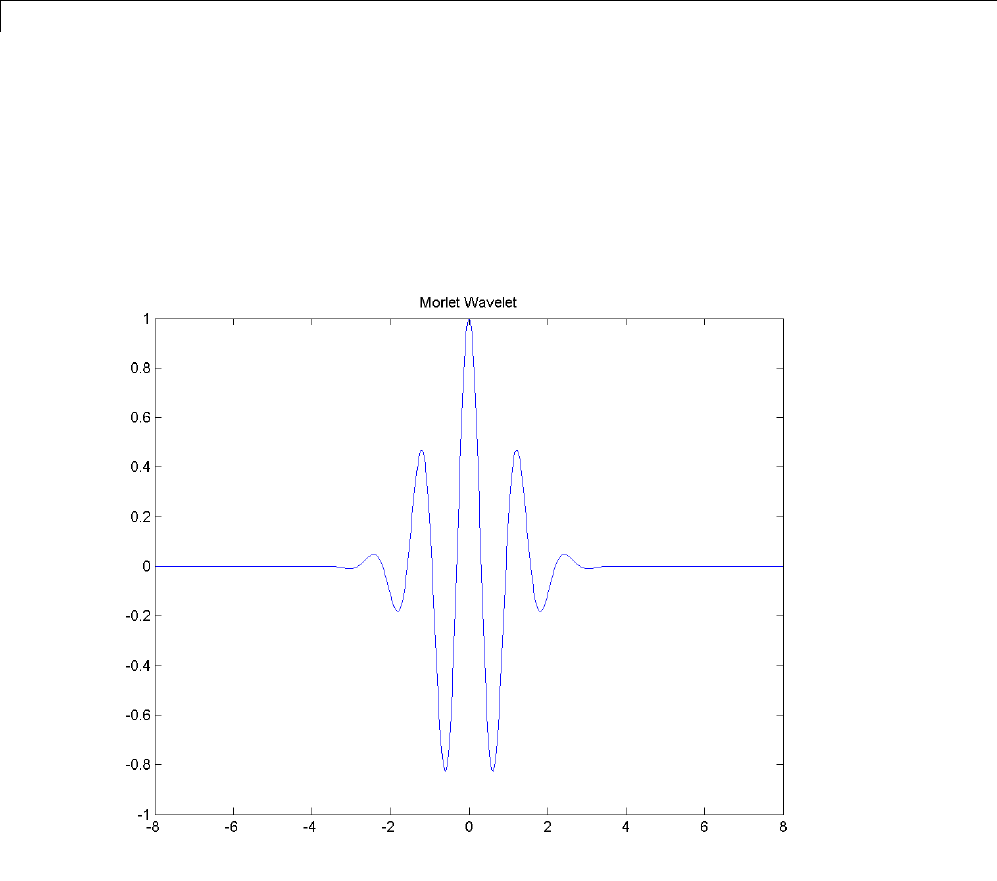
The Morlet wavelet is suitable for continuous analysis. There is no scaling
function associated with the Morlet wavelet. To compute the Morlet wavelet,
you can enter:
[psi,xval] = wavefun('morl',10);
plot(xval,psi); title('Morlet Wavelet');
For wavelets associated with a multiresolution analysis, you can compute
both the scaling function and wavelet. The following code returns the scaling
function and wavelet for the Daubechies’ extremal phase wavelet with 4
vanishing moments.
[phi,psi,xval] = wavefun('db4',10);
subplot(211);
1-4
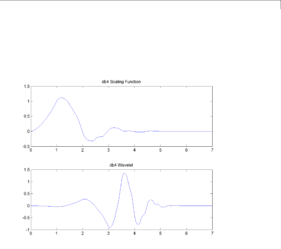
Wavelet Families
plot(xval,phi);
title('db4 Scaling Function');
subplot(212);
plot(xval,psi);
title('db4 Wavelet');
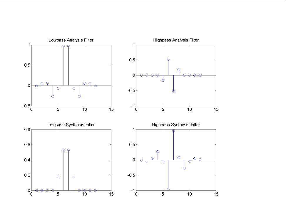
In discrete wavelet analysis, the analysis and synthesis filters are of more
interest than the associated scaling function and wavelet. You can use
wfilters to obtain the analysis and synthesis filters.
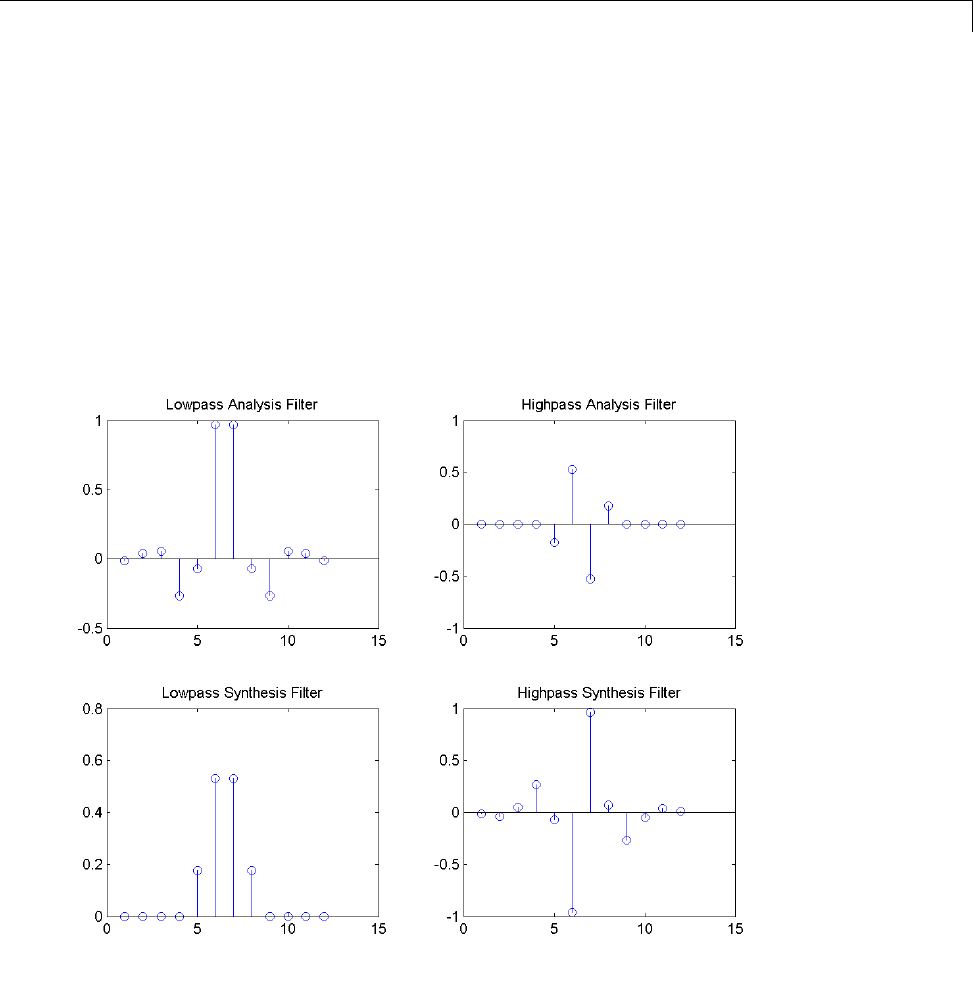
Obtain the decomposition (analysis) and reconstruction (synthesis) filters
for the B-spline biorthogonal wavelet. Specify 3 vanishing moments in the
1-5

1Wavelets, Scaling Functions, and Conjugate Quadrature Mirror Filters
synthesis wavelet and 5 vanishing moments in the analysis wavelet. Plot
the filters’ impulse responses.
[LoD,HiD,LoR,HiR] = wfilters('bior3.5');
subplot(221);
stem(LoD);
title('Lowpass Analysis Filter');
subplot(222);
stem(HiD);
title('Highpass Analysis Filter');
subplot(223);
stem(LoR);
title('Lowpass Synthesis Filter');
subplot(224);
stem(HiR);
title('Highpass Synthesis Filter');
1-6
Wavelet Families
Daubechies Wavelets: dbN
The dbN wavelets are the Daubechies’extremalphasewavelets. Nrefers to
the number of vanishing moments. These filters are also referred to in the
literature by the number of filter taps, which is 2N. More about this family
can be found in [Dau92] page 195. Enter waveinfo('db') at the MATLAB
command prompt to obtain a survey of the main properties of this family.
1-7
1Wavelets, Scaling Functions, and Conjugate Quadrature Mirror Filters
Daubechies Wavelets db4 on the Left and db8 on the Right
The db1 wavelet is also known as the Haar wavelet. The Haar wavelet is the
only orthogonal wavelet with linear phase. Using waveinfo('haar'),youcan
obtain a survey of the main properties of this wavelet.
Symlet Wavelets: symN
The symN wavelets are also known as Daubechies’ least-asymmetric wavelets.
The symlets are more symmetric than the extremal phase wavelets. In symN,
Nis the number of vanishing moments. These filters are also referred to in
the literature by the number of filter taps, which is 2N.Moreaboutsymlets
can be found in [Dau92], pages 198, 254-257. Enter waveinfo('sym') at
the MATLAB command prompt to obtain a survey of the main properties of
this family.
1-8
Wavelet Families
Symlets sym4 on the Left and sym8 on the Right
Coiflet Wavelets: coifN
Coiflet scaling functions also exhibit vanishing moments. In coifN,Nis the
number of vanishing moments for both the wavelet and scaling functions.
Thesefiltersarealsoreferredtointheliterature by the number of filter taps,
which is 2N.. For the coiflet construction, see [Dau92] pages 258–259. Enter
waveinfo('coif') at the MATLAB command prompt to obtain a survey of
the main properties of this family.
Coiflets coif3 on the Left and coif5 on the Right
1-9

1Wavelets, Scaling Functions, and Conjugate Quadrature Mirror Filters
If sis a sufficiently regular continuous time signal, for large jthe coefficient
sjk
,,
φ
−is approximated by 22
2−−jj
sk
/()
.
If sis a polynomial of degree d,d≤N– 1, the approximation becomes an
equality. This property is used, connected with sampling problems, when
calculating the difference between an expansion over the φj,lof a given signal
anditssampledversion.
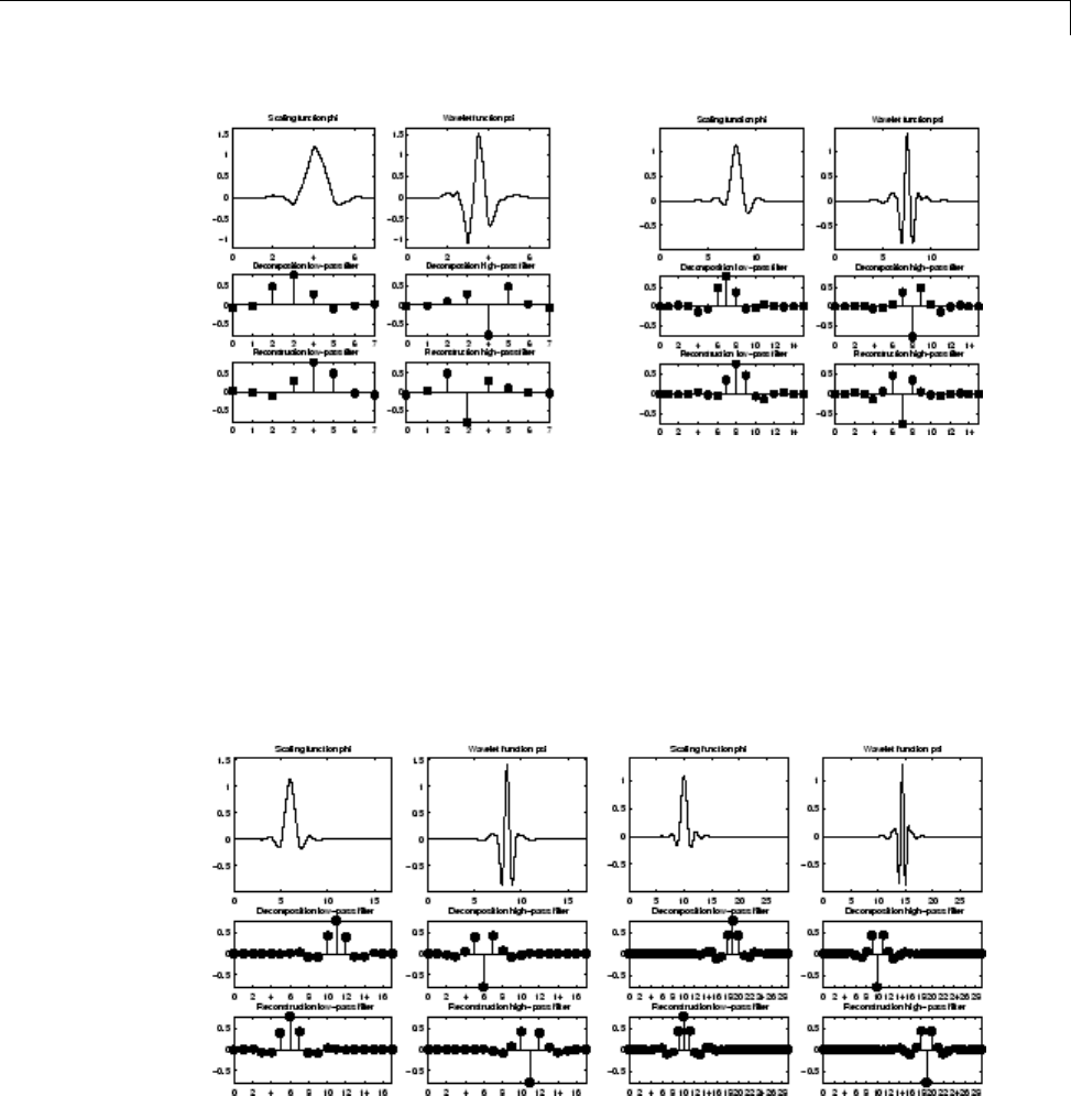
Biorthogonal Wavelet Pairs: biorNr.Nd
While the Haar wavelet is the only orthogonal wavelet with linear phase, you
can design biorthogonal wavelets with linear phase.
Biorthogonal wavelets feature a pair of scaling functions and associated
scaling filters — one for analysis and one for synthesis.
There is also a pair of wavelets and associated wavelet filters — one for
analysis and one for synthesis.
The analysis and synthesis wavelets can have different numbers of vanishing
moments and regularity properties. You can use the wavelet with the
greater number of vanishing moments for analysis resulting in a sparse
representation, while you use the smoother wavelet for reconstruction.
See [Dau92] pages 259, 262–85 and [Coh92] for more details on the
construction of biorthogonal wavelet bases. Enter waveinfo('bior') at the
command line to obtain a survey of the main properties of this family.
The following code returns the B-spline biorthogonal reconstruction and
decomposition filters with 3 and 5 vanishing moments and plots the impulse
responses.
The impulse responses of the lowpass filters are symmetric with respect to the
midpoint. The impulse responses of the highpass filters are antisymmetric
with respect to the midpoint.
[LoD,HiD,LoR,HiR] = wfilters('bior3.5');
subplot(221);
stem(LoD);
1-10
Wavelet Families
title('Lowpass Analysis Filter');
subplot(222);
stem(HiD);
title('Highpass Analysis Filter');
subplot(223);
stem(LoR);
title('Lowpass Synthesis Filter');
subplot(224);
stem(HiR);
title('Highpass Synthesis Filter');
1-11
1Wavelets, Scaling Functions, and Conjugate Quadrature Mirror Filters
Reverse Biorthogonal Wavelet Pairs: rbioNr.Nd
This family is obtained from the biorthogonal wavelet pairs previously
described.
You can obtain a survey of the main properties of this family by typing
waveinfo('rbio') from the MATLAB command line.
Reverse Biorthogonal Wavelet rbio1.5
Meyer Wavelet: meyr
Both ψand φare defined in the frequency domain, starting with an
auxiliary function ν(see [Dau92] pages 117, 119, 137, 152). By typing
waveinfo('meyr') at the MATLAB command prompt, you can obtain a
survey of the main properties of this wavelet.
1-12
Wavelet Families
Meyer Wavelet
The Meyer wavelet and scaling function are defined in the frequency domain:
•Wavelet function
ˆ() ( ) sin
//
ψ
ωπ πνπωπω
ω
=−
⎛
⎝
⎜⎞
⎠
⎟
⎛
⎝
⎜⎞
⎠
⎟≤≤
−
22
3
212
3
4
12 2
eif
i
ππ
ψ
ωπ πνπωπ
ω
3
22
3
414
3
12 2
ˆ() ( ) cos
//
=−
⎛
⎝
⎜⎞
⎠
⎟
⎛
⎝
⎜⎞
⎠
⎟≤
−eif
i
ωω π
≤8
3
and ˆ() ,
ψ
ωω
ππ
=∉
⎡
⎣
⎢⎤
⎦
⎥
02
3
8
3
if
where
ν
() [,]aa a a a a=−+−
()
∈
423
35 84 70 20 0 1
•Scaling function
ˆ() ( )
ˆ() ( )
/
/
φω π ω π
φω π πνπω
=≤
=−
⎛
⎝
⎜
−
−
22
3
22
3
21
12
12
cos
if
⎞⎞
⎠
⎟
⎛
⎝
⎜⎞
⎠
⎟≤≤
=>
if
if
2
3
4
3
04
3
πωπ
φω ω π
ˆ()
1-13

1Wavelets, Scaling Functions, and Conjugate Quadrature Mirror Filters
By changing the auxiliary function, you get a family of different wavelets. For
the required properties of the auxiliary function ν(see“References” for more
information). This wavelet ensures orthogonal analysis.
The function ψdoes not have finite support, but ψdecreases to 0 when ,
faster than any inverse polynomial
∀∈ ∃nC
n
Ν,such that
ψ
()xC x
n
n
≤+
()
−
12
This property holds also for the derivatives
∀∈ ∀∈ ∃kNnNC
kn
,,
,, such that
ψ
() ,()
kkn
xC x n≤+−12
The wavelet is infinitely differentiable.
Note Although the Meyer wavelet is not compactly supported, there exists a
good approximation leading to FIR filters that you can use in the DWT. Enter
waveinfo('dmey') at the MATLAB command prompt to obtain a survey of
the main properties of this pseudo-wavelet.
Gaussian Derivatives Family: gaus
This family is built starting from the Gaussian function fx Ce
px
()=−2by
taking the pth derivative of f.
The integer pis the parameter of this family and in the previous formula, Cp
is such that
fp()
21=where f(p)is the pth derivative of f.
You can obtain a survey of the main properties of this family by typing
waveinfo('gaus') from the MATLAB command line.
1-14
Wavelet Families
Gaussian Derivative Wavelet gaus8
You can use even-order derivative of Gaussian wavelets in the
Fourier-transform based CWT See cwtft for details.
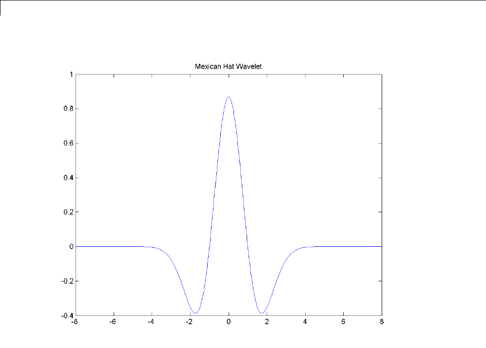
Mexican Hat Wavelet: mexh
This wavelet is proportional to the second derivative function of the Gaussian
probability density function. The wavelet is a special case of a larger family of
derivative of Gaussian (DOG) wavelets.
There is no scaling function associated with this wavelet.
Enter waveinfo('mexh') at the MATLAB command prompt to obtain a
survey of the main properties of this wavelet.
You can compute the wavelet with wavefun.
[psi,xval] = wavefun('mexh',10);
plot(xval,psi);
title('Mexican Hat Wavelet');
1-15
1Wavelets, Scaling Functions, and Conjugate Quadrature Mirror Filters
You can use the Mexican hat wavelet in the Fourier-transform based CWT.
See cwtft for details.
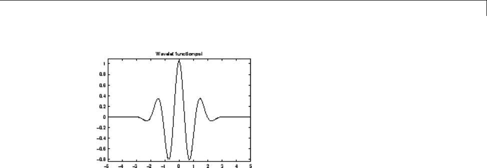
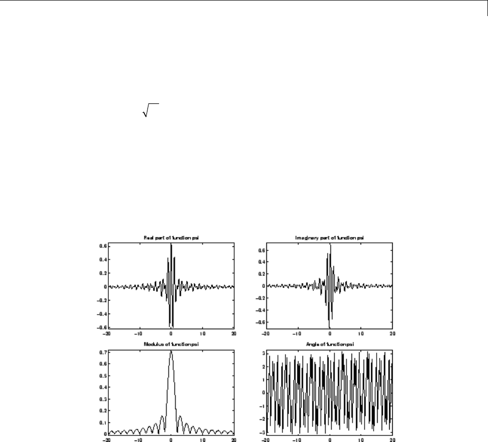
Morlet Wavelet: morl
Both real-valued and complex-valued versions of this wavelet exist. Enter
waveinfo('morl') at the MATLAB command line to obtain the properties of
the real-valued Morlet wavelet.
The real-valued Morlet wavelet is defined as:
ψ
() cos( )xCe x
x
=−25
1-16
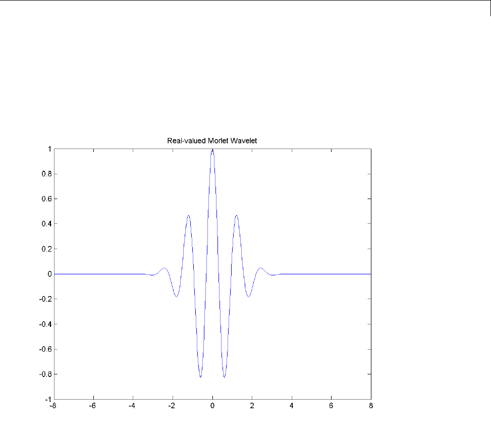
Wavelet Families
The constant Cis used for normalization in view of reconstruction.
[psi,xval] = wavefun('morl',10);
plot(xval,psi);
title('Real-valued Morlet Wavelet');
The Morlet wavelet does not technically satisfy the admissibility condition..
Additional Real Wavelets
Some other real wavelets are available in the toolbox.
1-17
1Wavelets, Scaling Functions, and Conjugate Quadrature Mirror Filters
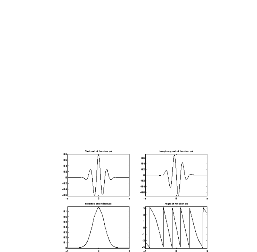
Complex Wavelets
The toolbox also provides a number of complex-valued wavelets for continuous
wavelet analysis. Complex-valued wavelets provide phase information and
are therefore very important in the time-frequency analysis of nonstationary
signals.
Complex Gaussian Wavelets: cgau
This family is built starting from the complex Gaussian function
fx Ce e
pix x
()=−−
2by taking the pth derivative of f.Theintegerpis the
parameter of this family and in the previous formula, Cpis such that
fp()
21=where f(p)is the pth derivative of f.
You can obtain a survey of the main properties of this family by typing
waveinfo('cgau') from the MATLAB command line.
Complex Gaussian Wavelet cgau8
1-18

Wavelet Families
Complex Morlet Wavelets: cmor
See [Teo98] pages 62–65.
A complex Morlet wavelet is defined by
ψ
π
π
()xfee
b
ifx
x
f
c
b
=12
2
depending on two parameters:
•fbis a bandwidth parameter.
•fcis a wavelet center frequency.
You can obtain a survey of the main properties of this family by typing
waveinfo('cmor') from the MATLAB command line.
Complex Morlet Wavelet morl 1.5-1
Complex Frequency B-Spline Wavelets: fbsp
See [Teo98] pages 62–65.
1-19

1Wavelets, Scaling Functions, and Conjugate Quadrature Mirror Filters
A complex frequency B-spline wavelet is defined by
ψ
π
()xf fx
me
bb
m
ifx
c
=⎛
⎝
⎜⎞
⎠
⎟
⎛
⎝
⎜⎞
⎠
⎟
sinc 2
depending on three parameters:
•mis an integer order parameter (m≥1).
•fbis a bandwidth parameter.
•fcis a wavelet center frequency.
You can obtain a survey of the main properties of this family by typing
waveinfo('fbsp') from the MATLAB command line.
Complex Frequency B-Spline Wavelet fbsp 2-0.5-1
Complex Shannon Wavelets: shan
See [Teo98] pages 62–65.
1-20
Wavelet Families
This family is obtained from the frequency B-spline wavelets by setting mto 1.
A complex Shannon wavelet is defined by
ψ
π
()xf fxe
bb
ifx
c
=
()
sinc 2
depending on two parameters:
•fbis a bandwidth parameter.
•fcis a wavelet center frequency.
You can obtain a survey of the main properties of this family by typing
waveinfo('shan') from the MATLAB command line.
Complex Shannon Wavelet shan 0.5-1
1-21

1Wavelets, Scaling Functions, and Conjugate Quadrature Mirror Filters
Wavelet Families and Associated Properties — I
Property morl mexh meyr haar dbNsymNcoifNbiorNr.Nd
Crude ■■
Infinitely regular ■■■
Arbitrary regularity ■■■■
Compactly supported
orthogonal
■■■■
Compactly supported
biothogonal
■
Symmetry ■■■■ ■
Asymmetry ■
Near symmetry ■■
Arbitrary number of
vanishing moments
■■■■
Vanishing moments
for φ
■
Existence of φ■■■■■■
Orthogonal analysis ■■■■■
Biorthogonal analysis ■■■■■■
Exact reconstruction ≈■■■■■■■
FIR filters ■■■■■
Continuous transform ■■■■■■■■
Discrete transform ■■■■■
Fast algorithm ■■■■■
Explicit expression ■■ ■ For splines
Crude wavelet — A wavelet is said to be crude when satisfying only the
admissibility condition.
Regularity
1-22

Wavelet Families
Orthogonal
Biorthogonal — See “Biorthogonal Wavelet Pairs: biorNr.Nd” on page 1-10.
Vanishing moments
Exact reconstruction — See “Reconstruction Filters” in the Wavelet Toolbox
Getting Started Guide.
Continuous — See “Continuous Wavelet Transform” in the Wavelet Toolbox
Getting Started Guide.
Discrete — See “Critically-Sampled Discrete Wavelet Transform” in the
Wavelet Toolbox Getting Started Guide.
FIR filters — See “Filters Used to Calculate the DWT and IDWT” on page
3-37.
Wavelet Families and Associated Properties — II
Property rbioNr.Nd gaus dmey cgau cmor fbsp shan
Crude ■■■■■
Infinitely regular ■■■■■
Arbitrary regularity ■
Compactly supported
orthogonal
Compactly supported
biothogonal
■
Symmetry ■ ■ ■■■■■
Asymmetry
Near symmetry
Arbitrary number of
vanishing moments
■
1-23

1Wavelets, Scaling Functions, and Conjugate Quadrature Mirror Filters
Property rbioNr.Nd gaus dmey cgau cmor fbsp shan
Vanishing moments for
φ
Existence of φ■
Orthogonal analysis
Biorthogonal analysis ■
Exact reconstruction ■■≈■■■■
FIR filters ■■
Continuous transform ■■
Discrete transform ■■
Fast algorithm ■■
Explicit expression For splines ■■■■■
Complex valued ■■■■
Complex continuous
transform
■■■■
FIR-based
approximation
■
Crude wavelet
Regularity
Orthogonal
Biorthogonal — See “Biorthogonal Wavelet Pairs: biorNr.Nd” on page 1-10.
Vanishing moments
Exact reconstruction — See “Reconstruction Filters” in the Wavelet Toolbox
Getting Started Guide.
Continuous — See “Continuous Wavelet Transform” in the Wavelet Toolbox
Getting Started Guide.
1-24


1Wavelets, Scaling Functions, and Conjugate Quadrature Mirror Filters
Adding Your Own Wavelets
This section shows you how to add your own wavelet families to the toolbox.
In this section...
“Preparing to Add a New Wavelet Family” on page 1-26
“Adding a New Wavelet Family” on page 1-32
“After Adding a New Wavelet Family” on page 1-40
Preparing to Add a New Wavelet Family
Wavelet Toolbox software contains a large number of the most commonly-used
wavelet families. Additionally, using wavemngr, you can add new wavelets to
the existing ones to implement your favorite wavelet or try out one of your
own design. The toolbox allows you to define new wavelets for use with both
the command line functions and the graphical interface tools.
Caution The toolbox does not check that your wavelet meets all the
mathematical requisites to constitute a valid wavelet.
wavemngr affords extensive wavelet management. However, this section
focuses only on the addition of a wavelet family. For more complete
information, see the wavemngr reference page.
To add a new wavelet, you must
1Choose the full name of the wavelet family (fn).
2Choose the short name of the wavelet family (fsn).
3Determine the wavelet type (wt).
4Define the orders of wavelets within the given family (nums).
5Build a MAT-file or a MATLAB file (file).
6For wavelets without FIR filters:Definetheeffectivesupport.
1-26

Adding Your Own Wavelets
These steps are described below.
Choose the Wavelet Family Full Name
The full name of the wavelet family, fn, must be a string. Do not use
predefined wavelet family names. Toseethepredefinedwaveletfamily
names, enter:
wavemngr('read')
The predefined wavelet family names are the displayed in the first column
of the output. Predefined wavelet family names are Haar,Daubechies,
Symlets,Coiflets,BiorSplines,ReverseBior,Meyer,DMeyer,Gaussian,
Mexican_hat,Morlet,Complex Gaussian,Shannon,Frequency B-Spline,
and Complex Morlet.
Choose the Wavelet Family Short Name
Theshortnameofthewaveletfamily,fsn, must be a string of four characters
or less. Do not use predefined wavelet family short names. To see the
predefined wavelet family short names, enter:
wavemngr('read')
The predefined wavelet family short names are the displayed in the second
column of the output..
Determine the Wavelet Type
We distinguish five types of wavelets:
1Orthogonal wavelets with FIR filters
These wavelets can be defined through the scaling filter h.Thescaling
filter is a lowpass filter. For orthogonal wavelets, the same scaling filter
is used for decomposition (analysis) and reconstruction (synthesis).
Predefined families of such wavelets include Haar,Daubechies,Coiflets,
and Symlets.
2Biorthogonal wavelets with FIR filters
1-27

1Wavelets, Scaling Functions, and Conjugate Quadrature Mirror Filters
These wavelets can be defined through the two scaling filters hr and hd,for
reconstruction and decomposition respectively. The BiorSplines wavelet
family is a predefined family of this type.
3Orthogonal wavelets without FIR filters, but with a scaling function
These wavelets can be defined through the definition of the wavelet
function and the scaling function. The Meyer wavelet family is a predefined
family of this type.
4Wavelets without FIR filters and without a scaling function
These wavelets can be defined through the definition of the wavelet
function. Predefined families of such wavelets include Morlet and
Mexican_hat.
5Complex wavelets without FIR filters and without a scaling function
These wavelets can be defined through the definition of the wavelet
function. Predefined families of such wavelets include Complex Gaussian
and Shannon.
Define the Orders of Wavelets Within the Given Family
If a family contains many wavelets, the short name and the order are
appended to form the wavelet name. Argument nums is a string containing the
orders separated with blanks. This argument is not used for wavelet families
that only have a single wavelet (Haar,Meyer,andMorlet for example).
For example, for the first extremal-phase Daubechies wavelets,
fsn = 'db'
nums = '1 2 3'
yields the three wavelets db1,db2,anddb3.
For the first B-spline biorthogonal wavelets,
fsn = 'bior'
nums = '1.1 1.3 1.5 2.2'
yields the four wavelets bior1.1,bior1.3,bior1.5,andbior2.2.
1-28

Adding Your Own Wavelets
You can display this information for the predefined wavelets with
wavemngr('read',1)
Build a MAT-File or Code File
wavemngr requires a file argument, which is a string containing a MATLAB
function or MAT file name.
If a family contains many wavelets,aMATLABcodefile(witha.m extension)
must be defined and must be of a specific form that depends on the wavelet
type. The specific file formats are described in the remainder of this section.
If a family contains a single wavelet, then a MAT-file can be defined for
wavelets of type 1. It must have the wavelet family short name (fsn)argument
as its name and must contain a single variable whose name is fsn and whose
value is the scaling filter. An code file can also be defined as discussed below.
Note If no file extension is specified, a .m extension is used as default.
Type 1 (Orthogonal with FIR Filter). The syntax of the first line in the
MATLAB function is
function w = file(wname)
where the input argument wname is a string containing the wavelet name, and
the output argument wis the corresponding scaling filter.
The filter wmust be of even length. If the scaling filter is not of even length,
the filter is zero-padded by the toolbox.
For predefined wavelets, the sum of the scaling filter coefficients is 1. This
follows the convention followed by Daubechies.
mhe
njn
0
1
2
()
1-29

1Wavelets, Scaling Functions, and Conjugate Quadrature Mirror Filters
When you access these coefficients using wfilters, the coefficients are scaled
by the square root of 2.
The toolbox normalizes your filter so that the resulting sum is 1.
Examples of such files for predefined wavelets are dbwavf.m for Daubechies,
coifwavf.m for coiflets, and symwavf.m for symlets.
Type 2 (Biorthogonal with FIR Filter). Thesyntaxofthefirstlineinthe
MATLAB function is
function [wr,wd] = file(wname)
where the input argument wname is a string containing the wavelet name and
the output arguments wr and wd are the corresponding reconstruction and
decomposition scaling filters, respectively.
The filters wr and wd must be of the same even length. In general, initial
biorthogonal filters do not meet these requirements, so they are zero-padded
by the toolbox.
For predefined wavelets, the sum of the scaling filter coefficients is 1. This
follows the convention followed by Daubechies.
mhe
njn
0
1
2
()
When you access these coefficients using wfilters, the coefficients are scaled
by the square root of 2.
The toolbox normalizes your filter so that the resulting sum is 1.
The file biorwavf.m (for BiorSplines) is an example of a file for a type 2
predefined wavelet family.
Type 3 (Orthogonal with Scale Function). The syntax of the first line
in the MATLAB function is
function [phi,psi,t] = file(lb,ub,n,wname)
1-30

Adding Your Own Wavelets
which returns values of the scaling function phi and the wavelet function psi
on t, a linearly-spaced n-point grid of the interval [lb ub].
The argument wname is optional (see Note below).
The file meyer.m is an example of a file for a type 3 predefined wavelet family.
Type4orType5(NoFIRFilter;NoScaleFunction). The syntax of the
first line in the MATLAB function is
function [psi,t] = file(lb,ub,n,wname)
or
function [psi,t] = file(lb,ub,n,wname, additional arguments)
which returns values of the wavelet function psi onta linearly-spaced n-point
grid of the interval [lb ub].
The argument wname is optional (see Note below).
Examples of type 4 files for predefined wavelet families are mexihat.m (for
Mexican_hat)andmorlet.m (for Morlet).
Examples of type 5 files for predefined wavelet families are shanwavf.m (for
Shannon)andcmorwavf.m (for Complex Morlet).
Note Forthetypes3,4,and5,thewname argument is optional unless the new
wavelet family contains more than one wavelet and if you plan to use this new
family in the GUI mode. For the types 4 and 5, a complete example of using
the additional arguments can be found on the fbspwavf reference page.
Define the Effective Support
This definition is required only for wavelets of types 3, 4, and 5, since they
are not compactly supported.
1-31

1Wavelets, Scaling Functions, and Conjugate Quadrature Mirror Filters
Defining the effective support means specifying an upper and lower bound.
The following table includes the lower and upper bounds for a few of the
toolbox wavelets.
Family Lower Bound (lb) Upper Bound (ub)
Meyer –8 8
Mexican_hat –5 5
Morlet –4 4
Adding a New Wavelet Family
To add a new wavelet, usewavemngr in one of two forms:
wavemngr('add',fn,fsn,wt,nums,file)
or
wavemngr('add',fn,fsn,wt,nums,file,b).
Here are a few examples to illustrate how you would use wavemngr to add
some of the predefined wavelet families. New wavelet family names and short
names are used for illustration purposes.
Type 1 wavelet — Add wavelets ndb1,ndb2,ndb3,ndb4,ndb5.
wavemngr('add','Ndaubechies','ndb',1,'1 2 3 4 5','dbwavf');
Type 1 wavelet — Add wavelets ndaub1,ndaub2,....dbwavf calls dbaux
to compute the Daubechies extremal phase wavelets with more than 10
vanishing moments. The computation in dbaux becomes unstable when the
number of vanishing moments becomes large. Therefore dbaux errors when
you specify the number of vanishing moments greater than 45.
wavemngr('add','Ndaubwav','ndaub',1,'1 2 3 4 5 **','dbwavf');
Type 2 wavelet — Add wavelets nbio1.1, nbio1.3.
wavemngr('add','Nbiorwavf','nbio',2,'1.1 1.3','biorwavf');
Type 3 wavelet — Add the wavelet Nmeyer with effective support [-8,8].
1-32

Adding Your Own Wavelets
wavemngr('add','Nmeyer','nmey',3,'','meyer',[-8,8]);
Type 4 wavelet — Add the wavelet Nmorlet with effective support [-4,4].
wavemngr('add','Nmorlet','nmor',4,'','morlet',[-4,4]);
You can delete the wavelets you have created with
wavemngr('del',familyShortName). For example:
wavemngr('del','nmey');
Example 1
Let us take the example of Binlets proposed by Strang and Nguyen in pages
216-217 of the book Wavelets and Filter Banks (see [StrN96] in “References”).
Note The files used in this example can be found in the wavedemo folder.
ThefullfamilynameisBinlets.
Theshortnameofthewaveletfamilyisbinl.
The wavelet type is 2(Biorthogonal with FIR filters).
The order of the wavelet within the family is 7.9 (wejustuseoneinthis
example).
Thefileusedtogeneratethefiltersisbinlwavf.m
Then to add the new wavelet, type
% Add new family of biorthogonal wavelets.
wavemngr('add','Binlets','binl',2,'7.9','binlwavf')
% List wavelets families.
wavemngr('read')
ans =
1-33

1Wavelets, Scaling Functions, and Conjugate Quadrature Mirror Filters
===================================
Haar haar
Daubechies db
Symlets sym
Coiflets coif
BiorSplines bior
ReverseBior rbio
Meyer meyr
DMeyer dmey
Gaussian gaus
Mexican_hat mexh
Morlet morl
Complex Gaussian cgau
Shannon shan
Frequency B-Spline fbsp
Complex Morlet cmor
Binlets binl
===================================
Ifyouwanttogetonlineinformationonthisnewfamily,youcanbuildan
associated help file which would look like the following:
function binlinfo
%BINLINFO Information on biorthogonal wavelets (binlets).
%
% Biorthogonal Wavelets (Binlets)
%
% Family Binlets
% Short name binl
% Order Nr,Nd Nr = 7 , Nd = 9
%
% Orthogonal no
% Biorthogonal yes
% Compact support yes
% DWT possible
% CWT possible
%
% binl Nr.Nd ld lr
% effective length effective length
% of LoF_D of HiF_D
1-34

Adding Your Own Wavelets
% binl 7.9 7 9
The associated file to generate the filters (binlwavf.m)is
function [Rf,Df] = binlwavf(wname)
%BINLWAVF Biorthogonal wavelet filters (Binlets).
% [RF,DF] = BINLWAVF(W) returns two scaling filters
% associated with the biorthogonal wavelet specified
% by the string W.
% W = 'binlNr.Nd' where possible values for Nr and Nd are:
Nr = 7 Nd = 9
% The output arguments are filters:
% RF is the reconstruction filter
% DF is the decomposition filter
% Check arguments.
if errargn('binlwavf',nargin,[0 1],nargout,[0:2]), error('*');
end
% suppress the following line for extension
Nr=7;Nd=9;
% for possible extension
% more wavelets in 'Binlets' family
%----------------------------------
if nargin==0
Nr=7;Nd=9;
elseif isempty(wname)
Nr=7;Nd=9;
else
if ischar(wname)
lw = length(wname);
ab = abs(wname);
ind = find(ab==46 | 47<ab | ab<58);
li = length(ind);
err=0;
if li==0
err = 1;
elseif ind(1)~=ind(li)-li+1
err = 1;
end
1-35

1Wavelets, Scaling Functions, and Conjugate Quadrature Mirror Filters
if err==0 ,
wname = str2num(wname(ind));
if isempty(wname) , err = 1; end
end
end
if err==0
Nr = fix(wname); Nd = 10*(wname-Nr);
else
Nr=0;Nd=0;
end
end
% suppress the following lines for extension
% and add a test for errors.
%-------------------------------------------
if Nr~=7 , Nr = 7; end
if Nd~=9 , Nd = 9; end
if Nr == 7
if Nd == 9
Rf = [-1 0 9 16 9 0 -1]/32;
Df = [ 1 0 -8 16 46 16 -8 0 1]/64;
end
end
Example 2
In the following example, new compactly supported orthogonal wavelets are
added to the toolbox. These wavelets, which are a slight generalization of the
Daubechies wavelets, are based on the use of Bernstein polynomials and are
due to Kateb and Lemarié in an unpublished work.
Note The files used in this example can be found in the wavedemo folder.
% List initial wavelets families.
wavemngr('read')
ans =
1-36

Adding Your Own Wavelets
===================================
Haar haar
Daubechies db
Symlets sym
Coiflets coif
BiorSplines bior
ReverseBior rbio
Meyer meyr
DMeyer dmey
Gaussian gaus
Mexican_hat mexh
Morlet morl
Complex Gaussian cgau
Shannon shan
Frequency B-Spline fbsp
Complex Morlet cmor
===================================
% List all wavelets.
wavemngr('read',1)
ans =
===================================
Haar haar
===================================
Daubechies db
------------------------------
db1 db2 db3 db4
db5 db6 db7 db8
db9 db10 db**
===================================
Symlets sym
------------------------------
sym2 sym3 sym4 sym5
sym6 sym7 sym8 sym**
===================================
Coiflets coif
------------------------------
coif1 coif2 coif3 coif4
coif5
1-37

1Wavelets, Scaling Functions, and Conjugate Quadrature Mirror Filters
===================================
BiorSplines bior
------------------------------
bior1.1 bior1.3 bior1.5 bior2.2
bior2.4 bior2.6 bior2.8 bior3.1
bior3.3 bior3.5 bior3.7 bior3.9
bior4.4 bior5.5 bior6.8
===================================
ReverseBior rbio
------------------------------
rbio1.1 rbio1.3 rbio1.5 rbio2.2
rbio2.4 rbio2.6 rbio2.8 rbio3.1
rbio3.3 rbio3.5 rbio3.7 rbio3.9
rbio4.4 rbio5.5 rbio6.8
===================================
Meyer meyr
===================================
DMeyer dmey
===================================
Gaussian gaus
------------------------------
gaus1 gaus2 gaus3 gaus4
gaus5 gaus6 gaus7 gaus8
gaus**
===================================
Mexican_hat mexh
===================================
Morlet morl
===================================
Complex Gaussian cgau
------------------------------
cgau1 cgau2 cgau3 cgau4
cgau5 cgau**
===================================
Shannon shan
------------------------------
shan1-1.5 shan1-1 shan1-0.5 shan1-0.1
shan2-3 shan**
===================================
Frequency B-Spline fbsp
1-38

Adding Your Own Wavelets
------------------------------
fbsp1-1-1.5 fbsp1-1-1 fbsp1-1-0.5 fbsp2-1-1
fbsp2-1-0.5 fbsp2-1-0.1 fbsp**
===================================
Complex Morlet cmor
------------------------------
cmor1-1.5 cmor1-1 cmor1-0.5 cmor1-1
cmor1-0.5 cmor1-0.1 cmor**
===================================
% Add new family of orthogonal wavelets.
% You must define:
%
% Family Name: Lemarie
% Family Short Name: lem
% Type of wavelet: 1 (orth)
% Wavelets numbers: 1 2 3 4 5
% File driver: lemwavf
%
% The function lemwavf.m must be as follow:
% function w = lemwavf(wname)
% where the input argument wname is a string:
% wname = 'lem1' or 'lem2' ... i.e.,
% wname = sh.name + number
% and w the corresponding scaling filter.
% The addition is obtained using:
wavemngr('add','Lemarie','lem',1,'1 2 3 4 5','lemwavf');
% The ascii file 'wavelets.asc' is saved as
% 'wavelets.prv', then it is modified and
% the MAT file 'wavelets.inf' is generated.
% List wavelets families.
wavemngr('read')
ans =
===================================
Haar haar
Daubechies db
Symlets sym
Coiflets coif
1-39

1Wavelets, Scaling Functions, and Conjugate Quadrature Mirror Filters
BiorSplines bior
ReverseBior rbio
Meyer meyr
DMeyer dmey
Gaussian gaus
Mexican_hat mexh
Morlet morl
Complex Gaussian cgau
Shannon shan
Frequency B-Spline fbsp
Complex Morlet cmor
Lemarie lem
===================================
After Adding a New Wavelet Family
When you use the wavemngr command to add a new wavelet, the toolbox
creates three wavelet extension files in the current folder: the two ASCII files
wavelets.asc and wavelets.prv,andtheMAT-filewavelets.inf.
If you want to use your own extended wavelet families with the Wavelet
Toolbox software, you should
1Create a new folder specifically to hold the wavelet extension files.
2Move the previously mentioned files into this new folder.
3Prepend this folder to the MATLAB folder search path (see the reference
entry for the path command).
4Use this same folder for subsequent modifications. Allowing many wavelet
extension files to proliferate in different folders may lead to unpredictable
results.
5Define a file called <fsn>info.m (for example, see dbinfo.m or morlinfo.m).
This file will be associated automatically with the Wavelet Family button
in the Wavelet Display option of the graphical tools.
1-40

Lifting Method for Constructing Wavelets
Lifting Method for Constructing Wavelets
The so-called first generation wavelets and scaling functions are dyadic
dilations and translates of a single function. Fourier methods play a key role
in the design of these wavelets. However, the requirement that the wavelet
basis consist of translates and dilates of a single function imposes some
constraints that limit the utility of the multiresolution idea at the core of
wavelet analysis.
The utility of wavelet methods is extended by the design of second generation
wavelets via lifting.
Typical settings where translation and dilation of a single function cannot
be used include:
•Designing wavelets on bounded domains — This includes the construction
of wavelets on an interval, or bounded domain in a higher-dimensional
Euclidean space.
•Weighted wavelets — In certain applications, such as the solution of partial
differential equations, wavelets biorthogonal with respect to a weighted
inner product are needed.
•Irregularly-spaced data — In many real-world applications, the sampling
interval between data samples is not equal.
Designing new first generation wavelets requires expertise in Fourier analysis.
The lifting method proposed by Sweldens (see [Swe98] in “References”)
removes the necessity of expertise in Fourier analysis and allows you to
generate an infinite number of discrete biorthogonal wavelets starting from an
initial one. In addition to generation of first generation wavelets with lifting,
the lifting method also enables you to design second generation wavelets,
which cannot be designed using Fourier-based methods. With lifting, you can
design wavelets that address the shortcomings of the first generation wavelets.
The following section introduces the theory behind lifting, presents the lifting
functions of Wavelet Toolbox software and gives two short examples:
•“Lifting Background” on page 1-42
•“Lifting Functions” on page 1-49
1-41
1Wavelets, Scaling Functions, and Conjugate Quadrature Mirror Filters
For more information on lifting, see [Swe98], [Mal98], [StrN96], and
[MisMOP03] in “References”.
Lifting Background
The DWT implemented by a filter bank is defined by four filters as described
in “Fast Wavelet Transform (FWT) Algorithm” on page 3-37. Two main
properties of interest are
•The perfect reconstruction property
•The link with “true” wavelets (how to generate, starting from the filters,
orthogonal or biorthogonal bases of the space of the functions of finite
energy)
To illustrate the perfect reconstruction property, the following filter
bank contains two decomposition filters and two synthesis filters. The
decomposition and synthesis filters may constitute a pair of biorthogonal
bases or an orthogonal basis. The capital letters denote the Z-transforms
of the filters..
X
H
X
G
H
G
~
~
This leads to the following two conditions for a perfect reconstruction (PR)
filter bank:
HzHz GzGz zL
~~
() () () ()
21
and
HzHz GzGz
~~
()() ()()0
1-42

Lifting Method for Constructing Wavelets
The first condition is usually (incorrectly) called the perfect reconstruction
condition and the second is the anti-aliasing condition.
The z–L+1 term implies that perfect reconstruction is achieved up to a delay of
onesamplelessthanthefilterlength,L. This results if the analysis filters are
shiftedtobecausal.
Lifting designs perfect reconstruction filter banks by beginning from the
basic nature of the wavelet transform. Wavelet transforms build sparse
representations by exploiting the correlation inherent in most real world data.
For example, plot the example of electricity consumption over a 3-day period.
load leleccum;
plot(leleccum)
grid on; axis tight;
1-43
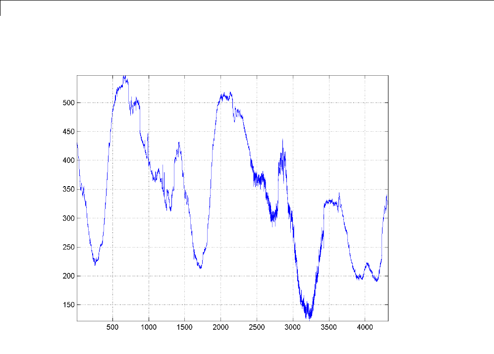
1Wavelets, Scaling Functions, and Conjugate Quadrature Mirror Filters
The data do not exhibit arbitrary changes from sample to sample. Neighboring
samples exhibit correlation. A relatively low (high) value at index (sample)
nis associated with a relatively low (high) value at index n-1 and n+1.This
implies that if you have only the odd or even samples from the data, you can
predict the even or odd samples. How accurate your prediction is obviously
depends on the nature of the correlation between adjacent samples and how
closely your predictor approximates that correlation.
Polyphase Representation
The polyphase representation of a signal is an important concept in lifting.
You can view each signal as consisting of phases, which consist of taking
every N-th sample beginning with some index. For example, if you index a
time series from n=0 and take every other sample starting at n=0, you extract
1-44

Lifting Method for Constructing Wavelets
the even samples. If you take every other sample starting from n=1, you
extract the odd samples. These are the even and odd polyphase components
of the data. Because your increment between samples is 2, there are only
two phases. If you increased your increment to 4, you can extract 4 phases.
For lifting, it is sufficient to concentrate on the even and odd polyphase
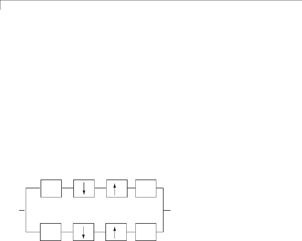
components. The following diagram illustrates this operation for an input
signal.
X
Z
2
2
Xe
Xo
where Zdenotes the unit advance operator and the downward arrow with
the number 2 represents downsampling by two. In the language of lifting,
the operation of separating an input signal into even and odd components is
known as the split operation, or the lazy wavelet.
To understand lifting mathematically, it is necessary to understand the
z-domain representation of the even and odd polyphase components.
The z-transform of the even polyphase component is
Xz xnz
n
n
02() ( )
The z-transform of the odd polyphase component is
Xz xn z
n
n
121() ( )
You can write the z-transform of the input signal as the sum of dilated
versions of the z-transforms of the polyphase components.
Xz x nz x n z X z z X z
n
n
n
n
() () ( ) () ()
221
221
021
12
1-45
1Wavelets, Scaling Functions, and Conjugate Quadrature Mirror Filters
Split, Predict, and Update
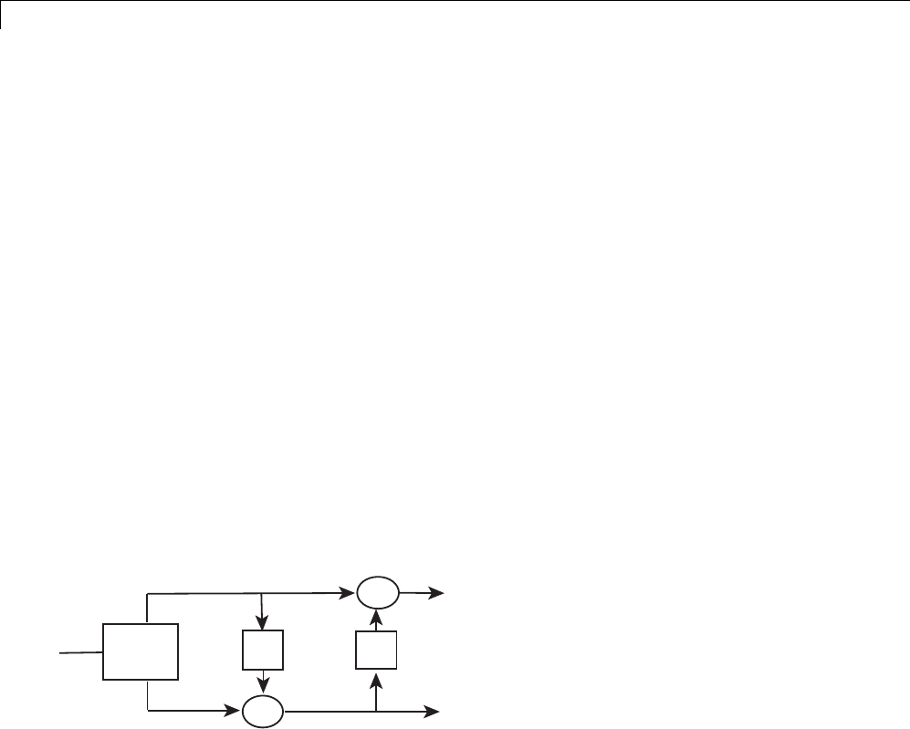
Asingleliftingstep can be described by the following three basic operations:
•Split —thesign
al into disjoint components. A common way to do this is to
extract the even and odd polyphase components explained in “Polyphase
Representation” on page 1-44. This is also known as the lazy wavelet.
•Predict —theo
dd polyphase component based on a linear combination
of samples of the even polyphase component. The samples of the odd
polyphase component are replaced by the difference between the odd
polyphase component and the predicted value. The predict operation is also
referred to as the dual lifting step.
•Update —theeven polyphase component based on a linear combination of
difference samples obtained from the predictstep.Theupdatestepisalso
referred toastheprimal lifting step.
In practice, a normalization is incorporated for both the primal and dual
liftings.
The following diagram illustrates one lifting step.
XSplit P
-
+
U
Xe
Xo
A
D
Haar Wavelet Via Lifting
Using the operations defined in “Split, Predict, and Update” on page 1-46, you
can implement the Haar wavelet via lifting.
•Split — Divide the signal into even and odd polyphase components.
•Predict —Replacex(2n+1) with d(n)=x(2n+1)–x(2n). The predict operator
is simply x(2n).
1-46

Lifting Method for Constructing Wavelets
•Update —Replacex(2n) with x(2n)+d(n)/2. Thisisequalto
(x(2n)+x(2n+1))/2.
Thedualliftinginthezdomaincanbewritteninthefollowingmatrixform
10
1
0
1
Pz
Xz
Xz
()
()
()
with P(z)=1.
Theprimalliftingcanbewritteninthezdomaininthefollowingmatrixform
1
01
10
1
0
1
Sz
Pz
Xz
Xz
()
()
()
()
with S(z)=1/2.
Finally, the primal and dual normalization can be incorporated as follows.
20
01
2
1
01
10
1
0
1
Sz
Pz
Xz
Xz
()
()
()
()
To construct this lifting step in MATLAB, enter:
LiftHaar = liftwave('haar');
displs(LiftHaar)
The following is displayed in the MATLAB command window.
LiftHaar = {...
'd' [ -1.00000000] [0]
'p' [ 0.50000000] [0]
[ 1.41421356] [ 0.70710678] []
};
'd' denotes the dual lifting. Note that for convenience, the negative sign is
incorporated into the dual lifting step in the Wavelet Toolbox software. 'p'
denotes the primal lifting and [ 1.41421356] [ 0.70710678] are the primal
and dual normalization constants. LiftHaar{1,3} and LiftHaar{2,3} give
1-47

1Wavelets, Scaling Functions, and Conjugate Quadrature Mirror Filters
the highest degree of the Laurent polynomials, which describe the dual and
primal liftings. In this case, both are zero because the dual and primal liftings
are both described by scalars.
Bior2.2 Wavelet Via Lifting
This examples presents the lifting scheme for the bior2.2 biorthogonal
scaling and wavelet filters.
In the Haar lifting scheme, the dual lifting (predict operator) differenced the
odd and even samples. In this example, define a new predict operator that
computes the average of the two neighboring even samples. Subtract the
average from the intervening odd sample.
dn xn xn xn() ( ) [( ) ( )] 21
1
2222
In the z-domain you can write the dual lifting step as
10
1
211
0
1
()
()
()
z
Xz
Xz
To obtain the primal lifting, or update, examine the primal lifting in “Haar
Wavelet Via Lifting” on page 1-46. The update is defined in such a way that
the sum of the approximation coefficients is proportional to the mean of the
input data vector.
xn an
nn
() ()
1
2
To obtain the same result in this lifting step, define the update as
11
41
01
10
1
211
10
1
()
()
()
()
z
z
Xz
Xz
1-48

Lifting Method for Constructing Wavelets
To obtain this lifting scheme at the command line, enter:
liftwave('bior2.2')
Lifting Functions
The lifting functions of the toolbox are organized into five groups:
•“Lifting Schemes ” on page 1-49
•“Biorthogonal Quadruplets of Filters and Lifting Schemes” on page 1-49
•“Usual Biorthogonal Quadruplets” on page 1-50
•“Lifting Wavelet Transform (LWT)” on page 1-50
•“Laurent Polynomials and Matrices” on page 1-51
Lifting Schemes
Function Name Description
lsinfo Information about lifting schemes
displs Display a lifting scheme
addlift Add primal or dual elementary lifting steps to a
lifting scheme
wavenames Wavelets with lifting schemes
Biorthogonal Quadruplets of Filters and Lifting Schemes
These functions connect lifting schemes to biorthogonal quadruplets of filters
and associated scaling and wavelet function pairs.
Function Name Description
liftfilt Apply elementary lifting steps on quadruplet of
filters
filt2ls Transform a quadruplet of filters to a lifting
scheme
1-49

1Wavelets, Scaling Functions, and Conjugate Quadrature Mirror Filters
Function Name Description
ls2filt Transform a lifting scheme to a quadruplet of
filters
bswfun Compute and plot biorthogonal “scaling and
wavelet” functions
Usual Biorthogonal Quadruplets
These functions provide some basic lifting schemes associated with some
usual orthogonal or biorthogonal (“true”) wavelets and the “lazy” one. These
schemes can be used to initialize a lifting procedure.
Function Name Description
wavenames Provides usual wavelet names available for LWT
liftwave Provides lifting scheme associated with a usual
wavelet
wave2lp Provides Laurent polynomials associated with a
usual wavelet
Lifting Wavelet Transform (LWT)
These functions contain the direct and inverse lifting wavelet transform
(LWT) files for both 1-D and 2-D signals. LWT reduces to the polyphase
version of the DWT algorithm with zero-padding extension mode and without
extra-coefficients.
Function Name Description
lwt 1-D lifting wavelet transform
ilwt Inverse 1-D lifting wavelet transform
lwtcoef Extract or reconstruct 1-D LWT wavelet
coefficients
lwt2 2-D lifting wavelet transform
1-50

Lifting Method for Constructing Wavelets
Function Name Description
ilwt2 Inverse 2-D lifting wavelet transform
lwtcoef2 Extract or reconstruct 2-D LWT wavelet
coefficients
Laurent Polynomials and Matrices
These functions permit an entry to representation and calculus of Laurent
polynomials and matrices.
Function Name Description
laurpoly Constructor for the class of Laurent polynomials
laurmat Constructor for the class of Laurent matrices
The lifting folder and the two object folders @laurpoly and @laurmat contain
many other files.
Primal Lifting from Haar
These two simple examples illustrate the basic lifting capabilities of Wavelet
Toolbox software.
A primal lifting starting from Haar wavelet.
Start from the Haar wavelet and get the corresponding lifting scheme.
lshaar = liftwave('haar');
displs(lshaar);
Add a primal ELS to the lifting scheme.
els = {'p',[-0.125 0.125],0};
lsnew = addlift(lshaar,els);
displs(lsnew);
Transform the lifting scheme to biorthogonal filters quadruplet and plot the
resulting scaling function and wavelet.
1-51

1Wavelets, Scaling Functions, and Conjugate Quadrature Mirror Filters
[LoD,HiD,LoR,HiR] = ls2filt(lsnew);
bswfun(LoD,HiD,LoR,HiR,'plot');
Integer-to-Integer Wavelet Transform
In several applications it is desirabletohaveawavelettransformthatmaps
integer inputs to integer scaling and wavelet coefficients. You can accomplish
easily using lifting.
Start with the Haar transform for an integer to integer wavelet transform
and apply a primal lifting step.
lshaar = liftwave('haar','int2int');
els = {'p',[-0.125 0.125],0};
1-52

Lifting Method for Constructing Wavelets
lsnewint = addlift(lshaar,els);
Obtain the integer-to-integer wavelet transform of a 1-D signal and invert the
transform to demonstrate perfect reconstruction.
x = 1:8;
[cA,cD] = lwt(x,lsnewint);
xnew = ilwt(cA,cD,lsnewint)
1-53

1Wavelets, Scaling Functions, and Conjugate Quadrature Mirror Filters
1-54


2Continuous Wavelet Analysis
1-D Continuous Wavelet Analysis
The Wavelet Toolbox software enables you to perform a continuous wavelet
analysis of your univariate or bivariate 1-D input signals. You can perform
continuous wavelet analyses at the command line or with graphical user
interfaces accessible through wavemenu.
Key features include:
•Continuous wavelet transform (CWT)ofa1-Dinputsignalusing
real-valued and complex-valued wavelets. The Wavelet Toolbox software
features CWT algorithms based on the correlation of the signal with an
analyzing wavelet, cwt, and based on the discrete Fourier transform of the
input signal and analyzing wavelet, cwtft.
•Inverse CWT of 1–D input signal. For select analyzing wavelets, you can
invert the CWT to reconstruct a time and scale-localized approximation to
your input signal. See icwtft and icwtlin for details.
•Wavelet cross spectrum and coherence. You can use wcoher to compute
the wavelet cross spectrum and coherence between two time series. The
wavelet cross spectrum and coherence can reveal localized similarities
between two time series in time and scale. See Wavelet Coherence for
examples.
•Pattern-adapted wavelets for signal analysis. A strength of wavelet
analysis is the ability to design wavelets that mimic the structures you
wish to detect. Using pat2cwav and wavemngr you can add custom wavelets
optimized to detect specified patterns in your data. See Pattern Adapted
Wavelets for Signal Detection for examples.
In this section, you’ll learn how to
•Load a signal
•Perform a continuous wavelet transform of a signal
•Produce a plot of the coefficients
•Produce a plot of coefficients at a given scale
•Produce a plot of local maxima of coefficients across scales
•Select the displayed plots
2-2

1-D Continuous Wavelet Analysis
•Switch from scale to pseudo-frequency information
•Zoom in on detail
•Display coefficients in normal or absolute mode
•Choose the scales at which analysis is performed
Since you can perform analyses either from the command line or using the
graphical interface tools, this section has subsections covering each method.
The final subsection discusses how to exchange signal and coefficient
information between the disk and the graphical tools.
2-3
2Continuous Wavelet Analysis
Command Line Continuous Wavelet Analysis
This example involves a noisy sinusoidal signal.
1Load a signal.
From the MATLAB prompt, type
load noissin;
You now have the signal noissin in your workspace:
whos
2-4

1-D Continuous Wavelet Analysis
Name Size Bytes Class
noissin 1x1000 8000 double array
2Perform a Continuous Wavelet Transform.
Use the cwt command. Type
c = cwt(noissin,1:48,'db4');
The arguments to cwt specify the signal to be analyzed, the scales of the
analysis, and the wavelet to be used. The returned argument ccontains
the coefficients at various scales. In this case, cis a 48-by-1000 matrix with
each row corresponding to a single scale.
3Plot the coefficients.
The cwt command accepts a fourth argument. This is a flag that, when
present, causes cwt to produce a plot of the absolute values of the
continuous wavelet transform coefficients.
The cwt command can accept more arguments to define the different
characteristics of the produced plot. For more information, see the cwt
reference page.
c = cwt(noissin,1:48,'db4','plot');
Aplotappears.
2-5
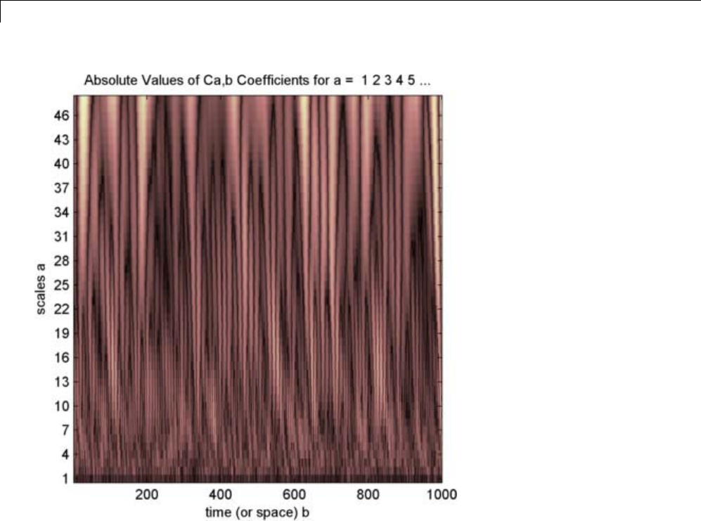
2Continuous Wavelet Analysis
Of course, coefficient plots generated from the command line can be
manipulated using ordinary MATLAB graphics commands.
4Choose scales for the analysis.
The second argument to cwt gives you fine control over the scale levels on
which the continuous analysis is performed. In the previous example, we
used all scales from 1 to 48, but you can construct any scale vector subject
to these constraints:
•All scales must be real positive numbers.
•The scale increment must be positive.
2-6
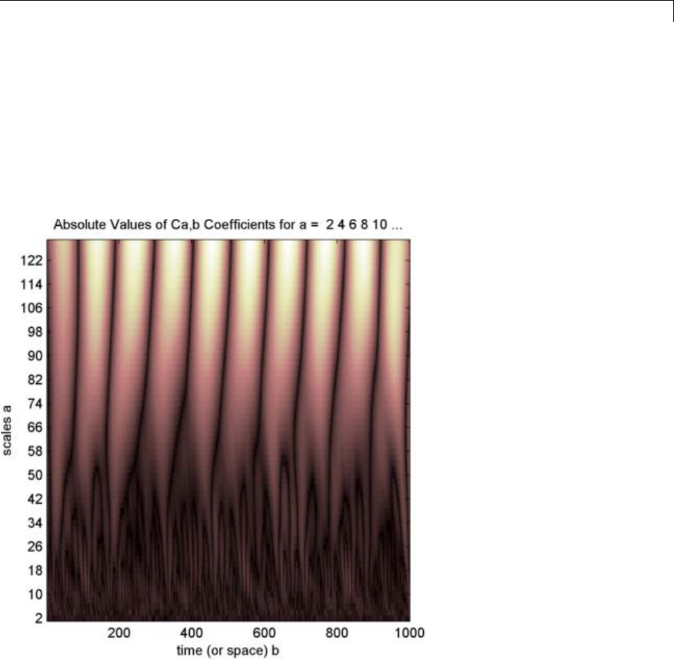
1-D Continuous Wavelet Analysis
•The highest scale cannot exceed a maximum value depending on the
signal.
Let’s repeat the analysis using every other scale from 2 to 128. Type
c = cwt(noissin,2:2:128,'db4','plot');
A new plot appears:
This plot gives a clearer picture of what’s happening with the signal,
highlighting the periodicity.
2-7
2Continuous Wavelet Analysis
Continuous Analysis Using the Graphical Interface
We now use the Continuous Wavelet 1-D tool to analyze the same noisy
sinusoidal signal we examined earlier using the command line interface in
“Command Line Continuous Wavelet Analysis” on page 2-4.
1Start the Continuous Wavelet 1-D Tool. From the MATLAB prompt, type
wavemenu
The Wavelet Toolbox Main Menu appears.
Click the Continuous Wavelet 1-D menu item.
The continuous wavelet analysis tool for one-dimensional signal data
appears.
2-8
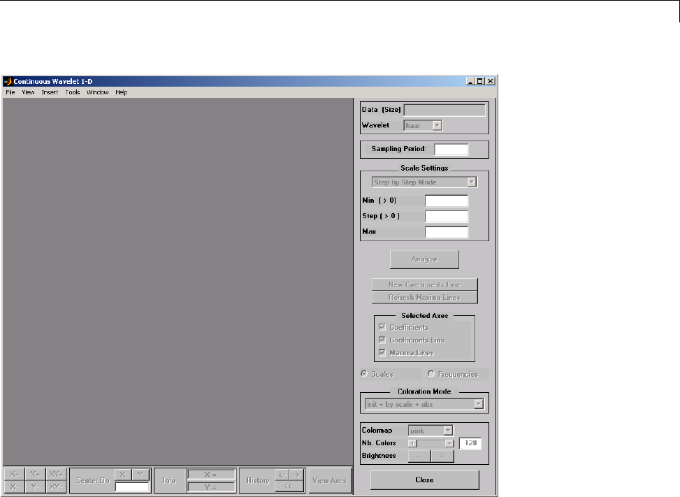
1-D Continuous Wavelet Analysis
2Load a signal.
Choose the File > Load Signal menu option.
When the Load Signal dialog box appears, select the MAT-file
noissin.mat, which should reside in the MATLAB folder
toolbox/wavelet/wavedemo.ClicktheOK button.
The noisy sinusoidal signal is loaded into the Continuous Wavelet 1-D
tool.
Thedefaultvalueforthesamplingperiodisequalto1(second).
3Perform a Continuous Wavelet Transform.
2-9
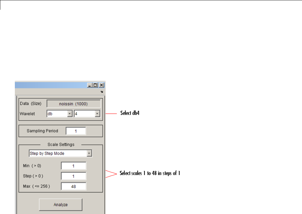
2Continuous Wavelet Analysis
To start our analysis, let’s perform an analysis using the db4 wavelet at
scales 1 through 48, just as we did using command line functions in the
previous section.
In the upper right portion of the Continuous Wavelet 1-D tool, select the
db4 wavelet and scales 1–48.
4Click the Analyze button.
After a pause for computation, the tool displays the coefficients plot, the
coefficients line plot corresponding to the scale a = 24, and the local maxima
plot, which displays the chaining across scales (from a = 48 down to a = 1)
of the coefficients local maxima.
2-10
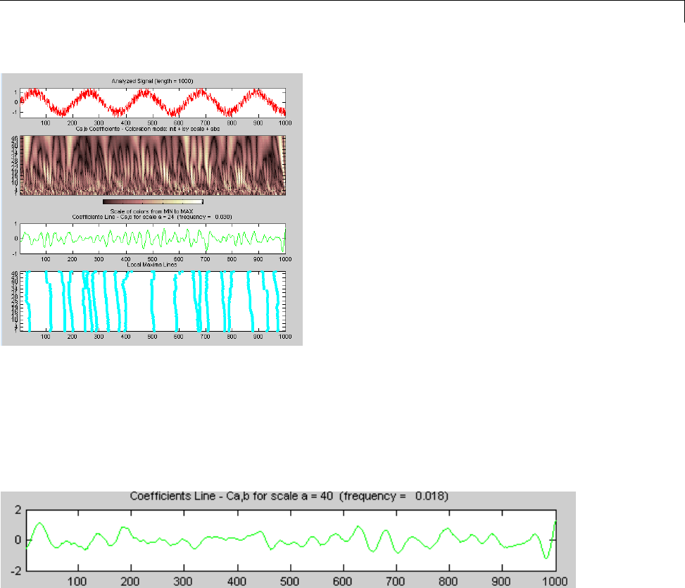
1-D Continuous Wavelet Analysis
5View Wavelet Coefficients Line.
Select another scale a = 40 by clicking in the coefficients plot with the
right mouse button. See step 9 to know, more precisely, how to select the
desired scale.
Click the New Coefficients Line button. The tool updates the plot.
6View Maxima Line.
Click the Refresh Maxima Line button. The local maxima plot displays
the chaining across scales of the coefficients local maxima from a = 40
down to a = 1.
2-11
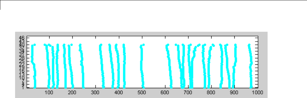
2Continuous Wavelet Analysis
Hold down the right mouse button over the coefficients plot. The position of
the mouse is given by the Info frame (located at the bottom of the screen)
in terms of location (X)andscale(Sca).
2-12
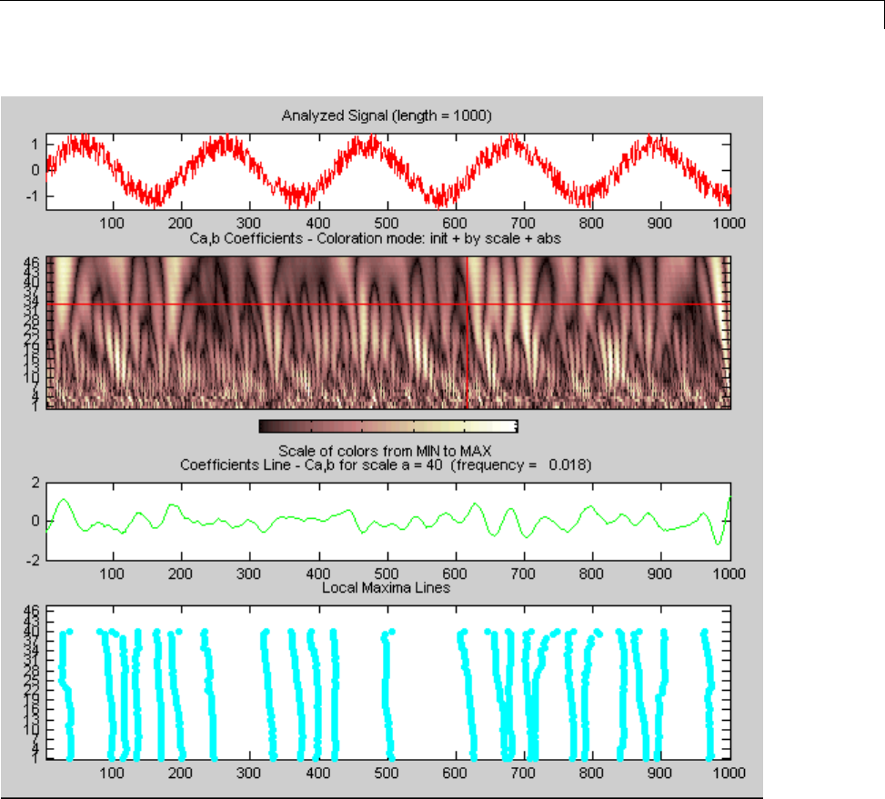
1-D Continuous Wavelet Analysis
7Switch from scale to Pseudo-Frequency Information.
Using the option button on the right part of the screen, select Frequencies
instead of Scales. Again hold down the right mouse button over the
coefficients plot, the position of the mouse is given in terms of location
(X) and frequency (Frq)inHertz.
2-13
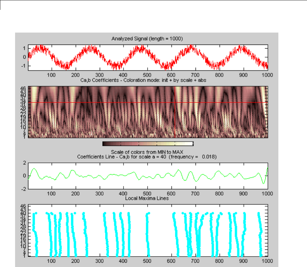
2Continuous Wavelet Analysis
This facility allows you to interpret scale in terms of an associated
pseudo-frequency, which depends on the wavelet and the sampling period..
8Deselect the last two plots using the check boxes in the Selected Axes
frame.
2-14

1-D Continuous Wavelet Analysis
9Zoom in on detail.
Drag a rubber band box (by holding down the left mouse button) over the
portion of the signal you want to magnify.
2-15
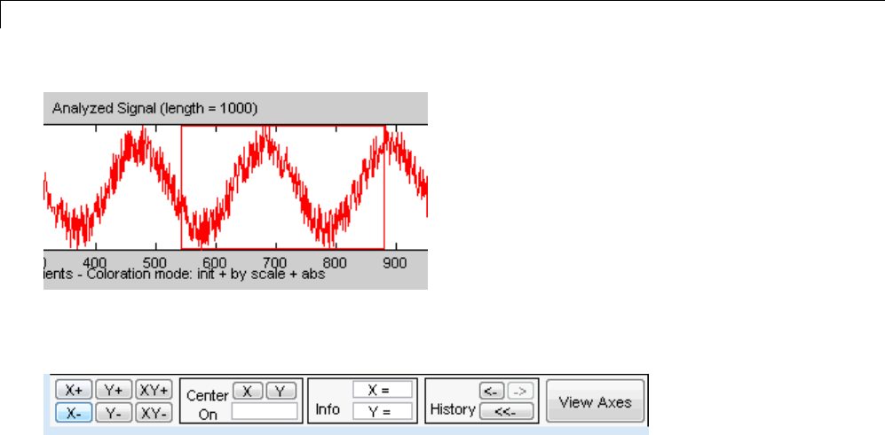
2Continuous Wavelet Analysis
10 Click the X+ button (located at the bottom of the screen) to zoom
horizontally only.
The Continuous Wavelet 1-D tool enlarges the displayed signal and
coefficients plot (for more informationonzooming,see“ConnectionofPlots”
on page A-3 in the Wavelet Toolbox User’s Guide).
2-16
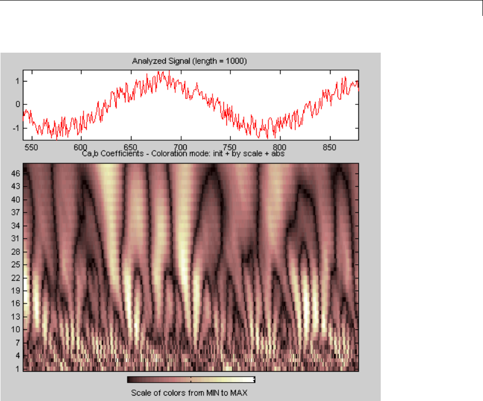
1-D Continuous Wavelet Analysis
As with the command line analysis on the preceding pages, you can change
the scales or the analyzing wavelet and repeat the analysis. To do this, just
edit the necessary fields and click the Analyze button.
11 View normal or absolute coefficients.
The Continuous Wavelet 1-D tool allows you to plot either the absolute
values of the wavelet coefficients, or the coefficients themselves.
2-17

2Continuous Wavelet Analysis
More generally, the coefficients coloration can be done in several different
ways. For more details on the Coloration Mode, see “Controlling the
Coloration Mode” on page A-8.
Choose either one of the absolute modes or normal modes from the
Coloration Mode menu. In normal modes, the colors are scaled between
the minimum and maximum of the coefficients. In absolute modes, the
colors are scaled between zero and the maximum absolute value of the
coefficients.
Importing and Exporting Information from the
Graphical Interface
The Continuous Wavelet 1-D graphical interface tool lets you import
information from and export information to disk.
You can
•Load signals from disk into the Continuous Wavelet 1-D tool.
•Save wavelet coefficients from the Continuous Wavelet 1-D tool to disk.
Loading Signals into the Continuous Wavelet 1-D Tool
To load a signal you’ve constructed in your MATLAB workspace into the
Continuous Wavelet 1-D tool, save the signal in a MAT-file (with extension
mat or other).
For instance, suppose you’ve designed a signal called warma and want to
analyze it in the Continuous Wavelet 1-D tool.
save warma warma
The workspace variable warma must be a vector.
sizwarma = size(warma)
sizwarma =
1 1000
2-18

1-D Continuous Wavelet Analysis
To load this signal into the Continuous Wavelet 1-D tool, use the menu
option File > Load Signal. A dialog box appears that lets you select the
appropriateMAT-filetobeloaded.
Note The first one-dimensional variable encountered in the file is considered
the signal. Variables are inspected in alphabetical order.
Saving Wavelet Coefficients
The Continuous Wavelet 1-D tool lets you save wavelet coefficients to disk.
The toolbox creates a MAT-file in the current folder with the extension wc1
and a name you give it.
To save the continuous wavelet coefficients from the present analysis, use the
menu option File > Save > Coefficients.
A dialog box appears that lets you specify a folder and filename for storing
the coefficients.
Consider the example analysis:
File > Example Analysis > with haar at scales [1:1:64] →Cantor curve.
After saving the continuous wavelet coefficients to the file cantor.wc1,load
the variables into your workspace:
load cantor.wc1 -mat
whos
Name Size Bytes Class
coeff 64x2188 1120256 double array
scales 1x64 512 double array
wname 1x4 8 char array
Variables coefs and scales contain the continuous wavelet coefficients
and the associated scales. More precisely, in the above example, coefs is a
2-19

2Continuous Wavelet Analysis
64-by-2188 matrix, one row for each scale; and scales is the 1-by-64 vector
1:64. Variable wname contains the wavelet name.
2-20

One-Dimensional Complex Continuous Wavelet Analysis
One-Dimensional Complex Continuous Wavelet Analysis
This section takes you through the features of complex continuous wavelet
analysis using the Wavelet Toolbox software and focuses on the differences
between the real and complex continuous analysis.
You can refer to the section “Command Line Continuous Wavelet Analysis” on
page 2-4 if you want to learn how to
•Zoom in on detail
•Display coefficients in normal or absolute mode
•Choose the scales at which the analysis is performed
•Switch from scale to pseudo-frequency information
•Exchange signal and coefficient information between the disk and the
graphical tools
Wavelet Toolbox software requires only one function for complex continuous
wavelet analysis of a real valued signal: cwt. You’llfindfullinformation
about this function in its reference page.
In this section, you’ll learn how to
•Load a signal
•Perform a complex continuous wavelet transform of a signal
•Produce plots of the coefficients
Since you can perform analyses either from the command line or using the
graphical interface tools, this section has subsections covering each method.
2-21
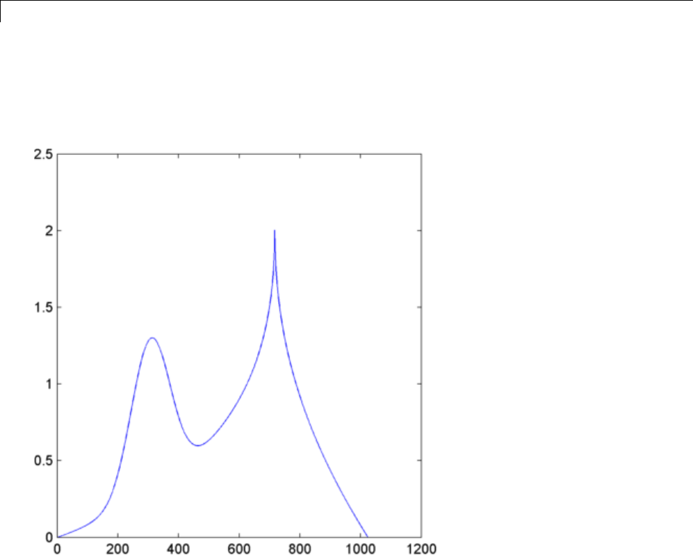
2Continuous Wavelet Analysis
Complex Continuous Analysis Using the Command
Line
This example involves a cusp signal.
1Load a signal.
From the MATLAB prompt, type
load cuspamax;
You now have the signal cuspamax in your workspace:
whos
2-22

One-Dimensional Complex Continuous Wavelet Analysis
Name Size Bytes Class
caption 1x71 142 char array
cuspamax 1x1024 8192 double array
caption
caption =
x = linspace(0,1,1024);
y = exp(-128*((x-0.3).^2))-3*(abs(x-0.7).^0.4);
caption is a string that contains the signal definition.
2Perform a Continuous Wavelet Transform.
Use the cwt command. Type
c = cwt(cuspamax,1:2:64,'cgau4');
The arguments to cwt specify the signal to be analyzed, the scales of the
analysis, and the wavelet to be used. The returned argument ccontains
the coefficients at various scales. In this case, cis a complex 32-by-1024
matrix, each row of which corresponds to a single scale.
3Plot the coefficients.
The cwt command accepts a fourth argument. This is a flag that, when
present, causes cwt to produce four plots related to the complex continuous
wavelet transform coefficients:
•Real and imaginary parts
•Modulus and angle
The cwt command can accept more arguments to define the different
characteristics of the produced plots. For more information, see the cwt
reference page.
Type
c = cwt(cuspamax,1:2:64,'cgau4','plot');
2-23
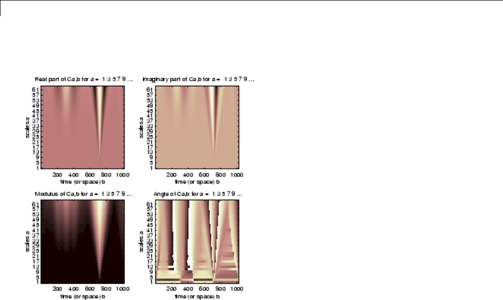
2Continuous Wavelet Analysis
Aplotappears:
Of course, coefficient plots generated from the command line can be
manipulated using ordinary MATLAB graphics commands.
Complex Continuous Analysis Using the Graphical
Interface
We now use the Complex Continuous Wavelet 1-D tool to analyze the
same cusp signal we examined using the command line interface in the
previous section.
1Start the Complex Continuous Wavelet 1-D Tool.
From the MATLAB prompt, type
wavemenu
The Wavelet Toolbox Main Menu appears.
2-24
One-Dimensional Complex Continuous Wavelet Analysis
Click the Complex Continuous Wavelet 1-D menu item.
The continuous wavelet analysis tool for one-dimensional signal data
appears.
2-25
2Continuous Wavelet Analysis
2Load a signal.
Choose the File > Load Signal menu option.
When the Load Signal dialog box appears, select the MAT-file
cuspamax.mat, which should reside in the MATLAB folder
toolbox/wavelet/wavedemo.ClicktheOK button.
ThecuspsignalisloadedintotheComplex Continuous Wavelet 1-D tool.
The default value for the sampling period is equal to 1 (second).
3Perform a Complex Continuous Wavelet Transform
To start our analysis, let’s perform an analysis using the cgau4 wavelet
at scales 1 through 64 in steps of 2, just as we did using command-line
functions in “One-Dimensional Complex Continuous Wavelet Analysis”
on page 2-21.
In the upper-right portion of the Complex Continuous Wavelet 1-D tool,
select the cgau4 wavelet and scales 1–64 in steps of 2.
2-26
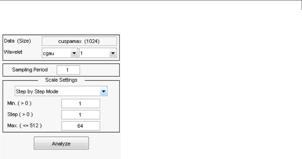
One-Dimensional Complex Continuous Wavelet Analysis
Click the Analyze button.
After a pause for computation, the tool displays the usual plots associated
to the modulus of the coefficients on the left side, and the angle of the
coefficients on the right side.
2-27

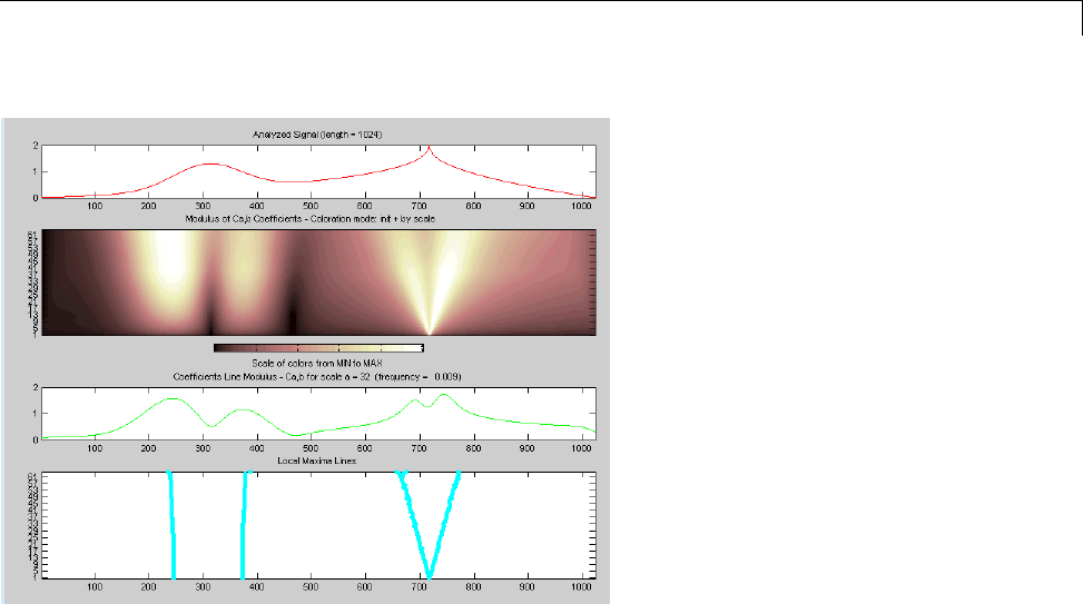
One-Dimensional Complex Continuous Wavelet Analysis
The figure now looks like the one in the real Continuous Wavelet 1-D tool.
Importing and Exporting Information from the
Graphical Interface
To know how to import and export information from the Complex Continuous
Wavelet Graphical Interface, see the corresponding paragraph in “Command
Line Continuous Wavelet Analysis” on page 2-4.
The only difference is that the variable coefs is a complex matrix (see “Saving
Wavelet Coefficients” on page 2-19).
2-29

2Continuous Wavelet Analysis
DFT-Based Continuous Wavelet Analysis — Command Line
In this section...
“CWT of Sum of Disjoint Sinusoids” on page 2-30
“Approximate Scale-Frequency Conversions” on page 2-33
“Signal Reconstruction from CWT Coefficients” on page 2-37
“Signal Approximation with Modified CWT Coefficients” on page 2-38
To implement a DFT-based continuous wavelet analysis in the MATLAB
command window, use cwtft and icwtft.
For the mathematical basis of the DFT-based continuous wavelet analysis
and synthesis see:
•“DFT-Based Continuous Wavelet Transform”
•“Inverse Continuous Wavelet Transform”
CWT of Sum of Disjoint Sinusoids
The signal is a sum of two disjoint sinusoids. The sampling frequency is
1023 Hz. The total signal duration is 1 second. The frequencies of the two
sinewavesare4and8Hz. The4-Hzsinewavehassupportontheinitial
1/2 second of the 1-second interval. The 8-Hz sine wave has support on the
final 1/2 second.
N = 1024;
t = linspace(0,1,N);
dt =1/(N-1);
Y = sin(8*pi*t).*(t<=0.5) + sin(16*pi*t).*(t>0.5);
Obtain the continuous wavelet transform (CWT) using the default analytic
Morlet wavelet, and plot the results.
sig = {Y,dt};
cwtS1 = cwtft(sig,'plot');
2-30
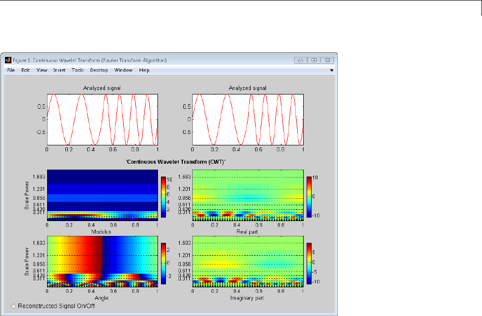
DFT-Based Continuous Wavelet Analysis — Command Line
The figure shows a plot of the original signal. The CWT moduli, real and
imaginary parts of the CWT coefficients, and the CWT coefficient arguments
(phase angles) also appear as plots.
You can display the reconstructed signal by enabling the radio button at the
bottom-left corner of the plot. Enabling the radio button superimposes the
reconstructed signal on the original signal in the top-left corner of the figure.
The relative maximum and quadratic (L2 norm) errors appear under the plot.
2-31
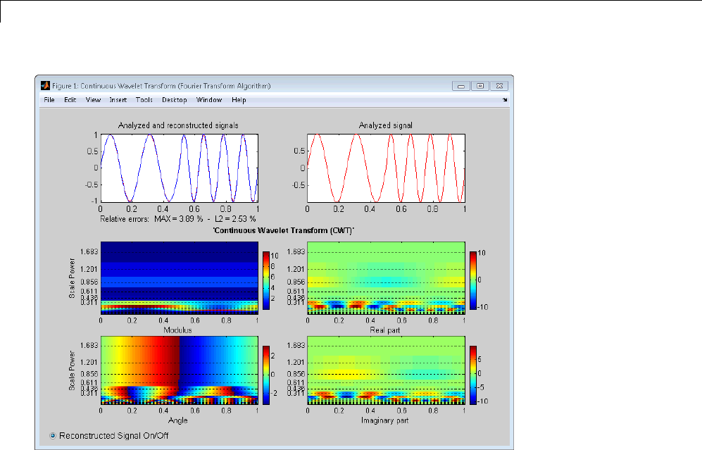
2Continuous Wavelet Analysis
You can customize your continuous wavelet analysis by providing additional
inputs to cwtft. In the following example, specify the analyzing wavelet as
the Paul wavelet of order 8. Specify theinitialscale,thespacingbetween
scales, and the number of scales. By default, the scale vector is logarithmic
to the base 2.
% smallest scale, spacing between scales, number of scales
dt = 1/1023;
s0 = 2*dt; ds = 0.5; NbSc = 20;
% scale vector is
% scales = s0*2.^((0:NbSc-1)*ds);
wname = 'paul';
SIG = {Y,dt};
% Create SCA input as cell array
SCA = {s0,ds,NbSc};
% Specify wavelet and parameters
WAV = {wname,8};
2-32
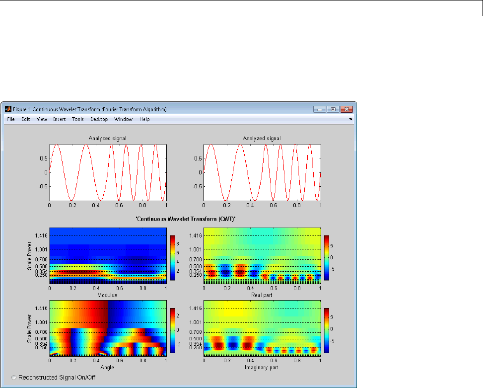
DFT-Based Continuous Wavelet Analysis — Command Line
% Compute and plot the CWT
cwtS2 = cwtft(SIG,'scales',SCA,'wavelet',WAV,'plot');
The oscillations at 4 and 8 Hz are clearly visible as alternating positive and
negative real and imaginary parts. The 4-Hz oscillation occurs at a longer
scale than the 8-Hz oscillation. In the plot of the CWT moduli, you see the
transition from the 4-Hz (longer scale) sinusoid to the 8-Hz sinusoid (shorter
scale) around 0.5 seconds.
Approximate Scale-Frequency Conversions
There is not a direct correspondence between Fourier wavelength and scale.
However, you can find conversion factors for select wavelets that yield an
2-33

2Continuous Wavelet Analysis
approximate scale-frequency correspondence. You can find these factors for
wavelets supported by cwtft listed on the reference page.
This example shows you how to change the scale axis to an approximate
frequency axis for analysis. Use the sum of disjoint sinusoids as the input
signal. Set the initial scale to 6*dt, the scale increment to 0.15,andthe
number of scales to 50. Use the Fourier factor for the Morlet wavelet to convert
the scale vector to an approximate frequency vector in hertz. Plot the result.
figure;
s0 = 6*dt; ds = 0.15; NbSc = 50;
wname = 'morl';
SCA = {s0,ds,NbSc};
cwtsig = cwtft({Y,dt},'scales',SCA,'wavelet',wname);
MorletFourierFactor = 4*pi/(6+sqrt(2+6^2));
Scales = cwtsig.scales.*MorletFourierFactor;
Freq = 1./Scales;
imagesc(t,[],abs(cwtsig.cfs));
indices = get(gca,'ytick');
set(gca,'yticklabel',Freq(indices));
xlabel('Time'); ylabel('Hz');
title('Time-Frequency Analysis with CWT');
2-34
DFT-Based Continuous Wavelet Analysis — Command Line
You can see the signal contains significantenergyatapproximately4Hzover
the first 1/2 second. In the final 1/2 second interval, the predominant signal
energy transitions higher in frequency to approximately 8 Hz.
Repeat the above example using the Paul analyzing wavelet with order, m,
equal to 8. Use a contour plot of the real part of the CWT to visualize the sine
wavesat4and8-Hz. Therealpartexhibits oscillations in the sign of the
wavelet coefficients at those frequencies.
s0 = 6*dt; ds = 0.15; NbSc = 50;
m=8;
% scale vector is
% scales = s0*2.^((0:NbSc-1)*ds);
wname = 'paul';
2-35
2Continuous Wavelet Analysis
SIG = {Y,dt};
% Create SCA input as cell array
SCA = {s0,ds,NbSc};
% Specify wavelet and parameters
WAV = {wname,m};
cwtPaul = cwtft(SIG,'scales',SCA,'wavelet',WAV);
scales = cwtPaul.scales;
PaulFourierFactor = 4*pi/(2*m+1);
Freq = 1./(PaulFourierFactor.*scales);
contour(t,Freq,real(cwtPaul.cfs));
xlabel('Time'); ylabel('Hz'); colorbar;
title('Real Part of CWT using Paul Wavelet (m=8)');
axis([0 1 1 15]); grid on;
2-36

DFT-Based Continuous Wavelet Analysis — Command Line
Signal Reconstruction from CWT Coefficients
You can use the critically sampled (decimated) and oversampled
(nondecimated) discrete wavelet transforms (DWT) to achieve perfect
reconstruction of the input signal from the wavelet coefficients. To obtain
a time and scale-dependent approximation to a signal, you can use a
possibly-modified subset of the decimated or undecimated DWT coefficients.
The inversion of the CWT is not as straightforward. The simplest CWT
inversion utilizes the single integral formula due to Morlet, which employs a
Dirac delta function as the synthesizing wavelet. See “Inverse Continuous
Wavelet Transform” for a brief mathematical motivation. icwtft and
icwtlin both implement the single integral formula. Because of necessary
approximations in the implementation of the single integral inverse CWT,
you cannot expect to obtain perfect reconstruction. However, you can use the
inverse CWT to obtain useful position and scale-dependent approximations to
the input signal.
Implement the inverse CWT with logarithmically-spaced scales.
N = 1024;
t = linspace(0,1,N);
dt =1/(N-1);
Y = sin(8*pi*t).*(t<=0.5) + sin(16*pi*t).*(t>0.5);
dt = 1/1023;
s0 = 2*dt; ds = 0.5; NbSc = 20;
% scale vector is
% scales = s0*2.^((0:NbSc-1)*ds);
wname = 'paul';
SIG = {Y,dt};
% Create SCA input as cell array
SCA = {s0,ds,NbSc};
% Specify wavelet and parameters
WAV = {wname,8};
cwtS2 = cwtft(SIG,'scales',SCA,'wavelet',WAV);
YR1 = icwtft(cwtS2,'plot','signal',SIG);
norm(Y-YR1,2)
Enable the radio button in the left corner of the figure to plot the reconstructed
signal.
2-37
2Continuous Wavelet Analysis
Signal Approximation with Modified CWT Coefficients
Obtain the CWT of a noisy Doppler (frequency-modulated) signal using the
analytic Morlet wavelet. Reconstruct an approximation by selecting a subset
of the CWT coefficients. By eliminating the smallest scales, you obtain a
lowpass approximation to the signal. The lowpass approximation produces a
smooth approximation to the lower-frequency features of the noisy Doppler
signal. The high-frequency (small scale) features at the beginning of the
signal are lost.
% Define the signal
load noisdopp; Y = noisdopp;
N = length(Y);
% Define parameters before analysis
dt = 1;
2-38

DFT-Based Continuous Wavelet Analysis — Command Line
s0 = 2*dt; ds = 0.4875; NbSc = 20;
wname = 'morl';
SIG = {Y,dt};
SCA = {s0,ds,NbSc};
WAV = {wname,[]};
% Compute CWT analysis
cwtS4 = cwtft(SIG,'scales',SCA,'wavelet',WAV);
% Thresholding step building the new structure
cwtS5 = cwtS4;
newCFS = zeros(size(cwtS4.cfs));
newCFS(11:end,:) = cwtS4.cfs(11:end,:);
cwtS5.cfs = newCFS;
% Reconstruction from the modified structure
YRDen = icwtft(cwtS5,'signal',SIG);
plot(Y,'k-.');
hold on;
plot(YRDen,'r','linewidth',3); axis tight;
legend('Original Signal', 'Selective inverse CWT');
title('Signal approximation based on a subset of CWT coefficients');
2-39
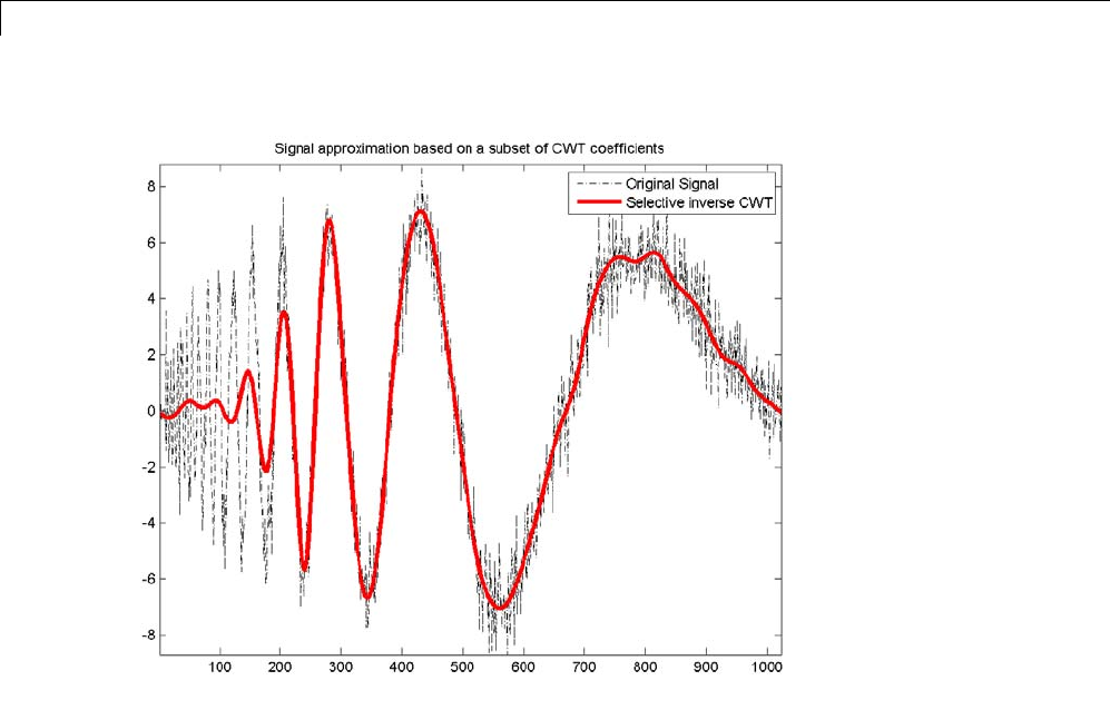
2Continuous Wavelet Analysis
2-40
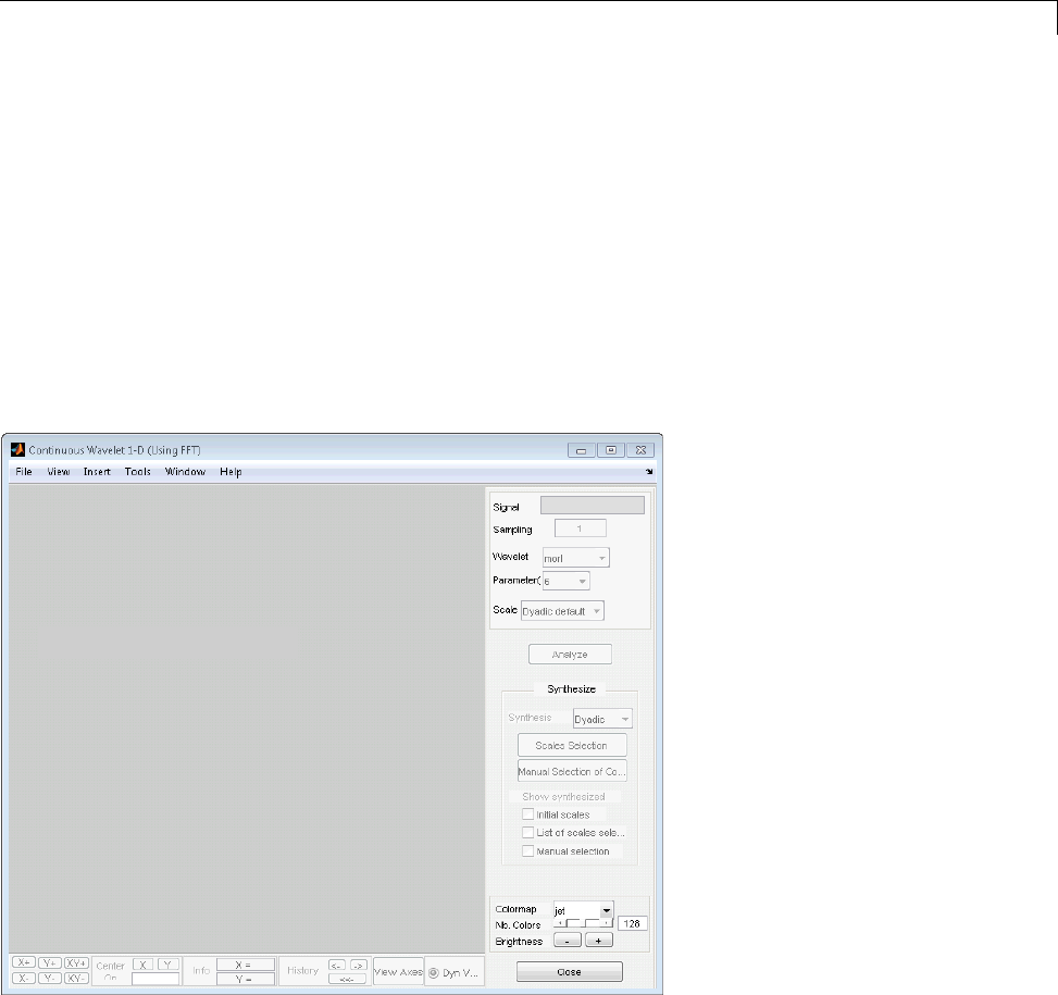
Interactive DFT-Based Continuous Wavelet Analysis
Interactive DFT-Based Continuous Wavelet Analysis
You can use the Continuous Wavelet 1-D (Using FFT) tool to analyze
the same signals examined in “DFT-Based Continuous Wavelet Analysis —
Command Line” on page 2-30.
1At the MATLAB command prompt, enter
wavemenu
2Click the Continuous Wavelet 1-D (Using FFT) menu item.
3Choose the File > Load Data option. When the Pick a file dialog appears,
select noisdopp.mat from the toolbox/wavelet/wavedemo folder.
2-41
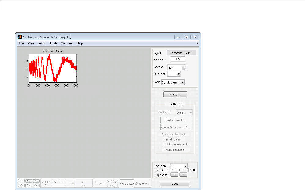
2Continuous Wavelet Analysis
4Using the menu default parameters, click Analyze.
2-42
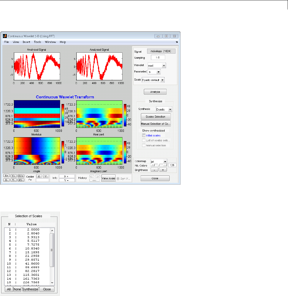
Interactive DFT-Based Continuous Wavelet Analysis
5Reconstruct the signal based on all the default dyadic scales. Click Scales
Selection.
Select all scales by clicking All.ClickSynthesize.
2-43
2Continuous Wavelet Analysis
In the top left, the synthesized signal plot is superimposed on the original
signal. The relative maximum and L2 errors are displayed under the plot.
The single integral CWT inversion does not produce perfect reconstruction,
but the relative errors using the default logarithmically–spaced scales
are small.
6Obtain a signal approximation from selected scales.
Click None in the Selection of Scales paneltoundothescaleselection.
Then, select only scale indices greater than 10 and reconstruct an
approximation to the original signal. Hold the Ctrl key while selecting
scale indices 11–21. The scale indices correspond to the following physical
scales.
dt = 1;
s0 = 2*dt;
ds = 0.4875;
2-44
Interactive DFT-Based Continuous Wavelet Analysis
nb = 21;
physical_scales = s0*pow.^((0:nb-1)*ds);
7Click Synthesize.
The reconstructed signal from scale indices 11–21 is a lowpass
approximation to the noisy Doppler signal.
8Analyze using linear scales. In the Scales drop-down menu in the upper
right, select Linear default and click Analyze.
2-45
2Continuous Wavelet Analysis
Note The other options under Scales include Dyadic default and
Manual.
If you select Manual,aDefine Scales button appears. Click Define
Scales to set the parameters for your scale vector.
Manual Selection of CWT Coefficients
Select coefficients manually by graphically selecting the CWT coefficients.
Reconstruct the signal from the selected coefficients. Click Manual Selection
of Coefficients.TheSelect the Coefficients Manually panel appears with
a single box containing all the CWT coefficient moduli.
2-46
Interactive DFT-Based Continuous Wavelet Analysis
You can change the CWT coefficient view to Angle,Real,orImaginary.
To select a subset of coefficients, draw a box by left-clicking and dragging the
mouse. When you release the mouse button, a semi-transparent box with a
green border is superimposed on the plot.
You can place multiple boxes on the same plot. To synthesize a signal based
on the selected coefficients, click Synthesize.
2-47
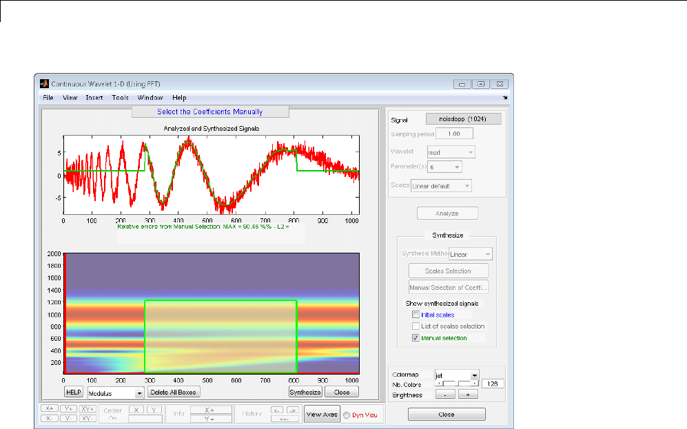
2Continuous Wavelet Analysis
To select, unselect, or delete a box, right-click in the box. A context menu
appearsthatallowsyoutoselect,unselect,ordelete the box. After you
select the coefficients within the box, the border of the box displays in green.
When the coefficients within the box are not selected, the border of the box
displays in red.
You can move a box by clicking the left mouse button inside the box while
simultaneously pressing the Shift key. The border of the box changes to
yellow, and you can drag the box to the desired location. You must keep the
Shift key pressed while you are moving the box.
Quit the manual selection mode by clicking the Close button.
In the Show synthesized signals from panel on the right, you can turn
the plot of your synthesized signal on and off by checking and unchecking
Manual selection.
2-48
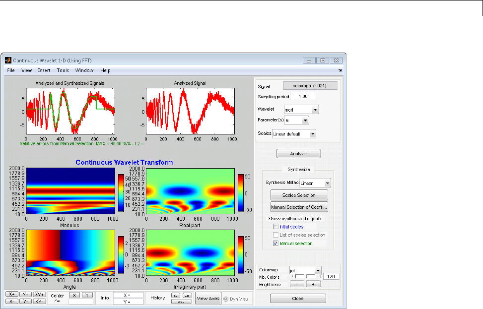
Interactive DFT-Based Continuous Wavelet Analysis
Using the File > Save > Synthesized signal menu, you can save the
available synthesized signals.
Using the File > Save > Decomposition menu, you can save the wavelet
analysis as a MAT file.
2-49

2Continuous Wavelet Analysis
2-50

3
Discrete Wavelet Analysis
•“1-D Decimated Wavelet Transforms” on page 3-2
•“Fast Wavelet Transform (FWT) Algorithm” on page 3-37
•“Border Effects” on page 3-52
•“Discrete Stationary Wavelet Transform (SWT)” on page 3-62
•“One-Dimensional Discrete Stationary Wavelet Analysis” on page 3-69
•“One-Dimensional Multisignal Analysis” on page 3-86
•“Two-Dimensional Discrete Wavelet Analysis” on page 3-137
•“Two-Dimensional Discrete Stationary Wavelet Analysis” on page 3-166
•“Three-Dimensional Discrete Wavelet Analysis” on page 3-181

3Discrete Wavelet Analysis
1-D Decimated Wavelet Transforms
This section takes you through the features of one-dimensional
critically-sampled wavelet analysis using the Wavelet Toolbox software.
The toolbox provides these functions for one-dimensional signal analysis. For
more information, see the reference pages.
Analysis-Decomposition Functions
Function Name Purpose
dwt Single-level decomposition
wavedec Decomposition
wmaxlev Maximum wavelet decomposition level
Synthesis-Reconstruction Functions
Function Name Purpose
idwt Single-level reconstruction
waverec Full reconstruction
wrcoef Selective reconstruction
upcoef Single reconstruction
Decomposition Structure Utilities
Function Name Purpose
detcoef Extraction of detail coefficients
appcoef Extraction of approximation coefficients
upwlev Recomposition of decomposition structure
3-2

1-D Decimated Wavelet Transforms
De-noising and Compression
Function Name Purpose
ddencmp Provide default values for de-noising and
compression
wbmpen Penalized threshold for wavelet 1-D or 2-D
de-noising
wdcbm Thresholds for wavelet 1-D using Birgé-Massart
strategy
wdencmp Wavelet de-noising and compression
wden Automatic wavelet de-noising
wthrmngr Threshold settings manager
In this section, you’ll learn how to
•Load a signal
•Perform a single-level wavelet decomposition of a signal
•Construct approximations and details from the coefficients
•Display the approximation and detail
•Regenerate a signal by inverse wavelet transform
•Perform a multilevel wavelet decomposition of a signal
•Extract approximation and detail coefficients
•Reconstruct the level 3 approximation
•Reconstruct the level 1, 2, and 3 details
•Display the results of a multilevel decomposition
•Reconstruct the original signal from the level 3 decomposition
•Remove noise from a signal
•Refine an analysis
•Compress a signal
•Show a signal’s statistics and histograms
3-3

3Discrete Wavelet Analysis
Since you can perform analyses either from the command line or using the
graphical interface tools, this section has subsections covering each method.
The final subsection discusses how to exchange signal and coefficient
information between the disk and the graphical tools.
One-Dimensional Analysis Using the Command Line
This example involves a real-world signal — electrical consumption measured
over the course of 3 days. This signal is particularly interesting because of
noise introduced when a defect developed in the monitoring equipment as
the measurements were being made. Wavelet analysis effectively removes
the noise.
1Load the signal and select a portion for wavelet analysis.
load leleccum;
s = leleccum(1:3920);
l_s = length(s);
2Perform a single-level wavelet decomposition of a signal.
Perform a single-level decomposition of the signal using the db1 wavelet.
[cA1,cD1] = dwt(s,'db1');
This generates the coefficients of the level 1 approximation (cA1)and
detail (cD1).
3Construct approximations and details from the coefficients.
To construct the level 1 approximation and detail (A1 and D1)fromthe
coefficients cA1 and cD1,type
A1 = upcoef('a',cA1,'db1',1,l_s);
D1 = upcoef('d',cD1,'db1',1,l_s);
or
A1 = idwt(cA1,[],'db1',l_s);
D1 = idwt([],cD1,'db1',l_s);
3-4
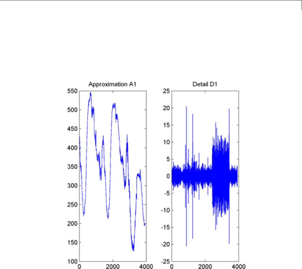
1-D Decimated Wavelet Transforms
4Display the approximation and detail.
To display the results of the level-one decomposition, type
subplot(1,2,1); plot(A1); title('Approximation A1')
subplot(1,2,2); plot(D1); title('Detail D1')
5Regenerate a signal by using the Inverse Wavelet Transform.
To find the inverse transform, enter
A0 = idwt(cA1,cD1,'db1',l_s);
err = max(abs(s-A0))
6Perform a multilevel wavelet decomposition of a signal.
3-5
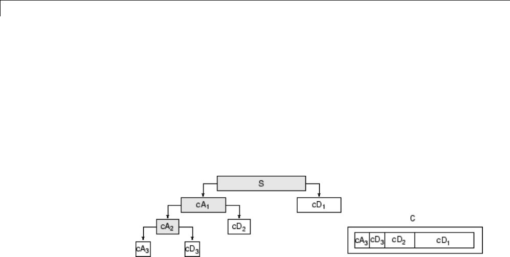
3Discrete Wavelet Analysis
To perform a level 3 decomposition of the signal (again using the db1
wavelet), type
[C,L] = wavedec(s,3,'db1');
The coefficients of all the components of a third-level decomposition (that
is, the third-level approximation and the first three levels of detail) are
returned concatenated into one vector, C. Vector L gives the lengths of
each component.
7Extract approximation and detail coefficients.
To extract the level 3 approximation coefficients from C,type
cA3 = appcoef(C,L,'db1',3);
To extract the levels 3, 2, and 1 detail coefficients from C,type
cD3 = detcoef(C,L,3);
cD2 = detcoef(C,L,2);
cD1 = detcoef(C,L,1);
or
[cD1,cD2,cD3] = detcoef(C,L,[1,2,3]);
8Reconstruct the Level 3 approximation and the Level 1, 2, and 3 details.
To reconstruct the level 3 approximation from C,type
A3 = wrcoef('a',C,L,'db1',3);
To reconstruct the details at levels 1, 2, and 3, from C,type
3-6

1-D Decimated Wavelet Transforms
D1 = wrcoef('d',C,L,'db1',1);
D2 = wrcoef('d',C,L,'db1',2);
D3 = wrcoef('d',C,L,'db1',3);
9Display the results of a multilevel decomposition.
To display the results of the level 3 decomposition, type
subplot(2,2,1); plot(A3);
title('Approximation A3')
subplot(2,2,2); plot(D1);
title('Detail D1')
subplot(2,2,3); plot(D2);
title('Detail D2')
subplot(2,2,4); plot(D3);
title('Detail D3')
3-7
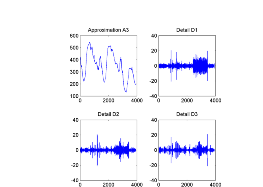
3Discrete Wavelet Analysis
10 Reconstruct the original signal from the Level 3 decomposition.
To reconstruct the original signal from the wavelet decomposition
structure, type
A0 = waverec(C,L,'db1');
err = max(abs(s-A0))
11 Crude de-noising of a signal.
Using wavelets to remove noise from a signal requires identifying which
component or components contain the noise, and then reconstructing the
signal without those components.
3-8
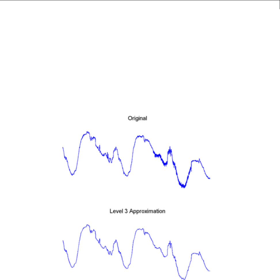
1-D Decimated Wavelet Transforms
In this example, we note that successive approximations become less and
less noisy as more and more high-frequency information is filtered out
of the signal.
The level 3 approximation, A3, is quite clean as a comparison between
it and the original signal.
To compare the approximation to the original signal, type
subplot(2,1,1);plot(s);title('Original'); axis off
subplot(2,1,2);plot(A3);title('Level 3 Approximation');
axis off
Of course, in discarding all the high-frequency information, we’ve also lost
many of the original signal’s sharpest features.
3-9
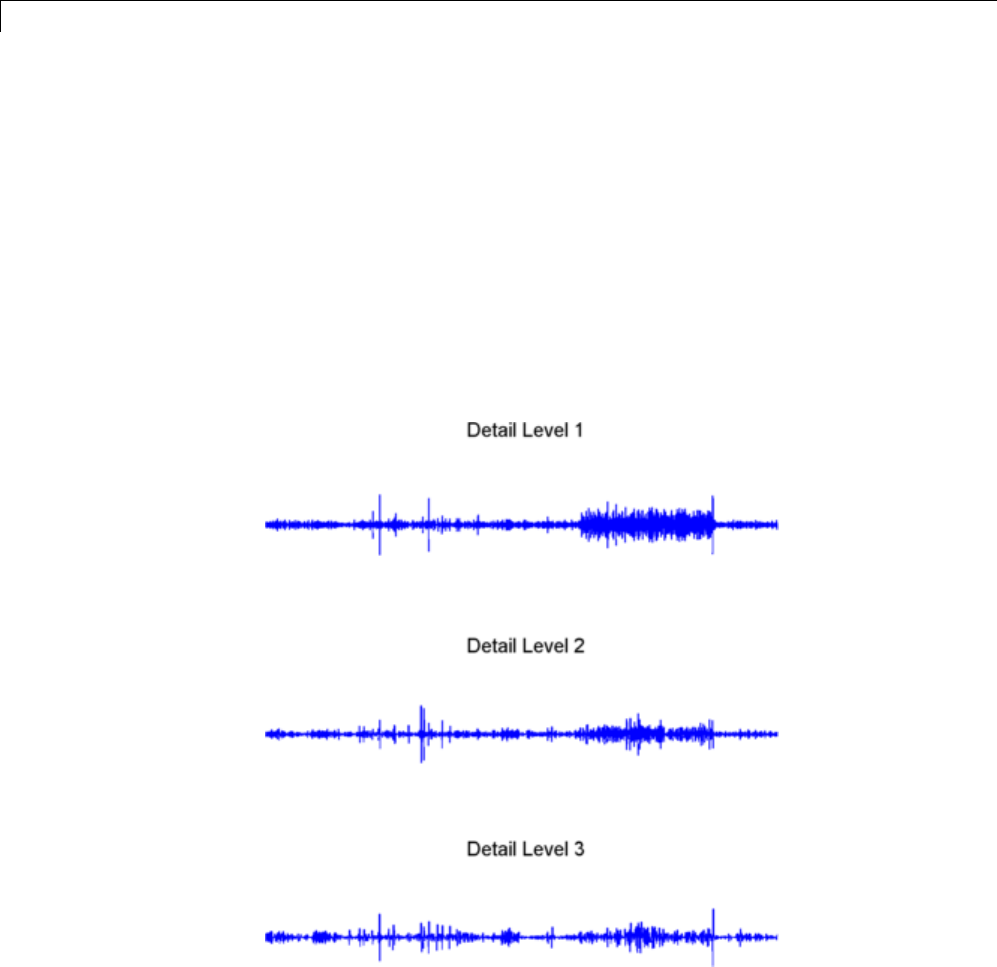
3Discrete Wavelet Analysis
Optimal de-noising requires a more subtle approach called thresholding.
This involves discarding only the portion of the details that exceeds a
certain limit.
12 Remove noise by thresholding.
Let’s look again at the details of our level 3 analysis.
To display the details D1,D2,andD3,type
subplot(3,1,1); plot(D1); title('Detail Level 1'); axis off
subplot(3,1,2); plot(D2); title('Detail Level 2'); axis off
subplot(3,1,3); plot(D3); title('Detail Level 3'); axis off
Most of the noise occurs in the latter part of the signal, where the details
show their greatest activity. What if we limited the strength of the details
by restricting their maximum values? This would have the effect of cutting
3-10

1-D Decimated Wavelet Transforms
back the noise while leaving the details unaffected through most of their
durations. But there’s a better way.
Note that cD1,cD2,andcD3 arejustMATLABvectors,sowecoulddirectly
manipulate each vector, setting each element to some fraction of the
vectors’ peak or average value. Then we could reconstruct new detail
signals D1,D2,andD3 from the thresholded coefficients.
To denoise the signal, use the ddencmp command to calculate the default
parameters and the wdencmp command to perform the actual de-noising,
type
[thr,sorh,keepapp] = ddencmp('den','wv',s);
clean = wdencmp('gbl',C,L,'db1',3,thr,sorh,keepapp);
Note that wdencmp uses the results of the decomposition (Cand L)that
we calculated in step 6. We also specify that we used the db1 wavelet
to perform the original analysis, and we specify the global thresholding
option 'gbl'.Seeddencmp and wdencmp in the reference pages for more
information about the use of these commands.
To display both the original and denoised signals, type
subplot(2,1,1); plot(s(2000:3920)); title('Original')
subplot(2,1,2); plot(clean(2000:3920)); title('denoised')
3-11
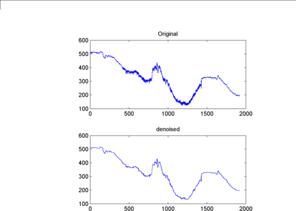
3Discrete Wavelet Analysis
We’ve plotted here only the noisy latterpartofthesignal. Noticehowwe’ve
removed the noise without compromising the sharp detail of the original
signal. This is a strength of wavelet analysis.
While using command line functions to remove the noise from a signal
can be cumbersome, the software’s graphical interface tools include an
easy-to-use de-noising feature that includes automatic thresholding.
More information on the de-noising process can be found in the following
sections:
•Remove noise from a signal
•“Denoising and Nonparametric Function Estimation” on page 5-2 in
the Wavelet Toolbox User’s Guide
3-12

1-D Decimated Wavelet Transforms
•“One-Dimensional Adaptive Thresholding of Wavelet Coefficients” on
page 5-17
•“One-Dimensional Wavelet Variance Adaptive Thresholding ” on page
5-14 in the Wavelet Toolbox User’s Guide
One-Dimensional Analysis Using the Graphical
Interface
In this section, we explore the same electrical consumption signal as in the
previous section, but we use the graphical interface tools to analyze the signal.
1Start the 1-D Wavelet Analysis Tool.
From the MATLAB prompt, type
wavemenu
3-13
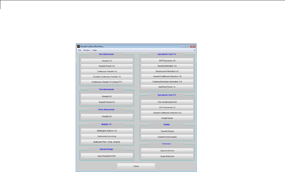
3Discrete Wavelet Analysis
The Wavelet Toolbox Main Menu appears.
Click the Wavelet 1-D menu item.
The discrete wavelet analysis tool for one-dimensional signal data appears.
2Load a signal.
From the File menu, choose the Load > Signal option.
3-14
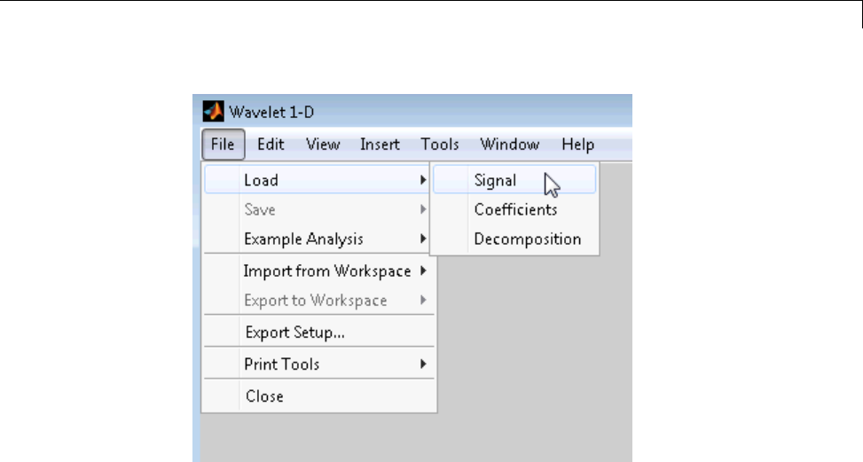
1-D Decimated Wavelet Transforms
When the Load Signal dialog box appears, select the
MAT-file leleccum.mat, which is in the MATLAB folder
toolbox/wavelet/wavedemo.ClicktheOK button.
The electrical consumption signal is loaded into the Wavelet 1-D tool.
3Perform a single-level wavelet decomposition.
To start our analysis, let’s perform a single-level decomposition using
the db1 wavelet, just as we did using the command-line functions in
“One-Dimensional Analysis Using the Command Line” on page 3-4.
In the upper right portion of the Wavelet 1-D tool, select the db1 wavelet
and single-level decomposition.
3-15
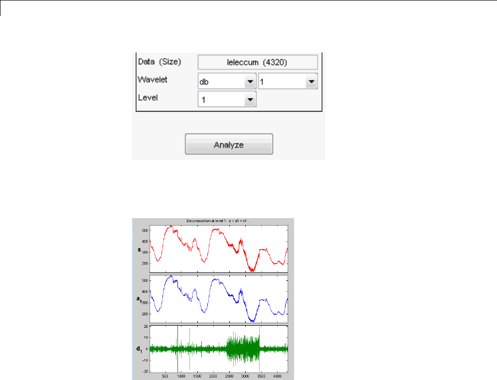
3Discrete Wavelet Analysis
Click the Analyze button.
After a pause for computation, the tool displays the decomposition.
4Zoom in on relevant detail.
One advantage of using the graphical interface tools is that you can zoom
in easily on any part of the signal and examine it in greater detail.
Drag a rubber band box (by holding down the left mouse button) over the
portion of the signal you want to magnify. Here, we’ve selected the noisy
part of the original signal.
3-16
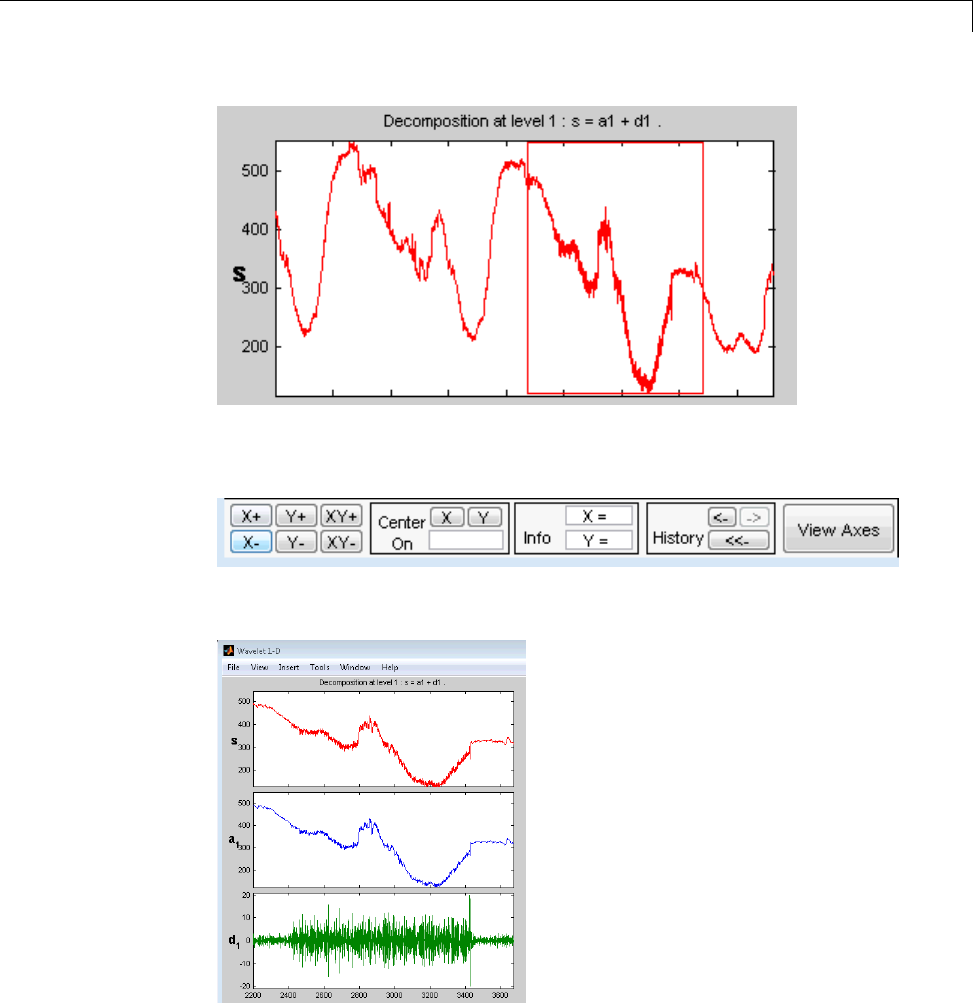
1-D Decimated Wavelet Transforms
Click the X+ button (located at the bottom of the screen) to zoom
horizontally.
The Wavelet 1-D tool zooms all the displayed signals.
3-17
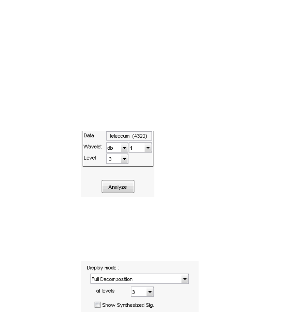
3Discrete Wavelet Analysis
The other zoom controls do more or less what you’d expect them to. The
X- button, for example, zooms out horizontally. The history function keeps
track of all your views of the signal. Return to a previous zoom level by
clicking the left arrow button.
5Perform a multilevel decomposition.
Again, we’ll use the graphical tools to emulate what we did in the previous
section using command line functions. To perform a level 3 decomposition
of the signal using the db1 wavelet:
Select 3from the Level menu at the upper right, and then click the
Analyze button again.
After the decomposition is performed, you’ll see a new analysis appear in
the Wavelet 1-D tool.
Selecting Different Views of the Decomposition
The Display mode menu (middle right) lets you choose different views of
the wavelet decomposition.
3-18

1-D Decimated Wavelet Transforms
The default display mode is called “Full Decomposition Mode.” Other
alternatives include:
•“Separate Mode,” which shows the details and the approximations in
separate columns.
•“Superimpose Mode,” which shows the details on a single plot
superimposed in different colors. The approximations are plotted
similarly.
•“Tree Mode,” which shows the decomposition tree, the original signal,
and one additional component of your choice. Click on the decomposition
tree to select the signal component you’d like to view.
•“Show and Scroll Mode,” which displays three windows. The first shows
the original signal superimposed on an approximation you select. The
second window shows a detail you select. The third window shows the
wavelet coefficients.
•“Show and Scroll Mode (Stem Cfs)” is very similar to the “Show and
ScrollMode”exceptthatitdisplays,inthethirdwindow,thewavelet
coefficients as stem plots instead of colored blocks.
You can change the default display mode on a per-session basis. Select the
desired mode from the View > Default Display Mode submenu.
Note The Compression and De-noising windows opened from the
Wavelet 1-D tool will inherit the current coefficient visualization attribute
(stems or colored blocks).
Depending on which display mode you select, you may have access to
additional display options through the More Display Options button.
3-19
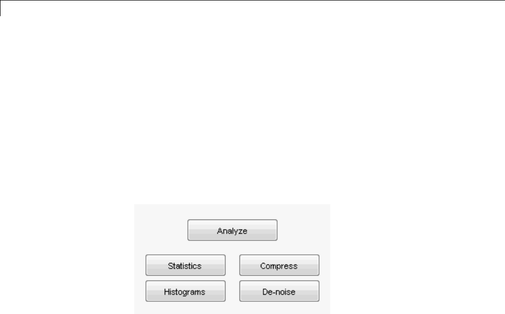
3Discrete Wavelet Analysis
These options include the ability to suppress the display of various
components, and to choose whether or nottodisplaytheoriginalsignal
along with the details and approximations.
6Remove noise from a signal.
The graphical interface tools feature a de-noising option with a predefined
thresholding strategy. This makes it very easy to remove noise from a
signal.
Bring up the de-noising tool: click the denoise button, located in the
middle right of the window, underneath the Analyze button.
The Wavelet 1-D De-noising window appears.
While a number of options are available for fine-tuning the de-noising
algorithm, we’ll accept the defaults of soft fixed form thresholding and
unscaled white noise.
Continue by clicking the denoise button.
The denoised signal appears superimposed on the original. The tool also
plots the wavelet coefficients of both signals.
3-20
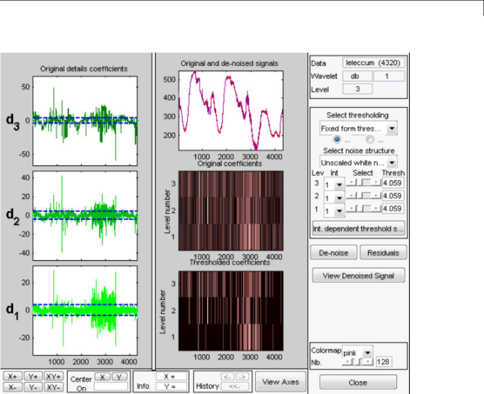
1-D Decimated Wavelet Transforms
Zoom in on the plot of the original and denoised signals for a closer look.
Drag a rubber band box around the pertinent area, and then click the XY+
button.
The denoise window magnifies your view. By default, the original signal
is shown in red, and the denoised signal in yellow.
3-21
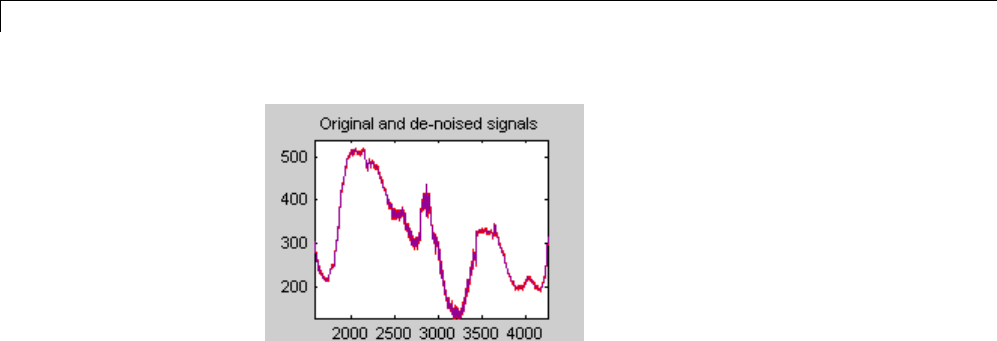
3Discrete Wavelet Analysis
Dismiss the Wavelet 1-D De-noising window: click the Close button.
You cannot have the denoise and Compression windows open
simultaneously, so close the Wavelet 1-D De-noising window to continue.
When the Update Synthesized Signal dialog box appears, click No.If
you click Yes,theSynthesized Signal is then available in the Wavelet
1-D main window.
7Refine the analysis.
The graphical tools make it easy to refine an analysis any time you want
to. Up to now, we’ve looked at a level 3 analysis using db1.Let’srefine
our analysis of the electrical consumption signal using the db3 wavelet at
level 5.
Select 5 from the Level menu at the upper right, and select the db3 from
the Wavelet menu. Click the Analyze button.
8Compress the signal.
The graphical interface tools feature a compression option with automatic
or manual thresholding.
3-22
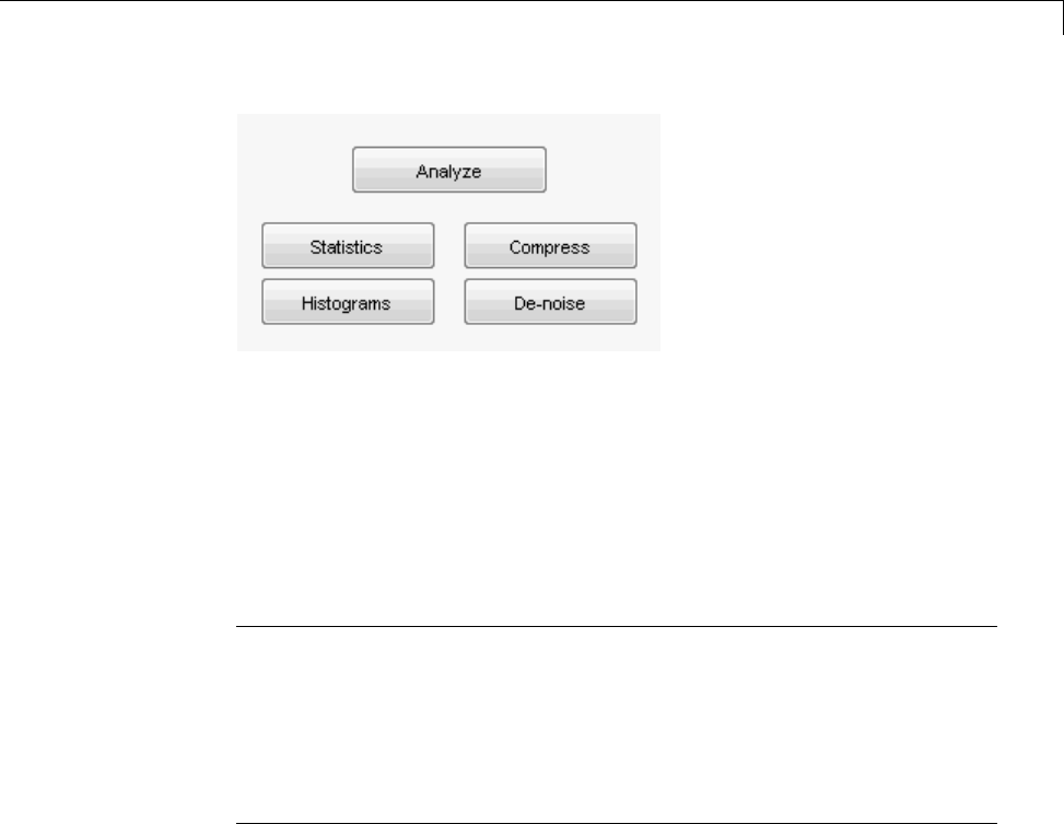
1-D Decimated Wavelet Transforms
Bring up the Compression window: click the Compress button, located
in the middle right of the window, underneath the Analyze button.
The Compression window appears.
While you always have the option of choosing by level thresholding, here
we’ll take advantage of the global thresholding feature for quick and easy
compression.
Note If you want to experiment with manual thresholding, choose the By
Level thresholding option from the menu located at the top right of the
Wavelet 1-D Compression window. The sliders located below this menu
then control the level-dependent thresholds, indicated by yellow dotted
lines running horizontally through the graphs on the left of the window.
The yellow dotted lines can also be dragged directly using the left mouse
button.
Click the Compress button, located at the center right.
After a pause for computation, the electrical consumption signal is
redisplayed in red with the compressed version superimposed in yellow.
Below,we’vezoomedintogetacloserlook at the noisy part of the signal.
3-23
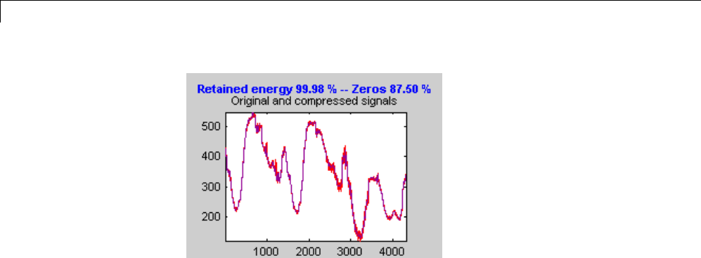
3Discrete Wavelet Analysis
You can see that the compression process removed most of the noise, but
preserved 99.99% of the energy of the signal.
9Show the residuals.
From the Wavelet 1-D Compression tool, click the Residuals button.
The More on Residuals for Wavelet 1-D Compression window appears.
3-24
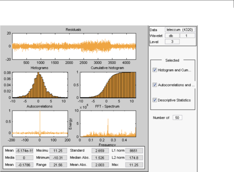
1-D Decimated Wavelet Transforms
Displayed statistics include measures of tendency (mean, mode, median)
and dispersion (range, standard deviation). In addition, the tool provides
frequency-distribution diagrams (histograms and cumulative histograms),
as well as time-series diagrams: autocorrelation function and spectrum.
The same feature exists for the Wavelet 1-D De-noising tool.
Dismiss the Wavelet 1-D Compression window: click the Close button.
When the Update Synthesized Signal dialog box appears, click No.
10 Show statistics.
You can view a variety of statistics about your signal and its components.
FromtheWavelet 1-D tool, click the Statistics button.
3-25
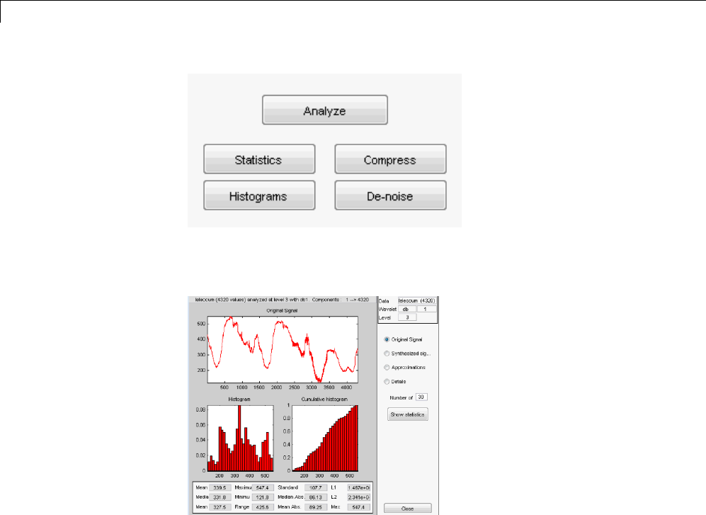
3Discrete Wavelet Analysis
The Wavelet 1-D Statistics window appears displaying by default
statistics on the original signal.
Select the synthesized signal or signal component whose statistics you
want to examine. Click the appropriate option button, and then click the
Show Statistics button. Here, we’ve chosen to examine the synthesized
signal using 100 bins instead of 30, which is the default:
3-26
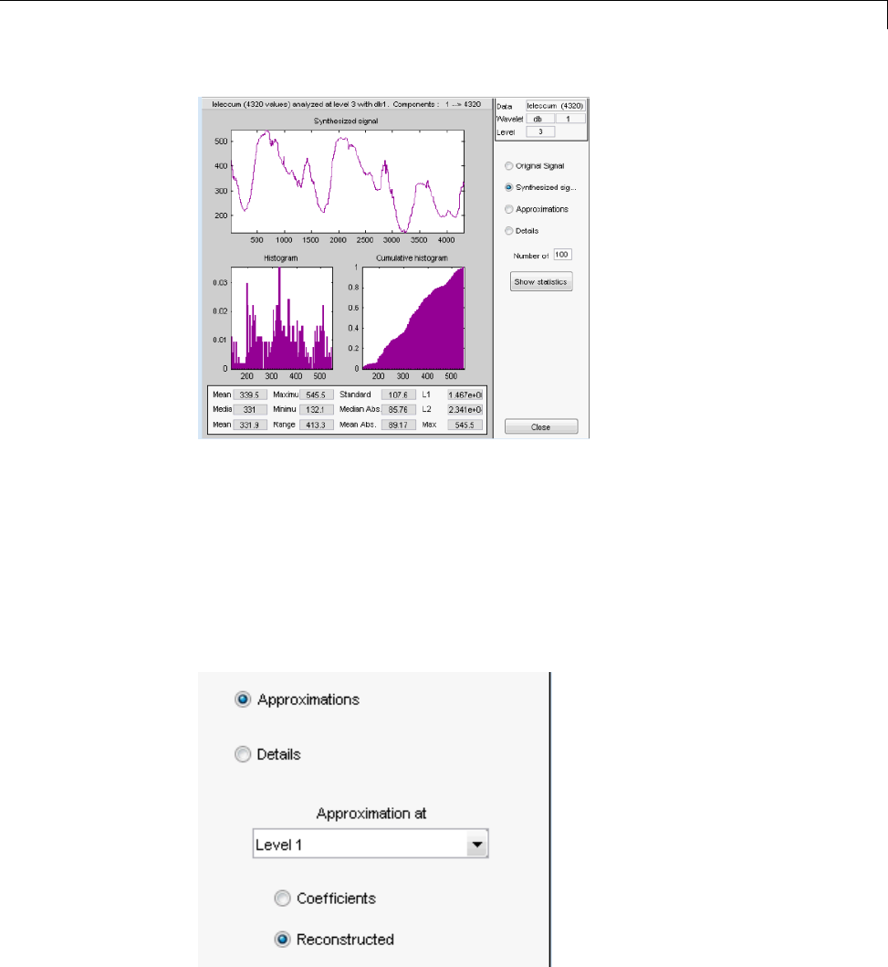
1-D Decimated Wavelet Transforms
Displayed statistics include measures of tendency (mean, mode, median)
and dispersion (range, standard deviation).
In addition, the tool provides frequency-distribution diagrams (histograms
and cumulative histograms). You can plot these histograms separately
using the Histograms button from the Wavelets 1-D window.
Click the Approximation option button. A menu appears from which you
choose the level of the approximation you want to examine.
3-27

3Discrete Wavelet Analysis
Select Level 1 and again click the Show Statistics button. Statistics
appear for the level 1 approximation.
Importing and Exporting Information from the
Graphical Interface
The Wavelet 1-D graphical interface tool lets you import information from
and export information to disk and the MATLAB workspace.
Saving Information to Disk
You can save synthesized signals, coefficients, and decompositions from the
Wavelet1-Dtool to the disk, where the information can be manipulated and
later reimported into the graphical tool.
3-28

1-D Decimated Wavelet Transforms
Saving Synthesized Signals. You can process a signal in the Wavelet
1-D tool and then save the processed signal to a MAT-file (with extension
mat or other).
For example, load the example analysis: File > Example Analysis > Basic
Signals > with db3 at level 5 →Sum of sines, and perform a compression
or de-noising operation on the original signal. When you close the De-noising
or Compression window, update the synthesized signal by clicking Yes
in the dialog box.
Then, from the Wavelet 1-D tool, select the File>Save>Signalmenu
option.
A dialog box appears allowing you to select a folder and filename for the
MAT-file. For this example, choose the name synthsig.
To load the signal into your workspace, simply type
load synthsig;
When the synthesized signal is obtained using any thresholding method
except a global one, the saved structure is
whos
Name Size Bytes Class
synthsig 1x1000 8000 double array
thrParams 1x5 580 cell array
wname 1x3 6 char array
The synthesized signal is given by the variable synthsig. In addition,
the parameters of the de-noising or compression process are given by the
wavelet name (wname) and the level dependent thresholds contained in the
thrParams variable, which is a cell array of length 5 (same as the level of the
decomposition).
For ifrom 1 to 5, thrParams{i} contains the lower and upper bounds of
the thresholding interval and the threshold value (since interval dependent
3-29

3Discrete Wavelet Analysis
thresholds are allowed, see “One-Dimensional Adaptive Thresholding of
Wavelet Coefficients” on page 5-17).
For example, for level 1,
thrParams{1}
ans =
1.0e+03 *
0.0010 1.0000 0.0014
When the synthesized signal is obtained using a global thresholding method,
the saved structure is
Name Size Bytes Class
synthsig 1x1000 8000 double array
valTHR 1x1 8 double array
wname 1x3 6 char array
where the variable valTHR contains the global threshold:
valTHR
valTHR =
1.2922
Saving Discrete Wavelet Transform Coefficients. The Wavelet 1-D tool
lets you save the coefficients of a discrete wavelet transform (DWT) to disk.
The toolbox creates a MAT-file in the current folder with a name you choose.
To save the DWT coefficients from the present analysis, use the menu option
File > Save > Coefficients.
A dialog box appears that lets you specify a folder and filename for storing
the coefficients.
Consider the example analysis:
3-30

1-D Decimated Wavelet Transforms
File > Example Analysis > Basic Signals > with db1 at level 5 →
Cantor curve.
After saving the wavelet coefficients to the file cantor.mat, load the variables
into your workspace:
load cantor
whos
Name Size Bytes Class
coefs 1x2190 17520 double array
longs 1x7 56 double array
thrParams 0x0 0 double array
wname 1x3 6 char array
Variable coefs contains the discrete wavelet coefficients. More precisely, in
the above example coefs is a 1-by-2190 vector of concatenated coefficients,
and longs is a vector giving the lengths of each component of coefs.
Variable wname contains the wavelet name and thrParams is empty since
the synthesized signal does not exist.
Saving Decompositions. The Wavelet 1-D tool lets you save the entire
set of data from a discrete wavelet analysis to disk. The toolbox creates
a MAT-file in the current folder with a name you choose, followed by the
extension wa1 (wavelet analysis 1-D).
Open the Wavelet 1-D tool and load the example analysis:
File > Example Analysis > Basic Signals > with db3 at level 5 →Sum
of sines
To save the data from this analysis, use the menu option File > Save >
Decomposition.
A dialog box appears that lets you specify a folder and filename for storing
the decomposition data. Type the name wdecex1d.
3-31

3Discrete Wavelet Analysis
After saving the decomposition data to the file wdecex1d.wa1,loadthe
variables into your workspace:
load wdecex1d.wa1 -mat
whos
Name Size Bytes Class
coefs 1x10²³ 8184 double array
data_name 1x6 12 char array
longs 1x7 56 double array
thrParams 0x0 0 double array
wave_name 1x3 6 char array
Note Save options are also available when performing de-noising or
compression inside the Wavelet 1-D tool. In the Wavelet 1-D De-noising
window, you can save denoised signal and decomposition. The same holds true
for the Wavelet 1-D Compression window. This way, you can save many
different trials from inside the De-noising and Compression windows without
going back to the main Wavelet 1-D window during a fine-tuning process.
Note When saving a synthesized signal, a decomposition or coefficients to a
MAT-file, the mat file extension is not necessary. You can save approximations
individually for each level or save them all at once.
Export to Workspace
The Wavelet 1-D tool allows you to export your 1-D wavelet analysis to the
MATLAB workspace in a number of formats.
For example, load the example analysis for the freqbrk signal.
3-32
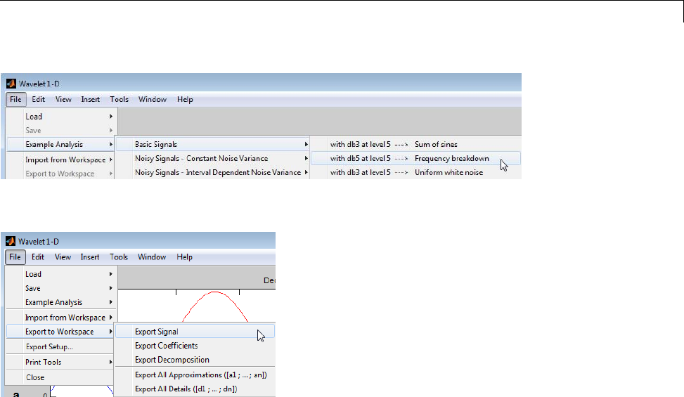
1-D Decimated Wavelet Transforms
After the wavelet 1-D analysis loads, select File > Export to Workspace.
You have the option to
•Export Signal — This option exports the synthesized signal vector.
•Export Coefficients — This option exports the vector of wavelet and
scaling coefficients, the bookkeeping vector, and the analyzing wavelet in
a structure array. The wavelet and scaling coefficient and bookkeeping
vectors are identical to the output of wavedec.
•Export Decomposition —ThisoptionisidenticaltoExport Coefficients
except that it also contains the name of the analyzed signal.
•Export All Approximations — This option exports a L-by-N matrix
whereListhevalueofLevel and N is the length of the input signal.
Each row of the matrix is the projection onto the approximation space at
the corresponding level. For example, the first row of the matrix is the
projection onto the approximation space at level 1.
•Export All Details — This option exports a L-by-N matrix where L is
the value of Level and N is the length of the input signal. Each row of the
matrix is the projection onto the detail (wavelet) space at the corresponding
3-33
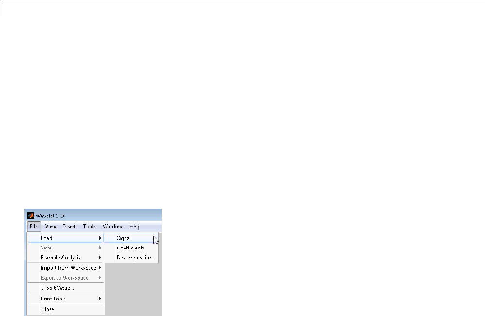
3Discrete Wavelet Analysis
level. For example, the first row of the matrix is the projection onto the
detail space at level 1.
Loading Information into the Wavelet 1-D Tool
You can load signals, coefficients, or decompositions into the graphical
interface. The information you load may have been previously exported from
the graphical interface, and then manipulated in the workspace, or it may
have been information you generated initially from the command line.
In either case, you must observe the strict file formats and data structures
used by the Wavelet 1-D tool, or else errors will result when you try to load
information.
Loading Signals. To load a signal you’ve constructed in your MATLAB
workspaceintotheWavelet 1-D tool, save the signal in a MAT-file (with
extension mat or other).
For instance, suppose you’ve designed a signal called warma and want to
analyze it in the Wavelet 1-D tool.
save warma warma
The workspace variable warma must be a vector.
sizwarma = size(warma)
sizwarma =
1 1000
3-34
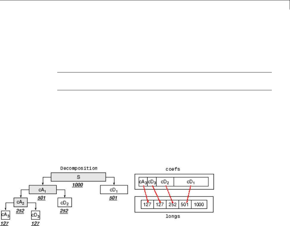
1-D Decimated Wavelet Transforms
To load this signal into the Wavelet 1-D tool, use the menu option File >
Load > Signal.
A dialog box appears that lets you select the appropriate MAT-file to be loaded.
Note The first one-dimensional variable encountered in the file is considered
the signal. Variables are inspected in alphabetical order.
Loading Discrete Wavelet Transform Coefficients. To load discrete
wavelet transform coefficients into the Wavelet 1-D tool, you must first save
the appropriate data in a MAT-file, which must contain at least the two
variables coefs and longs.
Variable coefs must be a vector of DWT coefficients (concatenated for the
various levels), and variable longs a vector specifying the length of each
component of coefs, as well as the length of the original signal.
After constructing or editing the appropriate data in your workspace, type
save myfile coefs longs
Use the File > Load > Coefficients menu option from the Wavelet 1-D tool
to load the data into the graphical tool.
A dialog box appears, allowing you to choose the folder and file in which your
data reside.
3-35

3Discrete Wavelet Analysis
Loading Decompositions. To load discrete wavelet transform decomposition
data into the Wavelet 1-D graphical interface, you must first save the
appropriate data in a MAT-file (with extension wa1 or other).
The MAT-file contains the following variables.
Variable Status Description
coefs Required Vector of concatenated DWT
coefficients
longs Required Vector specifying lengths of
components of coefs and of the
original signal
wave_name Required String specifying name of wavelet used
for decomposition (e.g., db3)
data_name Optional String specifying name of
decomposition
After constructing or editing the appropriate data in your workspace, type
save myfile coefs longs wave_name
Use the File > Load > Decomposition menu option from the Wavelet 1-D
tool to load the decomposition data into the graphical tool.
A dialog box appears, allowing you to choose the folder and file in which your
data reside.
Note When loading a signal, a decomposition or coefficients from a MAT-file,
the extension of this file is free. The mat extension is not necessary.
3-36

FastWaveletTransform(FWT)Algorithm
Fast Wavelet Transform (FWT) Algorithm
In 1988, Mallat produced a fast wavelet decomposition and reconstruction
algorithm [Mal89]. The Mallat algorithm for discrete wavelet transform
(DWT) is, in fact, a classical scheme in the signal processing community,
known as a two-channel subband coder using conjugate quadrature filters
or quadrature mirror filters (QMFs).
•The decomposition algorithm starts with signal s,nextcalculatesthe
coordinates of A1and D1,andthenthoseofA2and D2,andsoon.
•The reconstruction algorithm called the inverse discrete wavelet transform
(IDWT) starts from the coordinates of AJand DJ,nextcalculatesthe
coordinates of AJ–1, and then using the coordinates of AJ–1 and DJ–1
calculates those of AJ–2,andsoon.
This section addresses the following topics:
•“Filters Used to Calculate the DWT and IDWT” on page 3-37
•“Algorithms” on page 3-40
•“Why Does Such an Algorithm Exist?” on page 3-45
•“One-Dimensional Wavelet Capabilities” on page 3-49
•“Two-Dimensional Wavelet Capabilities” on page 3-50
Filters Used to Calculate the DWT and IDWT
For an orthogonal wavelet, in the multiresolution framework, we start with
the scaling function φand the wavelet function ψ. One of the fundamental
relations is the twin-scale relation (dilation equation or refinement equation):
1
22
φφ
xwxn
n
nZ
⎛
⎝
⎜⎞
⎠
⎟=−
∈
∑()
All the filters used in DWT and IDWT are intimately related to the sequence
(wn)n Z
3-37
3Discrete Wavelet Analysis
Clearly if φis compactly supported, the sequence (wn)isfiniteandcan
be viewed as a filter. The filter W, which is called the scaling filter
(nonnormalized), is
•Finite Impulse Response (FIR)
•Of length 2N
•Of sum 1
•Of norm
1
2
•Alow-passfilter
For example, for the db3 scaling filter,
load db3
db3
db3 =
0.2352 0.5706 0.3252 -0.0955 -0.0604 0.0249
sum(db3)
ans =
1.0000
norm(db3)
ans =
0.7071
From filter W, we define four FIR filters, of length 2Nand of norm 1,
organized as follows.
Filters Low-Pass High-Pass
Decomposition Lo_D Hi_D
Reconstruction Lo_R Hi_R
The four filters are computed using the following scheme.
3-38
FastWaveletTransform(FWT)Algorithm
where qmf is such that Hi_R and Lo_R are quadrature mirror filters (i.e.,
Hi_R(k)=(–1)kLo_R(2N+1–k)) for k=1,2,...,2N.
Note that wrev flips the filter coefficients. So Hi_D and Lo_D are also
quadrature mirror filters. The computation of these filters is performed using
orthfilt. Next, we illustrate these properties with the db6 wavelet.
Load the Daubechies’ extremal phase scaling filter and plot the coefficients.
load db6;
subplot(421); stem(db6,'markerfacecolor',[0 0 1]);
title('Original scaling filter');
Use orthfilt to return the analysis (decomposition) and synethsis
(reconstruction) filters.
Obtain the discrete Fourier transforms (DFT) of the lowpass and highpass
analysis filters. Plot the modulus of the DFT.
LoDFT = fft(Lo_D,64);
HiDFT = fft(Hi_D,64);
freq = -pi+(2*pi)/64:(2*pi)/64:pi;
subplot(427); plot(freq,fftshift(abs(LoDFT)));
set(gca,'xlim',[-pi,pi]); xlabel('Radians/sample');
title('DFT Modulus - Lowpass Filter')
subplot(428); plot(freq,fftshift(abs(HiDFT)));
set(gca,'xlim',[-pi,pi]); xlabel('Radians/sample');
title('Highpass Filter');
3-39
3Discrete Wavelet Analysis
Algorithms
Given a signal sof length N, the DWT consists of log2Nstages at most.
Starting from s, the first step produces two sets of coefficients: approximation
coefficients cA1, and detail coefficients cD1. These vectors are obtained by
convolving swith the low-pass filter Lo_D for approximation, and with the
high-pass filter Hi_D for detail, followed by dyadic decimation.
More precisely, the first step is
3-40
FastWaveletTransform(FWT)Algorithm
The length of each filter is equal to 2n.IfN=length(s), the signals Fand G
are of length N+2n– 1, and then the coefficients cA1and cD1are of length
floor ()Nn
−+
⎛
⎝
⎜⎞
⎠
⎟
1
2
The next step splits the approximation coefficients cA1in two parts using the
same scheme, replacing sby cA1and producing cA2and cD2,andsoon.
So the wavelet decomposition of the signal sanalyzed at level jhas the
following structure: [cAj,cDj, ..., cD1].
3-41

3Discrete Wavelet Analysis
This structure contains for J = 3 the terminal nodes of the following tree.
•Conversely, starting from cAjand cDj, the IDWT reconstructs cAj–1,
inverting the decomposition step by inserting zeros and convolving the
results with the reconstruction filters.
3-42
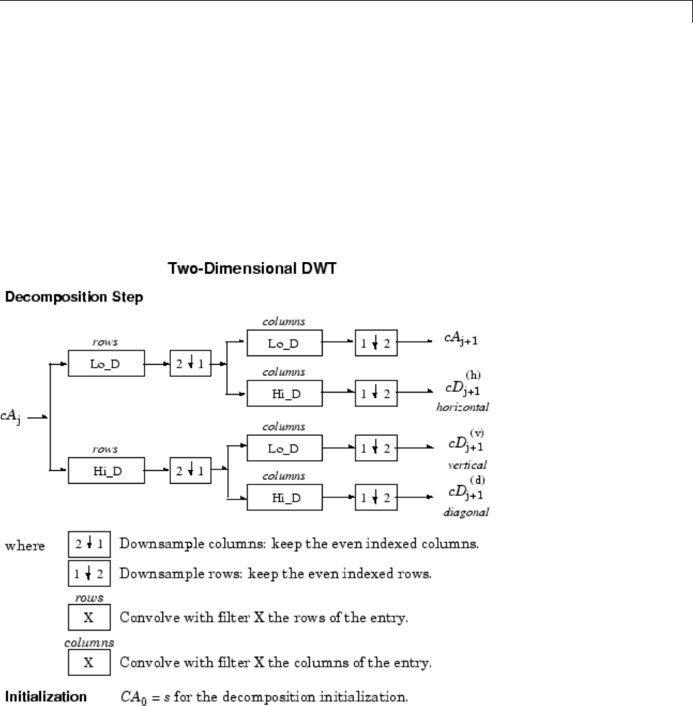
FastWaveletTransform(FWT)Algorithm
•For images, a similar algorithm is possible for two-dimensional wavelets
and scaling functions obtained from one-dimensional wavelets by tensorial
product.
This kind of two-dimensional DWT leads to a decomposition of
approximation coefficients at level jin four components: the approximation
at level j+ 1 and the details in three orientations (horizontal, vertical,
and diagonal).
The following charts describe the basic decomposition and reconstruction
steps for images.
3-43
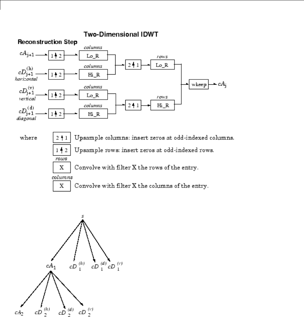
3Discrete Wavelet Analysis
So, for J= 2, the two-dimensional wavelet tree has the following form.
3-44

FastWaveletTransform(FWT)Algorithm
Finally, let us mention that, for biorthogonal wavelets, the same algorithms
hold but the decomposition filters on one hand and the reconstruction filters
on the other hand are obtained from two distinct scaling functions associated
with two multiresolution analyses in duality.
In this case, the filters for decomposition and reconstruction are, in general,
of different odd lengths. This situation occurs, for example, for “splines”
biorthogonal wavelets used in the toolbox. By zero-padding, the four filters
can be extended in such a way that they will have the same even length.
Why Does Such an Algorithm Exist?
The previous paragraph describes algorithms designed for finite-length
signals or images. To understand the rationale, we must consider
infinite-length signals. The methods for the extension of a given finite-length
signal are described in “Border Effects” on page 3-52.
Let us denote h= Lo_R and g= Hi_R and focus on the one-dimensional case.
We first justify how to go from level jto level j+1, for the approximation vector.
This is the main step of the decomposition algorithm for the computation
oftheapproximations. Thedetailsarecalculatedinthesamewayusing
the filter ginstead of filter h.
Let (Ak
(j))k Z be the coordinates of the vector Aj:
AA
jk
jjk
k
=∑() ,
φ
and Ak
(j+1) the coordinates of the vector Aj+1:
AA
jk
jjk
k
+++
=∑
111
() ,
φ
Ak
(j+1) is calculated using the formula
AhA
kjnkn
j
n
() ()+−
=∑
12
3-45

3Discrete Wavelet Analysis
This formula resembles a convolution formula.
The computation is very simple.
Let us define
hk h k F hk nAn
kjj
n
() ( ), () ()
=− = −
+∑
and
1
The sequence F(j+1) is the filtered output of the sequence A(j)by the filter
h.
We obtain
Ak
(j+1) =F2k
(j+1)
We have to take the even index values of F.Thisisdownsampling.
The sequence A(j+1) is the downsampled version of the sequence F(j+1).
The initialization is carried out using Ak
(0) =s(k), where s(k)isthesignal
value at time k.
There are several reasons for this surprising result, all of which are linked to
the multiresolution situation and to a few of the properties of the functions
φj,k and ψj,k.
Let us now describe some of them.
1The family (, )
,
φ
0kkZ∈is formed of orthonormal functions. As a
consequence for any j,thefamily (, )
,
φ
jk kZ∈is orthonormal.
2The double indexed family
(,,)
,
ψ
jk jZkZ∈∈
is orthonormal.
3For any j,the (, )
,
φ
jk kZ∈are orthogonal to (, , )
,
ψ
′′≤∈
jk jjkZ
.
3-46
FastWaveletTransform(FWT)Algorithm
4Between two successive scales, we have a fundamental relation, called
the twin-scale relation.
Twin-Scale Relation for φφ
φφ
10 0,,
=
∈
∑hkk
kZ
φφ
jkjk
kZ
h
+∈
=∑
10,,
This relation introduces the algorithm’s hfilter ()hnn
=2
ω
.Formore
information, see “Filters Used to Calculate the DWT and IDWT” on page
3-37.
5We check that:
aThecoordinateofφj+1,0 on φj,k is hkand does not depend on j.
bThe coordinate of φj+1,non φj,k is equal to
φφ
jnjk kn
h
+−
=
12,,
,.
6These relations supply the ingredients for the algorithm.
7Up to now we used the filter h. The high-pass filter gis used in the twin
scales relation linking the ψand φfunctions. Between two successive
scales, we have the following twin-scale fundamental relation.
Twin-Scale Relation Between ψψ and φφ
ψ
φ
10 0,,
=
∈
∑gkk
kZ
ψ
φ
jkjk
kZ
g
+∈
=∑
10,,
8After the decomposition step, we justify now the reconstruction algorithm
by building it. Let us simplify the notation. Starting from A1and D1,letus
study A0=A1+Dj1. The procedure is the same to calculate A=Aj+1 +Dj+1.
Let us define αn,δn,
α
k
0by
3-47

3Discrete Wavelet Analysis
Aa D Aa
nn
n
nn
n
kk
k
111 10
00
== =
∑∑∑
φδψ φ
,,,
Let us assess the
α
k
0coordinates as
aA AD A D
a
kk k k k
n
n
nk n
n
000 1 10 10 10
10
==+=+
=+
∑∑
,,,,
,
,,,,
,,
φφφφ
φφ δψ
110
22
,,
,
nk
nk n
n
nk n
n
ah g
φ
δ
=+
−−
∑∑
We will focus our study on the first sum ah
nk n
n−
∑2;the second sum
δ
nk n
ng−
∑2is handled in a similar manner.
The calculations are easily organized if we note that (taking k=0inthe
previous formulas, makes things simpler)
ah a h ah ah ah
ah h ah h
nn
n
−− −−
−−
=+ + + + +
=+ + + + +
∑212001224
12 1 00 1
00
aah h ah
12 3 24
0
−− −
++ +
If we transform the ()
α
nsequence into a new sequence ()
α
ndefined by
..., α–1,0,α0,0,α1,0,α2,0,... thatisprecisely
aaa
nnn22
10=+=,
Then
ah ah
nn
n
nn
n
−−
=
∑∑
2
and by extension
3-48

FastWaveletTransform(FWT)Algorithm
ah ah
nk n
n
nkn
n
−−
=
∑∑
2
Since
aah g
knkn
n
nkn
n
0=+
−−
∑∑
δ
the reconstruction steps are:
1Replace the αand δsequences by upsampled versions α˜and
δ
inserting
zeros.
2Filter by hand grespectively.
3Sum the obtained sequences.
One-Dimensional Wavelet Capabilities
Basic One-Dimensional Objects.
Objects Description
Signal in original time s
Ak,0≤k≤j
Dk,1≤k≤j
Original signal
Approximation at level k
Detail at level k
Coefficients in
scale-related time
cAk,1≤k≤j
cDk,1≤k≤j
[cAj,cDj,...,cD1]
Approximation coefficients at level k
Detail coefficients at level k
Wavelet decomposition at level j, j ≥1
Analysis-Decomposition Capabilities.
3-49

3Discrete Wavelet Analysis
Purpose Input Output File
Single-level decomposition scA1,cD1dwt
Single-level decomposition cAjcAj+1,cDj+1 dwt
Decomposition s[cAj,cDj, ..., cD1]wavedec
Synthesis-Reconstruction Capabilities.
Purpose Input Output File
Single-level reconstruction cA1,cD1sor A0idwt
Single-level reconstruction cAj+1,cDj+1 cAjidwt
Full reconstruction [cAj,cDj,...,cD1]sor A0waverec
Selective reconstruction [cAj,cDj,...,cD1]Al,Dmwrcoef
Decomposition Structure Utilities.
Purpose Input Output File
Extraction of detail coefficients [cAj,cDj,...,cD1]cDk,1≤k≤jdetcoef
Extraction of approximation
coefficients
[cAj,cDj,...,cD1]cAk,0≤k≤jappcoef
Recomposition of the
decomposition structure
[cAj,cDj,...,cD1][cAk,cDk, ..., cD1]1≤k
≤j
upwlev
To illustrate command-line mode for one-dimensional capabilities, see
“One-Dimensional Analysis Using the Command Line” on page 3-4. .
Two-Dimensional Wavelet Capabilities
Basic Two-Dimensional Objects.
3-50

FastWaveletTransform(FWT)Algorithm
Objects Description
sOriginal image
A0Approximation at level 0
Ak,1≤k≤jApproximation at level k
Image in original
resolution
Dk,1≤k≤jDetails at level k
cAk,1≤k≤jApproximation coefficients at level k
cDk,1≤k≤jDetail coefficients at level k
Coefficients in
scale-related resolution
[cAj,cDj, ..., cD1]Wavelet decomposition at level j
Dkstands for DDD
khkvkd() () ()
,,
⎡
⎣⎤
⎦, the horizontal, vertical, and diagonal
details at level k.
The same holds for cDk,whichstandsfor cD cD cD
khkvkd() () ()
,,
⎡
⎣⎤
⎦.
The two-dimensional files are the same as those for the one-dimensional case,
but with a 2appended on the end of the command.
For example, idwt becomes idwt2. For more information, see
“One-Dimensional Wavelet Capabilities” on page 3-49.
To illustrate command-line mode for two-dimensional capabilities, see
“Two-Dimensional Analysis — Command Line” on page 3-138..
3-51

3Discrete Wavelet Analysis
Border Effects
Classically, the DWT is defined for sequences with length of some power of 2,
and different ways of extending samples of other sizes are needed. Methods
for extending the signal include zero-padding, smooth padding, periodic
extension, and boundary value replication (symmetrization).
The basic algorithm for the DWT is not limited to dyadic length and is based
on a simple scheme: convolution and downsampling. As usual, when a
convolution is performed on finite-length signals, border distortions arise.
Signal Extensions: Zero-Padding, Symmetrization,
and Smooth Padding
To deal with border distortions, the border should be treated differently from
the other parts of the signal.
Various methods are available to deal with this problem, referred to as
“wavelets on the interval” (see [CohDJV93] in “References”). These interesting
constructions are effective in theory but are not entirely satisfactory from
a practical viewpoint.
Often it is preferable to use simple schemes based on signal extension on the
boundaries. This involves the computation of a few extra coefficients at each
stage of the decomposition process to get a perfect reconstruction. It should be
noted that extension is needed at each stage of the decomposition process.
Details on the rationale of these schemes are in Chapter 8 of the book Wavelets
and Filter Banks, by Strang and Nguyen (see [StrN96] in “References”).
The available signal extension modes are as follows (see dwtmode):
•Zero-padding ('zpd'): This method is used in the version of the DWT
given in the previous sections and assumes that the signal is zero outside
the original support.
The disadvantage of zero-padding is that discontinuities are artificially
created at the border.
3-52

Border Effects
•Symmetrization ('sym'): This method assumes that signals or images
can be recovered outside their original support by symmetric boundary
value replication.
It is the default mode of the wavelet transform in the toolbox.
Symmetrization has the disadvantage of artificially creating discontinuities
of the first derivative at the border, but this method works well in general
for images.
•Smooth padding of order 1 ('spd'or 'sp1'): This method assumes
that signals or images can be recovered outside their original support
by a simple first-order derivative extrapolation: padding using a linear
extension fit to the first two and last two values.
Smooth padding works well in general for smooth signals.
•Smooth padding of order 0 ('sp0'): This method assumes that signals
or images can be recovered outside their original support by a simple
constant extrapolation. For a signal extension this is the repetition of the
first value on the left and last value on the right.
•Periodic-padding (1) ('ppd'): This method assumes that signals
or images can be recovered outside their original support by periodic
extension.
The disadvantage of periodic padding is that discontinuities are artificially
created at the border.
TheDWTassociatedwiththesefivemodes is slightly redundant. But IDWT
ensures a perfect reconstruction for any of the five previous modes whatever
the extension mode used for DWT.
•Periodic-padding (2) ('per'): If the signal length is odd, the signal is
first extended by adding an extra-sample equal to the last value on the
right. Then a minimal periodic extension is performed on each side. The
same kind of rule exists for images. This extension mode is used for SWT
(1-D & 2-D).
This last mode produces the smallest length wavelet decomposition. But
the extension mode used for IDWT must be the same to ensure a perfect
reconstruction.
3-53

3Discrete Wavelet Analysis
Before looking at an illustrative example, let us compare some properties of
the theoretical Discrete Wavelet Transform versus the actual DWT.
The theoretical DWT is applied to signals that are defined on an infinite
length time interval (Z). For an orthogonal wavelet, this transform has the
following desirable properties:
1Norm preservation
Let cA and cD be the approximation and detail of the DWT coefficients of
an infinite length signal X. Then the l2–norm is preserved:
X2=cA 2+cD 2
2Orthogonality
Let Aand Dbe the reconstructed approximation and detail. Then, Aand
Dare orthogonal and
X2=A2+D2
3Perfect reconstruction
X=A+D
Since the DWT is applied to signals that are defined on a finite-length
time interval, extension is needed for the decomposition, and truncation is
necessary for reconstruction.
To ensure the crucial property 3(perfect reconstruction) for arbitrary choices
of
•The signal length
•The wavelet
•The extension mode
the properties 1and 2can be lost. These properties hold true for an extended
signal of length usually larger than the length of the original signal. So only
the perfect reconstruction property is always preserved. Nevertheless if the
3-54

Border Effects
DWT is performed using the periodic extension mode (’per’) and if the length
of the signal is divisible by 2J,whereJis the maximum level decomposition,
the properties 1,2,and3remain true.
It is interesting to notice that if arbitrary extension is used, and
decomposition performed using the convolution-downsampling scheme,
perfect reconstruction is recovered using idwt or idwt2. This point is
illustrated below.
% Set initial signal and get filters.
x = sin(0.3*[1:451]); w = 'db9';
[Lo_D,Hi_D,Lo_R,Hi_R] = wfilters(w);
% In fact using a slightly redundant scheme, any signal
% extension strategy works well.
% For example use random padding.
3-55
3Discrete Wavelet Analysis
lx = length(x); lf = length(Lo_D);
ex = [randn(1,lf) x randn(1,lf)];
axis([1 lx+2*lf -2 3])
subplot(211), plot(lf+1:lf+lx,x), title('Original signal')
axis([1 lx+2*lf -2 3])
subplot(212), plot(ex), title('Extended signal')
axis([1 lx+2*lf -2 3])
% Decomposition.
la = floor((lx+lf-1)/2);
ar = wkeep(dyaddown(conv(ex,Lo_D)),la);
dr = wkeep(dyaddown(conv(ex,Hi_D)),la);
% Reconstruction.
xr = idwt(ar,dr,w,lx);
3-56
Border Effects
% Check perfect reconstruction.
err0 = max(abs(x-xr))
Now let us illustrate the differences between the first three methods both for
1-D and 2-D signals.
Zero-Padding
Using the GUI we will examine the effects of zero-padding.
1From the MATLAB prompt, type
dwtmode('zpd')
2From the MATLAB prompt, type wavemenu.
The Wavelet Toolbox Main Menu appears.
3Click the Wavelet 1-D menu item.The discrete wavelet analysis tool for
one-dimensional signal data appears.
4From the File menu, choose the Example Analysis option and select
Basic Signals > with db2 at level 5 > Two nearby discontinuities.
5Select Display Mode: Show and Scroll.
The detail coefficients clearly show the signal end effects.
Symmetric Extension
6From the MATLAB prompt, type
dwtmode('sym')
3-57
3Discrete Wavelet Analysis
7Click the Wavelet 1-D menu item.
The discrete wavelet analysis tool for one-dimensional signal data appears.
8From the File menu, choose the Example Analysis option and select
Basic Signals > with db2 at level 5 > Two nearby discontinuities.
9From the MATLAB prompt, type
dwtmode('spd')
10 Click the Wavelet 1-D menu item.
The discrete wavelet analysis tool for one-dimensional signal data appears.
11 From the File menu, choose the Example Analysis option and select
Basic Signals > with db2 at level 5 > Two nearby discontinuities.
12 Select Display Mode: Show and Scroll.
The detail coefficients show the signal end effects are not present, and the
discontinuities are well detected.
Let us now consider an image example.
Original Image
1From the MATLAB prompt, type
load geometry;
% X contains the loaded image and
% map contains the loaded colormap.
nbcol = size(map,1);
3-58
Border Effects
colormap(pink(nbcol));
image(wcodemat(X,nbcol));
Zero-Padding
Now we set the extension mode to zero-padding and perform a
decomposition of the image to level 3 using the sym4 wavelet. Then we
reconstruct the approximation of level 3.
2From the MATLAB prompt, type
lev = 3; wname = 'sym4';
dwtmode('zpd')
[c,s] = wavedec2(X,lev,wname);
a = wrcoef2('a',c,s,wname,lev);
image(wcodemat(a,nbcol));
3-59
3Discrete Wavelet Analysis
Symmetric Extension
Nowwesettheextensionmodetosymmetric extension and perform a
decomposition of the image again to level 3 using the sym4 wavelet. Then
we reconstruct the approximation of level 3.
3From the MATLAB prompt, type
dwtmode('sym')
[c,s] = wavedec2(X,lev,wname);
a = wrcoef2('a',c,s,wname,lev);
image(wcodemat(a,nbcol));
Smooth Padding
3-60
Border Effects
Now set the extension mode to smooth padding and perform a
decomposition of the image again to level 3 using the sym4 wavelet. Then
reconstruct the approximation of level 3.
4From the MATLAB prompt, type
dwtmode('spd')
[c,s] = wavedec2(X,lev,wname);
a = wrcoef2('a',c,s,wname,lev);
image(wcodemat(a,nbcol));
3-61

3Discrete Wavelet Analysis
Discrete Stationary Wavelet Transform (SWT)
We know that the classical DWT suffers a drawback: the DWT is not a
time-invariant transform. This means that, even with periodic signal
extension, the DWT of a translated version of a signal Xis not, in general, the
translated version of the DWT of X.
How to restore the translation invariance, which is a desirable property lost by
theclassicalDWT?TheideaistoaveragesomeslightlydifferentDWT,called
ε-decimated DWT, to define the stationary wavelet transform (SWT). This
property is useful for several applications such as breakdown points detection.
The main application of the SWT is de-noising. For more information on the
rationale, see [CoiD95] in “References”. For examples, see “One-Dimensional
Discrete Stationary Wavelet Analysis” on page 3-69and “Two-Dimensional
Discrete Stationary Wavelet Analysis” on page 3-166. .
The principle is to average several denoised signals. Each of them is obtained
using the usual de-noising scheme (see “Denoising and Nonparametric
Function Estimation” on page 5-2), but applied to the coefficients of an
ε-decimated DWT.
Note We define the SWT only for signals of length divisible by 2J,where
Jis the maximum decomposition level, and we use the DWT with periodic
(per) extension.
ε
-Decimated DWT
What is an ε-decimated DWT?
There exist a lot of slightly different ways to handle the discrete wavelet
transform. Let us recall that the DWT basic computational step is a
convolution followed by a decimation. The decimation retains even indexed
elements.
But the decimation could be carried outbychoosingoddindexedelements
instead of even indexed elements. This choice concerns every step of the
decomposition process, so at every level we chose odd or even.
3-62

Discrete Stationary Wavelet Transform (SWT)
If we perform all the different possible decompositions of the original signal,
we have 2Jdifferent decompositions, for a given maximum level J.
Let us denote by εj= 1 or 0 the choice of odd or even indexed elements at step
j. Every decomposition is labeled by a sequence of 0s and 1s: ε=ε1...,εJ.This
transform is called the ε-decimated DWT.
You can obtain the basis vectors of the ε-decimated DWT from those of the
standard DWT by applying a shift and corresponds to a special choice of the
origin of the basis functions.
How to Calculate the
ε
-Decimated DWT: SWT
Itispossibletocalculatealltheε-decimated DWT for a given signal of length
N, by computing the approximation and detail coefficients for every possible
sequence ε. Do this using iteratively, a slightly modified version of the basic
step of the DWT of the form:
[A,D] = dwt(X,wname,'mode','per','shift',e);
The last two arguments specify the way to perform the decimation step. This
is the classical one for e=0, but for e=1 the odd indexed elements are
retained by the decimation.
Of course, this is not a good way to calculate all the ε-decimated DWT, because
many computations are performed many times. We shall now describe
another way, which is the stationary wavelet transform (SWT).
The SWT algorithm is very simple and is close to the DWT one. More precisely,
for level 1, all the ε-decimated DWT (only two at this level) for a given signal
can be obtained by convolving the signal with the appropriate filters as in the
DWT case but without downsampling. Then the approximation and detail
coefficients at level 1 are both of size N, which is the signal length. This can
be visualized in the following figure.
3-63

3Discrete Wavelet Analysis
The general step jconvolves the approximation coefficients at level j–1,
with upsampled versions of the appropriate original filters, to produce the
approximation and detail coefficients at level j. This can be visualized in
the following figure.
Next, we illustrate how to extract a given ε-decimated DWT from the
approximation and detail coefficients structure of the SWT.
3-64

Discrete Stationary Wavelet Transform (SWT)
We decompose a sequence of height numbers with the SWT, at level J=3,
using an orthogonal wavelet.
The function swt calculates successively the following arrays, where
A(j,ε1,...,εj)or D(j,ε1,...,εj)denotes an approximation or a detail coefficient at
level jobtained for the ε-decimated DWT characterized by ε=[ε1,...,εj].
Step 0 (Original Data).
A(0) A(0) A(0) A(0) A(0) A(0) A(0) A(0)
Step 1.
D(1,0) D(1,1) D(1,0) D(1,1) D(1,0) D(1,1) D(1,0) D(1,1)
A(1,0) A(1,1) A(1,0) A(1,1) A(1,0) A(1,1) A(1,0) A(1,1)
Step 2.
D(1,0) D(1,1) D(1,0) D(1,1) D(1,0) D(1,1) D(1,0) D(1,1)
D(2,0,0) D(2,1,0) D(2,0,1) D(2,1,1) D(2,0,0) D(2,1,0) D(2,0,1) D(2,1,1)
A(2,0,0) A(2,1,0) A(2,0,1) A(2,1,1) A(2,0,0) A(2,1,0) A(2,0,1) A(2,1,1)
Step 3.
D(1,0) D(1,1) D(1,0) D(1,1) D(1,0) D(1,1) D(1,0) D(1,1)
D(2,0,0) D(2,1,0) D(2,0,1) D(2,1,1) D(2,0,0) D(2,1,0) D(2,0,1) D(2,1,1)
D(3,0,0,0) D(3,1,0,0) D(3,0,1,0) D(3,1,1,0) D(3,0,0,1) D(3,1,0,1) D(3,0,1,1) D(3,1,1,1)
A(3,0,0,0) A(3,1,0,0) A(3,0,1,0) A(3,1,1,0) A(3,0,0,1) A(3,1,0,1) A(3,0,1,1) A(3,1,1,1)
Let jdenote the current level, where jis also the current step of the algorithm.
Then we have the following abstract relations with εi=0or1:
[tmpAPP,tmpDET] =
dwt(A(j, 1,,j),wname,'mode','per','shift', j+1);
A(j+1, 1,,j,j+1) = wshift('1D',tmpAPP, j+1);
D(j+1, 1,,j,j+1) = wshift('1D',tmpDET, j+1);
3-65

3Discrete Wavelet Analysis
where wshift performs a ε-circular shift of the input vector. Therefore, if
εj+1 =0,thewshift instruction is ineffective and can be suppressed.
Let ε=[ε1,...,εJ]withεi=0or1.Wehave2
J=2
3=eightdifferentε-decimated
DWTs at level 3. Choosing ε, we can retrieve the corresponding ε-decimated
DWT from the SWT array.
Now, consider the last step, J=3,andlet[Cε,Lε] denote the wavelet
decomposition structure of an ε-decimated DWT for a given ε. Then, it can be
retrieved from the SWT decomposition structure by selecting the appropriate
coefficients as follows:
Cε=
A(3, ε1,ε2,ε3)D(3,ε1,ε2,ε3)D(2,ε1,ε2)D(2,ε1,ε2)D(1,ε1)D(1,ε1)D(1,ε1)D(1,ε1)
Lε= [1,1,2,4,8]
For example, the ε-decimated DWT corresponding to ε=[ε1,ε2,ε3] = [1,0,1] is
shown in bold in the sequence of arrays of the previous example.
Thiscanbeextendedtothe2-Dcase. Thealgorithmforthestationarywavelet
transform for images is visualized in the following figure.
3-66
Discrete Stationary Wavelet Transform (SWT)
Inverse Discrete Stationary Wavelet Transform (ISWT)
Each ε-decimated DWT corresponding to a given εcan be inverted.
3-67

3Discrete Wavelet Analysis
To reconstruct the original signal using a given ε-decimated DWT
characterized by [ε1,...,εJ], we can use the abstract algorithm
FOR j = J:-1:1
A(j-1, 1,,j-1) = ...
idwt(A(j, 1,,j),D(S, 1,,j)],wname,'mode','per','shift', j);
END
For each choice of ε=(ε1,...,εJ), we obtain the original signal A(0), starting
from slightly different decompositions, and capturing in different ways the
main features of the analyzed signal.
The idea of the inverse discrete stationary wavelet transform is to average the
inverses obtained for every ε-decimated DWT. This can be done recursively,
starting from level Jdown to level 1.
The ISWT is obtained with the following abstract algorithm:
FOR j = J:-1:1
X0 = idwt(A(j, 1,,j),D(j, 1,,j)],wname, ...
'mode','per','shift',0);
X1 = idwt(A(j, 1,,j),D(j, 1,,j)],wname, ...
'mode','per','shift',1);
X1 = wshift('1D',X1,1);
A(j-1, 1,,j-1) = (X0+X1)/2;
END
Along the same lines, this can be extended to the 2-D case.
More About SWT
Some useful references for the Stationary Wavelet Transform (SWT) are
[CoiD95], [NasS95], and [PesKC96] in “References”.
3-68

One-Dimensional Discrete Stationary Wavelet Analysis
One-Dimensional Discrete Stationary Wavelet Analysis
Thissectiontakesyouthroughthefeatures of one-dimensional discrete
stationary wavelet analysis using the Wavelet Toolbox software. For more
information see “Discrete Stationary Wavelet Transform (SWT)” on page 3-62
in the Wavelet Toolbox User’s Guide.
The toolbox provides these functions for one-dimensional discrete stationary
wavelet analysis. For more information on the functions, see the reference
pages.
Analysis-Decomposition Functions
Function Name Purpose
swt Decomposition
Synthesis-Reconstruction Functions
Function Name Purpose
iswt Reconstruction
The stationary wavelet decomposition structure is more tractable than the
wavelet one. So the utilities, useful for the wavelet case, are not necessary for
the stationary wavelet transform (SWT).
In this section, you’ll learn to
•Load a signal
•Perform a stationary wavelet decomposition of a signal
•Construct approximations and details from the coefficients
•Display the approximation and detail at level 1
•Regenerate a signal by using inverse stationary wavelet transform
•Perform a multilevel stationary wavelet decomposition of a signal
•Reconstruct the level 3 approximation
3-69

3Discrete Wavelet Analysis
•Reconstruct the level 1, 2, and 3 details
•Reconstruct the level 1 and 2 approximations
•Display the results of a decomposition
•Reconstruct the original signal from the level 3 decomposition
•Remove noise from a signal
Since you can perform analyses either from the command line or using the
graphical interface tools, this section has subsections covering each method.
The final subsection discusses how to exchange signal and coefficient
information between the disk and the graphical tools.
One-Dimensional Analysis Using the Command Line
This example involves a noisy Doppler test signal.
1Load a signal.
From the MATLAB prompt, type
load noisdopp
2Set the variables. Type
s = noisdopp;
For the SWT, if a decomposition at level kis needed, 2^k must divide evenly
into the length of the signal. If your original signal does not have the
correct length, you can use the Signal Extension GUI tool or the wextend
function to extend it.
3Perform a single-level Stationary Wavelet Decomposition.
Perform a single-level decomposition of the signal using the db1 wavelet.
Type
[swa,swd] = swt(s,1,'db1');
3-70
One-Dimensional Discrete Stationary Wavelet Analysis
This generates the coefficients of the level 1 approximation (swa) and detail
(swd). Both are of the same length as the signal. Type
whos
Name Size Bytes Class
noisdopp 1x1024 8192 double array
s 1x1024 8192 double array
swa 1x1024 8192 double array
swd 1x1024 8192 double array
4Display the coefficients of approximation and detail.
To display the coefficients of approximation and detail at level 1, type
subplot(1,2,1), plot(swa); title('Approximation cfs')
subplot(1,2,2), plot(swd); title('Detail cfs')
5Regenerate the signal by Inverse Stationary Wavelet Transform.
To find the inverse transform, type
3-71

3Discrete Wavelet Analysis
A0 = iswt(swa,swd,'db1');
To check the perfect reconstruction, type
err = norm(s-A0)
err =
2.1450e-14
6Construct and display approximation and detail from the coefficients.
To construct the level 1 approximation and detail (A1 and D1)fromthe
coefficients swa and swd,type
nulcfs = zeros(size(swa));
A1 = iswt(swa,nulcfs,'db1');
D1 = iswt(nulcfs,swd,'db1');
To display the approximation and detail at level 1, type
subplot(1,2,1), plot(A1); title('Approximation A1');
subplot(1,2,2), plot(D1); title('Detail D1');
3-72
One-Dimensional Discrete Stationary Wavelet Analysis
7Perform a multilevel Stationary Wavelet Decomposition.
To perform a decomposition at level 3 of the signal (again using the db1
wavelet), type
[swa,swd] = swt(s,3,'db1');
This generates the coefficients of the approximations at levels 1, 2, and 3
(swa) and the coefficients of the details (swd). Observe that the rows of swa
and swd are the same length as the signal length. Type
clear A0 A1 D1 err nulcfs
whos
3-73

3Discrete Wavelet Analysis
Name Size Bytes Class
noisdopp 1x1024 8192 double array
s 1x1024 8192 double array
swa 3x1024 24576 double array
swd 3x1024 24576 double array
8Display the coefficients of approximations and details.
To display the coefficients of approximations and details, type
kp = 0;
fori=1:3
subplot(3,2,kp+1), plot(swa(i,:));
title(['Approx. cfs level ',num2str(i)])
subplot(3,2,kp+2), plot(swd(i,:));
title(['Detail cfs level ',num2str(i)])
kp = kp + 2;
end
3-74

One-Dimensional Discrete Stationary Wavelet Analysis
9Reconstruct approximation at Level 3 From coefficients.
To reconstruct the approximation at level 3, type
mzero = zeros(size(swd));
A = mzero;
A(3,:) = iswt(swa,mzero,'db1');
10 Reconstruct details from coefficients.
To reconstruct the details at levels 1, 2 and 3, type
D = mzero;
fori=1:3
3-75

3Discrete Wavelet Analysis
swcfs = mzero;
swcfs(i,:) = swd(i,:);
D(i,:) = iswt(mzero,swcfs,'db1');
end
11 Reconstruct and display approximations at Levels 1 and 2 from
approximation at Level 3 and details at Levels 2 and 3.
To reconstruct the approximations at levels 2 and 3, type
A(2,:) = A(3,:) + D(3,:);
A(1,:) = A(2,:) + D(2,:);
To display the approximations and details at levels 1, 2 and 3, type
kp = 0;
fori=1:3
subplot(3,2,kp+1), plot(A(i,:));
title(['Approx. level ',num2str(i)])
subplot(3,2,kp+2), plot(D(i,:));
title(['Detail level ',num2str(i)])
kp = kp + 2;
end
3-76
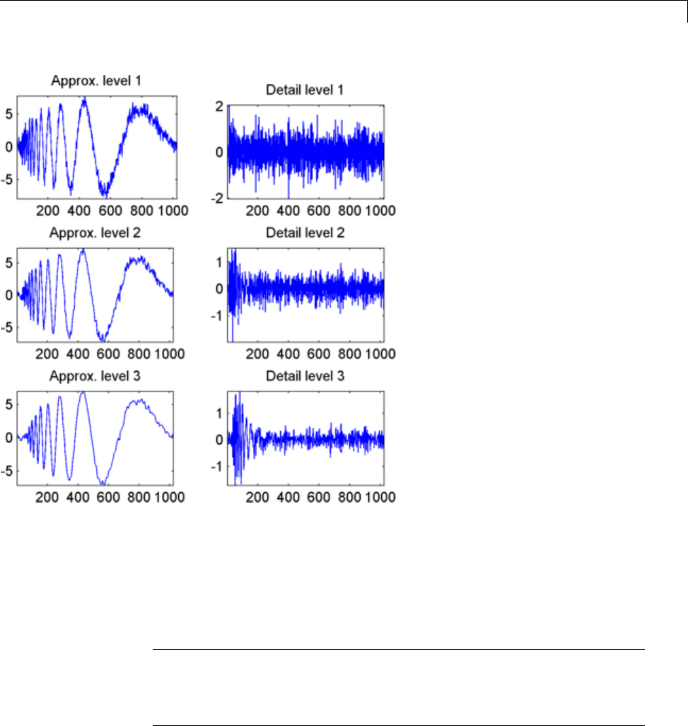
One-Dimensional Discrete Stationary Wavelet Analysis
12 Remove noise by thresholding.
To denoise the signal, use the ddencmp command to calculate a default
global threshold. Use the wthresh command to perform the actual
thresholding of the detail coefficients, and then use the iswt command to
obtain the denoised signal.
Note All methods for choosing thresholds in the 1-D Discrete Wavelet
Transform case are also valid for the 1-D Stationary Wavelet Transform,
which are also those used by the GUI tools. This is also true for the 2-D
transforms.
3-77
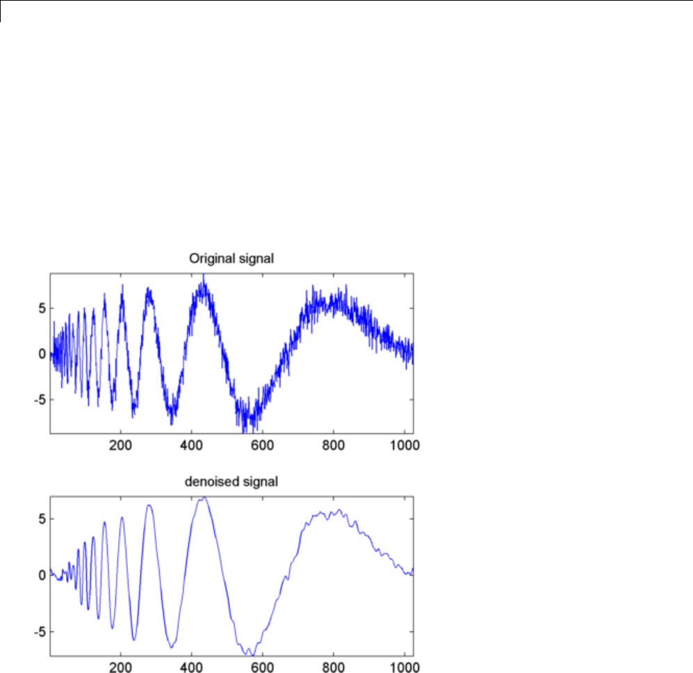
3Discrete Wavelet Analysis
[thr,sorh] = ddencmp('den','wv',s);
dswd = wthresh(swd,sorh,thr);
clean = iswt(swa,dswd,'db1');
To display both the original and denoised signals, type
subplot(2,1,1), plot(s);
title('Original signal')
subplot(2,1,2), plot(clean);
title('denoised signal')
The obtained signal remains a little bit noisy. The result can be improved by
considering the decomposition of sat level 5 instead of level 3, and repeating
steps 14 and 15. To improve the previous de-noising, type
3-78
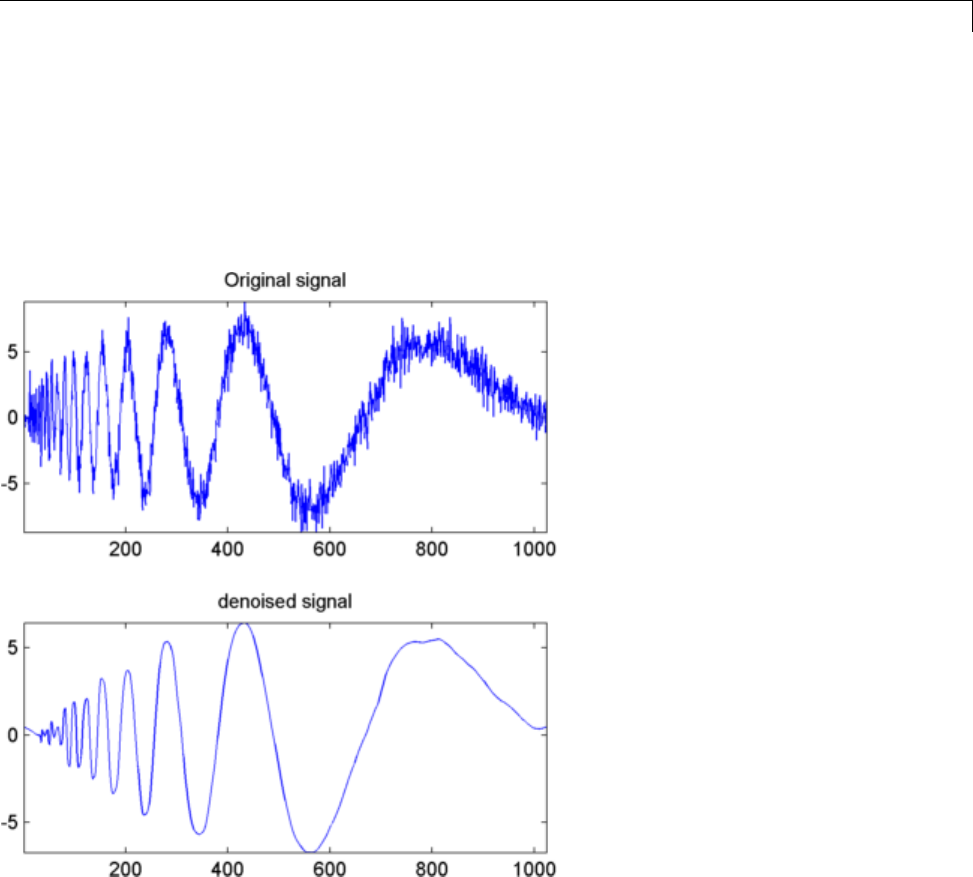
One-Dimensional Discrete Stationary Wavelet Analysis
[swa,swd] = swt(s,5,'db1');
[thr,sorh] = ddencmp('den','wv',s);
dswd = wthresh(swd,sorh,thr);
clean = iswt(swa,dswd,'db1');
subplot(2,1,1), plot(s); title('Original signal')
subplot(2,1,2), plot(clean); title('denoised signal')
A second syntax can be used for the swt and iswt functions, giving the same
results:
lev = 5; swc = swt(s,lev,'db1');
swcden = swc;
swcden(1:end-1,:) = wthresh(swcden(1:end-1,:),sorh,thr);
clean = iswt(swcden,'db1');
3-79

3Discrete Wavelet Analysis
Youcanobtainthesameplotbyusingthesameplotcommandsasinstep
16 above.
Interactive 1-D Stationary Wavelet Transform
Denoising
Now we explore a strategy to denoise signals, based on the one-dimensional
stationary wavelet analysis using the graphical interface tools. The basic idea
is to average many slightly different discrete wavelet analyses.
1Start the Stationary Wavelet Transform De-Noising 1-D Tool.
From the MATLAB prompt, type
wavemenu
The Wavelet Toolbox Main Menu appears.
3-80
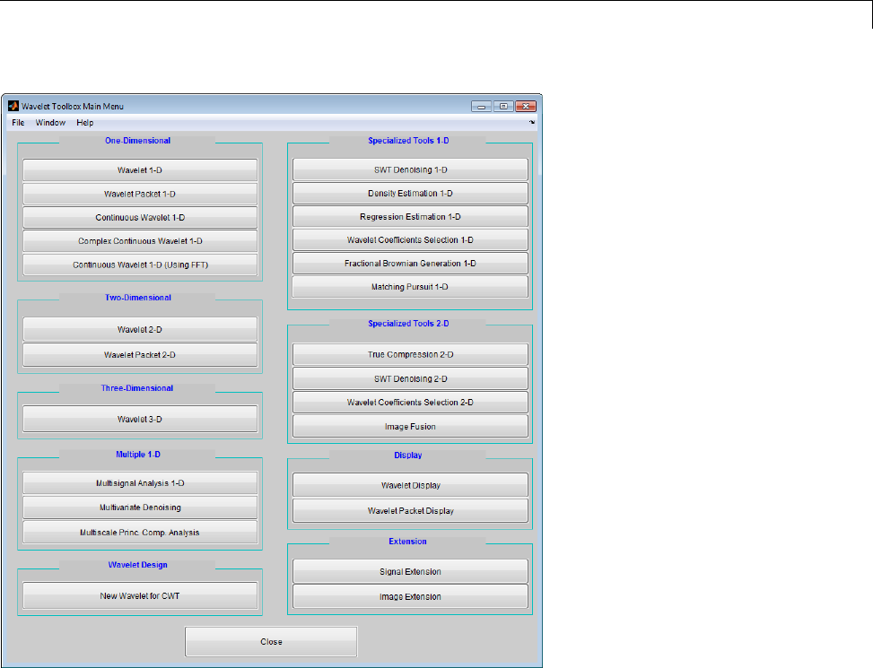
One-Dimensional Discrete Stationary Wavelet Analysis
Click the SWT De-noising 1-D menu item. The discrete stationary
wavelet transform de-noising tool for one-dimensional signals appears.
2Load data.
From the File menu, choose the Load Signal option.
When the Load Signal dialog box appears, select the MAT-file
noisbloc.mat, which should reside in the MATLAB folder
toolbox/wavelet/wavedemo.
Click the OK button. The noisy blocks signal is loaded into the SWT
De-noising 1-D tool.
3-81
3Discrete Wavelet Analysis
3Perform a Stationary Wavelet Decomposition.
Select the db1 wavelet from the Wavelet menu and select 5from the Level
menu, and then click the Decompose Signal button. After a pause for
computation, the tool displays the stationary wavelet approximation and
detail coefficients of the decomposition. These are also called nondecimated
coefficients since they are obtained using the same scheme as for the DWT,
but omitting the decimation step (see “Fast Wavelet Transform (FWT)
Algorithm” on page 3-37 in the Wavelet Toolbox User’s Guide).
4denoise the signal using the Stationary Wavelet Transform.
While a number of options are available for fine-tuning the de-noising
algorithm, we’ll accept the defaults of fixed form soft thresholding and
3-82
One-Dimensional Discrete Stationary Wavelet Analysis
unscaled white noise. The sliders located on the right part of the window
control the level-dependent thresholds, indicated by yellow dotted lines
running horizontally through the graphs of the detail coefficients to the left
ofthewindow. Theyellowdottedlinescanalsobedraggeddirectlyusing
the left mouse button over the graphs.
Note that the approximation coefficients are not thresholded.
Click the denoise button.
The result is quite satisfactory, but seems to be oversmoothed around the
discontinuities of the signal. This can be seen by looking at the residuals,
and zooming on a breakdown point, for example around position 800.
3-83
3Discrete Wavelet Analysis
Selecting a Thresholding Method. Select hard for the thresholding mode
instead of soft, and then click the denoise button.
The result is of good quality and the residuals look like a white noise sample.
To investigate this last point, you cangetmoreinformationonresidualsby
clicking the Residuals button.
Importing and Exporting from the GUI
The tool lets you save the denoised signal to disk. The toolbox creates a
MAT-file in the current folder with a name of your choice.
To save the above denoised signal, use the menu option File > Save denoised
Signal. A dialog box appears that lets you specify a folder and filename for
storing the signal. Type the name dnoibloc. After saving the signal data to
the file dnoibloc.mat, load the variables into your workspace:
load dnoibloc
whos
Name Size BytesClass
dnoibloc 1x1024 8192 double array
thrParams 1x5 580 cell array
wname 1x3 6 char array
3-84

One-Dimensional Discrete Stationary Wavelet Analysis
The denoised signal is given by dnoibloc. In addition, the parameters of the
de-noising process are available. The wavelet name is contained in wname:
wname
wname =
db1
and the level dependent thresholds are encoded in thrParams,whichis
a cell array of length 5 (the level of the decomposition). For i from 1 to
5, thrParams{i} contains the lower and upper bounds of the interval of
thresholding and the threshold value (since interval dependent thresholds are
allowed). For more information, see “One-Dimensional Adaptive Thresholding
of Wavelet Coefficients” on page 5-17.
For example, for level 1,
thrParams{1}
ans =
1.0e+03 *
0.0010 1.0240 0.0041
Here the lower bound is 1, the upper bound is 1024, and the threshold value is
4.1. The total time-interval is not segmented and the procedure does not use
the interval dependent thresholds.
3-85

3Discrete Wavelet Analysis
One-Dimensional Multisignal Analysis
This section takes you through the features of one-dimensional multisignal
wavelet analysis, compression and denoising using the Wavelet Toolbox
software. The rationale for each topic is the same as in the 1-D single signal
case.
The toolbox provides the following functions for multisignal analysis.
Analysis-Decomposition and Synthesis-Reconstruction Functions
Function NamePurpose
mdwtdec Multisignal wavelet decomposition
mdwtrec Multisignal wavelet reconstruction and
extraction of approximation and detail
coefficients
Decomposition Structure Utilities
Function Name Purpose
chgwdeccfs Change multisignal 1-D decomposition
coefficients
wdecenergy Multisignal 1-D decomposition energy repartition
Compression and Denoising Functions
Function Name Purpose
mswcmp Multisignal 1-D compression using wavelets
mswcmpscr Multisignal 1-D wavelet compression scores
mswcmptp Multisignal 1-D compression thresholds and
performance
mswden Multisignal 1-D denoising using wavelets
mswthresh Perform multisignal 1-D thresholding
3-86

One-Dimensional Multisignal Analysis
You can perform analyses from the MATLAB command line or by using the
graphical interface tools. This section describes each method. The last section
discusses how to exchange signal and coefficient information between the
disk and the graphical tools.
One-Dimensional Multisignal Analysis — Command
Line
1Load a file, from the MATLAB prompt, by typing
load thinker
The file thinker.mat contains a single variable X.Usewhos to show
information about X.
whos
Name Size Bytes Class
X 192x96 147456 double array
2Plot some signals.
figure;
plot(X(1:5,:)','r'); hold on
plot(X(21:25,:)','b'); plot(X(31:35,:)','g')
set(gca,'Xlim',[1,96])
grid
3-87
3Discrete Wavelet Analysis
3Perform a wavelet decomposition of signals at level 2 of row signals using
the db2 wavelet.
dec = mdwtdec('r',X,2,'db2')
This generates the decomposition structure dec:
dec =
dirDec: 'r'
level: 2
wname: 'db2'
dwtFilters: [1x1 struct]
dwtEXTM: 'sym'
dwtShift: 0
dataSize: [192 96]
ca: [192x26 double]
cd: {[192x49 double] [192x26 double]}
4Change wavelet coefficients.
For each signal change the wavelet coefficients by setting all the coefficients
of the detail of level 1 to zero.
decBIS = chgwdeccfs(dec,'cd',0,1);
This generates a new decomposition structure decBIS.
3-88
One-Dimensional Multisignal Analysis
5Perform a wavelet reconstruction of signals and plot some of the new
signals.
Xbis = mdwtrec(decBIS);
figure;
plot(Xbis(1:5,:)','r'); hold on
plot(Xbis(21:25,:)','b');
plot(Xbis(31:35,:)','g')
grid; set(gca,'Xlim',[1,96])
Compare old and new signals by plotting them together.
figure; idxSIG = [1 31];
plot(X(idxSIG,:)','r','linewidth',2); hold on
plot(Xbis(idxSIG,:)','b','linewidth',2);
3-89
3Discrete Wavelet Analysis
grid; set(gca,'Xlim',[1,96])
6Set the wavelet coefficients at level 1 and 2 for signals 31 to 35 to the value
zero, perform a wavelet reconstruction of signal 31, and compare some
of the old and new signals.
decTER = chgwdeccfs(dec,'cd',0,1:2,31:35);
Y = mdwtrec(decTER,'a',0,31);
figure;
plot(X([1 31],:)','r','linewidth',2); hold on
plot([Xbis(1,:)
; Y]','b','linewidth',2);
grid; set(gca,'Xlim',[1,96])
3-90

One-Dimensional Multisignal Analysis
7Compute the energy of signals and the percentage of energy for wavelet
components.
[E,PEC,PECFS] = wdecenergy(dec);
Energy of signals 1 and 31:
Ener_1_31 = E([1 31])
Ener_1_31 =
1.0e+006 *
3.7534
2.2411
8Compute the percentage of energy for wavelet components of signals 1
and 31.
PEC_1_31 = PEC([1 31],:)
PEC_1_31 =
99.7760 0.1718 0.0522
99.3850 0.2926 0.3225
The first column shows the percentage of energy for approximations at
level 2. Columns 2 and 3 show the percentage of energy for details at level
2and1,respectively.
9Display the percentage of energy for wavelet coefficients of signals 1 and
31. As we can see in the dec structure, there are 26 coefficients for the
approximation and the detail at level 2, and 49 coefficients for the detail at
level 1.
PECFS_1 = PECFS(1,:); PECFS_31 = PECFS(31,:);
figure;
plot(PECFS_1,'r','linewidth',2); hold on
plot(PECFS_31,'b','linewidth',2);
grid; set(gca,'Xlim',[1,size(PECFS,2)])
3-91
3Discrete Wavelet Analysis
10 Compress the signals to obtain a percentage of zeros near 95% for the
wavelet coefficients.
[XC,decCMP,THRESH] = mswcmp('cmp',dec,'N0_perf',95);
[Ecmp,PECcmp,PECFScmp] = wdecenergy(decCMP);
Plot the original signals 1 and 31, and the corresponding compressed
signals.
figure;
plot(X([1 31],:)','r','linewidth',2); hold on
plot(XC([1 31],:)','b','linewidth',2);
grid; set(gca,'Xlim',[1,96])
3-92

One-Dimensional Multisignal Analysis
Compute thresholds, percentage of energy preserved and percentage of
zeros associated with the L2_perf method preserving at least 95% of
energy.
[THR_VAL,L2_Perf,N0_Perf] = mswcmptp(dec,'L2_perf',95);
idxSIG = [1,31];
Thr = THR_VAL(idxSIG)
Thr =
256.1914
158.6085
L2per = L2_Perf(idxSIG)
L2per =
96.5488
94.7197
N0per = N0_Perf(idxSIG)
N0per =
79.2079
86.1386
Compress the signals to obtain a percentage of zeros near 60% for the
wavelet coefficients.
[XC,decCMP,THRESH] = mswcmp('cmp',dec,'N0_perf',60);
XC signals are the compressed versions of the original signals in the row
direction.
Compress the XC signals in the column direction
XX = mswcmp('cmpsig','c',XC,'db2',2,'N0_perf',60);
Plot original signals Xand the compressed signals XX as images.
figure;
subplot(1,2,1); image(X)
subplot(1,2,2); image(XX)
colormap(pink(222))
3-93
3Discrete Wavelet Analysis
11 Denoise the signals using the universal threshold:
[XD,decDEN,THRESH] = mswden('den',dec,'sqtwolog','sln'); figure;
plot(X([1 31],:)','r','linewidth',2); hold on
plot(XD([1 31],:)','b','linewidth',2);
grid; set(gca,'Xlim',[1,96])
XD signals are the denoised versions of the original signals in the row
direction.
Denoise the XD signals in column direction
3-94
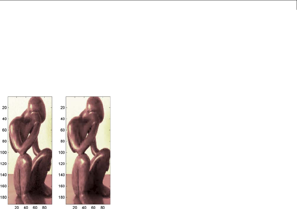
One-Dimensional Multisignal Analysis
XX = mswden('densig','c',XD,'db2',2,'sqtwolog','sln');
Plot original signals Xand the denoised signals XX as images.
figure;
subplot(1,2,1); image(X)
subplot(1,2,2); image(XX)
colormap(pink(222))
Interactive One-Dimensional Multisignal Analysis
In this section, we explore the same signal as in the previous section, but use
the graphical interfacetoolstoanalyzeit.
1Start the Wavelet 1-D Multisignal Analysis Tool.
From the MATLAB prompt, type:
wavemenu
The Wavelet Toolbox Main Menu appears.
3-95
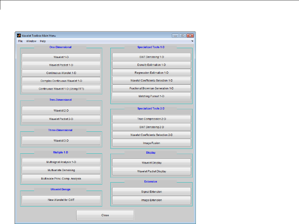
3Discrete Wavelet Analysis
Click Multisignal Analysis 1-D to open the Wavelet 1-D Multisignal
Analysis tool.
3-96
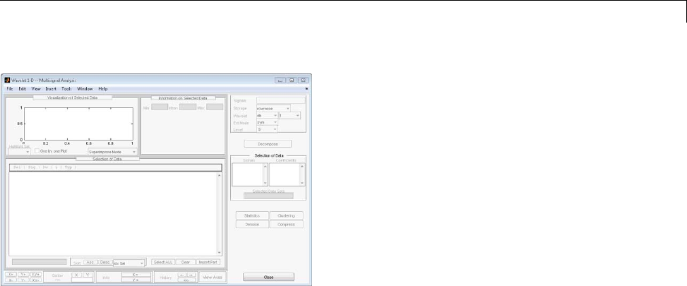
One-Dimensional Multisignal Analysis
The tool is divided into five panes. Two of them are the same as in all
Wavelet Toolbox GUIs: the Command Frame on the right side of the figure
and the Dynamic Visualization tool at the bottom. The Command Frame
contains a special component found in all multisignal tools: the Selection
of Data Sets pane which is used to manage two lists.
The three new panes are the Visualization of Selected Data pane, the
InformationonSelectedDatapane, and the Selection of Data pane.
2Load the signals.
From the File menu, select Load > Signals. When the Load Signal dialog
box appears, select the MAT-file thinker.mat from the MATLAB folder
toolbox/wavelet/wmultisig1d and click OK.
The data matrix loads in the Wavelet 1-D Multisignal Analysis tool,and
the first signal appears.
3-97
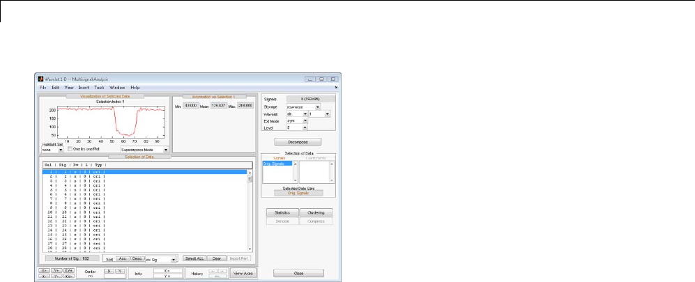
3Discrete Wavelet Analysis
The Selection of Data pane contains a list of selectable signals. At
the beginning, only the originally loaded signals are available. You can
generate and add new signals to the list by decomposing, compressing, or
denoising original signals.
Each row of the list displays the index of selectable signal (Idx Sel), the
index of original signal (Idx Sig) and three wavelet transform attributes
describing the process used to obtain the selectable signal from the original
one.
3View the signals and signal information.
With signal 1 highlighted, Shift-click the mouse on signal 3 to select signals
1, 2, and 3.
Ctrl-click the mouse on signals 7, 9, and 11. (The Select ALL button at the
bottom of the Selection of Data pane selects all signals and the Clear
button deselects all signals.)
Theselectedsignals(1,2,3,7,9and11)appearintheVisualization of
Selected Data pane. The Information on Selected Data pane contains
the box plots of the minimums, the means, and the maximums of these
signals.
3-98
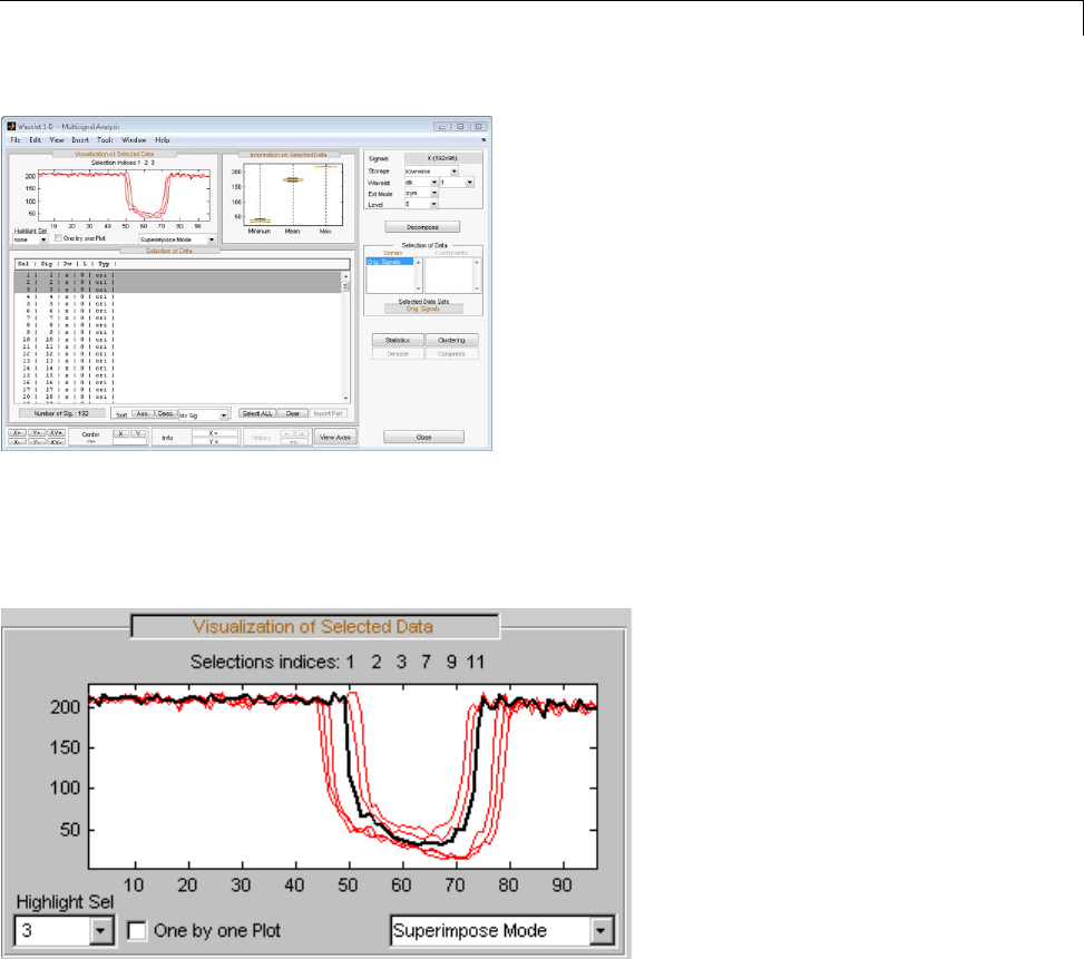
One-Dimensional Multisignal Analysis
4Highlight a signal.
Using the Highlight Sel button in the lower-left corner of the
Visualization of Selected Data pane, select signal 3.
5Select Different Views.
In the Visualization of Selected Data pane, change the view mode
using the pop-up in the lower-right corner. Choose Separate Mode.The
selected signals appear.
6Decompose a multisignal.
3-99
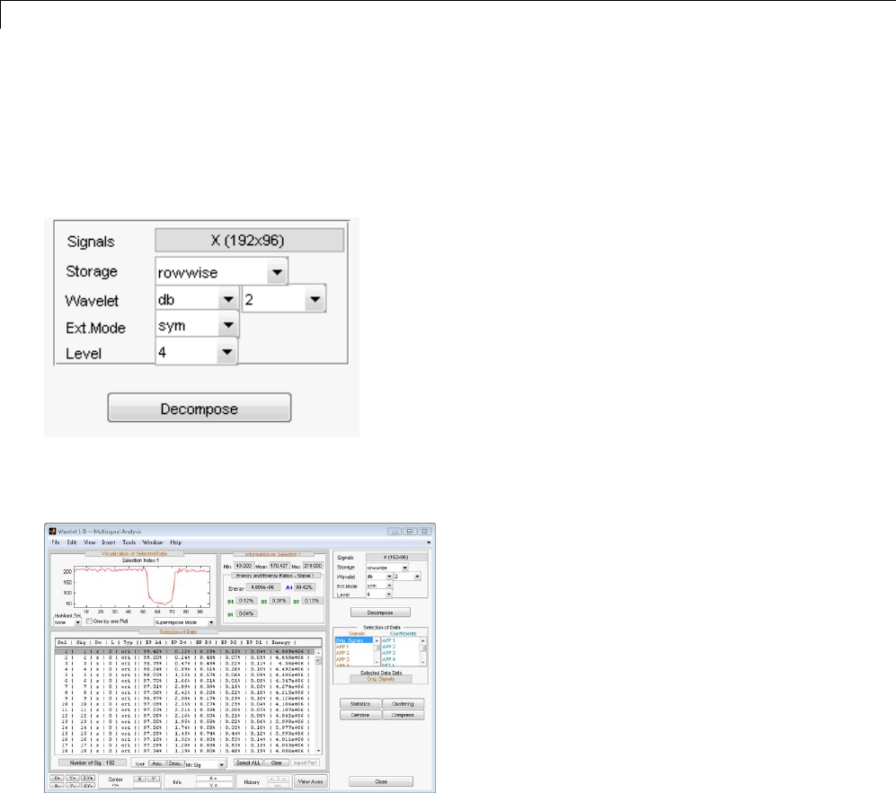
3Discrete Wavelet Analysis
Perform an analysis at level 4 using the db2 waveletandthesamefileused
in the command line section: thinker.mat.
In the upper right portion of the Wavelet 1-D Multisignal Analysis tool,
select db2 and level 4 in the Wavelet fields.
Click Decompose. After a pause for computation, all the original signals
are decomposed and signal 1 is automatically selected
In the Selection of Data pane, new information is added for each original
signal — the percentage of energy of the wavelet components (D1,...,D4
and A4) and the total energy. The InformationonSelectedDatapane
contains information on the single selected signal: Min,Mean,Max and
the energy distribution of the signal.
3-100
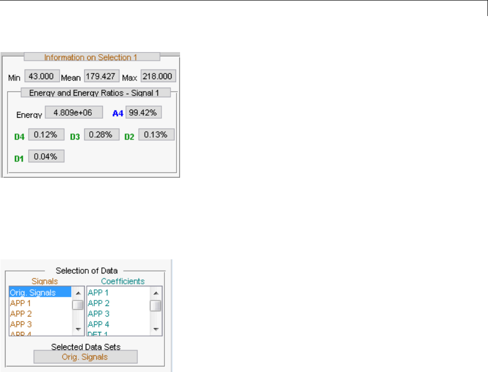
One-Dimensional Multisignal Analysis
Since the original signals are decomposed, new objects appear and the
Selection of Data Sets pane in the Command Frame updates.
The Selection of Data Sets pane defines the available signals that are
now selectable from the Selection of Data pane.
The list on the left allows you to select sets of signals and the right list
allows you to select sets of corresponding coefficients: original signals
(Orig. Signals),approximations(APP 1,...) anddetailsfromlevels1
to 4 (DET 1,...).
In the list on the right, the coefficients vectors can be of different lengths,
but only components of the same length can be selected together.
After a decomposition the original signals (Orig. Signals)dataset
appears automatically selected.
Selectsignals1,2,3,7,9and11.
3-101
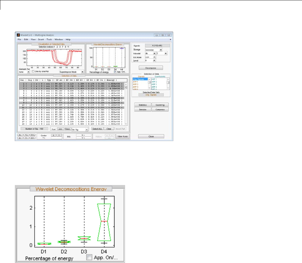
3Discrete Wavelet Analysis
The energy of selected signals is primarily concentrated in the
approximation A4, so the box plot is crushed (see following figure on the
left). Deselect App. On/Off to see a better representation of details energy
(see following figure on the right).
7Display multisignal decompositions.
In the Visualization of Selected Data pane, change the view mode using
the pop-up below the plots and select Full Dec Mode. The decompositions
of the selected signals display.
3-102
One-Dimensional Multisignal Analysis
Change the Level to 2.
Select the signal 7 in Highlight Sel.
8Change the visualization modes.
Using the second pop-up from the left at the bottom of the pane, select
Full Dec Mode (Cfs). The coefficients of the decompositions of the
selected signals display. At level k, coefficients are duplicated 2k times.
Changetheviewmodeto Stem Mode (Abs), and then, change to Tree
Mode. The wavelet tree corresponding to the decompositions of the selected
signals displays.
Select the level 4 and click the node a3. Then highlight signal 7.
9Select Different Wavelet Components.
Ctrl-click Orig. Signals,APP 1,APP 3 and DET 1 to select these four
sets of signals from the list on the left in the Selection of Data Sets pane.
The total number of selected data (Number of Sig.) appears in the
Selection of Data Sets pane: four sets of 192 signals each is a total of
768 signals.
3-103
3Discrete Wavelet Analysis
Click the Asc. buttonintheSort pane. The selected data are sorted in
ascending order with respect to the Idx Sig parameter
Note that DWT attributes of each selectable signal have been updated
where astands for approximation, dfor detail and sfor signal.
Click the Idx Sel 1 signal and then shift-click the Idx Sel 579 signal.
3-104
One-Dimensional Multisignal Analysis
Choose Separate Mode.
Ctrl-click to select two sets of signals from the right-most list of the
Selection of Data Sets pane: APP 1 and DET 1.
3-105
3Discrete Wavelet Analysis
Note that in this list of coefficients sets, the selected vectors must be of same
length, which means that you must select components of the same level.
Click the Asc. button in the Sort pane. The selected data are sorted in
ascending order with respect to Idx Sig parameter.
Select the ten first signals.
10 Compress a multisignal.
The graphical interface tools feature a compression option with automatic
or manual thresholding.
3-106
One-Dimensional Multisignal Analysis
Cick Compress, located in the lower-right side of the window. This
displays the Compression window.
Note The tool always compresses all the original signals when you click
the Compress button.
Before compressing, choose the particular strategy for computing the
thresholds. Select the adapted parameters in the Select Compression
Method frame. Then, apply this strategy to compute the thresholds
according to the current method, either to the current selected signals by
clicking the Selected button, or to all signals by clicking the ALL button.
For this example, accept the defaults and click the ALL button.
3-107
3Discrete Wavelet Analysis
The thresholds for each level (ThrD1 to ThrD4), the energy ratio (En. Rat.)
and the sparsity ratio (NbZ Rat.)aredisplayedintheSelection of Data
pane.
Click the Compress button at the bottom of the Thresholding pane.
Now you can select new data sets: compressed Signals, the corresponding
approximations, details and coefficients.
Press the Ctrl key and click the Compressed item in the left list of the
Selection of Data Sets pane. The original signals and their compressed
versionsareselected(2x192=384signals).
Click the Asc. button at the bottom of the Selection of Data pane to sort
the signals using Idx Sig number.
With the mouse, select the first four signals. They correspond to the
original signals 1, 2 and the corresponding compressed signals 193, 194.
3-108
One-Dimensional Multisignal Analysis
Click the Close button to close the Compression window.
11 Denoise a multisignal.
The graphical user interface offers a denoising option with either a
predefined thresholding strategy or a manual thresholding method. Using
this tool makes very easy to remove noise from many signals in one step.
Display the Denoising window by clicking the Denoise button located in
the bottom part of the Command Frame on the right of the window.
3-109
3Discrete Wavelet Analysis
A number of options are available for fine-tuning the denoising algorithm.
For this example, accept the defaults: soft type of thresholding, Fixed
form threshold method, and Scaled white noise as noise structure.
Click the ALL button in the Thresholding pane. The threshold for each
level (ThrD1, ..., ThrD4) computes and displays in the Selection of Data
pane.
Then click the Denoise button at the bottom of the Thresholding pane.
Ctrl-click the Denoised item in the list on the left of the Selection of
Data Sets pane. The original signals and the corresponding denoised ones
are selected (2 x 192 = 384 signals).
Click the Asc. button at the bottom of the Selection of Data pane to sort
the signals according to the Idx Sig parameter.
With the mouse, select the first four signals. They correspond to the
original signals 1, 2 and the corresponding denoised signals 193, 194
3-110

One-Dimensional Multisignal Analysis
Choose Separate Mode.
12 To view residuals, Ctrl-click the Orig. Signal,theDenoised and the
Residuals items in the list on the left of the Selection of Data Sets pane.
Original, denoised and residual signals are selected (3 x 192 = 576 signals).
Click the Asc. button at the bottom of the Selection of Data pane to sort
the signals using the Idx Sig parameter.
With the mouse, select the first six signals. They correspond to the original
signals 1, 2, the corresponding denoised signals 193, 194 and the residuals
385, 386.
Then, choose Separate Mode.
3-111
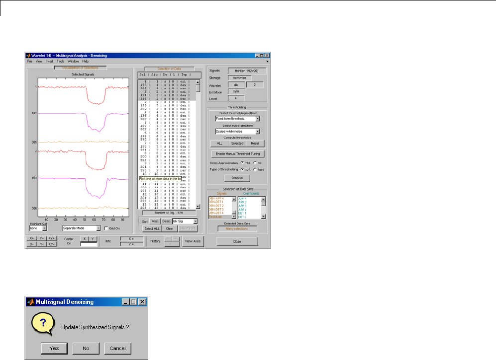
3Discrete Wavelet Analysis
13 Click Close to close the denoising tool. Then, click the Yes button to
update the synthesized signals.
Manual Threshold Tuning
1Choose a method, select one or several signals in the Selection of Data
pane using the mouse and keys. Then click the Selected button. You can
select another group of signals using the same method. Press the Denoise
button to denoise the selected signal(s).
3-112
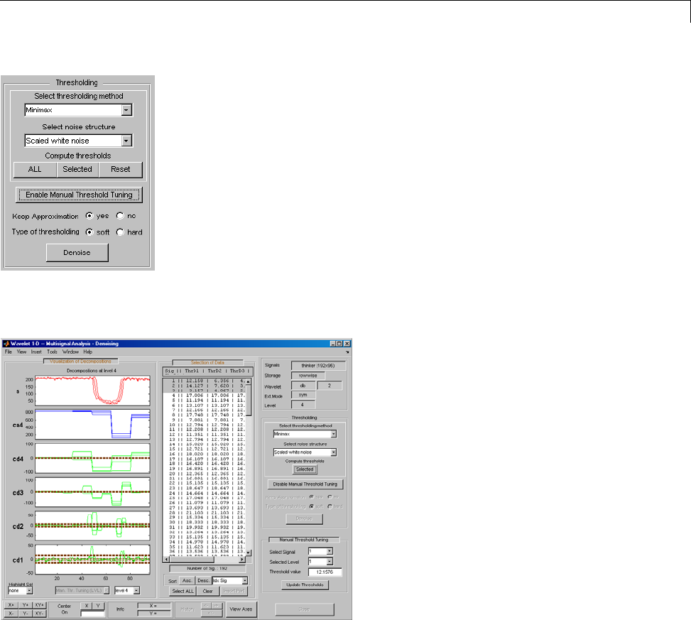
One-Dimensional Multisignal Analysis
You can also use manual threshold tuning. Click the Enable Manual
Thresholding Tuning button.
The horizontal lines in the wavelet coefficient axes (cd1, ..., cd4) can be
dragged using the mouse. This may be done individually, by group or all
together depending on the values in the Select Signal and Selected
Level fields in the Manual Threshold Tuning pane.
3-113
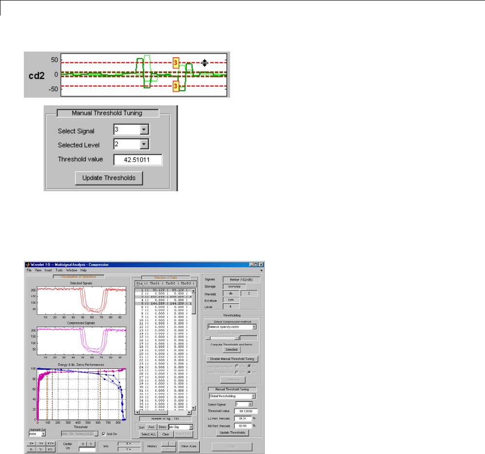
3Discrete Wavelet Analysis
2In the Wavelet 1-D Multisignal Analysis Compression tool, you can use two
methods for threshold tuning: the By level thresholding method which
is used in the Wavelet 1-D Multisignal Analysis Denoising tool, and the
Global thresholding method.
You can drag the vertical lines in the Energy and Nb. Zeros
Performances axes using the mouse. This can be done individually or
all together depending on the values of Select Signal in the Manual
Threshold Tuning pane.
3-114
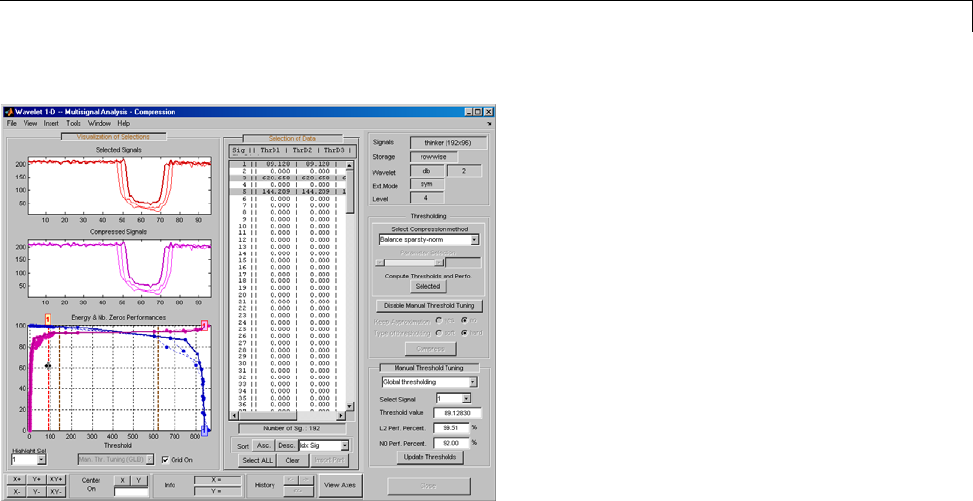
One-Dimensional Multisignal Analysis
The threshold value, L2 performance, and number of zeros performance
are updated in the corresponding edit buttons in the Manual Threshold
Tuning pane.
Statistics on Signals
1You can display various statistical parameters related to the signals and
their components. From the Wavelet 1-D Multisignal Analysis tool, click
the Statistics button. Then select the signal 1 in the Selection of Data
Sets pane.
3-115
3Discrete Wavelet Analysis
Select the signals 1, 2, 3, 7, 9 and 11 in the Selection of Data pane, and
display the corresponding boxplots and correlation plots.
3-116
One-Dimensional Multisignal Analysis
2To display statistics on many wavelet components, in the Selection
Data Sets pane, in the left column, select Orig. Signals,APP 1,DET 1,
Denoised and Residuals signals. Then choose Separate Mode,andclick
the Asc. buttonintheSort pane. The selected data are sorted in ascending
order with respect to Idx Sig parameter. In the Selection of Data pane,
select data related to signal 1.
Clustering Signals
Note To use clustering, you must have Statistics Toolbox™ software installed.
1Click the Clustering button located in the Command Frame, which is in
the lower right of the Wavelet 1-D Multisignal Analysis window to open
the Clustering tool.
3-117
3Discrete Wavelet Analysis
You can cluster various type of signals and wavelet components: original,
denoised or compressed, residuals, and approximations or details
(reconstructed or coefficients). Similarly, there are several methods for
constructing partitions of data.
Use the default parameters (Original and Signal in Data to Cluster, and
in Ascending Hierarchical, euclidean, ward,and6in Culstering)
and click the Compute Clusters button.
3-118
One-Dimensional Multisignal Analysis
A full dendrogram and a restricted dendrogram display in the Selection
by Dendrogram pane. For each signal, the cluster number displays in
the Selection of Data pane.
2Select one cluster, several clusters, or a part of a cluster.
Click thexticklabel 3 at the bottom of the restricted dendrogram. The
links of the third cluster blink in the full dendrogram and the 24 signals of
this class display in the Visualization of Selected Data pane. You can
see their numbers in the Selection of Data pane.
Clicking the line in the restricted or in the full dendrogram lets you select
one cluster, several linked clusters, or a part of a cluster. For a more
accurate selection, use the Dilate X and the Translate X sliders under
the full dendrogram. You can also use the Yscale button located above the
full dendrogram. The corresponding signals display in the Visualization
of Selected Data pane and in the list of the Selection of Data pane.
3-119
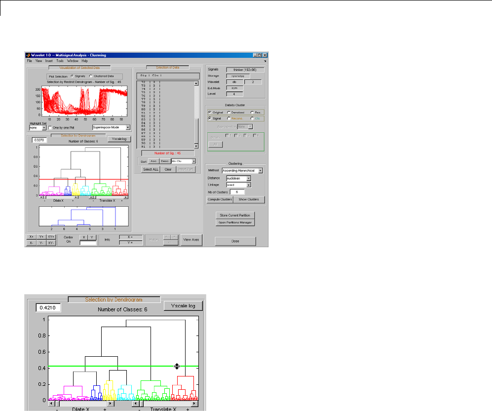
3Discrete Wavelet Analysis
You can use the horizontal line in the full dendrogram to change the
number of clusters. Use the left mouse button to drag the line up or down.
3Use the Show Clusters button to examine the clusters of the current
partition. You can display the mean (or the median) of each cluster, the
global standard deviation and the pointwise standard deviation distance
around the mean (or the median). The number of the cluster, the number
of elements, the percentage of signals, and two indices of quality display
for each cluster.
3-120
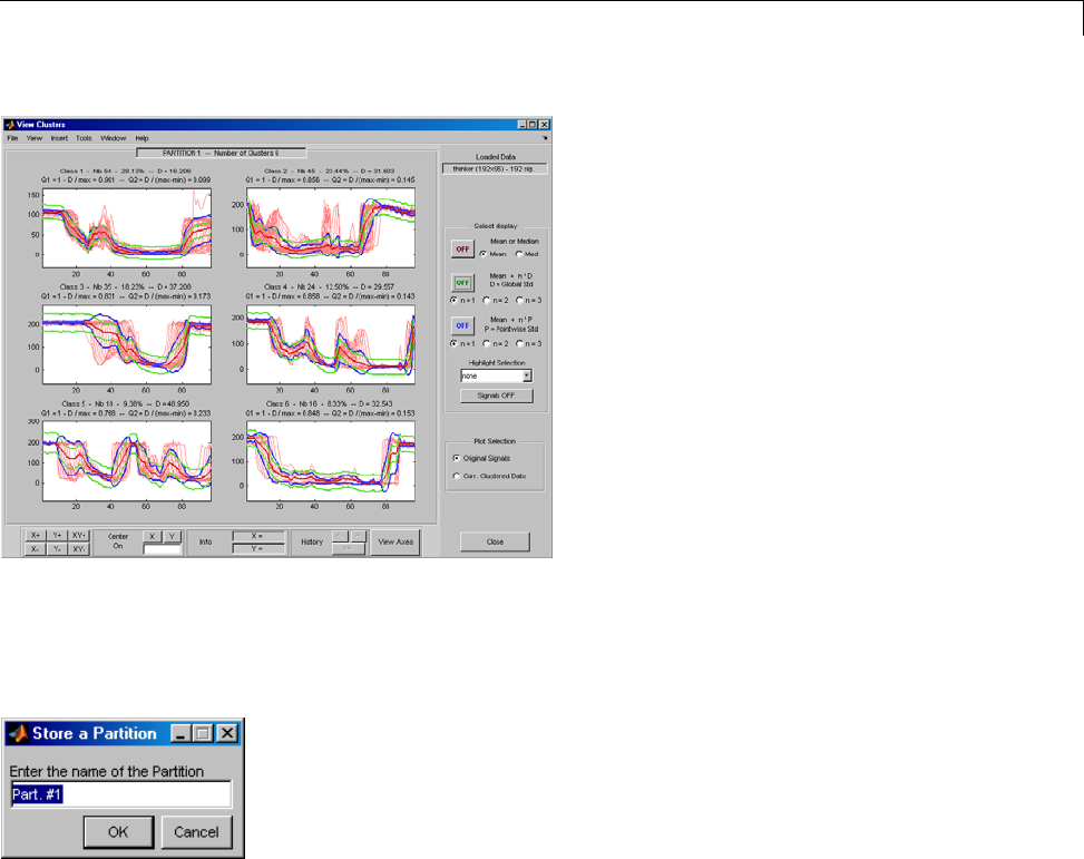
One-Dimensional Multisignal Analysis
4Click the Store Current Partition button below the Clustering pane
to store the current partition for further comparisons. A default name is
suggested. Note that the 1-D Wavelet Multisignal Analysis tool stores the
partitions and they are not saved on the disk.
Partitions
1Build and store several partitions (for example, partitions with signals,
denoised signals approximations at level 1, 2 and 3, and denoised signals).
Then, click the Open Partition Manager button below the Store
Current Partition button. The Partitions Management pane appears.
The names of all stored partitions are listed.
3-121
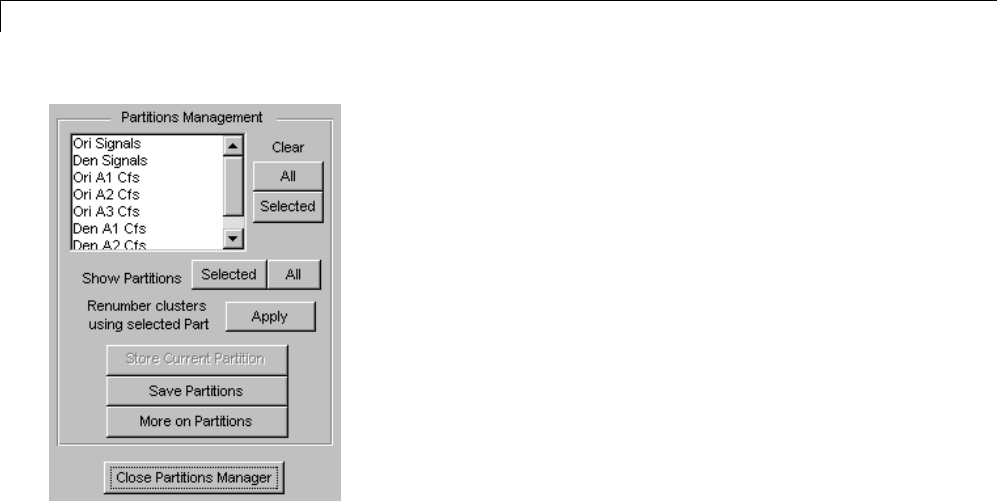
3Discrete Wavelet Analysis
Now, you can show, clear, or save the partitions (individually, selected
ones, or all together).
2To display partitions, select the Ori Signals and the Den Signals
partitions, and click the Selected button next to the Show Partitions
label.
Theclustersarealmostthesame,butitisdifficulttoseethisonthe
Selected Partitions axis, due to the scaling difference. Press the Apply
button to renumber the clusters (starting from the selected partition as
basic numbering) to compare the two partitions.
3-122
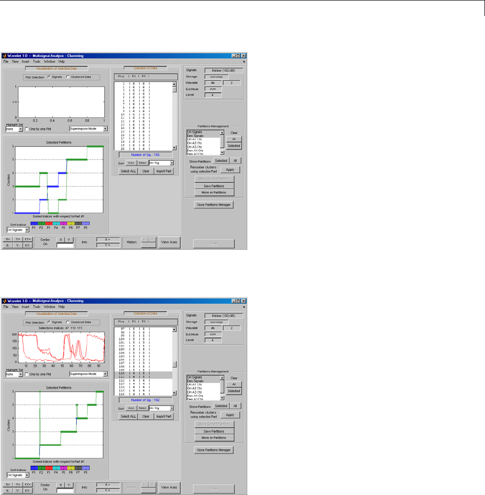
One-Dimensional Multisignal Analysis
Only threesignalsarenotclassifiedinthesameclusterforthetwo
considered partitions.
3-123

3Discrete Wavelet Analysis
3Select the partitions you want to save and click the Save Partitions
button below the Store Current Partition buttoninthePartitions
Management pane.
Partitions are saved as an array of integers, where each column corresponds
to one partition and contains the indices of clusters. When you choose the
Full Partitions option, an array object (wpartobj)issaved.
4To load or clear stored partitions use File > Partitions in the Wavelet
1-D Multisignal Analysis tool. (File > Partitions is also available in the
Wavelet 1-D Multisignal Analysis Clustering tool and you can also save
the current partition.)
3-124

One-Dimensional Multisignal Analysis
To clear one or more stored partitions, select File > Partitions > Clear
Partition.
Select File > Partitions > Load Partition to load one or several
partitions from the disk. The loaded partitions are stored in Wavelet 1-D
Multisignal Analysis tool with any previously stored partitions. A partition
can also be a manually created column vector.
3-125
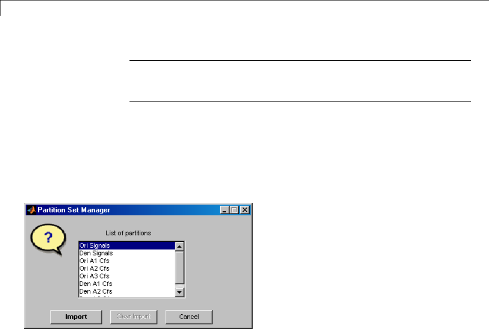
3Discrete Wavelet Analysis
Note The number of signals in loaded partitions must be equal to the
number of signals in the Wavelet 1-D Multisignal Analysis tool. A warning
appearsifthisconditionisnottrue.
5In each subcomponent of the Wavelet 1-D Multisignal Analysis tool (main,
statistics, denoising, compression, clustering), you can import a stored
partition from the list in the Selection of Data pane. Click the Import
Part button at the bottom of the Selection of Data pane, the Partition
Set Manager window appears. Select one partition and click the Import
button.
For this example, go back to the main window, import the Ori Signals
partition and sort the signals in descending order with respect to A4 energy
percentage.
3-126
One-Dimensional Multisignal Analysis
6Click the More on Partitions button at the bottom of the Partitions
Management pane to display the Partition tool.
7Select the Den Signals in Sel P2 in the upper-right corner of the window.
Then, in the lower left axis, click the yellow text containing the value 2(the
3-127
3Discrete Wavelet Analysis
coordinates of the corresponding point are (4,5)). The corresponding signals
are displayed together with all related information.
More on Clustering
Instead of the Ascending Hierarchical Tree clustering method, you can use
the K-means method. For this case, the partition cannot be represented by a
dendrogram and other representations should be used.
In the image representation (see figure below on the left), you can select a
cluster by clicking on the corresponding color on the colorbar. You can also
select a cluster or part of a cluster by clicking on the image.
In the center representation (see figure below on the right) you can select a
cluster by clicking on the corresponding colored center.
3-128
One-Dimensional Multisignal Analysis
Importing and Exporting Information from the
Graphical Interface
The Wavelet 1-D Multisignal Analysis tool lets you move data to and from
disk.
Saving Information to Disk
You can save decompositions and denoised or compressed signals (including
the corresponding decompositions from Wavelet 1-D Multisignal Analysis
tools) to disk. You then can manipulate the data and later import it again
into the graphical tools.
3-129
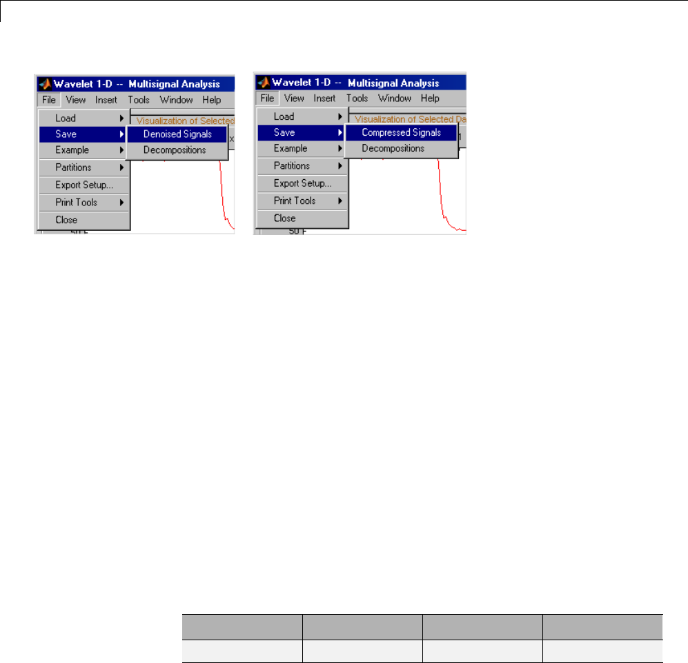
3Discrete Wavelet Analysis
Saving Decompositions
The Wavelet 1-D Multisignal Analysis main tool lets you save the entire set of
data from a wavelet analysis to disk. The toolbox creates a MAT-file in the
current folder with anameyouchoose.
1Open the Wavelet 1-D Multisignal Analysis main tool and load the example
analysis by selecting File>Example>Ex21:Thinker(rows).
2Save the data from this analysis, using the menu option File > Save
Decompositions.
A dialog box appears that lets you specify a folder and filename for storing
the decomposition data. For this example, use the name decORI.mat.
3Type the name decORI.
4After saving the decomposition data to the file decORI.mat,loadthe
variables into your workspace:
load decORI
whos
Name Size Bytes Class
dec 1x1 163306 struct
dec
dec =
dirDec: 'r'
3-130

One-Dimensional Multisignal Analysis
level: 4
wname: 'db2'
dwtFilters: [1x1 struct]
dwtEXTM: 'sym'
dwtShift: 0
dataSize: [192 96]
ca: [192x8 double]
cd: {1x4 cell}
The field ca of the structure dec gives the coefficients of approximation at
level 4, the field cd is a cell array which contains the coefficients of details.
size(dec.cd{1})
ans =
192 49
size(dec.cd{2})
ans =
192 26
size(dec.cd{3})
ans =
192 14
size(dec.cd{4})
ans =
192 8
You can change the coefficients using the chgwdeccfs function.
Note For a complete description of the dec structure, see “Loading
Decompositions” on page 3-133.
Loading Information into the Wavelet 1-D Multisignal Analysis
Tool
You can load signals or decompositions into the graphical interface. The
information you load may be previously exported from the graphical interface,
and then manipulated in the workspace; or it may be information you initially
generated from the command line. In either case, you must observe the strict
3-131
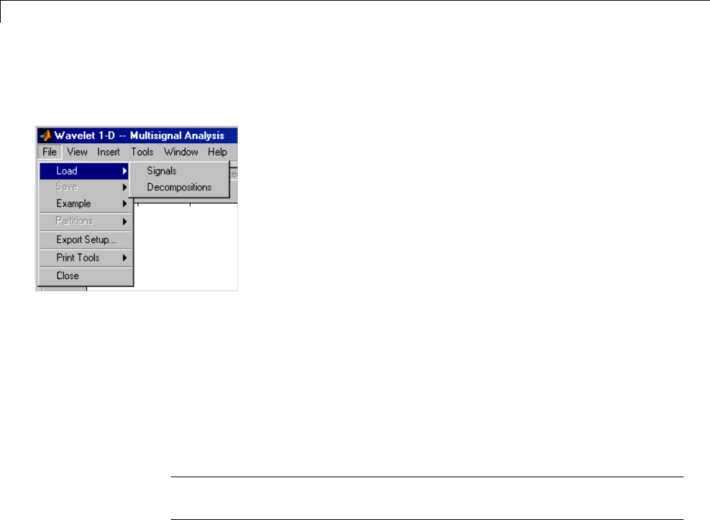
3Discrete Wavelet Analysis
file formats and data structures used by the Wavelet 1-D Multisignal Analysis
tools or errors will occur when you try to load information.
Loading Signals. To load a signal you constructed in your MATLAB
workspace into the Wavelet 1-D Multisignal Analysis tool, save the signal
in a MAT-file (with extension .mat).
For example, if you design a signal called magic128 and want to analyze it in
the Wavelet 1-D Multisignal Analysis tool, type
save magic128 magic128
Note The workspace variable magic128 must be a matrix and the number of
rows and columns must be greater than 1.
sizmag = size(magic128)
sizmag =
128 128
To load this signal into the Wavelet 1-D Multisignal Analysis tool, use the
File > Load Signal menu item. A dialog box appears in which you select the
appropriate MAT-file to be loaded.
3-132

One-Dimensional Multisignal Analysis
Note When you load a matrix of signals from the disk, the name of 2-D
variables are inspected in the following order: x,X,sigDATA,andsignals.
Then, the 2-D variables encountered in thefileareinspectedinalphabetical
order.
Loading Decompositions. To load decompositions that you constructed in
the MATLAB workspace into the Wavelet 1-D Multisignal Analysis tool, save
the signal in a MAT-file (with extension mat).
For instance, if you design a signal called magic128 and want to analyze it in
the Wavelet 1-D Multisignal Analysis too, the structure dec must have the
following fields:
'dirDec' Direction indicator with 'r' for row or 'c' for
column
'level' Level of DWT decomposition
'wname' Wavelet name
'dwtFilters' Structure with four fields: LoD,HiD,LoR,HiR
'dwtEXTM' DWT extension mode (see dwtmode)
'dwtShift' DWT shift parameter (0 or 1)
'dataSize' Size of original matrix X
'ca' Approximation coefficients at level dec.level
'cd' Cell array of detail coefficients, from 1 to
dec.level
The coefficients cA and cD{k},for(k=1to dec.level), are matrices and are
stored rowwise if dec.dirDec is equal to 'r' or columnwise if dec.dirDec
is equal to 'c'.
3-133
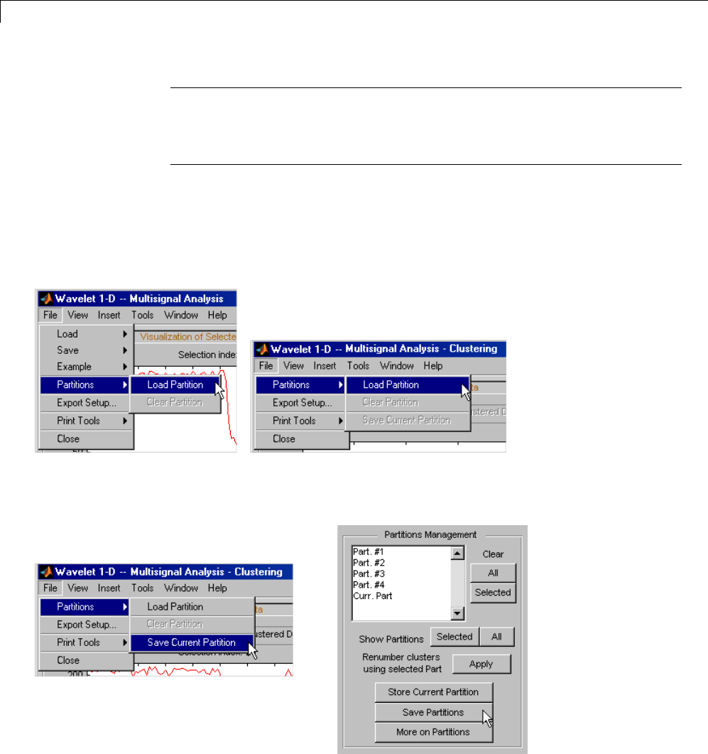
3Discrete Wavelet Analysis
Note The fields 'wname' and 'dwtFilters' have to be compatible (see the
wfilters function). The sizes of cA and cD{k},(fork=1to dec.level)
must be compatible with the direction, the level of the decomposition, and
the extension mode.
Loading and Saving Partitions.
Loading. The Wavelet 1-D Multisignal Analysis main tool and clustering
tool let you load a set of partitions from disk.
Saving Partitions. The Wavelet 1-D Multisignal Analysis clustering tool
lets you save a set of partitions to disk.
3-134
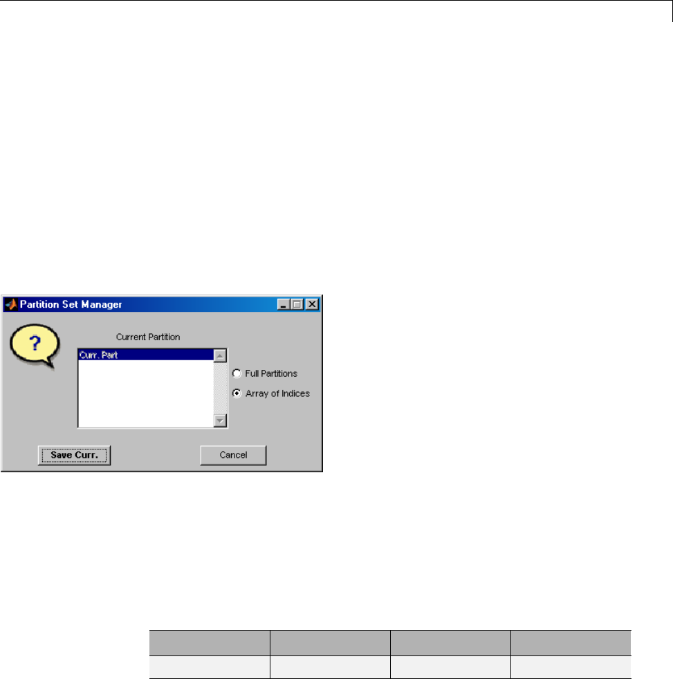
One-Dimensional Multisignal Analysis
For example:
1Open the Wavelet 1-D Multisignal Analysis main tool and load the example
analysis using File > Example > Ex 21: Thinker (rows).
2Click the Clustering button. The Wavelet 1-D Multisignal Analysis
Clustering window appears.
3Click the Compute Clusters button, and then save the current partition
using menu option File > Partitions > Save Current Partition.Adialog
box appears that lets you specify the type of data to save.
4Click the Save Curr. button.
5Another dialog box appears that lets you specify a folder and filename for
storing the partition data. Type the name curPART.
6After saving the partition data to the file curPART.mat,loadthevariables
into your workspace:
load curPART
whos
Name Size Bytes Class
tab_IdxCLU 192x1 1536 double
3-135

3Discrete Wavelet Analysis
7You can modify the array tab_IdxCLU in the workspace, and save the
partition data in a file. For example to create two new partitions with four
and two clusters, type the following lines:
tab_IdxCLU(:,2) = rem((1:192)',4) + 1;
tab_IdxCLU(:,3) = double((1:192)'>96) + 1;
save newpart tab_IdxCLU
Now you can use three partitions for the example Ex 21: Thinker (rows).
Then, you can load the partitions stored in the file newPART.mat in the
Wavelet 1-D Multisignal Analysis main tool and clustering tool.
Note A partition is a column vector of integers. The values must vary from
1to NbClusters (NbClusters > 1), and each cluster must contain at least
one element. The number of rows must be equal to the number of signals.
3-136

Two-Dimensional Discrete Wavelet Analysis
Two-Dimensional Discrete Wavelet Analysis
Thissectiontakesyouthroughthefeatures of two-dimensional discrete
wavelet analysis using the Wavelet Toolbox software. The toolbox provides
these functions for image analysis. For more information, see the function
reference pages.
Note In this section the presentation and examples use two-dimensional
arrays corresponding to indexed image representations. However, the
functions described are also available when using truecolor images, which are
represented by m-by-n-by-3 arrays of uint8. For more information on image
formats, see “Wavelets: Working with Images”.
Analysis-Decomposition Functions
Function Name Purpose
dwt2 Single-level decomposition
wavedec2 Decomposition
wmaxlevMaximum wavelet decomposition level
Synthesis-Reconstruction Functions
Function Name Purpose
idwt2 Single-level reconstruction
waverec2 Full reconstruction
wrcoef2 Selective reconstruction
upcoef2 Single reconstruction
3-137

3Discrete Wavelet Analysis
Decomposition Structure Utilities
Function Name Purpose
detcoef2 Extraction of detail coefficients
appcoef2 Extraction of approximation coefficients
upwlev2 Recomposition of decomposition structure
De-Noising and Compression
Function Name Purpose
ddencmp Provide default values for de-noising and
compression
wbmpen Penalized threshold for wavelet 1-D or 2-D
de-noising
wdcbm2 Thresholds for wavelet 2-D using
Birgé-Massart strategy
wdencmp Wavelet de-noising and compression
wthrmngr Threshold settings manager
In this section, you’ll learn
•How to load an image
•How to analyze an image
•How to perform single-level and multilevel image decompositions and
reconstructions (command line only)
•How to use Square and Tree mode features (GUI only)
•Howtozoominondetail(GUIonly)
•How to compress an image
Two-Dimensional Analysis — Command Line
In this example we’ll show how you can use two-dimensional wavelet analysis
to compress an image efficiently without sacrificing its clarity.
3-138

Two-Dimensional Discrete Wavelet Analysis
Note Instead of directly using image(I) to visualize the image I,weuse
image(wcodemat(I)), which displays a rescaled version of Ileading to
a clearer presentation of the details and approximations (see wcodemat
reference page).
1Load an image.
From the MATLAB prompt, type
load wbarb;
whos
Name Size Bytes Class
X 256x256 524288 double array
map 192x3 4608 double array
2Display the image. Type
image(X); colormap(map); colorbar;
3-139
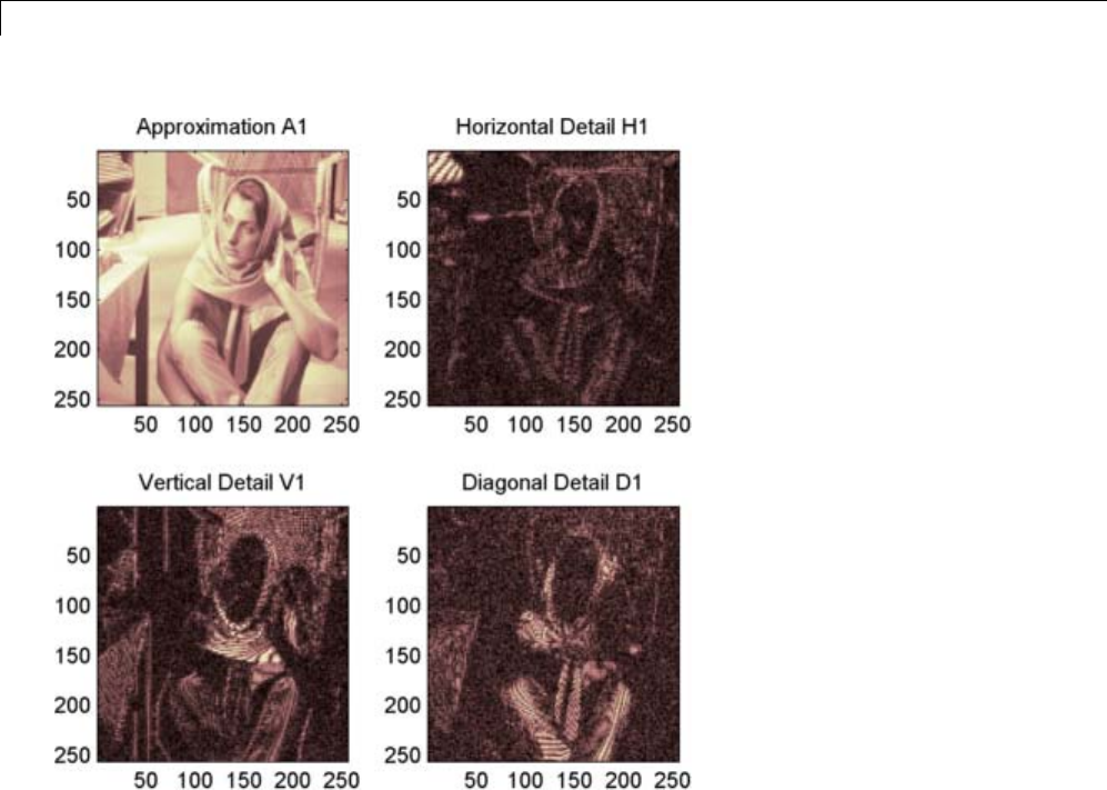
3Discrete Wavelet Analysis
3Convert an indexed image to a grayscale image.
If the colormap is smooth, the wavelet transform can be directly applied
to the indexed image; otherwise the indexed image should be converted to
grayscale format. For more information, see “Wavelets: Working with
Images”.
Since the colormap is smooth in this image, you can now perform the
decomposition.
4Perform a single-level wavelet decomposition.
To perform a single-level decomposition of the image using the bior3.7
wavelet, type
3-140

Two-Dimensional Discrete Wavelet Analysis
[cA1,cH1,cV1,cD1] = dwt2(X,'bior3.7');
This generates the coefficient matrices of the level-one approximation (cA1)
and horizontal, vertical and diagonal details (cH1,cV1,cD1,respectively).
5Construct and display approximations and details from the coefficients.
To construct the level-one approximation and details (A1,H1,V1,andD1)
from the coefficients cA1,cH1,cV1,andcD1,type
A1 = upcoef2('a',cA1,'bior3.7',1);
H1 = upcoef2('h',cH1,'bior3.7',1);
V1 = upcoef2('v',cV1,'bior3.7',1);
D1 = upcoef2('d',cD1,'bior3.7',1);
or
sx = size(X);
A1 = idwt2(cA1,[],[],[],'bior3.7',sx);
H1 = idwt2([],cH1,[],[],'bior3.7',sx);
V1 = idwt2([],[],cV1,[],'bior3.7',sx);
D1 = idwt2([],[],[],cD1,'bior3.7',sx);
To display the results of the level 1 decomposition, type
colormap(map);
subplot(2,2,1); image(wcodemat(A1,192));
title('Approximation A1')
subplot(2,2,2); image(wcodemat(H1,192));
title('Horizontal Detail H1')
subplot(2,2,3); image(wcodemat(V1,192));
title('Vertical Detail V1')
subplot(2,2,4); image(wcodemat(D1,192));
title('Diagonal Detail D1')
3-141
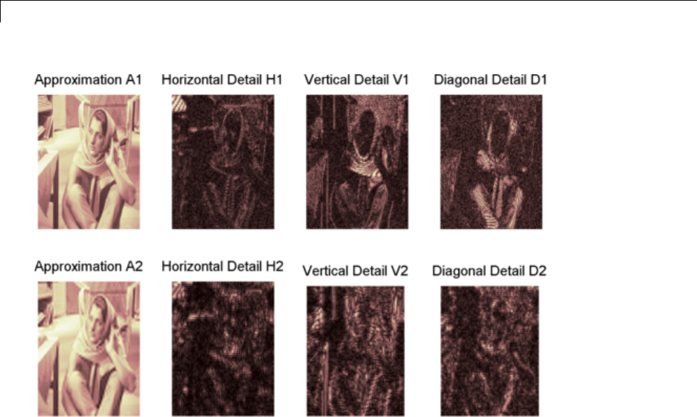
3Discrete Wavelet Analysis
6Regenerate an image by single-level Inverse Wavelet Transform.
To find the inverse transform, type
Xsyn = idwt2(cA1,cH1,cV1,cD1,'bior3.7');
This reconstructs or synthesizes the original image from the coefficients of
the level 1 approximation and details.
7Perform a multilevel wavelet decomposition.
To perform a level 2 decomposition of the image (again using the bior3.7
wavelet), type
[C,S] = wavedec2(X,2,'bior3.7');
where Xis the original image matrix, and 2 is the level of decomposition.
3-142

Two-Dimensional Discrete Wavelet Analysis
The coefficients of all the components of a second-level decomposition (that
is, the second-level approximation and the first two levels of detail) are
returned concatenated into one vector, C.ArgumentSis a bookkeeping
matrix that keeps track of the sizes of each component.
8Extract approximation and detail coefficients.
To extract the level 2 approximation coefficients from C,type
cA2 = appcoef2(C,S,'bior3.7',2);
To extract the first- and second-level detail coefficients from C,type
cH2 = detcoef2('h',C,S,2);
cV2 = detcoef2('v',C,S,2);
cD2 = detcoef2('d',C,S,2);
cH1 = detcoef2('h',C,S,1);
cV1 = detcoef2('v',C,S,1);
cD1 = detcoef2('d',C,S,1);
or
[cH2,cV2,cD2] = detcoef2('all',C,S,2);
[cH1,cV1,cD1] = detcoef2('all',C,S,1);
where the first argument ('h','v',or'd') determines the type of detail
(horizontal, vertical, diagonal) extracted, and the last argument determines
the level.
9Reconstruct the Level 2 approximation and the Level 1 and 2 details.
To reconstruct the level 2 approximation from C,type
A2 = wrcoef2('a',C,S,'bior3.7',2);
To reconstruct the level 1 and 2 details from C,type
H1 = wrcoef2('h',C,S,'bior3.7',1);
V1 = wrcoef2('v',C,S,'bior3.7',1);
D1 = wrcoef2('d',C,S,'bior3.7',1);
H2 = wrcoef2('h',C,S,'bior3.7',2);
V2 = wrcoef2('v',C,S,'bior3.7',2);
3-143

3Discrete Wavelet Analysis
D2 = wrcoef2('d',C,S,'bior3.7',2);
10 Display the results of a multilevel decomposition.
Note With all the details involved in a multilevel image decomposition, it
makes sense to import the decomposition into the Wavelet 2-D graphical
tool in order to more easily display it. For information on how to do this,
see “Loading Decompositions” on page 3-164.
To display the results of the level 2 decomposition, type
colormap(map);
subplot(2,4,1);image(wcodemat(A1,192));
title('Approximation A1')
subplot(2,4,2);image(wcodemat(H1,192));
title('Horizontal Detail H1')
subplot(2,4,3);image(wcodemat(V1,192));
title('Vertical Detail V1')
subplot(2,4,4);image(wcodemat(D1,192));
title('Diagonal Detail D1')
subplot(2,4,5);image(wcodemat(A2,192));
title('Approximation A2')
subplot(2,4,6);image(wcodemat(H2,192));
title('Horizontal Detail H2')
subplot(2,4,7);image(wcodemat(V2,192));
title('Vertical Detail V2')
subplot(2,4,8);image(wcodemat(D2,192));
title('Diagonal Detail D2')
11 Reconstruct the original image from the multilevel decomposition.
To reconstruct the original image from the wavelet decomposition
structure, type
X0 = waverec2(C,S,'bior3.7');
This reconstructs or synthesizes the original image from the coefficients
Cof the multilevel decomposition.
3-144
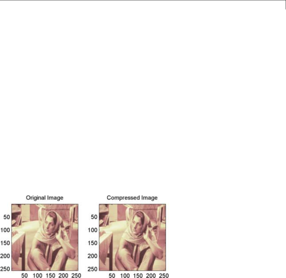
Two-Dimensional Discrete Wavelet Analysis
12 Compress the image and display it.
To compress the original image X,usetheddencmp command to calculate
the default parameters and the wdencmp command to perform the actual
compression. Type
[thr,sorh,keepapp]= ddencmp('cmp','wv',X);
[Xcomp,CXC,LXC,PERF0,PERFL2] = ...
wdencmp('gbl',C,S,'bior3.7',2,thr,sorh,keepapp);
Note that we pass in to wdencmp the results of the decomposition (Cand
S)wecalculatedinstep7. Wealsospecifythebior3.7 wavelets, because
we used this wavelet to perform the original analysis. Finally, we specify
the global thresholding option 'gbl'.Seeddencmp and wdencmp reference
pages for more information about the use of these commands.
To view the compressed image side by side with the original, type
colormap(map);
subplot(121); image(X); title('Original Image');
axis square
subplot(122); image(Xcomp); title('Compressed Image');
axis square
PERF0
PERF0 =
49.8076
3-145

3Discrete Wavelet Analysis
PERFL2
PERFL2 =
99.9817
These returned values tell, respectively, what percentage of the wavelet
coefficients was set to zero and what percentage of the image’s energy was
preserved in the compression process.
Note that, even though the compressed image is constructed from only
about half as many nonzero wavelet coefficients as the original, there is
almost no detectable deterioration in the image quality.
3-146
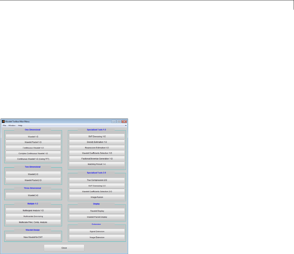
Two-Dimensional Discrete Wavelet Analysis
Interactive Two-Dimensional Wavelet Analysis
In this section weexplorethesameimageasintheprevioussection,butwe
use the graphical interface tools to analyze the image.
1Start the 2-D Wavelet Analysis Tool.
From the MATLAB prompt, type
wavemenu
The Wavelet Tool Main Menu appears.
Click the Wavelet 2-D menu item. The discrete wavelet analysis tool for
two-dimensional image data appears.
3-147
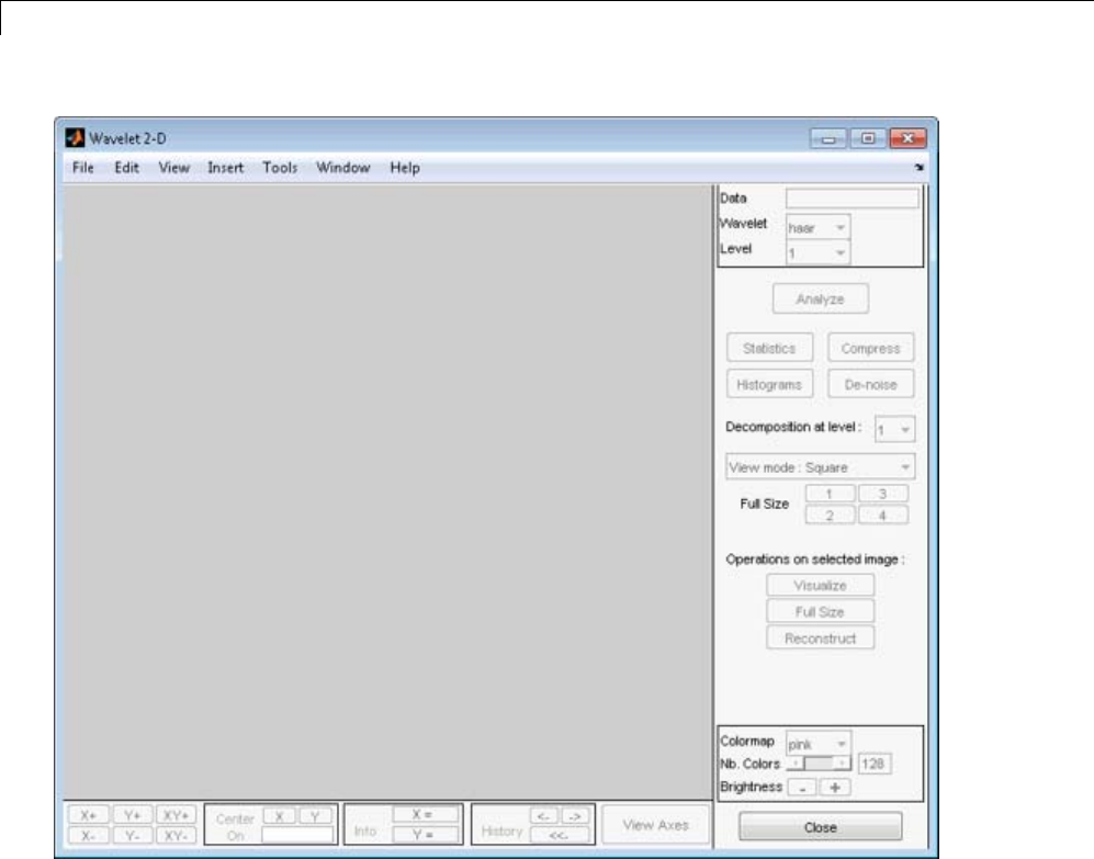
3Discrete Wavelet Analysis
2Load animage.
From the File menu, choose the Load > Image option.
3-148
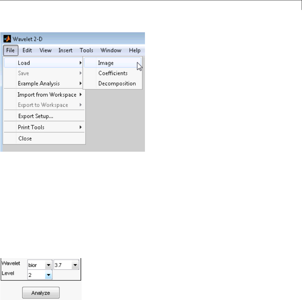
Two-Dimensional Discrete Wavelet Analysis
When the Load Image dialog box appears, select the MAT-file wbarb.mat,
whichisintheMATLABfoldertoolbox/wavelet/wavedemo.Clickthe
OK button.
The image is loaded into the Wavelet 2-D tool.
3Analyze the image.
Using the Wavelet and Level menus located to the upper right, determine
the wavelet family, the wavelet type, and the number of levels to be used
for the analysis.
For this analysis, select the bior3.7 wavelet at level 2.
Click the Analyze button. After a pause for computation, the Wavelet
2-D tool displays its analysis.
3-149
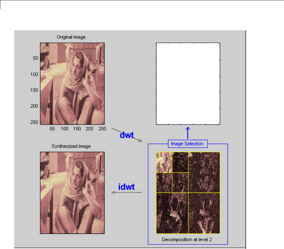
3Discrete Wavelet Analysis
UsingSquareModeFeatures
By default, the analysis appears in “Square Mode.” This mode includes
four different displays. In the upper left is the original image. Below that
is the image reconstructed from the various approximations and details.
To the lower right is a decomposition showing the coarsest approximation
coefficients and all the horizontal, diagonal, and vertical detail coefficients.
3-150
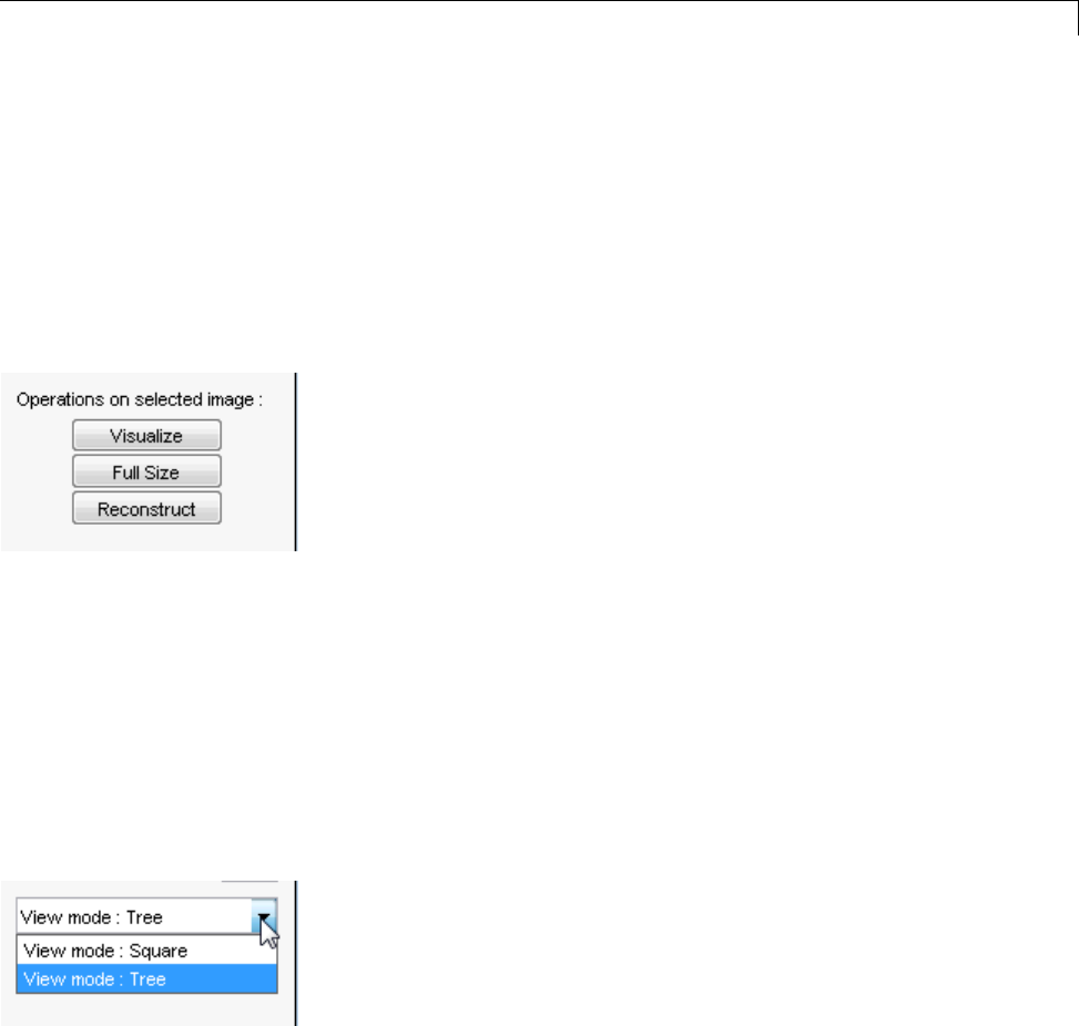
Two-Dimensional Discrete Wavelet Analysis
Finally, the visualization space at the top right displays any component of
the analysis that you want to look at more closely.
Click on any decomposition component in the lower right window.
A green border highlights the selected component. At the lower right of the
Wavelet 2-D window, there is a set of three buttons labeled “Operations
on selected image.” Note that if you click again on the same component,
you’ll deselect it and the green border disappears.
Click the Visualize button.
The selected image is displayed in the visualization area. You are seeing
the raw, unreconstructed two-dimensional wavelet coefficients. Using the
other buttons, you can display the reconstructed version of the selected
image component, or you can view the selected component at full screen
resolution.
UsingTreeModeFeatures
Choose Tree from the View Mode menu.
Your display changes to reveal the following.
3-151
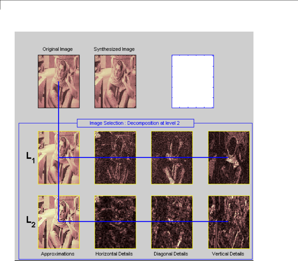
3Discrete Wavelet Analysis
This is the same information shown in square mode, with in addition all the
approximation coefficients, but arranged to emphasize the tree structure
of the decomposition. The various buttons and menus work just the same
as they do in square mode.
ZoominginonDetail
3-152
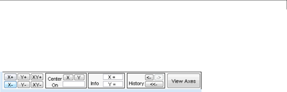
Two-Dimensional Discrete Wavelet Analysis
Drag a rubber band box (by holding down the left mouse button) over the
portion of the image you want to magnify.
Click the XY+ button (located at the bottom of the screen) to zoom
horizontally and vertically.
The Wavelet 2-D tool enlarges the displayed images.
To zoom back to original magnification, click the History <<- button.
4Compress the image
Click the Compress button, located to the upper right of the Wavelet 2-D
window. The Wavelet 2-D Compression window appears.
3-153
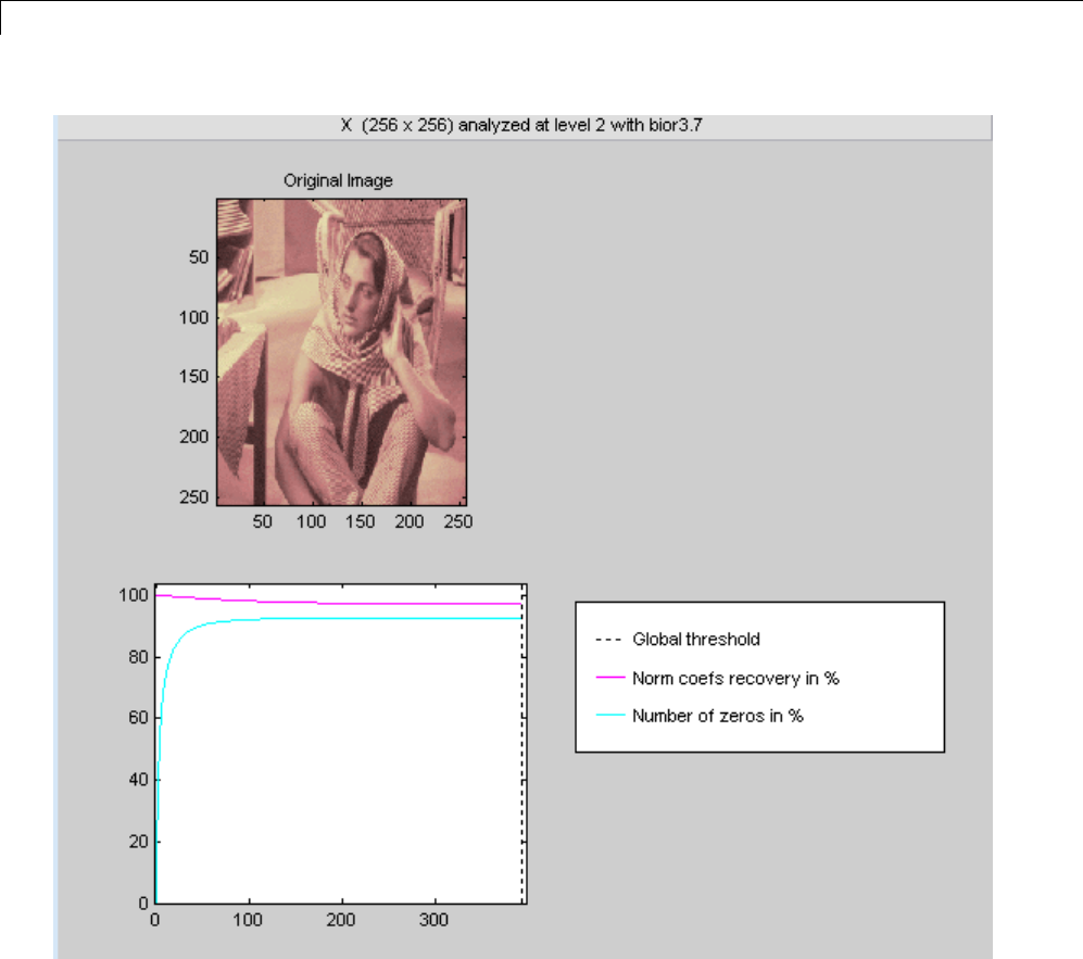
3Discrete Wavelet Analysis
The tool automatically selects thresholding levels to provide a good initial
balance between retaining the image’s energy while minimizing the
number of coefficients needed to represent the image.
However, you can also adjust thresholds manually using the By Level
thresholding option, and then the sliders or edits corresponding to each
level.
3-154
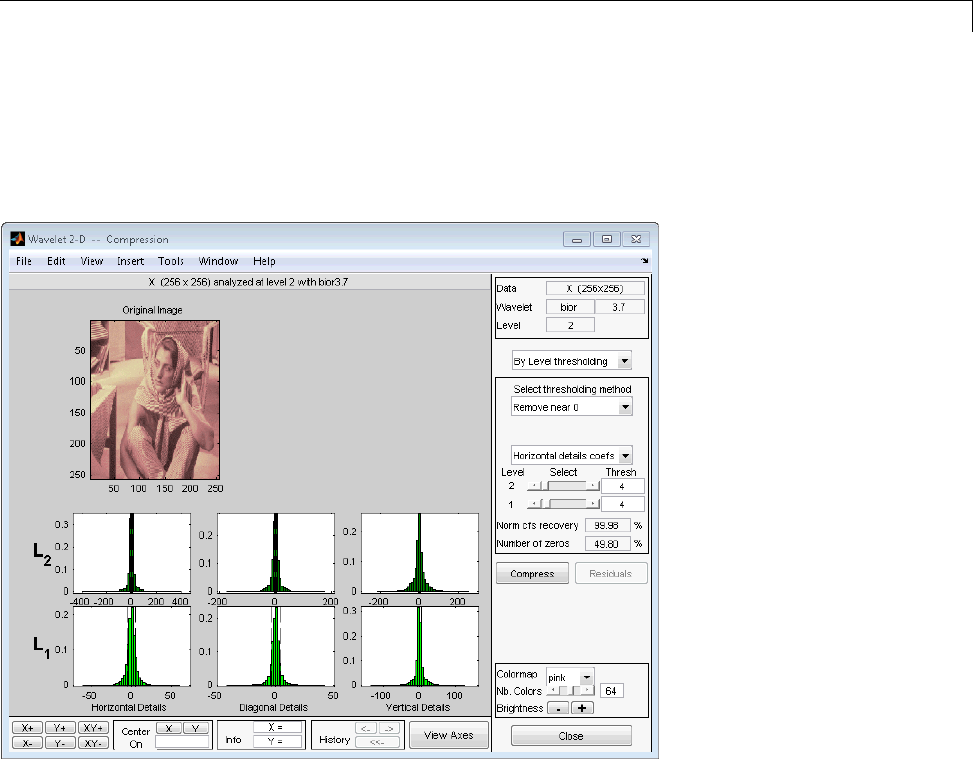
Two-Dimensional Discrete Wavelet Analysis
For this example, select the By Level thresholding option and select the
Remove near 0 method from the Select thresholding method menu.
The following window is displayed.
Select from the direction menu whether you want to adjust thresholds for
horizontal, diagonal or vertical details. To make the actual adjustments for
each level, use the sliders or use the left mouse button to directly drag the
yellow vertical lines.
To compress the original image, click the Compress button. After a pause
for computation, the compressed image is displayed beside the original.
Notice that compression eliminates almost half the coefficients, yet no
detectable deterioration of the image appears.
3-155
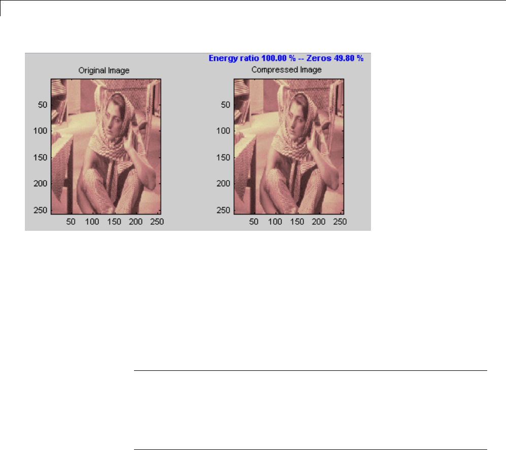
3Discrete Wavelet Analysis
5Show the residuals.
From the Wavelet 2-D Compression tool, click the Residuals button.
The More on Residuals for Wavelet 2-D Compression window appears.
Displayed statistics include measures of tendency (mean, mode, median)
and dispersion (range, standard deviation). In addition, the tool provides
frequency-distribution diagrams (histograms and cumulative histograms).
ThesametoolexistsfortheWavelet 2-D De-noising tool.
Note The statistics displayed in the above figure are related to the
displayed image but not to the original one. Usually this information is
the same, but in some cases, edge effects may cause the original image
to be cropped slightly. To see the exact statistics, use the command line
functions to get the desired image and then apply the desired MATLAB
statistical function(s).
Importing and Exporting Information from the
Graphical Interface
The Wavelet 2-D graphical tool lets you import information from and export
information to disk, if you adhere to the proper file formats.
3-156
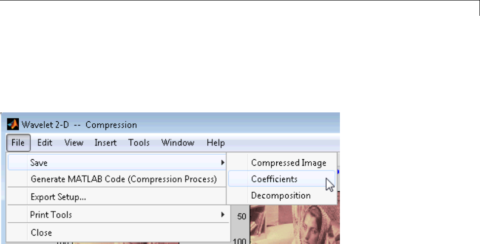
Two-Dimensional Discrete Wavelet Analysis
Saving Information to Disk
You can save synthesized images, coefficients, and decompositions from the
Wavelet 2-D tool to disk, where the information can be manipulated and
later reimported into the graphical tool.
Saving Synthesized Images. You can process an image in the Wavelet
2-D tool, and then save the processed image to a MAT-file (with extension
mat or other).
For example, load the example analysis:
File > Example Analysis > at level 3, with sym4 →detail Durer
and perform a compression on the original image. When you close the
Wavelet 2-D Compression window, update the synthesized image by
clicking Yes in the dialog box that appears.
Then, from the Wavelet 2-D tool, select the File > Save > Synthesized
Image menu option. A dialog box appears allowing you to select a folder and
filename for the MAT-file (with extension mat or other). For this example,
choose the name symage.
To load the image into your workspace, type
load symage
whos
3-157

3Discrete Wavelet Analysis
Name Size Bytes Class
X 359x371 1065512 double array
map 64x3 1536 double array
valTHR 1x1 8 double array
wname 1x4 8 char array
The synthesized image is given by Xand map contains the colormap. In
addition, the parameters of the de-noising or compression process are given
by the wavelet name (wname) and the global threshold (valTHR).
Saving Discrete Wavelet Transform Coefficients. The Wavelet 2-D tool
lets you save the coefficients of a discrete wavelet transform (DWT) to disk.
The toolbox creates a MAT-file in the current folder with a name you choose.
To save the DWT coefficients from the present analysis, use the menu option
File > Save > Coefficients.
A dialog box appears that lets you specify a folder and filename for storing
the coefficients.
Consider the example analysis:
File > Example Analysis > at level 3, with sym4 →Detail Durer
After saving the discrete wavelet coefficients to the file cfsdurer.mat,load
the variables into your workspace:
load cfsdurer
whos
Name Size Bytes Class
coefs 1x142299 1138392 double array
map 64x3 1536 double array
sizes 5x2 80 double array
3-158
Two-Dimensional Discrete Wavelet Analysis
Name Size Bytes Class
valTHR 0x0 0 double array
wname 1x4 8 char array
Variable map contains the colormap. Variable wname contains the wavelet
name and valTHR is empty since the synthesized image is the same as the
original one.
Variables coefs and sizes contain the discrete wavelet coefficients and the
associated matrix sizes. More precisely, in the above example, coefs is a
1-by-142299 vector of concatenated coefficients, and sizes gives the length of
each component.
Saving Decompositions. The Wavelet 2-D tool lets you save the entire
set of data from a discrete wavelet analysis to disk. The toolbox creates
a MAT-file in the current folder with a name you choose, followed by the
extension wa2 (wavelet analysis 2-D).
Open the Wavelet 2-D tool and load the example analysis:
File > Example Analysis > at level 3, with sym4 →Detail Durer.
To save the data from this analysis, use the menu option File > Save >
Decomposition.
A dialog box appears that lets you specify a folder and filename for storing
the decomposition data. Type the name decdurer.
After saving the decomposition data to the file decdurer.wa2,loadthe
variables into your workspace:
load decdurer.wa2 -mat
whos
Name Size Bytes Class
coefs 1x142299 1138392 double array
data_name 1x6 12 char array
3-159

3Discrete Wavelet Analysis
Name Size Bytes Class
map 64x3 1536 double array
sizes 5x2 80 double array
valTHR 0x0 0 double array
wave_name 1x4 8 char array
Variables coefs and sizes contain the wavelet decomposition structure.
Other variables contain the wavelet name, the colormap, and the filename
containing the data. Variable valTHR is empty since the synthesized image is
thesameastheoriginalone.
Note Save options are also available when performing de-noising or
compression inside the Wavelet 2-D tool. In the Wavelet 2-D De-noising
window, you can save denoised image and decomposition. The same holds
true for the Wavelet 2-D Compression window. This way, you can save
many different trials from inside the De-noising and Compression windows
without going back to the main Wavelet 2-D window during a fine-tuning
process. When saving a synthesized signal, a decomposition or coefficients to a
MAT-file, the mat file extension is not necessary. You can save approximations
individually for each level or save them all at once.
Loading Information into the Wavelet 2-D Tool
You can load images, coefficients, or decompositions into the graphical
interface. The information you load may have been previously exported from
the graphical interface, and then manipulated in the workspace; or it may
have been information you generated initially from the command line.
In either case, you must observe the strict file formats and data structures
used by the Wavelet 2-D tool, or else errors will result when you try to load
information.
3-160
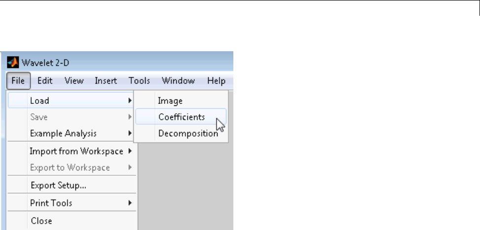
Two-Dimensional Discrete Wavelet Analysis
Loading Images. This toolbox supports only indexed images.Anindexed
image is a matrix containing only integers from 1 to n,wherenis the number
of colors in the image.
This imagemayoptionallybeaccompaniedbyann-by-3 matrix called map.
This is the colormap associated with the image. When MATLAB displays such
an image, it uses the values of the matrix to look up the desired color in this
colormap. If the colormap is not given, the Wavelet 2-D tool uses a monotonic
colormap with max(max(X))min(min(X))+1 colors.
To load an image you’ve constructed in your MATLAB workspace into the
Wavelet 2-D tool, save the image (and optionally, the variable map)ina
MAT-file (with extension mat or other).
For instance, suppose you’ve created an image called brain and want to
analyze it in the Wavelet 2-D tool. Type
X = brain;
map = pink(256);
save myfile X map
To load this image into the Wavelet 2-D tool, use the menu option File >
Load>Image.
3-161

3Discrete Wavelet Analysis
A dialog box appears that lets you select the appropriate MAT-file to be loaded.
Note Thegraphicaltoolsallowyoutoload an image that does not contain
integers from 1 to n. The computations are correct because they act directly
on the matrix, but the display of the image is strange. The values less than 1
are evaluated as 1, the values greater than nare evaluated as n,andareal
value within the interval [1,n] is evaluated as the closest integer.
The coefficients, approximations, and details produced by wavelet
decomposition are not indexed image matrices.
To display these images in a suitable way, the Wavelet 2-D tool follows
these rules:
•Reconstructed approximations are displayed using the colormap map.
•The coefficients and the reconstructed details are displayed using the
colormap map applied to a rescaled version of the matrices.
Note Thefirsttwo-dimensionalvariableencounteredinthefile(exceptthe
variable map, which is reserved for the colormap) is considered the image.
Variables are inspected in alphabetical order.
Loading Discrete Wavelet Transform Coefficients. To load discrete
wavelet transform (DWT) coefficients into the Wavelet 2-D tool, first save the
appropriate data in a MAT-file, which must contain at least the two variables:
•coefs, the coefficients vector
•sizes, the bookkeeping matrix
For an indexed image the matrix sizes is a (n+2-by-2) array:
3-162

Two-Dimensional Discrete Wavelet Analysis
Foratruecolorimage,thematrixsizes is a (n+2-by-3):
Variable coefs must be a vector of concatenated DWT coefficients. The coefs
vector for an n-level decomposition contains 3n+1 sections, consisting of the
level-napproximation coefficients, followed by the horizontal, vertical, and
diagonal detail coefficients, in that order, for each level. Variable sizes is
a matrix, the rows of which specify the size of cAn,thesizeofcHn(or cVn,or
cDn),..., the size of cH1(or cV1,orcD1), and the size of the original image X.The
sizes of vertical and diagonal details arethesameasthehorizontaldetail.
After constructing or editing the appropriate data in your workspace, type
3-163

3Discrete Wavelet Analysis
save myfile coefs sizes
Use the File > Load > Coefficients menu option from the Wavelet 2-D tool
to load the data into the graphical tool.
A dialog box appears, allowing you to choose the folder and file in which your
data reside.
Loading Decompositions. To load discrete wavelet transform decomposition
data into the Wavelet 2-D tool, you must first save the appropriate data in a
MAT-file (with extension wa2 or other).
TheMAT-filecontainsthesevariables.
Variable Status Description
coefs Required Vector of concatenated DWT coefficients
sizes Required Matrix specifying sizes of components of
coefs and of the original image
wave_name Required String specifying name of wavelet used
for decomposition (e.g., db3)
map Optional n-by-3 colormap matrix.
data_name Optional String specifying name of decomposition
After constructing or editing the appropriate data in your workspace, type
save myfile.wa2 coefs sizes wave_name
Use the File > Load > Decomposition menu option from the Wavelet 2-D
tool to load the image decomposition data.
A dialog box appears, allowing you to choose the folder and file in which your
data reside.
3-164

Two-Dimensional Discrete Wavelet Analysis
Note When loading an image, a decomposition, or coefficients from a
MAT-file, the extension of this file is free. The mat extension is not necessary.
3-165

3Discrete Wavelet Analysis
Two-Dimensional Discrete Stationary Wavelet Analysis
Thissectiontakesyouthroughthefeatures of two-dimensional discrete
stationary wavelet analysis using the Wavelet Toolbox software.
Analysis-Decomposition Function
Function Name Purpose
swt2 Decomposition
Synthesis-Reconstruction Function
Function Name Purpose
iswt2 Reconstruction
The stationary wavelet decomposition structure is more tractable than the
wavelet one. So, the utilities useful for the wavelet case are not necessary for
the Stationary Wavelet Transform (SWT).
In this section, you’ll learn to
•Load an image
•Analyze an image
•Perform single-level and multilevel image decompositions and
reconstructions (command line only)
•denoise an image
Two-Dimensional Analysis Using the Command Line
In this example, we’ll show how you can use two-dimensional stationary
wavelet analysis to denoise an image.
3-166

Two-Dimensional Discrete Stationary Wavelet Analysis
Note Instead of using image(I) to visualize the image I,weuse
image(wcodemat(I)), which displays a rescaled version of Ileading to a
clearer presentation of the details and approximations (see the wcodemat
reference page).
This example involves a image containing noise.
1Load an image.
From the MATLAB prompt, type
load noiswom
whos
Name Size Bytes Class
X 96x96 73728 double array
map 255x3 6120 double array
For the SWT, if a decomposition at level kis needed, 2^k must divide
evenly into size(X,1) and size(X,2). If your original image is not of
correct size, you can use the Image Extension GUI tool or the function
wextend to extend it.
2Perform a single-level Stationary Wavelet Decomposition.
Perform a single-level decomposition of the image using the db1 wavelet.
Type
[swa,swh,swv,swd] = swt2(X,1,'db1');
This generates the coefficients matrices of the level-one approximation
(swa) and horizontal, vertical and diagonal details (swh,swv,andswd,
respectively). Both are of size-the-image size. Type
whos
3-167

3Discrete Wavelet Analysis
Name Size Bytes Class
X 96x96 73728 double array
map 255x3 6120 double array
swa 96x96 73728 double array
swh 96x96 73728 double array
swv 96x96 73728 double array
swd 96x96 73728 double array
3Display the coefficients of approximation and details.
To display the coefficients of approximation and details at level 1, type
map = pink(size(map,1)); colormap(map)
subplot(2,2,1), image(wcodemat(swa,192));
title('Approximation swa')
subplot(2,2,2), image(wcodemat(swh,192));
title('Horiz. Detail swh')
subplot(2,2,3), image(wcodemat(swv,192));
title('Vertical Detail swv')
subplot(2,2,4), image(wcodemat(swd,192));
title('Diag. Detail swd');
3-168
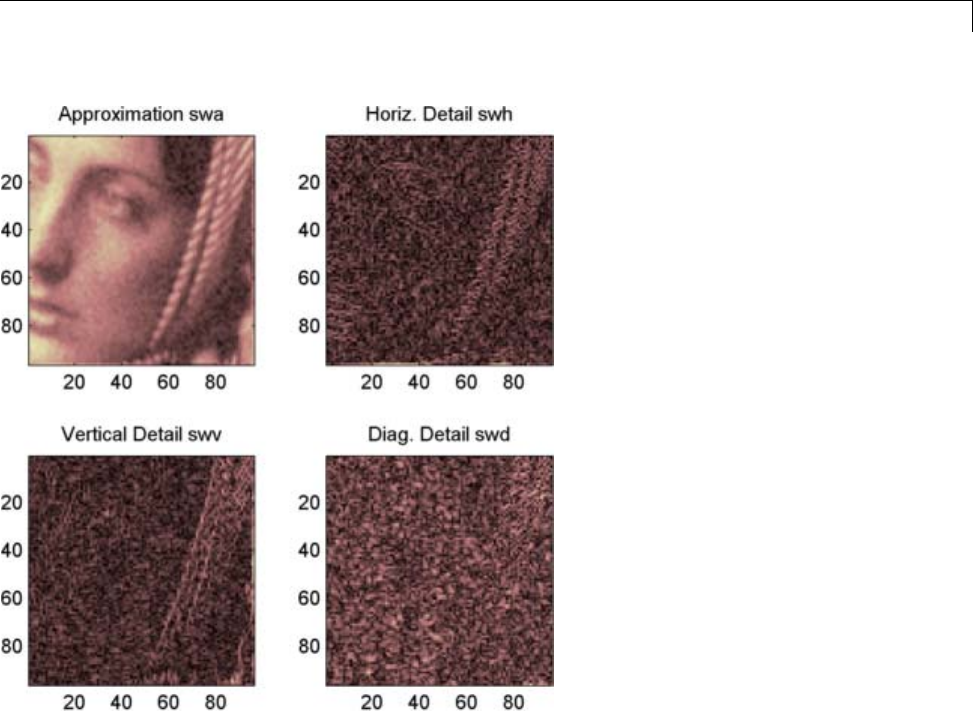
Two-Dimensional Discrete Stationary Wavelet Analysis
4Regenerate the image by Inverse Stationary Wavelet Transform.
To find the inverse transform, type
A0 = iswt2(swa,swh,swv,swd,'db1');
To check the perfect reconstruction, type
err = max(max(abs(X-A0)))
err =
1.1369e-13
5Construct and display approximation and details from the coefficients.
3-169

3Discrete Wavelet Analysis
To construct the level 1 approximation and details (A1,H1,V1 and D1)from
the coefficients swa,swh,swv and swd,type
nulcfs = zeros(size(swa));
A1 = iswt2(swa,nulcfs,nulcfs,nulcfs,'db1');
H1 = iswt2(nulcfs,swh,nulcfs,nulcfs,'db1');
V1 = iswt2(nulcfs,nulcfs,swv,nulcfs,'db1');
D1 = iswt2(nulcfs,nulcfs,nulcfs,swd,'db1');
To display the approximation and details at level 1, type
colormap(map)
subplot(2,2,1), image(wcodemat(A1,192));
title('Approximation A1')
subplot(2,2,2), image(wcodemat(H1,192));
title('Horiz. Detail H1')
subplot(2,2,3), image(wcodemat(V1,192));
title('Vertical Detail V1')
subplot(2,2,4), image(wcodemat(D1,192));
title('Diag. Detail D1')
3-170
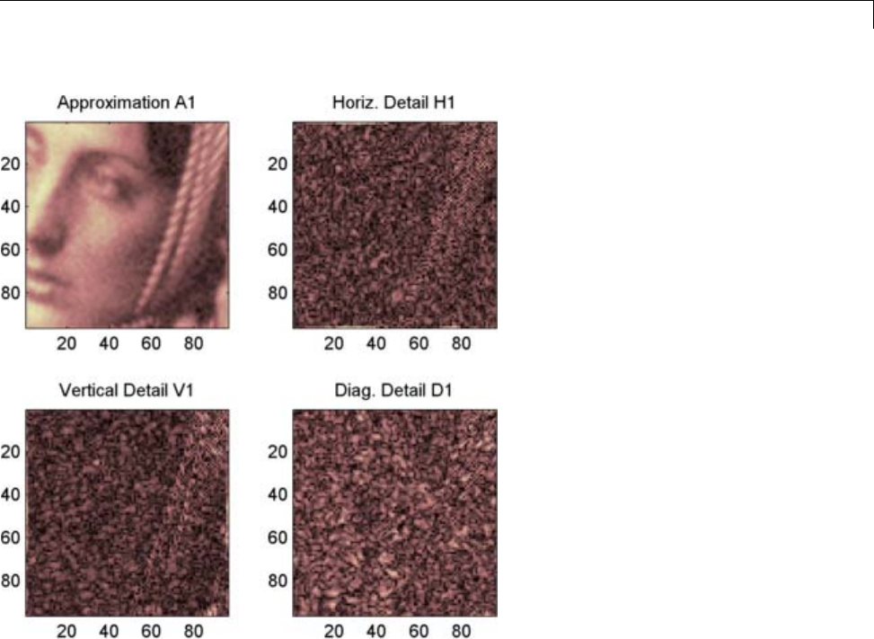
Two-Dimensional Discrete Stationary Wavelet Analysis
6Perform a multilevel Stationary Wavelet Decomposition.
To perform a decomposition at level 3 of the image (again using the db1
wavelet), type
[swa,swh,swv,swd] = swt2(X,3,'db1');
This generates the coefficients of the approximations at levels 1, 2, and 3
(swa)andthecoefficientsofthedetails(swh,swv and swd). Observe that
the matrices swa(:,:,i),swh(:,:,i),swv(:,:,i),andswd(:,:,i) for
agivenleveliare of size-the-image size. Type
clear A0 A1 D1 H1 V1 err nulcfs
whos
3-171

3Discrete Wavelet Analysis
Name Size Bytes Class
X 96x96 73728 double array
map 255x3 6120 double array
swa 96x96x3 221184 double array
swh 96x96x3 221184 double array
swv 96x96x3 221184 double array
swd 96x96x3 221184 double array
7Display the coefficients of approximations and details.
To display the coefficients of approximations and details, type
colormap(map)
kp = 0;
fori=1:3
subplot(3,4,kp+1), image(wcodemat(swa(:,:,i),192));
title(['Approx. cfs level ',num2str(i)])
subplot(3,4,kp+2), image(wcodemat(swh(:,:,i),192));
title(['Horiz. Det. cfs level ',num2str(i)])
subplot(3,4,kp+3), image(wcodemat(swv(:,:,i),192));
title(['Vert. Det. cfs level ',num2str(i)])
subplot(3,4,kp+4), image(wcodemat(swd(:,:,i),192));
title(['Diag. Det. cfs level ',num2str(i)])
kp = kp + 4;
end
8Reconstruct approximation at Level 3 and details from coefficients.
To reconstruct the approximation at level 3, type
mzero = zeros(size(swd));
A = mzero;
A(:,:,3) = iswt2(swa,mzero,mzero,mzero,'db1');
To reconstruct the details at levels 1, 2 and 3, type
H = mzero; V = mzero;
3-172

Two-Dimensional Discrete Stationary Wavelet Analysis
D = mzero;
fori=1:3
swcfs = mzero; swcfs(:,:,i) = swh(:,:,i);
H(:,:,i) = iswt2(mzero,swcfs,mzero,mzero,'db1');
swcfs = mzero; swcfs(:,:,i) = swv(:,:,i);
V(:,:,i) = iswt2(mzero,mzero,swcfs,mzero,'db1');
swcfs = mzero; swcfs(:,:,i) = swd(:,:,i);
D(:,:,i) = iswt2(mzero,mzero,mzero,swcfs,'db1');
end
9Reconstruct and display approximations at Levels 1, 2 from approximation
at Level 3 and details at Levels 1, 2, and 3.
To reconstruct the approximations at levels 2 and 3, type
A(:,:,2) = A(:,:,3) + H(:,:,3) + V(:,:,3) + D(:,:,3);
A(:,:,1) = A(:,:,2) + H(:,:,2) + V(:,:,2) + D(:,:,2);
To display the approximations and details at levels 1, 2, and 3, type
colormap(map)
kp = 0;
fori=1:3
subplot(3,4,kp+1), image(wcodemat(A(:,:,i),192));
title(['Approx. level ',num2str(i)])
subplot(3,4,kp+2), image(wcodemat(H(:,:,i),192));
title(['Horiz. Det. level ',num2str(i)])
subplot(3,4,kp+3), image(wcodemat(V(:,:,i),192));
title(['Vert. Det. level ',num2str(i)])
subplot(3,4,kp+4), image(wcodemat(D(:,:,i),192));
title(['Diag. Det. level ',num2str(i)])
kp = kp + 4;
end
10 Remove noise by thresholding.
Todenoiseanimage,usethethresholdvaluewefindusingtheGUItool
(see the next section), use the wthresh command to perform the actual
thresholding of the detail coefficients, and then use the iswt2 command to
obtain the denoised image.
3-173
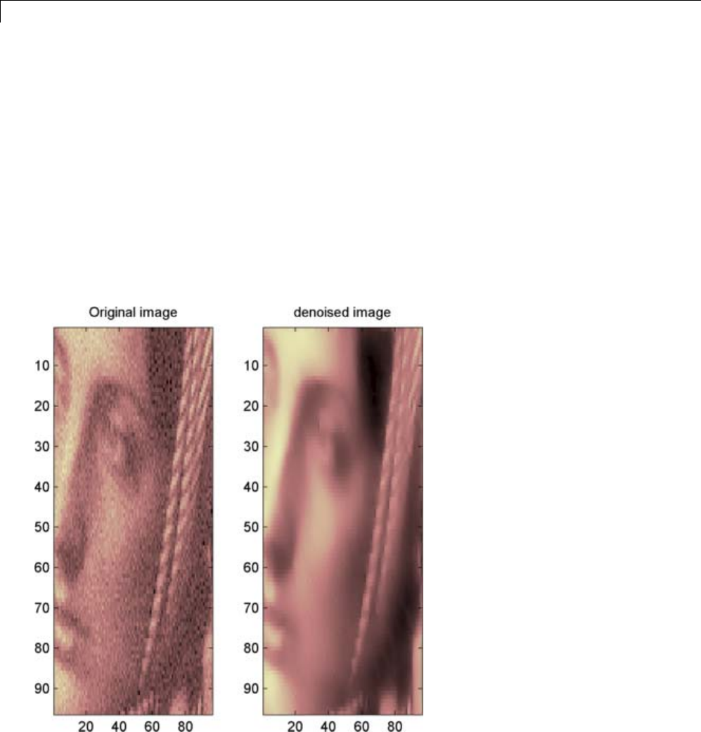
3Discrete Wavelet Analysis
thr = 44.5;
sorh = 's'; dswh = wthresh(swh,sorh,thr);
dswv = wthresh(swv,sorh,thr);
dswd = wthresh(swd,sorh,thr);
clean = iswt2(swa,dswh,dswv,dswd,'db1');
To display both the original and denoised images, type
colormap(map)
subplot(1,2,1), image(wcodemat(X,192));
title('Original image')
subplot(1,2,2), image(wcodemat(clean,192));
title('denoised image')
3-174

Two-Dimensional Discrete Stationary Wavelet Analysis
A second syntax can be used for the swt2 and iswt2 functions, giving the
same results:
lev= 4;
swc = swt2(X,lev,'db1');
swcden = swc;
swcden(:,:,1:end-1) =
wthresh(swcden(:,:,1:end-1),sorh,thr);
clean = iswt2(swcden,'db1');
You obtain the same plot by using the plot commands in step 9 above.
Interactive 2-D Stationary Wavelet Transform
Denoising
In this section, we explore a strategy for de-noising images based on the
two-dimensional stationary wavelet analysis using the graphical interface
tools. The basic idea is to average many slightly different discrete wavelet
analyses.
1Start the Stationary Wavelet Transform De-Noising 2-D Tool.
From the MATLAB prompt, type
wavemenu
The Wavelet Toolbox Main Menu appears:
3-175
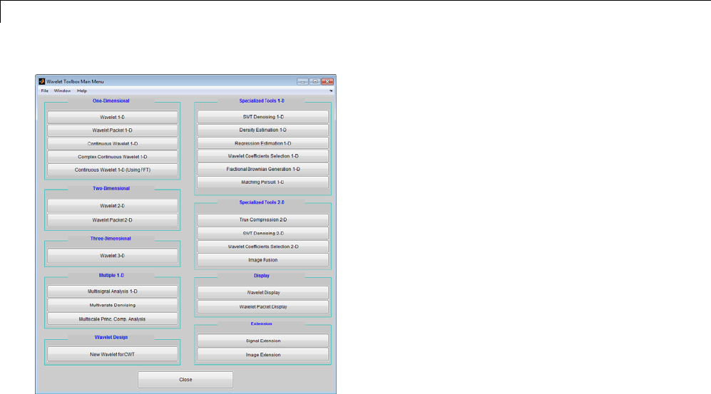
3Discrete Wavelet Analysis
Click the SWT De-noising 2-D menu item.
3-176
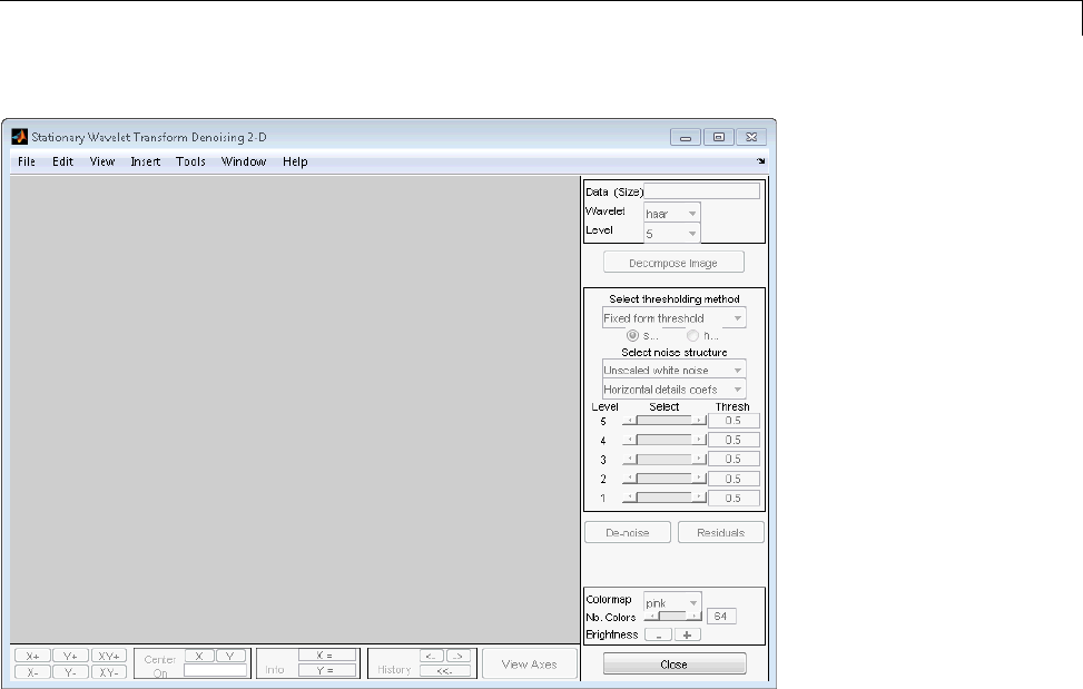
Two-Dimensional Discrete Stationary Wavelet Analysis
2Load data.
From theFile menu, choose the Load Image option.
When the Load Image dialog box appears, select the MAT-file
noiswom.mat, which should reside in the MATLAB folder
toolbox/wavelet/wavedemo.ClicktheOK button. The noisy woman
imageisloadedintotheSWT De-noising 2-D tool.
3Perform a Stationary Wavelet Decomposition.
Select the haar wavelet from the Wavelet menu, select 4from the Level
menu, and then click the Decompose Image button.
The tool displays the histograms of the stationary wavelet detail coefficients
of the image on the left of the window. These histograms are organized as
follows:
•From the bottom for level 1 to the top for level 4
3-177
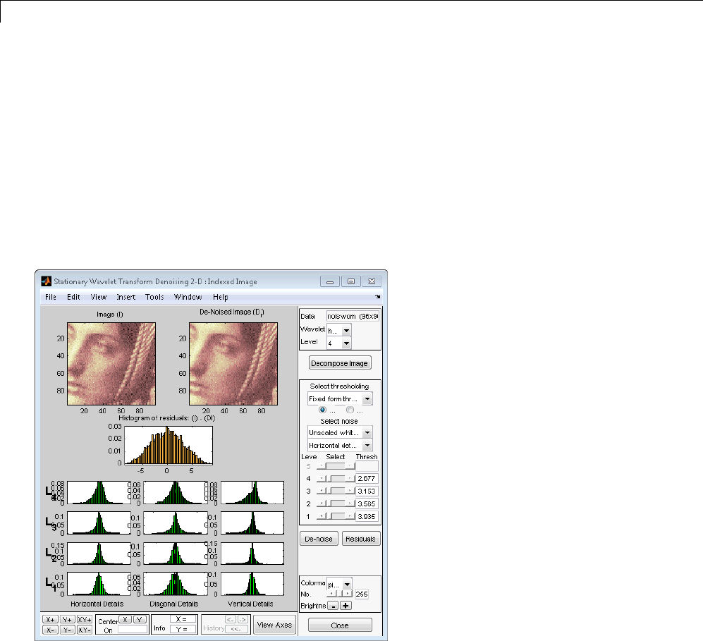
3Discrete Wavelet Analysis
•On the left horizontal coefficients, in the middle diagonal coefficients,
and on the right vertical coefficients
4denoise the image using the Stationary Wavelet Transform.
While a number of options are available for fine-tuning the de-noising
algorithm, we’ll accept the defaults of fixed form soft thresholding and
unscaled white noise. The sliders located to the right of the window control
the level dependent thresholds indicated by yellow dotted lines running
vertically through the histograms of the coefficients on the left of the
window. Click the denoise button.
The result seems to be oversmoothed and the selected thresholds too
aggressive. Nevertheless, the histogram of the residuals is quite good
since it is close to a Gaussian distribution, which is the noise introduced
to produce the analyzed image noiswom.mat from a piece of the original
image woman.mat.
3-178
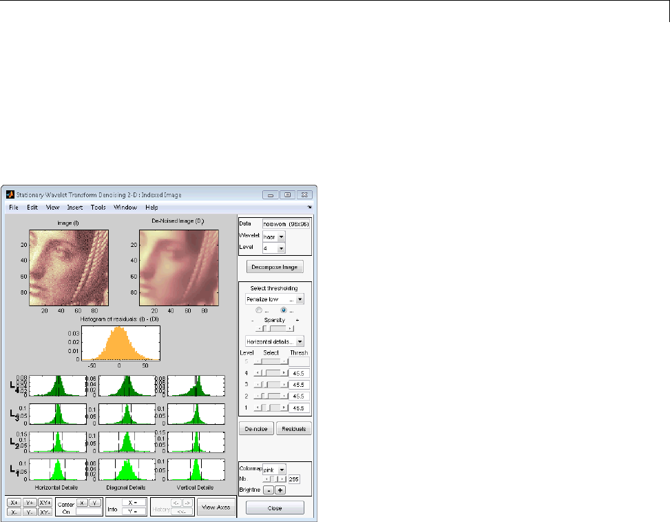
Two-Dimensional Discrete Stationary Wavelet Analysis
5Selecting a thresholding method.
From the Select thresholding method menu, choose the Penalize low
item. The associated default for the thresholding mode is automatically set
to hard; accept it. Use the Sparsity slider to adjust the threshold value
close to 45.5, and then click the denoise button.
The result is quite satisfactory, although it is possible to improve it slightly.
Select the sym6 wavelet and click the Decompose Image button. Use
the Sparsity slider to adjust the threshold value close to 40.44, and then
click the denoise button.
Importing and Exporting Information from the
Graphical Interface
The tool lets you save the denoised image to disk. The toolbox creates a
MAT-file in the current folder with a name you choose.
3-179

3Discrete Wavelet Analysis
To save the denoised image from the present de-noising process, use the menu
File > Save denoised Image. A dialog box appears that lets you specify a
folder and filename for storing the image. Type the name dnoiswom.After
saving the image data to the file dnoiswom.mat, load the variables into your
workspace:
load dnoiswom
whos
Name Size Bytes Class
X 96x96 73728 double array
map 255x3 6120 double array
valTHR 3x4 96 double array
wname 1x4 8 char array
The denoised image is Xand map is the colormap. In addition, the parameters
of the de-noising process are available. The wavelet name is contained
in wname, and the level dependent thresholds are encoded in valTHR.The
variable valTHR has four columns (the level of the decomposition) and three
rows (one for each detail orientation).
3-180

Three-Dimensional Discrete Wavelet Analysis
Three-Dimensional Discrete Wavelet Analysis
This section demonstrates the features of three-dimensional discrete wavelet
analysis using the Wavelet Toolbox software. The toolbox provides these
functions for 3-D data analysis. (You use the Wavelet 3-D GUI to perform all
tasksexceptthefirsttask.
•Getting information on the command line functions
•Loading 3-D data
•Analyzing a 3-D data
•Selecting and displaying slices
•Creating a slice movie
•Creating true 3-D display
•Importing and exporting information
Performing Three-Dimensional Analysis Using the
Command Line
The example wavelet3ddemo and the documentation of the
Analysis-Decomposition and Synthesis-Reconstruction functions show how you
can analyze 3-D arrays efficiently using command line functions dedicated
to the three-dimensional wavelet analysis. For more information, see the
function reference pages.
Analysis-Decomposition Functions
Function Name Purpose
dwt3 Single-level decomposition
wavedec3 Decomposition
3-181
3Discrete Wavelet Analysis
Synthesis-Reconstruction Functions
Function Name Purpose
idwt3 Single-level reconstruction
waverec3 Full reconstruction
Performing Three-Dimensional Analysis Using the
Graphical Interface
In this section you explore the same 3-D-data as in the wavelet3ddemo
example, but you use the graphical interface tools.
1Start the 3-D Wavelet Analysis Tool.
From the MATLAB prompt, type
wavemenu
The Wavelet Tool Main Menu appears.
Click the Wavelet 3-D menu item. The discrete wavelet analysis tool for
three-dimensional data opens.
3-182
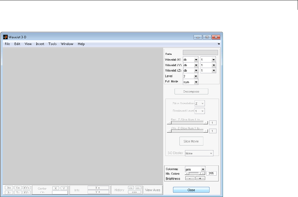
Three-Dimensional Discrete Wavelet Analysis
2Load a 3-D array.
From the File menu, choose Load > Data.
When the Load Data dialog box appears, select the MAT-file wmri.mat,
which is in the MATLAB folder toolbox/wavelet/wavelet.ClickOK to
load the 3-D data into the Wavelet 3-D tool.
3Analyze the 3-D array. Using the Wavelet and Level menus located in
the upper part of the tool, specify:
•The wavelet familes (one per direction X, Y and Z)
•The decomposition level and the wavelet extension mode to be used for
the analysis
For this analysis, accept the defaults: db1 wavelet for each direction,
decomposition at level 2and symmetric extension mode (sym).
3-183
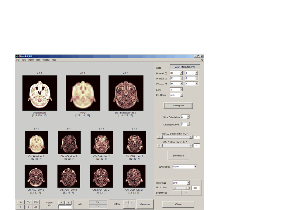
3Discrete Wavelet Analysis
Click Decompose. After a pause for computation, the Wavelet 3-D tool
displays its analysis.
3-184
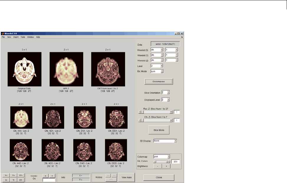
Three-Dimensional Discrete Wavelet Analysis
Review the slices of data and wavelet components in the graphical display.
These slices are orthogonal to the z-direction as indicated by Slice
Orientation in the command part of the window. This option lets you
choose the desired slice orientation.
The first row of the graphical display area displays from left to right and
for Z=1:
•The original data slice
•The approximation at level 2 slice (low-pass component APP2)
•The slice which is the sum of all the components from level 1 to level 2,
different from the low-pass one.
The x-labelsofthethreeaxesgiveyouthenameandthesizeofthe
displayed data.
3-185
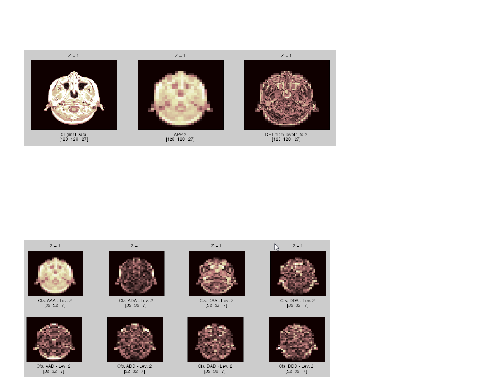
3Discrete Wavelet Analysis
The next two lines of axes, display the wavelet coefficients at level 2, which
is the desired level of the analysis. In the first line, the first graph contains
the coefficients of approximation at level 2. The remaining seven axes display
the seven types of wavelet coefficients at level 2. These coefficients contain
the x-labels of the eight axes and display the name, type and size of the
displayed data.
For example, in the third graphic of the bottom line, you can see the Cfs-DAD
coefficients at level 2, which correspondtoanarrayofsize32x32x7. The
name of the DAD coefficients group indicates that it is obtained using
•The high-pass filter in xdirection (Dfor detail)
•The low-pass filter in ydirection (Afor approximation)
•The high-pass filter in Z direction (Dagain for detail), leading to the DAD
component
3-186
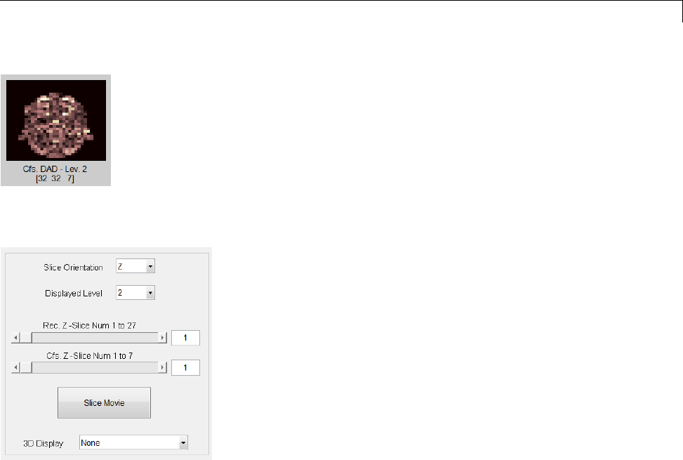
Three-Dimensional Discrete Wavelet Analysis
You use the Displayed Level in the command part of the window to choose
the level of the displayed component, from 1 to the decomposition level.
You can modify characteristics of the display using the options in the
command part of the window. Each pair of sliders controls part of graphical
array, the original and the reconstructed slices with the first pair or the
coefficients slices with the second pair. Above each slider you can see the
number of slices in the current slice orientation.
Using the slider (or by directly editing the values) of Rec. Z-Slice,choose
slice number twelve. Similarly, choose slice number two using Cfs. Z-Slice.
3-187

3Discrete Wavelet Analysis
The Slice Movie button lets you see a movie of all the slices, first for the
reconstructed slices and then for the coefficients slices. In this case, the
movie contains 27 reconstructed images and 7 coefficients images.
3D Display lets you examine the original data and the wavelet components
in true 3-D mode. Click 3D Display and select APP1.
3-188
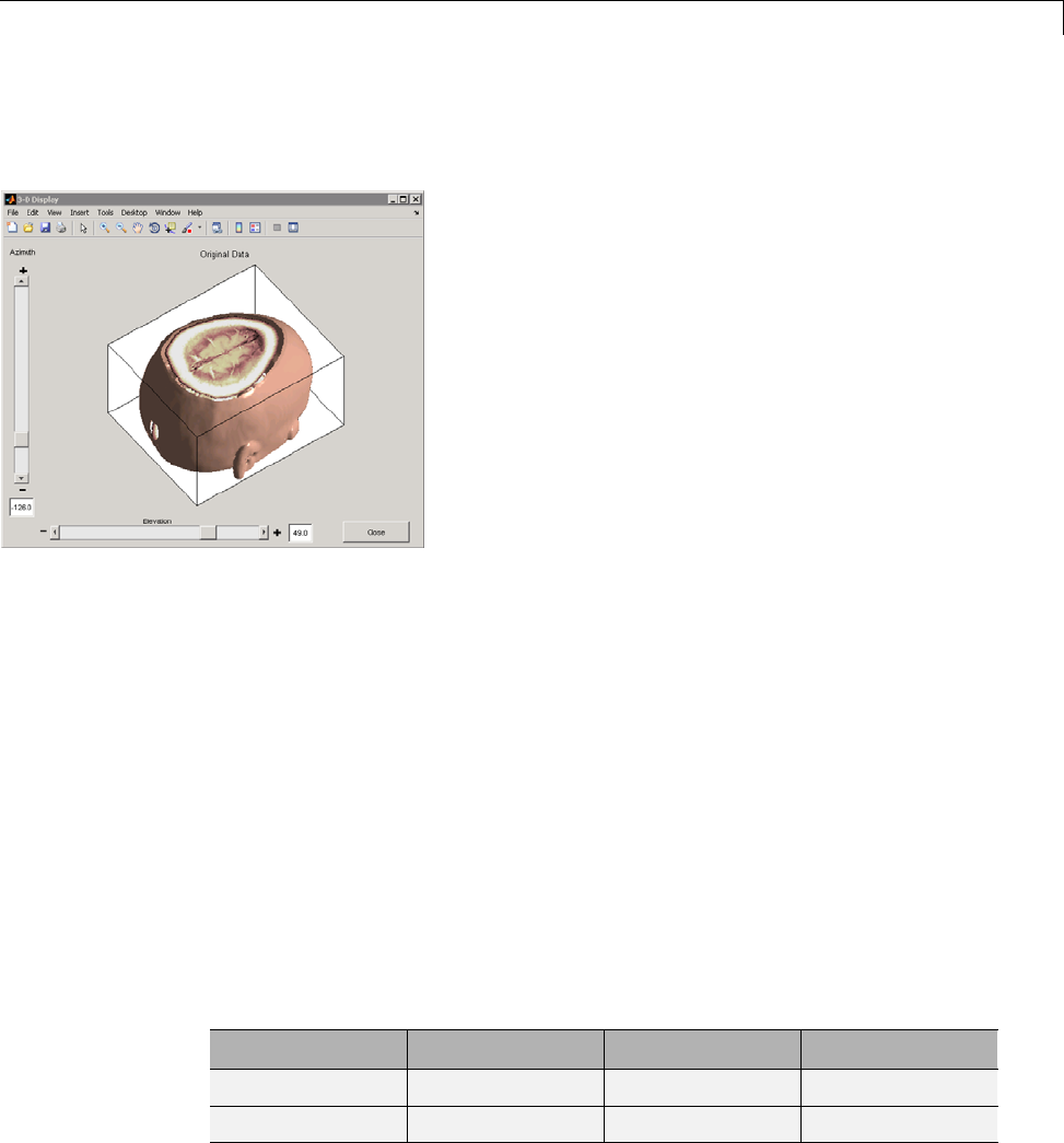
Three-Dimensional Discrete Wavelet Analysis
A rotated 3-D view of the approximation at level 1 opens in a new window.
Use the sliders in the 3-D tool to examine the 3-D data.
Importing and Exporting Information from the
Graphical Interface
You can import information from and export information either to disk or to
the workspace using the Wavelet 3-D graphical tool.
Loading Information into the Wavelet 3-D Tool
To load 3-D data you have constructed in your MATLAB workspace into the
Wavelet 3-D tool, save the 3-D data in a MAT-file, using
M = magic(8);
X = repmat(M,[1 1 8]);
save magic3d X
whos
where Mand Xare
Name Size Bytes Class
M 8x8 512 double
X 8x8x8 4096 double
3-189
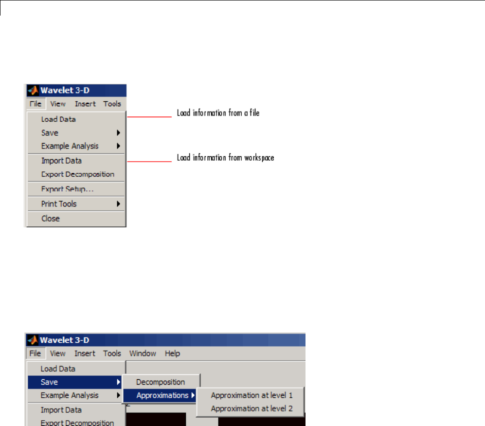
3Discrete Wavelet Analysis
To load this 3-D data into the Wavelet 3-D tool, use the menu option
File > Load Data. You then select the MAT-file to load.
Similarly, you can load information from the workspace using
File > Import Data. You then select the variable to load.
Saving Information to a File
You can save decompositions and approximations from the Wavelet 3-D tool
to a file or to the workspace.
Saving Decompositions. The Wavelet 3-D tool lets you save the entire
set of data from a discrete wavelet analysis to a file. The toolbox creates a
MAT-file in the current folder with a name you choose.
1Open the Wavelet 3-D tool with File > Load Data, and select magic3d to
load the 3-D data file.
3-190

Three-Dimensional Discrete Wavelet Analysis
2After analyzing your data, save it by using File > Save > Decomposition.
3In the dialog box that appears, specify a folder and file name for storing the
decomposition data. Type the name dec_magic3d.
4After saving the decomposition data to the file dec_magic3d.mat,load
the variables into your workspace.
load dec_magic3d
whos
where wdec is
Name Size Bytes Class
wdec 1x1 9182 struct
The variable wdec contains the wavelet decomposition structure.
wdec =
sizeINI: [8 8 8]
level: 2
filters: [1x1 struct]
mode: 'sym'
dec: {15x1 cell}
sizes: [3x3 double]
Saving Approximations. You can process a 3-D data in the Wavelet 3-D
tool and then save any desired approximation, depending on the level chosen
for the decomposition.
1Open the Wavelet 3-D tool and load the file containing the 3-D data to
analyze by using File > Load Data
2Select magic3d.
3Select the File > Save > Approximations > Approximation at level
2menu option.
3-191
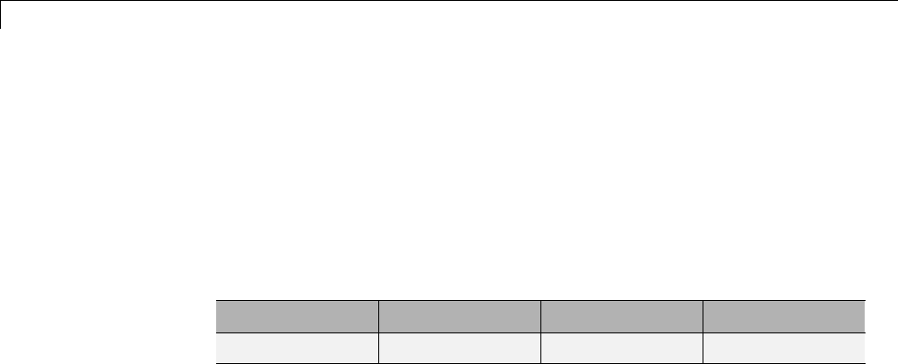
3Discrete Wavelet Analysis
4In the dialog box that appears, select a folder and file name for the
MAT-file. For this example, choose the name App2_magic3D.
5Load the image data into your workspace.
load App2_magic3D
whos
where xis
Name Size Bytes Class
x 8x8x8 4096 double
3-192

4
Wavelet Packets
•“AboutWaveletPacketAnalysis”onpage4-2
•“One-Dimensional Wavelet Packet Analysis” on page 4-7
•“Two-Dimensional Wavelet Packet Analysis” on page 4-15
•“Importing and Exporting from Graphical Tools” on page 4-22
•“Wavelet Packets” on page 4-30
•“Introduction to Object-Oriented Features” on page 4-52
•“Objects in the Wavelet Toolbox Software” on page 4-53
•“Examples Using Objects” on page 4-55
•“Description of Objects in the Wavelet Toolbox Software” on page 4-67
•“Advanced Use of Objects” on page 4-74

4Wavelet Packets
About Wavelet Packet Analysis
Wavelet Toolbox software contains graphical tools and command line
functions that let you
•Examine and explore characteristics of individual wavelet packets
•Perform wavelet packet analysis of one- and two-dimensional data
•Use wavelet packets to compress and remove noise from signals and images
This chapter takes you step-by-step through examples that teach you how
to use the WaveletPacket1-Dand Wavelet Packet 2-D graphical tools.
The last section discusses how to transfer information from the graphical
tools into your disk, and back again.
Note All the graphical user interface tools described in this chapter let you
import information from and export information to either disk or workspace.
Because of the inherent complexity of packing and unpacking complete
wavelet packet decomposition tree structures, we recommend using the
Wavelet Packet 1-D and Wavelet Packet 2-D graphical tools for performing
exploratory analyses.
The command line functions are also available and provide the same
capabilities. However, it is most efficient to use the command line only for
performing batch processing.
Note For more background on the wavelet packets, you can see the section
“Wavelet Packets” on page 4-30.
Some object-oriented programming features are used for wavelet packet
tree structures. For more detail, refer to “Introduction to Object-Oriented
Features” on page 4-52.
4-2
About Wavelet Packet Analysis
This chapter takes you through the features of one- and two-dimensional
wavelet packet analysis using the Wavelet Toolbox software. You’ll learn
how to
•Load a signal or image
•Performawaveletpacketanalysisofasignalorimage
•Compress a signal
•Remove noise from a signal
•Compress an image
•Show statistics and histograms
The toolbox provides these functions for wavelet packet analysis. For more
information, see the reference pages. The reference entries for these functions
include examples showing how to perform wavelet packet analysis via the
command line.
Some more advanced examples mixing command line and GUI functions can
be found in the section “Examples Using Objects” on page 4-55.
Analysis-Decomposition Functions
Function Name Purpose
wpcoef Waveletpacketcoefficients
wpdec and wpdec2 Full decomposition
wpsplt Decompose packet
Synthesis-Reconstruction Functions
Function Name Purpose
wprcoef Reconstruct coefficients
wprec and wprec2 Full reconstruction
wpjoin Recompose packet
4-3

4Wavelet Packets
Decomposition Structure Utilities
Function Name Purpose
besttree Find best tree
bestlevt Find best level tree
entrupd Update wavelet packets entropy
get Get WPTREE object fields contents
read Read values in WPTREE object fields
wenergy Entropy
wp2wtree Extract wavelet tree from wavelet packet tree
wpcutree Cut wavelet packet tree
De-Noising and Compression
Function Name Purpose
ddencmp Default values for de-noising and compression
wpbmpen Penalized threshold for wavelet packet
de-noising
wpdencmp De-noising and compression using wavelet
packets
wpthcoef Wavelet packets coefficients thresholding
wthrmngr Threshold settings manager
In the wavelet packet framework, compression and de-noising ideas are
exactly the same as those developed in the wavelet framework. The only
difference is that wavelet packets offer a more complex and flexible analysis,
because in wavelet packet analysis, the detailsaswellastheapproximations
are split.
4-4
About Wavelet Packet Analysis
A single wavelet packet decomposition gives a lot of bases from which you can
look for the best representation with respect to a design objective. This can be
done by finding the “best tree” based on an entropy criterion.
De-noising and compression are interesting applications of wavelet packet
analysis. The wavelet packet de-noising or compression procedure involves
four steps:
1Decomposition
For a given wavelet, compute the wavelet packet decomposition of signal
xat level N.
2Computation of the best tree
For a given entropy, compute the optimal wavelet packet tree. Of course,
this step is optional. The graphical tools provide a Best Tree button for
making this computation quick and easy.
3Thresholding of wavelet packet coefficients
Foreachpacket(exceptfortheapproximation), select a threshold and
apply thresholding to coefficients.
The graphical tools automatically provide an initial threshold based on
balancing the amount of compression andretainedenergy. Thisthreshold
is a reasonable first approximation for most cases. However, in general you
will have to refine your threshold by trial and error so as to optimize the
results to fit your particular analysis and design criteria.
4-5

4Wavelet Packets
The tools facilitate experimentation with different thresholds, and make
it easy to alter the tradeoff between amount of compression and retained
signal energy.
4Reconstruction
Compute wavelet packet reconstruction based on the original
approximation coefficients at level Nand the modified coefficients.
In this example, we’ll show how you can use one-dimensional wavelet packet
analysis to compress and to de-noise a signal.
4-6
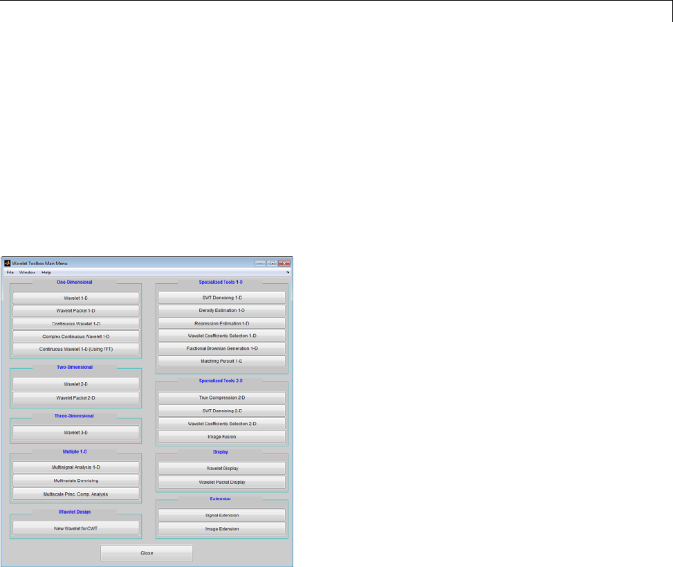
One-Dimensional Wavelet Packet Analysis
One-Dimensional Wavelet Packet Analysis
We now turn to the Wavelet Packet 1-D tool to analyze a synthetic signal
that is the sum of two linear chirps.
Starting the Wavelet Packet 1-D Tool.
1From the MATLAB prompt, type wavemenu.
The Wavelet Toolbox Main Menu appears.
Click the Wavelet Packet 1-D menu item.
Loading a Signal.
1From the File menu, choose the Load Signal option.
4-7

4Wavelet Packets
2When the Load Signal dialog box appears, select the MAT-file
sumlichr.mat, which should reside in the MATLAB folder
toolbox/wavelet/wavedemo.ClicktheOK button.
The sumlichr signal is loaded into the WaveletPacket1-Dtool.
4-8
One-Dimensional Wavelet Packet Analysis
Analyzing a Signal.
1Make the appropriate settings for the analysis. Select the db2 wavelet,
level 4,entropythreshold, and for the threshold parameter type 1.Click
the Analyze button.
The available entropy types are listed below.
Type Description
Shannon Nonnormalized entropy involving the logarithm
of the squared value of each signal sample — or,
more formally,
−∑ss
ii
22
log( ).
Threshold The number of samples for which the absolute
value of the signal exceeds a threshold ε.
Norm The concentration in lpnorm with 1 ≤p.
Log Energy The logarithm of “energy,” defined as the sum over
all samples:
log( ).si
2
∑
4-9
4Wavelet Packets
Type Description
SURE (Stein’s
Unbiased Risk
Estimate)
A threshold-based method in which the threshold
equals
22
log log ( )
enn
()
where nis the number of samples in the signal.
User An entropy type criterion you define in a file.
For more information about the available entropy types, user-defined entropy,
and threshold parameters, see the wentropy reference page and “Choosing
the Optimal Decomposition” on page 4-41.
Note Many capabilities are available using the command area on the right of
the Wavelet Packet 1-D window.
Computing the Best Tree.
Because there are so many ways to reconstruct the original signal from the
waveletpacketdecompositiontree,weselect the best tree before attempting
to compress the signal.
1Click the Best Tree button.
After a pause for computation, the Wavelet Packet 1-D tool displays the
best tree. Use the top and bottom sliders to spread nodes apart and pan
over to particular areas of the tree, respectively.
Observe that, for this analysis, the best tree and the initial tree are almost
the same. One branch at the far right of the tree was eliminated.
4-10
One-Dimensional Wavelet Packet Analysis
Compressing a Signal Using Wavelet Packets
Selecting a Threshold for Compression.
1Click the Compress button.
The Wavelet Packet 1-D Compression window appears with an
approximate threshold value automatically selected.
4-11
4Wavelet Packets
The leftmost graph shows how the threshold (vertical yellow dotted line)
has been chosen automatically (1.482) to balance the number of zeros in the
compressed signal (blue curve that increases as the threshold increases)
with the amount of energy retained in the compressed signal (purple curve
that decreases as the threshold increases).
This threshold means that any signal element whose value is less than
1.482willbesettozerowhenweperformthecompression.
Threshold controls are located to the right (see the red box in the figure
above). Note that the automatic threshold of 1.482 results in a retained
energy of only 81.49%. This may cause unacceptable amounts of distortion,
especially in the peak values of the oscillating signal. Depending on your
design criteria, you may want to choose a threshold that retains more of
the original signal’s energy.
2Adjust the threshold by typing 0.8938 in the text field opposite the
threshold slider, and then press the Enter key.
The value 0.8938 is a number that we have discovered through trial and
error yields more satisfactory results for this analysis.
4-12
One-Dimensional Wavelet Packet Analysis
After a pause, the Wavelet Packet 1-D Compression window displays
new information.
Note that, as we have reduced the threshold from 1.482 to 0.8938,
•The vertical yellow dotted line has shifted to the left.
•The retained energy has increased from 81.49% to 90.96%.
•The number of zeros (equivalent to the amount of compression) has
decreased from 81.55% to 75.28%.
Compressing a Signal.
1Click the Compress button.
The WaveletPacket1-Dtool compresses the signal using the thresholding
criterion we selected.
The original (red) and compressed (yellow) signals are displayed
superimposed. Visual inspection suggests the compression quality is quite
good.
Looking more closely at the compressed signal, we can see that the number of
zeros in the wavelet packets representation of the compressed signal is about
75.3%, and the retained energy about 91%.
If you try to compress the same signal using wavelets with exactly the same
parameters, only 89% of the signal energy is retained, and only 59% of the
4-13

4Wavelet Packets
wavelet coefficients set to zero. This illustrates the superiority of wavelet
packets for performing compression, at least on certain signals.
You can demonstrate this to yourself by returning to the main Wavelet
Packet 1-D window, computing the wavelet tree, and then repeating the
compression.
De-Noising a Signal Using Wavelet Packets
We now use the Wavelet Packet 1-D tool to analyze a noisy chirp signal.
This analysis illustrates the use of Stein’s Unbiased Estimate of Risk (SURE)
as a principle for selecting a threshold to be used for de-noising.
This technique calls for setting the threshold Tto
Tnn
e
=
()
22
log log ( )
where nis the length of the signal.
A more thorough discussion of the SURE criterion appears in “Choosing the
Optimal Decomposition” on page 4-41. For now, suffice it to say that this
method works well if your signal is normalized in such a way that the data
fit the model x(t)=f(t)+e(t), where e(t) is a Gaussian white noise with zero
mean and unit variance.
If you’ve already started the Wavelet Packet 1-D tool and it is active on your
computer’s desktop, skip ahead to step 3.
4-14

Two-Dimensional Wavelet Packet Analysis
Two-Dimensional Wavelet Packet Analysis
In this section, we employ the WaveletPacket2-Dtool to analyze and
compress an image of a fingerprint. This is a real-world problem: the Federal
Bureau of Investigation (FBI) maintains a large database of fingerprints
— about 30 million sets of them. The cost of storing all this data runs to
hundreds of millions of dollars.
“The FBI uses eight bits per pixel to define the shade of gray and stores 500
pixels per inch, which works out to about 700,000 pixels and 0.7 megabytes
per finger to store finger prints in electronic form.” (Wickerhauser, see the
reference [Wic94] p. 387, listed in “References”).
“The technique involves a two-dimensional DWT, uniform scalar quantization
(a process that truncates, or quantizes, the precision of the floating-point
DWT output) and Huffman entropy coding (i.e., encoding the quantized DWT
output with a minimal number of bits).” (Brislawn, see the reference [Bris95]
p. 1278, listed in “References”).
By turning to wavelets, the FBI has achieved a 15:1 compression ratio. In this
application, wavelet compression is better than the more traditional JPEG
compression, as it avoids small square artifacts and is particularly well suited
to detect discontinuities (lines) in the fingerprint.
Note that the international standard JPEG 2000 will include the wavelets
as a part of the compression and quantization process. This points out the
present strength of the wavelets.
StartingtheWaveletPacket2-DTool.
1From the MATLAB prompt, type
wavemenu
The Wavelet Toolbox Main Menu appears.
4-15

4Wavelet Packets
Click the Wavelet Packet 2-D menu item.
Loading an Image
From the File menu, choose the Load Image option.
4-16
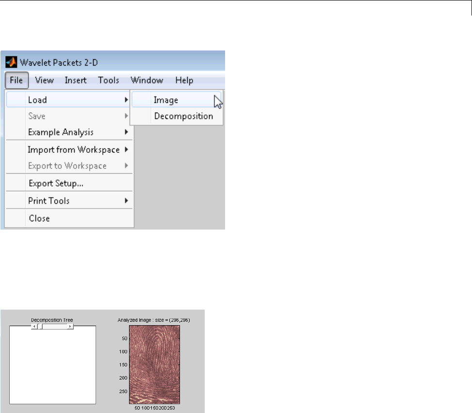
Two-Dimensional Wavelet Packet Analysis
2When the Load Image dialog box appears, select the MAT-file
detfingr.mat, which should reside in the MATLAB folder
toolbox/wavelet/wavedemo.ClicktheOK button.
The fingerprint image is loaded into the Wavelet Packet 2-D tool.
Analyzing an Image
3Make the appropriate settings for the analysis. Select the haar wavelet,
level 3, and entropy type shannon.ClicktheAnalyze button.
4-17
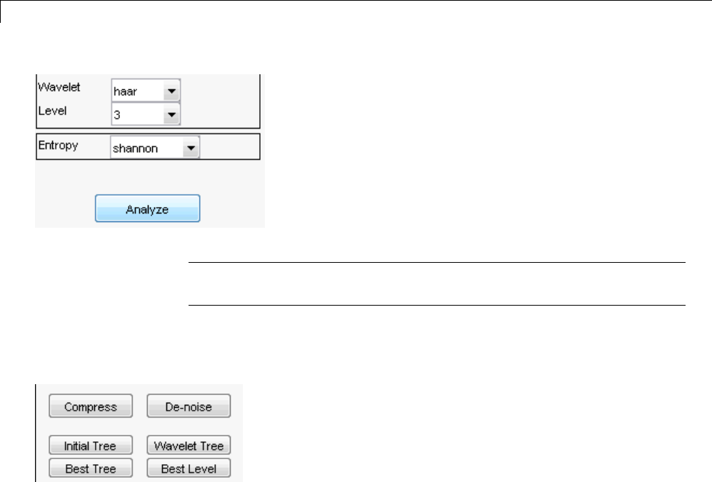
4Wavelet Packets
Note Many capabilities are available using the command area on the right
of the Wavelet Packet 2-D window.
4Click the Best Tree button to compute the best tree before compressing
the image.
Compressing an Image Using Wavelet Packets
1Click the Compress button to bring up the Wavelet Packet 2-D
Compression window. Select the Bal. sparsity-norm (sqrt) option from
the Select thresholding method menu.
4-18
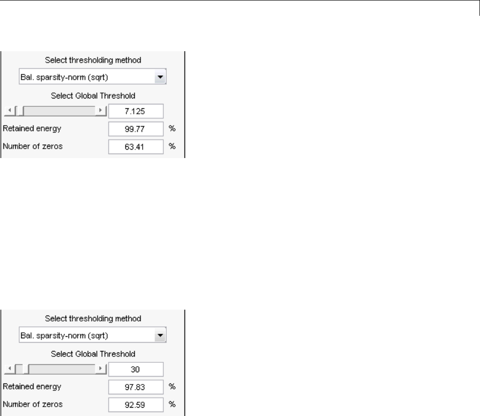
Two-Dimensional Wavelet Packet Analysis
Notice that the default threshold (7.125) provides about 64% compression
while retaining virtually all the energy of the original image. Depending on
your criteria, it may be worthwhile experimenting with more aggressive
thresholds to achieve a higher degree of compression. Recall that we are
not doing any quantization of the image, merely setting specific coefficients
to zero. This can be considered a precompression step in a broader
compression system.
2Alter the threshold: type the number 30 in the text field opposite the
threshold slider located on the right side of the Wavelet Packet 2-D
Compression window. Then press the Enter key.
Setting all wavelet packet coefficients whose value falls below 30 to zero
yields much better results. Note that the new threshold achieves around
92% of zeros, while still retaining nearly 98% of the image energy.
3Click the Compress button to start the compression.
You can see the result obtained by wavelet packet coefficients thresholding
and image reconstruction. The visual recovery is correct, but not perfect.
4-19
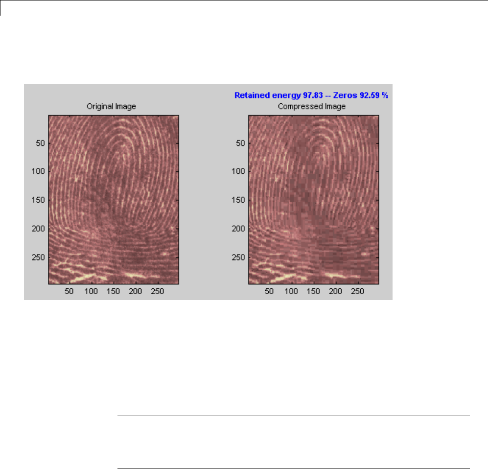
4Wavelet Packets
The compressed image, shown side by side with the original, shows some
artifacts.
4Click the Close button located at the bottom of the Wavelet Packet 2-D
Compression window. Update the synthesized image by clicking Yes
when the dialog box appears.
Take this opportunity to try out your own compression strategy. Adjust the
threshold value, the entropy function, and the wavelet, and see if you can
obtain better results.
Hint The bior6.8 wavelet is better suited to this analysis than is haar,and
can lead to a better compression ratio. When a biorthogonal wavelet is used,
then instead of “Retained energy” the information displayed is “Energy ratio.”
For more information, see “Compression Scores” on page 5-53.
Before concluding this analysis, it is worth turning our attention to the
“colored coefficients for terminal nodes plot” and considering the best tree
decomposition for this image.
4-20
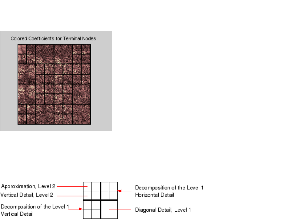
Two-Dimensional Wavelet Packet Analysis
This plot is shown in the lower right side of the Wavelet Packet 2-D tool.
The plot shows us which details have been decomposed and which have not.
Larger squares represent details that have not been broken down to as many
levels as smaller squares. Consider, for example, this level 2 decomposition
pattern:
Looking at the pattern of small and large squares in the fingerprint analysis
shows that the best tree algorithm has apparently singled out the diagonal
details, often sparing these from further decomposition. Why is this?
If we consider the original image, we realize that much of its information is
concentrated in the sharp edges that constitute the fingerprint’s pattern.
Looking at these edges, we see that they are predominantly oriented
horizontally and vertically. This explains why the best tree algorithm has
“chosen” not to decompose the diagonal details — they do not provide very
much information.
4-21

4Wavelet Packets
Importing and Exporting from Graphical Tools
The WaveletPacket1-Dand Wavelet Packet 2-D tools let you import
information from and export information to your disk.
Ifyouadheretotheproperfileformats,youcan
•Save decompositions as well as synthesized signals and images from the
waveletpacketgraphicaltoolstodisk
•Load signals, images, and one- and two-dimensional decompositions from
disk into the Wavelet Packet 1-D and WaveletPacket2-Dgraphical
tools
Saving Information to Disk
Using specific file formats, the graphical tools let you save synthesized signals
or images, as well as one- or two-dimensional wavelet packet decomposition
structures. This feature provides flexibility and allows you to combine
command line and graphical interface operations.
Saving Synthesized Signals
You can process a signal in the Wavelet Packet 1-D tool, and then save
the processed signal to a MAT-file.
For example, load the example analysis:
File > Example Analysis > db1 – depth: 2 – ent: shannon > sumsin
and perform a compression or de-noising operation on the original signal.
When you close the Wavelet Packet 1-D De-noising or Wavelet Packet
1-D Compression window, update the synthesized signal by clicking Yes
in the dialog box.
Then, from the WaveletPacket1-Dtool, select the File > Save >
Synthesized Signal menu option.
A dialog box appears allowing you to select a folder and filename for the
MAT-file. For this example, choose the name synthsig.
4-22

Importing and Exporting from Graphical Tools
To load the signal into your workspace, simply type
load synthsig
whos
Name Size Bytes Class
synthsig 1x1000 8000 double array
valTHR 1x1 8 double array
wname 1x3 6 char array
The synthesized signal is given by synthsig. In addition, the parameters of
the de-noising or compression process are given by the wavelet name (wname)
and the global threshold (valTHR).
valTHR
valTHR =
1.9961
Saving Synthesized Images
YoucanprocessanimageintheWaveletPacket2-Dtool, and then save the
processed image to a MAT-file (with extension mat or other).
For example, load the example analysis:
File > Example Analysis > db1 – depth: 1 – ent: shannon > woman
and perform a compression on the original image. When you close the
Wavelet Packet 2-D Compression window, update the synthesized image
by clicking Yes in the dialog box that appears.
Then, from the Wavelet 2-D tool, select the File > Save > Synthesized
Image menu option.
A dialog box appears allowing you to select a folder and filename for the
MAT-file. For this example, choose the name wpsymage.
4-23

4Wavelet Packets
To load the image into your workspace, simply type
load wpsymage
whos
Name Size Bytes Class
X 256x256 524288 double array
map 255x3 6120 double array
valTHR 1x1 8 double array
wname 1x3 6 char array
ThesynthesizedimageisgivenbyX. The variable map contains the associated
colormap. In addition, the parameters of the de-noising or compression process
are given by the wavelet name (wname) and the global threshold (valTHR).
Saving One-Dimensional Decomposition Structures
The Wavelet Packet 1-D tool lets you save an entire wavelet packet
decomposition tree and related data to your disk. The toolbox creates a
MAT-file in the current folder with a name you choose, followed by the
extension wp1 (wavelet packet 1-D).
Open the Wavelet Packet 1-D tool and load the example analysis:
File > Example Analysis > db1 – depth: 2 – ent: shannon > sumsin
To save the data from this analysis, use the menu option File > Save
Decomposition.
A dialog box appears that lets you specify a folder and file name for storing
the decomposition data. Type the name wpdecex1d.
After saving the decomposition data to the file wpdecex1d.wp1,loadthe
variables into your workspace.
load wpdecex1d.wp1 -mat
whos
4-24

Importing and Exporting from Graphical Tools
Name Size Bytes Class
data_name 1x6 12 char array
tree_struct 1x1 11176 wptree object
valTHR 0x0 0 double array
The variable tree_struct contains the wavelet packet tree structure. The
variable data_name contains the data name and valTHR contains the global
threshold, which is currently empty since the synthesized signal does not
exist.
Saving Two-Dimensional Decomposition Structures
The file format, variables, and conventions are exactly the same as in the
one-dimensional case except for the extension, which is wp2 (wavelet packet
2-D). The variables saved are the same as with the one-dimensional case, with
the addition of the colormap matrix map:
Name Size Bytes Class
data_name 1x5 10 char array
map 255x3 6120 double array
tree_struct 1x1 527400 wptree object
valTHR 1x1 8 double array
Save options are also available when performing de-noising or compression
inside the Wavelet Packet 1-D and Wavelet Packet 2-D tools.
In the Wavelet Packet De-Noising windows, you can save the de-noised signal
or image and the decomposition. The same holds true for the Wavelet Packet
Compression windows.
This way, you can save directly many different trials from inside the
De-Noising and Compression windows without going back to the main
Wavelet Packet windows during a fine-tuning process.
4-25

4Wavelet Packets
Note When saving a synthesized signal (1-D), a synthesized image (2-D)
or a decomposition to a MAT-file, the extension of this file is free. The mat
extension is not necessary.
Loading Information intotheGraphicalTools
You can load signals, images, or one- and two-dimensional wavelet packet
decompositions into the graphical interface tools. The information you load
may have been previously exported from the graphical interface, and then
manipulated in the workspace, or it may have been information you generated
initially from the command line.
In either case, you must observe the strict file formats and data structures
used by the graphical tools, or else errors will result when you try to load
information.
Loading Signals
To load a signal you’ve constructed in your MATLAB workspace into the
WaveletPacket1-Dtool, save the signal in a MAT-file (with extension mat
or other).
For instance, suppose you’ve designed a signal called warma and want to
analyze it in the Wavelet Packet 1-D tool.
save warma warma
The workspace variable warma must be a vector.
sizwarma = size(warma)
sizwarma =
1 1000
To load this signal into the Wavelet Packet 1-D tool, use the menu option
File > Load Signal.
A dialog box appears that lets you select the appropriate MAT-file to be loaded.
4-26

Importing and Exporting from Graphical Tools
Note The first one-dimensional variable encountered in the file is considered
the signal. Variables are inspected in alphabetical order.
Loading Images
This toolbox supports only indexed images. An indexed image is a matrix
containing only integers from 1 to n,wherenis the number of colors in the
image.
This image may optionally be accompanied by a n-by-3 matrix called map.This
is the colormap associated with the image. When MATLAB displays such an
image, it uses the values of the matrix to look up the desired color in this
colormap. If the colormap is not given, the Wavelet Packet 2-D graphical
tool uses a monotonic colormap with max(max(X)) min(min(X))+1 colors.
To load an image you’ve constructed in your MATLAB workspace into the
Wavelet Packet 2-D tool,savetheimage(andoptionally,thevariablemap)
in a MAT-file (with extension mat or other).
For instance, suppose you’ve created an image called brain and want to
analyze it in the Wavelet Packet 2-D tool. Type
X = brain;
map = pink(256);
save myfile X map
To load this image into the Wavelet Packet 2-D tool, use the menu option
File > Load Image.
A dialog box appears that lets you select the appropriate MAT-file to be loaded.
Note The first two-dimensional variable encountered in the file (except the
variable map, which is reserved for the colormap) is considered the image.
Variables are inspected in alphabetical order.
4-27

4Wavelet Packets
Caution The graphical tools allow you to load an image that does not contain
integers from 1 to n. The computations will be correct since they act directly on
the matrix, but the display of the image will be strange. The values less than
1 will be evaluated as 1, the values greater than nwill be evaluated as n,and
a real value within the interval [1,n] will be evaluated as the closest integer.
Note that the coefficients, approximations, and details produced by wavelet
packets decomposition are not indexed image matrices. To display these
images in a suitable way, the Wavelet Packet 2-D tool follows these rules:
•Reconstructed approximations are displayed using the colormap map.The
same holds for the result of the reconstruction of selected nodes.
•The coefficients and the reconstructed details are displayed using the
colormap map applied to a rescaled version of the matrices.
Loading Wavelet Packet Decomposition Structures
You can load one- and two-dimensional wavelet packet decompositions into
the graphical tools providing you have previously saved the decomposition
data in a MAT-file of the appropriate format.
Whileitispossibletoeditdataoriginally created using the graphical tools
and then exported, you must be careful about doing so. Wavelet packet data
structures are complex, and the graphical tools do not do any consistency
checking. This can lead to errors if you try to load improperly formatted data.
One-dimensional data file contains the following variables:
Variable Status Description
tree_struct Required Object specifying the tree structure
data_name Optional String specifying the name of the
decomposition
valTHR Optional Global threshold (can be empty if neither
compression nor de-noising has been done)
4-28

Importing and Exporting from Graphical Tools
These variables must be saved in a MAT-file (with extension wp1 or other).
Two-dimensional data file contains the following variables:
Variable Status Description
tree_struct Required Object specifying the tree structure
data_name Optional String specifying the name of the
decomposition
map Optional Image map
valTHR Optional Global threshold (can be empty if neither
compression nor de-noising has been done)
These variables must be saved in a MAT-file (with extension wp2 or other).
To load the properly formatted data, use the menu option File > Load
Decomposition Structure from the appropriate tool, and then select the
desired MAT-file from the dialog box that appears.
The WaveletPacket1-Dor 2-D graphical tool then automatically updates
its display to show the new analysis.
Note When loading a signal (1-D), an image (2-D), or a decomposition (1-D
or 2-D) from a MAT-file, the extension of this file is free. The mat extension
is not necessary.
4-29

4Wavelet Packets
Wavelet Packets
The wavelet packet method is a generalization of wavelet decomposition that
offers a richer signal analysis.
Waveletpacketatomsarewaveformsindexed by three naturally interpreted
parameters: position, scale (as in wavelet decomposition), and frequency.
For a given orthogonal wavelet function, we generate a library of bases called
waveletpacketbases. Each of these bases offers a particular way of coding
signals, preserving global energy, and reconstructing exact features. The
wavelet packets can be used for numerous expansions of a given signal. We
then select the most suitable decomposition of a given signal with respect to
an entropy-based criterion.
There exist simple and efficient algorithms for both wavelet packet
decomposition and optimal decomposition selection. We can then produce
adaptive filtering algorithms with direct applications in optimal signal coding
and data compression.
From Wavelets to Wavelet Packets
In the orthogonal wavelet decomposition procedure, the generic step splits the
approximation coefficients into two parts. After splitting we obtain a vector
of approximation coefficients and a vector of detail coefficients, both at a
coarser scale. The information lost between two successive approximations is
captured in the detail coefficients. Then the next step consists of splitting the
new approximation coefficient vector; successive details are never reanalyzed.
In the corresponding wavelet packet situation, each detail coefficient vector is
also decomposed into two parts using the same approach as in approximation
vector splitting. This offers the richestanalysis:thecompletebinarytreeis
produced as shown in the following figure.
4-30
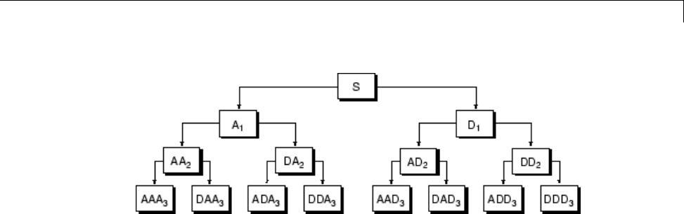
Wavelet Packets
Wavelet Packet Decomposition Tree at Level 3
The idea of this decomposition is to start from a scale-oriented decomposition,
and then to analyze the obtained signals on frequency subbands.
Wavelet Packets in Action: An Introduction
The following simple examples illustrate certain differences between wavelet
analysis and wavelet packet analysis.
WaveletPacketSpectrum
The spectral analysis of wide-sense stationary signals using the Fourier
transform is well-established. For nonstationary signals, there exist local
Fourier methods such as the short-time Fourier transform (STFT). See
“Short-Time Fourier Transform” for a brief description.
Because wavelets are localized in time and frequency, it is possible to use
wavelet-based counterparts to the STFT for the time-frequency analysis of
nonstationary signals. For example, it is possible to construct the scalogram
(wscalogram) based on the continuous wavelet transform (CWT). However, a
potential drawback of using the CWT is that it is computationally expensive.
The discrete wavelet transform (DWT) permits a time-frequency
decomposition of the input signal, but the degree of frequency resolution in the
DWT is typically considered too coarse for practical time-frequency analysis.
As a compromise between the DWT- and CWT-based techniques, wavelet
packets provide a computationally-efficient alternative with sufficient
frequency resolution. You can use wpspectrum to perform a time-frequency
analysis of your signal using wavelet packets.
4-31

4Wavelet Packets
The following examples illustrate the use of wavelet packets to perform a local
spectral analysis. The following examples also use spectrogram from the
Signal Processing Toolbox™ software as a benchmark to compare against the
waveletpacketspectrum. Ifyoudonothave the Signal Processing Toolbox
software, you can simply run the wavelet packet spectrum examples.
Waveletpacketspectrumofasinewave.
fs = 1000; % sampling rate
t = 0:1/fs:2; % 2 secs at 1kHz sample rate
y = sin(256*pi*t); % sine of period 128
level = 6;
wpt = wpdec(y,level,'sym8');
[Spec,Time,Freq] = wpspectrum(wpt,fs,'plot');
If you have the Signal Processing Toolbox software, you can compute the
short-time Fourier transform.
figure;
windowsize = 128;
window = hanning(windowsize);
nfft = windowsize;
noverlap = windowsize-1;
[S,F,T] = spectrogram(y,window,noverlap,nfft,fs);
imagesc(T,F,log10(abs(S)))
set(gca,'YDir','Normal')
xlabel('Time (secs)')
ylabel('Freq (Hz)')
title('Short-time Fourier Transform spectrum')
Sum of two sine waves with frequencies of 64 and 128 hertz.
fs = 1000;
t = 0:1/fs:2;
y = sin(128*pi*t) + sin(256*pi*t); % sine of periods 64 and 128.
level = 6;
wpt = wpdec(y,level,'sym8');
[Spec,Time,Freq] = wpspectrum(wpt,fs,'plot');
4-32

Wavelet Packets
If you have the Signal Processing Toolbox software, you can compute the
short-time Fourier transform.
figure;
windowsize = 128;
window = hanning(windowsize);
nfft = windowsize;
noverlap = windowsize-1;
[S,F,T] = spectrogram(y,window,noverlap,nfft,fs);
imagesc(T,F,log10(abs(S)))
set(gca,'YDir','Normal')
xlabel('Time (secs)')
ylabel('Freq (Hz)')
title('Short-time Fourier Transform spectrum')
Signal with an abrupt change in frequency from 16 to 64 hertz at two seconds.
fs = 500;
t = 0:1/fs:4;
y = sin(32*pi*t).*(t<2) + sin(128*pi*t).*(t>=2);
level = 6;
wpt = wpdec(y,level,'sym8');
[Spec,Time,Freq] = wpspectrum(wpt,fs,'plot');
If you have the Signal Processing Toolbox software, you can compute the
short-time Fourier transform.
figure;
windowsize = 128;
window = hanning(windowsize);
nfft = windowsize;
noverlap = windowsize-1;
[S,F,T] = spectrogram(y,window,noverlap,nfft,fs);
imagesc(T,F,log10(abs(S)))
set(gca,'YDir','Normal')
xlabel('Time (secs)')
ylabel('Freq (Hz)')
title('Short-time Fourier Transform spectrum')
4-33

4Wavelet Packets
Wavelet packet spectrum of a linear chirp.
fs = 1000;
t = 0:1/fs:2;
y = sin(256*pi*t.^2);
level = 6;
wpt = wpdec(y,level,'sym8');
[Spec,Time,Freq] = wpspectrum(wpt,fs,'plot');
If you have the Signal Processing Toolbox software, you can compute the
short-time Fourier transform.
figure;
windowsize = 128;
window = hanning(windowsize);
nfft = windowsize;
noverlap = windowsize-1;
[S,F,T] = spectrogram(y,window,noverlap,nfft,fs);
imagesc(T,F,log10(abs(S)))
set(gca,'YDir','Normal')
xlabel('Time (secs)')
ylabel('Freq (Hz)')
title('Short-time Fourier Transform spectrum')
Wavelet packet spectrum of quadratic chirp.
y = wnoise('quadchirp',10);
len = length(y);
t = linspace(0,5,len);
fs = 1/t(2);
level = 6;
wpt = wpdec(y,level,'sym8');
[Spec,Time,Freq] = wpspectrum(wpt,fs,'plot');
If you have the Signal Processing Toolbox software, you can compute the
short-time Fourier transform.
4-34

Wavelet Packets
windowsize = 128;
window = hanning(windowsize);
nfft = windowsize;
noverlap = windowsize-1;
imagesc(T,F,log10(abs(S)))
set(gca,'YDir','Normal')
xlabel('Time (secs)')
ylabel('Freq (Hz)')
title('Short-time Fourier Transform spectrum')
Building Wavelet Packets
The computation scheme for wavelet packets generation is easy when using
an orthogonal wavelet. We start with the two filters of length 2N,whereh(n)
and g(n), corresponding to the wavelet.
Now by induction let us define the following sequence of functions:
(Wn(x), n=0,1,2,...)
by
Wx hkWxk
nn
k
N
2
0
21
22() () ( )=−
=
−
∑
Wx gkWxk
nn
k
N
21
0
21
22
+=
−
=−
∑
() () ( )
where W0(x)=φ(x)is the scaling function and W1(x)=ψ(x)is the wavelet
function.
ForexamplefortheHaarwaveletwehave
Nh h===10 1 1
2
,() ()
and
4-35

4Wavelet Packets
gg() ()01
1
2
=− =
The equations become
WxWxWx
nn n2221() ( ) ( )=+−
and
W xWxWx
nnn21 221
+=−−() ( ) ( )
W0(x)=φ(x)is the Haar scaling function and W1(x)=ψ(x)is the Haar
wavelet, both supported in [0, 1]. Then we can obtain W2nby adding two
1/2-scaled versions of Wnwith distinct supports [0,1/2] and [1/2,1] and obtain
W2n+1 by subtracting the same versions of Wn.
For n= 0 to 7, we have the W-functions shown in the figure Haar Wavelet
Packets on page 4-37.
4-36
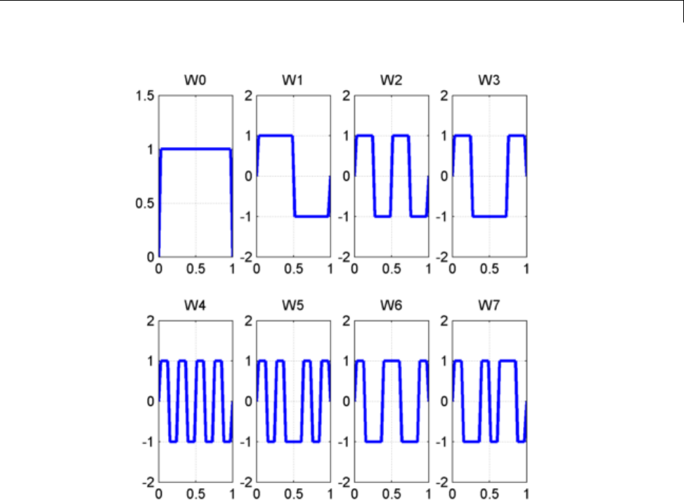
Wavelet Packets
Haar Wavelet Packets
This can be obtained using the following command:
[wfun,xgrid] = wpfun('db1',7,5);
which returns in wfun the approximate values of Wnfor n=0to7,computed
on a 1/25grid of the support xgrid.
Starting from more regular original wavelets and using a similar construction,
we obtain smoothed versions of this system of W-functions, all with support in
the interval [0, 2N–1]. The figure db2 Wavelet Packets on page 4-38 presents
the system of W-functions for the original db2 wavelet.
4-37
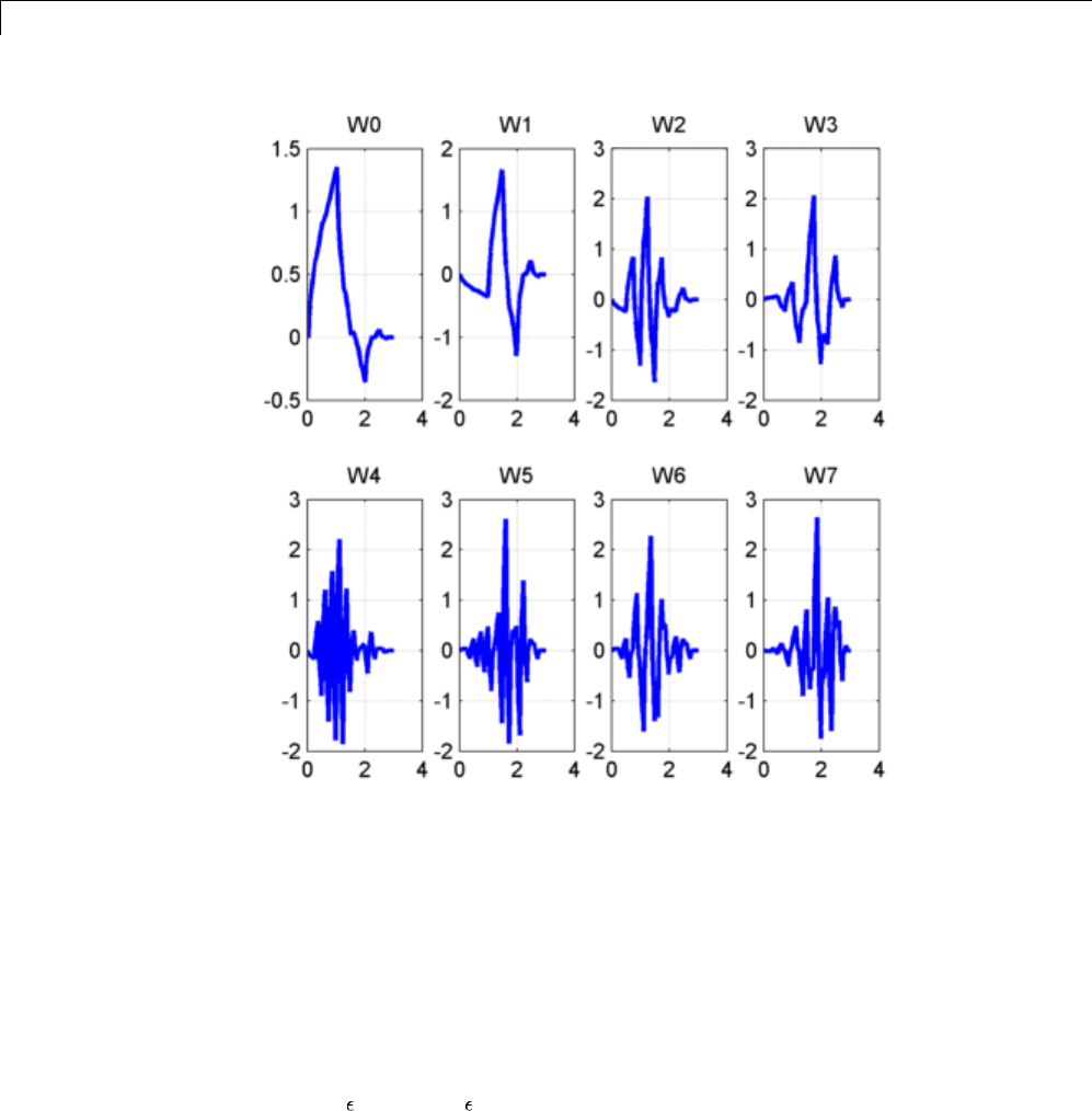
4Wavelet Packets
db2 Wavelet Packets
WaveletPacketAtoms
Starting from the functions ((), )Wxn N
n∈and following the same line leading
to orthogonal wavelets, we consider the three-indexed family of analyzing
functions (the waveforms):
(() ( )
,, /
Wx W xk
jnk jnj
=−
−−
22
2
where n N and (j,k)Z2.
4-38

Wavelet Packets
As in the wavelet framework, kcan be interpreted as a time-localization
parameter and jas a scale parameter. So what is the interpretation of n?
The basic idea of the wavelet packets is that for fixed values of jand k,Wj,n,k
analyzes the fluctuations of the signal roughly around the position 2j·k,at
the scale 2jand at various frequencies for the different admissible values of
the last parameter n.
In fact, examining carefully the wavelet packets displayed in Haar Wavelet
Packets on page 4-37 and db2 Wavelet Packets on page 4-38, the naturally
ordered Wnfor n=0,1,...,7,doesnotmatchexactlytheorderdefinedbythe
number of oscillations. More precisely, counting the number of zero crossings
(up-crossings and down-crossings) for the db1 wavelet packets, we have the
following.
Natural order n01234567
Number of zero
crossings for db1Wn
23549867
So, to restore the property that the main frequency increases monotonically
with the order, it is convenient to define the frequency order obtained from
thenaturalonerecursively.
Natural order n01234567
Frequency order r(n)01326754
Ascanbeseeninthepreviousfigures,Wr(n)(x)“oscillates” approximately
ntimes.
To analyze a signal (the chirp of Example 2 for instance), it is better to plot
the wavelet packet coefficients following the frequency order from the low
frequencies at the bottom to the high frequencies at the top, rather than
naturally ordered coefficients.
When plotting the coefficients, the various options related to the “Frequency”
or “Natural” order choice are available using the GUI tools.
4-39
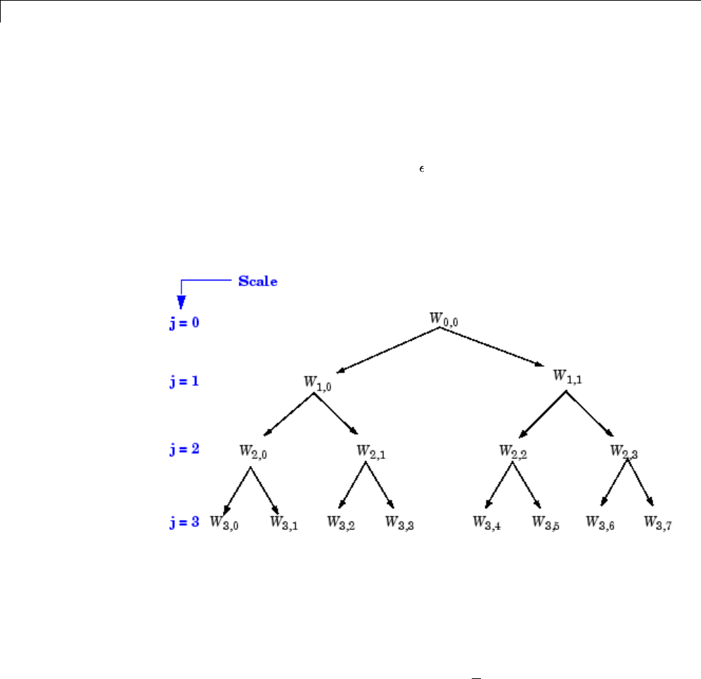
4Wavelet Packets
Theseoptionsarealsoavailablefromcommand-linemodewhenusingthe
wpviewcf function.
Organizing the Wavelet Packets
The set of functions Wj,n=(Wj,n,k(x),k Z)isthe(j,n) wavelet packet. For
positive values of integers jand n, wavelet packets are organized in trees.
The tree in the figure Wavelet Packets Organized in a Tree; Scale jDefines
Depth and Frequency n Defines Position in the Tree on page 4-40 is created to
give a maximum level decomposition equal to 3. For each scale j, the possible
valuesofparameternare0,1,...,2
j–1.
Wavelet Packets Organized in a Tree; Scale jDefines Depth and Frequency n
DefinesPositionintheTree
The notation Wj,n,wherejdenotes scale parameter and nthe frequency
parameter, is consistent with the usual depth-position tree labeling.
We have WxkkZ
00,(( ), )=−∈
φ
,and Wxkk Z
11 2
,(( ), )=−∈
ψ
.
It turns out that the library of wavelet packet bases contains the wavelet
basis and also several other bases. Let us have a look at some of those bases.
4-40
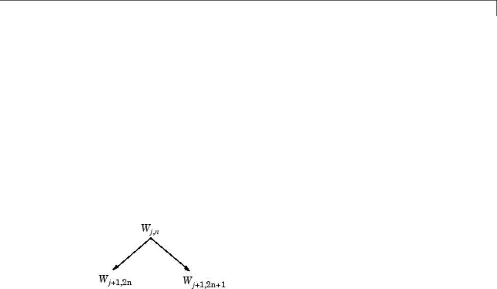
Wavelet Packets
More precisely, let V0denote the space (spanned by the family W0,0 )inwhich
thesignaltobeanalyzedlies;then(Wd,1;d≥1) is an orthogonal basis of V0.
For every strictly positive integer D,(WD,0,(Wd,1;1≤d≤D)) is an orthogonal
basis of V0.
We also know that the family of functions {(Wj+1,2n), (Wj+1,2n+1)} is an orthogonal
basis of the space spanned by Wj,n, which is split into two subspaces: Wj+1,2n
spans the first subspace, and Wj+1,2n+1 the second one.
This last property gives a precise interpretation of splitting in the wavelet
packet organization tree, because all the developed nodes are of the form
showninthefigureWaveletPacketTree:SplitandMergeonpage4-41.
Wavelet Packet Tree: Split and Merge
It follows that the leaves of every connected binary subtree of the complete
tree correspond to an orthogonal basis of the initial space.
For a finite energy signal belonging to V0,anywaveletpacketbasiswill
provide exact reconstruction and offer a specific way of coding the signal,
using information allocation in frequency scale subbands.
Choosing the Optimal Decomposition
Based on the organization of the wavelet packet library, it is natural to count
the decompositions issued from a given orthogonal wavelet.
AsignaloflengthN=2
Lcan be expanded in αdifferent ways, where αis the
number of binary subtrees of a complete binary tree of depth L.Asaresult,
α
≥22N/(see [Mal98] page 323).
As this number may be very large, and since explicit enumeration is generally
unmanageable, it is interesting to find an optimal decomposition with respect
4-41

4Wavelet Packets
to a convenient criterion, computable by an efficient algorithm. We are
looking for a minimum of the criterion.
Functions verifying an additivity-type property are well suited for
efficient searching of binary-tree structures and the fundamental splitting.
Classical entropy-based criteria match these conditions and describe
information-related properties for an accurate representation of a given
signal. Entropy is a common concept in many fields, mainly in signal
processing. Let us list four different entropy criteria (see [CoiW92]); many
others are available and can be easily integrated (type help wentropy). In
the following expressions sis the signal and (si)arethecoefficientsofsin
an orthonormal basis.
The entropy Emust be an additive cost function such that E(0) = 0 and
Es Es
i
i
() ( )=∑
•The (nonnormalized) Shannon entropy
Es s s
iii
122
() log( )=−
so
Es s s
ii
i
122
() log( )=−
∑
with the convention 0log(0) = 0.
•The concentration in lpnorm with 1 ℜ≤p
Es s
ii
p
2( ) =
so
Es s s
i
p
ip
p
2( ) ==
∑
•The logarithm of the “energy” entropy
Es s
ii
32
() log( )=
4-42

Wavelet Packets
so
Es s
i
i
32
() log( )=∑
with the convention log(0) = 0.
•The threshold entropy
Es
i
41()=if si>
ε
and 0 elsewhere, so E4(s)=#{isuch that si>
ε
}is
the number of time instants when the signal is greater than a threshold ε.
These entropy functions are available using the wentropy file.
Example 1: Compute Various Entropies.
1Generate a signal of energy equal to 1.
s= ones(1,16)*0.25;
2Compute the Shannon entropy of s.
e1 = wentropy(s,'shannon')
e1 = 2.7726
3Compute the l1.5 entropy of s, equivalent to norm(s,1.5)1.5.
e2 = wentropy(s,'norm',1.5)
e2 = 2
4Compute the “log energy” entropy of s.
e3 = wentropy(s,'log energy')
e3 = -44.3614
5Compute the threshold entropy of s, using a threshold value of 0.24.
e4 = wentropy(s,'threshold', 0.24)
e4 = 16
4-43

4Wavelet Packets
Example 2: Minimum-Entropy Decomposition.
This simple example illustrates the use of entropy to determine whether a
new splitting is of interest to obtain a minimum-entropy decomposition.
1We start with a constant original signal. Two pieces of information are
sufficient to define and to recover the signal (i.e., length and constant
value).
w00 = ones(1,16)*0.25;
2Compute entropy of original signal.
e00 = wentropy(w00,'shannon')
e00 = 2.7726
3Then split w00 using the haar wavelet.
[w10,w11] = dwt(w00,'db1');
4Compute entropy of approximation at level 1.
e10 = wentropy(w10,'shannon')
e10 = 2.0794
The detail of level 1, w11, is zero; the entropy e11 is zero. Due to
the additivity property the entropy of decomposition is given by
e10+e11=2.0794. This has to be compared to the initial entropy
e00=2.7726.Wehavee10 + e11 < e00, so the splitting is interesting.
5Now split w10 (not w11 because the splitting of a null vector is without
interest since the entropy is zero).
[w20,w21] = dwt(w10,'db1');
6We have w20=0.5*ones(1,4) and w21 is zero. The entropy of the
approximation level 2 is
e20 = wentropy(w20,'shannon')
e20 = 1.3863
4-44
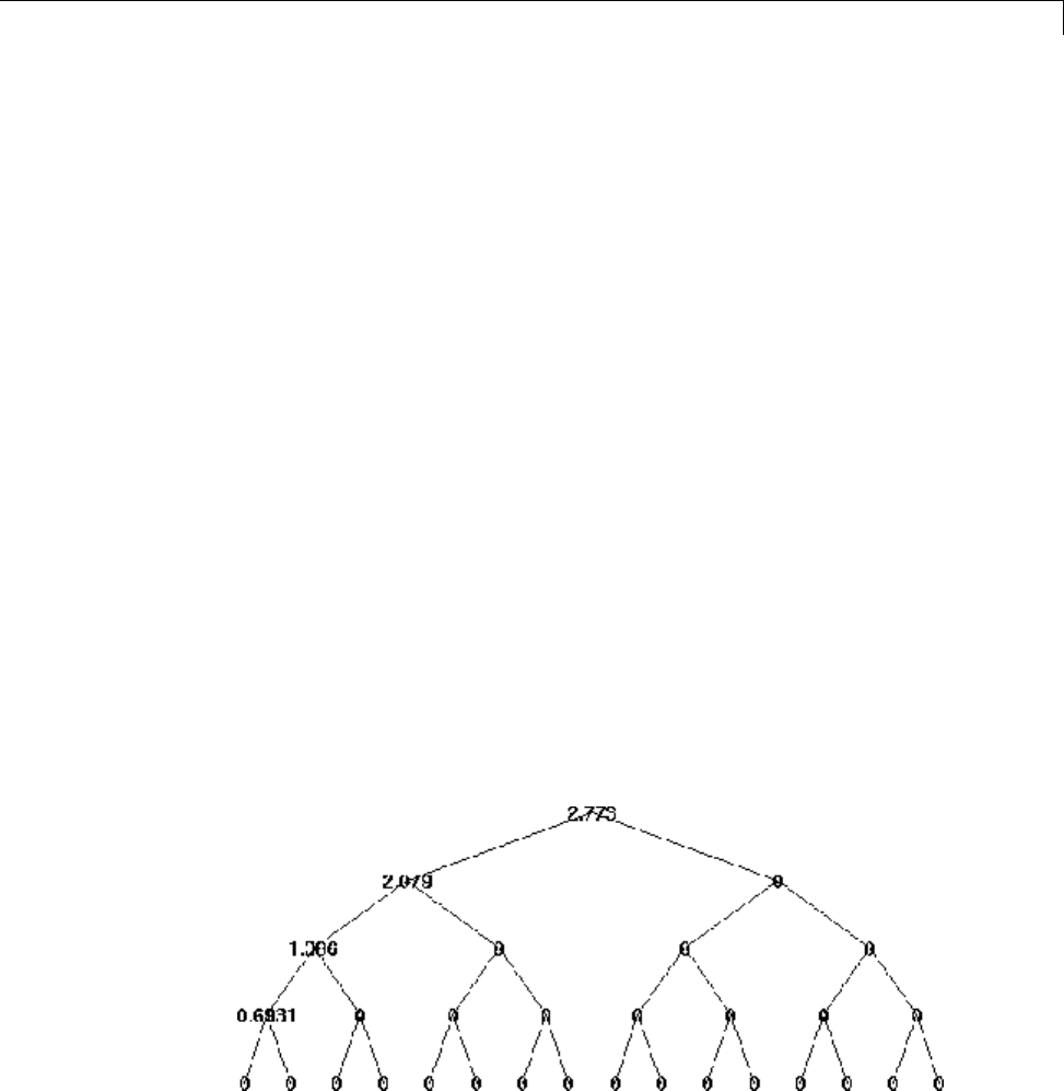
Wavelet Packets
Again we have e20 + 0 < e10, so splitting makes the entropy decrease.
7Then
[w30,w31] = dwt(w20,'db1');
e30 = wentropy(w30,'shannon')
e30 = 0.6931
[w40,w41] = dwt(w30,'db1')
w40 = 1.0000
w41 = 0
e40 = wentropy(w40,'shannon')
e40 = 0
In the last splitting operation we find that only one piece of information
is needed to reconstruct the original signal. The wavelet basis at level 4
is a best basis according to Shannon entropy (with null optimal entropy
since e40+e41+e31+e21+e11 = 0).
8Perform wavelet packets decomposition of the signal sdefined in example 1.
t = wpdec(s,4,'haar','shannon');
The wavelet packet tree in Entropy Values on page 4-45 shows the nodes
labeled with original entropy numbers.
Entropy Values
9Compute the best tree.
4-45
4Wavelet Packets
bt = besttree(t);
The best tree is shown in the following figure. In this case, the best tree
corresponds to the wavelet tree. The nodes are labeled with optimal
entropy.
Optimal Entropy Values
Some Interesting Subtrees
Using wavelet packets requires tree-related actions and labeling. The
implementation of the user interface is built around this consideration. For
more information on the technical details, see the reference pages.
ThecompletebinarytreeofdepthDcorresponding to a wavelet packet
decomposition tree developed at level Dis denoted by WPT.
We have the following interesting subtrees.
Decomposition Tree Subtree Such That the Set of Leaves Is a Basis
Wavelet packets decomposition tree Complete binary tree: WPT of depth D
Wavelet packets optimal decomposition
tree
Binary subtree of WPT
Wavelet packets best-level tree Complete binary subtree of WPT
Wavelet decomposition tree Left unilateral binary subtree of WPT of depth D
Wavelet best-basis tree Left unilateral binary subtree of WPT
4-46

Wavelet Packets
We deduce the following definitions of optimal decompositions, with respect to
an entropy criterion E.
Decompositions Optimal Decomposition Best-Level Decomposition
Wavelet packet
decompositions
Search among 2Dtrees Search among Dtrees
Wavelet decompositions Search among Dtrees Search among Dtrees
For any nonterminal node, we use the following basic step to find the optimal
subtree with respect to a given entropy criterion E(where Eopt denotes the
optimal entropy value).
Entropy Condition Action on Tree and on Entropy Labeling
E node Eopt c
c
() ()≤∑
child of node
If (node≠root), merge and set Eopt(node)=E(node)
E node Eopt c
c
() ()>∑
child of node
Split and set Eopt node Eopt c
c
() ()=∑
child of node
with the natural initial condition on the reference tree, Eopt(t)=E(t)for
each terminal node t.
Reconstructing a Signal Approximation from a Node
You can use the function wprcoef to reconstruct an approximation to your
signal from any node in the wavelet packet tree. This is true irrespective
of whether you are working with a full wavelet packet tree, or a subtree
4-47
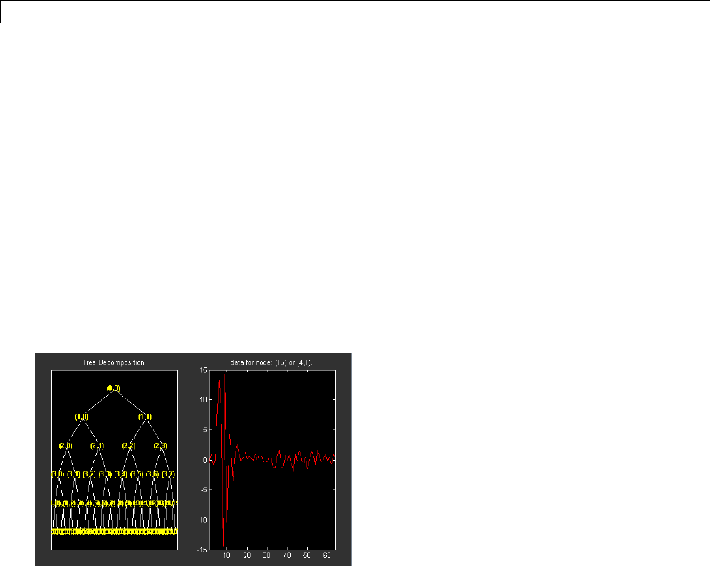
4Wavelet Packets
determined by an optimality criterion. Use wpcoef if you want to extract
the wavelet packet coefficients from a node without reconstructing an
approximation to the signal.
Load the noisy Doppler signal.
load noisdopp
Compute the wavelet packet decomposition down to level 5 using the sym4
wavelet. Use the periodization mode.
dwtmode('per');
T = wpdec(noisdopp,5,'sym4');
plot(T)
Plot the binary wavelet packet tree and click on the (4,1) doublet (node 16).
Extract the wavelet packet coefficients from node 16.
wpc = wpcoef(T,16);
% wpc is length 64
Obtain an approximation to the signal from node 16.
rwpc = wprcoef(T,16);
%rwpcislength1024
plot(noisdopp,'k'); hold on;
plot(rwpc,'b','linewidth',2);
4-48
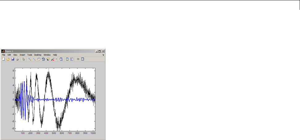
Wavelet Packets
axis tight;
Determine the optimum binary wavelet packet tree.
Topt = besttree(T);
% plot the best tree
plot(Topt)
Reconstruct an approximation to the signal from the (3,0) doublet (node 7).
rsig = wprcoef(Topt,7);
%rsigislength1024
plot(noisdopp,'k'); hold on;
plot(rsig,'b','linewidth',2);
axis tight;
4-49
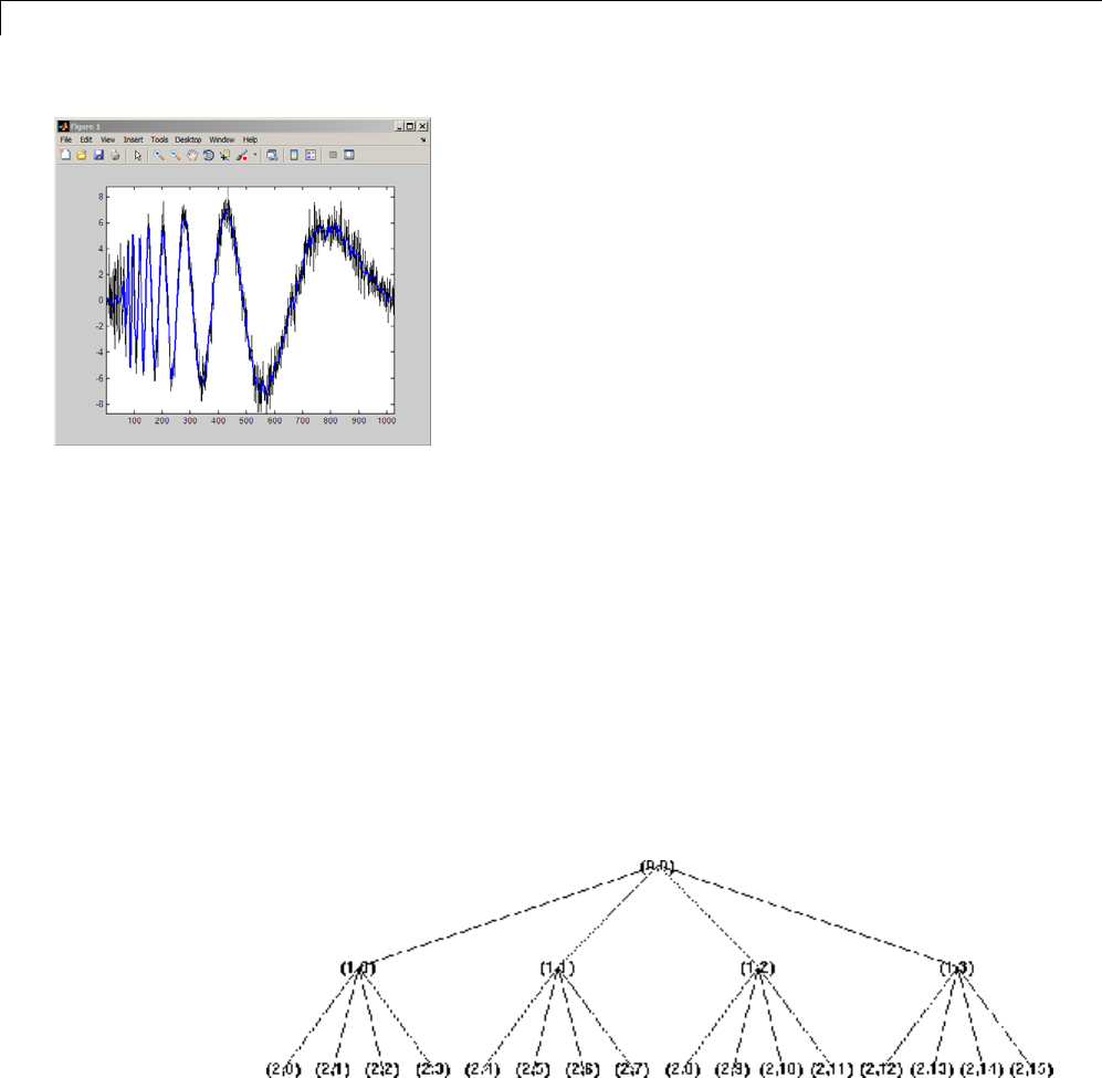
4Wavelet Packets
If you know which doublet in the binary wavelet packet tree you want to
extract, you can determine the node corresponding to that doublet with
depo2ind.
For example, to determine the node corresponding to the doublet (3,0), enter:
Node = depo2ind(2,[3 0]);
Wavelet Packets 2-D Decomposition Structure
Exactly as in the wavelet decomposition case, the preceding one-dimensional
framework can be extended to image analysis. Minor direct modifications lead
to quaternary tree-related definitions. An example is shown the following
figure for depth 2.
Quaternary Tree of Depth 2
4-50

Wavelet Packets
Wavelet Packets for Compression and De-Noising
In the wavelet packet framework, compression and de-noising ideas are
identical to those developed in the wavelet framework. The only new feature
is a more complete analysis that provides increased flexibility. A single
decomposition using wavelet packets generates a large number of bases. You
can then look for the best representation with respect to a design objective,
using the besttree with an entropy function.
4-51

4Wavelet Packets
Introduction to Object-Oriented Features
In the Wavelet Toolbox software, some object-oriented programming features
are used for wavelet packet tree structures.
You may want to skip this appendix, if you prefer to use the command line
functions and graphical user interface (GUI) without knowing about the
underlying objects and classes. But, it is useful for Save and Load actions
where objects are involved.
This appendix lets you understand the objects used in the toolbox, use some
functions that are not fully documented in the reference pages, and extend
the toolbox functionality using the predefined tree structures and some object
programming features.
It is helpful to be familiar with the basic MATLAB object-oriented language
and terminology.
4-52

Objects in the Wavelet Toolbox™ Software
Objects in the Wavelet Toolbox Software
Four classes of objects are defined in the Wavelet Toolbox software.
The hierarchical organization of these objects is described in the following
scheme:
Only the Wavelet Packet tools (1-D and 2-D) use the previous objects. More
precisely, WPTREE objects are used to build wavelet packets.
A short description of this hierarchy of objects follows.
The WTBO class is an abstract class. Any object in the toolbox is parented by
aWTBO object and would inherit the methods and fields of the WTBO class.
The NTREE class is dedicated to tree manipulation (node labels, node
splitting, node merging, ...), and it is also an abstract class. The main methods
are
•nodejoin, which recomposes nodes
•nodesplt, which decomposes nodes
•wtreemgr, which lets you access most of tree and node information (order,
depth, terminal nodes, ascendants of a node, ...)
In fact, the wtreemgr method is not used directly, but you can use the
functions treeord,treedpth,leaves,nodeasc, ..., and the method get.
The DTREE class is dedicated to trees with associated data: vectors or
matrices.
This class is also an abstract class and some methods have to be overloaded.
The aim of the WPTREE class is to manage wavelet packets 1-D and 2-D.
Some methods of the DTREE class have been overloaded, for example:
split,merge,andrecons.
4-53

4Wavelet Packets
MostofthemethodsarespecifictotheclassWPTREE; for example:
bestlevt,besttree,andwp2wtree.
By typing help wavelet you can see the available methods in the Tree
Management Utilities and Wavelets Packets Algorithms sections.
4-54

Examples Using Objects
Examples Using Objects
You can use command line functions, GUI functions, or you can mix both
of them to work with wavelet packet trees (WPTREE objects). The most
useful commands are
•plot,drawtree,andreadtree, which let you plot and get a wavelet packet
tree
•wpjoin and wpsplt, which let you change a wavelet packet tree structure
•get,read,andwrite, which let you read and write coefficients or
information in a wavelet packet tree
We can see some of these features in the following examples.
•“plotandwpviewcf”onpage4-55
•“drawtree and readtree” on page 4-59
•“Change Terminal Node Coefficients” on page 4-61
•“Thresholding Wavelet Packets” on page 4-63
plot and wpviewcf
load noisbump
x = noisbump;
t = wpdec(x,3,'db2');
fig = plot(t);
Click on node 7.
4-55

4Wavelet Packets
Change Node Action from Visualize to Split-Merge and merge the second
node.
4-56
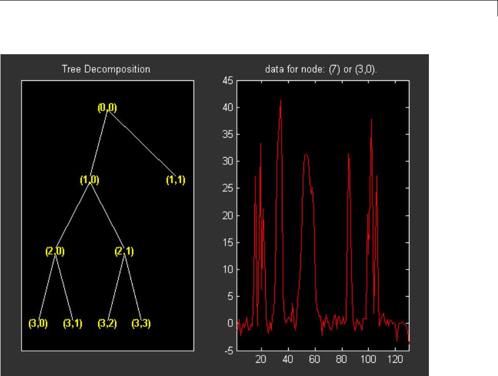
Examples Using Objects
%Fromthe command line, you can get the new tree.
newt = plot(t,'read',fig);
%Thef
irst argument of the plot function in the last command
%isd
ummy. Then the general syntax is:
% newt = plot(DUMMY,'read',fig);
%whe
re DUMMY is any object parented by an NTREE object.
%DUM
MY can be any object constructor name, which returns
%anobject parented by an NTREE object. For example:
%ne
wt = plot(ntree,'read',fig);
%ne
wt = plot(dtree,'read',fig);
%n
ewt = plot(wptree,'read',fig);
4-57
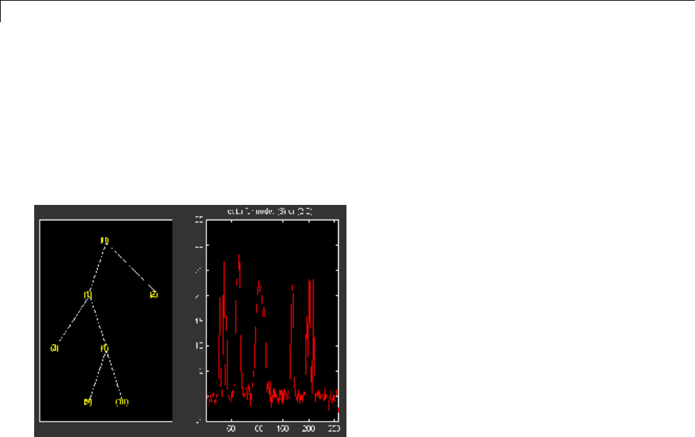
4Wavelet Packets
% From the command line you can modify the new tree,
% then plot it.
newt = wpjoin(newt,3);
fig2 = plot(newt);
% Change Node Label from Depth_position to Index and
% click the node (3). You get the following figure.
% Using plot(newt,fig), the plot is done in the figure fig,
% which already contains a tree object.
% You can see the colored wavelet packets coefficients using
% from the command line, the wpviewcf function (type help
% wpviewcf for more information).
wpviewcf(newt,1)
% You get the following plot, which contains the terminal nodes
% colored coefficients.
4-58
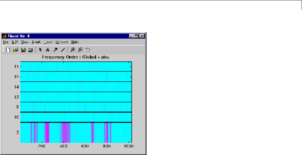
Examples Using Objects
drawtree and readtree
load noisbump
x = noisbump;
t = wpdec(x,3,'db2');
fig = drawtree(t);
% The last command creates a GUI.
% The same GUI can be obtained using the main menu and:
% - clicking the Wavelet Packet 1-D button,
% - loading the signal noisbump,
% - choosing the level and the wavelet
% - clicking the decomposition button.
% You get the following figure.
4-59
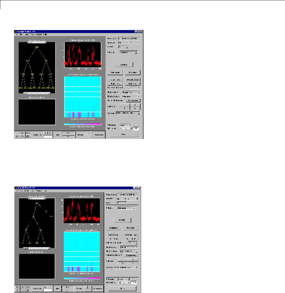
4Wavelet Packets
% From the GUI, you can modify the tree.
% For example, change Node label from Depth_Position to Index,
% change Node Action from Visualize to Split_Merge and
% merge the node 2.
% You get the following figure.
% From the command line, you can get the new tree.
4-60
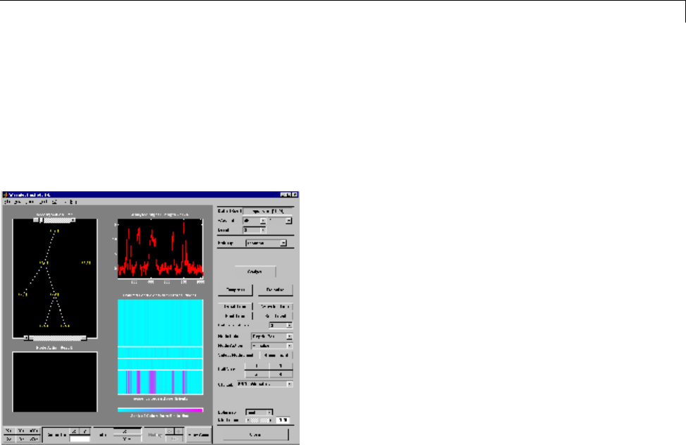
Examples Using Objects
newt = readtree(fig);
% From the command line you can modify the new tree;
% then plot it in the same figure.
newt = wpjoin(newt,3);
drawtree(newt,fig);
You can mix previous commands. The GUI associated with the plot command
is simpler and quicker, but more actions and information are available using
the full GUI tools related to wavelet packets.
The methods associated with WPTREE objects let you do more complicated
actions.
Namely, using read and write methods, you can change terminal node
coefficients.
Let’s illustrate this point with the following “funny” example.
Change Terminal Node Coefficients
load gatlin2
t=w
pdec2(X,1,'haar');
plot(t);
4-61
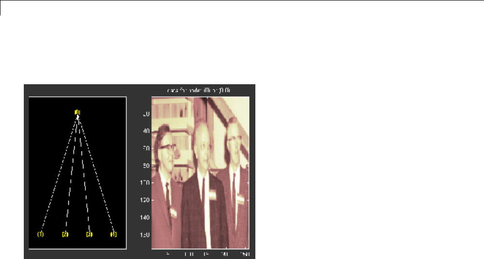
4Wavelet Packets
% Change Node Label from Depth_position to Index and
% click the node (0). You get the following figure.
% Now modify the coefficients of the four terminal nodes.
newt = t;
NBcols = 40;
for node =1:4
cfs = read(t,'data',node);
tmp = cfs(1:end,1:NBcols);
cfs(1:end,1:NBcols) = cfs(1:end,end-NBcols+1:end);
cfs(1:end,end-NBcols+1:end) = tmp;
newt = write(newt,'data',node,cfs);
end
plot(newt)
%Cha
nge Node Label from Depth_position to Index and
%cli
ck on the node (0). You get the following figure.
4-62
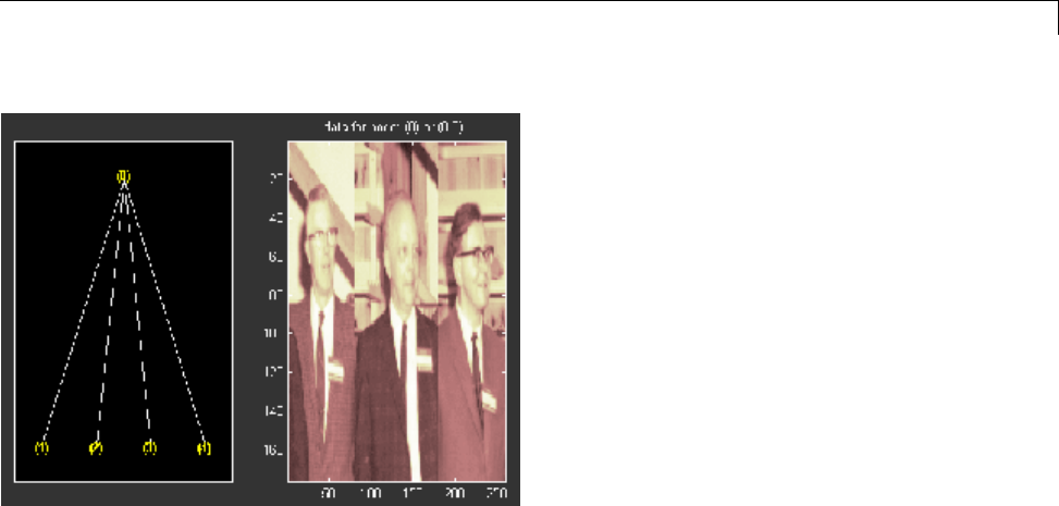
Examples Using Objects
You can use this method for a more useful purpose. Let’s see a de-noising
example.
Thresholding Wavelet Packets
load noisbloc
x = noisbloc;
t = wpdec(x,3,'sym4');
plot(t);
% Change Node Label from Depth_position to Index and
% click the node (0). You get the following plot.
4-63

4Wavelet Packets
% Global thresholding.
t1 = t;
sorh = 'h';
thr = wthrmngr('wp1ddenoGBL','penalhi',t);
cfs = read(t,'data');
cfs = wthresh(cfs,sorh,thr);
t1 = write(t1,'data',cfs);
plot(t1)
% Change Node Label from Depth_position to Index and
% click the node (0). You get the following plot.
4-64
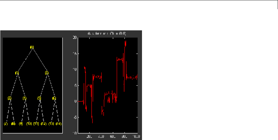
Examples Using Objects
% Node by node thresholding.
t2 = t;
sorh = 's';
thr(1) = wthrmngr('wp1ddenoGBL','penalhi',t);
thr(2) = wthrmngr('wp1ddenoGBL','sqtwologswn',t);
tn = leaves(t);
for k=1:length(tn)
node = tn(k);
cfs = read(t,'data',node);
numthr = rem(node,2)+1;
cfs = wthresh(cfs,sorh,thr(numthr));
t2 = write(t2,'data',node,cfs);
end
plot(t2)
% Change Node Label from Depth_position to Index and
% click the node (0). You get the following plot.
4-65
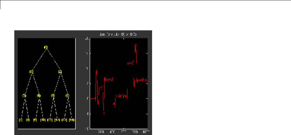
4Wavelet Packets
4-66

Description of Objects in the Wavelet Toolbox™ Software
Description of Objects in the Wavelet Toolbox Software
The following sections describe the objects in the Wavelet Toolbox software:
•“WTBO Object” on page 4-67
•“NTREE Object” on page 4-68
•“DTREE Object” on page 4-69
•“WPTREE Object” on page 4-71
WTBO Object
Class WTBO (Wavelet Toolbox Object) -- Parent class: none
Fields
wtboInfo Object information (Not used)
ud Userdata field
Methods
wtbo Constructor for the class WTBO.
get GetWTBOobjectfieldcontents.
set SetWTBOobjectfieldcontents.
Comments
Since any object in the toolbox is parented by a WTBO object, you can
associate your own data to an object using the 'ud' field, and then access it.
If Obj is an object (parented by a WTBO object), use
Obj = set(Obj,'ud',MyData)
to define the data.
To retrieve the data, use
4-67

4Wavelet Packets
MyData = get(O,'ud')
NTREE Object
Class NTREE (New Tree) -- Parent class: WTBO
Fields
wtbo Parent object
order Tree order
depth Tree depth
spsch Split scheme for nodes
tn Column vector with terminal nodes indices
Methods
ntree Constructor for the class NTREE.
findactn Find active nodes.
get Get NTREE object field contents.
nodejoin Recompose node(s).
nodesplt Split (decompose) node(s).
plot Plot NTREE object.
set Set NTREE object field contents.
tlabels Labels for the nodes of a tree.
wtreemgr Manager for NTREE object.
Private
locnumcn Local number for a child node
tabofasc Table of ascendants of nodes
4-68

Description of Objects in the Wavelet Toolbox™ Software
DTREE Object
Class DTREE (Data Tree) -- Parent class: NTREE
Fields
ntree Parent object
allNI All Nodes Information
terNI Terminal Nodes Information
Fields Description
allNI is a NBnodes-by-3 array such that
allNI(N,:) = [ind,size(1,1),size(1,2)]
•ind =inde
xofthenodeN
•size =siz
e of data associated with the node N
terNI is a1-by-2cellarraysuchthat
•terNI{1} is an NB_TerminalNodes-by-2 array such that
-terNI{1}(N,:) is the size of coefficients associated with the N-th
terminal node. The nodes are numbered from left to right and from top
to bottom. The root index is 0.
•terNI{2} is a row vector containing the previous coefficients stored
row-wise in the above specified order.
Methods
dtree Constructor for the class DTREE.
expand Expand data tree.
fmdtree Field manager for DTREE object.
nodejoin Recompose node.
4-69

4Wavelet Packets
nodesplt Split (decompose) node.
rnodcoef Reconstruct node coefficients.
defaninf Define node information (all nodes).
get Get DTREE object field contents.
plot Plot DTREE object.
read Read values in DTREE object fields.
set Set DTREE object field contents.
write Write values in DTREE object fields.
merge Merge (recompose) the data of a node.
recons Reconstruct node coefficients.
split Split (decompose) the data of a terminal node.
Comments
•After the constructor, the first set of methods (between line separators)
might not be overloaded (or only with great care). The second set of
methods can be overloaded. The third set of methods must be overloaded to
recompose, reconstruct, or decompose nodes data.
•The method nodejoin calls the method merge,themethodnodesplt calls
the method split, and the method rnodcoef calls the method recons.
•To define nodes information, you must overload the method defaninf.For
each node N, the basic information is given by
allNI(N,1:3): [index,size(1,1),size(1,2)];
You can add other information by adding columns to allNI.
See the WPTREE object method for an example.
•If the method get is not overloaded, using the DTREE get method you can
getsomeobjectfieldcontents(butnotall).
4-70

Description of Objects in the Wavelet Toolbox™ Software
For example, if Tis parented by a DTREE object of order 2 and if 'Tfield'
is a field of T,whosecontentisTval,[a,b] = get(t,'order','Tfield')
returns a=2and b = 'errorWTBX'. Nevertheless, using a
nondocumented method you can get the right values. Namely:
[a,b] = getwtbo(t,'order','Tfield') returns a=2and b=Tval.
WPTREE Object
Class WPTREE (Wavelet Packet Tree) -- Parent class: DTREE
Fields
dtree Parent object
wavInfo Structure (wavelet information)
entInfo Structure (entropy information)
Fields Description
wavInfo
wavName Wavelet Name
Lo_D Low Decomposition filter
Hi_D High Decomposition filter
Lo_R Low Reconstruction filter
Hi_R High Reconstruction filter
entInfo
entName Entropy Name
entPar Entropy Parameter
allNI Array(nbnode,5) (field of the dtree parent object)
[ind,size,ent,ento]
4-71

4Wavelet Packets
ind Index
size Size of data
ent Entropy
ento Optimal Entropy
Methods
Constructor.
Method Description
wptree Constructor for the class WPTREE
Methods That Overload Those of DTREE Class.
Method Description
defaninf Define node information (all nodes).
get Get WPTREE object field contents.
merge Merge (recompose) the data of a node.
read Read values in WPTREE object fields.
recons Reconstruct wavelet packet coefficients.
set Set WPTREE object field contents.
split Split (decompose) the data of a terminal node.
tlabels Labels for the nodes of a wavelet packet tree.
write Write values in WPTREE object fields.
Proper Methods of WPTREE Class.
Method Description
bestlevt Best level of a wavelet packet tree.
besttree Bestwaveletpackettree.
4-72

Description of Objects in the Wavelet Toolbox™ Software
Method Description
entrupd Entropy update (wavelet packet tree).
wp2wtree Extract wavelet tree from wavelet packet tree.
wpcoef Wavelet packet coefficients.
wpcutree Cut wavelet packet tree.
wpjoin Recompose wavelet packet.
wpplotcf Plot wavelet packets colored coefficients.
wprcoef Reconstruct wavelet packet coefficients.
wprec Wavelet packet reconstruction 1-D.
wprec2 Wavelet packet reconstruction 2-D.
wpsplt Split (decompose) wavelet packet.
wpthcoef Wavelet packet coefficients thresholding.
wpviewcf Plot wavelet packets colored coefficients.
4-73

4Wavelet Packets
Advanced Use of Objects
The following sections explain how to extend the toolbox with new objects
through four examples.
•“Building a Wavelet Tree Object (WTREE)” on page 4-74
•“Building a Right Wavelet Tree Object (RWVTREE)” on page 4-75
•“Building a Wavelet Tree Object (WVTREE)” on page 4-77
•“BuildingaWaveletTreeObject(EDWTTREE)”onpage4-79
Building a Wavelet Tree Object (WTREE)
This example creates a new class of objects: WTREE.
Starting from the class DTREE and overloading the methods split and
merge,wedefineawavelettreeclass.
To plot a WTREE, the DTREE plot method is used.
You can have a look at a one-dimensional example in the ex1_wt file
and at a two-dimensional example in the ex2_wt file located in the
toolbox/wavelet/wavedemo folder. These examples can be used directly, but
they are also useful to learn how to build new object-oriented programming
functions.
The definition of the new class is described below.
Class WTREE (parent class: DTREE)
Fields
dtree Parent object
dwtMode DWT extension mode
wavInfo Structure (wavelet information)
4-74

Advanced Use of Objects
wavInfo Structure information
wavName Wavelet Name
Lo_D Low Decomposition filter
Hi_D High Decomposition filter
Lo_R Low Reconstruction filter
Hi_R High Reconstruction filter
Methods
wtree Constructor for the class WTREE.
merge Merge (recompose) the data of a node.
split Split (decompose) the data of a terminal node.
BuildingaRightWaveletTreeObject(RWVTREE)
This example creates a new class of objects: RWVTREE.
We define a right wavelet tree class starting from the class WTREE and
overloading the methods split,merge,andplot (inherited from DTREE).
The plot method shows how to add Node Labels.
You can have a look at a one-dimensional example in the ex1_rwvt file
and at a two-dimensional example in the ex2_rwvt file located in the
toolbox/wavelet/wavedemo folder. These programs canbeuseddirectly,but
they are also useful to learn how to build new object-oriented programming
functions.
The definition of the new class is described below.
Class RWVTREE (parent class: WTREE)
4-75

4Wavelet Packets
Fields
dummy Not used
wtree Parent object
Methods
rwvtree Constructor for the class RWVTREE.
merge Merge (recompose) the data of a node.
plot Plot RWVTREE object.
split Split (decompose) the data of a terminal node.
Running This Example
The following figure is obtained using the example ex1_rwvt and clicking
the node 14.
The approximations are labeled in yellow and the details are labeled in red.
The last nodes cannot be split.
4-76
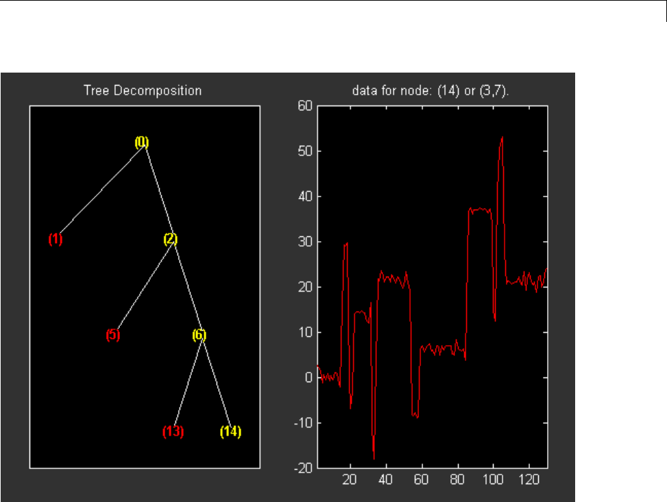
Advanced Use of Objects
Building a Wavelet Tree Object (WVTREE)
This example creates a new class of objects: WVTREE.
We define a wavelet tree class starting from the class WTREE and overloading
the methods get,plot,andrecons (all inherited from DTREE).
The split and merge methodsoftheclassWTREEareused.
The plot method shows how to add Node Labels and Node Actions.
You can have a look at a one-dimensional example in the ex1_wvt file
and at a two-dimensional example in the ex2_wvt file located in the
4-77

4Wavelet Packets
toolbox/wavelet/wavedemo folder. These programs canbeuseddirectly,but
they are also useful to learn how to build new object-oriented programming
functions.
The definition of the new class is described below.
Class WVTREE (parent class: WTREE)
Fields
dummy Not used
wtree Parent object
Methods
wvtree Constructor for the class WVTREE.
get Get WVTREE object field contents.
plot Plot WVTREE object.
recons Reconstruct node coefficients.
Running This Example
The following figure is obtained using the example ex2_wvt and clicking the
node 2.
The approximations are labeled in yellow and the details are labeled in red.
The last nodes cannot be split. The title of the figure contains the DWT
extension mode used ('sym' in the present example).
4-78
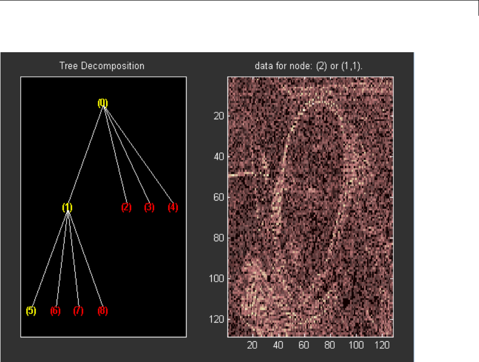
Advanced Use of Objects
Building a Wavelet Tree Object (EDWTTREE)
This example creates a new class of objects: EDWTTREE.
We define an ε-DWT tree class starting from the class DTREE and overloading
the methods merge,plot,recons,andsplit.
For more information on the ε-DWT, see the section “
ε
-Decimated DWT”
on page 3-62.
The plot method shows how to add Node Labels,Node Actions,andTree
Actions.
4-79

4Wavelet Packets
You can have a look at the example in the ex1_edwt file located in the
toolbox/wavelet/wavedemo folder. This program can be used directly, but
it is also useful to learn how to build new object-oriented programming
functions.
The definition of the new class is described below.
Class EDWTTREE (parent class: DTREE)
Fields
dtree Parent object
dwtMode DWT extension mode
wavInfo Structure (wavelet information)
Fields Description
wavInfo
wavName Wavelet Name
Lo_D Low Decomposition filter
Hi_D High Decomposition filter
Lo_R Low Reconstruction filter
Hi_R High Reconstruction filter
Methods
edwttree Constructor for the class EDWTTREE.
merge Merge (recompose) the data of a node.
plot Plot EDWTTREE object.
recons Reconstruct node coefficients.
split Split (decompose) the data of a terminal node.
4-80
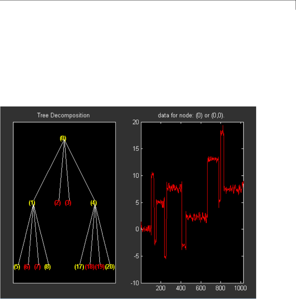
Advanced Use of Objects
Running This Example
The following figure is obtained using the example ex1_edwt, selecting the
De-noise option in the Tree Action menu and clicking the node 0.
The approximations are labeled in yellow and the details are labeled in red.
The last nodes cannot be split.
The title of the figure contains the DWT extension mode used ('sym' in the
present example) and the name of the de-noising method.
4-81

4Wavelet Packets
4-82

5
Denoising, Nonparametric
Function Estimation, and
Compression
•“Denoising and Nonparametric Function Estimation” on page 5-2
•“One-Dimensional Adaptive Thresholding of Wavelet Coefficients” on page
5-17
•“Multivariate Wavelet Denoising” on page 5-27
•“Multiscale Principal Components Analysis” on page 5-41
•“Data Compression” on page 5-51
•“True Compression for Images” on page 5-55
•“Two-Dimensional True Compression” on page 5-61
•“One-Dimensional Wavelet Regression Estimation” on page 5-80

5Denoising, Nonparametric Function Estimation, and Compression
Denoising and Nonparametric Function Estimation
The Wavelet Toolbox provides a number of functions for the estimation of an
unknown function (signal or image) in noise.
The most general 1-D model for this is
s(n)=f(n)+σe(n)
where n= 0,1,2,...N-1. The e(n) are Gaussian random variables distributed as
N(0,1). The variance of the σe(n)isσ2.
In practice, s(n) is often a discrete-time signal with equal time steps corrupted
by additive noise and you are attempting to recover that signal.
More generally, you can view s(n) as an N-dimensional random vector
fe
fe
fe
fN eN
() ()
() ()
() ()
.
.
.
()()
00
11
22
11
f
f
f
fN
()
()
()
.
.
.
()
0
1
2
1
ee
e
e
eN
()
()
()
.
.
.
()
0
1
2
1
In this general context, the relationship between denoising and regression
is clear.
You can replace the N-by-1 random vector by N-by-M random matrices to
obtain the problem of recovering an image corrupted by additive noise.
You can obtain a 1-D example of this model with the following code.
load cuspamax;
y = cuspamax+0.5*randn(size(cuspamax));
plot(y); hold on;
plot(cuspamax,'r','linewidth',2);
axis tight;
5-2
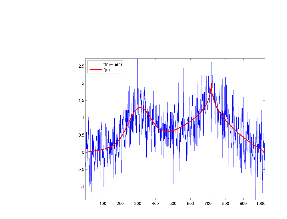
Denoising and Nonparametric Function Estimation
legend('f(n)+\sigma e(n)','f(n)', 'Location', 'NorthWest');
For a broad class of functions (signals, images) that possess certain
smoothness properties, wavelet techniques are optimal or near optimal for
function recovery.
Specifically, the method is efficient for families of functions fthat have only
a few nonzero wavelet coefficients. These functions have a sparse wavelet
representation. For example, a smooth function almost everywhere, with only
a few abrupt changes, has such a property.
5-3

5Denoising, Nonparametric Function Estimation, and Compression
The general wavelet–based method for denoising and nonparametric function
estimation is to transform the data into the wavelet domain, threshold the
wavelet coefficients, and invert the transform.
You can summarize these steps as:
1Decompose
Choose a wavelet and a level N. Compute the wavelet decomposition of
the signal sdown to level N.
2Threshold detail coefficients
For each level from 1 to N, threshold the detail coefficients.
3Reconstruct
Compute wavelet reconstruction using the original approximation
coefficients of level Nand the modified detail coefficients of levels from
1toN.
Threshold Selection Rules
The Wavelet Toolbox supports a number of threshold selection rules. Four
threshold selection rules are implemented in the thselect.Eachrule
corresponds to a tptr option in the command
thr = thselect(y,tptr)
which returns the threshold value.
Option Threshold Selection Rule
'rigrsure' Selection using principle of Stein’s Unbiased Risk
Estimate (SURE)
'sqtwolog' Fixed form (universal) threshold equal to
2ln( )N
with Nthe length of the signal.
5-4
Denoising and Nonparametric Function Estimation
Option Threshold Selection Rule
'heursure' Selection using a mixture of the first two options
'minimaxi' Selection using minimax principle
•Option 'rigrsure' uses for the soft threshold estimator a threshold
selection rule based on Stein’s Unbiased Estimate of Risk (quadratic loss
function). You get an estimate of the risk for a particular threshold value t.
Minimizing the risks in tgives a selection of the threshold value.
•Option 'sqtwolog' uses a fixed form threshold yielding minimax
performance multiplied by a small factor proportional to log(length(s)).
•Option 'heursure' is a mixture of the two previous options. As a result, if
the signal-to-noise ratio is very small, the SURE estimate is very noisy. So
if such a situation is detected, the fixed form threshold is used.
•Option 'minimaxi' uses a fixed threshold chosen to yield minimax
performance for mean square error against an ideal procedure. The
minimax principle is used in statistics to design estimators. Since the
denoised signal can be assimilated to the estimator of the unknown
regression function, the minimax estimator is the option that realizes the
minimum, over a given set of functions, of the maximum mean square error.
The following example shows the threshold rules for a 1000-by-1 N(0,1)
vector. The signal here is
f n en en N() () ()~ (,)01
with f(n) =0.
rng default;
sig = randn(1e3,1);
thr_rigrsure = thselect(sig,'rigrsure')
thr_univthresh = thselect(sig,'sqtwolog')
thr_heursure = thselect(sig,'heursure')
thr_minimaxi = thselect(sig,'minimaxi')
hist(sig);
h = findobj(gca,'Type','patch');
set(h,'FaceColor',[0.7 0.7 0.7],'EdgeColor','w');
hold on;
plot([thr_rigrsure thr_rigrsure], [0 300],'linewidth',2);
5-5
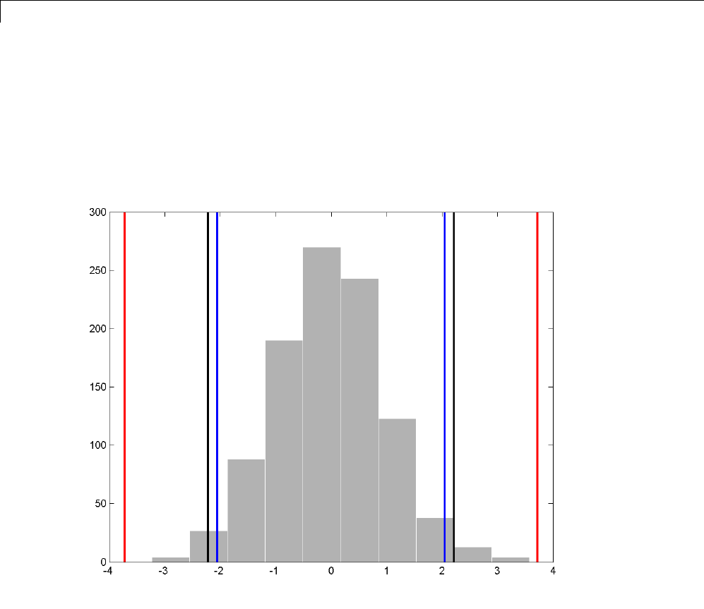
5Denoising, Nonparametric Function Estimation, and Compression
plot([thr_univthresh thr_univthresh], [0 300],'r','linewidth',2);
plot([thr_minimaxi thr_minimaxi], [0 300],'k','linewidth',2);
plot([-thr_rigrsure -thr_rigrsure], [0 300],'linewidth',2);
plot([-thr_univthresh -thr_univthresh], [0 300],'r','linewidth',2);
plot([-thr_minimaxi -thr_minimaxi], [0 300],'k','linewidth',2);
For Stein’s Unbiased Risk Estimate (SURE) and minimax thresholds,
approximately 3% of coefficients are retained. In the case of the universal
threshold, all values are rejected.
We know that the detail coefficientsvectoristhesuperpositionofthe
coefficients of fand the coefficients of e, and that the decomposition of eleads
to detail coefficients, which are standard Gaussian white noises.
5-6

Denoising and Nonparametric Function Estimation
After you use thselect to determine a threshold, you can threshold each
levelofa.Thissecondstepcanbedoneusingwthcoef,directlyhandlingthe
wavelet decomposition structure of the original signal s.
Soft or Hard Thresholding
Hard and soft thresholding are examples of shrinkage rules. After you have
determined your threshold, you have to decide how to apply that threshold
to your data.
The simplest scheme is hard thresholding. Let Tdenote the threshold and x
your data. The hard thresholding is
() ||
||
xxxT
xT
0
The soft thresholding is
() ||x
xT x T
xT
xTx T
0
You can apply your threshold using the hard or soft rule with wthresh.
y = linspace(-1,1,100);
thr = 0.4;
ythard = wthresh(y,'h',thr);
ytsoft = wthresh(y,'s',thr);
subplot(131);
plot(y); title('Original Data');
subplot(132);
plot(ythard,'*'); title('Hard Thresholding');
subplot(133);
plot(ytsoft,'*'); title('Soft Thresholding');
5-7
5Denoising, Nonparametric Function Estimation, and Compression
Dealing with Unscaled Noise and Nonwhite Noise
Usually in practice the basic model cannot be used directly. We examine here
the options available to deal with model deviations in the main de-noising
function wden.
The simplest use of wden is
sd = wden(s,tptr,sorh,scal,n,wav)
which returns the denoised version sd of the original signal sobtained using
the tptr threshold selection rule. Other parameters needed are sorh,scal,n,
and wav.Theparametersorh specifies the thresholding of details coefficients
of the decomposition at level nof sby the wavelet called wav. The remaining
5-8
Denoising and Nonparametric Function Estimation
parameter scal is to be specified. It corresponds to threshold’s rescaling
methods.
Option Corresponding Model
'one' Basic model
'sln' Basic model with unscaled noise
'mln' Basic model with nonwhite noise
•Option scal = 'one' corresponds to the basic model.
•In general, you can ignore the noise level and it must be estimated. The
detail coefficients cD1(the finest scale) are essentially noise coefficients
with standard deviation equal to σ. The median absolute deviation of the
coefficients is a robust estimate of σ. The use of a robust estimate is crucial
for two reasons. The first one is that if level 1 coefficients contain fdetails,
then these details are concentrated in a few coefficients if the function f is
sufficiently regular. The second reason is to avoid signal end effects, which
arepureartifactsduetocomputationsontheedges.
Option scal = 'sln' handles threshold rescaling using a single estimation
of level noise based on the first-level coefficients.
•When you suspect a nonwhite noise e, thresholds must be rescaled by a
level-dependent estimation of the level noise. The same kind of strategy as
in the previous option is used by estimating σlev level by level.
This estimation is implemented in the file wnoisest,directlyhandlingthe
wavelet decomposition structure of the original signal s.
Option scal = 'mln' handles threshold rescaling using a level-dependent
estimation of the level noise.
For a more general procedure, the wdencmp function performs wavelet
coefficients thresholding for both de-noising and compression purposes, while
directly handling one-dimensional and two-dimensional data. It allows you to
define your own thresholding strategy selecting in
xd = wdencmp(opt,x,wav,n,thr,sorh,keepapp);
where
5-9

5Denoising, Nonparametric Function Estimation, and Compression
•opt = 'gbl' and thr is a positive real number for uniform threshold.
•opt = 'lvd' and thr is a vector for level dependent threshold.
•keepapp = 1 to keep approximation coefficients, as previously and
•keepapp = 0 to allow approximation coefficients thresholding.
•xisthesignaltobedenoisedandwav,n,sorh are the same as above.
Denoising in Action
We begin with examples of one-dimensional de-noising methods with the first
example credited to Donoho and Johnstone. You can use the following file to
get the first test function using wnoise.
% Set signal to noise ratio and set rand seed.
sqrt_snr = 4; init = 2055615866;
% Generate original signal xref and a noisy version x adding
% a standard Gaussian white noise.
[xref,x] = wnoise(1,11,sqrt_snr,init);
% De-noise noisy signal using soft heuristic SURE thresholding
% and scaled noise option, on detail coefficients obtained
% from the decomposition of x, at level 3 by sym8 wavelet.
xd = wden(x,'heursure','s','one',3,'sym8');
5-10
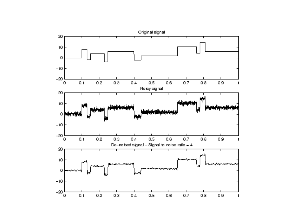
Denoising and Nonparametric Function Estimation
Blocks Signal Denoising
Since only a small number of large coefficients characterize the original
signal, the method performs very well.
As a second example, let us try the method on the highly perturbed part of
the electrical signal studied above.
According to this previous analysis, let us use db3 wavelet and decompose at
level 3.
To deal with the composite noise nature, let us try a level-dependent noise
size estimation.
% Load electrical signal and select part of it.
load leleccum; indx = 2000:3450;
5-11
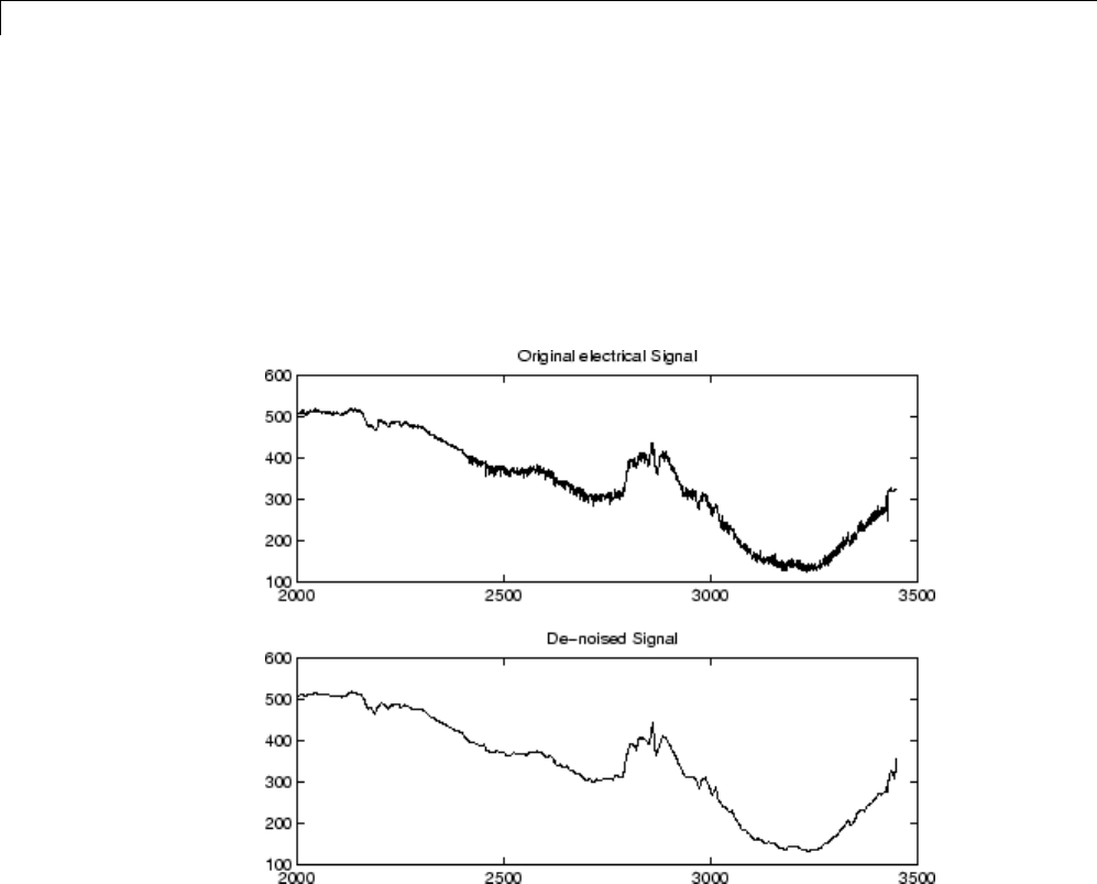
5Denoising, Nonparametric Function Estimation, and Compression
x = leleccum(indx);
% Find first value in order to avoid edge effects.
deb = x(1);
% De-noise signal using soft fixed form thresholding
% and unknown noise option.
xd = wden(x-deb,'sqtwolog','s','mln',3,'db3')+deb;
Electrical Signal De-Noising
The result is quite good in spite of the time heterogeneity of the nature of the
noise after and before the beginning of the sensor failure around time 2450.
Extension to Image De-Noising
The de-noising method described for the one-dimensional case applies also
to images and applies well to geometrical images. A direct translation of
the one-dimensional model is
5-12

Denoising and Nonparametric Function Estimation
s(i,j)=f(i,j)+σe(i,j)
where eis a white Gaussian noise with unit variance.
Thetwo-dimensionalde-noisingprocedurehasthesamethreestepsand
uses two-dimensional wavelet tools instead of one-dimensional ones. For
the threshold selection, prod(size(s)) is used instead of length(s) if the
fixed form threshold is used.
Note that except for the “automatic” one-dimensional de-noising case,
de-noising and compression are performed using wdencmp.Asanexample,
you can use the following file illustrating the de-noising of a real image.
% Load original image.
load woman
% Generate noisy image.
x = X + 15*randn(size(X));
% Find default values. In this case fixed form threshold
% is used with estimation of level noise, thresholding
% mode is soft and the approximation coefficients are
% kept.
[thr,sorh,keepapp] = ddencmp('den','wv',x);
% thr is equal to estimated_sigma*sqrt(log(prod(size(X))))
% De-noise image using global thresholding option.
xd = wdencmp('gbl',x,'sym4',2,thr,sorh,keepapp);
% Plots.
colormap(pink(255)), sm = size(map,1);
subplot(221), image(wcodemat(X,sm)), title('Original Image')
subplot(222), image(wcodemat(x,sm)), title('Noisy Image')
subplot(223), image(wcodemat(xd,sm)), title('denoised Image')
The result shown below is acceptable.
5-13
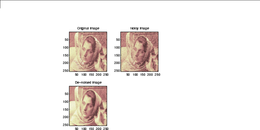
5Denoising, Nonparametric Function Estimation, and Compression
Image De-Noising
One-Dimensional Wavelet Variance Adaptive
Thresholding
The idea is to define level by level time-dependent thresholds, and then
increase the capability of the de-noising strategies to handle nonstationary
variance noise models.
More precisely, the model assumes (as previously) that the observation is
equal to the interesting signal superimposed on a noise (see “Denoising and
Nonparametric Function Estimation” on page 5-2).
s(n)=f(n)+σe(n)
But the noise variance can vary with time. There are several different
variance values on several time intervals. The values as well as the intervals
are unknown.
Let us focus on the problem of estimating the change points or equivalently
the intervals. The algorithm used is based on an original work of Marc
Lavielle about detection of change points using dynamic programming (see
[Lav99] in “References”).
5-14

Denoising and Nonparametric Function Estimation
Let us generate a signal from a fixed-design regression model with two noise
variance change points located at positions 200 and 600.
% Generate blocks test signal.
x = wnoise(1,10);
% Generate noisy blocks with change points.
bb = randn(1,length(x));
cp1 = 200; cp2 = 600;
x = x + [bb(1:cp1),bb(cp1+1:cp2)/4,bb(cp2+1:end)];
The aim of this example is to recover the two change points from the signal
x. In addition, this example illustrates how the GUI tools locate the change
points for interval dependent thresholding.
Step 1. Recover a noisy signal by suppressing an approximation.
% Perform a single-level wavelet decomposition
% of the signal using db3.
wname = 'db3'; lev = 1;
[c,l] = wavedec(x,lev,wname);
% Reconstruct detail at level 1.
det = wrcoef('d',c,l,wname,1);
The reconstructed detail at level 1 recovered at this stage is almost signal
free. It captures the main features of the noise from a change points
detection viewpoint if the interesting part of the signal has a sparse wavelet
representation. To remove almost all the signal, we replace the biggest values
by the mean.
Step 2. To remove almost all the signal, replace 2% of biggest values by
the mean.
x = sort(abs(det));
v2p100 = x(fix(length(x)*0.98));
ind = find(abs(det)>v2p100);
det(ind) = mean(det);
5-15

5Denoising, Nonparametric Function Estimation, and Compression
Step 3. Use the wvarchg function to estimate the change points with the
following parameters:
•The minimum delay between two change points is d = 10.
•The maximum number of change points is 5.
[cp_est,kopt,t_est] = wvarchg(det,5)
Two change points and three intervals are proposed. Since the three interval
variances for the noise are very different the optimization program detects
easily the correct structure.
The estimated change points are close to the true change points: 200 and 600.
Step 4. (Optional) Replace the estimated change points.
For 2≤i≤6,t_est(i,1:i-1) contains the i-1 instants of the variance
change points, and since kopt is the proposed number of change points; then
cp_est = t_est(kopt+1,1:kopt);
You can replace the estimated change points by computing
% cp_New = t_est(knew+1,1:knew); % where 1 knew 5
5-16

One-Dimensional Adaptive Thresholding of Wavelet Coefficients
One-Dimensional Adaptive Thresholding of Wavelet
Coefficients
This section takes you through the features of local thresholding of wavelet
coefficients for one-dimensional signals or data. This capability is available
through graphical interface tools throughout the Wavelet Toolbox software:
•Wavelet De-noising 1-D
•Wavelet Compression 1-D
•SWT De-noising 1-D
•Regression Estimation 1-D
•Density Estimation 1-D
This tool allows you to define, level by level, time-dependent (x-axis-dependent)
thresholds, and then increase the capability of the de-noising strategies
handling nonstationary variance noise. More precisely, the model assumes
that the observation is equal to the interesting signal superimposed on
noise. The noise variance can vary with time. There are several different
variance values on several time intervals. The values as well as the intervals
are unknown. This section will use one of the graphical interface tool
(SWT De-noising 1-D) to illustrate this capability. The behavior of all the
above-mentioned tools is similar.
One-Dimensional Interactive Local Thresholding
1From the MATLAB prompt, type
wavemenu
The Wavelet Toolbox Main Menu appears.
5-17

5Denoising, Nonparametric Function Estimation, and Compression
Click the SWT De-noising 1-D menu item.
The discrete stationary wavelet transform de-noising tool for
one-dimensional signals appears.
2Load data.
From the File menu, choose the Load Signal option.
When the Load Signal dialog box appears, select the MAT-file
nblocr1.mat, which should reside in the MATLAB folder
toolbox/wavelet/wavedemo.ClicktheOK button. The noisy blocks signal
with two change points in the noise variance located at positions 200 and
600, is loaded into the SWT De-noising 1-D tool.
3Perform signal decomposition.
5-18
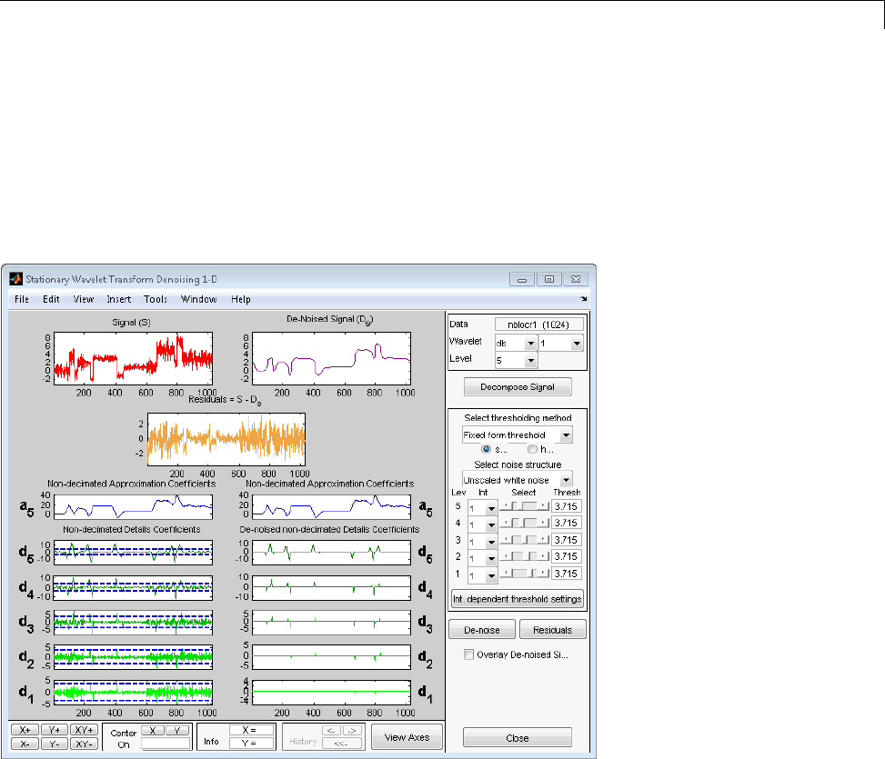
One-Dimensional Adaptive Thresholding of Wavelet Coefficients
Select the db1 wavelet from the Wavelet menu and select 5from the Level
menu, and then click the Decompose Signal button. After a pause for
computation, the tool displays the stationary wavelet approximation and
detail coefficients of the decomposition.
Accept the defaults of Fixed form soft thresholding and Unscaled white
noise.ClicktheDe-noise button.
The result is quite satisfactory, but seems to be oversmoothed when the
signal is irregular.
Select hard for the thresholding mode instead of soft, and then click the
De-noise button.
5-19

5Denoising, Nonparametric Function Estimation, and Compression
The result is not satisfactory. The denoised signal remains noisy before
position 200 and after position 700. This illustrates the limits of the
classical de-noising strategies. In addition, the residuals obtained during
the last trials clearly suggest to try a local thresholding strategy.
4Generate interval-dependent thresholds.
Click the Int. dependent threshold Settings button located at the
bottom of the thresholding method frame. A new window titled Int.
Dependent Threshold Settings for figure ... appears.
5-20
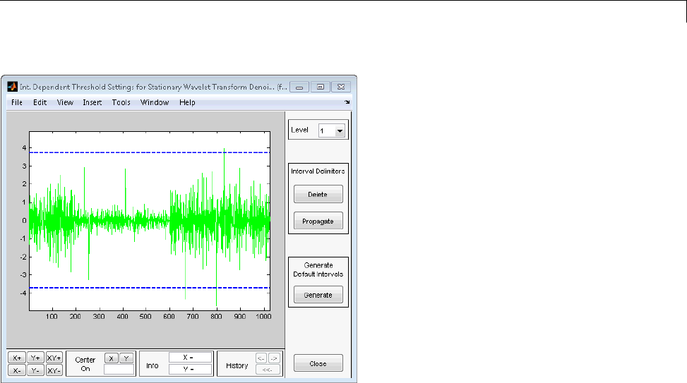
One-Dimensional Adaptive Thresholding of Wavelet Coefficients
Click the Generate button. After a pause for computation, the tool displays
the default intervals associated with adapted thresholds.
5-21
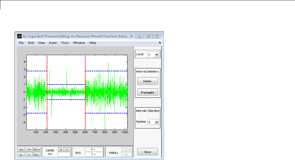
5Denoising, Nonparametric Function Estimation, and Compression
Three intervalsareproposed. Sincethevariances for the three intervals
are very different, the optimization program easily detects the correct
structure. Nevertheless, you can visualize the intervals proposed for a
number of intervals from 1 to 6 using the Select Number of Intervals
menu (which replaces the Generate button). Using the default intervals
automatically propagates the interval delimiters and associated thresholds
to all levels.
Denoise with Interval-Dependent Thresholds. Click the Close button in
the Int. Dependent Threshold Settings for ... window. When the Update
thresholds dialog box appears, click Yes.TheSWT De-noising 1-D main
window is updated. The sliders located to the right of the window control the
level and interval dependent thresholds. For a given interval, the threshold is
indicated by yellow dotted lines running horizontally through the graphs on
the left of the window. The red dotted lines running vertically through the
graphs indicate the interval delimiters. Next click the De-noise button.
5-22
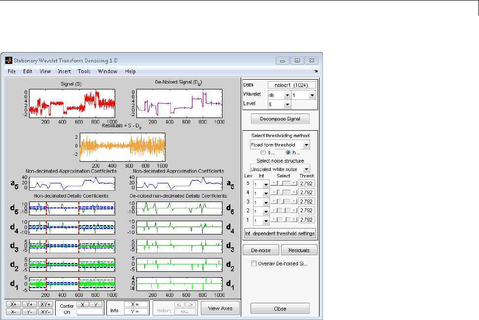
One-Dimensional Adaptive Thresholding of Wavelet Coefficients
Modifying Interval Dependent Thresholds. The thresholds can be
increased to keep only the highest values of the wavelet coefficients at each
level. Do this by dragging the yellow lines directly on the graphs on the left
of the window, or using the View Axes button (located at the bottom of the
screen near the Close button), which allows you to see each axis in full size.
Another way is to edit the thresholds by selecting the interval number located
near the sliders and typing the desired value.
5-23

5Denoising, Nonparametric Function Estimation, and Compression
Note that you can also change the interval limits by holding down the left
mouse button over the vertical dotted red lines, and dragging them.
You can also define your own interval dependent strategy. Click the Int.
dependent threshold settings button. The Int. Dependent Threshold
Settings for ... window appears again. We shall explore this window for a
little while. Click the Delete button, so that the interval delimiters disappear.
Double click the left mouse button to define new interval delimiters; for
example at positions 300 and 500 and adjust the thresholds manually. Each
level must be considered separately using the Level menu for adjusting the
thresholds. The current interval delimiters can be propagated to all levels by
clicking the Propagate button. So click the Propagate button. Adjust the
thresholds for each level, one by one. At the end, click the Close button of
the Int. Dependent Threshold settings for ... window. When the Update
thresholds dialog box appears, click Yes. Then click the denoise button.
Note that
•By double-clicking again on an interval delimiter with the left mouse
button, you delete it.
•You can move the interval delimiters (vertical red dotted lines) and the
threshold levels (horizontal yellow dotted lines) by holding down the left
mouse button over these lines and dragging them.
•The maximum number of interval delimiters at each level is 10.
5-24
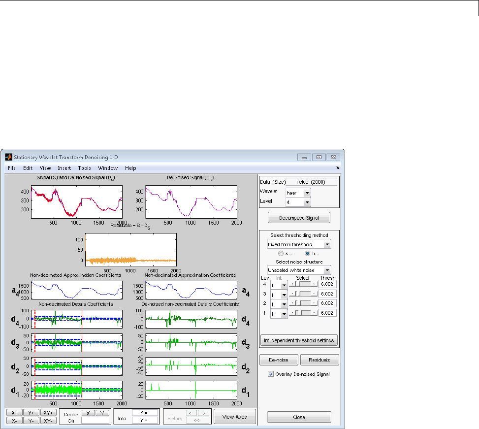
One-Dimensional Adaptive Thresholding of Wavelet Coefficients
Examples of Denoising with Interval Dependent Thresholds.
From the File menu, choose the Example Analysis > Noisy Signals -
Interval Dependent Noise Variance > option. From the drop down men,
choose with haar at level 4 ---> Elec. consumption 3 intervals.
The proposed items contain, in addition to the usual information, the “true”
number of intervals. You can then experiment with various signals for which
local thresholding is needed.
Importing and Exporting Information from the
Graphical Interface
The tool lets you save the denoised signal to disk. The toolbox creates a
MAT-file in the current folder with a name you choose.
5-25

5Denoising, Nonparametric Function Estimation, and Compression
To save the denoised signal from the present de-noising process, use the menu
option File > Save denoised Signal. A dialog box appears that lets you
specify a folder and filename for storing the signal. Type the name dnelec.
After saving the signal data to the file dnelec.mat,loadthevariablesinto
your workspace:
load dnelec
whos
Name Size Bytes Class
dnelec 1x2000 16000 double array
thrParams 1x4 656 cell array
wname 1x4 8 char array
The denoised signal is given by dnelec. In addition, the parameters of the
de-noising process are given by the wavelet name contained in wname:
wname
wname =
haar
and the level dependent thresholds contained in thrParams,whichisa
cell array of length 4 (the level of the decomposition). For ifrom 1 to 4,
thrParams{i} is an array nbintx3 (where nbint is the number of intervals,
here 3), and each row contains the lower and upper bounds of the interval of
thresholding and the threshold value. For example, for level 1,
thrParams{1}
ans =
1.0e+03 *
0.0010 0.0980 0.0060
0.0980 1.1240 0.0204
1.1240 2.0000 0.0049
5-26

Multivariate Wavelet Denoising
Multivariate Wavelet Denoising
This section demonstrates the features of multivariate de-noising provided in
the Wavelet Toolbox software. The toolbox includes the wmulden function and
a graphical user interface (GUI) tool available from wavemenu. This section
also describes the command-line and GUI methods and includes information
about transferring signal and parameter information between the disk and
the GUI.
This multivariate wavelet de-noising problem deals with models of the
form X(t)=F(t)+e(t), where the observation Xis p-dimensional, Fis the
deterministic signal to be recovered, and eis a spatially correlated noise
signal. This kind of model is well suited for situations for which such additive,
spatially correlated noise is realistic.
Multivariate Wavelet Denoising — Command Line
This example uses noisy test signals. In this section, you will
•Load a multivariate signal.
•Display the original and observed signals.
•Remove noise by a simple multivariate thresholding after a change of basis.
•Display the original and denoised signals.
•Improve the obtained result by retaining less principal components.
•Display the number of retained principal components.
•Display the estimated noise covariance matrix.
1Load a multivariate signal by typing the following at the MATLAB prompt:
load ex4mwden
whos
Name Size Bytes Class
covar 4x4 128 double array
x 1024x4 32768 double array
x_orig 1024x4 32768 double array
5-27

5Denoising, Nonparametric Function Estimation, and Compression
Usually, only the matrix of data xis available. Here, we also have the true
noise covariance matrix (covar) and the original signals (x_orig). These
signals are noisy versions of simple combinations of the two original signals.
The first one is “Blocks” which is irregular, and the second is “HeavySine,”
which is regular except around time 750. The other two signals are the
sum and the difference of the two original signals. Multivariate Gaussian
white noise exhibiting strong spatial correlation is added to the resulting
four signals, which leads to the observed data stored in x.
2Display the original and observed signals by typing
kp = 0;
fori=1:4
subplot(4,2,kp+1), plot(x_orig(:,i)); axis tight;
title(['Original signal ',num2str(i)])
subplot(4,2,kp+2), plot(x(:,i)); axis tight;
title(['Observed signal ',num2str(i)])
kp = kp + 2;
end
5-28
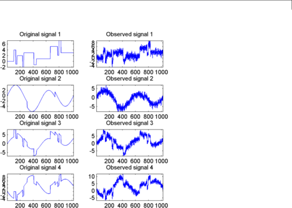
Multivariate Wavelet Denoising
The true noise covariance matrix is given by
covar
covar =
1.0000 0.8000 0.6000 0.7000
0.8000 1.0000 0.5000 0.6000
0.6000 0.5000 1.0000 0.7000
0.7000 0.6000 0.7000 1.0000
3Remove noise by simple multivariate thresholding.
The de-noising strategy combines univariate wavelet de-noising in the basis
where the estimated noise covariance matrix is diagonal with noncentered
5-29

5Denoising, Nonparametric Function Estimation, and Compression
Principal Component Analysis (PCA) on approximations in the wavelet
domain or with final PCA.
First,performunivariatede-noisingbytypingthefollowingtosetthe
de-noising parameters:
level = 5;
wname = 'sym4';
tptr = 'sqtwolog';
sorh = 's';
Then, set the PCA parameters by retaining all the principal components:
npc_app = 4;
npc_fin = 4;
Finally, perform multivariate de-noising by typing
x_den = wmulden(x, level, wname, npc_app, npc_fin, tptr, sorh);
4Display the original and denoised signals by typing
kp = 0;
fori=1:4
subplot(4,3,kp+1), plot(x_orig(:,i));
set(gca,'xtick',[]); axis tight;
title(['Original signal ',num2str(i)])
subplot(4,3,kp+2), plot(x(:,i)); set(gca,'xtick',[]);
axis tight;
title(['Observed signal ',num2str(i)])
subplot(4,3,kp+3), plot(x_den(:,i)); set(gca,'xtick',[]);
axis tight;
title(['denoised signal ',num2str(i)])
kp = kp + 3;
end
5-30
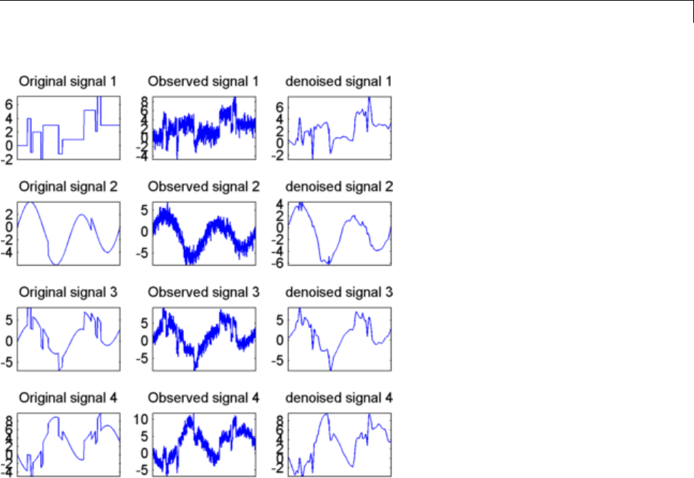
Multivariate Wavelet Denoising
5Improve the first result by retaining fewer principal components.
The results are satisfactory. Focusing on the two first signals, note that
they are correctly recovered, but the result can be improved by taking
advantage of the relationships between the signals, leading to an additional
de-noising effect.
To automatically select the numbers of retained principal components by
Kaiser’s rule (which keeps the components associated with eigenvalues
exceeding the mean of all eigenvalues), type
npc_app = 'kais';
npc_fin = 'kais';
Perform multivariate de-noising again by typing
5-31

5Denoising, Nonparametric Function Estimation, and Compression
[x_den, npc, nestco] = wmulden(x, level, wname, npc_app, ...
npc_fin, tptr, sorh);
6Display the number of retained principal components.
The second output argument gives the numbers of retained principal
components for PCA for approximations and for final PCA.
npc
npc =
22
As expected, since the signals are combinations of two initial ones, Kaiser’s
rule automatically detects that only two principal components are of
interest.
7Display the estimated noise covariance matrix.
The third output argument contains the estimated noise covariance matrix:
nestco
nestco =
1.0784 0.8333 0.6878 0.8141
0.8333 1.0025 0.5275 0.6814
0.6878 0.5275 1.0501 0.7734
0.8141 0.6814 0.7734 1.0967
As you can see by comparing with the true matrix covar given previously,
the estimation is satisfactory.
8Display the original and final denoised signals by typing
kp = 0;
fori=1:4
subplot(4,3,kp+1), plot(x_orig(:,i));
set(gca,'xtick',[]); axis tight;
title(['Original signal ',num2str(i)]); set(gca,'xtick',[]);
axis tight;
subplot(4,3,kp+2), plot(x(:,i)); set(gca,'xtick',[]);
5-32
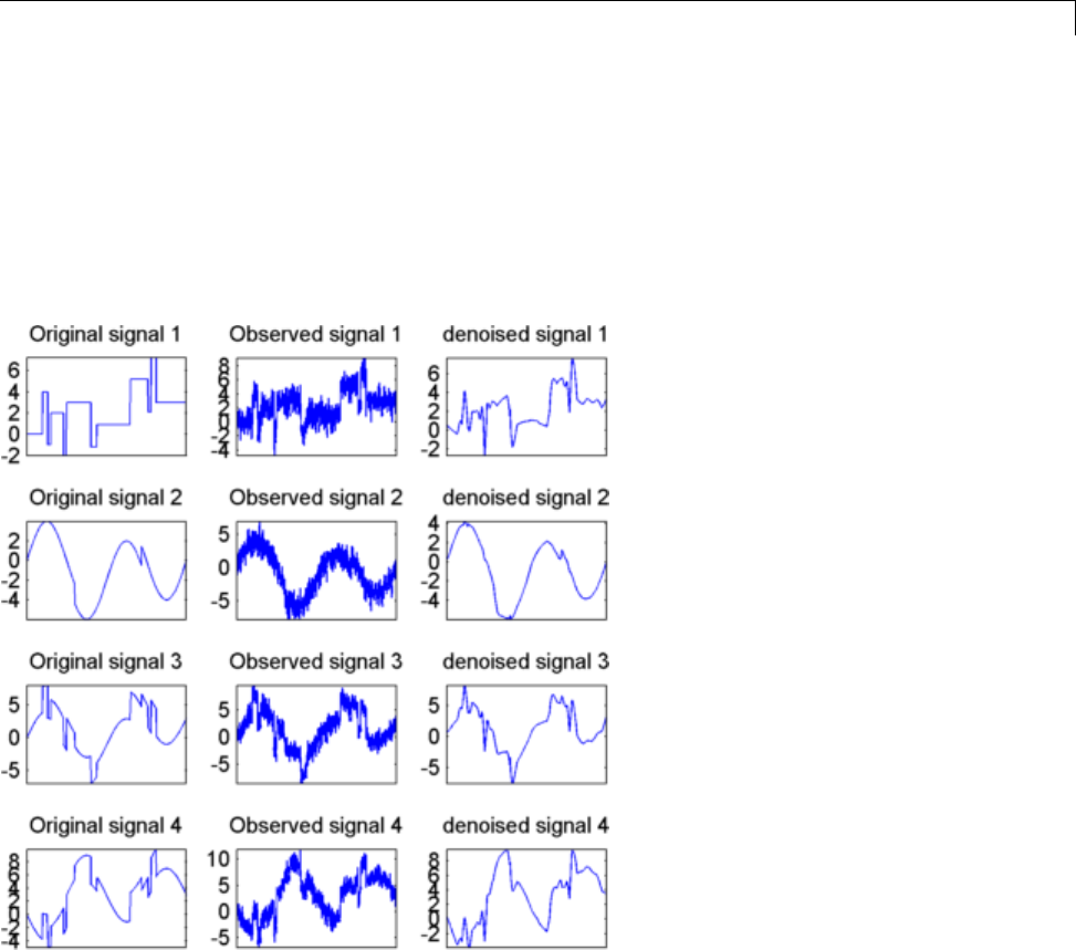
Multivariate Wavelet Denoising
axis tight;
title(['Observed signal ',num2str(i)])
subplot(4,3,kp+3), plot(x_den(:,i)); set(gca,'xtick',[]);
axis tight;
title(['denoised signal ',num2str(i)])
kp = kp + 3;
end
The results are better than those previously obtained. The first signal, which
is irregular, is still correctly recovered, while the second signal, which is more
regular, is denoised better after this second stage of PCA.
5-33
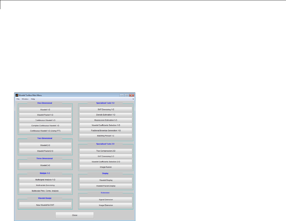
5Denoising, Nonparametric Function Estimation, and Compression
Interactive Multivariate Wavelet Denoising
This section explores a de-noising strategy for multivariate signals using
the graphical interface tools.
1Start the Multivariate De-noising Tool by first opening the Wavelet
Toolbox Main Menu.
wavemenu
2Click Multivariate Denoising to open the Multivariate De-Noising
GUI.
3Load data.
Select File > Load Signals.IntheSelect dialog box, select the MAT-file
ex4mwden.mat from the MATLAB folder toolbox/wavelet/wmultsig1d.
Click Open to load the noisy multivariate signal into the GUI. The signal
is a matrix containing four columns, where each column is a signal to be
denoised.
5-34
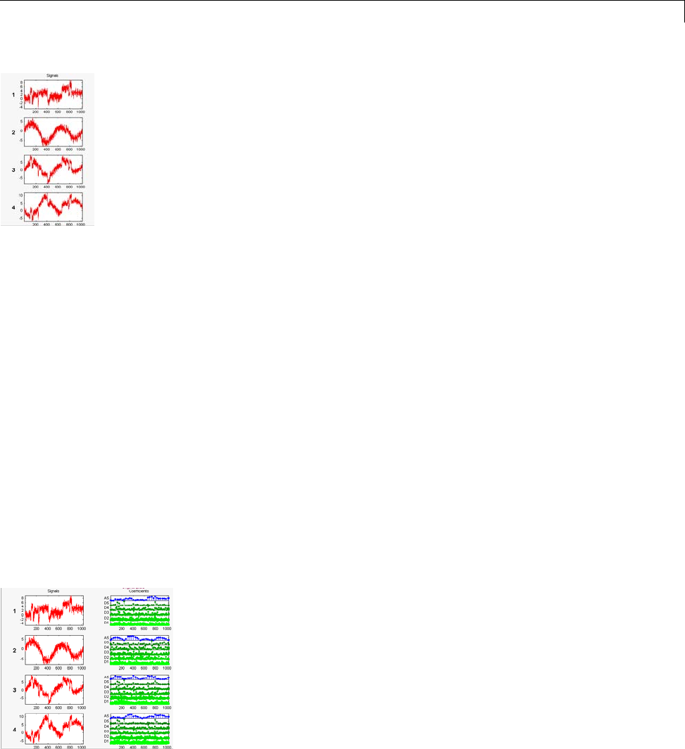
Multivariate Wavelet Denoising
These signals are noisy versions from simple combinations of the two
original signals. The first one is “Blocks” which is irregular and the
second is “HeavySine” which is regular except around time 750. The other
two signals are the sum and the difference between the original signals.
Multivariate Gaussian white noise exhibiting strong spatial correlation is
added to the resulting four signals.
The following example illustrates the two different aspects of the proposed
de-noising method. First, perform a convenient change of basis to cope
with spatial correlation and denoise in the new basis. Then, use PCA to
take advantage of the relationships between the signals, leading to an
additional de-noising effect.
4Perform a wavelet decomposition and diagonalize the noise covariance
matrix.
Use the displayed default values for the Wavelet,theDWT Extension
Mode, and the decomposition Level,andthenclickDecompose and
Diagonalize. The tool displays the wavelet approximation and detail
coefficients of the decomposition of each signal in the original basis.
5-35
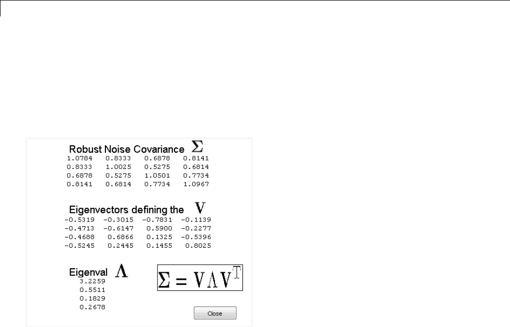
5Denoising, Nonparametric Function Estimation, and Compression
Select Noise Adapted Basis to display the signals and their coefficients
in the noise-adapted basis.
To see more information about this new basis, click More on Noise
Adapted Basis. A new figure displays the robust noise covariance
estimate matrix and the corresponding eigenvectors and eigenvalues.
Eigenvectors define the change of basis, and eigenvalues are the variances
of uncorrelated noises in the new basis.
The multivariate de-noising method proposed below is interesting if the
noise covariance matrix is far from diagonal exhibiting spatial correlation,
which,inthisexample,isthecase.
5denoise the multivariate signal.
A number of options are available for fine-tuning the de-noising algorithm.
However, we will use the defaults: fixed form soft thresholding, scaled
white noise model, and the proposed numbers of retained principal
components. In this case, the default values for PCA lead to retaining
all the components.
Select Original Basis to return to the originalbasisandthenclick
Denoise.
5-36
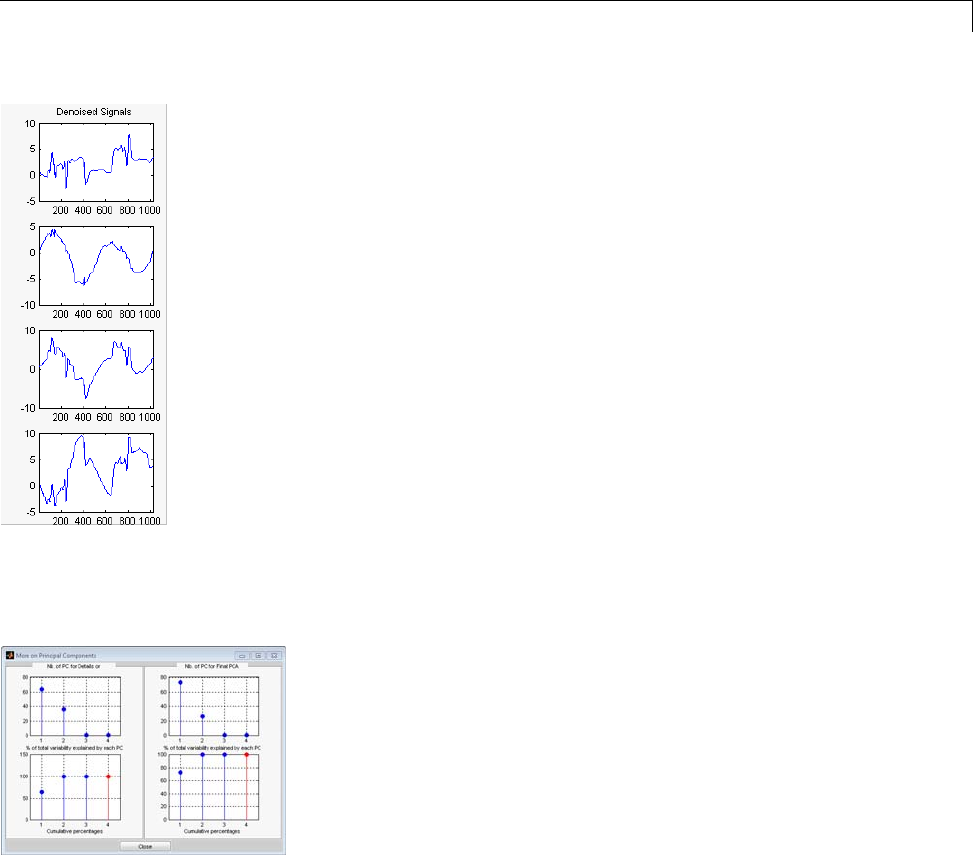
Multivariate Wavelet Denoising
The results are satisfactory. Both of the two first signals are correctly
recovered, but they can be improved by getting more information about the
principal components. Click More on Principal Components.
A new figure displays information to select the numbers of components to
keep for the PCA of approximations and for the final PCA after getting back
to the original basis. You can see the percentages of variability explained by
each principal component and the corresponding cumulative plot. Here, it is
clear that only two principal components are of interest.
5-37
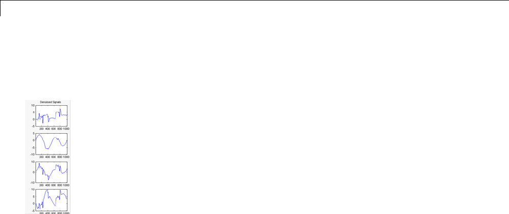
5Denoising, Nonparametric Function Estimation, and Compression
Close the More on Principal Components window. Select 2as the Nb.
of PC for APP. Select 2as the Nb. of PC for final PCA,andthenclick
denoise.
The results are better than those previously obtained. The first signal, which
is irregular, is still correctly recovered. The second signal, which is more
regular, is denoised better after this second stage of PCA. You can get more
information by clicking Residuals.
Importing and Exporting from the GUI
The tool lets you save denoised signals to disk by creating a MAT-file in the
current folder with a name of your choice.
To save the signal denoised in the previous section,
1Select File > Save denoised Signals.
2Select Save denoised Signals and Parameters. A dialog box appears
that lets you specify a folder and filename for storing the signal.
3Type the name s_ex4mwden and click OK to save the data.
4Load the variables into your workspace:
load s_ex4mwdent
whos
5-38

Multivariate Wavelet Denoising
Name Size Bytes Class
DEN_Params 1x1 430 struct array
PCA_Params 1x1 1536 struct array
x 1024x4 32768 struct array
The denoised signals are in matrix x. The parameters (PCA_Params and
DEN_Params) of the two-stage de-noising process are also available.
•PCA_Params are the change of basis and PCA parameters:
PCA_Params
PCA_Params =
NEST: {[4x4 double] [4x1 double] [4x4 double]}
APP: {[4x4 double] [4x1 double] [2]}
FIN: {[4x4 double] [4x1 double] [2]}
PCA_Params.NEST{1} contains the change of basis matrix.
PCA_Params.NEST{2} contains the eigenvalues, and PCA_Params.NEST{3} is
the estimated noise covariance matrix.
PCA_Params.APP{1} contains the change of basis matrix, PCA_Params.APP{2}
contains the eigenvalues, and PCA_Params.APP{3} is the number of retained
principal components for approximations.
The same structure is used for PCA_Params.FIN for the final PCA.
•DEN_Params are the de-noising parameters in the diagonal basis:
DEN_Params
DEN_Params =
thrVAL: [4.8445 2.0024 1.1536 1.3957 0]
thrMETH: 'sqtwolog'
thrTYPE: 's'
5-39

5Denoising, Nonparametric Function Estimation, and Compression
The thresholds are encoded in thrVAL.Forjfrom 1to 5,thrVAL(j) contains
the value used to threshold the detail coefficients at level j. The thresholding
method is given by thrMETH and the thresholding mode is given by thrTYPE.
5-40

Multiscale Principal Components Analysis
Multiscale Principal Components Analysis
This section demonstrates the features of multiscale principal components
analysis provided in the Wavelet Toolbox software. The toolbox includes
the wmspca function and a graphical user interface (GUI) available from
wavemenu. This section describes the command-line and GUI methods, and
information about transferring signal and parameter information between
the disk and the GUI.
The aim of multiscale PCA is to reconstruct, starting from a multivariate
signal and using a simple representation at each resolution level, a simplified
multivariate signal. The multiscale principal components generalizes the
normal PCA of a multivariate signal represented as a matrix by performing
a PCA on the matrices of details of different levels simultaneously. A PCA
is also performed on the coarser approximation coefficients matrix in the
wavelet domain as well as on the final reconstructed matrix. By selecting the
numbers of retained principal components, interesting simplified signals
can be reconstructed.
Since you can perform multiscale PCA either from the command line or using
the GUI, this section has subsections covering each method.
Multiscale Principal Components Analysis —
Command Line
This example uses noisy test signals. In this section, you will:
•Load a multivariate signal.
•Perform a simple multiscale PCA.
•Display the original and simplified signals.
•Improve the obtained result by retaining less principal components.
1Load a multivariate signal by typing at the MATLAB prompt:
load ex4mwden
whos
5-41

5Denoising, Nonparametric Function Estimation, and Compression
Name Size Bytes Class
covar 4x4 128 double array
x 1024x4 32768 double array
x_orig 1024x4 32768 double array
The data stored in matrix xcomes from two test signals, Blocks and
HeavySine,andfromtheirsumanddifference, to which multivariate
Gaussian white noise has been added.
2Perform a simple multiscale PCA.
The multiscale PCA combines noncentered PCA on approximations and
details in the wavelet domain and a final PCA. At each level, the most
significant principal components are selected.
First,setthewaveletparameters:
level= 5;
wname = 'sym4';
Then, automatically select the number of retained principal components
using Kaiser’s rule by typing
npc = 'kais';
Finally, perform multiscale PCA:
[x_sim, qual, npc] = wmspca(x ,level, wname, npc);
3Display the original and simplified signals:
kp = 0;
fori=1:4
subplot(4,2,kp+1), plot(x (:,i)); set(gca,'xtick',[]);
axis tight;
title(['Original signal ',num2str(i)])
subplot(4,2,kp+2), plot(x_sim(:,i)); set(gca,'xtick',[]);
axis tight;
title(['Simplified signal ',num2str(i)])
kp = kp + 2;
5-42

Multiscale Principal Components Analysis
end
The results from a compression perspective are good. The percentages
reflecting the quality of column reconstructions given by the relative mean
square errors are close to 100%.
qual
qual =
98.0545 93.2807 97.1172 98.8603
4Improve the first result by retaining fewer principal components.
The results can be improved by suppressing noise, because the details at
levels 1 to 3 are composed essentially of noise with small contributions from
the signal. Removing the noise leads to a crude, but large, denoising effect.
The output argument npc contains the numbers of retained principal
components selected by Kaiser’s rule:
npc
npc =
1111122
5-43

5Denoising, Nonparametric Function Estimation, and Compression
For dfrom 1 to 5, npc(d) is the number of retained noncentered principal
components (PCs) for details at level d. The number of retained noncentered
PCs for approximations at level 5 is npc(6),andnpc(7) is the number of
retained PCs for final PCA after wavelet reconstruction. As expected, the
rule keeps two principal components, both for the PCA approximations and
the final PCA, but one principal component is kept for details at each level.
Tosuppressthedetailsatlevels1to3,updatethenpc argument as follows:
npc(1:3) = zeros(1,3);
npc
npc =
0001122
Then, perform multiscale PCA again:
[x_sim, qual, npc] = wmspca(x, level, wname, npc);
5Display the original and final simplified signals:
kp = 0;
fori=1:4
subplot(4,2,kp+1), plot(x (:,i)); set(gca,'xtick',[]);
axis tight;
title(['Original signal ',num2str(i)]); set(gca,'xtick',[]);
axis tight;
subplot(4,2,kp+2), plot(x_sim(:,i)); set(gca,'xtick',[]);
axis tight;
title(['Simplified signal ',num2str(i)])
kp = kp + 2;
end
5-44
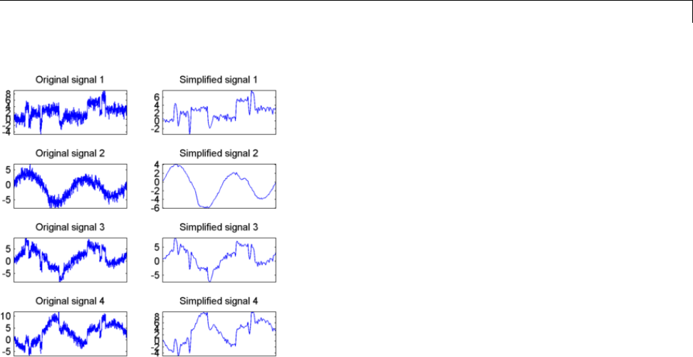
Multiscale Principal Components Analysis
As shown, the results are improved.
Interactive Multiscale Principal Components Analysis
This section explores multiscale PCA using the GUIs.
1Start the Multiscale Princ. Comp. Analysis tool by first opening the
Wavelet Toolbox Main Menu:
wavemenu
5-45
5Denoising, Nonparametric Function Estimation, and Compression
2Click Multiscale Princ. Comp. Analysis to open the Multiscale Principal
Components Analysis GUI.
3Load data.
Select File > Load Signals.IntheSelect dialog box, select the MAT-file
ex4mwden.mat from the MATLAB folder toolbox/wavelet/wmultsig1d.
Click Open to load the multivariate signal into the GUI. The signal is
a matrix containing four columns, where each column is a signal to be
simplified.
5-46
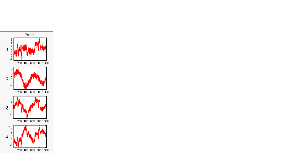
Multiscale Principal Components Analysis
These signals are noisy versions from simple combinations of the two
original signals, Blocks and HeavySine and their sum and difference, each
with added multivariate Gaussian white noise.
4Perform a wavelet decomposition and diagonalize each coefficients matrix.
Use the default values for the Wavelet,theDWT Extension Mode,and
the decomposition Level,andthenclickDecompose and Diagonalize.
The tool displays the wavelet approximation and detail coefficients of the
decomposition of each signal in the original basis.
To get more information about the new bases allowed for performing a PCA
for each scale, click More on Adapted Basis. A new figure displays the
corresponding eigenvectors and eigenvalues for the matrix of the detail
coefficients at level 1.
5-47
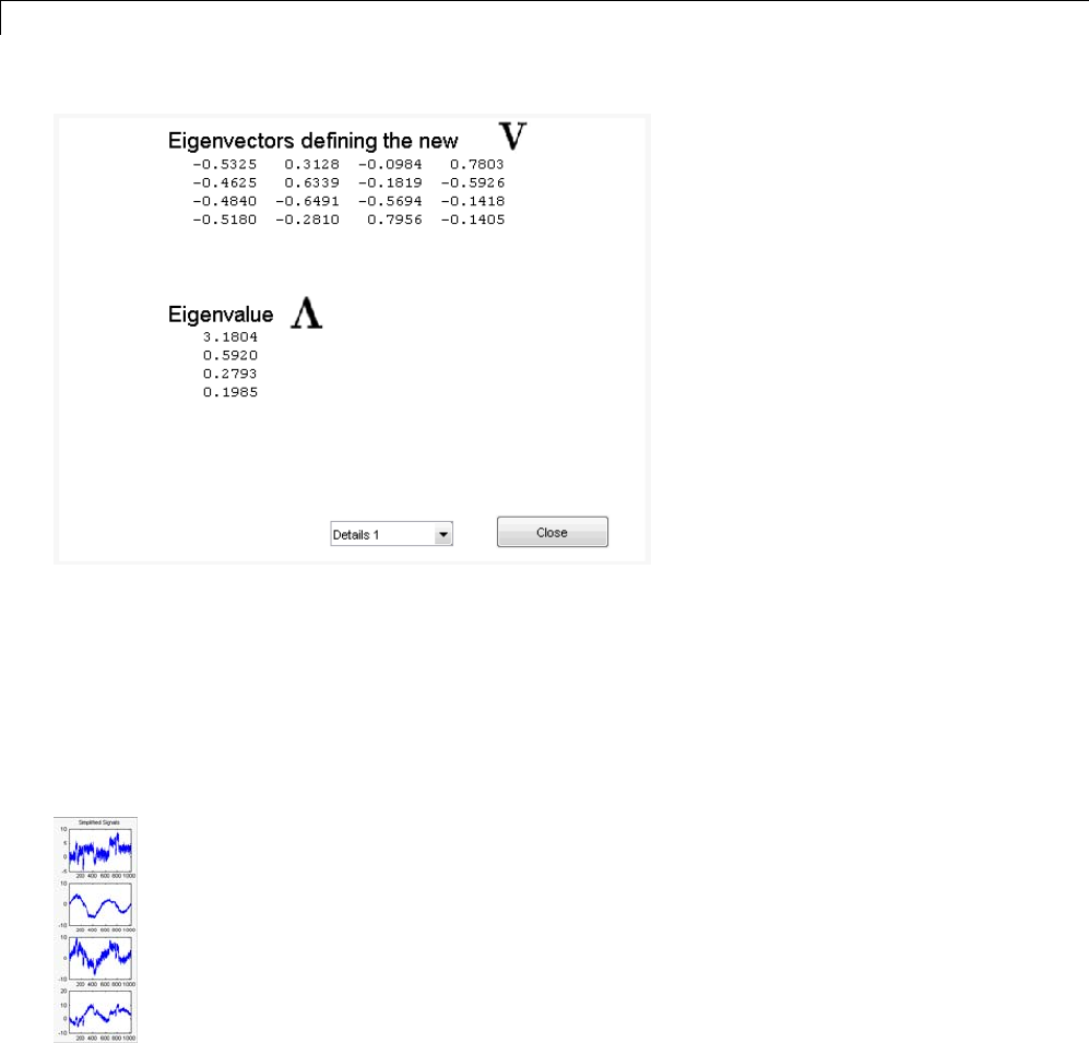
5Denoising, Nonparametric Function Estimation, and Compression
You can change the level or select the coarser approximations or the
reconstructed matrix to investigate the different bases. When you finish,
click Close.
5Perform a simple multiscale PCA.
The initial values for PCA lead to retaining all the components. Select
Kaiser from the Provide default using drop-down list, and click Apply.
Theresultsaregoodfromacompression perspective.
6Improve the obtained result by retaining fewer principal components.
5-48
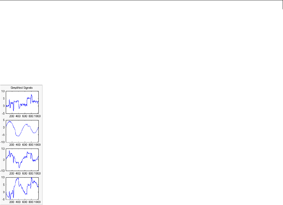
Multiscale Principal Components Analysis
The results can be improved by suppressing the noise, because the details at
levels 1 to 3 are composed essentially of noise with small contributions from
the signal, as you can see by careful inspection of the detail coefficients.
Removing the noise leads to a crude, but large, de-noising effect.
For D1,D2 and D3,select0as the Nb. of non-centered PC and click
Apply.
The results are better than those previously obtained. The first signal,
which is irregular, is still correctly recovered, while the second signal,
which is more regular, is denoised better after this second stage of PCA.
You can get more information by clicking Residuals.
Importing and Exporting from the GUI
TheMultiscalePrincipalComponents Analysis tool lets you save the
simplified signals to disk. The toolbox creates a MAT-file in the current folder
with a name of your choice.
To save the simplified signals from the previous section:
1Select File > Save Simplified Signals.
5-49

5Denoising, Nonparametric Function Estimation, and Compression
2Select Save Simplified Signals and Parameters. A dialog box appears
that lets you specify a folder and file name for storing the signal.
3Type the name s_ex4mwden and click OK to save the data.
4Load the variables into your workspace:
load s_ex4mwden
whos
Name Size Bytes Class
PCA_Params 1x7 2628 struct array
x 1024x4 32768 double array
The simplified signals are in matrix x. The parameters of multiscale PCA
are available in PCA_Params:
PCA_Params
PCA_Params =
1x7 struct array with fields:
pc
variances
npc
PCA_Params is a structure array of length d+2 (here, the maximum
decomposition level d=5) such that PCA_Params(d).pc is the matrix of
principal components. The columns are stored in descending order of the
variances. PCA_Params(d).variances is the principal component variances
vector, and PCA_Params(d).npc is the vector of selected numbers of retained
principal components.
5-50

Data Compression
Data Compression
The compression features of a given wavelet basis are primarily linked to the
relative scarceness of the wavelet domain representation for the signal. The
notion behind compression is based on the concept that the regular signal
component can be accurately approximated using the following elements: a
small number of approximation coefficients (at a suitably chosen level) and
some of the detail coefficients.
Like de-noising, the compression procedure contains three steps:
1Decompose
Choose a wavelet, choose a level N. Compute the wavelet decomposition of
the signal sat level N.
2Threshold detail coefficients
For each level from 1 to N, a threshold is selected and hard thresholding
is applied to the detail coefficients.
3Reconstruct
Compute wavelet reconstruction using the original approximation
coefficients of level Nand the modified detail coefficients of levels from
1toN.
The difference of the de-noising procedure is found in step 2.Therearetwo
compression approaches available. The first consists of taking the wavelet
expansion of the signal and keeping the largest absolute value coefficients.
In this case, you can set a global threshold, a compression performance, or a
relative square norm recovery performance.
Thus, only a single parameter needs to be selected. The second approach
consists of applying visually determined level-dependent thresholds.
Let us examine two real-life examples of compression using global
thresholding, for a given and unoptimized wavelet choice, to produce a nearly
complete square norm recovery for a signal (see Signal Compression on page
5-52)and for an image (see Image Compression on page 5-53).
5-51
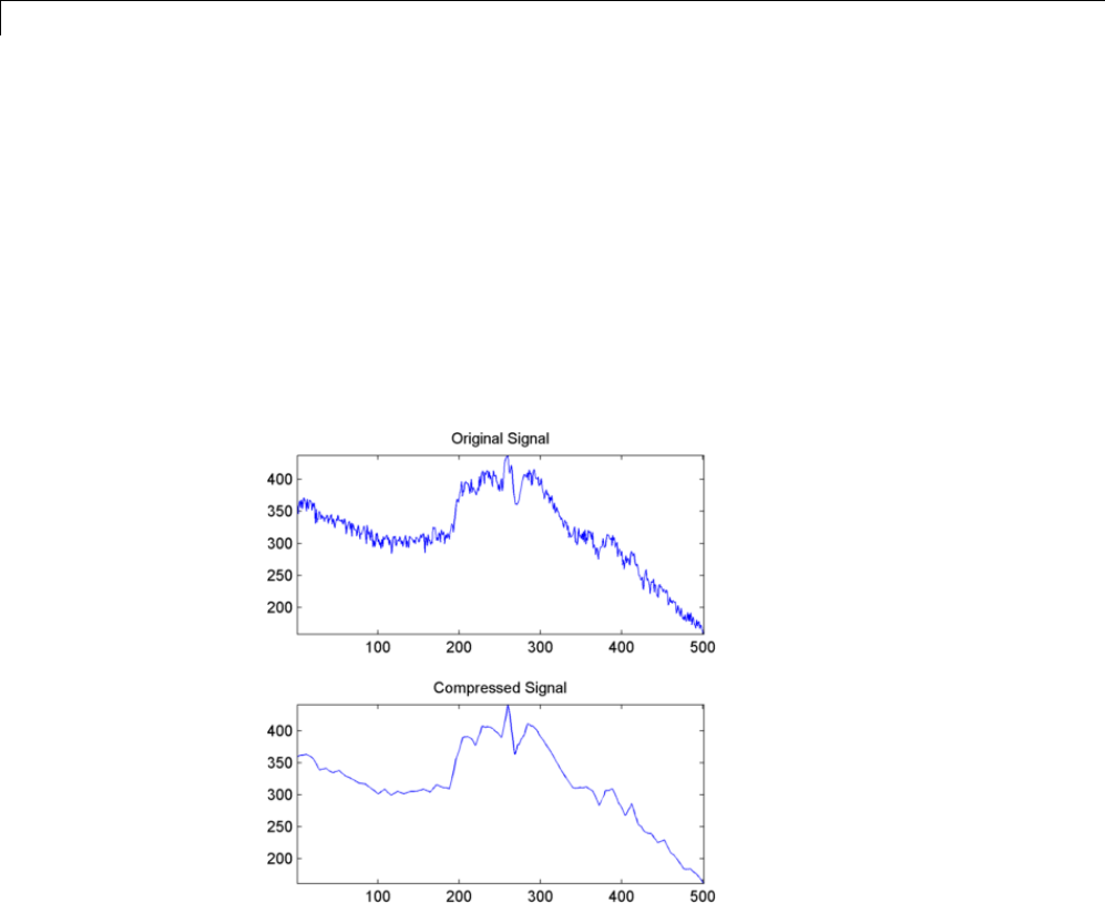
5Denoising, Nonparametric Function Estimation, and Compression
% Load electrical signal and select a part.
load leleccum; indx = 2600:3100;
x = leleccum(indx);
% Perform wavelet decomposition of the signal.
n = 3; w = 'db3';
[c,l] = wavedec(x,n,w);
% Compress using a fixed threshold.
thr = 35;
keepapp = 1;
[xd,cxd,lxd,perf0,perfl2] = ...
wdencmp('gbl',c,l,w,n,thr,'h',keepapp);
Signal Compression
The result is quite satisfactory, not only because of the norm recovery
criterion, but also on a visual perception point of view. The reconstruction
uses only 15% of the coefficients.
% Load original image.
load woman; x = X(100:200,100:200);
nbc = size(map,1);
5-52
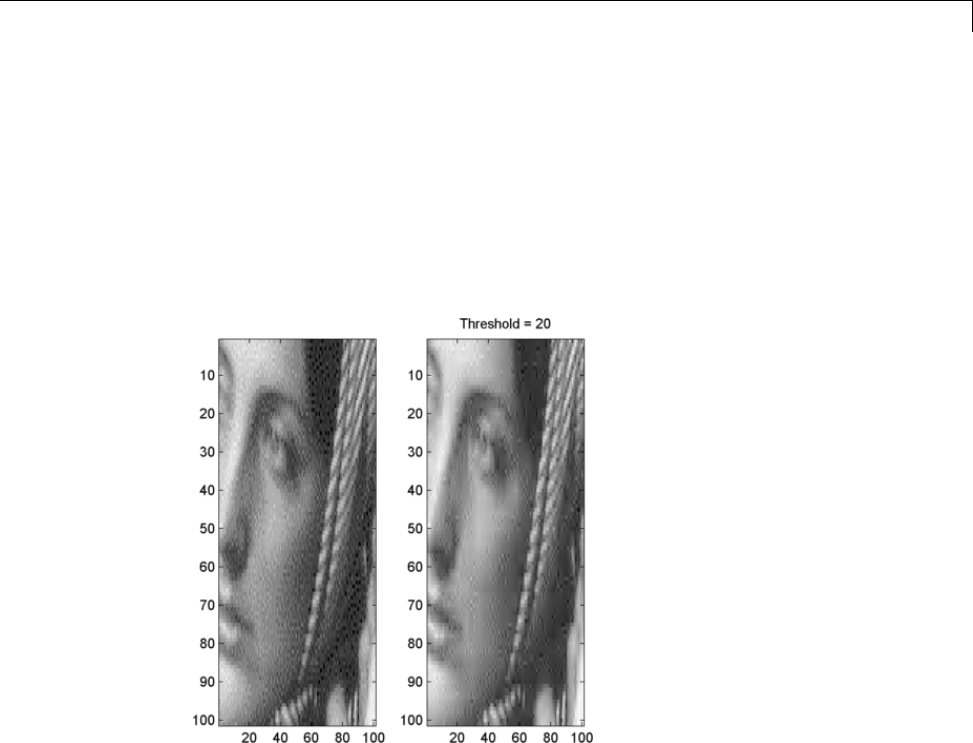
Data Compression
% Wavelet decomposition of x.
n = 5; w = 'sym2'; [c,l] = wavedec2(x,n,w);
% Wavelet coefficients thresholding.
thr = 20;
keepapp = 1;
[xd,cxd,lxd,perf0,perfl2] = ...
wdencmp('gbl',c,l,w,n,thr,'h',keepapp);
Image Compression
If the wavelet representation is too dense, similar strategies can be used in
the wavelet packet framework to obtain a sparser representation. You can
then determine the best decomposition with respect to a suitably selected
entropy-like criterion, which corresponds to the selected purpose (de-noising
or compression).
Compression Scores
When compressing using orthogonal wavelets, the Retained energy in
percentage is defined by
5-53

5Denoising, Nonparametric Function Estimation, and Compression
100 2 2
*,)vector-norm(coeffs of the current decomposition
v
()
eector-norm original signal(,)22
()
When compressing using biorthogonal wavelets, the previous definition is not
convenient. We use instead the Energy ratio in percentage defined by
100 2 2
*,)
(
vector-norm(compressed signal
vector-norm origina
()
ll signal, )22
()
and as a tuning parameter the Norm cfs recovery defined by
100 2 2
*,)vector-norm(coeffs of the current decomposition
v
()
eector-norm coeffs of the original decomposition(,)22
()
The Number of zeros in percentage is defined by
100 * (number of zeros of the current decomposition)
(number oof coefficients)
5-54
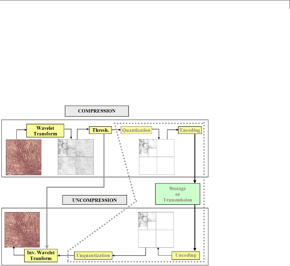
True Compression for Images
True Compression for Images
In “Data Compression” on page 5-51, we addressed the aspects specifically
related to compression using wavelets. However, in addition to the algorithms
related to wavelets like DWT and IDWT, it is necessary to use other
ingredients concerning the quantization mode and the coding type in order to
deal with true compression.
This more complex process can be represented by the following figure.
Effects of Quantization
Let us show the effects of quantization on the visualization of the fingerprint
image. This indexed image corresponds to a matrix of integers ranging
between 0 and 255. Through quantization we can decrease the number of
colors which is here equal to 256.
5-55
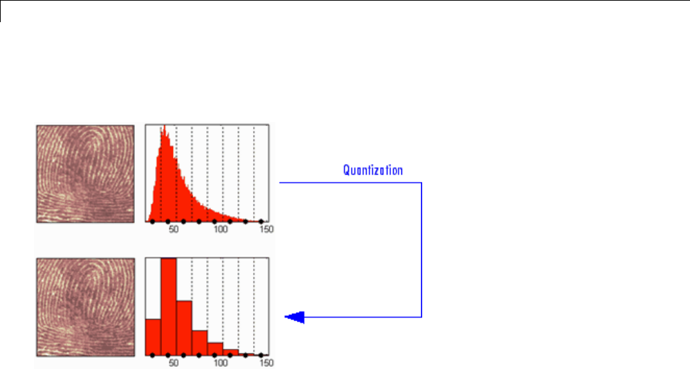
5Denoising, Nonparametric Function Estimation, and Compression
The next figure illustrates how to decrease from 256 to 16 colors by working
on the values of the original image.
We can see on this figure:
•At the top
-On the left: the original image
-On the right: the corresponding histogram of values
•At the bottom
-On the left: the reconstructed image
-On the right: the corresponding histogram of quantized values
This quantization leads to a compression of the image. Indeed, with a
fixed length binary code, 8 bits per pixel are needed to code 256 colors
and 4 bits per pixel to code 16 colors. We notice that the image obtained
after quantization is of good quality. However, within the framework of
true compression, quantization is not used on the original image, but on its
wavelet decomposition.
Let us decompose the fingerprint image at level 4 with the Haar wavelet. The
histogram of wavelet coefficients and the quantized histogram are normalized
5-56

True Compression for Images
so that the values vary between –1 and +1. The 15 intervals of quantization
do not have the same length.
The next figure illustrates how to decrease information by binning on the
wavelet coefficient values of the original image.
We can see on this figure:
•At the top
-On left: the original image
-On the right: the corresponding histogram (central part) of coefficient
values
•At the bottom
-On the left: the reconstructed image
-On the right: the corresponding histogram (central part) of quantized
coefficient values
The key point is that the histogram of the quantized coefficients is massively
concentrated in the class centered in 0. Let us note that yet again the image
obtained is of good quality.
5-57

5Denoising, Nonparametric Function Estimation, and Compression
True Compression Methods
The basic ideas presented above are used by three methods which cascade
in a single step, coefficient thresholding (global or by level), and encoding
by quantization. Fixed or Huffman coding can be used for the quantization
depending on themethod.
The following table summarizes these methods, often called Coefficients
Thresholding Methods (CTM), and gives the MATLAB name used by the true
compression tools for each of them.
MATLAB Name Compression Method Name
'gbl_mmc_f' Global thresholding of coefficients and fixed
encoding
'gbl_mmc_h' Global thresholding of coefficients and Huffman
encoding
'lvl_mmc' Subband thresholding of coefficients and Huffman
encoding
More sophisticated methods are available which combine wavelet
decomposition and quantization. This is the basic principle of progressive
methods.
On one hand, progressivity makes it possible during decoding to obtain an
image whose resolution increases gradually. In addition, it is possible to
obtain a set of compression ratios based on the length of the preserved code.
This compression usually involves a loss of information, but this kind of
algorithm enables also lossless compression.
Such methods are based on three ideas. The two first, already mentioned, are
the use of wavelet decomposition to ensure sparsity (a large number of zero
coefficients) and classical encoding methods. The third idea, decisive for the
use of wavelets in image compression, is to exploit fundamentally the tree
structure of the wavelet decomposition. Certain codes developed from 1993
to 2000 use this idea, in particular, the EZW coding algorithm introduced by
Shapiro. See [Sha93] in “References”.
EZW combines stepwise thresholding and progressive quantization, focusing
on themoreefficientwaytoencodetheimagecoefficients,inordertominimize
5-58

True Compression for Images
the compression ratio. Two variants SPIHT and STW (see the following table)
are refined versions of the seminal EZW algorithm.
Following a slightly different objective, WDR (and the refinement ASWDR)
focuses on the fact that in general some portions of a given image require
more refined coding leading to a better perceptual result even if there is
generally a small price to pay in terms of compression ratio.
A complete review of these progressive methods is in the Walker reference
[Wal99] in “References”.
The following table summarizes these methods, often called Progressive
Coefficients Significance Methods (PCSM), and gives the MATLAB coded
name used by the true compression tools for each of them.
MATLAB Name Compression Method Name
'ezw' Embedded Zerotree Wavelet
'spiht' Set Partitioning In Hierarchical Trees
'stw' Spatial-orientation Tree Wavelet
'wdr' Wavelet Difference Reduction
'aswdr' Adaptively Scanned Wavelet Difference Reduction
'spiht_3d' Set Partitioning In Hierarchical Trees 3D for
truecolor images
Quantitative and Perceptual Quality Measures
Let us close this section by defining two quantitative measures of the
compression performance as well as two measures of the perceptual quality.
Compression Performance
Two quantitative measures giving equivalent information are commonly used
as a performance indicator for the compression:
•The compression ratio CR, which means that the compressed image is
stored using only CR% of the initial storage size.
5-59

5Denoising, Nonparametric Function Estimation, and Compression
•The Bit-Per-Pixel ratio BPP, which gives the number of bits required to
store one pixel of the image.
Perceptual Quality
Two measures are commonly used to evaluate the perceptual quality:
•TheMeanSquareError(MSE). It represents the mean squared error
between the compressed and the original image and is given by:
MSE mn Xij X ij
c
j
n
i
m
=−
=
=
=
=∑∑
12
0
1
0
1
(, ) (, )
The lower the value of MSE, the lower the error.
•The Peak Signal to Noise Ratio (PSNR). It represents a measure of the
peak error and is expressed in decibels. It is defined by:
PSNR MSE
=⋅ ⎛
⎝
⎜⎞
⎠
⎟
10 255
10
2
log
The higher the PSNR, the better the quality of the compressed or
reconstructed image. Typical values for lossy compression of an image are
between 30 and 50 dB and when the PSNR is greater than 40 dB, then the
two images are indistinguishable.
More Information on True Compression
You can find examples illustrating command-line mode and GUI tools for true
compression in “True Compression for Images” on page 5-55 and the reference
page for wcompress.
More information on the true compression for images and more precisely
on the compression methods is in [Wal99], [Sha93], [Sai96], [StrN96], and
[Chr06]. See “References”..
5-60

Two-Dimensional True Compression
Two-Dimensional True Compression
This section takes you through the features of two-dimensional true
compression using the Wavelet Toolbox software.
For more information on the compression methods see “True Compression for
Images”onpage5-55intheWavelet Toolbox User’s Guide.
For more information on the main function available when using
command-line mode, see the wcompress reference pages.
Starting from a given image, the goal of the true compression is to minimize
the length of the sequence of bits needed to represent it, while preserving
information of acceptable quality. Wavelets contribute to effective solutions
for this problem.
Thecompletechainofcompressionincludes phases of quantization, coding
and decoding in addition of the wavelet processing itself.
The purpose of this section is to show how to compress and uncompress a
grayscale or truecolor image using various compression methods.
In this section, you’ll learn to
•Compress using global thresholding and Huffman encoding
•Uncompress
•Compress using progressive methods
•Handle truecolor images
Two-Dimensional True Compression — Command Line
Compression by Global Thresholding and Huffman Encoding
First load and display the grayscale image mask.
load mask;
image(X)
axis square;
5-61
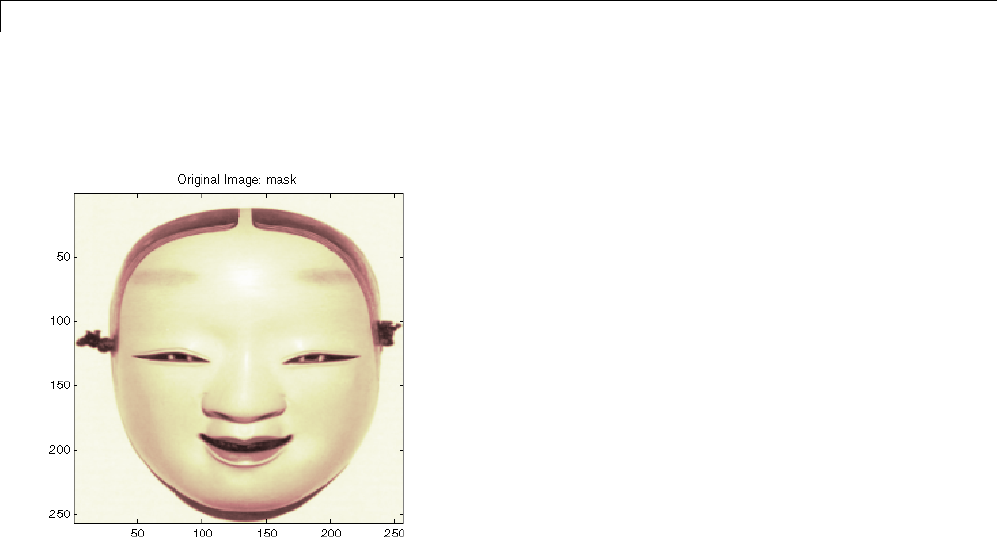
5Denoising, Nonparametric Function Estimation, and Compression
colormap(pink(255))
title('Original Image: mask')
A synthetic performance of the compression is given by the compression ratio
and the Bit-Per-Pixel ratio which are equivalent.
The compression ratio CR means that the compressed image is stored using
only CR% of the initial storage size.
The Bit-Per-Pixel ratio BPP gives the number of bits used to store one pixel
of the image.
For a grayscale image, the initial BPP is 8 while for a truecolor image the
initial BPP is 24 because 8 bits are used to encode each of the three colors
(RGB color space).
The challenge of compression methods is to find the best compromise between
a weak compression ratio and a good perceptual result.
Let us begin with a simple method cascading global coefficients thresholding
and Huffman encoding. We use the default wavelet bior4.4 and the default
level which is the maximum possible level (see the wmaxlev function) divided
by 2.
5-62

Two-Dimensional True Compression
The desired Bit-Per-Pixel ratio BPP is set to 0.5 and the compressed image
will be stored in the file named 'mask.wtc'.
meth = 'gbl_mmc_h'; % Method name
option = 'c'; % 'c' stands for compression
[CR,BPP] = wcompress(option,X,'mask.wtc',meth,'bpp',0.5)
CR =
6.6925
BPP =
0.5354
The achieved Bit-Per-Pixel ratio is actually about 0.53 (closed to the desired
one) for a compression ratio of 6.7%.
Uncompression
Let us uncompress the image retrieved from the file 'mask.wtc' and compare
it to the original image.
option = 'u'; % 'u' stands for uncompression
Xc = wcompress(option,'mask.wtc');
colormap(pink(255))
subplot(1,2,1); image(X);
axis square;
title('Original Image')
subplot(1,2,2); image(Xc);
axis square;
title('Compressed Image')
xlabel({['Compression Ratio: ' num2str(CR,'%1.2f %%')], ...
['BPP: ' num2str(BPP,'%3.2f')]})
5-63
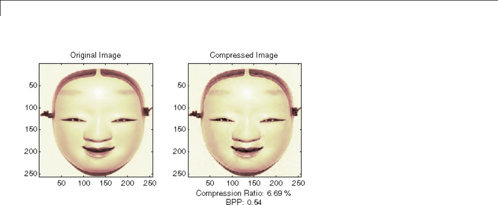
5Denoising, Nonparametric Function Estimation, and Compression
Compression by Progressive Methods
Let us now illustrate the use of progressive methods starting with the well
known EZW algorithm using the Haar wavelet. The key parameter is the
number of loops. Increasing it, leads to better recovery but worse compression
ratio.
meth = 'ezw'; % Method name
wname = 'haar'; % Wavelet name
nbloop = 6; % Number of loops
[CR,BPP] = wcompress('c',X,'mask.wtc',meth, ...
'maxloop',nbloop,'wname',wname);
Xc = wcompress('u','mask.wtc');
colormap(pink(255))
subplot(1,2,1); image(X);
axis square;
title('Original Image')
subplot(1,2,2); image(Xc);
axis square; title('Compressed Image - 6 steps')
xlabel({['Compression Ratio: ' num2str(CR,'%1.2f %%')], ...
['BPP: ' num2str(BPP,'%3.2f')]})
5-64
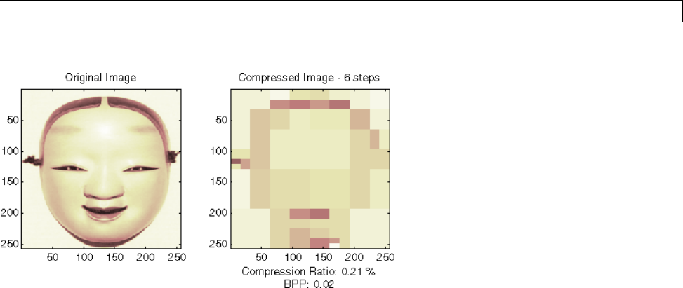
Two-Dimensional True Compression
A too small number of steps (here 6) produces a very coarse compressed
image. So let us examine a little better result for 9 steps and a satisfactory
result for 12 steps.
[CR,BPP]= wcompress('c',X,'mask.wtc',meth,'maxloop',9, ...
'wname','haar');
Xc = wcompress('u','mask.wtc');
colormap(pink(255))
subplot(1,2,1); image(Xc);
axis square; title('Compressed Image - 9 steps')
xlabel({['Compression Ratio: ' num2str(CR,'%1.2f %%')],...
['BPP: ' num2str(BPP,'%3.2f')]})
[CR,BPP] = wcompress('c',X,'mask.wtc',meth,'maxloop',12, ...
'wname','haar');
Xc = wcompress('u','mask.wtc');
subplot(1,2,2); image(Xc);
axis square;
title('Compressed Image - 12 steps')
xlabel({['Compression Ratio: ' num2str(CR,'%1.2f %%')],...
['BPP: ' num2str(BPP,'%3.2f')]})
5-65
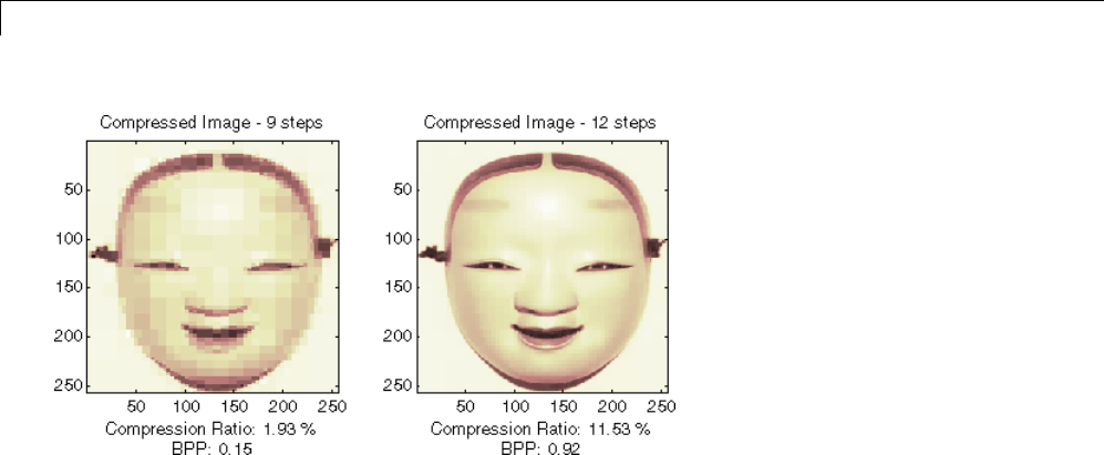
5Denoising, Nonparametric Function Estimation, and Compression
As can be seen, the reached BPP ratio is about 0.92 when using 12 steps.
Letustrytoimproveitbyusingthewaveletbior4.4 instead of haar and
looking at obtained results for steps 12 and 11.
[CR,BPP] = wcompress('c',X,'mask.wtc','ezw','maxloop',12, ...
'wname','bior4.4');
Xc = wcompress('u','mask.wtc');
colormap(pink(255))
subplot(1,2,1); image(Xc);
axis square;
title('Compressed Image - 12 steps - bior4.4')
xlabel({['Compression Ratio: ' num2str(CR,'%1.2f %%')], ...
['BPP: ' num2str(BPP,'%3.2f')]})
[CR,BPP] = wcompress('c',X,'mask.wtc','ezw','maxloop',11, ...
'wname','bior4.4');
Xc = wcompress('u','mask.wtc');
subplot(1,2,2); image(Xc);
axis square;
title('Compressed Image - 11 steps - bior4.4')
xlabel({['Compression Ratio: ' num2str(CR,'%1.2f %%')], ...
['BPP: ' num2str(BPP,'%3.2f')]})
5-66
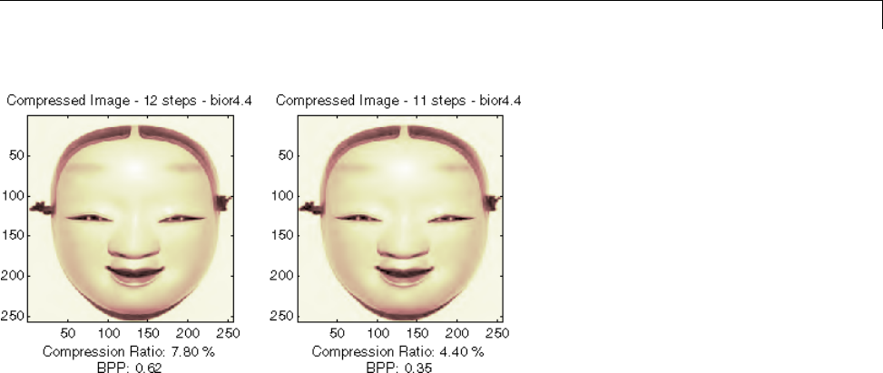
Two-Dimensional True Compression
Starting from the eleventh loop, the result can be considered satisfactory. The
reached BPP ratio is now about 0.35. It can even be slightly improved by
using a more recent method: SPIHT (Set Partitioning In Hierarchical Trees).
[CR,BPP] = wcompress('c',X,'mask.wtc','spiht','maxloop',12, ...
'wname','bior4.4');
Xc = wcompress('u','mask.wtc');
colormap(pink(255))
subplot(1,2,1); image(X);
axis square;
title('Original Image')
subplot(1,2,2); image(Xc);
axis square;
title('Compressed Image - 12 steps - bior4.4')
xlabel({['Compression Ratio: ' num2str(CR,'%1.2f %%')], ...
['BPP: ' num2str(BPP,'%3.2f')]})
[psnr,mse] = psnr_mse_maxerr(X,Xc)
delete('mask.wtc')
5-67
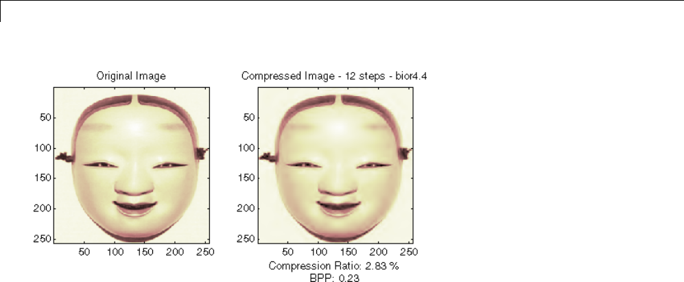
5Denoising, Nonparametric Function Estimation, and Compression
The final compression ratio (2.8%) and the Bit-Per-Pixel ratio (0.23) are very
satisfactory. Let us recall that the first ratio means that the compressed
image is stored using only 2.8% of the initial storage size.
Handling Truecolor Images
Finally, let us illustrate how to compress the wpeppers.jpg truecolor image.
Truecolor images can be compressed along the same scheme as the grayscale
images by applying the same strategies to each of the three color components.
The progressive compression method used is SPIHT (Set Partitioning In
Hierarchical Trees) and the number of encoding loops is set to 12.
X = imread('wpeppers.jpg');
[CR,BPP] = wcompress('c',X,'wpeppers.wtc','spiht','maxloop',12);
Xc = wcompress('u','wpeppers.wtc');
subplot(1,2,1); image(X);
axis square;
title('Original Image')
subplot(1,2,2); image(Xc);
axis square;
title('Compressed Image - 12 steps - bior4.4')
xlabel({['Compression Ratio: ' num2str(CR,'%1.2f %%')], ...
['BPP: ' num2str(BPP,'%3.2f')]})
delete('wpeppers.wtc')
5-68
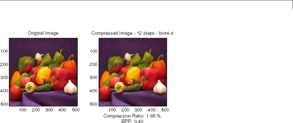
Two-Dimensional True Compression
The compression ratio (1.65%) and the Bit-Per-Pixel ratio (0.4) are very
satisfactory while maintaining a good visual perception.
Interactive Two-Dimensional True Compression
In this section, we explore the different methods for two-dimensional true
compression, using the graphical interface tools.
1Start the True Compression 2-D Tool.
From the MATLAB prompt, type
wavemenu
The Wavelet Toolbox Main Menu appears. Click the True
Compression 2-D menu item. The true compression tool for images
appears.
2Load the image.
From the File menu, choose the Load Image option and select the Matlab
Supported Formats item.
When the Load Image dialog box appears, select the MAT-file mask.mat,
which should reside in the MATLAB folder toolbox/wavelet/wavedemo.
5-69
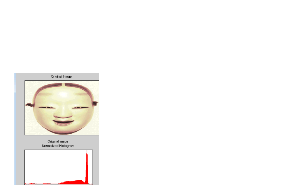
5Denoising, Nonparametric Function Estimation, and Compression
Click the OK button. A window appears asking you if you want to consider
the loaded image as a truecolor one. Click the No button since it is a
grayscaleimage. ThemaskimageisloadedintotheTrue Compression
2-D tool. It appears at the top left of the window together with the gray
level histogram just below.
3Perform a Wavelet Decomposition.
Accept the default wavelet bior4.4 and select 4from the Level menu
which is the maximum possible level divided by 2 and then click the
Decompose button. After a pause for computation, the tool displays the
wavelet approximation and details coefficients of the decomposition for the
three directions, together with the histogram of the original coefficients.
5-70
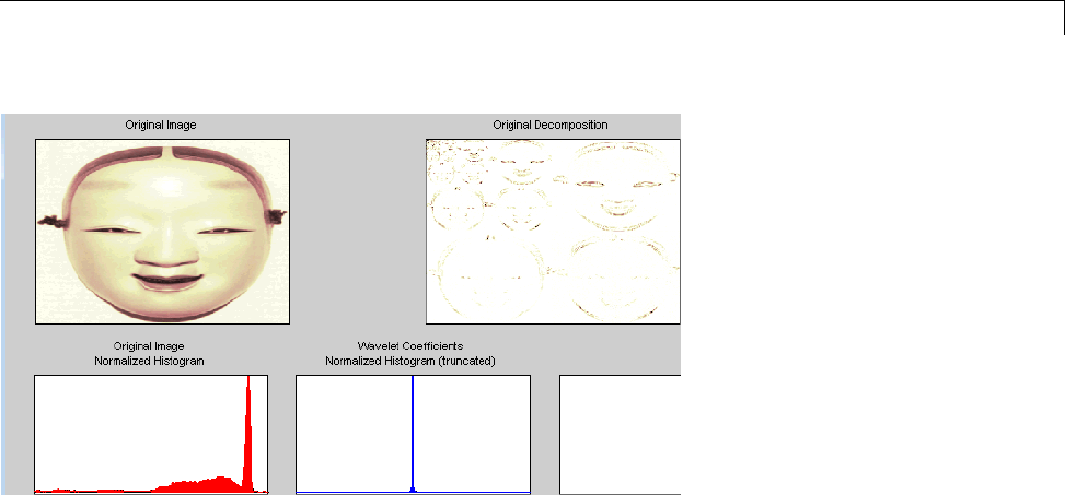
Two-Dimensional True Compression
The peak of the bin containing zero illustrates the capability of wavelets to
concentrate the image energy into a few nonzero coefficients.
4Try a simple method.
Begin with a simple method cascading global coefficients thresholding
and Huffman encoding.
Choose the GBL_MMC_H option from the menu Compression method
located at the top right of the Compression Parameters frame. For
more information on the compression methods, see “True Compression for
Images” on page 5-55 in the Wavelet Toolbox User’s Guide.
Set the desired Bit-Per-Pixel ratio to 0.5.
5-71
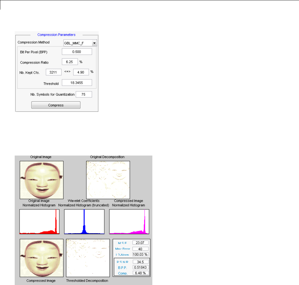
5Denoising, Nonparametric Function Estimation, and Compression
Values of the other parameters are automatically updated. Note that
these values are only approximations of the true performances since the
quantization step cannot be exactly predicted without performing it. Click
the Compress button.
Synthetic performance is given by the compression ratio and the computed
Bit-Per-Pixel (BPP). This last one is actually about 0.53 (close to the
desired one 0.5) for a compression ratio of 6.7%.
5-72
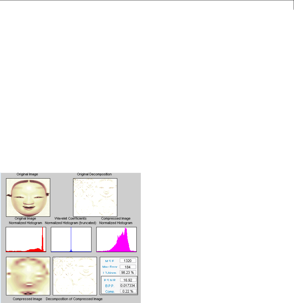
Two-Dimensional True Compression
The compressed image, at the bottom left, can be compared with the
original image.
The result is satisfactory but a better compromise between compression
ratio and visual quality can be obtained using more sophisticated true
compression which combines the thresholding and quantization steps.
5Compress using a first progressive method: EZW.
Let us now illustrate the use of progressive methods starting with the
well known EZW algorithm. Let us start by selecting the wavelet haar
from the Wavelet menu and select 8from the Level menu. Then click the
Decompose button.
Choose the EZW option from the menu Compression method.Thekey
parameter is the number of loops: increasing it leads to a better recovery
but worse compression ratio. From the Nb. Encoding Loops menu,
set the number of encoding loops to 6, which is a small value. Click the
Compress button.
6Refine the result by increasing the number of loops.
5-73
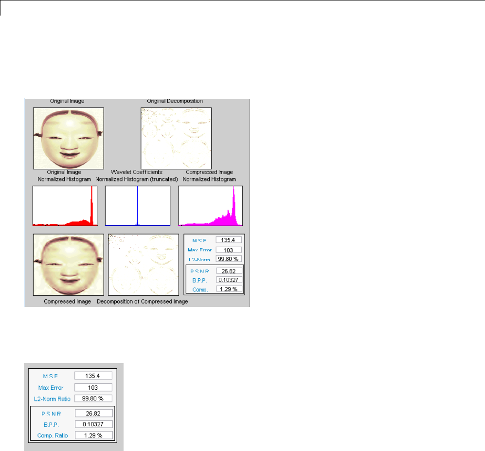
5Denoising, Nonparametric Function Estimation, and Compression
Too few steps produce a very coarse compressed image. So let us examine a
little better result for 9steps. Set the number of encoding loops to 9 and
click the Compress button.
As can be seen, the result is better but not satisfactory, both by visual
inspection and by calculating the PeakSignaltoNoiseRatio(PSNR)which
is less than 30.
Now try a large enough number of steps to get a satisfactory result. Set the
number of encoding loops to 12 and click the Compress button.
5-74
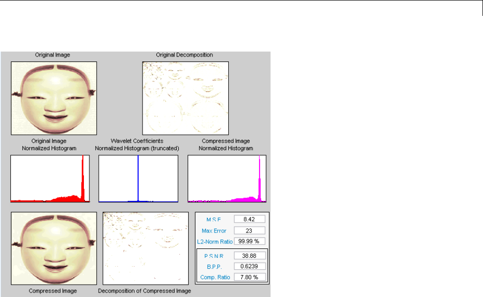
Two-Dimensional True Compression
The result is now acceptable. But for 12 steps, we attain a Bit-Per-Pixel
ratio about 0.92.
7Get better compression performance by changing the wavelet and selecting
the best adapted number of loops.
Let us try to improve the compression performance by changing the
wavelet: select bior4.4 instead of haar and then click the Decompose
button.
In order to select the number of loops, the GUI tool allows you to examine
the successive results obtained by this kind of stepwise procedure. Set
the number of encoding loops at a large value, for example 13,andclick
the Show Compression Steps button. Moreover you could execute the
procedure stepwise by clicking the Stepwise button.
5-75
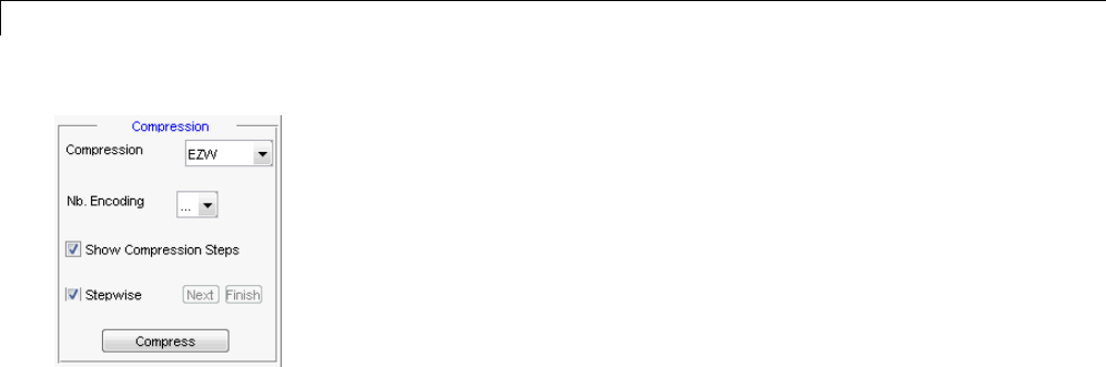
5Denoising, Nonparametric Function Estimation, and Compression
Then, click the Compress button. Thirteen progressively more finely
compressed images appear, and you can then select visually a convenient
value for the number of loops. A satisfactory result seems to be obtained
after 11 loops. So, you can set the number of encoding loops to 11 and
click the Compress button.
The reached BPP ratio is now about 0.35 which is commonly considered a
very satisfactory result. Nevertheless, it can be slightly improved by using
a more recent method SPIHT (Set Partitioning In Hierarchical Trees).
8Obtain a final compressed image by using a third method.
Choose the SPIHT option from the menu Compression method,setthe
number of encoding loops to 12, and click the Compress button.
5-76
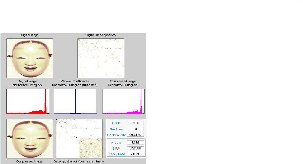
Two-Dimensional True Compression
The final compression ratio and the Bit-Per-Pixel ratio are very satisfactory:
2.8% and 0.22. Let us recall that the first ratio means that the compressed
image is stored using only 2.8% of the initial storage size.
9Handle truecolor images.
Finally, let us illustrate how to compress truecolor images. The truecolor
imagescanbecompressedalongthesameschemebyapplyingthesame
strategies to each of the three-color components.
From
the File menu, choose the Load Image option and select the Matlab
Supported Formats item.
When the Load Image dialog box appears, select the MAT-file
wpeppers.jpg which should reside in the MATLAB folder
toolbox/wavelet/wavedemo.
Click the OK button. A window appears asking you if you want to consider
the loaded image as a truecolor one. Click the Yes button. Accept the
5-77
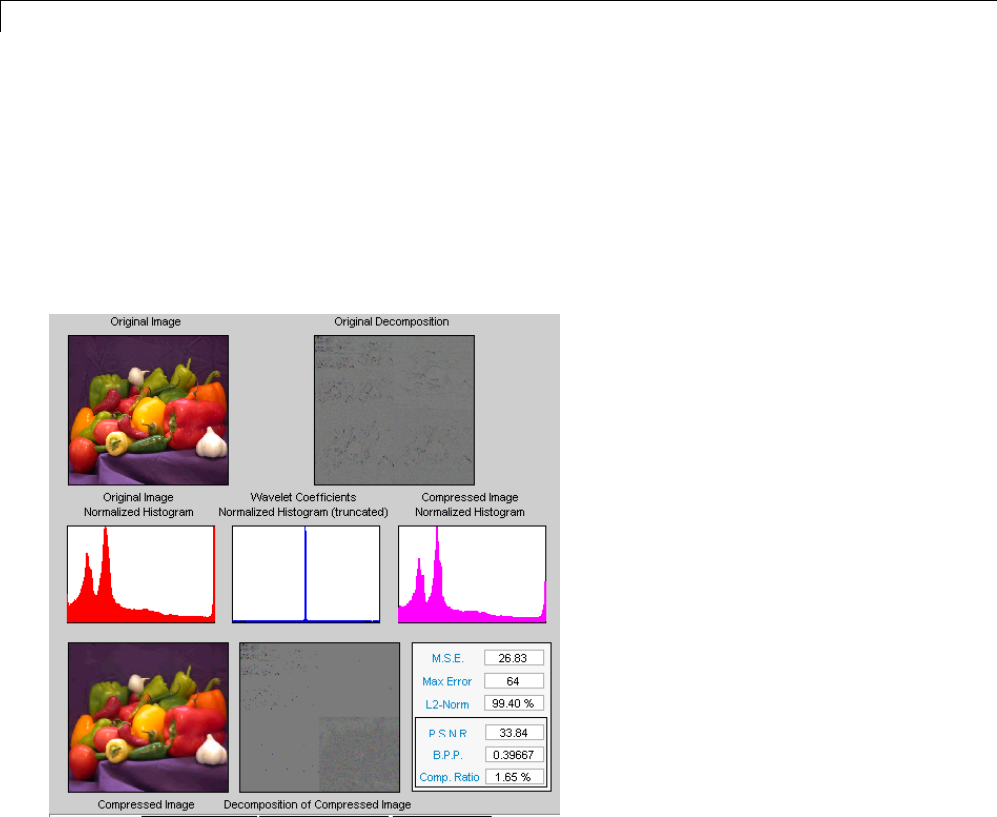
5Denoising, Nonparametric Function Estimation, and Compression
defaults for wavelet and decomposition level menus and then click the
Decompose button.
Then, accept the default compression method SPIHT and set the number
of encoding loops to 12. Click the Compress button.
The compression ratio and Bit-Per-Pixel (BPP) ratio are very satisfactory:
1.65% and 0.4 together with a very good perceptual result.
10 Inspectthewavelettree.
For both grayscale and truecolor images, more insight on the
multiresolution structure of the compressed image can be retrieved by
clicking the Inspect Wavelet Trees button and then on the various active
menus available from the displayed tree.
5-78
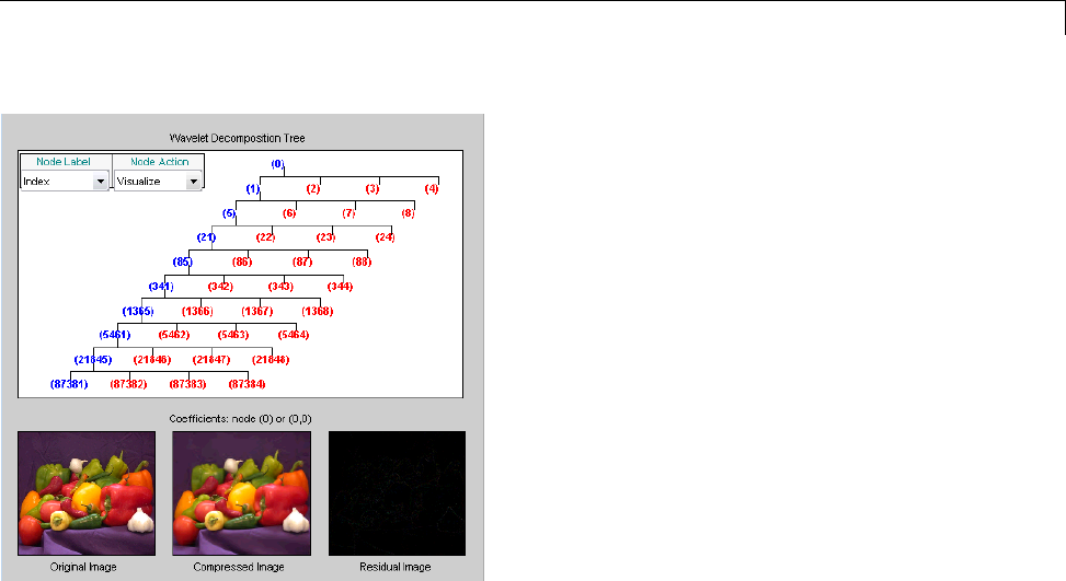
Two-Dimensional True Compression
Importing and Exporting from the GUI
You can save the compressed image to disk in the current folder with a name
of your choice.
The Wavelet Toolbox compression tools can create a file using either one of the
Matlab Supported Format types or a specific format which can be recognized
by the extension of the file: wtc (Wavelet Toolbox Compressed).
To save the above compressed image, use the menu option File > Save
Compressed Image > Wavelet Toolbox Compressed Image.Adialogbox
appears that lets you specify a folder and filename for storing the image. Of
course, the use of the wtc format requires you to uncompress the stored image
using the Wavelet Toolbox true compression tools.
5-79

5Denoising, Nonparametric Function Estimation, and Compression
One-Dimensional Wavelet Regression Estimation
Thissectiontakesyouthroughthefeatures of one-dimensional wavelet
regression estimation using one of the Wavelet Toolbox specialized tools. The
toolbox provides a graphical interface tool to explore some de-noising schemes
for equally or unequally sampled data.
For the examples in this section, switch the extension mode to symmetric
padding, using the command
dwtmode('sym')
Regression for Equally-Spaced Observations
1Start the Regression Estimation 1-D Tool.
From the MATLAB prompt, type
wavemenu
The Wavelet Toolbox Main Menu appears.
5-80
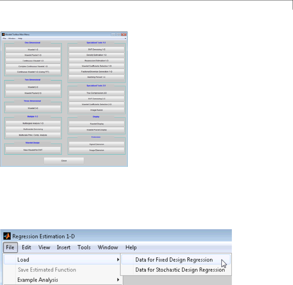
One-Dimensional Wavelet Regression Estimation
Click the Regression Estimation 1-D menu item. The discrete wavelet
analysis tool for one-dimensional regression estimation appears.
2Load data.
From the File menu, choose the Load Data for Fixed Design
Regression option.
When the Load data for Fixed Design Regression dialog box appears,
select the MAT-file noisbloc.mat, which should reside in the MATLAB
folder toolbox/wavelet/wavedemo.
5-81
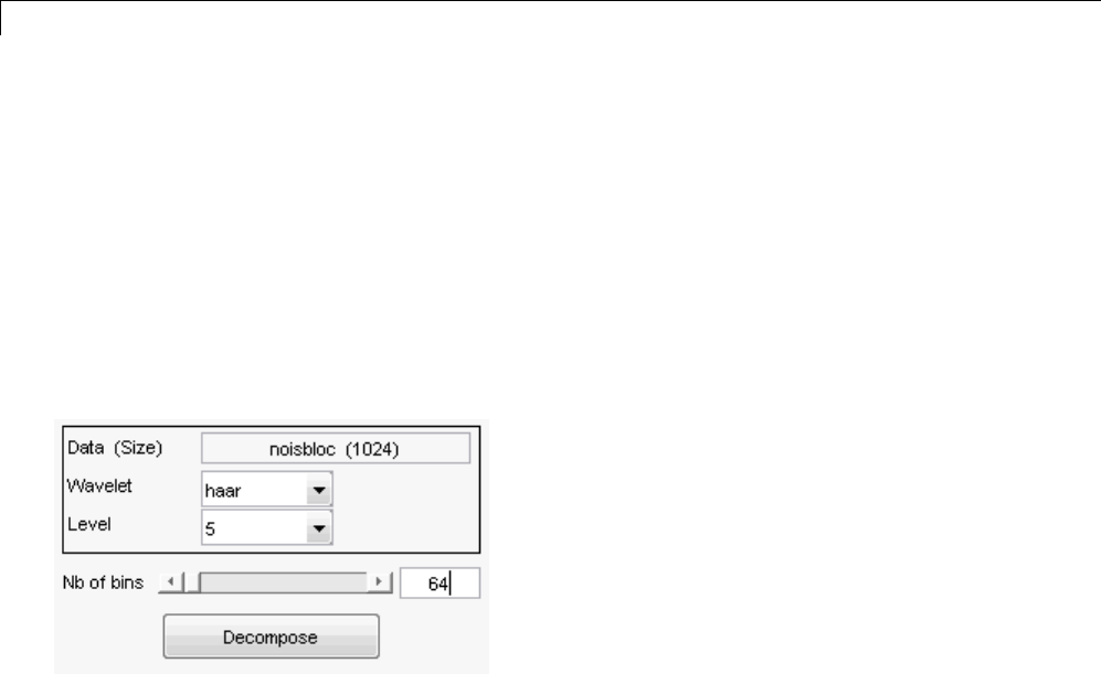
5Denoising, Nonparametric Function Estimation, and Compression
Click the OK button. The noisy blocks data is loaded into the Regression
Estimation 1-D - Fixed Design tool.
The loaded data denoted (X,Y) and the processed data obtained after a
binning, are displayed.
3Choose the processed data.
The default value for the number of bins is 256 for this example. Enter 64
in the Nb bins (number of bins) edit box, or use the slider to adjust the
value. The new binned data to be processed appears.
Thebinneddataappearstobevery smoothed. Select 1000 from the Nb
bins edit and press Enter orusetheslider.Thenewdatatobeprocessed
appears.
The binned data appears to be very close to the initial data, since noisbloc
is of length 1024.
4Perform a Wavelet Decomposition of the processed data.
Select the haar wavelet from the Wavelet menu and select 5from the
Level menu, and then click the Decompose button. After a pause for
computation, the tool displays the detail coefficients of the decomposition.
5-82
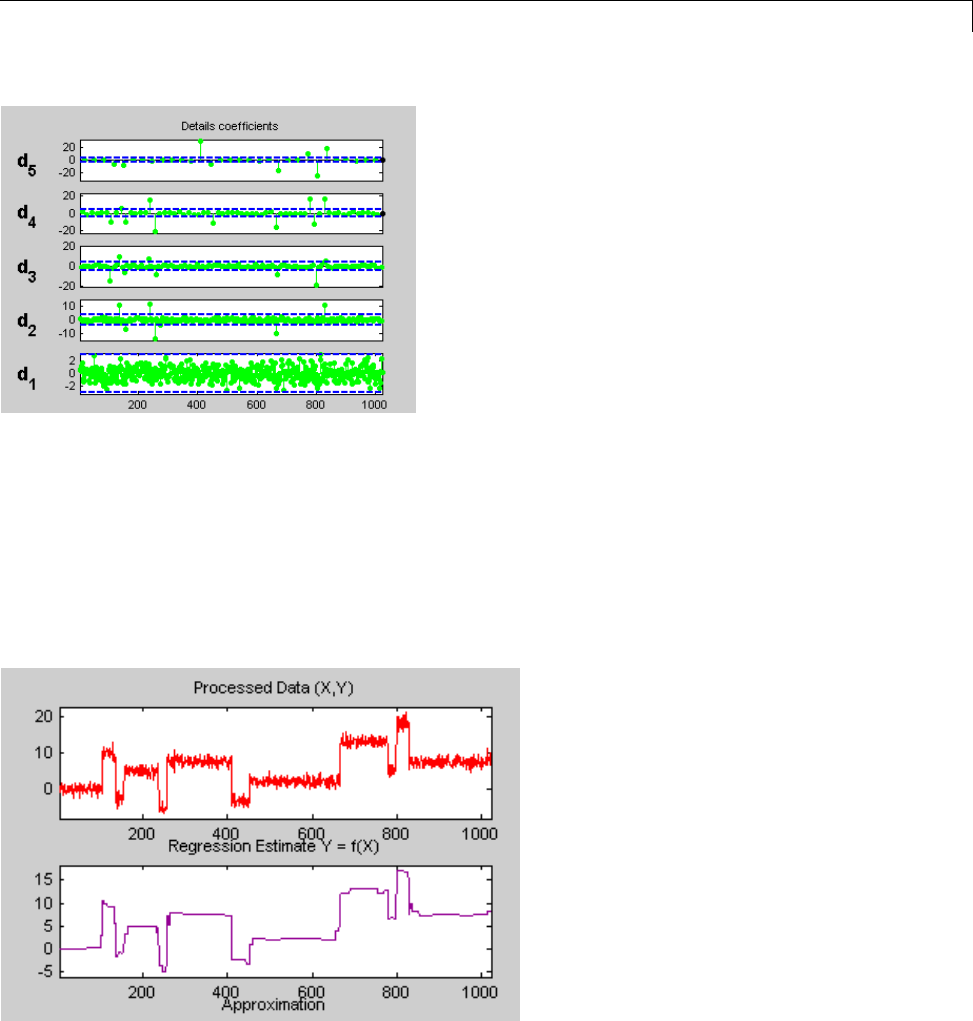
One-Dimensional Wavelet Regression Estimation
5Perform a regression estimation.
While a number of options are available for fine-tuning the estimation
algorithm, we’ll accept the defaults of fixed form soft thresholding and
unscaled white noise. The sliders located to the right of the window control
the level dependent thresholds, indicated by yellow dotted lines running
horizontally through the graphs on the left part of the window.
Continue by clicking the Estimate button.
5-83

5Denoising, Nonparametric Function Estimation, and Compression
You can see that the process removed the noise and that the blocks are well
reconstructed. The regression estimate (in yellow) is the sum of the signals
located below it: the approximation a5 and the reconstructed details after
coefficient thresholding.
You can experiment with the various predefined thresholding strategies
by selecting the appropriate options from the menu located on the right
part of the window or directly by dragging the yellow horizontal lines with
the left mouse button.
Let us now illustrate the regression estimation using the graphical
interface for randomly or irregularly spaced observations, focusing on the
differences from the previous situation.
Regression for Randomly-Spaced Observations
1From the File menu, choose the Load > Data for Stochastic Design
Regression option. When the Load data for Stochastic Design
Regression dialog box appears, select the MAT-file ex1nsto.mat,which
should reside in the MATLAB folder toolbox/wavelet/wavedemo.Click
the OK button. This short set of data (of size 500) is loaded into the
Regression Estimation 1-D -- Stochastic Design tool.
The loaded data denoted (X,Y), the histogram of X, and the processed
data obtained after a binning are displayed. The histogram is interesting,
because the values of X are randomly distributed. The binning step
is essential since it transforms a problem of regression estimation for
irregularly spaced X data into a classical fixed design scheme for which
fast wavelet transform can be used.
2Select the sym4 wavelet from the Wavelet menu, select 5from the Level
menu, and enter 125 in the Nb bins edit box. Click the Decompose
button. The tool displays the detail coefficients of the decomposition.
3From the Select thresholding method menu, select the item Penalize
low and click the Estimate button.
5-84
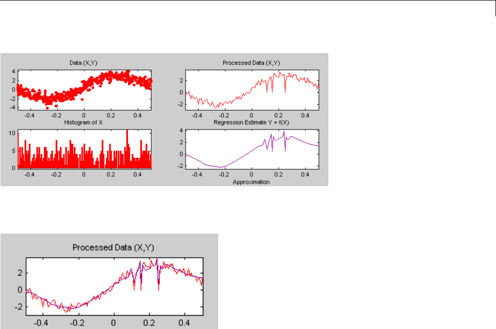
One-Dimensional Wavelet Regression Estimation
4Check Overlay Estimated Function to validate the fit of the original
data.
Importing and Exporting Information from the
Graphical Interface
Saving Function
This tool lets you save the estimated function to disk. The toolbox creates a
MAT-file in the current folder with a name you choose.
To save the estimated function from the present estimation, use the menu
option File > Save Estimated Function. A dialog box appears that lets
you specify a folder and filename for storing the function. Type the name
fex1nsto. After saving the function data to the file fex1nsto.mat,loadthe
variables into your workspace:
load fex1nsto
whos
5-85

5Denoising, Nonparametric Function Estimation, and Compression
Name Size Bytes Class
thrParams 1x5 580 cell array
wname 1x4 8 char array
xdata 1x125 1000 double array
ydata 1x125 1000 double array
The estimated function is given by xdata and ydata. The length of these
vectors is equal to the number of bins you choose in step 2. In addition, the
parameters of the estimation process are given by the wavelet name contained
in wname:
wname
wname =
sym4
and the level dependent thresholds contained in thrParams,whichisa
cell array of length 5 (the level of the decomposition). For ifrom 1 to
5, thrParams{i} contains the lower and upper bounds of the interval of
thresholding and the threshold value (since interval dependent thresholds are
allowed). For more information, see “One-Dimensional Adaptive Thresholding
of Wavelet Coefficients” on page 5-17 in the Wavelet Toolbox User’s Guide.
For example, for level 1,
thrParams{1}
ans =
-0.4987 0.4997 1.0395
Loading Data
To load data for regression estimation, your file must contain at least one
vector. If your file contains only one vector, this vector is considered as ydata
and an xdata vector is automatically generated.
5-86

One-Dimensional Wavelet Regression Estimation
If your file contains at least two vectors, they must be called xdata and
ydata or xand y.
These vectors must be the same length.
For example, load the file containing the data considered in the previous
example:
clear
load ex1nsto
whos
Name Size Bytes Class
x 1x500 4000 double array
y 1x500 4000 double array
At the end of this section, turn back the extension mode to zero padding using
the command
dwtmode('zpd')
5-87

5Denoising, Nonparametric Function Estimation, and Compression
5-88


6Matching Pursuit
Sparse Representation in Redundant Dictionaries
In this section...
“Redundant Dictionaries and Sparsity” on page 6-2
“Nonlinear Approximation in Dictionaries” on page 6-3
Redundant Dictionaries and Sparsity
Representing a signal in a particular basis involves finding the signal’s
unique set of expansion coefficients in that basis. While there are many
advantages to signal representation in a basis, particularly an orthogonal
basis, there are also disadvantages.
The ability of a basis to provide a sparse representation of a signal depends
on how well the signal characteristics match the characteristics of the basis
vectors. For example, smooth continuous signals are sparsely represented
in a Fourier basis, while impulses are not. On the other hand, a smooth
signal with isolated discontinuities is sparsely represented in a wavelet basis,
while a wavelet basis is not efficient at representing a signal whose Fourier
transform has narrow high frequency support.
Real-world signals often contain features that prohibit sparse representation
in any single basis. For these signals, you want the ability to choose vectors
from a set not limited to a single basis. Because you want to ensure that you
can represent every vector in the space, the dictionary of vectors you choose
from must span the space. However, because the set is not limited to a single
basis, the dictionary is not linearly independent.
Because the vectors in the dictionary are not a linearly independent set, the
signal representation in the dictionary is not unique. However, by creating
a redundant dictionary, you can expand your signal in a set of vectors that
adapt to the time-frequency or time-scale characteristics of your signal. You
are free to create a dictionary consisting of the union of several bases. For
example, you can form a basis for the space of square-integrable functions
consisting of a wavelet packet basis and a local cosine basis. A wavelet packet
basis is well adapted to signals with different behavior in different frequency
intervals. A local cosine basis is welladaptedtosignalswithdifferent
behavior in different time intervals. The ability to choose vectors from each
6-2

Sparse Representation in Redundant Dictionaries
of these bases greatly increases your ability to sparsely represent signals
with varying characteristics.
Nonlinear Approximation in Dictionaries
Define a dictionary as a collection of unit-norm elementary building blocks for
your signal space. These unit-norm vectors are called atoms.Iftheatomsof
the dictionary span the entire signal space, the dictionary is complete.
If the dictionary atoms form a linearly-dependent set, the dictionary is
redundant. In most applications of matching pursuit, the dictionary is
complete and redundant.
Let {φk} denote the atoms of a dictionary. Assume the dictionary is complete
and redundant. There is no unique way to represent a signal from the space
as a linear combination of the atoms.
xk
k
k
An important question is whether there exists a best way. An intuitively
satisfyingwaytochoosethebest representation is to select the φkyielding the
largest inner products (in absolute value) with the signal. For example, the
best single φkis
max
kk
x|, |
which for a unit-norm atom is the magnitude of the scalar projection onto
thesubspacespannedbyφk.
The central problem in matching pursuit is how you choose the optimal
M-term expansion of your signal in a dictionary.
6-3

6Matching Pursuit
Matching Pursuit Algorithms
In this section...
“Basic Matching Pursuit” on page 6-4
“Orthogonal Matching Pursuit” on page 6-7
“Weak Orthogonal Matching Pursuit” on page 6-8
Basic Matching Pursuit
Let Φdenote the dictionary of atoms as aN-by-MmatrixwithM>N.Ifthe
complete, redundant dictionary forms a frame for the signal space, you can
obtain the minimum L2 norm expansion coefficient vector by using the frame
operator.
†* *
()1
However, the coefficient vector returned by the frame operator does not
perserve sparsity. If the signal is sparse in the dictionary, the expansion
coefficients obtained with the canonical frame operator generally do not
reflect that sparsity. Sparsity of your signal in the dictionary is a trait
that you typically want to preserve. Matching pursuit addresses sparsity
preservation directly.
Matching pursuit is a greedy algorithm that computes the best nonlinear
approximation to a signal in a complete, redundant dictionary. Matching
pursuit builds a sequence of sparse approximations to the signal stepwise.
Let Φ={φk} denote a dictionary of unit-norm atoms. Let fbe your signal.
1Start by defining R0f=f
2Begin the matching pursuit by selecting the atom from the dictionary that
maximizes the absolute value of the inner product with R0f=f.Denote
thatatombyφp.
3Form the residual R1fby subtracting the orthogonal projection of R0fonto
the space spanned by φp.
6-4
Matching Pursuit Algorithms
Rf Rf Rf pp
10 0
,
4Iterate by repeating steps 2 and 3 on the residual.
R f Rf Rf
mmm
kk
1,
5Stop the algorithm when you reach some specified stopping criterion.
In nonorthogonal (or basic) matching pursuit, the dictionary atoms are not
mutually orthogonal vectors. Therefore, subtracting subsequent residuals
from the previous one can reintroduce components that are not orthogonal to
the span of the previously included atoms.
To illustrate this, consider the following example. The example is not
intended to present a working matching pursuit algorithm.
Consider the following dictionary for Euclidean 2-space. This dictionary is
an equal-norm frame.
{,/
/,/
/}
1
0
12
32
12
12
Assume you have the following signal.
1
12/
The following figure illustrates this example. The dictionary atoms are in red.
The signal vector is in blue.
6-5
6Matching Pursuit
Construct this dictionary and signal in MATLAB.
dictionary = [1 0; 1/2 sqrt(3)/2; -1/sqrt(2) -1/sqrt(2)]';
x = [1 1/2]';
Compute the inner (scalar) products between the signal and the dictionary
atoms.
scalarproducts = dictionary'*x;
The largest scalar product in absolute value occurs between the signal and
[-1/sqrt(2); -1/sqrt(2)]. This is clear because the angle between the two
vectors is almost πradians.
6-6

Matching Pursuit Algorithms
Form the residual by subtracting the orthogonal projection of the signal
onto [-1/sqrt(2); -1/sqrt(2)] from the signal. Next, compute the inner
products of the residual (new signal) with the remaining dictionary atoms. It
is not necessary to include [-1/sqrt(2); -1/sqrt(2)] because the residual
is orthogonal to that vector by construction.
residual = x-scalarproducts(3)*dictionary(:,3);
scalarproducts = dictionary(:,1:2)'*residual;
The largest scalar product in absolute value is obtained with [1;0].The
best two atoms in the dictionary from two iterations are [-1/sqrt(2);
-1/sqrt(2)] and [1;0]. If you iterate on the residual, you see that the
output is no longer orthogonal to the first atom chosen. This means that a
previously selected atom may be selected again. This fact and the associated
complications with convergence argues in favor of “Orthogonal Matching
Pursuit” on page 6-7 (OMP).
Orthogonal Matching Pursuit
In orthogonal matching pursuit (OMP), the residual is always orthogonal to
the atoms already selected. This means that the same atom can never be
selected twice and results in convergence for a d-dimensional vector after
at most dsteps.
Conceptually, you can do this by using Gram-Schmidt to create an
orthonormal set of atoms. With an orthonormal set of atoms, you see that for
ad-dimensional vector, you can find at most dorthogonal directions.
The OMP algorithm is:
1Denote your signal by f. Initialize the residual R0f=f.
2Select the atom that maximizes the absolute value of the inner product
with R0f=f. Denote that atom by φp.
3Form a matrix, Φ, with previously selected atoms as the columns. Define
the orthogonal projection operator onto the span of the columns of Φ.
P
()**1
6-7

6Matching Pursuit
4Apply the orthogonal projection operator to the residual.
5Update the residual.
RfIPRf
mm
1()
Iis the identity matrix.
Orthogonal matching pursuit ensures that the previously selected atoms are
not chosen again in subsequent steps.
Weak Orthogonal Matching Pursuit
It can be computationally efficient to relax the criterion that the selected atom
maximizes the absolute value of the inner product to a less strict one.
|, | |, | (,] xx
pkk
max 0 1
This is known as weak matching pursuit.
6-8

Matching Pursuit — Command Line
Matching Pursuit — Command Line
In this section...
“Creating Dictionaries” on page 6-9
“Matching Pursuit With Dictionaries” on page 6-11
“Matching Pursuit — Electricity Consumption Data” on page 6-12
Creating Dictionaries
To create dictionaries for matching pursuit at the command line, use
wmpdictionary.
This example shows you how to create a dictionary consisting of the discrete
cosine transform (DCT-II) and the shifted Kronecker delta bases for a signal
of length 1000.
Define the dictionary as a cell array.
dict = {'dct','RnIdent'};
Create the dictionary.
mpdict = wmpdictionary(1000,'LstCpt',dict);
This example shows you how to create a dictionary consisting of the
Daubechies extremal-phase wavelet with 2 vanishing moments and a basis
for polynomials of degree at most 19.
Specifying a wavelet family short name without the optional level input uses
wavelets at level 5 by default.
dict = {'db2','poly'};
mpdict = wmpdictionary(1000,'LstCpt',dict);
This example shows you how to create a dictionary with wavelet packets and
the discrete cosine transform basis (DCT-II). Construct the wavelet packets
from the Daubechies least-asymmetric wavelet with 4 vanishing moments at
level 3.
6-9

6Matching Pursuit
For a wavelet packet, prepend the wavelet family short name with wp and
provide the wavelet packet name and level in a cell array.
dict = {{'wpsym4',3},'dct'};
mpdict = wmpdictionary(1000,'LstCpt',dict);
This example shows you how to visualize the dictionary constructed from the
Haar wavelet down to level 2.
The Haar wavelet dictionary at level 2 consists of translated scaling functions
at level 2 and translated wavelet functions at levels 2 and 1.
Create the dictionary.
[mpdict,~,~,longs] = wmpdictionary(100,'lstcpt',{{'haar',2}});
Use the longs output argument to divide the wavelet dictionary by level and
type of function (scaling or wavelet).
Step through a plot of the translated scaling functions and wavelets by level.
for nn = 1:size(mpdict,2)
if (nn <= longs{1}(1))
plot(mpdict(:,nn),'k','linewidth',2); grid on;
xlabel('Translation');
title('Haar Scaling Function - Level 2');
elseif (nn>longs{1}(1) & nn<= longs{1}(1)+longs{1}(2))
plot(mpdict(:,nn),'r','linewidth',2); grid on;
xlabel('Translation');
title('Haar Wavelet - Level 2');
else
title('Haar Wavelet - Level 1');
plot(mpdict(:,nn),'b','linewidth',2); grid on;
title('Haar Wavelet - Level 1');
xlabel('Translation');
end
pause(0.2);
end
6-10

Matching Pursuit — Command Line
Matching Pursuit With Dictionaries
Use wmpalg to compute the matching pursuit of a 1-D input signal in a
dictionary.
This example shows you how to obtain the matching pursuit of the cuspamax
signal in a dictionary constructed from the discrete cosine transform (DCT-II)
basis and sym4 wavelets.
Load the cuspamax signal. Create a dictionary consisting of Daubechies
least-asymmetric wavelets with 4 vanishing moments at level 2 and level 5
along with theDCT-IIbasis.
load cuspamax;
dict = {{'sym4',2},'sym4','dct'};
mpdict = wmpdictionary(length(cuspamax),'LstCpt',dict);
Obtain the basic (nonorthogonal) matching pursuit in your dictionary with 25
iterations and plot the approximation.
[YFIT1,R1,COEFF1,IOPT1,QUAL1] = wmpalg('BMP',cuspamax,mpdict);
plot(YFIT1); axis tight; hold on;
plot(cuspamax,'k');
legend('BMP','Original Signal','Location','NorthWest');
6-11
6Matching Pursuit
Use orthogonal matching pursuit with the identical dictionary.
[YFIT2,R2,COEFF2,IOPT2,QUAL2] = wmpalg('OMP',cuspamax,mpdict);
Matching Pursuit — Electricity Consumption Data
This example compares matching pursuit with a nonlinear approximation in
the discrete Fourier transform basis. The data is electricity consumption
data collected over a 24-hour period.
This example shows you that by selecting atoms from a dictionary, matching
pursuit is often able to approximate a vector more efficiently with M vectors
than any single basis.
6-12
Matching Pursuit — Command Line
Use a signal measuring electric consumption sampled at one minute intervals
over 24 hours. This signal is also used in the wavelet multisignal analysis
example. See Multisignal 1-D Wavelet Analysis.
Load the dataset. The dataset contains 35 days of electric consumption.
Choose day 32 for further analysis. The data is centered and scaled.
Accordingly, the actual units of usage are not relevant.
Plot the data.
load elec35_nor;
x = signals(32,:);
plot(x); xlabel('Minutes'); ylabel('Usage');
set(gca,'xlim',[1 1440]);
6-13
6Matching Pursuit
The electricity consumption data contains smooth oscillations punctuated by
abrupt increases and decreases in usage.
Zoom in on a time interval from 500 minutes to 1200 minutes.
plot(x); xlabel('Minutes'); ylabel('Usage');
set(gca,'xlim',[500 1200]); grid on;
set(gca,'xtick',[500:50:1200]);
In the preceding plot, you can clearly see the abrupt changes in the
slowly-varying signal at approximately 650, 760, and 1120 minutes.
6-14

Matching Pursuit — Command Line
In many real-world signals like these data, the interesting and important
information is contained in the transients. Accordingly, it is important to
adequately model these transient phenomena.
Construct a signal approximation using 35 vectors chosen from a dictionary
with orthogonal matching pursuit.
Construct a dictionary consisting of the Daubechies extremal phase wavelet
and scaling vectors at level 2, the discrete cosine transform basis, a sine
basis, the Kronecker delta basis, and the Daubechies least asymmetric phase
wavelet and scaling vectors with 4 vanishing moments at levels 1 and 4.
dictionary = {{'db4',2},'dct','sin',{'sym4',1},{'sym4',4}};
[mpdict,nbvect] = wmpdictionary(length(x),'lstcpt',dictionary);
Use orthogonal matching pursuit to find the best 35-term greedy
approximation of the electric consumption data. Plot the result.
[y,r,coef,iopt,qual] = wmpalg('OMP',x,mpdict,'itermax',35);
plot(x); hold on;
plot(y,'r'); xlabel('Minutes'); ylabel('Usage');
legend('Original Signal','OMP','Location','NorthEast');
set(gca,'xlim',[1 1440]);
6-15
6Matching Pursuit
You can see in the preceding plot that with 35 coefficients, orthogonal
matching pursuit approximates both the smoothly-oscillating part of the
signal as well as the abrupt changes in electricity usage.
Determine how many vectors the OMP algorithm has selected from each
of the subdictionaries.
basez = cumsum(nbvect);
k=1;
for nn = 1:length(basez)
if (nn == 1)
basezind{nn} = 1:basez(nn);
else
basezind{nn} = basez(nn-1)+1:basez(nn);
6-16

Matching Pursuit — Command Line
end
end
dictvectors = cellfun(@(x) intersect(iopt,x),basezind,...
'UniformOutput',false)
The following table summarizes how many vectors the OMP algorithm
selected from each of the subdictionaries.
Subdictionary Number of Vectors Selected
Daubechies wavelet (db4) level 2 3
Discrete cosine transform 16
Sine 5
Daubechies least-asymmetric
wavelet (sym4) level 1
2
Daubechies least-asymmetric
wavelet (sym4) level 4
9
You see that the majority of the vectors come from the DCT or sine basis (60%).
This is not surprising given the overall slowly-varying nature of the electricity
consumption data. However, the addition of the 14 vectors from the wavelet
subdictionaries enables you to accurately capture the abrupt signal changes.
Compare matching pursuit with a DCT-sine dictionary to the full dictionary.
To demonstrate that the addition of the wavelet subdictionaries has improved
the signal approximation, repeat the OMP with just the DCT and sine
subdictionaries. Do not restrict the approximation to just the 21 vectors
chosen in the preceding example. Enable the OMP to select the 35 best
vectors from the DCT-sine dictionary.
Construct the dictionary and perform the OMP.
dictionary2 = {'dct','sin'};
[mpdict2,nbvect2] = wmpdictionary(length(x),'lstcpt',dictionary2);
[y2,r2,coef2,iopt2,qual2] = wmpalg('OMP',x,mpdict2,'itermax',35);
Compare the OMP with the DCT-sine dictionary to the OMP with the addition
of the wavelet subdictionaries.
6-17
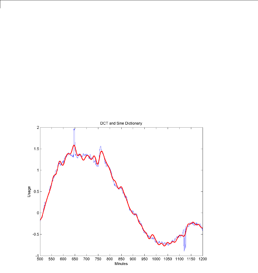
6Matching Pursuit
plot(x); hold on;
plot(y,'r','linewidth',2); title('Full Dictionary');
xlabel('Minutes'); ylabel('Usage');
set(gca,'xlim',[500 1200]);
set(gca,'xtick',[500:50:1200]);
figure;
plot(x); hold on;
plot(y2,'r','linewidth',2); title('DCT and Sine Dictionary');
xlabel('Minutes'); ylabel('Usage');
set(gca,'xlim',[500 1200]);
set(gca,'xtick',[500:50:1200]);
The results for the DCT-sine dictionaryareshowninthefollowingfigure.
6-18
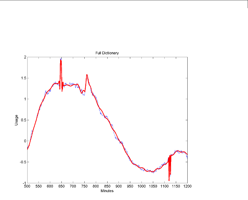
Matching Pursuit — Command Line
The results including the wavelet subdictionaries is shown in the following
figure.
The addition of the wavelet subdictionaries enables you to more accurately
model the abrupt changes in electricity usage in the data. The advantage of
including the wavelet bases is especially clear in approximating the upward
and downward spikes in usage at approximately 650 and 1120 minutes.
This example shows you how to obtain the best 35-term nonlinear
approximation of the signal in the discrete Fourier basis.
6-19

6Matching Pursuit
Obtain the DFT of the data. Sort the DFT coefficients and select the 35 largest
coefficients. Because the DFT of a real-valued signal is conjugate symmetric,
only consider frequencies from 0 (DC) to the Nyquist (1/2 cycles/minute).
xdft = fft(x);
[~,I] = sort(xdft(1:length(x)/2+1),'descend');
ind = I(1:35);
Examine the vector ind. None of the indices correspond to 0 or the Nyquist.
Therefore, you must add the corresponding complex conjugate in order to
obtain the nonlinear approximation in the DFT basis.
indconj = length(xdft)-ind+2;
ind = [ind indconj];
xdftapp = zeros(size(xdft));
xdftapp(ind) = xdft(ind);
xrec = ifft(xdftapp);
Plot the approximation along with the original signal.
plot(x); hold on;
plot(xrec,'r'); xlabel('Minutes'); ylabel('Usage');
legend('Original Signal','Nonlinear DFT Approximation',...
'Location','NorthEast');
set(gca,'xlim',[1 1440]);
Similar to the DCT-sine dictionary, the nonlinear DFT approximation does
well at matching the smooth oscillations in electricity consumption data.
Zoom in on the interval of the data containing the abrupt changes in
consumption.
plot(x); hold on;
plot(xrec,'r','linewidth',2);
xlabel('Minutes'); ylabel('Usage');
legend('Original Signal','Nonlinear DFT Approximation',...
'Location','NorthEast');
set(gca,'xlim',[500 1200]);
set(gca,'xtick',[500:50:1200]);
6-20
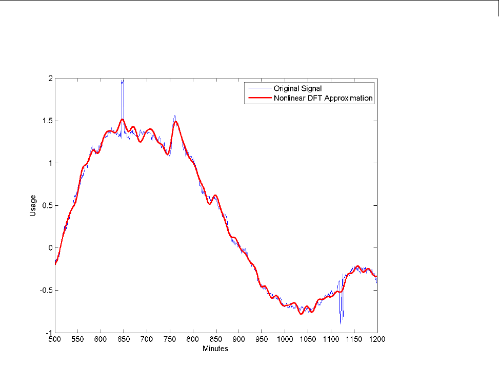
Matching Pursuit — Command Line
You can see in the above figure that the nonlinear DFT approximation is not
abletoaccuratelyapproximatetheabrupt changes in consumption.
6-21

6Matching Pursuit
Matching Pursuit — Interactive Analysis
In this section...
“Matching Pursuit 1-D Interactive Tool” on page 6-22
“Interactive Matching Pursuit of Electricity Consumption Data” on page
6-38
Matching Pursuit 1-D Interactive Tool
You can perform basic, orthogonal, and weak orthogonal matching pursuit
using the interactive tool wavemenu. To access the Matching Pursuit 1-D
interactive tool, enter
wavemenu
at the MATLAB command prompt.
6-22
Matching Pursuit — Interactive Analysis
Click Matching Pursuit 1-D.
6-23
6Matching Pursuit
To demonstrate the Matching Pursuit 1-D tool, select File —> Example
—> Cuspamax.
6-24
Matching Pursuit — Interactive Analysis
In the upper left corner, you see the plot of the signal with the matching
pursuit approximation superimposed.
6-25
6Matching Pursuit
Underneath the plot, you see the relative errors using the L1, L2, and
L-infinity norms.
The maximum relative error in a given norm is
100|| ||
|| ||,
R
Y
where || || denotes the specified norm, Ris the residual vector at each
iteration in the matching pursuit algorithm, and Yis the signal.
Inthemiddlepanelontheleftistheplotofthefinalresidualvectorafterthe
matching pursuit algorithm terminates.
6-26
Matching Pursuit — Interactive Analysis
The bottom left panel displays the percentage of retained signal energy (L2
norm) and the relative error percentages for the L1, L2, and L-infinity norms
over the algorithm iterations.
6-27
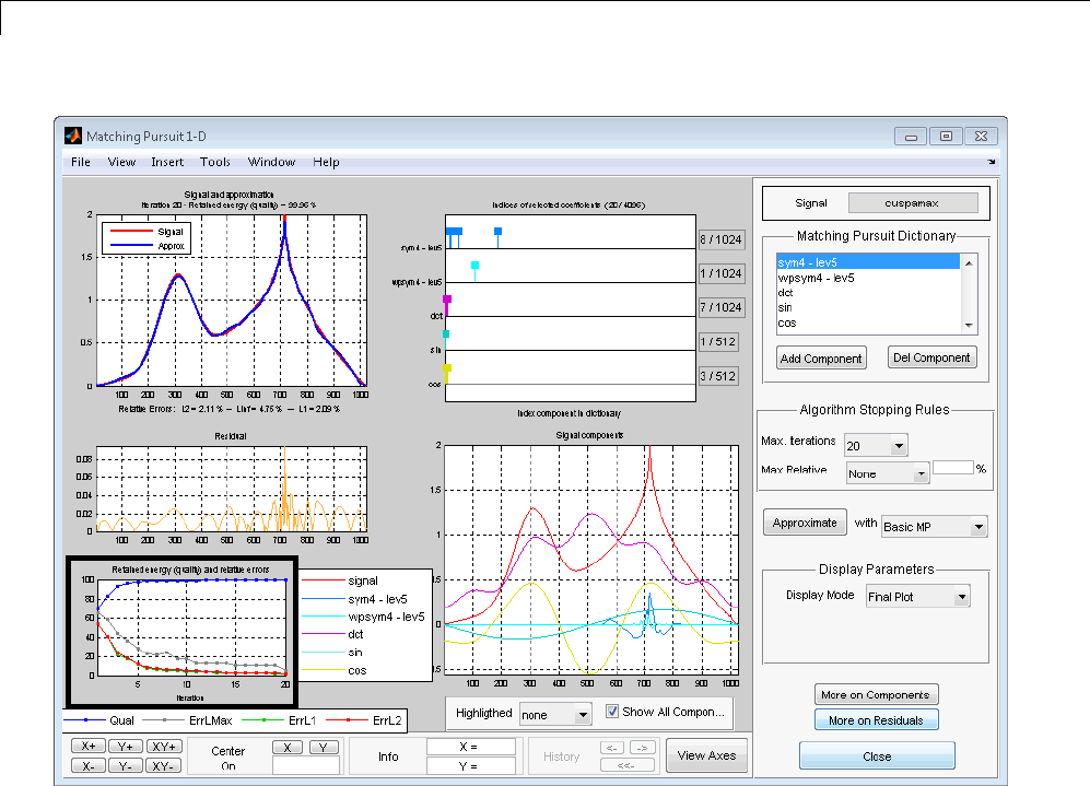
6Matching Pursuit
InthetopmiddlepaneloftheMatching Pursuit 1-D tool, you see the indices
of the selected coefficients from the subdictionaries.
6-28
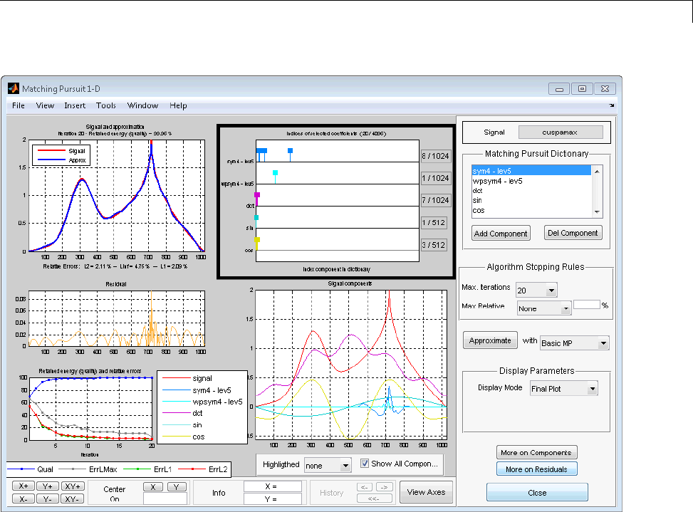
Matching Pursuit — Interactive Analysis
Theleftverticalaxisshowsthenameofthesubdictionary. Therightvertical
axis gives the ratio of selected vectors to the total number of vectors in the
subdictionary. The location of the vertical bars along the horizontal axis gives
therelativepositionsoftheselected vectors in the subdictionaries.
More detailed information on selected components is available by clicking
More on Components in the bottom right panel.
The bottom middle panel displays the superposition of selected vectors from
the subdictionaries.
6-29
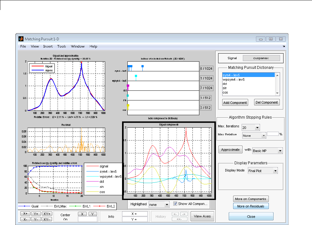
6Matching Pursuit
This plot enables you to assess the relative contribution of the subdictionaries
to the signal approximation. In this example, you can see that the cosine
and DCT subdictionaries contribute significantly to the approximation of
the slowly-varying portions of the signal. The Daubechies least asymmetric
wavelet with 4 vanishing moments (sym4) enables the matching pursuit to
sparsely represent the cusp around index 700.
In the top right panel of the Matching Pursuit 1-D tool, you see the
dictionary used in the analysis.
6-30
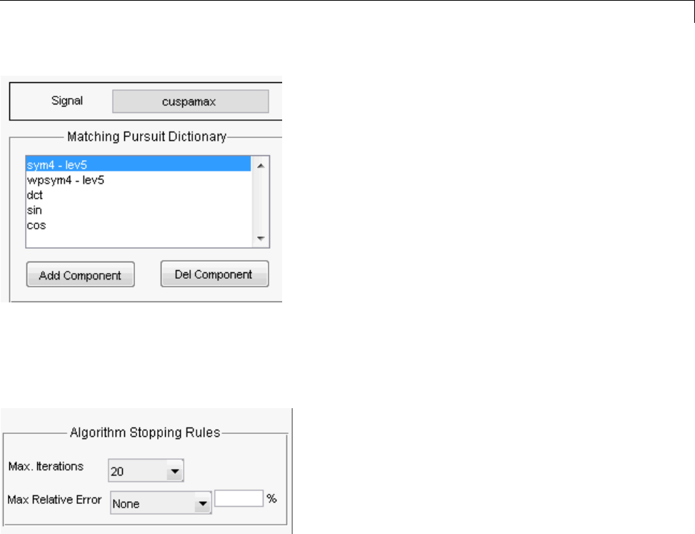
Matching Pursuit — Interactive Analysis
You have the ability to add or delete subdictionaries with Add Component
and Del Component.
The next panel contains the algorithm stopping rules.
•Max. Iterations — This controls the number of iterations of the greedy
matching pursuit algorithm. The value is equal to the number of expansion
coefficients (vectors) used in the approximation. The utility of matching
pursuit is that you can approximate many real-world signals efficiently
with far fewer vectors than needed to span the signal space.
•Max Relative Error — Specifies the stopping criterion based on the
maximum relative error. Choose one of None,L2 norm,L1 norm,orLinf
norm.
The maximum relative error in a given norm is
6-31
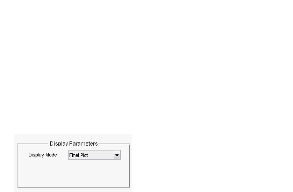
6Matching Pursuit
100|| ||
|| ||,
R
Y
where || || denotes the specified norm, Ris the residual vector at each
iteration in the matching pursuit algorithm, and Yis the signal.
In the next panel you select the algorithm used in the matching pursuit.
Choose one of Basic MP for basic matching pursuit, Orthogonal MP for
orthogonal matching pursuit, and Weak MP for weak orthogonal matching
pursuit. See “Matching Pursuit Algorithms” on page 6-4 for a brief description
of these algorithms.
In the Display Parameters panel, you can control how the progress of the
matching pursuit is displayed.
Select one of
•Final Plot — Plots the result of matching pursuit only after the algorithm
terminates.
•Stepwise —UpdatestheresulteveryNiterations where N is a positive
integer. If you select Stepwise,theDisplay every iterations item
becomes visible. Select the number of iterations from the drop down menu.
You are prompted to step through the algorithm with the Next or Final
Plot.
•Movie — Updates the result every N iterationswhereNisapositiveinteger
in a continous manner. If you select Movie,theDisplay every iterations
item becomes visible. Select the number of iterations from the drop down
menu. Click Continue to step through the algorithm as a movie, which
continues until the algorithm terminates. Click Pause to pause the
algorithm, or Final Plot to update only at the termination of the algorithm.
6-32
Matching Pursuit — Interactive Analysis
After you obtain a matching pursuit of a signal, use
to obtain detailed interactive plots and information on the selected dictionary
atoms and the final residual vector.
Click More on Components.
6-33
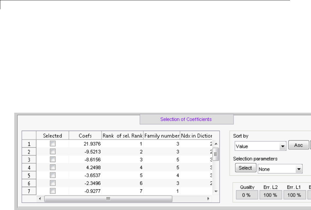
6Matching Pursuit
From the above figure, you can see that while the DCT and cosine
subdictionaries contribute energy across the extent of the signal, the wavelet
and wavelet packet contributions are localized at the cusp around sample 700.
This result is expected because wavelets and wavelet packets excel at sparsely
representing abrupt changes in a signal or image.
Change the Display to the Coefficients view.
The Selection of Coefficients panel enables you to selectively sort
and display contributions to the signal approximation by the various
subdictionaries.
Under Selection parameters,chooseBy Family and sym4 lev5.Click
Select
6-34
Matching Pursuit — Interactive Analysis
From the preceding operation, you see that the wavelet packet contributes
to the approximation of the cusp, but does not contribute significantly to the
global approximation.
Choose dct and click Select.
6-35
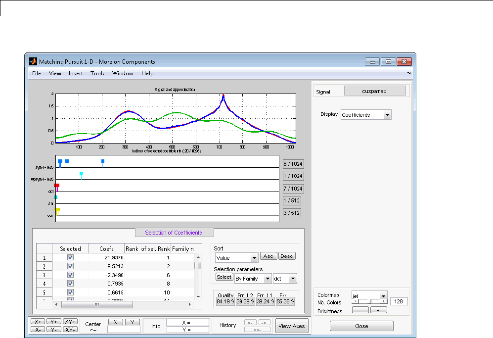
6Matching Pursuit
The DCT basis contributes significantly to the global approximation of the
signal but the smooth DCT basis vectors are not able to sparsely represent
the cusp.
Selecting More on Residuals allows you to examine the residual vector,
ahist
ogram of the residuals, a cumulative histogram, the estimated
autocorrelation sequence, and the magnitude-squared discrete Fourier
transform.
6-36
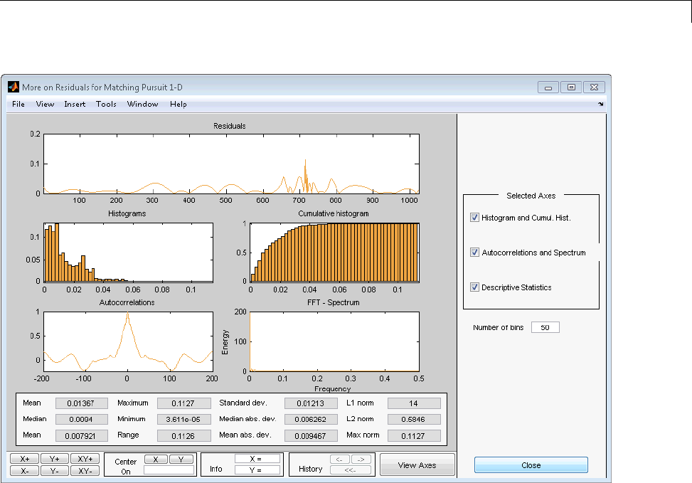
Matching Pursuit — Interactive Analysis
You can control which plots are displayed and the appearance of the histogram
by the options in the right panel.
6-37
6Matching Pursuit
Interactive Matching Pursuit of Electricity
Consumption Data
This example shows you how to perform an interactive matching pursuit of
electricity consumption data collected over a 24-hour period. You can see the
command-line equivalent of this example in “Matching Pursuit — Electricity
Consumption Data” on page 6-12.
Use a signal measuring electric consumption sampled at one minute intervals
over 24 hours. This signal is also used in the wavelet multisignal analysis
example, see Multisignal 1-D Wavelet Analysis.
Load the electricity consumption signals in the workspace. Select the data for
the 32nd day for further matching pursuit.
load elec35_nor;
x=si
gnals(32,:);
Start the interactive tool, wavemenu
wavemenu
Click the Matching Pursuit 1-D tool.
6-38
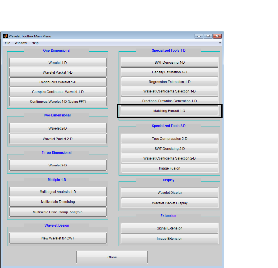
Matching Pursuit — Interactive Analysis
Select File —> Import Signal from Workspace
Load x.
6-39

6Matching Pursuit
Construct the following matching pursuit dictionary.
In the Algorithm Stopping Rules panel, set Max. Iterations to 30.
Select Orthogonal MP to use orthogonal matching pursuit.
Click Approximate.
6-40
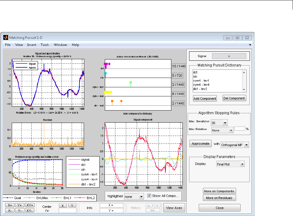
Matching Pursuit — Interactive Analysis
6-41

6Matching Pursuit
6-42

7
Generating MATLAB Code
from Wavelet Toolbox GUI
•“Generating MATLAB Code for 1-D Decimated Wavelet Denoising and
Compression” on page 7-2
•“Generating MATLAB Code for 2-D Decimated Wavelet Denoising and
Compression” on page 7-13
•“Generating MATLAB Code for 1-D Stationary Wavelet Denoising” on
page 7-20
•“Generating MATLAB Code for 2-D Stationary Wavelet Denoising” on
page 7-27
•“Generating MATLAB Code for 1-D Wavelet Packet Denoising and
Compression” on page 7-31
•“Generating MATLAB Code for 2-D Wavelet Packet Denoising and
Compression” on page 7-35
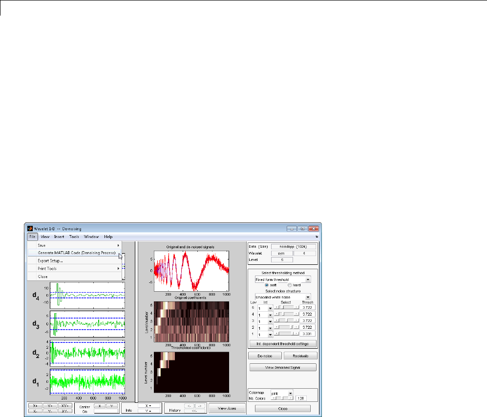
7Generating MATLAB®Code from Wavelet Toolbox™ GUI
Generating MATLAB Code for 1-D Decimated Wavelet
Denoising and Compression
Wavelet 1-D Denoising
You can generate MATLAB code to reproduce GUI-based 1-D wavelet
denoising at the command line. You must perform this operation in the
Wavelet 1-D - - De-noising tool. You must first denoise your signal before
you can enable the File > Generate Matlab Code (Denoising Process)
operation.
The generated MATLAB code does not include the calculation of the
thresholds using thselect or wbmpen.
Denoise Doppler Signal
1Enter wavemenu at the MATLAB command prompt.
2Select Wavelet 1-D in the Wavelet Toolbox Main Menu.
7-2
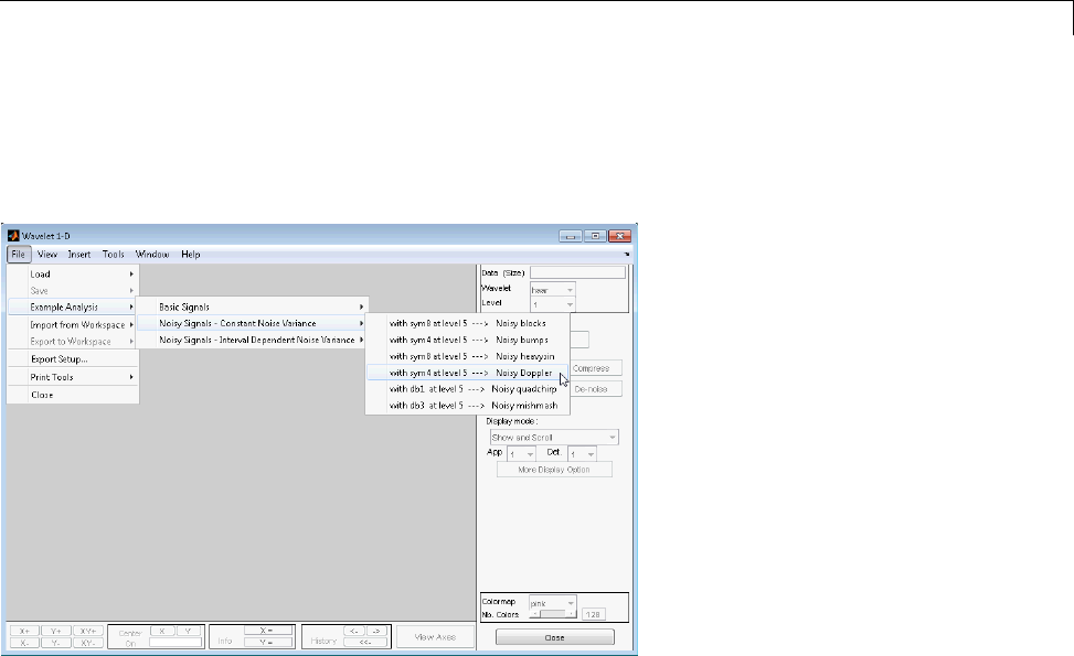
Generating MATLAB®Code for 1-D Decimated Wavelet Denoising and Compression
3Load the noisy Doppler example analysis. Select File > Example Analysis
> Noisy Signals - Constant Noise Variance > with sym4 at level 5 - -
-> Noisy Doppler.
4Click De-noise.
7-3
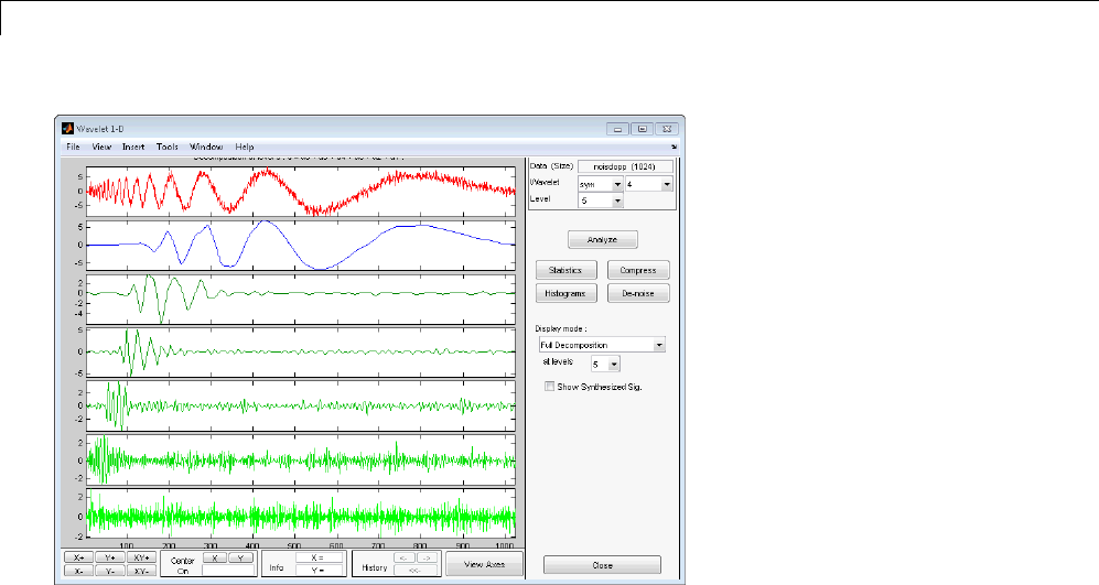
7Generating MATLAB®Code from Wavelet Toolbox™ GUI
5In the Select thresholding method drop-down menu, select the default
Fixed form threshold.Usethedefaultsoft option. Set the thresholds by
level as follows:
•level 5 — 3.5
•level 4 — 3.72
•level 3 — 3.0
•level 2 — 2.0
•level 1 — 3.0
7-4
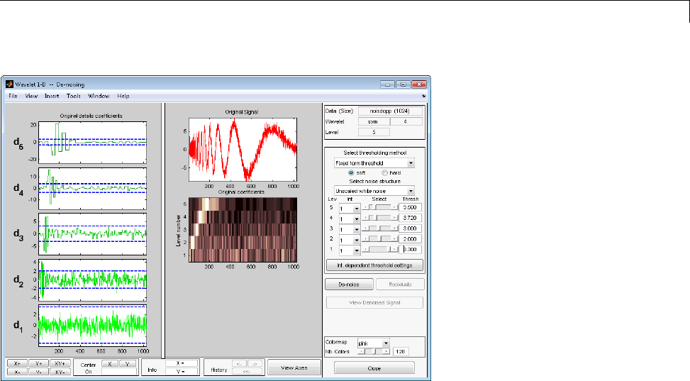
Generating MATLAB®Code for 1-D Decimated Wavelet Denoising and Compression
Click De-noise.
6Generate the MATLAB code by selecting File > Generate Matlab Code
(Denoising Process).
The operation generates the following MATLAB code.
function sigDEN = func_denoise_dw1d(SIG)
% FUNC_DENOISE_DW1-D Saved Denoising Process.
% SIG: vector of data
% -------------------
% sigDEN: vector of denoised data
%Ana
lysis parameters.
%---------------------
wname = 'sym4';
level=5;
%De
noising parameters.
%----------------------
7-5

7Generating MATLAB®Code from Wavelet Toolbox™ GUI
% meth = 'sqtwolog';
% scal_or_alfa = one;
sorh = 's'; % Specified soft or hard thresholding
thrParams = [...
3.00000000 ; ...
2.00000000 ; ...
3.00000000 ; ...
3.72000000 ; ...
3.50000000 ...
];
% Denoise using CMDDENOISE.
%--------------------------
sigDEN = cmddenoise(SIG,wname,level,sorh,NaN,thrParams);
7Save func_denoise_dw1d.m in a folder on the MATLAB search path.
Execute the following code.
load noisdopp;
SIG = noisdopp;
% func_denoise_dw1d.m is generated code
sigDEN = func_denoise_dw1d(SIG);
8Export the denoised signal from the GUI by selecting File > Save >
De-noised Signal.
7-6
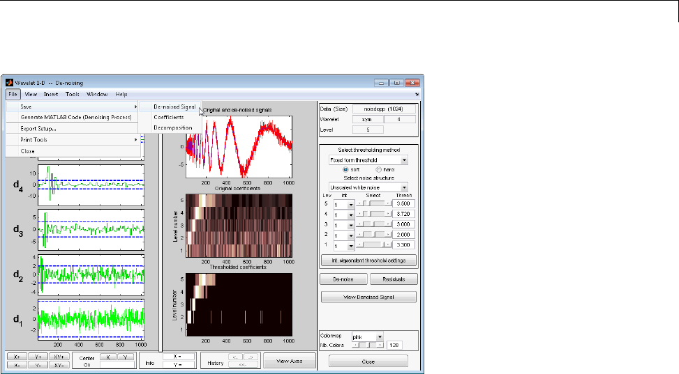
Generating MATLAB®Code for 1-D Decimated Wavelet Denoising and Compression
Save the denoised signal as denoiseddoppler.mat in a folder on the
MATLAB search path. Load denoiseddoppler.mat in the MATLAB
workspace. Compare denoiseddoppler with your command line result.
load denoiseddoppler;
plot(sigDEN,'k'); axis tight;
hold on;
plot(denoiseddoppler,'r');
legend('Command Line','GUI','Location','SouthEast');
7-7
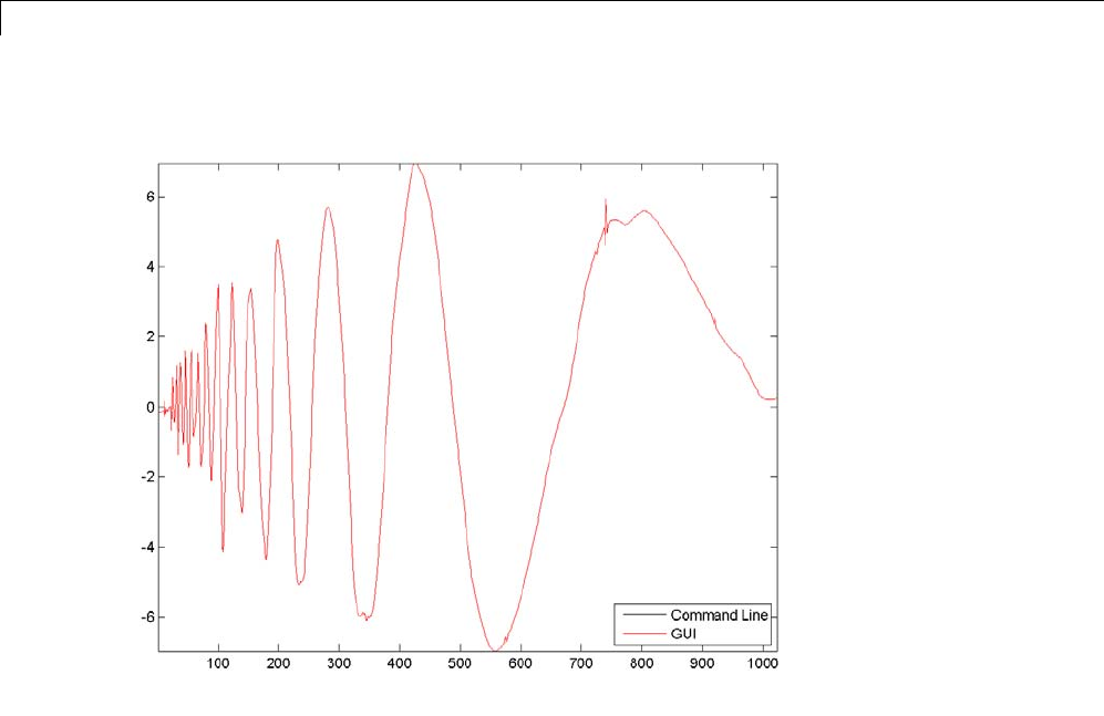
7Generating MATLAB®Code from Wavelet Toolbox™ GUI
Interval Dependent 1-D Wavelet Denoising
1Enter wavemenu at the MATLAB command prompt.
2Select Wavelet 1-D.
3SelectFile > Load > Signal,andloadleleccum.mat from the
matlab/toolbox/wavelet/wavedemo folder.
4Select the sym4 wavelet, and set Level equal to 3. Click Analyze.
7-8
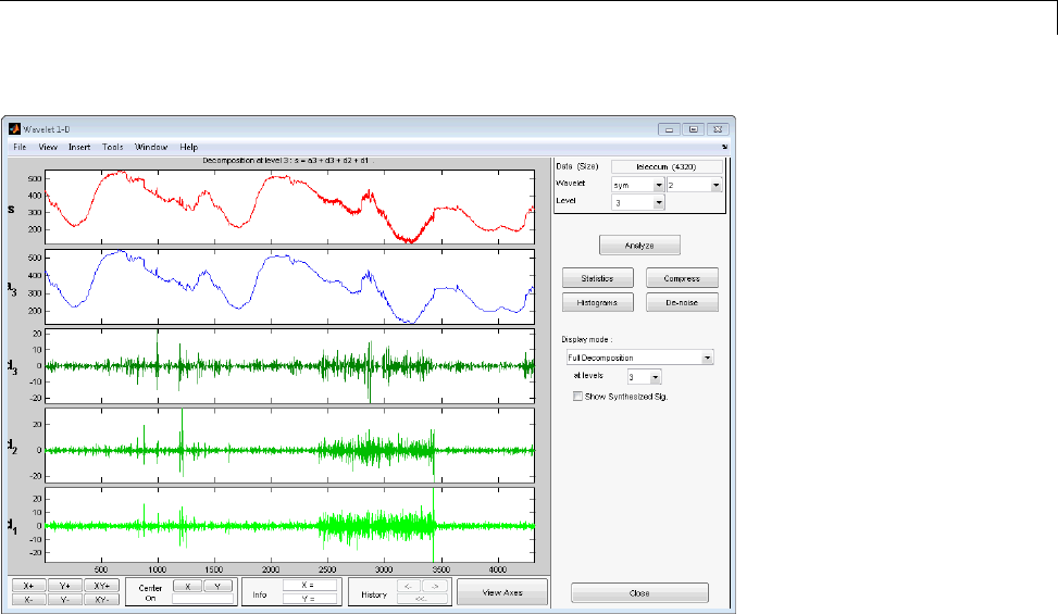
Generating MATLAB®Code for 1-D Decimated Wavelet Denoising and Compression
When you inspect the original signal and the finest-scale wavelet
coefficients, you see that the noise variance is not constant. In this situation,
interval-dependent thresholding is useful. To implement interval-dependent
denoising:
1Click De-noise.
2Under Select thresholding method,selectRigorous SURE.
3Select Int. dependent threshold settings.
4In the Interval Dependent Threshold Settings for Wavelet 1-D tool,
choose Generate Default Intervals. Three intervals are created. Click
Propagate to propagate the intervals to all levels.
5Click Close,andanswerYes to Update Thresholds?.
6Select De-noise.
7Generate the MATLAB code by selecting File > Generate Matlab Code
(Denoising Process).
7-9

7Generating MATLAB®Code from Wavelet Toolbox™ GUI
The operation generates the following MATLAB code.
function sigDEN = func_denoise_dw1d(SIG)
% FUNC_DENOISE_DW1D Saved Denoising Process.
% SIG: vector of data
% -------------------
% sigDEN: vector of denoised data
% Analysis parameters.
%---------------------
wname = 'sym4';
level = 3;
% Denoising parameters.
%----------------------
% meth = 'rigrsure';
% scal_or_alfa = one;
sorh = 's'; % Specified soft or hard thresholding
thrSettings = {...
[...
1.000000000000000 2410.000000000000000 5.659608351110114; ...
2410.000000000000000 3425.000000000000000 19.721391195242880; ...
3425.000000000000000 4320.000000000000000 4.907947952868359; ...
]; ...
[...
1.000000000000000 2410.000000000000000 5.659608351110114; ...
2410.000000000000000 3425.000000000000000 5.659608351110114; ...
3425.000000000000000 4320.000000000000000 5.659608351110114; ...
]; ...
[...
1.000000000000000 2410.000000000000000 5.659608351110114; ...
2410.000000000000000 3425.000000000000000 5.659608351110114; ...
3425.000000000000000 4320.000000000000000 5.659608351110114; ...
]; ...
};
% Denoise using CMDDENOISE.
%--------------------------
sigDEN = cmddenoise(SIG,wname,level,sorh,NaN,thrSettings);
7-10

Generating MATLAB®Code for 1-D Decimated Wavelet Denoising and Compression
8To avoid confusion with the MATLAB code generated in “Denoise Doppler
Signal ” on page 7-2, change the function definition line. Change the
function definition to:
function sigDEN = func_IDdenoise_dw1d(SIG)
Save the MATLAB program as func_IDdenoise_dw1d.m in a folder on
the MATLAB search path.
9Save the denoised signal as denoisedleleccum.mat with File > Save >
De-noised Signal in a folder on the MATLAB search path.
Execute the following code.
load leleccum;
load denoisedleleccum;
sigDEN = func_IDdenoise_dw1d(leleccum);
plot(sigDEN,'k');
hold on;
plot(denoisedleleccum,'r');
legend('Command Line','GUI');
norm(sigDEN-denoisedleleccum,2)
7-11
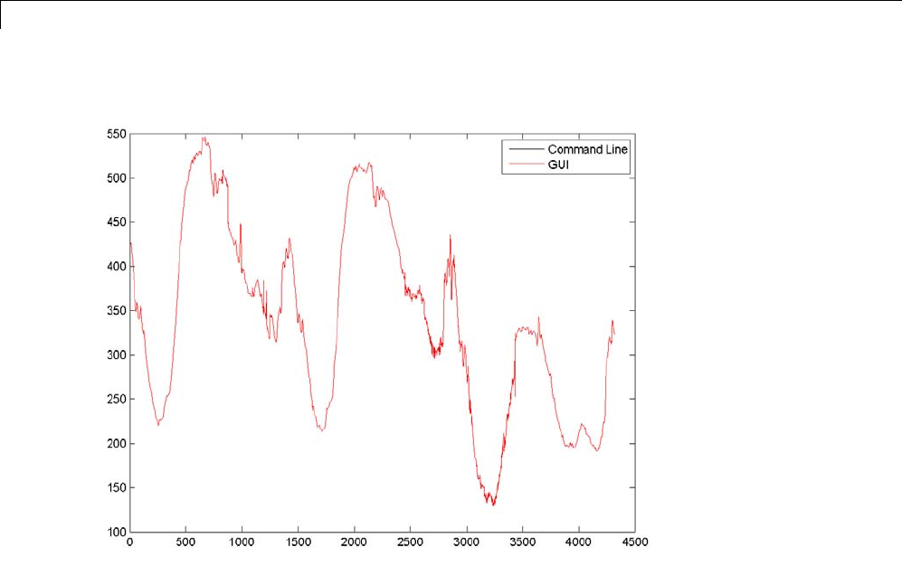
7Generating MATLAB®Code from Wavelet Toolbox™ GUI
7-12

Generating MATLAB®Code for 2-D Decimated Wavelet Denoising and Compression
Generating MATLAB Code for 2-D Decimated Wavelet
Denoising and Compression
In this section...
“2-D Decimated Discrete Wavelet Transform Denoising” on page 7-13
“2-D Decimated Discrete Wavelet Transform Compression” on page 7-17
2-D Decimated Discrete Wavelet Transform Denoising
You can generate MATLAB code to reproduce GUI-based 2-D decimated
wavelet denoising at the command line. You must perform this operation in
the Wavelet 2-D – –De-noising tool. You must first denoise your image
before you can enable the File > Generate Matlab Code (Denoising
Process) operation.
1Enter wavemenu at the MATLAB command prompt.
2Select Wavelet 2-D.
3Load the Noisy SinSin example indexed image. Using the default
biorthogonal wavelet and level 3 decomposition, click De-noise.
4In the Select thresholding method drop-down menu, select the default
Fixed form threshold and soft options. Use the default Unscaled white
noise. Set the thresholds by level for the horizontal, diagonal, and vertical
coefficients as follows:
•Level 3 — 4
•Level 2 — 4
•Level 1 — 8
Enter these thresholds for the horizontal, diagonal, and vertical coefficients.
5Select De-noise.
6Generate the MATLAB code with File > Generate Matlab Code
(Denoising Process).
7-13
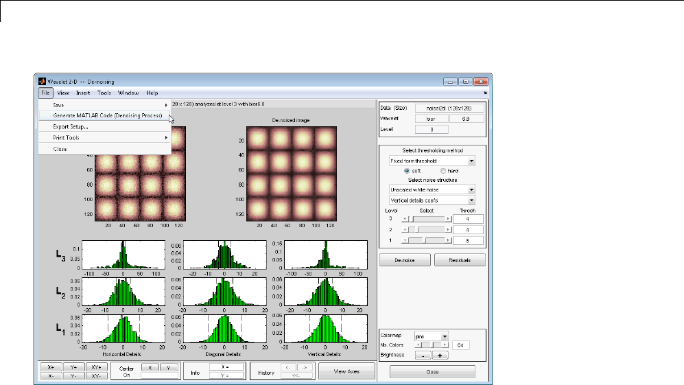
7Generating MATLAB®Code from Wavelet Toolbox™ GUI
The operation generates the following MATLAB code.
function [XDEN,cfsDEN,dimCFS] = func_denoise_dw2d(X)
% FUNC_DENOISE_DW2-D Saved Denoising Process.
% X: matrix of data
% -----------------
% XDEN: matrix of denoised data
% cfsDEN: decomposition vector (see WAVEDEC2)
% dimCFS: corresponding bookkeeping matrix
% Analysis parameters.
%---------------------
wname = 'bior6.8';
level=3;
%De
noising parameters.
%-----------------------
%me
th = 'sqtwolog';
%sc
al_OR_alfa = one;
7-14

Generating MATLAB®Code for 2-D Decimated Wavelet Denoising and Compression
sorh = 's'; % Specified soft or hard thresholding
thrParams = [...
8.00000000 4.00000000 4.00000000 ; ...
8.00000000 4.00000000 4.00000000 ; ...
8.00000000 4.00000000 4.00000000 ...
];
roundFLAG = true;
% Denoise using CMDDENOISE.
%--------------------------
[coefs,sizes] = wavedec2(X,level,wname);
[XDEN,cfsDEN,dimCFS] = wdencmp('lvd',coefs,sizes, ...
wname,level,thrParams,sorh);
if roundFLAG , XDEN = round(XDEN); end
if isequal(class(X),'uint8') , XDEN = uint8(XDEN); end
7Save func_denoise_dw2d.m in a folder on the MATLAB search path, and
execute the following code.
load noissi2d.mat;
noissi2d = X;
[XDEN,cfsDEN,dimCFS] = func_denoise_dw2d(noissi2d);
8Save your denoised image in a folder on the MATLAB search path as
denoisedsin.mat.
7-15

7Generating MATLAB®Code from Wavelet Toolbox™ GUI
Load the denoised image in the MATLAB workspace. Compare the result
with your generated code.
load denoisedsin.mat;
% denoised image loaded in variable X
subplot(121);
imagesc(X); title('Image denoised in the GUI');
subplot(122);
imagesc(XDEN); title('Image denoised with generated code');
%Normof the difference is zero
norm(XDEN-X,2)
7-16
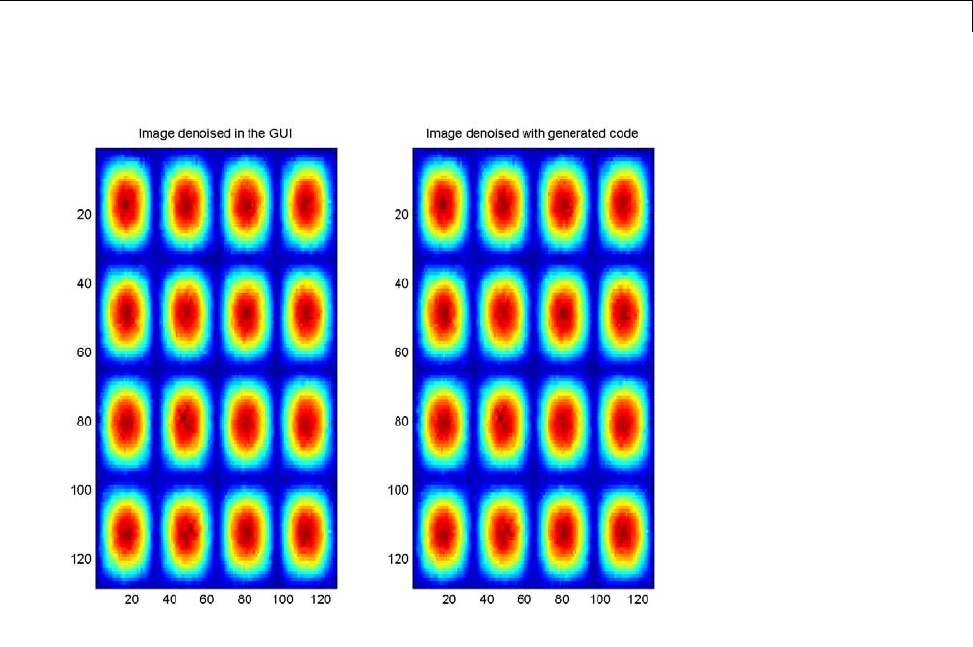
Generating MATLAB®Code for 2-D Decimated Wavelet Denoising and Compression
2-D Decimated Discrete Wavelet Transform
Compression
You can generate MATLAB code to reproduce GUI-based 2-D decimated
wavelet compression at the command line. You must perform this operation
in the Wavelet 2-D --Compression tool. You must first compress your image
beforeyoucanenabletheFile > Generate Matlab Code (Compression
Process) operation.
1Enterwavemenu at the MATLAB command prompt.
2Select Wavelet 2-D.
3Select File > Load > Image andloadthedetfingr.mat indexed image
from the matlab/toolbox/wavelet/wavedemo folder. When the Loading
an Image dialog appears, select No to load the grayscale image.
7-17

7Generating MATLAB®Code from Wavelet Toolbox™ GUI
4Select the bior3.5 wavelet, and set Level to 3.
5Click Analyze,thenclickCompress.
6Using the default Global thresholding,setSelect thresholding
method to Bal.sparsity-norm (sqrt).
7Click Compress.
8File > Generate Code (Compression Process) generates the following
code.
function [XCMP,cfsCMP,dimCFS] = func_compress_dw2d(X)
% FUNC_COMPRESS_DW2D Saved Compression Process.
% X: matrix of data
% -----------------
% XCMP: matrix of compressed data
% cfsCMP: decomposition vector (see WAVEDEC2)
% dimCFS: corresponding bookkeeping matrix
% Analysis parameters.
%---------------------
wname = 'bior3.5';
level = 3;
% Compression parameters.
%------------------------
% meth = 'sqrtbal_sn';
sorh = 'h'; % Specified soft or hard thresholding
thrSettings = 10.064453124999996;
roundFLAG = true;
% Compression using WDENCMP.
%--------------------------
[coefs,sizes] = wavedec2(X,level,wname);
[XCMP,cfsCMP,dimCFS] = wdencmp('gbl',coefs,sizes, ...
wname,level,thrSettings,sorh,1);
if roundFLAG , XCMP = round(XCMP); end
if isequal(class(X),'uint8') , XCMP = uint8(XCMP); end
7-18

Generating MATLAB®Code for 2-D Decimated Wavelet Denoising and Compression
9Save the MATLAB program, func_compress_dw2d.m,inafolderonthe
MATLAB search path. Execute the following code at the command line.
load detfingr.mat;
% Image data is in X
[XCMP,cfsCMP,dimCFS] = func_compress_dw2d(X);
10 Save the compressed image from the Wavelet 2-D - - Compression tool in
a folder on the MATLAB search path. Use File > Save > Compressed
Image,andnamethefilecompressed_fingerprint.mat.Executethe
following code.
load compressed_fingerprint.mat;
% Image data is in X
norm(XCMP-X,2)
7-19

7Generating MATLAB®Code from Wavelet Toolbox™ GUI
Generating MATLAB Code for 1-D Stationary Wavelet
Denoising
YoucangenerateMATLABcodetoreproduce GUI-based 1-D nondecimated
(stationary) wavelet denoising at the command line. You must perform this
operation in the Stationary Wavelet Transform Denoising 1-D tool. You
must first denoise your signal before you can enable the File > Generate
Matlab Code (Denoising Process) operation.
1-D Stationary Wavelet Transform Denoising
1Enter wavemenu at the MATLAB command prompt.
2Select SWT Denoising 1-D.
3Load the Noisy bumps example. Select File > Example Analysis > Noisy
Signals > with sym4 at level 5 - - -> Noisy bumps
7-20
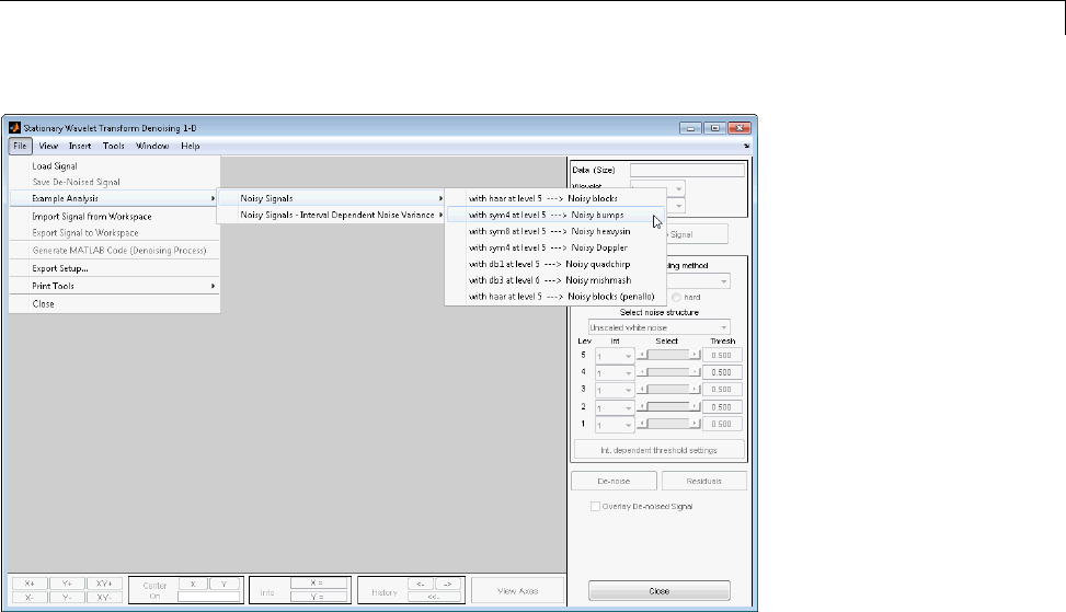
Generating MATLAB®Code for 1-D Stationary Wavelet Denoising
4Set the thresholds as follows:
•Level 1 — 3.5
•Level 2 — 3.4
•Level 3 —2.3
•Level 4 —5.3
•Level 5—2.2
Click De-noise.
7-21
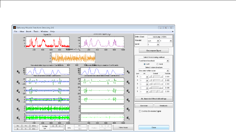
7Generating MATLAB®Code from Wavelet Toolbox™ GUI
5Generate the MATLAB code with File > Generate Matlab Code
(Denoising Process).
7-22
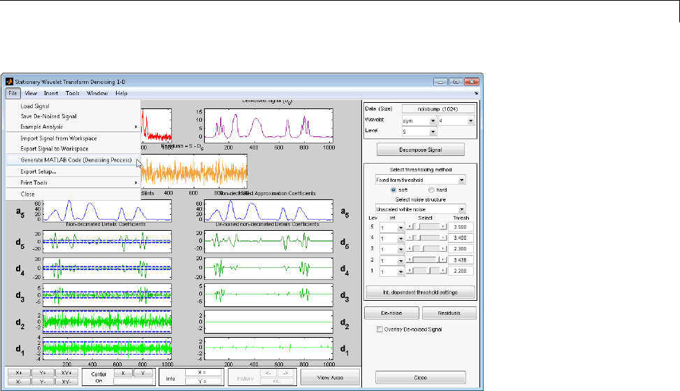
Generating MATLAB®Code for 1-D Stationary Wavelet Denoising
The operation generates the following MATLAB code.
function [sigDEN,wDEC] = func_denoise_sw1d(SIG)
% FUNC_DENOISE_SW1-D Saved Denoising Process.
% SIG: vector of data
% -------------------
% sigDEN: vector of denoised data
% wDEC: stationary wavelet decomposition
% Analysis parameters.
%---------------------
wname = 'sym4';
level = 5;
% Denoising parameters.
%----------------------
% meth = 'sqtwolog';
% scal_OR_alfa = one;
sorh = 's'; % Specified soft or hard thresholding
thrParams = {...
7-23

7Generating MATLAB®Code from Wavelet Toolbox™ GUI
[...
1.00000000 1024.00000000 3.50000000; ...
]; ...
[...
1.00000000 1024.00000000 3.40000000; ...
]; ...
[...
1.00000000 1024.00000000 2.30000000; ...
]; ...
[...
1.00000000 1024.00000000 5.29965570; ...
]; ...
[...
1.00000000 1024.00000000 2.20000000; ...
]; ...
};
% Decompose using SWT.
%---------------------
wDEC = swt(SIG,level,wname);
% Denoise.
%---------
len = length(SIG);
fork=1:level
thr_par = thrParams{k};
if ~isempty(thr_par)
NB_int = size(thr_par,1);
x = [thr_par(:,1) ; thr_par(NB_int,2)];
x = round(x);
x(x<1) = 1;
x(x>len) = len;
thr = thr_par(:,3);
for j = 1:NB_int
if j==1 , d_beg = 0; else d_beg = 1; end
j_beg = x(j)+d_beg;
j_end = x(j+1);
j_ind = (j_beg:j_end);
wDEC(k,j_ind) = wthresh(wDEC(k,j_ind),sorh,thr(j));
end
7-24
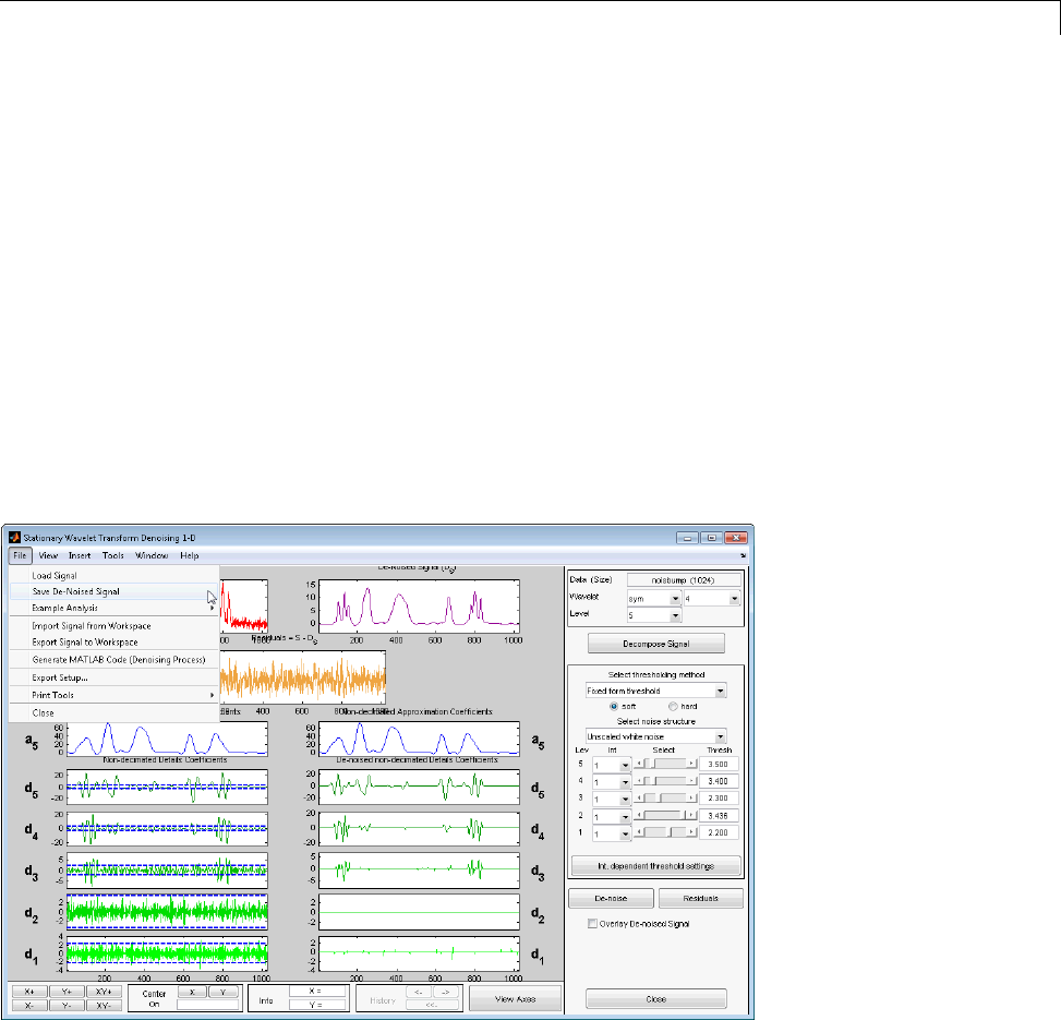
Generating MATLAB®Code for 1-D Stationary Wavelet Denoising
end
end
% Reconstruct the denoise signal using ISWT.
%-------------------------------------------
sigDEN = iswt(wDEC,wname);
6Save func_denoise_sw1d.m in a folder on the MATLAB search path.
Execute the following code.
load noisbump.mat;
[sigDEN,wDEC] = func_denoise_sw1d(noisbump);
7Select File > Save De-noised Signal, and save the denoised signal as
denoisedbumps.mat in a folder on the MATLAB search path.
Execute the following code.
load denoisedbump.mat;
plot(sigDEN,'k'); axis tight;
hold on;
7-25

7Generating MATLAB®Code from Wavelet Toolbox™ GUI
plot(denoisedbump,'r');
% norm of the difference
norm(sigDEN-denoisedbump,2)
7-26
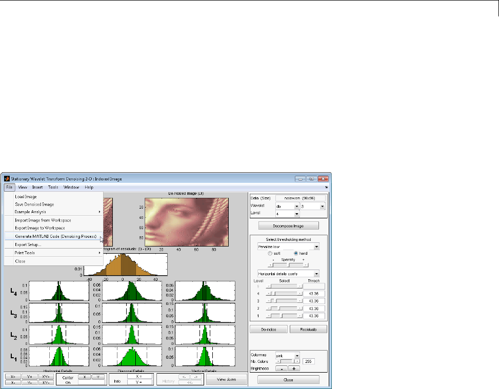
Generating MATLAB®Code for 2-D Stationary Wavelet Denoising
Generating MATLAB Code for 2-D Stationary Wavelet
Denoising
You can generate MATLAB code to reproduce GUI-based 2-D stationary
wavelet denoising at the command line. You can generate code to denoise both
indexed and truecolor images. You must perform this operation in the SWT
Denoising 2-D tool. You must first denoise your image before you can enable
the File > Generate Matlab Code (Denoising Process) operation.
2-D Stationary Wavelet Transform Denoising
1Enter wavemenu at the MATLAB command prompt.
2Select SWT Denoising 2-D.
3Select File > Load Image,andloadnoiswom.mat from the
matlab/toolbox/wavelet/wavedemo folder.
Choose No when prompted to use the grayscale image.
7-27

7Generating MATLAB®Code from Wavelet Toolbox™ GUI
4Select the db4 wavelet, and set the Level to 5.
5Click Decompose Image.
6Use the default soft thresholding method with Fixed form threshold
and Unscaled white noise for Select noise structure.
7Set the following thresholds for the horizontal, diagonal, and vertical
details. Ensure that you set the thresholds for the three detail coefficient
types.
•Level 1 — 5
•Level 2 — 4
•Level 3 — 3
•Level 4 — 2
•Level 5 — 1
8Click De-noise.
9Select File > Generate Matlab Code (Denoising Process).
The operation generates the following MATLAB code.
function [XDEN,wDEC] = func_denoise_sw2d(X)
% FUNC_DENOISE_SW2D Saved Denoising Process.
% X: matrix of data
% -----------------
% XDEN: matrix of denoised data
% wDEC: stationary wavelet decomposition
% Analysis parameters.
%---------------------
wname = 'db2';
level = 5;
% Denoising parameters.
%-----------------------
% meth = 'sqtwolog';
% scal_OR_alfa = one;
sorh = 's'; % Specified soft or hard thresholding
7-28

Generating MATLAB®Code for 2-D Stationary Wavelet Denoising
thrSettings = [...
1.0000 2.0000 3.0000 4.0000 5.0000 ; ...
1.0000 2.0000 3.0000 4.0000 5.0000 ; ...
1.0000 2.0000 3.0000 4.0000 5.0000 ...
];
roundFLAG = false;
% Decompose using SWT2.
%---------------------
wDEC = swt2(X,level,wname);
% Denoise.
%---------
permDir = [1 3 2];
for j = 1:level
for kk=1:3
ind = (permDir(kk)-1)*level+j;
thr = thrSettings(kk,j);
wDEC(:,:,ind) = wthresh(wDEC(:,:,ind),sorh,thr);
end
end
% Reconstruct the denoise signal using ISWT2.
%-------------------------------------------
XDEN = iswt2(wDEC,wname);
if roundFLAG , XDEN = round(XDEN); end
10 Save this MATLAB program as func_denoise_sw2d.m in a folder on the
MATLAB search path.
Execute the following code.
load noiswom
[XDEN,wDEC] = func_denoise_sw2d(X);
11 Save the denoised image as denoisedwom.mat in a folder on the MATLAB
search path.
7-29
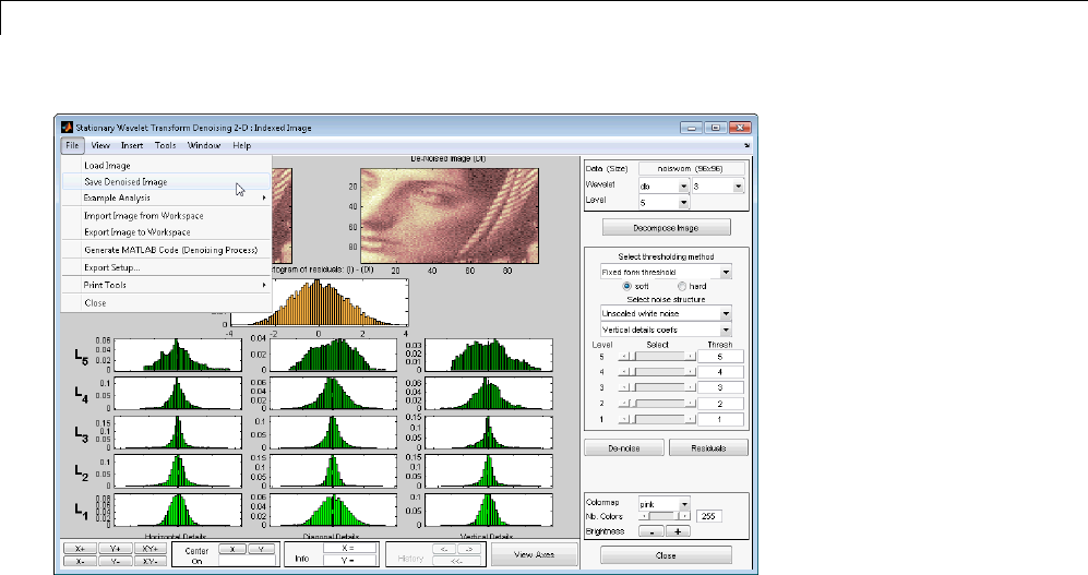
7Generating MATLAB®Code from Wavelet Toolbox™ GUI
12 Execute the following code.
load denoisedwom
% Compare the GUI and command line results
imagesc(X); title('GUI Operation'); colormap(gray);
figure;
imagesc(XDEN); title('Command Line Operation');
colormap(gray);
norm(XDEN-X,2)
7-30
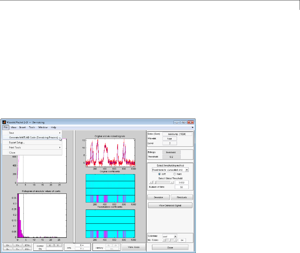
Generating MATLAB®Code for 1-D Wavelet Packet Denoising and Compression
Generating MATLAB Code for 1-D Wavelet Packet
Denoising and Compression
1-D Wavelet Packet Denoising
You can generate MATLAB code to reproduce GUI–based 1-D wavelet
packet denoising at the command line. You must perform this operation in
the WaveletPacket1-D--De-noisingtool. You must first denoise your
signal before you can enable the File > Generate Matlab Code (Denoising
Process) operation.
1Enter wavemenu at the MATLAB command prompt.
2Select Wavelet Packet 1-D.
3Select File > Load Signal and load noisbump.mat from the
matlab/toolbox/wavelet/wavedemo folder.
4Select the db4 wavelet, and set the Level to 4. Accept the default value
Shannon for Entropy.
7-31

7Generating MATLAB®Code from Wavelet Toolbox™ GUI
5Click Analyze.
6Click De-noise.
7Under Select thresholding method, accept the default Fixed form thr.
(unscaled wn) with the soft radio button enabled.
Set Select Global Threshold to 2.75.
8Click De-noise.
9Select File > Generate Matlab Code (Denoising Process)
The operation generates the following MATLAB code.
function [sigDEN,wptDEN] = func_denoise_wp1d(SIG)
% FUNC_DENOISE_WP1D Saved Denoising Process.
% SIG: vector of data
% -------------------
% sigDEN: vector of denoised data
% wptDEN: wavelet packet decomposition (wptree object)
% Analysis parameters.
%---------------------
Wav_Nam = 'db4';
Lev_Anal = 4;
Ent_Nam = 'shannon';
Ent_Par = 0;
% Denoising parameters.
%----------------------
% meth = 'sqtwologuwn';
sorh = 's'; % Specified soft or hard thresholding
thrSettings = {sorh,'nobest',2.750000000000000,1};
% Decompose using WPDEC.
%----------------------
wpt = wpdec(SIG,Lev_Anal,Wav_Nam,Ent_Nam,Ent_Par);
% Nodes to merge.
7-32
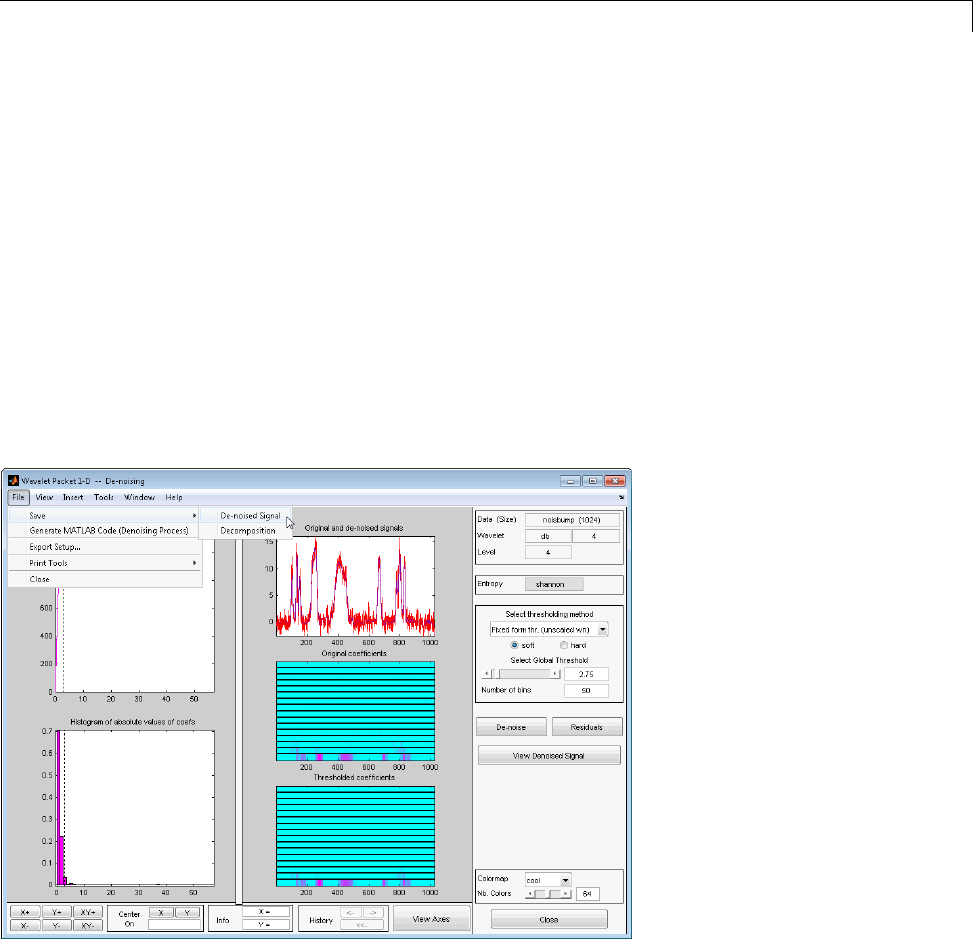
Generating MATLAB®Code for 1-D Wavelet Packet Denoising and Compression
%-----------------
n2m = [];
forj=1:length(n2m)
wpt = wpjoin(wpt,n2m(j));
end
% Denoise using WPDENCMP.
%------------------------
[sigDEN,wptDEN] = wpdencmp(wpt,thrSettings{:});
Save func_denoise_wp1d.m in a folder on the MATLAB search path.
Save the denoised signal from the Wavelet Packet 1-D - - De-noising tool
as wp_denoisedbump.mat in a folder on the MATLAB search path.
Execute the following code.
load noisbump;
[sigDEN,wptDEN] = func_denoise_wp1d(noisbump);
7-33
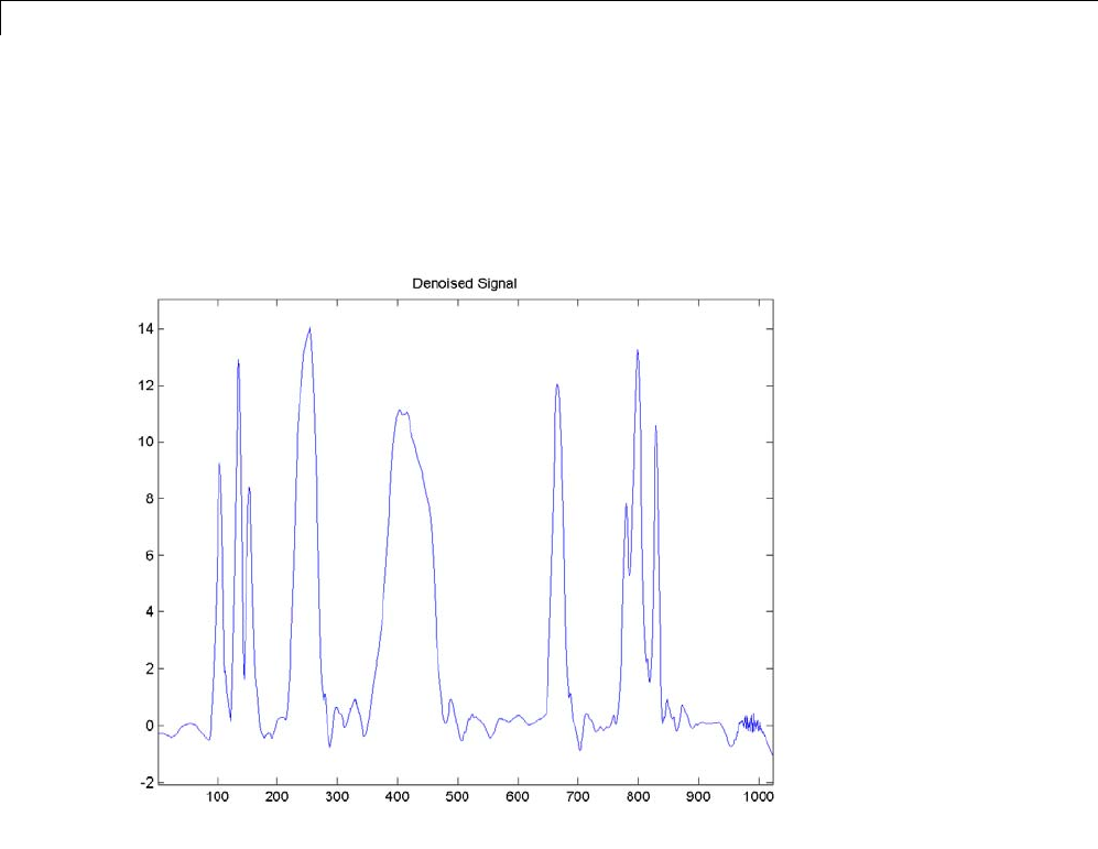
7Generating MATLAB®Code from Wavelet Toolbox™ GUI
load wp_denoisedbump;
plot(sigDEN); title('Denoised Signal');
axis([1 1024 min(sigDEN)-1 max(sigDEN+1)]);
norm(sigDEN-wp_denoisedbump,2)
7-34

Generating MATLAB®Code for 2-D Wavelet Packet Denoising and Compression
Generating MATLAB Code for 2-D Wavelet Packet
Denoising and Compression
2-D Wavelet Packet Compression
You can generate MATLAB code to reproduce GUI–based 2-D wavelet packet
compression at the command line. You must perform this operation in the
Wavelet 2-D - - Compression tool. You must first compress your image
before you can enable the File > Generate Matlab Code (Compression
Process) operation.
1Enter wavemenu at the MATLAB command prompt.
2Select Wavelet Packet 2-D.
3Select File > Load > Example Analysis > Indexed Images,andload
the tire.
4Using the default parameter settings, click Best Tree.
7-35
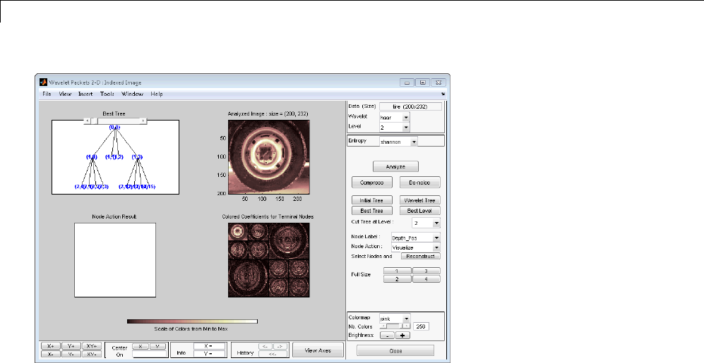
7Generating MATLAB®Code from Wavelet Toolbox™ GUI
5Click Compress.
6Set Select thresholding method to Bal.sparsity-norm (sqrt).
7Click Compress.
7-36
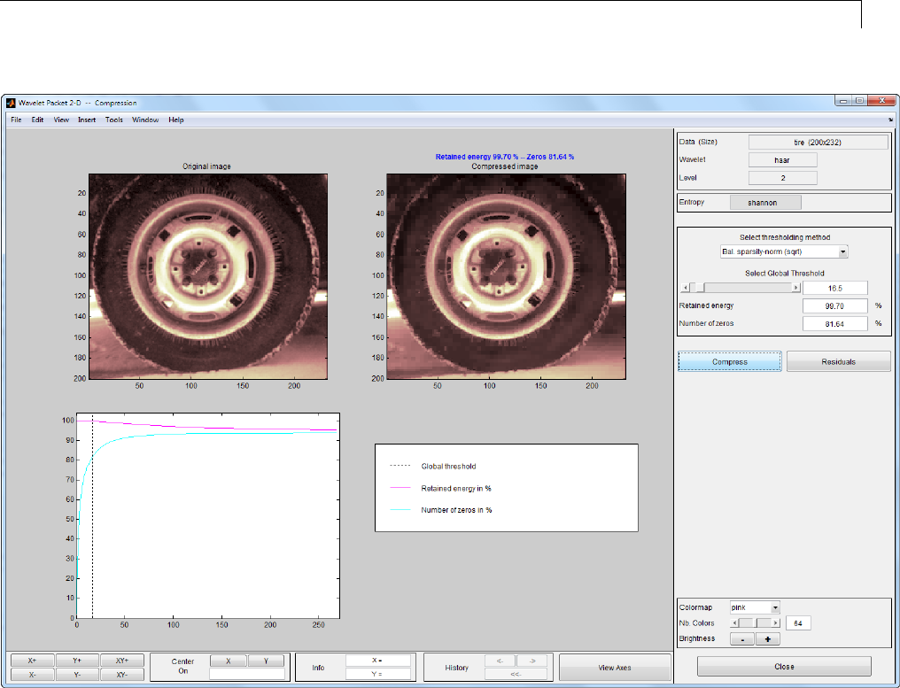
Generating MATLAB®Code for 2-D Wavelet Packet Denoising and Compression
8File > Generate Code (Compression Process) generates the following
code.
function [XCMP,wptCMP] = func_compress_wp2d(X)
% FUNC_COMPRESS_WP2D Saved Compression Process.
% X: matrix of data
% -----------------
% XCMP: matrix of compressed data
% wptCMP: wavelet packet decomposition (wptree object)
% Analysis parameters.
7-37

7Generating MATLAB®Code from Wavelet Toolbox™ GUI
%---------------------
Wav_Nam = 'haar';
Lev_Anal = 2;
Ent_Nam = 'shannon';
Ent_Par = 0;
% Compression parameters.
%-----------------------
% meth = 'sqrtbal_sn';
sorh = 'h'; % Specified soft or hard thresholding
thrSettings = {sorh,'nobest',16.499999999999886,1};
roundFLAG = true;
% Decompose using WPDEC2.
%-----------------------
wpt = wpdec2(X,Lev_Anal,Wav_Nam,Ent_Nam,Ent_Par);
% Nodes to merge.
%-----------------
n2m=[2 3];
forj=1:length(n2m)
wpt = wpjoin(wpt,n2m(j));
end
% Compression using WPDENCMP.
%----------------------------
[XCMP,wptCMP] = wpdencmp(wpt,thrSettings{:});
if roundFLAG , XCMP = round(XCMP); end
if isequal(class(X),'uint8') , XCMP = uint8(XCMP); end
9Save the generated MATLAB code as func_compress_wp2d.m in a folder on
the MATLAB search path, and execute the following code.
load tire;
[XCMP,wptCMP] = func_compress_wp2d(X);
10 Save the compressed image from the Wavelet 2-D -- Compression tool as
compressed_tire.mat in a folder on the MATLAB search path. Use File >
Save > Compressed Image to save the compressed image.
11 Execute the following code to compare the command line and GUI result.
7-38

Generating MATLAB®Code for 2-D Wavelet Packet Denoising and Compression
load compressed_tire.mat;
norm(XCMP-X,2)
7-39

7Generating MATLAB®Code from Wavelet Toolbox™ GUI
7-40

A
GUI Reference
This appendix explains some of the features of the Wavelet Toolbox graphical
user interface (GUI).
•“General Features” on page A-2
•“Continuous Wavelet Tool Features” on page A-12
•“Wavelet 2-D Tool Features” on page A-13
•“Wavelet Packet Tool Features (1-D and 2-D)” on page A-14
•“Wavelet Display Tool” on page A-16
•“Wavelet Packet Display Tool” on page A-17

AGUI Reference
General Features
Some features of the Wavelet Toolbox graphical user interface are
•Color coding
•Connectedness of plots
•Using the mouse
•Controlling the colormap
•Controlling the number of colors
•Controlling the coloration mode
•Customizing graphical objects
•Zoominginonplots
•Using menus
•Using View Axes button
•Using Interval Dependent Threshold Settings tool
Note In this appendix, axis (or axes) refers to the MATLAB graphic object.
Color Coding
In all the graphical tools, signals and analysis components are color coded as
follows.
Signal Shown In
Original Red
Reconstructed or synthesized Yellow
Approximations Variegated shades of blue
(high level = darker)
Details Variegated shades of green
(high level = darker)
A-2
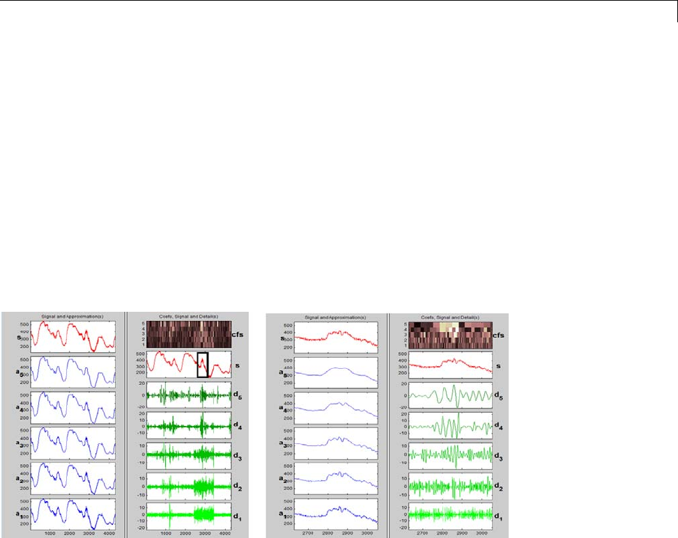
General Features
Connection of Plots
Plots containing related information and graphed on the same abscissa are
connected in the sense that manipulations performed on one plot affect all
others in the same way. For images, the connection holds in both abscissa and
ordinate. You can manipulate all plots along an individual axis (X or Y) or you
can manipulate all plots along both axes at the same time (XY).
For example, the approximations and details shown in the separate mode
view of a decomposition all respond together when any of the plots is
magnified or zoomed.
Click and drag your mouse over the region you want to zoom. Clicking XY+
results in the zoom being applied to all the plots.
•Zoom inonrelevantdetail.
One advantage of using the graphical interface tools is that you can zoom
in easily on any part of the signal and examine it in greater detail.
Drag a rubber band box (by holding down the left mouse button) over the
portion of the signal you want to magnify. Here, we’ve selected the noisy
part of the original signal.
A-3

AGUI Reference
Click the X+ button (located at the bottom of the screen) to zoom
horizontally.
The Wavelet 1-D tool zooms all the displayed signals.
The other zoom controls do more or less what you’d expect them to. The
X- button, for example, zooms out horizontally. The history function keeps
A-4
General Features
track of all your views of the signal. Return to a previous zoom level by
clicking the left arrow button.
•ZoominginonDetail
Drag a rubber band box (by holding down the left mouse button) over the
portion of the image you want to magnify.
Click the XY+ button (located at the bottom of the screen) to zoom
horizontally and vertically.
•The History pane enables you to remember how you zoom the axes so that
you can toggle back and forth between views.
Using the Mouse
Wavelet Toolbox software uses three types of mouse control.
Left Mouse Button Middle Mouse Button Right Mouse Button
Make selections.
Activate controls.
Display cross-hairs
to show
position-dependent
information.
Translate plots up and
down, and left and
right.
A-5
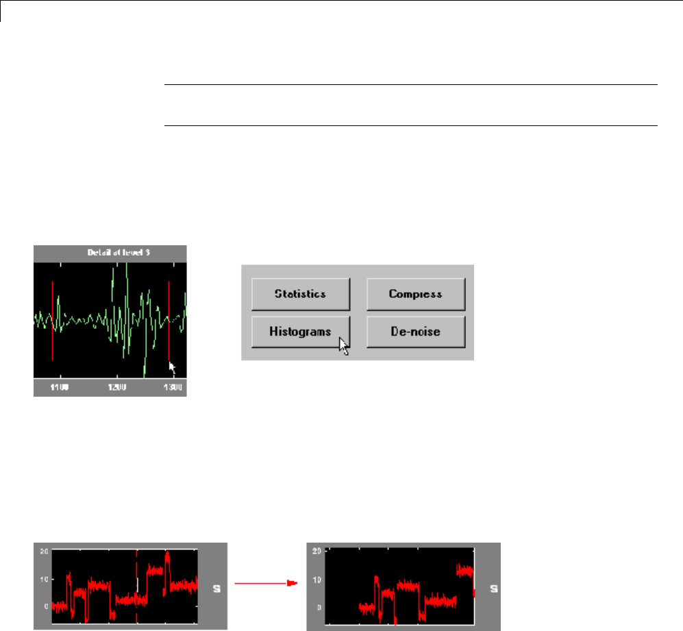
AGUI Reference
Note The functionality of the middle mouse button and the right mouse
button can be inverted depending on the platform.
Making Selections and Activating Controls
Most of your work with Wavelet Toolbox graphical tools involves making
selections and activating controls. You do this using the left (or only) mouse
button.
Translating Plots
By holding down the right mouse button (or its equivalent on a one- or
two-button mouse), you can move the mouse to draw a rectangle in either a
horizontal or vertical orientation. Releasing the middle mouse button then
causes the plot to shift horizontally (or vertically) by an amount proportional
to the width (or height) of the rectangle.
Displaying Position-Dependent Information
When you hold down the middle mouse button (or its equivalent on a one-
or two-button mouse), a cross-hair cursor appears over the graph or plot.
Position-dependent information also appears in the Info box located at the
A-6
General Features
bottom center of the tool. The type of information that appears depends on
what tool you are using and the plot in which your cursor is located..
Controlling the Colormap
The Colormap selection box, located at the lower right of the window, allows
you to adjust the colormap that is used to plot images or coefficients (wavelet
or wavelet packet).
This is more than an aesthetic adjustment because you are likely to see
different features depending on your colormap selection.
Controlling the Number of Colors
The Nb. Colors slider, located at the bottom right of the window, allows you
to adjust how many colors the tool uses to plot images or coefficients (wavelet
or wavelet packet). You can also use the edit control to adjust the number
of colors. Adjusting the number of colors can highlight different features of
the plot.
Consider the coefficients plot of the Koch curve generated in the Continuous
Wavelet tool, shown here using 129 colors.
A-7
AGUI Reference
and here using 68 colors.
Controlling the Coloration Mode
In the Continuous Wavelet tools, the coloration of coefficients can be done
in several different ways.
Colorationmode—Threeparametersareused color the coefficients.
•init or current —Whenyouselectinit, coloration is performed with
all the coefficient values. When you select current, only the coefficients
displayed in the current axis limits are used.
•by scalesor all scales —Whenyouselectby scale, the coloration is
done separately for each scale. When you select all scales,allscales
are used.
•abs —Wh
en you select abs, the absolute values of the coefficients are used.
In the Wavelet 1-D tool, you access coefficients coloration with the More
Display Options button, and then select the desired Coloration Mode
option.
A-8
General Features
The More Display Options button appears only when the Display mode
is one of the following — Show and Scroll, Show and Scroll (Stem Cfs),
Superimposed, and Separate). In this case, scales are replaced by levels in
all options of the Coloration Mode menu.
Using Menus
General Menu Bar
At the top of most windows you find the same kind of structure. The menu
bar of each figure in Wavelet Toolbox software is very similar to the menu
bar of the default MATLAB figures. You can use many of the tools that are
offered in the menus and associated toolbar of the standard MATLAB figures.
One of the main differences is the View menu, which depends on the current
tool used.
View Dynamical Visualization Tool Option. The View > Dynamical
Visualization Tool option lets you enable or disable the Dynamical
Visualization Tool located at the bottom of each window.
Enabling the Dynamical Visualization Tool activates the zoom, center,
history, and axes options at the bottom of the interactive tool.
Before using Zoom In,Zoom Out,orRotate 3D options (or the equivalent
icons from the toolbar), you must disable the Dynamical Visualization
Tool to avoid possible conflicts.
Default Display Mode Option. The Default Display Mode option is
specific to the Wavelet 1-D tool and lets you set a default Display Mode for
all the different analyses you perform inside the same tool.
A-9
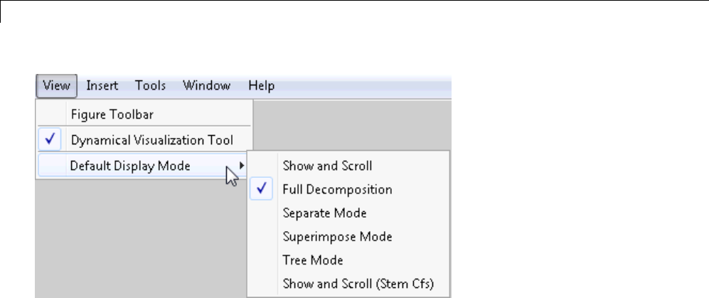
AGUI Reference
Using the View Axes Button
The Dynamical Visualization Tool is located at the bottom of most of the
windows in the Wavelet Toolbox software. In this tool, the View Axes toggle
button lets you magnify the axis that you choose.
A-10
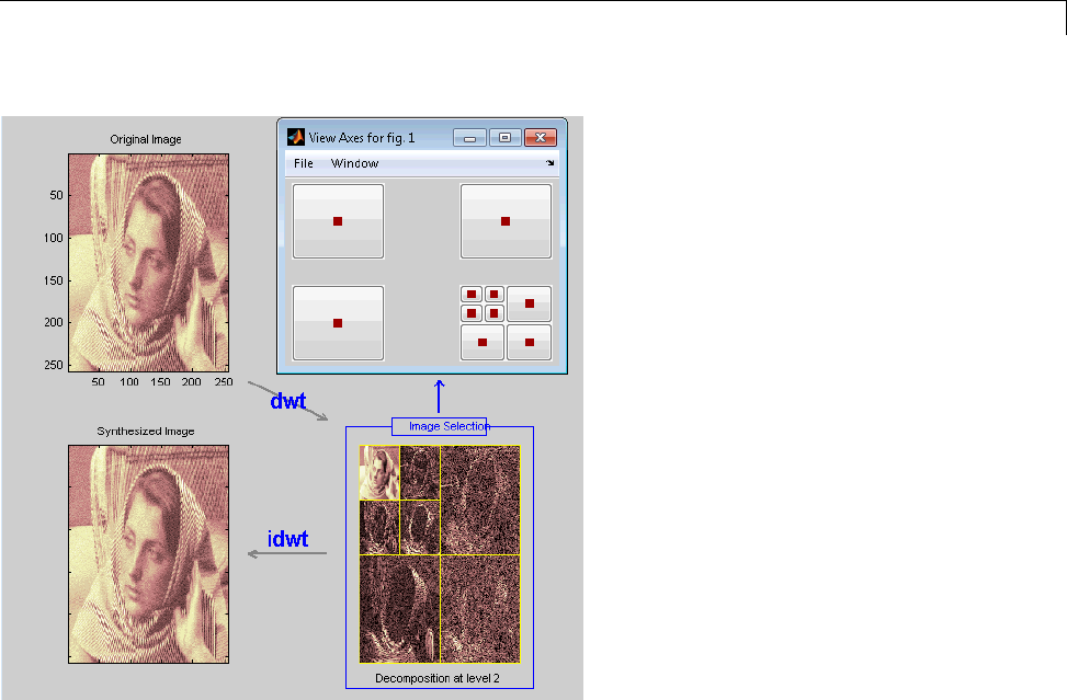
General Features
The toggle buttons in the View Axes figure are positioned so that you can
understand which axis is correlated with a button.
When youclickthesametogglebuttonagain,yourestoretheoriginalview.
Clicking the View Axes toggle button again closes the View Axes figure.
A-11
AGUI Reference
Continuous Wavelet Tool Features
Here is an example of an option that allows you to perform analysis using
different scale modes.
Scale Settings
•Step by Step Mode — Specify the initial scale, the step size, and the
maximum scale.
•Power 2 Mode — The scales are 20,2
1, up to power you select in the Power
drop down menu. These are the same scales used for discrete analysis.
•Manual Mode —Enteravectorofscales.
A-12
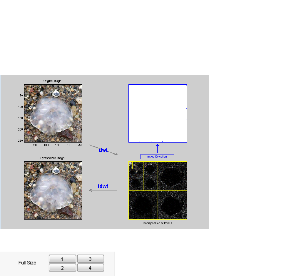
Wavelet 2-D Tool Features
Wavelet 2-D Tool Features
The Wavelet 2-D tool is described in “Two-Dimensional Discrete Wavelet
Analysis” on page 3-137. Here is an example of an option that allows you to
view a selected part of the window at a full window resolution.
In the Full Size menu on the right side of the interactive tool
choose the image you want to view as full size. Click your selection again
to restore the original view.
A-13

AGUI Reference
Wavelet Packet Tool Features (1-D and 2-D)
Coefficients Coloration
NAT or FRQ is for Natural or Frequency order.
By level or Global is for a coloration made level by level or taking all detail
levels.
abs is used to take the absolute values of coefficients.
Node Action
When you select a node in the tree, the selected option is performed. A
complete description of options is provided in the following sections.
Node Label
Thenodelabelscanbechangedusingthepop-upmenu. Forexample,the
Type option labels the nodes with (a) for approximation and (d) for detail.
Node Action Functionality
TheavailableoptionsintheNode Action menu are
•Visualize: When you select a node in the wavelet packet tree the
corresponding signal appears.
•Split/Merge: If a terminal node is selected, it is split, growing the wavelet
packet tree. Selecting other nodes has the behavior of merging all the nodes
below it in the wavelet packet tree.
•Recons.: When you select a node in the wavelet packet tree, the
corresponding reconstructed signal appears.
•Select On/Off: When On, you can select many nodes in the wavelet packet
tree. Then you can reconstruct a synthesized signal from the selected nodes
using the Reconstruct button on the main window. Use the Off selection
to deselect all the previous selected nodes.
•Statistics: Whenyouselectanodeinthewaveletpackettree,the
Statistics tool appears using the signal corresponding to the selected node.
A-14

WaveletPacketToolFeatures(1-Dand2-D)
•View Col. Cfs.: When active, this option removes all the colored
coefficients displayed, and lets you redraw only the corresponding
coefficients by selecting a node in the wavelet packet tree.
A-15
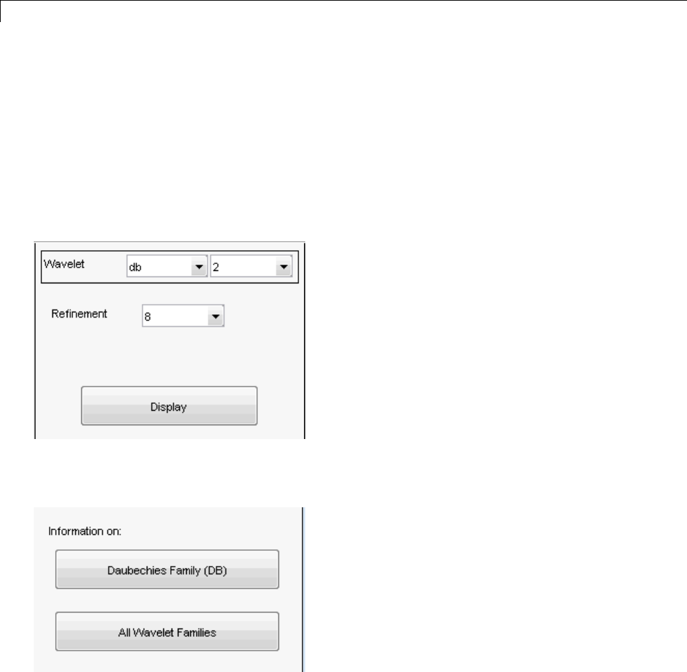
AGUI Reference
Wavelet Display Tool
The Wavelet Display tool is mentioned in the section “Introduction to
Wavelet Families” in the Wavelet Toolbox Getting Started Guide.
The Refinement drop down menu allows you choose the number of points
that the wavelet and scaling functions are computed over. The number of
points are in powers of 2. In the following figure, the db2 scaling and wavelet
functions are computed over a grid of 28points.
The Information on: selections allow you to obtain more detailed
information on the current wavelet family, or all supported families.
A-16
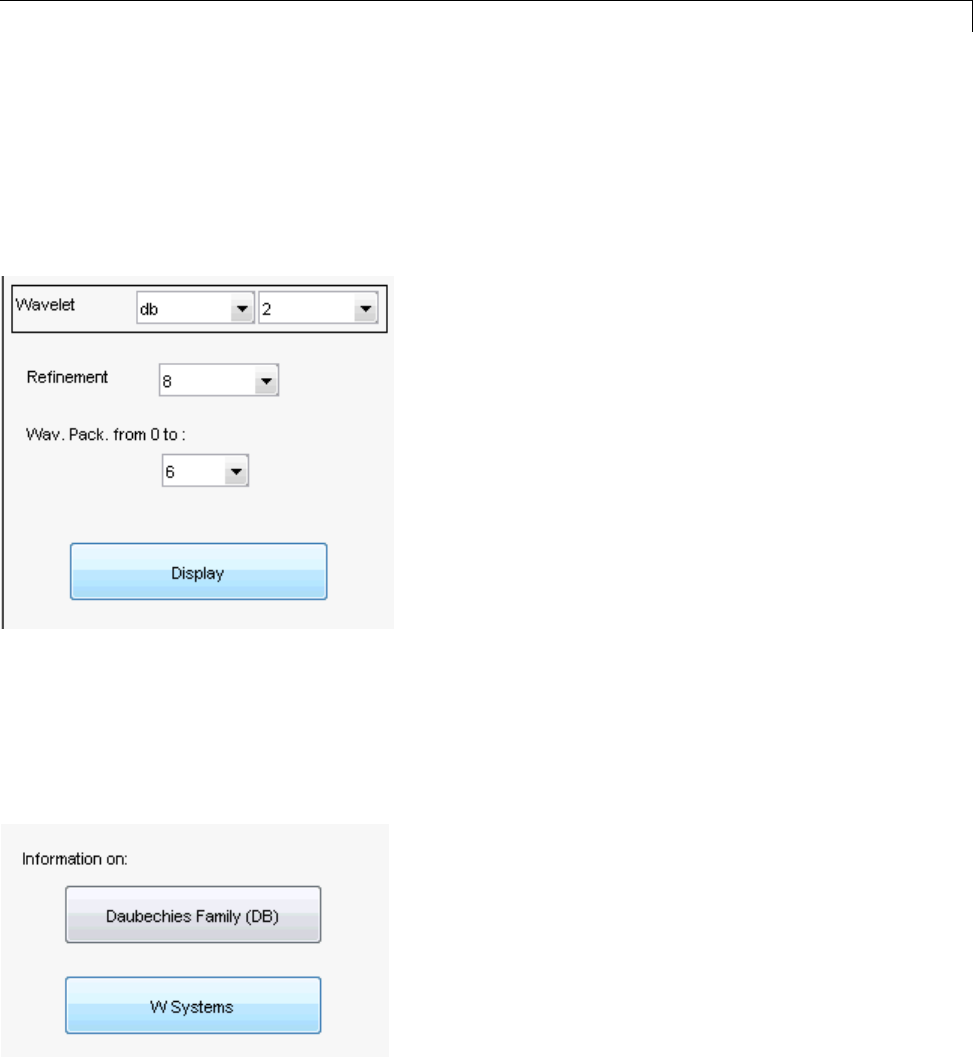
WaveletPacketDisplayTool
Wavelet Packet Display Tool
The Refinement drop down menu allows you choose the number of points
that the wavelet packets are computed over. The number of points are in
powers of 2. In the following figure, the db2 wavelet packets are computed
over a grid of 28points.
The Wav. Pack. from 0 to: allows you to choose the number of wavelet
packets to display.
The Information on: selections allow you to obtain more detailed
information on the current wavelet family, Daubechies Family (DB),or
wavelet packets in general, WSystems.
A-17

AGUI Reference
A-18

Index
IndexA
adding a new wavelet 1-26
algorithms
decomposition 3-40
discrete wavelet transform (DWT) 3-37
fast wavelet transform (FWT) 3-37
filters 3-37
for biorthogonal 3-45
Mallat 3-37
polyphase 1-50
rationale 3-45
reconstruction 3-47
stationary wavelet transform (SWT) 3-62
analysis
continuous
features 2-2
continuous complex 2-21
continuous real 2-2
discrete 3-2
one-dimensional discrete wavelet 3-2
one-dimensional wavelet packet 4-7
orthogonal
algorithm 3-45
filters 3-37
translation invariant 3-62
two-dimensional discrete wavelet 3-137
two-dimensional wavelet packet 4-15
wavelet packet 4-2
approximations
coefficients
discrete wavelet transform 3-40
extracting one-dimensional 3-6
extracting two-dimensional 3-143
reconstruction
example code 3-6
axes
view A-10
B
bases.Seeanalysis,wavelet packets
besttree function 4-51
binning
processed data 5-84
biorthogonal wavelets
definition 1-10
border distortion
boundary value replication 3-52
periodic extension 3-52
periodic padding 3-53
periodized wavelet transform 3-62
smooth padding 3-53
symmetric extension 3-52
symmetrization 3-52
zero-padding 3-52
breakdowns
variance 5-14
C
calculating a default global threshold 3-77
coefficients
approximation
extracting one-dimensional 3-6
fast wavelet transform 3-40
coloration A-14
complex continuous wavelet 2-23
continuous wavelet 2-5
detail
fast wavelet transform 3-40
one-dimensional 3-6
two-dimensional 3-143
discrete wavelet
Wavelet 1-D tool 3-35
Wavelet 2-D tool 3-162
line 2-10
load.Seeimporting to the GUI
save.Seeexporting from the GUI
coiflets
Index-1

Index
definition 1-9
Coloration Mode
color coding A-2
controlling A-8
controlling the colormap A-7
Coloration Mode menu 2-18
complex frequency B-spline wavelets 1-19
complex Gaussian wavelets 1-18
complex Morlet wavelets 1-19
complex Shannon wavelets 1-20
compressing images
true compression 5-55
using graphical interface 3-153
compression
ddencmp function 4-4
difference with de-noising 5-51
energy ratio 5-54
norm recovery 5-54
number of zeros 5-54
procedure
wavelet packets 4-5
wavelets 5-51
retained energy 5-53
true 5-55
using wavelet packets 4-18
continuous wavelet transform (CWT) 2-18
See also analysis, transforms
CWT.Seecontinuous wavelet transform (CWT)
D
ddencmp command 3-77
de-noising
basic model
two-dimensional 5-12
default values 4-4
fixed form threshold 5-5
minimax performance 5-5
noise size estimate 5-8
nonwhite noise 5-8
procedure
wavelet packets 4-5
SURE estimate 5-5
thresholding 3-10
using SWT
1-D using command line 3-77
1-D using graphical interface 3-80
2-D using graphical interface 3-175
using thresholding 3-173
variance adaptive 5-14
de-noising images
stationary wavelet transform 3-178
two-dimensional procedure 5-12
de-noising signals
process 3-8
decomposition
best-level 4-47
choosing optimal 4-41
displaying results of multilevel 3-7
entropy-based criteria 4-42
load.Seeimporting to the GUI
performing multilevel
using command line 3-5
using graphical interface 3-18
save.Seeexporting from the GUI
single-level 3-15
structure
one-dimensional 3-35
two-dimensional 3-162
details
coefficients
extracting one-dimensional 3-6
extracting two-dimensional 3-143
decomposition 4-30
orientation 3-43
reconstruction
from command line 3-6
dilation equation
twin-scale relation 3-37
discrete wavelet transform (DWT) 3-2
Index-2

Index
See also analysis, transforms
display mode 2-D
tree 3-151
downsampling
one-dimensional 3-41
two-dimensional 3-43
DWT.Seediscrete wavelet transform, transforms
E
edge effects.Seeborder distortion
entropy
definitions 4-42
exporting from the GUI
complex continuous wavelet 2-29
continuous wavelet 2-18
discrete stationary wavelet 1-D 3-84
discrete stationary wavelet 2-D 3-179
discrete wavelet 2-D 3-156
discrete wavelet 3-D 3-189
variance adaptive thresholding 5-25
wavelet 1-D 3-28
wavelet packets 4-22
wavelet regression estimation 1-D 5-85
F
fast wavelet transform (FWT).Seetransforms
filters
FIR
MATLAB file used for construction 1-29
high-pass 3-40
low-pass 3-40
quadrature mirror
construction example 3-39
scaling 3-38
frequencies
parameter 4-39
frequency B-spline wavelets 1-19
Full Decomposition Mode 3-19
FWT.Seetransforms
G
Gaussian wavelets 1-14
GUI
complex continuous wavelet 2-24
continuous wavelet 2-8
full window resolution A-13
image de-noising using SWT 3-175
local variance adaptive thresholding 5-17
multiscale principal components
analysis 5-45
multisignal analysis 3-95
multivariate wavelet de-noising 5-34
regression estimation 5-80
signal de-noising using SWT 3-80
true compression 5-61
using menus A-9
using the mouse A-5
wavelet display A-16
wavelet one-dimensional 3-13
wavelet packet 4-7
wavelet packet display A-17
wavelet three-dimensional 3-182
wavelet two-dimensional 3-147
I
IDWT.Seeinverse discrete wavelet transform,
transforms
images
indexed 3-161
importing to the GUI
complex continuous wavelet 2-29
continuous wavelet 2-18
discrete stationary wavelet 1-D 3-84
discrete stationary wavelet 2-D 3-179
discrete wavelet 2-D 3-156
discrete wavelet 3-D 3-189
Index-3

Index
variance adaptive thresholding 5-25
wavelet 1-D 3-28
wavelet packets 4-22
wavelet regression estimation 1-D 5-85
inverse lifting wavelet transform (ILWT) 1-50
inverse stationary wavelet transform
(ISWT) 3-67
L
lifting 1-42
lifting wavelet transform (LWT) 1-50
load.Seeimporting in the GUI
Load data for Stochastic Design Regression
dialog box 5-84
Load Signal dialog box
wavelet packets 4-8
wavelets 3-15
local maxima lines 2-10
M
MATLAB files
for wavelet families 1-29
merge.Seewavelet packets
Mexican hat wavelet
definition 1-15
Meyer wavelet
definition 1-12
minimax 5-5
More Display Options button 3-19
More on Residuals for Wavelet 1-D Compression
window 3-24
Morlet wavelet
definition 1-16
multiresolution 3-45
N
node
action A-14
noise
suppressing 3-3
See also de-noising
unscaled 5-8
nondecimated DWT.Seetransforms (stationary
wavelet)
O
objects 4-53
P
padding.Seeborder distortion
periodic-padding
signal extension 3-53
periodized wavelet transform.Seeborder
distortion
predefined wavelet families
type 1 1-29
type 2 1-30
type 3 1-30
type 4 1-31
type 5 1-31
Q
quadrature mirror filters (QMF)
orthfilt function 3-39
R
reconstruction
MATLAB files 3-49
one step 3-44
one-dimensional IDWT 3-42
two-dimensional IDWT 3-43
regression estimation
one-dimensional wavelet 5-80
regularity
wavelet families 1-22
Index-4

Index
residuals display
1-D discrete wavelet compression 3-24
1-D stationary wavelet decomposition 3-83
2-D discrete wavelet compression 3-156
2-D stationary wavelet decomposition 3-178
reverse biorthogonal wavelets 1-12
S
save.Seeexporting from the GUI
scale
choosing using command line 2-6
choosing using graphical interface 2-24
to frequency
display 2-13
scale mode A-12
scaling filters
definition 3-38
Separate Mode 3-19
Shannon wavelets 1-20
Show and Scroll Mode 3-19
Show and Scroll Mode (Stem Cfs) 3-19
shrink.Seethresholding
signal extensions
border distortion 3-52
signal-end effects.Seeborder distortion
smooth padding
signal extension 3-53
splines
filter lengths 3-45
split.Seewavelet packets
stationary wavelet transform (SWT) 3-62
Superimpose Mode 3-19
support.Seewavelet families
symlets
definition 1-8
symmetrization
signal extension 3-53
symmetry.Seewavelet families
T
thresholding
for optimal de-noising 3-10
hard 5-7
interval dependent 5-15
rules
tptr options 5-4
soft 5-7
thselect MATLAB file 5-4
transforms
fast wavelet (FWT) 3-37
inverse lifting wavelet transform
(ILWT) 1-50
inverse stationary wavelet (ISWT) 3-67
lifting wavelet (LWT) 1-50
stationary wavelet (SWT) 3-62
translation invariant 3-62
translation
using the mouse A-6
translation invariance 3-62
Tree Mode
definition 3-19
features 3-151
trees
best 4-10
best-level 4-47
mode
using 3-151
objects 4-53
Tree Mode 3-19
wavelet
two-dimensional 3-44
wavelet packet
notation 4-40
subtrees 4-46
true compression for images 5-55
twin-scale relations
definition 3-37
Index-5

Index
U
upsampling
two-dimensional IDWT 3-44
V
vanishing moments
wavelet families 1-22
variance adaptive thresholding 5-14
view axes A-10
W
wavelet families
adding new 1-26
criteria 1-2
full name 1-27
properties (Part 1) 1-22
properties (Part 2) 1-24
regularity
advantage 1-2
short name 1-27
support 1-2
symmetry 1-2
vanishing moments 1-2
Wavelet Packet 1-D Compression window 4-11
Wavelet Packet 1-D menu item 4-7
WaveletPacket1-Dtool
starting 4-7
Wavelet Packet 2-D Compression window 4-18
wavelet packets
and wavelet analysis
differences 4-31
atoms 4-38
bases 4-40
best level decomposition 4-47
best tree 4-10
besttree function 4-4
building 4-35
compression 4-51
de-noising
ideas 4-51
using SURE 4-14
decomposition 4-50
decomposition tree
subtrees 4-46
definition 4-30
finding best level 4-4
frequency order 4-39
from wavelets to 4-30
merge 4-41
natural order 4-39
objects 4-53
organization 4-40
selecting threshold for compression 4-11
split 4-41
tree
notation 4-40
wavelets
adding new 1-26
biorthogonal
definition 1-10
coiflets
definition 1-9
complex frequency B-spline 1-19
complex Gaussian 1-18
complex Morlet 1-19
complex Shannon 1-20
Daubechies
definition 1-7
defining order 1-28
determining type 1-27
Gaussian 1-14
Haar
definition 1-8
Mexican hat
definition 1-15
Meyer
definition 1-12
Morlet
Index-6

Index
definition 1-16
one-dimensional capabilities
objects 3-49
table 3-2
reverse biorthogonal 1-12
symlets
definition 1-8
tree
two-dimensional 3-44
two-dimensional capabilities
objects 3-50
table 3-137
vanishing moments
number of 1-2
wavelets.asc file 1-40
wavelets.inf file 1-40
wavelets.prv file 1-40
wthresh command 3-77
Z
zero-padding
signal extension 3-52
zoom 2-15
Index-7
