Web GL Beginner's Guide

User Manual:

Open the PDF directly: View PDF .
Page Count: 377 [warning: Documents this large are best viewed by clicking the View PDF Link!]

Cover
Copyright
Credits
About the Authors
Acknowledgement
About the Reviewers
www.PacktPub.com
Table of Contents
Preface
Chapter 1: Getting Started with WebGL
- System requirements
- What kind of rendering does WebGL offer?
- Structure of a WebGL application
- Creating an HTML5 canvas
- Time for action – creating an HTML5 canvas
- Accessing a WebGL context
- Time for action – accessing the WebGL context
- WebGL is a state machine
- Time for action – setting up WebGL context attributes
  - Using the context to access the WebGL API
- Loading a 3D scene
  - Virtual car showroom
- Time for action – visualizing a finished scene
- Summary
Chapter 2: Rendering Geometry
- Vertices and Indices
- Overview of WebGL's rendering pipeline
- Rendering geometry in WebGL
- Putting everything together
- Time for action – rendering a square
- Rendering modes
- Time for action – rendering modes
- WebGL as a state machine: buffer manipulation
- Time for action – enquiring on the state of buffers
- Advanced geometry loading techniques: JavaScript Object Notation (JSON) and AJAX
  - Introduction to JSON – JavaScript Object Notation
    - Defining JSON-based 3D models
    - JSON encoding and decoding
- Time for action – JSON encoding and decoding
  - Asynchronous loading with AJAX
    - Setting up a web server
    - Working around the web server requirement
- Time for action – loading a cone with AJAX + JSON
- Summary
Chapter 3: Lights!
- Lights, normals, and materials
- Using lights, normals, and materials in the pipeline
  - Parallelism and the difference between attributes and uniforms
- Shading methods and light reflection models
  - Shading/interpolation methods
    - Goraud interpolation
    - Phong interpolation
  - Light reflection models
    - Lambertian reflection model
    - Phong reflection model
- ESSL—OpenGL ES Shading Language
- Writing ESSL programs
  - Goraud shading with Lambertian reflections
- Time for action – updating uniforms in real time
  - Goraud shading with Phong reflections
- Time for action – Goraud shading
  - Phong shading
- Time for action – Phong shading with Phong lighting
- Back to WebGL
  - Creating a program
  - Initializing attributes and uniforms
- Bridging the gap between WebGL and ESSL
- Time for action – working on the wall
- More on lights: positional lights
- Time for action – positional lights in action
  - Nissan GTS example
- Summary
Chapter 4: Camera
- WebGL does not have cameras
- Vertex transformations
- Normal transformations
  - Calculating the Normal matrix
- WebGL implementation
- The Model-View matrix
  - Spatial encoding of the world
- The Camera matrix
  - Camera translation
- Time for action – exploring translations: world space versus camera space
  - Camera rotation
- Time for action – exploring rotations: world space versus camera space
  - The Camera matrix is the inverse of the Model-View matrix
  - Thinking about matrix multiplications in WebGL
- Basic camera types
  - Orbiting camera
  - Tracking camera
- Time for action – exploring the Nissan GTX
- The Perspective matrix
  - Field of view
  - Perspective or orthogonal projection
- Time for action – orthographic and perspective projections
- Structure of the WebGL examples
- Summary
Chapter 5: Action
- Matrix stacks
- Animating a 3D scene
  - requestAnimFrame function
  - JavaScript timers
- Timing strategies
- Architectural updates
- Connecting matrix stacks and JavaScript timers
- Time for action – simple animation
- Parametric curves
- Time for action – bouncing ball
- Optimization strategies
  - Optimizing batch performance
  - Performing translations in the vertex shader
- Interpolation
- Time for action – interpolation
- Summary
Chapter 6: Colors, Depth Testing, and Alpha Blending
- Using colors in WebGL
- Use of color in objects
- Time for action – coloring the cube
- Use of color in lights
  - Using multiple lights and the scalability problem
    - How many uniforms can we use?
    - Simplifying the problem
- Architectural updates
  - Adding support for light objects
    - Improving how we pass uniforms to the program
- Time for action – adding a blue light to a scene
  - Using uniform arrays to handle multiple lights
    - Uniform array declaration
    - JavaScript array mapping
- Time for action – adding a white light to a scene
- Time for action – directional point lights
- Use of color in the scene
  - Transparency
  - Updated rendering pipeline
- Depth testing
  - Depth function
- Alpha blending
- Time for action – blending workbench
- Creating transparent objects
- Time for action – culling
- Time for action – creating a transparent wall
- Summary
Chapter 7: Textures
- What is texture mapping?
- Creating and uploading a texture
- Using texture coordinates
- Using textures in a shader
- Time for action – texturing the cube
- Texture filter modes
- Time for action – trying different filter modes
- Texture wrapping
- Time for action – trying different wrap modes
  - CLAMP_TO_EDGE
    - REPEAT
    - MIRRORED_REPEAT
- Using multiple textures
- Time for action – using multitexturing
- Cube maps
- Time for action – trying out cube maps
- Summary
Chapter 8: Picking
- Picking
- Setting up an offscreen framebuffer
- Assigning one color per object in the scene
- Rendering to an offscreen framebuffer
- Clicking on the canvas
- Reading pixels from the offscreen framebuffer
- Looking for hits
- Processing hits
- Architectural updates
- Time for action – picking
  - Picker architecture
- Implementing unique object labels
- Time for action – unique object labels
- Summary
Chapter 9: Putting It All Together
- Creating a WebGL application
- Architectural review
- Virtual Car Showroom application
- Defining what the GUI will look like
  - Adding WebGL support
- Implementing the shaders
- Setting up the scene
- Configuring some WebGL properties
- Loading the cars
- Rendering
- Time for action – customizing the application
- Summary
Chapter 10: Advanced Techniques
- Post-processing
- Architectural updates
- Time for action – testing some post-process effects
- Point sprites
- Time for action – using point sprites to create a fountain of sparks
- Normal mapping
- Time for action – normal mapping in action
- Ray tracing in fragment shaders
- Time for action – examining the ray traced scene
- Summary
Index

WebGL Beginner's Guide

Become a master of 3D web programming in WebGL

and JavaScript

Diego Cantor

Brandon Jones

BIRMINGHAM - MUMBAI

WebGL Beginner's Guide

or transmied in any form or by any means, without the prior wrien permission of the

publisher, except in the case of brief quotaons embedded in crical arcles or reviews.

Every eort has been made in the preparaon of this book to ensure the accuracy of the

informaon presented. However, the informaon contained in this book is sold without

warranty, either express or implied. Neither the authors, nor Packt Publishing, and its dealers

and distributors will be held liable for any damages caused or alleged to be caused directly or

indirectly by this book.

Packt Publishing has endeavored to provide trademark informaon about all of the

companies and products menoned in this book by the appropriate use of capitals.

However, Packt Publishing cannot guarantee the accuracy of this informaon.

First published: June 2012

Producon Reference: 1070612

Published by Packt Publishing Ltd.

Livery Place

35 Livery Street

Birmingham B3 2PB, UK.

ISBN 978-1-84969-172-7

www.packtpub.com

Cover Image by Diego Cantor (diego.cantor@gmail.com)

Credits

Authors

Diego Cantor

Brandon Jones

Reviewers

Paul Brunt

Dan Ginsburg

Andor Salga

Giles Thomas

Acquision Editor

Wilson D'Souza

Lead Technical Editor

Azharuddin Sheikh

Technical Editors

Manasi Poonthoam

Manali Mehta

Ra Pillai

Ankita Shashi

Manmeet Singh Vasir

Copy Editor

Leonard D'Silva

Project Coordinator

Joel Goveya

Proofreader

Lesley Harrison

Indexer

Monica Ajmera Mehta

Graphics

Valenna D'silva

Manu Joseph

Producon Coordinator

Melwyn D'sa

Cover Work

Melwyn D'sa

About the Authors

Diego Hernando Cantor Rivera is a Soware Engineer born in 1980 in Bogota, Colombia.

Diego completed his undergraduate studies in 2002 with the development of a computer

vision system that tracked the human gaze as a mechanism to interact with computers.

Later on, in 2005, he nished his master's degree in Computer Engineering with emphasis

in Soware Architecture and Medical Imaging Processing. During his master's studies, Diego

worked as an intern at the imaging processing laboratory CREATIS in Lyon, France and later

on at the Australian E-Health Research Centre in Brisbane, Australia.

Diego is currently pursuing a PhD in Biomedical Engineering at Western University

in London, Canada, where he is involved in the development augmented reality systems

for neurosurgery.

When Diego is not wring code, he enjoys singing, cooking, travelling, watching a good play,

or bodybuilding.

Diego speaks Spanish, English, and French.

Acknowledgement

I would like to thank all the people that in one way or in another have been involved with

this project:

My partner Jose, thank you for your love and innite paence.

My family Cecy, Fredy, and Jonathan.

My mentors Dr. Terry Peters and Dr. Robert Bartha for allowing me to work on this project.

Thank you for your support and encouragement.

My friends and collegues Danielle Pace and Chris Russ. Guys your work ethic,

professionalism, and dedicaon are inspiring. Thank you for supporng me during

the development of this project.

Brandon Jones, my co-author for the awesome glMatrix library! This is a great contribuon

to the WebGL world! Also, thank you for your contribuons on chapters 7 and 10. Without

you this book would not had been a reality.

The technical reviewers who taught me a lot and gave me great feedback during the

development of this book: Dan Ginsburg, Giles Thomas, Andor Salga, and Paul Brunt.

You guys rock!

The reless PACKT team: Joel Goveya, Wilson D'souza, Maitreya Bhakal, Meeta Rajani,

Azharuddin Sheikh, Manasi Poonthoam, Manali Mehta, Manmeet Singh Vasir, Archana

Manjrekar, Duane Moraes, and all the other people that somehow contributed to this

project at PACKT publishing.

Brandon Jones has been developing WebGL demos since the technology rst began

appearing in browsers in early 2010. He nds that it's the perfect combinaon of two aspects

of programming that he loves, allowing him to combine eight years of web development

experience and a life-long passion for real-me graphics.

Brandon currently works with cung-edge HTML5 development at Motorola Mobility.

I'd like to thank my wife, Emily, and my dog, Cooper, for being very paent

with me while wring this book, and Zach for convincing me that I should

do it in the rst place.

About the Reviewers

Paul Brunt has over 10 years of web development experience, inially working on

e-commerce systems. However, with a strong programming background and a good grasp

of mathemacs, the emergence of HTML5 presented him with the opportunity to work

with richer media technologies with parcular focus on using these web technologies in the

creaon of games. He was working with JavaScript early on in the emergence of HTML5 to

create some early games and applicaons that made extensive use of SVG, canvas, and a

new generaon of fast JavaScript engines. This work included a proof of concept plaorm

game demonstraon called Berts Breakdown.

With a keen interest in computer art and an extensive knowledge of Blender, combined with

knowledge of real-me graphics, the introducon of WebGL was the catalyst for the creaon

of GLGE. He began working on GLGE in 2009 when WebGL was sll in its infancy, gearing it

heavily towards the development of online games.

Apart from GLGE he has also contributed to other WebGL frameworks and projects as well as

porng the JigLib physics library to JavaScript in 2010, demoing 3D physics within a browser

for the rst me.

Dan Ginsburg is the founder of Upsample Soware, LLC, a soware company

oering consulng services with a specializaon in 3D graphics and GPU compung.

Dan has co-authored several books including the OpenGL ES 2.0 Programming Guide

and OpenCL Programming Guide. He holds a B.Sc in Computer Science from Worcester

Polytechnic Instute and an MBA from Bentley University.

Andor Salga graduated from Seneca College with a bachelor's degree in soware

development. He worked as a research assistant and technical lead in Seneca's open

source research lab (CDOT) for four years, developing WebGL libraries such as Processing.

js, C3DL, and XB PointStream. He has presented his work at SIGGRAPH, MIT, and Seneca's

open source symposium.

I'd like to thank my family and my wife Marina.

Giles Thomas has been coding happily since he rst encountered an ICL DRS 20 at

the age of seven. Never short on ambion, he wrote his rst programming language

at 12 and his rst operang system at 14. Undaunted by their complete lack of success,

and thinking that the third me is a charm, he is currently trying to reinvent cloud

compung with a startup called PythonAnywhere. In his copious spare me, he runs

a blog at http://learningwebgl.com/

www.PacktPub.com

Support les, eBooks, discount offers, and more

You might want to visit www.PacktPub.com for support les and downloads related to

your book.

Did you know that Packt oers eBook versions of every book published, with PDF and ePub

les available? You can upgrade to the eBook version at www.PacktPub.com and as a print

book customer, you are entled to a discount on the eBook copy. Get in touch with us at

service@packtpub.com for more details.

At www.PacktPub.com, you can also read a collecon of free technical arcles, sign up for a

range of free newsleers and receive exclusive discounts and oers on Packt books and eBooks.

http://PacktLib.PacktPub.com

Do you need instant soluons to your IT quesons? PacktLib is Packt's online digital book

library. Here, you can access, read and search across Packt's enre library of books.

Why Subscribe?

Fully searchable across every book published by Packt

Copy and paste, print and bookmark content

On demand and accessible via web browser

Free Access for Packt account holders

If you have an account with Packt at www.PacktPub.com, you can use this to access

PacktLib today and view nine enrely free books. Simply use your login credenals for

immediate access.

Table of Contents

Preface 1

Chapter 1: Geng Started with WebGL 7

System requirements 8

What kind of rendering does WebGL oer? 8

Structure of a WebGL applicaon 10

Creang an HTML5 canvas 10

Time for acon – creang an HTML5 canvas 11

Dening a CSS style for the border 12

Understanding canvas aributes 12

What if the canvas is not supported? 12

Accessing a WebGL context 13

Time for acon – accessing the WebGL context 13

WebGL is a state machine 15

Time for acon – seng up WebGL context aributes 15

Using the context to access the WebGL API 18

Loading a 3D scene 18

Virtual car showroom 18

Time for acon – visualizing a nished scene 19

Summary 21

Chapter 2: Rendering Geometry 23

Verces and Indices 23

Overview of WebGL's rendering pipeline 24

Vertex Buer Objects (VBOs) 25

Vertex shader 25

Fragment shader 25

Framebuer 25

Aributes, uniforms, and varyings 26

Table of Contents

[ ii ]

Rendering geometry in WebGL 26

Dening a geometry using JavaScript arrays 26

Creang WebGL buers 27

Operaons to manipulate WebGL buers 30

Associang aributes to VBOs 31

Binding a VBO 32

Poinng an aribute to the currently bound VBO 32

Enabling the aribute 33

Rendering 33

The drawArrays and drawElements funcons 33

Pung everything together 37

Time for acon – rendering a square 37

Rendering modes 41

Time for acon – rendering modes 41

WebGL as a state machine: buer manipulaon 45

Time for acon – enquiring on the state of buers 46

Advanced geometry loading techniques: JavaScript Object Notaon (JSON)

and AJAX 48

Introducon to JSON – JavaScript Object Notaon 48

Dening JSON-based 3D models 48

JSON encoding and decoding 50

Time for acon – JSON encoding and decoding 50

Asynchronous loading with AJAX 51

Seng up a web server 53

Working around the web server requirement 54

Time for acon – loading a cone with AJAX + JSON 54

Summary 58

Chapter 3: Lights! 59

Lights, normals, and materials 60

Lights 60

Normals 61

Materials 62

Using lights, normals, and materials in the pipeline 62

Parallelism and the dierence between aributes and uniforms 63

Shading methods and light reecon models 64

Shading/interpolaon methods 65

Goraud interpolaon 65

Phong interpolaon 65

Light reecon models 66

Lamberan reecon model 66

Phong reecon model 67

ESSL—OpenGL ES Shading Language 68

Storage qualier 69

Table of Contents

[ iii ]

Types 69

Vector components 70

Operators and funcons 71

Vertex aributes 72

Uniforms 72

Varyings 73

Vertex shader 73

Fragment shader 75

Wring ESSL programs 75

Goraud shading with Lamberan reecons 76

Time for acon – updang uniforms in real me 77

Goraud shading with Phong reecons 80

Time for acon – Goraud shading 83

Phong shading 86

Time for acon – Phong shading with Phong lighng 88

Back to WebGL 89

Creang a program 90

Inializing aributes and uniforms 92

Bridging the gap between WebGL and ESSL 93

Time for acon – working on the wall 95

more advanced topics.

The components we are referring to are as follows:

Canvas: It is the placeholder where the scene will be rendered. It is a standard

HTML5 element and as such, it can be accessed using the Document Object Model

(DOM) through JavaScript.

Objects: These are the 3D enes that make up part of the scene. These enes

are composed of triangles. In Chapter 2, Rendering Geometry, we will see how

WebGL handles geometry. We will use WebGL buers to store polygonal data

and we will see how WebGL uses these buers to render the objects in the scene.

Lights: Nothing in a 3D world can be seen if there are no lights. This element of any

WebGL applicaon will be explored in Chapter 3, Lights!. We will learn that WebGL

uses shaders to model lights in the scene. We will see how 3D objects reect or

absorb light according to the laws of physics and we will also discuss dierent light

models that we can create in WebGL to visualize our objects.

Camera: The canvas acts as the viewport to the 3D world. We see and explore

a 3D scene through it. In Chapter 4, Camera, we will understand the dierent

matrix operaons that are required to produce a view perspecve. We will also

understand how these operaons can be modeled as a camera.

This chapter will cover the rst element of our list—the canvas. We will see in the coming

secons how to create a canvas and how to set up a WebGL context.

Creating an HTML5 canvas

Let's create a web page and add an HTML5 canvas. A canvas is a rectangular element

in your web page where your 3D scene will be rendered.

Chapter 1

[ 11 ]

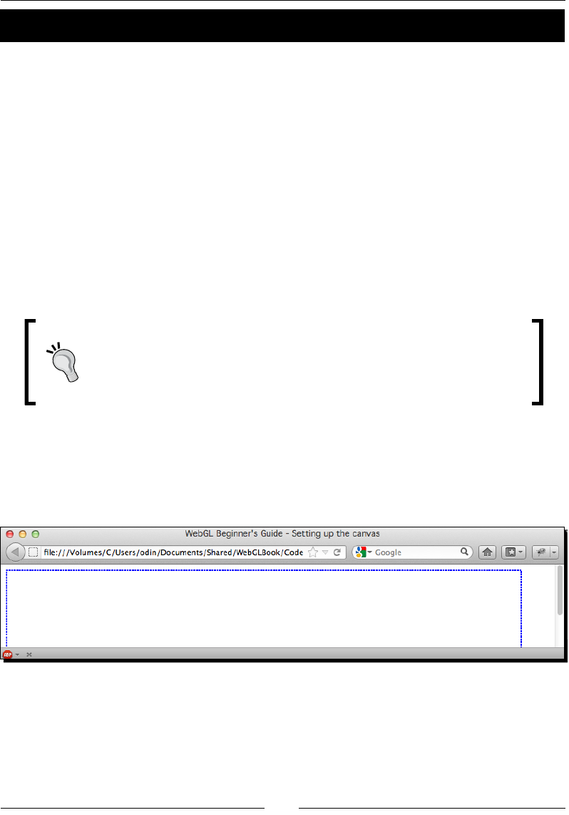
Time for action – creating an HTML5 canvas

1. Using your favorite editor, create a web page with the following code in it:

<!DOCTYPE html>

<html>

<head>

<title> WebGL Beginner's Guide - Setting up the canvas </title>

canvas {border: 2px dotted blue;}

</style>

</head>

<body>

Your browser does not support HTML5

</canvas>

</body>

</html>

Downloading the example code

You can download the example code les for all Packt books you have

purchased from your account at http://www.packtpub.com. If you

purchased this book elsewhere, you can visit http://www.packtpub.

com/support and register to have the les e-mailed directly to you.

2. Save the le as ch1_Canvas.html.

3. Open it with one of the supported browsers.

4. You should see something similar to the following screenshot:

Geng Started with WebGL

[ 12 ]

What just happened?

We have just created a simple web page with a canvas in it. This canvas will contain our

3D applicaon. Let's go very quickly to some relevant elements presented in this example.

Dening a CSS style for the border

This is the piece of code that determines the canvas style:

canvas {border: 2px dotted blue;}

</style>

As you can imagine, this code is not fundamental to build a WebGL applicaon. However,

a blue-doed border is a good way to verify where the canvas is located, given that the

canvas will be inially empty.

Understanding canvas attributes

There are three aributes in our previous example:

Id: This is the canvas idener in the Document Object Model (DOM).

Width and height: These two aributes determine the size of our canvas. When

these two aributes are missing, Firefox, Chrome, and WebKit will default to using

a 300x150 canvas.

What if the canvas is not supported?

If you see the message on your screen: Your browser does not support HTML5 (Which was

the message we put between <canvas> and </canvas>) then you need to make sure that

you are using one of the supported Internet browsers.

If you are using Firefox and you sll see the HTML5 not supported message. You might

want to be sure that WebGL is enabled (it is by default). To do so, go to Firefox and type

about:config in the address bar, then look for the property webgl.disabled. If is set to

true, then go ahead and change it. When you restart Firefox and load ch1_Canvas.html,

you should be able to see the doed border of the canvas, meaning everything is ok.

In the remote case where you sll do not see the canvas, it could be due to the fact that

Firefox has blacklisted some graphic card drivers. In that case, there is not much you can

do other than use a dierent computer.

Chapter 1

[ 13 ]

Accessing a WebGL context

A WebGL context is a handle (more strictly a JavaScript object) through which we can access

all the WebGL funcons and aributes. These constute WebGL's Applicaon Program

Interface (API).

We are going to create a JavaScript funcon that will check whether a WebGL context can be

obtained for the canvas or not. Unlike other JavaScript libraries that need to be downloaded

and included in your projects to work, WebGL is already in your browser. In other words, if

you are using one of the supported browsers, you don't need to install or include any library.

Time for action – accessing the WebGL context

We are going to modify the previous example to add a JavaScript funcon that is going to

check the WebGL availability in your browser (trying to get a handle). This funcon is going

to be called when the page is loaded. For this, we will use the standard DOM onLoad event.

1. Open the le ch1_Canvas.html in your favorite text editor (a text editor that

highlight HTML/JavaScript syntax is ideal).

2. Add the following code right below the </style> tag:

var gl = null;

function getGLContext(){

var canvas = document.getElementById("canvas-element-id");

if (canvas == null){

alert("there is no canvas on this page");

return;

}

var names = ["webgl",

"experimental-webgl",

"webkit-3d",

"moz-webgl"];

for (var i = 0; i < names.length; ++i) {

try {

gl = canvas.getContext(names[i]);

}

catch(e) {}

if (gl) break;

}

if (gl == null){

alert("WebGL is not available");

}

else{

Geng Started with WebGL

[ 14 ]

alert("Hooray! You got a WebGL context");

}

</script>

3. We need to call this funcon on the onLoad event. Modify your body tag so it looks

like the following:

4. Save the le as ch1_GL_Context.html.

5. Open the le ch1_GL_Context.html using one of the WebGL supported browsers.

6. If you can run WebGL you will see a dialog similar to the following:

What just happened?

Using a JavaScript variable (gl), we obtained a reference to a WebGL context. Let's go back

and check the code that allows accessing WebGL:

var names = ["webgl",

"experimental-webgl",

"webkit-3d",

"moz-webgl"];

for (var i = 0; i < names.length; ++i) {

try {

gl = canvas.getContext(names[i]);

}

catch(e) {}

if (gl) break;

}

The canvas getContext method gives us access to WebGL. All we need to specify a context

name that currently can vary from vendor to vendor. Therefore we have grouped them

in the possible context names in the names array. It is imperave to check on the WebGL

specicaon (you will nd it online) for any updates regarding the naming convenon.

Chapter 1

[ 15 ]

getContext also provides access to the HTML5 2D graphics library when using 2d as the

context name. Unlike WebGL, this naming convenon is standard. The HTML5 2D graphics

API is completely independent from WebGL and is beyond the scope of this book.

WebGL is a state machine

A WebGL context can be understood as a state machine: once you modify any of its aributes,

that modicaon is permanent unl you modify that aribute again. At any point you can

query the state of these aributes and so you can determine the current state of your WebGL

context. Let's analyze this behavior with an example.

Time for action – setting up WebGL context attributes

In this example, we are going to learn to modify the color that we use to clear the canvas:

1. Using your favorite text editor, open the le ch1_GL_Attributes.html:

<html>

<head>

<title> WebGL Beginner's Guide - Setting WebGL context

attributes </title>

canvas {border: 2px dotted blue;}

</style>

var gl = null;

var c_width = 0;

var c_height = 0;

window.onkeydown = checkKey;

function checkKey(ev){

switch(ev.keyCode){

case 49:{ // 1

gl.clearColor(0.3,0.7,0.2,1.0);

clear(gl);

break;

}

case 50:{ // 2

gl.clearColor(0.3,0.2,0.7,1.0);

clear(gl);

break;

Geng Started with WebGL

[ 16 ]

}

case 51:{ // 3

var color = gl.getParameter(gl.COLOR_CLEAR_VALUE);

// Don't get confused with the following line. It

// basically rounds up the numbers to one decimal

cipher

//just for visualization purposes

alert('clearColor = (' +

Math.round(color[0]*10)/10 +

',' + Math.round(color[1]*10)/10+

',' + Math.round(color[2]*10)/10+')');

window.focus();

break;

}

function getGLContext(){

var canvas = document.getElementById("canvas-element-id");

if (canvas == null){

alert("there is no canvas on this page");

return;

}

var names = ["webgl",

"experimental-webgl",

"webkit-3d",

"moz-webgl"];

var ctx = null;

for (var i = 0; i < names.length; ++i) {

try {

ctx = canvas.getContext(names[i]);

}

catch(e) {}

if (ctx) break;

}

if (ctx == null){

alert("WebGL is not available");

}

else{

return ctx;

}

Chapter 1

[ 17 ]

function clear(ctx){

ctx.clear(ctx.COLOR_BUFFER_BIT);

ctx.viewport(0, 0, c_width, c_height);

}

function initWebGL(){

gl = getGLContext();

}

</script>

</head>

Your browser does not support the HTML5 canvas element.

</canvas>

</body>

</html>

2. You will see that this le is very similar to our previous example. However,

there are new code constructs that we will explain briey. This le contains

four JavaScript funcons:

Funcon Descripon

checkKey This is an auxiliary funcon. It captures the keyboard input and executes

code depending on the key entered.

getGLContext Similar to the one used in the Time for acon – accessing the WebGL

context secon. In this version, we are adding some lines of code to

obtain the canvas' width and height.

clear Clear the canvas to the current clear color, which is one aribute of

the WebGL context. As was menoned previously, WebGL works as

a state machine, therefore it will maintain the selected color to clear

the canvas up to when this color is changed using the WebGL funcon

gl.clearColor (See the checkKey source code)

initWebGL This funcon replaces getGLContext as the funcon being called on

the document onLoad event. This funcon calls an improved version

of getGLContext that returns the context in the ctx variable. This

context is then assigned to the global variable gl.

Geng Started with WebGL

[ 18 ]

3. Open the le test_gl_attributes.html using one of the supported Internet

web browsers.

4. Press 1. You will see how the canvas changes its color to green. If you want to query

the exact color we used, press 3.

5. The canvas will maintain the green color unl we decided to change the aribute

clear color by calling gl.clearColor. Let's change it by pressing 2. If you look at

the source code, this will change the canvas clear color to blue. If you want to know

the exact color, press 3.

What just happened?

In this example, we saw that we can change or set the color that WebGL uses to clear the

canvas by calling the clearColor funcon. Correspondingly, we used getParameter

(gl.COLOR_CLEAR_VALUE) to obtain the current value for the canvas clear color.

Throughout the book we will see similar constructs where specic funcons

establish aributes of the WebGL context and the getParameter funcon retrieves

the current values for such aributes whenever the respecve argument (in our example,

COLOR_CLEAR_VALUE) is used.

Using the context to access the WebGL API

It is also essenal to note here that all of the WebGL funcons are accessed through the

WebGL context. In our examples, the context is being held by the gl variable. Therefore,

any call to the WebGL Applicaon Programming Interface (API) will be performed using

this variable.

Loading a 3D scene

So far we have seen how to set up a canvas and how to obtain a WebGL context; the next

step is to discuss objects, lights, and cameras. However, why should we wait to see what

WebGL can do? In this secon, we will have a glance at what a WebGL scene look like.

Virtual car showroom

Through the book, we will develop a virtual car showroom applicaon using WebGL. At this

point, we will load one simple scene in the canvas. This scene will contain a car, some lights,

and a camera.

Chapter 1

[ 19 ]

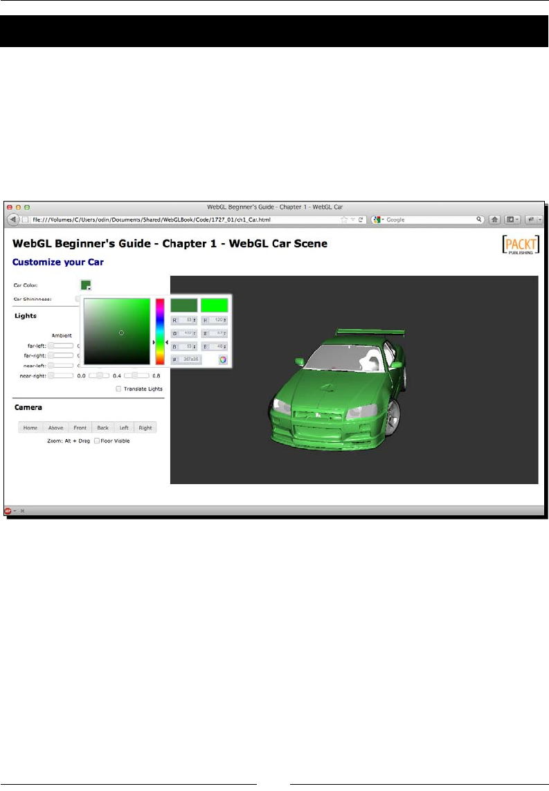
Time for action – visualizing a nished scene

Once you nish reading the book you will be able to create scenes like the one we are going

to play with next. This scene shows one of the cars from the book's virtual car showroom.

1. Open the le ch1_Car.html in one of the supported Internet web browsers.

2. You will see a WebGL scene with a car in it as shown in the following screenshot.

In Chapter 2, Rendering Geometry we will cover the topic of geometry rendering

and we will see how to load and render models as this car.

3. Use the sliders to interacvely update the four light sources that have been dened

for this scene. Each light source has three elements: ambient, diuse, and specular

elements. We will cover the topic about lights in Chapter 3, Lights!.

4. Click and drag on the canvas to rotate the car and visualize it from dierent

perspecves. You can zoom by pressing the Alt key while you drag the mouse on

the canvas. You can also use the arrow keys to rotate the camera around the car.

Make sure that the canvas is in focus by clicking on it before using the arrow keys.

In Chapter 4, Camera we will discuss how to create and operate with cameras

in WebGL.

Geng Started with WebGL

[ 20 ]

5. If you click on the Above, Front, Back, Le, or Right buons you will see an

animaon that stops when the camera reaches that posion. For achieving

this eect we are using a JavaScript mer. We will discuss animaon in

Chapter 5, Acon.

6. Use the color selector widget as shown in the previous screenshot to change the

color of the car. The use of colors in the scene will be discussed in Chapter 6, Colors,

Depth Tesng, and Alpha Blending. Chapters 7-10 will describe the use of textures

(Chapter 7, Textures), selecon of objects in the scene (Chapter 8, Picking), how

to build the virtual car show room (Chapter 9, Pung It All Together) and WebGL

advanced techniques (Chapter 10, Advanced Techniques).

What just happened?

We have loaded a simple scene in an Internet web browser using WebGL.

This scene consists of:

A canvas through which we see the scene.

A series of polygonal meshes (objects) that constute the car: roof, windows,

headlights, fenders, doors, wheels, spoiler, bumpers, and so on.

Light sources; otherwise everything would appear black.

A camera that determines where in the 3D world is our view point. The camera can

be made interacve and the view point can change, depending on the user input.

For this example, we were using the le and right arrow keys and the mouse to

move the camera around the car.

There are other elements that are not covered in this example such as textures, colors, and

special light eects (specularity). Do not panic! Each element will be explained later in the

book. The point here is to idenfy that the four basic elements we discussed previously are

present in the scene.

Chapter 1

[ 21 ]

Summary

In this chapter, we have looked at the four basic elements that are always present in any

WebGL applicaon: canvas, objects, lights, and camera.

We have learned how to add an HTML5 canvas to our web page and how to set its ID, width,

and height. Aer that, we have included the code to create a WebGL context. We have seen

that WebGL works as a state machine and as such, we can query any of its variables using

the getParameter funcon.

In the next chapter we will learn how to dene, load, and render 3D objects into

a WebGL scene.

Rendering Geometry

WebGL renders objects following a "divide and conquer" approach. Complex

polygons are decomposed into triangles, lines, and point primives. Then, each

geometric primive is processed in parallel by the GPU through a series of

steps, known as the rendering pipeline, in order to create the nal scene that is

displayed on the canvas.

The rst step to use the rendering pipeline is to dene geometric enes. In this

chapter, we will take a look at how geometric enes are dened in WebGL.

In this chapter, we will:

Understand how WebGL denes and processes geometric informaon

Discuss the relevant API methods that relate to geometry manipulaon

Examine why and how to use JavaScript Object Notaon (JSON) to dene,

store, and load complex geometries

Connue our analysis of WebGL as a state machine and describe the aributes

relevant to geometry manipulaon that can be set and retrieved from the

state machine

Experiment with creang and loading dierent geometry models!

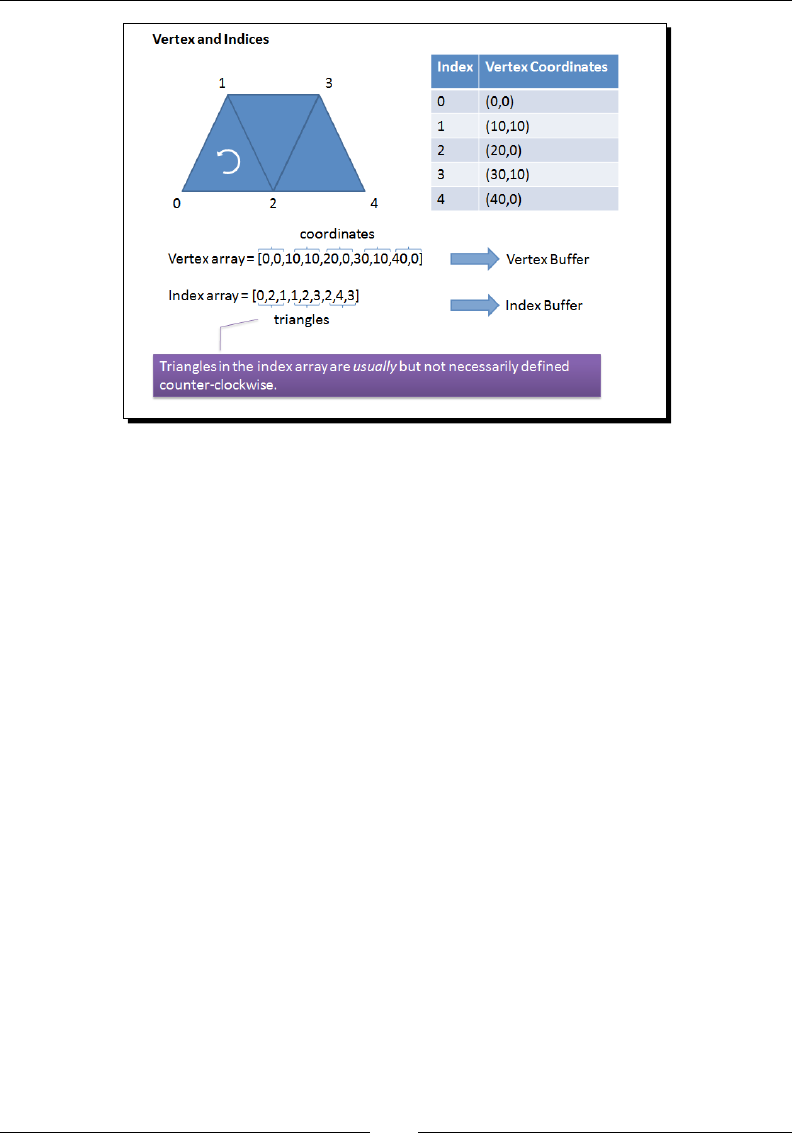
Vertices and Indices

WebGL handles geometry in a standard way, independently of the complexity and number

of points that surfaces can have. There are two data types that are fundamental to represent

the geometry of any 3D object: verces and indices.

Rendering Geometry

[ 24 ]

Verces are the points that dene the corners of 3D objects. Each vertex is represented by

three oang-point numbers that correspond to the x, y, and z coordinates of the vertex.

Unlike its cousin, OpenGL, WebGL does not provide API methods to pass independent

verces to the rendering pipeline, therefore we need to write all of our verces in a

JavaScript array and then construct a WebGL vertex buer with it.

Indices are numeric labels for the verces in a given 3D scene. Indices allow us to tell WebGL

how to connect verces in order to produce a surface. Just like with verces, indices are

stored in a JavaScript array and then they are passed along to WebGL's rendering pipeline

using a WebGL index buer.

There are two kind of WebGL buers used to describe and process geometry:

Buers that contain vertex data are known as Vertex Buer Objects (VBOs).

Similarly, buers that contain index data are known as Index Buer Objects

(IBOs).

Before geng any further, let's examine what WebGL's rendering pipeline looks like and

where WebGL buers t into this architecture.

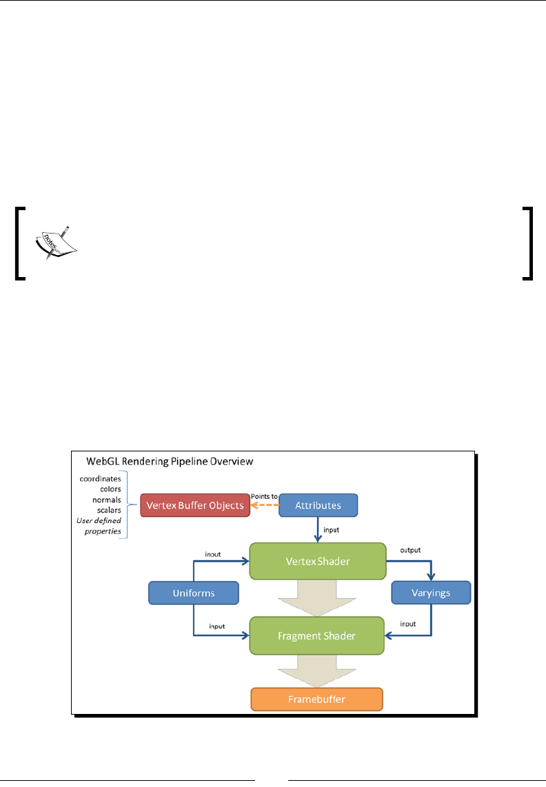
Overview of WebGL's rendering pipeline

Here we will see a simplied version of WebGL's rendering pipeline. In subsequent chapters,

we will discuss the pipeline in more detail.

Let's take a moment to describe every element separately.

Chapter 2

[ 25 ]

Vertex Buffer Objects (VBOs)

VBOs contain the data that WebGL requires to describe the geometry that is going to be

rendered. As menoned in the introducon, vertex coordinates are usually stored and

processed in WebGL as VBOs. Addionally, there are several data elements such as vertex

normals, colors, and texture coordinates, among others, that can be modeled as VBOs.

Vertex shader

The vertex shader is called on each vertex. This shader manipulates per-vertex data such

as vertex coordinates, normals, colors, and texture coordinates. This data is represented

by aributes inside the vertex shader. Each aribute points to a VBO from where it reads

vertex data.

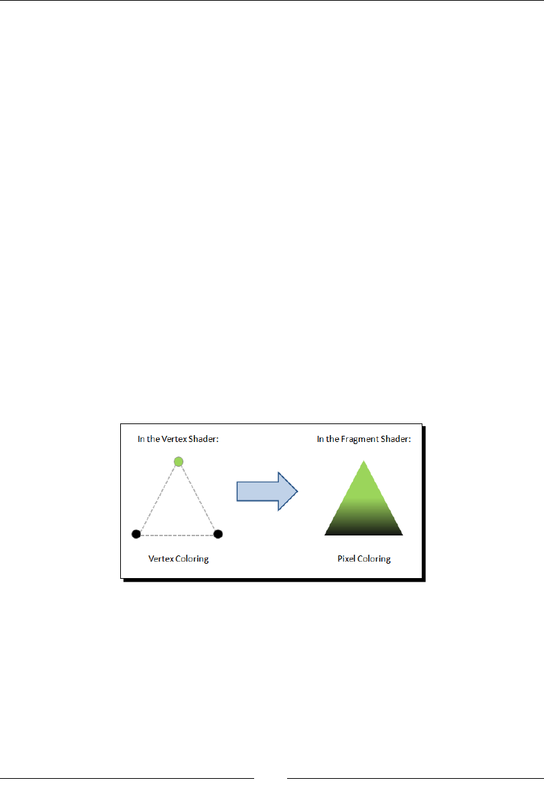
Fragment shader

Every set of three verces denes a triangle and each element on the surface of that triangle

needs to be assigned a color. Otherwise our surfaces would be transparent.

Each surface element is called a fragment. Since we are dealing with surfaces that are going

to be displayed on your screen, these elements are more commonly known as pixels.

The main goal of the fragment shader is to calculate the color of individual pixels.

The following diagram explains this idea:

Framebuffer

It is a two-dimensional buer that contains the fragments that have been processed by

the fragment shader. Once all fragments have been processed, a 2D image is formed and

displayed on screen. The framebuer is the nal desnaon of the rendering pipeline.

Rendering Geometry

[ 26 ]

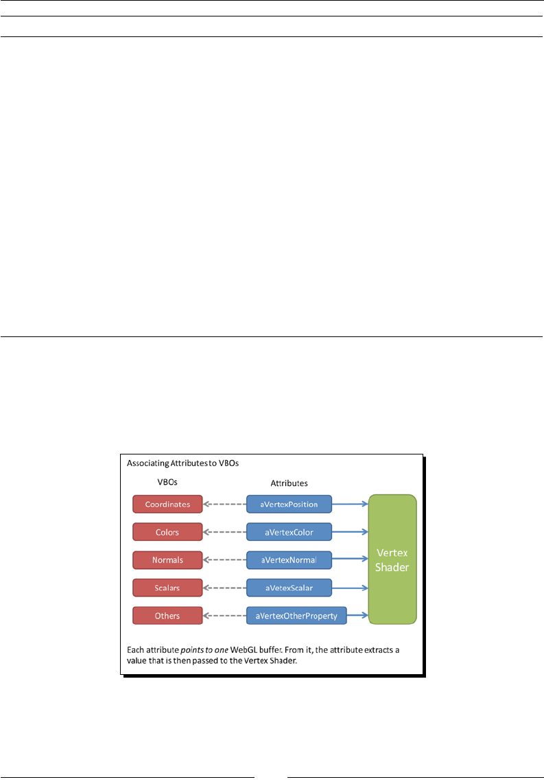
Attributes, uniforms, and varyings

Aributes, uniforms, and varyings are the three dierent types of variables that you will nd

when programming with shaders.

Aributes are input variables used in the vertex shader. For example, vertex coordinates,

vertex colors, and so on. Due to the fact that the vertex shader is called on each vertex,

the aributes will be dierent every me the vertex shader is invoked.

Uniforms are input variables available for both the vertex shader and fragment shader.

Unlike aributes, uniforms are constant during a rendering cycle. For example, lights posion.

Varyings are used for passing data from the vertex shader to the fragment shader.

Now let's create a simple geometric object.

Rendering geometry in WebGL

The following are the steps that we will follow in this secon to render an object in WebGL:

1. First, we will dene a geometry using JavaScript arrays.

2. Second, we will create the respecve WebGL buers.

3. Third, we will point a vertex shader aribute to the VBO that we created in the

previous step to store vertex coordinates.

4. Finally, we will use the IBO to perform the rendering.

Dening a geometry using JavaScript arrays

Let's see what we need to do to create a trapezoid. We need two JavaScript arrays:

one for the verces and one for the indices.

Chapter 2

[ 27 ]

As you can see from the previous screenshot, we have placed the coordinates sequenally in

the vertex array and then we have indicated in the index array how these coordinates are used

to draw the trapezoid. So, the rst triangle is formed with the verces having indices 0, 1, and

2; the second with the verces having indices 1, 2, and 3; and nally, the third, with verces

having indices 2, 3, and 4. We will follow the same procedure for all possible geometries.

Creating WebGL buffers

Once we have created the JavaScript arrays that dene the verces and indices for our

geometry, the next step consists of creang the respecve WebGL buers. Let's see how

this works with a dierent example. In this case, we have a simple square on the x-y plane

(z coordinates are zero for all four verces):

var vertices = [-50.0, 50.0, 0.0,

-50.0,-50.0, 0.0,

50.0,-50.0, 0.0,

50.0, 50.0, 0.0];/* our JavaScript vertex array */

var myBuffer = gl.createBuffer(); /*gl is our WebGL Context*/

Rendering Geometry

[ 28 ]

In the previous chapter, you may remember that WebGL operates as a state machine. Now,

when myBuffer is made the currently bound WebGL buer, this means that any subsequent

buer operaon will be executed on this buer unl it is unbound or another buer is made

the current one with a bound call. We bind a buer with the following instrucon:

gl.bindBuffer(gl.ARRAY_BUFFER, myBuffer);

The rst parameter is the type of buer that we are creang. We have two opons

for this parameter:

gl.ARRAY_BUFFER: Vertex data

gl.ELEMENT_ARRAY_BUFFER: Index data

In the previous example, we are creang the buer for vertex coordinates; therefore,

we use ARRAY_BUFFER. For indices, the type ELEMENT_ARRAY_BUFFER is used.

WebGL will always access the currently bound buer looking for the

data. Therefore, we should be careful and make sure that we have

always bound a buer before calling any other operaon for geometry

processing. If there is no buer bound, then you will obtain the error

INVALID_OPERATION

Once we have bound a buer, we need to pass along its contents. We do this with the

bufferData funcon:

gl.bufferData(gl.ARRAY_BUFFER, new Float32Array(vertices),

gl.STATIC_DRAW);

In this example, the vertices variable is a JavaScript array that contains the vertex

coordinates. WebGL does not accept JavaScript arrays directly as a parameter for the

bufferData method. Instead, WebGL uses typed arrays, so that the buer data can

be processed in its nave binary form with the objecve of speeding up geometry

processing performance.

The specicaon for typed arrays can be found at: http://www.khronos.

org/registry/typedarray/specs/latest/

The typed arrays used by WebGL are Int8Array, Uint8Array, Int16Array,

Uint16Array, Int32Array, UInt32Array, Float32Array, and Float64Array.

Chapter 2

[ 29 ]

Please observe that vertex coordinates can be oat, but indices are always

integer. Therefore, we will use Float32Array for VBOs and UInt16Array

for IBOs throughout the examples of this book. These two types represent the

largest typed arrays that you can use in WebGL per rendering call. The other

types can be or cannot be present in your browser, as this specicaon is not

yet nal at the me of wring the book.

Since the indices support in WebGL is restricted to 16 bit integers, an index

array can only be 65,535 elements in length. If you have a geometry that

requires more indices, you will need to use several rendering calls. More about

rendering calls will be seen later on in the Rendering secon of this chapter.

Finally, it is a good pracce to unbind the buer. We can achieve that by calling the

following instrucon:

gl.bindBuffer(gl.ARRAY_BUFFER, null);

We will repeat the same calls described here for every WebGL buer (VBO or IBO)

that we will use.

Let's review what we have just learned with an example. We are going to code the

initBuffers funcon to create the VBO and IBO for a cone. (You will nd this

funcon in the le named ch2_Cone.html):

var coneVBO = null; //Vertex Buffer Object

var coneIBO = null; //Index Buffer Object

function initBuffers() {

var vertices = []; //JavaScript Array that populates coneVBO

var indices = []; //JavaScript Array that populates coneIBO;

//Vertices that describe the geometry of a cone

vertices =[1.5, 0, 0,

-1.5, 1, 0,

-1.5, 0.809017, 0.587785,

-1.5, 0.309017, 0.951057,

-1.5, -0.309017, 0.951057,

-1.5, -0.809017, 0.587785,

-1.5, -1, 0.0,

-1.5, -0.809017, -0.587785,

-1.5, -0.309017, -0.951057,

-1.5, 0.309017, -0.951057,

-1.5, 0.809017, -0.587785];

//Indices that describe the geometry of a cone

indices = [0, 1, 2,

0, 2, 3,

0, 3, 4,

Rendering Geometry

[ 30 ]

0, 4, 5,

0, 5, 6,

0, 6, 7,

0, 7, 8,

0, 8, 9,

0, 9, 10,

0, 10, 1];

coneVBO = gl.createBuffer();

gl.bindBuffer(gl.ARRAY_BUFFER, coneVBO);

gl.bufferData(gl.ARRAY_BUFFER, new Float32Array(vertices),

gl.STATIC_DRAW);

gl.bindBuffer(gl.ARRAY_BUFFER, null);

coneIBO = gl.createBuffer();

gl.bindBuffer(gl.ELEMENT_ARRAY_BUFFER, coneIBO);

gl.bufferData(gl.ELEMENT_ARRAY_BUFFER, new Uint16Array(indices),

gl.STATIC_DRAW);

gl.bindBuffer(gl.ELEMENT_ARRAY_BUFFER, null);

}

If you want to see this scene in acon, launch the le ch2_Cone.html in your

HTML5 browser.

To summarize, for every buer, we want to:

Create a new buer

Bind it to make it the current buer

Pass the buer data using one of the typed arrays

Unbind the buer

Operations to manipulate WebGL buffers

The operaons to manipulate WebGL buers are summarized in the following table:

Method Descripon

var aBuffer =

createBuffer(void) Creates the aBuffer buer

deleteBuffer(Object aBuffer) Deletes the aBuffer buer

bindBuffer(ulong target,

Object buffer) Binds a buer object. The accepted values for

target are:

ARRAY_BUFFER (for verces)

ELEMENT_ARRAY_BUFFER

(for indices)

Chapter 2

[ 31 ]

Method Descripon

bufferData(ulong target,

Object data, ulong type) The accepted values for target are:

ARRAY_BUFFER (for verces)

ELEMENT_ARRAY_BUFFER(for

indices)

The parameter type is a performance hint for

WebGL. The accepted values for type are:

STATIC_DRAW: Data in the buer

will not be changed (specied once

and used many mes)

DYNAMIC_DRAW: Data will be

changed frequently (specied many

mes and used many mes)

STREAM_DRAW: Data will change on

every rendering cycle (specied once

and used once)

Associating attributes to VBOs

Once the VBOs have been created, we associate these buers to vertex shader aributes.

Each vertex shader aribute will refer to one and only one buer, depending on the

correspondence that is established, as shown in the following diagram:

Rendering Geometry

[ 32 ]

We can achieve this by following these steps:

1. First, we bind a VBO.

2. Next, we point an aribute to the currently bound VBO.

3. Finally, we enable the aribute.

Let's take a look at the rst step.

Binding a VBO

We already know how to do this:

gl.bindBuffer(gl.ARRAY_BUFFER, myBuffer);

where myBuffer is the buer we want to map.

Pointing an attribute to the currently bound VBO

In the next chapter, we will learn to dene vertex shader aributes. For now, let's assume

that we have the aVertexPosition aribute and that it will represent vertex coordinates

inside the vertex shader.

The WebGL funcon that allows poinng aributes to the currently bound VBOs is

vertexAttribPointer. The following is its signature:

gl.vertexAttribPointer(Index,Size,Type,Norm,Stride,Offset);

Let us describe each parameter individually:

Index: An aribute's index that we are going to map the currently bound buer to.

Size: Indicates the number of values per vertex that are stored in the currently

bound buer.

Type: Species the data type of the values stored in the current buer. It is one

of the following constants: FIXED, BYTE, UNSIGNED_BYTE, FLOAT, SHORT, or

UNSIGNED_SHORT.

Norm: This parameter can be set to true or false. It handles numeric conversions

that lie out of the scope of this introductory guide. For all praccal eects, we will

set this parameter to false.

Stride: If stride is zero, then we are indicang that elements are stored sequenally

in the buer.

Oset: The posion in the buer from which we will start reading values for the

corresponding aribute. It is usually set to zero to indicate that we will start reading

values from the rst element of the buer.

Chapter 2

[ 33 ]

vertexAttribPointer denes a pointer for reading informaon

from the currently bound buer. Remember that an error will be

generated if there is no VBO currently bound.

Enabling the attribute

Finally, we just need to acvate the vertex shader aribute. Following our example,

we just need to add:

gl.enableVertexAttribArray (aVertexPosition);

The following diagram summarizes the mapping procedure:

Rendering

Once we have dened our VBOs and we have mapped them to the corresponding vertex

shader aributes, we are ready to render!

To do this, we use can use one of the two API funcons: drawArrays or drawElements.

The drawArrays and drawElements functions

The funcons drawArrays and drawElements are used for wring on the framebuer.

drawArrays uses vertex data in the order in which it is dened in the buer to create the

geometry. In contrast, drawElements uses indices to access the vertex data buers and

create the geometry.

Rendering Geometry

[ 34 ]

Both drawArrays and drawElements will only use enabled arrays. These are the vertex

buer objects that are mapped to acve vertex shader aributes.

In our example, we only have one enabled array: the buer that contains the vertex

coordinates. However, in a more general scenario, we can have several enabled arrays.

For instance, we can have arrays with informaon about vertex colors, vertex normals

texture coordinates, and any other per-vertex data required by the applicaon. In this

case, each one of them would be mapped to an acve vertex shader aribute.

Using several VBOs

In the next chapter, we will see how we use a vertex normal buer in addion to

vertex coordinates to create a lighng model for our geometry. In that scenario,

we will have two acve arrays: vertex coordinates and vertex normals.

Using drawArrays

We will call drawArrays when informaon about indices is not available. In most cases,

drawArrays is used when the geometry is so simple that dening indices is an overkill; for

instance, when we want to render a triangle or a rectangle. In that case, WebGL will create

the geometry in the order in which the vertex coordinates are dened in the VBO. So if you

have conguous triangles (like in our trapezoid example), you will have to repeat these

coordinates in the VBO.

If you need to repeat a lot of verces to create geometry, probably drawArrays is not the

best way to go. The more vertex data you duplicate, the more calls you will have on the

vertex shader. This could reduce the overall applicaon performance since the same verces

have to go through the pipeline several mes. One for each me that they appear repeated

in the respecve VBO.

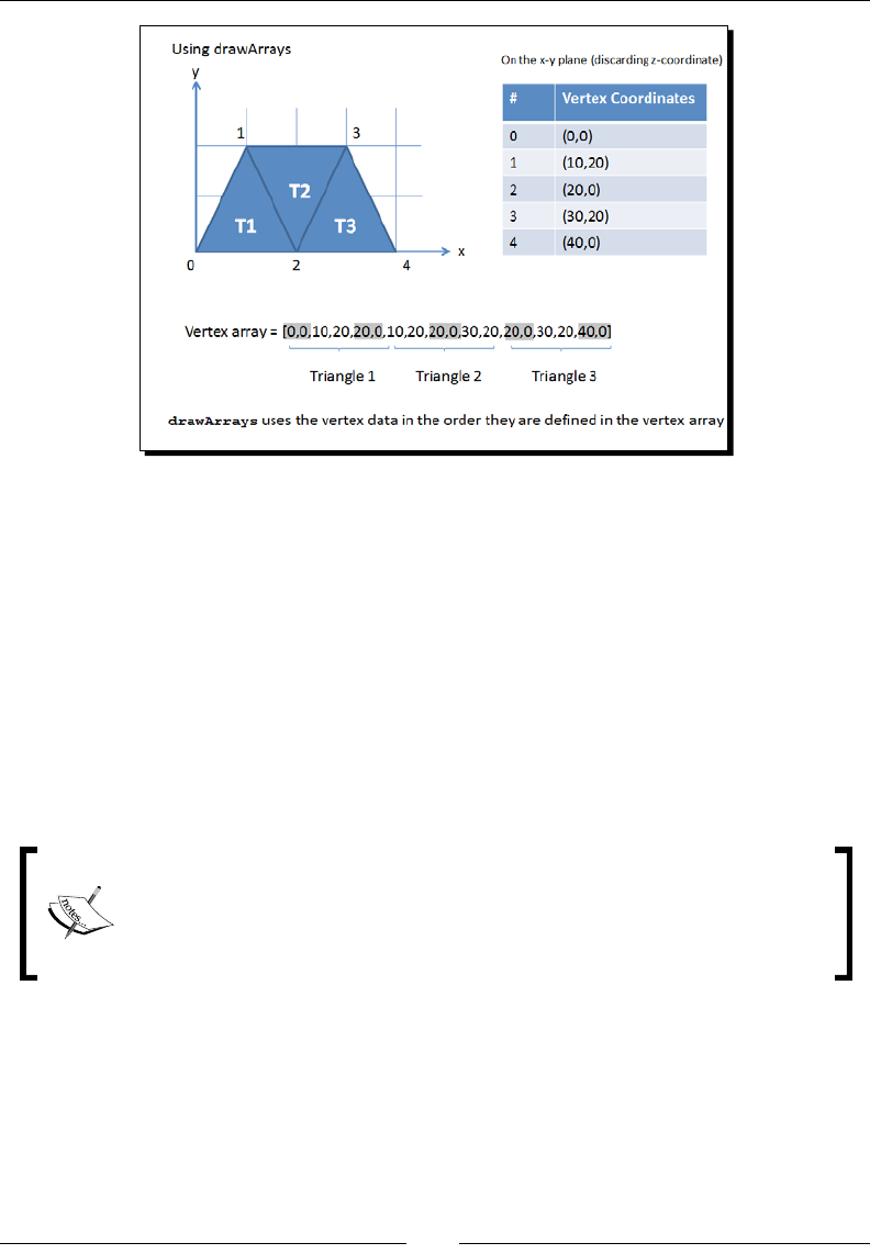
Chapter 2

[ 35 ]

The signature for drawArrays is:

gl.drawArrays(Mode, First, Count)

Where:

Mode: Represents the type of primive that we are going to render. Possible

values for mode are: gl.POINTS, gl.LINE_STRIP, gl.LINE_LOOP, gl.LINES,

gl.TRIANGLE_STRIP, gl.TRIANGLE_FAN, and gl.TRIANGLES (more about this

in the next secon).

First: Species the starng element in the enabled arrays.

Count: The number of elements to be rendered.

From the WebGL specicaon:

"When drawArrays is called, it uses count sequenal elements from each

enabled array to construct a sequence of geometric primives, beginning with

the element rst. Mode species what kinds of primives are constructed and

how the array elements construct those primives."

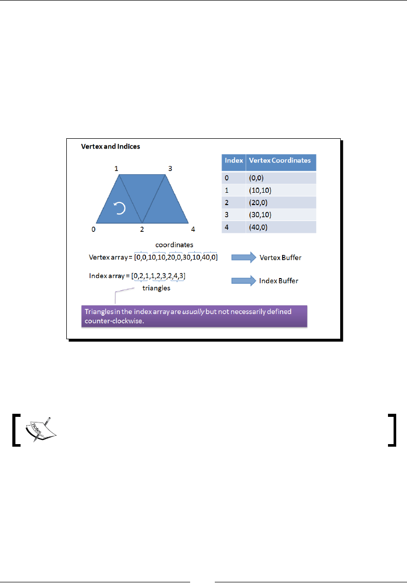
Rendering Geometry

[ 36 ]

Using drawElements

Unlike the previous case where no IBO was dened, drawElements allows us to use the

IBO, to tell WebGL how to render the geometry. Remember that drawArrays uses VBOs.

This means that the vertex shader will process repeated verces as many mes as they

appear in the VBO. Contrasngly, drawElements uses indices. Therefore, verces are

processed just once, and can be used as many mes as they are dened in the IBO. This

feature reduces both the memory and processing required on the GPU.

Let's revisit the following diagram of this chapter:

When we use drawElements, we need at least two buers: a VBO and an IBO. The vertex

shader will get executed on each vertex in the VBO and then the rendering pipeline will

assemble the geometry into triangles using the IBO.

When using drawElements, you need to make sure that the corresponding

IBO is currently bound.

Chapter 2

[ 37 ]

The signature for drawElements is:

gl.drawElements(Mode, Count, Type, Offset)

Where:

Mode: Represents the type of primive that we are going to render. Possible values

for mode are POINTS, LINE_STRIP, LINE_LOOP, LINES, TRIANGLE_STRIP,

TRIANGLE_FAN, and TRIANGLES (more about this later on).

Count: Species the number of elements to be rendered.

Type: Species the type of the values in indices. Must be UNSIGNED_BYTE

or UNSIGNED_SHORT, as we are handling indices (integer numbers).

Oset: Indicates which element in the buer will be the starng point for rendering.

It is usually the rst element (zero value).

WebGL inherits without any change this funcon from the OpenGL ES 2.0

specicaon. The following applies:

"When drawElements is called, it uses count sequenal elements from an

enabled array, starng at oset to construct a sequence of geometric primives.

Mode species what kinds of primives are constructed and how the array elements

construct these primives. If more than one array is enabled, each is used."

Putting everything together

I guess you have been waing to see how everything works together. Let's start with some

code. Let's create a simple WebGL program to render a square.

Time for action – rendering a square

Follow the given steps:

1. Open the le ch_Square.html in your favorite HTML editor (ideally one that

supports syntax highlighng like Notepad++ or Crimson Editor).

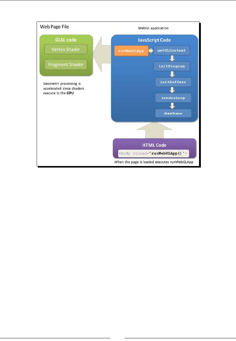
Rendering Geometry

[ 38 ]

2. Let's examine the structure of this le with the help of the following diagram:

3. The web page contains the following:

The script <script id="shader-fs" type="x-shader/x-

fragment"> contains the fragment shader code.

The script <script id="shader-vs" type="x-shader/x-vertex">

contains the vertex shader code. We will not be paying aenon to these

two scripts as these will be the main point of study in the next chapter. For

now, let's noce that we have a fragment shader and a vertex shader.

The next script on our web page <script id="code-js" type="text/

javascript"> contains all the JavaScript WebGL code that we will need.

This script is divided into the following funcons:

Chapter 2

[ 39 ]

getGLContext: Similar to the funcon that we saw in the previous chapter,

this funcon allows us to get a WebGL context for the canvas present in the

web page (ch_Square.html).

initProgram: This funcon obtains a reference for the vertex shader and

the fragment shader present in the web page (the rst two scripts that we

discussed) and passes them along to the GPU to be compiled. More about

this in the next chapter.

initBuers: Let's take a close look at this funcon. It contains the API calls

to create buers and to inialize them. In this example, we will be creang

a VBO to store coordinates for the square and an IBO to store the indices of

the square.

renderLoop: This funcon creates the rendering loop. The applicaon

invokes renderLoop periodically to update the scene (using the

requestAnimFrame funcon).

drawScene: This funcon maps the VBO to the respecve vertex buer

aribute and enables it by calling enableVertexAttribArray. It then

binds the IBO and calls the drawElements funcon.

Finally, we get to the <body> tag of our web page. Here we

invoke runWebGLApp the main funcon, ,which is executed by

the standard JavaScript onLoad event of the DOM document with

the following instrucon:

4. Open the le ch2_Square.html in the HTML5 browser of your preference

(Firefox, Safari, Chrome, or Opera).

5. You will see four tabs showing the code of: WebGL JS (JavaScript), Vertex Shader,

Fragment Shader, and HTML. You will always need these four elements in your web

page to write a WebGL app.

6. If the WebGL JS tab is not acve, select it.

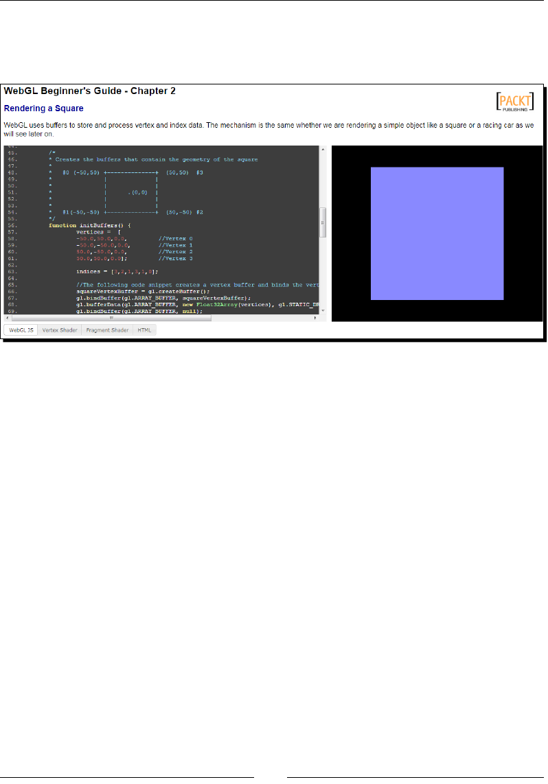
Rendering Geometry

[ 40 ]

7. Scroll down to the initBuffers funcon. Please pay aenon to the diagram that

appears as a comment before the funcon. This diagram describes how the verces

and indices are organized. You should see something like the following screenshot:

8. Go back to the text editor. If you have closed ch_Square.html, open it again.

9. Go to the initBuffers funcon.

10. Modify the buer array and index array so that the resulng gure is a pentagon

instead of a square. To do this, you need to add one vertex to the vertex array and

dene one more triangle in the index array.

11. Save the le with a dierent name and open it in the HTML5 browser of your

preference to test it.

What just happened?

You have learned about the dierent code elements that conform to a WebGL app. The

initBufferrs funcon has been examined and modied for rendering a dierent gure.

Chapter 2

[ 41 ]

Have a go hero – changing the square color

Go to the Fragment Shader and change the color of your pentagon.

The format is (red, green, blue, alpha). Alpha is always 1.0 (for now), and

the rst three arguments are oat numbers in the range 0.0 to 1.0.

Remember to save the le aer making the changes in your text editor and then open it in

the HTML5 browser of your preference to see the changes.

Rendering modes

Let's revisit the signature of the drawElements funcon:

gl.drawElements(Mode, Count, Type, Offset)

The rst parameter determines the type of primives that we are rendering. In the following

me for acon secon, we are going to see with examples the dierent rendering modes.

Time for action – rendering modes

Follow the given steps:

1. Open the le ch_RenderingModes.html in the HTML5 browser of your

preference. This example follows the same structure as discussed in the

previous secon.

2. Select the WebGL JS buon and scroll down to the initBuffer funcon.

3. You will see here that we are drawing a trapezoid. However, on screen you will see

two triangles! We will see how we did this later.

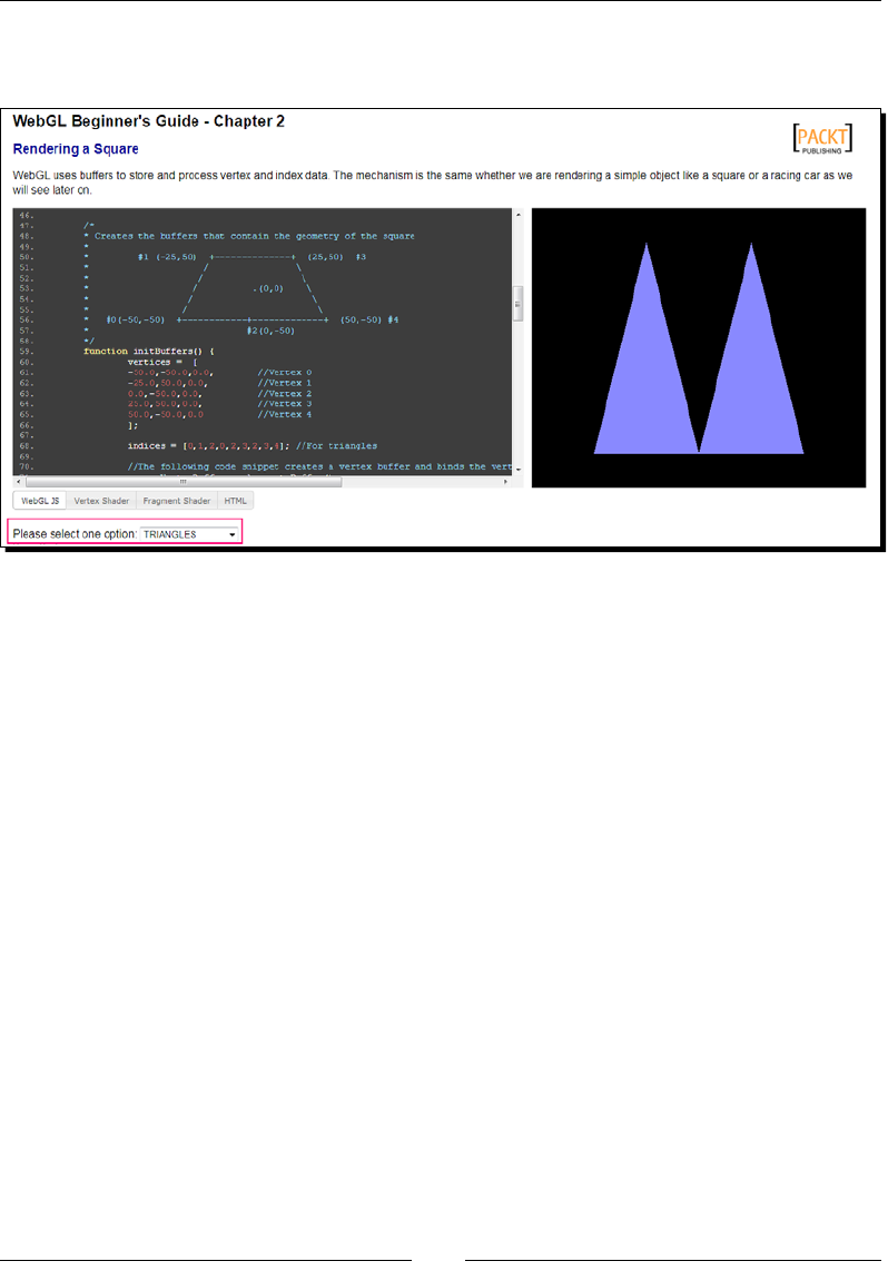
Rendering Geometry

[ 42 ]

4. At the boom of the page, there is a combobox that allows you to select the dierent

rendering modes that WebGL provides, as shown in the following screenshot:

5. When you select any opon from this combobox, you are changing the value of the

renderingMode variable dened at the top of the WebGL JS code (scroll up if you

want to see where it is dened).

6. To see how each opon modies the rendering, scroll down to the

drawScene funcon.

7. You will see there that aer binding the IBO trapezoidIndexBuffer with the

following instrucon:

gl.bindBuffer(gl.ELEMENT_ARRAY_BUFFER, trapezoidIndexBuffer);

you have a switch statement where there is a code that executes, depending on the

value of the renderingMode variable:

case 'TRIANGLES': {

...

}

case 'LINES': {

...

}

case'POINTS': {

...

}

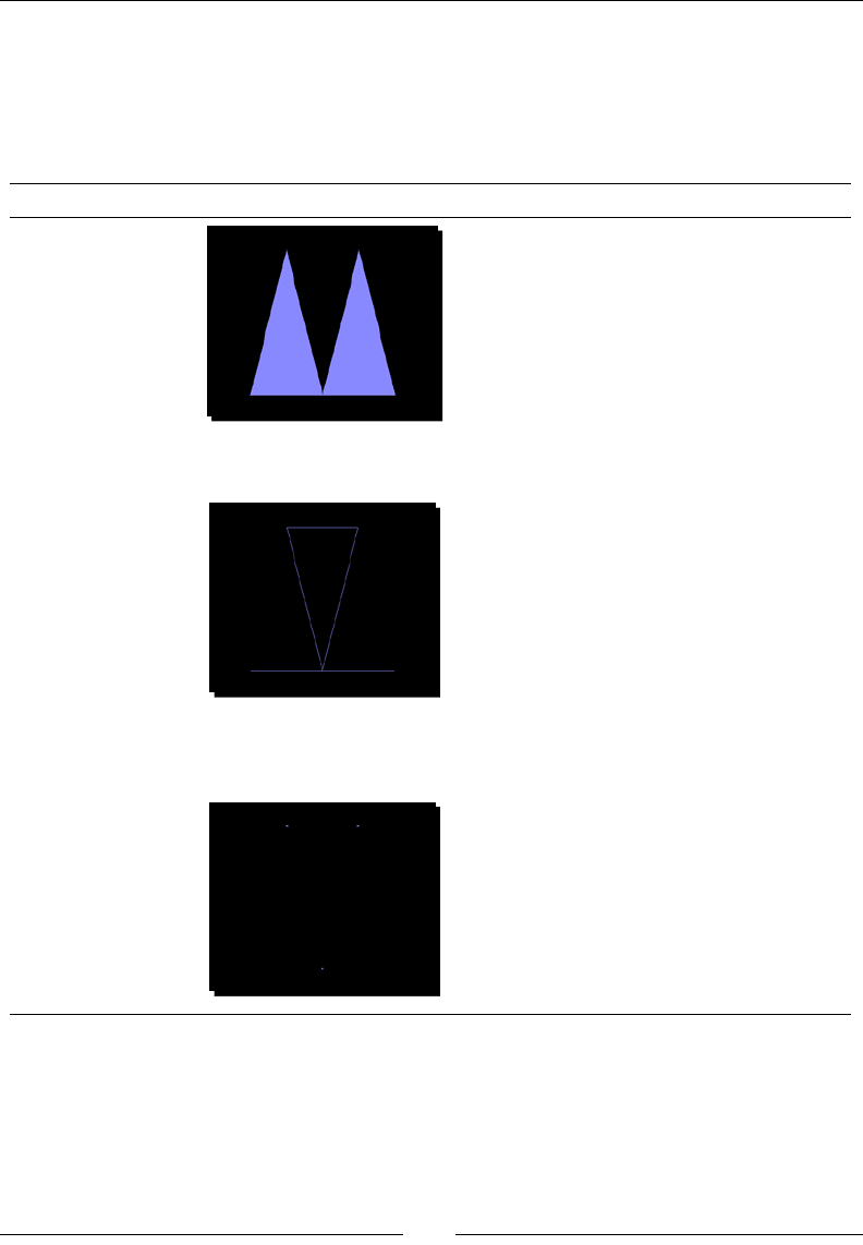
Chapter 2

[ 43 ]

8. For each mode, you dene the contents of the JavaScript array indices. Then, you

pass this array to the currently-bound buer (trapezoidIndexBuffer) by using

the bufferData funcon. Finally, you call the drawElements funcon.

9. Let's see what each mode does:

Mode Example Descripon

TRIANGLES When you use the TRIANGLES mode,

WebGL will use the rst three indices

dened in your IBO for construcng the rst

triangle, the next three for construcng the

second triangle, and so on. In this example,

we are drawing two triangles, which can

be veried by examining the following

indices JavaScript array that populates

the IBO:

indices = [0,1,2,2,3,4];

LINES The LINES mode will instruct WebGL

to take each consecuve pair of indices

dened in the IBO and draw lines taking the

coordinates of the corresponding verces.

For instance indices =

[1,3,0,4,1,2,2,3]; will draw four

lines: from vertex number 1 to vertex

number 3, from vertex number 0 to vertex

number 4, from vertex number 1 to vertex

number 2, and from vertex number 2 to

vertex number 3.

POINTS When we use the POINTS mode, WebGL

will not generate surfaces. Instead, it will

render the verces that we had dened

using the index array.

In this example, we will only render verces

number 1, number 2, and number 3 with

indices = [1,2,3];

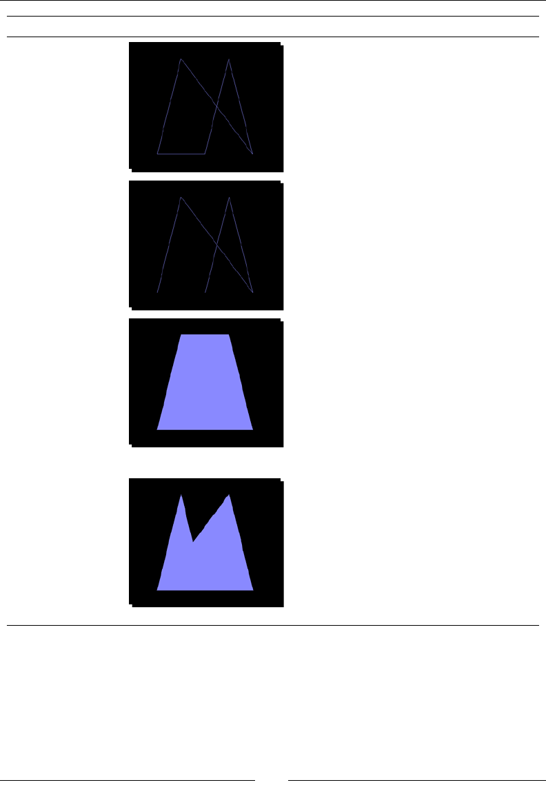
Rendering Geometry

[ 44 ]

Mode Example Descripon

LINE_LOOP LINE_LOOP draws a closed loop

connecng the verces dened in the

IBO to the next one. In our case, it will be

indices = [2,3,4,1,0];

LINE_STRIP It is similar to LINE_LOOP. The dierence

here is that WebGL does not connect the

last vertex to the rst one (not a closed

loop).

The indices JavaScript array will be

indices = [2,3,4,1,0];

TRIANGLE_

STRIP TRIANGLE_STRIP draws connected

triangles. Every vertex specied aer the

rst three (in our example, verces number

0, number 1, and number 2) creates a new

triangle.

If we have indices = [0,1,2,3,4];,

then we will generate the triangles:

(0,1,2) , (1,2,3), and (2,3,4).

TRIANGLE_FAN TRIANGLE_FAN creates triangles in

a similar way to TRIANGLE_STRIP.

However, the rst vertex dened in the IBO

is taken as the origin of the fan (the only

shared vertex among consecuve triangles).

In our example, indices =

[0,1,2,3,4];

will create the triangles: (0,1,2) and (0,3,4).

Now let's make some changes:

10. Edit the web page (ch_RenderingModes.html) so that when you select the

opon TRIANGLES, you render the trapezoid instead of two triangles.

Chapter 2

[ 45 ]

You need one extra triangle in the indices array.

11. Save the le and test it in the HTML5 browser of your preference.

12. Edit the web page so that you draw the leer 'M' using the opon LINES.

You need to dene four lines in the indices array.

13. Just like before, save your changes and test them in your HTML5 browser.

14. Using the LINE_LOOP mode, draw only the boundary of the trapezoid.

What just happened?

We have seen in acon through a simple exercise the dierent rendering modes supported

by WebGL. The dierent rendering modes determine how to interpret vertex and index data

to render an object.

WebGL as a state machine: buffer manipulation

There is some informaon about the state of the rendering pipeline that we can

retrieve when we are dealing with buers with the funcons: getParameter,

getBufferParameter, and isBuffer.

Just like we did in the previous chapter, we will use getParameter(parameter) where

parameter can have the following values:

ARRAY_BUFFER_BINDING: It retrieves a reference to the currently-bound VBO

ELEMENT_ARRAY_BUFFER_BINDING: It retrieves a reference to the

currently-bound IBO

Also, we can enquire about the size and the usage of the currently-bound VBO and IBO using

getBufferParameter(type, parameter) where type can have the following values:

ARRAY_BUFFER: To refer to the currently bound VBO

ELEMENT_ARRAY_BUFFER: To refer to the currently bound IBO

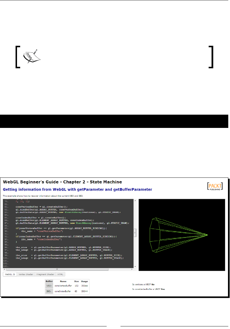
Rendering Geometry

[ 46 ]

And parameter can be:

BUFFER_SIZE: Returns the size of the requested buer

BUFFER_USAGE: Returns the usage of the requested buer

Your VBO and/or IBO needs to be bound when you enquire about the

state of the currently bound VBO and/or IBO with getParameter

and getBufferParameter.

Finally, isBuffer(object) will return true if the object is a WebGL buer, false, when

the buer is invalid, and an error if the object being evaluated is not a WebGL buer. Unlike

getParameter and getBufferParameter, isBuffer does not require any VBO or IBO to

be bound.

Time for action – enquiring on the state of buffers

Follow the given steps:

1. Open the le ch2_StateMachine.html in the HTML5 browser of your preference.

2. Scroll down to the initBuffers method. You will see something similar to the

following screenshot:

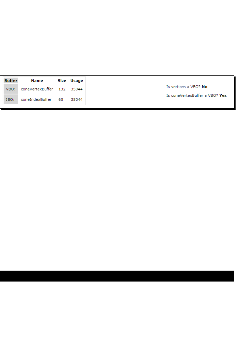
Chapter 2

[ 47 ]

3. Pay aenon to how we use the methods discussed in this secon to retrieve

and display informaon about the current state of the buers.

4. The informaon queried by the initBuffer funcon is shown at the boom

poron of the web page using updateInfo (if you look closely at runWebGLApp

code you will see that updateInfo is called right aer calling initBuffers).

5. At the boom of the web page (scroll down the web page if necessary), you will see

the following result:

6. Now, open the same le (ch2_StateMachine.html) in a text editor.

7. Cut the line:

gl.bindBuffer(gl.ARRAY_BUFFER,null);

and paste it right before the line:

coneIndexBuffer = gl.createBuffer();

8. What happens when you launch the page in your browser again?

9. Why do you think this behavior occurs?

What just happened?

You have learned that the currently bound buer is a state variable in WebGL. The buer

is bound unl you unbind it by calling bindBuffer again with the corresponding type

(ARRAY_BUFFER or ELEMENT_ARRAY_BUFFER) as the rst parameter and with null as the

second argument (that is, no buer to bind). You have also learned that you can only query

the state of the currently bound buer. Therefore, if you want to query a dierent buer,

you need to bind it rst.

Have a go hero – add one validation

Modify the le so that you can validate and show on screen whether the indices array

and the coneIndexBuffer are WebGL buers or not.

Rendering Geometry

[ 48 ]

You will have to modify the table in the HTML body of the le to allocate

space for the new validaons.

You will have to modify the updateInfo funcon accordingly.

Advanced geometry loading techniques: JavaScript

Object Notation (JSON) and AJAX

So far, we have rendered very simple objects. Now let's study a way to load the geometry

(verces and indices) from a le instead of declaring the verces and the indices every me

we call initBuffers. To achieve this, we will make asynchronous calls to the web server

using AJAX. We will retrieve the le with our geometry from the web server and then we will

use the built-in JSON parser to convert the context of our les into JavaScript objects. In our

case, these objects will be the vertices and indices array.

Introduction to JSON – JavaScript Object Notation

JSON stands for JavaScript Object Notaon. It is a lightweight, text-based, open format

used for data interchange. JSON is commonly used as an alternave to XML.

The JSON format is language-agnosc. This means that there are parsers in many languages

to read and interpret JSON objects. Also, JSON is a subset of the object literal notaon of

JavaScript. Therefore, we can dene JavaScript objects using JSON.

Dening JSON-based 3D models

Let's see how this work. Assume for example that we have the model object with two

arrays vertices and indices (does this ring any bells?). Say that these arrays contain

the informaon described in the cone example (ch2_Cone.html) as follows:

vertices =[1.5, 0, 0,

-1.5, 1, 0,

-1.5, 0.809017, 0.587785,

-1.5, 0.309017, 0.951057,

-1.5, -0.309017, 0.951057,

-1.5, -0.809017, 0.587785,

-1.5, -1, 0,

-1.5, -0.809017, -0.587785,

-1.5, -0.309017, -0.951057,

-1.5, 0.309017, -0.951057,

-1.5, 0.809017, -0.587785];

indices = [0, 1, 2,

Chapter 2

[ 49 ]

0, 2, 3,

0, 3, 4,

0, 4, 5,

0, 5, 6,

0, 6, 7,

0, 7, 8,

0, 8, 9,

0, 9, 10,

0, 10, 1];

Following the JSON notaon, we would represent these two arrays as an object, as follows:

var model = {

"vertices" : [1.5, 0, 0,

-1.5, 1, 0,

-1.5, 0.809017, 0.587785,

-1.5, 0.309017, 0.951057,

-1.5, -0.309017, 0.951057,

-1.5, -0.809017, 0.587785,

-1.5, -1, 0,

-1.5, -0.809017, -0.587785,

-1.5, -0.309017, -0.951057,

-1.5, 0.309017, -0.951057,

-1.5, 0.809017, -0.587785],

"indices" : [0, 1, 2,

0, 2, 3,

0, 3, 4,

0, 4, 5,

0, 5, 6,

0, 6, 7,

0, 7, 8,

0, 8, 9,

0, 9, 10,

0, 10, 1]};

From the previous example, we can infer the following syntax rules:

The extent of a JSON object is dened by curly brackets {}

Aributes in a JSON object are separated by comma ,

There is no comma aer the last aribute

Each aribute of a JSON object has two parts: a key and a value

The name of an aribute is enclosed by quotaon marks " "

Rendering Geometry

[ 50 ]

Each aribute key is separated from its corresponding value with a colon :

Aributes of the type Array are dened in the same way you would dene them

in JavaScript

JSON encoding and decoding

Most modern web browsers support nave JSON encoding and decoding through the built-in

JavaScript object JSON. Let's examine the methods available inside this object:

Method Descripon

var myText = JSON.

stringify(myObject) We use JSON.stringify for converng

JavaScript objects to JSON-formaed text.

var myObject = JSON.

parse(myText) We use JSON.parse for converng text

into JavaScript objects.

Let's learn how to encode and decode with the JSON notaon.

Time for action – JSON encoding and decoding

Let's create a simple model: a 3D line. Here we will be focusing on how we do JSON encoding

and decoding. Follow the given steps:

1. Go to your Internet browser and open the interacve JavaScript console. Use the

following table for assistance:

Web browser Menu opon Shortcut keys (PC / Mac)

Firefox Tools | Web Developer | Web Console Ctrl + Shi + K / Command + Alt + K

Safari Develop | Show Web Inspector Ctrl + Shi + C / Command + Alt + C

Chrome Tools | JavaScript Console Ctrl + Shi + J / Command + Alt + J

2. Create a JSON object by typing:

var model = {"vertices":[0,0,0,1,1,1], "indices":[0,1]};

3. Verify that the model is an object by wring:

typeof(model)

4. Now, let's print the model aributes. Write this in the console (press Enter at the

end of each line):

model.vertices

model.indices

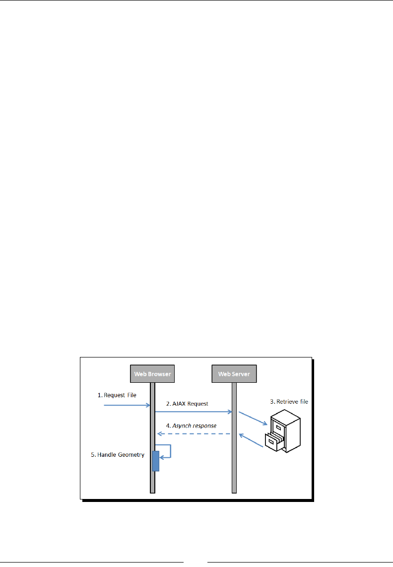
Chapter 2

[ 51 ]

5. Now, let's create a JSON text:

var text = JSON.stringify(model)

alert(text)

6. What happens when you type text.vertices?

As you can see, you get an error message saying that text.vertices is not

dened. This happens because text is not a JavaScript object but a string with

the peculiarity of being wrien according to JSON notaon to describe an object.

Everything in it is text and therefore it does not have any elds.

7. Now let's convert the JSON text back to an object. Type the following:

var model2 = JSON.parse(text)

typeof(model2)

model2.vertices

What just happened?

We have learned to encode and decode JSON objects. The example that we have used is

relevant because this is the way we will dene our geometry to be loaded from external les.

In the next secon, we will see how to download geometric models specied with JSON from

a web server.

Asynchronous loading with AJAX

The following diagram summarizes the asynchronous loading of les by the web browser

using AJAX:

Rendering Geometry

[ 52 ]

Let's analyze this more closely:

1. Request le: First of all, we should indicate the lename that we want to load.

Remember that this le contains the geometry that we will be loading from the

web server instead of coding the JavaScript arrays (verces and indices) directly

into the web page.

2. AJAX request: We need to write a funcon that will perform the AJAX request.

Let's call this funcon loadFile. The code can look like this:

function loadFile(name) {

var request = new XMLHttpRequest();

var resource = http:// + document.domain + name;

request.open("GET",resource);

request.onreadystatechange = function() {

if (request.readyState == 4) {

if(request.status == 200 || (request.status == 0 &&

document.domain.length == 0) {

handleLoadedGeometry(name,JSON.parse(request.responseText));

}

else {

alert ('There was a problem loading the file :' + name);

alert ('HTML error code: ' + request.status);

}

request.send();

}

If the readyState is 4, it means that the le has nished downloading.

More about this funcon later. Let's say for now that this funcon will perform the

AJAX request.

3. Retrieve le: The web server will receive and treat our request as a regular

HTTP request. As a maer of fact, the server does not know that this request

is asynchronous (it is asynchronous for the web browser as it does not wait for

the answer). The server will look for our le and whether it nds it or not, it will

generate a response. This will take us to step 4.

4. Asynchronous response: Once a response is sent to the web browser, the callback

specied in the loadFile funcon is invoked. This callback corresponds to the

request method onreadystatechange. This method examines the answer. If

we obtain a status dierent from 200 (OK according to the HTTP specicaon), it

means that there was a problem. Hopefully the specic error code that we get on

the status variable (instead of 200) can give us a clue about the error. For instance,

code 404 means that the resource does not exist. In that case, you would need to

Chapter 2

[ 53 ]

check if there is a typo, or you are requesng a le from a directory dierent from

the directory where the page is located on the web server. Dierent error codes will

give you dierent alternaves to treat the respecve problem. Now if we get a 200

status, we can invoke the handleLoadedGeometry funcon.

There is an excepon where things can work, even if you do not

have a web server. If you are running the example from your

computer, the ready state will be 4 but the request status will be

0. This is a valid conguraon too.

5. Handling the loaded model: In order to keep our code looking prey, we can

create a new funcon to process the le retrieved from the server. Let's call this

handleLoadedGeometry funcon. Please noce that in the previous segment

of code, we used the JSON parser in order to create a JavaScript object from the

le before passing it along to the handleLoadedGeometry funcon. This object

corresponds to the second argument (model) as we can see here. The code for the

handleLoadedGeometry funcon looks like this:

function handleLoadedGeometry(name,model){

alert(name + ' has been retrieved from the server');

modelVertexBuffer = gl.createBuffer();

gl.bindBuffer(gl.ARRAY_BUFFER, modelVertexBuffer);

gl.bufferData(gl.ARRAY_BUFFER, new Float32Array(model.vertices),

gl.STATIC_DRAW);

modelIndexBuffer = gl.createBuffer();

gl.bindBuffer(gl.ELEMENT_ARRAY_BUFFER, modelIndexBuffer);

gl.bufferData(gl.ELEMENT_ARRAY_BUFFER,

new Uint16Array(model.indices), gl.STATIC_DRAW);

gl.bindBuffer(gl.ELEMENT_ARRAY_BUFFER, null);

gl.bindBuffer(gl.ARRAY_BUFFER,null);

}

If you look closely, this funcon is very similar to one of our funcons that we

saw previously: the initBuffers funcon. This makes sense because we cannot

inialize the buers unl we retrieve the geometry data from the server. Just like

initBuffers, we bind our VBO and IBO and pass them the informaon contained

in the JavaScript arrays of our model object.

Setting up a web server

If you do not have a web server, we recommend you install a lightweight web server such as

lighpd (http://www.lighttpd.net/).

Rendering Geometry

[ 54 ]

Please note that if you are using Windows:

1. The installer can be found at http://en.wlmp-project.net/downloads.

php?cat=lighty

2. Once installed, you should go to the subfolder bin and double-click on

Service-Install.exe to install lighpd as a Windows service.

3. You should copy Chapter 2's exercises in the subfolder htdocs or change lighpd's

conguraon le to point to your working directory (which is the one you have used

to run the examples so far).

4. To be able to edit server.document-root in the le conf/lighttpd-inc.

conf you need to run a console with administrave privileges.

Working around the web server requirement

If you have Firefox and do not want to install a web server, you can change

strict_origin_policy to false in about:config.

If you are using Chrome and do not want to install a web server, make sure you run it from

the command line with the following modier:

--allow-file-access-from-files

Let's use AJAX + JSON to load a cone from our web server.

Time for action – loading a cone with AJAX + JSON

Follow the given steps:

1. Make sure that your web server is running and access the le ch2_AJAXJSON.html

using your web server.

You know you are using the web server if the URL in the address

bar starts with localhost/… instead of file://...

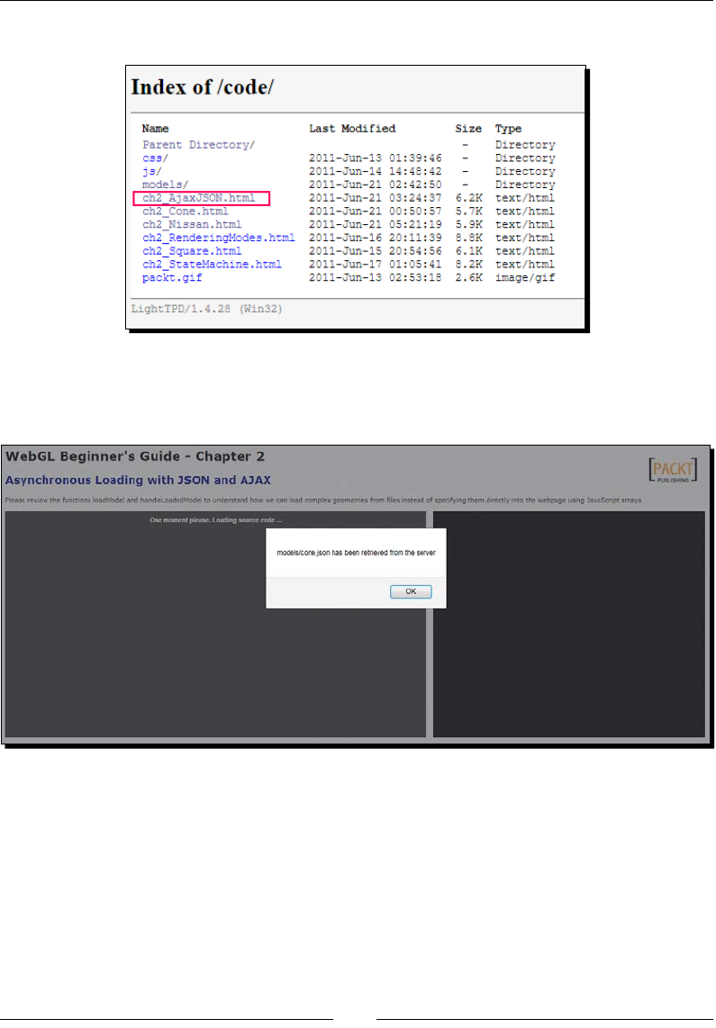
Chapter 2

[ 55 ]

2. The folder where you have the code for this chapter should look like this:

3. Click on ch2_AjaxJSON.html.

4. The example will load in your browser and you will see something similar to this:

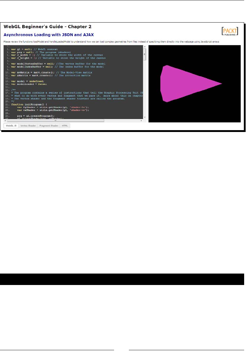
Rendering Geometry

[ 56 ]

5. When you click on the JavaScript alert, you will see:

6. As the page says, please review the funcons loadModel and

handleLoadedModel to beer understand the use of AJAX and JSON

in the applicaon.

7. What does the modelLoaded variable do? (check the source code).

8. See what happens when you change the color in the le models/cone.json and

reload the page.

9. Modify the coordinates of the cone in the le models/cone.json and reload the

page. Here you can verify that WebGL reads and renders the coordinates from the

le. If you modify them in the le, the geometry will be updated on the screen.

What just happened?

You learned about using AJAX and JSON to load geometries from a remote locaon (web

server) instead of specifying these geometries (using JavaScript arrays) inside the web page.

Have a go hero – loading a Nissan GTX

Follow the given steps:

1. Open the le ch2_Nissan.html using your web server. Again, you should see

something like http://localhost./.../code

2. You should see something like this:

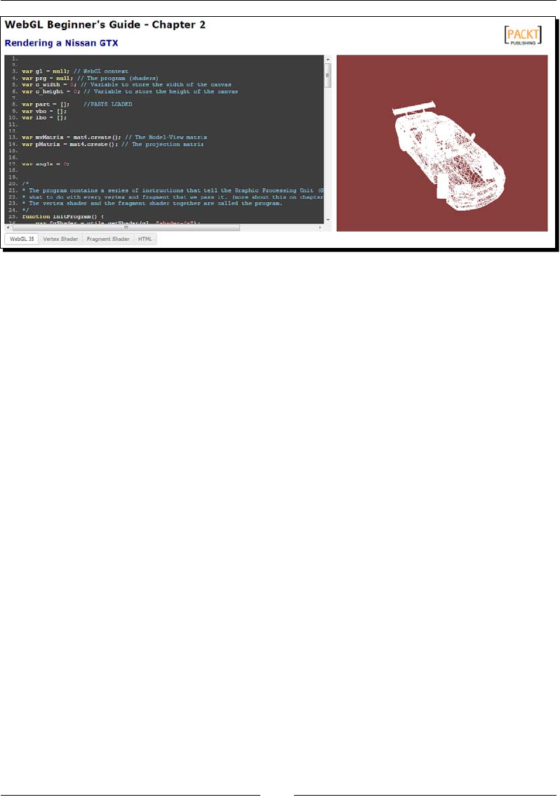
Chapter 2

[ 57 ]

3. The reason we selected the mode LINES instead of the model TRIANGLES

(explained previously in this chapter) is to visualize beer the structure of this car.

4. Find the line where the rendering mode is being selected and make sure you

understand what the code does.

5. Next, go to the drawScene funcon.

6. In the drawElements instrucon, change the mode from gl.LINES to

gl.TRIANGLES.

7. Refresh the page in the web browser (Ctrl + F5 for full refresh).

8. What do you see? Can you hypothesize about the reasons for this? What is

your raonale?

When the geometry is complex, the lighng model allows us to visualize it beer. Without

lights, all our volumes will look opaque and it would be dicult to disnguish their parts

(just as in the previous case) when changing from LINES to TRIANGLES.

In the next chapter, we will see how to create a lighng model for our scene. Our work there

will be focused on the shaders and how we communicate informaon back and forth between

the WebGL JavaScript API and the aributes, uniforms, and varyings. Do you remember them?

We menoned when we were talking about passing informaon to the GPU.

Rendering Geometry

[ 58 ]

Summary

In this chapter, we have discussed how WebGL renders geometry. Remember that there

are two kinds of WebGL buers that deal with geometry rendering: VBOs and IBOs.

WebGL's rendering pipeline describes how the WebGL buers are used and passed in the

form of aributes to be processed by the vertex shader. The vertex shader parallelizes

vertex processing in the GPU. Verces dene the surface of the geometry that is going to

be rendered. Every element on this surface is known as a fragment. These fragments are

processed by the fragment shader. Fragment processing also occurs in parallel in the GPU.

When all the fragments have been processed, the framebuer, a two-dimensional array,

contains the image that is then displayed on your screen.

WebGL works as a state machine. As such, properes referring to buers are available and

their values will be dependent on the buer currently bound.

We also saw that JSON and AJAX are two JavaScript technologies that integrate really well

with WebGL, enabling us to load really complex geometries without having to specify them

inside our webpage.

In the next chapter, we will learn more about the vertex and fragment shaders and we will

see how we can use them to implement light sources in our WebGL scene.

Lights!

In WebGL, we make use of the vertex and fragment shaders to create a

lighng model for our scene. Shaders allow us to dene a mathemacal model

that governs how our scene is lit. We will study dierent algorithms and see

examples about their implementaon.

A basic knowledge of linear algebra will be really useful to help you understand the contents

of this chapter. We will use glMatrix, a JavaScript library that handles most of the vector

and matrix operaon, so you do not need to worry about the details. Nonetheless, it is

paramount to have a conceptual understanding of the linear algebra operaons that we

will discuss.

In this chapter, we will:

Learn about light sources, normals, and materials

Learn the dierence between shading and lighng

Use the Goraud and Phong shading methods, and the Lamberan and Phong

lighng models

Dene and use uniforms, aributes, and varyings

Work with ESSL, the shading language for WebGL

Discuss relevant WebGL API methods that relate to shaders

Connue our analysis of WebGL as a state machine and describe the aributes

relevant to shaders that can be set and retrieved from the state machine

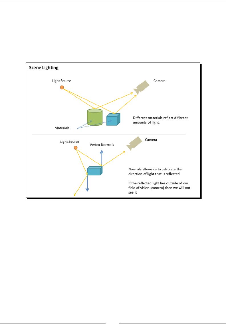
Lights!

[ 60 ]

Lights, normals, and materials

In the real world, we see objects because they reect light. Any object will reect light

depending on the posion and relave distance to the light source; the orientaon of

its surface, which is represented by normal vectors and the material of the object which

determines how much light is reected. In this chapter, we will learn how to combine

these three elements in WebGL to model dierent illuminaon schemes.

Lights

Light sources can be posional or direconal. A light source is called posional when its

locaon will aect how the scene is lit. For instance, a lamp inside a room falls under this

category. Objects far from the lamp will receive very lile light and they will appear obscure.

In contrast, direconal lights refer to lights that produce the same result independent from

their posion. For example, the light of the sun will illuminate all the objects in a terrestrial

scene, regardless of their distance from the sun.

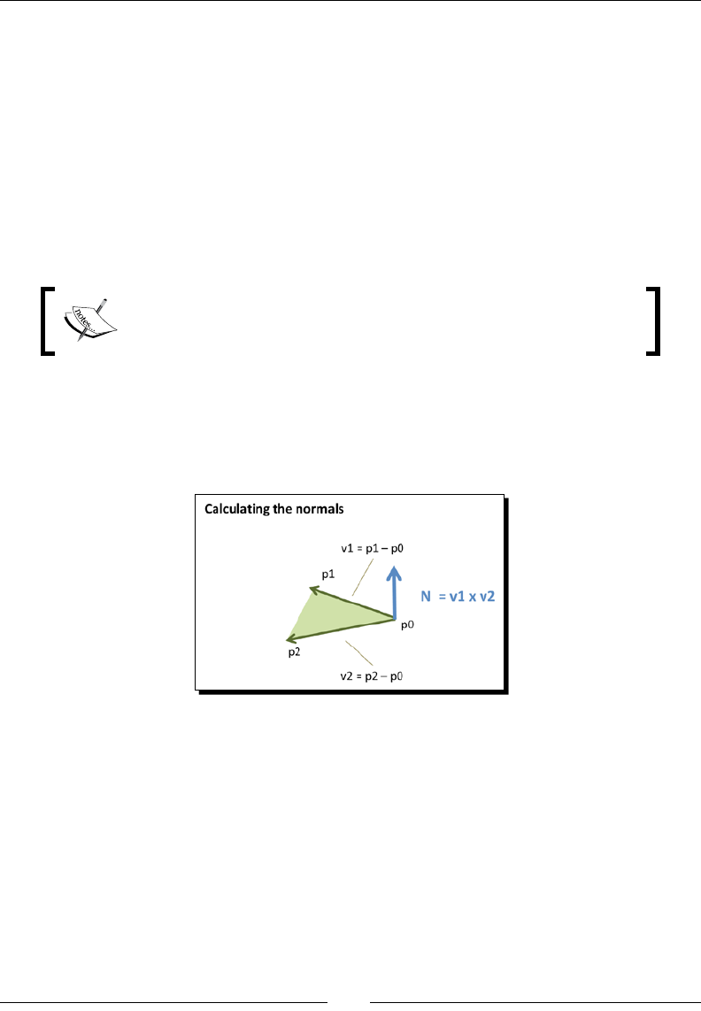
Chapter 3

[ 61 ]

A posional light is modeled by a point in space, while a direconal light is modeled with a

vector that indicates its direcon. It is common to use a normalized vector for this purpose,

given that this simplies mathemacal operaons.

Normals

Normals are vectors that are perpendicular to the surface that we want to illuminate. Normals

represent the orientaon of the surface and therefore they are crical to model the interacon

between a light source and the object. Each vertex has an associated normal vector.

We make use of a cross product for calculang normals.

Cross Product:

By denion, the cross product of vectors A and B will be perpendicular

to both vectors A and B.

Let's break this down. If we have the triangle conformed by verces p0, p1, and p2,

then we can dene the vector v1 as p2-p1 and the vector v2 as p0-p1. Then the normal

is obtained by calculang the cross product v1 x v2. Graphically, this procedure looks

something like the following:

Then we repeat the same calculaon for each vertex on each triangle. But, what about the

verces that are shared by more than one triangle? The answer is that each shared vertex

normal will receive a contribuon from each of the triangles in which the vertex appears.

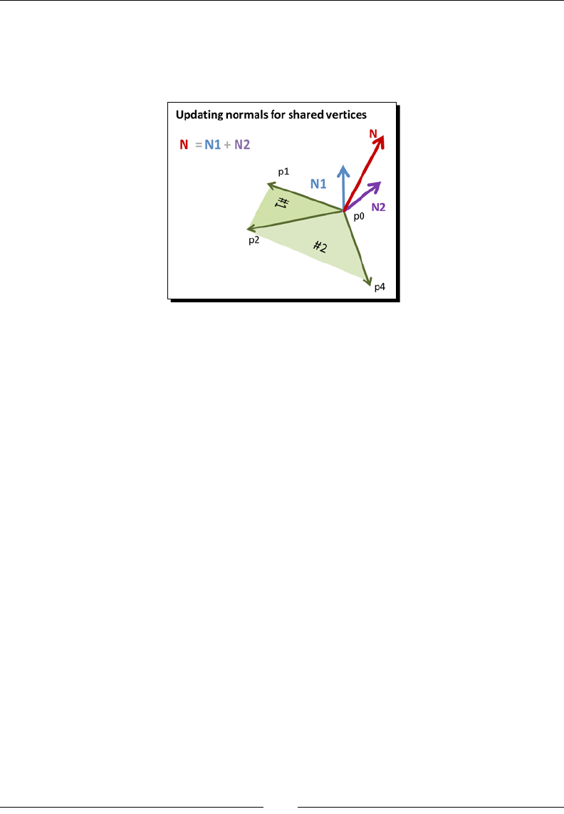
Lights!

[ 62 ]

For example, say that the vertex p1 is being shared by triangles #1 and #2, and we have

already calculated the normals for the verces of triangle #1. Then, we need to update the

p1 normal by adding up the calculated normal for p1 on triangle #2. This is a vector sum.

Graphically, this looks similar to the following:

Similar to lights, normals are usually normalized to facilitate mathemacal operaons.

Materials

The material of an object in WebGL can be modeled by several parameters, including its

color and its texture. Material colors are usually modeled as triplets in the RGB space

(Red, Green, Blue). Textures, on the other hand, correspond to images that are mapped

to the surface of the object. This process is usually called Texture Mapping. We will see

how to perform texture mapping in Chapter 7, Textures.

Using lights, normals, and materials in the pipeline

We menoned in Chapter 2, Rendering Geometry, that WebGL buers, aributes, and

uniforms are used as input variables to the shaders and that varyings are used to carry

informaon between the vertex shader and the fragment shader. Let's revisit the pipeline

and see where lights, normals, and materials t in.

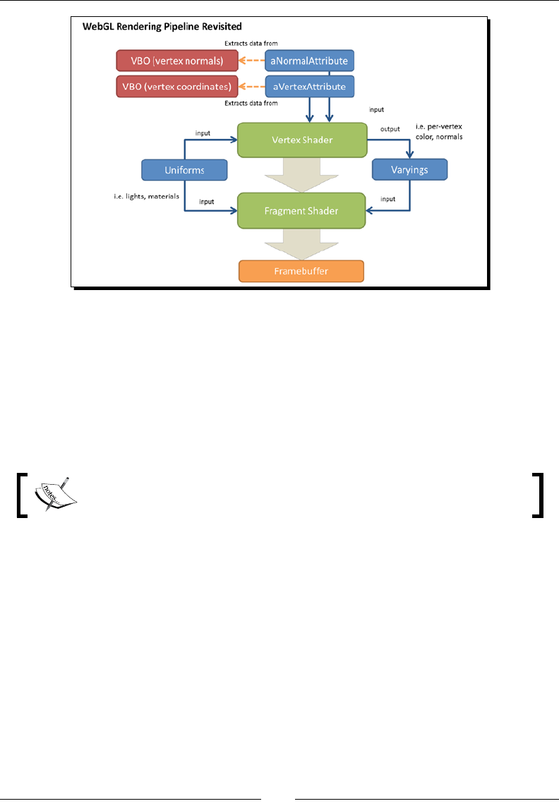
Chapter 3

[ 63 ]

Normals are dened on a vertex-per-vertex basis; therefore normals are modeled in WebGL

as a VBO and they are mapped using an aribute, as shown in the preceding diagram. Please

noce that aributes are never passed to the fragment shader.

Lights and materials are passed as uniforms. Uniforms are available to both the vertex

shader and the fragment shader. This gives us a lot of exibility to calculate our lighng

model because we can calculate how the light is reected on a vertex-by-vertex basis

(vertex shader) or on a fragment-per-fragment basis (fragment shader).

Remember that the vertex shader and fragment shader together are referred

to as the program.

Parallelism and the difference between attributes and uniforms

There is an important disncon to make between aributes and uniforms. When a draw

call is invoked (using drawArrays or drawElements), the GPU will launch in parallel

several copies of the vertex shader. Each copy will receive a dierent set of aributes.

These aributes are drawn from the VBOs that are mapped to the respecve aributes.

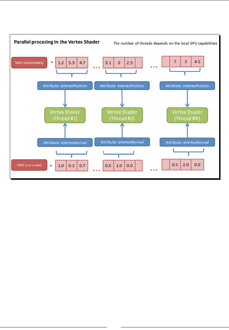
Lights!

[ 64 ]

On the other hand, all the copies of the vertex shaders will receive the same uniforms,

therefore the name, uniform. In other words, uniforms can be seen as constants per

draw call.

Once lights, normals, and materials are passed to the program, the next step is to determine

which shading and lighng models we will implement. Let's see what this is about.

Shading methods and light reection models

The terms shading and lighng are commonly interchanged ambiguously. However, they

refer to two dierent concepts: on one hand, shading refers to the type of interpolaon that

is performed to obtain the nal color for every fragment in the scene. We will explain this

in a moment. Let's say here as well that the type of shading denes where the nal color

is calculated—in the vertex shader or in the fragment shader; on the other hand, once the

shading model is established, the lighng model determines how the normals, materials,

and lights are combined to produce the nal color. The equaons for lighng models use

the physical principles of light reecon. Therefore, lighng models are also referred to in

literature as reecon models.

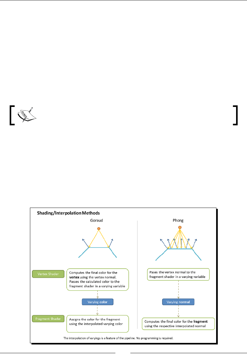
Chapter 3

[ 65 ]

Shading/interpolation methods

In this secon, we will analyze two basic types of interpolaon method: Goraud and

Phong shading.

Goraud interpolation

The Goraud interpolaon method calculates the nal color in the vertex shader. The vertex

normals are used in this calculaon. Then the nal color for the vertex is carried to the

fragment shader using a varying variable. Due to the automac interpolaon of varyings,

provided by the rendering pipeline, each fragment will have a color that is a result of

interpolang the colors of the enclosing triangle for each fragment.

The interpolaon of varyings is automac in the pipeline. No programming

is required.

Phong interpolation

The Phong method calculates the nal color in the fragment shader. To do so, each vertex

normal is passed along from the vertex shader to the fragment shader using a varying.

Because of the interpolaon mechanism of varyings included in the pipeline, each fragment

will have its own normal. Fragment normals are then used to perform the calculaon of the

nal color in the fragment shader.

The two interpolaon models can be summarized by the following diagram:

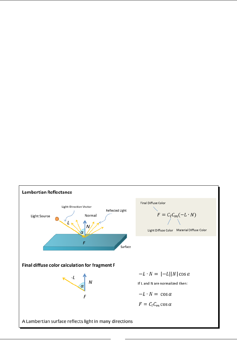
Lights!

[ 66 ]

Again, please note here that the shading method does not specify how the nal color for

every fragment is calculated. It only species where (vertex or fragment shader) and also the

type of interpolaon (vertex colors or vertex normals).

Light reection models

As previously menoned, the lighng model is independent from the shading/interpolaon

model. The shading model only determines where the nal color is calculated. Now it is me

to talk about how to perform such calculaons.

Lambertian reection model

Lamberan reecons are commonly used in computer graphics as a model for diuse

reecons, which are the kind of reecons where an incident light ray is reected in many

angles instead of only in one angle as it is the case for specular reecons.

This lighng model is based on the cosine emission law or Lambert's emission law. It is

named aer Johann Heinrich Lambert, from his Photometria, published in 1760.

The Lamberan reecon is usually calculated as the dot product between the surface

normal (vertex or fragment normal, depending on the interpolaon method used) and

the negave of the light-direcon vector, which is the vector that starts on the surface and

ends on the light source posion. Then, the number is mulplied by the material and light

source colors.

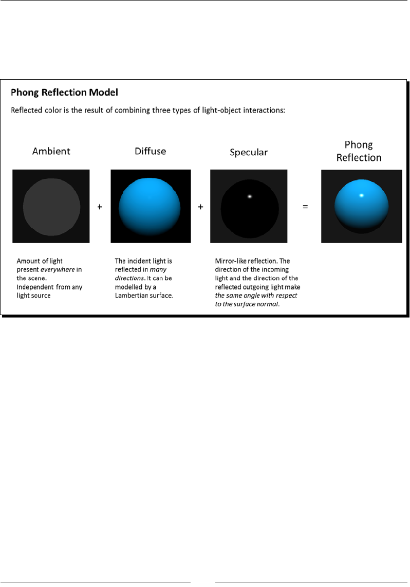
Chapter 3

[ 67 ]

Phong reection model

The Phong reecon model describes the way a surface reects the light as the sum of three

types of reecon: ambient, diuse, and specular. It was developed by Bui Tuong Phong who

published it in his 1973 Ph.D. dissertaon.

The ambient term accounts for the scaered light present in the scene. This term is

independent from any light source and it is the same for all fragments.

The diuse term corresponds to diuse reecons. Usually a Lamberan model is used for

this component.

The specular term provides mirror-like reecons. Conceptually, the specular reecon

will be at its maximum when we are looking at the object on an angle that is equal to the

reected light-direcon vector.

This is modeled by the dot product of two vectors, namely, the eye vector and the

reected light-direcon vector. The eye vector has its origin in the fragment and its end

in the view posion (camera). The reected light-direcon vector is obtained by reecng

the light-direcon vector upon the surface normal vector. When this dot product equals 1

(by working with normalized vectors) then our camera will capture the maximum

specular reecon.

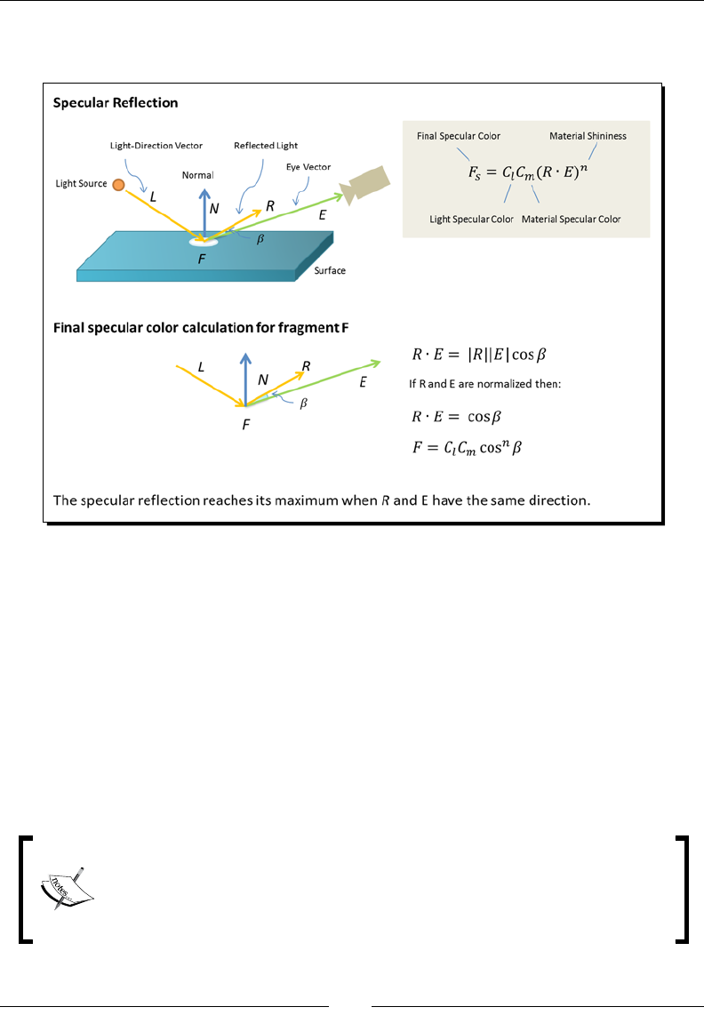
Lights!

[ 68 ]

The dot product is then exponenated by a number that represents the shininess of the

surface. Aer that, the result is mulplied by the light and material specular components.

The ambient, diuse, and specular terms are added to nd the nal color of the fragment.

Now it is me for us to learn the language that will allow us to implement the shading and

lighng strategies inside the vertex and fragment shaders. This language is called ESSL.

ESSL—OpenGL ES Shading Language

OpenGL ES Shading Language (ESSL) is the language in which we write our shaders. Its syntax

and semancs are very similar to C/C++. However, it has types and built-in funcons that

make it easier and more intuive to manipulate vectors and matrices. In this secon,

we will cover the basics of ESSL so we can start using it right away.

This secon is a summary of the ocial GLSL ES specicaon. It is a subset of

GLSL (the shading language for OpenGL).

You can nd the complete reference at http://www.khronos.org/

registry/gles/specs/2.0/GLSL_ES_Specification_1.0.17.

pdf

Chapter 3

[ 69 ]

Storage qualier

Variable declaraons may have a storage qualier specied in front of the type:

aribute: Linkage between a vertex shader and a WebGL applicaon for per-vertex

data. This storage qualier is only legal inside the vertex shader.

uniform: Value does not change across the object being processed, and uniforms

form the linkage between a shader and a WebGL applicaon. Uniforms are legal

in both the vertex and fragment shaders. If a uniform is shared by the vertex and

fragment shader, the respecve declaraons need to match.

varying: Linkage between a vertex shader and a fragment shader for interpolated

data. By denion, varyings are necessarily shared by the vertex shader and the

fragment shader. The declaraon of varyings needs to match between the vertex

and fragment shaders.

const: a compile-me constant, or a funcon parameter that is read-only. They can

be used anywhere in the code of an ESSL program.

Types

ESSL provides the following basic types:

void: For funcons that do not return a value or for an empty parameter list

bool: A condional type, taking on values of true or false

int: A signed integer

float: A single oang-point scalar

vec2: A two component oang-point vector

vec3: A three component oang-point vector

vec4: A four component oang-point vector

bvec2: A two component boolean vector

bvec3: A three component boolean vector

bvec4: A four component boolean vector

ivec2: A two component integer vector

ivec3: A three component integer vector

ivec4: A four component integer vector

mat2: A 2×2 oang-point matrix

Lights!

[ 70 ]

mat3: A 3×3 oang-point matrix

mat4: A 4×4 oang-point matrix

sampler2D: A handle for accessing a 2D texture

samplerCube: A handle for accessing a cube mapped texture

So an input variable will have one of the three qualiers followed by one type. For example,

we will declare our vFinalColor varying as follows:

varying vec4 vFinalColor;

This means that the vFinalColor variable is a varying vector with four components.

Vector components

We can refer to each one of the components of an ESSL vector by its index.

For example:

vFinalColor[3] will refer to the fourth element of the vector (zero-based vectors).

However, we can also refer to each component by a leer, as it is shown in the

following table:

{x,y,z,w} Useful when accessing vectors represenng points or vectors

{r,g,b,a} Useful when accessing vectors represenng colors

{s,t,p,q} Useful when accessing vectors that represent texture coordinates

So, for example, if we want to set the alpha channel (fourth component) of our variable

vFinalColor to 1, we can write:

vFinalColor[3] = 1.0;

vFinalColor.a = 1.0;

We could also do this:

vFinalColor.w = 1.0;

In all three cases, we are referring to the same fourth component. However, given that

vFinalColor represents a color, it makes more sense to use the {r,g,b,a} notaon.

Chapter 3

[ 71 ]

Also, it is possible to use the vector component notaon to refer to subsets inside a vector.

For example (taken from page 44 in the GLSL ES 1.0.17 specicaon):

vec4 v4;

v4.rgba; // is a vec4 and the same as just using v4,

v4.rgb; // is a vec3,

v4.b; // is a float,

v4.xy; // is a vec2,

v4.xgba; // is illegal - the component names do not come from

// the same set.

Operators and functions

ESSL also provides many useful operators and funcons that simplify vector and matrix

operaons. According to the specicaon: the arithmec binary operators add (+), subtract

(-), mulply (*), and divide (/) operate on integer and oang-point typed expressions

(including vectors and matrices). The two operands must be the same type, or one can be

a scalar oat and the other a oat vector or matrix, or one can be a scalar integer and the

other an integer vector. Addionally, for mulply (*), one can be a vector and the other a

matrix with the same dimensional size of the vector. These result in the same fundamental

type (integer or oat) as the expressions they operate on. If one operand is a scalar and

the other is a vector or a matrix, the scalar is applied component-wise to the vector or the

matrix, with the nal result being of the same type as the vector or the matrix. Dividing by

zero does not cause an excepon but does result in an unspecied value.

-x: The negave of the x vector. It produces the same vector in the exact

opposite direcon.

x+y : Sum of the vectors x and y. They need to have the same number

of components.

x-y: Subtracon of the vectors x and y. They need to have the same number

of components.

x*y: If x and y are both vectors, then this operator yields a component-wise

mulplicaon. Mulply applied to two matrices return a linear algebraic matrix

mulplicaon, not a component-wise mulplicaon (for it, you must use the

matrixCompMult funcon).

x/y: The division operator behaves similarly to the mulply operator.

dot(x,y): Returns the dot product (scalar) of two vectors. They need to have the

same dimensions.

cross(vec3 x, vec3 y): Returns the cross product (vector) of two vectors. They

have to be vec3.

Lights!

[ 72 ]

matrixCompMult (mat x, mat y): Component-wise mulplicaon of matrices.

They need to have the same dimensions (mat2, mat3, or mat4).

normalize(x): Returns a vector in the same direcon but with a length of 1.

reflect(t, n): Reects the vector t along the vector n.

There are many more funcons including trigonometry and exponenal funcons. We will

refer to those as we need them in the development of the dierent lighng models.

Let's see now a quick example of the shaders ESSL code for a scene with the

following properes:

Lamberan reecon model: We account for the diuse interacon between one

light source and our scene. This means that we will use uniforms to dene the light

properes, the material properes, and we will follow the Lambert's Emission Law

to calculate the nal color for every vertex.

Goraud shading: We will interpolate vertex colors to obtain fragment colors

and therefore we need one varying to pass the vertex color informaon

between shaders.

Let's dissect rst what the aributes, uniforms, and varyings will be.

Vertex attributes

We start by dening two aributes in the vertex shader. Every vertex will have:

attribute vec3 aVertexPosition;

attribute vec3 aVertexNormal;

Right aer the attribute keyword, we nd the type of the variable. In this case, this

is vec3, as each vertex posion is determined by three elements (x,y,z). Similarly, the

normals are also determined by three elements (x,y,z). Please noce that a posion is a

point in tridimensional space that tells us where the vertex is, while a normal is a vector that

gives us informaon about the orientaon of the surface that passes along that vertex.

Remember that aributes are only available for use inside the vertex shader.

Uniforms

Uniforms are available to both the vertex shader and the fragment shader. While aributes

are dierent every me the vertex shader is invoked (remember, we process the verces

in parallel, therefore each copy/thread of the vertex shader processes a dierent vertex).

Uniforms are constant throughout a rendering cycle. That is, during a drawArrays or

drawElements WebGL call.

Chapter 3

[ 73 ]

We can use uniforms to pass along informaon about lights (such as diuse color and

direcon), and materials (diuse color).

For example:

uniform vec3 uLightDirection; //incoming light source direction

uniform vec4 uLightDiffuse; //light diffuse component

uniform vec4 uMaterialDiffuse; //material diffuse color

Again, here the keyword uniform tells us that these variables are uniforms and the ESSL

types vec3 and vec4 tell us that these variables have three or four components. In the case

of the colors, these components are the red, blue, green, and alpha channels (RGBA) and in

the case of the light direcon, these components are the x, y, and z coordinates that dene

the vector in which the light source is directed in the scene.

Varyings

We need to carry the vertex color from the vertex shader to the fragment shader:

varying vec4 vFinalColor;

As previously menoned in the secon Storage Qualier, the declaraon of varyings need to

match between the vertex and fragment shaders.

Now let's plug the aributes, uniforms, and varyings into the code and see how the vertex

shader and fragment shader look like.

Vertex shader

This is what a vertex shader looks like. On a rst look, we idenfy the aributes, uniforms,

and varyings that we will use along with some matrices that we will discuss in a minute.

Also we see that the vertex shader has a main funcon that does not accept parameters and

returns void. Inside, we can see some ESSL funcons such as normalize and dot and some

arithmecal operators.

attribute vec3 aVertexPosition;

attribute vec3 aVertexNormal;

uniform mat4 uMVMatrix;

uniform mat4 uPMatrix;

uniform mat4 uNMatrix;

uniform vec3 uLightDirection;

uniform vec4 uLightDiffuse;

uniform vec4 uMaterialDiffuse;

Lights!

[ 74 ]

varying vec4 vFinalColor;

void main(void) {

vec3 N = normalize(vec3(uNMatrix * vec4(aVertexNormal, 1.0)));

vec3 L = normalize(uLightDirection);

float lambertTerm = dot(N,-L);

vFinalColor = uMaterialDiffuse * uLightDiffuse * lambertTerm;

vFinalColor.a = 1.0;

gl_Position = uPMatrix * uMVMatrix * vec4(aVertexPosition, 1.0);

}

There are three uniforms that we have not discussed yet:

uniform mat4 uMVMatrix;

uniform mat4 uPMatrix;

uniform mat4 uNMatrix;

We can see that these three uniforms are 4x4 matrices. These matrices are required in the

vertex shader to calculate the locaon for verces and normals whenever we move the

camera. There are a couple of operaons here that involve using these matrices:

vec3 N = vec3(uNMatrix * vec4(aVertexNormal, 1.0));

The previous line of code calculates the transformed normal.

And:

gl_Position = uPMatrix * uMVMatrix * vec4(aVertexPosition, 1.0);

This line calculates the transformed vertex posion. gl_Position is a special output

variable that stores the transformed vertex posion.

We will come back to these operaons in Chapter 4, Camera. For now, let's acknowledge

that these uniforms and operaons deal with camera and world transformaons (rotaon,

scale, and translaon).

Going back to the code of the main funcon, we can clearly see that the Lamberan

reecon model is being implemented. The dot product of the normalized normal and

light direcon vector is obtained and then it is mulplied by the light and material diuse

components. Finally, this result is passed into the vFinalColor varying to be used in

the fragment shader. Also, as we are calculang the color in the vertex shader and then

interpolang the vertex colors for the fragments of every triangle, we are using a Goraud

interpolaon method.

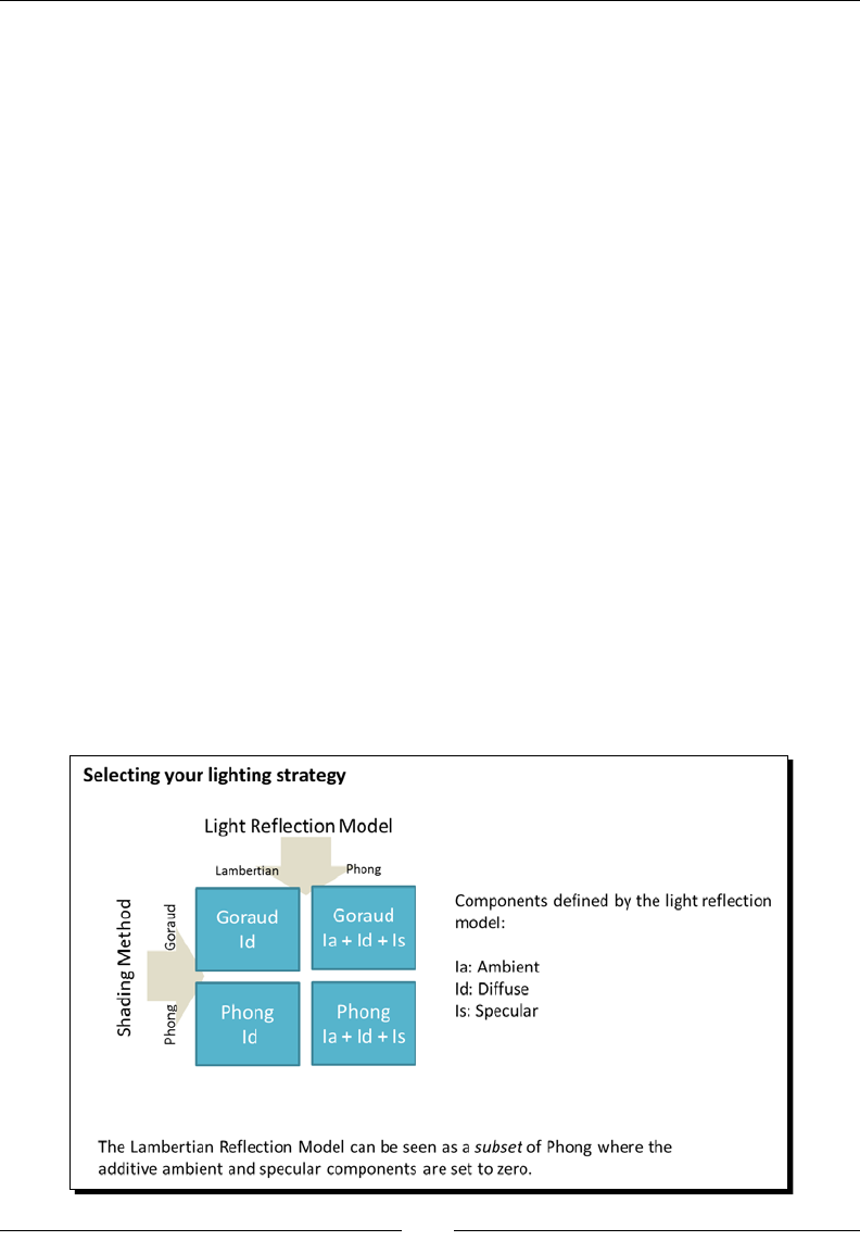
Chapter 3

[ 75 ]

Fragment shader

The fragment shader is very simple. The rst three lines dene the precision of the shader.

This is mandatory according to the ESSL specicaon. Similarly, to the vertex shader, we

dene our inputs; in this case, just one varying variable and then we have the main funcon.

#ifdef GL_SL

precision highp float;

#endif

varying vec4 vFinalColor;

void main(void) {

gl_FragColor = vFinalColor;

}

We just need to assign the vFinalColor varying to the output variable gl_FragColor.

Remember that the value of the vFinalColor varying will be dierent from the one

calculated in the vertex shader as WebGL will interpolate it by taking the corresponding

calculated colors for the verces surrounding the correspondent fragment (pixel).

Writing ESSL programs

Let's now take a step back and take a look at the big picture. ESSL allows us to implement a

lighng strategy provided that we dene a shading method and a light reecon model. In

this secon, we will take a sphere as the object that we want to illuminate and we will see

how the selecon of a lighng strategy changes the scene.

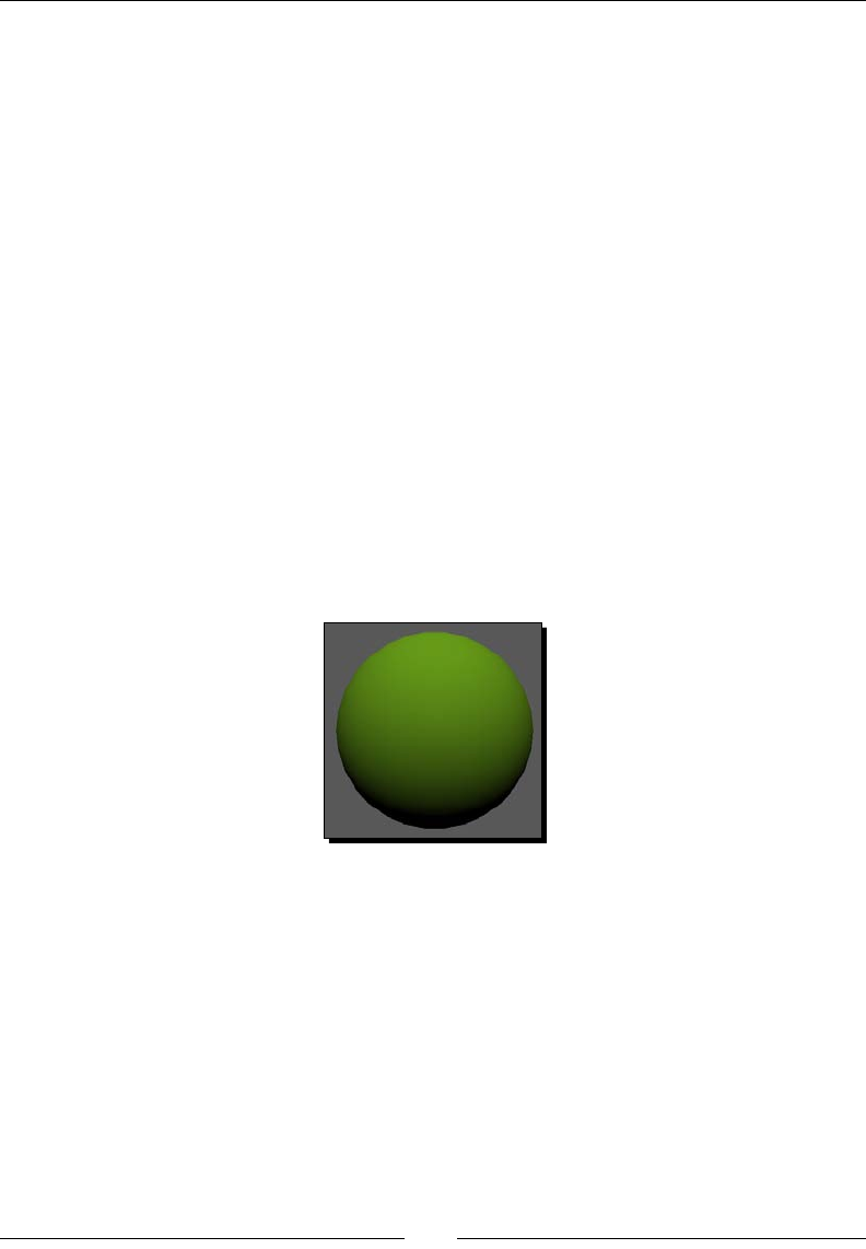
Lights!

[ 76 ]

We will see two scenarios for Goraud interpolaon: with Lamberan and with Phong

reecons; and only one case for Phong interpolaon: under Phong shading the Lamberan

reecon model is no dierent from a Phong reecon model where the ambient and

specular components are set to zero.

Goraud shading with Lambertian reections

The Lamberan reecon model only considers the interacon of diuse material and

diuse light properes. In short, we assign the nal color as:

Final Vertex Color = Id

where the following value is seen:

Id = Light Diffuse Property * Material Diffuse Property * Lambert

coefficient

Under Goraud shading, the Lambert coecient is obtained by calculang the dot product of

the vertex normal and the inverse of the light-direcon vector. Both vectors are normalized

previous to nding the dot product.

Now let's take a look at the vertex shader and the fragment shader of the example

ch3_Sphere_Goraud_Lambert.html:

Vertex shader:

attribute vec3 aVertexPosition;

attribute vec3 aVertexNormal;

uniform mat4 uMVMatrix;

uniform mat4 uPMatrix;

uniform mat4 uNMatrix;

uniform vec3 uLightDirection;

uniform vec4 uLightDiffuse;

uniform vec4 uMaterialDiffuse;

varying vec4 vFinalColor;

Chapter 3

[ 77 ]

void main(void) {

vec3 N = normalize(vec3(uNMatrix * vec4(aVertexNormal, 1.0)));

vec3 L = normalize(uLightDirection);

float lambertTerm = dot(N,-L);

vec4 Id = uMaterialDiffuse * uLightDiffuse * lambertTerm;

vFinalColor = Id;

vFinalColor.a = 1.0;

gl_Position = uPMatrix * uMVMatrix * vec4(aVertexPosition, 1.0);

}

Fragment shader:

#ifdef GL_ES

precision highp float;

#endif

varying vec4 vFinalColor;

void main(void) {

gl_FragColor = vFinalColor;

}

We can see that the nal vertex color that we process in the vertex shader is carried into a

varying variable to the fragment (pixel) shader. However, please remember that the value

that arrives to the fragment shader is not the original value that we calculated in the vertex

shader. The fragment shader interpolates the vFinalColor variable to generate a nal

color for the respecve fragment. This interpolaon takes into account the verces that

enclose the current fragment as we saw in Chapter 2, Rendering Geometry.

Time for action – updating uniforms in real time

1. Open the le ch3_Sphere_Goraud_Lambert.html in your favorite

HTML5 browser.

2. You will see that this example has some widgets at the boom of the page. These

widgets were created using JQuery UI. You can check the code for those in the HTML

<body> of the page.

X,Y,Z: controls the direcon of the light. By changing these sliders you will

modify the uniform uLightDirection.

Sphere color: changes the uniform uMaterialDiffuse, which represents

the diuse color of the sphere. Here we use a color selecon widget so you

can try dierent colors. The updateObjectColor funcon receives the

updates from the widgets and updates the uMaterialDiffuse uniform.

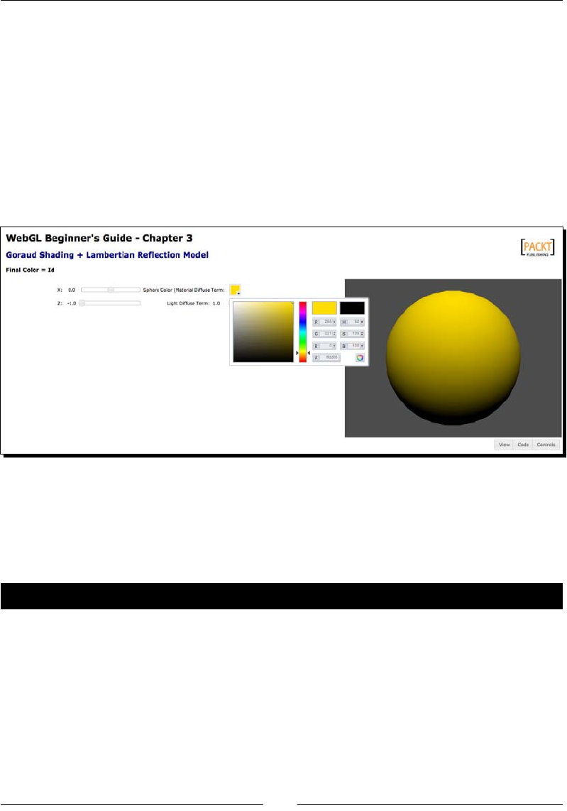
Lights!

[ 78 ]

Light diuse term: changes the uniform uLightDiffuse, which

represents the diuse color of the light source. There are no reasons as to

why the light color has to be white; however for the sake of simplicity, in

this case, we are using a slider instead of a color to restrict the light color

to the gray scale. We achieve this by assigning the slider value to the RGB

components of uLightDiffuse while we keep the alpha channel set to

1.0. We do this inside the updateLightDiffuseTerm funcon, which

receives the slider updates.

3. Try dierent sengs for light source posion (which will aect the light-direcon

vector), the diuse material, and light properes.

What just happened?

We have seen an example of a simple scene illuminated using Goraud interpolaon and a

Lamberan reecon model. We have also seen the immediate eects of changing uniform

values for the Lamberan lighng model.

Have a go hero – moving light

We have menoned before that we use matrices to move the camera around the scene.

Well, we can also use matrices to move lights!

1. Check the le ch3_Sphere_Moving.html using your favorite source code editor.

The vertex shader is very similar to the previous diuse model example. However,

there is one extra line:

vec4 light = uMVMatrix * vec4(uLightDirection, 0.0);

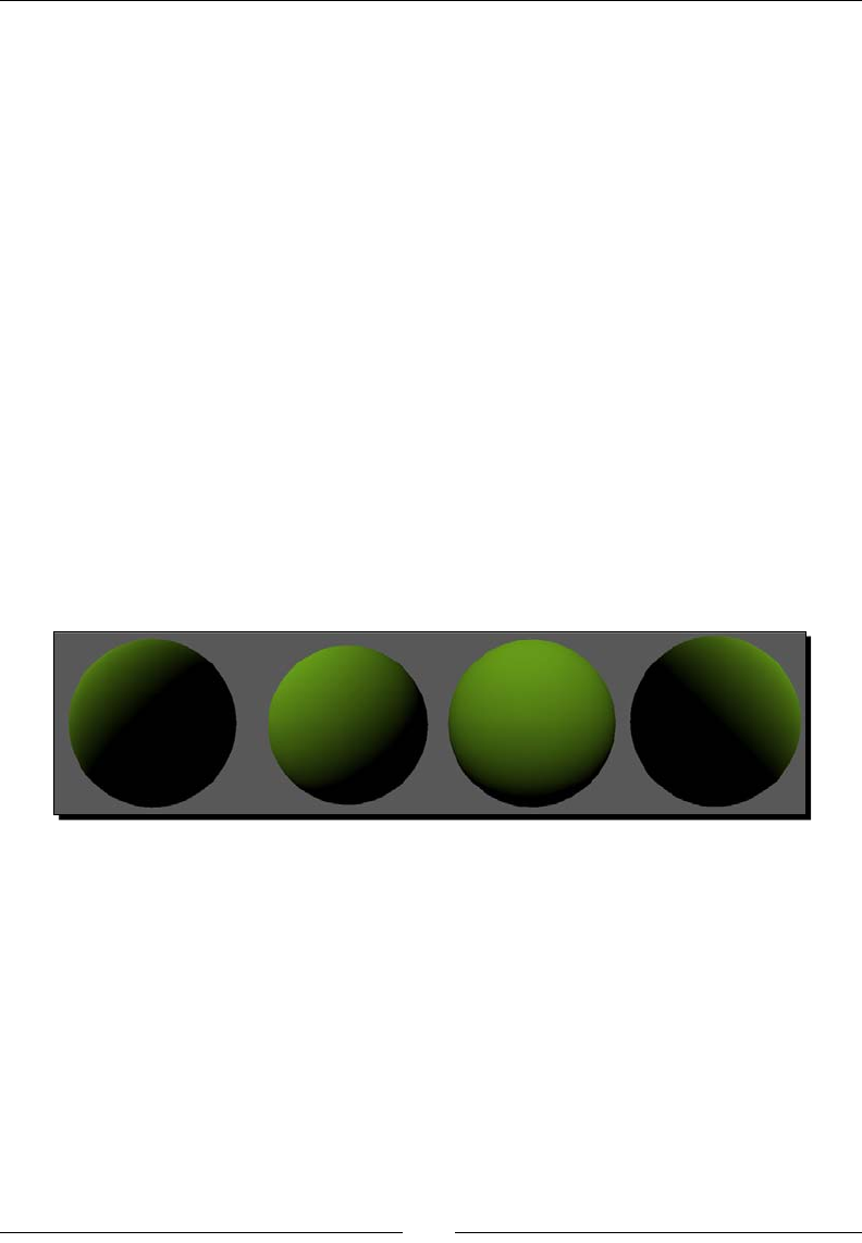
Chapter 3

[ 79 ]

Here we are transforming the uLightDirection vector to the light variable.

Noce that the uniform uLightDirection is a vector with three components

(vec3) and that uMVMatrix is a 4x4 matrix. In order to do the mulplicaon, we

need to transform this uniform to a four-component vector (vec4). We achieve this

with the construct:

vec4(uLightDirection, 0.0);

The matrix uMVMatrix contains the Model-view-transform. We will see how all this

works in the next chapter. However, for now, let's say that this matrix allows us to

update verces posions and also, as we see in this example, lights posions.

2. Take another look at the vertex shader. In this example, we are rotang the sphere

and the light. Every me the drawScene funcon is invoked, we rotate the matrix

mvMatrix a lile bit in the y axis:

mat4.rotate(mvMatrix, angle * Math.PI / 180, [0, 1, 0]);

3. If you examine the code more closely, you will noce that the matrix mvMatrix is

mapped to the uniform:

uMVMatrix:gl.uniformMatrix4fv(prg.uMVMatrix, false, mvMatrix);

4. Now run the example in your HTML5 browser. You will see a sphere and a light

source rotang on the y-axis:

5. Look for the initLights funcon and change the light orientaon so the light is

poinng in the negave z-axis direcon:

gl.uniform3f(prg.uLightDirection, 0.0, 0.0, -1.0)

6. Save the le and run it again. What happened? Now change the light direcon

uniform so it points to [-1.0, 0.0, 0.0]. Save the le and run it again on your browser.

What happened?

Lights!

[ 80 ]

7. Now set the light back to the 45 degree angle by changing the uniform

uLightDirection so it goes back to its inial value:

gl.uniform3f(prg.uLightDirection, 0.0, 0.0, -1.0)

8. Go to drawScene and change the line:

mat4.rotate(mvMatrix, angle * Math.PI / 180, [0, 1, 0]);

with:

mat4.rotate(mvMatrix, angle * Math.PI / 180, [1, 0, 0]);

9. Save the le and launch it again in your browser. What happens?

What can you conclude? As you see, the vector that is passed as the third argument to mat4.

rotate determines the axis of the rotaon. The rst component corresponds to the x-axis, the

second to the y-axis and the third to the z-axis.

Goraud shading with Phong reections

In contrast with the Lamberan reecon model, the Phong reecon model considers three

properes: the ambient, diuse, and specular. Following the same analogy that we used in

the previous secon:

Final Vertex Color = Ia + Id + Is

where:

Ia = Light Ambient Property * Material Ambient Property

Id = Light Diffuse Property * Material Diffuse Property * Lambert

coefficient

Is = Light Specular Property * Material Specular Property * specular

coefficient

Please noce that:

As we are using Goraud interpolaon, we sll use vertex normals to calculate the

diuse term. This will change when using Phong interpolaon where we will be

using fragment normals.

Both light and material have three properes: the ambient, diuse,

and specular colors.

We can see on these equaons that Ia, Id, and Is receive contribuons from their

respecve light and material properes.

Chapter 3

[ 81 ]

Based on our knowledge of the Phong reecon model, let's see how to calculate the

specular coecient in ESSL:

float specular = pow(max(dot(R, E), 0.0), f );

where:

E is the view vector or camera vector.

R is the reected light vector.

f is the specular exponenal factor or shininess.

R is calculated as:

R = reflect(L, N)

where N is the vertex normal considered and L the light direcon that we have been using to

calculate the Lambert coecient.

Let's take a look at the ESSL implementaon for the vertex and fragment shaders.

Vertex shader:

attribute vec3 aVertexPosition;

attribute vec3 aVertexNormal;

uniform mat4 uMVMatrix;

uniform mat4 uPMatrix;

uniform mat4 uNMatrix;

uniform float uShininess;

uniform vec3 uLightDirection;

uniform vec4 uLightAmbient;

uniform vec4 uLightDiffuse;

uniform vec4 uLightSpecular;

uniform vec4 uMaterialAmbient;

uniform vec4 uMaterialDiffuse;

uniform vec4 uMaterialSpecular;

varying vec4 vFinalColor;

void main(void) {

vec4 vertex = uMVMatrix * vec4(aVertexPosition, 1.0);

vec3 N = vec3(uNMatrix * vec4(aVertexNormal, 1.0));

vec3 L = normalize(uLightDirection);

float lambertTerm = clamp(dot(N,-L),0.0,1.0);

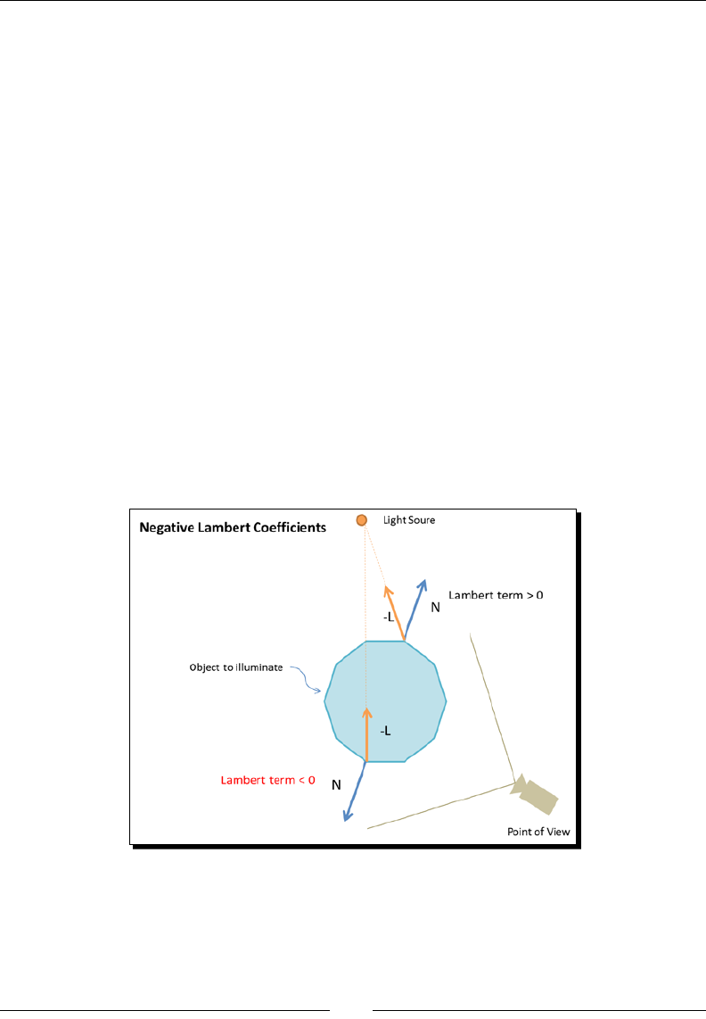
Lights!

[ 82 ]

vec4 Ia = uLightAmbient * uMaterialAmbient;

vec4 Id = vec4(0.0,0.0,0.0,1.0);

vec4 Is = vec4(0.0,0.0,0.0,1.0);

Id = uLightDiffuse* uMaterialDiffuse * lambertTerm;

vec3 eyeVec = -vec3(vertex.xyz);

vec3 E = normalize(eyeVec);

vec3 R = reflect(L, N);

float specular = pow(max(dot(R, E), 0.0), uShininess );

Is = uLightSpecular * uMaterialSpecular * specular;

vFinalColor = Ia + Id + Is;

vFinalColor.a = 1.0;

gl_Position = uPMatrix * vertex;

}

We can obtain negave dot products for the Lambert term when the geometry of our

objects is concave or when the object is in the way between the light source and our point

of view, in either case the negave of the light-direcon vector and the normals will form

an obtuse angle producing a negave dot product, as shown in the following gure:

For that reason we are using the ESSL built-in clamp funcon to restrict the dot product

to the posive range. In the case of obtaining a negave dot product, the clamp funcon

will set the lambert term to zero and the respecve diuse contribuon will be discarded,

generang the correct result.

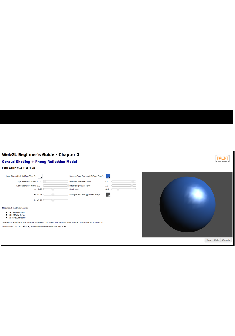
Chapter 3

[ 83 ]

Given that we are sll using Goraud interpolaon, the fragment shader is exactly as before:

#ifdef GL_ES

precision highp float;

#endif

varying vec4 vFinalColor;

void main(void)

{

gl_FragColor = vFinalColor;

}

In the following secon, we will explore the scene and see what it looks like when we have

negave Lambert coecients that have been clamped to the [0,1] range.

Time for action – Goraud shading

1. Open the le ch3_Sphere_Goraud_Phong.html in your HTML5 browser. You will

see something similar to the following screenshot:

2. The interface looks a lile bit more elaborate than the diuse lighng example. Let's

stop here for a moment to explain these widgets:

Light color (light diuse term): As menoned at the beginning of the

chapter, we can have a case where our light is not white. We have included

a color selector widget here for the light color so you can experiment with

dierent combinaons.

Light ambient term: The light ambient property. In this example, a gray

value: r = g = b.

Lights!

[ 84 ]

Light specular term: The light specular property. A gray value: r=g=b.

X,Y,Z: The coordinates that dene the light orientaon.

Sphere color (material diuse term): The material diuse property. We

have included a color selector so you can try dierent combinaons for the

r, g, b channels.

Material ambient term: The material ambient property. We have included it

just for the sake of it. But as you might have noced in the diuse example,

this vector is not always used.

Material specular term: The material specular property. A gray value.

Shininess: The specular exponenal factor for the Goraud model.

Background color (gl.clearColor): This widget simply allows us to

change the background color. We used this code in Chapter 1, Geng

started with WebGL. Now we have a nice color selector widget.

3. Let's prove that when the light source is behind the object, we only see the

ambient term.

4. Open the web page (ch3_Sphere_Goraud_Phong.html) in a text editor.

5. Look for the updateLightAmbientTerm funcon and replace the line:

gl.uniform4fv(prg.uLightAmbient,[la,la,la,1.0]);

with:

gl.uniform4fv(prg.uLightAmbient,[0.0,la,0.0,1.0]);

This will make the ambient property of the light a green color (r = 0, g = la, b=0).

6. Save the le with a new name.

7. Open this new le in your HTML5 browser.

8. Move the light ambient term slider so it is larger than 0.4.

9. Move X close to 0.0

10. See what happens as you move Z towards 1.0. It should be clear then that the light

direcon is coming behind the object and we are only geng the light ambient term

which, in this case, is a color in the green scale (r=0,g=0.3,b=0).

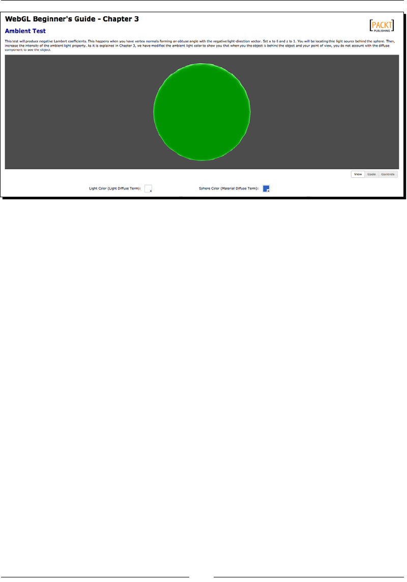
Chapter 3

[ 85 ]

11. Go back to the original web page (ch3_Sphere_Goraud_Phong.html) in your

HTML5 browser.

12. The specular reecon in the Phong reecon model depends on the shininess, the

specular property of the material, and the specular property of the light. When the

specular property of the material is close to zero (vector [0,0,0,1]), the material loses

its specular property. Check this behavior with the widgets provided.

13. What happens when the specularity of the material is low and the shininess is high?

14. What happens when the specularity of the material is high and the shininess is low?

15. Using the widgets, try dierent combinaons for the light and material properes.

What just happened?

We have seen how the dierent parameters of the Phong lighng model interact

with each other.

We have modied the light orientaon, the properes of the light, and the material

to observe dierent behaviors of the Phong lighng model.

Unlike the Lamberan reecon model, the Goraud lighng model has two extra

terms: the ambient and specular components. We have seen how these parameters

aect the scene.

Just like the Lamberan reecon model, the Phong reecon model obtains the vertex

color in the vertex shader. This color is interpolated in the fragment shader to obtain the

nal pixel color. This is because, in both cases, we are using Goraud interpolaon. Let's now

move the heavy processing to the fragment shader and study how we implement the Phong

interpolaon method.

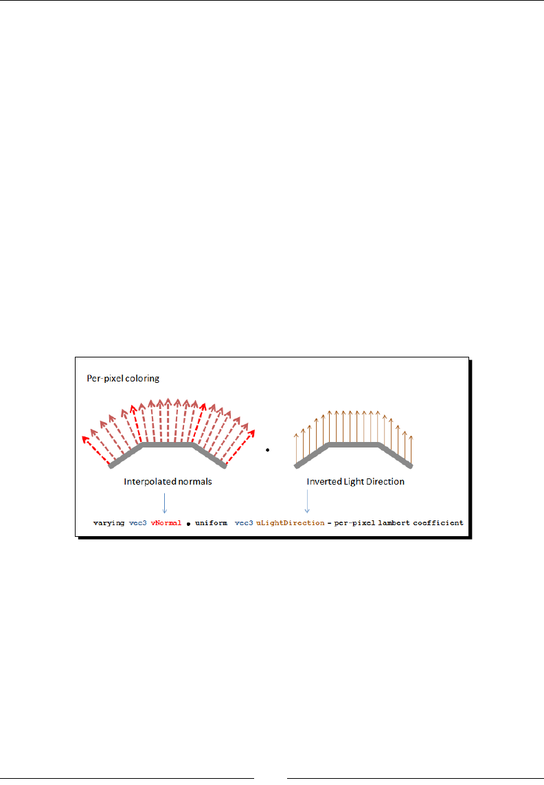
Lights!

[ 86 ]

Phong shading

Unlike the Goraud interpolaon, where we calculated the nal color for each vertex, the

Phong interpolaon calculates the nal color for every fragment. This means that the

calculaon of the ambient, diuse, and specular terms in the Phong model are performed

in the fragment shader instead of the vertex shader. As you can imagine, this is more

computaonally intensive than performing a simple interpolaon like in the two previous

scenarios where we were using Goraud interpolaon. However, we obtain a scene that

seems more realisc.

What do we do in the vertex shader then? Well, in this case, we are going to create varyings

here that will allow us to do all of the calculaons in the fragment shader later on. Think for

example of the normals.

Whereas before we had a normal per vertex, now, we need to generate a normal for

every pixel so we can calculate the Lambert coecient for each fragment. We do so by

interpolang the normals that we pass to the vertex shader. Nevertheless, the code is very

simple. All we need to know is to create a varying that stores the normal for the vertex that

we are processing in the vertex shader and obtain the interpolated value in the fragment

shader (courtesy of ESSL). That's all! Conceptually, this looks like the following diagram:

Now let's take a look at the vertex shader under Phong shading:

attribute vec3 aVertexPosition;

attribute vec3 aVertexNormal;

uniform mat4 uMVMatrix;

uniform mat4 uPMatrix;

uniform mat4 uNMatrix;

varying vec3 vNormal;

varying vec3 vEyeVec;

void main(void) {

vec4 vertex = uMVMatrix * vec4(aVertexPosition, 1.0);

Chapter 3

[ 87 ]

vNormal = vec3(uNMatrix * vec4(aVertexNormal, 1.0));

vEyeVec = -vec3(vertex.xyz);

gl_Position = uPMatrix * uMVMatrix * vec4(aVertexPosition, 1.0);

}

In contrast with the Goraud interpolaon, the vertex shader looks really simple. There is no

nal color calculaon and we are using two varyings to pass informaon to the fragment

shader. The fragment shader will now look like the following:

uniform float uShininess;

uniform vec3 uLightDirection;

uniform vec4 uLightAmbient;

uniform vec4 uLightDiffuse;

uniform vec4 uLightSpecular;

uniform vec4 uMaterialAmbient;

uniform vec4 uMaterialDiffuse;

uniform vec4 uMaterialSpecular;

varying vec3 vNormal;

varying vec3 vEyeVec;

void main(void)

{

vec3 L = normalize(uLightDirection);

vec3 N = normalize(vNormal);

float lambertTerm = dot(N,-L);

vec4 Ia = uLightAmbient * uMaterialAmbient;

vec4 Id = vec4(0.0,0.0,0.0,1.0);

vec4 Is = vec4(0.0,0.0,0.0,1.0);

if(lambertTerm > 0.0)

{

Id = uLightDiffuse * uMaterialDiffuse * lambertTerm;

vec3 E = normalize(vEyeVec);

vec3 R = reflect(L, N);

float specular = pow( max(dot(R, E), 0.0), uShininess);

Is = uLightSpecular * uMaterialSpecular * specular;

}

vec4 finalColor = Ia + Id + Is;

finalColor.a = 1.0;

gl_FragColor = finalColor;

}

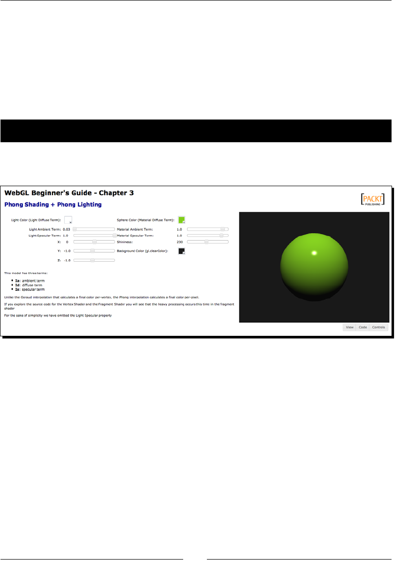
Lights!

[ 88 ]

When we pass vectors as varyings, it is possible that they denormalized in the interpolaon

step. Therefore, you may have noced that both vNormal and vEyeVec are normalized

before they are used in the fragment shader.

As we menoned before, under Phong lighng, the Lamberan reecon model can be seen

as a Phong reecon model where the ambient and specular components are set to zero.

Therefore, we will only cover the general case in the next secon where we will see how the

sphere scene looks like when using Phong shading and Phong lighng combined.

Time for action – Phong shading with Phong lighting

1. Open the le ch3 Sphere_Phong.html in your HTML5 Internet browser. The page

will look similar to the following screenshot:

2. The interface is very similar to the Goraud example's interface. Please noce how

the Phong shading combined with Phong lighng delivers a more realisc scene.

3. Click on the buon Code. This will bring up the code viewer area. Check the vertex

shader and the fragment shader with the respecve buons that will appear under

the code viewer area. As in previous examples, the code has been commented

extensively so you can understand every step of the process.

4. Now click on the buon Controls to go back to the original layout. Modify the

dierent parameters of the Phong lighng model to see the immediate result

on the scene to the right.

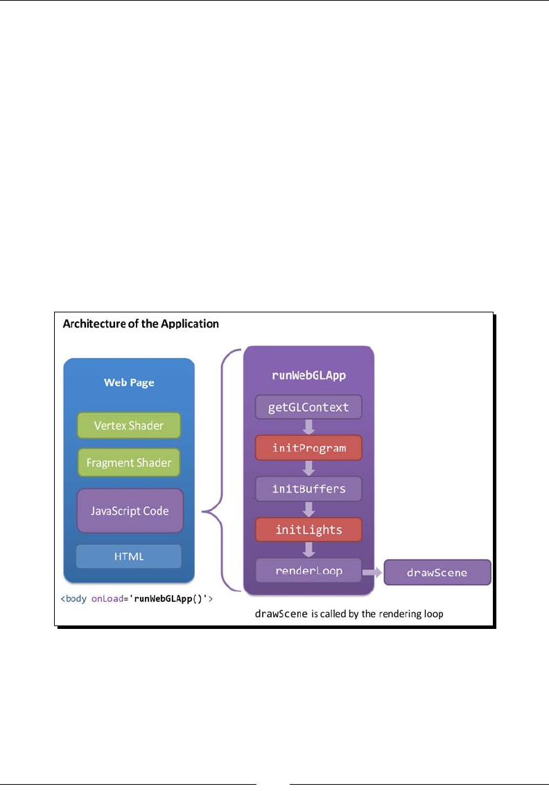
Chapter 3

[ 89 ]

What just happened?

We have seen the Phong shading and Phong lighng in acon. We have explored the source

code for the vertex and fragment shaders. We have also modied the dierent parameters of

the model and we have observed the immediate eect of the changes on the scene.

Back to WebGL

It is me to go back to our JavaScript code. Now, how do we close the gap between our

JavaScript code and our ESSL code?

First, we need to take a look at how we create a program using our WebGL context. Please

remember that we refer to both the vertex shader and fragment shader as the program.

Second, we need to know how to inialize aributes and uniforms.

Let's take a look at the structure of the web apps that we have developed so far:

Each applicaon has a vertex shader and a fragment shader embedded in the web page.

Then we have a script secon where we write all of our WebGL code. Finally, we have the

HTML code that denes the page components such as tles and the locaon of the widgets

and the canvas.

Lights!

[ 90 ]

In the JavaScript code, we are calling the runWebGLApp funcon on the onLoad event of the

web page. This is the entry point for our applicaon. The rst thing that runWebGLApp does

is to obtain a WebGL context for the canvas, and then calls a series of funcons that inialize

the program, the WebGL buers, and the lights. Finally it gets into a render loop where

every me that the loop goes o, the drawScene callback is invoked. In this secon, we will

take a closer look at the initProgram and initLights funcons. initPrograms allows

creang and compiling a ESSL program while initLights allows inializing and passing

values to the uniforms dened in the programs. It is inside initLights where we will

dene the light posion, direcon, and color components (ambient, diuse, and specular)

as well as default values for material properes.

Creating a program

Let's take a step-by-step look at initProgram:

var prg; //global variable

function initProgram() {

First we use the ulity funcon utils.getShader(WebGLContext, DOM_ID) to retrieve

the contents of the vertex shader and the fragment shader.

var fragmentShader= utils.getShader(gl, "shader-fs");

var vertexShader= utils.getShader(gl, "shader-vs");

Let's make a small parenthesis here and talk a bit about the getShader funcon. The rst

parameter of getShader is the WebGL context. The second parameter is the DOM ID of

the script that contains the source code of the shader that we want to add to the program.

Internally, getShader reads the source code of the script and it stores it in a local variable

named str. Then it executes the following piece of code:

var shader;

if (script.type == "x-shader/x-fragment") {

shader = gl.createShader(gl.FRAGMENT_SHADER);

} else if (script.type == "x-shader/x-vertex") {

shader = gl.createShader(gl.VERTEX_SHADER);

} else {

return null;

}

gl.shaderSource(shader, str);

gl.compileShader(shader);

Chapter 3

[ 91 ]

Basically, the preceding code fragment will create a new shader using the WebGL

createShader funcon. Then it will add the source code to it using the shaderSource

funcon and nally it will try to compile the shader using the compileShader funcon.

The source code for the getShader funcon is in the le js/utils.js, which

accompanies this chapter.

Going back to initProgram, the program creaon occurs in the following lines:

prg = gl.createProgram();

gl.attachShader(prg, vertexShader);

gl.attachShader(prg, fragmentShader);

gl.linkProgram(prg);

if (!gl.getProgramParameter(prg, gl.LINK_STATUS)) {

alert("Could not initialize shaders");

}

gl.useProgram(prg);

Here we have used several funcons provided by the WebGL context. These are as follows:

WebGL Funcon Descripon

createProgram() Creates a new program (prg)

attachShader(Object program,

Object shader) Aaches a shader to the current program

linkProgram(Object program) Creates executable versions of the vertex and

fragment shaders that are passed to the GPU

getProgramParameter(Object

program, Object parameter) This is part of the WebGL State Machine query

mechanism. It allows querying the program

parameters. We use this funcon here to verify

whether the program has been successfully

linked or not.

useProgram(Object program) It will install the program in the GPU if the

program contains valid code (that is, it has been

successfully linked).

Finally, we create a mapping between JavaScript variables and the program aributes and

uniforms. Instead of creang several JavaScript variables here (one per program aribute or

uniform), we are aaching properes to the prg object. This does not have anything to do

with WebGL. It is just a convenience step to keep all of our JavaScript variables as part of the

program object.

prg.aVertexPosition = gl.getAttribLocation(prg, "aVertexPosition");

prg.aVertexNormal = gl.getAttribLocation(prg, "aVertexNormal");

Lights!

[ 92 ]

prg.uPMatrix =gl.getUniformLocation(prg, "uPMatrix");

prg.uMVMatrix = gl.getUniformLocation(prg, "uMVMatrix");

prg.uNMatrix = gl.getUniformLocation(prg, "uNMatrix");

prg.uLightDirection = gl.getUniformLocation(prg, "uLightDirection");

prg.uLightAmbient = gl.getUniformLocation(prg, "uLightAmbient");

prg.uLightDiffuse = gl.getUniformLocation(prg, "uLightDiffuse");

prg.uMaterialDiffuse = gl.getUniformLocation(prg,"uMaterialDiffuse");

}

This is all for initProgram. Here we have used these WebGL API funcons:

WebGL Funcon Descripon

Var reference =

getAttribLocation(Object

program,String name)

This funcon receives the current program

object and a string that contains the name of the

aribute that needs to be retrieved. Then this

funcon returns a reference to the respecve

aribute.

var reference=

getUniformLocation(Object

program,String uniform)

This funcon receives the current program object

and a string that contains the name of the uniform

that needs to be retrieved. Then this funcon

returns a reference to the respecve uniform.

Using this mapping, we can inialize the uniforms and aributes from our JavaScript code,

as we will see in the next secon.

Initializing attributes and uniforms

Once we have compiled and installed the program, the next step is to inialize the aributes

and variables. We will inialize our uniforms using the initLights funcon.

function initLights(){

gl.uniform3fv(prg.uLightDirection, [0.0, 0.0, -1.0]);

gl.uniform4fv(prg.uLightAmbient, [0.01,0.01,0.01,1.0]);

gl.uniform4fv(prg.uLightDiffuse, [0.5,0.5,0.5,1.0]);

gl.uniform4fv(prg.uMaterialDiffuse, [0.1,0.5,0.8,1.0]);

}

Chapter 3

[ 93 ]

You can see here that we are using the references obtained with getUniformLocation

(we did this in initProgram).

These are the funcons that the WebGL API provides to set and get uniform values:

WebGL Funcon Descripon

uniform[1234][fi] Species 1-4 oat or int values of a uniform

variable

uniform[1234][fi]v Species the value of a uniform variable as an

array of 1-4 oat or int values.

getUniform(program, reference) Retrieves the contents of a uniform variable.

The reference parameter has been previously

obtained with getUniformLocation.

In Chapter 2, Rendering Geometry, we saw that there is a three-step process to inialize and

use aributes (review the Associang Aributes to VBOs secon in Chapter 2, Rendering

Geometry). Let's remember that we:

1. Bind a VBO.

2. Point an aribute to the currently bound VBO.

3. Enable the aribute.

The key piece here is step 2. We do this with the instrucon:

gl.vertexAttribPointer(Index,Size,Type,Norm,Stride,Offset);

If you check the example ch3_Wall.html, you will see that we do this inside the

drawScene funcon:

gl.vertexAttribPointer(prg.aVertexPosition, 3, gl.FLOAT, false, 0, 0);

gl.vertexAttribPointer(prg.aVertexNormal,3,gl.FLOAT, false, 0,0);

Bridging the gap between WebGL and ESSL

Let's see in pracce how we integrate our ESSL program to our WebGL code by working on a

simple example from scratch.

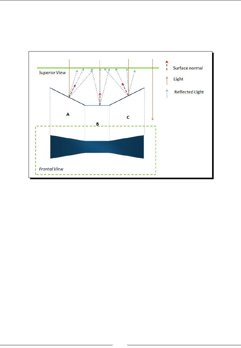
Lights!

[ 94 ]

We have a wall composed of the secons A, B, and C. Imagine that you are facing secon

B (as shown in the following diagram) and that you have a ashlight on your hand (Frontal

View). Intuively secon A and secon C will be darker than secon B. This fact can be

modeled by starng at the color of the center of secon B and darkening the color of the

surrounding pixels as we move away from the center.

Let's summarize here the code that we need to write:

1. Write the ESSL program. Code the ESSL vertex and fragment shaders. We know

how to do this already. For the wall, we are going to select Goraud shading with

a Diuse/Lamberan reecon model.

2. Write the initProgram funcon. We already saw how to do this. We need to make

sure that we map all the aributes and uniforms that we had dened in the ESSL

code. Including the normals:

prg.aVertexNormal= gl.getAttribLocation(prg, "aVertexNormal");

3. Write initBuffers. Here we need to create our geometry: we can represent

the wall with eight verces that dene six triangles such as the ones shown in

the previous diagram. In init buers, we apply what we learned in Chapter 2,

Rendering Geometry to set up the appropriate WebGL buers. This me, we need

to set up an addional buer: the VBO that contain informaon about normals.

The code to set up the normals VBO looks like this:

var normals = utils.calculateNormals(vertices, indices);

var normalsBuffer = gl.createBuffer();

gl.bindBuffer(gl.ARRAY_BUFFER, normalsBuffer);

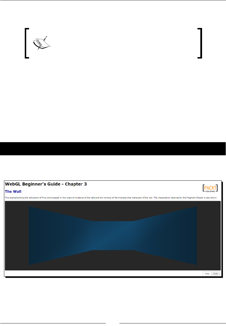
Chapter 3

[ 95 ]

gl.bufferData(gl.ARRAY_BUFFER, new Float32Array(normals),

gl.STATIC_DRAW);

To calculate the normals, we use the following funcon:

calculateNormals(vertices, indices)

You will nd this funcon in the le js/utils.js

4. Write initLights. We also saw how to do that.

5. There is only a minor but important change to make inside the drawScene

funcon. We need to make sure that the normals VBO is bound before we use

drawElements. The code to do that looks like this:

gl.bindBuffer(gl.ARRAY_BUFFER, normalsBuffer);

gl.vertexAttribPointer(prg.aVertexNormal,3,gl.FLOAT, false, 0,0);

In the following secon, we will explore the funcons that we just described for building and

illuminang the wall.

Time for action – working on the wall

1. Open the le ch3_Wall.html in your HTML5 browse. You will see something

similar to the following screenshot:

2. Now, open the le again, this me in your favorite text editor (for example,

Notepad ++).

Lights!

[ 96 ]

3. Go to the vertex shader (Hint: look for the tag <script id="shader-vs"

type="x-shader/x-vertex">). Make sure that you idenfy the aributes

uniforms and varyings that are declared there.

4. Now go to the fragment shader. Noce that there are no aributes here

(Remember: aributes are exclusive of the vertex shader).

5. Go to the runWebGLApp funcon. Verify that we are calling initProgram and

initLights there.

6. Go to initProgram. Make sure you understand how the program is built and how

we obtain references to aributes and uniforms.

7. Now go to initLights. Update the values of the uniforms, as shown here.

gl.uniform3fv(prg.uLightDirection, [0.0, 0.0, -1.0]);

gl.uniform4fv(prg.uLightAmbient, [0.1,0.1,0.1,1.0]);

gl.uniform4fv(prg.uLightDiffuse, [0.6,0.6,0.6,1.0]);

gl.uniform4fv(prg.uMaterialDiffuse, [0.6,0.15,0.15,1.0]);

8. Please noce that one of the updates consists of changing from uniform4f to

uniform4fv for the uniform uMaterialDiffuse.

9. Save the le.

10. Open it again (or reload it) in your HTML5 Internet browser. What happened?

11. Now let's do something a bit more interesng. We are going to create a key listener

so every me we hit a key, the light orientaon changes.

12. Right aer the initLights funcon, write the following code:

var azimuth = 0;

var elevation = 0;

document.onkeypress = processKey;

function processKey(ev){

var lightDirection = gl.getUniform(prg,prg.uLightDirection);

var incrAzimuth = 10;

var incrElevation = 10;

switch(ev.keyCode){

case 37:{ // left arrow

azimuth -= incrAzimuth;

break;

}

case 38:{ //up arrow

Chapter 3

[ 97 ]

elevation += incrElevation;

break;

}

case 39:{ // right arrow

azimuth += incrAzimuth;

break;

}

case 40:{ //down arrow

elevation -= incrElevation;

break;

}

azimuth %= 360;

elevation %=360;

var theta = elevation * Math.PI / 180;

var phi = azimuth * Math.PI / 180;

//Spherical to Cartesian coordinate transformation

lightDirection[0] = Math.cos(theta)* Math.sin(phi);

lightDirection[1] = Math.sin(theta);

lightDirection[2] = Math.cos(theta)* -Math.cos(phi);

gl.uniform3fv(prg.uLightDirection, lightDirection);

}

This funcon processes the arrow keys and changes the light direcon accordingly.

There is a bit of trigonometry (Math.cos, Math.sin) Mat.sin) there but do not

worry. We are just converng the angles (azimuth and elevaon) calculated by the

entered arrow keys into Cartesian coordinates.

Please noce that we are geng the current light direcon using the funcon:

var lightDirection = gl.getUniform(prg,prg.uLightDirection);

Aer processing the key strokes, we can save the updated light direcon with:

gl.uniform3fv(prg.uLightDirection, lightDirection);

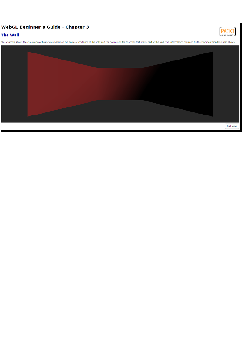
Lights!

[ 98 ]

13. Save the work and reload the web page:

14. Use the arrow keys to change the light direcon.

15. If you have any problem during the development of the exercise or you just want to

verify the nal result, please check the le ch3_Wall_Final.html that contains

the completed exercise.

What just happened?

In this exercise, we have created a keyboard listener that allows us to update the light

orientaon so we can move it around the wall and see how it reacts to surface normals. We

have also seen how the vertex shader and fragment shader input variables are declared and

used. We understood how to build a program by reviewing the initProgram funcon. We

also learned about inializing uniforms on the initLights funcon. We also studied the

getUniform funcon to retrieve the current value of a uniform.

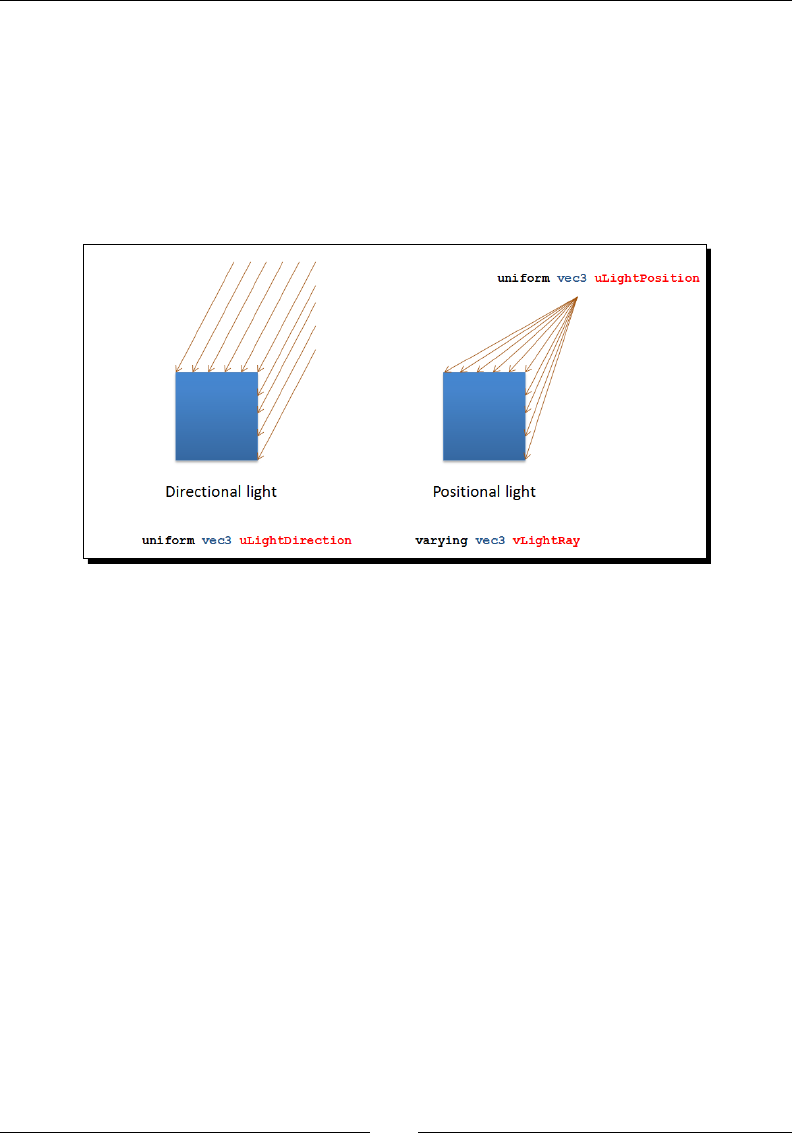
Chapter 3

[ 99 ]

More on lights: positional lights

Before we nish the chapter, let's revisit the topic of lights. So far we have assumed that

our light source is innitely far away from the scene. This assumpon allows us to model

the light rays as being parallel to each other. An example of this is sunlight. These lights are

called direconal lights; now we are going to consider the case where the light source is

relavely close to the object that it is going to illuminate. Think, for example, of a lamp

desk illuminang the document you are reading. These lights are called posional lights.

As we experienced before, when working with direconal lights, only one variable

is required. This is the light direcon that we have represented in the uniform

uLightDirection.

Contrasngly, when working with posional lights, we need to know the locaon of the light.

We can represent it using a uniform that we will name uLightPosition. As when using

posional lights, the light rays are not parallel to each other, we will need to calculate each

light ray separately. We will do this by using a varying that we will name vLightRay.

In the following Time for acon secon, we will see how a posional light interacts

with a scene.

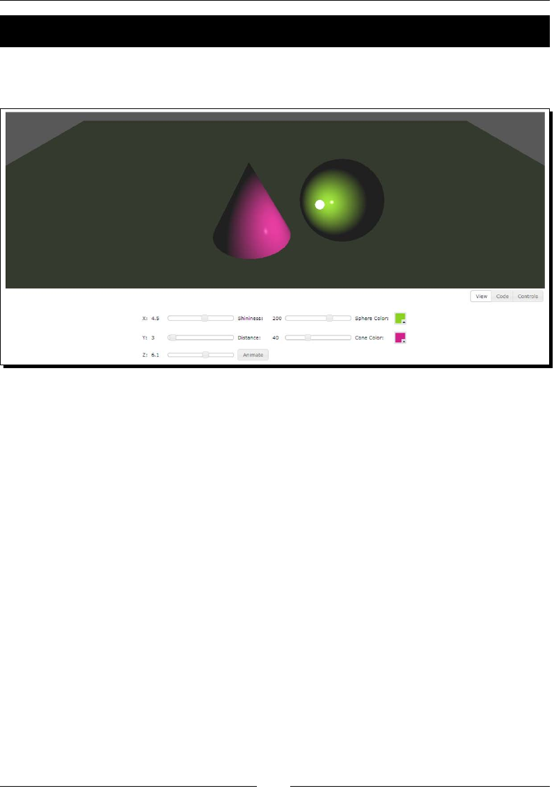
Lights!

[ 100 ]

Time for action – positional lights in action

1. Open the le ch3_Positional Lighting.html in your HTML5 Internet browser.

The page will look similar to the following screenshot:

2. The interface of this exercise is very simple. You will noce that there are no sliders

to select the ambient and specular properes for the objects or the light source.

This has been done deliberately with the objecve of focusing on the new element

of study—the light posion. Unlike in previous exercises, the X, Y, and Z sliders do

not represent light direcon here. Instead, they allow us to set the light source

posion. Go ahead and play with them.

3. For clarity, a lile sphere represenng the posion of the light source has been

added to the scene. However, this is not generally required.

4. What happens when the light source is located on the surface of the cone or on the

surface of the sphere?

5. What happens when the light source is inside the sphere?

6. Now, click on the buon Animate. As you would expect, the lighng of the scene

changes according to the light source and the posion of the camera.

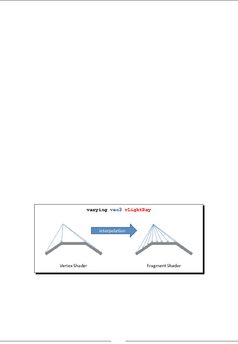
Chapter 3

[ 101 ]

7. Let's take a look at the way we calculate the light rays. Click on the Code buon.

Once the code viewer area is displayed, click on the Vertex Shader buon.

The light ray calculaon is performed in the following two lines of code:

vec4 light = uMVMatrix * vec4(uLightPosition,1.0);

vLightRay = vertex.xyz-light.xyz;

8. The rst line allows us to obtain a transformed light posion by mulplying the

Model-view matrix by the uniform uLightPosition. If you check the code in

the vertex shader, we also use this matrix for calculang transformed verces and

normals. We will discuss these matrix operaons in the next chapter. For now,

believe me when I say that this is necessary to obtain transformed verces, normals,

and light posions whenever we move the camera. If you do not believe me, then

go ahead and modify this line by removing the matrix from the equaon so the line

looks like the following:

vec4 light = vec4(uLightPosition,1.0);

Save the le with a dierent name and launch it in your HTML5 browser. What is the

eect of not transforming the light posion? Click on the buon Animate. What you

see is that the camera is moving, but the light source posion is not being updated!

9. In the second line of code (step 7), we can see that the light ray is calculated as the

vector that goes from the transformed light posion (light) to the vertex posion.

Thanks to the interpolaon of varyings that is provided by ESSL, we automacally

obtain all the light rays per pixel in the fragment shader.

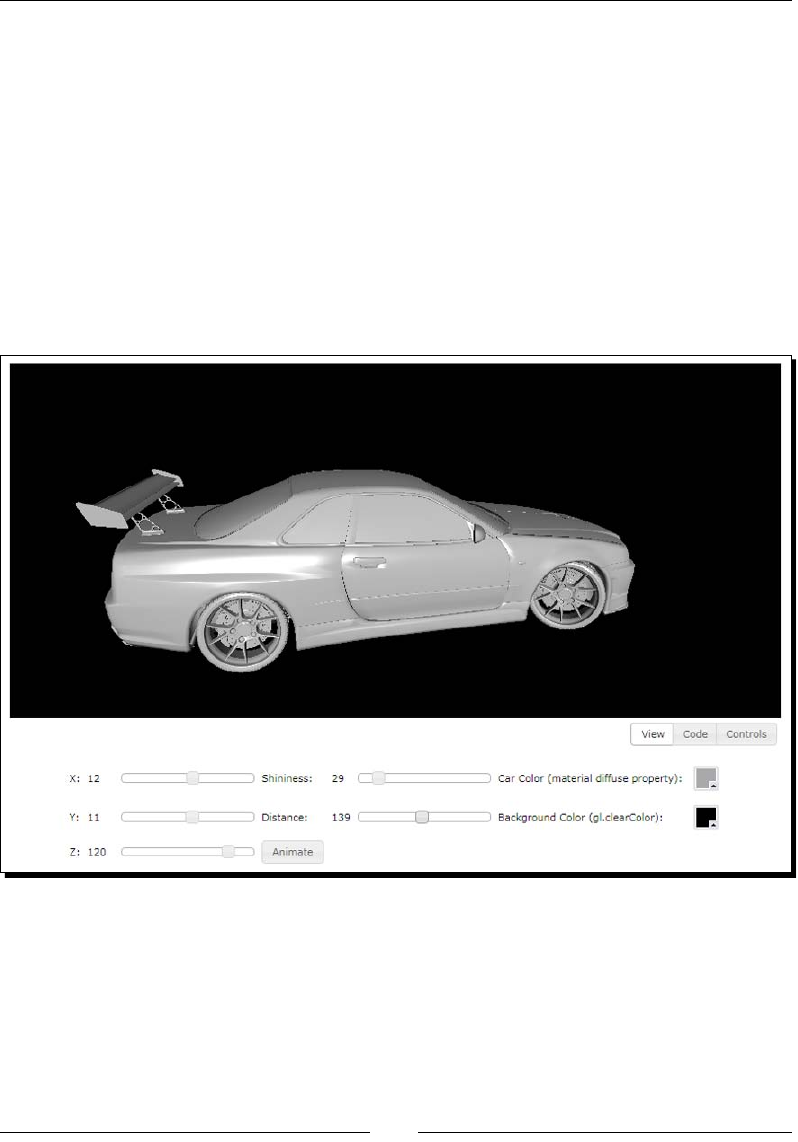
Lights!

[ 102 ]

What just happened?

We have studied the dierence between direconal lights and posional lights. We have

also seen the importance of the Model-view matrix for the correct calculaon of posional

lights when the camera is moving. Also, the procedure to obtain per-vertex light rays has

been shown.

Nissan GTS example

We have included in this chapter an example of the Nissan GTS exercise that we saw

in Chapter 2, Rendering Geometry. This me, we have used a Phong lighng model with

a posional light to illuminate the scene. The le where you will nd this example is

ch3_Nissan.html.

Here you can experiment with dierent light posions. You can see the nice specular

reecons that you obtain thanks to the specularity property of the car and the shininess

of the light.

Chapter 3

[ 103 ]

Summary

In this chapter, we have seen how to use the vertex shader and the fragment shader to

dene a lighng model for our 3D scene. We have learned in detail what light sources,

materials, and normals are, and how these elements interact to illuminate a WebGL scene.

We have also learned the dierence between a shading method and a lighng model and

have studied the basic Goraud and Phong shading methods and the Lamberan and Phong

lighng models. We have also seen several examples of how to implement these shading and

lighng models in code using ESSL, and how to communicate between the WebGL code and

the ESSL code through aributes and uniforms.

In the following chapter, we will expand on the use of matrices in ESSL and we will see how

we use them to represent and move our viewpoint in a 3D scene.

Camera

In this chapter, we will learn more about the matrices that we have seen in

the source code. These matrices represent transformaons that when applied

to our scene, allow us to move things around. We have used them so far to

set the camera to a distance that is good enough to see all the objects in

our scene and also for spinning our Nissan GTS model (Animate buon in

ch3_Nissan.html). In general, we move the camera and the objects in the

scene using matrices.

The bad news is that you will not see a camera object in the WebGL API, only matrices.

The good news is that having matrices instead of a camera object gives WebGL a lot of

exibility to represent complex animaons (as we will see in Chapter 5, Acon). In this

chapter, we will learn what these matrix transformaons mean and how we can use them

to dene and operate a virtual camera.

In this chapter, we will:

Understand the transformaons that the scene undergoes from a 3D world

to a 2D screen

Learn about ane transformaons

Map matrices to ESSL uniforms

Work with the Model-View matrix and the Perspecve matrix

Appreciate the value of the Normal matrix

Create a camera and use it to move around a 3D scene

Camera

[ 106 ]

WebGL does not have cameras

This statement should be shocking! How is it that there are no cameras in a 3D computer

graphics technology? Well, let me rephrase this in a more amicable way. WebGL does not

have a camera object that you can manipulate. However, we can assume that what we see

rendered in the canvas is what our camera captures. In this chapter, we are going to solve

the problem of how to represent a camera in WebGL. The short answer is we need

4x4 matrices.

Every me that we move our camera around, we will need to update the objects according

to the new camera posion. To do this, we need to systemacally process each vertex

applying a transformaon that produces the new viewing posion. Similarly, we need to

make sure that the object normals and light direcons are sll consistent aer the camera

has moved. In summary, we need to analyze two dierent types of transformaons: vertex

(points) and normal (vectors).

Vertex transformations

Objects in a WebGL scene go through dierent transformaons before we can see them on

our screen. Each transformaon is encoded by a 4x4 matrix, as we will see later. How do we

mulply verces that have three components (x,y,z) by a 4x4 matrix? The short answer is

that we need to augment the cardinality of our tuples by one dimension. Each vertex then

will have a fourth component called the homogenous coordinate. Let's see what they are

and why they are useful.

Homogeneous coordinates

Homogeneous coordinates are a key component of any computer graphics program.

Thanks to them, it is possible to represent ane transformaons (rotaon, scaling,

shear, and translaon) and projecve transformaons as 4x4 matrices.

In Homogeneous coordinates, verces have four components: x, y, z, and w. The rst three

components are the vertex coordinates in Euclidian Space. The fourth is the perspecve

component. The 4-tuple (x,y,z,w) take us to a new space: The Projecve Space.

Homogeneous coordinates make possible to solve a system of linear equaons where each

equaon represents a line that is parallel with all the others in the system. Let's remember

here that in Euclidian Space, a system like that does not have soluons, because there are

not intersecons. However, in Projecve Space, this system has a soluon—the lines will

intersect at innite. This fact is represented by the perspecve component having a value of

zero. A good physical analogy of this idea is the image of train tracks: parallel lines that touch

in the vanishing point when you look at them.

Chapter 4

[ 107 ]

It is easy to convert from Homogeneous coordinates to non-homogeneous, old-fashioned,

Euclidean coordinates. All you need to do is divide the coordinate by w:

h(x, y, z, w)=v(x/w,y/w,z/w)

v(x, y, z)=h(x, y, z, )1

Consequently, if we want to go from Euclidian to Projecve space, we just add the fourth

component w and make it 1.

As a maer of fact, this is what we have been doing so far! Let's go back to one of the

shaders we discussed in the last chapter: the Phong vertex shader. The code looks like

the following:

attributevec3aVertexPosition;

attributevec3aVertexNormal;

uniformmat4uMVMatrix;

uniformmat4uPMatrix;

uniformmat4uNMatrix;

varyingvec3vNormal;

varyingvec3vEyeVec;

voidmain(void){

//Transformedvertexposition

vec4vertex=uMVMatrix*vec4(aVertexPosition,1.0);



//Transformednormalposition

vNormal=vec3(uNMatrix*vec4(aVertexNormal,0.0));

//VectorEye

vEyeVec=-vec3(vertex.xyz);



//Finalvertexposition

gl_Position=uPMatrix*uMVMatrix*vec4(aVertexPosition,1.0);

}

Please noce that for the aVertexPosition aribute, which contains a vertex of our

geometry, we create a 4-tuple from the 3-tuple that we receive. We do this with the ESSL

construct vec4(). ESSL knows that aVertexPosition is a vec3 and therefore we only

need the fourth component to create a vec4.

Camera

[ 108 ]

To pass from Homogeneous coordinates to Euclidean coordinates, we divide by w

To pass from Euclidean coordinates to Homogeneous coordinates, we add w =1

Homogeneous coordinates with w = 0 represent a point at innity

There is one more thing you should know about Homogeneous coordinates—while verces

have a Homogeneous coordinate w = 1, vectors have a Homogeneous coordinate w = 0.

This is the reason why, in the Phong vertex shader, the line that processes the normals

looks like this:

vNormal = vec3(uNMatrix * vec4(aVertexNormal, 0.0));

To code vertex transformaons, we will be using Homogeneous coordinates unless indicated

otherwise. Now let's see the dierent transformaons that our geometry undergoes to be

displayed on screen.

Model transform

We start our analysis from the object coordinate system. It is in this space where vertex

coordinates are specied. Then if we want to translate or move objects around, we use

a matrix that encodes these transformaons. This matrix is known as the model matrix.

Once we mulply the verces of our object by the model matrix, we will obtain new vertex

coordinates. These new verces will determine the posion of the object in our 3D world.

Chapter 4

[ 109 ]

While in object coordinates, each object is free to dene where its origin is and then specify

where its verces are with respect to this origin, in world coordinates, the origin is shared by

all the objects. World coordinates allow us to know where objects are located with respect

to each other. It is with the model transform that we determine where the objects are in the

3D world.

View transform

The next transformaon, the view transform, shis the origin of the coordinate system to the

view origin. The view origin is where our eye or camera is located with respect to the world

origin. In other words, the view transform switches world coordinates by view coordinates.

This transformaon is encoded in the view matrix. We mulply this matrix by the vertex

coordinates obtained by the model transform. The result of this operaon is a new set of

vertex coordinates whose origin is the view origin. It is in this coordinate system that our

camera is going to operate. We will go back to this later in the chapter.

Camera

[ 110 ]

Projection transform

The next operaon is called the projecon transform. This operaon determines how much

of the view space will be rendered and how it will be mapped onto the computer screen.

This region is known as the frustum and it is dened by six planes (near, far, top, boom,

right, and le planes), as shown in the following diagram:

These six planes are encoded in the Perspecve matrix. Any verces lying outside of the

frustum aer applying the transformaon are clipped out and discarded from further

processing. Therefore, the frustum denes, and the projecon matrix that encodes the

frustum produces, clipping coordinates.

The shape and extent of the frustum determines the type of projecon from the 3D viewing

space to the 2D screen. If the far and near planes have the same dimensions, then the

frustum will determine an orthographic projecon. Otherwise, it will be a perspecve

projecon, as shown in the following diagram:

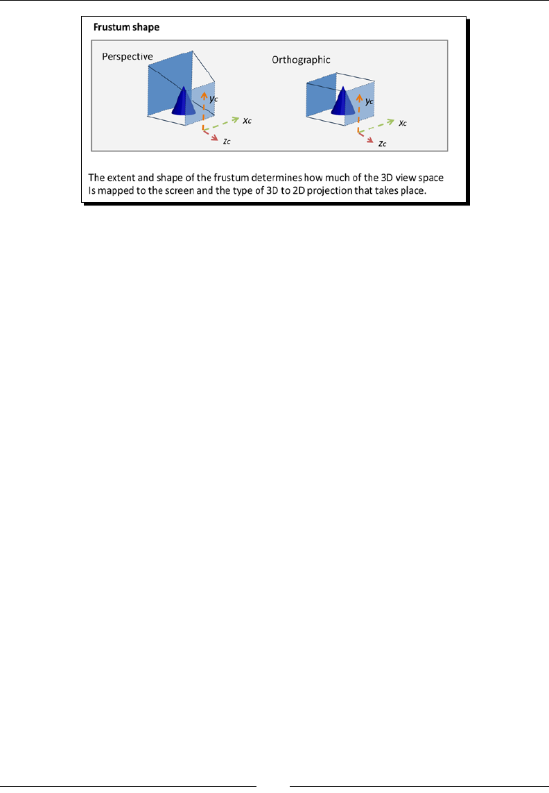
Chapter 4

[ 111 ]

Up to this point, we are sll working with Homogeneous coordinates, so the clipping

coordinates have four components: x, y, z, and w. The clipping is done by comparing the x, y,

and z components against the Homogeneous coordinate w. If any of them is more than, +w,

or less than, –w , then that vertex lies outside the frustum and is discarded.

Perspective division

Once it is determined how much of the viewing space will be rendered, the frustum is

mapped into the near plane in order to produce a 2D image. The near plane is what is

going to be rendered on your computer screen.

Dierent operave systems and displaying devices can have mechanisms to represent 2D

informaon on screen. To provide robustness for all possible cases, WebGL (also in OpenGL

ES) provides an intermediate coordinate system that is independent from any specic

hardware. This space is known as the Normalized Device Coordinates (NDC).

Normalized device coordinates are obtained by dividing the clipping coordinates by the

w component. This is the reason why this step is known as perspecve division. Also,

please remember that when you divide by the Homogeneous coordinate, we go from

projecve space (4-components) to Euclidean space (3-components), so NDC only has

three components. In the NDC space, the x and y coordinates represent the locaon of your

verces on a normalized 2D screen, while the z-coordinate encodes depth informaon,

which is the relave locaon of the objects with respect to the near and far planes. Though,

at this point, we are working on a 2D screen, we sll keep the depth informaon. This will

allow WebGL to determine later how to display overlapping objects based on their distance

to the near plane. When using normalized device coordinates, the depth is encoded in the

z-component.

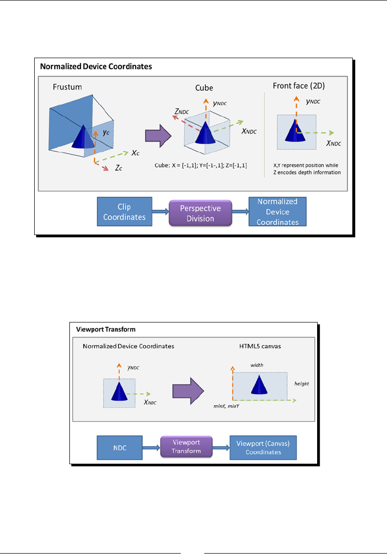
Camera

[ 112 ]

The perspecve division transforms the viewing frustum into a cube centered in the origin

with minimum coordinates [-1,-1,-1] and maximum coordinates [1,1,1]. Also, the direcon

of the z-axis is inverted, as shown in the following gure:

Viewport transform

Finally, NDCs are mapped to viewport coordinates. This step maps these coordinates to the

available space in your screen. In WebGL, this space is provided by the HTML5 canvas, as

shown in the following gure:

Unlike the previous cases, the viewport transform is not generated by a matrix

transformaon. In this case, we use the WebGL viewport funcon. We will learn more

about this funcon later in the chapter. Now it is me to see what happens to normals.

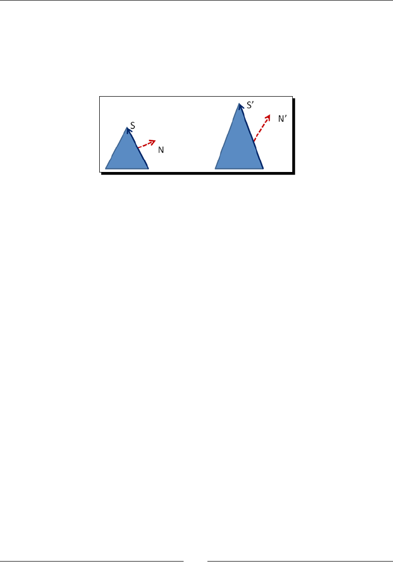
Chapter 4

[ 113 ]

Normal transformations

Whenever verces are transformed, normal vectors should also be transformed, so they

point in the right direcon. We could think of using the Model-View matrix that transforms

verces to do this, but there is a problem: The Model-View matrix will not always keep the

perpendicularity of normals.

This problem occurs if there is a unidireconal (one axis) scaling transformaon or a

shearing transformaon in the Model-View matrix. In our example, we have a triangle

that has undergone a scaling transformaon on the y-axis. As you can see, the normal

N' is not normal anymore aer this kind of transformaon. How do we solve this?

Calculating the Normal matrix

If you are not interested in nding out how we calculate the Normal matrix and just want the

answer, please feel free to jump to the end of this secon. Otherwise, sck around to see

some linear algebra in acon!

Let's start from the mathemacal denion of perpendicularity. Two vectors are

perpendicular if their dot product is zero. In our example:

N.S = 0

Here, S is the surface vector and it can be calculated as the dierence of two verces,

as shown in the previous diagram at the beginning of this secon.

Let M be the Model-View matrix. We can use M to transform S as follows:

S' = MS

This is because S is the dierence of two verces and we use M to transform verces onto

the viewing space.

Camera

[ 114 ]

We want to nd a matrix K that allows us to transform normals in a similar way. For the

normal N, we want:

N' = KN

For the scene to be consistent aer obtaining N' and S', these two need to keep the

perpendicularity that the original vectors N and S had. This is:

N'.S' = 0

Substung N' and S':

(KN).(MS) =0

A dot product can also be wrien as a vector mulplicaon by transposing the rst vector,

so we have that this sll holds:

(KN)T(MS) = 0

The transpose of a product is the product of the transposes in the reverse order:

NTKTMS = 0

Grouping the inner terms:

NT(KTM)S = 0

Now remember that N.S =0 so NTS = 0 (again, a dot product can be wrien as a vector

mulplicaon). This means that in the previous equaon, (KTM) needs to be the identy

matrix I, so the original condion of N and S being perpendicular holds:

KTM = I

Applying a bit of algebra:

KTMM-1 = IM-1 = M-1 mulply by the inverse of M on both

sides

KT(I) = M-1 because MM-1 = I

(KT)T = (M-1)Ttransposing on both sides

K = (M-1)TDouble transpose of K is the original

matrix K.

Conclusions:

K is the correct matrix transform that keeps the normal vectors being perpendicular

to the surface of the object. We call K the Normal matrix.

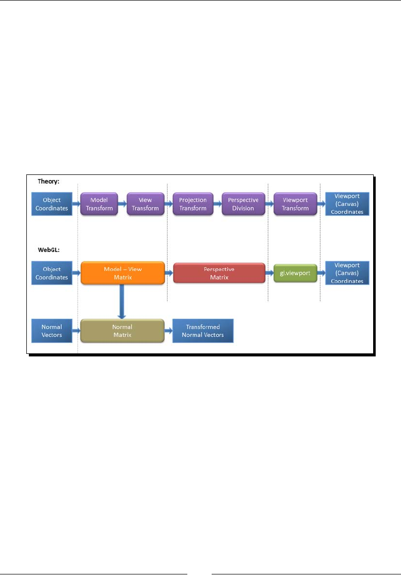
Chapter 4

[ 115 ]

K is obtained by transposing the inverse of the Model-View matrix

(M in this example).

We need to use K to mulply the normal vectors so they keep being perpendicular

to surface when these are transformed.

WebGL implementation

Now let's take a look at how we can implement vertex and normal transformaons in

WebGL. The following diagram shows the theory that we have learned so far and it

shows the relaonships between the steps in the theory and the implementaon

in WebGL.

In WebGL, the ve transformaons that we apply to object coordinates to obtain viewport

coordinates are grouped in three matrices and one WebGL method:

1. The Model-View matrix that groups the model and view transform in one single

matrix. When we mulply our verces by this matrix, we end up in view coordinates.

2. The Normal matrix is obtained by inverng and transposing the Model-View matrix.

This matrix is applied to normal vectors for lighng purposes.

3. The Perspecve matrix groups the projecon transformaon and the perspecve

division, and as a result, we end up in normalized device coordinates (NDC).

Finally, we use the operaon gl.viewport to map NDCs to viewport coordinates:

gl.viewport(minX, minY, width, height);

The viewport coordinates have their origin in the lower-le corner of the

HTML5 canvas.

Camera

[ 116 ]

JavaScript matrices

WebGL does not provide its own methods to perform operaons on matrices. All WebGL

does is it provides a way to pass matrices to the shaders (as uniforms). So, we need to use a

JavaScript library that enables us to manipulate matrices in JavaScript. In this book, we have

used glMatrix to manipulate matrices. However, there are other libraries available online

that can do this for you.

We used glMatrix to manipulate matrices in this book. You can nd more

informaon about this library here: https://github.com/toji/gl-

matrix. And the documentaon (linked further down the page) can be

found at: http://toji.github.com/gl-matrix/doc

These are some of the operaons that you can perform with glMatrix:

Operaon Syntax Descripon

Creaon var m = mat4.create() Creates the matrix m

Identy mat4.identity(m) Sets m as the identy matrix of rank 4

Copy mat4.

set(origin,target) Copies the matrix origin into the matrix target

Transpose mat4.transpose(m) Transposes matrix m

Inverse mat4.inverse(m) Inverts m

Rotate mat4.rotate(m,r,a) Rotates the matrix m by r radians around the axis a

(this is a 3-element array [x,y,z]).

glMatrix also provides funcons to perform other linear algebra operaons. It also

operates on vectors and matrices of rank 3. To get the full list, visit https://github.com/

toji/gl-matrix

Mapping JavaScript matrices to ESSL uniforms

As the Model-View and Perspecve matrices do not change during a single rendering step,

they are passed as uniforms to the shading program. For example, if we were applying

a translaon to an object in our scene, we would have to paint the whole object in the

new coordinates given by the translaon. Painng the whole object in the new posion

is achieved in exactly one rendering step.

However, before the rendering step is invoked (by calling drawArrays or drawElements,

as we saw in Chapter 2, Rendering Geometry), we need to make sure that the shaders have

an updated version of our matrices. We have seen how to do that for other uniforms such

as light and color properes. The method map JavaScript matrices to uniforms is similar to

the following:

Chapter 4

[ 117 ]

First, we get a JavaScript reference to the uniform with:

var reference= getUniformLocation(Object program, String uniformName)

Then, we use the reference to pass the matrix to the shader with:

gl.uniformMatrix4fv(WebGLUniformLocation reference, bool transpose,

float[] matrix);

matrix is the JavaScript matrix variable.

As it is the case for other uniforms, ESSL supports 2, 3, and 4-dimensional matrices:

uniformMatrix[234]fv(ref,transpose,matrix): will load 2x2, 3x3, or 4x4 matrices

(corresponding to 2, 3, or 4 in the command name) of oang points into the uniform

referenced by ref. The type of ref is WebGLUniformLocation. For praccal purposes, it is

an integer number. According to the specicaon, the transpose value must be set to false.

The matrix uniforms are always of oang point type (f). The matrices are passed as 4,

9, or 16 element vectors (v) and are always specied in a column-major order. The matrix

parameter can also be of type Float32Array. This is one of JavaScript's typed arrays. These

arrays are included in the language to provide access and manipulaon of raw binary data,

therefore increasing eciency.

Working with matrices in ESSL

Let's revisit the Phong vertex shader, which was introduced in the last chapter. Please pay

aenon to the fact that matrices are dened as uniform mat4.

In this shader, we have dened three matrices:

uMVMatrix: the Model-View matrix

uPMatrix: the Perspecve matrix

uNMatrix: the Normal matrix

attribute vec3 aVertexPosition;

attribute vec3 aVertexNormal;

uniform mat4 uMVMatrix;

uniform mat4 uPMatrix;

uniform mat3 uNMatrix;

varying vec3 vNormal;

varying vec3 vEyeVec;

void main(void) {

//Transformed vertex position

vec4 vertex = uMVMatrix * vec4(aVertexPosition, 1.0);

Camera

[ 118 ]

//Transformed normal vector

vNormal = uNMatrix * aVertexNormal;

//Vector Eye

vEyeVec = -vec3(vertex.xyz);

//Final vertex position

gl_Position = uPMatrix * uMVMatrix * vec4(aVertexPosition,

1.0);

}

In ESSL, the mulplicaon of matrices is straighorward, that is, you do not need to mulply

element by element, but as ESSL knows that you are working with matrices, it performs the

mulplicaon for you.

gl_Position = uPMatrix * uMVMatrix * vec4(aVertexPosition, 1.0);

The last line of this shader assigns a value to the predened gl_Position variable. This

will contain the clipping coordinates for the vertex that is currently being processed by the

shader. We should remember here that the shaders work in parallel: each vertex is processed

by an instance of the vertex shader.

To obtain the clipping coordinates for a given vertex, we need to mulply rst by the Model-

View matrix and then by the Projecon matrix. To achieve this, we need to mulply to the

le (because matrix mulplicaon is not commutave).

Also, noce that we have had to augment the aVertexPosition aribute by including

the Homogeneous coordinate. This is because we have always dened our geometry in

Euclidean space. Luckily, ESSL lets us do this just by adding the missing component and

creang a vec4 on the y. We need to do this because both the Model-View matrix and

the Perspecve matrix are described in homogeneous coordinates (4 rows by 4 columns).

Now that we have seen how to map JavaScript matrices to ESSL uniforms in our shaders,

let's talk about how to operate with the three matrices: the Model-View matrix, the Normal

matrix, and the Perspecve matrix.

The Model-View matrix

This matrix allows us to perform ane transformaons in our scene. Ane is a

mathemacal name to describe transformaons that do not change the structure of the

object that undergoes such transformaons. In our 3D world scene, such transformaons

are rotaon, scaling, reecon shearing, and translaon. Luckily for us, we do not need to

understand how to represent such transformaons with matrices. We just have to use one

of the many JavaScript matrix libraries that are available online (such as glMatrix).

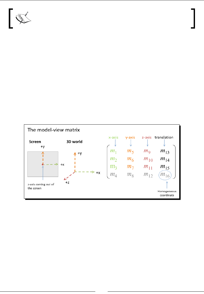
Chapter 4

[ 119 ]

You can nd more informaon on how transformaon matrices work in

any linear algebra book. Look for ane transforms in computer graphics.

Understanding the structure of the Model-View matrix is of no value if you just want to apply

transformaons to the scene or to objects in the scene. For that eect, you just use a library

such as glMatrix to do the transformaons on your behalf. However, the structure of this

matrix could be invaluable informaon when you are trying to troubleshoot your

3D applicaon.

Let's take a look.

Spatial encoding of the world

By default, when you render a scene, you are looking at it from the origin of the world in the

negave direcon of the z-axis. As shown in the following diagram, the z-axis is coming out

of the screen (which means that you are looking at the negave z-axis).

From the center of the screen to the right, you will have the posive x-axis and from the

center of the screen up, you will have the posive y-axis. This is the inial conguraon

and it is the reference for ane transformaons.

In this conguraon, the Model-View matrix is the identy matrix of rank four.

The rst three rows of the Model-View matrix contain informaon about rotaons

and translaons that are aecng the world.

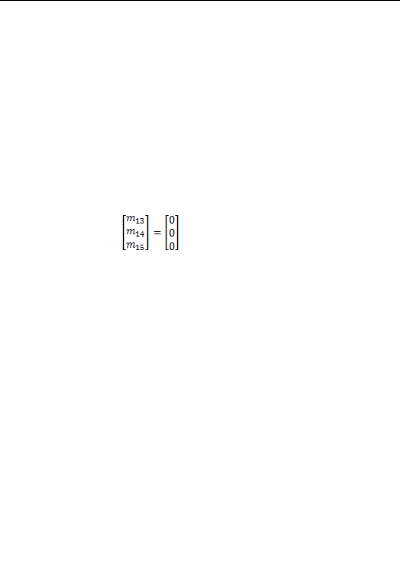
Camera

[ 120 ]

Rotation matrix

The intersecon of the rst three rows with the rst three columns denes the 3x3 Rotaon

matrix. This matrix contains informaon about rotaons around the standard axis. In the

inial conguraon, this corresponds to:

[m1,m2,m3] = [1, 0, 0] = x-axis

[m5,m6,m7] = [0, 1, 0] = y-axis

[m9,m10,m11] = [0, 0, 1] = z-axis

Translation vector

The intersecon of the rst three rows with the last column denes a three-component

Translaon vector. This vector indicates how much the origin, and for the same sake, the

world, have been translated. In the inial conguraon, this corresponds to:

= origin (no translaon)

The mysterious fourth row

The fourth row does not bear any special meaning.

Elements m4, m8, m12 are always zero.

Element

16 (the homogeneous coordinate) will always be 1.

As we described at the beginning of this chapter, there are no cameras in WebGL. However,

all the informaon that we need to operate a camera (mainly rotaons and translaons) can

be extracted from the Model-View matrix itself!

The Camera matrix

Let's say, for a moment, that we do have a camera in WebGL. A camera should be able to

rotate and translate to explore this 3D world. For example, think of a rst person shooter

game where you have to walk through levels killing zombies. As we saw in the previous

secon, a 4x4 matrix can encode rotaons and translaons. Therefore, our hypothecal

camera could also be represented by one such matrix.

Assume that our camera is located at the origin of the world and that it is oriented in a way

that it is looking towards the negave z-axis direcon. This is a good starng point—we

already know what transformaon represents such a conguraon in WebGL (identy matrix

of rank 4).

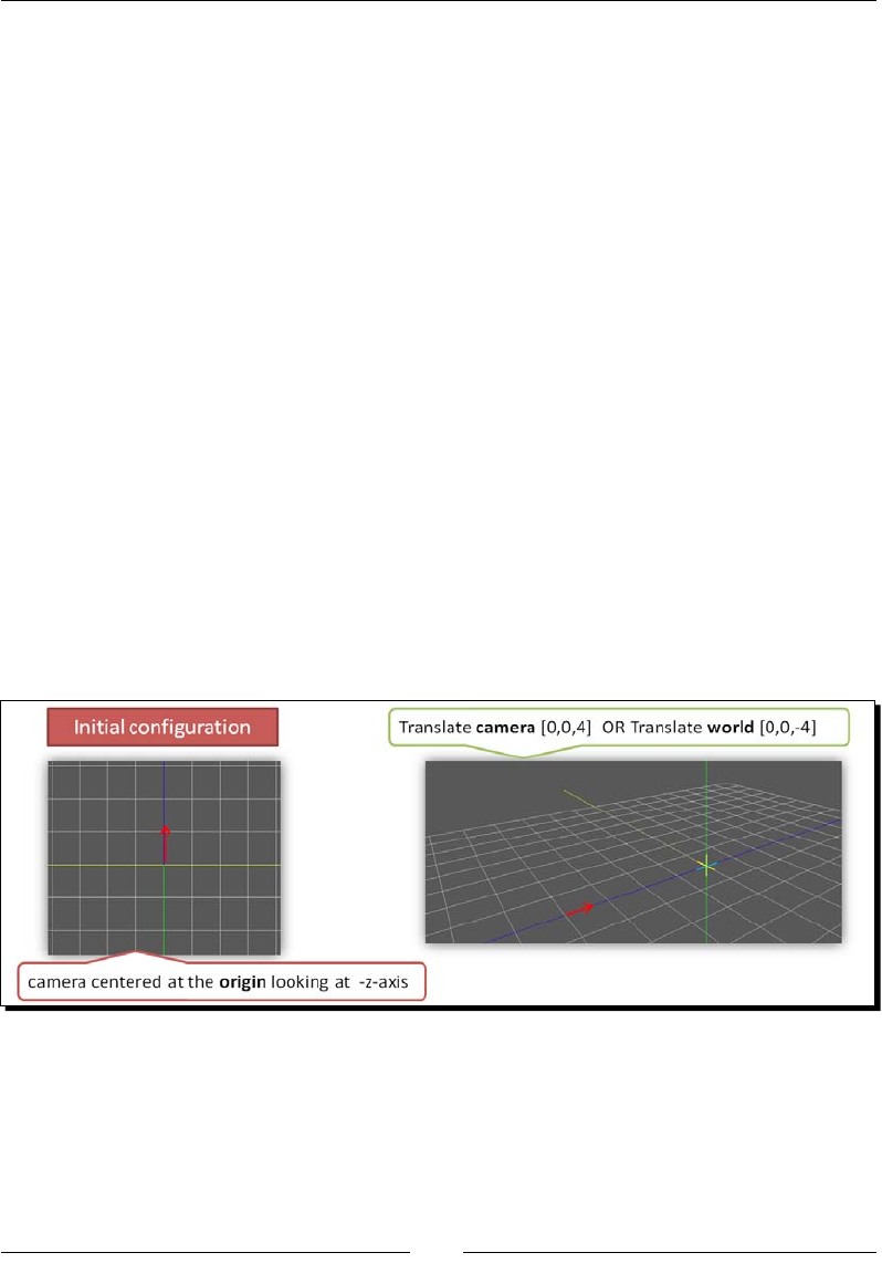
Chapter 4

[ 121 ]

For the sake of analysis, let's break the problem down into two sub-problems: camera

translaon and camera rotaon. We will have a praccal demo on each one.

Camera translation

Let's move the camera to [0 ,0, 4] in world coordinates. This means 4 units from the origin on

the posive z-axis.

Remember that we do not know at this point of a matrix to move the camera, we only know

how to move the world (with the Model-View matrix). If we applied:

mat4.translate(mvMatrix, [0,0,4]);

In such a case, the world would be translated 4 units on the posive z-axis and as the camera

posion has not been changed (as we do not know a matrix to do this), it would be located

at [0,0,-4], which is exactly the opposite of what we wanted in the rst place!

Now, say that we applied the translaon in the opposite direcon:

mat4.translate(mvMatrix, [0,0,-4]);

In such a case, the world would be moved 4 units on the negave z-axis and then the camera

would be located at [0,0,4] in the new world coordinate system.

We can see here that translang the camera is equivalent to translang the world in the

opposite direcon.

In the following secon, we are going to explore translaons both in world space and in

camera space.

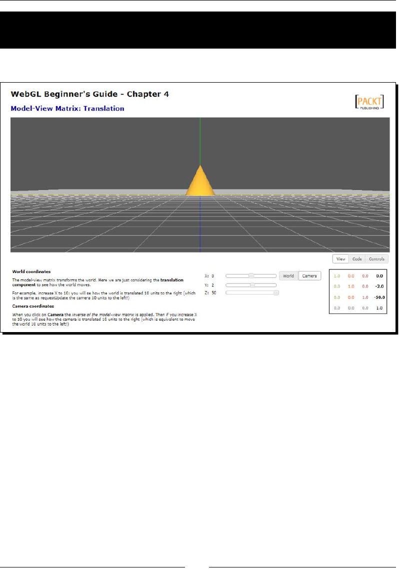
Camera

[ 122 ]

Time for action – exploring translations: world space versus

camera space

1. Open ch4_ModelView_Translation.html in your HTML5 browser:

2. We are looking from a distance at the posive z-axis at a cone located at the origin

of the world. There are three sliders that will allow you to translate either the world

or the camera on the x, y, and z axis, respecvely. The world space is acvated

by default.

3. Can you tell by looking at the World-View matrix on the screen where the origin of

the world is? Is it [0,0,0]? (Hint: check where we dene translaons in the Model-

View matrix).

4. We can think of the canvas as the image that our camera sees. If the world center is

at [0,-2,-50], where is the camera?

5. If we want to see the cone closer, we would have to move the center of the world

towards the camera. We know that the camera is far on the posive z-axis of the

world, so the translaon will occur on the z-axis. Given that you are on world

coordinates, do we need to increase or decrease the z-axis slider? Go ahead

and try your answer.

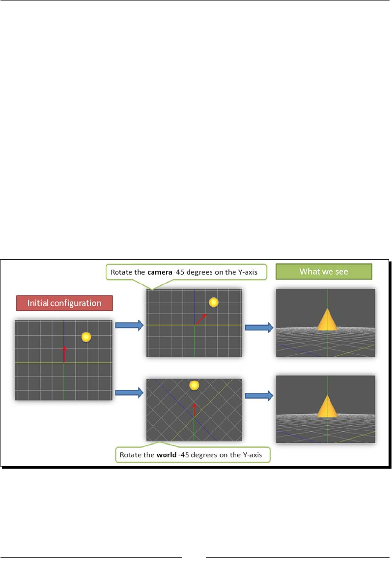
Chapter 4

[ 123 ]

6. Now switch to camera coordinates by clicking on the Camera buon. What is the

translaon component of this matrix? What do you need to do if you want to move

the camera closer to the cone? What does the nal translaon look like? What can

you conclude?

7. Go ahead and try to move the camera on the x-axis and the y-axis. Check what the

correspondent transformaons would be on the Model-View matrix.

What just happened?

We saw that the camera translaon is the inverse of the Model-View matrix translaon.

We also learned where to nd translaon informaon in a transformaon matrix.

Camera rotation

Similarly, if we want to rotate the camera, say, 45 degrees to the right, this would be

equivalent to rotang the world 45 degrees to the le. Using glMatrix to achieve this,

we write the following:

mat4.rotate(mvMatrix,45 * Math.PI/180, [0,1,0]);

Let's see this behavior in acon!

Similar to the previous secon where we explored translaons, in the following me for

acon, we are going to play with rotaons in both world and camera spaces.

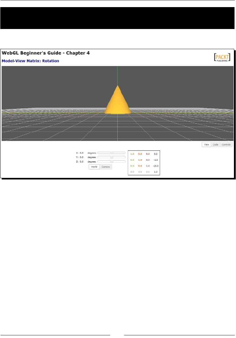
Camera

[ 124 ]

Time for action – exploring rotations: world space versus

camera space

1. Open ch4_ModelView_Rotation.html in your HTML5 browser:

2. Just like in the previous example, we will see:

A cone at the origin of the world

The camera is located at [0,2,50] in world coordinates

Three sliders that will allows us to rotate either the world or the camera

Also, we have a matrix where we can see the result of dierent rotaons

3. Let's see what happens to the axis aer we apply a rotaon. With the World

coordinates buon selected, rotate the world 90 degrees around the x-axis.

What does the Model-View matrix look like?

4. Let's see where the axes end up aer a 90 degree rotaon around the x-axis:

By looking at the rst column, we can see that the x-axis has not changed.

It is sll [1,0,0]. This makes sense as we are rotang around this axis.

The second column of the matrix indicates where the y-axis is aer

the rotaon. In this case, we went from [0,1,0] , which is the original

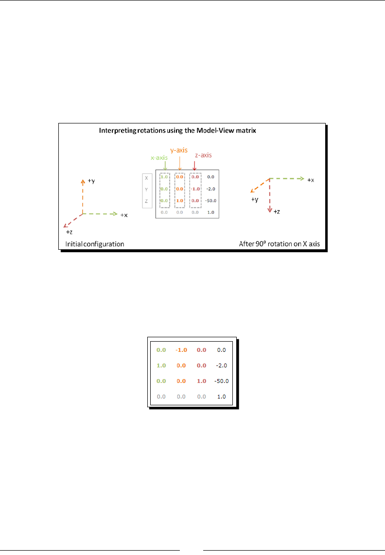
Chapter 4

[ 125 ]

conguraon, to [0,0,1], which is the axis that is coming out of the screen.

This is the z-axis in the inial conguraon. This makes sense as now we are

looking from above, down to the cone.

The third column of the matrix indicates the new locaon of the z-axis. It

changed from [0,0,1], which as we know is the z-axis in the standard spaal

conguraon (without transforms), to [0,-1,0], which is the negave poron

of the y-axis in the original conguraon. This makes sense as we rotated

around the x-axis.

5. As we just saw, understanding the Rotaon matrix (3x3 upper-le corner of the

Model-View matrix) is simple: the rst three columns are always telling us where

the axis is.

6. Where are the axis in this transformaon:

Check your answer by using the sliders to achieve the rotaon that you believe

produce this matrix.

7. Now let's see how rotaons work in Camera space. Click on the Camera buon.

8. Start increasing the angle of rotaon in the X axis by incremenng the slider

posion. What do you noce?

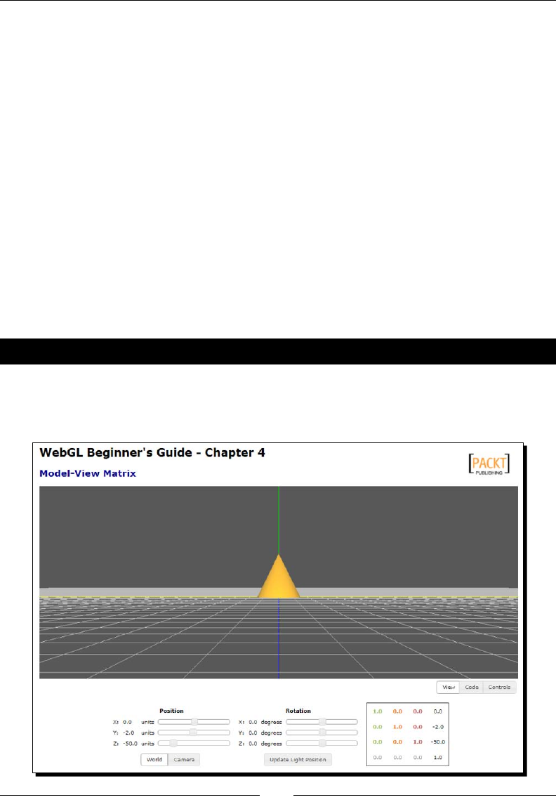
Camera

[ 126 ]

9. Go ahead and try dierent rotaons in camera space using the sliders.

10. Are the rotaons commutave? That is, do you get the same result if you rotate,

for example, 5 degrees on the X axis and 90 degrees on the Z axis, compared to the

case where you rotate 90 degrees on the Z axis and then you rotate 5 degrees on

the X axis?

11. Now, go back to World space. Please check that when you are in World space, you

need to reverse the rotaons to obtain the same pose. So, if you were applying 5

degrees on the X axis and 90 degrees on the Z axis. Check that when you apply -5

degrees on the X axis and -90 degrees on the Z axis you obtain the same image as in

point 10.

What just happened?

We just saw that the Camera matrix rotaon is the inverse of the Model-View matrix rotaon.

We also learned how to idenfy the orientaon of our world or camera upon analysis of the

rotaon matrix (3x3 upper-le corner of the correspondent transformaon matrix).

Have a go hero – combining rotations and translations

1. The le ch4_ModelView.html contains the combinaon of rotaons and

translaons. When you open it your HTML5 browser, you see something

like the following:

Chapter 4

[ 127 ]

2. Try dierent conguraons of rotaons and translaons in both World and

Camera spaces.

The Camera matrix is the inverse of the Model-View matrix

We can see through these two scenarios that a Camera matrix would require being the exact

Model-View matrix opposite. In linear algebra, we know this as the inverse of a matrix.

The inverse of a matrix is such that when mulplying it by the original matrix, we obtain the

identy matrix. In other words, if M is the Model-View matrix and C is the Camera matrix,

we have the following:

MC = I

M-1MC = M-1

C= M-1

We can create the Camera matrix using glMatrix by wring something like the following:

varcMatrix=mat4.create();

mat4.inverse(mvMatrix,cMatrix);

Thinking about matrix multiplications in WebGL

Please do not skip this secon. If you want to, just put a scker on this page so you

remember where to go when you need to debug Model-View transformaons. I spent so

many nights trying to understand this (sigh) and I wish I had had a book like this to explain

this to me.

Before moving forward, we need to know that in WebGL, the matrix operaons

are wrien in the reverse order in which they are applied to the verces.

Here is the explanaon. Assume, for a moment, that you are wring the code to rotate/

move the world, that is, you rotate your verces around the origin and then you move away.

The nal transformaon would look like this:

RTv

Here, R is the 4x4 matrix encoding pure rotaon, T is the 4x4 matrix encoding

pure translaon, and v corresponds to the verces present in your scene

(in homogeneous coordinates).

Camera

[ 128 ]

Now, if you noce, the rst transformaon that we actually apply to the verces is the

translaon and then we apply the rotaon! Verces need to be mulplied rst by the matrix

that is to the le. In this scenario, that matrix is T. Then, the result needs to be mulplied by R.

This fact is reected in the order of the operaons (here mvMatrix is the

Model-View matrix):

mat4.identity(mvMatrix)

mat4.translate(mvMatrix,position);mat4.rotateX(mvMatrix,rotation[0]

*Math.PI/180);

mat4.rotateY(mvMatrix,rotation[1]*Math.PI/180);

mat4.rotateZ(mvMatrix,rotation[2]*Math.PI/180);

Now if we were working in camera coordinates and we wanted to apply the same

transformaon as before, we need to apply a bit of linear algebra rst:

M = RT The Model-View matrix M is the result of mulplying

rotaon and translaon together

C = M-1 We know that the Camera matrix is the inverse of the

Model-View matrix

C =(RT)-1 By substuon

C=T-1R-1 Inverse of a matrix product is the reverse product of the

inverses

Luckily for us, when we are working in camera coordinates in the chapter's examples,

we have the inverse translaon and the inverse rotaon already calculated in the global

variables position and rotation. Therefore, we would write something like this in the

code (here cMatrix is the Camera matrix):

mat4.identity(cMatrix);

mat4.rotateX(cMatrix,rotation[0]*Math.PI/180);

mat4.rotateY(cMatrix,rotation[1]*Math.PI/180);

mat4.rotateZ(cMatrix,rotation[2]*Math.PI/180);

mat4.translate(cMatrix,position);

Basic camera types

The following are the camera types that we will discuss in this chapter.

Orbing camera

Tracking camera

Chapter 4

[ 129 ]

Orbiting camera

Up to this point, we have seen how we can generate rotaons and translaons of the world

in the world or camera coordinates. However, in both cases, we are always generang the

rotaons around the center of the world. This could be ideal for many cases where we are

orbing around a 3D object such as our Nissan GTX model. You put the object at the center

of the world, then you can examine the object at dierent angles (rotaon) and then you

move away (translaon) to see the result. Let's call this type of camera an orbing camera.

Tracking camera

Now, going back to the example of the rst person shoong game, we need to have a

camera that is able to look up when we want to see if there are enemies above us. Just

the same, we should be able to look around le and right (rotaons) and then move in the

direcon in which our camera is poinng (translaon). This camera type can be designated

as a rst-person camera. This same type is used when the game follows the main character.

Therefore, it is also known as a tracking camera.

To implement rst-person cameras, we need to set up the rotaons on the camera axis

instead of using the world origin.

Rotating the camera around its location

When we mulply matrices, the order in which matrices are mulplied is relevant. Say, for

instance, that we have two 4x4 matrices. Let R be the rst matrix and let's assume that this

matrix encodes pure rotaon; let T be the second matrix and let's assume that T encodes

pure translaon. Now:

RT ≠ TR

In other words, the order of the operaons aects the result. It is not the same to rotate

around the origin and then translate away from it (orbing camera), as compared to

translang the origin and then rotang around it (tracking camera)!

So in order to set the locaon of the camera as the center for rotaons, we just need to

invert the order in which the operaons are called. This is equivalent to converng from

an orbing camera to a tracking camera.

Translating the camera in the line of sight

When we have an orbing camera, the camera will be always looking towards the center

of the world. Therefore, we will always use the z-axis to move to and from the object that

we are examining. However, when we have a tracking camera, as the rotaon occurs at the

camera locaon, we can end up looking to any posion in the world (which is ideal if you

want to move around it and explore it). Then, we need to know the direcon in which the

camera is poinng to in world coordinates (camera axis). We will see how to obtain this next.

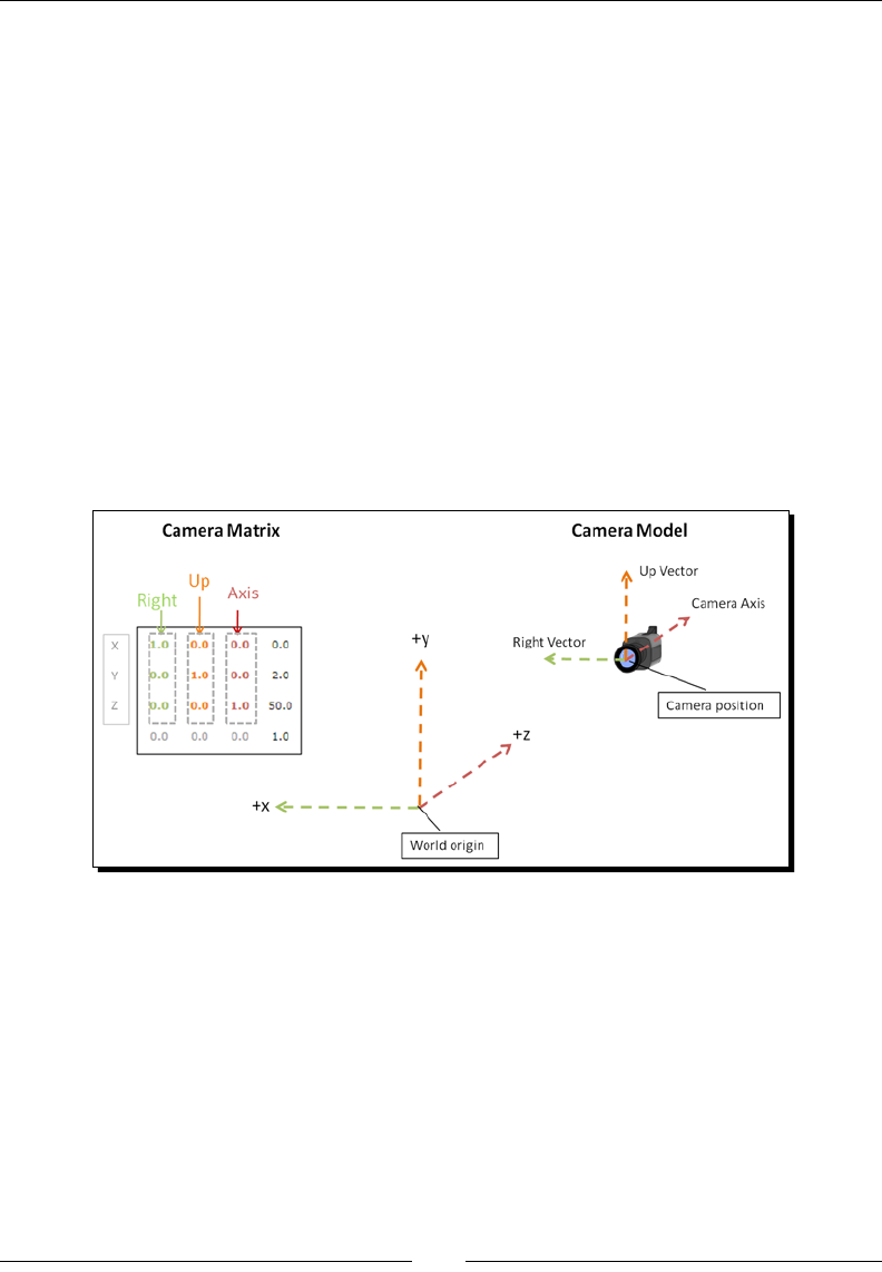
Camera

[ 130 ]

Camera model

Just like its counterpart, the Model-View matrix, the Camera matrix encodes informaon

about the camera axes orientaon. As we can see in the gure, the upper-le 3x3 matrix

corresponds to the camera axes:

The rst column corresponds to the x-axis of the camera. We will call it the

Right vector.

The second column is the y-axis of the camera. This will be the Up vector.

The third column determines the vector in which the camera can move back

and forth. This is the z-axis of the camera and we will call it the Camera axis.

Due to the fact that the Camera matrix is the inverse of the Model-View matrix, the

upper-le 3x3 rotaon matrix contained in the Camera matrix gives us the orientaon

of the camera axes in world space. This is a plus, because it means that we can tell the

orientaon of our camera in world space, just by looking at the columns of this 3x3

rotaon matrix (And we know now what each column means).

In the following secon, we will play with orbing and tracking cameras and we will see how

we can change the camera posion using mouse gestures, page widgets (sliders), and also

we will have a graphical representaon of the resulng Model-View matrix. In this exercise,

we will integrate both rotaons and translaons and we will see how they behave under the

two basic types of cameras that we are studying.

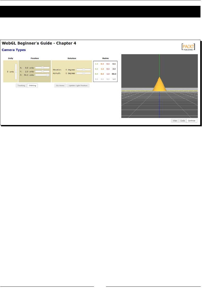
Chapter 4

[ 131 ]

Time for action – exploring the Nissan GTX

1. Open the le ch4_CameraTypes.html in your HTML5 browser. You will see

something like the following:

2. Go around the world using the sliders in Tracking mode. Cool eh?

3. Now, change the camera type to Orbing mode and do the same.

4. Now, please check that besides the slider controls, both in Tracking and Orbing

mode, you can use your mouse and keyboard to move around the world.

5. In this exercise, we have implemented a camera using two new classes:

Camera: to manipulate the camera.

CameraInteractor: to connect the camera to the canvas. It will receive

mouse and keyboard events and it will pass them along to the camera.

If you are curious, you can see the source code of these two classes in /js/webgl.

We have applied the concepts explained in this chapter to build these two classes.

6. So far, we have seen a cone in the center of the world. Let's change that for

something more interesng to explore.

7. Open the le ch4_CameraTypes.html in your source code editor.

Camera

[ 132 ]

8. Go to the load funcon. Let's add the car to the scene. Rewrite the contents of this

funcon so it looks like the following:

function load(){

Floor.build(2000,100);

Axis.build(2000);

Scene.addObject(Floor);

Scene.addObject(Axis);

Scene.loadObjectByParts('models/nissan_gts/pr','Nissan',178);

}

You will see that we have increased the size of the axis and the oor so we can see

them. We do need to do this because the car is an object much larger than the

original cone.

9. There are some steps that we need to take in order to be able to see the car

correctly. First we need to make sure that we have a large enough view volume.

Go to the initTransforms funcon and update this line:

mat4.perspective(30, c_width / c_height, 0.1, 1000.0, pMatrix);

With this:

mat4.perspective(30, c_width / c_height, 10, 5000.0, pMatrix);

10. Do the same in the updateTransforms funcon.

11. Now, let's change the type of our camera so when we load the page, we have

an orbing camera by default. In the configure funcon, change this line:

camera = new Camera(CAMERA_TRACKING_TYPE);

With:

camera = new Camera(CAMERA_ORBIT_TYPE);

12. Another thing we need to take into account is the locaon of the camera. For a large

object like this car, we need to be far away from the center of the world. For that

purpose, go to the configure funcon and change:

camera.goHome([0,2,50]);

Add:

camera.goHome([0,200,2000]);

13. Let's modify the lighng of our scene so it ts beer in the model we are displaying.

In the funcon configure funcon, right aer this line:

interactor = new CameraInteractor(camera, canvas);

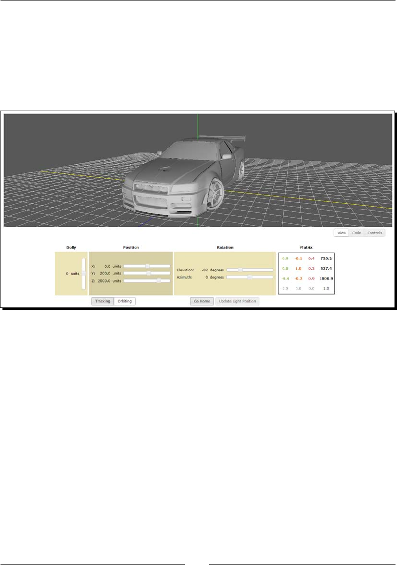
Chapter 4

[ 133 ]

Write:

gl.uniform4fv(prg.uLightAmbient, [0.1,0.1,0.1,1.0]);

gl.uniform3fv(prg.uLightPosition, [0, 0, 2120]);

gl.uniform4fv(prg.uLightDiffuse, [0.7,0.7,0.7,1.0]);

14. Save the le with a dierent name and then load this new le in your HTML5

Internet browser. You should see something like the following screenshot:

15. Using the mouse, keyboard, or/and the sliders, explore the new scene.

Hint: use orbing mode to explore the car from dierent angles.

16. See how the Camera matrix is updated when you move around the scene.

17. You can see what the nal exercise looks like by opening the le

ch4_NissanGTR.html.

What just happened?

We added mouse and keyboard interacon to our scene. We also experimented with the two

basic camera types—tracking and orbing cameras. We modied the sengs of our scene to

visualize a complex model.

Camera

[ 134 ]

Have a go hero – updating light positions

Remember that when we move the camera, we are applying the inverse transformaon to

the world. If we do not update the light posion, then the light source will be located at the

same stac point, regardless of the nal transformaon applied to the world.

This is very convenient when we are moving around or exploring an object in the scene.

We will always be able to see if the light is located on the same axis of the camera. This is

the case for the exercises in this chapter. Nevertheless, we can simulate the case when the

camera movement is independent from the light source. To do so, we need to calculate the

new light posion whenever we move the camera. We do this in two steps:

First, we calculate the light direcon. We can do this by simply calculang the dierence

vector between our target and our origin. Say that the light source is located at [0,2,50].

If we want to direct our light source towards the origin, we calculate the vector [0,0,0] -

[0,2,50] (target - origin). This vector has the correct orientaon of the light when we target

the origin. We repeat the same procedure if we have a dierent target that needs to be lit.

In that case, we just use the coordinates of the target and from them we subtract the

locaon of the light.

As we are direcng our light source towards the origin, we can nd the direcon of the light

just by inverng the light posion. If you noce, we do this in ESSL in the vertex shader:

vec3 L = normalize(-uLightPosition);

Now as L is a vector, if we want to update the direcon of the light, then we need to use

the Normal matrix, discussed earlier in this chapter, in order to update this vector under

any world transformaon. This step is oponal in the vertex shader:

if(uUpdateLight){

L=vec3(uNMatrix*vec4(L,0.0));

}

In the previous fragment of code, L is augmented to 4-components, so we can use the direct

mulplicaon provided by ESSL. (Remember that uNMatrix is a 4x4 matrix and as such, the

vectors that are transformed by it need to be 4-dimensional). Also, please bear in mind that,

as explained in the beginning of the chapter, vectors have their homogeneous coordinate

always set to zero, while verces have their homogeneous coordinate set to one.

Aer the mulplicaon, we reduce the result to 3-components before assigning the result

back to L.

You can test the eects of updang the light posion by using the buon Update Light

Posion, provided in the les ch4_NissanGTR.html and ch4_CameraTypes.html.

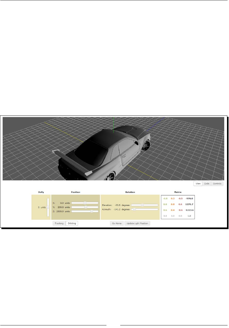
Chapter 4

[ 135 ]

We connect a global variable that keeps track of the state of this buon with the uniform

uUpdateLight.

1. Edit

ch4_NissanGTR.html and set the light posion to a dierent locaon.

To do this, edit the configure funcon. Go to:

gl.uniform3fv(prg.uLightPosition,[0, 0, 2120]);

Try dierent light posions:

[2120,0,0]

[0,2120,0]

[100,100,100]

2. For each opon, save the le and try it with and without updang the light posion

(use the buon Update Light Posion).

3. For a beer visualizaon, use an Orbing camera.

The Perspective matrix

At the beginning of the chapter, we said that the Perspecve matrix combines the

projecon transformaon and the perspecve division. These two steps combined

take a 3D scene and converts it into a cube that is then mapped to the 2D canvas

by the viewport transformaon.

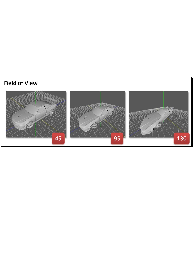
Camera

[ 136 ]

In pracce, the Perspecve matrix determines the geometry of the image that is captured by

the camera. In a real world camera, the lens of the camera would determine how distorted

the nal images are. In a WebGL world, we use the Perspecve matrix to simulate that. Also,

unlike in the real world where our images are always aected by perspecve, in WebGL, we

can pick a dierent representaon: the orthographic projecon.

Field of view

The Perspecve matrix determines the Field of View (FOV) of the camera, that is, how

much of the 3D space will be captured by the camera. The eld of view is a measure given

in degrees and the term is used interchangeably with the term angle of view.

Perspective or orthogonal projection

A perspecve projecon assigns more space to details that are closer to the camera than the

details that are farther from it. In other words, the geometry that is close to the camera will

appear bigger than the geometry that is farther from it. This is the way our eyes see the real

world. Perspecve projecon allows us to assess the distance because it gives our brain a

depth cue.

In contrast, an orthogonal projecon uses parallel lines; this means that will look the same

size regardless of their distance to the camera. Therefore, the depth cue is lost when using

orthogonal projecon.

Using glMatrix, we can set up the perspecve or the orthogonal projecon by calling

mat4.persective or mat4.ortho respecvely. The signatures for these methods are:

Chapter 4

[ 137 ]

Funcon Descripon (Taken from the documentaon of

the library)

mat4.perspective(fovy, aspect,

near, far, dest) Generates a perspecve projecon matrix with

the given bounds

Parameters:

fovy - vercal eld of view

aspect - aspect rao—typically viewport width/

height

near, far - near and far bounds of the frustum

dest - Oponal, mat4 frustum matrix will be

wrien into

Returns:

dest if specied, a new mat4 otherwise

mat4.ortho(left, right, bottom,

top, near, far, dest)

Generates an orthogonal projecon matrix with

the given bounds:

Parameters:

left, right - le and right bounds of the

frustum

bottom, top - boom and top bounds of the

frustum

near, far - near and far bounds of the frustum

dest - Oponal, mat4 frustum matrix will be

wrien into

Returns:

dest if specied, a new mat4 otherwise.

In the following me for acon secon, we will see how the eld of view and the perspecve

projecon aects the image that our camera captures. We will experiment perspecve and

orthographic projecons for both orbing and tracking cameras.

Time for action – orthographic and perspective projections

1. Open the le ch4_ProjectiveModes.html in your HTML5 Internet browser.

2. This exercise is very similar to the previous one. However, there are two new

buons: Perspecve and Orthogonal. As you can see, Perspecve is acvated

by default.

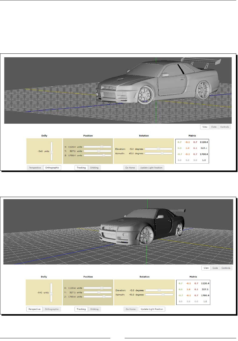
Camera

[ 138 ]

3. Change the camera type to Orbing.

4. Change the projecve mode to Orthographic.

5. Explore the scene. Noce the lack of depth cues that is characterisc of

orthogonal projecons:

6. Now switch to Perspecve mode:

Chapter 4

[ 139 ]

7. Explore the source code. Go to the updateTransforms funcon:

function updateTransforms(){

if (projectionMode == PROJ_PERSPECTIVE){

mat4.perspective(30, c_width / c_height, 10, 5000,

pMatrix);

}

else{

mat4.ortho(-c_width, c_width, -c_height, c_height, -5000,

5000, pMatrix);

}

8. Please take a look at the parameters that we are using to set up the projecve view.

9. Let's modify the eld of view. Create a global variable right before the

updateTransforms funcon:

var fovy = 30;

10. Let's use this variable instead of the hardcoded value:

Replace:

mat4.perspective(30, c_width / c_height, 10, 5000, pMatrix);

With:

mat4.perspective(fovy, c_width / c_height, 10, 5000, pMatrix);

11. Now let's update the camera interactor to update this variable. Open the le /js/

webgl/CameraInteractor.js in your source code editor.

Append these lines to CameraInteractor.prototype.onKeyDown inside if

(!this.ctrl){:

else if (this.key == 87) { //w

if(fovy<120) fovy+=5;

console.info('FovY:'+fovy);

}

else if (this.key == 78) { //n

if(fovy>15) fovy-=5;

console.info('FovY:'+fovy);

}

Please make sure that you are inside the if secon.

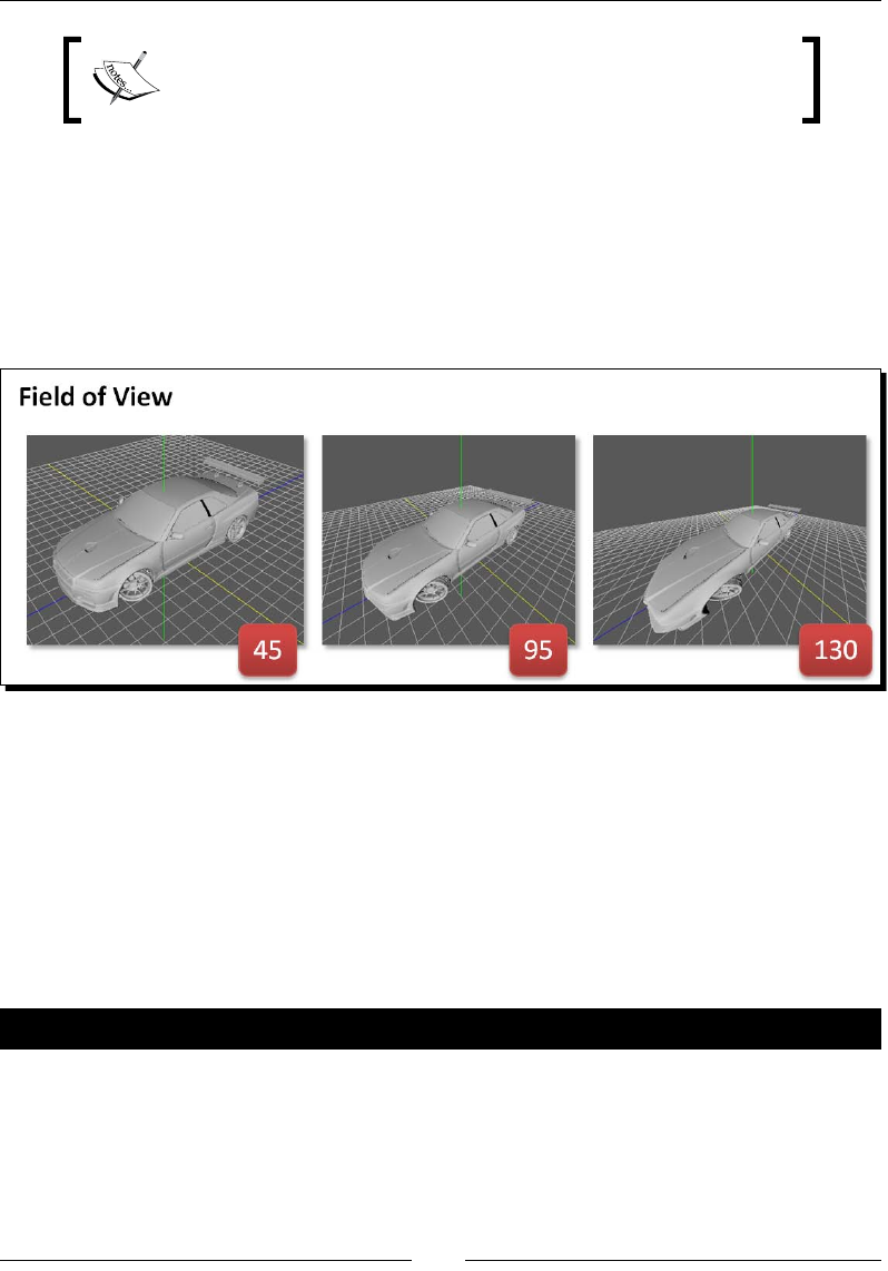
Camera

[ 140 ]

If these instrucons are already there, do not write them again. Just

make sure you understand that the goal here is to update the global

fovy variable that refers to the eld of view in perspecve mode.

12.Save the changes made to CameraInteractor.js.

13. Save the changes made to ch4_ProjectiveModes.html. Use a dierent name.

You can see the nal result in the le ch4_ProjectiveModesFOVY.html.

14. Open the renamed le in your HTML5 Internet browser. Try dierent elds of view

by pressing w or n repeatedly. Can you replicate these scenes:

15. Noce that as you increase the eld of view, your camera will capture more of the

3D space. Think of this as the lens of a real-world camera. With a wide-angle lens,

you capture more space with the trade-o of deforming the objects as they move

towards the boundaries of your viewing box.

What just happened?

We experimented with dierent conguraons for the Perspecve matrix and we saw how

these conguraons produce dierent results in the scene.

Have a go hero – integrating the Model-view and the projective transform

Remember that once we have applied the Model-View transformaon to the verces, the

next step is to transform the view coordinates to NDC coordinates:

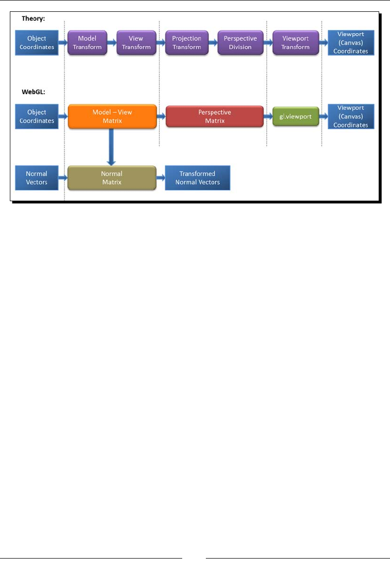
Chapter 4

[ 141 ]

We do this by a simple mulplicaon using ESSL in the vertex shader:

gl_Position = uPMatrix * uMVMatrix * vec4(aVertexPosition,1.0);

The predened variable, gl_Position, stores the NDC coordinates for each vertex

of every object dened in the scene.

In the previous mulplicaon, we augment the shader aribute, aVertexPosition,

to a 4-component vertex because our matrices are 4x4. Unlike normals, verces have a

homogeneous coordinate equal to one (w=1).

Aer this step, WebGL will convert the computed clipping coordinates to normalized device

coordinates and from there to canvas coordinates using the WebGL viewport funcon. We

are going to see what happens when we change this mapping.

1. Open the le ch4_NisanGTS.html in your source code editor.

2. Go to the draw funcon. This is the rendering funcon that is invoked every me

we interact with the scene (by using the mouse, the keyboard, or the widgets on

the page).

3. Change this line:

gl.viewport(0, 0, c_width, c_height);

Make it:

gl.viewport(0, 0, c_width/2, c_height/2);

gl.viewport(c_width/2,c_height/2, c_width, c_height);

gl.viewport(50, 50, c_width-100, c_height-100);

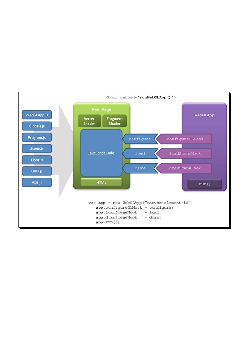
Camera

[ 142 ]

4. For each opon, save the le and open it on your HTML5 browser.

5. What do you see? Please noce that you can interact with the scene just like before.

Structure of the WebGL examples

We have improved the structure of the code examples in this chapter. As the complexity of

our WebGL applicaons increases, it is wise to have a good, maintainable, and clear design.

We have le this secon at the end of the chapter so you can use it as a reference when

working on the exercises.

Just like in previous exercises, our entry point is the runWebGLApp funcon which

is called when the page is loaded. There we create an instance of WebGLApp, as shown

in the previous diagram.

WebGLApp

This class encapsulates some of the ulity funcons that were present in our examples in

previous chapters. It also declares a clear and simple life cycle for a WebGL applicaon.

WebGLApp has three funcon hooks that we can map to funcons in our web page. These

hooks determine what funcons will be called for each stage in the life cycle of the app. In

the examples of this chapter, we have created the following mappings:

Chapter 4

[ 143 ]

configureGLHook: which points to the configure funcon in the web page

loadSceneHook: which is mapped to the load funcon in the webpage

drawSceneHook: which corresponds to the draw funcon in the webpage

A funcon hook can be described as a pointer to a funcon. In JavaScript,

you can write:

function foo(){alert("function foo invoked");}

var hook = foo;

hook();

This fragment of code will execute foo when hook() is executed. This

allows a pluggable behavior that is more dicult to express in fully typed

languages.

WebGLApp will use the funcon hooks to call configure, load, and draw in our page in

that order.

Aer seng these hooks, the run method is invoked.

The source code for WebGLApp and other supporng objects can be

found in /js/webgl

Supporting objects

We have created the following objects, each one in its own le:

Globals.js: Contains the global variables used in the example.

Program.js: Creates the program using the shader denions. Provides

the mapping between JavaScript variables (prg.*) and program aributes

and uniforms.

Scene.js: Maintains a list of objects to be rendered. Contains the AJAX/JSON

funconality to retrieve remote objects. It also allows adding local objects to

the scene.

Floor.js: Denes a grid on the X-Z plane. This object is added to the Scene to

have a reference of where the oor is.

Axis.js: Represents the axis in world space. When added to the scene, we will

have a reference of where the origin is.

Camera

[ 144 ]

WebGLApp.js: Represents a WebGL applicaon. It has three funcon hooks that

dene the conguraon stage, the scene loading stage, and the rendering stage.

These hooks can be connected to funcons in our web page.

Utils.js: Ulity funcons such as obtaining a gl context.

You can refer to Globals.js to nd the global variables used in this

example (the denion of the JavaScript matrices is there) and Program.

js to nd the prg.* JavaScript variables that map to aributes and

uniforms in the shaders.

Life-cycle functions

The following are the funcons that dene the life-cycle of a WebGLApp applicaon:

Congure

The configure funcon sets some parameters of our gl context, such as the color

for clearing the canvas, and then it calls the initTransforms funcon.

Load

The load funcon sets up the objects Floor and Axis. These two locally-created objects

are added to the Scene by calling the addObject method. Aer that, a remote object

(AJAX call) is loaded using the Scene.loadObject method.

Draw

The draw funcon calls updateTransforms to calculate the matrices for the new posion

(that is, when we move), then iterates over the objects in the Scene to render them. Inside

this loop, it calls setMatrixUniforms for every object to be rendered.

Matrix handling functions

The following are the funcons that inialize, update, and pass matrices to the shaders:

initTransforms

As you can see, the Model-View matrix, the Camera matrix, the Perspecve matrix, and the

Normal matrix are set up here:

functioninitTransforms(){

mat4.identity(mvMatrix);

mat4.translate(mvMatrix,home);

Chapter 4

[ 145 ]

displayMatrix(mvMatrix);



mat4.identity(cMatrix);

mat4.inverse(mvMatrix,cMatrix);



mat4.identity(pMatrix);

mat4.perspective(30,c_width/c_height,0.1,1000.0,pMatrix);

mat4.identity(nMatrix);

mat4.set(mvMatrix,nMatrix);

mat4.inverse(nMatrix);

mat4.transpose(nMatrix);

coords=COORDS_WORLD;

}

updateTransforms

In updateTransforms, we use the contents of the global variables position and

rotation to update the matrices. This is, of course, if the requestUpdate variable

is set to true. We set requestUpdate to true from the GUI controls. The code for these

is located at the boom of the webpage (for instance, check the le ch4_ModelView_

Rotation.html).

functionupdateTransforms(){



mat4.perspective(30,c_width/c_height,0.1,1000.0,pMatrix);

if(coords==COORDS_WORLD){

mat4.identity(mvMatrix);

mat4.translate(mvMatrix,position);

mat4.rotateX(mvMatrix,rotation[0]*Math.PI/180);

mat4.rotateY(mvMatrix,rotation[1]*Math.PI/180);

mat4.rotateZ(mvMatrix,rotation[2]*Math.PI/180);

}

else{

mat4.identity(cMatrix);

mat4.rotateX(cMatrix,rotation[0]*Math.PI/180);

mat4.rotateY(cMatrix,rotation[1]*Math.PI/180);

mat4.rotateZ(cMatrix,rotation[2]*Math.PI/180);

mat4.translate(cMatrix,position);

}

}

Camera

[ 146 ]

setMatrixUniforms

This funcon performs the mapping:

functionsetMatrixUniforms(){

if(coords==COORDS_WORLD){

mat4.inverse(mvMatrix,cMatrix);

displayMatrix(mvMatrix);

gl.uniformMatrix4fv(prg.uMVMatrix,false,mvMatrix);

}

else{

mat4.inverse(cMatrix,mvMatrix);

displayMatrix(cMatrix);



}



gl.uniformMatrix4fv(prg.uPMatrix,false,pMatrix);

gl.uniformMatrix4fv(prg.uMVMatrix,false,mvMatrix);

mat4.transpose(cMatrix,nMatrix);

gl.uniformMatrix4fv(prg.uNMatrix,false,nMatrix);

}

Summary

Let's summarize what we have learned in this chapter:

There is no camera object in WebGL. However, we can build one using the

Model-View matrix.

3D objects undergo several transformaons to be displayed on a 2D screen.

These transformaons are represented as 4x4 matrices.

Scene transformaons are ane. Ane transformaons are constuted by a linear

transformaon followed by a translaon. WebGL groups ane transforms in three

matrices: the Model-View matrix, the Perspecve matrix, and the Normal matrix

and one WebGL operaon: gl.viewport().

Chapter 4

[ 147 ]

Ane transforms are applied in projecve space so they can be represented by 4x4 matrices.

To work in projecve space, verces need to be augmented to contain an extra term, namely,

w, which is called the perspecve coordinate. The 4-tuple (x,y,z,w) is called homogeneous

coordinates. Homogeneous coordinates allows representaon of lines that intersect on

innity by making the perspecve coordinate w = 0. Vectors always have a homogeneous

coordinate w = 0; While points have a homogenous coordinate, namely, w = 1 (unless they

are at innity, in which case w=0).

By default, a WebGL scene is viewed from the world origin in the negave direcon of the

z-axis. This can be altered by changing the Model-View matrix.

The Camera matrix is the inverse of the Model-View matrix. Camera and World operaons

are opposite. There are two basic types of camera—orbing and tracking camera.

Normals receive special treatment whenever the object suers an ane transform. Normals

are transformed by the Normal matrix, which can be obtained from the Model-View matrix.

The Perspecve matrix allows the determining of two basic projecve modes, namely,

orthographic projecon and perspecve projecon.

Action

So far, we have seen stac scenes where all interacons are done by moving the

camera. The camera transformaon is applied to all objects in the 3D scene,

therefore we call it a global transform. However, objects in 3D scenes can have

acons on their own. For instance, in a racing car game, each car has its own

speed and trajectory. In a rst-person shoong game your enemies can hide

behind barricades then come and ght you or run away. In general, each one

of these acons is modeled as a matrix transformaon that is aached to the

corresponding actor in the scene. These are called local transforms. In this

chapter we will study dierent techniques to make use of local transforms.

In this chapter, we will discuss the following topics:

Global versus local transformaons

Matrix stacks and using them to perform animaon

Using JavaScript mers to do me-based animaon

Parametric curves

Interpolaon

In the previous chapter, we saw that when we apply the same transformaon to all the

objects in our scene we move the world. This global transformaon allowed us to create two

dierent kinds of cameras. Once we have applied the camera transform to all the objects in

the scene, each one of them could update its posion; represenng, for instance, targets

that are moving in a rst-person shoong game, or the posion of other competors

in a car racing game.

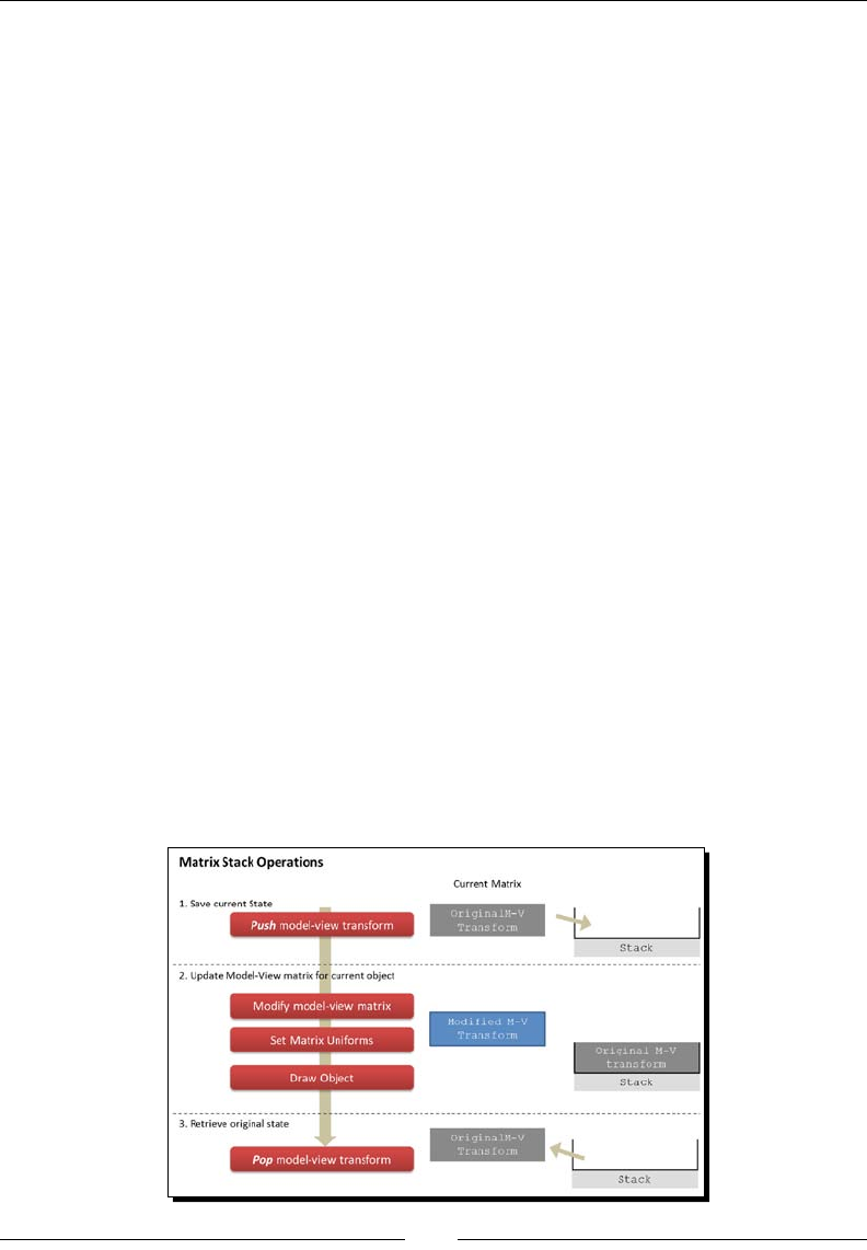
Acon

[ 150 ]

This can be achieved by modifying the current Model-View transform for each object. However,

if we modied the Model-View matrix, how could we make sure that these modicaons do

not aect other objects? Aer all, we only have one Model-View matrix, right?

The soluon to this dilemma is to use matrix stacks.

Matrix stacks

A matrix stack provides a way to apply local transforms to individual objects in our scene

while at the same me we keep the global transform (camera transform) coherent for all

of them. Let's see how it works.

Each rendering cycle (each call to our draw funcon) requires calculang the scene matrices

to react to camera movements. We are going to update the Model-View matrix for each

object in our scene before passing the matrices to the shading program (as aributes).

We do this in three steps as follows:

Step 1: Once the global Model-View matrix (camera transform) has been calculated,

we proceed to save it in a stack. This step will allow us to recover the original matrix

once we had applied to any local transforms.

Step 2: Calculate an updated Model-View matrix for each object in the scene.

This update consists of mulplying the original Model-View matrix by a matrix

that represents the rotaon, translaon, and/or scaling of each object in the scene.

The updated Model-View matrix is passed to the program and the respecve object

then appears in the locaon indicated by its local transform.

Step 3: We recover the original matrix from the stack and then we repeat steps 1

to 3 for the next object that needs to be rendered.

The following diagram shows this three-step procedure for one object:

Chapter 5

[ 151 ]

Animating a 3D scene

To animate a scene is nothing else than applying the appropriate local transformaons to

objects in it. For instance, if we have a cone and a sphere and we want to move them, each

one of them will have a corresponding local transformaon that will describe its locaon,

orientaon, and scale. In the previous secon, we saw that matrix stacks allow recovering

the original Model-View transform so we can apply the correct local transform for the next

object to be rendered.

Knowing how to move objects with local transforms and matrix stacks, the queson that

needs to be addressed is: When?

If we calculated the posion that we want to give to the cone and the sphere of our example

every me we called the draw funcon, this would imply that the animaon rate would be

dependent on how fast our rendering cycle goes. A slower rendering cycle would produce

choppy animaons and a too fast rendering cycle would create the illusion of objects

jumping from one side to the other without smooth transions.

Therefore, it is important to make the animaon independent from the rendering cycle.

There are a couple of JavaScript elements that we can use to achieve this goal: The

requestAnimFrame funcon and JavaScript mers.

requestAnimFrame function

The window.requestAnimFrame() funcon is currently being implemented in HTML5-

WebGL enabled Internet browsers. This funcon is designed such that it calls the rendering

funcon (whatever funcon we indicate) in a safe way only when the browser/tab window is

in focus. Otherwise, there is no call. This saves precious CPU, GPU, and memory resources.

Using the requestAnimFrame funcon, we can obtain a rendering cycle that goes as fast

as the hardware allows and at the same me, it is automacally suspended whenever the

window is out of focus. If we used requestAnimFrame to implement our rendering cycle,

we could use then a JavaScript mer that res up periodically calculang the elapsed me

and updang the animaon me accordingly. However, the funcon is a feature that is sll

in development.

To check on the status of the requestAnimFrame funcon, please refer to

the following URL:

https://developer.mozilla.org/en/DOM/window.requestAn

imationFrame#AutoCompatibilityTable.

Acon

[ 152 ]

JavaScript timers

We can use two JavaScript mers to isolate the rendering rate from the animaon rate.

In our previous code examples, the rendering rate is controlled by the class WebGLApp.

This class invokes the draw funcon, dened in our page, periodically using a JavaScript mer.

Unlike the requestAnimFrame funcon, JavaScript mers keep running in the background

even when the page is not in focus. This is not opmal performance for your computer given

that you are allocang resources to a scene that you are not even looking. To mimic some

of the requestAnimFrame intelligent behavior provided for this purpose, we can use the

onblur and onfocus events of the JavaScript window object.

Let's see what we can do:

Acon (What) Goal (Why) Method (How)

Pause the rendering To stop the rendering unl the

window is in focus

Clear the mer calling

clearInterval in the window.

onblur funcon

Slow the rendering To reduce resource

consumpon but make sure

that the 3D scene keeps

evolving even if we are not

looking at it

We can clear current mer calling

clearInterval in the window.

onblur funcon and create a new

mer with a more relaxed interval

(higher value)

Resume the rendering To acvate the 3D scene at

full speed when the browser

window recovers its focus

We start a new mer with the

original render rate in the window.

onfocus funcon

By reducing the JavaScript mer rate or clearing the mer, we can handle hardware

resources more eciently.

The source code for WebGLApp is located in the le /js/webgl/

WebGLApp.js that accompanies this chapter. In WebGLApp you can see how

the onblur and onfocus events have been used to control the rendering

mer as described previously.

Timing strategies

In this secon, we will create the second JavaScript mer that will allow controlling the

animaon. As previously menoned, a second JavaScript mer will provide independency

between how fast your computer can render frames and how fast we want the animaon

to go. We have called this property the animation rate.

Chapter 5

[ 153 ]

However, before moving forward you should know that there is a caveat when working with

mers: JavaScript is not a mul-threaded language.

This means that if there are several asynchronous events occurring at the same me

(blocking events) the browser will queue them for their posterior execuon. Each browser

has a dierent mechanism to deal with blocking event queues.

There are two blocking event-handling alternaves for the purpose of developing an

animaon mer.

Animation strategy

The rst alternave is to calculate the elapsed me inside the mer callback.

The pseudo-code looks like the following :

var initialTime = undefined;

var elapsedTime = undefined;

var animationRate = 30; //30 ms

function animate(deltaT){

//calculate object positions based on deltaT

}

function onFrame(){

elapsedTime = (new Date).getTime() – initialTime;

if (elapsedTime < animationRate) return; //come back later

animate(elapsedTime);

initialTime = (new Date).getTime();

}

function startAnimation(){

setInterval(onFrame,animationRate/1000);

}

Doing so, we can guarantee that the animaon me is independent from how oen the

mer callback is actually executed. If there are big delays (due to other blocking events) this

method can result in dropped frames. This means the object's posions in our scene will be

immediately moved to the current posion that they should be in according to the elapsed

me (between consecuve animaon mer callbacks) and then the intermediate posions

are to be ignored. The moon on screen may jump but oen a dropped animaon frame is

an acceptable loss in a real-me applicaon, for instance, when we move one object from

point A to point B over a given period of me. However, if we were using this strategy when

shoong a target in a 3D shoong game, we could quickly run into problems. Imagine that

you shoot a target and then there is a delay, next thing you know the target is no longer

there! Noce that in this case where we need to calculate a collision, we cannot aord to

miss frames, because the collision could occur in any of the frames that we would drop

otherwise without analyzing. The following strategy solves that problem.

Acon

[ 154 ]

Simulation strategy

There are several applicaons such as the shoong game example where we need all the

intermediate frames to assure the integrity of the outcome. For example, when working

with collision detecon, physics simulaons, or arcial intelligence for games. In this case,

we need to update the object's posions at a constant rate. We do so by directly calculang

the next posion for the objects inside the mer callback.

var animationRate = 30; //30 ms

var deltaPosition = 0.1

function animate(deltaP){

//calculate object positions based on deltaP

}

function onFrame(){

animate(deltaPosition);

}

function startAnimation(){

setInterval(onFrame,animationRate/1000);

}

This may lead to frozen frames when there is a long list of blocking events because the

object's posions would not be mely updated.

Combined approach: animation and simulation

Generally speaking, browsers are really ecient at handling blocking events and in most

cases the performance would be similar regardless of the chosen strategy. Then, deciding to

calculate the elapsed me or the next posion in mer callbacks will then depend on your

parcular applicaon.

Nonetheless, there are some cases where it is desirable to combine both animaon and

simulaon strategies. We can create a mer callback that calculates the elapsed me and

updates the animaon as many mes as required per frame. The pseudocode looks like

the following:

var initialTime = undefined;

var elapsedTime = undefined;

var animationRate = 30; //30 ms

var deltaPosition = 0.1;

function animate(delta){

//calculate object positions based on delta

}

function onFrame(){

elapsedTime = (new Date).getTime() - initialTime;

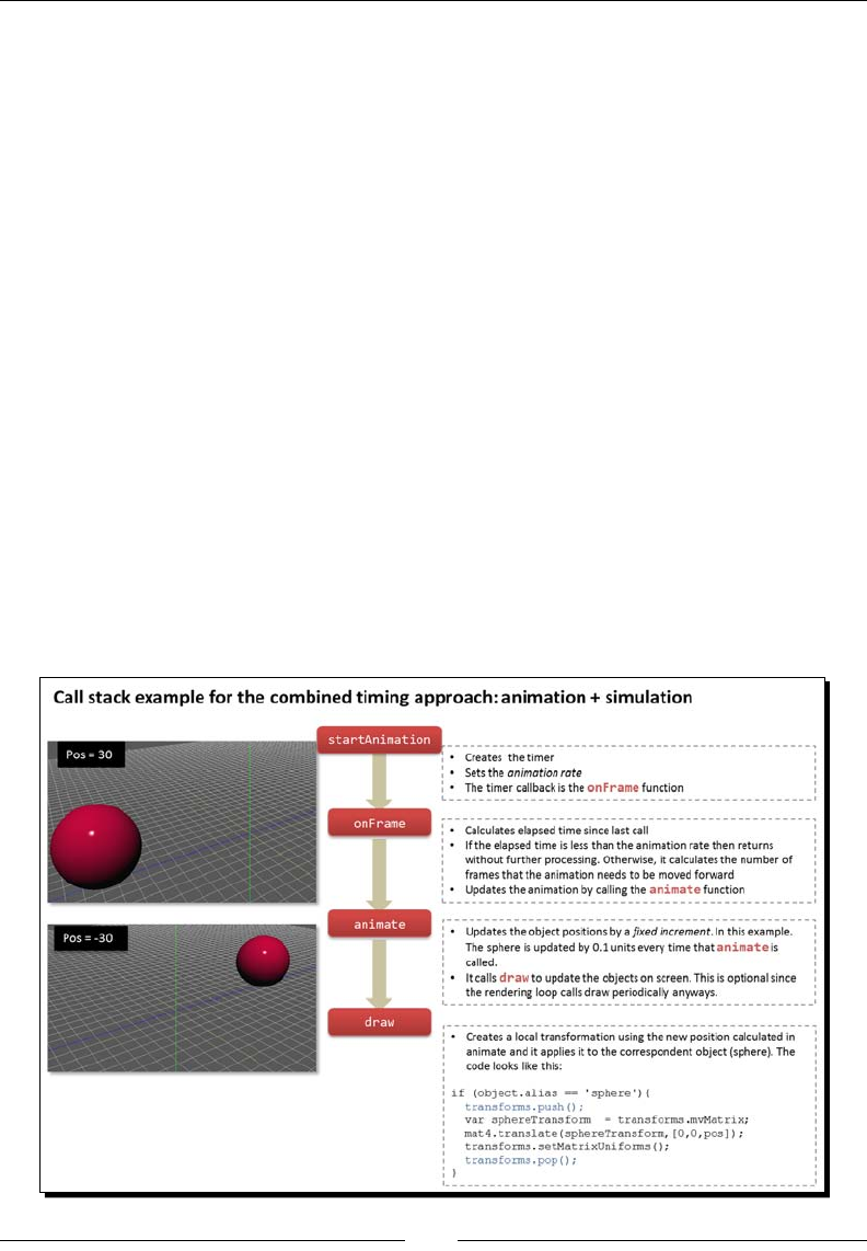
Chapter 5

[ 155 ]

if (elapsedTime < animationRate) return; //come back later!

var steps = Math.floor(elapsedTime / animationRate);

while(steps > 0){

animate(deltaPosition);

steps -= 1;

}

initialTime = (new Date).getTime();

}

function startAnimation(){

initialTime = (new Date).getTime();

setInterval(onFrame,animationRate/1000);

}

You can see from the preceding code snippet that the animaon will always update at a xed

rate, no maer how much me elapses between frames. If the app is running at 60 Hz, the

animaon will update once every other frame, if the app runs at 30 Hz the animaon will

update once per frame, and if the app runs at 15 Hz the animaon will update twice per

frame. The key is that by always moving the animaon forward a xed amount it is far

more stable and determinisc.

The following diagram shows the responsibilies of each funcon in the call stack for the

combined approach:

Acon

[ 156 ]

This approach can cause issues if for whatever reason an animaon step actually takes longer

to compute than the xed step, but if that is occurring, you really ought to simplify your

animaon code or put out a recommended minimum system spec for your applicaon.

Web Workers: Real multithreading in JavaScript

Though it is beyond the scope of this book, you may want to know that if performance is

really crical to you and you need to ensure that a parcular update loop always res at a

consistent rate then you could use Web Workers.

Web Workers is an API that allows web applicaons to spawn background processes

running scripts in parallel to their main page. This allows for thread-like operaon

with message-passing as the coordinaon mechanism.

You can nd the Web Workers specicaon at the following URL: http://dev.w3.org/

html5/workers/

Architectural updates

Let's review the structure of the examples developed in the book. Each web page includes

several scripts. One of them is WebGLApp.js. This script contains the WebGLApp object.

WebGLApp review

The WebGLApp object denes three funcon hooks that control the life cycle of the

applicaon. As shown in the diagram, we create a WebGLApp instance inside the

runWebGLApp funcon. Then, we connect the WebGLApp hooks to the configure, load,

and draw funcons that we coded. Also, please noce that the runWebGLApp funcon is

the entry point for the applicaon and it is automacally invoked using the onload event

of the web page.

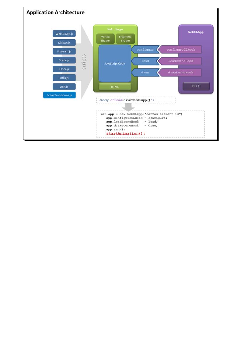
Chapter 5

[ 157 ]

Adding support for matrix stacks

The diagram also shows a new script: SceneTransforms.js. This le contains

the SceneTransforms objects that encapsulate the matrix-handling operaons

including matrix stacks operaons push and pop. The SceneTransforms object

replaces the funconality provided in Chapter 4, Camera, by the initTransforms,

updateTransforms, and setMatrixUniforms funcons.

You can nd the source code for SceneTransforms in js/webgl/SceneTransforms.js.

Conguring the rendering rate

Aer seng the connecons between the WebGLApp hooks and our congure, load and

draw funcons, WebGLApp.run() is invoked. This call creates a JavaScript mer that is

triggered every 500 ms. The callback for this mer is the draw funcon. Up to now a refresh

rate of 500 ms was more than acceptable because we did not have any animaons. However,

this is a parameter that you could tweak later on to opmize your rendering speed. To do so

please change the value of the constant WEBGLAPP_RENDER_RATE. This constant is dened

in the source code for WebGLApp.

You can nd the source code for WebGLApp in js/webgl/WebGLApp.js.

Acon

[ 158 ]

Creating an animation timer

As shown in the previous architecture diagram, we have added a call to the new

startAnimation funcon inside the runWebGLApp funcon. This causes the

animaon to start when the page loads.

Connecting matrix stacks and JavaScript timers

In the following Time for acon secon, we will take a look at a simple scene where we have

animated a cone and a sphere. In this example, we are using matrix stacks to implement

local transformaons and JavaScript mers to implement the animaon sequence.

Time for action – simple animation

1. Open ch5_SimpleAnimation.html using your WebGL-enabled Internet browser

of choice.

2. Move the camera around and see how the objects (sphere and cone) move

independently of each other (local transformaons) and from the camera posion

(global transformaon).

3. Move the camera around pressing the le mouse buon and holding it while you

drag the mouse.

4. You can also dolly the camera by clicking the le mouse buon while pressing the

Alt key and then dragging the mouse.

5. Now change the camera type to Tracking. If for any reason you lose your bearings,

click on go home.

6. Let's examine the source code to see how we have implemented this example.

Open ch5_SimpleAnimation.html using the source code editor of your choice.

7. Take a look at the funcons startAnimation, onFrame, and animate.

Which ming strategy are we using here?

8. The global variables pos_sphere and pos_cone contain the posion of the

sphere and the cone respecvely. Scroll up to the draw funcon. Inside the

main for loop where each object of the scene is rendered, a dierent local

transformaon is calculated depending on the current object being rendered.

The code looks like the following:

Chapter 5

[ 159 ]

transforms.calculateModelView();

transforms.push();

if (object.alias == 'sphere'){

var sphereTransform = transforms.mvMatrix;

mat4.translate(sphereTransform,[0,0,pos_sphere]);

}

else if (object.alias == 'cone'){

var coneTransform = transforms.mvMatrix;

mat4.translate(coneTransform, [pos_cone,0,0]);

}

transforms.setMatrixUniforms();

transforms.pop();

Using the transforms object (which is an instance of SceneTransforms) we obtain

the global Model-View matrix by calling transforms.calculateModelView().

Then, we push it into a matrix stack by calling the push method. Now we can apply

any transform that we want, knowing that we can retrieve the global transform so it

is available for the next object on the list. We actually do so at the end of the code

snippet by calling the pop method. Between the push and pop calls, we determine

which object is currently being rendered and depending on that, we use the global

pos_sphere or pos_cone to apply a translaon to the current Model-View matrix.

By doing so, we create a local transform.

9. Take a second look at the previous code. As you saw at the beginning of this

exercise, the cone is moving in the x axis while the sphere is moving in the z axis.

What do you need to change to animate the cone in the y axis? Test your hypothesis

by modifying this code, saving the web page, and opening it again on your HTML5

web browser.

10. Let's go now back to the animate funcon. What do we need to modify here to

make the objects to move faster? Hint: take a look at the global variables that this

funcon uses.

What just happened?

In this exercise, we saw a simple animaon of two objects. We examined the source code

to understand the call stack of funcons that make the animaon possible. At the end of

this call stack, there is a draw funcon that takes the informaon of the calculated object

posions and applies the respecve local transforms.

Acon

[ 160 ]

Have a go hero – simulating dropped and frozen frames

1. Open the ch5_DroppingFrames.html le using your HTML5 web browser.

Here you will see the same scene that we analyzed in the previous Time for

acon secon. You can see here that the animaon is not smooth because

we are simulang dropping frames.

2. Take a look at the source code in an editor of your choice. Scroll to the animate

funcon. You can see that we have included a new variable: simulationRate. In

the onFrame funcon, this new variable calculates how many simulaon steps need

to be performed when the me elapsed is around 300 ms (animationRate). Given

that the simulationRate is 30 ms this will produce a total of 10 simulaon steps.

These steps can be more if there are unexpected delays and the elapsed me is

considerably higher. This is the behavior that we expect.

3. In this secon we want you to experiment with dierent values for the

animationRate and simulationRate variables to answer the following quesons:

How do we get rid of the dropping frames issue?

How can we simulate frozen frames?

Hint: the calculated steps should always be zero.

What is the relaonship between the animationRate and the

simulationRate variables when simulang frozen frames?

Parametric curves

There are many situaons where we don't know the exact posion that an object will have

at a given me but we know an equaon that describe its movement. These equaons are

known as parametric curves and are called like that because the posion depends on one

parameter: the me.

There are many examples of parametric curves. We can think for instance of a projecle

that we shoot on a game, a car that is going downhill or a bouncing ball. In each case, there

are equaons that describe the moon of these objects under ideal condions. The next

diagram shows the parametric equaon that describes free fall moon.

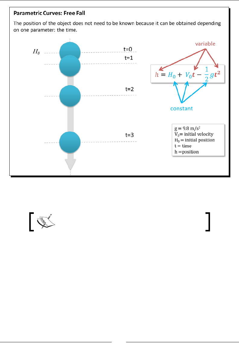
Chapter 5

[ 161 ]

We are going to use parametric curves for animang objects in a WebGL scene.

In this example, we will model a set of bouncing balls.

The complete source code for this exercise can be found in

/code/ch5_BouncingBalls.html.

Initialization steps

We will create a global variable that will store the me (simulaon me).

var sceneTime = 0;

We also create the global variables that regulate the animaon:

var animationRate = 15; /* 15 ms */

var elapsedTime = undefined;

var initialTime = undefined;

Acon

[ 162 ]

The load funcon is updated to load a bunch of balls using the same geometry

(same JSON le) but adding it several mes to the scene object. The code looks

like this:

function load(){

Floor.build(80,2);

Axis.build(82);

Scene.addObject(Floor);

for (var i=0;i<NUM_BALLS;i++){

var pos = generatePosition();

ball.push(new BouncingBall(pos[0],pos[1],pos[2]));

Scene.loadObject('models/geometry/ball.json','ball'+i);

}

Noce that here we also populate an array named ball[]. We do this so that we can

store the ball posions every me the global me changes. We will talk in depth about the

bouncing ball simulaon in the next Time for acon secon. For the moment, it is worth

menoning that it is on the load funcon that we load the geometry and inialize the ball

array with the inial ball posions.

Setting up the animation timer

The startAnimation and onFrame funcons look exactly as in the previous examples:

function onFrame() {

elapsedTime = (new Date).getTime() - initialTime;

if (elapsedTime < animationRate) { return;} //come back later

var steps = Math.floor(elapsedTime / animationRate);

while(steps > 0){

animate();

steps -= 1;

}

initialTime = (new Date).getTime();

}

function startAnimation(){

initialTime = (new Date).getTime();

setInterval(onFrame,animationRate/1000); // animation rate

}

Chapter 5

[ 163 ]

Running the animation

The animate funcon passes the sceneTime variable to the update method of every ball

in the ball array. Then, sceneTime is updated by a xed amount. The code looks like this:

function animate(){

for (var i = 0; i<ball.length; i++){

ball[i].update(sceneTime);

}

sceneTime += 33/1000; //simulation time

draw();

}

Again, parametric curves are really helpful because we do not need to know beforehand

the locaon of every object that we want to move. We just apply a parametric equaon

that gives us the locaon based on the current me. This occurs for every ball inside its

update method.

Drawing each ball in its current position

In the draw funcon, we use matrix stack to save the state of the Model-View matrix

before applying a local transformaon for each one of the balls. The code looks like this:

transforms.calculateModelView();

transforms.push();

if (object.alias.substring(0,4) == 'ball'){

var index = parseInt(object.alias.substring(4,8));

var ballTransform = transforms.mvMatrix;

mat4.translate(ballTransform,ball[index].position);

object.diffuse = ball[index].color;

}

transforms.setMatrixUniforms();

transforms.pop();

The trick here is to use the number that makes part of the ball alias to look up the respecve

ball posion in the ball array. For example, if the ball being rendered has the alias ball32

then this code will look for the current posion of the ball whose index is 32 in the ball

array. This one-to-one correspondence between the ball alias and its locaon in the ball

array was established in the load funcon.

In the following Time for acon secon, we will see the bouncing balls animaon working.

We will also discuss some of the code details.

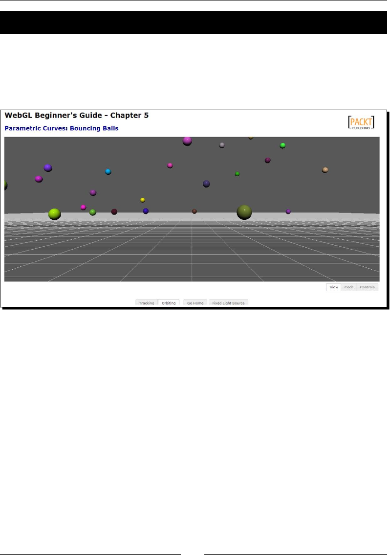
Acon

[ 164 ]

Time for action – bouncing ball

1. Open ch5_BouncingBalls.html in your HTML5-enabled Internet browser.

2. The orbing camera is acvated by default. Move the camera and you will see how

all the objects adjust to the global transform (camera) and yet they keep bouncing

according to its local transform (bouncing ball).

3. Let's explain here a lile bit more in detail how we keep track of each ball.

First of all let's dene some global variables and constants:

var ball = []; //Each element of this array is a ball

var BALL_GRAVITY = 9.8; //Earth acceleration 9.8 m/s2

var NUM_BALLS = 50; //Number of balls in this

simulation

Next, we need to inialize the ball array. We use a for loop in the load

funcon to achieve it:

for (var i=0;i<NUM_BALLS;i++){

ball.push(new BouncingBall());

Scene.loadObject('models/geometry/ball.

json','ball'+i);

}

Chapter 5

[ 165 ]

The BouncingBall funcon inializes the simulaon variables for

each ball in the ball array. One of this aributes is the posion,

which we select randomly. You can see how we do this by using

the generatePosition funcon.

Aer adding a new ball to the ball array, we add a new ball object

(geometry) to the Scene object. Please noce that the alias that we create

includes the current index of the ball object in the ball array. For example,

if we are adding the 32nd ball to the array, the alias that the corresponding

geometry will have in the Scene will be ball32.

The only other object that we add to the scene here is the Floor object.

We have used this object in previous exercises. You can nd the code for

the Floor object in /js/webgl/Floor.js.

4. Now let's talk about the draw funcon. Here, we go through the elements of the

Scene and retrieve each object's alias. If the alias starts with the word ball then

we know that the reminder of the alias corresponds to its index in the ball array.

We could have probably used an associave array here to make it look nicer but

it does not really change the goal. The main point here is to make sure that we

can associate the simulaon variables for each ball with the corresponding object

(geometry) in the Scene.

It is important to noce here that for each object (ball geometry) in the scene,

we extract the current posion and the color from the respecve BouncingBall

object in the ball array.

Also, we alter the current Model-View matrix for each ball using a matrix stack to

handle local transformaons, as previously described in this chapter. In our case, we

want the animaon for each ball to be independent from the camera transform and

from each other.

5. Up to this point, we have described how the bouncing balls are created (load) and

how they are rendered (draw). None of these funcons modify the current posion

of the balls. We do that using BouncingBall.update(). The code there uses the

animaon me (global variable named sceneTime) to calculate the posion for the

bouncing ball. As each BouncingBall has its own simulaon parameters, we can

calculate the posion for each given posion when a sceneTime is given. In short,

the ball posion is a funcon of me and as such, it falls into the category of moon

described by parametric curves.

6. The BouncingBall.update() method is called inside the animate funcon. As

we saw before, this funcon is invoked by the animaon mer each me the mer

is up. You can see inside this funcon how the simulaon variables are updated in

order to reect the current state of that ball in the simulaon.

Acon

[ 166 ]

What just happened?

We have seen how to handle several object local transformaons using the matrix stack

strategy while we keep global transformaon consistent through each rendering frame.

In the bouncing ball example, we have used an animaon mer for the animaon that is

independent from the rendering mer.

The bouncing ball update method shows how parametric curves work.

Optimization strategies

If you play a lile and increase the value of the global constant NUM_BALLS from 50 to 500,

you will start nocing degradaon in the frame rate at which the simulaon runs as shown in

the following screenshot:

Depending on your computer, the average me for the draw funcon can be higher than

the frequency at which the animaon mer callback is invoked. This will result in dropped

frames. We need to make the draw funcon faster. Let's see a couple of strategies to do this.

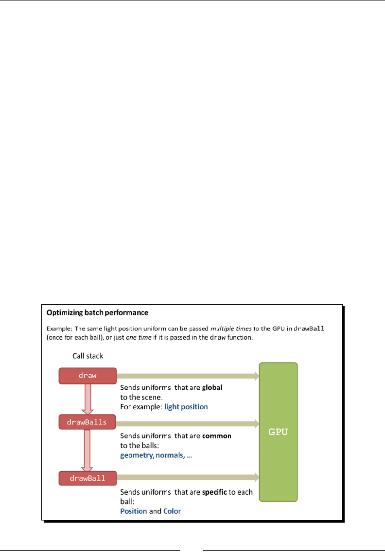
Chapter 5

[ 167 ]

Optimizing batch performance

We can use geometry caching as a way to opmize the animaon of a scene full of similar

objects. This is the case of the bouncing balls example. Each bouncing ball has a dierent

posion and color. These features are unique and independent for each ball. However, all

balls share the same geometry.

In the load funcon, for ch5_BouncingBalls.html we created 50 vertex buer objects

(VBOs) one for each ball. Addionally, the same geometry is loaded 50 mes, and on every

rendering loop (draw funcon) a dierent VBO is bound every me, despite of the fact that

the geometry is the same for all the balls!

In ch5_BouncingBalls_Optimized.html we modied the funcons load

and draw to handle geometry caching. In the rst place, the geometry is loaded just once

(load funcon):

Scene.loadObject('models/geometry/ball.json','ball');

Secondly, when the object with alias 'ball' is the current object in the rendering loop

(draw funcon), the delegate drawBalls funcon is invoked. This funcon sets some of

the uniforms that are common to all bouncing balls (so we do not waste me passing them

every me to the program for every ball). Aer that, the drawBall funcon is invoked. This

funcon will set up those elements that are unique for each ball. In our case, we set up the

program uniform that corresponds to the ball color, and the Model-View matrix, which is

unique for each ball too because of the local transformaon (ball posion).

Acon

[ 168 ]

Performing translations in the vertex shader

If you take a look at the code in ch5_BouncingBalls_Optimized.html, you may noce

that we have taken an extra step and that the Model-View matrix is cached!

The basic idea behind it is to transfer once the original matrix to the GPU (global) and then

perform the translaon for each ball (local) directly into the vertex shader. This change

improves performance considerably because of the parallel nature of the vertex shader.

This is what we do, step-by-step:

1. Create a new uniform that tells the vertex shader if it should perform a translaon

or not (uTranslate).

2. Create a new uniform that contains the ball posion for each ball (uTranslation).

3. Map these two new uniforms to JavaScript variables (we do this in the

configure funcon).

prg.uTranslation = gl.getUniformLocation(prg, "uTranslation");

gl.uniform3fv(prg.uTranslation, [0,0,0]);

prg.uTranslate = gl.getUniformLocation(prg, "uTranslate");

gl.uniform1i(prg.uTranslate, false);

4. Perform the translaon inside the vertex shader. This part is probably the trickiest as

it implies a lile bit of ESSL programming.

//translate vertex if there is a translation uniform

vec3 vecPosition = aVertexPosition;

if (uTranslate){

vecPosition += uTranslation;

}

//Transformed vertex position

vec4 vertex = uMVMatrix * vec4(vecPosition, 1.0);

In this code fragment we are dening vecPosition, a variable of vec3 type.

This vector is inialized to the vertex posion. If the uTranslate uniform is acve

(meaning we are trying to render a bouncing ball) then we update vecPosition

with the translaon. This is implemented using vector addion.

Aer this we need to make sure that the transformed vertex carries the translaon

in case of having one. So the next line looks like the following code:

//Transformed vertex position

vec4 vertex = MV * vec4(vecPosition, 1.0);

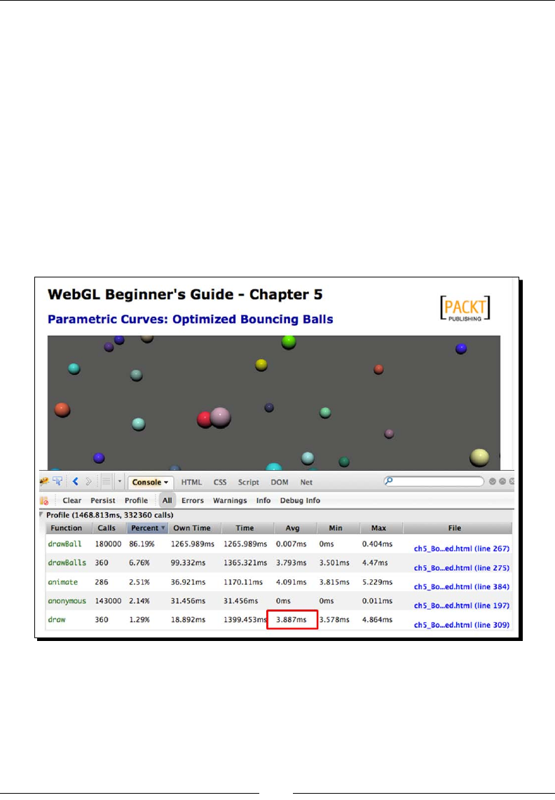
Chapter 5

[ 169 ]

5. In drawBall we pass the current ball posion as the content for the uniform

uTranslation:

gl.uniform3fv(prg.uTranslation, ball.position);

6. In drawBalls we set the uniform uTranslate to true:

gl.uniform1i(prg.uTranslate, true);

7. In draw we pass the Model-View matrix once for all balls by using the following line

of code:

transforms.setMatrixUniforms();

Aer making these changes we can increase the global variable NUM_BALLS from 50 to 300

and see how the applicaon keeps performing reasonably well regardless of the increased

scene complexity. The improvement in execuon mes is shown in the following screenshot:

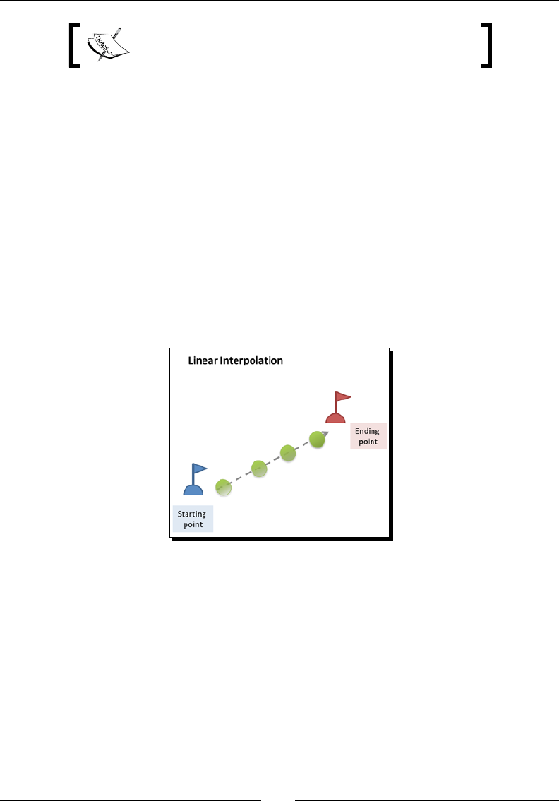
Acon

[ 170 ]

The opmized source code is available at: /code/ch5_

BouncingBalls_Optimized.html

Interpolation

Interpolaon greatly simplies 3D object's animaon. Unlike parametric curves, it is not

necessary to dene the posion of the object as a funcon of me. When interpolaon is

used, we only need to dene control points or knots. The set of control points describes

the path that the object that we want to animate will follow. There are many interpolaon

methods in the literature; however, it is always a good idea to start from the basics.

Linear interpolation

This method requires that we dene the starng and ending points for the locaon of

our object and also the number of interpolang steps. The object will move on the line

determined by the starng and ending points.

Polynomial interpolation

This method allows us to determine as many control points as we want. The object will move

from the starng point to the ending point and it will go through each one of the control

points in between.

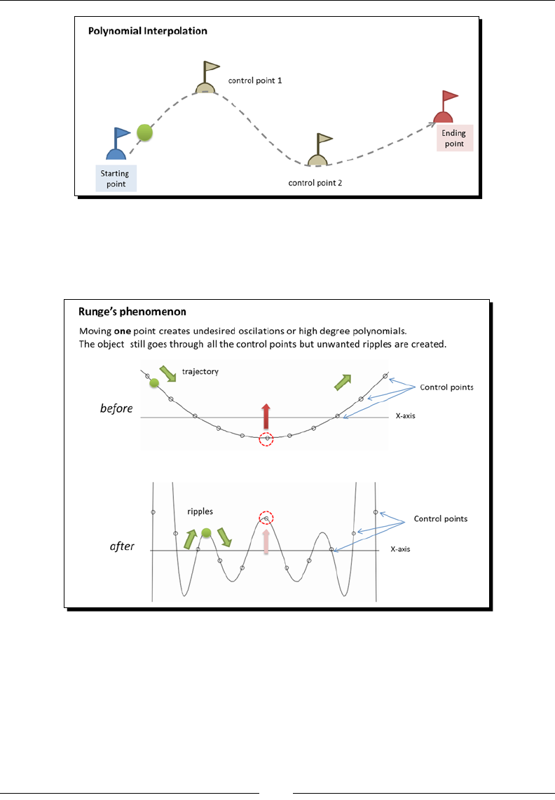
Chapter 5

[ 171 ]

When using polynomials, an increasing number of control points can produce undesired

oscillaons on the object's path described by this technique. This is known as the Runge's

phenomenon. In the following gure, you can see the result of moving one of the control

points of a polynomial described with 11 control points.

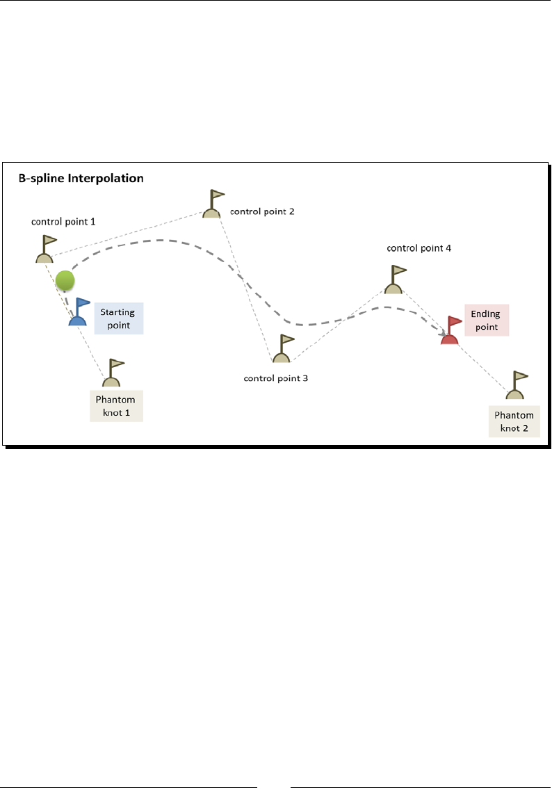
Acon

[ 172 ]

B-Splines

This method is similar to polynomial interpolaon with the dierence that the control points

are outside from the object's path. In other words, the object does not go through the

control points as it moves. This method is common in computer graphics in general because

the knots allow a much smoother path generaon than the polynomial equivalent at the

same me that fewer knots are required. B-Splines also respond beer to the

Runge's phenomenon.

In the following Time for acon secon we are going to see in pracce the three

dierent interpolaon techniques that have been introduced: linear, polynomial

and b-splines interpolaon.

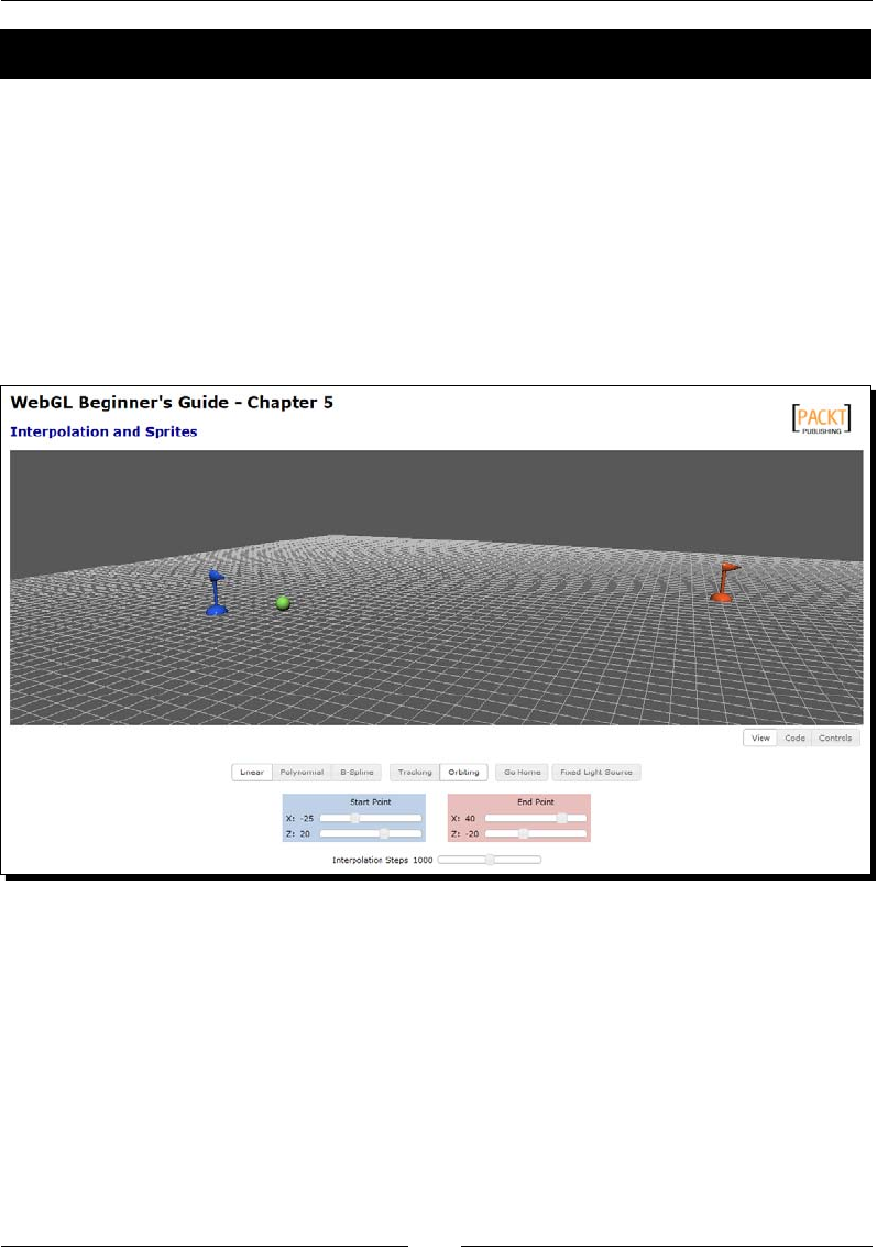
Chapter 5

[ 173 ]

Time for action – interpolation

1. Open ch5_Interpolation.html using your HTML5 Internet browser.

2. Select Linear interpolaon if it is not already selected.

3. Move the start and end points using the slider provided.

4. Change the number of interpolaon steps. What happens to the animaon when

you decrease the number of steps?

5. The code for the linear interpolaon has been implemented in the

doLinearInterpolation funcon.

6. Now select Polynomial interpolaon. In this example we have implemented

Lagrange's interpolaon method. You can see the source code in the

doLagrangeInterpolation funcon.

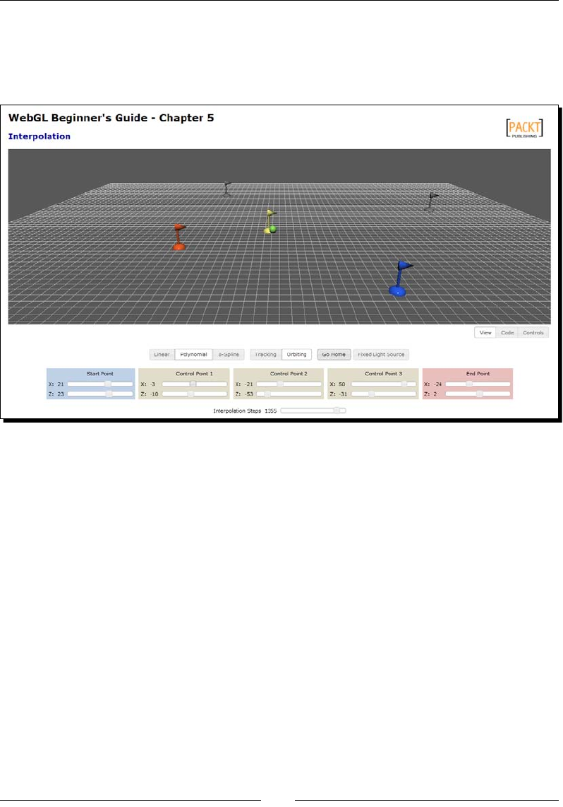
Acon

[ 174 ]

7. Aer selecng the polynomial interpolaon, you will see that three new control

points (ags) appear on screen. Using the sliders provided on the webpage, you

can change the locaon of these control points. You can also change the number

of interpolaon steps.

8. You also may have noced that whenever the ball approaches one of the ags

(with the excepon of the start and end points) the ag changes color. To do that,

we have wrien the ancillary close funcon. We use this funcon inside the

draw roune to determine the color of the ags. If the current posion of the ball,

determined by position[sceneTime] is close to one of the ag posions, the

respecve ag changes color. When the ball is far from the ag, the ag changes

back to its original color.

9. Modify the source code so each ag remains acvated, this is, with a new color aer

the ball passes by unl the animaon loops back to the beginning. This happens

when sceneTime is equal to ISTEPS (see the animate funcon).

10. Now select the B-Spline interpolaon. Noce how the ball does not reach any of the

intermediate ags in the inial conguraon. Is there any conguraon that you can

try so the ball passes through at least two of the ags?

Chapter 5

[ 175 ]

What just happened?

We have learned how to use interpolaon to describe the movement of an object in our

3D world. Also, we have created very simple scripts to detect object proximity and alter

our scene accordingly (changing ag colors in this example). Reacon to proximity is a key

element in game design!

Summary

In this chapter, we have covered the basic concepts behind object animaon in WebGL.

Specically we have learned about the dierence between local and global transformaons.

We have seen how matrix stacks allows us saving and retrieving the Model-View matrix and

how a stack allows us to implement local transformaon.

We learned to use JavaScript mers for animaon. The fact that an animaon mer is not

ed up to the rendering cycle gives a lot of exibility. Think a moment about it: the me in

the scene should be independent of how fast you can render it on your computer. We also

disnguished between animaon and simulaon strategies and learned what problems

they solve.

We discussed a couple of methods to opmize animaons through a praccal example

and we have seen what we need to do to implement these opmizaons in the code.

Finally, interpolaon methods and sprites were introduced and the Runge's phenomenon

was explained.

In the next chapter, we will play with colors in a WebGL scene. We will study the interacon

between the objects and light colors and we will see how to create translucent objects.

Colors, Depth Testing, and Alpha

Blending

In this chapter, we will go a lile bit deeper in the use of colors in WebGL. We

will start by examining how colors are structured and handled in both WebGL

and ESSL. Then we will discuss the use of colors in objects, lights and in the

scene. Aer this we will see how WebGL knows how perform object occlusion

when one object is in front of another. This is possible thanks to depth tesng.

In contrast, alpha blending will allows us to combine the colors of objects when

one is occluding the other. We will use alpha blending to create translucent

objects.

This chapter talks about:

Using colors in objects

Assigning colors to light sources

Working with several light sources in the ESSL program

The depth test and the z-buer

Blending funcons and equaons

Creang transparent objects with face culling

Colors, Depth Tesng, and Alpha Blending

[ 178 ]

Using colors in WebGL

WebGL includes a fourth aribute to the RGB model. This aribute is called the alpha

channel. The extended model then is known as the RGBA model, where A stands for alpha.

The alpha channel contains values in the range from 0.0 to 1.0, just like the other three

channels (red, green, and blue). The following diagram shows the RGBA color space. On the

horizontal axis you can see the dierent colors that can be obtained by combining the R, G,

and B channels. The vercal axis corresponds to the alpha channel.

The alpha channel carries extra informaon about the color. This informaon aects the way

the color is rendered on the screen. For instance, in most cases, the alpha value will refer to

the amount of opacity that the color contains. A completely opaque color will have an alpha

value of 1.0, whereas a completely transparent color will have an alpha value of 0.0. This is

the general case, but as we will see later on, there are some consideraons that we need to

take into account to obtain translucent colors.

We use colors everywhere in our WebGL 3D scenes:

Objects: 3D objects can be colored selecng one color for every pixel (fragment) of

the object, or by selecng the color that the object will have. This would usually be

the material diuse property.

Lights: Though we have been using white lights so far in the book, there is no reason

why we can't have lights whose ambient or diuse properes contain colors other

than white.

Chapter 6

[ 179 ]

Scene: The background of our scene has a color that we can change by calling

gl.clearColor. Also, as we will see later, there are special operaons on objects'

colors in the scene when we have translucent objects.

Use of color in objects

The nal color of pixel is assigned in the fragment shader by seng the ESSL special variable

gl_FragColor. If all the fragments in the object have the same color we can say that the

object has a constant color. Otherwise, the object has a per-vertex color.

Constant coloring

To obtain a constant color we store the desired color in a uniform that is passed to the

fragment shader. This uniform is usually called the object's diuse material property.

We can also combine object normals and light source informaon to obtain a Lambert

coecient. We can use the Lambert coecient to proporonally change the reecng

color depending on the angle on which the light hits the object.

As shown in the following diagram, we lose depth percepon when we do not use

informaon about the normals to obtain a Lambert coecient. Please noce that

we are using a diusive lighng model.

Usually constant coloring is indicated for objects that are going to become assets in

a 3D game.

Colors, Depth Tesng, and Alpha Blending

[ 180 ]

Per-vertex coloring

In medical and engineering visualizaon applicaons, it is common to nd color maps that

are associated to the verces of the models that we are rendering. These maps assign each

vertex a color depending on its scalar value. An example of this idea is the temperature

charts where we can see cold temperatures as blue and hot temperatures as red overlaid

on a map.

To implement per-vertex coloring, we need to dene an aribute that stores the color for the

vertex in the vertex shader:

attribute vec4 aVertexColor;

The next step is to assign the aVertexColor aribute to a varying so it can be carried into

the fragment shader. Remember that varyings are automacally interpolated. Therefore, each

fragment will have a color that is the weighted contribuon of the verces surrounding it.

If we want our color map to be sensive to lighng condions we can mulply each vertex

color by the diuse component of the light. The result is then assigned to the varying that

will transfer the result to the fragment shader as menoned before. The following diagram

shows two dierent possibilies for this case. On the le the vertex color is mulplied by

the diuse term of the light source without any weighng due to the light source relave

posion; on the right, the Lambert coecient generates the expected shadows giving

informaon about the relave locaon of the light source.

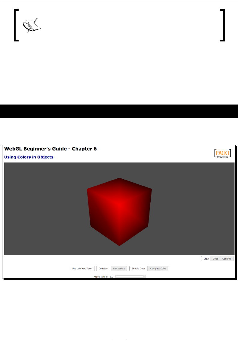
Chapter 6

[ 181 ]

Here we are using a Vertex Buffer object that is mapped to the

Vertex Shader aribute aVertexColor. We learned how to map

VBOs in the secon Associang Aributes to VBOs discussed in Chapter

2, Rendering Geometry.

Per-fragment coloring

We could also assign a random color to each pixel of the object we are rendering. However,

ESSL does not have a pre-built random funcon. Although there are algorithms that can be

used to generate pseudo-random numbers, the purpose and the usefulness of this technique

go beyond the scope of this book.

Time for action – coloring the cube

1. Open the le ch6_Cube.html using your HTML5 Internet browser. You will see a

page like the one shown in the following screenshot:

In this exercise, we are going to compare constant versus per-vertex coloring.

Let's talk about the page's widgets:

Use Lambert Coecient: When selected it will include the Lambert

coecient in the calculaon of the nal color.

Colors, Depth Tesng, and Alpha Blending

[ 182 ]

Constant/Per-Vertex: The two opons to color objects explained before.

Simple Cube: Corresponds to a JSON object where the verces are dened

once.

Complex Cube: Loads a JSON object where the verces are repeated with

the goal of obtaining mulple normals and mulple colors per vertex. We

will explain how this works later.

Alpha Value: This slider is mapped to the oat uniform uAlpha in the

vertex shader. uAlpha sets the alpha value for the vertex color.

2. Disable the use of the Lambert coecient by clicking on Use Lambert Coecient.

Rotate the cube clicking on it with the mouse and dragging it around. As you see,

there is loss of depth percepon when the Lambert coecient is not included in

the nal color calculaon. The Use Lambert Coecient buon is mapped to the

Boolean uniform uUseLambert. The code that calculates the Lambert coecient

can be found in the vertex shader included in the page:

float lambertTerm = 1.0;

if (uUseLambert){

//Transformed normal position

vec3 normal = vec3(uNMatrix * vec4(aVertexNormal, 1.0));

//light direction: pointing at the origin

vec3 lightDirection = normalize(-uLightPosition);

//weighting factor

lambertTerm = max(dot(normal,-lightDirection),0.20);

}

If the uniform uUseLambert is false, then lambertTerm keeps being 1.0 and then

it will not aect the nal diuse term which is calculated later on:

Id = uLightDiffuse * uMaterialDiffuse * lambertTerm;

Otherwise, Id will have the Lambert coecient factored in.

3. Having Use Lambert Coecient disabled, click on the buon Per Vertex. Rotate the

cube to see how ESSL interpolates the vertex colors. The vertex shader key code

fragment that allows us to switch from a constant diuse color to per- vertex colors

uses the Boolean uniform uUseVertexColors and the aVertexColor aribute.

This fragment is shown here:

if (uUseVertexColor){

Id = uLightDiffuse * aVertexColor * lambertTerm;

}

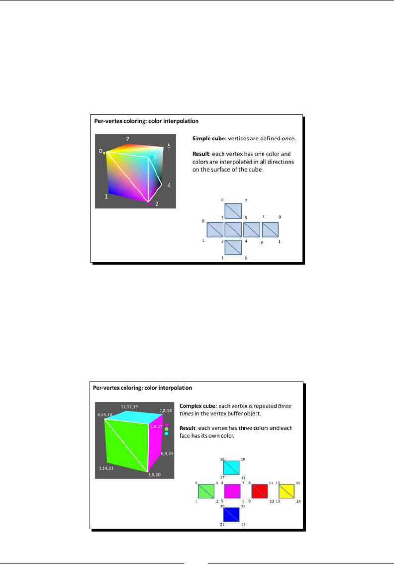
Chapter 6

[ 183 ]

else {

Id = uLightDiffuse * uMaterialDiffuse * lambertTerm;

}

Take a look at the le /models/simpleCube.js. There, the eight verces of the

cube are dened in the vertices array and there is an element in the scalars

array for every vertex. As you may expect, each one of these elements correspond

to the respecve vertex color, as shown in the following diagram:

4. Make sure that the Use Lambert Coecient buon is not acve and then click

on the buon Complex Cube. By repeang verces in the vertex array in the

corresponding JSON le /models/complexCube.js, we can achieve independent

face coloring. The following diagram explains how the verces are organized in

complexCube.js. Also note that as the denion of colors occurs by vertex

(as we are using the shader aribute), we need to repeat each color four mes,

because each face has four verces. This idea is depicted in the following diagram:

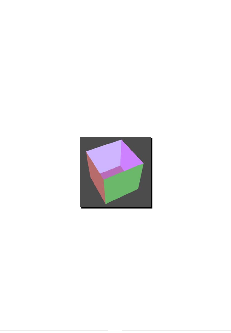
Colors, Depth Tesng, and Alpha Blending

[ 184 ]

5. Acvate the Use Lambert Coecient buon and see how the Lambert coecient

aects the color of the object. Try dierent buon conguraons and see

what happens.

6. Finally, let's quickly explore the eect of changing the alpha channel to a value less

than 1.0. For that, click-and-drag the slider to the le that appears at the boom

of the page. What do you see? Please noce that the object does not become

transparent but instead it starts losing its color. To obtain transparency, we need to

acvate blending. We will discuss blending in depth later in this chapter. For now,

uncomment these lines in the configure funcon, in the source code:

//gl.disable(gl.DEPTH_TEST);

//gl.enable(gl.BLEND);

//gl.blendFunc(gl.SRC_ALPHA, gl.ONE_MINUS_SRC_ALPHA);

7. Save the page and reload it in your Internet browser. If you select Per Vertex,

Complex Cube and reduce the alpha value to 0.25 you will see something like

the following screenshot:

What just happened?

We have studied two dierent ways for coloring objects: constant coloring and per-vertex

coloring. In both cases, the nal color for each fragment is assigned by using the fragment

shader gl_FragColor variable.

We also saw how, by acvang the calculaon of the Lambert coecient, we can obtain

sensory depth informaon.

By repeang verces in our object, we can obtain dierent coloring eects. For instance,

we can color an object by faces instead of doing it by verces.

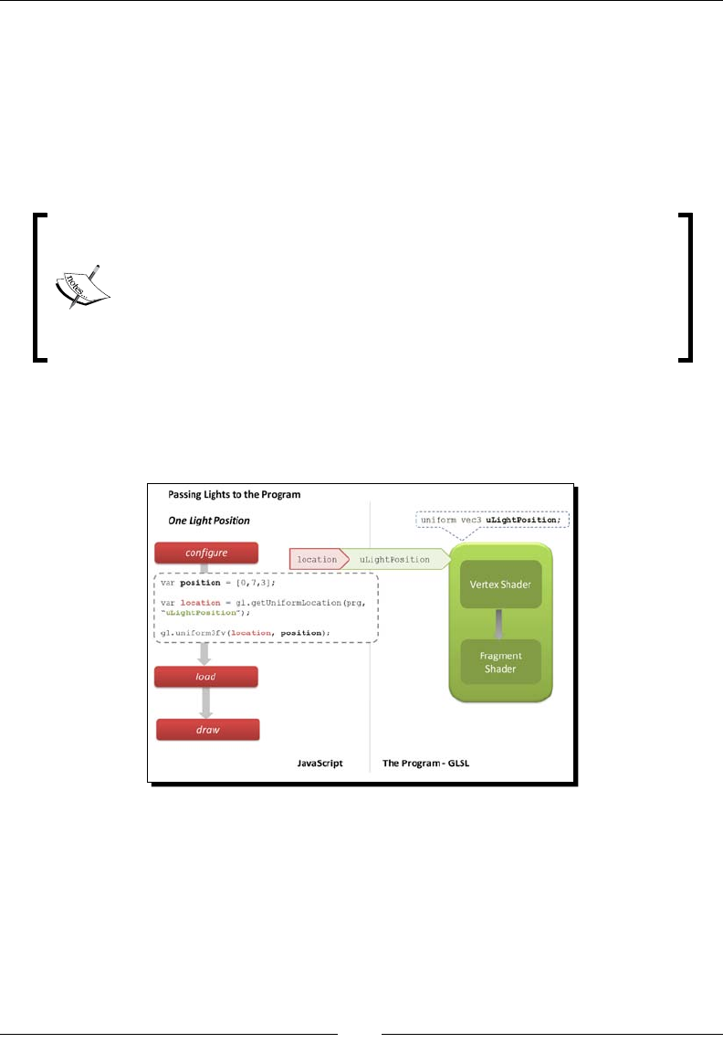
Chapter 6

[ 185 ]

Use of color in lights

Colors are light properes. In Chapter 3, Lights, we saw that the number of light properes

depend on the lighng reecon model selected for the scene. For instance, using a

Lamberan reecon model we would only need to model one shader uniform: the light

diuse property/color. In contrast, if the Phong reecon model were selected, each light

source would need to have three properes: the ambient, diuse, and specular colors.

The light posion is usually also modeled as a uniform when the shader

needs to know where the light source is. Therefore, a Phong model with a

posional light would have four uniforms: ambient, diuse, specular, and

posion.

For the case of direconal lights, the fourth uniform is the light direcon.

Refer to the More on Lights: posional lights secon discussed in Chapter

3, Lights!.

We have also seen that each light property is represented by a four-element array in

JavaScript and that these arrays are mapped to the vec4 uniforms in the shaders as

shown in the following diagram:

The two funcons we use to pass lights to the shaders are:

getUniformLocation—locates the uniform in the program and returns

an index we can use to set the value

uniform4fv—since the light components are RGBA, we need to pass

a four-element oat vector

Colors, Depth Tesng, and Alpha Blending

[ 186 ]

Using multiple lights and the scalability problem

As you could imagine, the number of uniforms grow rapidly when we want to use more than

one light source in our scene—for each one of them, we need to dene and map as many

uniforms as we need depending on the lighng model of choice. This approach makes the

programming eort simple enough—we have exactly one uniform for each light property

we want to have, for each light. However, let's think about this for a moment. If we have

four properes per light (ambient, diuse, specular, and locaon) this means that we have

to dene four uniforms per each light. If we want to have three lights, we will have to write,

use, and map 12 uniforms!

How many uniforms can we use?

The OpenGL Shading Language ES specicaon delineates the number of uniforms that we

are allowed to use. (Secon 4.3.4 - Uniforms):

There is an implementaon dependent limit on the amount of storage for uniforms

that can be used for each type of shader and if this is exceeded it will cause a

compile-me or link-me error.

In order to know what the limit is for your WebGL implementaon, you can query WebGL

using the gl.getParameter funcon with these constants:

gl.MAX_VERTEX_UNIFORM_VECTORS

gl.MAX_FRAGMENT_UNIFORM_VECTORS

The implementaon limit is given by your browser and it depends greatly on your

graphics hardware. For instance, my MacBook Pro running Firefox tells me that

I can use 1024 uniforms.

Now, the fact that we have enough variable space does not necessarily mean that the

problem is solved. We sll have to write and map each one of the uniforms and as we will

see later in exercise ch6_Wall_Initial.html, the shaders become a lot more verbose

doing this.

Simplifying the problem

In order to simplify the problem (and code less), we could assume, for instance, that the

ambient component is the same for all the lights. This allows reducing the number of

uniforms—one uniform less for each light. However, this is not a prey or an extensible

soluon for more general cases where we cannot assume that the ambient light is a constant.

Let's see how the shaders in a scene with mulple lights look like. First, let's address some

pending updates to our architecture.

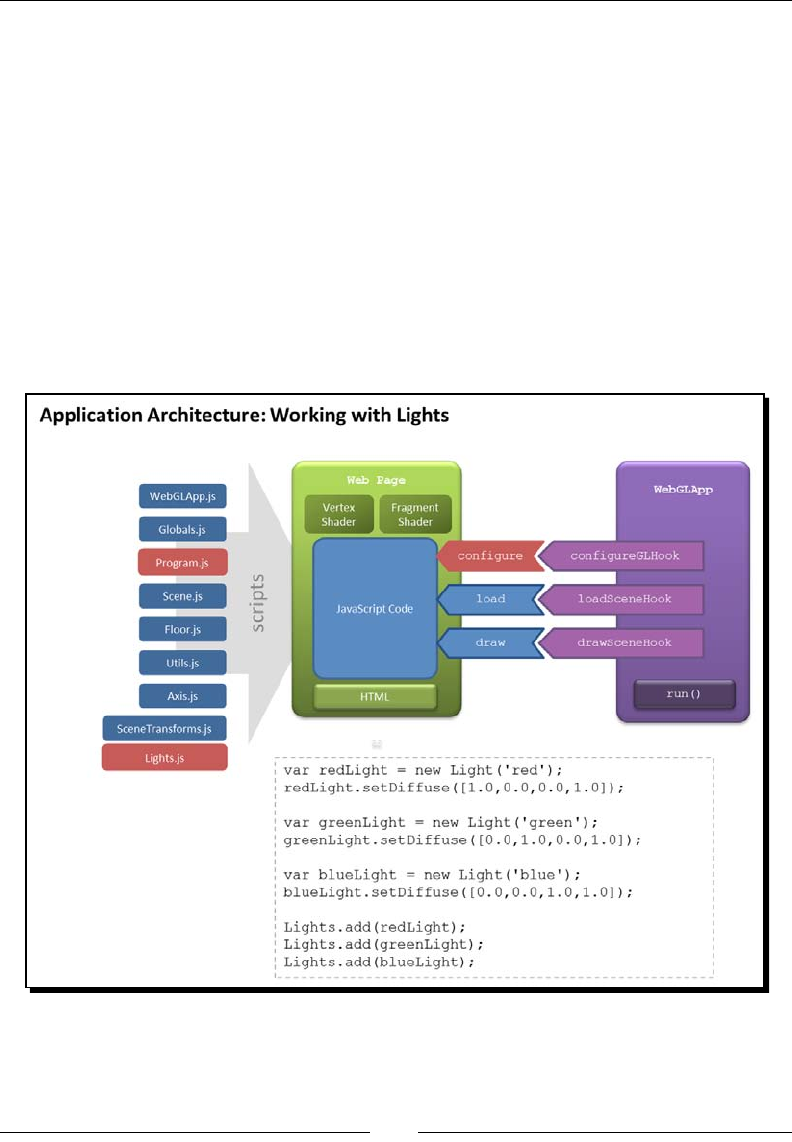
Chapter 6

[ 187 ]

Architectural updates

As we move from chapter to chapter and study dierent WebGL concepts, we should also

update our architecture to reect what we have learned. In this occasion as we are handling

a lot of uniforms, we will add support for mulple lights and will improve the way we pass

uniforms to the program.

Adding support for light objects

The following diagram shows the changes and addions that we have implemented in

the architecture of our exercises. We have updated Program.js to simplify how we

handle uniforms and we have included a new le: Ligths.js. Also, we have modied

the configure funcon to use the changes implemented in the Program object.

We will discuss these improvements next.

Colors, Depth Tesng, and Alpha Blending

[ 188 ]

We have created a new JavaScript module Lights.js that has two objects:

Light—aggregates lights properes (posion, diuse, specular, and so on) in one

single enty.

Lights—contain the lights in our scene. It allows us to retrieve each light by index

and by name.

Lights also contains the getArray method to aen the arrays of properes by type:

getArray: function(type){ //type = 'diffuse' or 'position' or ..

var a = [];

for(var i = 0, max = this.list.length; i < max; i+=1){

a = a.concat(this.list[i][type]); //list: the list of lights

}

return a;

}

This will be useful when we use uniform arrays later on.

Improving how we pass uniforms to the program

We have also improved the way we pass uniforms to the program. In WebGLApp.js we have

removed the call to Program.load().

function WebGLApp(canvas) {

this.loadSceneHook = undefined;

this.configureGLHook = undefined;

gl = Utils.getGLContext(canvas);

Program.load();

}

And we have deferred this call to the configure funcon in the web page. Remember that

WebGLApp will call three funcons in the web page: configure, load, and draw. These

three funcons dene the life cycle of our applicaon.

The configure funcon is the appropriate place to load the program. We are also going to

create a dynamic mapping between JavaScript variables and uniforms. With this in mind, we

have updated the Program.load method to receive two arrays:

attributeList—an array containing the names of the aributes that we will map

between JavaScript and ESSL

uniformList—an array containing the names of the uniforms that we will map

between JavaScript and ESSL

Chapter 6

[ 189 ]

The implementaon of the funcon now looks as follows:

load : function(attributeList, uniformList) {

var fragmentShader = Program.getShader(gl, "shader-fs");

var vertexShader = Program.getShader(gl, "shader-vs");

prg = gl.createProgram();

gl.attachShader(prg, vertexShader);

gl.attachShader(prg, fragmentShader);

gl.linkProgram(prg);

if (!gl.getProgramParameter(prg, gl.LINK_STATUS)) {

alert("Could not initialise shaders");

}

gl.useProgram(prg);

this.setAttributeLocations(attributeList);

this.setUniformLocations(uniformList);

}

The last two lines correspond to the two new funcons setAttributeLocations and

setUniformLocations:

setAttributeLocations: function (attrList){

for(var i=0, max = attrList.length; i <max; i+=1){

this[attrList[i]] = gl.getAttribLocation(prg, attrList[i]);

}

setUniformLocations: function (uniformList){

for(var i=0, max = uniformList.length; i < max; i +=1){

this[uniformList[i]] = gl.getUniformLocation(prg,

uniformList[i]);

}

As you can see, these funcons read the aribute and uniform lists, respecvely, and aer

obtaining the locaon for each element of the list, aach the locaon as a property of the

object Program.

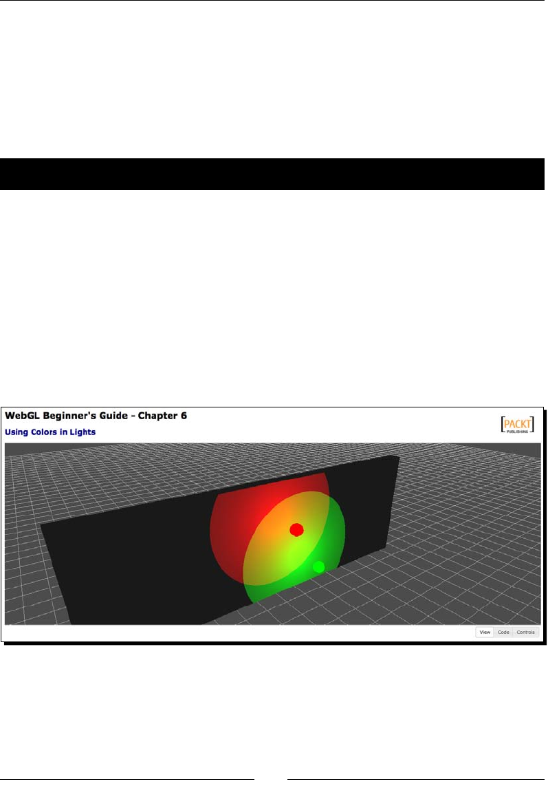
Colors, Depth Tesng, and Alpha Blending

[ 190 ]

This way, if we include the uniform name uLightPosition in the list uniformList that

we pass to Program.load, then we will have a property Program.uLightPosition that

will contain the locaon of the respecve uniform! Neat, isn't it?

Once we load the program in the configure funcon, we can also inialize the values of

the uniforms that we want right there by wring something as follows:

gl.uniform3fv(Program.uLightPosition, value);

Time for action – adding a blue light to a scene

Now we are ready to take a look at the rst example of this chapter. We will work on a scene

with per-fragment lighng that has three light sources.

Each light has a posion and a diuse color property. This means we have two uniforms

per light.

1. Also for simplicity, we have assumed here that the ambient color is the same for

the three light sources. For the sake of simplicity, we have removed the specular

property. Open the le ch6_Wall_Initial.html using your HTML5 web browser.

2. You will see a scene such as the one displayed in the following screenshot where

there are two lights (red and green) illuminang a black wall:

3. Open the le ch6_Wall_Initial.html using your preferred text editor. We will

update the vertex shader, the fragment shader, the JavaScript code, and the HTML

code to add the blue light.

Chapter 6

[ 191 ]

4. Updang the vertex shader: Go to the vertex shader. You can see these

two uniforms:

uniform vec3 uPositionRedLight;

uniform vec3 uPositionGreenLight;

Let's add the third uniform here:

uniform vec3 uPositionBlueLight;

5. We also need to dene a varying to carry the interpolated light ray direcon

to the fragment shader. Remember here that we are using per-fragment lighng.

Check where the varyings are dened:

varying vec3 vRedRay;

varying vec3 vGreenRay;

And add the third varying there:

varying vec3 vBlueRay;

6. Now let's take a look at the body of the vertex shader. We need to update each

one of the light locaons according to our posion in the scene. We achieve this

by wring:

vec4 bluePosition = uMVMatrix * vec4(uPositionBlueLight, 1.0);

As you can see there, the posions for the other two lights are being calculated too.

7. Now let's calculate the light ray for the updated posion from our blue light to the

current vertex. We do that by wring the following code:

vBlueRay = vertex.xyz-bluePosition.xyz;

That is all we need to modify in the vertex shader.

8. Updang the fragment shader: So far, we have included a new light posion and we

have calculated the light rays in the vertex shader. These rays will be interpolated by

the fragment shader.

Now let's work out how the colors on the wall will change by including our

new blue source of light. Scroll down to the fragment shader and let's add

a new uniform—the blue diuse property. Look for these uniforms declared

right before the main funcon:

uniform vec4 uDiffuseRedLight;

uniform vec4 uDiffuseGreenLight;

Then insert the following line of code:

uniform vec4 uDiffuseBlueLight;

Colors, Depth Tesng, and Alpha Blending

[ 192 ]

To calculate the contribuon of the blue light to the nal color we need to obtain

the light ray we dened previously in the vertex shader. So this varying is available in

the fragment shader, you need to also declare it before the main funcon. Look for:

varying vec3 vRedRay;

varying vec3 vGreenRay;

Then insert the following code right below:

varing vec3 vBlueRay;

9. It is assumed that the ambient component is the same for all the lights. This is

reected in the code by having only one uLightAmbient variable. The ambient

term Ia is obtained as the product of uLightAmbient and the wall's material

ambient property:

//Ambient Term

vec4 Ia = uLightAmbient * uMaterialAmbient;

If uLightAmbient is set to (1,1,1,1) and uMaterialAmbient is set to (

0.1,0.1,0.1,1.0) then the resulng ambient term Ia will be really small.

This means that the contribuon of the ambient light will be low in this scene.

In contrast, the diuse component will be dierent for every light.

Let's add the eect of the blue diuse term. In the fragment shader main funcon,

look for the following code:

//Diffuse Term

vec4 Id1 = vec4(0.0,0.0,0.0,1.0);

vec4 Id2 = vec4(0.0,0.0,0.0,1.0);

Then add the following line immediately below:

vec Id3 = vec4(0.0,0.0,0.0,1.0);

Then scroll down to:

//Lambert's cosine law

float lambertTermOne = dot(N,-normalize(vRedRay));

float lambertTermTwo = dot(N,-normalize(vGreenRay));

And add the following line of code right below:

float lambertTermThree = dot(N,-normalize(vBlueRay));

Now scroll to:

if(lambertTermTwo > uCutOff){

Id2 = uDiffuseGreenLight * uMaterialDiffuse * lambertTermTwo;

}

Chapter 6

[ 193 ]

And insert the following code aer it:

if(lambertTermThree > uCutOff){

Id3 = uDiffuseBlueLight * uMaterialDiffuse * lambertTermTwo;

}

Finally update finalColor so it includes Id3:

vec4 finalColor = Ia + Id1 + Id2 +Id3;

That's all we need to do in the fragment shader. Let's move on to our

JavaScript code.

10. Updang the congure funcon: Up to this point, we have wrien the code that

is needed to handle one more light inside our shaders. Let's see how we create the

blue light from the JavaScript side and how we map it to the shaders. Scroll down to

the configure funcon and look for the following code:

var green = new Light('green');

green.setPosition([2.5,3,3]);

green.setDiffuse([0.0,1.0,0.0,1.0]);

11. Then insert the following code:

var blue = new Light('blue');

blue.setPosition([-2.5,3,3]);

blue.setDiffuse([0.0,0.0,1.0,1.0]);

Next, Scroll down to:

Lights.add(red);

Lights.add(green);

Then add the blue light:

Lights.add(blue);

12. Scroll down to the point where the aribute list is dened. As menoned earlier

in this chapter, this new mechanism makes it easier to obtain locaons for the

uniforms. Add the two new uniforms that we are using for the blue light. The list

should look like the following code:

uniformList = [ "uPMatrix",

"uMVMatrix",

"uNMatrix",

"uMaterialDiffuse",

"uMaterialAmbient",

"uLightAmbient",

"uDiffuseRedLight",

"uDiffuseGreenLight",

Colors, Depth Tesng, and Alpha Blending

[ 194 ]

"uDiffuseBlueLight",

"uPositionRedLight",

"uPositionGreenLight",

"uPositionBlueLight",

"uWireframe",

"uLightSource",

"uCutOff"

];

13. Let's pass the posion and diuse values of our newly dened light to the program.

Aer the line that loads the program (what line is that?), insert the following code:

gl.uniform3fv(Program.uPositionBlueLight, blue.position);

gl.uniform4fv(Program.uDiffuseBlueLight, blue.diffuse);

That's all we need to do in the configure funcon.

Coding lights code using one uniform per light property makes the code

really verbose. Please bear with me; we will see later on in the exercise

ch6_Wall_LightArrays.html that the coding eorts are reduced by

using uniform arrays. If you are really eager, you can go now and check the

code in that exercise, and see how uniform arrays are used.

14. Updang the load funcon: Now let's update the load funcon. We need a new

sphere to represent the blue light, the same way we have two spheres in the scene:

one for the red light and the other for the green light. Append the following line:

Scene.loadObject('models/geometry/smallsph.json','light3');

15. Updang the draw funcon: As we saw in the load funcon, we are loading

the same geometry (sphere) three mes. In order to dierenate the sphere that

represents the light source we are using local transforms for the sphere (inially

centered at the origin).

Then add the following code:

if (object.alias == 'light2'){

mat4.translate(transforms.mvMatrix,gl.getUniform(prg,

Program.uPositionGreenLight));

object.diffuse = gl.getUniform(prg, Program.uDiffuseGreenLight);

gl.uniform1i(Program.uLightSource,true);

}

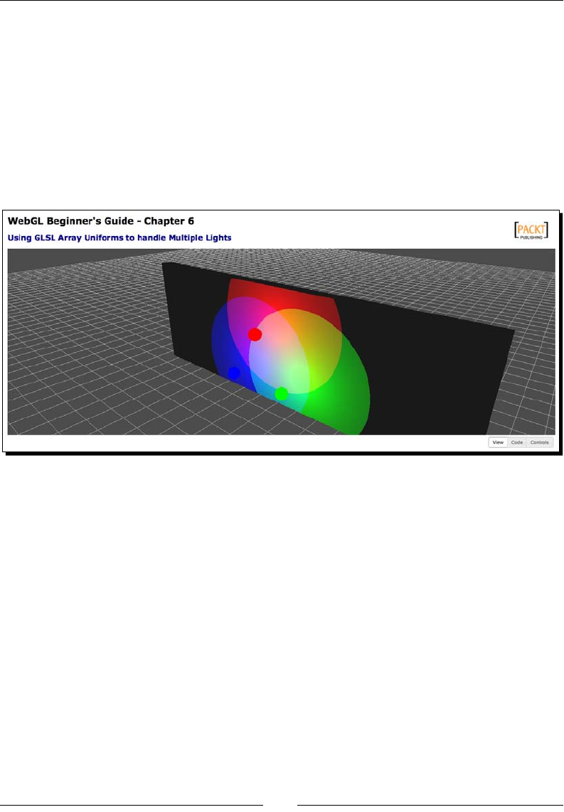
Chapter 6

[ 195 ]

Next, add the following code:

if (object.alias == 'light3'){

mat4.translate(transforms.mvMatrix,gl.getUniform(prg,

Program.uPositionBlueLight));

object.diffuse = gl.getUniform(prg, Program.uDiffuseBlueLight);

gl.uniform1i(Program.uLightSource,true);

}

16. That is it. Now, save the page with a dierent name and try it on your

HTML5 browser.

17. If you do not obtain the expected result, please go back and check the steps. You will

nd the completed exercise in the le ch6_Wall_Final.html.

What just happened?

We have modied our sample scene by adding one more light: a blue light. We have updated

the following:

The vertex shader

The fragment shader

The configure funcon

The load funcon

The draw funcon

Handling light properes one uniform at a me is not very ecient as you can see.

We will study a more eecve way to handle lights in a WebGL scene later in this chapter.

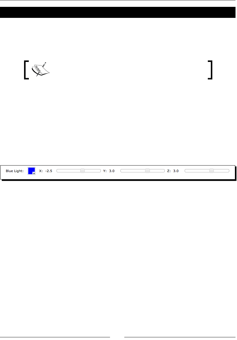
Colors, Depth Tesng, and Alpha Blending

[ 196 ]

Have a go hero – adding interactivity with JQuery UI

We are going to add some HTML and JQuery UI code to interacvely change the posion of

the blue light that we just added.

We will use three JQuery UI Sliders, one for each one of the blue light coordinates.

You can nd more informaon about JQuery UI widgets here:

http://jqueryui.com

1. Create three sliders: one for the x coordinate, one for the y coordinate, and a third

one for the z coordinate for the blue light. The funcon that you need to call on the

change and slide events for these sliders is updateLightPosition(3).

2. For this to work, you need to update the updateLightPosition funcon and add

the following case:

case 3: gl.uniform3fv(Program.uPositionBlueLight, [x,y,z]); break;

3. The nal GUI should include the new blue light sliders which should look as shown

in the following diagram:

4. Use the sliders present in the page to guide your work.

Using uniform arrays to handle multiple lights

As stated before, handling light properes with individual uniforms make the code verbose

and also dicult to maintain. Hopefully, ESSL provides several mechanisms that we can use

to solve the problem of handling mulple lights. One of them is uniform arrays.

This technique allows us to handle mulple lights by introducing light arrays in the shaders.

This way we calculate light contribuons by iterang through the light arrays in the shaders.

We sll need to dene each light in JavaScript but the mapping to ESSL becomes simpler as

we are not dening one uniform per light property. Let's see how this technique works.

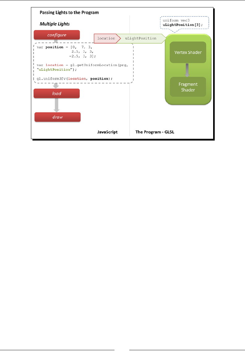
Chapter 6

[ 197 ]

We just need to do two simple changes in our code.

Uniform array declaration

First, we need to declare the light uniforms as arrays inside of our ESSL shaders. For instance,

for the light posion in a scene with three lights we would write something like:

uniform vec3 uPositionLight[3];

It is important to realize here that ESSL does not support dynamic inializaon of uniform

arrays. If you wrote something like:

uniform int uNumLights;

uniform vec3 uPositionLight[uNumLights]; //will not work

the shader will not compile and you will obtain an error as follows:

ERROR: 0:12: ":constant expression required

ERROR: 0:12: ":array size must be a constant integer expression"

However, this construct is valid:

const int uNumLights = 3;

uniform vec3 uPositionLight[uNumLights]; //will work

Colors, Depth Tesng, and Alpha Blending

[ 198 ]

We declare one uniform array per light property, regardless of how many lights we are going

to have. So, if we want to pass informaon about diuse and specular components of ve

lights, for example, we need to declare two uniform arrays as follows:

uniform vec4 uDiffuseLight[5];

uniform vec4 uSpecularLight[5];

JavaScript array mapping

Next, we will need to map the JavaScript variables where we have the light property

informaon to the program. For example, if we wanted to map these three light posions:

var LightPos1 = [0.0, 7.0, 3.0];

var LightPosition2 = [2.5, 3.0, 3.0];

var LightPosition3 = [-2.5, 3.0, 3.0];

Then, we need to retrieve the uniform array locaon (just like in any other case):

var location = gl.getUniformLocation(prg,"uPositionLight");

Here is the dierence, we map these posions as a concatenated at array:

gl.uniform3fv(location, [0.0,7.0,3.0,2.5,3.0,3.0,-2.5,3.0,3.0]);

There are two things you should noce here:

The name of the uniform is passed to getUniformLocation the same way it was

passed before. That is, the fact that uPositionLight is now an array does not

change a thing when you locate the uniform with getUniformLocation.

The JavaScript array that we are passing to the uniform is a at array. If you write

something as follows the mapping will not work:

gl.uniform3fv(location, [[0.0,7.0,3.0],[2.5,3.0,3.0],[-

2.5,3.0,3.0]]);

So, if you have one variable per light you should make sure to concatenate them

appropriately before passing them to the shader.

Time for action – adding a white light to a scene

1. Open the le ch6_Wall_LightArrays.html in your HTML5 browser. This scene

looks exactly as ch6_Wall_Final.html, however the code required to write this

scene is much less as we are using uniform arrays. Let's see how the use of uniform

arrays change our code.

Chapter 6

[ 199 ]

2. Let's update the vertex shader rst. Open the le ch6_Wall_LightArrays.html

using your favorite source code editor. Let's take a look at the vertex shader. Note

the use of the constant integer expression const int NUM_LIGHTS = 3; to

declare the number of lights that the shader will handle.

3. Also, you can see there that a uniform array is being used to operate on

light posions.

Note that we are using a varying array to pass the light rays (for each light) to the

fragment shader.

//Calculate light ray per each light

for(int i=0; i < NUM_LIGHTS; i++){

vec 4 lightPosition = uMVMatrix * vec4(uLightPosition[i], 1.0);

vLightRay[i] = vertex.xyz - lightPosition[i].xyz;

}

This fragment of code calculates one varying light ray per light. If you remember, the

same code in the le ch6_Wall_Final.html looks like the following code:

//Transformed light position

vec4 redPosition = uMVMatrix * vec4(uPositionRedLight,1.0);

vec4 greenPosition = uMVMatrix * vec4(uPositionGreenLight,1.0);

vec4 bluePosition = uMVMatrix * vec4(uPositionBlueLight, 1.0);

//Light position

vRedRay = vertex.xyz-redPosition.xyz;

vGreenRay = vertex.xyz-greenPosition.xyz;

vBlueRay = vertex.xyz-bluePosition.xyz;

At this point the advantage of using uniform arrays (and array varyings) to write

shading programs should start being evident.

4. Similarly, the fragment shader also uses uniform arrays. In this case, the fragment

shader iterates through the light diuse properes to calculate the contribuon of

each one to the nal color on the wall:

for(int i = 0; i < NUM_LIGHTS; i++){ //For each light

L = normalize(vLightRay[i]); //Calculate reflexion

lambertTerm = dot(N, -L);

if (lambertTerm > uCutOff){

finalColor += uLightDiffuse[i] * uMaterialDiffuse

*lambertTerm;

//Add diffuse component, one per light

}

Colors, Depth Tesng, and Alpha Blending

[ 200 ]

5. For the sake of brevity we will not see the corresponding verbose code from

the ch6_Wall_Final.html exercise.

6. In the configure funcon, the size of the JavaScript array that contains the

uniform names has decreased considerably because now we have just one

element per property regardless of the number of lights:

var uniformList = [

"uPMatrix",

"uMVMatrix",

"uNMatrix",

"uMaterialDiffuse",

"uMaterialAmbient",

"uLightAmbient",

"uLightDiffuse",

"uPositionLight",

"uWireframe",

"uLightSource",

"uCutOff"

];

7. Also, the mapping between JavaScript Light objects and uniform arrays is simpler

because of the getArray method of the Lights class. As we described in the

secon Architectural Updates, the getArray method concatenates in one at

array the property that we want for all the lights.

8. The load and draw funcons look exactly the same. If we wanted to add a new

light, we will sll need to load a new sphere in the load funcon (to represent

the light source in our scene) and we sll need to translate this sphere to the

appropriate locaon in the draw funcon.

9. Let's see how much eort we need to add a new light. Go to the configure

funcon and create a new light object like this:

var whiteLight = new Light('white');

whiteLight.setPosition([0,10,2]);

whiteLight.setDiffuse([1.0,1.0,1.0,1.0]);

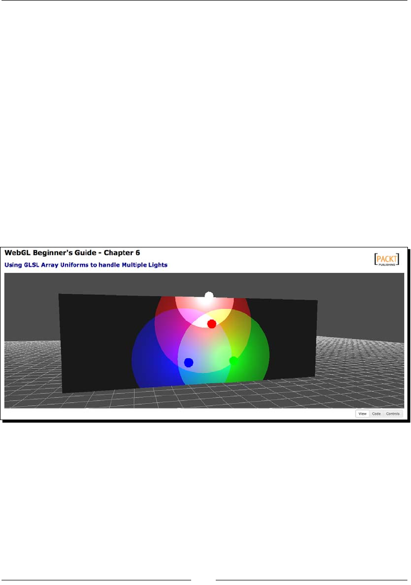
Chapter 6

[ 201 ]

10. Add whiteLight to the Lights object as follows:

Lights.add(whiteLight);

11. Now move to the load funcon and append this line:

Scene.loadObject('models/geometry/smallsph.json','light4');

12. And just like in the previous Time For Acon secon, add this to the draw funcon:

if (object.alias == 'light4'){

mat4.translate(transforms.mvMatrix,Lights.get('white').

position);

object.diffuse = Lights.get('white').diffuse;

gl.uniform1i(Program.uLightSource,true);

}

13. Save the webpage with a dierent name and open it using your HTML5 browser.

We have also included the completed exercise in ch6_Wall_LightArrays_

White.html. The following diagram shows the nal result:

That is all you need to do! Evidently, if you want to control the white light properes through

JQuery UI you would need to write the corresponding code, the same way we did it for the

previous hero secon. And talking about heroes.

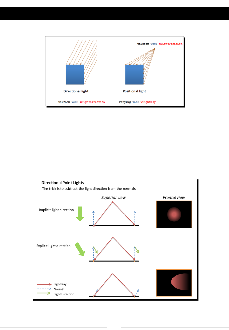
Colors, Depth Tesng, and Alpha Blending

[ 202 ]

Time for action – directional point lights

In Chapter 3, Lights!, we compared point and direconal lights:

In this secon, we will combine direconal and posional lights. We are going to

create a third type of light: a direconal point light. This light has both posion and

direcon properes. We are ready to do this as our shaders can easily handle lights

with mulple properes.

The trick to create these lights consist into subtract the light direcon vector from the

normal for each vertex. The resulng vector will originate a dierent Lambert coecient

that will reect into the cone generated by the light source.

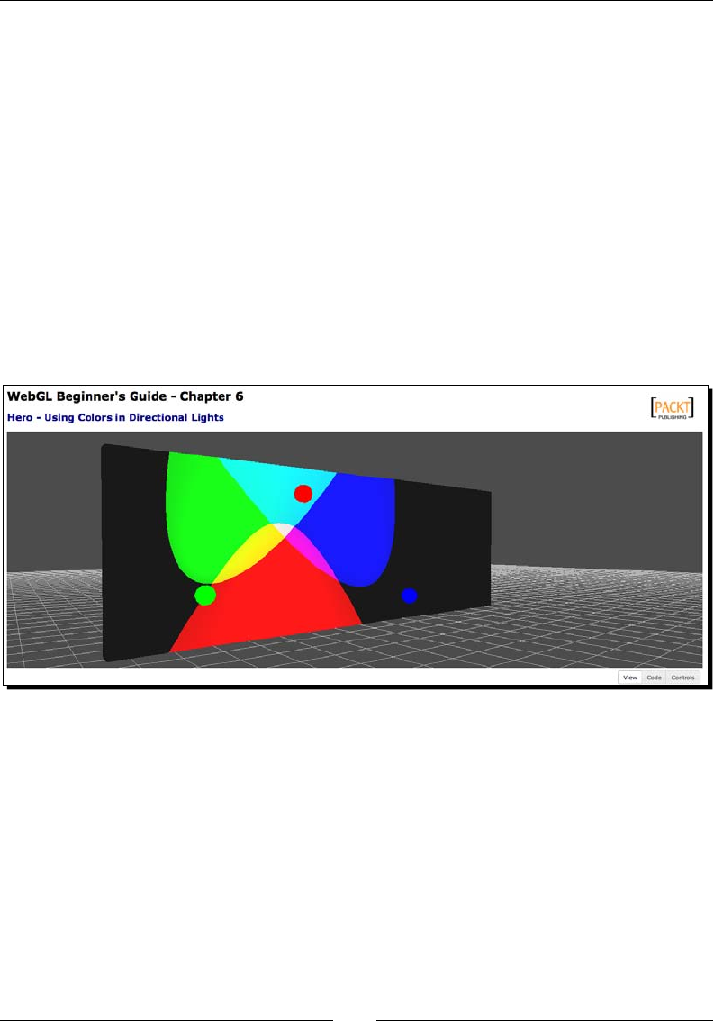
Chapter 6

[ 203 ]

1. Open ch6_Wall_Directional.html in your HTML5 Internet web browser.

As you can see there, the three light sources have now a direcon.

Let's take a look at the code.

2. Open ch6_Wall_Directional.html in your source code editor.

3. To create a light cone we need to obtain a Lambert coecient per fragment. Just

like in previous exercises, we obtain these coecients in the fragment shader by

calculang the dot product between the inverted light ray and the normal that has

been interpolated. So far, we have been using one varying to do this: vNormal.

4. Only one varying has suced so far, as we have not had to update the normals, no

maer how many lights we have in the scene. However to create direconal point

lights we do have to update the normals: the direcon of each light will create a

dierent normal. Therefore, we replace vNormal with a varying array:

varying vec3 vNormal[numLights];

5. The line that subtracts the light direcon from the normal occurs inside the for

loop. This is because we do this for every light in the scene, as every light has its

own light direcon:

//Calculate normals and light rays

for(int i = 0; i < numLights; i++){

vec4 positionLight = uMVMatrix * vec4(uLightPosition[i],1.0);

vec3 directionLight = vec3(uNMatrix * vec4(uLightDirection[i],

1.0));

vNormal[i] = normal - directionLight;

vLightRay[i] = vertex.xyz-positionLight.xyz;

}

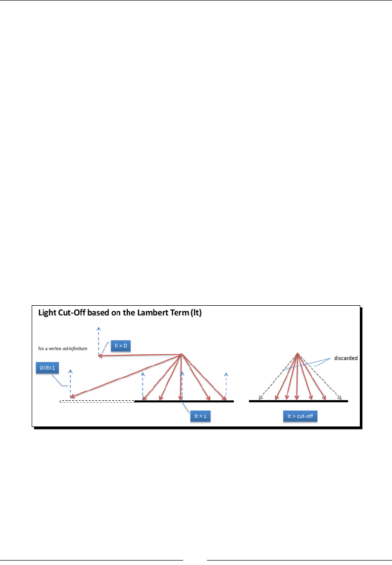
Colors, Depth Tesng, and Alpha Blending

[ 204 ]

Also, here the light direcon is transformed by the Normal matrix while the light

posion is transformed by the Model-View matrix.

6. In the fragment shader, we calculate the Lambert coecients: one per light

and per fragment. The key dierence is this line in the fragment shader:

N = normalize(vNormal[i]);

Here we obtain the interpolated updated normal per light.

7. Let's create a cut-o by restricng the allowed Lambert coecients. There are

at least two dierent ways to obtain a light cone in the fragment shader. The rst

one consists of restricng the Lambert coecient to be higher than the uniform

uCutOff (cut-o value). Let's us take a look at the fragment shader:

if (lambertTerm > uCutOff){

finalColor += uLightDiffuse[i] * uMaterialDiffuse

}

Remember that the Lambert coecient is the cosine of the angle between the

reected light and the surface normal. If the light ray is perpendicular to the surface

we obtain the highest Lambert coecient, and as we move away from the center,

the Lambert coecients changes following the cosine funcon unl the light rays

are completely parallel to the surface creang a cosine of 90 degrees between the

normal and the light ray. This produces a Lambert coecient of zero.

8. Open ch6_Wall_Directional.html in your HTML5 browser if you have not

done so yet. Use the cut-o slider on the page and noce how this aects the light

cone making it wider or narrower. Aer playing with the slider, you can noce that

these lights do not look very realisc. The reason is that the nal color is the same

no maer what Lambert coecient you obtained: as long as the Lambert coecient

is higher than the set cut-o value, you will obtain the full diuse contribuon from

the three light sources.

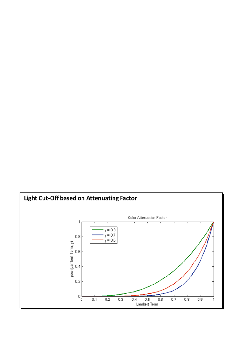
Chapter 6

[ 205 ]

9. To change it, open the web page using your source code editor, go to the fragment

shader and mulply the Lambert coecient in the line that calculates the nal color:

finalColor += uLightDiffuse[i] * uMaterialDiffuse * lambertTerm;

10. Save the web page with a dierent name (so you can keep the original) and then go

ahead and load it on your web browser. You will noce that the light colors appear

aenuated as you depart from the center of each light reecon on the wall. This

looks beer but there is an even beer way to create light cut-os.

11. Now let's create a cut-o by using an exponenal aenuaon factor. In the

fragment shader replace the following code:

if (lambertTerm > uCutOff){

finalColor += uLightDiffuse[i] * uMaterialDiffuse;

}

With:

finalColor += uLightDiffuse[i] * uMaterialDiffuse *

pow(lambertTerm, 10.0 * uCutOff);

Yes, we have goen rid of the if secon and we have only le its contents.

This me the aenuaon factor is pow(lambertTerm, 10*uCutOff).

This modicaon works because this factor aenuates the nal color exponenally.

If the Lambert coecient is close to zero, the nal color will be heavily aenuated.

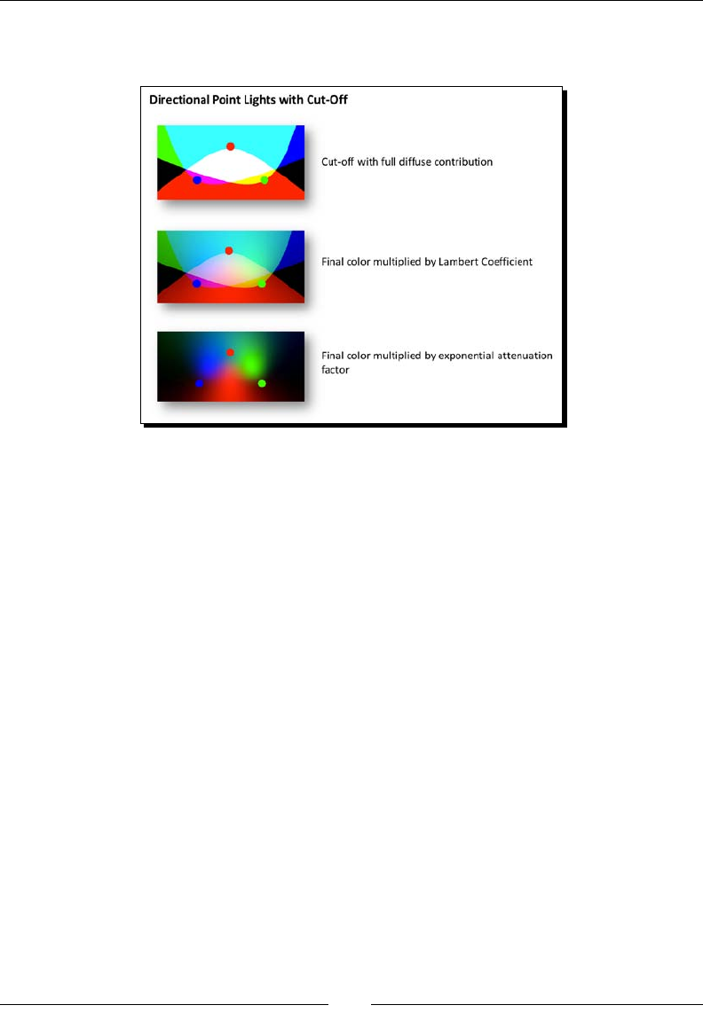
Colors, Depth Tesng, and Alpha Blending

[ 206 ]

12. Save the web page with a dierent name and load it in your browser.

The improvement is dramac!

We have included the completed exercises here:

Ch6_Wall_Directional_Proportional.html

Ch6_Wall_Directional_Exponential.html

What just happened?

We have learned how to implement direconal point lights. We have also discussed

aenuaon factors that improve lighng eects.

Use of color in the scene

It is me to discuss transparency and alpha blending. We menoned before that the alpha

channel can carry informaon about the opacity of the color with which the object is being

painted. However, as we saw in the cube example, it is not possible to obtain a translucent

object unless alpha blending is acvated. Things get a bit more complicated when we have

several objects in the scene. We will see here what to do in order to have a consistent scene

when we have translucent and opaque objects.

Chapter 6

[ 207 ]

Transparency

The rst approach to obtain transparent objects is to use polygon sppling. This technique

consists of discarding some fragments so you can see through the object. Think of it as

punching lile holes throughout the surface of your object.

OpenGL supports polygon sppling through the glPolygonStipple funcon. This funcon

is not available in WebGL. You could try to replicate this funconality by dropping some

fragments in the fragment shader using the ESSL discard command.

More commonly, we can use the alpha channel informaon to obtain translucent objects.

However, as we saw in the cube example, modifying the alpha values does not produce

transparency automacally.

Creang transparencies corresponds to alter the fragments that we have already wrien to

the frame buer. Think for instance of a scene where there is one translucent object in front

of an opaque object (from our camera view). For the scene to be rendered correctly we need

to be able to see the opaque object through the translucent object. Therefore, the fragments

that overlap between the far and the near objects need to be combined somehow to create

the transparency eect.

Similarly, when there is only one translucent object in the scene, the same idea applies.

The only dierence is that, in this case, the far fragments correspond to the back face of

the object and the near fragments correspond to the front face of the object. In this case,

to produce the transparency eect, the far and near fragments need to be combined.

To implement transparencies, we need to learn about two important WebGL concepts:

depth tesng and alpha blending.

Updated rendering pipeline

Depth tesng and alpha blending are two oponal stages for the fragments once they have

been processed by the fragment shader. If the depth test is not acvated, all the fragments

are automacally available for alpha blending. If the depth test is enabled, those fragments

that fail the test will be automacally discarded by the pipeline and will no longer be

available for any other operaon. This means that discarded fragments will not be

rendered. This behavior is similar to using the ESSL discard command.

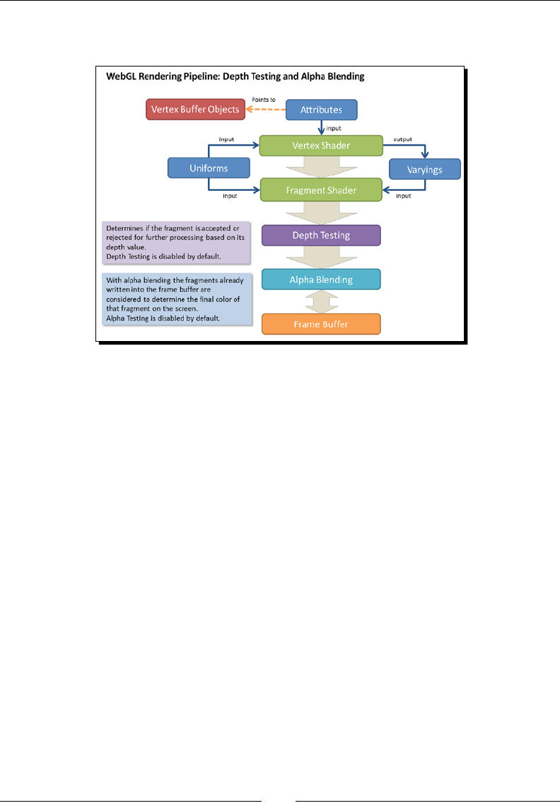
Colors, Depth Tesng, and Alpha Blending

[ 208 ]

The following diagram shows the order in which depth tesng and alpha blending

are performed:

Now let's see what depth tesng is about and why it is relevant for alpha blending.

Depth testing

Each fragment that has been processed by the fragment shader carries an associated

depth value. Though fragments are two-dimensional as they are going to be displayed on

the screen, the depth value keeps the informaon of how distant the fragment is from the

camera (screen). Depth values are stored in a special WebGL buer named depth buer or

z-buer. The z comes from the fact that x and y values correspond to the screen coordinates

of the fragment while the z value measures distance perpendicular to the screen.

Aer the fragment has been calculated by the fragment shader, it is eligible for depth tesng.

This only occurs if the depth test is enabled. Assuming that gl is the JavaScript variable that

contains our WebGL context, we can enable depth tesng by wring:

gl.enable(gl.DEPTH_TEST)

The depth test takes into consideraon the depth value of a fragment and it compares it to

the depth value for the same fragment coordinates already stored in the depth buer. The

depth test determines whether or not that fragment is accepted for further processing in the

rendering pipeline.

Only the fragments that pass the depth test will be processed. Otherwise, any fragment that

does not pass the depth test will be discarded.

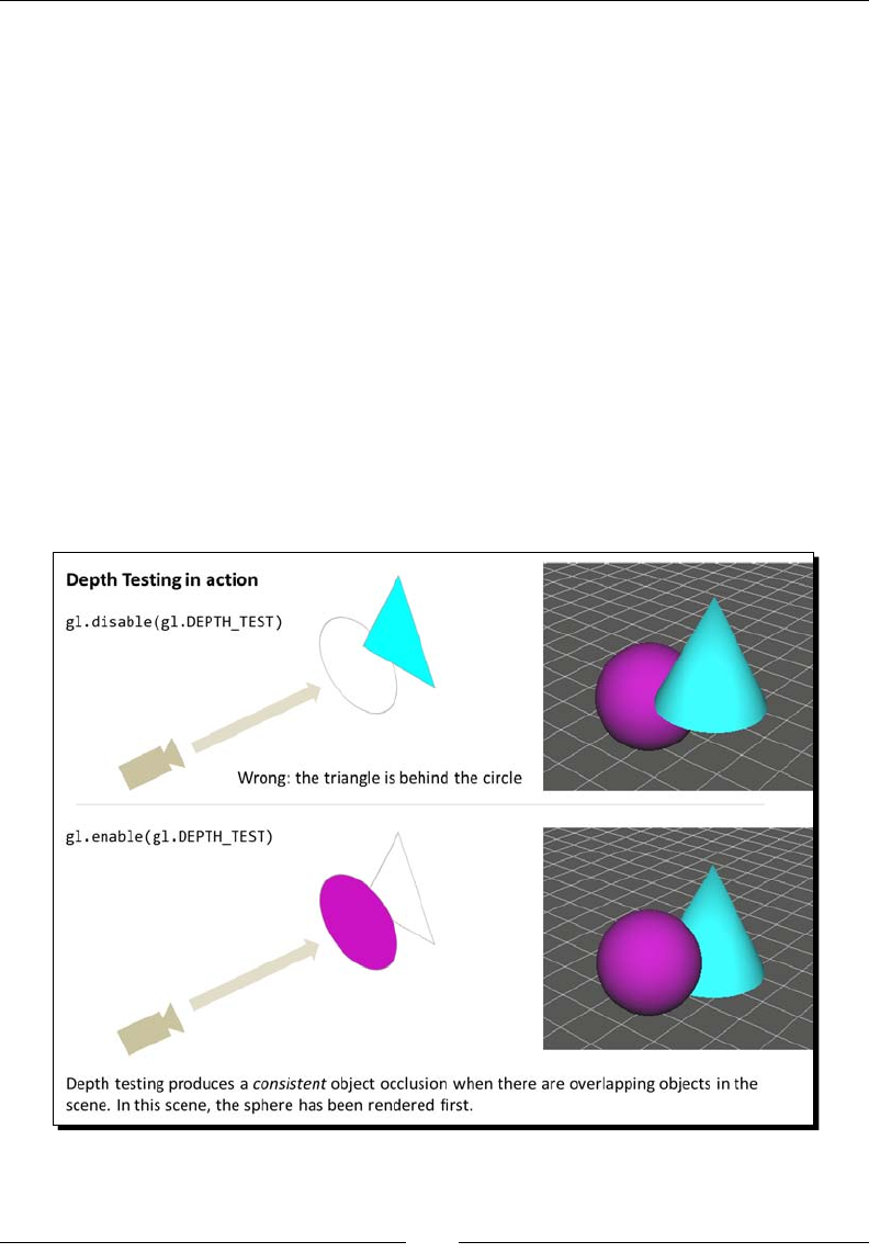
Chapter 6

[ 209 ]

In normal circumstances when the depth test is enabled, only those fragments with a lower

depth value than the corresponding fragments present in the depth buer will be accepted.

Depth tesng is a commutave operaon with respect to the rendering order. This means

that no maer which object gets rendered rst, as long as depth tesng is enabled, we will

always have a consistent scene.

Let's see this with an example. In the following diagram, there is a cone and a sphere.

The depth test is disabled using the following code:

gl.disable(gl.DEPTH_TEST)

The sphere is rendered rst. As it is expected, the cone fragments that overlap the cone

are not discarded when the cone is rendered. This occurs because there is no depth test

between the overlapping fragments.

Now let's enable the depth test and render the same scene. The sphere is rendered rst.

Since all the cone fragments that overlap the sphere have a higher depth value (they are

farer from the camera) these fragments fail the depth test and are discarded creang a

consistent scene.

Colors, Depth Tesng, and Alpha Blending

[ 210 ]

Depth function

In some applicaons, we could be interested in changing the default funcon of

the depth-tesng mechanism which discards fragments with a higher depth value

than those fragments in the depth buer. For that purpose WebGL provides the

gl.depthFunc(function) funcon.

This funcon has only one parameter, the function to use:

Parameter Descripon

gl.NEVER The depth test always fails

gl.LESS Only fragments with a depth lower than current fragments on the depth buer

will pass the test

gL.LEQUAL Fragments with a depth less than or equal to corresponding current fragments

in the depth buer will pass the test

gl.EQUAL Only fragments with the same depth as current fragments on the depth buer

will pass the test

gl.NOTEQUAL Only fragments that do not have the same depth value as fragments on the

depth buer will pass the test

gl.GEQUAL Fragments with greater or equal depth value will pass the test

gl.GREATER Only fragments with a greater depth value will pass the test

gl.ALWAYS The depth test always passes

The depth test is disabled by default in WebGL. When enabled, if no

depth funcon is set, the gl.LESS funcon is selected by default.

Alpha blending

A fragment is eligible for alpha blending if it has passed the depth test. However, when depth

tesng is disabled, all fragments are eligible for alpha blending.

Alpha blending is enabled using the following line of code:

gl.enable(gl.BLEND);

Chapter 6

[ 211 ]

For each eligible fragment the alpha blending operaon reads the color present in the

frame buer for those fragment coordinates and creates a new color that is the result

of a linear interpolaon between the color previously calculated in the fragment shader

(gl_FragColor) and the color already present in the frame buer.

Alpha blending is disabled by default in WebGL.

Blending function

With blending enabled, the next step is to dene a blending funcon. This funcon will

determine how the fragment colors coming from the object we are rendering (source)

will be combined with the fragment colors already present in the frame buer (desnaon).

We combine source and desnaon as follows:

Color Output = S * sW + D * dW

Here,

S: source color

D: desnaon color

sW: source scaling factor

dW: desnaon scaling factor

S.rgb: rgb components of the source color

S.a: alpha component of the source color

D.rgb: rgb components of the desnaon color

D.a: alpha component of the desnaon color

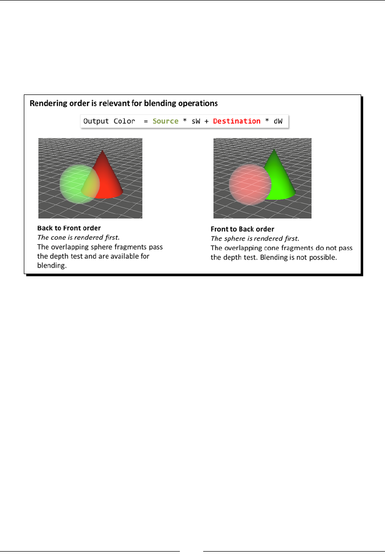
Colors, Depth Tesng, and Alpha Blending

[ 212 ]

It is very important to noce here that the rendering order will determine what the source

and the desnaon fragments are in the previous equaons. Following the example from the

previous secon, if the sphere is rendered rst, then it will become the desnaon of the

blending operaon because the sphere fragments will be already stored in the frame buer

when the cone is rendered. In other words, alpha blending is a non-commutave operaon

with respect to the rendering order.

Separate blending functions

It is also possible to determine how the RGB channels are going to be combined independently

from the alpha channels. For that, we use the gl.blendFuncSeparate funcon.

We dene two independent funcons this way:

Color output = S.rgb * sW.rgb + D.rgb * dW.rgb

Alpha output = S.a * sW.a + D.a * dW.a

Here,

sW.rgb: source scaling factor (only rgb)

dW.rgb: desnaon scaling factor (only rgb)

sW.a: source scaling factor for the source alpha value

dW.a: desnaon scaling factor for the desnaon alpha value

Then we could have something as follows:

Color output = S.rgb * S.a + D.rbg * (1 - S.a)

Alpha output = S.a * 1 + D.a * 0

Chapter 6

[ 213 ]

This would be translated into code as:

gl.blendFuncSeparate(gl.SRC_ALPHA, gl.ONE_MINUS_SRC_ALPHA, gl.ONE,

gl.ZERO)

This parcular conguraon is equivalent to our previous case where we did not separate

the funcons. The parameters for the gl.blendFuncSeparate funcon are the same as

that can be passed to gl.blendFunc. As stated before, you will nd the complete list later

in this secon.

Blend equation

We could have the case where we do not want to interpolate the source and desnaon

fragment colors by scaling them and adding them as shown before. It could be the

case where we want to subtract one from the other. In that case, WebGL provides

the gl.blendEquation funcon. This funcon receives one parameter that

determines the operaon on the scaled source and desnaon fragment colors.

gl.blendEquation(gl.FUNC_ADD) will correspond to:

Color output = S * sW + D *dW

While gl.blendEquation(gl.FUNC_SUBTRACT) corresponds to:

Color output = S * sW - D *dW

There is a third opon: gl.blendEquation(gl.FUNC_REVERSE_SUBTRACT)

that corresponds to:

Color output = D* dw – S*sW

As it is expected, it is also possible to dene the blending equaon separately for the RGB

channels and for the alpha channel. For that, we use the gl.blendEquationSeparate

funcon.

Blend color

WebGL provides the scaling factors gl.CONSTANT_COLOR and gl.ONE_MINUS_

CONSTANT_COLOR. These scaling factors can be used with gl.blendFunc and with

gl.blendFuncSeparate. However, we need to establish beforehand what the blend

color is going to be. We do so by invoking gl.blendColor.

Colors, Depth Tesng, and Alpha Blending

[ 214 ]

WebGL alpha blending API

The following table summarizes the WebGL funcons that are relevant to performing alpha

blending operaons:

WebGL Funcon Descripon

gl.enable|disable (gl.BLEND) Enable/disable blending

gl.blendFunc (sW, dW) Specify pixel arithmec. Accepted values for sW

and dW are:

ZERO

ONE

SRC_COLOR

DST_COLOR

SRC_ALPHA

DST_ALPHA

CONSTANT_COLOR

CONSTANT_ALPHA

ONE_MINUS_SRC_ALPHA

ONE_MINUS_DST_ALPHA

ONE_MINUS_SRC_COLOR

ONE_MINUS_DST_COLOR

ONE_MINUS_CONSTANT_COLOR

ONE_MINUS_CONSTANT_ALPHA

In addion, sW can also be SRC_ALPHA_

SATURATE

gl.blendFuncSeparate(sW_rgb, dW_

rgb, sW_a, dW_a) Specify pixel arithmec for RGB and alpha

components separately

Chapter 6

[ 215 ]

WebGL Funcon Descripon

gl.blendEquation(mode) Specify the equaon used for both the RGB

blend equaon and the alpha blend equaon.

Accepted values for mode are:

gl.FUNC_ADD

gl.FUNC_SUBTRACT

gl.FUNC_REVERSE_SUBTRACT

gl.blendEquationSeparate(modeRGB

, modeAlpha) Set the RGB blend equaon and the alpha blend

equaon separately

gl.blendColor ( red, green,

blue, alpha) Set the blend color

gl.getParameter(pname) Just like with other WebGL variables, it is

possible to query blending parameters using

gl.getParameter.

Relevant parameters are:

gl.BLEND

gl.BLEND_COLOR

gl.BLEND_DST_RGB

gl.BLEND_SRC_RGB

gl.BLEND_DST_ALPHA

gl.BLEND_SRC_ALPHA

gl.BLEND_EQUATION_RGB

gl.BLEND_EQUATION_ALPHA

Alpha blending modes

Depending on the parameter selecon for sW and dW we can create dierent blending modes.

In this secon we are going to see how to create addive, subtracve, mulplicave, and

interpolave blending modes. All blending modes depart from the already known formula:

Color output = S * (sW) + D * dW

Colors, Depth Tesng, and Alpha Blending

[ 216 ]

Additive blending

Addive blending simply adds the colors of the source and desnaon fragments, creang

a lighter image. We obtain addive blending by wring:

gl.blendFunc(gl.ONE, gl.ONE);

This assigns the weights for source and desnaon fragments sW and dW to 1. The color

output will be:

Color output = S * 1 + D * 1

Color output = S + D

Since each color channel is in the [0, 1] range, this blending will clamp all values over 1.

When all channels are 1 this results in a white color.

Subtractive blending

Similarly, we can obtain subtracve blending by wring:

gl.blendEquation(gl.FUNC_SUBTRACT);

gl.blendFunc(gl.ONE, gl.ONE);

This will change the blending equaon to:

Color output = S * (1) - D * (1)

Color output = S - D

Any negave values will be simply shown as zero. When all channels are negave this results

in black color.

Multiplicative blending

We obtain mulplicave blending by wring:

gl.blendFunc(gl.DST_COLOR, gl.ZERO);

This will be reected in the blending equaon as:

Color output = S * (D) + D * (0)

Color output = S * D

The result will be always a darker blending.

Interpolative blending

If we set sW to S.a and dW to 1-S.a then:

Color output = S * S.a + D *(1-S.a)

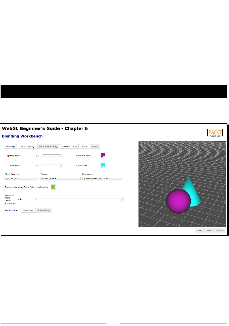
Chapter 6

[ 217 ]

This will create a linear interpolaon between the source and desnaon color using the

source alpha color S.a as the scaling factor. In code, this is translated as:

gl.blendFunc(gl.SRC_ALPHA, gl.ONE_MINUS_SRC_ALPHA);

Interpolave blending allows us to create a transparency eect as long as the desnaon

fragments have passed the depth test. This implies that the objects need to be rendered

from back to front.

In the next secon you will play with dierent blending modes on a simple scene constuted

by a cone and a sphere.

Time for action – blending workbench

1. Open the le ch6_Blending.html in your HTML5 Internet browser. You will see an

interface like the one shown in the following screenshot:

2. This interface has most of the parameters that allow you to congure alpha

blending. The sengs by default are source: gl.SRC_ALPHA and desnaon:

gl.ONE_MINUS_SRC_ALPHA. These are the parameters for interpolave

blending. Which slider do you need to use in order to change the scaling factor

for interpolave blending? Why?

3. Change the sphere alpha slider to 0.5. You will see some shadow-like arfacts on

the surface of the sphere. This occurs because the sphere back face is now visible.

To get rid of the back face click on Back Face Culling.

Colors, Depth Tesng, and Alpha Blending

[ 218 ]

4. Click on the Reset buon.

5. Disable the Lambert Term and Floor buons.

6. Enable the Back Face Culling buon.

7. Let's implement mulplicave blending. What values do source and desnaon

need to have?

8. Click-and-drag on the canvas. Check that the mulplicave blending create dark

regions where the objects overlap.

9. Change the blending funcon to gl.FUNC_SUBTRACT using the provided

drop-down menu.

10. Change Source to gl.ONE and Desnaon to gl.ONE.

11. What blending mode is this? Click-and-drag on the canvas to check the appearance

of the overlapped regions.

12. Go ahead and try dierent parameter conguraons. Remember you can also

change the blending funcon. If you decide to use a constant color or constant

alpha, please use the color widget and the respecve slider to modify the values

of these parameters.

What just happened?

You have seen how the addive, mulplicave, subtracve, and interpolave blending

modes work through a simple exercise.

You have seen that the combinaon gl.SRC_ALPHA and gl.ONE_MINUS_SRC_ALPHA

produces transparency.

Creating transparent objects

We have seen that in order to create transparencies we need to:

1. Enable alpha blending and select the interpolave blending funcon.

2. Render the objects back-to-front.

How do we create transparent objects when there is nothing to blend them against? In other

words, if there is only one object, how do we make it transparent?

One alternave to do this is to use face culling.

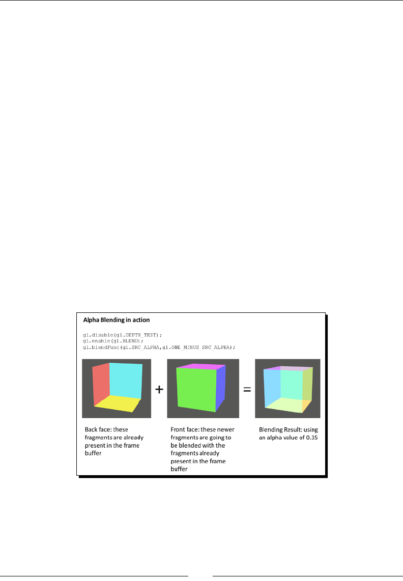
Chapter 6

[ 219 ]

Face culling allows rendering the back face or the front face of an object only. You saw this in

the previous Time For Acon secon when we only rendered the front face by enabling the

Back Face Culling buon.

Let's use the color cube that we used earlier in the chapter. We are going to make it

transparent. For that eect, we will:

1. Enable alpha blending and use the interpolave blending mode.

2. Enable face culling.

3. Render the back face (by culling the front face).

4. Render the front face (by culling the back face).

Similar to other opons in the pipeline, culling is disabled by default. We enable it by calling:

gl.enable(gl.FACE_CULLING);

To render only the back face of an object we call gl.cullFace(gl.FRONT) before we call

drawArrays or drawElements.

Similarly, to render only the front face, we use gl.cullFace(gl.BACK) before the

draw call.

The following diagram summarizes the steps to create a transparent object with alpha

blending and face culling.

In the following secon we see the transparent cube in acon and we will take a look at the

code that makes it possible.

Colors, Depth Tesng, and Alpha Blending

[ 220 ]

Time for action – culling

1. Open the ch6_Culling.html le using your HTML5 Internet browser.

2. You will see that the interface is similar to the blending workbench exercise.

However, on the top row you will see these three opons:

Alpha Blending: enables or disables alpha blending

Render Front Face: if acve, renders the front face

Render Back Face: if acve, renders the back face

Remember that for blending to work objects need to be rendered back-to-front.

Therefore, the back face of the cube is rendered rst.

This is reected in the draw funcon:

if(showBackFace){

gl.cullFace(gl.FRONT); //renders the back face

gl.drawElements(gl.TRIANGLES, object.indices.length,

gl.UNSIGNED_SHORT,0);

}

if (showFrontFace){

gl.cullFace(gl.BACK); //renders the front face

gl.drawElements(gl.TRIANGLES, object.indices.length,

gl.UNSIGNED_SHORT,0);

}

Going back to the web page, noce how the interpolave blending

funcon produces the expected transparency eect. Move the alpha value

slider that appears below the buon opons to adjust the scaling factor for

interpolave blending.

3. Review to the interpolave blending funcon. In this case, the desnaon is the

back face (rendered rst) and the source is the front face. If the alpha source = 1

what would you obtain according to the funcon? Go ahead and test the result by

moving the alpha slider to zero.

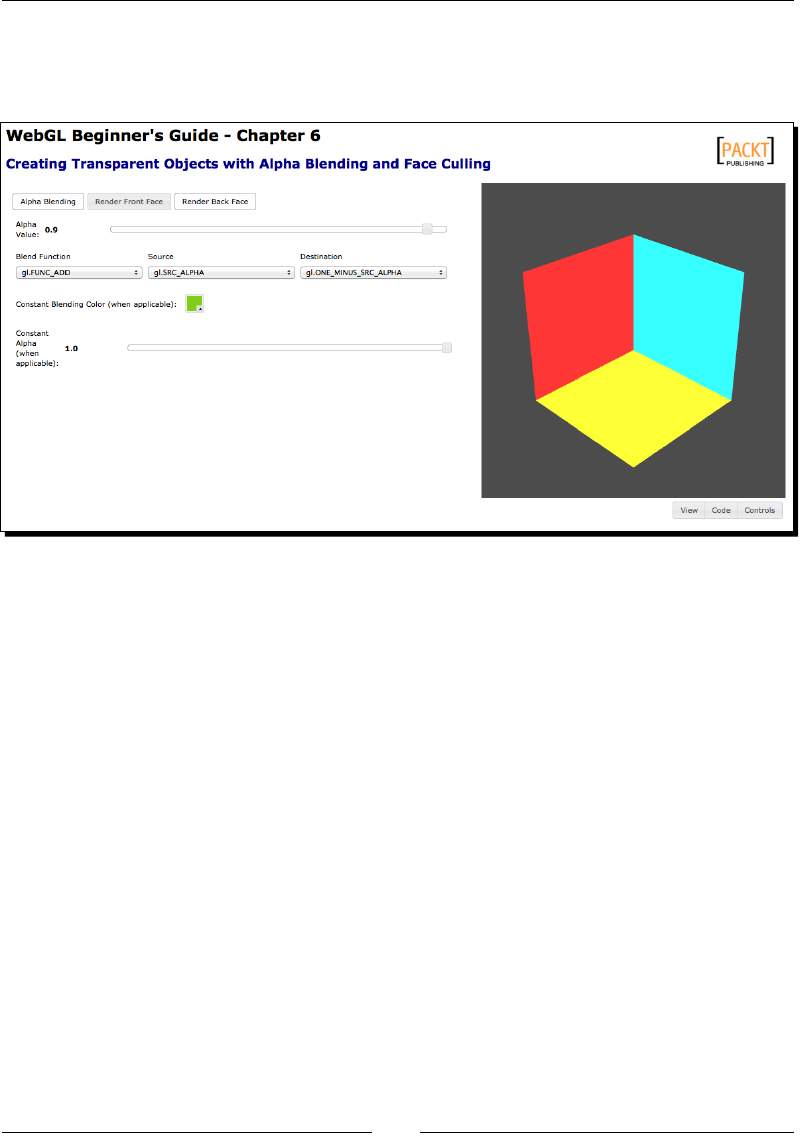
Chapter 6

[ 221 ]

4. Let's visualize the back face only. For that, disable the Render Front Face buon by

clicking on it. Increase the alpha value using the alpha value slider that appears right

below the buon opons. Your screen should look like this:

5. Click-and-drag the cube on the canvas. Noce how the back face is calculated every

me you move the camera around.

6. Click on the Render Front Face again to acvate it. Change the blending funcon so

you can obtain subtracve blending.

7. Try dierent blending conguraons using the controls provided in this exercise.

What just happened?

We have seen how to create transparent objects using alpha blending interpolave mode

and face culling.

Now let's see how to implement transparencies when there are two objects on the screen.

In this case we have a wall that we want to make transparent. Behind it there is a cone.

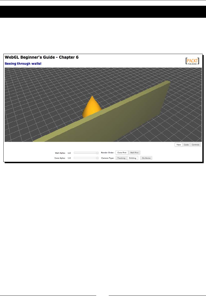
Colors, Depth Tesng, and Alpha Blending

[ 222 ]

Time for action – creating a transparent wall

1. Open ch6_Transparency_Initial.html in your HTML5 web browser.

We have two completely opaque objects: a cone behind a wall. Click-and-drag

on the canvas to move the camera behind the wall and see the cone as shown

in the following screenshot:

2. Change the wall alpha value by using the provided slider.

3. As you can see, modifying the alpha value does not produce any transparency. The

reason for this is that the alpha blending is not being enabled. Let's edit the source

code and include alpha blending. Open the le ch6_Transparency_Initial.

html using your preferred source code editor. Scroll to the configure funcon

and below these lines:

gl.enable(gl.DEPTH_TEST);

gl.depthFunc(gl.LEQUAL);

Add:

gl.enable(gl.BLEND);

gl.blendFunc(gl.SRC_ALPHA,gl.ONE_MINUS_SRC_ALPHA);

4. Save your changes as ch6_Transparency_Final.html and load this page on

your web browser.

5. As expected, the wall changes its transparency as you modify its alpha value using

the respecve slider.

Chapter 6

[ 223 ]

6. A note on rendering order: Remember that in order for transparency to be eecve

the objects need to be rendered back to front. Let's take a look at the source code.

Open ch6_Transparency_Final.html in your source code editor.

The cone is the farthest object in the scene. Hence, it is loaded rst. You can check

that by looking at the load funcon:

Scene.loadObject('models/geometry/cone.json','cone');

Scene.loadObject('models/geometry/wall.json','wall',{diffu

se:[0.5,0.5,0.2,1.0], ambient:[0.2,0.2,0.2,1.0]});

Therefore it occupies a lower index in the Scene.objects list. In the draw

funcon, the objects are rendered in the order in which they appear in the Scene.

objects list like this:

for (var i = 0, max=Scene.objects.length; i < max; i++){

var object = Scene.objects[i];

...

7. What happens if we rotate the scene so the cone is closer to the camera and the

wall is farer away? Open ch6_Transparency_Final.html and rotate the scene

such that the cone appears in front of the wall. Now decrease the alpha value of the

cone while the alpha value of the wall remains at 1.0.

8. As you can see, the blending is inconsistent. This does not have to do with alpha

blending because in ch6_Transparency_Final.html the blending is enabled

(you just enabled it on step 3). It has to do with the rendering order. Click on the

Wall First buon. The scene should appear consistent now.

The Cone First and Wall First buons use a couple of new funcons that we have

included in the Scene object to change the rendering order. These funcons are

renderSooner and renderFirst.

In total, we have added these funcons to the Scene object to deal with

rendering order:

renderSooner(objectName)—moves the object with name

objectName one posion before in the Scene.objects list.

renderLater(objectName)—moves the object with name objectName

one posion aer in the Scene.objects list.

renderFirst(objectName)—moves the object with name objectName

to the rst posion of the list (index 0).

renderLast(objectName)—moves the object with name objectName

to the last posion of the list.

Colors, Depth Tesng, and Alpha Blending

[ 224 ]

renderOrder()—lists the objects in the Scene.objects list in the order

in which they are rendered. This is the same order in which they are stored

in the list. For any two given objects, the object with the lower index will be

rendered rst.

You can use these funcons from the JavaScript console in your browser and see

what eect these have on the scene.

What just happened?

We have taken a simple scene where we have implemented alpha blending.

Aer that we have analyzed the importance of the rendering order in creang consistent

transparencies. Finally, we have presented the new methods of the Scene object that

control the rendering order.

Summary

In this chapter, we have seen how to use colors on objects, lights, and on the scene

in general. Specically, we have learned that an object can be colored per vertex,

per fragment, or it can have a constant color.

The color of light sources in the scene depends on implemented lighng model. Not all

lights need to be always white. We have also seen how uniform arrays simplify working with

mulple lights in ESSL and in JavaScript WebGL. Also we have created point direconal lights.

The alpha value does not necessarily make an object translucent. Interpolave blending is

necessary to create translucent objects. Also, the objects need to be rendered back-to-front.

Addionally, face culling can help to produce beer results when there are mulple

translucent objects present in the scene.

In Chapter 7, Textures, we will study how to paint images over our objects. For that we will

use WebGL textures.

Textures

So far, we've added details to our scene with geometry, vertex colors, and

lighng; but oen that won't be enough to achieve the look that we want.

Wouldn't it be great if we could "paint" addional details onto our scene

without needing addional geometry? We can, through a technique called

texture mapping. In this chapter, we'll examine how we can use textures to

make our scene more detailed.

In this chapter, we'll learn the following:

How to create a texture

How to use a texture when rendering

Filter and wrapping modes and how they aect the texture's use

Mul-texturing

Cube mapping

Let's get started!

Textures

[ 226 ]

What is texture mapping?

Texture mapping is, at its most basic, a method for adding detail to the geometry being

rendered by displaying an image on the surface. Consider the following image:

Using only the techniques that we've learned so far, this relavely simple scene would be

very dicult to build and unnecessarily complex. The WebGL logo would have to be carefully

constructed out of many lile triangles with appropriate colors. Certainly such an approach

is possible, but the addional geometry needed would make it quickly impraccal for use in

even a marginally complex scene.

Luckily for us, texture mapping makes the above scene incredibly simple. All that's required

is an image of the WebGL logo in an appropriate le format, an addional vertex aribute on

the mesh, and a few addions to our shader code.

Creating and uploading a texture

First o, for various reasons your browser will naturally load textures "upside down" from

how textures are tradionally used in desktop OpenGL. As a result, many WebGL applicaons

specify that the textures should be loaded with the Y coordinate ipped. This is done with a

single call from somewhere near the beginning of the code.

gl.pixelStorei(gl.UNPACK_FLIP_Y_WEBGL, true);

Whether or not you use this mode is up to you, but we will be using it throughout

this chapter.

The process of creang a texture is very similar to that of creang a vertex or an index buer.

We start by creang the texture object as follows:

var texture = gl.createTexture();

Textures, like buers, must be bound before we can manipulate it in any way.

gl.bindTexture(gl.TEXTURE_2D, texture);

Chapter 7

[ 227 ]

The rst parameter indicates the type of texture we're binding, or the texture target.

For now, we'll focus on 2D textures, indicated with gl.TEXTURE_2D in the previous

code snippet. More targets will be introduced in the Cube maps secon.

Once we have bound the texture, we can provide it with image data. The simplest way

to do that is to pass a DOM image into the texImage2D funcon as shown in the following

code snippet:

var image = document.getElementById("textureImage");

gl.texImage2D(gl.TEXTURE_2D, 0, gl.RGBA, gl.RGBA, gl.UNSIGNED_BYTE,

image);

You can see in this example that we have selected an image element from our page with the

ID of "textureImage" to act as the source for our texture. This is known as Uploading the

texture, since the image will be stored for fast access during rendering, oen in the GPU's

video memory. The source can be in any image format that can be displayed on a web page,

such as JPEG, PNG, GIF, or BMP les.

The image source for the texture is passed in as the last parameter of the texImage2D

call. When texImage2D is called with an image in this way, WebGL will automacally

determine the dimensions of the texture from the image you provide. The rest of the

parameters instruct WebGL about the type of informaon the image contains and how to

store it. Most of the me, the only value you will need to worry about changing is the third

and fourth parameter, which can also be gl.RGB to indicate that your texture has no alpha

(transparency) channel.

In addion to the image, we also need to instruct WebGL how to lter the texture when

rendering. We'll get into what ltering means and what the dierent ltering modes do

in a bit. In the meanme let's use the simplest one to get us started:

gl.texParameteri(gl.TEXTURE_2D, gl.TEXTURE_MAG_FILTER, gl.NEAREST);

gl.texParameteri(gl.TEXTURE_2D, gl.TEXTURE_MIN_FILTER, gl.NEAREST);

Finally, just as with buers, it's a good pracce to unbind a texture when you are nished

using it, which is accomplished by binding null as the acve texture:

gl.bindTexture(gl.TEXTURE_2D, null);

Of course, in many cases you won't want to have all of the textures for your scene embedded

on your web page, so it's oen more convenient to create the image element on the y and

have it dynamically load the image needed. Pung all of this together gives us a simple

funcon that will load any image URL that we provide as a texture.

var texture = gl.createTexture();

var image = new Image();

image.onload = function(){

gl.bindTexture(gl.TEXTURE_2D, texture);

Textures

[ 228 ]

gl.texImage2D(gl.TEXTURE_2D, 0, gl.RGBA, gl.RGBA, gl.UNSIGNED_

BYTE, image);

gl.texParameteri(gl.TEXTURE_2D, gl.TEXTURE_MAG_FILTER,

gl.NEAREST);

gl.texParameteri(gl.TEXTURE_2D, gl.TEXTURE_MIN_FILTER,

gl.NEAREST);

gl.bindTexture(gl.TEXTURE_2D, null);

}

image.src = "textureFile.png";

There is a slight 'gotcha' when loading images in this way. The image loading

is asynchronous, which means that your program won't stop and wait for the

image to nish loading before connuing execuon. So what happens if you

try to use a texture before it's been populated with image data? Your scene

will sll render, but any texture values you sample will be black.

In summary, creang textures follows the same paern as using buers. For every texture

we create, we want to do the following:

Create a new texture

Bind it to make it the current texture

Pass the texture contents, typically from an image

Set the lter mode or other texture parameters

Unbind the texture

If we reach a point where we no longer need a texture, we can remove it and free up the

associated memory using deleteTexture:

gl.deleteTexture(texture);

Aer this the texture is no longer valid. Aempts to use it will react as though null has

been passed.

Using texture coordinates

So now that we have our texture ready to go, we need to apply it to our mesh somehow.

The most basic queson that arises then is what part of the texture to show on which part

of the mesh. We do this through another vertex aribute named texture coordinates.

Chapter 7

[ 229 ]

Texture coordinates are two-element oat vectors that describe a locaon on the texture that

coincides with that vertex. You might think that it would be most natural to have this vector

be an actual pixel locaon on the image, but instead, WebGL forces all the texture coordinates

into a 0 to 1 range, where [0, 0] represents the top le-hand side corner of the texture and

[1, 1] represents the boom right-hand side corner, as is shown in the following image:

This means that to map a vertex to the center of any texture, you would give it a texture

coordinate of [0.5, 0.5]. This coordinate system holds true even for rectangular textures.

At rst this may seem strange. Aer all, it's easier to determine what the pixel coordinates

of a parcular point are than what percentage of an image's height and width that point is

at, but there is a benet to the coordinate system that WebGL uses.

Let's say you create a WebGL applicaon with some very high resoluon textures. At some

point aer releasing your applicaon, you get feedback from users saying that the textures

are taking too long to load, or that the large textures are causing their device to render

slowly. As a result, you decide to oer a lower resoluon texture opon for these users.

If your texture coordinates were dened in terms of pixels, you would now have to

modify every mesh used by your applicaon to ensure that the texture coordinates match

up to the new, smaller textures correctly. However, when using WebGL's 0 to 1 coordinate

range, the smaller textures can use the exact same coordinates as the larger ones and sll

display correctly!

Figuring out what the texture coordinates for your mesh should be, especially if the mesh is

complex, can be one of the trickier parts of creang 3D resources, but fortunately most 3D

modeling tools come with excellent ulies for laying out texture coordinates. This process

is called Unwrapping.

Textures

[ 230 ]

Just like the vertex posion components are commonly represented with

the characters X, Y, and Z, texture coordinates also have a common symbolic

representaon. Unfortunately, it's not consistent across all 3D soware

applicaons. OpenGL (and therefore WebGL) refers to the coordinates as S and

T for the X and Y components respecvely. However, DirectX and many popular

modeling packages refer to them as U and V. As a result, you'll oen see people

referring to texture coordinates as "UVs" and Unwrapping as "UV Mapping".

We will use ST for the remainder of the book to be consistent with WebGL's usage.

Using textures in a shader

Texture coordinates are exposed to the shader code in the same way that we have any other

vertex aribute; no surprises here. We'll want to include a two-element vector aribute in

our vertex shader that will map to our texture coordinates:

attribute vec2 aVertexTextureCoords;

Addionally, we will also want to add a new uniform to the fragment shader that uses a type

we haven't seen before: sampler2D. The sampler2D uniform is what allows us to access

the texture data in the shader.

uniform sampler2D uSampler;

In the past, when we've used uniforms, we have always set them to the value that we want

them to be in the shader, such as a light color. Samplers work a lile dierently, however.

The following shows how to associate a texture with a specic sampler uniform:

gl.activeTexture(gl.TEXTURE0);

gl.bindTexture(gl.TEXTURE_2D, texture);

gl.uniform1i(Program.uSampler, 0);

So what's going on here? First o, we are changing the acve texture index with

gl.activeTexture. WebGL supports using mulple textures at once (which we'll talk

about later on in this chapter), so it's a good pracce to specify which texture index we're

working with, even though it won't change for the duraon of this program. Next, we bind

the texture we wish to use, which associates it with the currently acve texture TEXTURE0.

Finally, we tell the sampler uniform which texture it should be associated with, not with the

texture itself, but with the texture unit provided via gl.uniform1i. Here we give it 0 to

indicate that the sampler should use TEXTURE0.

That's quite a bit of setup, but now we are nally ready to use our texture in the fragment

shader! The simplest way to use a texture is to return its value as the fragment color as

shown here:

gl_FragColor = texture2D(uSampler, vTextureCoord);

Chapter 7

[ 231 ]

texture2D takes in the sampler uniform we wish to query and the coordinates to lookup,

and returns the color of the texture image at those coordinates as a vec4. Even if the image

has no alpha channel, a vec4 will sll be returned with the alpha component always set to 1.

Time for action – texturing the cube

Open the le ch7_Textured_Cube.html in your favorite HTML editor. This contains the

simple lit cube example from the previous chapter. If you open it in an HTML5 browser, you

should see a scene that looks like the following screenshot:

In this example we will add a texture map to this cube as shown here:

1. First, let's load the texture image. At the top of the script block, add a new variable

to hold the texture:

var texture = null;

2. Then, at the boom of the configure funcon, add the following code, which

creates the texture object, loads an image, and sets the image as the texture data.

In this case, we'll use a PNG image with the WebGL logo on it as our texture.

//Init texture

texture = gl.createTexture();

var image = new Image();

image.onload = function(){

Textures

[ 232 ]

gl.bindTexture(gl.TEXTURE_2D, texture);

gl.texImage2D(gl.TEXTURE_2D, 0, gl.RGBA, gl.RGBA, gl.UNSIGNED_

BYTE, image);

gl.texParameteri(gl.TEXTURE_2D, gl.TEXTURE_MAG_FILTER,

gl.NEAREST);

gl.texParameteri(gl.TEXTURE_2D, gl.TEXTURE_MIN_FILTER,

gl.NEAREST);

gl.bindTexture(gl.TEXTURE_2D, null);

}

image.src = 'textures/webgl.png';

3. Next, in the draw funcon aer the vertexColors binding block, add the

following code to expose the texture coordinate aribute to the shader:

if (object.texture_coords){

gl.enableVertexAttribArray(Program.aVertexTextureCoords);

gl.bindBuffer(gl.ARRAY_BUFFER, object.tbo);

gl.vertexAttribPointer(Program.aVertexTextureCoords, 2,

gl.FLOAT, false, 0, 0);

}

4. Within that same if block, add the following code to bind the texture to the shader

sampler uniform:

gl.activeTexture(gl.TEXTURE0);

gl.bindTexture(gl.TEXTURE_2D, texture);

gl.uniform1i(Program.uSampler, 0);

5. Now we need to add the texture-specic code to the shader. In the vertex shader,

add the following attribute and varying to the variable declaraons:

attribute vec2 aVertexTextureCoords;

varying vec2 vTextureCoords;

6. And at the end of the vertex shader's main funcon, make sure to copy the texture

coordinate aribute into the varying so that the fragment shader can access it:

vTextureCoord = aVertexTextureCoords;

7. The fragment shader also needs two new variable declaraons: The sampler

uniform and the varying from the vertex shader.

uniform sampler2D uSampler;

varying vec2 vTextureCoord;

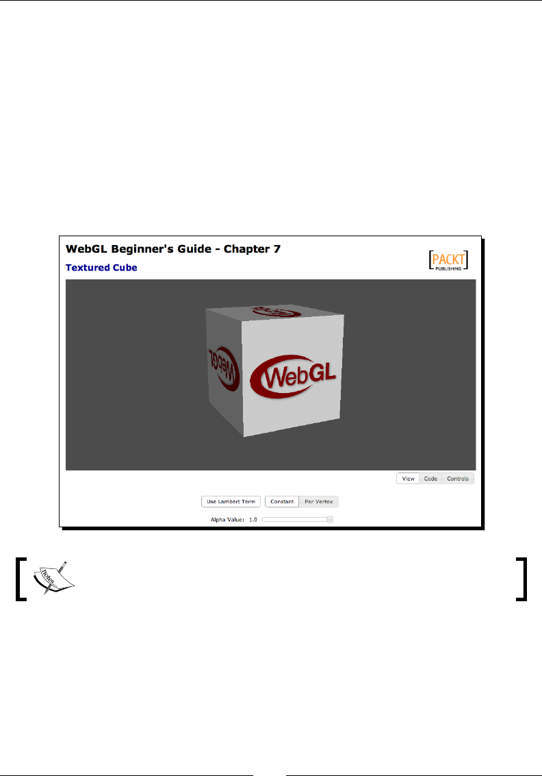
Chapter 7

[ 233 ]

8. We must also remember to add aVertexTextureCoords to the attributeList

and uSampler to the uniformList in the configure funcon so that the new

variables can be accessed from our JavaScript binding code.

9. To access the texture color, we call texture2D with the sampler and the texture

coordinates. As we want the textured surface to retain the lighng that was

calculated, we'll mulply the lighng color and the texture color together, giving

us the following line to calculate the fragment color:

gl_FragColor = vColor * texture2D(uSampler, vTextureCoord);

10. If everything has gone according to the plan, opening the le now in an HTML5

browser should yield a scene like this one:

If you're having trouble with a parcular step and would like a reference, the

completed code is available in ch7_Textured_Cube_Finished.html.

What just happened?

We've just loaded a texture from a le, uploaded it to the GPU, rendered it on the cube

geometry, and blended with the lighng informaon that was already being calculated.

The remaining examples in this chapter will omit calculaon of lighng for simplicity

and clarity, but all of the examples could have lighng applied to them if desired.

Textures

[ 234 ]

Have a go hero – try a different texture

Go grab one of your own images and see if you can get it to display as the texture instead.

What happens if you provide a rectangular image rather than a square one?

Texture lter modes

So far, we've seen how textures can be used to sample image data in a fragment shader,

but we've only used them in a limited context. Some interesng issues arise when you

start to look at texture use in more robust situaons.

For example, if you were to zoom in on the cube from the previous demo, you would see

that the texture begins to alias prey severely.

As we zoom in, you can see jagged edges develop around the WebGL logo. Similar problems

become apparent when the texture is very small on the screen. Isolated to a single object,

such arfacts are easy to overlook, but they can become very distracng in complex scenes.

So why do we see these arfacts in the rst place?

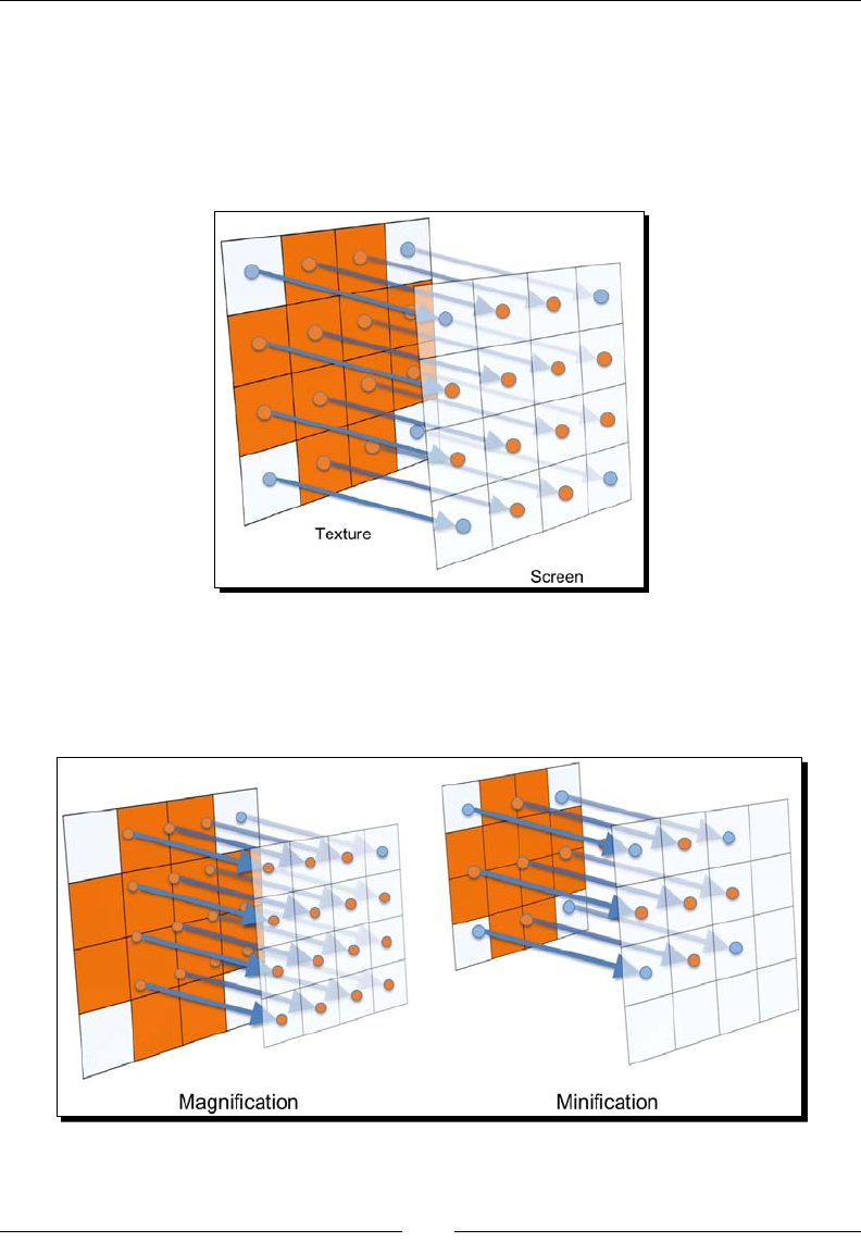
Chapter 7

[ 235 ]

Recall from the previous chapter how vertex colors are interpolated, so that the fragment

shader is provided a smooth gradient of color. Texture coordinates are interpolated in

exactly the same way, with the resulng coordinates being provided to the fragment shader

and used to sample color values from the texture. In a perfect situaon, the texture would

display at a 1:1 rao on screen, meaning each pixel of the texture (known as texels) would

take up exactly one pixel on screen. In this scenario, there would be no arfacts.

The reality of 3D applicaons, however, is that the textures are almost never displayed

at their nave resoluon. We refer to these scenarios as magnicaon and minicaon,

depending on whether the texture has a lower or higher resoluon than the screen space

it occupies.

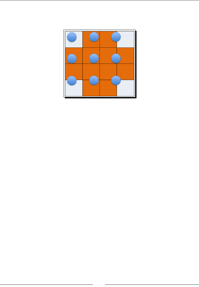
Textures

[ 236 ]

When a texture is magnied or minied, there can be some ambiguity about what color the

texture sampler should return. For example, consider the following diagram of sample points

against a slightly magnied texture:

It's prey obvious what color you would want the top le-hand side or middle sample points

to return, but what about those that sit between texels? What color should they return? The

answer is determined by your lter mode. Texture ltering gives us a way to control how

textures are sampled and achieve the look that we want.

Seng a texture's lter mode is very straighorward, and we've already seen an example

of how it works when talking about creang textures.

gl.texParameteri(gl.TEXTURE_2D, gl.TEXTURE_MAG_FILTER, gl.NEAREST);

gl.texParameteri(gl.TEXTURE_2D, gl.TEXTURE_MIN_FILTER, gl.NEAREST);

As with most WebGL calls, texParameteri operates on the currently bound texture, and

must be set for every texture you create. This also means that dierent textures can have

dierent lters, which can be useful when trying to achieve specic eects.

In this example we are seng both the magnicaon lter (TEXTURE_MAG_FILTER) and

the minicaon lter (TEXTURE_MIN_FILTER) to NEAREST. There are several modes that

can be passed for the third parameter, and the best way to understand the visual impact that

they have on a scene is to see the various lter modes in acon.

Let's look at a demonstraon of the lters in your browser while we discuss

dierent parameters.

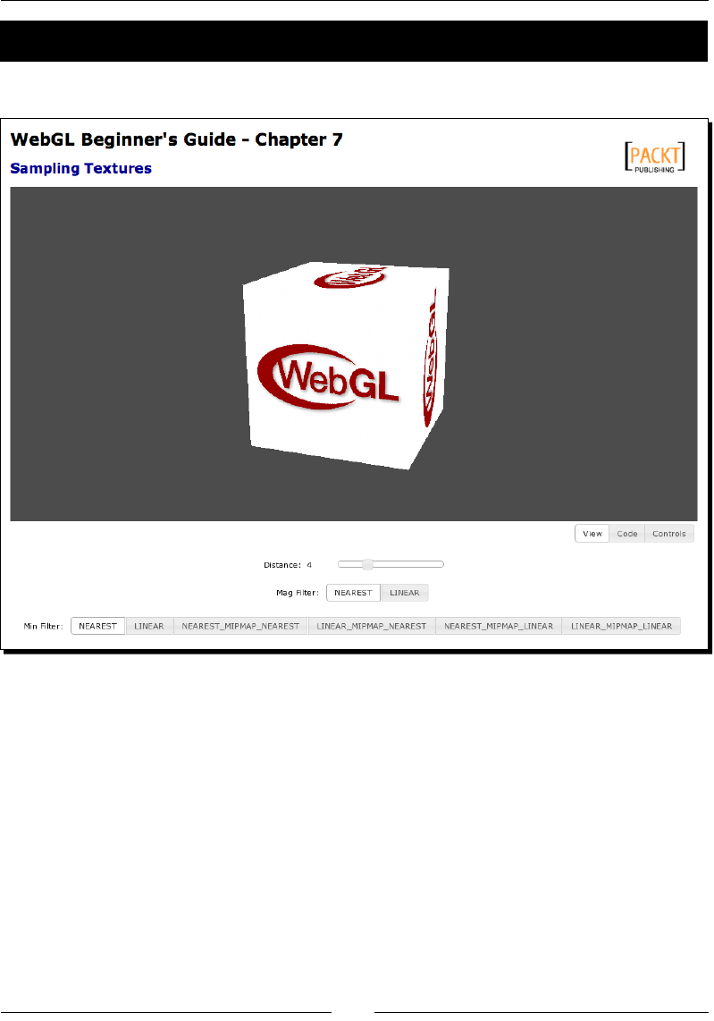
Chapter 7

[ 237 ]

Time for action – trying different lter modes

1. Open the le ch7_Texture_Filters.html using your HTML5 Internet browser:

2. The controls along the boom include a slider to adjust the distance of the box from

the viewer, and the buons modify the magnicaon and minicaon lters.

3. Experiment with dierent modes to observe the eect they have on the texture.

Magnicaon lters take eect when the cube is closer, minicaon lters when it is

further away. Be sure to rotate the cube as well and observe what the texture looks

like when viewed at an angle with each mode.

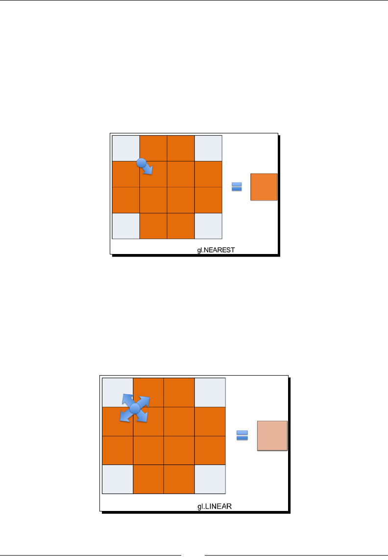
Textures

[ 238 ]

What just happened?

Let's look at each of the lter modes in depth, and discuss how they work.

NEAREST

Textures using the NEAREST lter always return the color of the texel whose center is

nearest to the sample point. Using this mode textures will look blocky and pixilated when

viewed up close, which can be useful for creang "retro" graphics. NEAREST can be used

for both MIN and MAG lters.

LINEAR

The LINEAR lter returns the weighted average of the four pixels whose centers are nearest

to the sample point. This provides a smooth blending of texel colors when looking at textures

close up, and generally is a much more desirable eect. This does mean that the graphics

hardware has to read four mes as many pixels per fragment, so naturally it's slower than

NEAREST, but modern graphics hardware is so fast that this is almost never an issue. LINEAR

can be used for both MIN and MAG lters. This ltering mode is also known as bilinear ltering.

Chapter 7

[ 239 ]

Looking back at the close-up example image we showed earlier in the chapter,

had we used LINEAR ltering it would have looked like this:

Mipmapping

Before we can discuss the remaining lter modes that are only applicable to

TEXTURE_MIN_FILTER, we need to introduce a new concept: mipmapping.

A problem arises when sampling minied textures; even when using LINEAR ltering

where the sample points can be so far apart that we can completely miss some details

of the texture. As the view shis, the texture fragments that we miss changes and the

result is a shimmering eect. You can see this in acon by seng the MIN lter in the

demo to NEAREST or LINEAR, zooming out, and rotang the cube.

Textures

[ 240 ]

To avoid this, graphics cards can ulize a mipmap chain.

Mipmaps are scaled-down copies of a texture, with each copy being exactly half the size of

the previous one. If you were to show a texture and all of it's mipmaps in a row, it would look

like this:

The advantage is that when rendering, the graphics hardware can choose the copy of the

texture that most closely matches the size of the texture on screen and sample from it

instead, which reduces the number of skipped texels and the jiery arfacts that accompany

it. However, mipmapping is only used if you use the appropriate texture lters. The following

TEXTURE_MIN_FILTER modes will ulize mipmaps in some fashion or the other.

NEAREST_MIPMAP_NEAREST

This lter will select the mipmap that most closely matches the size of the texture on screen

and sample from it using the NEAREST algorithm.

LINEAR_MIPMAP_NEAREST

This lter selects the mipmap that most closely matches the size of the texture on screen

and sample from it using the LINEAR algorithm.

NEAREST_MIPMAP_LINEAR

This lter selects two mipmaps that most closely matches the size of the texture on screen

and samples from both of them using the NEAREST algorithm. The color returned is a

weighted average of those two samples.

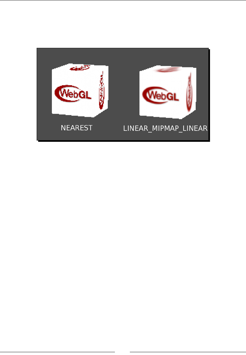
Chapter 7

[ 241 ]

LINEAR_MIPMAP_LINEAR

This lter selects two mipmaps that most closely matches the size of the texture on screen

and samples from both of them using the LINEAR algorithm. The color returned is a

weighted average of those two samples. This mode is also known as trilinear ltering.

Of the *_MIPMAP_* lter modes, NEAREST_MIPMAP_NEAREST is the fastest and of

lowest quality while LINEAR_MIPMAP_LINEAR will provide the best quality at the lowest

performance, with the other two modes sing somewhere in between on the quality/speed

scale. In most cases, however, the performance tradeo will be minor enough so that you

should always favor LINEAR_MIPMAP_LINEAR.

Generating mipmaps

WebGL doesn't automacally create mipmaps for every texture; so if we want to use one

of the *_MIPMAP_* lter modes, we have to create the mipmaps for the texture rst.

Fortunately, all this takes is a single funcon call:

gl.generateMipmap(gl.TEXTURE_2D);

generateMipmap must be called aer the texture has been populated with texImage2D

and will automacally create a full mipmap chain for the image.

Alternately, if you want to provide the mipmaps manually you can always specify that you

are providing a mipmap level rather than the source texture when calling texImage2D by

passing a number other than 0 as the second parameter.

gl.texImage2D(gl.TEXTURE_2D, 1, gl.RGBA, gl.RGBA, gl.UNSIGNED_BYTE,

mipmapImage);

Textures

[ 242 ]

Here we're manually creang the rst mipmap level, which is half the height and width

of the normal texture. The second level would be quarter the dimensions of the normal

texture, and so on.

This can be useful in some advanced eects, or when using compressed textures which

cannot be used with generateMipmap.

In order to use mipmaps with a texture it needs to sasfy some dimension restricons.

Namely, the texture width and height must both be Powers Of Two (POT). That is, the width

and height can be pow(2,n) pixels, where n is any integer. Examples are 16px, 32px, 64px,

128px, 256px, 512px, 1024px, and so on. Also, note that the width and height do not have

to be the same as long as both are powers of two. For example, a 512x128 texture can sll

be mipmapped.

Why the restricon to power of two textures? Recall that the mipmap chain is made of

textures whose sizes are half of the previous level. When the dimensions are powers of

two this will always produce integer numbers, which means that the number of pixels

never needs to be rounded o and hence produces clean and fast scaling algorithms.

Non Power Of Two (NPOT) textures can sll be used with WebGL, but are restricted to only

using NEAREST and LINEAR lters.

For all the texture code samples aer this point, we'll be using a simple

texture class that cleanly wraps up the texture's download, creaon, and

setup. Any textures created with the class will automacally have mipmaps

generated for them and be set to use LINEAR for the magnicaon lter

and LINEAR_MIPMAP_LINEAR for the minicaon lter.

Texture wrapping

In the previous secon, we used texParameteri to set the lter mode for textures, but

as you might expect from the generic funcon name, that's not all that it can do. Another

texture behavior that we can manipulate is the texture wrapping mode.

Texture wrapping describes the behavior of the sampler when the texture coordinates fall

outside the range of 0-1.

The wrapping mode can be set independently for both the S and T coordinates, so changing

the wrapping mode typically takes two calls:

gl.texParameteri(gl.TEXTURE_2D, gl.TEXTURE_WRAP_S, gl.CLAMP_TO_EDGE);

gl.texParameteri(gl.TEXTURE_2D, gl.TEXTURE_WRAP_T, gl.CLAMP_TO_EDGE);

Chapter 7

[ 243 ]

Here we're seng both the S and T wrapping modes for the currently bound texture to

CLAMP_TO_EDGE, the eects of which we will see in a moment.

As with texture lters, it's easiest to demonstrate the eects of the dierent wrapping

modes via an example and then discuss the results. Let's open up your browser again for

another demonstraon.

Time for action – trying different wrap modes

1. Open the le ch7_Texture_Wrapping.html using your HTML5 Internet browser.

2. The cube shown has texture coordinates that range from -1 to 2, which forces the

texture wrapping mode to be used for everything but the center le of the texture.

3. Experiment with the controls along the boom to see the eect that the dierent

wrap modes have on the texture.

What just happened?

Let's look at each of the wrap modes and discuss how they work.

Textures

[ 244 ]

CLAMP_TO_EDGE

This wrap mode rounds any texture coordinates greater than 1 down to 1 and lower than 0

up to 0, "clamping" the values to the 0-1 range. Visually, this has the eect of repeang the

border pixels of the texture indenitely once the coordinates go out of the 0-1 range. Note

that this is the only wrapping mode that is compable with NPOT textures.

REPEAT

This is the default wrap mode, and the one that you'll probably use most oen.

In mathemacal terms this wrap mode simply ignores the integer part of the texture

coordinate. This creates the visual eect of the texture repeang as you go outside the

0-1 range. This can be a useful eect for displaying surfaces that have a natural repeang

paern to them, such as a le oor or brick wall.

Chapter 7

[ 245 ]

MIRRORED_REPEAT

The algorithm for this mode is a lile more complicated. If the coordinate's integer poron

is even, the texture coordinates will be the same as with REPEAT. If the integer poron of the

coordinate is odd, however, the resulng coordinate is 1 minus the fraconal poron of the

coordinate. This results in a texture that "ip-ops" as it repeats, with every other repeon

being a mirror image.

As was menoned earlier, these modes can be mixed and matched if needed. For example,

consider the following code snippet:

gl.texParameteri(gl.TEXTURE_2D, gl.TEXTURE_WRAP_S, gl.REPEAT);

gl.texParameteri(gl.TEXTURE_2D, gl.TEXTURE_WRAP_T, gl.CLAMP_TO_EDGE);

It would produce the following eect on the texture from the sample:

Textures

[ 246 ]

Wondering why the shader uniforms are called "samplers" instead of

"textures"? A texture is just the image data stored on the GPU, while

a sampler contains all the informaon about how to look up texture

informaon, including lter and wrap modes.

Using multiple textures

Up to this point, we've been doing all of our rendering using a single texture at a me.

As you've seen this can be a useful tool. But there are mes where we may want to have

mulple textures that contribute to a fragment to create more complex eects. For these

cases, we can use the WebGL's ability to access mulple textures in a single draw call,

otherwise known as multexturing.

We've already brushed up against multexturing earlier in a chapter, so let's go back and

look at it again. When talking about exposing a texture to a shader as a sampler uniform we

used the following code:

gl.activeTexture(gl.TEXTURE0);

gl.bindTexture(gl.TEXTURE_2D, texture);

The rst line, gl.activeTexture, is the key to ulizing multexturing. We use it to tell

the WebGL state machine which texture we are going to be manipulang with, in subsequent

texture funcons. In this case, we passed gl.TEXTURE0, which means that any following

texture calls (such as gl.bindTexture) will alter the state of the rst texture unit.

If we wanted to aach a dierent texture to the second texture unit, we would use

gl.TEXTURE1 instead.

Dierent devices will support dierent numbers of texture units, but WebGL species that

compable hardware must always support at least two texture units. We can nd out how

many texture units the current device supports with the following funcon call:

gl.getParameter(gl.MAX_COMBINED_TEXTURE_IMAGE_UNITS);

WebGL provides explicit enumeraons for gl.TEXTURE0 thorough gl.TEXTURE31, which

is likely more than your hardware is capable of using. Somemes it is convenient to specify

the texture unit programmacally, or you may nd a need to refer a texture unit above 31.

To that end, you can always substute gl.TEXTURE0 + i for gl.TEXTUREi. For example:

gl.TEXTURE0 + 2 === gl.TEXTURE2;

Chapter 7

[ 247 ]

Accessing mulple textures in a shader is as simple as declaring mulple samplers.

uniform sampler2D uSampler;

uniform sampler2D uOtherSampler;

When seng up your draw call, you tell the shader which texture is associated with which

sampler by providing the texture unit to gl.uniform1i. The code to bind two textures to

the samplers above would look something like this:

// Bind the first texture

gl.activeTexture(gl.TEXTURE0);

gl.bindTexture(gl.TEXTURE_2D, texture);

gl.uniform1i(Program.uSampler, 0);

// Bind the second texture

gl.activeTexture(gl.TEXTURE1);

gl.bindTexture(gl.TEXTURE_2D, otherTexture);

gl.uniform1i(Program. uOtherSampler, 1);

So now we have two textures available to our fragment shader. The queson is what do we

want to do with them?

As an example we're going to implement a simple multexture eect that layers another

texture on top of a simple textured cube to simulate stac lighng.

Time for action – using multitexturing

1. Open the le ch7_Multitexture.html with your choice of HTML editor.

2. At the top of the script block, add another texture variable:

var texture2 = null;

3. At the boom of the configure funcon, add the code to load the second texture.

As menoned earlier, we're using a class to make this process easier, so the new

code is as follows:

texture2 = new Texture();

texture2.setImage('textures/light.png');

Textures

[ 248 ]

4. The texture we're using is a white radial gradient that simulates a spot light:

5. In the draw funcon, directly below the code that binds the rst texture,

add the following to expose the new texture to the shader:

gl.activeTexture(gl.TEXTURE1);

gl.bindTexture(gl.TEXTURE_2D, texture2.tex);

gl.uniform1i(Program.uSampler1, 1);

6. Next, we need to add the new sampler uniform to the fragment shader:

uniform sampler2D uSampler1;

7. Don't forget to add the corresponding string to the uniformList in the

configure funcon.

8. Finally, we add the code to sample the new texture value and blend it with the

rst texture. In this case, since we want the second texture to simulate a light, we

mulply the two values together as we did with the per-vertex lighng in the rst

texture example.

gl_FragColor = texture2D(uSampler, vTextureCoord) *

texture2D(uSampler1, vTextureCoord);

9. Note that we're re-using the same texture coordinate for both textures. It's

convenient to do so in this case, but if needed, a second texture coordinate aribute

could have been used, or we could even calculate a new texture coordinate from the

vertex posion or other criteria.

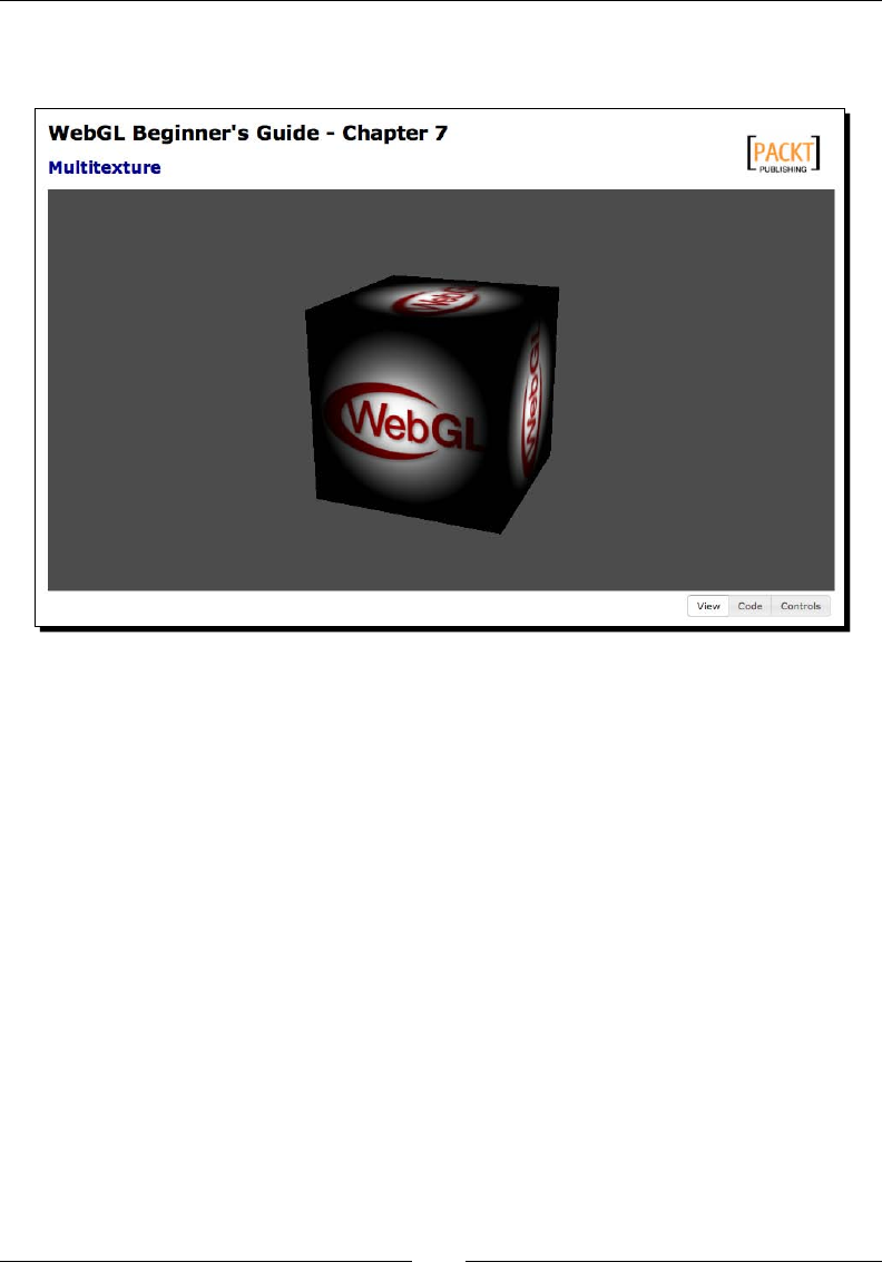
Chapter 7

[ 249 ]

10. Assuming that everything works as intended, you should see a scene that looks like

this when you open the le in your browser:

11. You can see the completed example in ch7_Multitexture_Finished.html.

What just happened?

We've added a second texture to the draw call and blended it with the rst to create a new

eect, in this case simulang a simple stac spotlight.

It's important to realize that the colors sampled from a texture are treated just like any

other color in the shader, that is as a generic 4-dimensional vector. As a result, we can

combine textures together just like we would combine vertex and light colors, or any

other color manipulaon.

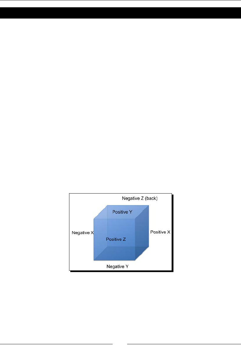
Textures

[ 250 ]

Have a go hero – moving beyond multiply

Mulplicaon is one of the most common ways to blend colors in a shader, but there's

really no limit to how you can combine color values. Try experimenng with some dierent

algorithms in the fragment shader and see what eect it has on the output. What happens

when you add values instead of mulply? What if you use the red channel from one texture

and the blue and green from the other? Or try out the following algorithm and see what the

result is:

gl_FragColor = vec4(texture2D(uSampler2, vTextureCoord).rgb -

texture2D(uSampler, vTextureCoord).rgb, 1.0);

Cube maps

Earlier in this chapter, we menoned that aside from 2D textures the funcons we've

been discussing can also be used for cube maps. But what are cube maps and how

do we use them?

A cube map is, very much like it sounds, a cube of textures. Six individual textures are

created, each assigned to a dierent face of the cube. The graphics hardware can sample

them as a single enty, using a 3D texture coordinate.

The faces of the cube are idened by the axis they face and whether they are on the

posive or negave side of that axis.

Up unl this point, any me we have manipulated a texture, we have specied a texture

target of TEXTURE_2D. Cube mapping introduces a few new texture targets that indicate

that we are working with cube maps, and which face of the cube map we're manipulang:

TEXTURE_CUBE_MAP

TEXTURE_CUBE_MAP_POSITIVE_X

TEXTURE_CUBE_MAP_NEGATIVE_X

Chapter 7

[ 251 ]

TEXTURE_CUBE_MAP_POSITIVE_Y

TEXTURE_CUBE_MAP_NEGATIVE_Y

TEXTURE_CUBE_MAP_POSITIVE_Z

TEXTURE_CUBE_MAP_NEGATIVE_Z

These targets are collecvely known as the gl.TEXTURE_CUBE_MAP_* targets. Which one

you use depends on the funcon you are calling.

Cube maps are created like a normal texture, but binding and property manipulaon happen

with the TEXTURE_CUBE_MAP target, as shown here:

var cubeTexture = gl.createTexture();

gl.bindTexture(gl.TEXTURE_CUBE_MAP, cubeTexture);

gl.texParameteri(gl.TEXTURE_CUBE_MAP, gl.TEXTURE_MAG_FILTER,

gl.LINEAR);

gl.texParameteri(gl.TEXTURE_CUBE_MAP, gl.TEXTURE_MIN_FILTER,

gl.LINEAR);

When uploading the image data for the texture, however, you specify the side that you are

manipulang as shown here:

gl.texImage2D(gl.TEXTURE_CUBE_MAP_POSITIVE_X, 0, gl.RGBA, gl.RGBA,

gl.UNSIGNED_BYTE, positiveXImage);

gl.texImage2D(gl.TEXTURE_CUBE_MAP_NEGATIVE_X, 0, gl.RGBA, gl.RGBA,

gl.UNSIGNED_BYTE, negativeXImage);

gl.texImage2D(gl.TEXTURE_CUBE_MAP_POSITIVE_Y, 0, gl.RGBA, gl.RGBA,

gl.UNSIGNED_BYTE, positiveYImage);

// Etc.

Exposing the cube map texture to the shader is done in the same way as a normal texture,

just with the cube map target:

gl.activeTexture(gl.TEXTURE0);

gl.bindTexture(gl.TEXTURE_CUBE_MAP, cubeTexture);

gl.uniform1i(Program.uCubeSampler, 0);

However, the uniform type within the shader is specic to cube maps:

uniform samplerCube uCubeSampler;

When sampling from the cube map, you also use a cube map-specic funcon:

gl_FragColor = textureCube(uCubeSampler, vCubeTextureCoord);

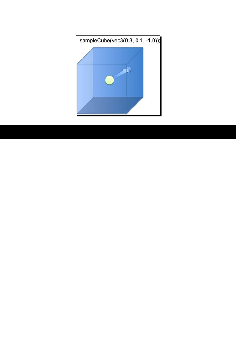
Textures

[ 252 ]

The 3D coordinates that you provide is normalized by the graphics hardware into a unit

vector, which species a direcon from the center of the "cube". A ray is traced along that

vector and where it intersects the cube face is where the texture is sampled.

Time for action – trying out cube maps

1. Open the le ch7_Cubemap.html using your HTML5 internet browser. Once again,

this contains a simple textured cube example on top of which we'll build the cube

map example. We want to use the cube map to create a reecve-looking surface.

2. Creang the cube map is a bit more complicated than the textures we've loaded in

the past, so this me we'll use a funcon to simplify the asynchronous loading of

individual cube faces. It's called loadCubemapFace and has already been added to

the configure funcon. Below that funcon, add the following code which creates

and loads the cube map faces:

cubeTexture = gl.createTexture();

gl.bindTexture(gl.TEXTURE_CUBE_MAP, cubeTexture);

gl.texParameteri(gl.TEXTURE_CUBE_MAP, gl.TEXTURE_MAG_FILTER,

gl.LINEAR);

gl.texParameteri(gl.TEXTURE_CUBE_MAP, gl.TEXTURE_MIN_FILTER,

gl.LINEAR);

loadCubemapFace(gl, gl.TEXTURE_CUBE_MAP_POSITIVE_X, cubeTexture,

'textures/cubemap/positive_x.png');

loadCubemapFace(gl, gl.TEXTURE_CUBE_MAP_NEGATIVE_X, cubeTexture,

'textures/cubemap/negative_x.png');

loadCubemapFace(gl, gl.TEXTURE_CUBE_MAP_POSITIVE_Y, cubeTexture,

Chapter 7

[ 253 ]

'textures/cubemap/positive_y.png');

loadCubemapFace(gl, gl.TEXTURE_CUBE_MAP_NEGATIVE_Y, cubeTexture,

'textures/cubemap/negative_y.png');

loadCubemapFace(gl, gl.TEXTURE_CUBE_MAP_POSITIVE_Z, cubeTexture,

'textures/cubemap/positive_z.png');

loadCubemapFace(gl, gl.TEXTURE_CUBE_MAP_NEGATIVE_Z, cubeTexture,

'textures/cubemap/negative_z.png');

3. In the draw funcon, add the code to bind the cube map to the

appropriate sampler:

gl.activeTexture(gl.TEXTURE1);

gl.bindTexture(gl.TEXTURE_CUBE_MAP, cubeTexture);

gl.uniform1i(Program.uCubeSampler, 1);

4. Turning to the shader now, rst o we want to add a new varying to the vertex

and fragment shader:

varying vec3 vVertexNormal;

5. We'll be using the vertex normals instead of a dedicated texture coordinate to do

the cube map sampling, which will give us the mirror eect that we're looking for.

Unfortunately, the actual normals of each face on the cube point straight out. If we

were to use them, we would only get a single color per face from the cube map. In

this case, we can "cheat" and use the vertex posion as the normal instead. (For

most models, using the normals would be appropriate).

vVertexNormal = (uNMatrix * vec4(-aVertexPosition, 1.0)).xyz;

6. In the fragment shader, we need to add the new sampler uniform:

uniform samplerCube uCubeSampler;

7. And then in the fragment shader's main funcon, add the code to actually sample

the cubemap and blend it with the base texture:

gl_FragColor = texture2D(uSampler, vTextureCoord) *

textureCube(uCubeSampler, vVertexNormal);

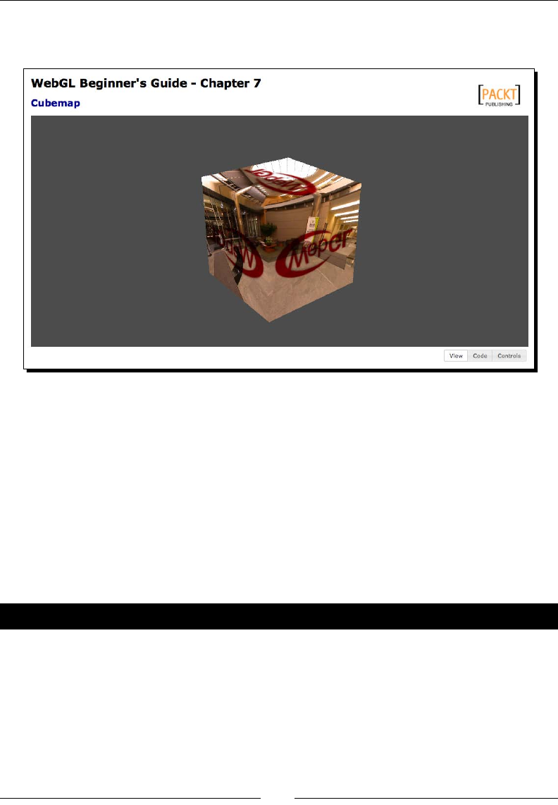
Textures

[ 254 ]

8. We should now be able to reload the le in a browser and see the scene shown

in the next screenshot:

9. The completed example is available in ch7_Cubemap_Finished.html.

What just happened?

As you rotate the cube, you should noce that the scene portrayed in the cube map does

not rotate along with it, which creates a "mirror" eect in the cube faces. This is due to

mulplicaon of the normals by the normal matrix when assigning the vVertexNormal

varying, which puts the normals in world space.

Using cube maps for reecve surfaces like this is a very common technique, but not the

only use for cube maps. Other common uses are for skyboxes or advanced lighng models.

Have a go hero – shiny logo

In this example, we've created a completely reecve "mirrored" cube, but what if the only

part of the cube we wanted to be reecve was the logo? How could we constrain the cube

map to only display within the red poron of the texture?

Chapter 7

[ 255 ]

Summary

In this chapter we learned how to use textures to add a new level of detail to our scenes.

We covered how to create and manage texture objects, and use HTML images as textures.

We examined the various lter modes and how they aect the texture appearance and

usage, as well as the available texture wrapping modes and how they alter the way texture

coordinates are interpreted. We learned how to use mulple textures in a single draw call,

and how to combine them in a shader. Finally, we learned how to create and render cube

maps, and saw how they can be used to simulate reecve surfaces.

Coming up in the next chapter, we'll look at selecng and interacng with objects in the

WebGL scene with your mouse, otherwise known as picking.

Picking

Picking refers to the ability of selecng objects in a 3D scene by poinng at

them. The most common device used for picking is the mouse. However, picking

can also be performed using other human computer interfaces such as tacle

screens and hapc devices. In this chapter we will see how picking can be

implemented in WebGL.

This chapter talks about:

Selecng objects in a WebGL scene using the mouse

Creang and using oscreen framebuers

What renderbuers are and how they are used by framebuers

Reading pixels from framebuers

Using color labels to perform object selecon based on color

Picking

Virtually any 3D computer graphics applicaon needs to provide mechanisms for the user to

interact with the scene being displayed on the screen. For instance, you are wring a game

you want to point at your target and perform an acon upon it. Similarly, if you are wring a

CAD system, you want to be able to select an object in your scene to modify its properes.

In this chapter, we will see the basis of implemenng these kinds of interacons in WebGL.

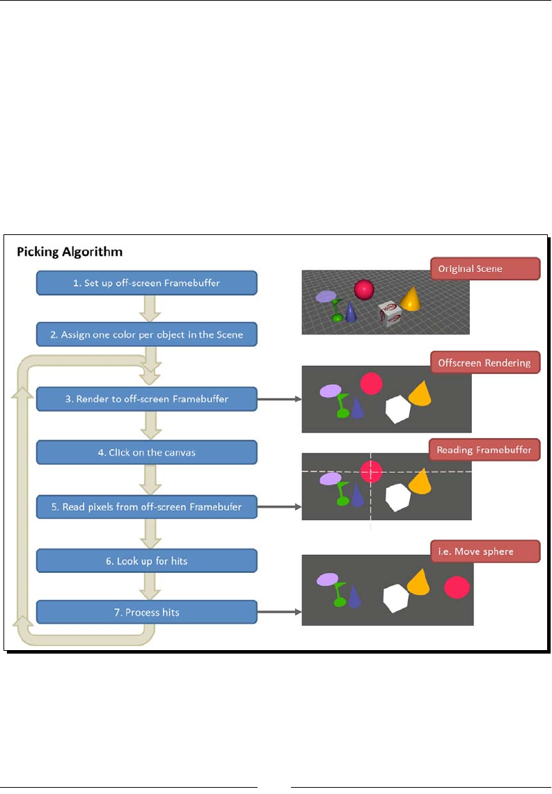
Picking

[ 258 ]

We could select objects by casng a ray (vector) from the camera posion (also known as

eye posion) into the scene and calculate what objects lie along the ray path. This is known

as ray casng and it involves detecng intersecons between the ray and object surfaces in

the scene. However, because of its complexity it is beyond the scope of this beginner's guide.

Instead, we will use picking based on object colors. This method is easier to implement and it

is a good starng point to help you understand how picking works.

The basic idea is to assign a dierent color to every object in the scene and render the scene

to an oscreen framebuer. Then, when the user clicks on the scene, we go to the oscreen

framebuer and read the color for the correspondent click coordinates. As we assigned

beforehand the object colors in the oscreen buer, we can idenfy the object that has

been selected and perform an acon upon it. The following gure depicts this idea:

Let's break it down into the steps that we need to take.

Chapter 8

[ 259 ]

Setting up an offscreen framebuffer

As shown in Chapter 2, Rendering Geometry, the framebuer is the nal rendering

desnaon in WebGL. When you visualize a scene on your screen, you are looking

at the framebuer contents. Assuming that gl is our WebGL context, every call to

gl.drawArrays, gl.drawElements, and gl.clear will change the contents

of the framebuer.

Instead of rendering to the default framebuer, we can also render our scene oscreen. This

will be the rst step for implemenng picking. To do so, we need to set up a new framebuer

and tell WebGL that we want to use it instead of the default one. Let's see how to do that.

To set up a framebuer, we need to be able to create storage for at least two things:

colors and depth informaon. We need to be able to store the color for every fragment

that is rendered in the framebuer so we can create an image; in contrast, we need depth

informaon to make sure that we have a scene where overlapping objects look consistent.

If we did not have depth informaon, then we would not be able to tell, in the case of two

overlapping objects, which object is in front and which one is at the back.

To store colors we will use a WebGL texture, and to store depth informaon we will

use a renderbuer.

Creating a texture to store colors

The code to create a texture is prey straighorward aer reading Chapter 7, Textures.

If you have not read it, you can go back there and review that chapter.

var canvas = document.getElementById('canvas-element-id');

var width = canvas.width;

var height = canvas.height;

var texture = gl.createTexture();

gl.bindTexture(gl.TEXTURE_2D, texture);

gl.texImage2D(gl.TEXTURE_2D, 0, gl.RGBA, width, height, 0, gl.RGBA,

gl.UNSIGNED_BYTE, null);

The only dierence here is that we do not have an image to bind to the texture so when

we call gl.texImage2D, the last argument is null. This is ok, as we are just allocang the

space to store colors for the oscreen framebuer.

Also, please noce that the width and height of the texture are set to the canvas size.

Picking

[ 260 ]

Creating a Renderbuffer to store depth information

Renderbuers are used to provide storage for the individual buers used in a framebuer.

The depth buer (z-buer) is an example of a renderbuer.It is always aached to the screen

framebuer which is the default rendering desnaon in WebGL.

The code to create a renderbuer looks like the following code:

var renderbuffer = gl.createRenderbuffer();

gl.bindRenderbuffer(gl.RENDERBUFFER, renderbuffer);

gl.renderbufferStorage(gl.RENDERBUFFER, gl.DEPTH_COMPONENT16, width,

height);

The rst line of code creates the renderbuer. Similar to other WebGL buers, the

renderbuer needs to be bound before we can operate on it. The third line of code

determines the storage size of the renderbuer.

Please noce that the size of the storage is the same as with the texture. This way we make

sure that for every fragment (pixel) in the framebuer, we can have a color (stored in the

texture) and a depth value (stored in the renderbuer).

Creating a framebuffer for offscreen rendering

We need to create a framebuer and aach the texture and the renderbuer that

we created in the two previous steps to it. Let's see how this works in code.

First, we create a new framebuer using a line of code like this:

var framebuffer = gl.createFramebuffer();

Similar to the VBO manipulaon, we will tell WebGL that we are going to operate

on this framebuer by making it the currently bound framebuer. We do so with

the following instrucon:

gl.bindFramebuffer(gl.FRAMEBUFFER, framebuffer);

With the framebuer bound, the texture is aached by calling the following method:

gl.framebufferTexture2D(gl.FRAMEBUFFER, gl.COLOR_ATTACHMENT0,

gl.TEXTURE_2D, texture, 0);

Then, the renderbuer is aached to the bound framebuer using:

gl.framebufferRenderbuffer(gl.FRAMEBUFFER, gl.DEPTH_ATTACHMENT,

gl.RENDERBUFFER, renderbuffer);

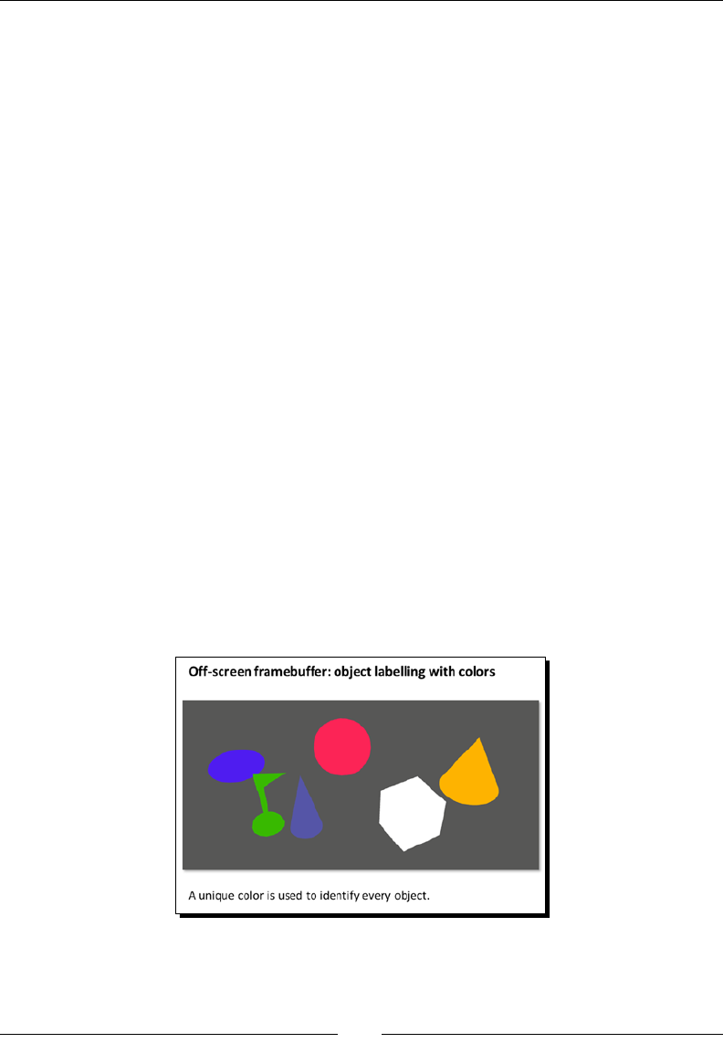
Chapter 8

[ 261 ]

Finally, we do a bit of cleaning up as usual:

gl.bindTexture(gl.TEXTURE_2D, null);

gl.bindRenderbuffer(gl.RENDERBUFFER, null);

gl.bindFramebuffer(gl.FRAMEBUFFER, null);

When the previously created framebuer is unbound, the WebGL state machine goes back

to rendering into the screen framebuer.

Assigning one color per object in the scene

We will pick an object based on its color. If the object has shiny reecons or shadows,

then the color throughout it will not be uniform. Therefore, to pick an object based on its

color we need to make sure that the color is constant per object and that each object has

a dierent color.

We achieve constant coloring by telling the fragment shader to use only the material diuse

property to set the ESSL gl_FragColor variable. Here we are assuming that each object

has a unique diuse property.

When there are objects sharing the same diuse color, then we need to create a new ESSL

uniform to store the picking color and make it unique for every object that is rendered into

the oscreen framebuer. This way, the objects will look the same when they are rendered

on screen but every me we render them into the oscreen framebuer, their colors will be

unique. This is something that we will do later on in this chapter.

For now, let's assume that the objects in our scene have unique diuse colors as shown in

the following diagram:

Let's see how to render the scene oscreen using the framebuer that we just set up.

Picking

[ 262 ]

Rendering to an offscreen framebuffer

In order to perform object selecon using the oscreen framebuer, this one has to be

synchronized with the onscreen default framebuer every me that this last one receives an

update. If the onscreen framebuer and the oscreen framebuer were not synchronized,

then we could be missing addion or deleon of objects, or updates in the camera posion

between buers. As a result of it there would not be a correspondence.

A lack of correspondence will hinder us from reading the picking colors from the oscreen

framebuer and use them to idenfy the objects in the scene. We can also refer to picking

colors as object labels.

To implement this synchronicity, we will create the render funcon. This funcon calls

the draw funcon twice. First when the oscreen buer is bound and second me when

onscreen default framebuer is bound. The code looks like this:

function render(){

//off-screen rendering

gl.bindFramebuffer(gl.FRAMEBUFFER, framebuffer);

gl.uniform1i(Program.uOffscreen, true);

draw();

//on-screen rendering

gl.bindFramebuffer(gl.FRAMEBUFFER, null);

gl.uniform1i(Program.uOffscreen, false);

draw();

}

We tell the ESSL program to use only diuse colors when rendering into the oscreen

framebuer using the uOffscreen uniform. The fragment shader looks like the

following code:

void main(void) {

if(uOffscreen){

gl_FragColor = uMaterialDiffuse;

return;

}

...

}

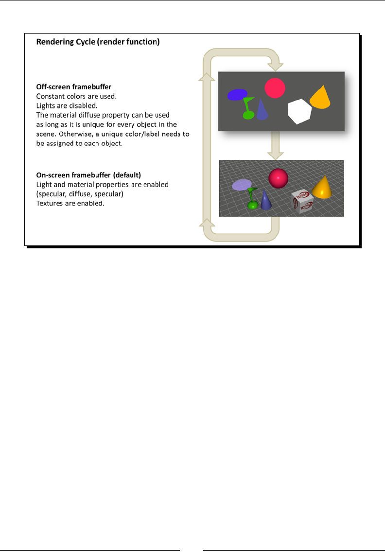
Chapter 8

[ 263 ]

The following diagram shows the behavior of the render funcon:

Consequently, every me that there is a scene update the render funcon should be called

instead of calling the draw funcon.

We change this in the runWebGLApp funcon:

var app = null;

function runWebGLApp() {

app = new WebGLApp("canvas-element-id");

app.configureGLHook = configure;

app.loadSceneHook = load;

app.drawSceneHook = render;

app.run();

}

In this way, the scene will be periodically updated using the render funcon instead of the

original draw funcon.

We also need to update the funcon hook that the camera uses to render the scene

whenever we interact with it. Originally, this hook is set to the draw funcon. If we do

not change it, it points to the render funcon. We will have to wait unl WebGLApp.

drawSceneHook is invoked again to synchronize the oscreen and the onscreen

framebuers (every 500 ms by default as you can check in WebGLApp.js). During

this me, picking will not work.

Picking

[ 264 ]

We change the camera render hook in the configure funcon:

function configure{

...

camera = new Camera(CAMERA_ORBITING_TYPE);

camera.goHome([0,0,40]);

camera.setFocus([0.0,0.0,0.0]);

camera.setElevation(-40);

camera.setAzimuth(-30);

camera.hookRenderer = render;

...

}

Clicking on the canvas

The next step is to capture the mouse coordinates when the user clicks on an object in

the scene and reads the color value for these coordinates from the oscreen framebuer.

For that, we use the standard onmouseup event from the canvas element in our webpage:

var canvas = document.getElementById('my-canvas-id');

canvas.onmouseup = function (ev){

//capture coordinates from the ev event

...

}

There is an extra bit of work to do here given that the ev event does not return the mouse

coordinates with respect to the canvas but with respect to the upper-le corner of the

browser window (ev.clientX and ev.clientY). Then, we need to bubble up through the

DOM geng the locaon of the elements that are in the DOM hierarchy to know the total

oset that we have.

We do this with a code fragment like this inside the canvas.onmouseup funcon:

var x, y, top = 0, left = 0, obj = canvas;

while (obj&& && obj.tagName !== 'BODY') {

top += obj.offsetTop;

left += obj.offsetLeft;

obj = obj.offsetParent;

}

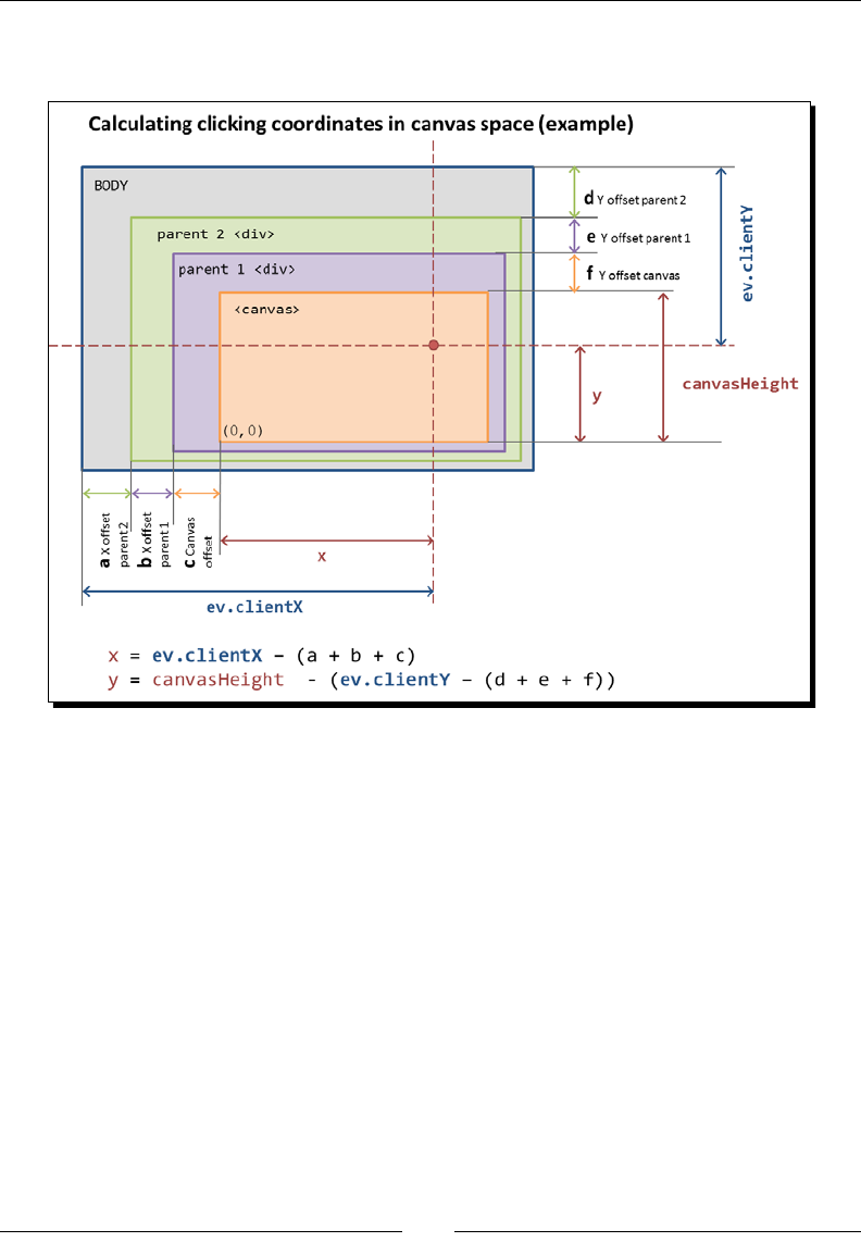
Chapter 8

[ 265 ]

The following diagram shows how we are going to use the oset calculaon to obtain the

clicked canvas coordinates:

Also, we take into account any page oset if present. The page oset is the result of scrolling

and aects the calculaon of the coordinates. We want to obtain the same coordinates for

the canvas every me regardless of any possible scrolling. For that we add the following two

lines of code just before calculang the clicked canvas coordinates:

left += window.pageXOffset;

top -= window.pageYOffset;

Finally, we calculate the canvas coordinates:

x = ev.clientX - left;

y = c_height - (ev.clientY - top);

Remember that unlike the browser window, the canvas coordinates (and also the

framebuer coordinates for this purpose) start in the lower-le corner as explained

in the previous diagram.

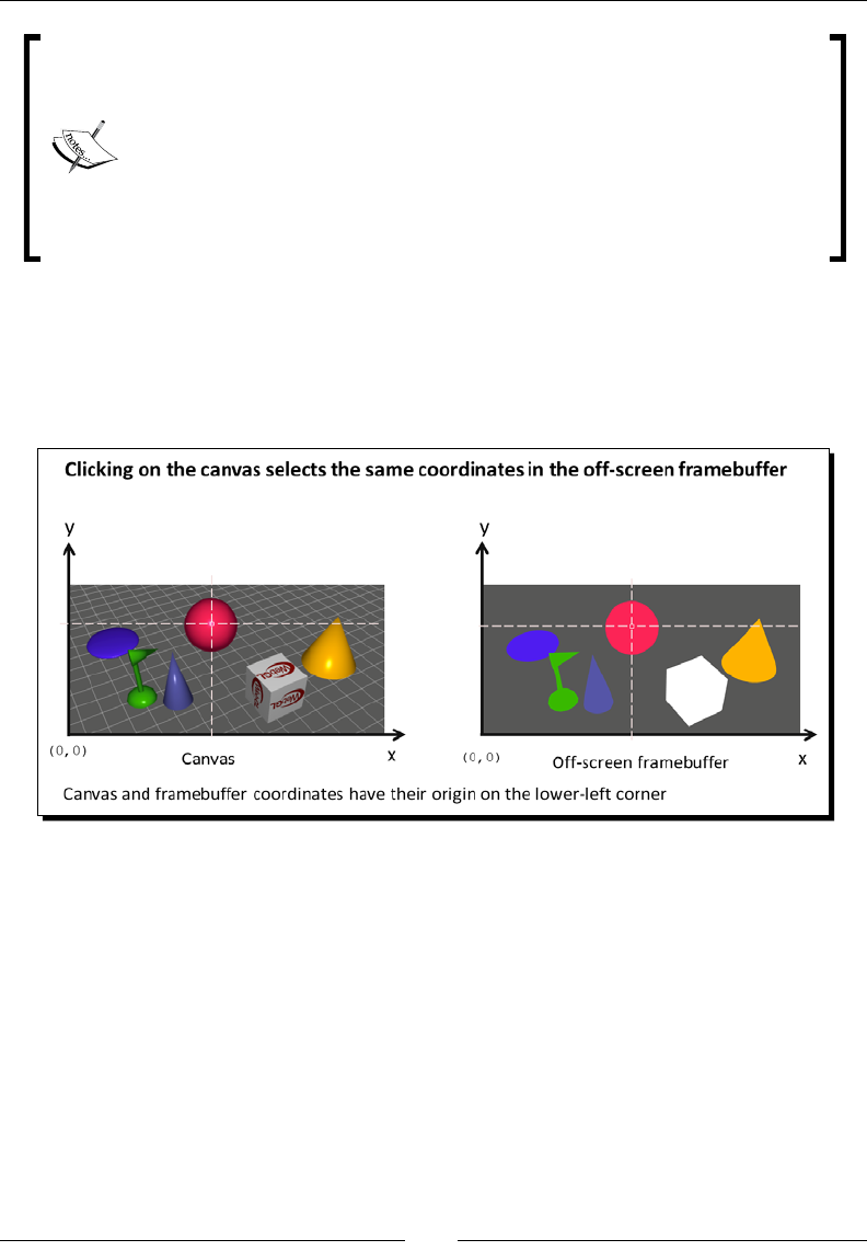
Picking

[ 266 ]

c_height is a global variable that we are maintaining in the le

codeview.js, it refers to the canvas height and it is updated along with

c_width whenever we resize the browser's window. If you are developing

your own applicaon, codeview.js might not be available or applicable

and then you might want to replace c_height in this snippet of code

by something like clientHeight which is a standard canvas property.

Also, noce that resizing the browser window will not resize your canvas.

The exercises in this book do, because we have implemented this inside

codeview.js.

Reading pixels from the offscreen framebuffer

We can go now to the oscreen buer and read the color from the coordinates that we

clicked on the canvas.

WebGL allows us to read back from a framebuer using the readPixels funcon. As usual,

having gl as the WebGL context variable:

Chapter 8

[ 267 ]

Funcon Descripon

gl.readPixels(x, y, width,

height, format, type, pixels) x and y: Starng coordinates.

width, height: The extent of pixels to read

from the framebuer. In our example we are just

reading one pixel (where the user clicks) so this

will be 1,1.

format: At the me of wring this book the only

supported format is gl.RGBA.

type: At the me of wring this book the only

supported type is gl.UNSIGNED_BYTE.

pixels: It is a typed array that will contain

the results of querying the framebuer. It

needs to have sucient space to store the

results depending on the extent of the query

(x,y,width,height).

According to the WebGL specicaon at the

me of wring this book it needs to be of type

Uint8Array.

Remember that WebGL works as a state machine and many operaons only make sense if

this machine is in a valid state. In this case, we need to make sure that the framebuer from

which we want to read, the oscreen framebuer, is the current one. To do that, we bind it

using bindFramebuffer. Pung everything together, the code looks like this:

//read one pixel

var readout = new Uint8Array(1 * 1 * 4);

gl.bindFramebuffer(gl.FRAMEBUFFER, framebuffer);

gl.readPixels(coords.x,coords.y,1,1,gl.RGBA,gl.UNSIGNED_BYTE,readout);

gl.bindFramebuffer(gl.FRAMEBUFFER, null);

Here the size of the readout array is 1*1*4. This means it has one pixel of

width mes one pixel height mes four channels, as the format is RGBA. You

do not need to specify the size this way; we just did it so that it was clear why

the size is 4 when we are just retrieving one pixel.

Picking

[ 268 ]

Looking for hits

We are going to check now whether or not the color that was obtained from the o-screen

framebuer corresponds to any of the objects in the scene. Remember here that we are

using colors as object labels. If the color matches one of the objects then we call it a hit.

If it does not we call it a miss.

When looking for hits, we compare each object's diuse color with the label obtained from

the oscreen framebuer. There is a consideraon to make here: each color channel of the

label is in the [0,255] range while the object diuse colors are in the [0,1] range. So, we

need to consider this before we can actually check for any possible hits. We do this in the

compare funcon:

function compare(readout, color){

return (Math.abs(Math.round(color[0]*255) - readout[0]) <= 1 &&

Math.abs(Math.round(color[1]*255) - readout[1]) <= 1 &&

Math.abs(Math.round(color[2]*255) - readout[2]) <= 1);

}

Here we are scaling the diuse property to the [0,255] range and then we are comparing

each channel individually. Note that we do not need to compare the alpha channel. If we

had the two objects with the same color but dierent alpha channel, we would use the

alpha channel in the comparison as well but in our example we do not have that scenario,

therefore the comparison of the alpha channel is not relevant.

Also, note that the comparison is not precise because of the fact that we are dealing with

decimal values in the [0,1] range. Therefore, we assume that aer rescaling colors in this

range and subtracng the readout (object label) if the dierence is less than one for all the

channels then we have a hit. The less then or equal to one comparison is a fudge factor.

Now, we just need to go through the object list in the Scene object and check if we have a

miss or a hit. We are going to use two auxiliary variables here: found, which will be true in

case of having a hit and pickedObject to retrieve the object that was hit.

var pickedObject = null, ob = null;

for(var i = 0, max = Scene.objects.length; i < max; i+=1){

ob = Scene.objects[i];

if (compare(readout, ob.diffuse)){

pickedObject = ob;

break;

}

The previous snippet of code will tell us if we have had a hit or a miss, and also what object

we hit.

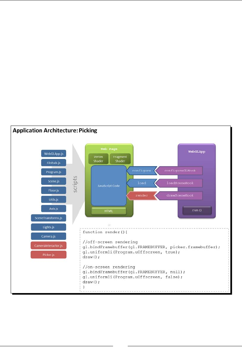
Chapter 8

[ 269 ]

Processing hits

Processing a hit is a very wide concept. It basically depends on the type of applicaon that

you are building. For instance if your applicaon is a CAD system, you might want to retrieve

on screen the properes of the object that you picked to edit them. You might also want to

move the object or change its dimensions. In contrast, if you are developing a game, you

could have selected the next target that your main character has to ght. We will leave this

part of the code for you to decide. Nevertheless, we have included a simple example in the

next Time for acon secon where you can drag-and-drop objects, which is one of the most

common interacons you could have with your scene.

Architectural updates

The picking method described in this chapter has been implemented in our architecture:

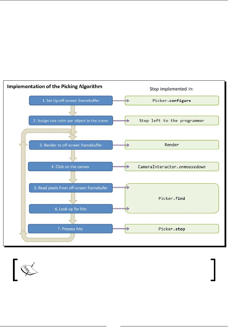
Picking

[ 270 ]

We have replaced the draw funcon with the render funcon. This funcon is the same

that we previously described in the secon Rendering to an oscreen framebuer.

There is a new class: Picker. The source code for this class can be obtained from /js/

webgl/Picker.js. This class encapsulates the oscreen framebuer and encapsulates

the code necessary to create it, congure it, and read from it.

We also updated the class CameraInteractor to nofy the picker whenever the user clicks

on the canvas. The following diagram explains how the picking algorithm is implemented

using the Render funcon and the classes Picker and CameraInteractor:

The source code for Picker and CameraInteractor can be found

in the code accompanying this chapter under /js/webgl.

Now let's see picking in acon!

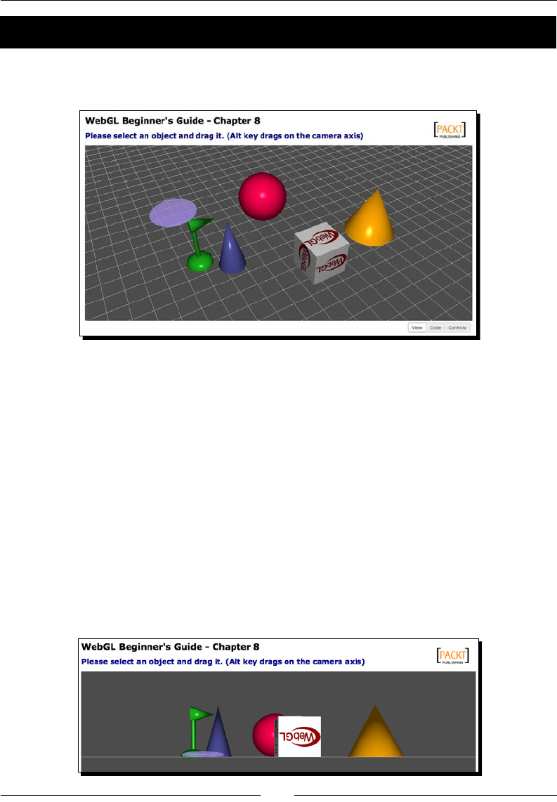
Chapter 8

[ 271 ]

Time for action – picking

1. Open the le ch8_Picking.html using your HTML5 Internet browser. You will see

a screen similar to this:

Here you have a set of objects, each one of which has a unique diuse color

property. As in the previous exercises you can rotate the camera around the scene.

Please noce that the cube has a texture and that the at disk is translucent. As you

may expect, the code in the draw funcon handles textures coordinates and also

transparencies, so it looks a bit more complex than before (you can check it out in

the source code). This is a more realisc draw funcon. In a real applicaon, you will

have to handle these variables.

2. Click on the sphere and drag it around the scene. Noce that the object becomes

translucent. Also, note that the displacement occurs along the axis of the camera.

To make this evident, please go to your web browser's console and type:

camera.setElevation(0);

You will see that the camera updates its posion to an elevaon of zero degrees

as shown in the following screenshot:

Picking

[ 272 ]

To access the console using:

Firefox go to Tools | Web Developer | Web Console

Safari go to Develop | Show Web Inspector

Chrome go to Tools | Javascript Console

3. Now when you click-and-drag objects in the scene from this perspecve, you will

see that they change their posion according to the camera axis. In this case the

up axis of the camera is aligned with the scene's y axis. If you move an object up

and down, you will see that they change their posion in the y coordinate. If you

change the camera posion (by clicking on the background and dragging the mouse

around) and then you pick and move a dierent object, you will see that this moves

according to the new camera axis.

Try dierent camera angles and see what happens.

4. Now let's see what the oscreen framebuer looks like. Click on the Show Picking

Image buon. Here we are instrucng the fragment shader to use each of the object

diuse properes to color the fragments. You can also rotate the scene and pick

objects in this mode. If you want to go back to the original shading method, click

again on Show Picking Image to deacvate it.

5. To reset the scene, click on Reset Scene.

What just happened?

We have seen an example of picking in acon. The source code uses the Picker object

that we previously described in the architectural update secon. Let's examine it a bit closer.

Picker architecture

The following diagram tells us what happens in the Picker object when the user clicks

the mouse on the canvas, drags it, and releases it:

Chapter 8

[ 273 ]

User interaction with Picker and Picker Callbacks

User clicks on Canvas

Picker seaches for hit

Picker finds hit

Start Picking Mode

in picking

list? Remove hit from picking list

Add hit to picking list

drags mouse

Stays in picking

mode

Is shift

pressed

releases mouse button

moveCallback

hitPropertyCallback

removeHitCallback

addHitCallback

End Picking Mode

processHitsCallback

yes

User

Picker

callback

As you can see, every picker state has a callback funcon associated to it:

State Callback

Picker searches for hit hitPropertyCallback(object): This callback informs the

picker which object property we will use to make the comparison

with the color retrieved from the oscreen framebuer.

User drags mouse in picking

mode

moveCallback(hits,interactor, dx, dy): When the

picking mode is acvated (by having picked at least one object), this

callback allows us to move the objects in the picking list (hits).

This list is maintained internally by the Picker class.

Remove hit from picking list addHitCallback(object): If we click on an object and this

object is not in the picking list, the picker noes the applicaon by

triggering this callback.

Add hit to picking list removeHitCallback(object): If we click on an object and

this object is already in the picking list, the picker will remove it

from the list and then it will inform the applicaon by triggering

this callback.

End Picking Mode processHitsCallback(hits): if the user releases the

mouse buon and the Shi key is not pressed when this happens,

then the picking mode nishes and the applicaon is noed by

triggering this callback. If the Shi key is pressed then the picking

mode connues and the picker waits for a new click to connue

looking for hits.

Picking

[ 274 ]

Implementing unique object labels

We previously menoned that picking based on the diuse property could be dicult if

two or more objects in the scene share the same diuse color. If that were the case and you

selected one of them, how would you know which one is picked based on its color? In the

next Time for Acon secon, we will implement unique object labels. The objects will be

rendered in the oscreen framebuer using these color labels instead of the diuse colors.

The scene will sll be rendered on screen using the non-unique diuse colors.

Time for action – unique object labels

This secon is divided in two parts. In the rst part you will develop the code to generate a

random scene with cones and cylinders. Each object will be assigned a unique object label

that will be used for coloring the object in the oscreen renderbuer. In the second part,

we will congure the picker to work with unique labels. Let's get started!

1. Creang a random scene: Open the ch8_Picking_Scene_Initial.html le in

your HTML5 browser. As you can see this is a scene that is only showing the oor

object. We are going to create a scene that contains mulple objects that can be

either balls or cylinders.

2. Open ch8_Picking_Scene_Initial.html in a source code editor.

We will write code so each object in the scene can have:

A posion assigned randomly

A unique object label color

A non-unique diuse color

A scale factor that will determine the size of the object

3. We have provided empty funcons that you will implement in this secon.

4. Let's start by wring the positionGenerator funcon. Scroll down to it

and add the following code:

function positionGenerator(){

var x = Math.floor(Math.random()*60);

var z = Math.floor(Math.random()*60);

var flagX = Math.floor(Math.random()*10);

var flagZ = Math.floor(Math.random()*10);

if (flagX >= 5) {x=-x;}

if (flagZ >= 5) {z=-z;}

return [x,0,z];

}

Chapter 8

[ 275 ]

Here we are using the Math.random funcon to generate the x and z coordinates

for an object in the scene. Since Math.random always returns a posive number,

we use the flagX and flagZ variables to randomly distribute the objects on

the x-z plane (oor). Also, as we want all the objects to be on the x-z plane, the y

component is set to zero in the return statement.

5. Now let's write a unique object label generator funcon. Scroll to the empty

objectLabelGenerator funcon and add this code:

var colorset = {};

function objectLabelGenerator(){

var color = [Math.random(), Math.random(),Math.random(),1.0];

var key = color[0] + ':' + color[1] + ':' + color[2];

if (key in colorset){

return uniqueColorGenerator();

}

else {

colorset[key] = true;

return color;

}

Here we are creang a random color using the Math.random funcon. If the

key variable is already a property of the colorset object then we call the

objectLabelGenerator funcon recursively; otherwise, we make key a property

of colorset and then return the respecve color. Noce how nicely the idea of

handling JavaScript objects as sets allows here to resolve possible key collisions.

6. Now write the diffuseColorGenerator funcon. We will use this funcon

to assign diuse properes to the objects.

function diffuseColorGenerator(index){

var c = (index % 30 / 60) + 0.2;

return [c,c,c,1];

}

This funcon represents the case where we want to generate colors that are not

unique. The index parameter represents the index of the object in the Scene.

objects list to which we are assigning the diuse color. In this funcon we are

creang a gray-level color as the r, g, and b components in the return statement

all have the same c value.

Picking

[ 276 ]

The diffuseColorGenerator funcon will create collisions every 30 indices. The

remainder of the division of the index by 30 will create a loop in the sequence:

0 % 30 = 0

1 % 30 = 1

…

29 % 30 = 29

30 % 30 = 0

31 % 30 = 1

…

As this result is being divided by 60, the result will be a number in the [0, 0.5]

range. Then we add 0.2 to make sure that the minimum value that c has is 0.2.

This way the objects will not look too dark during the onscreen rendering

(they would be black if the calculated diuse color were zero).

7. The last auxiliary funcon that we will write is the scaleGenerator funcon:

function scaleGenerator() {

var f = Math.random()+0.3;

return [f, f, f];

}

This funcon will allow us to have objects of dierent sizes. 0.3 is added to control

the minimum scaling factor that any object will have in the scene.

Now let's load 100 objects to our scene. By the end of this secon you will be able

to test picking on any of them!

8. Go to the load funcon and edit it so it looks like this:

function load(){

Floor.build(80,5);

Floor.pcolor = [0.0,0.0,0.0,1.0];

Scene.addObject(Floor);

var positionValue,

scaleFactor,

objectLabel,

objectType,

diffuseColor;

for (var i = 0; i < 100; i++){

positionValue = positionGenerator();

objectLabel = objectLabelGenerator();

scaleFactor = scaleGenerator();

diffuseColor = diffuseColorGenerator(i);

Chapter 8

[ 277 ]

objectType = Math.floor(Math.random()*2);

switch (objectType){

case 1: Scene.loadObject('models/geometry/sphere.

json',

'ball_'+i,

{

position:positionValue,

scale:scaleFactor,

diffuse:diffuseColor,

pcolor:objectLabel

});

break;

case 0: Scene.loadObject('models/geometry/cylinder.

json',

'cylinder_'+i,

{

position:positionValue,

scale:scaleFactor,

diffuse:diffuseColor,

pcolor:objectLabel

});

break;

}

Note here that the picking color is represented by the pcolor aribute. This

aribute is passed in a list of aributes to the loadObject funcon from the

Scene object. Once the object is loaded (using the JSON/Ajax mechanism discussed

in Chapter 2, Rendering Geometry), loadObject uses this list of aributes and adds

them as object properes.

9. Using unique labels in the fragment shader: The shaders in this exercise have

already been set up for you. The pcolor property that corresponds to the unique

object label is mapped to the uPickingColor uniform and the uOffscreen

uniform determines if it is used or not in the fragment shader:

uniform vec4 uPickingColor;

... //other uniforms and varyings

main(void){

if(uOffscreen){

Picking

[ 278 ]

gl_FragColor = uPickingColor;

return;

}

else {

... //on-screen rendering

}

10. As menoned before, we keep the oscreen and onscreen buer in sync using the

render funcon which looks like this:

function render(){

//off-screen rendering

gl.bindFramebuffer(gl.FRAMEBUFFER, picker.framebuffer);

gl.uniform1i(Program.uOffscreen, true);

draw();

//on-screen rendering

gl.uniform1i(Program.uOffscreen, showPickingImage);

gl.bindFramebuffer(gl.FRAMEBUFFER, null);

draw();

}

11. Save your work as ch8_Picking_Scene_NoPicker.html.

12. Open ch8_Picking_Scene_Final_NoPicker.html in your HTML5 Internet

browser. As you can see the scene is generated as expected.

13. Click on Show Picking Image. What happens?

14. The scene is being rendered in the oscreen framebuer and in the default

(onscreen) framebuer. However, we have not congured the Picker object

callbacks yet.

15. Conguring the picker to work with unique object labels: Open ch8_Picking_

Scene_Final_NoPicker.html in your source code editor.

16. Scroll down to the configure funcon. As you can see, the picker is already set up

for you:

picker = new Picker(canvas);

picker.hitPropertyCallback = hitProperty;

picker.addHitCallback = addHit;

picker.removeHitCallback = removeHit;

picker.processHitsCallback = processHits;

picker.moveCallback = movePickedObjects;

Chapter 8

[ 279 ]

This code fragment maps funcons in the web page to picker callback hooks. These

callbacks are invoked according to the picking state. If you need to review how this

works, please go back to the Picker Architecture secon.

In this part of the secon, we are going to implement these callbacks. Again, we

have provided empty funcons that you will need to code.

17. Let's create the hitProperty funcon. Scroll down to the empty hitProperty

funcon and add this code:

function hitProperty(ob){

return ob.pcolor;

}

Here we are telling the picker to use the pcolor property to make the comparison

with the color that will be read from the oscreen framebuer. If these colors match

then we have a hit.

18. Now we are going to write the addHit and removeHit funcons. We want to

create the eect where the diuse color is changed to the picking color during

picking. For that we need an extra property to save temporarily the original diuse

color so we can restore it later :

function addHit(ob){

ob.previous = ob.diffuse.slice(0);

ob.diffuse = ob.pcolor;

render();

}

The addHit funcon stores the current diuse color in an auxiliary property named

previous. Then it changes the diuse color to pcolor, the object picking label.

function removeHit(ob){

ob.diffuse = ob.previous.slice(0);

render();

}

The removeHit funcon restores the diuse color. In both funcons we are calling

render which we will implement later.

19. Now let's write the code for processHits:

function processHits(hits){

var ob;

for(var i = 0; i< hits.length; i+=1){

ob = hits[i];

ob.diffuse = ob.previous;

}

render();

}

Picking

[ 280 ]

Remember that processHits is called upon exing picking mode. This funcon

will receive one parameter: the hits that the picker detected. Each element of

the hits list is an object in the scene. In this case, we want to give back the hits

their diuse color. For that we use the previous property that we set in the

addHit funcon.

20. The last picker callback that we need to implement is the

movePickedObjects funcon:

function movePickedObjects(hits,interactor,dx,dy){

if (hits == 0) return;

var camera = interactor.camera;

var depth = interactor.alt;

var factor = Math.max(Math.max(

camera.position[0],

camera.position[1]),

camera.position[2])/1000;

var scaleX, scaleY;

for (var i = 0, max = hits.length; i < max; i+=1){

scaleX = vec3.create();

scaleY = vec3.create();

if (depth){

//moving along the camera normal vector

vec3.scale(camera.normal, dy * factor, scaleY);

}

else{

//moving along the plane defined by the up and right

//camera vectors

vec3.scale(camera.up, -dy * factor, scaleY);

vec3.scale(camera.right, dx * factor, scaleX);

}

vec3.add(hits[i].position, scaleY);

vec3.add(hits[i].position, scaleX);

}

render();

}

This funcon allows us to move the objects in the hits list interacvely.

The parameters that this callback funcon receives are:

hits: The list of objects that have been picked

interactor: The camera interactor object that is set up in the

configure funcon

Chapter 8

[ 281 ]

dx: Displacement in the horizontal direcon obtained from the mouse

when it is dragged on the canvas

dy: Displacement in the vercal direcon obtained from the mouse

when it is dragged on the canvas.

Let's analyze the code. First, if there are no hits the funcon returns immediately.

if (hits == 0) return;

Otherwise, we obtain a reference to the camera and we determine if the user

is pressing the Alt key.

var camera = interactor.camera;

var depth = interactor.alt;

We calculate a weighing factor that we will use later (fudge factor):

factor = Math.max(Math.max(

camera.position[0],

camera.position[1]),

camera.position[2])/1000;

Next we create a loop to go through the hits list so we can update each

object posion:

Var scaleX, scaleY;

for (var i = 0, max = hits.length; i < max; i+=1){

scaleX = vec3.create();

scaleY = vec3.create();

The scaleX and scaleY variables are inialized for every hit.

As we have seen in previous exercises, the Alt key is being used to perform dollying

(move the camera along its normal). In this case we want to move the objects that

are in the picking list along the camera normal direcon when the user is pressing

the Alt key to provide a consistent user experience.

To move the hits along the camera normal we use the dy (up-down) displacement

as follows:

if (depth){

vec3.scale(camera.normal, dy * factor, scaleY);

}

This creates a scaled version of camera.normal and stores it into the scaleY

variable. Noce that vec3.scale is an operaon available in the glMatrix library.

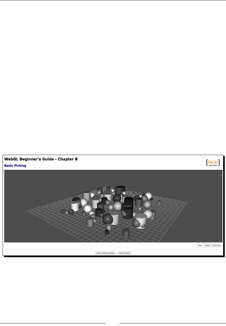
Picking

[ 282 ]

If the user is not pressing the Alt key then we use dx (le-right) and dy (up-down) to

move the hits in the camera plane. Here we use the camera up and right vectors

like this to calculate the scaleX and scaleY parameters:

else {

vec3.scale(camera.right, dx * factor, scaleX);

vec3.scale(camera.up, -dy * factor, scaleY);

}

Finally we update the posion of the hit:

vec3.add(hits[i].position, scaleY);

vec3.add(hits[i].position, scaleX);

}

Aer calculang the new posion for all hits we call render:

render();

}

21. Tesng the scene: Save the page as ch8_Picking_Scene_Final.html and open

it using your HTML5 web browser.

22. You will see a scene as shown in the following screenshot:

23. Click on Reset Scene several mes and verify that you get a new scene every me.

24. In this scene, all the objects have very similar colors. However, each one has

a unique picking color. To verify that click on the Show Picking Image buon.

You will see on screen what it is being rendered in the oscreen buer:

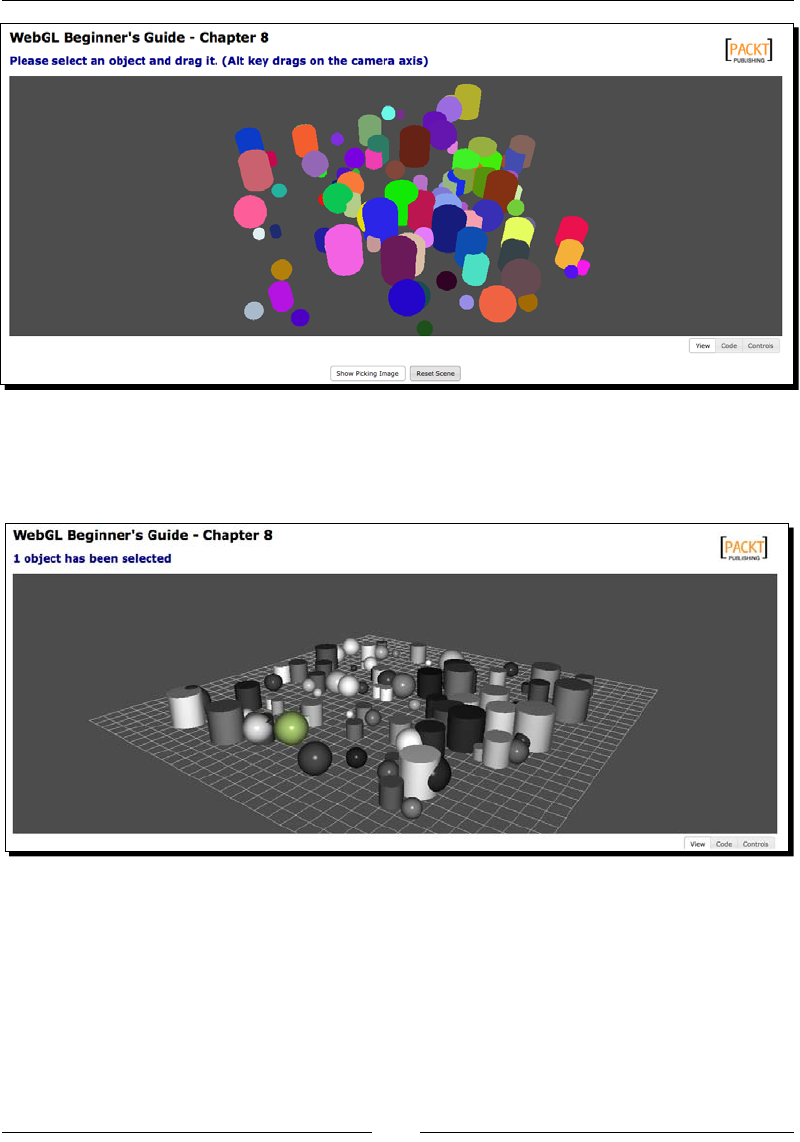
Chapter 8

[ 283 ]

25. Now let's validate the changes that we made to the picker callbacks. Let's start by

picking one object. As you see, the object diuse color becomes its picking color

(this was the change you implemented in the addHit funcon):

26. When the mouse is released, the object goes back to the original color! This is the

change that was implemented in the processHits funcon.

27. While the mouse buon is held down over an object, you can drag it around.

While this is done, the movePickedObjects is being invoked.

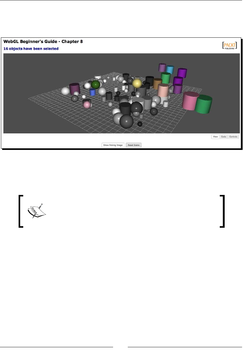
Picking

[ 284 ]

28. If the Shi key is pressed while objects are being selected, you will be telling the

picker not to exit picking mode. This way you can select and move more than one

object at once:

29. You will exit picking mode if you select an object and the Shi key is no longer

pressed or if your next click does not produce any hits (in other words: clicking

anywhere else).

If you have any problems with the exercise or you missed one

of the steps, we have included the complete exercise in the les

ch8_Picking_Scene_NoPicker.html and ch8_Picking_

Scene_Final.html.

What just happened?

We have done the following:

Created the property picking color. This property is unique for every object

in the scene and allows us to implement picking based on it.

Modied the fragment shader to use the picking color property by including

a new uniform: uPickingColor and mapping this uniform to the pcolor

object property.

Learned about the dierent picking states. We have also learned how to modify

the Picker callbacks to perform specic applicaon logic such as removing picked

objects from the scene.

Chapter 8

[ 285 ]

Have a go hero – clearing the scene

Rewrite the processHits funcon to remove the balls in the hit list from the scene.

If the user has removed all the balls from the scene then display a message telling the

elapsed me accomplishing this task.

Hint 1: Use Scene.removeObject(ob.alias) in the processHits funcon if alias

starts with ball_.

Hint 2: Once the hits are removed from the scene, go again through the Scene.objects list

and make sure that there are no objects whose alias starts with ball_.

Hint 3: Use a JavaScript mer to measure and display the elapsed me unl task compleon.

Summary

In this chapter, we have learned how to implement color-based picking in WebGL. Picking

based on a diuse color is a bad idea because there could be scenarios where several objects

have the same diuse color. It is beer to assign a new color property that is unique for

every object to perform picking. We called this property picking color/object label.

Through the discussion of the picking implementaon, we learned that WebGL provides

mechanisms to create oscreen framebuers and that what we see on screen when we

render a scene corresponds to the default framebuer contents.

We also studied the dierence between a framebuer and a renderbuer. We saw that a

renderbuer is a special buer that is aached to a framebuer. Renderbuers are used

to store informaon that does not have a texture representaon such as depth values.

In contrast, textures can be used to store colors.

We saw too that a framebuer needs at least one texture to store colors and a renderbuer

to store depth informaon.

We discussed how to convert from clicking coordinates in the page to canvas coordinates.

We said also that the framebuer coordinates and the canvas coordinates originate in the

lower-le corner with a (0,0) origin.

The architecture of the picker implementaon was discussed. We saw that picking can have

dierent states and that each state can be associated to a callback funcon. Picker callbacks

allow coding-specic logic applicaon that will determine what we see in our scene when

picking is in progress.

In the next chapter, we will develop a car showroom applicaon. We will see how to import

car models from Blender into a WebGL applicaon.

Putting It All Together

In this chapter, we will apply the concepts and use the infrastructure code that

we have previously developed to build a Virtual Car Showroom. During the

development of this demo applicaon, we will use models, lights, cameras,

animaon, colors, and textures. We will also see how we can integrate these

elements with a simple yet powerful graphical user interface.

This chapter talks about:

The architecture that we have developed throughout the book

Creang a virtual car showroom applicaon using our architecture

Imporng car models from Blender into a WebGL scene

Seng up several light sources

Creang robust shaders to handle mulple materials

The OBJ and MTL le formats

Programming the camera to y through the scene

Creating a WebGL application

At this point, we have covered the basic topics that you need to be familiar with in order to

create a WebGL applicaon. These topics have been implemented in the infrastructure code

that we have iteravely built up throughout the book. Let's see what we have learned so far.

In Chapter 3, Lights!, we introduced WebGL and learned how to enable it in our browser.

We also learned that WebGL behaves as a state machine and that we can query the dierent

variables that determine the current state using gl. getParameter.

Pung It All Together

[ 288 ]

Aer that, we studied in Chapter 2, Rendering Geometry, that the objects of a WebGL scene

are dened by verces. We said that usually we use indices to label those verces so we can

quickly tell WebGL how to 'connect the dots' to render the object. We studied the funcons

that manipulate buers and the two main funcons to render geometry drawArrays

(no indices) and drawElements (with indices). We also learned about the JSON format to

represent geometry and how we can download models from a web server using AJAX.

In Chapter 3, Lights!, we studied about lights. We learned about normal vectors and the

physics of light reecon. We saw how to implement dierent lighng models using shaders

in ESSL.

We learned in Chapter 4, Camera, that WebGL does not have cameras and that we need to

dene our own cameras. We studied the Camera matrix and we showed that the Camera

matrix is the inverse of the Model-View matrix. In other words, rotaon, translaon, and

scaling in the world space produce the inverse operaons in camera space.

The basics of animaon were covered in Chapter 5, Acon. We discussed the matrix stack

with its push and pop operaons to represent local object transformaons. We also analyzed

how to set up an animaon cycle that is independent from the rendering cycle. We also

studied dierent types of interpolaon and saw examples of how interpolaon is used to

create animaons.

In Chapter 6, Colors, Depth Tesng, and Alpha Blending, we discussed a bit deeper about

color representaon and how we can use colors in objects, in lights, and in the scene.

We also studied blending and the use of transparencies.

Chapter 7, Textures, covered textures and we saw an implementaon for picking in Chapter

8, Picking.

In this chapter, we will use our knowledge to create a simple applicaon. Fortunately,

we are going to use all the infrastructure code that we have developed so far. Let's review it.

Architectural review

The following diagram presents the architecture that has been built throughout the book:

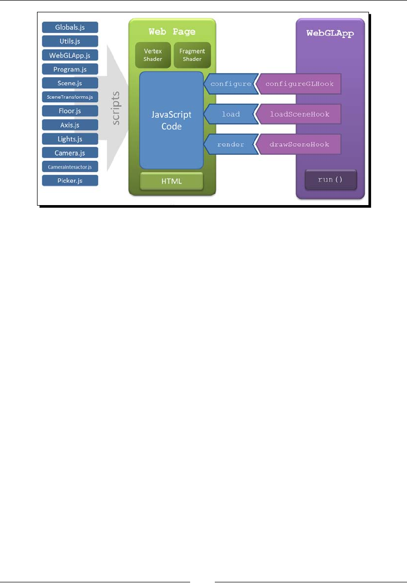
Chapter 9

[ 289 ]

Globals.js: Denes the global variables gl (WebGL context), prg (ESSL program),

and the canvas width (c_width) and height (c_height).

Utils.js: Contains auxiliary funcons such as getGLContext which tries to create

a WebGL context for a given HTML5 canvas.

WebGLApp.js: It provides three funcon hooks, namely: configureGLHook,

loadSceneHook, and drawSceneHook that dene the life cycle of a WebGL applicaon.

As the previous diagram shows these hooks are mapped to JavaScript funcons in our

web page:

configure: Here we create cameras, lights, and instanate the Program.object.

load: Here we request objects from the web server by calling Scene.loadObject.

We can also add locally generated geometry (such as the Floor) by calling Scene.

addObject.

render (or draw): This is the funcon that is called every me when the rendering

mer goes o. Here we will retrieve the objects from the Scene, one by one, and we

will render them paying aenon to their locaon (applying local transforms using

the matrix stack), and their properes (passing the respecve uniforms to

the Program).

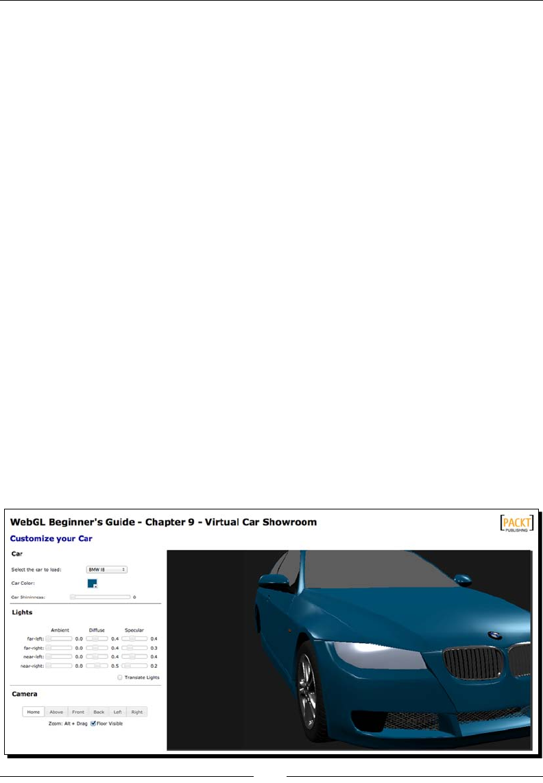
Pung It All Together

[ 290 ]

Program.js: Is composed of the funcons that handle programs, shaders, and the mapping

between JavaScript variables and ESSL uniforms.

Scene.js: Contains a list of objects to be rendered by WebGL.

SceneTransform.js: Contains the matrices discussed in the book: The Model-View

matrix, the Camera matrix, the Perspecve matrix, and the Normal matrix. It implements

the matrix stack with the operaons push and pop.

Floor.js: Auxiliary object that when rendered appears like a rectangular mesh providing

the oor reference for the scene.

Axis.js: Auxiliary object that represents the center of the scene.

Lights.js: Simplies the creaon and managing of lights in the scene.

Camera.js: Contains a camera representaon. We have developed two types of camera:

orbing and tracking.

CameraInteractor.js: Listens for mouse and keyboard events on the HTML5 canvas that

it is being used. It interprets these events and then transforms them into camera acons.

Picker.js: Provides color-based object picking.

Let's see how we can put everything together to create a Virtual Car Showroom.

Virtual Car Showroom application

Using our WebGL skills and the infrastructure code that we have developed, we will

create an applicaon that allows visualizing dierent 3D car models. The nal result will

look like this:

Chapter 9

[ 291 ]

First of all, we need to dene what the graphical user interface (GUI) is going to look like.

Then, we will be adding WebGL support by creang a canvas element and obtaining the

correspondent WebGL context. Simultaneously, we need to dene and implement the

Vertex Shader and Fragment Shader using ESSL. Aer that, we need to implement the three

funcons that constute the lifecycle of our applicaon: configure, load, and render.

First, let's consider some parcularies of our virtual showroom applicaon.

Complexity of the models

A real-world applicaon is dierent from a proof of concept demo in that the models that

we will be loading are much more detailed than simple spheres, cones, and other geometric

gures. Usually, models have lots of verces conforming very complicated conguraons

that give the level of detail and realism that people would expect. Also, in many cases, these

models are accompanied by one or more textures. Creang the geometry and the texture

mapping by hand in JSON les is nothing less than a daunng task.

Hopefully, we can use 3D design soware to create our own models and then import them

into a WebGL scene. For the Virtual Car Showroom we will use models created with Blender.

Blender is an open-source 3D computer graphics soware that allows you to create

animaons, games, and other interacve applicaons. Blender provides numerous features

to create complex models. In this chapter, we will import car models created with Blender

into a WebGL scene. To do so, we will export them to an intermediary le format called OBJ

and then we will parse OBJ les into JSON les.

Shader quality

Because we will be using complex models, such as cars, we will see that there is a need to

develop shaders that can render the dierent materials that our models are made of. This

is not a big deal for us since the shaders that we previously developed can handle diuse,

specular, and ambient components for materials. In Blender, we will select the opon to

export materials when generang the OBJ les. When we do so, Blender will generate a

second le known as the Material Template Library (MTL). Also, our shaders will use

Phong shading, Phong lighng, and will support mulple lights.

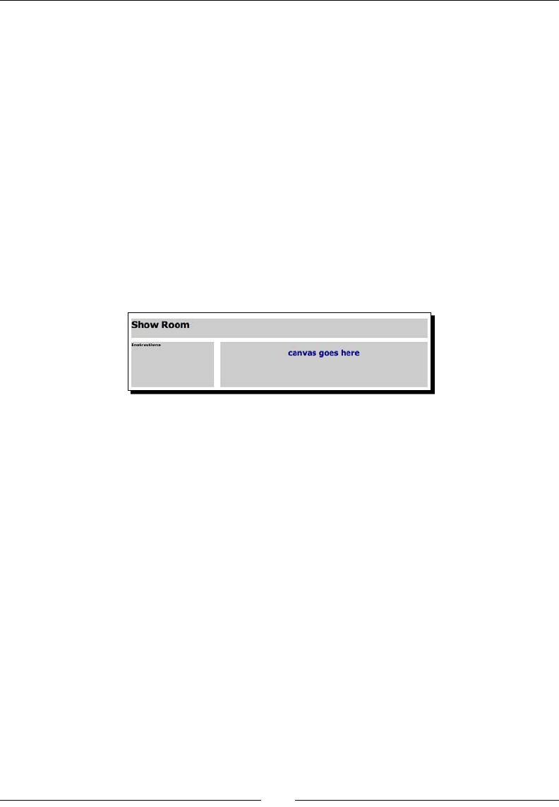
Pung It All Together

[ 292 ]

Network delays and bandwidth consumption

Due to the nature of WebGL, we will need to download the geometry and the textures from

a web server. Depending on the quality of the network connecon and the amount of data

that needs to be transferred this can take a while. There are several strategies that you

could invesgate, such as geometry compression. Another alternave is background data

downloading (using AJAX for example) while the applicaon is idle or the user is busy and

not waing for something to download.

With these consideraons in mind let's get started.

Dening what the GUI will look like

We will dene a very simple layout for our applicaon. The tle will go on top, and then we

have two div tags. The div on the le will contain the instrucons and the tools we can use

on the scene. The canvas will be placed inside the div on the right, shown as follows:

The code to achieve this layout looks like this (css/cars.css):

#header

{

height: 50px;

background-color: #ccc;

margin-bottom: 10px;

}

#nav

{

float: left;

width: 28%;

height: 80%;

background-color: #ccc;

margin-bottom: 1px;

}

#content

{

float: right;

Chapter 9

[ 293 ]

margin-left: 1%;

width: 70%;

height: 80%;

background-color: #ccc;

margin-bottom: 1px;

}

And we can use it like this (taken from ch9_GUI.html):

<body>

</div>

<b>Instructions</b>

</div>

<h2>canvas goes here</h2>

</div>

</body>

Please make sure that you include cars.css in your page. As you can see in ch9_GUI.

html, cars.css has been included in the header secon:

Now let's add the canvas. Replace:

<h2>canvas goes here</h2>

With:

inside the content div.

Adding WebGL support

Now, please check the source code for ch9_Scaffolding.html. We have taken ch9_GUI.

html which denes the basic layout and we have added the following:

References to the elements dened in our architecture: Globals.js, Utils.js,

Program.js, and so on.

A reference to glMatrix.js, the matrix manipulaon library that we use in

our architecture.

Pung It All Together

[ 294 ]

References to JQuery and JQuery UI.

References to the JQuery UI customized theme that we used in the book.

We have created the scaolding for the three main funcons that we will

need to develop in our applicaon: congure, load and render.

Using JQuery we have included a funcon that allows resizing the canvas

to its container:

function resizeCanvas(){

c_width = $('#content').width();

c_height = $('#content').height();

$('#the-canvas').attr('width',c_width);

$('#the-canvas').attr('height',c_height);

}

We bind this funcon to the resize event of the window here:

$(window).resize(function(){resizeCanvas();});

This funcon is very useful because it allows us adapt the size of the canvas

automacally to the available window space. Also, we do not need to hardcode

the size of the canvas.

As in all previous exercises, we need to dene the entry point for the applicaon.

We do this here:

var app;

function runShowRoom(){

app = new WebGLApp("the-canvas");

app.configureGLHook = configure;

app.loadSceneHook = load;

app.drawSceneHook = render;

app.run();

}

And we bind it to the onLoad event:

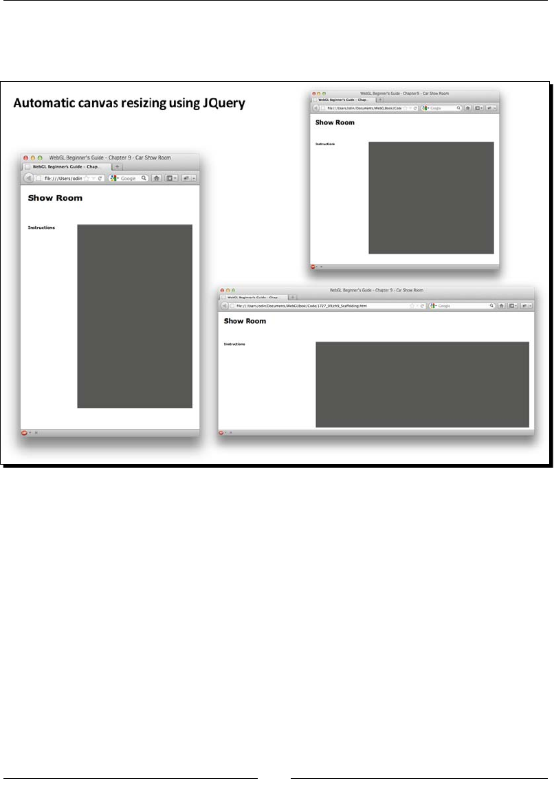
Chapter 9

[ 295 ]

Now if you run ch9_Scaffolding.html in your HTML5-enabled web browser, you will see

that the canvas resizes according to the current size of content, its parent container, shown

as follows:

Implementing the shaders

The shaders in this chapter will implement Phong shading and the Phong reecon model.

Remember that Phong shading interpolates vertex normals and creates a normal for every

fragment. Aer that, the Phong reecon model describes the light that an object reects

as the addion of the ambient, diuse, and specular interacon of the object with the light

sources present in the scene.

Pung It All Together

[ 296 ]

To keep consistency with the Material Template Library (MTL) format, we will use the

following convenon for the uniforms that refer to material properes:

Material

Uniform

Descripon

uKa Ambient property

uKd Diuse property

uKs Specular property

uNi Opcal density. We will not use this feature but you will see it on the MTL le.

uNs Specular exponent. A high exponent results in a ght, concentrated highlight. Ns

values normally range from 0 to 1000.

dTransparency (alpha channel)

illum Determines the illuminaon model for the object being rendered. Unlike previous

chapters where we had one model for all the objects, here we let the object to

decide how it is going to reect the light.

According to the MTL le format specicaon illum can be:

0: Diuse on and Ambient o (purely diuse)

1: Diuse on and Ambient on

2: Highlight on (Phong illuminaon model)

There are other values that are dened in the MTL specicaon that we menon

here for completeness but that our shaders will not implement. These values are:

3: Reecon on and Ray trace on

4: Transparency: Glass on, Reecon: Ray trace on

5: Reecon: Fresnel on and Ray trace on

6: Transparency: Refracon on, Reecon: Fresnel o and Ray trace on

7: Transparency: Refracon on, Reecon: Fresnel on and Ray trace on

8: Reecon on and Ray trace o

9: Transparency: Glass on, Reecon: Ray trace o

10: Casts shadows onto invisible surfaces

The shaders that we will use support mulple lights using uniform arrays as we saw in

Chapter 6, Colors, Depth Tesng, and Alpha Blending. The number of lights is dened

by a constant in both the Vertex and the Fragment shaders:

const int NUM_LIGHTS = 4;

Chapter 9

[ 297 ]

We will use the following uniform arrays to work with lights:

Light

Uniform Array

Descripon

uLa[NUM_LIGHTS] Ambient property

uLd[NUM_LIGHTS] Diuse property

uLs[NUM_LIGHTS] Specular property

Please refer to ch9_Car_Showroom.html to explore the source code

for the shaders in this chapter.

Next, we are going to work on the three main funcons that constute the lifecycle

of our WebGL applicaon. These are the configure, load, and render funcons.

Setting up the scene

We set up the scene by wring the code for the configure funcon. Let's analyze it line

by line:

var camera = null, transforms = null;

function configure(){

At this stage, we want to set some of the WebGL properes such as the clear color and

the depth test. Aer that, we need to create a camera and set its original posion and

orientaon. Also we need to create a camera interactor so that we can update the camera

posion when we click and drag on the HTML5 canvas in our web page. Finally, we want

to dene the JavaScript variables that will be mapped to the shaders. We can also inialize

some of them at this point.

To accomplish the aforemenoned tasks we will use Camera.js, CameraInteractor.js,

and Program.js and SceneTransforms.js from our architecture.

Conguring some WebGL properties

Here we set the background color and the depth test properes as follows:

gl.clearColor(0.3,0.3,0.3, 1.0);

gl.clearDepth(1.0);

gl.enable(gl.DEPTH_TEST);

gl.depthFunc(gl.LEQUAL);

Pung It All Together

[ 298 ]

Setting up the camera

The camera variable needs to be global so we can access it later on from the GUI funcons

that we will write. For instance, we want to be able to click on a buon (dierent funcon

in the code) and use the camera variable to update the camera posion:

camera = new Camera(CAMERA_ORBITING_TYPE);

camera.goHome([0,0,7]);

camera.setFocus([0.0,0.0,0.0]);

camera.setAzimuth(25);

camera.setElevation(-30);

The azimuth and elevaon of the camera are relave to the negave z-axis, which will be

the default pose if you do not specify any other. An azimuth of 25 degrees and elevaon

of -30 degrees will give you a nice inial angle to see the cars. However, you can set any

combinaon that you prefer as the default pose in here.

Here we make sure that the camera's rendering callback is our rendering funcon:

camera.hookRenderer = render;

Creating the Camera Interactor

We create a CameraInteractor that will bind the mouse gestures to camera acons.

The rst argument here is the camera we are controlling and the second element is a DOM

reference to the canvas in our webpage:

var interactor = new CameraInteractor(camera, document.

getElementById('the-canvas');

The SceneTransforms object

Once we have instanated the camera, we create a new SceneTransforms object passing

the camera to the SceneTransforms constructor as follows:

transforms = new SceneTransforms(camera);

transforms.init();

The transforms variable is also declared globally so we can use it later in the rendering

funcon to retrieve the current matrix transformaons and pass them to the shaders.

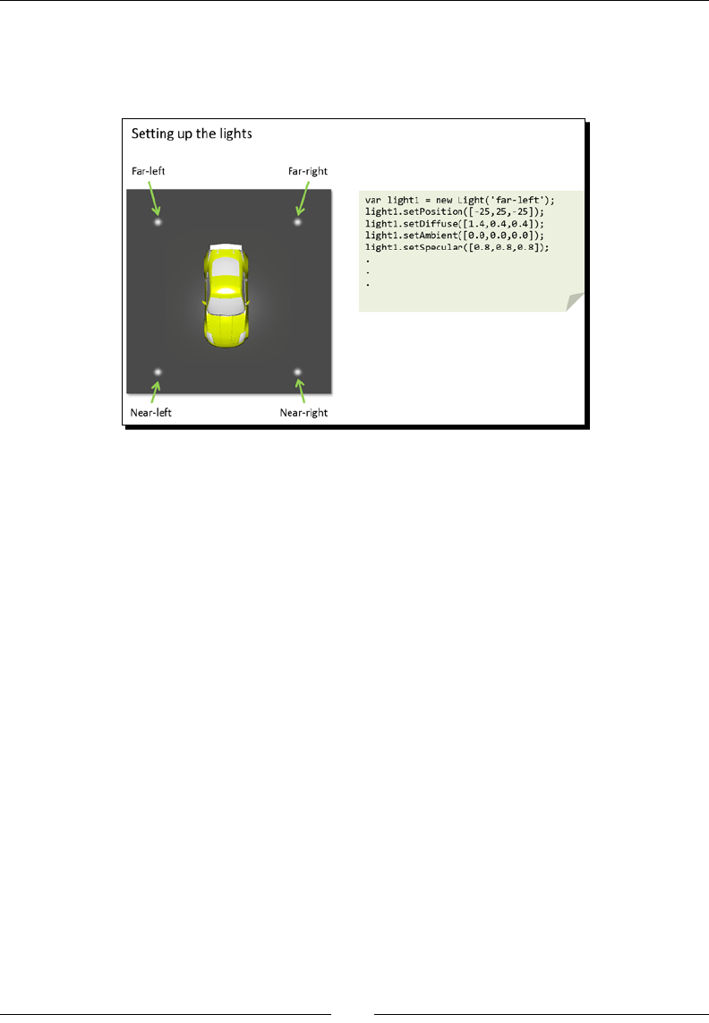
Chapter 9

[ 299 ]

Creating the lights

We will create four lights using the Light object from our infrastructure code. The scene will

look like in the following image:

For each light we will create a Light object:

var light1 = new Light('far-left');

light1.setPosition([-25,25,-25]);

light1.setDiffuse([1.4,0.4,0.4]);

light1.setAmbient([0.0,0.0,0.0]);

light1.setSpecular([0.8,0.8,0.8]);

var light2 = new Light('far-right');

light2.setPosition([25,25,-25]);

light2.setDiffuse([0.4,1.4,0.4]);

light2.setAmbient([0.0,0.0,0.0]);

light2.setSpecular([0.8,0.8,0.8]);

var light3 = new Light('near-left');

light3.setPosition([-25,25,25]);

light3.setDiffuse([0.5,0.5,1.5]);

light3.setAmbient([0.0,0.0,0.0]);

light3.setSpecular([0.8,0.38,0.38]);

var light4 = new Light('near-right');

light4.setPosition([25,25,25]);

light4.setDiffuse([0.2,0.2,0.2]);

light4.setAmbient([0.0,0.0,0.0]);

light4.setSpecular([0.38,0.38,0.38]);

Pung It All Together

[ 300 ]

Then, we add them to the Lights list (also dened in Lights.js):

Lights.add(light1);

Lights.add(light2);

Lights.add(light3);

Lights.add(light4);

Mapping the Program attributes and uniforms

The last thing to do inside configure funcon is to map the JavaScript variables that

we will use in our code to the aributes and uniforms that we will use in the shaders.

Using the Program object from our infrastructure code, we will set up the JavaScript

variables that we will use to map aributes and uniforms to the shaders. The code looks

like this:

var attributeList = ["aVertexPosition",

"aVertexNormal",

"aVertexColor"];

var uniformList = [ "uPMatrix",

"uMVMatrix",

"uNMatrix",

"uLightPosition",

"uWireframe",

"uLa",

"uLd",

"uLs",

"uKa",

"uKd",

"uKs",

"uNs",

"d",

"illum"];

Program.load(attributeList, uniformList);

When creang your own shaders, make sure that the shader aributes

and uniforms are properly mapped to JavaScript variables. Remember that

this mapping step allows us referring to aributes and uniforms through

their locaon. In this way, we can pass aribute and uniform values to the

shaders. Please check the methods setAttributeLocations and

setUniformLocations, which are called by load in the Program object

(Program.js) to see how we do the mapping in the infrastructure code.

Chapter 9

[ 301 ]

Uniform initialization

Aer the mapping, we can inialize shader uniforms such as lights:

gl.uniform3fv(Program.uLightPosition, Lights.getArray('position'));

gl.uniform3fv(Program.uLa, Lights.getArray('ambient'));

gl.uniform3fv(Program.uLd, Lights.getArray('diffuse'));

gl.uniform3fv(Program.uLs, Lights.getArray('specular'));

The default material properes are as follows:

gl.uniform3fv(Program.uKa , [1.0,1.0,1.0]);

gl.uniform3fv(Program.uKd , [1.0,1.0,1.0]);

gl.uniform3fv(Program.uKs , [1.0,1.0,1.0]);

gl.uniform1f(Program.uNs , 1.0);

}

With that, we have nished seng up the scene.

Loading the cars

Next, we need to implement the load funcon. Here is where we usually use AJAX to

download the objects that will appear on the scene.

When we have the JSON les corresponding to the cars the procedure is really simple, we

just use the Scene object to load these les. However, most commonly than not, you will

not have ready-to-use JSON les. As menoned at the beginning of this chapter, there are

specialized design tools such as Blender that allow creang these models.

Nonetheless, we are assuming that you are not an expert 3D modeler (neither we are).

So we will use pre-built models. We will use cars from blendswap.org, these models

are publically available, free of charge, and free to distribute.

Before we can use the models, we need to export them to an intermediate le format

from where we can extract the geometry and the material properes so we can create

our corresponding JSON les. The le format that we are going to use is Wavefront OBJ.

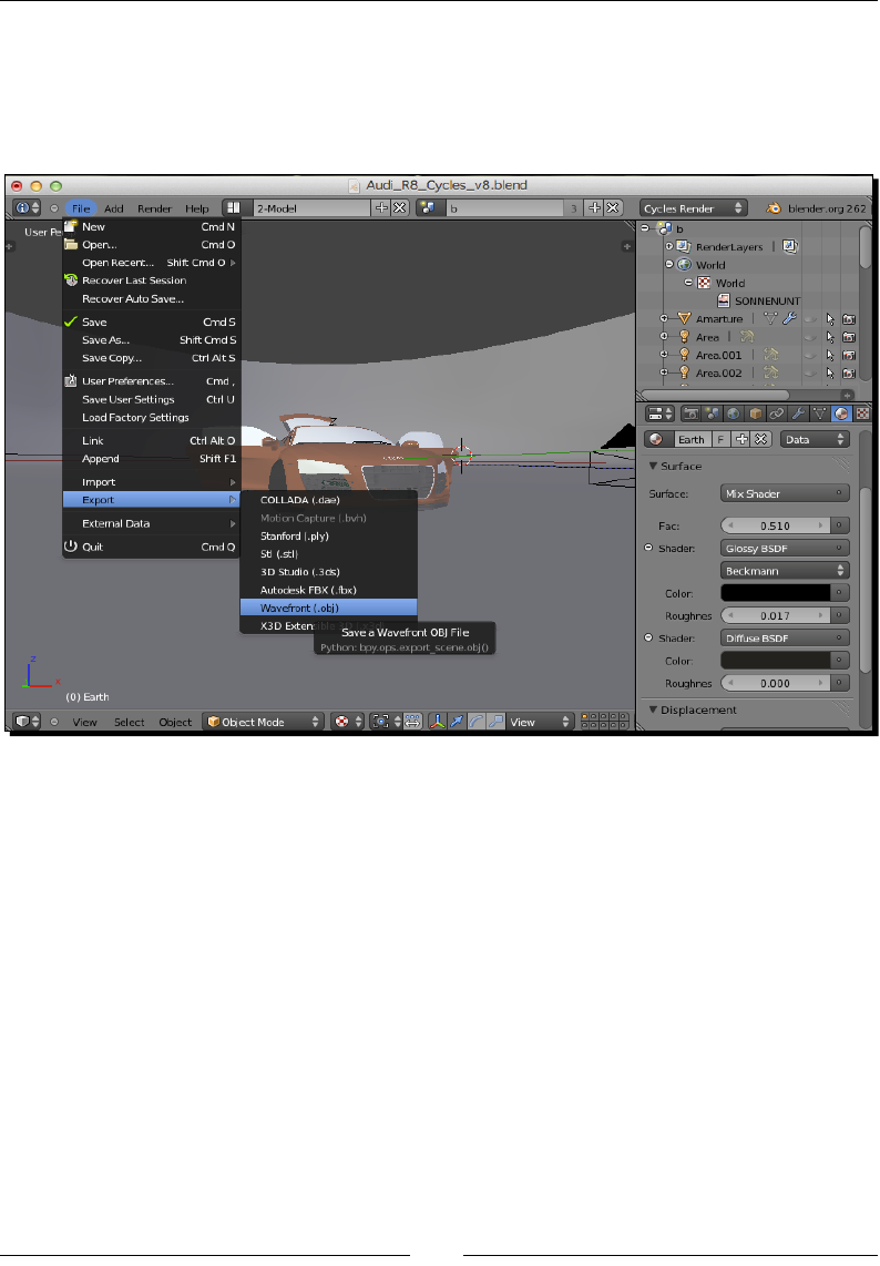
Pung It All Together

[ 302 ]

Exporting the Blender models

Here we are using the current Blender version (2.6). Once you have loaded the car that you

want to render in WebGL you need to export it as an OBJ le. To do so go to File | Export |

Wavefront (.obj) as shown in the following screenshot:

In the Export OBJ panel, make sure that the following opons are acve:

Apply Modiers: This will write the verces in the scene that are the result of

a mathemacal operaon instead of direct modeling. For instance, reecons,

smoothing, and so on. If you do not check this opon, the model may appear

incomplete in the WebGL scene.

Write Materials: Blender will create the correspondent Material Template Library

(MTL le). More about this in the following secon.

Triangulate Faces: Blender will write the indices as triangles. Ideal for

WebGL rendering.

Objects as OBJ Objects: This conguraon will idenfy every object in the Blender

scene as an object in the OBJ le.

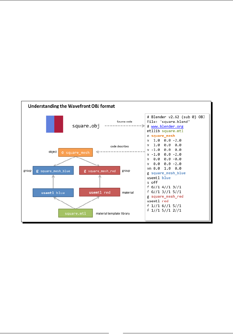
Chapter 9

[ 303 ]

Material Groups: If an object in the Blender scene has several materials, for instance

a car re can have aluminum and rubber, then the object will be subdivided into

groups, one per material in the OBJ le. Once you have checked these export

parameters, select the directory and the name for your OBJ le and then click

on Export.

Understanding the OBJ format

There are several types of denions in an OBJ le. Let's see them with a line-by-line

example. We are going to dissect the le square.obj that we have exported from the

Blender le square.blend. This le represents a square divided into two parts, one

painted in red and the other painted in blue, as shown in the following image:

When we export Blender models to the OBJ format, the resulng le would normally start

with a comment:

# Blender v2.62 (sub 0) OBJ File: 'squares.blend'

# www.blender.org

As we can see here, comments are denoted with a hash (#) symbol at the beginning

of the line.

Pung It All Together

[ 304 ]

Next, we will usually nd a line referring to the Material Template Library that this OBJ le is

using. Such line will start with the keyword mtllib followed by the name of the materials

library le:

mtllib square.mtl

There are several ways in which geometries can be grouped into enes in an OBJ le.

We can nd lines starng with the prex o followed by the object name; or by the prex g,

followed again by the group name:

o squares_mesh

Aer an object declaraon, the following lines will refer to verces (v) and oponally to

vertex normals (vn) and texture coordinates (vt). It is important to menon that verces

are shared by all the groups in an object in the OBJ format. That is, you will not nd lines

referring to verces when dening a group because it is assumed that all vertex data was

dened rst when the object was dened:

v 1.0 0.0 -2.0

v 1.0 0.0 0.0

v -1.0 0.0 0.0

v -1.0 0.0 -2.0

v 0.0 0.0 0.0

v 0.0 0.0 -2.0

vn 0.0 1.0 0.0

In our case, we have instructed Blender to export group materials. This means that each

part of the object that has dierent set of material properes will appear in the OBJ le as

a group. In this example, we are dening an object with two groups (squares_mesh_blue

and squares_mesh_red) and two corresponding materials (blue and red):

g squares_mesh_blue

If materials are being used, the line aer the group declaraon will be the material that is

being used for that group. Here only the name of the material is required. It is assumed that

the material properes for this material are dened in the Material Template Library le that

was declared at the beginning of the OBJ le:

usemtl blue

The lines that start with the prex s refer to smooth shading across polygons. We menon it

here in case you see it on your les but we will not be using this denion when parsing the

OBJ les into JSON les:

s off

Chapter 9

[ 305 ]

The lines that start with f refer to faces. There are dierent ways to represent faces.

Let's see them:

Vertex:

f i1 i2 i3...

In this conguraon, every face element corresponds to a vertex index. Depending

on the number of indices per face, you could have triangular, rectangular, or

polygonal faces. However, we have instructed Blender to use triangular faces to

create the OBJ le. Otherwise, we would need to decompose the polygons into

triangles before we could call drawElements.

Vertex / Texture Coordinate:

f i1/t1 i2/t2 i3/t3...

In this combinaon, every vertex index appears followed by a slash sign and a

texture coordinate index. You will normally nd this combinaon when texture

coordinates are dened at the object level with vt.

Vertex / Texture Coordinate / Normal:

f i1/t1/n1 i2/t2/n2 i3/t3/n3...

Here a normal index has been added as the third element of the conguraon. If

both texture coordinates and vertex normals are dened at the object level, you

most likely see this conguraon at the group level.

Vertex // Normal:

There could also be a case where normals are dened but not texture coordinates.

In this case, the second part of the face conguraon is missing:

f i1//n1 i2//n2 i3//n3...

This is the case for square.obj, which looks like this:

f 6//1 4//1 3//1

f 6//1 3//1 5//1

Please noce that faces are dened using indices. In our example, we have

dened a square divided in two parts. Here we can see that all verces

share the same normal idened with index 1.

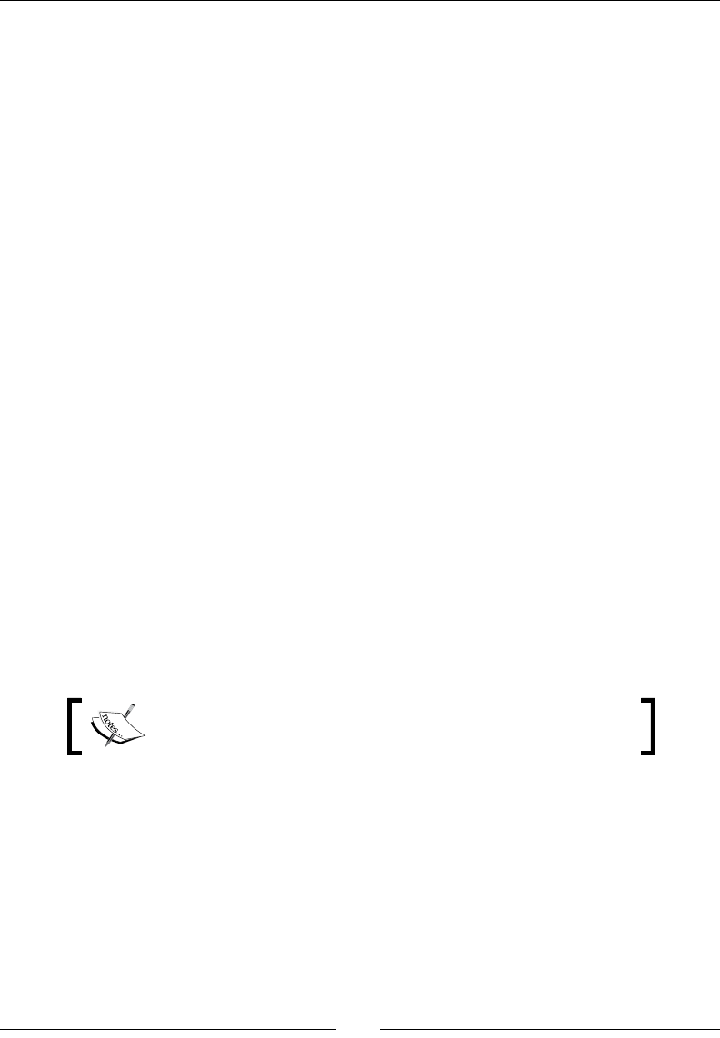
Pung It All Together

[ 306 ]

The remaining lines in this le represent the red group:

g squares_mesh_red

usemtl red

f 1//1 6//1 5//1

f 1//1 5//1 2//1

As menoned before, groups belonging to the same object share indices.

Parsing the OBJ les

Aer exporng our cars to the OBJ format, the next step is parse the OBJ les to create

WebGL JSON les that we can load into our scene. We have included the parser that we

developed for this step into the code les accompanying this chapter. This parser has the

following features:

It is wrien in python and can be called on the command line like this:

obj_parser.py arg1 arg2

Where arg1 is the name of the obj le to parse and arg2 is the name of the

Material Template Library. The le extension is needed in both cases. For example:

obj_parser.py square.obj square.mtl

It creates one JSON le per OBJ group.

It searches into the Material Template Library (if dened) for the material properes

for each group and adds them to the correspondent JSON le.

It will calculate the appropriate indices for each group. Remember that OBJ groups

share indices. Since we are creang one independent WebGL object per group, each

object needs to have indices starng in zero. The parser takes care of this for you.

If you do not have python installed in your system you can get it

from: http://www.python.org/

The following diagram summarizes the procedure to create JSON les from

Blender scenes:

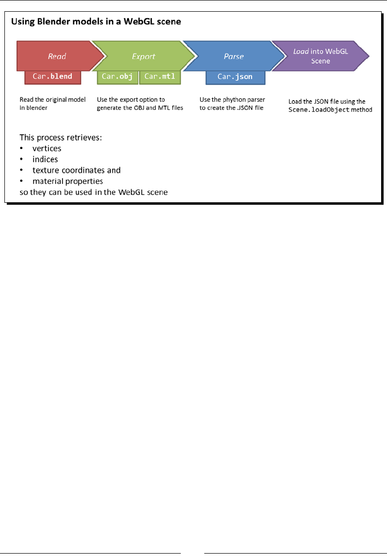
Chapter 9

[ 307 ]

Load cars into our WebGL scene

Now we have cars stored as JSON les, ready to be used in our WebGL scene. Now we have

to let the user tell us which car he wants to visualize. We could, however, load by default one

of the cars so our GUI looks more aracve. To do so, we will write the following code inside

the load funcon (nally!):

function load(){

loadBMW();

}

// The bmw model has 24 parts. We retrieve them all in a loop

function loadBMW(){

for(var i = 1; i <= 24; i+=1){

Scene.loadObject('models/cars/bmw/part'+i+'.json');

}

We will add other cases later on.

Pung It All Together

[ 308 ]

Rendering

Let's take a step back to take a look at the big picture. We menoned before that in our

architecture we have dened three main funcons that dene the lifecycle of our WebGL

applicaon. These funcons are: configure, load, and render.

Up to this point, we have set up the scene wring the code for the configure funcon.

Aer that, we have created our JSON cars and loaded them by wring the code for the load

funcon. Now, we will implement the code for the third funcon: the render funcon.

The code is prey standard and almost idencal to the draw/render funcons that we

have wrien in previous chapters. As we can see in the following diagram, we set and clear

the area that we are going to draw on, then we check on the camera perspecve and then

we process every object in Scene.objects.

The only consideraon that we need to have here is to make sure that we are mapping

correctly the material properes dened in our JSON objects to the appropriate shader

uniforms. The code that takes care of this in the render funcon looks like this:

gl.uniform3fv(Program.uKa, object.Ka);

gl.uniform3fv(Program.uKd, object.Kd);

gl.uniform3fv(Program.uKs, object.Ks);

gl.uniform1f(Program.uNi, object.Ni);

gl.uniform1f(Program.uNs, object.Ns);

gl.uniform1f(Program.d, object.d);

gl.uniform1i(Program.illum, object.illum);

If you want, please take a look at the list of uniforms that was dened in the secon

Implemenng the shaders. We need to make sure that all the shader uniforms are paired

with object aributes.

The following diagram shows the process inside the render funcon:

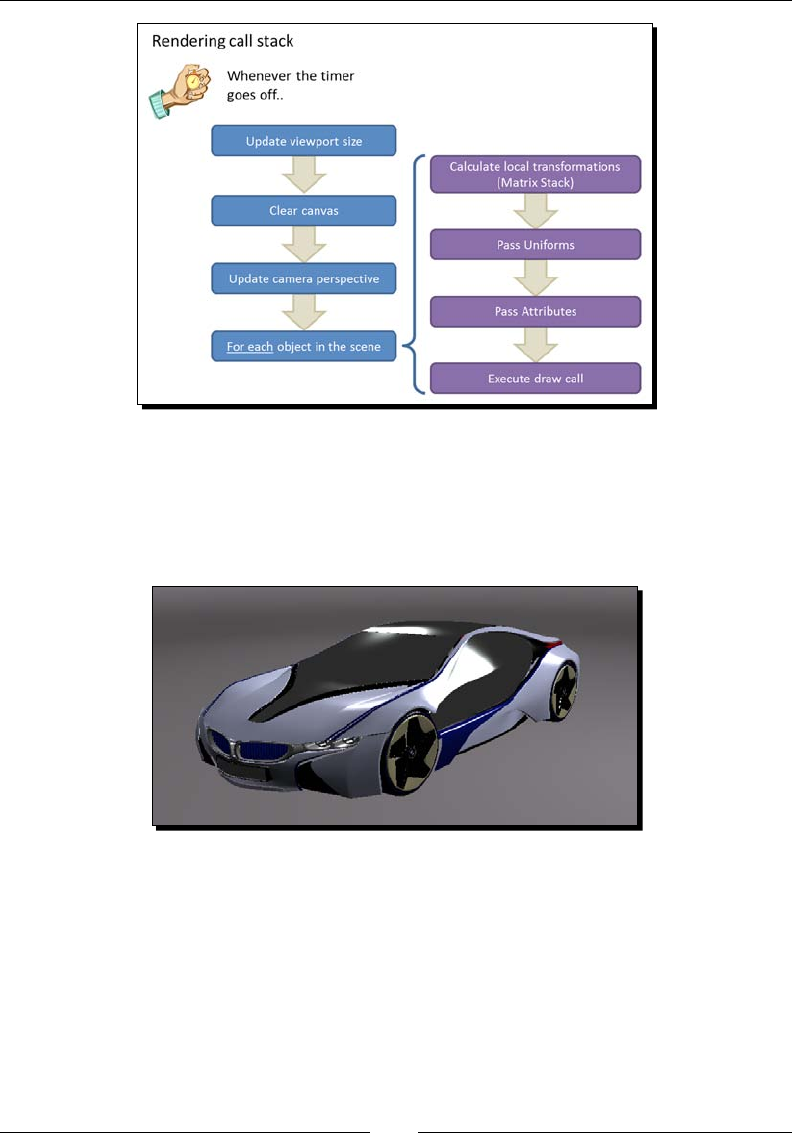
Chapter 9

[ 309 ]

Each car part is a dierent JSON le. The render funcon goes through all the parts stored

as JSON objects inside the Scene object. For each part, the material properes are passed

as uniforms to the shaders and the geometry is passed as aributes (reading data from

the respecve VBOs). Finally, the draw call (drawElements) is executed. The result looks

something like this:

The le ch9_Car_Showroom.html contains all the code described up to now.

Pung It All Together

[ 310 ]

Time for action – customizing the application

1. Open the le ch9_Car_Showroom.html using your favorite code editor.

2. We will assign a dierent home for the camera when we load the Ford Mustang.

To do so, please check the cameraHome, cameraAzimuth, and cameraElevation

global variables. We set up the camera home posion by using this variable inside

the configure funcon like this:

camera.goHome(cameraHome);

camera.setAzimuth(cameraAzimuth);

camera.setElevation(cameraElevation);

Let's use this code to congure the default pose for the camera when we load

the Ford Mustang. Go to the loadMustang funcon and append these lines:

cameraHome = [0,0,10];

cameraAzimuth = -25;

cameraElevation = -15;

camera.goHome(cameraHome);

camera.setAzimuth(cameraAzimuth);

camera.setElevation(cameraElevation);

3. Now save your work and load the page in your web browser. Check that the camera

appears in the indicated posion when you load the Ford Mustang.

4. We can also set up the lighng scheme on a car-per-car basis. For instance, while

low-diusive, high-specular lights work well for the BMW I8, these conguraons

are not as good for the Audi R8. Let's take for example light1 in the configure

funcon. First we set the light aributes like this:

light1.setPosition([-25,25,-25]);

light1.setDiffuse([0.4,0.4,0.4]);

light1.setAmbient([0.0,0.0,0.0]);

light1.setSpecular([0.8,0.8,0.8]);

Then, we add light1 to the Lights object:

Lights.add(light1);

Finally, we map the light arrays contained in the Lights object to the respecve

uniform arrays in our shaders:

gl.uniform3fv(Program.uLightPosition, Lights.

getArray('position'));

gl.uniform3fv(Program.uLa , Lights.getArray('ambient'));

gl.uniform3fv(Program.uLd, Lights.getArray('diffuse'));

gl.uniform3fv(Program.uLs, Lights.getArray('specular'));

Chapter 9

[ 311 ]

Noce though that we need to add light1 to Lights only once. Now check

the code for the one in the updateLightProperty funcon at the boom

of the page:

function updateLightProperty(index,property){

var v = $('#slider-l'+property+''+index).slider('value');

$('#slider-l'+property+''+index+'-value').html(v);

var light;

switch(index){

case 1: light = light1; break;

case 2: light = light2; break;

case 3: light = light3; break;

case 4: light = light4; break;

}

switch(property){

case 'a':light.setAmbient([v,v,v]);

gl.uniform3fv(Program.uLa, Lights.getArray('ambient'));

break;

case 'd':light.setDiffuse([v,v,v]);

gl.uniform3fv(Program.uLd, Lights.getArray('diffuse'));

break;

case 's':light.setSpecular([v,v,v]);

gl.uniform3fv(Program.uLs, Lights.getArray('specular'));

break;

}

render();

}

Here we are detecng what slider changed and we are updang the correspondent

light. Noce that we refer to light1, light2, light3, or light4 directly as these

are global variables. We update the light that corresponds to the slider that changed

and then we map the Lights object arrays to the correspondent uniform arrays.

Noce that here we are not adding light1 or any other light again to the Lights

object. The reason we do not need to do this is that the Lights object keeps a

reference to light1 and the other lights. This saves us from having to clear the

Lights object and mapping all the lights again every me we want to update one

of them.

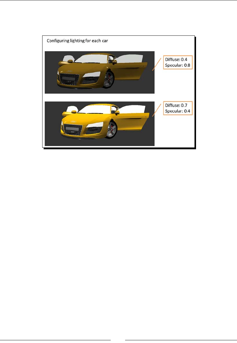
Pung It All Together

[ 312 ]

Using the same mechanism described in updateLightProperty, update the

loadAudi funcon to set the diuse terms of all four lights to [0.7,0.7,0.7]

and the specular terms to [0.4,0.4,0.4].

5. Save your work and reload the page on your web browser. Try dierent lighng

schemes for dierent cars.

What just happened?

We have built a demo that uses many of the elements that we have discussed in the

book. For that purpose, we have used the infrastructure code wring three main funcons:

configure, load, and render. These funcons dene the lifecycle of our applicaon.

On each of these funcons, we have used the objects dened by the architecture of the

examples in the book. For example, we have used a camera object, several light objects,

the program, and the scene object among others.

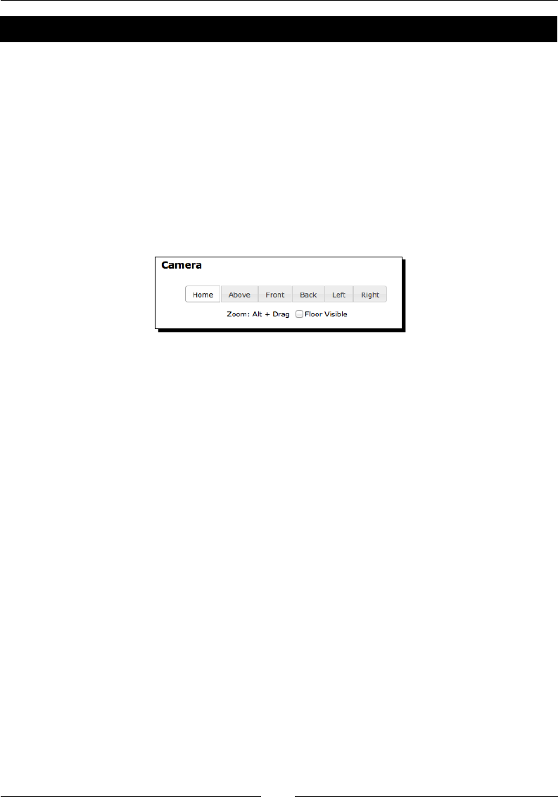
Chapter 9

[ 313 ]

Have a go Hero – ying through the scene

We want to animate the camera to produce a y-through eect. You will need to consider

three variables to be interpolated: the camera posion, elevaon, and azimuth. Start by

dening the key frames, these are the intermediate poses that you want the camera to have.

One could start for instance by looking at the car in the front view and then ying by one of

the sides. You could also try a y-through starng from a 45 degree angle in the back view.

In both cases, you want to make sure that the camera follows the car. To achieve that eect,

you need to make sure to update the azimuth and elevaon on each key frame so the car

keeps in focus.

Hint: Take a look at the code for the animCamera funcon and the funcons that we have

dened for the click events on the Camera buons:

Summary

In this chapter, we have reviewed the concepts and the code developed throughout the

book. We have also built a simple applicaon that shows how all the elements t together.

We have learned that designing complex models requires specialized tools such as Blender.

We also saw that most of the current 3D graphics formats require the denion of verces,

indices, normals, and texture coordinates. We studied how to obtain these elements from

a Blender model and parse them into JSON les that we can load into a WebGL scene.

In the next and nal chapter, we will give you a sneak peak of some of the advanced

techniques that are used regularly in 3D computer graphic systems including games,

simulaons, and other 3D applicaons in general. We will see how to implement these

techniques in WebGL.

Advanced Techniques

At this point, you have all the informaon you need to create rich 3D

applicaons with WebGL. However, we've only just scratched the surface of

what's possible with the API! Creave use of shaders, textures, and vertex

aributes can yield fantasc results. The possibilies are, literally, limitless!

In this nal chapter, we'll provide a few glimpses into some advanced WebGL

techniques, and hopefully leave you eager to explore more on your own.

In this chapter, we'll learn the following topics:

Post-process eects

Point sprites

Normal mapping

Ray tracing in fragment shaders

Post-processing

Post-processing eects are the eects that are created by re-rendering the image of

the scene with a shader that alters the nal image somehow. Think of it as if you took

a screenshot of your scene, opened it up in your favorite image editor, and applied

some lters. The dierence is that we can do it in real me!

Advanced Techniques

[ 316 ]

Examples of some simple post-processing eects are:

Grayscale

Sepia tone

Inverted color

Film grain

Blur

Wavy/dizzy eect

The basic technique for creang these eects is relavely simple: A framebuer is created

that is of the same dimensions as the canvas. At the beginning of the draw cycle, the

framebuer is set as the render target, and the enre scene is rendered normally to it.

Next, a full-screen quad is rendered to the default framebuer using the texture that makes

up the framebuer's color aachment. The shader used during the rendering of the quad

is what contains the post-process eect. It can transform the color values of the rendered

scene as they get wrien to the quad to produce the desired visuals.

Let's look at the individual steps of this process more closely.

Creating the framebuffer

The code that we use to create the framebuer is largely same as the code used in

Chapter 8, Picking, for the picking system. However, there is a key dierence worth nong:

var width = canvas.width;

var height = canvas.height;

//1. Init Color Texture

var texture = gl.createTexture();

gl.bindTexture(gl.TEXTURE_2D, texture);

gl.texParameteri(gl.TEXTURE_2D, gl.TEXTURE_MAG_FILTER, gl.NEAREST);

gl.texParameteri(gl.TEXTURE_2D, gl.TEXTURE_MIN_FILTER, gl.NEAREST);

gl.texParameteri(gl.TEXTURE_2D, gl.TEXTURE_WRAP_S, gl.CLAMP_TO_EDGE);

gl.texParameteri(gl.TEXTURE_2D, gl.TEXTURE_WRAP_T, gl.CLAMP_TO_EDGE);

gl.texImage2D(gl.TEXTURE_2D, 0, gl.RGBA, width, height, 0, gl.RGBA,

gl.UNSIGNED_BYTE, null);

//2. Init Render Buffer

var renderbuffer = gl.createRenderbuffer();

gl.bindRenderbuffer(gl.RENDERBUFFER, renderbuffer);

gl.renderbufferStorage(gl.RENDERBUFFER, gl.DEPTH_COMPONENT16, width,

height);

Chapter 10

[ 317 ]

//3. Init Frame Buffer

var framebuffer = gl.createFramebuffer();

gl.bindFramebuffer(gl.FRAMEBUFFER, framebuffer);

gl.framebufferTexture2D(gl.FRAMEBUFFER, gl.COLOR_ATTACHMENT0,

gl.TEXTURE_2D, texture, 0);

gl.framebufferRenderbuffer(gl.FRAMEBUFFER, gl.DEPTH_ATTACHMENT,

gl.RENDERBUFFER, renderbuffer);

The change is that we are now using the canvas width and height to determine our buer

size instead of the arbitrary values that we used for the picker. This is because the content

of the picker buer was not meant to be rendered to the screen, and as such didn't need to

worry too much about resoluon. For the post-process buer, however, we'll get the best

results if the output matches the dimensions of the canvas exactly.

The canvas size won't always be a power of two, and as such we can't use the mipmapped

texture ltering modes on it. However, in this case that won't maer. Since the texture

will be exactly the same size as the canvas, and we'll be rendering it as a full-screen quad

we have one of the rare situaons where most of the me the texture will be displayed at

exactly a 1:1 rao on the screen, which means no lters need to be applied. This means

that we could use the NEAREST ltering with no visual arfacts, though in the case of

post-process eects that warp the texture coordinates (such as the wavy eect described

later) we will sll benet from using LINEAR ltering. We also need to use a wrap mode

of CLAMP_TO_EDGE, but again this won't pose many issues for our intended use.

Otherwise, the code is idencal to the picker framebuer creaon.

Creating the geometry

While we could load the quad from a le, in this case the geometry is simple enough that

we can put it directly into our code. All that's needed in this case is the vertex posions and

texture coordinates:

//1. Define the geometry for the fullscreen quad

var vertices = [

-1.0,-1.0,

1.0,-1.0,

-1.0, 1.0,

1.0,-1.0,

1.0, 1.0

];

var textureCoords = [

0.0, 0.0,

Advanced Techniques

[ 318 ]

1.0, 0.0,

0.0, 1.0,

1.0, 0.0,

1.0, 1.0

];

//2. Init the buffers

this.vertexBuffer = gl.createBuffer();

gl.bindBuffer(gl.ARRAY_BUFFER, this.vertexBuffer);

gl.bufferData(gl.ARRAY_BUFFER, new Float32Array(vertices), gl.STATIC_

DRAW);

this.textureBuffer = gl.createBuffer();

gl.bindBuffer(gl.ARRAY_BUFFER, this.textureBuffer);

gl.bufferData(gl.ARRAY_BUFFER, new Float32Array(textureCoords),

gl.STATIC_DRAW);

//3. Clean up

gl.bindBuffer(gl.ARRAY_BUFFER, null);

Setting up the shader

The vertex shader for the post-process draw is the simplest one you are likely to see

in a WebGL applicaon:

attribute vec2 aVertexPosition;

attribute vec2 aVertexTextureCoords;

varying vec2 vTextureCoord;

void main(void) {

vTextureCoord = aVertexTextureCoords;

gl_Position = vec4(aVertexPosition, 0.0, 1.0);

}

Something to note here is that unlike every other vertex shader that we've worked with so

far, this one doesn't make use of any matrices. That's because the verces that we declared

in the previous step are pre-transformed.

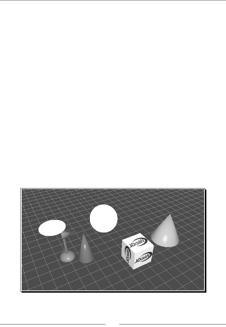
Chapter 10

[ 319 ]

Recall from Chapter 4, Camera, that typically we retrieve normalized device coordinates

by mulplying the vertex posion by the Perspecve matrix, which maps the posions to

a [-1,1] range on each axis, represenng the full extents of the viewport. In this case our

vertex posions are already mapped to that [-1,1] range, and as such no transformaon

is needed. They will map perfectly to the viewport bounds when we render.

The fragment shader is where most of the interesng work happens, and will be dierent

based on the post-process eect that is desired. Let's look at a simple grayscale shader as

an example:

uniform sampler2D uSampler;

varying vec2 vTextureCoord;

void main(void)

{

vec4 frameColor = texture2D(uSampler, vTextureCoord);

float luminance = frameColor.r * 0.3 + frameColor.g * 0.59 +

frameColor.b * 0.11;

gl_FragColor = vec4(luminance, luminance, luminance,

frameColor.a);

}

Here we are sampling the original color rendered by our scene (available through

uSampler), taking a weighted average of the red, green, and blue channels, and outpung

the averaged result to all color channels. The output is a simple grayscale version of the

original scene.

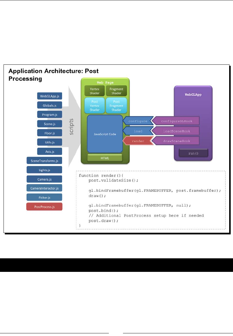
Advanced Techniques

[ 320 ]

Architectural updates

We've added a new class, PostProcess, to our architecture to assist in applying

post-process eects. The code can be found in js/webgl/PostProcess.js.

This class will create the appropriate framebuer and quad geometry for us, compile

the post-process shader, and perform the appropriate render setup needed to draw

the scene out to the quad.

Let's see it in acon!

Time for action – testing some post-process effects

1. Open the le ch10_PostProcess.html in an HTML5 browser.

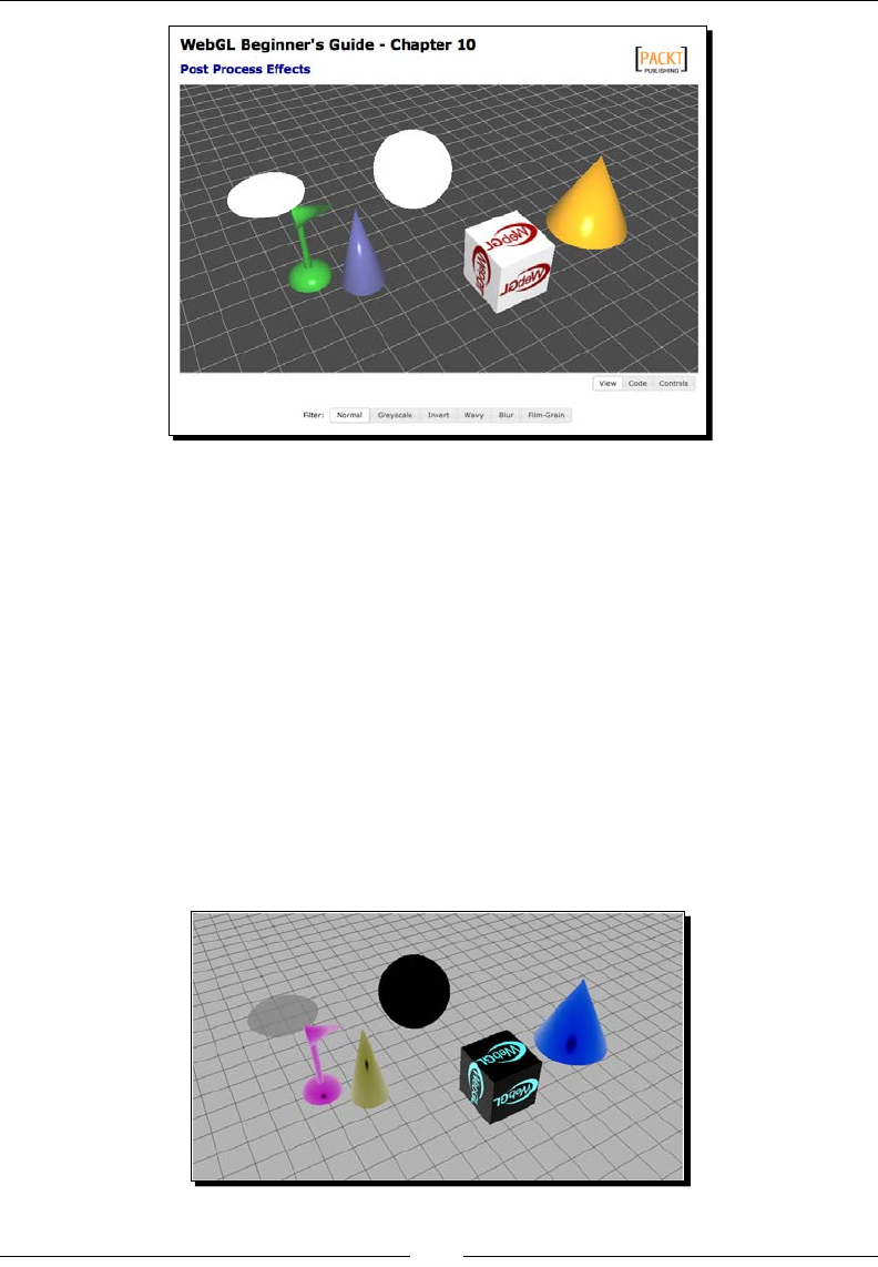
Chapter 10

[ 321 ]

The buons at the boom allow you to switch between several sample eects.

Try each of them to get a feel for the eect they have on the scene. We've already

looked at grayscale, so let's examine the rest of lters individually.

2. The invert eect is similar to grayscale, in that it only modies the color output;

this me inverng each color channel.

uniform sampler2D uSampler;

varying vec2 vTextureCoord;

void main(void)

{

vec4 frameColor = texture2D(uSampler, vTextureCoord);

gl_FragColor = vec4(1.0-frameColor.r, 1.0-frameColor.g,

1.0-frameColor.b, frameColor.a);

}

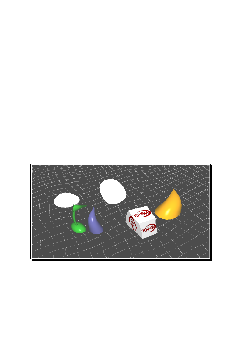
Advanced Techniques

[ 322 ]

3. The wavy eect manipulates the texture coordinates to make the scene swirl

and sway. In this eect, we also provide the current me to allow the distoron

to change as me progresses.

uniform sampler2D uSampler;

uniform float uTime;

varying vec2 vTextureCoord;

const float speed = 15.0;

const float magnitude = 0.015;

void main(void)

{

vec2 wavyCoord;

wavyCoord.s = vTextureCoord.s + (sin(uTime+vTextureCoord.t*spe

ed) * magnitude);

wavyCoord.t = vTextureCoord.t + (cos(uTime+vTextureCoord.s*spe

ed) * magnitude);

vec4 frameColor = texture2D(uSampler, wavyCoord);

gl_FragColor = frameColor;

}

4. The blur eect samples several pixels to either side of the current one and uses a

weighted blend to produce a fragment output that is the average of it's neighbors.

This gives a blurry feel to the scene.

A new uniform used here is uInverseTextureSize, which is 1 over the

width and height of the viewport, respecvely. We can use this to accurately

target individual pixels within the texture. For example, vTextureCoord.x +

2*uInverseTextureSize.x will be exactly two pixels to the le of the original

texture coordinate.

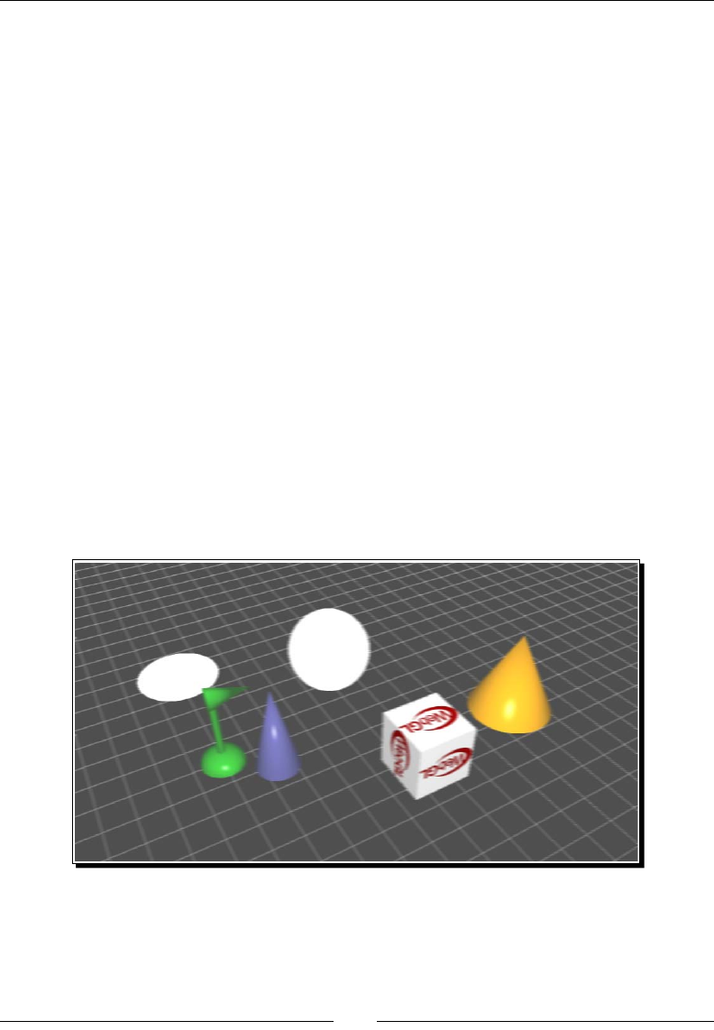
Chapter 10

[ 323 ]

uniform sampler2D uSampler;

uniform vec2 uInverseTextureSize;

varying vec2 vTextureCoord;

vec4 offsetLookup(float xOff, float yOff) {

return texture2D(uSampler, vec2(vTextureCoord.x

+ xOff*uInverseTextureSize.x, vTextureCoord.y +

yOff*uInverseTextureSize.y));

}

void main(void)

{

vec4 frameColor = offsetLookup(-4.0, 0.0) * 0.05;

frameColor += offsetLookup(-3.0, 0.0) * 0.09;

frameColor += offsetLookup(-2.0, 0.0) * 0.12;

frameColor += offsetLookup(-1.0, 0.0) * 0.15;

frameColor += offsetLookup(0.0, 0.0) * 0.16;

frameColor += offsetLookup(1.0, 0.0) * 0.15;

frameColor += offsetLookup(2.0, 0.0) * 0.12;

frameColor += offsetLookup(3.0, 0.0) * 0.09;

frameColor += offsetLookup(4.0, 0.0) * 0.05;

gl_FragColor = frameColor;

}

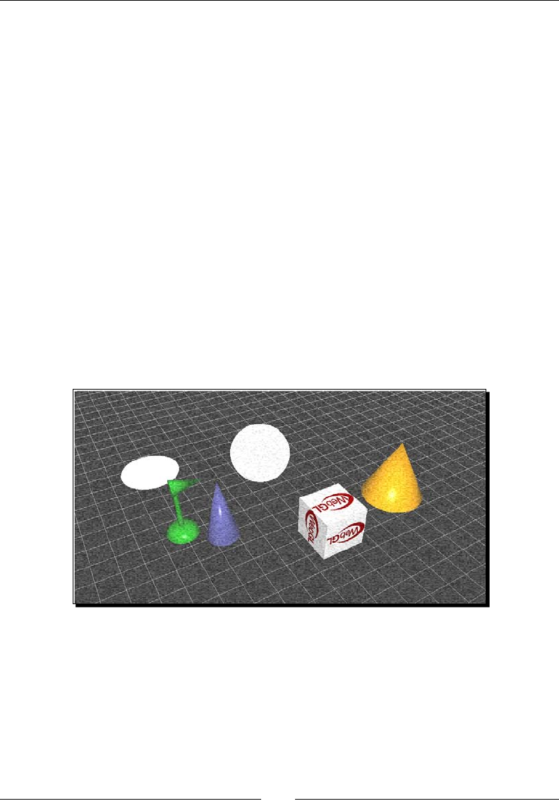
Advanced Techniques

[ 324 ]

5. Our nal example is a lm grain eect. This uses a noisy texture to create a grainy

look to the scene, which simulates the use of an old camera. This example is

signicant because it shows the use of a second texture besides the framebuer

when rendering.

uniform sampler2D uSampler;

uniform sampler2D uNoiseSampler;

uniform vec2 uInverseTextureSize;

uniform float uTime;

varying vec2 vTextureCoord;

const float grainIntensity = 0.1;

const float scrollSpeed = 4000.0;

void main(void)

{

vec4 frameColor = texture2D(uSampler, vTextureCoord);

vec4 grain = texture2D(uNoiseSampler, vTextureCoord * 2.0 +

uTime * scrollSpeed * uInverseTextureSize);

gl_FragColor = frameColor - (grain * grainIntensity);

}

What just happened?

All of these eects are achieved by manipulang the rendered image before it is output to

the screen. Since the amount of geometry processed for these eects is quite small, they can

oen be performed very quickly regardless of the complexity of the scene itself. Performance

may sll be aected by the size of the canvas or the complexity of the post-process shader.

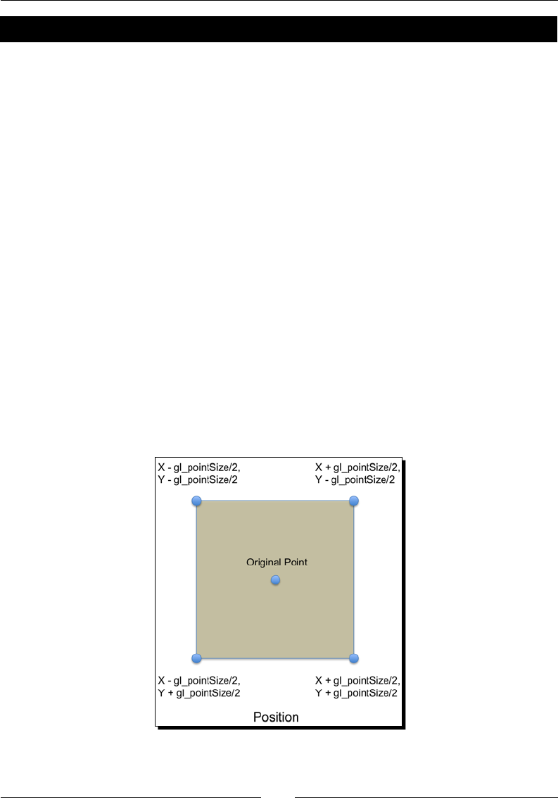
Chapter 10

[ 325 ]

Have a go hero – funhouse mirror effect

What would it take to create a post-process eect that stretches the image near the center

of the viewport and squashes it towards the edges?

Point sprites

Common techniques in many 3D applicaons and games are parcle eects. A parcle eect

is a generic term for any special eect created by rendering groups of parcles (displayed as

points, textured quads, or repeated geometry), typically with some simple form of physics

simulaon acng on the individual parcles. They can be used for simulang smoke, re,

bullets, explosions, water, sparks, and many other eects that are dicult to represent

as a single geometric model.

One very ecient way of rendering the parcles is to use point sprites. Typically, if you

render verces with the POINTS primive type each vertex will be rendered as a single

pixel on the screen. A point sprite is an extension of the POINTS primive rendering

where each point is provided a size and textured in the shader.

A point sprite is created by seng the gl_PointSize value in the vertex shader. It can be

set to either a constant value or a value calculated from shader inputs. If it is set to a number

greater than one, the point is rendered as a quad which always faces the screen (also known

as a billboard). The quad is centered on the original point, and has a width and height equal

to the gl_PointSize in pixels.

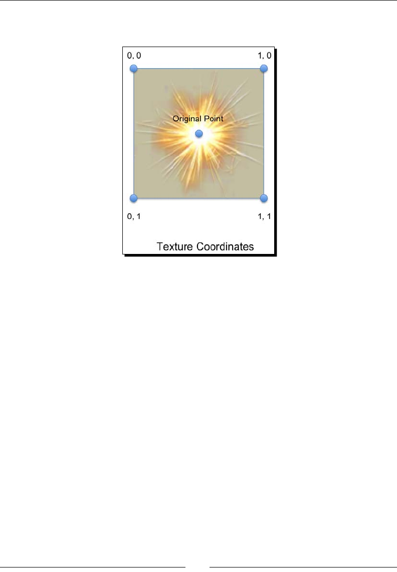
Advanced Techniques

[ 326 ]

When the point sprite is rendered, it also generates texture coordinates for the quad

automacally, covering a simple 0-1 range from upper le to lower right.

The texture coordinates are accessible in the fragment shader as the built-in vec2

gl_PointCoord. Combining these properes gives us a simple point sprite shader

that looks like this:

//Vertex Shader

attribute vec4 aVertexPosition;

uniform mat4 uMVMatrix;

uniform mat4 uPMatrix;

void main(void) {

gl_Position = uPMatrix * uMVMatrix * vec4(aVertexPosition, 1.0);

gl_PointSize = 16.0;

}

//Fragment Shader

precision highp float;

uniform sampler2D uSampler;

void main(void) {

gl_FragColor = texture2D(uSampler, gl_PointCoord);

}

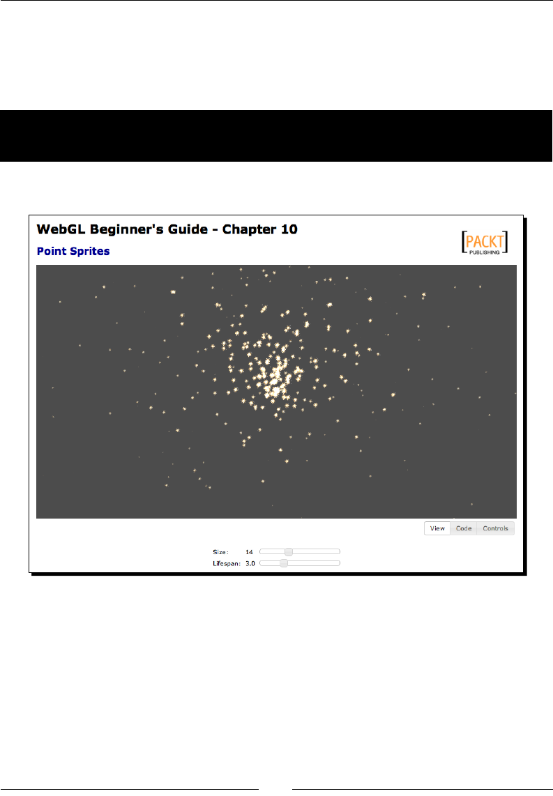
Chapter 10

[ 327 ]

This could be used to render any vertex buer with the following call:

gl.drawArrays(gl.POINTS, 0, vertexCount);

As you can see, this would render each point in the vertex buer as a 16 x 16 texture.

Time for action – using point sprites to create a fountain of

sparks

1. Open the le ch10_PointSprites.html in an HTML5 browser.

2. This sample creates a simple fountain of sparks eect with point sprites. You can

adjust the size and lifeme of the parcles using the sliders at the boom. Play with

them to see the eect it has on the parcles.

3. The parcle simulaon is performed by maintaining a list of parcles that comprises

of a posion, velocity, and lifespan. This list is iterated over every frame and

updated, moving the parcle posion according to the velocity and applying gravity

while reducing the remaining lifespan. Once a parcle's lifespan has reached zero, it

gets reset to the origin with a new randomized velocity and a replenished lifespan.

Advanced Techniques

[ 328 ]

4. With every iteraon of the parcle simulaon, the parcle posions and lifespans

are copied to an array which is then used to update a vertex buer. That vertex

buer is what is rendered to produce the onscreen sprites.

5. Let's play with some of the other values that control the simulaon and see how

they aect the scene. Open up ch10_PointSprites.html in an editor.

6. First, locate the call to configureParticles at the boom of the configure

funcon. The number passed into it, inially set to 1024, determines how many

parcles are created. Try manipulang it to lower or higher values to see the eect it

has on the parcle system. Be careful, as extremely high values (for example, in the

millions) could cause performance issues for your page!

7. Next, nd the resetParticle funcon. This funcon is called any me a parcle

is created or reset. There are several values here that can have a signicant eect

on how the scene renders.

function resetParticle(p) {

p.pos = [0.0, 0.0, 0.0];

p.vel = [

(Math.random() * 20.0) - 10.0,

(Math.random() * 20.0),

(Math.random() * 20.0) - 10.0,

];

p.lifespan = Math.random() * particleLifespan;

p.remainingLife = p.lifespan;

}

8. The p.pos is the x, y, z starng coordinates for the parcle. Inially all points start

at the world origin (0, 0, 0), but this could be set to anything. Oen it is desirable

to have the parcles originate from the locaon of another object in the scene, to

make it appear as if that object is producing the parcles. You can also randomize

the posion to make the parcles appear within a given area.

9. p.vel is the inial velocity of the parcle. You can see here that it's randomized

so that parcles spread out as they move away from the origin. Parcles that move

in random direcons tend to look more like explosions or sprays, while those that

move in the same direcon give the appearance of a steady stream. In this case,

the y value is designed to always be posive, while the x and z values may be either

posive or negave. Experiment with what happens when you increase or decrease

any of the values in the velocity, or if you remove the random element from one of

the components.

Chapter 10

[ 329 ]

10. Finally, p.lifespan determines how long a parcle is displayed before being reset.

This uses the value from the slider on the page, but it's also randomized to provide

visual variety. If you remove the random element from the parcle lifespan all the

parcles will expire and reset at the same me, resulng in reworks-like bursts

of parcles.

11. Next, nd the updateParticles funcon. This funcon is called once per frame

to update the posion and velocity of all parcles and push the new values to the

vertex buer. The interesng part here, in terms of manipulang the simulaon

behavior, is the applicaon of gravity to the parcle velocity mid way through

the funcon:

// Apply gravity to the velocity

p.vel[1] -= 9.8 * elapsed;

if(p.pos[1] < 0) {

p.vel[1] *= -0.75; // Allow particles to bounce off the floor

p.pos[1] = 0;

}

The 9.8 here is the acceleraon applied to the y component over me. In other

words, gravity. We can remove this calculaon enrely to create an environment

where the parcles oat indenitely along their original trajectories. We can

increase the value to make the parcles fall very quickly (giving them a heavy

appearance), or we could change the component that the deceleraon is applied to

change the direcon of gravity. For example, subtracng from vel[0] makes the

parcles fall sideways.

12. This is also where we apply simple collision response for the oor. Any parcles

with a y posion less than 0 (below the oor) have their velocies reversed and

reduced. This gives us a realisc bouncing moon. We can make the parcles less

bouncy by reducing the mulplier (that is, 0.25 instead of 0.75) or even eliminate

bouncing altogether by simply seng the y velocity to 0 at that point. Addionally,

we can remove the oor by taking away the check for y < 0, which would allow the

parcles to fall indenitely.

13. It's also worth seeing the dierent eects that can be achieved with dierent

textures. Try changing path for the spriteTexture in the configure funcon

to see what it looks like when you use dierent images.

What just happened?

We've seen how point sprites can be used to eciently render parcle eects, and seen

some of the ways we can manipulate the parcle simulaon to achieve dierent eects.

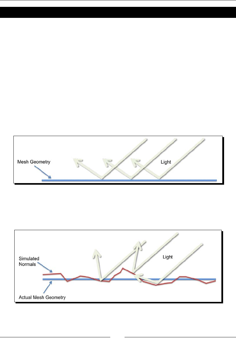
Advanced Techniques

[ 330 ]

Have a go hero – bubbles!

The parcle system in place here could be used to simulate bubbles or smoke oang

upward just as easily as bouncing sparks. How would you need to change the simulaon

to make the parcles oat rather than fall?

Normal mapping

One technique that is very popular among real-me 3D applicaons today is normal

mapping. Normal mapping creates the illusion of highly detailed geometry on a low-poly

model by storing surface normals in a texture map, which is then used to calculate the

lighng of the mesh. This method is especially popular in modern games, where it allows

developers to strike a balance between high performance and detailed scenes.

Typically, lighng is calculated using nothing but the surface normal of the triangle being

rendered, meaning that the enre polygon will be lit as a connuous, smooth surface.

With normal mapping, the surface normals are replaced by normals encoded within a

texture, which can give the appearance of a rough or bumpy surface. Note that the actual

geometry is not changed when using a normal map, only how it is lit. If you look at a normal

mapped polygon from the side, it will sll appear perfectly at.

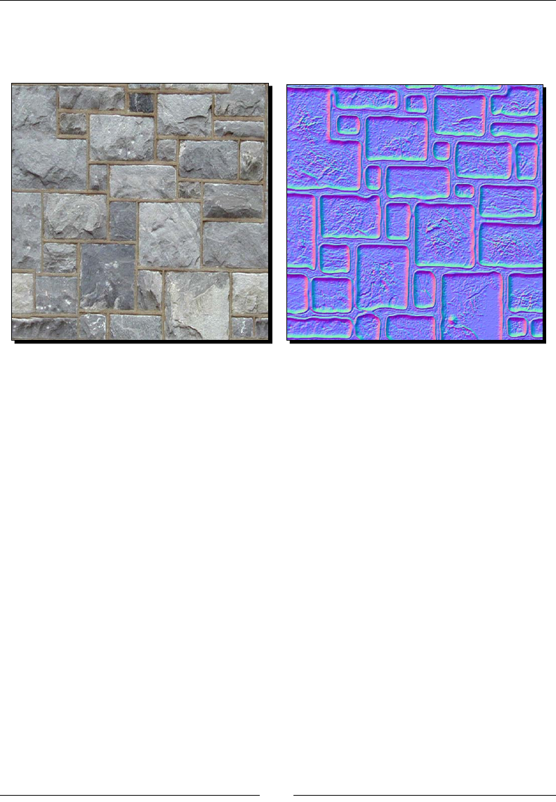
Chapter 10

[ 331 ]

The texture used to store the normals is called a normal map, and is typically paired with a

specic diuse texture that complements the surface the normal map is trying to simulate.

For example, here is a diuse texture of some agstones and the corresponding normal map:

You can see that the normal map contains a similar paern to the diuse texture. The two

textures work in tandem to give the appearance that the stones are raised and rough, while

the grout between them is sunk in.

The normal map contains very specically formaed color informaon that can be

interpreted by the shader at runme as a fragment normal. A fragment normal is essenally

the same as the vertex normals that we are already familiar with: a three-component vector

that points away from the surface. The normal texture encodes the three components of the

normal vector into the three channels of the texture's texel color. Red represents the X axis,

green the Y axis, and blue the Z axis.

The normal encoded in the map is typically stored in tangent space as opposed to world or

object space. Tangent space is the coordinate system that the texture coordinates for a face

are dened in. Normal maps are almost always predominantly blue, since the normals they

represent generally point away from the surface and thus have larger Z components.

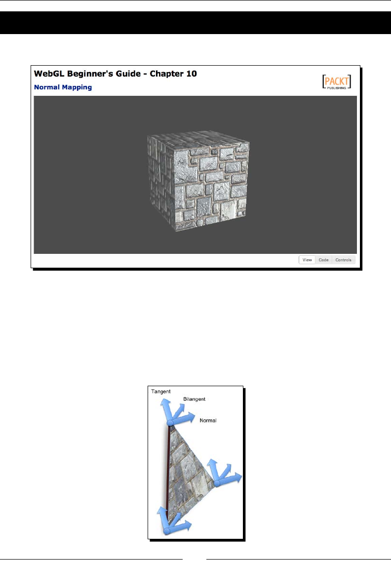
Advanced Techniques

[ 332 ]

Time for action – normal mapping in action

1. Open the le ch10_NormalMap.html in an HTML5 browser.

2. Rotate the cube to see the eect that the normal map has on how the cube is lit.

Also observe how the prole of the cube has not changed. Let's examine how this

eect is achieved.

3. First, we need to add a new aribute to our vertex buers. There are actually three

vectors that are needed to calculate the tangent space coordinates that the lighng

is calculated in: the normal, the tangent, and bitangent.

Chapter 10

[ 333 ]

We already know what the normal represents, so let's look at the other two vectors.

The tangent essenally represents the up (posive Y) vector for the texture relave

to the polygon surface. Likewise, the bitangent represents the le (posive X) vector

for the texture relave to the polygon surface.

We only need to provide two of the three vectors as vertex aributes, tradionally

the normal and tangent. The third vector can be calculated as the cross-product of

the other two in the vertex shader code.

4. Many mes 3D modeling packages will generate tangents for you, but if they

aren't provided, they can be calculated from the vertex posions and texture

coordinates, similar to how we can calculate the vertex normals. We won't cover

the algorithm here, but it has been implemented in js/webgl/Utils.js as

calculateTangents and used in Scene.addObject.

var tangentBufferObject = gl.createBuffer();

gl.bindBuffer(gl.ARRAY_BUFFER, tangentBufferObject);

gl.bufferData(gl.ARRAY_BUFFER, new Float32Array(Utils.

calculateTangents(object.vertices, object.texture_coords, object.

indices)), gl.STATIC_DRAW);

5. In the vertex shader, seen at the top of ch10_NormalMap.html, the tangent needs

to be transformed by the Normal matrix just like the normal does to ensure that

it's appropriately oriented relave to the world-space mesh. The two transformed

vectors can be used to calculate the third as menoned earlier.

vec3 normal = vec3(uNMatrix * vec4(aVertexNormal, 1.0));

vec3 tangent = vec3(uNMatrix * vec4(aVertexTangent, 1.0));

vec3 bitangent = cross(normal, tangent);

The three vectors can then be used to create a matrix that transforms vectors into

tangent space.

mat3 tbnMatrix = mat3(

tangent.x, bitangent.x, normal.x,

tangent.y, bitangent.y, normal.y,

tangent.z, bitangent.z, normal.z

);

6. Instead of applying lighng in the vertex shader, as we did previously, the bulk of the

lighng calculaons need to happen in the fragment shader here so that they can

incorporate the normals from the texture. We do transform the light direcon into

tangent space in the vertex shader, however, and pass it to the fragment shader

as a varying.

//light direction, from light position to vertex

vec3 lightDirection = uLightPosition - vertex.xyz;

vTangentLightDir = lightDirection * tbnMatrix;

Advanced Techniques

[ 334 ]

7. In the fragment shader, rst we extract the tangent space normal from the

normal map texture. Since textures texels don't store negave values, the normal

components must be encoded to map from the [-1,1] range into the [0,1]

range. Therefore, they must be unpacked back into the correct range before use

in the shader. Fortunately, the algorithm to do so is simple to express in ESSL:

vec3 normal = normalize(2.0 * (texture2D(uNormalSampler,

vTextureCoord).rgb - 0.5));

8. At this point, lighng is calculated almost idencally to the vertex-lit model,

using the texture normal and tangent space light direcon.

// Normalize the light direction and determine how much light is

hitting this point

vec3 lightDirection = normalize(vTangentLightDir);

float lambertTerm = max(dot(normal,lightDirection),0.20);

// Combine lighting and material colors

vec4 Ia = uLightAmbient * uMaterialAmbient;

vec4 Id = uLightDiffuse * uMaterialDiffuse * texture2D(uSampler,

vTextureCoord) * lambertTerm;

gl_FragColor = Ia + Id;

The code sample also includes calculaon of a specular term, to help accentuate

the normal mapping eect.

What just happened?

We've seen how to use normal informaon encoded into a texture to add a new level of

complexity to our lit models without addional geometry.

Ray tracing in fragment shaders

A common (if somewhat impraccal) technique used to show how powerful shaders can be

is using them to ray trace a scene. Thus far, all of our rendering has been done with polygon

rasterizaon, which is the technical term for the triangle-based rendering that WebGL

operates with). Ray tracing is an alternate rendering technique that traces the path of light

through a scene as it interacts with mathemacally dened geometry.

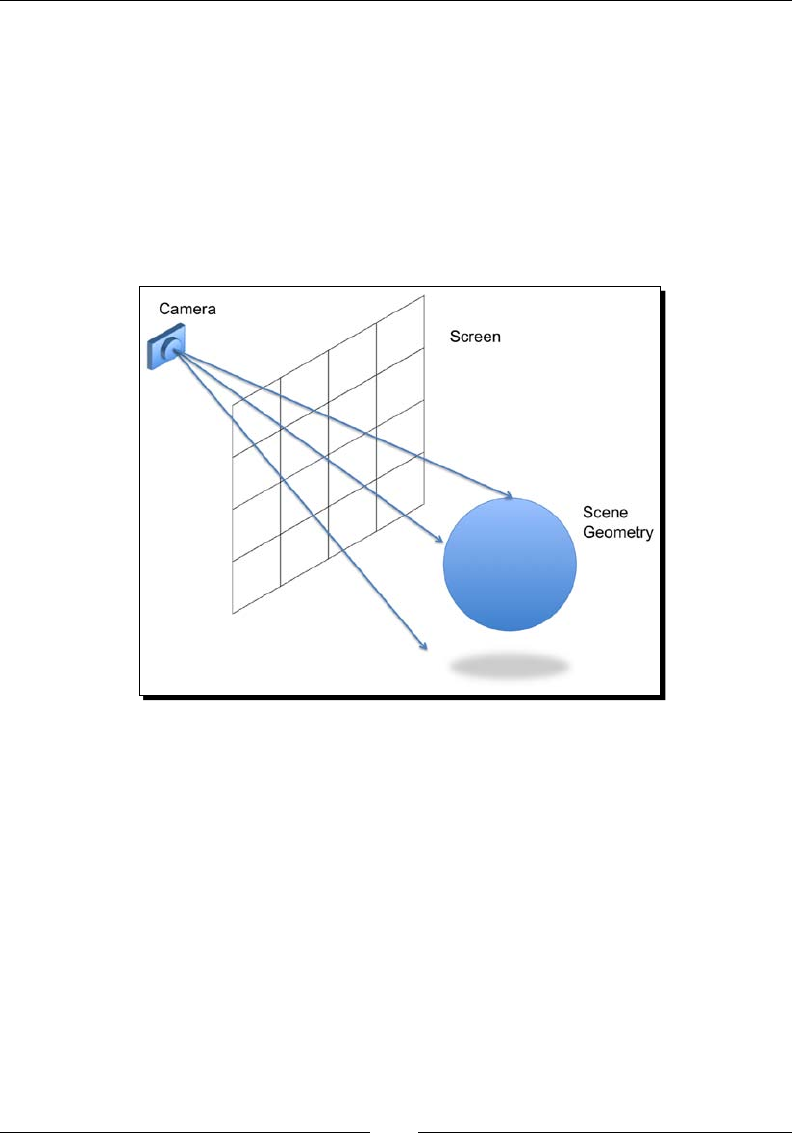
Chapter 10

[ 335 ]

Ray tracing has several advantages compared to polygonal rendering, the primary of which is

that it can create more realisc scenes due to a more accurate lighng model that can easily

account for things like reecon and reected lighng. Ray tracing also tends to be far slower

than polygonal rendering, which is why it's not used much for real-me applicaons.

Ray tracing a scene is done by creang a series of rays (represented by an origin and

direcon) that start at the camera's locaon and pass through each pixel in the viewport.

These rays are then tested against every object in the scene to determine if there are any

intersecons, and if so the closest intersecon to the ray origin is returned. That is then

used to determine the color that pixel should be.

There are a lot of algorithms that can be used to determine the color of the intersecon

point, ranging from simple diuse lighng to mulple bounces of rays o other objects to

simulate reecon, but we'll be keeping it simple in our case. The key thing to remember

is that everything about our scene will be enrely a product of the shader code.

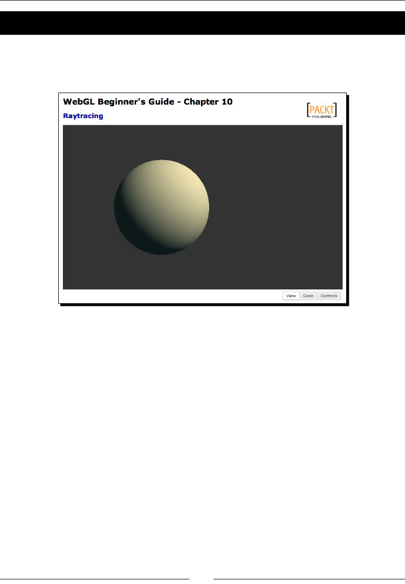
Advanced Techniques

[ 336 ]

Time for action – examining the ray traced scene

1. Open the le ch10_Raytracing.html in an HTML5 browser. You should

see a scene with a simple lit, bobbing sphere like the one shown in the

following screenshot:

2. First, in order to give us a way of triggering the shader, we need to draw a full screen

quad. Luckily for us, we already have a class that helps us do exactly that from the

post-processing example earlier in this chapter! Since we don't have a scene to

process, we're able to cut a large part of the rendering code out, and the enrety

of our JavaScript drawing code becomes:

function render(){

gl.viewport(0, 0, c_width, c_height);

gl.clear(gl.COLOR_BUFFER_BIT | gl.DEPTH_BUFFER_BIT);

//Checks to see if the framebuffer needs to be resized to

match the canvas

post.validateSize();

post.bind();

//Render the fullscreen quad

post.draw();

}

Chapter 10

[ 337 ]

3. That's it. The remainder of our scene will be built in the fragment shader.

4. At the core of our shader, there are two funcons: One which determines if a ray is

intersecng a sphere and one that determines the normal of a point on the sphere.

We're using spheres because they're typically the easiest type of geometry to

raycast, and they also happen to be a type of geometry that is dicult to represent

accurately with polygons.

// ro is the ray origin, rd is the ray direction, and s is the

sphere

float sphereInter( vec3 ro, vec3 rd, vec4 s ) {

// Transform the ray into object space

vec3 oro = ro - s.xyz;

float a = dot(rd, rd);

float b = 2.0 * dot(oro, rd);

float c = dot(oro, oro) - s.w * s.w; // w is the sphere radius

float d = b * b - 4.0 * a * c;

if(d < 0.0) { return d; }// No intersection

return (-b - sqrt(d)) / 2.0; // Intersection occurred

}

vec3 sphereNorm( vec3 pt, vec4 s ) {

return ( pt - s.xyz )/ s.w;

}

5. Next, we will use those two funcons to determine where the ray is intersecng

with a sphere (if at all) and what the normal and color of the sphere is at that point.

In this case, the sphere informaon is hardcoded into a couple of global variables

to make things easier, but they could just as easily be provided as uniforms

from JavaScript.

vec4 sphere1 = vec4(0.0, 1.0, 0.0, 1.0);

vec3 sphere1Color = vec3(0.9, 0.8, 0.6);

float maxDist = 1024.0;

float intersect( vec3 ro, vec3 rd, out vec3 norm, out vec3 color )

{

float dist = maxDist;

float interDist = sphereInter( ro, rd, sphere1 );

if ( interDist > 0.0 && interDist < dist ) {

Advanced Techniques

[ 338 ]

dist = interDist;

vec3 pt = ro + dist * rd; // Point of intersection

norm = sphereNorm(pt, sphere1); // Get normal for that

point

color = sphere1Color; // Get color for the sphere

}

return dist;

}

6. Now that we can determine the normal and color of a point with a ray, we need to

generate the rays to test with. We do this by determining the pixel that the current

fragment represents and creang a ray that points from the desired camera posion

through that pixel. To aid in this, we will ulize the uInverseTextureSize

uniform that the PostProcess class provides to the shader.

vec2 uv = gl_FragCoord.xy * uInverseTextureSize;

float aspectRatio = uInverseTextureSize.y/uInverseTextureSize.x;

// Cast a ray out from the eye position into the scene

vec3 ro = vec3(0.0, 1.0, 4.0); // Eye position is slightly up and

back from the scene origin

// Ray we cast is tilted slightly downward to give a better view

of the scene

vec3 rd = normalize(vec3( -0.5 + uv * vec2(aspectRatio, 1.0),

-1.0));

7. Finally, using the ray that we just generated, we call the intersect funcon to

get the informaon about the sphere intersecon and then apply the same diuse

lighng calculaons that we've been using all throughout the book! We're using

direconal lighng here for simplicity, but it would be trivial to convert to a point

light or spotlight model if desired.

// Default color if we don't intersect with anything

vec3 rayColor = vec3(0.2, 0.2, 0.2);

// Direction the lighting is coming from

vec3 lightDir = normalize(vec3(0.5, 0.5, 0.5));

// Ambient light color

vec3 ambient = vec3(0.05, 0.1, 0.1);

// See if the ray intesects with any objects.

// Provides the normal of the nearest intersection point and color

vec3 objNorm, objColor;

Chapter 10

[ 339 ]

float t = intersect(ro, rd, objNorm, objColor);

if ( t < maxDist ) {

float diffuse = clamp(dot(objNorm, lightDir), 0.0, 1.0); //

diffuse factor

rayColor = objColor * diffuse + ambient;

}

gl_FragColor = vec4(rayColor, 1.0);

8. Rendering with the preceding code will produce a stac, lit sphere. That's great,

but we'd also like to add a bit of moon to the scene to give us a beer sense of

how fast the scene renders and how the lighng interacts with the sphere. To add

a simple looping circular moon to the sphere we use the uTime uniform to modify

the X and Z coordinates at the beginning of the shader.

sphere1.x = sin(uTime);

sphere1.z = cos(uTime);

What just happened?

We've just seen how we can construct a scene, lighng and all, completely in a fragment

shader. It's a simple scene, certainly, but also one that would be nearly impossible to render

using polygon-based rendering. Perfect spheres can only be approximated with triangles.

Have a go hero – multiple spheres

For this example, we've kept things simple by having only a single sphere in the scene.

However, all of the pieces needed to render several spheres in the same scene are in

place! See if you can set up a scene with three of four spheres all with dierent coloring

and movement.

As a hint: The main shader funcon that needs eding is intersect.

Summary

In this chapter, we tried out several advanced techniques and learned how we could use

them to create more visually complex and compelling scenes. We learned how to apply

post-process eects by rendering a framebuer, created parcle eects through the use

of point sprites, created the illusion of complex geometry through the use of normal maps,

and rendered a raycast scene using nothing but a fragment shader.

These eects are only a ny preview of the vast variety of eects possible with WebGL.

Given the power and exibility of shaders, the possibilies are endless!

Index

Symbols

3D objects 178

3D scene

animang 151

loading 18

addHitCallback(object) callback 273

addHit funcon 279, 283

add hit to picking list 273

addive blending, alpha blending mode 216

Ane 118

AJAX

asynchronous loading 51-53

alpha blending

about 210

blend color 213

blend equaon 213

blending funcon, separate 212

alpha blending, modes

addive blending 216

interpolave blending 216

mulplicave blending 216

subtracve blending 216

alpha channel 178

ambient 67

angle of view 136

animaon mer

creang 158

applicaon architecture

picking 269-272

Apply Modiers, Export OBJ panel 302

architectural updates, WebGLApp

about 156

animaon mer, creang 158

rendering rate, conguring 157

support, for matrix stacks 157

WebGLApp review 156

architecture

reviewing 288-290

ARRAY_BUFFER_BINDING value 45

ARRAY_BUFFER value 45

aspect 137

asynchronous loading, with AJAX

about 51-53

cone, loading with AJAX + JSON 54-56

Nissan GTX, loading 56, 57

web server requirement 54

web server, seng up 53

asynchronous response 52

aachShader(Object program, Object shader),

WebGL funcon 91

aributeList array 188

aributes

about 26

and uniforms, dierences 63

associang, to VBOs 31, 32

aVertexColor aribute 180

aVertexPosion aribute 107

Axis.js 143, 290

[ 342 ]

Back Face Culling buon 219

background color 84

bilinear ltering 238

billboard 325

bindBuer(ulong target, Object buer) method

blend color, alpha blending 213

blend equaon, alpha blending 213

Blender 291

Blender models

exporng 302

blending funcon

about 211, 212

separate 212

blending funcon, alpha blending 211, 212

bool 69

boom 137

BouncingBall funcon 165

BouncingBall.update() method 165

b-splines interpolaon 172-174

buerData funcon 43

buerData method 28

buerData(ulong target, Object data, ulong

type) method 31

BUFFER_SIZE parameter 46

buers, WebGL

bindBuer(ulong target, Object buer) method

buerData(ulong target, Object data, ulong

type) method 31

creang 27-30

deleteBuer(Object aBuer) method 30

getBuerParameter(type, parameter)

parameter 45

getParameter(parameter) parameter 45

manipulang 30, 45

states 46, 47

validaon, adding 47

var aBuer = createBuer(void) method 30

BUFFER_USAGE parameter 46

bvec2 69

bvec3 69

bvec4 69

camera

about 10

camera axis 130

light posions, updang 134, 135

Nissan GTX, exploring 131-133

right vector 130

rotang, around locaon 129

tracking 129

tracking camera 129

translang, in line of sight 129

types 128

up vector 130

camera axis 130

CameraInteractor class 131, 270

CameraInteractor.js 290

camera interactor, WebGL properes

creang 298

Camera.js 290

camera matrix

about 120

camera rotaon 123

camera transform 127

camera translaon 121-123

matrix mulplicaons, in WebGL 127, 128

rotaons, combining 126, 127

rotaons, exploring 124-126

translaons, combining 126, 127

camera posion 298

camera rotaon

about 123

and camera translaons, combining 126, 127

exploring 124-126

camera space

versus world space 122-126

camera transform 127

camera translaon

about 121

and camera rotaon, combining 126, 127

exploring 122, 123

camera, types

about 128

orbing camera 129

camera variable 298

[ 343 ]

camera, WebGL properes

seng up 298

canvas

about 10

clicking on 264, 265

canvas element 264

canvas.onmouseup funcon 264

checkKey funcon 17

c_height 266

CLAMP_TO_EDGE 317

CLAMP_TO_EDGE wrap mode 244

clear funcon 17

client-based rendering 9

clientHeight 266

cMatrix. See camera matrix

colors

constant coloring 179

per-fragment coloring 181

pre-vertex coloring 180, 181

storing, by creang texture 259

using, in lights 185

using, in objects 179

using, in scene 206

using, in WebGL 178

colors, using in lights

about 185

getUniformLocaon funcon 185

uniform4fv funcon 185

compileShader funcon 91

Cone First buon 223

congure funcon

about 144, 184, 200, 248, 264, 278, 308

updang 193, 194

congureGLHook 143

congure, JavaScript funcons 289

congureParcles 328

constant coloring

about 179

and per-fragment coloring, comparing 181-184

context

used, for accessing WebGL API 18

context aributes, WebGL

seng up 15-18

copy operaon 116

cosine emission law 66

createProgram(), WebGL funcon 91

createShader funcon 91

creaon operaon 116

cross product

used, for calculang normals 61

cube

texturing 231-233

cube maps

about 250, 251

cube map-specic funcon 251

using 252-254

deleteBuer(Object aBuer) method 30

depth buer 208

depth funcon

about 210

gl.ALWAYS parameter 210

gl.EQUAL parameter 210

gl.GEQUAL parameter 210

gl.GREATER parameter 210

gL.LEQUAL parameter 210

gl.LESS parameter 210

gl.NEVER parameter 210

gl.NOTEQUAL parameter 210

depth informaon

storing, by creang Renderbuer 260

depth tesng 208, 209

dest 137

diuse 67

diuseColorGenerator funcon 275, 276

diuse material property 179

direconal lights 99

direconal point light 202-204

discard command 207

div tags 292

d, materials uniforms 296

doLagrangeInterpolaon funcon 173

doLinearInterpolaon funcon 173

drawArrays funcon

about 33, 34, 288

using 34, 35

drawElements funcon

about 33, 43, 288

using 36, 37

[ 344 ]

draw funcon

about 144, 151, 200, 220, 248, 263, 270

updang 194, 195

drawScene funcon 39

drawSceneHook 143

dropped frames 153

dx funcon 281

dy funcon 281

DYNAMIC_DRAW 31

E 81

ELEMENT_ARRAY_BUFFER_BINDING value 45

ELEMENT_ARRAY_BUFFER value 45

end picking mode 273

ESSL

about 68

and WebGL, gap bridging 93-95

fragment shader 75

funcons 71, 72

operators 71, 72

programs, wring 75, 76

storage qualier 69

uniforms 72, 73

varyings 73

vector, components 70

vertex aributes 72

vertex shader 73, 74

ESSL programs, wring

Lamberan reecon model, Goraud shading

with 76, 77

Phong reecon model, Goraud shading with

80-83

Phong shading 86-88

Euclidian Space 106

exponenal aenuaon factor 205

Export OBJ panel

Apply Modiers 302

Material Groups 303

Objects as OBJ Objects 302

Triangulate Faces 302

Write Materials 302

eye posion 258

f 81

far 137

Field of View. See FOV

lter modes, texture

about 234, 235

LINEAR lter 238, 239

magnicaon 235

minicaon 235

NEAREST lter 238

seng 236

texels 235

using 237

rst-person camera 129

agX variable 275

agZ variable 275

oat 69

Floor.js 143, 290

fountain sparks

creang, point sprites used 327-329

FOV 136

fovy 137

fragment shader

about 25

ray tracing 334, 335

unique labels, using 277, 278

updang 191-193

fragment shader, ESSL 75

framebuer

about 25, 316

creang, for oscreen rendering 260, 261

framebuer, post processing eect

creang 316, 317

frozen frames 154

frustum 110

funcons, ESSL 71, 72

generateMipmap 241

generatePosion funcon 165

geometry

rendering, in WebGL 26

geometry, post processing eect

creang 317, 318

[ 345 ]

getBuerParameter(type, parameter) parameter

getGLContext funcon 17, 39

getParameter funcon 287

getParameter(parameter) parameter 45

getProgramParameter(Object program, Object

parameter), WebGL funcon 91

getShader funcon 90, 91

getUniformLocaon funcon 185

getUniform(program, reference), WebGL

funcon 93

gl.ALWAYS parameter 210

gl.ARRAY_BUFFER opon 28

gl.bindTexture 246

gl.blendColor ( red, green, blue, alpha) funcon

215

gl.blendEquaon funcon 213

gl.blendEquaon(mode) funcon 215

gl.blendEquaonSeparate(modeRGB,

modeAlpha) funcon 215

gl.blendFuncSeparate(sW_rgb, dW_rgb, sW_a,

dW_a) funcon 214

gl.blendFunc (sW, dW) funcon 214

gl.ELEMENT_ARRAY_BUFFER opon 28

gl.enable|disable (gl.BLEND) funcon 214

gl.EQUAL parameter 210

gl_FragColor variable 261

gl.GEQUAL parameter 210

gl.getParameter funcon 186

gl.getParameter(pname) funcon 215

gl.GREATER parameter 210

gL.LEQUAL parameter 210

gl.LESS parameter 210

glMatrix operaons

copy operaon 116

creaon operaon 116

identy operaon 116

inverse operaon 116

rotate operaon 116

transpose operaon 116

gl.NEVER parameter 210

gl.NOTEQUAL parameter 210

Globals.js 143, 289

gl_PointSize value 325

glPolygonSpple funcon 207

gl.readPixels(x, y, width, height, format, type,

pixels) funcon 267

ESSL

bool 69

bvec2 69

bvec3 69

bvec4 69

oat 69

int 69

ivec2 69

ivec3 69

ivec4 69

mat2 69

mat3 70

mat4 70

matrices in 117, 118

sampler2D 70

samplerCube 70

vec2 69

vec3 69

vec4 69

void 69

ESSL uniforms

JavaScript, mapping 116, 117

gl.TEXTURE_CUBE_MAP_* targets 251

Goraud interpolaon method 65

Goraud shading

about 83-85

with Lamberan reecon model 76, 77

with Phong reecon model 80-83

GUI

about 292, 293

WebGL support, adding 293, 295

hardware-based rendering 8

height aribute 12

hitPropertyCallback(object) callback 273

hitProperty funcon 279

hits

looking for 268

processing 269

hits funcon 280

homogeneous coordinates 106-108

hook() 143

[ 346 ]

HTML5 canvas

aributes 12

creang, steps for 10

CSS style, dening 12

height aribute 12

id aribute 12

not supported 12

width aribute 12

IBOs 24

id aribute 12

identy operaon 116

illum, materials uniforms 296

Index Buer Objects. See IBOs

index parameter 32, 275

indices 24

initBuers funcon 39, 40

initLights funcon 90

initProgram funcon 39, 90, 94

initTransforms funcon 144, 157

initWebGL funcon 17

int 69

interacvity

adding, with JQuery UI 196

interactor funcon 280

interpolaon

about 170

B-Splines 172

linear interpolaon 170

polynomial interpolaon 170, 171

interpolaon methods

about 65

Goraud interpolaon method 65

Phong interpolaon method 65, 66

interpolave blending, alpha blending mode

216

intersect funcon 338

INVALID_OPERATION 28

inverse of matrix 127

inverse operaon 116

ivec2 69

ivec3 69

ivec4 69

JavaScript

mapping, to ESSL uniforms 116, 117

JavaScript array

used, for dening geometry 26, 27

JavaScript elements

JavaScript mers 152

requestAnimFrame funcon 151

JavaScript matrices 116

JavaScript Object Notaon. See JSON

JavaScript mers

about 152

used, for implemenng animaon sequence

158

JQuery UI

interacvity, adding with 196

JQuery UI widgets

URL 196

JSON

about 48

decoding 50, 51

encoding 50, 51

JSON-based 3D models, dening 48-50

Khronos Group web page

URL 8

KTM 114

Lambert coecient 76

Lamberan reecon model

Goraud shading with 76, 77

light, moving 78, 80

uniforms, updang 77, 78

Lamberan reecon model, light reecon

models 66

Lambert’s emission law 66

le 137

life-cycle funcons, WebGL

about 144

congure funcon 144

draw funcon 144

load funcon 144

[ 347 ]

light ambient term 83

light color (light diuse term) 83

light diuse term 78

lighng 64

light posions

about 185

updang 134, 135

light reecon models

about 66

Lamberan reecon model 66

Phong reecon model 67

lights

about 10, 60, 63, 178, 188

colors, using 185

mulple lights, using 186

objects, support adding for 187, 188

properes 186

Lights.js 290

light specular term 84

lights, WebGL properes

creang 299

light uniform arrays

uLa[NUM_LIGHTS] 297

uLd[NUM_LIGHTS] 297

uLs[NUM_LIGHTS] 297

LINEAR lter 238, 239

linear interpolaon 170

LINEAR_MIPMAP_LINEAR lter 241

LINEAR_MIPMAP_NEAREST lter 240

LINE_LOOP mode 44

LINES mode 43

LINE_STRIP mode 44

linkProgram(Object program), WebGL funcon

loadCubemapFace 252

load funcon 144, 162, 194, 200, 301, 308

load, JavaScript funcons 289

loadObject funcon 277

loadSceneHook 143

local transformaons, with matrix stacks

about 158

dropped and frozen frames, simulang 160

simple animaon 158, 159

local transforms 149

magnicaon 235

mat2 69

mat3 70

mat4 70

mat4.ortho(le, right, boom, top, near, far,

dest) funcon 137

mat4.perspecve(fovy, aspect, near, far, dest)

funcon 137

material ambient term 84

Material Groups, Export OBJ panel 303

materials 62, 63

material specular term 84

materials uniforms

d 296

illum 296

uKa 296

uKd 296

uKs 296

uNi 296

uNs 296

Material Template Library (MTL) 291

Math.random funcon 275

Marx Stack Operaons

diagrammac representaon 150

matrices

in ESSL 117, 118

uMVMatrix 117

uNMatrix 117

uPMatrix 117

matrix handling funcons, WebGL

initTransforms 144

setMatrixUniforms 146

updateTransforms 145

matrix mulplicaons

in WebGL 127, 128

matrix stacks

about 150

connecng 158

support, adding for 157

used, for implemenng local transformaons

158

minicaon 235

mipmap chain 240

[ 348 ]

mipmapping

about 239

generang 241, 242

LINEAR_MIPMAP_LINEAR lter 241

LINEAR_MIPMAP_NEAREST lter 240

mipmap chain 240

NEAREST_MIPMAP_LINEAR lter 240

NEAREST_MIPMAP_NEAREST lter 240

MIRRORED_REPEAT wrap mode 245, 246

miss 268

model matrix 108

Model-View matrix

about 115-119

fourth row 120

identy matrix 119

rotaon matrix 120

translaon vector 120

updang 150

Model-View transform

and projecve transform, integrang 140-142

updang 150

modes

LINE_LOOP mode 44

LINES mode 43

LINE_STRIP mode 44

POINTS mode 43

rendering 41, 42

TRIANGLE_FAN mode 44

TRIANGLES mode 43

TRIANGLE_STRIP mode 44

moveCallback(hits,interactor, dx, dy) callback

273

movePickedObjects funcon 280

mulple lights

handling, uniform arrays used 196, 197

mulplicave blending, alpha blending mode

216

multexturing

about 246

accessing 247

using 247-249

mvMatrix 128

NDC 111

near 137

NEAREST lter 238

NEAREST_MIPMAP_LINEAR lter 240

NEAREST_MIPMAP_NEAREST lter 240

Nissan GTX

example 102

exploring 131-133

Nissan GTX, asynchronous response

loading 56, 57

non-homogeneous coordinates 107

Non Power Of Two (NPOT) texture 242

Normalized Device Coordinates. See NDC

normal mapping

about 330, 331

using 332-334

normal matrix

about 114, 115

calculang 113, 114

normals

about 61-63

calculang 61

calculang, cross product used 61

updang, for shared verces 62

normal transformaons

about 113

normal matrix, calculang 113, 114

normal vectors 113

norm parameter 32

objectLabelGenerator funcon 275

objects

about 10

colors, using 179

Objects as OBJ Objects, Export OBJ panel 302

OBJ les

parsing 306

OBJ format

about 303, 304

Vertex 305

Vertex // Normal 305

Vertex / Texture Coordinate 305

Vertex / Texture Coordinate / Normal 305

oscreen framebuer

framebuer, creang to oscreen rendering

260, 261

pixels, reading from 266, 267

[ 349 ]

Renderbuer, creang to store depth informa-

on 260

rendering to 262-264

seng up 259

texture, creang to store colors 259

oscreen rendering

framebuer, creang 260, 261

oset parameter 32

onblur event 152

one color per object

assigning, in scene 261

onfocus event 152

onFrame funcon 162

onLoad event 90, 156

onmouseup event 264

OpenGL ES Shading Language. See ESSL

OpenGL Shading Language ES specicaon

uniforms 186

operators, ESSL 71, 72

opmizaon strategies

about 166

batch performance, opmizing 167

translaons, performing in vertex shader 168,

169

orbing camera 129

orthogonal projecon 137, 139, 140

about 136

parametric curves

about 160

animaon, running 163

animaon mer, seng up 162

ball, bouncing 164, 165

ball, drawing in current posion 163

inializaon steps 161

parcle eect 325

pcolor property 277, 279

per-fragment coloring

about 181

and constant coloring, comparing 181-184

cube, coloring 181-184

perspecve division 111, 112

perspecve matrix

about 110, 115, 135, 136

Field of view (FOV) 136

orthogonal projecon 137-140

perspecve projecon 136-140

projecve transform and Model-View

transform, integrang 140-142

perspecve projecon 136, 137-140

per-vertex coloring 180, 181

Phong lighng

Phong shading with 88

Phong reecon model

about 295

Goraud shading with 80-83

Phong reecon model, light reecon models

Phong shading

about 86, 88, 295

with Phong lighng 88

pickedObject 268

picker architecture

about 272

add hit to picking list 273

end picking mode 273

picker searches for hit 273

remove hit from picking list 273

user drags mouse in picking mode 273

picker conguraon

for unique object labels 278- 282

Picker.js 290

Picker object 272

picker searches for hit 273

picking

about 257, 258

applicaon architecture 269-272

Picking Image buon 272

pixels 25

about 25

reading, from oscreen framebuer 266, 267

POINTS mode 43

POINTS primive type 325

point sprites

about 325

POINTS primive type 325

using, to create sparks fountain 327-329

polygon rasterizaon 334

polygon sppling 207

polynomial interpolaon 170, 171

pos_cone variable 158

posional lights

[ 350 ]

about 61, 99

in acon 100, 101

posionGenerator funcon 274

pos_sphere variable 158

PostProcess class 338

post processing eect

about 315

architectural updates 320

example 316

framebuer, creang 316, 317

geometry, creang 317, 318

shader, seng up 318, 319

tesng 320-324

previous property 280

processHitsCallback(hits) callback 273

processHits funcon 283, 285

program aributes, WebGL properes

mapping 300

Program.js 143, 290

projecon transform 110

projecve Space 106

projecve transform

and Model-View transform, integrang 140,

141, 142

projecve transformaons 106

R 81

ray casng 258

ray tracing

in fragment shaders 334, 335

scene, examining 336-339

removeHitCallback(object) callback 273

remove hit from picking list 273

removeHit funcon 279

Renderbuer

creang, to store depth informaon 260

renderFirst(objectName) 223

render funcon 262, 263, 270, 278, 308

rendering

about 8, 308

applicaon, customizing 310-312

client-based rendering 9

hardware-based rendering 8

server-based rendering 9

soware-based rendering 8

rendering order 223

rendering pipeline

about 24

aributes 26

fragment shader 25

framebuer 25

uniforms 26

updang 207, 208

varyings 26

Vertex Buer Objects (VBOs) 25

vertex shader 25

rendering rate

conguring 157

render, JavaScript funcons 289

renderLast(objectName) 223

renderLater(objectName) 223

renderLoop funcon 39

renderOrder() 224

renderSooner(objectName) 223

REPEAT wrap mode 244

requestAnimFrame funcon 151, 152

resetParcle funcon 328

RGBA model 178

right 137

right vector 130

rotate operaon 116

rotaon matrix 120

Runge’s phenomenon 171

runWebGLApp funcon 90, 156, 158, 263

sampler2D 70

sampler2D uniform 230

samplerCube 70

samplers 230

scalars array 183

scaleX variable 281

scaleY variable 281

scene

about 179

blue light, adding 190

color, using 206

one color per object, assigning 261

seng up 297

scene.js 143, 290

scene object 301, 309

[ 351 ]

sceneTime variable 163

SceneTransform.js 290

SceneTransforms object 157

SceneTransforms object, WebGL properes 298

server-based rendering 9

setMatrixUniforms funcon 146, 157

shader

about 295

textures, using 230

shader, post processing eect

seng up 318, 319

shaderSource funcon 91

shading 64

sharing method. See interpolaon methods

shininess 84

size parameter 32

soware-based rendering 8

specular 67

sphere color (material diuse term) 77, 84

square

color, changing 41

drawScene funcon 39

getGLContext funcon 39

initBuers funcon 39, 40

initProgram funcon 39

rendering 37, 38

renderLoop funcon 39

square.blend 303

startAnimaon funcon 158, 162

STATIC_DRAW 31

storage qualier, ESSL

aribute 69

const 69

uniform 69

varying 69

STREAM_DRAW 31

stride parameter 32

subtracve blending, alpha blending mode 216

system requisites, WebGL 8

tangent space 331

texels 235

texImage2D call 227

texParameteri 236, 242

texture

coordinates, using 228, 229

creang 226, 227

creang, to store colors 259

lter modes 234, 235

mapping 226

mipmapping 239

texImage2D call 227

uploading 227, 228

using, in shader 230

texture2D 231

texture coordinates

using 228, 229

TEXTURE_CUBE_MAP target 251

texture mapping 226

TEXTURE_MIN_FILTER mode 239, 240

texture, using in shader

about 230

cube, texturing 231-233

texture wrapping

about 242

CLAMP_TO_EDGE mode 244

MIRRORED_REPEAT mode 245, 246

modes 243

REPEAT mode 244

ming strategies

about 152

animaon and simulaon, combined approach

154-156

animaon strategy 153

simulaon strategy 154

top 137

tracking camera

about 129

camera model 130

camera, rotang around locaon 129

camera, translang in line of sight 129

light posions, updang 134, 135

Nissan GTX, exploring 131-133

transforms.calculateModelView() 159

translaon vector 120

transparent objects

creang 218, 219

face culling 218

face culling used 220, 221

transparent wall

creang 222

[ 352 ]

transpose operaon 116

TRIANGLE_FAN mode 44

TRIANGLES mode 43

TRIANGLE_STRIP mode 44

Triangulate Faces, Export OBJ panel 302

trilinear ltering 241

type parameter 32

uKa, materials uniforms 296

uKd, materials uniforms 296

uKs, materials uniforms 296

uLa[NUM_LIGHTS], light uniform arrays 297

uLd[NUM_LIGHTS], light uniform arrays 297

uLs[NUM_LIGHTS], light uniform arrays 297

uMVMatrix 117

uniform4fv funcon 185

uniform[1234][]v, WebGL funcon 93

uniform[1234][], WebGL funcon 93

uniform arrays

declaraon 197, 198

JavaScript array mapping 198

light uniform arrays 297

using, to handle mulple lights 196, 197

white light, adding to scene 198-201

uniformList array 188

uniforms

about 26, 186

and aributes, dierences 63

passing, to programs 188, 189

uniforms, ESSL 72

uniforms, WebGL properes

inializaon 301

mapping 300

uNi, materials uniforms 296

unique object labels

implemenng 274

picker, conguring for 278-282

random scene, creang 274- 277

scene, tesng 282-284

using, in fragment shader 277, 278

uNMatrix 117

uNs, materials uniforms 296

unwrapping 229

uOscreen uniform 262

updateLightPosion funcon 196

update method 163

updateParcles funcon 329

updateTransforms 145

updateTransforms funcon 139, 145, 157

uPMatrix 117

up vector 130

Use Lambert Coecient buon 184

useProgram(Object program), WebGL funcon

user drags mouse in picking mode 273

Uls.js 144, 289

UV Mapping 230

UVs 230

var aBuer = createBuer(void) method 30

variable declaraon

storage qualier 69

Var reference = getAribLocaon(Object

program,String name), WebGL funcon

var reference= getUniformLocaon(Object

program,String uniform), WebGL funcon

varyings 26

varyings, ESSL 73

VBOs

about 24, 25, 181

aribute, enabling 33

aribute, poinng 32

aributes, associang 31, 32

drawArrays funcon 33, 34

drawElements funcon 33, 34

index parameter 32

norm parameter 32

oset parameter 32

rendering 33

size parameter 32

stride parameter 32

type parameter 32

vec2 69

vec3 69

[ 353 ]

vec4 69

vector components, ESSL 70, 71

vector sum 62

vertexAribPointer 33

vertex aributes, ESSL 72

Vertex Buer Objects. See VBOs

Vertex // Normal, OBJ format 305

Vertex, OBJ format 305

Vertex Shader

about 25

updang 191

Vertex Shader aribute 181

vertex shader, ESSL 73, 74

Vertex / Texture Coordinate / Normal, OBJ

format 305

Vertex / Texture Coordinate, OBJ format 305

vertex transformaons

about 106, 109

homogeneous coordinates 106-108

model transform 108, 109

perspecve division 111, 112

projecon transform 110, 111

viewport transform 112

verces 24

verces array 183

vFinalColor[3] 70

vFinalColor variable 70

view matrix 109

viewport coordinates 112

viewport funcon 112, 141

viewport transform 112

Virtual Car Showroom applicaon

about 18

applicaon, customizing 310-312

bandwidth consumpon 292

cars, loading in WebGl scene 307

creang 290, 291

nished scene, visualizing 19, 20

models, complexity 291

network delays 292

shader quality 291

void 69

wall

working on 95-98

Wall First buon 223

Wavefront OBJ 301

WebGL

about 7

advantages 9

and ESSL, gap bridging 93-95

applicaon, architecture 89, 90

aributes, inializing 92

buers, creang 27-30

client-based rendering 9

colors, using 178

context aributes, seng up 15-18

geometry dening, JavaScript arrays used 26,

geometry, rendering 26

hardware-based rendering 8

matrix mulplicaons 127, 128

program, creang 90-92

rendering 8

server-based rendering 9

soware-based rendering 8

system requisites 8

uniforms, inializing 92

WebGL 3D scenes

lights 178

objects 178

scene 179

WebGL alpha blending API

about 214

gl.blendColor ( red, green, blue, alpha) funcon

215

gl.blendEquaon(mode) funcon 215

gl.blendEquaonSeparate(modeRGB,

modeAlpha) funcon 215

gl.blendFuncSeparate(sW_rgb, dW_rgb, sW_a,

dW_a) funcon 214

gl.blendFunc (sW, dW) funcon 214

gl.enable|disable (gl.BLEND) funcon 214

gl.getParameter(pname) funcon 215

WebGL API

accessing, context used 18

WebGLApp class 152

WebGLApp.js 144, 289

WebGL applicaon

creang 287, 288

structure 10

Virtual Car Showroom applicaon 290, 291

WebGL applicaon, structure

[ 354 ]

about 10

camera 10

canvas 10

lights 10

objects 10

WebGLApp object 156

WEBGLAPP_RENDER_RATE 157

WebGLApp.run() 157

WebGL context

about 13

accessing, steps for 13, 14

WebGL examples, structure

about 142

life-cycle funcons 144

matrix handling funcons 144

objects supported 143

WebGL funcon

aachShader(Object program, Object shader)

createProgram() 91

getProgramParameter(Object program, Object

parameter) 91

getUniform(program, reference) 93

linkProgram(Object program) 91

uniform[1234][] 93

uniform[1234][]v 93

useProgram(Object program) 91

Var reference = getAribLocaon(Object

program,String name) 92

var reference= getUniformLocaon(Object

program,String uniform) 92

WebGL, implementaon

about 115

JavaScript matrices 116

JavaScript matrices, mapping to ESSL uniforms

116, 117

matrices, in ESSL 117, 118

Model-View matrix 115

Normal matrix 115

Perspecve matrix 115

WebGL index buer 24

WebGL properes

camera interactor, creang 298

camera, seng up 298

conguring 297

lights, creang 299

program aributes, mapping 300

SceneTransforms object 298

uniform inializaon 301

uniforms, mapping 300

WebGL vertex buer 24

web server, asynchronous response

seng up 53

web server requirement, asynchronous response

Web Workers

about 156

URL 156

width aribute 12

window.requestAnimFrame() funcon 151

world space

versus camera space 122-126

Write Materials, Export OBJ panel 302

z-buer. See depth buer

Thank you for buying

WebGL Beginner's Guide

About Packt Publishing

Packt, pronounced 'packed', published its rst book "Mastering phpMyAdmin for Eecve MySQL

Management" in April 2004 and subsequently connued to specialize in publishing highly focused

books on specic technologies and soluons.

Our books and publicaons share the experiences of your fellow IT professionals in adapng and

customizing today's systems, applicaons, and frameworks. Our soluon-based books give you the

knowledge and power to customize the soware and technologies you're using to get the job done.

Packt books are more specic and less general than the IT books you have seen in the past. Our unique

business model allows us to bring you more focused informaon, giving you more of what you need to

know, and less of what you don't.

Packt is a modern, yet unique publishing company, which focuses on producing quality, cung-edge

books for communies of developers, administrators, and newbies alike. For more informaon, please

visit our website: www.PacktPub.com.

Wring for Packt

We welcome all inquiries from people who are interested in authoring. Book proposals should be sent

to author@packtpub.com. If your book idea is sll at an early stage and you would like to discuss

it rst before wring a formal book proposal, contact us; one of our commissioning editors will get in

touch with you.

We're not just looking for published authors; if you have strong technical skills but no wring

experience, our experienced editors can help you develop a wring career, or simply get some

addional reward for your experse.

HTML5 Games Development by

Example: Beginner’s Guide

ISBN: 978-1-84969-126-0 Paperback:352 pages

Create six fun games using the latest HTML5, Canvas, CSS,

and JavaScript techniques.

1. Learn HTML5 game development by building six

fun example projects

2. Full, clear explanaons of all the essenal

techniques

3. Covers puzzle games, acon games, mulplayer,

and Box 2D physics

4. Use the Canvas with mulple layers and sprite

sheets for rich graphical games

HTML5 Canvas Cookbook

ISBN: 978-1-84969-136-9 Paperback: 348 pages

Over 80 recipes to revoluonize the web experience with

HTML5 Canvas

1. The quickest way to get up to speed with HTML5

Canvas applicaon and game development

2. Create stunning 3D visualizaons and games

without Flash

3. Wrien in a modern, unobtrusive, and objected

oriented JavaScript style so that the code can be

reused in your own applicaons.

Please check www.PacktPub.com for information on our titles

HTML5 Mobile Development

Cookbook

ISBN: 978-1-84969-196-3 Paperback:254 pages

Over 60 recipes for building fast, responsive HTML5 mobile

websites for iPhone 5, Android, Windows Phone and

Blackberry.

1. Solve your cross plaorm development issues

by implemenng device and content adaptaon

recipes.

2. Maximum acon, minimum theory allowing

you to dive straight into HTML5 mobile web

development.

3. Incorporate HTML5-rich media and geo-locaon

into your mobile websites.

HTML5 Mulmedia Development

Cookbook

ISBN: 978-1-84969-104-8 Paperback: 288 pages

Recipes for praccal, real-world HTML5 mulmedia-driven

development

1. Use HTML5 to enhance JavaScript funconality.

Display videos dynamically and create movable ads

using JQuery.

2. Set up the canvas environment, process shapes

dynamically and create interacve visualizaons.

3. Enhance accessibility by tesng browser support,

providing alternave site views and displaying

alternate content for non supported browsers.

Please check www.PacktPub.com for information on our titles

Web GL Beginner's Guide

Navigation menu

Versions of this User Manual:

Views

Navigation