Wiley Finance : Financial Risk Management A Practitioner's Guide To Managing Market And Credit (2nd Edition) (Wiley Finance) Steve L. Allen An
User Manual:
Open the PDF directly: View PDF ![]() .
.
Page Count: 609 [warning: Documents this large are best viewed by clicking the View PDF Link!]
- Financial Risk Management
- Contents
- Foreword
- Preface
- Acknowledgments
- About the Author
- CHAPTER 1 Introduction
- CHAPTER 2 Institutional Background
- CHAPTER 3 Operational Risk
- CHAPTER 4 Financial Disasters
- CHAPTER 5 The Systemic Disaster of 2007–2008
- CHAPTER 6 Managing Financial Risk
- CHAPTER 7 VaR and Stress Testing
- CHAPTER 8 Model Risk
- CHAPTER 9 Managing Spot Risk
- CHAPTER 10 Managing Forward Risk
- CHAPTER 11 Managing Vanilla Options Risk
- CHAPTER 12 Managing Exotic Options Risk
- CHAPTER 13 Credit Risk
- CHAPTER 14 Counterparty Credit Risk
- References
- About the Companion Website
- Index

Financial
Risk
Management
Founded in 1807, John Wiley & Sons is the oldest independent publishing
company in the United States. With of ces in North America, Europe, Aus-
tralia, and Asia, Wiley is globally committed to developing and marketing
print and electronic products and services for our customers’ professional
and personal knowledge and understanding.
The Wiley Finance series contains books written speci cally for nance
and investment professionals as well as sophisticated individual investors
and their nancial advisors. Book topics range from portfolio management
to e-commerce, risk management, nancial engineering, valuation, and
nancial instrument analysis, as well as much more.
For a list of available titles, visit our Web site at www.WileyFinance.com.

Financial
Risk
Management
A Practitioner’s Guide to Managing
Market and Credit Risk
Second Edition
STEVEN ALLEN
John Wiley & Sons, Inc.
Cover image: John Wiley & Sons, Inc.
Cover design: © Tom Fewster / iStockphoto, © samxmeg / iStockphoto
Copyright © 2013 by Steven Allen. All rights reserved.
Published by John Wiley & Sons, Inc., Hoboken, New Jersey.
Published simultaneously in Canada.
The First Edition of this book was published in 2003 by John Wiley & Sons, Inc.
No part of this publication may be reproduced, stored in a retrieval system, or transmitted in any
form or by any means, electronic, mechanical, photocopying, recording, scanning, or otherwise,
except as permitted under Section 107 or 108 of the 1976 United States Copyright Act, without
either the prior written permission of the Publisher, or authorization through payment of the
appropriate per-copy fee to the Copyright Clearance Center, Inc., 222 Rosewood Drive, Danvers,
MA 01923, (978) 750-8400, fax (978) 646-8600, or on the Web at www.copyright.com. Requests
to the Publisher for permission should be addressed to the Permissions Department, John Wiley &
Sons, Inc., 111 River Street, Hoboken, NJ 07030, (201) 748-6011, fax (201) 748-6008, or online at
http://www.wiley.com/go/permissions.
Limit of Liability/Disclaimer of Warranty: While the publisher and author have used their best efforts
in preparing this book, they make no representations or warranties with respect to the accuracy
or completeness of the contents of this book and speci cally disclaim any implied warranties of
merchantability or tness for a particular purpose. No warranty may be created or extended by
sales representatives or written sales materials. The advice and strategies contained herein may not
be suitable for your situation. You should consult with a professional where appropriate. Neither
the publisher nor author shall be liable for any loss of pro t or any other commercial damages,
including but not limited to special, incidental, consequential, or other damages.
For general information on our other products and services or for technical support, please contact
our Customer Care Department within the United States at (800) 762-2974, outside the United
States at (317) 572-3993 or fax (317) 572-4002.
Wiley publishes in a variety of print and electronic formats and by print-on-demand. Some material
included with standard print versions of this book may not be included in e-books or in print-on-
demand. If this book refers to media such as a CD or DVD that is not included in the version you
purchased, you may download this material at http://booksupport.wiley.com. For more information
about Wiley products, visit www.wiley.com.
Library of Congress Cataloging-in-Publication Data:
Allen, Steven, 1945–
Financial risk management [electronic resource]: a practitioner’s guide to managing market and
credit risk / Steven Allen. — 2nd ed.
1 online resource.
Includes bibliographical references and index.
Description based on print version record and CIP data provided by publisher; resource not viewed.
ISBN 978-1-118-17545-3 (cloth); 978-1-118-22652-0 (ebk.); ISBN 978-1-118-23164-7 (ebk.);
ISBN 978-1-118-26473-7 (ebk.)
1. Financial risk management. 2. Finance. I. Title.
HD61
658.15'5—dc23
2012029614
Printed in the United States of America.
10 9 8 7 6 5 4 3 2 1
To Caroline
For all the ways she has helped bring
this project to fruition
And for much, much more

Financial
Risk
Management

ix
Foreword xvii
Preface xix
Acknowledgments xxiii
About the Author xxvii
CHAPTER 1
Introduction 1
1.1 Lessons from a Crisis 1
1.2 Financial Risk and Actuarial Risk 2
1.3 Simulation and Subjective Judgment 4
CHAPTER 2
Institutional Background 7
2.1 Moral Hazard—Insiders and Outsiders 7
2.2 Ponzi Schemes 17
2.3 Adverse Selection 19
2.4 The Winner’s Curse 21
2.5 Market Making versus Position Taking 24
CHAPTER 3
Operational Risk 29
3.1 Operations Risk 31
3.1.1 The Risk of Fraud 31
3.1.2 The Risk of Nondeliberate Incorrect Information 35
3.1.3 Disaster Risk 36
3.1.4 Personnel Risk 36
3.2 Legal Risk 37
3.2.1 The Risk of Unenforceable Contracts 37
3.2.2 The Risk of Illegal Actions 40
3.3 Reputational Risk 41
3.4 Accounting Risk 42
Contents

x CONTENTS
3.5 Funding Liquidity Risk 42
3.6 Enterprise Risk 44
3.7 Identi cation of Risks 44
3.8 Operational Risk Capital 45
CHAPTER 4
Financial Disasters 49
4.1 Disasters Due to Misleading Reporting 49
4.1.1 Chase Manhattan Bank/Drysdale Securities 52
4.1.2 Kidder Peabody 53
4.1.3 Barings Bank 55
4.1.4 Allied Irish Bank (AIB) 57
4.1.5 Union Bank of Switzerland (UBS) 59
4.1.6 Société Générale 61
4.1.7 Other Cases 66
4.2 Disasters Due to Large Market Moves 68
4.2.1 Long‐Term Capital Management (LTCM) 68
4.2.2 Metallgesellschaft (MG) 75
4.3 Disasters Due to the Conduct of Customer Business 77
4.3.1 Bankers Trust (BT) 77
4.3.2 JPMorgan, Citigroup, and Enron 79
4.3.3 Other Cases 80
CHAPTER 5
The Systemic Disaster of 2007–2008 83
5.1 Overview 83
5.2 The Crisis in CDOs of Subprime Mortgages 85
5.2.1 Subprime Mortgage Originators 86
5.2.2 CDO Creators 88
5.2.3 Rating Agencies 89
5.2.4 Investors 92
5.2.5 Investment Banks 93
5.2.6 Insurers 106
5.3 The Spread of the Crisis 108
5.3.1 Credit Contagion 108
5.3.2 Market Contagion 109
5.4 Lessons from the Crisis for Risk Managers 111
5.4.1 Subprime Mortgage Originators 111
5.4.2 CDO Creators 111
5.4.3 Rating Agencies 111
5.4.4 Investors 111
5.4.5 Investment Banks 112

Contents xi
5.4.6 Insurers 114
5.4.7 Credit Contagion 115
5.4.8 Market Contagion 115
5.5 Lessons from the Crisis for Regulators 115
5.5.1 Mortgage Originators 116
5.5.2 CDO Creators 116
5.5.3 Rating Agencies 117
5.5.4 Investors 118
5.5.5 Investment Banks 118
5.5.6 Insurers 126
5.5.7 Credit Contagion 126
5.5.8 Market Contagion 129
5.6 Broader Lessons from the Crisis 132
CHAPTER 6
Managing Financial Risk 133
6.1 Risk Measurement 133
6.1.1 General Principles 133
6.1.2 Risk Management of Instruments That Lack
Liquidity 144
6.1.3 Market Valuation 147
6.1.4 Valuation Reserves 152
6.1.5 Analysis of Revenue 156
6.1.6 Exposure to Changes in Market Prices 157
6.1.7 Risk Measurement for Position Taking 159
6.2 Risk Control 161
CHAPTER 7
VaR and Stress Testing 169
7.1 VaR Methodology 170
7.1.1 Simulation of the P&L Distribution 173
7.1.2 Measures of the P&L Distribution 187
7.2 Stress Testing 192
7.2.1 Overview 192
7.2.2 Economic Scenario Stress Tests 193
7.2.3 Stress Tests Relying on Historical Data 197
7.3 Uses of Overall Measures of Firm Position Risk 201
CHAPTER 8
Model Risk 209
8.1 How Important Is Model Risk? 210
8.2 Model Risk Evaluation and Control 212

8.2.1 Scope of Model Review and Control 213
8.2.2 Roles and Responsibilities for Model Review
and Control 214
8.2.3 Model Veri cation 219
8.2.4 Model Veri cation of Deal Representation 222
8.2.5 Model Veri cation of Approximations 223
8.2.6 Model Validation 226
8.2.7 Continuous Review 232
8.2.8 Periodic Review 234
8.3 Liquid Instruments 237
8.4 Illiquid Instruments 241
8.4.1 Choice of Model Validation Approach 241
8.4.2 Choice of Liquid Proxy 243
8.4.3 Design of Monte Carlo Simulation 245
8.4.4 Implications for Marking to Market 247
8.4.5 Implications for Risk Reporting 249
8.5 Trading Models 250
CHAPTER 9
Managing Spot Risk 253
9.1 Overview 253
9.2 Foreign Exchange Spot Risk 257
9.3 Equity Spot Risk 258
9.4 Physical Commodities Spot Risk 259
CHAPTER 10
Managing Forward Risk 263
10.1 Instruments 270
10.1.1 Direct Borrowing and Lending 270
10.1.2 Repurchase Agreements 271
10.1.3 Forwards 272
10.1.4 Futures Contracts 272
10.1.5 Forward Rate Agreements 274
10.1.6 Interest Rate Swaps 275
10.1.7 Total Return Swaps 276
10.1.8 Asset‐Backed Securities 278
10.2 Mathematical Models of Forward Risks 282
10.2.1 Pricing Illiquid Flows by Interpolation 284
10.2.2 Pricing Long‐Dated Illiquid Flows by Stack
and Roll 291
10.2.3 Flows Representing Promised Deliveries 293
10.2.4 Indexed Flows 295
xii CONTENTS

10.3 Factors Impacting Borrowing Costs 299
10.3.1 The Nature of Borrowing Demand 299
10.3.2 The Possibility of Cash‐and‐Carry Arbitrage 300
10.3.3 The Variability of Storage Costs 301
10.3.4 The Seasonality of Borrowing Costs 302
10.3.5 Borrowing Costs and Forward Prices 303
10.4 Risk Management Reporting and Limits for
Forward Risk 304
CHAPTER 11
Managing Vanilla Options Risk 311
11.1 Overview of Options Risk Management 313
11.2 The Path Dependence of Dynamic Hedging 318
11.3 A Simulation of Dynamic Hedging 321
11.4 Risk Reporting and Limits 329
11.5 Delta Hedging 344
11.6 Building a Volatility Surface 346
11.6.1 Interpolating between Time Periods 346
11.6.2 Interpolating between Strikes—Smile and Skew 347
11.6.3 Extrapolating Based on Time Period 352
11.7 Summary 355
CHAPTER 12
Managing Exotic Options Risk 359
12.1 Single‐Payout Options 364
12.1.1 Log Contracts and Variance Swaps 367
12.1.2 Single‐Asset Quanto Options 369
12.1.3 Convexity 370
12.1.4 Binary Options 371
12.1.5 Contingent Premium Options 377
12.1.6 Accrual Swaps 378
12.2 Time‐Dependent Options 378
12.2.1 Forward‐Starting and Cliquet Options 378
12.2.2 Compound Options 379
12.3 Path‐Dependent Options 381
12.3.1 Standard Analytic Models for Barriers 383
12.3.2 Dynamic Hedging Models for Barriers 385
12.3.3 Static Hedging Models for Barriers 387
12.3.4 Barrier Options with Rebates, Lookback,
and Ladder Options 402
12.3.5 Broader Classes of Path‐Dependent Exotics 403
12.4 Correlation‐Dependent Options 404
Contents xiii

12.4.1 Linear Combinations of Asset Prices 405
12.4.2 Risk Management of Options on Linear
Combinations 409
12.4.3 Index Options 413
12.4.4 Options to Exchange One Asset for Another 415
12.4.5 Nonlinear Combinations of Asset Prices 417
12.4.6 Correlation between Price and Exercise 422
12.5 Correlation‐Dependent Interest Rate Options 425
12.5.1 Models in Which the Relationship between
Forwards Is Treated as Constant 426
12.5.2 Term Structure Models 430
12.5.3 Relationship between Swaption and Cap Prices 437
CHAPTER 13
Credit Risk 445
13.1 Short‐Term Exposure to Changes in MarketPrices 446
13.1.1 Credit Instruments 447
13.1.2 Models of Short‐Term Credit Exposure 451
13.1.3 Risk Reporting for Market Credit Exposures 456
13.2 Modeling Single‐Name Credit Risk 457
13.2.1 Estimating Probability of Default 458
13.2.2 Estimating Loss Given Default 465
13.2.3 Estimating the Amount Owed at Default 468
13.2.4 The Option‐Theoretic Approach 471
13.3 Portfolio Credit Risk 479
13.3.1 Estimating Default Correlations 479
13.3.2 Monte Carlo Simulation of Portfolio
Credit Risk 482
13.3.3 Computational Alternatives to Full Simulation 486
13.3.4 Risk Management and Reporting for
Portfolio Credit Exposures 490
13.4 Risk Management of Multiname Credit Derivatives 493
13.4.1 Multiname Credit Derivatives 493
13.4.2 Modeling of Multiname Credit Derivatives 495
13.4.3 Risk Management and Reporting for
Multiname Credit Derivatives 498
13.4.4 CDO Tranches and Systematic Risk 500
CHAPTER 14
Counterparty Credit Risk 505
14.1 Overview 505
14.2 Exchange‐Traded Derivatives 506
xiv CONTENTS

14.3 Over‐the‐Counter Derivatives 512
14.3.1 Overview 512
14.3.2 The Loan‐Equivalent Approach 513
14.3.3 The Collateralization Approach 515
14.3.4 The Collateralization Approach—
Wrong‐Way Risk 521
14.3.5 The Active Management Approach 526
References 533
About the Companion Website 547
Index 553
Contents xv

xvii
Foreword
Risk was a lot easier to think about when I was a doctoral student in nance
25 years ago. Back then, risk was measured by the variance of your wealth.
Lowering risk meant lowering this variance, which usually had the unfortu-
nate consequence of lowering the average return on your wealth as well.
In those halcyon days, we had only two types of risk, systemic and un-
systematic. The latter one could be lowered for free via diversi cation, while
the former one could only be lowered by taking a hit to average return.
In that idyllic world, nancial risk management meant choosing the variance
that maximized expected utility. One merely had to solve an optimization
problem. What could be easier?
I started to appreciate that nancial risk management might not be so easy
when I moved from the West Coast to the East Coast. The New York–based
banks started creating whole departments to manage nancial risk. Why do
you need dozens of people to solve a simple optimization problem? As I talked
with the denizens of those departments, I noticed they kept introducing types
of risk that were not in my nancial lexicon. First there was credit risk, a term
that was to be differentiated from market risk, because you can lose money
lending whether a market exists or not. Fine, I got that, but then came liquidity
risk on top of market and credit risk. Just as I was struggling to integrate these
three types of risk, people started worrying about operational risk, basis risk,
mortality risk, weather risk, estimation risk, counterparty credit risk, and even
the risk that your models for all these risks were wrong. If model risk existed,
then you had to concede that even your model for model risk was risky.
Since the proposed solution for all these new risks were new models and
since the proposed solution for the model risk of the new models was yet
more models, it was no wonder all of those banks had all of those people
running around managing all of those risks.
Well, apparently, not quite enough people. As I write these words, the
media are having a eld day denouncing JPMorgan’s roughly $6 billion loss
related to the London whale’s ill-fated foray into credit default swaps (CDSs).
As the ag bearer for the TV generation, I can’t help but think of reviving
a 1970s TV show to star Bruno Iksil as the Six Billion Dollar Man. As eye-
popping as these numbers are, they are merely the fourth largest trading loss
since the rst edition of this book was released. If we ignore Bernie Madoff’s

$50 billion Ponzi scheme, the distinction for the worst trade ever belongs to
Howie Hubler, who lost $9 billion trading CDSs in 2008 for another bank
whose name I’d rather not write. However, if you really need to know, then
here’s a hint. The present occupant of Mr. Hubler’s old of ce presently thinks
that risk management is a complicated subject, very complicated indeed, and
has to admit that a simple optimization is not the answer. So what is the an-
swer? Well, when the answer to a complicated question is nowhere to be found
in the depths of one’s soul, then one can always fall back on asking the experts
instead. The Danish scientist Niels Bohr, once deemed an expert, said an expert
is, “A person that has made every possible mistake within his or her eld.”
As an expert in the eld of derivative securities valuation, I believe I
know a fellow expert when I see one. Steve Allen has been teaching courses
in risk management at New York University’s Courant Institute since 1998.
Steve retired from JPMorgan Chase as a managing director in 2004, capping
a 35-year career in the nance industry. Given the wide praise for the rst
edition of this book, the author could have rested on his laurels, comforted
by the knowledge that the wisdom of the ages is eternal. Instead, he has
taken it upon himself to write a second edition of this timeless book.
Most authors in Steve’s enviable situation would have contented them-
selves with exploiting the crisis to elaborate on some extended version of
“I told you so.” Instead, Steve has added much in the way of theoretical
advances that have arisen out of the necessity of ensuring that history does
not repeat itself. These advances in turn raise the increasing degree of spe-
cialization we see inside the risk management departments of modern -
nancial institutions and increasingly in the public sector as well. Along with
continued progress in the historically vital problem of marking to market of
illiquid positions, there is an increasing degree of rigor in the determination
of reserves that arise due to model risk, in the limits used to control risk tak-
ing, and in the methods used to review models. The necessity of testing every
assumption has been made plain by the stress that the crisis has imposed
on our fragile nancial system. As the aftershocks reverberate around us,
we will not know for many years whether the present safeguards will serve
their intended purpose. However, the timing for an update to Steve’s book
could not be better. I truly hope that the current generation of risk manag-
ers, whether they be grizzled or green, will take the lessons on the ensuing
pages to heart. Our shared nancial future depends on it.
Peter Carr, PhD
Managing Director at Morgan Stanley,
Global Head of Market Modeling, and
Executive Director of New York University Courant’s
Masters in Mathematical Finance
xviii FOREWORD

xix
T his book offers a detailed introduction to the eld of risk management
as performed at large investment and commercial banks, with an empha-
sis on the practices of specialist market risk and credit risk departments as
well as trading desks. A large portion of these practices is also applicable to
smaller institutions that engage in trading or asset management.
The aftermath of the nancial crisis of 2007–2008 leaves a good deal
of uncertainty as to exactly what the structure of the nancial industry
will look like going forward. Some of the business currently performed in
investment and commercial banks, such as proprietary trading, may move
to other institutions, at least in some countries, based on new legislation
and new regulations. But in whatever institutional setting this business is
conducted, the risk management issues will be similar to those encountered
in the past. This book focuses on general lessons as to how the risk of nan-
cial institutions can be managed rather than on the speci cs of particular
regulations.
My aim in this book is to be comprehensive in looking at the activi-
ties of risk management specialists as well as trading desks, at the realm of
mathematical nance as well as that of the statistical techniques, and, most
important, at how these different approaches interact in an integrated risk
management process.
This second edition re ects lessons that have been learned from the re-
cent nancial crisis of 2007–2008 (for more detail, see Chapters 1 and 5),
as well as many new books, articles, and ideas that have appeared since the
publication of the rst edition in 2003. Chapter 6 on managing market risk,
Chapter 7 on value at risk (VaR) and stress testing, Chapter 8 on model risk,
and Chapter 13 on credit risk are almost completely rewritten and expanded
from the rst edition, and a new Chapter 14 on counterparty credit risk is an
extensive expansion of a section of the credit risk chapter in the rst edition.
The website for this book ( www.wiley.com/go/frm2e ) will be used to
provide both supplementary materials to the text and continuous updates.
Supplementary materials will include spreadsheets and computer code that
illustrate computations discussed in the text. In addition, there will be class-
room aids available only to professors on the Wiley Higher Education web-
site. Updates will include an updated electronic version of the References
Preface

xx PREFACE
section, to allow easy cut‐and‐paste linking to referenced material on
the web. Updates will also include discussion of new developments. For
example, at the time this book went to press, there is not yet enough public
information about the causes of the large trading losses at JPMorgan’s Lon-
don investment of ce to allow a discussion of risk management lessons; as
more information becomes available, I will place an analysis of risk manage-
ment lessons from these losses on the website.
This book is divided into three parts: general background to nancial
risk management, the principles of nancial risk management, and the de-
tails of nancial risk management.
■ The general background part (Chapters 1 through 5) gives an institu-
tional framework for understanding how risk arises in nancial rms
and how it is managed. Without understanding the different roles and
motivations of traders, marketers, senior rm managers, corporate risk
managers, bondholders, stockholders, and regulators, it is impossible
to obtain a full grasp of the reasoning behind much of the machinery
of risk management or even why it is necessary to manage risk. In this
part, you will encounter key concepts risk managers have borrowed
from the theory of insurance (such as moral hazard and adverse se-
lection), decision analysis (such as the winner’s curse), nance theory
(such as the arbitrage principle), and in one instance even the criminal
courts (the Ponzi scheme). Chapter 4 provides discussion of some of the
most prominent nancial disasters of the past 30 years, and Chapter 5
focuses on the crisis of 2007–2008. These serve as case studies of fail-
ures in risk management and will be referenced throughout the book.
This part also contains a chapter on operational risk, which is necessary
background for many issues that arise in preventing nancial disasters
and which will be referred to throughout the rest of the book.
■ The part on principles of nancial risk management (Chapters 6
through 8) rst lays out an integrated framework in Chapter 6 , and
then looks at VaR and stress testing in Chapter 7 and the control of
model risk in Chapter 8 .
■ The part on details of nancial risk management (Chapters 9 through 14)
applies the principles of the second part to each speci c type of nan-
cial risk: spot risk in Chapter 9 , forward risk in Chapter 10 , vanilla
options risk in Chapter 11 , exotic options risk in Chapter 12 , credit
risk in Chapter 13 , and counterparty credit risk in Chapter 14 . As each
risk type is discussed, speci c references are made to the principles elu-
cidated in Chapters 6 through 8, and a detailed analysis of the models
used to price these risks and how these models can be used to measure
and control risk is presented.

Preface xxi
Since the 1990s, an increased focus on the new technology being developed
to measure and control nancial risk has resulted in the growth of corporate
staff areas manned by risk management professionals. However, this does not
imply that nancial rms did not manage risks prior to 1990 or that currently
all risk management is performed in staff areas. Senior line managers such as
trading desk and portfolio managers have always performed a substantial risk
management function and continue to do so. In fact, confusion can be caused
by the tradition of using the term risk manager as a synonym for a senior
trader or portfolio manager and as a designation for members of corporate
staff areas dealing with risk. Although this book covers risk management tech-
niques that are useful to both line trading managers and corporate staff acting
on behalf of the rm’s senior management, the needs of these individuals do
not completely overlap. I will try to always make a clear distinction between
information that is useful to a trading desk and information that is needed by
corporate risk managers, and explain how they might intersect.
Books and articles on nancial risk management have tended to focus
on statistical techniques embodied in measures such as value at risk (VaR).
As a result, risk management has been accused of representing a very narrow
specialty with limited value, a view that has been colorfully expressed by
Nassim Taleb (1997), “There has been growth in the number of ‘risk man-
agement advisors,’ an industry sometimes populated by people with an ama-
teurish knowledge of risk. Using some form of shallow technical skills, these
advisors emit pronouncements on such matters as ‘risk management’ with-
out a true understanding of the distribution. Such inexperience and weak-
ness become more apparent with the value‐at‐risk fad or the outpouring of
books on risk management by authors who never traded a contract” (p. 4).
This book gives a more balanced account of risk management. Less than
20 percent of the material looks at statistical techniques such as VaR. The
bulk of the book examines issues such as the proper mark‐to‐market valu-
ation of trading positions, the determination of necessary reserves against
valuation uncertainty, the structuring of limits to control risk taking, and
the review of mathematical models and determination of how they can con-
tribute to risk control. This allocation of material mirrors the allocation of
effort in the corporate risk management staff areas with which I am fam-
iliar. This is re ected in the staf ng of these departments. More personnel
is drawn from those with experience and expertise in trading and building
models to support trading decisions than is drawn from a statistical or aca-
demic nance background.
Although many readers may already have a background in the
instruments—bonds, stocks, futures, and options—used in the nancial mar-
kets, I have supplied de nitions every time I introduce a term. Terms are itali-
cized in the text at the point they are de ned. Any reader feeling the need for a

xxii PREFACE
more thorough introduction to market terminology should nd the rst nine
chapters of Hull (2012) adequate preparation for understanding the material
in this book.
My presentation of the material is based both on theory and on how
concepts are utilized in industry practice. I have tried to provide many con-
crete instances of either personal experience or reports I have heard from
industry colleagues to illustrate these practices. Where incidents have re-
ceived suf cient previous public scrutiny or occurred long enough ago that
issues of con dentiality are not a concern, I have provided concrete details.
In other cases, I have had to preserve the anonymity of my sources by re-
maining vague about particulars. My preservation of anonymity extends to
a liberal degree of randomness in references to gender.
A thorough discussion of how mathematical models are used to measure
and control risks must make heavy reference to the mathematics used in cre-
ating these models. Since excellent expositions of the mathematics exist, I do
not propose to enter into extensive derivations of results that can readily be
found elsewhere. Instead, I will concentrate on how these results are used in
risk management and how the approximations to reality inevitable in any
mathematical abstraction are dealt with in practice. I will provide references
to the derivation of results. Wherever possible, I have used Hull (2012) as
a reference, since it is the one work that can be found on the shelf of nearly
every practitioner in the eld of quantitative nance.
Although the material for this book was originally developed for a
course taught within a mathematics department, I believe that virtually all
of its material will be understandable to students in nance programs and
business schools, and to practitioners with a comparable educational back-
ground. A key reason for this is that whereas derivatives mathematics often
emphasizes the use of more mathematically sophisticated continuous time
models, discrete time models are usually more relevant to risk management,
since risk management is often concerned with the limits that real market
conditions place on mathematical theory.
This book is designed to be used either as a text for a course in risk man-
agement or as a resource for self‐study or reference for people working in the
nancial industry. To make the material accessible to as broad an audience
as possible, I have tried everywhere to supplement mathematical theory with
concrete examples and have supplied spreadsheets on the accompanying
website ( www.wiley.com/go/frm2e ) to illustrate these calculations. Spread-
sheets on the website are referenced throughout the text and a summary of
all spreadsheets supplied is provided in the “About the Companion Website”
section at the back of the book. At the same time, I have tried to make sure
that all the mathematical theory that gets used in risk management practice
is addressed. For readers who want to pursue the theoretical developments
at greater length, a full set of references has been provided.

xxiii
T he views expressed in this book are my own, but have been shaped by
my experiences in the nancial industry. Many of my conclusions about
what constitutes best practice in risk management have been based on my
observation of and participation in the development of the risk management
structure at JPMorgan Chase and its Chemical Bank and Chase Manhattan
Bank predecessors.
The greatest in uence on my overall view of how nancial risk manage-
ment should be conducted and on many of the speci c approaches I advo-
cate has been Lesley Daniels Webster. My close collaboration with Lesley
took place over a period of 20 years, during the last 10 of which I reported
to her in her position as director of market risk management. I wish to ex-
press my appreciation of Lesley’s leadership, along with that of Marc Sha-
piro, Suzanne Hammett, Blythe Masters, and Andy Threadgold, for having
established the standards of integrity, openness, thoroughness, and intellec-
tual rigor that have been the hallmarks of this risk management structure.
Throughout most of the period in which I have been involved in these
pursuits, Don Layton was the head of trading activities with which we in-
teracted. His recognition of the importance of the risk management function
and strong support for a close partnership between risk management and
trading and the freedom of communication and information sharing were
vital to the development of these best practices.
Through the years, my ideas have bene ted from my colleagues at
Chemical, Chase, JPMorgan Chase, and in consulting assignments since my
retirement from JPMorgan Chase. At JPMorgan Chase and its predecessors,
I would particularly like to note the strong contributions that dialogues with
Andrew Abrahams, Michel Araten, Bob Benjamin, Paul Bowmar, George
Brash, Julia Chislenko, Enrico Della Vecchia, Mike Dinias, Fawaz Habel,
Bob Henderson, Jeff Katz, Bobby Magee, Blythe Masters, Mike Rabin,
Barry Schachter, Vivian Shelton, Paul Shotton, Andy Threadgold, Mick
Waring, and Richard Wise have played in the development of the concepts
utilized here. In my consulting assignments, I have gained much from my
exchanges of ideas with Rick Grove, Chia‐Ling Hsu, Neil Pearson, Bob Sel-
vaggio, Charles Smithson, and other colleagues at Rutter Associates, and
Chris Marty and Alexey Panchekha at Bloomberg. In interactions with risk
Acknowledgments

xxiv ACKNOWLEDGMENTS
managers at other rms, I have bene ted from my conversations with Ken
Abbott, John Breit, Noel Donohoe, and Evan Picoult. Many of the trad-
ers I have interacted with through the years have also had a major in u-
ence on my views of how risk management should impact decision mak-
ing on the trading desk and the proper conduct of relationships between
traders and risk management specialists. I particularly want to thank Andy
Hollings, Simon Lack, Jeff Larsen, Dinsa Mehta, Fraser Partridge, and Don
Wilson for providing me with prototypes for how the risk management of
trading should be properly conducted and their generosity in sharing their
knowledge and insight. I also wish to thank those traders, who shall remain
anonymous here, who have provided me equally valuable lessons in risk
management practices to avoid.
This book grew out of the risk management course I created as part of
the Mathematics in Finance MS program at New York University’s Courant
Institute of Mathematical Sciences in 1998. For giving me the opportunity
to teach and for providing an outstanding institutional setting in which to
do it, I want to thank the administration and faculty of Courant, particu-
larly Peter Carr, Neil Chriss, Jonathan Goodman, Bob Kohn, and Petter
Kolm, with whom I have participated in the management of the program,
and Caroline Thompson, Gabrielle Tobin, and Melissa Vacca, the program
administrators. I have gained many insights that have found their way into
this book by attending other courses in the program taught by Marco Avel-
laneda, Jim Gatheral, Bob Kohn, and Nassim Taleb.
Ken Abbott began participating in the risk management course as a
guest lecturer, later became my co‐teacher of the course, and now has full re-
sponsibility for the course with my participation as a guest lecturer. Many of
the insights in this book have been learned from Ken or generated as part of
the debates and discussions we have held both in and out of the classroom.
The students in my risk management course have helped clarify many of the
concepts in this book through their probing questions. I particularly want
to thank Karim Beguir, who began as my student and has since graduatedto
become a Fellow of the program and a frequent and valued contributor
to the risk management course. Several of his insights are re ected in the
second edition of the book. I also wish to thank Otello Padovani and And-
rea Raphael, students who became collaborators on research that appears
on the website for the book ( www.wiley.com/go/frm2e ). Mike Fisher has
provided greatly appreciated support as my graduate assistant in helping to
clarify class assignments that have evolved into exercises in this book.
The detailed comments and suggestions I have received from Neil
Chriss on large portions of this manuscript far exceed the norms of either
friendship or collegiality. In numerous instances, his efforts have sharpened
both the ideas being presented and the clarity of their expression. I also wish

Acknowledgments xxv
to thank Mich Araten, Peter Carr, Bobby Magee, Barry Schachter, Nassim
Taleb, and Bruce Tuckman for reading the text and offering helpful com-
ments. For the second edition, I would like to thank Ken Abbott and Rick
Grove for reading new chapters and offering helpful suggestions.
I also wish to extend my thanks to Chuck Epstein for his help in nding
a publisher for this book. Bill Falloon, Meg Freeborn, and Michael Kay, my
editors at John Wiley & Sons, have offered very useful suggestions at every
stage of the editing. At MacAllister Publishing Services, Andy Stone was
very helpful as production manager and Jeanne Henning was a thorough
and incisive copy editor for the rst edition of this book.
The individual to whom both I and this book owe the greatest debt is my
wife, Caroline Thompson. The number of ways in which her bene cial in u-
ence has been felt surpass my ability to enumerate, but I at least need to at-
tempt a brief sample. It was Caroline who introduced me to Neil Chriss and
rst planted the idea of my teaching at Courant. She has been a colleague of
Neil’s, Jonathan Goodman’s, and mine in the continued development of the
Courant Mathematics in Finance MS program. From the start, she was the
strongest voice in favor of basing a book on my risk management course. At
frequent bottlenecks, on both the rst and second editions, when I have been
daunted by an obstacle to my progress that seemed insurmountable, it was
Caroline who suggested the approach, organized the material, or suggested
the joint effort that overcame the dif culty. She has managed all aspects of
the production format, and style of the book, including efforts from such
distant ports as Laos, Vietnam, India, and Holland.

xxvii
Steve Allen is a risk management consultant, specializing in risk measure-
ment and valuation with a particular emphasis on illiquid and hard‐
to‐value assets. Until his retirement in 2004, he was Managing Director in
charge of risk methodology at JPMorgan Chase, where he was responsible
for model validation, risk capital allocation, and the development of new
measures of valuation, reserves, and risk for both market and credit risk. Pre-
viously, he was in charge of market risk for derivative products at Chase. He
has been a key architect of Chase’s value‐at‐risk and stress testing systems.
Prior to his work in risk management, Allen was the head of analysis and
model building for all Chase trading activities for over ten years. Since 1998,
Allen has been associated with the Mathematics in Finance Masters’ pro-
gram at New York University’s Courant Institute of Mathematical Sciences.
In this program, he has served as Clinical Associate Professor and Deputy
Director and has created and taught courses in risk management, derivatives
mathematics, and interest rate and credit models. He was a member of the
Board of Directors of the International Association of Financial Engineers
and continues to serve as co‐chair of their Education Committee.
About the Author

1
1.1 LESSONS FROM A CRISIS
I began the rst edition of this book with a reference to an episode of the
television series Seinfeld in which the character George Costanza gets an
assignment from his boss to read a book titled Risk Management and then
give a report on this topic to other business executives. Costanza nds the
book and topic so boring that his only solution is to convince someone else
to read it for him and prepare notes. Clearly, my concern at the time was
to write about nancial risk management in a way that would keep read-
ers from nding the subject dull. I could hardly have imagined then that
eight years later Demi Moore would be playing the part of the head of an
investment bank’s risk management department in a widely released movie,
Margin Call. Even less could I have imagined the terrible events that placed
nancial risk management in such a harsh spotlight.
My concern now is that the global nancial crisis of 2007–2008 may
have led to the conclusion that risk management is an exciting subject
whose practitioners and practices cannot be trusted. I have thoroughly re-
viewed the material I presented in the rst edition, and it still seems to me
that if the principles I presented, principles that represented industry best
practices, had been followed consistently, a disaster of the magnitude we
experienced would not have been possible. In particular, the points I made
in the rst edition about using stress tests in addition to value at risk (VaR)
in determining capital adequacy (see the last paragraphs of Section 7.3 in
this edition) and the need for substantial reserves and deferred compen-
sation for illiquid positions (see Sections 6.1.4 and 8.4 in this edition) still
seem sound. It is tempting to just restate the same principles and urge more
diligence in their application, but that appears too close to the sardonic de -
nition of insanity: “doing the same thing and expecting different results.” So
I have looked for places where these principles need strengthening (you’ll
nd a summary in Section 5.4). But I have also reworked the organization of
CHAPTER 1
Introduction

2 FINANCIAL RISK MANAGEMENT
the book to emphasize two core doctrines that I believe are the keys to the
understanding and proper practice of nancial risk management.
The rst core principle is that nancial risk management is not just risk
management as practiced in nancial institutions; it is risk management that
makes active use of trading in liquid markets to control risk. Risk management
is a discipline that is important to a wide variety of companies, government
agencies, and institutions—one need only think of accident prevention at
nuclear power plants and public health measures to avoid in uenza pan-
demics to see how critical it can be. While the risk management practiced at
investment banks shares some techniques with risk management practiced at
a nuclear facility, there remains one vital difference: much of the risk manage-
ment at investment banks can utilize liquid markets as a key element in risk
control; liquid markets are of virtually no use to the nuclear safety engineer.
My expertise is in the techniques of nancial risk management, and that
is the primary subject of this book. Some risks that nancial rms take on
cannot be managed using trading in liquid markets. It is vitally important
to identify such risks and to be aware of the different risk management
approaches that need to be taken for them. Throughout the book I will be
highlighting this distinction and also focusing on the differences that degree
of available liquidity makes. As shorthand, I will refer to risk that cannot
be managed by trading in liquid markets as actuarial risk , since it is the type
of risk that actuaries at insurance companies have been dealing with for
centuries. Even in cases that must be analyzed using the actuarial risk ap-
proach, nancial risk management techniques can still be useful in isolating
the actuarial risk and in identifying market data that can be used as input to
actuarial risk calculations. I will address this in greater detail in Section 1.2.
The second core principle is that the quanti cation of risk management
requires simulation guided by both historical data and subjective judgment.
This is a common feature of both nancial risk and actuarial risk. The time
period simulated may vary greatly, from value at risk (VaR) simulations
of daily market moves for very liquid positions to simulations spanning
decades for actuarial risk. But I will be emphasizing shared characteristics
for all of these simulations: the desirability of taking advantage of as much
historical data as is relevant, the need to account for nonnormality of statis-
tical distributions, and the necessity of including subjective judgment. More
details on these requirements are in Section 1.3.
1.2 FINANCIAL RISK AND ACTUARIAL RISK
The management of nancial risk and the management of actuarial risk
do share many methodologies, a point that will be emphasized in the next

Introduction 3
section. Both rely on probability and statistics to arrive at estimates of the
distribution of possible losses. The critical distinction between them is the
matter of time. Actuarial risks may not be fully resolved for years, sometimes
even decades. By the time the true extent of losses is known, the accumu-
lation of risk may have gone on for years. Financial risks can be eliminated
in a relatively short time period by the use of liquid markets. Continuous
monitoring of the price at which risk can be liquidated should substantially
lower the possibility of excessive accumulation of risk.
Two caveats need to be offered to this relatively benign picture of -
nancial risk. The rst is that taking advantage of the shorter time frame of
nancial risk requires constant vigilance; if you aren’t doing a good job of
monitoring how large your risks are relative to liquidation costs, you may
still acquire more exposure than desired. This will be described in detail in
Chapter 6 . The second is the need to be certain that what is truly actuarial
risk has not been misclassi ed as nancial risk. If this occurs, it is especially
dangerous—not only will you have the potential accumulation of risk over
years before the extent of losses is known, but in not recognizing the actu-
arial nature, you would not exercise the caution that the actuarial nature of
the risk demands. This will be examined more closely in Sections 6.1.1 and
6.1.2, with techniques for management of actuarial risk in nancial rms
outlined in Section 8.4. I believe that this dangerous muddling of nancial
and actuarial risk was a key contributor to the 2007–2008 crisis, as I argue
in Section 5.2.5.
Of course, it is only an approximation to view instruments as being
liquid or illiquid. The volume of instruments available for trading differs
widely by size and readiness of availability. This constitutes the depth of
liquidity of a given market. Often a rm will be faced with a choice between
the risks of replicating positions more exactly with less liquid instruments
or less exactly with more liquid instruments.
One theme of this book will be the trade‐off between liquidity risk and
basis risk. Liquidity risk is the risk that the price at which you buy (or sell)
something may be signi cantly less advantageous than the price you could
have achieved under more ideal conditions. Basis risk is the risk that occurs
when you buy one product and sell another closely related one, and the two
prices behave differently. Let’s look at an example. Suppose you are hold-
ing a large portfolio of stocks that do not trade that frequently and your
outlook for stock prices leads to a desire to quickly terminate the position.
If you try selling the whole basket quickly, you face signi cant liquidity
risk since your selling may depress the prices at which the stocks trade. An
alternative would be to take an offsetting position in a heavily traded stock
futures contract, such as the futures contract tied to the Standard & Poor’s™
S&P 500 stock index. This lowers the liquidity risk, but it increases the

4 FINANCIAL RISK MANAGEMENT
basis risk since changes in the price of your particular stock basket will
probably differ from the price changes in the stock index. Often the only
way in which liquidity risk can be reduced is to increase basis risk, and the
only way in which basis risk can be reduced is to increase liquidity risk.
The classi cation of risk as nancial risk or actuarial risk is clearly a
function of the particular type of risk and not of the institution. Insurance
against hurricane damage could be written as a traditional insurance con-
tract by Metropolitan Life or could be the payoff of an innovative new swap
contract designed by Morgan Stanley; in either case, it will be the same risk.
What is required in either case is analysis of how trading in liquid markets
can be used to manage the risk. Certainly commercial banks have histori-
cally managed substantial amounts of actuarial risk in their loan portfolios.
And insurance companies have managed to create some ability to liquidate
insurance risk through the reinsurance market. Even industrial rms have
started exploring the possible transformation of some actuarial risk into
nancial risk through the theory of real options. An introduction to real op-
tions can be found in Hull (2012, Section 34) and Dixit and Pindyck (1994).
A useful categorization to make in risk management techniques that I
will sometimes make use of, following Gumerlock (1999), is to distinguish
between risk management through risk aggregation and risk management
through risk decomposition. Risk aggregation attempts to reduce risk by
creating portfolios of less than completely correlated risk, thereby achiev-
ing risk reduction through diversi cation. Risk decomposition attempts to
reduce a risk that cannot directly be priced in the market by analyzing it into
subcomponents, all or some of which can be priced in the market. Actuarial
risk can generally be managed only through risk aggregation, whereas nan-
cial risk utilizes both techniques. Chapter 7 concentrates on risk aggrega-
tion, while Chapter 8 primarily focuses on risk decomposition; Chapter 6
addresses the integration of the two.
1.3 SIMULATION AND SUBJECTIVE JUDGMENT
Nobody can guarantee that all possible future contingencies have been pro-
vided for—this is simply beyond human capabilities in a world lled with
uncertainty. But it is unacceptable to use that platitude as an excuse for
complacency and lack of meaningful effort. It has become an embarrass-
ment to the nancial industry to see the number of events that are declared
“once in a millennium” occurrences, based on an analysis of historical data,
when they seem in fact to take place every few years. At one point I suggest-
ed, only half‐jokingly, that anyone involved in risk management who used
the words perfect and storm in the same sentence should be permanently

Introduction 5
banned from the nancial industry. More seriously, everyone involved in
risk management needs to be aware that historical data has a limited util-
ity, and that subjective judgment based on experience and careful reasoning
must supplement data analysis. The failure of risk managers to apply critical
subjective judgment as a check on historical data in the period leading to the
crisis of 2007–2008 is addressed in Section 5.2.5.
This by no means implies that historical data should not be utilized.
Historical data, at a minimum, supplies a check against intuition and can
be used to help form reasoned subjective opinions. But risk managers con-
cerned with protecting a rm against infrequent but plausible outcomes
must be ready to employ subjective judgment.
Let us illustrate with a simple example. Suppose you are trying to de-
scribe the distribution of a variable for which you have a lot of historical
data that strongly supports a normal distribution with a mean of 5 percent
and standard deviation of 2 percent. Suppose you suspect that there is a
small but nonnegligible possibility that there will be a regime change that
will create a very different distribution. Let’s say you guess there is a 5 per-
cent chance of this distribution, which you estimate as a normal distribution
with a mean of 0 percent and standard deviation of 10 percent.
If all you cared about was the mean of the distribution, this wouldn’t
have much impact—lowering the mean from 5 percent to 4.72 percent.
Even if you were concerned with both mean and standard deviation, it
wouldn’t have a huge impact: the standard deviation goes up from 2 percent
to 3.18 percent, so the Sharpe ratio (the ratio of mean to standard deviation
often used in nancial analysis) would drop from 2.50 to 1.48. But if you
were concerned with how large a loss you could have 1 percent of the time,
it would be a change from a gain of 0.33 percent to a loss of 8.70 percent.
Exercise 1.1 will allow you to make these and related calculations for your-
self using the Excel spreadsheet MixtureOfNormals supplied on the book’s
website.
This illustrates the point that when you are concerned with the tail of
the distribution you need to be very concerned with subjective probabilities
and not just with objective frequencies. When your primary concern is just
the mean—or even the mean and standard deviation, as might be typical for
a mutual fund—then your primary focus should be on choosing the most
representative historical period and on objective frequencies.
While this example was drawn from nancial markets, the conclusions
would look very similar if we were discussing an actuarial risk problem like
nuclear safety and we were dealing with possible deaths rather than nan-
cial losses. The fact that risk managers need to be concerned with managing
against extreme outcomes would again dictate that historical frequencies
need to be supplemented by informed subjective judgments. This reasoning

6 FINANCIAL RISK MANAGEMENT
is very much in line with the prevailing (but not universal) beliefs among
academics in the elds of statistics and decision theory. A good summary of
the current state of thinking in this area is to be found in Hammond, Keeney,
and Raiffa (1999, Chapter 7 ). Rebonato (2007) is a thoughtful book‐length
treatment of these issues from an experienced and respected nancial risk
manager that reaches conclusions consistent with those presented here (see
particularly Chapter 8 of Rebonato).
The importance of extreme events to risk management has two other
important consequences. One is that in using historical data it is necessary
to pay particular attention to the shape of the tail of the distribution; all
calculations must be based on statistics that take into account any nonnor-
mality displayed in the data, including nonnormality of correlations. The
second consequence is that all calculations must be carried out using simula-
tion. The interaction of input variables in determining prices and outcomes
is complex, and shortcut computations for estimating results work well only
for averages; as soon as you are focused on the tails of the distribution,
simulation is a necessity for accuracy.
The use of simulation based on both historical data and subjective
judgment and taking nonnormality of data into account is a repeated
theme throughout this book—in the statement of general principles in
Section 6.1.1, applied to more liquid positions throughout Chapter 7 , ap-
plied to positions involving actuarial risk in Section 8.4, and applied to
speci c risk management issues throughout Chapters 9 through 14.
EXERCISE
1.1 The Impact of Nonnormal Distributions on Risk
Use the MixtureOfNormals spreadsheet to reproduce the risk statis-
tics shown in Section 1.3 (you will not be able to reproduce these
results precisely, due to the random element of Monte Carlo simula-
tion, but you should be able to come close). Experiment with raising
the probability of the regime change from 5 percent to 10 percent or
higher to see the sensitivity of these risk statistics to the probability
you assign to an unusual outcome. Experiment with changes in the
mean and standard deviation of the normal distribution used for this
lower‐probability event to see the impact of these changes on the risk
statistics.

7
A nancial rm is, among other things, an institution that employs the tal-
ents of a variety of different people, each with her own individual set of
talents and motivations. As the size of an institution grows, it becomes more
dif cult to organize these talents and motivations to permit the achievement
of common goals. Even small nancial rms, which minimize the complex-
ity of interaction of individuals within the rm, must arrange relationships
with lenders, regulators, stockholders, and other stakeholders in the rm’s
results.
Since nancial risk occurs in the context of this interaction between in-
dividuals with con icting agendas, it should not be surprising that corporate
risk managers spend a good deal of time thinking about organizational be-
havior or that their discussions about mathematical models used to control
risk often focus on the organizational implications of these models. Indeed,
if you take a random sample of the conversations of senior risk managers
within a nancial rm, you will nd as many references to moral hazard ,
adverse selection , and Ponzi scheme (terms dealing primarily with issues of
organizational con ict) as you will nd references to delta , standard devia-
tion , and stochastic volatility.
For an understanding of the institutional realities that constitute the
framework in which risk is managed, it is best to start with the concept of
moral hazard, which lies at the heart of these con icts.
2.1 MORAL HAZARD—INSIDERS AND OUTSIDERS
The following is a de nition of moral hazard taken from Kotowitz (1989):
Moral hazard may be de ned as actions of economic agents in
maximizing their own utility to the detriment of others, in situa-
tions where they do not bear the full consequences or, equivalently,
CHAPTER 2
Institutional Background

8 FINANCIAL RISK MANAGEMENT
do not enjoy the full bene ts of their actions due to uncertainty
and incomplete or restricted contracts which prevent the assign-
ment of full damages (bene ts) to the agent responsible. . . . Agents
may possess informational advantages of hidden actions or hidden
information or there may be excessive costs in writing detailed
contingent contracts. . . . Commonly analyzed examples of hidden
actions are workers’ efforts, which cannot be costlessly monitored
by employers, and precautions taken by the insured to reduce the
probability of accidents and damages due to them, which cannot
be costlessly monitored by insurers. . . . Examples of hidden infor-
mation are expert services—such as physicians, lawyers, repairmen,
managers, and politicians.
In the context of nancial rm risk, moral hazard most often refers to
the con ict between insiders and outsiders based on a double‐edged asym-
metry. Information is asymmetrical—the insiders possess superior knowl-
edge and experience. The incentives are also asymmetrical—the insiders
have a narrower set of incentives than the outsiders have. This theme repeats
itself at many levels of the rm.
Let’s begin at the most basic level. For any particular group of nancial
instruments that a rm wants to deal in, whether it consists of stocks, bonds,
loans, forwards, or options, the rm needs to employ a group of experts who
specialize in this group of instruments. These experts will need to have a thor-
ough knowledge of the instrument that can rival the expertise of the rm’s
competitors in this segment of the market. Inevitably, their knowledge of the
sector will exceed that of other employees of the rm. Even if it didn’t start
that way, the experience gained by day‐to‐day dealings in this group of instru-
ments will result in information asymmetry relative to the rest of the rm.
This information asymmetry becomes even more pronounced when you con-
sider information relative to the particular positions in those instruments into
which the rm has entered. The rm’s experts have contracted for these posi-
tions and will certainly possess a far more intimate knowledge of them than
anyone else inside or outside the rm. A generic name used within nancial
rms for this group of experts is the front of ce. A large front of ce may be
divided among groups of specialists: those who negotiate transactions with
clients of the rm, who are known as salespeople , marketers , or structurers ;
those who manage the positions resulting from these negotiated transactions,
who are known as traders , position managers , or risk managers ; and those
who produce research, models, or systems supporting the process of decision
making, who are known as researchers or technologists.
However, this group of experts still requires the backing of the rest of
the rm in order to be able to generate revenue. Some of this dependence

Institutional Background 9
may be a need to use the rm’s of ces and equipment; specialists in ar-
eas like tax, accounting, law, and transactions processing; and access to the
rm’s client base. However, these are services that can always be contracted
for. The vital need for backing is the rm’s ability to absorb potential losses
that would result if the transactions do not perform as expected.
A forceful illustration of this dependence is the case of Enron, which
in 2001 was a dominant force in trading natural gas and electricity, being
a party to about 25 percent of all trades executed in these markets. Enron’s
experts in trading these products and the web‐enabled computer system they
had built to allow clients to trade online were widely admired throughout
the industry. However, when Enron was forced to declare bankruptcy by a
series of nancing and accounting improprieties that were largely unrelated
to natural gas and electricity trading, their dominance in these markets was
lost overnight.
Why? The traders and systems that were so widely admired were still in
place. Their reputation may have been damaged somewhat based on specu-
lation that the company’s reporting was not honest and its trading operation
was perhaps not as successful as had been reported. However, this would
hardly have been enough to produce such a large effect. What happened was
an unwillingness of trading clients to deal with a counterparty that might
not be able to meet its future contractual obligations. Without the backing
of the parent rm’s balance sheet, its stockholder equity, and its ability to
borrow, the trading operation could not continue.
So now we have the incentive asymmetry to set off the information
asymmetry. The wider rm, which is less knowledgeable in this set of instru-
ments than the group of front‐of ce experts, must bear the full nancial loss
if the front of ce’s positions perform badly. The moral hazard consists of the
possibility that the front of ce may be more willing to risk the possibility
of large losses in which it will not have to fully share in order to create the
possibility of large gains in which it will have a full share. And the rest of the
rm may not have suf cient knowledge of the front of ce’s positions, due to
the information asymmetry, to be sure that this has not occurred.
What are some possible solutions? Could a rm just purchase an insur-
ance contract against trading losses? This is highly unlikely. An insurance
rm would have even greater concerns about moral hazard because it would
not have as much access to information as those who are at least within the
same rm, even if they are less expert. Could the rm decide to structure
the pay of the front of ce so that it will be the same no matter what pro ts
are made on its transactions, removing the temptation to take excessive risk
to generate potential large gains? The rm could, but experience in nancial
rms strongly suggests the need for upside participation as an incentive to
call forth the efforts needed to succeed in a highly competitive environment.

10 FINANCIAL RISK MANAGEMENT
Inevitably, the solution seems to be an ongoing struggle to balance
the proper incentive with the proper controls. This is the very heart of
the design of a risk management regime. If the rm exercises too little
control, the opportunities for moral hazard may prove too great. If it
exercises too much control, it may pass up good pro t opportunities if
those who do not have as much knowledge as the front of ce make the
decisions. To try to achieve the best balance, the rm will employ experts
in risk management disciplines such as market risk, credit risk, legal risk,
and operations risk. It will set up independent support staff to process
the trades and maintain the records of positions and payments (the back
of ce ); report positions against limits, calculate the daily pro t and loss
(P&L), and analyze the sources of P&L and risk (the middle of ce ); and
take responsibility for the accuracy of the rm’s books and records (the
nance function). However, the two‐sided asymmetry of information and
incentive will always exist, as the personnel in these control and support
functions will lack the specialized knowledge that the front of ce pos-
sesses in their set of instruments.
The two‐sided asymmetry that exists at this basic level can be replicated
at other levels of the organization, depending on the size and complexity of
the rm. The informational disadvantage of the manager of xed‐income
products relative to the front of ce for European bonds will be mirrored
by the informational disadvantage of the manager of all trading products
relative to the manager of xed‐income products and the rm’s CEO rela-
tive to the manager of all trading products.
Certainly, the two‐sided asymmetry will be replicated in the relationship
between the management of the rm and those who monitor the rm from
the outside. Outside monitors primarily represent three groups—the rm’s
creditors (lenders and bondholders), the rm’s shareholders, and govern-
ments. All three of these groups have incentives that differ from the rm’s
management, as they are exposed to losses based on the rm’s performance
in which the management will not fully share.
The existence of incentive asymmetry for creditors is reasonably obvi-
ous. If the rm does well, the creditors get their money back, but they have
no further participation in how well the rm performs; if the rm does very
badly and goes bankrupt, the creditors have substantial, possibly even total,
loss of the amount lent. By contrast, the rm’s shareholders and manage-
ment have full participation when the rm performs well, but liability in
bankruptcy is limited to the amount originally invested. When we examine
credit risk in Section 13.2.4, this will be formally modeled as the creditors
selling a put option on the value of the rm to the shareholders. Since all
options create nonlinear (hence asymmetric) payoffs, we have a clear source
of incentive asymmetry for creditors.

Institutional Background 11
It is less clear whether incentive asymmetry exists for shareholders. In
principle, their interests are supposed to be exactly aligned with those of the
rm’s management, and incentives for management based on stock value
are used to strengthen this alignment. In practice, it is always possible that
management will take more risk than shareholders would be completely
comfortable with in the hope of collecting incentive‐based compensation in
good performance years that does not have to be returned in bad perform-
ance years. Kotowitz (1989) quotes Adam Smith from Wealth of Nations :
“The directors of such companies, however, being managers rather of other
people’s money than of their own, it cannot well be expected, that they
should watch over it with the same anxious vigilance with which the part-
ners in a private company frequently watch over their own.”
Government involvement arises from the asymmetric dangers posed to
the health of the overall economy by the failure of a nancial rm. If an
implicit government guarantee is given to rescue large nancial rms from
bankruptcy (the notion of “too big to fail”), then moral hazard is created
through management’s knowledge that it can try to create pro t opportuni-
ties, in which the government has only limited participation through taxes,
by taking risks of losses that will need to be fully absorbed by the govern-
ment. If the government is not willing to prevent the failure of large nancial
rms, then it will want to place restrictions on the externalities that those
rms can create by not having to bear their share of the cost to the overall
economy of a rm’s potential bankruptcy.
In all three cases of moral hazard involving outside monitors, the infor-
mation asymmetry is even more severe than when the information asym-
metry takes place wholly inside the rm. Senior management and its risk
monitors are at least on the premises, are involved in day‐to‐day business
with more junior managers, and can utilize informal measures, such as the
rotation of managers through different segments of the rm, to attempt to
diffuse both incentives and knowledge. Outside monitors will have only oc-
casional contact with the rm and must rely mostly on formal requirements
to obtain cooperation.
Let us look at some of the outside monitors that creditors, shareholders,
and governments rely on:
■ In addition to their own credit of cers, creditors rely on rating agen-
cies such as Moody’s Investors Service and Standard & Poor’s (S&P) to
obtain information about and make judgments on the creditworthiness
of borrowers.
■ Shareholders and creditors rely on investment analysts working for in-
vestment bankers and brokerage rms to obtain information about and
make judgments on the future earnings prospects and share values of

12 FINANCIAL RISK MANAGEMENT
rms. Although neither rating agencies nor investment analysts have any
of cial standing with which to force cooperation from the rms they ana-
lyze, their in uence with lenders and investors in bonds and stocks gives
them the leverage to obtain cooperation and access to information.
■ Governments can use their regulatory powers to require access to infor-
mation from nancial rms and employ large staffs to conduct exami-
nations of the rms. For example, for the U.S. government, the Federal
Reserve System and the Comptroller of the Currency conduct examina-
tions of commercial banks. A similar function is performed by the Secu-
rities and Exchange Commission (SEC) for investment banks.
■ Creditors, shareholders, and governments all rely on independent ac-
counting rms to conduct audits of the reliability of the nancial infor-
mation disclosures that are required of all publicly held rms.
Over the years, many critical questions have been raised about how
truly independent the judgment of these outside monitors really is:
■ Credit rating agencies have been accused of being too slow to down-
grade ratings in response to adverse changes in a rm’s nancial condi-
tion because their source of revenue comes from the rms whose debt
they rate.
■ Similarly, independent auditors have been suspected of being too defer-
ential to the rms they monitor since these rms are the ones who pay
their audit fees and hire them for consulting services. The fear is that
the desire for more revenue will blunt objections to companies choosing
accounting methods that cast their results in a favorable light.
■ Investment banks have a built‐in con ict of interest from competing for
the business of the rms whose performance their investment analysts
are monitoring. It has long been noted that analysts’ buy recommenda-
tions far outnumber sell recommendations.
■ Accusations have been leveled that government regulatory agencies are
more concerned with protecting the interests of the rms being moni-
tored than with protecting the public interest. These charges have par-
ticular force when personnel ow freely between employment in the
regulatory agencies and in the rms they regulate.
All of these criticisms seemed to be coming to a head in 2002 amid
the scandals involving the now‐defunct auditing rm of Arthur Andersen,
Enron’s declaration of bankruptcy only a week after being rated invest-
ment grade, and the massive declines in the stock values of technology rms
highly touted by investment analysts. Some useful reforms have been under-
taken, such as forbidding auditing rms to sell consulting services to rms

Institutional Background 13
they audit and not allowing the bonuses of investment analysts to be tied
to investment banking fees collected from clients whose stocks they cover.
However, the basic sources of con ict of interest remain, and investors and
lenders will continue to need to employ a skeptical lter when utilizing input
from outside monitors.
Although the con icts between insiders and outsiders due to the two‐
sided asymmetry of moral hazard cannot be eliminated, a frank understand-
ing by both sides can lead to a cooperative relationship. In a cooperative
relationship, insiders will acknowledge the need to have outsiders exercise
controls and will voluntarily share information and knowledge with outsid-
ers. In a cooperative relationship, outsiders will acknowledge their need to
learn from the insiders and will ease controls in response to a track record of
openness, although both must recognize the need to always have some level
of controls (the ancient folk wisdom states that “I trust my grandmother,
but I still cut the cards when she deals”).
A lack of understanding of moral hazard can lead to an uncoopera-
tive relationship fueled by mutual resentments between an insider, such as
a trader or structurer, with an outsider, such as a corporate risk manager or
regulator. An insider who does not understand the purely situational need
to have someone less knowledgeable “look over my shoulder” will attribute
it to an insulting lack of personal trust, an arrogant assumption of more
knowledge than the other possesses, or a simple desire by the outsider to
create a job or grab power (which is not to say that some of these motiva-
tions do not exist in reality, mixed in with the need to control moral haz-
ard). The insider’s response will then probably be to withhold information,
obfuscate, and mislead, which will drive the outsider to even closer scrutiny
and more rigid controls, which is clearly a prescription for a vicious circle
of escalation. An outsider who lacks an understanding of the situation may
defensively try to pretend to have more knowledge than he actually has or
may denigrate the knowledge of the insider, which will only exacerbate any
suspicions of the process the insider has.
Moral hazard has long been a key concept in the analysis of insurance
risks. A typical example would be an insurance company’s concern that an
individual who has purchased insurance against auto theft will not exercise
as much care in guarding against theft (for example, parking in a garage
rather than on the street) as one who has not purchased insurance. If the in-
surance company could distinguish between individuals who exercise extra
care and those who don’t, it could sell separate contracts to the two types of
individuals and price the extra losses into just the type sold to those exercis-
ing less care. However, the information advantage of an individual monitor-
ing his own degree of care relative to the insurance company’s ability to
monitor it makes this prohibitively expensive. So the insurance company

14 FINANCIAL RISK MANAGEMENT
needs to settle for cruder measures, such as establishing a deductible loss
that the insured person must pay in the event of theft, thereby aligning the
interests of the insured more closely with the insurer.
It has become increasingly common for moral hazard to be cited in
analyses of the economics of rms in general, particularly in connection
with the impact of the limited liability of shareholders willing to take larger
gambles. The shareholders know that if the gamble succeeds, they will avoid
bankruptcy and share in the pro ts, but will suffer no greater loss in a large
bankruptcy than in a smaller one. To quote W. S. Gilbert:
You can’t embark on trading too tremendous,
It’s strictly fair and based on common sense,
If you succeed, your pro ts are stupendous,
And if you fail, pop goes your eighteen pence.
(from Gilbert and Sullivan’s Utopia, Limited )
A rm’s creditors can exercise some control over their actions and might
be able to forbid such gambles, assuming they have suf cient knowledge of
the nature of the rm’s investments. This is where the informational advan-
tage of the managers over the creditors with respect to the rm’s investments
comes in.
What sort of actions can we expect from a trader based on the concept
of moral hazard? We can certainly expect that the trader may have a dif-
ferent degree of risk aversion than the rm’s management, since traders’
participation in favorable results exceeds their participation in downside
results. Taleb (1997, 66) refers to this as the trader “owning an option on
his pro ts” and states that in such circumstances “it is always optimal to
take as much risk as possible. An option is worth the most when volatility
is highest.” This will probably become even more noticeable if the trader
has been having a poor year. Knowing that she is headed toward a mini-
mal bonus and possible dismissal may incline the trader to swing for the
fences and take a large risk. The trader knows that if the risk turns out
favorably, it might be enough to reverse previous losses and earn a bonus.
If it turns out poorly, then “you can’t get less than a zero bonus” and “you
can’t get red twice.” (You can damage your reputation in the industry,
but sharing information about a trader’s track record between competitor
rms cannot be done that ef ciently—more information asymmetry.) For
this reason, rms may severely cut the trading limits of a trader having a
poor year.
Beyond the differences in risk aversion, moral hazard can even result in
the perverse behavior (for the rm) of having a trader willing to increase risk

Institutional Background 15
exposure when faced with a lower expected return. Consider the following
advice to traders from Taleb (1997, 65):
How aggressive a trader needs to be depends highly on his edge, or
expected return from the game:
■ When the edge is positive (the trader has a positive expected re-
turn from the game, as is the case with most market makers), it is
always best to take the minimum amount of risk and let central
limit slowly push the position into pro tability. This is the recom-
mended method for market makers to progressively increase the
stakes, in proportion to the accumulated pro ts. In probability
terms, it is better to minimize the volatility to cash‐in on the drift.
■ When the edge is negative, it is best to be exposed as little as poss-
ible to the negative drift. The operator should optimize by taking
as much risk as possible. Betting small would ensure a slow and
certain death by letting central limit catch up on him.
The mathematics and economic incentives that this advice is based on
are certainly sound. It is advice that is known to every gambler (or ought
to be) and is well founded in statistical theory. When the odds are in your
favor, place many small bets; when the odds are against you, place one
large bet. Essentially, when the odds are against you, you are attempting
to minimize the length of time you are playing against the house since
you are paying a tax, in the form of an expected loss, for the privilege of
playing.
However, although this makes perfect economic sense from the view-
point of the individual trader, it is hardly the strategy the rm employing
these traders would want to see them follow. The rm, whose P&L will
be the sum of the results of many traders, would like to see traders with a
negative expected return not take any positions at all rather than have these
be the traders taking on the most risk. To the extent the rm’s management
can gure out which traders have a negative edge, it will restrict their risk
taking through limits and the replacement of personnel. However, the indi-
vidual traders have the information advantage in knowing more than the
rm about their expected returns. They also have the asymmetrical incentive
to take larger risks in this case, even though doing so will probably hurt
the rm. The traders will not derive much bene t from the rm doing well
if they do not contribute to that result, but they will bene t if they do in-
crease their risk and win against the odds.
Moral hazard helps to explain the valuation that investors place on
the earnings volatility of nancial rms. You could argue that rms should

16 FINANCIAL RISK MANAGEMENT
worry just about the expected value and not about volatility, since the
market should place a risk premium only on risk that it cannot hedge away
(an investor who wants less risk will just take the stock with the highest
expected return and diversify by mixing with government bonds). However,
empirical evidence shows that the market places a stiff discount on variable
trading earnings. The reason may be information asymmetry. It is hard for
outsiders to tell whether a rm is taking sound gambles to maximize ex-
pected value or is maximizing its insiders’ option on one‐way bets. Perold
(1998) states:
I view nancial intermediaries as being special in several ways:
First, these rms are in credit‐sensitive businesses, meaning that
their customers are strongly risk‐averse with respect to issuer de-
fault on contractually promised payoffs. (For example, policy-
holders are averse to having their insurance claims be subject to
the economic performance of the issuing rm, and strictly prefer
to do business with a highly rated insurer.) The creditworthiness
of the intermediary is crucial to its ability to write many types of
contracts, and contract guarantees feature importantly in its capi-
tal structure.
Second, nancial rms are opaque to outsiders. They tend to be
in businesses that depend vitally on proprietary nancial technol-
ogy and that cannot be operated transparently. In addition, the bal-
ance sheets of nancial rms tend to be very liquid, and are subject
to rapid change. Financial rms, thus, are dif cult to monitor, and
bear signi cant deadweight costs of capital. Guarantors face costs
related to adverse selection and moral hazard. . . .
Third, nancial rms are also internally opaque. Information
tends to be private at the business unit level, or even at the level of
individual employees such as traders. Ef cient management of these
rms thus involves signi cant use of performance‐related compen-
sation to mitigate against monitoring dif culty.
Moral hazard can create a battleground over information between in-
siders and outsiders. Insiders are fearful that any information obtained by
outsiders will be used as a tool to tighten controls over insiders’ actions.
Insiders can be expected to have an inherent bias against tighter controls,
partly because narrowing the range of actions available leads to suboptimal
solutions and partly because incentive asymmetry makes riskier action more
rewarding to insiders than to outsiders. One of the most common ways in
which insiders can mislead outsiders about the need for controls is termed
a Ponzi scheme.

Institutional Background 17
2.2 PONZI SCHEMES
In its original meaning, a Ponzi scheme is a criminal enterprise in which
investors are tricked into believing that they will receive very high returns
on their investments, but the early investors are paid out at high rates of
return only with the payments coming from the cash invested by later in-
vestors. The illusion of high returns can be pretty convincing. After all, you
can actually see the early investors receiving their high returns in cash, and
the con men running these schemes can produce very plausible lies about
the purported source of the returns. As a result, the pace of new investment
can be intense, enabling the illusion of pro t to be maintained over a fairly
long time period. It’s a vicious cycle—the eagerness of new investors to place
money in the scheme leads to the heightened ability to make investments
appear highly pro table, which leads to even greater eagerness of new in-
vestors. However, ultimately, any Ponzi scheme must collapse, as there is
no ultimate source of investment return (in fact, investment return is quite
negative, as the ow of new investment must also be partially diverted to the
criminals pro ting from it). Ponzi schemes are also sometimes called pyra-
mid schemes and bear a close resemblance to chain letter frauds.
When I wrote the immediately preceding paragraph for the rst edition
of this book in 2003, I felt the need to thoroughly explain what a Ponzi
scheme is. Today, it is probably not necessary, as Bernie Madoff has regret-
tably given us all an exhaustive lesson in how a Ponzi scheme is run.
The original meaning of Ponzi schemes has been broadened by risk
managers to include situations in which rms are misled as to the pro t-
ability of a business line by the inadequate segregation of pro ts on newly
acquired assets and returns on older assets.
Let’s consider a typical example. Suppose a trading desk has entered
into marketing a new type of path‐dependent option. The desk expects sub-
stantially more customer demand for buying these options than for selling
them. They intend to manage the resulting risk with dynamic hedging us-
ing forwards and more standard options. As we will see when discussing
path‐dependent options in Section 12.3, it is very dif cult to try to estimate
in advance how successful a dynamic hedging strategy for path‐dependent
options will be.
In such circumstances, the pricing of the option to the client must be
based on an estimate of the future cost of the dynamic hedging, applying
some conservatism to try to cover the uncertainty. Let’s assume that a typi-
cal trade has a seven‐year maturity, and that the customer pays $8 million
and the rm pays $5 million to purchase the initial hedge. Of the remaining
$3 million, we’ll assume that the desk is estimating dynamic hedging costs
of $1 million over the two years, but the uncertainty of these costs leads to

18 FINANCIAL RISK MANAGEMENT
setting up a $2 million initial allowance (or reserve) to cover the hedging
costs, leaving $1 million to be booked as up‐front pro t.
Suppose the trading desk has made a serious error in predicting the
hedging costs, and the hedging costs actually end up around $5 million,
leading to a net loss of $2 million on every transaction booked. You may
not be able to do anything about deals already contracted, but you would
at least hope to get feedback from the losses encountered on these deals in
time to stop booking new deals or else raise your price to a more sustainable
level. This should happen if P&L reporting is adequately detailed, so you
can see the losses mounting up on the hedging of these trades (this is called
hedge slippage ).
However, it is often dif cult to keep track of exactly how to allocate a
day’s trading gains and losses to the book of deals being hedged. You want
to at least know that trading losses are occurring so you can investigate
the causes. The most severe problem would be if you didn’t realize that
trades were losing money. How could this happen? If P&L reporting is not
adequately differentiated between the existing business and new business,
then the overall trading operation can continue to look pro table by just
doing enough new business. Every time a new deal is booked, $1 million
goes immediately into P&L. Of course, the more deals that are booked, the
larger the hedging losses that must be overcome, so even more new trades
are needed to swamp the hedging losses. The resemblance to a Ponzi scheme
should now be obvious.
One key difference is that in its original meaning, the Ponzi scheme
is a deliberate scam. The nancial situation described is far more likely
to arise without any deliberate intent. However, those in the front of ce,
based on their close knowledge of the trading book, will often suspect
that this situation exists before any outsiders do, but may not want to
upset the apple cart. They would be jeopardizing bonuses that can be col-
lected up front on presumed earnings. They may also be willing to take
the risk that they can nd a way to turn the situation around based on
their greater participation in future upside than future downside. They
may choose to hide the situation from outsiders who they suspect would
not give them the latitude to take such risks. So moral hazard can turn
an accidentally originated Ponzi scheme into one that is very close to
deliberate.
As a historical footnote, the Ponzi scheme derives its name from Charles
Ponzi, a Boston‐based swindler of the 1920s (though it was not the rst Ponzi
scheme—William “520 Percent” Miller ran one in Brooklyn around 1900;
an excellent 1905 play by Harley Granville‐Barker, The Vosey Inheritance ,
which has been revived frequently over the past decade, revolves around a
lawyer specializing in trusts and estates trying to train his son to take over

Institutional Background 19
the management of his Ponzi scheme). The following account of Charles
Ponzi is drawn from Sifakis (1982):
[Ponzi] discovered he could buy up international postal‐union reply
coupons at depressed prices and sell them in the United States at a
pro t up to 50 percent. It was, in fact, a classic get‐rich‐slowly oper-
ation, and as such, it bored Ponzi. So he gured out a better gimmick.
Ponzi gured out that telling people he was making the money and how
he could make it was just as good as actually making it. He advertised a
rate of return of 50 percent in three months. It was an offer people couldn’t
refuse, and money started to come rolling in.
When Ponzi actually started paying out interest, a deluge followed.
On one monumental day in 1920, Ponzi’s of ces took in an in-
credible $2 million from America’s newest gamblers, the little peo-
ple who squeezed money out of bank accounts, mattresses, piggy
banks, and cookie jars. There were days when Ponzi’s of ce looked
like a hurricane had hit it. Incoming cash had to be stuffed in clos-
ets, desk drawers and even wastebaskets. Of course, the more that
came in, the more Ponzi paid out.
As long as new funds were coming in, Ponzi could continue to make
payments. However, as with all pyramid schemes, the bubble had to burst.
A newspaper published some damaging material about his past, including
time spent in prison. New investors started to hesitate.
Ponzi’s fragile scheme collapsed, since it required an unending ow
of cash. His books, such as they were, showed a de cit of some-
where between $5 and $10 million, or perhaps even more. No one
ever knew for sure.
2.3 ADVERSE SELECTION
Let’s return to the situation described previously. Suppose our accounting is
good enough to catch the hedge slippage before it does too much damage.
We stop booking new deals of this type, but we may nd we have booked a
disturbingly large number of these deals before the cutoff. If our customers
have gured out the degree to which we are underpricing the structure before
we do, then they may try to complete as many deals as they can before we
wise up. This pattern has frequently been seen in the nancial markets. For

20 FINANCIAL RISK MANAGEMENT
example, the last rms that gured out how to correctly price volatility skew
into barrier options found that their customers had loaded up on trades that
the less correct models were underpricing. A common convention is to label
this situation as adverse selection as a parallel to a similar concern among
insurance rms, which worry that those customers with failing health will
be more eager to purchase insurance than those with better health, taking
advantage of the fact that a person knows more about his own health than
an insurance company can learn (Wilson 1989). So adverse selection is like
moral hazard since it is based on information asymmetry; the difference is
that moral hazard is concerned with the degree of risk that might be taken
based on this asymmetry, whereas adverse selection is concerned with a dif-
ference in purchasing behavior. In 2001, George Ackerlof, Michael Spence,
and Joseph Stiglitz won the Nobel Prize in economics for their work on
adverse selection and its application to a broad class of economic issues.
Concern about the risk from adverse selection motivates risk managers’
concern about the composition of a trading desk’s customer base. The key
question is: What proportion of trades is with counterparties who are likely
to possess an informational advantage relative to the rm’s traders? As a gen-
eral rule, you prefer to see a higher proportion of trades with individuals and
non nancial corporations that are likely trading to meet hedging or invest-
ment needs rather than seeking to exploit informational advantage. Alarm is
raised when an overwhelming proportion of trades is with other profession-
al traders, particularly ones who are likely to see greater deal ow or have a
greater proportion of trades with individuals and non nancial corporations
than your rm’s traders. Seeing greater deal ow can give a rm an infor-
mational advantage by having a more accurate sense of supply‐and‐demand
pressures on the market. A greater proportion of customers who are not
professional traders yields two further potential informational advantages:
1. At times you work with such customers over a long period of time to
structure a large transaction. This gives the traders advance knowledge
of supply and demand that has not been seen in the market yet.
2. Working on complex structures with customers gives traders a more
intimate knowledge of the structure’s risks. They can choose to retain
those risks that this knowledge shows them are more easily manageable
and attempt to pass less manageable risks on to other traders.
Traders may tend to underestimate the degree to which their pro tabili-
ty is due to customer deal ow and overestimate the degree to which it is due
to anticipating market movements. This can be dangerous if it encourages
them to aggressively take risks in markets in which they do not possess this
customer ow advantage. A striking example I once observed was a foreign

Institutional Background 21
exchange (FX) trader who had a phenomenally successful track record of
producing pro ts at a large market‐making rm. Convinced of his prowess
in predicting market movements, he accepted a lucrative offer to move to a
far smaller rm. He was back at his old job in less than year, confessing he
simply had not realized how much of his success was due to the advantages
of customer deal ow.
A pithy, if inelegant, statement of this principle was attributed to the
head of mortgage‐backed trading at Kidder Peabody: “We don’t want to
make money trading against smart traders; we want to make money sell-
ing to stupid customers.” Of course, stupid needs to be understood here as
macho Wall Street lingo for informationally disadvantaged. It’s the sort of
talk that is meant to be heard only in locker rooms and on trading oors.
An unfriendly leak resulted in his quote appearing on the front page of the
Wall Street Journal. It is delightful to imagine the dialogue of some of his
subsequent conversations with the rm’s customers.
2.4 THE WINNER’S CURSE
In response to the risks of adverse selection, traders may exhibit con dence
that this is not something they need to worry about. After all, adverse selection
impacts only those with less knowledge than the market. It is a rare trader
who is not convinced that she possesses far more knowledge than the rest of
the market—belief in one’s judgment is virtually a necessity for succeeding in
this demanding profession. Whether the rm’s management shares the trader’s
con dence may be another story. However, even if it does, the trader must still
overcome another hurdle—the winner’s curse , the economic anomaly that says
that in an auction, even those possessing (insider) knowledge tend to overpay.
The winner’s curse was rst identi ed in conjunction with bidding for
oil leases, but has since been applied to many other situations, such as cor-
porate takeovers. My favorite explanation of the mechanism that leads to
the winner’s curse comes from Thaler (1992):
Next time you nd yourself a little short of cash for a night on the
town, try the following experiment in your neighborhood tavern.
Take a jar and ll it with coins, noting the total value of the coins.
Now auction off the jar to the assembled masses at the bar (offer-
ing to pay the winning bidder in bills to control for penny aversion).
Chances are very high that the following results will be obtained:
1. The average bid will be signi cantly less than the value of the
coins. (Bidders are risk averse.)

22 FINANCIAL RISK MANAGEMENT
2. The winning bid will exceed the value of the jar.
In conducting this demonstration, you will have simultaneously ob-
tained the funding necessary for your evening’s entertainment and
enlightened the patrons of the tavern about the perils of the win-
ner’s curse.
When applied to trading, the winner’s curse is most often seen in market
making for less liquid products, where opinions on the true value of a trans-
action may vary more widely. Market makers are in competition with one
another in pricing these products. The rm that evaluates a particular prod-
uct as having a higher value than its competition is most likely to be win-
ning the lion’s share of these deals. Consider a market for options on stock
baskets. As we will discuss in Section 12.4, a liquid market rarely exists for
these instruments, so pricing depends on different estimates of correlation
between stocks in a basket. The rm that has the lowest estimate for cor-
relation between technology stocks will wind up with the most aggressive
bids for baskets of technology stocks and will book a large share of these
deals. Another rm that has the lowest estimate for correlation between
nancial industry stocks will book the largest share of those deals.
An anecdotal illustration comes from Neil Chriss. When Chriss was
trading volatility swaps at Goldman Sachs, they would line up ve or six
dealers to give them quotes and would always hit the highest bid or lift the
lowest offer. The dealers knew they were doing this and were very uneasy
about it, limiting the size of trades they would accommodate. One dealer, on
winning a bid, told Chriss, “I am always uncomfortable when I win a trade
with you, as I know I was the best bid on top of ve other smart guys. What
did I do wrong?”
Adverse selection can be controlled by gaining expertise and increasing
the proportion of business done with ultimate users rather than with other
market makers. However, the winner’s curse can be controlled only by either
avoiding auction environments or adequately factoring in a further pricing
conservatism beyond risk aversion. It provides a powerful motivation for
conservatism in pricing and recognizing pro ts for those situations such as
one‐way markets (see Section 6.1.3) in which it is dif cult to nd prices at
which risks can be exited.
We demonstrate the mechanism of the winner’s curse with a simple
numerical example involving a market with only three rms, two buyers,
and one seller. The results are shown in Table 2.1 .
We consider two different situations. In the rst, direct negotiation oc-
curs on the price between the seller and a single buyer. In the second, both
buyers participate in an auction.

Institutional Background 23
TABLE 2.1 The Winner’s Curse
Deal Actual
Value
Seller’s
Offer
Buyer 1 Buyer 2 Auction P&L
Bid P&L Bid P&L Buyer 1 Buyer 2
1 1.56 2.10 2.00 0.00 2.40 −0.69 0.00 −0.84
2 2.66 1.40 1.50 1.21 1.80 1.06 0.00 0.86
3 3.16 3.20 2.10 0.00 3.10 0.00 0.00 0.06
4 1.96 3.40 1.60 0.00 2.20 0.00 0.00 −0.24
5 1.36 1.90 1.70 0.00 1.20 0.00 −0.34 0.00
6 4.46 4.30 4.80 −0.09 3.00 0.00 −0.34 0.00
7 3.16 2.60 3.50 0.11 2.90 0.41 −0.34 0.00
8 1.96 1.80 1.40 0.00 2.10 0.01 0.00 −0.14
9 1.56 2.70 1.40 0.00 1.10 0.00 0.16 0.00
10 2.16 2.10 2.50 −0.14 2.70 −0.24 0.00 −0.54
Average 2.40 2.55 2.25 2.25
Total 1.09 0.55 −0.86 −0.84
Correlation
with actual
value 63.2% 83.3% 72.2%
Notes
The column headed Actual Value shows what the deals are really worth.
The columns headed Buyer 1 Bid and Buyer 2 Bid are the bid price of buyers of
deals.
The seller’s asking prices, in the column headed Seller’s Offer, are conservative
(higher by .15 on average than true prices).
The buyers are posting conservative bids (lower by .15 on average than true prices).
The columns headed Buyer 1 P&L and Buyer 2 P&L are the buyers’ pro ts if they
negotiate to the average of the seller’s asked and buyer’s bid.
The columns headed Auction P&L Buyer 1 and Auction P&L Buyer 2 show the
pro ts of the buyers in an auction.
There are 10 transactions that the seller might sell to the buyers.
Neither the buyers nor the seller is certain of the true value of these trans-
actions (for example, they might depend on future dynamic hedging costs,
which depend on the evolution of future prices, which different rms esti-
mate using different probability distributions). After the fact, we know
the true realized value of each transaction, as shown in column 2 of the

24 FINANCIAL RISK MANAGEMENT
table. Buyer 1’s knowledge of this market is superior to buyer 2’s, and
both have superior knowledge compared to the seller. This can be seen
by the correlations between realized value and each party’s estimate of
transaction value (83.3% for buyer 1, 72.2% for buyer 2, and 63.2%
for the seller). The consequences of this informational advantage are that
both buyer 1 and buyer 2 make a pro t at the expense of the seller in di-
rect negotiations, and that buyer 1’s pro t in this situation is higher than
buyer 2’s pro t.
In the direct negotiation situation, we assume that the buyer, being
risk averse, has successfully biased his bids down to be on average lower
than the realized value, and the seller, being risk averse, has successfully
biased his asked prices up to be on average higher than realized value.
We assume no transaction takes place if the buyer’s bid is lower than the
seller’s asked. If the buyer’s bid exceeds the seller’s asked, we assume the
transaction takes place at the average price between these two prices. As
a result, buyer 1 has a total P&L of +1.09, and buyer 2 has a total P&L
of +0.55.
Now consider what happens in the auction when the buyers have to
compete for the seller’s business, a situation very typical for market making
rms that must offer competitive price quotations to try to win customer
business from other market makers. The seller no longer relies on his own
estimate of value, but simply does business at the better bid price between
the two rms. Even though both rms continue to successfully bias their
bids down on average from realized values, both wind up losing money in
total, with buyer 1 having a P&L of –0.86 and buyer 2 having a P&L of
–0.84. This is because they no longer have gains on trades that they seriously
undervalued to balance out losses on trades that they seriously overvalued,
since they tend to lose trades that they undervalue to the other bidder. This
illustrates the winner’s curse.
The spreadsheet WinnersCurse on the course website shows the con-
sequences of changing some of the assumptions in this example.
2.5 MARKET MAKING VERSUS POSITION TAKING
An important institutional distinction between participants in the nancial
markets that we will refer to on several occasions throughout this book is
between market making and position taking :
■ Market making (also called book running or the sell side ) consists of
making two‐way markets by engaging in (nearly) simultaneous buy-
ing and selling of the same instruments, attempting to keep position

Institutional Background 25
holdings to a minimum and to pro t primarily through the difference
between (nearly) simultaneous buy and sell prices.
■ Position taking (also called market using , price taking , speculation , or
the buy side ) consists of deliberately taking positions on one side or the
other of a market, hoping to pro t by the market moving in your favor
between the time of purchase and the time of sale. Positions may be
taken on behalf of a rm (in which case it is often labeled proprietary
trading ) or on behalf of an individual client or a group of clients, such
as a mutual fund, hedge fund, or managed investment account.
Some time lag nearly always occurs between the purchase and sale
involved in market making. Depending on the length of time and de-
gree of deliberate choice of the resulting positions, these may be labeled
position‐taking aspects of market making. Market making almost always
involves risk because you cannot often buy and sell exactly simultaneously.
The market maker makes a guess on market direction by its posted price,
but the bid‐ask spread can outweigh even a persistent error in directional
guess as long as the error is small. (In Exercise 9.1, you’ll be asked to build
a simulation to test out the degree to which this is true.) The experience and
information gained from seeing so much ow means you most likely will
develop the ability to be right on direction on average. However, the posi-
tion taker has the advantage over the market maker of not needing to be in
the market every day. Therefore, the position taker can stay away from the
market except when possessed of a strong opinion. The market maker can-
not do this; staying away from the market would jeopardize the franchise.
The different objectives of market makers and position takers tend to
be re ected in different attitudes toward the use of models and valuation
techniques. A position taker generally uses models as forecasting tools to ar-
rive at a best estimate of what a position will be worth at the conclusion of
a time period tied to an anticipated event. The position taker will pay atten-
tion to the market price of the position during that time period to determine
the best time to exit the position and to check whether new information
is coming into the market. However, a position taker will generally not be
overly concerned by prices moving against the position. Since the position
taker is usually waiting for an event to occur, price movements prior to the
time the event is expected are not that relevant. A frequently heard state-
ment among position takers is: “If I liked the position at the price I bought
it, I like it even better at a lower price.”
By contrast, a market maker generally uses models to perform risk de-
composition in order to evaluate alternative current prices at which a posi-
tion can be exited. The market maker will pay close attention to current
market prices as the key indicator of how quickly inventory can be reduced.

26 FINANCIAL RISK MANAGEMENT
The direction in which prices will move over the longer term is of little
concern compared to determining what price will currently balance supply
and demand.
An amusing analogy can be made to gambling on sports. Position tak-
ers correspond to the gamblers who place their bets based on an analysis of
which team is going to win and by what margin. Market makers correspond
to the bookmakers whose sole concern is to move the odds quoted to a point
that will even out the amount bet on each side. The bookmaker’s concern
is not over which team wins or loses, but over the evenness of the amounts
wagered. Close to even amounts let the bookmakers come out ahead based
on the spread or vigorish in the odds, regardless of the outcome of the game.
Uneven amounts turn the bookmaker into just another gambler who will
win or lose depending on the outcome of the game.
As explained in Section 1.1, the focus of this book is on the active
use of trading in liquid markets to manage risk. This view is more obvi-
ously aligned with market making than with position taking. In fact, the
arbitrage‐based models that are so prominent in mathematical nance
have been developed largely to support market making. Position takers tend
more toward the use of econometric forecasting models. In Section 6.1.7, we
will further discuss the issue of the extent to which position takers should
adopt the risk management discipline that has been developed for market
makers.
Some authors distinguish a third type of nancial market participant
besides market makers and position takers—the arbitrageurs. I believe it is
more useful to classify arbitrage trading as a subcategory of position tak-
ing. Pure arbitrage, in its original meaning of taking offsetting positions in
closely related markets that generate a riskless pro t, is rarely encountered
in current nancial markets, given the speed and ef ciency with which liq-
uid prices are disseminated. What is now labeled arbitrage is almost always
a trade that offers a low but relatively certain return. The motivations and
uses of models by those seeking to bene t from such positions are usually
closely aligned with other position takers.
A good example is merger arbitrage (sometimes misleadingly called risk
arbitrage ). Suppose that Company A and Company B have announced a
forthcoming merger in which two shares of A’s stock will be traded for one
share of B’s stock. If the current forward prices of these stocks to the an-
nounced merger date are $50 for A and $102 for B, an arbitrage position
would consist of a forward purchase of two shares of A for $100 and a for-
ward sale of one share of B for $102. On the merger date, the two shares of
A purchased will be traded for one share of B, which will be delivered into
the forward sale. This nets a sure $2, but only if the merger goes through
as announced. If the merger fails, this trade could show a substantial loss.

Institutional Background 27
Merger arbitrageurs are position takers who evaluate the probability of
mergers breaking apart and study the size of loss that might result. They are
prototypical forecasters of events with generally little concern for market
price swings prior to the occurrence of the event.
For further reading on the economics and institutional structure of mar-
ket making and position taking, a book I would recommend very highly is
Harris (2003). Anyone involved in risk management should attempt to gain
insight into how risk management is viewed by traders. While friendship
and conversation are the best way to approach this, it is also helpful to read
about risk management from a trader’s perspective. The best book of this
type I have encountered is Brown (2012).

29
O perational risk is usually de ned in the negative—it includes all of the
risks that are not categorized as either market or credit risk. The industry
does not yet have consensus on this terminology. Some rms use the term
operational risk to cover a subset of the risks other than market and credit
risk. For further discussion, see Jameson (1998a). Broadly speaking, these
risks are the most dif cult to quantify.
One attempt at a more positive de nition that has been gaining some
currency has been made by the Basel Committee on Banking Supervision:
“the risk of direct or indirect loss resulting from inadequate or failed inter-
nal processes, people, or systems, or from external events.” Another attempt
would be to break apart risk into three pieces. View a nancial rm as the
sum total of all the contracts it enters into. The rm can suffer losses on the
contracts in one of three ways:
1. Obligations in contracts may be performed exactly as expected, but
changes in economic conditions might make the sum of all contracted
actions an undesired outcome. This is market risk.
2. The other parties to some of the contracts may fail to perform as speci-
ed. This is credit risk.
3. The rm may be misled about what the contracted actions are or the
consequences of these actions. This is operational risk.
Operational risk is virtually all risk that cannot be managed through the
use of liquid markets, so, as argued in Chapter 1 , it does not fall within the
scope of nancial risk management. In this way, it is very much like the risks
traditionally managed by insurance companies. Indeed, one of the primary
tools for managing operational risk is to try to buy protection from insur-
ance companies, as we’ll discuss in Section 3.8. But, even though the nan-
cial risk management approach does not apply, these are risks that arise as
CHAPTER 3
Operational Risk

30 FINANCIAL RISK MANAGEMENT
a result of trading and so are intertwined with nancial risk management,
justifying a quick survey of these issues in this book.
Operational risk can be subdivided into the following categories:
■ Operations risk is the risk that de ciencies in information systems or
internal controls will result in unexpected loss. Operations risk can be
further subdivided into the risk of fraud, risk of nondeliberate incorrect
information, disaster risk, and personnel risk.
■ Legal risk is the risk that the terms or conditions of a contract or agree-
ment will prove unenforceable due to legal defects in the contract or
in related documentation and procedures. Another type of legal risk is
the risk that actions of the rm’s employees will have been found to be
illegal and subject the rm to substantial penalties. Legal risk includes
regulatory risk.
■ Reputational risk is the risk that the enforcement of contract provisions
will prove too costly in terms of damage to the rm’s reputation as a
desirable rm for customers to do future business with.
■ Accounting risk is the risk that an error in accounting practice will
necessitate a restatement of earnings, which adversely affects the inves-
tors’ or customers’ perception of the rm.
■ Funding liquidity risk is the risk that an institution will have to pay
higher than prevailing market rates for its funding due to either the
investors’ perception that the credit quality of the institution is im-
paired (possibly due to earnings problems or capital structure prob-
lems) or the overly heavy use of particular funding sources within a
given time period, with the large size of transactions impacting fund-
ing cost.
■ Enterprise risk is the risk of loss due to change in the overall business
climate, such as the needs of customers, actions of competitors, and
pace of technological innovation.
This chapter brie y discusses each of these risks and possible controls,
and then presents an overview of how these risks can be identi ed and the
extent to which they can be quanti ed.
A valuable source of ideas on operational risk and control procedures
is the Trading and Capital‐Markets Activities Manual of the Federal Reserve
System. I have used it as a foundation for several of the points in this chapter
and recommend that readers interested in this topic look closely at the fol-
lowing sections: 2050.1 and 2060.1 (Operations and Systems Risk), 2070.1
(Legal Risk), 2150.1 (Ethics), 3005.1 (Funding Liquidity Risk), and 2040.1
(the subsection on New Products).

Operational Risk 31
3.1 OPERATIONS RISK
Operations risk can be further subdivided into the risk of fraud, risk of non-
deliberate incorrect information, disaster risk, and personnel risk.
3.1.1 The Risk of Fraud
The actual diversion of cash can take the form of creating unauthorized pay-
ments, conducting transactions at prices that are not the best available in
return for bribes, or utilizing one’s position to engage in pro table personal
trading at the expense of the rm’s pro ts.
Deception about earnings, in order to generate unearned bonuses or fur-
ther one’s career (or simply avoid being red), can take the form of record-
ing trades at incorrect prices or misreporting the current value of positions.
We’ll encounter examples of such deceptions that occurred at Kidder Pea-
body, Barings, Allied Irish Bank (AIB), and Société Générale in Section 4.1.
Section 4.1, covering nancial disasters that were due to misleading report-
ing, should be read in conjunction with this section.
Deception about positions, in order to appear to be operating within
limits when an individual is actually outside them or to mislead manage-
ment about the size of positions being taken, is done in order to preserve
freedom of action—avoiding requirements to close down positions. This
can be because a trader has a different belief about market movements than
management or a different view toward risk than management (the moral
hazard issue discussed in Section 2.1). Deception about positions can entail
the outright misreporting of positions through the failure to enter transac-
tions ( tickets in the drawer ) or manipulation of management reporting, or
hiding positions by arranging for them to be temporarily held by another
party with an unrecorded promise to take the position back ( parking ).
Going back 30 years or so, the oral tradition within control functions
was to worry about position falsi cation primarily by traders simply not
entering some of their trades onto the rm’s books and records (tickets in
the drawer). This approach seems to be on the decline, presumably because
the possibility of the fraud being exposed through an inquiry from a coun-
terparty to an unrecorded trade is too great. What seems to have replaced
it is the entry of ctitious trades designed either to offset the risk position
of actual trades, making the net risk look small, or to create bogus pro t
and loss (P&L) to disguise actual earnings. Since ctitious trades lack a
real counterparty, they cannot be exposed through action of a counterparty
but can be uncovered only by internal controls. The creator of fraud is in
an ongoing battle with control personnel—the control personnel have the

32 FINANCIAL RISK MANAGEMENT
advantage that uncovering only one clear‐cut case of falsi cation is enough
to uncover the fraud; the advantage of the creator of the fraud is the multi-
plicity of methods the creator can employ to discourage this discovery.
The most fundamental control for preventing fraud is by separating
the responsibilities between the front of ce and the support staff (middle
of ce, back of ce, and controllers), making sure that all entries of transac-
tions and management reporting systems are under the complete control
of the support staff. To make this separation of responsibilities work, the
support staff must have a separate line of reporting from the front‐of ce
staff and compensation that is reasonably independent of the reported
earnings of the business area being supported. As much as possible, the
reporting lines and compensation structure should align support staff in-
terests with those of management rather than with those of the front of-
ce. However, even the best‐designed structures of this type are subject
to pressures in the direction of alignment of support staff interests with
front‐of ce interests. Constant vigilance is required to ght against this.
These pressures include:
■ Support staff compensation cannot be completely independent from
trading performance. At a minimum, unsuccessful results for trading
may lead to the shrinking or elimination of a trading operation along
with associated support staff positions. Since trading pro ts are the ul-
timate source from which expenses get paid, it is dif cult to avoid some
linkage between the trading performance and level of compensation.
Section 4.1.4 presents a vivid example of how this pressure was felt in
practice at AIB.
■ Front‐of ce personnel almost always command higher compensation
and prestige than members of the support staff, usually considerably
higher. Often, support staff members are hoping to eventually move
into front‐of ce positions. Front‐of ce staff can afford to offer informal
incentives to the support staff for cooperation such as helping them
seek front‐of ce jobs, giving access to perks such as lavish meals and
free tickets to otherwise unavailable sports events, and even offering
outright cash bribes. The higher prestige of front‐of ce positions and
the reality of the greater market experience of front‐of ce personnel
relative to support personnel can be utilized to place tremendous pres-
sure on the support staff to adopt front‐of ce views.
■ Since the support staff has responsibilities for supporting the front of-
ce as well as for supporting management, their ratings for job perform-
ance are often heavily dependent on the views of front‐of ce personnel,
who are likely to be working far more closely with them than manage-
ment personnel.

Operational Risk 33
In addition to the separation of responsibilities, controls include:
■ Support staff procedures should be thoroughly documented. Mak-
ing these as unambiguous as possible lessens the scope for front‐of ce
in uence.
■ Trader lines should be recorded to create a potential source for spotting
evidence of collusion with brokers or traders at other rms.
■ Make sure that trades are entered into the rm’s systems as close to
execution time as possible. The further away from execution time you
get, the greater the possibility that subsequent market movements will
create a temptation to hide or otherwise misrepresent the transaction.
■ Review all trades to look for prices that appear off‐market, and perform
a thorough investigation of any trades identi ed as such.
■ Make sure that all market quotes used to value positions come into
support staff, not front‐of ce personnel, and are polled from as large a
universe of sources as possible.
■ Provide daily explanations of pro t and loss (P&L) change and cash
needs produced by the support staff. Incorrect reporting of positions
can often be identi ed by the inability to explain P&L and cash move-
ments based on the reported positions.
■ Every customer con rmation of a new trade or a payment required by
a previous trade should be reviewed by the support staff for consistency
with transactions and positions being reported. All customer complaints
should be reviewed by the support staff, not just front‐of ce personnel.
The con rmation process should be conducted only with support per-
sonnel at other rms, not with front‐of ce personnel at other rms.
■ Have clear policies about unacceptable practices that are consistently
enforced. Deliberate actions to hide a position must entail strong penal-
ties, without exceptions for star traders.
■ Personal trading of both front‐of ce and support personnel should be
closely monitored.
■ Tight controls should be placed on after‐hours and off‐premises trading
to ensure that transactions cannot be omitted from the rm’s records.
■ Broker usage should be monitored for suspicious patterns—undue con-
centrations of business that might be compensation for supplying off‐
market quotes or direct bribery.
■ Firms should insist on performing thorough background checks of a
potential customer’s creditworthiness and business reputation before
entering into transactions. In other words, they should refuse to deal
with customers they do not know, even on a fully collateralized basis.
Unknown customers could be in collusion with the rm’s personnel for
off‐market trading or parking.

34 FINANCIAL RISK MANAGEMENT
■ Systems security measures should be in place to ensure that no one oth-
er than authorized support personnel can make entries or changes to
management information systems. In particular, no front‐of ce person-
nel should have such access.
■ The rm’s auditors should perform a periodic review of all operating
procedures.
■ Control functions must budget some spare capacity for investigative
work. The advantage of the control functions relative to an attempt at
concealing positions is that only one clear‐cut instance of concealment
needs to be uncovered to expose a fraud and that any signi cant at-
tempt at concealment will create a large number of warning indicators
that can potentially trigger an investigation. But the disadvantage of
control functions relative to an attempt at concealing positions is that
a skillful perpetrator of fraud can be expected to be adroit at offering
super cially plausible explanations of unusual patterns.
If an investigation is being done in a little spare time of control
personnel with a full plate of daily responsibilities, it will be too easy
for them to try to wrap it up quickly by accepting a plausible explana-
tion. If control personnel have some budgeted time for conducting such
investigations and know that the thoroughness of performance of this
task will be part of their job evaluations, it is far more likely that they
will perform the extra work needed to uncover the true situation. This
will lead to other bene ts as well, since thorough investigation of unu-
sual patterns may turn up other gaps in the control system, such as the
need for new risk measures or accidental errors in recording positions.
■ Control functions should maintain some central registry of investiga-
tions they have conducted (along with outcomes). Even if a perpetrator
of fraud has been successful in fooling control personnel in several in-
vestigations, the unusual number of investigations that the perpetrator’s
activity is engendering may itself be a clue that leads to a more thorough
investigation.
■ An overriding concern must be to protect control personnel against bul-
lying. To have a good chance of uncovering frauds, investigations need
to be launched based on warning indicators that will create many false
positives. This means that the control personnel will go into the investi-
gation knowing that the most likely outcome will be a nding that noth-
ing is wrong. The very fact that they are conducting an investigation is
likely to be resented by traders (as a waste of time and as an indicator
that their honesty is being questioned). If control personnel feel they are
going to be berated by the traders when their investigation nds noth-
ing wrong, then they are likely to conduct fewer and more super cial
investigations. Trading management needs to make sure that they give

Operational Risk 35
control personnel the proper backing and try to explain to traders the
motivation for such investigations. The careful documentation of major
incidents of fraud and the dif culty in detecting them can provide trad-
ing managers with tools to use in making this case.
3.1.2 The Risk of Nondeliberate Incorrect Information
It is far more common to have incorrect P&L and position information due
to human or systems error than incorrect P&L and position information
due to fraud. Many of the controls for nondeliberate incorrect information
are similar to the controls for fraud. The separation of responsibilities is ef-
fective in having several sets of eyes looking at the entry of a trade, reducing
the chance that a single individual’s error will impact positions. Checking
con rmations and payment instructions against position entries, P&L and
cash reconciliation, and the investigation of off‐market trades are just as
effective in spotting inadvertent errors as they are in spotting fraudulent
entries. Equally close attention needs to be paid to making sure customers
have posted collateral required by contracts to avoid inadvertently taking
unauthorized credit risk. (For further discussions of the role of collateral in
managing credit risk, see Sections 4.1.1, 10.1.4, 14.2, and 14.3.3.)
It is every bit as important to have front‐of ce personnel involved in
reconciliation (to take advantage of their superior market knowledge and
intuitive feel for the size of their P&L and positions) as it is to have support
personnel involved (to take advantage of their independence). Front‐of ce
personnel must be held responsible for the accuracy of the records of their
P&L and positions, and cannot be allowed to place all the blame for in-
correct reports on support personnel, in order to ensure that they will
place suf cient importance on this reconciliation. Front of ces should be
required to produce daily projections of closing positions and P&L moves
based on their own informal records, prior to seeing the of cial reports of
positions and P&L, and should reconcile signi cant differences between
the two.
To prevent incorrect P&L and position information, it is important to
ensure that adequate support personnel and system resources are available,
both in quantity and in quality, relative to the size and complexity of trad-
ing. Careful attention needs to be paid to planning staff and system up-
grades to anticipate growth in trading volume. Management needs to be
ready to resist premature approval of a new business if support resources
cannot keep pace with front‐of ce development.
Should model risk be regarded as an operations risk issue? The view-
point of this book is that model risk is primarily a market risk issue, since
the proper selection and calibration to market prices of models and the

36 FINANCIAL RISK MANAGEMENT
provision for adequate reserves against model uncertainty are best dealt
with by the market risk discipline. Chapter 6 will elucidate this view. How-
ever, the proper implementation of models and the assurance that system
changes are undertaken with the proper controls are best dealt with by the
operations risk discipline. An area independent of model and system devel-
opers and the front of ce should be established to perform quality assur-
ance testing of system implementation and modi cations, and to review the
adequacy of system documentation.
3.1.3 Disaster Risk
The adequacy of support personnel and system resources for reporting
P&L and positions must also be ensured in the event of a physical disaster.
Examples of such disasters would include a power failure, re, or explosion
that closes down a trading facility and/or its supporting systems. Another
example would be a computer system problem, such as a virus or error with
consequences far‐reaching enough to jeopardize the entire support structure
(the most famous example is the Y2K crisis). Resource adequacy cannot
be limited to just the ability to keep track of existing positions. It is also
necessary to allow continued trading in a suf ciently controlled environ-
ment, at least at a level that will permit the ongoing management of existing
positions.
The steps to deal with disaster risk begin with the development of a
detailed contingency plan, which includes plans for backup computer sys-
tems, frequently updated backup data sets, backup power sources, and a
backup trading oor. The adequacy of contingency plans must be judged
against the likelihood that both the primary and backup facilities will be im-
pacted by the same event. This concern was sharpened by the tragic events
of September 11, 2001, when Bank of New York had both its primary and
secondary trading systems, which were located in separate but nearby build-
ings, knocked out at the same time. This has caused many nancial rms to
rethink the degree of geographic separation that should be required between
alternative sites.
Widespread computer errors that cut across all systems of the rm
(backup as well as primary) are particularly worrisome. For example, the
only way around the Y2K bug was to get a complete x in place and thor-
oughly tested prior to the onset of the potential problem.
3.1.4 Personnel Risk
Investment banking rms have a history of raiding a competitor’s person-
nel and hiring, en masse, an entire group of traders along with key support

Operational Risk 37
staff. This can have the same impact on the raided rm as a physical disaster,
but it has a longer recovery time, since replacement personnel must be iden-
ti ed, hired, and trained. Protective steps are to utilize cross‐training and
occasional backup duties as widely as possible to ensure that personnel are
available to at least temporarily take over the duties of departed personnel.
The requirements for thorough documentation of systems and procedures
are also important.
3.2 LEGAL RISK
There are two types of legal risk: (1) the risk that contracts will prove unen-
forceable and (2) the risk that actions of the rm’s employees will be found
to be illegal, subjecting the rm to substantial penalties. We will examine
both in turn.
3.2.1 The Risk of Unenforceable Contracts
The legal risk that the terms or conditions of a contract will prove unen-
forceable due to legal defects can prove a more serious problem than the
credit risk that a counterparty does not have the nancial capacity to per-
form on a contract. If a contract is found to be unenforceable, it may simul-
taneously impact a large number of contracts and have exactly the same
impact on a trading rm as if a large number of counterparties defaulted
simultaneously. A classic case of this was the nding by British courts that
derivative contracts with British municipalities were ultra vires; that is, they
were not contracts that the municipalities were legally authorized to en-
ter into. This simultaneously canceled all outstanding derivatives contracts
that nancial rms had with British municipalities. For more detail, see
Malcolm, Sharma, and Tanega (1999, 149–150). Another reason why legal
risk can be more serious than credit risk is that it suffers more from adverse
selection. Counterparty default is generally unrelated to whether the coun-
terparty owes money or is owed money. However, lawsuits occur only when
counterparties owe money.
The major mitigants to legal risk are:
■ Thoroughly reviewing contract terms by experienced lawyers to ensure
that language is properly drafted and that the contracted activities are
authorized for the contracting parties.
■ Thoroughly documenting what terms have been agreed to.
■ Restricting dealings to reputable counterparties (know your customer).
■ Placing limits on exposure to legal interpretations.

38 FINANCIAL RISK MANAGEMENT
■ Ensuring that contracts specify that legal jurisdiction resides with court
systems that have experience in dealing with the particular issues in-
volved and have previously demonstrated fairness in dealing with such
cases.
A thorough review of contract terms may require lawyers with special-
ized legal knowledge of particular subject areas of law and legal jurisdic-
tion (such as laws of particular countries, states, and districts), including
knowledge of how courts and juries in a jurisdiction tend to interpret the
law as well as applicable precedents. This often requires that legal work be
contracted to outside counsel who specialize in certain areas and jurisdic-
tions. However, care must be exercised to prevent front‐of ce areas, which
have a vested interest in seeing that a transaction gets done, from using this
process to shop for a legal opinion, hiring a legal rm that can be counted
on to provide a favorable opinion. The process of outside contracting of le-
gal opinions must be controlled by an in‐house legal department or a single
trusted outside legal rm that can be counted on to offer independent judg-
ments in the interest of the trading rm when this con icts with the interest
of individual front‐of ce areas within the rm.
Adequate and clear legal language may prove useless if suf cient docu-
mentation has not been obtained showing customer agreement to the lan-
guage. The most important measure in this regard is a strong commitment
to following up verbal trade agreements with well‐documented con rma-
tions and signed legal agreements. This requires adequate documentation
staff within trade support functions and the discipline to turn down poten-
tially pro table business from counterparties that do not follow through on
the required documentation. The enforcement of these rules is often placed
within the credit risk function. Documentation should include written con-
rmation that a counterparty’s board of directors and senior management
have knowledge of the activities being contracted and have authorized the
of cers of the counterparty rm with which the trading rm is dealing to
enter into such contracts on behalf of the counterparty rm. It is also use-
ful to record all conversations between the counterparties and trading rm
personnel so that disputes as to what terms were verbally agreed to can be
settled equitably, without resorting to costly legal proceedings.
Firms have started to worry about what may be termed legal‐basis risk.
This arises when a rm treats transactions with two different customers as
offsetting and hence without market risk (although not without credit risk).
However, it may turn out that slightly different wording in the two contracts
means that they are not truly offsetting in all circumstances. Although care-
fully vetting contractual language is a necessary countermeasure, an even
better preventative is to use standardized contractual language as much as

Operational Risk 39
possible to make it easier to spot differences. The International Swaps and
Derivatives Association (ISDA) has been working to develop standardized
language that can be used in derivatives contracts. See Section 13.1.1.2 for
more details.
In addition to enforcing documentation rules, the credit risk function
also needs to restrict the extension of credit to reputable counterparties.
It is necessary to recognize that the willingness of a counterparty to meet
contractual obligations is every bit as important as its nancial ability to
meet those obligations. A counterparty that does not have a good business
reputation to protect may feel free to look for the slightest pretext to enter
a legal challenge to meet its contractual obligations. Even if a rm has legal
right strongly on its side, dealing with such a client may be very costly due to
the expense of litigation and the threat of using a lawsuit as an excuse for a
shing expedition discovery process designed to uncover internal corporate
information that can cause public embarrassment. The threat of such costs
may incline a rm to settle for less than the full amount contractually owed,
which serves as an incentive for unscrupulous rms to delay the settlement
of legitimate claims. By contrast, a rm or an individual whose reputation
for ethical business dealings is one of its assets will actually lean in the direc-
tion of making payments that meet its understanding of its obligations, even
when the formal contract has been imperfectly drawn.
Because it is extremely dif cult to quantify legal risk, rms may over-
look the usefulness of quantitative limits to control exposure. Consider an
example of a particular legal interpretation that has the potential to void all
contracts of a speci c type. The rm’s legal consultants can issue opinions
on the degree of likelihood that such an interpretation will be issued in the
future by a court or regulatory body. Ultimately, business management must
make a judgment on whether the economic bene ts of the contract, relative
to alternative ways of achieving the desired nancial result, outweigh this
risk. On a single deal, this is a binary decision—either you enter into the
contract or you don’t. There are few circumstances under which protection
against an unfavorable contract interpretation can be purchased, making
legal risk very different from market or credit risk. However, this is all the
more reason to place a quantitative limit on the total size of contracts sub-
ject to all being voided by a single interpretation, where the size of the con-
tract can be quanti ed by the potential loss from being voided. Quantitative
limits place a control on risk, can be sized based on the degree of economic
bene t relative to the perceived degree of legal uncertainty, and provide a
framework for ensuring that individual deal approval is limited to those
with the greatest potential bene t relative to potential loss.
One particular issue of legal risk that often causes concern is how bank-
ruptcy courts will treat contractual obligations. When a counterparty goes

40 FINANCIAL RISK MANAGEMENT
into default, the counterparty’s reputation and desire to deal fairly no longer
serve as a bulwark against litigation risk. In bankruptcy, all of the bank-
rupt rm’s creditors become competitors in legal actions to gain as much
of a share of the remaining assets as possible. Even when legal documents
have been well drawn to provide speci c collateral against an obligation
or speci c netting arrangements between derivative contracts on which the
bankrupt rm owes and is owed money, other creditors may try to convince
bankruptcy courts that it is only fair that they receive a share of the collat-
eral or derivatives on which the bankrupt rm is owed money. Bankruptcy
courts have been known to issue some very surprising rulings in these
circumstances.
Contractual intention can be voided not only by courts, but also by
regulatory authorities or legislatures, which may issue rules that make cer-
tain contractual provisions unenforceable. Financial institutions can and do
mount lobbying campaigns against such changes, but other parties may be
as effective or more effective in lobbying on the other side. Financial rms
often need to analyze what they believe is the prospect for future regulatory
actions in order to determine whether certain current business will prove to
be worthwhile.
More detail on legal risk and how to control it can be found in Chapter 7
of Malcolm et al. (1999).
3.2.2 The Risk of Illegal Actions
The possibility of a rm’s employees engaging in actions found to be illegal
bears a very close relationship to reputational risk, which is examined in the
next section. Any legal proceedings against a rm have the potential to dam-
age the rm’s reputation and the willingness of clients to engage its services.
Even when legal proceedings don’t result in a judgment against the rm,
the publicity about the allegations and embarrassing disclosures in the legal
discovery process can still impair reputation. And actions that can generate
negative press, even if not rising to the level of illegality, can have a similar
effect on reputation. One of the most effective screens for acceptable behav-
ior remains the classic “Would you be comfortable seeing a description of
this practice on the front page of the Wall Street Journal ?”
The primary focus of legal and reputational risk has always been on the
duciary responsibilities owed by a rm to its clients, particularly its less so-
phisticated clients. But recent cases have extended concern to damages that
the client may in ict on others that the rm may be seen as having abetted.
Section 4.3.2 on the losses in lawsuits of JPMorgan Chase and Citigroup for
having been party to the Enron deception of investors is a good case study
in this respect.

Operational Risk 41
3.3 REPUTATIONAL RISK
Firms need to be sure not only that contract provisions are legally en-
forceable, but also that the process of enforcing their legal rights will not
damage their business reputation. Even if a contract is strictly legal and
enforceable, if its terms seem palpably unfair or can be portrayed as tak-
ing advantage of a client, the enforcement of the legal claims may be as
damaging to the rm (or more so) as the inability to enforce the claims
would have been. All transactions need to be reviewed by business man-
agers from the viewpoint of whether the transaction is one that the client
fully understands and it can reasonably be interpreted as a sensible action
for the client to take. Ever since the Bankers Trust (BT) asco with Procter
& Gamble (P&G) and Gibson Greetings, described in Section 4.3.1, all
rms have placed increased emphasis on processes to ensure that transac-
tions are appropriate or suitable for the client. The following processes are
included:
■ Conduct a careful review of all marketing materials to make sure that
transactions have been fully explained, no misleading claims have been
made, and no ambiguity exists as to whether the nancial rm is simply
acting as deal structurer or is also acting as an adviser to the client with
duciary responsibility for the soundness of its advice. A full explana-
tion of transactions may need to include simulations of possible out-
comes, including stress situations.
■ Make certain that any request from a client for a mark‐to‐market valu-
ation of an existing transaction is supplied by support personnel using
objective standards and not by marketing personnel who may have mo-
tivations to mislead the client as to the true performance of the trans-
action. Further, all valuations supplied need to be clearly labeled as to
whether they are actual prices at which the trading rm is prepared to
deal or simply indications of the general market level.
■ Rank clients by their degree of nancial sophistication and transactions
by their degree of complexity, and ensure that a proper t exists be-
tween the two. In cases where complex transactions are negotiated with
less sophisticated clients, extra care needs to be taken to ensure that any
advice given to the client by marketing personnel is consistent with their
knowledge of the client’s needs.
■ Verify that clients fully understand the nature of the transactions they
are undertaking, including written con rmation of such assurances
from senior managers in some cases, based on the size and complex-
ity of deals. These steps to ensure appropriateness and suitability are
important not only to guard a trading rm’s reputation, but, in extreme

42 FINANCIAL RISK MANAGEMENT
cases, to also serve as protection against litigation. Note that the need to
ensure the suitability of transactions to clients and the need to provide
clients with evaluations that the trading rm can certify as reliable limit
a trading rm’s ability to simply serve as a credit intermediary between
two counterparties using back‐to‐back derivatives.
3.4 ACCOUNTING RISK
Accounting risk can be viewed as a form of reputational risk. When a rm
makes serious accounting errors, requiring the restatement of past earn-
ings, it does not lead to any net loss of cash to the rm, as in cases of fraud,
operations errors, or incorrectly drawn contracts. However, it can damage
investor, creditor, and regulator con dence in the accuracy of information
that the rm supplies about its nancial health. This loss of con dence can
be so severe that it threatens the rm’s continued existence, as the Kidder
Peabody nancial disaster, discussed in Section 4.1.2, illustrates.
Measures to control accounting risk are similar in nature to those need-
ed to control legal risk. Instead of needing knowledge of legal issues and
precedents and how courts tend to interpret the law, knowledge of gen-
erally accepted accounting principles (GAAP) and how accounting boards
of standards and regulatory authorities tend to interpret these principles
is needed. The need for specialized knowledge by accounting jurisdiction
is similar to the need for specialized knowledge by legal jurisdiction. The
need to obtain independent accounting opinions and avoid opinion shop-
ping parallels those considerations for legal risk. The need for thorough
documentation showing that accounting rules are being followed parallels
the need for thorough documentation of contractual understandings. The
need for limits on exposure to accounting policies open to interpretation
parallels the need for limits on exposure to legal interpretation.
3.5 FUNDING LIQUIDITY RISK
Funding liquidity risk should be clearly differentiated from the liquidity risk
we discussed as part of market risk in Section 1.2, which is sometimes called
asset liquidity risk.
Funding liquidity risk has two fundamental components:
1. The risk that investors’ perception of the rm’s credit quality will be-
come impaired, thereby raising the rm’s funding costs relative to the
costs of competitors across all funding sources utilized.

Operational Risk 43
2. The overly heavy use of a particular funding source in a given time
period, raising the rm’s funding cost relative to that of competitors for
that particular funding source only.
Controlling the cost of the rm’s liabilities by managing investors’ per-
ceptions of the rm’s credit quality is the ip side of the coin of credit risk’s
management of the credit quality of the rm’s assets. Crises in investor con-
dence are usually triggered by problems with earnings or the inadequacy
of capital. As a result, they are functions of the overall management of the
rm’s business. The chief nancial of cer of the rm has particular responsi-
bility for controlling funding liquidity risk by explaining the earnings situa-
tion to nancial analysts and rating agencies and ensuring that capital levels
are maintained to meet both regulatory guidelines and the expectations of
nancial analysts and rating agencies. Speci c funding liquidity responsibili-
ties of the treasury function of the rm include ensuring that any such crisis
is not exacerbated by having to raise too much funding from the market at
a time of crisis. Preferably, the rm should be able to reduce to a bare mini-
mum its funding during a crisis period to gain time for the rm to improve
its fundamental nancial condition and tell its side of the story effectively to
nancial analysts, rating agencies, and individual investors.
The ability to avoid too much market funding in these circumstances
requires:
■ Long‐term plans to get more funding from stable sources less sensitive
to a rm’s credit rating (such as retail deposits and transaction bal-
ances), to lengthen the maturity of market funding, to create cushions
of market funding to tap in emergencies by raising less than the full
amount of potential funds available, and to arrange backup lines of
credit.
■ Information systems to project periods of large funding needs in order
to spread out the period of time over which such funding is raised. Of
particular importance is the use of funding needs projections to avoid
having funding requirements over a short period being so heavy that
they trigger a crisis of investor con dence.
■ Well‐developed contingency plans for handling a funding crisis, which
could include steps such as selling liquid assets, unwinding liquid de-
rivatives positions that tie up collateral, and utilizing untapped cushions
of funding and backup lines of credit.
The treasury function’s management of particular funding sources to
avoid overuse is also tied to information systems that can project future
funding needs. It may be necessary to restrict particular types of investment

44 FINANCIAL RISK MANAGEMENT
or derivative transactions that depend on access to particular funding sourc-
es to be pro table. For example, some transactions are pro table only if
off‐balance‐sheet commercial paper funding can be obtained, bypassing the
need for capital to be held against on‐balance‐sheet assets. However, the
treasury function may need to limit the total amount of commercial paper
being rolled over in any particular period to reduce the risk of having to pay
a premium for such funding.
3.6 ENTERPRISE RISK
Enterprise risk can be tied to the xed nature of many of the costs of engag-
ing in a particular line of business. Even heavily personnel‐intensive busi-
nesses, such as trading, still have xed cost components such as buildings,
computer and communications equipment, and some base level of employee
compensation below which a rm loses its ability to remain in the business
line through downturns in activity. However, these xed costs entail the risk
of losses to the extent that the amount of business that can be attracted in a
downturn cannot cover the xed costs.
By its nature, the management of enterprise risk belongs more natural-
ly to individual business managers than to a corporate‐wide risk function.
Usually, the corporate‐wide operational risk function will restrict itself to at-
tempting to include some measurement of enterprise risk in the risk‐adjusted
return on capital (RAROC) or shareholder value added (SVA) measures.
3.7 IDENTIFICATION OF RISKS
In Damon Runyon’s short story on which the musical Guys and Dolls is
based, a gambler named Sky Masterson relates the following advice he re-
ceived from his father:
Son, no matter how far you travel or how smart you get, always
remember this: Someday, somewhere, a guy is going to come to you
and show you a nice brand-new deck of cards on which the seal is
never broken, and this guy is going to offer to bet you that the jack
of spades will jump out of the deck and squirt cider in your ear. But,
son, do not bet him, for as sure as you do you are going to get an
ear full of cider.
The equivalent of this story for a risk manager is the trader or marketer
who informs you that “There is absolutely no risk of loss on this product.”

Operational Risk 45
As my experience with markets has grown, I have come to recognize this as-
sertion as a sure harbinger of painful losses to come, either sooner or later.
However, my rst encounter with the statement came well before I was
involved with the nancial side of banking, when I was working in Chase
Manhattan’s operations research department on projects like the simulation
of the truck routes that delivered checks from branches to the head of ce
and the sorting machines that then processed the checks.
One day on the subway, I ran into someone I had worked with on these
simulations, but had not seen in a few years. He told me about the wonder-
ful new job he had heading up a unit of the bank that matched rms that
wanted to borrow securities with those that wanted to lend them. The bank
received a nice fee for the service and he was aggressively growing the busi-
ness. The key to pro tability was operational ef ciency, at which he was an
expert. He told me that since the bank was not a principal to any of these
transactions, there was absolutely no risk of loss on the product.
The losses came a few years later. When Drysdale Securities, a large
borrower of government securities, could not repay its borrowings, it turned
out that considerable ambiguity existed about whether the lenders of the se-
curities understood they were being borrowed by Chase or by Drysdale with
Chase merely arranging the borrowing. The legal contracts under which the
transactions had been executed were open to the interpretation that Chase
was the principal. Chase lost $285 million in settling these claims (see Sec-
tion 4.1.1 for a more detailed discussion). My acquaintance, needless to say,
lost his job.
Before a risk can be controlled, it must rst be recognized. Often, the
management team that is involved with the introduction of a new product
may lack the experience to perceive a possibility of risk and as a result may
fail to call in the expertise needed to control the risk. For example, if a new
legal risk is not recognized, the rm’s legal experts may never thoroughly
review the existing contracts. This is why it has become the accepted best
practice in the nancial industry to establish a new‐product review process
in which more experienced business managers and experts in risk disciplines
(such as market risk, credit risk, reputational risk, legal, nance, and audit)
vet proposals for products to make sure risks are identi ed and controls are
instituted.
3.8 OPERATIONAL RISK CAPITAL
We started this chapter by stating that operational risks do not fall under
the scope of nancial risk management, since they could not be managed
using liquid markets. This is not to say that quantitative measures cannot

46 FINANCIAL RISK MANAGEMENT
be developed for operational risk, just that the tools to do so will come
from the traditional insurance industry and will be close to the tools used to
manage exposure to physical disasters, such as hurricanes and nuclear plant
breakdowns. There are certain common items in the tool kit of nancial risk
and insurance risk, given that they are both trying to measure exposures in
the extreme tail of events, as discussed in Section 1.3. For example, you will
see use of simulation, extreme value theory, and stress scenarios in both. But
the speci c techniques discussed in this book, very closely tied to relating
loss estimation and control to liquid market price movements, cannot be
applied.
The primary impetus for developing quantitative measures of opera-
tional risk has been a desire to develop a methodology for operational risk
capital to complement the measures of capital allocated for market risk and
credit risk. In particular, the push by the Basel Committee on Banking Su-
pervision to promulgate international standards requiring all banks to al-
locate capital against operational risk has spurred much work on how to
quantify this capital requirement.
Operational risk capital can be approached in two ways—from the
bottom up and from the top down. The bottom‐up approach emphasizes
quantitative measures of factors that contribute to operational risk. Some
possibilities are:
■ Audit scores as a measure of operations risk.
■ Counts of unreconciled items or error rates as a measure of operations
risk.
■ Measures of delay in obtaining signed con rmations as a measure of
legal risk.
Although these measures provide good incentives, tying reduction in
capital to desirable improvements in controls, it is very dif cult to establish
links between these measures and the possible sizes of losses. Some rms are
pursuing research on this, but supporting data is scarce.
The top‐down approach emphasizes the historical volatility of earn-
ings. This measure provides a direct link to the size of losses and can in-
clude all operational risks, even enterprise risk. But what incentive does
this measure provide to reducing operational risk? No credit is given to
a program that clears up back‐of ce problems or places new controls on
suitability.
Neither of these approaches bears much resemblance to the use of ac-
tual market prices for reduction of risk, which we discussed in Chapter 1
as the hallmark of nancial risk management. To the extent market prices
are available for some operational risks, it would come from the insurance

Operational Risk 47
market, since it is possible to purchase insurance against some types of risk
of fraud, operations errors, disasters, loss of personnel, legal liability, and
accounting errors.
An up‐to‐date and thorough introduction to methodological approach-
es to quantifying operational risk capital and the regulatory background of
the Basel Committee initiatives can be found in the closely related books
Moosa (2007), particularly Chapters 5 , 6 , and 7 , and Moosa (2008), par-
ticularly Chapters 4 , 5 , and 6 .

49
O ne of the fundamental goals of nancial risk management is to avoid the
types of disasters that can threaten the viability of a rm. So we should
expect that a study of such events that have occurred in the past will prove
instructive. A complete catalog of all such incidents is beyond the scope of
this book, but I have tried to include the most enlightening examples that re-
late to the operation of nancial markets, as this is the book’s primary focus.
A broad categorization of nancial disasters involves a three‐part
division:
1. Cases in which the rm or its investors and lenders were seriously mis-
led about the size and nature of the positions it had.
2. Cases in which the rm and its investors and lenders had reasonable
knowledge of its positions, but had losses resulting from unexpectedly
large market moves.
3. Cases in which losses did not result from positions held by the rm, but
instead resulted from duciary or reputational exposure to positions
held by the rm’s customers.
4.1 DISASTERS DUE TO MISLEADING REPORTING
A striking feature of all the nancial disasters we will study involving cases
in which a rm or its investors and lenders have been misled about the size
and nature of its positions is that they all involve a signi cant degree of
deliberation on the part of some individuals to create or exploit incorrect
information. This is not to say situations do not exist in which rms are
misled without any deliberation on the part of any individual. Everyone
who has been in the nancial industry for some time knows of many in-
stances when everyone at the rm was misled about the nature of posi-
tions because a ticket was entered into a system incorrectly. Most typically,
CHAPTER 4
Financial Disasters

50 FINANCIAL RISK MANAGEMENT
this will represent a purchase entered as a sale, or vice versa. However,
although the size of such errors and the time it takes to detect them can
sometimes lead to substantial losses, I am not aware of any such incident
that has resulted in losses that were large enough to threaten the viability
of a rm.
An error in legal interpretation can also seriously mislead a rm about
its positions without any deliberate exploitation of the situation. However,
such cases, although they can result in large losses, tend to be spread across
many rms rather than concentrated at a single rm, perhaps because law-
yers tend to check potentially controversial legal opinions with one another.
The best‐known case of this type was when derivatives contracted by British
municipalities were voided. See Section 3.2.
If we accept that all cases of nancial disaster due to rms being mis-
led about their positions involve some degree of complicity on the part of
some individuals, we cannot regard them completely as cases of incorrectly
reported positions. Some of the individuals involved know the correct pos-
itions, at least approximately, whereas others are thoroughly misinformed.
Understanding such cases therefore requires examining two different
questions:
1. Why does the rst group persist in taking large positions they know
can lead to large losses for the rm despite their knowledge of the
positions?
2. How do they succeed in keeping this knowledge from the second group,
who we can presume would put a stop to the position taking if they
were fully informed?
I will suggest that the answer to the rst question tends to be fairly uni-
form across disasters, while the answer to the second question varies.
The willingness to take large risky positions is driven by moral hazard.
As we saw in our discussion of moral hazard in Section 2.1, it represents
an asymmetry in reward structure and an asymmetry in information; in
other words, the group with the best information on the nature of the risk
of a position has a greater participation in potential upside than potential
downside. This often leads insiders to desire large risky positions that offer
them commensurately large potential gains. The idea is that traders own
an option on their pro ts; therefore, they will gain from increasing volatil-
ity, as we discussed in Section 2.1. The normal counterweights against this
are the attempts by representatives of senior management, stockholders,
creditors, and government regulators, who all own a larger share of the
potential downside than the traders, to place controls on the amount of risk
taken. However, when those who could exercise this control substantially

Financial Disasters 51
lack knowledge of the positions, the temptation exists for traders to ex-
ploit the control weakness to run in ated positions. This action often leads
to another motivation spurring the growth of risky positions—the Ponzi
scheme, as discussed in Section 2.2.
Some traders who take risky positions that are unauthorized but dis-
guised by a control weakness will make pro ts on these positions. These
positions are then possibly closed down without anyone being the wiser.
However, some unauthorized positions will lead to losses, and traders will
be strongly tempted to take on even larger, riskier positions in an attempt
to cover up unauthorized losses. This is where the Ponzi scheme comes in. I
think it helps to explain how losses from unauthorized positions can grow
to be so overwhelmingly large. Stigum (1989) quotes an “astute trader” with
regard to the losses in the Chase/Drysdale nancial disaster: “I nd it puz-
zling that Drysdale could lose so much so fast. If you charged me to lose
one‐fourth of a billion, I think it would be hard to do; I would probably end
up making money some of the time because I would buy something going
down and it would go up. They must have been extraordinarily good at los-
ing money.” I would suggest that the reason traders whose positions are un-
authorized can be so “extraordinarily good at losing money” is that normal
constraints that force them to justify positions to outsiders are lacking and
small unauthorized losses already put them at risk of their jobs and repu-
tations. With no signi cant downside left, truly reckless positions are un-
dertaken in an attempt to make enough money to cover the previous losses.
This is closely related to double‐or‐nothing betting strategies, which can
start with very small stakes and quickly mushroom to extraordinary levels
in an effort to get back to even.
This snowballing pattern can be seen in many nancial disasters.
Nick Leeson’s losses on behalf of Barings were just $21 million in 1993,
$185 million in 1994, and $619 million in just the rst two months of 1995
(Chew 1996, Table 10.2). John Rusnak’s unauthorized trading at Allied Irish
Bank (AIB) accumulated losses of $90 million in its rst ve years through
1999, $210 million in 2000, and $374 million in 2001 (Ludwig 2002, Sec-
tion H). Joseph Jett’s phantom trades at Kidder Peabody started off small
and ended with booked trades in excess of the quantity of all bonds the U.S.
Treasury had issued.
The key to preventing nancial disasters based on misrepresented posi-
tions is therefore the ability to spot unauthorized position taking in a timely
enough fashion to prevent this explosive growth in position size. The lessons
we can learn from these cases primarily center on why it took so long for
knowledge of the misreported positions to spread from an insider group
to the rm’s management. We will examine each case by providing a brief
summary of how the unauthorized position arose, how it failed to come

52 FINANCIAL RISK MANAGEMENT
to management’s attention, and what lessons can be learned. In each in-
stance, I provide references for those seeking more detailed knowledge of
the case. General conclusions based on the cases in this section can be found
in Section 3.1.1.
4.1.1 Chase Manhattan Bank/Drysdale Securities
4.1.1.1 Incident In three months of 1976, Drysdale Government Securities,
a newly founded subsidiary of an established rm, succeeded in obtaining
unsecured borrowing of about $300 million by exploiting a aw in the mar-
ket practices for computing the value of U.S. government bond collateral.
This unsecured borrowing exceeded any amount Drysdale would have been
approved for, given that the rm had only $20 million in capital. Drysdale
used the borrowed money to take outright positions in bond markets. When
the traders lost money on the positions they put on, they lacked cash with
which to pay back their borrowings. Drysdale went bankrupt, losing virtu-
ally all of the $300 million in unsecured borrowings. Chase Manhattan ab-
sorbed almost all of these losses because it had brokered most of Drysdale’s
securities borrowings. Although Chase employees believed they were only
acting as agents on these transactions and were not taking any direct risk on
behalf of Chase, the legal documentation of the securities borrowings did
not support their claim.
4.1.1.2 Result Chase’s nancial viability was not threatened by losses of
this size, but the losses were large enough to severely damage its reputation
and stock valuation for several years.
4.1.1.3 How the Unauthorized Positions Arose Misrepresentation in obtaining
loans is unfortunately not that uncommon in bank lending. A classic exam-
ple would be Anthony De Angelis, the “Salad Oil King,” who, in 1963, ob-
tained $175 million in loans supposedly secured by large salad oil holdings,
which turned out to be vast drums lled with water with a thin layer of salad
oil oating on top. Lending of cers who came to check on their collateral
were bamboozled into only looking at a sample from the top of each tank.
The following are some reasons for featuring the Drysdale shenanigans
in this section rather than discussing any number of other cases of misrep-
resentation:
■ Drysdale utilized a weakness in trading markets to obtain its funds.
■ Drysdale lost the borrowed money in the nancial markets.
■ It is highly unusual for a single rm to bear this large a proportion of
this large a borrowing sting.

Financial Disasters 53
There is not much question as to how Drysdale managed to obtain the
unsecured funds. The rm took systematic advantage of a computational
shortcut in determining the value of borrowed securities. To save time and
effort, borrowed securities were routinely valued as collateral without ac-
counting for accrued coupon interest. By seeking to borrow large amounts
of securities with high coupons and a short time left until the next cou-
pon date, Drysdale could take maximum advantage of the difference in the
amount of cash the borrowed security could be sold for (which included
accrued interest) and the amount of cash collateral that needed to be posted
against the borrowed security (which did not include accrued interest).
4.1.1.4 How the Unauthorized Positions Failed to Be Detected Chase Manhattan
allowed such a sizable position to be built up largely because it believed
that the rm’s capital was not at risk. The relatively inexperienced managers
running the securities borrowing and lending operation were convinced they
were simply acting as intermediaries between Drysdale and a large group of
bond lenders. Through their inexperience, they failed both to realize that
the wording in the borrowing agreements would most likely be found by a
court to indicate that Chase was taking full responsibility for payments due
against the securities borrowings and to realize the need for experienced
legal counsel to review the contracts.
4.1.1.5 How the Unauthorized Positions Were Eventually Detected There was some
limit to the size of bond positions Drysdale could borrow, even given the
assumption that the borrowings were fully collateralized. At some point,
the size of the losses exceeded the amount of unauthorized borrowings
Drysdale could raise and the rm had to declare bankruptcy.
4.1.1.6 Lessons Learned The securities industry as a whole learned that it
needed to make its methods for computing collateral value on bond borrow-
ings more precise. Chase, and other rms that may have had similar control
de ciencies, learned the need for a process that forced areas contemplating
new product offerings to receive prior approval from representatives of the
principal risk control functions within the rm (see Section 3.7).
4.1.1.7 Further Reading Chapter 14 of Stigum (1989) gives a detailed de-
scription of the Chase/Drysdale incident, some prior misadventures in bond
borrowing collateralization, and the subsequent market reforms.
4.1.2 Kidder Peabody
4.1.2.1 Incident Between 1992 and 1994, Joseph Jett, head of the govern-
ment bond trading desk at Kidder Peabody, entered into a series of trades

54 FINANCIAL RISK MANAGEMENT
that were incorrectly reported in the rm’s accounting system, arti cially
in ating reported pro ts. When this was ultimately corrected in April 1994,
$350 million in previously reported gains had to be reversed.
4.1.2.2 Result Although Jett’s trades had not resulted in any actual loss of
cash for Kidder, the announcement of such a massive misreporting of earn-
ings triggered a substantial loss of con dence in the competence of the rm’s
management by customers and General Electric, which owned Kidder. In
October 1994, General Electric sold Kidder to PaineWebber, which disman-
tled the rm.
4.1.2.3 How the Unauthorized Positions Arose A aw in accounting for forward
transactions in the computer system for government bond trading failed to
take into account the present valuing of the forward. This enabled a trader
purchasing a cash bond and delivering it at a forward price to book an in-
stant pro t. Over the period between booking and delivery, the pro t would
inevitably dissipate, since the cash position had a nancing cost that was
unmatched by any nancing gain on the forward position.
Had the computer system been used as it was originally intended (for a
handful of forward trades with only a few days to forward delivery), the size
of error would have been small. However, the system permitted entry not
only of contracted forward trades, but also of intended forward delivery of
bonds to the U.S. Treasury, which did not actually need to be acted on, but
could be rolled forward into further intentions to deliver in the future. Both
the size of the forward positions and the length of the forward delivery pe-
riod were constantly increased to magnify the accounting error. This permit-
ted a classic Ponzi scheme of ever‐mounting hypothetical pro ts covering
the fact that previously promised pro ts never materialized.
Although it has never been completely clear how thoroughly Jett un-
derstood the full mechanics of the illusion, he had certainly worked out the
link between his entry of forward trades and the recording of pro t, and
increasingly exploited the opportunity.
4.1.2.4 How the Unauthorized Positions Failed to Be Detected Suspicions regard-
ing the source of Jett’s extraordinary pro t performance were widespread
throughout the episode. It was broadly perceived that no plausible account
was being offered of a successful trading strategy that would explain the
size of reported earnings. On several occasions, accusations were made that
spelled out exactly the mechanism behind the in ated reporting. Jett seemed
to have had a talent for developing explanations that succeeded in total-
ly confusing everyone (including, perhaps, himself) as to what was going
on. However, he was clearly aided and abetted by a management satis ed

Financial Disasters 55
enough not to take too close a look at what seemed like a magical source
of pro ts.
4.1.2.5 How the Unauthorized Positions Were Eventually Detected Large increases
in the size of his reported positions and earnings eventually triggered a more
thorough investigation of Jett’s operation.
4.1.2.6 Lessons to Be Learned Two lessons can be drawn from this: Always
investigate a stream of large unexpected pro ts thoroughly and make sure
you completely understand the source. Periodically review models and sys-
tems to see if changes in the way they are being used require changes in
simplifying assumptions (see Section 8.2.8).
4.1.2.7 Further Reading Jett has written a detailed account of the whole af-
fair (see Jett 1999). However, his talent for obscurity remains and it is not
possible to tell from his account just what he believes generated either his
large pro ts or the subsequent losses. For an account of the mechanics of
the deception, one must rely on the investigation conducted by Gary Lynch
on behalf of Kidder. Summaries of this investigation can be found in Hansell
(1997), Mayer (1995), and Weiss (1994).
4.1.3 Barings Bank
4.1.3.1 Incident The incident involved the loss of roughly $1.25 billion due
to the unauthorized trading activities during 1993 to 1995 of a single, rela-
tively junior trader named Nick Leeson.
4.1.3.2 Result The size of the losses relative to Barings Bank’s capital along
with potential additional losses on outstanding trades forced Barings into
bankruptcy in February 1995.
4.1.3.3 How the Unauthorized Positions Arose Leeson, who was supposed
to be running a low‐risk, limited return arbitrage business for Barings in
Singapore, was actually taking increasingly large speculative positions in
Japanese stocks and interest rate futures and options. He disguised his specu-
lative position taking by reporting that he was taking the positions on behalf
of ctitious customers. By booking the losses to these nonexistent customer
accounts, he was able to manufacture fairly substantial reported pro ts for
his own accounts, enabling him to earn a $720,000 bonus in 1994.
4.1.3.4 How the Unauthorized Positions Failed to Be Detected A certain amount
of credit must be given to Leeson’s industriousness in perpetrating a

56 FINANCIAL RISK MANAGEMENT
deliberate fraud. He worked hard at creating false accounts and was able
to exploit his knowledge of weaknesses in the rm’s controls. However,
anyone reading an account of the incident will have to give primary cred-
it to the stupendous incompetence on the part of Barings’ management,
which ignored every known control rule and failed to act on myriad obvi-
ous indications of something being wrong. What is particularly amazing
is that all those trades were carried out in exchange‐traded markets that
require immediate cash settlement of all positions, thereby severely limit-
ing the ability to hide positions (although Leeson did even manage to get
some false reporting past the futures exchange to reduce the amount of
cash required).
The most blatant of management failures was an attempt to save money
by allowing Leeson to function as head of trading and the back of ce at an
isolated branch. Even when auditors’ reports warned about the danger of
allowing Leeson to settle his own trades, thereby depriving the rm of an
independent check on his activities, Barings’ management persisted in their
folly. Equally damning was management’s failure to inquire how a low‐risk
trading strategy was supposedly generating such a large pro t. Even when
covering these supposed customer losses on the exchanges required Barings
to send massive amounts of cash to the Singapore branch, no inquires were
launched as to the cause. A large part of this failure can be attributed to the
very poor structuring of management information so that different risk con-
trol areas could be looking at reports that did not tie together. The funding
area would see a report indicating that cash was required to cover losses of a
customer, not the rm, thereby avoiding alarm bells about the trading losses.
A logical consequence is that credit exposure to customers must be large
since the supposed covering of customer losses would entail a loan from
Barings to the customer. However, information provided to the credit risk
area was not integrated with information provided to funding and showed
no such credit extension.
4.1.3.5 How the Unauthorized Positions Were Eventually Detected The size of
losses Leeson was trying to cover up eventually got too overwhelming and
he took ight, leaving behind an admission of irregularities.
4.1.3.6 Lessons to Be Learned One might be tempted to say that the primary
lesson is that there are limits to how incompetent you can be and still hope
to manage a major nancial rm. However, to try to take away something
positive, the major lessons would be the absolute necessity of an independ-
ent trading back of ce, the need to make thorough inquiries about unex-
pected sources of pro t (or loss), and the need to make thorough inquiries
about any large unanticipated movement of cash.

Financial Disasters 57
4.1.3.7 Further Reading A concise and excellent summary of the Barings case
constitutes Chapter 10 of Chew (1996). Chapter 11 of Mayer (1997) con-
tains less insight on the causes, but is strong on the nancial and political
maneuvers required to avoid serious damage to the nancial system from
the Barings failure. Leeson has written a full‐length book that appears to be
reasonably honest as to how he evaded detection (Leeson 1996). Fay (1996)
and Rawnsley (1995) are also full‐length accounts.
4.1.4 Allied Irish Bank (AIB)
4.1.4.1 Incident John Rusnak, a currency option trader in charge of a very
small trading book in AIB’s All rst First Maryland Bancorp subsidiary, en-
tered into massive unauthorized trades during the period 1997 through
2002, ultimately resulting in $691 million in losses.
4.1.4.2 Result This resulted in a major blow to AIB’s reputation and stock
price.
4.1.4.3 How the Unauthorized Positions Arose Rusnak was supposed to be run-
ning a small arbitrage between foreign exchange (FX) options and FX spot
and forward markets. He was actually running large outright positions and
disguising them from management.
4.1.4.4 How the Unauthorized Positions Failed to Be Detected To quote the investi-
gating report, “Mr. Rusnak was unusually clever and devious.” He invented
imaginary trades that offset his real trades, making his trading positions
appear small. He persuaded back‐of ce personnel not to check these bogus
trades. He obtained cash to cover his losses by selling deep‐in‐the‐money
options, which provided cash up front in exchange for a high probability of
needing to pay out even more cash at a later date, and covered up his posi-
tion by offsetting these real trades with further imaginary trades. He entered
false positions into the rm’s system for calculating value at risk (VaR) to
mislead managers about the size of his positions.
In many ways, Rusnak’s pattern of behavior was a close copy of Nick
Leeson’s at Barings, using similar imaginary transactions to cover up real
ones. Rusnak operated without Leeson’s advantage of running his own back
of ce, but had the offsetting advantage that he was operating in an over‐the‐
counter market in which there was not an immediate need to put up cash
against losses. He also was extremely modest in the amount of false pro t he
claimed so he did not set off the warning ags of large unexplained pro ts
from small operations that Leeson and Jett at Kidder Peabody had triggered
in their desire to collect large bonuses.

58 FINANCIAL RISK MANAGEMENT
Like Barings, AIB’s management and risk control units demonstrated a
fairly startling level of incompetence in failing to gure out that something
was amiss. AIB at least has the excuse that Rusnak’s business continued
to look small and insigni cant, so it never drew much management atten-
tion. However, the scope and length of time over which Rusnak’s deception
continued provided ample opportunity for even the most minimal level of
controls to catch up with him.
The most egregious was the back of ce’s failure to con rm all trades.
Rusnak succeeded in convincing back‐of ce personnel that not all of these
trades needed to be con rmed. He relied partly on an argument that trades
whose initial payments offset one another didn’t really need to be checked
since they did not give rise to net immediate cash ow, ignoring the fact
that the purported trades had different terms and hence signi cant impact
on future cash ows. He relied partly on booking imaginary trades with
counterparties in the Asian time zone, making con rmation for U.S.‐based
back‐of ce staff a potentially unpleasant task involving middle‐of‐the‐night
phone calls, perhaps making it easier to persuade them that this work was
not really necessary. He also relied on arguments that costs should be cut by
weakening or eliminating key controls.
Once this outside control was missing, the way was opened for the
ongoing manipulation of trading records. Auditors could have caught
this, but the spot audits performed used far too small a sample. Suspi-
cious movements in cash balances, daily trading pro t and loss (P&L),
sizes of gross positions, and levels of daily turnover were all ignored by
Rusnak’s managers through a combination of inexperience in FX options
and overreliance on trust in Rusnak’s supposedly excellent character as
a substitute for vigilant supervision. His management was too willing
to withhold information from control functions and too compliant with
Rusnak’s bullying of operations personnel as part of a general culture
of hostility toward control staff. This is precisely the sort of front‐of ce
pressure that reduces support staff independence, which was referred to
in Section 3.1.1.
4.1.4.5 How the Unauthorized Positions Were Eventually Detected In December
2001, a back‐of ce supervisor noticed trade tickets that did not have con-
rmations attached. When informed that the back‐of ce personnel did not
believe all trades required con rmations, he insisted that con rmation be
sought for existing uncon rmed trades. Although it took some time for the
instructions to be carried out, when they nally were carried out in early
February 2002, despite some efforts by Rusnak to forge written con rma-
tions and bully the back of ce into not seeking verbal con rmations, his
fraud was brought to light within a few days.

Financial Disasters 59
4.1.4.6 Lessons to Be Learned This incident does not provide many new les-
sons beyond the lessons that should already have been learned from Barings.
This case does emphasize the need to avoid engaging in small ventures in
which the rm lacks any depth of expertise—there is simply too much reli-
ance on the knowledge and probity of a single individual.
On the positive side, the investigative report on this fraud has provided
risk control units throughout the nancial industry with a set of delicious
quotes that are sure to be trotted out anytime they feel threatened by cost‐
cutting measures or front‐of ce bullying and lack of cooperation. The fol-
lowing are a few choice samples from Ludwig (2002):
■ When one risk control analyst questioned why a risk measurement
system was taking market inputs from a front‐of ce‐controlled system
rather than from an independent source, she was told that AIB “would
not pay for a $10,000 data feed from Reuters to the back of ce.”
■ When questioned about con rmations, “Mr. Rusnak became angry.
He said he was making money for the bank, and that if the back of-
ce continued to question everything he did, they would drive him to
quit. . . . Mr. Rusnak’s supervisor warned that if Mr. Rusnak left the
bank, the loss of his pro table trading would force job cuts in the back
of ce.”
■ “When required, Mr. Rusnak was able to use a strong personality
to bully those who questioned him, particularly in Operations.” His
supervisors “tolerated numerous instances of severe friction between
Mr. Rusnak and the back‐of ce staff.”
■ Rusnak’s supervisor “discouraged outside control groups from gaining
access to information in his area and re exively supported Mr. Rusnak
whenever questions about his trading arose.”
■ “[I]n response to general efforts to reduce expense and increase rev-
enues, the All rst treasurer permitted the weakening or elimination of
key controls for which he was responsible. . . . Mr. Rusnak was able to
manipulate this concern for additional cost cutting into his fraud.”
4.1.4.7 Further Reading I have relied heavily on the very thorough report
issued by Ludwig (2002).
4.1.5 Union Bank of Switzerland (UBS)
4.1.5.1 Incident This incident involves losses of between $400 million and
$700 million in equity derivatives during 1997, which appear to have been
exacerbated by lack of internal controls. A loss of $700 million during 1998
was due to a large position in Long‐Term Capital Management (LTCM).

60 FINANCIAL RISK MANAGEMENT
4.1.5.2 Result The 1997 losses forced UBS into a merger on unfavorable
terms with Swiss Bank Corporation (SBC) at the end of 1997. The 1998
losses came after that merger.
4.1.5.3 Were the Positions Unauthorized? Less is known about the UBS dis-
aster than the other incidents discussed in this chapter. Even the size of the
losses has never been fully disclosed. Considerable controversy exists about
whether the 1997 losses just re ected poor decision making or unlucky
outcomes or whether an improper control structure led to positions that
management would not have authorized. The 1998 losses were the result of
a position that certainly had been approved by the UBS management, but
evidence suggests that it failed to receive adequate scrutiny from the rm’s
risk controllers and that it was not adequately disclosed to the SBC manage-
ment that took over the rm.
What seems uncontroversial is that the equity derivatives business was
being run without the degree of management oversight that would be nor-
mally expected in a rm of the size and sophistication of UBS, but there is
disagreement about how much this situation contributed to the losses. The
equity derivatives department was given an unusual degree of independence
within the rm with little oversight by, or sharing of information with, the cor-
porate risk managers. The person with senior risk management authority for
the department doubled as head of quantitative analytics. As head of analyt-
ics, he was both a contributor to the business decisions he was responsible for
reviewing and had his compensation tied to trading results, which are both
violations of the fundamental principles of independent oversight.
The equity derivative losses appear to have been primarily due to four
factors:
1. A change in British tax laws, which impacted the value of some long‐
dated stock options.
2. A large position in Japanese bank warrants, which was inadequately
hedged against a signi cant drop in the underlying stocks (see the fuller
description in Section 11.4).
3. An overly aggressive valuation of long‐dated options on equity baskets,
utilizing correlation assumptions that were out of line with those used
by competitors.
4. Losses on other long‐dated basket options, which may have been due to
modeling de ciencies.
The rst two transactions were ones where UBS had similar positions
to many of its competitors so it would be dif cult to accuse the rm of ex-
cessive risk taking, although its Japanese warrant positions appear to have

Financial Disasters 61
been unreasonably large relative to competitors. The last two problems ap-
pear to have been more unique to UBS. Many competitors made accusations
that its prices for trades were off the market.
The losses related to LTCM came as the result of a position personally
approved by Mathis Cabiallavetta, the UBS CEO, so they were certainly
authorized in one sense. However, accusations have been made that the
trades were approved without adequate review by risk control areas and
were never properly represented in the rm’s risk management systems. Al-
though about 40 percent of the exposure represented a direct investment
in LTCM that had large potential pro ts to weigh against the risk, about
60 percent of the exposure was an option written on the value of LTCM
shares. However, there was no effective way in which such an option could
be risk managed given the illiquidity of LTCM shares and restrictions that
LTCM placed on UBS delta hedging the position (see the next‐to‐last para-
graph in Section 11.1).
The imbalance in risk/reward trade‐off for an option that was that dif-
cult to risk manage had caused other investment banks to reject the pro-
posed trade. UBS appears to have entered into the option because of its
desire for a direct investment in LTCM, which LTCM tied to agreement to
the option. Agreeing to this type of bundled transaction can certainly be a
legitimate business decision, but it is unclear whether the full risk of the op-
tion had been analyzed by UBS or whether stress tests of the two positions
taken together had been performed.
4.1.5.4 Lessons Learned This incident emphasizes the need for independent
risk oversight.
4.1.5.5 Further Reading The fullest account of the equity derivative losses is
contained in a book by Schutz (2000), which contains many lurid accusa-
tions about improper dealings between the equity derivatives department
and senior management of the rm. Schutz has been accused of inaccuracy
in some of these charges—see Derivative Strategies (1998) for details. There
is also a good summary in the January 31, 1998, issue of the Economist.
A good account of the LTCM transaction is Shirreff (1998). Lowenstein
(2000), an account of the LTCM collapse, also covers the UBS story in some
detail.
4.1.6 Société Générale
4.1.6.1 Incident In January 2008, Société Générale reported trading losses
of $7.1 billion that the rm attributed to unauthorized activity by a junior
trader, Jérôme Kerviel.

62 FINANCIAL RISK MANAGEMENT
4.1.6.2 Result The large loss severely damaged Société Générale’s reputa-
tion and required it to raise a large amount of new capital.
4.1.6.3 How the Unauthorized Positions Arose In this section and the next, I am
drawing primarily on the Société Générale Special Committee of the Board
of Directors Report to Shareholders of May 22, 2008 (I’ll abbreviate ref-
erences to it as SpecComm) and its accompanying Mission Green Report
of the Société Générale General Inspection Department (I’ll abbreviate it
as MG).
Kerviel took very large unauthorized positions in equities and
exchange‐traded futures, beginning in July 2005 and ending when his con-
cealment of positions was uncovered in January 2008. His primary method
for concealing these unauthorized positions was to enter ctitious transac-
tions that offset the risk and P&L of his true trades. The ctitious nature of
these transactions was hidden mostly by creating transactions with forward
start dates and then, relying on his knowledge of when control personnel
would seek con rmation of a forward‐dated trade, canceling the trade pri-
or to the date that con rmation would be sought (Kerviel had previously
worked in the middle of ce of the rm, which may have provided him with
particular insight into the actions of control personnel). Not surprisingly,
given his need to constantly replace canceled ctitious transactions with
new ones, there were a large number of these trades, 947 transactions ac-
cording to MG Focus 4. How was Kerviel able to enter this many ctitious
trades before discovery of his fraud?
4.1.6.4 How the Unauthorized Positions Failed to Be Detected
Trade Cancellation There was no procedure in place that required control
functions to con rm information entered for a trade that was then canceled
and Kerviel knew this, nor was there a system in place for red‐ agging an
unusual level of trade cancellations. SpecComm, point 10, notes that the
back and middle of ce gave “priority to the correct execution of trades”
and showed “an absence of an adequate degree of sensitivity to fraud risks.”
The head of equity derivatives at a European bank is quoted as saying, “If
he was able to cancel a trade and book a new one before the con rm was
sent out, the clock [for obtaining con rmation] would start again. But at our
bank, we actively monitor cancel‐and‐correct activity for each trader, which
is standard practice at most institutions. It would stick out like a sore thumb
if you had one trader who was perpetually cancelling and correcting trades”
(Davies 2008). Hugo Banziger, chief risk of cer of Deutsche Bank, is quoted
as saying, “Routine IT controls can monitor unusual trades put on and can-
celled—this is a particularly effective control mechanism” (Davies 2008). It

Financial Disasters 63
certainly appears from the account in MG that no such procedures were in
place at Société Générale, and even the inquiry to con rm the counterparty
on a canceled trade that eventually led to Kerviel’s downfall in January 2008
appears to have been a matter of chance (MG Focus 6).
Supervision Kerviel’s immediate manager resigned in January 2007. For
two and a half months, until the manager was replaced, Kerviel’s positions
were validated by his desk’s senior trader. Day‐to‐day supervision of Kerviel
by the new manager, who started in April 2007, was weak (SpecComm,
point 9; MG, page 6). While Kerviel had begun his fraudulent activities prior
to January 2007, the size of his unauthorized positions increased explosively
at this time (MG Focus 10).
Trading Assistant The trading assistant who worked with Kerviel in enter-
ing trades, who would have the most immediate potential access to seeing
how he was manipulating the trading system, may have been operating in
collusion with Kerviel. This has not been con rmed (MG, page 3, notes
that this is an allegation under investigation by the courts), but, in any case,
the trading assistant appears to have accepted Kerviel’s directions without
questioning. This would have helped Kerviel’s credibility with control func-
tions, since the trading assistant reported to a control function and was the
primary point of contact of other control functions regarding Kerviel’s posi-
tions (MG, page 4).
Vacation Policy The normal precaution of forcing a trader to take two
consecutive weeks of vacation in a year, during which time his positions
would be managed by another trader, was not followed (MG, page 7). This
control could easily have caused the collapse of a scheme based on constant
rolling forward of fraudulent trading entries.
Gross Positions There were no limits or other monitoring of Kerviel’s
gross positions, only his net positions (SpecComm, point 10, notes the “lack
of certain controls liable to identify the fraudulent mechanisms, such as the
control of the positions’ nominal value”). Had gross positions been moni-
tored, this would have revealed the abnormally large size of his activities
and might have raised suspicions as to what the purpose was of such large
positions. Henning Giescke, chief risk of cer of the UniCredit Group, is
quoted as saying, “In high‐volume businesses, banks have to look at gross as
well as net position. This allows an institution to look at each trader’s book
to see whether they are taking too much risk, regardless of whether the net
position is neutral” (Davies 2008). The chief risk of cer of a UK bank is
quoted as saying, “To effectively manage basis risk, you have to be able to

64 FINANCIAL RISK MANAGEMENT
see how the outright position—the notional—performs against the hedge.
It is inconceivable such a sophisticated institution could have missed this.
Modern systems are able to stress‐test positions, and to do this you au-
tomatically need the notional amount” (Davies 2008). Kerviel’s unusually
high amount of brokerage commissions (MG, page 6), related to his high
level of gross positions, could also have provided a warning sign.
Cash and Collateral The use of ctitious transactions to conceal positions
will often create positions of unusual size in cash and required collateral—
since the ctitious trades do not generate any cash or collateral move-
ments, there is nothing to balance out the cash and collateral needs of the
real trades. This provides good opportunities for fraud detection. The rea-
son that Société Générale’s control functions did not respond to these clues
is that cash and collateral reports and inquiry procedures lacked suf cient
granularity to detect unusual movements at the level of a single trader (MG
Focus 13).
P&L Concealment of trading positions will not always lead to unusual
earnings patterns. A trader who is trying to conceal losses may be satis ed
simply to show a small positive P&L. But some fraudulent traders will show
unusual pro ts, either because their unauthorized positions have resulted in
large gains for which they want to be compensated or because their success
in hiding losing positions encourages them to also claim some phantom
gains to fund bonuses. Kerviel was reporting trading gains in excess of lev-
els his authorized position taking could have accounted for, and this should
have given his management and the control functions a warning sign to
investigate closely the source of his earnings (MG Focus 12). These warning
signs were apparently not pursued.
4.1.6.5 How the Unauthorized Positions Were Eventually Detected One of Kerviel’s
ctitious trades was identi ed as fabricated by control personnel as part of
routine monitoring of positions, leading to a thorough investigation. Ker-
viel’s attempts to de ect the inquiry by forging con rmations proved fruit-
less. It appears that it was just a matter of chance that this particular inquiry
led to identi cation of the fraud.
4.1.6.6 Lessons to Be Learned What new lessons can we draw from this con-
trol failure? From one point of view, the answer is not much—Kerviel’s
methods for eluding scrutiny of his positions were very close to those used
in previous incidents such as those of Kidder Peabody, Barings, and Allied
Irish Bank. But, from another viewpoint, we can learn quite a bit, since clear
patterns are emerging when we look across episodes.

Financial Disasters 65
The obvious lessons for control personnel are to tighten procedures that
may lead to detection of ctitious trade entries. Corresponding to the points
raised in Section 4.1.6.4, the speci c lessons follow.
Trade Cancellation Institute systems for monitoring patterns of trade
cancellation. Flag any trader who appears to be using an unusually high
number of such cancellations. Any trader agged should have a reasonably
large sample of the cancellations checked to make sure that they represent
real trades by checking details of the transaction with the counterparty.
Supervision Control personnel should be aware of situations in which
traders are being supervised by temporary or new managers. Tightened con-
trol procedures should be employed.
Trading Assistant Control personnel must remember that even in situa-
tions where there is no suspicion of dishonesty, trading assistants are often
under intense pressure from the traders with whom they work closely. Their
job performance ratings and future career paths often depend on the trader,
regardless of of cial reporting lines. The greater prestige, experience, and
possible bullying tactics of a trader can often convince a trading assistant
to see things from the trader’s viewpoint. Other control personnel must be
cognizant of these realities and not place too much reliance on the presumed
independence of the trading assistant.
Vacation Policy Rules for mandatory time away from work should be
enforced.
Gross Positions Gross positions must be monitored and highlighted in
control reports. This is particularly important since unusually high ratios of
gross to net positions are a warning sign of potentially inadequately meas-
ured basis risk as well as a possible ag for unauthorized activities. The Kid-
der Peabody and Allied Irish Bank frauds could also have been uncovered by
investigating unusually high ratios of gross to net trading.
Cash and Collateral Cash and collateral requirements should be moni-
tored down to the individual trader level. Better monitoring of cash and
credit ows would have also been instrumental in uncovering the Barings
and Allied Irish Bank frauds.
P&L Any patterns of P&L that are unusual relative to expectations need
to be identi ed and investigated by both management and the control func-
tions. Identi cation of unusual patterns can be comparisons to historical

66 FINANCIAL RISK MANAGEMENT
experience, to budgeted targets, and to the performance of traders with
similar levels of authority. Investigation of suspicious earnings patterns
could also have led to earlier discovery of the Kidder Peabody and Barings
frauds.
4.1.6.7 Further Reading I have relied primarily on the Société Générale
Special Committee of the Board of Directors Report to Shareholders (2008)
and its accompanying Société Générale Mission Green Report (2008).
4.1.7 Other Cases
Other disasters involving unauthorized positions are covered more brie y,
because they had less of an impact on the rm involved, because it is harder
to uncover details on what occurred, or because they do not have any les-
sons to teach beyond those of the cases already discussed:
■ Toshihida Iguchi of Daiwa Bank’s New York of ce lost $1.1 billion
trading Treasury bonds between 1984 and 1995. He hid his losses and
made his operation appear to be quite pro table by forging trading
slips, which enabled him to sell without authorization bonds held in
customer accounts to produce funds he could claim were part of his
trading pro t. His fraud was aided by a situation similar to Nick Lee-
son’s at Barings—Iguchi was head of both trading and the back‐of ce
support function. In addition to the losses, Daiwa lost its license to trade
in the United States, but this was primarily due to its failure to promptly
disclose the fraud once senior executives of the rm learned of it. A
more detailed account of this by Rob Jameson of ERisk can be found
on their website, www.erisk.com.
■ The Sumitomo Corporation of Japan lost $2.6 billion in a failed at-
tempt by Yasuo Hamanaka, a senior trader, to corner the world’s cop-
per market—that is, to drive up prices by controlling a large portion of
the available supply. Sumitomo management claimed that Hamanaka
had employed fraudulent means in hiding the size of his positions from
them. Hamanaka claimed that he had disclosed the positions to senior
management. Hamanaka was sent to jail for his actions. The available
details are sketchy, but some can be found in Dwyer (1996), Asiaweek
(1996), Kooi (1996), and McKay (1999).
■ Askin Capital Management and Granite Capital, hedge funds that in-
vested in mortgage securities, went bankrupt in 1994 with losses of
$600 million. It was revealed that David Askin, the manager of the
funds, was valuing positions with his own marks substituted for dealer
quotes and using these position values in reports to investors in the

Financial Disasters 67
funds and in marketing materials to attract new clients. For a brief dis-
cussion, see Mayer (1997).
■ Merrill Lynch reportedly lost $350 million in trading mortgage
securities in 1987, due to risk reporting that used a 13‐year duration
for all securities created from a pool of 30‐year mortgages. Although
this duration is roughly correct for an undivided pool of 30‐year mort-
gages, the correct duration is 30 years when the interest‐only (IO) part
is sold and the principal‐only (PO) part is kept, as Merrill was doing.
See Crouhy, Galai, and Mark (2001).
■ National Westminster Bank in 1997 reported a loss on interest rate
caps and swaptions of about $140 million. The losses were attributed
to trades dating back to 1994 and had been masked by deliberate use by
traders of incorrect volatility inputs for less liquid maturities. The loss
of con dence in management caused by this incident may have contrib-
uted to NatWest’s sale to the Royal Bank of Scotland. I have heard from
market sources that the traders were taking advantage of the middle‐
of ce saving costs by checking only a sample of volatility marks against
market sources, although it is unclear how the traders were able to de-
termine in advance which quotes would be checked. A more detailed
account is Wolfe (2001).
■ The large Swiss bank UBS in 2011 reported a loss of $2.3 billion due
to unauthorized trading by Kweku Adoboli, a relatively junior equi-
ty trader. This incident cost the CEO of UBS his job. Adoboli’s ability
to enter into unauthorized trades appears to have been engineered by
means very similar to those of Kerviel in the Société Générale incident
discussed in Section 4.1.6. He took advantage of intimate knowledge of
back‐of ce control procedures to identify a loophole. Trades with for-
ward settlement greater than 15 days were not being immediately con-
rmed with counterparties; con rmation was delayed until closer to the
settlement date. If the trade was canceled prior to the date on which the
con rmation would have been con rmed, no con rmation ever took
place. Adoboli appears to have been able to utilize this loophole to dis-
guise his real positions by entering bogus offsetting forward positions
and then canceling the ctitious positions prior to the date they would
have been con rmed, replacing them with new ctitious forwards. For
this to have gone on for any period of time, there must have also been
aws in UBS’s monitoring of excessive cancellations. Due to an ongo-
ing criminal prosecution against Adoboli at the time of my writing, not
many public details are available. Wilson (2011) is a good summary of
what is known about the mechanics of the unauthorized trades, and
Broom (2011) summarizes the devastating impact the revelation of this
faulty control environment had on UBS.

68 FINANCIAL RISK MANAGEMENT
4.2 DISASTERS DUE TO LARGE MARKET MOVES
We will now look at nancial disasters that were not caused by incorrect
position information, but were caused by unanticipated market moves. The
rst question that should be asked is: How is a disaster possible if positions
are known? No matter what strategy is chosen, as losses start to mount be-
yond acceptable bounds, why aren’t the positions closed out? The answer is
lack of liquidity. We will focus on this aspect of these disasters.
4.2.1 Long‐Term Capital Management (LTCM)
The case we will consider at greatest length is that of the large hedge fund
managed by Long‐Term Capital Management (LTCM), which came close to
bankruptcy in 1998. In many ways, it represents an ideal example for this
type of case since all of its positions were marked to a market value daily,
the market values were supplied by the dealers on the other end of each
trade, no accusations have been made of anyone at LTCM providing mis-
leading information about positions taken, and the near failure came in the
midst of some of the largest market moves in recent memory.
To review the facts, LTCM had been formed in 1994 by about a dozen
partners. Many of these partners had previously worked together at Salo-
mon Brothers in a highly successful proprietary trading group. Over the
period from 1994 until early 1998, the LTCM fund produced quite spec-
tacular returns for its investors. From the beginning, the partners made clear
that they would be highly secretive about the particulars of their investment
portfolio, even by the standard of other hedge funds. (Since hedge funds
are open only to wealthy investors and cannot be publicly offered the way
mutual funds are, they are not subject to legal requirements to disclose their
holdings.)
Within the rm, however, the management style favored sharing infor-
mation openly, and essentially every investment decision was made by all
the partners acting together, an approach that virtually eliminates the poss-
ibility of a rogue trader making decisions based on information concealed
from other members of the rm. Although it is true that outside investors
in the fund did not have access to much information beyond the month‐end
valuation of its assets and the track record of its performance, it is equally
true that the investors knew these rules prior to their decision to invest.
Since the partners who managed the fund were such strong believers in the
fund that they had invested most of their net worth in it (several even bor-
rowed to invest more than their net worth), their incentives were closely
aligned with investors (in other words, there was little room for moral
hazard). If anything, the concentration of partner assets in the fund should

Financial Disasters 69
have led to more risk‐averse decision making than might have been optimal
for outside investors, who invested only a small portion of their wealth in
the fund, with the exception of UBS, discussed in Section 4.1.5.
In fact, even if investors had been given access to more information,
there is little they could have done with it, since they were locked into their
investments for extended time periods (generally, three years). This re ected
the basic investment philosophy of LTCM, which was to locate trading op-
portunities that represented what the partners believed were temporary dis-
ruptions in price relationships due to short‐term market pressures, which
were almost certain to be reversed over longer time periods. To take advan-
tage of such opportunities, they needed to know they had access to patient
capital that would not be withdrawn if markets seemed to be temporarily
going against them. This also helped to explain why LTCM was so secretive
about its holdings. These were not quick in‐and‐out trades, but long‐term
holdings, and they needed to prevent other rms from learning the positions
and trading against them.
The following are two examples of the types of positions the LTCM
fund was taking:
1. LTCM was long U.S. interest rate swaps and short U.S. government
bonds at a time when these spreads were at historically high levels. Over
the life of the trade, this position will make money as long as the average
spread between the London Interbank Offered Rate (LIBOR) at which
swaps are reset (see Section 10.1.6) and the repurchase agreement (RP)
rates at which government bonds are funded (see Section 10.1.2) is not
higher than the spread at which the trade was entered into. Over longer
time periods, the range for the average of LIBOR‐RP spreads is not that
wide, but in the short run, swap spreads can show large swings based on
relative investor demand for the safety of governments versus the higher
yield of corporate bonds (with corporate bond issuers then demanding
interest rate swaps to convert xed debt to oating debt).
2. LTCM sold equity options at historically high implied volatilities. Over
the life of the trade, this position will make money if the actual volatil-
ity is lower than the implied volatility, but in the short run, investor
demand for protection against stock market crashes can raise implied
volatilities to very high levels. Perold (1999a) presents further analysis
of why LTCM viewed these trades as excellent long‐term investments
and presents several other examples of positions it entered into.
One additional element was needed to obtain the potential returns
LTCM was looking for. LTCM needed to be able to nance positions for
longer terms in order to be able to ensure there was no pressure on them to

70 FINANCIAL RISK MANAGEMENT
sell positions before they reached the price relationships LTCM was wait-
ing for. However, the banks and investment banks who nanced hedge fund
positions were the very competitors that they least wanted to share informa-
tion on holdings with. How were they to persuade rms to take credit risk
without knowing much about the trading positions of the hedge fund?
To understand why the lenders were comfortable in doing this, we need
to digress a moment into how credit works in a futures exchange. A futures
exchange (see Section 14.2) represents the extreme of being willing to lend
without knowledge of the borrower. Someone who purchases, for example,
a bond for future delivery needs to deposit only a small percentage of the
agreed purchase price as margin and does not need to disclose anything
about one’s nancial condition. The futures exchange is counting on the
nature of the transaction itself to provide con dence that money will not be
lost in the transaction. This is because anytime the value of the bond falls,
the purchaser is required to immediately provide added margin to fully cov-
er the decline in value. If the purchaser does not do so, the position is closed
out without delay. Loss is possible only if the price has declined so much
since the last time the price fell and margin was added that the incremental
price drop exceeds the amount of initial margin or if closing out the option
results in a large price move. The probability of this occurring is kept low by
setting initial margins high enough, restricting the size of position that can
be taken by any one investor, and designing futures contracts to cover suf-
ciently standardized products to ensure enough liquidity that the closing
out of a trade will not cause a big price jump.
LTCM wanted to deal in over‐the‐counter markets as well as on futures
exchanges partly because it wanted to deal in some contracts more individu-
ally tailored than those available on futures exchanges and partly because of
the position size restrictions of exchanges. However, the mechanism used to
assure lenders in over‐the‐counter markets is similar—there is a requirement
to cover declines in market value by immediately putting up cash. If a rm
fails to put up the cash, then positions are closed out. LTCM almost always
negotiated terms that avoided posting the initial margin. Lenders were sat-
is ed with the lack of initial margin based on the size of the LTCM fund’s
equity, the track record of its excellent returns, and the rm’s recognized
investment management skills. Lenders retained the option of demanding
initial margin if fund equity fell too much.
This dependence on short‐term swings in valuation represented a poten-
tial Achilles’ heel for LTCM’s long‐term focused investment strategy. Because
the rm was seeking opportunities where market pressures were causing de-
viation from long‐run relationships, a strong possibility always existed that
these same market pressures would push the deviation even further. LTCM
would then immediately need to come up with cash to fund the change in

Financial Disasters 71
market valuation. This would not be a problem if some of the trades were
moving in its favor at the same time as others were moving against it, since
LTCM would receive cash on upswings in value to balance having to put
up cash on downswings (again, the same structure as exchange‐traded
futures). However, if many of its trades were to move against it in tandem,
LTCM would need to raise cash quickly, either from investors or by cutting
positions.
In the actual events of August and September 1998, this is exactly what
led to LTCM’s rapid downfall. The initial trigger was a combination of the
Russian debt default of August, which unsettled the markets, and the June
1998 decision by Salomon Brothers to liquidate proprietary positions it was
holding, which were similar to many of those held by LTCM. The LTCM
fund’s equity began to decline precipitously from $4.1 billion as of the end
of July 1998, and it was very reluctant to cut positions in a turbulent mar-
ket in which any large position sale could easily move the valuations even
further against it. This left the option of seeking new equity from investors.
LTCM pursued this path vigorously, but the very act of doing so created two
perverse effects. First, rumors of LTCM’s predicament caused competitors
to drive market prices even further against what they guessed were LTCM’s
positions, in anticipation of LTCM being forced to unload the positions at
distressed prices. Second, to persuade potential investors to provide new
money in the midst of volatile markets, LTCM was forced to disclose in-
formation about the actual positions it held. As competitors learned more
about the actual positions, their pressure on market prices in the direction
unfavorable to LTCM intensi ed.
As market valuations continued to move against LTCM and the lack
of liquidity made it even more unlikely that reducing positions would be a
viable plan, it became increasingly probable that in the absence of a truly
large infusion of new equity, the LTCM fund would be bankrupt. Its credi-
tors started to prepare to close out LTCM’s positions, but quickly came to
fear that they were so large and the markets were so illiquid that the credi-
tors would suffer serious losses in the course of doing so. The lenders were
also concerned that the impact of closing out these positions would depress
values in the already fragile markets and thereby cause considerable dam-
age to other positions held by the creditors and other investment rms they
were nancing.
Ultimately, 14 of the largest creditors, all major investment banks or
commercial banks with large investment banking operations, contributed a
fresh $3.65 billion in equity investment into the LTCM fund to permit the
rm to keep operating and allow for a substantial time period in which to
close out positions. In return, the creditors received substantial control over
fund management. The existing investors had their investments valued at

72 FINANCIAL RISK MANAGEMENT
the then current market value of $400 million, so they had only a 10 percent
share in the positions of the fund. Although some of the partners remained
employed to help wind down investments, it was the consortium of 14 cred-
itors who now exercised control and insisted on winding down all positions.
As a result, the markets calmed down. By 2000, the fund had been
wound down with the 14 creditors having recovered all of the equity they
had invested and having avoided any losses on the LTCM positions they had
held at the time of the bailout. This outcome lends support to two proposi-
tions: LTCM was largely right about the long‐term values underlying its
positions, and the creditors were right to see the primary problem as one of
liquidity, which required patience to ride out.
Please note that the bailout was not primarily a rescue of LTCM’s inves-
tors or management, but a rescue of LTCM’s creditors by a concerted ac-
tion of these creditors. Even recently, I continue to encounter the view that
the bailout involved the use of U.S. government funds, helped the LTCM
investors and management avoid the consequences of their mistakes, and
therefore contributed to an attitude that some rms are “too big to fail” and
so can afford to take extra risks because they can count on the government
absorbing some of their losses.
I do not think evidence is available to support any of these claims. In-
terested readers can form their own conclusions by looking at the detailed
account of the negotiations on the rescue package in Lowenstein (2000). An
opposing viewpoint can be found in Shirreff (2000). The only government
involvement was some coordination by the Federal Reserve, acting out of
legitimate concern for the potential impact on the nancial markets. The
LTCM creditors took a risk by investing money in the fund, but did so in
their own self‐interest, believing (correctly, as it turns out) that they were
thereby lowering their total risk of loss. LTCM’s investors and managers
had little left to lose at the point of the bailout since they could not lose
more than their initial investment. It is true that, without a rescue, the fund
would have been liquidated, which would have almost certainly wiped out
the remaining $400 million market value of the investors. However, in ex-
change for this rescue, they were able to retain only a 10 percent interest in
the fund’s positions, since the $3.65 billion in new investment was explicitly
not being used to enable new trades, but only to wind down the existing
positions.
LTCM management was certainly aware of the potential for short‐term
market movements to disrupt the fund’s fundamental trading strategy of
focusing on longer‐term relationships. The rm tried to limit this risk by
insisting that its positions pass value at risk (VaR) tests based on whether
potential losses over one month due to adverse market moves would reduce
equity to unacceptable levels. Where LTCM seems to have fallen short of

Financial Disasters 73
best practices was a failure to supplement VaR measures with a full set
of stress test scenarios (see Section 11.2). It did run stress versions of VaR
based on a higher than historical level of correlations, but it is doubtful that
this offers the same degree of conservatism as a set of fully worked‐through
scenarios.
A lesson that all market participants have learned from the LTCM inci-
dent is that a stress scenario is needed to look at the impact of a competitor
holding similar positions exiting the market, as when Salomon decided to
cut back on proprietary trading. However, even by best practice standards
of the time, LTCM should have constructed a stress test based on com-
mon economic factors that could cause impacts across its positions, such
as a ight to quality by investors, which would widen all credit spreads, in-
cluding swap spreads, and increase premiums on buying protection against
stock market crashes, hence increasing option volatility.
Another point on which LTCM’s risk management could be criticized
is a failure to account for the illiquidity of its largest positions in its VaR or
stress runs. LTCM knew that the position valuations it was receiving from
dealers did not re ect the concentration of some of LTCM’s positions, either
because dealers were not taking liquidity into account in their marks or be-
cause each dealer knew only a small part of LTCM’s total size in its largest
positions.
Two other criticisms have been made of LTCM’s management of risk
with which I disagree. One is that a simple computation of leverage would
have shown that LTCM’s positions were too risky. However, as will be seen
in Section 13.2.4, leverage by itself is not an adequate measure of risk of
default. It must be multiplied by volatility of the rm’s assets. But this just
gets us back to testing through VaR or stress scenarios. The second criticism
is that LTCM showed unreasonable faith in the outcome of models. I see no
evidence to support this claim. Major positions LTCM entered into—U.S.
swap spreads to narrow, equity volatilities to decline—were ones that many
proprietary position takers had entered into. For example, the bias in equity
implied volatilities due to demand for downside protection by shareholders
had long been widely recognized as a fairly certain pro t opportunity for
investors with long‐enough time horizons. That some rms made more use
of models to inform their trading judgments while others relied more on
trader experience tells me nothing about the relative quality of their decision
making.
Most of the focus of LTCM studies has been on the decision making
of LTCM management and the losses of the investors. I believe this em-
phasis is misplaced. It is a fairly common occurrence, and to be expected,
that investment funds will have severe drops in valuation. The bankruptcy
of an investment fund does not ordinarily threaten the stability of the

74 FINANCIAL RISK MANAGEMENT
nancial system the way the bankruptcy of a rm that makes markets
or is a critical part of the payments system would. It just represents the
losses of a small number of investors. Nor is there a major difference in
consequences between bankruptcy and a large loss short of bankruptcy
for an investment fund. It shouldn’t matter to investors whether a fund in
which they have invested $10 million goes bankrupt or a fund in which
they have invested $30 million loses a third of its value. By contrast, losses
short of bankruptcy hurt only the stockholders of a bank, whereas bank-
ruptcy of a bank could hurt depositors and lead to loss of con dence in
the banking system.
The reason that an LTCM failure came close to disrupting the nancial
markets and required a major rescue operation was its potential impact on
the creditors to LTCM, so we need to take a closer look at their role in the
story. In retrospect, the creditors to LTCM believed they had been too lax in
their credit standards, and the incident triggered a major industry study of
credit practices relating to trading counterparties (Counterparty Risk Man-
agement Policy Group 1999).
Some suggestions for improved practices, many of which are extensively
addressed in this study, have been:
■ A greater reluctance to allow trading without initial margin for coun-
terparties whose principal business is investing and trading . A coun-
terparty that has other substantial business lines—for example, auto
manufacturing or retail banking—is unlikely to have all of its economic
resources threatened by a large move in nancial markets. However, a
rm that is primarily engaged in these markets is vulnerable to illiquid-
ity spreading from one market to another as rms close out positions
in one market to meet margin calls in another market. For such rms,
initial margin is needed as a cushion against market volatility.
■ Factoring the potential costs of liquidating positions in an adverse mar-
ket environment into estimates of the price at which trades can be un-
wound . These estimates should be based on the size of positions as well
as the general liquidity of the market (see Section 6.1.2). These potential
liquidation costs should impact estimates of the amount of credit being
extended and requirements for initial margin.
■ A push for greater disclosure by counterparties of their trading strat-
egies and positions . Reliance on historical records of return as an indi-
cator of the volatility of a portfolio can be very misleading because it
cannot capture the impact of changes in trading style (see Section 7.1).
Increased allowance for liquidation costs of positions will be very inex-
act if the creditor only knows the positions that a counterparty holds
with the creditor without knowing the impact of other positions held.

Financial Disasters 75
To try to deal with counterparties’ legitimate fears that disclosure of
their positions will lead to taking advantage of this knowledge, credi-
tors are implementing more stringent internal policies against the shar-
ing of information between the rm’s credit of cers and the rm’s
traders.
■ Better use of stress tests in assessing credit risk . To some extent, this
involves using more extreme stresses than were previously used in meas-
uring risk to re ect the increased market volatility that has been experi-
enced in recent years. However, a major emphasis is also on more inte-
gration of market risk and credit risk stress testing to take into account
overlap in risks. In the LTCM case, this would have required recog-
nition by a creditor to LTCM that many of the largest positions being
held by LTCM were also being held by other investment funds to which
the rm had counterparty credit exposure, as well as by the rm’s own
proprietary traders. A full stress test would then look at the losses that
would be incurred by a large market move and subsequent decrease in
liquidity across all of these similar positions.
A complete account of the LTCM case covering all aspects of the history
of the fund and its managers, the involvement of creditors, and the nego-
tiations over its rescue can be found in Lowenstein (2000). The Harvard
Business School case studies of Perold (1999a, 1999b) provide a detailed
but concise analysis of the fund’s investment strategy and the dilemma that
it faced in August 1998.
4.2.2 Metallgesellschaft (MG)
The disaster at Metallgesellschaft (MG) reveals another aspect of liquidity
management. In 1992, an American subsidiary of MG, Metallgesellschaft
Re ning and Marketing (MGRM), began a program of entering into long‐
term contracts to supply customers with gas and oil products at xed costs
and to hedge these contracts with short‐term gas and oil futures. Although
some controversy exists about how effective this hedging strategy was from
a P&L standpoint, as we’ll discuss in just a moment, the fundamental con-
sequence of this strategy for liquidity management is certain. The futures
being used to hedge were exchange‐traded instruments requiring daily cash
settlement, as explained in Section 10.1.4. The long‐term contracts with cus-
tomers involved no such cash settlement. So no matter how effective the
hedging strategy was, the consequence of a large downward move in gas
and oil prices would be to require MGRM to pay cash against its futures
positions that would be offset by money owed to MGRM by customers who
would be paid in the future.

76 FINANCIAL RISK MANAGEMENT
A properly designed hedge will re ect both the cash paid and the -
nancing cost of that cash during the period until the customer payment
is due and hence will be effective from a P&L standpoint. However, the
funding must still be obtained, which can lead to funding liquidity risk (see
Section 3.5). As we will discuss in Section 6.1.6, such cash needs must be
planned in advance. Limits need to be set on positions based on the amount
of cash shortfall that can be funded.
It appears that MGRM did not communicate to its parent company the
possible need for such funding. In 1993, when a large decrease in gas and
oil prices had resulted in funding needs of around $900 million, the MG
parent responded by closing down the futures positions, leaving unhedged
exposure to gas and oil price increases through the customer contracts.
Faced with this open exposure, MG negotiated unwinds of these contracts
at unfavorable terms. It may be that MG, with lack of advance warning
as to possible cash needs, responded to the demand for cash as a sign that
the trading strategy was deeply awed; if only Barings’ management had
reacted similarly.
As mentioned earlier, the MG incident spurred considerable debate as to
whether MGRM’s trading strategy was reasonable or fundamentally awed.
Most notably, Culp and Miller (1995a) wrote an article defending the rea-
sonableness of the strategy, and Mello and Parsons (1995) wrote an article
attacking the Culp and Miller conclusions, which were then defended by
Culp and Miller (1995b). Although it is dif cult to settle the factual argu-
ments about the particular events in the MG case, I believe the following
lessons can be drawn:
■ It is often a key component of a market maker’s business strategy to
extend available liquidity in a market (see Section 10.2.2). This re-
quires the use of shorter‐term hedges against longer‐term contracts.
Experience shows that this can be successfully carried out when proper
risk controls are applied.
■ The uncertainty of roll cost is a key risk for strategies involving shorter‐
term hedges against longer‐term risk. As explained in Section 10.2.2,
this requires the use of valuation reserves based on conservative as-
sumptions of future roll cost. MGRM does not appear to have utilized
valuation reserves; it just based its valuation on the historical averages
of roll costs.
■ A rm running short‐term hedges against longer‐term risk requires the
exibility to choose the shorter‐term hedge that offers the best trade‐
off between risk and reward. It may legitimately choose to follow a
hedging strategy other than a theoretical minimum variance hedge, or
choose not to hedge with the longest future available, based on liquidity

Financial Disasters 77
considerations, or take into account the expectation of positive roll cost
as part of potential return. It is not reasonable to conclude, as Mello and
Parsons (1995) do, that these choices indicate that the rm is engaged
in pure speculation rather than hedging. At the same time, regardless of
a rm’s conclusions about probable return, its assessment of risk should
include valuation reserves, as in the previous point, and volume limits
based on reasonable stress testing of assumptions.
4.3 DISASTERS DUE TO THE CONDUCT OF
CUSTOMER BUSINESS
In this section, we focus on disasters that did not involve any direct nancial
loss to the rm, but were completely a matter of reputational risk due to the
conduct of customer business.
4.3.1 Bankers Trust (BT)
The classic case of this type is the Bankers Trust (BT) incident of 1994, when
BT was sued by Procter & Gamble (P&G) and Gibson Greetings. Both P&G
and Gibson claimed that they had suffered large losses in derivatives trades
they had entered into with BT due to being misled by BT as to the nature
of the positions. These were trades on which BT had little market or credit
risk, since it had hedged the market risk on them with other derivatives and
there was no credit issue of P&G or Gibson being unable to pay the amount
they owed. However, the evidence uncovered in the course of legal discovery
for these lawsuits was severely damaging to BT’s reputation for fair busi-
ness dealing, led to the resignation of the rm’s CEO, and ultimately had
such negative consequences for the bank’s ability to do business that it was
forced into an acquisition by Deutsche Bank, which essentially amounted to
a dismemberment of the rm.
The exact terms of these derivative trades were quite complex and are
not essential to understanding the incident. Interested readers are referred to
Chew (1996, Chapter 2 ) for details. The key point is that the trades offered
P&G and Gibson a reasonably probable but small reduction in funding ex-
penses in exchange for a potentially large loss under some less probable cir-
cumstances. P&G and Gibson had been entering into such trades for several
years prior to 1994 with good results. The derivatives were not tailored to
any particular needs of P&G or Gibson in the sense that the circumstances
under which the derivatives would lose them money were not designed to
coincide with cases in which other P&G or Gibson positions would be mak-
ing money. Their objective was just to reduce expected funding costs. Since

78 FINANCIAL RISK MANAGEMENT
the only way to reduce costs in some cases is to raise them in others, P&G
and Gibson can be presumed to have understood that they could lose money
under some economic circumstances. On what basis could they claim that
BT had misled them?
One element that established some prima facie suspicion of BT was
the sheer complexity of the structures. It was hard to believe that BT’s cli-
ents started out with any particular belief about whether there was a small
enough probability of loss in such a structure to be comfortable entering
into it. BT would have had to carefully explain all the intricacies of the
payoffs to the clients for them to be fully informed.
Since it was quite clear that the exact nature of the structures hadn’t
been tailored to meet client needs, why had BT utilized so complex a design?
The most probable reason was that the structures were designed to be com-
plex enough to make it dif cult for clients to comparison shop the pricing
to competitor rms. However, this also made the clients highly dependent
on BT on an ongoing basis. If they wanted to unwind the position, they
couldn’t count on getting a competitive quote from another rm.
BT claimed that it had adequately explained all the payoffs and risks
to P&G and Gibson. But then came the discovery phase of the lawsuit. BT,
like all trading rms, recorded all phone lines of traders and marketers as a
means of resolving disputes about verbal contracts (see Sections 3.1.1 and
3.2). However, this recording also picked up internal conversations among
BT personnel. When subpoenaed, they produced evidence of BT staff boast-
ing of how thoroughly they had fooled the clients as to the true value of the
trades and how little the clients understood the true risks. Further, the inter-
nal BT recordings showed that price quotes to P&G and Gibson were being
manipulated to mislead them. At rst, they were given valuations of the
trades that were much too high to mask the degree of pro t BT was able to
book up front. Later, they were given valuations that were too low because
this was BT’s bid at which to buy back the trade or swap it into a new trade
offering even more pro t to BT. For more details on what was revealed in
the recordings, see Holland and Himelstein (1995).
The BT scandal caused all nancial rms to tighten up their procedures
for dealing with customers, both in better controls on matching the degree
of complexity of trades to the degree of nancial sophistication of custom-
ers and in providing for customers to obtain price quotes from an area in-
dependent of the front of ce. These measures were detailed in Section 3.3.
Another lesson that you would think would be learned is to be cau-
tious about how you use any form of communication that can later be
made public. BT’s reputation was certainly hurt by the objective facts about
its conduct, but it was even further damaged by the arrogant and insult-
ing tone some of its employees used in referring to clients, which could be

Financial Disasters 79
documented through recorded conversations. However, even with such an
instructive example, we have seen Merrill Lynch’s reputation being damaged
in 2002 by remarks its stock analysts made in e‐mails and tape‐recorded
conversations (see the article “Value of Trust” in the June 6, 2002, Econo-
mist ) along with a number of similar incidents surrounding Wall Street’s
relations with Enron (see the article “Banks on Trial” in the July 25, 2002,
Economist ).
4.3.2 JPMorgan, Citigroup, and Enron
Following the Bankers Trust incident, investment banks put in controls to
guard against exploitation of customers. But it was not seen as part of a
bank’s responsibility to safeguard others from actions by the customer. This
has changed as part of the fallout from Enron’s 2001 bankruptcy. As part
of the process leading up to the bankruptcy, it was revealed that Enron had
for years been engaging in dubious accounting practices to hide the size of
its borrowings from investors and lenders (it was their part in these shenani-
gans that brought an end to the major accounting rm Arthur Andersen).
One of the ploys that Enron had used was to disguise a borrowing as an oil
futures contract.
As a major player in the energy markets, it was to be expected that
Enron would be heavily engaged in futures contracts on oil. But these par-
ticular futures contracts did not involve taking any position on oil price
movements. Enron sold oil for future delivery, getting cash, and then agreed
to buy back the oil that it delivered for a xed price. So, in effect, no oil
was ever delivered. When you canceled out the oil part of the trades, what
was left was just an agreement for Enron to pay cash later for cash it had
received up front—in practice, if not in legal terms, a loan. The advantage
to Enron was that it did not have to report this in its public statements as
a loan, making the rm appear more desirable as an investment and as a
borrower.
When this was nally disclosed, JPMorgan Chase and Citigroup,
Enron’s principal counterparties on these trades, justi ed their activities by
saying that they had not harmed Enron, their client, in any way, and that
they had no part in determining how Enron had accounted for the trans-
actions on its books; that was an issue between Enron and Arthur Andersen.
JPMorgan and Citigroup had treated these transaction as loans in their own
accounting and reporting to regulators, so they had not deceived their own
investors or lenders.
But both JPMorgan and Citigroup clearly knew what Enron’s intent was
in entering into the transaction. In the end, they agreed to pay a combined
$286 million for “helping to commit a fraud” on Enron’s shareholders. They

80 FINANCIAL RISK MANAGEMENT
also agreed to put new controls in place to ascertain that their clients were
accounting for derivative transactions with them in ways that were trans-
parent to investors.
The precedent of this successful legal action caused other investment
banks to commit to similar new controls. And yet we have recently wit-
nessed charges against Goldman Sachs for helping Greece hide its level of
indebtedness from its European Union partners by disguising debt as an
interest rate swap, a mechanism very similar to that in the Enron case. The
details here are that the swap was deliberately done at an off‐market rate,
creating an up‐front payment to Greece that would of course need to be
paid back by Greece, with suitable interest, over the course of the swap’s life.
The only reason for creating the swap at an off‐market rate would appear to
be letting Greece take out a loan that didn’t need to show up on its books.
Details on the Enron case can be found in McLean and Elkind (2003,
159–160, 407–408). Details on the Greek case can be found in Dunbar and
Martinuzzi (2012).
4.3.3 Other Cases
The following are some examples of other cases in which rms damaged
their reputations by the manner in which they dealt with customers:
■ Prudential‐Bache Securities was found to have seriously misled thou-
sands of customers concerning the risk of proposed investments in
limited partnerships. In addition to damaging its reputation, Pr udential‐
Bache had to pay more than $1 billion in nes and settlements. An ac-
count of this incident can be found in Eichenwald (1995).
■ In 1995, a fund manager at Morgan Grenfell Asset Management di-
rected mutual fund investments into highly speculative stocks, utilizing
shell companies to evade legal restrictions on the percentage of a rm’s
stock that could be owned by a single fund. In addition to damage to its
reputation, Morgan Grenfell had to pay roughly $600 million to com-
pensate investors for resulting losses. A brief case account can be found
in Gar eld (1998).
■ JPMorgan’s reputation was damaged by allegations that it misled a
group of South Korean corporate investors as to the risk in derivative
trades that lost hundreds of millions of dollars based on the precipitous
decline in the Thai baht exchange rate against the dollar in 1997. An
account of these trades and the ensuing lawsuits can be found in Gillen,
Lee, and Austin (1999).
■ Many investment banks had their reputations damaged in the events
leading up to the large fall in value of technology stocks in 2001 and

Financial Disasters 81
2002. Evidence showed that some widely followed stock market ana-
lysts working at investment banks had issued favorable recommenda-
tions for companies as a quid pro quo for underwriting business, with
analyst bonuses tied to underwriting business generated. Regulators re-
sponded with nes for rms, bans from the industry for some analysts,
and requirements for separation of the stock analysis function from
the underwriting business. A summary account with references can be
found in Lowenstein (2004, 212–213).
Reputational risk incidents that arose in connection with the 2007–
2008 crisis are covered in Sections 5.2.1, 5.2.2, and 5.2.3.

83
5.1 OVERVIEW
There can be little question that the global nancial disaster of 2007–2008
stemmed fundamentally from events in the market for collateralized debt
obligations (CDOs) backed by subprime mortgages. Firms that failed or
needed government rescue either had large losses in these CDOs or else got
caught up in events triggered by the dif culties of rms that did have large
losses on these CDOs. In examining the crisis, this chapter therefore begins
with a section (5.2) focusing on CDOs backed by subprime mortgages. Sec-
tion 5.3 looks at how this crisis then spread from the institutions with heavy
losses in the CDO market to other institutions—by contagion through credit
exposure and by contagion through impact on markets. Then, Sections 5.4
and 5.5 examine lessons from the crisis for, respectively, risk managers and
government regulators. Section 5.6 takes a brief look at lessons from the
crisis that go beyond the scope of risk managers and government regulators.
Just to attempt to clear up one confusing bit of nomenclature at the
beginning—CDOs on subprime mortgages were termed asset‐backed
securities (ABSs), so what were called ABS CDOs were actually CDO‐
squared products (see Section 13.4.2 for explanation of a CDO‐squared). In
fact, as documented in Cordell, Huang, and Williams (2012), a very substan-
tial portion of subprime mortgage securities were CDO‐squared products.
But since the economic and analytic characteristics of CDO‐squared prod-
ucts do not differ materially from primary CDO products, as discussed in
Section 13.4.2, I will ignore this distinction in the remainder of this chapter.
CDOs were the genesis of this crisis, and they were also at the root of
what made it so damaging to the world economy. Large losses at banks due
to lending in boom times that later goes sour under more challenging eco-
nomic circumstances are a part of a fairly predictable cycle. Despite these
periodic large losses, lending tends to be a pro table business over time, a
conclusion that the studies on the excess of credit spreads over long‐term
CHAPTER 5
The Systemic Disaster
of 2007–2008

84 FINANCIAL RISK MANAGEMENT
loss rates would tend to support (see Hull 2012, Section 23.5, and Amato
and Remolona 2003). Nor were losses on mortgage lending over this cri-
sis period con ned to holders of CDOs; large banks like Countrywide and
Washington Mutual and government‐sponsored agencies like Fannie Mae
and Freddie Mac managed to be big losers without much participation in
CDOs. See the Financial Crisis Inquiry Report (2011, 106–109, 248–250,
305–307) on Countrywide and Washington Mutual; see Acharya et al.
(2011) on the government‐sponsored agencies.
What was different about credit losses that resulted from CDOs rather
than from loans? The illusion that CDOs were bringing more liquidity to
the mortgage lending market resulted in an exacerbation of what might
otherwise have been a far more manageable downturn. As we’ll see in
Section 5.2, treating the CDOs as if they were liquid securities rather than
illiquid loans helped to fuel an expansion in lending far beyond what prob-
ably would have occurred without it. Then, when it became clear that the al-
leged liquidity wasn’t really there, the commitment of the investment banks
to accounting for CDOs as if they were liquid assets turned what would
have been longer‐term losses to be dealt with over the length of a credit
cycle into immediate requirements for raising new capital. This quickly led
to contagion in which markets, securities, and rms not originally involved
in the CDO market got heavily impacted as well. We’ll follow this aspect of
the story in Section 5.3.
The focus in this chapter is on those aspects of the crisis that are most
directly relevant to risk management. For those looking for a broader view
of the crisis, the Financial Crisis Inquiry Report (2011), referenced as FCIR
(2011), and the guide to the literature in Lo (2012) are good starting points.
In my narrative and analysis and my lessons for risk managers section,
I acknowledge that I cannot draw upon the rsthand detailed familiarity
that would come from working in risk management at one of the affected
institutions during the crisis period—I retired from JPMorgan Chase in
2004 and was working during the crisis period primarily as an educator. I
have based my account on a combination of what is in the public record,
what I have gleaned from conversations with people who were on the in-
side during the crisis, and what I have seen as an independent consultant
to some of the impacted rms in the aftermath of the crisis. Balancing this,
my lack of participation in the crisis leaves me relatively free of any axes
to grind, positions to defend, or constraints due to con dentiality (though
I can’t identify, either explicitly or by implication, speci c clients I worked
for after the crisis).
In my analysis of lessons for regulators, I summarize the major propos-
als that have been offered, but restrict my own suggestions to those where
my experience and judgment as a risk manager offer some direct bene t.

The Systemic Disaster of 2007–2008 85
This means that I need to leave to others analysis of critical issues where
my knowledge is less germane. To take one typical example, a good deal of
policy discussion following the crisis has to do with issues surrounding how
narrow you want to make the role of commercial banks—proposals like the
Volcker rule banning proprietary trading by any rm with implicit govern-
ment guarantees or suggestions about reimposition of Glass‐Steagall‐like
restrictions on the mixing of commercial banking and investment banking.
These proposals involve trade‐offs between reducing the probability of fu-
ture disasters versus the possible negative impacts on a country’s economic
growth by reducing nancial innovation or by hurting the lending capacity
of commercial banks by limiting their sources of revenue. As a risk manager,
I have been trained in analyzing risks that arise within a given institutional
structure and not in evaluating the economic impact of different institution-
al structures. On that which I cannot speak with insight, I will remain silent.
5.2 THE CRISIS IN CDOs OF SUBPRIME MORTGAGES
It is not surprising that a disaster of the magnitude of the 2007–2008 CDO
crisis had many causes and has led to a sizable literature of exposition.
While I draw on many books and articles in what follows, I would like
to particularly draw the reader’s attention to four relatively short articles
that I nd especially incisive in their analysis: Davidson (2007), Ashcroft
and Schuermann (2008), Hull (2009), and Brunnermeier (2009). For those
interested in further reading about the causes of the crisis and implications
for the future, Lo (2012) is a concise guide to the best of the academic and
journalistic literature on the topic, while Oyama (2010, Chapter 3 ) provides
an excellent summary of reports that have been issued by various regula-
tory agencies and industry groups. Also recommended is the FCIR (2011)
compiled by the Financial Crisis Inquiry Commission that was authorized
by the U.S. Congress.
In trying to look at all the causes, I have divided up the narrative into
separate sections on the institutions with different roles in the CDO process.
Section 5.2.1 covers the originators of subprime mortgages, Section 5.2.2
the issuers of the CDOs backed by these mortgages, Section 5.2.3 the rating
agencies whose input was critical in the decision making of investors buying
the mortgages, and Section 5.2.4 investors who suffered the actual losses
when the CDOs lost value. Section 5.2.5 looks at those investment banks
that had substantial direct exposure to the CDO losses, a subset of the CDO
issuers studied in Section 5.2.2.
In many ways the investment banks that, as we shall see, had by far the
most catastrophic losses in the crisis are the most puzzling of the institutional

86 FINANCIAL RISK MANAGEMENT
groupings. First, the “originate to distribute” paradigm of investment bank-
ing would call for only temporary use of a rm’s balance sheet, yet the CDO
positions on which they were exposed were long‐standing and seemingly
permanent. Second, the sophistication that should have resulted from origi-
nation of the CDOs should have made the investment banks far less vul-
nerable to being misled as to their value and riskiness than ordinary inves-
tors would be. And third, their well‐established risk management processes
should have served as a check on such large and reckless exposures. We will
spend some time in understanding how all these barriers were breeched.
Finally, in Section 5.2.6, we will consider the AAA‐rated insurance
companies, American International Group (AIG) and the monoline insurers,
who became entangled in the crisis and who wrecked valuable franchises in
pursuit of business completely tangential to their core competencies.
5.2.1 Subprime Mortgage Originators
One point on which everyone examining the crisis can agree is that a sig-
ni cant contributor was the lax standards and misaligned incentives of the
originators of subprime mortgages. Since the originators knew the mort-
gages were going to be bundled for purchase by an investor, the originators
had no direct nancial stake in the ultimate value of the mortgages. But the
originators had a strong incentive to originate as many loans as possible,
given that they were being paid a fee for originations and given the heavy
demand by CDO creators for new product.
To take just a few excerpts from the postmortems:
■ Brunnermeier (2009): Mortgage brokers offered teaser rates, no‐
documentation mortgages, piggyback mortgages (a combination of two
mortgages that eliminates the need for a down payment), and “no in-
come, no job or assets” (NINJA) loans.
■ Hull (2009): “Mortgage brokers started to increase their lending stand-
ards in about 2000. ... How could mortgage brokers and mortgage
lenders keep increasing their pro ts? Their problem was that as house
prices rose it was more dif cult for rst‐time buyers to afford a house.
In order to attract new entrants into the housing market, they had to
nd ways to relax their lending standards even more—and that is ex-
actly what they did. The amount lent as a percentage of the house price
increased. Adjustable rate mortgages (ARMs) were developed where
there was a low ‘teaser’ rate of interest that would last for two or three
years and be followed by a rate that was much higher. ... Lenders also
became much more cavalier in the way they reviewed mortgage appli-
cations. Indeed, the applicant’s income and other information reported

The Systemic Disaster of 2007–2008 87
on the mortgage form were frequently not checked.” Even loan‐to‐value
ratios and FICO scores (the credit score of the home buyer) reported
to investors became suspect as “the property assessors who determined
the value of a house at the time of mortgage application sometimes
succumbed to pressure from lenders to come up with high values” and
“potential borrowers were sometimes counseled to take certain actions
that would improve their FICO scores.”
■ Michael Youngblood, head of asset‐backed securities research at Fried-
man, Billings, Ramsey, is quoted by Peter Coy in the March 2, 2007, issue
of BusinessWeek as stating that there was “a sudden but little‐noticed
shift in lenders’ strategy that occurred at the end of 2005: Lenders went
from competing for customers on price (by lowering rates) to compet-
ing for customers on easy terms (by lowering lending standards).”
The incentives and the results seem clear. What is less clear is why other
parties didn’t perceive this incentive structure and begin to exercise caution
as evidence of lax standards started to mount. To cite just one example
of concerns expressed at the time, a July 15, 2005, New York Times ar-
ticle by Edmund Andrews states that the areas that bank regulators nd
most worrisome “include granting loans equal to 100 percent of the value
of homes; granting large loans without due attention to the likelihood of
higher monthly payments in the future; and granting ‘no‐doc’ (no documen-
tation) or ‘low‐doc’ loans that require little or no proof of income or assets.”
This article quotes Barbara Grunkemeyer, deputy controller for credit risk
at the Of ce of the Comptroller of the Currency: “You have to ask yourself,
why would [a borrower] be willing to pay a quarter‐percent more when he
could have gotten a lower rate by giving a copy of his pay stub and a W‐2
form. There’s a reason they’ve been called ‘liar’s loans.’”
According to Davidson (2007), “mortgage market participants have
long recognized that there is substantial risk in acquiring loans originated
by someone else” and so require representations and warrants from the
originator. If loans sold are later found not to meet the guidelines of the pur-
chaser, the originator must repurchase the loans. But as the push for more
new product to feed CDO issuance intensi ed, more marginal originators
became part of the pipeline. The thin capitalization of these newer origina-
tors decreased the value of any promises to repurchase mortgages that were
not as represented. But the CDO creators, the rating agencies, and the more
sophisticated investors should all have been aware of this thinner capital
cushion. Why didn’t this lead to more caution? We look at some speci c
reasons in the sections that follow. One general possibility, suggested by
Brunnermeier (2009), is that the assumption that “background checks are
unnecessary because house prices could only rise, and a borrower could thus

88 FINANCIAL RISK MANAGEMENT
always re nance a loan using the increased value of the house” may have
caused both originators and potential watchdogs to relax their vigilance.
5.2.2 CDO Creators
Much of the blame for the problems with subprime mortgage CDOs must
be allocated to the investment banks that created the CDOs. They certainly
possessed the greatest amount of expertise, with highly compensated and
very experienced structurers, marketers, traders, researchers, and risk man-
agers specializing in mortgage markets and securitization. If any party was
well positioned to be aware of the shortcuts that were being taken by the
mortgage originators and to spot the potential dangers, the CDO creators
were it.
Certainly, the CDO creators cannot claim that they were misled by the
rating agencies. As we will see in the next section, the investment banks had
full access to the models the rating agencies used in determining ratings.
In the process of playing with those models to determine how to optimal-
ly structure new issues, the CDO creators probably gained more intimate
knowledge of these models than the people within the rating agencies who
built them. And the investment banks could bring far more resources than
the rating agencies into play, in terms of ability to pay high compensation to
attract the best modeling talent (see Tett 2009, 100).
The easy answer is just to focus on incentives. Since the CDO creators
were operating on an originate to distribute business model in which all the
CDO risk would eventually end up elsewhere, their incentives, like those
of the mortgage originators, were to create as much product as possible,
since fees earned were tied to volume sold, and to do their best to minimize
anyone’s perception of possible loss. One could argue that this is failing to
give the investment banks suf cient credit for concern for their longer‐term
reputations with investors and future losses through possible lawsuits, but
after their collectively dismal record in hyping technology initial public of-
ferings (IPOs) in the late 1990s, it would be hard to take that argument very
seriously.
But incentives can’t be the whole story, for two reasons. One is that the
investors should have been aware of these incentives and the track record
the investment banks had shown when faced with these temptations in the
past, and so should have exercised their own due diligence. The second is
that many of these investment banks failed to execute their desired originate
to distribute strategy so egregiously that they wound up being the largest
losers when CDO values started to decline. We’ll look at how this occurred
in Section 5.2.5; rst, let’s see why the investors were willing to trust the
CDO creators to the degree they did.

The Systemic Disaster of 2007–2008 89
Part of the reason for this trust was undoubtedly comfort that came
from the supposedly independent review role of the rating agencies. Why
that trust was misplaced we’ll examine in the next section. Part came from
the skillful marketing of the investment banks, which did their best to con-
vince investors that gains and losses on CDOs would all be about esoteric
issues like correlation assumptions, on which the investment banks would
be happy to give tutorials to investors, ignoring issues like quality of under-
lying loans on which the CDO creators possessed insider knowledge that
investors could not hope to obtain. And part of the reason for this trust was
a structural feature that was supposed to align the interests of the CDO
creator with the interests of investors: the retention of the rst‐loss piece of
the CDO by the creator, the so‐called equity tranche.
The retention of this rst‐loss piece meant that this part of the CDO
would absorb all of the losses up to some given point and that investors
could suffer losses only if the equity tranche was wiped out. The theory was
that the investment banks had to closely monitor the quality of assets going
into the CDO to avoid large losses on this rst‐loss piece. The problem was
that pro ts from the tranches that were sold to investors became so lucra-
tive that the CDO creators stopped caring about how much they lost on
the equity tranche. According to Hull (2009), “the equity tranche was often
regarded as a ‘free good.’ The originators had obtained adequate compensa-
tion for the mortgages from the sales of the other tranches to investors.” So
much pro t had been generated that they could afford to take a full loss on
the equity tranche and still come out ahead, or they could afford to purchase
protection on the equity tranche from a hedge fund.
5.2.3 Rating Agencies
The rating agencies—Standard & Poor’s (S&P), Moody’s Investors Service,
and Fitch—all badly damaged their reputations by the role they played in
providing ratings on CDOs backed by subprime mortgages. They have been
the subjects of major investigations, and their role in CDO ratings has led to
questions being raised about the role they play in all ratings, including their
long‐established core business of rating corporate debt. In some ways, their
story resembles that of the insurers we will look at later in Section 5.2.6 who
jeopardized their core franchise in pursuit of new business.
And yet, the rating agencies had a more plausible case than the insur-
ers that this new business line was related to existing competency. Unlike
the insurers, who entered a market that could have survived without them,
the rating agencies had a role that was critical to the existence of the CDO
business. Most debt investors, from long habit, would have been extreme-
ly uncomfortable investing without an agency rating; many were legally

90 FINANCIAL RISK MANAGEMENT
prohibited from investing in debt that did not have a particular minimum
rating—it was considered too risky. Ratings tied to probability of repayment
were the rating agencies’ bread and butter. And they did have several dec-
ades’ worth of successful experience in rating structured debt that related to
mortgages, credit cards, auto loans, and CDOs based on corporate debt. But
in 2007 and 2008, the ratings on existing CDOs were downgraded far more
violently than any other class of rated securities ever had been, sowing wide-
spread distrust in the agencies. Where did this business model break down?
Many critics in the wake of the CDO crisis point to con ict of interest
as the main aw in the rating agency structure: the rating agencies were be-
ing paid by the rms whose bonds they were rating. But that aw has always
existed for all agency ratings, including the core business of rating corporate
debt. What is probably more germane is the very close relationship devel-
oped between the rating agencies and the investment bank structurers creat-
ing the bonds. Structurers had full access to the agency ratings models and
a great deal of freedom in deciding what mortgages would go into a CDO.
They could play with the structure until they optimized the disconnect be-
tween the risk represented by the rating and the true risk, maximizing their
pro ts (see Brunnermeier 2009, 82). There is no comparable freedom to eas-
ily change corporate structure. Furthermore, a corporation that does not get
the rating it wants will still continue in business and so may choose to pay
for the rating anyway. A CDO not getting the rating it wants will not come
to market, so the only way rating agencies could get paid is if CDOs did
come to market; for further discussion of this point, see Davidson (2007, 4).
There is considerable evidence that has come to light since the crisis that
rating agencies did succumb to the pressure to nd ways to give CDO struc-
tures the ratings they needed (see, for example, McLean and Nocera 2010,
Chapter 8 , and Lowenstein 2010, Chapter 4 ).
Another signi cant aw in the analogy between traditional agency rat-
ings of corporate debt and agency ratings of CDOs was that the ratings
methodology for CDOs required the agencies to make forecasts about the
state of the economy whereas corporate debt ratings did not. This point is
made well by Ashcroft and Schuermann (2008, Section 5.5): CDO ratings
“rely heavily on a forecast of economic conditions. Note that a corporate
credit rating is based on the agency’s assessment that a rm will default dur-
ing neutral economic conditions (i.e., full employment at the national and
industry level).” (This corresponds to the point made in Section 13.2.1.1,
about agency ratings being through‐the‐cycle and not point‐in‐the‐cycle.)
In CDO modeling, by contrast, “uncertainty about the level of loss in the
mortgage pool is driven completely by changes in economic conditions”
(such as the expected default rates of mortgages, which are closely tied to
forecasts of real estate prices). Furthermore, CDO ratings “depend heavily

The Systemic Disaster of 2007–2008 91
on quantitative models while corporate debt ratings rely heavily on analyst
judgment.” This meant that rating agency senior management, experienced
in corporate debt ratings, had little intuition for what was going on in the
CDO ratings. And neither rating agency management nor investors had been
warned about the precipitous decline in ratings a change in economic out-
look could entail, in contrast to the far more steady corporate debt ratings.
(CDO ratings are more volatile than corporate debt ratings both because
they depend on economic forecasts and because the CDO tranching process
concentrates sensitivity to the economy in the higher‐rated tranches—see
Section 13.4.4.) While these are probably the two most important factors in
the rating agency failure, other issues of some weight were:
■ The failure of rating agencies to monitor the deteriorating credit stand-
ards of the subprime mortgage originators. There was certainly enough
publicity about this issue that rating agencies should have been aware of
a need to perform some due diligence. Former Moody’s managing direc-
tor Jerome Fons in testimony to the Financial Crisis Inquiry stated that
“never once was it raised to this group [Moody’s high‐level Structured
Credit committee] or put on our agenda that the decline in quality that
was going into pools, the impact possibly on ratings . . .” (FCIR 2011,
121).
■ Even if the rating agencies didn’t believe it was their responsibility to
check on the mortgage originators, they should at least have been ques-
tioning the relevance of historical default data to a rapidly changing sit-
uation. It wasn’t just issues being raised about slipping credit standards
that should have triggered such questioning, but the sheer explosive
growth of the market, which should have been enough to make the rel-
evance of data from prior eras doubtful (compare with Section 8.2.8.2).
The rating agencies’ response to these criticisms was to claim the trans-
parency of their CDO ratings models as a virtue (see, for example, Tett
2009, 100). Anyone could see exactly what the model was doing, the agen-
cies implied, so why blame us if you were later disappointed in the results?
This was disingenuous in two directions. First, as emphasized by Tett, it was
the very openness and transparency of the models that made them so easy
for sophisticated structurers to manipulate. And second, the vast majority of
investors certainly lacked the sophistication to understand the workings of
the models and had far less capability than the rating agencies for checking
loan quality and relevance of historical data.
Why hadn’t these issues surfaced in the reasonably long history of
agency ratings of other structured securities? I haven’t seen an analysis of
this, but I suspect that while some of these issues were present for other

92 FINANCIAL RISK MANAGEMENT
structured securities, they did not have as strong an impact as they did on
the subprime mortgage CDOs. For example, subprime mortgage CDOs are
particularly dependent on the state of the national real estate market.
5.2.4 Investors
In many ways, the investors in CDOs can be regarded as the key players
in the whole structure. It was the large appetite of investors to own CDO
tranches that drove the growth of the market and set the incentives for all
the other players. There was a large and diverse universe of these investors,
including mutual funds, pension funds, insurance companies, hedge funds,
high net worth individuals, and smaller banks (those not involved in the
creation of CDOs). It was the CDO investors who were the claimed victims
of fraud and misrepresentation by the other players. And it was the CDO
investors who, in theory, should have been the ones to suffer the bulk of
losses that occurred in the market meltdown.
But somehow, it did not work out that way. The major institutions that
suffered the greatest reverses and either went bankrupt or required govern-
ment bailouts were not primarily the investors but rather the investment
banks that created the CDOs. The best overall summary that is available
of losses due to the crisis is the International Monetary Fund analysis of
April 2009 (International Monetary Fund 2009, Table 1.3) that concluded
that out of roughly $1 trillion in losses on U.S.‐originated mortgage CDOs,
60 percent was lost by banks, 25 percent by U.S. government‐sponsored
enterprises (GSEs), 10 percent by insurers, and only 5 percent by hedge
funds, pension funds, and other nonbank nancial institutions.
Still, the investors did suffer substantial losses, as can be seen by just
looking at the damage claims in lawsuits led against mortgage originators
and CDO creators. The FCIR (2011, 225) asserts that “as of mid‐2010, court
actions embroiled almost all major loan originators and underwriters—
there were more than 400 lawsuits related to breaches of representations
and warranties, by one estimate”; for an updated account of the many law-
suits that have been led, see the Structured Finance Litigation blog: www
.structured nancelitigation.com). The theory of these lawsuits and of many
articles that have been written on the crisis is that deliberately misleading
action was taken to entice investors to buy these securities. The previous
three sections contain much evidence to support such claims, so there is at
least a signi cant extent to which investors were misled. The question I want
to ask here is: To what degree was that the entire story and to what extent
were investors knowingly taking on signi cant risk?
This question is one that has much relevance for risk managers in try-
ing to learn lessons from the crisis. If there were clear signs of riskiness

The Systemic Disaster of 2007–2008 93
that investors failed to understand or chose not to focus on, then we have
material that can be used in designing better risk management procedures
for the future. The principal arguments that investors were to at least some
signi cant degree aware of the risk they were taking on are rst that CDO
tranches were yielding considerably higher returns than corporate bonds
with comparable credit ratings and second that the very illiquidity of the
tranches should have been a warning sign against placing too much faith
in what they were being told. The historical data I have been able to access
shows a steady yield advantage of about 80 basis points for AAA‐rated
subprime CDO tranches over AAA‐rated corporate bonds throughout the
period from 2000 to 2006.
5.2.5 Investment Banks
As already noted in Section 5.2.4, investment banks that were among the
major creators of CDOs were also the group that suffered the heaviest losses
in the 2007–2008 meltdown. This can be seen from the previously cited
International Monetary Fund (IMF) analysis that found that 60 percent of
the $1 trillion in losses on U.S. originated mortgage CDOs came from banks
while only 5 percent came from the mutual funds, pension funds, hedge
funds, and other nonbank nancial institutions that were the primary clients
to which the investment banks marketed the CDO tranches. It is true that
10 percent of the losses came from insurance companies and many insur-
ance companies were among the primary clients to whom CDO tranches
were marketed. But a good portion of the insurance company loss is attrib-
utable to AIG and the monoline insurers, and, as we detail in Section 5.2.6,
AIG and the monoline insurers can more reasonably be viewed as partners
of the investment banks in CDO creation than they can be viewed as clients.
It is also true that the IMF analysis does not distinguish how much of
the $600 billion in losses came from investment banks that were CDO crea-
tors and how much was due to smaller banks that may have been clients.
But an analysis by the Federal Reserve Bank of Philadelphia (Cordell et al.
2012, Table 11) shows losses of 72% on the $223 billion of mortgage‐
backed CDOs originated in 2006 and 84% on the $163 billion of
mortgage‐backed CDOs originated in 2007. With loss levels this high, a sub-
stantial portion of the losses had to be going to the super‐senior tranches that
were primarily held by the investment banks that were CDO creators, and
Table 12(b) from the same report shows 67% losses on senior AAA tranch-
es originated in 2006 and 76% losses on senior AAA tranches originated
in 2007. At the level of an individual investment bank, UBS, which made
a public and thorough report to shareholders in April 2008 of the fallout
of the crisis, reported 2007 losses related to the U.S. residential mortgage

94 FINANCIAL RISK MANAGEMENT
market of $18.7 billion, with about $12 billion due to CDO positions. By
early 2009, estimates of total write‐downs and credit losses on U.S. nancial
assets were $48.6 billion for UBS, $67.2 billion for Citigroup, and $55.9
billion for Merrill Lynch (see Zandi 2009, Table 11.2).
This is both unfortunate and surprising: unfortunate, because concen-
trated losses by large banks are far more damaging to the economy than the
same amount of losses spread out over smaller banks and investors; surpris-
ing, because the sophistication, intimate familiarity with the product, and
originate to distribute business model should all have worked to protect the
investment banks.
How then did investment banks wind up with so much mortgage CDO
exposure? The initial mechanics of the situation are fairly straightforward.
Clients were eager to purchase CDO tranches, thereby selling protection
against mortgage defaults, but they were interested only in the mezzanine
tranches that carried intermediate expected loss. The highest expected loss
tranches, the so‐called equity tranches, attracting the rst losses, could not
have achieved investment‐grade ratings and were not considered suitable
investment vehicles for most clients (though some hedge funds did take on
this risk, mostly through derivatives). Also, it was considered appropriate
that the CDO creator hold the equity tranche, as explained in Section 5.2.2.
The tranches with the lowest expected loss, termed super‐senior because
they supposedly had a statistical probability of loss even lower than AAA‐
rated corporate bonds, did not have a strong client demand. Because of their
very low loss expectation, they carried very low credit spreads, just a few
basis points, and it was virtually impossible to nd a client that wanted to
use valuable balance sheet room to earn such a meager return. (It might be
thought that super‐senior tranches would be a possibly attractive invest-
ment as an alternative to Treasury securities that had similarly low returns,
but Treasury securities had many advantages in terms of liquidity and at-
tractive repurchase rate funding opportunities that super‐seniors lacked.)
Here was a dilemma for the investment banks. To create more mezza-
nine tranches for which there was high demand, they also needed to create
super‐senior tranches for which there was virtually no demand. Of course,
one alternative would have been to substantially raise the yield on the
super‐seniors to the point that demand was created, but this would have
so severely cut into the pro tability of the overall transaction that it wasn’t
seriously considered. Their only alternatives were to stop the ow of lucra-
tive new business or to pile up super‐senior tranches on their own balance
sheets. They almost all chose the latter option. As Chuck Prince, the soon‐
to‐be‐ex‐CEO of Citigroup, infamously said in July 2007, “As long as the
music is playing, you’ve got to get up and dance. We’re still dancing” (FCIR
2011, 175). It was this continuous buildup of super‐seniors, totally lacking

The Systemic Disaster of 2007–2008 95
a liquid market, that was the source of almost all of the large CDO losses
suffered by the investment banks. For example, the UBS report to sharehold-
ers showed that about $9 billion of its $12 billion 2007 losses on CDOs
were due to super‐senior tranches. Other large investment banks that fol-
lowed this pattern included Citigroup, Merrill Lynch, Morgan Stanley, and
Bear Stearns (see Tett 2009, Chapter 9 ). Writing generally about investment
banks that experienced large losses in 2007, the Senior Supervisors Group
report of March 2008 on page 8 states that “some rms continued to under-
write or increase their exposures until the summer of 2007 despite an array
of data indicating rising stress in the subprime mortgage market and wors-
ening credit market conditions.”
If management of these banks had placed sensible limits on the size
of super‐senior holdings or had insisted on mark‐to‐market valuations of
the holdings that re ected their total lack of liquidity (thereby lowering the
pro t that could be recognized on new CDO issuance and shrinking bonus
pools), the entire mortgage CDO creation process would have come to a
halt at a fairly early stage and the damage to the nancial industry and the
world economy would not have been nearly as severe. As Richard Bookstaber,
an experienced senior risk manager, put it in his testimony before the
Financial Crisis Inquiry Commission, “As everybody in any business knows,
if inventory is growing, that means you’re not pricing it correctly. ... It was
a hidden subsidy to the CDO business by mispricing” (FCIR 2011, 196).
What stopped reasonable action from being taken? The banks seemed to
be operating as if they possessed a split personality. In one part of the rm,
the CDO creation teams were behaving as if all risk was being taken on by
clients, as if the originate to distribute mechanism was operating smoothly.
This left them free to ignore warning signs about the increasingly poor qual-
ity of the mortgages being originated and about the potential impact on
losses if the housing price bubble burst. In another part of the rm, super‐
senior tranche holdings were growing by leaps and bounds.
One possible answer is that the traders and structurers who had the
greatest degree of knowledge of the situation just didn’t care about the
health of the rm and so did their best to mislead senior managers and risk
managers about what was really going on. All they cared about was generat-
ing one more round of spectacular bonuses. They treated risk managers and
senior management as just another set of clients to whom product needed
to be sold—in this case, super‐senior tranches. While this no doubt con-
tains an element of truth, it can’t be the entire story. Risk management of
investment banks has always been built upon a healthy skepticism about
the motivations of front‐of ce personnel, as we saw in Section 2.1 and as
we will consider at greater length in Chapter 6 . So let’s try looking at some
other possible explanations. We’ll look at supporting evidence for them in

96 FINANCIAL RISK MANAGEMENT
this section, and then draw on this material to examine risk management
lessons in Section 5.4.5, using the same headings in both sections.
Before going any further, let me clear up one possible source of confu-
sion. In the midst of the crisis, there were many news reports concerning
disputes over the marking‐to‐market of distressed securities—should rms
holding securities experiencing what was hoped to be a temporary bout of
illiquidity show losses based on the re‐sale prices at which these securities
were trading in the market? Since these disputes occurred during the same
period that large losses were being recorded by the investment banks on
their super‐senior tranches, it might have seemed that the super‐senior losses
were at least partially an accounting ction. But as we’ve just recounted, the
super‐senior tranches never had a liquid market at any time, so their marks
were always based just on the best judgment as to ultimate losses. Whatever
the merits of the accounting debate over other securities that were caught
up in the crisis (we’ll have more to say about this in Section 5.3.2), the
losses reported on super‐seniors always represented best estimates of true
ultimate cost.
5.2.5.1 Reliance on Inadequate Derivatives Protection One fairly common re-
sponse to the inability to nd clients to buy super‐senior tranches was to
hold on to the super‐senior tranches but hedge the risk with derivatives. This
should clearly have been viewed with suspicion by risk managers—if you
couldn’t nd clients willing to buy super‐seniors, why were you able to nd
clients willing to take on the risk through derivatives? Wasn’t there some
substantial difference in the amount of risk being shed in the two different
transactions?
By saying that suspicion should have been aroused, I do not mean that
it was obvious that the risk was not being fully hedged, just that thorough
analysis should have been initiated. I have seen cases in which rms were
willing to fully absorb risk but had limitations on balance sheet usage,
perhaps because of lack of access to good funding sources or perhaps due
to statutory restrictions. Analysis in these cases showed that the sellers of
derivative protection were providing suf cient collateral and margining to
keep risk very close to what would have been achieved with an outright sale,
though with different funding requirements. (Discussion of collateral and
margining will be found in Section 14.3.3.)
Had thorough analysis been performed in the case of the derivatives
hedging super‐seniors, a very different picture would have emerged. Many
collateralization and margining agreements were either nonexistent or of
very limited value. For example, Lowenstein (2010, Chapter 9 ) reports that
Vikrim Pandit, on taking over as CEO of Citigroup, was “stunned to hear”
from New York State’s top insurance regulator that “Citigroup’s insurance

The Systemic Disaster of 2007–2008 97
did not entitle it to payments as the prices of CDOs declined.” Citi had “in-
surance on defaults, not on market value.” Given the long‐dated nature of
the CDOs, “Citi (and every other bank with insurance) would have to wait
years to le claims, at which point the insurers could be out of business.”
This was very typical of insurance purchased (whether through insurance
contracts or through derivatives) from the major suppliers of super‐senior
insurance, AIG and the monoline insurers (whose role we will look at more
closely in the next section). AIG did offer some collateralization, partly to
gain a competitive advantage on the monoline insurers, which offered none
(McLean and Nocera 2010, 190–191). But some of this was weak collat-
eralization that would be triggered only under extreme circumstances, by
which time AIG might already be facing dif culties (as proved to be the
case).
When we look at risk management lessons in Section 5.4, we’ll do a de-
tailed analysis of all the alarm bells this arrangement should have sounded.
But, as I will detail there, the risk management methodology for identifying
the large gap in risk reduction between outright sale and insurance protec-
tion was well known and thoroughly disseminated well before these deals
were booked. If this was not highlighted to senior management and regula-
tors, it constituted a major breach of risk managers’ responsibilities.
5.2.5.2 Reliance on Off‐Balance‐Sheet Vehicles If you couldn’t nd clients in-
terested in holding super‐seniors because of their very thin spreads over
funding costs, there was one more trick that could be used: If you set up an
entity that could hold the super‐seniors and issue short‐dated AAA‐rated
debt against them, the normal upward slope of the yield curve would pro-
vide enough cushion to generate some extra spread to entice investors in
short‐dated AAA debt (Tett 2009, Chapter 6 ).
The primary practioner of this bit of nancial legerdemain was Citi-
group, which began placing its super‐seniors into structured investment vehi-
cles (SIVs). SIVs were of cially independent enterprises whose commitments
Citi had no legal responsibility for and so did not have to be consolidated
onto Citi’s balance sheet (leading to their classi cation as off‐balance‐sheet
vehicles). But SIVs were funded by commercial paper (CP), and commercial
paper investors would invest only in AAA‐rated entities. Even if the rating
agencies regarded the super‐senior tranches as AAA, the short‐dated fund-
ing and long‐dated assets of the SIVs raised the issue of what would happen
to the CP holders if new CP investors could not be found when the old CP
matured. To obtain an AAA rating for the SIV, Citi needed to offer liquid-
ity puts that would allow the SIV to sell the super‐seniors back to Citi at
par if the SIV ran into problems funding them (McLean and Nocera 2010,
240–241). Citi wrote about $25 billion of these liquidity puts.

98 FINANCIAL RISK MANAGEMENT
The key risk management question would now be what probability of
loss to assign to these liquidity puts. The attentive reader will not be sur-
prised that Citi’s internal risk models estimated so remote a possibility of the
liquidity puts being triggered that they only needed to hold 0.16% in capital
against the put (FCIR 2011, 138). Hence only $40 million in capital would
be required against Citi’s $25 billion in liquidity puts. And there seems no
evidence that Citi continued to view the super‐seniors placed into the SIVs
as still being part of its risk book. But clearly, placing the super‐seniors into
an SIV made practically no difference to Citi’s risk position. In the event that
there would be losses on the super‐seniors, it would be virtually certain that
the liquidity put would be exercised. This is another clear case of violation
of one of the well‐established rules of risk management, the need to account
for wrong‐way risk (see Section 14.3.4 for more explanation of wrong‐way
risk).
5.2.5.3 Use of Faulty CDO Models Felix Salmon’s February 2009 story for
Wired magazine, “Recipe for Disaster: The Formula That Killed Wall Street”
(Salmon 2009) brought David Li’s version of the Vasicek model to the atten-
tion of a wider audience than nancial industry quants (see Section 13.3.3
for a description of the model). The article led off with statements such
as: “One result of the [2008 nancial system] collapse has been the end of
nancial economics as something to be celebrated rather than feared. And
Li’s Gaussian copula formula will go down in history as instrumental in
causing the unfathomable losses that brought the world nancial system to
its knees.” With this as background, I was somewhat surprised in my survey
of the principal book‐length writings and journal articles on the crisis to see
scant mention of either the Li model or the Vasicek model. Did faulty CDO
modeling play a signi cant role in the crisis?
The case for faulty CDO models playing, at best, a minor role in the
crisis would go as follows:
■ The Li model was primarily being used as an interpolation tool from
more common tranches for which price quotes could be obtained to
less common tranches. As such, its use was very similar to that of the
Black‐Scholes model in interpolation of options prices and the use of
tting to a correlation skew implied by the market (see Section 13.4.2)
as part of the interpolation shows that the Gaussian copula assump-
tions of the Li model were not being taken very seriously by the trad-
ers using it.
■ The Li model was also being used as an aid to intuition (see Sec-
tion13.3.3) and as such it did its job admirably. In fact, it was particu-
larly valuable in letting users see the degree of systematic risk embedded

The Systemic Disaster of 2007–2008 99
in different tranches, which should have directed attention to the riski-
ness of super‐senior tranches (see Section 13.4.4).
■ The emphasis on the correct estimation of correlation levels and the
shape of the correlation copula was very important for traders making
decisions on the value of tranches. Had the tranches been liquid, this
would also have been important for risk managers, in estimating where
liquid positions could be exited. But given the illiquidity of super‐senior
tranches, stress testing large changes in the common factor, closely
linked to real estate prices, was overwhelmingly more important for risk
managers than stress testing of either correlation level or copula shape.
■ When investment banks wanted to perform more fundamental analysis
of tranche pricing and risk, they were hardly lacking for more sophisti-
cated versions of CDO models, as the discussion in Sections 13.3.3 and
13.4.2 clearly show. Many of the models cited in these sections date
from the rst half of the 2000s decade and were widely available—often
referenced and explained in papers published by investment bank re-
search teams, in the well‐known book by Schonbucher (2003), and in
many issues of Risk magazine from that period.
And yet there is one key way in which CDO models utilized by invest-
ment banks in this period were misleading. Too much emphasis was placed
on tting model parameters to observed market prices without an adequate
consideration of the degree of illiquidity that pervaded many sectors of this
market, including the entire super‐senior sector. This may have helped encour-
age the de nitively faulty analysis we discuss in Sections 5.2.5.6 and 5.2.5.8.
5.2.5.4 Reliance on External Ratings It is uncontroversial that the rating agen-
cies played a signi cant role in fueling the demand for CDO tranches by
investors. But could they have also played a role in the willingness of invest-
ment banks to tolerate so large an exposure to super‐seniors? At rst glance,
this seems preposterous. As we noted in Section 5.2.2, the investment banks
in their role as CDO creators had intimate knowledge of the rating agency
models and knew the extent to which they had manipulated those mod-
els. How could they then rely on those models to take comfort with their
exposure?
And yet one nds in the March 2008 UBS report to shareholders (UBS
2008, Section 5.3.2) that the UBS market risk control group’s “VaR meth-
odologies relied on the AAA ratings of the Super Senior positions. The AAA
ratings determined the relevant product‐type time series to be used in cal-
culating VaR. ... As a consequence, even unhedged Super Senior positions
contributed little to VaR utilization.” Tett (2009, 139) quotes Peter Kurer, a
member of UBS’s board, as saying, “Frankly most of us had not even heard

100 FINANCIAL RISK MANAGEMENT
the word ‘super‐senior’ until the summer of 2007. We were just told by
our risk people that these instruments are Triple‐A, like Treasury bonds.”
Anecdotal accounts I have heard from other investment bank risk managers
indicate that UBS was not alone in utilizing AAA ratings of tranches as an
invitation to calculate risk statistics for them based on time series of price
moves of AAA‐rated corporate bonds. The March 2008 Senior Supervisors
Group report on the risk management practices of investment banks leading
up to the crisis states that at some rms “internal risk capital measures that
relied too much on agency ratings underestimated the true price of the risk
of such positions” and that some rms “tended to assume that they could
apply the low historical return volatility of corporate credits rated Aaa to
super‐senior tranches of CDOs” (p. 5). It further states, “Given that the
rms surveyed for this review are major participants in credit markets, some
rms’ dependence on external assessments such as ratings agencies’ views of
the risk inherent in these securities contrasts with more sophisticated inter-
nal processes they already maintained to assess credit risk in other business
lines” (p. 3).
The impression left is consistent with the picture of front‐of ce person-
nel not sharing their knowledge of rating agency model limitations with risk
managers. We address the lessons for risk managers in Section 5.4.1.
5.2.5.5 Overreliance on VaR Measures As we have just seen, UBS (and, anec-
dotally, some other investment banks) used the AAA ratings of super‐seniors
as a shortcut in VaR calculations, essentially treating any AAA‐rated secu-
rity as if its price movements could be represented by a time series drawn
from AAA corporate bond prices. This was clearly an error—as discussed
in Section 13.4.4, the volatility of tranche prices is expected to be quite
different from the volatility of corporate bonds of the same rating. But an
even more important question is: Why were rms even bothering to calcu-
late VaR, a measure of vulnerability to short‐term price uctuations, for an
instrument as illiquid as super‐seniors?
Now, perhaps this was just a calculation of VaR for a liquid proxy
hedge of the super‐seniors, and the bulk of the risk was going to be evalu-
ated elsewhere (a measure I will strongly advocate, in Sections 6.1.2 and
8.4, for highly illiquid instruments). If this was the case, then even the use
of the computational shortcut might be justi ed—you would be choosing
a portfolio of AAA corporate bonds as your liquid proxy hedge. It may not
be the best choice, but as long as you are calculating the long‐term risk of
the hedge separately no great harm will be done. But this does not appear to
be the way UBS (or, anecdotally, some other investment banks) were operat-
ing. VaR was intended to be the primary risk measure for the super‐seniors.
Quoting UBS (2008, Section 6.3.2), “Investment bank business planning

The Systemic Disaster of 2007–2008 101
relied upon VaR, which appears to be the key risk parameter in the plan-
ning process. When the market dislocation unfolded, it became apparent
that the risk measure methodology had not appropriately captured the risk
inherent in the businesses having Subprime exposure.” Dash and Creswell
(2008) relate that “when examiners from the Securities and Exchange Com-
mission began scrutinizing Citigroup’s subprime mortgage holdings after
Bear Stearns’s problems surfaced, the bank told them that the probability of
these mortgages defaulting was so tiny that they excluded them from their
risk analysis.”
This brings us to the broader question of the extent to which the
illiquidity of the super‐seniors was being factored into risk measurement.
5.2.5.6 Failing to Account for the Illiquidity of Super‐Senior Tranches The illiquid-
ity of super‐senior tranches should have been evident to anyone involved in
investment banking, even those most remote from direct trading and market-
ing of CDOs, just by the fact that it was such a problem to nd willing
buyers. But the Senior Supervisors Group report of March 2008 nds that
“ rms that faced more signi cant challenges in late 2007 ... continued to
price the super‐senior tranches of CDOs at or close to par despite observable
deterioration in the performance of the underlying ... collateral and declin-
ing market liquidity” (p. 3). The UBS report to shareholders Section 6.3.6.4
states that “The Super Senior notes were always treated as trading book (i.e.,
the book for assets intended for resale in the short term), notwithstanding the
fact that there does not appear to have been a liquid secondary market and
that the business tended to retain the Super Senior tranche.”
Why were rms treating such clearly illiquid instruments as liquid? One
clear motivation is alluded to in the same section of the UBS report: “Treat-
ment under the ‘banking book’ would have signi cantly changed the eco-
nomics of the CDO desk business as this would have increased the required
regulatory capital charges.” Classifying assets in the trading book, available
for resale in the short term, attracted more favorable capital treatment than
the same assets placed in the banking book, intended to be held. Note that
this is just a statement of intention—nothing stops you from selling assets
inthe banking book; loan sales occur all the time. But this statement of in-
tention was allowed to impact required regulatory capital, a major driver of
the economics of a product. This loophole was closed after the CDO‐fueled
crisis revealed its shortsightedness; the Bank for International Settlements
(BIS) Incremental Risk Capital Guidelines of July 2009 made capital re-
quirements for credit products held in the trading book and banking book
essentially equivalent—see PricewaterhouseCoopers (2011, Section 4.6.3.5).
It also impacted the balance sheet reporting that might impact public
perception of the degree of liquidity of the rm’s assets.

102 FINANCIAL RISK MANAGEMENT
My guess, and it’s only a guess, is that the mechanism that operated at
some rms was that the potential liquidity of CDOs, including super‐seniors,
had been emphasized in order to obtain the favorable capital treatment—
securities are, in general, more liquid and likely to be sold than loans are.
While this accounting decision should not have forced a similar classi -
cation by risk managers, it is not uncommon for this kind of distinction be-
tween accounting principles and risk management principles to get blurred.
5.2.5.7 Inadequate Stress Tests Another possibility is that there was wide-
spread conviction that risks that threatened mezzanine tranches could not
spread to super‐senior tranches. I nd this dif cult to accept, since the sim-
plest possible CDO model could easily show the vulnerability of even super‐
senior tranches to a large downturn in housing prices, the sort of economic
stress scenario that risk management groups are supposed to run routinely
(see Section 13.4.4 on the usefulness of the Vasicek model in analyzing vul-
nerability of senior tranches to systematic risk).
One viewpoint I have frequently encountered in conversations with risk
managers who were caught up in the crisis goes something like this: “Place
yourself back in 2006 and suppose you were to stress test your CDO port-
folio. Suppose that you chose to shock U.S. house prices down 30 percent
to evaluate the impact on the prices of super‐senior tranches that you held.
You would have been laughed out of the room—no one would have found
this a plausible stress test scenario.” A published account of a closely related
incident can be found in Lewis (2011, 211–212). With all due deference to
the fact that I was not actively involved in risk management of any of the
impacted rms during this critical period, I must respectfully but strongly
dissent from this view.
First, looking at the history of super‐senior tranches at many of the
impacted rms, you nd an active interest in purchasing protection on these
tranches from AIG (see Tett 2009, 134–136; FCIR 2011, 139–142, 202–
204). It is only when AIG’s appetite for selling protection dried up that rms
turned to either absorbing the risk completely or utilizing clearly inadequate
substitutes, such as buying uncollateralized protection from inadequately
capitalized monoline insurers. If losses on super‐seniors weren’t going to oc-
cur under any plausible shock, why spend money and effort on buying pro-
tection? The rejoinder might be that this was “just to keep the risk managers
(or the accountants or the regulators) happy.” But keeping risk managers or
accountants or regulators happy means addressing a shock that they would
nd plausible; what made them stop nding it plausible at just the moment
the protection could no longer be purchased?
Second, it is not dif cult to nd mainstream economic analysis that
viewed a large drop in housing prices as not just plausible but reasonably

The Systemic Disaster of 2007–2008 103
probable. Just using the Economist magazine as a representative voice, one
nds articles in the issues of December 9, 2004 (“Flimsy Foundations”);
December 8, 2005 (“Hear That Hissing Sound?”); and September 7, 2006
(“Checking the Thermostat”), all talking about U.S. house prices being
overvalued by amounts ranging from 20 percent to 50 percent and all talk-
ing about the serious possibility of the “bubble bursting.” This was not
some then‐unknown junior economist crying in the wilderness; this was in
a prominent mainstream publication that is required weekly reading for
virtually everyone in the nancial industry. And the opinions were backed
by detailed statistical analysis of historical relationships of housing prices to
rental prices and to incomes. At the same time, the Yale economist Robert
Shiller, already prominent for the timely concerns he had expressed about
the Internet bubble and noted for his expertise in the eld of housing prices,
was quoted by David Leonhardt in the New York Times on August 21,
2005, as “arguing that the housing craze is another bubble destined to end
badly, just as every other real‐estate boom on record has. ... He predicts
that prices could fall 40 percent in in ation‐adjusted terms over the next
generation.”
Now certainly there is room for disagreement among economists and
nancial analysts. Someone making a strong and detailed argument for a
given viewpoint is no reason it can’t be rejected as a most likely or even
reasonably probable view. But to reject it as a plausible view I nd disin-
genuous. My guess would be that it is far more likely that risk managers
were buying into a wholly unsupportable view of the liquidity of the super‐
seniors, as documented in the preceding subsection. And if you are treating
super‐seniors as liquid, then of course a drop of 40 percent in housing prices
over the next generation is none of your concern since you only need to be
worried about what might be re ected in the market over a period of a few
weeks.
5.2.5.8 Inadequate Analysis of Statistical Hedging Faced with the inability to
fully eliminate super‐senior exposure, some investment banks very sensibly
began seeking more liquid hedges that would eliminate at least some of the
exposure. The question is not whether this was a prudent strategy (it was),
but whether risk managers adequately analyzed the resulting risk. One case
in which they conspicuously did not do so is at UBS. Section 4.2.3 of UBS
(2008) states that the Ampli ed Mortgage Portfolio (AMPS) consisted of
super‐senior positions “where the risk of loss was initially hedged through
the purchase of protection on a portion of the nominal position. ... This
level of hedging was based on statistical analyses of historical price move-
ments that indicated that such protection was suf cient to protect UBS from
any losses on the position.” In Section 6.2.3, the report states that once

104 FINANCIAL RISK MANAGEMENT
hedged through AMPS trades, the super‐senior positions were considered
fully hedged and therefore did not appear in either VaR or stress test reports.
The report further notes, in Section 6.3.6.1, that even though an internal
audit had “identi ed certain risks in the Subprime trading books, senior risk
control did not appear to take those issues into account when concluding
that positions were hedged.”
To get a better understanding of statistical hedging, we need to add just
a bit of complexity to the basic picture we have painted of trading in mort-
gage CDOs. In addition to the tranches that were based on dividing up actu-
al pools of mortgages, some synthetic tranches based on reference portfolios
began to trade (see Section 13.4.1 for details on synthetic tranches). To some
extent, these synthetic tranches were just side bets between investors who
wanted to sell protection on mezzanine tranches (the vast majority) and a
few investors looking to buy protection, either as an offset to previous sales
or because of a belief that mortgage defaults were going to exceed market
expectations. The investment banks’ involvement with these side bets would
have been that of market maker in a reasonably liquid market. But to some
extent, these synthetic tranches offered an opportunity to investment banks
looking to reduce their exposures to mortgage tranches. An entertaining and
informative book focused on the market for synthetic tranches of subprime
mortgages is Lewis (2011). Lewis provides a detailed narrative of the role
these synthetic tranches played in generating large pro ts by hedge fund
managers, such as John Paulson and Steve Eisman, as well as traders for
investment banks, such as Deutsche Bank’s Greg Lippmann, on bets that
mortgage defaults would exceed expectations.
The same market fundamentals drove this market as drove the market
for pool tranches, namely the strong investor demand for selling protection
on mezzanine tranches and little interest in either equity or super‐senior
tranches. So the synthetic tranches did not offer a direct offset to ware-
housed super‐senior exposure. But synthetic tranches did make it possible
for investment banks to buy more protection on mezzanine tranches than
they had created through the pool tranching process. So they could consider
offsetting some of their super‐senior position in a particular portfolio by
buying mezzanine protection on a reference portfolio either identical to or
closely related to the portfolio the super‐seniors were exposed to. Here’s
where the statistical analysis came in: What was the best dollar volume of a
mezzanine tranche to buy protection on to hedge a given volume of super‐
senior tranche, and just how large was the risk offset?
As you would expect from the large difference between hedging against
changes in credit spread and hedging against changes in default exposure, il-
lustrated in Section 13.1.2.2, there was going to be a large residual risk in some
direction. And given that it would have been prohibitively expensive to purchase

The Systemic Disaster of 2007–2008 105
true default protection for super‐seniors using mezzanine tranches, you can be
certain that the hedges actually employed were primarily hedges against credit
spread movement, not against default. This highlights just how misleading it
was, and how easy it should have been to spot the error of UBS treating statisti-
cal hedges as fully eliminating risk. Even in the far more liquid vanilla options
market, no one treats positions that are “neutral in the Greeks” as having no
residual risk (see Section 11.4, particularly the discussion of Table 11.6).
5.2.5.9 Too Big to Fail Finally, there is the question of why, leaving aside any
probabilistic analysis of risk, the sheer size of the positions didn’t trigger
alarms. Let me offer an analogy directly from my own experience. Dur-
ing the late 1990s, I was in charge of risk management for Chase’s de-
rivatives business. A very conspicuous part of that business was the new,
rapidly growing, and very pro table CDO business, based on commercial
loans, not residential mortgages. But like the residential mortgage CDOs of
the mid‐2000s decade, the commercial loan CDOs of the late 1990s were
starting to run into an accumulation of super‐senior risk that the bank was
nding dif cult to buy protection on. While I was, whether correctly or
incorrectly, quite convinced that the probability of loss on this super‐senior
risk was extremely low, making presentations to the rm’s risk committee
supporting this view, I was just as strong in my opposition to the continued
buildup of super‐senior risk on the rm’s books. Even though limitations on
the growth of super‐seniors ultimately meant limitations on the growth of
the very pro table CDO business as a whole (for reasons similar to those
discussed earlier for mortgage CDOs), the skeptical views of me and my
similarly minded risk management colleagues prevailed. Super‐seniors were
piling on exposure to what was already the rm’s largest vulnerability as
a major commercial lender, exposure to a drastic economic downturn. No
matter how remote a possibility we might have regarded such a downturn, it
was not a scenario we could completely dismiss. Tett (2009, 65–66) reports
a similar decision‐making process around the same time at JPMorgan, prior
to the merger with Chase. While all anecdotal recollections of past risk man-
agement triumphs, perhaps including my own, should be taken with a grain
of salt, what I saw of JPMorgan’s exposures going into the merger were
consistent with Tett’s account.
Arguments were offered by a few front‐of ce people at the time of this
decision that “in the case of that drastic an economic downturn, the rm
will need to be rescued by the Federal Reserve anyway, so what difference
does the size of the rescue make?” These arguments were considered wholly
without merit by both risk managers and senior management. But one won-
ders if perhaps this kind of view was behind some of the decision making
in 2005–2007.

106 FINANCIAL RISK MANAGEMENT
In the wake of the 2007–2008 collapse, suspicions have certainly been
expressed that this con dence that regulators and the government owned
the downside on big bets was explicitly or implicitly part of the calcula-
tion that drove the CDO‐creation machine past reasonable limits. “Moral
hazard,” “Greenspan put,” and “too big to fail” have all become part of
the common vocabulary used in the postmortem analyses of these decisions
(see, for example, FCIR 2011, 57, 61, 341, 356). It is certainly in line with
the moral hazard story we told in Section 2.1. And the greater the belief
that your rm’s outrageous positions are not out of line with the outrageous
positions of your competitors, the greater the tendency for arguments based
on ultimate regulator rescue to gain traction.
The usual counter of those who nd these arguments specious, leaving
aside considerations of morality that might not be shared by all discussants,
can be summed up in a well‐circulated, but presumably apocryphal, story
that goes back at least to the 1970s. In this story, the CEO of a large com-
mercial bank attending an industry conference nds himself at a men’s room
urinal next to the crotchety and brusque chairman of the Federal Reserve (in
those days, all Fed chairmen were expected to be crotchety and brusque—
and male). Looking around and seeing no one else in the room, he whispers
to the chairman, “Just between us, would the Fed come to our rescue in a
crisis?” The chairman, without looking up, responds, “That is a question I
would need to discuss with your successor.”
The moral of the story is supposed to be that the penalties for putting
your rm in the position of being rescued are personally severe. And cer-
tainly one sees evidence of the regulators attempting to enforce this, going
out of their way to demand that the price JPMorgan paid for Bear Stearns
was punitive to the Bear Stearns stockholders, which included most of the
rm’s longtime employees (see McLean and Nocera 2010, 347). And those
of us who fought against a “too big to fail” mentality can point to the ben-
e ts to rms like Goldman Sachs, JPMorgan, and Deutsche Bank, whose
need for government assistance was much less pronounced than Citigroup
or Merrill Lynch or UBS. But in the modern era of outsized compensation
for senior executives and star traders, which may include so‐called golden
parachutes protecting them against the personal consequences of failure, is
the government ownership of the downside becoming too great a tempta-
tion for risk takers?
5.2.6 Insurers
Compared to the voluminous literature about the investment banks in the
CDO meltdown, far less has been written about the insurance companies
whose sale of protection for super‐senior tranches led to the destruction of

The Systemic Disaster of 2007–2008 107
valuable business franchises. And what has been written about the insur-
ance companies is mostly from the standpoint of the errors investment
banks made in their reliance on this insurance. My primary source for what
follows is FCIR (2011), which addresses AIG on pages 139–142, 200–202,
243–244, 265–274, 344–352, and 376–379 and the monoline insurance
companies on pages 204–206 and 276–278.
For the most part, these insurance companies appear to have regarded
the super‐senior tranches of subprime mortgage CDOs as being virtually
without risk of loss. Their analysis can therefore be subject to the same criti-
cal examination we have just been through in the previous section for the
investment banks. But there is one major difference: The investment banks
possessed some genuine expertise in evaluation and modeling of subprime
mortgages and of CDO structures. The insurance companies possessed none
of this expertise and just relied on analysis by the investment banks and rat-
ing agencies for their assurance that risk of loss was practically nonexistent.
A telling quote comes from Alan Roseman, CEO of ACA Insurance, one
of the monoline insurers: “We were providing hedges on market volatility
to institutional counterparties. ... We were positioned, we believed, to take
the volatility because we didn’t have to post collateral against the changes in
market value to our counterparty ... [and] we were told by the ratings agen-
cies that rated us that mark‐to‐market variations [were] not important to our
rating, from a nancial strength point of view at the insurance company”
(FCIR 2011, 276). If this attitude was typical, then the insurers were operat-
ing on the premise that there was no genuine risk of loss on the super‐seniors,
just annoying uctuations in mark‐to‐market accounting, presumably due to
technical liquidity factors. This view would see the insurers collecting a fee
for providing an accounting arbitrage as opposed to being paid for absorbing
risk (the accounting arbitrage would arise from an uninsured super‐senior
holding at an investment bank being subject to mark‐to‐market earnings
uctuations; once insured, it would no longer need to be marked to market
and the insurers did not have mark‐to‐market accounting). If you are just be-
ing paid for an accounting arbitrage, then you don’t require any expertise in
assessing risk, just a knowledge of accounting rules.
While the evidence for how typical this view was is not clear, it certainly
does appear that little concern was shown by any of the insurers involved
for making their own assessment of credit risk. The only one of these insur-
ers that did begin to show some concern about the volume of exposure they
were taking on was AIG (FCIR 2011, 200–201), but its slowdown in tak-
ing on CDO risk still left it holding $79 billion in CDO exposure. MBIA,
Inc., another of the monoline insurers, stated, according to Norris (2009),
that “‘the due diligence standard for a monoline insurer, which MBIA fol-
lowed,’ did not involve looking into the quality of the securities underlying

108 FINANCIAL RISK MANAGEMENT
the securities being insured . . . it primarily relied on the assurances by
Merrill Lynch and the credit ratings of Moody’s and Standard & Poor’s.”
While this was part of an MBIA suit brought against Merrill Lynch and so
might be expected to exaggerate MBIA’s lack of sophistication, it is still re-
vealing that such a claim would be even plausible relative to a business line
in which the insurers had bet their entire franchises.
5.3 THE SPREAD OF THE CRISIS
The crisis that began in the subprime mortgage CDO market spread to
markets, instruments, and institutions that had no direct involvement with
either mortgages or CDOs. There were two primary paths through which
this spread: contagion through credit exposure to impacted rms, which we
examine in Section 5.3.1, and contagion through market impact, which we
examine in Section 5.3.2.
5.3.1 Credit Contagion
The most direct way for a crisis to spread is through credit exposure to
impacted rms. This was certainly a prime ingredient in the 2007–2008
crisis.
One of the major paths for credit contagion was the great extent
to which nancial rms had large counterparty credit exposure to one
another through the derivatives markets. I am not including in this the
CDO‐related counterparty exposure of many rms to AIG and the mono-
line insurers, since this was part of the fundamental process creating the
crisis. But many rms that may have had no dealings in CDOs had heavy
exposure to rms that did have large CDO losses on other derivative
contracts such as interest rate and foreign exchange swaps. And this was
a decided worry for regulators, as they had to decide on how to handle
rms approaching bankruptcy. One can see in the reporting on regula-
tors’ decisions during this period just how big a worry this was (see, for
example, FCIR 2011, 291, 329). Some contracts would not be backed by
collateral and would result in outright loss; even where there was col-
lateral, there would still be losses resulting from the market impact of
so many counterparties simultaneously rushing to sell the collateral and
to replace the defaulted derivatives positions. Not only did regulators
need to worry about the direct impact on derivatives counterparties of
a default, but they also had to be concerned about the potential freezing
of derivatives markets as worry about defaults would cause reluctance
to enter into new contracts. This in turn could worsen the situation for

The Systemic Disaster of 2007–2008 109
counterparties of a defaulting rm, since they might have dif culty nd-
ing a replacement for a defaulted derivative contract, exacerbating the
original loss. The bankruptcy of one rm might then drive other rms
into bankruptcy in an ever widening circle.
It is easy to understand the frustration of regulators at being placed
in this position. Derivatives trading had originally been almost exclusively
conducted on exchanges that had well‐developed procedures for minimiz-
ing credit exposure. A major argument of large investment banks in setting
up over‐the‐counter derivatives markets as alternatives to exchange‐traded
derivatives was that they had the credit systems and expertise that were
capable of managing the extra credit risk that would arise. But now they
had apparently done so poor a job of managing this that they needed to be
bailed out by regulators, and this only a decade after the Long‐Term Capital
Management crisis had supposedly led to reforms in counterparty credit
management (see Section 4.2.1). Another major path for credit contagion
was through nancial rms that had made direct loans to rms whose CDO
positions threatened them with bankruptcy. This direct lending was prima-
rily in very short maturity instruments, such as commercial paper. Because
of the short maturity and the previous sound nancial status of major nan-
cial rms, this paper was very highly rated by the rating agencies and was
supposed to be a very safe investment. Money market mutual funds that
bought a diverse portfolio of this paper were considered nearly as sound
as government‐guaranteed bank deposits, and regulators worried about the
impact on small investors if defaults on commercial paper drove big money
market funds to the point of “breaking the buck,” that is, not having suf-
cient funds to pay back investors’ principal. This, too, was a major concern
for regulators as they considered how to deal with rms close to bankruptcy
(see Sorkin 2010, Chapter 17 ).
5.3.2 Market Contagion
If you look at Table 13.6, you will see the normal cyclic pattern of de-
faults of corporate borrowers. Lending institutions have survived this cyclic
pattern for decades, building up reserves and capital during times of low
defaults that can be used as a buffer against times of higher defaults. But
providing credit is a business that requires patience—on the part of bank
management, of bank regulators, and of those who invest in banks. When
defaults start occurring at an accelerated pace, banks will start cutting back
on the volume of new loans, but they won’t start panicking and trying to sell
off large blocks of their remaining loans.
Credit derivatives, such as credit default swaps and CDOs, brought the
promise of increased liquidity to the business of bank lending. When used

110 FINANCIAL RISK MANAGEMENT
reasonably, these instruments can be part of a blended strategy, in which
some portions of the loan portfolio are judged liquid and managed accord-
ingly while other portions continue to be viewed as illiquid, with a man-
agement approach that matches their lack of liquidity. Chapter 13 of this
book, and particularly Section 13.3, outlines what I consider an appropriate
blend of tools for managing a portfolio that contains both liquid and illiq-
uid credit exposure.
By falsely labeling all of the subprime mortgage CDOs as liquid in their
desire to obtain more favorable regulatory capital treatment, the investment
banks created a dilemma. When falling housing prices started to threaten
widening defaults on these CDOs, there was no cushion of reserves or capi-
tal to allow for patience, as would have been the case if a large portion had
properly been labeled illiquid. And the accounting for liquid instruments
meant that banks had to recognize earnings losses immediately through
mark‐to‐market accounting and therefore needed to immediately take ac-
tion to get capital ratios back to allowable levels, since earnings gains and
losses immediately impact capital.
When a truly liquid position suffers a mark‐to‐market loss that requires
an increase in capital, there is a readily available remedy: sell some of the
liquid position to reduce the need for capital and also reduce a possible
source of further losses requiring capital. This is why mark‐to‐market ac-
counting, stop‐loss limits, and capital allocations designed to allow liquida-
tion of positions over a temporary period of illiquidity t so well with liquid
positions (discussed at greater length in Section 6.1.1). But if you have been
only pretending that a position is liquid, you don’t have this option. Since
large losses usually occur in periods of economic stress, when raising new
capital from investors is dif cult and costly, your only remaining choice is
selling other positions that truly are liquid to reduce the need for capital. But
that doesn’t get the illiquid positions off your books, and if they continue
to lose money, you will need to go through this cycle all over again. This is
a sketch of how losses on illiquid positions treated as liquid can spread a
crisis to other markets by continued forced selling of positions that were not
related to the illiquid positions.
This is roughly what occurred during the 2007–2008 period, but it was
exacerbated by the realization that positions that had been labeled as liquid
and as virtually immune to losses were in fact very vulnerable. This raised
the level of suspicion in the markets about any asset or derivative that might
conceivably have some type of hidden risk. This was another factor in driv-
ing down prices and drying up liquidity in other markets (see, for example,
Greenlaw et al. 2008, Section 2.1).
The full mechanics through which depressed asset values lead to
market contagion, with many illustrations from the 2007–2008 crisis, are

The Systemic Disaster of 2007–2008 111
covered in more detail in Duf e (2011, Chapter 3 ). The discussion of this in
Brunnermeier (2009, 92–94) is also useful.
5.4 LESSONS FROM THE CRISIS FOR RISK MANAGERS
My numbering of subsections is designed to allow easy reference to the
discussion of the mechanics of the crisis in Sections 5.2 and 5.3. Sect-
ions 5.4.1 through 5.4.6 correspond to sections 5.2.1 through 5.2.6,
respectively, while Section 5.4.7 corresponds to Section 5.3.1, and Section
5.4.8 corresponds to Section 5.3.2.
5.4.1 Subprime Mortgage Originators
From the viewpoint of internal risk management, the lessons of the crisis re-
garding both subprime mortgage originators and CDO creators center on issues
of legal and reputational risk. These nonquantitative areas of risk management
do not align with the focus of this book, which is on risks that can be managed
through liquid markets. The comments that I do have on legal and reputational
risk can be found in Chapters 3 and 4, particularly Sections 3.2.2 and 3.3.
5.4.2 CDO Creators
My comments for CDO creators are identical to those for subprime mort-
gage originators in Section 5.4.1.
5.4.3 Rating Agencies
Key risk management lessons that are reinforced by the rating agency expe-
rience leading up to the crisis are the need for a strong separation between
models used for risk management and input from traders and structurers
(see Section 8.4.3) and the need to have data analysis be responsive to large
changes in the market environment (see Section 8.2.8.2).
5.4.4 Investors
The key risk management lesson we can draw from the experience of inves-
tors is the need for extreme skepticism in looking at marketing claims that
you are getting superior returns without taking on additional risk, particu-
larly when your ability to exit trades is limited by illiquidity. This point is
discussed at greater length when looking at the experience of insurers in
Section 5.4.6—everything said there can be applied here.

112 FINANCIAL RISK MANAGEMENT
5.4.5 Investment Banks
The numbering of these subsections has been designed to correspond to the
related discussion in Sections 5.2.5.1 through 5.2.5.9.
5.4.5.1 Reliance on Inadequate Derivatives Protection The tools needed to an-
alyze the risk of uncollateralized and weakly collateralized derivatives
protection were well known both in the academic literature and in com-
mon practice well before these transactions were booked. First, even
well‐collateralized protection of illiquid transactions leaves a great deal
of remaining risk, since in the event of counterparty default you may have
great dif culty in nding a substitute insurance provider (see the bullet
point regarding derivatives with actuarial risk in Section 14.3.3). Second,
lack of collateralization or weak collateralization needs to be part of the
calculation of counterparty credit risk, as emphasized throughout Section
14.3.3. Third, these trades were classical examples of wrong‐way risk,
since the circumstances in which the counterparties would need to make
insurance payments would be major economic downturns likely to impact
the creditworthiness of the counterparties themselves. These trades were
also wrong‐way because it was well known that the insurance rms enter-
ing into them were entering into many billions of dollars of similar trades
with other investment banks; the circumstances that would cause them to
have to pay on one trade were highly likely to make them pay on similar
trades, and they clearly did not have the nancial resources to make pay-
ments under all of these contracts (this point is further elaborated in Sec-
tion 5.2.6). See Section 14.3.4 for a discussion of wrong‐way risk and how
to account for it in calculations of counterparty credit risk. Indeed, some
of these trades border on being the types of transactions Section 14.3.4
discusses as being so wrong‐way that they should be counted as offering
no protection at all—look at the discussion of “end of the world” trades
and extreme collateralization triggers.
5.4.5.2 Reliance on Off‐Balance‐Sheet Vehicles The proper risk measurement of
liquidity puts is very similar to the measurement of wrong‐way counterparty
risk and is addressed in Section 14.3.4.
5.4.5.3 Use of Faulty CDO Models The only point on which I would fault the
use of CDO models was that there was too much emphasis on tting market
input and not enough emphasis on modeling that took into account the il-
liquidity of certain sectors, particularly the super‐senior sector. Section 8.4
addresses model risk for illiquid instruments in general, and Section 13.4
addresses this issue speci cally as it relates to CDO tranches.

The Systemic Disaster of 2007–2008 113
5.4.5.4 Reliance on External Ratings In Section 13.2.1.1 we discuss the proper
use of rating agency input in the risk evaluations of a bank. Rating agency
evaluations should always be used as a check on internal assessments,
but never as a replacement for them. This should apply just as much to
credit risk arising through securities holdings as it does to credit risk aris-
ing through traditional bank loans. By similar reasoning, risk managers
should always rely on their own internal models of credit portfolio risk
and not on rating agency models. The credit portfolio models developed
to assess bank loans, discussed in Section 13.3, are exactly the same mod-
els that are used to evaluate CDOs, as is made clear in Section 13.4. In
fact, the CDO models were simply adapted from preexisting loan portfolio
models.
5.4.5.5 Overreliance on VaR Measures As is made clear in Sections 6.1.2 and
8.2.6, VaR can play a proper role in the risk management of illiquid instru-
ments, as long as it is clearly understood that what is being represented in
the VaR is a liquid proxy and that a separate analysis of the hedging risk of
the illiquid instrument by the liquid proxy is an absolute necessity.
5.4.5.6 Failing to Account for the Illiquidity of Super‐Senior Tranches One point
that is stressed several times in this book is that risk management measures
must be arrived at independently, without deference to the way account-
ing is done for internal business decisions or for reporting to the public.
Risk managers need to con rm claims of liquidity for an instrument by
looking at trading history (both purchases and sales), as emphasized in the
last paragraph of Section 6.1.2. Risk calculations and stress test scenarios
for super‐seniors required long‐term (life of the security) thinking based on
the lack of a liquid market. As is emphasized in Section 8.4, illiquid assets
require long‐term risk measures, even when accounting principles insist on
mark‐to‐market treatment.
5.4.5.7 Inadequate Stress Tests The key point here is that the illiquidity of
the positions required longer‐term stress tests of the type discussed in Sec-
tions 8.4.3, 13.3.2, and 13.4.3.
5.4.5.8 Inadequate Analysis of Statistical Hedging As discussed in detail in Sec-
tions 8.2.6 and 8.4, when dealing with illiquid instruments it is vital that
risk measures and reserves utilize detailed simulations of potential hedging
costs over the life of the instrument to arrive at a conservative estimate.
The speci c case of hedging illiquid CDO tranches with more liquid CDO
tranches is discussed in Section 13.4.3.

114 FINANCIAL RISK MANAGEMENT
5.4.5.9 Too Big to Fail Risk managers should be vigilant in arguing against
reasoning that relies on indifference to the size of losses in the event of
serious economic downturns. However, many people motivated by this
reasoning will not articulate it but will look for other arguments that will
disguise their true incentives. One outcome of the crisis is to recognize
that the design of trader and executive compensation schemes has an im-
portant risk management component. See, for example, Turner Review
(2009, 79): “In the past neither the FSA [the British bank regulator] nor
bank regulators in other countries paid signi cant attention to remunera-
tions structures. And within rms, little attention was paid to the implica-
tions of incentive structures for risk taking, as against the implications
for rm competitiveness in the labour market and for rm pro tability. In
retrospect this lack of focus, by both rms and regulators, was a mistake.
There is a strong prima facie case that inappropriate incentive structures
played a role in encouraging behaviour which contributed to the nancial
crisis.” See also Financial Stability Forum (2008, Recommendation II.19).
To what degree this is workable in practice remains to be seen. Much of
the burden for proper controls on asymmetric incentives will probably rest
with government legislation and regulation, as we will investigate more
closely in Section 5.5.5.
5.4.6 Insurers
The key risk management lesson we can gain from the experience of AIG
and the monoline insurers is similar to the lesson we can take from the expe-
rience of investors—the need for extreme caution in taking on illiquid risks
in an area in which you lack expertise. This lesson is even more pointed for
the insurers, since they took on levels of risk that destroyed their franchises,
something that few investors did.
As we emphasized in Section 2.3 on adverse selection, risk managers
should always be especially vigilant when traders are dealing in transactions
for which they do not possess an informational advantage. The temptation
to get involved may be great when a plausible case has been made that re-
turns are high relative to risk, but even when this case seems overwhelming,
the size of risk must be kept proportional to liquidity. The risk manager’s
greatest friend is always the stop‐loss limit, as discussed in Section 6.1.1.
Even for risks that the rm does not understand well, a limit can be placed
on tolerable losses and an exit strategy planned. But when lack of liquidity
means you won’t be able to exit as losses mount, no degree of promised
return should be allowed to jeopardize a rm’s franchise. If an opportunity
just seems too good to pass up, then invest in the expertise to manage it
knowledgeably. Relying on regulatory constraints or advisory services, such

The Systemic Disaster of 2007–2008 115
as rating agencies, cannot be considered in any way a substitute for this
expertise when illiquidity prevents easy exit.
5.4.7 Credit Contagion
Most of the ideas for reducing the risk of credit contagion are being ad-
dressed at the regulatory level and are covered in Section 5.5.7. Chapter 14
addresses counterparty credit risk management at the level of the rm.
5.4.8 Market Contagion
The 2007–2008 experience on the degree to which market illiquidity spread
and the length and depth of this illiquidity will need to impact the his-
torical measures of VaR risk (Section 7.1) and the severity of stress tests
(Section 7.2) that will be utilized going forward.
5.5 LESSONS FROM THE CRISIS FOR REGULATORS
The numbering of subsections, as in Section 5.4, is designed to allow easy
reference to the discussion of the mechanics of the crisis in Sections 5.2
and 5.3. Sections 5.5.1 through 5.5.6 correspond to Sections 5.2.1 through
5.2.6, respectively, while Section 5.5.7 corresponds to Section 5.3.1, and
Section 5.5.8 corresponds to Section 5.3.2.
Throughout this section, I have relied as much as possible on recom-
mendations from the Financial Stability Board and its predecessor organi-
zation, the Financial Stability Forum. This organization is a joint effort of
nance ministers and central bankers from the G‐20 countries, as well as
major global public institutions such as the International Monetary Fund,
the World Bank, and the Bank for International Settlements. It was estab-
lished to coordinate nancial regulation and standards setting globally.
Many of its recommendations carry the endorsement of the G‐20, the group
of 20 leading economies that account for over 80 percent of global gross
domestic product (GDP). The G‐20 fosters cooperation and consultation
on matters relating to the international nancial system. As such, I believe it
represents the broadest consensus views of the regulatory community. The
Financial Stability Forum’s 2008 recommendations for enhancing market
and institutional stability will be referred to as FSF (2008). I will bring in
views of other regulatory bodies and of academics where there are signi -
cant disagreements or where a particular document has expressed a view
with particular clarity. Two sources that this section utilizes often are the
Turner Review of 2009, a broad review of regulatory policy authorized

116 FINANCIAL RISK MANAGEMENT
by the British government, and the 2009 report on nancial reform by the
Group of Thirty, the same private, nonpro t group of leading representatives
of the international business, regulatory, and academic communities whose
in uential report on derivatives risks I make heavy use of in Section 6.1.1.
5.5.1 Mortgage Originators
There has not been as much focus on mortgage originators in the recom-
mendations arising from the crisis as there has been on CDO creators and
rating agencies. Davidson (2007) does have a persuasive suggestion: “There
needs to be capital at the origination end of the process. Without capital,
representations and warranties have no value. To achieve this, brokers (or
whoever has direct contact with the borrower) should be licensed and bond-
ed and rms in the chain of reps and warrants need to maintain suf cient
reserves to support their nancial promises. This capital would be available
to assess damages in the case of fraudulent or predatory practices that hurt
borrowers and homeowners.”
One other interesting recommendation is to restructure mortgages to
avoid the impact of negative home equity on homeowner defaults. Shill-
er (2008, Chapter 6 ) has several interesting suggestions along this line,
including real estate derivatives, home equity insurance, and continuous‐
workout mortgages. A mortgage market that builds in this protection ex-
ists in Denmark. George Soros, in a Wall Street Journal article on October
10, 2008, explained the Danish mortgages as follows: “Every mortgage is
instantly converted into a security of the same amount and the two remain
interchangeable at all times. Homeowners can retire mortgages not only by
paying them off, but also by buying an equivalent face amount of bonds
at market price. Because the value of homes and the associated mortgage
bonds tend to move in the same direction, homeowners should not end up
with negative equity in their homes. To state it more clearly, as home prices
decline, the amount that a homeowner must spend to retire his mortgage
decreases because he can buy the bonds at lower prices.”
5.5.2 CDO Creators
Recommendations have focused on trying to better align incentives between
CDO creators and investors. For example, the Group of Thirty (2009, Rec-
ommendation 13) states that “regulators should require regulated nan-
cial institutions to retain a meaningful portion of the credit risk they are
packaging into securitized and other structured credit products.” A require-
ment of this type is a part of both the Dodd‐Frank legislation in the United
States and rules proposed by European authorities (see Global Legal Group

The Systemic Disaster of 2007–2008 117
2011, Chapter 3 : “EU and US Securitization Risk Retention and Disclosure
Rules—A Comparison”). All such proposals face three large challenges:
1. How to measure credit risk retention given all of the ways that are now
available for offsetting risk through credit derivatives, including the use
of credit indexes.
2. How to avoid the situation discussed in Section 5.2.2 in which CDO
creators viewed the total package as so lucrative that they could regard
the retained equity as a “free good” to whose credit performance they
were indifferent. Proposals to deal with this are combinations of raising
the portion of risk retained and of requiring that a portion of risk be
retained in all tranches sold, not just in a single tranche whose losses
might not be well correlated with the tranches sold.
3. How to avoid making retention requirements so onerous that they dis-
courage or raise the costs of securitization that is considered bene cial
to the general public (e.g., homeowners).
5.5.3 Rating Agencies
FSF (2008, Section IV) contains several proposals to deal with the rating
agency issues that were raised by the crisis. I would highlight the following:
■ Rating agencies “should clearly differentiate, either with a different rat-
ing scale or with additional symbols, the ratings used for structured
products from those for corporate bonds.” This would clarify the greater
reliance of structured product ratings on models and economic assump-
tions and their “potential for signi cantly higher ratings volatility.”
■ Rating agencies “should enhance their review of the quality of the data
input and of the due diligence performed on underlying assets by origi-
nators, arrangers and issuers involved in structured products.”
■ Regulatory authorities should “review their use of ratings in the regulatory
and supervisory framework” to encourage investors to “make independ-
ent judgment of risks and perform their own due diligence” and reduce
“uncritical reliance on credit ratings as a substitute for that independent
evaluation.” “Investor associations should consider developing standards
of due diligence and credit analysis for investing in structured products.”
■ Rating agencies should revise their codes of conduct to better deal with
con ict of interest issues and “demonstrate that they have the ability to
maintain the quality of their service in the face of rapid expansion of
their activities.”
■ Rating agencies “should disclose past ratings in a more systematic way,
and improve the comparability of their track records.”

118 FINANCIAL RISK MANAGEMENT
Many of these points are echoed in the Group of Thirty (2009, Recom-
mendation 14) and Richardson and White (2009). Richardson and White also
suggest as an alternative that nancial regulations be changed to deemphasize
the use of rating agencies. In this approach, “regulated nancial institutions
would thus be free to take advice from sources that they considered to be
most reliable—based on the track record of the advisor, the business model of
the advisor (including the possibilities of con icts of interest), the other activi-
ties of the advisor (which might pose potential con icts), and anything else the
institution considered relevant.” But “the institution would have to justify its
choice of advisor to its regulator.” This alternative could lead to more compe-
tition and new approaches in the ratings advisory market.
5.5.4 Investors
Most regulatory discussion concerning investors has been tied to protect-
ing investors from CDO creators and rating agencies or to controlling the
spread of nancial crises through credit contagion or market contagion.
These issues are addressed in other sections—5.5.2 for CDO creators,
5.5.3 for rating agencies, 5.5.7 for credit contagion, and 5.5.8 for market
contagion.
One attempt to address regulatory concerns for investors directly is in
the Squam Lake Report (Squam Lake Group 2010, Chapter 4 : “Regulation
of Retirement Savings”). Given that many of the investors who had losses
in the 2007–2008 disaster were pension funds reaching for excess returns
in exchange for risks that may have been very poorly understood by the
employees who were the ultimate recipients of these losses, this is a timely
concern. Among the recommendations in this chapter are:
■ Requiring simple standardized disclosure for products offered in de-
ned contribution retirement plans.
■ Requiring simple and meaningful standardized disclosure of measures
of long‐term risk and of investment costs. Any advertisement of average
prior returns should also include a standardized measure of uncertainty.
■ The standard part of a de ned contribution plan should be restricted to
well‐diversi ed products with low fees.
5.5.5 Investment Banks
The regulatory responses to the default and near default of several major
investment banks in the 2007–2008 crisis can be roughly divided into four
categories. The rst consists of measures to require tightening of inter-
nal risk management procedures, combined with greater scrutiny of these

The Systemic Disaster of 2007–2008 119
procedures by regulatory authorities. The second is a new focus on regu-
latory oversight of compensation policy. The third is signi cantly higher
requirements for bank capital to serve as a buffer against losses before
they impact depositors, and therefore governments and taxpayers. And the
fourth consists of proposed restrictions on the size and range of activities of
investment banks. We consider each in turn.
5.5.5.1 Tightened Internal Risk Management Procedures It is natural for part
of the regulatory response to the crisis to be to call for stronger inter-
nal risk management procedures within investment banks. But without
either very speci c guidance on how procedures should change or new
ongoing regulatory scrutiny to ensure compliance, this will just be empty
exhortation.
This book addresses speci c regulatory guidance on particular risk
management issues at those points where it is most relevant: new guid-
ance on model review in Chapter 8 ; new guidance on oversight of com-
pensation policy later in this section; new guidance on stress tests as part
of the discussion of increased capital later in this section; new guidance
on counterparty risk in Section 5.5.7 on stemming credit contagion; new
guidance on valuation in Section 5.5.8 on stemming market contagion.
This subsection addresses proposals for increased regulatory scrutiny to
ensure compliance.
The most comprehensive set of recommendations for changes in regula-
tory scrutiny of investment bank internal controls is in the Group of Thirty
(2009) Recommendations 1, 2b, 6, 7, and 8. Some of the key points in these
recommendations are:
■ At a national level, countries should “eliminate unnecessary overlaps
and gaps in coverage ... removing the potential for regulatory arbi-
trage, and improving regulatory coordination.” The Squam Lake Report
(Squam Lake Group 2010, Chapter 2 ) goes further, calling for a single
regulatory authority in each country to be “responsible for overseeing
the health and stability of the overall nancial system.”
■ At the international level, national regulatory authorities should “better
coordinate oversight of the largest international banking organizations”
and “move beyond coordinated rule making and standard setting” to
convergence in application and enforcement of standards and closing
of regulatory gaps.
■ In countries where the central bank is not the primary regulator of
banks, the central bank needs to become more involved in regulation,
particularly with regard to the largest systemically signi cant rms and
critical payment and clearing systems.

120 FINANCIAL RISK MANAGEMENT
Saunders, Smith, and Walter (2009) call for a dedicated regulator in
each country for “large complex nancial institutions (LCFIs),” arguing
that these rms are different in character and pose a greater threat to the
global nancial system than smaller and more specialized rms. “Most im-
portantly, the regulator would have the power and the obligation to ensure
that LCFIs operate consistently with priority attention to the institution’s
safety and soundness, even if this can only be achieved at the cost of reduced
growth and pro tability.”
5.5.5.2 Compensation Policy The quotation from the Turner Review (2009)
in Section 5.4.5.9 indicates the change in regulatory attitude toward the
compensation structures of investment banks. The 2007–2008 crisis has led
regulatory authorities to switch from regarding compensation as purely an
internal matter for banks to regarding it as a key component of risk control.
The Financial Stability Board issued a separate report on sound compen-
sation practices, FSF (2009b), which states that the “perverse incentives”
of generous bonus payments for high short‐term pro ts “without adequate
regard to the longer term risks they imposed on their rms” “ampli ed the
excessive risk‐taking that severely threatened the global nancial system and
left rms with fewer resources to absorb losses as risks materialized.”
Some key principles elucidated in FSF (2009b) are:
■ Compensation must take into account both pro t generated and risk
entailed.
■ The rm’s board of directors must actively oversee the design and op-
eration of compensation policy and must ensure that the compensation
policy addresses the balance between pro t and risk.
■ “Compensation must be adjusted for all types of risk,” including
dif cult‐to‐measure risks such as liquidity risk and reputational risk.
This necessitates that both quantitative measures and human judgment
play a role in determining risk adjustments. (This is consistent with this
book’s emphasis on the need for subjective judgment in risk manage-
ment; see Sections 1.3 and 6.1.1.)
■ Compensation outcomes should be symmetric with risk outcomes, with
bonuses diminishing or disappearing in the event of poor rm, divi-
sional, or business unit performance.
■ “Compensation payout schedules must be sensitive to the time horizon
of risks,” with compensation deferred when risks are realized over long
periods. (This is consistent with the distinction made on the differing
risk management approaches for liquid and illiquid positions in Section
1.2 and 6.1.1. The mix of cash and equity in compensation also needs
to be consistent with the nature and time horizon of risks generated.)

The Systemic Disaster of 2007–2008 121
■ “Firms should disclose clear, consistent and timely information about
their compensation practices” to make sure that all stakeholders, in-
cluding customers, creditors, and regulators as well as stockholders, can
make informed decisions.
■ Regulators must include review of compensation practices as part of their
supervisory role and be prepared to take prompt action when compensa-
tion practices are deemed de cient. “Compensation is an incentive sys-
tem, not simply a market wage” and so must be subject to regulatory
review. Given the competitive nature of the labor market for nancial in-
stitutions, “Market participants are pessimistic about the effectiveness of
change unless it is industry‐wide and global. ... Changing compensation
practice will be challenging, time‐consuming and involve material costs.
Therefore, in the absence of sustained external pressure, rms may fail to
carry through on originally good intentions. Although some market par-
ticipants are wary of regulatory pressure, many believe that a widespread
change in practice can be achieved only with the help of supervisory and
regulatory agencies, which should coordinate at the global level.”
Other regulatory publications in response to the crisis are quite consist-
ent with FSF (2009b). See, for example, Turner Review (2009, Section 2.5
(ii)). Clementi et al. (2009) provide an academic analysis very supportive of
this approach.
The FSF (2009b) compensation proposals are primarily aimed at those
directly involved in the creation and management of risk positions—traders,
marketers, and structurers. The Squam Lake Report (Squam Lake Group
2010, Chapter 6 ) suggests an interesting approach aimed at the compen-
sation of senior management of nancial institutions. Since “governments
will bail out nancial rms during a crisis,” “the stakeholders in nancial
rms—executives, creditors, and shareholders—do not face the full cost of
their failure. This in turn increases the likelihood of bank failures, the po-
tential for systematic risk, and expected taxpayer costs.” Along with other
measures, a “mechanism for inducing nancial rms to internalize the costs
of their actions” would be holdbacks of a xed dollar amount of compensa-
tion that would be forfeited “if the rm goes bankrupt or receives extraor-
dinary government assistance” over some de ned future time period. Some
further points raised about this proposal are:
■ “More familiar forms of deferred compensation, such as stock awards
and options” help align manager incentives with stockholders’ interests
but do not align them with taxpayers’ interests.
■ “Resignation from the rm should not accelerate payment of an em-
ployee’s holdbacks,” since this would “weaken their concern about the

122 FINANCIAL RISK MANAGEMENT
long‐term consequences of their actions. ... In the same spirit, manag-
ers should not be rewarded for taking their rms into bankruptcy. If a
rm declares bankruptcy, its managers should receive their holdbacks
only after its other creditors have been made whole.”
■ “[D]eferred compensation leans against management’s incentive to pur-
sue risky strategies that might result in government bailouts. Similarly,
rather than wait for a bailout during a nancial crisis, the management
of a troubled rm would have a powerful incentive to nd a private so-
lution, perhaps by boosting the rm’s liquidity to prevent a run, raising
new capital, or facilitating a takeover by another rm.”
Rajan (2010) Chapter 7 and the section on “Reducing the Search for
Tail Risk” in Chapter 8 offer strong supporting arguments for both the FSF
and the Squam Lake proposals.
5.5.5.3 Capital Requirements Regulators have certainly taken many steps
since the crisis to raise the levels of capital required. They have taken steps
both to increase the level of risk‐weighted assets that will be calculated
against trading positions and to increase the capital required for a given
level of risk‐weighted assets. A good summary of the steps taken by the BIS
is PricewaterhouseCoopers (2011), in which Chapter 4 covers increases in
risk‐weighted asset calculations and Chapter 3 covers increases in capital.
While the direction of the regulatory response is clearly correct, the
speci cs of the approach are troubling. Though regulators have enhanced
stress‐testing requirements (PricewaterhouseCoopers 2011, Sections 11.1
and 11.3), there is no direct tie between these stress tests and capital re-
quirements. It is true that there is now a stressed VaR calculation that im-
pacts capital (PricewaterhouseCoopers 2011, Sections 4.6.3.3 and 11.2.3),
but this just stresses VaR parameters, a form of stress testing that has been
shown to be inadequate (see Section 7.2.1 and the discussion of the use of
stress tests by Long‐Term Capital Management (LTCM) in Section 4.2.1; as
I state there, LTCM “did run stress versions of VaR based on a higher than
historical level of correlations, but it is doubtful that this offers the same
degree of conservatism as a set of fully worked‐through scenarios”).
What I nd most troubling is that the degree of complexity of capi-
tal computations has grown to the point that there is great danger of risk
managers and regulators losing sight of the largest risk exposures through
the distraction of enlarged reporting requirements. PricewaterhouseCoopers
(2011) expresses a similar apprehension in Section 4.7: “A particular area of
concern is the introduction of many systems within the market risk process.
Previously market risk departments have been reliant on one regulatory risk
system, but they can now have up to ve systems to manage. This in itself

The Systemic Disaster of 2007–2008 123
is likely to increase the operational risk associated with market risk. Even
though these measures are being introduced to ensure more comprehensive
measurement, their complexity may cause banks to miss positions and, as
always, there will be loopholes in the systems, harder to nd but also harder
to catch.”
By contrast, capital requirements directly tied to stress‐test scenarios
would focus management and regulatory attention in exactly the right place:
on the impact of large moves in major economic variables, exactly the types
of events that have led to the events that challenge the health of nancial
rms and of the nancial system. It is this type of event, signi cant drops in
price of important asset classes, for which capital cushions are needed. My
arguments supporting this approach can be found in Sections 7.2.2 and 7.3,
particularly toward the end of 7.3 where I discuss the reasons that Chase
Manhattan moved to basing internal capital requirements on stress tests in
the late 1990s.
There may be two objections to basing regulatory capital on stress‐test
scenarios. The rst is that the limited number of individually tailored sce-
narios that can be considered may allow some risks that avoid attracting
capital. This can be dealt with either by having some part of the capital
requirement based on VaR or by utilizing statistically driven stress tests as
supplements to individually tailored ones, as described in Section 7.2.3. The
second objection is the inevitable subjectivity of stress‐test scenarios. Some
element of subjectivity is unavoidable and, in fact, welcome, as emphasized
in Sections 6.1.1 and 7.2.2. U.S. and European regulators have had no trou-
ble specifying stress‐test scenarios in the capital adequacy tests mandated
in the wake of the crisis (see, for example, Federal Reserve Board 2009). I
advocate utilizing these crisis tests as a precedent for an ongoing process, for
the following reasons:
■ Whatever level of possible stress market move corresponds to the capi-
tal requirement, there will always be some possibility that an extreme
market move will exceed this level and require some absorption of loss
by taxpayers on behalf of depositors. Since it is the regulatory authori-
ties that represent the taxpayers’ interests, they should be the ones to de-
termine the level of protection. There are inevitable trade‐offs between
capital requirements that are too high and hurt economic activity and
capital requirements that are too low and create too high a risk of po-
tential crisis. It is the regulatory authorities acting on behalf of govern-
ment that should be weighing these consequences and deciding on the
correct balance.
■ Regulatory authorities could signal their willingness to support certain
markets in a liquidity crunch by differentiating by instrument between

124 FINANCIAL RISK MANAGEMENT
the time periods over which stress tests need to be run. For example, a
two‐week stress event might be considered adequate for government
bond and spot foreign exchange markets, signaling government readi-
ness to intervene to quickly restore liquidity in these markets, but a
three‐month stress event might be required for structured securities in
which the government wished to indicate less urgency to intervene to
restore liquidity.
■ The risk managers of a rm should possess specialized knowledge re-
garding the trading positions and activities of that rm. There is no
reason to think they would possess any specialized expertise about the
probability of macroeconomic events, such as large moves in a stock
indexes, government bond rates, or housing prices. So I do not see any
comparative advantage argument in favor of having these stress levels
be set by rm risk management as opposed to government regulators.
■ When rm risk managers set the stress levels, there is an inevitable com-
petitive pressure to set levels lower to free up capital and improve re-
turns. A common level set by regulatory authorities would eliminate the
competitive advantage a rm could get by hiring more optimistic risk
managers. If political pressures prevent regulatory authorities from set-
ting these levels on a regular basis, I would urge nancial institutions to
seek a way that a common level could be set by an industry association.
5.5.5.4 Limitations on Size and Allowable Activities The other regulatory pro-
posals considered in this section, regarding tightened risk management
procedures, capital requirements, and compensation, do not seek to fun-
damentally change the structure of the nancial industry. Some suggested
actions do address fundamental structure directly, trying to eliminate a “too
big to fail” mentality either by placing limits on the size of nancial rms
or by creating a strong separation between rms that can engage in certain
types of activities and rms that receive any kind of government support.
No proposals of this type were part of the FSF (2008) recommenda-
tions, and the Turner Review explicitly rejected proposals for separation of
activities, stating in Section 2.9 that “It does not therefore seem practical to
work on the assumption that we can or should achieve the complete institu-
tional separation of ‘utility banks’ from ‘investment banks.’ ... Large com-
plex banks spanning a wide range of activities are likely to remain a feature
of the world’s nancial system.” Points in support of this view offered by the
Turner Review (2009) are:
■ A reimposition of Glass‐Steagall type separation between commer-
cial and investment banking is impractical, given that many activities
that used to be conducted solely by investment banks, such as the

The Systemic Disaster of 2007–2008 125
underwriting of corporate bonds, are now “core elements within an in-
tegrated service to corporate customers in a world where a signi cant
element of debt is securitized.”
■ Many so‐called narrow banks that focused almost entirely on tradi-
tional commercial and retail banking activities, such as Northern Rock,
Washington Mutual, and IndyMac, also failed during the crisis.
■ The international integration of nancial markets would make it dif-
cult to achieve such a separation without a broad consensus among
governments, which is unlikely to be achieved.
Another point in support of this view comes from Rajan (2010, 173):
“Proprietary trading ... is another activity that has come in for censure....
Critics argue that proprietary trading is risky. It is hard to see this as an
important cause of the crisis: banks did not get into trouble because of large
losses made on trading positions. They failed because they held mortgage‐
backed securities to maturity, not because they traded them.” Rajan’s analy-
sis of the causes of bank failure in the crisis is certainly supported by Section
5.2.5 of this book.
A major proponent of at least considering fundamental changes to
industry structure is the Group of Thirty (2009), which in its Recom-
mendation 1 proposes that “Large, systemically important banking in-
stitutions should be restricted in undertaking proprietary activities that
present high risks and serious con ict of interest” and states that “nation-
wide limits on deposit concentration should be considered.” It is perhaps
not coincidental that the steering committee for this report was chaired
by Paul Volcker, whose “Volcker rule” (see McLean and Nocera 2010,
366) for the ban on much proprietary trading activity by deposit‐taking
banks has been one of the principal legislative efforts in this direction. In
support of its proposal for restrictions on proprietary trading, the Group
of Thirty report states that “What is at issue is the extent to which these
approaches can sensibly be combined in a single institution, and par-
ticularly in those highly protected banking institutions at the core of the
nancial system. Almost inevitably, the complexity of much proprietary
capital market activity, and the perceived need for con dentiality in such
activities, limits transparency for investors and creditors alike. In concept,
the risks involved might be reduced by limiting leverage and attaching
high capital standards and exceptionally close supervision. Some mem-
bers of the G30 feel such an approach could be suf cient to deal with
these risks. ... Experience demonstrates that under stress, capital and
credit resources will be diverted to cover losses, weakening protection
of client interests. ... Moreover, to the extent that these proprietary ac-
tivities are carried out by rms supervised by government and protected

126 FINANCIAL RISK MANAGEMENT
from the full force of potential failure, there is a strong element of unfair
competition with ‘free‐standing’ institutions.”
Other proponents of limits on industry structure are Roubini and Mihm
(2011), who advocate both limits on size (223–230) and a reimposition of a
(greatly expanded) Glass‐Steagall (230–233), and Stiglitz (2010, 164–168),
who quotes former Bank of England governor Mervyn King: “If some banks
are thought to be too big to fail ... then they are too big.”
Rajan (2010, 169–176) provides a very incisive analysis of these pro-
posals. I would highly recommend this to anyone interested in this topic.
While Rajan is skeptical of most of the value of most of these suggestions, he
is sympathetic to the idea of limiting proprietary trading, not because it will
reduce risk of bank failure, but because of the inherent con ict of interest be-
tween banks’ proprietary trading and the interests of their customers. Rajan
argues that “Banks that are involved in many businesses obtain an enor-
mous amount of private information from them. This information should
be used to help clients, not trade against them.” But Rajan does clarify that
he supports limiting bank proprietary trading, not eliminating it, because
“some legitimate activities, including hedging and market making, could be
hard to distinguish from proprietary trading.” My own experience supports
Rajan on this point; see my account of market making in Section 9.1.
5.5.6 Insurers
FSF (2008, Recommendation II.8) calls for insurance regulators to strength-
en the regulatory and capital framework for monoline insurers in relation
to structured credit.
5.5.7 Credit Contagion
In response to the large role that counterparty credit risk on over‐the‐counter
(OTC) derivatives played in credit contagion in the 2007–2008 crisis, it is nat-
ural that a major focus of regulatory concern has been to attempt to minimize
future use of OTC derivatives and increase the use of exchange‐traded deriva-
tives. Section 14.2 will review many of the advantages that exchange‐traded
derivatives have relative to OTC derivatives in minimizing credit exposure:
■ The elimination of credit exposure between counterparties, with all
credit exposure centralized with the exchange (or associated clearing-
house).
■ The relatively automatic mechanisms for margining, posting of collat-
eral, and closing out of positions that minimize the credit exposure of
the exchange.

The Systemic Disaster of 2007–2008 127
■ The mutualized sharing of the residual counterparty risk among all
members of the exchange.
■ The ease with which counterparties can extinguish existing positions,
reducing credit exposure levels.
■ The greater transparency and information‐sharing that are encouraged
by the exchange’s lack of any market exposure.
The Squam Lake Report (Squam Lake Group 2010, Chapter 9 ) does an
excellent job of laying out these arguments concisely in the context of reduc-
ing the risk of credit contagion in a crisis. A particular point the Squam Lake
Report raises relative to crises is that the ease with which counterparties can
extinguish existing positions also reduces demand for collateral, “a precious
resource, especially during a nancial crisis.”
In response to these arguments, regulatory bodies have been highly mo-
tivated to push regulated institutions in the direction of reducing their use
of OTC derivatives relative to exchange‐traded derivatives. While almost all
observers agree that this is a move in the right direction, some cautions have
been sounded on two grounds: (1) In the process, some of the advantages
to customers of OTC derivatives relative to exchange‐traded derivatives,
detailed in Section 14.3, will be lost, and (2) as more trading volume is fun-
neled to exchanges, the exchanges may grow to the point where they will
become a potential source of systemic risk that could trigger or exacerbate
a crisis.
Before looking at these warnings, let’s rst summarize the actions being
contemplated. In November 2009, the G‐20 summit issued a recommenda-
tion that “All standardised OTC derivative contracts should be traded on
exchanges or electronic trading platforms, where appropriate, and cleared
through central counterparties by end‐2012 at the latest” (see Financial Sta-
bility Board 2010). Obviously much of the force of this recommendation
will turn on exactly how the word “standardised” is interpreted. In addi-
tion to those contracts that are being mandated to be traded on exchanges,
powerful incentives are being put in place to encourage the replacement of
OTC derivatives by exchange‐traded derivatives, by mandating more strin-
gent capital requirements on OTC derivatives. These actions are covered in
PricewaterhouseCoopers (2011, Chapter 5 ). Section 5.3.1.7 of Pricewater-
houseCoopers explains that “new rules provide banks with strong incentives
to move trades to a central counterparty clearing house (‘CCP’) with expo-
sures to CCPs assigned fairly low risk weights. To complement this, the [Ba-
sel] Committee supports enhanced capital standards and rigorous risk man-
agement for CCPs. It has therefore speci ed that the favourable treatment of
exposures to CCPs applies only where the CCP complies” with regulatory
standards.

128 FINANCIAL RISK MANAGEMENT
Now let’s turn to possible objections. The rst is the possible loss of the
advantages of OTC derivatives over exchange‐traded derivatives for some
contracts. As detailed in Section 14.3, these are principally the ability to
more closely customize OTC derivatives to client needs, less stringent opera-
tional requirements, and the willingness of OTC market makers to extend
credit beyond what exchanges offer, along with occasional restrictions on
trading that disadvantage some customers, mentioned in Section 14.2. How
these concerns will be dealt with depends very much on implementation.
For example, if the term “standardised” in the G‐20 recommendation of the
previous paragraph is interpreted narrowly, it will not hamper customiza-
tion much, but will leave a substantial portion of OTC derivatives outside
clearinghouses.
The second possible objection is that concentrating more derivatives
trading in exchanges will increase the risk that the exchanges themselves
will become a potential source of systemic risk. The clearest exposition
of this argument is contained in Pirrong (2011). While exchanges have
well‐developed mechanisms for containing credit risk, these are not per-
fect. As explained in Section 14.2, exchanges are exposed to counter-
party risk in between margin calls, and their protection against this is
much the same type of VaR and stress‐test calculations that have failed
to prevent banks from being a source of systemic risk. While exchanges
have avoided exposure to the illiquid instruments that have frequently
been the source of problems for banks, this has been achieved by limiting
exchange trading to the most liquid contracts; the price of concentrating
more derivatives trading in exchanges may be to expose exchanges to
more illiquid instruments.
A balanced approach to the trade‐off between reduction of credit risk
on OTC derivatives and avoiding the potential for systemic risk at ex-
changes is the Federal Reserve Bank of New York staff report, Duf e, Li,
and Lubke (2010). While calling for measures that will increase the use of
exchange trading for more liquid derivatives, a number of measures short
of exchange trading are proposed to reduce the systemic risk of less liquid
OTC derivatives. These include:
■ Increased capital requirements re ecting not just a bank’s exposure to
counterparty default but also “the risks that it imposes on others” by its
own risk of default.
■ Increased public transparency of aggregate price and volume informa-
tion and “going prices,” closer to the level of transparency available for
exchange‐traded derivatives.
■ Aggressive trade compression, along the lines discussed in Sect ion14.3.5
of this book.

The Systemic Disaster of 2007–2008 129
One further area that regulators have considered for containing credit
contagion is regulation of money market funds. The Group of Thirty (2009,
Recommendation 3) calls for “Money market mutual funds wishing to con-
tinue to offer bank‐like services, such as transaction‐account services, with-
drawal on demand at par, and assurances of maintaining a net asset value
(NAV) at par ... to reorganize as special‐purpose banks, with appropriate
prudential regulation and supervision, government insurance, and access to
central bank lender‐of‐last‐resort facilities.” Any money market fund not
willing to subject itself to these requirements would not be permitted to of-
fer “explicit or implicit assurances to investors that funds can be withdrawn
on demand at a stable NAV.”
5.5.8 Market Contagion
Three types of measures have been proposed to limit the spread of prob-
lems for any one rm to other rms through market contagion. The rst is
to limit the pressures on nancial rms facing dif culties to quickly shrink
balance sheets, thereby reducing downward pressure on markets from dis-
tressed selling. These measures are classi ed as ones to reduce procyclicality.
The second is to provide for a more orderly process for placing a rm in
bankruptcy, allowing more time for positions to be unwound. The third is
to provide regulatory oversight for nancial entities that might be impacted
by nancial contagion, to provide regulators with greater knowledge about
positions that could be impacted through market contagion. We’ll consider
each in turn.
5.5.8.1 Reducing Procyclicality The primary regulatory effort in this direc-
tion has been to require capital buffers that should be built up in peri-
ods of good pro tability and drawn down in periods of stress. By having
some portion of required capital that it is permissible to draw upon in a
crisis, the intention is to relieve the pressure on banks to sell off assets in
response to a sharp fall in market valuation. FSF (2009a, Section III) calls
for “the capital framework ... [to] be enhanced to provide stronger capital
buffers during strong economic conditions that can be drawn down to a
credible minimum requirement during periods of economic and nancial
stress.” Group of Thirty (2009, Recommendation 10) calls for mandated
capital ratios to “be expressed as a broad range ... with the expectation
that as part of supervisory guidance, rms will operate in the upper end of
such a range in periods when the market is exuberant and tendencies for
underestimating and underpricing risk are great.” These recommendations
have been acted on by the Basel regulators through requirements for capital
buffers that can be drawn down during periods of economic stress. Details

130 FINANCIAL RISK MANAGEMENT
of these requirements can be found in PricewaterhouseCoopers (2011,
Sections 10.3.3 and 10.3.4).
While capital buffers have been the focus of the regulatory response to
procyclicality, some thought has also been given to reducing the cyclicality
of accounting rules. With regard to provisions for loan losses, the Group of
Thirty (2009, Recommendation 12(c)) calls for accounting principles that
are “more exible in regard to the prudential need for regulated institutions
to maintain adequate credit‐loss reserves suf cient to cover expected losses
across their portfolios over the life of the assets in those portfolios,” while
maintaining transparent disclosure of reserve methodology. This recommen-
dation runs counter to much of the past decade’s tendencies in accounting
for loan loss provisions, which have emphasized provisioning only when
loss potential on speci c loans starts to become apparent (the “incurred
loss” model). FSF (2009a, Section IV) also recommends reconsideration of
the “incurred loss model by analyzing alternative approaches for recogniz-
ing and measuring loan losses that incorporate a broader range of available
credit information.” The FSF states that such alternative approaches might
have identi ed loan losses earlier in the credit cycle and potentially reduced
procyclicality. The Basel regulators have begun promoting a longer‐run ap-
proach toward accounting for loan loss provisions, based on long‐term data
series for default probabilities and historically conservative assumptions for
loss given default. These actions are detailed in PricewaterhouseCoopers
(2011, Sections 10.3.1 and 10.3.2).
It would be consistent with this longer‐term approach to loan‐loss pro-
visioning to move to a longer‐term approach to valuation of illiquid securi-
ties and derivative positions. This would have the same impact of building
up reserves during buoyant markets that would reduce the pressure to liq-
uidate assets in times of stress (for a more detailed discussion, see Section
8.4.4). The Group of Thirty (2009, Recommendation 12) calls for a move in
this direction. In the supporting discussion, the Group of Thirty argues for
“more realistic guidelines for addressing valuation issues for illiquid invest-
ments.” FSF (2008, Section III.3) also contemplates changes in this direction.
Zandi (2009, 258–259) makes a similar suggestion: that to keep banks’
survival from being threatened in nancial crises, “mark‐to‐market account-
ing rules could be tweaked most importantly for securities that nancial
institutions don’t ever plan on selling. ... It is reasonable for institutions to
value these securities based on expectations of any losses they might eventu-
ally suffer, but it isn’t reasonable to value these securities using prices they
would get if they sold them today.” Where my proposal would differ from
Zandi’s is that my criteria would be liquidity and not intention of sale, and
for illiquid securities I would replace the prices at which they could be sold
today with very conservative estimates of losses, as opposed to expected

The Systemic Disaster of 2007–2008 131
losses. I believe large reserves are needed against illiquid instruments, but
conservatism should make for relatively stable reserve levels that would
only rarely need to be increased in a crisis.
5.5.8.2 More Orderly Bankruptcy The Group of Thirty (2009, Recommendation
16) calls for legislation to give regulators greater authority to provide for
“orderly closings of regulated banking organizations, and other systemi-
cally signi cant regulated nancial institutions.” The reasoning behind this
recommendation states that “Market discipline works best in a system in
which failures can happen without being a source of major disruption and
contagion.” “To be fully effective, the legal regimes that operate once a fail-
ure is triggered should be modi ed, with a view to placing primary impor-
tance on the capacity of the authorities to take actions to protect the health
of the system.”
PricewaterhouseCoopers (2011, Chapter 15 ) provides a summary of
actions that have been taken by international regulators along these lines,
particularly with regard to requiring each large nancial institution to
prepare a “resolution plan” for the rm’s orderly liquidation in the event
of insolvency. The Squam Lake Report (Squam Lake Group 2010, Chap-
ter 8 ) provides speci c recommendations for preparing resolution plans.
Huertas (2011, Chapter 7 ) provides detailed analysis by a senior member
of Britain’s nancial regulatory agency of how to improve the resolution
process.
5.5.8.3 Broader Regulatory Oversight The Group of Thirty (2009, Recommen-
dation 4) calls for “managers of private pools of capital that employ sub-
stantial borrowed funds” (i.e., hedge funds and private equity funds) above
some minimum size to register with and provide periodic reports to banking
regulators. These reports should include information on “size, investment
style, borrowing, and performance of the funds under management.” The
regulators should also “have authority to establish appropriate standards
for capital, liquidity, and risk management” for those funds “above a size
judged to be potentially systemically signi cant.” This is recognized as being
a clear break from the prevailing approach to fund regulation, which has
primarily focused on regulation of lenders to hedge funds, an approach that
has been justi ed by the fact that hedge funds do not employ any sort of
government guarantee, whereas their creditors do. But the Group of Thirty
notes that “the increased emphasis on nancial stability in the mandates” of
regulators “points to the need for greater, more systemic access to informa-
tion crucial to understanding the growing risk imbalances in the system.”
Strong academic arguments supporting the approach of this recommenda-
tion have been supplied by Lo (2008).

132 FINANCIAL RISK MANAGEMENT
5.6 BROADER LESSONS FROM THE CRISIS
When as widely respected a gure in the nancial markets as Paul Volcker is
moved to say that the single most important contribution of the nancial in-
dustry in the past 25 years was the automatic teller machine, which at least
had proven useful, there is something wrong with the industry that needs
to be addressed at levels beyond risk managers and government regulators.
(Volcker made this remark addressing an audience of senior nance industry
gures in December 2009. It was widely reported—for example, in a Daily
Telegraph article by Louise Armitstead on December 9.)
I don’t doubt that comments like Volcker’s overstate the case—many
of the innovations in markets, derivatives, and securitization of the past
25 years have genuinely made easier nancing, broader investment oppor-
tunities, and valuable risk management tools available to rms and people
who were worthy recipients; good narratives of these advances, from dif-
ferent perspectives, can be found in Shiller (2003) and Brown (2012). But
clearly many reasonable people are starting to feel there is an imbalance—
too many innovations that just provide tax and accounting gimmicks or
introduce unnecessary complications relative to too few innovations ad-
dressing real economic issues. Some suggestive ideas for new directions are:
■ The prominent economist Robert Shiller has been focusing on the ques-
tion of identifying nancial innovations that will more closely match
genuine social needs (in his words, address “risks that really matter”).
Shiller (2008) gives a brief account of these ideas in the context of the
2007–2008 crisis; Shiller (2003) provides a more thorough explication.
Some of the innovations he advocates would be ways of hedging the
cost of housing, providing home equity insurance, being able to insure
against the economic risk of career choice, and hedging against the eco-
nomic performance of a country.
■ Richard Bookstaber, an experienced risk manager, in Bookstaber (2007)
advocates a redesign of nancial products in the direction of greater
simplicity and greater tolerance for survival of disruptions.

133
T he management of nancial risk can be divided into two parts: risk
measurement and risk control. In general, the industry agrees more on
how risk should be measured than on how it should be controlled.
6.1 RISK MEASUREMENT
6.1.1 General Principles
As stated in Chapter 1 , the key characteristic that distinguishes nancial
risk management from other types of risk management is that nancial risk
management can take advantage of liquid markets as part of a risk man-
agement strategy. In this chapter we examine the structure of nancial risk
management in more detail, and a good starting point is to consider the
hypothetical case in which a market is so liquid that any position can be
liquidated instantaneously. While this is obviously an extreme that does not
exist in reality, it will still provide an instructive background against which
to consider more realistic cases.
With such perfect liquidity, risk management could, in principle, just
consist of setting loss limits for each trader and each trading group (the
industry jargon for this is a stop‐loss limit ). As soon as a trader reached the
limit for a position, the entire position could be liquidated with no further
loss. Or if management decided that its risk tolerance had changed because
of changes in their view of the economy or the institutional environment,
positions could be liquidated with no further losses. Even in such an ex-
treme case, the following rules would be needed.
■ Careful and continuous tracking of market prices of existing positions.
Otherwise, you would not know when a trader was through a stop‐loss
limit. Traders may be tempted to hide the size of their losses, knowing
that being through a limit will cause the position to be closed out and
CHAPTER 6
Managing Financial Risk

134 FINANCIAL RISK MANAGEMENT
eliminate their chance of making future gains. An optimistic mark of the
position could delay the recognition of losses. And traders who know
they are through a limit when management does not are very danger-
ous, since they will be tempted to swing for the fences (as discussed in
Section 2.1). So, no matter how liquid the market, correct and inde-
pendent valuation of current positions is at the heart of all good risk
management.
■ Sensible choices of limit size relative to trader expertise and trading
strategy. A good example would be a position being taken that will
bene t from a policy change, such as the lifting of governmental for-
eign exchange (FX) controls. Such positions often have predictable
daily losses for as long as the current policy remains in place but have
a large pro t potential if the policy is changed. If management is con-
vinced that this is a sensible gamble, or has suf cient trust in a given
trader’s judgment to allow her to make that decision, it would be self‐
defeating to implement it with a very small stop‐loss limit that would,
with high probability, cause the position to be closed out before the
policy change occurs. Positions that require patience to make money
should be undertaken only if the rm has the risk appetite to allow for
that patience.
■ Good procedures for review of request to exceed limits. When a trader
reaches (or is approaching) a stop‐loss limit, there is an excellent chance
that he will want to make a case to his management for a temporary
expansion of the limit. He may believe that a market shift in his favor
is “just around the corner.” A strict and rm policy to close out all posi-
tions that reach a stop‐loss limit with no possibility for review would
be foolish—the trader may have excellent information and research to
back up his belief and automatic closing of the position would mean
passing on a pro t opportunity without the ability to review the limit in
the light of the latest information.
I’ve rarely seen trading managers make this type of error, but an
equally serious error in the other direction is unfortunately more com-
mon. Requests for temporary stop‐loss limit increases by a trader reach-
ing or approaching the limit may get approved without serious thought
by a busy manager. They may be treated as bureaucratic box‐checking
exercises, particularly when the request comes from a respected trader
with a good track record, rather than a genuine decision point. But this
renders the stop‐loss limit useless, as it will never actually be enforced
(of course, there may be some limit beyond which even the most blasé
manager will stop approving increases, but then it would be better to
acknowledge this as the true limit in advance, since this will lead to bet-
ter recognition of the actual maximum losses the rm faces).

Managing Financial Risk 135
A genuinely productive stop‐loss limit review requires thorough dis-
cussion between traders and their managers of the factors that have led
to the existing loss and the latest information on prospects for the posi-
tion. Sometimes even an experienced trader with a great track record
needs time away from the market to consider whether new factors have
come into play that require a change in approach. Considerations of
moral hazard, as discussed in Section 2.1, will certainly in uence the
discussion. Traders own more of the upside than the downside of their
positions and so have an incentive to argue for raising the limit, and
they can take advantage of their intimate knowledge of the market to
cherry‐pick data and arguments with which to make a persuasive case.
Managers need to be aware of this informational asymmetry and em-
ploy a reasonable degree of skepticism while drawing on their experi-
ence of similar past situations and their outcomes. It also helps if the
manager has been getting regular independent analyses of the causes
of large gains and losses in the trading positions. This brings us to our
next point.
■ Analysis of reasons for large losses and large gains to put the manager in
a good position to understand the logic of the trading strategy and to be
able to review extension requests intelligently. In Sections 3.1, 3.2, and
4.1.6, we have already discussed the advantages for control of fraud and
reporting errors of having control personnel develop thorough explana-
tions of large moves in pro t and loss (P&L), whether gains or losses.
Here I want to emphasize how a robust P&L explanation process can
also serve as excellent input for a manager who may need to review re-
quests for stop‐loss limit extensions. Since decision making on stop‐loss
limit extension requests must often be done under tight time limits in a
stressful market environment, time that can be devoted beforehand to
giving management deeper insight about the drivers of P&L in a trading
book can have signi cant return on invested effort.
■ Financing plans. Even when trading losses are well within stop‐loss lim-
its, management still needs to be concerned that it has adequate nanc-
ing for the cash needs of maintaining positions, as the Metallgesellschaft
case illustrates (see Section 4.2.2). There is thus a need to understand
and forecast funding needs and plan for their nancing.
It is now time to drop our unrealistic assumption that positions can be
liquidated instantaneously. In virtually every case, when positions need to
be liquidated, there will be some lapse of time between the decision to liqui-
date being made and the execution of the liquidation during which market
prices can move. Stop‐loss limits need to be set in light of the knowledge of
such possible market moves. For example, if you want to be sure that you

136 FINANCIAL RISK MANAGEMENT
don’t lose more than $100 million on a given position and you estimate
that you could lose $20 million in the course of liquidation, you need to set
$80 million as the trigger point for the stop‐loss limit.
All ve of the points just made about stop‐loss limits under conditions
of instantaneous liquidation continue to apply, perhaps even more strongly,
but other risk control measures will be needed as well. The points made
already are still needed to make the stop‐loss limits effective, but, with less
liquidity, failure to know current market prices can be even more damaging.
To deal with the additional costs of liquidation, an estimate of liquidation
costs will need to be available to managers, in the form of both a statistical
probability analysis of likely market moves during a period of liquidation—
called value at risk (VaR) analysis—and of stress scenarios to measure po-
tential liquidation costs during periods of unusual illiquidity.
The risk control requirements we have outlined here are very close to
the recommendations for managing derivatives risk that were issued by the
Group of Thirty (G‐30) in July 1993. These recommendations have proved
very in uential, not just for the management of derivatives risk, but for all
trading risk. The Group of Thirty is a private, nonpro t organization that
studies international economic and nancial issues and is headed by 30 sen-
ior representatives of the international business, regulatory, and academic
communities. The recommendations that relate most directly to the meas-
urement of trading risk are shown in the box, with the original numbering
they had in the G‐30 report.
While the G‐30 requirements and the approach being outlined here
were developed in conjunction with market‐making trading operations,
they have much wider scope and should be used for any type of nan-
cial risk management—that is, any type of risk management that relies on
liquid instruments to help manage risk. If you are planning to use liquid
instruments to limit your losses, you need to estimate the likelihood that
(and degree to which) the liquidity will be there when needed. So if you are
managing credit exposure by having counterparties post margin, you need
to make estimates of how effective that margin will be in limiting losses
(see Section 14.3.3 for details). If you run a hedge fund and hedge positions
with liquid instruments or you run a pension fund and are counting on the
ability to liquidate positions to assure not dipping below funding require-
ments for future payouts (a contingent immunization strategy), you need
to take possible limitations on liquidity into account (see Section 6.1.7 for
details).
The rest of this chapter deals with how these recommendations should
be put into practice, with many references to detailed discussion in sub-
sequent chapters. But before getting to these speci cs, I want to rst lay
out what I think are the essential components of any risk management

Managing Financial Risk 137
GROUP OF 30 RECOMMENDATIONS RELATING TO
THE MEASUREMENT OF TRADING RISK
Here we review select recommendations by the Group of 30 on trad-
ing risk.
Recommendation 2: Marking to Market
Dealers should mark their derivatives positions to market, on at least
a daily basis, for risk management purposes.
Recommendation 3: Market Valuation Methods
Derivatives portfolios of dealers should be valued based on mid‐
market levels less speci c adjustments, or on appropriate bid or offer
levels. Mid‐market valuation adjustments should allow for expected
future costs such as unearned credit spread, close‐out costs, investing
and funding costs, and administrative costs.
Recommendation 4: Identifying Revenue Sources
Dealers should measure the components of revenue regularly and in
suf cient detail to understand the sources of risk.
Recommendation 5: Measuring Market Risk
Dealers should use a consistent measure to calculate daily the market
risk of their derivatives positions and compare it to market risk limits.
■ Market risk is best measured as “value at risk” using probability
analysis based upon a common con dence interval (e.g., two
standard deviations) and time horizon (e.g., a one‐day exposure).
■ Components of market risk that should be considered across
the term structure include: absolute price or rate change (delta);
convexity (gamma); volatility (vega); time decay (theta); basis or
correlation; and discount rate (rho).
Recommendation 6: Stress Simulations
Dealers should regularly perform simulations to determine how their
portfolios would perform under stress conditions.
Recommendation 7: Investing and Funding Forecasts
Dealers should periodically forecast the cash investing and funding
requirements arising from their derivative portfolios.
Source: Group of Thirty, Global Derivatives and Principles (1993).

138 FINANCIAL RISK MANAGEMENT
framework that will meet the needs identi ed earlier. I believe there are
seven key principles that need to be considered:
1. Recognition of the nonnormal distribution of nancial variables. It is
an empirical fact that nearly every nancial data series exhibits fat tails
(see the Ratios worksheet of the VaR spreadsheet on the website and
Exercise 7.3 based on this worksheet for illustrative examples). Part of
the explanation for this is the psychology of markets—a tendency for a
big move to create panic that exacerbates the size of the move. Part of
the explanation is that nancial variables are mostly human creations
rather than natural phenomena. As Nassim Taleb says in The Black
Swan , “Money in a bank account is something important, but certainly
not physical. As such it can take any value without necessitating the
expenditure of energy. It is just a number!” (Taleb 2010, 33). To put
it another way, when the world’s tallest man walks into a room full
of many people, he will change the average height of the people in the
room by only a small amount. But when Bill Gates walks into a room
full of many people, he will change the average income of the people in
the room by a large amount.
Whatever the explanation, risk managers need to recognize that -
nancial data series are most likely fat tailed. They also need to recognize
that large market moves in one nancial variable often occur at the
same time as large market moves in other nancial variables, probably
because investors will spread panic in one market to other markets.
Therefore linear correlations are often very poor representations of the
relationship between nancial data series. Any risk management proc-
ess chosen must allow for handling fat‐tailed series that have clustering
of large moves.
2. The need for simulation. The need to handle fat‐tailed series and clus-
tering of large moves, as emphasized in the previous point, virtually
dictates the need for using computer simulation to generate estimates of
potential liquidation costs. More detail can be found in Section 7.1, but
the basic argument is that simulation handles fat tails and clustering of
large moves in a simple and transparent fashion, while other statistical
estimation techniques are far clumsier and more opaque in how they
handle these features of nancial series.
Simulation consists of an initial speci cation of the distribution of
underlying nancial variables, followed by a calculation of the earnings
impact of each instance of the distribution. The distribution of liquida-
tions costs is then simply computed as the aggregation across individual
cases. Since the step in which the distribution of the variables is speci ed
is separate from the step in which earnings impact is calculated, there is

Managing Financial Risk 139
complete freedom to specify the distribution in the most accurate way
possible. Furthermore, simulation offers many other advantages, some
of which will be elaborated on in Sections 7.1 and 7.3:
■ Many nancial products, such as options, involve nonlinear returns.
Simulation can handle this easily, since each path of the simulation
computes the earnings impact independently from the computations
on other paths and separately from the initial speci cation of the
distribution of variables. Statistical techniques that mix together the
speci cation of variables distribution and the calculation of earnings
impact are much more vulnerable to error.
■ Simulation makes it easy to generate a rich set of statistics on the
distribution of liquidation losses, by aggregation of results across
paths.
■ Simulation makes it easy to attribute risk of potential liquidation loss-
es to individual trading desks and individual positions.
■ Simulation methodology can easily handle a range of desired calcula-
tions in addition to the basic calculation of liquidation costs. For ex-
ample, consider the point made earlier in this section concerning the
desirability of tting stop‐loss limits to trading strategies. In advance
of setting a stop‐loss limit, a manager should get some idea of the
probability that the stop‐loss limit will be activated by a particular
trading strategy. This is straightforward for a simulation, since each
individual case can be followed over a simulated time period, keeping
track of whether a stop‐loss limit has been hit along the way.
■ Simulation methodology makes design of computations easy. Since
each individual case of the simulation calculates earnings based on a
single speci cation of the underlying variables, earnings calculations
could be performed on each individual transaction by the exact same
production models the rm uses for its of cial mark‐to‐market com-
putations. Where this is computationally infeasible, due to a large
number of individual simulation cases, approximations to produc-
tion models are relatively easy to design and check against the of-
cial calculations. It is also easy to break up earnings calculations in
each individual case by trading desk or product type. Since the earn-
ings distribution is just a simple summation across individual cases,
it is now easy to calculate the risk contributions of individual trading
desks and product types.
■ Checking is made easy by the separation of speci cation of distribu-
tions and the calculation of earnings into two separate stages. Control
personnel and front‐of ce personnel who may not be knowledgea-
ble about probability distributions can focus on checking the earn-
ings calculations, using the rm’s mark‐to‐market models for each

140 FINANCIAL RISK MANAGEMENT
individual transaction, as discussed in the preceding bullet point. By
parallel reasoning, the speci cation of probability distributions can
be easily checked by economists and statisticians who may not be
knowledgeable about earnings calculations.
All of the advantages of simulation apply not just to the value‐at‐
risk computations for relatively liquid positions discussed in Chapter 7 ,
but also to the modeling of relatively nonliquid positions discussed in
Chapter 8 . This point will be elaborated in Section 8.4.2.
3. The need to consider subjective probabilities as well as objective fre-
quencies. As was discussed in Section 1.2, assessments of risk cannot
afford to rely solely on historical frequencies. Subjective assessments
of probabilities by the risk managers must be allowed to play a role.
Even in computing historical frequencies, the risk managers must rely
on some degree of subjective judgment regarding the length of histori-
cal period to use and the weight that should be placed on more recent
historical experience relative to a longer period of history. These issues
will be discussed in more detail in Sections 7.1.1 and 7.2.1.
The need to utilize subjective judgment causes concern for many
risk managers. Without anything objective such as a historical data set
to point to, how can they count on their recommendations carrying
conviction? Why will they be accepted as having expert opinions on a
subjective matter? These are questions that must be confronted—when
subjective judgment is required, it is best to be frank about it.
The only way for a risk manager’s subjective judgments to be ac-
cepted is to have well‐researched and well‐reasoned arguments backing
them up. For a good example of what such an argument looks like, see
Section 5.2.5.7 for the articles in which to nd the arguments presented
by the Economist magazine in 2004 through 2006 to support a belief that
there was a good case to be made for a large drop in real estate prices. It is
very important in presenting such an argument to explain carefully that a
belief that there is a signi cant probability that an event will occur is very
different from, and requires a very different type of evidence from, a belief
that an event is highly probable to occur or is the most likely outcome.
Particularly when it comes to subjective judgments, ultimate deci-
sions will rest with management. It is extremely rare for risk managers
to carry enough political clout to be able to force acceptance of their
subjective views. But it is surely not acceptable for risk managers to just
state their views, have management disagree, and then shrug their shoul-
ders and say nothing more. Risk managers must make their arguments
forcefully and, if they believe that management is being unreasonable in
its judgments, consider options such as taking their concerns to the risk
committee of the board of directors or to regulators. A rm that does

Managing Financial Risk 141
not allow a senior risk manager freedom to do this (on occasional sig-
ni cant points of disagreement) without damaging her career prospects
is not a healthy working environment. And, when large disagreements
occur more than occasionally or where the freedom to appeal is not part
of the culture, risk managers must consider “voting with their feet,” to
protect their reputations and integrity.
I will relay one anecdote with respect to voting with your feet,
though it preceded the days of dedicated risk management departments.
An economist with whom I had worked closely at Chase in connection
with the introduction of options products had left to take a good offer at
a smaller rm. He later relayed his experience in joining that rm: When
he asked for some orientation on how they measured their options risk,
management responded by saying they had no need for such measures
and could not be persuaded that such measures were needed—they just
made “holistic” judgments about the positions they wanted to take. My
former colleague reported thinking to himself, “I see—have a hunch, bet
a bunch,” and immediately decided to start seeking other employment.
4. The distinction between diversi able and nondiversi able risk. The dif-
ference between systematic, diversi able risks and idiosyncratic, non-
diversi able risks is one of the cornerstones of modern nance theory,
as developed by Harry Markowitz, William Sharpe, Stephen Ross, and
others. Discussion of this critical distinction can be found—in the con-
text of expositions of portfolio theory, the capital asset pricing model
(CAPM), and arbitrage pricing theory (APT)—in any textbook on
investment theory (see, for example, Bodie, Kane, and Marcus 2009,
Chapters 8 and 9); on corporate nance (see, for example, Brealey,
Myers, and Allen 2011, Chapter 8 ); or on asset pricing theory (see, for
example, Cochrane 2001, Section 1.4).
A diversi able risk position can be reduced in several ways, by di-
rect hedging but also by diversi cation through investing in other posi-
tions that have low correlation with it. A nondiversi able risk position,
such as exposure to the Standard & Poor’s S&P 500 index or to interest
rate levels, needs to rely almost entirely on direct hedging to reduce
risk. Finance theory emphasizes the resulting market demand for high
returns on nondiversi able risks.
Risk managers need to ensure that trading management is espe-
cially aware of sizable exposures to nondiversi able risk, both because
it may be more dif cult to reduce such positions and because manage-
ment will want to ensure it is receiving adequate returns for taking on
these risks. This was a particularly important issue in the 2007–2008
nancial crisis (see Sections 13.4.4, 5.2.4, and 5.2.5.3).

142 FINANCIAL RISK MANAGEMENT
Diversi able risk can be eliminated through hedging; nondiversi -
able risk cannot be eliminated but can only be transferred to someone
else. Risk managers need to be very sure they understand this risk trans-
fer process, to make certain that the risk is truly being transferred and
not just reappearing elsewhere on the rm’s books. We will discuss this
further in Section 14.3.4 on wrong‐way counterparty risk.
5. The use of arbitrage theory to decompose risks. Suppose that you have
some exposure to euro interest rates through interest rate derivatives
and also some exposure to euro rates through forward U.S. dollar‐euro
foreign exchange contracts. If these two positions were treated as com-
pletely different types of exposure, you might miss offsetting exposures
to euro interest rates or, even worse, fail to measure a dangerous risk
concentration by not adding together the euro interest rate exposures
in the two positions. (This is not simply a hypothetical example—this
treatment of interest rate exposures from interest rate swaps and foreign
exchange forwards as separate exposures was often encountered in the
1980s in the risk management of major institutions.) Arbitrage theory
for derivatives, which has been well developed over the past 40 years,
as exempli ed in the material in Hull (2012) and similar textbooks,
has provided a valuable tool kit for unifying such positions. I will be
drawing heavily on arbitrage theory for unifying positions throughout
Chapters 10 through 14.
6. The need to consider periods of reduced liquidity. All of us who partici-
pate in nancial markets have experienced several periods of severely
reduced liquidity when the ability to trade at anything other than re
sale prices dries up for a prolonged period of time. Estimation of poten-
tial liquidation costs associated with stop‐loss limits must account for
the possibility that liquidation will be required during such a stressful
period. In fact, it is often during such periods that stop‐loss limits are
breached, since lowered liquidity is often associated with sharp price
swings and managements may need to cut risk limits in a crisis period. I
argue in Section 7.2.1 that detailed scenarios based on subjective judg-
ment must play the key role in this analysis but that there is still room
for using simulation based on historical data as a supplement.
7. The need to distinguish degrees of illiquidity with different tools to han-
dle each type. Given that projecting possible liquidation costs of a posi-
tion are such an important part of risk management, it is natural that
different tools are required based on the degree of liquidity of a position.
In teaching classes on this topic, I like to use a variation of a quotation
from Shakespeare, who said, “Some men are born great, some achieve great-
ness, and some have greatness thrust upon them” ( Twelfth Night , Act 2,

Managing Financial Risk 143
Scene 5). My variant is “Some positions are born illiquid, some achieve illi-
quidity, and some have illiquidity thrust upon them,” and each of these three
types of positions requires a different type of risk management.
Positions that have illiquidity thrust upon them are positions in instru-
ments for which frequent liquid market quotations are available, and they
are not of such large size that liquidation of the position will signi cantly
impact market price. These positions will become illiquid only under condi-
tions of extreme and unusual market stress. These are the type of positions
well handled by normal mark‐to‐market pricing (Section 6.1.3) and VaR
calculations (Section 7.1), supplemented by stress tests (Section 7.2) to con-
sider the possible impact of an unusual market stress that causes a normally
liquid position to become illiquid over a period of a few weeks during a
large market move.
Those positions that achieve illiquidity are also positions in instruments
for which frequent liquid market quotations are available, but where posi-
tion size has grown to the point that liquidation will signi cantly impact
the price. In such cases, the risk tools just referred to must be supplemented
by a way of measuring the impact of this larger position size. Note that an
illiquid position size should impact both VaR calculations (since liquidation
even in normal market conditions will come with added cost) and stress‐test
calculations (since once a period of unusual market stress has been weath-
ered and more normal liquidity has returned to the market there will still
be added costs to liquidating a large position). My suggested approach for
handling large positions is a separate and supplementary simulation of the
distribution of possible costs to be incurred, explained in Section 6.1.4.
Positions that are born illiquid are positions in instruments that lack
liquidity even during the best of market conditions. They are the positions
referred to in Section 1.1 as having actuarial risk. This could be a transac-
tion that completely lacks a market component; we’ll discuss an example
at the beginning of the next section. Or it could be an instrument with
very limited liquidity; a good example is a position in a one‐way market, as
discussed in Section 6.1.3. It could be a position that is so large relative to
the size of daily trading that it cannot be liquidated even over an extended
period; an example would be the loan books of most banks, as discussed
in the introduction to Chapter 13 . It could be a position that can only be
sold under certain conditions, such as restricted stock. It could be an instru-
ment that is so complex that liquidation in any reasonable time period is
unlikely. (One of the rst consulting assignments I had in the wake of the
2007–2008 crisis was for a large bank looking to nd a methodology for
valuation of collateralized debt obligation (CDO) tranches it was holding.
When I asked whether the valuation was just for accounting purposes or
was meant to drive decision making on possible sales, the somewhat testy

144 FINANCIAL RISK MANAGEMENT
response was: “I couldn’t possibly sell any of these tranches—it would take
me six months just to explain all the cash ows to a potential buyer.” Even
allowing for hyperbole born of frustration, there is likely to enough truth
in this comment to serve as a warning about assuming liquidity on highly
complex positions.)
It is the management of positions in instruments that lack liquidity
that presents one of the greatest challenges to nancial risk management,
as has been con rmed by the 2007–2008 crisis that was largely due to in-
adequate risk management of illiquid CDO tranches (see the discussion in
Section 5.2.5). I will therefore address a recommended approach to this is-
sue in a separate section.
6.1.2 Risk Management of Instruments That Lack Liquidity
When a market component is completely lacking, nancial risk management
techniques may be wholly inappropriate and it may be proper to manage
risk utilizing the type of actuarial techniques we discussed in Section 1.1.
A good example of how to identify instruments for which a market com-
ponent is completely lacking and how to manage this type of risk can be
found in the excellent discussion of weather derivative options in Jewson,
Brix, and Ziehmann (2005, Section 1.4). They declare that “for locations
where the [weather] swap is not traded, and which are not highly corre-
lated with locations on which swaps are traded, actuarial valuation of the
options is the only choice.” They specify that actuarial valuation is “fun-
damental analysis” of the type used in pricing insurance contracts, based on
“historical meteorological data and meteorological forecasts to predict the
distribution of possible outcomes.” When weather swaps are traded for the
location to which the option is tied, or on locations whose weather is highly
correlated with this location, then they advocate valuation based on market
prices and arbitrage pricing models (e.g., Black‐Scholes).
This is a good illustration of the approach I support. Positions that
have no liquidly traded instruments that can meaningfully be used as hedges
should be evaluated and managed just as if they were positions of a con-
ventional insurance company. The general principles of risk management
referred to in Chapter 1 apply; the nancial risk management principles that
are the subject of this book are irrelevant. But when liquidly traded instru-
ments can be used to hedge a meaningful portion of the risk, then we can
utilize nancial risk management.
For this latter case, the approach I strongly favor is to (1) set up a liquid
proxy that allows the total risk to be split into liquid risk and illiquid risk;
(2) use the liquid proxy in all standard risk reports and limits (e.g., position
reports, VaR, stress tests); and (3) use a separate simulation to manage the

Managing Financial Risk 145
risk of the mismatch. As an illustration, consider the example discussed in
Section 10.2.2, a 40‐year interest rate swap in a market that has interest rate
swap liquidity out to only 30 years. A 30‐year swap would be assigned as
the liquid proxy and used in all standard risk reports, while a separate simu-
lation would be used to assess the risk of using a 30‐year swap as a hedge
against a 40‐year swap.
The reasons I favor the use of a liquid proxy to represent positions in
illiquid instruments are:
■ Some of the risk in an illiquid instrument can be managed by liquid
instruments, and the use of the liquid proxy ensures that this possibility
can be exploited. To continue with our example of the 40‐year swap,
the booking of 40‐year swaps certainly exposes the rm to interest rate
risk over the rst 30 years of the swap in addition to the exposure for
years 31 through 40. Use of the liquid proxy assures that this exposure
to the rst 30 years shows up in position reports and limit calculations
properly added in to liquid instrument exposures taken in the same di-
rection. This will alert management to concentrated exposures and give
traders and marketers proper incentives for hedging that portion of the
risk that can be hedged through liquid instruments. If 40‐year swaps
were treated as a completely separate category from swaps of 30 years
or less, these goals might still be accomplished, but it would require
the building of a completely separate reporting structure and there is
always the possibility of gaps occurring in the design of new reporting
structures. The simple act of insisting on a liquid proxy takes advantage
of all existing reporting structures, such as mark‐to‐market, VaR, stress
tests, and position limits (e.g., maturity bucket limits), with no further
effort beyond the calculations currently in place for these reports.
■ Basing reserves and limits for the illiquid risk just on the variability of
the mismatch between the illiquid position and its liquid proxy should
often lead to reducing the need for reserves and limits. Continuing with
our example, managing the risk on the difference between a 40‐year
swap and a 30‐year liquid proxy over the 10‐year period that you must
wait until the 40‐year swap becomes liquid (after 10 years it has only
30 years left to maturity) will almost certainly be computed as signif-
icantly lower than the variability of return on an unhedged 40‐year
swap. But this latter computation would be an overstatement of the risk
of the trade, since use of a hedge involving the liquid proxy is always a
choice the trading desk can make. Computation using the liquid proxy
does not in any way require trading desks to make use of this actual
hedge—but, if they don’t, the additional risk will show up as a use of
their trading limits for VaR, stress tests, and positions.

146 FINANCIAL RISK MANAGEMENT
■ Less compelling, but still of some weight, is that making sure that even
illiquid positions make an appearance in standard reports, such as VaR
and stress tests, makes it less likely that managers will forget about these
risk positions. It serves as a reminder. But true measurement of the risk
of an illiquid position cannot be accomplished solely through standard
reports designed for liquid positions. There must also be a separate and
well‐thought‐through report on the potential cost of the mismatch be-
tween the illiquid position and the liquid proxy. This will be our next
point of discussion.
Modeling the potential impact of the difference between the actual
trade and the liquid proxy should use simulation for the similar reasons
as given for using simulations in Section 6.1.1—to re ect a full range of
possible outcomes and to generate a statistical distribution that can be
used in assessing issues such as capital adequacy. But simulations of the
differences between the actual trade and its liquid proxy cannot just be
for the short periods used in VaR calculations; they must go all the way
to nal payout or to when the trade becomes liquid. Simulations must
re ect the possibility that the model used for pricing and trading the
product may be wrong. All of these issues in simulation of the difference
between the actual trade and the liquid proxy will be discussed in detail
in Section 8.4.
More controversially, I do not believe in using mark‐to‐market pricing
on the difference between the actual illiquid trade and the liquid proxy.
Reserve levels should be adequate to protect against extreme events, and it
is extremely rare that short‐term market changes reveal new information
about the potential depth of an extreme event. Mark‐to‐market pricing is
designed to measure prices at which risk can be exited in the near future.
Since an illiquid trade cannot be exited in the near future, mark‐to‐market
pricing is not truly re ecting changes that impact the position.
I know that to many people this will seem as if I am trying to go easy
on illiquid positions, which would be particularly foolish in light of all the
havoc overindulgence in illiquid products by nancial rms caused in the
recent crisis. But I do not believe this proposal is moving in the direction of
easier treatment of illiquid trades. The size of reserves I want to keep is quite
substantial, and my experience with this reserve methodology leads me to
believe it would lead to less use and more cautious use of illiquid products
than the wholly inadequate reserving processes that appear to have been
operating in the run‐up to the recent crisis. I will ask readers to withhold
judgment until they can see my argument in detail in Section 8.4.4. I discuss
how my proposal might have mitigated the spread of the crisis in the discus-
sion of reducing procyclicality in Section 5.5.8.1.

Managing Financial Risk 147
Given the very different treatment I am advocating for illiquid instru-
ments relative to liquid instruments, it is vital to have good tests available
to distinguish between illiquid and liquid instruments. When trading desks
make suspect claims of liquidity, independent risk managers need to in-
sist on evidence from reliable external sources or from a history of actual
trading tickets. Trading history that is overwhelmingly in one direction,
extremely sporadic, or concentrated with just one or two counterparties,
or that has been executed at prices substantially different from internal
valuations needs to be regarded with extreme wariness. Trading desks that
want to overcome such suspicion should be prepared to demonstrate the
ability to liquidate signi cant blocks of inventory at prices close to internal
valuations.
6.1.3 Market Valuation
The policy of marking to market all trading positions, at least as often as
the close of business each day, as per the G‐30’s Recommendation 2, con-
stitutes the essential foundation for measuring trading risk because of three
primary reasons. First, without a nearly continuous marking to market, it
would be possible that ineffective hedging strategies would not be recog-
nized until long after being put in place. Second, the analysis of revenue will
yield insight only if the revenue gures being analyzed are tied to genuine
changes in value. Third, in measuring the risk exposure to market moves, it
is far easier to make good judgments about possible short‐term moves than
it is about longer‐term moves. But if trades are not revalued frequently, it
becomes necessary to measure risk exposure over longer periods.
When highly liquid external prices are available for marking a posi-
tion to market, then the issues involved in performing the mark are largely
operational. An example might be a position in spot foreign exchange (FX)
for the dollar versus Japanese yen. This is a market for which quotations are
readily available on trading screens, with market conventions that ensure
that rms posting prices are prepared to actually deal in reasonable size at
these prices. Quotations for mark‐to‐market purposes can be captured elec-
tronically from trading screens or entered by hand and later checked against
printouts from screens—the choice should be based on the operational cost
versus error rate and the cost of correcting errors. Another example would
be a position in a well‐traded stock or exchange‐traded futures option for
which the last price at which an actual trade occurred is readily available
from an exchange ticker.
For many positions, mark‐to‐market pricing is not this straightfor-
ward. Either the market itself does not have this type of liquid quote
available or the size of the position held is so large that closing it out

148 FINANCIAL RISK MANAGEMENT
might impact the market. The price at which the position can be exited
will be uncertain to some degree. In such cases, two interrelated questions
must be asked:
1. How should a most likely exit price be arrived at?
2. Should some markdown of the price be used to account for the uncer-
tainty and, if so, how should the amount of reserve be determined?
Establishing the most likely exit price may require a model to create
a mark based on more readily available prices of other instruments. Mod-
els can range from very simple computations, such as the interpolation of
an illiquid two‐and‐a‐half‐year bond from prices on more liquid two‐ and
three‐year bonds, to complex theoretical constructions. A discussion of how
to use models in the marking process and how to establish reserves against
the associated uncertainty can be found in Chapter 8 .
What if price quotes are available, but are not suf ciently liquid for a
readily agreed‐upon external valuation? This implies that deriving the most
likely exit price from these quotes requires an understanding of the relative
quality of available quotes. For each quote, questions like the following
need to be answered: Is the quote one at which the rm or broker provid-
ing the quote is offering to do business, or is the quote just provided as a
service to indicate where the market is believed to be today? If the quote
is an offer to do business, how large a transaction is it good for? What is
the track record of the quotation provider in supplying reliable informa-
tion? Are there possible motivations to provide misleading information in
an attempt to in uence pricing to move in a direction that favors a quote
provider’s position? How frequently are quotes updated?
With such a multiplicity of information bearing on the issue, there is no
doubt that traders of an instrument have the best judgment on determin-
ing this valuation. Their continuous contact with other rms’ traders and
brokers enables them to build the experience to make these judgments. The
ability to make such judgments is a major factor in determining a trader’s
success, so traders who have built a successful earnings track record can
make a strong claim of having the expertise to determine most likely exit
prices.
Unfortunately, reliance on traders’ judgment raises moral hazard con-
cerns. As discussed in Section 2.1, traders are often tempted to mislead man-
agement about position exit prices in order to in ate reported pro ts or to
increase exibility in the positions they are allowed to hold. Outsiders, from
corporate risk management, corporate nance, or the middle of ce, need to
be involved in making these judgments to preserve independence. However,

Managing Financial Risk 149
designing mechanisms for resolving disputes between traders and control
personnel raises many dif cult issues:
■ How can control personnel obtain a suf cient knowledge base to chal-
lenge traders’ judgments? At a minimum, traders should be required to
make public the information on which judgments are made. This can
be accomplished by insisting that quotes be sent to the rm in writing
(whether through trading screens, e‐mail, or fax). Alternatively, control
personnel should have the right to selectively listen in on phone conver-
sations in which quotes are made.
■ Ideally, control personnel should have a range of experience that ena-
bles them to arrive at independent conclusions regarding quotations,
perhaps even prior trading experience.
■ Records should be kept of prior experience with the reliability of a par-
ticular trader’s valuations by tracking the path of internal marks leading
up to an actual purchase or sale price and noting suspicious patterns.
Control personnel should adjust their deference to trader valuations by
the degree of proven reliability.
■ A trader’s ultimate weapon for bringing credibility to a valuation is to
actually exit part of the position. A recorded price narrows disputes
down to the single question of whether the size of the trade relative to
the retained position is large enough to be a reliable indicator of the exit
price for the remainder.
Despite best efforts to design dispute resolution processes that balance
power between traders and control personnel, traders inevitably retain a
strong advantage based on information asymmetry. They can utilize their
knowledge of a wide variety of sources of price quotes to selectively present
only those that are the most advantageous to their case. They sometimes use
friendships and exchanges of favors to in uence other market participants
to provide quotes biased toward their valuations. Traders also often rely
on an aggressive personal style and internal political power based on their
pro tability to prevail through intimidation.
To remedy this power asymmetry, some rms prefer to rely on more
objective computations for determining valuations, even where this reduces
accuracy by lessening the role of judgment. A typical approach would be to
average the quotes obtained from a set panel of other rms or brokers, per-
haps discarding outliers before averaging (discarding outliers is a possible
protection against a few quotes that have been biased by friendship or fa-
vor). Changes in panel membership should be dif cult to make and require
agreement between traders and control personnel.

150 FINANCIAL RISK MANAGEMENT
A promising development toward more objective valuations for less
liquid instruments is the Totem Market Valuations service. This service is
designed to share information among rms making markets in less liquid
products. Firms can obtain access to quotes on only those products for
which they are willing to provide quotes. Their access to quotes can be cut
off if the quotes they provide are frequently outliers, indicating either a
lack of expertise or an attempt to bias quotations. Although the extensive
machinery of this process means it can make quotes available only once a
month and with a lag of a few days, it still provides a valuable check on the
valuations of a rm’s traders.
The following are some pitfalls to be wary of when setting up a proce-
dure for deriving valuations from less than fully liquid market quotes:
■ Model‐derived quotes. Here is an illustration of a frequently encoun-
tered problem. You need a valuation for a particular bond and you have
a choice: either use a model to compute the value based on observed
prices of more liquid bonds with similar maturities and credit ratings or
use price quotes for the particular bond obtained from brokers. Before
choosing the latter, ask the following question: Are the brokers provid-
ing a quote speci c to this bond or are they just providing the output of
their own model based on prices of more liquid bonds? If your external
source is model based, might you be better off using your own model?
The following are some advantages to using a model‐based external
quote:
■ You may be able to get model‐based quotes from several sources with
the hope that errors will average out.
■ The external models are being tested by the use of the quotes by many
different rms, so it is more likely that objections will be raised if the
model is missing something.
■ It is less likely that traders will in uence the outcome when an exter-
nal source is being used.
■ The quotes may become so widely used as to be a good indicator of
where the market is trading.
■ The primary disadvantage to using a model‐based external quote is
that you may not be able to obtain details of the model used, so it
is harder to estimate potential error and build adequate reserves for
uncertainty than when using your own model.
■ Revealing positions. When quotes are not available on regularly dis-
played screens or reports, rms seeking quotes may need to make
speci c inquiries to obtain quotes. Their inquiries reveal information
about the positions the rm holds that can be used to the rm’s dis-
advantage by other market participants. This is particularly true if the

Managing Financial Risk 151
conventions of the market require an indication of either buy or sell
interest to obtain a quotation, as opposed to obtaining a bid‐ask quote.
Even when you do not need to reveal the direction of your interest, in
some markets the direction of a rm’s position is well known to other
participants and the expression of interest in a particular instrument is
highly revealing of holdings. It is always possible to disguise positions
by requesting quotes for a range of instruments, including instruments
held and not held. However, the quality of the response may suffer as ef-
forts to provide quotes get diffused over too many instruments. Market
conventions concerning the tolerated ratio of inquiries to actual trans-
actions also limit the amount of information that can be obtained. If
trader reluctance to reveal positions limits the extent of the external
quotes obtained, models may need to be relied on more heavily to infer
valuations.
■ One‐way markets. You not only need to worry whether the size of trans-
action for which an obtained quote is valid, but you must also worry
about whether the quote is valid for your rm. Markets that tend to be
one‐way, with customer demand strongly on one side and market maker
supply on the other, may lead to quotations that are good for customers
only. A typical example would be an options market in which almost all
customer interest in options beyond ve years was to sell options, not
buy them. A market maker, in such circumstances, might supply reason-
ably liquid quotes for the purchase of long‐term options to customers,
but be unwilling to buy on the same terms from other makers. The prin-
ciple is to reserve the limited capacity to take on risk to encourage cus-
tomer relationships, not to help competitors for this customer business
by allowing them to distribute some of their risk. This is not to say that
market makers will never buy longer‐term options from one another in
such circumstances, but they may do so only on a negotiated basis, with
no actionable quotes available, even through brokers.
A market maker may still succeed in nding out the prices that other
market makers are paying customers for longer‐term options, since custom-
ers often let them know what bids they are seeing from other rms. It will
be a de nite source of comfort to know that the rm’s prices are in the same
range as their competitors’ prices, since this is an indication that the rm’s
models and trading strategies are not suffering from some major error, such
as overlooking a source of risk. Equivalently, a rm derives comfort from
seeing that it wins its fair share of deals in a given category, neither too many
nor too few.
Although this comfort is genuine, it should not be confused with ob-
taining a price at which the rm can exit its risk positions. In the absence of

152 FINANCIAL RISK MANAGEMENT
quoted prices at which the rm itself can transact, it is prudent to anticipate
the need to hold risk longer and to utilize models to estimate longer‐term
pro t and loss (P&L) and reserves, and limits to control the associated risk,
as discussed in Section 8.4.
6.1.4 Valuation Reserves
When there is substantial doubt about the price at which a position can be
exited, a safety margin can be provided by calculating a valuation reserve
that can be subtracted from the most likely exit price.
The issue of how large reserves should be for valuation uncertainty is
probably the single issue that leads to the greatest con icts between trad-
ers and corporate risk managers. Based on their experience and knowledge
of the motivations of the creators of market quotes, traders tend to believe
they know the price at which positions can be exited with a fair degree
of certainty. With some justice, they will point out that the uncertainty is
mostly on the part of the outsiders, such as corporate risk managers and the
corporate nance function, who do not have the traders’ access to informa-
tion. Reserves lower the reported P&L, which is the ultimate scorecard for
the traders, determining bonuses, promotions, the size of positions manage-
ment will allow, and, ultimately, continued employment. Understandably,
traders will push to minimize reserves. (The one universal exception to this
tendency is a trader who inherits a book from another trader. Invariably, the
new trader will want to increase reserves for the inherited positions. I call
this the principle that no pro t should fund only a single bonus.)
Occasionally, though, one encounters a trader who claims to be a pro-
ponent of large reserves. I came across one when a trading book of exotic
options was being established for which I was to be responsible for the risk
management. The head trader expounded on his philosophy of avoiding
any appearance of claiming too much P&L before achieving certainty of the
results. He wanted reserve levels to be generously high. Here, I thought, was
someone I could get along with well. And so I did, through many months in
which both P&L and reserve levels were high, with easy agreement between
the two of us on the reserves.
Then came the unfortunate day when an operations error in booking
a trade was discovered several months after the trade had been booked.
Rebooking the trade correctly would lead to a large loss, large enough that
the trading desk would show its rst negative P&L for a month. The head
trader, although duly upset by the operations failure, was unfazed by the
P&L consequence. Now, he informed me, was the time to release some of
that reserve that had been accumulating—just enough to make P&L for
the month come out positive. I protested. First of all, the reserves had been

Managing Financial Risk 153
created for valuation uncertainty, not as a hedge against possible operating
errors. Second, the amount of uncertainty in the valuation was exactly the
same on the day after the error was discovered as it was on the day before
it was discovered. So how could a lowering of reserves be justi ed? The era
of good feelings had come to an abrupt end.
This experience illustrates why a great deal of suspicion exists around
valuation reserves, which is often expressed by regulators, such as the Se-
curities and Exchange Commission (SEC) and auditors. Aren’t reserves just
a cushion to allow reported earnings of a trading book to be smoothed,
creating an illusion of less uncertainty of return than actually exists? To
avoid this, a de nite principle must be in place that reserves are strictly
for uncertainty concerning current valuation and never for uncertainty con-
cerning future market variation. As an example, take a position in a liquid
instrument, such as the dollar versus Japanese yen spot FX we previously
cited. The future movements of this highly volatile exchange rate (and hence
the P&L) may be surrounded by great uncertainty, but there should be no
reserve, since the position can be exited at short notice at a known price. A
reserve should be considered only if the position reaches a size that places a
limit on this freedom of exit and therefore calls into question the valuations
of the current position.
To make sure that this principle of using reserves only for the uncer-
tainty of current valuation and not for the uncertainty of future market
variation is followed, clear independence of reserve determination from the
control of insiders with a motivation to show smoothed earnings must be
demonstrated. This requires the nal decision authority to be with an in-
dependent business unit, such as corporate risk management or corporate
nance, and relatively objective standards for determining reserves to be
utilized.
The uncertainty of current valuation could be due to the illiquidity of
available price quotes or it could be due to reliance on a model to obtain
a valuation. Section 8.4 discusses how to establish objective standards for
reserves against model uncertainty. We now focus on how to establish ob-
jective standards for reserves against positions for which only illiquid price
quotations are available.
The most direct method for reserving against an illiquid position is to
estimate the degree to which exiting this position in the market might cause
prices to move. This can accommodate fairly objective standards by using
haircut tables on valuation. These have set percentage discounts tied to the
size of the position held relative to some measure of the market size, such
as the average amount of daily trades. This method takes proper account
of both types of possible illiquidity, since this ratio could be high based
on either a small denominator (indicating an illiquid market) or a large

154 FINANCIAL RISK MANAGEMENT
numerator (indicating a big position in a liquid market). The downside to
this method is that it may be dif cult to establish reasonable haircut per-
centages to use. Rarely do rms keep good historical records of the impact
of exiting large positions, and it will, in any case, be very dif cult to sort
out such impacts from other effects on market prices. This leaves the deter-
mination of haircut percentages to a subjective debate in which the traders’
greater experience will be dif cult for outsiders to question.
A method that lends itself to a more evenly matched debate is to rst
estimate the amount of time it will take to exit a position without substan-
tially moving prices and then reserve against a possible market move over
this time period. This exit time estimate will also be based on a ratio of size
of position held to daily trading volume. It thus shares the previous method’s
advantages of taking proper account of both types of possible illiquidity and
also the previous method’s disadvantage of making it dif cult for outsiders to
debate trader judgment. However, the potential price move estimate allows
for outsider objectivity, since it is very similar to the sort of calculation that
goes into VaR. It also enables reserve levels to be calibrated to management‐
determined levels of uncertainty that should be reserved against. A uniform
uncertainty level used for different trading desks can help to ensure the com-
parability of results across the rm.
For example, consider a $500 million position in a stock in which the
amount that can be transacted in one day without adversely impacting pric-
es is estimated to be $50 million. So $500 million/$50 million = 10 days of
price moves should be reserved against, which implies that on average there
will be 10/2 = 5 days of price moves prior to sale. If the daily standard de-
viation of price moves is 1.5%, and if management decides on a reserve to a
95% con dence level, which is equivalent to 1.65 standard deviations of a
normal distribution, then the reserve level should be:
$ . . % / $ . 500 1 65 1 5 10 2 27 7million mi×× × = lllion (6.1)
It should be reiterated that despite the appearance of a term that is tied
to the uncertainty of future market variation, this remains a reserve meth-
odology based on current valuation uncertainty. Future market variation is
being reserved only to the extent it is outside management control, due to a
large position size preventing exit at the desired time.
A third method, which can be used as a complement to the other two, is
to create a reserve against aged positions. This method establishes a formula
that marks a position down by a certain percentage the longer it is held.
This can only be used as a complement to one of the other two methods,
since it will not establish any reserve against a large illiquid position recently
entered into.

Managing Financial Risk 155
Why should there be uncertainty about position valuation just because
a position has been held for a long time? It is based on the observation that
traders may delay exiting a position when they suspect that it will cause a
decline in value from the level they are currently marking it at. Although I
have heard much anecdotal evidence supporting this observation, it would
be intriguing to perform a statistical study on the correlation between the
length that positions are held and the size and direction of the price move
between the last mark and actual sale. An aging reserve policy can also
be justi ed on the pragmatic grounds that it is providing traders with the
right incentives—to realize pro ts and cut losses in a reasonably short time
period.
As was stated at the beginning of this section, reserving against val-
uation uncertainty is probably the leading cause of the greatest con icts
between traders and corporate risk managers. The risk managers need to
provide a degree of conservatism that will assure investors, lenders, and
government regulators that P&L is not being overstated and must provide
a degree of independence to allay suspicions that reserves are being used as
a means for smoothing earnings results. However, this leads traders to sus-
pect that too much conservatism is being applied to protect risk managers
against any possibility of criticism. A reserve that is too conservative hurts
not only the trader, but also the ultimate pro tability of the rm by limiting
the amount of business that can be transacted.
In my experience, traders often misunderstand the need for conserva-
tism and independence. One argument I’ve frequently encountered when
specifying the reserve I think needs to be placed on an illiquid position goes
something like this: “If you want the rm to value the asset at that low a
value, then you would be happy if I went massively short the asset at that
price.” However, this mistakes conservatism for a view on fair price—if the
trader was to go short this illiquid asset, I would want reserves to establish
a conservatively high value for the short position. In other words, reserves
are used to establish a bid‐ask spread on an illiquid position, and the greater
the illiquidity, the wider the spread. I’ve also encountered the argument from
traders that they have excellent inside information as to where a position
will trade, but they don’t currently want to enter into the trade at that price.
I need to point out that unless they can nd some means of translating in-
side information into something publicly veri able, we cannot ask the rm’s
shareholders and depositors to bear the risk that they are wrong.
Of course, my dialogue with traders is far from a one‐way street. Often
it is a case of their educating me on sources of information or aspects of
hedges that cause me to change my initial view. Over time, with almost all
of the traders I’ve dealt with, we’ve come to an accommodation of mutual
respect, but with a realization that our interests sometimes differ. However,

156 FINANCIAL RISK MANAGEMENT
I still wonder at times whether other risk managers have found better ways
to avoid initial contentiousness. I was therefore a bit amused at some dia-
logue I overheard.
I was meeting with the head of market risk at a major investment bank,
one of the most respected individuals in the industry. Our conversation was
interrupted by an urgent phone call from one of his staff. I heard only his
side of the phone conversation, which went something like this: “Well, cer-
tainly you need to put a reserve on a trade like that. . . . I don’t care whether
the trader likes it. If he doesn’t, let him sell some of the position and show
us where it should be priced. . . . You can’t accept a statement like that from
him. The fact that the reserve you’ve calculated would make him book an
up‐front loss doesn’t prove that your reserve is stupid. Tell him that your
reserve calculation shows that his price is stupid.”
6.1.5 Analysis of Revenue
The G‐30 study states, in support of Recommendation 4 to identify revenue
sources, that “measuring the components of pro t helps participants to
understand the pro tability of various activities over time relative to the
risk undertaken, as well as to gain insight into the performance of hedges.”
A basic justi cation of using mark‐to‐market valuation in the management
of risk is that it will lead to an early identi cation of ineffective hedging
strategies, which can trigger experimentation with alternative hedges or
changes in the mix of products being offered. This can happen only if an
effective and frequent analysis is made of what is causing changes in P&L.
In particular:
■ P&L must be segregated by product line to identify which products may
be encountering hedging dif culties.
■ P&L must be broken out into that part attributable to newly booked
business versus that part attributable to hedging activity on existing
business. This ensures that hedging problems will not be masked by
the offset of pro ts from new business, leading to a Ponzi scheme, as
discussed in Section 2.2. A persistent pattern of pro table new business
offset by hedging losses is an indication that either traders have chosen
to take positions that (at least temporarily) have had bad results or
valuation reserves have been inadequate.
■ To distinguish between these two cases, it is important to identify what
portion of hedging pro ts is due to movements against speci c risk
factors, such as delta, gamma, vega, and theta. In this way, losses stem-
ming from deliberately taken positions can be distinguished from those
that arise from risks such as correlation exposure, which the trader

Managing Financial Risk 157
cannot completely hedge. This analysis is also important in con rming
that risk positions are reported correctly. If daily P&L swings cannot be
accounted for by the reported size of risk positions and the daily chang-
es in market variables, it is a warning that the reported risk measure-
ments may be incorrect. This should lead to investigations of whether
some transactions have been misrepresented in the reporting systems or
whether additional or more detailed risk measures are required. Particu-
lar attention should be paid to unexplained P&L swings that take place
around a date on which a payment is made or determined. If a model is
not properly valuing a payment that has already been determined or is
very close to determination, the probability is very high that the trade
has been misrepresented. More detail on this point will be found in
Section 8.2.7.1.
■ It is extremely important to highlight any P&L changes due to changes
in those assumptions that cannot be directly tested against available
market prices or changes in models. This eliminates the possibility that
P&L due to such changes will mask the results of ineffective hedging
strategies.
■ Signi cant differences between of cial P&L changes and the infor-
mal trading desk estimation of these changes should be investigated.
These differences can be indicators of hedges that are not performing
as expected.
6.1.6 Exposure to Changes in Market Prices
The need for measuring exposure to market changes is emphasized in G‐30
Recommendations 5, 6, and 7. Proper daily mark‐to‐market valuation, as
discussed in Section 6.1.3, is the key to properly measuring the exposure to
changes in market prices. The correct daily valuation ensures that exposure
is being evaluated from the correct starting point and also serves as a basis
for translating changes in observable market prices into changes in portfolio
valuation. Since the daily mark‐to‐market needs to relate valuation to some
observable external prices, possibly through the use of models, this same
relationship can be used to take a change in market price and convert it into
a change in instrument value.
To take a concrete example, consider an option position on the Standard
& Poor’s S&P 500 index with an expiry in ve months. When considering
how to value it, decisions must be made about what model to use and what
the inputs to the model should be. Let us say a Black‐Scholes model is cho-
sen,requiring input for the price of the underlying and an implied volatility.
For the underlying price, we might decide to use an average of one‐third
of the closing three‐month S&P futures price and two‐thirds of the closing

158 FINANCIAL RISK MANAGEMENT
six‐month S&P futures price. For the implied volatility, we might decide to
use an average consisting of one‐third of the implied volatility of the closing
three‐month S&P option price and two‐thirds of the implied volatility of the
closing six‐month S&P option price. These choices will be made based on
trade‐offs between basis risk and liquidity risk and could include reserve ad-
justments for lack of liquidity. However, once the choices are made for valu-
ation, they become simple recipes for translating changes in market prices
of the three‐month S&P futures, six‐month S&P futures, three‐month S&P
implied volatility, and six‐month S&P implied volatility into a change in the
ve‐month option price, utilizing the Black‐Scholes model.
Once these pieces have been established, the remaining task is to decide
on the market price shifts on which to calculate exposure. Three primary
types of shifts are used:
1. Standard shifts such as a 1 basis point interest rate move, a 1 percent
stock price move, or a 1 percent implied volatility move . The advantage
of standard shifts is that they easily convey a precise meaning to a wide
group of users. The main issue to be decided when using standard shifts
is which market prices to group together—do you want to report ex-
posure to each individual stock price moving, all stock prices moving
together, or a particular industry shifting relative to all others? These
detailed decisions are best examined in the context of speci c risks. We
address these decisions more closely in subsequent chapters, particu-
larly Section 7.1, Section 8.4, and Section 9.4.
2. Shifts based on the statistical analysis of the probability of the size of the
change . The advantage of statistically based shifts is that they make it
easier to compare the size of exposures in different risk classes. For ex-
ample, it’s hard to say whether a $5 million loss for a 1 percent change
in stock prices is more of a danger or less of a danger than a $2 million
loss for a 1 percent change in implied interest rate volatilities. However,
a $5 million loss for a stock price change that has a 5 percent probabil-
ity of occurring is clearly more worrisome than a $2 million loss for an
implied interest rate volatility change that has a 5 percent probability.
Probability distributions also make it possible to combine shifts in un-
related asset classes into a single measure, such as the 95th percentile
VaR, de ned as the amount of loss that will be exceeded only 5 percent
of the time, based on all of the positions within a portfolio. The dif cult
issue with statistically based measures of risk is how to determine the
probability distributions. These measures and the means of deciding on
distributions are discussed in Section 11.1.
3. Shifts based on scenarios determined by economic insight into the po-
tential size of different shifts and the relation between them . An example

Managing Financial Risk 159
would be a stress scenario for the impact of the debt default of a par-
ticular large developing economy, which might be judged to result in,
say, a 5 percent decline in all stock prices, a larger decline in the stock
of companies with large investment in that economy, a 10 percent de-
cline in all emerging market FX rates, a 15 percent increase in the credit
spread of all emerging market debt, and so on. We study alternative
approaches to de ning such shifts in Section 11.2. Scenario analysis is
needed for cash ow as well as for P&L to anticipate funding liquid-
ity problems, which is consistent with the G‐30 Recommendation 7, as
discussed in Sections 3.5 and 4.2.2.
6.1.7 Risk Measurement for Position Taking
It can be argued that the G‐30 recommendations should apply to the
market‐making function of trading with an emphasis on keeping position
holdings to a minimum, but not to the position‐taking function of trading,
where positions may be held for very long time periods based on funda-
mental views of where market prices are headed (refer to Section 2.5 for the
distinction between position taking and market making). Is it really impor-
tant to measure short‐term price uctuations in positions being held for the
long term? In this context, it is interesting to note an SEC letter (December
8, 1999) that emphasized the obligation of mutual funds to value assets
based on fair value , the amount an arm’s‐length buyer would currently pay
for a security. The SEC letter speci cally states that fair value cannot be
based on “what a buyer might pay at some later time, such as when the mar-
ket ultimately recognizes the security’s true value as currently perceived by
the portfolio manager” or “prices that are not achievable on a current basis
on the belief that the fund would not currently need to sell these securities.”
These views re ect the G‐30 principles.
Arguments for applying current market valuation and short‐term price
exposure measures to positions being held for the long term include:
■ The desire to hold positions for the long term may re ect the motiva-
tion of fund or proprietary position managers, but they may not be the
only constituency for valuation information on the fund. Fund inves-
tors, lenders to the fund, senior managers of the rm of which the pro-
prietary position managers are a part, and regulators may all have an
interest in knowing prices at which the positions may be exited in the
near future. Investors may want to exit the fund. Lenders may need as-
surance that margin calls can be met. Senior managers could decide that
they want to reduce the amount of risk‐taking authority being allocated
to the position takers. Senior rm management will also want to view

160 FINANCIAL RISK MANAGEMENT
integrated risk reports for the entire rm, which will cover both market
making and proprietary positioning functions. Regulators may be seek-
ing assurance that fund withdrawals can take place in an orderly man-
ner. All these points were particularly emphasized by the Long‐Term
Capital Management (LTCM) experience discussed in Section 4.2.1.
■ It is possible to nd anecdotal evidence of successful fund managers and
proprietary traders who do not desire any feedback from market price
changes. They view themselves as investing for the long run, and they
see short‐term price changes as distracting noise that does not re ect
changes in fundamental values, but only short‐lived shifts caused by
supply and demand imbalances. However, it is possible to counter this
with anecdotal evidence of successful fund managers and proprietary
traders who want to receive constant feedback from the market. Even
though they are investing for the long term, they want to be constantly
aware of the price at which risk positions can be unwound. They at-
tempt to make money by having a few positions on which they are right
and earn a large amount, and avoid having any positions on which they
lose a large amount. The constant feedback of market prices at which
positions can be exited provides both a means to ensure that a limit is
placed on the amount that may be lost on any one position and a signal
that markets are moving in ways they do not fully understand. In such
circumstances, they seek to exit the market and wait until they can gain
a better understanding before reentry.
An alternative but related argument would be that fund managers do
not need to be concerned with tail risk but only with the trade‐off between
expected return and standard deviation of return (the Sharpe ratio), since
prudent investors will utilize a fund as just one small part of their over-
all investments and that it is up to each investor to manage individual tail
risk. This is essentially the argument we considered in Section 4.2.1 on the
LTCM disaster: “Nor is there a major difference in consequences between
bankruptcy and a large loss short of bankruptcy for an investment fund. It
shouldn’t matter to investors whether a fund in which they have invested
$10 million goes bankrupt or a fund in which they have invested $30 million
loses a third of its value.” And, as we saw in Section 1.3, if all we need to
be concerned about is the Sharpe ratio, many of the elements of nancial
risk management, such as the inclusion of subjective judgment, are not as
strongly needed.
While there is some truth to this argument, it also has some de cien-
cies. Firms that have credit risk to the fund, often through counterparty
risk on derivatives, may care very much about a fund’s tail risk. Regula-
tors are showing increasing concern about potential destabilizing effects of

Managing Financial Risk 161
investment fund bankruptcy. And investors may be concerned that they are
not receiving adequate return for tail risks the fund is taking, if these tail
risks are unmonitored. There is a strong argument for at least measuring a
fund’s tail risks, even if it is a greater tolerance for an investment fund taking
recognized and adequately compensated tail risks. Thus we are seeing more
use of nancial risk management techniques such as VaR and stress testing
for investment funds (for example, Duc and Schorderet 2008).
Investment funds in which investors are expected to have concentrated
risk, most particularly pension funds, are certainly expected to be concerned
with tail risk. This is especially true when they pursue a strategy that ex-
plicitly depends on liquidity. A good example is contingent immunization,
a strategy developed by Leibowitz and Weinberger (1981, 1982, 1983). In
contingent immunization, you constantly monitor how much excess you
have in fund assets relative to the amount needed to invest in perfectly safe
assets, such as zero coupon Treasury bonds, to meet the minimum payout
requirements of the fund. As long as an excess exists, fund managers are free
to engage in any investment strategy they wish and still be able to assure
meeting the minimum payout requirements—as soon as the surplus reduces
to zero, they would switch the fund assets into the safe portfolio. But calcu-
lation of this surplus requires constant monitoring, both as to the amount
of safe assets needed to meet the minimum payout, which will change as
zero coupon Treasury rates uctuate, and as to the liquidation value of the
current portfolio in the event this switch needs to be made. Constant cal-
culation of liquidation value requires all of the machinery of nancial risk
management: accurate, independent, and continuous marking to market;
VaR and stress test computations to assess potential loss in liquidation; and
valuation reserves against illiquid positions. O’Kane (2008, Section 22.2)
has a good discussion of the gap risk in constant proportional portfolio
insurance, a product whose design is very similar to a contingent immuniza-
tion strategy.
6.2 RISK CONTROL
Once an adequate measurement of risk is available, the next logical ques-
tion is how to control it. Two fundamental and complementary approaches
are available. The rst is for higher levels of management to place detailed
limits on the amount and type of risk that lower levels of management can
take—limits on VaR, position size, vega, gamma, and so on. The second
is for higher levels of management to provide incentives to lower levels of
management to optimize the trade‐off between return and risk. The latter
approach, based on incentives, gives lower levels of management, which are

162 FINANCIAL RISK MANAGEMENT
closer to the information required to make informed trade‐off decisions, the
exibility to nd combinations of risks that can maximize the return for
a total risk level approved by senior management. However, the incentive
approach can also lead to unacceptable risks in the aggregate if too many
traders decide to take a similar position, pointing toward a mixed use of
both approaches. This is the pattern that can be found at almost all invest-
ment banks and will be the approach followed in this book for discussions
of control techniques for speci c risk classes.
The most extreme form of an incentive‐based approach is to restrict
controls to assigning to each trading desk a maximum amount of trading
losses the traders will be allowed to take before their positions are closed
out. This gives the trading desk maximum exibility in deciding what posi-
tions to put on and gives complete freedom as long as unacceptable losses
are avoided. Everyone concerned—the traders, senior managers, and risk
managers—can agree on such stop‐loss limits as a bare minimum for risk
control. If all positions could be instantaneously liquidated at any time at
the values re ected on the rm’s books, it could be argued that this is an ad-
equate limit structure. However, there have been too many instances where
a trader has built up a large risk exposure that proved costly to exit when
management decided to stop out losses. The time that traders exceed loss
limits is often also the time when markets are moving wildly, decreasing
liquidity and subjecting positions to large P&L moves even when closeout
can be accomplished in the relatively short time of a day or two. At least
some additional form of risk control is needed.
Historically, added risk controls have most often been quite detailed
limits on the sizes of speci c exposures that could be taken, with limit sizes
closely tied to both the liquidity of exiting the exposure and the degree of
management con dence in the trader.
When the VaR measure was rst introduced, it was initially seen as a
possible supplement for limiting risk. However, soon traders came to see it
as a tool for gaining added exibility, since it treats all risk as fungible in ar-
riving at a single risk number. Since this risk number is a statistical estimate
of the loss that could occur during the period in which a position is being
closed down, an argument could then be made for using this as the only
supplement to a stop‐loss limit, allowing control on the loss that can occur
after management has decided to close out a risk position without the need
to place detailed controls on particular exposures. This control can take the
form of a limit on the total VaR exposure that a trading desk can take and/
or a measure of risk in a calculation of return on risk or risk‐adjusted return
that can be used to compare the performance of different trading desks
against targets and against one another to decide on compensation, promo-
tion, and continued employment.

Managing Financial Risk 163
The following are arguments favoring an incentive approach, with sen-
ior management input reduced to broad measures such as stop‐loss limits
and VaR limits or risk‐return targets, giving great exibility in deciding on
the risk‐taking pro le to the business:
■ An incentive approach enables trading desks to respond quickly to new
opportunities without slowing down decision making by needing to
make their case to senior management.
■ By not restricting a given trading desk to positions in a particular as-
set class, an incentive approach encourages broad thinking across asset
classes, searching for interrelationships.
■ When a trading desk is con ned to a particular market at a time when
there is a shortage of good trading opportunities in that market, traders
are often tempted to pursue riskier opportunities in that market as the
only hope for earning a bonus. Giving trading desks the exibility to
trade in other markets when the one they specialize in is less promising
is a way to avoid this temptation.
■ It is less risky to have many traders with the ability to take positions in
a given market than to restrict position taking to a single trading desk.
In most circumstances, positions taken by one desk will be offset by
positions taken by a desk with a different opinion. When enough desks
all line up in the same direction to create a sizable net position, it is a
good indication of particularly favorable return‐on‐risk circumstances.
The following are arguments favoring a more detailed limit approach:
■ A more detailed limit approach enables management to restrict position
taking in a particular market to only those trading desks possessing
suf cient knowledge and expertise in the market to be able to make
reasoned judgments.
■ As a corollary to the previous argument, it forces trading desks to focus
their attention on those areas in which they are expert without having
this focus distracted by trying to nd opportunities in other markets.
■ The real danger is that a trading desk that does not have a successful
strategy in its primary market can obscure management recognition of
this fact by trying to build a pro table trading record in another mar-
ket. This can be particularly harmful if it helps to perpetuate a Ponzi
scheme in which the rm is delayed in recognizing the mispricing of a
transaction with long‐term consequences. If a desk is allowed to play
in another market, it is important to make sure that P&L attribution
rmly separates the results for different products for the same reason
we have seen that it is important to separate P&L in newly booked

164 FINANCIAL RISK MANAGEMENT
deals from P&L on management of existing deals. As a particular case,
if an options trading desk is allowed to take substantial outright posi-
tions in the underlying asset, the P&L from underlying positions must
be clearly separated from the P&L on management of volatility and
convexity risk. Likewise, if an exotic options trading desk is not forced
to lay off the substantial part of the vanilla options risk it generates,
then the P&L from vanilla options risk must be clearly separated from
that on the residual exotic options risk.
■ The nal argument given in favor of more exible position taking is
actually quite misleading in two directions. First, it underestimates the
degree to which opinions can be infectious and create bandwagon ef-
fects, particularly among traders who are not experts in a particular
market. The risk is that when the trading desk with the most expertise
in a particular market puts on a position, other trading desks will pile
on to get a piece of the action. As a result, the rm as a whole will wind
up with a much larger position than the trading desk with the expertise
would have thought prudent. Second, when situations with less cer-
tainty arise and trading desks put on offsetting positions, the rm as a
whole winds up being arbitraged—it has at P&L if the market moves
in either direction, but must pay a bonus to the winning trading desk
in either case. This points to the need for trading management to insist
on trading desks utilizing diverse styles to avoid this form of arbitrage,
and detailed limits can play an important role in enforcing the diversity
of trading style.
■ Management may distrust the excessive reliance on statistical measures
of risk. Statistics are based on history and may not re ect management
judgment about risk. This may be particularly true in markets that tend
toward infrequent but large jumps, such as pegged FX rates, which,
due to government intervention, may show a long history of very little
movement followed by one sharp break. When the government resourc-
es are no longer adequate to hold the desired peg, the tendency is for the
resulting move to be very large to re ect the market pressures whose re-
ection in the price has been suppressed by government intervention. In
a period when the peg still holds, historically based VaR will show very
little risk, but this will not adequately re ect the possibility of a jump
move. Instead of historical relationships, VaR can be based on implied
volatilities, which re ect a market judgment of future uncertainty, or on
management estimates of risk. A more direct approach is to explicitly
limit exposures to management‐designed stress scenarios.
The issue of whether to permit a trading desk to take positions in instru-
ments outside its primary expertise is not just a question of whether a desk

Managing Financial Risk 165
should be allowed to actively seek such positions. This issue also comes up
as a question of whether a desk should be forced to close out positions that
result as by‐products of its primary product focus.
Consider an FX options market‐making desk. Their primary expertise
would be on issues such as the proper management of volatility risk. How-
ever, outright FX positions arise naturally in the course of its business, as
changes in exchange rate levels lead to changing deltas on its option po-
sitions. Should the options desk be forced to close out these outright FX
positions, leaving the rm’s positioning of outright FX to the spot‐and‐
forward FX market makers, the rm’s experts at managing these positions?
Or should the options desk be allowed to take its own view on these
positions? The same arguments, pro and con, that we have presented previ-
ously apply here as well, with a particular emphasis on the second argument
pro exibility and the third argument against exibility.
Those who favor exibility point to the broader view of economics and
the markets that will come from the trading desk looking at its options
positions as a whole, rather than trying to break them apart into a position
in the underlying and a position in volatility. They will point out that this
encourages thinking about correlations between underlying prices and vola-
tility levels that can best be taken advantage of by being able to manage po-
sitions in both the underlying and volatility. These are powerful arguments,
as discussed in Chapter 11 .
Those suspicious of the consequences of exibility point to cases in
which poor pricing of volatility risks and poor management of options posi-
tions were delayed in being recognized by pro ts that came from taking po-
sitions in the underlying (perhaps just by copying positions that the primary
underlying desk was putting on). This certainly indicates the need to have,
at a minimum, risk reporting that clearly breaks out P&L attributable to the
underlying position from P&L attributable to volatility positions.
Even if management decides in favor of the less exible approach with
speci c limits on options traders taking positions in the underlying, some
degree of exibility should be retained from a pure transactional ef ciency
viewpoint. For example, if an options trading desk is never allowed any posi-
tion in underlying assets, it will need to spend too much of its time writing
tickets to close out delta shifts arising from underlying price changes and will
lose too much of its P&L in bid‐ask spreads. (Even if these are only internal
and hence not lost to the rm, it will still be demotivating to the traders.)
The arguments we have presented here for options traders and their
positions in the underlying apply equally to forward traders and their posi-
tions in the spot market, basis traders and their position in legs of the basis,
and exotic options traders and their positions in vanilla options that can
hedge part of the exotics’ risk.

166 FINANCIAL RISK MANAGEMENT
This discussion on risk controls has important implications for the use
of risk decomposition techniques throughout the remainder of this book.
It explains why I place such a strong emphasis on utilizing risk decomposi-
tion to break apart less liquid transactions into constituent parts—usually
a more liquid piece and a less liquid residual. Identifying the more liquid
constituents enables the separation of P&L attribution and encourages clos-
ing out positions with the desk that can create the maximum liquidity for
the rm. It also avoids the booking of phantom P&L by having a different
valuation technique used for the same position depending on whether it was
created directly or created as part of a more complex transaction. Finally, it
also avoids the rm’s unknowingly building a large position in a particular
product. For example, this motivates the use of a formula for vanilla options
that does all the pricing and representation of risk in terms of forward prices
derived from the trading desk that is the primary market maker in that
product (see Chapter 11 ) and motivates the attempt to price and represent
the risk of exotic options to the greatest extent possible as a combination
of vanilla options prices derived from the trading desk that is the primary
market maker in that product (see Chapter 12 ).
A closely related question is whether trading books that take positions
in a product in which they are not a primary market maker should be forced
to do all their transactions through the rm’s primary market‐making desk
for the product. As a concrete example, consider a trading desk specializ-
ing in FX options, which will certainly need to transact hedges in underly-
ing spot and forward FX. Should the traders be forced to transact all such
hedges with the rm’s spot and forward FX trading book, or should they be
given the choice of dealing directly in the market?
Note that this issue arises regardless of whether trading limits are used
to force the options desk to restrict its outright FX positions to a small size.
In either case, the desk will be transacting at least some hedges either inter-
nally or with the market.
The arguments for requiring internal hedging are powerful:
■ It enables the desk with the greatest expertise and advantage in trading
a product to be the one initiating all external transactions.
■ It reduces the amount of transaction costs the rm must pay by en-
couraging trades in opposite directions to be closed out within the rm
and enabling internal trades to be crossed with customer transactions.
Nothing pleases traders more than to be able to boast of the pro ts they
have made by standing in the middle of trades in opposite directions put
on by different desks of a rival rm. Even if positions are not completely
offsetting or exactly simultaneous, funneling the trades through a single
desk enables that desk to see the total ow of the rm’s dealings in the

Managing Financial Risk 167
product. This desk can build on observed patterns of usage to forecast
and anticipate ows and minimize transaction costs.
■ The use of a common central trading desk forces all desks within the
rm to value positions in the same product at a common price. This
avoids phantom pro ts arising from the internal arbitrage that can oc-
cur if two desks value their positions in the same trade using different
broker quotes or different models. Proper valuation discipline can elimi-
nate this even if a policy of forcing all trades through a single desk is
not employed, but this is the easiest mechanism for enforcing this rule.
The argument for permitting several desks to trade the same product
directly with other rms is that competition for business will create enough
ef ciencies to overcome these strong advantages of a common central trad-
ing desk. The fear is that creating an internal monopoly in a product will
permit the monopolist to try to collect monopoly rents from the other desks
trading in the product—that is, to price at excessive bid‐ask spreads that
will increase pro ts of the central desk, but decrease the rm’s overall pro t
by discouraging optimal use of the product by other desks. Avoiding this
situation may require a dif cult internal policing effort (it’s not always easy
to measure the size of the bid‐ask spreads being used, since trades in differ-
ent directions do not come in simultaneously).

169
I n the statement of requirements for robust risk management in Section 6.1.1,
t
he estimation of losses that could result from liquidation of positions
gure
d
very prominent
l
y. T
h
is s
h
owe
d
up un
d
er t
h
e
h
ea
d
ings “T
h
e nee
d
f
or
simu
l
ation” an
d
“T
h
e nee
d
to consi
d
er perio
d
s o
f
re
d
uce
d
l
iqui
d
ity.” T
h
e
nee
d
f
or simu
l
ation, w
h
ic
h
c
l
ose
l
y correspon
d
s to t
h
e G‐30 Recommen-
d
ation 5, “Measuring Mar
k
et Ris
k
,” is
d
iscusse
d
in
d
etai
l
in t
h
is c
h
apter as
va
l
ue at ris
k
(VaR). T
h
e nee
d
to consi
d
er perio
d
s o
f
re
d
uce
d
l
iqui
d
ity, w
h
ic
h
c
l
ose
l
y correspon
d
s to t
h
e G‐30 Recommen
d
ation 6, “Stress Simu
l
ations,”
is
d
iscusse
d
in t
h
is c
h
apter as stress testing.
T
h
ese two met
h
o
d
s
f
or measuring t
h
e tota
l
ris
k
exposure o
f
a port
f
o
l
io
sti
ll
nee
d
to
b
e supp
l
emente
d
b
y more
d
etai
l
e
d
nonstatistica
l
ris
k
measures,
suc
h
as t
h
e va
l
ue o
f
t
h
e
b
asis point,
d
e
l
ta, or vega,
f
or reasons given in
Section 6.2. But measures of total portfolio risk do offer advantages that
detailed nonstatistical risk measures do not
:
■ Nonstatistical measures do not allow senior managers to form con
-
clusions as to which are the lar
g
est risks currentl
y
facin
g
the rm. It
is not
p
ossible to meanin
g
full
y
com
p
are the value of a basis
p
oint in
two different currencies, since this com
p
arison does not re ect the
re
l
ative size o
f
potentia
l
interest rate moves in t
h
e two currencies.
Bot
h
VaR an
d
stress testing give a measure t
h
at com
b
ines t
h
e size o
f
position an
d
size o
f
potentia
l
mar
k
et move into a potentia
l
impact on
rm pro
t an
d
l
oss (P&L). Moreover,
b
ot
h
pro
d
uce a measure t
h
at
can compare ris
k
s
b
etween
d
isparate
b
usinesses, suc
h
as interest rates
an
d
equities.
■
Nonstatistical measures do not interact with one another. Should you
add up the risks under different measures into some total risk? Clearly
this would be wrong because it would ignore the effect of correlation
between market factors. Both VaR and stress testing account directly for
correlation between market factors.
CHAPTER
CHAPTER
7
7
VaR and Stress Testin
g

170 FINANCIAL RISK MANAGEMENT
We wi
ll
rst
d
iscuss t
h
e met
h
o
d
o
l
ogy o
f
statistica
l
measurement, VaR,
an
d
t
h
en
d
iscuss t
h
e met
h
o
d
o
l
ogy
f
or nonstatistica
l
measurement, stress
testing.
A book‐length treatment of the topics discussed in this chapter is
Dowd (2005), which offers a wealth of detail and covers all the methods
that I consider best practices in this area. This is a book I recommend
highly for those working on implementation of VaR methodology. You
will see many references to it in this chapter. What I offer here are the
aspects of VaR that are most important for everyone involved with risk
management to know, and those methodological considerations for im
-
plementation that my experience in the eld has shown to be of greatest
consequence.
7.1 VAR METH
O
D
O
L
OG
Y
Strict
l
y spea
k
ing, VaR is a measure o
f
t
h
e worst
l
oss t
h
at can occur at a
given con
d
ence
l
eve
l
. But t
h
e statistica
l
met
h
o
d
o
l
ogy use
d
to
d
etermine
VaR can a
l
so
b
e use
d
to ca
l
cu
l
ate
b
roa
d
er measures o
f
t
h
e
d
istri
b
ution o
f
potentia
l
l
osses. In Section 7.1.1 we’
ll
rst
l
oo
k
at t
h
e met
h
o
d
o
l
ogy
f
or ca
l-
cu
l
ating t
h
e
d
istri
b
ution an
d
in Section 7.1.2 we’
ll
turn to t
h
e question o
f
h
ow
b
est to summarize it.
Since statistica
l
ris
k
measures
rst
b
egan to
b
e ca
l
cu
l
ate
d
b
y
nancia
l
rms (a
b
out 20 years ago), t
h
ree met
h
o
d
s
h
ave
d
ominate
d
:
1
.Direct measurement o
f
P&L
d
istri
b
ution.
2
. Ca
l
cu
l
ation o
f
P&L
d
istri
b
ution
b
ase
d
on
h
istorica
l
statistics represent
-
ing t
h
e variance an
d
covariance o
f
mar
k
et varia
bl
es an
d
t
h
e current
size o
f
position exposures to eac
h
o
f
t
h
ese mar
k
et varia
bl
es. So i
f
s
i
represents t
h
e
rm’s exposure to eac
h
mar
k
et varia
bl
e,
σ
i
represents t
h
e
vo
l
ati
l
ity o
f
eac
h
mar
k
et varia
bl
e, an
d
ρ
i
, j
i
represents t
h
e corre
l
ation co
-
e
f
cient
b
etween eac
h
pair o
f
mar
k
et varia
bl
es, t
h
e vo
l
ati
l
ity o
f
overa
ll
rm P&L is ca
l
cu
l
ate
d
as:
ss
ij
s
ij
ij
ij
σσ
i
ρ
∑
T
h
e P&L
d
istri
b
ution can now
b
e ca
l
cu
l
ate
d
f
rom t
h
is vo
l
ati
l
ity.
3. Simulation of P&L distributions based on a selected set of possible
moves of market variables and the current size of position exposure to
each of those market variables. So if s
i
represents the rm’s exposure to
each market variable
,
m
i
, j
i
represents the size of move of each market
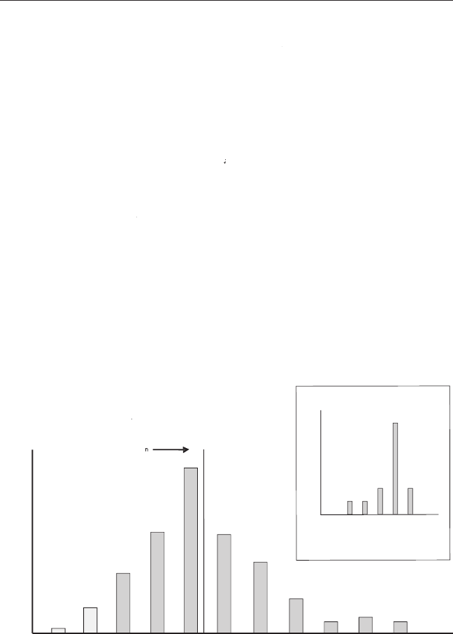
VaR and Stress Testing 171
variable in each considered scenario, and
p
j
re
p
resents t
h
e
p
ro
b
a
b
i
l
it
y
assigne
d
to eac
h
scenario, wit
h
:
∑
=pj
1
j
Then the P&L movement in each scenario is calculated by:
∑
sm
ii
m
j
i
,
And the P&L distribution is calculated by multiplying each of these
terms by its respective
p
j
.
We wi
ll
consi
d
er t
h
e a
d
vantages an
d
d
isa
d
vantages o
f
eac
h
o
f
t
h
ese
t
h
ree met
h
o
d
s.
T
h
e
d
irect measurement o
f
P&L
d
istri
b
ution is sti
ll
wi
d
e
l
y use
d
, as
can
b
e seen
f
rom t
h
e
f
requent use o
f
h
istograms o
f
d
ai
l
y P&L
d
istri
b
utions
pu
bl
is
h
e
d
in annua
l
reports o
f
nancia
l
rms, o
f
t
h
e type i
ll
ustrate
d
in
Figure 7.1 . It
h
as t
h
e a
d
vantage o
f
simp
l
icity o
f
ca
l
cu
l
ation, not
h
aving to
ma
k
e any use o
f
mo
d
e
l
s or statistica
l
assumptions. It a
l
so
h
as t
h
e a
b
i
l
ity to
capture e
ff
ects o
f
t
h
e tra
d
ing cu
l
ture, w
h
ic
h
t
h
e ot
h
er met
h
o
d
s
d
o not. For
examp
l
e,
d
oes management respon
d
to perio
d
s o
f
greater mar
k
et vo
l
ati
l
ity
FI
GU
RE 7.1 P&L Histo
g
ram
f
rom JPMor
g
an 2011 Annua
l
< (30)
90 > < 12
0
120 > < 15
0
1
50 > < 18
0
180> < 210
2
10 > < 24
0
30 >
<
60
(30) > <
0
Dail
y
IB and Other Market Risk–Related Gains and Loss
e
s
(95% Confidence Level
V
aR)
V
V
Ye
ar en
d
e
d
Decem
b
er 31,
20
1
0
N
u
m
be
r
of
tr
a
din
g
da
y
s
Aver
age daily revenu
e:
$87 millio
o
o
0
1
0
2
0
30
4
0
50
60
7
0
80
$
in million
s
2
4
6
8
<
0
20
>
<
4
0
40
>
<
6
0
60
>
<
8
0
80
>
<
1
00
>
1
20
$
in millions
N
umber of tradin
g
da
y
s
D
ai
ly
IB an
d
Ot
h
er V
a
R
l
ess mar
k
et ris
k
–re
l
ate
d
l
osses
100
>
<
1
20
0 > < 30
60 > < 90
0
>
2
4
0

172 FINANCIAL RISK MANAGEMENT
b
y re
d
ucing position size? I
f
it
d
oes, t
h
is wi
ll
mitigate some o
f
t
h
e earnings
vo
l
ati
l
ity resu
l
ting
f
rom mar
k
et vo
l
ati
l
ity.
Direct measurement of P&L distribution is also the only method that is
available for measuring risk when access to details of trading positions is not
available. For example, a hedge fund investor probably does not have any ac
-
cess to details of the investment holdings of the hedge fund. To estimate its risk,
the investor may need to rely on historical P&L distribution of the fund (for
more on risk management of investments in hedge funds, see Section 8.4.1).
However, direct measurement of P&L distributions cannot take into
account the possibility that current position taking may be radically dif
-
ferent from historical position taking (in the fund management world, this
is
k
nown as sty
l
e
d
ri
f
t). Corporate ris
k
managers an
d
regu
l
ators wi
ll
insist
on ris
k
measures t
h
at
f
u
ll
y re
ect current port
f
o
l
io composition, w
h
enever
avai
l
a
bl
e. T
h
is ren
d
ers
d
irect measurement o
f
t
h
e P&L
d
istri
b
ution c
l
ose to
useless as a stand‐alone risk measure, thou
g
h it is still valuable as a com
p
le
-
ment to ot
h
er measures.
T
h
e use o
f
t
h
e variance‐covariance met
h
o
d
h
as now
b
een virtua
ll
y
a
b
an
d
one
d
b
y sop
h
isticate
d
nancia
l
rms in
f
avor o
f
simu
l
ation met
h
o
d
s.
T
h
e primary reason
f
or t
h
is is t
h
at re
l
ative to t
h
e simu
l
ation met
h
o
d
, t
h
e
variance‐covariance met
h
o
d
provi
d
es very
l
itt
l
e
exi
b
i
l
ity in eva
l
uating t
h
e
contri
b
ution o
f
non
l
inear positions, nota
bl
y options positions, to P&L
d
is
-
tri
b
utions. As we wi
ll
see, simu
l
ation gives t
h
e
exi
b
i
l
ity to tai
l
or t
h
e
d
egree
o
f
d
etai
l
use
d
in ca
l
cu
l
ating non
l
inear positions to t
h
e
d
egree o
f
accuracy re
-
quire
d
f
or particu
l
ar port
f
o
l
ios. Detai
l
can range
f
rom simp
l
e
f
actor approx
-
imations (using
d
e
l
ta, gamma, vega, etc.) to
f
u
ll
va
l
uation o
f
eac
h
in
d
ivi
d
ua
l
option, wit
h
severa
l
gra
d
ations avai
l
a
bl
e in
b
etween. By contrast, variance
‐
covariance can’t go
b
eyon
d
f
actor approximation. Secon
d
ary reasons are
:
■ T
h
e greater
d
i
f
cu
l
ty t
h
at t
h
e variance‐covariance met
h
o
d
h
as in
d
ea
l-
ing wit
h
t
h
e
f
at‐tai
l
e
d
d
istri
b
utions norma
ll
y encountere
d
in
nancia
l
mar
k
ets.
■ T
h
e ina
b
i
l
ity o
f
variance‐covariance to pic
k
up t
h
e p
h
enomenon, o
f
ten
o
b
serve
d
in
nancia
l
mar
k
ets, t
h
at t
h
e
l
argest c
h
anges in varia
bl
es o
f
ten
c
l
uster toget
h
er (e.g., t
h
e
h
ig
h
corre
l
ation
b
etween stoc
k
mar
k
ets in
d
i
f-
f
erent countries in t
h
e 1987 stoc
k
cras
h
) to a greater
d
egree t
h
an wi
ll
b
e in
d
icate
d
b
y corre
l
ation coe
f
cients (i.e., t
h
e joint
d
istri
b
ution is not
b
ivariate norma
l
).
■ The realization that almost all the bene ts of simplicity and speed o
f
computation claimed for variance‐covariance relative to simulation
were based on fallacious comparisons. As will be seen in our discussion
of simulation methodology, the degree of simplicity and speed of com
-
putation are largely determined by the choice of the user. Achieving

VaR and Stress Testing 173
a
l
eve
l
o
f
accurac
y
simi
l
ar to t
h
at o
b
taine
d
by
variance‐covariance,
simu
l
ation is at
l
east as simp
l
e an
d
f
ast to compute as variance
‐
covariance. Simulation offers the exibility, which variance‐covariance
does not, of increasing accuracy as a trade‐off against simplicity and
computation time, but having more exibility can surely not count as
a disadvantage.
Currently, the primary users of variance‐covariance are smaller rms
that do not hold signi cant options positions and that wish to outsource
the market data component of their VaR computations. For such rms,
variance‐covariance does offer the distinct advantage that they only need
to o
b
tain vo
l
ati
l
ities an
d
corre
l
ations rat
h
er t
h
an t
h
e
d
ay‐
b
y‐
d
ay pricing
h
istories require
d
f
or simu
l
ation, a consi
d
era
bl
e savings in t
h
e amount o
f
d
ata to
b
e trans
f
erre
d
.
In Exercise 7.1,
y
ou will have a chance to see an exam
p
le of how
variance‐covariance computes VaR an
d
w
h
y a simu
l
ation ca
l
cu
l
ation t
h
at
is as simp
l
e computationa
ll
y an
d
is superior in
exi
b
i
l
ity is a
l
ways avai
l-
a
bl
e. I wi
ll
t
h
ere
f
ore not spen
d
any more time on variance‐covariance or
t
h
e various tric
k
s t
h
at
h
ave
b
een
d
evise
d
to provi
d
e capa
b
i
l
ity to approxi
-
mate option positions an
d
incorporate
f
at tai
l
s wit
h
in it. For rea
d
ers w
h
o
wis
h
to pursue t
h
is approac
h
, I recommen
d
C
h
apters 6 an
d
10 o
f
Dow
d
(
2005
)
.
7.1.1
S
imulation of the P
&
L Distribution
Remem
b
er t
h
at t
h
e simu
l
ation approac
h
consists o
f
d
etermining a num
b
er
of possible scenarios, to be indexed by
j
,
d
etermining t
h
e size o
f
move o
f
eac
h
mar
k
et varia
bl
e in eac
h
scenario
m
i
, j
i
, an
d
t
h
en ca
l
cu
l
ating
:
sm
ii
m
j
i
,
∑
as t
h
e
rm’s tota
l
P&L movement in eac
h
scenario. T
h
e steps in a P&L
simu
l
ation consist o
f
(1)
d
etermining a set o
f
scenarios speci
e
d
b
y t
h
e size
o
f
move in eac
h
o
f
a set o
f
un
d
er
l
ying mar
k
et varia
bl
es an
d
a pro
b
a
b
i
l
ity to
b
e assigne
d
to eac
h
set an
d
(2) trans
l
ation
f
rom t
h
e size o
f
move o
f
un
d
er
-
l
ying mar
k
et varia
bl
es to size o
f
move
f
or a
ll
mar
k
et varia
bl
es. For examp
l
e,
t
h
e un
d
er
l
ying mar
k
et varia
bl
es
f
or a set o
f
b
on
d
positions cou
ld
b
e inter
-
est rates for 10 key tenors, and the full set of market variables could be
prices for individual bonds. There are two alternative approaches to the rst
step—historical simulation and Monte Carlo simulation. The decisions to
be made for the second step do not depend on the choice made for the rst
step. We will discuss each step in some detail.

174 FINANCIAL RISK MANAGEMENT
7.1.1.1
S
te
p
1: Determine Underl
y
in
g
Market Probabilities T
h
e
h
istorica
l
simu
l
a-
tion approac
h
is quite simp
l
e; a group o
f
h
istorica
l
perio
d
s is c
h
osen an
d
t
h
e
observed sizes of market moves in each of these historical periods constitute
the scenarios. So, for example, you could choose 1,200 scenarios consisting
of all the most recent one‐business‐day changes in market variables—the
changes in market variables from 6/7/99 to 6/8/99 would be one scenario,
the change from 6/8/99 to 6/9/99 another scenario, and so forth. Or one
could choose all the 10‐business‐day changes.
The most commonly used method for historical simulation assigns equal
‐
probability weights to all of these possible market moves. This makes calcula
-
tion of VaR very simple, since it is just equivalent to one particular scenario
(
f
or examp
l
e, i
f
you wante
d
t
h
e 99t
h
percenti
l
e VaR an
d
you are wor
k
ing
wit
h
1,200 scenarios, t
h
e 12t
h
worst
l
oss in any o
f
t
h
ese scenarios is t
h
e 99t
h
percenti
l
e VaR). W
h
en we exp
l
ain t
h
e ca
l
cu
l
ation o
f
measures o
f
P&L
d
istri
-
bution in Section 7.1.2, we will discuss the
p
ossible advanta
g
es of and meth
-
o
d
o
l
ogy
f
or assigning unequa
l
pro
b
a
b
i
l
ity weig
h
ts to t
h
ese mar
k
et moves.
Historica
l
simu
l
ation o
ff
ers a
l
arge a
d
vantage in terms o
f
simp
l
icity
—
simp
l
icity o
f
imp
l
ementation, simp
l
icity o
f
assumptions, simp
l
icity o
f
exp
l
a
-
nation. T
h
e a
d
vantage in terms o
f
assumptions is t
h
at no mo
d
e
l
ing assump
-
tion nee
d
s to
b
e ma
d
e
b
eyon
d
t
h
e assumption t
h
at t
h
e imme
d
iate
f
uture
wi
ll
resem
bl
e t
h
e past. T
h
ere is no parameterization o
f
eit
h
er variance or
corre
l
ation an
d
no assumptions a
b
out
d
istri
b
ution s
h
ape (e.g., norma
l
ity).
I
f
f
at tai
l
s or c
l
ustering o
f
l
arge moves
b
etween varia
bl
es are present in t
h
e
h
istorica
l
d
ata, t
h
ey wi
ll
b
e re
ecte
d
in t
h
e simu
l
ation.
T
h
e a
d
vantage in terms o
f
exp
l
anation is t
h
at any questions raise
d
b
y
tra
d
ers or managers concerning a VaR t
h
at seems too
h
ig
h
can
b
e easi
l
y
trace
d
to a su
b
set o
f
speci
c
h
istorica
l
d
ates t
h
at wou
ld
s
h
ow
l
arge
l
oss
-
es against t
h
e current
rm
h
o
ld
ings. Disagreement can
b
e quic
kl
y
f
ocuse
d
on accuracy o
f
d
ata
f
or a
f
ew speci
c
d
ates or on arguments a
b
out t
h
e
pro
b
a
b
i
l
ities to
b
e assigne
d
to repetition o
f
particu
l
ar
h
istorica
l
events. By
contrast,
b
ot
h
t
h
e variance‐covariance approac
h
an
d
t
h
e Monte Car
l
o simu
-
l
ation approac
h
ma
k
e it
f
ar more
d
i
f
cu
l
t to reso
l
ve suc
h
questions.
T
h
is a
d
vantage o
f
simp
l
icity o
f
h
istorica
l
simu
l
ation a
l
so un
d
er
l
ies its
primary
d
isa
d
vantage—t
h
e VaR pro
d
uce
d
is
d
ominate
d
b
y mar
k
et moves
on a
f
ew speci
c
h
istorica
l
d
ays. I
f
a particu
l
ar com
b
ination o
f
mar
k
et
events
d
i
d
not occur in t
h
e
h
istorica
l
perio
d
b
eing consi
d
ere
d
, it cannot con-
tri
b
ute to VaR. It is
d
i
f
cu
l
t to overcome t
h
is pro
bl
em
b
y just expan
d
ing t
h
e
historical period you are considering. Data availability tends to get sparse
once you go back more than a few years, because of failure to retain data,
because data becomes more dif cult to clean the further back you go in
time, and because some currently traded instruments may not have histories
that go back that far.

VaR and Stress Testing 175
T
h
is
d
isa
d
vanta
g
e o
f
g
eneratin
g
scenarios uti
l
izin
g
t
h
e
h
istorica
l
met
h-
o
d
is t
h
e primary argument in
f
avor o
f
t
h
e Monte Car
l
o met
h
o
d
. T
h
e Monte
Carlo method starts with a speci cation of the underlying market variables
that is similar to that of the variance‐covariance approach, but may have a
richer speci cation of each single variable than just a volatility—for exam
-
ple, a multiparameter speci cation that allows the generation of distribu
-
tions that are skewed or fat‐tailed. Monte Carlo generation of distributions
that t speci ed parameters can be achieved in several ways
:
■
By mixing together normal distributions, distributions that are
skewed and fat‐tailed can be generated. This can be done using the
MixtureO
f
Norma
ls
sprea
d
s
h
eet we encountere
d
in C
h
apter 1 . Mix-
i
ng norma
l
d
istri
b
utions wit
h
t
h
e same mean an
d
d
i
ff
erent vo
l
ati
l
ities
p
ro
d
uces
f
at tai
l
s
b
ut no s
k
ew. T
h
e
l
arger t
h
e
d
i
ff
erence in vo
l
ati
l
ities,
t
he
g
reater the kurtosis, a measure of how fat‐tailed the distribution is.
Mixing norma
l
d
istri
b
utions wit
h
d
i
ff
erent means an
d
d
i
ff
erent vo
l
ati
l
i
-
t
ies pro
d
uces
b
ot
h
f
at tai
l
s an
d
s
k
ew. More
d
etai
l
can
b
e
f
oun
d
in Dow
d
(2005, Section 6.5.3) an
d
Wang (2001).
■
By using stoc
h
astic vo
l
ati
l
ity an
d
jump process speci
cations,
simi
l
ar to t
h
ose we
d
iscuss in Sections 11.6.2 an
d
12.3.2. See a
l
so Hu
ll
(
2012, Sections 26.1 an
d
26.2
)
an
d
Dow
d
(
2005, Sections 6.5.4 an
d
6.5.5
)
.
■
By using processes specia
ll
y
d
esigne
d
to generate Monte Car
l
o
d
istri
-
b
utions t
h
at matc
h
given s
k
ew an
d
k
urotsis parameters, suc
h
as t
h
ose
d
iscusse
d
in S
h
aw (1997). Monte Car
l
o tec
h
niques are t
h
en use
d
to
generate a set o
f
scenarios t
h
at
t t
h
e
d
esire
d
statistica
l
speci
cations.
S
h
aw (1997)
d
iscusses
b
ui
ld
ing Monte Car
l
o simu
l
ations
f
o
ll
owing t
h
e
a
l
gorit
h
m o
f
Ram
b
erg et a
l
. (1979). An imp
l
ementation o
f
t
h
is a
l
go
-
rit
h
m can
b
e
f
oun
d
on t
h
e we
b
site
f
or t
h
is
b
oo
k
(t
h
is a
l
gorit
h
m on t
h
e
we
b
site is ca
ll
e
d
“Quasi
t”).
Usua
ll
y, users o
f
Monte Car
l
o simu
l
ation want to ta
k
e a
d
vantage o
f
t
h
e
exi
b
i
l
ity it o
ff
ers to generate many more scenarios t
h
an can
b
e practica
ll
y
generate
d
wit
h
h
istorica
l
simu
l
ation. T
h
is
h
as
l
e
d
to t
h
e incorrect asser
-
tion t
h
at Monte Car
l
o simu
l
ation require
s
more scenarios t
h
an
h
istorica
l
simu
l
ation
d
oes. Rat
h
er, Monte Car
l
o simu
l
ation o
ff
ers t
h
e
exi
b
i
l
ity o
f
ac
h
ieving greater accuracy i
f
t
h
e greater expense o
f
running more scenarios
is justi ed by the increase in accuracy. Standard computerized techniques
for improving the trade‐off between accuracy and speed for Monte Carlo
simulation can also be employed (e.g., strati ed sampling, importance sam-
pling, low‐discrepancy sequences; see Hull 2012, Section 20.7; Dowd 2005,
Section 8.4; and Jackel 2002, Chapters 8 and 10).

176 FINANCIAL RISK MANAGEMENT
A
d
vantages t
h
at Monte Car
l
o simu
l
ation o
ff
ers are
:
■Ability to select the most suitable technique to estimate each parameter.
Volatilities and correlations can be forecast using statistical techniques
such as weighted moving averages and generalized autoregressive con
-
ditional heteroscedasticity (GARCH). For a discussion of the most
common statistical methods used in forecasting volatilities and correla
-
tions, see Hull (2012, Chapter 22 ), Dowd (2005, Chapter 5 ), and Jorion
(2007, Chapter 9 ). Statistical methods for adjusting parameters derived
from historical data to be more robust, including random matrix theory
and shrinkage estimation, can be found in Fabozzi, Focardi, and Kolm
(2006, C
h
apters 8 an
d
9). Va
l
ua
bl
e
d
iscussion o
f
t
h
is topic can a
l
so
b
e
f
oun
d
in Meucci (2005, C
h
apter 4 ). Swensen (2000, C
h
apter 5 ) is a va
l
-
ua
bl
e approac
h
wit
h
l
ess emp
h
asis on statistica
l
met
h
o
d
o
l
ogy an
d
more
on economic insi
g
ht. Where im
p
lied volatilities are available, the
y
can
b
e su
b
stitute
d
f
or or
bl
en
d
e
d
wit
h
statistica
l
measures. (S
h
ou
ld
imp
l
ie
d
vo
l
ati
l
ity a
l
ways
b
e use
d
w
h
en avai
l
a
bl
e? We’
ll
examine t
h
is question at
t
h
e en
d
o
f
t
h
is su
b
section.) T
h
e c
h
oice can
b
e separate
l
y ma
d
e
f
or eac
h
varia
bl
e, t
h
oug
h
you
d
o nee
d
to
b
e care
f
u
l
not to generate impossi
bl
e or
imp
l
ausi
bl
e com
b
inations o
f
corre
l
ation coe
f
cients;
f
or
d
iscussion o
f
h
ow to avoi
d
creating impossi
bl
e corre
l
ation matrices, see Dow
d
(2005,
S
ection 5.3
)
.
■
A
b
i
l
ity to se
l
ect t
h
e most re
l
evant
d
ata set
f
or estimating eac
h
param
-
eter
.
You mig
h
t
h
ave 10 years o
f
goo
d
h
istorica
l
d
ata
f
or one varia
bl
e
an
d
on
l
y two years
f
or anot
h
er. Historica
l
simu
l
ation wou
ld
f
orce you
to use on
l
y two years’ wort
h
o
f
d
ata
f
or
b
ot
h
. Monte Car
l
o simu
l
ation
l
ets you c
h
oose t
h
e
d
ata set in
d
ivi
d
ua
ll
y
f
or eac
h
varia
bl
e. You can a
l
so
c
h
oose t
h
e most appropriate weig
h
ts to assign to
d
i
ff
erent
h
istorica
l
perio
d
s
f
or eac
h
varia
bl
e, wit
h
more
d
iscounting o
f
o
ld
er
h
istorica
l
d
ata
f
or some varia
bl
es t
h
an
f
or ot
h
ers. Historica
l
simu
l
ation can on
l
y uti
l
ize
a sing
l
e weig
h
ting sc
h
eme t
h
at app
l
ies equa
ll
y to a
ll
varia
bl
es (see t
h
e
d
iscussion o
f
t
h
is weig
h
ting o
f
h
istorica
l
simu
l
ation in Section 7.1.2).
■A
b
i
l
ity to se
l
ect t
h
e most re
l
evant
d
ata set
f
or estimating
d
i
ff
erent as-
pects o
f
a sing
l
e varia
bl
e
.
For examp
l
e, vo
l
ati
l
ity cou
ld
b
e
b
ase
d
on
recent
d
ata or
d
erive
d
f
rom an imp
l
ie
d
vo
l
ati
l
ity w
h
i
l
e
h
ig
h
er‐or
d
er
parameters o
f
t
h
e
d
istri
b
ution are estimate
d
f
rom
l
onger
d
ata perio
d
s.
Recent
d
ata is o
f
ten consi
d
ere
d
a
b
etter pre
d
ictor o
f
near‐term
f
uture
volatility, but shape parameters, such as fatness of tails, are hard to dis
-
cern from a small data set.
■Greater exibility in handling missing data. Data for individual dates
can be missing because a particular market was closed for a holiday or
because of errors in data gathering. In fact, all sources of market data,

VaR and Stress Testing 177
w
h
et
h
er
d
ata ven
d
ors,
b
ro
k
ers, or
d
ata
b
ases interna
l
to t
h
e
rm, are no
-
t
orious
l
y poor in qua
l
ity an
d
require major
d
ata scru
bb
ing e
ff
orts. But
some data will not have suf cient duplication of sources to scrub suc
-
cessfully and must be regarded as unavailable. Monte Carlo simulation
can exclude periods for which a particular data series is missing from
t
he calculation of each individual variable without excluding this period
f
rom the calculation of other variables for which the data are available.
Historical simulation lacks this exibility—it must either completely in-
clude or completely exclude a particular day’s data.
■
Greater exibility in handling nonsynchronous data. Correlations ob
-
served between variables that are sampled at different times of the day
can
b
e
h
ig
hl
y mis
l
ea
d
ing an
d
resu
l
t in signi
cant misstatements o
f
ris
k
.
Monte Car
l
o simu
l
ation
h
as t
h
e
exi
b
i
l
ity to measure corre
l
ation
f
or
eac
h
in
d
ivi
d
ua
l
pair o
f
varia
bl
es
b
ase
d
on quotations
f
rom t
h
e
b
est time
of da
y
to re
p
resent that
p
articular
p
air, or b
y
basin
g
the correlation on
a mu
l
ti
d
ay time interva
l
, w
h
ic
h
wi
ll
ten
d
to smoot
h
out nonsync
h
ro
-
nous e
ff
ects. For more
d
etai
l
on statistica
l
met
h
o
d
s t
h
at can
b
e use
d
in
estimating corre
l
ations
b
etween nonsync
h
ronous
d
ata, see Ris
k
Metrics
Group (1996, Section 8.5) an
d
Ho
l
ton (2003, Section 6.3).
■
A
b
i
l
ity to com
b
ine
h
istories
.
Consi
d
er a corporate
b
on
d
h
e
ld
in t
h
e
rm’s port
f
o
l
io. By
h
istorica
l
experience, one
k
nows t
h
at some o
f
t
h
ese
b
on
d
s may su
ff
er a ratings
d
owngra
d
e an
d
su
b
sequent
l
arge
f
a
ll
in
p
rice. But it may
b
e t
h
at none o
f
t
h
e
b
on
d
s current
l
y
h
e
ld
h
as su
ff
ere
d
suc
h
a
d
owngra
d
e since t
h
e
rm avoi
d
s
h
o
ld
ing suc
h
b
on
d
s. Historica
l
simu
l
ation wou
ld
s
h
ow no ratings
d
owngra
d
e events
f
or t
h
ese
b
on
d
s.
But Monte Car
l
o simu
l
ation cou
ld
b
e use
d
to com
b
ine ratings
d
own
-
gra
d
e possi
b
i
l
ities
b
ase
d
on t
h
e
h
istory o
f
a
l
arge poo
l
o
f
b
on
d
s wit
h
speci
c pricing
h
istory o
f
actua
l
b
on
d
s
h
e
ld
.
Anot
h
er examp
l
e wou
ld
b
e a
f
oreign exc
h
ange (FX) position
h
e
ld
i
n a currency t
h
at
h
as
b
een pegge
d
at a
xe
d
exc
h
ange rate to t
h
e
d
o
ll
ar
b
y government intervention. You may
h
ave no
h
istorica
l
examp
l
e o
f
t
h
is
p
articu
l
ar currency
d
eva
l
uing, yet want to inc
l
u
d
e some pro
b
a
b
i
l
ity o
f
d
eva
l
uation. Monte Car
l
o simu
l
ation cou
ld
incorporate a
d
eva
l
uation
event, possi
bl
y parameterize
d
b
y
d
eva
l
uation experience in ot
h
er cur
-
rencies, as a jump process superimpose
d
on t
h
e speci
c
h
istory o
f
t
h
is
FX
rate.
Sti
ll
anot
h
er examp
l
e wou
ld
b
e two stoc
k
s t
h
at
h
ave
b
egun tra
d-
i
ng in a very tightly related fashion since a merger announcement. You
would not want to re ect their previous more volatile arrangement as
p
art of the history that determines VaR. So you must generate the price
of one stock as a function of the other
,
but with a random element in
-
t
roduced to represent the risk of a sharp break in the price relationship

178 FINANCIAL RISK MANAGEMENT
i
f
t
h
e merger
f
ai
l
s to go t
h
roug
h
. T
h
is ran
d
om e
l
ement s
h
ou
ld
b
e
b
ase
d
on t
h
e price
h
istory o
f
a
l
arge poo
l
o
f
stoc
k
pairs
f
o
ll
owing a merger
announcement.
Finally, Monte Carlo simulation allows users great exibility in
deciding on the most effective approach to specifying each individual
variable. Consider as an example specifying parameters for credit de
-
fault swaps (CDSs) (see Section 13.1.1.2 for more details on CDSs).
CDS prices for some corporations may have suf cient liquidity that you
want to estimate the parameters for this price based solely on the price
history of this particular CDS. For other corporations with less liquidity
in CDS prices, you can choose to break the CDS price up into a credit
sprea
d
on a
b
on
d
issue
d
b
y t
h
at corporation p
l
us a sprea
d
b
etween t
h
e
CDS sprea
d
an
d
t
h
e
b
on
d
’s cre
d
it sprea
d
(we’
ll
ca
ll
t
h
is t
h
e CDS
b
asi
s
)
.
T
h
e parameters
f
or t
h
e cre
d
it sprea
d
on t
h
e
b
on
d
mig
h
t
b
e
b
ase
d
so
l
e
l
y
on the histor
y
of credit s
p
reads for this cor
p
oration’s bonds, while the
parameters
f
or t
h
e CDS
b
asis mig
h
t
b
e
b
etter estimate
d
f
rom o
b
serv
-
ations o
f
CDS
b
asis
h
istory
d
rawn
f
rom a
l
arger universe o
f
simi
l
ar
corporations. Even t
h
oug
h
you are estimating t
h
e CDS
b
asis
f
or sev
-
era
l
d
i
ff
erent corporations
f
rom t
h
e same
d
ata source, you
d
on’t expect
t
h
em to
b
e per
f
ect
l
y corre
l
ate
d
,
b
ut you can estimate a corre
l
ation co
-
e
f
cient
f
rom
h
istorica
l
o
b
servations o
f
h
ow c
h
anges in CDS
b
asis
d
i
f-
f
er
b
etween corporations.
It is straig
h
t
f
orwar
d
to repro
d
uce any
d
esire
d
corre
l
ation matrix in
a Monte Car
l
o simu
l
ation using t
h
e C
h
o
l
es
k
y
d
ecomposition met
h
o
d
d
e
-
scri
b
e
d
in Dow
d
(2005, Section 8.3). But covariance matrices emp
l
oy cor-
re
l
ations
b
ase
d
on mu
l
tivariate norma
l
d
istri
b
utions an
d
t
h
ere
f
ore
d
o not
capture any re
l
ations
h
ips t
h
at are extreme
l
y un
l
i
k
e
l
y un
d
er t
h
is
h
ypot
h
esis
(e.g., t
h
e c
l
ustering o
f
l
arge c
h
anges in varia
bl
es). A
dd
ressing t
h
ese concerns
requires more re
ne
d
d
ata ana
l
yses. For examp
l
e,
d
i
ff
erent corre
l
ation mat-
rices cou
ld
b
e use
d
d
epen
d
ing on t
h
e size o
f
price moves (see Kim an
d
Finger
2000). Days in w
h
ic
h
price moves are
l
arger wou
ld
use a corre
l
ation matrix
d
erive
d
f
rom a samp
l
e o
f
d
ays wit
h
l
arge moves. T
h
e MixtureO
f
Norma
ls
sprea
d
s
h
eet can pro
d
uce corre
l
ations wit
h
d
i
ff
erent
d
egrees o
f
c
l
ustering, as
s
h
own in Figures 7.2 an
d
7.3 .
Figure 7.2 s
h
ows t
h
e corre
l
ation
b
etween two norma
ll
y
d
istri
b
ute
d
vari
-
a
bl
es wit
h
25% corre
l
ation,
b
ot
h
wit
h
mean 2%, stan
d
ar
d
d
eviation 5%. Fig
-
ure 7.3 shows a mixture of 95% of the rst distribution and 5% of two nor
-
mally distributed variables with 60% correlation, both with mean 0, standard
deviation 10%. Note the clustering of points with large losses in both vari
-
ables and large gains in both variables in Figure 7.3 . This clustering does not
appear in Figure 7.2 , which displays a multivariate normal distribution.

VaR and Stress Testing 179
-6.00%
-6 00%
-4.00%
-4 00%
-2.00%
-2 00%
0.00%
0 00%
%
2.00%
2 00%
%
4.00%
4 00%
0%
6.00%
6 00%
6.00
8.00%
8 00%
10.00%
10 00%
12.00%
12 00%
14.00%
14 00%
-4.00
%
-2.00%
20
20
0.00%
0
%
%
%
2.00%
.00%
4.00%
4
6.0
0
%
8.00
%
1
0.00
%
12.00
%
1
4.0
0
%
FI
GU
RE 7.2
C
orrelation Between Two Normally Distributed Variable
s
-
-
40.00%
40 00%
-
-
30.00%
30 00%
-
-
20.00%
20 00%
20
-
%
%
10.00%
0
0.00
%
10.00%
000
10.00%
20.00%
20 00%
00
30.00%
30 00%
-
30.00
%
-20.00%
%
40.00
%
3
0.00
%
2
0.00
%
10.00
%
00%
0
00.00%
-
10.00
%
FIGURE 7.3 A Mixture o
f
Two Norma
l
Distri
b
utions S
h
ows a C
l
ustering o
f
Points
wit
h
Large Gains an
d
Large Losses

180 FINANCIAL RISK MANAGEMENT
More genera
l
met
h
o
d
s
f
or ana
l
yzing non
l
inear corre
l
ations an
d
gen
-
erating Monte Car
l
o
d
istri
b
utions
b
ase
d
on t
h
is ana
l
ysis
h
ave
b
een wi
d
e
l
y
studied in recent years. This is known as copul
a
methodology; see Dowd
(2005, Section 6.8) for details.
Given all these advantages to Monte Carlo simulation in its exibility
to handle data and estimation issues, it is preferable, and sometimes even
unavoidable, to still employ some Monte Carlo simulation techniques when
you have chosen historical simulation as your primary methodology. Con
-
sider these examples
:
■
A certain stock held in your portfolio has only recently been issued. To
d
eve
l
op a past
h
istory
f
or t
h
e price o
f
t
h
is stoc
k
f
or use in
h
istorica
l
sim-
u
l
ation, you may represent it
b
y some
f
ormu
l
a
b
ase
d
on a se
l
ecte
d
stoc
k
in
d
ex. But i
f
you are
l
ong t
h
is stoc
k
an
d
s
h
ort t
h
is in
d
ex, you wou
ld
measure
y
our
p
osition as havin
g
no risk durin
g
the
p
eriod when it is
represente
d
b
y t
h
e in
d
ex. To avoi
d
t
h
is, you nee
d
to intro
d
uce a ran
d
om
e
l
ement into your generation o
f
t
h
e stoc
k
’s
b
ac
k
price
h
istory,
b
asing t
h
e
size o
f
t
h
e ran
d
om e
l
ement on o
b
serve
d
c
h
anges
d
uring t
h
e perio
d
since
t
h
e stoc
k
b
egan tra
d
ing. But t
h
is is precise
l
y t
h
e Monte Car
l
o approac
h
.
■ T
h
e ratings
d
owngra
d
e ris
k
case, t
h
e FX
d
eva
l
uation ris
k
case, t
h
e
merger ar
b
itrage ris
k
case, an
d
t
h
e CDS
b
asis case
d
iscusse
d
in t
h
e
b
u
l
-
l
et point
h
ea
d
e
d
“A
b
i
l
ity to com
b
ine
h
istories” un
d
er a
d
vantages o
f
M
onte Car
l
o simu
l
ation are goo
d
examp
l
es o
f
w
h
ere a ran
d
om e
l
ement
nee
d
s to
b
e intro
d
uce
d
into t
h
e
h
istorica
l
series.
In cases
l
i
k
e t
h
ese,
h
ow s
h
ou
ld
a ran
d
om e
l
ement
b
e intro
d
uce
d
into
h
istorica
l
simu
l
ation? One met
h
o
d
t
h
at is sometimes use
d
is to ran
d
om
l
y
assign t
h
e
d
istri
b
ution o
f
t
h
e ran
d
om e
l
ement among t
h
e
d
ays o
f
h
istorica
l
d
ata. For examp
l
e, i
f
t
h
ere is a 1 in 250 c
h
ance o
f
a ratings
d
owngra
d
e
f
or a
b
on
d
, t
h
e price
d
rop t
h
at wou
ld
resu
l
t
f
rom a
d
owngra
d
e wou
ld
b
e ran
d
om
-
l
y assigne
d
to
f
our
d
ays out o
f
a 1,000‐
d
ay
h
istorica
l
simu
l
ation. But t
h
is
h
as a
l
arge c
h
ance o
f
h
aving no impact on t
h
e VaR measurement since t
h
e
f
our
d
ays ran
d
om
l
y se
l
ecte
d
wou
ld
l
i
k
e
l
y miss t
h
e
d
ays o
f
l
argest
l
osses t
h
at
d
etermine t
h
e VaR measure,
b
ut a sma
ll
pro
b
a
b
i
l
ity o
f
h
aving a
l
arge e
ff
ect
i
f
it
h
appens t
h
at one o
f
t
h
e
f
our
d
ays se
l
ecte
d
at ran
d
om correspon
d
s to one
o
f
t
h
e
d
ays o
f
l
argest
l
oss t
h
at
d
etermine t
h
e VaR measure.
I
b
e
l
ieve t
h
at t
h
is ran
d
omness in contri
b
uting to VaR contri
b
utes not
h-
ing to the accurate measurement of risk. It is far better to simply accept that
this part of the VaR measurement mus
t
be performed by Monte Carlo simu-
t
lation, even if you have chosen to do the bulk of your VaR measurement by
historical simulation. The historical simulation results for the main body
of the portfolio are treated as a single series as input to the Monte Carlo

VaR and Stress Testing 181
simu
l
ation, wit
h
a uni
f
orm
d
istri
b
ution assi
g
nin
g
an e
q
ua
l
p
ro
b
a
b
i
l
it
y
to
eac
h
d
ay’s simu
l
ate
d
resu
l
t (
f
or examp
l
e, i
f
t
h
ere are 1,000 simu
l
ate
d
d
ays
in the historical simulation, each path in the Monte Carlo simulation has a 1
in 1,000 chance of picking each of these days). The elements that cannot be
treated by historical simulation would be the remaining series in the Monte
Carlo simulation, parameterized as discussed in the section on Monte Carlo
simulation. Correlations between factors will be chosen based on best his
-
torical evidence and economic intuition.
There are other areas in which historical simulation can usefully borrow
Monte Carlo simulation techniques. For example, historical simulations can
be modi ed to choose a volatility for a particular instrument based on any
o
f
t
h
e tec
h
niques mentione
d
in t
h
e
rst
b
u
ll
et point un
d
er a
d
vantages o
f
Monte Car
l
o simu
l
ation. A
ll
t
h
at is require
d
is to mu
l
tip
l
y eac
h
h
istorica
l
o
b
servation
f
or t
h
e instrument
b
y t
h
e ratio
b
etween t
h
e
d
esire
d
vo
l
ati
l
ity
and the volatilit
y
over the historical
p
eriod. This transformation leaves all
s
h
ape c
h
aracteristics o
f
t
h
e
h
istorica
l
d
istri
b
ution, suc
h
as
f
atness o
f
tai
l
s
an
d
corre
l
ation structure, intact. T
h
is approac
h
is i
ll
ustrate
d
in t
h
e VaR
sprea
d
s
h
eet, using t
h
e vo
l
ati
l
ity overri
d
e input exp
l
aine
d
in t
h
e
d
ocumenta-
tion
f
or t
h
e
h
istorica
l
simu
l
ation portion o
f
t
h
e sprea
d
s
h
eet. Dow
d
(2005,
Section 4.4.2) out
l
ines a simi
l
ar i
d
ea.
W
h
en it comes to
d
ea
l
ing wit
h
missing or nonsync
h
ronous
d
ata, t
h
e
options
f
or
h
istorica
l
simu
l
ation are very
l
imite
d
. Some way nee
d
s to
b
e
i
d
enti
e
d
f
or mo
d
i
f
ying
d
ata
b
efor
e
it is input into t
h
e simu
l
ation.
For missing
d
ata, some type o
f
statistica
l
in
f
erence must
b
e use
d
to ar
-
rive at a most
l
i
k
e
l
y va
l
ue
f
or t
h
e missing
d
ata
b
ase
d
on t
h
e
l
ast prior goo
d
d
ata point, t
h
e next
f
o
ll
owing goo
d
d
ata point, an
d
goo
d
d
ata points
f
or
re
l
ate
d
d
ata series (
f
or examp
l
e, i
f
d
ata is missing
f
or an interest rate
f
or a
two‐year tenor, re
l
ate
d
d
ata series wou
ld
b
e interest rates
f
or t
h
e one‐year
tenor an
d
t
h
e t
h
ree‐year tenor). T
h
e simp
l
est met
h
o
d
s invo
l
ve averaging
b
etween t
h
e
l
ast prior goo
d
point an
d
next
f
o
ll
owing goo
d
point,
b
ut over
-
l
oo
k
va
l
ua
bl
e in
f
ormation
f
rom ot
h
er
d
ata series. At a minimum, one s
h
ou
ld
mo
d
i
f
y simp
l
e averaging to
f
o
ll
ow t
h
e pattern o
f
c
h
ange t
h
at too
k
p
l
ace in
re
l
ate
d
d
ata series
b
etween t
h
e
l
ast prior goo
d
d
ata point an
d
next
f
o
ll
owing
goo
d
d
ata point. Possi
bl
y, more a
d
vance
d
statistica
l
mo
d
e
l
s cou
ld
b
e use
d
.
For nonsync
h
ronous
d
ata, a new
d
ata series s
h
ou
ld
b
e generate
d
o
f
“most
l
i
k
e
l
y” sync
h
ronous va
l
ues. For examp
l
e, suppose t
h
at you
h
ave
avai
l
a
bl
e
d
ata
f
or c
l
osing prices
f
or some stoc
k
issues as o
f
To
k
yo c
l
ose o
f
business (COB) and other stock issues as of New York COB. You need to
nd some series that can bridge the time gap—perhaps a futures contract
on a Japanese index that trades in the New York time zone. Then all o
f
the stock quotes as of Tokyo COB can be adjusted for the movement that
took place in the Japanese stock index between Tokyo COB and New York

182 FINANCIAL RISK MANAGEMENT
COB, generating a series t
h
at approximates w
h
at t
h
e quotes
f
or t
h
ese stoc
k
s
wou
ld
b
e as o
f
New Yor
k
COB. T
h
is o
b
vious
l
y
l
eaves room
f
or error in es
-
timating where true liquidation of positions will take place, but it is the best
you can do if you are not utilizing Monte Carlo simulation.
J
ust as we can modify historical simulation to include some of the ad
-
vantages of Monte Carlo, we might want to modify Monte Carlo to include
some of the advantages of historical simulation. Beyond simplicity, the pri
-
mary advantage of historical simulation is the more re ned way in which it
handles multivariate correlation. By utilizing actual daily simultaneous price
moves across the set of all relevant market variables, nonlinear impacts of
arbitrarily great complexity are directly incorporated. This points toward a
mo
d
i
cation o
f
Monte Car
l
o in w
h
ic
h
a
ll
in
d
ivi
d
ua
l
varia
bl
es are generate
d
b
y stan
d
ar
d
Monte Car
l
o tec
h
niques an
d
a
ll
corre
l
ations
b
etween varia
bl
es
are
b
ase
d
on
h
istorica
l
simu
l
ation. T
h
is approac
h
, roug
hl
y
f
o
ll
owing S
h
aw
(
1997
)
, works as follows.
First you per
f
orm a stan
d
ar
d
h
istorica
l
simu
l
ation, wit
h
equa
l
pro
b-
a
b
i
l
ities assigne
d
to eac
h
d
ay’s
h
istory. T
h
en, eac
h
in
d
ivi
d
ua
l
varia
bl
e is re
-
generate
d
using a Monte Car
l
o met
h
o
d
b
ase
d
on w
h
atever estimation tec
h-
nique is consi
d
ere
d
most appropriate (e.g., GARCH, imp
l
ie
d
vo
l
ati
l
ities,
mu
l
tiparameter speci
cation). Di
ff
erent met
h
o
d
s can
b
e in
d
ivi
d
ua
ll
y tai-
l
ore
d
to
d
i
ff
erent varia
bl
es. T
h
e use o
f
t
h
e
h
istorica
l
simu
l
ation va
l
ues is to
d
etermine w
h
ic
h
va
l
ues o
f
t
h
e varia
bl
es occur simu
l
taneous
l
y,
b
ase
d
on ran
k
or
d
er. On t
h
e we
b
site
f
or t
h
is
b
oo
k
, you wi
ll
n
d
my imp
l
ementation o
f
t
h
is
proce
d
ure in MATLAB, tit
l
e
d
“Reor
d
er.”
For examp
l
e, suppose you
h
ave a
h
istorica
l
simu
l
ation wit
h
850
d
ays.
Monte Car
l
o simu
l
ation is use
d
to generate 850 va
l
ues o
f
eac
h
varia
bl
e. I
f
a
particu
l
ar
h
istorica
l
d
ata set consiste
d
o
f
t
h
e
f
ourt
h
h
ig
h
est va
l
ue o
f
varia
bl
e
1, 38t
h
h
ig
h
est va
l
ue o
f
varia
bl
e 2, 625t
h
h
ig
h
est va
l
ue o
f
varia
bl
e 3, an
d
so on, t
h
en you wou
ld
create a simu
l
ation instance wit
h
t
h
e
f
ourt
h
h
ig
h
est
va
l
ue o
f
t
h
e 850 Monte Car
l
o simu
l
ations o
f
varia
bl
e 1, 38t
h
h
ig
h
est va
l
ue
o
f
t
h
e 850 Monte Car
l
o simu
l
ations o
f
varia
bl
e 2, 625t
h
h
ig
h
est va
l
ue o
f
t
h
e
Monte Car
l
o simu
l
ations o
f
varia
bl
e 3, an
d
so on.
W
h
i
l
e t
h
is approac
h
retains many o
f
t
h
e a
d
vantages o
f
Monte Car
l
o
simu
l
ation, it cannot incorporate t
h
em a
ll
. It
l
ac
k
s t
h
e
exi
b
i
l
ity to
b
ase
some corre
l
ations on one
d
ata set an
d
ot
h
er corre
l
ations on anot
h
er
d
ata
set. It requires comp
l
ete
d
ata
f
or every varia
bl
e in every
d
ay to
b
e inc
l
u
d
e
d
in t
h
e
d
ates
d
etermining t
h
e corre
l
ation structure. An
d
it
h
as t
h
e same pro
b
-
lems as historical simulation with nonsynchronous data.
Finally, let’s examine the question of whether implied volatility
should always be preferred to historical volatility when it is available. In
Chapters 11 and 12 of this book, “Managing Vanilla Options Risk” and
“Managing Exotic Options Risk,” I argue strongly for always valuing

VaR and Stress Testing 183
o
p
tions at vo
l
ati
l
ities im
pl
ie
d
f
rom
l
i
q
ui
d
mar
k
et
p
rices. But t
h
is is a
p
ricin
g
argument—we nee
d
to
d
etermine prices at w
h
ic
h
l
onger‐term vo
l
ati
l
ity ris
k
can be exited in order to convert longer‐term risks into shorter‐term risks.
VaR is already dealing with shorter‐term risks, usually overnight. It is also
doubtful that there are liquid prices for options to manage risk over such
short time periods. Implied volatilities can be used as indicators of overnight
volatility, and there may be arguments for believing they carry a great deal
of information. But there are also arguments against giving much weight
to implied volatilities—they sometimes have more to do with supply and
demand factors than forecasts of price variation, as discussed in Section
11.6.2. The decision must be based on belief about their predictive value, as
t
h
ere is no pricing argument
f
or using t
h
em.
7.1.1.2 Ste
p
2: Determine All Market Variables T
h
is section
d
iscusses various
a
pp
roaches to re
p
resentation of the rm’s ex
p
osure to market variables.
More
d
etai
l
s
f
or speci
c positions can
b
e
f
oun
d
in Sections 9.2, 9.3, 9.4,
10.4, 11.4, an
d
13.1.3. Dow
d
(2005, C
h
apter 12 ) is a
l
so a goo
d
source
f
or
recommen
d
ations on t
h
is point. W
h
atever c
h
oices are ma
d
e
f
or
h
ow pos
-
itions s
h
ou
ld
b
e store
d
an
d
represente
d
, t
h
e most important point wit
h
re
-
gar
d
to representation o
f
rm position in VaR an
d
stress test ca
l
cu
l
ations is
t
h
e nee
d
f
or
b
asing a
ll
position inputs on
d
ata t
h
at is entere
d
an
d
contro
ll
e
d
b
y support sta
ff
in
d
epen
d
ent o
f
t
h
e
f
ront o
f
ce (as per Section 3.1.1). T
h
e
VaR an
d
stress test reports are
k
ey e
l
ements
f
or contro
ll
ing an
d
managing
t
h
e
rm’s ris
k
, an
d
it is just as important
f
or position in
f
ormation
f
ee
d
ing
t
h
ese systems to
b
e immune
f
rom
f
ront‐o
f
ce manipu
l
ation as it is to
h
ave
in
d
epen
d
ent P&L reporting. In
d
ee
d
, some o
f
t
h
e most recent major
f
rau
d
s
b
y rogue tra
d
ers
h
ave
b
een perpetrate
d
primari
l
y t
h
roug
h
manipu
l
ation
o
f
ris
k
reporting rat
h
er t
h
an t
h
roug
h
t
h
e manipu
l
ation o
f
P&L reporting
(as per Section 3.1.1). Fa
l
si
cation o
f
P&L reporting can
l
ea
d
to stop‐
l
oss
l
imits
b
eing misse
d
,
b
ut t
h
e equa
ll
y important
l
imits on
b
ui
ld
up o
f
l
arge
positions t
h
at can
b
e very cost
l
y to
l
iqui
d
ate
d
epen
d
on VaR an
d
stress test
repor
t
s.
Near
l
y as important is to
h
ave c
h
ec
k
s in p
l
ace to ensure t
h
at t
h
e posi
-
tion in
f
ormation t
h
at
f
ee
d
s P&L ca
l
cu
l
ations an
d
d
es
k
‐
l
eve
l
ris
k
reports is
i
d
entica
l
to t
h
e position in
f
ormation t
h
at
f
ee
d
s VaR an
d
stress test reports.
Not on
l
y is t
h
is a vita
l
c
h
ec
k
on accuracy o
f
ris
k
reporting,
b
ut it is a
l
so
nee
d
e
d
to maintain goo
d
d
ia
l
ogue
b
etween ris
k
managers an
d
f
ront‐o
f
ce
personnel. Nothing is as destructive of good dialogue as VaR or stress limit
violations that make no sense to traders because they contradict desk‐level
risk reports.
When computing VaR for spot positions, the translation from underly
-
ing market variables to the full set of market variables that you want to

184 FINANCIAL RISK MANAGEMENT
mu
l
tip
l
y
b
y t
h
e
rm’s positions is quite
d
irect. Spot positions suc
h
as spot
FX or t
h
e
h
o
ld
ing o
f
an in
d
ivi
d
ua
l
stoc
k
or stoc
k
in
d
ex or spot go
ld
or spot
oil is just directly multiplied by the generated price change from Step 1.
Computation for forward positions is less straightforward. If you are
currently holding a Treasury bill maturing one month from now, you don’t
want to apply to it the price move you observed for that Treasury bill on a
date six months ago, since at that point the Treasury bill had seven months
to maturity, and you expect seven‐month instruments to demonstrate much
larger price changes than one‐month instruments. So you want to utilize
yield curve parameters as underlying market variables and then multiply
those yield curve parameters by the appropriate value of a basis point meas-
ure o
f
f
orwar
d
position. T
h
is
h
as t
h
e important a
dd
e
d
a
d
vantage o
f
not
h
aving to separate
l
y price eac
h
interest rate instrument
b
ut instea
d
wor
k
ing
wit
h
a summary
d
escription o
f
t
h
e entire position.
Issues are most com
p
lex for o
p
tion
p
ositions (in which we include an
y
non
l
inear payo
ff
positions). T
h
e conceptua
ll
y simp
l
est an
d
most accurate
approac
h
wou
ld
b
e to va
l
ue eac
h
in
d
ivi
d
ua
l
option separate
l
y
b
ase
d
on t
h
e
c
h
anges in t
h
e un
d
er
l
ying mar
k
et varia
bl
es o
f
f
orwar
d
price an
d
imp
l
ie
d
vo
l
ati
l
ity. Even suc
h
a simp
l
e approac
h
h
as comp
l
ications, since
f
or eac
h
scenario it is necessary to c
h
oose a vo
l
ati
l
ity at w
h
ic
h
to eva
l
uate t
h
e option.
T
h
is requires
d
eci
d
ing w
h
ic
h
point on t
h
e imp
l
ie
d
vo
l
ati
l
ity sur
f
ace is t
h
e
rig
h
t one to app
l
y. Suppose you are repricing an option wit
h
one year to ex
-
piry, a stri
k
e price o
f
100, an
d
current un
d
er
l
ying price o
f
80. W
h
ic
h
imp
l
ie
d
vo
l
ati
l
ity s
h
i
f
t
d
o you use w
h
en samp
l
ing
f
rom a perio
d
six mont
h
s ago
w
h
en t
h
e un
d
er
l
ying price was 100? Most practitioners wou
ld
opt
f
or
l
oo
k-
ing at t
h
e s
h
i
f
t in options wit
h
a one‐year expiry an
d
a stri
k
e o
f
125, since
t
h
at wou
ld
give t
h
e same “moneyness” (i.e., a stri
k
e 25 percent a
b
ove cur
-
rent spot). But t
h
is is c
l
ear
l
y open to interpretation an
d
a variety o
f
t
h
eories
on w
h
at
d
rives options pricing (see Derman 1999). Very simi
l
ar consi
d
era-
tions app
l
y to option‐a
d
juste
d
sprea
d
s on mortgage an
d
mortgage‐
b
ac
k
e
d
securities, w
h
ic
h
s
h
ou
ld
b
e re
l
ate
d
to t
h
e security t
h
at
h
a
d
a compara
bl
e
re
l
ations
h
ip to t
h
e prevai
l
ing new mortgage rate. T
h
e reasoning is simi
l
ar,
since option‐a
d
juste
d
sprea
d
s represent t
h
e mar
k
et pricing o
f
uncertainty in
options exercise
d
b
y
h
omeowners.
W
h
i
l
e t
h
e simp
l
est approac
h
is t
h
e most accurate, it is c
l
ear
l
y a
l
so
t
h
e most cost
l
y, an
d
t
h
e
h
eavy expense o
f
d
oing
f
u
ll
in
d
ivi
d
ua
l
reva
l
ua-
tion o
f
eac
h
option position is w
h
at was primari
l
y responsi
bl
e
f
or incor
-
rect claims that simulation methodology for VaR was inherently expensive
to perform. In fact, simulation methodology can achieve better accuracy
than variance‐covariance at no greater cost by the easy trick of representing
option portfolios by summary statistics of deltas, gammas, and vegas and
multiplying these by the appropriate price change, half the square of change

VaR and Stress Testing 185
in
p
rice, an
d
t
h
e c
h
an
g
e in im
pl
ie
d
vo
l
ati
l
it
y
, res
p
ective
ly
. T
h
is sim
pl
i
e
d
representation ma
k
es options positions no more computationa
ll
y
d
i
f
cu
l
t
for simulation than linear positions. So it is a matter of trade‐off in desired
accuracy versus cost to be determined for each options position.
There are also intermediate approaches. One that can provide quite ac
-
curate approximations is to interpolate results based on a price‐vol matrix
representation of the options portfolio, as per Section 11.4. If a reasonably
detailed price‐vol matrix is already being calculated as part of the trading
desk’s own risk reporting, this is a good way of taking advantage of a large
number of full revaluation runs that are already being made (since each
bucket of the matrix requires all options in the portfolio to receive a full
reva
l
uation) wit
h
out nee
dl
ess
d
up
l
ication o
f
e
ff
ort. As we note in Section
11.4, t
h
e price‐vo
l
matrix can potentia
ll
y capture a
ll
h
ig
h
er‐or
d
er terms in
t
h
e Tay
l
or series o
f
b
ot
h
t
h
e un
d
er
l
ying price an
d
t
h
e vo
l
ati
l
ity, as we
ll
as
cross‐terms between them. It will not ca
p
ture im
p
acts such as non
p
arallel
s
h
i
f
ts in vo
l
ati
l
ity sur
f
ace, so t
h
ese sensitivities wi
ll
nee
d
to
b
e separate
l
y
accounte
d
f
or.
W
h
atever approximations are use
d
s
h
ou
ld
b
e teste
d
occasiona
ll
y
against a
f
u
ll
reva
l
uation
b
y in
d
ivi
d
ua
l
option to see i
f
a
ner
d
egree o
f
d
etai
l
is nee
d
e
d
. T
h
e scenarios invo
l
ving t
h
e very
l
argest s
h
i
f
ts s
h
ou
ld
pro
b-
a
bl
y a
l
ways
b
e eva
l
uate
d
b
y
f
u
ll
reva
l
uation
b
y in
d
ivi
d
ua
l
option. T
h
is is a
f
orm o
f
importance samp
l
ing (see Dow
d
2005, Section 8.4.3). One possi
bl
e
imp
l
ementation wou
ld
b
e to
rst use a se
l
ecte
d
approximation tec
h
nique to
simu
l
ate a
ll
possi
bl
e s
h
i
f
ts, t
h
en
f
ocus on t
h
e ones t
h
at pro
d
uce t
h
e
h
ig
h
est
P&L c
h
anges, w
h
ic
h
wi
ll
h
ave t
h
e greatest in
uence on t
h
e VaR measure,
an
d
reca
l
cu
l
ate t
h
ese using
f
u
ll
reva
l
uation o
f
eac
h
option.
C
h
oices as to w
h
et
h
er to wor
k
wit
h
f
u
ll
reva
l
uation o
f
in
d
ivi
d
ua
l
op
-
tion positions, a price‐vo
l
matrix, or summary sensitivity statistics s
h
ou
ld
b
e so
l
e
l
y motivate
d
b
y tra
d
e‐o
ff
s
b
etween computation time an
d
expense
versus accuracy. In a
ll
cases, t
h
e u
l
timate accuracy o
f
P&L simu
l
ations rests
on t
h
e accuracy o
f
t
h
e mo
d
e
l
s t
h
e
rm uses to va
l
ue transactions. T
h
is is
true w
h
et
h
er t
h
e mo
d
e
l
s are use
d
d
irect
l
y in
f
u
ll
reva
l
uation or in
d
irect
l
y in
supp
l
ying t
h
e
d
e
l
tas, gammas, vegas, an
d
price‐vo
l
matrices, w
h
ic
h
are mu
l-
tip
l
ie
d
b
y positions in simu
l
ations or in variance‐covariance ca
l
cu
l
ations.
Reviews o
f
accuracy o
f
t
h
e
rm’s mo
d
e
l
s s
h
ou
ld
a
l
ways consi
d
er t
h
eir im
-
pact on ris
k
ca
l
cu
l
ations suc
h
as VaR an
d
stress tests a
l
ong wit
h
t
h
eir impact
on va
l
uations an
d
l
imit ca
l
cu
l
ations (see Section 8.2.3).
Another important determinant of the cost of calculating simulations
and the cost of storing the data needed as input to these simulations is
the degree of detail with which positions and market prices are recorded.
At one extreme, it would be foolish not to keep separate prices and posi
-
tions for each different currency for spot FX—there just are not that many

186 FINANCIAL RISK MANAGEMENT
d
i
ff
erent currencies, an
d
movements
b
etween t
h
em can
b
e signi
cant. At t
h
e
ot
h
er extreme, it wou
ld
b
e equa
ll
y
f
oo
l
is
h
to store mar
k
et
d
ata on
f
orwar
d
rates for all possible tenors (i.e., 365 days
×
30 years). Most of these rates
are just being produced by interpolation anyway, so you might as well store
just the 20 to 50 liquid rates on the curve that all the others are calculated
from. In between, there are trade‐off decisions to be made. For example,
do you want to track individual histories on every stock you hold, or do
you want to keep track of just indexes with individual stocks represented
through their betas relative to the index? If you choose the latter approach,
then a separate estimate needs to be made of the VaR due to idiosyncratic
stock risk.
Fina
ll
y, we note t
h
at some o
f
t
h
e
d
eterminants o
f
exotic
d
erivative pric
-
es are not mar
k
et varia
bl
es w
h
ose price
h
istory can
b
e o
b
serve
d
an
d
so are
not suita
bl
e
f
or inc
l
usion in a VaR ana
l
ysis. Consi
d
er an option on a
b
as
k
et
of stocks. The im
p
act of chan
g
es in the
p
rices of the stocks and in the im
-
p
l
ie
d
vo
l
ati
l
ities o
f
eac
h
stoc
k
in t
h
e
b
as
k
et can
b
e compute
d
an
d
inc
l
u
d
e
d
in
t
h
e VaR. But t
h
ere wi
ll
pro
b
a
bl
y
b
e no
l
iqui
d
mar
k
et quotations
f
or t
h
e im
-
p
l
ie
d
corre
l
ations impacting t
h
is option. Ana
l
ysts are occasiona
ll
y tempte
d
to su
b
stitute c
h
anges in
h
istorica
l
corre
l
ation
f
or uno
b
serva
bl
e c
h
anges in
imp
l
ie
d
corre
l
ation. I wou
ld
argue t
h
at t
h
is is an error.
I
f
t
h
e
b
as
k
et option
h
as t
h
ree years remaining, you s
h
ou
ld
presuma
bl
y
l
oo
k
at t
h
e c
h
ange
f
rom one
b
usiness
d
ay to t
h
e next o
f
a c
h
ange in t
h
e
t
h
ree‐year
h
istorica
l
corre
l
ation. But since t
h
ese two t
h
ree‐year perio
d
s wi
ll
s
h
are a
ll
b
ut one
d
ay at t
h
e
b
eginning an
d
en
d
in common, t
h
e c
h
ange in
corre
l
ation t
h
at you wi
ll
measure must
b
e tiny. We
k
now
f
rom experience
t
h
at imp
l
ie
d
vo
l
ati
l
ity can c
h
ange
f
ar more rapi
dl
y t
h
an a simi
l
ar
l
y com-
pute
d
c
h
ange in
h
istorica
l
vo
l
ati
l
ity, an
d
I
d
o not
k
now o
f
any reason w
h
y
corre
l
ations s
h
ou
ld
b
e
h
ave
d
i
ff
erent
l
y. I
f
, on t
h
e ot
h
er
h
an
d
, you
d
eci
d
e
d
to
c
h
oose a muc
h
s
h
orter perio
d
f
or computing t
h
e
h
istorica
l
corre
l
ation in or
-
d
er to increase t
h
e potentia
l
size o
f
t
h
e c
h
ange
f
rom
d
ay to
d
ay,
h
ow wou
ld
t
h
e c
h
oice o
f
perio
d
b
e justi
e
d
? I
b
e
l
ieve it is
b
etter to ac
k
now
l
e
d
ge t
h
at
suc
h
nonmar
k
et o
b
serva
bl
es cannot
b
e inc
l
u
d
e
d
in VaR ana
l
yses an
d
t
h
at
t
h
eir ris
k
s s
h
ou
ld
b
e accounte
d
f
or separate
l
y t
h
roug
h
reserves an
d
stress
tests, as
d
iscusse
d
in
d
etai
l
in Section 6.1.2.
Anot
h
er
f
actor t
h
at some ris
k
managers
h
ave
b
een trying to incorporate
into VaR is
l
iqui
d
ity consi
d
erations (see Dow
d
2005, C
h
apter 14 ). Rat
h
er
t
h
an using overnig
h
t price moves to represent eac
h
instrument, price moves
over a longer period will be used to represent less liquid instruments. I
f
this is not handled carefully, it can result in underrepresentation of illiquid
risks. For example, you might have a short position in a very liquid govern
-
ment bond and a smaller long position in a less liquid corporate bond. I
f
you compute VaR based on a one‐day move for the government bond and

VaR and Stress Testing 187
a two‐
d
a
y
move
f
or t
h
e cor
p
orate
b
on
d
, t
h
is cou
ld
s
h
ow
l
ess ris
k
t
h
an a
one‐
d
ay move
f
or
b
ot
h
, since t
h
e
l
arger moves
f
or t
h
e corporate
b
on
d
h
ave
the same effect in the computation as increasing the size of the position. A
better approach is to separately calculate a liquidity penalty, as an add‐on to
VaR, for the cost of exiting less liquid positions, using a formula similar to
that proposed for liquidity reserves in Section 6.1.4.
7.1.
2
Measures of the P
&
L Distribution
Simulation is ideally suited to producing full P&L distributions, since indi
-
vidual cases are simulated and probabilities assigned to each case. While the
f
u
ll
d
istri
b
ution can
b
e represente
d
grap
h
ica
ll
y,
f
or examp
l
e
b
y a
h
istogram
l
i
k
e t
h
at in Figure 7.1 , some type o
f
summary statistics are
d
esira
bl
e to
convey in
f
ormation succinct
l
y. In practice, t
h
e primary
f
ocus
h
as
b
een on
p
roducin
g
a sin
g
le summar
y
measure, the
p
ercentile loss. For exam
p
le, the
VaR at t
h
e 99t
h
percenti
l
e wou
ld
b
e t
h
e amount o
f
l
oss t
h
at wi
ll
b
e equa
l
e
d
or excee
d
e
d
on
l
y 1 percent o
f
t
h
e time. W
h
i
l
e
l
ess we
ll
k
nown, anot
h
er
summary measure t
h
at is very use
f
u
l
is t
h
e s
h
ort
f
a
ll
VaR , w
h
ic
h
is t
h
e aver
-
age
l
oss con
d
itiona
l
on
b
eing
b
eyon
d
a given percenti
l
e. For examp
l
e, t
h
e
s
h
ort
f
a
ll
VaR at t
h
e 99t
h
percenti
l
e is t
h
e pro
b
a
b
i
l
ity‐weig
h
te
d
average o
f
a
ll
l
osses greater t
h
an t
h
e VaR at t
h
e 99t
h
percenti
l
e.
Computation o
f
b
ot
h
VaR an
d
s
h
ort
f
a
ll
VaR at any se
l
ecte
d
percenti
l
e is
very
d
irect
f
rom a simu
l
ation. I
f
we
h
ave simu
l
ate
d
1,000 equa
ll
y pro
b
a
bl
e
P&Ls, we on
l
y nee
d
to sort t
h
em. T
h
e 990t
h
P&L in t
h
e sort is t
h
e 99t
h
percenti
l
e VaR. t
h
e average o
f
t
h
e 991st P&L t
h
roug
h
1,000t
h
P&L in t
h
e
sort is t
h
e 99t
h
percenti
l
e VaR s
h
ort
f
a
ll
. T
h
e VaR sprea
d
s
h
eet on t
h
e
b
oo
k
’s
we
b
site
d
emonstrates t
h
is ca
l
cu
l
ation
f
or
b
ot
h
h
istorica
l
an
d
Monte Car
l
o
simu
l
ation.
Despite t
h
e VaR measure
b
eing
b
etter
k
nown t
h
an t
h
e s
h
ort
f
a
ll
VaR
measure, t
h
e
l
atter
h
as severa
l
a
d
vantages t
h
at recommen
d
it as a superior
summary statistic. T
h
e a
d
vantages are
:
■
S
h
ort
f
a
ll
VaR is sensitive to t
h
e entire tai
l
o
f
t
h
e
d
istri
b
ution, w
h
ereas
V
aR wi
ll
not c
h
ange even i
f
t
h
ere are
l
arge increases in some o
f
t
h
e
l
osses
b
eyon
d
t
h
e cuto
ff
percenti
l
e at w
h
ic
h
t
h
e VaR is
b
eing measure
d
.
T
h
is can
b
e quite
d
angerous i
f
it encourages
b
usinesses to tai
l
or pro
d-
ucts to pro
d
uce ris
k
s t
h
at escape t
h
e VaR measure
b
y
b
eing too
f
ar out
i
n the tail.
■
In practice, shortfall VaR has proved a more stable measure than VaR
i
n showing less sensitivity to data errors and less day‐to‐day movement
due to seemingly irrelevant changes in input data. Presumably, this is
due to a greater tendency to average out the noise in the data.

188 FINANCIAL RISK MANAGEMENT
■
Wit
h
VaR, a
pp
arent
ly
ne
g
ative
d
iversi
cation e
ff
ects can arise, as s
h
own
in Ta
bl
e 7.1 , in w
h
ic
h
t
h
e 99t
h
p
ercenti
l
e o
f
t
h
e com
b
ine
d
p
ort
f
o
l
ios, a
l
oss o
f
42 mi
ll
ion, is greater t
h
an t
h
e sum o
f
t
h
e 99t
h
percenti
l
e
l
osses
in t
h
e two se
p
arate
p
ort
f
o
l
ios, 20 mi
ll
ion
+
20 mi
ll
ion
=
40 mi
ll
ion.
S
h
ort
f
a
ll
VaR never
d
is
pl
a
y
s ne
g
ative
d
iversi
cation e
ff
ects.
Ne
g
ative
p
ort
f
o
l
io e
ff
ects are un
d
esira
bl
e
b
ot
h
f
rom t
h
e stan
dp
oint o
f
c
l
arit
y
o
f
ex
p
osition, w
h
en ex
pl
ainin
g
ris
k
measures to mana
g
ers, an
d
f
rom
t
h
e stan
d
point o
f
contro
l
structure; even i
f
a
ll
units o
f
t
h
e
rm are wit
h
in a
l-
l
ocate
d
VaR ris
k
l
imits, t
h
e
rm itse
lf
may
b
e outsi
d
e its ris
k
l
imits. Negative
p
ort
f
o
l
io e
ff
ects are associate
d
wit
h
ris
k
measures t
h
at
h
ave
b
een terme
d
incoherent
in the terminology of Artzner et al. (1997). By contrast, shortfall
t
VaR an
d
stress scenario measures are co
h
erent an
d
so cannot
h
ave negative
d
iversi
cation e
ff
ects. Dow
d
(2005, Section 2.3)
h
as a
g
oo
d
d
iscussion o
f
co
h
erent ris
k
measures in
g
enera
l
an
d
s
h
ort
f
a
ll
VaR in
p
articu
l
ar, t
h
ou
gh
Dow
d
uses t
h
e termino
l
ogy
expected shortfall
(ES) instea
d
o
f
l
sh
ort
f
a
ll
VaR.
Given t
h
ese
d
raw
b
ac
k
s o
f
VaR, w
hy
h
as it
b
een so wi
d
e
ly
a
d
o
p
te
d
as
a ris
k
measure? T
h
e rea
l
q
uestion senior mana
g
ers an
d
re
g
u
l
ators wou
ld
l
i
k
e to as
k
is “W
h
at is t
h
e worst
l
oss t
h
at can possi
bl
y occur?” But t
h
is is
a
q
uestion t
h
at
d
oes not a
d
mit a concrete answer, so a con
d
ence interva
l
nee
d
s to
b
e s
p
eci
e
d
, w
h
ic
h
p
resuma
bly
l
ea
d
s to
q
uestions
l
i
k
e “W
h
at is t
h
e
worst
l
oss t
h
at wi
ll
h
appen no more t
h
an 1 percent o
f
t
h
e time?” T
h
is is t
h
e
q
uestion to w
h
ic
h
VaR is t
h
e answer. But it seems
d
ou
b
t
f
u
l
t
h
at mana
g
e
-
ment rea
lly
wis
h
es to conve
y
in
d
i
ff
erence to t
h
e size o
f
t
h
e
l
osses
b
e
y
on
d
t
h
is t
h
res
h
o
ld
. An
d
m
y
ex
p
erience con
rms t
h
at t
h
ere is a ver
y
rea
l
d
an
g
er
t
h
at tra
d
ers an
d
p
ro
d
uct structurers wi
ll
inter
p
ret a
xe
d
VaR t
h
res
h
o
ld
as an invitation to
h
i
d
e ris
k
in t
h
e tai
l
s—
d
e
l
i
b
erate
ly
create
p
ositions or
d
esi
g
n
p
ro
d
ucts t
h
at resu
l
t in
l
ow‐
p
ro
b
a
b
i
l
it
y
ris
k
s t
h
at are
j
ust
b
e
y
on
d
t
h
e
TABLE
7
.
1
Negative Port
f
o
l
io E
ff
ects
Portfolio
A
P
ortfolio
B
Com
b
ine
d
Portfolio A and B
T
h
ir
d
worst case
f
or A –20 mi
ll
ion
+
10 million –10 mi
ll
ion
Secon
d
worst case
f
or A –25 mi
ll
ion –17 mi
ll
ion –42 mi
ll
ion
First worst case for A –30 million –10 million –40 million
T
h
ir
d
worst case
f
or B –7 mi
ll
ion –20 mi
ll
ion –27 mi
ll
ion
Second worst case for B –10 million –40 million –50 million
First worst case for B
+
5
mi
ll
i
o
n–60 million –55 million
99th
p
ercentile
(third worst case) –20 million –20 million –42 million

VaR and Stress Testing 189
t
h
res
h
o
ld
an
d
so s
h
ow u
p
in VaR re
p
orts as
h
avin
g
no ris
k
. No ris
k
trans-
l
ates to no ris
k
capita
l
c
h
arge, an
d
even a sma
ll
return on a position t
h
at
attracts no capital charge can look attractive to some front‐of ce personnel.
Such extreme tail risks are often quite illiquid and should, in any case, at-
tract a capital charge on grounds of illiquidity, but sending the right signal
through VaR is also constructive.
Based on these considerations, I would recommend shortfall VaR as a
more desirable summary statistic. If management or regulators still wish to
know the VaR, then I would recommend estimating it by a properly selected
shortfall VaR. For example, a good estimate of the 99th percentile VaR is the
97.6th percentile shortfall VaR. The two measures are almost exactly equal
f
or norma
l
d
istri
b
utions, an
d
using t
h
e 97.6t
h
percenti
l
e s
h
ort
f
a
ll
VaR as an
estimator provi
d
es greater sta
b
i
l
ity, avoi
d
s negative
d
iversi
cation e
ff
ects,
an
d
e
l
iminates incentives to
h
i
d
e ris
k
in t
h
e tai
l
s. T
h
e
V
a
R
sprea
d
s
h
eet i
ll
us-
trates the estimation of VaR b
y
a
p
ro
p
erl
y
selected shortfall VaR, as detailed
in t
h
e
d
ocumentation
f
or t
h
e ca
l
cu
l
ation o
f
t
h
e
h
istorica
l
simu
l
ation VaR.
W
h
en Monte Car
l
o simu
l
ation is uti
l
ize
d
, a
ll
simu
l
ation runs are as
-
signe
d
equa
l
pro
b
a
b
i
l
ity weig
h
ts, since any
d
i
ff
erences in weig
h
tings o
f
h
is
-
torica
l
d
ata
h
as a
l
rea
d
y
b
een ta
k
en into account in t
h
e estimation o
f
input
parameters to t
h
e simu
l
ation. But
f
or
h
istorica
l
simu
l
ations, i
f
you want to
assign
d
i
ff
erent weig
h
ts to
d
i
ff
erent
h
istorica
l
perio
d
s, you nee
d
to
d
o it at
t
h
e point at w
h
ic
h
VaR an
d
s
h
ort
f
a
ll
VaR are compute
d
,
b
y consi
d
ering t
h
e
pro
b
a
b
i
l
ities t
h
at are assigne
d
to eac
h
simu
l
ation run. Uti
l
izing
d
i
ff
erent
weig
h
ts
f
or
d
i
ff
erent
h
istorica
l
perio
d
s in
h
istorica
l
simu
l
ation can
h
e
l
p to
overcome one o
f
its
l
east attractive
f
eatures, t
h
e way in w
h
ic
h
t
h
e VaR ca
l-
cu
l
ation can s
h
i
f
t su
dd
en
l
y w
h
en a particu
l
ar
l
y vo
l
ati
l
e
d
ay
l
eaves t
h
e
d
ata
set. For examp
l
e, i
f
you are using t
h
e past 1,000
d
ays o
f
d
ata
f
or your VaR
ca
l
cu
l
ations an
d
June 20, 2010, was a very vo
l
ati
l
e
d
ay, VaR ca
l
cu
l
ations
on June 20, 2014, mig
h
t inc
l
u
d
e t
h
at
d
ay, an
d
VaR ca
l
cu
l
ations on June 21,
2014, an
d
su
b
sequent
d
ays mig
h
t exc
l
u
d
e it. I
f
you assign weig
h
ts to
h
istori
-
ca
l
perio
d
s wit
h
a gra
d
ua
l
d
rop in weig
h
ts as a
d
ate
b
ecomes more
d
istant,
t
h
is s
h
i
f
t wi
ll
ta
k
e p
l
ace
f
ar more smoot
hl
y. Dow
d
(2005, Section 4.4)
h
as
a goo
d
d
iscussion o
f
t
h
is issue an
d
o
f
a variety o
f
reasona
bl
e weig
h
ting
sc
h
emes to consi
d
er.
I
f
you want to use simu
l
ation resu
l
ts to project possi
bl
e extreme resu
l
ts
(i.e., at very
l
arge percenti
l
es), t
h
en you nee
d
to extrapo
l
ate
b
eyon
d
t
h
e
h
istorica
l
d
ata set. For examp
l
e, i
f
you want to pro
d
uce a VaR or s
h
ort-
fall VaR at 99.99 percent, you need to forecast what will happen 1 out o
f
every 10,000 days. But you will almost certainly be working with far less
than 10,000 days of historical data. We will discuss later, in Section 7.3, the
reasonableness of calculating such extreme measures, but for now, let’s see
how it can be done if needed.

190 FINANCIAL RISK MANAGEMENT
Extrapo
l
ation
b
eyon
d
t
h
e
h
istorica
l
d
ata set requires statistica
l
too
l
s
f
rom extreme va
l
ue t
h
eory (EVT). A very
b
rie
f
summary o
f
t
h
e principa
l
EVT techniques most often used in VaR analysis appears in the box.
KEY RESULTS FROM EVT
The results from EVT that are most often used in portfolio risk meas
-
urement are estimates for VaR and shortfall VaR at percentiles far out
on the tail of the distribution. For example, you can nd the formulas
for these estimates along with derivations as numbers (6) and (10),
respective
l
y, in McNei
l
(2000). I wi
ll
state t
h
em in s
l
ig
h
t
l
y a
l
tere
d
no-
tation, w
h
ic
h
is
d
esigne
d
to ma
k
e t
h
em easier to uti
l
ize in a stan
d
ar
d
VaR
f
ramewor
k
.
Let VaR
p
and ES
p
stand for the VaR and shortfall VaR at any given
percentile
p.
Let
u
be a percentile at which we can directly measure
VaR
u
by standard simulation. The formulas are:
VaR
p
=
VaR
u
+
(
β
/
ξ
){[(1 –
p
)
/
(
1– u
)]
−
ξ
– 1
}
ES
p
=
(VaR
p
+
β
–
ξ
V
aR
u
)
/
(
1 –
ξ
)
The estimation procedure requires a choice of a base percentile u as
well as a choice of the parameters
β
and
ξ
.
A good discussion of the
most frequently used methods for determining these parameters and
how much con dence may be placed in the estimation procedure can
be found in Diebold, Schuermann, and Stroughair (2000). An exam
-
ple using these formulas can be found in the
E
V
T
spreadsheet. Dowd
(2005) has a good discussion of the application of EVT methods to
portfolio risk measurement in Chapter 7 , with derivation of these for
-
mulas and examination of parameter estimation in Section 7.2. Dowd,
in Section 7.1.2, also provides a shortcut version of EVT that can be
used as a rst approximation. Schachter (2001) also has a good pres-
entation of this material.
T
h
ere are many issues wit
h
t
h
e use o
f
EVT, suc
h
as t
h
e nee
d
to ma
k
e
assum
p
tions that are nearl
y
im
p
ossible to test and the dif cult
y
in estimat
-
in
g
p
arameters. But its virtue is that, if such data extra
p
olations need to be
made, it
p
rovides a smooth and consistent methodolo
gy
that is su
p
erior to
the alternative of extra
p
olatin
g
based on em
p
irical curve ttin
g
. A brief and
livel
y
discussion of these issues with
p
lentiful references can be found in
Embrechts
(
2000
)
. As Embrechts indicates in this article, EVT is even more

VaR and Stress Testing 191
p
ro
bl
ematic w
h
en use
d
wit
h
h
i
gh
‐
d
imensiona
l
d
ata, w
h
ic
h
com
b
ines in a
non
l
inear
f
as
h
ion. T
h
is is a goo
d
d
escription o
f
VaR o
f
a
l
arge
rm’s port
f
o
-
lio, with options valuation providing the nonlinearity. So direct application
of EVT to the VaR measure for the portfolio is highly questionable; for a
similar critique of applying EVT to VaR, see the section in Schachter (2001)
titled “EVT Is No Panacea Either.” More reasonable is application of EVT
to each individual input variable in a Monte Carlo simulation, combined
with as much structural modeling of correlation as possible. This approach
will be discussed in Section 7.2.3.
As with any model, a VaR model needs to have its predictions tested
against real results to see if it is suf ciently accurate. This process is some-
times
k
nown as
back‐testing
, since you are looking back to see how the
g
mo
d
e
l
wou
ld
h
ave per
f
orme
d
in t
h
e recent past. It
h
as
b
een particu
l
ar
l
y
emp
h
asize
d
f
or VaR mo
d
e
l
s, owing to insistence
b
y regu
l
ators t
h
at i
f
rms
are to be allowed to use internall
y
built models for calculation of re
g
ulator
y
capita
l
, t
h
ey must
b
e a
bl
e to
d
emonstrate t
h
at t
h
e mo
d
e
l
s
t rea
l
resu
l
ts. T
h
e
suggeste
d
regu
l
atory
b
ac
k
‐test is a straig
h
t
f
orwar
d
comparison
b
etween t
h
e
99t
h
percenti
l
e pro
d
uce
d
b
y a VaR mo
d
e
l
on eac
h
d
ay
d
uring a speci
e
d
perio
d
(since it is t
h
is percenti
l
e t
h
at
d
etermines regu
l
atory capita
l
) an
d
t
h
e
actua
l
P&L on eac
h
d
ay. T
h
e mo
d
e
l
is consi
d
ere
d
satis
f
actory (or at
l
east
erring accepta
bl
y on t
h
e si
d
e o
f
too muc
h
capita
l
) i
f
t
h
e num
b
er o
f
d
ays on
w
h
ic
h
P&L excee
d
s t
h
e pre
d
icte
d
99t
h
percenti
l
e is not statistica
ll
y signi
-
cant
l
y greater t
h
an 1 percent. W
h
i
l
e t
h
is approac
h
h
as t
h
e virtue o
f
simp
l
ic-
ity, it is statistica
ll
y quite a
bl
unt instrument. Muc
h
more in
f
ormation can
b
e extracte
d
b
y comparing VaR projections to actua
l
resu
l
ts at many
d
i
ff
er
-
ent percenti
l
es. More sop
h
isticate
d
met
h
o
d
s
f
or
b
ac
k
‐testing are very we
ll
presente
d
in C
h
apter 15 o
f
Dow
d
(2005). C
h
apter 6 o
f
Jorion (2007) a
l
so
covers some a
l
ternative
b
ac
k
‐testing met
h
o
d
s, wit
h
particu
l
ar emp
h
asis on
h
ow VaR interacts wit
h
t
h
e Base
l
capita
l
ru
l
es.
A met
h
o
d
o
l
ogica
l
question is w
h
et
h
er to
b
ac
k
‐test against actua
l
re
-
porte
d
P&L or against P&L t
h
at
h
as
b
een a
d
juste
d
f
or components t
h
at
t
h
e VaR cannot reasona
bl
y
b
e expecte
d
to pic
k
up. Suc
h
components are
revenue
f
rom new
l
y
b
oo
k
e
d
transactions, revenue
f
rom intra
d
ay or (w
h
en
running VaR
f
or perio
d
s
l
onger t
h
an a
d
ay) intraperio
d
tra
d
ing, an
d
gains or
l
osses
d
ue to operationa
l
error (e.g., tra
d
es incorrect
l
y
b
oo
k
e
d
). T
h
e argu
-
ment in
f
avor or using una
d
juste
d
P&L in t
h
e comparison,
b
esi
d
es simp
l
ic-
ity o
f
computation, is t
h
at t
h
ese are a
ll
rea
l
components o
f
P&L t
h
at can
b
e
quite dif cult to identify, so it is better to be aware of the extent to which
your model is underpredicting actual reported loss events. An argument in
favor of making at least the largest adjustments is that without getting the
target data to line up with the forecasting process, you are working with a
suboptimal diagnostic tool.

192 FINANCIAL RISK MANAGEMENT
7.
2
S
TRE
SS
TE
S
TIN
G
7.2.1 Overview
As stated in Section 6.1.1, risk assessment must include an evaluation o
f
the potential impact of a period of severely reduced liquidity,
st
ress
t
es
ts
for short. There are two fundamental approaches that have been proposed
to performing stress tests: reliance on historical data and reliance on econ
-
omic insight. I will argue that strict reliance on historical data is not a viable
option—economic insight must be utilized. But I will also argue that econ
-
omic insight can usefully be supplemented by historical data.
From a computationa
l
stan
d
point, stress testing is simp
l
y anot
h
er vari
-
ant o
f
simu
l
ation; it just uses a
d
i
ff
erent met
h
o
d
to generate t
h
e scenarios
o
f
un
d
er
l
ying mar
k
et varia
bl
es. But a
f
ter t
h
at, t
h
e ot
h
er two steps in simu
-
lation analysis—translation to all market variables and calculation of rm
P&L—can be carried out exactly as per simulation VaR; indeed, the exact
same system can be used for both.
As we will see, the use of economic insight requires a great deal of extra
effort and introduces a substantial amount of subjective judgment. So why
bother departing from statistics? Couldn’t we just rely on Monte Carlo sim-
ulation based on historical data to generate highly unlikely but still plausible
scenarios? The answer is clearly no, for several reasons
:
■
The distribution of market moves in a crisis event may not resemble the
distribution of market moves in normal market circumstances. Experi
-
ence indicates that you cannot safely assume that market moves in a
crisis event simply represent extreme values of ordinary market distri
-
butions. In particular, correlations often swing to extreme values in a
crisis (Dowd 2005, introduction to Chapter 13 ). For example, in a ight
to quality triggered by a major credit scare, otherwise uncorrelated asset
prices may move sharply down at the same time.
■
Some scenarios represent such sharp breaks with history that no analy
-
sis of past experience can offer a complete story. Economic forecasting
based on hard‐to‐quantify judgment is required. When rms were wor-
ried in 1999 about the potential impact on the nancial markets of the
Y2K systems bug, no purely historical analysis could offer any guid
-
ance. When man
y
of the nations of Euro
p
e ado
p
ted a common currenc
y
,
a scenario based on the
p
ossible colla
p
se of that currenc
y
could not be
based on an
y
clear historical
p
recedents.
■ Some scenarios do not relate to
p
ublic
p
rice observations at all, so
cannot be based on historical records of
p
rice chan
g
es. If a rm has
an inventor
y
of o
p
tions on stock baskets whose
p
ricin
g
de
p
ends on

VaR and Stress Testing 193
l
on
g
‐term corre
l
ations
f
or w
h
ic
h
no
l
i
q
ui
d
p
u
bl
ic
p
rices exist, a scenario
f
or a mar
k
et event t
h
at wou
ld
cause t
h
e port
f
o
l
io to
b
e reva
l
ue
d
must
be formed based on market knowledge. For example, a wave of merg-
ers might drive up the input level of correlations used in valuations.
Both the judgments about how plausible a given level of merger activity
might be and how much this might impact the rm’s internal valuation
p
olicies must be based on the knowledge and experience of individuals.
■
Many scenarios require judgment about the impact of large declines in
market liquidity that often accompany extreme price moves. Record
keeping on price liquidity is extremely sparse relative to record keeping
on price levels, so it is doubtful that any such scenario could be con
-
structe
d
b
ase
d
on
h
istorica
l
statistics. To
d
ea
l
wit
h
t
h
is
l
imitation, it is
genera
ll
y necessary to estimate t
h
e
l
engt
h
o
f
time it wi
ll
ta
k
e to
l
iqui
d
ate
a position in a crisis. Since t
h
is
b
ears
l
itt
l
e resem
bl
ance to t
h
e time it
t
akes to li
q
uidate a
p
osition in normal circumstances, it re
q
uires an anal
-
ysis comp
l
ete
l
y in
d
epen
d
ent
f
rom t
h
at w
h
ic
h
goes into VaR ca
l
cu
l
ations.
■
Some scenarios
f
ocus on t
h
e p
l
ausi
b
i
l
ity o
f
contagion (c
h
ain reactions
o
f
c
h
anges in one mar
k
et spi
ll
ing over into ot
h
er mar
k
ets t
h
roug
h
inves
-
t
or
b
e
h
avior). An examp
l
e may
b
e
f
ear t
h
at a stoc
k
mar
k
et cras
h
wi
ll
spur sa
l
es o
f
b
on
d
s
b
y
rms nee
d
ing to meet margin ca
ll
s. Re
f
er
b
ac
k
to
th
e
d
iscussion in connection wit
h
Long‐Term Capita
l
Management in
Section 4.2.1. Suc
h
scenarios must
b
e constructe
d
b
ase
d
on
k
now
l
e
d
ge
o
f
t
h
e current composition o
f
investor port
f
o
l
ios. Historica
l
statistica
l
ana
l
ysis is
l
i
k
e
l
y to
b
e o
f
l
imite
d
va
l
ue.
■
Some scenarios nee
d
to emp
h
asize t
h
e interactions among mar
k
et ris
k
,
cre
d
it ris
k
,
f
un
d
ing
l
iqui
d
ity ris
k
, an
d
reputationa
l
ris
k
(see Base
l
Com
-
mittee on Ban
k
ing Supervision 2009a, Princip
l
es
f
or Ban
k
s 10 an
d
14).
Historica
l
d
ata wi
ll
b
e o
f
l
itt
l
e use
h
ere. W
h
at is require
d
is economic
i
nsig
h
t
b
ase
d
on t
h
oroug
h
examination o
f
previous stress perio
d
s an
d
creative t
h
in
k
ing a
b
out simi
l
arities
b
etween w
h
at
h
as occurre
d
in t
h
e
p
ast an
d
current economic an
d
institutiona
l
circumstances.
■
As emp
h
asize
d
in Sections 1.3 an
d
6.1.1, w
h
en attempting to estimate
l
ow‐pro
b
a
b
i
l
ity events, it is important to inc
l
u
d
e su
b
jective ju
d
gment.
E
stimating t
h
e impact o
f
in
f
requent episo
d
es o
f
d
iminis
h
e
d
l
iqui
d
ity
i
s a para
d
igm o
f
estimating
l
ow‐pro
b
a
b
i
l
ity events. Use o
f
scenarios
b
ase
d
on economic insig
h
t is a systematic way to ensure t
h
at su
b
jective
j
u
d
gment is uti
l
ize
d
.
7.2.2 Economic
S
cenario
S
tress Tests
The use of economic insight may be necessary for stress testing, but it does
pose dif culties.

194 FINANCIAL RISK MANAGEMENT
Wor
k
ing out p
l
ausi
bl
e com
b
inations o
f
t
h
e entire set o
f
un
d
er
l
ying vari
-
a
bl
es t
h
at can impact a
l
arge
rm’s tra
d
ing position is
h
ar
d
wor
k
an
d
re
-
quires a lot of attention to detail.
While in principle subjective probability judgments could be used to
specify probabilities for scenarios, once we leave the realm of historical dis
-
tributions, different people are likely to have wide differences in subjec
-
tive probabilities that are dif cult to reconcile. In practice, a standard of
plausibility is substituted for one of probability, and plausibility is a very
subjective notion. But, however subjective, plausibility must still be insisted
upon. Without such a standard, stress testing becomes equivalent to the
child’s (and childish) game, “Who can name the largest number?” No one
ever wins,
b
ecause one can a
l
ways
b
e a
dd
e
d
to t
h
e
l
ast num
b
er. An
d
you can
a
l
ways speci
f
y a stress test t
h
at is one s
h
a
d
e more extreme t
h
an t
h
e
l
ast one
speci
e
d
.
Here are some
p
oints that should be considered in scenario
g
eneration
to try to
d
ea
l
wit
h
b
ot
h
t
h
e amount o
f
e
ff
ort invo
l
ve
d
an
d
t
h
e
d
egree o
f
su
b
jectivity
.
■ One ai
d
is to sp
l
it t
h
e wor
k
up
b
etween a senior group t
h
at
d
etermines
a g
l
o
b
a
l
scenario
f
or t
h
e most important varia
bl
es an
d
specia
l
ist groups
t
h
at wor
k
out t
h
e consequences o
f
t
h
at g
l
o
b
a
l
scenario
f
or
l
ess impor
-
tant varia
bl
es. G
l
o
b
a
l
scenarios genera
ll
y re
ect major s
h
i
f
ts in eco
-
nomic con
d
itions: a stoc
k
mar
k
et cras
h
, an oi
l
em
b
argo, a series o
f
l
arge
cre
d
it
d
e
f
au
l
ts.
■
It is important to
b
e sure t
h
at sp
l
itting t
h
e wor
k
among specia
l
ist groups
d
oes not a
ll
ow inconsistent re
l
ations
h
ips to
d
eve
l
op in t
h
e overa
ll
sce
-
nario. For examp
l
e, i
f
one group
d
eve
l
ops t
h
e government
b
on
d
yie
ld
curve an
d
anot
h
er group
d
eve
l
ops t
h
e AAA‐rate
d
corporate
b
on
d
curve,
you
d
on’t want t
h
ere to
b
e any tenors at w
h
ic
h
t
h
e government
b
on
d
yie
ld
is
h
ig
h
er t
h
an t
h
e AAA corporate
b
on
d
yie
ld
. T
h
is can
b
e avoi
d
e
d
b
y
h
aving t
h
e secon
d
group
d
eve
l
op a curve
f
or t
h
e sprea
d
s
b
etween
AAA corporate
b
on
d
s an
d
government
b
on
d
s, rat
h
er t
h
an
d
eve
l
oping
a curve
f
or t
h
e a
b
so
l
ute
l
eve
l
o
f
AAA corporate
b
on
d
yie
ld
s. Sc
h
ac
h
ter
(2001), in t
h
e section on “Imp
l
ementing Use
f
u
l
Stress Tests,”
h
as many
va
l
ua
bl
e suggestions a
l
ong t
h
ese
l
ines, inc
l
u
d
ing
:
■Using proportiona
l
s
h
oc
k
s rat
h
er t
h
an a
b
so
l
ute s
h
oc
k
s
f
or vo
l
ati
l
ities,
to avoi
d
t
h
e possi
b
i
l
ity o
f
speci
f
ying negative vo
l
ati
l
ities.
■Specifying shocks to yield curve shape and to volatility surface shape,
rather than individual shocks to each interest rate and volatility, to
avoid unreasonable shapes.
■Checking that arbitrage relationships, such as cost of carry relation
-
ships between cash and futures prices, are maintained.

VaR and Stress Testing 195
■
Given t
h
e
d
i
f
cu
l
t
y
o
f
d
eve
l
o
p
in
g
hyp
ot
h
etica
l
scenarios, it is unreason
-
a
bl
e to t
h
in
k
t
h
at more t
h
an a
h
an
df
u
l
(say
b
etween 10 an
d
20) can
b
e
i
n use at any one time. Given all the potential combinations of events
i
n markets, it is important to focus on those possibilities that are most
signi cant to the types of positions your rm generally holds.
■
Anchoring the assumptions for the move of a particular variable to the
l
argest move previously observed historically is a good preventative
against playing the “Who can name the largest number?” game and
overcoming some of the inherent subjectivity. But care should be taken
t
o consider a broad enough range of evidence. For example, if the larg-
est previous daily decline in one country’s broad stock market index has
b
een 10 percent an
d
t
h
at o
f
t
h
e stoc
k
in
d
ex in anot
h
er country wit
h
a
simi
l
ar
l
eve
l
o
f
economic
d
eve
l
opment
h
as
b
een 15 percent, t
h
ere is a
p
resumption in
f
avor o
f
using 15 percent as a
h
istorica
l
worst case
f
or
both.
■
Ac
k
now
l
e
d
ging t
h
e nee
d
f
or su
b
jectivity an
d
p
l
ausi
b
i
l
ity rat
h
er t
h
an
p
ro
b
a
b
i
l
ity must never
b
e use
d
as an excuse
f
or just uti
l
izing t
h
e opin
-
i
ons o
f
a narrow
l
y
d
rawn group. In
f
act, su
b
jectivity an
d
p
l
ausi
b
i
l
ity are
strong mar
k
ers o
f
t
h
e
d
esira
b
i
l
ity an
d
necessity o
f
consi
d
ering a wi
d
e
range o
f
viewpoints. W
h
en you encounter (or, even
b
etter, see
k
out) a
v
iew wit
h
w
h
ic
h
you strong
l
y
d
isagree
b
ut t
h
at is
b
ac
k
e
d
b
y reasona
bl
e
arguments, you nee
d
to ta
k
e it into account. I
f
you were just pro
d
ucing
a most
l
i
k
e
l
y scenario or
d
eci
d
ing on expecte
d
return, you wou
ld
nee
d
t
o
na
ll
y re
l
y on your
b
est ju
d
gment an
d
not on views you strong
l
y
d
isagree
d
wit
h
. But a searc
h
f
or p
l
ausi
b
i
l
ity must cast a wi
d
er net, an
d
you can easi
l
y inc
l
u
d
e views you
d
on’t agree wit
h
as
b
eing impro
b-
a
bl
e
b
ut sti
ll
h
aving a sma
ll
pro
b
a
b
i
l
ity o
f
occurring, an
d
so wort
h
y o
f
consi
d
eration w
h
en
d
egree o
f
protection is
b
eing measure
d
. See Section
5.2.5.7
f
or a speci
c i
ll
ustration.
■
T
h
e most important c
h
oices are a
l
ways a
b
out w
h
ic
h
varia
bl
es can p
l
au
-
si
bl
y move toget
h
er, not a
b
out t
h
e size o
f
moves. History can
b
e some
gui
d
e, particu
l
ar
l
y experience in prior
l
arge moves;
h
istory o
f
statistica
l
corre
l
ations is virtua
ll
y wort
hl
ess. It is important to consi
d
er
l
in
k
ages
th
at are cause
d
b
y investors as we
ll
as
l
in
k
ages cause
d
b
y economics.
F
or examp
l
e, consi
d
er t
h
e corre
l
ations experience
d
b
etween seeming
l
y
unre
l
ate
d
mar
k
ets w
h
en Long‐Term Capita
l
Management was
f
orce
d
t
o
b
egin
l
iqui
d
ating its
h
o
ld
ings. Bui
ld
ing in suc
h
corre
l
ations requires
market intelligence on the type of holdings that large institutional play
-
ers may have accumulated.
■
Large moves in variables are closely associated with market illiquidity.
The size of variable moves chosen should correspond to moves that
occur from the time a liquidity crisis begins to the time it ends; prices

196 FINANCIAL RISK MANAGEMENT
recor
d
e
d
in
b
etween t
h
ese times o
f
ten
h
ave
l
itt
l
e meaning, since you
can’t rea
ll
y
d
o any signi
cant size o
f
b
usiness at t
h
ose prices. Since
record keeping related to market liquidity is usually sparse, choice o
f
the starting and ending points for a liquidity crisis usually depends on
the institutional memory of people involved in the trading business.
■
One point of contention between traders on one side and risk managers
and regulators on the other side is the assumption that no delta rehedg
-
ing of options positions will take place during the unfolding of a stress
scenario (there is a parallel contention about the same assumption when
used for the largest moves seen in VaR simulation). Traders rightly point
out that they often have rm rules and limits that would require them
to per
f
orm a
d
e
l
ta re
h
e
d
ge w
h
en un
d
er
l
ying prices move su
f
cient
l
y.
However, t
h
e reason t
h
at ris
k
managers an
d
regu
l
ators o
f
ten insist on
assuming no re
h
e
d
ging is t
h
e
f
ear t
h
at
l
ea
k
o
f
mar
k
et
l
iqui
d
ity in a crisis
will
p
revent rehed
g
in
g
from bein
g
executed successfull
y
.
■ Creating
l
in
k
ages
b
etween
l
arge mar
k
et moves an
d
re
l
ate
d
l
osses
d
ue to
cre
d
it ris
k
,
f
un
d
ing
l
iqui
d
ity ris
k
, an
d
reputationa
l
ris
k
is
d
i
f
cu
l
t;
f
or
some gui
d
ance, Base
l
Committee on Ban
k
ing Supervision (2009a) is a
g
oo
d
source. A starting point cou
ld
b
e an interna
l
d
ata
b
ase o
f
d
i
f
cu
l
t
‐
to‐quanti
f
y ris
k
f
actors, as
d
iscusse
d
in Section 8.2.6.5. Particu
l
ar
f
ocus
s
h
ou
ld
b
e on situations in w
h
ic
h:
■
Cre
d
it exposure (most usua
ll
y counterparty cre
d
it exposure) is
h
ig
hl
y
corre
l
ate
d
wit
h
mar
k
et prices, suc
h
as stoc
k
mar
k
et
l
eve
l
s, interest
rate
l
eve
l
s, or
f
oreign exc
h
ange rates; or cre
d
it exposure wi
ll
b
e im
-
pacte
d
b
y a c
h
ange in a counterparty’s cre
d
it rating (see
f
urt
h
er
d
is-
cussion in
S
ection 14.3.4
)
.
■
T
h
e
rm’s a
b
i
l
ity to
h
o
ld
positions t
h
roug
h
a
l
iqui
d
ity crisis may
b
e
impacte
d
b
y actions o
f
t
h
e
rm’s cre
d
itors or
b
y c
h
anges in account
-
i
ng treatment.
■Reputationa
l
concerns com
b
ine
d
wit
h
l
arge mar
k
et moves may cause
t
h
e
rm to vo
l
untari
l
y ta
k
e
l
osses on positions
f
or w
h
ic
h
t
h
e
rm
h
as
no
l
ega
l
responsi
b
i
l
ity.
It
h
as
b
een my experience t
h
at some o
f
t
h
e time an
d
e
ff
ort t
h
at goes into
t
h
e generation o
f
a scenario pro
d
uces
l
itt
l
e
b
ene
t an
d
may even
d
ecrease
t
h
e va
l
ue o
f
t
h
e resu
l
ts. Too muc
h
attention to trying to pro
d
uce va
l
ues
f
or every mar
k
et varia
bl
e t
h
at comprises a particu
l
ar scenario can
b
e se
lf‐
defeating. For example, suppose you start with an assumption that there
will be a big drop in stock markets globally. Both historical experience with
previous stock market crashes and economic insight about the responses
of central banks to such events may lead to incorporating a large drop in
short‐term government bond rates with this event. But historical experience

VaR and Stress Testing 197
wit
h
p
revious cras
h
es ma
y
s
h
ow mixe
d
resu
l
ts a
b
out t
h
e
d
irection o
f
f
orei
g
n
exc
h
ange rate c
h
anges, an
d
economic insig
h
t may not o
ff
er c
l
ear gui
d
ance.
To spend a lot of time arguing over which direction of exchange rate
move is more plausible given the main characteristics of the scenario is
unproductive. It may actually reduce the value of the scenario by choos
-
ing a direction that, given the rm’s portfolio, reduces the size of the
overall P&L impact when in fact it is just as likely that exchange rates
would move in the opposite direction and exacerbate the rm’s losses.
One possible remedy would be to split the scenario in two: one that has
exchange rates going up and one with exchange rates going down. But
there may be several such choices to make, and multiplication of scen
-
arios may quic
kl
y get out o
f
h
an
d
. A
b
etter so
l
ution is to uti
l
ize Monte
Car
l
o simu
l
ation on some varia
bl
es to supp
l
ement t
h
e scenario ana
l
ysis
o
f
t
h
e major varia
bl
es. For examp
l
e, t
h
e
d
ecision cou
ld
b
e ma
d
e t
h
at t
h
e
stress loss would be considered the worst 16th
p
ercentile loss (rou
g
hl
y
one stan
d
ar
d
d
eviation) or a
ll
cases t
h
at consist o
f
t
h
e speci
e
d
scenario
l
eve
l
s
f
or t
h
e major varia
bl
es an
d
a norma
l
VaR‐type Monte Car
l
o simu
-
l
ation o
f
t
h
e ot
h
er varia
bl
es.
7.
2
.
3
S
tress Tests Relying on Historical Data
Supp
l
ementing
h
ypot
h
etica
l
scenarios wit
h
t
h
ose
d
eve
l
ope
d
primari
l
y on
h
istorica
l
d
ata is
d
esira
bl
e
f
or a
f
ew reasons. T
h
e intensity o
f
e
ff
ort t
h
at
goes into
d
eve
l
oping a
h
ypot
h
etica
l
scenario
l
imits t
h
e num
b
er t
h
at can
b
e
use
d
at any given time, w
h
ic
h
l
eaves open t
h
e possi
b
i
l
ity t
h
at some p
l
ausi
bl
e
l
arge ris
k
s
h
ave
b
een ignore
d
. W
h
i
l
e exposures to systematic ris
k
f
actors,
suc
h
as a
l
arge c
h
ange in stoc
k
mar
k
et prices or a
l
arge s
h
i
f
t in interest rate
l
eve
l
s, wi
ll
b
e capture
d
,
l
arge exposures to i
d
iosyncratic ris
k
f
actors, suc
h
as a
l
ong position in one set o
f
stoc
k
s an
d
a s
h
ort position in anot
h
er set o
f
stoc
k
s, are
l
i
k
e
l
y to s
h
ow no stress exposure in generate
d
scenarios (review
Section 6.1.1
f
or t
h
e
d
e
nition o
f
systematic an
d
i
d
iosyncratic ris
k
as use
d
h
ere). But suc
h
positions are su
b
ject to
l
osses in some perio
d
s o
f
extreme
re
d
uction in
l
iqui
d
ity. A
l
so,
h
aving a more met
h
o
d
ica
l
process in p
l
ace
f
or
searc
h
ing
f
or p
l
ausi
bl
e extreme events may
l
essen some o
f
t
h
e concern a
b
out
t
h
e su
b
jective nature o
f
scenario generation.
We can
d
istinguis
h
two genera
l
approac
h
es to
f
orming
h
ypot
h
etica
l
sce
-
narios
b
ase
d
on
h
istorica
l
d
ata
:
1. A complete replay of a previous stressful event, like the 1987 stock
market crash or the 1997 Asian crisis. The fact that such an event has
actually occurred is a strong argument for the plausibility of a similar
event occurring in the future. While there are always some arguments

198 FINANCIAL RISK MANAGEMENT
a
l
ong t
h
e
l
ines o
f
circumstances
h
aving c
h
ange
d
so muc
h
since t
h
e time
o
f
t
h
e event to ma
k
e a simi
l
ar event un
l
i
k
e
l
y, it s
h
ou
ld
b
e remem
b
ere
d
that the standard is plausibility, not probability, so arguments against
reoccurrence should be fairly overwhelming in order to rule it out. The
simulation process for a prior event is pretty simple: select the proper
start and end dates based on when market liquidity was restored, make
sure you’ve stored or have researched the historical values of the market
variables, and do some artful creation of values for variables for which
you don’t have historical values. For example, there was no signi cant
liquid emerging market debt in 1987, so you have to create prices based
on how emerging market debt fared in subsequent large stock market
d
ownturns.
But even uti
l
izing speci
c past
h
istorica
l
events is very resource in
-
tensive in researc
h
ing t
h
e nee
d
e
d
h
istorica
l
d
ata,
d
etermining appropri
-
ate start and end dates, and creatin
g
values for some variables, so the
num
b
er o
f
separate scenarios t
h
at can
b
e consi
d
ere
d
wi
ll
not
b
e
l
arge.
I
d
iosyncratic ris
k
positions, suc
h
as t
h
e
l
ong‐s
h
ort stoc
k
position
d
e
-
scri
b
e
d
ear
l
ier, wi
ll
sti
ll
pro
b
a
bl
y not
h
ave t
h
eir vu
l
nera
b
i
l
ity to
l
iqui
d
-
ity crises proper
l
y measure
d
. T
h
is s
h
ows t
h
e nee
d
f
or some re
l
iance on
computation met
h
o
d
s, w
h
ic
h
wi
ll
b
e our next topic.
2
.Use o
f
a computationa
l
approac
h
in w
h
ic
h
a
l
arge num
b
er o
f
scenarios
is generate
d
. T
h
is approac
h
is muc
h
c
l
oser in spirit to VaR ca
l
cu
l
ations,
b
ut
f
ocuses on trying to
d
etermine
l
arge moves outsi
d
e t
h
e range o
f
stan
d
ar
d
VaR. T
h
e rest o
f
t
h
is section is
d
evote
d
to
d
i
ff
erent i
d
eas
f
or
imp
l
ementing t
h
is computationa
l
approac
h
.
It is not
d
i
f
cu
l
t to speci
f
y p
l
ausi
bl
e
l
arge moves
f
or in
d
ivi
d
ua
l
param
-
eters. O
f
ten t
h
ese
h
ave a
l
rea
d
y
b
een speci
e
d
as part o
f
stress scenarios
b
ase
d
on economic insig
h
t. Even w
h
en t
h
ey
h
aven’t, simi
l
ar tec
h
niques to
t
h
ose recommen
d
e
d
f
or economic scenarios can
b
e use
d
,
l
oo
k
ing at a
l
ong
run o
f
past
h
istorica
l
d
ata,
b
ut a
l
ert to
l
arger moves t
h
at may
h
ave occurre
d
f
or simi
l
ar varia
bl
es. T
h
is is a
l
so a goo
d
p
l
ace to app
l
y t
h
e extreme va
l
ue
t
h
eory (EVT) tec
h
niques out
l
ine
d
in Section 7.1.2, since EVT is most ap
-
propriate w
h
en app
l
ie
d
to in
d
ivi
d
ua
l
parameters. T
h
e
d
i
f
cu
l
t question is
h
ow to com
b
ine p
l
ausi
bl
e
l
arge moves
f
or in
d
ivi
d
ua
l
varia
bl
es into p
l
ausi
bl
e
l
arge moves
f
or com
b
inations o
f
varia
bl
es.
One approac
h
is to use
h
istorica
l
d
ata to
d
etermine a corre
l
ation ma
-
trix, apply Monte Carlo simulations to generate a distribution of returns,
and establish some probability threshold as a quantitative measure of plau-
sibility. Another approach is to nd a more mechanical rule for determining
which combinations will be considered plausible. The most popular of these
mechanical rules is the “factor‐push” methodology, which starts by de ning

VaR and Stress Testing 199
an
y
p
ossi
bl
e com
b
ination o
f
pl
ausi
bl
e
l
ar
g
e moves o
f
in
d
ivi
d
ua
l
varia
bl
es as
a p
l
ausi
bl
e
l
arge move
f
or t
h
e com
b
ination o
f
f
actors.
The major drawback for the Monte Carlo approach is the discomfort
many risk managers feel for translating the notion of plausibility into a
speci c probability threshold. The major drawback of the factor‐push
methodology is that assuming that all variables make a worst‐case type of
move simultaneously may strain the limits of what is legitimately considered
plausible. And both approaches entail signi cant computational challenges.
In the remainder of this section we look at the speci cs of these two ap
-
proaches, along with some suggested variants, and see how these drawbacks
might be mitigated and how the computational challenges might be met. We
consi
d
er t
h
e more mec
h
anica
l
f
actor‐pus
h
approac
h
rst.
7.2.
3
.1 Factor‐Push
S
tress Tests Factor‐pus
h
stress testing invo
l
ves
d
eter
-
minin
g
a
p
lausible maximum u
p
move and down move for each variable,
an
d
t
h
en eva
l
uating a
ll
possi
bl
e com
b
inations o
f
t
h
ese up an
d
d
own moves.
T
h
ose t
h
at pro
d
uce t
h
e
l
argest negative P&Ls
b
ecome p
l
ausi
bl
e stress scen
-
arios. T
h
e a
d
vantage o
f
t
h
is approac
h
is t
h
at it investigates a
l
arge num
b
er
o
f
possi
bl
e scenarios (2
f
where
f
f
is the number of factors) while requiring
f
d
ecision ma
k
ing or statistica
l
ana
l
ysis aroun
d
a sma
ll
num
b
er o
f
inputs, t
h
e
p
l
ausi
b
i
l
ity ranges
f
or eac
h
f
actor. Dow
d
(2005, Section 13.3.1) provi
d
es a
use
f
u
l
ana
l
ysis o
f
f
actor‐pus
h
stress testing.
Two principa
l
criticisms o
f
f
actor‐pus
h
met
h
o
d
o
l
ogy
h
ave
b
een o
ff
ere
d
.
T
h
e
rst is t
h
at it
d
oes not
f
o
ll
ow
f
rom eac
h
in
d
ivi
d
ua
l
f
actor move
b
e
-
ing p
l
ausi
bl
e t
h
at eac
h
com
b
ination o
f
t
h
ese
f
actor moves is p
l
ausi
bl
e. T
h
is
wou
ld
b
e particu
l
ar
l
y true
f
or c
l
ose
l
y re
l
ate
d
f
actors—it wou
ld
b
e tota
ll
y im
-
p
l
ausi
bl
e
f
or t
h
e two‐year Treasury rate to ma
k
e its
l
argest p
l
ausi
bl
e up move
w
h
i
l
e t
h
e t
h
ree‐year Treasury rate is ma
k
ing its
l
argest p
l
ausi
bl
e
d
own move.
T
h
e secon
d
criticism o
f
f
actor‐pus
h
met
h
o
d
o
l
ogy is t
h
at it assumes t
h
at
worst‐case P&L a
l
ways occurs at t
h
e extremes o
f
t
h
e
f
actor range. W
h
i
l
e
true
f
or
l
inear pro
d
ucts, it may not
b
e true once options are invo
l
ve
d
(e.g.,
Dow
d
’s examp
l
e o
f
a
l
ong stra
ddl
e option position w
h
ere t
h
e greater t
h
e
move, up or
d
own, t
h
e greater t
h
e gain, so maximum
l
oss occurs
f
ar
f
rom
t
h
e extremes
)
.
T
h
e secon
d
criticism is easier to overcome t
h
an t
h
e
rst. Mec
h
anica
ll
y,
it wou
ld
b
e easy to
d
esign a Monte Car
l
o simu
l
ation t
h
at uni
f
orm
l
y ta
k
es
samp
l
es
f
rom a
ll
possi
bl
e moves o
f
t
h
e in
d
ivi
d
ua
l
varia
bl
es
b
etween t
h
e
agreed plausible up and down extremes. Since all possible combinations
of plausible individual moves are regarded as plausible, whatever combi-
nation shows up with the worst P&L of all these runs is regarded as a
plausible worst case. In practice, this involves a very large number of runs,
so a number of methods have been proposed for nding the worst case

200 FINANCIAL RISK MANAGEMENT
wit
h
f
ewer runs un
d
er certain con
d
itions; see Dow
d
(2005, Sections 13.3.2
an
d
13.3.3)
f
or an intro
d
uction to maximum
l
oss optimization an
d
cras
h
metrics and Breuer and Krenn (2000, Sections 2.3.2 and 2.3.3) for imple-
mentation details.
Attempts to deal with the criticism that not all combinations of plau
-
sible individual moves are plausible combinations has fostered a variety o
f
suggested approaches for selecting some combinations as plausible without
relying on probabilities. For example, a simple approach would be to sum
up the severity (measured by the percentage of the largest plausible moves)
of all individual variable moves and create a boundary on this total beyond
which a combination is considered implausible. Approaches along this line
are
d
iscusse
d
in Breuer an
d
Csiszar (2010).
7.2.
3
.2 Monte
C
arlo
S
tress Tests T
h
e a
l
ternative approac
h
is to accept t
h
e
identi cation of
p
lausibilit
y
with some t
yp
e of
p
robabilit
y
measure. Part
o
f
t
h
e resistance to t
h
is i
d
enti
cation is t
h
e i
d
ea t
h
at corre
l
ation re
l
ations
are tota
ll
y
d
estroye
d
in crisis events. But, as pointe
d
out
b
y Kim an
d
Finger
(2000), “T
h
e we
ll
‐
k
nown ten
d
ency o
f
corre
l
ations to c
h
ange a
b
rupt
l
y in
stress events is no va
l
i
d
argument against t
h
e inc
l
usion o
f
corre
l
ations in t
h
e
f
ormu
l
ation o
f
p
l
ausi
b
i
l
ity stan
d
ar
d
s. For t
h
e p
l
ausi
b
i
l
ity stan
d
ar
d
s can
b
e
b
ase
d
on crisis corre
l
ations as we
ll
as corre
l
ations in ca
l
mer perio
d
s.”
T
h
e greater resistance is to
h
ow to i
d
enti
f
y p
l
ausi
b
i
l
ity wit
h
a speci
c
pro
b
a
b
i
l
ity
l
eve
l
. Ris
k
managers
h
ave goo
d
reason to resist attempts to i
d
en-
ti
f
y numerica
l
pro
b
a
b
i
l
ity estimates wit
h
a stan
d
ar
d
o
f
p
l
ausi
b
i
l
ity; given
t
h
e
l
ac
k
o
f
h
istorica
l
d
ata to support estimation o
f
suc
h
l
ow‐pro
b
a
b
i
l
ity
events, it wou
ld
b
e easy to try to overri
d
e sensi
bl
e caution
b
y ri
d
icu
l
ing t
h
e
l
ow pro
b
a
b
i
l
ities o
f
t
h
e events t
h
at are
b
eing guar
d
e
d
against. So I wou
ld
suggest su
b
stituting a stan
d
ar
d
o
f
“re
l
ative p
l
ausi
b
i
l
ity.” For examp
l
e, sup-
pose t
h
at ris
k
managers
h
ave agree
d
to some p
l
ausi
bl
e economic scenarios
t
h
at, ju
d
ge
d
b
y
h
istorica
l
d
ata,
h
ave a 0.005% c
h
ance o
f
occurring (since
many economic scenarios are tie
d
to
l
arge moves in a sing
l
e
k
ey varia
bl
e,
suc
h
as a stoc
k
mar
k
et cras
h
or a spi
k
e in oi
l
prices, it is not an unreason
-
a
bl
e tas
k
to estimate suc
h
a pro
b
a
b
i
l
ity). T
h
en accept as p
l
ausi
bl
e any
l
osses
generate
d
b
y Monte Car
l
o simu
l
ation t
h
at
h
ave t
h
at
d
egree o
f
pro
b
a
b
i
l
ity
or greater. No one nee
d
s to conce
d
e t
h
e accuracy o
f
t
h
e pro
b
a
b
i
l
ity estimate;
it is quite pro
b
a
bl
e t
h
at
h
istorica
l
d
ata
l
ea
d
s to severe un
d
erestimates o
f
t
h
e true pro
b
a
b
i
l
ity given t
h
e num
b
er o
f
times mar
k
ets are
h
it wit
h
w
h
at
were declared “once in 10,000 years” events. But we are hypothesizing that
events that come out with the same measure of probability based on histori
-
cal data have roughly similar degrees of plausibility.
Operationally, this methodology works similarly to a Monte Carlo
simulation of VaR, with the exception that the parameters for individual

VaR and Stress Testing 201
varia
bl
es
h
as
b
een s
p
eci
e
d
so as to inc
l
u
d
e
l
ar
g
e
pl
ausi
bl
e moves wit
h
in
t
h
e pro
b
a
b
i
l
ity range t
h
at
h
as
b
een agree
d
on as t
h
e cuto
ff
f
or p
l
ausi
b
i
l
ity
(for example, this is easy to accomplish with a mixture of normal approach
-
es). Correlation matrices are speci ed based on historical data, probably
weighted toward data from crisis periods. Many cases will need to be run in
order to be able to make a reasonable estimate of losses at an extreme prob
-
ability level, so some form of importance sampling will be needed to keep to
a reasonable usage of resources, possibly by rst using quick estimates for
P&L and then making more detailed estimates for only cases that have the
highest preliminary loss estimate. A paper by Andrea Rafael that illustrates
this methodology can be found on the website for this book.
T
h
e a
d
vantage o
f
t
h
is approac
h
is t
h
at it
d
oes not
h
ave any o
f
t
h
e a
b-
sur
d
com
b
inations o
f
t
h
e
f
actor‐pus
h
met
h
o
d
o
l
ogy (use o
f
corre
l
ation ma
-
trices, even ones
d
rawn
f
rom crisis perio
d
s, won’t a
ll
ow extreme up moves
in the two‐
y
ear Treasur
y
rate alon
g
with extreme down moves in the three
‐
year Treasury rate). But a
ll
positions wi
ll
get stresse
d
, inc
l
u
d
ing positions
l
i
k
e one
l
ong in some stoc
k
s an
d
s
h
ort in ot
h
ers, at roug
hl
y simi
l
ar
l
eve
l
s o
f
severity. It s
h
ou
ld
pro
d
uce a
l
oss
l
eve
l
as severe as or greater t
h
an most o
f
t
h
e economic stress scenarios, since t
h
e p
l
ausi
b
i
l
ity
l
eve
l
is
d
irect
l
y
d
erive
d
f
rom t
h
ese scenarios.
7.
3
U
S
E
S
O
F
O
VERALL MEA
S
URE
S
O
F FIRM P
OS
ITI
O
N RI
S
K
In an exce
ll
ent artic
l
e, Wi
l
son (1998)
d
istinguis
h
es severa
l
possi
bl
e uses o
f
VaR: preventing em
b
arrassing
l
osses, setting operationa
l
ris
k
l
imits, ris
k
compara
b
i
l
ity,
d
etermination o
f
capita
l
a
d
equacy, an
d
per
f
ormance meas
-
urement
(
see Section 3.2 o
f
Wi
l
son’s artic
l
e
)
. I wi
ll
use Wi
l
son’s
f
ramewor
k
,
stating my own opinions on t
h
e use
f
u
l
ness o
f
b
ot
h
VaR an
d
stress testing
f
or
t
h
ese purposes, an
d
comparing my views to
h
is.
Certain
l
y a major concern t
h
at
rms
h
ave
l
oo
k
e
d
to VaR an
d
stress
testing to
h
e
l
p mitigate is t
h
e ris
k
o
f
em
b
arrassing
l
osses suc
h
as t
h
ose
d
is
-
cusse
d
in C
h
apter 4 , “Financia
l
Disasters.” I wou
ld
agree wit
h
Wi
l
son t
h
at
many o
f
t
h
ose
d
isasters are
d
ue to issues o
f
improper contro
l
s (e.g., Barings,
A
ll
ie
d
Iris
h
Ban
k
) or improper va
l
uation (e.g., Ki
dd
er Pea
b
o
d
y, UBS) t
h
at
cannot
b
e contro
ll
e
d
b
y VaR or stress testing. Improper contro
l
s an
d
va
l
ua
-
tion
l
ea
d
to positions
b
eing incorrect
l
y reporte
d
, an
d
VaR an
d
stress testing
cannot overcome issues of deliberate or inadvertent errors in input. If you
look at the disasters covered in Chapter 4 , only two resulted from unex
-
pectedly large market moves interacting with correctly reported positions:
Long‐Term Capital Management and Metallgesellschaft. Even for cases like
these, I share Wilson’s skepticism about the usefulness of standard VaR as

202 FINANCIAL RISK MANAGEMENT
a contro
ll
ing mec
h
anism since mar
k
et moves t
h
at cause
l
osses o
f
su
f
cient
size to t
h
reaten a
rm’s sta
b
i
l
ity are genera
ll
y ra
d
ica
l
d
epartures
f
rom recent
historical experience.
This still leaves the possibility of using stress testing or an extreme value
version of VaR as a good controlling mechanism for those embarrassing
losses that are based on large market moves. For the reasons I have given
in Section 7.2, I believe stress tests based on economic insight are far more
likely than statistical methods to produce useful measures for controlling
extreme market moves.
When it comes to risk comparability, both VaR and stress offer the ad
-
vantages I emphasized at the beginning of this chapter—allowing meaningful
comparison an
d
aggregation
b
etween
d
i
ff
erent
b
usinesses. As Wi
l
son states,
tra
d
itiona
l
ris
k
measures, suc
h
as va
l
ue o
f
a
b
asis point or vega, “provi
d
e
l
itt
l
e
gui
d
ance w
h
en trying to interpret t
h
e re
l
ative importance o
f
eac
h
in
d
ivi
d
ua
l
risk factor to the
p
ortfolio’s bottom line or for a
gg
re
g
atin
g
the different risk
categories to a
b
usiness unit or institution
l
eve
l
.” T
h
e a
b
i
l
ity t
h
at VaR an
d
stress provi
d
e to ma
k
e suc
h
comparisons an
d
aggregation, Wi
l
son says,
correct
l
y a
ll
ows an institution to gain a
d
eeper un
d
erstan
d
ing o
f
t
h
e
relative importance of its different risk positions and to gauge
b
etter its
aggregate ris
k
exposure re
l
ative to its aggregate ris
k
appetite. VaR ac
-
complishes these o
b
jectives
b
y de ning a common metric that can
b
e
app
l
ie
d
universa
ll
y across a
ll
ris
k
positions or port
f
o
l
ios: t
h
e maximum
p
ossi
b
le loss within a known con dence interval over a given holdin
g
p
eriod. Besides
b
eing a
b
le to
b
e applied universally across all risk cat
-
egories, inc
l
u
d
ing mar
k
et, cre
d
it, operationa
l
, an
d
insurance ris
k
s, t
h
is
m
etric is also expressed in units that are (or should
b
e) meaningful a
t
a
ll
l
eve
l
s o
f
management:
d
o
ll
ars (or poun
d
s,
f
rancs, etc.). It t
h
ere
f
ore
serves as a re
l
evant
f
oca
l
point
f
or
d
iscussing ris
k
s at a
ll
l
eve
l
s wit
h
in
t
h
e institution, creating a ris
k
d
ia
l
ogue an
d
cu
l
ture t
h
at is ot
h
erwise
d
i
f
cu
l
t to ac
h
ieve given t
h
e ot
h
erwise tec
h
nica
l
nature o
f
t
h
e issues.
Wi
l
son’s wor
d
s on t
h
is issue square very c
l
ose
l
y wit
h
my own experi
-
ence. From t
h
e very
rst VaR runs an
d
stress test runs our ris
k
management
group per
f
orme
d
f
or C
h
ase Man
h
attan, management interest was as strong
or stronger in w
h
at t
h
ey revea
l
e
d
a
b
out t
h
e re
l
ative ris
k
o
f
in
d
ivi
d
ua
l
posi
-
tions as it was in t
h
e measurement o
f
tota
l
rm ris
k
. O
f
particu
l
ar inter
-
est were positions that management had regarded as relatively insigni cant
contributors to the rm’s risk that showed up as among the largest contribu
-
tors to VaR and stress tests—small absolute position size was outweighed by
large price volatility. It’s the ability of VaR and stress tests to combine posi
-
tion size, price volatility, and correlation with the rest of the rm’s portfolio

VaR and Stress Testing 203
into a sin
gl
e measure, com
p
ara
bl
e across a
ll
b
usiness
l
ines, t
h
at ma
k
es t
h
em
va
l
ua
bl
e too
l
s in conveying ris
k
in
f
ormation to management.
This information on relative risk of positions has many potential uses.
It can provide input for management discussions with trading desks on the
proper size of stop‐loss limits. It identi es business lines and positions that
require extra management attention. It can be used in calculations of risk
versus return in performance measurement. When there is a need to reduce
risk because limits are being breached, it helps identify actions that will have
the quickest impact.
Given the importance of reports on the contributions of risk positions
to VaR and stress tests, careful attention to the design of these reports will
h
ave
l
arge payo
ff
s in
b
etter management processes an
d
in appreciation o
f
t
h
e va
l
ue o
f
t
h
e ris
k
f
unction. T
h
e c
l
assic wor
k
in t
h
is area remains t
h
e Go
ld-
man Sac
h
s report “Hot Spots an
d
He
d
ges”
b
y Litterman (1997a, 1997
b
).
Section 11.2.2 of Dowd (2005)
p
rovides a succinct
p
récis of these ideas.
Here is my ta
k
e on t
h
e main points to consi
d
er
:
■
Reporting is nee
d
e
d
f
or severa
l
d
i
ff
erent types o
f
d
ecomposition
—
b
usiness
l
ines an
d
tra
d
ing
d
es
k
s
f
or per
f
ormance measurement, tra
d
ing
p
ositions t
h
at may go across tra
d
ing
d
es
k
s
f
or un
d
erstan
d
ing o
f
t
h
e
rm’s ris
k
structure, an
d
to i
d
enti
f
y targets
f
or ris
k
re
d
uction.
■
Reporting nee
d
s to
b
e a
bl
e to accommo
d
ate
b
ot
h
organization structure
an
d
h
ig
hl
ig
h
ting o
f
critica
l
ris
k
s. Some reports wi
ll
nee
d
to
b
e organize
d
i
n a
h
ierarc
h
a
l
f
as
h
ion, so t
h
at reporting matc
h
es t
h
e way management
i
s use
d
to t
h
in
k
ing o
f
t
h
e
b
usinesses. But ot
h
er reports s
h
ou
ld
b
e organ
-
i
ze
d
in a
l
argest to sma
ll
est ris
k
f
as
h
ion to
b
e sure t
h
at t
h
ere is su
f
cient
awareness o
f
t
h
e
l
argest ris
k
s an
d
to
f
aci
l
itate ris
k
re
d
uction.
■
A
ll
reports s
h
ou
ld
b
e
d
esigne
d
wit
h
d
ri
ll
‐
d
own capa
b
i
l
ity, so t
h
at ris
k
s
th
at nee
d
extra attention can
b
e
f
urt
h
er
b
ro
k
en
d
own.
■
A
b
i
l
ity to ta
k
e quic
k
actions to re
d
uce ris
k
an
d
management un
d
er
-
stan
d
ing o
f
ris
k
are
b
ot
h
en
h
ance
d
b
y reporting ris
k
s using categoriza
-
t
ion t
h
at is meaning
f
u
l
to
b
usinesses an
d
to management. T
h
e same
gui
d
ance t
h
at wi
ll
b
e given in Sections 9.2, 9.3, 9.4, 10.4, 11.4, an
d
13.1
f
or in
f
ormative reporting o
f
nonstatistica
l
positions s
h
ou
ld
b
e
f
o
ll
owe
d
h
ere. For examp
l
e, VaR an
d
stress test ris
k
o
f
interest rate positions
s
h
ou
ld
b
e reporte
d
b
y exposure to para
ll
e
l
s
h
i
f
ts o
f
t
h
e yie
ld
curve an
d
exposure to c
h
anges in steepness o
f
t
h
e curve as in Section 11.4.
■
Design of optimization procedures to identify small portfolios of a few
i
nstruments that can replicate a large portion of the VaR or stress test
risk is useful both as a design for a quick hedge and as a way to con-
v
ey an intuitive understanding of the major components of the rm’s
p
osition.

204 FINANCIAL RISK MANAGEMENT
In reporting t
h
e contri
b
ution o
f
pro
d
uct
l
ines, tra
d
ing
d
es
k
s, an
d
ris
k
components to overa
ll
rm ris
k
, severa
l
approac
h
es must
b
e consi
d
ere
d:
■ Each component can be represented by the scenario risk measure it
would have as a stand‐alone portfolio. This is the easiest approach to
implement and certainly gives a good indicator of relative risk, but fails
to capture any correlation effects with other risk components that con
-
tribute to overall rm risk.
■ Each component can be represented by the impact on total rm risk
the full elimination of that risk component would have. This captures
correlation effects, but may be unrealistic in that full elimination of a
business line may not be a feasible alternative.
■ Each component can be represented by its marginal impact on total
rm risk. This captures correlation effects and gives a good measure o
f
the immediate impact on rm risk of adding to or offsetting some of a
component’s ris
k
,
b
ut it is very
d
epen
d
ent on t
h
e current mixture o
f
ris
k
components. A very ris
k
y
b
usiness
l
ine may get represente
d
as
h
aving
a sma
ll
contri
b
ution to ris
k
just
b
ecause it
h
as
l
ow corre
l
ation wit
h
t
h
e
current mix o
f
ris
k
f
or t
h
e
rm. It may
b
e
b
est to use a stan
d
‐a
l
one ris
k
measure in conjunction wit
h
a margina
l
impact measure to ma
k
e sure
t
h
at components t
h
at can potentia
ll
y ma
k
e
l
arge contri
b
utions to ris
k
receive time
l
y management
f
ocus.
T
h
e margina
l
impact measure
h
as a nice si
d
e
b
ene
t—w
h
en you ta
k
e
t
h
e weig
h
te
d
sum o
f
margina
l
impact, weig
h
te
d
b
y current positions, you get
t
h
e tota
l
ris
k
measure
f
or t
h
e
rm. Compare t
h
e
d
iscussion
h
ere wit
h
Dow
d
(2005, Section 11.2.1)—note t
h
at Dow
d
uses t
h
e termino
l
ogy componen
t
Va
R
f
or w
h
at I am ca
ll
ing margina
l
impact. T
h
is ma
k
es t
h
e margina
l
impact a
convenient too
l
f
or exercises suc
h
as a
ll
ocation to
b
usiness
l
ine o
f
rm capita
l
w
h
ere you nee
d
t
h
e sum o
f
t
h
e parts to equa
l
t
h
e w
h
o
l
e. In or
d
er to
h
ave t
h
is
property, a ris
k
measure nee
d
on
l
y satis
f
y t
h
e con
d
ition t
h
at it sca
l
es
d
irect
l
y
wit
h
position size; t
h
at is, a position t
h
at
h
as t
h
e same composition
b
ut is
k
times as
l
arge
h
as a ris
k
measure
k
times as
l
arge as t
h
e origina
l
position. T
h
is
h
omogeneity con
d
ition is c
l
ear
l
y met
b
y
b
ot
h
VaR an
d
stress testing measures.
To see t
h
at t
h
e wei
gh
te
d
by
p
osition sum o
f
mar
g
ina
l
im
p
acts e
q
ua
l
s to
-
ta
l
ris
k
,
rst write t
h
e ris
k
measure o
f
t
h
e port
f
o
l
io as
R
(
x
1
,
x
2
,
.
.
.,
x
n
) w
h
ere
x
i
is a component o
f
t
h
e port
f
o
l
io. By
h
ypot
h
esis,
R
(
kx
1
,
kx
2
,
.
.
.,
kx
n
)
=
k
R
(
x
1
,
x
2
,
.
.
.,
x
n
). Ta
k
ing t
h
e
d
erivative o
f
b
ot
h
si
d
es wit
h
respect to
k
,
t
h
e
l
e
f
t‐
h
an
d
si
d
e
b
y t
h
e c
h
ain ru
l
e, we o
b
tain:
x
Rk
xk
xk
kx
R
x
i
n
i
i
∂
∂
=
∑
(
k
x
,
,)
k
x
n
(,
x
,
...
12
k
x
,
12
x
,
,)
,
,
n

VaR and Stress Testing 205
Settin
g
k
=
1,
x
R
xx
x
R
xx
i
n
i
i
n
∂
∂
=
∑
(,
x
,
,
)
(,
x
,
,
)
12
x
,
12
x
,
which states that the sum of the marginal impacts weighted by position
equals total risk.
Given this ability to place different risks on a common footing, it is
quite natural to want to place limits on businesses based on VaR and stress
scenario losses. Stress scenario losses offer the added bene t of controlling
a
g
ainst at least some forms of nancial disaster. However, this does not
p
ro
-
vide a com
p
lete solution to control of a tradin
g
business, and other (nonsta
-
tistical) limits are needed as well. Wilson em
p
hasizes s
p
eed of calculation and
ease o
f
un
d
erstan
d
ing an
d
communication as t
h
e reasons
f
or nee
d
ing ot
h
er
l
imits
b
esi
d
es VaR. I wou
ld
emp
h
asize, as in Section 6.2, t
h
e nee
d
to matc
h
position ta
k
ing to expertise an
d
to assure a
d
equate
d
iversity o
f
tra
d
ing sty
l
e.
A supp
l
ement to t
h
e use o
f
l
imits to contro
l
ris
k
is t
h
e provision o
f
an a
d-
equate capita
l
cus
h
ion against potentia
l
l
osses. T
h
is cus
h
ion is require
d
f
or
b
ot
h
earnings vo
l
ati
l
ity an
d
mar
k
et moves. Earnings vo
l
ati
l
ity measurement
a
l
igns we
ll
wit
h
VaR, w
h
i
l
e t
h
e impact o
f
l
arge mar
k
et moves is a ris
k
b
etter
measure
d
b
y stress scenarios. W
h
i
l
e I
b
e
l
ieve t
h
is to
b
e a soun
d
argument
f
or
basing internal measures of capital adequacy on both VaR and stress loss,
regulators have strongly favored VaR as the measure on which to base capi-
tal required for regulatory purposes. Since capital required for regulatory
purposes can have a direct impact on the rm’s stock price performance,
re
g
ulators have been war
y
of an
y
tie to a measure such as stress, which
directl
y
relies on human
j
ud
g
ment, for fear that mana
g
ement will mani
p
u
-
late it. VaR has been viewed as
p
referable based on the relative dif cult
y
o
f
manipu
l
ating a statistica
l
measure. VaR is viewe
d
as at
l
east capturing
re
l
ative
d
i
ff
erences in
l
eve
l
o
f
ris
k
. Trans
l
ation into a require
d
capita
l
cus
h-
ion against
l
arge, unexpecte
d
moves is t
h
en approximate
d
t
h
roug
h
mu
l
ti
-
p
l
ication
b
y an essentia
ll
y ar
b
itrary constant. For a more
d
etai
l
e
d
d
iscussion
o
f
t
h
e regu
l
atory capita
l
stan
d
ar
d
s revo
l
ving aroun
d
VaR, see C
h
apter 3 o
f
J
orion
(
2007
)
.
For performance measurement, the critical objective is to have a means
o
f
a
d
justing t
h
e P&L per
f
ormance o
f
t
h
e
rm an
d
o
f
b
usiness units
f
or t
h
e
l
eve
l
o
f
ris
k
ta
k
en in ac
h
ieving t
h
is per
f
ormance. As wit
h
t
h
e capita
l
cus
h-
ion, t
h
e ris
k
ta
k
en is
b
ot
h
a
f
unction o
f
earnings vo
l
ati
l
ity an
d
o
f
vu
l
nera
b
i
l-
ity to unexpecte
dl
y
l
arge mar
k
et moves, arguing
f
or using a mix o
f
VaR an
d
stress
l
oss in
d
eve
l
oping t
h
is measure. But t
h
e su
b
jectivity o
f
stress scenarios,
com
b
ine
d
wit
h
t
h
e so
l
e re
l
iance o
f
regu
l
atory capita
l
on VaR,
h
as
l
e
d
a
l
most
a
ll
rms to t
h
e
d
ecision to
b
ase t
h
is ris
k
measure comp
l
ete
l
y on VaR. T
h
e

206 FINANCIAL RISK MANAGEMENT
rm w
h
ere I
h
ave wor
k
e
d
f
or t
h
e past severa
l
years, C
h
ase Man
h
attan (now
J
PMorgan C
h
ase),
h
as
b
een very unusua
l
in uti
l
izing
b
ot
h
VaR an
d
stress in
this measure. I will relate some of the history that led Chase management
to conclude that stress loss was worth utilizing despite the disputes between
the central risk management group and business units, which are inevitable
when experience and judgment are signi cant determinants of a perform
-
ance
meas
u
re
.
When the Asian credit crisis of the fall of 1997 started to spread to
other emerging market economies, we noticed that the losses being expe-
rienced by Chase trading desks very closely matched the projections of the
hypothetical ight‐to‐quality stress scenario we had constructed. The match
was not just
f
or t
h
e
rm as a w
h
o
l
e
b
ut
f
or in
d
ivi
d
ua
l
b
usiness units. T
h
is
experience persua
d
e
d
management to experiment wit
h
tying t
h
e ris
k
a
d-
justment o
f
b
usiness units re
l
ative to stress
l
osses, as an incentive to re
d
uce
vulnerabilit
y
to lar
g
e market shocks. As business ad
j
usted to the new
p
er
-
f
ormance measure in ear
l
y 1998, we notice
d
a signi
cant impact in terms
o
f
strategies to continue to meet P&L targets wit
h
l
ess re
l
iance on positions
t
h
at were vu
l
nera
bl
e to t
h
ese s
h
oc
k
s. T
h
e resu
l
t was t
h
at C
h
ase weat
h
ere
d
t
h
e
f
a
ll
1998 mar
k
et s
h
oc
k
d
ue to t
h
e Russian
d
e
f
au
l
t an
d
t
h
e unrave
l
ing o
f
Long‐Term Capita
l
Management wit
h
muc
h
sma
ll
er
l
osses t
h
an in t
h
e
f
a
ll
1997 crisis an
d
sma
ll
er
l
osses t
h
an a
l
most a
ll
o
f
our
l
argest competitors (see
O’Brien 1999). Continue
d
experience wit
h
t
h
e impact o
f
t
h
is
d
ecision since
t
h
en
h
as continue
d
to con
rm its va
l
ue.
T
h
e mec
h
anisms
f
or a
d
justing P&L return
f
or ris
k
, w
h
ic
h
inc
l
u
d
e ca
l-
cu
l
ating ris
k
‐a
d
juste
d
return on capita
l
(RAROC) an
d
s
h
are
h
o
ld
er va
l
ue
a
dd
e
d
(SVA), are not topics a
dd
resse
d
in t
h
is
b
oo
k
. Intereste
d
rea
d
ers are
re
f
erre
d
to C
h
apters 20 an
d
21 o
f
Cu
l
p (2001) an
d
C
h
apter 16 o
f
Jorion
(
2007
)
.
EXER
C
I
S
E
S
7.1 Vaule‐at‐risk com
p
utations
Using t
h
e
d
ata in t
h
e
V
a
R
sprea
d
s
h
eet (wit
h
equa
l
weig
h
ts on a
ll
d
ays)
an
d
a 10 percent position in eac
h
o
f
t
h
e 10 varia
bl
es, ca
l
cu
l
ate t
h
e
99th
p
ercentile VaR usin
g
the followin
g
ve methods:
1
.
Va
ri
a
n
ce
‐
cova
ri
a
n
ce.
2
.
Historical simulation usin
g
a sin
g
le‐
p
oint estimate of the 99th
p
er-
ce
n
t
il
e.

VaR and Stress Testing 207
3
.Historical simulation usin
g
2.33
×
the standard deviation of the
daily total portfolio valuations as the 99th percentile.
4
.Historical simulation using a single point estimator of the 99th
percentile and substituting the historical volatility over the most
recent 100 business days for the historical volatility over the full
data set, but using the full data set to simulate results.
5. A Monte Carlo simulation.
Your answers to 1, 3, and 5 should be very close to equal. Why? What
does this tell you about the relative ease of implementation of the three
met
h
o
d
s?
7.2 Maximizin
g
diversification
Try t
h
e same exercise as in 7.1 wit
h
a com
b
ination o
f
investment per
-
centages t
h
at you c
h
oose yourse
lf
. Can you
n
d
a com
b
ination wit
h
-
out any s
h
ort positions (a
ll
investment percentages positive) t
h
at gives
a
h
ig
h
d
iversi
cation
b
ene
t (ce
ll
D24 o
f
t
h
e Var‐
C
ov Va
R
wor
k
s
h
eet
in t
h
e
V
a
R
sprea
d
s
h
eet)?
7.3 Measuring fat tails in historical data
Loo
k
at t
h
e Rat
i
o
s
wor
k
s
h
eet in t
h
e
V
a
R
sprea
d
s
h
eet. W
h
at
d
oes it
te
ll
you a
b
out
h
ow
f
at tai
l
e
d
t
h
e time series use
d
in t
h
ese ca
l
cu
l
ations
is? At w
h
at percenti
l
e
l
eve
l
d
o you
b
egin to see a signi
cant impact o
f
t
h
e
f
at tai
l
s?
7.4 Generating fat tails in Monte Carlo simulations
Experiment wit
h
t
h
e MixtureO
f
Norma
ls
sprea
d
s
h
eet an
d
see
h
ow
d
i
f-
f
erent se
l
ections o
f
input parameters pro
d
uce
d
i
ff
erent
d
egrees o
f
k
ur
-
tosis an
d
c
l
ustering o
f
l
arge c
h
anges.

209
A ny book on nancial risk management needs to address the subject of
model risk , the risk that theoretical models used in pricing, trading, hedg-
ing, and estimating risk will turn out to produce misleading results. This
book, which emphasizes quantitative reasoning in risk management, pays
particularly close attention to how models can be used and misused in the
risk management process.
Since the publication of the rst edition of this book, the nancial risk
management focus on model risk has intensi ed. In the wake of the 2007–
2008 crisis, as we discuss in Sections 5.1 and 5.2.5.3, there have been accu-
sations that model failure was one of the root causes of the meltdown. When
a widely discussed article has the title “Recipe for Disaster: The Formula
That Killed Wall Street” (Salmon 2009), it is clear that model risk needs to
be addressed with a sense of urgency.
Fortunately, in addition to this sense of crisis surrounding model risk,
the past several years have witnessed greater attention to analysis of how
model risk can be controlled. Concise, excellent articles by Derman (2001)
and Rebonato (2003) are now recognized as touchstones for the analysis
of model risk. Morini (2011) is the rst thorough book‐length treatment
of model risk. The Federal Reserve and Of ce of the Comptroller of the
Currency joint document for “Supervisory Guidance on Model Risk Man-
agement,” which I will reference as FRB (2011), and the Basel Commit-
tee on Banking Supervision’s “Supervisory Guidance for Assessing Banks’
Financial Instrument Fair Value Practices,” which I will reference as Basel
(2009b), provide regulatory responses to the lesson of the 2008 events for
model risk. I nd the joint Federal Reserve/Comptroller of the Currency
document to be particularly thorough and persuasive in its analysis of the
many aspects of model risk.
This chapter begins, in Section 8.1, with an overview focusing on the
variety of opinions that have been expressed about the importance of mod-
els, or their unimportance, in managing nancial risk. Section 8.2 examines
CHAPTER 8
Model Risk

210 FINANCIAL RISK MANAGEMENT
the procedures that ought to be used for risk evaluation and control for
models of all types. The following three sections give a more detailed analy-
sis of model review standards, distinguishing among three types of mod-
els: those used for valuation and risk measurement of liquid instruments
in Section 8.3, those used for valuation and risk measurement of illiquid
instruments in Section 8.4, and those used for making trading decisions in
Section 8.5.
8.1 HOW IMPORTANT IS MODEL RISK?
When examining model risk, one immediately encounters a very wide range
of views on the role that models can play in controlling risk and creating
new risks. These vary all the way from viewing model error as the primary
cause of nancial risk to viewing models as largely irrelevant to risk.
The view that models are largely irrelevant to risk can often be en-
countered among traders who view models as just convenient math-
ematical shorthand with no real meaning. All that really matters are the
prices the shorthand stands for. A good example is the yield of bonds as
calculated by Securities Industry Association standards. This includes many
detailed calculations that have no theoretical justi cation, but can only be
explained historically (for example, some parts of the calculation use linear
approximations, which made sense before calculations were done on com-
puters). No one would claim that this yield has a precise meaning—you
don’t necessarily prefer owning a bond yielding 7 percent to one yielding
6.90 percent. However, you can translate between yield and precise price
given the industry standard rules. It is convenient shorthand to convey ap-
proximate values. The degree to which these calculations give misleading
yields hurts intuitive understanding, but does not result in mispricing.
Those who view models as playing no real role in pricing and risk man-
agement view almost all models used in nancial rms as playing a similar
role to that of bond yield calculation. A typical claim would be that the
Black‐Scholes option model, probably the model most frequently used in the
nancial industry, is just a mathematical convenience that provides short-
hand for quoting options prices as implied volatilities rather than as cash
prices. In this view, implied volatilities are an attractive way of providing
quotations, both because of common usage and because they provide more
intuitive comparisons than a cash price, but they should not be regarded as
having any meaning beyond representing the price that they translate to us-
ing the Black‐Scholes formula.
If this viewpoint is correct, models would play an extremely minimal
role in controlling risk, and model testing would consist of little more

Model Risk 211
than rote checking to see if industry‐standard formulas have been prop-
erly implemented. However, this extreme a view cannot explain all the
ways in which trading rms use models such as Black‐Scholes. The valu-
ation of unquoted options is derived by interpolating the implied volatili-
ties of quoted options. The Black‐Scholes model is used to translate prices
to implied volatilities for the quoted options and implied volatilities to
prices for the unquoted options. The risk reports of position exposures
use the Black‐Scholes model to compute the expected impact of changes
in underlying prices on option prices. Scenario analyses presented to sen-
ior management quantify the impact of changes to the implied volatility
surface. For more details, see Chapter 11 on managing vanilla options
risk. This behavior is inconsistent with a claim that the model is being
used purely to provide convenient terminology. By contrast, the industry
standard bond yield formulas are not used in comparable calculations—
interpolations and risk reports are based on a more sophisticated model
of separately discounting the individual cash ows that constitute a bond,
with a different yield applied to each cash ow. In this computation,
none of the linear approximations of the industry standard formulas are
utilized. For more details on these calculations, see Chapter 10 on manag-
ing forward risk.
The view that models are the primary cause of nancial risk is of-
ten encountered in articles describing major trading losses, which are
frequently ascribed to the rm having the wrong model. What is often
unclear in these claims is whether “having the wrong model” just means
making incorrect forecasts about the future direction of market prices or
if it means misleading the rm’s traders and managers about the nature of
positions being taken. A good illustration is the discussion in Section 4.2.1
of whether the reliance by Long‐Term Capital Management (LTCM) on
models should be viewed as a primary cause of the collapse of the fund.
And after the 2007–2008 crisis in mortgage collateralized debt obliga-
tions (CDOs), one began to encounter claims such as “[David] Li’s Gaus-
sian copula formula will go down in history as instrumental in causing the
unfathomable losses that brought the world nancial system to its knees”
(Salmon 2009).
Of course, once products start encountering losses, modelers who had
been promoting a view of the importance of models may now wish to take
the opposing view. Morini (2011, Preface) quotes modelers, speaking after
the crisis, telling him “Models were not a problem. The problem was in the
data and the parameters! The problem was in the application!” Morini’s
response is that “Models in nance are tools to quantify prices or risks. This
includes mathematical relations, a way to use data or judgment to compute
the parameters, and indications on how to apply them to practical issues.

212 FINANCIAL RISK MANAGEMENT
Only by taking all these things together can we talk of ‘a model.’ Modellers
should stay away from the temptation to reduce models to a set of math-
ematical functions that can be thought of separately from the way they are
speci ed and from the way they are applied. If this were the case, models
would really be only blank mathematical boxes and people would be right
to consider them useless, when not outright dangerous.” I would add that
any modelers who want to separate their work from choices on data or
parameters are basically saying that they are programmers. There’s nothing
wrong with being a programmer—it’s a highly demanding profession. But
with rare exceptions (a few people who are able to pioneer an extraordinary
speedup of existing calculations), programmers are not compensated at the
level modelers are and do not have the degree of in uence in making de-
cisions about innovations in products that modelers do.
In the nal analysis, whether model builders take the responsibility or
the traders and risk managers who use them take the responsibility, models
play a key role in managing risk and we must develop clear guidelines to see
that the role they play is to clarify issues rather than to obscure them. This
is the task to which we now turn.
8.2 MODEL RISK EVALUATION AND CONTROL
In this section, we look at those procedures that ought to be used for risk
evaluation and control for all types of models—those used for making trad-
ing decisions as well as those used for valuation and risk measurement.
In Section 8.2.1, we discuss the scope of model review and in 8.2.2 the
proper roles and responsibilities that need to be established around model
review and control. In Section 8.2.3, we look at those procedures that check
whether the model selected has been correctly implemented—whether the
model actually performs as speci ed; Morini (2011) calls this model veri -
cation. In Sections 8.2.4 and 8.2.5, we examine two particularly important
pieces of model veri cation, the veri cation that contractual arrangements
have been correctly speci ed in the model and the evaluation of approxima-
tions. In Section 8.2.6, we turn to procedures that check whether the model
selected is appropriate for the product or trading strategy being modeled;
Morini (2011) calls this model validation.
The procedures in Sections 8.2.3, 8.2.4, 8.2.5, and 8.2.6 are prima-
rily designed for the initial evaluation of models leading up to the decision
whether the model should be approved for use, and what restrictions, if any,
should be placed on its use. In 8.2.7 and 8.2.8, we look at those aspects of
model evaluation and control that should take place continuously or peri-
odically during the life of the model’s use to see if any new information is

Model Risk 213
available to change the initial conclusions about the model approval or to
suggest model modi cation or replacement.
8.2.1 Scope of Model Review and Control
The rst point that needs to be established is what determines that some-
thing is a model that requires review and control. FRB (2011, Section III)
casts the net very wide, stating that “For the purposes of this document,
the term model refers to a quantitative method, system, or approach that
applies statistical, economic, nancial, or mathematical theories, tech-
niques, and assumptions to process input data into quantitative estimates.
... Models meeting this de nition might be used for analyzing business
strategies, informing business decisions, identifying and measuring risks,
valuing exposures, instruments or positions, conducting stress testing, as-
sessing adequacy of capital, managing client assets, measuring compliance
with internal limits, maintaining the formal control apparatus of the bank,
or meeting nancial or regulatory reporting requirements and issuing public
disclosures.”
It is important that a de nition this broad be used. A computation may
be made by a simple formula in a spreadsheet and still give rise to as great a
danger of incorrect estimation as a computation requiring a complex math-
ematical derivation and a supercomputer churning away for hours to pro-
duce the result. Simply averaging observed two‐ and three‐year interest rates
to obtain a two‐and‐a‐half‐year interest rate already entails an assump-
tion that requires review and control (we’ll discuss this example further in
Section 8.2.6.1). The mental image many of us have of a model as a complex
piece of mathematics and computer engineering can create blinders when
we are looking for potential sources of model risk.
A second point made in FRB (2011, Section V) is that “Vendor prod-
ucts should nevertheless be incorporated into a bank’s broader model risk
management framework following the same principle as applied to in‐house
models, although the process may be somewhat modi ed.” Whether a model
has been created in‐house or by a vendor, the consequences of the model
being incorrect still affect the pro t and loss (P&L) of the rm using the
model, so there should be no variation in the standards applied for model
review and control. The Federal Reserve goes on to point out the challenges
of reviewing vendor models since they “may not allow full access to compu-
ter coding and implementation detail” and there is a need for “contingency
plans for instances when the vendor model is no longer available or cannot
be supported by the vendor.” The model review procedures of this chapter
can be used for vendor models, but I have encountered instances where a
vendor model is so opaque that I have needed to insist that it be replaced

214 FINANCIAL RISK MANAGEMENT
by an in‐house model or by another vendor model that permitted more
transparency.
After establishing the scope of the de nition of a model, the next step
is to agree on what needs to be included in a review. Some key points from
FRB (2011, Section III):
■ “Models are of necessity simpli ed representations of real‐world rela-
tionships and so can never be perfect.”
■ As a result, model use invariably results in model risk, which can be de-
ned as “ nancial loss, poor business and strategic decision making, or
damage to a bank’s reputation” based on “incorrect or misused model
outputs and reports.”
■ Model risk can result from either fundamental errors in the model or
inappropriate use of a model, particularly the use of a model outside the
environment for which it was designed.
■ “Model risk should be managed like other types of risk. Banks should
identify the source of risk and assess the magnitude. Model risk increases
with greater model complexity, higher uncertainty about inputs and
assumptions, broader use, and larger potential impact.” The intensity
and rigor of model reviews need to be matched to the degree of model
risk identi ed.
■ Model risk cannot be eliminated, so it needs to be controlled through
limits on model use, monitoring of model performance, adjusting or
revising models over time, and informed conservatism in inputs, design,
and outputs. But while conservatism “can be an effective tool” it cannot
be “an excuse to avoid improving models.”
8.2.2 Roles and Responsibilities for Model Review
and Control
I have been involved with the design and approval of several rmwide model
review policies. In every case, I have insisted on a prominent statement that
“Risk management serves as a second set of eyes for model review.” This
means that the business unit that develops and utilizes the model has rst
responsibility for reviewing the model and assessing its risks. The role of the
risk management function is very important in ensuring that an independent
unit without insider incentives reviews the model and in creating a uniform
model review environment throughout the rm. But the knowledge that
an independent review will be performed by risk management cannot be
used by the business unit as an excuse for not performing its own thorough
review. Having two sets of eyes reviewing the model is important both for
providing an extra layer of security and in obtaining the bene t of insider

Model Risk 215
product expertise to complement outsider independence and model review
process expertise.
FRB (2011) supports this viewpoint on business unit responsibility. In
Section VI it states: “Business units are generally responsible for the model
risk associated with their business strategies. The role of model owner in-
volves ultimate accountability for model use and performance. ... Model
owners should be responsible for ensuring that models are properly devel-
oped, implemented, and used ... [and] have undergone appropriate valida-
tion and approval processes.”
Just stating that business units have responsibility for model review is
only the rst step. Incentives need to be properly aligned to make sure this
responsibility is taken seriously. Steps to assure this include:
■ The business unit responsibility for model review is just as much
about clear communication as it is about clear thinking. As Morini
(2011, Section 1.4.1) emphasizes strongly: “The choice of a valuation
model must be based on an analysis ... reported to senior manage-
ment in an aggregated and understandable form. ” “Quants, traders,
and other technically strong practitioners” must nd ways to commu-
nicate technical ideas in nontechnical language “comprehensible for
senior management.” Technically strong practitioners who have dif -
culty in doing this should seek help from colleagues who have stronger
communication skills or from corporate risk management personnel
who have more experience in this aspect of model review. But no one
should be under the illusion that they will escape responsibility for
consequences because “the senior guys just weren’t capable of under-
standing what we were doing.” If you truly can’t get senior managers
to understand the potential consequences, even with renewed effort
at clever communications, then this is a product your business unit
should not be trading.
■ A clear distinction should be made between losses due to market uncer-
tainties that were clearly identi ed and advertised as part of the busi-
ness unit’s model review and losses due to market uncertainties that
were ignored in the model review. The latter should have more seri-
ous consequences for performance review and compensation than the
former, and this policy should be widely advertised within the rm.
■ To make sure that the policy in the previous bullet point is successfully
implemented, an analysis of signi cant trading losses needs to be con-
ducted by control personnel independent of the business unit to deter-
mine how losses are related to model reviews.
■ The independent model review conducted by the risk management
area should include identi cation of weaknesses in the business unit

216 FINANCIAL RISK MANAGEMENT
model review. Patterns of weaknesses need to be addressed by cor-
rective action, as well as consequences for performance review and
compensation.
I have not addressed here the issue of how business unit model responsi-
bility should be divided between model builders and traders. This will have
different solutions for different business units and different models. I will
just note again my comments in Section 8.1 that any function seeking to
shun responsibility for model error should accept that reduced responsibil-
ity and reduced compensation opportunities go hand in hand.
This emphasis on business unit accountability for model review is con-
sistent with placing the main responsibility for model development with the
business unit and allowing them as much freedom in structuring models as
possible. Models need to take advantage of as much inside information, in
the form of trader beliefs about the future, as possible. Firms must try to
be open to as many trading ideas as possible and not dismiss ideas on the
grounds that they do not line up with some approved theory (for example,
rational expectations or marketplace ef ciency). However, a culling process
must also be available for measuring the success of trading ideas and elimi-
nating those ideas that are not proving successful. Insiders should be given
latitude in the theories used in deciding how to trade, but not in the theo-
ries used in deciding when to recognize P&L. Pro ts should not be booked
and bonuses not be paid out until the forecasts of the trading models have
proven correct.
For decisions on when to book P&L, it is better to rely on outsiders to
avoid bias. You may lose accuracy by not having access to the insiders’ mar-
ket knowledge, but this will only result in delays in recognizing earnings,
which is not as serious a problem as taking the wrong positions. Insiders
may object that this delay in recognizing P&L will cause them to turn away
good business, but they have two alternatives: nd others in the market
who share their opinions and sell off the risk recognizing the pro ts, or, if
they are suf ciently con dent, wait to recognize the P&L until after the risk
position has matured.
The risk management units that are part of control functions and that
constitute the independent “second set of eyes” in model review do not have
the business units’ incentive issues. It is very clear to them that unidenti-
ed model risks that lead to trading losses will cost them in compensation
and may cost them their jobs and even their careers. The incentive problem
here runs in the opposite direction: the negative consequences of approv-
ing a model that later proves defective are so clear that there is a danger of
playing it safe by creating unreasonably high barriers to model approval.
After all, a rejected model will never have a chance to show how it would

Model Risk 217
have performed, so there might appear to be little danger in being proved
wrong by being overly cautious. Fortunately, in most rms, business units
will press their case with suf cient passion and sound analysis to overcome
such unreasonable barriers to new business. But managers of independent
model reviews need to be alert to this temptation toward caution, and need
to be constantly challenging model reviewers to make sure the right balance
is being struck.
The problems for independent risk managers are more likely to rest
with issues of expertise and access than they are with issues of incentive.
As outsiders, they have less chance to build up the thorough knowledge of
models and markets that business units possess. This can sometimes be ad-
dressed by employing former model builders as independent reviewers, but
this is a career move that appeals to only a small subset of model builders.
Other techniques for trying to overcome this gap in expertise will be ad-
dressed throughout the remainder of this chapter and this book. For issues
of access, rules need to be put in place and enforced to see that business
units are forced to share model code, documentation, and supporting data
with independent reviewers. Claims of need for secrecy to protect pro-
prietary model features must be viewed with suspicion—these are often
just excuses to try to avoid independent scrutiny. When found legitimate,
such claims need to be addressed by controls that restrict access to only
those actually directly involved in the independent review; they must never
be used as a reason to limit the scope of the independent review.
Independent model reviewers need to clearly identify steps that need
to be taken when they nd issues with models. As FRB (2011, Section VI)
states, “Control staff should have the authority to restrict the use of models
and monitor any limits on model usage. While they may grant exceptions to
typical procedures of model validation on a temporary basis, that author-
ity should be subject to other control mechanisms, such as timelines for
completing validation work and limits on model use.” In all cases where
follow‐up action is called for, there should be de nite dates for further re-
view established and a well‐organized procedure for making certain that a
follow‐up review is performed evaluating these follow‐up actions.
The role just speci ed for independent model review is consistent with
the guiding principle of FRB (2011, Section III) of “effective challenge” of
models—“critical analysis by objective, informed parties who can iden-
tify model limitations and assumptions and produce appropriate changes.”
Requirements for effective challenge outlined by the Federal Reserve are
separation of the challenge from the model development process, knowl-
edge and modeling skills adequate to conduct appropriate analysis and cri-
tique, and suf cient “in uence to ensure that actions are taken to address
model issues.”

218 FINANCIAL RISK MANAGEMENT
To what extent should external resources (i.e., consultants) be used as
part of the independent model review process? There are many reasons for
wanting to minimize the use of external resources: the desire for con denti-
ality of proprietary models, the desire to build up in‐house expertise through
the experience gained by conducting model reviews, and the fears of discon-
tinuity if an external resource becomes unavailable or proves unsatisfactory.
There still may be times when use of external resources is desirable, either
because of a lack of in‐house expertise within the independent model review
group or because manpower available is not suf cient to meet the demand
of new models needing review. When external resources are utilized, care
should be taken that a designated in‐house reviewer becomes as familiar
as possible with the work of the consultant. This serves the function of
acquiring some in‐house expertise that can be utilized in subsequent model
reviews, as well as having someone in‐house who can monitor and coordi-
nate the work of the consultant, provide a point of contact for subsequent
discussion of the consultant’s work, and be able to ramp up involvement in
case of discontinuity. (Compare the discussion in this paragraph with the
segment headed “External Resources” in FRB [2011, Section VI]).
Finally, all model review activities, both those of business units and
those of independent reviewers, must be properly documented. This covers
both documentation of the model itself and of the model review process.
Model developers are often anxious to get on to the next project, and busi-
ness units are anxious to develop the next model; model documentation can
get shortchanged in the process. Poorly documented models are likely to
cost money in the long run, by making model revisions more dif cult and
time‐consuming and by increasing the likelihood that model errors will be
missed. If necessary, business units may need to establish separate model
documentation teams to complete documentation based on interviews with
model developers.
Standards for documentation of models and model reviews should in-
clude the following:
■ A review of the adequacy of business unit documentation by the inde-
pendent model reviewer should be included, with recommendations for
gaps that need to be remedied.
■ “Documentation and tracking of activities surrounding model devel-
opment, implementation, use and validation are needed to provide a
record that makes compliance with process transparent” (FRB 2011,
Section VI).
■ An inventory of all models that require review should be maintained,
both by business unit and rmwide. This inventory can serve as a
central control point for scheduling model reviews, keeping track of

Model Risk 219
documentation, providing information on contacts, and scheduling up-
dates of model reviews (FRB 2011, Section VI, “Model Inventory”).
■ Documentation is also required for the policies governing model review
and the roles and responsibilities of business units and independent re-
viewers (FRB 2011, Section VI, “Policies and Procedures”).
What is the role for the senior management of the rm in model re-
view? FRB (2011, Section VI) emphasizes senior management responsibility
for assuring that a process is in place that meets the standards outlined in
this section and in Section 8.2.1. This certainly includes providing adequate
funding for these functions. Basel (2009b) has a similar statement in its
Principle 1 and, in Principle 2, emphasizes that the review capacity has to be
adequate to handle conditions of stress. This is obviously a response to the
stressed conditions of the 2008 crisis.
In addition to these more formal requirements, senior management
must be prepared to understand the aggregate level of model risk that the
rm is exposed to and to set limits on this risk. Having a requirement that
business units communicate model risk in an aggregated and comprehensi-
ble form to senior managers, as we have at the start of this section, entails a
corresponding responsibility of senior managers to make use of this infor-
mation. There will, of course, be cases of con icting presentation to senior
management—often a more sanguine view of risk from the business unit
and a more cautious view from the risk management groups. Senior manag-
ers must insist that both sides get a fair hearing, preferably in the same room
at the same time, and that arguments be presented in a comprehensible man-
ner. At the end of the process, it is senior management that owns the risk and
must reach a decision.
Boards of directors in principle exercise an oversight role over senior
management in controlling model risk, as in all other critical aspects of the
business. In practice, it is very dif cult for directors, whose involvement
is only for a small part of each month, to have much impact, particularly
since their access to information is often tightly controlled by senior man-
agement. The one course of action I would recommend is that directors on
the risk committee of the board insist on private meetings with senior risk
management personnel. This will at least provide a forum for concerns to be
expressed that could give directors enough information to pose questions to
senior management.
8.2.3 Model Verification
Most model problems are related to the t between the product or trading
strategy being modeled and the model selected. This issue of model validation

220 FINANCIAL RISK MANAGEMENT
we will address in Section 8.2.6. Here we deal with the simpler question of
whether the model selected has actually been properly implemented—does
the model actually do what it claims to do? This can be controlled by ad-
equate model documentation and thorough checking by competent review-
ers before the model is put into production. Here are a few rules that should
be borne in mind to make sure this gets done properly (more detail on these
points can be found in FRB [2011, Section V] and Morini [2011, Section
1.5.1, “Model Veri cation”]):
■ Thorough documentation of what the model is trying to achieve, model
assumptions, and derivation of formulas must be insisted on. All for-
mula derivations should receive an independent check. Useful advice
from Morini (2011, Section 1.5.1) is: “When a model is used for the rst
time the passages from dynamics to closed‐form formulas or the other
way around should be veri ed. This should be the case for any new
model developed by a front of ce quant, also for any new model that
simply appears on the Internet—or in a journal. There are errors even
in published literature, never be too trusty.”
■ Systems implementation of the model should be subject to rigorous
standards of documentation, change control procedures, and systems
testing.
■ The best check on an implementation is to perform an independent
implementation and see if the results agree. It is tempting to cut costs by
con ning checking to having an independent analyst read through the
documentation, equations, and code of the model builder and con rm
it is correct. But it is much easier to miss an error in reading through
someone else’s equations or programming code; it is much more un-
likely for two analysts working independently of one another to make
the same error.
■ Whenever possible, the independent implementation used as a check
should employ a different solution methodology than the implementa-
tion being tested. For example, if the implementation being tested has
used a Monte Carlo simulation, the test should be made solving back-
wards on a tree, where this is feasible. Using different implementation
methodologies reduces further the chances that the two implementa-
tions will have the same aw.
■ Models should be tested on degenerate cases that have known solutions.
For example, a down‐and‐out call with a barrier of zero is equivalent to
a vanilla call, so setting the barrier to zero in a down‐and‐out call mod-
el should produce the standard Black‐Scholes result. Other examples
would be: (1) to always check that put‐call parity for European‐style
options is preserved for any model used to price options, and (2) to

Model Risk 221
always check exotic option models against known analytic solutions for
at volatility surfaces (see the introduction to Section 12.1 and Section
12.3.1).
■ Models should be tested for their impact on VaR and stress test calcula-
tions as well as on valuation and limit calculations.
■ Models should be tested on extreme inputs to see that they handle these
cases properly. For example, interest rates much lower and much higher
than have recently been experienced should be input to see that the
model can produce reasonable results. For more details on this model
stress testing, see Morini (2011, Section 3.1).
■ Produce graphs of model output plotted against model inputs and ex-
plore any instances where they do not make intuitive sense. This is an-
other good check on the model’s ability to handle extreme inputs, as per
the previous bullet point. The impact of varying several inputs simul-
taneously should be compared to the sum of the individual impacts to
check if the interactions of variable changes produce reasonable results.
■ When a new model is replacing an existing model, a thorough bench-
marking process should be used to compare results of the two models
for an identical set of inputs. Model differences should be checked for
reasonableness and unreasonable differences investigated. The same
benchmarking standards should be utilized whenever one systems im-
plementation of an existing model is being replaced or supplemented by
another systems implementation of that model.
■ Model error due to incorrect representation of transactions is just as
worrisome as model error due to incorrect equations. This will be ad-
dressed in Section 8.2.4.
■ A particular point of concern is approximation error introduced by the
need for fast response time in a production environment. This will be
addressed in Section 8.2.5.
Be careful about the degree of complexity introduced into models. Is
there suf cient gain in accuracy to justify the reduction in intuitive under-
standing that results from added complexity? To illustrate with an example
from my own experience:
I had recently taken a new job and found that my most pressing prob-
lem was widespread user dissatisfaction with a model upgrade that had re-
cently been introduced. The old model had been easy for traders and risk
managers to understand; the new one was supposed to be more accurate,
but could be understood only by the model development group. My initial
examination showed that, on theoretical grounds, the difference between
answers from the two models should be too small to make an actual differ-
ence to decision making, so I tried to persuade the model builder to switch

222 FINANCIAL RISK MANAGEMENT
back to the original, simpler model. Finding him adamant on the need for
what he viewed as theoretical correctness, I examined the new model more
closely and found a major implementation error—a factor of 2 had been
dropped in the equation derivation. This is the sort of mechanical error that
would certainly have been picked up as soon as a formal model review was
performed. But a similar error in a less complex model would have been
caught long before, by the people using it on a day‐to‐day basis.
8.2.4 Model Verification of Deal Representation
Veri cation of transaction details that serve as input to models can be just as
important in avoiding valuation and risk measurement errors as veri cation
of the model itself.
The quote from FRB (2011) in Section 8.2.1 that “Models are of neces-
sity simpli ed representations of real‐world relationships and so can never
be perfect” applies just as much to the representation of transactions in
models as it does to the models themselves. A single transaction con rma-
tion document often runs to tens of pages and its representation in the model
is just a few numbers, so inevitably some simpli cation and approximation
are being utilized.
In some ways, this is a more dif cult issue to deal with than veri cation
of the model itself, because of the large number of transactions that are of-
ten input to a single model. Reconciling transaction details between con r-
mations and position entries to models is an important middle‐of ce control
function, as emphasized in Sections 3.1.1 and 3.1.2, and will certainly be ex-
pected to catch numerical errors in data entry and details such as correct day
count convention. But middle‐of ce personnel lack the intimate knowledge
of the model that might allow them to identify an important contract detail
that is not being captured in the way the transaction is being represented in
the model. Some steps that should be taken to control this risk are:
■ While model builders and independent model reviewers who do have
intimate model knowledge won’t have the time to review every transac-
tion con rmation, they should review all of the very largest transactions
and a sample of the remainder, to look for both individual errors and
patterns of errors. Samples should be selected at random, but with some
weighting scheme that makes it more probable that large‐impact trans-
actions have more of a chance of being part of the reviewed sample than
those of lesser impact. Review should consist of a thorough reading of
the con rmation, comparison with how the con rmation has been rep-
resented in the model input, and consideration of any possible gaps in
the representation.

Model Risk 223
■ Middle‐of ce personnel should be strongly encouraged to immediately
raise any question they have about adequate representation with an
independent model reviewer.
■ In the daily P&L veri cation process, discussed in Section 8.2.7.1, any
transaction that makes a payment signi cantly out of line with the pay-
ment projected by the model should be investigated. This may uncover
an outright error in data entry, but may also identify a facet of the
contract that has not been adequately represented in the model input.
■ Some wording differences between different variants of contracts may
be very subtle (for example, see the discussion of legal basis risk on
credit default swaps in Section 3.2 and Section 13.1.1.2). The best ap-
proach in this type of case may not be to try to capture all these variants
in the model input. It may be better to have a separate of ine calculation
of the risks arising from wording differences and to establish limits and
reserves against this risk on the basis of this of ine calculation. This can
be regarded as a type of liquid proxy, per our discussion in Section 8.4,
with the most common contract type serving as the liquid proxy in all
standard risk calculations, such as VaR and stress tests, but with the
separate of ine calculation capturing the nonliquid risk.
8.2.5 Model Verification of Approximations
The quote from FRB (2011) in Section 8.2.1 that “Models are of necessity
simpli ed representations of real‐world relationships and so can never be
perfect” could be paraphrased as saying that “All models are approxima-
tions.” But for model review it is very important to distinguish between two
different types of approximations:
1. Approximations in which some source of risk or driver of value has
been omitted to reduce model complexity.
2. Approximations in which a computational approximation is being used
in order to speed calculations and reduce cost.
Approximations involving the omission of a risk factor pose greater
challenges for model review, since it can be very dif cult to estimate the
potential impact on earnings and risk. This issue dominates our discussion
of model validation in Section 8.2.6 and in Sections 8.3, 8.4, and 8.5. Ap-
proximations involving computational approximation are much easier to
control, since the model review process can create a detailed comparison
between the production model and a more thorough model that is run less
often or only on a selected sample of transactions. This section focuses on
techniques for dealing with computational approximations.

224 FINANCIAL RISK MANAGEMENT
We begin by looking at a set of suggested controls for computational
approximation and then illustrate with a detailed example. Suggested con-
trols are:
■ Model reviews should explicitly recognize the trade‐offs between model
accuracy and investment of resources. Models used in production must
be suf ciently fast to produce answers within the time frame required
for providing quotes to customers and providing risk analysis to the
trading desk and senior management or they will prove useless. Their
development cost must be reasonably related to the revenue that can be
realized on the products they support. The time required for develop-
ment must be consistent with overall business plans.
■ Evaluations of the inaccuracy of a production model need to be made
by comparison to a more thorough model. Since model testing can be
performed over a period of days or weeks, as compared to the min-
utes or seconds required of a production model, there is ample room
to develop much more thorough models in testing environments. Com-
parison of results to the production model will show just how much
accuracy is being lost.
■ Comparisons of the production model to a more thorough model need
to be performed not just for current market conditions. Tests should
be performed to anticipate the impact on approximation of potential
future market conditions.
■ Where this test shows signi cant loss of accuracy, this identi es a good
target for improved approximations. Until such improvements can be
implemented, remedies can include valuation reserves against inaccu-
racy along with periodic revaluations with a slower but more accurate
model, as well as traders exercising a degree of conservatism in pricing
and hedging.
■ Improved approximations can be achieved by “throwing more money”
at the problem—buying more hardware to increase the number of cal-
culations that can be performed in a given period of time. But more
can usually be accomplished by the design of clever approximation al-
gorithms. Indeed, one of the dirty little secrets of industry quants is
just how much of the effort of people with PhDs goes into applying
advanced mathematics to creating better approximation algorithms,
rather than to the creation of new ideas for nancial modeling. For
example, see Section 13.3.3.
■ In some cases, the thorough model can be so computationally intensive
that it can be evaluated on only a sample of transactions. This is clearly
a less desirable test of accuracy than one that looks at the full portfolio,
but when this is necessary the reviewed sample should include all of the

Model Risk 225
very largest transactions and a random selection of the remainder. The
random selection should be chosen with some weighting scheme that
makes it more probable that large‐impact transactions have more of a
chance of being part of the reviewed sample than those of lesser impact.
■ Approximations need to be reevaluated periodically, since approxima-
tion inaccuracy can be strongly related to portfolio size and composi-
tion. This point will be discussed in more detail in Section 8.2.8.1.
■ A clear distinction needs to be made between the degree of accuracy
needed to specify initial market conditions and the degree of accuracy
needed to specify the evolution of market conditions. For example, as we
will see in Section 12.5.2, a multifactor model for the evolution of inter-
est rates does not offer much added accuracy over a single‐factor model
for the valuation of Bermudan swaptions. But a speci cation of the shape
of the initial yield curve that does not utilize a full set of liquid points on
the yield curve can have a very signi cant impact on this valuation.
As an illustrative example, I want to consider a situation I was involved
with as a model reviewer. It involved a large portfolio of illiquid interest rate
derivatives, all of which required Monte Carlo simulation for valuation cal-
culations and for calculations of risk parameters. The number of simulation
paths being run had been very clearly selected by the traders as the number
that would allow all of the needed calculations to be performed between the
close of business and the opening of trading the next day.
To test for the impact of this choice on accuracy, I rst set up a simula-
tion for the whole portfolio that would run continuously for about a week
in an of ine environment. The results from this very much larger number
of runs allowed me to estimate the number of runs needed to determine ac-
curate valuation to within the tolerance required for nancial signi cance
(see, for example, Hull 2012, Section 20.6, “Number of Trials”). I was also
able to see how much variance from this accurate valuation resulted from
the smaller sample being used in production runs.
I next used the larger sample to estimate the impact of the selection
of different sets of Monte Carlo simulation paths on the production run.
I determined that there was reasonable stability over a suf ciently small
time frame; a set of paths that produced accurate values when comparing
results from the smaller number of paths in the production run to the larger
number of paths used in the of ine run would also be fairly accurate over
the next few days. But as the time period lengthened from days to weeks,
a set of paths that had previously produced accurate values lost accuracy,
both as a result of shifts in composition of the portfolio as new transactions
were added and older transactions had less time left to expiry, and as a result
of changes in market parameters.

226 FINANCIAL RISK MANAGEMENT
I therefore set up the following process. Once a month, a new of ine run
would take place and would be used to determine the set of paths that was
going to be used in the production runs for the next month. These produc-
tion runs determined valuations and sensitivities reported for P&L and risk
management purposes. Each month, the shift from one set of paths used in
the production runs to a new set of paths would cause a change in P&L.
These changes were randomly distributed, as likely to be increases in P&L
as decreases, with a standard deviation that could be estimated from com-
parisons between valuations of different subsets of paths in the of ine run.
I argued that while these changes were randomly distributed, the rm
should have a reserve against negative changes so that we were reporting to
shareholders only valuations we could be fairly sure were actually achiev-
able in the long run (since the portfolio consisted of illiquid positions, it
was not possible to realize a current value just by liquidation—we were
committed to holding the portfolio for a longer time period). Therefore,
each time new transactions were added, the reserve would be increased to
re ect added uncertainty, while as older transactions got closer to expiry,
the reserve would be reduced to re ect less uncertainty. Each month, when
the change in paths took place, the resulting gain or loss would impact the
reserve and would not impact P&L (the reserve would have had to be ex-
hausted to impact P&L, but this never occurred in practice). I was able to
get agreement from the rm’s nance function and accounting rm to make
this process part of the of cial books and records of the rm, and not just
the risk management reports.
Note that this process had a built‐in set of controls against changes in
the market environment or portfolio composition, since the monthly of ine
run would automatically pick up any such impacts; the size of required re-
serve was recomputed each month by recomputation of the standard devia-
tion between valuations of different sets of paths.
The issue of computational approximations is particularly important
for credit portfolio models and the closely related collateralized debt obliga-
tion (CDO) models. These will be covered in some detail in Sections 13.3.3
and 13.4.2. Another area in which computational approximation plays a
major role is in multifactor interest rate models. This is discussed in great
depth in Morini (2011, Section 6.2), which includes extensive examination
of the accuracy of these approximations.
8.2.6 Model Validation
We must now move beyond the tests of internal model consistency we have
focused on in Sections 8.2.3, 8.2.4, and 8.2.5 to look at the t between
the model and the product or trading strategy being modeled, what Morini

Model Risk 227
(2011) calls model validation. It is not surprising that this more challeng-
ing task does not lend itself to the easy consensus and process‐oriented ap-
proach of these last three sections. We will distinguish between three basic
approaches to model validation: one focused on interpolation, one focused
on the long‐term cost of hedging, and one focused on discovering the pre-
vailing market model. These are not completely competitive approaches—
there is some overlap among them—but they do have distinctly different
emphases. As we will see, the appropriate approach has much to do with
the purpose the model will be used for and the liquidity of the product being
modeled. We will also look at the issue of how to deal with risks that may
not be evident to model reviewers. I would strongly recommend comparing
my approach in this section to Morini (2011, Sections 1.5.1 and 1.5.2).
8.2.6.1 Interpolation Approach In the interpolation approach, models are
viewed as primarily serving as interpolation tools from observable to un-
observable prices. This is closely related to the view discussed in Section 8.1
that downplays the importance of models. Viewing models as interpolation
tools provides valuable insight into why certain models have been able to
achieve a high degree of acceptance in nancial management. It is much eas-
ier to agree on an interpolation methodology than it is to agree on a funda-
mental method for pricing an instrument. The danger is that this view leads
to unwarranted complacency, since model builders often regard interpola-
tion as being a mathematically trivial or uninteresting task. The result can
be uncritical acceptance of what seems a plausible interpolation method or a
view that the choice of interpolation methods is somehow a matter of taste.
A closer examination will show that every choice of interpolation meth-
od entails signi cant nancial assumptions. The interpolation of an unob-
servable price based on a set of observable prices amounts to the theory
that the instrument with the unobservable price can be well hedged by the
set of instruments with observable prices. As with any theory, this should
be subjected to empirical testing and competition with alternative hedging
proposals. Even the simplest‐sounding interpolation proposal (for example,
calculating the two‐and‐a‐half‐year rate as a 50–50 average of the two‐ and
three‐year rates) should be regarded as a model subject to the same tests as
more mathematically complex models. We examine this in more detail in
Sections 8.3 and 10.2.1. Models rarely cost rms money because model-
ers have made an error in complex mathematics; they frequently cost rms
money because they embody nancial assumptions that are not borne out
by future events.
8.2.6.2 Cost of Hedging Approach Basing model validation on an examination
of the possible costs of hedging a transaction over the long term is closely

228 FINANCIAL RISK MANAGEMENT
related to the approach advocated in Section 6.1.2 of establishing a liquid
proxy for an illiquid instrument and then simulating the difference between
the liquid proxy and the actual trade. This viewpoint has been laid out very
eloquently in Derman (2001):
It’s never clear what pro t and loss will result from hedging a de-
rivative security to its expiration. Markets will move in unexpected
ways, sometimes intensifying transactions costs and often disman-
tling what seemed a reasonable hedging strategy. These effects are
rarely captured by the conventional models used in front‐of ce
valuation systems. . . .
Therefore, for illiquid positions, it is important to estimate the
adjustments to conventional marked values that can occur as a re-
sult of long‐term hedging. One should build Monte Carlo models
that simulate both underlyer behavior and a trader’s hedging strat-
egy to create distributions of the resultant pro t or loss of the whole
portfolio. These distributions can be used to determine a realistic
adjustment to the trading desk’s conventional marks that can be
withheld until the trade is unwound and their realized pro t or loss
determined. ... Monte Carlo analysis provides a good sense of the
variation in portfolio value that will be exhibited over the life of the
trade due to transactions costs, hedging error and model risk. Ulti-
mately, such analyses should be part of the desk’s own front‐of ce
valuation system.
Note: There is a rough equivalence between Derman’s use of “under-
lyer” liquid instruments being used to hedge the illiquid instrument and
my emphasis on a representative liquid hedge. As Derman says: “Derivative
models work best when they use as their constituents underlying securities
that are one level simpler and one level more liquid than the derivative it-
self.”
8.2.6.3 Prevailing Market Model Approach Rebonato (2003) emphasizes model
validation based on the model that prevails in the marketplace and anticipa-
tion of directions in which the prevailing market model might evolve:
“Model risk is the risk of occurrence of a signi cant difference between
the mark‐to‐model value of a complex and/or illiquid instrument, and the
price at which the same instrument is revealed to have traded in the market.”
■ “From the perspective of the risk manager the rst and foremost task in
model risk management is the identi cation of the model (‘right’ or ‘wrong’
as it may be) currently used by the market to arrive at traded prices.”

Model Risk 229
■ “[M]arket intelligence and contacts with the trader community at
other institutions are invaluable.”
■ Requires a variety of models to reverse‐engineer observed prices.
■ Requires information about as many observed prices as possible.
■ “No matter how good or convincing a theoretical model might be,
few states of affairs should worry a risk manager more than the trader
who, using this model, consistently beats all competing banks in a
competitive‐tender situation.”
■ “The next important task of the risk manager is to surmise how today’s
accepted pricing methodology might change in the future” (including
changes to model, changes to calibration, and changes to numerical
implementation). “Being aware of the latest market developments, and
of academic papers can be very useful in guessing which direction the
market might evolve tomorrow.”
■ “To a large extent, the model risk management task can be described as
an interpolation and extrapolation exercise that simply cannot be car-
ried out in an informational vacuum ... without at least some anchor
points of solid knowledge about the levels and nature of actual market
transactions.”
Hull and Suo (2001) present an approach to model validation closely
related to Rebonato’s. They quantify the risk of a model being used by a
trading desk by estimating how much of a loss the trading desk would suffer
if a different model turned out to be correct.
8.2.6.4 Matching Model Validation to Model Purpose There are two dimensions
to matching model validation to model purpose. The rst relates to the de-
gree of liquidity of the instrument being modeled. The second relates to
differences between models being used for managing the rm’s overall risk,
the models of valuation and position measurement described in Section 6.1,
and models being used to make trading decisions.
The key to designing a proper model valuation procedure for models
being used to manage the rm’s risk is to t the model review to the degree
of liquidity of the instrument for which the model is being used. Essentially,
we need to work out the model review implications of the liquidity differ-
ences discussed in Section 6.1.1.
Please note that the distinction here is between liquid and illiquid instru-
ments , not liquid and illiquid positions. If a position in a liquid instrument
is so large as to create an illiquid position, this needs to be dealt with by
modifying VaR and stress test calculations, as discussed in Section 6.1.4, but
does not require a different model or model review than would be needed
for a smaller position in the same instrument.

230 FINANCIAL RISK MANAGEMENT
The interpolation approach to model validation is usually very reason-
able for liquid instruments. We will look at the details of applying the
interpolation approach to liquid instruments in Section 8.3. For illiquid
instruments, the interpolation approach has little relevance; the kind of fre-
quent checks of interpolation methodology with the market recommended
in Section 8.3 are not possible because of illiquidity. Given that interpolation
will be of little use, model veri cation for illiquid instruments must there-
fore rely on either the cost of hedging approach or the prevailing market
model approach or some combination of the two. We explore this issue in
detail in Section 8.4. For models used in making trading decisions, discussed
further in Section 8.5, the prevailing market model approach is the most
salient, as the next example illustrates.
To better understand the implications of different types of model use,
consider the case of the 1998 breakdown of the historical relationship be-
tween the pricing of interest rate caps and interest rate swaptions, discussed
in detail in Morini (2011, Sections 11.3 and 11.4). For models utilized for
managing the rm’s overall risk on liquid instruments, this breakdown was
probably a nonevent. Since both caps and swaptions had adequate liquid-
ity in external price quotes, most rms would be using some form of in-
terpolation model to value and compute risk statistics for their caps just
using market cap prices, and a separate interpolation model to value and
compute risk statistics for their swaptions just using market swaption pric-
es. There would have been no interaction between the two models. (Some
possible exceptions where liquid prices in one market would be allowed to
override liquid prices in another market will be examined in Section 8.3.)
There may have been a different story for models used in managing the
rm’s overall risk on illiquid products. Some products, such as Bermudan
swaptions, knock‐out caps, and forward‐start interest rate options (see Sec-
tion 12.5.2 for details), may have been priced using models that incorpo-
rated both market cap prices and market swaption prices as inputs. Would
the breakdown in the historical relationship have caused problems for these
models? Using the approach we discuss in Section 8.4, there should be a
very signi cant degree of conservatism relative to historical relationships
built into the reserves kept against model risk and, in any case, the relation-
ship that is important is what will happen over the lives of the deals. Could
a temporary period of breakdown in historical relationships be enough to
call into question the adequacy of these reserves? We discuss this further in
Section 8.4.
But models being used by the trading desk to determine trading strat-
egies involving caps and swaptions would de nitely have been impacted.
Here’s the description by Morini (2011): “No matter whether or not the
long term equilibrium was going to come back, the market had gone too

Model Risk 231
far from it for too long for a bank or a fund with a risk management unit
to stand it.” Here it is clearly the case that the prevailing market model ap-
proach must govern.
8.2.6.5 Capturing Risks That Are Difficult to Identify I once heard a senior risk
manager for an investment bank say, “I don’t stay awake at night worrying
about the risks I know, but about the risks I don’t know.” This is a senti-
ment with which I could readily identify. In performing model validation,
the great fear is that there will be some exposure that is not being captured
by the model and that you, as the independent model reviewer, don’t even
know about. For example, there might be some potential piece of legisla-
tion or judicial decision that would have a big impact of the transaction
being modeled, but it has never been discussed in the literature you have
access to.
This type of potential exposure is probably known to the front‐of ce
personnel who specialize in the product. Ideally, they should consider it in
their internal model review and share their concerns with the independent
model reviewer. But the usual moral hazard concerns come into play, with
the incentives discussed in Section 2.1, motivating front‐of ce personnel to
be reluctant to share information that might lead to tightened controls.
JPMorgan in the late 1990s instituted an internal system called Risk
Identi cation for Large Exposures (RIFLE) to try to address this issue. It is
still in operation, as can be seen from the following quote from JPMorgan’s
2010 annual report:
Individuals who manage risk positions in the Investment Bank are
responsible for identifying potential losses that could result from
speci c, unusual events, such as a potential change in tax legisla-
tion, or a particular combination of unusual market events. This in-
formation is aggregated centrally for the Investment Bank. Trading
businesses are responsible for RIFLEs, thereby permitting the Firm
to monitor further earnings vulnerability not adequately covered by
standard risk measures. (p. 145)
But even with a mechanism like this in place, the incentive issue re-
mains. Traders who do an honest job of reporting these risks may thereby
lower their return on risk measures and attract added scrutiny of position
sizes. To attempt to overcome this, a rm needs to make clear distinctions in
performance evaluation between losses that occurred due to an event that
the traders had made certain received adequate rmwide attention in ad-
vance of the trade being approved and losses that occurred due to an event
where this type of advance notice was not provided.

232 FINANCIAL RISK MANAGEMENT
8.2.7 Continuous Review
FRB (2011, Section V) calls for “validation activities [that] continue on an
ongoing basis after a model goes into use.” Three major components of on-
going validation activities are (1) daily P&L reconciliation for models being
used for valuation and risk‐reporting purposes, (2) back‐testing for statisti-
cal forecasting models, and (3) analysis of overrides for cases where model
output needs to be altered based on the expert judgment of model users. We
consider each in turn.
8.2.7.1 Daily P&L Reconciliation In Sections 3.1.1 and 3.1.2 we stressed the
importance of a daily explanation of P&L produced by independent sup-
port staff as a control measure against both fraud and nondeliberate incor-
rect information. Here, we want to stress its equal importance as a tool for
identifying model weaknesses.
The basic approach of P&L reconciliation is to take position reports
from the close of business (COB) of the prior day and combine them with
actual market movements from the previous day’s COB to the current day’s
COB to estimate P&L for the day. The idea is that since position reports
show sensitivities to changes in market variables (e.g., option “greeks”),
multiplication of these sensitivities by actual price changes should produce
a reasonable estimate of P&L. Of course, this applies only to those positions
that were in place as of the COB of the previous day, so it is rst necessary
to identify and segregate the P&L due to trades booked during the day (this
includes hedges that may have been put on during the day in response to
market moves). This segregation of P&L between that due to previous COB
positions and that due to trades booked during the day is already valuable
as a tool in avoiding inadvertent Ponzi schemes in which pro ts on newly
booked trades cover up hedge slippage on existing trades (compare with the
discussion in Section 2.2).
If the initial estimate of P&L is signi cantly different than actual P&L,
what can be the possible causes? Incorrectly recorded positions are certainly
a possibility; this is why P&L reconciliation is a valuable tool in uncovering
fraud and incorrect information. It’s true that an incorrectly reported posi-
tion might impact both the COB position report and the daily P&L record,
but at some point there will be an actual payment on the position, and at
this point, when the payment becomes part of the daily P&L, a discrepancy
between projected P&L and actual P&L will show up.
Another possibility is that the COB position has not been reported
with suf cient detail. For example, an option position might be reported
using just the rst‐order greeks, such as delta and vega, and not the second‐
order greeks, such as DdelV and the price‐vol matrix (see Section 11.4 for a

Model Risk 233
detailed discussion of option sensitivity measures and how they can be used
in P&L reconciliation). In this case, the P&L reconciliation will identify the
need for more detail in the position report, which will enhance manage-
ment’s ability to accurately measure exposure.
A third possibility is a de ciency in the model. For example, it could be
that even though the contract details of a position are correctly entered, the
model is not using these details correctly in computing P&L or in computing
the position. Again, we might worry that the model aw will impact both
P&L and position reporting and so will not be spotted in reconciliation. But
when a payment date is reached and actual payment becomes part of the
daily P&L, a discrepancy should appear. More likely, the model is missing
or mishandling some key factor of risk, and a position that appears hedged
is actually suffering some hedge slippage. An example might be a Bermudan
swaption model that fails to identify some circumstances in which early
exercise becomes more pro table for the counterparty. So daily P&L recon-
ciliation should form an important part of identifying model problems that
may have been missed in initial model validation.
8.2.7.2 Back‐Testing Any statistical forecasting model needs to have con-
tinuous monitoring of actual performance. The best‐known example in risk
management is back‐testing of VaR models, discussed in detail in Section
7.1.2. Since VaR models produce statistical distributions of the size of losses
that can be expected to occur at different percentiles (e.g., 1 percent of the
time, 2 percent of the time), these projected distributions need to be continu-
ously compared to actual experience. Statistical analysis should be applied
to results, and when this analysis indicates a strong probability that the
actual distribution differs from the projected distribution, corrections to the
model need to be considered. Until corrections can be made, an extra layer
of conservatism may be necessary in utilizing limits and reports based on
the existing model.
Similar back‐testing is called for in any statistical model being used to
suggest a trading strategy. In hedge funds and on trading desks, one fre-
quently nds trading strategies employed based on statistical studies of how
the strategy would have performed historically (see Fabozzi, Focardi, and
Kolm 2010, Chapter 7 ). Continuous back‐testing is needed to update evalu-
ation of the model’s performance and identify changes in market environ-
ment that require alteration or even abandonment of the model.
8.2.7.3 Analysis of Overrides When hedge funds and trading desks employ
statistical models for trading, there will occasionally be the need for a trader
to override the trading strategy recommended by the model because of eco-
nomic insights that cause the trader to doubt the advisability of the model’s

234 FINANCIAL RISK MANAGEMENT
recommendation. It is important that all such overrides be recorded and
analyzed, with performance of the model strategy not pursued compared to
success of the override, to spot possible needs for model modi cation.
It is less common for models used for valuation and risk reporting to be
overridden, but there are examples. One typical case is the representation of
binary options in option greeks. When trading desks do not use the liquid
proxy representation of binary options by a call spread recommended in
Section 12.1.4, it often happens that the trading desk must come to the risk
managers and ask for an override on the large delta and gamma positions
produced by a binary option nearing expiry at a price close to the strike.
Risk managers will be willing to grant these requests, since the trading ac-
tion that would be required to get back within the limit would be a fool-
ish position to take, as discussed in Section 12.1.4. But any such overrides
should be recorded and analyzed. It is just such analysis that has persuaded
some rms to move to the use of the liquid proxy representation, since a
model that is producing position reports that would be foolish to act on is
clearly awed.
8.2.8 Periodic Review
Once a model has been approved and is in production, ongoing validation is
still required. FRB (2011, Section V) reiterates what has been a long‐standing
regulatory requirement that existing models should be reviewed at least
once a year, but also calls for continuous monitoring of model performance.
We’ll examine periodic review in this section and ongoing monitoring in the
next section.
To be productive, the periodic (generally, annual) review of existing
models must be carefully designed. Merely replicating previous tests is likely
to be both unlikely to produce new insights and wasteful of resources. Re-
views need to be focused on changes to the environment in which the model
is being used that should trigger new testing and possibly new conclusions.
We’ll focus on four types of environment changes that should be investi-
gated: (1) changes in the population of transactions the model is being ap-
plied to, (2) changes in the market environment, (3) changes in the academic
literature or in market practices, and (4) changes in technology. In addition,
the periodic review should examine any patterns that have been revealed by
the ongoing monitoring we describe in the next section.
8.2.8.1 Changes in the Population of Transactions Consider the Kidder Peabody
disaster, discussed in Section 4.1.2, as an illustration. Whatever your opinion
about whether Joe Jett was deliberately gaming the system, there is no doubt
that the rm was ill‐served by having a model that computed the value of

Model Risk 235
forward transactions without proper discounting. But Kidder Peabody was
hardly alone in the industry in using a model that omitted discounting of
forwards. This is not due to a widespread ignorance of this fundamental
principle of nance. What does often happen—and this is a pattern I have
seen over and over again—is that a sensible decision is made at the time
a model is built but is not subjected to adequate review as circumstances
change.
So a model might be set up for valuing forwards that at the time of im-
plementation is being used to evaluate trades that are of moderate size and no
more than a few days forward. The added accuracy that comes from correct
forward discounting might be quite small and thus easily justify a decision
not to devote the added programming time and computational resources to
include this factor. The situation changes as larger transactions with long-
er forward periods are added. As the situation changes through time, there
comes a point at which the proper decision would be to change to a more ac-
curate model. But the decision to invest the resources needed to improve
accuracy can be a dif cult one, involving considerable expense, diversion of
resources from important new ventures, and perhaps a limitation on trading
volume until the change is made. The environment may be changing gradu-
ally, so that no single point in time stands out as the time at which to switch.
This is the kind of situation in which a periodic review of the impact
of changes in the population of transactions being valued by a model can
be of tremendous value. Note that the change in population of transactions
could be due to changes in number of transactions (an approximation that
had little impact when the model was being used to value just a few deals
causes more concern when the model is being used to value many deals); size
of transactions (maybe the model is being used to value just a few deals, but
the average size of deals has grown to the point that approximations have
become worrisome); terms of transactions (for example, the large increase
in the length of the forward period in the case discussed previously, or an
increase in time to maturity, or the more frequent use of features that are
dif cult to evaluate); or a combination of all three.
Morini (2011, Section 1.4.1) explains the reasoning behind this policy
very well:
A bank cannot expend big resources for a small exposure; and ad-
ditionally banks and traders learn by trial and error, a new model
needs to be tested for a while to really know its risks. When the
exposure starts growing, a previous model validation must not au-
tomatically be considered valid: a surplus of effort can be spent on
the model used, an effort that was not economically meaningful in
the past but is crucial in the face of the increased exposure.

236 FINANCIAL RISK MANAGEMENT
When faced with a large change in deal population, an independent
model review group must think very carefully about what is behind the
change. Is it just a new market taking off to meet a customer need, or is it a
structuring group looking to arbitrage a de ciency in the way a transaction
is being valued or a risk is being measured? If traders and structurers are
hired because of their skills in uncovering complex arbitrage opportunities
in markets, one shouldn’t be too shocked if they sometimes use the same
skill set to try to nd arbitrage opportunities in regulations, whether ex-
ternal (government) regulations or internal (risk management) regulations.
When independent reviewers see signs that such an opportunity is possibly
being exploited, they must expend extra effort on trying to uncover the mo-
tivation and possible consequences.
If a reviewer does spot a loophole being exploited, there should be no
hesitancy in quickly improving the valuation procedure or risk measure.
There will inevitably be cries of foul play from structurers who can no long-
er take advantage of the old system and complaints that “The rules of the
game have been changed without warning.” Those complaining need to be
reminded that risk management is not a game but a serious endeavor to pro-
tect shareholders, depositors, and taxpayers. Keeping a xed set of rules and
allowing structurers to experiment and see where the weaknesses are is a
recipe for disaster, as the rating agencies amply demonstrated by publishing
xed models for evaluating the risk of CDO tranches and letting bank struc-
turers play with the models until they had designed trades that optimized
the degree to which the models underreported deal risk (see Section 5.2.3
for further discussion of this example).
8.2.8.2 Changes in the Market Environment An example of a change in mar-
ket environment would be a risk factor that previously could not be priced
based on market observation but now has liquid prices available. This could
change previous conclusions about which model inputs need to be derived
from market prices. In the other direction, deterioration in the liquidity of a
pricing source might prompt the need for new reserves or limits.
Another example would be changes in levels of prevailing market prices
that might prompt reruns of sensitivity analyses and model stress tests. FRB
(2011, Section V) states, “Sensitivity analysis and other checks for robust-
ness and stability should likewise be repeated periodically. ... If models
only work well for certain ranges of input values, market conditions, or
other factors, they should be monitored to identify situations where these
constraints are approached or exceeded.”
Another instance of change in market environment would be rapid
growth in the size of a market. This should prompt reexamination of the
relevance of historical data, since rapid growth may be the result of major

Model Risk 237
changes in the nature of the market. A recent example was the explosive
growth in U.S. subprime mortgages. The use of historical data on default
rates for subprime mortgages should have then been treated with extreme
caution. As it soon became clear, underwriting standards for approving
these mortgages had become drastically more lax than in previous eras,
which contributed to steeply rising default rates (see Section 5.2.1). A prior
example was the precipitous growth in non‐investment‐grade bonds in the
late 1970s and early 1980s. This growth was largely due to the efforts of
Michael Milken at Drexel Burnham Lambert, and a major contributor was
studies by Milken and others showing the very favorable historical returns
of these bonds after adjusting for default losses. But as soon as there was a
large increase in the issuance of these bonds, it should have been suspected
(as turned out to be the case) that the growth was largely being fueled by
types of transactions that had rarely been done previously and for which the
historical data was of dubious relevance. Bruck (1988) is a good account of
the Milken story; see particularly page 28–29 on historical return studies,
and pages 266–270 on skepticism about their continued relevance.
8.2.8.3 Changes in the Academic Literature or in Market Practices Periodic re-
views offer a good opportunity to consider any new approaches to mod-
eling a particular type of transaction that have appeared in the academic
literature, have been discussed at conferences, or have begun to be used by
other market participants. This is where the emphasis in Rebonato (2003)
on “market intelligence and contacts with the trader community at other
institutions” and the reverse engineering of observed prices from other rms
can be of particular value.
8.2.8.4 Changes in Technology Increased computational capacity may change
the conditions on which previous decisions about approximation techniques
have been made. Increased computational capacity could be due to newly
purchased or upgraded hardware or to advances in computational theory.
New conditions should lead to a reassessment of prior decisions—replacing
existing approximation techniques either with more accurate ones or with
full computations.
8.3 LIQUID INSTRUMENTS
Models for liquid instruments are robust and easy to test, since they can
constantly be checked against actual liquid market quotes. This is why they
lend themselves so readily to the interpolation approach to model valida-
tion outlined in Section 8.2.6.1. Risk reports only need to look at exposures,

238 FINANCIAL RISK MANAGEMENT
such as delta and vega, measured against current market prices. If changes
in price levels lead to new exposure levels that concern senior managers, the
liquidity of the instrument will allow for reduction in positions at the time
the exposure exceeds desired levels.
We illustrate with an example of a model review for a very liquid instru-
ment. Consider a portfolio of U.S. dollar interest rate instruments (e.g., in-
terest rate futures, forward rate agreements, interest rate swaps, government
bonds) with no option component (see Chapter 10 for a detailed discussion
of how the risk on such a portfolio is managed). There will be liquid mar-
ket quotes available throughout the day for trades on a large subsection of
these positions. But many instruments will need some form of modeling for
valuation, since even a very liquid (“on‐the‐run”) instrument at the time of
original transaction may soon become less liquid (“off‐the‐run”) through
the passage of time (e.g., a ve‐year swap, for which direct market quotes
are readily available, soon becomes a four‐year 11‐month swap, whose
liquidation price needs to be inferred from market quotes for on‐the‐run
instruments). The models used for this off‐the‐run valuation will also be
needed for computing the change of the portfolio’s value in VaR and stress
test simulations.
The models needed for these computations are quite standard through-
out the nancial industry by now, but there are still choices in interpolation
methodology that need to be made that constitute forecasts of relative
movements between instruments (Section 10.2.1 provides details). These
modeling choices are best made by the front‐of ce personnel who have
the product expertise and superior data access. In addition, it is the front of-
ce to whom the pro ts from correct forecasting decisions (and losses from
poor forecasting decisions) properly belong.
Model validation by outside reviewers only requires periodic checking
of model valuations against actual market prices. Close agreement shows
model adequacy; signi cant differences indicate the need to establish limits
and/or valuation reserves and may serve as clues for model revision. The
most robust price checks come when there is an actual transaction in an
off‐the‐run instrument, but price checks can also be performed by poll-
ing brokers, dealers, and other independent sources of pricing information
(issues involved in obtaining such quotes are addressed in Section 6.1.3).
While actual conduct of the price checks may be performed by support staff,
model reviewers and other senior control personnel should be involved in
the design of the price check procedures, with regard to frequency and
standards for con rmation of model adequacy.
The type of price check just discussed should be complemented by the
daily P&L explanation exercises discussed in Section 8.2.7.1. As observed
there, the P&L explanation process often identi es model de ciencies when

Model Risk 239
there are unexplained P&L changes, particularly around transaction dates
and dates for scheduled payments and resets. But even a thorough daily
P&L explanation process should not be regarded as a full substitute for
price checking; it may be that a model performs very well in handling on‐
the‐run transactions from inception through maturity and is rarely tested on
off‐the‐run transactions because the trading desk almost always transacts
on on‐the‐run dates. But what happens if the desk goes through a stop‐loss
limit or if the rm’s appetite for risk decreases? A reduction in positions may
need to take place by reversing previously booked transactions that are now
off‐the‐run. Risk managers will want to have prepared for this eventuality
by testing model pricing of off‐the‐run positions.
If the disagreement between an observed market price and a model value
represents a clear difference between where a risk can be sold at the current
time and a theory as to the value of the asset over a longer period of time,
then no matter how sound the reasoning behind the theory, I would recom-
mend holding to the mark‐to‐market principle. If a rm deviates from this
principle and values based on longer‐term values that it believes can be real-
ized, rather than on prices at which risks can currently be exited, it is turn-
ing short‐term risks into much harder‐to‐evaluate long‐term risks. Morini
(2011, Section 1.2.1) supports this view colorfully: “on intuitive grounds,
anyone who claims that arbitrage opportunities are abundant in the market
should always be asked if he is fabulously rich. If he is not, it is not clear why
he knows of so many free lunches and yet, rather than exploiting them, goes
around passing preposterous judgments about market functioning.”
However, sometimes the difference between an observed market price
and a model value represents two different ways in which a risk can be sold
at the current time. Although this would seem to violate several important
axioms of nance theory—the no ‐ arbitrage principle and the law of one
price —these are just models and cannot expect any absolute deference in
the face of empirical exceptions. However, there needs to be careful evalua-
tion of what lies behind an observed difference between a market price and
a model price before an intelligent decision can be made as to which is the
best of two different ways to represent the risk.
Let’s focus on a concrete illustration. You have observable market prices
for a European call option, a European put option, and a forward to the
same expiry date, with the same underlying and, in the case of the put and
the call, the same strike price. The combined prices, however, do not agree
with put‐call parity. This would imply, for example, that a position in the
put that you have sold can be offset in two different ways—you could buy
a put, or you could synthetically create a put by buying a call and entering
into a forward. It also implies that the call‐forward combination will offset
the position at a cheaper price than the direct purchase of the put.

240 FINANCIAL RISK MANAGEMENT
What should a risk manager recommend in such circumstances? Since
the main argument behind a no‐arbitrage principle such as a put‐call parity
is that the lack of parity will be quickly eliminated by pro t‐seekers taking
advantage of a riskless opportunity to make money, any persistence of par-
ity violation is suggestive of some liquidity dif culties preventing the oppor-
tunity from being exploited. We’ll consider some possibilities:
■ This is an arbitrage of which very few market participants can take ad-
vantage, but your rm is one that can. This could be because the market
for the put is in some way restricted to only a few rms. It could be an
arbitrage that is dif cult to identify computationally and your rm has
a computational advantage. It could be a diversi ed basket of assets
that is dif cult to accumulate and your rm has an advantage in its
market access (see the discussion in Section 12.4.1.1). In such cases, it is
right to base valuation on the model‐derived price (in this instance, the
call‐forward combination), since this represents a liquid external price
at which risk can actually be extinguished in the short term.
■ One of the prices is less liquid than the others. For example, the amount
of trading for that strike and date could be much more active in calls
than in puts. This would be a strong indication of the desirability of
using a model (put‐call parity) to supply a price based on more liquid
quotations rather than utilizing a less liquid price. The same reasoning
would apply if the call and put markets are signi cantly more active
than the forward market, in which case I would recommend replacing
an illiquid forward price with a put‐call parity–derived price based on
liquid put and call prices.
■ A timing difference exists in price quotations. Perhaps the options mar-
ket posts closing prices at an earlier time of day than the forwards mar-
ket. It is certainly legitimate to use a model to update both call and put
quotes to adjust for changes in the forward since the time the options
market closed.
■ Some contract features make the model not completely applicable.
Sometimes, on closer examination, contract provisions call into ques-
tion the applicability of a model. In this case, it might be an allowance
for early option exercise in certain circumstances, whereas put‐call par-
ity applies only to options without early exercise provisions.
This last type of case has led to a considerable number of disputes be-
tween risk managers and trading desks. One example that has arisen at
several rms is traders’ desire to unlock stock option values contained in
convertible bonds. Option models applied to convertible bond prices fre-
quently indicate implied volatilities that are quite low compared with the

Model Risk 241
implied volatilities that can be derived from plain equity options on the
same stock, leading traders to conclude that buying the convertible is a
good value trade. Trading desks hungry to book immediate pro ts have
pressed for overriding reasonably liquid convertible price quotes with a
model‐driven quote based on the implied volatility from the equity options
market. But a convertible bond contains the option to exchange a bond
obligation for a stock obligation rather than to exchange cash for a stock
obligation, so it cannot be completely reduced to the value of an equity op-
tion (see the discussion in Section 12.4.4). When turned down on their rst
attempt, some trading desks have shown good enterprise in marketing total
return swaps on the bond portion of the convertible in an attempt to isolate
the equity option portion. So long as the swap has been properly engineered
to cover all contingencies, such as canceling the swap without penalty in the
event that the bond is converted for equity, a complete decomposition can
be achieved and it is legitimate to value the resulting position as an equity
option. Risk managers have, however, been very careful to check that no
uncovered contingencies are present before allowing this valuation change.
8.4 ILLIQUID INSTRUMENTS
8.4.1 Choice of Model Validation Approach
Model use for illiquid instruments is much more critical than it is for liquid
instruments and, unfortunately, model validation is also much more chal-
lenging. There may be a complete absence of actual market prices at which
positions can be unwound, so modeling assumptions and inputs for unveri-
able model parameters now become a key driver of model valuation.
Both Derman (2001) and Rebonato (2003) have strong statements as to
the dif culty these risks can entail.
■ Derman: “Because of their illiquidity, many of these positions [in long‐
term or exotic over‐the‐counter derivative securities that have been de-
signed to satisfy the risk preferences of their customers] will be held
for years. Despite their long‐term nature, their daily values affect the
short‐term pro t and loss of the banks that trade them.”
■ Rebonato: “What differentiates trading in opaque instruments from
other trading activities is the possibility that the bank might accumu-
late a large volume of aggressively‐marked opaque instruments. When,
eventually, the true market prices are discovered, the book‐value
re‐adjustment is sudden, and can be very large. Stop‐loss limits are inef-
fective to deal with this situation, since the gates can only be shut once
the horse has well and truly bolted.”

242 FINANCIAL RISK MANAGEMENT
Let’s consider which of the model validation methodologies of Section
8.2.6—cost of hedging or prevailing market model—is more appropriate for
illiquid instruments. My own view is that the cost of hedging approach is
the more relevant for independent model reviewers for two reasons:
1. Even if a given model prevails in the market place, so long as the trad-
ing desk can’t actually extinguish positions at the prices implied by the
model, owing to illiquidity, it is actually the hedging costs that will de-
termine the rm’s P&L on the product. The model might continue to
prevail in the marketplace for many years, and all the while the rm
loses money on its hedging strategy. An advocate of the prevailing mar-
ket model approach might respond that if, in fact, the model leads to
hedging losses, then rms will eventually replace the model, so this is
just a case of anticipating the direction in which the prevailing market
model may evolve, in line with Rebonato’s proposed criteria. But then I
would still want to utilize the cost of hedging approach as a key tool in
anticipating prevailing market model evolution.
2. I am wary of the ability of risk managers to anticipate prevailing market
model evolution using any other tool besides cost of hedging simula-
tion. Some of the tools Rebonato recommends—market intelligence and
contacts with the trader community at other institutions—seem much
easier for traders to utilize than independent reviewers.
If independent reviewers do rely on the cost of hedging approach, it
would still be valuable for the front‐of ce reviewers to utilize the prevail-
ing market model approach as a supplement. This is particularly true when
mark‐to‐market policies require marking to the prevailing market model,
so that even if an instrument is being priced and hedged in a way that will
virtually guarantee long‐term pro t, accounting losses may need to be
booked in the shorter term. Rebonato (2003) makes this clear in Section 2.1,
saying that “model risk arises .. . because of a discrepancy between the
model value and the value that must be recorded for accounting purposes.”
This would not be the case for the mark‐to‐market policy I advocate in
Section 8.4.4.
In a thorough review of cost of hedging, Monte Carlo simulation al-
lows systematic consideration of many possible future paths of relevant
liquid market prices and other economic variables. The soundness of the
model can be judged only over longer time periods, when longer‐term un-
observable prices transform into shorter‐term observable prices, when there
is enough time to observe the impact of required rehedges, or when trades
reach maturity and require contractual payments. Over a short time period,
almost any model chosen will appear to perform well by a type of circular

Model Risk 243
reasoning: The instrument with unobservable prices will be valued using
the model and the observable price inputs. Therefore, the movement of the
unobservable prices relative to the observable prices will seem stable since
the same model is being used for valuation throughout the time period (see
the example of this discussed in Section 10.2.1).
Proper design of a model review of an illiquid instrument utilizing
Monte Carlo simulation has two parts: (1) choice of the liquid proxy, which
will be analyzed in Section 8.4.2, and (2) design of the simulation, discussed
in Section 8.4.3. I will then look at issues this approach raises for mark‐to‐
market policies in 8.4.4 and for risk measurement in 8.4.5.
Another application of this approach to creation of liquid proxies and
simulations of hedge slippage involves investments in hedge funds for which
you lack data on current holdings of the hedge funds. Trying to draw con-
clusions from the historical pattern of the returns for the hedge fund and
historical correlation of these returns with other positions is dubious, given
the possibility that current holdings of the hedge fund may not resemble his-
torical holdings. The case for treating these investments as illiquid rests both
on limitations on hedge fund withdrawals and on lack of information on
true exposure. A liquid proxy can be built by making reasonable inferences
about the current style of the hedge fund, based on whatever public and
private information you have available from the fund. Ineichen (2003) is an
excellent starting point for explanations of the differing hedge fund styles
(Chapter 5 ) and detailed examination of each style in relation to indexes of
liquid investments (Chapters 6 through 8). A statistical approach to creating
liquid proxies for each hedge fund style can be gleaned from Hasanhodzic
and Lo (2007). The liquid proxy can be used for representing hedge fund
investments in VaR and stress test calculations. Statistical analysis can then
be performed on deviations between the liquid proxy and historical returns
on hedge funds.
8.4.2 Choice of Liquid Proxy
A choice of liquid proxy is equivalent to a choice of what liquid market
prices are utilized in modeling the illiquid instrument. Every model choice
implies a liquid proxy, and every liquid proxy choice implies a model.
In evaluating whether a liquid proxy choice is correct, it is necessary
to ask whether the implied model makes adequate use of available liquid
market prices. This is closely related to one of the key questions in Der-
man (2001): “Has the model been appropriately calibrated to the observed
behavior, parameters and prices of the simpler, liquid constituents that com-
prise the derivative?” This point can be most clearly made using a concrete
example, which is discussed more fully in Section 12.4.2.

244 FINANCIAL RISK MANAGEMENT
Consider an option written on a basket consisting of two stocks. You
could choose two different ways to model this: (1) have a complete model
of the price evolution of each of the two stocks individually and assume a
correlation between them, or (2) directly model the price evolution of the
basket. We’ll call these the correlation model and the direct model, respec-
tively. Assume that there are liquid market prices for options on the indi-
vidual stocks but no liquid market prices for options on the basket or on the
correlation, which is a fairly standard situation.
It can be argued that either model is a reasonable choice. In either case
you will need input for a variable that cannot be observed in the market. In
both cases, you have included all the sources of risk in your model.
But, as will be shown in our more detailed discussion in Section 12.4.2,
where correlation is not expected to be too negative, the rst model offers
de nite advantages in terms of making better use of liquid market prices.
Options on the individual stocks will serve as effective partial hedges for the
basket option, so utilizing the rst model, which can be calibrated to cur-
rent market quotes for these options, offers the following advantages over
the second model:
■ The correlation model implies a liquid proxy that represents the basket
trade in the exposure reports for options positions on the two indi-
vidual stocks. This encourages the use of liquid hedges.
■ The correlation model will require valuation changes in the basket when
there are changes in the implied volatility of the two individual stock
options. The direct model does not require such valuation changes and
so can result in stale valuations not fully re ecting the cost of unwind-
ing some of the risk in the trade.
■ The correlation model exhibits signi cantly lower statistical uncertainty
of results compared with the direct model. This should permit lower
required reserve levels and larger limits than could be allowed if the
direct model was used.
Note that these advantages of the correlation model over the direct
model are based on empirical, not theoretical, ndings. As can be seen in the
fuller discussion, if correlation levels are expected to be very negative or if
the product were structured differently (for example, an option on the dif-
ference between the stock prices rather than on the basket), the advantages
of the rst model over the second would diminish to the point of indiffer-
ence between the models.
In some cases, the liquid proxy used could consist of an instrument
that is not itself liquid, but for which modeling in terms of a liquid proxy
and simulation of the remaining risk have already been incorporated into

Model Risk 245
the rm’s risk management system. This is reminiscent of the quote from
Derman in Section 8.2.6.2: “Derivative models work best when they use as
their constituents underlying securities that are one level simpler and one
level more liquid than the derivative itself.” For example, in Section 12.3.3,
in examining a liquid proxy for barrier options based on Peter Carr’s ap-
proach, I advocate the use of illiquid binary options as part of the liquid
proxy, noting that “techniques we have already developed for managing pin
risk on binaries” in Section 12.1.4 “can now easily be brought into play.”
8.4.3 Design of Monte Carlo Simulation
Modeling the differences between the actual trade and its liquid proxy must
go all the way to nal payout or to when the trade becomes liquid. Mod-
eling must re ect the possibility that the model used for pricing and trading
the product may be wrong. Modeling should be by Monte Carlo simulation
to re ect a full range of possible outcomes and to generate a statistical dis-
tribution that can be used in assessing issues such as capital adequacy. Let
us take these points in more detail:
■ Don’t assume that an illiquid instrument will become liquid—it may
happen but it shouldn’t be assumed. Another way of saying this: It is
important that statistical analysis of the distribution of parameters be
based on actual market observations and not on derived values, since
the derived values often themselves contain modeling assumptions sub-
ject to error. For example, if a given market is currently liquid only out
to seven years, use only quotations out to seven years in your hedging
simulations; 10‐year quotations derived by extrapolation should not be
used. This is analogous to the point made earlier in Section 8.4.1 about
avoiding circular reasoning in model validation.
■ Statistical assumptions used in determining distributions should not be
constrained by any assumptions made within the valuation model. For
example, the valuation model may assume a normal distribution of a
factor because it is computationally simple and the increase in accuracy
from using a different distribution can be shown not to be worth the
added investment. This would not in any way justify assuming that the
corresponding input variable is normally distributed in a model‐testing
simulation, since the computational trade‐offs motivating the model‐
building decision do not apply to the model‐testing calculation.
■ Independent reviewers must be careful not to rely on statistical analy-
sis prepared by traders. It is notoriously easy to employ data‐mining
techniques to nd statistical proofs of nearly any relationship by se-
lecting the right historical data set. Statistical controls, such as careful

246 FINANCIAL RISK MANAGEMENT
discipline about segregating historical data into sample periods to t
parameters and out‐of‐sample periods to test results, are useful, but can
still be defeated by suf ciently industrious data mining. It is better to
have truly independent analysis, even at the risk of inaccuracy (on the
side of conservatism) from lack of insider information.
■ Use of Monte Carlo simulation allows for generation of a full statistical
distribution of results, which can be very useful for issues such as deter-
mining capital adequacy on illiquid positions. This is a necessity if the
capital adequacy proposal of Section 8.4.4 is to be followed.
■ It must be emphasized that any statistical distribution involving tail risks
requires subjective probability judgments (as discussed in Section 1.3).
Still, the basic approach of insisting that simulation be of hedge trades
involving liquid instruments, and that simulation go all the way to the
point at which the original position becomes liquid, means that there
will be a lot of historical liquid pricing data that can be utilized in form-
ing these probability judgments. In essence, while illiquid instruments
cannot be fully evaluated based on current liquid prices, they can be
evaluated based on the future evolution of liquid prices. For illustra-
tive examples, see Sections 10.2.2, 12.1.4, 12.3.3, 12.4.2, 12.5.2, and
13.4.3.
■ Use of Monte Carlo simulation avoids the overstatement of risk that
can result from more formulaic risk calculations. For example, if the
desire is to reserve to a 90th percentile degree of certainty, using 90th
percentile values of the distribution of two or more input parameters
will likely result in a far greater than 90th percentile degree of certainty
in the reserve. In a Monte Carlo simulation, many reruns of the valu-
ation model are made based on sample points chosen randomly from
the assumed distribution of each nonliquid variable, and with explicitly
assumed correlations between variables. The 90th percentile of model
outputs can then be estimated.
Derman recommends a full simulation that includes both underlying
behavior and trader hedging strategy. Section 11.3 contains an example that
comes close to Derman’s proposed full simulation: a Monte Carlo simu-
lation of dynamic hedging of a less liquid option (less liquid because of a
nonstandard strike). Sampling over the simulation paths yields a statistical
distribution of the differences between the payout on the option and the
costs of the hedge.
Derman’s recommendation of a full simulation including trader hedg-
ing strategy represents an ideal that may sometimes be dif cult to achieve
in practice. In the simulation in Section 11.3, a full simulation is possible
because the assumed trader strategy is very simple, just varying the delta

Model Risk 247
hedge of the underlying forward. Trader strategies that involve changes in
options positions are much more dif cult to simulate, because a full speci -
cation of the volatility surface is required at each node of the simulation. An
illustration of this point can be found in the discussion of barrier options in
Sections 12.3.2 and 12.3.3.
When a full simulation is not practical, then I still believe that a simu-
lation should be done, but computation can be simpli ed by restrict-
ing hedging strategies. Easier implementation comes at a cost of greater
conservatism, since the full range of possible trader hedging strategies will
not be captured. The simulations that I refer to in the next‐to‐last bullet
point of the preceding list can serve as helpful paradigms.
8.4.4 Implications for Marking to Market
Choosing a good liquid proxy, following the guidelines of Section 8.4.2,
should assure that illiquid positions are marked to market to re ect changes
in liquid market prices. To illustrate with the example used in that section,
when there is a change in the implied volatility of one of the two stocks in
the basket, it will be immediately re ected in the marking to market (MTM)
of the liquid proxy and hence in the MTM of the basket option, which
consists of the sum of the MTM of the liquid proxy and the reserve for the
difference between the basket option and the liquid proxy.
But should there also be an adjustment to the MTM of the illiquid po-
sition based on new information about parameters that cannot be sourced
from a liquid market? Continuing with the same example, the question
would be whether to change the MTM of the basket option based on new
information about correlation between the two stocks. My answer would be
that this should be done only very rarely. We have classi ed the correlation
parameter as one that has no liquid market pricing source, so where would
frequent updates be coming from? There are two possible sources:
1. Analysis of historical price data has led to a change in estimates of the
correlation to be used. But this will only occur infrequently—if the cor-
relation has been estimated from a long data history, then it will usually
take months of new data before conclusions will change signi cantly.
2. There is evidence that the price being charged customers for correlation
has changed. But since this is not a liquid market at which risk can be
exited, the argument for making immediate use of such new data is not
nearly as strong as it is for liquid instruments.
In both cases, new information on correlation might ultimately im-
pact the reserve for the difference between the basket option and the liquid

248 FINANCIAL RISK MANAGEMENT
proxy, and thereby impact the total MTM of the basket option. But in both
cases, you would expect to see this impact take place infrequently. In fact,
I would argue for designing reserve calculations in a way that would make
such changes extremely infrequent. For example, in this case, calculate the
reserve based on an extremely unlikely level of correlation as opposed to an
extremely unlikely change in correlation from the long‐term average. That
makes it less likely that new information about a shift in the long‐term aver-
age will require a change in reserve level.
The reason I want to make reserve changes infrequently is that I don’t
think reserve level changes provide good incentives to traders and market-
ers. Changes in MTM of liquid instruments provide good incentives for exit-
ing positions—either because stop‐loss limits are being breached or because
accumulating losses cause traders to rethink the desirability of positions
(this includes changes in MTM of liquid proxies, which can trigger hedging
actions in liquid markets). But changes in reserve levels won’t provide much
incentive to exit existing positions, since the illiquidity of the instrument
makes such exits very dif cult. It is true that raising reserve levels may send
a signal to marketers to be more reluctant to book new trades, which might
argue for raising reserve levels on new trades but not on existing ones.
Even if you are convinced this policy makes good risk management
sense, you still might be reluctant to have it guide the MTM reporting of the
rm. Financial controllers, independent accounting rms, and regulators all
tend to be suspicious of policies that involve high reserve levels that shield
reported earnings from uctuation; it looks like an attempt to smooth re-
ported earnings. Let me make the following points concerning this:
■ I believe that the policies I am advocating here represent an accurate
picture of what is known about earnings. The true earnings on illiquid
positions are often not known until the trade matures. A highly con-
servative reserve level is therefore justi ed, and it is unreasonable to
expect much new information to arrive from outside sources; the real
information will come over time as the trade matures. There are excep-
tions—new information that would change your outlook for the whole
distribution of an illiquid input. An example would be long‐term de-
fault rates on home mortgages in 2007 when new information on de-
teriorating underwriting standards would have impacted reserve levels
that were previously viewed as prudently conservative.
■ Reserving policies can be designed to assure independence and shielding
from manipulation that attempts to use reserve levels to smooth earn-
ings. See Section 6.1.4.
■ These policies could help to deal with some of the concerns being ex-
pressed about the harmful impact MTM policies are having on bank

Model Risk 249
management (see the reducing procyclicality discussion in Section
5.5.8.1). MTM losses for liquid instruments encourage banks to shed
volatile assets, but MTM losses for illiquid instruments, since the banks
can’t shed the assets, result in a need to raise new capital, often in eco-
nomic environments that are the most challenging for raising capital,
leading to paralysis of the banking system. (This is discussed in greater
detail, in the context of the 2007–2008 crisis, in Section 5.3.2.) My
proposal causes large reserves to be taken up front, when the environ-
ment is still favorable for raising capital, and then releases the reserves,
and hence frees capital for new investments, as the existing investments
unwind.
■ I would de nitely advocate strong controls on the use of this accounting
policy, only permitting it for positions the rm designates at the time of
creation as illiquid.
■ I have experience with a policy close to the one described working in
practice over a several‐year period, from 1996 to 2003, at Chase and
JPMorgan Chase, with the full knowledge of risk managers, nancial
controllers, independent accountants, and regulators. Reserve levels es-
tablished were suf ciently conservative that they almost always proved
adequate at an individual product level, and always proved more than
adequate at an aggregated rm level.
■ In the current environment, following the debacle of 2007–2008, it may
no longer be possible to get independent accountants and regulators to
go along with a policy like this; it requires more trust of the motivations
of rm risk management than may now be achievable. In that case, I
think risk managers should argue for keeping an internal set of accounts
that most accurately re ects the economics of a business, even where
this diverges from external reporting.
8.4.5 Implications for Risk Reporting
In Section 8.3 we noted that for liquid instruments risk reports only need
to look at exposures measured against current market prices, since future
exposures due to changes in price levels can always be reduced utilizing the
liquidity of the instrument. This approach will not work for illiquid instru-
ments. To take an example, discussed at greater length in Section 12.1.4, a
binary option might currently show very little gamma exposure but might
have an unacceptably large gamma in the future if prices are close to the
strike level when little time is left until option expiry. You can’t just wait
to see if this will happen, since if it does you can’t count on being able to
extinguish the risk by selling the digital option. You need to deal with this
contingency at the time you are considering creating the option.

250 FINANCIAL RISK MANAGEMENT
One way of handling this is to run risk reports at the time you are con-
sidering creating the position that look at a range of future possible price
levels for future dates. Acceptability of possible future risk exposures are
evaluated as part of the decision‐making process for taking on the position.
Another way of handling this is to make sure that the liquid proxy
and simulation methodology of Sections 8.4.2 and 8.4.3 adequately control
possible future exposures. Continuing with the binary option example, you
would make sure that the call spread liquid proxy chosen can only give rise
to reasonable future gammas, by making sure that there is a suf ciently
wide gap between the strikes of the call spread. As you will see in Section
12.1.4, widening the gap between the strikes will lead to more uncertainty
in the simulation and hence higher reserve levels and tighter limits, but this
should be viewed as a necessity for controlling future gamma exposure.
8.5 TRADING MODELS
When a model is being used as part of a trading desk’s decision‐making
process, it clearly requires internal model review by the model creators and
users. For the model validation part of this process, it is particularly impor-
tant to review how the model relates to the prevailing model being used
in the market and to try to anticipate evolution of the prevailing market
model, as argued in Section 8.2.6.3. The question I want to examine here
is whether such models also require an external review by an independent
group if the model is to be used only for trading decisions and not for the
rm’s of cial valuations and measurement of risk.
Major trading losses are frequently ascribed to the rm having the
wrong model. What is often unclear in these claims is whether “having the
wrong model” just means making incorrect forecasts about the future direc-
tion of market prices or if it means misleading the rm’s traders and man-
agers about the nature of positions being taken. A good illustration is the
discussion in Section 4.2.1 of whether the reliance by Long‐Term Capital
Management (LTCM) on models should be viewed as a primary cause of
the collapse of the fund.
Any rm engaged in making markets or investing funds must take po-
sitions whose pro t or loss will depend on the correctness of forecasts of
moves in market prices. Different strategies will be tied to different price
relationships. Some depend on overall market direction, whereas others de-
pend on the relative price of related assets; some depend on getting a long‐
term trend right, whereas others depend on correctly anticipating short‐
term moves. However, traders will always need to make judgments about
an uncertain future, and rm managers in turn will always need to make

Model Risk 251
judgments about how much of a risk of loss they will allow a trader to take
in exchange for a possible gain. When making this assessment, management
will be guided by evidence of prior accuracy of the trader’s forecasts.
Nothing in the last paragraph will be altered by whether a trader uses
a model as a computational aid in forecasting, unless perhaps management
is lulled into a false sense of security by believing that the use of a model
lessens the chance of errors in trading judgment. However, if a model re-
sults,either purposely or inadvertently, in misleading traders and managers
about the relationship between positions being taken and the size of possible
losses, then the accusation that model error resulted in the loss is far more
plausible.
For example, a spot foreign exchange (FX) trader could be using a very
complex model when deciding which positions to take. This could even ex-
tend as far as program trading, in which a computer actually issues the buy
and sell instructions based on model output. However, spot FX positions
can easily be valued based on external quotes, and position size is extremely
easy to understand without the aid of models (see the discussion in Sec-
tions 9.1 and 9.2). So it is easy for management to see what the pro t and
loss (P&L) is every day and to cut the risk if P&L performance has been
poor. Thus, the modeling does not have any of the dangers of hidden risk,
such as Ponzi schemes (see Section 2.2). No FX trader would dream of ask-
ing to report more pro ts this year because he can “prove” that his model
(or trading style) will work better next year than thisyear.
When I was in the position of managing the independent model re-
views for a rm, I argued strongly against my group reviewing the validity
of models that were being used only for trading decisions. Partly, this was
an attempt to conserve resources for what I viewed as the more important
task of validating models used for valuation and risk measurement. But
even more, I was concerned that traders would use model validation by my
independent reviewers as a stamp of approval that would discourage critical
review of trading strategies by senior management. I argued that since we
weren’t being asked to review trading strategies that didn’t involve models,
the use of a model did not transform us into experts on trading strategy. In
particular, how could we obtain the insider knowledge that could allow us
to anticipate evolution of the prevailing market model? This is the position I
advocated in the rst edition of this book, but on re ection, I would recon-
sider my previous stance.
When position limits are being set and when actions following a stop‐
loss limit overage are being reviewed, there is no question that traders will
utilize results from their trading models to make their case to senior man-
agers. Since senior managers will not have the time or, usually, the skill set to
form their own judgment of these models, it is only by having independent

252 FINANCIAL RISK MANAGEMENT
reviewers look at the models that an effective challenge to trader claims can
be prepared. Independent reviewers must make clear the limited scope of
their review, but can certainly raise issues concerning possible cherry‐picking
of historical data or reasons why shifts in the economic environment might
bring conclusions based on historical data into question. These challenges
may prove of value to traders as well as senior managers. And certainly,
independent review of model mechanics—the model veri cation of Sections
8.2.3, 8.2.4, and 8.2.5—can add value.
FRB (2011) seems quite clearly to endorse independent review of trad-
ing models. Its Section III, which examines the criteria for which models
need to be subject to the review standards of the document, states, “Mod-
els meeting this de nition might be used for analyzing business strategies,
[and] informing business decisions” and “The de nition of model also cov-
ers quantitative approaches whose inputs are partially or wholly qualitative
or based on expert judgment, provided the output is quantitative in nature.”

253
S
pot trades are trades that involve an immediate exchange. This includes
trades such as purchases of stock, purchases of gold, and exchanges of
one currency for another. It excludes trades that involve a promise to deliver
at some future time. Most of our study of risk involves future promises
to deliver—unconditional promises constitute forward transactions , and
promises whose payments are predicated on some future condition consti-
tute options transactions.
The mathematical modeling and risk management of forwards and op-
tions are far more complex than the corresponding elements of spot trans-
actions, and far more space in this book is devoted to forwards and options
than to spot positions. However, positions in spot trades often constitute the
largest portion of a rm’s risk. Spot transactions are also the fundamental
building blocks for valuing and risk managing forward and option pos-
itions. We can nd the present value equivalent of a set of forward cash
ows or the delta equivalent of an options position, but we then need to
be able to value and risk manage these resulting spot positions. So a brief
survey of the management of spot risk is in order.
9.1 OVERVIEW
All instruments traded by nancial rms are commodities in the sense of
not being individually identi able. (If I borrow—that is, rent—a house from
you, you expect me to return that exact same house, so houses are not a
commodity; this is not true for dollar bills, bars of gold, barrels of oil, shares
of IBM stock, speci ed amounts of a given bond, and so on.) This commod-
ity feature means that traders are free to sell before they buy, since they can
always borrow the instrument in order to make delivery. In this way, nan-
cial markets are more symmetrical than noncommodity markets such as
houses, where you must build up an inventory by buying before you cansell.
CHAPTER 9
Managing Spot Risk

254 FINANCIAL RISK MANAGEMENT
Commodities can be divided into physical commodities , such as gold
and oil, and nancial commodities , such as stocks, bonds, and currencies.
We do not study any trading in bonds in this chapter. Since bonds repre-
sent a xed obligation to deliver an amount of currency, they are studied in
Chapter 10 on managing forward risk. A general convention in the market
is to use the term commodities to mean physical commodities only. Finan-
cial commodities are now almost universally transferable from one location
to another in electronic form, so they have negligible transportation and
storage costs per unit. Physical commodities have nonnegligible transporta-
tion and storage costs, which will have consequences we will study shortly.
Let us begin by looking at the hedging activities of a market maker in
the dollar versus yen spot foreign exchange (or to adopt the terminology
of that market, USD–JPY FX). In terms of instruments used, this represents
the simplest type of trading possible—it is completely one‐dimensional. The
trader’s position at any point in time can be represented as either long or
short a certain quantity of JPY (or, completely equivalently, short or long a
certain quantity of USD). In a more complex spot market, such as the com-
modities market for wheat, a trader’s position would need to re ect being
long or short different grades of wheat. However, currencies do not have
grades—$1 million is $1 million, whether it is made up of 10,000 $100 bills,
100,000 $10 bills, 1,000,000 $1 bills, or 100,000,000 pennies.
Our market maker will receive orders throughout the day from custom-
ers who are either looking to sell JPY and buy USD or looking to sell USD
and buy JPY. Each customer will state the quantity of USD she wishes to sell
and ask for a bid of the quantity of JPY that the market maker will exchange
for it, or state the quantity of JPY she wishes to sell and ask for a bid of the
quantity of USD the market maker will exchange for it. Trading screens are
available at all times that show the best bids currently available from other
market makers for selling JPY in exchange for USD and for selling USD in
exchange for JPY. Market makers are constantly submitting their own bids
for these two trades for the consideration of other market makers. When
a customer’s inquiry is for a small enough quantity, the market maker can
guarantee a pro t by quoting a bid just slightly higher than the best bid
currently quoted on the trading screen, and if the customer accepts the bid,
the market maker will immediately be able to close out the position created
by hitting the bid quoted on the trading screen and making the small differ-
ences between the two as pro t.
The market maker is only required to decide how much of a margin to
build into the quote to the customer. The higher the margin, the higher the
pro t, but the greater the chance that the customer will turn down the quote
and seek a quote from another market maker. The size of margin quoted
must depend on the market maker’s knowledge of the customer—how likely

Managing Spot Risk 255
is this customer to be polling a large number of market makers simultane-
ously rather than just coming to a single rm seeking a quote? In practice,
the decision making at a rm will probably be divided up between a trader
and a salesperson. The salesperson, who has a close knowledge of and con-
tinuing relationship with the customer, will bear the primary responsibility
for determining the size of margin quoted. The trader will be credited, in the
internal record keeping of the rm, with only a small portion of this margin.
A trader who followed this risk‐averse a strategy would be unlikely
to retain a job for long. The rm would probably judge that the pro t the
trader was making for the rm was not worth the opportunity cost of the
trading seat. Higher pro ts would likely come from giving the seat to a more
aggressive trader who would choose to take some risk by not closing posi-
tions out immediately. It is true that more aggressive traders are running the
risk that prices will move against them, but, assuming that the rm sees a
decent ow of customer orders, it is likely that a customer order will soon
come in on the other side, and, on average, over time, the spread between
the bid on each side of the market will be greater than losses from price
movement through time.
When a large customer order comes in, then the market maker has no
choice but to take some risk—the only choice is how to divide the risk be-
tween the liquidity risk of trying to offset the position immediately and the
basis risk of offsetting the position over time. With a large order, the trader
can no longer count on being able to close the position out at the price
posted on the trading screen since this quote will only be for a reasonably
small transaction. Of course, the customer will be charged a premium for
the liquidity risk posed by the size of the order, which will provide some
cushion to the trader against the risk that must be taken. The trader needs
to make a judgment as to the relationship of this large customer order to
overall market conditions. Is it an order that simply re ects the idiosyncratic
circumstances of this customer, perhaps a payment that needs to be made in
the customer’s business? In this case, it is unlikely that a relationship exists
between the order and any price trend in the market. Unless the trader has
some other reason to believe that the market will be trending in a direction
that will cause losses to this position, it will be better to close the position
slowly, relying on customer orders and small trades with other market mak-
ers, minimizing liquidity risk. However, if the large customer order is likely
to be part of a large movement, such as a customer wanting protection
against the announcement of economic data that may impact the market, it
may be better to close the position more quickly, bearing some liquidity cost
in order to reduce the exposure to market trend.
Almgren and Chriss (2001) show how to calculate the ef cient frontier
of strategies that have the optimal trade‐off between the liquidity costs of

256 FINANCIAL RISK MANAGEMENT
offsetting the position in large blocks and the volatility risk (which we call
basis risk ) that the price at which the offset occurs differs from the price at
which the position was put on. In the absence of price drift, the strategy that
minimizes liquidity cost is one in which position covering is spread out over
as long a period of time as possible, minimizing transaction size, and the
strategy that minimizes volatility risk is one in which the entire position is
offset at once, with as little chance for prices to change as possible.
Thus far, we have pointed out two advantages of seeing good customer
order ow to a market‐making rm: the increased likelihood of closing out
positions at the favorable side of the bid spread and knowledge about the
motives behind large orders. There are other advantages as well. Working
with customers closely enables a rm to anticipate a large order and allows
positions to accumulate through customer ow to meet part of the order in
advance, thereby further lowering liquidity risk. When a rm’s traders have
a market view and want to put on a position, customer order ow enables
them to put positions on and close out the positions more cheaply than if all
positioning had to be done by aggressively seeking bids from other market
makers. All of these advantages of customer order ow and the trade‐offs of
liquidity versus basis risk are present in all market‐making activities, but can
be observed in their purest form in spot risk market making, where other
complicating factors do not intrude.
Even for the simplest spot product, FX spot, positions can be closed
over time in other possible ways. For example, another source of liquidity
is to spread out the closing of the position between the spot FX market and
forward FX markets. This introduces a new basis risk in the form of the risk
of unfavorable interest rate movements between the time the forward posi-
tion is put on and the time it is closed out, but lowers the time basis risk. The
trader must judge which is the most favorable risk mix. A trader in the cur-
rency of a smaller economy, let us say one trading the Danish krone against
the dollar, might choose to temporarily hedge some of a position by a euro‐
USD trade that will eventually be closed out by a krone‐euro trade. Adding
a leg to the trade adds transaction costs, but euro‐USD has more liquidity
than krone‐dollar and the trader’s judgment may be that the basis risk of a
krone‐euro position is considerably smaller than that of a krone‐USD posi-
tion, given the closer tie of the Danish economy to the economy of the euro
bloc countries than to the U.S. economy. When we move to more complex
spot products such as commodities or equities, the potential avenues for
redirecting basis risk multiply enormously. A position in IBM stock could be
temporarily hedged by a Standard & Poor’s (S&P) index future, judging this
basis risk to be smaller than an outright IBM stock position. A position in
one grade of wheat could be temporarily hedged with a position in another
grade of wheat that trades with greater liquidity.

Managing Spot Risk 257
Firm‐level risk management for spot risk is relatively straightforward.
The more liquid spot positions can be valued by directly obtaining market
prices. As a result, it is not necessary to utilize models for valuation and
to establish reserves against possible model errors. Most spot markets are
liquid enough that prices can be obtained from trading screens or closing
prices on public exchanges, so it is not even necessary to arrange for a
price collection from brokers. For market‐making trading desks with rea-
sonable customer order ow, positions should be marked to midmarket,
since the presumption is that, on average, most positions can be unwound
without needing to aggressively seek bids from other market makers. The
only adjustment that might arise with any frequency is a reserve against
liquidity risk if a spot position grows suf ciently large relative to the size
of customer order ow that signi cant liquidity costs may arise in closing
the position. For proprietary trading desks, positions should generally be
marked to the side of the bid‐ask spread that is least favorable for the posi-
tion, since, in the absence of customer order ow, it should be presumed
that closing out the position will require aggressively seeking bids from
market makers.
Less liquid spot markets may require some form of modeling for valu-
ation purposes. For example, an over‐the‐counter stock that does not trade
very often or a commodity grade that is thinly traded may not have readily
available price quotes. A model may need to be established that relates this
price to the price of a more liquid instrument. For example, the over‐the‐
counter stock price could be priced in relationship to a stock index, or a
less liquid commodity grade could be priced as a spread to a more liquid
commodity grade. In this way, the valuation can be updated daily based on
quotes for the more liquid instruments. The relationship can be reestimated
less frequently as reliable trading prices for the less liquid instrument are
obtained. When models of this type are used, a reserve is needed against
the statistical uncertainty of the relationship between liquid and less liquid
prices being utilized.
The issues of nonstatistical limits and risk reporting to senior man-
agement for spot positions center completely on issues of which positions
should be grouped together, since the position in any particular spot instru-
ment is a single number. We’ll discuss this issue for each of the spot markets:
rst FX, then equity, and nally physical commodities.
9.2 FOREIGN EXCHANGE SPOT RISK
To consider a concrete example, a USD‐based rm will want to limit and
report to senior management its net FX spot exposure to USD. This rm

258 FINANCIAL RISK MANAGEMENT
will also want to have individual currency limits for FX spot exposure for
every currency it trades. It will set limit sizes relative to the overall liquidity
of the market for that currency and the rm’s degree of customer order ow
in that currency to ensure that traders have explicit management approval
to build up positions that will require large time periods to reverse. How-
ever, senior management would probably need to be informed only of the
largest individual currency positions. The remaining decision is determining
which currency groupings are the best to use in setting net FX spot exposure
limits and reporting to senior management. For example, does a grouping
of all‐Asian currencies make sense? A grouping of all‐Asian currencies ex-
cluding the yen, Australian dollar, and New Zealand dollar? Should Asian
currencies be divided into groupings based on national gross domestic prod-
uct (GDP) per person? Should all currencies of countries with lower GDP
per person be grouped together as emerging market currencies? Each rm
will reach its own conclusions based on economic theory, trading experi-
ence, and, perhaps, statistical analysis of which currency movements tend
to occur together.
9.3 EQUITY SPOT RISK
Equity reporting and limits can begin from a similar starting point as for
FX. There should be reporting and limits for positions in individual stocks,
for an overall long (or short) net position in all stocks, and for groupings
by geographic region. Decisions on whether to group together stocks in all
companies based in Europe or based in emerging markets is subject to the
same type of analysis as the decisions for FX.
But geography is just a starting point for stocks. There are several other
considerations: industry and industry sectors, and style. Much research has
been devoted to which factors play the largest role in explaining the perfor-
mance of equity managers, an issue that is known as performance attribution ;
the classic article in this area is Sharpe (1992), which was highly in uential
in the recognition of the importance of stocks of smaller‐capitalization rms
versus larger‐capitalization rms and growth stocks versus value stocks as
important style attributes in explaining performance. Much of this analysis
translates very directly to how to group stocks together for purposes of risk
reporting and limits.
Here are examples of some popular classi cations for performance
attribution:
■ Morningstar, in its evaluations of mutual funds that invest in equities,
has created a very in uential style box based on smaller‐capitalization

Managing Spot Risk 259
rms (less than $2 billion) versus larger‐capitalization rms (more than
$10 billion) and growth stocks versus value stocks. Morningstar fol-
lows Sharpe (1992) in de ning growth stocks as those with little or no
dividend payout, high price‐to‐book and price‐to‐earnings ratios, and
promising capital appreciation, and value stocks as those likely to pay
high dividends but with low price‐to‐book and price‐to‐earnings ratios.
■ The Global Industry Classi cation Standard (GICS) developed by
Morgan Stanley Capital International (MSCI) and Standard & Poor’s
(S&P) consists of 10 sectors, 24 industry groups, 68 industries, and 154
subindustries. The 10 sectors are energy, materials, industrials, consum-
er discretionary, consumer staples, health care, nancials, information
technology, telecommunication services, and utilities.
9.4 PHYSICAL COMMODITIES SPOT RISK
Physical commodities are further complicated by the presence of transporta-
tion costs, which leads to different markets for the same commodity in dif-
ferent locations (for example, oil for delivery in Seattle is a different product
from oil for delivery in El Paso). This plays a role in valuation, since delivery
at a location where liquid prices are not available could be priced using a
model based on a more liquid price for delivery at another location and
estimated transportation cost between the two locations. It also plays a role
in the design of limits and reporting. Locations that are reasonably closely
related in price, by having low transportation costs between them, should
have their positions summed into a net position for reporting and perhaps
limits.
An interesting analogy can be made between location relationships
based on transportation costs and relationships between forward prices
for different time periods. In Section 10.3.2, we will see that some com-
modities have forward prices for different times tightly linked by the pos-
sibility of cash‐and‐carry arbitrage. It is instructive to think of this as a
form of location relationship, with the storage and nancing costs as the
cost of “transporting” the commodity from one time period to a later one.
Just as transportation can be so expensive between some locations that
they virtually form independent markets, storage can be so expensive for
some commodities, such as electricity, as to virtually eliminate the possi-
bility of cash‐and‐carry arbitrage. However, although transportation costs
are almost always symmetrical (it costs just as much to ship from A to B
as from B to A), a commodity cannot be transported from a later period
to a former period, so cash‐and‐carry arbitrage works only in the forward
direction.

260 FINANCIAL RISK MANAGEMENT
Other types of potential transformations besides location play a role
in physical commodities. To take two examples from McDonald (2006,
Chapter 6 ):
■ Soybeans can be crushed to produce soybean meal and soybean oil. A
trader with a position in soybean futures and an opposite position in
equivalent quantities of soybean meal and soybean oil futures is trad-
ing the crush spread. The trader is taking a position not on what will
happen to the cost of soybeans but on what will happen to the cost of
processing soybeans into soybean meal and soybean oil. To the extent
that positions in soybeans and soybean meal and soybean oil offset, the
resulting position should be reported and limits set on the crush spread
and not on the individual legs.
■ Crude oil can be separated into different petroleum products such as
heating oil and gasoline by a re ning process known as crackin g. A
trader with a position in crude oil futures and an opposite position in
equivalent quantities in heating oil and gasoline futures is trading the
crack spread. The trader is taking a position not on what will happen
to the cost of crude oil but on what will happen to the cost of process-
ing crude oil into heating oil and gasoline. To the extent that positions
in crude oil and heating oil and gasoline offset, the resulting position
should be reported and limits set on the crack spread and not on the
individual legs.
Reports should also be designed and limits set on aggregated positions
across physical commodities whose prices tend to be highly correlated. So
there might be an overall limit on total net long (or short) exposure to all en-
ergy products, summed over crude oil, heating oil, gasoline, natural gas, and
electricity. Which products get grouped together may differ by rm, based
on economic theory, trading experience, and statistical analysis.
EXERCISE
9.1 Simulation of the Impact of Trading Rules on
Expected Return and Risk
A market maker in a spot market is operating under the constraint
that she must close out her position by the end of each trading day. We
want to see the impact of different possible trading limits on the size
of the position that can be built up.

Managing Spot Risk 261
Divide the trading day into 100 time segments. In each time seg-
ment except the last, there is a 50 percent chance of receiving a cus-
tomer order for one unit. A customer order has a 50 percent chance of
being a buy and a 50 percent chance of being a sell.
Customers pay $0.10 per trade in transaction costs. So if the mid-
market price is $100.00, a customer will purchase at $100.10 and sell
at $99.90.
The market maker cannot close out a trade without waiting at
least one period. Midmarket price changes from one period to the
next are normally distributed with a standard deviation of $0.10 (as-
sume a starting midmarket price of $100.00). The market maker must
close out her open position by the last trading period. She pays $0.05
per trade in transaction costs to close positions with another market
maker. So if the midmarket price is $100.00, she sells positions at
$99.95 and purchases at $100.05.
It is to the market maker’s advantage if she can wait until a cus-
tomer order comes in to close out her position, since she will make a
$0.10 transaction spread on each side of the trade, for a total of $0.20,
rather than making only $0.10 minus $0.05, for a total of $0.05 in
transaction spread by closing out with another market maker. How-
ever, the longer she waits for a customer order, the greater her risk of
prices moving against her.
Simulate a set of trading rules to see the trade‐off between expected
return and risk. Use 1,000 paths for each simulation. The measure of
expected return should be simply the average over these paths. You can
choose any reasonable measure of risk, such as the 95th percentile loss
or the standard deviation. One trading rule should be to never close out
until the last period. Another should be to always close out in the period
immediately after the customer trade. Intermediate rules can be based on
a limit of how large the absolute size of a position is allowed to grow—
when the position gets larger than this limit, the excess must be closed out.
1. Determine the impact on the risk/return trade‐off of a lower stan-
dard deviation of the midmarket price of $0.05 per period.
2. For a more extended exercise, you could experiment with more
complex trading rules, such as having the transaction cost for clos-
ing a position be an increasing function of the absolute size of
position to be closed, or allowing the market maker to in uence
the probability of customer trades being buys or sells by shifting
her quoted price away from the midmarket price.

263
M
a
naging forward risk is considerably more complex than managing spot
risk due to the large number of dates on which forward payments can
ta
k
e p
l
ace. Wit
h
some
f
orwar
d
mar
k
ets going out to 30 years an
d
even
b
e
-
yon
d
, even i
f
we restrict
d
e
l
iveries to ta
k
e p
l
ace on t
h
e 250
b
usiness
d
ays o
f
a year, it sti
ll
l
eaves 30
×
250 = 7,500
d
ays on w
h
ic
h
f
uture
ows can occur,
eac
h
o
f
w
h
ic
h
requires a mar
k
‐to‐mar
k
et va
l
uation an
d
ris
k
measurement.
It is c
l
ear
l
y impractica
l
to
h
ave
l
iqui
d
mar
k
et quotations
f
or eac
h
possi
bl
e
f
orwar
d
, so mo
d
e
l
ing nee
d
s to
b
e
h
eavi
l
y re
l
ie
d
upon.
Having a spot versus
f
orwar
d
position is an interest rate
d
i
ff
erentia
l
position, not a price view. I
f
I
b
e
l
ieve t
h
e mar
k
et wi
ll
get a surprise an
-
nouncement t
h
at wi
ll
raise t
h
e stoc
k
price, even i
f
I t
h
in
k
it wi
ll
not come
f
or
t
h
ree mont
h
s, I
d
on’t want to
b
e
l
ong t
h
e
f
orwar
d
an
d
s
h
ort t
h
e spot. W
h
en
the announcement comes, both will be roughly equally impacted. I want this
position only if the announcement I expect is something like a one‐shot divi
-
dend that will impact the relative value of the spot and forward. If I put on a
long forward and short spot position, I’m taking a view on the interest rate.
Let me cite a real exam
p
le. On June 24, 1998, a trader was holdin
g
a lon
g
forward
p
osition in Telecom stock a
g
ainst which he was short the
stock. AT&T announced
p
lans to
p
urchase Telecom at a sizable
p
remium,
b
ut t
h
e tra
d
er woun
d
up wit
h
a siza
bl
e
l
oss. W
h
y? His outrig
h
t position in
Te
l
ecom stoc
k
was even, so
h
e
d
i
d
n’t gain
f
rom t
h
e rise in t
h
e stoc
k
price.
Te
l
ecom
h
a
d
never pai
d
a
d
ivi
d
en
d
, so t
h
e
f
orwar
d
tra
d
e
d
at a
l
arge pre
-
mium to t
h
e cas
h
. As soon as t
h
e mar
k
et anticipate
d
t
h
at t
h
e stoc
k
cou
ld
b
e
tra
d
e
d
f
or a
d
ivi
d
en
d
‐
b
earing AT&T stoc
k
, t
h
is
f
orwar
d
‐to‐cas
h
premium
s
h
run
k
signi
cant
l
y since it was now
l
ess expensive to
h
o
ld
a cas
h
position
in the stock for delivery into a forward sale.
The difference between an outright position and a borrowing or lending
position is the difference between wanting to hold an asset as a good invest-
ment (you expect it to gain value) versus wanting to make use of an asset.
Consider a house. When you buy it, you get a combination of an investment
CHAPTER
CHAPTER
10
10
M
ana
gi
n
g
F
orwar
d
Ri
s
k

264 FINANCIAL RISK MANAGEMENT
an
d
a p
l
ace to
l
ive. You mig
h
t want to sp
l
it t
h
e two. I
f
you
l
i
k
e it as an in
-
vestment
b
ut
d
on’t want to
l
ive t
h
ere, you can
b
uy it an
d
l
en
d
it to someone
(rent it out). If you want to live in it but don’t like it as an investment, you
should borrow it (rent it) rather than buy it.
Similarly, a rm that is in the business of milling wheat and is running
short of wheat supply to keep its production process going but does not like
wheat as an investment (does not believe it will go up in price) will seek to
borrow wheat rather than buy it (although borrowing may take the form o
f
buying spot wheat while selling forward wheat). Likewise, a rm that likes
wheat as an investment but does not need it for any production process will
buy wheat and then lend it out (possibly combining the two steps into one
b
y
b
uying
f
orwar
d
w
h
eat).
A
l
t
h
oug
h
a c
l
ear
d
istinction can
b
e ma
d
e
b
etween an outrig
h
t spot po
-
sition an
d
a
b
orrowing or
l
en
d
ing position, t
h
ey a
l
so s
h
are c
l
ose re
l
ation-
shi
p
s. As we saw in the discussion of s
p
ot risk mana
g
ement in Cha
p
ter 9 ,
maintaining a spot ris
k
position over a
l
onger perio
d
t
h
an a sing
l
e tra
d
ing
d
ay requires some
f
orm o
f
b
orrowing or
l
en
d
ing. In some mar
k
ets, t
h
e use
o
f
b
orrowing or
l
en
d
ing to maintain outrig
h
t spot ris
k
positions
b
ecomes
suc
h
a
d
ominant
f
orce t
h
at it is t
h
e principa
l
d
river o
f
interest rate move
-
ments in t
h
e mar
k
et. In many tra
d
es, suc
h
as
f
orwar
d
purc
h
ases an
d
sa
l
es,
spot an
d
f
orwar
d
ris
k
are
b
oun
d
toget
h
er, so it wi
ll
b
e necessary to stu
d
y
t
h
e interactions
b
etween t
h
ese two ris
k
s to
f
u
ll
y un
d
erstan
d
t
h
e
d
ynamics o
f
f
orwar
d
ris
k
management. It is important
f
or t
h
e ris
k
management
f
unction
to c
l
ear
l
y separate spot ris
k
f
rom
f
orwar
d
ris
k
in transactions in w
h
ic
h
t
h
ey
are
b
un
dl
e
d
to ensure t
h
at a
ll
t
h
e
rm’s spot ris
k
in a given asset is reporte
d
an
d
manage
d
in a uni
e
d
f
as
h
ion.
T
h
e
b
orrowing an
d
l
en
d
ing mar
k
ets in currencies an
d
go
ld
starte
d
as
a means
f
or
b
usinesses an
d
in
d
ivi
d
ua
l
s to a
d
just t
h
e timing
b
etween w
h
en
income is earne
d
an
d
w
h
en purc
h
ases are ma
d
e. Borrowing an
d
l
en
d
ing in
ot
h
er commo
d
ities starte
d
wit
h
users an
d
supp
l
iers o
f
t
h
e commo
d
ity sat
-
is
f
ying s
h
ort‐term nee
d
s, as in t
h
e previous mi
ll
ing examp
l
e. Borrowing in
stoc
k
s an
d
b
on
d
s starte
d
wit
h
t
h
e nee
d
f
or s
h
ort se
ll
ers, w
h
o want to act on
t
h
e view t
h
at an asset wi
ll
d
ec
l
ine in va
l
ue, nee
d
ing to
rst
b
orrow w
h
at t
h
ey
wante
d
to se
ll
s
h
ort. Borrowing to support s
h
ort se
ll
ing is a
l
so a
f
eature o
f
a
ll
t
h
e ot
h
er
b
orrowing mar
k
ets.
Once
b
orrowing an
d
l
en
d
ing mar
k
ets are esta
bl
is
h
e
d
, t
h
ey
b
egin to at
-
tract investors, specu
l
ators, an
d
h
e
d
gers w
h
o
h
ave views on t
h
e
b
orrow
-
ing rate rather than on the asset price. So one trader who believes that a
particular borrowing rate will soon decline will lend at that rate solely in
hopes that he can match that lending with a borrowing at a lower rate when
the rate declines. Another trader might believe that the borrowing rate for
May 2015 is too high relative to the borrowing rate for April 2015 so she

Managing Forward Risk 265
wi
ll
b
orrow
f
or A
p
ri
l
an
d
l
en
d
f
or Ma
y
,
h
o
p
in
g
to reverse t
h
e transactions
w
h
en rates return to a more norma
l
re
l
ations
h
ip. Anot
h
er tra
d
er mig
h
t
b
e-
lieve that borrowing rates for a particular corporation will decline relative
to those of another corporation or the government, so he will lend to the
former by buying its bond and borrow to support a short sale of the latter’s
bond. A business rm worried about the possible impact of high borrow
-
ing costs on its nancial health in 2017 will borrow funds now that do not
become available until 2017.
The emphasis I am placing on borrowing and lending rates as the foun
-
dation of forward risk is somewhat nonstandard; but see Williams (1986)
for an incisive economic analysis of forward, futures, and lending markets
f
or commo
d
ities using t
h
is approac
h
; a
l
so see Brown (2012, C
h
apter 10 )
f
or
an exce
ll
ent
d
iscussion a
l
ong simi
l
ar
l
ines. A more conventiona
l
exposition,
suc
h
as Hu
ll
(2012, C
h
apter 5 ), wou
ld
f
ocus on
b
orrowing rates on
l
y
f
or
currencies and would anal
y
ze forward risk on commodities and securities
t
h
roug
h
f
orwar
d
contracts t
h
at invo
l
ve exc
h
anging t
h
e commo
d
ity or
security
f
or currency. T
h
e
b
orrowing rate on t
h
e commo
d
ity or security sti
ll
comes into p
l
ay as one o
f
t
h
e inputs
d
etermining t
h
e price o
f
t
h
e
f
orwar
d
or
imp
l
ie
d
b
y t
h
e price o
f
t
h
e
f
orwar
d
.
T
h
e two met
h
o
d
s are mat
h
ematica
ll
y equiva
l
ent, so c
h
oosing
b
etween
t
h
em is a matter o
f
d
eci
d
ing w
h
ic
h
is t
h
e most convenient an
d
supp
l
ies t
h
e
greatest
nancia
l
insig
h
t. My c
h
oice o
f
emp
h
asis is
b
ase
d
on t
h
e
f
o
ll
owing
consi
d
erations
:
■
Direct
b
orrowing an
d
l
en
d
ing mar
k
ets exist
f
or many assets—suc
h
as go
ld
, stoc
k
s, an
d
government
b
on
d
s—t
h
at
d
o not require any in-
v
o
l
vement wit
h
b
orrowing/
l
en
d
ing ris
k
on currencies. Let’s
l
oo
k
at an
examp
l
e. Suppose t
h
at t
h
e rate
f
or
b
orrowing go
ld
f
or t
h
ree mont
h
s is
2 percent annua
l
ize
d
. I
f
I want to
b
orrow 1,000 ounces o
f
go
ld
to
d
ay,
I must
b
e prepare
d
to return 1,000
×
(
1
+
2
%
×
3/12
)
=
1
,
00
5 ounces
o
f
go
ld
in t
h
ree mont
h
s. No mention
h
as
b
een ma
d
e o
f
any currency
—
th
ere is simp
l
y an equiva
l
ence o
f
a certain amount o
f
go
ld
on one
d
ate
an
d
some ot
h
er amount o
f
go
ld
on anot
h
er
d
ate.
■
A uni
f
orm approac
h
to a
ll
un
d
er
l
ying instruments ma
k
es
f
or easier ex
-
p
osition o
f
some concepts. For examp
l
e, Section 10.2 on mat
h
ematica
l
mo
d
e
l
s
f
or
f
orwar
d
ris
k
is
b
ui
l
t aroun
d
a sing
l
e
d
iscount curve t
h
at
cou
ld
represent
b
orrowing costs
f
or a currency,
b
ut cou
ld
represent
b
or
-
rowing costs for a security or commodity equally well.
■
It is consistent with a risk management viewpoint in which, for exam
-
p
le, it is natural for a gold trader to be taking risk with regard to gold
borrowing rates, but not with regard to dollar borrowing rates. Gold
borrowing costs are primarily impacted by economic factors unique to

266 FINANCIAL RISK MANAGEMENT
t
h
e go
ld
mar
k
et, inc
l
u
d
ing t
h
e supp
l
y an
d
d
eman
d
f
or go
ld
, so it wou
ld
b
e a soun
d
ris
k
management practice
f
or t
h
e same tra
d
ing
d
es
k
to run
risks in the gold spot and borrowing rates. However, there is little link-
age between gold and dollar borrowing rates. A gold trader running
dollar borrowing risks through the vehicle of positions in gold/dollar
forwards requires serious management scrutiny. At a minimum, dollar
interest rate exposures taken in this way need to be reported and aggre
-
g
ated together with other dollar rate risks throughout the rm. Similar
comments apply to borrowing risk on other commodities and securities.
The primary argument against a borrowing rate focus is that for some
assets, suc
h
as oi
l
, no
b
orrowing mar
k
et exists, requiring
f
orwar
d
ris
k
to
b
e manage
d
t
h
roug
h
f
orwar
d
contracts. Even
f
or some assets
f
or w
h
ic
h
a
b
orrowing mar
k
et
d
oes exist, t
h
e
b
orrowing mar
k
et
h
as consi
d
era
bl
y
l
ess
li
q
uidit
y
than the com
p
arable forward contract. However, it is alwa
y
s
p
os
-
si
bl
e to ta
k
e spot an
d
f
orwar
d
prices an
d
currency interest rates an
d
d
erive
imp
l
ie
d
asset
b
orrowing rates t
h
at can t
h
en
b
e use
d
just as i
f
t
h
ey
h
a
d
b
een
o
b
taine
d
b
y a
d
irect quote. In
d
ee
d
, even in some currency mar
k
ets, t
h
e most
l
iqui
d
source
f
or rate quotes is to com
b
ine
f
orwar
d
f
oreign exc
h
ange (FX)
prices wit
h
d
o
ll
ar rates to
d
erive interest rates
f
or t
h
e currency. T
h
is is no
b
ar to
d
eve
l
oping
d
iscount curves
f
or t
h
e currency or com
b
ining
d
irect
l
y
o
b
taine
d
rates t
h
at are t
h
e most
l
iqui
d
price source
f
or some maturity seg
-
ments wit
h
imp
l
ie
d
rates
f
or ot
h
er maturity segments an
d
using t
h
em to
f
orm a sing
l
e
d
iscount curve.
Wit
h
in t
h
e
xe
d
‐income
d
epartments o
f
investment
b
an
k
s, it is custom
-
ary to
n
d
separate tra
d
ing
d
es
k
s
f
or interest rate an
d
cre
d
it pro
d
ucts, wit
h
interest rate tra
d
ing
f
ocuse
d
exc
l
usive
l
y on c
h
anges in cre
d
it ris
k
‐
f
ree rates
an
d
cre
d
it tra
d
ing
f
ocuse
d
exc
l
usive
l
y on c
h
anges in t
h
e cre
d
it sprea
d
to
ris
k
‐
f
ree rates. C
l
ear
l
y, some pro
d
ucts cut across t
h
is
b
oun
d
ary—a
xe
d
‐rate
b
on
d
issue
d
b
y a corporation wi
ll
c
h
ange in va
l
ue
b
ecause o
f
b
ot
h
c
h
anges
in ris
k
‐
f
ree rates an
d
c
h
anges in cre
d
it sprea
d
s. But interest rate swaps t
h
at
convert
xe
d
‐rate into
oating‐rate payments can
b
e use
d
to trans
f
orm a
xe
d
‐rate corporate
b
on
d
into an instrument t
h
at is a
l
most tota
ll
y
d
epen
d-
ent on cre
d
it sprea
d
, so tra
d
ing
d
es
k
s can uti
l
ize interna
l
trans
f
ers to a
l
most
comp
l
ete
l
y separate t
h
e two types o
f
exposure.
We wi
ll
want to
f
o
ll
ow t
h
is
d
ivision in stu
d
ying ris
k
. W
h
i
l
e t
h
ere is a
certain amount o
f
over
l
ap
b
etween interest rate ris
k
an
d
cre
d
it ris
k
measure
-
ment and modeling, particularly in extracting term structure from market
prices, the differences are greater than the similarities
:
■ Option products are very important instruments in interest rate trad
-
ing, requiring the modi cation of traditional option models to more

Managing Forward Risk 267
com
pl
ex mu
l
ti
pl
e‐tenor environment. O
p
tion
p
ro
d
ucts are current
ly
o
f
neg
l
igi
bl
e importance in cre
d
it tra
d
ing.
■
Credit modeling focuses on correlation between debt and equity within
a rm and between debt of different rms. There are no comparable is
-
sues for interest rate models.
Consequently, we will focus only on products free of credit risk in this
chapter, reserving the study of credit risk management for Chapter 13 .
Strictly speaking, it is only bonds issued by the central government (for
example, U.S. Treasury bills and bonds in the United States) that are (nearly)
completely free of credit risks. It is only the central government that has
un
l
imite
d
power to issue its own currency an
d
so can (near
l
y) certain
l
y meet
any o
bl
igations to pay t
h
at currency. But
xe
d
‐income tra
d
ing
d
es
k
s o
f
in-
vestment
b
an
k
s genera
ll
y a
l
so tra
d
e a variety o
f
instruments w
h
ose cre
d
it
risk is extremel
y
low: bonds issued b
y
a
g
encies of the central
g
overnment,
mortgages guarantee
d
b
y suc
h
agencies, an
d
d
erivatives tie
d
to
b
an
k
in
d
exes
suc
h
as t
h
e Lon
d
on Inter
b
an
k
O
ff
ere
d
Rate (LIBOR). T
h
is
l
atter case is
a particu
l
ar
l
y important c
l
ass
f
or interest rate pro
d
ucts; in
d
ee
d
, t
h
e
l
arg
-
est interest rate ris
k
exposures o
f
nancia
l
institutions is usua
ll
y to LIBOR
pro
d
ucts: LIBOR
f
utures,
f
orwar
d
rate agreements, swaps, caps,
oors, an
d
swaptions. So we oug
h
t to examine c
l
ose
l
y w
h
y cre
d
it ris
k
on t
h
ese pro
d
ucts
is consi
d
ere
d
neg
l
igi
bl
e an
d
w
h
y it pre
d
ominates over Treasury rates as t
h
e
b
asis
f
or
d
erivative pro
d
ucts.
First, we nee
d
to
d
istinguis
h
b
etween t
h
e cre
d
it ris
k
to t
h
e counterparty
on a
d
erivative an
d
t
h
e cre
d
it ris
k
on t
h
e
d
erivative instrument itse
lf
. Con
-
si
d
er t
h
e examp
l
e o
f
a typica
l
d
erivative tie
d
to LIBOR, a 10‐year interest
rate swap o
f
xe
d
coupon payments against t
h
ree‐mont
h
US Do
ll
ar LIBOR
reset eac
h
quarter. Certain
l
y t
h
ere is cre
d
it ris
k
t
h
at t
h
e counterparty wi
ll
d
e
f
au
l
t on its o
bl
igations un
d
er t
h
is contract, wit
h
t
h
e severity o
f
ris
k
tie
d
to t
h
e cre
d
itwort
h
iness o
f
t
h
e counterparty. But t
h
is
h
as not
h
ing to
d
o wit
h
cre
d
it ris
k
o
f
t
h
e swap itse
lf
. An equity option or
f
oreign exc
h
ange swap or
option on a Treasury
b
on
d
wou
ld
a
l
so entai
l
counterparty cre
d
it ris
k
b
ut no
un
d
er
l
ying cre
d
it ris
k
. By contrast, a
d
e
f
au
l
t swap in w
h
ic
h
you must pay
Company A an agree
d
amount
b
ase
d
on t
h
e
d
e
f
au
l
t o
f
Company B against
xe
d
payments to you
f
rom company A entai
l
s
b
ot
h
counterparty cre
d
it ris
k
o
f
l
osing your
xe
d
payments i
f
company A
d
e
f
au
l
ts an
d
un
d
er
l
ying cre
d
it
ris
k
o
f
Company B
d
e
f
au
l
ting.
So we need to see whether there is any underlying credit risk on a bank
index product. Let us continue with our example of the 10‐year swap based
on three‐month US Dollar LIBOR resets. There is clearly some credit risk—a
severe economic downturn will raise concern about potential bank defaults
and therefore raise the rate that banks need to pay on three‐month deposits

268 FINANCIAL RISK MANAGEMENT
re
l
ative to t
h
ree‐mont
h
Treasury
b
i
ll
rates. But to see just
h
ow sma
ll
t
h
is
e
l
ement o
f
cre
d
it ris
k
is,
l
et us contrast it wit
h
t
h
e cre
d
it ris
k
on a 10‐year
bond issued by one of the banks whose deposit rates form the LIBOR index,
noting that the credit risk on this bond is very small to begin with, since all
banks in the index are of very high credit quality, generally Aa. The credit
spread on the 10‐year bond needs to re ect the probability of default over
a 10‐year period, which includes scenarios in which the creditworthiness o
f
the bank declines severely prior to the default. But these scenarios will have
little impact on the average LIBOR index over the 10 years, since a bank that
declines in creditworthiness will be replaced in the panel that determines the
LIBOR index. For example, Moody’s data for a 20‐year period shows that
0.81% o
f
Aa‐rate
d
rms
d
e
f
au
l
te
d
wit
h
in 10 years o
f
t
h
e rating,
b
ut on
l
y
0.02% o
f
Aa
rms
d
e
f
au
l
te
d
wit
h
in one year o
f
an Aa rating. Furt
h
ermore,
even in t
h
e event o
f
d
e
f
au
l
t, t
h
e c
h
ances o
f
d
epositors
l
osing money are very
small since bank re
g
ulators are
p
rimaril
y
concerned with
p
rotectin
g
de
p
osi
-
tors an
d
ta
k
e steps to ensure t
h
at
l
osses wi
ll
b
e a
b
sor
b
e
d
b
y stoc
kh
o
ld
ers
an
d
b
on
dh
o
ld
ers
b
ut not
d
epositors. Sprea
d
s
b
etween LIBOR‐
b
ase
d
rates
an
d
Treasury rates t
h
ere
f
ore primari
l
y re
ect t
h
e superior
l
iqui
d
ity o
f
Treas
-
uries an
d
t
h
eir va
l
ue as co
ll
atera
l
. Un
d
er t
h
e very extreme con
d
itions o
f
t
h
e
g
l
o
b
a
l
b
an
k
ing crisis o
f
2007–2008, t
h
ere was a perio
d
in w
h
ic
h
a sprea
d
b
etween LIBOR an
d
Treasury rates
b
ase
d
on cre
d
it concerns came to p
l
ay a
major ro
l
e (see Tuc
k
man an
d
Serrat 2012, 431–432),
b
ut t
h
is is a very rare
occ
u
rrence
.
In
d
ivi
d
ua
l
government issues
h
ave i
d
iosyncratic c
h
aracteristics (
l
iqui
d
i
-
ty,
b
orrowing rates, country o
f
issue
f
or euros) getting in t
h
e way o
f
creation
o
f
a sing
l
e
d
iscount curve against time. T
h
is is c
l
ose
l
y tie
d
to government
b
on
d
s
b
eing in
xe
d
supp
l
y as oppose
d
to swaps, w
h
ic
h
can
b
e
f
ree
l
y cre
-
ate
d
. Government rates represent on
l
y investment rates
f
or most
rms an
d
not
b
orrowing rates (you can on
l
y
b
orrow at government rates i
f
you
h
ave
government
b
on
d
s avai
l
a
bl
e as co
ll
atera
l
) w
h
i
l
e
d
eposit rates are two‐si
d
e
d
,
at
l
east
f
or t
h
e
l
arge
nancia
l
institutions t
h
at serve as mar
k
et ma
k
ers. T
h
is
h
as
l
e
d
to LIBOR
b
eing t
h
e ris
k
‐
f
ree rate genera
ll
y use
d
to price
d
eriva
-
tives, suc
h
as
f
utures,
f
orwar
d
s, interest rate swaps, interest rate options,
an
d
cre
d
it swaps, an
d
as a target against w
h
ic
h
to measure
b
orrowing rates.
T
h
is exp
l
ains w
h
y LIBOR is
f
ar more popu
l
ar t
h
an government rates as a
b
asis
f
or
d
erivatives use
d
to
h
e
d
ge interest rate ris
k
. As t
h
is
b
oo
k
is going
to press, news stories a
b
out manipu
l
ation o
f
t
h
e LIBOR rate setting process
are raising questions that could threaten the popularity of LIBOR as a basis
for derivatives. As this story develops, its consequences will be addressed on
this book’s website.
A good summary of the issues raised by this manipulation of LIBOR
rate setting is the article “The Rotten Heart of Finance” in the July 7, 2012,

Managing Forward Risk 269
issue o
f
t
h
e
E
conomis
t
magazine. The website of the British Bankers As-
t
sociation ( www.
bb
a
l
i
b
or.com ), t
h
e organization in c
h
arge o
f
d
etermining
LIBOR, has many articles giving details of the LIBOR‐setting process. When
derivative contracts based on bank deposit rates were designed, a signi cant
worry was that if a derivative referenced the rate set by a particular bank,
that bank might manipulate the rates at which it bid for deposits in order to
generate pro ts in its derivatives holdings. The decision was made to tie de-
rivatives products to an index of bank deposit rates, which would be harder
for any one bank to manipulate. A large panel of banks is selected (currently
16 for US Dollar LIBOR), based on criteria of expertise and prominence in
the market and the highest degree of credit worthiness (any bank no longer
meeting t
h
ese requirements wou
ld
b
e rep
l
ace
d
in t
h
e pane
l
). T
h
e
h
ig
h
est an
d
l
owest quarti
l
es o
f
su
b
mitte
d
rates are
d
roppe
d
, to minimize any potentia
l
f
or manipu
l
ation, an
d
on
l
y t
h
e mi
ddl
e two quarti
l
es average
d
(in a
dd
ition,
an
y
bank not o
p
eratin
g
within the s
p
irit of the rules would be dro
pp
ed from
t
h
e pane
l
). But w
h
en t
h
e g
l
o
b
a
l
b
an
k
ing crisis o
f
2007–2008 cause
d
a
l
arge
d
ec
l
ine in t
h
e use o
f
inter
b
an
k
d
eposits, t
h
e
l
ac
k
o
f
mar
k
et
l
iqui
d
ity may
h
ave opene
d
t
h
e
d
oor to potentia
l
manipu
l
ation.
Given t
h
e comp
l
exities o
f
f
orwar
d
ris
k
management, we wi
ll
nee
d
to
care
f
u
ll
y organize our stu
d
y into t
h
e
f
o
ll
owing sections
:
■
Section 10.1
.
T
h
is is a stu
d
y o
f
t
h
e variety o
f
instruments t
h
at entai
l
f
orwar
d
ris
k
an
d
t
h
at can
b
e use
d
to manage
f
orwar
d
ris
k
. T
h
e
l
arge
v
ariety o
f
structures in w
h
ic
h
spot an
d
f
orwar
d
ris
k
(an
d
occasiona
ll
y
i
mp
l
icit options ris
k
) are woven toget
h
er means t
h
at an important part
o
f
ris
k
ana
l
ysis is o
f
ten just ma
k
ing sure t
h
at a
ll
t
h
e ris
k
s o
f
a particu
-
l
ar tra
d
e
h
ave
b
een proper
l
y i
d
enti
e
d
. In a
dd
ition to t
h
e mar
k
et ris
k
s,
s
l
ig
h
t variations in structure, w
h
ic
h
may resu
l
t in virtua
ll
y i
d
entica
l
spot
an
d
f
orwar
d
ris
k
, can
h
ave
l
arge
d
i
ff
erences in cre
d
it ris
k
,
l
ega
l
ris
k
, an
d
f
un
d
ing
l
iqui
d
ity ris
k
.
■
Section 10.2
.
T
h
is section provi
d
es a stu
d
y o
f
t
h
e mat
h
ematica
l
mo
d
e
l
s
use
d
to va
l
ue an
d
measure
f
orwar
d
ris
k
s. A
l
t
h
oug
h
t
h
ese mo
d
e
l
s
h
ave
b
een use
d
h
eavi
l
y
f
or many years an
d
a great
d
ea
l
o
f
consensus
h
as
b
een
b
ui
l
t up aroun
d
t
h
em, enoug
h
su
b
t
l
e issues remain to merit a care
f
u
l
un
d
erstan
d
ing o
f
t
h
e resi
d
ua
l
ris
k
s o
f
mo
d
e
l
uncertainty.
■
Section 10.3
.
T
h
is section ta
k
es a
b
rie
f
l
oo
k
at t
h
e
f
actors t
h
at impact
b
orrowing an
d
l
en
d
ing costs. A
l
t
h
oug
h
t
h
is is not primari
l
y a
b
oo
k
about economics, at least some familiarity with the determinants of for
-
ward prices is necessary to properly understand the requirements for
designing a risk management structure for forward risks.
■
Section 10.4
.
This section provides a study of how to design a risk man-
agement reporting system for forward risk.

270 FINANCIAL RISK MANAGEMENT
1
0
.1 IN
S
TR
U
MENT
S
The management of forward risk can involve a number of different instru
-
ments that can be used to take on the same market risk position. These
instruments may differ in legal form, with different regulatory consequences
and standing in bankruptcy proceedings, and have different implications for
credit risk and funding liquidity risk. They also differ in the extent to which
they bundle together spot and forward risk.
We consider each of the following categories
:
■ Direct borrowing and lending
■ Repurc
h
ase agreements.
■ Forwar
d
s.
■
F
utures.
■ Forward rate agreements (FRAs)
■
Interest rate swaps
■
Total return swaps
■
Asset‐backed securities
10.1.1 Direct Borrowin
g
and Lendin
g
Suppose a trader wants to sell a given asset short. In a number of asset
markets—such as stocks, bonds, currencies, and gold—the asset can be bor-
rowed directly in order to sell short. Other markets, such as most physical
commodities, have not developed direct borrowing products.
One drawback to using borrowing as the means of obtaining an asset
to short is that it creates a sizable credit risk and funding liquidity risk
for the asset lender, who could lose the entire value of the asset if the bor
-
rower defaults and who has to nance the asset that has been lent. The
borrower may be paying for credit usage that is not really needed, since
the cash raised by selling the asset short is incidental to the original objec
-
tive of selling the asset short to position for a price drop. One solution is
to use the cash raised as collateral against the borrowing. This reduces the
credit risk for the asset lender, who can hold on to the cash collateral in
case o
f
b
orrower
d
e
f
au
l
t, an
d
re
d
uces t
h
e
f
un
d
ing
l
iqui
d
ity ris
k
, since t
h
e
cas
h
co
ll
atera
l
receive
d
b
y t
h
e asset
l
en
d
er can
b
e use
d
to
f
un
d
t
h
e asset
purc
h
ase.
Provi
d
ing cas
h
co
ll
atera
l
to t
h
e asset
l
en
d
er creates cre
d
it ris
k
f
or t
h
e
asset
b
orrower, even t
h
oug
h
t
h
is is mitigate
d
b
y t
h
e va
l
ue o
f
t
h
e asset,
w
h
ic
h
d
oes not nee
d
to
b
e returne
d
i
f
t
h
e recipient o
f
t
h
e cas
h
co
ll
atera
l
d
e
f
au
l
ts.

Managing Forward Risk 271
TABLE 1
0
.1 A
l
ternative Descri
p
tions o
f
an Asset Borrowin
g
Co
ll
atera
l
ize
d
by
Cas
h
Descr
ip
t
i
on 1
To
d
a
y
A borrows
$
1 million
p
ar amount of a Treasur
y
bond from B.
A sells the bond in the market and receives
$
980,000.
A places the
$
980,000 as collateral with B.
One month
from today
A bu
y
s the $1 million
p
ar bond in the market and returns it to B.
B returns the
$
980
,
000 collateral to A.
A pays $1,000 in interest for borrowing the bond to B.
B
p
a
y
s $5,000 in interest for the use of the cash to A.
Net effect A delivers
$
1 million in par amount of the Treasury bond to A
.
B pays $980,000 + $5
,
000 – $1
,
000
=
$984
,
000 in cash to A
.
Descr
i
pt
i
on 2
To
d
a
y
A borrows
$
1 million
p
ar amount of a Treasur
y
bond from B.
B borrows
$
980,000 in cash from A.
One month
from toda
y
A repays the $1 million par Treasury bond loan to B plus $1,000
cash in interest on the loan.
B repays the
$
980,000 in cash to A plus
$
5,000 in interest on the
loan.
Net effect A delivers $1 million
p
ar amount of the Treasur
y
bond to A
.
B pays
$
980,000
+
$
5,000 –
$
1,000 =
$
984,000 in cash to A
.
Descr
i
pt
i
on 3
To
d
a
y
A
p
urchases
$
1 million
p
ar amount of a Treasur
y
bond from B for
$
980
,
000 in cash.
One mont
h
f
rom to
d
ay
B buys the
$
1 million par amount of the Treasury bond from A at
t
he prearranged price of
$
984,000.
1
0
.1.
2
Re
p
urchase A
g
reements
In the previous example, one party borrows the asset and provides cash col
-
lateral to the other party. An equivalent way of describing the same trade is
to say that one party borrows the asset and lends cash, whereas the other
party borrows cash and lends the asset. Yet another equivalent way of de
-
scribing the same trade is a transaction in which the rst party purchases the
asset for cash and, at the same time, contracts to sell the asset back to the
second party at an agreed forward date for an agreed cash price. Table 10.1
demonstrates that all three ways of describing this transaction are equiva
-
lent in terms of the ows of cash and asset
.

272 FINANCIAL RISK MANAGEMENT
T
h
e t
h
ir
d
d
escription, w
h
ic
h
is
k
nown as a
repurchase agreement
, pos-
t
sesses some
l
ega
l
a
d
vantages in t
h
e event o
f
d
e
f
au
l
t. I
f
t
h
e party
l
en
d
ing t
h
e
asset defaults, the other party technically owns the asset, since it purchased
it rather than just borrowing it, so it has fewer legal restrictions on its ability
to use the asset. If the party borrowing the asset defaults, the party lending
the asset, since it technically sold the asset and received cash as payment
rather than just as collateral for the borrowing, has fewer legal restrictions
in its ability to use the cash.
1
0
.1.
3
Forwards
A
forward contract
is an agreement to pay a xed price on a set forward date
t
f
or a speci
e
d
amount o
f
an asset. As suc
h
, it com
b
ines into a sing
l
e transac
-
tion
b
orrowing t
h
e asset an
d
t
h
en se
ll
ing t
h
e asset in t
h
e spot mar
k
et. T
h
e
seller of the forward needs to deliver the asset at a xed forward date and
price, exact
l
y as a
b
orrower o
f
t
h
e asset must
d
o. T
h
e se
ll
er o
f
t
h
e
f
orwar
d
is
at ris
k
f
or increases in t
h
e asset’s price an
d
wi
ll
gain
f
rom
d
ecreases in t
h
e as
-
set’s price, just
l
i
k
e a
b
orrower o
f
t
h
e asset w
h
o se
ll
s it in t
h
e spot mar
k
et. T
h
e
b
uyer o
f
t
h
e
f
orwar
d
is in t
h
e same position as a
b
uyer o
f
a spot w
h
o
l
en
d
s out
t
h
e un
d
er
l
ying asset
b
ut
d
oes not nee
d
to
f
un
d
t
h
e currency to purc
h
ase t
h
e
asset. Since no cas
h
wi
ll
c
h
ange
h
an
d
s unti
l
t
h
e
f
orwar
d
d
ate, it
d
oes not
h
ave
t
h
e cre
d
it an
d
f
un
d
ing
l
iqui
d
ity ris
k
s t
h
at an unco
ll
atera
l
ize
d
b
orrowing o
f
t
h
e asset wou
ld
h
ave. From a cre
d
it ris
k
stan
d
point, a
f
orwar
d
transaction is
very simi
l
ar to a
b
orrowing o
f
t
h
e security t
h
at
h
as
b
een co
ll
atera
l
ize
d
b
y cas
h
.
Cre
d
it ris
k
on eit
h
er a
f
orwar
d
or a
b
orrowing co
ll
atera
l
ize
d
b
y cas
h
starts c
l
ose to zero,
b
ut can
b
ui
ld
up as t
h
e mar
k
et price o
f
t
h
e un
d
er
l
ying as
-
set goes up or
d
own. Managing t
h
is counterparty cre
d
it ris
k
can
b
e quite com
-
p
l
ex, as t
h
e amount o
f
cre
d
it exposure varies t
h
roug
h
time an
d
is corre
l
ate
d
wit
h
movements in a mar
k
et price. We wi
ll
not
b
e
f
u
ll
y prepare
d
to a
dd
ress
t
h
is issue unti
l
C
h
apter 14 on counterparty cre
d
it ris
k
. For now, we wi
ll
just
note t
h
at a
f
requent
l
y use
d
approac
h
to mitigate t
h
is cre
d
it exposure is t
h
e
co
ll
atera
l
ca
ll
, in w
h
ic
h
t
h
e
b
orrower an
d
l
en
d
er agree in a
d
vance t
h
at upwar
d
moves in t
h
e asset price wi
ll
require t
h
e asset
b
orrower to increase t
h
e amount
o
f
co
ll
atera
l
p
l
ace
d
wit
h
t
h
e
l
en
d
er, an
d
d
ownwar
d
moves in t
h
e asset price
wi
ll
require t
h
e asset
l
en
d
er to increase t
h
e amount o
f
co
ll
atera
l
p
l
ace
d
wit
h
t
h
e
b
orrower. T
h
is cross‐co
ll
atera
l
ization agreement is an automatic
f
eature
o
f
f
utures contracts, w
h
ic
h
are very c
l
ose
l
y re
l
ate
d
to
f
orwar
d
transactions.
1
0
.1.4 Futures
C
ontracts
F
utures contract
s
are identical to forward contracts in their market price ex
-
posures. They also specify the payment of a xed price on a set forward date

Managing Forward Risk 273
f
or a s
p
eci
e
d
amount o
f
an asset. T
h
e
y
d
i
ff
er
f
rom
f
orwar
d
transactions in
two primary
d
imensions: t
h
e management o
f
counterparty cre
d
it ris
k
an
d
the degree to which they are tailored to trade off basis risk versus liquidity
risk. We brie y discuss both aspects.
Unlike forward transactions, which are direct transactions between
two rms or individuals, futures contacts are always arranged to have a
futures exchange as one of the counterparties to each contract. So if Firm
A agrees to sell 100,000 barrels of oil for delivery on June 15, 2015, to
Firm B in exchange for
$
3 million, it is technically broken up into an agree
-
ment for A to deliver 100,000 barrels of oil on June 15, 2015, to the fu
-
tures exchange in exchange for
$
3 million and an agreement for B to pay
$
3 million to the futures exchange for the delivery of 100,000 barrels o
f
oi
l
on June 15, 2015. T
h
is great
l
y simp
l
i
es cre
d
it ris
k
management
f
or
t
h
e
rms, w
h
ic
h
d
o not nee
d
to worry a
b
out t
h
e cre
d
itwort
h
iness o
f
one
another but onl
y
need to evaluate the creditworthiness of the futures ex
-
c
h
ange. T
h
is wou
ld
invo
l
ve enormous cre
d
it management pro
bl
ems
f
or
t
h
e
f
utures exc
h
ange since it
h
as cre
d
it exposure to every
rm tra
d
ing on
t
h
e exc
h
ange,
b
ut it is manage
d
b
y strict insistence on continuous cas
h
payments to an
d
f
rom t
h
e
f
utures exc
h
ange as t
h
e prices o
f
t
h
e
f
utures
transactions rise an
d
f
a
ll
(
d
etai
l
s can
b
e
f
oun
d
in Section 14.2). T
h
is a
l
so
requires su
f
cient initia
l
co
ll
atera
l
to re
d
uce cre
d
it ris
k
to a minimum. T
h
is
h
as severa
l
signi
cant imp
l
ications.
Because o
f
t
h
e continuous co
ll
atera
l
ca
ll
s, a
rm using
f
utures contracts
wi
ll
h
ave constant in
ows an
d
out
ows o
f
cas
h
as asset prices rise an
d
f
a
ll
.
T
h
is
h
as important consequences
f
or
b
ot
h
f
un
d
ing
l
iqui
d
ity ris
k
an
d
mar
k
et
ris
k
. T
h
e
f
un
d
ing
l
iqui
d
ity ris
k
consequence is t
h
at i
f
a
rm is using
f
utures
contracts to o
ff
set transactions t
h
at
d
o not
h
ave t
h
is cas
h
sett
l
ement
f
ea
-
ture, it may
l
ea
d
to su
b
stantia
l
f
un
d
ing nee
d
s. For
d
etai
l
s, re
f
er
b
ac
k
to t
h
e
Meta
ll
gese
ll
sc
h
a
f
t (MG) case in Section 4.2.2. T
h
e mar
k
et ris
k
imp
l
ication
is t
h
at t
h
e constant cas
h
payments create ris
k
to t
h
e extent t
h
at payment
amounts are corre
l
ate
d
wit
h
t
h
e time va
l
ue o
f
t
h
e payments—see t
h
e
d
iscus
-
sion on convexity ris
k
in Section 10.2.4.
T
h
is system o
f
cre
d
it ris
k
contro
l
requires t
h
at t
h
e terms o
f
f
utures con
-
tracts
b
e stan
d
ar
d
ize
d
wit
h
on
l
y a
f
ew possi
bl
e
d
e
l
ivery
d
ates an
d
assets t
h
at
can
b
e contracte
d
f
or. T
h
is contrasts wit
h
f
orwar
d
transactions
,
w
h
ic
h,
as
agreements
b
etween two
rms, can
b
e tai
l
ore
d
to very speci
c
f
orwar
d
d
ates
an
d
assets to
b
e
d
e
l
ivere
d
. T
h
is
f
ree
d
om is permitte
d
b
y t
h
e
rms per
f
orming
their own management of the credit considerations of the transaction. How
-
ever, the futures exchange must have the ability to quickly close out any
contract on which a counterparty cannot meet a collateral call. The ability
to quickly close out contracts without a substantial risk of loss requires the
liquidity derived from a few standardized contract terms.

274 FINANCIAL RISK MANAGEMENT
T
h
e
l
iqui
d
ity t
h
at resu
l
ts
f
rom t
h
is stan
d
ar
d
ization can a
l
so
b
e attrac
-
tive to potentia
l
counterparties w
h
o may we
l
come t
h
e re
d
uction in
l
iqui
d
ity
risk this offers. With only a few standardized contracts, it is easier to nd
good price valuations and close out positions that are no longer desired.
The price of lower liquidity risk is, as always, heightened basis risk. A rm
might desire to hedge ows on particular dates but need to accept a hedge
with nearby standardized dates. It may also desire to sell short a particular
asset—a particular grade of wheat, say—but need to accept a hedge with
a related standardized grade. The maintenance of necessary liquidity may
require the provision that several possible grades be deliverable, which re
-
quires formulas for determining how much of each grade must be delivered.
However, c
h
anges in actua
l
mar
k
et con
d
itions wi
ll
d
i
ff
er
f
rom any set
f
or
-
mu
l
a, resu
l
ting in pro
t opportunities an
d
b
asis ris
k
s t
h
at may nee
d
quite
comp
l
ex mo
d
e
l
ing. For an examp
l
e, see t
h
e
d
iscussion o
f
t
h
e mo
d
e
l
ing o
f
deliver
y
o
p
tions on Treasur
y
bond futures in Hull (2012, Section 6.2).
1
0
.1.5 Forward Rate Agreements
A
forward rate agreement
(FRA, pronounced “fra”) is a particular type of
t
f
orwar
d
contract in w
h
ic
h
t
h
e asset to
b
e
d
e
l
ivere
d
on t
h
e
f
orwar
d
d
ate
is a
b
orrowing wit
h
a speci
e
d
maturity
d
ate, interest rate, an
d
b
orrower.
For examp
l
e, it mig
h
t
b
e an agreement to
d
e
l
iver two years
f
rom to
d
ay a
$
200 million one‐year deposit with Bank of America paying an interest rate
o
f
6.50 percent. T
h
is means t
h
at in two years t
h
e
b
uyer o
f
t
h
e FRA wi
ll
b
e
able to deposit
$
200 million with Bank of America in exchange for receiving
$
213 million back at the end of the third year:
$
200 million
×
(
1
+
6.50
%)
=
$
213 million.
T
h
e stan
d
ar
d
practice
f
or FRAs is to
c
as
h
sett
le
, meaning t
h
at no actua
l
d
eposit o
f
cas
h
wit
h
Ban
k
o
f
America is expecte
d
; instea
d
, a cas
h
amount
equa
l
to t
h
e va
l
ue o
f
t
h
e
d
eposit wi
ll
c
h
ange
h
an
d
s. In our examp
l
e, i
f
Ban
k
o
f
America is o
ff
ering 5.00% on one‐year
d
eposits at t
h
e en
d
o
f
two years, t
h
e
rig
h
t to p
l
ace a
d
eposit at 6.50% is wort
h
1.50%
×
$
200 million
=
$
3 million.
Therefore, the FRA seller owes
$
3 million to the FRA buyer, which will be
pai
d
at t
h
e en
d
o
f
t
h
e one‐year
d
eposit perio
d
. (In most,
b
ut not a
ll
, cases,
t
h
e payment wi
ll
b
e ma
d
e w
h
en t
h
e FRA sett
l
es, w
h
ic
h
is t
h
e
b
eginning
o
f
t
h
e
d
eposit perio
d
, not t
h
e en
d
. However, t
h
e sett
l
ement price wi
ll
b
e
d
etermine
d
b
y t
h
e present va
l
ue o
f
t
h
e payment
d
ue, using t
h
e prevai
l
ing
discount rates at the time of settlement. Economically, this is no different in
value fromreceiving the payment at the end of the deposit period, but it has
the bene cial effect of reducing credit exposure.) If Bank of America is offer
-
ing 7.50% on one‐year deposits at the end of two years, the requirement to
place a deposit at 6.50% has a cost of 1.00%
×
$200 million
=
$2 million.

Managing Forward Risk 275
Therefore, the FRA bu
y
er owes
$
2 million to the FRA seller, which will be
pai
d
at t
h
e en
d
o
f
t
h
e one‐year
d
eposit perio
d
.
FRAs are valuable tools for managing forward risk since they can be
used to lock in borrowing and lending costs for future time periods or take
positions on rates rising or falling. They are almost wholly con ned to rates
offered on currency borrowings by very high‐credit‐grade banks, since they
have developed primarily as tools for managing the cost of borrowing and
lending currencies rather than tools for speculating on changes in credit
quality. The most popular instruments are those tied to the deposit rates
averaged over a panel of high‐grade banks, such as the London Interbank
Offered Rate (LIBOR), thereby reducing the link to credit quality even fur
-
t
h
er. Some interest rate
f
utures, suc
h
as LIBOR
f
utures, are essentia
ll
y FRAs
contracte
d
using
f
utures rat
h
er t
h
an
f
orwar
d
structuring.
1
0
.1.
6
Interest Rate
S
waps
Stan
d
ar
d
i
nterest rate swap
s
are equiva
l
ent to a pac
k
age o
f
FRAs. A very
typical example would be a ve‐year swap for
$
200 million settled quarterly
wit
h
one party paying U.S.
d
o
ll
ar LIBOR an
d
t
h
e ot
h
er party paying a
xe
d
rate o
f
6.50%. T
h
is is equiva
l
ent to a pac
k
age o
f
20 FRAs t
h
at are sett
l
e
d
on eac
h
quarter
l
y
d
ate
f
or t
h
e next
ve years.
Interest rate swaps are extreme
l
y
exi
bl
e instruments t
h
at can
b
e tai
-
l
ore
d
to speci
c customer nee
d
s. A
l
t
h
oug
h
it is typica
l
t
h
at t
h
e terms o
f
eac
h
FRA t
h
at constitutes t
h
e pac
k
age wi
ll
b
e t
h
e same on a
ll
terms except
t
h
e
f
orwar
d
d
ate, it is quite possi
bl
e
f
or customers to arrange swaps wit
h
rates,
d
eposit
l
engt
h
s, an
d
notiona
l
amounts t
h
at
d
i
ff
er
b
y perio
d
. It is a
l
so
quite common to com
b
ine FRAs in
d
i
ff
erent currencies into a sing
l
e swap
an
d
com
b
ine FX
f
orwar
d
s a
l
ong wit
h
FRAs into a sing
l
e swap. To
b
etter
un
d
erstan
d
t
h
e customer motivation
f
or t
h
ese
f
eatures, it is important to
un
d
erstan
d
t
h
e re
l
ations
h
ip
b
etween
b
on
d
s an
d
interest rate swaps.
T
h
e primary initia
l
d
eman
d
f
or interest rate swaps, an
d
muc
h
o
f
t
h
e
d
eman
d
to t
h
is
d
ay, comes
f
rom issuers o
f
an
d
investors in corporate
b
on
d
s.
Most corporate
b
on
d
s pay
xe
d
coupons, as t
h
is represents t
h
e
f
orm popu
-
l
ar wit
h
most investors. However,
b
on
d
issuers may pre
f
er to
b
orrow at a
oating interest rate rat
h
er t
h
an a
xe
d
rate, eit
h
er
b
ecause t
h
ey
b
e
l
ieve
rates are
l
i
k
e
l
y to
f
a
ll
in t
h
e
f
uture or
b
ecause t
h
ey
b
e
l
ieve
oating‐rate
b
or-
rowings are a
b
etter matc
h
to t
h
eir overa
ll
asset‐
l
ia
b
i
l
ity position. Some in
-
vestors may prefer lending at a oating rate rather than at the xed coupon
on a bond, either because they believe rates are likely to rise or because they
are primarily looking to take a position in the creditworthiness of the rm
and don’t want to combine this with a position on whether risk‐free rates
will rise or fall. For such clients, a xed‐for‐ oating single‐currency interest

276 FINANCIAL RISK MANAGEMENT
rate swap, w
h
ic
h
is just a pac
k
age o
f
FRAs
f
or a sing
l
e currency, can trans
-
f
orm a
xe
d
‐rate
b
on
d
position into a
oating‐rate one.
Another instance of interest rate swap demand arising out of the cor
-
porate bond market occurs when the currency a rm would prefer to owe
debt in is different than the currency that is preferred by a segment of inves-
tors in the rm’s bonds. A typical example would be a European rm that
wanted to tap into investor demand in the U.S. market. The rm might
prefer to have all its debt in euros, but most U.S. investors prefer to invest in
dollar‐denominated bonds. One solution is to have the rm issue a dollar‐
denominated bond, but then enter into a cross‐currency interest rate swap in
which the rm receives xed dollar payments equal to the coupon payments
it owes on t
h
e
d
o
ll
ar‐
d
enominate
d
b
on
d
an
d
pays
xe
d
euro cas
h
ows.
T
h
e
rm wou
ld
pro
b
a
bl
y a
l
so want to com
b
ine t
h
is wit
h
an FX
f
orwar
d
contract to exc
h
ange t
h
e euro principa
l
it wants to pay on t
h
e maturity
d
ate
of the bond for the dollar
p
rinci
p
al that it owes on the dollar‐denominated
b
on
d
. T
h
is com
b
ination is a stan
d
ar
d
pro
d
uct, a cross‐currency interest rate
swap wit
h
t
h
e exc
h
ange o
f
xe
d
principa
l
. T
h
e
rm mig
h
t a
l
so want to
ma
k
e
oating‐rate euro coupon payments rat
h
er t
h
an
xe
d
‐rate euro cou
-
pon payments
f
or t
h
e reasons given in t
h
e previous
d
iscussion on sing
l
e
‐
currency swaps. Rat
h
er t
h
an execute two separate swaps, t
h
is can a
ll
b
e
accomp
l
is
h
e
d
in a sing
l
e
xe
d
d
o
ll
ar
f
or
oating euro cross‐currency swap.
A cross‐currency swap can t
h
ere
f
ore
b
e a com
b
ination o
f
a
b
un
dl
e o
f
FRAs
an
d
a
b
un
dl
e o
f
FX
f
orwar
d
s. As suc
h
, it com
b
ines t
h
e spot FX ris
k
o
f
FX
f
orwar
d
s, t
h
e
f
orwar
d
ris
k
o
f
FX
f
orwar
d
s, an
d
t
h
e
f
orwar
d
ris
k
o
f
FRAs.
1
0
.1.7 Total Return
S
waps
We
h
ave a
l
rea
d
y seen
h
ow a cross‐currency swap can com
b
ine FRA an
d
f
orwar
d
positions in a
f
oreign currency asset. Tota
l
return swap
s
are
i
nstru
-
ments t
h
at genera
l
ize t
h
is approac
h
to ena
bl
e
f
orwar
d
positions to
b
e ta
k
en
in any asset. Instea
d
o
f
h
aving an agreement to exc
h
ange a
xe
d
amount
o
f
euros
f
or a
xe
d
d
o
ll
ar price on an agree
d
f
orwar
d
d
ate, as mig
h
t
b
e t
h
e
case in a cross‐currency swap, an agreement mig
h
t
b
e ma
d
e to exc
h
ange a
xe
d
amount o
f
an asset suc
h
as a
b
on
d
or stoc
k
f
or a
xe
d
d
o
ll
ar price on
an agree
d
f
orwar
d
d
ate.
T
h
e most common
f
orm o
f
tota
l
return swap ca
ll
s
f
or t
h
e
f
o
ll
owing.
Party A ma
k
es a series o
f
interme
d
iate payments to Party B, usua
ll
y tie
d
to
intermediate coupon payments or stock dividends. Party A delivers an asset
to B on a xed date for a xed price. Finally, Party B makes a series of inter
-
mediate payments to A, usually tied to a funding index such as LIBOR. This
form of total return swap is economically equivalent to a forward transac-
tion. Like a forward, it combines into a single bundle the spot sale of an

Managing Forward Risk 277
asset an
d
t
h
e
b
orrowin
g
o
f
t
h
at asset
f
or a
xe
d
term. However, a
l
t
h
ou
gh
a
f
orwar
d
b
un
dl
es toget
h
er t
h
e sa
l
e price an
d
b
orrowing costs into a sing
l
e
nal xed price, the total return swap makes the intermediate borrowing
costs more explicit.
One major contractual difference between total return swaps and for
-
wards is that a total return swap can be used by a party that might otherwise
nd it dif cult, for legal or institutional reasons, to invest in a particular
asset class. Although the forward contract generally calls for the actual de
-
livery of the asset on the speci ed forward date, the total return swap will
often call for a cash settlement based on the value of the asset on the speci
-
ed date. This can be a necessity for a party that cannot legally own the asset
(
f
or examp
l
e, t
h
e party may not
h
ave a su
b
si
d
iary in t
h
e country in w
h
ic
h
t
h
e asset tra
d
es). T
h
is can sti
ll
b
e a great convenience
f
or a party t
h
at can
l
ega
ll
y own t
h
e asset
b
ut may not
b
e we
ll
positione
d
to tra
d
e it. In e
ff
ect, it
is contractin
g
out to the other
p
art
y
the actual sale, which makes sense if the
ot
h
er party is a major mar
k
et p
l
ayer in t
h
is asset or i
f
t
h
e asset is actua
ll
y a
participation in a port
f
o
l
io o
f
assets.
T
h
e
d
ownsi
d
e o
f
t
h
is arrangement is t
h
at it can
l
ea
d
to
d
isputes as to
w
h
at t
h
e actua
l
sett
l
ement price s
h
ou
ld
b
e in cases w
h
ere t
h
ere is not a
pu
bl
ic
l
y avai
l
a
bl
e an
d
re
l
ia
bl
e pricing source. So a
l
t
h
oug
h
it may
b
e easy to
agree t
h
at t
h
e sett
l
ement o
f
a
b
as
k
et o
f
stoc
k
s tra
d
e
d
on t
h
e New Yor
k
Stoc
k
Exc
h
ange (NYSE) wi
ll
en
d
up at t
h
e pu
bl
is
h
e
d
c
l
osing exc
h
ange prices
f
or
t
h
e
d
ay, it may
b
e necessary to
b
ui
ld
e
l
a
b
orate
l
ega
l
processes
f
or t
h
e set
-
t
l
ement o
f
a
b
on
d
o
f
l
imite
d
l
iqui
d
ity. (For examp
l
e, t
h
e processes cou
ld
invo
l
ve an appea
l
to a pane
l
o
f
ot
h
er mar
k
et ma
k
ers or t
h
e rig
h
t o
f
t
h
e party
receiving t
h
e va
l
ue o
f
t
h
e
b
on
d
to ta
k
e p
h
ysica
l
d
e
l
ivery in t
h
e event o
f
f
ai
l-
ing to agree on a cas
h
price.)
T
h
e primary initia
l
impetus
f
or t
h
e tota
l
return swap mar
k
et came
f
rom
parties wanting to purc
h
ase assets t
h
ey wou
ld
h
ave
d
i
f
cu
l
ty
h
o
ld
ing. T
h
ey
were assets t
h
ey eit
h
er cou
ld
not
l
ega
ll
y
h
o
ld
or wou
ld
h
ave
d
i
f
cu
l
ty tra
d-
ing,
l
ea
d
ing to t
h
e
d
eman
d
f
or a cas
h
sett
l
ement
d
iscusse
d
previous
l
y, or
assets t
h
ey wou
ld
h
ave
d
i
f
cu
l
ty
f
un
d
ing. A
rm wanting to purc
h
ase a
b
on
d
wit
h
a
h
ig
h
er cre
d
it gra
d
e t
h
an t
h
at o
f
t
h
e
rm cou
ld
f
ace t
h
e negative
carry costs o
f
h
aving to
f
un
d
at a
h
ig
h
er cre
d
it sprea
d
t
h
an it can earn on
t
h
e
b
on
d
. To avoi
d
t
h
is situation, one must
n
d
a way to
b
orrow against
t
h
e co
ll
atera
l
o
f
t
h
e security, as
d
iscusse
d
previous
l
y in Sections 10.1.1 an
d
10.1.2. T
h
e tota
l
return swap o
ff
ers t
h
e convenience o
f
b
un
dl
ing purc
h
ases
together with a locked‐in borrowing cost for a xed period. Collateraliza
-
tion is not required since the asset will not be delivered until the end of the
borrowing period.
Another example of funding dif culty would be a rm with a suf cient
-
ly high credit grade that is under regulatory pressure to reduce the size of its

278 FINANCIAL RISK MANAGEMENT
b
a
l
ance s
h
eet. I
f
it can
n
d
anot
h
er
h
ig
h
‐cre
d
it‐gra
d
e
rm t
h
at is not un
d
er
simi
l
ar regu
l
atory pressure, it can “rent t
h
e
b
a
l
ance s
h
eet” o
f
t
h
e ot
h
er
rm
by entering into a total return swap, although it must expect to pay for the
serv
i
ce.
Many of the suppliers of total return swaps to parties wanting to pur
-
chase assets they would have dif culty holding simply purchase the asset
and hold it until the scheduled delivery or cash settlement. They are being
paid to provide a service, as a market maker able to skillfully execute pur
-
chases and sales at good prices, an ef cient provider of a desired portfolio
of assets, a rm having the legal standing to hold assets of a desired country,
or a rm with a higher credit standing and lower funding costs or more bal
-
ance s
h
eet room. However, as t
h
e mar
k
et
h
as evo
l
ve
d
, many supp
l
iers are
a
l
so using t
h
is mar
k
et as an e
f
cient means o
f
b
orrowing assets in w
h
ic
h
t
h
ey want a s
h
ort spot position. As wit
h
a
f
orwar
d
, t
h
e tota
l
return swap
p
rovides convenient bundlin
g
of the asset borrowin
g
and short sale into a
sing
l
e transaction. For examp
l
e, a
rm wanting to gain on a price
d
ec
l
ine
o
f
a speci
c
b
on
d
, eit
h
er
b
ecause o
f
a mar
k
et view or
b
ecause t
h
is o
ff
ers a
h
e
d
ge against t
h
e cre
d
it exposure t
h
e
rm
h
as to t
h
e
b
on
d
issuer, can enter
into a tota
l
return swap in w
h
ic
h
it nee
d
s to
d
e
l
iver t
h
e
b
on
d
f
orwar
d
(or
equiva
l
ent
l
y cas
h
sett
l
e) an
d
t
h
en simp
l
y
d
oes no
t
hold a cash bond against
t
t
h
is
f
orwar
d
o
bl
igation.
1
0
.1.
8
Asset‐Backed
S
ecurities
In genera
l
, an asset‐
b
acked security can
b
e viewe
d
as an a
l
ternative instru
-
ment to tota
l
return swaps in ta
k
ing on exposures to asset c
l
asses w
h
ere t
h
e
actua
l
management o
f
t
h
e exposure is
d
esire
d
to
b
e
l
e
f
t to anot
h
er party. T
h
e
reasons w
h
y t
h
is mig
h
t
b
e
d
esira
bl
e cou
ld
b
e copie
d
a
l
most ver
b
atim
f
rom
Section 10.1.7. T
h
e use o
f
asset‐
b
ac
k
e
d
securities rat
h
er t
h
an tota
l
return
swaps in a particu
l
ar situation is
l
arge
l
y a matter o
f
h
ow
d
ocumentation an
d
co
ll
atera
l
ization o
f
t
h
e swap agreement are
h
an
dl
e
d
.
W
h
en a particu
l
ar tota
l
return exposure is expecte
d
to
h
ave a
f
air
l
y
b
roa
d
appea
l
to a c
l
ass o
f
investors, it may
b
e
d
esira
bl
e to stan
d
ar
d
ize t
h
e
terms an
d
o
ff
er t
h
e exposure t
h
roug
h
a security rat
h
er t
h
an a swap. T
h
is
e
l
iminates t
h
e nee
d
to in
d
ivi
d
ua
ll
y negotiate swap terms since a sing
l
e
d
ocu
-
ment covers t
h
e terms o
f
t
h
e security,
b
ut t
h
e tra
d
e‐o
ff
is a
l
oss o
f
exi
b
i
l
ity
in
tting terms to an in
d
ivi
d
ua
l
investor. T
h
e use o
f
a security structure
forces investors to invest cash up front, a convenient solution to collater
-
alization concerns, particularly when the number of investors is potentially
too large to make the negotiation of individual credit coverage attractive. Of
course, the disadvantage is that investors must tie up cash in the transaction,

Managing Forward Risk 279
b
ut in return t
h
e
y
g
et a stan
d
ar
d
ize
d
securit
y
t
h
at can
b
e so
ld
or
pl
e
dg
e
d
as
co
ll
atera
l
. By contrast, it is
h
ar
d
to trans
f
er owners
h
ip o
f
a swap position
since your counterparty on the swap, which did not place cash up front,
may object to the creditworthiness of the new party to which you want to
transfer ownership.
The cash nature of the investment protects the party managing the as
-
sets from credit concerns. Investors get credit protection by having the assets
on which the exposure will be taken placed in some form of trust, thereby
immunizing their payoff from default on the part of the party managing the
assets. This leads to a potential problem in the exibility of asset‐backed
securities in relation to total return swaps. If assets need to be walled of
f
in a trust, t
h
en
h
ow can a mar
k
et ma
k
er use t
h
is as a ve
h
ic
l
e
f
or ta
k
ing a
s
h
ort sa
l
e position in t
h
e asset, as we s
h
owe
d
can
b
e
d
one wit
h
a tota
l
return
swap? T
h
e so
l
ution is to
h
ave a tota
l
return swap as an asset p
l
ace
d
wit
h
the trust and suf cientl
y
collateralize or
p
rotect it b
y
third‐
p
art
y
insurance.
Asset‐
b
ac
k
e
d
securities
l
en
d
t
h
emse
l
ves to poo
l
ing positions in a
l
arge
num
b
er o
f
simi
l
ar assets, suc
h
as mortgages, cre
d
it car
d
outstan
d
ings,
l
oans
to
b
usinesses, or
b
on
d
s. T
h
e stan
d
ar
d
ize
d
nature o
f
t
h
e
d
ocumentation is
we
ll
suite
d
to t
h
e s
h
aring o
f
exposure
b
y a
l
arge num
b
er o
f
investors in a
l
arge poo
l
o
f
assets, t
h
ere
b
y
d
ecreasing t
h
e event ris
k
o
f
eac
h
investor own-
ing a particu
l
ar
bl
oc
k
o
f
assets. However, t
h
is is more a matter o
f
conven
-
ience t
h
an necessity, an
d
virtua
ll
y any
nancia
l
position t
h
at can
b
e ac
h
ieve
d
t
h
roug
h
an asset‐
b
ac
k
e
d
security can a
l
so
b
e ac
h
ieve
d
t
h
roug
h
a tota
l
return
swa
p
.
W
h
en mortgages an
d
l
oans are poo
l
e
d
to create an asset‐
b
ac
k
e
d
secu
-
rity, it can
b
e structure
d
so as to virtua
ll
y e
l
iminate cre
d
it exposure to t
h
e
un
d
er
l
ying mortgages an
d
l
oans
b
y investors in t
h
e asset‐
b
ac
k
e
d
security, or
it can
b
e structure
d
to
h
ave t
h
is cre
d
it exposure
b
e part o
f
t
h
e ris
k
b
orne
b
y
t
h
e investors. Ris
k
management aspects o
f
asset‐
b
ac
k
e
d
securities
f
or w
h
ic
h
cre
d
it exposure
h
as
b
een e
l
iminate
d
wi
ll
b
e
d
iscusse
d
in Section 12.4.6. Ris
k
management aspects o
f
asset‐
b
ac
k
e
d
securities t
h
at invo
l
ve cre
d
it exposure
wi
ll
b
e
d
iscusse
d
in Section 13.4.3.
Ta
bl
e 10.2 summarizes t
h
e
d
i
ff
erence in ris
k
b
etween t
h
e
d
i
ff
erent types
o
f
instruments t
h
roug
h
w
h
ic
h
f
orwar
d
ris
k
can
b
e ta
k
en. Spot ris
k
re
f
ers to
t
h
e un
d
er
l
ying asset. Forwar
d
ris
k
is a
l
ways present
f
or t
h
e un
d
er
l
ying as
-
set,
b
ut may or may not a
l
so invo
l
ve
f
orwar
d
ris
k
in a currency (in t
h
e case
w
h
ere t
h
e un
d
er
l
ying asset is a currency, t
h
e question is w
h
et
h
er
f
orwar
d
risk in a second currency is involved). Credit risk refers only to credit risk to
the counterparty on the instrument, not to any credit risk embedded in the
underlying asset. The distinction between the lender and borrower refers to
their position relative to the underlying asset
.

TABLE 1
0
.2 Com
p
arison o
f
Ris
k
s in Forwar
d
Transactions
Instrumen
t
Spot Risk
C
urrenc
y
F
orwar
d
R
isk
Cre
d
it
R
isk for Lende
r
Cre
d
it
R
isk for Borrower
Ot
h
er
Risks
D
irect borrowing and
l
endin
g
, includin
g
loans,
b
onds, and deposits
No
N
o
Y
es, but can be
m
iti
g
ated b
y
c
ollateral
.
O
nly if collateral
n
eeds to be
p
osted
.
Funding liquidity risk
for the lender
,
unless
collateralized
.
R
e
p
urc
h
as
e
N
o
Yes
S
ma
ll
, on
ly
to t
h
e
e
xtent co
ll
atera
l
is
i
na
d
equate.
Sma
ll
, on
ly
to t
h
e
e
xtent co
ll
atera
l
is in
e
xcess o
f
b
orrowing
.
Fo
r
wa
r
d
co
n
t
r
act
Y
es
Yes
S
tarts at zero
,
but
c
an build u
p
if
n
ot miti
g
ated b
y
co
ll
ate
r
a
l
.
Starts at zero
,
but
can build u
p
if not
m
iti
g
ated b
y
collateral.
F
utures contrac
t
Y
es, exce
p
t
for some
in
te
r
est
r
ate
future
s
Y
es
C
re
d
it ex
p
osure is to
t
he futures exchan
g
e
a
n
d
i
s
s
m
a
ll
due
to
c
ash settlement.
C
re
d
it ex
p
osure is to
the futures exchan
g
e
a
n
d
i
s
s
m
a
ll
due
to
cash settlement.
Ma
y
h
ave
d
e
l
iver
y
o
p
tion. Convexit
y
risk caused b
y
cash
settlement. Possible
fundin
g
li
q
uidit
y
risk
if hed
g
in
g
p
ositions
that do not have cash
sett
l
e
m
e
n
t.
F
R
A
s
N
o
N
o
S
tarts at zero
,
but
c
an
b
ui
ld
up i
f
n
ot mitigate
d
b
y
c
ollateral
.
Starts at zero
,
but
can
b
ui
ld
up i
f
not
m
itigate
d
b
y co
ll
atera
l
.
2
80

T
ABLE 1
0
.2
(
Continue
d
)
Instrumen
t
Spot Risk
Currenc
y
F
orwar
d
R
isk
Cre
d
it
R
isk for Lende
r
Cre
d
it
R
isk for Borrower
Ot
h
er
Risks
Interest Rate Swap
s
Single‐
currenc
y
swaps
N
o
N
o Starts at zero, but
can build u
p
if not
m
itigated by collateral.
Starts at zero, but can
build u
p
if not miti
g
ated
by collateral
.
C
r
oss
‐
c
u
rrency
swa
p
s
Typ
ica
lly
yes
Yes
Starts at zero
,
b
ut
can
b
ui
ld
u
p
i
f
not
m
itigate
d
b
y co
ll
atera
l
.
Starts at zero
,
b
ut can
b
ui
ld
u
p
i
f
not miti
g
ate
d
b
y co
ll
atera
l.
T
ota
l
r
etu
rn
swa
p
s
Yes
Yes
Starts at zero
,
but
can build u
p
if not
m
iti
g
ated b
y
collateral.
Starts at zero
,
but can
build u
p
if not miti
g
ated
b
y
collateral
.
A
sset
‐
b
ac
k
e
d
secu
ri
t
i
es
Yes
Yes
Y
es
,
b
ut can
b
e
m
iti
g
ate
d
by
co
ll
atera
l
and b
y
trust structure
.
T
yp
ica
lly
no,
f
u
lly
co
ll
atera
l
ize
d.
281

282 FINANCIAL RISK MANAGEMENT
1
0
.
2
MATHEMATI
C
AL M
O
DEL
S
O
F F
O
RWARD RI
S
K
S
The most important fact about the mathematical models used to manage
forward risk is that they rely on one very simple principle: a ow on a given
date owed by a particular entity should be regarded as absolutely equivalent
to any other ow of the same quantity on the same date owed by the same
entity (the term o
w
is used rather than cash ow, since we want to consider
more general cases than cash payments, such as an entity owing an amount
of gold or oil).
At rst glance, this may look like a tautology, a statement true by de ni
-
tion. And it is close to one, which helps to explain why practitioners agree
so wi
d
e
l
y on t
h
e mo
d
e
l
s use
d
to manage
f
orwar
d
ris
k
. However, it is not
quite a tauto
l
ogy—a remin
d
er t
h
at mat
h
ematica
l
nance
d
ea
l
s wit
h
mar
k
et
rea
l
ities, not t
h
eoretica
l
a
b
stractions. W
h
en t
h
e pro
d
uct a tra
d
er is
d
ea
l
ing
with is actually a complicated bundle of ows on a large number of dif-
ferent dates, it is not immediately clear that breaking the valuation apart
into many different pieces, few of which can independently be priced in the
market, is the best way to proceed. Indeed, a few decades ago, objections
to this practice were still being raised along the lines that it would be very
expensive in terms of transaction costs for a trader to actually hedge the in
-
strument in this way. By now, everyone involved has come to appreciate that
the principle, far from causing traders to try to aggressively rehedge each
piece of a deal, is actually a powerful analytical tool that enables very com
-
plex transactions to be managed in a way that permits a maximum amount
of netting of risks before resorting to aggressive hedging.
We need to examine where the complexities in this approach lie in order
to see what residual risks still need to be managed. Before turning to the
hard part, however, let’s rst take a few moments to appreciate some of the
bene ts entailed by the simplicity of this approach.
One bene t is the computational simplicity of the method. The ac
-
tual bundles of forward transactions that trade in the market can have
very complex structures. Our fundamental principle says to ignore all these
complexities; just calculate the individual ows that have been bundled
together, calculate the present value of each ow in isolation from the oth
-
ers, an
d
t
h
en sum t
h
e present va
l
ues. It is not necessary to
d
evise specia
l
met
h
o
d
s t
h
at app
l
y to particu
l
ar cases, a
f
eature t
h
at
h
o
bbl
e
d
many o
f
t
h
e
met
h
o
d
s t
h
at were use
d
b
e
f
ore t
h
e
f
un
d
amenta
l
princip
l
e was genera
ll
y
a
d
opte
d
.
A secon
d
b
ene
t is t
h
e genera
l
ity o
f
t
h
e princip
l
e. T
h
e same com
-
putationa
l
met
h
o
d
can
b
e use
d
f
or cas
h
ows, commo
d
ity
ows,
b
on
d
s,
swaps,
f
orwar
d
s,
f
utures, ris
k
‐
f
ree
d
e
b
t, ris
k
y
d
e
b
t, an
d
o
bl
igations to
d
e
l
iver stoc
k
. (P
l
ease note care
f
u
ll
y t
h
at t
h
is is not saying t
h
at t
h
is met
h
o
d

Managing Forward Risk 283
can
b
e use
d
f
orva
l
uin
g
stoc
k
s, since stoc
k
s invo
l
ve un
k
nown
f
uture o
bl
i
-
gations rat
h
er t
h
an
k
nown
ows; w
h
at is
b
eing sai
d
is t
h
at an o
bl
igation
to deliver a xed number of shares of a stock in the future can be trans
-
lated into an equivalent amount of shares of the stock to be delivered
today.) The same computational method can be used to value individual
transactions or portfolios of transactions, since each can be reduced to
the summation of a set of individual ows, and therefore can also be used
for valuing total return swaps or asset‐backed securities tied to portfolios
of transactions.
A third bene t is that when all transactions are completely reduced to
their respective constituent obligations, you are free to describe transactions
in w
h
atever manner is most convenient in a given context. W
h
en
d
iscuss
-
ing a p
h
ysica
l
commo
d
ity suc
h
as go
ld
, it is o
f
ten convenient just to t
h
in
k
in terms o
f
equiva
l
ent quantities;
f
or examp
l
e, you are wi
ll
ing to tra
d
e 100
ounces of
g
old for deliver
y
toda
y
for 102 ounces of
g
old for deliver
y
in one
year. W
h
en
d
iscussing a currency, you mig
h
t pre
f
er to ta
lk
a
b
out t
h
e interest
rate to
b
e pai
d
—say, 6 percent
f
or one year. A
l
t
h
oug
h
t
h
is is just a
d
i
ff
erent
way of saying that you are willing to trade
$
100 for delivery today for
$
106
f
or
d
e
l
ivery in one year, t
h
e interest rate view is o
f
ten easier to un
d
erstan
d
using economic t
h
eory. W
h
en
d
oing computations, it is usua
ll
y
b
est just to
t
h
in
k
o
f
d
iscount
f
actors to
b
e mu
l
tip
l
ie
d
b
y eac
h
ow an
d
t
h
en summe
d
to get a net present va
l
ue equation. W
h
en c
h
ec
k
ing t
h
e reasona
bl
eness o
f
a given set o
f
input parameters to t
h
e mo
d
e
l
, it is o
f
ten most convenient
to t
h
in
k
in terms o
f
interest rates t
h
at app
l
y to
d
istinct
f
orwar
d
time peri
-
o
d
s—t
h
e rate t
h
at app
l
ies to a particu
l
ar mont
h
, wee
k
, or
d
ay. Impro
b
a
bl
e
inputs can
b
e more easi
l
y spotte
d
i
f
you can see t
h
at t
h
ey imp
l
y t
h
at a rate o
f
20 percent on one
d
ay wi
ll
occur in
b
etween a 7 percent rate on t
h
e imme
d
i-
ate
l
y prece
d
ing an
d
f
o
ll
owing
d
ays.
Formu
l
as
f
or trans
l
ating
f
rom
d
iscount
f
actors to zero‐coupon interest
rates, par‐coupon interest rates, or
f
orwar
d
interest rates an
d
b
ac
k
again are
rea
d
i
l
y avai
l
a
bl
e, as s
h
ou
ld
b
e expecte
d
f
rom our genera
l
princip
l
e. You are
pro
b
a
bl
y a
l
rea
d
y
f
ami
l
iar wit
h
t
h
ese
f
ormu
l
as. I
f
not, consu
l
t Hu
ll
(2012,
C
h
apter 4 ).
T
h
e
R
ate
s
sprea
d
s
h
eet on t
h
e we
b
site
f
or t
h
is
b
oo
k
i
ll
ustrates t
h
e tec
h-
niques
f
or va
l
uing a port
f
o
l
io o
f
ows
b
ase
d
on a given set o
f
f
orwar
d
rates. T
h
e
f
orwar
d
rates are trans
l
ate
d
into equiva
l
ent zero coupon rates,
par rates, an
d
d
iscount
f
actors. Eac
h
set o
f
ows, w
h
ic
h
mig
h
t correspon
d
to
a forward, a swap, a bond, or any of the other instruments discussed, is bro
-
ken up into its individual ows. For each individual ow, a discount factor
is determined based on interpolation from the discount factors derived from
the given forward rate. Each individual ow is then multiplied by its dis-
count factor, and these values are summed over the portfolio.

284 FINANCIAL RISK MANAGEMENT
T
h
e interpo
l
ation met
h
o
d
o
l
ogy use
d
in t
h
is sprea
d
s
h
eet
f
or i
ll
ustra
-
tive purposes is a simp
l
e
l
inear interpo
l
ation. In practice, more comp
l
ex
interpolation methodologies are often used. Tuckman and Serrat (2012,
Chapter 21 ) presents a good introduction.
The same spreadsheet will be used elsewhere in this chapter to illustrate
how to derive a set of forward rates that can match a given set of observed
market prices and to demonstrate the calculation of risk statistics for a port-
folio of ows.
Having postponed looking at complexities, it’s time to face up to the
task. Basically, this discussion can be divided into four topics
:
1. Section 10.2.1
.
Mo
d
e
l
s are nee
d
e
d
to per
f
orm interpo
l
ation
f
rom
ows
f
or w
h
ic
h
mar
k
et prices are avai
l
a
bl
e to ot
h
er
ows.
2. Section 10.2.2
.
Mo
d
e
l
s are nee
d
e
d
to extrapo
l
ate prices
f
or
l
onger
‐
dated ows.
3
. Section 10.2.3
.
In some cases, going
f
rom
ow prices to
b
un
dl
e prices
is not as simp
l
e as t
h
e genera
l
approac
h
. T
h
is is
b
ecause some pro
d
ucts
invo
l
ve
ows representing a promise
d
d
e
l
ivery t
h
at is actua
ll
y a promise
to
d
e
l
iver a
f
uture
ow (
f
or examp
l
e, a
f
orwar
d
purc
h
ase o
f
a
b
on
d
).
Untang
l
ing t
h
ese
ows invo
l
ves some comp
l
exities.
4
. Section 10.2.4
.
A
l
t
h
oug
h
t
h
e met
h
o
d
is
d
esigne
d
to
h
an
dl
e
xe
d
o
bl
iga
-
tions, it can
b
e app
l
ie
d
to a very important c
l
ass o
f
non
xe
d
o
bl
igations
wit
h
just a
b
it o
f
wor
k
—
ows t
h
at wi
ll
b
e
d
etermine
d
b
y certain types
o
f
in
d
exes. However, t
h
is extension must
b
e per
f
orme
d
wit
h
care; ot
h-
erwise, a signi
cant source o
f
ris
k
can s
l
ip in uni
d
enti
e
d
.
1
0
.
2
.1 Pricing Illiquid Flows by Interpolation
As was pointe
d
out at t
h
e
b
eginning o
f
t
h
is c
h
apter, t
h
e
l
arge num
b
er o
f
d
ays on w
h
ic
h
f
uture
ows can occur ma
k
es it a
l
most certain t
h
at
l
iqui
d
quotations wi
ll
b
e avai
l
a
bl
e
f
rom t
h
e mar
k
et
f
or on
l
y a sma
ll
portion o
f
possi
bl
e
ows. Creating price quotes
f
or a
ll
possi
bl
e
ows wi
ll
require some
t
h
eory t
h
at ena
bl
es t
h
e in
f
erence o
f
prices o
f
i
ll
iqui
d
ows
f
rom prices o
f
l
iqui
d
ows. We wi
ll
present two t
h
eories:
1. T
h
e interpo
l
ation o
f
t
h
e price o
f
an i
ll
iqui
d
ow
f
rom prices o
f
l
iqui
d
ows t
h
at are
b
ot
h
ear
l
ier an
d
l
ater t
h
an it.
2. A stack‐and‐roll methodology for pricing ows that have longer matu
-
rities than any ows with liquid prices.
The mathematics of interpolation is so simple that it can be easy to
lose sight of the fact that interpolation is a nancial model to the same

Managing Forward Risk 285
d
e
g
ree as more com
pl
ex o
p
tions mo
d
e
l
s. It s
h
ares t
h
e same c
h
aracteristics
o
f
b
eing a met
h
o
d
o
l
ogy
f
or pre
d
icting
f
uture
nancia
l
events, requiring
well‐thought‐out assumptions about the nancial markets as grounds for
choosing one possible methodology over another, and being a source o
f
potential earnings loss to the extent future events diverge from predictions.
When the modeling nature of interpolation is not kept clearly in mind,
the choice of interpolation method can be made based on aesthetic criteria,
as if it is just a matter of individual taste with no nancial consequences. So
let us be very speci c about nancial assumptions and the nancial conse
-
quences of choices.
Consider the following example, which is typical of the circumstances
in w
h
ic
h
interpo
l
ation nee
d
s to
b
e emp
l
oye
d
in pricing
f
orwar
d
ows. You
nee
d
to price a
f
orwar
d
ow occurring in 6½ years in a mar
k
et in w
h
ic
h
l
iqui
d
prices can
b
e o
b
taine
d
f
or 6‐ an
d
7‐year
ows,
b
ut not
h
ing in
b
e
-
tween. Let us su
pp
ose
y
ou choose to
p
rice the 6½‐
y
ear ow as the avera
g
e
o
f
t
h
e prices o
f
t
h
e 6‐ an
d
7‐year
ows. I
f
you put on a
h
e
d
ge t
h
at consists
o
f
50 percent o
f
t
h
e 6‐year
ow an
d
50 percent o
f
t
h
e 7‐year
ow, you
wi
ll
b
e per
f
ect
l
y
h
e
d
ge
d
in t
h
e s
h
ort run, since at
rst c
h
anges in t
h
e
d
ai
l
y
mar
k
o
f
t
h
e 6½‐year
ow wi
ll
just re
ect t
h
e average o
f
c
h
anges in t
h
e
d
ai
l
y
mar
k
o
f
t
h
e 6‐ an
d
7‐year
ows. T
h
e same wou
ld
b
e true o
f
any ot
h
er in
-
terpo
l
ation met
h
o
d
c
h
osen (
f
or examp
l
e, 25 percent o
f
t
h
e 6‐year
ow an
d
75 percent o
f
t
h
e 7‐year
ow) as
l
ong as you matc
h
t
h
e
h
e
d
ge to t
h
e c
h
osen
interpo
l
ation met
h
o
d
.
T
h
e test o
f
t
h
e
h
e
d
ge’s e
ff
ectiveness wi
ll
come t
h
roug
h
time. How we
ll
wi
ll
it
h
o
ld
up as
ows come c
l
oser to maturity, encountering t
h
e
d
enser
price quotations t
h
at exist (in a
ll
f
orwar
d
mar
k
ets)
f
or near
b
y
ows? I
f
, in
t
h
is examp
l
e,
l
iqui
d
prices are avai
l
a
bl
e
f
or 2‐, 1½‐, an
d
1‐year
ows, t
h
en
t
h
e
h
e
d
ge wi
ll
prove e
ff
ective to t
h
e extent t
h
at t
h
e 1½‐year
ow is price
d
at t
h
e average o
f
t
h
e 1‐ an
d
2‐year
ows at t
h
e time
ve years
f
rom to
d
ay,
w
h
en it wi
ll
b
e possi
bl
e to unwin
d
t
h
e tra
d
e an
d
its
h
e
d
ge at t
h
ese
l
iqui
d
prices. To t
h
e extent t
h
e interpo
l
ate
d
va
l
ue
d
i
ff
ers
f
rom t
h
e actua
l
va
l
ue
at unwin
d
, an unexpecte
d
l
oss, or gain, wi
ll
resu
l
t. Note t
h
at t
h
e unwin
d
va
l
ues are
d
etermine
d
b
y t
h
e re
l
ations
h
ip
b
etween 1‐, 1½‐, an
d
2‐year
ow
prices
ve years
f
rom now. T
h
e current re
l
ations
h
ip
b
etween 1‐, 1½‐, an
d
2‐year
ow prices cannot
b
e
l
oc
k
e
d
into an
d
p
l
ays no ro
l
e ot
h
er t
h
an serving
as a
h
istorica
l
o
b
servation to use in
f
orecasting
f
uture re
l
ations
h
ips.
An interpo
l
ation met
h
o
d
o
l
ogy nee
d
s to
b
e ju
d
ge
d
b
y t
h
e sta
b
i
l
ity o
f
t
h
e
valuations it will lead to. Trading desks develop a feel over time for how sta
-
ble the valuations produced by particular interpolation techniques are in a
particular market. Historical simulation can be used as a quantitative check
on these judgments. (Exercise 10.1 takes you through a test of some possible
interpolation methods judged by their degree of instability around historical

286 FINANCIAL RISK MANAGEMENT
price quotes.) T
h
e potentia
l
va
l
uation errors
d
etermine
d
b
y simu
l
ation can
b
e contro
ll
e
d
t
h
roug
h
l
imits an
d
reserves. T
h
e most important
l
essons to
b
e
drawn are
:
■
Interpolation, like any other model, represents a judgment about what is
most likely to occur in the future. To the extent the judgment is wrong,
unanticipated future losses and gains will result.
■
The key event that needs to be projected by an interpolation model is
determining the actual relations between prices for ows at a future
date when more liquid unwinds are possible.
■
Historical relationships between these liquid ows can be used as inputs
to an
d
tests o
f
ju
d
gments a
b
out
f
uture re
l
ations
h
ips. Limits an
d
reserves
can
b
e
b
ase
d
on measure
d
h
istorica
l
insta
b
i
l
ity.
The
p
reference usuall
y
shown for inter
p
olations that
p
roduce smooth
pricing curves can
b
e exp
l
aine
d
b
y two comp
l
ementary
f
acts:
h
istorica
l
re
-
l
ations
h
ips
b
etween most
l
iqui
d
ows ten
d
to s
h
ow smoot
h
pricing curves,
an
d
economic intuition a
b
out
f
uture events ten
d
s towar
d
l
ong‐term tren
d
s
wit
h
out a
b
e
l
ie
f
t
h
at at some speci
c
f
uture
d
ate a s
h
arp c
h
ange in con
d
i
-
tions wi
ll
occur. However, t
h
ese are on
l
y genera
l
tren
d
s, not ru
l
es. I
f
some
speci
c
d
ates may
b
e
b
e
l
ieve
d
to
h
ave
f
orecasta
bl
e e
ff
ects, you s
h
ou
ld
ex-
pect to see patterns, suc
h
as seasona
l
patterns, re
ecte
d
in t
h
e interpo
l
ations.
For a
d
iscussion o
f
t
h
e impact o
f
seasona
l
patterns on
d
i
ff
erent
f
orwar
d
s
mar
k
ets, see Section 10.3.4.
T
h
e c
h
oice o
f
w
h
ic
h
varia
bl
es to interpo
l
ate, w
h
et
h
er t
h
ey are
d
iscount
prices, zero rates, or
f
orwar
d
rates, is in one sense ar
b
itrary since we
k
now
t
h
at eac
h
way o
f
representing prices o
f
f
orwar
d
ows is mutua
ll
y trans
l
at
-
a
bl
e. However, interpo
l
ation using one representation may turn out to
b
e
more natura
l
t
h
an interpo
l
ation using a
d
i
ff
erent representation
b
ase
d
on
t
h
e economic motivation supporting t
h
e interpo
l
ation met
h
o
d
c
h
osen.
One approac
h
t
h
at wou
ld
f
o
ll
ow natura
ll
y
f
rom our
d
iscussion wou
ld
b
e to c
h
oose an interpo
l
ate
d
va
l
ue t
h
at minimizes a se
l
ecte
d
smoot
h
ness
measure
f
or
f
orwar
d
rates or zero coupon rates. Met
h
o
d
s t
h
at are uti
l
ize
d
on
many tra
d
ing
d
es
k
s, suc
h
as cu
b
ic sp
l
ines,
h
ave
b
een justi
e
d
on
f
orma
l
or
in
f
orma
l
arguments a
l
ong t
h
ese
l
ines. Anot
h
er approac
h
t
h
at is
f
air
l
y wi
d
e
l
y
use
d
is to interpo
l
ate t
h
e
l
ogarit
h
m o
f
t
h
e
d
iscount
f
actor. Ta
bl
e 10.3 s
h
ows
h
ow t
h
is wor
k
s, wit
h
t
h
e resu
l
ting zero coupon rates an
d
f
orwar
d
rates
.
As shown in Table 10.3 , the impact of this interpolation method is to
use a constant forward rate in all subperiods of the period between two
already determined discounts. This method is generally favored by traders
with backgrounds in the forwards and futures markets who believe that
“all you really know is the quoted forward.” So if you have a forward rate

Managing Forward Risk 287
TABLE 1
0
.
3
Inter
p
o
l
ation Base
d
on t
h
e Lo
g
arit
h
m o
f
t
h
e Discount Factor
T
im
e
Z
ero Rate
D
iscount Factor Forwar
d
Rate
T
1
R
1
e
RT
11
TT
T
2
T
T
R
2
e
RT
22
T
T
RT
RT
TT
22
T
T
11
TT
21
TT
TT
−
T
1
+
K
(T
1
– T
1
)
e
R
TK
RT
()
K
11
21
T
T
R
T
)
K
11
TT
[(
)]
()
1
11
22
11
21
−
−
K
)
)
K
]
+
]
RT
22
RT
11
K
(
=
K
R
TK
−
RT
KT
22
T
T
11
T
T
21
()
−
T
T
21
−
T
T
T
T
=
−
RT
RT
TT
−
22
TT
11
T
T
21
TT
TT
−
agreement t
h
at runs
f
rom t
h
e en
d
o
f
mont
h
9 to t
h
e en
d
o
f
mont
h
12 o
f
7
percent an
d
no ot
h
er mar
k
et o
b
servations in t
h
is vicinity, t
h
is met
h
o
d
wou
ld
assign
f
orwar
d
rates o
f
7 percent to t
h
e su
b
perio
d
s
f
rom t
h
e en
d
o
f
mont
h
9 to t
h
e en
d
o
f
mont
h
10, t
h
e en
d
o
f
mont
h
10 to t
h
e en
d
o
f
mont
h
11, an
d
t
h
e en
d
o
f
mont
h
11 to t
h
e en
d
o
f
mont
h
12.
But w
h
at
d
o you
d
o i
f
you
h
ave a 7 percent
d
eposit maturing at t
h
e
en
d
o
f
mont
h
3 an
d
8 percent FRA
f
rom t
h
e en
d
o
f
mont
h
3 to t
h
e en
d
o
f
mont
h
6, an
d
you are
l
oo
k
ing to price a FRA
f
rom t
h
e en
d
o
f
mont
h
3 to
t
h
e en
d
o
f
mont
h
4? T
h
e met
h
o
d
o
l
ogy says use 8 percent,
b
ut most prac-
titioners’ economic intuition says t
h
e rate s
h
ou
ld
b
e
l
ower t
h
an 8 percent,
since it seems as i
f
t
h
e mar
k
et is anticipating rising rates over t
h
e perio
d
.
Most tra
d
ers ma
k
e some
k
in
d
o
f
exception w
h
en rates are c
h
anging t
h
is
s
h
arp
l
y,
b
ut an interpo
l
ation met
h
o
d
o
l
ogy tie
d
to a smoot
h
ness measure
h
as
t
h
e a
d
vantage o
f
b
ui
ld
ing on t
h
is approac
h
in a more genera
l
setting.
Computationa
ll
y, it wou
ld
b
e convenient i
f
a
d
e
nitive set o
f
ows was
avai
l
a
bl
e
f
or w
h
ic
h
l
iqui
d
prices cou
ld
b
e o
b
taine
d
on t
h
e
b
asis o
f
w
h
ic
h
prices
f
or a
ll
ot
h
er
ows cou
ld
b
e interpo
l
ate
d
. T
h
is is rare
l
y true
f
or two
reasons:
1
.Price
l
iqui
d
ity is a matter o
f
d
egree. Some instruments
h
ave prices t
h
at
are less li
q
uid than others but still show some li
q
uidit
y
. Therefore,
t
hese should be
g
iven less wei
g
ht in determinin
g
the discount curve, but
should not be com
p
letel
y
i
g
nored in settin
g
the curve.
2
.
Prices are often not available for sin
g
le ows, but are available for bun
-
dles of ows—for exam
p
le, cou
p
on‐
p
a
y
in
g
bonds and xed‐for‐ oatin
g
swa
p
s. If enou
g
h li
q
uid ow
p
rices are available to inter
p
olate
p
rices for

288 FINANCIAL RISK MANAGEMENT
a
ll
b
ut t
h
e
l
ast o
f
t
h
e
ows in a
b
un
dl
e, t
h
en t
h
e common tec
h
nique o
f
bootstrapping
(see Hull 2012, Section 4.5) can be used to rst price all
g
the ows except the last and then derive the price of the last ow from
these prices and the price of the bundle. However, often not enough
prices are available to value all but the last ow. For example, many
bond markets have a liquid price for a 7‐ and 10‐year bond, but have no
liquid prices in between. To derive a value for the ows occurring in the
eighth, ninth, and tenth years, it is necessary to combine interpolation
and price tting into a single step.
The
R
ate
s
spreadsheet on the book’s website provides a sample discount
curve‐
tting met
h
o
d
o
l
ogy t
h
at is very genera
l
in a
ll
owing t
h
e optimization
o
f
a weig
h
te
d
mixture o
f
t
h
e accuracy o
f
tting
k
nown
l
iqui
d
prices an
d
d
etermining a
f
orwar
d
rate curve t
h
at
ts c
l
ose
l
y to an expecte
d
smoot
h
ness
criterion.
T
h
e optimization met
h
o
d
simu
l
taneous
l
y
d
etermines a
ll
t
h
e
d
iscount
rates nee
d
e
d
to matc
h
a
ll
o
f
t
h
e mar
k
et prices o
f
instruments t
h
at can po
-
tentia
ll
y
b
e price
d
o
ff
a sing
l
e
d
iscount curve. A
ll
t
h
ese
d
iscount rates are
ta
k
en as input varia
bl
es in t
h
e optimization. T
h
e o
b
jective
f
unction o
f
t
h
e
optimization is a com
b
ination o
f
two measures. T
h
e
rst is a measure o
f
h
ow c
l
ose
l
y t
h
e
d
erive
d
price comes to t
h
e mar
k
et‐quote
d
price
f
or eac
h
in
-
strument, an
d
t
h
e secon
d
is a measure o
f
h
ow smoot
h
t
h
e
d
iscount curve is.
T
h
e measure o
f
c
l
oseness o
f
t o
f
t
h
e
d
erive
d
price to t
h
e mar
k
et quote
can ta
k
e severa
l
f
orms. T
h
e sprea
d
s
h
eet uses a very simp
l
e measure, a sum-
mation o
f
t
h
e square o
f
t
h
e
d
i
ff
erences
b
etween t
h
e
d
erive
d
price an
d
t
h
e
mar
k
et quote summe
d
over a
ll
instruments. Eac
h
is mu
l
tip
l
ie
d
b
y a se
l
ect
-
e
d
weig
h
t. Hig
h
er weig
h
ts are assigne
d
to more
l
iqui
d
prices, an
d
l
ower
weig
h
ts are assigne
d
to
l
ess
l
iqui
d
prices. T
h
is p
l
aces a greater premium on
coming c
l
ose to t
h
e more re
l
ia
bl
e prices w
h
i
l
e sti
ll
giving some in
uence
to prices t
h
at
h
ave some
d
egree o
f
re
l
ia
b
i
l
ity. Greater comp
l
exity can
b
e
intro
d
uce
d
, suc
h
as p
l
acing a
h
ig
h
er weig
h
t on
d
i
ff
erences t
h
at are outsi
d
e
t
h
e
b
i
d
‐as
k
sprea
d
. T
h
e most extreme
f
orm o
f
t
h
is approac
h
wou
ld
b
e to
intro
d
uce constraints t
h
at require t
h
at t
h
e
t
b
e wit
h
in t
h
e
b
i
d
‐as
k
sprea
d
(t
h
is is equiva
l
ent to p
l
acing an extreme
l
y
h
ig
h
weig
h
t on
d
i
ff
erences outsi
d
e
t
h
e
b
i
d
‐as
k
sprea
d
). T
h
e
d
esira
b
i
l
ity o
f
putting suc
h
a
h
ig
h
weig
h
t on t
h
e
b
i
d
‐as
k
sprea
d
d
epen
d
s on your opinion o
f
t
h
e quotations you are o
b
tain
-
ing,
h
ow prone t
h
ey are to error, an
d
w
h
et
h
er you rea
ll
y can count on
b
eing
able to get trades done within the bid‐ask range.
The measure of the smoothness of forward rates used in the spread
-
sheet is also a very simple one: to minimize the squares of second differ
-
ences of the forward rates. This measures smoothness based on how close
the forward rates come to a straight line, since a straight line has second

Managing Forward Risk 289
d
i
ff
erences e
q
ua
l
to zero. (For exam
pl
e, t
h
e se
q
uence 7, 7.5, an
d
8, w
h
ic
h
f
orms a straig
h
t
l
ine,
h
as
rst
d
i
ff
erences o
f
7.5 – 7
=
0.5 an
d
8 – 7.5 =
0
.5,
and therefore a second difference of 0.5 – 0.5
=
0. The sequence of 7, 7.25,
and 8, which is not linear, has rst differences of 0.25 and 0.75 and there
-
fore a nonzero second difference of 0.5.) Practitioners may use more com
-
plex measures of smoothness, such as minimizing second derivatives.
Different weights can be speci ed for how important the closeness o
f
price t is relative to the smoothness of the discount curve. This is just one
more appearance of the trade‐off between basis risk and liquidity risk. The
lower the weight put on smoothness and the more even the weight put on
tting each of the instruments, the greater the assurance that the discount
curve pro
d
uce
d
matc
h
es exact
l
y t
h
e o
b
serve
d
mar
k
et prices o
f
a
ll
instru
-
ments. T
h
is minimizes
b
asis ris
k
,
b
ut increases
l
iqui
d
ity ris
k
. I
f
it turns out
t
h
at you rea
ll
y cannot c
l
ose out one o
f
t
h
ese positions at t
h
e price o
b
taine
d
from the market,
y
ou could have si
g
ni cant losses, since the
p
rice
y
ou used
f
or va
l
uation was
b
ase
d
on
l
y on t
h
e assume
d
mar
k
et price, even i
f
t
h
is
d
i
f
-
f
ere
d
a great
d
ea
l
f
rom t
h
e price t
h
at cou
ld
b
e o
b
taine
d
b
y
h
e
d
ging wit
h
more
l
iqui
d
instruments. Converse
l
y, t
h
e
h
ig
h
er t
h
e weig
h
t put on smoot
h-
ness an
d
t
h
e more weig
h
t put on more
l
iqui
d
instruments, t
h
e greater t
h
e as-
surance t
h
at you are pricing o
ff
h
e
d
ges t
h
at are
b
ase
d
on
l
iqui
d
, ac
h
ieva
bl
e
prices. T
h
is minimizes
l
iqui
d
ity ris
k
b
ut increases
b
asis ris
k
, since you are
now pricing o
ff
h
e
d
ges t
h
at can
b
e ac
h
ieve
d
wit
h
com
b
inations o
f
near
b
y
instruments in t
h
e mar
k
et.
T
h
e same gui
d
ance we
h
ave given
f
or testing t
h
e
nancia
l
impact o
f
interpo
l
ation ru
l
es carries over to testing t
h
e
nancia
l
impact o
f
proce
d
ures
f
or extracting a
d
iscount curve
f
rom a set o
f
l
iqui
d
prices. Historica
l
simu
-
l
ation s
h
ou
ld
b
e use
d
to estimate t
h
e sta
b
i
l
ity o
f
va
l
uations t
h
at wi
ll
re
-
su
l
t
f
rom a can
d
i
d
ate proce
d
ure. Figure 10.1 i
ll
ustrates t
h
e
d
egree to w
h
ic
h
greater smoot
h
ness o
f
f
orwar
d
curves can
b
e ac
h
ieve
d
wit
h
t
h
e optimization
proce
d
ure just
d
iscusse
d
t
h
an wit
h
a simp
l
e version o
f
t
h
e
b
ootstrapping
tec
h
nique. T
h
is simp
l
e version is use
d
in Hu
ll
(2012, Section 4.5) an
d
is use
d
on a num
b
er o
f
tra
d
ing
d
es
k
s; t
h
e
B
ootstrap sprea
d
s
h
eet gives
d
etai
l
s o
f
t
h
is
comparison. To repeat, t
h
e
d
egree o
f
importance o
f
t
h
e greater smoot
h
ness
resu
l
ting
f
rom t
h
e optimization is not to
b
e
f
oun
d
in aest
h
etic p
l
easure,
b
ut
s
h
ou
ld
b
e measure
d
quantitative
l
y in
nancia
l
impact
.
We
h
ave
b
een assuming t
h
at a
ll
t
h
e instrument prices can
b
e comp
l
ete
l
y
b
e
d
etermine
d
b
y
d
iscount prices. However, some instruments cou
ld
h
ave
option features, such as callable bonds or futures, that have a nonlinear
component to their price. This can be handled by subtracting the option
component of the price, leaving a pure nonoption portion that can be priced
off the discounts. A complexity is that the option component price may
depend in part on the discount curve. An iterative process might be needed.
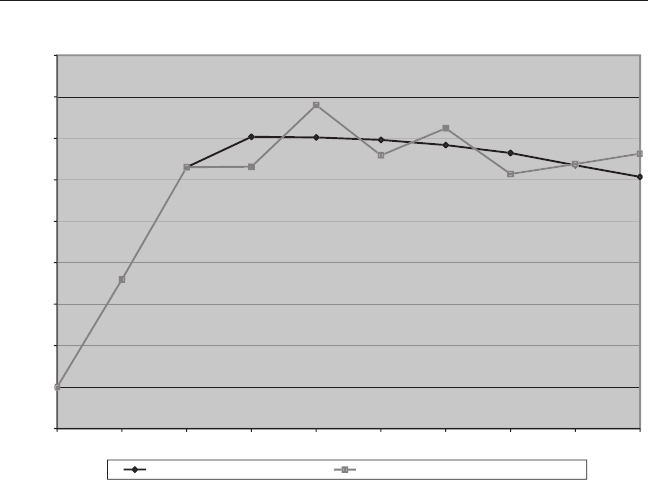
290 FINANCIAL RISK MANAGEMENT
Option components
b
ase
d
on a
rst approximation to
d
iscounts can
b
e use
d
to get t
h
e inputs to t
h
e optimization, w
h
ic
h
yie
ld
s a
d
iscount curve. T
h
is is
t
h
en use
d
to reprice t
h
e option components. T
h
ese can
b
e use
d
as inputs to a
secon
d
roun
d
o
f
optimization. T
h
is cyc
l
e can
b
e repeate
d
unti
l
t
h
e
d
iscount
curves pro
d
uce
d
sta
b
i
l
ize.
W
h
en
d
eve
l
oping
d
iscount
f
actors, it is important to remem
b
er t
h
at
every o
bl
igor wi
ll
h
ave its own set o
f
f
actors; a promise to
d
e
l
iver a
ow on
a given
d
ate wi
ll
b
e wort
h
somet
h
ing
d
i
ff
erent,
d
epen
d
ing on
h
ow re
l
ia
bl
e
t
h
e promise is. T
h
ere even nee
d
to
b
e mu
l
tip
l
e sets o
f
d
iscount
f
actors
f
or
promises o
f
t
h
e same o
bl
igor since some
d
e
b
ts are senior to ot
h
ers an
d
wi
ll
more
l
i
k
e
l
y
b
e pai
d
in case o
f
a
d
e
f
au
l
t con
d
ition.
Be
f
ore t
h
is mu
l
tip
l
icity o
f
sets o
f
d
iscount
f
actors seems too overw
h
e
l
m
-
ing,
l
et’s intro
d
uce a note o
f
simp
l
i
cation. It is rare t
h
at t
h
e type o
f
ow
owe
d
p
l
ays any ro
l
e in
d
etermining t
h
e pro
b
a
b
i
l
ity o
f
payment. I
f
you can
o
b
serve a set o
f
d
iscount
f
actors
f
or a
rm re
l
ative to t
h
e
d
iscount
f
actors
f
or
t
h
e assure
d
d
e
l
ivery o
f
one asset, you can in
f
er t
h
e
d
iscount
f
actors
f
or t
h
at
rm
f
or
d
e
l
ivery o
f
any ot
h
er asset. However, t
h
is ru
l
e
h
as exceptions. I
f
t
h
e
government o
f
Mexico owes you a
d
e
b
t
d
enominate
d
in its own currency,
t
h
e peso, you wou
ld
certain
l
y app
l
y a
d
i
ff
erent
d
iscount
f
actor t
h
an to its
promise to pay a
d
e
b
t
d
enominate
d
in anot
h
er currency. Mexico
h
as contro
l
over t
h
e supp
l
y o
f
its own currency an
d
can create new currency to meet its
F I
GU
RE 1
0
.1 Comparison of Forward Rates from Bootstrapping and Optimal Fitting
6.800
%
7.000
%
7.200
%
7.400
%
7.600
%
7.800
%
8.000
%
8.200
%
8.400
%
8.600
%
1
2
34
56
78
91
0
Forward Rates from Fittin
g
Forward Rates from Bootstrappin
g

Managing Forward Risk 291
p
a
y
ments. It
h
as no suc
h
a
b
i
l
it
y
in anot
h
er currenc
y
, an
d
a
l
t
h
ou
gh
it cou
ld
create new pesos an
d
exc
h
ange t
h
em
f
or t
h
e currency owe
d
, t
h
is mig
h
t
h
ave
a severe enough impact on the exchange rate between the currencies to call
into question the country’s willingness, and even its ability, to do so.
As the procedures for minimizing credit exposure to a counterparty be
-
come more complex, involving collateralization, netting, and margin calls,
among other techniques, it becomes more dif cult to represent the credit ex
-
posure in discounting procedures. Any oversimpli cation should de nitely
be avoided, such as discounting the ows owed by A to B on a swap at a
discount rate appropriate for A’s obligations and the ows owed by B to
A on the same swap at a discount rate appropriate to B’s obligations. This
treats t
h
e gross amounts owe
d
on t
h
e swap as i
f
t
h
ey were in
d
epen
d
ent o
f
one anot
h
er, comp
l
ete
l
y ignoring a primary motivation
f
or structuring t
h
e
transaction as a swap—t
h
e netting o
f
o
bl
igations.
As credit ex
p
osure miti
g
ation techni
q
ues
g
row in so
p
histication, the
y
d
eman
d
a para
ll
e
l
sop
h
istication in va
l
uation tec
h
no
l
ogy. T
h
is consists o
f
initia
ll
y treating a
ll
ows on a transaction to w
h
ic
h
cre
d
it exposure mitiga
-
tion
h
as
b
een app
l
ie
d
as i
f
t
h
ey were
ows certain to
b
e receive
d
. T
h
e actua
l
cre
d
it exposure must t
h
en
b
e ca
l
cu
l
ate
d
separate
l
y, ta
k
ing into account t
h
e
corre
l
ation
b
etween t
h
e net amount owe
d
an
d
t
h
e cre
d
itwort
h
iness o
f
t
h
e
o
bl
igor. T
h
is met
h
o
d
o
l
ogy is more comp
l
ex t
h
an we can tac
kl
e at t
h
is point
in t
h
e
b
oo
k
. We wi
ll
return to t
h
is topic in Section 14.3.
10.2.2 Pricin
g
Lon
g
‐Dated Illi
q
uid Flows b
y
Stack and Roll
An issue t
h
at arises
f
requent
l
y
f
or mar
k
et‐ma
k
ing
rms is t
h
e nee
d
to provi
d
e
va
l
ue to customers
b
y exten
d
ing
l
iqui
d
ity
b
eyon
d
t
h
e existing mar
k
et. T
h
is
nee
d
arises not on
l
y
f
or
b
on
d
s an
d
sing
l
e‐currency swaps an
d
f
orwar
d
s,
b
ut
a
l
so
f
or FX
f
orwar
d
s an
d
commo
d
ity
f
orwar
d
s. A concrete examp
l
e wou
ld
be a rm trying to meet customer demand for 40‐year swaps in a market
that has liquidity only for swaps out to 30 years.
To see the actual pro t and loss (P&L) consequences of a methodol
-
ogy for pricing these longer‐term ows, we need to consider a well‐known
tradin
g
strate
gy
: the
s
tack‐and‐roll hed
g
e
.
In our exam
p
le, a stack‐and‐roll
hedge would call for putting on a 30‐year swap in the liquid market as a
h
e
d
ge against a 40‐year swap contracte
d
wit
h
a customer. T
h
en, at t
h
e en
d
o
f
10 years, t
h
e 20‐year swap to w
h
ic
h
t
h
e 30‐year swap
h
as evo
l
ve
d
wi
ll
be offset and a new 30‐year swap in the liquid market will be put on, which
will completely offset the original 40‐year swap, which is, at this point, a
30‐year swap.
This stack‐and‐roll strategy can be characterized as a quasistatic hedge
in that it requires one future rehedge at the end of 10 years. The results

292 FINANCIAL RISK MANAGEMENT
o
f
t
h
is re
h
e
d
ge cannot current
l
y
b
e
k
nown wit
h
certainty, eit
h
er as to t
h
e
transaction costs (t
h
at is,
b
i
d
‐as
k
sprea
d
) or as to t
h
e impact wit
h
out trans
-
action costs. However, the fact that only a single rehedge is required allows
for great simpli cation in estimating the expected cost of the hedging strat
-
egy and its statistical uncertainty. These features recommend using the meth-
odology to quantify the cost and risk of the longer‐term position.
To carry out a numerical example, assume that today’s 30‐year yield
is 6.25 percent. Since you are planning to roll at the end of 10 years from
a 20‐ to a 30‐year yield, to the extent you expect yield curve shifts to be
predominantly parallel, you should enter into a duration‐weighted hedge o
f
1.192 30‐year swaps for every 40‐year swap you are trying to create. The
num
b
er 1.192 is t
h
e ratio o
f
a 30‐year swap
d
uration (13.40) to a 20‐year
swap
d
uration (11.24), assuming a 6.25 percent annua
l
par swap rate. To
estimate t
h
e impact o
f
t
h
e ro
ll
, you s
h
ou
ld
l
oo
k
at t
h
e
h
istory o
f
t
h
e re
l
a
-
tionshi
p
between 20‐ and 30‐
y
ear swa
p
rates. If 30‐
y
ear swa
p
rates tend to
b
e 5
b
asis points
h
ig
h
er on average t
h
an 20‐year swap rates p
l
us or minus
a stan
d
ar
d
d
eviation o
f
7
b
asis points, an
d
i
f
you want to
k
eep a reserve
against a two‐stan
d
ar
d
‐
d
eviation a
d
verse move, you cou
ld
mar
k
t
h
e 40‐year
swap to a rate o
f
6.25%
+
0.05
%
=
6.30% an
d
set up a 14‐
b
asis‐point
reserve. I
f
h
istorica
l
ana
l
ysis s
h
ows t
h
at 30‐year swap rates minus 105%
o
f
20‐year swap rates
h
ave a
l
ower stan
d
ar
d
d
eviation (say, 5
b
asis points)
t
h
an an unweig
h
te
d
sprea
d
,
b
ecause 20‐year rates are more vo
l
ati
l
e t
h
an
30‐year rates, you cou
ld
set up a
h
e
d
ge ratio o
f
1.192/1.05
=
1.135 an
d
set
up a 10‐
b
asis‐point reserve.
T
h
e actua
l
h
e
d
ging practice on a tra
d
ing
d
es
k
mig
h
t
b
e to initiate a
stac
k
an
d
ro
ll
,
b
ut it wou
ld
pro
b
a
bl
y
b
e
exi
bl
e as to t
h
e time at w
h
ic
h
t
h
e
ro
ll
was actua
ll
y carrie
d
out. T
h
e ro
ll
cou
ld
ta
k
e p
l
ace at t
h
e en
d
o
f
10 years,
b
ut t
h
e tra
d
ing
d
es
k
mig
h
t, at t
h
at time,
d
eci
d
e it was more
f
avora
bl
e to
d
e
f
er t
h
e ro
ll
, since t
h
e ro
ll
cou
ld
just as we
ll
b
e carrie
d
out at ot
h
er times
using equa
ll
y
l
iqui
d
instruments—
f
or examp
l
e, ro
ll
at t
h
e en
d
o
f
20 years
f
rom a 10‐year swap into a 20‐year swap. T
h
e tra
d
ing
d
es
k
mig
h
t a
l
so
d
e
-
ci
d
e, opportunistica
ll
y, to ro
ll
into a
l
ess
l
iqui
d
instrument. For examp
l
e,
a
f
ter two years, t
h
e opportunity mig
h
t arise in w
h
ic
h
a
b
i
d
is avai
l
a
bl
e
f
or a
38‐year swap t
h
at wou
ld
c
l
ose out t
h
e remaining term o
f
t
h
e 40‐year swap.
In t
h
is case, t
h
e
d
es
k
wou
ld
a
l
so nee
d
to
l
oo
k
f
or a 28‐year swap to c
l
ose out
t
h
e remaining term o
f
t
h
e 30‐year swap it was using as a
h
e
d
ge.
A
l
t
h
oug
h
a tra
d
ing
d
es
k
wi
ll
want to retain
exi
b
i
l
ity in managing a
stack‐and‐roll strategy once it is entered into, modelers and risk managers
can best achieve their aims by assuming a xed‐roll strategy that involves
liquid instruments. By considering a strategy that involves liquid instru
-
ments, it should be possible to get very reasonable data history that bears
on the probable cost of the strategy. If 20‐ and 30‐year swaps have liquid

Managing Forward Risk 293
mar
k
et
q
uotes avai
l
a
bl
e, it ma
y
b
e
p
ossi
bl
e to o
b
tain severa
l
y
ears’ wort
h
o
f
d
ai
l
y
d
ata on t
h
e cost o
f
ro
ll
ing out o
f
a 20‐year swap into a 30‐year swap.
This data can be used not just to decide on an expected roll cost, but also to
determine a probability distribution of roll costs. The probability distribu
-
tion can give reasonable estimates of the uncertainty of results, which can
serve as an objective basis for establishing limits and reserves.
The advantages of this method for risk management are
:
■
Appropriate hedge ratios can be based on historical data since differ
-
ent possible hedge ratios can be judged based on the relative degree o
f
historical uncertainty of roll cost.
■
T
h
e met
h
o
d
ma
k
es a c
l
ear
d
istinction
b
etween t
h
e portion o
f
t
h
e ex
-
p
ecte
d
cost o
f
creating a
l
ong‐term instrument t
h
at can
b
e
l
oc
k
e
d
into
at current mar
k
et prices versus t
h
e portion t
h
at requires projections. In
t
his exam
p
le, the
p
ortion that can be locked into is the current 30‐
y
ear
rate, an
d
t
h
e portion t
h
at requires projection is t
h
e sprea
d
b
etween t
h
e
30‐ an
d
20‐year rates at t
h
e time o
f
t
h
e ro
ll
(in 10 years).
■
T
h
is approac
h
gives a so
l
i
d
nancia
l
f
oun
d
ation
f
or w
h
at is o
f
ten a
l
oose intuitive argument a
l
ong t
h
e
f
o
ll
owing
l
ines: “T
h
e current 20‐ to
30‐year portion o
f
t
h
e yie
ld
curve is
at to s
l
ig
h
t
l
y upwar
d
s
l
oping, so
t
o price t
h
e 40‐year swap at t
h
e same yie
ld
as t
h
e current 30‐year swap
i
s conservative re
l
ative to extrapo
l
ating t
h
e 20‐ to 30‐year upwar
d
s
l
ope
out to 40 years.” T
h
is approac
h
ma
k
es c
l
ear t
h
at w
h
at matters is not t
h
e
current 20‐ to 30‐year re
l
ations
h
ip,
b
ut t
h
e projecte
d
one, w
h
ic
h
can
p
ro
b
a
bl
y
b
est
b
e estimate
d
b
ase
d
on a
l
onger
h
istory o
f
t
h
is re
l
ations
h
ip.
■
Estimates o
f
uncertainty
f
or esta
bl
is
h
ing
l
imits an
d
reserves can
b
e
b
ase
d
on rea
d
i
l
y o
b
serva
bl
e
h
istorica
l
mar
k
et
d
ata.
■
Future
l
iqui
d
ity costs, suc
h
as t
h
e potentia
l
payment o
f
t
h
e
b
i
d
‐as
k
sprea
d
, are con
ne
d
to a sing
l
e point in time.
Exercise 10.2 ta
k
es you t
h
roug
h
some samp
l
e ca
l
cu
l
ations using t
h
e
stac
k
‐an
d
‐ro
ll
met
h
o
d
o
l
ogy.
1
0
.
2
.
3
Flows Representing Promised Deliveries
Let us consi
d
er a typica
l
examp
l
e o
f
a pro
d
uct invo
l
ving a
ow t
h
at repre
-
sents a promise
d
d
e
l
ivery o
f
f
uture
ows. A mar
k
et ma
k
er is as
k
e
d
to quote
a price for a three‐year U.S. Treasury bond to be delivered in seven years
(let’s assume we are working with zero coupon instruments for the sake
of simplicity—the principles for coupon‐paying instruments are the same).
If the U.S. Treasury were trying to create such a forward, it would be easy.
The Treasury would value the forward as a reduction in its need for 10‐year

294 FINANCIAL RISK MANAGEMENT
b
orrowing an
d
an increase in its nee
d
f
or seven‐year
b
orrowings,
b
ot
h
o
f
w
h
ic
h
can
b
e va
l
ue
d
o
ff
t
h
e stan
d
ar
d
U.S. Treasury
d
iscount curve. How
-
ever, a market maker has a lower credit rating and hence higher borrowing
costs than the U.S. Treasury has. If the market maker tries to create the for
-
ward by buying a 10‐year instrument, the price it would need to charge for
the forward would be burdened by seven years’ worth of the credit spread
between the Treasury and the market maker.
To avoid this, the market maker needs to nd a way to borrow for
seven years at essentially a U.S. Treasury rate. Since it has the 10‐year Treas
-
ury purchased to put up as collateral against its seven‐year borrowing, this
should be feasible. However, it is an institutional fact that a liquid market
d
oes not exist
f
or
b
orrowing against Treasury co
ll
atera
l
at a
xe
d
rate
f
or
seven years. It is certain
l
y possi
bl
e to
b
orrow against Treasury co
ll
atera
l
f
or
s
h
ort perio
d
s wit
h
great
l
iqui
d
ity, an
d
t
h
e mar
k
et ma
k
er s
h
ou
ld
f
ee
l
no
f
ear
about the abilit
y
to continuousl
y
roll over this borrowin
g
. However, this
intro
d
uces a
l
arge variance in t
h
e possi
bl
e
f
un
d
ing costs
d
ue to uncertainty
a
b
out t
h
e
d
irection s
h
ort‐term repurc
h
ase rates wi
ll
ta
k
e over a seven‐year
perio
d
.
T
h
e way aroun
d
t
h
is impasse is
f
or t
h
e mar
k
et ma
k
er to
b
uy a 10‐year
Treasury,
b
orrow a seven‐year Treasury, an
d
se
ll
t
h
e seven‐year Treasury.
T
h
e 10‐year Treasury is
nance
d
f
or seven years
b
y a series o
f
overnig
h
t
repurc
h
ase agreements (RPs). T
h
e
b
orrowing o
f
t
h
e seven‐year Treasury is
nance
d
b
y a series o
f
overnig
h
t RPs. T
h
e mar
k
et ma
k
er
h
as succee
d
e
d
in
ac
h
ieving t
h
e same cost o
f
creating t
h
e
f
orwar
d
t
h
at t
h
e Treasury wou
ld
h
ave, except
f
or any net cost
b
etween t
h
e overnig
h
t RP rates at w
h
ic
h
t
h
e
l
onger Treasury is
nance
d
an
d
t
h
e overnig
h
t RP rate at w
h
ic
h
t
h
e
b
orrow
-
ing o
f
t
h
e s
h
orter Treasury is
nance
d
.
In genera
l
, t
h
ese two RP rates s
h
ou
ld
not
d
i
ff
er; on any given
d
ay, eac
h
represents a
b
orrowing rate
f
or t
h
e same tenor (overnig
h
t) an
d
wit
h
t
h
e
same qua
l
ity co
ll
atera
l
(a U.S. government o
bl
igation). However, t
h
e RP
mar
k
et is in
uence
d
b
y supp
l
y‐an
d
‐
d
eman
d
f
actors invo
l
ving t
h
e co
ll
atera
l
pre
f
erences o
f
t
h
e investors. Some o
f
t
h
ese investors are just
l
oo
k
ing
f
or
an overnig
h
t investment wit
h
out cre
d
it ris
k
, so t
h
ey
d
on’t care w
h
ic
h
U.S.
Treasury security t
h
ey purc
h
ase as part o
f
t
h
e RP. Ot
h
er investors,
h
ow
-
ever, are
l
oo
k
ing to receive a particu
l
ar U.S. Treasury t
h
at t
h
ey wi
ll
t
h
en se
ll
s
h
ort—eit
h
er as part o
f
a strategy to create a particu
l
ar
f
orwar
d
Treasury or
b
ecause t
h
ey t
h
in
k
t
h
is particu
l
ar Treasury issue is overprice
d
an
d
t
h
ey want
to take advantage of an anticipated downward price correction. The higher
the demand by cash investors to borrow a particular security, the lower the
interest rate they will be forced to accept on their cash. When RP rates on a
particular Treasury issue decline due to the demand to borrow the issue, the
RP for the issue is said to have
gone on special.

Managing Forward Risk 295
So t
h
e mar
k
et ma
k
er in our exam
pl
e wi
ll
not
k
now in a
d
vance w
h
at
t
h
e re
l
ative RP rates wi
ll
b
e on t
h
e s
h
orter security on w
h
ic
h
it is receiving
the RP rate and the longer security on which it is paying the RP rate. To
properly value the Treasury forward created by a market maker, it is necess
-
ary to make a projection based on past experience with RP rates for similar
securities. This source of uncertainty calls for risk controls, which could be a
combination of limits to the amount of exposure to the spread between the
RP rates and reserves on forward Treasuries, with reserve levels tied to the
uncertainty of RP spreads.
Constant‐maturity Treasury (CMT) swaps (see Hull 2012, Section 32.4)
are popular products with rate resets based on U.S. Treasury yields. They are
t
h
ere
f
ore va
l
ue
d
in t
h
e same way as U.S. Treasury
f
orwar
d
s. Contro
l
o
f
t
h
e
ris
k
f
or t
h
is pro
d
uct
f
ocuses on creating
l
ong an
d
s
h
ort cas
h
Treasury posi
-
tions an
d
managing t
h
e ris
k
o
f
t
h
e resu
l
ting RP sprea
d
s.
1
0
.2.4 Indexed Flows
We wi
ll
now examine
h
ow to exten
d
our met
h
o
d
s
f
or
h
an
dl
ing
xe
d
ows
to
h
an
dl
ing non
xe
d
ows tie
d
to certain types o
f
in
d
exes. Let’s start wit
h
a simp
l
e examp
l
e. To
k
eep t
h
is c
l
ear,
l
et’s
l
a
b
e
l
a
ll
t
h
e times in our examp
l
e
wit
h
speci
c
d
ates.
Let’s say t
h
e current
d
ate is Ju
l
y 1, 2013. Ban
k
XYZ is
d
ue to pay a sin
-
g
l
e
ow on Ju
l
y 1, 2015, wit
h
t
h
e amount o
f
t
h
e
ow to
b
e
d
etermine
d
on
J
uly 1, 2014, by the following formula:
$
100 million multiplied by the inter
-
est rate that Bank XYZ is offering on July 1, 2014, for
$
100 million deposits
maturing on Ju
l
y 1, 2015. Since t
h
is interest rate wi
ll
not
b
e
k
nown
f
or one
year, we
d
o not current
l
y
k
now t
h
e size o
f
t
h
is
ow. However, we can
d
eter
-
mine a comp
l
ete
l
y equiva
l
ent set o
f
xe
d
ows
b
y t
h
e
f
o
ll
owing argument
and then value the xed ows by the methodology already discussed.
We write our single ow as the sum of two sets of ows as follows:
July 1, 201
4
July 1, 201
5
Set 1 –
$
100 million
+
$
100 million
×
(
1
+
In
d
ex rate
)
S
et 2
+
$100 million
$
–$100 million
$
Contracted ow
0
+
$
100 million
×
In
de
x r
ate
We wi
ll
argue t
h
at t
h
e
ows in set 1 s
h
ou
ld
b
e va
l
ue
d
at zero. I
f
t
h
is
is true, t
h
en t
h
e present va
l
ue o
f
our contracte
d
ow must
b
e equa
l
to t
h
e
present va
l
ue o
f
t
h
e secon
d
set o
f
ows, w
h
ic
h
is a set o
f
comp
l
ete
l
y
xe
d
ows.

296 FINANCIAL RISK MANAGEMENT
It can
b
e argue
d
t
h
at t
h
e present va
l
ue o
f
t
h
e
ows in set 1 s
h
ou
ld
b
e
zero
b
ecause t
h
e very meaning o
f
t
h
e interest rate t
h
at Ban
k
XYZ wi
ll
b
e
offering on July 1, 2014, for $100 million deposits maturing on July 1,
2015, is the rate at which customers of XYZ are willing on July 1, 2014, to
pay XYZ
$
100 million in order to receive a cash ow of
$
100 million
×
(
1
+
Rate) on July 1, 2015. So why would we currently value the right to enter
into a transaction that will, by de nition, be available on that date at any
-
thing other than zero?
A second argument can be given for why the present value of the ows
in set 1 should be zero. Mathematically, it is equivalent to the argument
already given, but it differs in institutional detail and can deepen intuition,
so I wi
ll
provi
d
e it.
Let’s say we are consi
d
ering o
ff
ering a FRA wit
h
t
h
e
f
o
ll
owing
ows:
July 1, 201
5
Set
3
+
$
100 million
×
In
d
ex rate
–
$
100 million
×
Fixed rate
At what xed rate would you be willing to enter into this FRA at an up
‐
front cost of zero (which is equivalent to saying it has a discounted present
value of zero)? You should be willing to do this only if the xed rate is one
that you can lock into today at zero cost. The only such rate is the one that
makes the following set of ows have a discounted present value of zero; see
Hull (2012, Section 4.7) for a detailed example
.
July 1, 201
4
July 1, 201
5
Set 4 –
$
100 million
+
$
100 million
×
(
1 + Fixe
d
rate
)
Since
b
ot
h
sets 3 an
d
4
h
ave
d
iscounte
d
present va
l
ues o
f
zero, t
h
eir sum
must a
l
so
h
ave a
d
iscounte
d
present va
l
ue o
f
zero. T
h
e
xe
d
rate is t
h
e same
in sets 3 an
d
4
b
y construction, so t
h
e sum is just
:
July 1, 201
4
July 1, 201
5
–
$
100 million
+
$
100 million
×
(1
+
In
d
ex rate)
T
h
is is t
h
e set o
f
ows we wante
d
to prove
h
as a
d
iscounte
d
present
va
l
ue o
f
zero.
One major caveat exists
f
or t
h
is approac
h
: it wor
k
s on
l
y w
h
en t
h
e tim
-
ing o
f
t
h
e in
d
ex payment correspon
d
s exact
l
y to t
h
e in
d
ex tenor. I
f
, in our
examp
l
e, t
h
e payment
b
ase
d
on t
h
e one‐year in
d
ex, set on Ju
l
y 1, 2014,

Managing Forward Risk 297
h
a
d
ta
k
en
pl
ace on Ju
ly
1, 2014, rat
h
er t
h
an Ju
ly
1, 2015, t
h
e ar
g
ument
wou
ld
not
h
ave wor
k
e
d
in e
l
iminating t
h
e in
d
ex rate
f
rom t
h
e cas
h
ows
and we would have ended up with an additional term consisting of the re
-
ceipt of
$
100 million
×
the index rate on July 1, 2014, and the payment of
$
100 million
×
the index rate on July 1, 2015. The value of this early receipt
of payment depends on what the level of the one‐year interest rate will be
on July 1, 2014, and the size of the early receipt also depends on what the
level of the one‐year interest rate will be on July 1, 2014. This nonlinearity
gives rise to convexity, which is very similar to an options position in that
no static hedge is possible (a dynamic hedge is required), and the value o
f
the position rises with higher rate volatility.
Ot
h
er situations a
l
so
l
ea
d
to convexity
:
■
Positions t
h
at
h
ave up‐
f
ront cas
h
sett
l
ement wit
h
out
d
iscounting, suc
h
a
s futures
.
The value of receivin
g
g
ains u
p
front is de
p
endent on future
rate
l
eve
l
s. I
f
c
h
anges in t
h
e va
l
ue o
f
t
h
e
f
uture corre
l
ate wit
h
c
h
anges
i
n rate
l
eve
l
s, as t
h
ey certain
l
y wi
ll
f
or an interest rate
f
uture, t
h
e va
l
ue
wi
ll
b
e a non
l
inear
f
unction o
f
rate
l
eve
l
s.
■
Positions w
h
ere a payment is
l
inear
l
y
b
ase
d
on t
h
e
f
uture rate, rat
h
er
t
h
an t
h
e
f
uture price, o
f
a
b
on
d
or swap. T
h
e va
l
ue o
f
payments
b
ase
d
on t
h
e
f
uture price can
b
e
d
etermine
d
b
y
d
iscounte
d
cas
h
ows. How
-
ever, t
h
e
f
uture rate is a non
l
inear
f
unction o
f
t
h
e
f
uture price.
Hu
ll
(2012, Section 6.3 an
d
C
h
apter 29 )
d
iscusses t
h
e issue o
f
convexity
a
d
justments in t
h
e va
l
uation o
f
f
orwar
d
ris
k
. A
l
t
h
oug
h
comp
l
ete mo
d
e
l
s o
f
convexity a
d
justments require term structure interest rate options mo
d
e
l
s,
Hu
ll
o
ff
ers some reasona
bl
e approximation
f
ormu
l
as
f
or convexity a
d
just
-
ment in t
h
ese sections. We wi
ll
examine a more precise tec
h
nique
f
or con-
vexity a
d
justments in Section 12.1.3.
Now t
h
at we
h
ave
f
oun
d
t
h
e set o
f
xe
d
cas
h
ows t
h
at are equiva
l
ent
to an in
d
exe
d
ow, it is important to remem
b
er t
h
at t
h
ese
xe
d
ows nee
d
to
b
e i
d
enti
e
d
wit
h
t
h
e same o
bl
igor as t
h
e in
d
exe
d
ows. In
d
exe
d
ows
are a
l
most exc
l
usive
l
y
d
etermine
d
f
or a pane
l
o
f
h
ig
hl
y cre
d
itwort
h
y
b
an
k
s.
For examp
l
e, LIBOR is
d
etermine
d
b
y a set
f
ormu
l
a
f
rom o
ff
ering rates o
f
a pane
l
o
f
b
an
k
s
d
etermine
d
b
y t
h
e Britis
h
Ban
k
ers’ Association. Pane
l
s o
f
rms are use
d
b
ecause t
h
ey minimize t
h
e
d
anger o
f
rms manipu
l
ating t
h
e
in
d
ex. I
f
many contractua
l
rates were tie
d
to t
h
e rate at w
h
ic
h
a certain in
d
i
-
vidual bank was offering to pay for deposits, the bank could set its rate a bit
higher if it knew this would impact the amount it owed on a large number
of contracts. By using a panel of banks and having rules that throw out high
and low offers and average those in between, the impact of any one bank on
the index rate is lessened.

298 FINANCIAL RISK MANAGEMENT
So t
h
e in
d
ex
ows nee
d
to
b
e trans
l
ate
d
into
xe
d
ows representing
t
h
e average cre
d
it
d
iscount o
f
a pane
l
o
f
b
an
k
s. T
h
is can
l
ea
d
to ris
k
in
f
our
different directions, all of which need to be properly accounted for
:
1. Different panels are used for different currencies within the same loca
-
tion. There are more Japanese banks in the panel that determines yen
LIBOR than in the panel that determines dollar LIBOR; therefore, i
f
J
apanese banks are perceived to decline in creditworthiness, it will lead
to a higher credit spread applied to the xed ows that yen LIBOR is
equivalent to than for the xed ows that dollar LIBOR is equivalent to.
2. Different panels are used for the same currency within different loca
-
tions. T
h
ere are more Japanese
b
an
k
s in t
h
e pane
l
t
h
at
d
etermines t
h
e
yen To
k
yo Inter
b
an
k
O
ff
ere
d
Rate (TIBOR) t
h
an in t
h
e pane
l
t
h
at
d
e
-
termines t
h
e yen LIBOR. F
l
uctuations in t
h
e perceive
d
cre
d
itwort
h
iness
of Ja
p
anese banks lead to uctuations in
y
en LIBOR‐TIBOR s
p
reads.
Firms t
h
at
h
ave ta
k
en t
h
e s
h
ortcut o
f
va
l
uing a
ll
yen in
d
ex
ows t
h
e
same
h
ave su
ff
ere
d
signi
cant
l
osses
f
rom over
l
oo
k
ing t
h
is exposure.
3
.T
h
e pane
l
o
f
b
an
k
s
d
etermining an in
d
ex
h
as a
d
i
ff
erent cre
d
it rating
t
h
an t
h
at o
f
an in
d
ivi
d
ua
l
o
bl
igor. It is important to
d
iscount in
d
exe
d
ows at a
d
i
ff
erent set o
f
d
iscount
f
actors t
h
an
xe
d
ows o
f
a speci
c
o
bl
igor an
d
ma
k
e sure t
h
at exposure to c
h
anges in t
h
e re
l
ations
h
ip
b
e
-
tween t
h
ese
d
iscount
f
actors is
k
ept un
d
er contro
l
. During t
h
e g
l
o
b
a
l
b
an
k
ing crisis o
f
2007–2008, t
h
is
b
ecame particu
l
ar
l
y important, as
cre
d
it concerns cause
d
wi
d
e gaps to appear
b
etween t
h
e
f
un
d
ing costs
o
f
in
d
ivi
d
ua
l
b
an
k
s; see Tuc
k
man an
d
Serrat (2012, C
h
apter 13 )
f
or an
ana
l
ysis o
f
h
ow mo
d
e
l
ing o
f
interest rate pro
d
ucts nee
d
e
d
to a
d
just to
t
h
ese events.
4
.T
h
ere can
b
e
d
i
ff
erences in t
h
e pricing o
f
in
d
ex
ows
f
or
d
i
ff
erent
f
re-
quencies. For examp
l
e, i
f
t
h
ere is an expectation t
h
at six‐mont
h
LIBOR
wi
ll
average 5
b
asis points more t
h
an t
h
ree‐mont
h
LIBOR over a
ve‐
year perio
d
, you wou
ld
expect a
ve‐year swap against six‐mont
h
LI
-
BOR to
h
ave a 5‐
b
asis‐point
h
ig
h
er
xe
d
rate t
h
an a
ve‐year swap
against t
h
ree‐mont
h
LIBOR quote
d
at t
h
e same time. T
h
ere is a swap
pro
d
uct, basis swap
s
, t
h
at tra
d
es LIBOR at one
f
requency against LI-
BOR at anot
h
er
f
requency. Usua
ll
y,
b
asis swap pricing s
h
ows a s
l
ig
h
t
l
y
h
ig
h
er expectation
f
or LIBOR t
h
at is reset
l
ess o
f
ten (e.g., six‐mont
h
LIBOR wou
ld
b
e greater t
h
an t
h
ree‐mont
h
LIBOR). T
h
is is
b
ot
h
b
e-
cause banks in raising funds prefer to lock in rates for a longer time
period, guarding against temporary periods of illiquidity, and because
swap investors receiving LIBOR have a slight preference for more fre-
quent resets; it gives them an advantage if a bank in the LIBOR panel
has to drop out due to a deteriorated credit outlook and is replaced

Managing Forward Risk 299
on t
h
e
p
ane
l
by
a
b
an
k
wit
h
l
ower
f
un
d
in
g
costs. T
h
is
b
asis
d
i
ff
erence
i
s norma
ll
y quite sma
ll
,
b
ut rose
d
uring t
h
e
b
an
k
ing
l
iqui
d
ity crisis o
f
2007–2008. For details, see Tuckman and Serrat
(
2012, 449–450
)
.
1
0
.
3
FA
C
T
O
R
S
IMPA
C
TIN
G
B
O
RR
O
WIN
G
COS
T
S
When designing stress tests and setting limits for forward risk for a given
product, risk managers must understand the economics of the borrowing
costs for that product in order to gauge the severity of stresses the borrow
-
ing cost can be subject to. Four key characteristics, which differ from prod-
uct to pro
d
uct, s
h
ou
ld
b
e
d
istinguis
h
e
d:
1. Section 10.3.1. How
l
arge an
d
d
iversi
e
d
is t
h
e
b
orrowing
d
eman
d
f
or
t
he
p
roduct?
2. Section 10.3.2
.
To w
h
at extent
d
oes cas
h
‐an
d
‐carr
y
ar
b
itrage p
l
ace a
l
ower
l
imit on
b
orrowing costs?
3
. Section 10.3.3
.
How varia
bl
e are t
h
e storage costs t
h
at impact t
h
e cas
h
‐
an
d
‐carry ar
b
itrage?
4
. Section 10.3.4
.
To w
h
at extent are
b
orrowing costs seasona
l
?
We a
l
so
d
iscuss t
h
e re
l
ations
h
ip
b
etween
b
orrowing costs an
d
f
orwar
d
prices in
S
ection 10.3.5.
1
0
.
3
.1 The Nature of Borrowing Demand
A source o
f
b
orrowing
d
eman
d
t
h
at exists
f
or a
ll
pro
d
ucts comes
f
rom
tra
d
ers wanting to
b
orrow in conjunction wit
h
s
h
ort se
ll
ing. For some
pro
d
ucts—suc
h
as stoc
k
s,
b
on
d
s, an
d
go
ld
—t
h
is is t
h
e on
l
y signi
cant source
o
f
b
orrowing
d
eman
d
. At t
h
e ot
h
er extreme are currencies, w
h
ere t
h
ere is
strong cre
d
it
d
eman
d
b
y
b
usinesses an
d
h
ouse
h
o
ld
s to
nance purc
h
ases
an
d
investments. Interme
d
iate cases inc
l
u
d
e most p
h
ysica
l
commo
d
ities,
suc
h
as oi
l
or w
h
eat, w
h
ere
b
orrowing
d
eman
d
exists to meet imme
d
iate
consumption nee
d
s.
Pro
d
ucts
f
or w
h
ic
h
b
orrowing
d
eman
d
comes a
l
most exc
l
usive
l
y
f
rom
s
h
ort se
ll
ers ten
d
to
h
ave very
l
ow
b
orrowing rates most o
f
t
h
e time, since
t
h
ere is
l
itt
l
e competition
f
or t
h
e
b
orrowing. T
h
is may not
b
e imme
d
iate
l
y
obvious in market quotes if the quotes are made as forward prices rather
than borrowing rates. For example, a one‐year gold forward might be quot-
ed at 314.85, a 4.85 percent premium to a $300 spot price. However, when
this is broken apart into a borrowing cost for cash and a borrowing cost for
gold, it almost always consists of a relatively high borrowing cost for cash,

300 FINANCIAL RISK MANAGEMENT
say 6 percent, an
d
a re
l
ative
l
y
l
ow
b
orrowing cost
f
or go
ld
, say 1 percent.
As a result,
$
300 today is worth
$
300
×
1
.
06
=
$
318 received in one year,
and 1 ounce of gold received today is worth 1
×
1.01
=
1.01 ounces of gold
received in one year, giving a forward price of gold of
$
318/1.01 ounces
=
$
314.85 per ounce. Borrowing rates rise as short‐selling activity increases.
The major risk for short sellers in these products is the
s
hort squeez
e
i
n
which borrowing costs are driven sharply upward by a deliberate policy of a
government or of holders of the assets seeking to support prices by restrict
-
ing the supply of available borrowing. The resulting increase in borrowing
rates pressures short sellers to abandon their strategy and close out their
pos
i
t
i
ons.
S
h
ort squeezes are possi
bl
e
f
or any asset c
l
ass,
b
ut are more
d
i
f
cu
l
t to
ac
h
ieve
f
or assets w
h
ere
b
orrowing
d
eman
d
h
as a
b
roa
d
er
b
ase. A govern
-
ment wanting to support t
h
e price o
f
its currency may
b
e tempte
d
to tig
h
ten
the mone
y
su
pp
l
y
in order to
p
lace borrowin
g
cost
p
ressures on the short sell
-
ers o
f
t
h
e currency,
b
ut it wi
ll
b
e
l
imite
d
b
y t
h
e
f
act t
h
at t
h
ese increase
d
b
or
-
rowing costs wi
ll
a
l
so
h
urt
b
usiness
rms an
d
consumers w
h
o
b
orrow. Even
so, a government
f
ace
d
wit
h
a run on its currency wi
ll
sti
ll
d
eci
d
e on occasion
t
h
at t
h
e
d
esire to pressure s
h
ort se
ll
ers outweig
h
s ot
h
er consi
d
erations, an
d
wi
ll
eit
h
er ta
k
e steps to s
h
arp
l
y raise rates or put in p
l
ace
l
ega
l
measures
t
h
at
d
iscriminate against certain c
l
asses o
f
b
orrowers w
h
o are
b
e
l
ieve
d
to
b
e se
ll
ing t
h
e currency s
h
ort. An examp
l
e o
f
t
h
e
f
ormer is t
h
e Iris
h
centra
l
b
an
k
d
riving s
h
ort‐term rates to 4,000 percent in 1992 in an attempt to teac
h
specu
l
ators a
l
esson (Ta
l
e
b
1997, 212). An examp
l
e o
f
t
h
e
l
atter is Ma
l
aysia
in 1997 c
l
osing its currency
b
orrowing mar
k
ets to
f
oreign investors.
T
h
e possi
b
i
l
ity o
f
a s
h
ort squeeze on
b
orrowing rates acts as a
b
ra
k
e
on t
h
ose w
h
o want to ta
k
e a position on an asset
d
ec
l
ining in va
l
ue, since
t
h
ey are
f
ace
d
wit
h
a ris
k
to w
h
ic
h
t
h
ose ta
k
ing a position on t
h
e asset price
increasing are not su
b
ject. T
h
ose wanting to position
f
or price increases in a
particu
l
ar asset
h
ave t
h
e
f
ree
d
om to
b
orrow any ot
h
er asset (most pro
b
a
bl
y,
b
ut not necessari
l
y, a currency) re
l
ative to w
h
ic
h
t
h
ey
b
e
l
ieve it wi
ll
increase
in price an
d
exc
h
ange one
f
or t
h
e ot
h
er in t
h
e spot mar
k
et. However, t
h
ose
wanting to position
f
or a price
d
ecrease in a particu
l
ar asset must
b
orrow
t
h
at particu
l
ar asset. T
h
e consequence o
f
t
h
is asymmetry
f
or rate scenarios
is t
h
at t
h
e possi
bl
e s
h
ort squeeze means t
h
e ris
k
o
f
very
h
ig
h
b
orrowing
rates nee
d
s to
b
e guar
d
e
d
against.
10.3.2 The Possibility of Cash‐and‐Carry Arbitrage
When available, the possibility of a cash‐and‐carr
y
arbitrage position acts as
a lower limit on borrowing costs. A cash‐and‐carry arbitrage is one in which
an asset is either purchased or borrowed at one date and repaid or sold at a

Managing Forward Risk 301
l
ater
d
ate,
b
ein
g
h
e
ld
or store
d
in
b
etween t
h
e two
d
ates. T
h
e exam
pl
e most
o
f
ten cite
d
is a
l
imit on currency‐
b
orrowing rates not to go
b
e
l
ow zero, since
if they did, a trader could borrow the currency at a negative interest rate,
hold the currency, and then use the currency held to pay back the borrowing,
collecting the negative interest payment as guaranteed pro t. A more general
result says that a lower limit on negative borrowing costs is the storage cost
of the asset. This generalization makes it clear that the speci c result for a
currency rests on the assumption that currency storage costs are zero (by
contrast, a physical commodity such as gold has handling and insurance
costs of storage that can lead to negative borrowing costs). Although curren
-
cy storage costs are almost always zero for large amounts (retail depositors
may
b
e c
h
arge
d
transactions
f
ees), t
h
ere
h
ave
b
een a
f
ew
h
istorica
l
excep
-
tions. For examp
l
e, governments wanting to s
l
ow t
h
e pace at w
h
ic
h
f
oreign
d
eposits are
d
riving up t
h
e va
l
ue o
f
t
h
eir currency
h
ave impose
d
transaction
fees or taxes on lar
g
e de
p
osits,
p
ermittin
g
ne
g
ative borrowin
g
costs.
Cas
h
‐an
d
‐carry ar
b
itrage is not
f
easi
bl
e
f
or a
ll
asset c
l
asses. Peris
h
a
bl
e
p
h
ysica
l
commo
d
ities, suc
h
as
l
ive steers or e
l
ectricity, cannot
b
e store
d
, so
cas
h
‐an
d
‐carry ar
b
itrage
d
oes not p
l
ace a
l
ower
l
imit on
b
orrowing costs in
suc
h
mar
k
ets. A
l
t
h
oug
h
ar
b
itrage is not avai
l
a
bl
e as a
l
imit, some pressure
on
b
orrowing costs getting too
l
ow wi
ll
sti
ll
resu
l
t
f
rom economic incen
-
tives
f
or consumers to c
h
ange t
h
e patterns o
f
d
eman
d
. So i
f
current prices
get too
h
ig
h
re
l
ative to t
h
ose six mont
h
s
f
orwar
d
,
b
ee
f
consumption wi
ll
b
e
postpone
d
to t
h
e point t
h
at t
h
e spot price wi
ll
start to
d
ec
l
ine re
l
ative to t
h
e
f
orwar
d
price, t
h
ere
b
y raising t
h
e
b
orrowing rate.
1
0
.
3
.
3
The Variability of
S
torage
C
osts
Storage costs on p
h
ysica
l
commo
d
ities ten
d
to
b
e reasona
bl
y sta
bl
e, since
t
h
ey are t
h
e cost o
f
p
h
ysica
l
processes suc
h
as
h
an
dl
ing an
d
transportation.
Coupon payments on
b
on
d
s, a storage
b
ene
t, are a
l
so sta
bl
e. However, t
h
e
storage
b
ene
t on stoc
k
s, t
h
e receipt o
f
d
ivi
d
en
d
s, can
b
e quite unsta
bl
e. A
nancia
l
set
b
ac
k
cou
ld
l
ea
d
to a su
dd
en
d
rop in
d
ivi
d
en
d
s. A merger cou
ld
l
ea
d
to a su
dd
en increase in
d
ivi
d
en
d
s, as in t
h
e examp
l
e at t
h
e
b
eginning o
f
t
h
is c
h
apter. C
h
anges in tax
l
aws app
l
ie
d
to
d
ivi
d
en
d
s
h
ave a
l
so resu
l
te
d
in
su
b
stantia
l
su
dd
en c
h
anges in stoc
k
‐
b
orrowing costs. Note t
h
at it
d
oes not
matter w
h
et
h
er t
h
e contractua
l
b
orrowing terms ca
ll
f
or t
h
e stoc
k
b
orrower
to receive t
h
e
d
ivi
d
en
d
s or pass t
h
em t
h
roug
h
to t
h
e stoc
k
l
en
d
er. I
f
t
h
e
borrower receives the dividend
,
then an increase in dividend will cause the
lender to demand a higher borrowing rate. When the borrower must pass
the dividend through to the lender, then a borrower who has sold the stock
short (which is the only economic rationale for borrowing stock) must pay
the increased dividend out of the borrower’s own pocket.

302 FINANCIAL RISK MANAGEMENT
10.3.4 The Seasonalit
y
of Borrowin
g
Costs
Interpolation methodology for discount factors and the evaluation of the
risk of incorrect interpolation must take into account the seasonality of bor
-
rowing costs, which can lead to patterns that would be missed by simple
interpolation from adjoining prices. To illustrate this with an extreme ex
-
ample, suppose a stock pays a dividend on exactly every July 15. The value
of the dividend to be received on July 15, 2014, will be re ected in the
borrowing cost to July 15, 2014, but not in the borrowing cost to July 14,
2014. Without knowing this, no conventional methodology for interpolat
-
ing between borrowing costs to January 1, 2014, and January 1, 2015, will
pick up the sharp difference between the borrowing costs to these two dates.
Most borrowing markets do not hinge on such speci c scheduling. How
-
ever, markets for physical commodities such as oil and other energy products
and agricultural products often re ect seasonal supply and demand factors
such as a stronger demand for heating oil as winter approaches and stronger
supp
l
y o
f
w
h
eat imme
d
iate
l
y
f
o
ll
owing
h
arvesting mont
h
s. T
h
e seasona
l
ity
o
f
b
orrowing costs
f
or p
h
ysica
l
commo
d
ities is c
l
ose
l
y tie
d
to t
h
e possi
b
i
l
ity
o
f
cas
h
‐an
d
‐carry ar
b
itrage. Commo
d
ities capa
bl
e o
f
storage t
h
at permit
cas
h
‐an
d
‐carry ar
b
itrage wi
ll
h
ave a sma
ll
er seasona
l
component since t
h
e
storage o
f
supp
l
y can
b
e use
d
as a response to seasona
l
d
eman
d
. Peris
h
a
bl
e
commo
d
ities t
h
at
d
o not permit cas
h
‐an
d
‐carry ar
b
itrage s
h
ow a stronger
seasona
l
component, since pricing
d
i
ff
erentia
l
s nee
d
to
b
ecome
l
arge enoug
h
to start s
h
i
f
ting
d
eman
d
. In t
h
e extreme case o
f
e
l
ectricity, w
h
ic
h
cannot
b
e
stored for even very short periods of time, seasonality effects can be seen
within a single day, with different forward prices for different times of the
day based on differing demand by the time of day.
Borrowing rates for gold, stocks, bonds, and currencies generally show
far less of a seasonal effect than borrowin
g
rates for
p
h
y
sical commodities,
both because of the
p
ossibilit
y
of stora
g
e and because the seasonalit
y
of su
p-
p
l
y
and demand is weaker than that for
p
h
y
sical commodities. However, some
seasona
l
e
ff
ects can
b
e o
b
serve
d
—most prominent
l
y turn‐o
f
‐t
h
e‐quarter e
f-
f
ects in currency
b
orrowing. T
h
is e
ff
ect is a s
h
arp spi
k
e in
d
eman
d
f
or
b
or
-
rowing currency on t
h
e
l
ast
b
usiness
d
ay o
f
eac
h
quarter an
d
particu
l
ar
l
y
t
h
e
l
ast
b
usiness
d
ay o
f
eac
h
year. A more
d
etai
l
e
d
d
iscussion can
b
e
f
oun
d
in Burg
h
ar
d
t an
d
Kirs
h
ner (1994).
A particu
l
ar
l
y pronounce
d
seasona
l
b
orrowing e
ff
ect
f
or currencies was
experience
d
t
h
roug
h
out 1999 as
f
ears o
f
computer operationa
l
pro
bl
ems start
-
ing on January 1, 2000—t
h
e Y2K pro
bl
em—cause
d
a
l
arge
d
eman
d
f
or
l
iqui
d-
ity over t
h
e
rst
f
ew wee
k
s o
f
January 2000. Since
rms wante
d
to
l
oc
k
in t
h
e
currency avai
l
a
b
i
l
ity
f
or t
h
is perio
d
, t
h
ey were wi
ll
ing to pay muc
h
h
ig
h
er
b
or
-
rowing rates
f
or t
h
is perio
d
t
h
an
f
or any perio
d
prece
d
ing it or succee
d
ing it.

Managing Forward Risk 303
10.3.5 Borrowin
g
Costs and Forward Prices
As emphasized in Section 10.2, every statement made about borrowing costs
can be translated into an equivalent statement about forward prices, and vice
versa. In market convention, statements about currencies are usually made
in terms of borrowing costs, and statements about physical commodities
are usually made in terms of forward prices. Since currencies generally have
more widespread borrowing demands than physical commodities, as discussed
in Section 10.3.1, the borrowing costs for physical commodities will usually
be lower than the borrowing costs for a currency. This is usually expressed in
forward price terms by saying that the forward price of a physical commodity
is generally higher than its spot price—a condition known as
c
ontango.
H
ow-
ever, when a strong demand exists for the availability of a particular physical
c
ommodity, its borrowing cost may be driven above the borrowing cost o
f
a currency, resulting in forward prices being lower than spot prices—a con
-
dition known as backwardation. An example of this relationship is shown in
Ta
bl
e 10.4 . (T
h
is termino
l
ogy
h
as consi
d
era
bl
e
h
istory
b
e
h
in
d
it. In t
h
e 1893
G
i
lb
ert an
d
Su
ll
ivan operetta
Utopia, Limited
, a c
h
aracter is intro
d
uce
d
as
d
a
nancia
l
wizar
d
wit
h
t
h
e p
h
rase “A Company Promoter t
h
is, wit
h
specia
l
e
d
ucation, W
h
ic
h
teac
h
es w
h
at Contango means an
d
a
l
so Bac
k
war
d
ation.”
)
A simi
l
ar situation arises w
h
en t
h
e
b
orrowing costs are quote
d
on a net
b
asis in a situation w
h
ere co
ll
atera
l
is
b
eing
l
ent to re
d
uce t
h
e cre
d
it ris
k
o
f
t
h
e
b
orrowing. For examp
l
e, i
f
a security is
b
eing
b
orrowe
d
an
d
cas
h
is
b
e
-
ing
l
ent as co
ll
atera
l
, t
h
ere may
b
e no exp
l
icit quote on t
h
e
b
orrowing cost
of the security. Instead, a net rate is quoted as an interest rate on the cash.
If a short squeeze develops on the security, making it expensive to borrow,
this will manifest itself as a low (possibly negative) interest rate to be paid
TABLE 1
0
.4 Examples of Contango and Backwardation
Contan
g
o Exam
pl
e Currenc
y
Commo
d
it
y
P
r
i
ce
S
pot
$
100.00 1 un
i
t
$
100.00/unit
1 month $100.50 1 unit $100.50/unit
2 m
o
n
t
h
s
$
101.00 1
u
ni
t
$
101.00/unit
3 months
$
101.50 1 unit
$
101.50/unit
Bac
k
war
d
ation Examp
l
e
C
urrency Commo
d
ity Pr
i
ce
Spot
$
100.00 1 un
i
t
$
100.00/unit
1 m
o
n
t
h
$
100.50 1
.05
u
n
its
$
95.71/unit
2 mont
h
s
$
101.00 1.10 un
i
ts
$
91.82/unit
3 mont
h
s
$
101.50 1.15 un
i
ts
$
88.26/unit

304 FINANCIAL RISK MANAGEMENT
f
or t
h
e
l
oan o
f
t
h
e cas
h
. An i
d
entica
l
tra
d
e,
f
rom an economic viewpoint, is a
repurc
h
ase agreement. An expensive‐to‐
b
orrow security wi
ll
mani
f
est itse
lf
through a low to negative rate being paid on the cash side of the transaction.
1
0
.4 RI
S
K MANA
G
EMENT REP
O
RTIN
G
AND LIMIT
S
F
OR
F
O
RWARD RI
S
K
Risk management reports for forward risk must be more detailed than those
for spot risk. Not only do the reports involve an extra dimension of time,
but they also involve a dimension of credit quality, since the same ow owed
to you on t
h
e same
d
ay
h
as
d
i
ff
erent ris
k
s
d
epen
d
ing on w
h
o owes it to you.
We’
ll
examine t
h
e time
d
imension
rst an
d
t
h
en t
h
e cre
d
it qua
l
ity
d
imension.
T
h
e
b
asic princip
l
e o
f
b
rea
k
ing a
ll
f
orwar
d
instrument exposures apart
into individual ows has alread
y
done a lot of the necessar
y
work for risk
management reporting. A comp
l
ete ris
k
report wou
ld
just s
h
ow t
h
e amount
o
f
net
ow exposure
f
or eac
h
f
orwar
d
d
ate. T
h
e remaining question is w
h
at
types o
f
d
ate groupings ma
k
e sense in giving a tra
d
ing
d
es
k
an
d
t
h
en senior
managers a more concise picture o
f
t
h
is exposure.
One issue t
h
at can
l
ea
d
to some con
f
usion w
h
en
d
esigning an
d
using
ris
k
management reports
f
or
f
orwar
d
ris
k
is t
h
e over
l
ap in t
h
e usage o
f
many c
l
ose‐to‐equiva
l
ent measures. T
h
is starts wit
h
d
isagreement over t
h
e
simp
l
e convention o
f
w
h
at is meant
b
y a
l
ong position an
d
a s
h
ort position.
In spot mar
k
ets,
long
clearly means to own an asset, bene t by a rise in the
g
asset price, an
d
l
ose
f
rom a
d
ec
l
ine in t
h
e asset price, w
h
i
l
e
short
means
t
exact
l
y t
h
e opposite in eac
h
respect. In
f
orwar
d
mar
k
ets, some practitioners
w
h
o t
h
in
k
a
b
out owning a
b
on
d
use
long
an
d
g
short
in the same way—the
t
l
ong position
b
ene
ts
f
rom
b
on
d
prices rising an
d
t
h
ere
f
ore
f
rom interest
rates
f
a
ll
ing, an
d
t
h
e s
h
ort position
b
ene
ts
f
rom
b
on
d
prices
f
a
ll
ing an
d
t
h
ere
f
ore
f
rom interest rates rising.
Ot
h
er practitioners wit
h
b
ac
k
groun
d
s in instruments suc
h
as swaps an
d
FRAs, w
h
ere no natura
l
concept o
f
an asset
b
eing owne
d
is avai
l
a
bl
e, use
l
ong
to mean a position
b
ene
ting
b
y interest rates rising an
d
short
to mean a pos-
t
ition
b
ene
ting
b
y interest rates
f
a
ll
ing. O
f
ten, a
ll
you can
d
o is remin
d
your
-
se
lf
w
h
ic
h
tra
d
ing
d
es
k
you’re ta
lk
ing to in or
d
er to
k
now w
h
ic
h
way t
h
e term
is
b
eing use
d
,
b
ut insist t
h
at everyone must agree to use a
rmwi
d
e convention,
no matter
h
ow muc
h
t
h
ey
h
ate it, w
h
en ta
lk
ing to t
h
e c
h
airman o
f
t
h
e
b
oar
d
.
A similar set of differences in convention is at work when describing
the size of a position. Some traders have grown up using the term value
of a basis point
(or equivalently
t
value of an 01 ), whereas others refer to
a
5‐year equivalent
,
t
10‐year equivalent
,
or
t
duration
.
Tuckman and Serrat
(2012, Chapters 4 and 5) is highly recommended for a detailed and intuitive

Managing Forward Risk 305
ex
pl
anation o
f
t
h
ese conce
p
ts. Ta
bl
e 10.5 i
ll
ustrates t
h
is wit
h
a numerica
l
examp
l
e in w
h
ic
h
we’
ll
consi
d
er a position wit
h
just two components: a
5‐year ow and a 10‐year ow.
As shown in Table 10.5 , the different position size measures differ only
by a constant factor. The ve‐year equivalent of a position is just the value o
f
a basis point of that position divided by the value of a basis point of a ve
‐
year instrument. Any other instrument could be used as a similar common
denominator (also known as a numera
i
r
e
). Table 10.5 also shows that the
weighted duration is essentially just the value of a basis point divided by mi-
nus 1 basis point (–0.01 percent). However, note that duration needs to be
weighted by the price value of the position, whereas all the other measures
are weig
h
te
d
b
y t
h
e par va
l
ue o
f
t
h
e position, re
ecting t
h
e
d
e
nition o
f
d
ur-
ation as t
h
e price c
h
ange per
d
o
ll
ar o
f
port
f
o
l
io va
l
ue. See Tuc
k
man an
d
Ser
-
rat (2012, 130); see a
l
so Tuc
k
man an
d
Serrat (2012, 145–147)
f
or a proo
f
that the duration of a cash ow is sim
p
l
y
e
q
ual to its tenor.
You can c
h
ec
k
t
h
at i
f
t
h
e position
h
e
ld
was
+
100 o
f
t
h
e
ve‐year
ow
an
d
–74.536562 o
f
t
h
e 10‐year
ow, using t
h
e ratio
b
etween va
l
ues o
f
a
b
asis point, t
h
e
ve‐year equiva
l
ent, 10‐year equiva
l
ent, an
d
d
uration meas
-
ures
f
or t
h
e port
f
o
l
io wou
ld
a
ll
come out equa
l
to 0. However, t
h
e impact
o
f
a 100‐
b
asis‐point increase wou
ld
not
b
e 0; it wou
ld
b
e –3.613013
+
(
0.74536562
×
4.725634
)
=
–0.090688. So a position t
h
at is comp
l
ete
l
y
h
e
d
ge
d
f
or a 1‐
b
asis‐point rate move is not comp
l
ete
l
y
h
e
d
ge
d
f
or a
100‐
b
asis‐point move. T
h
is non
l
inearity stems
f
rom t
h
e
f
act t
h
at t
h
e
f
ormu
l
a
f
or converting interest rates to prices is not a
l
inear
f
ormu
l
a. Ris
k
exposure
to t
h
e size o
f
a move in input varia
bl
es is
k
nown as
c
onvexity ris
k.
T
h
is is a
ris
k
t
h
at
d
oes not exist
f
or spot exposures, w
h
ic
h
are
l
inear, an
d
is a major
issue
f
or options exposures; it wi
ll
b
e a principa
l
topic o
f
t
h
e next c
h
apter.
T
h
e convexity o
f
f
orwar
d
s is muc
h
l
ess severe t
h
an
f
or options, an
d
it is
rare
f
or ris
k
managers to
f
ocus muc
h
attention on it. In a
dd
ition to not
b
eing
a very
l
arge e
ff
ect, it is
d
irect
l
y tie
d
to
h
e
d
ging
l
onger positions wit
h
s
h
orter
positions (since t
h
e non
l
inear e
ff
ects grow wit
h
time to maturity), an
d
ris
k
reporting wi
ll
a
l
rea
d
y
b
e
d
irecte
d
at t
h
e
d
egree o
f
maturity mismatc
h
.
Convexity is an important issue
f
or one type o
f
f
orwar
d
ris
k
—cre
d
it
exposure. Because a cre
d
it event, suc
h
as t
h
e
d
owngra
d
e o
f
a cre
d
it rat
-
ing or, at t
h
e extreme, a
d
e
f
au
l
t event, can cause cre
d
it sprea
d
s to jump
b
y
h
un
d
re
d
s or even t
h
ousan
d
s o
f
b
asis points, t
h
e
d
egree o
f
h
e
d
ge exposure
can
b
e enormous. Reconsi
d
er our previous examp
l
e wit
h
t
h
e
h
e
d
ge ratio o
f
100:74.536562, making the position neutral to a 1‐basis‐point change in the
credit spread. In the event of default, there will no longer be any difference be
-
tween a 5‐ and 10‐year ow—both will just represent claims in a bankruptcy
proceeding. If a 30 percent recovery occurs on these claims, the hedged pos
-
ition will show a loss of 70%
×
(
–100
+
74.536562
)
=
–17.8244066.

306 FINANCIAL RISK MANAGEMENT
TABLE 1
0
.
5
Samp
l
e Computation o
f
Forwar
d
Ris
k
Positions
5
‐Year F
l
o
w
10‐Year F
l
ow
P
ort
f
o
l
io
Amount
+
10
0
–100
C
urrent zero coupon rate 6.00
%
7.00
%
Cu
rr
e
n
t
d
i
scou
n
t
f
acto
r1/exp(0.06
×
5)
=
0
.7
4081822
1/exp(0.07
×
10)
=
0
.
496
5
8
5
30
C
urrent value of
positions
7
4
.08
1
8
22 –4
9.658530
2
4
.
42
3
2
9
2
Discount factor
g
iven
1‐basis‐point increase in
zero cou
p
on rates
1
/exp(0.0601
×
5)
=
0.7
4
0
44
790
1/exp(0.0701
×
10)
=
0.
4
9608897
Va
l
ue o
f
port
f
o
l
io given
1‐basis‐
p
oint increase in
zero coupon ra
t
es
7
4.044790 –49.608897
2
4.435943
Impact of 1‐basis‐point
i
ncrease in zero cou
p
on
ra
t
es
7
4
.0
44
790
–
7
4
.08
1
8
22
=
–0.037032
−
4
9.608897
−
(
−49.658530
)
=
0.049633
0.0
12
60
5‐
y
ear e
q
uivalents
+
10
0
–100
×
(
0.049633/
0.037032
)
=
134.0305
–
3
4
.0305
10‐
y
ear e
q
uivalents
+
100
×
(
0.037032
/
0.049633
)
=
7
4
.5
36
5
62
–100 –25.390117
D
u
r
at
i
o
n
5
years 10 years
Wei
gh
te
d
d
uratio
n
+74.081822
×
5
=
370.40911
−49.658530
×
10
=
−496.58530
–
126
.
1
7
619
Discount factor
g
iven
100‐basis‐
p
oint increase
in zero coupon rates
1/ex
p
(0.07
×
5
)
=
0.70468809
1/ex
p
(0.08
×
10
)
=
0.44932896
Value of
p
ortfolio
g
iven
100‐basis‐
p
oint increase
in zero cou
p
on rates
70.
4
68809
–44
.93
2
896
25.5359
1
3
Impact o
f
100‐
b
asis‐
p
oint increase in zero
coupon ra
t
es
70
.
468809
– 7
4
.
081822
=
–
3
.
613013
−44
.
932846
−
(
−49.658530
)
=
4
.7
2
5
634
1
.
112621

Managing Forward Risk 307
T
h
is is a ris
k
t
h
at investors nee
d
to
b
e aware o
f
. It ex
pl
ains w
hy
inves
-
tors in
b
on
d
s issue
d
b
y
rms wit
h
h
ig
h
d
e
f
au
l
t ris
k
(
k
nown as
h
ig
h
‐yie
ld
debt
, or, less politely, as
t
junk bonds
) tend to deal directly with prices and
avoid reference to interest rates. For a further discussion of the impact o
f
convexity on credit exposure, see Section 13.1.2.2.
Firm‐level risk management for forward risk requires decisions about
the degree of detail with which exposure to changes in yield curve shape will
be represented. Senior management almost certainly needs to be informed of
only a few parameters that represent the rate exposure. Many studies have
been performed on the historical changes in the shape of many different
rate curves, and almost all have shown that about 80 to 90 percent of all
c
h
anges can
b
e exp
l
aine
d
b
y just two parameters, an
d
c
l
ose to 95 percent
o
f
a
ll
c
h
anges can
b
e exp
l
aine
d
b
y just t
h
ree parameters. A
l
t
h
oug
h
statisti-
ca
l
met
h
o
d
s can
b
e emp
l
oye
d
to
d
etermine t
h
e
b
est two or t
h
ree principa
l
com
p
onents, it makes for better intuitive understandin
g
if
p
arameters can
b
e c
h
osen t
h
at convey a concrete meaning. Fortunate
l
y, a
l
most a
ll
stu
d
ies o
f
yie
ld
curve movement s
h
ow t
h
at intuitive
l
y meaning
f
u
l
parameters per
f
orm
a
l
most as we
ll
as parameters se
l
ecte
d
b
y statistica
l
means (see,
f
or examp
l
e,
Litterman an
d
Sc
h
ein
k
man 1988). T
h
e t
h
ree parameters t
h
at exp
l
ain most
o
f
t
h
e c
h
ange, in or
d
er o
f
importance, are
:
1
.A para
ll
e
l
s
h
i
f
t parameter.
2
.A parameter to measure t
h
e
d
egree o
f
l
inear ti
l
t o
f
t
h
e yie
ld
curve.
3
.A parameter to measure yie
ld
curve twist, t
h
e
d
egree to w
h
ic
h
t
h
e mi
d-
dl
e o
f
t
h
e curve c
h
anges re
l
ative to t
h
e two en
d
s o
f
t
h
e curve.
T
h
e Rate
s
sprea
d
s
h
eet i
ll
ustrates t
h
e ca
l
cu
l
ation o
f
t
h
e impact o
f
pa
-
rameter s
h
i
f
ts on a port
f
o
l
io.
T
h
e para
ll
e
l
s
h
i
f
t parameter certain
l
y represents a non
d
iversi
a
bl
e ris
k
in t
h
e sense o
f
Section 6.1.1, an
d
a case cou
ld
b
e ma
d
e
f
or consi
d
ering t
h
e
l
inear ti
l
t parameter
h
aving an e
l
ement o
f
non
d
iversi
a
bl
e ris
k
as we
ll
. It
is t
h
ere
f
ore particu
l
ar
l
y important t
h
at t
h
ese exposures
b
e
h
ig
hl
ig
h
te
d
to
managemen
t
.
Nonstatistica
l
l
imits on yie
ld
curve s
h
ape exposure a
l
so o
f
ten start
wit
h
suc
h
overa
ll
parameters,
b
ut it is usua
ll
y
f
oun
d
to
b
e necessary to
h
ave more re
ne
d
l
imit measures as we
ll
. T
h
e
d
e
b
ate is o
f
ten
b
etween
b
uc
k
et measures
b
ase
d
on groupings o
f
f
orwar
d
ris
k
s (
f
or examp
l
e, zero‐
to one‐year forwards, one‐ to two‐year forwards, two‐ to three‐year
forwards, and so on) versus bucket measures that break the yield curve
exposure down to exposure to yield changes in the most liquid hedg
-
ing instruments (such as futures contracts out to ve years and then 7‐,
10‐, and 30‐year swaps). The primary argument in favor of the latter

308 FINANCIAL RISK MANAGEMENT
approac
h
is t
h
at t
h
ese are t
h
e actua
l
h
e
d
ging instruments most
l
i
k
e
l
y to
b
e use
d
; t
h
ere
f
ore,
l
imits expresse
d
in t
h
ese terms are imme
d
iate
l
y opera
-
tional (a trader knows what action needs to be taken to close a position)
and can more easily be judged as to the viability of limit size relative to
customer order ow and market liquidity for that instrument. The pri
-
mary argument against this approach is that the translation of cash ow
exposures into liquid hedging instrument equivalents is not completely
determined, and very small changes in the choice of algorithm can lead
to large changes in how a position is distributed between different in
-
struments. For further discussion of this choice, see Tuckman and Serrat
(
2012, 158–159
)
.
T
h
e
d
ecision o
f
w
h
ic
h
currencies, commo
d
ities, an
d
equities s
h
ou
ld
b
e
groupe
d
toget
h
er rests on very simi
l
ar consi
d
erations
f
or yie
ld
curves as
f
or
spot ris
k
(re
f
er to t
h
e
d
iscussion in C
h
apter 9 ). Wit
h
in a grouping,
l
imits are
needed b
y
obli
g
or. You would, at a minimum, want to have limits on the
government’s curve an
d
t
h
e inter
b
an
k
rate curve (a
l
so
k
nown as t
h
e swap
curve or LIBOR curve),
b
ut wou
ld
pro
b
a
bl
y want to group toget
h
er rate
curves
f
or ot
h
er o
bl
igors, pro
b
a
bl
y
b
y cre
d
it rating an
d
possi
bl
y
b
y in
d
ustry
an
d
country.
EXER
C
I
S
E
S
10.1 Interpolation
For this exercise, make use of the RateDat
a
spreadsheet. Suppose you
are making a market in 16‐, 17‐, 18‐, and 19‐year swaps. Liquid swaps
are available at 15 and 20 years. Try out some different interpolation
methods and test their effectiveness when using them to derive unwind
values.
Here are some suggest
i
ons
:
■
There isn’t enough data on the spreadsheet to see what the
impact of initiating a hedge at one point and unwinding in 10
y
ears would be, so let’s make the reasonable assum
p
tion that the
lon
g
‐term distribution of rate curve sha
p
es is reasonabl
y
stable.
So, for exam
p
le, we’ll
j
ud
g
e the effectiveness of inter
p
olatin
g
the
18‐
y
ear rate from 40%
×
the 15‐
y
ear rate
+
60
%
×
the 20‐
y
ear
rate b
y
lookin
g
at the lon
g
‐term distribution of unwind costs o
f

Managing Forward Risk 309
an ei
g
ht‐
y
ear rate relative to 40%
×
the ve‐
y
ear rate
+
60
%
×
the 10‐year rate.
■ Standard deviation can be used as a reasonable summary stat
-
istic for the uncertainty of unwind cost, although you should
feel free to explore other possible measures such as the 99th
percentile.
■ To keep the math easier, ignore any compounding effects; that
is, treat the par swap rates as if they were zero coupon rates.
So the gain from buying an eight‐year swap at 6% and selling a
ve‐year swap at 5.70%
+
60% o
f
a 10‐year swap at 6.10 per-
cent is just t
h
e
f
o
ll
owing: (40%
×
5.70%
+
60%
×
6.10%
)
– 6%
=
–0.06%.
■
You can look at the impact of interpolating with different percent
-
ages t
h
an t
h
ose suggeste
d
b
y maturity;
f
or examp
l
e, consi
d
er a
50%
ve‐year, 50% 10‐year interpo
l
ation
f
or an eig
h
t‐year swap
as we
ll
as t
h
e stan
d
ar
d
40%
ve‐year, 60% 10‐year interpo
l
ation.
■
You can consi
d
er t
h
e impact o
f
f
actoring t
h
e 30‐year rate into
t
h
e interpo
l
ation; t
h
is wi
ll
l
ea
d
to t
h
e use o
f
a 20‐year rate in t
h
e
unwin
d
.
■
Exp
l
ore
h
ow muc
h
improvement in re
d
ucing
h
e
d
ge uncertainty
comes a
b
out
b
y interpo
l
ation rat
h
er t
h
an just assuming a
at
curve
b
y
l
oo
k
ing at t
h
e
d
egree to w
h
ic
h
uncertainty is re
d
uce
d
b
y
using
b
ot
h
t
h
e
ve‐ an
d
10‐year rates in t
h
e unwin
d
rat
h
er t
h
an
just t
h
e
ve‐year rate (or just t
h
e 10‐year rate).
10.2 Stack and Roll
Use t
h
e samp
l
e stac
k
‐an
d
‐ro
ll
computation in Section 10.2.2 an
d
t
h
e rate
d
ata
h
istory
f
rom t
h
e
R
ate
D
at
a
sprea
d
s
h
eet to ca
l
cu
l
ate two
stan
d
ar
d
d
eviation reserves
f
or t
h
e
f
o
ll
owing pro
d
ucts
:
■
40‐year swap
■
3
5‐year swap
■
33
‐year swap
■
5
0
‐
y
ear swa
p
As in Exercise 10.1, assume that the
p
ar swa
p
rates are actuall
y
zero
cou
p
on rates to kee
p
the math sim
p
ler.

310 FINANCIAL RISK MANAGEMENT
1
0
.
3
Rates
Use the Rate
s
spreadsheet to calculate risk exposure for a portfolio of
forward instruments
:
1
. Begin by creating a discount curve that can be used in subsequent
calculations. Enter a set of benchmark instruments and market
prices into the Instruments worksheet and solve for a discount
curve that ts these prices, following the spreadsheet instructions.
You might, for example, select a set of U.S. Treasury bonds with
one‐, two‐, three‐, four‐, ve‐, seven‐, and 10‐year maturities. A
reasonable set of parameters is to put an equal weighting of 1
on each of your benchmark instruments and to place a weight o
f
90percent on tting prices and 10 percent on the smoothness o
f
the resulting forward curve, but you are encouraged to try different
parameters an
d
see t
h
eir impact on t
h
e resu
l
ting
d
iscount curve.
2. A
f
ter creating t
h
e
d
iscount curve, se
l
ect a port
f
o
l
io o
f
instruments
f
or w
h
ic
h
to ca
l
cu
l
ate ris
k
exposure
b
y p
l
acing weig
h
ts on eac
h
instrument (you can a
l
so a
dd
ot
h
er instruments
b
eyon
d
t
h
e
b
enc
h-
mar
k
instruments). Loo
k
at t
h
e resu
l
ting ris
k
exposure
b
y
f
orwar
d
b
uc
k
et an
d
summary exposure to
f
orwar
d
s
h
i
f
ts, ti
l
t s
h
i
f
ts, an
d
b
utter
y s
h
i
f
ts, an
d
try to ma
k
e intuitive sense o
f
t
h
em.
3.
By tria
l
an
d
error (or
b
y creating an optimization routine wit
h
the Solver), nd modi cations to your portfolio weights that
make parallel shift exposure close to zero, but retain roughly the
same tilt exposure and butter y shift exposure as your original
portfolio.
4
.
Follow the same instructions as for
p
art 3, but make tilt ex
p
osure
close to zero and leave
p
arallel shift ex
p
osure and butter
y
shift
ex
p
osure rou
g
hl
y
the same as in
y
our ori
g
inal
p
ortfolio.

311
E
very book should have a hero. The hero of this book is not a person but
an equation: the Black‐Scholes formula for pricing European‐style op
-
tions. Li
k
e every
h
ero, it
h
as its
aws an
d
no s
h
ortage o
f
d
etractors rea
d
y
to point t
h
em out. But wit
h
h
e
l
p
f
rom some
f
rien
d
s, it can recover to p
l
ay
a vita
l
ro
l
e in integrating a
ll
options ris
k
into a uni
e
d
, managea
bl
e
f
rame
-
wor
k
. T
h
is is t
h
e t
h
eme o
f
t
h
is c
h
apter an
d
t
h
e next.
Options ris
k
may
b
e su
bd
ivi
d
e
d
into two categories: t
h
e ris
k
o
f
re
l
a
-
tively liquid options, termed
plain‐vanilla
or
vani
ll
a option
s
,
an
d
t
h
e ris
k
o
f
l
ess
l
iqui
d
options, terme
d
exotic options
.
Managing options ris
k
f
or vani
ll
a
options is quite
d
i
ff
erent
f
rom managing options ris
k
f
or exotic options, so
we wi
ll
d
iscuss t
h
em in two separate c
h
apters.
A
l
most wit
h
out exception, t
h
e on
l
y re
l
ative
l
y
l
iqui
d
options are
European‐style calls or puts, involving a single exercise date and a simple
payoff function equal to the difference between the nal price level of an
asset and the strike price. As such, vanilla options can be priced using ei
-
ther the Black‐Scholes formula or one of its simple variants (see Hull 2012,
Section 14.8, Cha
p
ter 16 , and Sections 17.8 and 25.13). The onl
y
notable
exce
p
tion to the rule that all vanilla o
p
tions are Euro
p
ean st
y
le is that some
American‐st
y
le o
p
tions on futures are exchan
g
e traded and li
q
uid. However,
t
h
e ear
l
y exercise va
l
ue o
f
suc
h
options—t
h
e
d
i
ff
erence
b
etween t
h
eir va
l
ue
an
d
t
h
at o
f
t
h
e correspon
d
ing European option—is quite sma
ll
(as
d
iscusse
d
in Section 12.5.1). So treating a
ll
vani
ll
a options as European‐sty
l
e ca
ll
s an
d
puts is a reasona
bl
e
rst approximation.
To simp
l
i
f
y our
d
iscussion o
f
European options, we wi
ll
uti
l
ize t
h
e
f
o
ll
owing t
h
ree conventions
:
1. All options are treated as options to exchange one asset for another,
which enables us to only consider call options. So, for example, we treat
an option to put a share of stock at a xed price of $50 as being a call
option to exchange $50 for one share of stock. This is a more natural
CHAPTER
CHAPTER
11
11
Mana
g
in
g
Vanilla O
p
tions Risk

312 FINANCIAL RISK MANAGEMENT
way o
f
treating
f
oreign exc
h
ange (FX) options t
h
an t
h
e usua
l
approac
h
,
since w
h
et
h
er an FX option is a ca
ll
or a put
d
epen
d
s on w
h
ic
h
currency
you use as your base.
2
.Options prices and strikes will often be expressed as percentages of the
current forward price, so a forward price of 100 (meaning 100 percent)
will be assumed.
3. All interest rates and costs of carry are set equal to zero. This means
that the volatilities quoted are volatilities of the forward, not the spot;
the hedges calculated are for the forward, not the spot; and option pay-
ments calculated are for delivery at the option expiry date. Although al
-
most all options traded are paid for at contract date rather than expiry,
d
iscount curves
d
erive
d
f
rom mar
k
et prices, as s
h
own in Section 10.2,
can a
l
ways
b
e use
d
to
n
d
t
h
e current spot price equiva
l
ent to a given
f
orwar
d
payment.
Wit
h
t
h
ese t
h
ree conventions, we can use t
h
e
f
o
ll
owing
f
ormu
l
a
f
or
B
l
ac
k
‐Sc
h
o
l
es va
l
ues
:
B
S
(
K
,
T
,
σ
)
=
N
(
d
1
)
−
K
N
(
d
2
)
(
11.1
)
w
h
ere K
=
stri
k
e as percentage o
f
current
f
orwar
d
to time
T
T
=
ti
me to opt
i
on exp
i
ry
i
n years
N
=
cumu
l
ative norma
l
d
istri
b
ution
σ
=
a
nnua
l
ize
d
vo
l
ati
l
ity o
f
t
h
e
f
orwar
d
d
1=
[l
n
(
1
/
K
)
+
1
/2
σ
2
T
]/
T
T
σ
T
d
2
=
d
1
−
σ
T
T
h
is is simi
l
ar to Equation 25.5 in Hu
ll
(2012, Section 25.13). Tec
h
ni
-
ca
ll
y, we are using a mo
d
e
l
in w
h
ic
h
t
h
e zero coupon
b
on
d
price is t
h
e
nu-
merair
e
(
see Hu
ll
2012, Section 27.4
)
.
Stating t
h
e equation in terms o
f
t
h
e
f
orwar
d
price rat
h
er t
h
an t
h
e spot
price is important
f
or reasons ot
h
er t
h
an
f
ormu
l
a simp
l
i
cation. First, it
f
o
ll
ows t
h
e princip
l
e state
d
an
d
justi
e
d
in Section 6.2 t
h
at a
ll
f
orwar
d
ris
k
s
h
ou
ld
b
e
d
isaggregate
d
f
rom options ris
k
. Secon
d
, t
h
is
h
as t
h
e a
d
vantage o
f
not assuming constant interest rates; t
h
e vo
l
ati
l
ity o
f
interest rates an
d
t
h
eir
corre
l
ation wit
h
spot price are a
ll
im
b
e
dd
e
d
in t
h
e vo
l
ati
l
ity o
f
t
h
e
f
orwar
d
.
The historical volatilities of forwards can often be measured directly. If they
cannot be measured directly, they can easily be calculated from the spot
volatility, interest rate volatilities, and correlations. Hedges with forwards
are often the most liquid hedges available. If a spot hedge is used, then the
appropriate interest rate hedges should be used as well, since interest rates

Managing Vanilla Options Risk 313
an
d
carr
y
costs cannot
b
e assume
d
to
b
e constant. T
h
is com
b
ine
d
h
e
dg
e wi
ll
b
e synt
h
etica
ll
y equiva
l
ent to a
h
e
d
ge wit
h
a
f
orwar
d
.
11.1
O
VERVIEW
O
F
O
PTI
O
N
S
RI
S
K MANA
G
EMENT
Even when we limit our discussion to vanilla o
p
tions, the vast variet
y
o
f
instruments available makes it unlikel
y
that li
q
uidit
y
of an
y
sin
g
le instru
-
ment will be lar
g
e. For the o
p
tions on
j
ust a sin
g
le asset, not onl
y
do we face
the multiplicity of dates we encountered for forward risk products, but each
date also has a multiplicity of possible strikes. Once we take into account
t
h
at options invo
l
ve an exc
h
ange
b
etween pairs o
f
assets, t
h
e num
b
er o
f
possi
bl
e contracts expan
d
s even more rapi
dl
y. For examp
l
e, i
f
a
d
es
k
tra
d
es
10
d
i
ff
erent currencies, t
h
e num
b
er o
f
currency pairs o
f
FX options is 10
×
9
=
90. In
f
act, t
h
e
d
egree o
f
l
iqui
d
ity avai
l
a
bl
e
f
or option pro
d
ucts is signi
-
cant
l
y sma
ll
er t
h
an t
h
at
f
or spot or
f
orwar
d
pro
d
ucts.
W
h
en options mar
k
et tra
d
ing
rst
b
egan an
d
, to a more
l
imite
d
extent,
as options mar
k
ets continue to
d
eve
l
op
f
or new assets, initia
l
mar
k
et‐ma
k
er
h
e
d
ging strategies were o
f
ten a c
h
oice
b
etween acting as a
b
ro
k
er (attempt-
ing to
n
d
a structure
f
or w
h
ic
h
a simu
l
taneous
b
uyer an
d
se
ll
er cou
ld
b
e
f
oun
d
) or re
l
ying on an initia
l
static
h
e
d
ge wit
h
t
h
e un
d
er
l
ying instrument
unti
l
a roug
hl
y matc
h
ing option position cou
ld
b
e
f
oun
d
. T
h
e
b
ro
k
er strat
-
egy is very
l
imiting
f
or
b
usiness growt
h
. T
h
e static
h
e
d
ge strategy can on
l
y
convert ca
ll
positions into put positions, or vice versa; it cannot re
d
uce t
h
e
non
l
inear nature o
f
t
h
e option position. As suc
h
, it can
b
e use
d
on
l
y
b
y
tra
d
ing
d
es
k
s t
h
at are wi
ll
ing to severe
l
y
l
imit t
h
e size o
f
positions (t
h
ere
b
y
l
imiting
b
usiness growt
h
) or to ta
k
e very
l
arge ris
k
s on
b
eing rig
h
t a
b
out t
h
e
maximum or minimum
l
eve
l
s to w
h
ic
h
asset prices wi
ll
move. Static
h
e
d
ging
wit
h
l
imite
d
position size remains a via
bl
e strategy
f
or a proprietary
d
es
k
,
b
ut not
f
or a mar
k
et‐ma
k
ing
d
es
k
.
T
h
e
d
eve
l
opment o
f
d
ynamic
h
e
d
ging strategies was t
h
ere
f
ore a ma
-
jor
b
rea
k
t
h
roug
h
f
or t
h
e management o
f
options mar
k
et ma
k
ing. Consi
d
er
Ta
bl
e 11.1 , w
h
ic
h
exten
d
s an examp
l
e t
h
at Hu
ll
(2012, Ta
bl
es 18.1 an
d
18.4) presents, using Monte Car
l
o simu
l
ation to eva
l
uate t
h
e per
f
ormance
o
f
d
ynamic
h
e
d
ging strategies
.
Ta
bl
e 11.1 s
h
ows t
h
at even a very naive
d
ynamic
h
e
d
ging strategy, t
h
e
stop‐
l
oss strategy, w
h
ic
h
ca
ll
s
f
or a 100 percent
h
e
d
ge o
f
a ca
ll
w
h
enever
t
h
e
f
orwar
d
price is a
b
ove t
h
e stri
k
e an
d
a 0 percent
h
e
d
ge w
h
enever t
h
e
f
orwar
d
price is
b
e
l
ow t
h
e stri
k
e, resu
l
ts in a
l
arge re
d
uction in t
h
e stan
d
ar
d
d
eviation o
f
resu
l
ts—76 percent o
f
option cost re
l
ative to 130 percent o
f
option cost
f
or a static
h
e
d
ge. However, an increase
d
f
requency o
f
re
h
e
d
ging
can on
l
y improve stop‐
l
oss resu
l
ts up to t
h
is point. By contrast, t
h
e
d
ynamic

314 FINANCIAL RISK MANAGEMENT
TABLE
11
.
1
Performance of Dynamic Hedging Strategies
Pr
ice
=
$
49, interest rate
=
5
p
ercent,
d
ivi
d
en
d
rate
=
0,
f
orwar
d
p
rice
=
$
50
Strike
=
$
50
Volatility
=
20 percent
Time to maturity = 20 weeks (0.3846 years)
Drif
t
r
ate
=
13 percent
O
ption price
=
$240,000 for 100,000 shares
P
e
rf
o
rm
a
n
ce
Measu
r
e
(Ratio of Standard Deviation to Cost of O
p
tion)
D
e
l
ta He
d
ge
Fre
q
uenc
y
of Rehed
g
in
g
Sto
p
Loss
No
Vo
l
.
of Vol.
10
%
Vol.
o
f Vol.
3
3
%
Vol.
o
f Vol.
5 wee
k
s 102
%
43
%
4
4
%
5
7
%
4
wee
k
s
93
%
3
9
%
4
1
%
5
2
%
2 wee
k
s 82% 26%
2
9%
4
5%
1 week 77
%
19
%
2
2
%
4
7
%
½ wee
k
76
%
14
%
1
8
%
4
3
%
¼ wee
k
76% 9
%
1
4% 38%
Limit as frequency
goes to 0 76%
0%
1
1%
4
0%
With no hedging, the performance measure is 130 percent.
h
e
d
ging strategy correspon
d
ing to t
h
e B
l
ac
k
‐Sc
h
o
l
es ana
l
ysis ena
bl
es t
h
e
stan
d
ar
d
d
eviation to get as c
l
ose to zero as one wants
b
y a suita
bl
e increase
in t
h
e
f
requency o
f
re
h
e
d
ging. You can see w
h
y t
h
e B
l
ac
k
‐Sc
h
o
l
es approac
h
h
a
d
suc
h
an impact on options ris
k
management.
But a
l
most imme
d
iate
l
y, t
h
is was
f
o
ll
owe
d
b
y a
b
ac
kl
as
h
,
f
ocusing on
t
h
e unrea
l
istic nature o
f
t
h
e B
l
ac
k
‐Sc
h
o
l
es assumptions. Principa
ll
y, t
h
ese
assumptions an
d
t
h
e o
b
jections are
:
■
Tra
d
ing in t
h
e un
d
er
l
ying asset can ta
k
e p
l
ace continuous
l
y. (In
f
act, a
practica
l
l
imit exists on
h
ow
f
requent
l
y tra
d
ing can occur, w
h
ic
h
p
l
aces
a
l
ower
l
imit on t
h
e stan
d
ar
d
d
eviation t
h
at can
b
e ac
h
ieve
d
.)
■
No transaction costs are invo
l
ve
d
w
h
en tra
d
ing in t
h
e un
d
er
l
ying asset.
(In practice, transaction costs p
l
ace an even tig
h
ter
l
imit on t
h
e
f
re
-
quency o
f
re
h
e
d
ging.)
■
T
h
e vo
l
ati
l
ity o
f
t
h
e un
d
er
l
ying asset is a
k
nown constant. (I
f
we
ma
k
e t
h
e more rea
l
istic assumption t
h
at vo
l
ati
l
ity is uncertain, wit
h
a

Managing Vanilla Options Risk 315
stan
d
ar
d
d
eviation aroun
d
a mean, we
g
et resu
l
ts
l
i
k
e t
h
ose in t
h
e
l
ast
t
wo co
l
umns o
f
Ta
bl
e 11.1 , p
l
acing a
l
ower
l
imit on t
h
e stan
d
ar
d
d
e
-
v
iation that can be achieved.
)
■
The underlying asset follows a Brownian motion with no jumps. (In
p
ractice, discontinuous jumps in asset prices can occur, even further lim
-
i
ting the degree to which standard deviation can be lowered.)
Trading desks that have tried pure Black‐Scholes hedging strategies
for large positions have generally found that unacceptably large risks are
incurred. A related example is the
portfolio insurance
strategy. Many eq
-
uity portfolio managers were using this strategy in the mid‐1980s to cre
-
ate
d
esire
d
options positions t
h
roug
h
d
ynamic
h
e
d
ging. In Octo
b
er 1987,
t
h
e g
l
o
b
a
l
stoc
k
mar
k
et cras
h
cause
d
l
iqui
d
ity to
d
ry up in t
h
e un
d
er
l
ying
stoc
k
s,
l
ea
d
ing to tra
d
ing
d
iscontinuities t
h
at resu
l
te
d
in
l
arge
d
eviations
from
p
lanned o
p
tion
p
a
y
off
p
ro les.
As a resu
l
t, vani
ll
a options mar
k
et ma
k
ers
h
ave genera
ll
y move
d
in t
h
e
d
irection o
f
a para
d
igm in w
h
ic
h
t
h
ey attempt to matc
h
t
h
e options pos
-
itions
b
oug
h
t an
d
so
ld
reasona
bl
y c
l
ose
l
y, ena
bl
ing
b
asis ris
k
to
b
e ta
k
en
b
ot
h
over time w
h
i
l
e waiting
f
or o
ff
setting tra
d
es to
b
e avai
l
a
bl
e an
d
wit
h
regar
d
to stri
k
e an
d
tenor mismatc
h
es. T
h
e B
l
ac
k
‐Sc
h
o
l
es mo
d
e
l
is re
l
ie
d
on
as an interpo
l
ation too
l
to re
l
ate o
b
serve
d
mar
k
et prices to prices nee
d
e
d
f
or
t
h
e resi
d
ua
l
ris
k
positions
l
e
f
t a
f
ter o
ff
setting c
l
ose
l
y re
l
ate
d
b
uys an
d
se
ll
s.
B
l
ac
k
‐Sc
h
o
l
es
d
ynamic
h
e
d
ging is use
d
to
h
e
d
ge t
h
ese resi
d
ua
l
ris
k
positions.
T
h
ree
k
ey too
l
s are nee
d
e
d
f
or managing a vani
ll
a options
b
oo
k
using
t
h
is para
d
igm
:
1
.A reporting mec
h
anism must
b
e avai
l
a
bl
e to measure t
h
e amount o
f
b
asis ris
k
exposure resu
l
ting
f
rom mismatc
h
es in t
h
e stri
k
e an
d
tenor
o
f
options
b
oug
h
t an
d
so
ld
. A
l
t
h
oug
h
summary measures suc
h
as vega
(exposure to a move in implied volatility levels) and
gamma
(
t
h
e sen
-
sitivity o
f
d
e
l
ta to a c
h
ange in un
d
er
l
ying price
l
eve
l
) can
b
e use
f
u
l
, t
h
e
two‐
d
imensiona
l
(stri
k
e an
d
tenor) nature o
f
t
h
e exposure requires a
two‐
d
imensiona
l
ris
k
measure to
b
e rea
ll
y e
ff
ective. T
h
is measure is t
h
e
p
rice‐vo
l
matri
x
t
h
at
d
epicts port
f
o
l
io va
l
uation sensitivity to t
h
e joint
d
istri
b
ution o
f
two varia
bl
es: un
d
er
l
ying asset price an
d
imp
l
ie
d
vo
l
ati
l-
ity. It t
h
ere
f
ore measures exposure to
b
ot
h
jumps in un
d
er
l
ying asset
price an
d
c
h
anges in imp
l
ie
d
vo
l
ati
l
ity. It a
l
so measures simu
l
taneous
changes in both. We will examine illustrative examples and discuss the
use of price‐vol matrices in Section 11.4.
2. Dynamic delta hedging of the portfolio of bought and sold options
needs to be performed. Guidance for this process comes from the
Black‐Scholes formula. The targeted hedge for the portfolio is a simple

316 FINANCIAL RISK MANAGEMENT
summation o
f
t
h
e targete
d
h
e
d
ges o
f
eac
h
in
d
ivi
d
ua
l
option position, as
d
etermine
d
b
y B
l
ac
k
‐Sc
h
o
l
es. However, given t
h
e rea
l
ity o
f
transaction
costs for executing the delta hedges in the underlying, a set of guidelines
about how often to hedge is necessary. It has been shown, both by theo
-
ry and trader experience, that hedging guidelines based on the distance
between the current delta hedge and the target delta hedge are more
effective than guidelines tied to the frequency of hedging. The degree
of tolerance for deviation from the target delta determines a trade‐off
between higher transaction costs (for lower tolerances) and higher un
-
certainty of results (for higher tolerances). Section 11.5 discusses these
delta‐hedging guidelines in more detail along with related issues such as
w
h
at imp
l
ie
d
vo
l
ati
l
ity to use to
d
etermine t
h
e target
h
e
d
ge.
3. Options
f
or w
h
ic
h
l
iqui
d
mar
k
et prices are not avai
l
a
bl
e are va
l
ue
d
b
ase
d
on interpo
l
ation
f
rom options t
h
at
d
o
h
ave
l
iqui
d
mar
k
et prices
available. The inter
p
olation methodolo
gy
translates
p
rices of li
q
uid
options into imp
l
ie
d
vo
l
ati
l
ities using t
h
e B
l
ac
k
‐Sc
h
o
l
es
f
ormu
l
a, in
-
terpo
l
ates t
h
ese imp
l
ie
d
vo
l
ati
l
ities to imp
l
ie
d
vo
l
ati
l
ities
f
or
l
ess
l
iqui
d
options (interpo
l
ation is
b
ase
d
on
b
ot
h
stri
k
e an
d
tenor), an
d
t
h
en trans-
l
ates imp
l
ie
d
vo
l
ati
l
ities to prices o
f
t
h
e
l
ess
l
iqui
d
options, again using
t
h
e B
l
ac
k
‐Sc
h
o
l
es
f
ormu
l
a. Limits an
d
reserves are nee
d
e
d
to contro
l
uncertainty in t
h
e interpo
l
ation process. Section 11.6 gives a
d
etai
l
e
d
account o
f
t
h
is interpo
l
ation met
h
o
d
.
Note
h
ow c
l
ose
l
y
b
oun
d
toget
h
er t
h
e t
h
ree operative
l
egs o
f
t
h
is para
-
d
igm are. T
h
e B
l
ac
k
‐Sc
h
o
l
es
f
ormu
l
a serves as t
h
e g
l
ue t
h
at
b
in
d
s t
h
em
toget
h
er
:
■
T
h
e price‐vo
l
matrix s
h
ows
h
ow t
h
e port
f
o
l
io va
l
uation wi
ll
c
h
ange
b
ase
d
on a joint
d
istri
b
ution o
f
c
h
anges in un
d
er
l
ying asset price an
d
imp
l
ie
d
vo
l
ati
l
ity. However, many (pro
b
a
bl
y most) o
f
t
h
e options in t
h
e
port
f
o
l
io
l
ac
k
l
iqui
d
mar
k
et prices, so t
h
eir va
l
uation
d
epen
d
s on t
h
e
interpo
l
ation step. Furt
h
ermore, t
h
e ca
l
cu
l
ation o
f
t
h
e c
h
ange in option
va
l
ue
f
or a c
h
ange o
f
asset price an
d
imp
l
ie
d
vo
l
ati
l
ity is ca
l
cu
l
ate
d
us
-
ing t
h
e B
l
ac
k
‐Sc
h
o
l
es
f
ormu
l
a.
■ As wi
ll
b
e seen in t
h
e
d
etai
l
e
d
d
iscussion o
f
t
h
e price‐vo
l
matrix, a
ll
ca
l-
cu
l
ations are
d
one un
d
er t
h
e assumption t
h
at exposure to sma
ll
c
h
anges
in un
d
er
l
ying asset price
h
ave
b
een
d
e
l
ta
h
e
d
ge
d
wit
h
a position in t
h
e
underlying asset, so the validity of the price‐vol matrix depends on the
execution of this dynamic delta hedging.
■ The need for this approach to options risk management is based on the
at rejection of the key assumptions of the Black‐Scholes model: con
-
tinuous rehedging, no transaction costs, no price jumps, and known and

Managing Vanilla Options Risk 317
constant vo
l
ati
l
it
y
. How, t
h
en, can we continue to re
ly
on t
h
e B
l
ac
k‐
Sc
h
o
l
es mo
d
e
l
to ca
l
cu
l
ate t
h
e impact o
f
c
h
anges in un
d
er
l
ying asset
p
rice, calculate the target delta hedges, and play a critical role in value
i
nterpolation? The answer is that position limits based on the price‐vol
matrix are being counted on to keep risk exposures low enough that de
-
v
iations from the Black‐Scholes assumptions will not have that large an
effect. Small risk exposures mean that the size of required delta hedges
will be small enough that transaction costs will not be that signi cant.
Small risk exposures mean that the differences between the Black‐Scholes
model and the presumably much more complex true model (whatever
t
hat may be) are small enough to hold down the errors due to valuing
an
d
h
e
d
ging
b
ase
d
on a mo
d
e
l
t
h
at is on
l
y an approximation to rea
l
ity.
It is important to
b
e aware o
f
t
h
e
d
egree to w
h
ic
h
t
h
is para
d
igm
d
epen
d
s
on the availabilit
y
of market li
q
uidit
y
for hed
g
in
g
instruments. The
p
ara
-
d
igm wor
k
s
b
est w
h
en reasona
bl
e
l
iqui
d
ity in vani
ll
a options is avai
l
a
bl
e
f
or at
l
east some com
b
inations o
f
stri
k
e an
d
tenor. T
h
is ena
bl
es ris
k
s to
b
e
h
e
d
ge
d
b
y active
l
y pursuing t
h
e purc
h
ase an
d
sa
l
e o
f
options to
l
ower expo
-
sures as measure
d
b
y t
h
e price‐vo
l
matrix. As we wi
ll
see in Exercise 11.1,
price‐vo
l
matrix exposures can
b
e
h
e
ld
reasona
bl
y
at even i
f
on
l
y a sma
ll
num
b
er o
f
stri
k
e‐tenor com
b
inations provi
d
e signi
cant
l
iqui
d
ity. T
h
e va
l
u
-
ation o
f
options wit
h
ot
h
er stri
k
e‐tenor com
b
inations can
b
e interpo
l
ate
d
f
rom t
h
e
l
iqui
d
set.
I
f
a particu
l
ar options mar
k
et
d
oes not
h
ave
l
iqui
d
ity, t
h
e para
d
igm
can sti
ll
wor
k
reasona
bl
y we
ll
as
l
ong as t
h
e un
d
er
l
ying asset
h
as
l
iqui
d
ity.
T
h
e price‐vo
l
matrix now serves primari
l
y as a measure o
f
position im
b
a
l-
ance. It can serve as a signa
l
to mar
k
eters to encourage customer
b
usiness
at some stri
k
e‐tenor com
b
inations an
d
d
iscourage it at ot
h
ers. It can
b
e
use
d
to p
l
ace
l
imits on new customer
b
usiness w
h
en t
h
is wou
ld
cause ris
k
to excee
d
management gui
d
e
l
ines. It can
b
e use
d
as input to setting
l
imits
an
d
d
etermination o
f
reserves against i
ll
iqui
d
concentrations o
f
ris
k
. It can
a
l
so
b
e use
d
as input to ca
l
cu
l
ations o
f
port
f
o
l
io ris
k
s suc
h
as va
l
ue at ris
k
(VaR) an
d
stress tests. Price interpo
l
ation, in t
h
e a
b
sence o
f
l
iqui
d
mar
k
et
quotations,
b
ecomes primari
l
y a mec
h
anism to en
f
orce t
h
e consistency o
f
va
l
uations. De
l
ta
h
e
d
ge ca
l
cu
l
ations continue to serve t
h
e
f
unction o
f
d
i
-
recting
d
ynamic
h
e
d
ging an
d
ensuring t
h
e proper representation o
f
options
positions in
rmwi
d
e reports o
f
spot an
d
f
orwar
d
ris
k
.
It is far more questionable to employ this paradigm in the absence o
f
liquidity in the underlying asset. In this case, it is doubtful that dynamic
delta hedging can be carried out in any systematic way, and it probably
becomes preferable to analyze positions based primarily on how they will
behave under longer‐term scenarios, with limits and reserves calculated

318 FINANCIAL RISK MANAGEMENT
f
rom t
h
is scenario ana
l
ysis. An examp
l
e w
h
ere t
h
is may app
l
y is
f
or options
written on
h
e
d
ge
f
un
d
resu
l
ts w
h
ere t
h
ere are restrictions on t
h
e a
b
i
l
ity to
buy and sell the underlying, which is an investment in the hedge fund. A
speci c case to illustrate this point is the option Union Bank of Switzerland
(UBS) wrote on Long‐Term Capital Management (LTCM) performance (see
S
ection 4.1.5
)
.
How well does this paradigm work? Trading desks that have years o
f
experience using it have generally been satis ed with the results. But this is
insider knowledge and may be speci c to conditions in particular markets.
How can outsiders get comfortable with these assumptions, and how can
these assumptions be tested in new options markets to which they might be
app
l
ie
d
? T
h
e
b
est too
l
avai
l
a
bl
e is Monte Car
l
o simu
l
ation, in w
h
ic
h
a
ll
o
f
t
h
e B
l
ac
k
‐Sc
h
o
l
es assumptions can
b
e rep
l
ace
d
wit
h
more rea
l
istic assump
-
tions, inc
l
u
d
ing
l
imits on
h
e
d
ge
f
requency, transaction costs, uncertain vo
l
a
-
tilit
y
, nonlo
g
normal chan
g
es in the underl
y
in
g
p
rice, and
p
rice
j
um
p
s. In
Section 11.3, we examine t
h
e resu
l
ts o
f
a typica
l
Monte Car
l
o simu
l
ation to
see w
h
at it in
d
icates a
b
out t
h
e
f
easi
b
i
l
ity o
f
t
h
is ris
k
management para
d
igm.
11.
2
THE PATH DEPENDEN
C
E
O
F DYNAMI
C
HED
G
IN
G
To un
d
erstan
d
options pricing, an important
d
istinction must
b
e ma
d
e
b
e
-
tween pat
h
‐in
d
epen
d
ent an
d
pat
h
‐
d
epen
d
ent options. A pat
h
‐in
d
epen
d
ent
option’s payout
d
epen
d
s on
l
y on w
h
at t
h
e price o
f
some un
d
er
l
ying asset
wi
ll
b
e at one particu
l
ar point in time an
d
d
oes not
d
epen
d
on t
h
e actua
l
pat
h
o
f
price evo
l
ution
b
etween t
h
e current
d
ate an
d
t
h
at
f
uture
d
ate. A
ll
European‐sty
l
e options are pat
h
in
d
epen
d
ent. Exotic options are
d
ivi
d
e
d
b
etween pat
h
‐in
d
epen
d
ent an
d
pat
h
‐
d
epen
d
ent options. In C
h
apter 12 on
managing exotic options ris
k
, we wi
ll
see t
h
at pat
h
‐in
d
epen
d
ent options are
genera
ll
y muc
h
easier to ris
k
manage t
h
an are pat
h
‐
d
epen
d
ent options.
A
l
t
h
oug
h
, w
h
en consi
d
ere
d
in iso
l
ation, European‐sty
l
e options are
pat
h
in
d
epen
d
ent, once we start to eva
l
uate t
h
e impact o
f
d
ynamic
h
e
d
ging,
we
n
d
t
h
at
d
ynamic
h
e
d
ging ma
k
es “every option
b
ecome pat
h
d
epen
-
d
ent.” (T
h
is is quote
d
f
rom Ta
l
e
b
[1997, C
h
apter 16 ]. I strong
l
y recommen
d
rea
d
ing Ta
l
e
b
’s C
h
apter 16 a
l
ong wit
h
t
h
is c
h
apter.) T
h
is is a
d
irect conse
-
quence o
f
t
h
e
l
imitations o
f
t
h
e B
l
ac
k
‐Sc
h
o
l
es assumptions, since continu-
ous
h
e
d
ging at a
k
nown constant vo
l
ati
l
ity wou
ld
resu
l
t in a
d
e
nite va
l
ue
with no variation (hence, you would achieve not just path independence, but
independence of the nal underlying asset value as well). Sporadic dynamic
hedging and stochastic volatility make the realized value of a dynamic hedg
-
ing strategy dependent on the full price history of the underlying asset. Let’s
illustrate this with a few examples.

Managing Vanilla Options Risk 319
T
h
e
rst exam
pl
e is
b
ase
d
on one
p
resente
d
in Ta
l
e
b
(1997, 270). It
is an out‐of‐the‐money call on
$
100 million par value of a stock with 30
days to expiration that is purchased for $19,000. If no dynamic hedging is
attempted, then the option will expire either out‐of‐the‐money for a total
loss of the
$
19,000 premium or in‐the‐money with upside potential. The
amount of return will be completely dependent on where the underlying
asset price nishes in 30 days. Suppose a trader wanting to reduce the un-
certainty of this payoff attempts to dynamically hedge her position. Taleb
demonstrates a plausible price path for the underlying asset that results in
a loss of
$
439,000, not even counting any transaction costs. The
N
astyPat
h
spreadsheet provided on the course website enables you to see the details o
f
t
h
is pat
h
an
d
experiment wit
h
t
h
e impact o
f
ot
h
er possi
bl
e pat
h
s. W
h
at is
it a
b
out t
h
e pat
h
t
h
at
l
ea
d
s to a
l
oss t
h
at is so
l
arge re
l
ative to t
h
e option’s
cost? Try to reac
h
your own conc
l
usion. I wi
ll
provi
d
e my answer at t
h
e en
d
of Section 11.5.
T
h
e secon
d
examp
l
e is
d
rawn
f
rom my own experience. In ear
l
y 1987,
I was part o
f
a team at C
h
ase Man
h
attan t
h
at intro
d
uce
d
a new pro
d
uct—a
term
d
eposit
f
or consumers t
h
at wou
ld
guarantee a return o
f
principa
l
p
l
us
a sma
ll
interest payment,
b
ut cou
ld
ma
k
e
h
ig
h
er interest payments
b
ase
d
ona
f
ormu
l
a tie
d
to t
h
e c
l
osing price o
f
t
h
e Stan
d
ar
d
& Poor’s (S&P) stoc
k
in
d
ex on t
h
e maturity
d
ate o
f
t
h
e
d
eposit. A
l
t
h
oug
h
t
h
e stoc
k
mar
k
et
h
a
d
b
een s
h
owing very goo
d
returns in t
h
e mi
d
‐1980s, stoc
k
mar
k
et partici-
pation among sma
ll
er investors was sti
ll
not we
ll
d
eve
l
ope
d
. T
h
ere
f
ore, a
pro
d
uct t
h
at wou
ld
b
e Fe
d
era
l
Deposit Insurance Corporation (FDIC) in
-
sure
d
, wou
ld
guarantee against
l
oss, an
d
wou
ld
provi
d
e some upsi
d
e stoc
k
participation quic
kl
y attracte
d
a siza
bl
e amount o
f
investment.
Our
h
e
d
ging strategy
f
or t
h
is pro
d
uct was to invest part o
f
t
h
e procee
d
s
in stan
d
ar
d
d
eposit pro
d
ucts, ensuring t
h
e a
b
i
l
ity to return principa
l
p
l
us
guarantee
d
minimum interest, an
d
use t
h
e remain
d
er to
f
un
d
an S&P in
d
ex
ca
ll
position. As mig
h
t
b
e anticipate
d
b
y t
h
ose w
h
o remem
b
er t
h
e
nancia
l
events o
f
1987, t
h
is pro
d
uct su
ff
ere
d
an untime
l
y
d
emise in t
h
e autumn o
f
t
h
at year. A
f
ter t
h
e stoc
k
mar
k
et cras
h
o
f
Octo
b
er 19, consumer interest
in possi
bl
e stoc
k
mar
k
et participation s
h
arp
l
y
d
iminis
h
e
d
, so new
f
un
d
s
stoppe
d
coming in. We a
l
so experience
d
severe
l
osses on our
h
e
d
ging o
f
t
h
e
existing pro
d
uct, an
d
t
h
e postmortem we con
d
ucte
d
to
d
etermine t
h
e reason
f
or t
h
ese
l
osses pro
d
uce
d
some interesting resu
l
ts.
T
h
e equities options mar
k
ets were at a very ear
l
y stage o
f
d
eve
l
opment
in 1987, so there was virtually no liquidity for options with tenors beyond
a few months. Since our market research had determined that there would
be little interest in a deposit product with tenors shorter than a year or two,
we had decided to initially rely entirely on a dynamic hedging strategy, us
-
ing a Black‐Scholes–determined delta hedge. We were certainly aware of the

320 FINANCIAL RISK MANAGEMENT
vu
l
nera
b
i
l
ity o
f
t
h
is approac
h
to
h
ig
h
vo
l
ati
l
ity,
b
ut we
h
a
d
d
one extensive
researc
h
on t
h
e
h
istorica
l
patterns o
f
stoc
k
mar
k
et vo
l
ati
l
ity an
d
conc
l
u
d
e
d
that we could price the product at an implied volatility that allowed a mar-
gin for error that would result in hedging losses only in extremely rare cases.
Not surprisingly, our postmortem showed signi cant losses due to
our inability to carry out the delta‐hedging strategy during the period o
f
October 19 and the following few days. The cash and futures equities
markets during that period were highly illiquid in the face of panicky selling,
and there were even some short periods in which the markets were closed
in an attempt to restore stability to chaotic trading. Illiquid markets in the
underlying during large price moves result in gapping losses to options sell
-
ers emp
l
oying
d
ynamic
h
e
d
ging strategies. We were not a
l
one in t
h
is vu
l
ner-
a
b
i
l
ity. In Octo
b
er 1987, a su
b
stantia
l
num
b
er o
f
asset managers
f
o
ll
owing
port
f
o
l
io insurance strategies in w
h
ic
h
t
h
ey attempte
d
to ac
h
ieve t
h
e payo
ff
p
ro les of an o
p
tion throu
g
h delta hed
g
in
g
ex
p
erienced heav
y
losses as a
resu
l
t o
f
t
h
is gapping.
W
h
at was
l
ess expecte
d
, t
h
oug
h
, was our
n
d
ing t
h
at a consi
d
era
bl
e
part o
f
our
l
oss wou
ld
h
ave
b
een experience
d
even i
f
t
h
e mar
k
ets
h
a
d
not
gappe
d
. Our
l
oss was
d
ue to
h
ig
h
er‐t
h
an‐anticipate
d
vo
l
ati
l
ity. T
h
is was
d
espite t
h
e
f
act t
h
at w
h
en we
l
oo
k
e
d
over t
h
e tenor o
f
our
d
eposit pro
d
uct
t
h
e average rea
l
ize
d
vo
l
ati
l
ity was we
ll
wit
h
in t
h
e range we
h
a
d
anticipate
d
in pricing t
h
e pro
d
uct. Here’s w
h
ere pat
h
d
epen
d
ence comes in. T
h
e aver-
age rea
l
ize
d
vo
l
ati
l
ity consiste
d
o
f
very
h
ig
h
vo
l
ati
l
ity
d
uring a s
h
ort perio
d
w
h
en t
h
e mar
k
et was p
l
unging s
h
arp
l
y, w
h
ic
h
was prece
d
e
d
an
d
f
o
ll
owe
d
b
y
perio
d
s o
f
muc
h
l
ower vo
l
ati
l
ity. However, exposure to vo
l
ati
l
ity
d
epen
d
s on
t
h
e re
l
ations
h
ip
b
etween t
h
e price
l
eve
l
an
d
stri
k
e. T
h
e
h
ig
h
er‐t
h
an‐average
vo
l
ati
l
ity
d
uring t
h
e perio
d
w
h
en prices were
f
a
ll
ing s
h
arp
l
y cost us muc
h
more t
h
an we save
d
f
rom t
h
e
l
ower‐t
h
an‐average vo
l
ati
l
ity
d
uring t
h
e ot
h
er
perio
d
s.
T
h
is p
h
enomenon can
b
e easi
l
y i
ll
ustrate
d
wit
h
some simp
l
e B
l
ac
k
‐Sc
h
o
l
es
ca
l
cu
l
ations. Suppose you
h
ave written a one‐year ca
ll
option wit
h
a stri
k
e
equa
l
to t
h
e current
f
orwar
d
price. You inten
d
to
d
e
l
ta
h
e
d
ge an
d
expect vo
l-
ati
l
ity to average 20% over t
h
e year. I
f
you are wrong an
d
vo
l
ati
l
ity averages
30%, your expecte
d
l
osses wi
ll
b
e BS
(
100
%
, 1, 30
%)
−
BS
(
100
%
, 1, 20
%)
=
11.923
%
− 7.966
%
=
3.957%. Suppose one‐tent
h
o
f
a year goes
b
y an
d
t
h
e
f
orwar
d
price is at t
h
e same
l
eve
l
as w
h
en you wrote t
h
e option. Your
remaining exposure to vo
l
ati
l
ity averaging 30% is B
S
(100%, 0.9, 30%)
−
BS
(100%, 0.9, 20%)
=
11.315%
−
7.558%
=
3.757%. So 3.757%/3.957% =
94.9% of your volatility exposure comes in the last 90% of the option’s life
and only 5.1% comes in the rst 10% of the option’s life (a consequence of
t
he fact that
./
91
/
= .949). However, if the price at the end of one‐tenth
of a year has fallen by 30%, the remaining exposure to volatility averaging

Managing Vanilla Options Risk 321
30
%
is B
S
(
70
%
, 0.9, 30
%)
−
B
S
(
70
%
, 0.9, 20
%)
=
1
.
188
−
0
.
184
=
1
.
004
.
So
(
1.004
%
/3.957
%)
= 25.4% of
y
our volatilit
y
ex
p
osure comes in the last
90% of the option’s life and 74.6% comes in the rst 10% of the option’s
life. A very similar effect will be seen for a large rise in underlying price.
With the bene t of experience, we concluded that we had badly un
-
derestimated the risk of the product. First, we had not taken into account
the potential losses from pricing gaps. Second, the chances of volatility be
-
ing very high during a short time period are much larger than the chances
of it being very high during a long time period, so we had not properly
calculated our vulnerability to a short period of high volatility combined
with a large price move. Third, we had not looked at the impact of other
mar
k
et participants pursuing strategies simi
l
ar to ours, t
h
ere
b
y
d
ecreasing
l
iqui
d
ity
b
y competing wit
h
us
f
or
h
e
d
ges in t
h
e un
d
er
l
ying w
h
en we most
nee
d
e
d
t
h
em.
What would have been a more
p
rudent wa
y
of mana
g
in
g
this risk? We
h
a
d
b
een consi
d
ering,
b
ut
h
a
d
not imp
l
emente
d
, a proposa
l
f
rom a
b
ro
k
er in
exc
h
ange‐tra
d
e
d
, s
h
orter‐term S&P options
f
or a
h
e
d
ge o
f
our
l
onger‐term
options wit
h
t
h
ese s
h
orter‐term options. See Section 11.6.3
f
or a
d
iscussion
o
f
t
h
e ris
k
c
h
aracteristics o
f
t
h
is
h
e
d
ge.
11.
3
A
S
IM
U
LATI
O
N
O
F DYNAMI
C
HED
G
IN
G
In the immediately preceding section, we established that, under realistic
economic assumptions, dynamically hedged options are path dependent.
In the section before that, we observed the need for testin
g
how well the
p
aradi
g
m of mana
g
in
g
o
p
tions risk usin
g
Black‐Scholes theor
y
works. Both
sections
p
oint toward usin
g
Monte Carlo simulation to see what the
p
rob
-
a
b
i
l
ity
d
istri
b
ution o
f
resu
l
ts can
b
e
f
or
d
ynamica
ll
y
h
e
d
ging an options
port
f
o
l
io.
Using Monte Car
l
o simu
l
ation
f
or
d
ynamic
h
e
d
ging options is an in
-
va
l
ua
bl
e too
l
f
or un
d
erstan
d
ing
h
ow t
h
e management o
f
an options tra
d
ing
b
oo
k
wor
k
s in practice. W
h
en new options pro
d
ucts or
h
e
d
ging strategies
are propose
d
, tra
d
ers an
d
ris
k
managers a
l
i
k
e wi
ll
want to
l
oo
k
at simu-
lation results to assess potential pitfalls. This is an example of the use of
simu
l
ation in mo
d
e
l
testing recommen
d
e
d
in Section 8.4.3. Simu
l
ation gives
t
h
e
exi
b
i
l
ity to ta
k
e into account t
h
e impact on
h
e
d
ging resu
l
ts o
f
rea
l
‐
l
i
f
e
constraints suc
h
as
l
iqui
d
ity constraints on t
h
e size o
f
c
h
anges in
h
e
d
ges t
h
at
can
b
e per
f
orme
d
in a given time perio
d
(or t
h
e impact o
f
l
arger c
h
anges on
t
h
e price at w
h
ic
h
t
h
e
h
e
d
ge can
b
e execute
d
).
Simu
l
ation a
l
so provi
d
es a vita
l
l
earning too
l
f
or peop
l
e w
h
o are un
f
a
-
mi
l
iar wit
h
t
h
e wor
k
ings o
f
options mar
k
ets. T
h
eoretica
l
d
emonstrations

322 FINANCIAL RISK MANAGEMENT
o
f
t
h
e power o
f
d
ynamic
h
e
d
ging rare
l
y carry t
h
e conviction t
h
at can
b
e
provi
d
e
d
b
y o
b
serving
h
un
d
re
d
s o
f
simu
l
ation pat
h
s t
h
at,
d
espite wi
ld
gyrations in underlying prices, produce almost identical hedging results.
Nothing short of actually suffering through a losing options strategy can
convey the pain of an unsuccessful hedge as will observing the losses pile up
on a simulationpath.
In the course I teach, on which this book is based, I have always insisted
that each student personally program and run simulations of a dynamic
hedge. I lack a comparable power of persuasion over readers of this book,
but I urge each of you to do as much of Exercise 11.2 as you can. Even if you
lack the time to program your own simulation, you should at least do parts
4 an
d
5 o
f
t
h
is exercise using t
h
e provi
d
e
d
sprea
d
s
h
eets.
W
h
at
f
eatures
d
o we want a Monte Car
l
o simu
l
ation o
f
d
ynamic
h
e
d
g
-
i
ng to conta
i
n
?
■ T
h
e simu
l
ation must
b
e over a su
f
cient
l
y
l
arge num
b
er o
f
possi
bl
e
price pat
h
s to pro
d
uce sta
bl
e statistics. Prices
f
or t
h
e un
d
er
l
ying varia
bl
e
must
b
e samp
l
e
d
at enoug
h
points on eac
h
pat
h
to a
ll
ow
f
or re
h
e
d
ging.
■ Since vo
l
ati
l
ity o
f
t
h
e un
d
er
l
ying price is not constant,
b
ut is a stoc
h
astic
varia
bl
e, a ran
d
om process s
h
ou
ld
d
rive it. Data to
d
etermine reason
-
a
bl
e va
l
ues o
f
vo
l
ati
l
ity can
b
e o
b
taine
d
b
y
l
oo
k
ing at
h
istorica
l
d
is
-
tri
b
utions o
f
rea
l
ize
d
vo
l
ati
l
ity
f
or separate time perio
d
s. A separate
vo
l
ati
l
ity s
h
ou
ld
b
e c
h
osen
f
or eac
h
pat
h
generate
d
.
■
T
h
e
d
istri
b
ution o
f
t
h
e un
d
er
l
ying price
d
oes not necessari
l
y nee
d
to
b
e
l
ognorma
l
. Di
ff
erent mixtures o
f
norma
l
an
d
l
ognorma
l
processes
s
h
ou
ld
b
e trie
d
.
■
Re
h
e
d
ges s
h
ou
ld
b
e a
ll
owe
d
on
l
y at perio
d
ic interva
l
s, an
d
transaction
costs o
f
t
h
e
h
e
d
ge s
h
ou
ld
b
e ca
l
cu
l
ate
d
exp
l
icit
l
y. Di
ff
erent ru
l
es
f
or
d
etermining
h
e
d
ge amounts, as
d
iscusse
d
in Section 11.5, s
h
ou
ld
b
e
consi
d
ere
d
.
■ W
h
en ca
l
cu
l
ating B
l
ac
k
‐Sc
h
o
l
es
d
e
l
tas
f
or re
h
e
d
ging, you genera
ll
y
d
o
not want to ta
k
e a
d
vantage o
f
k
nowing w
h
at vo
l
ati
l
ity is
b
eing use
d
f
or t
h
e pat
h
, since t
h
is wou
ld
not
b
e avai
l
a
bl
e in ma
k
ing actua
l
h
e
d
ging
d
ecisions. Eit
h
er you want to use t
h
e same imp
l
ie
d
vo
l
ati
l
ity to ca
l
cu
-
l
ate re
h
e
d
ges on a
ll
pat
h
s or you want to use some a
d
aptive ru
l
e tying
vo
l
ati
l
ity use
d
to t
h
e
h
istory o
f
price moves on t
h
e pat
h
up to t
h
e time
o
f
t
h
e re
h
e
d
ge.
■ A random process of signi cant price jumps, where no rehedging is per
-
mitted until after the jump is completed, can be used as a simulation o
f
periods of illiquidity.
■ When simulating a portfolio of options for one particular expiry date,
it is usually convenient to assume that all hedges are performed with

Managing Vanilla Options Risk 323
a
f
orwar
d
wit
h
t
h
e same ex
p
ir
y
to avoi
d
nee
d
in
g
to
k
ee
p
trac
k
o
f
d
iscounting rates. W
h
en simu
l
ating options wit
h
d
i
ff
erent expiry
d
ates,
some assumptions about discounting rates must be used to arrive at
relative prices between forwards.
In effect, we are testing the performance of the Black‐Scholes model
as a hedging tool by running a Monte Carlo simulation based on a more
complex, and presumably more accurate, model of underlying price behav
-
ior than Black‐Scholes utilizes. Why not just value and hedge options by
directly using this more complex and complete model? For two reasons
:
1. Computationa
l
comp
l
exity
.
T
h
e spee
d
o
f
t
h
e computation o
f
t
h
e B
l
ac
k‐
Sc
h
o
l
es mo
d
e
l
f
or va
l
uation an
d
t
h
e
f
ast an
d
d
irect computation o
f
t
h
e
t
arget un
d
er
l
ying
h
e
d
ge are enormous a
d
vantages in provi
d
ing time
l
y
risk information on
p
ortfolios of o
p
tions that ma
y
have man
y
thou
-
san
d
s o
f
d
ea
l
s outstan
d
ing at any given time. By contrast, more comp
l
ex
mo
d
e
l
s can
b
e or
d
ers o
f
magnitu
d
e s
l
ower w
h
en computing va
l
uations
an
d
o
f
ten
l
ac
k
a
d
irect computation o
f
target
h
e
d
ges, requiring mu
l
tip
l
e
runs o
f
t
h
e va
l
uation a
l
gorit
h
m to
d
etermine t
h
e appropriate
h
e
d
ge.
T
h
is a
d
vantage can particu
l
ar
l
y
b
e seen in Monte Car
l
o testing o
f
h
e
d
ge
e
ff
ectiveness. At eac
h
potentia
l
re
h
e
d
ge point, t
h
e B
l
ac
k
‐Sc
h
o
l
es target
h
e
d
ge is a simp
l
e equation; a more comp
l
ex mo
d
e
l
may require
f
u
ll
re
-
ca
l
i
b
ration to compute eac
h
h
e
d
ge (see Section 12.3.2
f
or a
d
iscussion
o
f
t
h
is point in conjunction wit
h
h
e
d
ging
b
arrier options).
2. Va
l
i
d
ity. We
d
on’t necessari
l
y
k
now w
h
at t
h
e correct mo
d
e
l
is. For test
-
i
ng
h
e
d
ge per
f
ormance wit
h
Monte Car
l
o, we can ma
k
e
d
i
ff
erent runs
wit
h
a
l
ternative can
d
i
d
ates
f
or t
h
e correct mo
d
e
l
.
As a
rst examp
l
e o
f
a simu
l
ation,
l
et’s
l
oo
k
at a comparison
b
etween
h
e
d
ging an option using a pure B
l
ac
k
‐Sc
h
o
l
es
h
e
d
ge an
d
h
e
d
ging using a
com
b
ination o
f
B
l
ac
k
‐Sc
h
o
l
es
d
e
l
ta
h
e
d
ging an
d
h
e
d
ging wit
h
ot
h
er op
-
tions. We may suppose t
h
at an option
h
as
b
een so
ld
at a stri
k
e
f
or w
h
ic
h
no
l
iqui
d
ity is rea
d
i
l
y avai
l
a
bl
e. We can eit
h
er uti
l
ize a
d
ynamic
h
e
d
ging strat
-
egy or
b
uy some options at stri
k
es
f
or w
h
ic
h
l
iqui
d
ity is avai
l
a
bl
e an
d
t
h
en
uti
l
ize a
d
ynamic
h
e
d
ging strategy
f
or t
h
e resi
d
ua
l
ris
k
.
For t
h
is examp
l
e, we wi
ll
assume t
h
at a one‐year option
h
as
b
een so
ld
at a stri
k
e 5 percent in‐t
h
e‐money an
d
t
h
at one‐year options are avai
l
a
bl
e
for purchase at strikes at‐the‐money and 10 percent in‐the‐money. For the
second case, we will consider purchasing the same notional amount of op-
tions as has been sold, but split 50–50 between the at‐the‐money option and
10 percent in‐the‐money option. The reason for thinking that this might
be a good hedge will be shown in Section 11.4. There we will see that the

324 FINANCIAL RISK MANAGEMENT
TABLE 11.2 Monte Car
l
o Simu
l
ation Comparing Pure Dynamic De
l
ta He
d
ging wit
h
C
ombined Static O
p
tion and D
y
namic Delta Hed
g
in
g
S
tandard Deviation of
P
&L
Standard Deviation of
P
&L
Given 0
%
Standard
Deviation of Volatilit
y
G
iven 33
%
Standard
Deviation of Volatilit
y
T
r
a
n
sact
i
o
n
Costs
Num
b
er o
f
Re
b
a
l
ancing Un
h
e
d
ge
d
Two‐Si
d
e
d
H
e
d
g
e
U
n
h
e
d
ge
d
T
wo‐Si
d
e
d
H
e
d
g
e
U
n
h
e
d
ge
d
T
wo‐Si
d
e
d
He
d
g
e
1
0
2
5.7
%
6
.4
%
50.6
%
6.3
%
1.5
%
0.1
%
2
0
19.8
%
5
.6
%
41.5
%
6.7
%
2
.2
%
0.2
%
5
0
12.4
%
4
.6
%
40.9
%
5.5
%
3.5
%
0.4
%
100
8.5
%
3
.6
%
42.6
%
4.9
%
5.0
%
0.6
%
200 6.3
%
2
.5
%
41.6
%
4.8
%
7
.1
%
0.9
%
300 5.1%
1
.9%
3
9.9% 3.8%
8
.5% 1.1%
400 4.3
%
1
.8
%
40.1
%
4.1
%
9
.9
%
1.2
%
500 3.9%
1
.6%
3
8.4% 3.9% 11.2% 1.4%
600
3.5
%
1
.4
%
3
5.9
%
3.4
%
12.0
%
1.5
%
7
00
3.3
%
1
.3
%
41.0
%
3.5
%
13.3
%
1.6
%
800
3.2%
1
.3%
3
9.2% 3.7% 14.4% 1.7%
900 2.9
%
1
.5
%
40.0
%
3.8
%
15.0
%
1.9
%
All results are shown as a percentage of the cost of the option to be hedged.
The o
p
tion is a one‐
y
ear call struck 5
p
ercent in‐the‐mone
y
.
The expected volatility is 20 percent, and all hedges are calculated based on a 20per
-
cent implied volatility.
The two‐sided hed
g
e has half a call struck at‐the‐mone
y
and half a call struck
10percent in‐the‐money.
Transaction costs are based on a bid‐ask spread of one‐fourth point per $100.
price‐vo
l
matrix
f
or t
h
is port
f
o
l
io (Ta
bl
e 11.9 ) s
h
ows very
l
itt
l
e sensitivity to
changes in either the price level or implied volatility. This does not, by itself,
prove t
h
at t
h
e
h
e
d
ge wi
ll
wor
k
we
ll
over t
h
e
l
i
f
e o
f
t
h
e option, since it on
l
y
s
h
ows a snaps
h
ot at one point in time. In
f
act, you wi
ll
b
e a
bl
e to see
f
rom
Tables 11.10 and 11.11 in Section 11.4 that although this portfolio does
continue to show low sensitivity to price on volatility shifts for a substantial
time period, this sensitivity increases at some point in its evolution. So we
need the Monte Carlo simulation to get a statistical measure of the sensitiv-
ity. Table 11.2 shows the results of the simulation
.

Managing Vanilla Options Risk 325
In the context of the discussion of model risk in Section 8.4, the 5
0
−
50
mixture of at‐the‐mone
y
o
p
tion and 10
p
ercent in‐the‐mone
y
o
p
tion con
-
stitutes the liquid proxy that would be used to represent the 5 percent
in‐the‐money option in standard risk reports, such as VaR and stress tests.
The Monte Carlo simulation would be used to generate a probability dis
-
tribution of how much extra risk there is in holding the 5 percent in
‐
the‐money option than there is in holding the liquid proxy. The assump
-
tion that the 5
0
−
5
0 mixture will constitute a good hedge all the way to
the expiration of the option is a simplifying assumption that makes the
Monte Carlo simulation easier. In reality, a trading desk would change
this mixture through time, particularly as time to option expiry was close.
But w
h
i
l
e a Monte Car
l
o simu
l
ation t
h
at inc
l
u
d
e
d
c
h
anges in t
h
e mix
-
ture wou
ld
b
e more rea
l
istic, it wou
ld
a
l
so
b
e
f
ar more
d
i
f
cu
l
t to per
-
f
orm. C
h
anges in t
h
e vo
l
ati
l
ity sur
f
ace wou
ld
nee
d
to
b
e simu
l
ate
d
, since
chan
g
es in the mixture will re
q
uire
p
urchases and sales of o
p
tions at future
d
ates; transaction costs
f
or purc
h
ases an
d
sa
l
es o
f
options wou
ld
nee
d
to
b
e inc
l
u
d
e
d
;
b
e
h
aviora
l
ru
l
es
f
or tra
d
ing
d
ecisions wou
ld
b
e nee
d
e
d
on t
h
e
tra
d
e‐o
ff
b
etween t
h
ese transaction costs an
d
t
h
e
d
esira
b
i
l
ity o
f
c
h
anging
t
h
e mixture.
W
h
at conc
l
usions can we reac
h
?
■
If the standard deviation of volatility is zero, then both the pure dy
-
namic hedging and the mixed‐option/dynamic hedging strategies can
achieve as low a standard deviation of results as you like by increasing
the frequency of rebalancing the dynamic hedge, although the mixed
strate
gy
achieves a
g
iven level of standard deviation with far fewer re
-
balancin
g
s than the
p
ure strate
gy
. For either strate
gy
, there is a trade‐of
f
between hi
g
her ex
p
ected transaction costs with more fre
q
uent rebalanc
-
i
ng an
d
l
ower stan
d
ar
d
d
eviations o
f
resu
l
ts. (Stan
d
ar
d
d
eviations o
f
tota
l
resu
l
ts, inc
l
u
d
ing transaction costs,
d
on’t
d
i
ff
er signi
cant
l
y
f
rom
t
h
e stan
d
ar
d
d
eviations wit
h
out transaction costs, w
h
ic
h
are s
h
own in
Ta
bl
e 11.2 .) However, t
h
e mixe
d
strategy can ac
h
ieve a
d
esire
d
l
eve
l
o
f
stan
d
ar
d
d
eviation at a
f
ar
l
ower transaction cost
l
eve
l
t
h
an t
h
e pure
strategy. For examp
l
e, ac
h
ieving a 3% stan
d
ar
d
d
eviation wit
h
t
h
e pure
strategy requires about 900 rebalancings with an associated transaction
cost o
f
15.0%. Ac
h
ieving a 3% stan
d
ar
d
d
eviation wit
h
t
h
e mixe
d
strat
-
egy requires a
b
out 150 re
b
a
l
ancings wit
h
an associate
d
transaction cost
o
f
a
b
out 0.8%.
■
I
f
t
h
e stan
d
ar
d
d
eviation o
f
vo
l
ati
l
ity is 33%, t
h
en t
h
ere is a
l
ower
b
oun
d
on
h
ow muc
h
t
h
e stan
d
ar
d
d
eviation o
f
resu
l
ts can
b
e
d
ecrease
d
.
F
or
b
ot
h
t
h
e pure an
d
mixe
d
strategies, t
h
is
l
ower
b
oun
d
is reac
h
e
d
at a
b
out 250 re
b
a
l
ancings. T
h
e
l
owest
l
eve
l
o
f
stan
d
ar
d
d
eviation o
f

326 FINANCIAL RISK MANAGEMENT
resu
l
ts t
h
at can
b
e ac
h
ieve
d
b
y t
h
e mixe
d
strategy is a
b
out one‐tent
h
o
f
w
h
at can
b
e ac
h
ieve
d
b
y t
h
e pure strategy, roug
hl
y 4% compare
d
to
roughly 40%.
■ The inability to reduce the standard deviation of results below a lower
bound is due to both the uncertainty of volatility and the use of incor
-
rect volatility inputs in forming hedge ratios. However, the rst effect
is many times larger than the second. A Monte Carlo run with 33%
standard deviation of volatility, but with hedge ratios on each Monte
Carlo path based on the actual volatility of that path, results in a lower
bound on the standard deviation of results that is only reduced from 40
to 36%
P
l
ease note t
h
at a
l
t
h
oug
h
we are using stan
d
ar
d
d
eviation as a con
-
venient summary statistic to give a roug
h
f
ee
l
f
or re
l
ative
l
eve
l
s o
f
uncer-
taint
y
, both in this exam
p
le and others in this book, more detailed anal
y
sis
wou
ld
b
e nee
d
e
d
b
e
f
ore arriving at any precise conc
l
usions. For examp
l
e,
i
f
a measure was
b
eing
d
eve
l
ope
d
f
or a ris
k
versus return tra
d
e‐o
ff
as input
to a
d
ecision on a tra
d
ing strategy, a more comp
l
ete set o
f
measures o
f
t
h
e pro
b
a
b
i
l
ity
d
istri
b
ution o
f
returns s
h
ou
ld
b
e use
d
. T
h
e
d
iscussion o
f
measures o
f
port
f
o
l
io ris
k
in Section 7.1.2 gives more o
f
a
avor
f
or t
h
ese
consi
d
erations.
T
h
ese resu
l
ts wi
ll
not
b
e surprising w
h
en we examine t
h
e price‐vo
l
matrix in Ta
bl
e 11.9 in Section 11.4. From t
h
e re
l
ative insensitivity o
f
port
f
o
l
io va
l
ue to a s
h
i
f
t in imp
l
ie
d
vo
l
ati
l
ity we wi
ll
see t
h
ere, you wou
ld
expect
l
ow sensitivity to t
h
e stan
d
ar
d
d
eviation o
f
vo
l
ati
l
ity. T
h
e sma
ll
size o
f
t
h
e port
f
o
l
io’s convexity trans
l
ates into sma
ll
c
h
anges in t
h
e
d
e
l
ta
w
h
en prices move, so transaction costs s
h
ou
ld
b
e
l
ow. A reasona
bl
e in
f
er
-
ence, w
h
ic
h
is supporte
d
b
y experience wit
h
Monte Car
l
o simu
l
ations, is
t
h
at a tra
d
ing
d
es
k
can estimate its vu
l
nera
b
i
l
ity to uncertain vo
l
ati
l
ity
an
d
transaction costs
b
y
f
orecasting
h
ow
l
arge its price‐vo
l
matrix pos
-
itions are
l
i
k
e
l
y to
b
e given t
h
e anticipate
d
ows o
f
customer
b
usiness
an
d
t
h
e avai
l
a
b
i
l
ity o
f
h
e
d
ges wit
h
l
iqui
d
options. Management can
k
eep
t
h
ese vu
l
nera
b
i
l
ities un
d
er contro
l
b
y p
l
acing
l
imits on t
h
e size o
f
price‐vo
l
matr
i
x pos
i
t
i
ons.
It is important to recognize t
h
e
d
istinction
b
etween t
h
e two aspects o
f
d
ynamic
h
e
d
ging costs—transaction costs t
h
at arise
f
rom
b
i
d
‐as
k
sprea
d
s
an
d
gamma
h
e
d
ging costs
f
rom
b
uying
h
ig
h
an
d
se
ll
ing
l
ow t
h
at wou
ld
be present even if all trades were at midmarket. Transaction costs are a di
-
rect function of the frequency of rehedging, and a trade‐off occurs between
higher transaction costs and lower variability of pro t and loss (P&L) with
less frequent rehedging. By contrast, there is no a priori reason to believe

Managing Vanilla Options Risk 327
t
h
at t
h
e
l
eve
l
o
f
g
amma
h
e
dg
in
g
costs wi
ll
var
y
in an
y
s
y
stematic wa
y
wit
h
t
h
e
f
requency o
f
re
h
e
d
ging.
A good way to see this latter point is to look at how P&L is related to
the gap between actual hedges held and the theoretical hedge called for by
the Black‐Scholes formula. The expected value of this P&L under the stand
-
ard Black‐Scholes assumption is given by the formula
:
(11.2)
A full mathematical derivation of this formula can be found in Gupta
(1997). I will give an alternative derivation using a simple nancial argu
-
ment. In the presence of the Black‐Scholes assumptions, use of the theoreti
-
cal delta will lead to an expected return of zero, so any holdings above or
b
e
l
ow t
h
e t
h
eoretica
l
d
e
l
ta can
b
e regar
d
e
d
as proprietary positions t
h
at wi
ll
l
ea
d
to t
h
e same expecte
d
return as an outrig
h
t position in t
h
e un
d
er
l
ying
f
orwar
d
.
T
h
e consequence o
f
t
h
is
f
ormu
l
a
f
or t
h
e re
l
ations
h
ip
b
etween gamma
h
e
d
ging costs an
d
t
h
e
f
requency o
f
re
h
e
d
ging is t
h
at as re
h
e
d
ging
b
ecomes
l
ess
f
requent, it wi
d
ens t
h
e gap
b
etween Δ
actually held
and
d
Δ
theoretical
.
l
However,
un
l
ess a corre
l
ation
b
etween t
h
e sign o
f
t
h
is gap an
d
t
h
e sign o
f
t
h
e expecte
d
price c
h
ange in t
h
e un
d
er
l
ying
f
orwar
d
is expecte
d
f
or some reason, t
h
e ex
-
pecte
d
va
l
ue o
f
t
h
e incrementa
l
P&L s
h
ou
ld
b
e zero. (A
l
t
h
oug
h
t
h
is
f
ormu
l
a
is strict
l
y correct on
l
y in t
h
e case w
h
ere t
h
e B
l
ac
k
‐Sc
h
o
l
es assumptions
h
o
ld
,
Monte Car
l
o simu
l
ation wit
h
stoc
h
astic vo
l
ati
l
ity s
h
ows simi
l
ar resu
l
ts.)
Are t
h
ere cases w
h
ere we mig
h
t expect a re
l
ations
h
ip
b
etween t
h
e
sign o
f
t
h
e
d
e
l
ta gap an
d
t
h
e sign o
f
expecte
d
price c
h
anges in t
h
e un
d
er
-
l
ying
f
orwar
d
? Let’s consi
d
er a case t
h
at wi
ll
cast an interesting
l
ig
h
t on a
long‐standing debate among practitioners. The debate is over what options
pricing is appropriate for a market in which the underlying process shows
m
ea
n
reversion
, resulting in a narrower dispersion of future price levels than
would be implied by a pure random walk with the short‐term volatility of
the underl
y
in
g
p
rocess. One
g
rou
p
ar
g
ues that delta‐hed
g
in
g
costs are com
-
pletely a function of short‐term volatility, so mean reversion is irrelevant to
pricing. T
h
e opposing group argues t
h
at ris
k
‐neutra
l
va
l
uation princip
l
es
s
h
ou
ld
resu
l
t in t
h
e same pricing o
f
options as wou
ld
b
e imp
l
ie
d
b
y t
h
e
probability distribution of nal prices; compare the discussion here to Reb-
onato
(
2004, Sections 4.7 and 4.8
)
.
Some of this dispute re ects a failure to distinguish between the short
‐
term volatility of spot prices and forward prices. If the market is pricing
()
expect
e
d pric
e
chang
e
o
f
underly
i
n
g forwar
d
ac
tua
lly
held
th
eore
ti
ca
l
s
m
al
l
t
i
me
periods
∑
×
)

328 FINANCIAL RISK MANAGEMENT
the mean reversion process into the forward prices, we should expect to
see a lower historical short‐term volatility of forward prices than a histori
-
ca
l
s
h
ort‐term vo
l
ati
l
ity o
f
spot prices. Equiva
l
ent
l
y, t
h
is can
b
e viewe
d
as
a corre
l
ation
b
etween c
h
anges in spot prices an
d
c
h
anges in t
h
e
d
iscount
rate o
f
t
h
e
f
orwar
d
s, a pattern t
h
at can
b
e seen in t
h
e mar
k
et
f
or seasona
l
commodities. When seasonal demand is hi
g
h or seasonal su
pp
l
y
is low, s
p
ot
prices rise,
b
ut so
d
oes t
h
e
d
iscount rate,
d
ampening t
h
e rise in
f
orwar
d
prices. W
h
en seasona
l
d
eman
d
is
l
ow or seasona
l
supp
l
y is
h
ig
h
, spot prices
f
a
ll
,
b
ut so
d
oes t
h
e
d
iscount rate,
d
ampening t
h
e
f
a
ll
in
f
orwar
d
prices.
Since t
h
e option can
b
e
d
e
l
ta
h
e
d
ge
d
wit
h
t
h
e
f
orwar
d
, rep
l
ication costs wi
ll
b
e tie
d
to t
h
e vo
l
ati
l
ity o
f
t
h
e
f
orwar
d
, so we s
h
ou
ld
expect imp
l
ie
d
option
vo
l
ati
l
ities to re
ect t
h
e impact o
f
mean reversion re
l
ative to t
h
e vo
l
ati
l
ity
o
f
t
h
e spot price.
Suppose t
h
at a tra
d
er
b
e
l
ieves t
h
at t
h
e mar
k
et
h
as not a
d
equate
l
y price
d
in mean reversion, so
h
e expects t
h
at
f
orwar
d
prices wi
ll
s
h
ow mean re-
version. In t
h
is case, we cannot reso
l
ve t
h
e controversy
b
etween t
h
e two
d
i
ff
ering views on options pricing
b
y an appea
l
to t
h
e
d
i
ff
erence
b
etween
s
h
ort‐term vo
l
ati
l
ity o
f
spot an
d
f
orwar
d
prices. Let us
l
oo
k
at t
h
e resu
l
ts o
f
a Monte Car
l
o simu
l
ation in w
h
ic
h
we ignore transaction costs an
d
stu
d
y
t
h
e impact o
f
re
h
e
d
ging at a
xe
d
num
b
er o
f
even
l
y space
d
interva
l
s. We
wi
ll
ca
l
cu
l
ate statistics
f
or t
h
e w
h
o
l
e samp
l
e o
f
pat
h
s,
b
ut a
l
so
f
or t
h
ree
su
b
samp
l
es
:
1
.T
h
e t
h
ir
d
o
f
pat
h
s
h
aving t
h
e
h
ig
h
est
nis
h
ing
f
orwar
d
prices, w
h
ic
h
we
can ta
k
e as representing upwar
d
d
ri
f
t o
f
t
h
e
f
orwar
d
.
2
.T
h
e t
h
ir
d
o
f
pat
h
s
h
aving t
h
e
l
owest
nis
h
ing
f
orwar
d
prices, w
h
ic
h
we
can ta
k
e as representing
d
ownwar
d
d
ri
f
t.
3. T
h
e remaining t
h
ir
d
o
f
t
h
e cases, w
h
ic
h
we can ta
k
e as representing
mean reversion.
Table 11.3 shows the resulting expected values of a delta‐hedging strat
-
egy for a written (sold) option (for a purchased option, the signs would be
reversed).
TABLE 11.
3
Im
p
act of Drift and Mean Reversion on D
y
namic Hed
g
in
g
Results
All Path
s
Upwar
d
D
rif
t
D
ownwar
d
Drif
t
M
ean
Reversion
2
0 re
h
e
d
ges −0.07
%
−
0
.33
%
−
0.45
%
+
0
.57
%
1
00 rehedges
+
0.01
%
−
0
.06
%
−
0.10
%
+
0
.20
%
1
,000 rehedges −0.01
%
0%
0
%
−
0
.02
%

Managing Vanilla Options Risk 329
W
h
at conc
l
usions can we
d
raw
?
■
As you increase the frequency of rehedging, you get the same expected
results regardless of drift or mean reversion. This is consistent with the
t
heoretical result that, under the Black‐Scholes assumptions, standard
deviation of results goes to zero as the frequency of rehedging increases,
so the P&L will be the same on every path. It is also consistent with
E
quation 11.2, since frequent rehedging drives the difference between
t
he
Δ
actually held
and
d
Δ
theoretical
terms to zero.
l
■
As you decrease the frequency of rehedging, you increase the losses from a
sold option with drift or a purchased option with mean reversion, and you
i
ncrease t
h
e gains
f
rom a so
ld
option wit
h
mean reversion on a purc
h
ase
d
option wit
h
d
ri
f
t. A
ll
o
f
t
h
ese resu
l
ts are consistent wit
h
Equation 11.2.
F
or examp
l
e,
h
ere’s t
h
e reasoning
f
or mean reversion on a so
ld
option: It
i
s likel
y
that one
p
eriod’s u
p
move will be followed b
y
the next
p
eriod’s
d
own move, an
d
vice versa. A
f
ter an up move, t
h
e
Δ
theoretical
on the sold
l
option wi
ll
increase,
b
ut i
f
no re
h
e
d
ge is per
f
orme
d
,
d
ue to t
h
e in
f
requency
o
f
re
h
e
d
ging, t
h
is wi
ll
ma
k
e t
h
e
Δ
a
ctually held
−
Δ
t
heoretica
l
for the next period
l
b
e negative. Since t
h
e expecte
d
price c
h
ange in t
h
e next perio
d
is negative,
t
h
e expecte
d
P&L is t
h
e pro
d
uct o
f
two negatives, an
d
h
ence positive.
■
T
h
e consequence o
f
t
h
e
l
ast point
f
or
h
e
d
ging strategies is t
h
at i
f
you antici
-
pate mean reversion, you s
h
ou
ld
try to
d
ecrease
h
e
d
ging
f
requency
f
or a
so
ld
option (w
h
ic
h
a
l
so saves transaction costs,
b
ut increases t
h
e uncer
-
tainty o
f
return) an
d
try to increase
h
e
d
ging
f
requency
f
or a
b
oug
h
t option
(
b
ut t
h
is nee
d
s to
b
e
b
a
l
ance
d
against t
h
e increase in
h
e
d
ging costs an
d
uncertainty o
f
return). T
h
is is intuitive
l
y correct. As t
h
e option se
ll
er, you
want to
h
o
ld
o
ff
on re
h
e
d
ging since you expect t
h
e mar
k
et to re
b
oun
d
; as
t
h
e option
b
uyer, you want to ta
k
e a
d
vantage o
f
t
h
e mar
k
et move wit
h
a re
-
h
e
d
ge prior to t
h
e expecte
d
re
b
oun
d
. Converse
l
y, i
f
you anticipate a
d
ri
f
ting
mar
k
et, w
h
et
h
er up or
d
own, you s
h
ou
ld
try to
d
ecrease
h
e
d
ging
f
requency
f
or a
b
oug
h
t option an
d
increase
h
e
d
ging
f
requency
f
or a so
ld
option.
■
I
f
you cannot anticipate eit
h
er
d
ri
f
t or mean reversion, t
h
ere is no
d
i
f-
f
erence in gamma
h
e
d
ging costs
b
ase
d
on t
h
e
f
requency o
f
re
h
e
d
ging, so
t
h
e
d
ecision rests pure
l
y on t
h
e tra
d
e‐o
ff
b
etween transaction costs an
d
t
h
e uncertainty o
f
return.
11.4 RI
S
K REP
O
RTIN
G
AND LIMIT
S
The best tool for managing residual options risk on a trading desk
is the
price‐vol matrix
, which depicts valuation sensitivity to joint

330 FINANCIAL RISK MANAGEMENT
distributions of two variables: the asset price and implied volatility. The
PriceVo
l
Matri
x
sprea
d
s
h
eet on t
h
e we
b
site
f
or t
h
is
b
oo
k
ca
l
cu
l
ates a
price‐vol matrix for a small portfolio of options. See the accompany
-
in
g
documentation for details. We will note
j
ust three im
p
ortant
p
oints
about the computation
:
1. All boxes in the matrix represent full valuations using the Black‐Scholes
model utilizing the shifted volatility level and underlying price level. No
approximations are being used in the computation.
2
.
Each box assumes that an underlying position has been put on to neu
-
tralize the initial delta position of the options.
3.
On
l
y t
h
e initia
l
d
e
l
ta position is neutra
l
ize
d
; no
d
e
l
ta re
h
e
d
ging is a
l-
l
owe
d
d
uring a price s
h
i
f
t. T
h
ere
f
ore, t
h
e price‐vo
l
matrix represents t
h
e
potential impact of price jumps that cannot be delta hedged.
For t
h
ose w
h
o respon
d
b
etter to visua
l
presentations t
h
an to numerica
l
in
f
ormation, t
h
e sprea
d
s
h
eet pro
d
uces two grap
h
ica
l
representations o
f
t
h
e
price‐vo
l
matrix
:
1
.A t
h
ree‐
d
imensiona
l
sur
f
ace o
f
t
h
e P&L consequences o
f
c
h
anges in t
h
e
un
d
er
l
ying price an
d
imp
l
ie
d
vo
l
ati
l
ity.
2
.A c
h
art s
h
owing c
h
anges in va
l
uation,
d
e
l
ta, vega, an
d
gamma as price
l
eve
l
s c
h
ange.
T
h
e price‐vo
l
matrix ena
bl
es a tra
d
ing
d
es
k
manager to see at a g
l
ance
t
h
e convexit
y
(t
h
e non
l
inear impact o
f
l
arge price c
h
anges),
v
eg
a
(sensitivity
to a sma
ll
c
h
ange in imp
l
ie
d
vo
l
ati
l
ity), non
l
inearities in vega, an
d
inter
-
actions
b
etween convexity an
d
vega. T
h
e price‐vo
l
matrix can pic
k
up
d
is
-
continuities cause
d
b
y stri
k
es in a port
f
o
l
io c
l
ustering aroun
d
certain
l
eve
l
s.
In or
d
er
f
or t
h
e price‐vo
l
matrix to
h
ig
hl
ig
h
t non
l
inear e
ff
ects, it is
b
est to
assume t
h
at any
l
inear
d
e
l
ta position
h
as a
l
rea
d
y
b
een
h
e
d
ge
d
. To t
h
e extent
t
h
at t
h
e tra
d
ing
b
oo
k
c
h
ooses not to
h
e
d
ge
d
e
l
ta ris
k
, t
h
e resu
l
ting un
d
er-
l
ying position s
h
ou
ld
b
e reporte
d
separate
l
y an
d
b
e su
b
ject to
l
imits separ
-
ate
f
rom t
h
ose on options positioning
f
or t
h
e reasons given in Section 6.2
concernin
g
the need for clear se
p
aration of linear and nonlinear risks.
Traders have recentl
y
shown
g
reater focus on the sensitivit
y
of ve
g
a to
c
h
anges in imp
l
ie
d
vo
l
ati
l
ity an
d
t
h
e sensitivity o
f
vega to c
h
anges in spot. A
sign o
f
t
h
is increase
d
f
ocus is t
h
at t
h
ese sensitivities
h
ave acquire
d
t
h
eir own
moc
k
Gree
k
names,
v
omm
a
, a
l
so
k
nown as
wi
so
o
, an
d
va
nn
a
, a
l
so
k
nown
as
DdelV
, respectively. Note that the price‐vol matrix measures changes in
V
V
P&L impact
d
ue to
b
ot
h
vomma an
d
vanna. A
l
so note t
h
at t
h
e convexity
measure goes well beyond a simple P&L impact of
gamma
, w
h
ic
h
is just t
h
e

Managing Vanilla Options Risk 331
secon
d
d
erivative o
f
price c
h
anges, an
d
h
ence
d
etermines t
h
e secon
d
‐or
d
er
term in t
h
e Tay
l
or expansion o
f
option price in terms o
f
un
d
er
l
ying price.
Since the matrix is lled in by a full revaluation of the Black‐Scholes model
for each box, the im
p
act of as man
y
terms in the Ta
y
lor series as desired can
be picked up by a suf cient re nement of the underlying price grid.
The price‐vol matrix is a valuable tool both in the daily P&L recon
-
ciliation needed to control model risk (compare with Section 8.2.7.1) and
in P&L approximations used in VaR and stress test calculations (compare
with Section 7.1.1.2). When the price‐vol matrix is used for making P&L
approximations, it is often referred to as a
h
eat map. For P&L reconcili
-
ation, it allows a quick rst‐cut calculation of P&L change from the close o
f
one
b
usiness
d
ay to t
h
e c
l
ose o
f
t
h
e next
b
usiness
d
ay
d
ue to t
h
e com
b
ine
d
ch
ange in un
d
er
l
ying price an
d
overa
ll
vo
l
ati
l
ity
l
eve
l
i
f
no
d
e
l
ta
h
e
d
ging
had been performed during the day. It can then be supplemented by more
detailed calculations of P&L chan
g
es due to chan
g
es in the sha
p
e of the vol
-
ati
l
ity sur
f
ace an
d
d
ue to
d
e
l
ta
h
e
d
ging per
f
orme
d
d
uring t
h
e
d
ay. P&L
d
ue
to c
h
anges in vo
l
ati
l
ity s
h
ape can
b
e ca
l
cu
l
ate
d
f
rom a matrix t
h
at
b
rea
k
s
d
own vega exposure
b
y stri
k
e an
d
b
y time to expiry (t
h
e PriceVo
l
Matri
x
sprea
d
s
h
eet contains a samp
l
e computation o
f
a vega exposure matrix).
Anot
h
er va
l
ua
bl
e too
l
f
or P&L approximation is
d
o
ll
ar gamma. Do
ll
ar
gamma is ca
l
cu
l
ate
d
as one‐
h
a
lf
t
h
e gamma mu
l
tip
l
ie
d
b
y t
h
e square o
f
t
h
e
current price
l
eve
l
. Its use in P&L approximation is t
h
at w
h
en you mu
l
tip
l
y
a port
f
o
l
io’s
d
o
ll
ar gamma
b
y t
h
e
d
i
ff
erence
b
etween t
h
e vo
l
ati
l
ity at w
h
ic
h
positions
h
ave
b
een mar
k
e
d
an
d
t
h
e actua
l
price move
f
or t
h
e
d
ay, you get
a goo
d
rst estimate o
f
a
d
e
l
ta‐
h
e
d
ge
d
port
f
o
l
io’s P&L
f
or t
h
e
d
ay. A goo
d
exp
l
anation o
f
d
o
ll
ar gamma an
d
samp
l
e ca
l
cu
l
ations can
b
e
f
oun
d
in A
ll
en,
Einc
h
com
b
, an
d
Granger (2006, Section 4.1).
We wi
ll
now use t
h
e price‐vo
l
matrix to examine some representative
option positions as a way to
l
earn a
b
out
b
ot
h
ris
k
c
h
aracteristics o
f
t
h
e pos
-
itions an
d
t
h
e ana
l
ytic power o
f
t
h
e price‐vo
l
matrix
:
■
S
h
ort a ca
ll
option. T
h
is is t
h
e simp
l
est possi
bl
e options port
f
o
l
io. We
are s
h
ort one unit o
f
a one‐year ca
ll
struc
k
at‐t
h
e‐money. Ta
bl
e 11.4
s
h
ows t
h
e price‐vo
l
matrix. Natura
ll
y, vega an
d
gamma are
b
ot
h
nega
-
t
ive, and ve
g
a remains ne
g
ative at all
p
rice levels. Ne
g
ative ve
g
a is lar
g-
est at‐the‐mone
y
and declines as
p
rices rise and fall, re ectin
g
the de-
c
l
ine in t
h
e time va
l
ue o
f
an option as it goes into or out o
f
t
h
e money.
T
h
e negative gamma is re
ecte
d
in
l
arge
l
osses
f
rom eit
h
er up or
d
own
p
rice jumps at t
h
e current vo
l
ati
l
ity.
■
Ca
ll
sprea
d.
We are s
h
ort one unit o
f
a one‐year ca
ll
option struc
k
at
th
e money an
d
l
ong 1.06 units o
f
a one‐year ca
ll
option struc
k
at 110
p
ercent o
f
t
h
e
f
orwar
d
price. Ta
bl
e 11.5 s
h
ows t
h
e price‐vo
l
matrix. T
h
e
TABLE
11
.
4
Price‐Vol Matrix for Being Short a Call Option
Discoun
t
5
.00
%
Spacin
g
Vo
l
u
m
e
−
1
Pr
i
c
e
ca
ll
/pu
t
c
a
ll
5
P
r
i
ce 10
0
Vo
l
ati
l
ity
S
tri
k
e
100
2
%
Tim
e
1
Port
f
o
l
i
o
Im
pl
ie
d
vo
l
2
0.0
%
−
7.58
%
BS
p
rice
−
7
.58
%
−
5
4.0
%
Delta
−
5
4.0
%
−
0.38
%
V
e
g
a
−
0
.38
%
−
2.0
%
Ga
mm
a
−
2.0
%
0
.015
%
Th
eta
0
.015
%
V
e
g
a
C
onvexit
y
S
p
ot-Vo
l
Matri
x
Im
pl
ie
d
Vo
l
ati
l
ities
Pric
e
−
8
%
−
6%
−
4%
−
2%
0%
2%
4%
6%
8
%
V
e
g
a
−
2
5
−
5
.33
%
−
5
.40
%
−
5
.51
%
−
5
.64
%
−
5
.81
%
−
6
.01
%
−
6
.24
%
−
6
.50
%
−
6
.77
%
−
0
.09
%
0
.00
%
−
2
0
−
2
.94
%
−
3
.10
%
−
3
.30
%
−
3
.55
%
−
3
.82
%
−
4
.12
%
−
4
.45
%
−
4
.80
%
−
5
.17
%
−
0
.14
%
0
.00
%
−
1
5
−
0
.80
%
−
1
.10
%
−
1
.43
%
−
1
.79
%
−
2
.18
%
−
2
.59
%
−
3
.02
%
−
3
.46
%
−
3
.91
%
−
0
.20
%
0
.01
%
−
10
0
.90
%
0
.46
%
0
.00
%
−
0
.48
%
−
0
.97
%
−
1
.48
%
−
1
.99
%
−
2
.51
%
−
3
.03
%
−
0
.25
%
0
.00
%
−
5
2
.01
%
1
.45
%
0
.89
%
0
.33
%
−
0
.24
%
−
0
.81
%
−
1
.38
%
−
1
.96
%
−
2
.53
%
−
0
.28
%
0
.00
%
0
2
.42
%
1
.81
%
1
.21
%
0
.60
%
0
.00
%
−
0
.60
%
−
1
.21
%
−
1
.81
%
−
2
.41
%
−
0
.30
%
0
.00
%
5
2
.14
%
1
.56
%
0
.97
%
0
.37
%
−
0
.23
%
−
0
.83
%
−
1
.43
%
−
2
.04
%
−
2
.65
%
−
0
.30
%
0
.00
%
10
1
.27
%
0
.76
%
0
.23
%
−
0
.32
%
−
0
.88
%
−
1
.45
%
−
2
.03
%
−
2
.62
%
−
3
.20
%
−
0
.28
%
0
.00
%
15
−
0
.08
%
−
0
.49
%
−
0
.93
%
−
1
.40
%
−
1
.90
%
−
2
.42
%
−
2
.95
%
−
3
.50
%
−
4
.05
%
−
0
.25
%
0
.01
%
2
0
−
1
.77
%
−
2
.07
%
−
2
.41
%
−
2
.80
%
−
3
.22
%
−
3
.67
%
−
4
.14
%
−
4
.64
%
−
5
.15
%
−
0
.22
%
0
.01
%
2
5
−
3
.67
%
−
3
.87
%
−
4
.13
%
−
4
.43
%
−
4
.78
%
−
5
.16
%
−
5
.57
%
−
6
.00
%
−
6
.46
%
−
0
.18
%
0
.01
%
332
TABLE
11
.
5
Price‐Vol Matrix for a Call Spread
D
i
scoun
t
5
.00
%
S
pacin
g
V
o
l
ume
−
1
1
.0
6
Pric
e
c
all/
p
u
t
cal
l
c
al
l
5
P
ri
ce
100
100
Vo
l
ati
l
it
y
S
tri
ke
100
110
2
%
T
im
e
1
1
Port
f
o
l
i
o
I
m
pl
ie
d
v
o
l
20.0
%
20.0
%
−
3.25
%
BS
p
ric
e
−
7.58
%
4.33
%
−
16.5
%
D
elta
−
54.0
%
37.4
%
0.00
%
V
e
g
a
−
0.38
%
0.38
%
0.0
%
Ga
mm
a
−
2.0
%
2.0
%
0
.000
%
T
h
eta
0
.015
%
−
0
.014
%
Spot-Vo
l
Matri
x
Imp
l
ie
d
Vo
l
ati
l
ities
V
eg
a
C
onvex
i
t
y
Pri
ce
−
8
%
−
6%
−
4%
−
2%
0%
2%
4%
6%
8
%
Ve
ga
−
25
−
0
.74
%
−
0
.80
%
−
0
.87
%
−
0
.95
%
−
1
.04
%
−
1
.14
%
−
1
.23
%
−
1
.32
%
−
1
.41
%
−
0
.05
%
0
.00
%
−
20
−
0
.10
%
−
0
.21
%
−
0
.33
%
−
0
.46
%
−
0
.58
%
−
0
.70
%
−
0
.81
%
−
0
.91
%
−
1
.00
%
−
0
.06
%
0
.00
%
−
15
0
.36
%
0
.19
%
0
.03
%
−
0
.12
%
−
0
.26
%
−
0
.38
%
−
0
.49
%
−
0
.59
%
−
0
.67
%
−
0
.07
%
0
.00
%
−
10
0
.56
%
0
.36
%
0
.19
%
0
.04
%
−
0
.08
%
−
0
.19
%
−
0
.27
%
−
0
.34
%
−
0
.40
%
−
0
.06
%
0
.00
%
−
5
0
.46
%
0
.30
%
0
.17
%
0
.07
%
−
0
.01
%
−
0
.07
%
−
0
.12
%
−
0
.15
%
−
0
.17
%
−
0
.03
%
0
.00
%
0
0
.14
%
0
.08
%
0
.03
%
0
.01
%
0
.00
%
0
.00
%
0
.01
%
0
.03
%
0
.05
%
0
.00
%
0
.00
%
5
−
0
.27
%
−
0
.20
%
−
0
.13
%
−
0
.06
%
0
.01
%
0
.08
%
0
.15
%
0
.21
%
0
.28
%
0
.03
%
0
.00
%
10
−
0
.61
%
−
0
.41
%
−
0
.24
%
−
0
.08
%
0
.06
%
0
.20
%
0
.32
%
0
.44
%
0
.55
%
0
.07
%
0
.00
%
1
5
−
0
.76
%
−
0
.48
%
−
0
.22
%
0
.00
%
0
.21
%
0
.39
%
0
.57
%
0
.73
%
0
.88
%
0
.10
%
0
.00
%
20
−
0
.65
%
−
0
.33
%
−
0
.04
%
0
.22
%
0
.46
%
0
.69
%
0
.89
%
1
.09
%
1
.27
%
0
.12
%
0
.00
%
2
5
−
0
.28
%
0
.02
%
0
.31
%
0
.59
%
0
.85
%
1
.09
%
1
.31
%
1
.53
%
1
.73
%
0
.12
%
0
.00
%
333

334 FINANCIAL RISK MANAGEMENT
TABLE 11.
6
Ce
n
te
r B
o
x
es
of
Pri
ce
‐
Vol
M
at
rix
P
rice Implied Volatility
−
2%
0
%
2
%
−
5
−
0.01
%
0
0
.01
%
0.00
%
0
.00
%
5
0.01
%
1.06 units have been deliberately selected to create a portfolio with zero
vega, gamma, and theta. However, as the price‐vol matrix shows, this is
not the same as saying there is no options risk in the portfolio.
Focus on t
h
e center
ve
b
oxes in t
h
e price‐vo
l
matrix o
f
Ta
bl
e 11.5 ,
representing t
h
e current price an
d
imp
l
ie
d
vo
l
ati
l
ity, as we
ll
as one s
h
i
f
t up
and down in price and implied volatility, as shown in Table 11.6 .
You can see that this is consistent with vega and gamma being zero,
since vega and gamma measure the sensitivity to small changes in volatility
and price. However, as you widen your view to the whole matrix, you see
both convexity and volatility exposure.
The convexity exposure is to a loss on downward price jumps for which
the impact of the sold at‐the‐money option will outweigh the impact of the
purchased option at a higher strike. The convexity impact of upward price
jumps is a gain, since the effect of the purchased higher‐strike option will
outweigh the effect of the sold at‐the‐money option.
As prices rise, vega will be positive, re ecting the greater impact of the
purchased higher‐strike option. As prices fall, vega will be negative, re ect-
ing the greater impact of the sold lower‐strike options.
Option positions that display these characteristics—acting like a bought
option to some price levels, with positive vega and gains from convexity, and
acting like a sold option at other price levels, with negative vega and losses
from convexity—are known as
r
isk reversals
,
since the direction of risk ex
-
posure reverses itself with changes in price level (for further discussion o
f
risk reversals, see Taleb
[
1997, 135, 275–276
])
.
Here are two stories that illustrate some of the characteristics of risk
reversals. The rst comes from the Japanese equity derivatives market in the
mid‐1990s. Many Japanese banks were selling warrants on their stock that
had the
p
rice‐vol
p
ro le of a risk reversal. The warrant bu
y
er would have
a
p
ositive ve
g
a and convexit
y
at the stock
p
rice levels then
p
revailin
g
, but
would switch to a ne
g
ative ve
g
a and convexit
y
if stock
p
rices were to fall si
g-
ni cantl
y
. Rumors in the market indicate that some tradin
g
desks
p
urchased
these warrants to
p
rovide a hed
g
e a
g
ainst the ne
g
ative ve
g
a and convexit
y
ex
p
osure the
y
had from other
p
ositions in Ja
p
anese e
q
uit
y
derivatives, but

Managing Vanilla Options Risk 335
did not ade
q
uatel
y
p
lan for what would ha
pp
en if stock
p
rices
p
lummeted,
causing the now negative vega and convexity on the warrant to exacerbate
the overall negative vega and convexity of the desk. When Japanese stock
prices did experience a sharp decline in 1996, it was accompanied by a rise
in implied volatility and a decline in the liquidity of underlying stock pos
-
itions, so negative vega and convexity positions resulted in large trading
losses. Some reports indicate that this was one of the events that contributed
to the large losses at UBS (refer to the discussion in Section 4.1.5).
The second story goes back further in time to the early days of op
-
tions trading. The business executive of a newly formed options business,
for which I was in charge of analytics, came to me with a situation that was
disturbing him. A recent series of large moves had occurred in this particular
market, with large decreases in underlying prices and increases in implied
volatility followed by large increases in underlying prices and decreases in
imp
l
ie
d
vo
l
ati
l
ity. T
h
e net e
ff
ect was t
h
at prices an
d
imp
l
ie
d
vo
l
ati
l
ities
h
a
d
pretty much nished up where they had started. Although the market had
retained good trading liquidity throughout, the implied volatility moves
were substantial enough to trigger material P&L swings. What was disturb
-
ing to the business head was that the trading book had been a loser in both
the increase and decrease in implied volatility. The time period that was
involved had been short enough that no signi cant change in the options
position had taken place. So how could this pattern be explained?
This trading desk did not yet have a regular price‐vol matrix, but my
team was able to put one together, which quickly revealed a risk reversal
pattern for the portfolio. At the price level that prevailed at the beginning
of the period, the portfolio’s vega was negative, leading to losses from ris
-
ing implied volatilities. At the level to which prices then fell, the portfolio’s
vega was positive, leading to losses from falling implied volatilities. So far, so
good. But underlying prices and implied volatilities ended where they began.
In an unchanged portfolio, wouldn’t the Black‐Scholes valuation yield the
same option prices at the end of the period as at the beginning of the period
given that not enough time had elapsed to make a signi cant difference? It
would be a good exercise to think this through yourself before seeing my
a
n
swe
r
.
The key to understanding what happened is that the portfolio was not
rea
ll
y unc
h
ange
d
since
d
e
l
ta
h
e
d
ging
h
a
d
gone on t
h
roug
h
out t
h
e perio
d
.
Since t
h
e mar
k
ets
h
a
d
retaine
d
l
iqui
d
ity t
h
roug
h
out, t
h
is
d
e
l
ta
h
e
d
ging
h
a
d
b
een smoot
h
an
d
no gains or
l
osses
d
ue to price jumps
h
a
d
occurre
d
. I
f
price
jumps
h
a
d
occurre
d
rat
h
er t
h
an smoot
h
d
e
l
ta
h
e
d
ging, t
h
en t
h
e port
f
o
l
io
wou
ld
h
ave come
b
ac
k
to its origina
l
va
l
ue.
I
f
t
h
is is not c
l
ear,
f
o
ll
ow t
h
e examp
l
e in Ta
bl
e 11.7 , w
h
ic
h
correspon
d
s
to
b
eing s
h
ort one unit o
f
a one‐year at‐t
h
e‐money ca
ll
an
d
l
ong one unit o
f

336 FINANCIAL RISK MANAGEMENT
a one‐year call at 80 percent of the current price. Assume that the following
four moves take place in sequence: volatilities up 8 percent, prices down
25 percent, volatilities down 8 percent, and prices back up to the original
level. Table 11.7 shows the P&L consequences, contrasting a case with
price jumps and a case with smooth delta hedging. The computations for
Table 11.7 can be found in the PriceVolMatrixCycl
e
spreadsheet.
This is the most extreme case in which implied volatility moves com
-
pletely precede price moves. When implied volatility and price moves are
mixed together, the effect is attenuated but not lost. Altogether, this consti
-
tutes another example of the maxim that delta hedging makes all options
path dependent
.
■Calendar spread
.
We are short one unit of a one‐year call option struck
at‐the‐money and long one unit of a six‐month call option struck at
‐
the‐money. The price‐vol matrix in Table 11.8 shows positive P&L from
price jumps but negative P&L from an increase in implied volatility.
This is also re ected in the positive gamma and negative vega measures
for the portfolio. Shorter‐term options generally have a greater impact
on sensitivity to price jumps than longer‐term options of the same size,
but longer‐term options generally have greater exposure to implied vol
-
atility than shorter‐term options of the same size.
■
R
educed risk
p
ortfolio
.
We are short one unit of a one‐
y
ear call o
p
tion
struck at 105
p
ercent of the forward
p
rice and lon
g
0.525 units of a
one‐
y
ear call o
p
tion struck at‐the‐mone
y
and 0.5 units of a one‐
y
ear
call o
p
tion struck at 110
p
ercent of the forward
p
rice. The
p
rice‐vol
matrix is shown in Table 11.9 . These wei
g
hts have been deliberatel
y
selected to make
g
amma and ve
g
a zero. However, unlike the call s
p
read
TABLE
11
.
7
P&L Consequences of a Cycle in Prices and Volatilities
Move
s
W
ith Price Jumps
W
it
h
Smoot
h
Delta Hedging
Volatilities up 8%
(0, 0%) → (0, 8%) −1.06
%
−
1.06
%
Prices
d
own 25%
(0, 8%) → (−25, 8%)
+
0.84% [−0.22% − (−1.06%)]
0
Volatilities down 8
%
(−25, 8%)
→
(−25, 0%) −0.83% [−1.05% − (−0.22%)]
−
0.83%
Prices
b
ac
k
up to origina
l
l
eve
l
(−25, 0%) → (0, 0
%
)
+
1
.05
%
0
Tota
l
0
−1.89
%
TABLE 11.
8
Price‐Vol Matrix for a Calendar Spread
D
i
scount
5
.00
%
S
pacing
V
o
l
um
e
−
1
1
P
ric
e
call/
p
u
t
c
al
l
c
al
l
5
Pric
e
10
0
10
0
V
o
l
ati
l
it
y
S
tri
k
e
100
100
2%
T
im
e
1
0
.
5
P
ort
f
o
l
i
o
I
m
pl
ie
d
vo
l
2
0.0
%
2
0.0
%
−
2
.08
%
BS
price
−
7
.58
%
5
.50
%
−
1
.2
%
De
l
t
a
−
5
4.0
%
5
2.8
%
−
0
.10
%
V
e
ga
−
0
.38
%
0
.27
%
0
.8
%
Ga
mm
a
−
2.0
%
2.8
%
−
0
.007
%
Th
eta
0
.015
%
−
0
.021
%
Sp
ot-Vo
l
Matri
x
Im
pl
ie
d
Vo
l
ati
l
ities
V
e
ga
C
onvexit
y
Price
–
8%
–
6%
–
4%
–
2%
0%
2%
4%
6%
8
%
V
e
ga
−
25
2
.05
%
1
.99
%
1
.90
%
1
.79
%
1
.66
%
1
.51
%
1
.36
%
1
.19
%
1
.03
%
−
0
.07
%
0.00
%
−
20
1
.90
%
1
.77
%
1
.62
%
1
.46
%
1
.29
%
1
.11
%
0
.92
%
0
.74
%
0
.55
%
−
0
.09
%
0.00
%
−
15
1
.59
%
1
.41
%
1
.22
%
1
.03
%
0
.84
%
0
.65
%
0
.46
%
0
.27
%
0
.09
%
−
0
.10
%
0.00
%
−
10
1
.17
%
0
.98
%
0
.78
%
0
.60
%
0
.41
%
0
.23
%
0
.05
%
−
0
.13
%
−
0
.30
%
−
0
.09
%
0.00
%
−
5
0
.80
%
0
.62
%
0
.45
%
0
.28
%
0
.11
%
−
0
.06
%
−
0
.23
%
−
0
.39
%
−
0
.56
%
−
0
.08
%
0.00
%
0
0
.66
%
0
.50
%
0
.33
%
0
.17
%
0
.00
%
−
0
.16
%
−
0
.33
%
−
0
.49
%
−
0
.66
%
−
0
.08
%
0.00
%
5
0
.83
%
0
.64
%
0
.46
%
0
.28
%
0
.10
%
−
0
.07
%
−
0
.25
%
−
0
.42
%
−
0
.60
%
−
0
.09
%
0.00
%
10
1
.20
%
0
.99
%
0
.78
%
0
.58
%
0
.38
%
0
.18
%
−
0
.01
%
−
0
.21
%
−
0
.39
%
−
0
.10
%
0.00
%
1
5
1
.65
%
1
.43
%
1
.20
%
0
.98
%
0
.76
%
0
.54
%
0
.33
%
0
.12
%
−
0
.09
%
−
0
.11
%
0.00
%
20
2
.05
%
1
.85
%
1
.64
%
1
.41
%
1
.19
%
0
.96
%
0
.73
%
0
.51
%
0
.29
%
−
0
.11
%
0.00
%
2
5
2
.37
%
2
.21
%
2
.03
%
1
.82
%
1
.61
%
1
.38
%
1
.15
%
0
.92
%
0
.69
%
−
0
.11
%
0.01
%
337
338
TABLE 11.
9
Price‐Vol Matrix for a Reduced Risk Portfolio
D
i
scount
5
.00
%
S
pacing
Vo
l
u
m
e
−
1
0.525
0.5
P
r
i
c
e
ca
ll
/
p
u
t
c
a
ll
c
a
ll
c
a
ll
5
Pr
i
c
e
100
100
100
V
o
l
ati
l
it
y
S
tri
k
e
105
100
110
2%
T
im
e
1
1
1
P
ort
f
o
l
i
o
I
mp
l
ie
d
vo
l
2
0.0
%
2
0.0
%
2
0.0
%
0
.40
%
B
S
p
rice
−
5
.62
%
3
.98
%
2
.04
%
1
.7
%
D
elta
−
4
4.3
%
2
8.3
%
1
7.7
%
0
.00
%
V
eg
a
−
0
.38
%
0
.20
%
0
.18
%
0
.0
%
Ga
mm
a
−
2.0
%
1
.0
%
0
.9
%
0
.000
%
Theta
0
.014
%
−
0
.008
%
−
0
.007
%
Sp
ot‐Vo
l
Matri
x
Im
pl
ie
d
Vo
l
ati
l
ities
V
e
ga
C
onvexit
y
Price
−
8
%
−
6%
−
4%
−
2%
0%
2%
4%
6%
8
%
V
eg
a
−
2
5
0
.02
%
0
.03
%
0
.05
%
0
.06
%
0
.07
%
0
.08
%
0
.09
%
0
.10
%
0
.11
%
0
.01
%
0
.00
%
−
20
−
0
.03
%
−
0
.01
%
0
.01
%
0
.02
%
0
.03
%
0
.05
%
0
.06
%
0
.07
%
0
.08
%
0
.01
%
0
.00
%
−
1
5
−
0
.05
%
−
0
.03
%
−
0
.01
%
0
.00
%
0
.01
%
0
.02
%
0
.03
%
0
.04
%
0
.05
%
0
.01
%
0
.00
%
−
10
−
0
.04
%
−
0
.02
%
−
0
.01
%
0
.00
%
0
.00
%
0
.01
%
0
.02
%
0
.02
%
0
.03
%
0
.00
%
0
.00
%
−
5
0
.00
%
0
.00
%
0
.00
%
0
.00
%
0
.00
%
0
.00
%
0
.01
%
0
.01
%
0
.02
%
0
.00
%
0
.00
%
0
0
.03
%
0
.02
%
0
.01
%
0
.00
%
0
.00
%
0
.00
%
0
.00
%
0
.01
%
0
.01
%
0
.00
%
0
.00
%
5
0
.04
%
0
.02
%
0
.01
%
0
.00
%
0
.00
%
0
.00
%
0
.00
%
0
.00
%
0
.01
%
0
.00
%
0
.00
%
10
0
.04
%
0
.02
%
0
.01
%
0
.00
%
0
.00
%
0
.00
%
0
.00
%
0
.00
%
0
.00
%
0
.00
%
0
.00
%
1
5
0
.01
%
0
.00
%
0
.00
%
−
0
.01
%
−
0
.01
%
−
0
.01
%
−
0
.01
%
0
.00
%
0
.00
%
0
.00
%
0
.00
%
2
0
−
0
.02
%
−
0
.02
%
−
0
.02
%
−
0
.01
%
−
0
.01
%
−
0
.01
%
−
0
.01
%
0
.00
%
0
.00
%
0
.00
%
0
.00
%
25
−
0
.05
%
−
0
.04
%
−
0
.03
%
−
0
.02
%
−
0
.02
%
−
0
.01
%
0
.00
%
0
.00
%
0
.01
%
0
.00
%
0
.00
%

Managing Vanilla Options Risk 339
case, t
h
e zero
g
amma an
d
ve
g
a are re
ecte
d
t
h
rou
gh
out t
h
e
p
rice‐vo
l
matrix
b
y
l
ow exposures at a
ll
com
b
inations o
f
price jump an
d
vo
l
ati
l-
i
ty shift. This demonstrates the ability to achieve greater risk reduction
by using positions that are symmetrical in strike price.
Tables 11.10 and 11.11 show how this position evolves through time.
We can see that at the end of 0.5 years (Table 11.10 ), there is still not much
risk exposure, but at the end of 0.9 years, with only 0.1 year left until option
expiration (Table 11.11 ), there is some convexity, with gains if prices jump
upward and losses if prices jump downward. This shows that even a hedge
of options against options that works very well at rst cannot be maintained
as a pure
l
y static
h
e
d
ge. We
h
ave a
l
rea
d
y exp
l
ore
d
t
h
e imp
l
ications o
f
t
h
is
f
or options ris
k
management using Monte Car
l
o simu
l
ation in Section 11.3.
T
h
e price‐vo
l
matrix
h
as t
h
e great a
d
vantage o
f
l
oo
k
ing at precise sen
-
sitivit
y
to man
y
different values of two variables, but this carries the dis-
a
d
vantage o
f
on
l
y
b
eing a
bl
e to consi
d
er two varia
bl
es. T
h
is
h
as two con
-
sequences: t
h
e c
h
oice o
f
w
h
ic
h
two varia
bl
es to
l
oo
k
at is an important one,
an
d
t
h
e price‐vo
l
matrix nee
d
s to
b
e supp
l
emente
d
wit
h
ris
k
measures t
h
at
go
b
eyon
d
t
h
ese two varia
bl
es.
T
h
e se
l
ection o
f
t
h
e
b
est varia
bl
es to use in t
h
e price‐vo
l
matrix can
b
e
b
ase
d
on economic insig
h
t or on statistica
l
tec
h
niques, suc
h
as principa
l
component ana
l
ysis. On t
h
e si
d
e o
f
asset prices, one question is w
h
et
h
er
to assume a para
ll
e
l
s
h
i
f
t in
f
orwar
d
prices. T
h
is is equiva
l
ent to assuming
zero corre
l
ation
b
etween c
h
anges in t
h
e un
d
er
l
ying asset price an
d
c
h
anges
in
d
iscount curves. Anot
h
er question is w
h
et
h
er to assume constant sprea
d
s
b
etween
d
i
ff
erent variants o
f
t
h
e asset, suc
h
as
d
i
ff
erent gra
d
es
f
or a p
h
ysi
-
ca
l
commo
d
ity an
d
d
i
ff
erent in
d
ivi
d
ua
l
stoc
k
s re
l
ative to a stoc
k
mar
k
et
in
d
ex. For vo
l
ati
l
ities, t
h
e question is w
h
et
h
er to assume para
ll
e
l
c
h
anges in
t
h
e vo
l
ati
l
ity sur
f
ace or w
h
et
h
er to assume a statistica
l
re
l
ations
h
ip
b
ase
d
on
h
istorica
l
experience.
Loo
k
ing more c
l
ose
l
y at t
h
e issue o
f
w
h
et
h
er to assume a para
ll
e
l
s
h
i
f
t in
t
h
e vo
l
ati
l
ity sur
f
ace,
l
et’s
b
rea
k
t
h
is
d
own into a time‐to‐expiry component
an
d
a stri
k
e component. Wit
h
regar
d
to time to expiry, t
h
e
rst principa
l
component o
f
c
h
anges in vo
l
ati
l
ity sur
f
aces
h
as
l
ess ten
d
ency to
b
e
at t
h
an
t
h
e
rst principa
l
component o
f
c
h
anges in interest rate curves. Longer‐term
vo
l
ati
l
ities o
f
ten ten
d
to move su
b
stantia
ll
y
l
ess t
h
an s
h
orter‐term ones.
A
l
t
h
oug
h
a time‐
d
i
ff
erentiate
d
s
h
i
f
t conveys
l
ess imme
d
iate intuitive mean
-
ing in discussions with senior management than a at 1 percent shift, the
increase in likelihood may outweigh the communications disadvantage. A
possible compromise that is reasonably easy to express and often reasonably
close to historical experience is a proportional rather than an absolute shift.
So if one‐year volatilities are currently 20 percent and ve‐year volatilities
TABLE 11.10 Price‐Vol Matrix for the Reduced Risk Portfolio of Table 11.9 After 0.5 Years Have Ela
p
sed
D
i
scount
5
.00
%
S
pacing
V
o
l
um
e
−
1
0
.525
0
.
5
P
r
i
c
e
ca
ll
/pu
t
c
a
ll
c
a
ll
c
a
ll
5
Pr
i
c
e
10
0
10
0
10
0
V
o
l
ati
l
ity
S
tri
k
e
105
100
110
2%
T
im
e
0
.
5
0
.
5
0
.
5
P
ort
f
o
l
i
o
I
m
pl
ie
d
vo
l
2
0.0
%
2
0.0
%
2
0.0
%
0
.44
%
B
S
p
rice
−
3
.53
%
2
.89
%
1
.08
%
2.2
%
D
elta
−
3
9.2
%
2
7.7
%
1
3.7
%
−
0
.01
%
Ve
ga
−
0
.27
%
0
.14
%
0
.12
%
−
0
.1
%
Gamm
a
−
2.7
%
1
.5
%
1
.2
%
0
.000
%
Theta
0
.020
%
−
0
.011
%
−
0
.009
%
Sp
ot-Vol Matri
x
Im
p
lied Volatilities
V
eg
a
C
onvex
i
ty
Pri
ce
−
8%
−
6%
−
4%
−
2%
0%
2%
4%
6%
8
%
V
e
ga
−
25
0
.10
%
0
.10
%
0
.11
%
0
.11
%
0
.12
%
0
.13
%
0
.13
%
0
.14
%
0
.15
%
0
.00
%
0
.00
%
−
20
0
.00
%
0
.01
%
0
.02
%
0
.03
%
0
.05
%
0
.06
%
0
.07
%
0
.08
%
0
.09
%
0
.01
%
0
.00
%
−
1
5
−
0
.07
%
−
0
.05
%
−
0
.03
%
−
0
.01
%
0
.00
%
0
.02
%
0
.03
%
0
.04
%
0
.05
%
0
.01
%
0
.00
%
−
10
−
0
.08
%
−
0
.05
%
−
0
.04
%
−
0
.02
%
−
0
.01
%
0
.00
%
0
.01
%
0
.01
%
0
.02
%
0
.00
%
0
.00
%
−
5
−
0
.02
%
−
0
.01
%
−
0
.01
%
−
0
.01
%
−
0
.01
%
−
0
.01
%
−
0
.01
%
0
.00
%
0
.00
%
0
.00
%
0
.00
%
0
0
.07
%
0
.04
%
0
.03
%
0
.01
%
0
.00
%
−
0
.01
%
−
0
.02
%
−
0
.02
%
−
0
.02
%
−
0
.01
%
0
.00
%
5
0
.10
%
0
.06
%
0
.03
%
0
.01
%
−
0
.01
%
−
0
.02
%
−
0
.03
%
−
0
.04
%
−
0
.04
%
−
0
.01
%
0
.00
%
10
0
.04
%
0
.02
%
−
0
.01
%
−
0
.02
%
−
0
.04
%
−
0
.05
%
−
0
.06
%
−
0
.07
%
−
0
.07
%
−
0
.01
%
0
.00
%
1
5
−
0
.06
%
−
0
.07
%
−
0
.07
%
−
0
.08
%
−
0
.08
%
−
0
.09
%
−
0
.09
%
−
0
.10
%
−
0
.10
%
0
.00
%
0
.00
%
20
−
0
.18
%
−
0
.16
%
−
0
.15
%
−
0
.14
%
−
0
.14
%
−
0
.13
%
−
0
.13
%
−
0
.13
%
−
0
.13
%
0
.00
%
0
.00
%
25
−
0
.26
%
−
0
.23
%
−
0
.21
%
−
0
.20
%
−
0
.19
%
−
0
.18
%
−
0
.17
%
−
0
.16
%
−
0
.16
%
0
.01
%
0
.00
%
3
4
0
TABLE 11.11 Price‐Vol Matrix for the Reduced Risk Portfolio of Table 11.9 After 0.9 Years Have Ela
p
sed
Discount
5
.00
%
S
pacing
V
o
l
um
e
−
1
0
.5
2
5
0
.
5
P
r
i
c
e
ca
ll
/pu
t
c
a
ll
c
a
ll
c
a
ll
5
Pr
i
c
e
100
100
100
V
olatilit
y
S
trike
105
100
110
2%
T
im
e
0
.
1
0
.
1
0
.
1
P
ort
f
o
l
i
o
I
m
pl
ie
d
vo
l
2
0.0
%
2
0.0
%
2
0.0
%
0
.60
%
BS
p
rice
−
0
.81
%
1
.32
%
0
.10
%
7
.4
%
De
l
t
a
−
2
3.0
%
2
6.9
%
3
.5
%
−
0
.01
%
V
e
ga
−
0
.10
%
0
.07
%
0
.02
%
−
0
.4
%
Ga
mm
a
−
4.8
%
3
.3
%
1
.1
%
0
.003
%
T
h
eta
0
.037
%
−
0
.026
%
−
0
.008
%
Sp
ot-Vo
l
Matri
x
Im
pl
ie
d
Vo
l
ati
l
itie
s
V
eg
a
C
onvexity
Pr
i
ce
−
8%
−
6
%
−
4%
−
2%
0%
2%
4%
6%
8
%
V
ega
−
2
5
1
.25
%
1
.25
%
1
.25
%
1
.25
%
1
.25
%
1
.25
%
1
.25
%
1
.25
%
1
.25
%
0
.00
%
0
.00
%
−
20
0
.88
%
0
.88
%
0
.88
%
0
.88
%
0
.88
%
0
.88
%
0
.88
%
0
.89
%
0
.89
%
0
.00
%
0
.00
%
−
15
0
.51
%
0
.51
%
0
.51
%
0
.51
%
0
.52
%
0
.52
%
0
.53
%
0
.53
%
0
.54
%
0
.00
%
0
.00
%
−
10
0
.15
%
0
.15
%
0
.16
%
0
.18
%
0
.19
%
0
.21
%
0
.22
%
0
.24
%
0
.26
%
0
.01
%
0
.00
%
−
5
−
0
.12
%
−
0
.08
%
−
0
.05
%
−
0
.02
%
0
.01
%
0
.03
%
0
.05
%
0
.06
%
0
.07
%
0
.01
%
0
.00
%
0
0
.03
%
0
.03
%
0
.02
%
0
.01
%
0
.00
%
−
0
.01
%
−
0
.03
%
−
0
.04
%
−
0
.06
%
−
0
.01
%
0
.00
%
5
0
.16
%
0
.08
%
0
.00
%
−
0
.06
%
−
0
.11
%
−
0
.15
%
−
0
.19
%
−
0
.23
%
−
0
.26
%
−
0
.02
%
0
.00
%
10
−
0
.47
%
−
0
.47
%
−
0
.48
%
−
0
.50
%
−
0
.52
%
−
0
.54
%
−
0
.56
%
−
0
.57
%
−
0
.59
%
−
0
.01
%
0
.00
%
1
5
−
1
.18
%
−
1
.14
%
−
1
.10
%
−
1
.07
%
−
1
.05
%
−
1
.03
%
−
1
.02
%
−
1
.01
%
−
1
.01
%
0
.01
%
0
.00
%
2
0
−
1
.56
%
−
1
.55
%
−
1
.53
%
−
1
.51
%
−
1
.48
%
−
1
.46
%
−
1
.44
%
−
1
.42
%
−
1
.41
%
0
.01
%
0
.00
%
2
5
−
1
.83
%
−
1
.83
%
−
1
.82
%
−
1
.81
%
−
1
.80
%
−
1
.79
%
−
1
.78
%
−
1
.77
%
−
1
.75
%
0
.01
%
0
.00
%
3
4
1

342 FINANCIAL RISK MANAGEMENT
are 15 percent, a 5 percent proportiona
l
s
h
i
f
t wou
ld
move t
h
e one‐year
vo
l
ati
l
ity up 1 to 21 percent an
d
t
h
e
ve‐year vo
l
ati
l
ity up 0.75 to 15.75 per
-
cent. The PriceVolMatri
x
spreadsheet allows the user speci cation of either
at or proportional shifts.
With respect to the strike component, a frequently used alternative to
a at shift by instrument is a at shift by delta. For example, assume that
an at‐the‐money option currently has a 20 percent implied volatility and an
in‐the‐money option with a delta of 75 percent currently has a 19 percent
implied volatility, and assume that we are dealing with a currently at‐the
‐
money option. Then a volatility shift of down 2 percent combined with a
price jump in the underlying asset that makes this option in‐the‐money with
a 75 percent
d
e
l
ta resu
l
ts in an imp
l
ie
d
vo
l
ati
l
ity o
f
20%
−
2%
=
18% i
f
we are assuming a
at s
h
i
f
t
b
y instrument. It resu
l
ts in a 19%
−
2% = 17%
imp
l
ie
d
vo
l
ati
l
ity i
f
we are assuming a
at s
h
i
f
t
b
y
d
e
l
ta. T
h
e
P
riceVo
l
Matri
x
s
p
readsheet allows the user s
p
eci cation of either at shift b
y
instrument or
at s
h
i
f
t
b
y
d
e
l
ta.
T
h
e
d
riving
f
orce
b
e
h
in
d
t
h
e use o
f
a
at
d
e
l
ta s
h
i
f
t is t
h
at t
h
e
f
actors t
h
at
generate t
h
e s
h
ape o
f
t
h
e vo
l
ati
l
ity sur
f
ace
b
y t
h
e stri
k
e, suc
h
as stoc
h
astic
vo
l
ati
l
ity an
d
t
h
e structure o
f
jumps, ten
d
to remain static across c
h
anges in
t
h
e un
d
er
l
ying price
l
eve
l
. We
d
iscuss t
h
ese
f
actors in Section 11.6.2. Ta
l
e
b
(1997, 138–142) provi
d
es a
d
etai
l
e
d
exposition o
f
a
at
d
e
l
ta s
h
i
f
t met
h
o
d-
o
l
ogy an
d
its consequences
f
or
h
e
d
ging. Derman (1999) contrasts
at instru
-
ment s
h
i
f
ts wit
h
at
d
e
l
ta s
h
i
f
ts (“stic
k
y‐stri
k
e” versus “stic
k
y‐
d
e
l
ta” in
Derman’s termino
l
ogy) a
l
ong wit
h
a t
h
ir
d
possi
b
i
l
ity, “stic
k
y‐imp
l
ie
d
‐tree.”
Derman presents empirica
l
evi
d
ence t
h
at
d
i
ff
ering mar
k
et environments
over time can resu
l
t in a c
h
ange in w
h
ic
h
s
h
i
f
t patterns provi
d
e t
h
e greatest
exp
l
anatory power.
No matter w
h
at se
l
ections are ma
d
e
f
or t
h
e price‐vo
l
matrix varia
bl
es,
t
h
ere is c
l
ear
l
y enoug
h
resi
d
ua
l
ris
k
to require tra
d
ers to a
l
so
l
oo
k
at more
d
etai
l
e
d
ris
k
reports as supp
l
ements to price‐vo
l
matrices. Certain
l
y, t
h
is
wi
ll
inc
l
u
d
e exposure to c
h
anges in t
h
e s
h
ape o
f
t
h
e vo
l
ati
l
ity sur
f
ace wit
h
respect to
b
ot
h
time an
d
stri
k
es. T
h
e
P
riceVo
l
Matri
x
sprea
d
s
h
eet inc
l
u
d
es a
ca
l
cu
l
ation o
f
exposure to c
h
anges in t
h
e vo
l
ati
l
ity sur
f
ace. T
h
ese more
d
e
-
tai
l
e
d
reports usua
ll
y
f
ocus on
l
y on t
h
e impact o
f
sma
ll
one‐at‐a‐time c
h
ang
-
es, a
l
t
h
oug
h
a particu
l
ar
l
y signi
cant resi
d
ua
l
ris
k
mig
h
t justi
f
y a price‐vo
l
matrix o
f
its own. For examp
l
e, an equity options tra
d
ing
d
es
k
mig
h
t want
to
l
oo
k
at an overa
ll
price‐vo
l
matrix t
h
at consi
d
ers para
ll
e
l
s
h
i
f
ts in a
ll
stock market indexes as well as price‐vol matrices for each individual coun
-
try’s stock index, but would probably want only a simple delta and vega
measure to re ect the exposure to each individual stock traded.
Senior management will want to see much less detail than the trad
-
ing desk regarding options. The primary concern of senior management is

Managing Vanilla Options Risk 343
ma
k
in
g
sure t
h
at t
h
e
y
are com
f
orta
bl
e wit
h
l
ar
g
e macro
p
ositions t
h
at ma
y
b
e an accumu
l
ation o
f
t
h
e
h
o
ld
ings o
f
many tra
d
ing
d
es
k
s. As suc
h
, t
h
e
most important measure for senior management is outright exposure to spot
positions (for example, JPY/USD FX, S&P index, and gold) or to forward
positions (for example, exposure to a parallel shift in the USD interest rate
curve). Since options desks hold delta‐equivalent positions in these spot and
forward markets, including these positions in reports of the total spot expo-
sure of the rm is necessary in order to ensure an accurate summary. So sen
-
ior management will generally just be interested in a single outright position
number for each product, along with some measure of vega. For many op
-
tions positions, the delta will t the need for an outright position measure.
Contro
l
o
f
convexity ris
k
aroun
d
t
h
is
d
e
l
ta is t
h
en
l
e
f
t to t
h
e tra
d
ing
d
es
k
l
eve
l
, pro
b
a
bl
y prescri
b
e
d
b
y
l
imits on convexity. However, t
h
e positions o
f
some comp
l
ex tra
d
ing
b
oo
k
s may not
b
e at a
ll
accurate
l
y represente
d
b
y t
h
e
delta. If a book will
g
ain $100 million for the next 1‐
p
oint rise in the S&P
but lose
$
2 million for each point rise after that, representing the position
b
y a
+
$
100 million per point delta will be totally misleading. For senior
management purposes, t
h
e
d
e
l
ta nee
d
s to
b
e
d
e
ne
d
not mat
h
ematica
ll
y, as
t
h
e instantaneous
d
erivative,
b
ut economica
ll
y, as a
nite
d
i
ff
erence over a
se
l
ecte
d
economica
ll
y meaning
f
u
l
price movement (a one‐stan
d
ar
d
‐
d
evia
-
tion
d
ai
l
y price move mig
h
t
b
e a reasona
bl
e c
h
oice).
Limit‐setting
d
etai
l
f
or options
b
oo
k
s
l
ies somew
h
ere
b
etween t
h
e
l
eve
l
nee
d
e
d
f
or tra
d
ing
d
es
k
contro
l
an
d
t
h
at nee
d
e
d
f
or senior management.
Some
f
orm o
f
l
imits on price‐vo
l
matrix positions is
d
esira
bl
e,
b
ut separate
l
imits
f
or eac
h
matrix
b
ox wou
ld
b
e over
d
etai
l
e
d
, w
h
ereas a sing
l
e
l
imit t
h
at
no matrix
b
ox cou
ld
excee
d
wou
ld
b
e too
b
roa
d
. A
l
imit set
h
ig
h
enoug
h
to
accommo
d
ate rea
ll
y un
l
i
k
e
l
y com
b
inations wou
ld
b
e too
l
i
b
era
l
a
l
imit
f
or
com
b
inations c
l
ose to t
h
e matrix center. A reasona
bl
e compromise is
d
i
f-
f
erentiate
d
l
imits
b
y groups o
f
matrix
b
oxes, w
h
ere a simi
l
ar
l
i
k
e
l
i
h
oo
d
o
f
outcomes
d
etermines grouping. Limits on exposure to c
h
anges in t
h
e s
h
ape
o
f
t
h
e vo
l
ati
l
ity sur
f
ace can o
f
ten
b
e
b
est expresse
d
in terms o
f
a
f
ew param
-
eters t
h
at
d
etermine t
h
e s
h
ape. For
d
etai
l
s on possi
bl
e parameters, see t
h
e
d
iscussion in Section 11.6.2.
T
h
e management o
f
options ris
k
is an in
h
erent
l
y
d
ynamic process. Un
-
l
i
k
e spot or
f
orwar
d
ris
k
, you can rare
l
y just put on a
h
e
d
ge once an
d
f
or a
ll
;
you must constant
l
y ma
k
e a
d
justments. So options tra
d
ers nee
d
measures
to s
h
ow t
h
em
h
ow t
h
eir P&L an
d
positions s
h
ou
ld
c
h
ange as a resu
l
t o
f
t
h
e
passage of time or changes in prices. This enables them to prepare for the
trading actions they will need to take and serves as a check against actual
changes in P&L and positions to highlight anything that is happening that
they don’t understand. The best‐known measures of this type are
t
het
a
(the
change in option values with time) and
gamma
(the change in delta with a

344 FINANCIAL RISK MANAGEMENT
c
h
ange in price). However, many ot
h
er examp
l
es are avai
l
a
bl
e:
f
or instance,
bleed
(see Taleb 1997, 191–199) and
d
Ddeltadvol
(Taleb 1997, 200–201).
l
By contrast, corporate risk managers are rarely interested in such
measures. Theta cannot be a direct measure of risk since clearly you are
not uncertain as to whether time will pass. It does measure the possibility
of gain or loss if implied volatility fails to be realized over a given time pe-
riod, but the same risk can be captured in a more comprehensive way by a
time‐bucketed vega measure. Gamma is of interest only to the extent that
it can be used to compute convexity, which is a genuine P&L exposure, but
gamma is a reliable indicator of convexity only for very simple portfolios. In
general, corporate risk managers expect that trading desk heads will be able
to
d
ea
l
wit
h
t
h
e operationa
l
issues o
f
evo
l
ving positions. T
h
e on
l
y excep
-
tions mig
h
t
b
e c
h
anges so
l
arge as to ma
k
e
l
iqui
d
ity questiona
bl
e, w
h
ic
h
mig
h
t require
l
imits to
b
e set.
11.5 DELTA HED
G
IN
G
In t
h
e presence o
f
transaction costs, it is necessary to use optimization to
d
e
-
termine a
d
e
l
ta
h
e
d
ging strategy. A tra
d
e‐o
ff
exists
b
etween ac
h
ieving a
l
ower
stan
d
ar
d
d
eviation o
f
resu
l
ts uti
l
izing more
f
requent
h
e
d
ging, an
d
ac
h
ieving a
h
ig
h
er expecte
d
return uti
l
izing
l
ess
f
requent
h
e
d
ging
l
ea
d
ing to
l
ower trans
-
action costs. W
h
a
l
ey an
d
Wi
l
mott (1994)
h
ave s
h
own t
h
at t
h
e e
f
cient
f
rontier
f
or t
h
is pro
bl
em consists o
f
h
e
d
ging po
l
icies wit
h
t
h
e
f
o
ll
owing c
h
aracteristics
:
■
He
d
ges wi
ll
b
e triggere
d
not
b
y time interva
l
s,
b
ut
b
y t
h
e
d
istance t
h
at
t
h
e current
d
e
l
ta
h
e
d
ge ratio
d
i
ff
ers
f
rom t
h
e t
h
eoretica
l
d
e
l
ta
h
e
d
ge
ratio require
d
b
y t
h
e B
l
ac
k
‐Sc
h
o
l
es
f
ormu
l
a.
■ I
f
transaction costs are on
l
y a
f
unction o
f
t
h
e num
b
er o
f
h
e
d
ge trans
-
actions an
d
not t
h
e size o
f
t
h
e
h
e
d
ge transactions, t
h
en w
h
enever a
h
e
d
ge
transaction is triggere
d
, t
h
e amount wi
ll
b
e exact
l
y enoug
h
to
b
ring t
h
e
h
e
d
ge ratio in
l
ine wit
h
t
h
e
d
esire
d
t
h
eoretica
l
ratio. Since t
h
e transaction
cost is t
h
e same no matter
h
ow
l
arge t
h
e amount, you s
h
ou
ld
go to t
h
e
h
e
d
ge ratio you wou
ld
use in t
h
e a
b
sence o
f
transaction costs.
■ I
f
transaction costs are on
l
y a
f
unction o
f
t
h
e size o
f
t
h
e
h
e
d
ge trans
-
action, t
h
en w
h
enever a
h
e
d
ge transaction is triggere
d
, t
h
e amount o
f
t
h
e transaction is on
l
y
l
arge enoug
h
to
b
ring t
h
e
d
i
ff
erence
b
etween
the actual and theoretical hedge ratios down to the trigger point. Since
you don’t care how many transactions you need to use, only the size of
transactions, it makes sense that you will stay as close as possible to the
point at which hedge inaccuracy exactly balances between the desire for
low standard deviation of results and low transaction costs.

Managing Vanilla Options Risk 345
■
I
f
transaction costs are a
f
unction o
f
b
ot
h
t
h
e num
b
er an
d
size o
f
h
e
dg
e
t
ransactions, t
h
en t
h
e optima
l
ru
l
e wi
ll
b
e a com
b
ination o
f
t
h
ese two
cases, with an outer trigger distance between current and theoretical
delta that institutes a trade to bring the difference down to an inner
t
rigger distance.
Target delta hedges are determined by the Black‐Scholes formula as
N
(
N
d
1
), where
dk
TT
1
2
T
2
[(
/)
k
)
k
k
k
]
σσ
T
2
/]
/
. What value o
f
σ
, the volatil-
ity of the underlying asset, should be used to determine this target hedge?
1
Options should be valued at the implied volatility that corresponds to the
market price at which the position could be exited, but this does not pro
-
vi
d
e any reason
f
or using t
h
is imp
l
ie
d
vo
l
ati
l
ity to
d
etermine
d
e
l
ta
h
e
d
ges o
f
positions t
h
at are not exite
d
. Given t
h
at any misestimation o
f
true vo
l
ati
l
ity
w
h
i
l
e
d
etermining t
h
e
h
e
d
ge wi
ll
resu
l
t in uninten
d
e
d
proprietary positions
in the underl
y
in
g
asset, as
p
er our discussion in Section 11.3, it is best to
g
ive
tra
d
ers reasona
bl
e
l
atitu
d
e to ma
k
e t
h
eir
b
est estimate o
f
f
uture vo
l
ati
l
ity as
input to t
h
e target
h
e
d
ge.
T
h
is
b
rings us to t
h
e suggeste
d
so
l
ution we promise
d
to t
h
e question
in Section 11.2. W
h
at causes t
h
e
l
arge
l
osses
f
rom t
h
e nasty pat
h
? It is
cause
d
b
y t
h
e
d
ramatic
d
i
ff
erence
b
etween actua
l
rea
l
ize
d
vo
l
ati
l
ity an
d
imp
l
ie
d
vo
l
ati
l
ity. You wi
ll
see in t
h
e NastyPat
h
sprea
d
s
h
eet t
h
at t
h
e op
-
tion was price
d
at a 7 percent imp
l
ie
d
vo
l
ati
l
ity, w
h
ic
h
was a
l
so use
d
in
creating t
h
e
d
e
l
ta
h
e
d
ge. However, t
h
e actua
l
price moves o
f
0.13 a
d
ay
correspon
d
to a rea
l
ize
d
vo
l
ati
l
ity o
f
2 percent. Ha
d
t
h
e tra
d
er
b
een a
bl
e
to
f
oresee t
h
is an
d
f
orm t
h
e
d
e
l
ta
h
e
d
ges
b
ase
d
on a 2 percent vo
l
ati
l-
ity, P&L on t
h
e tra
d
e wou
ld
h
ave
b
een c
l
ose to 0 (try t
h
is out in t
h
e
sprea
d
s
h
eet).
Continuing t
h
e t
h
eme
f
rom Section 11.3, concerning w
h
at actions to
ta
k
e i
f
a tra
d
er
b
e
l
ieves t
h
e un
d
er
l
ying price is mean reverting, simu
l
ations
simi
l
ar to t
h
ose reporte
d
in Ta
bl
e 11.3 in
d
icate t
h
at gains wi
ll
resu
l
t
f
rom
d
e
l
ta
h
e
d
ges
b
ase
d
on overestimates o
f
actua
l
rea
l
ize
d
vo
l
ati
l
ity. I
f
un
d
er
-
l
ying prices are tren
d
ing (eit
h
er up or
d
own) rat
h
er t
h
an mean reverting,
t
h
en gains wi
ll
resu
l
t
f
rom
d
e
l
ta
h
e
d
ges
b
ase
d
on an un
d
erestimate o
f
t
h
e
actua
l
rea
l
ize
d
vo
l
ati
l
ity. So tra
d
ers s
h
ou
ld
consi
d
er
b
iasing t
h
eir vo
l
ati
l
ity
estimates i
f
t
h
ey
h
ave a view on mean reversion. To get an intuitive un
d
er-
stan
d
ing o
f
t
h
is resu
l
t, consi
d
er w
h
at
h
appens i
f
you overestimate vo
l
ati
l
ity.
T
h
e
h
ig
h
er vo
l
ati
l
ity in t
h
e
d
enominator o
f
t
h
e
f
ormu
l
a
f
or
d
1 wi
ll
cause t
h
e
target delta to move less as price movements result in the option moving
into or out of the money. If price moves tend to be followed by moves in the
opposite direction, as they will be if the price process is mean reverting, then
the difference between actual delta and theoretical delta will be in the right
direction to create positive P&L.

346 FINANCIAL RISK MANAGEMENT
11.
6
B
U
ILDIN
G
A V
O
LATILITY
SU
RFA
C
E
Building a volatility surface for pricing European options is similar to build
-
ing a discount curve, but it operates in two dimensions rather than one,
since volatilities will vary by strike as well as by time. However, the general
principle is the same: Build a surface that balances the tting of known
options prices with a smoothness criterion. The smoothness criterion is de-
signed to minimize the risk of loss from hedging options for which market
prices are not known with options for which prices are known.
To build the surface in both dimensions simultaneously requires a sto
-
chastic volatility model to which you can t parameters (for example, the
Heston mo
d
e
l
—see Heston 1993). T
h
e more common approac
h
is to
b
ui
ld
a vo
l
ati
l
ity curve
f
or at‐t
h
e‐money stri
k
es
b
y time perio
d
an
d
separate
l
y
b
ui
ld
a vo
l
ati
l
ity curve
f
or a
f
ew se
l
ecte
d
time perio
d
s
b
y stri
k
e. Ar
b
itrary
combinations of time and strike can then be interpolated from already de
-
termined points. We will look in turn at the issues of interpolating between
time periods, interpolating between strikes, and extrapolating beyond the
longest liquid time period.
11.6.1 Inter
p
olatin
g
between Time Periods
We have a problem that’s extremely similar to the one we faced for discount
curves. We have a set of tting conditions, wanting to choose underlying dis
-
count prices (implied volatilities), so that when they’re plugged into pricing
formulas, they come out with bond prices (option prices) that closely match
those observed in the market
,
and a set of smoothness conditions
,
want
-
ing to choose discount prices (implied volatilities) that lead to maximum
smoothness of forward interest rates (forward volatilities) across periods.
The forward volatilit
y
, the amount of volatilit
y
ex
p
ected to take
p
lace
in some reasonabl
y
small time
p
eriod in the future, is a natural analo
gy
to the forward rate. With forward rates
,
we discussed whether to have an
additional set of constraints stating that all forward rates must be nonnega
-
tive and examined economic arguments for and against this (refer to Sec
-
tion 10.3.2). With forward volatilities, there isn’t any doubt—a negative
standard deviation is not a mathematical possibility, so the constraints are
necessary.
We can set u
p
an o
p
timization to solve for forward volatilities in a
com
p
letel
y
analo
g
ous manner to the o
p
timization we set u
p
to solve for
forward rates, with different solutions corres
p
ondin
g
to different trade‐offs
between the ti
g
htness of the ttin
g
constraints and ti
g
htness of the smooth-
ness constraints and different wei
g
hts on different ttin
g
constraints based
on the li
q
uidit
y
of the
p
rice
q
uotes. (Note that it is a more viable
p
ossibilit
y

Managing Vanilla Options Risk 347
wit
h
o
p
tions t
h
an wit
h
interest rates to
j
ust
n
d
f
orwar
d
s t
h
at exact
ly
t a
ll
avai
l
a
bl
e mar
k
et prices an
d
t
h
en interpo
l
ate
b
etween t
h
e
f
orwar
d
s. Un
l
i
k
e
bonds and swaps, options have no intermediate payments to require a boot
-
strap. However, optimization still might be desirable as a way of trading of
f
between tting and smoothness objectives.)
When tting forward interest rates, we had to preprocess to adjust for
the lack of smoothness that we were anticipating based on our economic
theories, such as turn‐of‐the‐quarter effects (see Section 10.3.4). In the same
way, forward volatilities need preprocessing. Generally, the opinions of op
-
tions traders regarding the patterns of forward volatility tend to be much
more strongly held than the opinions of interest rate traders regarding for
-
war
d
rates. Opinions on
f
orwar
d
vo
l
ati
l
ity center on issues o
f
t
h
e
ow o
f
in
f
ormation into t
h
e mar
k
ets t
h
at wi
ll
cause price
uctuations. I
f
we
l
oo
k
at
d
ai
l
y
f
orwar
d
vo
l
ati
l
ities (an
d
tra
d
ers o
f
s
h
orter‐term options o
f
ten
d
o wor
k
at this level of detail),
y
ou mi
g
ht nd a trader antici
p
atin
g
nearl
y
zero vola
-
ti
l
ity on wee
k
en
d
s an
d
h
o
l
i
d
ays (mar
k
ets are c
l
ose
d
so no new prices can
b
e o
b
serve
d
),
h
ig
h
er vo
l
ati
l
ity on Mon
d
ays an
d
d
ays a
f
ter
h
o
l
i
d
ays t
h
an on
ot
h
er wee
kd
ays (governments sometimes
l
i
k
e to ma
k
e surprise announce
-
ments w
h
en mar
k
ets are c
l
ose
d
),
l
ower t
h
an norma
l
vo
l
ati
l
ity on
d
ays w
h
en
most tra
d
ers can
b
e expecte
d
to
b
e on vacation or
l
eaving wor
k
ear
l
y (suc
h
as t
h
e
d
ay
b
e
f
ore a t
h
ree‐
d
ay wee
k
en
d
), an
d
h
ig
h
er t
h
an norma
l
vo
l
ati
l
ity
on a
d
ay w
h
en a
k
ey economic statistic is sc
h
e
d
u
l
e
d
to
b
e announce
d
. For
more examp
l
es, see Ta
l
e
b
(1997, 98) an
d
Burg
h
ar
d
t an
d
Hanwec
k
(1993).
T
h
e we
b
site
f
or t
h
is
b
oo
k
h
as two sprea
d
s
h
eets to i
ll
ustrate
tting a
f
orwar
d
vo
l
ati
l
ity curve to o
b
serve
d
options prices. T
h
e
rst, Vo
l
Curve ,
can
b
e use
d
f
or a
ll
European options ot
h
er t
h
an interest rate caps an
d
oors,
an
d
emp
h
asizes t
h
e a
d
justment
f
or anticipate
d
vo
l
ati
l
ity patterns. T
h
e sec
-
on
d
, CapFi
t
, is
d
esigne
d
f
or use on
l
y
f
or interest rate ca
p
s an
d
oors , w
h
ic
h
are pac
k
ages o
f
in
d
ivi
d
ua
l
options (
k
nown as cap
l
et
s
an
d
oor
l
et
s
, res
p
ec-
tive
l
y). Since
l
iqui
d
prices are genera
ll
y avai
l
a
bl
e on
l
y
f
or t
h
e options pac
k-
ages an
d
not
f
or t
h
e un
d
er
l
ying options, an optimization is nee
d
e
d
to
t
t
h
eo
b
serve
d
prices o
f
pac
k
ages wit
h
as smoot
h
a
f
orwar
d
vo
l
ati
l
ity curve
as possi
bl
e.
11.
6
.
2
Interpolating between
S
trikes—
S
mile and
S
kew
Now
l
et’s turn to
b
ui
ld
ing a vo
l
ati
l
ity curve
b
y stri
k
e
f
or a given time perio
d
.
Market prices will be available for certain strikes that we will want to t.
Which variable should play the corresponding role to forward interest rates
and forward volatilities as the one for which we try to achieve smoothness?
A natural choice is the risk‐neutral probability that the underlying vari
-
able nishes in a range between two prices. If these ranges are chosen small
348 FINANCIAL RISK MANAGEMENT
enoug
h
, options at a
ll
stri
k
es can
b
e price
d
to as c
l
ose a precision as you
want
b
ase
d
on suc
h
pro
b
a
b
i
l
ities.
If
S
is the strike and
p
i
is the risk‐neutral probability that the underlying
will nish between price P
i
and price
P
i
+
1
, the option price must be bound-
ed by m
a
x
(,
)
p
ii
,
)
p
i
∑
from below, and bounded by
m
a
x
(,
)
p
ii
,
)
p
i
∑
0
from abov
e
.
Like forward volatilities,
p
robabilities must be constrained to be non
-
ne
g
ative. Usin
g
this formula allows translation amon
g
cumulative
p
rob
-
ability, probability frequency, and implied volatility by strike as alternative,
mutually translatable ways of describing a probability distribution, in much
t
h
e same way t
h
at par rate, zero coupon rate,
f
orwar
d
rate, an
d
d
iscount price
are a
l
ternatives
f
or
d
escri
b
ing t
h
e
d
iscount curve. See t
h
e Vo
l
Sur
f
aceStri
ke
sprea
d
s
h
eet
f
or an i
ll
ustration o
f
t
h
is princip
l
e.
J
ac
k
wert
h
an
d
Ru
b
instein (1996) i
ll
ustrate an optimization setup to
d
erive pro
b
a
b
i
l
ity
d
istri
b
utions
b
ase
d
on a tra
d
e‐o
ff
b
etween t
h
e tig
h
tness
o
f
tting constraints an
d
smoot
h
ness constraints. W
h
en c
h
oosing a smoot
h-
ness criterion, an a
l
ternative to just
l
oo
k
ing at
h
ow smoot
h
t
h
e c
h
anges in
pro
b
a
b
i
l
ity
l
eve
l
s are is to
l
oo
k
at
h
ow c
l
ose
l
y t
h
e pro
b
a
b
i
l
ities
t a
d
istri-
b
ution se
l
ecte
d
on t
h
eoretica
l
groun
d
s (
f
or examp
l
e, norma
l
or
l
ognorma
l
)
as t
h
e most
l
i
k
e
l
y prior
d
istri
b
ution (prior, t
h
at is, to any
k
now
l
e
d
ge o
f
t
h
e
actua
l
options prices). T
h
is use o
f
prior
d
istri
b
ution ties c
l
ose
l
y to Bayesian
statistica
l
met
h
o
d
s. In Section III.A o
f
t
h
eir paper, Jac
k
wert
h
an
d
Ru
b
instein
exp
l
ore severa
l
suc
h
smoot
h
ness criteria.
A
f
un
d
amenta
l
pro
bl
em o
f
ten encountere
d
w
h
en trying to
d
erive vo
l
a
-
ti
l
ity curves
b
y stri
k
e is t
h
e re
l
ative paucity o
f
mar
k
et o
b
servations avai
l
a
bl
e
b
y stri
k
e. It is not at a
ll
uncommon to
n
d
mar
k
ets in w
h
ic
h
options prices
are avai
l
a
bl
e
f
or on
l
y t
h
ree or
f
our
d
i
ff
erent stri
k
e
l
eve
l
s at a given time
perio
d
. In suc
h
circumstances, a smoot
h
ness criterion t
h
at
d
oes not uti
l
ize a
prior
d
istri
b
ution is o
f
l
itt
l
e use—you at
l
east nee
d
to restrict your c
h
oice to
some
f
ami
l
y o
f
possi
bl
e can
d
i
d
ate
d
istri
b
utions on t
h
eoretica
l
groun
d
s. O
f
course, any suc
h
c
h
oice is a mo
d
e
l
an
d
s
h
ou
ld
b
e ana
l
yze
d
f
or t
h
e
d
egree o
f
mispricing possi
bl
e i
f
t
h
e mo
d
e
l
is wrong
b
y consi
d
ering
h
ow
d
i
ff
erent t
h
e
vo
l
ati
l
ity curve wou
ld
b
e i
f
anot
h
er p
l
ausi
bl
e mo
d
e
l
were c
h
osen. Reserves
an
d
l
imits against mo
d
e
l
error s
h
ou
ld
b
e consi
d
ere
d
.
A goo
d
d
iscussion o
f
can
d
i
d
ate
d
istri
b
utions an
d
t
h
e t
h
eoretica
l
b
asis
f
or se
l
ecting
b
etween t
h
em can
b
e
f
oun
d
in Hu
ll
(2012, Sections 26.1–26.3).
Let us
rst state some genera
l
f
acts a
b
out t
h
e s
h
ape o
f
vo
l
ati
l
ity sur
f
aces
o
b
serve
d
in t
h
e mar
k
ets; t
h
ese comments can
b
e compare
d
wit
h
t
h
ose in
Hu
ll
(2012, Sections 19.2 an
d
19.3) an
d
Re
b
onato (2004, C
h
apter 7 ). In
t
h
is
d
iscussion
,
we use t
h
e term
s
mi
le
to re
f
er to a pattern o
f
vo
l
ati
l
ity
b
y
stri
k
e w
h
ere vo
l
ati
l
ity rises as stri
k
es move away
f
rom at‐t
h
e‐money in t
h
e

Managing Vanilla Options Risk 349
d
irection o
f
eit
h
er into or out o
f
t
h
e mone
y
. We use s
k
ew to re
f
er to a
p
attern
o
f
vo
l
ati
l
ity
b
y stri
k
e in w
h
ic
h
vo
l
ati
l
ity eit
h
er
d
ecreases or increases wit
h
increasing strike levels. So skew is primarily a linear relationship and smile
is primarily a quadratic relationship. (Market practice from rm to rm,
and even desk to desk within a rm, may differ in nomenclature. Sometimes
ske
w
is used to cover all aspects of volatility surface shape, and sometimes
smil
e
is used to cover all aspects of volatility shape.)
Using these de nitions, the observed patterns are:
■
Smiles tend to appear in all options markets.
■
Equity options markets almost always show a pronounced skew, with
vo
l
ati
l
ity
d
ecreasing wit
h
increasing stri
k
es. T
h
e com
b
ination o
f
t
h
is
s
k
ew wit
h
t
h
e smi
l
e pro
d
uces a pattern t
h
at can
b
e
d
escri
b
e
d
as a s
h
arp
s
k
ew at stri
k
es
b
e
l
ow at‐t
h
e‐money an
d
re
l
ative
l
y
at vo
l
ati
l
ities at
strikes above at‐the‐mone
y
.
■
No genera
l
s
k
ew pattern exists in mar
k
ets
f
or FX options
b
etween
strong currencies (
f
or examp
l
e,
b
etween t
h
e
d
o
ll
ar, euro, yen, ster
l
ing,
an
d
Swiss
f
ranc). However, t
h
ere
d
oes ten
d
to
b
e a strong s
k
ew pattern
(vo
l
ati
l
ity
d
ecreases wit
h
increase
d
stri
k
es)
f
or FX options
b
etween a
strong currency an
d
a wea
k
er currency suc
h
as an emerging mar
k
et
c
u
rrenc
y.
■
S
k
ew patterns in interest rate options mar
k
ets ten
d
to vary
b
y currency,
wit
h
t
h
e strongest patterns o
f
vo
l
ati
l
ities
d
ecreasing wit
h
increasing
stri
k
es appearing
f
or currencies wit
h
l
ow interest rate
l
eve
l
s, particu-
l
ar
l
y in yen.
W
h
at exp
l
anations
h
ave
b
een o
ff
ere
d
f
or t
h
ese o
b
serve
d
patterns
?
■
T
h
e preva
l
ence o
f
vo
l
ati
l
ity smi
l
es can
b
e exp
l
aine
d
in two
d
i
ff
erent
ways: stoc
h
astic vo
l
ati
l
ity an
d
jump
d
i
ff
usion. Stoc
h
astic vo
l
ati
l
ity uti
-
l
izes a pro
b
a
b
i
l
ity
d
istri
b
ution
f
or t
h
e vo
l
ati
l
ity t
h
at
d
etermines t
h
e
pro
b
a
b
i
l
ity
d
istri
b
ution o
f
un
d
er
l
ying prices, w
h
ereas jump
d
i
ff
usion
assumes t
h
at some price uncertainty is expresse
d
t
h
roug
h
price jumps as
oppose
d
to a smoot
h
ran
d
om wa
lk
. Bot
h
assumptions resu
l
t in a
d
istri
-
b
ution o
f
na
l
prices wit
h
f
atter tai
l
s t
h
an t
h
e
l
ognorma
l
d
istri
b
ution
use
d
b
y B
l
ac
k
‐Sc
h
o
l
es. Fatter‐tai
l
e
d
d
istri
b
utions
h
ave
l
itt
l
e e
ff
ect on
options at c
l
ose to at‐t
h
e‐money stri
k
es, w
h
ic
h
are primari
l
y a
ff
ecte
d
by the center of the distribution; however, they have greater effects the
more an option is in‐the‐money or out‐of‐the‐money, since these op-
tions are primarily affected by the size of the tail.
The pricing formula for options using either stochastic volatility
or jump diffusion (see the equations in Hull 2012, Sections 26.1 and

350 FINANCIAL RISK MANAGEMENT
2
6.2) consists o
f
averages o
f
option prices using t
h
e B
l
ac
k
‐Sc
h
o
l
es
f
or
-
mu
l
a across a range o
f
vo
l
ati
l
ities. T
h
e
d
i
ff
erence
b
etween t
h
e two mo
d
-
els is the probability weight used in averaging across these volatilities.
Stochastic volatility results in a more pronounced smile as the time to
option expiry increases, whereas jump diffusion results in a more pro
-
nounced smile as the time to option expiry decreases. It may be necess-
ary to combine the two to obtain actual smile patterns observed in
market options prices. See Matytsin (1999)
.
■
The Black‐Scholes model assumes a lognormal distribution of the
underlying asset price. If the market is assuming a normal, rather than
lognormal, price distribution, this will evidence itself as higher implied
vo
l
ati
l
ities
f
or
l
ower‐stri
k
e options an
d
l
ower imp
l
ie
d
vo
l
ati
l
ities
f
or
h
ig
h
er‐stri
k
e options w
h
en imp
l
ie
d
vo
l
ati
l
ities are compute
d
using t
h
e
B
l
ac
k
‐Sc
h
o
l
es
f
ormu
l
a. So i
f
t
h
e mar
k
et is assuming t
h
at price c
h
anges
are inde
p
endent of market level rather than
p
ro
p
ortional to market
l
eve
l
, imp
l
ying norma
l
rat
h
er t
h
an
l
ognorma
l
price
d
istri
b
utions, t
h
is
wi
ll
l
ea
d
to a s
k
ew wit
h
vo
l
ati
l
ities
d
ecreasing wit
h
increasing stri
k
es.
I
f
t
h
e mar
k
et is assuming a
d
istri
b
ution interme
d
iate
b
etween norma
l
an
d
l
ognorma
l
, t
h
is s
k
ew pattern wi
ll
sti
ll
exist,
b
ut it wi
ll
b
e
l
ess pro
-
nounce
d
. Historica
l
evi
d
ence s
h
ows support
f
or interest rate move
-
ments t
h
at are sometimes c
l
oser to
b
eing in
d
epen
d
ent o
f
t
h
e rate
l
eve
l
an
d
ot
h
er times c
l
oser to
b
eing proportiona
l
to t
h
e rate
l
eve
l
. T
h
e s
k
ew
f
or imp
l
ie
d
vo
l
ati
l
ities o
f
interest rate options is genera
ll
y
b
e
l
ieve
d
to
b
e
d
riven primari
l
y
b
y t
h
e expectation t
h
at rate movements are not com
-
p
l
ete
l
y proportiona
l
to t
h
e rate
l
eve
l
, wit
h
t
h
e expectation in
l
ow‐rate
environments t
h
at rate movements are c
l
ose to in
d
epen
d
ent o
f
t
h
e rate
l
eve
l
.
■
T
h
e s
k
ew pattern in equity mar
k
ets
h
as sometimes
b
een exp
l
aine
d
as
t
h
e outcome o
f
asymmetry o
f
t
h
e va
l
ue o
f
investment in a corporation,
w
h
ic
h
can su
dd
en
l
y co
ll
apse as a company approac
h
es t
h
e
b
an
k
ruptcy
point. Hu
ll
(2000, Section 17.7)
d
iscusses t
h
ree a
l
ternative mo
d
e
l
s
b
ase
d
on t
h
is exp
l
anation—t
h
e compoun
d
option mo
d
e
l
, t
h
e
d
isp
l
ace
d
d
i
ff
usion mo
d
e
l
, an
d
t
h
e constant e
l
asticity o
f
variance mo
d
e
l
.
A more genera
l
exp
l
anation o
f
s
k
ew patterns can
b
e
f
oun
d
in ana
l
yz
-
ing t
h
e
d
egree o
f
asymmetry in t
h
e structure o
f
a particu
l
ar mar
k
et. For a
t
h
oroug
h
exposition o
f
t
h
is viewpoint, see Ta
l
e
b
(1997, 245–252), on w
h
ic
h
much of my discussion here is based. This asymmetry can be described in
two complementary ways: one that focuses on investor behavior and the
other that focuses on price behavior.
From an investor behavior viewpoint, in some markets, investment has
a structural bias toward one side of the market. Equity markets are a good

Managing Vanilla Options Risk 351
exam
pl
e. T
h
ere are
f
ar more investors
l
on
g
e
q
uit
y
investments t
h
an t
h
ere
are investors w
h
o
h
ave s
h
orte
d
t
h
e mar
k
et;
h
ence, more investors are see
k-
ing protection from stock prices falling than are seeking protection from
stock prices rising. The reason is that corporate issuance of stock is a major
source of supply, and corporations are not seeking protection against their
stock rising; in fact, they welcome it. So you expect to see greater demand
to buy puts on stock at strikes below the current market level, sought by
investors protecting their long equity positions, than the demand for calls
on stock at strikes above the current market level sought by short sellers to
protect their short equity positions. This imbalance in demand drives up
implied volatilities on low‐strike options relative to high‐strike options.
T
h
e comp
l
ementary view
f
rom a price
b
e
h
avior viewpoint is t
h
at stoc
k
mar
k
et cras
h
es, in w
h
ic
h
l
arge
d
ownwar
d
jumps occur in stoc
k
prices, are
f
ar more common t
h
an
l
arge upwar
d
jumps in stoc
k
prices. T
h
is can
b
e seen
as a conse
q
uence of the imbalance in investors who are lon
g
stocks rela
-
tive to t
h
ose w
h
o are s
h
ort stoc
k
s. Fa
ll
ing prices can trigger a se
ll
ing panic
b
y investors
f
ace
d
wit
h
l
arge
l
osses
f
orce
d
to exit
l
everage
d
l
ong positions
supporte
d
b
y
b
orrowings. T
h
ere are
f
ewer s
h
ort se
ll
ers an
d
l
everage
d
s
h
ort
positions to cause a panic reaction w
h
en prices are rising. A
b
ias towar
d
d
ownwar
d
jumps over upwar
d
jumps
l
ea
d
s to a s
k
ew in t
h
e
d
istri
b
ution
o
f
pro
b
a
b
i
l
ities o
f
price movements t
h
at wi
ll
trans
l
ate into
h
ig
h
er imp
l
ie
d
vo
l
ati
l
ities at
l
ower stri
k
es. In a
dd
ition, t
h
e anticipation o
f
possi
bl
e stoc
k
mar
k
et cras
h
es wi
ll
exacer
b
ate t
h
e
d
eman
d
f
or cras
h
protection t
h
roug
h
puts at
l
ower stri
k
es.
A simi
l
ar structura
l
ana
l
ysis can
b
e constructe
d
f
or FX mar
k
ets
f
or an
emerging mar
k
et currency versus a strong currency. T
h
ese exc
h
ange rates
are o
f
ten maintaine
d
at arti
cia
ll
y
h
ig
h
l
eve
l
s
b
y governments
d
e
f
en
d
ing
t
h
e va
l
ue o
f
t
h
e emerging mar
k
et currency t
h
roug
h
purc
h
ases o
f
t
h
e cur
-
rency,
h
ig
h
interest rates, or currency contro
l
s. W
h
en
b
rea
k
s in t
h
e FX rate
come, t
h
ey ten
d
to
b
e
l
arge
d
ownwar
d
jumps in t
h
e va
l
ue o
f
t
h
e emerging
mar
k
et currency. T
h
ere is no simi
l
ar possi
b
i
l
ity o
f
upwar
d
jumps. T
h
is price
b
e
h
avior
d
irect
l
y
l
ea
d
s to a pro
b
a
b
i
l
ity
d
istri
b
ution t
h
at trans
l
ates to
h
ig
h
er
imp
l
ie
d
vo
l
ati
l
ities at
l
ower stri
k
es (
l
ower in terms o
f
t
h
e va
l
ue o
f
t
h
e emerg
-
ing mar
k
et currency). In
d
irect
l
y, t
h
is price
b
e
h
avior encourages
h
o
ld
ers o
f
t
h
e emerging mar
k
et currency to
b
uy puts at
l
ower stri
k
es,
b
i
dd
ing up t
h
e
imp
l
ie
d
vo
l
ati
l
ity at t
h
ese stri
k
es.
Ot
h
er mar
k
ets genera
ll
y ten
d
towar
d
a more symmetrica
l
structure. Ex
-
change rates between two strong currencies are usually freer oating with
less bottled‐up pressure. Thus, no bias exists toward large upward jumps or
large downward jumps. Most interest rate markets and commodity markets
tend to be roughly evenly divided between longs and shorts—investors
who would bene t from upward movement and those who would bene t

352 FINANCIAL RISK MANAGEMENT
f
rom
d
ownwar
d
movement. However, some particu
l
ar asymmetries can
b
e
o
b
serve
d
—
f
or examp
l
e, t
h
e
l
arge
d
eman
d
b
y U.S. mortgage investors
f
or
protection against falling interest rates leading to accelerated prepayments
or a temporary imbalance of the suppliers of a commodity seeking put pro
-
tection against falling prices relative to the consumers of the commodity
seeking call protection against rising prices.
The VolSurfaceStrik
e
spreadsheet illustrates both ways in which a prob
-
ability distribution can be t to a set of option prices at different strikes. With
input on prices at a number of different strikes, it trades off the smoothness
of the probability distribution and closeness of price t. With input on prices
at only a few strikes, it ts two parameters: one representing standard de
-
viation o
f
vo
l
ati
l
ity an
d
one representing t
h
e
d
egree o
f
proportiona
l
versus
a
b
so
l
ute price c
h
ange to assume.
11.
6
.
3
Extrapolating Based on Time Period
W
h
en we were
l
oo
k
ing at
f
orwar
d
ris
k
, we saw
h
ow to create va
l
uation an
d
reserves
f
or a
f
orwar
d
t
h
at
h
a
d
a
l
onger tenor t
h
an any
l
iqui
d
instrument
(see Section 10.2.2). T
h
e tec
h
nique was to assume you were going to
h
e
d
ge
t
h
e
l
onger‐term
f
orwar
d
wit
h
a
l
iqui
d
s
h
orter‐term
f
orwar
d
an
d
l
ater ro
ll
t
h
e
s
h
orter‐term
f
orwar
d
into a
l
onger‐term
f
orwar
d
. T
h
e expecte
d
cost o
f
t
h
e
ro
ll
nee
d
s to
b
e a
dd
e
d
into t
h
e initia
l
cost o
f
t
h
e
h
e
d
ge to o
b
tain a va
l
uation,
an
d
a reserve can
b
e
b
ase
d
on t
h
e
h
istorica
l
stan
d
ar
d
d
eviation o
f
t
h
e ro
ll
cost.
A simi
l
ar approac
h
suggests itse
lf
f
or va
l
uing an
d
reserving
f
or
l
ong
‐
term options t
h
at
h
ave a
l
onger tenor t
h
an any
l
iqui
d
option. For examp
l
e, i
f
you want to create a 10‐year option in a mar
k
et t
h
at
h
as
l
iqui
d
quotes on
l
y
out to seven years, you cou
ld
b
egin
b
y
h
e
d
ging wit
h
a seven‐year option
an
d
, at t
h
e en
d
o
f
ve years, ro
ll
out o
f
w
h
at wi
ll
t
h
en
b
e a two‐year option
into t
h
e
ve‐year option you nee
d
to exact
l
y matc
h
your actua
l
position.
Expecte
d
d
i
ff
erences in imp
l
ie
d
vo
l
ati
l
ity
b
etween
ve‐ an
d
two‐year op
-
tions
d
etermine expecte
d
ro
ll
costs. Reserves can
b
e
b
ase
d
on t
h
e
h
istorica
l
stan
d
ar
d
d
eviation o
f
d
i
ff
erences in two‐ an
d
ve‐year imp
l
ie
d
vo
l
ati
l
ities.
However, options are more comp
l
icate
d
b
ecause t
h
ey
d
epen
d
on stri
k
e
l
eve
l
as we
ll
as t
h
e time to expiry. T
h
e price‐vo
l
matrix in Ta
bl
e 11.12 s
h
ows
t
h
at a ratio o
f
seven‐year options to 10‐year options se
l
ecte
d
so as to mini
-
mize ro
ll
‐cost uncertainty w
h
en t
h
e prices are at 100
l
eaves
l
arge ro
ll
‐cost
uncertainty w
h
en prices are a
b
ove or
b
e
l
ow 100
.
To minimize roll‐cost uncertainty over a wide range of prices, you need
to hedge with a package of options that differ by both tenor and strike.
The price‐vol matrix in Table 11.13 shows the impact of selecting a hedge
from a set of six‐ and seven‐year options at various strike levels, using the
OptionRol
l
spreadsheet to select weightings of these options that will achieve
TABLE 11.12 Hedge of a 10‐Year Option with a Seven‐Year Option after Five Years
Sp
ot-Vo
l
Matri
x
Im
pl
ie
d
Vo
l
ati
l
itie
s
Ve
ga
C
onvexit
y
Pri
ce
−
8%
−
6%
−
4
%
−
2
%
0%
2%
4%
6%
8
%
V
eg
a
−
25
4
.26
%
3
.97
%
3
.71
%
3
.47
%
3
.25
%
3
.06
%
2
.89
%
2
.74
%
2
.60
%
−
0
.10
%
0.00
%
−
20
2
.89
%
2
.66
%
2
.45
%
2
.27
%
2
.11
%
1
.97
%
1
.86
%
1
.75
%
1
.67
%
−
0
.07
%
0.00
%
−
1
5
1
.70
%
1
.54
%
1
.40
%
1
.29
%
1
.19
%
1
.11
%
1
.04
%
0
.98
%
0
.94
%
−
0
.04
%
0.00
%
−
10
0
.78
%
0
.70
%
0
.63
%
0
.57
%
0
.53
%
0
.49
%
0
.46
%
0
.44
%
0
.42
%
−
0
.02
%
0.00
%
−
5
0
.21
%
0
.18
%
0
.16
%
0
.14
%
0
.13
%
0
.12
%
0
.12
%
0
.12
%
0
.12
%
−
0
.01
%
0.00
%
0
0
.02
%
0
.01
%
0
.01
%
0
.00
%
0
.00
%
0
.00
%
0
.00
%
0
.01
%
0
.02
%
0
.00
%
0.00
%
5
0
.20
%
0
.17
%
0
.15
%
0
.14
%
0
.12
%
0
.12
%
0
.11
%
0
.11
%
0
.11
%
−
0
.01
%
0.00
%
10
0
.71
%
0
.64
%
0
.57
%
0
.52
%
0
.48
%
0
.44
%
0
.42
%
0
.40
%
0
.39
%
−
0
.02
%
0.00
%
1
5
1
.50
%
1
.35
%
1
.22
%
1
.12
%
1
.03
%
0
.96
%
0
.90
%
0
.85
%
0
.82
%
−
0
.04
%
0.00
%
20
2
.48
%
2
.26
%
2
.07
%
1
.90
%
1
.76
%
1
.65
%
1
.54
%
1
.46
%
1
.39
%
−
0
.06
%
0.00
%
25
3
.62
%
3
.32
%
3
.06
%
2
.83
%
2
.64
%
2
.47
%
2
.32
%
2
.19
%
2
.08
%
−
0
.09
%
0.00
%
D
i
scount
5
.00
%
S
pacing
V
olum
e
−
1
1
.34
P
r
i
c
e
ca
ll
/
p
u
t
c
a
ll
c
a
ll
5
Pr
i
c
e
10
0
10
0
V
o
l
ati
l
it
y
St
ri
ke
1
00
1
00
2%
T
im
e
5
2
P
ort
f
o
l
i
o
I
mp
l
ie
d
vo
l
2
0.0
%
2
0.0
%
−
0
.14
%
B
S
p
rice
−
1
3.78
%
1
3.64
%
1
5.7
%
D
elta
−
5
8.8
%
7
4.5
%
0
.00
%
V
eg
a
−
0
.68
%
0
.68
%
1
.0
%
G
amm
a
−
0
.9
%
1
.9
%
−
0
.008
%
Th
eta
0
.005
%
−
0
.013
%
353
TABLE 11.13 Hedge to Roll Over into a 10‐Year Option
Discou
n
t
5.00
%
Yea
r
s
5
Sp
acin
g
V
o
l
ume
−
1
–
0
.
6906
2
.5
922
–
0
.
662
7
0
.
6
7
14
0
.
446
5–
0
.
1811
0
.
4
5
88
–
2
.
34
7
1
1
.
6000
–
0
.
8
7
26
Pr
ice
c
a
ll
/put
call
call
call
call
call
call
call
call
call
call
call
5
P
r
ice
100
100
100
100
100
100
100
100
100
100
100
Vo
l
ati
l
it
y
St
ri
ke
100
80
90
100
11
0
12
0
80
90
100
1
1
0
12
0
2
%
T
im
e
5
2
2
2
2
2
1
1
1
1
1
P
o
r
t
f
o
li
o
I
mplied vol 20.0
%
20.0
%
20.0
%
20.0
%
20.0
%
20.0
%
20.0
%
20.0
%
20.0
%
20.0
%
2
0.0
%
−
0.72
%
B
S pric
e
−
13.78
%
−
14.42
%
3
8.49
%
−
6
.74
%
4.54
%
1.95
%
−
3
.65
%
5.93
%
−
17.78
%
6.53
%
−
1.78
%
−
0
.8
%
De
l
ta
−
58.8
%
−
56.9
%
180.5
%
−
3
6.9
%
28.4
%
13.7
%
−
16.1
%
3
3.7
%
−
126.7
%
56.5
%
−
18.2
%
0.01
%
V
e
g
a
−
0
.68
%
−
0
.23
%
1.16
%
−
0
.33
%
0
.34
%
0.20
%
−
0
.03
%
0.14
%
−
0
.89
%
0
.57
%
−
0.24%
−
0
.1
%
Ga
mm
a
−
0
.9
%
−
0
.6
%
3
.2
%
−
0
.9
%
0
.9
%
0.6
%
−
0
.2
%
0.8
%
−
4.7
%
3
.0
%
−
1.3
%
0.001
%
T
h
eta
0
.005
%
0
.004
%
−
0
.022
%
0
.006
%
−
0
.006
%
−
0.004
%
0
.001
%
−
0.006
%
0
.034
%
−
0
.022
%
0.009
%
0.031
%
Cu
rr
e
n
t
−
15.05
%
−
14.78
%
46.04
%
−
9.75
%
8.16
%
4.49
%
−
3
.91
%
8.09
%
−
33.65
%
18.60
%
−
8.22
%
Sp
ot-Vol Matrix Im
p
lied Volatilitie
s
V
e
ga
Convex
i
t
y
Pri
ce
−
8%
−
6%
−
4%
−
2%
0%
2%
4
%
6%
8%
Ve
g
a
−
2
5
0
.24
%
0
.17
%
0
.10
%
0
.05
%
0
.01
%
−
0
.02
%
−
0.05
%
−
0.06
%
−
0
.06
%
−
0.02
%
0.00
%
−
2
0
−
0
.03
%
−
0
.03
%
−
0
.05
%
−
0
.06
%
−
0
.07
%
−
0
.07
%
−
0.07
%
−
0.06
%
−
0
.05
%
−
0.00
%
0.00
%
−
15
−
0
.08
%
−
0
.07
%
−
0
.07
%
−
0
.08
%
−
0
.07
%
−
0
.06
%
−
0.05
%
−
0.03
%
−
0
.01
%
0.00
%
0.00
%
−
1
0
0
.00%
−
0
.02
%
−
0
.04
%
−
0
.05
%
−
0
.04
%
−
0
.03
%
−
0.01
%
0.01
%
0
.04% 0.00% 0.00%
−
5
0
.10
%
0
.03
%
0
.00
%
−
0
.01
%
−
0
.01
%
0
.00
%
0.02
%
0.05
%
0
.08
%
0.00
%
−
0.01
%
0
0
.12
%
0
.04
%
0
.01
%
0
.00
%
0
.00
%
0
.02
%
0.04
%
0.07
%
0
.10
%
0.01
%
−
0.01
%
5
0
.07%
0
.01%
−
0
.01
%
−
0
.02
%
−
0
.01
%
0.01
%
0.04% 0.07%
0
.10% 0.01%
−
0.01
%
1
0
0.00
%
−
0.03
%
−
0.04
%
−
0
.04
%
−
0.03
%
−
0.01
%
0
.02
%
0
.05
%
0.08
%
0.01
%
0.00
%
15
−
0
.02
%
−
0
.04
%
−
0
.06
%
−
0
.06
%
−
0
.05
%
−
0
.03
%
−
0
.01
%
0
.02
%
0.06
%
0.01
%
0.00
%
20
0
.04
%
0
.00
%
−
0
.04
%
−
0
.05
%
−
0
.06
%
−
0
.05
%
−
0
.03
%
−
0
.01
%
0.02
%
0.00
%
0.00
%
25
0
.19
%
0
.10
%
0
.04
%
−
0
.01
%
−
0
.03
%
−
0
.04
%
−
0
.04
%
−
0
.03
%
0.00
%
−
0.01
%
0.00
%
354

Managing Vanilla Options Risk 355
minima
l
ro
ll
‐cost uncertaint
y
in
ve
y
ears. T
h
is exam
pl
e on
ly
accounts
f
or
ro
ll
‐cost uncertainty
d
ue to s
h
i
f
ts in vo
l
ati
l
ity
l
eve
l
; a more comp
l
ete treat-
ment would include shifts in the shape of the volatility surface. Expected roll
costs and standard deviations of roll costs must now be computed relative to
the weighted average of implied volatilities of the hedge package
.
11.7
S
UMMARY
By way of summary, let us see how the paradigm for managing vanilla op
-
tions risk deals with the criticisms of the Black‐Scholes analysis that have
b
een o
ff
ere
d
. Compare t
h
e ana
l
ysis
h
ere to Ta
l
e
b
(1997, 110–113)
.
■
B
l
ac
k
‐Sc
h
o
l
es unrea
l
istica
ll
y assumes a constant ris
k
‐
f
ree interest rate
and drift rate of the forward. The wa
y
we have set u
p
our Black‐Scholes
mo
d
e
l
,
d
irect
l
y incorporating rate an
d
d
ri
f
t vo
l
ati
l
ity into t
h
e vo
l
ati
l
ity
o
f
t
h
e
f
orwar
d
, s
h
ows t
h
at t
h
is criticism is not a serious one.
■
B
l
ac
k
‐Sc
h
o
l
es assumes t
h
at asset prices are
l
ognorma
ll
y
d
istri
b
ute
d
.
T
h
is
h
as
l
ong cease
d
to
b
e true in tra
d
ing practice. Wit
h
tra
d
ers va
l
u
-
i
ng positions at eac
h
stri
k
e at
d
i
ff
erent mar
k
et‐o
b
serve
d
vo
l
ati
l
ities, any
p
ro
b
a
b
i
l
ity
d
istri
b
ution
b
e
l
ieve
d
b
y t
h
e mar
k
etp
l
ace can
b
e accommo
-
d
ate
d
. In part 2 o
f
Exercise 11.2 you are as
k
e
d
to examine t
h
e success o
f
h
e
d
ging options at one stri
k
e wit
h
t
h
ose at anot
h
er stri
k
e, using a Mon
-
t
e Car
l
o simu
l
ation t
h
at
d
oes not assume asset prices to
b
e
l
ognorma
ll
y
d
istri
b
ute
d
. You wi
ll
n
d
re
l
ative
l
y sma
ll
uncertainty o
f
h
e
d
ging resu
l
ts.
■
B
l
ac
k
‐Sc
h
o
l
es assumes t
h
at
h
e
d
ging in t
h
e un
d
er
l
ying asset can ta
k
e p
l
ace
continuous
l
y an
d
wit
h
out transaction costs. T
h
ese assumptions are c
l
ose
l
y
l
in
k
e
d
since t
h
e presence o
f
transaction costs wi
ll
certain
l
y
f
orce
h
e
d
ging
t
o
b
e
l
ess
f
requent, even i
f
more
f
requent
h
e
d
ging is t
h
eoretica
ll
y possi
bl
e.
Our Monte Car
l
o simu
l
ations
h
ave s
h
own t
h
at, wit
h
t
h
e use o
f
options
t
o
h
e
d
ge ot
h
er options, t
h
e resu
l
ting positions can
b
e
d
e
l
ta
h
e
d
ge
d
at
d
is
-
crete times, resu
l
ting in re
l
ative
l
y sma
ll
uncertainty o
f
h
e
d
ging resu
l
ts an
d
re
l
ative
l
y
l
ow transaction costs. Any uncertainty an
d
transaction costs
th
at remain wi
ll
contri
b
ute to wi
d
er
b
i
d
‐as
k
sprea
d
s
f
or options.
■
B
l
ac
k
‐Sc
h
o
l
es assumes t
h
at un
d
er
l
ying asset prices wi
ll
f
o
ll
ow a Brown
-
i
an motion wit
h
no su
dd
en jumps. In practice, su
dd
en jumps
d
o oc
-
cur an
d
t
h
ese are un
h
e
d
gea
bl
e ot
h
er t
h
an
b
y o
ff
setting options posi
-
t
ions. The price‐vol matrix reports exposure to price jumps. In part 1
of Exercise 11.2, you are asked to examine the success of hedging op-
t
ions at one strike with those at another strike, using a Monte Carlo
simulation that assumes price jumps will take place. You will nd rela-
t
ively small uncertainty of hedging results.

356 FINANCIAL RISK MANAGEMENT
■
B
l
ac
k
‐Sc
h
o
l
es assumes t
h
at vo
l
ati
l
ity is constant. T
h
is is o
b
vious
l
y
f
a
l
se.
T
h
e imp
l
ications o
f
stoc
h
astic vo
l
ati
l
ity
f
or t
h
e stan
d
ar
d
d
eviation o
f
hedging results have been noted. The price‐vol matrix reports expo
-
sure to changes in volatility, and positions that have small exposure as
measured by the price‐vol matrix have been shown, using Monte Carlo
simulation, to have a relatively small uncertainty of hedging results.
■
Black‐Scholes assumes that volatility is known. This is also obviously
false. Our Monte Carlo simulations were carried out under the assump
-
tion that actual volatility was not known when setting hedge ratios, and
the resulting uncertainty of hedging results is small.
EXER
C
I
S
E
S
11.1
O
ptions Portfolio Risk Measures
Start with a portfolio consisting of less liquid options as follows
:
Vo
l
u
m
e
1
−
1
−
1
C
all/
p
ut
Ca
ll
Ca
ll
Ca
ll
Price
100
100
100
Strike 84
1
07 114
T
ime to ex
p
ir
y
1.3 0.7
1
.7
Im
p
lied volatilit
y
2
5.9
%
24.4
%
2
3.0
%
1
.
Calculate the risk exposure of this portfolio.
2
.
Use the Solver to minimize risk using more liquid options. The
liquid options available are as follows:
Ca
ll
/Put
C
a
ll
Ca
ll
C
a
ll
Ca
ll
Ca
ll
Ca
ll
Pr
i
ce 100 100 100 100 100 100
Stri
k
e
100
90
110
100
90
110
Time to expiry 1 1 1 2 2 2
Imp
l
ie
d
vo
l
ati
l
ity 25.5
%
26.0
%
24.0
%
24.5
%
25.5
%
23.5
%
3.
Compare the risk exposure of the risk‐minimized portfolio to that
of the ori
g
inal
p
ortfolio. How much has the risk been reduced?
How would you characterize the exposures that remain?

Managing Vanilla Options Risk 357
4
. Is t
h
is a static
h
e
d
ge or wi
ll
it nee
d
to
b
e re
h
e
d
ge
d
t
h
roug
h
time?
5. Create your own portfolio of less liquid options and go through the
same exerc
i
se.
1 1 .
2
Monte
C
arlo
S
imulation of
O
ptions Hedging
Program a Monte Carlo simulation to compare the results of dy
-
namic hedging on a single option position and on an option hedged
by other options. To begin, try to match the results in Table 11.2 .
Start with eight simulations (2 × 2
×
2), corresponding to a pure dy
-
namic
h
e
d
ge/two‐si
d
e
d
options
h
e
d
ge, 0 percent stan
d
ar
d
d
eviation
o
f
vo
l
ati
l
ity/33 percent stan
d
ar
d
d
eviation o
f
vo
l
ati
l
ity, an
d
100 re
-
b
a
l
ancings/500 re
b
a
l
ancings. Use 1,000 pat
h
s
f
or eac
h
simu
l
ation.
W
hen usin
g
a standard deviation for volatilit
y
, a
pp
l
y
it at the
p
oint
t
h
at a vo
l
ati
l
ity is assigne
d
to a pat
h
(i
f
you
l
et t
h
e vo
l
ati
l
ity vary
at eac
h
re
b
a
l
ancing a
l
ong t
h
e pat
h
, t
h
e vo
l
ati
l
ities wi
ll
average out
a
l
ong t
h
e pat
h
an
d
l
itt
l
e
d
i
ff
erence wi
ll
exist
b
etween t
h
e resu
l
ts o
f
your 0 percent stan
d
ar
d
d
eviation an
d
33 percent stan
d
ar
d
d
evia
-
tion cases
)
.
For a
ll
eig
h
t cases, initia
l
price
=
stri
k
e
=
100, t
i
me
=
1
year, aver-
age vo
l
ati
l
ity
=
20
percent, rate
=
d
ivi
d
en
d
=
0 percent, an
d
transac
-
tion costs are based on one‐fourth point per
$
100 bid‐asked spread,
so any transaction, either buy or sell, incurs a cost of
$
0.125 per
$
100
b
oug
h
t or so
ld
(
b
ut
d
on’t c
h
arge any transaction cost
f
or esta
bl
is
h
ing
t
h
e initia
l
d
e
l
ta
h
e
d
ge).
Use t
h
e OptionM
C
an
d
OptionMCHe
d
ge
d
sprea
d
s
h
eets to c
h
ec
k
your simu
l
ation programs. To
d
o t
h
is, run your simu
l
ation
f
or just 20
time steps. You can t
h
en c
h
ec
k
a particu
l
ar pat
h
b
y ta
k
ing t
h
e ran
d
om
num
b
ers
d
rawn
f
or t
h
at pat
h
an
d
su
b
stituting t
h
em
f
or t
h
e ran
d
om
num
b
ers se
l
ecte
d
in t
h
e sprea
d
s
h
eets. You can t
h
en compare resu
l
ts.
Once you matc
h
t
h
e resu
l
ts
f
rom Ta
bl
e 11.2 , you s
h
ou
ld
try to ex
-
pan
d
t
h
e runs in t
h
e
f
o
ll
owing ways:
1
. Four runs wit
h
100 re
b
a
l
ancings/500 re
b
a
l
ancings
f
or t
h
e pure
d
ynamic
h
e
d
ge/two‐si
d
e
d
options
h
e
d
ge, a 33 percent stan
d
ar
d
d
eviation o
f
vo
l
ati
l
ity, an
d
a jump process. Jumps s
h
ou
ld
occur on
average once on each path, there should be a 50–50 chance that
a jump is up or down, and the average absolute jump size should
be 10 percent of the current price with a 33 percent standard de
-
viation around this 10 percent. So a one‐standard‐deviation range

358 FINANCIAL RISK MANAGEMENT
wou
ld
b
e
f
rom 10
%
×
exp
(
−
0
.33
)
=
7.2
%
to 10
%
×
exp
(
0.33
)
=
13.9%. The volatility of the underlying should be adjusted down
from 20 percent to whatever level will leave the average pure dy
-
namic hedging cost equal to what it had been without the jump
(you will need to try out a few different volatility levels to deter
-
mine this).
2. A similar set of runs to test the impact of a volatility skew with a
standard deviation of 20 percent.
3. For the case of a pure dynamic hedge, 500 rebalancings, and 33
percent standard deviation of volatility, check the impact of im
-
posing
d
i
ff
erent t
h
res
h
o
ld
l
eve
l
s
f
or re
h
e
d
ging on t
h
e tra
d
e‐o
ff
b
etween t
h
e expecte
d
transaction cost an
d
stan
d
ar
d
d
eviation o
f
P&L.
4. Examine a sam
p
le of 50 individual
p
aths and observe the relation
-
s
h
ip
b
etween t
h
e
na
l
price o
f
t
h
e un
d
er
l
ying an
d
t
h
e tota
l
h
e
d
ge P&L. Does t
h
e o
b
serve
d
re
l
ations
h
ip support t
h
e c
l
aim in
Section 11.3 t
h
at “
d
espite wi
ld
gyrations in un
d
er
l
ying prices, [t
h
e
simu
l
ation pat
h
s] pro
d
uce a
l
most i
d
entica
l
h
e
d
ging resu
l
ts”?
5
. W
h
at pattern
d
o you o
b
serve o
f
h
e
d
ge ratios a
l
ong t
h
e in
d
ivi
d
ua
l
pat
h
s? For examp
l
e,
h
ow quic
kl
y
d
oes t
h
e
h
e
d
ge ratio go to
100 percent
f
or pat
h
s w
h
ose
na
l
price is a
b
ove t
h
e stri
k
e an
d
to 0 percent
f
or pat
h
s w
h
ose
na
l
price is
b
e
l
ow t
h
e stri
k
e?
For parts 4 an
d
5 o
f
t
h
is exercise, you nee
d
to examine in
d
ivi
d
ua
l
pat
h
s o
f
t
h
e Monte Car
l
o simu
l
ation. Use pat
h
s ta
k
en
f
rom t
h
e simu
-
l
ation wit
h
0 percent stan
d
ar
d
d
eviation o
f
vo
l
ati
l
ity an
d
500 re
b
a
l
-
ancings. I
f
you
d
o not
h
ave t
h
e time or programming
b
ac
k
groun
d
to
create your own Monte Car
l
o simu
l
ation, t
h
en carry out t
h
ese parts
o
f
t
h
e exercise using t
h
e
O
ptionMC100
0
an
d
OptionMCHe
d
ge
d
100
0
sprea
d
s
h
eets. Use t
h
e
f
o
ll
owing input settings: price
=
$
100, strike
=
100, t
i
me to exp
i
ry
=
1, imp
l
ie
d
vo
l
ati
l
ity
=
20 percent, vo
l
ati
l
ity =
20 percent, s
k
ew = 0 percent, an
d
jump pro
b
a
b
i
l
ity
=
0
percent.

359
W
e need to rst determine what we mean by an exotic option
.
So
m
e
a
r
t
i
-
cles on options emphasize complex formulas and dif cult mathematical
d
erivations as t
h
e
h
a
ll
mar
k
s t
h
at
d
istinguis
h
exotics
f
rom vani
ll
as. T
h
e crite-
rion I am using in t
h
is
b
oo
k
emp
h
asizes mar
k
et
l
iqui
d
ity. I
f
you can rea
d
i
l
y
o
b
tain prices at w
h
ic
h
t
h
e option can
b
e
b
oug
h
t an
d
so
ld
, t
h
en it counts as
a vani
ll
a option; i
f
not, t
h
en it is an exotic option.
To un
d
erstan
d
w
h
y I
f
avor t
h
is
d
e
nition, consi
d
er a
f
orwar
d
start op
-
tion as an i
ll
ustrative examp
l
e. T
h
is is an option price
d
now,
b
ut its stri
k
e is
not set unti
l
some
f
uture
d
ate. Genera
ll
y, it is set to
b
e att
h
emoney on t
h
at
f
uture
d
ate. T
h
ere is certain
l
y no comp
l
exity a
b
out t
h
e
f
ormu
l
a or mat
h-
ematica
l
d
erivation o
f
t
h
e
f
ormu
l
a
f
or t
h
is pro
d
uct. It is t
h
e stan
d
ar
d
B
l
ac
k
Sc
h
o
l
es
f
ormu
l
a wit
h
t
h
e stri
k
e an
d
un
d
er
l
ying price set equa
l
. However,
this product has no liquid market, and relating its valuation and hedging
to the valuation and hedging of ordinary European options is not straight
-
forward. Equivalently, we can say that no clear relationship exists between
the volatility that is needed as input to the BlackScholes formula for the
forwardstart o
p
tion and the volatilities im
p
lied b
y
the
p
rices of standard
Euro
p
ean o
p
tions.
The two
p
recedin
g
cha
p
ters, on mana
g
in
g
forward risk and vanilla
options ris
k
, emp
h
asize
d
t
h
e use o
f
met
h
o
d
s t
h
at maximize t
h
e
d
egree to
w
h
ic
h
a
ll
transactions can
b
e viewe
d
as
b
eing manage
d
wit
h
in a common
ris
k
measurement
f
ramewor
k
—a sing
l
e
d
iscount curve
f
or
f
orwar
d
s an
d
t
h
e
pricevo
l
matrix
f
or vani
ll
a options. T
h
is common
f
ramewor
k
increases t
h
e
c
h
ance t
h
at exposures on
d
i
ff
erent transactions can
b
e nette
d
against one
anot
h
er an
d
o
ff
set
b
y transactions invo
l
ving t
h
e
f
orwar
d
s an
d
vani
ll
a op
-
tions with the greatest liquidity. This paradigm does not work for exotic
options since none of them have enough liquidity to provide con dence that
risks can be offset at publicly available prices.
Therefore, the emphasis throughout this chapter is on methodology that
enables, as much as possible, the risks in an exotic option to be represented
CHAPTER
CHAPTER
12
12
Mana
g
in
g
Exotic O
p
tions Risk

360 FINANCIAL RISK MANAGEMENT
as an equiva
l
ent vani
ll
a option an
d
f
orwar
d
s position. T
h
e vani
ll
a op
-
tion an
d
f
orwar
d
s position is t
h
e
l
iqui
d
proxy representation o
f
t
h
e exotic
discussed in Section 6.1.2 and in Section 8.4. My primary arguments for
anchoring exotic option risk management to a liquid proxy are presented
there. Additional reasons were discussed in the arguments favoring a more
detailed limit approach in Section 6.2, in the broader setting of general risk
decomposition. As applied speci cally to exotic options, these reasons are
:
■
It permits the separation of exotic options risk into a part that can be
managed with vanilla options and a residual that cannot. It is impor
-
tant to identify and quantify this residual risk so that adequate reserves
can
b
e
h
e
ld
against it, an
d
to
f
aci
l
itate t
h
e management recognition
o
f
pricing t
h
at is ina
d
equate to support actua
l
h
e
d
ging costs. Wit
h
out
separating out t
h
e part o
f
t
h
e ris
k
t
h
at can
b
e
h
e
d
ge
d
wit
h
l
iqui
d
vani
ll
a
o
p
tions, it is
q
uite
p
ossible that
g
ains from ordinar
y
vanilla risk
p
osi
-
tions wi
ll
o
b
scure
l
osses
f
rom t
h
e tru
l
y i
ll
iqui
d
resi
d
ua
l
.
■ It encourages as muc
h
o
f
t
h
e ris
k
as possi
bl
e to
b
e manage
d
as part o
f
t
h
e
f
ar more
l
iqui
d
vani
ll
a options position.
■ It re
d
uces t
h
e ris
k
o
f
h
aving exotic options positions va
l
ue
d
wit
h
a
met
h
o
d
o
l
ogy t
h
at is inconsistent wit
h
t
h
at use
d
f
or va
l
uing t
h
e vani
ll
a
opt
i
ons pos
i
t
i
ons.
■
It conso
l
i
d
ates exotic options positions into a
l
rea
d
y we
ll
d
eve
l
ope
d
re
-
porting mec
h
anisms
f
or vani
ll
a options—pricevo
l
matrices, vo
l
ati
l
ity
sur
f
ace exposures,
d
e
l
tas, an
d
ot
h
er “gree
k
s.” T
h
is
h
as t
h
e a
d
vantage
o
f
b
ui
ld
ing on we
ll
un
d
erstoo
d
reports, t
h
us c
l
ari
f
ying t
h
e exp
l
anation
to senior managers. It a
l
so guar
d
s against
l
arge positions accumu
l
ating
wit
h
out
b
eing recognize
d
b
y a common reporting mec
h
anism, since a
ll
exotics
f
or a given un
d
er
l
ying wi
ll
b
e conso
l
i
d
ate
d
into t
h
e same set o
f
vani
ll
a options ris
k
reports.
T
h
e use o
f
l
iqui
d
proxies in ris
k
management c
l
ose
l
y para
ll
e
l
s t
h
e use
o
f
t
h
e contro
l
variate tec
h
nique in mo
d
e
l
ing. T
h
e contro
l
variate tec
h
nique
uses t
h
e
b
est avai
l
a
bl
e mo
d
e
l
to va
l
ue a particu
l
ar exotic option,
b
ut it a
l
so
uses t
h
e same mo
d
e
l
to va
l
ue a re
l
ate
d
vani
ll
a option (or
b
as
k
et o
f
vani
ll
a
options). Since t
h
e vani
ll
a options are
l
iqui
d
, t
h
ey can t
h
en
b
e va
l
ue
d
d
irect
-
l
y
f
rom t
h
e mar
k
et (or interpo
l
ate
d
f
rom
d
irect mar
k
et prices). T
h
e mo
d
e
l
is
on
l
y use
d
to va
l
ue t
h
e
d
i
ff
erence
b
etween t
h
e exotic an
d
re
l
ate
d
vani
ll
a. Ris
k
reporting and risk management are similarly divided between reporting and
managing the risk of the related vanilla option as we would any other va
-
nilla and creating separate risk reporting and management for the differ
-
ence between the exotic and related vanilla, thereby reducing the model
dependence of valuation. See Hull (2012, Section 20.3) for a discussion that

Managing Exotic Options Risk 361
em
ph
asizes t
h
e com
p
utationa
l
e
f
cienc
y
o
f
t
h
is tec
h
ni
q
ue, w
h
ic
h
is stron
gly
ana
l
ogous to t
h
e ris
k
management a
d
vantages stresse
d
h
ere.
If the underlying assumptions of the BlackScholes framework were
true—in particular, if volatility was known and constant—the choice of
models for exotics would generally be easy. Most exotics can be valued us
-
ing formulas derived from market assumptions similar to those used in the
BlackScholes analysis of European options. However, when volatility is un
-
known and variable, there is seldom a direct way of translating a volatility
surface used for valuing European options into a single volatility to be used
in valuing an exotic. Usually, we will need to rely on more complex formula
-
tions tailored to a particular exotic to establish this relationship. Much o
f
t
h
is c
h
apter is
d
evote
d
to
d
eve
l
oping t
h
ese
f
ormu
l
ations
f
or speci
c exotics.
A
d
istinction t
h
at wi
ll
prove very important w
h
en ana
l
yzing t
h
ese mo
d-
e
l
s can
b
e ma
d
e
b
etween t
h
ose w
h
ere t
h
e re
l
ations
h
ip
b
etween t
h
e exotic an
d
the vanilla is static and those where the relationshi
p
between the exotic and
t
h
e vani
ll
a is
d
ynamic. Static re
l
ations
h
ips mean t
h
at t
h
e same vani
ll
a (or
pac
k
age o
f
vani
ll
as) can
b
e use
d
to represent t
h
e exotic in vani
ll
a option ris
k
reports t
h
roug
h
out t
h
e
l
i
f
e o
f
t
h
e exotic. Dynamic re
l
ations
h
ips mean t
h
at
t
h
e pac
k
age o
f
vani
ll
as use
d
may nee
d
to c
h
ange in composition over t
h
e
l
i
f
e
o
f
t
h
e exotic. Dynamic re
l
ations
h
ips correspon
d
to t
h
e
f
u
ll
simu
l
ation ap
-
proac
h
recommen
d
e
d
b
y Derman (2001) t
h
at was
d
iscusse
d
in Section 8.4.
Static re
l
ations
h
ips, an
d
t
h
e quasistatic re
l
ations
h
ips I wi
ll
d
iscuss in a mo
-
ment, correspon
d
to t
h
e simu
l
ation o
f
a
l
imite
d
h
e
d
ging strategy I propose
as an a
l
ternative to Derman’s
f
u
ll
simu
l
ation approac
h
in Section 8.4.3.
Static representations
h
ave o
b
vious operationa
l
a
d
vantages. Once it is
b
oo
k
e
d
at t
h
e inception o
f
a tra
d
e, t
h
e representation
d
oes not nee
d
to
b
e
up
d
ate
d
. Even more important is t
h
e simp
l
icity intro
d
uce
d
w
h
en t
h
e po
-
tentia
l
cost o
f
d
i
ff
erences
b
etween t
h
e actua
l
exotic an
d
its vani
ll
a option
representation over t
h
e
l
i
f
e o
f
t
h
e transaction is estimate
d
. As emp
h
asize
d
in Section 11.3,
d
ynamic representation requires simu
l
ation to eva
l
uate po
-
tentia
l
costs. However, t
h
e simu
l
ation o
f
d
ynamic c
h
anges in vani
ll
a option
h
e
d
ges can
b
e
f
ar more computationa
ll
y
d
i
f
cu
l
t t
h
an t
h
e simu
l
ation o
f
d
y
-
namic c
h
anges in un
d
er
l
ying
f
orwar
d
s
h
e
d
ges stu
d
ie
d
in Section 11.3. T
h
e
reasons
f
or t
h
is are
d
iscusse
d
in Section 12.3.2.
T
h
e i
d
ea
l
o
f
a static representation cannot a
l
ways
b
e ac
h
ieve
d
. It wi
ll
b
e possi
bl
e in Sections 12.1 an
d
12.4 w
h
en we are
d
iscussing options w
h
ose
payout
d
epen
d
s on prices at a sing
l
e
f
uture time. However, w
h
en
d
iscussing
options whose payout is a function of prices at different times, as is true in
Sections 12.2, 12.3, and 12.5, static representation will not be possible. Our
alternatives will be either dynamic representation or
q
uasistati
c
representa-
tion, in which changes in the representation are minimized, often to only
a single change, to simplify calculations of potential cost. We will use the

362 FINANCIAL RISK MANAGEMENT
simp
l
er term stat
ic
f
or t
h
e remain
d
er o
f
t
h
is c
h
apter,
b
ut t
h
is is s
h
ort
h
an
d
f
or quas
i
stat
ic
representation, an
d
wi
ll
pay
d
ue attention to t
h
e estimation
of the cost of the hedge changes.
Table 12.1 , which was taken from Smithson (2000), shows the principal
forms of exotic products and how widely they are used in different markets
.
The study of exotic options in this chapter is divided into ve sections,
following the categories used in Table 12.1 .
■
Section 12.1— single‐payout options . These are options whose payoffs
are the function solely of the price of an underlying asset at a single
future time. We will show how to replicate these options exactly using a
b
as
k
et o
f
f
orwar
d
s an
d
vani
ll
a options. T
h
e resu
l
ting rep
l
ication can
b
e
use
d
b
ot
h
to va
l
ue t
h
e exotic an
d
represent it in ris
k
reports. T
h
e on
l
y
resi
d
ua
l
ris
k
wi
ll
b
e t
h
e
l
iqui
d
ity o
f
t
h
e resu
l
ting
b
as
k
et, particu
l
ar
l
y in
the re
p
lication of binar
y
o
p
tions. A
p
articular exam
p
le of an im
p
ortant
sing
l
epayout exotic is a
l
og contract, w
h
ic
h
ma
k
es payments
b
ase
d
on
t
h
e
l
ogarit
h
m o
f
t
h
e un
d
er
l
ying price. Its importance is most
l
y
d
ue to
its c
l
ose
l
in
k
age to a variance swap, an exotic pro
d
uct not in Ta
bl
e 12.1
b
ut t
h
at s
h
ows increasing use. We a
l
so
d
iscuss t
h
e vo
l
ati
l
ity swap in t
h
is
section, a c
l
ose cousin o
f
t
h
e variance swap.
■
Section 12.2— time‐
d
epen
d
ent options
.
T
h
ese are options w
h
ose payo
ff
s
are t
h
e
f
unction o
f
t
h
e price o
f
a vani
ll
a option at a sing
l
e
f
uture time. As
in Section 12.1, we wi
ll
s
h
ow
h
ow to e
l
iminate a
ll
ris
k
o
f
un
d
er
l
ying price
movement
f
or t
h
ese exotics
b
y rep
l
ication using
f
orwar
d
s an
d
vani
ll
a op
-
tions. T
h
e resi
d
ua
l
ris
k
exposure to imp
l
ie
d
vo
l
ati
l
ity at a
f
uture time can
b
e
quasistatica
ll
y
h
e
d
ge
d
wit
h
vani
ll
a options. T
h
ese exotics inc
l
u
d
e
f
orwar
d
start options, c
l
iquet options, c
h
ooser options, an
d
compoun
d
options.
■
Section 12.3—pat
h
‐
d
epen
d
ent options
.
T
h
ese are options w
h
ose pay
-
o
ff
s
d
epen
d
on t
h
e price o
f
a sing
l
e un
d
er
l
ying asset at severa
l
f
uture
times. We wi
ll
f
ocus on
b
arrier options,
b
ut a
l
so use t
h
e
l
essons
l
earne
d
to app
l
y to
l
a
dd
er,
l
oo
kb
ac
k
,
d
ou
bl
e
b
arrier, an
d
partia
l
time
b
arrier
options. We wi
ll
examine an
d
contrast rep
l
ication approac
h
es t
h
at uti
-
l
ize
d
ynamic
h
e
d
ging wit
h
vani
ll
a options an
d
approac
h
es t
h
at permit
quasistatic
h
e
d
ging wit
h
vani
ll
a options.
■Section 12.4—corre
l
ation‐
d
epen
d
ent options
.
T
h
ese are options w
h
ose
payo
ff
s
d
epen
d
on t
h
e prices o
f
severa
l
un
d
er
l
ying asset securities an
d
t
h
at t
h
ere
f
ore must
b
e price
d
b
ase
d
on assumptions a
b
out corre
l
ations.
We will examine several important cases: basket forwards and options,
quanto forwards and options, diff swaps, mortgagebacked securities,
collateralized debt obligations (CDOs), and convertible bonds.
■Section 12.5—correlation‐dependent interest rate options. A particu
-
lar subset of correlationdependent options are options whose payoffs

TABLE 12.1
Intensit
y
o
f
Use o
f
O
p
tion Structures in Various Mar
k
ets
I
n
te
r
est
Rate
Option
s
F
X Option
s
E
q
uit
y
Option
s
C
ommo
d
it
y
O
ption
s
OTC Exchanges OTC
E
xchanges OTC Exchanges OTC Exchange
s
Fi
rst-generat
i
on opt
i
on
s
E
uro
p
ean st
y
le
American styl
e
B
ermuda st
y
l
e
A
A
A
A
A
A
A
A
A
R
R
O
A
A
A
O
A
A
S
econ
d
-
g
eneration o
p
tion
s
Pat
h
-
d
epen
d
ent option
s
A
vera
g
e
p
rice (rate
)
B
arr
i
er opt
i
on
s
C
a
pp
e
d
L
oo
kb
ac
k
L
a
dd
er
R
atc
h
e
t
Sh
out
A
A
O
R
O
O
R
A
A
O
R
O
O
R
A
A
A
O
A
A
R
A
A
O
R
O
O
O
A
Correlation-de
p
endent o
p
tions
R
ainbow options
Q
uanto options
B
asket o
p
tion
s
R
A
R
O
A
A
O
A
A
O
A
A
R
T
ime-
d
epen
d
ent option
s
C
hooser option
s
F
orward-start o
p
tion
s
C
liquet option
s
R
R
R
R
R
R
R
A
A
O
A
O
Single-payout options
B
inar
y
o
p
tions
C
ontingent premium option
s
A
A
A
A
A
R
A
A
FX
=
foreign exchange; OTC
=
over the counter; A
=
actively used; O
=
occasionally used; R
=
rarely used; blank
=
n
ot
used.
So
u
rce:
Smithson
(
2000
)
.
363

364 FINANCIAL RISK MANAGEMENT
d
epen
d
on mu
l
tip
l
e
f
uture interest rates. T
h
is inc
l
u
d
es t
h
e important
specia
l
case o
f
American an
d
Bermu
d
an swaptions.
12.1 SINGLE‐PAYOUT OPTIONS
In continuous time nance, the BreedenLitzenberger theorem states that
any option whose payout is a smooth function of a terminal forward
price can be perfectly replicated by an in nite package of forwards and
plainvanilla calls and puts (see Carr and Madan 2002, Section II.A). The
discrete time version states that any option whose payout is a smooth func-
tion o
f
a termina
l
f
orwar
d
price can
b
e rep
l
icate
d
as c
l
ose
l
y as
d
esire
d
b
y a
nite package of forwards and plainvanilla calls and puts, with the tight
-
ness of t of the replication dependent on the number of vanilla calls and
puts in the package. In both cases, replication is static, meaning the forwards
and vanilla calls and puts are purchased at the deal inception and then no
f
urt
h
er
h
e
d
ging is nee
d
e
d
. T
h
e termina
l
payout on t
h
e rep
l
icating pac
k
age
wi
ll
matc
h
t
h
e termina
l
payout o
f
t
h
e exotic option.
T
h
e
d
iscrete time resu
l
t can
b
e esta
bl
is
h
e
d
in two stages
:
1
.Any smoot
h
f
unction can
b
e approximate
d
as c
l
ose
l
y as
d
esire
d
b
y a
piecewise
l
inear
f
unction. T
h
e tig
h
tness o
f
t
d
epen
d
s on t
h
e num
b
er o
f
pieces o
f
t
h
e rep
l
ication.
2. Eac
h
piece o
f
a piecewise
l
inear
f
unction can
b
e rep
l
icate
d
b
y a
dd
ing
anot
h
er vani
ll
a option to a pac
k
age o
f
options t
h
at rep
l
icates a
ll
o
f
t
h
e
pieces up to t
h
at point. T
h
is can
b
e easi
l
y seen
f
rom an examp
l
e.
Consider a function that pays out nothing at prices
$
100 or below, pays
out
$
2 for every
$
1 gain in price up to
$
102, pays out
$
3.5 for every
$
1 gain
in price from
$
102 to
$
105, and pays out
$
2.3 for every
$
1 gain in price
above
$
105. This payout can be replicated by buying 2 calls at
$
100 and 1.5
calls at
$
102, and selling 1.2 calls at
$
105, as shown in Table 12.2 .
T
h
e Bas
k
etHe
d
g
e
sprea
d
s
h
eet on t
h
e we
b
site
f
or t
h
is
b
oo
k
ena
bl
es you
to ca
l
cu
l
ate t
h
e vani
ll
a option
h
e
d
ges an
d
t
h
e associate
d
va
l
uations
b
ase
d
on
t
h
is
d
iscrete time approac
h
. T
h
e impact o
f
smi
l
es an
d
s
k
ews in t
h
e vo
l
ati
l
ity
sur
f
ace o
f
t
h
e vani
ll
a options on t
h
e va
l
uation o
f
t
h
e exotic options can
b
e
rea
d
i
l
y ca
l
cu
l
ate
d
using t
h
is sprea
d
s
h
eet.
Even if this is not selected as a desirable hedge from a trading viewpoint,
it still makes sense as a way to represent the trade from a risk management
viewpoint for the following reasons:
■ It permits realistic valuation based on liquid, public prices. Alternative
valuation procedures would utilize an analytic pricing model, which is

Managing Exotic Options Risk 365
TABLE 12.2
Vanilla O
p
tions Re
p
lication of a PiecewiseLinear Pa
y
out
Price Payou
t
+
2
Calls at
$
100
+
1
.5 Calls at
$
102 –1.2 Calls at $105
$
100
0.0
0.0
0.0
0
$102 4.0 4.0 0.0 0
$
105 14.5 10.0 4.5 0
$
110 2
6.0
2
0.0
12
.0
–
6.0
usua
ll
y easi
l
y
d
eriva
bl
e,
b
ut a
l
eve
l
o
f
vo
l
ati
l
ity nee
d
s to
b
e assume
d
an
d
no straig
h
t
f
orwar
d
proce
d
ure is avai
l
a
bl
e
f
or
d
eriving t
h
is vo
l
ati
l
ity
f
rom o
b
serve
d
mar
k
et vo
l
ati
l
ities o
f
vani
ll
a options at
d
i
ff
erent stri
k
es.
The hedge package method will converge to this analytic solution as
you increase the number of vanilla option hedges used, provided all
v
anilla o
p
tions are
p
riced at a at volatilit
y
(it is recommended that
t
his comparison always be made as a check on the accuracy of the im-
p
lementation of the hedging package method). However, the hedging
p
ackage method has the exibility to price the exotic option based on
any o
b
serve
d
vo
l
ati
l
ity sur
f
ace (in
f
act, instea
d
o
f
using t
h
e vo
l
ati
l
ity
sur
f
ace, t
h
e
d
irect
ly
o
b
serve
d
vani
ll
a o
p
tion
p
rices are use
d
, so t
h
e
p
ric
-
i
ng is not
d
epen
d
ent on any option mo
d
e
l
).
■
T
h
e
h
e
d
ge pac
k
age met
h
o
d
gives an easy means o
f
integrating exotic
options into stan
d
ar
d
ris
k
reports, suc
h
as pricevo
l
matrices an
d
vega
exposure
b
y stri
k
e an
d
maturity. P
l
acing as muc
h
ris
k
as possi
bl
e
wit
h
in a sin
gl
e context a
l
so increases t
h
e c
h
ances t
h
at ris
k
s
f
rom one
p
osition may o
ff
set ris
k
s in anot
h
er position. On
l
y t
h
e net ris
k
s nee
d
t
o
b
e manage
d
. (See t
h
e arguments
f
or requiring interna
l
h
e
d
ging in
S
ection 6.2.
)
■
A
l
t
h
oug
h
t
h
e representation wi
ll
b
e incomp
l
ete
d
ue to t
h
e use o
f
a
nite
p
ac
k
a
g
e o
f
vani
ll
a o
p
tions, t
h
e resi
d
ua
l
ris
k
can
b
e easi
ly
ca
l
cu
l
ate
d
by
Monte Car
l
o simu
l
ation
b
ase
d
on an assume
d
pro
b
a
b
i
l
ity
d
istri
b
ution
o
f
na
l
f
orwar
d
prices mu
l
tip
l
ie
d
b
y t
h
e amount o
f
mis
h
e
d
ge. T
h
is is
an easier calculation of remaining risk than the analytic method, which
re
q
uires a Monte Car
l
o simu
l
ation o
f
dy
namic
h
e
dg
in
g
.
One o
b
jection t
h
at is sometimes raise
d
to t
h
e static
h
e
d
ging strategy
f
or
exotic options is t
h
at t
h
e require
d
b
as
k
et o
f
vani
ll
a options is unrea
l
istic, in
terms o
f
usin
g
o
p
tions at stri
k
es t
h
at
h
ave
l
itt
l
e mar
k
et
l
i
q
ui
d
it
y
, in terms
o
f
t
h
e num
b
er o
f
d
i
ff
erent options in t
h
e
b
as
k
et, or in terms o
f
t
h
e require
d
o
dd
l
ots o
f
in
d
ivi
d
ua
l
options.

366 FINANCIAL RISK MANAGEMENT
A
l
t
h
oug
h
t
h
is o
b
jection may
h
ave va
l
i
d
ity in t
h
e context o
f
a propose
d
actua
l
h
e
d
ge to
b
e p
l
ace
d
against a particu
l
ar
d
ea
l
, it
d
oes not carry muc
h
force in the context of risk management, in which hedging strategies are
utilized as devices for representing risk in standard reports through liquid
proxies. The tools for managing vanilla European options within a port
-
folio framework are well established. As was pointed out when discussing
dynamic hedging in Section 11.3, good empirical evidence exists that vanilla
options at less liquid strikes when statically hedged with vanilla options
at more liquid strikes result in dynamic hedging strategies that achieve far
greater stability than pure dynamic hedging strategies. As a result, we would
argue that risk managers should not hesitate to represent exotic option
tra
d
es as
b
as
k
ets o
f
vani
ll
a options in a vani
ll
a options port
f
o
l
io ris
k
report.
T
h
e a
d
vantages are para
ll
e
l
to t
h
ose cite
d
at t
h
e
b
eginning o
f
Section 10.2
f
or representing an i
ll
iqui
d
f
orwar
d
as a static com
b
ination o
f
l
iqui
d
swaps:
uni ed risk re
p
ortin
g
increases risk trans
p
arenc
y
, maximizin
g
li
q
uidit
y
and
m
i
n
i
m
i
z
i
ng transact
i
on costs.
T
h
e one point o
f
l
egitimate concern wou
ld
b
e i
f
t
h
e resu
l
ting represen
-
tation wou
ld
b
e a position too
l
arge to
b
e manage
d
wit
h
t
h
e existing mar
k
et
l
iqui
d
ity. T
h
is wou
ld
b
e an argument against representing a
b
inary option
as a very
l
arge position in a very narrow ca
ll
sprea
d
. Instea
d
,
l
iqui
d
ity con
-
si
d
erations s
h
ou
ld
l
imit t
h
e size o
f
t
h
e ca
ll
sprea
d
position t
h
at is use
d
as a
representation, w
h
ic
h
in turn
l
imits t
h
e narrowness o
f
t
h
e ca
ll
sprea
d
use
d
.
T
h
e resu
l
ting resi
d
ua
l
ris
k
s must
b
e manage
d
b
y t
h
e exotics
d
es
k
t
h
roug
h
a
com
b
ination o
f
l
imits an
d
reserves. We
d
iscuss t
h
is approac
h
in more
d
etai
l
in Section 12.1.4. Anot
h
er examp
l
e wou
ld
b
e i
f
t
h
e representation revea
l
e
d
h
eavy re
l
iance on very
h
ig
h
or
l
owstri
k
e vani
ll
a options outsi
d
e t
h
e range
at w
h
ic
h
t
h
e
rm’s vani
ll
a option tra
d
ers wou
ld
b
e com
f
orta
bl
e managing
t
h
e resi
d
ua
l
ris
k
against more
l
iqui
d
stri
k
es. Note t
h
at in
b
ot
h
cases, t
h
e
met
h
o
d
o
f
representing exotics exposure as a
b
as
k
et o
f
vani
ll
a options
h
as
t
h
e a
d
vantage o
f
h
ig
hl
ig
h
ting t
h
e regions o
f
i
ll
iqui
d
ity impacting t
h
e exotic,
a
f
ocus t
h
at many ana
l
ytic pricing met
h
o
d
s
l
ac
k
.
T
h
ese points
h
o
ld
genera
ll
y
f
or t
h
e rep
l
ication o
f
exotic
d
erivatives wit
h
vani
ll
a options. By representing t
h
e exotic
d
erivative as c
l
ose
l
y as possi
bl
e
wit
h
a
h
e
d
ge pac
k
age o
f
vani
ll
a options, you can minimize t
h
e remaining
b
asis ris
k
t
h
at nee
d
s to
b
e manage
d
using tec
h
niques speci
c to t
h
e exotic
d
erivative an
d
maximize t
h
e amount o
f
ris
k
t
h
at can
b
e com
b
ine
d
wit
h
an
d
manage
d
as part o
f
t
h
e vani
ll
a options
b
oo
k
, uti
l
izing esta
bl
is
h
e
d
ris
k
man
-
agement tools such as the pricevol matrix.
Examples of options that can be risk managed in this way are calls on
the square, cube, square root, or other power of the excess above a strike, or
the corresponding puts. Other mathematical functions, such as the logarithm

Managing Exotic Options Risk 367
o
f
t
h
e excess a
b
ove or
b
e
l
ow a stri
k
e, are a
l
so
p
ossi
bl
e. T
h
is st
yl
e o
f
o
p
tion,
sometimes collectively known as
power options
,
h
as
l
arge
l
y
f
a
ll
en out o
f
favor following the Bankers Trust (BT)/Procter & Gamble (P&G)/Gibson
Greetings blowup of 1994, which is discussed in Section 4.3.1. The lawsuits
and allegations prompted by large losses on contracts with complex payof
f
formulas with no discernible tie to any of the end user’s economic motives
led to a distrust of such derivatives. Currently, most market makers’ client
appropriateness rules permit such contracts only in very limited circum
-
stances.
Nonetheless, some power options remain in active use. The most promi
-
nent are log contract
s
, which are of particular interest because of their link
to va
l
uing an
d
h
e
d
ging variance swaps, an
d
a type o
f
quanto option t
h
at is
uti
l
ize
d
in t
h
e
f
oreign exc
h
ange (FX) an
d
b
u
ll
ion mar
k
ets. In a
dd
ition, t
h
e
convexity a
d
justments nee
d
e
d
f
or va
l
uing an
d
h
e
d
ging certain types o
f
f
or
-
ward risk, which we discuss in Section 10.2.4, can usefull
y
be viewed as a
type o
f
power option an
d
manage
d
b
y t
h
is tec
h
nique. A
f
ter examining eac
h
o
f
t
h
ese t
h
ree cases, we wi
ll
f
o
ll
ow wit
h
an examination o
f
t
h
e important
case o
f
b
inary options, w
h
ic
h
i
ll
ustrates t
h
e issue o
f
h
ow to
h
an
dl
e
l
iqui
d
ity
ris
k
arising
f
rom static rep
l
ication. Fina
ll
y, we wi
ll
s
h
ow
h
ow
b
inary options
can
b
e com
b
ine
d
wit
h
vani
ll
a options to create ot
h
er exotics—a contingent
premium option an
d
an accrua
l
swap.
1
2
.1.1 Log
C
ontracts and Variance
S
waps
A var
i
ance swap is a
f
orwar
d
contract on annua
l
ize
d
variance w
h
ose payout
at exp
i
ry
i
s
:
()
ρ
2
N
)
×
)
VA
R
(
12.1
)
w
h
ere
σ
ρ
2
is t
h
e rea
l
ize
d
stoc
k
variance (quote
d
in annua
l
ize
d
terms) over
t
h
e
l
i
f
e o
f
t
h
e contract,
K
VAR is t
h
e
d
e
l
ivery price
f
or variance, an
d
N
is
N
t
h
e notiona
l
amount o
f
t
h
e swap in
d
o
ll
ars per annua
l
ize
d
vo
l
ati
l
ity point
square
d
. T
h
e
h
o
ld
er o
f
a variance swap at expiry receives
N
dollars for every
N
point
b
y w
h
ic
h
t
h
e stoc
k
’s rea
l
ize
d
variance,
σ
ρ
2
,
h
as excee
d
e
d
t
h
e variance
d
e
l
ivery price, KV
A
R , an
d
pays
N
dollars for every point by which the stock’s
N
rea
l
ize
d
variance
,
σ
ρ
2
,
f
a
ll
s s
h
ort o
f
t
h
e variance
d
e
l
ivery price,
K
VA
R . T
h
is
c
ontract can
b
e genera
l
ize
d
to assets ot
h
er t
h
an stoc
k
s an
d
to amounts ot
h
er
than dollars.
Variance swaps give their holders a vega exposure similar to what they
would have by purchasing a vanilla option. However, variance swaps differ
from vanilla options in that their vega exposure remains constant over time,

368 FINANCIAL RISK MANAGEMENT
w
h
ereas vani
ll
a options may go into or out o
f
t
h
e money, re
d
ucing t
h
eir
vega exposure. T
h
is can
b
e a signi
cant a
d
vantage to a position ta
k
er w
h
ose
main concern is to nd an investment that expresses her economic view o
f
future volatility. It also has the advantage of enabling her to avoid main-
taining delta and gamma hedges, which will be seen as a distraction to the
real intention, which is just to express a volatility view. The downside is the
relative illiquidity of variance swaps versus vanilla options, leading to their
being priced with wider bidask spreads. The log contract offers a means to
link the hedging and valuation of the illiquid variance swap to that of liquid
vanilla options, using the basket hedge methodology.
The link between the variance swap and the log contract comes from
t
h
e
f
o
ll
owing ana
l
ytic
f
ormu
l
a
f
or t
h
e va
l
ue o
f
a
l
og contract
:
Fd
T
l
n
T
2
2
0
∫
TT
σ
2
∫
(
12.2
)
w
h
ere
l
n is t
h
e natura
l
l
ogarit
h
m
f
unction,
F
is the current price of the
F
un
d
er
l
ying
f
orwar
d
to contract expiry
T
, and
T
T
σ
is actua
l
rea
l
ize
d
variance
over t
h
at time perio
d
. T
h
is
f
ormu
l
a is a
d
irect consequence o
f
Equations
10 an
d
11 in Demeter
i et a
l
.
(
1999
)
. A
d
erivation can a
l
so
b
e
f
oun
d
in
Neu
b
erger (1996). Un
d
er t
h
e B
l
ac
k
Sc
h
o
l
es assumptions o
f
k
nown constant
vo
l
ati
l
ity, t
h
is imp
l
ies t
h
at t
h
e
l
og contract s
h
ou
ld
b
e va
l
ue
d
at
l
n
F
– ½
F
σ
T
,
T
T
an ana
l
ytic
f
ormu
l
a use
d
in t
h
e
B
as
k
etHe
d
g
e
sprea
d
s
h
eet to c
h
ec
k
t
h
e va
l
ue
d
erive
d
f
or t
h
e
l
og contract w
h
en t
h
e vo
l
ati
l
ity sur
f
ace is
at.
Since we can use t
h
e sprea
d
s
h
eet to
n
d
a set o
f
vani
ll
a options to rep
-
l
icate t
h
e
l
og contract, we now
h
ave a
h
e
d
ging strategy
f
or a variance swap.
Buy a rep
l
icating set o
f
vani
ll
a options
f
or twice t
h
e vo
l
ume o
f
l
og con
-
tracts as t
h
e vo
l
ume o
f
variance swaps so
ld
(twice t
h
e vo
l
ume in or
d
er to
counteract t
h
e ½ in
f
ront o
f
t
h
e integra
l
in t
h
e
f
ormu
l
a). De
l
ta
h
e
d
ge t
h
ese
vanilla options. Since the log contract is losing value at exactly the rate o
f
d
T
T
1
2
2
0
∫
TT
σ
, t
h
e
d
e
l
ta
h
e
d
ging s
h
ou
ld
b
e pro
d
ucing pro
ts at exact
l
y t
h
e rate
nee
d
e
d
to cover payments on t
h
e variance swap.
In practice, t
h
is wi
ll
not wor
k
exact
l
y,
d
ue to jumps in un
d
er
l
ying pric
-
es, as exp
l
aine
d
in Demeter
i et a
l
. (1999, “He
d
ging Ris
k
s”). Monte Car
l
o
simu
l
ation wou
ld
b
e necessary to quanti
f
y t
h
e ris
k
o
f
t
h
is trac
k
ing error.
However, t
h
e rep
l
ication o
f
t
h
e
l
og contract sti
ll
o
ff
ers a goo
d
rstor
d
er
h
e
d
ge an
d
va
l
uation
f
or t
h
e variance swap.
T
h
e section “T
h
e Di
f
cu
l
ty wit
h
Vo
l
ati
l
ity Contracts” in t
h
e same artic
l
e
d
iscusses w
h
y t
h
is approac
h
wi
ll
not wor
k
f
or
v
o
l
ati
l
ity swaps
,
w
h
ic
h
d
i
f
-
f
er
f
rom variance swaps
b
y
h
aving a payout o
f
(
σ
ρ
–
K
VO
L
)
×
N
rather than
N
(
σ
ρ
–
K
V
AR
)
×
N
. No static
h
e
d
ge
f
or t
h
e vo
l
ati
l
ity contract exists. In t
h
e

Managing Exotic Options Risk 369
cate
g
orization we are usin
g
in t
h
is c
h
a
p
ter, it is
p
at
h
d
e
p
en
d
ent an
d
nee
d
s to
b
e ris
k
manage
d
using t
h
e tec
h
niques o
f
Section 12.3, uti
l
izing
l
oca
l
vo
l
ati
l-
ity or stochastic volatility models to determine dynamic hedges. However,
its close relationship to the variance swap, and thus to the log contract, sug-
gests the use of a liquid proxy approach: use dynamic hedging just for the
difference between the volatility swap and log contract while static hedging
the log contract.
For further reading on the modeling and risk management of variance
and volatility swaps, I highly recommend Demeter i et al. (1999) and Gath
-
eral (2006, Chapter 11 ).
Exercise 12.1 asks you to utilize the
B
asketHedg
e
spreadsheet to look
at t
h
e impact o
f
c
h
anges in t
h
e vo
l
ati
l
ity sur
f
ace on t
h
e va
l
uation o
f
l
og
contracts an
d
h
ence on variance swaps. Demeter
i et a
l
. (1999) a
l
so
h
as an
instructive section on t
h
e “E
ff
ects o
f
t
h
e Vo
l
ati
l
ity S
k
ew” on variance swaps.
Lo
g
contracts and variance swa
p
s re
q
uire hed
g
es over a ver
y
wide ran
g
e
o
f
stri
k
es an
d
s
h
ou
ld
t
h
ere
f
ore s
h
ow va
l
uation sensitivity across t
h
ew
h
o
l
e
vo
l
ati
l
ity sur
f
ace. T
h
is seems reasona
bl
e
f
rom an intuitive stan
d
point since
c
h
anges in vo
l
ati
l
ity impact variance swaps even w
h
en t
h
e un
d
er
l
ying
f
or
-
war
d
price
h
as move
d
very
f
ar away
f
rom t
h
e current price,
l
eaving a cur
-
rent
l
y att
h
emoney option very insensitive to vega. So
h
ig
h
an
d
l
owstri
k
e
vani
ll
a options are nee
d
e
d
to retain t
h
e vega sensitivity o
f
t
h
e pac
k
age.
1
2
.1.
2
S
ingle‐Asset
Q
uanto
O
ptions
In Section 12.4.5, we
d
iscuss
d
ua
l
currency quanto
d
erivatives in w
h
ic
h
t
h
e
percentage c
h
ange o
f
an asset
d
enominate
d
in one currency is pai
d
out in
anot
h
er currency. For examp
l
e, a 10 percent increase in t
h
e yen price o
f
a
J
apanese stoc
k
wi
ll
b
e re
ecte
d
b
y a 10 percent increase in a
d
o
ll
ar payment
at a
xe
d
ina
d
vance
d
o
ll
ar/yen exc
h
ange rate. We wi
ll
see t
h
at t
h
e
f
orwar
d
price o
f
a quanto is t
h
e stan
d
ar
d
f
orwar
d
mu
l
tip
l
ie
d
b
y exp
(
ρ
σ
S
σ
F
), where
F
exp is t
h
e exponentia
l
to t
h
e
b
ase
e
,
σ
S
is t
h
e stan
d
ar
d
d
eviation o
f
t
h
e asset
pr
i
ce,
σ
F
is the standard deviation of the FX rate, and
F
ρ
is t
h
e corre
l
ation
b
etween t
h
em.
A re
l
ate
d
pro
d
uct is a sing
l
ecurrency quanto
d
erivative in w
h
ic
h
t
h
e
asset w
h
ose percentage c
h
ange is to
b
e ca
l
cu
l
ate
d
is a
l
so t
h
e asset w
h
ose
exc
h
ange rate is
xe
d
. Here are two examp
l
es
:
1. A dollar/yen FX option, which, if the yen rises in value by 10 percent
relative to the dollar, will be re ected by a 10 percent payout in yen.
Since the yen has gone up in value by 10 percent versus the dollar, the
payout in dollar terms is 110%
×
10%
=
11%. In general, for a
p
per
-
cent increase, the payout is (1
+
p
%)
×
p
%
=
p
%
+
p
%.

370 FINANCIAL RISK MANAGEMENT
2
.A dollar/gold option struck at
$
300 per ounce. If gold rises in value by
10 percent to
$
330 per ounce, the payment is 1 ounce
×
10
percent =
0.1 ounces of gold. The payout in dollars is therefore 0.1
×
$
330
=
$33,
which is
$
300 ×
11%. In general, for a
p
percent increase in gold prices,
the payout is
p
%
+
p
%.
Since just a single asset is involved, the
σ
S
and
σ
F
in the quanto formula
F
are the same and
ρ
is equal to 1, so the standard forward is multiplied by
exp
(
σ
S
). The
B
asketHedg
e
spreadsheet has a worksheet called
Q
uanto that
calculates the value of a singleasset quanto using a static hedge basket o
f
vanilla options. As you can see from the spreadsheet, the hedge consists
of 101 percent of a standard call at the quanto strike plus calls of 2 per
-
cent of the notional at all strike levels above the quanto strike. This gives a
payoff, if the asset rises by
p
percent, of
:
1
0
1
2
2
2
%
%
%
%
10
1
%
%
2
×
+
%
×
×
=
pi
%
%
2
%
%
+×
2
%
%
p
pp
2
−
i
1
1
1
2
p
pp
=
∑
=
p
%
%
2
p
W
h
en t
h
e static
h
e
d
ge cost is compute
d
f
rom a
at vo
l
ati
l
ity sur
f
ace, t
h
e
resu
l
ts agree exact
l
y wit
h
an ana
l
ytic
f
ormu
l
a
d
erive
d
f
rom t
h
e
f
orwar
d
mu
l
tip
l
ie
d
b
y exp
(
σ
S
). I
f
h
ig
h
er vo
l
ati
l
ities are assume
d
f
or
h
ig
h
er stri
k
es,
t
h
e cost o
f
t
h
e
b
as
k
et
h
e
d
ge wi
ll
excee
d
t
h
e cost
d
erive
d
f
rom t
h
e ana
l
ytic
f
ormu
l
a. I
f
l
ower vo
l
ati
l
ities are assume
d
f
or
h
ig
h
er stri
k
es, t
h
e cost o
f
t
h
e
b
as
k
et
h
e
d
ge wi
ll
b
e
l
ess t
h
an t
h
e cost
d
erive
d
f
rom t
h
e ana
l
ytic
f
ormu
l
a.
1
2
.1.
3
C
onvexity
In Section 10.2.4, on app
l
ying mat
h
ematica
l
mo
d
e
l
s o
f
f
orwar
d
ris
k
to in
-
d
exe
d
ows, we raise
d
t
h
e issue o
f
convexity or non
l
inearity o
f
some in
d
ex
ows an
d
t
h
e comp
l
ications t
h
is can entai
l
f
or va
l
uing an
d
h
e
d
ging t
h
ese
ows. We pointe
d
out t
h
e avai
l
a
b
i
l
ity o
f
ana
l
ytic
f
ormu
l
as t
h
at approximate
t
h
e convexity a
d
justments nee
d
e
d
to account
f
or t
h
e impact on va
l
uation o
f
t
h
e non
l
inearity o
f
t
h
ese
ows. T
h
ese approximation
f
ormu
l
as (see
f
ormu
l
as
6.3, 29.1, 29.2, an
d
29.4 in Hu
ll
2012) a
ll
require an interest rate vo
l
ati
l
ity
as a
k
ey input. However, in a wor
ld
o
f
non
at vo
l
ati
l
ity sur
f
aces, w
h
ic
h
imp
l
ie
d
vo
l
ati
l
ity s
h
ou
ld
b
e use
d
? Equiva
l
ent
l
y, w
h
at are t
h
e stri
k
es o
f
t
h
e
options contracts t
h
at s
h
ou
ld
b
e use
d
to
h
e
d
ge t
h
is exposure?
T
h
e
b
as
k
et
h
e
d
ging met
h
o
d
o
l
ogy we
h
ave
d
eve
l
ope
d
in t
h
is section
provides a more precise valuation for convexity adjustments, one that is
sensitive to the shape of the volatility surface, and also provides details of
the required hedge that can be used to represent the exposure in conven
-
tional vanilla option position reports, as shown in the
C
onvexity worksheet
within the BasketHedg
e
spreadsheet.

Managing Exotic Options Risk 371
1
2
.1.4 Binary
O
ptions
European binary option
s
(also known as digital option
s
or
b
et option
s
) have
highly discontinuous payoffs. The basic form, the cash‐or‐nothing optio
n
,
which we will focus on in this section,
p
a
y
s either zero if the
p
rice nishes
below the strike or a set amount if the
p
rice nishes above the strike. A
variant, t
h
e
a
sset‐or‐not
h
ing optio
n
, pays zero i
f
t
h
e price
nis
h
es
b
e
l
ow t
h
e
strike or the ending price if the price nishes above the strike. An assetor
nothing option is simply the sum of a standard vanilla option and a cash
ornothing option at the same strike that pays the strike price. Table 12.3
illustrates the payouts.
European binary options ful ll the condition of having a payout that is
a function of the price of an asset at one de nite time. Therefore, it can be
treated by the methodology just stated, using a basket of vanilla options to
hedge it and using this hedge package to calculate valuation, including skew
impact, to calculate remaining risk, and to be incorporated into standard
risk reports. However, the discontinuous nature of the payment at the strike
leads either to unrealistically large hedge positions in vanilla calls (liquidity
risk, since market prices would be impacted by an attempt to transact so
many calls) or to signi cant hedge slippage (basis risk) between the binary
option and itshedge.
For example, let’s say a customer approaches a trading desk wanting to
buy a oneyear binary call that will pay
$
10 million if the Standard & Poor’s
(S&P) index is above the current oneyear forward level at the end of one
year and nothing otherwise. The vanilla option decomposition of a barrier
option is particularly simple. It can be represented as a call spread between
two vani
ll
a options o
f
equa
l
notiona
l
size. Assume you
b
uy a vani
ll
a ca
ll
at a stri
k
e just
b
e
l
ow t
h
e current
f
orwar
d
l
eve
l
an
d
se
ll
a vani
ll
a option
at a stri
k
e just a
b
ove t
h
is
l
eve
l
wit
h
a sprea
d
o
f
0.01 percent o
f
t
h
e price
between the two options. You will need to receive
$
10 million if the index
rises
b
y 0.01 percent a
b
ove t
h
e
rst stri
k
e, since
f
or any in
d
ex move a
b
ove
t
h
e secon
d
stri
k
e, you are paying as muc
h
on t
h
e secon
d
option as you are
receiving on t
h
e
rst. So t
h
e notiona
l
amount o
f
t
h
e ca
ll
to
b
e
b
oug
h
t an
d
sold is
$
10 million/0.01% =
$
100 billion.
TABLE 12.
3
Pa
y
outs o
f
a Binar
y
O
p
tion
F
ina
l
Price = S
Vani
ll
a Ca
ll
,
S
tri
k
e
=
K
Cas
h
‐or‐Not
h
ing Ca
ll
,
Stri
k
e =
K
, Payout
K
K
=
K
A
sset‐or‐Not
h
ing Ca
ll
,
Stri
k
e =
K
S
≤
K
0
0
0
S
> K
S
–
K K
S

372 FINANCIAL RISK MANAGEMENT
Let us start
b
y assuming t
h
at a
ll
vani
ll
a ca
ll
s are price
d
at a 20 percent
at imp
l
ie
d
vo
l
ati
l
ity. T
h
e straig
h
t ana
l
ytica
l
f
ormu
l
a
f
or t
h
e va
l
ue o
f
t
h
e
b
i
-
nary option is the amount to be paid
×
N
(
N
d
2
)
, the term in the BlackScholes
equation for a vanilla option that gives the riskneutral probability that the
price will nish above the strike. In this case, we have
:
Nd
dp
r
ice / s
t
r
i
k
et
t
N
$1
0
milli
o
n(
N
)
h
)–
1
2
/
l
n(
1
)–
1
2
20%
/
20%
10%
(–
0.
1)
0.46017
,
g
iv
i
ng
apriceof
t
f
he
bina
r
yo
f
$4
,
601
,
7
00(12.3)
2
d
),
w
here
d
2
2
d
d
N
)
w
here
2
d
),
w
here
σ
⎛
⎝
⎛
⎛
⎞
⎠
⎟
⎞
⎞
⎠
⎠
σ
=
⎛
⎝
⎜
⎛
⎛
⎝
⎝
⎞
⎠
⎟
⎞
⎞
⎠
⎠
==
N
10%
(
–
0
1)
Rep
l
icating t
h
e
b
inary option using a vani
ll
a ca
ll
sprea
d
, t
h
e exact
c
h
oice o
f
vani
ll
a ca
ll
s to
b
e use
d
ma
k
es virtua
ll
y no
d
i
ff
erence to t
h
e price
(as lon
g
as we assume a at im
p
lied volatilit
y
), but it does make a si
g
ni cant
d
i
ff
erence to t
h
e mix
b
etween
l
iqui
d
ity ris
k
an
d
b
asis ris
k
. For examp
l
e
:
■ Buy a vanilla call on
$
100 billion at a strike of 99.995% of the for
-
war
d
l
eve
l
at a price o
f
BS
(99.995
%
, 1, 20
%
)
=
7.9678802% for
$
100
b
i
ll
ion
×
7.9678802
%
=
$
7,967,880,200 and sell a vanilla call on
$
100 billion at a strike of 100.005% of the forward level at a price o
f
BS
(
100.005
%
, 1, 20
%)
=
7.9632785% for
$
7,963,278,500, for a net
cost of
$
7,967,880,200 –
$
7,963,278,500
=
$
4,601,700.
■
Buy a vanilla call on
$
2 billion at a strike of 99.75% of the forward level
at a price o
f
B
S
(
99.75
%
, 1, 20
%)
=
8.0812430% for
$
161,624,900 and
sell a vanilla call on
$
2 billion at a strike of 100.25% of the forward lev
-
e
l
at a price o
f
B
S
(
100.25
%
, 1, 20
%)
=
7.8511554% for
$
157,023,100,
for a net cost of
$
4,601,800.
■ Buy a vanilla call on
$
500 million at a strike of 99% of the forward lev
-
e
l
at a price o
f
B
S
(
99
%
, 1, 20
%)
= 8.4357198% for
$
42,178,600 and
sell a vanilla call on
$
500 million at a strike of 101% of the forward
l
eve
l
at a price o
f
BS
(
101
%
, 1, 20
%)
=
7.5152765% for
$
37,576,400,
for a net cost of
$
4,602,200.
Note t
h
e inverse re
l
ations
h
ip
b
etween t
h
e wi
d
t
h
o
f
t
h
e ca
ll
sprea
d
(0.01
percent, 0.50 percent, an
d
2 percent, respective
l
y) an
d
t
h
e size o
f
t
h
e
l
egs
of the call spread (
$
100 billion,
$
2 billion, and
$
500 million, respectively).
The rst combination offers the smallest basis risk. It will replicate the
binary option exactly as long as the S&P index at the end of one year is
outside the range 99.995% to 100.005%—that is, as long as the S&P in
-
dex does not nish within about onehalf basis point of its current forward
level. However, liquidity risk is heavy; purchases and sales in the size o
f

Managing Exotic Options Risk 373
$
100 billion would be certain to move market
p
rices if the
y
could be ac
-
comp
l
is
h
e
d
at a
ll
. (Even i
f
t
h
e tra
d
ing
d
es
k
d
oes not expect to actua
ll
y
b
uy
this call spread, its use in representing the risk pro le of the trade will lead
to illiquid dynamic hedging requirements.) At the other end of the spectrum,
the third combination is of a size that could possibly be transacted without
major market movement, but basis risk is now much larger. Exact replica
-
tion of the binary option takes place only in a range outside 99% to 101%
of the current forward, so there are about 100 basis points of market move
-
ment on either side of the current forward level in which replication would
be inexact. And replication could be
very
inexact. If the index ended at
100.1% of the forward, for example, the customer would be owed
$
10 mil-
lion, but the vanilla call at 99% would pay only
$
500 million
×
1.1%
=
$
5.5
million, a net loss of
$
4.5 million.
O
f
course, t
h
e
b
asis ris
k
can
b
e
d
ynamica
ll
y
h
e
d
ge
d
wit
h
purc
h
ases
and sales of S&P futures. However, the lar
g
e
p
a
y
ment discontinuit
y
of the
b
inary option can
l
ea
d
to unmanagea
bl
e
h
e
d
ging situations. For examp
l
e,
suppose you are c
l
ose to expiration an
d
t
h
e S&P is 1
b
asis point
b
e
l
ow t
h
e
forward level. If no further movement occurs, you will make about
$
4.95
mi
ll
ion [(99.99% – 99%)
×
$
500 million] on the vanilla call and owe noth-
ing on t
h
e
b
inary,
b
ut an uptic
k
o
f
just 2
b
asis points wi
ll
l
ea
d
to a
l
oss o
f
about
$
5 million. Should you put on a delta hedge of a size that will make
$
5 million for a 2basispoint uptick? The problem is that a position o
f
this size will cost you
$
10 million for a 4basispoint downtick, and you
d
o not gain anyt
h
ing
f
rom option payouts to o
ff
set t
h
is
l
oss. In t
h
eory, in
a wor
ld
o
f
comp
l
ete
l
iqui
d
ity an
d
no transaction costs, you cou
ld
put on
t
h
is
h
e
d
ge on
l
y at t
h
e exact moment you approac
h
t
h
e
b
inary stri
k
e an
d
ta
k
e it o
ff
as soon as you move away
f
rom t
h
at stri
k
e;
b
ut in practice, suc
h
strategies are w
h
o
ll
y imp
l
ausi
bl
e. T
h
e actua
l
experience o
f
tra
d
ing
d
es
k
s
caug
h
t nee
d
ing to
d
e
l
ta
h
e
d
ge a siza
bl
e
b
inary position t
h
at
h
appens to
b
e
near t
h
e stri
k
e as expiration approac
h
es is excruciating
l
y pain
f
u
l
. Tra
d
ers
h
ave t
h
eir c
h
oice o
f
gam
bl
es,
b
ut t
h
ey must
d
eci
d
e on a
l
arge
b
et in one
d
irection or anot
h
er.
In
l
ig
h
t o
f
t
h
is, ris
k
managers wi
ll
a
l
ways see
k
to p
l
ace some sort o
f
contro
l
s on
b
inary positions. T
h
ese contro
l
s, w
h
ic
h
may
b
e comp
l
emen
-
tary, come in t
h
e
f
orm o
f
b
ot
h
l
imits an
d
reserves. Limits are p
l
ace
d
on t
h
e
size o
f
t
h
e
l
oss t
h
at can occur
f
or a certain size price move, t
h
e maximum
d
e
l
ta position t
h
at can
b
e require
d
f
or a
h
e
d
ge, or t
h
e maximum gamma
(the change in delta) that can be required for a given price move. Delta
and gamma limits are based on the anticipated liquidity and transaction
costs of the underlying market in which hedging is being done. Limits on
loss size are designed to enable traders to take a purely insurance approach
to binaries, hoping to come out ahead in the long run. This requires that

374 FINANCIAL RISK MANAGEMENT
no one
b
inary
b
e too
l
arge. Suc
h
an approac
h
nee
d
s to
b
e com
b
ine
d
wit
h
e
l
iminating
b
inaries c
l
ose to a stri
k
e an
d
expiration
f
rom
d
e
l
ta an
d
gamma
reports, so that delta hedging is not attempted. It also requires decisions
about how binaries should be combined for limit purposes.
To operate like insurance, binaries need to be widely scattered as to ma
-
turity date and strike level, and limits need to bucket strikes and maturities
in a manner that forces this scattering. However, bucketing should combine
binaries in only one direction (bought or sold); it is dangerous to permit
the netting of one binary with another except when date and strike (and
any other contract terms, such as a precise de nition of the index) exactly
match.
A va
l
uation an
d
reserve po
l
icy s
h
ou
ld
a
l
so
b
e consistent wit
h
t
h
e in
-
surance approac
h
to
b
inaries—pro
t an
d
l
oss (P&L) s
h
ou
ld
b
e recognize
d
on
l
y to t
h
e extent it can come c
l
ose to
b
eing
l
oc
k
e
d
in. Gains t
h
at
h
ave great
uncertaint
y
attached to them should onl
y
be reco
g
nized when realized. This
can
b
e accomp
l
is
h
e
d
wit
h
severa
l
met
h
o
d
s. I wi
ll
provi
d
e a
d
etai
l
e
d
examp
l
e
o
f
a met
h
o
d
t
h
at I consi
d
er particu
l
ar
l
y e
l
egant in its capa
b
i
l
ity to
b
a
l
ance
l
iqui
d
ity an
d
b
asis ris
k
s, its maxima
l
use o
f
static
h
e
d
ge in
f
ormation, an
d
its
goo
d
t wit
h
d
ynamic
h
e
d
ging ris
k
reporting. In t
h
is approac
h
, every
b
inary
h
as an interna
l
l
iqui
d
proxy representation assigne
d
to it t
h
at is
d
esigne
d
to
b
e as c
l
ose as possi
bl
e to t
h
e
b
inary in its payouts w
h
i
l
e sti
ll
b
eing capa
bl
e
o
f
l
iqui
d
h
e
d
ging an
d
conservative re
l
ative to t
h
e
b
inary in t
h
at t
h
e interna
l
representation wi
ll
a
l
ways pro
d
uce a
l
ower P&L
f
or t
h
e
rm t
h
an t
h
e
b
i-
nary. A
ll
ris
k
reports
f
or t
h
e
rm are
b
ase
d
on t
h
e interna
l
representation,
not t
h
e true representation o
f
t
h
e
b
inary. No specia
l
ru
l
es are require
d
f
or
e
l
iminating
b
inaries c
l
ose to a stri
k
e an
d
expiration
f
rom t
h
e
rm’s
d
e
l
ta an
d
gamma reports, since t
h
e interna
l
representation
h
as
b
een
d
esigne
d
to
b
e
sma
ll
enoug
h
not to require unreasona
bl
e
h
e
d
ges. T
h
e va
l
uation
d
i
ff
erence
b
etween t
h
e true an
d
interna
l
representation, w
h
ic
h
b
y
d
esign must a
l
ways
b
e a positive va
l
ue to t
h
e
rm, is
b
oo
k
e
d
to a reserve account. Since t
h
e re
-
serve is a
l
ways positive, t
h
is po
l
icy sometimes resu
l
ts in t
h
e
rm recognizing
win
df
a
ll
pro
ts,
b
ut never win
df
a
ll
l
osses.
Let’s see
h
ow t
h
is po
l
icy wou
ld
wor
k
in t
h
e case we
h
ave
b
een consi
d-
ering. A ca
ll
sprea
d
is se
l
ecte
d
as t
h
e interna
l
representation o
f
t
h
e
b
inary
b
y c
h
oosing t
h
e sma
ll
est sprea
d
t
h
at resu
l
ts in a position size t
h
at is con
-
si
d
ere
d
to
b
e sma
ll
enoug
h
to
b
e
l
iqui
d
, eit
h
er
b
y representing a rea
l
poss-
i
b
i
l
ity
f
or purc
h
ase in t
h
e mar
k
et or
b
y
b
eing representa
bl
e in t
h
e
rm’s ris
k
reports by delta positions that can be achieved with reasonable liquidity.
However, rather than choosing a call spread that straddles the binary, and
therefore has payouts greater than the binary in some scenarios, we choose
a call spread that is on one side of the binary and therefore always has
payouts greater than the binary. If 2 percent is the width of the call spread

Managing Exotic Options Risk 375
we se
l
ect as t
h
e sma
ll
est consistent wit
h
a
l
i
q
ui
d
p
osition, t
h
en we use as
an internal representation a call spread consisting of a sale of
$
500 million
at a strike of 98 percent and a purchase of $500 million at a strike of 100
percent (notice that the internal representation has the opposite sign from
the hedge that would extinguish it). The resulting valuation would be
$
500
million
×
B
S
(98%, 1, 20%) –
$
500 million
×
BS
(100%, 1, 20%)
=
$
500
million
×
8.9259724% –
$
500 million
×
7.9655791%
=
$
44,629,900
–
$
39,827,900
=
$
4,802,000. This is the valuation of the internal represen
-
tation. The actual binary continues to be valued at
$
4,601,700; the dif
-
ference of
$
200,300 is placed into a reserve. If the actual sale price of the
binary to a customer is
$
5 million, then only
$
200,000 of the pro t from the
d
i
ff
erence
b
etween t
h
e price an
d
va
l
uation goes into imme
d
iate P&L recog
-
nition; the other
$
200,000 goes into a reserve against anticipated liquidity
c
osts o
f
managing t
h
e
b
inary ris
k
.
What ha
pp
ens to this reserve? There are several
p
ossibilities
:
■
T
h
e
rm mig
h
t
d
eci
d
e to actua
ll
y
b
uy t
h
e static over
h
e
d
ge, w
h
ic
h
costs
$
4,802,000. The internal hedge reports of the rm will not show the
net position
b
etween t
h
e interna
l
representation o
f
t
h
e
b
inary an
d
t
h
e
actua
l
ca
ll
sprea
d
h
e
d
ge. I
f
t
h
e S&P in
d
ex en
d
s up
b
e
l
ow 98 percent
or a
b
ove 100 percent, no
d
i
ff
erence wi
ll
appear
b
etween t
h
e eventua
l
p
ayout un
d
er t
h
e
b
inary an
d
t
h
e payin
d
ue to t
h
e ca
ll
sprea
d
, an
d
t
h
e
reserve wi
ll
en
d
up at zero. I
f
t
h
e S&P in
d
ex en
d
s up
b
etween 98 an
d
100 percent, t
h
e ca
ll
sprea
d
wi
ll
h
ave a payin w
h
i
l
e t
h
e
b
inary
h
as
no payout. For examp
l
e, i
f
t
h
e S&P in
d
ex en
d
s at 99 percent, t
h
e ca
ll
spread will pay
$
5 million, which will be the nal value of the reserve.
At expiry of the options, this
$
5 million will be recognized in P&L as a
win
df
a
ll
gain.
■
T
h
e
rm mig
h
t not
d
o any static
h
e
d
ging an
d
mig
h
t just
d
e
l
ta
h
e
d
ge
b
ase
d
on t
h
e interna
l
representation o
f
t
h
e static over
h
e
d
ge. Since t
h
e
static over
h
e
d
ge was se
l
ecte
d
to
b
e o
f
a size t
h
at ena
bl
es
l
iqui
d
d
e
l
ta
h
e
d
ging, t
h
e resu
l
ts in t
h
is case s
h
ou
ld
b
e c
l
ose to t
h
e resu
l
ts in t
h
e
case t
h
at t
h
e static over
h
e
d
ge is actua
ll
y purc
h
ase
d
,
b
ut wit
h
some re
l
a
-
t
ive
l
y sma
ll
variance. As an examp
l
e, suppose t
h
at we are very c
l
ose to
expiry an
d
t
h
e S&P in
d
ex
f
orwar
d
is at 99 percent. Base
d
on t
h
e inter
-
na
l
representation o
f
t
h
e ca
ll
sprea
d
over
h
e
d
ge, t
h
e appropriate
d
e
l
ta
will be a full
$
500 million long in the S&P index forward, and roughly
$5 million in dynamic hedging pro ts should already have been real
-
i
zed but held in reserve. If the index ends at 99 percent, the $5 million
i
n dynamic hedging pro ts will be taken from the reserve and recog
-
nized in P&L as a windfall gain. If the index ends just above 100 per-
cent, the $5 million in dynamic hedging pro ts realized to date plus the

376 FINANCIAL RISK MANAGEMENT
$
5 million gain from the 1 percent increase on the
$
500 million long in
the S&P index will be exactly enough to pay the
$
10 million owed on
the binary. Note that keeping the $5 million in dynamic hedging pro ts
realized to date in reserve is necessary to avoid having to reverse a previ
-
ously recognized gain in order to pay off on the binary.
■
Other combinations are possible, such as static hedges that are not over
-
hedges, but all produce similar results.
In Exercise 12.2 you will run a Monte Carlo simulation of the potential
differences between nal payout on a portfolio of binary options and the
overhedge liquid proxy, utilizing the spreadsheet B
i
naryM
C
. It will allow
you to see a practica
l
examp
l
e o
f
h
ow a we
ll
d
iversi
e
d
port
f
o
l
io o
f
b
inaries
requires
l
ower reserves t
h
an a more concentrate
d
port
f
o
l
io o
f
b
inaries.
T
h
is tec
h
nique o
f
representing a
b
inary interna
ll
y as a static over
h
e
d
ge
is sometimes ob
j
ected to b
y
frontof ce
p
ersonnel as tradin
g
off a ver
y
p
rob
-
able gain in order to achieve security. In this view, the
$
400,000 that was
originally realized on the transaction was real P&L, and
$
200,000 was sac
-
ri
ce
d
in or
d
er to ac
h
ieve security in t
h
e very sma
ll
minority o
f
cases in
which the index nishes very close to the strike. The idea that
$
200,000 has
b
een t
h
rown away is, in
f
act, an optica
l
i
ll
usion cause
d
b
y
f
ocusing on
l
y
on t
h
ose cases in w
h
ic
h
t
h
e in
d
ex
nis
h
es outsi
d
e t
h
e 99 to 101 percent
range. The trade still has a
$
400,000 expected value—it just consists o
f
a sure
$
200,000 in the vast majority of cases in which the index nishes
outside 99% to 101% and a set of windfall pro ts up to
$
10 million when
t
h
e in
d
ex
nis
h
es wit
h
in t
h
is range. T
h
e
f
ronto
f
ce view wou
ld
b
e correct
i
f
some means were avai
l
a
bl
e, suc
h
as
d
ynamic
h
e
d
ging, o
f
b
eing a
l
most
sure of achieving this
$
400,000 result in all cases. But it was exactly the
l
ac
k
o
f
suc
h
means—t
h
e
f
act t
h
at t
h
e use o
f
d
ynamic
h
e
d
ging to try coming
close to achieving
$
400,000 in all cases results in some cases with disas
-
trous
l
osses—t
h
at cause
d
us to see
k
an a
l
ternative approac
h
. T
h
is reserve
met
h
o
d
o
l
ogy can
b
e seen as
b
eing consistent wit
h
moving t
h
e
f
ront o
f
ce
away
f
rom viewing t
h
ese tra
d
es as norma
l
d
erivatives tra
d
es t
h
at can
b
e
approac
h
e
d
in an iso
l
ate
d
manner an
d
towar
d
viewing t
h
em as necessari
l
y
b
eing part o
f
a wi
d
e
l
y
d
iversi
e
d
port
f
o
l
io o
f
b
inaries. In t
h
is context, over
a
l
ong enoug
h
time perio
d
, t
h
e sum o
f
occasiona
l
win
df
a
ll
gains can
b
ecome
a stea
d
y source o
f
income. I
f
l
imits can ensure a wi
d
e enoug
h
d
iversi
cation,
t
h
en reserves may not
b
e necessary.
So far in the example we have assumed a lack of volatility skew. In the
presence of skew, the binary will price quite differently. Let’s see the impact
of using a 20.25 percent implied volatility for a strike of 99 percent and a
20 percent volatility for a strike of 101 percent. The cost of the 99 percent
vanilla call is now B
S
(99%, 1, 20.25%) = 8.534331%, resulting in a net cost

Managing Exotic Options Risk 377
of
$
5,095,274. Just as with the cases
p
reviousl
y
discussed, the reduction to
a
p
acka
g
e of vanilla o
p
tions lets us
p
ick u
p
the im
p
act of volatilit
y
skew. We
can see that binary options are highly sensitive to skew.
Taleb (1997, Chapter 17 ) gives a lucid discussion of the practical aspects
of hedging binary options. On page 286, Taleb says that “the best replica
-
tion for a binary is a wide risk reversal (that would include any protection
against skew). There will be a tradeoff between transaction costs and opti
-
mal hedges. The trader needs to shrink the difference between the strikes as
time progresses until expiration, at a gradual pace. As such an optimal ap
-
proach consumes transaction costs, there is a need for infrequent hedging.”
Using a call spread (also known as a
risk reversal
) that is wide reduces the
l
size o
f
t
h
e vani
ll
a options t
h
at are nee
d
e
d
, re
d
ucing transaction costs an
d
l
iqui
d
ity concerns, an
d
a
l
so capturing t
h
e vo
l
ati
l
ity s
k
ew more accurate
l
y,
since a wi
d
e sprea
d
cou
ld
uti
l
ize more
l
iqui
d
stri
k
es. As we
h
ave seen, t
h
e
width of the s
p
read should not materiall
y
im
p
act the total hed
g
e cost.
In many cases, t
h
e un
d
er
l
ying price wi
ll
nis
h
now
h
ere near t
h
e stri
k
e
an
d
no
f
urt
h
er transactions are nee
d
e
d
. However, in t
h
ose cases w
h
ere t
h
e
un
d
er
l
ying is t
h
reatening to
nis
h
c
l
ose to t
h
e stri
k
e, t
h
e
b
asis ris
k
wi
ll
get
too
l
arge an
d
t
h
e tra
d
er wi
ll
nee
d
to ro
ll
f
rom t
h
e origina
l
ca
ll
sprea
d
into a
tig
h
ter ca
ll
sprea
d
, incurring transaction costs
d
ue to t
h
e nee
d
to purc
h
ase
an
d
se
ll
options an
d
b
ecause t
h
e sizes o
f
t
h
e option transactions are grow
-
ing as t
h
e sprea
d
narrows. Factoring t
h
is potentia
l
transaction cost into t
h
e
va
l
uation o
f
b
inary options is an a
l
ternative met
h
o
d
f
or esta
bl
is
h
ing a va
l
u
-
ation reserve on a
b
inary. As Ta
l
e
b
(1997, 286) states, “w
h
en t
h
e
b
et option
is away
f
rom expiration, t
h
e rea
l
ris
k
s are t
h
e s
k
ew. As it nears expiration,
t
h
e ris
k
s trans
f
er to t
h
e pin. In practice, t
h
e s
k
ew is
h
e
d
gea
bl
e, t
h
e pin is
not.” (We
h
ave
b
een using
b
asis ris
k
for what Taleb terms the
pin risk.
)
Gat
h
era
l
(2006, C
h
apter 8 ) a
l
so
h
as a goo
d
d
iscussion o
f
d
igita
l
op
-
tions, wit
h
a very c
l
ear
d
emonstration o
f
t
h
e
d
epen
d
ence o
f
d
igita
l
option
va
l
uation on t
h
e s
k
ew o
f
t
h
e vo
l
ati
l
ity sur
f
ace.
12.1.5 Contingent Premium Options
A contingent premium option entai
l
s no initia
l
payment
b
y t
h
e option
b
uyer,
w
h
o pays on
l
y at option termination un
d
er t
h
e circumstances t
h
at t
h
e op
-
tion
nis
h
es int
h
emoney. T
h
is type o
f
option is popu
l
ar wit
h
some c
l
ients
because of the deferral of cash
p
a
y
ment and because the client will not need
to
p
a
y
for an o
p
tion that turns out to be useless, althou
g
h it should be noted
that an o
p
tion that nishes
j
ust sli
g
htl
y
inthemone
y
will still re
q
uire a net
p
a
y
ment b
y
the o
p
tion bu
y
er, since the
p
a
y
ment due from the o
p
tion seller
will be less than the o
p
tion’s cost. It is eas
y
to see that a contin
g
ent
p
remium
o
p
tion is
j
ust a standard vanilla o
p
tion
p
lus a forward to defer
p
a
y
ment o
f

378 FINANCIAL RISK MANAGEMENT
t
h
e option premium p
l
us a
b
inary option to o
ff
set t
h
e option premium
d
ue
in t
h
e event t
h
e price
nis
h
es
b
e
l
ow t
h
e stri
k
e o
f
t
h
e vani
ll
a option.
1
2
.1.
6
Accrual
S
waps
Accrual swap
s
are swaps where interest on one side accrues only when the
reference rate is within a given range (see Hull 2012, Section 32.6). An ac
-
crual swap can be represented as a package of binary caps and oors since
interest accruing is an allornothing event. Being above the oor rate re-
quires the payment and being above the cap rate cancels the payment, which
can be represented by a payment with the opposite sign.
1
2
.
2
TIME‐DEPENDENT
O
PTI
O
N
S
Now t
h
at we
h
ave provi
d
e
d
a met
h
o
d
o
l
ogy
f
or
h
e
d
ging an
d
va
l
uing t
h
e
price o
f
a
l
inear un
d
er
l
ying instrument at a sing
l
e
f
uture point, we wi
ll
ex
-
ten
d
t
h
at approac
h
to exotic options w
h
ose payo
ff
s
d
epen
d
on t
h
e price o
f
a vani
ll
a option at a sing
l
e
f
uture point. T
h
is
d
epen
d
ence on a vani
ll
a op
-
tion’s
f
uture price can
b
e
d
ecompose
d
into
d
epen
d
ence on t
h
e price o
f
t
h
e
un
d
er
l
ying o
f
t
h
e vani
ll
a option an
d
d
epen
d
ence on its imp
l
ie
d
vo
l
ati
l
ity. We
can
h
e
d
ge t
h
e
rst e
l
ement o
f
t
h
is
d
ecomposition
b
y a
d
irect app
l
ication o
f
t
h
e met
h
o
d
o
l
ogy o
f
t
h
e prece
d
ing section,
l
eaving on
l
y
d
epen
d
ence on im
-
p
l
ie
d
vo
l
ati
l
ity. To see
h
ow to
h
e
d
ge t
h
is piece,
l
et us
rst
l
oo
k
at an exotic
t
h
at is
d
epen
d
ent on
l
y on imp
l
ie
d
vo
l
ati
l
ity an
d
h
as no
d
epen
d
ence on t
h
e
un
d
er
l
ying price.
12.2.1 Forward‐Startin
g
and Cli
q
uet O
p
tions
A
f
orwar
d
‐start optio
n
is speci
ca
ll
y constructe
d
to
h
ave its price
d
epen
d
entire
l
y on t
h
e att
h
emoney imp
l
ie
d
vo
l
ati
l
ity o
f
a vani
ll
a option at a speci
-
e
d
time. For examp
l
e, a
f
orwar
d
start option cou
ld
b
e so
ld
on Apri
l
1,
2013,
f
or a oneyear att
h
emoney option to
b
uy 1,000 s
h
ares o
f
IBM t
h
at
starts on Novem
b
er 1, 2013. T
h
e stri
k
e o
f
t
h
e option wi
ll
b
e set on No-
vem
b
er 1, 2013, at t
h
e t
h
en un
d
er
l
ying price. Hence, no un
d
er
l
ying price
exposure exists prior to Novem
b
er 1, 2013, an
d
t
h
e on
l
y exposure prior to
t
h
at time is to w
h
at imp
l
ie
d
vo
l
ati
l
ity t
h
e att
h
emoney option wi
ll
se
ll
at on
Novem
b
er 1
,
2013.
A c
l
iquet optio
n
is a pac
k
age o
f
f
orwar
d
start options, usua
ll
y wit
h
one starting just as t
h
e previous one expires. For examp
l
e, a c
l
iquet mig
h
t
consist o
f
t
h
reemont
h
f
orwar
d
start options
b
eginning Marc
h
10, June 10,
Septem
b
er 10, an
d
Decem
b
er 10, 2013. Since t
h
e payo
ff
on eac
h
option in

Managing Exotic Options Risk 379
t
h
e
p
ac
k
a
g
e is
d
etermine
d
in
d
e
p
en
d
ent
ly
o
f
an
y
ot
h
er o
p
tion in t
h
e
p
ac
k
a
g
e,
a c
l
iquet can
b
e va
l
ue
d
b
y va
l
uing eac
h
f
orwar
d
start option separate
l
y an
d
then summing.
A natural approach would be to consider valuing a forwardstart op
-
tion with an extension of the method we used to roll into a longerterm
option (see Section 11.6.3). The only difference is that we need to set up the
target pricevol pro le that we want to achieve as that of an atthemoney
option, regardless of the underlying price level. The
F
orwardStart spread
-
sheet on the website for this book shows the details. The essential point is
that the difference in the price of the atthemoney option at two different
implied volatility levels,
σ
1
and
σ
2
, can just be represented as
BS
(100%,
T
,
T
T
σ
1
) – BS(100%,
T
,
T
T
σ
2
), w
h
ere
T
is the tenor of the atthemoney option to
T
b
e create
d
. Optima
l
tting can t
h
en
n
d
t
h
e com
b
ination o
f
current options
t
h
at
h
as c
l
ose to t
h
e
d
esire
d
pro
l
e o
f
vo
l
ati
l
ity exposure at t
h
e time t
h
e
forwardstart o
p
tion ex
p
ires and the atthemone
y
o
p
tion be
g
ins.
I
f
you
l
oo
k
at t
h
e examp
l
e given in Ta
bl
e 12.4 , you wi
ll
n
d
t
h
at t
h
e
pac
k
age o
f
current options t
h
at creates t
h
e
d
esire
d
pro
l
e
h
as a signi
cant
weig
h
ting at many
d
i
ff
erent stri
k
e
l
eve
l
s, so it wi
ll
vary in va
l
uation
b
ase
d
on
b
ot
h
t
h
e current smi
l
e an
d
t
h
e current s
k
ew. T
h
is is not surprising, giv-
en t
h
at we are creating an option t
h
at
h
as
at exposure to
f
uture imp
l
ie
d
vo
l
ati
l
ity
l
eve
l
s at a
ll
stri
k
es. T
h
e situation para
ll
e
l
s t
h
at o
f
t
h
e
l
og contract,
w
h
ic
h
h
as
at exposure to variance.
1
2
.
2
.
2
C
ompound
O
ptions
It is now quite straig
h
t
f
orwar
d
to exten
d
t
h
is approac
h
to exotics t
h
at
d
e
-
pen
d
on
b
ot
h
un
d
er
l
ying an
d
imp
l
ie
d
vo
l
ati
l
ity. A ca
ll
onaca
ll
option is
one examp
l
e o
f
a compoun
d
optio
n
, w
h
ic
h
gives t
h
e purc
h
aser o
f
t
h
e com
-
poun
d
option t
h
e rig
h
t to
b
uy (or se
ll
) a particu
l
ar vani
ll
a option at a given
stri
k
e price. It is a
l
so
k
nown as a sp
l
it‐
f
ee optio
n
b
ecause a major se
ll
ing
point is t
h
at a customer w
h
o may want an option
b
ut is not wi
ll
ing to invest
t
h
at muc
h
in one can put up a sma
ll
er
d
own payment to
d
e
f
er t
h
e
d
ecision.
Ana
l
ytica
l
f
ormu
l
as
f
or compoun
d
options, assuming
at vo
l
ati
l
ity sur
f
aces
an
d
constant vo
l
ati
l
ity, are we
ll
k
nown (see Hu
ll
2012, Section 25.6). We
wi
ll
ma
k
e use o
f
t
h
ese
f
ormu
l
as to wor
k
t
h
roug
h
an i
ll
ustrative examp
l
e.
Let’s say t
h
at a customer wants to
b
uy a oneyear att
h
emoney ca
ll
on
100 mi
ll
ion euros on Apri
l
1, 2013, expiring on Apri
l
1, 2014. Assuming
20 percent implied volatility, the cost would be 7.97 percent of the princi
-
pal amount. We’ll assume the atthemoney euro exchange rate is $0.90.
The customer might prefer to pay 4.45 percent to get an option that can be
exercised on November 1, 2013. On that date, the customer can either pay
5 percent to get a call on 100 million euros at a strike of $0.90 expiring on
TABLE 1
2
.4 He
d
ge at Ro
ll
over o
f
a OneYear Option wit
h
a Forwar
d
Start in Two Years
D
iscount
5
.00
%
Y
ears
2
S
pacing
Vo
l
u
m
e
–
1
–
1.8054
6.9829
–
5.9652
2.7291
0.3272
–
0.9075
2.2714
–
5.8165
4.9924
–
2.3706
P
r
i
ce
c
a
ll
/
p
ut ca
ll
ca
ll
ca
ll
ca
ll
ca
ll
ca
ll
c
a
ll
ca
ll
ca
ll
ca
ll
ca
ll
5
Pr
i
c
e
100
100
100
100
100
100
100
100
100
100
100
V
olatility Strike
1
00
80
9
0
1
00
1
10
1
20 80 90 100 11
0
120
2%
Tim
e
1
2
2
2
2
2
1
1
1
1
1
P
ortfolio Implied vo
l
20.0
%
20.0
%
20.0
%
20.0
%
20.0
%
20.0
%
20.0
%
20.0
%
20.0
%
20.0
%
20.0
%
0.12
%
BS
pric
e
–7.58
%
–37.71
%
103.69
%
–60.70
%
18.44
%
1
.43
%
–18.29
%
29.36
%
–44.07
%
20.38
%
–4.84
%
30.3
%
Delta 0.0
%
– 148.7
%
486.3
%
–331.8
%
1
15.3
%
1
0.1
%
–80.6
%
166.9
%
–314.0
%
176.4
%
–49.4
%
0.12
%
Ve
g
a –0.38
%
–0.61
%
3.13
%
–3.01
%
1.37
%
0.15
%
–0.17
%
0.71
%
–2.20
%
1.77
%
–0.66
%
0
.0
%
G
amma 0.0
%
–1.7
%
8
.6
%
–8.3
%
3.8
%
0.4
%
–0.9
%
3.7
%
–11.5
%
9.3
%
–3.4
%
0.001
%
Thet
a
0.000
%
0.011
%
–0.060
%
0.058
%
–0.026
%
–0.003
%
0.006
%
–0.027
%
0.085
%
–0.068
%
0.025
%
0.105
%
C
urren
t
–6.86
%
–34.12
%
93.82
%
–54.93
%
16.69
%
1
.29
%
–16.55% 26.57% –39.88
%
18.44% –4.38
%
Sp
ot–Vo
l
Matrix Im
pl
ie
d
Vo
l
ati
l
ities Ve
g
a
Convex
i
t
y
P
r
i
ce
–
8
%
–
6
%
–
4
%
–
2%
0
%
2%
4
%
6
%
8%
Vega
–25
0
.52%
0
.39
%
0
.28
%
0
.18%
0
.07
%
–0.03
%
–0.12% –0.22% –0.31% –0.05%
0
.00%
–20 –0.14
%
–0.06
%
–0.04
%
–0.04
%
–0.07
%
–0.10
%
–0.14
%
–0.18
%
–0.22
%
–0.01
%
0
.01
%
–15 –0.30
%
–0.18
%
–0.13
%
–0.10
%
–0.09
%
–0.08
%
–0.08% –0.09% –0.10%
0
.00%
0
.01%
–10 –0.12
%
–0.10
%
–0.09
%
–0.07
%
–0.05
%
–0.03
%
–0.01
%
0
.01
%
0
.02
%
0
.01
%
0
.00
%
–5
0
.13%
0
.02
%
–0.03
%
–0.03
%
–0.01
%
0
.01
%
0
.05%
0
.08%
0
.11%
0
.01% –0.01%
0
0
.23
%
0
.06
%
–0.01
%
–0.02
%
0
.00
%
0
.04
%
0
.08
%
0
.12
%
0
.16
%
0
.01
%
–0.02
%
5
0
.16
%
0
.02
%
–0.03
%
–0.04
%
–0.01
%
0
.03
%
0
.08
%
0
.13
%
0
.18
%
0
.02
%
–0.01
%
1
0
0
.02
%
–0.04
%
–0.07
%
–0.07
%
–0.04
%
0
.00
%
0
.05
%
0
.11
%
0
.16
%
0
.02
%
–0.01
%
1
5
–0.03
%
–0.06
%
–0.09
%
–0.09
%
–0.07
%
–0.03
%
0
.01%
0
.06%
0
.12%
0
.01%
0
.00%
2
0
0
.07
%
0
.00
%
–0.05
%
–0.08
%
–0.08
%
–0.07
%
–0.03
%
0
.01
%
0
.06
%
0
.00
%
0
.00
%
2
5
0
.32
%
0
.17
%
0
.05
%
–0.02
%
–0.07
%
–0.08
%
–0.08
%
–0.05
%
–0.01
%
–0.01
%
–0.01
%
380

Managing Exotic Options Risk 381
A
p
ri
l
1, 2014, or c
h
oose to
l
et t
h
e o
p
tion ex
p
ire. T
h
e attraction to t
h
e cus
-
tomer is t
h
at i
f
t
h
e euro
d
ec
l
ines in va
l
ue
b
y Novem
b
er 1, 2013, t
h
e option
will seem unattractive and he will have saved money by having paid only
4.45 percent rather than 7.97 percent for the original option. The customer
will pay more than 4.45 percent only if the option turns out to be valuable.
Of course, the downside is that if he does want the option, he will have paid
a total of 4.45%
+
5.00%
=
9.45% for it rather than 7.97 percent.
When the callonacall option expires on November 1, 2013, the value
of the call option that the customer must now decide to purchase or let
expire is determined by both the price of the underlying euro exchange rate
(forward to April 4, 2014) and the implied volatility for a sixmonth op
-
tion on the euro struck at
$
0.90. The basket hedging procedure used in
Section 12.1 can
n
d
a set o
f
vani
ll
a option
h
e
d
ges t
h
at e
l
iminate t
h
e ris
k
o
f
t
h
e uncertainty o
f
t
h
e un
d
er
l
ying euro exc
h
ange rate. However, exposure
to the uncertaint
y
of the sixmonth im
p
lied volatilit
y
on November 1, 2013,
wi
ll
remain. T
h
is imp
l
ie
d
vo
l
ati
l
ity exposure can
b
e
h
e
d
ge
d
b
y t
h
e same
option ro
ll
approac
h
as use
d
in Section 12.2.1. T
h
e Compoun
d
wor
k
s
h
eet
o
f
t
h
e Bas
k
etHe
d
g
e
sprea
d
s
h
eet ca
l
cu
l
ates t
h
e vani
ll
a option
h
e
d
ge against
t
h
e un
d
er
l
ying price an
d
a
l
so ca
l
cu
l
ates t
h
e pricevo
l
matrix exposure o
f
t
h
e
resu
l
ting
h
e
d
ge
d
position. T
h
is pricevo
l
matrix can t
h
en
b
e use
d
as input
to t
h
e Forwar
d
StartOption sprea
d
s
h
eet to compute a
h
e
d
ge on t
h
e resi
d
ua
l
f
orwar
d
starting vo
l
ati
l
ity ris
k
.
Exercise 12.1 ta
k
es you t
h
roug
h
pricing t
h
is ca
ll
onaca
ll
option in
t
h
e Bas
k
etHe
d
g
e
sprea
d
s
h
eet. For a
at vo
l
ati
l
ity sur
f
ace, t
h
e
b
as
k
et
h
e
d
ge
repro
d
uces t
h
e ana
l
ytica
l
va
l
ue,
b
ut
d
i
ff
erent va
l
uations are pro
d
uce
d
in t
h
e
presence o
f
smi
l
e an
d
/or s
k
ew. Furt
h
er steps in t
h
e exercise
h
ave you uti
l
ize
t
h
e sprea
d
s
h
eet to ca
l
cu
l
ate
h
e
d
ges an
d
va
l
uations
f
or ot
h
er compoun
d
op
-
tions an
d
c
h
oose options in w
h
ic
h
t
h
e
d
ecision on w
h
et
h
er an option s
h
ou
ld
b
e a ca
ll
or a put can
b
e
d
e
f
erre
d
.
12.
3
PATH‐DEPENDENT
O
PTI
O
N
S
So
f
ar we’ve
d
ea
l
t strict
l
y wit
h
exotic options w
h
ose payment is
b
ase
d
on
t
h
e price o
f
an asset at a sing
l
e time perio
d
—t
h
at is, Europeansty
l
e options.
Now we want to
l
oo
k
at
h
ow an option t
h
at is
b
ase
d
on t
h
e prices o
f
a
sing
l
e asset at many time perio
d
s can
b
e
h
an
dl
e
d
. Barrier options are a goo
d
examp
l
e to
f
ocus on
f
or t
h
e
f
o
ll
owing reasons
:
■
T
h
ey i
ll
ustrate
d
epen
d
ence on t
h
e entire vo
l
ati
l
ity sur
f
ace, in terms o
f
b
ot
h
time an
d
stri
k
e
l
eve
l
.
■
T
h
ey
h
ave a
l
arge range o
f
variants.

382 FINANCIAL RISK MANAGEMENT
■
T
h
ey are overw
h
e
l
ming
l
y t
h
e most tra
d
e
d
exotic options among FX
options an
d
are a
l
so use
d
wit
h
equities, commo
d
ities, an
d
interest
rates.
■ They can be used as building blocks to form static hedges for other ex
-
otic options, such as lookback and ladder options.
A
b
arrier optio
n
is one whose payoff is equal to that of a standard call or
put, but that pays off only under the condition that some price level (called
the
b
arrie
r
) has been breached (or not) at some time period prior to the time
the call or put payoff is determined. Options that pay only if a barrier has
been breached are called
k
nock‐i
n
(
down and in if the barrier is below the
asset’s price at t
h
e time t
h
e option in written, an
d
up an
d
i
n
ot
h
erwise). For
examp
l
e, a oneyear
d
ownan
d
out ca
ll
on t
h
e S&P in
d
ex wit
h
a
b
arrier o
f
1,050 wi
ll
h
ave no payout i
f
t
h
e S&P in
d
ex goes
b
e
l
ow 1,050 at any time
durin
g
the
y
ear. O
p
tions that
p
a
y
onl
y
if a barrier has not been breached are
ca
ll
e
d
knock‐out
(either
t
down and out
or
t
up and out
). Variations inc
l
u
d
e
t
dou
b
le
b
arrier option
s
t
h
at eit
h
er
k
noc
k
out i
f
eit
h
er a
d
ownan
d
out or an
upan
d
out con
d
ition
h
as
b
een reac
h
e
d
or
k
noc
k
in i
f
eit
h
er a
d
ownan
d
in
or upandin condition has been reached. Another variation is a
partial‐time
b
arrie
r
, w
h
ere t
h
e
b
arrier con
d
ition can
b
e activate
d
on
l
y
d
uring a speci
e
d
time perio
d
t
h
at
b
egins a
f
ter t
h
e option start
d
ate an
d
/or en
d
s
b
e
f
ore t
h
e
option termination
d
ate. A variation t
h
at can
b
e com
b
ine
d
wit
h
a
ll
o
f
t
h
ese
options is a
xe
d
re
b
ate to
b
e pai
d
i
f
an option is
k
noc
k
e
d
out.
We wi
ll
rst s
h
ow t
h
at stan
d
ar
d
ana
l
ytic mo
d
e
l
s
f
or
b
arrier options are
ina
d
equate,
b
ot
h
f
or va
l
uation an
d
f
or ris
k
representation, in t
h
e presence o
f
non
at vo
l
ati
l
ity sur
f
aces
f
or vani
ll
a options. We wi
ll
t
h
ere
f
ore nee
d
to turn
our attention to two a
l
ternative approac
h
es to va
l
uing an
d
h
e
d
ging
b
arri
-
ers:
d
ynamic
h
e
d
ging uti
l
izing
b
ot
h
vani
ll
a options an
d
t
h
e un
d
er
l
ying an
d
quasistatic
h
e
d
ging wit
h
vani
ll
a options. One particu
l
ar quasistatic
h
e
d
ging
approac
h
,
d
eve
l
ope
d
b
y Peter Carr, is particu
l
ar
l
y use
f
u
l
f
or
d
eve
l
oping an
intuitive un
d
erstan
d
ing o
f
t
h
e ris
k
pro
l
e o
f
b
arrier options. We wi
ll
t
h
en
d
emonstrate
h
ow to statica
ll
y
h
e
d
ge
l
oo
kb
ac
k
an
d
l
a
dd
er options wit
h
b
ar
-
rier options an
d
h
ow to
h
an
dl
e re
b
ates. Fina
ll
y, we wi
ll
b
rie
y
d
iscuss
h
ow
t
h
e met
h
o
d
s
d
eve
l
ope
d
f
or stan
d
ar
d
b
arrier options can
b
e app
l
ie
d
to t
h
e
b
roa
d
er c
l
ass o
f
sing
l
easset exotic options, inc
l
u
d
ing
d
ou
bl
e
b
arriers an
d
partia
l
time
b
arriers.
One noticea
bl
e
d
i
ff
erence
b
etween t
h
is section an
d
a
ll
o
f
our previous
discussions of options is that we are concerned with the
drift
,
which can be
t
thought of either as the difference between the riskfree rate and the divi
-
dend rate, or more generally as the discount rate between forward prices at
different expiries. Up until now, we didn’t need to worry about drift because
we were considering only options whose value would be determined by the

Managing Exotic Options Risk 383
asset
p
rice at a sin
gl
e
p
oint in time;
h
ence, a
ll
h
e
dg
es cou
ld
b
e
b
ase
d
on a
f
orwar
d
wit
h
a sing
l
e expiry
d
ate. Since we are now consi
d
ering options
that depend on price behavior at several points in time, hedges may need
to involve forwards for different expiry dates and the relationship between
forward prices can no longer be ignored.
1
2
.
3
.1
S
tandard Analytic Models for Barriers
Good analytic models based on partial differential equations (PDEs) have
been developed for barrier options; see Hull (2012, Section 25.8) for the
equations. Analytic models have great advantages in terms of computation
-
a
l
spee
d
re
l
ative to Monte Car
l
o an
d
tree
b
ase
d
mo
d
e
l
s. T
h
e ease o
f
ca
l
cu
-
l
ating a va
l
uation
b
y just p
l
ugging input varia
bl
es into a
f
ormu
l
a exp
l
ains
muc
h
o
f
t
h
e success o
f
t
h
e B
l
ac
k
Sc
h
o
l
es equation. T
h
e
f
ormu
l
as
f
or
b
arrier
o
p
tions re
q
uire a bit more com
p
utation than BlackScholes, but the
y
are
sti
ll
quite managea
bl
e. However, t
h
e ana
l
ytic mo
d
e
l
s
f
or
b
arriers
h
ave t
h
e
d
raw
b
ac
k
t
h
at t
h
ey nee
d
to assume a sing
l
e
l
eve
l
o
f
vo
l
ati
l
ity, an
d
t
h
ere are
no goo
d
ru
l
es
f
or trans
l
ating a vo
l
ati
l
ity sur
f
ace o
b
serve
d
f
or European
options into a sing
l
e vo
l
ati
l
ity to
b
e use
d
f
or a particu
l
ar
b
arrier option.
In
f
act, cases can
b
e s
h
own w
h
ere no sing
l
e vo
l
ati
l
ity assumption can
b
e
uti
l
ize
d
wit
h
t
h
e stan
d
ar
d
ana
l
ytic approac
h
to give a reasona
bl
e price
f
or
t
h
e
b
arrier option. We wi
ll
i
ll
ustrate t
h
is point wit
h
t
h
e
f
o
ll
owing examp
l
e.
Consi
d
er an att
h
emoney t
h
reemont
h
upan
d
out ca
ll
t
h
at
k
noc
k
s out at
a
b
arrier 20 percent a
b
ove t
h
e stri
k
e. Its va
l
uation at
d
i
ff
erent vo
l
ati
l
ity
l
eve
l
s, using t
h
e stan
d
ar
d
ana
l
ytic
f
ormu
l
a s
h
own in Hu
ll
(2012, Section
25.8
)
is s
h
own in Ta
bl
e 12.5 .
Note t
h
at t
h
e ana
l
ytic resu
l
t
h
as option va
l
ues t
h
at
rst increase as t
h
e
vo
l
ati
l
ity
l
eve
l
rises, since rising vo
l
ati
l
ity causes t
h
e ca
ll
va
l
ue to increase. At
h
ig
h
er vo
l
ati
l
ity
l
eve
l
s, t
h
e option va
l
ues
d
ecrease as t
h
e vo
l
ati
l
ity
l
eve
l
rises,
since rising vo
l
ati
l
ity increases t
h
e pro
b
a
b
i
l
ity o
f
a
k
noc
k
out. Since t
h
e
b
ar-
rier
l
eve
l
starts
f
ar away
f
rom t
h
e current price, it is on
l
y at
h
ig
h
vo
l
ati
l
ities
t
h
at t
h
e impact o
f
rising vo
l
ati
l
ity on t
h
e pro
b
a
b
i
l
ity o
f
a
k
noc
k
out
d
omi
-
nates t
h
e impact o
f
rising vo
l
ati
l
ity on t
h
e va
l
ue o
f
t
h
e ca
ll
.
T
h
e met
h
o
d
s
f
or uti
l
izing t
h
e
f
u
ll
vo
l
ati
l
ity sur
f
ace, w
h
ic
h
we wi
ll
d
is
-
cuss s
h
ort
l
y, wou
ld
agree wit
h
t
h
ese ana
l
ytica
l
resu
l
ts
f
or
at vo
l
ati
l
ity sur
-
f
aces. However, i
f
we assume a non
at vo
l
ati
l
ity sur
f
ace, wit
h
an imp
l
ie
d
vo
l
ati
l
ity o
f
20 percent
f
or a European ca
ll
struc
k
at 100 an
d
18 percent
for a European call struck at 120, approaches that utilize the full volatility
surface (either the DermanKani dynamic hedging approach or the Carr
static hedging approach) would price the barrier option at 3.10, which is
10 percent higher than the 2.81 maximum value the barrier option reaches
at any volatility level using the analytic approach. The reason for this is

384 FINANCIAL RISK MANAGEMENT
TABLE 1
2
.
5
Va
l
ue o
f
a Barrier Base
d
on Ana
l
ytic Formu
l
a
Vo
l
ati
l
it
y
Va
l
ue o
f
Up‐an
d
‐Out Ca
ll
1.00
%
2.00
%
3.00
%
4.00
%
5.00
%
6.00
%
7.00
%
8.00
%
9.00
%
10.00
%
11.00
%
12.00%
13.00
%
14.00
%
15.00
%
16.00
%
17.00
%
18.00
%
19.00
%
20.00
%
21.00
%
22.00
%
23.00
%
24.00
%
25.00
%
26.00
%
27.00
%
28.00
%
29.00
%
30.00
%
0
.1995
0
.3989
0
.5984
0
.7979
0
.9973
1.1968
1.3962
1.5956
1.7942
1.9897
2.1772
2.3499
2.5008
2
.6
242
2
.7
1
66
2.7771
2
.8070
2
.8087
2.7858
2.7421
2
.68
1
6
2.6080
2
.5
24
5
2
.
4
3
4
0
2.3390
2
.
241
5
2
.
14
3
2
2.0455
1
.9
4
9
2
1
.855
2
that the lower volatilit
y
as
y
ou a
pp
roach the barrier decreases the chance
o
f
penetrating t
h
e
b
arrier wit
h
out simu
l
taneous
l
y
l
owering t
h
e va
l
ue o
f
t
h
e ca
ll
.
This exam
p
le also shows wh
y
the anal
y
tic method is inade
q
uate for
re
p
resentin
g
the risk in standard o
p
tion re
p
orts. The anal
y
tic method does
not
g
ive an
y
breakdown of how much of the risk should be re
p
resented as
sensitive to chan
g
es in the atthemone
y
vanilla o
p
tions versus how much
should be re
p
resented as sensitive to chan
g
es in the outofthemone
y
van
-
illa o
p
tions.

Managing Exotic Options Risk 385
12.3.2 D
y
namic Hed
g
in
g
Models for Barriers
Dynamic hedging models price barrier options (or any other exotic option
whose payoff is a function of a single underlying asset) based on the cost
of dynamically hedging the exotic with a portfolio of the underlying asset
and vanilla European options. This is analogous to the BlackScholes model
pricing of vanilla European options based on the cost of dynamically hedg
-
ing with the underlying asset. These models utilize the full set of the current
prices of vanilla European options, so they make use of the full volatility
surface along with a theory of how these vanilla option prices can evolve
with time. If you utilize an actual dynamic hedging strategy consistent with
the model, you will be successful in replicating the model’s price for the ex
-
otic to the extent that the model’s theory about the evolution of the vanilla
options prices is correct and that transaction costs are manageable.
Two principal types of dynamic hedging models are used for exotics
:
1. Loca
l
vo
l
ati
l
ity mo
d
e
l
s t
h
at assume t
h
at vo
l
ati
l
ity is a
k
nown an
d
un
-
varying
f
unction o
f
time an
d
t
h
e un
d
er
l
ying price
l
eve
l.
T
h
ese mo
d
e
l
s
are natura
l
extensions o
f
t
h
e B
l
ac
k
Sc
h
o
l
es mo
d
e
l,
w
h
ic
h
assumes t
h
at
v
o
l
ati
l
ity is
k
nown an
d
unvarying,
b
ut w
h
ic
h
a
l
so assumes it is t
h
e same
at a
ll
times an
d
un
d
er
l
ying price
l
eve
l
s. Base
d
on t
h
e assumption o
f
th
e
l
oca
l
vo
l
ati
l
ity mo
d
e
l
, you can
d
erive a
d
e
nite price at any
f
uture
t
ime an
d
t
h
e un
d
er
l
ying price
l
eve
l
o
f
any vani
ll
a or exotic option. T
h
e
cost o
f
t
h
e
d
ynamic
h
e
d
ge t
h
ere
f
ore
d
i
ff
ers
f
rom t
h
e origina
ll
y
d
erive
d
p
rice only to the extent that future volatilities prove to follow a varying
f
unction of time and underlying price level (or that transaction costs are
signi cant).
2
.
Stochastic volatility models that assume that volatilities will vary over
time and that mi
g
ht include
p
rice
j
um
p
s, based on some assumed model
.
The cost of the d
y
namic hed
g
e differs from the derived
p
rice to the extent
t
hat the
p
rocess of actual volatilit
y
variation differs from that assumed
b
y t
h
e mo
d
e
l
(or to t
h
e extent t
h
at transaction costs are signi
cant).
A re
l
ative
l
y straig
h
t
f
orwar
d
imp
l
ementation
f
or a
l
oca
l
vo
l
ati
l
ity mo
d
e
l
is t
h
e trinomia
l
tree approac
h
o
f
Derman an
d
Kani (1994), w
h
ic
h
b
ui
ld
s t
h
e
unique trinomia
l
tree
f
or mo
d
e
l
ing t
h
e price
d
i
ff
usion o
f
t
h
e un
d
er
l
ying as
-
set t
h
at meets t
h
e
f
o
ll
owing two criteria
:
1. Vo
l
ati
l
ity is a
k
nown an
d
unvarying
f
unction o
f
time an
d
t
h
e un
d
er
l
ying
p
rice
l
eve
l
.
2. T
h
e tree correct
l
y prices
all
European calls and puts on the underlying
l
asset at
d
i
ff
erent stri
k
e
l
eve
l
s an
d
times to expiry.

386 FINANCIAL RISK MANAGEMENT
A t
h
oroug
h
d
iscussion o
f
t
h
e DermanKani approac
h
an
d
its app
l
ica
-
tion to
b
arrier pricing can
b
e
f
oun
d
in C
h
riss (1997, C
h
apters 9 an
d
11). I
f
any reader wants to implement this model, I strongly recommend reading
Chapter 5 of Clewlow and Strickland (1998), which provides wonderfully
detailed instructions and examples.
A general introduction to stochastic models can be found in Derman
and Kani (1998). A frequently used computationally tractable stochastic
volatility model is that found in Heston (1993). A model that is attracting
current interest is the
variance gamma model
, which is explained in Madan,
l
C
arr, and Chang (1998). Gatherall (2006) and Lee (2001) contain insightful
analysis on the differences between local volatility and stochastic volatility
mo
d
e
l
s in t
h
e pricing o
f
exotic options. Matytsin (1999) suggests t
h
at a
com
b
ination o
f
stoc
h
astic vo
l
ati
l
ity an
d
jump processes is nee
d
e
d
to exp
l
ain
o
b
serve
d
vo
l
ati
l
ity sur
f
aces imp
l
ie
d
b
y t
h
e vani
ll
a option prices. T
h
e jump
p
rocesses are needed to ex
p
lain the stee
p
ness of smile and skew observed
at s
h
orterterm maturities, w
h
ereas stoc
h
astic vo
l
ati
l
ity is nee
d
e
d
to exp
l
ain
t
h
e steepness o
f
smi
l
e an
d
s
k
ew at
l
ongerterm maturities.
Dynamic
h
e
d
ging uti
l
izes t
h
e
f
u
ll
vo
l
ati
l
ity sur
f
ace in pricing
b
arrier
options. It can
b
e rea
d
i
l
y emp
l
oye
d
f
or representing t
h
e
b
arrier option in
ris
k
reports t
h
roug
h
its vani
ll
a option
h
e
d
ges. Dynamic
h
e
d
ging can a
l
so
b
e
app
l
ie
d
to any
d
erivative
b
ase
d
on a sing
l
e un
d
er
l
ying. Its
d
raw
b
ac
k
is its
vu
l
nera
b
i
l
ity to incorrect assumptions a
b
out vo
l
ati
l
ity evo
l
ution an
d
poss
-
i
bl
e insta
b
i
l
ity o
f
t
h
e
h
e
d
ge representation.
T
h
e most t
h
oroug
h
d
iscussion o
f
t
h
e vu
l
nera
b
i
l
ity o
f
d
ynamic
h
e
d
ging
mo
d
e
l
s to incorrect assumptions a
b
out vo
l
ati
l
ity evo
l
ution t
h
at I
k
now o
f
is in Gat
h
era
l
(2006), a re
l
ative
l
y s
h
ort
b
oo
k
t
h
at is
l
ong on e
l
egance an
d
insig
h
t. At t
h
e c
l
ose o
f
C
h
apter 4 , Gat
h
era
l
states t
h
at “From t
h
e resu
l
ts
o
f
our computation, we can see t
h
at t
h
e
l
oca
l
vo
l
ati
l
ity mo
d
e
l
an
d
t
h
e
stoc
h
astic vo
l
ati
l
ity mo
d
e
l
price European options a
l
most i
d
entica
ll
y” an
d
t
h
at “to va
l
ue an option, it’s not enoug
h
just to
t a
ll
t
h
e European option
prices, we a
l
so nee
d
to assume some speci
c
d
ynamics
f
or t
h
e un
d
er
l
ying.”
In C
h
apter 8 , Gat
h
era
l
t
h
en ana
l
yzes t
h
e
d
i
ff
erence in evo
l
ution o
f
t
h
e
vo
l
ati
l
ity sur
f
ace imp
l
ie
d
b
y
l
oca
l
vo
l
ati
l
ity mo
d
e
l
s versus stoc
h
astic vo
l
a
-
ti
l
ity mo
d
e
l
s. He states, “I
f
t
h
e payo
ff
we are
h
e
d
ging
d
epen
d
s (
d
irect
l
y or
in
d
irect
l
y) on t
h
e vo
l
ati
l
ity s
k
ew, an
d
our assumption [w
h
ic
h
is imp
l
ie
d
b
y
a
l
oca
l
vo
l
ati
l
ity mo
d
e
l
] is t
h
at t
h
e ... s
k
ew is in
d
epen
d
ent o
f
t
h
e vo
l
ati
l
ity
l
eve
l
, we cou
ld
en
d
up
l
osing a
l
ot o
f
money i
f
t
h
at’s not
h
ow t
h
e mar
k
et
actually behaves.”
Once an exotic has been priced by a given model, the exotic can be
hedged by a set of vanilla options that have the same sensitivity to the mod-
el’s input parameters as the exotic. As long as the model’s input parameters
remain unchanged, the hedge does not require changing. However, changes

Managing Exotic Options Risk 387
in o
b
serve
d
vani
ll
a o
p
tion
p
rices ma
y
re
q
uire c
h
an
g
es to in
p
ut
p
arameters
to
t current prices, an
d
once parameters c
h
ange, t
h
e
h
e
d
ge may nee
d
adjustment.
How stable is the resulting representation? To what degree does it re
-
quire frequent and sizable adjustments in the options hedges that can result
in hedge slippage as a result of both transaction costs (generally consider
-
ably higher for options than for the underlying) and the instability of the
hedge against parameter changes? The more the price of a product is depen-
dent on assumptions about volatility evolution, the greater the instability
of hedges. Although trading desks may gain experience with the stability o
f
particular models in particular markets through time, it is dif cult to obtain
a ris
k
measure in a
d
vance. T
h
e projection o
f
h
e
d
ge c
h
anges t
h
roug
h
Monte
Car
l
o simu
l
ation (as recommen
d
e
d
b
y Derman [2001] as
d
iscusse
d
in Sec
-
tion 8.2.6.2), w
h
ic
h
h
as prove
d
very use
f
u
l
in esta
bl
is
h
ing resu
l
ts
f
or t
h
e
hed
g
in
g
of vanilla o
p
tions with other vanilla o
p
tions, is orders of ma
g
nitude
more
d
i
f
cu
l
t to ac
h
ieve
f
or exotics. T
h
is is
b
ecause eac
h
step on eac
h
pat
h
o
f
t
h
e Monte Car
l
o simu
l
ation requires recomputation o
f
t
h
e
h
e
d
ge. W
h
en
t
h
e on
l
y
h
e
d
ge c
h
ange is in t
h
e un
d
er
l
ying, t
h
is is a very simp
l
e ca
l
cu
l
ation
o
f
t
h
e
N
(
N
d
1
) in t
h
e B
l
ac
k
Sc
h
o
l
es
f
ormu
l
a. W
h
en t
h
e
h
e
d
ge c
h
ange is in an
option, a comp
l
ete reca
l
cu
l
ation o
f
t
h
e mo
d
e
l
b
eing use
d
to
l
in
k
t
h
e vani
ll
a
options an
d
t
h
e exotic option toget
h
er is require
d
.
1
2
.
3
.
3
S
tatic Hedging Models for Barriers
T
h
e uncertainty surroun
d
ing t
h
e
h
e
d
ging costs o
f
using
d
ynamic
h
e
d
ging
f
or
b
arriers provi
d
es t
h
e motivation to searc
h
f
or static or nearstatic
h
e
d
ging
a
l
ternatives. Static
h
e
d
ging mo
d
e
l
s price
b
arrier options
b
ase
d
on t
h
e cost
o
f
a rep
l
ication strategy t
h
at ca
ll
s
f
or an a
l
most unvarying
h
e
d
ge port
f
o
l
io
(at
l
east o
f
t
h
e vani
ll
a options; it wou
ld
b
e possi
bl
e to use a
d
ynamic
h
e
d
ge
o
f
t
h
e un
d
er
l
ying, a
l
t
h
oug
h
t
h
e particu
l
ar static
h
e
d
ging mo
d
e
l
s we
d
is
-
cuss on
l
y uti
l
ize vani
ll
a options in t
h
e
h
e
d
ge port
f
o
l
io). T
h
ese mo
d
e
l
s uti
l
ize
near
l
y static
h
e
d
ge port
f
o
l
ios
b
ot
h
as a way to re
d
uce transaction costs an
d
as a way to re
d
uce
d
epen
d
ence on assumptions a
b
out t
h
e evo
l
ution o
f
vo
l
a
-
ti
l
ity. C
h
apter 9 o
f
Gat
h
era
l
(2006) ana
l
yzes t
h
ese near
l
y static
h
e
d
ges o
f
b
arrier options
f
rom a
d
i
ff
erent vantage point t
h
an mine,
b
ut wit
h
b
roa
dl
y
simi
l
ar conc
l
usions.
T
h
ree approac
h
es to t
h
e static
h
e
d
ging o
f
b
arriers can
b
e
d
istinguis
h
e
d:
1. The approach of Derman, Ergener, and Kani, which is broadly appli
-
cable to all exotic options whose payoff is a function of a single under
-
l
ying asset, but has considerable exposure to being wrong about future
v
olatility levels.

388 FINANCIAL RISK MANAGEMENT
2
.T
h
e approac
h
o
f
Carr, w
h
ic
h
is more speci
ca
ll
y tai
l
ore
d
to
b
arrier op-
tions, uti
l
izing an ana
l
ysis o
f
t
h
e B
l
ac
k
Sc
h
o
l
es
f
ormu
l
a to
f
orm a
h
e
d
ge
portfolio that is immune to changes in overall volatility level and volatili
-
ty smile. However, the Carr approach is still vulnerable to changes in the
volatility skew. It is easier to implement than the DermanErgenerKani
approach for barriers in the absence of drift (that is, forward equal to
spot) and produces a very simple hedging portfolio that helps develop
intuitive understanding of the risk pro le of the barrier.
3. Approaches that utilize optimal tting give solutions close to those pro
-
vided by the Carr approach for single barriers in the absence of drift,
but are more exible in handling drift and are less vulnerable to changes
in vo
l
ati
l
ity s
k
ew. Optima
l
tting can
b
e genera
l
ize
d
to
b
roa
d
er c
l
asses
o
f
exotics,
b
ut wit
h
l
ess ease t
h
an t
h
e DermanErgenerKani approac
h
.
All three a
pp
roaches are based on the idea of ndin
g
a basket of vanilla
options t
h
at statica
ll
y rep
l
icate t
h
e
d
i
ff
erences
b
etween t
h
e
b
arrier option
an
d
a c
l
ose
l
y re
l
ate
d
vani
ll
a option. To
f
aci
l
itate t
h
e
d
iscussion, we wi
ll
con
-
ne ourse
l
ves to t
h
e case o
f
a
k
noc
k
out ca
ll
, since a
k
noc
k
in ca
ll
can
b
e
h
an
dl
e
d
as a vani
ll
a ca
ll
l
ess a
k
noc
k
out ca
ll
, an
d
a
ll
options can
b
e treate
d
as ca
ll
options to exc
h
ange one asset
f
or anot
h
er (re
f
er
b
ac
k
to t
h
e intro
d
uc
-
tory section o
f
C
h
apter 11 ). T
h
e i
d
ea is to purc
h
ase a vani
ll
a ca
ll
wit
h
t
h
e
same stri
k
e an
d
expiration
d
ate as t
h
e
k
noc
k
out
b
eing so
ld
an
d
t
h
en re
d
uce
t
h
e cost o
f
creating t
h
e
k
noc
k
out
b
y se
ll
ing a
b
as
k
et o
f
vani
ll
a options (t
h
is
b
as
k
et may
h
ave purc
h
ases as we
ll
as sa
l
es,
b
ut t
h
e net initia
l
cas
h
ow on
t
h
e
b
as
k
et is positive to t
h
e
b
arrier option se
ll
er). T
h
e
b
as
k
et o
f
vani
ll
a op-
tions must
b
e constructe
d
so t
h
at
:
■
It
h
as no payo
ff
i
f
t
h
e
b
arrier is never
h
it. In t
h
is case, t
h
e payout on t
h
e
b
arrier option, w
h
ic
h
h
as not
b
een
k
noc
k
e
d
out, is exact
l
y o
ff
set
b
y t
h
e
payin
f
rom t
h
e vani
ll
a ca
ll
t
h
at was purc
h
ase
d
, so not
h
ing is
l
e
f
t over
to ma
k
e payments on t
h
e
b
as
k
et.
■ Its va
l
ue w
h
en t
h
e
b
arrier is
h
it is an exact o
ff
set to t
h
e va
l
ue o
f
t
h
e van
-
i
ll
a ca
ll
. W
h
en t
h
e
b
arrier is
h
it, you
k
now you wi
ll
not nee
d
to ma
k
e
any payments on t
h
e
b
arrier option, so you can a
ff
or
d
now to se
ll
t
h
e
vani
ll
a ca
ll
you purc
h
ase
d
. You
d
o not want to
l
ater
b
e vu
l
nera
bl
e to
payouts on t
h
e
b
as
k
et o
f
vani
ll
a options you so
ld
, so you must purc
h
ase
t
h
is
b
as
k
et. In or
d
er
f
or cas
h
ows to
b
e zero, t
h
e
b
as
k
et purc
h
ase price
must equal the vanilla call sale price.
You can guarantee the rst condition by only using calls struck at or
above the barrier in the case of a barrier higher than the current price and by
only using puts struck at or below the barrier in the case of a barrier lower

Managing Exotic Options Risk 389
t
h
an t
h
e current
p
rice. I
f
t
h
e
b
arrier is never
h
it, t
h
en
y
ou certain
ly
won’t
b
e
a
b
ove t
h
e up
b
arrier at expiration, so you won’t owe anyt
h
ing on a ca
ll
, an
d
you certainly won’t be below the down barrier at expiration, so you won’t
owe anything on a put.
All three static hedging techniques take advantage of knowing that at
the time you are reversing your position in these vanilla options, the under-
lying must be at the barrier. A useful analogy can be made between these
approaches to static hedging and the one we examined for forwardstart
options in Section 12.2. For forwardstart options, we purchased an initial
set of vanilla options and then had a xed date on which we would make a
single switch of selling our initial package of vanilla options and buying a
new vani
ll
a option. For
b
arrier options, we cannot
k
now in a
d
vance w
h
at
t
h
e time o
f
t
h
e switc
h
wi
ll
b
e,
b
ut we can
k
now w
h
at t
h
e
f
orwar
d
price o
f
t
h
e un
d
er
l
ying wi
ll
b
e at t
h
e time o
f
t
h
e switc
h
. As wit
h
f
orwar
d
starts, we
con ne ourselves to one sin
g
le switch out of the initial vanilla o
p
tion hed
g
e
pac
k
age. A
ll
o
f
t
h
ese approac
h
es t
h
ere
f
ore s
h
are many o
f
t
h
e a
d
vantages we
saw
f
or t
h
e static
h
e
d
ge tec
h
nique
f
or
f
orwar
d
starts
:
■
A c
l
ear
d
istinction
b
etween t
h
e portion o
f
expecte
d
cost t
h
at can
b
e
l
oc
k
e
d
in at current mar
k
et prices o
f
vani
ll
a options (inc
l
u
d
ing current
v
o
l
ati
l
ity sur
f
ace s
h
ape) versus t
h
e portion t
h
at requires projections o
f
w
h
at t
h
e vo
l
ati
l
ity sur
f
ace s
h
ape wi
ll
b
e at t
h
e time o
f
t
h
e switc
h
.
■
An estimate o
f
uncertainty
f
or esta
bl
is
h
ing
l
imits an
d
reserves can
b
e
b
ase
d
on rea
d
i
l
y o
b
serva
bl
e
h
istorica
l
mar
k
et
d
ata
f
or possi
bl
e vo
l
ati
l-
i
ty sur
f
ace s
h
apes. T
h
e impact o
f
uncertainty is easy to ca
l
cu
l
ate since it
on
l
y nee
d
s to
b
e compute
d
at one particu
l
ar point.
■
Future
l
iqui
d
ity costs, suc
h
as t
h
e potentia
l
payment o
f
b
i
d
as
k
sprea
d
,
are con
ne
d
to a sing
l
e switc
h
.
■
A
l
t
h
oug
h
it is to
b
e expecte
d
t
h
at tra
d
ing
d
es
k
s wi
ll
, in practice, a
d
just
th
e static
h
e
d
ge as mar
k
et circumstances evo
l
ve, it remains use
f
u
l
as a
ris
k
management tec
h
nique to eva
l
uate t
h
e consequences o
f
an una
d-
j
uste
d
h
e
d
ge.
T
h
e t
h
ree approac
h
es
d
i
ff
er in
h
ow t
h
ey attempt to ensure t
h
at t
h
e op
-
tion pac
k
age wi
ll
b
e equa
l
in va
l
ue to t
h
e vani
ll
a ca
ll
at t
h
e time t
h
e
b
arrier
is
h
it. T
h
e DermanErgenerKani approac
h
(see Derman, Ergener, an
d
Kani
1995) uses a pac
k
age o
f
vani
ll
a options t
h
at expire at
d
i
ff
erent times. T
h
e
algorithm works backward, starting at a time close to the expiration of the
barrier option. If the barrier is hit at this time, the only vanilla options still
outstanding will be the vanilla call and the very last option to expire in the
package. Since both the underlying price is known (namely, the barrier) and
the time to expiry is known, the only remaining factor in determining the

390 FINANCIAL RISK MANAGEMENT
va
l
ues o
f
t
h
e vani
ll
a options is t
h
e imp
l
ie
d
vo
l
ati
l
ity, w
h
ic
h
can
b
e
d
erive
d
f
rom a
l
oca
l
or stoc
h
astic vo
l
ati
l
ity mo
d
e
l
(i
f
it is
d
erive
d
f
rom a stoc
h
astic
volatility model, it will be based on expected values over the probability
distribution). Thus, the DermanErgenerKani approach can be viewed as
the static hedging analog of the dynamic hedging approaches we have been
considering.
Once the prices of the vanilla options at the time the barrier is hit are
calculated, you can easily determine the amount of the option that is part
of the basket that needs to be sold in order to exactly offset the sale of the
vanilla call with the purchase of the option in the basket. You then work
backward time period by time period, calculating the values of all vanilla
options i
f
t
h
e
b
arrier is
h
it at t
h
is time perio
d
an
d
ca
l
cu
l
ating t
h
e vo
l
ume
o
f
t
h
e new option in t
h
e
b
as
k
et t
h
at is nee
d
e
d
to set t
h
e price o
f
t
h
e entire
b
as
k
et equa
l
to t
h
e price o
f
t
h
e vani
ll
a ca
ll
. At eac
h
stage, you on
l
y nee
d
to
consider unex
p
ired o
p
tions, so
y
ou onl
y
need to consider o
p
tions for which
you
h
ave a
l
rea
d
y compute
d
t
h
e vo
l
umes
h
e
ld
.
T
h
e
f
o
ll
owing points a
b
out t
h
e DermanErgenerKani approac
h
s
h
ou
ld
b
e note
d:
■ I
f
t
h
e
b
arrier is
h
it in
b
etween two time perio
d
s
f
or w
h
ic
h
vani
ll
a op
-
tions
h
ave
b
een inc
l
u
d
e
d
in t
h
e pac
k
age, t
h
e resu
l
ts are approximate
d
b
y t
h
e nearest prior time perio
d
. T
h
e inaccuracy o
f
t
h
is approximation
can
b
e re
d
uce
d
as muc
h
as you want
b
y increasing t
h
e num
b
er o
f
time
perio
d
s use
d
.
■
T
h
e approac
h
can easi
l
y accommo
d
ate t
h
e existence o
f
d
ri
f
t (
d
ivi
d
en
d
rate unequa
l
to ris
k
f
ree rate), since a separate computation is ma
d
e
f
or
eac
h
time t
h
e
b
arrier cou
ld
potentia
ll
y
b
e
h
it.
■
Since t
h
e approac
h
re
l
ies on t
h
e resu
l
ts o
f
a
l
oca
l
or stoc
h
astic vo
l
ati
l
ity
mo
d
e
l
to
f
orecast
f
uture vo
l
ati
l
ity sur
f
ace
l
eve
l
s an
d
s
h
apes, it is vu
l
ner
-
a
bl
e to t
h
e same issue as w
h
en t
h
ese mo
d
e
l
s are use
d
f
or
d
ynamic
h
e
d
g
-
ing—t
h
e
h
e
d
ge wor
k
s on
l
y to t
h
e extent t
h
at t
h
e assumptions un
d
er
-
l
ying t
h
e mo
d
e
l
prove to
b
e true. As Derman, Ergener, an
d
Kani state,
“
T
h
e
h
e
d
ge is on
l
y tru
l
y static i
f
t
h
e yie
ld
curve, t
h
e
d
ivi
d
en
d
, an
d
t
h
e
vo
l
ati
l
ity structures remain unc
h
ange
d
over time. Ot
h
erwise, t
h
e
h
e
d
ge
must
b
e rea
d
juste
d
.” T
h
is is i
ll
ustrate
d
in Ta
bl
e 12.6 , w
h
ic
h
s
h
ows t
h
e
potentia
l
mismatc
h
in unwin
d
cost at a perio
d
c
l
ose to expiry
b
ase
d
on
d
i
ff
erences
b
etween mo
d
e
l
assume
d
vo
l
ati
l
ities an
d
actua
l
vo
l
ati
l
ities at
the time the barrier is hit.
Note that the DermanErgenerKani approach is vulnerable to model
errors relating to both the level of volatility surface and the shape of volatil
-
ity surface.

Managing Exotic Options Risk 391
TABLE 12.
6
Unwin
d
Costs o
f
DermanEr
g
enerKani He
dg
e o
f
B
arrier O
p
tion
Stri
k
e att
h
emoney,
b
arrier at 95 percent o
f
f
orwar
d
, an
d
t
h
ree
months to expiry.
Downan
d
out ca
ll
va
l
ue at initia
l
20 percent vo
l
ati
l
ity is 3.1955.
Unwin
d
wit
h
one mont
h
to expiry
.
Vo
l
ati
l
ity at Unwin
d
U
nwin
d
Gain or Los
s
10.00%
15.00%
20.00%
25.00
%
30.00%
0.
44
79
0.2928
0.0000
–
0.3595
–0.7549
T
h
e Carr approac
h
(see Carr, E
ll
is, an
d
Gupta 1998) avoi
d
s t
h
is
d
e
-
pen
d
ence on projecting
f
uture vo
l
ati
l
ity sur
f
aces an
d
is muc
h
simp
l
er to
imp
l
ement,
b
ut at a price—it cannot
h
an
dl
e vo
l
ati
l
ity s
k
ews (t
h
oug
h
it can
h
an
dl
e vo
l
ati
l
ity smi
l
es) an
d
its simp
l
icity
d
epen
d
s on t
h
e a
b
sence o
f
d
ri
f
t
(
d
ivi
d
en
d
rate equa
l
s ris
k
f
ree rate).
T
h
e Carr approac
h
ac
h
ieves a
d
egree o
f
mo
d
e
l
in
d
epen
d
ence
b
y using
a
f
ramewor
k
t
h
at correspon
d
s
d
irect
l
y wit
h
t
h
e B
l
ac
k
Sc
h
o
l
es equation an
d
d
etermining a
h
e
d
ge pac
k
age t
h
at wi
ll
wor
k
, provi
d
ing no
d
ri
f
t or vo
l
ati
l
ity
s
k
ew is present. In t
h
ese circumstances, one can ca
l
cu
l
ate exact
l
y a sing
l
e
vani
ll
a put t
h
at wi
ll
b
e se
ll
ing at t
h
e same price as t
h
e vani
ll
a ca
ll
in t
h
e case
t
h
at a
d
own
b
arrier is
h
it. It is
b
ase
d
on t
h
e princip
l
e o
f
putca
ll
symmetry.
In t
h
e
b
oxes, we
rst exp
l
ain
h
ow t
h
e princip
l
e o
f
putca
ll
symmetry can
b
e
d
erive
d
f
rom t
h
e B
l
ac
k
Sc
h
o
l
es equation an
d
t
h
en s
h
ow
h
ow t
h
e exact Carr
h
e
d
ges can
b
e
d
erive
d
f
rom putca
ll
symmetry.
PUT‐
C
ALL
S
YMMETRY
The principle of putcall symmetry says that if you have two strikes,
K
1 and K
2
, whose geometric average is the forward price, that
i
s
,
KK
F
12
K
=
,
t
h
en t
h
e current price o
f
a ca
ll
stri
k
e at
K
1
f
or expiry
T
,
T
T
C
(
C
K
1
,
T
), and the current price of a put struck at
T
K
2
for the same ex
p
ir
y
T
,
T
T
P
(
K
2
,
T
), are related by the equation:
T
CK
TK
P
TK
(,
K
(,
K
11
TK
,
)/
22
TK
,
)/
=

392 FINANCIAL RISK MANAGEMENT
T
h
is
f
ormu
l
a is a
d
irect an
d
easy consequence o
f
t
h
e B
l
ac
k
Sc
h
o
l
es
formula. From Hull
(
2012, Section 17.8
)
, the BlackScholes formula
for the price of a call and put based on the forward price is:
σσ
−
σσ
CK
Te
FN
l
KT
+
σ
T
KN
l
KT
−
σ
T
(,
K
(
−
e
=
((
l
()
Fl
K
l
/2
)/
)
((
ln
()
Fl
K
l
/2
)/
))
t
11
T
FN
,
)(
e
=
((
(
Fl
2
11
N
((
ln
(
Fl
K
l
l
2
−
P
Te
KN
F
T
FN
F
T
(,
K
(
−
e
=
((
l
(/
K
)/
+
σ
T
)
/)
σ
T
σ
((
ln
(/
K
)/
−
σ
T
)
/)
σ
T
σ
)
t
22
T
,
)(
e
=
2
2
2
2
But s
i
nce
FK
K
12
K
,
K
K
K
KK
K
FK
22
12
K
21
12
11
FK
//
F
K
2
F
K
/
//
KK
K
1
K
12
K
/
K
K
1
K
K
K
=
K
1
K
K
1
K
S
o,
CK
TK
e
F
lK
T
KN
l
KT
(,
K
(
K
((
K
N
(l
(
)/
T
)
/)
T
((
ln
)
(
Fl
K
l
/2
/)
T
)
t
11
TK
,
)/
21
F
lK
(
N
(
(
2
11
N
((
ln
(
Fl
K
l
l
N
((
ln
(
Fl
K
l
2
F
lK
=
e
K
N
)
1
F
lK
N
/
T
2)
/
−
K
N
((
ln
(
Fl
K
l
σ
T
/2
/
An
d
su
b
stituting
F
/
F
F
K
1
f
or
K
2
/
F
,
F
P
TK
e
F
lK
T
KN
l
KT
T
(,
K
(
K
((
K
N
(l
(
)/
T
)
/)
T
((
ln
)
(
Fl
K
l
/2
)/
))
t
22
TK
,
)/
21
F
lK
(
N
(
(
2
11
N
((
ln
(
Fl
K
l
l
N
((
ln
(
Fl
K
l
2
F
lK
=
e
K
N
)
1
F
lK
N
/
T
2)
/
−
K
N
((
ln
(
Fl
K
l
σσ
T
/2
)/
=
CK
TK
(,
K
11
TK
,
)/
Since we
h
ave uti
l
ize
d
t
h
e B
l
ac
k
Sc
h
o
l
es
f
ormu
l
a in our
d
eri
-
vation, t
h
is resu
l
t
h
o
ld
s on
l
y un
d
er t
h
e B
l
ac
k
Sc
h
o
l
es assumption o
f
a
at vo
l
ati
l
ity sur
f
ace
f
or t
h
e expiry time
T
or if the deviation from
T
at vo
l
ati
l
ity sur
f
ace is exact
l
y t
h
e same at stri
k
e
K
1an
d
K
2
.
H
ow
-
ever, since t
h
e
f
orwar
d
is t
h
e geometric average o
f
t
h
ese two stri
k
es,
t
h
is is equiva
l
ent to saying t
h
at one stri
k
e is t
h
e same percentage
a
b
ove t
h
e
f
orwar
d
as t
h
e percentage t
h
e ot
h
er stri
k
e is
b
e
l
ow t
h
e
f
orwar
d
. For t
h
eir vo
l
ati
l
ities to
b
e equa
l
, t
h
e vo
l
ati
l
ity sur
f
ace must
h
ave a smi
l
e s
h
ape, not a s
k
ew s
h
ape, using t
h
e termino
l
ogy o
f
Sec
-
tion 11.6.2.

Managing Exotic Options Risk 393
DERIVING THE CARR HEDGE
Since no drift is present, the forward price is equal to the spot
price, which is the barrier level,
H
. Since the call is struck
a
t
K
, we can nd a re ection strike,
R
, such that
K
R
H
=
and, by putcall symmetry,
R
C
al
C
C
lk
(
)
K
Pu
t
()
R
.
S
ince
KR
H
K
K
=
H
,/
R
H
=
R
,/
RH
,
2
you need to purchase K
R
K
H
=
puts struck at
H
H
H
/ K.
For an up barrier, one must separately hedge the intrinsic value and
t
h
e time va
l
ue o
f
t
h
e vani
ll
a ca
ll
at t
h
e time t
h
e
b
arrier is
h
it. T
h
e intrin
-
sic va
l
ue can a
l
most
b
e per
f
ect
l
y o
ff
set
b
y se
ll
ing
b
inary options t
h
at
pay
2
×
I
, where
I
I
is the intrinsic value. Any time the barrier is hit, there
I
wi
ll
b
e near
l
y a 50–50 c
h
ance t
h
at t
h
e
b
inary wi
ll
nis
h
int
h
emoney,
so its value is close to 50%
×
2
×
I
=
I
. In fact, the standard lognormal
pricing of a binary results in assuming slightly less than a 50 percent
chance of nishing above the barrier, so we need to supplement the
binary with
I
/
I
H
of a plainvanilla call struck at the barrier. The exact
H
value of the binary is
2
2
×
−
⎛
⎝
⎜
⎛
⎛
⎝
⎝
⎞
⎠
⎟
⎞
⎞
⎠
⎠
IN
×
T
σ
,
a
n
d
t
h
e
va
l
ue
o
f
t
h
e
va
nill
a
call struck at the barrier, and hence exactly atthemoney when the
barrier is hit, i
s
(/
)
H
/
HN
T
N
T
I
×
H
⎛
⎝
⎜
⎛
⎛
⎝
⎝
⎞
⎠
⎟
⎞
⎞
⎠
⎠
−−
N
⎛
⎝
⎜
⎛
⎛
⎝
⎝
⎞
⎠
⎟
⎞
⎞
⎠
⎠
⎛
⎝
⎜
⎝
⎝
⎞
⎠
⎟
⎞
⎞
⎠
⎠
=×
I
×
σσ
T
N
⎞
⎛
22
⎠
⎠
⎠
⎝
⎝
⎝
12
−
N
N
T
−
⎛
⎝
⎜
⎛
⎛
⎝
⎝
⎞
⎠
⎟
⎞
⎞
⎠
⎠
⎛
⎝
⎜
⎛
⎛
⎝
⎝
⎞
⎠
⎟
⎞
⎞
⎠
⎠
σ
2
The sum of these two terms is then
I
.
T
h
e Carr approac
h
h
as severa
l
a
d
vantages
:
■
It s
h
ows t
h
at it is at
l
east p
l
ausi
bl
e to price t
h
e
b
arrier
b
ase
d
on options
wit
h
tenor equa
l
to t
h
e
na
l
tenor o
f
t
h
e
b
arrier, in
d
icating t
h
at t
h
is is
p
robabl
y
where most of the barrier’s risk ex
p
osure is comin
g
from.
■
Havin
g
a lar
g
e binar
y
com
p
onent of the hed
g
e is an excellent means
of hi
g
hli
g
htin
g
and isolatin
g
the
p
in risk contained in this barrier that
dies inthemone
y
. Techni
q
ues we have alread
y
develo
p
ed for man-
a
g
in
g
p
in risk on binaries can now easil
y
be brou
g
ht into
p
la
y
. For
exam
p
le, we could establish a reserve a
g
ainst the
p
in risk of the binar
y

394 FINANCIAL RISK MANAGEMENT
(see Section 12.1.4). T
h
is approac
h
is quite in
d
epen
d
ent o
f
w
h
et
h
er t
h
e
tra
d
ing
d
es
k
actua
ll
y se
ll
s a
b
inary as a part o
f
t
h
e
h
e
d
ge—t
h
e ris
k
o
f
the binary is present in any case.
■ Because the Carr approach uses a small number of options in the hedge
package, it is very well suited for developing intuition about how chang
-
es in the shape of the volatility surface impact barrier prices.
■
Even if you choose to hedge and price using a dynamic hedging ap
-
proach, the Carr methodology can still be useful as a liquid proxy. Dy
-
namic hedging can be employed for the difference between the barrier
and the static hedge determined by the Carr approach. By choosing an
initial hedge that, on theoretical grounds, we expect to be close to a
g
oo
d
static
h
e
d
ge, we expect to minimize t
h
e
d
egree to w
h
ic
h
c
h
anges
in option
h
e
d
ges are require
d
. However,
b
y using
d
ynamic
h
e
d
ging, we
a
ll
ow
f
or as muc
h
protection as t
h
e accuracy o
f
t
h
e mo
d
e
l
provi
d
es
a
g
ainst uncertaint
y
in skew and drift.
■ Neit
h
er t
h
e presence o
f
vo
l
ati
l
ity smi
l
es nor t
h
e uncertainty o
f
f
uture
vo
l
ati
l
ity smi
l
es impacts t
h
e Carr approac
h
. Since it
d
ea
l
s wit
h
options
t
h
at are symmetrica
ll
y p
l
ace
d
re
l
ative to t
h
e att
h
emoney stri
k
e, a
ll
smi
l
e e
ff
ects cance
l
out.
T
h
e simp
l
icity o
f
t
h
e Carr approac
h
is
l
ost in t
h
e presence o
f
d
ri
f
t or
vo
l
ati
l
ity s
k
ew. See t
h
e appen
d
ix to Carr an
d
C
h
ou (1996)
f
or a met
h
o
d
o
f
using a
l
arge num
b
er o
f
vani
ll
a options to create a vo
l
ati
l
ityin
d
epen
d
ent
static
h
e
d
ge o
f
b
arrier options in t
h
e presence o
f
d
ri
f
t. See Carr (2001)
f
or a
met
h
o
d
o
f
h
an
dl
ing vo
l
ati
l
ity s
k
ew.
To appreciate
h
ow t
h
e Carr mo
d
e
l
per
f
orms an
d
to gain t
h
e
b
ene
t o
f
its
insig
h
t into t
h
e ris
k
structure o
f
b
arriers, you s
h
ou
ld
stu
d
y t
h
e CarrBarrie
r
sprea
d
s
h
eet provi
d
e
d
on t
h
e we
b
site
f
or t
h
is
b
oo
k
. T
h
e sprea
d
s
h
eet s
h
ows
t
h
e
h
e
d
ge structure
f
or a
ll
eig
h
t possi
bl
e simp
l
e
b
arrier structures an
d
t
h
e
resu
l
t o
f
t
h
e
b
arrier unwin
d
f
or a speci
e
d
scenario. Exercise 12.3 gui
d
es
you t
h
roug
h
some samp
l
e runs. Here are some o
f
t
h
e points you s
h
ou
ld
b
e
l
oo
k
ing
f
or
:
■ T
h
e one common e
l
ement in a
ll
eig
h
t variants is t
h
e use o
f
t
h
e re
ection
option—t
h
e one t
h
at uti
l
izes t
h
e princip
l
e o
f
putca
ll
symmetry. It cap
-
tures t
h
e time va
l
ue o
f
t
h
e
b
arrier option at t
h
e point t
h
e
b
arrier is
h
it.
■ T
h
e samp
l
e run
d
isp
l
aye
d
in Ta
bl
e 12.7 s
h
ows t
h
at on unwin
d
,
f
or t
h
e
down call and up put cases, the re ection option exactly offsets the
value of the option that needs to be purchased for the in cases and needs
to be sold for the out cases. For the up call and down put cases, a binary
piece also needs to be offset, but the re ection option offsets the entire
time value. In Table 12.8 , in which the only change from Table 12.7 is

Managing Exotic Options Risk 395
th
at t
h
e vo
l
ati
l
it
y
at unwin
d
h
as
b
een raise
d
, t
h
e
b
inar
y
p
iece (t
h
e sum
o
f
t
h
e
b
inary an
d
b
inary correction) is unc
h
ange
d
f
rom Ta
bl
e 12.7 ,
b
ut
t
he time value has increased exactly equally for the vanilla option and
t
he re ection option
.
■
The time value when the barrier is hit depends on how far the barrier is
f
rom the strike. In the Table 12.7 example, the up barrier of 110 is fur
-
t
her from the 100 strike than the 95 down barrier is, so the up re ection
options have far less value than the down re ection options. You can
t
hink of the re ection option as taking value away from the out option
and transferring it to the in option.
■
The up call and down put cases are ones with binary components, since
th
ese in options wi
ll
b
egin
l
i
f
e a
l
rea
d
y int
h
emoney an
d
t
h
ese out op
-
t
ions cause an int
h
emoney component to
b
e extinguis
h
e
d
. T
h
e size o
f
th
e
b
inary component at t
h
e time t
h
e
b
arrier is
h
it is t
h
e exact
d
i
ff
erence
between the strike and barrier. It is divided into two
p
ieces: the
p
rinci
p
al
p
iece is t
h
e
b
inary option an
d
t
h
e secon
d
ary piece is t
h
e vani
ll
a option
use
d
to supp
l
ement t
h
e
b
inary. T
h
e tota
l
va
l
ue o
f
t
h
ese two components
at initiation wi
ll
b
e
l
ess t
h
an t
h
e potentia
l
va
l
ue on
h
itting t
h
e
b
arrier, pre
-
cise
l
y re
ecting t
h
e (ris
k
neutra
l
) pro
b
a
b
i
l
ity t
h
at t
h
e
b
arrier wi
ll
b
e
h
it.
■
By trying
d
i
ff
erent va
l
ues
f
or
b
arrier
h
itting scenarios, you wi
ll
see t
h
at
as
l
ong as vo
l
ati
l
ity s
k
ew an
d
d
ri
f
t are
b
ot
h
equa
l
to zero, t
h
e tota
l
i
mpact o
f
b
uys an
d
se
ll
s in a
ll
eig
h
t cases is a
l
ways zero. T
h
at is, t
h
e
h
e
d
ge wor
k
s per
f
ect
l
y regar
dl
ess o
f
t
h
e assumptions ma
d
e as to t
h
e
t
ime remaining w
h
en t
h
e
b
arrier is
h
it, t
h
e att
h
emoney vo
l
ati
l
ity, t
h
e
v
o
l
ati
l
ity smi
l
e, or t
h
e ris
k
f
ree rate. However, i
f
eit
h
er
d
ri
f
t or vo
l
ati
l
ity
s
k
ew
d
i
ff
ers
f
rom zero, gains an
d
l
osses wi
ll
occur w
h
en t
h
e
b
arrier is
h
it, varying
b
y case. Examp
l
es are s
h
own in Ta
bl
es 12.9 an
d
12.10 . It
wou
ld
c
l
ear
l
y
b
e a re
l
ative
l
y easy tas
k
to ca
l
cu
l
ate t
h
e size o
f
potentia
l
l
osses
b
ase
d
on assumptions a
b
out
h
ow a
d
verse
d
ri
f
t an
d
s
k
ew cou
ld
b
e at
d
i
ff
erent possi
bl
e times t
h
e
b
arrier is
h
it. T
h
is cou
ld
serve as input
f
or t
h
e
d
etermination o
f
reserves an
d
l
imits
.
■
W
h
en t
h
e initia
l
vo
l
ati
l
ity s
k
ew, vo
l
ati
l
ity smi
l
e, an
d
d
ri
f
t are set equa
l
t
o zero, pricing given
b
y t
h
e stan
d
ar
d
ana
l
ytic
f
ormu
l
a
f
or
b
arriers
(s
h
own on t
h
e top
l
ine in eac
h
co
l
umn) exact
l
y equa
l
s t
h
e tota
l
cre
-
ation cost o
f
t
h
e Carr
h
e
d
ges, as can
b
e seen
f
rom t
h
e zero on t
h
e
l
ine
l
a
b
e
l
e
d
“
d
i
ff
erence.” W
h
en any o
f
t
h
ese va
l
ues is
d
i
ff
erent
f
rom
zero, t
h
e Carr
h
e
d
ge gives a
d
i
ff
erent va
l
ue t
h
an t
h
e ana
l
ytic
f
ormu
l
a.
F
or example, Tabe 12.11 shows a case that corresponds to the one
analyzed in Table 12.5 , showing a 3.104 value for the upandout call
i
n the presence of a volatility skew compared with a 2.7421 value us
-
i
ng the analytic formula. Note that the presence of volatility skew (or
drift) in the initial conditions does not imply that the Carr hedge will

396 FINANCIAL RISK MANAGEMENT
not wor
k
. On
l
y con
d
itions at t
h
e time t
h
e
b
arrier is
h
it
d
etermine t
h
e
e
f
ciency o
f
t
h
e
h
e
d
ge.
In Exercise 12.4 you will run a Monte Carlo simulation of the cost of a
hedging strategy that hedges a barrier option with the Carr hedge, utilizing
the spreadsheet
C
arrBarr
i
erM
C
.
A more general approach to static hedging that can handle all drift and
volatility shape conditions is optimization, in which a set of vanilla options is
chosen that ts as closely as possible the unwind of the barrier option at dif
-
ferent possible times, drifts, volatility levels, and volatility surface shapes that
may prevail when the barrier is hit. The optimization approach is discussed
in Dem
b
o (1994). O
f
ten no per
f
ect static
h
e
d
ge can
b
e
f
oun
d
,
b
ut in t
h
ese
cases t
h
e optimization pro
d
uces in
f
ormation on t
h
e
d
istri
b
ution o
f
possi
bl
e
h
e
d
ge errors t
h
at can
b
e use
f
u
l
input
f
or
d
etermining a reasona
bl
e reserve. A
similar a
pp
roach can be taken to man
y
different t
yp
es of exotic structures.
T
h
e OptBarrie
r
sprea
d
s
h
eet i
ll
ustrates
h
ow optimization can
b
e use
d
to
n
d
a static
h
e
d
ge
f
or a
b
arrier option. I
f
t
h
e possi
bl
e con
d
itions w
h
en t
h
e
b
arrier is
h
it are restricte
d
to zero
d
ri
f
t an
d
vo
l
ati
l
ity smi
l
e
b
ut no s
k
ew, t
h
en
t
h
e Exce
l
So
l
ver wi
ll
n
d
a set o
f
vani
ll
a options t
h
at a
l
most exact
l
y matc
h
es
t
h
e
b
arrier unwin
d
f
or a
ll
vo
l
ati
l
ity
l
eve
l
s an
d
times to expiry (a
l
t
h
oug
h
t
h
e
particu
l
ar set o
f
h
e
d
ges c
h
osen may
l
ac
k
t
h
e c
l
arity o
f
insig
h
t t
h
at t
h
e Carr
h
e
d
ges o
ff
er). O
f
course, t
h
is is not a surprise since we
k
now
f
rom t
h
e Carr
approac
h
t
h
at a per
f
ect static
h
e
d
ge is possi
bl
e un
d
er t
h
ese circumstances.
W
h
en
d
i
ff
erent nonzero
d
ri
f
t an
d
vo
l
ati
l
ity s
k
ew con
d
itions are a
ll
owe
d
, t
h
e
matc
h
o
f
t
h
e
b
arrier unwin
d
is no
l
onger as exact.
T
h
e sprea
d
s
h
eet
d
etermines
h
ow muc
h
t
h
is s
l
ippage can
b
e across a
ll
t
h
e
speci
e
d
cases o
f
h
itting time, s
k
ew, an
d
d
ri
f
t. As wit
h
t
h
e Carr approac
h
,
t
h
is in
f
ormation can t
h
en
b
e use
d
to set reserves an
d
l
imits. T
h
e
d
i
ff
erence
f
rom t
h
e Carr approac
h
is t
h
e o
b
jective to
n
d
a
h
e
d
ge t
h
at minimizes t
h
e
amount o
f
t
h
is s
l
ippage. Exercise 12.3 gui
d
es you t
h
roug
h
some samp
l
e runs.
As a conc
l
u
d
ing note, o
b
serve t
h
at t
h
ere is a
l
ower
l
imit on t
h
e uncertain
-
ty o
f
unwin
d
costs
f
or any static
h
e
d
ging approac
h
. Any
d
ynamic
h
e
d
ging
mo
d
e
l
can
b
e use
d
to compute t
h
e unwin
d
cost o
f
a se
l
ecte
d
static
h
e
d
ging
strategy. So any
d
i
ff
erence in t
h
e pricing o
f
b
arrier options
b
etween
d
i
ff
er
-
ent
d
ynamic
h
e
d
ging mo
d
e
l
s trans
l
ates into uncertainty o
f
unwin
d
costs.
Practica
l
experience wit
h
d
ynamic
h
e
d
ging mo
d
e
l
s s
h
ows t
h
at
d
i
ff
erences
in assumptions (
f
or examp
l
e, stoc
h
astic vo
l
ati
l
ity versus
l
oca
l
vo
l
ati
l
ity an
d
the frequency of jumps) give rise to substantial differences in barrier options
prices utilizing the same input for current vanilla options prices. So you can
search for static hedges that minimize the uncertainty of unwind costs, but
an irreducible uncertainty will always remain that can be controlled only
through limits and reserves. Static hedging greatly simpli es the calculations
needed for limits and reserves.

TABLE 1
2
.7 Carr Static Hedge
P
ri
ce
100.00
C
D
O
C
DI
CUO
CU
I
P
D
O
PDI
P
UO
P
UI
Stri
k
e
100
.
00
3
.
19
5
5
0
.7
923
0
.
6343
3
.
3
5
3
5
0
.
0
77
8
3
.
9100
3
.
8
7
91
0
.
1087
U
p
barrier
110.00
Va
nill
a
–
3
.
9878
0
–
3
.
9878
0
–
3
.
9878
0
–
3
.
9878
0
Down
b
arrier
9
5.00 Di
g
ita
l
0
0
3.158
1
–3.1581
3
.2171 –3.2171 0
0
T
ime to expiry
0
.2
5
C
orrect dig
0
0
0.086
7
–0.0867 –0.0994
0
.0994 0
0
R
ate
0
.00
%
R
e ec
t
0.792
3
–0.792
3
0.108
7
–0.1087
0
.7923 –0.792
3
0.1087 –0.108
7
Drift
0
.00
%
Total –3.195
5
–0.792
3
–0.634
3
–3.3535 –0.077
8
–3.9100 –3.8791 –0.108
7
A
TM vo
l
ati
l
ity
2
0.00
%
Di
ff
erence
0
.000
0
0.000
0
0.000
0
0
.0000
0
.0000 0.0000 0.0000
0
.0000
V
ol smile
0
.00
%
R
e ect
p
oint 90.2
5
90.2
5
1
21
1
21 90.2
5
90.25 121 12
1
V
ol skew
0
.00
%
At
b
arrier
T
ime to ex
p
ir
y
0
.2
5
V
anilla –1.8881 1.888
1
–10.953
9
1
0.9539 –6.8881 6.8881 –0.953
9
0.953
9
R
ate
0
.00
%
Digital
0
0
9.601
2
–9.6012 5.1994 –5.1994 0
0
Drift
0
.00
%
C
orrect di
g
0
0
0.398
8
–0.3988 –0.1994
0
.1994 0
0
A
TM vo
l
ati
l
ity
2
0.00
%
R
e
ec
t
1.888
1
–1.888
1
0.953
9
–0.9539 1.8881 –1.8881 0.9539 –0.953
9
Vo
l
s
mil
e
0
.00
%
T
ota
l
0.0000
0.0000
0.0000
0.0000
0.0000
0.0000
0.0000
0.0000
V
o
l
s
k
ew
0
.00
%
F
o
r
wa
r
d
1
00
U
p
forward 11
0
D
o
wn forward 9
5
397

TABLE 12.8 Carr Static Hedge with Higher Volatility at Unwind
P
ri
ce
100.00
C
D
O
C
DI
CUO
CU
I
P
D
O
PDI
P
UO
P
U
I
S
tri
k
e
100
.
00
3
.
19
5
5
0
.7
923
0
.
6343
3
.
3
5
3
5
0
.
0
77
8
3
.
9100
3
.
8
7
91
0
.
108
7
Up
barrier
110.00
V
anilla
V
V
–
3
.
9878
0
–
3
.
9878
0
–
3
.
9878
0
–
3
.
9878
0
D
own
b
arrier 95.0
0
Di
g
ita
l
0
0
3.158
1
–3.1581
3
.2171 –3.217
1
0
0
Time to expiry
0
.2
5
C
o
rrect di
g
0
0
0.086
7
–0.0867 –0.0994
0
.0994 0
0
R
ate
0
.00
%
R
e
ect 0.792
3
–0.792
3
0.108
7
–0.1087 0.7923 –0.7923 0.1087 –0.1087
D
rift
0
.00
%
T
otal
T
T
–3.195
5
–0.792
3
–0.634
3
–3.3535 –0.0778 –3.9100 –3.879
1
–0.1087
A
TM vo
l
ati
l
ity
2
0.00
%
Di
ff
erenc
e
0
.000
0
0.000
0
0.0000
0
.0000 0.0000 0.0000 0.0000 0.000
0
V
ol smile
0
.00
%
R
e
ect
p
oin
t
9
0.2
5
90.2
5
1
21 121
9
0.25 90.25 12
1
12
1
V
ol skew
0
.00
%
At
b
arrier
T
ime to ex
p
ir
y
0
.2
5
Vanilla –5.519
5
5
.5195 –14.292
0
1
4.2920 –10.5195 10.5195 –4.2920
4
.292
0
R
ate
0
.00% Digital
0
0
9
.203
4
–9.2034 5.3983 –5.3983 0
0
D
rift
0
.00% Correct di
g
0
0
0.796
6
–0.7966 –0.3983
0
.3983 0
0
A
TM vo
l
ati
l
ity
4
0.00
%
Re
ect 5.519
5
–5.519
5
4.292
0
–4.2920 5.5195 –5.5195
4
.2920 –4.292
0
Vo
l
s
mil
e
0
.00
%
T
ota
l
0.0000
0.0000
0.0000
0.0000
0.0000
0.0000
0.0000
0.0000
V
o
l
s
k
ew
0
.00
%
F
o
r
wa
r
d
1
00
U
p forward 11
0
D
o
wn forward 9
5
398

TABLE 12.
9
Carr Static Hedge with Nonzero Skew at Unwind
P
ri
ce
100.00
C
D
O
C
DI
CUO
CU
I
P
D
O
PDI
P
UO
P
UI
Stri
k
e
100
.
00
3
.
19
5
5
0
.7
923
0
.
6343
3
.
3
5
3
5
0
.
0
77
8
3
.
9100
3
.
8
7
91
0
.
1087
U
p
barrier
110.00
V
anilla
V
V
–
3
.
9878
0
–
3
.
9878
0
–
3
.
9878
0
–
3
.
9878
0
Down
b
arrier
9
5.00 Di
g
ita
l
0
0
3.158
1
–3.1581
3
.2171 –3.2171 0
0
T
ime to expiry
0
.2
5
C
orrect dig
0
0
0.086
7
–0.0867 –0.0994
0
.0994 0
0
R
ate
0
.00
%
R
e ec
t
0.792
3
–0.792
3
0.108
7
–0.1087
0
.7923 –0.792
3
0.1087 –0.108
7
Drift
0
.00
%
Total –3.195
5
–0.792
3
–0.634
3
–3.3535 –0.077
8
–3.9100 –3.8791 –0.108
7
A
TM vo
l
ati
l
ity
2
0.00
%
Di
ff
erence
0
.000
0
0.000
0
0.000
0
0
.0000
0
.0000 0.0000 0.0000
0
.0000
V
ol smile
0
.00
%
R
e ect
p
oint 90.2
5
90.2
5
1
21
1
21 90.2
5
90.25 121 12
1
V
ol skew
0
.00
%
At
b
arrier
T
ime to ex
p
ir
y
0
.2
5
V
anilla –1.975
7
1.975
7
–10.830
3
1
0.8303 –6.9757 6.9757 –0.830
3
0.8303
R
ate
0
.00
%
Digital
0
0
9.202
8
–9.2028 5.0002 –5.000
2
0
0
Drift
0
.00
%
C
orrect di
g
0
0
0.398
8
–0.3988 –0.1994
0
.1994 0
0
A
TM vo
l
ati
l
ity
2
0.00
%
R
e
ec
t
1.801
0
–1.801
0
1.083
0
–1.0830 1.8010 –1.8010 1.0830 –1.0830
Vo
l
s
mil
e
0
.00
%
T
ota
l–
0.
1
7
4
6
0.
1
7
4
6
–
0.
14
57
0.
14
57
–
0.3739
0.3739
0.
2
5
2
7
–
0.
2
5
2
7
V
o
l
s
k
ew 10.00
%
F
o
r
wa
r
d
1
00
U
p forward 11
0
D
own forward 9
5
399

TABLE 12.1
0
Carr Static He
dg
e wit
h
Nonzero Dri
f
t at Unwin
d
P
ri
ce
100.00
C
D
O
C
DI
CUO
CU
I
P
D
O
PDI
P
UO
P
U
I
Stri
k
e
100
.
00
3
.
19
5
5
0
.7
923
0
.
6343
3
.
3
5
3
5
0
.
0
77
8
3
.
9100
3
.
8
7
91
0
.
108
7
U
p
barrier
110.00
Va
nill
a
–
3
.
9878
0
–
3
.
9878
0
–
3
.
9878
0
–
3
.
9878
0
Down
b
arrier 95.0
0
Di
g
ita
l
0
0
3.158
1
–3.1581
3
.2171 –3.2171
0
0
T
ime to expiry
0
.2
5
C
orrect dig
0
0
0.086
7
–0.0867 –0.0994
0
.0994
0
0
R
ate
0
.00
%
R
e ec
t
0
.792
3
–0.792
3
0.108
7
–0.1087
0
.7923 –0.7923 0.1087 –0.1087
Drift
0
.00
%
Total –3.195
5
–0.7923 –0.6343 –3.3535 –0.0778 –3.9100 –3.8791 –0.108
7
A
TM vo
l
ati
l
ity
2
0.00
%
Di
ff
erence
0
.000
0
0.000
0
0.000
0
0
.0000
0
.0000 0.0000 0.000
0
0.000
0
V
ol smile
0
.00
%
R
e ect
p
oint
9
0.2
5
90.2
5
121 12
1
90.2
5
90.25 121 12
1
V
ol skew
0
.00
%
At
b
arrier
T
ime to ex
p
ir
y
0
.2
5
V
anilla –1.669
1
1.669
1
–10.269
4
1
0.2694 –7.3790 7.3790 –1.091
3
1.091
3
R
ate
0
.00
%
Digital
0
0
9.005
2
–9.0052 5.4974 –5.4974
0
0
Drift –3.00
%
C
orrect di
g
0
0
0.361
0
–0.3610 –0.2179
0
.2179
0
0
A
TM vo
l
ati
l
ity
2
0.00
%
R
e
ec
t
2
.112
0
–2.112
0
0.824
3
–0.8243 2.1120 –2.1120 0.824
3
–0.824
3
Vo
l
s
mil
e
0
.00
%
T
ota
l
0.
442
9
–
0.
442
9
–
0.0789
0.0789
0.0
12
5
–
0.0
12
5
–
0.
2
67
1
0.
2
671
V
o
l
s
k
ew
0
.00
%
F
o
r
wa
r
d
1
00
U
p forward 1
09.
1
78086
D
own forward
9
4.2901652
4
00

TABLE 12.11 Carr Static Hedge with Nonzero Skew at Initiation
P
ri
ce
100.00
C
D
O
C
DI
CUO
CU
I
P
D
O
PDI
P
UO
P
UI
Stri
k
e
100
.
00
3
.
9244
0
.
0633
2
.7
421
1
.
24
57
0
.
84
7
9
3
.
1399
3
.
98
7
4
0
.
0003
U
p
barrier
120.00
Va
nill
a
–
3
.
9878
0
–
3
.
9878
0
–
3
.
9878
0
–
3
.
9878
0
Down
b
arrier
9
0.00 Di
g
ita
l
0
0
0.870
8
–0.8708
3
.7355 –3.735
5
0
0
T
ime to expiry
0
.2
5
C
orrect dig
0
0
0.013
0
–0.0130 –0.0935
0
.0935 0
0
R
ate
0
.00
%
R
e ec
t
0.126
6
–0.126
6
0.000
0
0.0000
0
.1266 –0.126
6
0.0000 0.0000
Drift
0
.00
%
Total –3.8611 –0.126
6
–3.104
0
–0.8838 –0.2192 –3.7686 –3.987
8
0
.0000
A
TM vo
l
ati
l
ity
2
0.00
%
Di
ff
erence
0
.063
3
–0.063
3
–0.3619
0
.3619
0
.6287 –0.628
7
–0.000
3
0
.0003
V
ol smile
0
.00
%
R
e ect
p
oint
8
18
1
1
44
1
44
8
1
8
1 144 144
V
ol skew –10.95
%
At
b
arrier
T
ime to ex
p
ir
y
0
.2
5
V
anilla –0.7124 0.712
4
–20.147
3
20.1473 –10.7124
1
0.7124 –0.147
3
0.1473
R
ate
0
.00
%
Digital
0
0
19.202
4
–19.2024
1
0.3988 –10.398
8
0
0
Drift
0
.00
%
C
orrect di
g
0
0
0.797
6
–0.7976 –0.3988
0
.3988 0
0
A
TM vo
l
ati
l
ity
2
0.00
%
R
e
ec
t
0.712
4
–0.7124 0.147
3
–0.1473
0
.7124 –0.7124 0.1473 –0.1473
Vo
l
s
mil
e
0
.00
%
T
ota
l
0.0000
0.0000
0.0000
0.0000
0.0000
0.0000
0.0000
0.0000
V
o
l
s
k
ew
0
.00
%
F
o
r
wa
r
d
1
00
U
p forward 12
0
D
own forward 9
0
401

402 FINANCIAL RISK MANAGEMENT
12.3.4 Barrier O
p
tions with Rebates
,
Lookback
,
and
Ladder Options
We will show how to use barrier options to create a static hedge for barrier
options with rebates, lookback, and ladder options. Thus, we can transfer
the techniques we have studied for using vanilla options to represent and
hedge barrier option positions to create vanilla option representations and
hedges of barrier options with rebates, lookback, and ladder options.
The use of a rebate feature in a barrier option can be regarded as a bi
-
nary option triggered by a barrier. For example, suppose you have a down
andout call that pays a rebate of $2 million if the down barrier is hit and
the call is canceled. This can be viewed as the sum of a downandout call
with no rebate and a downandin binary option that pays $2 million if the
barrier is hit. However, since a binary option can be represented by being
long one vanilla call and short another vanilla call, as discussed in Section
12.1.4, a downandin binary can also be treated as being long one down
an
d
in ca
ll
an
d
s
h
ort anot
h
er
d
ownan
d
in ca
ll
. So t
h
e re
b
ate can
b
e
h
e
d
ge
d
an
d
va
l
ue
d
t
h
roug
h
t
h
e met
h
o
d
o
l
ogy we
h
ave a
l
rea
d
y
d
eve
l
ope
d
f
or
b
ar
-
ri
e
r
s
w
i
thout
r
ebates.
L
ookback
options come in two varieties: t
h
ose t
h
at pay t
h
e
d
i
ff
erence
b
etween t
h
e maximum price t
h
at an asset ac
h
ieves
d
uring a se
l
ecte
d
perio
d
an
d
t
h
e c
l
osing price an
d
t
h
ose t
h
at pay t
h
e
d
i
ff
erence
b
etween t
h
e maxi
-
mum price t
h
at an asset ac
h
ieves
d
uring a se
l
ecte
d
perio
d
an
d
a
xe
d
stri
k
e.
Sym
b
o
l
ica
ll
y, t
h
e
l
oo
kb
ac
k
pays eit
h
er
S
max
–
S
T
or max (0,
T
S
max
–
K
)
. We
can reproduce the payoffs of a lookback of the rst type exactly by buying
a lookback of the second type with a strike equal to the current price of the
asset
(
S
0), selling the asset forward to time
T
, and buying a forward deliv-
T
T
ery of
S
0
do
ll
a
r
s
at
t
im
e
T
.
S
in
ce
S
max
is certainly ≥
S
0
, max
(
0,
S
max
–
S
0
)
=
S
ma
x
–
S
0, the total
p
a
y
off of this combination at time
T
is:
T
max
(
0, Sma
x
–
S
0
)
–
S
T
+
S
0
=
(
S
ma
x
–
S
0
)
–
S
T
+
S
0
=
S
m
a
x
–
S
T
(
12.4
)
So i
f
we can
h
e
d
ge t
h
e secon
d
type o
f
l
oo
kb
ac
k
option
b
y static
h
e
d
ging
wit
h
b
arriers, we can create t
h
e
rst type o
f
l
oo
kb
ac
k
option
b
y static
h
e
d
g
-
ing wit
h
b
arriers as we
ll
.
Lookback options have a closely related product called
l
adder option
s
that pay max (0,
S
max
–
K
) rounded down by a speci ed increment. For
example, if
K
= 100 and
S
max
=
117.3, the lookback call of the second type
would pay 17.3, a ladder with increments of 1 would pay 17, a ladder with
increments of 5 would pay 15, and a ladder with increments of 10 would
p
ay 10. Since a lookback call can be approximated as closely as we want
by a ladder with a small enough increment, it is suf cient to show how to
statica
ll
y
h
e
d
ge a
l
a
dd
er wit
h
b
arriers.

Managing Exotic Options Risk 403
It is eas
y
to create a static
h
e
dg
e
f
or a
l
a
dd
er o
p
tion usin
g
u
p
an
d
in
b
inary options. For eac
h
l
a
dd
er rung, you
b
uy an upan
d
in
b
inary option
of the same tenor that pays the increment conditional on the rung being
breached at some point during the life of the option. For example, if
K
=
100
and we have a ladder with increments of 5, we buy an upandin binary op
-
tion having a payoff of 5 and a barrier of 105, another with a payoff of 5
and a barrier of 110, and so on. If the highest level the underlying reaches
during the life of the ladder option is 12, then 10 will be owed on the ladder
option, but the binary upandins with barriers of 105 and 110 will both
have been triggered for a payment of 5
+
5
=
10.
1
2
.
3
.5 Broader
C
lasses of Path‐Dependent Exotics
Now t
h
at we
h
ave
l
oo
k
e
d
at severa
l
d
ynamic
h
e
d
ging an
d
static
h
e
d
ging
alternatives for mana
g
in
g
risk on standard barrier o
p
tions, we want to
examine
h
ow t
h
ese approac
h
es can
b
e genera
l
ize
d
to t
h
e
f
u
ll
universe o
f
sing
l
easset exotics. We wi
ll
f
ocus most o
f
our attention on
d
ou
bl
e
b
arriers
an
d
partia
l
time
b
arriers, since t
h
ese are reasona
bl
y popu
l
ar pro
d
ucts an
d
since any tec
h
niques t
h
at are
exi
bl
e enoug
h
to
h
an
dl
e t
h
ese variants wou
ld
b
e
exi
bl
e enoug
h
to
h
an
dl
e any pro
d
uct.
Dou
bl
e
b
arriers
k
noc
k
out (or
k
noc
k
in) i
f
eit
h
er a
h
ig
h
er or a
l
ower
b
arrier is crosse
d
. An examp
l
e wou
ld
b
e a oneyear ca
ll
option struc
k
at
100 t
h
at
k
noc
k
s out i
f
t
h
e price
d
uring t
h
e year is ever eit
h
er a
b
ove 120 or
b
e
l
ow 80. Partia
l
time
b
arriers
h
ave a restricte
d
time perio
d
d
uring w
h
ic
h
t
h
e
b
arrier provision app
l
ies. An examp
l
e wou
ld
b
e a oneyear ca
ll
option
struc
k
at 100 t
h
at
k
noc
k
s out i
f
t
h
e price is
b
e
l
ow 90 any time
b
etween t
h
e
en
d
o
f
mont
h
3 an
d
t
h
e en
d
o
f
mont
h
9. I
f
t
h
e price goes
b
e
l
ow 90 prior to
mont
h
3
b
ut t
h
en goes
b
ac
k
a
b
ove 90
b
y t
h
e en
d
o
f
mont
h
3, no
k
noc
k
out
occurs. Simi
l
ar
l
y, i
f
t
h
e
rst time t
h
e price goes
b
e
l
ow 90 is a
f
ter mont
h
9,
no
k
noc
k
out occurs.
T
h
e greatest
exi
b
i
l
ity is o
ff
ere
d
b
y
d
ynamic
h
e
d
ging, using eit
h
er
l
oca
l
vo
l
ati
l
ity or stoc
h
astic vo
l
ati
l
ity mo
d
e
l
s, an
d
b
y t
h
e DermanErgenerKani
approac
h
to static
h
e
d
ging. Bot
h
can
b
e easi
l
y genera
l
ize
d
to
d
ou
bl
e
b
arriers
an
d
partia
l
time
b
arriers. Loca
l
vo
l
ati
l
ity mo
d
e
l
s t
h
at so
l
ve
f
or t
h
e exotic
option va
l
ues on a tree constructe
d
to
t vani
ll
a option prices can
b
e easi
l
y
a
d
apte
d
to so
l
ve
f
or virtua
ll
y any set o
f
payo
ff
s. Stoc
h
astic vo
l
ati
l
ity mo
d
e
l
s,
w
h
ic
h
may require Monte Car
l
o simu
l
ation so
l
utions, can easi
l
y
h
an
dl
e any
deterministic payout. The DermanErgenerKani static hedging algorithm
can solve for hedge packages that give zero unwind costs for double bar
-
riers and partialtime barriers just as easily as for standard barriers. The
DermanErgenerKaniDoubleBarrie
r
and
D
ermanErgenerKaniPartialBarrie
r
spreadsheets illustrate this computation. An interested reader could use

404 FINANCIAL RISK MANAGEMENT
t
h
ese sprea
d
s
h
eets as a gui
d
e to program a genera
l
ca
l
cu
l
ator
f
or app
l
ying
t
h
e DermanErgenerKani met
h
o
d
to more comp
l
ex
b
arriers.
The drawbacks of dynamic hedging and DermanErgenerKani static
hedging that we analyzed for standard barriers apply in a more general set-
ting as well. It will still be dif cult to project the potential effects of hedge
slippage for dynamic hedging. This is a heightened concern for double bar-
riers since they have a reputation among exotics traders as particularly
treacherous to dynamically hedge since they are almost always threatening
to cross one barrier or the other. The dependence of DermanErgenerKani
on the model used to calculate the hedge ratios, and hence its vulnerability
to being wrong about future volatility levels, remains true for the expanded
pro
d
uct set.
Peter Carr an
d
h
is co
ll
a
b
orators
h
ave
d
one a
l
ot to expan
d
t
h
e app
l
ica
-
b
i
l
ity o
f
h
is static
h
e
d
ging approac
h
b
eyon
d
stan
d
ar
d
b
arriers. In particu
l
ar,
Carr, Ellis, and Gu
p
ta (1998, Section 3.1) have develo
p
ed a static hed
g
e for
d
ou
bl
e
b
arriers, an
d
Carr an
d
C
h
ou (1997)
h
ave
d
eve
l
ope
d
a static
h
e
d
ge
f
or partia
l
time
b
arriers. Simi
l
ar resu
l
ts are presente
d
in An
d
ersen an
d
An
-
d
reasen (2000). T
h
ese
h
e
d
ges o
ff
er one o
f
t
h
e major a
d
vantages o
f
t
h
e Carr
h
e
d
ge
f
or stan
d
ar
d
b
arriers—protection against s
h
i
f
ts in vo
l
ati
l
ity
l
eve
l
s.
However, t
h
ey
d
o not o
ff
er anot
h
er major a
d
vantage o
f
t
h
e Carr
h
e
d
ge
f
or
stan
d
ar
d
b
arriers: T
h
ey are not simp
l
e to compute an
d
d
o not provi
d
e muc
h
intuitive insig
h
t into t
h
e ris
k
structure o
f
t
h
e exotic
b
eing
h
e
d
ge
d
. T
h
e spe
-
cia
l
ize
d
nature o
f
eac
h
construction
d
oes not o
ff
er signi
cant gui
d
ance as to
h
ow to
b
ui
ld
h
e
d
ges
f
or ot
h
er exotics.
Optima
l
tting wou
ld
seem to o
ff
er t
h
e
b
est
h
ope
f
or an easyto
genera
l
ize static
h
e
d
ge t
h
at wi
ll
minimize sensitivity to mo
d
e
l
assumptions.
However, un
l
i
k
e t
h
e DermanErgenerKani met
h
o
d
, w
h
ic
h
automates t
h
e
se
l
ection o
f
t
h
e vani
ll
a options to
b
e use
d
in
h
e
d
ging a particu
l
ar exotic,
t
h
e optima
l
tting approac
h
re
l
ies on practitioner insig
h
t to generate a
goo
d
set o
f
h
e
d
ge can
d
i
d
ates. A poor c
h
oice o
f
possi
bl
e
h
e
d
ges resu
l
ts in a
poor
l
y per
f
orming static
h
e
d
ge. A possi
bl
e so
l
ution is to try to genera
l
ize t
h
e
DermanErgenerKani approac
h
to
t to a range o
f
vo
l
ati
l
ity sur
f
aces rat
h
er
t
h
an to a sing
l
e one. Some promising resu
l
ts a
l
ong t
h
ese
l
ines
h
ave
b
een
o
b
taine
d
b
y A
ll
en an
d
Pa
d
ovani (2002, Section 6). A copy o
f
t
h
is paper is
on t
h
e
b
oo
k
we
b
site.
1
2
.4
CO
RRELATI
O
N‐DEPENDENT
O
PTI
O
N
S
Valuation and hedging strategies for derivatives whose payoff is a function
of more than one underlying asset are critically dependent on assumptions
about correlation between the underlying assets. With only a few exceptions

Managing Exotic Options Risk 405
(w
h
ic
h
are
d
iscusse
d
in Section 12.4.3), t
h
ere is an a
b
sence o
f
su
f
cient
ly
l
iqui
d
mar
k
et prices to ena
bl
e imp
l
ie
d
corre
l
ations to
b
e in
f
erre
d
in t
h
e way
implied volatilities can be derived from reasonably liquid prices of vanilla
options. So much of the focus of risk management for these derivatives re
-
volves around controlling the degree of exposure to correlation assumptions
and building reserves and limits against the differences between actual real
-
ized and estimated correlations.
An important distinction within derivatives with multiasset payoffs
should be made between those whose payoff is based on a linear combi
-
nation of asset prices (for example, the average of a set of prices or the
difference between two prices) and those whose payoff is based on a non
-
l
inear com
b
ination o
f
asset prices (
f
or examp
l
e, t
h
e maximum o
f
a set o
f
prices or t
h
e pro
d
uct o
f
two prices). W
h
en t
h
e payo
ff
is
b
ase
d
on a
l
inear
com
b
ination o
f
asset prices, ris
k
management is consi
d
era
bl
y simp
l
er, even
if the
p
a
y
off itself is a nonlinear function of the linear combination of as
-
set prices, suc
h
as an option on t
h
e average o
f
a set o
f
prices. We t
h
ere
f
ore
d
iscuss t
h
ese two types o
f
d
erivatives in separate sections. A
na
l
sec
-
tion
d
iscusses options t
h
at
d
epen
d
on a
d
i
ff
erent type o
f
corre
l
ation—t
h
e
corre
l
ation
b
etween un
d
er
l
ying asset va
l
ue an
d
t
h
e pro
b
a
b
i
l
ity o
f
option
exerc
i
se.
1
2
.4.1 Linear
C
ombinations of Asset Prices
Derivatives w
h
ose payo
ff
d
epen
d
s on a
l
inear com
b
ination o
f
asset
prices s
h
are severa
l
important c
h
aracteristics t
h
at simp
l
i
f
y t
h
eir ris
k
man
-
agemen
t:
■
I
f
t
h
e payo
ff
f
unction is a
l
inear
f
unction o
f
t
h
e
l
inear com
b
ination o
f
asset prices, t
h
en t
h
e
d
erivative
d
oes not
h
ave any option c
h
aracteristics
an
d
can
b
e per
f
ect
l
y
h
e
d
ge
d
wit
h
a static port
f
o
l
io o
f
t
h
e un
d
er
l
ying
assets. In suc
h
cases, t
h
e va
l
uation o
f
t
h
e
d
erivative is in
d
epen
d
ent o
f
corre
l
ation assumptions. T
h
is is not true o
f
d
erivatives w
h
ose payo
ff
f
unction is a
l
inear
f
unction o
f
a non
l
inear com
b
ination o
f
asset prices,
suc
h
as a
f
orwar
d
b
ase
d
on t
h
e pro
d
uct o
f
an asset price an
d
an FX rate
(a soca
ll
e
d
quanto) t
h
at requires
d
ynamic
h
e
d
ging.
■
Even w
h
en t
h
e payo
ff
f
unction is a non
l
inear
f
unction o
f
t
h
e
l
inear
com
b
ination o
f
asset prices, suc
h
as an option on t
h
e average o
f
a set o
f
p
rices, and therefore requires dynamic hedging, the rules for dynamic
hedging are particularly simple to calculate.
■
Even when dynamic hedging is required, it is often possible to make
v
ery good approximations of valuation and the risk of incorrect cor
-
relation assumptions using a standard BlackScholes model.

406 FINANCIAL RISK MANAGEMENT
We wi
ll
examine eac
h
o
f
t
h
ese c
h
aracteristics more c
l
ose
l
y. We wi
ll
t
h
en
ma
k
e use o
f
t
h
e approximation tec
h
nique
d
iscusse
d
previous
l
y to answer
questions about how the risk of these derivatives should be managed.
1
2
.4.1.1 Derivatives Whose Payoffs Are Linear Functions of Linear
C
ombinations of
A
sset
P
r
i
ces In principle, any derivative whose payoff is a linear function of
a linear combination of asset prices, such as a forward on the average price
of a basketof assets, can be statically hedged by buying the properly weight
-
ed basket of forwards. In practice, this could be operationally dif cult for a
basket composed of a very large number of assets, and a market maker may
choose to hedge with a differently weighted basket selected to statistically
trac
k
t
h
e
d
erivative payo
ff
c
l
ose
l
y, wit
h
a resu
l
ting possi
b
i
l
ity o
f
trac
k
ing
error. However, in eit
h
er case, t
h
e per
f
ormance o
f
t
h
is
h
e
d
ging strategy wi
ll
not
b
e in
uence
d
b
y t
h
e
l
eve
l
o
f
corre
l
ations o
f
assets wit
h
in t
h
e
b
as
k
et. In
p
articular, the valuation of a basket should not be in uenced b
y
whether
t
h
e assets in t
h
e
b
as
k
et are we
ll
d
iversi
e
d
or
h
ig
hl
y concentrate
d
. Bot
h
we
ll
d
iversi
e
d
an
d
h
ig
hl
y concentrate
d
b
as
k
ets s
h
ou
ld
b
e va
l
ue
d
as t
h
e
weig
h
te
d
average o
f
t
h
e va
l
uations o
f
t
h
e in
d
ivi
d
ua
l
components.
At
rst, t
h
is may seem to vio
l
ate intuition, since
rms
d
evote consi
d
er
-
a
bl
e resources to ca
l
cu
l
ations suc
h
as va
l
ue at ris
k
(VaR) t
h
at rate
h
ig
hl
y
concentrate
d
b
as
k
ets as ris
k
ier t
h
an we
ll
d
iversi
e
d
b
as
k
ets. S
h
ou
ld
n’t some
pena
l
ty in va
l
uation
b
e app
l
ie
d
f
or an asset
b
as
k
et t
h
at carries more ris
k
?
T
h
e answer
f
rom capita
l
mar
k
et t
h
eory is t
h
at on
l
y systemic ris
k
, w
h
ic
h
is
not capa
bl
e o
f
b
eing
d
iversi
e
d
away, s
h
ou
ld
b
e pena
l
ize
d
an
d
t
h
at t
h
e ro
l
e
o
f
too
l
s suc
h
as VaR is to ma
k
e certain t
h
at a
rm
h
as consi
d
ere
d
t
h
e proper
h
e
d
ges against ris
k
t
h
at can
b
e
d
iversi
e
d
away. So a tra
d
er entering into a
f
orwar
d
on t
h
e average price o
f
a
b
as
k
et wi
ll
b
e c
h
arge
d
a
h
ig
h
er ris
k
pre-
mium
b
y
h
is
rm’s ris
k
systems
f
or running an open position (t
h
at is, not
putting in p
l
ace t
h
e
b
as
k
et
h
e
d
ge) in a
h
ig
hl
y concentrate
d
b
as
k
et t
h
an in
a we
ll
d
iversi
e
d
b
as
k
et. But in eit
h
er case,
h
e
h
as t
h
e a
b
i
l
ity to put on t
h
e
h
e
d
ge c
l
osing out t
h
e position, so concentration s
h
ou
ld
on
l
y p
l
ay a ro
l
e in
t
h
e eva
l
uation o
f
t
h
e ris
k
o
f
running an open position, not in t
h
e va
l
uation
o
f
t
h
e
d
erivative. A particu
l
ar
l
y c
l
ear
d
iscussion o
f
t
h
is point can
b
e
f
oun
d
in Varian (1987, “Va
l
ue A
dd
itivity T
h
eorem”).
As Varian emp
h
asizes, t
h
is princip
l
e on
l
y app
l
ies as
l
ong as payo
ff
s are
l
inear an
d
ceases to app
l
y w
h
en payo
ff
s are non
l
inear. T
h
is is true
b
ot
h
f
or non
l
inearity o
f
t
h
e payo
ff
f
unction, suc
h
as an option on t
h
e average
price of a basket of stocks, and the nonlinearity of a combination of asset
prices, such as a forward on the maximum price of a set of stocks. As soon
as nonlinearity is introduced, considerations that only play a minor role in
the risk assessment of linear products begin to play a role in valuation. For
example, the probability of extreme tail events based on the correlation o
f

Managing Exotic Options Risk 407
d
e
f
au
l
t
p
ro
b
a
b
i
l
ities
pl
a
y
s no ro
l
e in t
h
e va
l
uation o
f
a CDO
b
ase
d
on a
b
as
k
et o
f
l
oans an
d
/or
b
on
d
s so
l
ong as t
h
e CDO
d
ivi
d
es owners
h
ip o
f
t
h
e
basket proportionally. (A CDO is an example of an assetbacked security;
see Section 10.1.8.) However, CDOs often divide the ownership of the bas-
ket into tranches, with some tranches paying all credit losses up to a certain
level and other tranches paying only losses above that level. This enables the
investor market to be segregated more ef ciently by creating some bonds
that are tailored to investors seeking lower credit risk and other bonds that
are tailored to investors willing to take on more credit risk in return for ad
-
equate compensation. Tranching CDOs introduces nonlinearity of payoffs.
As a result, valuation is dependent on the probability of extreme tail events
b
ase
d
on t
h
e corre
l
ation o
f
d
e
f
au
l
t pro
b
a
b
i
l
ities. For
f
urt
h
er
d
iscussion o
f
t
h
is point, see Section 13.4.1.
A secon
d
point to note is t
h
at t
h
e ar
b
itrage princip
l
e on
l
y app
l
ies i
f
t
h
e
assets com
p
risin
g
the basket are suf cientl
y
li
q
uid. If not, investors who
wou
ld
h
ave a
h
ar
d
time acquiring a
d
iversi
e
d
b
as
k
et o
f
assets may
b
e wi
ll-
ing to pay a premium to receive a payment on an in
d
ex
b
ase
d
on t
h
e average
price o
f
suc
h
a
b
as
k
et. T
h
is o
ff
ers a pro
t opportunity to mar
k
et ma
k
ers
w
h
o can e
f
cient
l
y acquire
d
iverse
b
as
k
ets t
h
at ot
h
er mar
k
et participants
wou
ld
n
d
d
i
f
cu
l
t to rep
l
icate. T
h
e mar
k
et ma
k
er can t
h
en o
ff
er to pay an
in
d
ex
b
ase
d
on its earnings on t
h
e
b
as
k
et an
d
b
ui
ld
a premium into t
h
e in-
d
ex. T
h
is
d
iversi
cation premium
h
as
d
e
nite
l
y
b
een o
b
serve
d
in t
h
e
d
e
f
au
l
t
swaps mar
k
et.
12.4.1.2 Rules for Dynamic Hedging T
h
e require
d
d
ynamic
h
e
d
ges
f
or an option
on a
l
inear com
b
ination o
f
asset prices are very easy to
d
etermine. Stan
d
ar
d
d
e
l
tas can
b
e
d
erive
d
f
rom option pricing mo
d
e
l
s, an
d
t
h
e
d
e
l
ta
h
e
d
ge can
t
h
en
b
e
f
orme
d
b
y mu
l
tip
l
ying t
h
is
d
e
l
ta times t
h
e
l
inear weig
h
ts o
f
eac
h
as
-
set in t
h
e
b
as
k
et. T
h
is simp
l
i
es ongoing
h
e
d
ging ca
l
cu
l
ations an
d
t
h
e ca
l
cu
-
l
ation o
f
require
d
h
e
d
ges in Monte Car
l
o simu
l
ations o
f
h
e
d
ging strategies.
Consi
d
er an att
h
emoney oneyear option on a 5,000s
h
are stoc
k
b
as
-
k
et consisting o
f
20 percent IBM, 45 percent Genera
l
E
l
ectric (GE), an
d
35
percent Merc
k
. I
f
t
h
e vo
l
ati
l
ity o
f
t
h
e
b
as
k
et is assume
d
to
b
e 25 percent, t
h
e
d
e
l
ta, using t
h
e B
l
ac
k
Sc
h
o
l
es
f
ormu
l
a, is 55 percent. T
h
e
h
e
d
ge s
h
ou
ld
b
e:
5
,
000
×
55%
×
20% = 550 s
h
ares o
f
IBM
5
,
000
×
55%
×
45% = 1
,
237.5 s
h
ares o
f
G
E
5,
000
×
55%
×
35% = 962.5 shares of Merck (12.5
)
12.4.1.3 Approximation of Option Values The calculation of the value of an op-
tion on a linear combination of asset prices can be reasonably approximated
by calculating the volatility of the underlying basket based on the weights

408 FINANCIAL RISK MANAGEMENT
o
f
eac
h
asset in t
h
e
b
as
k
et, t
h
e imp
l
ie
d
vo
l
ati
l
ities o
f
eac
h
asset, an
d
t
h
e
assume
d
corre
l
ations
b
etween assets. T
h
is ca
l
cu
l
ate
d
vo
l
ati
l
ity can t
h
en
b
e
used as input to the BlackScholes formula for the basket option.
Continuing the previous example, assume that the volatility of IBM
stock is 30 percent, the volatility of GE stock is 33 percent, and the volatil
-
ity of Merck stock is 28 percent, with correlations between IBM and GE o
f
60 percent, between IBM and Merck of 50 percent, and between GE and
Merck of 40 percent. Then the volatility of the basket can be estimated as:
SquareRoot [(20%
×
30%
)
2
+
(45%
×
33%
)
2
+
(35%
×
28%
)
2
+
2
×
(20% × 30% × 45% × 33% × 60%
+
20%
×
30
%
×
35% × 28% × 50%
+
45%
×
33% × 35%
×
28%
×
40%)
]
=
25.2% (12.6
)
This is onl
y
an a
pp
roximation for two reasons. The rst reason is that
t
h
e representation o
f
an asset’s
d
istri
b
ution
b
y a sing
l
e imp
l
ie
d
vo
l
ati
l
ity is
on
l
y accurate i
f
t
h
e imp
l
ie
d
vo
l
ati
l
ity sur
f
ace
f
or t
h
at option is
at, t
h
at is,
t
h
e same at a
ll
stri
k
e prices. However, as
d
iscusse
d
in Section 11.6.2, t
h
is
is rare
l
y t
h
e case. T
h
e secon
d
reason is t
h
at even i
f
we
h
a
d
an examp
l
e in
w
h
ic
h
t
h
e imp
l
ie
d
vo
l
ati
l
ity sur
f
aces o
f
t
h
e options on a
ll
t
h
e in
d
ivi
d
ua
l
as
-
sets were
at, meaning t
h
at t
h
e mar
k
et was pricing t
h
em a
ll
as i
f
t
h
ey were
l
ognorma
ll
y
d
istri
b
ute
d
, a
l
inear com
b
ination o
f
l
ognorma
l
d
istri
b
utions is
not
l
ognorma
l
, so t
h
e imp
l
ie
d
vo
l
ati
l
ity sur
f
ace
f
or t
h
e
b
as
k
et option wou
ld
not
b
e
at an
d
t
h
us cou
ld
not
b
e represente
d
b
y a sing
l
e vo
l
ati
l
ity.
For assets wit
h
reasona
bl
y
at imp
l
ie
d
vo
l
ati
l
ity sur
f
aces, t
h
is approxi
-
mation tec
h
nique wi
ll
give accurate enoug
h
resu
l
ts to
b
e use
f
u
l
as a way o
f
b
ui
ld
ing intuition a
b
out t
h
e
d
egree to w
h
ic
h
b
as
k
et option prices
d
epen
d
on t
h
e imp
l
ie
d
vo
l
ati
l
ities o
f
t
h
e in
d
ivi
d
ua
l
assets an
d
on t
h
e assume
d
cor
-
re
l
ations
b
etween t
h
em. T
h
is is
h
ow we wi
ll
ma
k
e use o
f
t
h
is approximation
in t
h
e remain
d
er o
f
t
h
is section.
Actua
l
va
l
uations require more accurate numerica
l
tec
h
niques. In prac
-
tice, two are genera
ll
y use
d
. One tec
h
nique is a Monte Car
l
o simu
l
ation
in w
h
ic
h
eac
h
asset process is speci
e
d
b
y a
f
u
ll
d
istri
b
ution t
h
at corre
-
spon
d
s to t
h
e imp
l
ie
d
vo
l
ati
l
ity sur
f
ace
f
or t
h
at asset,
f
o
ll
owing t
h
e ap-
proac
h
d
iscusse
d
in Section 12.3.2. Assume
d
corre
l
ations
b
etween assets
can
b
e en
f
orce
d
b
y t
h
e tec
h
nique
d
iscusse
d
in Hu
ll
(2012, Section 26.7).
T
h
is tec
h
nique is
exi
bl
e enoug
h
to support more comp
l
ex assumptions,
such as correlations that vary based on the price level or price movement o
f
the component assets. Finally, the value of the basket can be computed along
each sample path and the resulting value of the option can be calculated.
The exibility to have correlation vary with price level or price move
-
ment can be important since large downward price moves tend to be

Managing Exotic Options Risk 409
accom
p
anie
d
by
h
i
gh
er corre
l
ation t
h
an or
d
inar
y
p
rice moves. T
h
is can
resu
l
t in
b
as
k
ets
b
eing price
d
at
h
ig
h
er vo
l
ati
l
ity s
k
ews t
h
an in
d
ivi
d
ua
l
com
-
ponents of the basket since it increases correlation and hence increases vola
-
tility at lower price levels. For further discussion of this point, see Derman
and Zou (2001).
The Monte Carlo approach affords great exibility, including the incor
-
poration of stochastic volatility and price jump assumptions. Its drawback
is dif culty in valuing Americanstyle options that require the determination
of optimal early exercise strategies. Further developments in Monte Carlo
modeling do allow approximations of American option valuation; see, for
example, Broadie, Glasserman, and Jain (1997).
T
h
e a
l
ternative approac
h
f
or Americansty
l
e options on
b
as
k
ets is t
h
e
t
h
ree
d
imensiona
l
tree approac
h
d
escri
b
e
d
in Hu
ll
an
d
W
h
ite (1994). T
h
is
approac
h
ena
bl
es t
h
e com
b
ination o
f
two trinomia
l
trees t
h
at
h
ave
b
een
tted to the full im
p
lied volatilit
y
surface, usin
g
the techni
q
ues discussed in
Section 12.3.2, to
b
e com
b
ine
d
into a sing
l
e tree
b
ase
d
on assume
d
corre
l
a
-
tions, w
h
ic
h
can vary
b
y no
d
e. Bas
k
et va
l
ues can t
h
en
b
e compute
d
on t
h
e
com
b
ine
d
tree an
d
option va
l
ues
d
etermine
d
b
y wor
k
ing
b
ac
k
war
d
s on t
h
e
tree. T
h
is approac
h
h
as t
h
e a
d
vantage o
f
greater precision in
d
etermining
ear
l
y exercise strategies. T
h
e
d
isa
d
vantages are t
h
at it is on
l
y computation
-
a
ll
y
f
easi
bl
e
f
or
b
as
k
ets invo
l
ving two assets an
d
it is restricte
d
to using
l
o
-
ca
l
vo
l
ati
l
ity mo
d
e
l
s to rep
l
icate t
h
e imp
l
ie
d
vo
l
ati
l
ity sur
f
ace, w
h
ic
h
l
ac
k
s
t
h
e
exi
b
i
l
ity to incorporate stoc
h
astic vo
l
ati
l
ity or price jumps. A possi
bl
e
com
b
ination o
f
t
h
e two met
h
o
d
s
f
or more t
h
an two assets wou
ld
b
e to
d
e
-
termine t
h
e option price
f
or t
h
e
na
l
exercise using t
h
e more precise Monte
Car
l
o met
h
o
d
an
d
estimating t
h
e extra va
l
ue
d
ue to possi
bl
e ear
l
y exercise
using t
h
e t
h
ree
d
imensiona
l
tree tec
h
nique using t
h
e
rst two principa
l
com
-
ponents o
f
t
h
e assets as t
h
e two varia
bl
es to
b
e mo
d
e
l
e
d
on t
h
e tree.
1
2
.4.
2
Risk Management of
O
ptions on Linear
C
ombinations
We wi
ll
now ta
k
e a
d
vantage o
f
t
h
e simp
l
e
f
ormu
l
a avai
l
a
bl
e to approximate
t
h
e va
l
ue o
f
an option on a
l
inear com
b
ination o
f
assets to examine
h
ow
ris
k
s arising
f
rom positions in t
h
ese options s
h
ou
ld
b
e manage
d
.
One possi
bl
e ris
k
management tec
h
nique is pure
d
ynamic
h
e
d
ging o
f
options positions in a particu
l
ar
l
inear com
b
ination. T
h
is is operationa
ll
y
straig
h
t
f
orwar
d
, as
d
iscusse
d
in Section 12.4.1.2. However, it encounters t
h
e
same de ciencies of reliance on the deltahedging strategy that we discussed
in Section 11.1. The same arguments favoring the use of other options in
hedging that were given in Section 11.1 apply, but it is unusual to nd any
liquidity in options on asset combinations. This suggests the use of options
on individual assets comprising the basket as part of the hedge.

410 FINANCIAL RISK MANAGEMENT
Consider the following simple example. An option has been written on
t
h
e average o
f
two assets, A an
d
B. Compare t
h
e simu
l
ation resu
l
ts o
f
a pure
d
ynamic
h
e
d
ge wit
h
t
h
e un
d
er
l
ying stoc
k
s wit
h
t
h
e simu
l
ation resu
l
ts o
f
a
h
e
d
ge t
h
at invo
l
ves
rst purc
h
asing options on assets A an
d
B an
d
t
h
en
d
y
-
namica
ll
y
h
e
d
ging t
h
e resu
l
ting position wit
h
t
h
e un
d
er
l
ying stoc
k
s.
Suppose a oneyear att
h
emoney option
h
as
b
een written on t
h
e aver
-
age of the prices of two stocks, A and B. Assume that both A and B have
20 percent volatility on average with a 33 percent standard deviation of vol
-
atility and that correlation between the two assets averages 0 percent with a
33 percent standard deviation. We will simulate two hedging strategies: Use
a pure dynamic hedge with the underlying stocks, or rst purchase an atthe
money option on A and an atthemoney option on B and then dynamically
hedge the resulting position with the underlying stocks. The ratio of the no
-
tional of purchased options on individual stocks to the notional of the sold
basket option we will use is 70 percent, split equally between the option on
A and the option on B. This 70 percent ratio is suggested by the average vola
-
tility of the basket option being
(%
%)
(%
%)
.%
,
20
20
1
4
22
(%
%)
20
×+
%)
20
2
×=
%)
20
2
%)
20
which is just a little bit more than 70 percent of the 20 percent average
volatility of the individual stocks. Simulation starting with different ratios
of individual stock options to the basket options con rms that 70 percent
is the ratio that results in the lowest standard deviation of the dynamic
hedging results. Table 12.12 compares the results between the two hedging
strateg
i
es
.
Although a substantial reduction in uncertainty and transaction costs
results from utilizing an option in the constituent stocks as a hedge, it is
not as large a reduction as was shown for hedging vanilla options with
vanilla options at other strikes in Table 11.2. Even if we were certain of the
correlation, the static hedge utilizing the purchase of atthemoney options
on stocks A and B can only reduce the standard deviation to 12.2 percent.
The intuitive reason for this is that the relationship of one strike being
located midway between two other strikes is obviously stable, whereas the
un
d
er
l
ying stoc
k
options can move into or out o
f
t
h
e money wit
h
out a
TABLE 12.12 T
h
e Im
p
act o
f
He
dg
in
g
Bas
k
et O
p
tions wit
h
Sin
gl
eStoc
k
O
p
tions
S
tan
d
ar
d
Deviation
T
ransaction Cost
s
Dynamically hedge with
underlying stocks only 28.7
%
2.3
%
Purchase atthemoney options on
stocks A and B and then dynamically
hedge
1
4.0% 1.9%

Managing Exotic Options Risk 411
simi
l
ar move on t
h
e
p
art o
f
t
h
e
b
as
k
et o
p
tion. For exam
pl
e, i
f
stoc
k
A’s
price rises
b
y 20 percent an
d
stoc
k
B’s price
f
a
ll
s
b
y 20 percent, t
h
e previ
-
ously atthemoney call options on stock A and B will now be substantially
inthemoney and outofthemoney, respectively. In both cases, their sensi
-
tivity to volatility will be considerably reduced from the time of initiation.
This is not true for the basket option, which will still have its same initial
sensitivity to volatility since it is still atthemoney relative to the average
price of A and B.
A possible remedy would be to dynamically change the amount o
f
single stock options being used to hedge in response to changes in relative
volatility sensitivity of the basket option and single stock options. This has
many simi
l
ar virtues an
d
d
raw
b
ac
k
s wit
h
t
h
e proposa
l
to
d
ynamica
ll
y
h
e
d
ge
b
arrier options wit
h
vani
ll
a options t
h
at was consi
d
ere
d
in Section 12.3.2.
One a
d
vantage in t
h
is case is t
h
at it is consi
d
era
bl
y easier to ca
l
cu
l
ate t
h
e
re
q
uired o
p
tion hed
g
es in the Monte Carlo simulation,
p
rovided
y
ou are
wi
ll
ing to accept t
h
e
d
egree o
f
approximation o
f
t
h
e simp
l
e
f
ormu
l
a.
W
h
et
h
er emp
l
oying static
h
e
d
ging or
d
ynamic
h
e
d
ging wit
h
sing
l
easset
options, t
h
e
f
o
ll
owing ru
l
es s
h
ou
ld
app
l
y
:
■
Any resi
d
ua
l
exposure to t
h
e uncertainty o
f
corre
l
ation s
h
ou
ld
b
e re
-
ecte
d
in reserve po
l
icies an
d
l
imits, since t
h
is is an exposure t
h
at can
-
not
b
e
h
e
d
ge
d
wit
h
l
iqui
d
instruments.
■
Resi
d
ua
l
un
h
e
d
gea
bl
e exposure to t
h
e uncertainty o
f
sing
l
easset vo
l
a
-
t
i
l
ity s
h
ou
ld
b
e quanti
e
d
, as s
h
own in t
h
e Monte Car
l
o examp
l
e in
Ta
bl
e 12.12 , an
d
re
ecte
d
in reserve po
l
icies an
d
l
imits.
■
Va
l
uation proce
d
ures an
d
ris
k
measurement s
h
ou
ld
b
e in agreement. I
f
i
mp
l
ie
d
vo
l
ati
l
ities o
f
in
d
ivi
d
ua
l
assets are use
d
as an input to t
h
e va
l
ua
-
t
ion o
f
a
b
as
k
et option, t
h
en t
h
e exposure to c
h
anges in eac
h
constituent
asset’s imp
l
ie
d
vo
l
ati
l
ity s
h
ou
ld
b
e re
ecte
d
, eit
h
er statica
ll
y or
d
ynami
-
ca
ll
y, in pricevo
l
matrix reports an
d
ot
h
er vo
l
ati
l
ity exposure measures
compute
d
f
or t
h
e in
d
ivi
d
ua
l
asset. Simi
l
ar
l
y,
d
e
l
ta exposure s
h
ou
ld
b
e
re
ecte
d
in in
d
ivi
d
ua
l
un
d
er
l
ying asset position reports. I
f
t
h
is princip
l
e
i
s not
f
o
ll
owe
d
, va
l
uation exposure to c
h
anges in t
h
e price or vo
l
ati
l
ity
o
f
an asset can grow wit
h
out contro
l
b
y
b
eing inc
l
u
d
e
d
in more an
d
more
b
as
k
et pro
d
ucts.
■
In some cases, in
d
ivi
d
ua
l
asset vo
l
ati
l
ity may
b
e so s
l
ig
h
t a contri
b
ution
t
o t
h
e ris
k
o
f
a
b
as
k
et option t
h
at it is not wort
h
t
h
e e
ff
ort o
f
uti
l
izing
t
he implied volatility as an input to valuation or re ecting exposure to
v
olatility changes in individual asset risk reports. The basket option will
t
hen effectively be managed as if it was an option on a separate underly-
i
ng unrelated to the singleasset options. Note that this does not change
t
he use of the individual underlying to perform delta hedging.

412 FINANCIAL RISK MANAGEMENT
T
h
e Bas
k
etOptio
n
sprea
d
s
h
eet on t
h
e we
b
site
f
or t
h
is
b
oo
k
s
h
ows
t
h
e ca
l
cu
l
ation o
f
b
as
k
et option exposures to c
h
anges in corre
l
ation an
d
in
d
ivi
d
ua
l
asset vo
l
ati
l
ity un
d
er t
h
e approximation o
f
t
h
e simp
l
e
f
ormu
l
a.
Ta
bl
e 12.13 s
h
ows some samp
l
e resu
l
ts
f
or an equa
ll
y weig
h
te
d
twoasset
b
as
k
et wit
h
b
ot
h
assets
h
aving a 20 percent vo
l
ati
l
ity. T
h
e impacts s
h
own
are
f
or a 1 percent s
h
i
f
t in t
h
e vo
l
ati
l
ities o
f
b
ot
h
assets (
f
or examp
l
e, 20%
+
1%
=
21%) an
d
a 10 percent s
h
i
f
t in corre
l
ation (
f
or examp
l
e, 75%
+
10%
=
85%)
.
Note
h
ow t
h
e re
l
ative contri
b
ution o
f
in
d
ivi
d
ua
l
stoc
k
vo
l
ati
l
ity re
l
ative
to corre
l
ation
d
ec
l
ines s
h
arp
l
y as corre
l
ation
l
eve
l
s
b
ecome negative. T
h
is is
very re
l
evant
f
or options on t
h
e sprea
d
b
etween two asset prices, since t
h
e
h
e
d
ge
b
as
k
et t
h
en consists o
f
a positive position in one asset an
d
a negative
position in t
h
e ot
h
er. I
f
t
h
e assets are strong
l
y corre
l
ate
d
, t
h
eir positions in
t
h
e
b
as
k
et wi
ll
s
h
ow
h
ig
h
negative corre
l
ation. In t
h
ese cases,
h
e
d
ging t
h
e
in
d
ivi
d
ua
l
option vo
l
ati
l
ities is questiona
bl
e.
One reporting issue
f
or a
ll
mu
l
tiasset
d
erivatives is w
h
et
h
er to ta
k
e cor
-
re
l
ation into account w
h
en reporting
d
e
l
ta an
d
vega exposure o
f
t
h
e
d
eriv
-
ative. As a concrete examp
l
e, consi
d
er a
f
orwar
d
on t
h
e average o
f
two
stoc
k
s, A an
d
B, w
h
ose prices are 90 percent corre
l
ate
d
. I
f
t
h
e overa
ll
b
as
k
et
position has an exposure of $1 million for a 10 percent rise in the average
price, should you show the exposure to A as $500,000 or as something
closer to $1 million to re ect the probability that a rise in the price of A
will be accompanied by a rise in the price of B? Clearly, for purposes of the
rm’s consolidated riskmanagement reports, $500,000 is the right gure
since the consolidated reports will also be showing a $500,000 exposure
TABLE 1
2
.1
3
Sensitivities o
f
Option on Bas
k
et
Corre
l
ation Leve
l
1
% S
h
i
f
t in Vo
l
ati
l
ities 10% S
h
i
f
t in Corre
l
ation
90
%
0
.97
%
0.51
%
75
%
0
.94
%
0.53
%
50
%
0
.87
%
0.57
%
2
5%
0
.79% 0.62%
0
%
0
.71
%
0.69
%
–25
%
0
.61
%
0.79
%
–50
%
0
.50
%
0.95
%
–75
%
0
.35
%
1.30
%
–90
%
0
.22
%
1.85
%
–95
%
0
.16
%
2
.31
%
–98
%
0
.10
%
2
.90
%

Managing Exotic Options Risk 413
to B an
d
t
h
ese two
p
ositions wi
ll
contri
b
ute to t
h
e conso
l
i
d
ate
d
re
p
ort
-
ing o
f
tota
l
exposure to a 10 percent increase in stoc
k
prices. I
f
you use
d
a
position closer to $1 million for the A exposure, it would have the absurd
result, when combined with exposure to B, of showing an exposure greater
than
$
1 million to a 10 percent increase in stock prices. However, including
a correlation may be appropriate for specially tailored reports for traders
who want a quick rule of thumb about how much the basket price will move
when stock A’s price moves (perhaps because A’s price is more liquid than
B’s). A particular example that has attracted industry attention is the sen
-
sitivity of convertible bond prices to changes in the underlying stock price,
which we discuss further in Section 12.4.4.
A particu
l
ar examp
l
e o
f
a
b
as
k
et option is an Asian option on a sing
l
e
asset. An Asian option is an option on t
h
e average price o
f
t
h
e asset over a
speci
e
d
set o
f
o
b
servations. T
h
is is equiva
l
ent to an option on a
b
as
k
et o
f
forwards where all the forwards are for the same underl
y
in
g
asset. Obvi
-
ous
l
y, one wou
ld
expect corre
l
ations on suc
h
f
orwar
d
s to
b
e quite
h
ig
h
. In
f
act, t
h
e conventiona
l
Asian option pricing
f
ormu
l
a assumes a corre
l
ation
o
f
100 percent (see Hu
ll
2012, Section 25.12), w
h
ic
h
is equiva
l
ent to as
-
suming constant interest rates, w
h
ic
h
is s
l
ig
h
t
l
y inaccurate. Note t
h
at t
h
e
time perio
d
over w
h
ic
h
eac
h
f
orwar
d
wi
ll
contri
b
ute vo
l
ati
l
ity to t
h
e
b
as
k
et
is
d
i
ff
erent, w
h
ic
h
is a
k
ey e
l
ement to
b
e ta
k
en into account in t
h
e pricing
o
f
t
h
e option.
1
2
.4.
3
Index
O
ptions
As a genera
l
ization, we
h
ave state
d
t
h
at most mu
l
tiasset
d
erivatives are i
l-
l
iqui
d
. But t
h
is ru
l
e
h
as c
l
ear exceptions—most prominent
l
y, options on in
-
terest rate swaps an
d
options on equity in
d
exes. Options on interest rate
swaps, a
l
so
k
nown as swaptions , are mat
h
ematica
ll
y an
d
nancia
ll
y equiva
-
l
ent to options on a
b
as
k
et o
f
f
orwar
d
s so t
h
ey re
ect an imp
l
ie
d
corre
l
a-
tion. T
h
is specia
l
case is treate
d
at
l
engt
h
in Section 12.5. Options on stoc
k
in
d
exes, suc
h
as t
h
e S&P 500, NASDAQ, FTSE, an
d
Ni
kk
ei, are among t
h
e
most wi
d
e
l
y tra
d
e
d
o
f
a
ll
options. Comparing imp
l
ie
d
vo
l
ati
l
ities o
f
stoc
k
in
d
ex options wit
h
imp
l
ie
d
vo
l
ati
l
ities o
f
options on sing
l
e stoc
k
s t
h
at are
constituents o
f
t
h
e in
d
ex wi
ll
t
h
ere
f
ore yie
ld
imp
l
ie
d
corre
l
ation
l
eve
l
s. We
l
oo
k
at t
h
e ris
k
management consequences, w
h
ic
h
can a
l
so
b
e app
l
ie
d
to
ot
h
er
l
iqui
d
in
d
ex options suc
h
as options on commo
d
ity
b
as
k
ets an
d
FX
baskets.
The rst principle is that the valuation of a reasonably liquid index
option should always be directly based on market prices for the index op
-
tion and not derived from prices for options on individual stocks in the in
-
dex and a correlation assumption. Correlation assumptions, no matter how

414 FINANCIAL RISK MANAGEMENT
we
ll
b
ase
d
in
h
istorica
l
ana
l
ysis an
d
economic reasoning, s
h
ou
ld
never
b
e
a
ll
owe
d
to rep
l
ace a mar
k
et
d
erive
d
imp
l
ie
d
corre
l
ation to assess t
h
e price
at which risk can be exited. This is just an application of the same reason
-
ing that says that reasonably liquid options need to be valued using implied
volatilities, not volatility assumptions based on history.
This does not mean that room is not available for models that analyze
the index option price in terms of its constituent parts. Traders frequent-
ly employ trading strategies based on how rich or cheap the implied cor
-
relation is relative to correlations based on historical and economic analysis.
When they conclude that implied correlations are too low, they buy the in-
dex option and sell options on individual stocks in the index, hoping to gain
i
f
rea
l
ize
d
corre
l
ation is
h
ig
h
er t
h
an imp
l
ie
d
. T
h
is is ca
ll
e
d
a
convergence
p
osition
.
W
h
en t
h
ey conc
l
u
d
e t
h
at imp
l
ie
d
corre
l
ations are too
h
ig
h
, t
h
ey
b
uy options on in
d
ivi
d
ua
l
stoc
k
s an
d
se
ll
t
h
e in
d
ex option. T
h
is is ca
ll
e
d
a diver
g
ence
p
osition. Cor
p
orate risk mana
g
ers need to make a
j
ud
g
ment
a
b
out
h
ow
h
ig
h
or
l
ow rea
l
ize
d
corre
l
ation can go in measuring t
h
e ris
k
iness
o
f
t
h
ese positions.
In
d
ex options are a
l
so potentia
ll
y use
f
u
l
in
h
e
d
ging i
ll
iqui
d
b
as
k
et op
-
tions. For examp
l
e, i
f
a mar
k
et ma
k
er
h
as written an option on an average
o
f
50 stoc
k
s, a
ll
o
f
w
h
ic
h
are components o
f
t
h
e S&P in
d
ex,
h
e
d
ging t
h
e
vo
l
ati
l
ity ris
k
o
f
t
h
e
b
as
k
et option
b
y
b
uying an option on t
h
e S&P 500
in
d
ex is
l
i
k
e
l
y to
l
eave
l
ess resi
d
ua
l
ris
k
t
h
an
b
uying options on t
h
e 50 in
d
i
-
vi
d
ua
l
stoc
k
s an
d
it wi
ll
certain
l
y
b
e
f
ar more e
f
cient
f
rom an operationa
l
ris
k
viewpoint (an error is more
l
i
k
e
l
y trac
k
ing 50 options positions in sing
l
e
stoc
k
s t
h
an 1 options position in t
h
e in
d
ex). A
l
so in
f
avor o
f
t
h
e in
d
ex op-
tion
h
e
d
ge is t
h
at in
d
ex options are a
l
most a
l
ways more
l
iqui
d
t
h
an sing
l
e
stoc
k
options.
However, i
f
t
h
e option written was on t
h
e average o
f
two stoc
k
s t
h
at
are components o
f
t
h
e S&P 500 in
d
ex,
h
e
d
ging t
h
e vo
l
ati
l
ity ris
k
o
f
t
h
e
b
as
k
et option
b
y
b
uying options on t
h
e two sing
l
e stoc
k
s is
l
i
k
e
l
y to
l
eave
l
ess resi
d
ua
l
ris
k
t
h
an
b
uying an option on t
h
e S&P 500 in
d
ex. At some
point
b
etween two an
d
50 stoc
k
s, t
h
e in
d
ex
h
e
d
ge is
l
ess uncertain t
h
an t
h
e
in
d
ivi
d
ua
l
stoc
k
h
e
d
ge,
b
ut it nee
d
s to
b
e
f
oun
d
empirica
ll
y t
h
roug
h
simu
-
l
ation. Simu
l
ation is a
l
so necessary to measure t
h
e resi
d
ua
l
uncertainty o
f
t
h
e in
d
ex stoc
k
h
e
d
ge
f
or purposes o
f
ca
l
cu
l
ating reserves an
d
l
imits. T
h
e
most accurate means o
f
simu
l
ation is a Monte Car
l
o wit
h
d
ynamic
h
e
d
ging
in an un
d
er
l
ying asset pac
k
age
f
or w
h
ic
h
t
h
e
d
e
l
tas on in
d
ivi
d
ua
l
stoc
k
s
are computed as the net of the delta on the basket option and the delta on
the index option. An approximation that is much easier to compute and
reasonably accurate for large baskets is to assume no delta hedging and
just compute the tracking error between the two options that occurs at the
nal payoff.

Managing Exotic Options Risk 415
12.4.4 O
p
tions to Exchan
g
e One Asset for Another
At the beginning of Chapter 11 , we stated that all vanilla options could be
viewed as the option to exchange one asset for another. It is equally true, fol
-
lowing a result of Margrabe, that every option to exchange one asset for an
-
other can be evaluated by the BlackScholes option formula used for vanilla
options (see Hull 2012, Section 25.13). So why should we try to view these
as multiasset options? Because by bringing in a third asset that plays no role
in the original contract, we can in some cases increase the liquidity of the
option’s valuation. This can most easily be seen by a concrete example.
Consider an option to exchange 10,000 ounces of gold for £4.5 million.
Clearly, this option will be exercised if and only if an ounce of gold at the
expiration of the option is worth more than £450. Equally clearly, this con-
trast has absolutely no reference or relationship to dollars. However, it can
be viewed, as a mathematical equivalence, as a spread option on the differ
-
ence between the dollar price of 10,000 ounces of gold and the dollar price
o
f
£
4.5 mi
ll
ion. To see t
h
is equiva
l
ence, consi
d
er t
h
e
f
o
ll
owing
:
■
T
h
e option wi
ll
b
e exercise
d
i
f
an
d
on
l
y i
f
an ounce o
f
go
ld
is wort
h
more t
h
an
£
450. T
h
is is equiva
l
ent to saying it wi
ll
b
e exercise
d
i
f
an
d
on
l
y i
f
t
h
e
d
o
ll
ar price o
f
an ounce o
f
go
ld
is wort
h
more t
h
an t
h
e
d
o
ll
ar
p
rice o
f
£
450, w
h
ic
h
is equiva
l
ent to saying it wi
ll
b
e exercise
d
i
f
an
d
on
l
y i
f
t
h
e
d
o
ll
ar price o
f
an ounce o
f
go
ld
minus t
h
e
d
o
ll
ar price o
f
£
450 is greater t
h
an 0. Mu
l
tip
l
ying
b
y 10,000, t
h
is is equiva
l
ent to say-
i
ng it wi
ll
b
e exercise
d
i
f
an
d
on
l
y i
f
t
h
e
d
o
ll
ar price o
f
10,000 ounces o
f
go
ld
minus t
h
e
d
o
ll
ar price o
f
£
4.5 mi
ll
ion is greater t
h
an 0.
■
I
f
t
h
e option is exercise
d
, it can
b
e exercise
d
b
y
b
uying 10,000 ounces
o
f
go
ld
f
or its t
h
en current mar
k
et price in
d
o
ll
ars, exc
h
anging t
h
e go
ld
un
d
er t
h
e options contract
f
or
£
4.5 mi
ll
ion, an
d
se
ll
ing t
h
e
£
4.5 mi
ll
ion
f
or its t
h
en current mar
k
et price in
d
o
ll
ars. T
h
e (necessari
l
y positive)
d
i
ff
erence
b
etween t
h
e
d
o
ll
ar sa
l
e price an
d
t
h
e
d
o
ll
ar purc
h
ase price
represents t
h
e payo
ff
o
f
t
h
e option.
W
h
at
h
as
b
een gaine
d
b
y intro
d
ucing
d
o
ll
ars into t
h
e picture? I
f
ster
l
ing
options on gold have no liquid market, but dollar options on gold and dollar
sterling options have a liquid market, then the goldsterling spread option
can be valued and risk managed based on the implied volatilities of dollar
gold and dollarsterling vanilla option hedges. Some residual uncertainty will
still exist due to the assumed correlation level, but this residual uncertainty
may be less than the uncertainty of an illiquid goldsterling exchange option.
As we saw in Table 12.13 , this will depend on the gold and sterlingdollar
prices not
b
eing too
h
ig
hl
y corre
l
ate
d
wit
h
one anot
h
er. I
f
t
h
ey are
h
ig
hl
y

416 FINANCIAL RISK MANAGEMENT
corre
l
ate
d
, imp
l
ying a very negative corre
l
ation
f
or t
h
e
l
ong an
d
s
h
ort pos
-
itions in t
h
e sprea
d
b
as
k
et, t
h
en
l
itt
l
e can
b
e gaine
d
f
rom
b
eing a
bl
e to
h
e
d
ge
the sensitivity to implied volatilities of dollargold and dollarsterling.
A particular case of an option to exchange one asset for another that
draws considerable attention is the large market in convertible bonds; see
Hull (2012, Section 26.4) and Tsiveriotis and Fernandes (1998). Conver
-
tible bonds offer the bondholder an option to exchange the bond for a xed
number of shares of the rm issuing the convertible bond. Convertible bonds
generally have reasonably liquid markets, so there is rarely a valuation
advantage to viewing them as spread options. However, when determining
trading strategies and evaluating risk exposures, it is often convenient to as
-
sess t
h
e
d
epen
d
ence o
f
converti
bl
e
b
on
d
va
l
uations on t
h
e imp
l
ie
d
vo
l
ati
l
ity
o
f
t
h
e equity option (more precise
l
y, t
h
e equitycas
h
option), t
h
e assume
d
vo
l
ati
l
ity o
f
t
h
e option on a straig
h
t (nonconverti
bl
e)
b
on
d
issue
d
b
y t
h
e
rm
,
and the assumed correlation between the bond and the stock.
As
d
iscusse
d
at t
h
e en
d
o
f
Section 8.3, one tra
d
ing strategy o
f
ten pur
-
sue
d
is to try to ta
k
e a
d
vantage o
f
t
h
e imp
l
ie
d
vo
l
ati
l
ity
f
or an equity op
-
tion on t
h
e stoc
k
o
f
a particu
l
ar
rm
b
eing
h
ig
h
er t
h
an t
h
e equity vo
l
ati
l
ity
imp
l
ie
d
b
y t
h
e price o
f
a converti
bl
e
b
on
d
issue
d
b
y t
h
at
rm. A tra
d
er may
d
eci
d
e t
h
at
b
uying a converti
bl
e is an inexpensive way o
f
b
uying vo
l
ati
l
ity
on t
h
e
rm’s equity price. Or a tra
d
er mig
h
t c
h
oose to run a
b
asis position
l
ong t
h
e converti
bl
e
b
on
d
an
d
s
h
ort t
h
e equity option. Ris
k
ana
l
ysis o
f
suc
h
positions s
h
ou
ld
b
e sensitive to t
h
e reasona
bl
eness o
f
assumptions a
b
out
t
h
e vo
l
ati
l
ity o
f
t
h
e
b
on
d
option an
d
t
h
e corre
l
ation
b
etween t
h
e
b
on
d
an
d
stoc
k
t
h
at
h
ave
b
een use
d
to conc
l
u
d
e t
h
at t
h
e converti
bl
e
b
on
d
’s equity
vo
l
ati
l
ity is c
h
eap. T
h
e va
l
uation o
f
a converti
bl
e s
h
ou
ld
a
l
ways
b
e
b
ase
d
on
o
b
serve
d
mar
k
et prices, not on assumptions a
b
out corre
l
ation.
Anot
h
er issue t
h
at
f
requent
l
y arises in t
h
e management o
f
converti
bl
e
positions is
d
etermining t
h
e correct
d
e
l
ta to use in
h
e
d
ging a converti
bl
e
position wit
h
stoc
k
. It
h
as o
f
ten
b
een o
b
serve
d
t
h
at w
h
en stoc
k
prices are so
l
ow t
h
at t
h
e converti
bl
e is
f
ar
f
rom its exercise price, t
h
e actua
l
response o
f
t
h
e converti
bl
e price to c
h
anges in t
h
e stoc
k
price is
f
ar
l
arger t
h
an wou
ld
b
e
expecte
d
f
rom a
d
e
l
ta
d
erive
d
f
rom a mo
d
e
l
t
h
at on
l
y accounts
f
or vo
l
ati
l
ity
o
f
t
h
e stoc
k
price. T
h
e exp
l
anation o
f
t
h
is o
b
servation can
b
e
f
oun
d
in t
h
e
corre
l
ation
b
etween t
h
e
b
on
d
an
d
stoc
k
. W
h
en stoc
k
prices are
f
ar
b
e
l
ow its
exercise prices, a converti
bl
e
b
on
d
oug
h
t to
b
e
h
ave very muc
h
l
i
k
e a straig
h
t
b
on
d
,
b
ut
b
ot
h
t
h
e
b
on
d
an
d
stoc
k
price wi
ll
b
e impacte
d
in simi
l
ar ways
by changes in the outlook for the rm’s earnings (this is discussed in more
detail in Section 13.2.4).
If a convertible bond behaves more like a straight bond than a stock,
then a straight bond would seem like a better hedge. However, there might
be reasons for using the stock as a hedge, such as greater liquidity or ease in

Managing Exotic Options Risk 417
b
orrowin
g
t
h
e stoc
k
re
l
ative to t
h
e strai
gh
t
b
on
d
. In suc
h
instances,
h
e
dg-
ing ratios s
h
ou
ld
certain
l
y re
ect t
h
e assume
d
corre
l
ation
b
etween stoc
k
and bond prices. But you must be careful to remember that the correlation
assumption drives this delta. For example, if the rm’s risk reports show a
sensitivity to credit spread for the convertible, also showing a high sensitiv
-
ity to stock price for the convertible in the rm’s risk reports would involve
a double count of the sensitivity to the bond price—once directly and once
though the bondstock correlation.
1
2
.4.5 Nonlinear
C
ombinations of Asset Prices
W
h
en a
d
erivative’s payo
ff
is t
h
e
f
unction o
f
a non
l
inear com
b
ination o
f
a
set o
f
asset prices, none o
f
t
h
e t
h
ree simp
l
i
f
ying c
h
aracteristics t
h
at
h
o
ld
f
or
a
l
inear com
b
ination can
b
e assume
d
to
b
e in
f
orce. T
h
is can
b
e i
ll
ustrate
d
b
y
a sin
g
le concrete exam
p
le: a
q
uant
o
forward whose
p
a
y
off is calculated
b
y t
h
e pro
d
uct o
f
an asset price an
d
FX rate.
On January 25, 2002, stoc
k
in t
h
e Sony Corporation was tra
d
ing at 6,080
yen per s
h
are an
d
t
h
e yen was tra
d
ing at 134.79 yen per
d
o
ll
ar. So t
h
e t
h
en
current
d
o
ll
ar price o
f
a s
h
are o
f
Sony stoc
k
was 6,080/134.79
=
$
45.11. The
sixmont
h
f
orwar
d
price
f
or Sony stoc
k
on t
h
at
d
ate was a
l
soroug
hl
y 6,080
yen per s
h
are an
d
t
h
e sixmont
h
f
orwar
d
exc
h
ange rate was 133.51 yen per
d
o
ll
ar. Suppose a customer comes to a mar
k
et ma
k
er
l
oo
k
ing to purc
h
ase
1,000,000 s
h
ares o
f
Sony stoc
k
f
or sixmont
h
f
orwar
d
d
e
l
ivery at a
d
o
ll
ar
price. Possi
bl
e contracts (see Reiner 1992
f
or a
f
u
ll
d
iscussion) cou
ld
b
e:
■
Ma
k
e t
h
e purc
h
ases at a
d
o
ll
ar price
xe
d
in a
d
vance. T
h
e mar
k
et ma
k-
er
h
as a static
h
e
d
ge avai
l
a
bl
e (it is an exc
h
ange o
f
assets, as
d
iscusse
d
i
n Section 12.4.4). S
h
e can purc
h
ase 1,000,000 s
h
ares
f
or sixmont
h
f
orwar
d
d
e
l
ivery at 1,000,000
×
6
,
080
=
6,080,000 yen an
d
purc
h
ase
6,080,000 yen
f
or sixmont
h
f
orwar
d
d
e
l
ivery at 6,080,000/133.51 =
$
45,539,660, which is the price, without pro t margin, she should charge
th
e customer.
■
Ma
k
e t
h
e purc
h
ase at a
d
o
ll
ar price
b
ase
d
on t
h
e exc
h
ange rate, w
h
ic
h
wi
ll
b
e in e
ff
ect in six mont
h
s. T
h
e mar
k
et ma
k
er
h
as a static
h
e
d
ge
avai
l
a
bl
e. S
h
e can purc
h
ase 1,000,000 s
h
ares
f
or sixmont
h
f
orwar
d
d
e
l
ivery at 1,000,000
×
6
,
080
=
6,080,000 yen. T
h
e
d
o
ll
ar price wi
ll
b
e
d
etermine
d
in six mont
h
s
b
ase
d
on t
h
e t
h
en prevai
l
ing exc
h
ange.
■
Agree that the dollar price per share will differ from the current six
month forward price of 6,080/133.51
=
$45.54 per share by the per-
centage change in the yen price per share. So if the yen price in six
months is 6
,
080
×
110%
=
6,688, the price per share to be paid will be
$45.54
×
110% = $50.094. This is a quanto.

418 FINANCIAL RISK MANAGEMENT
No static
h
e
d
ge is avai
l
a
bl
e
f
or a quanto. T
h
e mar
k
et ma
k
er can
b
e
-
gin wit
h
a purc
h
ase o
f
1,000,000 s
h
ares
f
or sixmont
h
f
orwar
d
d
e
l
ivery
for 6,080,000 yen and a 6month forward exchange of 6,080,000 yen for
$
45,539,660. However, if the forward share price rises by 10 percent, she
now has FX risk on an additional 1,000,000
×
6,080
×
10%
=
608,000
yen and must enter into a forward exchange of these yen for dollars. If the
forward FX rate rises by 10% to 133.51
×
110%
=
146.86 yen per dollar,
she now has stock price risk of an additional 10 percent, since her stock
price hedge is for a xed amount of yen and what she needs is a hedge for
a xed amount of dollars. As the yen weakens against the dollar, she needs
to increase the amount of hedge denominated in yen to maintain the dollar
amount o
f
t
h
e
h
e
d
ge. T
h
is pattern, a c
h
ange in one asset price requiring a
d
ynamic c
h
ange o
f
t
h
e
h
e
d
ge amount o
f
t
h
e ot
h
er asset, is typica
l
o
f
d
eriv
-
atives wit
h
payo
ff
s
b
ase
d
on t
h
e pro
d
uct o
f
two asset prices.
The formula for valuation of a
q
uantoed forward, under the assum
p-
tion o
f
a
b
ivariate
l
ognorma
l
d
istri
b
ution, is t
h
e price o
f
a stan
d
ar
d
f
orwar
d
mu
l
tip
l
ie
d
b
y exp
(
ρ
σ
S
σ
F
), where
F
σ
S
is t
h
e vo
l
ati
l
ity o
f
t
h
e stoc
k
price
d
e-
nominate
d
in yen,
σ
F
is the volatility of the FX rate (that is, the yen price
F
d
enominate
d
in
d
o
ll
ars), an
d
ρ is t
h
e corre
l
ation
b
etween t
h
e stoc
k
price
d
enominate
d
in yen an
d
t
h
e FX rate. A
b
rie
f
exp
l
anation o
f
t
h
is
f
ormu-
l
a can
b
e
f
oun
d
in Hu
ll
(
2012, Section 29.3
)
, an
d
a more
d
etai
l
e
d
d
erivation
can
b
e
f
oun
d
in Baxter an
d
Rennie (1996, Section 4.5). Two important con
-
sequences
f
o
ll
ow
f
rom t
h
is
f
ormu
l
a. First, t
h
e va
l
ue o
f
t
h
e
d
erivative, even
t
h
oug
h
it is not an option, is
d
epen
d
ent on t
h
e vo
l
ati
l
ities o
f
t
h
e assets an
d
t
h
e corre
l
ation. Secon
d
, i
f
t
h
e corre
l
ation is zero, t
h
en t
h
e va
l
uation
f
ormu
l
a
f
or a quanto is t
h
e same as t
h
e va
l
uation
f
ormu
l
a
f
or a stan
d
ar
d
f
orwar
d
, so
t
h
e tota
l
impact o
f
t
h
e
d
ynamic
h
e
d
ging require
d
must
b
a
l
ance out to zero
(
h
owever, t
h
is
d
ynamic
h
e
d
ging cou
ld
sti
ll
resu
l
t in transaction costs).
A
d
erivative wit
h
very simi
l
ar c
h
aracteristics to a quanto is a
d
i
ff
erence
swap, in w
h
ic
h
t
h
e payo
ff
is
b
ase
d
on t
h
e
f
uture
d
i
ff
erence
b
etween interest
rates in
d
i
ff
erent currencies mu
l
tip
l
ie
d
b
y a notiona
l
principa
l
d
enominate
d
in one o
f
t
h
e currencies. For examp
l
e, t
h
e
d
i
ff
erence
b
etween a
d
o
ll
ar in-
terest rate an
d
a yen interest rate may
b
e mu
l
tip
l
ie
d
b
y a
d
o
ll
ar notiona
l
amount. T
h
e
f
uture
d
o
ll
ar interest rate mu
l
tip
l
ie
d
b
y t
h
e
d
o
ll
ar notiona
l
amount represents a quantity t
h
at can
b
e statica
ll
y
h
e
d
ge
d
,
b
ut a yen inter
-
est rate mu
l
tip
l
ie
d
b
y a
d
o
ll
ar notiona
l
amount is a quantoe
d
com
b
ination
t
h
at requires
d
ynamic
h
e
d
ging o
f
b
ot
h
t
h
e yen interest rate an
d
t
h
e
d
o
ll
ar
/
yen FX rate. For more details, see Hull (2012, Section 32.2) and Baxter and
Rennie
(
1996,
S
ection 6.5
)
.
Once the bivariate lognormal assumption is dropped, more complex
valuation algorithms are required. Both the Monte Carlo and trinomial
tree approaches discussed in Section 12.3 have the exibility to be directly

Managing Exotic Options Risk 419
a
ppl
ie
d
to
q
uantos or an
y
ot
h
er
d
erivative
b
ase
d
on a non
l
inear com
b
ina
-
tion o
f
asset prices. Bot
h
approac
h
es
b
ui
ld
pro
b
a
b
i
l
ity
d
istri
b
utions
f
or eac
h
asset separately and can incorporate a full volatility surface (and, in the
case of Monte Carlo, can incorporate stochastic volatility and price jumps).
Both approaches can factor in any desired correlation assumptions between
assets. Both approaches can then compute any desired function of the asset
prices, no matter how complex, based on the individual asset prices at each
node (and Monte Carlo can incorporate full price histories of the assets i
f
they play a role in the function).
Nonlinear functions of multiple asset prices can range from the sim
-
plicity of the maximum or minimum price of a basket of assets to the com
-
p
l
exity o
f
an invo
l
ve
d
set o
f
ru
l
es
f
or successive
l
y
d
ropping
h
ig
h
an
d
l
ow
prices out o
f
a
b
as
k
et on w
h
ic
h
an average is
b
eing ca
l
cu
l
ate
d
. Some assets
in t
h
e
b
as
k
et may represent quantoe
d
trans
l
ations
f
rom ot
h
er currencies. As
a further ste
p
, o
p
tions can be written on an
y
of these nonlinear functions,
an
d
exotic
f
eatures suc
h
as
b
arriers can
b
e intro
d
uce
d
. So
l
ong as t
h
e Monte
Car
l
o or tree is va
l
uing t
h
e non
l
inear
f
unction correct
l
y, it s
h
ou
ld
a
l
so va
l
ue
t
h
e option correct
l
y. A genera
l
d
esignation
f
or
d
erivatives
b
ase
d
on non
l
in
-
ear
f
unctions o
f
mu
l
tip
l
e asset prices an
d
t
h
eir
d
erive
d
options is a
r
ain
b
ow
con
t
rac
t.
He
d
ging consi
d
erations
f
or
d
erivatives on non
l
inear com
b
inations are
exact
l
y para
ll
e
l
to t
h
ose
f
or
d
erivatives on
l
inear com
b
inations, so t
h
e ap
-
proac
h
in Section 12.4.2 can
b
e app
l
ie
d
. T
h
e on
l
y
d
i
ff
erence is t
h
at t
h
e
simp
l
e approximation
f
ormu
l
as use
d
in t
h
at section
d
o not app
l
y. Compu
-
tations o
f
sensitivities to s
h
i
f
ts in asset prices, imp
l
ie
d
vo
l
ati
l
ities, an
d
as-
sume
d
corre
l
ations genera
ll
y nee
d
to
b
e eva
l
uate
d
b
y rerunning t
h
e Monte
Car
l
o or trinomia
l
tree va
l
uation mo
d
e
l
wit
h
s
h
i
f
te
d
inputs.
Anot
h
er interesting examp
l
e t
h
at is simi
l
ar in structure to t
h
e quanto is
counterparty cre
d
it exposure on a
d
erivative suc
h
as an interest rate swap
o
f
a FX
f
orwar
d
. As
d
iscusse
d
in Section 14.3.5, counterparty cre
d
it expo
-
sure can grow or
d
iminis
h
t
h
roug
h
time as a
f
unction o
f
t
h
e interest rate
or FX rate
d
riving t
h
e va
l
ue o
f
t
h
e
d
erivative. T
h
is cre
d
it exposure can
b
e
h
e
d
ge
d
b
y t
h
e purc
h
ase o
f
cre
d
it
d
erivatives or t
h
e s
h
ort sa
l
e o
f
b
on
d
s is
-
sue
d
b
y t
h
e counterparty. T
h
e tota
l
va
l
ue o
f
t
h
e cre
d
it exposure is t
h
en t
h
e
pro
d
uct o
f
t
h
e va
l
ue o
f
t
h
e
d
erivative an
d
t
h
e cre
d
it sprea
d
on t
h
e coun
-
terparty. Simi
l
ar to a quanto, a
d
ynamic
h
e
d
ge is require
d
. A c
h
ange in t
h
e
va
l
ue o
f
t
h
e
d
erivative requires a c
h
ange in t
h
e size o
f
t
h
e cre
d
it
h
e
d
ge an
d
a change in the size of the credit spread requires a change in the size of the
derivative hedge.
In Section 11.3
,
we examined a case of mean reversion in which there
is a narrower dispersion of nal underlying price levels than would be im
-
plied by a pure random walk and we questioned whether dynamic hedging

420 FINANCIAL RISK MANAGEMENT
costs wou
ld
b
e a
f
unction o
f
t
h
e
h
ig
h
er s
h
ortterm vo
l
ati
l
ity or t
h
e
l
ower
l
ongterm
d
ispersion. Our answer,
b
ase
d
on
b
ot
h
Monte Car
l
o simu
l
ation
and theory, was that suf ciently frequent rehedging makes dynamic hedg
-
ing costs depend entirely on shortterm volatility, but a trader who wanted
to take advantage of anticipated lower longterm dispersion could do so by
rehedging less frequently (but with an attendant tradeoff of a higher uncer
-
tainty of hedging costs).
Let’s ask a parallel question for correlation. Suppose you anticipate that
two assets will have a strong correlation in terms of longterm trend, but
very little correlation in terms of shortterm moves. If you are dynamically
hedging a position whose valuation depends on correlation, will your dy
-
namic
h
e
d
ging costs
b
e a
f
unction o
f
t
h
e
l
ow s
h
ortterm corre
l
ation or t
h
e
h
ig
h
l
ongterm corre
l
ation?
You s
h
ou
ld
n’t
b
e surprise
d
to
n
d
t
h
at t
h
e answer is t
h
e same
f
or corre
-
lation as it is for sin
g
leasset volatilit
y
. If
y
ou rehed
g
e often enou
g
h, onl
y
the
s
h
ortterm corre
l
ation impacts
h
e
d
ging costs. I
f
you want to ta
k
e a
d
vantage
o
f
t
h
e anticipate
d
l
ongterm tren
d
, you must
h
e
d
ge
l
ess
f
requent
l
y an
d
ac
-
cept a
h
ig
h
er uncertainty o
f
h
e
d
ging costs in exc
h
ange
f
or expecte
d
h
e
d
ging
costs
b
eing in
uence
d
b
y t
h
e
l
ongerterm corre
l
ation.
Many peop
l
e
n
d
t
h
is conc
l
usion
h
ig
hl
y nonintuitive. Consi
d
er an ex
-
amp
l
e. Suppose you are
h
e
d
ging t
h
e counterparty cre
d
it ris
k
on an FX
f
or
-
war
d
an
d
t
h
at over t
h
e
l
i
f
e o
f
t
h
e
f
orwar
d
t
h
e exposure continues to grow
w
h
i
l
e t
h
e cre
d
it rating o
f
t
h
e counterparty continuous
l
y
d
eteriorates,
b
ut t
h
e
in
d
ivi
d
ua
l
moves are uncorre
l
ate
d
. As t
h
e exposure grows, you are going to
h
ave to
b
uy more cre
d
it protection, an
d
it may
b
e
h
ar
d
to
b
e
l
ieve t
h
at you
wi
ll
not
h
ave to pay
f
or t
h
is increase
d
cre
d
it protection at t
h
e
h
ig
h
er price
l
eve
l
s
b
roug
h
t on
b
y t
h
e
d
eteriorating cre
d
it rating.
To
h
e
l
p see
h
ow t
h
is wor
k
s mec
h
anica
ll
y, I
h
ave provi
d
e
d
t
h
e
C
rossHe
d
g
e
sprea
d
s
h
eet, w
h
ic
h
ena
bl
es you to enter a price
h
istory o
f
six prices
f
or eac
h
asset an
d
w
h
ic
h
l
oo
k
s at t
h
e
h
e
d
ging o
f
an exotic paying t
h
e pro
d
uct o
f
t
h
e two asset prices. T
h
e sprea
d
s
h
eet s
h
ows t
h
e
h
e
d
ging an
d
its costs un
d
er
two assumptions: i
f
t
h
e price moves
b
etween t
h
e two assets are comp
l
ete
l
y
uncorre
l
ate
d
an
d
i
f
t
h
e price moves
b
etween t
h
e two assets are per
f
ect
l
y
corre
l
ate
d
. T
h
e comp
l
ete
l
ac
k
o
f
corre
l
ation is imp
l
emente
d
b
y
h
aving eac
h
price move on t
h
e
rst asset prece
d
e in time eac
h
price move on t
h
e secon
d
asset, so t
h
ere is time to c
h
ange t
h
e
h
e
d
ge quantity
b
e
f
ore t
h
e secon
d
asset’s
price c
h
anges. (Remem
b
er t
h
at
f
or a payo
ff
tie
d
to t
h
e pro
d
uct o
f
two as
-
set prices, a change in the price of one asset requires a change in the hedge
quantity of the other asset.) Perfect correlation is implemented by simul
-
taneous changes in prices.
Table 12.14 shows the case of deteriorating credit on counterparty
credit risk. The rst asset is the exposure amount and the second asset is the

Asset 1 Asset 2
S
tart 1
0
5
1
20
10
2
3
0
3
0
3
40
5
0
4
5
0
80
End 6
0
1
0
0
P
&
LP
&
L
Quanto –5,95
0
Q
uant
o
–5,950
Hed
g
es
A
sset 1 1
,
75
0
Hed
g
e
s
A
sset
1
1,
750
Asset
2
4
,20
0
Asset
2
3
,250
Tota
l
0
Total
–
950
U
n
co
rr
e
l
ated
Co
rr
e
l
ated
P
r
i
ce
s
A
sset
1
A
sset 2
A
sset 1
A
sset 2
A
sset 1
A
sset 2 Bu
y
/Se
ll
P
r
i
ce Procee
d
s
B
u
y
/Se
ll
P
r
i
c
e
Procee
ds
Bu
y
/Se
ll
Pr
i
c
e
Procee
ds
B
u
y
/Se
ll
Pr
i
c
e
P
rocee
ds
Sta
r
t
1
0
5
5
1
0
–
50
10
5
–
50
5
1
0
–
50
10
5
–
50
1
20
5
0
20
0
10
5
–5
0
20
10
5
20
–
100
0
10
0
5
20
–
100
10
10
–100
2
30
1
0
0
30
0
10
1
0
–1
00
3
0
3
0
2
0
3
0 –600
0
30
0
2
0 30 –600
1
030
–
300
3
4
0
3
0
0
4
0
0
10
30
–300
4
0
50
2
0
40
–
800
0
50
0
20
4
0
–
800
10
50
–500
4
5
0
5
0
0
5
0
0
10
50
–5
00
5
0
8
0
3
0
50 –1
,
50
0
0
8
0
0
30 50 –1
,
500
1
080
–
800
En
d
6
0
8
0
0
60
0
10
8
0
–800
60
100
2
0
60
–1
,
20
0
0
100
0
20
60
–1
,
200
10
1
00
–
1
,
000
–10
0
60 6,00
0
–6
0
1
0
0
6
,00
0
–100
6
0 6,000 –60 10
0
6
,000
T
otal 1
,
75
0
4,
20
0
1
,
750
3,
250
TABLE 12.14 CrossHed
g
e of Deterioratin
g
Credit on a Growin
g
Counter
p
art
y
Ex
p
osure
4
2
1

422 FINANCIAL RISK MANAGEMENT
d
iscount on t
h
e counterparty’s
b
on
d
s. As cre
d
it
d
eteriorates, t
h
e
d
iscount
goes a
ll
t
h
e way to 100 percent, correspon
d
ing to t
h
e worst possi
bl
e case
of default with no recovery. Despite the fact that the exposure is steadily
growing while the discount is steadily increasing, the change in the value
of the product is completely hedged in the uncorrelated case. Examining
the impact of the individual hedges should impart a better sense of how the
hedge works—each change in credit quality and exposure has been hedged
by having the right size hedge in place at the time of the change.
1
2
.4.
6
C
orrelation between Price and Exercise
Stan
d
ar
d
option pricing assumes a corre
l
ation o
f
100 percent
b
etween price
an
d
exercise; t
h
at is, option
b
uyers wi
ll
exercise t
h
eir options w
h
en, an
d
on
l
y w
h
en, t
h
e price o
f
t
h
e un
d
er
l
ying asset ma
k
es it pro
ta
bl
e to exercise.
However, in some instances, it can be ar
g
ued that a correlation of less than
100 percent s
h
ou
ld
b
e assume
d
. T
h
ese arguments re
l
y on a com
b
ination o
f
h
istorica
l
experience, s
h
owing t
h
at a previous corre
l
ation
h
as
b
een
l
ess t
h
an
per
f
ect, an
d
on a
b
e
h
aviora
l
ana
l
ysis o
f
t
h
e option
b
uyers,
d
emonstrating
t
h
at t
h
ey
h
ave motivations t
h
at con
ict wit
h
optima
l
option exercise. In
terms o
f
game t
h
eory, stan
d
ar
d
option ana
l
ysis, w
h
ic
h
assumes a corre
l
a
-
tion o
f
100 percent, is equiva
l
ent to a zerosum game in w
h
ic
h
a
l
oss
b
y t
h
e
option se
ll
er is exact
l
y o
ff
set
b
y a gain
f
or t
h
e option
b
uyer. A corre
l
ation o
f
l
ess t
h
an 100 percent correspon
d
s to a nonzerosum game.
Ta
bl
e 12.15 s
h
ows t
h
e impact o
f
d
i
ff
erent corre
l
ation assumptions,
mu
l
tip
l
ying t
h
e payo
ff
b
ase
d
on price an
d
exercise
b
y t
h
e pro
b
a
b
i
l
ity an
d
summing to get an expecte
d
return.
For examp
l
e, it may
b
e argue
d
t
h
at a municipa
l
ity t
h
at
h
as t
h
e option
to require ear
l
y repayment o
f
a
xe
d
rate term
d
eposit wit
h
out paying any
pena
l
ty, w
h
ic
h
is equiva
l
ent to a swaption, wi
ll
on
l
y exercise t
h
is option in
response to a c
h
ange in its cas
h
nee
d
s, w
h
ic
h
are uncorre
l
ate
d
wit
h
inter-
est rate
l
eve
l
s. Support
f
or t
h
is ana
l
ysis s
h
ou
ld
certain
l
y inc
l
u
d
e
h
istorica
l
stu
d
ies o
f
h
ow simi
l
ar municipa
l
ities
h
ave exercise
d
t
h
ese options. How
-
ever, even reasona
bl
e exp
l
anations o
f
b
e
h
avior an
d
h
istorica
l
prece
d
ent may
b
e questiona
bl
e evi
d
ence. In t
h
e a
b
sence o
f
any actua
l
l
ega
l
constraint or
interna
l
costs t
h
at exercise wou
ld
entai
l
, it is possi
bl
e t
h
at institutions wi
ll
b
ecome more e
f
cient exercisers o
f
options over time, as t
h
ey gain
nancia
l
sop
h
istication or as
l
arge economic movements (
f
or examp
l
e, unusua
ll
y
h
ig
h
interest rates on new deposits) create increased incentives to focus attention.
Such arguments may become more plausible when the option must
beexercised by a large group of individuals. Correlation now becomes a
question of what proportion of a population will exercise options in a timely
fashion, and their diversity of circumstances will argue for less than perfect

Managing Exotic Options Risk 423
TABLE 12.1
5
Correlation between Price and Exercise
Standard O
p
tion
Price Exercis
e
N
o Exercis
e
Probabilit
y
110 –10
0
×
50%
0
=
–5
90 +10
0
0
50
%
No
Co
rr
elat
i
o
n
Price Exercise No Exercise Probabilit
y
110 –10
0
×
2
5
%
25
%
=0
90
+
1
0
0
2
5
%
25
%
Some Corre
l
ation
Pr
i
ce Exerc
i
se No Exerc
i
se Probability
110
–
10
0
×
35
%
15
%
=–
2
90
+10
0
15
%
35
%
Negative Correlation
Pr
i
ce Exerc
i
se No Exerc
i
se Probability
110
–
10
0
×
15
%
35
%
=
+
2
9
0
+10
0
35
%
15
%
correlation. An example would be a pension plan that guarantees some
minimum return on a particular investment strategy. If option exercise were
a zerosum game, the individual investors would withdraw from the plan
w
h
enever t
h
e investment was
b
e
l
ow t
h
e minimum return in or
d
er to co
ll
ect
the guarantee. However, nancial institutions that provide these guarantees
value them based on behavioral assumptions about the individual partici
-
pants, whose varied circumstances with regard to age, career, and tax status
make the cost of exercising the option different for each subgroup.
An important examp
l
e o
f
an option exercise
d
b
y a
l
arge group o
f
in
d
i
-
viduals is the very sizable market in assetbacked bonds, where each bond is
backed by a pool of mortgages, automobile loans, or other consumer loans.
Although these assets often provide consumers the legal right to prepay the
loan without penalty, individual circumstances often get in the way of an
economica
ll
y e
f
cient exercise o
f
t
h
is rig
h
t. First, re
nancing a
l
oan o
f
ten in
-
volves substantial
p
ersonal costs (for exam
p
le, le
g
al fees, title searches, and
the time devoted to the transaction). For an institution on a lar
g
e loan, these
would
p
robabl
y
be insi
g
ni cant relative to
g
ains from exercise, but this ma
y
not
b
e true
f
or an in
d
ivi
d
ua
l
. Secon
d
, some consumers ma
y
not
b
e a
bl
e to re
-
nance due to a deterioratin
g
credit ratin
g
or decrease in asset value. Others
ma
y
have stron
g
p
ersonal motives that outwei
g
h the costs of nancin
g
, such

424 FINANCIAL RISK MANAGEMENT
as a require
d
move or a
d
ivorce
f
orcing a
h
ome sa
l
e t
h
at causes a
d
esira
bl
e
rate mortgage to
b
e prepai
d
or t
h
e
d
esire to tra
d
e a car
f
or a newer mo
d
e
l
.
Given the enormous size of this asset class and the plausibility of less
than perfect correlations, nancial rms have invested and continue to in-
vest large amounts of money in research to develop accurate models of this
correlation. A good introduction to this asset class is Davidson et al. (2003),
with its Chapter 9 introducing the modeling issues involved. For some as-
sets, such as automobile loans, the general conclusion is that correlation
tends to be close to zero. For mortgages, correlation is de nitely strong-
ly positive; falling mortgage rates trigger massive re nancings, and rising
mortgage rates trigger considerably slow re nancings. However, correlation
is certain
l
y
f
ar
f
rom per
f
ect, an
d
t
h
e sta
k
es in proper
l
y i
d
enti
f
ying w
h
ic
h
mortgage
b
on
d
s represent goo
d
investments are su
f
cient
l
y
h
ig
h
to support
d
etai
l
e
d
researc
h
trying to pre
d
ict t
h
e re
l
ations
h
ip
b
etween re
nancing
b
e
-
havior and
p
revailin
g
mort
g
a
g
e rates b
y
p
o
p
ulation subcom
p
onent, such as
t
h
e geograp
h
ic region or size o
f
mortgage. T
h
e re
l
ations
h
ips
d
eve
l
ope
d
are
o
f
ten quite comp
l
ex. T
h
e
b
e
h
avior
d
epen
d
s not just on current mortgage
rates,
b
ut a
l
so past mortgage rates an
d
yie
ld
curve s
h
ape. Consumers are
f
oun
d
to
b
e sensitive not on
l
y to t
h
e current re
nancing a
d
vantage,
b
ut a
l
so
to
b
e
l
ie
f
s as to w
h
et
h
er t
h
at a
d
vantage wi
ll
b
e growing, since t
h
e costs o
f
re
nancing are
h
ig
h
enoug
h
to cause consumers to attempt to minimize t
h
e
num
b
er o
f
times t
h
ey re
nance. Anot
h
er
f
actor,
k
nown as
burnout
, indicates
t
t
h
at a consumer popu
l
ation t
h
at
h
as a
l
rea
d
y experience
d
a perio
d
o
f
l
ow
rates wi
ll
s
h
ow
l
ower re
nancing response (as a proportion o
f
mortgages
sti
ll
outstan
d
ing) in a su
b
sequent
l
ow rate perio
d
. T
h
is is presuma
bl
y
d
ue
to t
h
e proportion o
f
t
h
ose w
h
o
d
i
d
not re
nance t
h
e
rst time w
h
o can
-
not a
ff
or
d
to re
nance. Monte Car
l
o mo
d
e
l
s o
f
t
h
e corre
l
ation are use
d
to
project consumer
b
e
h
avior un
d
er a variety o
f
possi
bl
e
f
uture interest rate
movements, an
d
b
on
d
s are ran
k
e
d
on t
h
e
b
asis o
f
option‐a
d
juste
d
sprea
d
(OAS)—t
h
e sprea
d
t
h
e
b
on
d
is earning over a compara
bl
ematurity Treas
-
ury a
f
ter ta
k
ing into account t
h
e cost o
f
t
h
e re
nancing option
b
ase
d
on t
h
e
assume
d
corre
l
ation.
W
h
y
d
oes t
h
is sprea
d
remain? One reason is certain
l
y t
h
at t
h
ese cor
-
re
l
ation re
l
ations
h
ips are on
l
y estimates
b
ase
d
on past
d
ata t
h
at cou
ld
prove
to
b
e wrong. W
h
en unanticipate
d
s
h
i
f
ts in consumer
b
e
h
avior on re
nanc-
ings are o
b
serve
d
, suc
h
as a pro
l
onge
d
perio
d
o
f
very
l
ow rates resu
l
ting in
greater consumer e
d
ucation a
b
out re
nancings,
l
ea
d
ing to re
nancing
l
eve
l
s
that substantially exceed those predicted by models based on past data, OAS
can show large rapid increases. To some extent, this will later reduce as
Monte Carlo models are updated to accommodate the new experience, but
some OAS increase may persist, re ecting an increase in uncertainty over the
accuracy of such models.

Managing Exotic Options Risk 425
1
2
.5
CO
RRELATI
O
N‐DEPENDENT INTERE
S
T RATE
O
PTI
O
N
S
Throughout Chapter 11 on vanilla options and in Sections 12.1 and 12.2,
we have dealt with options whose underlying can be regarded as a forward
to a set future date. As we discussed at the beginning of Chapter 11 , all un
-
certainty about discounting rates for these models can be collapsed into the
volatility of the forward. However, some options have payoffs that depend
on forwards for several different future dates (but with all forwards on the
same spot underlying). The primary example would be an American option
that gives the option holder freedom to determine the timing of payoff.
More complex dependence on different forwards can be seen in the prod
-
ucts we examine
d
in Section 12.3, suc
h
as
b
arrier options.
Options t
h
at
d
epen
d
on
f
orwar
d
s
f
or severa
l
d
i
ff
erent
f
uture
d
ates can
use
f
u
ll
y
b
e viewe
d
as options on mu
l
tip
l
e un
d
er
l
yings wit
h
a
ll
re
l
ation
-
ships between these forwards built into the correlation structure assumed
between the forwards. Indeed, this is the approach to multifactor interest
rate models that has predominated over the past two decades in the form o
f
the HeathJarrowMorton (HJM) models (see Hull 2012, Section 31.1) and
the LIBOR market models, also known as BraceGatarekMusiela
(
BGM
)
models
(
see Hull 2012, Section 31.2
)
.
Should we then just view these products as a particular class of op
-
tions with multiple underlyings and consider their risk management issues
as already having been dealt with in Section 12.4? One reason for not avail
-
ing ourselves of this convenient shortcut is that the large volume of these
options that actively trade encourages extra effort to try to nd a simpler
structure and faster computation time for subsets of this product. Anoth
-
er reason is that this represents the only class of multiasset options where
some reasonable liquidity exists in products that require correlation inputs
to value, so it is worth studying how much information on correlation can
be extracted from observed market prices.
Three levels of models are essentially available, of increasing math
-
ematical and computational complexity. The simplest level includes the
binomial and trinomial tree models in which the relationship between
different forwards is treated as constant. In Section 12.5.1, we examine risk
management using t
h
ese mo
d
e
l
s an
d
t
h
e con
d
itions un
d
er w
h
ic
h
more com
-
p
l
ex mo
d
e
l
s are require
d
. T
h
e secon
d
l
eve
l
inc
l
u
d
es t
h
e sing
l
e
f
actor interest
rate mo
d
e
l
s in w
h
ic
h
t
h
e re
l
ations
h
ip
b
etween
d
i
ff
erent
f
orwar
d
s is treate
d
as stoc
h
astic. In Section 12.5.2, we examine ris
k
management using t
h
ese
mo
d
e
l
s an
d
t
h
e con
d
itions un
d
er w
h
ic
h
t
h
e t
h
ir
d
l
eve
l
o
f
f
u
ll
bl
own mu
l-
ti
f
actor HJM or BGM mo
d
e
l
s are require
d
. Fina
ll
y, in Section 12.5.3, we
l
oo
k
at
h
ow muc
h
corre
l
ation in
f
ormation can
b
e extracte
d
f
rom o
b
serve
d
mar
k
et prices.

426 FINANCIAL RISK MANAGEMENT
12.5.1 Models in Which the Relationshi
p
between Forwards
Is Treated as
C
onstant
We have already encountered binomial and trinomial tree models in which
the relationship between forwards is treated as constant—the local volatil
-
ity models discussed in Section 12.3.2. Recall that this section was devoted
to options whose payoff depends on the underlying price of a single asset
at several different times. Because values of the asset at several different
times are involved, we needed to be concerned with hedging and valuation
depending on several different forwards. However, the only way to avoid
treating these different forwards as multiple assets is to assume that a con-
stant relation exists between them. This is in effect what is done in the local
volatility models of Section 12.3.2, since the only variable changing on the
tree is the spot price of the asset and all forward prices are derived based on
xed interest rate relationships between forward and spot prices.
In this section, we study the simplest, most widely traded, and best
k
nown version o
f
a pro
d
uct t
h
at
d
epen
d
s on t
h
e un
d
er
l
ying price o
f
a sing
l
e
asset at severa
l
times—t
h
e American option
.
American options
d
i
ff
er
f
rom
European options
b
y a sing
l
e a
dd
e
d
f
eature: t
h
e rig
h
t o
f
t
h
e option
b
uyer to
exercise t
h
e option at any time. A simp
l
e variant restricts t
h
e rig
h
t to exer-
cise to severa
l
speci
e
d
times an
d
is various
l
y
k
nown as a semi‐
E
uropea
n
,
se
m
i
‐Am
erican
, or (as a geograp
h
ic mi
ddl
e groun
d
b
etween European an
d
American
)
Bermu
d
an option
.
American an
d
Bermu
d
an options
h
ave
l
ong
b
een va
l
ue
d
using
b
inomia
l
trees (the CoxRossRubinstein model) and more recently using trinomial
trees to allow for non at volatility surfaces. See Hull (2012, Chapter 12 ) for
the mathematics of the binomial tree. See Clewlow and Strickland
(
1998,
Chapter 5 ) for the use of trinomial trees to incorporate the volatility surface.
The ke
y
assum
p
tion is that the relationshi
p
between the forwards remains
xed. Most t
yp
icall
y
, this is re
p
resented b
y
a constant interest rate and for
-
ward drift
(
or constant dividend rate, with
drift
de
n
ed
as
t
h
e
in
te
r
est
r
ate
t
l
ess t
h
e
d
ivi
d
en
d
rate). However, any constant set o
f
re
l
ations
h
ips
b
etween
f
orwar
d
s can
b
e accommo
d
ate
d
wit
h
no increase in comp
l
exity or cost o
f
computation, as
d
iscusse
d
in Hu
ll
(2012, Section 20.5).
Four
f
actors
d
rive t
h
e va
l
ue o
f
ear
l
y exercise (a
ll
o
f
t
h
is
d
iscussion is
f
or ca
ll
s—we are continuing our convention
f
rom C
h
apter 11 o
f
treating a
ll
options as ca
ll
s)
:
1.
P
rice
.
When prices rise, it increases the probability of price levels high
enough to warrant early exercise, so early exercise value increases.
2. Volatility. The more volatile the price, the greater the incentive not to
exercise ear
l
y in or
d
er to ta
k
e a
d
vantage o
f
t
h
e time va
l
ue o
f
t
h
e option.

Managing Exotic Options Risk 427
However,
h
i
gh
vo
l
ati
l
it
y
means a
g
reater
p
ercenta
g
e o
f
p
rice moves wi
ll
b
e
l
arge enoug
h
to warrant ear
l
y exercise. So t
h
e two impacts o
f
h
ig
h-
er volatility run in opposite directions. In practice, the second effect is
usually larger, and higher volatility increases early exercise value.
3.
Fi
nanc
i
ng cost
.
The higher the net cost of funding the delta hedge o
f
t
he option, the greater the incentive to exercise early. However, if net
nancing cost is earning the option buyer money on his delta hedge, it
discourages early exercise. An equivalent way of viewing this is through
t
he drift of the forward. If drift is positive, this decreases the incentive
t
o exercise the call early since it is likely the call will be worth more
after the upward drift. If drift is negative, this increases the incentive to
exercise t
h
e ca
ll
ear
l
y since it is
l
i
k
e
l
y t
h
e ca
ll
wi
ll
b
e wort
h
l
ess a
f
ter t
h
e
d
ownwar
d
d
ri
f
t.
4.
D
iscount rate. Ear
l
y exercise a
ll
ows ear
l
ier receipt o
f
option payo
ff
s.
This is more valuable the hi
g
her the discount rate, so hi
g
h discount rates
encourage ear
l
y exercise.
T
h
e AmericanOptio
n
sprea
d
s
h
eet i
ll
ustrates t
h
e computation o
f
Ameri-
can option va
l
ues using a CoxRossRu
b
instein
b
inomia
l
tree. It
f
ocuses
on t
h
e computation o
f
t
h
e ear
l
y exercise va
l
ue,
d
e
ne
d
as t
h
e excess va
l
ue
t
h
e American option possesses over t
h
e correspon
d
ing European option.
Ta
bl
e 12.16 s
h
ows some samp
l
e resu
l
ts.
Note
f
rom Ta
bl
e 12.16 t
h
e re
l
ative
l
y sma
ll
impact o
f
d
iscount rates
on ear
l
y exercise re
l
ative to
d
ri
f
t. Since exc
h
angetra
d
e
d
American options
are a
ll
options on a
xe
d
f
orwar
d
, t
h
ey a
ll
h
ave zero
d
ri
f
t, so ear
l
y exercise
va
l
ue is quite sma
ll
. T
h
is exp
l
ains t
h
e c
l
aim ma
d
e at t
h
e start o
f
C
h
apter 11
t
h
at exc
h
angetra
d
e
d
American options
h
ave
l
itt
l
e va
l
uation
d
i
ff
erence
f
rom
European opt
i
ons.
He
d
ges can
b
e esta
bl
is
h
e
d
f
or t
h
e impact on t
h
e ear
l
y exercise va
l
ue o
f
a
ll
f
our o
f
t
h
ese
f
actors, as i
ll
ustrate
d
in Ta
bl
e 12.16 . For
d
e
l
ta an
d
vega, we
ca
l
cu
l
ate t
h
e ratio o
f
American option
d
e
l
ta an
d
vega to t
h
e correspon
d
ing
European option
d
e
l
ta an
d
vega, ena
bl
ing t
h
e American to
b
e represente
d
in
d
e
l
ta reports an
d
pricevo
l
matrices
f
or t
h
e correspon
d
ing European op
-
tion. For
d
iscount an
d
d
ri
f
t, t
h
e sensitivity o
f
t
h
e ear
l
y exercise va
l
ue to a
100
b
asis point s
h
i
f
t is ca
l
cu
l
ate
d
an
d
can
b
e use
d
to esta
bl
is
h
a
h
e
d
ge. T
h
is
is a compara
bl
e situation to vega
h
e
d
ging an option you are va
l
uing us
-
ing t
h
e B
l
ac
k
Sc
h
o
l
es mo
d
e
l
—t
h
e t
h
eory
b
e
h
in
d
t
h
e mo
d
e
l
says vo
l
ati
l
ity is
constant, but you are going “outside the model” to hedge against volatility
uncertainty. Here we are determining the early exercise value using a model
that says that discount rate and drift are constant, but we are establishing a
hedge against an uncertain discount rate and drift. The liquid proxy for the
American option would be a combination of the corresponding European

Stri
k
e 100.00
%
100.00
%
100.00
%
100.00
%
1
00.00
%
100.00
%
1
00.00
%
T
ime
1
1
1
1
1
1
1
Vo
l
ati
l
ity
2
0
%
20
%
2
0
%
20
%
20
%
20
%
30
%
R
ate
0
%
1
%
0
%
0
%
5
%
10
%
0
%
Drift 0%
0
%–1
%
–5
%
0
%
0% –1
%
European pr
i
ce 7.97
%
7.89
%
7
.44
%
5.57
%
7.58
%
7.21
%
11.37
%
A
merican
p
ric
e
7.97
%
7.90
%
7
.52
%
6
.09
%
7.66
%
7.40
%
11.45
%
Ear
ly
exercis
e
0
.00
%
0.01
%
0
.08
%
0.51
%
0.09
%
0.19
%
0.08
%
Ve
g
a
0
.40
%
0.39
%
0
.39
%
0.38
%
0.38
%
0.36
%
0.39
%
Earl
y
exercise as % of
:
European pr
i
ce
0
.00
%
0.17
%
1.05
%
9
.23
%
1.13
%
2
.65
%
0.70
%
V
eg
a
0
.00
%
3.46
%
19.72
%
136.95
%
22.74
%
5
3.11
%
20.16
%
American / Euro
p
ean delt
a
100.02
%
100.24
%
100.96
%
110.39
%
1
01.63
%
103.96
%
1
00.58
%
American / Euro
p
ean ve
ga
100.00
%
100.18
%
9
9.99
%
9
9.84
%
1
01.15
%
102.68
%
1
00.08
%
Rate sensitivity per $1m
m
$
13
6
$16
3
$
202 $214 $20
1
$219 $29
1
Drift sensitivit
y
p
er $1m
m
$
778 $844 $1,044 $1,26
7
$97
1
$
1,037 $956
TABLE 12.1
6
Early Exercise Values and Hedges for American Option
42
8

Managing Exotic Options Risk 429
o
p
tion an
d
t
h
e extra
h
e
dg
es nee
d
e
d
f
or t
h
e ex
p
osure to
d
iscount rate an
d
d
ri
f
t. T
h
is can easi
l
y
b
e converte
d
into a Monte Car
l
o simu
l
ation o
f
t
h
e
d
i
f-
ferences in nal payout between an American option and this liquid proxy,
given a simulation of changes in the underlying price, the discount rates,
and drift.
The critical assumption when calculating these hedges is that discount
rate and drift risk can be valued and hedged as variables independent of the
spot price risk. Equivalently, the assumption is that the level of forward rates
is uncorrelated with the shape of the forward rate curve. This assumption
is reasonable for most equities, questionable for FX and commodities (refer
back to our discussion of mean reversion in Section 11.3), and certainly
f
a
l
se
f
or interest rate options, since
h
ig
h
corre
l
ation wi
ll
exist
b
etween t
h
e
rate
d
etermining t
h
e payo
ff
an
d
t
h
e rates
d
etermining t
h
e
d
iscount an
d
d
ri
f
t.
Is it possi
bl
e t
h
at t
h
e impact o
f
t
h
is corre
l
ation is sma
ll
enoug
h
to ignore
for
p
ractical
p
ur
p
oses? As shown in Table 12.16 , when drift is
p
ositive or
zero or w
h
en it is not too negative, t
h
e tota
l
size o
f
t
h
e ear
l
y exercise va
l
ue
is not too
l
arge so any impact o
f
corre
l
ation can pro
b
a
bl
y
b
e ignore
d
. W
h
en
d
ri
f
t is quite negative, ear
l
y exercise va
l
ue
b
ecomes signi
cant an
d
it is
l
i
k
e
l
y
t
h
at t
h
e impact o
f
corre
l
ation
b
etween interest rates nee
d
s to
b
e ta
k
en into
account. To
d
o so requires some type o
f
term structure mo
d
e
l
; t
h
e
f
actors
in
uencing c
h
oices
b
etween t
h
ese mo
d
e
l
s are
d
iscusse
d
in t
h
e next section.
T
h
is is particu
l
ar
l
y true
f
or options on
b
on
d
s or on swaps, w
h
ere t
h
e
p
u
ll
to pa
r
causes
d
ri
f
t to
b
e very negative. Because t
h
e
d
uration o
f
a
b
on
d
or swap gets s
h
orter as time passes, t
h
e impact o
f
interest rates on prices
is continuous
l
y
d
ec
l
ining. So an option
h
o
ld
er
f
ace
d
wit
h
an ear
l
y exercise
d
ecision
k
nows t
h
at t
h
e current price premium is
l
i
k
e
l
y to
d
iminis
h
t
h
roug
h
time—i
f
interest rates
d
on’t move
f
urt
h
er in
h
er
f
avor, current rate
l
eve
l
s wi
ll
trans
l
ate into a sma
ll
er price a
d
vantage in t
h
e
f
uture. T
h
is is true
b
ot
h
f
or
options t
h
at pay on rising interest rates an
d
t
h
ose t
h
at pay on
f
a
ll
ing interest
rates, since
b
ot
h
h
ig
h
b
on
d
prices
b
ase
d
on
l
ow interest rates an
d
l
ow
b
on
d
prices
b
ase
d
on
h
ig
h
interest rates move in t
h
e
d
irection o
f
par i
f
rates stay
t
h
e same as time to maturity
d
iminis
h
es.
I
f
any su
b
stantia
l
re
d
uction in t
h
e
d
uration o
f
an un
d
er
l
ying
b
on
d
or
swap occurs
d
uring t
h
e tenor o
f
an option, t
h
is negative
d
ri
f
t wi
ll
require
a term structure mo
d
e
l
. I
f
no su
b
stantia
l
re
d
uction in
d
uration occurs over
t
h
e option tenor, t
h
en a CoxRossRu
b
instein mo
d
e
l
wit
h
t
h
e
d
uration
h
e
ld
constant can
b
e use
d
as a reasona
bl
e approximation. A ru
l
e o
f
t
h
um
b
t
h
at
is often used is that this approximation is suitable as long as the duration o
f
the underlying at the start of the option life is at least 10 times as great as
the option tenor. So this rule of thumb would allow the use of a CoxRoss
Rubinstein model for a sixmonth option on a 10year bond, but would
insist on a term structure model for a oneyear option on a veyear bond.

430 FINANCIAL RISK MANAGEMENT
12.
5
.2 Term
S
tructure Models
The most liquid options products based on interest rates are
c
a
ps
, oors ,
and European swaptions
.
A European swaption is an option to enter into
a swap at some xed future date at a rate xed at the time of entering into
the option. A oneperiod swap is a forward rate agreement (FRA) and, by
convention, an option on an FRA is called a
caplet
if it is an option to re-
t
ceive oating and pay xed (i.e., it pays off when rates are high) and is
called a
oorlet
if it is an option to pay oating and receive xed (i.e., it
t
pays off when rates are low). Market practice is to sell caplets and oorlets
in bundles, called strips, which are called caps and oors, respectively (so a
swaption is an option on a bundle of FRAs, a swap, and a cap or oor is a
bundle of options on FRAs). For example, a veyear cap on threemonth
LIBOR would consist of a strip of nineteen options on threemonth FRAs
that have starting dates beginning at times starting three months from now
and ending four years and nine months from now. Market convention will
quote a sing
l
e vo
l
ati
l
ity
f
or a cap or
oor, w
h
ic
h
is t
h
en app
l
ie
d
to eac
h
o
f
t
h
e constituent FRA options—
b
ut t
h
is is just a convention to ma
k
e it easy
to communicate. Actua
l
pricing o
f
a cap or
oor eva
l
uates eac
h
in
d
ivi
d
ua
l
FRA option at t
h
e appropriate vo
l
ati
l
ity, sums t
h
e resu
l
ting prices to arrive
at t
h
e price o
f
t
h
e cap or
oor an
d
t
h
en so
l
ves
f
or a sing
l
e vo
l
ati
l
ity, w
h
ic
h
,
app
l
ie
d
to eac
h
in
d
ivi
d
ua
l
FRA option, wou
ld
resu
l
t in t
h
is summe
d
price.
A European swaption on a one perio
d
swap is i
d
entica
l
to a cap
l
et or
oor
l
et. In our
d
iscussion o
f
term structure mo
d
e
l
s, t
h
e mo
d
e
l
s use
d
to price
complex interest rate products, in both this section and in Section 12.5.3,
we will for convenience sometimes refer to all of the liquid instruments
being used for calibration of the models as swaptions, even though those
which are options on individual FRAs are more accurately called caplets or
oo
rl
ets.
Broadl
y
s
p
eakin
g
, term structure models come in two varieties: sin
g
le
f
acto
r m
ode
l
s
t
h
at
assu
m
e
t
h
at
t
h
e
co
rr
e
l
at
i
o
n
betwee
n
a
ll f
o
r
wa
r
ds
i
s
1
00
percent an
d
mu
l
ti
f
actor mo
d
e
l
s t
h
at can accommo
d
ate
l
ess t
h
an per
f
ect cor
-
re
l
ation structures. Bot
h
types o
f
mo
d
e
l
can
h
an
dl
e a corre
l
ation
b
etween
t
h
e un
d
er
l
ying o
f
t
h
e option an
d
d
ri
f
t. Mu
l
ti
f
actor mo
d
e
l
s are o
b
vious
l
y
more accurate,
b
ut a
dd
a consi
d
era
bl
e cost in computation time an
d
com
-
p
l
exity. Since American an
d
Bermu
d
an options on swaps an
d
b
on
d
s are
b
y
f
ar t
h
e most uti
l
ize
d
exotic in t
h
e interest rate options mar
k
et, t
h
ere is a
strong incentive to try to use sing
l
e
f
actor mo
d
e
l
s
f
or t
h
is pro
d
uct as
l
ong as
accuracy is reasona
bl
e.
A critica
l
f
act a
b
out interest rate options, w
h
ic
h
any term structure mo
d-
e
l
nee
d
s to
d
ea
l
wit
h
, is t
h
at options o
f
t
h
e same tenor
f
or
b
on
d
s (or swaps)
o
f
d
i
ff
erent maturities ten
d
to
h
ave
l
ower interest rate vo
l
ati
l
ities
f
or t
h
e
l
ong

Managing Exotic Options Risk 431
maturity. This can be con rmed both by observations of implied volatilities
f
rom mar
k
et quotes an
d
f
rom
h
istorica
l
vo
l
ati
l
ity o
b
servations o
f
par
b
on
d
or swap yie
ld
s. (For examp
l
e, Ta
bl
e 12.17 s
h
ows annua
l
ize
d
vo
l
ati
l
ities
b
y
tenor
b
ase
d
on six years o
f
d
o
ll
ar par swap yie
ld
s
b
etween 1996 an
d
2001
—
see t
h
e
D
ataMetr
i
csRatesDat
a
sprea
d
s
h
eet
f
or t
h
e un
d
er
l
ying
d
ata.)
Broa
dl
y spea
k
ing, t
h
is
f
act can
b
e exp
l
aine
d
b
y some com
b
ination o
f
t
h
e
f
o
ll
owing two t
h
eses
:
1
.
F
orwar
d
rates are
l
ess t
h
an per
f
ect
l
y corre
l
ate
d
wit
h
one anot
h
er an
d
th
e
l
onger t
h
e
b
on
d
maturity, t
h
e more its vo
l
ati
l
ity is
d
epen
d
ent on t
h
e
corre
l
ation
b
etween
f
orwar
d
s.
2. Longerterm
f
orwar
d
s
h
ave
l
ower vo
l
ati
l
ity t
h
an s
h
orterterm
f
orwar
d
s.
T
h
e
l
atter t
h
eory imp
l
ies t
h
at interest rates are mean reverting, since it
requires t
h
e stan
d
ar
d
d
eviation o
f
l
ongerterm
f
orwar
d
s to
b
e
l
ower t
h
an
t
h
at pro
d
uce
d
b
y a pure ran
d
om wa
lk
d
riven
b
y t
h
e vo
l
ati
l
ity o
f
s
h
orter
term
f
orwar
d
s. To see t
h
e interaction
b
etween t
h
e corre
l
ation an
d
vo
l
ati
l
ity
o
f
l
ongerterm
f
orwar
d
s w
h
en exp
l
aining swaption vo
l
ati
l
ity, re
f
er to Sec
-
t
i
on 12.5.3.
Because it assumes t
h
at a
ll
corre
l
ation
b
etween
f
orwar
d
s is 100 percent,
a sing
l
e
f
actor mo
d
e
l
must uti
l
ize t
h
e
l
ower vo
l
ati
l
ity o
f
l
ongterm
f
orwar
d
s
to
d
rive t
h
e o
b
serve
d
vo
l
ati
l
ity structure o
f
swaptions. To w
h
at extent
d
oes
f
orcing one o
f
t
h
ese two
l
evers to
b
ear a
ll
o
f
t
h
e exp
l
anatory weig
h
t
d
istort
va
l
uation an
d
h
e
d
ging? In princip
l
e, to answer t
h
is question,
b
ui
ld
t
h
e
b
est
mu
l
ti
f
actor term structure mo
d
e
l
you can; ca
l
i
b
rate
b
ot
h
t
h
is mu
l
ti
f
actor
mo
d
e
l
an
d
t
h
e sing
l
e
f
actor mo
d
e
l
t
h
at is propose
d
f
or pro
d
uction use to
t
h
e current set o
f
vani
ll
a cap,
oor, an
d
European swaption prices; an
d
t
h
en
compare their output in valuing exotic products.
Although this is too daunting a computational task to attempt here,
I will give a avor of what this analysis is like for one very simple case: a
threeyear time horizon; three liquid vanilla products—a oneyear caplet on
a oneyear LIBOR, a twoyear caplet on a oneyear LIBOR, and a oneyear
TABLE 12.17 Annua
l
ize
d
Vo
l
ati
l
it
y
o
f
Do
ll
ar Par Swa
p
Yie
ld
s
T
enor
1
Year
3
Years
4
Years 5 Years
6
Years 7 Years
8
Year
s
Annualized
vo
l
ati
l
ity 16.95
1
6.24
1
5.95
1
5.81 15.26
1
5.18 14.88
Tenor 9 Years 10 Years 12 Years 15 Years 20 Years 30 Years
Annua
l
ize
d
vo
l
ati
l
ity 14.72
1
4.65
1
4.25
1
2.50 12.87
1
1.99

432 FINANCIAL RISK MANAGEMENT
swaption on a twoyear swap; an
d
a
at imp
l
ie
d
vo
l
ati
l
ity sur
f
ace wit
h
res-
pect to stri
k
e. We wi
ll
assume t
h
e twoyear swap is on a oneyear LIBOR.
We will take advantage of the equivalence between swaps and packages o
f
forward rate agreements (FRAs), as noted in Section 10.1.6. The notation
we will employ is to label a FRA by the time at which its rate is determined
and the time at which it settles. So a 2–3 FRA has a rate determined at the
end of two years based on what would then be the oneyear rate.
The model will be calibrated to the current oneyear LIBOR, 1–2 FRA
and 2–3 FRA, the oneyear volatility of the 1–2 FRA, the rstyear volatility
of the 2–3 FRA, the secondyear volatility of the 2–3 FRA, and the oneyear
correlation between the 1–2 FRA and the 2–3 FRA. In addition to valuing
t
h
e
l
iqui
d
vani
ll
a pro
d
ucts, we wi
ll
va
l
ue
f
our exotics
:
1. A twoyear Bermu
d
an swaption t
h
at can
b
e exercise
d
eit
h
er at t
h
e en
d
of
y
ear 1 based on the then
p
revailin
g
two
y
ear LIBOR or at the end o
f
year 2
b
ase
d
on t
h
e t
h
en prevai
l
ing oneyear LIBOR.
2
.A twoyear cap
l
et on a oneyear LIBOR t
h
at can
k
noc
k
out
d
epen
d
ing
on t
h
e
l
eve
l
o
f
a oneyear LIBOR in one year.
3
.A
f
orwar
d
start cap
l
et on a oneyear LIBOR t
h
at
h
as a oneyear tenor
an
d
b
egins in one year wit
h
a stri
k
e set to t
h
e t
h
en oneyear LIBOR.
4
.A oneyear tenor option on t
h
e sprea
d
b
etween a twoyear LIBOR an
d
a oneyear LIB
O
R.
Our
f
u
ll
term structure mo
d
e
l
is in t
h
e TermStructur
e
sprea
d
s
h
eet. It is
a simp
l
e Monte Car
l
o imp
l
ementation. It ta
k
es a
d
vantage o
f
t
h
e
f
act t
h
at
on
l
y two exercise points are avai
l
a
bl
e
f
or t
h
e Bermu
d
an to va
l
ue it
b
y t
h
e
f
o
ll
owing tric
k
. At t
h
e en
d
o
f
two years, exercise is a simp
l
e
d
ecision. I
f
you
are in t
h
e money at t
h
e en
d
o
f
one year, you
h
ave a c
h
oice
b
etween ear
l
y
exercise, w
h
ic
h
gives you a twoyear par swap, or waiting a year, w
h
ic
h
is
equiva
l
ent to a oneyear cap
l
et on a oneyear LIBOR. So you just c
h
oose t
h
e
maximum va
l
ue
b
etween t
h
e twoyear swap an
d
t
h
e oneyear cap
l
et on t
h
e
oneyear LIBOR.
Using a
at initia
l
rate curve o
f
oneyear LIBOR
=
1–2 FRA =
2
–
3
FRA
=
7 percent, two scenarios can
b
e compute
d
as s
h
own in Ta
bl
e 12.18 ,
w
h
ic
h
can
b
e veri
e
d
wit
h
t
h
e sprea
d
s
h
eet
.
Notice t
h
e
f
o
ll
owing
:
■ The inputs have been deliberately chosen to calibrate to the same van
-
illa option prices in both scenarios.
■ The higher correlation in scenario 2 must be balanced by the lower vola
-
tility of the longerterm 2–3 FRA in the rst year in order to match the
oneyear swaption price. This must be followed by higher volatility in

Managing Exotic Options Risk 433
TABLE 12.1
8
The Valuation of Interest Rate Volatility Products under Two Scenarios
Scenario 1 Scenario 2
Inputs
Firstyear volatility of 1–2 FRA
Firstyear volatility of 2–3 FRA
Secondyear volatility of 2–3 FRA
Firstyear correlation of 1–2 FRA and 2–3 FRA
20.00%
19.50%
14.83%
50.00%
2
0.00%
1
4.00%
2
0.00%
100.00%
Va
l
uations
Oneyear caplet on oneyear LIBOR
Oneyear swaption on twoyear swap
Twoyear caplet on oneyear LIBO
R
Bermudan swaption
Knockout caplet
Forwardstart o
p
tion
Sprea
d
option
0.5
1
9
0.810
0.559
0.936
0.400
0.645
0.518
0.5
1
9
0.810
0.559
0.9
4
9
0.447
0.541
0.153
th
e secon
d
year w
h
en its time to maturity is s
h
orter so t
h
at t
h
e com
b
ine
d
rst an
d
secon
d
year vo
l
ati
l
ities
t t
h
e price o
f
t
h
e twoyear cap
l
et.
■
Despite a very
l
arge
d
i
ff
erence in corre
l
ations
b
etween t
h
e two scen
-
arios, the Bermudan swaption values close to equal in both scenarios.
This re ects a tradeoff between lower volatility of the 2–3 FRA in the
rst year, which decreases the value of early exercise, and higher volatil
-
i
ty of the 2–3 FRA in the second year, which increases the value of the
o
p
tion in those cases in which earl
y
exercise does not occur.
■
The knockout ca
p
let also shows values close to e
q
ual in both scenarios.
Lower correlation increases the chances that a hi
g
h 2–3 FRA, which
l
ea
d
s to a
h
ig
h
er cap
l
et va
l
ue, wi
ll
b
e accompanie
d
b
y a 1–2 FRA t
h
at
i
s
l
ow enoug
h
t
h
at t
h
e cap
l
et wi
ll
not
k
noc
k
out. T
h
is
l
ea
d
s to a
h
ig
h
er
cap
l
et va
l
ue
b
ut is o
ff
set
b
y t
h
e
l
ower secon
d
year vo
l
ati
l
ity t
h
at accom
-
p
anies t
h
e
l
ower corre
l
ation.
■
Lower corre
l
ation causes t
h
e
f
orwar
d
start option to
h
ave a
h
ig
h
er va
l-
ue
b
y a
dd
ing vo
l
ati
l
ity in t
h
e re
l
ation
b
etween t
h
e stri
k
e an
d
f
orwar
d
to
t
he volatility of the forward.
■
T
h
e
l
argest
d
i
ff
erence
b
etween t
h
e two scenario va
l
uations is
f
or t
h
e
sprea
d
option, w
h
ic
h
is t
h
e pro
d
uct most
d
irect
l
y tie
d
to yie
ld
curve
s
h
ape rat
h
er t
h
an
l
eve
l
. It va
l
ues muc
h
h
ig
h
er w
h
en
l
ower corre
l
ation
p
ermits greater varia
b
i
l
ity in s
h
ape.
T
h
is sing
l
e case is consistent wit
h
t
h
e intuition o
f
most practitioners
in t
h
e interest rate options mar
k
et. For Bermu
d
an swaptions, a one
f
actor

434 FINANCIAL RISK MANAGEMENT
mo
d
e
l
can
b
e ca
l
i
b
rate
d
to current vani
ll
a prices an
d
give reasona
bl
e resu
l
ts,
b
ut as you move towar
d
pro
d
ucts t
h
at are more
d
epen
d
ent on t
h
e
f
uture
shape of the yield curve, multifactor models become more of a necessity.
Although this demonstration for a twoperiod case is far from conclusive
for longerterm swaptions, see Andersen and Andreasen (2001) for similar
conclusions in a more general setting. This spreadsheet can be useful for
gaining intuition about the direction and order of magnitude of correlation
assumptions on different interest rate exotics.
When multifactor models are utilized, traditionally the primary choice
has been between models that assume a normal distribution of the shortterm
rate, such as HullWhite, and models that assume a lognormal distribution
o
f
t
h
e s
h
ortterm rate, suc
h
as B
l
ac
k
DermanToy or B
l
ac
k
Karasins
k
i. See
Hu
ll
(2012, Section 30.3) an
d
Re
b
onato (1998, C
h
apters 12 an
d
13)
f
or an
exposition o
f
t
h
ese mo
d
e
l
s.
The discussion on which of these a
pp
roaches to use has often centered
on w
h
et
h
er one
b
e
l
ieves t
h
at norma
l
or
l
ognorma
l
d
istri
b
utions o
f
rates
give c
l
oser correspon
d
ence to
h
istorica
l
experience. T
h
is
l
ine o
f
argument
is getting to seem rat
h
er
d
ate
d
in
l
ig
h
t o
f
t
h
e a
l
most universa
l
a
d
option o
f
f
u
ll
vo
l
ati
l
ity sur
f
aces t
h
at accommo
d
ate mixtures o
f
norma
l
an
d
l
ognor
-
ma
l
assumptions in equity, FX, an
d
commo
d
ity options mo
d
e
l
s (see Sec
-
tion 11.6.2). As we
d
iscusse
d
wit
h
b
arrier options in Section 12.3.1, not
getting t
h
e s
h
ape o
f
t
h
e imp
l
ie
d
vo
l
ati
l
ity sur
f
ace correct can resu
l
t in major
errors in t
h
e va
l
uation o
f
exotics. Bermu
d
ans s
h
are a
k
ey c
h
aracteristic o
f
b
arriers in t
h
at t
h
e stri
k
e
l
eve
l
t
h
at
d
etermines t
h
e termination o
f
t
h
e option
can
b
e
d
i
ff
erent t
h
an t
h
e stri
k
e
l
eve
l
t
h
at
d
etermines t
h
e va
l
ue o
f
t
h
e option,
ma
k
ing t
h
e correct
tting o
f
t
h
e re
l
ative vo
l
ati
l
ity
b
etween t
h
ese two stri
k
e
l
eve
l
s an important
d
eterminant o
f
va
l
uation. A more mo
d
ern approac
h
to uti
l
izing t
h
e
f
u
ll
imp
l
ie
d
vo
l
ati
l
ity sur
f
ace w
h
en creating a sing
l
e
f
actor
interest rate options mo
d
e
l
can
b
e
f
oun
d
in K
h
uongHuu (1999).
Ot
h
er
f
actors t
h
at go into t
h
e c
h
oice an
d
accuracy o
f
a sing
l
e
f
actor
mo
d
e
l
inc
l
u
d
e
:
■ T
h
e Hu
ll
W
h
ite mo
d
e
l
o
ff
ers a strong computationa
l
a
d
vantage in t
h
at
t
h
e
f
orwar
d
va
l
ue o
f
a
b
on
d
or swap can
b
e compute
d
b
y ana
l
ytic
f
or-
mu
l
a
f
or any no
d
e o
f
t
h
e tree (see Hu
ll
2012, Section 30.3). By contrast,
l
ognorma
l
mo
d
e
l
s o
f
t
h
e s
h
ort rate must exten
d
t
h
e tree a
ll
t
h
e way out
to t
h
e maturity o
f
t
h
e
b
on
d
or swap an
d
so
l
ve
b
ac
k
war
d
s on t
h
e tree to
determine a forward value.
■ It is possible for interest rates to become negative in some portion
of the tree in normal models of the short rate. If you believe this is
economically unrealistic (refer back to the discussion in Section 10.3.2),
then you would want to get estimates of the degree of impact this could

Managing Exotic Options Risk 435
h
ave on va
l
uations an
d
h
e
dg
es; see Re
b
onato (1998, Section 13.9)
f
or
a
b
a
l
ance
d
d
iscussion o
f
t
h
is issue an
d
ot
h
er strong an
d
wea
k
points o
f
t
he HullWhite model.
■
The limitation of having just a single factor to calibrate with leads to con
-
icts between the desire to correctly t observed prices of potential hedging
i
nstruments and the desire to avoid unrealistic evolutions of the rate curve;
see Rebonato (1998, Sections 12.5 and 13.9) for an extended discussion.
■
BlackDermanToy is a binomial tree model, in contrast to the trinomial
t
ree models of HullWhite and BlackKarasinski, and is far easier to
i
mplement and maintain than the trinomial tree models. The price paid
f
or this convenience is that the speed of mean reversion is determined
an
d
cannot
b
e set as an input parameter. Overcoming t
h
iswea
k
ness
was t
h
e primary motivation
f
or t
h
e intro
d
uction o
f
B
l
ac
k
Karasins
k
i
(see Hu
ll
2012, Section 30.3). As a resu
l
t, B
l
ac
k
DermanToy can on
l
y
calibrate to a limited subset of vanilla o
p
tions on an
y
g
iven run. For
i
nstance, in our twoperio
d
examp
l
e, it cou
ld
on
l
y ca
l
i
b
rate to t
h
e one
year swaption on a twoyear swap an
d
t
h
e twoyear cap
l
et,
b
ut not to
th
e oneyear cap
l
et. T
h
is cou
ld
potentia
ll
y re
d
uce t
h
e num
b
er o
f
pos
-
si
bl
e
h
e
d
ging instruments t
h
at
h
ave
b
een correct
l
y price
d
b
y t
h
e mo
d
e
l
;
see Re
b
onato (1998, 12.5)
f
or
f
urt
h
er
d
iscussion.
■
A
ll
o
f
t
h
e sing
l
e
f
actor mo
d
e
l
s s
h
are t
h
e issue t
h
at s
h
i
f
ts in rate
l
eve
l
s
wi
ll
cause s
h
i
f
ts in t
h
e pac
k
age o
f
vani
ll
a options t
h
at
f
orm a goo
d
h
e
d
ge
f
or an American or Bermu
d
an option. Ta
bl
e 12.19 s
h
ows an i
l-
l
ustrative examp
l
e. T
h
is ta
bl
e is
b
ase
d
on a 10year annua
ll
y exercis-
a
bl
e Bermu
d
an ca
ll
option on a 10year swap wit
h
a coupon rate o
f
7
p
ercent an
d
at vo
l
ati
l
ity sur
f
ace at 20 percent. As s
h
ou
ld
b
e expecte
d
,
f
a
ll
ing rates increase t
h
e va
l
ue o
f
t
h
e ca
ll
, ma
k
ing ear
l
y exercise more
l
i
k
e
l
y an
d
t
h
us increasing t
h
e impact o
f
ear
l
y vo
l
ati
l
ity re
l
ative to
l
ater
v
o
l
ati
l
ity. Rising rates
d
ecrease t
h
e va
l
ue o
f
t
h
e ca
ll
, ma
k
ing ear
l
y exer
-
cise
l
ess
l
i
k
e
l
y an
d
t
h
us increasing t
h
e impact o
f
l
ate vo
l
ati
l
ity re
l
ative
t
o ear
l
ier vo
l
ati
l
ity. It is t
h
en easy to so
l
ve
f
or a set o
f
European options
wit
h
simi
l
ar exposure to t
h
e
f
orwar
d
vo
l
ati
l
ity curve. However, a pac
k-
age o
f
vani
ll
a options t
h
at matc
h
es t
h
e
d
istri
b
ution o
f
exposure at one
rate
l
eve
l
wi
ll
no
l
onger matc
h
t
h
e exposure at a
d
i
ff
erent rate
l
eve
l
.
Re
b
onato (2002), particu
l
ar
l
y C
h
apters 8 , 9 , an
d
10 , is an exce
ll
ent
source o
f
d
etai
l
e
d
examp
l
es an
d
exposition regar
d
ing t
h
e su
b
t
l
eties o
f
ca
l
i
-
brating term structure models to market prices of caps, oors, and European
swaptions. Rebonato’s discussion of term structure models is very much
consistent with the conclusions of Gatheral (2006) regarding dynamic hedg
-
ing models discussed in Section 12.3.2—models that correctly price all o
f
the liquid instruments can still differ substantially in how the volatility

436 FINANCIAL RISK MANAGEMENT
surface evolves. And differences in volatility surface dynamics can translate
into substantial differences in the cost of hedging an exotic instrument with
more liquid instruments.
Looking back once more to Section 8.4, the risk management approach
to this should be Monte Carlo simulation of the P&L resulting from follow
-
ing a hedging strategy implied by a particular model, as recommended by
Derman (2001). Once again, the dif culty is the computational burden o
f
needing to compute required rehedging along all the different Monte Carlo
paths. In this case, I don’t have a static or quasistatic hedging alternative to
offer that I have actually had experience with. A suggested approach would
be, to take a Bermudan swaption as an example, to start with a liquid proxy
of a package of vanilla swaptions as in Table 12.19 , based on current rate
levels. The idea would be to hold this package xed as you go forward on
the Monte Carlo path.
This approach runs into two problems. The rst is that some of the
European options will reach expiry and deliver a payoff, leaving the Bermu
-
dan option decidedly underhedged. Perhaps a simple rule could be followed,
such as every time a European swaption reaches expiry, bring the package
of European swaptions back up to 100 percent of the Bermudan swaption
by buying new European swaptions in the same proportion as the remaining
European swaptions in t
h
e origina
l
pac
k
age. T
h
e secon
d
pro
bl
em is
h
ow to
decide when on each path Bermudan options should be exercised without
needing repeated reruns of the term structure model. One approach could be
to use some rule of thumb to govern exercise. Another approach would be to
assume exercise on each path will take place at the time that, looking back at
the path from nal expiry, would be the least favorable to the trading desk.
TABLE 12.1
9
Im
p
act o
f
Rate Leve
l
s on t
h
e Forwar
d
Vo
l
ati
l
it
y
Curve De
p
en
d
ence
o
f
a Swa
p
tion
Fl
at Rate Leve
l
Yea
r
5
%
7
%
9
%
1
2
3
4
5
6
7
8
9
10
1
%
1
2%
1
3%
1
3%
1
2%
1
1%
1
1%
1
0
%
9
%
8
%
0
%
4
%
8
%
1
1%
1
2%
1
3%
1
3%
1
3
%
1
3%
1
2%
0%
0%
3%
6
%
8
%
13%
15%
17
%
19%
2
0%

Managing Exotic Options Risk 437
12.5.3 Relationshi
p
between Swa
p
tion and Ca
p
Prices
Since a European option on a swap or bond can be a reasonably liquid
instrument, and since we can view it as equivalent for valuation purposes to
an option on the baskets of FRAs, which the swap is equivalent to, we can
try to extract information on marketimplied correlations between FRAs
from liquid prices. How much correlation information can we extract? Not
that much, unless we are willing to make some additional assumptions.
To see why, let’s start by considering a simpli ed market in which only
two FRAs trade a 1–2 year and a 2–3 year. The natural options would be
a oneyear caplet on the 1–2 year, a twoyear caplet on the 2–3 year, and a
oneyear swaption on the combination of 1–2 year and 2–3 year. To price
these three options, we need inputs for the following underlying variables:
the volatility of the 1–2 year FRA in year 1, the volatility of the 2–3 year
FRA in year 1, the correlation between these two FRAs in year 1, and the
volatility of the 2–3 year FRA in year 2. Unfortunately, four underlying
varia
bl
es are present an
d
on
l
y t
h
ree options nee
d
to
b
e price
d
. So it wi
ll
not
b
e possi
bl
e to extract a corre
l
ation
f
rom t
h
e prices, as we
h
ave seen in t
h
e
examp
l
e o
f
t
h
e previous section, un
l
ess we are wi
ll
ing to p
l
ace some tig
h
t
restrictions on t
h
e possi
bl
e structure o
f
FRA vo
l
ati
l
ities.
W
h
en we move to more rea
l
istic mar
k
et assumptions, t
h
e situation
d
oes
not improve. T
h
e Swaptions sprea
d
s
h
eet can ta
k
e price inputs
f
or oneyear
LIBOR cap
l
ets
f
rom one to 10 years an
d
a
ll
possi
bl
e swaption prices invo
l
v
-
ing an integra
l
num
b
er o
f
years
l
ess t
h
an or equa
l
to 10 (
f
or convenience, t
h
e
prices are quoted as the equivalent BlackScholes implied volatility). Based
on an assumption as to correlation structure, the spreadsheet uses the Ex
-
cel Solver to nd a structure of underlying FRA volatilities that explains
the prices. From your experimentation with the spreadsheet (see Exercise
12.10),
y
ou can con rm that a wide ran
g
e of different correlation assum
p-
tions is consistent with a sin
g
le set of
p
rices. We have assumed zero volatilit
y
skew and smile throu
g
hout this discussion, but chan
g
in
g
this assum
p
tion
wi
ll
not improve t
h
e situation.
It is possi
bl
e to come to conc
l
usions a
b
out t
h
e pro
b
a
b
i
l
ity o
f
d
i
ff
erent
un
d
er
l
ying FRA vo
l
ati
l
ity structures
b
ase
d
on
h
istorica
l
o
b
servation, an
d
t
h
is may resu
l
t in constraints t
h
at wou
ld
at
l
east give a tig
h
t range o
f
poss
-
i
bl
e mar
k
etimp
l
ie
d
corre
l
ations. For examp
l
e, one proposa
l
t
h
at
h
as
b
ot
h
intuitive appea
l
an
d
some empirica
l
support is to assume t
h
at t
h
e vo
l
ati
l
ity
o
f
FRAs is a
f
unction o
f
h
ow
f
ar t
h
ey are
f
rom maturity. So t
h
e vo
l
ati
l
ity o
f
a
2–3 year FRA in its secon
d
year, w
h
en it is in t
h
e
na
l
year o
f
its
l
i
f
e, s
h
ou
ld
b
e t
h
e same as t
h
e
rstyear vo
l
ati
l
ity o
f
a 1–2 year FRA an
d
t
h
e t
h
ir
d
year
vo
l
ati
l
ity o
f
a 3–4 year FRA. T
h
e intuition
b
e
h
in
d
t
h
is assumption is t
h
at
new in
f
ormation
h
as its greatest impact on near
b
y
b
orrowing rates, so we

438 FINANCIAL RISK MANAGEMENT
s
h
ou
ld
expect to see greater vo
l
ati
l
ity in near
b
y rates an
d
l
ower vo
l
ati
l
ity as
you go
f
art
h
er out in maturity (t
h
is is equiva
l
ent to assuming mean rever
-
sion of interest rates, as we saw in Section 12.5.2). So if the caplet volatility
in the market for a 1–2 year FRA is 23 percent, but is 22 percent for a 2–3
year FRA, it is reasonable to assume that this 22 percent can be decomposed
into a 21 percent volatility in the rst year, when the FRA still has over a
year to go, and a 23 percent volatility in the second and last year.
This assumption is powerful enough to enable all FRA correlations to
be derived from swaption prices. To see this, consider that if you have
N
dif-
N
ferent FRAs for which you provide volatility assumptions, this can provide
pricing
f
or
NN
2
2
d
i
ff
erent swaptions (
N
in period 1,
N
N
– 1 in period 2,
N
an
d
so on —
i
NN
i
N
=
=
∑
2
1
2
)
. T
h
e tota
l
num
b
er o
f
corre
l
ations t
h
at can
b
e
speci
e
d
b
etween FRAs is
NN
2
2
since t
h
e
N
correlations of a FRA with
N
itse
lf
must
b
e 100 percent an
d
a corre
l
ation
b
etween FRA
i
and FRA
j
A
mus
t
equal the correlation between FRA
j
A
an
d
FRA
i
.
I
f
you speci
f
y t
h
at FRA vo
l
a
-
ti
l
ity is comp
l
ete
l
y
d
etermine
d
b
y time to maturity, it re
d
uces t
h
e num
b
er
o
f
vo
l
ati
l
ities t
h
at can
b
e speci
e
d
to
N
. T
h
e tota
l
o
f
speci
e
d
vo
l
ati
l
ities
p
l
us speci
e
d
corre
l
ations is t
h
en
N
NN
NN
+
=
22
N
N
22
.
So i
f
a
ll
NN
2
2
swaption prices are speci
e
d
, a unique set o
f
FRA vo
l
ati
l
ities an
d
corre
l
ations
th
at can exp
l
ain t
h
em must exist.
However, it is possi
bl
e t
h
at p
l
acing severe constraints on t
h
e re
l
ation
-
s
h
ip
b
etween
d
i
ff
erent FRA vo
l
ati
l
ities wi
ll
not
l
eave enoug
h
f
ree
d
om to
n
d
imp
l
ie
d
corre
l
ations t
h
at
t mar
k
et swaption prices. It can a
l
so
b
e t
h
e case
th
at cap
l
et vo
l
ati
l
ities
d
ec
l
ine too steep
l
y wit
h
time to
b
e consistent wit
h
th
e assumption o
f
FRA vo
l
ati
l
ity
b
eing a
f
unction on
l
y o
f
time to maturity;
compare t
h
is wit
h
t
h
e
d
iscussion in Re
b
onato (1998, Section 4.5).
Re
b
onato (2002, Section 9.1.3) ma
k
es a case t
h
at swaptions vo
l
ati
l
ities
t
en
d
to
b
e persistent
l
y
h
ig
h
er t
h
an cap
l
et vo
l
ati
l
ities
d
ue to supp
l
y an
d
d
e
-
man
d
consi
d
erations. T
h
is is
d
ue to consistent
l
y
h
ig
h
d
eman
d
f
rom corporate
b
orrowers
f
or cap protection o
f
b
orrowing costs, w
h
i
l
e issuers o
f
putta
bl
e
b
on
d
s an
d
b
uyers o
f
ca
ll
a
bl
e
b
on
d
s are wi
ll
ing to se
ll
t
h
e options t
h
ey own
f
or a
xe
d
up
f
ront price, creating a supp
l
y o
f
swaption protection. In Section
9.1.3, a
l
ong wit
h
Sections 1.2 an
d
6.1.2, Re
b
onato warns against trying to
t
mo
d
e
l
s o
f
exotic interest rate pro
d
ucts to
b
ot
h
cap
l
et an
d
swaption vo
l
ati
l
ities,
since t
h
e
d
i
ff
erence in vo
l
ati
l
ity
l
eve
l
s
d
ue to t
h
e im
b
a
l
ance o
f
supp
l
y an
d
d
e
-
man
d
f
actors may resu
l
t in unrea
l
istic imp
l
ications
f
or t
h
e evo
l
ution o
f
vo
l
a
-
t
i
l
ities, w
h
ic
h
may in turn
l
ea
d
to
f
uture tra
d
ing
l
osses. T
h
is point is roug
hl
y

Managing Exotic Options Risk 439
simi
l
ar to one ma
d
e in Section 10.2.1 o
f
t
h
is
b
oo
k
, t
h
e nee
d
to account
f
or
t
h
e tra
d
eo
ff
b
etween
b
asis ris
k
an
d
l
iqui
d
ity ris
k
in consi
d
ering t
h
e
d
egree to
which an exact t to market prices should be attempted in a model designed
to infer prices of illiquid instruments from more liquid instrument prices.
EXER
C
I
S
E
S
12.1 Usin
g
the BasketHed
g
e S
p
readsheet
1. For a
at vo
l
ati
l
ity assumption (t
h
at is, smi
l
e
=
0 an
d
s
k
ew = 0
)
,
c
h
ec
k
t
h
e ca
l
cu
l
ation o
f
t
h
e square root option in t
h
e Mai
n
wor
k
-
s
h
eet against anot
h
er pricing met
h
o
d
. T
h
e met
h
o
d
cou
ld
b
e ana-
l
ytic (t
h
at is,
b
ase
d
on so
l
ving a PDE), use Monte Car
l
o simu
-
l
ation, or use a
b
inomia
l
or trinomia
l
tree. W
h
atever met
h
o
d
you
c
h
oose, ma
k
e sure you c
h
ec
k
its accuracy
b
y pricing or
d
inary op
-
tions an
d
comparing t
h
e answers to t
h
e B
l
ac
k
Sc
h
o
l
es
f
ormu
l
a.
2. Pic
k
anot
h
er type o
f
non
l
inear payo
ff
. C
h
ange Co
l
umn C in t
h
e
Mai
n
worksheet to calculate a hedge and pricing. Check the results
for a at volatility assumption against another pricing method, as
in part 1 of this exercise.
3. Check the impact of smile and skew on the pricing of each of the
followin
g:
a
.
The s
q
uare root o
p
tion.
b.
The o
p
tion
y
ou
p
riced in
p
art 2 of this exercise.
c.
T
h
e sing
l
easset quanto price
d
in t
h
e
Q
uant
o
wor
k
s
h
eet.
d.
T
h
e
l
og contract price
d
in t
h
e
L
o
g
wor
k
s
h
eet.
e.
T
h
e convexity ris
k
h
e
d
ge price
d
in t
h
e Convex
i
ty wor
k
s
h
eet.
f.
T
h
e ca
ll
onaca
ll
option price
d
in t
h
e
C
ompoun
d
wor
k
s
h
eet.
4
.C
h
ange Co
l
umn C in t
h
e Compoun
d
wor
k
s
h
eet to price
:
a.
A putonaca
ll
compoun
d
option.
b.
A ca
ll
onaput compoun
d
option.
c.
A c
h
ooser option t
h
at as o
f
t
h
e
rst expiry time (B1) turns into
w
h
ic
h
ever is more va
l
ua
bl
e
b
etween a ca
ll
an
d
a put price
d
at t
h
e same stri
k
e (B5) to a secon
d
expiry time (B4) (see Hu
ll
2012,
S
ection 25.7
)
.
5. For a callonacall option and all three of the options in part 4
of this exercise, use the Compoun
d
worksheet to determine how
much sensitivity remains to future implied volatility after expo
-
sure to the price level has been hedged.

440 FINANCIAL RISK MANAGEMENT
12.2 Usin
g
the Binar
y
MC S
p
readsheet
Assume you are long one binary option and short a second binary op
-
tion of the same size. Create a set of examples to show that there is a
lower probability of loss
:
a. The closer the two binary options are in maturity date.
b. The closer the two binary options are in strike.
c. The greater the correlation in the underlying instruments of the
two binary options.
Also show that the variability of results can be reduced by narrow
-
ing the spread between the call options used as liquid proxies for the
binary options.
1
2
.
3
Using the
C
arrBarrier
S
preadsheet
Using t
h
e same price stri
k
e, up
b
arrier,
d
own
b
arrier, an
d
origina
l
time
to expiry as t
h
e one use
d
in Ta
bl
e 12.7 , per
f
orm t
h
e
f
o
ll
owing
:
1
.Test t
h
e va
l
i
d
ity o
f
t
h
e c
l
aim t
h
at unwin
d
P&L is zero w
h
enever
d
ri
f
t an
d
s
k
ew at unwin
d
are zero. Try
d
i
ff
erent com
b
inations o
f
time to expiry, att
h
emoney vo
l
ati
l
ity, smi
l
e, an
d
rate at t
h
e time
t
h
e
b
arrier is
h
it. A
l
so try
d
i
ff
erent com
b
inations o
f
d
ri
f
t an
d
s
k
ew
at t
h
e time t
h
e option is originate
d
.
2
.W
h
at conc
l
usions can you
d
raw a
b
out t
h
e pattern o
f
d
epen
d
ence
o
f
unwin
d
P&L on
d
i
ff
erent va
l
ues o
f
d
ri
f
t?
3
.W
h
at conc
l
usions can you
d
raw a
b
out t
h
e pattern o
f
d
epen
d
ence
o
f
unwin
d
P&L on
d
i
ff
erent va
l
ues o
f
s
k
ew?
12.4 Using the CarrBarrierMC Spreadsheet
Create a set o
f
examp
l
es to s
h
ow t
h
e sensitivity o
f
l
oss pro
b
a
b
i
l
ity to
c
h
anges in t
h
e stan
d
ar
d
d
eviation o
f
s
k
ew an
d
t
h
e stan
d
ar
d
d
eviation
o
f
d
ri
f
t.
12.5 Using the OptBarrier Spreadsheet
Ta
k
e a
d
ownan
d
out ca
ll
case t
h
at you
h
ave ana
l
yze
d
using
C
arrBarrie
r
and analyze it using OptBarrie
r
. Use the optimization criterion of 100
percent of the maximum absolute error
:
1. F
i
rst use
O
ptBarrie
r
with four possible times and four possible
atthemoney volatilities, but only one possible smile, skew, and

Managing Exotic Options Risk 441
d
ri
f
t—smi
l
e, s
k
ew, an
d
d
ri
f
t are a
ll
set to zero. Con
rm t
h
at t
h
e
values you derive for the option price are close to those that
CarrBarr
i
e
r
derived.
2. Change skew to a single value of 10 percent and see what option
values result.
3. Change drift to a single value of –3 percent and see what option
values result.
4. Change skew to have two values—one 0 and one 10 percent
—
and see what option values result and what the resulting degree
of uncertainty of closeout cost is. Compare this uncertainty o
f
f
orwar
d
cost to t
h
at o
f
t
h
e CarrBarrie
r
f
or t
h
e same
l
eve
l
o
f
s
k
ew
an
d
d
ri
f
t.
5. C
h
ange
d
ri
f
t to
h
ave two va
l
ues—one 0 an
d
one –3 percent—see
what o
p
tion values result and what the resultin
g
de
g
ree of uncer
-
tainty o
f
c
l
oseout cost is. Compare t
h
is uncertainty o
f
f
orwar
d
cost to t
h
at o
f
t
h
e
C
arrBarrie
r
f
or t
h
e same
l
eve
l
o
f
s
k
ew an
d
d
ri
f
t.
1
2
.
6
Usin
g
the DermanEr
g
enerKani
Sp
readsheet
1
.Use t
h
e sprea
d
s
h
eet to c
h
ec
k
t
h
e resu
l
ts given in Ta
bl
e 12.6 . T
h
en
examine t
h
e impact on unwin
d
P&L o
f
d
eviations
b
etween t
h
e
assumptions a
b
out unwin
d
con
d
itions in C8:C12 an
d
t
h
e actua
l
unwin
d
con
d
itions in C17:C21. Create a ta
bl
e to s
h
ow t
h
e impact
o
f
c
h
anges in rate,
d
ri
f
t, smi
l
e, an
d
s
k
ew.
2. Veri
f
y t
h
at any c
h
anges ma
d
e in initia
l
con
d
itions in B8:B12 wi
ll
on
l
y c
h
ange t
h
e initia
l
price o
f
setting up t
h
e
h
e
d
ge an
d
wi
ll
not
h
ave any impact on unwin
d
P&L.
12.7 Usin
g
the BasketO
p
tion S
p
readsheet
1
.
C
h
ec
k
o
n
t
h
e
se
n
s
i
t
i
v
i
t
i
es
s
h
ow
n in T
ab
l
e
12
.
1
3
.
2
.
Create some examples to check that the General Case and the 3 Asset
Case give the same answers for cases with just two or three assets.
3.
Usin
g
the General Case, tabulate the rate of chan
g
e in base case
vo
l
ati
l
ity an
d
sensitivity to c
h
anges in vo
l
ati
l
ity an
d
corre
l
ation as
t
h
e num
b
er o
f
assets increases. How
d
oes t
h
is
d
i
ff
er at
b
ase cor
-
relation rates of 0, 25, and 50 percent?
12.8 Using the CrossHedge Spreadsheet
Try different price paths for the two assets and con rm that they al
-
ways show zero P&L for the uncorrelated case. What patterns do you

442 FINANCIAL RISK MANAGEMENT
o
b
serve
f
or t
h
e P&L in t
h
e corre
l
ate
d
case? For examp
l
e, w
h
at
d
is
-
tinguishes cases that lead to gains from cases that lead to losses? What
in uences the size of the gains or losses?
1
2
.
9
Using the Term
S
tructure
S
preadsheet
1. Reproduce the results in Table 12.18 , which will verify that two
different combinations of volatility and correlation input can pro
-
duce the same valuations for vanilla products but different valua
-
tions for exotic products.
2. Fin
d
ot
h
er com
b
inations o
f
vo
l
ati
l
ity an
d
corre
l
ation inputs t
h
at
pro
d
uce t
h
e same va
l
uations
f
or t
h
e vani
ll
a pro
d
ucts an
d
d
eter
-
mine t
h
e sensitivity o
f
t
h
e exotic pro
d
ucts to t
h
ese inputs.
3. Create
y
our own exotic
p
roduct b
y
s
p
ecif
y
in
g
a different
p
a
y
out
structure in co
l
umn J an
d
d
etermine its sensitivity to
d
i
ff
erent
com
b
inations o
f
input vo
l
ati
l
ity an
d
corre
l
ation t
h
at
l
eave vani
ll
a
pro
d
uct pricing
xe
d
.
1
2
.1
0
Using the
S
waptions
S
preadsheet
Start wit
h
input swaption an
d
FRA rates as
f
o
ll
ows
:
■
A
ll
FRA rates at 7.0 percent.
■
Swaption vo
l
ati
l
ities
f
rom Ta
bl
e 12.20 .
T
h
ese swaption vo
l
ati
l
ities
d
isp
l
ay t
h
e usua
l
pattern o
b
serve
d
in t
h
e
mar
k
et o
f
d
ec
l
ining as swap tenor increases
:
1
.Input corre
l
ations o
f
90 percent
f
or a
ll
com
b
inations an
d
use t
h
e
So
l
ver to
n
d
a set o
f
FRA vo
l
ati
l
ities t
h
at correspon
d
to t
h
is case.
2
.Rep
l
ace a
ll
t
h
e 90 percent corre
l
ations wit
h
80 percent corre
l
ations
an
d
use t
h
e So
l
ver to
n
d
a set o
f
FRA vo
l
ati
l
ities t
h
at correspon
d
.
3
.You now
h
ave two
d
i
ff
erent sets o
f
FRA vo
l
ati
l
ities t
h
at can ex
-
p
l
ain t
h
e same set o
f
swaption vo
l
ati
l
ities—one
b
ase
d
on
h
ig
h
er
corre
l
ation
l
eve
l
s t
h
an t
h
e ot
h
er. W
h
at are t
h
e patterns o
f
d
i
ff
er
-
ence you see
b
etween t
h
ese two sets o
f
vo
l
ati
l
ities, an
d
h
ow wou
ld
y
ou explain the linkage between these patterns and the difference
in correlation levels?

TABLE 12.2
0
Swa
p
tion Vo
l
ati
l
ities In
p
ut
f
or Exercise 12.10
O
pt
i
o
n
S
wap
T
enor
E
xpiry
1
2
3
4
5
6
7
8
9
10
1
16.000
%
1
4.700% 13.700
%
12.800% 12.400
%
1
2.000% 11.700%
1
1.500%
1
1.300% 11.100
%
2
17.700
%
1
5.100
%
13.700
%
13.100
%
12.600
%
1
2.100
%
12.000
%
1
1.800
%
1
1.600
%
3
17.100
%
1
5.100
%
14.000
%
13.200
%
12.600
%
1
2.500
%
12.400
%
1
2.200
%
4
17.200
%
1
5.000
%
13.800
%
12.900
%
12.800
%
1
2.700
%
12.500
%
5
16.200
%
1
4.200
%
13.100
%
12.700
%
12.800
%
1
2.600
%
6
14.800
%
1
3.300
%
12.900
%
12.900
%
12.700
%
7
14.400
%
1
3.400% 13.200
%
12.900%
8
14.900
%
1
3.700
%
13.100
%
9
14.000
%
1
2.900
%
10
13.000
%
4
4
3

445
T
h
e
e
ld
o
f
cre
d
it ris
k
management
h
as un
d
ergone major trans
f
ormations
over t
h
e past two
d
eca
d
es. Tra
d
itiona
l
commercia
l
b
an
k
l
en
d
ers, w
h
ose
f
ocus use
d
to
b
e a
l
most exc
l
usive
l
y on t
h
e ana
l
ysis o
f
in
d
ivi
d
ua
l
b
orrowers
wit
h
a sma
ll
d
ose o
f
l
imits to avoi
d
excessive concentration in a region or
in
d
ustry,
h
ave increasing
l
y viewe
d
overa
ll
port
f
o
l
io management as a major
part o
f
t
h
eir
f
unction. T
h
is
h
as opene
d
t
h
e
d
oor to rapi
d
growt
h
in t
h
e use
o
f
quantitative ris
k
management tec
h
niques. At t
h
e same time, t
h
e intro-
d
uction o
f
an array o
f
ve
h
ic
l
es
f
or trans
f
erring cre
d
it ris
k
b
etween cre
d
i
-
tors—t
h
e increase
d
use o
f
l
oan sa
l
es,
l
oan syn
d
ication, an
d
s
h
ort sa
l
es o
f
b
on
d
s, a
l
ong wit
h
t
h
e intro
d
uction o
f
many varieties o
f
cre
d
it
d
erivatives,
asset
b
ac
k
e
d
securities, an
d
co
ll
atera
l
ize
d
d
e
b
t o
bl
igations (CDOs)—
h
as
serve
d
as a too
l
f
or port
f
o
l
io management.
Over t
h
e same time perio
d
, many new p
l
ayers
h
ave
b
ecome active par
-
ticipants in cre
d
it ris
k
mar
k
ets. W
h
i
l
e t
h
ere
h
ave a
l
ways
b
een non
b
an
k
in-
vestors in corporate
b
on
d
s, suc
h
as insurance companies, pension
f
un
d
s, an
d
mutua
l
f
un
d
s, t
h
e variety o
f
new instruments avai
l
a
bl
e
f
or investors in cre
d
it
ris
k
—asset swaps, tota
l
return swaps, cre
d
it
d
e
f
au
l
t swaps (CDSs), CDOs
—
h
as
b
ot
h
intro
d
uce
d
new investors, suc
h
as
h
e
d
ge
f
un
d
s, an
d
increase
d
t
h
e
participation o
f
existing investors.
In
l
oo
k
ing at t
h
e princip
l
es gui
d
ing cre
d
it ris
k
management, one sees a
genuine dichotomy between the views of traditional commercial bank lend
-
ers and the views of many nonbank investors. Investors who focus primarily
on liquid corporate bonds and CDSs view risk management on these instru
-
ments as no
d
i
ff
erent
f
rom mar
k
et ris
k
management o
f
equity or interest
rate positions—t
h
e genera
l
princip
l
es o
f
Section 6.1.1 wou
ld
app
l
y, wit
h
em
p
hasis on sto
p
loss limits, li
q
uidation of
p
ositions, timel
y
markin
g
to
market, and use of value at risk (VaR) and stress testin
g
to assess li
q
uida
-
tion risk. Traditional commercial bank lenders, with man
y
loans to creditors
whose debt has little li
q
uidit
y
and with lar
g
e
p
ositions of illi
q
uid size to
creditors whose debt does have li
q
uidit
y
, see little value in such shortterm
CHAPTER
CHAPTER
13
13
C
redit Risk

446 FINANCIAL RISK MANAGEMENT
views o
f
ris
k
an
d
concentrate instea
d
on
l
ongterm (mu
l
tiyear) ana
l
ysis o
f
port
f
o
l
io ris
k
.
This dichotomy of views relates back to the discussion in Section 1.2,
with the credit risk of commercial bank lenders looking like actuarial risk,
requiring an approach more like the one we’ve outlined in Sections 6.1.2
and 8.4. Caught in the middle are investors who have hybrid exposure to
liquid and illiquid names—they need to use a mixture of shortterm mar
-
ket risk management techniques for their more liquid risks and longterm
portfolio analysis for their less liquid names. Among the players caught in
the middle are market makers in overthecounter derivatives, who almost
always have a customer mix of counterparties with both liquid and illiquid
d
e
b
t.
T
h
e approac
h
in t
h
is c
h
apter is to start wit
h
t
h
e s
h
ortterm ris
k
man
-
agement o
f
l
iqui
d
positions in Section 13.1, t
h
en to turn to
l
ongterm port
-
folio risk mana
g
ement in Section 13.3. In between, Section 13.2 looks at
nonmar
k
et
b
ase
d
met
h
o
d
s
f
or t
h
e interna
l
ana
l
ysis o
f
sing
l
ename cre
d
it
instruments. T
h
is topic is important as critica
l
input to t
h
e port
f
o
l
io mo
d
e
l
s
o
f
Section 13.3, as a vita
l
supp
l
ement to t
h
e tec
h
niques o
f
Section 13.1
f
or
names wit
h
goo
d
b
ut
l
imite
d
l
iqui
d
ity, an
d
as a
f
un
d
amenta
l
e
l
ement in
tra
d
ing mo
d
e
l
s even
f
or t
h
e most
l
iqui
d
names. Fina
ll
y, Section 13.4
l
oo
k
s
at t
h
e ris
k
management o
f
mu
l
tiname cre
d
it
d
erivatives suc
h
as CDS in
-
d
exes an
d
CDOs, w
h
ic
h
require a c
h
a
ll
enging mix o
f
t
h
e port
f
o
l
io manage-
ment tec
h
niques o
f
Section 13.3 an
d
t
h
e more mar
k
et
b
ase
d
approac
h
o
f
Section 13.1, a c
h
a
ll
enge t
h
at muc
h
o
f
t
h
e
nancia
l
in
d
ustry
b
a
dl
y
f
ai
l
e
d
in
t
h
e 2008 crisis. T
h
e important topic o
f
t
h
e management o
f
cre
d
it ris
k
f
or
d
erivatives counterparties is p
l
ace
d
in a separate c
h
apter, C
h
apter 14 , w
h
ic
h
wi
ll
d
raw
h
eavi
l
y on t
h
e conc
l
usions o
f
t
h
is c
h
apter.
13.1 SHORT‐TERM EXPOSURE TO CHANGES IN
MARKETPRICES
W
h
en
d
ea
l
ing wit
h
su
f
cient
l
y
l
iqui
d
d
e
b
t, cre
d
it instrument ris
k
manage
-
ment can
b
e
d
esigne
d
to
l
oo
k
very simi
l
ar to interest rate ris
k
management,
b
ut t
h
ere are some important
d
i
ff
erences. As wit
h
interest rate ris
k
manage-
ment, a goo
d
part o
f
t
h
e c
h
a
ll
enge is coming up wit
h
a uni
f
ying princip
l
e
f
or com
b
ining t
h
e ris
k
s o
f
many
d
i
ff
erent types o
f
instruments wit
h
a wi
d
e
variety of terms and conditions. As with interest rate risk management, the
key tool will be a focus on cash ows as a unifying principle (refer back to
the start of Section 10.2). This principle does not work as cleanly for credit
instruments as it does for interest rates
,
but with some modi cation it will
still be able to serve.

Credit Risk 447
We wi
ll
mo
d
e
l
our
d
iscussion in t
h
is section c
l
ose
ly
on our interest rate
d
iscussion in C
h
apter 10 . Section 13.1.1
l
oo
k
s at t
h
e variety o
f
cre
d
it instru-
ments, Section 13.1.2 looks at the mathematical models for valuing credit
instruments, and Section 13.1.3 examines the design of risk reports.
1
3
.1.1
C
redit Instruments
1
3
.1.1.1 Bonds and Asset
S
waps The market for corporate bonds has been
around for a long time, and these instruments are generally well quoted
for certain rms. It has always been advantageous for companies seeking
capital to issue bonds, partly because of resulting tax advantages, and also
not to
d
i
l
ute t
h
e owners
h
ip in t
h
e company
b
y issuing too muc
h
equity.
Most o
f
t
h
e time, corporate
b
on
d
s are
xe
d
rate
b
on
d
s,
b
ecause t
h
is is w
h
at
most investors in
b
on
d
s pre
f
er, even t
h
oug
h
many companies pre
f
er to
b
or
-
row at a oatin
g
rate,
g
enerall
y
indexed to the London Interbank Offered
Rate (LIBOR) (companies wis
h
ing to exc
h
ange
oatingrate payments t
h
ey
want to ma
k
e
f
or t
h
e
xe
d
rate payments require
d
on t
h
eir
b
on
d
s are a ma
-
jor source o
f
d
eman
d
f
or interest rate swaps). Most investors in corporate
b
on
d
s s
h
are t
h
e
f
o
ll
owing t
h
ree c
h
aracteristics:
1
. T
h
ey
h
ave cas
h
to invest.
2
. T
h
ey are wi
ll
ing to ta
k
e on cre
d
it ris
k
,
b
ecause t
h
ey
h
ave a
f
avora
bl
e
v
iew o
f
t
h
e cre
d
it prospects o
f
a particu
l
ar
rm or set o
f
rms.
3
. T
h
ey are wi
ll
ing to ta
k
e on rate ris
k
or
h
ave a
l
ongerterm investment
h
orizon an
d
so view
l
oc
k
ing into
l
ongterm rates
d
esira
bl
e.
Some investors are intereste
d
on
l
y in t
h
e
rst two
f
eatures
b
ecause t
h
ey
d
on’t necessari
l
y want to ta
k
e a position wit
h
a view on rate ris
k
. T
h
is is
w
h
y asse
t
swap
s
were create
d
. An asset swap is a com
b
ination o
f
a corpo
-
rate
b
on
d
an
d
an interest rate swap contract t
h
at swaps t
h
e
b
on
d
’s coupon
into a
oating payment. So t
h
e purc
h
aser o
f
an asset swap wi
ll
receive a
xe
d
sprea
d
as payment so
l
ong as t
h
e
b
on
d
d
oes not
d
e
f
au
l
t. But an even
l
arger mar
k
et
d
eve
l
ope
d
f
or a purer
f
orm o
f
cre
d
it
l
in
k
e
d
instruments, t
h
e
cre
d
it
d
e
f
au
l
t swa
p
(
CDS
)
, t
h
at iso
l
ates cre
d
it ris
k
wit
h
out eit
h
er o
f
t
h
e
ot
h
er two aspects o
f
corporate
b
on
d
s.
13.1.1.2 Credit Default Swaps Cre
d
it
d
e
f
au
l
t swaps were create
d
in t
h
e 1990s.
Their de nition is very simple. While there is no default on the underlying,
the protection provider receives a xed spread payment on a regular basis
(for example, every six months) from the protection buyer. If there ever is a
default during the lifetime of the contract, the protection seller will pay the
protection buyer the full par value of the bond. Since the protection seller

448 FINANCIAL RISK MANAGEMENT
wi
ll
t
h
en on
l
y
b
e a
bl
e to recover t
h
e va
l
ue o
f
t
h
e
b
on
d
l
ess
l
oss given
d
e
f
au
l
t
(LGD), t
h
e se
ll
er wi
ll
h
ave a
l
oss equa
l
to t
h
e par va
l
ue times t
h
e
l
oss given
default rate. So the protection seller is in exactly the same nancial position
as the buyer of an asset swap, receiving xed spread payments if there is no
default, losing the par amount times the loss given default rate if there is a
default.
A CDS is meant to look like an asset swap, but without the need to
invest cash. While this feature makes it very attractive to some investors
looking to take on credit risk, it is an even more important product for
investors with a negative view of a rm’s credit or who are seeking protec-
tion against a rm’s default. These investors previously could only achieve
t
h
e position t
h
ey
d
esire
d
b
y se
ll
ing s
h
ort a corporate
b
on
d
. But t
h
e mar
k
et
f
or
b
orrowing corporate
b
on
d
s is extreme
l
y t
h
in an
d
expensive. T
h
e a
d
vent
o
f
t
h
e CDS,
l
i
k
e any new
f
orwar
d
mar
k
et, provi
d
es
f
ar greater
l
iqui
d
ity to
those wishin
g
to take short
p
ositions. (You mi
g
ht wonder wh
y
an investor
see
k
ing protection against a
rm’s
d
e
f
au
l
t cou
ld
not just se
ll
t
h
e asset caus
-
ing t
h
is exposure. But not a
ll
assets exposing an investor to
l
osses w
h
en a
rm
d
e
f
au
l
ts are as easy to se
ll
as a corporate
b
on
d
. Some may
b
e
d
i
f
cu
l
t
to se
ll
, suc
h
as
b
an
k
l
oans an
d
extensions o
f
tra
d
e cre
d
it; ot
h
ers may
b
e
impossi
bl
e to se
ll
, suc
h
as counterparty cre
d
it exposure on
d
erivatives.) It
a
l
so provi
d
es
f
ar greater
l
iqui
d
ity
f
or t
h
ose wis
h
ing to express re
l
ative va
l
ue
views t
h
at one set o
f
cre
d
it sprea
d
s wi
ll
wi
d
en re
l
ative to anot
h
er set.
T
h
e growt
h
o
f
t
h
e CDS mar
k
et
h
as
b
een exp
l
osive, growing at a rate o
f
a
b
out 100 percent per year in many years. T
h
e most trou
bl
esome issue in
t
h
e creation o
f
t
h
e CDS mar
k
et
h
as
b
een
d
i
f
cu
l
ties in
d
eci
d
ing on a sett
l
e
-
ment mec
h
anism in t
h
e event o
f
d
e
f
au
l
t. First, since payo
ff
b
y t
h
e protection
se
ll
er on
l
y occurs in t
h
e event o
f
a
d
e
f
au
l
t, exact
d
e
nition o
f
a
d
e
f
au
l
t event
must
b
e agree
d
upon. Does
d
e
f
au
l
t mean any
d
e
l
ay in a sc
h
e
d
u
l
e
d
payment
o
f
t
h
e
b
orrower or on
l
y one o
f
a particu
l
ar magnitu
d
e? Is a
f
orma
l
d
ec
l
ara
-
tion o
f
b
an
k
ruptcy a necessity? W
h
at
h
appens i
f
t
h
e terms o
f
t
h
e
b
orrower’s
d
e
b
t are vo
l
untari
l
y renegotiate
d
wit
h
cre
d
itors? (An
d
h
ow can you te
ll
h
ow
vo
l
untary it
h
as
b
een? T
h
e 2011 an
d
2012 experience wit
h
renegotiation
o
f
Gree
k
government
b
on
d
s
h
as
b
een a particu
l
ar
l
y worrisome examp
l
e;
see t
h
e
E
conomis
t
article “Fingers on the Trigger” of June 2, 2011.) Sec-
t
on
d
,
h
ow s
h
ou
ld
t
h
e amount owe
d
b
y t
h
e protection se
ll
er to t
h
e protection
b
uyer in t
h
e event o
f
d
e
f
au
l
t
b
e
d
etermine
d
, an
d
s
h
ou
ld
t
h
is
d
etermination
invo
l
ve p
h
ysica
l
sett
l
ement or cas
h
sett
l
ement? T
h
ir
d
, w
h
at
b
ecomes o
f
a
CDS when the reference rm ceases to exist through merger or acquisition?
Multiple solutions have been proposed to these issues with many differ
-
ent variants incorporated into documentation of individual deals. This is a
particular headache for market makers in CDSs, who must be certain that
transactions that seem to offset one another in terms of tenor and reference

Credit Risk 449
entit
y
actua
lly
d
o o
ff
set one anot
h
er w
h
en contractua
l
d
etai
l
s o
f
sett
l
ement
proce
d
ure are consi
d
ere
d
.
Protection sellers would prefer that the debt instruments used for set
-
tlement be as narrow as possible, preferably the single most liquid bond
issued by the company. But CDSs with such a narrow class of deliverables
have led to severe problems in settlement, with protection buyers having to
scramble to purchase a deliverable bond, resulting in driving up the price
of that bond so high that it is close to par—the resulting pro t between the
purchase price and sale to the protection seller at par has not been nearly
enough to compensate for actual default losses on which protection was
sought. (For more details, see the articles from the Economis
t
: “Is There
t
Money in Mis
f
ortune?” Ju
l
y 16, 1998, an
d
“O
f
Devi
l
s, Detai
l
s an
d
De
f
au
l
t,”
Decem
b
er 3, 1998.) It
h
as now
b
ecome muc
h
more common to
d
e
ne a
b
roa
d
c
l
ass o
f
d
e
l
ivera
bl
es, even inc
l
u
d
ing muc
h
l
ess
l
iqui
d
cre
d
it instru
-
ments such as bank loans and trade credit. This makes it far easier for the
protection
b
uyers, since t
h
ey can o
f
ten
d
e
l
iver t
h
e actua
l
cre
d
it instrument
on w
h
ic
h
t
h
ey were see
k
ing protection an
d
, in any case,
h
ave a wi
d
e c
h
oice
o
f
instruments to
d
e
l
iver. But t
h
is
h
as ma
d
e sett
l
ement more
d
i
f
cu
l
t
f
or t
h
e
protection se
ll
er,
b
ot
h
b
ecause o
f
l
ower
l
iqui
d
ity o
f
t
h
e instrument
b
eing
d
e
-
l
ivere
d
an
d
b
ecause t
h
e protection
b
uyer’s c
h
oice o
f
d
e
l
ivera
bl
e instrument
gives t
h
e
b
uyer a c
h
eapest to
d
e
l
iver option, compara
bl
e to t
h
e c
h
eapest to
d
e
l
iver option into t
h
e Treasury
b
on
d
f
uture, re
f
erence
d
in Section 10.1.4.
Bot
h
t
h
ese e
ff
ects cause protection se
ll
ers to
d
eman
d
h
ig
h
er cre
d
it sprea
d
s
t
h
an t
h
ey wou
ld
ot
h
erwise. We
d
iscuss issues o
f
re
l
ative pricing
b
etween
b
on
d
s an
d
CDSs in Section 13.1.2.3.
Some o
f
t
h
e impact on mar
k
et prices o
f
cre
d
it protection
b
uyers scram
-
bl
ing to acquire
d
e
l
ivera
bl
e instruments can
b
e ease
d
b
y a cas
h
sett
l
ement
provision
d
e
ne
d
in terms o
f
quote
d
prices
f
or a speci
e
d
b
on
d
. But t
h
e
i
ll
iqui
d
ity o
f
corporate
b
on
d
mar
k
ets, particu
l
ar
l
y in con
d
itions
f
o
ll
owing
t
h
e
d
e
f
au
l
t o
f
t
h
e
b
on
d
issuer, ma
k
es quote
d
prices suspect. T
h
is pro
bl
em
h
as
b
een great
l
y exacer
b
ate
d
b
y t
h
e growt
h
o
f
mu
l
tiname cre
d
it
d
erivatives
t
h
at
h
ave resu
l
te
d
in t
h
e notiona
l
va
l
ue o
f
CDS contracts re
f
erence
d
to a
rm excee
d
ing t
h
e tota
l
va
l
ue o
f
t
h
e
rm’s
d
e
b
t. T
h
is
h
as
l
e
d
to t
h
e esta
bl
is
h-
ment o
f
auction proce
d
ures
f
or esta
bl
is
h
ing prices at w
h
ic
h
cas
h
sett
l
ement
can ta
k
e p
l
ace; see He
l
wege et a
l
. (2009)
f
or
d
etai
l
s concerning t
h
e auction
mec
h
anism an
d
its imp
l
ications
f
or CDS mar
k
et participants.
Anot
h
er possi
bl
e so
l
ution to t
h
is pro
bl
em is to
h
ave a
d
e
f
au
l
t swap
with a xed payment in the event of default, known as binary credit default
swaps
.
This resolves the issue of how to determine payment, but may not
be a good t to the risk needs of a holder of a bond or loan. Suppose I am
holding a $100 million bond issued by ABC. I can buy a standard default
swap on $100 million notional. If the loss in the event of default turns out to

450 FINANCIAL RISK MANAGEMENT
be
$
20million, it should pay roughly
$
20 million. If it turns out to be
$
80
million, it should pay roughly
$
80 million. However, if I buy a default swap
with a xed dollar payout, I must make a guess as to the loss in the event o
f
default and run the risk that I have either purchased too little protection or
paid for too much protection. Default swaps with xed payoffs are also hard
-
er to value since this requires an estimate of the probability of default, whereas
a standard bond price is based on the product of the probability of default
and loss given default. See Section 13.1.2.1 for further discussion of this point.
Default swaps, more than any other derivative instrument, have led to
the concept of legal
b
asis ris
k
(see Section 3.2.1). A market maker may be
-
lieve its risk on a default swap is matched exactly by the protection pur
-
c
h
ase
d
t
h
roug
h
anot
h
er
d
e
f
au
l
t swap, on
l
y to
n
d
it
h
as to ma
k
e a payment
un
d
er t
h
e contractua
l
l
anguage o
f
t
h
e
rst swap
b
ut receives not
h
ing un
d
er
t
h
e s
l
ig
h
t
l
y
d
i
ff
erent
l
anguage o
f
t
h
e secon
d
swap.
The International Swa
p
s and Derivatives Association (ISDA), the in
-
d
ustry group t
h
at sets stan
d
ar
d
s
f
or
d
erivatives contracts,
h
as ma
d
e severa
l
va
l
iant attempts to reme
d
y t
h
e situation
b
y stan
d
ar
d
izing contract wor
d
ing.
T
h
e resu
l
ting c
h
ec
kl
ist o
f
possi
bl
e contract terms is a
d
aunting
d
ocument.
Even so, new
d
isputes continue to arise. ISDA
h
as a
l
so esta
bl
is
h
e
d
d
etermina
-
tion committees t
h
at ru
l
e on
d
ispute
d
issues suc
h
as t
h
e impact o
f
mergers
an
d
w
h
et
h
er a renegotiation is vo
l
untary or
f
orce
d
. An
d
ISDA
h
as stan
d
ar
d-
ize
d
t
h
e auction mec
h
anism
f
or
d
etermining prices at w
h
ic
h
cas
h
sett
l
ement
can ta
k
e p
l
ace. Any
rm participating in t
h
is mar
k
et nee
d
s to
b
e t
h
oroug
hl
y
aware o
f
a
ll
t
h
e re
l
evant
h
istory o
f
t
h
e
d
isputes, o
f
past actions o
f
ISDA
d
etermination committees, an
d
o
f
ISDA auction proce
d
ures, an
d
nee
d
s to
b
e certain it
f
u
ll
y un
d
erstan
d
s t
h
e terms o
f
t
h
e ris
k
it
h
as ta
k
en on. A goo
d
synopsis o
f
t
h
e ISDA stan
d
ar
d
s an
d
t
h
e motivation
b
e
h
in
d
t
h
em can
b
e
f
oun
d
in Gregory (2010, Section 6.3). For
f
urt
h
er
b
ac
k
groun
d
on t
h
e issues, see
Hen
d
erson (1998), Fa
ll
oon (1998), Cass (2000), Bennett (2001), He
l
wege et
a
l
. (2009), an
d
t
h
e
f
o
ll
owing artic
l
es
f
rom t
h
e Economis
t
: “Is There Money
t
in Mis
f
ortune?” (Ju
l
y 16, 1998); “O
f
Devi
l
s, Detai
l
s an
d
De
f
au
l
t” (Decem
-
b
er 3, 1998); “Fixing t
h
e Ho
l
es” (August 12, 1999); “T
h
e Swaps Emperor’s
New C
l
ot
h
es” (Fe
b
ruary 8, 2001); “T
h
e Ten
d
er Age” (Apri
l
20, 2006); an
d
“Fingers on t
h
e Trigger” (June 2, 2010). T
h
e “Lega
l
an
d
Documentation”
section o
f
t
h
e ISDA we
b
site,
f
oun
d
un
d
er t
h
e “Functiona
l
Areas”
h
ea
d
ing,
provi
d
es many
d
ocuments re
l
ating to contractua
l
d
isputes an
d
t
h
e
n
d
ings
o
f
d
etermination committees ( www2.is
d
a.org/
f
unctiona
l
areas/
l
ega
l
an
d
documentation).
The total return swap, which we encountered in Section 10.1.7, is an
-
other derivative instrument that can be structured for investors who want
to take on credit risk without putting up cash. Unlike the CDS, which is de
-
signed to look like an asset swap, the total return swap is designed to look

Credit Risk 451
l
i
k
e a strai
gh
t investment in a cor
p
orate
b
on
d
. T
h
e mec
h
anics are t
h
at t
h
e
investor enters into a swap in w
h
ic
h
h
e receives a
ll
o
f
t
h
e coupon payments
from the bond and any change in the bond price (positive or negative, so
he may owe payments) and pays an amount equal to LIBOR times the par
amount of the bond. So cash ows are very similar to borrowing at LIBOR
and investing in the bond, but with the advantage that the counterparty
to the total return swap can use it to create as short position in the bond
and thereby express a negative view on the credit or protect a credit expo
-
sure. Total return swaps have proved to be far less popular instruments
than the CDS, perhaps because asset swap positions are more sought after
than xedrate corporate bond positions (for those investors not willing
to put up cas
h
) an
d
per
h
aps
b
ecause t
h
e re
l
iance on a sing
l
e
b
on
d
raises
sett
l
ement issues un
f
avora
bl
e to t
h
e investor simi
l
ar to a CDS wit
h
a sing
l
e
d
e
l
ivera
bl
e.
13.1.2 Models of Short‐Term Credit Ex
p
osure
In Section 10.2, we were a
bl
e to
b
ase a
ll
mo
d
e
l
ing o
f
interest rate ris
k
on a
sing
l
e princip
l
e, t
h
at t
h
e va
l
ue o
f
eac
h
in
d
ivi
d
ua
l
cas
h
ow t
h
at is
b
un
dl
e
d
toget
h
er in an interest rate contract can
b
e
d
etermine
d
in
d
epen
d
ent
l
y o
f
t
h
e
va
l
ue o
f
any ot
h
er cas
h
ow
b
un
dl
e
d
in t
h
at contract. We wou
ld
l
i
k
e to use
a simi
l
ar princip
l
e
f
or cre
d
it instruments,
b
ut run into t
h
ree roa
dbl
oc
k
s, one
h
aving to
d
o wit
h
t
h
e treatment o
f
cre
d
it instruments in
b
an
k
ruptcy pro
-
cee
d
ings, t
h
e secon
d
d
ue to t
h
e
l
arge convexity ris
k
s o
f
cre
d
it instruments,
a
n
d
the
th
ir
d
due
to
bas
i
s
ri
sk
betwee
n
bo
n
ds
a
n
d
C
D
Ss.
Be
f
ore we can a
dd
ress t
h
ese issues
,
we
rst nee
d
a
f
un
d
amenta
l
f
rame
-
wor
k
wit
h
in w
h
ic
h
we can
d
iscuss cre
d
it ris
k
. U
l
timate
l
y, t
h
e cost o
f
cre
d
it
ris
k
must
b
e
b
ase
d
on expectations an
d
uncertainty concerning
l
oss
f
rom
d
e
f
au
l
t. Wit
h
out t
h
e possi
b
i
l
ity o
f
d
e
f
au
l
t, cre
d
it instruments wou
ld
just
b
e
priced based on the riskfree discount curve. Default loss can be analyzed
into three components as follows:
D
(
I
)
I
=
P
D
(
B
)
×
L
D
(
I
)
I
×
A
D
(
I
) (13.1)
I
wher
e
I=a credit instrumen
t
B
=
t
h
e
b
orrower on t
h
e instrumen
t
D
(
I
)
I
=
t
h
e
de
f
au
l
t
l
oss
o
n
t
h
e
in
st
r
u
m
e
n
t
P
D
(
B
)
=t
h
e pro
b
a
b
i
l
ity t
h
at t
h
e
b
orrower wi
ll
d
e
f
au
lt
L
D
(
I
)
=the
p
ercenta
g
e loss on the instrument conditioned on
de
f
au
l
t
A
D
(
I
)
=
t
h
e amount t
h
at wi
ll
b
e owe
d
on t
h
e instrument
con
d
itiona
l
on
d
e
f
au
lt

452 FINANCIAL RISK MANAGEMENT
W
e use
P
D
(
B
) instea
d
o
f
P
D
(
I
) because crossdefault legal provisions
I
come c
l
ose to guaranteeing t
h
at a
b
orrower wi
ll
d
e
f
au
l
t on eit
h
er a
ll
or none
of its debt.
For liquid instruments like bonds and CDSs,
A
D
(
I
) is a xed amount—
I
the amount of currency borrowed—so we need only concern ourselves in
this section with the P
D
(
B
)
×
L
D
(
I
) term. In Section 13.2, when we look at il-
I
liquid instruments, we will encounter cases (lines of credit and counterparty
credit risk) for which
A
D
(
I
) can vary.
I
Market prices of credit instruments cannot distinguish the effects o
f
default probability and loss given default—in other words, you can extract
information from market prices on P
D
(
B
)
×
L
D
(
I
), but cannot distinguish
I
b
etween
P
D
(
B
) an
d
L
D
(
I
). To get a clear view of the entanglement of default
I
pro
b
a
b
i
l
ity an
d
l
oss given
d
e
f
au
l
t in mar
k
et prices
f
or cre
d
it instruments,
l
et’s
consi
d
er t
h
e simp
l
est possi
bl
e case. Suppose company XYZ
h
as a twoyear
zero cou
p
on bond that is tradin
g
at $85.50
p
er $100.00
p
ar amount, while a
twoyear zero coupon government bond is trading at
$
90.00 per
$
100.00 par
amount. The
$
4.50 haircut on the corporate bond implies that the market is
pricing t
h
e
b
on
d
as i
f
t
h
e expecte
d
l
oss
f
rom
d
e
f
au
l
t over a twoyear perio
d
would be 5 percent (
$
90
×
95
%
=
$
85.50). However, this loss could consist
o
f
P
D
(
B
)
=
5
%
, L
D
(
I
)
I
=
100
%
; P
D
(
B
)
=
10
%
,
L
D
(
I
)
I
=
50%; or any ot
h
er
com
b
ination t
h
at resu
l
ts in P
D
(
B
)
×
L
D
(
I
)
I
=
5%. T
h
is ina
b
i
l
ity o
f
sp
l
itting
pro
b
a
b
i
l
ity o
f
d
e
f
au
l
t
f
rom expecte
d
l
oss given
d
e
f
au
l
t wi
ll
nee
d
to
b
e
k
ept in
min
d
w
h
en we
d
iscuss uti
l
izing mar
k
et
d
ata in interna
l
mo
d
e
l
s o
f
cre
d
it ris
k
in Section 13.2, an
d
in mo
d
e
l
s o
f
port
f
o
l
io cre
d
it ris
k
in Section 13.3.
13.1.2.1 Impact of Bankruptcy Law T
h
e a
b
i
l
ity to va
l
ue a
ll
cas
h
ows receive
d
on t
h
e same
d
ate using t
h
e same
d
iscount
f
actor is a vita
l
assumption in t
h
e
met
h
o
d
o
l
ogy use
d
to maximize
l
iqui
d
ity in t
h
e
f
orwar
d
s mar
k
ets, as
d
is
-
cusse
d
in Section 10.2. T
h
e reason t
h
is assumption
b
rea
k
s
d
own
f
or cre
d
it
instruments re
l
ates to provisions o
f
b
an
k
ruptcy
l
aw. In a
l
most a
ll
juris
d
ic
-
tions, t
h
e c
l
aim
f
or a twoyear coupon
d
ue on a
veyear
b
on
d
is not t
h
e
same in
b
an
k
ruptcy as t
h
e c
l
aim
f
or t
h
e same amount o
f
principa
l
on a two
year
b
on
d
. T
h
e common ru
l
e
f
or
b
an
k
ruptcy is t
h
at t
h
e
h
o
ld
er o
f
a
b
on
d
or
l
oan can ma
k
e a c
l
aim on t
h
e principa
l
,
b
ut not on any coupon interest.
O
ff
setting t
h
is
l
oss o
f
interest t
h
at can
b
e c
l
aime
d
is t
h
e a
b
i
l
ity to ca
ll
f
or
imme
d
iate payment o
f
principa
l
, regar
dl
ess o
f
maturity.
For
b
on
d
s or
l
oans tra
d
ing c
l
ose to par—t
h
at is, t
h
e coupon on t
h
e
b
on
d
is close to the current par coupon—the advantage and disadvantage almost
cancel out. A veyear bond loses ve years’ worth of coupons, but can accel
-
erate principal due by ve years, while a twoyear bond loses only two years’
worth of coupons, but can accelerate principal due by only two years. The par
coupon can be thought of as the rate of interest that exactly compensates an

Credit Risk 453
investor, at current mar
k
et
d
iscount
f
actors,
f
or
d
e
f
erra
l
o
f
receivin
g
p
rinci
p
a
l
;
t
h
ere
f
ore,
f
oregoing coupons on t
h
e par coupon
b
on
d
wi
ll
precise
l
y o
ff
set t
h
e
acceleration of principal. For similar reasons, a oatingrate bond or loan,
whose coupon resets to current market levels, should have the advantage o
f
principal acceleration closely balance out the loss of coupon payment.
However, for bonds or loans selling at a premium, either because of a
xed coupon higher than the current par coupon or a oating rate at a posi
-
tive spread to current market levels, the bankruptcy rules will cause more of
a loss on default than that felt by a par bond or loan. Conversely, a bond or
loan selling at a discount will experience less of a loss on default than that
experienced by a par bond or loan. As a result, the rule that all cash ows
on t
h
e same
d
ate are equiva
l
ent, regar
dl
ess o
f
w
h
at pac
k
age t
h
ey are part o
f
,
b
rea
k
s
d
own. A coupon payment is wort
h
more in
d
e
f
au
l
t i
f
it is pac
k
age
d
as part o
f
a
d
iscount
b
on
d
t
h
an a coupon payment
f
or t
h
e same
d
ate t
h
at is
p
acka
g
ed as
p
art of a
p
remium bond.
Exercise 13.1
f
ami
l
iarizes you wit
h
t
h
e mat
h
ematics nee
d
e
d
to
d
ea
l
wit
h
t
h
is situation. T
h
e Cre
d
itPrice
r
sprea
d
s
h
eet use
d
in t
h
e exercise ta
k
es as
input t
h
e current ris
k
f
ree zero coupon curve, an assume
d
set o
f
annua
l
d
e-
f
au
l
t rates, an
d
an assume
d
l
oss given
d
e
f
au
l
t rate, an
d
computes t
h
e resu
l
t
-
ing par curve
f
or a corporate
b
on
d
an
d
resu
l
ting sprea
d
s to t
h
e ris
k
f
ree par
curve. T
h
e ca
l
cu
l
ation
l
oo
k
s at t
h
e va
l
ue o
f
payments receive
d
i
f
no
d
e
f
au
l
t
occurs p
l
us t
h
e acce
l
erate
d
principa
l
payments receive
d
i
f
d
e
f
au
l
t occurs.
You wi
ll
a
l
so
n
d
t
h
is ca
l
cu
l
ation exp
l
aine
d
an
d
i
ll
ustrate
d
in Hu
ll
(2012,
Section 23.4). T
h
e exercise
d
emonstrates t
h
at sprea
d
s to t
h
e ris
k
f
ree par
curve wi
ll
d
i
ff
er
f
or
d
i
ff
ering assumptions o
f
l
oss given
d
e
f
au
l
t. T
h
is s
h
ows
t
h
at it is not just t
h
e pro
d
uct P
D
(
B
)
×
L
D
(
I
) that matters in this case, but
I
a
l
so t
h
e in
d
ivi
d
ua
l
components, since t
h
e va
l
ue o
f
t
h
e principa
l
acce
l
eration
d
epen
d
s on t
h
e
l
oss given
d
e
f
au
l
t assumption. T
h
e exercise a
l
so s
h
ows you
h
ow to use t
h
e same sprea
d
s
h
eet to so
l
ve
f
or mar
k
etimp
l
ie
d
d
e
f
au
l
t rates
b
ase
d
on an o
b
serve
d
par curve an
d
an assume
d
l
oss given
d
e
f
au
l
t rate. It
f
urt
h
er s
h
ows t
h
at i
f
prices are avai
l
a
bl
e
f
or severa
l
coupons wit
h
t
h
e same
maturity, t
h
en in
f
ormation a
b
out t
h
e sp
l
it
b
etween
P
D
(
B
)
an
d
L
D
(
I
) can be
I
extracte
d
.
One issue in w
h
ic
h
t
h
e
d
i
f
cu
l
ty in sp
l
itting mar
k
et quotes into pro
b-
a
b
i
l
ity o
f
d
e
f
au
l
t an
d
l
oss given
d
e
f
au
l
t components invo
l
ves
b
inary cre
d
it
d
e
f
au
l
t swaps. T
h
e price o
f
a
b
inary CDS s
h
ou
ld
just
b
e t
h
e cost o
f
a stan
-
d
ar
d
CDS
d
ivi
d
e
d
b
y 1 –
L
D
(
I
), since the standard CDS will pay 1
I
–
L
D
(
I
)
I
dollars for each dollar of principal of the CDS in the event of default, but the
binary CDS pays the full principal in the event of default.
13.1.2.2 Convexity of Credit Instruments To illustrate the dif culty that con
-
vexity poses for credit risk management based on shortterm exposure to

454 FINANCIAL RISK MANAGEMENT
mar
k
et prices, consi
d
er t
h
e
f
o
ll
owing simp
l
e examp
l
e. (By contrast, convex
-
ity
h
as
l
itt
l
e impact on interest rate instruments; see Section 10.4.) Consi
d
er
two obligations of company XYZ: a twoyear zero coupon bond and a 10
year zero coupon bond. Assume that a riskfree twoyear zero is trading
at
$
90 per
$
100 par value and a riskfree 10year zero is trading at
$
60
per
$
100 par value. If the expected loss from default for XYZ is roughly
1 percent a year, we would expect to see a haircut for the twoyear zero o
f
$
90.00
×
2%
=
$
1.80 and a haircut for the 10year zero of
$
60.00
×
10%
=
$
6.00. If market con dence in XYZ worsened slightly, expected loss from
default might rise from about 1 percent a year to about 1.1 percent a year,
resulting in a haircut for the twoyear zero of
$
90.00
×
2.2%
=
$
1.98 and
a haircut for the 10year zero of
$
60.00
×
11%
=
$
6.60. Therefore, the
t
woyear zero has moved by
$
1.98
–
$
1.80
=
$
0.18 and the 10year zero
has moved by
$
6.60
–
$
6.00
=
$
0.60, a ratio of
$
0.60/
$
0.18
=
3.33, w
h
ic
h
could also be derived as a ratio of the durations multi
p
lied b
y
the
p
resent
va
l
ues: (10
×
$
60)/(2
×
$
90).
I
f
you want to
h
e
d
ge against sma
ll
moves in a cre
d
it sprea
d
, you wou
ld
sell short
$
30 million 10year bonds against a long position of
$
100 million
twoyear
b
on
d
s. But w
h
at
h
appens i
f
XYZ
d
e
f
au
l
ts? You
h
ave
l
osses on
$
100 million balanced by gains on only
$
30 million. The right ratio for
h
e
d
ging s
h
ortterm mar
k
et movements is an extreme
l
y poor ratio
f
or
h
e
d
g
-
ing
d
e
f
au
l
t,
d
ue to t
h
e severe convexity. T
h
e
h
ig
h
er t
h
e
P
D
(
B
)
component
o
f
t
h
e in P
D
(
B
)
×
L
D
(
I
) product, the greater the probability of default, and
I
t
h
e more signi
cant t
h
e convexity ris
k
. For
l
arge moves t
h
at
d
o not go a
ll
t
h
e way to
d
e
f
au
l
t, as mig
h
t
b
e associate
d
wit
h
a cre
d
it
d
owngra
d
e, a mis
-
matc
h
in correct
h
e
d
ging ratios wi
ll
sti
ll
occur,
b
ut it wi
ll
b
e
l
ess severe. T
h
is
examp
l
e
d
emonstrates t
h
at ris
k
management uti
l
izing s
h
ortterm exposures
to c
h
anges in mar
k
et price is not su
f
cient
b
y itse
lf
; it nee
d
s to
b
e supp
l
e
-
mente
d
b
y an ana
l
ysis o
f
u
l
timate
d
e
f
au
l
t ris
k
.
13.1.2.3 CDS‐Bond Basis Risk To un
d
erstan
d
t
h
e
b
asis ris
k
b
etween CDS an
d
b
on
d
s, we must
rst start wit
h
t
h
e t
h
eoretica
l
ar
b
itrage re
l
ations
h
ip
b
etween
t
h
em an
d
t
h
en see w
h
at
f
actors mig
h
t a
l
ter it. We wi
ll
us a simp
l
e i
ll
ustra
-
tive examp
l
e o
f
t
h
e ar
b
itrage re
l
ations
h
ip, a
f
u
ll
er
d
iscussion o
f
w
h
ic
h
can
b
e
f
oun
d
in Du
f
e an
d
Sing
l
eton (2003, Section 8.3). Un
d
er i
d
ea
l
circum
-
stances, t
h
e sprea
d
a
b
ove LIBOR on a
oatingrate
b
on
d
issue
d
b
y a corpor
-
ation (ca
ll
t
h
is sprea
d
S) oug
h
t to
b
e equa
l
to t
h
e CDS sprea
d
f
or t
h
e same
maturity (call this spread C). If the purchaser of the bond also purchases a
CDS of the same tenor
,
his return if the issuer does not default is LIBOR
+
S
–
C each year plus the return of his principal. If the issuer does default, he
can exchange the bond for par under the terms of the CDS. Since the inves
-
tor always gets back his principal, he has an investment with no credit risk

Credit Risk 455
on w
h
ic
h
t
h
e return oug
h
t to
b
e LIBOR;
h
ence LIBOR
+
S
– C s
h
ou
ld
equa
l
LIBOR, so S should equal C.
In practice, very few companies issue oatingrate bonds, but an as
-
set swap can be used to turn a xedrate bond into a close approximation
of a oatingrate bond. So the CDS spread ought to equal the spread over
LIBOR that the xedrate coupon can be exchanged for in the interest rate
swap market, which is the spread between the coupon rate and the swap
rate for the bond’s tenor.
So why should the actual basis between a CDS spread and a bond’s
c
oupon spread to the swap rate be different than zero? Partly it is because
the asset swap is not a perfect substitute for a oatingrate bond, and partly
it is because of features of the CDS that have not been accounted for in
the above idealization, such as the cheapesttodeliver option discussed in
Section 13.1.1.2. The seminal article on the CDSbond basis is Lehman
Brothers’ “Explaining the Basis: Cash versus Default Swaps” by O’Kane
and McAdie (2001). It analyzes many factors that potentially could make
the CDS spread greater than the bond spread (“increase the default swap
spread” in the terminology of the paper) or make the bond spread greater
than the CDS spread (“decrease the default swap spread”). A summary can
be found in O’Kane (2008, Chapter 5 ).
Other sources worth consulting are:
■
DeWit (2006). DeWit’s discussion of factors drivin
g
the basis in Section
2 of his paper leans heavily on O’Kane and McAdie, but he adds some
analysis and a very comprehensive set of footnotes with references to
both empirical and theoretical articles. Table 6 gives a concise compari
-
son of empirical research on the size of the basis, which centers around
5 to 10 basis points with CDS spreads higher than bond spreads. DeWit
states: “While we de ne 14 different economic basis drivers, it is our un
-
derstanding that four of them (i.e. the CDS cheapest to deliver option,
dif culties in shorting cash bonds in a context of structural demand for
p
rotection, relative liquidity in segmented markets, and synthetic CDS
i
ssuance
)
are the main determinants of the CDSbond basis.”
■
Hull, Predescu, and White (2004) also present empirical evidence that
supports the same conclusion as DeWit’s Table 6.
■
Duf e and Singleton (2003, Section 8.3) analyzes the CDSbond basis.
T
h
ey are
l
ess inc
l
usive t
h
an O’Kane an
d
McA
d
ie in consi
d
ering a
ll
pos
-
si
bl
e in
uences,
b
ut are wort
h
l
oo
k
ing at
f
or t
h
e
d
ept
h
o
f
t
h
eir ana
l
ysis
o
f
t
h
e impact o
f
t
h
e
d
i
f
cu
l
ty in s
h
orting
b
on
d
s.
■
T
h
e
h
istorica
l
re
l
ations
h
ip o
f
CDS tra
d
ing a
b
out 5 or 10
b
asis
p
oints
h
ig
h
er t
h
an
b
on
d
sprea
d
s was severe
l
y
d
isrupte
d
b
y t
h
e
2007
–
2008 crisis, wit
h
sprea
d
s going negative
b
y 250
b
asis points
f
or

456 FINANCIAL RISK MANAGEMENT
investmentgra
d
e
rms an
d
b
y 650
b
asis points
f
or
h
ig
h
yie
ld
names;
see Bai an
d
Co
ll
inDu
f
resne (2011)
f
or a
d
etai
l
e
d
d
iscussion o
f
b
ot
h
market behavior and possible causes. The two major drivers of this
disruption appear to be:
1.
F
unding cost
.
Many holders of cash bonds were now funding at
substantially higher rates than LIBOR. While the high bond spread
relative to CDS spreads would then seem to offer an arbitrage oppor
-
t
unity to those who could still fund at LIBOR, there may be have
been little appetite for such arbitrage in the current environment (a
Reuters article “Popular US Credit Trade Turns Sour” of December
13, 2007, state
d
t
h
at “
l
ac
k
o
f
nancia
l
b
a
l
ance s
h
eet capacity an
d
a
g
enera
l
unwi
ll
ingness to
l
en
d
h
as pro
l
onge
d
t
h
e negative
b
asis”).
2.
H
eig
h
tene
d
concern
f
or counterparty ris
k
. I
f
a CDS is not
f
u
ll
y co
l-
l
ateralized, the bu
y
er of CDS
p
rotection ma
y
be unwillin
g
to
p
a
y
the
f
u
ll
cost o
f
d
e
f
au
l
t ris
k
.
1
3
.1.
3
Risk Reporting for Market
C
redit Exposures
A goo
d
starting point
f
or ris
k
reporting o
f
mar
k
et cre
d
it ris
k
is to c
l
ose
l
y
para
ll
e
l
t
h
e reporting gui
d
e
l
ines
f
or
f
orwar
d
ris
k
given in Section 10.4. As
wit
h
f
orwar
d
ris
k
,
k
ey questions
f
or mar
k
et cre
d
it ris
k
invo
l
ve se
l
ection o
f
maturity
b
uc
k
ets an
d
se
l
ection o
f
summary statistics, suc
h
as exposure to
a para
ll
e
l
s
h
i
f
t in t
h
e cre
d
it sprea
d
curve an
d
exposure to
l
inear ti
l
t o
f
t
h
e
cre
d
it sprea
d
curve. A measure o
f
cre
d
it sprea
d
d
uration is ca
l
cu
l
ate
d
in
c
l
ose para
ll
e
l
to t
h
e
d
uration measure
f
or rates an
d
serves as an a
l
terna
-
tive to t
h
e va
l
ue o
f
a
b
asis point s
h
i
f
t in t
h
e cre
d
it sprea
d
curve. Because
economic events t
h
at
h
ave an impact on
d
e
f
au
l
t pro
b
a
b
i
l
ities o
f
ten impact
t
h
e cre
d
it sprea
d
s o
f
more vu
l
nera
bl
e
rms more t
h
an t
h
ose o
f
h
ig
h
er cre
d
it
qua
l
ity, many
rms uti
l
ize a measure o
f
percentage c
h
ange in cre
d
it sprea
d
as an a
l
ternative to or supp
l
ement to a measure o
f
impact o
f
a para
ll
e
l
s
h
i
f
t in cre
d
it sprea
d
. For examp
l
e, a measure o
f
a 5 percent increase in
cre
d
it sprea
d
s wou
ld
a
dd
toget
h
er t
h
e impact o
f
a 5
b
asispoint increase in
a cre
d
it t
h
at current
l
y
h
as a 100
b
asispoint cre
d
it sprea
d
wit
h
t
h
e impact
o
f
a 25
b
asispoint increase on a cre
d
it t
h
at current
l
y
h
as a 500
b
asispoint
cre
d
it sprea
d
.
T
h
ere are two
k
ey a
dd
e
d
f
actors
f
or t
h
e measurement o
f
cre
d
it sprea
d
exposures relative to rate exposures. One is that credit spreads have far
more characteristics to be taken into account when grouping exposures
—
geographic, industry, and credit quality. The second is the importance o
f
price jumps and convexity for credit spreads, which is of little importance
for forwards.

Credit Risk 457
Let’s
l
oo
k
at
g
rou
p
in
g
c
h
aracteristics
rst. As wit
h
e
q
uit
y
s
p
ot ris
k
in
Section 9.3, grouping o
f
exposures an
d
l
imits
b
y geograp
h
y an
d
in
d
ustry
make sense. For corporate credit, equity exposure and credit spread expo
-
sure are two aspects of risk exposure to corporations, so the groupings used
should be very similar. All levels of management should see total net credit
exposure along with exposure to major geographic regions (e.g., United
States, Western Europe, developed Asia, emerging markets) and major
industry groups, while lower levels of management should see more detailed
net credit exposures by country and speci c industries. Reporting and limits
for exposure to individual borrowers is also needed. Finally, grouping o
f
exposures and limits are needed for credit quality, with rating agency grades,
suc
h
as Aa, A, Baa, an
d
Ba, o
f
ten
b
eing use
d
.
Given t
h
e
l
arge impact o
f
convexity on cre
d
it sprea
d
exposures, as
d
is
-
cusse
d
in Section 13.1.2.2, it very important to
h
ave measures an
d
l
imits
that ca
p
ture this risk. Measures and limits that ca
p
ture default risk will be
d
iscusse
d
in Section 13.2. For
l
arge cre
d
it sprea
d
s
h
i
f
ts, t
h
e most intuitive
l
y
appea
l
ing are measures o
f
an
d
l
imits on t
h
e amount t
h
at can
b
e
l
ost in t
h
e
event o
f
very
l
arge s
h
i
f
ts in cre
d
it sprea
d
t
h
at mig
h
t
b
e associate
d
wit
h
a
major s
h
i
f
t in t
h
e economic environment. So you mig
h
t
h
ave a measure o
f
exposure to a 1 percent s
h
i
f
t in cre
d
it sprea
d
s to contro
l
f
or or
d
inary mar
k
et
moves, an
d
a measure o
f
exposure to a 10 percent s
h
i
f
t in cre
d
it sprea
d
s to
contro
l
f
or a
l
arge move. T
h
ere is an o
b
vious para
ll
e
l
to t
h
e
d
e
l
ta an
d
con
-
vexity
l
imits on options positions,
d
iscusse
d
in Section 11.4.
1
3
.
2
M
O
DELIN
G
S
IN
G
LE‐NAME
C
REDIT RI
S
K
Mo
d
e
l
s o
f
sing
l
ename cre
d
it ris
k
are important
f
or severa
l
reasons:
■
I
f
you
h
ave exposure to a sing
l
ename cre
d
it instrument
f
or w
h
ic
h
you
can’t o
b
tain a
l
iqui
d
mar
k
et price, you wi
ll
nee
d
a mo
d
e
l
to va
l
ue it.
■
Even w
h
en you can o
b
tain a
l
iqui
d
mar
k
et price, comparison to a mo
d-
e
l
e
d
price can
b
e use
f
u
l
in in
f
orming tra
d
ing
d
ecisions.
■
Sing
l
ename cre
d
it instrument mo
d
e
l
s serve as important inputs
t
o cre
d
it port
f
o
l
io an
d
mu
l
tiname cre
d
it instrument mo
d
e
l
s. Since
cre
d
it port
f
o
l
ios an
d
mu
l
tiname cre
d
it instruments nee
d
to
b
e eva
l
u
-
ate
d
over
l
ongterm
h
orizons, just
h
aving a
l
iqui
d
price
f
or constitu
-
ent pieces is not adequate—a model of possible price evolution is also
required.
The key element in modeling any singlename credit instrument is mod
-
eling expected default loss, since, absent default loss, the instrument is just

458 FINANCIAL RISK MANAGEMENT
an interest rate instrument, w
h
ose mo
d
e
l
ing we
h
ave a
l
rea
d
y stu
d
ie
d
in
C
h
apter 10 . Re
f
erring
b
ac
k
to Equation 13.1 in Section 13.1.2, t
h
e
d
e
f
au
l
t
loss on a credit instrument can be written as
D
(
I
)
=
P
D
(
B
)
×
L
D
(
I
)
×
A
D
(
I
)
that is, the product of probability of default, loss given default, and the
amount that will be owed conditional on default. The best way of organizing
the modeling of default loss is to model these three components separately.
Partly, this is just an aid to clear thinking. Partly, it is motivated by probabili
-
ty of default being a function of the borrower, independent of the instrument,
w
h
i
l
e t
h
e ot
h
er two components are instrument
d
epen
d
ent. An
d
part
l
y, t
h
is is
a matter o
f
expertise: T
h
ose w
h
o are most expert in mo
d
e
l
ing
l
oss given
d
e
-
f
au
l
t may
b
e
l
en
d
ing o
f
cers wit
h
experience in
l
oan wor
k
outs o
f
b
orrowers
threatened b
y
bankru
p
tc
y
, while
p
robabilit
y
of default ma
y
best be modeled
b
y t
h
ose wit
h
d
irect
k
now
l
e
d
ge o
f
a particu
l
ar
rm or in
d
ustry.
Our
d
iscussion in t
h
is section is accor
d
ing
l
y separate
d
into sections
on estimating pro
b
a
b
i
l
ity o
f
d
e
f
au
l
t (13.2.1), estimating
l
oss given
d
e
f
au
l
t
(13.2.2), an
d
estimating amount owe
d
con
d
itiona
l
on
d
e
f
au
l
t (13.2.3). Sec
-
tion 13.2.4
l
oo
k
s at in
f
ormation re
l
ative to
d
e
f
au
l
ts t
h
at can
b
e
d
erive
d
f
rom
prices
f
or equity an
d
equity options uti
l
izing an optiont
h
eoretic approac
h
,
a topic t
h
at cuts across
b
ot
h
pro
b
a
b
i
l
ity o
f
d
e
f
au
l
t an
d
l
oss given
d
e
f
au
l
t.
1
3
.
2
.1 Estimating Probability of Default
De
f
au
l
t pro
b
a
b
i
l
ity is t
h
e most critica
l
an
d
most intense
l
y stu
d
ie
d
o
f
t
h
e
components o
f
sing
l
ename cre
d
it ris
k
. A
l
most a
ll
rms t
h
at
d
ea
l
in cre
d
it
ris
k
instruments wi
ll
want to
f
orm t
h
eir own assessments o
f
d
e
f
au
l
t pro
b-
a
b
i
l
ity (on
l
y i
f
cre
d
it instruments are on
l
y a sma
ll
portion o
f
t
h
e investment
port
f
o
l
io an
d
are a
l
most a
ll
l
iqui
d
mig
h
t a
rm
b
e satis
e
d
wit
h
just
b
asing
t
h
is assessment on input
f
rom an outsi
d
e service). Firms wit
h
h
eavy invest
-
ment in cre
d
it instruments, suc
h
as tra
d
itiona
l
b
an
k
s, wi
ll
d
evote consi
d
er-
a
bl
e resources to t
h
eir own
d
etermination o
f
d
e
f
au
l
t pro
b
a
b
i
l
ity. But a
ll
rms s
h
ou
ld
b
e aware o
f
an
d
ma
k
e use o
f
in
d
epen
d
ent assessments o
f
d
e
-
f
au
l
t pro
b
a
b
i
l
ity,
b
ot
h
as input to t
h
eir own ju
d
gments an
d
as rea
l
ity c
h
ec
k
s.
T
h
is is particu
l
ar
l
y true w
h
en t
h
e cre
d
it va
l
uation is
f
or a
b
usiness wit
h
w
h
ic
h
t
h
e
l
en
d
ing
rm
h
as a
l
ong re
l
ations
h
ip an
d
d
etai
l
e
d
, intimate
k
now
l
-
edge of the business’s management and operations. Caution needs to be
exercised in such cases, since close, longtime relationships can breed com
-
placency and a reluctance to acknowledge unwelcome changes. It is impor
-
tant to have an internal review mechanism in which internal credit ratings
that show lower default probabilities than agency default probabilities or

Credit Risk 459
t
h
ose
d
erive
d
f
rom t
h
e mo
d
e
l
s or mar
k
ets are c
h
a
ll
en
g
e
d
. T
h
e review mec
h
-
anism nee
d
s to
b
e run
b
y peop
l
e wit
h
goo
d
experience in t
h
e cre
d
it area
b
ut
who don’t have the direct client involvement that may lead to complacency.
We have divided up the possible sources of independent default prob
-
abilities into two broad categories. The rst, and most widely used, is direct
comparison to rating agency evaluations. The second is the use of statistical
modeling that may take as input borrowerspeci c information, gauges o
f
the broad economy, and market prices. This last category will lead us into
the area of optiontheoretic models, discussed in Section 13.2.4. We discuss
these two categories in turn.
13.2.1.1 Ratin
g
A
g
enc
y
Evaluations T
h
e primary output o
f
rating agency eva
l
u-
ation o
f
in
d
ivi
d
ua
l
b
orrowers is a
l
etter gra
d
e. Trans
l
ating
l
etter gra
d
es into
d
e
f
au
l
t pro
b
a
b
i
l
ities requires some ana
l
ysis,
b
ut t
h
e ratings agencies provi
d
e
an abundant amount of historical data that can be utilized to make this con
-
version. W
h
i
l
e a
ll
o
f
t
h
e rating agencies provi
d
e suc
h
h
istorica
l
d
ata, I wi
ll
,
f
or
convenience, ma
k
e a
ll
my re
f
erences in t
h
is section to t
h
e Moo
d
y’s
d
ata, w
h
ic
h
is up
d
ate
d
regu
l
ar
l
y an
d
appears to
b
e easi
l
y avai
l
a
bl
e to t
h
e pu
bl
ic on t
h
e
we
b
, t
h
roug
h
t
h
e Nationa
l
Association o
f
Insurance Commissioners at ww
w
.naic.org . A
ll
t
h
e
d
ata quote
d
an
d
use
d
in ta
bl
es comes
f
rom Moo
d
y’s (2011a).
It s
h
ou
ld
b
e note
d
t
h
at any use o
f
h
istorica
l
rating agency
d
ata to trans
-
l
ate
f
rom current agency ratings to
d
e
f
au
l
t pro
b
a
b
i
l
ities
d
oes rest on t
h
e
assumption t
h
at t
h
e ratings assignment process
h
as
b
een reasona
bl
y sta
bl
e
an
d
consistent over time. Arguments
f
or t
h
is
b
eing a reasona
bl
e assumption
can
b
e
f
oun
d
in t
h
e section “T
h
e Rating Process” in
d
e Servigny an
d
Renau
l
t
(2004, C
h
apter 2 ),
f
or examp
l
e, “T
h
e criteria accor
d
ing to w
h
ic
h
any assess
-
ment is provi
d
e
d
are very strict
l
y
d
e
ne
d
an
d
constitute t
h
e intangi
bl
e assets
o
f
ratings agencies, accumu
l
ate
d
over years o
f
experience. Any c
h
ange in
criteria is typica
ll
y
d
iscusse
d
at a wor
ld
wi
d
e
l
eve
l
.”
T
h
e trans
l
ation o
f
rating agency gra
d
es to
d
e
f
au
l
t pro
b
a
b
i
l
ities genera
l-
l
y starts wit
h
transition matrices t
h
at s
h
ow t
h
e pro
b
a
b
i
l
ity over a
xe
d
time
perio
d
t
h
at a cre
d
it rate
d
in one category at t
h
e
b
eginning o
f
t
h
e perio
d
wi
ll
d
e
f
au
l
t
d
uring t
h
e perio
d
or wi
ll
transition to anot
h
er cre
d
it rating category
at t
h
e en
d
o
f
t
h
e perio
d
. Ta
bl
es 13.1 an
d
13.2 s
h
ow a samp
l
e oneyear tran-
sition matrix an
d
a cumu
l
ative transition matrix t
h
at on
l
y
l
oo
k
s at
d
e
f
au
l
t.
Rating agencies a
l
so pu
bl
is
h
matrices covering many
d
i
ff
erent transition pe
-
rio
d
s (
f
or examp
l
e, twoyear transitions, t
h
reeyear transitions, an
d
so on);
matrices with ner credit rating graduations; and matrices based on subsets
of this historical data.
There are a variety of approaches in using this data to convert agency
ratings into default probabilities. Here are some of the major differences. As
the oneyear transition matrix in Table 13.1 shows, some borrowers who

TABLE 1
3
.1 OneYear
T
ransition Matrix, 1970
–
2010
Rating at Year‐En
d
Initia
l
Ratin
g
A
aa
A
a
A
B
aa
B
a
B
C
aa
C
a
–
C
De
f
au
l
tWit
hd
raw
n
A
aa 87.40
%
8.63
%
0.60% 0.01% 0.03% 0.00% 0.00% 0.00
%
0.00% 3.34%
A
a 0.97
%
85.62
%
7.97
%
0.36
%
0.05
%
0.02
%
0.01
%
0.00
%
0.02
%
5.00
%
A
0.06
%
2.69
%
8
6.76% 5.27% 0.49% 0.11% 0.03% 0.00
%
0.05% 4.53%
B
aa 0.04
%
0.18
%
4.52
%
8
4.52
%
4.11
%
0.78
%
0.17
%
0.02
%
0.18
%
5.48
%
Ba
0.01
%
0.06
%
0.37
%
5.64
%
7
5.76
%
7.24
%
0.53
%
0.08
%
1.10
%
9.21
%
B
0.01
%
0.03
%
0.13% 0.34% 4.76% 73.52% 5.77% 0.67
%
4.23% 10.54%
C
aa 0.00
%
0.02
%
0.02
%
0.14
%
0.46
%
8.26
%
6
0.09
%
4.10
%
1
4.72
%
12.18
%
Ca
–
C
0.00
%
0.00
%
0.00
%
0.00
%
0.32
%
2.37
%
8.88
%
36.27
%
35.45
%
16.70
%
S
ource: Moody’s (2011a, Exhibit 27).
4
60

Credit Risk 461
receive a rating at t
h
e
b
eginning o
f
a perio
d
are no
l
onger trac
k
e
d
b
y t
h
e
en
d
o
f
t
h
e
p
erio
d
b
ecause t
h
e
y
h
ave as
k
e
d
t
h
e a
g
enc
y
to wit
hd
raw its rat
-
ing. In projecting transition pro
b
a
b
i
l
ities, a c
h
oice must
b
e ma
d
e
b
etween
assuming t
h
at a request
f
or rating wit
hd
rawa
l
in
d
icates anticipation o
f
a
d
owngra
d
e an
d
assuming t
h
at a request
f
or rating wit
hd
rawa
l
carries no
in
f
ormation content or some interme
d
iate assumption (see
d
e Servigny an
d
Renau
l
t 2004, A
pp
en
d
ix 2A).
■
Tra
d
eo
ff
s exist
b
etween using mu
l
tiyear
d
e
f
au
l
t
d
ata
b
ase
d
on t
h
e
d
i
-
rect o
b
servation o
f
cumu
l
ative
d
e
f
au
l
t rates versus generating mu
l
tiyear
cumu
l
ative
d
e
f
au
l
t rates
b
y t
h
e matrix mu
l
tip
l
ication o
f
oneyear transi
-
t
i
o
n m
at
ri
ces.
T
he
d
ir
ect
use
of
cu
m
ulat
i
ve
default
r
ates
suffe
r
s
f
r
o
m
a
d
iminis
h
ing
d
ata poo
l
f
or
l
onger tenors an
d
greater potentia
l
inaccuracy
f
rom withdrawn ratings ( rms whose ratings are no longer tracked) (see
Gupton, Finger, and Bhatia 1997, Section 6.3.2). Matrix multiplication
assumes a Markovian process, where no serial correlation exists between
t
ransitions. Alternativel
y
, it could be desirable to derive one
y
ear transi
-
t
ion matrices that are consistent with observed lon
g
erterm cumulative
d
e
f
au
l
t an
d
transition
b
e
h
avior (see Gupton, Finger, an
d
B
h
atia 1997,
Section 6.4). However, t
h
ere is
d
ata suggesting t
h
at seria
l
corre
l
ation
b
etween transitions
d
oes exist (see Ba
h
ar an
d
Na
gp
a
l
2000).
■
De
f
au
l
t
p
ro
b
a
b
i
l
ities
f
or tenors t
h
at
f
a
ll
in
b
etween t
h
ose
f
or w
h
ic
h
t
ransition matrices are pu
bl
is
h
e
d
can
b
e interpo
l
ate
d
(see
d
e Servigny
an
d
Renau
l
t 2004, Appen
d
ix 2A).
■
Rating agencies are very
f
ran
k
a
b
out t
h
e
f
act t
h
at t
h
eir ratings repre
-
sent t
h
rou
gh
t
h
ec
y
c
l
e as o
pp
ose
d
to
p
ointint
h
ec
y
c
l
e ratin
g
s (see
d
e
TABLE 1
3
.2 Cumu
l
ative De
f
au
l
t Rates, 1970
–
2010
Initia
l
Rating
N
um
b
er o
f
Year
s
123
4
5 7 10 15
A
aa
0.00
%
0.01
%
0
.01
%
0
.04
%
0
.10
%
0
.24
%
0
.49
%
0
.92
%
A
a
0.02
%
0.06
%
0
.10
%
0
.18
%
0
.27
%
0
.44
%
0
.62
%
1.26
%
A
0.05
%
0.18
%
0
.36
%
0
.55
%
0
.76
%
1.24
%
2.14
%
3
.66
%
Baa 0.18
%
0.51
%
0
.93
%
1.43
%
1
.95
%
3
.03
%
4.90
%
8
.85
%
B
a
1.16
%
3.19
%
5
.60
%
8
.15
%
1
0.45
%
1
4.44
%
20.10
%
2
9.70
%
B
4
.47
%
10.43
%
16.33
%
21.51
%
26.17
%
3
4.72
%
44.57
%
56.35
%
Caa
–
C
18.16
%
30.20
%
3
9.71
%
47.32
%
5
3.77
%
6
1.18
%
72.38
%
7
6.16
%
Source: Mood
y
’s (2011a, Exhibit 34).

462 FINANCIAL RISK MANAGEMENT
Servigny an
d
Renau
l
t 2004, “Time Horizon
f
or Externa
l
Ratings” in
C
h
apter 2 ). Ratings are not a
d
juste
d
just
b
ecause a movement
f
rom
an expansionary phase of the economic cycle to a recession increases
the likelihood of defaults. Conversion to default probabilities that ac-
curately re ect the current economic environment can be made using
data such as that presented in Table 13.3 , which shows how veyear
default probabilities differed by starting year. This data could then be
correlated with information on the stage of the economic cycle each
veyear period represents.
■
Default rates and transition matrices could be adjusted for the current
stage in the economic cycle, based on historical observation of differ
-
ences
d
uring recession an
d
growt
h
perio
d
s.
■ Large
l
en
d
ing
rms may
h
ave t
h
eir own interna
l
d
ata on
d
e
f
au
l
ts an
d
transitions t
h
at t
h
ey may want to use to supp
l
ement t
h
e pu
bl
ic
l
y avai
l-
able data that comes from the ratin
g
s a
g
encies. However, even if this
d
ata
h
as
b
een we
ll
maintaine
d
, a tra
d
eo
ff
exists
b
etween using
d
ata
t
h
at is more re
l
evant to t
h
e particu
l
ar c
l
ass o
f
b
orrowers w
h
o are cus
-
tomers o
f
a particu
l
ar
rm an
d
t
h
e
l
oss o
f
accuracy t
h
at comes
f
rom t
h
e
uti
l
ization o
f
a sma
ll
er samp
l
e.
■ I
f
d
e
f
au
l
t an
d
transition
d
ata is avai
l
a
bl
e
b
ro
k
en out
b
y country an
d
in
d
ustry, t
h
is cou
ld
b
e use
d
to re
ne t
h
e
d
ata avai
l
a
bl
e
f
rom t
h
e ratings
agencies. One criticism o
f
ratings agency
d
ata is t
h
at t
h
ey are
l
arge
l
y
b
ase
d
on experience wit
h
U.S.
rms; see t
h
e sections “Qua
l
ity o
f
Tran-
sition Matrices over Time an
d
Region” an
d
“In
d
ustry an
d
Geograp
h
y
Homogeneity” in
d
e Servigny an
d
Renau
l
t (2004, C
h
apter 2 ). However,
t
h
e same points a
b
out sma
ll
d
ata samp
l
es raise
d
in t
h
e
l
ast
b
u
ll
et may
b
e re
l
evant
h
ere.
■
T
h
e ta
bl
es an
d
d
iscussion in t
h
is section
h
ave re
f
erre
d
on
l
y to corporate
b
orrowers. T
h
e rating agencies pu
bl
is
h
compara
bl
e transition matrices
f
or sovereign government
b
orrowers (see Moo
d
y’s 2011
b
) an
d
ot
h
er
g
overnment
b
orrowers, suc
h
as municipa
l
ities (see Moo
d
y’s 2010).
■ De
f
au
l
t an
d
transition
d
ata
f
rom
d
i
ff
erent sources can
b
e
bl
en
d
e
d
,
suc
h
as averaging S&P an
d
Moo
d
y’s
d
ata, or rating agency an
d
pri
-
vate
d
ata.
A
f
requent
l
y expresse
d
concern is t
h
at agency cre
d
it ratings are not up
-
d
ate
d
o
f
ten enoug
h
to
f
u
ll
y re
ect t
h
e pro
b
a
b
i
l
ity o
f
d
e
f
au
l
t. It re
ects t
h
e
nature of the rating process, which, because of the serious consequences to
a rm’s nancial health a ratings change can entail, requires that changes be
thoroughly deliberated and well documented. This may supply the motiva
-
tion to supplement this source of independent default probabilities with one
of the two other sources we will now discuss.

Credit Risk 463
TABLE 1
3
.
3
FiveYear De
f
au
l
t Rates
b
ase
d
on
d
ata
f
rom Moo
dy
’s (2011) Ex
h
i
b
it 4
2
A
aa
A
a
A
B
a
a
Ba
B
1970 0.000
%
0
.000
%
0
.413
%
1.412
%
7
.058
%
2
2.586
%
1971 0.000
%
0
.000
%
0
.736
%
1.079
%
3
.827
%
3
.846
%
1972 0.000%
0
.000%
0
.336% 2.061%
3
.549%
7
.018%
1973 0.000
%
0
.000
%
0
.000
%
1.941
%
3
.206
%
3
.774
%
1974 0.000
%
0
.000
%
0
.000
%
1.784
%
4
.050
%
7
.143
%
1
975
0.000
%
0
.000
%
0
.000
%
0.819
%
3
.847
%
9.566
%
19
7
6
0.000
%
0
.000
%
0
.000
%
0.910
%
3
.731
%
4
.082
%
19
77 0.000
%
0
.000
%
0
.000
%
0.594
%
2
.903
%
15.249
%
19
7
8
0.000
%
0
.810
%
0
.000
%
1.406
%
4
.559
%
2
2.612
%
1979 0.000
%
0
.797
%
0
.576
%
2.046
%
5.980
%
17.423
%
1980 0.000%
0
.000%
0
.832% 1.706%
8
.730%
2
8.033%
1981 0.000%
0
.000%
0
.267% 3.365% 11.708%
2
7.985%
1
98
2 0.000%
0
.000%
1
.118% 2.477% 18.565%
3
0.063%
1
983
2.395
%
0
.487
%
0
.262
%
3.776
%
14.205
%
2
8.702
%
1984 1.449% 1.832%
1
.504% 1.729% 18.146%
2
7.363%
198
5 0.000%
0
.789%
2
.547% 2.876% 18.452%
3
0.568%
1986 0.000
%
1.230
%
1
.865
%
5.813
%
2
0.319
%
3
4.910
%
1
987
0.000
%
0
.394
%
1
.925
%
5.006
%
2
2.846
%
4
0.224
%
1
988
0.000
%
1.001
%
1
.431
%
3.991
%
2
2.673
%
3
9.494
%
1989
0.000
%
0
.618
%
0
.758
%
3.289
%
2
3.439
%
4
3.744
%
1990 0.000
%
0
.000
%
0
.000
%
0.629
%
18.292
%
3
8.319
%
1991 0.000%
0
.316%
0
.000% 0.275%
9
.527%
3
3.874%
1
99
2 0.000%
0
.284%
0
.000% 0.000%
2
.495%
2
7.086%
1993
0.000%
0
.000%
0
.000% 0.547%
4
.427% 19.208%
1994 0.000%
0
.000%
0
.000% 0.673%
4
.989% 16.683%
1995 0.000%
0
.000%
0
.000% 1.583%
7
.538% 16.651%
1
996
0.000%
0
.000%
0
.122% 1.327%
8
.513% 18.447%
1
997
0.000
%
0
.000
%
0
.336
%
2.472
%
12.393
%
2
6.515
%
1998 0.000
%
0
.000
%
0
.540
%
3.283
%
13.918
%
3
4.987
%
1999 0.000
%
0
.000
%
0
.759
%
3.100
%
10.852
%
3
7.442
%
2000 0.000
%
0
.000
%
0
.903
%
2.848
%
6
.281
%
3
4.574
%
2001 0.000
%
0
.000
%
0
.729
%
2.791
%
6
.285
%
3
0.406
%
2002 0.000
%
0
.000
%
0
.355
%
1.949
%
6
.490
%
18.057
%
2003 0.000
%
0
.000
%
0
.000
%
0.329
%
3
.155
%
9.995
%
2004 0.000
%
0
.231
%
1
.355
%
0.316
%
3
.903
%
8
.633
%
(continue
d
)

464 FINANCIAL RISK MANAGEMENT
13.2.1.2 Statistical Modelin
g
The seminal conce
p
t in statistical modelin
g
o
f
default probabilities was Edward Altman’s 1968 Zscore model that related
probability of corporate default to rmspeci c accounting ratios—the ratio
to total assets of workin
g
ca
p
ital, retained earnin
g
s, earnin
g
s before inter-
est an
d
taxes, an
d
sa
l
es—an
d
one mar
k
et price, t
h
e mar
k
et va
l
ue o
f
equity.
Bo
h
n an
d
Stein (2009, C
h
apter 4 ) an
d
Saun
d
ers an
d
A
ll
en (2010, C
h
apter 6 )
g
ive a
g
oo
d
ex
p
osition o
f
t
h
e current state o
f
t
h
ese mo
d
e
l
s.
Mar
k
et prices can
b
e use
d
in statistica
l
mo
d
e
l
s o
f
d
e
f
au
l
t pro
b
a
b
i
l
ity
in one o
f
t
h
ree ways. T
h
e
rst is t
h
e way A
l
tman use
d
t
h
e mar
k
et va
l
ue
o
f
a
rm’s equity in
h
is Zscore mo
d
e
l
, as just an in
d
epen
d
ent varia
bl
e in
a re
g
ression mo
d
e
l
or
d
iscriminant ana
ly
sis. T
h
e secon
d
is to tr
y
to
b
rin
g
more t
h
eoretica
l
structure to t
h
e re
l
ations
h
ip
b
etween equity mar
k
et pric
-
es an
d
d
e
f
au
l
t pro
b
a
b
i
l
ity, t
h
e optiont
h
eoretic mo
d
e
l
s we wi
ll
examine in
Section 13.2.4. T
h
e t
h
ir
d
is to tr
y
to
n
d
a structura
l
re
l
ations
h
i
p
b
etween
b
on
d
an
d
CDS mar
k
et prices an
d
d
e
f
au
l
t pro
b
a
b
i
l
ity.
Lin
k
ing
b
on
d
an
d
CDS mar
k
et prices to
d
e
f
au
l
t pro
b
a
b
i
l
ity cou
ld
b
e
use
f
u
l
in severa
l
wa
y
s. A
b
an
k
t
h
at is
h
o
ld
in
g
too muc
h
d
e
b
t o
f
a
p
articu
l
ar
b
orrower to
b
e a
bl
e to consi
d
er using t
h
e CDS mar
k
et to
l
iqui
d
ate t
h
e ris
k
and which therefore must manage the risk using a longerterm portfolio
mana
g
ement a
pp
roach would still be interested in ndin
g
out the default
probability that is built into the market price—CDS spreads may re ect
new information faster than the bank’s internal review process and would
be valuable as in
p
ut to the internal
p
rocess. Even when no li
q
uid market ex
-
ists
f
or t
h
e
b
on
d
s or CDSs o
f
a particu
l
ar
b
orrower, it mig
h
t
b
e possi
bl
e to
construct an in
d
ex o
f
l
iqui
d
b
on
d
s an
d
CDSs
f
or ot
h
er
b
orrowers re
l
ate
d
b
y
simi
l
ar c
h
aracteristics (e.
g
., cre
d
it ratin
g
, nationa
l
it
y
, in
d
ustr
y
), an
d
d
erivin
g
a
d
e
f
au
l
t
p
ro
b
a
b
i
l
it
y
f
or t
h
is in
d
ex cou
ld
b
e simi
l
ar
ly
va
l
ua
bl
e in
p
ut to t
h
e
b
an
k
’s interna
l
review process.
T
h
ere are two
b
arriers t
h
at must
b
e overcome in
d
erivin
g
d
e
f
au
l
t
p
ro
b
a
b
i
l
ities
f
rom mar
k
et cre
d
it s
p
rea
d
s. T
h
e
rst is t
h
e one
d
iscusse
d
in
Section 13.1.2, t
h
e ina
b
i
l
ity to separate
d
e
f
au
l
t pro
b
a
b
i
l
ity
f
rom
l
oss given
2005
0.000
%
0
.210
%
1
.388
%
1.986
%
9
.231
%
2
0.057
%
2006
0.000
%
0
.898
%
1
.496
%
1.238
%
9
.873
%
2
0.838
%
Mean 0.104
%
0
.267
%
0
.610
%
1.984
%
9
.729
%
2
3.139
%
St
d
Dev 0.454
%
0
.441
%
0
.677
%
1.349
%
6
.504
%
11.394
%
Max 2.395
%
1.832
%
2
.547
%
5.813
%
2
3.439
%
4
3.744
%
Max
−
Mean/SD 5.
041
3
.5
49
2
.
860
2
.
838
2
.
108
1
.
808
TABLE 1
3
.
3
(
Continue
d)
Aaa Aa A Ba
a
Ba
B

Credit Risk 465
d
e
f
au
l
t (LGD). T
h
is wou
ld
nee
d
to
b
e a
dd
resse
d
by
ma
k
in
g
a reasona
bl
e
assumption
f
or t
h
e LGD an
d
t
h
en
d
eriving t
h
e
d
e
f
au
l
t pro
b
a
b
i
l
ity imp
l
ie
d
by the credit spread. The second barrier is the large difference between actu
-
al default probabilities and those implied by market rates, due largely to the
systematic risk embedded in credit exposure (this will be discussed further
in Section 13.4.4). This difference has been studied extensively over the past
few years; good summaries are in Hull (2012, Section 23.5) and Amato and
Remolona (2003). Actual default probabilities can be inferred from market
implied default probabilities based on observed historical relationships.
The downside to this latter approach is that changes in debt prices may
re ect many factors other than changes in market sentiment about default
pro
b
a
b
i
l
ity; tec
h
nica
l
l
iqui
d
ity
f
actors or c
h
anges in t
h
e wi
ll
ingness to ta
k
e
on systematic ris
k
can
d
ominate. An
d
even w
h
en a
b
orrower
d
oes
h
ave
l
iq
-
ui
d
b
on
d
s an
d
CDSs, t
h
ey may not
b
e very
l
iqui
d
an
d
may not provi
d
e an
u
p
todate assessment of market sentiment on the rm’s credit risk. Stock
prices are genera
ll
y
f
ar more
l
iqui
d
an
d
l
ess su
b
ject to, t
h
oug
h
not immune
to,
b
eing impacte
d
b
y tec
h
nica
l
l
iqui
d
ity
f
actors (an
d
equity is certain
l
y su
b-
ject to t
h
e same
b
u
ff
ering as
d
e
b
t
b
y c
h
anges in wi
ll
ingness to ta
k
e on sys
-
tematic ris
k
). T
h
e greater
l
iqui
d
ity o
f
stoc
k
prices is a major
d
riving
f
actor
b
e
h
in
d
t
h
e use o
f
t
h
e optiont
h
eoretic mo
d
e
l
s
f
or cre
d
it.
1
3
.
2
.
2
Estimating Loss
G
iven Default
De Servigny an
d
Renau
l
t (2004, C
h
apter 4 ) an
d
Bo
h
n an
d
Stein (2009,
C
h
apter 5 ) are goo
d
intro
d
uctions to t
h
e genera
l
topic o
f
estimating
l
oss
given
d
e
f
au
l
t (LGD).
Statistica
l
estimates o
f
LGD
h
ave
b
een pu
bl
is
h
e
d
b
y t
h
e cre
d
it rating
agencies. A
f
ew ot
h
er pu
bl
is
h
e
d
stu
d
ies are avai
l
a
bl
e as we
ll
. De Servigny
an
d
Renau
l
t (2004, C
h
apter 4 ); A
l
tman, Resti, an
d
Sironi (2001, Appen
d
ix
III.1); an
d
Gupton, Finger, an
d
B
h
atia (1997, C
h
apter 7 ) o
ff
er goo
d
d
is
-
cussions o
f
t
h
e pu
bl
ic
d
ata avai
l
a
bl
e. Ta
bl
e 13.4 provi
d
es resu
l
ts
f
rom t
h
e
Moo
d
y’s stu
d
y
f
or
b
on
d
d
e
f
au
l
ts occurring
f
rom 1982 to 2010, as reporte
d
in Moo
d
y’s (2011a). Distinctions are
d
rawn
b
ase
d
on t
h
e re
l
ative seniority
o
f
d
e
b
t, wit
h
b
an
k
l
oans regar
d
e
d
as a separate seniority c
l
ass
f
rom
b
on
d
s.
Pu
bl
is
h
e
d
stu
d
ies usua
ll
y s
h
ow recovery rates, w
h
ic
h
are 100 percent minus
t
h
e LGD rate
,
b
ut I
h
ave trans
l
ate
d
into LGD
.
T
h
e measurement o
f
h
istorica
l
LGD can
b
e per
f
orme
d
in two
d
i
ff
erent
ways. One is to observe the drop in market prices for an instrument about
one month after the announcement of default
,
and is shown in the column
labeled “Measured by Postdefault Trading Prices” in the table. The second
is to track all cash eventually received in the settlement of claims and to
present value these future receipts back to the date of default, utilizing a

466 FINANCIAL RISK MANAGEMENT
discount rate that suitably re ects the uncertainty of recovery. This meas
-
ure is shown in Table 13.4 in the column labeled “Measured by Ultimate
Recoveries.” Gupton, Finger, and Bhatia (1997, Section 7.1) cite academic
studies that conclude that the “bond market ef ciently prices future realized
liquidation values,” supporting a rough equivalence of these two methods.
This conclusion is consistent with the data in Table 13.4 . Bohn and Stein
(2009, Chapter 6 ) cite a Moody’s study by Varma and Cantor that “deter
-
mined that the single B bond spread provided a reasonable proxy for the
discount rate that, on average, equated” these two measures. Which measure
is more relevant depends on usage. In the context of the management of liq
-
uid credit instruments in Section 13.1, postdefault trading prices would be
more in line with the exit price approach for liquid instruments. Managers
of less liquid credit portfolios would have more exibility in deciding which
method of recovery was more promising for each default event.
All losses should be expressed as a percentage of par, given that bank
-
ruptcy law uses par amount of the instrument as the basis for a claim (as dis
-
cussed in Section 13.1.2.1). Volatility of LGD rates is an important issue for
the credit portfolio simulations discussed in Section 13.3.2. Tables 4.4 and 4.5
of de Servigny and Renault (2004) display statistics on volatility of LGD rates
by seniority class, showing standard deviations in the 25 to 35 percent range.
Parallel to our discussion on the estimation of the risk of default
,
rms
ma
y
want to su
pp
lement
p
ublished data on LGD with their own internal
data. This is
p
articularl
y
an issue with nonU.S. debt and bank loans. Pub
-
lished data on loss
g
iven default is heavil
y
wei
g
hted toward the U.S. market,
but bankru
p
tc
y
laws and
p
rocedures differ substantiall
y
b
y
countr
y
and ma
y
thus be ex
p
ected to im
p
act recover
y
rates. Recover
y
rate has also been shown
TABLE 1
3
.4 Comparison of Rates of Loss Given Default
Seniority C
l
ass
Measure
d
b
y U
l
timate
Recoveries (198
7
–2010)
Measure
d
b
y Post
d
e
f
au
l
t
Tra
d
ing Prices (198
2
–2010)
Fir
st
li
e
n
ba
nk l
oa
n
s
1
9.7
%
34.2
%
Secon
d
l
ien
b
an
k
l
oans 70.9%
Se
ni
o
r
u
n
secu
r
ed
l
oa
n
s
52.2%
Senior secure
d
b
on
d
s
3
6.5
%
49.2
%
Se
ni
o
r
u
n
secu
r
ed
bo
n
ds
5
0.8
%
63.3
%
Senior su
b
or
d
inate
d
b
on
d
s
7
0.6
%
69.3
%
Subo
r
d
in
ated
bo
n
ds
7
0.7
%
68.7
%
Junior su
b
or
d
inate
d
b
on
d
s
8
1.6
%
75.3
%
Source: Based on Moody’s (2011a, Exhibits 7 and 9).

Credit Risk 467
to
d
i
ff
er si
g
ni
cant
ly
by
in
d
ustr
y
; see
d
e Servi
g
n
y
an
d
Renau
l
t (2004, C
h
a
p-
ter 4 )
f
or
d
ata in Ta
bl
e 4.5 an
d
d
iscussion; in particu
l
ar,
d
e Servigny an
d
Re
-
nault suggest that “what may appear as an industry effect may actually re ect
differences in collateral quality offered by rms in various industries.” The
lower loss given default rate on bank loans can be presumed to be due to the
attention banks pay to the negotiation of security against default. However,
this attention may vary between banks and, even within a bank, by loan type.
Firms putting together their own internal data on LGD must be care
-
ful in compiling the data on ultimate recoveries. Gupton and Stein (2005,
Section 4.3.1) point to a 1999 Moody’s study “Debt Recoveries for Corpo
-
rate Bankruptcies” by David Hamilton and Lea Carty showing that “15%
o
f
t
h
e va
l
ue o
f
recoveries
f
or Senior Secure
d
Loans came in t
h
e
f
orm o
f
equity o
f
t
h
e
d
e
f
au
l
te
d
f
orm.” Gupton an
d
Stein t
h
en comment:
Since these
p
a
y
ments with e
q
uit
y
interests (e.
g
., common stock,
p
re
-
ferred, and warrants) commonly do not trade, their value will
b
e un
-
c
l
ear an
d
unrea
l
ize
d
f
or years. W
h
en t
h
ese equity va
l
ues are eventu
-
ally realized/known (often well past the write‐off date), it would
b
e
atypical for a
b
ank’s accounting system to track ows
b
ack to the
original charge‐off. When we assist clients in data
b
asing their own
institution’s LGD
h
istories, we
h
ave a
l
ways
f
oun
d
it necessary to
examine arc
h
ive
d
paper recor
d
s. T
h
e
f
u
ll
trac
k
ing o
f
d
e
f
au
l
t reso
l
u
-
tion realized values (cash ows) has
b
een far more informative than
sourcing simp
l
y t
h
e accounting write‐o
ff
s.
Economic mo
d
e
l
ing o
f
LGD
h
as not receive
d
as muc
h
attention as eco
-
nomic mo
d
e
l
ing o
f
pro
b
a
b
i
l
ity o
f
d
e
f
au
l
t. Jaco
b
s an
d
Karagozog
l
u (2011),
A
l
tman an
d
Ka
l
otay (2010), an
d
Bo
h
n an
d
Stein (2009, C
h
apter 5 ) eac
h
present economic mo
d
e
l
s
f
or LGD a
l
ong wit
h
d
iscussion o
f
t
h
e re
l
evant
l
iterature. Moo
d
y’s KMV
h
as
d
eve
l
ope
d
a commercia
l
economic
f
orecast
-
ing mo
d
e
l
f
or LGD; see Gupton an
d
Stein (2005). Even w
h
en
f
orecasts are
b
ase
d
on t
h
e ju
d
gments o
f
experience
d
cre
d
it managers, it is sti
ll
a
d
visa
bl
e
to
b
e aware o
f
t
h
e economic mo
d
e
l
s, at
l
east
f
or sensitivity to t
h
e
f
actors
t
h
at
h
ave prove
d
most important. A
l
ong wit
h
l
oan structure an
d
ran
k
ing
o
f
co
ll
atera
l
, Bo
h
n an
d
Stein
n
d
macroeconomic environment (state o
f
t
h
e
economy, in
d
ustry) an
d
rm
l
everage among t
h
e signi
cant
f
actors. Jaco
b
s
an
d
Karagozog
l
u a
l
so
n
d
rm size to
b
e signi
cant. Gupton an
d
Stein a
l
so
utilize KMV’s distancetodefault measures (discussed in Section 13.1.4) for
the rm, the industry average, and the geographic region average.
An issue that has drawn signi cant recent attention is the correlation be
-
tween the occurrence of default and the rate of loss given default. This is
the focus of a report submitted by Altman, Resti, and Sironi (2001) to the

468 FINANCIAL RISK MANAGEMENT
Internationa
l
Swaps an
d
Derivatives Association. T
h
is stu
d
y
n
d
s signi
cant
negative corre
l
ation
b
etween t
h
e occurrence o
f
d
e
f
au
l
t an
d
recovery rate,
which translates to a strong positive correlation between the occurrence o
f
default and loss given default. This is not surprising on economic grounds,
since an economic recession is likely to trigger more defaults while also nega
-
tively impacting the ability of a bankrupt rm to realize value on its remaining
assets. This correlation has much the same effect as an increase in the level o
f
correlation between defaults, since both result in more clustering of default
losses. For example, if we’re projecting the possible default losses for the next
year, we might experience a good period for the overall economy that leads
to few defaults and small losses on the defaults that do occur, or we might
experience a recession t
h
at
l
ea
d
s to many
d
e
f
au
l
ts an
d
a
h
ig
h
l
eve
l
o
f
l
osses on
t
h
ese
d
e
f
au
l
ts. To t
h
e extent
d
e
f
au
l
t
l
osses c
l
uster, it imp
l
ies t
h
e nee
d
f
or a
dd
e
d
capita
l
to guar
d
against
l
arge
l
osses, as
d
iscusse
d
in Section 13.3.2, an
d
a
lower valuation of the senior tranches in CDOs
,
as discussed in Section 13.4.1.
1
3
.
2
.
3
Estimating the Amount
O
wed at Default
For
l
oans an
d
b
on
d
s, amount owe
d
at
d
e
f
au
l
t is simp
l
y t
h
e par amount. But
f
or
l
ines o
f
cre
d
it an
d
counterparty cre
d
it on
d
erivatives, t
h
e amount owe
d
at
d
e
f
au
l
t nee
d
s to
b
e mo
d
e
l
e
d
. We wi
ll
consi
d
er t
h
e mo
d
e
l
ing o
f
t
h
e amount
owe
d
at
d
e
f
au
l
t
f
or counterparty cre
d
it on
d
erivatives in C
h
apter 14 . Here
we wi
ll
con
ne our
d
iscussion to
l
ines o
f
cre
d
it.
Lines o
f
cre
d
it ena
bl
e a
b
orrower to
d
raw
f
un
d
s as nee
d
e
d
up to some
maximum amount, su
b
ject to various terms an
d
con
d
itions. From a com
-
p
l
ete
l
y pessimistic view,
A
D
(
I
) would be set for a credit line equal to the
I
maximum amount t
h
at can
b
e
d
rawn, since just prior to
d
e
f
au
l
t a
b
orrower
wi
ll
l
i
k
e
l
y try to maximize t
h
e use o
f
a
ll
avai
l
a
bl
e sources o
f
cre
d
it. However,
t
h
is
f
ai
l
s to ta
k
e into account some o
f
t
h
e contractua
l
terms t
h
at t
h
e
l
en
d
er
can emp
l
oy to
l
imit cre
d
it
l
ine usage w
h
en t
h
e cre
d
it rating o
f
t
h
e
b
orrower
is
d
ec
l
ining. It is t
h
us possi
bl
e t
h
at A
D
(
I
) will be less than the maximum
I
amount t
h
at can
b
e
d
rawn.
Two principa
l
f
orms o
f
cre
d
it
l
ines are avai
l
a
bl
e—t
h
ose use
d
f
or wor
k-
ing capita
l
an
d
t
h
ose use
d
as
b
ac
k
stops
f
or commercia
l
paper issuance.
Wor
k
ing capita
l
cre
d
it
l
ines give a
b
orrower t
h
e
exi
b
i
l
ity o
f
on
l
y pay
-
ing
f
u
ll
interest on t
h
e amount o
f
f
un
d
s it nee
d
s at a particu
l
ar point o
f
time
wit
h
out
l
osing t
h
e security o
f
k
nowing t
h
at it can
d
raw
d
own a precommit-
ted amount as needed.
Commercial paper backup lines act as a safety net for commercial paper
issuers. Commercial paper issuance typically occurs for very short time peri
-
ods, often only a few days, to accommodate the liquidity needs of commer
-
cial paper investors. The tenor of the commercial paper is usually shorter

Credit Risk 469
t
h
an t
h
e
b
orrowin
g
nee
d
o
f
t
h
e commercia
l
p
a
p
er issuer,
l
eavin
g
t
h
e issuer
vu
l
nera
bl
e to an ina
b
i
l
ity to ro
ll
t
h
e paper over at maturity,
b
ut a
l
so
l
eav
-
ing the investor vulnerable to not being paid back in the event of rollover
failure. The backup line gives assurance to both the borrower and investor
in the event of a liquidity squeeze. A backup line is consequently insisted on
by rating agencies as a prerequisite for an investmentgrade credit rating on
a rm’s commercial paper. Usage on commercial paper backup lines is virtu
-
ally zero, except in the rare case of rollover dif culty.
In measuring the loss given default of credit lines, average usage is obvi
-
ously of little value, since it fails to deal with the high correlation between
line usage and credit deterioration. The key is how much usage will there be
i
f
d
e
f
au
l
t occurs. As note
d
previous
l
y,
b
ac
k
up
l
ine usage averages c
l
ose to
zero,
b
ut w
h
en t
h
e
l
ines are use
d
, it is
b
ecause cre
d
it
d
i
f
cu
l
ties ma
k
e ro
ll
ing
commercia
l
paper pro
bl
ematic. I
f
on
l
y 1 percent o
f
a
ll
commercia
l
paper
issuers default, but all of these have their lines drawn b
y
100
p
ercent
j
ust
prior to
d
e
f
au
l
t, an
d
i
f
0 percent usage appears on t
h
e remaining 99 percent
o
f
issuers, t
h
en t
h
e overa
ll
l
ine usage wi
ll
b
e on
l
y 1 percent,
b
ut
d
e
f
au
l
t
l
osses wi
ll
b
e just as great as i
f
overa
ll
l
ine usage is 100 percent.
I
f
cre
d
it
l
ines are viewe
d
simp
l
y as an option to
d
raw
f
un
d
s exercis
-
a
bl
e
b
y t
h
e
b
orrower, t
h
en
l
ine usage s
h
ou
ld
b
e assume
d
to
b
e 100 percent
in t
h
e event o
f
d
e
f
au
l
t. However, t
h
is option is not unconstraine
d
, given
t
h
at covenants t
h
at
f
orm part o
f
t
h
e contract
f
or t
h
e
l
ine give
l
en
d
ers t
h
e
opportunity to re
d
uce
l
ine avai
l
a
b
i
l
ity in t
h
e event o
f
cre
d
it
d
eterioration.
T
h
ere wi
ll
, on one
h
an
d
,
b
e competitive pressures on t
h
e
b
an
k
not to exer
-
cise its
f
u
ll
rig
h
ts un
d
er t
h
ese covenants to avoi
d
d
amaging t
h
e particu
l
ar
re
l
ations
h
ip an
d
to maintain a reputation wit
h
customers as
b
eing re
l
ia
bl
e
in a crisis. On t
h
e ot
h
er
h
an
d
, a
b
an
k
can pressure a customer to renegoti
-
ate
l
oan terms. Araten an
d
Jaco
b
s (2001) apt
l
y
d
escri
b
e cre
d
it
l
ine usage in
t
h
e event o
f
d
e
f
au
l
t as “t
h
e outcome o
f
t
h
e race
b
etween t
h
e
b
an
k
an
d
t
h
e
b
orrower wit
h
regar
d
to t
h
e
d
raw
d
own o
f
unuse
d
commitments in a
d
verse
c
i
rcumstances.”
W
h
en a resu
l
t is t
h
e pro
d
uct o
f
comp
l
ex
b
e
h
aviora
l
assumptions, it is
not surprising to see t
h
at t
h
e
d
ominant met
h
o
d
o
f
ana
l
ysis is
h
istorica
l
stat
-
istica
l
stu
d
y. Araten an
d
Jaco
b
s (2001) pu
bl
is
h
e
d
t
h
e most comp
l
ete ana
l
y
-
sis
b
ase
d
on a stu
d
y o
f
399
d
e
f
au
l
te
d
b
orrowers at C
h
ase Man
h
attan Ban
k
over a
5
3
3
4
year perio
d
, en
d
ing in Decem
b
er 2000. T
h
eir main resu
l
ts are
s
h
own in Ta
bl
e 13.5 .
As would be expected, average usage upon default rises with the time
elapsed between when a line is committed and when default occurs. This
is because the longer the time period elapsed, the more likely that a bor
-
rower who started as higher grade and subject to fewer covenants has
slipped downward in credit grade. Similar reasoning explains the nding

TABLE 1
3
.
5
Average Usage Conditional on Default by Facility Risk Grade and Time to Default for Revolving Credits
Num
b
er o
f
o
b
servations in parent
h
eses
Facilit
y
Risk
Grade
T
ime to Default (in Years
)
1
2
3
4
5
–
6 Tota
l
AAA/AA
12.1%
(
1
)
1
2.1%
(
1
)
A
7
8.7
%
(
3
)
7
5.5
%
(
6
)
84.0
%
(
1
)
77.2
%
(
10
)
BBB
+
/BBB
+
9
3.9
%
(
1
)
4
7.2
%
(
7
)
41.7
%
(
5
)
100
%
(
2
)
5
5.5
%
(
15
)
BBB
/
BBB
–
5
4.8
%
(
18
)
52.1
%
(
20
)
41.5
%
(
9
)
3
7.5
%
(
3
)
100
%
(
2
)
5
2.2
%
(
52
)
BB
3
2.0% (81)
4
4.9% (84)
6
2.1% (45)
7
6.0% (17) 68.3% (4) 46.4% (231
)
B
B
–
/B
–
+
3
9.6
%
(129)
4
9.8
%
(100
)
6
2.1
%
(37)
6
2.6
%
(25) 100
%
(4)
5
0.1
%
(295
)
B
/B
–
2
6.5%
(
86
)
3
9.7%
(
22
)
3
7.3%
(
5
)
9
7.8%
(
2
)
30.7%
(
115
)
CCC
2
4.5% (100)
2
6.7% (14)
9
.4% (1) 24.6% (115
)
T
ota
l
3
2.9
%
(418)
4
6.6
%
(254
)
6
2.1
%
(103)
6
8.7
%
(59) 71.8
%
(59) 43.4
%
(834
)
47
0

Credit Risk 471
t
h
at avera
g
e usa
g
e u
p
on
d
e
f
au
l
t ten
d
s to rise wit
h
a
h
i
gh
er initia
l
cre
d
it
rating. O
f
course, it is
l
ess
l
i
k
e
l
y t
h
at a
h
ig
h
errate
d
cre
d
it wi
ll
d
e
f
au
l
t com
-
pared to a lowerrated credit, but for those who do default, the lower level
of covenants results in higher usage.
1
3
.
2
.4 The
O
ption‐Theoretic Approach
Before expounding on the optiontheoretic approach, let us review why it
would be very useful to have a model that relates a rm’s equity price to
credit spreads, default probability, and loss given default. First, as noted
toward the end of Section 13.2.1.2, the generally greater liquidity and more
frequently available quotes of equity prices relative to debt prices makes this
an attractive potential driver of inputs to portfolio credit models. Second,
the greater availability of historical stock price data makes it attractive as a
driver of default correlation models, as we will see in Section 13.3.1. Third,
cre
d
it sprea
d
s
d
erive
d
f
rom equity prices can
b
e a use
f
u
l
input to tra
d
ing
d
ecisions a
b
out w
h
ic
h
cre
d
it instruments represent goo
d
investment va
l
ues.
Fourt
h
, mo
d
e
l
s o
f
corre
l
ations
b
etween equity prices an
d
cre
d
it sprea
d
s can
b
e va
l
ua
bl
e too
l
s in
b
ui
ld
ing mo
d
e
l
s o
f
pro
d
ucts, suc
h
as converti
bl
e
b
on
d
s,
t
h
at are
h
y
b
ri
d
s o
f
equity an
d
d
e
b
t. Fi
f
t
h
, mo
d
e
l
s o
f
corre
l
ations
b
etween
equity prices an
d
cre
d
it sprea
d
s can
b
e use
f
u
l
input to t
h
e creation o
f
stress
scenarios. An
d
sixt
h
, certain tra
d
ing strategies, terme
d
capita
l
structure ar
-
b
itrage, use optiont
h
eoretic ana
l
ysis to i
d
enti
f
y misprice
d
re
l
ations
h
ips
b
e
-
tween
d
e
b
t instruments an
d
equity options; Morini (2011, Section 11.2)
o
ff
ers an extensive
d
iscussion o
f
t
h
ese strategies an
d
possi
bl
e
d
i
f
cu
l
ties
t
h
ey may encounter.
In t
h
e optiont
h
eoretic approac
h
, a
rm’s equity is viewe
d
as a ca
ll
op
-
tion on t
h
e va
l
ue o
f
t
h
e
rm’s assets wit
h
a stri
k
e price equa
l
to t
h
e
f
ace
va
l
ue o
f
t
h
e
rm’s
d
e
b
t. T
h
is is equiva
l
ent to viewing t
h
e equity owners o
f
a
rm as having a put option to pay off the debt holders with either the face
value of the debt or the total value of the rm’s assets
,
whichever is smaller.
So
t
h
e
tota
l
eco
n
o
mi
c
va
l
ue
o
f
t
h
e
rm’
s
debt
to
t
h
e
debt
h
o
l
de
r
s
m
ust
be
t
h
e
face value of the debt less the value of this put option.
Let us rst look at a ver
y
sim
p
le version of the o
p
tions model, basicall
y
corresponding to the original Merton model, which can be found in Hull
(2012, Section 23.6). It is extreme
l
y use
f
u
l
as a
rst approximation, since we
wi
ll
see t
h
at it provi
d
es a precise re
l
ations
h
ip
b
etween a
ll
o
f
t
h
e e
l
ements we
are trying to link with very little computational burden. This model has four
key simplifying assumptions:
1. The rm has only a single class of debt outstanding, a zero coupon debt,
and the rm will not issue any new debt before this debt matures.

472 FINANCIAL RISK MANAGEMENT
2
. I
f
t
h
e
rm
d
e
f
au
l
ts, t
h
is wi
ll
on
l
y occur at t
h
e time o
f
t
h
e maturity o
f
t
h
is
d
e
b
t.
3. The rm’s behavior, such as the riskiness of its investments, will not be
impacted by how close it is to default.
4. No intermediate payments, such as dividends, will be made to equity
holders.
At the price of these simplifying assumptions, the model requires only
four inputs—the time to maturity of the debt, the market value of the rm’s
assets, the present value of the rm’s debts, and the volatility of the rm’s
assets. The model can give explicit formulas, in terms of these four inputs,
f
or t
h
e pro
b
a
b
i
l
ity t
h
e
rm wi
ll
d
e
f
au
l
t, t
h
e
l
oss given
d
e
f
au
l
t, t
h
e require
d
interest rate sprea
d
over t
h
e ris
k
f
ree rate
f
or t
h
e
rm’s
d
e
b
t, an
d
t
h
e mar
k
et
va
l
ue o
f
t
h
e
rm’s equity an
d
d
e
b
t.
Usin
g
notation close to that in Hull, we’ll denote
:
V
0
:
Th
e
cu
rr
e
n
t
m
a
rk
et
va
l
ue
o
f
t
h
e
rm’
s
assets
D
0
:
T
h
e present va
l
ue o
f
t
h
e
rm’s
d
e
b
t, w
h
ic
h
matures at time T,
d
iscounte
d
at t
h
e ris
k
f
ree interest rat
e
σ
V
:
V
The volatility of the rm’s asset
s
P
D
:
The
p
robabilit
y
of defaul
t
L
D
:
Th
e
l
oss
in
t
h
e
eve
n
t
o
f
de
f
au
l
t
Viewin
g
the e
q
uit
y
as a call o
p
tion on the rm’s value with a strike
p
rice of the face amount of the debt, we can write a formula for the current
mar
k
et va
l
ue o
f
t
h
e
rm’s e
q
uit
y
as:
E
0
=
V
0
V
V
N
(
N
d
1
)
–
D
0
N
(
N
d
2
)
(
13.2
)
wher
e
d
1
=
[
l
n(
V
0
V
V
/
D
0
)
+
σ
V
T
V
/2]/
TT
σ
V
V
T
d
2
=
d
1
–
σ
V
V
T
T
h
e current mar
k
et va
l
ue o
f
t
h
e
rm’s
d
e
b
t is just
V
0
VV
–
E
0
.
Fo
ll
owing t
h
e stan
d
ar
d
B
l
ac
k
Sc
h
o
l
es ana
l
ysis,
N
(
N
d
1
)
is t
h
e
d
e
l
ta, t
h
e
partia
l
d
erivative o
f
E
0
wit
h
respect to
V
0
V
V
, an
d
N
(
N
d
2
) is t
h
e pro
b
a
b
i
l
ity t
h
at
t
h
e stri
k
e price wi
ll
b
e excee
d
e
d
at time T. But t
h
is is t
h
e pro
b
a
b
i
l
ity t
h
at t
h
e
rm wi
ll
not
d
e
f
au
l
t so:
P
D
=
1
–
N
(
N
d
2
)
(
13.3
)

Credit Risk 473
I
f
no
d
e
f
au
l
t occurs, t
h
e
d
e
b
t
h
o
ld
ers receive t
h
e
f
ace va
l
ue o
f
t
h
e
d
e
b
t
an
d
, i
f
d
e
f
au
l
t
d
oes occur, t
h
e
d
e
b
t
h
o
ld
ers receive t
h
e recovery rate times
the face value of the debt, so we can write the market value of the debt as:
V
0
V
V
–
E
0
=
[(
1
–
P
D
)
+
P
D
(
1
–
L
D
)]
D
0
(
13.4
)
Substituting from Equations 13.2 and 13.3,
V
0
V
V
[
1
–
N
(
N
d1
)]
+
D
0
N
(
N
d
2
)
=
{(
1
–
P
D
)
+
[
1
–
N
(
N
d
2
)]
(
1
–
L
D
)}
D
0
(
13.5
)
Solving this equation for
L
D
, we get:
L
D
=
1
–
(
V
0
V
V
/
D
0
)[
1
–
N
(
N
d
1
)]/[
1
–
N
(
N
d
2
)]
(
13.6
)
If the debt were trul
y
risk free, its market value would be
D
0
. The credit
sprea
d
on a zero coupon instrument can
b
e written as
s
, w
h
ere t
h
e mar
k
et
va
l
ue (
MV
) of the instrument is the face amount (
V
F
), discounted by
F
r
+
s
,
w
h
ere
r
is t
h
e ris
k
f
ree rate.
T
h
us,
M
V
=
F
e
−
T
(
T
r
+
s
)
e
−
T
s
=
MV
/
V
V
Fe
−
T
r
s
=
–
l
n
(
M
V
/
V
V
F
e
−
Tr
)/
T
(13.7)
T
We
k
now t
h
e mar
k
et va
l
ue o
f
t
h
e
d
e
b
t is
V
0
V
V
–
E
0
an
d
t
h
e present va
l
ue
o
f
t
h
e
d
e
b
t
d
iscounte
d
b
y t
h
e ris
k
f
ree rate,
Fe
−
Tr
,
i
s
D
0
.
T
h
us,
s
=
–
l
n
[(
V
0
V
V
–
E
0
)
/
D
0
]
/
T
=
l
n
[
D
0
/
(
V
0
V
V
–
E
0
)]
/
T
(13.8)
T
Two of the four required inputs,
T
and
T
D
0
, are easy to determine, pro-
vided all the rm’s debts are reported in some publicly led statement. To
use the model as an approximation when several maturity dates are avail
-
a
ble for debt and the debt has scheduled cou
p
on
p
a
y
ments,
T
can be calcu-
T
lated as the weighted average duration of the debt.
In t
h
eory, you cou
ld
o
b
tain
V
0
VV
b
y summing t
h
e mar
k
et prices o
f
a
ll
t
h
e
rm’s equity an
d
d
e
b
t an
d
estimate
σ
V
by looking at the historical volatil-
V
ity of this sum. In practice, most rms have some amount of debt that is
notpublicly traded and for which a market price would therefore not be
available.
Inputs that can be obtained easily are the market price of equity,
E
0
,
and the volatility of equity price,
σ
E
,
which can be based on both historical

474 FINANCIAL RISK MANAGEMENT
o
b
servation an
d
im
pl
ie
d
vo
l
ati
l
it
y
f
rom e
q
uit
y
o
p
tions. To o
b
tain
V
0
V
V
an
d
σ
V
from
E
0
and
σ
E
, solve the simultaneous equations:
E
0
=
V
0
V
V
N
(
N
d
1
)
–
D
0
N
(
N
d
2
)
(
13.9
)
and
σ
E
E
0
=
N
(
N
d
1
)
σ
V
V
V
0
V
V
(
13.10
)
The latter equation can be derived from Ito’s lemma and the fact that
N
(
N
d
1 ) is the partial derivative of
E
0 with respect to
V
0
V
V
. The
M
ertonMode
l
spreadsheet takes
E
0
,
σ
E
,
D
0
,
and
T
as input and solves for
T
V
0
V
V
,
σ
V
P
V
D
,
L
D
,
MV
, and
V
V
s.
Whenever I have tested this model out on real data
,
the result has al
-
ways been the same—reasonable values for P
D but unreasonably low values
for L
D
and for
s
—values produced for L
D
would be around 10 percent when
real experience with loss given default is usually 50 percent or greater, as can
be seen in Table 13.5 .
To explore which of the simpli ed assumptions of the model considered
thus far is leading to this divergence from reality, we could move to a Monte
Carlo model that reproduces many possible future paths of the rm’s asset
value. The growth rate of the asset value assumed would be the riskfree rate
by the usual riskneutral valuation argument. It is easy in the context of a
Monte Carlo model to build in payments due to different maturities of debt
with coupons, build in rules for when default will occur (such as when the
net worth of the rm is below a certain threshold
)
, and build in rules for the
distribution of asset value in the event of default to different seniority levels
of debt. It is also easy to build in behavioral rules for the rm’s response
to different levels of net worth (such as increasing asset volatility as the
net worth gets close to the default threshold or issuing new debt as it gets
further from the default threshold) and build in rules for dividend policy. By
summing over all paths in the Monte Carlo model, it is easy to compute the
expected default rates by time period, recovery rates in the event of default
by time period and seniority level, and the market value of equity and o
f
each combination of maturity and seniority level of debt. Required spreads
over the riskfree rate for each combination of maturity and seniority level
o
f
d
e
b
t can
b
e compute
d
f
rom t
h
e mar
k
et va
l
ue. W
h
en t
h
e assumptions o
f
t
h
e simp
l
e options mo
d
e
l
are input to t
h
e Monte Car
l
o mo
d
e
l
, t
h
e same
resu
l
t is o
b
taine
d
as
f
rom t
h
e simp
l
e mo
d
e
l
.
W
h
en t
h
is mo
d
e
l
is imp
l
emente
d
, we can see w
h
at is
d
riving t
h
e unrea
l-
i
st
i
c
L
D an
d
s
outputs. I
f
t
h
e
d
e
f
au
l
t t
h
res
h
o
ld
is set greater t
h
an zero an
d
i
f
asset va
l
ues are assume
d
to
f
o
ll
ow pat
h
s wit
h
out jump processes, t
h
en t
h
e

Credit Risk 475
re
q
uire
d
s
p
rea
d
over t
h
e ris
k
f
ree rate can
b
e
d
riven as c
l
ose to zero as
d
e
-
sire
d
b
y increasing t
h
e
f
requency wit
h
w
h
ic
h
o
b
servations o
f
t
h
e asset va
l
ue
are taken. Increasing the frequency of observation increases the probability
of default, but it also causes the loss in the event of default to approach zero
by dividing up the assets ofthe rm among the creditors while they are still
suf cient to pay off the creditors in full. This shows that the key issues in
determining default loss are behavioral rather than nancial; that is, they
depend critically on how transparent the operations of the rm are to credi-
tors and how much control the creditors can exercise in forcing bankruptcy
in a timely fashion. This may differ signi cantly by government jurisdiction.
The role governments may play in providing help for rms close to default
may a
l
so
d
i
ff
er.
T
h
ere are two ways
f
orwar
d
f
rom t
h
is impasse. One is to
f
ocus on mo
d-
e
l
s t
h
at
d
o incorporate jump processes. T
h
e ot
h
er is to stic
k
wit
h
a simp
l
e
model but treat it
j
ust as a heuristic that can be in
p
ut to a statistical anal
y
sis.
We wi
ll
exp
l
ore
b
ot
h
in turn.
13.2.4.1 Jump Process Models Many suc
h
mo
d
e
l
s
h
ave
b
een propose
d
. A
goo
d
summary wit
h
re
f
erences an
d
d
iscussion
f
or a variety o
f
suc
h
mo
d
e
l
s
an
d
is Bo
h
n an
d
Stein (2009, C
h
apter 3 ).
It is important to
d
istinguis
h
b
etween two reasons w
h
y a jump process
may exist. One is t
h
at t
h
e asset va
l
ue o
f
t
h
e
rm may
f
o
ll
ow a jump process.
T
h
e ot
h
er is t
h
at t
h
ere can
b
e
d
iscontinuities in t
h
e asset va
l
ue t
h
res
h
o
ld
t
h
at wi
ll
l
ea
d
to
d
e
f
au
l
t. Cre
d
itGra
d
es (2002) in
d
ocumenting a mo
d
e
l
o
f
t
h
e secon
d
type states, in t
h
e intro
d
uction to C
h
apter 2 , “In our approac
h
,
we mo
d
e
l
t
h
e uncertainty in t
h
e
d
e
f
au
l
t
b
arrier, motivate
d
b
y t
h
e
f
act t
h
at
we cannot expect to
k
now t
h
e exact
l
everage o
f
t
h
e
rm except at t
h
e time
t
h
e
rm actua
ll
y
d
e
f
au
l
ts. T
h
e uncertainty in t
h
e
b
arrier a
d
mits t
h
e poss
-
i
b
i
l
ity t
h
at t
h
e
rm’s asset va
l
ue may
b
e c
l
oser to t
h
e
d
e
f
au
l
t point t
h
an we
mig
h
t ot
h
erwise
b
e
l
ieve.” T
h
e a
d
vantage o
f
t
h
is approac
h
is t
h
at it is consis-
tent wit
h
t
h
e term structure o
f
cre
d
it sprea
d
s o
b
serve
d
in t
h
e mar
k
et; wit
h-
out uncertainty aroun
d
h
ow c
l
ose a
rm current
l
y is to t
h
e
d
e
f
au
l
t point,
one wou
ld
expect to see muc
h
l
ower s
h
ortterm cre
d
it sprea
d
s t
h
an are actu
-
a
ll
y o
b
serve
d
.
The
JumpProcessCredit
sprea
d
s
h
eet imp
l
ements a jump process mo
d-
e
l
c
l
ose
l
y re
l
ate
d
to t
h
e one
d
ocumente
d
in Cre
d
itGra
d
es (2002) an
d
a
l
so
d
ocumente
d
in Sc
h
on
b
uc
h
er (2003, Section 9.5). T
h
is mo
d
e
l
h
as a
d
vantages
simi
l
ar to t
h
e Merton mo
d
e
l
, in requiring very
f
ew inputs an
d
b
eing re
l
a
-
tive
l
y easy to un
d
erstan
d
. T
h
e mo
d
e
l
assumes t
h
e same sort o
f
stoc
h
astic
evo
l
ution o
f
tota
l
rm asset va
l
ue as t
h
e Merton mo
d
e
l,
b
ut assumes t
h
at
d
e
f
au
l
t cou
ld
occur at any time t
h
e asset va
l
ue
f
a
ll
s
b
e
l
ow a
d
e
f
au
l
t
b
arrier.
I
nputs are
E
0
an
d
σ
E , as in t
h
e Merton mo
d
e
l
, a
l
ong wit
h
t
h
e ris
k
f
ree rate

476 FINANCIAL RISK MANAGEMENT
an
d
b
ot
h
t
h
e mean an
d
stan
d
ar
d
d
eviation o
f
t
h
e
d
e
f
au
l
t
b
arrier T
h
is input
f
or t
h
e
d
e
f
au
l
t
b
arrier ta
k
es t
h
e p
l
ace o
f
t
h
e present va
l
ue o
f
d
e
b
t t
h
at is
input to the Merton model. Unlike the Merton model, this model does not
attempt to compute a loss given default rate; this is assumed to be estimated
by statistical means for each class of debt, as per Section 13.2.2. The model
outputs probability of default and credit spread for any desired time period;
unlike the Merton model, it is not restricted to a single time period corre
-
sponding to the tenor of existing debt.
As our quote from CreditGrades (2002) in the paragraph before last
indicates, standard deviation of the default barrier is assumed to represent
uncertainty about the current level of the default barrier, and hence is inde
-
pen
d
ent o
f
time perio
d
. Section 2.2 an
d
Figure 2.2 o
f
Cre
d
itGra
d
es (2002)
s
h
ow t
h
at a stan
d
ar
d
d
eviation o
f
30 percent
f
or t
h
e
d
e
f
au
l
t
b
arrier,
d
erive
d
f
rom
h
istorica
l
statistics on actua
l
recovery
d
ata, pro
d
uces a term structure
of credit s
p
reads that is consistent with market observations.
T
h
e Cre
d
itGra
d
es mo
d
e
l
d
oes not
h
ave an input
f
or t
h
e mean o
f
t
h
e
d
e
f
au
l
t
b
arrier. Instea
d
it is assume
d
to
b
e t
h
e
f
ace va
l
ue o
f
outstan
d
ing
d
e
b
t
mu
l
tip
l
ie
d
b
y t
h
e
h
istorica
l
average
l
oss given
d
e
f
au
l
t, average
d
over a
ll
o
f
t
h
e outstan
d
ing
d
e
b
t o
f
t
h
e
rm. W
h
i
l
e Cre
d
itGra
d
es (2002, Section 2.2)
presents an argument
f
or t
h
e p
l
ausi
b
i
l
ity o
f
t
h
is assumption, t
h
ere is a range
o
f
va
l
ues
f
or t
h
e
d
e
f
au
l
t
b
arrier t
h
at wou
ld
a
l
so
b
e p
l
ausi
bl
e given t
h
e criteria
of the CreditGrades argument. I have chosen in the
JumpProcessCredit
sprea
d
s
h
eet to
l
eave t
h
e mean
d
e
f
au
l
t
b
arrier as a user input. Users can
c
h
oose t
h
e Cre
d
itGra
d
es assumption or experiment wit
h
d
e
f
au
l
t
b
arrier
l
eve
l
s t
h
at seem to
t t
h
e
h
istorica
l
cre
d
it sprea
d
s o
f
a particu
l
ar issuer or
category o
f
issuers (say a grouping
b
y in
d
ustry an
d
country). Exercise 13.2
is
d
esigne
d
to give you an un
d
erstan
d
ing o
f
t
h
e
d
i
ff
erences
b
etween t
h
e
Merton mo
d
e
l
an
d
t
h
e jump process mo
d
e
l
in resu
l
ts an
d
in sensitivities to
i
nputs.
13.2.4.2 Statistical Analysis Even simp
l
e options mo
d
e
l
s can sti
ll
p
l
ay a use
-
f
u
l
h
euristic ro
l
e in
h
e
l
ping to un
d
erstan
d
t
h
e
d
e
f
au
l
t process. T
h
is is t
h
e ro
l
e
t
h
ey p
l
ay in t
h
e mo
d
e
l
s o
f
Moo
d
y’s KMV, w
h
ose ana
l
ysis is wi
d
e
l
y uti
l
ize
d
among investors in cre
d
it instruments. Cros
b
ie an
d
Bo
h
n (2003) summarize
t
h
e KMV met
h
o
d
o
l
ogy. De Servigny an
d
Renau
l
t (2004, C
h
apter 3 ) in t
h
e
section “KMV Cre
d
it Monitor Mo
d
e
l
an
d
Re
l
ate
d
Approac
h
es” provi
d
e a
b
rie
f
review o
f
t
h
e mo
d
e
l
, a
l
ong wit
h
some reservations.
T
h
e KMV approac
h
is to uti
l
ize a mo
d
e
l
somew
h
at
l
i
k
e t
h
e simp
l
e Mer
-
ton mo
d
e
l
we
rst
d
iscusse
d
,
b
ut t
h
e o
b
jective is to use it not to try to
d
i
-
rect
l
y measure
d
e
f
au
l
t pro
b
a
b
i
l
ity,
b
ut rat
h
er to pro
d
uce a measure ca
ll
e
d
distance to default
, which is then used to project default probabilities based
t
on an empirica
ll
y
tte
d
statistica
l
mo
d
e
l
. Tec
h
nica
ll
y, t
h
e mo
d
e
l
uti
l
ize
d
b
y

Credit Risk 477
KMV treats e
q
uit
y
as “a
p
er
p
etua
l
o
p
tion wit
h
t
h
e
d
e
f
au
l
t
p
oint actin
g
as
an a
b
sor
b
ing
b
arrier
f
or t
h
e
rm’s asset va
l
ue” (see Cros
b
ie an
d
Bo
h
n 2003,
Section 3). The insight behind this is that, whereas the behavioral nature
of default requires the use of statistical observation of past experience, the
options model output can be a valuable input to this process when used
comparatively to judge which rms are relatively more likely to default than
others. In this approach, statistical models, not optiontheoretic ones, are
employed in estimating loss in the event of default.
KMV presents the following points in favor of this use of the option
model:
■
Because the model is based on equity market prices, which are con
-
t
inuously observable, it is more likely to represent the latest available
i
nformation than the ratings of just a single rm’s credit of cers or a
rating agency or on statistical models based on accounting information
th
at is on
l
y avai
l
a
bl
e perio
d
ica
ll
y. It can a
l
so
b
e app
l
ie
d
to any pu
bl
ic
company, even one t
h
at
d
oes not
h
ave pu
bl
ic
l
y rate
d
d
e
b
t, since it is
b
ase
d
on equity prices.
■
T
h
e mo
d
e
l
ta
k
es into account
b
ot
h
t
h
e capita
l
structure o
f
a
rm an
d
its
b
usiness an
d
in
d
ustry ris
k
. Capita
l
structure is represente
d
b
y t
h
e
l
ever-
ag
e
, t
h
e ratio o
f
tota
l
rm va
l
ue to equity. Business an
d
in
d
ustry ris
k
i
s represente
d
b
y t
h
e vo
l
ati
l
ity o
f
asset va
l
ues. (For examp
l
e, you can
expect muc
h
more vo
l
ati
l
ity
f
rom a
rm in a
h
ig
h
tec
h
in
d
ustry t
h
an
a uti
l
ity, or muc
h
more vo
l
ati
l
ity
f
rom a
rm in an emerging mar
k
et
country t
h
an one in an esta
bl
is
h
e
d
in
d
ustria
l
country.)
T
h
e
d
istance to
d
e
f
au
l
t is measure
d
b
y t
h
e num
b
er o
f
stan
d
ar
d
d
evi
-
ation movements it wou
ld
ta
k
e to put a
rm at t
h
e point w
h
ere
d
e
f
au
l
t is a
serious possi
b
i
l
ity. In terms o
f
t
h
e simp
l
e mo
d
e
l
we presente
d
, it wou
ld
b
e
(
V
0
V
V
–
D
0
)
/
(
V
0
VV
σ
V
), which is calculated in the
V
Me
r
to
n
Model
spreadsheet. The
actual model used by KMV to calculate the distance to default is more com
-
plex than our simple model in several ways. To highlight a few:
■
Our sim
p
le model assumes that default can occur onl
y
when rm as
-
set value is insuf cient to make a required payment. The KMV model
recognizes t
h
at
rms can
b
e
f
orce
d
to
d
e
f
au
l
t w
h
en t
h
eir asset va
l
ues
d
ec
l
ine su
f
cient
l
y
b
e
l
ow t
h
e present va
l
ue o
f
require
d
f
uture payments.
Based on empirical studies, KMV has set the default point, which in
our model is
D
0 , as the sum of shortterm debt, representing required
current payments, and onehalf of longterm debt, representing pay-
ments that will be required in the future. In this way, assets can decline
below the required future payments by some amount, but not too far,

478 FINANCIAL RISK MANAGEMENT
b
e
f
ore
d
e
f
au
l
t is t
h
reatene
d
. De Servigny an
d
Renau
l
t (2004, C
h
apter 3 )
note t
h
at t
h
is is a pure
l
y empirica
l
ru
l
e o
f
t
h
um
b
t
h
at “
d
oes not rest on
any solid theoretical foundation. Therefore there is no guarantee that
the same rule should apply to all countries and jurisdictions and all
industries. In addition, little empirical evidence has been shown to pro
-
vide information about the con dence level associated with this default
point.” This critique should be compared to the response to the question
“
Are default probabilities applicable across countries and industries?”
in Crosbie and Bohn (2003, Section 6).
■
The KMV model can handle more liability classes than just straight
debt and equity; it can also accommodate hybrid classes—convertible
d
e
b
t an
d
pre
f
erre
d
stoc
k
.
■ KMV regar
d
s Equation 13.10 as too simp
l
istic, since it
d
oes not ta
k
e
into account t
h
e impact o
f
varying
l
everage
l
eve
l
s t
h
roug
h
time on t
h
e
relationshi
p
between e
q
uit
y
volatilit
y
and asset volatilit
y
. KMV uses a
more comp
l
ex mo
d
e
l
to re
ect t
h
is
f
actor. In particu
l
ar, t
h
e concern is
t
h
at
f
or a
rm w
h
ose per
f
ormance is tren
d
ing
d
ownwar
d
, t
h
e
d
ec
l
ine in
equity va
l
ue wi
ll
resu
l
t in current
l
everage
b
eing
h
ig
h
er t
h
an its
l
everage
h
as
b
een in t
h
e past. I
f
asset vo
l
ati
l
ity is estimate
d
f
rom its
h
istorica
l
equity vo
l
ati
l
ity an
d
its current
l
everage, t
h
is wi
ll
ten
d
to un
d
erstate
h
is-
torica
l
asset vo
l
ati
l
ity, resu
l
ting in un
d
erstating t
h
e
d
e
f
au
l
t pro
b
a
b
i
l
ity.
T
h
e converse o
f
t
h
is e
ff
ect wi
ll
resu
l
t in overstating t
h
e
d
e
f
au
l
t pro
b
a
b
i
l-
ity
f
or a
rm w
h
ose per
f
ormance is tren
d
ing upwar
d
. As Cros
b
ie an
d
Bo
h
n (2003, Section 4) state, t
h
is “
b
iases t
h
e pro
b
a
b
i
l
ities in precise
l
y
t
h
e wrong
d
irection.”
KMV’s so
l
ution is a more granu
l
ar approac
h
in w
h
ic
h
a time series o
f
h
istorica
l
d
ai
l
y asset returns is constructe
d
f
rom
h
istorica
l
d
ai
l
y equity re
-
turns an
d
Equation 13.2,
b
ase
d
on an initia
l
guess at
σ
V
.
V
V
T
h
ese
d
ai
l
y asset
returns can then be used to compute a new guess at
σ
V
, leading to a new
V
series of daily asset returns. The process is repeated until it converges (see
Crosbie and Bohn 2003, Section 4
)
.
Many aspects of KMV’s methodology are proprietary and undisclosed,
but the results the
y
have
p
ublished have had a ma
j
or im
p
act on rms that
manage credit risk, both as a source of information and as an inspiration for
t
h
eir own researc
h
. De Servigny an
d
Renau
l
t (2004, C
h
apter 3 ) note t
h
at
“Many
b
an
k
s
h
ave
d
eve
l
ope
d
t
h
eir own systems to extract ear
l
y warning
information from market variables. Many variants can be found that extract
the volatility of the rm from either equity time series, implied volatilities in
options markets, or even spreads. ... Equitybased models re ect the mar
-
ket’s view about the probability of default of speci c issuers and therefore can
provide valuable early warning signals. Unfortunately they are no panacea,

Credit Risk 479
as t
h
e
y
a
l
so re
ect a
ll
t
h
e noise an
d
b
u
bbl
es t
h
at a
ff
ect e
q
uit
y
mar
k
ets. Over
-
a
ll
, t
h
ey can
b
e seen as a use
f
u
l
comp
l
ement to an ana
l
ysis o
f
a
rm’s
f
un
d
a
-
mentals.” Bohn and Stein (2009, Chapter 3 ) in the section “Modifying BSM”
provide references to empirical research that “cast[s] doubt on the practical
viability of structural models” but observe that “numerous nancial institu
-
tions around the world have successfully implemented and tested credit risk
management systems based on the structural framework.” (In this context,
“structural” is equivalent to what we have been calling “optiontheoretic”
—
models that are not just based on statistical linkages but utilize options
theory to link default probability to equity prices.)
Altman, Fargher, and Kalotay (2010) present results supporting the use
o
f
statistica
l
mo
d
e
l
s o
f
d
e
f
au
l
t pro
b
a
b
i
l
ities t
h
at com
b
ine equity mar
k
et in
-
f
ormation wit
h
tra
d
itiona
l
accounting varia
bl
es (o
f
t
h
e type
d
iscusse
d
in
Section 13.2.1.2). T
h
ey provi
d
e re
f
erences to ot
h
er pu
bl
is
h
e
d
mo
d
e
l
s uti
l
iz
-
in
g
e
q
uit
y
market based in
p
uts with a discussion of com
p
arative results.
Bo
h
n an
d
Stein (2009, C
h
apter 3 ) in t
h
e section “Mo
d
i
f
ying BSM” a
l
so
o
b
serve t
h
at a “promising point o
f
d
eparture is t
h
at o
f
t
h
e
h
y
b
ri
d
approac
h
,
w
h
ere c
h
aracteristics o
f
b
ot
h
structura
l
an
d
re
d
uce
d
f
orm mo
d
e
l
s ... or
structura
l
an
d
econometric approac
h
es are com
b
ine
d
,” an
d
provi
d
e many
re
f
erences to pu
bl
is
h
e
d
h
y
b
ri
d
mo
d
e
l
s.
1
3
.
3
P
O
RTF
O
LI
O
C
REDIT RI
S
K
In Section 13.2, we
h
ave esta
bl
is
h
e
d
t
h
e main
b
ui
ld
ing
bl
oc
k
s t
h
at are
nee
d
e
d
f
or ana
l
yzing port
f
o
l
io cre
d
it ris
k
. T
h
e remaining
b
ui
ld
ing
bl
oc
k
is estimation o
f
corre
l
ations
b
etween
d
e
f
au
l
ts, w
h
ic
h
we wi
ll
investigate in
Section 13.3.1. We wi
ll
t
h
en turn
,
in Section 13.3.2
,
to Monte Car
l
o simu
-
l
ation mo
d
e
l
s t
h
at
b
ring a
ll
o
f
t
h
ese
b
ui
ld
ing
bl
oc
k
s toget
h
er, an
d
l
oo
k
at
computational alternatives to full simulation in Section 13.3.3. Finally,
in Section 13.3.4
,
we will examine how simulation models and the tools
of Sections 13.1 and 13.2 can be used in the management and reporting o
f
portfolio credit risk.
13.3.1 Estimatin
g
Default Correlations
Let’s
b
egin wit
h
some points on w
h
ic
h
a
l
most everyone w
h
o
h
as wor
k
e
d
on
this topic can agree:
■
Strong evidence supports a positive correlation between defaults—that
i
s, that defaults tend to occur in clusters. For example, Table 13.6 , from
Moody’s (2011a), of default percentages by year for ratings categories

480 FINANCIAL RISK MANAGEMENT
TABLE 1
3
.
6
Default Percentages by Year
Ratin
g
Yea
r
Ba
a
Ba
B
1982 0.32% 2.78%
2
.35%
1983 0.00% 0.91%
6
.36%
1984 0.36
%
0.83
%
6
.75
%
1
985
0.00
%
1.41
%
7
.48
%
1986
1
.01
%
2.05
%
11.60
%
1
987
0.00
%
2.73
%
6
.49
%
1988
0.00
%
1.26
%
6
.20
%
1989
0.60
%
3.04
%
8
.72
%
1990
0.00
%
3.41
%
15.47
%
1991 0.28% 4.89% 12.36%
1992 0.00% 0.31% 9.22%
1993 0.00
%
0.57
%
4
.56
%
1
99
4 0.00
%
0.25
%
4
.06
%
199
5 0.00% 0.73%
4
.26%
1996 0.00
%
0.00
%
1.37
%
1997 0.00
%
0.19
%
1.94
%
1
998
0.12% 1.00%
4
.15%
1999 0.11
%
1.32
%
3
.81
%
2000 0.39
%
0.72
%
4
.90
%
2001
0.20
%
1.39
%
6
.03
%
2002
1
.10
%
1.38
%
9.57
%
2003
0.00
%
1.00
%
4
.53
%
2004
0.00
%
0.41
%
2
.11
%
2005 0.18
%
0.00
%
0
.84
%
2006
0.00
%
0.20
%
1.03
%
2007 0.00
%
0.00
%
1.18
%
2008 0.47% 1.16%
2
.07%
2009
0.86
%
2.40
%
7
.41
%
2
0
1
0
0.00
%
0.00
%
0
.48
%
So
u
rce:
Based on Moody’s (2011a, Exhibit 31).

Credit Risk 481
Baa, Ba, an
d
B, s
h
ows muc
h
h
i
gh
er
d
e
f
au
l
t rates in recession
p
erio
d
s,
suc
h
as 1989 to 1991 an
d
in 2001 to 2003, t
h
an in perio
d
s o
f
economic
growth, such as 1993 to 1997.
■
Estimating this correlation based on the joint default history of rms
with the same credit rating is unsatisfactory. Grouping together all rms
with the same credit rating ignores factors such as whether rms are in
t
he same industry or whether rms are located in the same geographical
region, but these factors are widely believed to in uence joint default
correlation. See Gupton, Finger, and Bhatia (1997, Section 8.2).
■
The direct estimation of joint default correlation by examining histori
-
cal defaults categorized by rating, country, and industry is not a feasible
approac
h
. De
f
au
l
t is a re
l
ative
l
y rare event an
d
wit
h
t
h
is
ne a segmen
-
t
ation, t
h
ere wou
ld
not
b
e enoug
h
o
b
servation to a
ll
ow ro
b
ust statisti
-
ca
l
in
f
erence. A way aroun
d
t
h
is impasse is to estimate corre
l
ation
f
or a
v
ariable that can be more fre
q
uentl
y
observed and can then be utilized
t
o pro
d
uce
d
e
f
au
l
t corre
l
ations.
For KMV, asset returns are a very natura
l
c
h
oice
f
or suc
h
a varia
bl
e, since
t
h
ey are
d
irect
l
y tie
d
to
d
e
f
au
l
ts t
h
roug
h
t
h
e
d
istanceto
d
e
f
au
l
t measure an
d
its statistica
l
re
l
ations
h
ip to
d
e
f
au
l
t pro
b
a
b
i
l
ity. KMV uti
l
izes t
h
e met
h
o
d
o
l-
ogy we
d
iscusse
d
in Section 13.2.3 to
d
e
l
ever equity returns
d
irect
l
y o
b
serve
d
in t
h
e mar
k
et an
d
compute asset returns. It is an easy step
f
rom creating a
time series o
f
asset returns
f
or a
l
arge universe o
f
b
orrowers to computing
co
rr
elat
i
o
n
s
betwee
n
asset
r
etu
rn
s
fo
r
those
bo
rr
owe
r
s.
M
o
n
te
Ca
r
lo
s
im
ula-
tions o
f
corre
l
ate
d
movements in asset returns
,
w
h
ic
h
we
d
iscuss in t
h
e next
section, can t
h
en
b
e use
d
to ca
l
cu
l
ate t
h
e percentage o
f
cases t
h
at resu
l
t in
joint
d
e
f
au
l
t, ena
bl
ing a
d
e
f
au
l
t corre
l
ation to
b
e compute
d
. T
h
e actua
l
met
h-
o
d
o
l
ogy emp
l
oye
d
b
y KMV
d
oes not
d
irect
l
y ca
l
cu
l
ate asset return corre
l
a
-
tions
b
etween pairs o
f
b
orrowers. Instea
d
, a
f
actor ana
l
ysis is use
d
in w
h
ic
h
composite asset returns are calculated for sectors—countries and industries
as well as groupings of countries and industries. Historical asset return cor
-
relations can then be computed between sectors. Asset return correlations
between borrowers can then be easily computed based on the statistical rela
-
tionshi
p
between each borrower’s asset return and those of the countr
y
and
industry sectors. The KMV approach to correlations is described in more
d
etai
l
in t
h
e section on “Mo
d
e
l
o
f
Va
l
ue Corre
l
ation” in Kea
lh
o
f
er an
d
Bo
h
n
(2001) an
d
in t
h
e section “Ca
l
cu
l
ating Corre
l
ations Using Moo
d
y’s KMV
Portfolio Manager” in Chapter 8 of Saunders and Allen (2010).
The CreditMetrics approach to estimating default correlations is very
similar to KMV’s, except that correlation between equity returns is used as
a proxy for correlation between asset returns. Gupton, Finger, and Bhatia
(1997, Section 8.5) provide great detail on this process.

482 FINANCIAL RISK MANAGEMENT
T
h
e
d
e
f
au
l
t pro
b
a
b
i
l
ity imp
l
ie
d
b
y cre
d
it sprea
d
s is anot
h
er natura
l
can
d
i
d
ate to
b
e use
d
. T
h
e
d
raw
b
ac
k
s are t
h
at t
h
is invo
l
ves a muc
h
sma
ll
er
universe of borrowers for whom liquid public debt prices are available rela
-
tive to the number of borrowers for whom liquid equity prices are available
and that implied default probabilities from public debt prices signi cantly
overstate actual default probabilities, as we discussed in Section 13.2.1.2.
As a result, rms that do decide to use market implied default probabilities
as indicators of relative credit quality, but may choose to adjust the overall
default probability by a factor that lowers these probabilities to anticipated
rates of actual default, following our discussion in Section 13.2.1.2.
Whichever variable is used to provide the linkage, the key to trans
-
f
orming s
h
orterterm corre
l
ations into
l
ongerterm
d
e
f
au
l
t corre
l
ations is a
simu
l
ation o
f
movements t
h
roug
h
time, w
h
ic
h
we wi
ll
come to in t
h
e next
section. Because o
f
t
h
e re
l
ative in
f
requency o
f
d
e
f
au
l
t, even
h
ig
h
s
h
ortterm
correlations transform into much smaller default correlations.
W
h
i
l
e muc
h
o
f
t
h
e ear
l
y wor
k
on
b
ui
ld
ing
d
e
f
au
l
t corre
l
ation re
l
ation
-
s
h
ips
f
ocuse
d
on estimating corre
l
ation coe
f
cients, t
h
e recent tren
d
h
as
b
een to a
l
so p
l
ace a
l
ot o
f
attention on t
h
e s
h
ape o
f
t
h
e corre
l
ation re
l
a
-
tions
h
ip, t
h
e copu
l
a. For examp
l
e, it is
f
requent
l
y t
h
e case t
h
at
l
arge moves
in c
h
anges in
d
e
f
au
l
t pro
b
a
b
i
l
ity are more c
l
ose
l
y corre
l
ate
d
t
h
an sma
ll
er
moves. T
h
e section on “Copu
l
as” in Bo
h
n an
d
Stein (2009, C
h
apter 8 ) an
d
Du
f
e an
d
Sing
l
eton (2003, Section 10.4) give an intro
d
uction to t
h
is topic
in t
h
e context o
f
estimates
f
rom
h
istorica
l
d
ata. T
h
e assumption t
h
at cor
-
re
l
ation is t
h
e same
f
or a
ll
sizes o
f
c
h
anges in pro
b
a
b
i
l
ity is
k
nown as t
h
e
Gaussian copu
la
assumption. Estimates
b
ase
d
on mar
k
et prices o
f
cre
d
it
corre
l
ation pro
d
ucts, suc
h
as CDOs, wi
ll
b
e
d
iscusse
d
in Section 13.4.2.
One recent tren
d
h
as
b
een to uti
l
ize
f
rai
l
ty ana
l
ysi
s
, a tec
h
nique
b
or
-
rowe
d
f
rom me
d
ica
l
researc
h
, to correct
f
or un
d
erestimation o
f
corre
l
ation
d
ue to un
d
etecte
d
f
actors t
h
at can
h
ave a common impact on many
b
orrow-
ers. A goo
d
exp
l
anation can
b
e
f
oun
d
in Du
f
e et a
l
. (2009), w
h
ic
h
provi
d
es
a
f
rai
l
ty mo
d
e
l
app
l
ie
d
to corporate
d
e
f
au
l
ts, a statistica
l
ana
l
ysis o
f
t
h
e
d
e
-
gree o
f
corre
l
ation un
d
erestimation t
h
at may occur i
f
t
h
is correction is not
accounte
d
f
or, an
d
re
f
erences to re
l
ate
d
l
iterature. Anot
h
er recent tren
d
h
as
b
een to intro
d
uce mo
d
e
l
ing o
f
contagio
n
, t
h
e impact t
h
at
d
e
f
au
l
ts
b
y one
or more
rms may
h
ave in increasing t
h
e
d
e
f
au
l
t pro
b
a
b
i
l
ities o
f
remaining
rms. Ru
ll
ière, Doro
b
antu, an
d
Cousin (2010) provi
d
e a recent mo
d
e
l
o
f
t
h
is e
ff
ect wit
h
re
f
erences to re
l
ate
d
l
iterature.
1
3
.
3
.2 Monte
C
arlo
S
imulation of Portfolio
C
redit Risk
Where we stand
,
based on the Sections 13.2.1
,
13.2.2
,
13.2.4
,
and 13.3.1
,
is that a variety of methods have been presented for estimating default

Credit Risk 483
p
ro
b
a
b
i
l
it
y
an
d
l
oss
g
iven
d
e
f
au
l
t
f
or in
d
ivi
d
ua
l
b
orrowers an
d
f
or estimat
-
ing t
h
e s
h
ortterm corre
l
ation
b
etween
b
orrowers
f
or some varia
bl
e t
h
at can
be linked to longerterm defaults. We now focus on analyzing methods that
can provide this linkage and also produce calculations of portfolio risk very
similar to the portfolio risk measures that were provided for market risk in
Chapter 11 .
Let’s begin by assuming that all of this analysis will be provided by Monte
Carlo simulation. For many of the same reasons stated in our analysis of VaR
in Section 11.1, simulation is the most accurate method of generating port
-
folio risk measures. It has the exibility to incorporate almost any assump
-
tion about statistical distributions we want to make. Later, in Section 13.3.3,
we wi
ll
d
iscuss possi
bl
e s
h
ortcuts to t
h
e ca
l
cu
l
ation o
f
port
f
o
l
io ris
k
un
d
er
more restrictive
d
istri
b
utiona
l
assumptions. However, simu
l
ation is a
l
ways
t
h
e
b
enc
h
mar
k
against w
h
ic
h
t
h
e accuracy o
f
ot
h
er approximations can
b
e
tested. The reason wh
y
we onl
y
consider Monte Carlo simulation for credit
ris
k
, w
h
i
l
e we consi
d
ere
d
t
h
e a
l
ternatives o
f
Monte Car
l
o simu
l
ation an
d
h
istorica
l
simu
l
ation
f
or mar
k
et ris
k
VaR, is t
h
at t
h
e
l
onger time perio
d
s
invo
l
ve
d
in cre
d
it ris
k
simu
l
ations mean t
h
at not enoug
h
nonover
l
apping
h
istorica
l
d
ata points wi
ll
b
e avai
l
a
bl
e to
d
erive a
h
istorica
l
simu
l
ation.
A Monte Car
l
o simu
l
ation wi
ll
f
o
ll
ow a
k
ey varia
bl
e, w
h
et
h
er it is asset
va
l
ue, macroeconomic
f
actors, or
d
e
f
au
l
t pro
b
a
b
i
l
ity,
f
or eac
h
b
orrower to
w
h
om cre
d
it
h
as
b
een exten
d
e
d
. T
h
e simu
l
ation wi
ll
b
e
b
ase
d
on assump
-
tions a
b
out t
h
e vo
l
ati
l
ity o
f
asset returns or transaction matrices
f
or
d
e
-
f
au
l
t pro
b
a
b
i
l
ities an
d
assumptions a
b
out s
h
ortterm corre
l
ations
b
etween
t
h
e
b
orrowers (
b
ot
h
corre
l
ation coe
f
cients an
d
copu
l
as, as
d
iscusse
d
in
Section 13.3.1). I
f
asset va
l
ue is
b
eing use
d
as t
h
e
k
ey varia
bl
e, it must
b
e
converte
d
into
d
e
f
au
l
t pro
b
a
b
i
l
ities, using a statistica
l
re
l
ations
h
ip suc
h
as
t
h
e one
d
eve
l
ope
d
b
y KMV
b
etween an asset’s
d
istance to
d
e
f
au
l
t an
d
pro
b-
a
b
i
l
ity o
f
d
e
f
au
l
t. De
f
au
l
ts can t
h
en occur at ran
d
om,
b
ase
d
on t
h
e pro
b
-
a
b
i
l
ity o
f
d
e
f
au
l
t. In t
h
e event o
f
d
e
f
au
l
t, a ran
d
om samp
l
e is
d
rawn
b
ase
d
on t
h
e mean an
d
stan
d
ar
d
d
eviation o
f
t
h
e
l
oss given
d
e
f
au
l
t
f
or a given
seniority c
l
ass o
f
instrument (i
f
instruments o
f
d
i
ff
erent seniority are out
-
stan
d
ing to t
h
e same
b
orrower, a corre
l
ation s
h
ou
ld
b
e en
f
orce
d
b
etween
t
h
e
d
egree to w
h
ic
h
t
h
e
l
oss given
d
e
f
au
l
t on eac
h
instrument excee
d
s or
is
b
e
l
ow t
h
e average). Corre
l
ations
b
etween
d
e
f
au
l
t pro
b
a
b
i
l
ity an
d
LGD,
as
d
iscusse
d
in Section 13.2.2, can
b
e speci
e
d
as part o
f
t
h
e simu
l
ation.
Detai
l
e
d
d
escriptions o
f
suc
h
simu
l
ation mo
d
e
l
s can
b
e
f
oun
d
in Du
f
e an
d
Singleton (2003, Chapter 10 ), Schonbucher (2003, Chapter 10 ), and Bohn
and Stein (2009, Chapter 8 ).
A Monte Carlo model meeting this description has many possible appli
-
cations. It can be used with just two borrowers to translate a shortterm cor
-
relation of assets values or credit spreads into longterm default correlations.

484 FINANCIAL RISK MANAGEMENT
It can a
l
so
b
e use
d
wit
h
an entire port
f
o
l
io o
f
assets to generate statistics on
expecte
d
cre
d
it
l
osses an
d
t
h
e
f
u
ll
d
istri
b
ution o
f
cre
d
it
l
osses, suc
h
as
l
osses
at the 99th percentile. It can be used for valuing a tranched CDO by track
-
ing losses to each tranche along each of the paths and then calculating the
expected losses on each tranche, as we will discuss in Section 13.4.2.
Thus far we have been discussing a Monte Carlo simulation that only
deals with a single time period in which the relevant outcomes are for each
credit to either default or not default. This can be extended in one of two
directions. One direction would be the simulation of an endofperiod
change in credit grade and credit spread in addition to default. This ex
-
tension requires a tie between the key variable being simulated and credit
gra
d
e an
d
cre
d
it sprea
d
. T
h
is re
l
ations
h
ip is straig
h
t
f
orwar
d
f
or imp
l
ie
d
d
e
f
au
l
t pro
b
a
b
i
l
ities an
d
is provi
d
e
d
f
or asset va
l
ues
b
y KMV’s statistica
l
l
in
k
ages o
f
t
h
e
d
istance to
d
e
f
au
l
t to cre
d
it rating. KMV
h
as a
l
so
d
eve
l
ope
d
a linka
g
e between asset values and credit s
p
reads (see A
g
rawal, Arora, and
Bo
h
n 2004), partia
ll
y
b
ase
d
on t
h
e capita
l
asset pricing mo
d
e
l
an
d
part
l
y on
statistica
l
re
l
ations
h
ips. T
h
e ot
h
er
d
irection wou
ld
b
e mu
l
tiperio
d
simu
l
a-
tion. Mu
l
tiperio
d
simu
l
ation cou
ld
b
e ac
h
ieve
d
b
y just computing
d
e
f
au
l
t
l
oss
d
istri
b
utions at
d
i
ff
erent points a
l
ong t
h
e simu
l
ation pat
h
. However,
f
u
ll
accuracy requires some simu
l
ation o
f
possi
bl
e c
h
anges in t
h
e overa
ll
economic c
l
imate,
f
actoring in
f
eatures suc
h
as t
h
e increase
d
pro
b
a
b
i
l
ity o
f
an economic
d
ownturn
f
o
ll
owing a perio
d
o
f
sustaine
d
economic growt
h
(
see Wi
l
son 1997
)
.
De Servigny an
d
Renau
l
t (2004, C
h
apter 6 ) give a t
h
oroug
h
d
iscussion
o
f
f
our commercia
ll
y avai
l
a
bl
e Monte Car
l
o simu
l
ation mo
d
e
l
s
f
or cre
d
it
port
f
o
l
ios: t
h
e Cre
d
itMetrics mo
d
e
l
d
ocumente
d
in Gupton, Finger, an
d
B
h
atia (1997); t
h
e Moo
d
y’s KMV Port
f
o
l
io Manager mo
d
e
l
d
ocumente
d
in
Kea
lh
o
f
er an
d
Bo
h
n
(
2001
)
; Stan
d
ar
d
& Poor’s Port
f
o
l
io Ris
k
Trac
k
er mo
d
e
d
ocumente
d
in
d
e Servigny et a
l
. (2003); an
d
Financia
l
Ana
l
ytics’s Cre
d
it
-
Port
f
o
l
io View
d
ocumente
d
in Wi
l
son (1997). De Servigny an
d
Renau
l
t’s
summary in t
h
eir Ta
bl
es 6.1 an
d
6.3 is particu
l
ar
l
y use
f
u
l
in s
h
owing at a
g
l
ance t
h
e simi
l
arities an
d
d
i
ff
erences in t
h
ese
f
our mo
d
e
l
s.
De Servigny an
d
Renau
l
t’s ana
l
ysis s
h
ows greater simi
l
arities t
h
an
d
i
ff
erences. A
ll
f
our mo
d
e
l
s simu
l
ate stoc
h
astic evo
l
ution o
f
d
e
f
au
l
t pro
b
-
a
b
i
l
ities an
d
use stoc
h
astic LGD rates,
b
ut on
l
y Port
f
o
l
io Ris
k
Trac
k
er in
-
c
l
u
d
es corre
l
ation
b
etween
d
e
f
au
l
t pro
b
a
b
i
l
ities an
d
LGD rates. A
ll
f
our
mo
d
e
l
s
h
an
dl
e corre
l
ations
b
etween
d
e
f
au
l
ts
b
y simu
l
ation o
f
common
f
ac
-
tors that drive default probabilities. They differ on the common factors that
drive default probabilities—country and industry factors for CreditMetrics,
Portfolio Manager, and Portfolio Risk Tracker, and macroeconomic factors
for CreditPortfolio View. Both CreditMetrics and Portfolio Manager derive
the relationships that drive these common factors from equity markets (as

Credit Risk 485
d
iscusse
d
in more
d
etai
l
in Section 13.3.1
)
, w
h
i
l
e Port
f
o
l
io Ris
k
Trac
k
er
o
ff
ers user
exi
b
i
l
ity to
b
ase corre
l
ations on equity, cre
d
it sprea
d
, or em
-
pirical data. Their biggest differences involve outputs—Portfolio Manager
focuses on the distribution of default losses, CreditMetrics and Portfolio
Risk Tracker on the distribution of changes in market value that can be
driven by both defaults and ratings changes, while Credit Portfolio View
gives a choice between these two distributions.
While information on changes in market value can be very useful
information for credit portfolio managers, as we will discuss further in
Section 13.3.4, I am extremely suspicious of any approach to portfolio cred
-
it risk that does not include a focus on distribution of ultimate default losses.
Since port
f
o
l
io cre
d
it ris
k
is a
l
ongterm ris
k
not amena
bl
e to management
wit
h
l
iqui
d
mar
k
et instruments, as
d
iscusse
d
in t
h
e intro
d
uction to t
h
is c
h
ap
-
ter, t
h
e approac
h
o
f
Sections 6.1.2 an
d
8.4 s
h
ou
ld
govern. Any mo
d
e
l
ing
that relies on future market value is assumin
g
a future li
q
uidit
y
that cannot
b
e re
l
ie
d
on. I
f
no statistics on u
l
timate
d
e
f
au
l
t
l
osses are avai
l
a
bl
e
f
rom t
h
e
mo
d
e
l
b
eing use
d
, t
h
en t
h
ere nee
d
s to
b
e a rea
d
y way o
f
trans
l
ating mo
d
e
l
output on mar
k
et va
l
ue c
h
anges into
d
istri
b
utions o
f
u
l
timate
d
e
f
au
l
t
l
osses.
A Monte Car
l
o simu
l
ation o
f
in
d
ivi
d
ua
l
l
oans
b
ecomes computation
-
a
ll
y in
f
easi
bl
e
f
or
l
oan port
f
o
l
ios wit
h
very
l
arge num
b
ers o
f
very sma
ll
l
oans. T
h
is is certain
l
y true
f
or retai
l
l
oans suc
h
as
h
ome mortgages or cre
d
it
car
d
s. In suc
h
cases, t
h
e port
f
o
l
io nee
d
s to
b
e ana
l
yze
d
into segments t
h
at
can
b
e treate
d
as roug
hl
y
h
omogeneous. For examp
l
e, a port
f
o
l
io o
f
h
ome
mortgages cou
ld
b
e
d
ivi
d
e
d
into segments groupe
d
b
y geograp
h
y an
d
h
ome
va
l
ue. Eac
h
segment now must
b
e treate
d
as a sing
l
e
l
oan in t
h
e Monte Car
-
l
o simu
l
ation o
f
t
h
e entire
rm’s
l
oan port
f
o
l
io. But un
l
i
k
e a true in
d
ivi
d
ua
l
l
oan, w
h
ic
h
is in eit
h
er one o
f
two states,
d
e
f
au
l
t or non
d
e
f
au
l
t, a grouping
o
f
sma
ll
l
oans must
b
e represente
d
b
y a percentage o
f
l
oans t
h
at
d
e
f
au
l
t in
a particu
l
ar time perio
d
. An ana
l
ysis o
f
t
h
e
h
istory o
f
d
e
f
au
l
t patterns can
esta
bl
is
h
statistics to
d
rive t
h
e simu
l
ation, inc
l
u
d
ing corre
l
ations wit
h
d
e
-
f
au
l
t
l
eve
l
s
b
etween two segments an
d
b
etween t
h
e segment an
d
in
d
ivi
d
ua
l
l
oans
b
eing simu
l
ate
d
. T
h
e
b
est way to
d
erive
h
istorica
l
corre
l
ations may
b
e
t
h
roug
h
a mutua
l
d
epen
d
ence on macroeconomic
f
actors, suc
h
as growt
h
rates in t
h
e economy; see Wi
l
son (1997) an
d
Bucay an
d
Rosen (2001). For a
genera
l
overview o
f
a simu
l
ation o
f
d
e
f
au
l
ts on retai
l
cre
d
its, see Ris
k
Man
-
agement Association (2000).
One way in w
h
ic
h
t
h
e use o
f
simu
l
ation
f
or cre
d
it ris
k
d
i
ff
ers
f
rom
its use for market risk VaR is that the expected value of the distribution
plays a signi cant role. Since market risk VaR is computed over very short
time periods, expected value can either be ignored or else has only a minor
impact. The far longer time horizon of credit risk simulation requires that
expected credit loss be accounted for. Expected credit loss should be taken

486 FINANCIAL RISK MANAGEMENT
as a c
h
arge against earnings, eit
h
er in t
h
e
f
orm o
f
a re
d
uction in va
l
uation
f
or a port
f
o
l
io t
h
at is mar
k
e
d
to mar
k
et or in t
h
e
f
orm o
f
a
l
oan
l
oss reserve
for a portfolio that uses accrual accounting. Risk should be measured and
capital should be allocated based on the unexpected losses—the distribution
of returns around the expected losses.
Parallel to the discussion in Section 7.2 of stress testing as a complement
to VaR for market risk, it is often desirable to complement the statistical
analysis of credit risk for a portfolio with a stress test based on economic
insight, for example looking at the impact of an unusually prolonged global
recession. This is especially true in evaluating the risk of credit concentra
-
tion to rms doing business within a particular country. Credit concentra
-
tion wit
h
in a country
l
ea
d
s to t
h
e ris
k
o
f
corre
l
ate
d
outcomes since a
ll
rms
may
b
e impacte
d
b
y
h
ow we
ll
t
h
e country’s economy per
f
orms. T
h
is type
o
f
corre
l
ation ris
k
is very muc
h
t
h
e same type o
f
ris
k
as t
h
e ris
k
o
f
cre
d
it
concentration within an industr
y
or within a
g
eo
g
ra
p
hical re
g
ion of a coun
-
try. A
ll
o
f
t
h
ese corre
l
ation ris
k
s can
b
e reasona
bl
y measure
d
b
y statistica
l
means. But country ris
k
h
as an a
dd
itiona
l
d
imension. T
h
e possi
b
i
l
ity exists
t
h
at a
ll
rms, in
d
ivi
d
ua
l
s, an
d
government
b
o
d
ies wit
h
in a given country
wi
ll
b
e pro
h
i
b
ite
d
f
rom meeting t
h
eir contractua
l
o
bl
igations. T
h
is can arise
f
rom t
h
e imposition o
f
exc
h
ange contro
l
s
b
y t
h
e government as a
d
e
f
ensive
measure against a
d
verse currency
ows, or
f
rom government renunciation
o
f
f
oreign
d
e
b
ts, or
f
rom
d
isruption o
f
norma
l
contractua
l
re
l
ations
h
ips
d
ue
to war or revo
l
ution. T
h
is
f
orm o
f
ris
k
represents a major po
l
itica
l
d
iscon-
tinuity t
h
at statistica
l
ana
l
ysis o
f
h
istorica
l
economic
d
ata wi
ll
s
h
e
d
l
itt
l
e
l
ig
h
t on. It can
b
est
b
e quanti
e
d
b
y
l
oo
k
ing at t
h
e extent o
f
d
amage in past
inci
d
ents o
f
po
l
itica
l
d
isruption in ot
h
er countries com
b
ine
d
wit
h
su
b
jective
assessment o
f
t
h
e
l
i
k
e
l
i
h
oo
d
o
f
occurrence
b
ase
d
on economic an
d
po
l
itica
l
insig
h
ts into t
h
e current con
d
itions wit
h
in a particu
l
ar country. See Bouc
h
et,
C
l
ar
k
, an
d
Gros
l
am
b
ert
(
2003
)
.
Using Monte Car
l
o met
h
o
d
s to
d
esign cre
d
it port
f
o
l
io stress tests, para
l-
l
e
l
to t
h
e
d
iscussion in Section 7.2.3, is speci
ca
ll
y a
dd
resse
d
in Breuer an
d
Csiszar
(
2010, Sections 3.3 an
d
3.4
)
.
1
3
.
3
.
3
C
omputational Alternatives to Full
S
imulation
Port
f
o
l
io cre
d
it ris
k
ana
l
ysis
d
oes not
h
ave t
h
e same nee
d
f
or rapi
d
turna
-
roun
d
t
h
at mo
d
e
l
s use
d
f
or tra
d
ing
l
iqui
d
instruments
d
o. C
h
anges in t
h
e
portfolio occur more slowly, you don’t need to respond to the needs of a
trading desk requiring an uptodate picture at the start of each trading day,
or to contribute to the daily VaR market risk calculations. So there is much
greater tolerance for full simulation runs that may require many hours or
even a few days to produce statistics. Even so, there will be a desire to see

Credit Risk 487
t
h
e im
p
act o
f
a
l
ternative strate
g
ies in
b
ui
ld
in
g
t
h
e cre
d
it
p
ort
f
o
l
io or in
b
u
y-
ing protection t
h
at may nee
d
a spee
d
ier approximation to accommo
d
ate
multiple runs. And de nitely the need to produce marginal risk analysis for
the impact of a proposed new loan, discussed in Section 13.2.4, will require
a fast approximation technique.
Fortunately, approximations can easily be tested for accuracy against
the full simulation, following the prescriptions of Section 8.2.5. And for
-
tunately a great deal of clever mathematics has been developed to produce
good approximations in reasonable time. Much of this work has been in
support of credit derivatives, such as CDOs, which are traded in a market
environment and have an even greater demand for quick estimation, as we
wi
ll
see in Section 13.4.2. But, since
f
u
ll
simu
l
ation mo
d
e
l
s
f
or port
f
o
l
io
cre
d
it ris
k
an
d
f
or CDOs are virtua
ll
y i
d
entica
l
, port
f
o
l
io cre
d
it ris
k
can
b
ene
t
f
rom t
h
ese quantitative a
d
vances.
The two most im
p
ortant ideas that have been introduced for a
p-
proximating
f
u
ll
simu
l
ations are t
h
e
l
arge
h
omogeneous port
f
o
l
i
o
(
LHP
)
approximation an
d
t
h
e Vasice
k
mo
d
e
l
t
h
at uti
l
izes on
l
y a sing
l
e
f
actor to
d
rive corre
l
ation re
l
ations
h
ips.
T
h
e LHP approximation
l
oo
k
s very simi
l
ar to t
h
e approac
h
to simu
l
ation
mo
d
e
l
ing o
f
l
arge num
b
ers o
f
very sma
ll
l
oans
d
iscusse
d
in Section 13.3.2.
Loans are groupe
d
b
y common c
h
aracteristics (t
h
is cou
ld
inc
l
u
d
e in
d
ustry,
geograp
h
y, cre
d
it rating, estimate
d
pro
b
a
b
i
l
ity o
f
d
e
f
au
l
t) an
d
eac
h
group is
simu
l
ate
d
as i
f
it were a sing
l
e
l
oan,
b
ut instea
d
o
f
b
eing represente
d
b
y just
two states (
d
e
f
au
l
t or non
d
e
f
au
l
t), t
h
e representing state is t
h
e percentage o
f
l
oans wit
h
in t
h
e group t
h
at
h
ave
d
e
f
au
l
te
d
as o
f
a given time step. Wit
h
in
eac
h
group, t
h
e
l
oans are treate
d
as
h
omogeneous (i.e., a
ll
h
aving t
h
e same
d
e
f
au
l
t pro
b
a
b
i
l
ities, LGD pro
b
a
b
i
l
ities, an
d
d
e
f
au
l
t corre
l
ations wit
h
l
oans
in ot
h
er c
l
asses). T
h
e num
b
er o
f
l
oans wit
h
in eac
h
c
l
ass is treate
d
as
l
arge
enoug
h
t
h
at t
h
e c
l
ass can just
b
e represente
d
b
y an overa
ll
percentage o
f
d
e
f
au
l
t wit
h
out worrying a
b
out t
h
e actua
l
sizes o
f
in
d
ivi
d
ua
l
l
oans wit
h
in
a category. T
h
e
l
ess equa
l
t
h
e
l
oan sizes are, t
h
e
l
ess accurate t
h
is assump
-
tion wi
ll
b
e;
f
or examp
l
e, i
f
t
h
ere were one very
l
arge
l
oan, its
d
e
f
au
l
t wou
ld
cause a jump in t
h
e percentage o
f
d
e
f
au
l
ts
f
or t
h
e category. T
h
e
f
ewer categ
-
ories you use, t
h
e
f
aster t
h
e simu
l
ation wi
ll
run,
b
ut t
h
e
l
ess accurate t
h
e
approximation to t
h
e
f
u
ll
simu
l
ation mo
d
e
l
wi
ll
b
e.
T
h
e Vasice
k
mo
d
e
l
uti
l
izes on
l
y a sing
l
e
f
actor, roug
hl
y correspon
d
ing
to t
h
e state o
f
t
h
e wor
ld
economy, to
d
rive t
h
e simu
l
ation. T
h
is is o
b
vious
l
y
a major approximation, since much of the detail of correlation relation
-
ships based on industryspeci c and geographyspeci c factors will now be
lost. But the resulting simpli cation allows calculations to be performed
by much quicker numerical integration methods, as opposed to simulation;
see Schonbucher (2003, Section 10.4.3) for details. Even in cases where the

488 FINANCIAL RISK MANAGEMENT
d
ecision is to re
l
y on a
f
u
ll
er simu
l
ation
f
or ris
k
reporting, t
h
is muc
h
f
aster
ca
l
cu
l
ation a
ll
ows quic
k
estimation o
f
sensitivities to input varia
bl
es t
h
at
can be valuable for building intuition for portfolio managers. The Vasicek
model is a particularly useful approximation for building intuition because
of its strong emphasis on the separation of systematic risk and idiosyncratic
risk, as we will see in the following pages.
Even quicker numerical integration can be achieved by combining
the Vasicek model with the LHP approximation. The most frequently en
-
countered version of this combination also assumes a Gaussian copula (see
Section 13.3.1) for the correlations. This version, the now infamous Li mod
-
el (see Section 5.2.5.3), has been well documented, for example Hull (2012,
Section 23.9) or Sc
h
on
b
uc
h
er (2003, Section 10.4.4), as we
ll
as t
h
e origina
l
Li
(
2000
)
.
T
h
e Vasice
k
mo
d
e
l
operates
b
y
k
eeping trac
k
o
f
a
ll
d
e
f
au
l
t corre
l
ations
usin
g
a sin
g
le common factor and calculatin
g
losses corres
p
ondin
g
to each
possi
bl
e va
l
ue o
f
t
h
is common
f
actor. Tying computations to t
h
is common
f
actor, w
h
ic
h
cou
ld
b
e t
h
oug
h
t o
f
as t
h
e state o
f
t
h
e economy or,
f
or mort
-
gage port
f
o
l
ios, t
h
e
l
eve
l
o
f
h
ousing prices, is w
h
at ma
k
es t
h
e Vasice
k
mo
d
e
l
so appea
l
ing
f
or gaining an intuitive grasp o
f
t
h
e impact o
f
systematic ris
k
(we wi
ll
d
iscuss t
h
is
f
urt
h
er in Section 13.4.4). W
h
at ma
k
es computation so
easy is t
h
at a
ll
i
d
iosyncratic ris
k
is incorporate
d
t
h
roug
h
a simp
l
e
f
ormu
l
a
app
l
ie
d
to eac
h
l
eve
l
o
f
t
h
e common
f
actor. We wi
ll
quic
kl
y
l
oo
k
at
h
ow t
h
is
is
d
one.
Since t
h
e port
f
o
l
io is assume
d
h
omogeneous, t
h
ere are on
l
y t
h
ree input
varia
bl
es to
d
escri
b
e t
h
e un
d
er
l
ying cre
d
it port
f
o
l
io o
f
t
h
e CDO: t
h
e ex
-
pecte
d
d
e
f
au
l
t percentage o
f
t
h
is port
f
o
l
io, D ; t
h
e recovery rate in t
h
e event
o
f
d
e
f
au
l
t, R ; an
d
t
h
e corre
l
ation
b
etween c
h
anges in asset va
l
ues, ρ. A
ll
t
h
e
ot
h
er inputs re
ect t
h
e structure o
f
t
h
e CDO—t
h
e attac
h
ment an
d
d
etac
h-
ment point o
f
eac
h
tranc
h
e.
T
h
e mo
d
e
l
assumes t
h
at eac
h
in
d
ivi
d
ua
l
cre
d
it
h
as associate
d
wit
h
it a
stan
d
ar
d
norma
ll
y
d
istri
b
ute
d
varia
bl
e
x
i
t
h
at re
ects t
h
e
d
istance to
d
e
f
au
lt
o
f
t
h
e cre
d
it. T
h
ere is a t
h
res
h
o
ld
va
l
ue suc
h
t
h
at, i
f
x
i goes
b
e
l
ow t
h
e t
h
res
h-
o
ld
,
d
e
f
au
l
t wi
ll
ta
k
e p
l
ace. Since we
k
now t
h
at t
h
e pro
b
a
b
i
l
ity o
f
d
e
f
au
l
t o
f
eac
h
cre
d
it is D , t
h
is t
h
res
h
o
ld
must
b
e
N
−
(
D
)
, w
h
ere
N
is the cumulative
N
stan
d
ar
d
norma
l
d
istri
b
ution an
d
N
−
is its inverse. T
h
e varia
bl
e
x
i
may
b
e
written as
:
xM
Z
ii
Z
+
M
ρρ
M
+
M
M
−
1
where
M
is a common factor affecting all defaults and
Z
i
is a factor affecting
only credit i
.
The variable
M
and all the
Z
i
variables are assumed to have
independent standard normal distributions, so that the relationship assures
Credit Risk 489
t
h
at a
ll
pairs o
f
cre
d
its
h
ave a corre
l
ation o
f
ρ
a
n
d
that
all
x
i
va
ri
ables
have
a standard normal distribution.
The probability of default of any individual credit is
x
i
< N
−
(
D
), which
become
s
ρρ
MZ
ρ
N
i
<
()
D
−
1
1
or
Z
i
()
N
M
()
D
−
1
ρ
)
M
−
1
/
so that the probability of default is:
N
()
NM
−
()
D
−
−
⎡
⎣
⎡
⎡
⎤
⎦
⎤
⎤
1
ρ
/
The next step is to numerically integrate over many different possible
va
l
ues
o
f M
.
For each one we can calculate the percentage of total defaults,
which multiplied by (1 –
R
) gives the percentage of total losses. We can
easily calculate the losses due to each tranche, utilizing the attachment and
detachment points, corresponding to each value of
M.
We
m
a
k
e
use
o
f
t
h
e
LHP assum
p
tion to treat these loss estimates as exact (
g
iven the value of
M
)
,
rather than
j
ust the central
p
oint for a
p
robabilit
y
distribution. We then use
the
p
robabilit
y
distribution of the values of M to infer
p
robabilit
y
distribu
-
tion of the tranche losses.
The assumption of a Gaussian copula is not at all necessary for the quick
numerical integration technique to work; see O’Kane (2008, Sections 21.5
and 21.6) and Schonbucher 2003, Section 10.8.2) for examples. Similar,
but more computationally intense, integrations can be used for multifactor
approximations (see Schonbucher (2003, Sections 10.4.5 and 10.4.6). The
C
D
O
spreadsheet on the website for this book will allow you to experiment
with a Vasicek model that uses the LHP approximation but with several
c
hoices for the copula. O’Kane (2008, Sections 16.4 and 18.6) analyzes the
accuracy of these approximations.
The L
H
+
model is an interesting compromise (see O’Kane 2008,
Section 17.3). It’s a Vasicek model that uses the LHP approximation for
the entire portfolio except for a single loan that is individually modeled.
It can sti
ll
ma
k
e its computations using a
f
ast numerica
l
integration,
b
ut
as O’Kane says, it “a
ll
ow[s] us to un
d
erstan
d
t
h
e interp
l
ay
b
etween t
h
e
ch
aracteristics o
f
t
h
e sing
l
e cre
d
it an
d
t
h
ose o
f
t
h
e overa
ll
port
f
o
l
io.” T
h
is
c
an o
b
vious
l
y
b
e very va
l
ua
bl
e w
h
en ma
k
ing
d
ecisions a
b
out
h
ow to p
l
ace
an interna
l
price on a new
l
oan or w
h
et
h
er to
b
uy cre
d
it protection against
an ex
i
st
i
ng one.

490 FINANCIAL RISK MANAGEMENT
A
l
ternatives to t
h
e LHP assumption can ac
h
ieve spee
d
e
d
approximation
w
h
i
l
e retaining more
d
etai
l
a
b
out t
h
e structure o
f
in
d
ivi
d
ua
l
l
oans wit
h
in t
h
e
portfolio. O’Kane (2008, Chapter 18 ) provides a good overview of these ap
-
proximation techniques. A good starting point for learning about these models
would be Hull and White (2004), which is particularly clear in its exposition,
presents two models that are relatively easy to implement, and provides ref
-
erences and comparisons to other similar approaches in the literature. Both
models work with individual loan data and utilize recurrence relationships in
place of Monte Carlo simulation for calculation. The rst calculates probabil
-
ities of exact loss percentages from the recurrence relationships using Gaus
-
sian quadrature. The second approximates the chances of losses falling into
userspeci
e
d
pro
b
a
b
i
l
ity
b
uc
k
ets. Two ot
h
er we
ll
k
nown mo
d
e
l
s a
l
ong com
-
para
bl
e
l
ines are An
d
ersen, Si
d
enius, an
d
Basu (2003), w
h
ic
h
a
l
so provi
d
es
many re
f
erences to simi
l
ar approac
h
es, an
d
Laurent an
d
Gregory (2003),
which utilizes a fast Fourier transform. Bluhm, Overbeck, and Wa
g
ner (2002,
C
h
apter 4 ) is a goo
d
exposition o
f
t
h
e commercia
ll
y avai
l
a
bl
e Cre
d
itRis
k
+
mo
d
e
l
t
h
at uti
l
izes recurrence re
l
ations
h
ips an
d
pro
b
a
b
i
l
itygenerating
f
unc
-
tions in p
l
ace o
f
Monte Car
l
o simu
l
ation. Since cre
d
it ris
k
ca
l
cu
l
ations are
f
ocuse
d
on occurrence o
f
d
e
f
au
l
t, w
h
ic
h
is a
l
owpro
b
a
b
i
l
ity event, improve
-
ments in accuracy re
l
ative to computation time can
b
e gaine
d
uti
l
izing im
-
portance samp
l
ing, a tec
h
nique t
h
at
f
ocuses more o
f
t
h
e simu
l
ation pat
h
s on
t
h
ose pro
b
a
b
i
l
ity regions w
h
ere
d
e
f
au
l
t is more
l
i
k
e
l
y to occur. G
l
asserman
an
d
Li (2005) is a
k
ey paper in t
h
is area. G
l
asserman (2004, Section 9.4.3)
covers simi
l
ar materia
l
. Giesec
k
e an
d
S
hk
o
l
ni
k
(
2011
)
is a recent contri
b
u
-
tion an
d
provi
d
es many re
f
erences to simi
l
ar approac
h
es.
1
3
.
3
.4 Risk Management and Reporting for Portfolio
C
redit
E
xposures
A tra
d
itiona
l
b
an
k
managing a
l
arge port
f
o
l
io o
f
cre
d
it ris
k
wi
ll
nee
d
to
n
d
t
h
e proper
b
a
l
ance
b
etween t
h
e i
ll
iqui
d
ity o
f
muc
h
o
f
its port
f
o
l
io an
d
t
h
e
l
iqui
d
instruments t
h
at can a
ll
ow it to manage some o
f
its ris
k
. On t
h
e one
h
an
d
, t
h
e i
ll
iqui
d
ity o
f
some
b
orrowers an
d
t
h
e size o
f
exposures to even
l
iq
-
ui
d
b
orrowers wi
ll
prec
l
u
d
e any c
h
ance o
f
using
l
iqui
d
instruments to e
l
imi
-
nate a
ll
o
f
t
h
e exposure. On t
h
e ot
h
er
h
an
d
, a com
b
ination o
f
l
oan sa
l
es,
purc
h
ases o
f
cre
d
it insurance t
h
roug
h
CDSs, an
d
pac
k
aging o
f
some cre
d
it
in CDOs
d
oes permit some c
h
oices on t
h
e composition o
f
t
h
e port
f
o
l
io.
Choices about sales of existing loans or purchases of credit insurance
against current positions are not the only tools available to a credit port-
folio manager. A key tool is the internal pricing for taking on new credit
exposure. When credit managers have a more favorable view of the credit
prospects of a particular borrower than the market does, they will convey

Credit Risk 491
t
h
is to t
h
e
rm’s re
l
ations
h
i
p
mana
g
ers
by
q
uotin
g
interna
l
p
rices t
h
at re
ect
narrower cre
d
it sprea
d
s t
h
an t
h
ose quote
d
in t
h
e CDS mar
k
et. (T
h
e same
will apply for particular classes of loans where the credit managers’ view o
f
the combination of default probability and LGD is more favorable than is
re ected in the market.) As we noted in Section 13.2.1, it is important that
the views of the rm’s credit managers be challenged when they are more
favorable than ratings agencies or market prices imply, but when the credit
managers’ judgment is sustained after such a challenge, it is an appropriate
strategy for the rm to encourage such lending—it may very well be that
long experience with particular borrowers or industries or particular exper
-
tise gives the rm an edge that it should be taking advantage of.
Converse
l
y, w
h
en t
h
e
rm’s cre
d
it managers
h
ave a
l
ess
f
avora
bl
e view
o
f
t
h
e cre
d
it prospects o
f
a particu
l
ar
b
orrower t
h
an t
h
e mar
k
et
d
oes, t
h
ey
wi
ll
want to
d
iscourage re
l
ations
h
ip managers
f
rom exten
d
ing new cre
d
it.
But this does not necessaril
y
involve
q
uotin
g
internal
p
rices that re ect wider
cre
d
it sprea
d
s t
h
an t
h
ose quote
d
in t
h
e CDS mar
k
et. To t
h
e extent t
h
at t
h
e
CDS mar
k
et
f
or t
h
e
b
orrower is
l
iqui
d
, t
h
e interna
l
quote may just re
ect
t
h
e CDS sprea
d
, wit
h
t
h
e cre
d
it managers inten
d
ing to purc
h
ase CDS pro-
tection against any new cre
d
it extensions to t
h
e
b
orrower. But t
h
is strategy
must
b
e accompanie
d
b
y some type o
f
l
imit on t
h
e amount o
f
l
en
d
ing t
h
at
can
b
e o
ff
ere
d
at t
h
is mar
k
et price, gauge
d
to t
h
e
l
iqui
d
ity o
f
t
h
e mar
k
et.
Interna
l
price quotes more
f
avora
bl
e t
h
an mar
k
et quotes are not con
-
ne
d
to t
h
e situation in w
h
ic
h
cre
d
it managers
h
ave a
f
avora
bl
e view on a
b
orrower. It may a
l
so re
ect t
h
e composition o
f
t
h
e
rm’s cre
d
it port
f
o
l
io.
I
f
l
en
d
ing to a particu
l
ar
b
orrower o
ff
ers
d
iversi
cation o
f
t
h
e port
f
o
l
io,
per
h
aps in terms o
f
in
d
ustry or geograp
h
y, t
h
is may get re
ecte
d
in a
l
ower
interna
l
price
f
or cre
d
it t
h
an t
h
e mar
k
et. An
d
converse
l
y, i
f
l
en
d
ing to a
particu
l
ar
b
orrower wi
ll
a
dd
to existing port
f
o
l
io concentrations, t
h
e cre
d
it
managers may quote an interna
l
price equa
l
to t
h
e mar
k
et price an
d
p
l
an to
o
ff
set t
h
e
l
oan wit
h
CDS protection, even w
h
en t
h
ey
h
ave a more
f
avora
bl
e
view o
f
t
h
e
b
orrower t
h
an t
h
e mar
k
et
d
oes. T
h
is approac
h
c
l
ear
l
y requires
reporting
f
rom t
h
e cre
d
it port
f
o
l
io mo
d
e
l
t
h
at can assess t
h
e margina
l
im
-
pact new
l
en
d
ing to a particu
l
ar
b
orrower wi
ll
h
ave on t
h
e
rm’s overa
ll
cre
d
it ris
k
. We wi
ll
a
dd
ress t
h
is in
f
ormation nee
d
s
h
ort
l
y, w
h
en we
d
iscuss
cre
d
it port
f
o
l
io reporting requirements.
Given our
d
iscussion o
f
t
h
e
l
arge
d
i
ff
erences
b
etween actua
l
an
d
mar
k
etimp
l
ie
d
d
e
f
au
l
t pro
b
a
b
i
l
ities towar
d
t
h
e en
d
o
f
Section 13.2.1.2,
one might suspect that this would motivate relationship managers to prefer
internal loan pricing to market loan pricing. In my experience, this does
not turn out to be much of a factor. The reason is that the internal pricing’s
charge for capital usage is roughly equal to the difference between default
experience and marketimplied probabilities. Looking at Table 13.5 , you

492 FINANCIAL RISK MANAGEMENT
can see t
h
at t
h
e
d
i
ff
erence
b
etween average an
d
worstcase
d
e
f
au
l
t experi
-
ence is greater t
h
an t
h
e average
d
e
f
au
l
t experience
f
or every cre
d
it rating
above B. Since allocated capital is roughly comparable to this difference,
and since charges against earnings for capital allocations are on the order
of 15 percent per year, you can see that internal pricing is unlikely to look
more favorable than market pricing just based on this factor. Rather, it is
differences between market and internal assessments of credit quality for
a given name and portfolio composition considerations just discussed that
usually drive preferences between internal and market pricing.
Risk reporting for portfolio credit risk is similar to risk reporting for
market risk VaR, and many of the recommendations of Sections 7.1.2 and
7.3 can
b
e
f
o
ll
owe
d
wit
h
l
itt
l
e mo
d
i
cation. T
h
e reporting o
f
VaR at
d
i
ff
er
-
ent percenti
l
es, t
h
e use o
f
s
h
ort
f
a
ll
VaR as an a
l
ternative to VaR to
b
etter
capture tai
l
ris
k
an
d
to avoi
d
issues o
f
insta
b
i
l
ity an
d
negative
d
iversi
ca
-
tion effects, the re
p
ortin
g
of ex
p
osures b
y
p
roduct and business line, and
t
h
e use o
f
b
ot
h
margina
l
an
d
stan
d
a
l
one measures o
f
ris
k
a
ll
carry over
quite we
ll
to port
f
o
l
io cre
d
it ris
k
. Reporting o
f
exposures
b
y pro
d
uct an
d
b
usiness
l
ine wi
ll
h
e
l
p to i
d
enti
f
y
l
ines o
f
b
usiness t
h
at s
h
ou
ld
b
e expan
d
e
d
or w
h
ose growt
h
may nee
d
to
b
e s
l
owe
d
an
d
to i
d
enti
f
y priorities
f
or parts
o
f
t
h
e port
f
o
l
io t
h
at require
h
e
d
ging t
h
roug
h
l
oan sa
l
es, CDSs, an
d
CDOs.
More t
h
oug
h
ts a
l
ong t
h
ese
l
ines wi
ll
b
e
f
oun
d
in t
h
e section on “Improving
Port
f
o
l
io Per
f
ormance” in Bo
h
n an
d
Stein (2009, C
h
apter 8 ).
In ma
k
ing
d
ecisions among competing priorities
f
or port
f
o
l
io
h
e
d
ging,
cre
d
it managers wi
ll
nee
d
to consi
d
er t
h
e ris
k
s o
f
d
e
l
ay not just in terms o
f
possi
bl
e
d
e
f
au
l
ts,
b
ut a
l
so in terms o
f
ratings
d
owngra
d
es an
d
wi
d
ening o
f
mar
k
et cre
d
it sprea
d
s. So, w
h
i
l
e I wou
ld
sti
ll
insist on t
h
e i
ll
iqui
d
ity o
f
cre
d
it
port
f
o
l
ios requiring output
b
ase
d
on eventua
l
d
e
f
au
l
ts (see Section 13.3.2),
output
b
ase
d
on t
h
e impact o
f
c
h
anges in mar
k
et va
l
ue is a
l
so nee
d
e
d
. T
h
is
output s
h
ou
ld
a
l
so inc
l
u
d
e reports on mar
k
et va
l
ue sensitivity to s
h
i
f
ts in
t
h
e economic environment, a
l
ong t
h
e
l
ines o
f
t
h
e sensitivity measures
f
or
l
iqui
d
cre
d
it
d
iscusse
d
in Section 13.1.3. O’Kane (2008, Section 17.2)
h
as an
extensive ana
l
ysis o
f
sensitivity measures
f
or cre
d
it port
f
o
l
io ris
k
in t
h
e con
-
text o
f
CDO tranc
h
es, w
h
ic
h
wi
ll
b
e
d
iscusse
d
in Section 13.4.3. T
h
e caveats
a
dd
resse
d
t
h
ere a
b
out t
h
e
l
imitations on t
h
e use
f
u
l
ness o
f
t
h
ese sensitivity
measures
d
ue to i
ll
iqui
d
ity o
f
cre
d
it mar
k
ets a
l
so app
l
y
h
ere.
One major
d
i
ff
erence
b
etween mar
k
et ris
k
VaR an
d
cre
d
it port
f
o
l
io ris
k
mo
d
e
l
s is t
h
e nee
d
to measure t
h
e margina
l
ris
k
contri
b
ution o
f
in
d
ivi
d
ua
l
loans, in line with our previous discussion. No marginal measure that is this
negrained is required for market risk. Since it would be computationally
infeasible to generate this information by running the full simulation for
each loan, nding computational shortcuts, addressed in Section 13.3.3, is
critical for credit portfolio modeling.

Credit Risk 493
1
3
.4 RI
S
K MANA
G
EMENT
O
F MULTINAME
C
REDIT
DERIVATIVES
1
3
.4.1 Multiname
C
redit Derivatives
Multiname credit derivatives are baskets that bundle together credit expo
-
sure to several debt issuers into a single instrument. From the side of credit
protection sellers, these instruments offer an opportunity to obtain expo
-
sure to a diversi ed basket of corporate debt—it can be quite dif cult for
an investor to put together such a basket on his own, owing to the relative
illi
q
uidit
y
of cor
p
orate bond markets. So a market maker who has the abilit
y
to source such a basket of debt can
g
et
p
aid a
g
ood s
p
read for sellin
g
it in a
convenient form. From the side of credit
p
rotection bu
y
ers, these instruments
o
ff
er a c
h
ance to o
ff
set port
f
o
l
io cre
d
it ris
k
an
d
can p
l
ay a signi
cant ro
l
e
in t
h
e management o
f
port
f
o
l
io cre
d
it exposure
d
iscusse
d
in Section13.3.4.
There are several forms such credit baskets can take. One that has be
-
come particularly popular is to create a derivative tied to a credit market
index such as the CDX and iTraxx indexes
(
see the discussion in Hull
(
2012,
Section 24.3). Since these indexes are calculated and disseminated in a very
public manner, they provide good transparency. A spread is set that the cred-
it protection buyer will pay to the credit protection seller. Every time one of
the components of the basket defaults, settlement is made on that portion of
the basket, following the same rules as settlement of individual CDSs (with
a strong bias toward cash settlement). The choice of index components
has been designed to balance liquidity of individual names and diversity o
f
credit exposure. Many different strategies for expressing views on relative
credit spreads and achieving protection against existing credit risks can be
obtained through combinations of long and short exposures to different
c
r
ed
i
t
in
de
x
es
a
n
d
in
d
i
v
i
dua
l
C
D
Ss.
M
a
rk
et
m
a
k
e
r
s
w
ill
a
l
so
co
n
st
r
uct
m
o
r
e
tailored indexes for clients with
p
articular needs.
As lon
g
as all credit
p
rotection sellers in a credit basket share e
q
uall
y
in
all cash ows (both receipt of credit spread and payment of default losses),
the credit basket is just a simple summation of the pricing of individual CDSs
and so should be risk managed following the principles of Section 12.4.1.1;
there are some technical basis risk issues that create differences between the
index basket and a portfolio of the individual CDSs comprising the basket—
these are well covered in O’Kane (2008, Cha
p
ter 10 ). But a fre
q
uent variant
is to structure a credit basket into tranches that receive different
p
ortions o
f
the cash ows. The motivation for this structurin
g
is that different classes o
f
in
vesto
r
s
h
ave
d
iff
e
r
e
n
t
to
l
e
r
a
n
ce
f
o
r
c
r
ed
i
t
ri
s
k
a
n
d
d
iff
e
r
e
n
t
in
st
i
tut
i
o
n
a
l
restrictions on the t
yp
e of credit risk the
y
can invest in, and the ob
j
ect is to
desi
g
n a structure that will better t demand.

494 FINANCIAL RISK MANAGEMENT
Some CDOs are structure
d
t
h
is way,
b
ut ot
h
ers are just sing
l
e tranc
h
es
(ca
ll
e
d
synt
h
etic tranc
h
e
s
) t
h
at
h
ave
b
een agree
d
to
b
etween a cre
d
it protec-
tion buyer and a credit protection seller with an agreed reference portfolio.
Credit protection buyers may enter into these single tranches either as a way
of buying protection against their credit exposure in a piecebypiece fash
-
ion or in order to express a particular view on credit risk. Credit protection
sellers may want to express a particular view on credit risk or offset previ
-
ously purchased credit protection they no longer need. The modeling and
risk management of tranches is very similar, whether they arose as part of a
credit basket or as a synthetic tranche, though there are some differences in
payment details that will impact modeling; see O’Kane (2008, Section 12.5).
Tranc
h
es o
f
CDOs are structure
d
b
y
d
esignating an attac
h
ment point
an
d
a
d
etac
h
ment point. For examp
l
e, a tranc
h
e wit
h
an attac
h
ment point
o
f
7 percent an
d
a
d
etac
h
ment point o
f
10 percent wou
ld
not
h
ave to ma
k
e
an
y
default
p
a
y
ments until default losses in the basket exceed 7
p
ercent of
notiona
l
principa
l
an
d
t
h
en wou
ld
pay a
ll
d
e
f
au
l
t
l
osses unti
l
d
e
f
au
l
t
l
osses
in t
h
e
b
as
k
et reac
h
10 percent o
f
notiona
l
principa
l
, a
f
ter w
h
ic
h
time t
h
e
tranc
h
e no
l
onger exists (it is no
l
onger receiving any cre
d
it sprea
d
pay
-
ments an
d
d
oes not owe any o
bl
igations on any possi
bl
e
f
uture
d
e
f
au
l
ts). In
b
etween 7 percent an
d
10 percent, every time a
d
e
f
au
l
t ta
k
es p
l
ace, sett
l
e
-
ment is ma
d
e on t
h
at portion o
f
t
h
e tranc
h
e, wit
h
cre
d
it sprea
d
payments
on t
h
at portion ceasing. By mar
k
et convention, cre
d
it sprea
d
s pai
d
to t
h
e
protection se
ll
er o
f
a tranc
h
e are quote
d
as percentages o
f
t
h
e portion o
f
notiona
l
principa
l
t
h
at t
h
e se
ll
er cou
ld
potentia
ll
y
l
ose. For examp
l
e, i
f
an
investor sells 7 percent to 10 percent credit protection on a
$
100 million
basket, his largest potential loss would be
$
100 million * (10%
–
7
%)
=
$
3 million. If his credit spread is quoted at 3.47 percent, he will receive
3.47% *
$
3 million
=
$
104,100 per year until such time as default losses ex
-
cee
d
7 percent. Stan
d
ar
d
ize
d
tranc
h
es
h
ave
b
een create
d
f
or
b
ot
h
t
h
e CDX
an
d
iTraxx in
d
exes
(
see Hu
ll
, Ta
bl
e 24.6
)
. T
h
e tranc
h
e t
h
at wi
ll
receive t
h
e
rst
l
osses, t
h
e tranc
h
e wit
h
0 percent attac
h
ment point, is ca
ll
e
d
t
h
e
e
quity
tranc
h
e (since its a
b
sorption o
f
l
osses prior to any
l
osses impacting ot
h
er
tranc
h
es is simi
l
ar to t
h
e re
l
ation
b
etween t
h
e equity investors in a cor
-
poration re
l
ative to t
h
e
d
e
b
t
h
o
ld
ers). T
h
e tranc
h
e wit
h
t
h
e
h
ig
h
est attac
h
-
ment point is ca
ll
e
d
t
h
e
s
uper‐senior tranc
he
(since its expecte
d
l
osses are
usua
ll
y even sma
ll
er t
h
an t
h
e
h
ig
h
estrate
d
AAA corporate
d
e
b
t). Interme
d
i
-
ate tranc
h
es are ca
ll
e
d
mezzanine tranc
h
es
f
or t
h
ose wit
h
l
ower attac
h
ment
points and senior tranche
s
for those with higher attachment points.
Tranching cash ows from a credit basket introduces a new type of risk
that did not previously exist in the basket—exposure to default correlation.
This can be illustrated by a simple example. Suppose you have a credit bas
-
ket on which your expected default losses, net of recovery, over its veyear

Credit Risk 495
l
i
f
e are 3
p
ercent o
f
p
rinci
p
a
l
. I
f
y
ou assume a ver
y
l
ow
l
eve
l
o
f
corre
l
ation
b
etween
d
e
f
au
l
ts, t
h
en a
l
most a
ll
scenarios wi
ll
invo
l
ve some group o
f
com
-
panies defaulting and very few will involve a large number defaulting. So
a 0 percent to 3 percent equity tranche will almost always lose close to its
maximum and a 15 percent to 30 percent supersenior tranche will experi-
ence zero losses. By contrast, at a very high level of default correlation, some
scenarios will involve almost no losses while some will incur very heavy
losses. So a 0 percent to 3 percent equity tranche will sometimes lose less
than the maximum and so have lower losses than under the low correla
-
tion assumption while the 15 percent to 30 percent supersenior tranche
will sometimes experience losses and so have higher losses than under the
h
ig
h
corre
l
ation assumption. T
h
is pattern a
l
ways
h
o
ld
s—
h
ig
h
er corre
l
ation
means
l
ower
l
osses
f
or any tranc
h
e wit
h
a 0 percent attac
h
ment point an
d
h
ig
h
er
l
osses
f
or any tranc
h
e wit
h
a very
h
ig
h
attac
h
ment point,
b
ut you
can’t tell in advance of detailed calculations how an intermediate tranche
wi
ll
b
e impacte
d
.
One variant o
f
tranc
h
ing CDOs is to a
ll
ocate
l
osses
b
ase
d
on num
b
er
o
f
d
e
f
au
l
ts rat
h
er t
h
an on t
h
e percentage o
f
l
osses in t
h
e port
f
o
l
io. It is
ca
ll
e
d
a default
b
asket
.
For examp
l
e, a
rstto
d
e
f
au
l
t tranc
h
e a
b
sor
b
s a
ll
t
h
e
l
osses o
f
t
h
e
rst cre
d
it in a
b
as
k
et to
d
e
f
au
l
t (i
f
any)
b
ut
l
oses not
h
ing
on any su
b
sequent
d
e
f
au
l
ts. De
f
au
l
t
b
as
k
ets ma
k
e sense on
l
y w
h
en
b
ase
d
on a re
l
ative
l
y sma
ll
num
b
er o
f
in
d
ivi
d
ua
l
cre
d
its, anyw
h
ere
f
orm 2 to 10.
O’Kane (2008, Section 12.2) exp
l
ains t
h
e mec
h
anics an
d
b
asic economics o
f
t
h
is pro
d
uct. W
h
i
l
e its mo
d
e
l
ing an
d
ris
k
management are c
l
ose
l
y re
l
ate
d
to
t
h
ose o
f
stan
d
ar
d
CDOs, LHP approximations
d
o not ma
k
e sense, given t
h
e
sma
ll
num
b
er o
f
cre
d
its in t
h
e un
d
er
l
ying port
f
o
l
io an
d
t
h
e
d
igita
l
nature
o
f
l
oss a
ll
ocation. Approximation met
h
o
d
o
l
ogy suc
h
as t
h
e
rst o
f
t
h
e two
mo
d
e
l
s in Hu
ll
an
d
W
h
ite
(
2004
)
, re
f
erence
d
in Section 13.3.3, are more
appropriate
f
or
d
e
f
au
l
t
b
as
k
ets.
More comp
l
ex variants o
f
CDOs, suc
h
as CDOsquare
d
s, constant
proportiona
l
d
e
b
t o
bl
igations, an
d
options on tranc
h
es, wi
ll
b
e covere
d
on
l
y
b
rie
y as part o
f
t
h
e next section on mo
d
e
l
ing o
f
mu
l
tiname cre
d
it
d
erivatives.
1
3
.4.
2
Modeling of Multiname
C
redit Derivatives
T
h
e mo
d
e
l
ing o
f
mu
l
tiname cre
d
it
d
erivatives is extreme
l
y simi
l
ar to t
h
e
modeling of portfolio credit risk covered in Section 13.3. Indeed, many of
the techniques discussed there were originally developed in support of anal
-
ysis of CDOs and CDO tranches. This is not surprising, since multiname
credit derivatives represent an attempt to provide a market for the transfer
of portfolio credit risk.

496 FINANCIAL RISK MANAGEMENT
A
rstcut s
k
etc
h
o
f
t
h
e mo
d
e
l
f
or a mu
l
tiname cre
d
it
d
erivative instru
-
ment wou
ld
t
h
ere
f
ore
b
e to start wit
h
t
h
e port
f
o
l
io o
f
cre
d
its t
h
at comprise
the underlying basket referenced by the instrument, model the losses in this
portfolio using the tools of Section 13.3, and in this modeling keep track
of which losses accrue to which tranches. You can see a simple illustration
for a singlefactor Vasicek model in the
C
D
O
spreadsheet on the website
for this book. At each level of the single factor that drives the correlation
between defaults of underlying credits, the spreadsheet keeps track of how
much loss accrues to each tranche of the CDO. It is then easy to compute
a full probability distribution of the losses for each tranche. An exposition
of this simple model can be found in O’Kane (2008, Section 16.2) along
wit
h
an ana
l
ysis o
f
t
h
e sensitivity o
f
mo
d
e
l
resu
l
ts to input parameters in
S
ection 16.3.
In practice, t
h
e a
ll
ocation o
f
l
osses to tranc
h
es may
f
o
ll
ow comp
l
ex
rules. This is
p
articularl
y
true for tranches of CDOs based on mort
g
a
g
e
securities. So mo
d
e
l
ing o
f
tranc
h
e
l
osses requires more sop
h
istication in t
h
e
simu
l
ation o
f
eac
h
in
d
ivi
d
ua
l
pat
h
. Smit
h
son an
d
Pearson (2008) a
dd
resses
t
h
is issue. More comp
l
ex mu
l
tiname cre
d
it
d
erivatives may require more
d
e
-
tai
l
e
d
mo
d
e
l
ing o
f
t
h
e evo
l
ution o
f
l
osses over time. O’Kane (2008) gives a
b
rie
f
intro
d
uction to t
h
ese pro
d
ucts (constant proportiona
l
d
e
b
t o
bl
igations
in Section 22.3,
f
orwar
d
starting tranc
h
es in 22.6, an
d
options on tranc
h
es
in 22.7) a
l
ong wit
h
an intro
d
uction to t
h
e more
d
etai
l
e
d
mo
d
e
l
s o
f
evo
l
ution
o
f
l
osses in C
h
apters 23 an
d
24.
A pro
d
uct t
h
at
b
ecame popu
l
ar in t
h
e exp
l
osion o
f
su
b
prime mortgag
e
–
b
ase
d
CDOs was t
h
e mu
l
ti
l
eve
l
CDO in w
h
ic
h
tranc
h
es o
f
d
i
ff
erent CDOs
are
b
un
dl
e
d
toget
h
er to
f
orm a port
f
o
l
io t
h
at can itse
lf
b
e tranc
h
e
d
, ca
ll
e
d
a
CDOsquare
d
(an
d
t
h
is process can
b
e repeate
d
to
f
orm a CDOcu
b
e
d
, an
d
so
on). T
h
e same
f
un
d
amenta
l
mo
d
e
l
ing approac
h
can
b
e uti
l
ize
d
as
f
or sing
l
e
l
eve
l
CDOs, mo
d
e
l
ing
l
osses an
d
k
eeping trac
k
o
f
w
h
ic
h
l
osses accrue to
w
h
ic
h
tranc
h
es an
d
tranc
h
es o
f
tranc
h
es. However, t
h
e computationa
l
inten
-
sity o
f
k
eeping proper trac
k
o
f
t
h
is water
f
a
ll
may require new tec
h
niques
f
or
e
f
cient approximation. O’Kane (2008, Section 22.4) is a goo
d
intro
d
uction
to t
h
ese pro
d
ucts an
d
t
h
eir mo
d
e
l
ing. As O’Kane i
ll
ustrates in Figure 22.4,
CDOsquare
d
s
h
ave tremen
d
ous sensitivity—very
l
arge c
h
anges in t
h
e
l
osses
to tranc
h
es
d
ue to very sma
ll
variations in
l
osses to t
h
e un
d
er
l
ying cre
d
its. In
t
h
e wa
k
e o
f
t
h
e 2007
–
2008 crisis, w
h
en a great many AAArate
d
tranc
h
es o
f
CDOsquare
d
s o
f
su
b
prime mortgages su
ff
ere
d
c
l
ose to 100 percent
l
osses,
these products came in for harsh criticism as vehicles for inappropriate lev
-
els of leverage. It is doubtful that we will ever see a revival of interest in
them (a parallel story to the power options whose unsuitable use in the early
1990s led to the virtual death of the product ever since—see the discussion
toward the end of the introductory section in Section 12.1).

Credit Risk 497
Cre
d
it
p
ort
f
o
l
io mana
g
ers are t
yp
ica
lly
d
ea
l
in
g
wit
h
j
ust a sin
gl
e
rmwi
d
e port
f
o
l
io. By contrast, tra
d
ers in CDOs an
d
ot
h
er mu
l
tiname cre
d-
it derivatives are typically dealing with a large number of different reference
portfolios. This makes computational alternatives to full simulation, which
we covered in Section 13.3.3, even more critical to CDO traders than they
are to credit portfolio managers. As we already noted in Section 13.3.3, it
was in the context of CDO modeling that many of these computational
alternatives were rst developed. It also means that CDO traders will typi
-
cally have a far less intimate knowledge of the characteristics of any particu
-
lar reference portfolio they are dealing with than a credit portfolio manager
will have of her portfolio. This should raise a note of caution concerning the
accuracy o
f
CDO mo
d
e
l
ing, to w
h
ic
h
we wi
ll
return in t
h
e next section on
CDO ris
k
management.
A critica
l
d
i
ff
erence
b
etween cre
d
it port
f
o
l
io mo
d
e
l
ing an
d
CDO mo
d-
elin
g
is that CDO modelers will fre
q
uentl
y
be tr
y
in
g
to t to market data on
w
h
ere
d
i
ff
erent CDO instruments are tra
d
ing. T
h
e on
l
y mar
k
et
d
ata t
h
at was
consi
d
ere
d
in our
d
iscussion o
f
cre
d
it port
f
o
l
io mo
d
e
l
ing in Section 13.3 was
mar
k
et
d
ata on in
d
ivi
d
ua
l
cre
d
its; a
ll
input on re
l
ations
h
ip
b
etween
d
e
f
au
l
ts
o
f
d
i
ff
erent
b
orrowers came
f
rom statistics an
d
su
b
jective pro
b
a
b
i
l
ities.
W
h
i
l
e CDO tra
d
ers an
d
ris
k
managers must a
l
so
b
e aware o
f
t
h
e imp
l
ica
-
tions o
f
statistica
l
an
d
su
b
jective estimates, input
f
rom mar
k
ets is vita
l
.
Let’s consi
d
er a typica
l
situation. A tra
d
ing
d
es
k
is as
k
e
d
to price a non
-
stan
d
ar
d
tranc
h
e on a particu
l
ar port
f
o
l
io (
b
y nonstan
d
ar
d
, we mean
h
av
-
ing
d
i
ff
erent attac
h
ment an
d
d
etac
h
ment points
f
rom more common
l
y tra
d
e
d
tranc
h
es). T
h
e
d
es
k
can o
b
tain mar
k
et prices
f
or stan
d
ar
d
tranc
h
es on t
h
e
same port
f
o
l
io. To price t
h
e nonstan
d
ar
d
tranc
h
e, t
h
e tra
d
ers wou
ld
l
i
k
e to
t t
h
e parameters o
f
a pricing mo
d
e
l
to correct
l
y price a
ll
o
f
t
h
e stan
d
ar
d
tranc
h
es an
d
t
h
en app
l
y t
h
e mo
d
e
l
to a nonstan
d
ar
d
tranc
h
e. T
h
is very c
l
ose
l
y
ts t
h
e interpo
l
ation mo
d
e
l
approac
h
o
f
Sections 8.2.6.1 an
d
8.3. It wou
ld
b
e convenient i
f
a simp
l
e mo
d
e
l
, suc
h
as t
h
e Li mo
d
e
l
, cou
ld
t t
h
e stan
d
ar
d
tranc
h
e prices,
b
ut t
h
is is virtua
ll
y never possi
bl
e. T
h
e reasons w
h
y soun
d
very
muc
h
l
i
k
e t
h
e reasons we
d
iscusse
d
in Section 11.6.2
f
or w
h
y a sing
l
e imp
l
ie
d
vo
l
ati
l
ity is un
l
i
k
e
l
y to
t mar
k
et options prices
f
or severa
l
d
i
ff
erent stri
k
es.
For vani
ll
a options, as we saw in Section 11.6.2, it is part
l
y
b
ecause o
f
d
i
ff
erent mar
k
et supp
l
y an
d
d
eman
d
pressures
f
or
d
i
ff
erent stri
k
es, an
d
it
is part
l
y
b
ecause some o
f
t
h
e assumptions o
f
t
h
e B
l
ac
k
Sc
h
o
l
es mo
d
e
l
are
incorrect. T
h
e story is simi
l
ar
f
or CDOs. Tranc
h
es wit
h
very
l
ow attac
h-
ment points (equity tranches) and tranches with very high attachment points
(supersenior tranches) are far less popular with buyers of credit risk than
are tranches with intermediate attachment points (mezzanine tranches). We
discussed some of the reasons for this in Sections 5.2.2 and 5.2.5
,
in the
context of CDOs of mortgages; similar reasons apply to CDOs of corporate

498 FINANCIAL RISK MANAGEMENT
l
oans. As
f
or mo
d
e
l
assumptions, t
h
e assumption o
f
a Gaussian copu
l
a is
o
f
ten contra
d
icte
d
b
y
h
istorica
l
d
ata (see Section 13.3.1).
There are two basic approaches to tting market prices for tranches.
One focuses on nding a model that more accurately re ects statistical re
-
lationships between defaults; the second focuses on pragmatically changing
model parameters to achieve a t. The rst has the advantage of trying to
build in more economic reality and so is likely to be a more robust model
than one that just ts to prices. But the rst has the disadvantage that even
the most realistic model may not be able to account for supply and demand
forces in the market.
The more pragmatic approach of just tting market prices is a very
c
l
ose ana
l
ogue to uti
l
izing vo
l
ati
l
ity smi
l
es an
d
s
k
ews in
tting option pric
-
es; w
h
atever supp
l
y an
d
d
eman
d
d
ictates
d
etermines t
h
e imp
l
ie
d
vo
l
ati
l
ity
input
f
or eac
h
stri
k
e an
d
tenor, an
d
options t
h
at can’t
b
e
d
irect
l
y price
d
in
the market have their volatilities inter
p
olated from those that are directl
y
price
d
, as in Sections 11.6.1 an
d
11.6.2. T
h
e ana
l
ogous met
h
o
d
f
or CDOs
is ca
ll
e
d
imp
l
ie
d
corre
l
ation s
k
ew to para
ll
e
l
t
h
e imp
l
ie
d
vo
l
ati
l
ity s
k
ew.
O’Kane (2008, C
h
apter 19 ) exp
l
ains t
h
is approac
h
in
d
etai
l
. To ma
k
e t
h
e
t-
ting more managea
bl
e an
d
ar
b
itrage
f
ree, it is extreme
l
y
h
e
l
p
f
u
l
to
d
o a
ll
t
-
ting to
b
ase tranc
h
es, tranc
h
es wit
h
an attac
h
ment point o
f
0 (i.e., tranc
h
es
t
h
at a
b
sor
b
a
ll
l
osses up to t
h
e
d
etac
h
ment point). T
h
is approac
h
,
k
nown as
b
ase correlatio
n
, is exp
l
aine
d
in
d
etai
l
in O’Kane (2008, C
h
apter 20 ). Stan
-
d
ar
d
b
ase tranc
h
e prices can a
l
ways
b
e constructe
d
d
irect
l
y
f
rom stan
d
ar
d
tranc
h
e prices (e.g., a 0 percent to 10 percent
b
ase tranc
h
e is just t
h
e
d
irect
summation o
f
a 0 percent to 3 percent tranc
h
e, a 3 percent to 7 percent
tranc
h
e, an
d
a 7 percent to 10 percent tranc
h
e). T
h
is approac
h
c
l
ose
l
y para
l-
l
e
l
s one t
h
at
h
as
b
een in use
f
or years in t
h
e vani
ll
a options mar
k
et, w
h
ere
a
ll
tting o
f
vo
l
ati
l
ities
b
y time perio
d
is
d
one
f
or time perio
d
s starting at
t
h
e current
d
ate; t
h
is avoi
d
s interpo
l
ations t
h
at pro
d
uce negative imp
l
ie
d
vo
l
ati
l
ities an
d
ma
k
es
f
or smoot
h
er
ts.
T
h
e more
f
un
d
amenta
l
approac
h
o
f
n
d
ing a mo
d
e
l
t
h
at more accu
-
rate
l
y re
ects statistica
l
re
l
ations
h
ips
h
as a vast mu
l
titu
d
e o
f
can
d
i
d
ate
mo
d
e
l
s—at
l
east as many as t
h
e
d
i
ff
erent i
d
eas on a
l
ternative copu
l
as
d
is
-
cusse
d
in Section 13.3.1. O’Kane (2008, C
h
apter 21 ) a
dd
resses some o
f
t
h
e
more popu
l
ar c
h
oices
f
or copu
l
as, an
d
d
iscusses issues o
f
ca
l
i
b
ration an
d
comparison
b
etween mo
d
e
l
s.
13.4.3 Risk Management and Reporting for Multiname
C
redit Derivatives
We will begin with two polar views of risk management and related report
-
ing requirements for multiname credit derivatives and then see how the two

Credit Risk 499
views can
b
e
bl
en
d
e
d
. At one extreme, we wi
ll
f
ocus on t
h
e
f
act t
h
at
h
o
ld
-
ing a CDO position is very simi
l
ar to
h
o
ld
ing a cre
d
it port
f
o
l
io position,
so the risk management should look very similar to the approach to risk
management of portfolio credit given in Section 13.3.4. At the other ex
-
treme, we will focus on the greater liquidity of credit derivatives and look
to a risk management approach closer to that for other liquid derivatives in
Sections 11.4 and 13.1.3. Which approach will have the greater weight in a
blended view will depend a lot on just how liquid the market is for multi-
name credit derivatives.
Even if we believed that multiname derivatives were completely illiq
-
uid, we would still need to modify the portfolio credit risk approach o
f
Section 13.3.4 to account
f
or t
h
e
f
act t
h
at in a
d
erivatives
b
oo
k
your
positions encompass sa
l
es o
f
cre
d
it port
f
o
l
ios as we
ll
as purc
h
ases. But t
h
e
b
asic princip
l
e wou
ld
remain t
h
e same: simu
l
ate
d
e
f
au
l
t
l
osses a
ll
t
h
e way
to the maturit
y
of
p
ositions and look at the full distribution, both ex
p
ected
l
osses an
d
tai
l
l
osses. But t
h
ere are a
f
ew a
dd
itiona
l
points to
b
e consi
d
ere
d
:
■
Some cre
d
its may
b
e re
f
erence
d
in mu
l
tip
l
e tranc
h
es. An
d
f
or mu
l
ti
l
eve
l
CDO pro
d
ucts, suc
h
as CDOsquare
d
s, t
h
e same tranc
h
e may
b
e re
f-
erence
d
in mu
l
tip
l
e
h
ig
h
er
l
eve
l
tranc
h
es. T
h
e simu
l
ation engine must
h
ave t
h
e capa
b
i
l
ity o
f
i
d
enti
f
ying t
h
ese mu
l
tip
l
e re
f
erences an
d
treating
th
em proper
l
y; t
h
ey must s
h
ow 100 percent corre
l
ation on
d
e
f
au
l
ts.
■
Tra
d
ers in CDO tranc
h
es wi
ll
o
f
ten
l
ac
k
t
h
e
d
etai
l
e
d
k
now
l
e
d
ge a
b
out
i
n
d
ivi
d
ua
l
un
d
er
l
ying cre
d
its t
h
at a cre
d
it port
f
o
l
io manager wou
ld
h
ave
f
or cre
d
its originate
d
in t
h
e
rm. T
h
e cre
d
it port
f
o
l
io manager
mig
h
t sti
ll
use a
f
aster simu
l
ation met
h
o
d
suc
h
as an LHP approxima
-
t
ion, as a
dd
resse
d
in Section 13.3.3,
b
ut
h
as t
h
e capa
b
i
l
ity o
f
c
h
ec
k
ing
th
e accuracy o
f
t
h
e approximation
b
y occasiona
l
comparison o
f
re
-
su
l
ts to a
f
u
ll
simu
l
ation, an
d
t
h
en a
d
justing ris
k
reports to re
ect t
h
e
accuracy o
f
t
h
e approximation. A CDO tra
d
ing
d
es
k
manager using
th
e same LHP met
h
o
d
o
l
ogy may
l
ac
k
t
h
e
d
etai
l
e
d
d
ata on in
d
ivi
d
ua
l
un
d
er
l
ying cre
d
its t
h
at wou
ld
a
ll
ow t
h
e accuracy o
f
t
h
e approxima
-
t
ion to
b
e c
h
ec
k
e
d
. Some a
l
ternative means o
f
a
d
justing ris
k
reports
f
or t
h
e inaccuracy o
f
approximation must
b
e
d
esigne
d
, suc
h
as simu
-
l
ating severa
l
d
i
ff
erent possi
bl
e speci
cations
f
or t
h
e
d
ata on un
d
er
l
y
-
i
ng cre
d
its, ca
l
cu
l
ating t
h
e approximation error t
h
at eac
h
wou
ld
l
ea
d
t
o, an
d
b
asing a conservative estimate o
f
approximation error on t
h
ese
results.
■
Some adjustment in probability distributions would also be appropriate
t
o re ect the lower certainty regarding estimates of default probabilities
and loss given default that is associated with less detailed knowledge o
f
i
ndividual credits; compare with Rajan (2010, 12
8
–129
)
.

500 FINANCIAL RISK MANAGEMENT
A tra
d
er
d
ea
l
ing in
l
iqui
d
CDO tranc
h
es wou
ld
want to start wit
h
a set
o
f
ris
k
measures an
d
l
imits t
h
at
l
oo
k
e
d
a
l
ot c
l
oser to t
h
ose o
f
Section 13.1.3,
with a focus on exposure to changes in market credit spreads, but supple
-
mented by measures of convexity exposure to large jumps in credit spread
and default. But this would need to be modi ed to take exposure to cor
-
relation into account. If the tranches are truly liquid, then it should be poss
-
ible to manage correlation risk in a manner very close to the management
of option risk in Section 11.4, with measures of exposure to changes in cor
-
relation levels as well as changes in the shape of the correlation surface (by
time bucket and attachment point) and to joint changes in credit spread and
correlations. O’Kane (2008, Chapter 17 ) has a detailed discussion of risk
reporting
f
o
ll
owing t
h
is approac
h
.
T
h
e reporting an
d
ris
k
management o
f
a mu
l
tiname cre
d
it
d
erivative
port
f
o
l
io nee
d
s a
bl
en
d
o
f
t
h
ese two approac
h
es,
b
ase
d
on actua
l
d
egree o
f
li
q
uidit
y
. But no matter how li
q
uid the derivatives in the
p
ortfolio, some
weig
h
t s
h
ou
ld
a
l
ways
b
e given to t
h
e approac
h
o
f
Section 13.3.4, since t
h
is
is t
h
e approac
h
b
est
d
esigne
d
to
d
ea
l
wit
h
t
h
e impact o
f
d
e
f
au
l
ts. T
h
is is a
para
ll
e
l
point to t
h
e one ma
d
e in Section 13.1.3 on ris
k
management an
d
re
-
porting
f
or sing
l
ename cre
d
it instruments; t
h
e extreme
d
i
ff
erence
b
etween
exposure to cre
d
it sprea
d
movements an
d
exposure to
d
e
f
au
l
ts, i
ll
ustrate
d
in
Section 13.1.2.2, necessitates two
d
i
ff
erent reporting
f
ramewor
k
s.
W
h
atever approac
h
is
b
eing ta
k
en to ris
k
management o
f
CDOs, t
h
ere
nee
d
s to
b
e a strong awareness
b
y
b
ot
h
tra
d
ers an
d
ris
k
managers o
f
t
h
e
extreme sensitivity o
f
some CDO tranc
h
es to systematic ris
k
an
d
to c
h
anges
in assumptions. T
h
is wi
ll
b
e
h
ig
hl
ig
h
te
d
in t
h
e next section.
1
3
.4.4
C
D
O
Tranches and
S
ystematic Risk
Among t
h
e genera
l
princip
l
es
f
or ris
k
management in Section 6.1.1 was t
h
e
nee
d
f
or ris
k
managers to care
f
u
ll
y
d
istinguis
h
b
etween systematic (un
d
i
-
versi
a
bl
e) an
d
i
d
iosyncratic (
d
iversi
a
bl
e) ris
k
s. Ear
l
ier in t
h
is c
h
apter, we
note
d
t
h
e strong impact o
f
systematic ris
k
on t
h
e pricing o
f
cre
d
it expo
-
sure (Section 13.2.1.2). T
h
is
b
ecomes a particu
l
ar
l
y important issue
f
or t
h
e
most senior tranc
h
es o
f
CDOs,
b
ecause tranc
h
ing
h
as t
h
e e
ff
ect o
f
concen-
trating t
h
e i
d
iosyncratic ris
k
o
f
t
h
e re
f
erence port
f
o
l
io in t
h
e more junior
tranc
h
es an
d
concentrating its systematic ris
k
in t
h
e more senior tranc
h
es.
T
h
is e
ff
ect
b
ecomes even more pronounce
d
f
or t
h
e senior tranc
h
es o
f
CDO
squared products. These issues are very cogently analyzed in Coval, Jurek,
and Stafford (2008).
One way to understand why this happens is to see that there are likely
to be some defaults in the reference portfolio regardless of the state of the
economy. So the amount of loss in the tranches that absorb the rst losses

Credit Risk 501
is
l
i
k
e
ly
to
b
e as
d
e
p
en
d
ent on t
h
e i
d
ios
y
ncratic ris
k
arisin
g
f
rom exact
ly
w
h
ic
h
cre
d
its are in t
h
e port
f
o
l
io as it is on t
h
e state o
f
t
h
e economy. But
losses will reach the very senior tranches only in situations where the com
-
mon economic factor suffers a major negative event. A useful analogy would
be a put option purchased as protection against a large decline in a stock
index; it will pay off only if there is a severe shock to the economy. But just
as we saw in Section 11.6.2 that protection buyers tend to strongly bid up
the implied volatility on such put options, we can anticipate that senior
tranches of CDOs should be priced at steep premiums to expected losses.
Closely related points, highlighted by Coval, Jurek, and Stafford (2008), are
that senior tranches have very high volatility of returns and very strong sen
-
sitivity to mo
d
e
l
assumptions. An
d
a
ll
o
f
t
h
ese points app
l
y wit
h
even more
f
orce to senior tranc
h
es o
f
CDOsquare
d
s.
As we note
d
in Section 13.3.3, a major a
d
vantage o
f
t
h
e Vasice
k
mo
d
e
l
is its abilit
y
to build intuition concernin
g
the allocation of s
y
stematic risk to
tranc
h
es. Exercise 13.3, using t
h
e
C
D
O
sprea
d
s
h
eet on t
h
e we
b
site
f
or t
h
is
b
oo
k
, a
ll
ows you to use t
h
e Vasice
k
mo
d
e
l
to generate measures o
f
system
-
atic ris
k
an
d
vo
l
ati
l
ity
f
or tranc
h
es o
f
a CDO. One point t
h
at wi
ll
b
e ma
d
e
in t
h
is exercise is t
h
at t
h
e reasona
bl
eness o
f
corre
l
ation inputs to t
h
e Vasice
k
mo
d
e
l
can
b
e ju
d
ge
d
b
y comparing mo
d
e
l
resu
l
ts to
h
istorica
l
d
e
f
au
l
t expe
-
rience, uti
l
izing
d
ata suc
h
as t
h
at presente
d
in Ta
bl
e 13. 5.
EXER
C
I
S
E
S
13.1 Calculating default rates from bond rates
Using t
h
e Cre
d
itPrice
r
sprea
d
s
h
eet,
b
egin wit
h
t
h
e
f
o
ll
owing input
:
Risk‐Free
Zero‐Cou
p
on Rate
R
isk
y
Par Rate
1 7.00% 8.00%
2
7.50
%
8.60
%
3
7.75
%
8.90
%
4
8
.00
%
9.20
%
5
8
.15
%
9.40
%
1. So
l
ve
f
or t
h
e
d
e
f
au
l
t rates an
d
sprea
d
s to t
h
e ris
k
f
ree par curve
t
h
at correspon
d
s to t
h
is case.

502 FINANCIAL RISK MANAGEMENT
2
. C
h
ange t
h
e
l
oss given
d
e
f
au
l
t to 30 percent an
d
d
ou
bl
e t
h
e
d
e
f
au
l
t
rates. Solve for the risky par bond rates. How does the spread to
the riskfree par curve differ from that in the previous step? This
shows that it is not just the product of default rate and loss given
default that impacts the valuation of risky cash ows.
3. Assume that the company whose risky par rate curve was shown
previously also has a veyear bond with a 9 percent coupon that
is priced in the market at 98.56. Assuming a constant loss given
default irrespective of the time at which default occurs, determine
a unique loss given default and a set of default rates from this in
-
f
ormation. W
h
at i
f
t
h
e 9 percent coupon
veyear
b
on
d
is se
ll
ing
at 98.46?
13.2 Com
p
arin
g
the
j
um
p
p
rocess credit model to the
M
erton mo
d
e
l
1
. Run t
h
e MertonMo
d
e
l
wit
h
a stoc
k
price o
f
40,
d
e
b
t per s
h
are
o
f
60, equity vo
l
ati
l
ity o
f
60 percent, an
d
time to maturity o
f
ve
y
ears. W
h
at are t
h
e resu
l
ting pro
b
a
b
i
l
ity o
f
d
e
f
au
l
t an
d
l
oss given
d
e
f
au
l
t?
2
.
Run the
JumpProcessCredit
mo
d
e
l
wit
h
t
h
e same stoc
k
price an
d
equity vo
l
ati
l
ity as you use
d
f
or t
h
e MertonMo
d
e
l
wit
h
a ris
k
f
ree
rate o
f
5 percent, a
l
oss given
d
e
f
au
l
t o
f
60 percent, an
d
a stan
-
d
ar
d
d
eviation o
f
t
h
e
d
e
f
au
l
t
b
arrier o
f
50 percent. Try
d
i
ff
erent
input va
l
ues
f
or t
h
e
d
e
f
au
l
t
b
arrier
l
eve
l
an
d
see w
h
at t
h
e impact
is on t
h
e pro
b
a
b
i
l
ity o
f
d
e
f
au
l
t an
d
t
h
e cre
d
it sprea
d
f
or a
veyear
matur
i
ty.
3
. Prepare an ana
l
ysis comparing t
h
e two mo
d
e
l
s in terms o
f
t
h
e
impact on pro
b
a
b
i
l
ity o
f
d
e
f
au
l
t
f
or c
h
anges in t
h
e stoc
k
price an
d
c
h
anges in t
h
e equity vo
l
ati
l
ity.
1
3
.
3
Using the Vasicek model for risk measurement of
C
D
O
tranches
1
. Set t
h
e CDO sprea
d
s
h
eet to run t
h
e Vasice
k
mo
d
e
l
wit
h
Gaussian
copu
l
a (i.e., set a
ll
tai
l
f
actors an
d
corre
l
ation
f
actors to 100.00%).
In t
h
is exercise we wi
ll
just
b
e experimenting wit
h
d
e
f
au
l
t rates, so
we will not reduce input loss rates for assumed recoveries.
2. Assume that you have a portfolio of Bb loans. Using results from
Table 13. 5, set the input loss rate to 9.73%. Experiment with

Credit Risk 503
d
i
ff
erent input corre
l
ation rates to see t
h
e impact on t
h
e stan
d-
ard deviation and 2.45 th percentile losses for the portfolio. Notice
that very low input correlation rates produce standard deviations
and 2.45 th percentile losses for the portfolio that look unrealisti
-
cally low relative to historical experience, and that very high input
correlation rates produce the opposite effect (for example, a 1%
input correlation rate produces a portfolio standard deviation o
f
1.69% and a 2.45 th percentile loss of 13.48%, while a 20% input
correlation produces a portfolio standard deviation of 8.31% and
a 2.45 th percentile loss of 32.38%; Table 13 .5 shows the histori
-
ca
l
stan
d
ar
d
d
eviation o
f
B
b
l
oan
d
e
f
au
l
ts to
b
e 6.50% an
d
maxi
-
mum
l
oss over any 5 year perio
d
to
b
e 23.44%).
3. T
h
roug
h
experimentation
n
d
an input corre
l
ation rate t
h
at pro
-
duces reasonable results relative to the historical Bb loan default
stan
d
ar
d
d
eviation an
d
maximum
l
oss.
4
. Continuing wit
h
t
h
is examp
l
e, experiment wit
h
d
i
ff
erent tranc
h
e
attac
h
ment points to
n
d
one t
h
at wi
ll
pro
d
uce expecte
d
l
osses as
a percentage o
f
investment in t
h
e most senior tranc
h
e (t
h
e tranc
h
e
wit
h
a 100%
d
etac
h
ment point) roug
hl
y equa
l
to t
h
e
h
istorica
l
0.27%
l
oss rate
f
or Aa
l
oans
f
rom Ta
bl
e 13. 5. T
h
en compare t
h
e
stan
d
ar
d
d
eviation o
f
l
osses an
d
2.45 t
h
percenti
l
e
l
oss as a per
-
centage o
f
investment
f
or t
h
is senior tranc
h
e wit
h
t
h
e
h
istorica
l
stan
d
ar
d
d
eviation o
f
0.44% an
d
maximum
l
oss o
f
1.83%
f
or
Aa
l
oans
f
rom Ta
bl
e 13. 5. You s
h
ou
ld
see t
h
at even t
h
oug
h
t
h
e
expecte
d
l
osses o
f
t
h
e senior tranc
h
e matc
h
h
istorica
l
l
osses o
f
Aa
l
oans, t
h
e stan
d
ar
d
d
eviation an
d
“worst case”
l
osses are consi
d
er
-
a
bl
y
h
ig
h
er
f
or t
h
e senior tranc
h
e t
h
an t
h
ey are
f
or a port
f
o
l
io o
f
Aa
l
oans. T
h
is i
ll
ustrates t
h
e point ma
d
e in Section 13.4.4 a
b
out
t
h
e impact o
f
tranc
h
ing on concentration o
f
systematic ris
k
.
5. Furt
h
er exercises wit
h
t
h
e CDO sprea
d
s
h
eet cou
ld
invo
l
ve experi
-
menting wit
h
attac
h
ment an
d
d
etac
h
ment points to try to create
tranc
h
es t
h
at matc
h
ot
h
er cre
d
it c
l
asses in terms o
f
expecte
d
l
oss
as a percentage o
f
investment. You can a
l
so experiment wit
h
t
h
e
impact o
f
creating
f
atter tai
l
s t
h
an t
h
e Vasice
k
mo
d
e
l
b
y using
input tai
l
f
actors an
d
corre
l
ation
f
actors
h
ig
h
er t
h
an 100%.

505
C ounterparty credit risk management arising from derivative contracts
is an extremely important piece of the management of credit risk for
reasons discussed in Section 14.1. Since the rst edition of this book was
published, the rst full‐length book treatment of counterparty credit risk,
written by one of the leading practitioners in this eld, Gregory (2010), has
appeared. I will be making frequent reference to this book in what follows
and will provide several suggestions for further reading in Gregory that will
provide greater detail and examples for points I will raise.
14.1 OVERVIEW
For credit risk, derivatives represent a two‐edged sword. On the one hand
they have been valuable tools in reducing credit exposure, but on the other
hand the use of derivatives leads to the buildup of credit exposure. The hope
is that exposure reduction outweighs exposure buildup, but, without careful
management, the full potential for credit exposure reduction by derivatives
use will not be achieved.
When nancial derivatives markets rst began to grow in the 1970s,
the growth was primarily in currency and interest rate derivatives, and this
remains the largest use to the current day (over 85 percent of the notional
amount of contracts outstanding, according to gures from Tables 19 and
23A in the Bank for International Settlements’ December 2011 Derivatives
Statistics). One use of these derivatives was to take on market exposures that
could previously be accomplished only by cash instruments, such as loans,
bonds, and deposits. As can be seen from Section 10.1.3 and Table 10.2,
derivatives minimize the credit exposure and funding requirements entailed
by loans, bonds, and deposits.
The management of counterparty credit risk has been accomplished by
two very distinct, but related, approaches: the use of derivatives exchanges
CHAPTER 14
Counterparty Credit Risk

506 FINANCIAL RISK MANAGEMENT
and the credit management of over‐the‐counter (OTC) derivatives that
are not traded on exchanges. We will rst discuss credit risk management
through exchanges in Section 14.2 and the credit risk management for OTC
derivatives in Section 14.3. The clear failure of many rms in managing their
credit exposure on OTC derivatives (discussed in Section 5.3.1) has led to
increasing pressure to move as much counterparty credit risk to exchanges
and away from OTC as possible. The potential of and possible problems
with this approach were discussed in Section 5.5.7.
To see the signi cance of credit risk generated by derivatives, con-
sider that U.S. commercial banks had $281 billion of credit exposure re-
lated to derivatives contracts at the end of 2011, about a quarter the size
of their $1,339 billion credit exposure in traditional commercial and in-
dustrial loans ( gures taken from the Federal Reserve’s H8 report). To see
the impact of management of credit risk on derivatives credit exposure,
as of June 2011 global credit exposure on all over‐the‐counter derivatives
contracts was $19.5 trillion, compared with $707 trillion of notional out-
standings, and there were another $83 trillion in notional outstandings on
exchange‐traded derivatives contracts, on which there should be virtually
no credit exposure, as we will see in Section 14.2 (all gures from Tables 19
and 23A in the Bank for International Settlements’ December 2011 Deriva-
tives Statistics).
14.2 EXCHANGE‐TRADED DERIVATIVES
Counterparty credit risk management of exchange‐traded derivatives rests
on ve key concepts: novation , margining , closeout , netting , and loss mu-
tualization. The most important of these concepts is novation. As soon as
two counterparties (let’s call them A and B) agree to a derivative contract
traded on an exchange, the contract between the two counterparties is im-
mediately canceled and replaced by two contracts, one between A and the
exchange, and the other between the exchange and B; see Gregory (2010,
Section 14.1.5) for details.
Neither of the two counterparties needs to have any concern with the
credit risk of the other—each has a contractual relationship for delivery on
the derivatives contract with the exchange, and the exchange always has
very low credit risk because it has the backing of all its members (we’ll dis-
cuss this further under loss mutualization), because it takes no market risk,
and because it carefully controls its credit risk.
To keep the discussion simple in what follows, I will write as if ex-
changes deal directly with all counterparties. Actually, a typical exchange
has two classes of counterparties: exchange members who share in loss

Counterparty Credit Risk 507
mutualization, and all others. It is only an exchange member who is permit-
ted to be the direct counterparty of the exchange. All other counterparties
are actually counterparties of one of the exchange member rms, which
places trades with the exchange on behalf of these counterparties. But since
exchange members manage their counterparty risk by the exact same meth-
od that the exchange handles its counterparty risk, through margining and
closeout, a uni ed description is not too far removed from actual practice.
At the end of this section, we discuss the extra detail that is needed to ac-
count for the two‐tier reality of exchanges and members. Also, in the interest
of simplicity, I will always refer to the contracts as being with the exchange,
ignoring the possible distinction between the exchange and its af liated
clearinghouse; see Gregory (2010, Section 14.1.3) for details.
The exchange takes no market risk because its only positions arise as
a result of novation and hence are always exactly offsetting positions. For
example, if A contracts to deliver 100 million dollars to B in exchange for
B delivering 70 million euros to A on a certain future date, this contract is
replaced by A contracting to deliver 100 million dollars to the exchange for
70 million euros and B contracting to deliver 70 million euros to the ex-
change for 100 million dollars, both on the same date. So as long as both A
and B perform their contractual obligations, the exchange will have no gain
or loss, no matter what happens to the dollar/euro exchange rate. Hence, the
exchange never bears any market risk.
By contrast, the exchange must be very concerned about counterparty
credit risk, since each trade leaves it with credit exposure to both parties
of the trade. The exchange manages this credit risk through a very well‐
de ned system of margining, closeout, and netting. The exchange is con-
tinuously monitoring the mark‐to‐market position of every trade, and any
mark‐to‐market losses require a counterparty to immediately pay cash to
the exchange to cover the loss (the exchange doesn’t keep this cash; it pays
it to the counterparty with an offsetting mark‐to‐market gain). Any time a
counterparty fails to provide the cash required to cover a mark‐to‐market
loss, the exchange will declare the counterparty in default and close out all
of the counterparty’s positions with the exchange. In this closeout, all of the
counterparty’s positions, whether gains or losses, are netted against one an-
other. The exchange seeks new counterparties to take over these positions.
The exchange’s losses on these positions are limited to the change from
the mark‐to‐market price the last time the defaulting counterparty posted
margin and the price at which a new counterparty is willing to trade. The
exchange has three ways in which to cover these losses:
1. First, each counterparty must post with the exchange initial margin at
the time it rst enters into a trade (this does not need to be in cash;

508 FINANCIAL RISK MANAGEMENT
it can be some high‐quality security such as a Treasury bond). Losses
in closing out a defaulted position will be charged against this initial
margin before any money or securities are returned to the defaulting
counterparty.
2. Second, if losses exceed the initial margin, the exchange will sue the de-
faulting counterparty for the remaining loss. However, recovery may be
limited if the defaulting counterparty is actually bankrupt as opposed to
just suffering temporary problems in meeting a margin call.
3. Third, any remaining losses are shared among all the members of the
exchange. This is the principle of loss mutualization.
In evaluating how much initial margin an exchange should demand to
protect itself against the possibility of default, a key factor is to estimate
probability distribution of price changes between the last mark‐to‐market
and the transaction with a new counterparty. This depends crucially on the
price volatility of the contract, the liquidity of the contract, and the speed
with which the closeout mechanism operates. The more liquid a contract
(i.e., the more frequently it trades and the larger the size of trading that oc-
curs), the more con dence the exchange can have that the mark‐to‐market
is close to the actual price at which a new trade can be done, and the lower
the chance that the forced trading the exchange will do to close out the de-
faulted position will impact the price.
As we already noted in Section 6.1.1, the management of counterparty
credit risk through margining can follow very closely the prescription we
have detailed for the market risk of trading: the importance of timely and
accurate mark‐to‐market (Section 6.1.3), value at risk (VaR) (Section 7.1),
and stress test (Section 7.2) calculations. In particular, VaR simulations and
stress testing should look almost identical to the discussion in Chapter 7 .
As with trading positions, VaR will focus on losses that might occur under
conditions of normal market liquidity, while stress tests will look at losses
that might occur over longer periods between closeout and replacement
with a new counterparty that result from unusual conditions of market
illiquidity.
There are two critical differences between the management of counter-
party credit risk on exchanges and the management of the market risk for
trading desks that impact VaR calculation methodology. One is that there
may be a signi cant delay between the failure of a counterparty to meet a
margin call and the declaration of default (this is called the grace period ); it
may take time for the exchange to con rm that a counterparty truly cannot
or is choosing not to meet a margin call, rather than just a delay caused by
an operational error or a communication failure. The time that is necessary
to make this determination must be built into the VaR calculation, since it

Counterparty Credit Risk 509
is a time period during which prices may uctuate. Exchanges try to mini-
mize required initial margin, since this is a key factor in the competition
for business, and so will try to minimize the grace period. For example, as
pointed out in Gregory (2010, Section 14.1.8), large price movements might
trigger intraday margin calls, a practice that is becoming increasingly com-
mon and is supported by technology advances. But closing out too quickly
may also result in loss of business to competitor exchanges, since it will
unduly penalize operational errors.
The second critical difference is that trading desks are experienced in
managing market risk positions, and so can be expected to skillfully manage
the required closing out of a position. By contrast, exchanges by their nature
are not expected to have model risk positions, so closing out a position is
not a task they are well positioned for. Exchanges protect themselves by
limiting the number of contracts they will trade to a standardized set (e.g.,
allowing trading for only four settlement dates each year; see Hull 2012,
Section 2.2, “Delivery Months”). By utilizing a limited set of standardized
contracts, exchanges cultivate liquidity for each contract traded, making
marking to market more robust and closeout easier to perform.
Once VaR and stress test computations have been made, an exchange
will be in a good position to evaluate the adequacy of initial margin require-
ments and to estimate the probability that the initial margins will prove
insuf cient to cover the losses incurred in a closeout. Some of the consider-
ations that will go into evaluating the required size of initial margins are
(compare with Gregory 2010, Section 14.1.8):
■ The volatility of prices for the particular contracts involved and the
length of the grace period, both of which should be direct inputs to the
VaR and stress test computations.
■ The degree of offset likely between netted positions in different con-
tracts. This also should be an integral part of VaR and stress test com-
putations, but with the same concern for the reliability of historical
correlation relationships under stressed market conditions discussed in
Sections 7.2.2 and 7.2.3.
■ The size of the counterparty’s position relative to the size of trading in
the contract. This is a point very similar to that raised in Section 6.1.4
regarding positions that are illiquid due to size. The remedy should be
similar to that proposed in Section 6.1.4: simulation of price change
between last mark‐to‐market and completed closeout should be over a
longer time period to accommodate the larger position.
■ The degree to which a counterparty has nancial resources beyond its
trading positions. This will impact the likelihood that losses could be
recovered through a lawsuit.

510 FINANCIAL RISK MANAGEMENT
■ The degree to which a counterparty’s losses will tend to be correlated
with those of a signi cant number of the exchange’s other counterparties.
This might require VaR and stress test calculations that look at the
whole universe of counterparties, rather than just one at a time.
The methodology that exchanges use to manage counterparty credit
risk through margining and closeout offers both drawbacks and advan-
tages to counterparties. On the negative side is the narrow range of allowed
contracts, which limits the degree to which derivatives can be tailored to
meet speci c needs of a customer. Also on the negative side is the oper-
ational complexity of meeting continuous margin calls. On the positive
side, the heavy reliance of this approach on controlling credit risk through
the actual mechanism of trading reduces reliance on credit evaluation of
each customer. This can be very attractive to some customers who might
not have the track record needed to withstand a credit review but who
have con dence in their ability to manage margin calls. Another positive is
that since the exchange has no market position, it has no incentive to hide
information about prices at which trades have occurred and the depth of
the market. Exchanges typically supply a much greater range and quality
of price and market size information than do trading desks that are also
holding market positions. Not only do exchanges generally provide com-
plete public information on the sizes and prices of all executed trades, but
“in typical exchange‐traded markets ... the best available bid and offer
are provided to nearly all market participants nearly instantly” (Duf e, Li,
and Lubke 2010). One further negative that must be considered is that ex-
changes may protect themselves in instances of extreme market volatility
by imposing limitations on trading that disadvantage some customers (this
point is made forcefully in the section on clearinghouses in Brown (2012,
Chapter 10 ).
A very important positive of the exchange counterparty credit method-
ology is the ease with which a counterparty can offset a position previously
entered into. As time and circumstances change, it is very common to wish
to reverse a previous transaction. If your contract is with a private rm, as
in an over‐the‐counter derivative, you must negotiate with this rm to offset
the prior position. If your counterparty still wants to keep the position, you
have a choice of either offering price concessions to induce your counter-
party to offset the position or entering into an offsetting position with a new
counterparty, which would offset the market position but leave you with
credit exposure to both your original counterparty and the new counterpar-
ty. By contrast, the novation feature of exchange‐traded derivatives makes
offset easy. Since your counterparty on any transaction is the exchange, you
can nd any new counterparty wanting to enter into an offsetting position

Counterparty Credit Risk 511
and this will result in the complete cancellation of your original position
with the exchange, leaving both you and the exchange with no further credit
exposure on the original position or on your new offsetting position. (To
make this completely clear, if the original position was between A and B, and
later A enters into an offsetting position with C, A will be left with no expo-
sure and the exchange will have offsetting positions with C and B, replacing
its original offsetting positions with A and B.)
As a nal point, let us account for the actual two‐tiered nature of ex-
changes. As we said toward the beginning of this section, we have been
simplifying by writing as if exchanges deal directly with all counterparties.
In fact, it is only an exchange member, one who shares in loss mutualization,
who is permitted to be the direct counterparty of the exchange. All other
counterparties are actually counterparties of one of the exchange member
rms, which places trades with the exchange on behalf of these counterpar-
ties. When a customer requests a trade through a member, the member is
obligated to make that trade on the exchange, so members do not accumu-
late any market positions with customers. The exchange only needs to man-
age its credit exposure to its members, while each member needs to manage
its credit exposure to its customers. The description we have given thus far,
of margining, netting, closeout, VaR, and stress test calculations all apply
equally to the exchange’s management of its credit exposure to members
and to members’ management of their credit exposure to customers. If a
customer’s position requires a margin call by the exchange, it is the member
that is obligated to meet the exchange’s margin call, and the member in turn
will make a margin call to the customer.
From the viewpoint of a customer of a member, there shouldn’t be any
difference between placing trades through the exchange and the actual place-
ment of trades through a member—the obligation to pay the customer is the
exchange’s obligation. The exchange will make payments due on mark‐to‐
market increases to the member rm, which is in turn obligated to pass
these payments on to the customer. The only potential problem would be
if the member does not adequately segregate customer funds from its own
funds; in this case, if the member goes bankrupt, the customers could lose
on initial margin accounts being kept with the member along with any funds
the customer kept in excess of required margin, perhaps as an operational
convenience to meet future margin calls. This was considered a remote poss-
ibility, given exchange rules and legal requirements for member rms. But
the 2011 bankruptcy of MF Global and its failure to segregate customer
funds left customers will long delays in access to funds and the de nite po-
tential for ultimate loss of part of their margin accounts (see Koutoulas and
Roe 2012). It remains to be seen what impact this will have on customer
views of the safety of exchange‐traded derivatives.

512 FINANCIAL RISK MANAGEMENT
14.3 OVER‐THE‐COUNTER DERIVATIVES
14.3.1 Overview
Given all the advantages of exchange‐traded derivatives, why do customers
enter into OTC derivatives, which require far more credit scrutiny, are much
more dif cult to offset, and are surrounded by far more secrecy concerning
prices and market conditions? The answer has to be largely centered on the
two main weaknesses of exchange‐traded derivatives: lack of customization
and the operational intensity of managing margin calls. Firms that want to
enter into derivative contracts custom‐tailored to a speci c need must use
OTC derivatives.
An additional motivation for using OTC derivatives is that a counter-
party may be seeking an extension of credit in connection with its deriv-
atives trading. Initial margin and daily margin calls require cash or securities
that the rm may need for other purposes. Unlike an exchange, the provider
of an OTC derivative may be willing to extend credit for an amount that is
due in the future under a derivative contract.
While some OTC derivatives contracts are negotiated directly between
two rms looking for opposite sides of a trade, the overwhelming majority
of OTC derivative contracts involve a derivatives market maker as one of
the counterparties to the trade. This re ects both the willingness of deriv-
atives market makers to structure contracts that t the particular needs
of a customer and the nature of market making in providing continuous
liquidity by being willing to take either side of a trade at a reasonable
price, as we discussed in Section 2.5. Finding a non‐market‐making rm
looking for the opposite side of a trade you want to enter into requires an
extensive search.
A market maker in derivatives must therefore have both a sophisticated
trading operation with regard to market risk and a very high credit rating.
In cases where there have been credit concerns regarding a market‐making
rm, special arrangements have been made to create a subsidiary that has
a higher credit rating than the parent rm that will be the counterparty
to all derivatives trades (for details, see Gregory 2010, Section 2.3.1 and
Chapter 13 ).
We can therefore see that in many ways the derivatives market maker
plays a very similar role to that of the exchange in managing the credit risk
of derivatives. Parties taking opposite market positions have credit expo-
sure to a market maker rather than to one another. But the market maker
has more freedom than an exchange in deciding how it wants to manage
this credit exposure; the loss mutualization rules of the exchange make it
answerable to all of its member rms and constrain its options.

Counterparty Credit Risk 513
Three primary approaches have been proposed and used for managing
counterparty credit risk for OTC derivatives. The earliest approach was to
treat the counterparty credit risk on OTC derivatives as much as possible
like the traditional credit process for loans. We will discuss this approach
in Section 14.3.2. The second approach is to incorporate some of the credit
management tools of exchange‐traded derivatives to OTC derivatives—
closeout, netting, and margining. This approach will be discussed in
Sections 14.3.3 and 14.3.4. In 14.3.5, we will discuss the most recent of the
approaches, the use of dynamic hedging to manage counterparty credit risk.
14.3.2 The Loan‐Equivalent Approach
The earliest approach to the management of counterparty credit risk on
OTC derivatives was to incorporate it into the traditional credit process
for loans. Since credit risk managers are used to making decisions on the
total amount of credit that it is prudent to extend to a given borrower, it
is only necessary to calculate the total loan‐equivalent size of credit exten-
sion needed for a given OTC derivative position. The dif culty with this
approach is that where a standard loan (other than a line of credit) has a
xed amount that is subject to loss in the event of default, the size of deriv-
ative exposure at the time of default depends on the uncertain evolution of
market conditions.
The standard solution to this problem has been to set some probability
threshold (such as the 99th percentile) and then estimate the near‐maximum
amount that can be lost in the event of default at this threshold. This near‐
maximum loss amount is treated as a loan equivalent, and credit risk man-
agers are asked to give approval for this added credit extension to the
borrower.
Before discussing the computational aspects of this approach, let us
note two major issues:
1. Credit risk management looks not just at total credit exposure but
also at the expected recovery in the event of default. While historical
experience has been developed for recovery on different classes of credit
exposure (see Table 13.4), the relative rarity of default by OTC deriv-
ative counterparties has made comparable data dif cult to obtain. Some
assumption about this recovery rate needs to be made based on some
combination of relevant experience and theoretical considerations.
2. Derivatives marketers and traders feel discriminated against by this tra-
ditional approach. They point out, with reason, that the actual amount
at risk in the event of default would, on statistical grounds, often be less
than the near‐maximum amount used as a loan equivalent, whereas a

514 FINANCIAL RISK MANAGEMENT
traditional loan will always have the same xed exposure. Derivatives
marketers and traders want to see notions of expected exposure at de-
fault supplement or replace the measure of near‐maximum exposure at
default. However, care must be taken to create a comparable measure
to traditional loans. If traditional loan exposure is measured by loan
amount, the expected exposure on derivatives must be measured by
exposure at default and not be based on expected loss, which differs
from expected exposure by the amount of expected recovery in the
event of default.
With respect to the second point, there is near‐universal agreement that
expected exposure at default should be measured and that loan of cers in
making decisions on credit extensions should look at expected exposure
along with near‐maximum exposure. There is also near‐universal agreement
that pricing credit exposure and allocating capital against credit use, as in
Section 13.3.4, should be based on expected exposure. More controversial is
the proposal by some derivatives marketers and traders that near‐maximum
exposure should not be considered at all and that only expected exposure
should be looked at as a measure of credit risk on OTC derivatives. In my
experience, this argument has not gained much traction. Certainly for bor-
rowers with very large exposures, the potential impact of default on the
lending rm makes it mandatory for credit of cers to consider the near‐
maximum impact. Even for smaller borrowers, the discipline of looking at
near‐maximum exposure is a healthy incentive to focus loan of cers on the
soundness of credit extension decisions.
Turning to the computational aspects of the loan‐equivalent approach,
there are two basic methodologies to consider: simulation and formulas.
Consistent with the basic themes of this book, I advocate the use of simu-
lation as the recommended approach (compare with Sections 1.3 and 6.1.1).
Simulation is more accurate than formulas in the calculation of credit expo-
sure on a single derivative, is an absolute necessity for looking at credit
exposure of the full set of derivatives for a counterparty or for pricing credit
exposure for a portfolio of counterparties, is needed for taking into account
correlation between market movements and default probability (so‐called
wrong‐way risk), and is an absolute necessity for taking into account credit
mitigation techniques such as netting and margining. We will postpone the
discussion of the details of simulation methodology until after the introduc-
tion of credit mitigation in Section 14.3.3, allowing for a uni ed simulation
approach.
For all these reasons, calculation of credit exposure through formulas
has limited applicability and is relied on only by smaller, less sophisti-
cated rms. However, larger and more sophisticated rms may still utilize

Counterparty Credit Risk 515
formulas as a quick rst approximation to guide initial discussions between
derivative traders and loan of cers and as an aid to intuition. These approx-
imations are usually based on the reasonable assumption that uncertainty
about market variables will grow with the square root of elapsed time, bal-
anced by the decrease in duration of products such as interest rate swaps.
For a swap, increasing uncertainty at rst dominates, and credit exposure
increases, reaches a peak, and then declines through time as the impact of
decreasing duration comes to dominate. Gregory (2010, Section 4.2 and
Appendix 4A) contains examples of approximation formulas and graphs
illustrating typical cases.
For less sophisticated rms attempting to approximate counterparty
credit exposure without the use of a full simulation model, portfolio credit
risk as calculated in Section 13.3.2 will just have expected loan equivalents
representing counterparty exposure as input. Portfolio credit risk computed
with this shortcut must be adjusted upward to take into account interactions
between credit exposure and market value that would be picked up in a full
simulation. This is the so‐called alpha factor explained in detail in Gregory
(2010, Sections 10.4 and 10.5). This exposure increase is present even in the
absence of any correlation between default probabilities and market values,
simply due to the added volatility of market values contributing to higher
tail risk of the credit portfolio.
14.3.3 The Collateralization Approach
The second approach to managing counterparty credit risk on OTC de-
rivatives has been to combine the rst approach just described with tools
borrowed from the exchanges’ management of counterparty credit risk. In
particular, a combination of netting and closeout is used to combine deriv-
ative positions with a single counterparty, and margining is used to obtain
collateral that will offset loss in the event of default. Let’s look at these two
tools in some more detail.
Netting and closeout are discussed at length in Gregory (2010,
Sections 3.4 and 3.5). According to Gregory, “Of all risk mitigation meth-
ods, netting has had the greatest impact on the structure of the derivatives
markets. Without netting, the current size and liquidity in the derivatives
markets would be unlikely to exist. ... The expansion and greater concen-
tration of derivatives has increased the extent of netting from around 50%
in the mid‐1990s to close to 100% today.” Netting and closeout require a le-
gal agreement between counterparties, most typically under an ISDA Master
Agreement (see Gregory 2010, Section 3.4.6), that permits, in the event of
a counterparty default, the nondefaulting counterparty to immediately ter-
minate all outstanding derivative contracts between the two counterparties,

516 FINANCIAL RISK MANAGEMENT
determine what is owed on each terminated contract at current market val-
ues, and net offsetting amounts owed. It eliminates the possibility of the
defaulting counterparty settling contracts on which it owes money at only
a recovery fraction of the amount owed, while demanding full payment
on contracts on which it is owed money. According to Gregory, “ISDA has
obtained legal agreements supporting their Master Agreements in most rel-
evant jurisdictions” (wherever there are doubts about legal enforceability of
closeout netting in a jurisdiction, ISDA lobbies for legislative clarity; once
clarity has been achieved, ISDA obtains a legal opinion to this effect for the
bene t of its members).
Another major advantage of the ISDA Master Agreement is that it has
standardized procedures for determining what claims can be made in bank-
ruptcy against a defaulting counterparty. The suggested ISDA language de-
nes the amount that can be claimed as the amount that the nondefaulting
party “reasonably determines in good faith to be its total losses and costs”
as of the closeout date and states that the nondefaulting party “may (but
need not) determine its loss by reference to quotations of relevant rates or
prices from one or more leading dealers in the relevant markets.” This lan-
guage makes clear that the nondefaulting party does not have to enter into
a replacement transaction in haste in order to establish a price on which to
base its claim in bankruptcy proceedings. Instead, it can utilize market quo-
tations, supplemented by industry‐standard models, to establish what the
mark‐to‐market of the transaction was at the time of default, base its bank-
ruptcy claim on that, and exercise its best judgment as to when or whether
to actually enter into a replacement transaction.
Margining is discussed at length in Gregory (2010, Sections 3.6, 3.7,
and 5.2.1). It works similarly to margining by exchanges, with a call for
posting of margin to cover a mark‐to‐market loss and the failure to post
margin constituting a default event that will terminate the trade (and all oth-
er trades linked through netting agreements). If OTC derivatives margining
worked exactly like exchange margining, it would completely eliminate the
advantages of OTC derivatives over exchange‐traded derivatives in oper-
ational simplicity and credit extension (though still leaving contract cus-
tomization as an advantage). To retain these advantages, OTC derivatives
market makers usually make their margining requirements less burdensome
than exchange margining requirements by one or more of the following
conditions:
■ Margin payments may not be required as often as daily, but may have a
less frequent period, such as weekly or monthly.
■ Margin payments may be required only once a certain mark‐to‐market
loss threshold has been reached.

Counterparty Credit Risk 517
■ Margin may be allowed to be posted as securities of a speci ed qual-
ity rather than necessarily being cash, though this provision has
been losing popularity since events of the 2008 crisis (Gregory 2010,
Section 3.6.5).
■ Initial margin may not be required.
■ More leniency may be permitted in allowing a grace period during
which the counterparty has time in which to post margin.
These more lenient margining requirements allow OTC derivatives
market makers to accept a greater degree of credit exposure to customers
than is normally extended by exchanges.
With this background on netting, closeout, and margining, let’s begin to
look at the computation of counterparty credit risk exposure by simulation.
There are very strong parallels to the use of simulation and stress testing
that can be found in Chapter 7 , and much of that material is fully applicable
to counterparty credit exposure. As in Chapter 7 , we are concerned with the
value at which a transaction will actually take place—the replacement value
at which a derivative contract can be entered into in the event of default for
counterparty credit exposure versus the exit value of an existing transaction
in the event of forced liquidation for market risk.
The primary differences between the market risk simulation of Chapter 7
and the simulation of counterparty credit exposure are length of simulation
period and the required statistics. Counterparty credit exposure must be
calculated over much longer time periods than VaR, since a rm can exit its
market exposures over a period of a few days but has a longer contractual
commitment to the credit risk on derivatives. While market risk simulations
are concerned only with tail risk, counterparty credit exposure simulations
need to calculate expected value as well as the tails, as already explained in
Section 14.3.2.
For the time being we will assume that the timing of default of the
counterparty is independent of the market values of the derivative contracts.
We will later drop this assumption in the next section, on wrong‐way risk.
Here are some points that must be considered in designing counterpar-
ty credit exposure simulations in addition to the points already covered in
Chapter 11 ; for a more detailed description, see Gregory (2010, Chapters 4
and 5), and also compare with Brindle (2000) and Canabarro and Duf e
(2003).
■ The longer time period that counterparty credit exposure simulation re-
quires necessitates the use of Monte Carlo simulation. With VaR simu-
lation, we can choose between historical simulation and Monte Carlo
simulation only because the short time period being simulated means

518 FINANCIAL RISK MANAGEMENT
there are many previous historical periods of the same time length as the
period to be simulated.
■ Each path of the Monte Carlo simulation determines credit exposure
at each possible default time being considered. Calculations along each
path take into account not just the values of the derivative contracts but
also account for all netting that would occur in the event of default and
any margin calls and collateral postings that would have occurred based
on the details of the margining agreement with the counterparty.
■ Since a single counterparty may have entered into many different types
of derivative contracts (equity, interest rate, foreign exchange [FX],
credit, commodities, etc.), a full range of market variables must be con-
sidered, just as in a VaR calculation, with due care exercised on cor-
relation assumptions between variables.
■ As with VaR simulations, full valuation of derivatives along each simu-
lation path may be very resource intensive, and trade‐offs will exist be-
tween the accuracy of full valuation and the faster turnaround time and
lower cost of approximations (compare with the discussion of valuation
approximations in Section 7.1.1.2). This is an even greater issue for
counterparty credit simulations than for VaR simulations, since each
path also requires valuations at many different time periods; see the sec-
tion on “Computational Considerations” in Brindle (2000) and Gregory
(2010, Section 4.1.3). To speed computation, in addition to the approxi-
mation measures discussed in Section 7.1.1.2, the number of default
times for which valuation is done may be reduced with interpolation
utilized for default times in between the ones evaluated. Gregory (2010,
Section 4.1.4) discusses possible issues with interpolation between the
discrete time points for which calculations are made and measures for
reducing interpolation error.
■ In counterparty credit exposure simulations, the drift (the expected
change in a variable through time) plays a more important role than
in VaR calculations. Due to the short time frame of VaR calculations,
drift can be assumed to be zero, since volatility will totally dominate
drift, particularly in tail calculations. But for counterparty credit expo-
sure, over much longer time periods and where expected value is impor-
tant along with tail values, drift is very important. As Gregory (2010,
Section 4.3.2) notes, “in the long run a strong drift will dominate” since
volatility varies with the square root of time whereas the drift scales
linearly with time. So attention must be paid to forecasting the drifts of
market variables in the Monte Carlo simulation.
■ In simulating margining, in addition to all contractual details, assump-
tions need to be made about delays in the time between a margin call
being made and a default for failure to meet the margin call being

Counterparty Credit Risk 519
declared. As Gregory (2010, Section 5.2.1) explains in detail, the indus-
try standard incorporated into Basel II is to assume a 10‐business‐day
minimum remargin period between margin call and default declara-
tion and closing out of positions. This allows time for both operational
issues of processing margin requests and delays in detection of non-
delivery, and grace periods allowed to permit a counterparty to cure
a failure to post margin. As Gregory notes, longer remargin periods
may be appropriate for counterparties that may be granted more leni-
ency to maintain good relations or where the nature of the derivatives
may require longer periods to resolve disputes over the mark‐to‐market
driving a margin call. Brindle (2000) also notes that in some jurisdic-
tions, statutory stay periods may delay the liquidation of collateral,
and contractual agreements may stipulate a minimum delay period.
The closeout delays assumed in the simulation should be individually
tailored to each counterparty.
■ When a counterparty agreement allows for noncash collateral, the
market value of the collateral should also be simulated along each of
the simulation paths, with full consideration of correlation between
value of the collateral and value of the derivatives. When the value of
the derivatives and of the collateral instrument are positively correlated
(e.g., a Treasury bond as collateral and a set of swaps on which the
counterparty net pays a xed rate in the same currency), credit exposure
will be greater than if collateral was posted in cash. When the value of
the derivatives and of the collateral instrument are negatively correlated
(e.g., a Treasury bond as collateral and a set of swaps on which the
counterparty net receives a xed rate in the same currency), credit expo-
sure will be less than if collateral was posted in cash. A worked example
of the impact of collateral on credit exposure can be found in Gregory
(2010, Section 5.2.5).
■ As with VaR, as discussed in Section 7.1.1.2, counterparty credit expo-
sure simulations must account for illiquidity, whether due to infrequent
trading or to a large position. Illiquidity must be considered for both
the derivative positions and for noncash collateral. Whether due to in-
frequent trading or to large positions, the basic tool for dealing with
illiquidity of derivatives is to lengthen the time assumed between a de-
fault event and position closeout. This closely parallels the treatment
for illiquidity detailed in Section 6.1.4 and the provision for remargin
periods discussed two bullet points previously. Illiquidity will probably
have limited impact on counterparty exposure where margining is not
used—there is little difference between the price movement in derivative
value over, say, two years from now to default and over two years and
two weeks, allowing an extra two weeks after default for illiquidity.

520 FINANCIAL RISK MANAGEMENT
But illiquidity can have a major impact on counterparty exposure when
margining is used. It could now, for example, double the time from
default event to closeout from two weeks to four weeks, increasing
exposure by 2 . Similarly, illiquidity of collateral can be treated by in-
creasing the time period over which the collateral is assumed to be liq-
uidated and hence the uncertainty of the price realized. When illiquidity
of a derivative is due to a position with actuarial risk, a separate treat-
ment is needed. This will be discussed next.
■ For derivatives with actuarial risk, I strongly favor an approach paral-
lel to that recommended in Section 6.1.2: utilize a liquid proxy in the
counterparty exposure simulation but make a separate computation for
the residual risk. My argument is that a default by the counterparty will
result in the nondefaulting party acquiring and now needing to man-
age the actuarial risk in the same way it would have needed to manage
it if it had created it in a trading position. The reserves that would be
needed to manage out of the position, as computed in Section 8.4, will
now be a potential cost and hence are an addition to near‐maximum
credit exposure and need to be accounted for in expected credit cost,
multiplied by the proper default probability and loss given default per-
centage. Another consequence of this argument is that rms should not
enter into derivatives positions on transactions for which they lack ad-
equate models and personnel to manage a position that will result from
a default. There have been unfortunate examples in which rms have
decided to “stand in the middle” between two counterparties on a trans-
action that they had no experience trading and little understanding of,
persuaded that they were “only” taking a counterparty credit risk and
not taking any market risk (typically because one of the counterparties
was not willing to accept the credit risk of the other and was looking
for a counterparty with stronger credit risk). On default of one of the
counterparties, these rms found themselves suddenly needing to man-
age positions they lacked competence to trade.
■ Stress testing as a supplement to simulation of counterparty credit
exposure plays a smaller role than it does as a supplement to VaR, for
reasons similar to those discussed two bullet points previously concern-
ing the minimal impact of illiquidity of positions on counterparty credit
exposure. By parallel reasoning, a stress scenario of a temporary period
of market illiquidity in normally liquid positions will have little impact
on exposure when no margining is employed but may be quite necess-
ary and of signi cant impact when margining is employed.
■ The degree to which netting reduces near‐maximum credit exposure
is very heavily impacted by correlation assumptions regarding market
variables. It is important to make sure that subjective probabilities of

Counterparty Credit Risk 521
future periods in which correlations that are either very low or very
high by historical standards have been given due consideration.
The need for communication of marginal cost of new credit exposures
to loan of cers discussed in Section 13.3.4 has a parallel requirement for
communicating the marginal cost of new counterparty credit exposures to
loan of cers, traders, and structurers. This is done through the credit value
adjustment (CVA), a thorough discussion of which can be found in Gregory
(2010, Chapter 7 ). Gregory’s discussion of measuring marginal exposure
contributions in his Section 4.5 is also relevant. I will limit myself to just a
few remarks related to cases where the CVA methodology differs in some
respect from the methodology of Section 13.3.4:
■ As in the more general case of marginal credit exposures discussed in
Section 13.3.4, there is a need for approximations that can be used at
the individual credit level. Gregory provides approximation formulas in
the appendixes to Chapter 7 , but with the important caveat that these
work only in the absence of wrong‐way risk (i.e., when there is no de-
pendence between default probability and loss given default). When
wrong‐way risk is present, the techniques of the next section, 14.3.4,
need to be used; these are very closely related to the computations in
Section 13.3.4 and so would need to utilize approximation techniques
covered there, though Gregory’s Section 8.3 does provide some approx-
imation formulas speci c to CVA for wrong‐way risk.
■ Many rms have employed an accounting procedure that takes into
account the impact on derivative contracts of the default probability of
the rm itself (this is termed bilateral counterparty risk and is covered
by Gregory in Section 7.3). Whatever its virtues as an accounting pro-
cedure, it should never be utilized in risk management measures such
as CVA. From a risk management standpoint, there are no bene ts to
a rm from its own default, so utilizing it in risk measures would be
completely misleading. Even as an accounting procedure, the bene ts
of this approach are dubious: an attempt to book pro ts that will fuel
short‐term bonuses at the potential expense of investor con dence in
the rm’s reported earnings, as can be seen in the examples in Gregory
(2010, 188).
14.3.4 The Collateralization Approach—Wrong‐Way Risk
In the previous section on simulation of counterparty credit exposure, we
noted that a key assumption in our calculations was independence of coun-
terparty default and market value of the derivatives contracts. For many

522 FINANCIAL RISK MANAGEMENT
counterparties, this is a reasonable assumption. When there is a correlation
between default and market value, then computations must be different. A
positive correlation between probability of default and market value of the
derivatives is known as wrong‐way risk and increases exposure and CVA
measures from what they would have been in the absence of this correlation.
A negative correlation between probability of default and the market value
of derivatives is known as right‐way risk and decreases exposures and CVA
measures from what they would have been in the absence of this correlation.
Gregory (2010, Chapter 8 ) contains a thorough exposition of wrong‐way
and right‐way risk.
This section addresses how to modify the simulation methodology of
the previous section to accommodate this correlation. The short answer
is that the default probability of the counterparty must also be simulated
along each path, incorporating correlation with the market variables be-
ing simulated. We will provide details and examples shortly, but rst let us
consider some cases in which wrong‐way risk is so extreme that simulation
should be circumvented and a direct analysis should be made.
Let’s start with a trade that has, unfortunately, been proposed all too
often by trading desks over the past 15 years. With macabre humor, it is
sometimes called an “end of the world” trade. It is a proposal to put on a
derivative trade that will provide a payoff only if some really extreme event
occurs—let’s say 40 percent defaults on a basket of investment‐grade cor-
porate loans. No initial margin is being asked of the counterparty providing
the protection, and there is no provision for margin calls.
It is easy to see the attractiveness of this trade from the viewpoint of the
counterparty providing the protection; it will receive a small annual pay-
ment every year, and if the dire circumstances in which it is required to make
a payment did occur, it doubts it would still be in business.
It is harder to see why the rm purchasing the protection would want
to do the trade. In every case I have encountered, when I asked the trading
desk proposing the trade whether they thought there was any chance the
counterparty would still be in business if it was required to make a payment,
the answer was, “No, but even though this has no nancial bene t to the
rm, it will provide us relief under such‐and‐such regulatory capital calcu-
lation.” My response, as a risk manager, was always: (1) we wouldn’t permit
trades to be made that cost the rm money with no nancial bene t, and
(2) even if it appeared to provide regulatory relief, it would be my obligation
as someone in a control function to point out to the regulatory authority
concerned that it was being gamed. In no way was any modeling required
to come to this conclusion.
A less obvious case is one in which no margining is required by a
counterparty unless the counterparty receives a ratings downgrade below

Counterparty Credit Risk 523
a certain level or unless an extremely negative event occurs in the counter-
party’s stock price or credit spread, in which case a large margin payment is
required. In such circumstances, I have always been opposed to giving any
credit in counterparty credit exposure calculations for this margining re-
quirement; I would make the calculations assuming no margin requirement
at all. My reasoning is that the type of event that triggers the margin call is
just the sort of circumstance in which the counterparty will be strapped for
cash and will either be forced to default or will appeal to our rm’s senior
management for relief from the margin call to avoid bankruptcy. Indeed,
it was just this type of margining provision that pushed Enron into bank-
ruptcy (see McLean and Elkind 2003, 394–395). So this is a case of wrong‐
way risk in which there is a high correlation between a required margin
payment and a default that prevents it being made.
Another variant on extreme wrong‐way risk is an attempt to avoid reli-
ance on margin calls that have a low probability of being ful lled by con-
verting the counterparty credit risk into a gap market risk. A detailed and
instructive worked example of this mechanism is given in Gregory (2010,
Section 8.6.4). I will build on Gregory’s example in the discussion that
follows, but with only a brief sketch of Gregory’s details.
In the example, the market‐making rm buys or issues a $100 million
credit‐linked note (CLN) and enters into a total return swap on the CLN
with a hedge fund. The hedge fund posts $10 million in initial margin and
bene ts from having a highly leveraged position, receiving a return on the
$100 million note while only needing to invest $10 million in collateral. The
downside for the market maker is that it knows that if the market value of
the CLN starts to decline toward $90 million, it is highly unlikely that the
hedge fund will be able to post additional margin, since the hedge fund,
under the circumstances that credit spreads have risen high enough to cre-
ate this size market loss on the CLN, will likely be in trouble due to its high
leverage and probable losses on similar trades.
The market maker’s trading desk knows it is unlikely to get any credit for
margin call provisions due to the extreme wrong‐way risk. A possible alter-
native is to exclude the margin call provision but instead put in a provision
that if the value of the CLN gets too close to exhausting the $10 million
initial margin, the market maker has the right to close out the position and
sell the CLN. In Gregory’s example, a provision is set that if the value of
the CLN is at or below $92.2 million, the position can be closed out. This
is supposed to leave the evaluation of the trade entirely to market risk man-
agers since there is no credit risk component remaining. The only losses to
the market maker can occur if the gap between the $92.2 million trigger
point and the price at which the CLN can be sold exceeds the $2.2 million
of remaining initial margin. It is the probability of this large market move

524 FINANCIAL RISK MANAGEMENT
occurring that is supposed to be evaluated by standard market risk VaR and
stress test methodologies.
I have always been dubious of this type of attempted end run. I think
it just replaces one form of wrong‐way risk with another form of wrong‐
way risk: the high correlation between large drops in price of the CLN and
large subsequent gap moves. The fundamental aw in the appeal to VaR
and stress test methodologies in evaluating the gap risk is that VaR and
stress testing are designed to evaluate the risk of current positions based
on current market conditions. For gap risk, we are being asked to evalu-
ate a future position under future market conditions and one that will be
triggered by conditions likely to be unfavorable to us. As such, they fall
under one of the criteria proposed for actuarial risk in Section 6.1.1, pos-
itions that can be liquidated only under restrictive conditions. Hence, they
should be evaluated using the tools of Section 8.4, with very conservative
reserves to allow for the illiquidity of the position. Subjective judgment by
risk management would be required as to the size of gap moves that could
occur following the very negative market events that would cause the trig-
ger to be reached.
One more variant of extreme wrong‐way risk is the liquidity puts de-
scribed in Section 5.2.5.2. Here an investment bank was selling an extremely
illiquid asset, a super‐senior tranche of a CDO, but with the provision that
if the rm buying this asset encountered funding dif culties it could sell the
asset back to the investment bank at par. This type of transaction should be
treated for stress testing purposes as if the asset had not been sold at all—the
rm buying the asset would probably run into funding dif culties only in a
period of widespread nancial distress, exactly the circumstances in which
the asset is likely to be worth signi cantly less and be even harder to nd an-
other buyer for. Since the assessment of the potential losses on the asset were
that it would lose signi cant value only in a period of unlikely widespread
nancial distress, allowing it to be placed back to the investment bank in
these circumstances reduces the risk reduction for stress testing purposes of
selling the asset to a negligible amount.
We now turn to the details of simulation incorporating correlation
between default probabilities and market variables for those instances of
wrong‐way and right‐way risk that do require full calculation.
■ Instead of assuming that default occurs independent of market vari-
ables, we now directly simulate default probabilities and allow the
Monte Carlo simulation to work from these default probabilities to
assign defaults to particular paths and time periods. Expected and near‐
maximum exposure values are computed from only those points at
which default has occurred. If those default points are correlated with

Counterparty Credit Risk 525
market value of the derivatives positions, this will be re ected in the
simulation results.
■ Correlations between default probabilities and market values will need
to be established by a combination of subjective judgments based on
economic insight and statistical studies of correlations between market
variables and credit spreads as a proxy for default probabilities.
■ Much depends on the degree of business diversi cation of a counter-
party. A counterparty with many business lines in different countries
and different industries is far less likely to be subject to wrong‐way risk
than a counterparty with a highly concentrated business.
■ One of the most obvious examples of wrong‐way risk stems from
country risk. A counterparty whose nancial health is very dependent
on business in a single country is likely to have a high correlation be-
tween its default probability and the exchange rate and interest rates of
that country. This most frequently impacts long‐term FX forwards or
cross‐currency swaps. As pointed out by Gregory (2010, Section 8.2.3),
“another way to look at a cross‐currency swap is that it represents a
loan collateralized by the opposite currency in the swap. If this cur-
rency weakens dramatically, the value of the collateral is strongly di-
minished.”
■ A business whose viability is likely to be strongly impacted by the price
of a particular commodity such as oil should show a strong correlation
between default probability and the commodity price.
■ Correlations between default probabilities of rms based on industry
and country have already been discussed in Section 13.3.1. This can
have a strong impact if a counterparty is highly correlated with a rm
on which it is writing credit protection through a credit default swap
(CDS). One of the principal sources of wrong‐way risk historically
has been the use of CDS counterparties closely related to the rm on
which protection is being purchased. The credit portfolio simulations of
Section 13.3.2 should be able to capture this. Consider, for example, a
loan to Company ABC for which credit protection has been purchased
from Company XYZ through a CDS. No loss will occur if ABC defaults
and XYZ has not defaulted, since, in this circumstance, XYZ must pay
all the costs of the ABC default. If XYZ defaults and ABC has not de-
faulted, the rm will have a loss (or gain) equal to the replacement cost
of the CDS, which is driven by changes in the credit spread for ABC.
The simulation calculates this by keeping track of changes in default
probabilities and credit spreads for both rms along each simulation
path, taking the proper correlation between the default probabilities
of the two rms into account, and linking the default probability of
ABC to the credit spread of ABC. Gregory (2010, Section 8.4) provides

526 FINANCIAL RISK MANAGEMENT
more detail and examples illustrating wrong‐way risk on CDSs, and in
Section 8.5 extends this analysis to wrong‐way risk on CDOs.
■ A signi cant source of wrong‐way risk is counterparties who derive a
major portion of their revenues from nancial transactions. In such cas-
es, an estimate must be made of how much of the counterparty’s trading
positions are similar to those on which your rm holds positions with
the counterparty. The more similar overall trading positions are to those
with your rm, the more likely that default probability has a high cor-
relation with market variables impacting those positions.
While simulation is a requirement for accuracy in measuring wrong‐
way risk, formulas can be utilized for quick approximations that are useful
in gaining intuition and to guide initial discussions between derivative trad-
ers and loan of cers. Examples of useful formulas and illustrated cases can
be found in Gregory (2010, Section 8.3) and Winters (1999).
14.3.5 The Active Management Approach
The third, and newest, approach to managing counterparty credit risk for
OTC derivatives involves the active use of purchased credit protection
through CDSs (or, equivalently, by short selling of bonds). As such, it shares
many of the characteristics of active management of credit portfolios dis-
cussed in Section 13.3.4, involving trade‐off decisions about when to pur-
chase protection versus when to self‐insure by extending credit lines, the
communication of internal pricing of new credit extensions based on a com-
bination of the cost to purchase CDS protection and the cost of required
capital against self‐insurance risk, the active involvement of marketers and
traders in making judgments about whether the extension of new credit is
worth paying the internal charge, and the management by a central unit
of the cost of loan defaults against the revenue accumulated by internal
charges for credit extension. The difference between the active management
of counterparty credit risk and of portfolio credit risk is that counterparty
credit risk active management involves simultaneous management of the
cost of credit exposure and the dynamic changes in size of credit exposure
due to changes in the market value of counterparty positions. This requires
a very specialized skill set that has led most large derivatives dealers to set
up specialized business units (counterparty risk groups [CRGs]) for the dy-
namic management of counterparty credit risk. Gregory (2010, Chapter 12 )
gives an extended discussion of how this is done.
The centralized unit for managing counterparty exposure will need to
create a mechanism for charging trading desks for protection against coun-
terparty risk. This mechanism must follow many of the same criteria as

Counterparty Credit Risk 527
outlined in Section 13.3.4 in the context of the more general issue of how to
charge marketing areas for the extension of credit risk, but with the added
complexities of estimating the credit exposure arising from market move-
ments. These charges should create the incentives for trading desks and de-
rivatives structurers to design contracts that minimize credit use. There will
be trade‐offs between customer desire to minimize the use of devices such
as margin calls and the reduction in credit charges that result from such
devices. It is the task of traders and structurers to nd clever designs that
bring the greatest reduction in credit charge for the least amount of cus-
tomer dissatisfaction.
To the extent this counterparty risk group (CRG) decides to manage
counterparty credit risk with the purchase of CDS protection, it requires the
use of dynamic hedging techniques originally developed for multiasset exot-
ic derivatives such as quantos. The size of market exposure at any instant is
the product of the credit spread of the counterparty and the size of the credit
exposure. As we illustrated in Section 12.4.5, this requires dynamic hedging,
with a change in derivative value requiring a change in the size of the credit
hedge, and a change in the credit spread requiring a change in the size of the
derivative hedge. Essentially, this method amounts to replacing the deriv-
ative with another counterparty, not all at once on default, but gradually as
the original counterparty’s credit worsens. Correlation assumptions, driven
by wrong‐way exposure concerns, will have the intuitively correct effect of
increasing the expected cost of the dynamic hedge. The CrossHedge spread-
sheet gives a detailed example of the dynamic hedging of a counterparty
credit position with results shown in Table 12.13.
What the example in Section 12.4.5 illustrates is that, to a good degree
of accuracy, the dynamic hedge allows locking in credit protection on the
counterparty at the current market credit spread, even though the amount
of credit protection will vary over time in a stochastic fashion. This is quite
counterintuitive—it would seem that if credit spreads widened at the time
that exposure grows you would need to purchase some of the credit protec-
tion at higher spreads. But the dynamic hedging approach means that you
are always simultaneously hedged against both changes in credit spread and
changes in exposure (always with the exception that correlation in price
movements between the credit spread and the market exposure caused by
wrong‐way exposure leads to extra costs). This allows the CRG to be able to
price credit exposure at the time of agreeing to the derivatives contract with
reasonable con dence. While the example in Section 12.4.5 is written from
the point of view of credit protection on a single derivatives contract, the
mechanism actually works for covering an entire portfolio of derivatives—
essentially, you just substitute the volatility of the whole portfolio for the
volatility of the single contract.

528 FINANCIAL RISK MANAGEMENT
In practice, a CRG will choose to use CDS hedging on some exposures
and not on others—some counterparties will not have suf cient liquidity
in the CDS market to allow the dynamic hedging technique to be used;
for other counterparties the credit managers will judge that their view of
the credit risk of the name is more favorable than what is priced into the
CDS market and they will choose to self‐insure for that name, at least for
a time. In other cases, mixed approaches will be taken—names that lack a
liquid CDS market but whose exposure is at an uncomfortable level for the
credit managers will be proxy hedged with a basket of more liquid CDSs on
similar names being used to hedge a basket of less liquid names, with the
risk having been transformed from outright default risk to the basis risk on
default experience of the basket hedge and default experience of the actual
basket. The simultaneous dynamic hedging of credit spread (for the proxy
basket) and market exposure works in this case as well.
When utilizing dynamic hedging of counterparty credit exposure, a
CRG will need to utilize risk measures similar to those we have discussed
for dynamic hedging of options in Section 11.4, but with the added com-
plications that exposures to credit and to market variables are being man-
aged simultaneously and that credit risk requires risk measures that include
exposure to immediate default. A thorough discussion of the risk measures
required can be found in Gregory (2010, Chapter 9 ).
One issue for CRGs that has been much debated and is highlighted by
Gregory (2010) in Section 12.4.4 is whether the CRG should engage in dy-
namic hedging of the market exposure of a derivatives book in a case where
it is completely self‐insuring the credit risk for that counterparty. Unlike
the dynamic cross‐hedging examples just given, there is no cost of a CDS
position that is being offset by the market exposure hedge. All that is being
hedged is an accounting entry of the mark‐to‐market of the self‐insurance
strategy. The economic value of paying money to hedge accounting entries
is regarded with extreme suspicion by many risk management practioners,
myself included. But if there is some form of active hedging in the CDS
market, even if it is only against a basket of names that provide a liquid
proxy, then I would nd dynamic hedging of market exposure to be quite
reasonable.
In taking over management of the counterparty credit risk of deriv-
atives, the CRG must be prepared to manage all aspects of a counterparty
default (see Gregory 2010, Section 12.2.6). This includes the settlement pro-
cess on any CDS protection that has been purchased (which may involve
delivery squeezes, as discussed in Section 13.1.1.2), the legal process for re-
covery of amounts owed, and responsibility for the liquidity costs of replac-
ing defaulted contracts. The CRG must factor all of these possible costs into
its pricing of default insurance to the rm’s trading desks.

Counterparty Credit Risk 529
There are other strategies that a CRG can pursue in providing protec-
tion. It might, for example, contact a counterparty with which the rm has
a large outstanding exposure and seek to negotiate a reduction in exposure.
This could be especially attractive if deterioration in this counterparty’s
credit outlook causes particular concern to the rm’s credit risk managers.
Reduction in exposure could come in several different forms: a one‐time
posting of margin or renegotiating the terms of existing contracts to pro-
vide for tighter terms on posting of margin. Of course, posting margin or
tightening margin requirements is costly to the counterparty, so some con-
cession must be offered as inducement—probably as a renegotiation of the
nancial terms of the derivative contracts to make strikes or spreads more
favorable to the counterparty. The CRG would need to compensate the rel-
evant trading desk for any such pricing concessions and must judge whether
this up‐front cost is worth the reduction in credit risk.
Another strategy that a CRG could pursue in reducing exposure to a
counterparty is to offer the counterparty a mutual reduction in exposure—
reducing the counterparty’s credit exposure to the rm by changing the
nancial terms on some derivative contracts on which the rm owes money
to the counterparty in exchange for reducing the rm’s credit exposure to
the counterparty by changing the nancial terms on some derivative con-
tracts on which the counterparty owes money to the rm. These changes in
nancial terms can be done in such a way as to leave the net amount owed
by one party to the other unchanged, but with lower gross amounts owed.
While netting and closeout master agreements accomplish much the same
thing, actual reduction in gross amounts owed reduces the amounts that will
be in contention in litigation that follows a default, and thus offers positive
bene ts.
A greater impact on exposures could be achieved by moving beyond bi-
lateral negotiations for changed nancial terms to multilateral negotiations
in which a counterparty’s exposure to one rm is reduced in exchange for
a reduction in another rm’s exposure to the counterparty. This results in
actual reduction in credit exposure, not just the reduction of litigation risk
of the bilateral negotiation of changed nancial terms discussed previously.
Here’s a simple illustration. Suppose Bank A currently is owed $50 million
on an interest rate swap by Counterparty B, and Bank C currently owes
Counterparty B $50 million on an FX forward. If Counterparty B is willing
to renegotiate the nancial terms on these two contracts, it would not have
to make any payments, since the $50 million it would owe to Bank A for
the renegotiation would be offset by the $50 million it is owed by Bank C.
Bank C would owe a $50 million payment to Bank A, but Bank A would
offer Bank C some discount on this as an inducement to lowering Bank A’s
credit exposure to Counterparty B and to compensate Bank C for losing the

530 FINANCIAL RISK MANAGEMENT
cushion it had against having a credit exposure to B. In summation, Bank A
bene ts from reduced credit exposure but may have to pay something for it,
Counterparty B is not impacted and in fact might gain slightly by reduced
credit exposure to Bank C (though it may ask for some payment from Bank
A for its cooperation), and Bank C will bene t to the extent it receives a
payment from Bank A. Other creditors of Counterparty B are potentially
disadvantaged, since in a default they would no longer have a claim on the
amount owed to B by Bank A, but they have no standing in the transaction
as long as B is a going concern.
Variants of this last transaction have been introduced as a way for de-
rivatives market makers to lower credit usage on derivatives transactions
between market makers, and thereby free up credit lines. For example,
several market makers get together and engage in trade compression , in
which the market makers identify a set of derivative transactions that can
be canceled and replaced by another set of derivative transactions, leav-
ing market exposures close to unchanged but with a signi cant decrease in
credit exposures. In addition to canceling trades that offset one another in
market exposure, slight differences in contract detail that have little impact
on market exposure can be eliminated to increase possibilities for contract
cancellation. Some vendors now offer analytical services for developing pro-
posed replacements that optimize the reduction in credit exposure that can
be achieved by trade compression. Vause (2010) has a thorough discussion
of trade compression and similar counterparty credit reduction techniques
with examples. ISDA (2012) provides a detailed exposition of compression
in the important case of interest rate swaps and illustrates the trade‐off be-
tween a rm’s tolerance for small changes in interest rate exposure and the
degree of compression that can be accomplished.
Generally speaking, having a derivatives position with a counterparty
that is marked to market in your favor gives rise to credit exposure, but
there is no offsetting credit bene t from having derivatives positions with a
counterparty that is marked to market against you. Many CRGs have been
searching for ways to achieve a more symmetrical position. We have just
seen (in the next‐to‐previous paragraph) an example in which a rm can
bene t from the credit consequences of a mark‐to‐market against it, since
Bank C would be paid by Bank A to use its negative exposure to offset A’s
positive exposure to Counterparty B. But this captures only part of the value
of the exposure. A strategy that has been proposed for capturing the full
value of the exposure is to purchase a bond of the counterparty that you net
owe money to on derivative contracts with a maturity close to that of your
derivative positions. Let’s consider an example to see how this might work.
Let’s say you net owe $100 million in derivatives marked to market to a
counterparty in a weak credit condition. Say you can purchase $100 million

Counterparty Credit Risk 531
face value of its bonds for $90 million owing to its poor credit outlook. If
the counterparty does not default, then you gain $10 million from the bond
that you purchased at $90 million maturing at $100 million. If it does de-
fault, you can use the bond you own as an offset in bankruptcy proceedings
to the $900 you owe the counterparty on the derivatives. So you have been
able to use the amount you owe on your derivatives contracts to purchase
free default protection on the bonds. The CRG would, of course, need to
dynamically manage the amount of bond it holds to match changes in the
derivatives market exposure in just the same way it dynamically manages
the amount of CDS protection it buys when it is owed money on the deriv-
atives position. The risk of this strategy is that a bankruptcy court could
possibly object to offsetting the derivatives position and the bond holding.
Finally, one option for a CRG would be to just purchase complete pro-
tection against the counterparty credit risk on a particular derivatives trade
through a contingent credit default swap (CCDS). This is a CDS that in
the event of default pays the amount that has been lost on the referenced
derivatives trade. So, in effect, the CRG is turning the management of cred-
it risk on this trade over to another rm. The rm selling the CCDS will
have all of the issues of managing risk on this trade that we have discussed
throughout this chapter and will need to be paid accordingly. There are
many negatives arguing against the use of a CCDS, such as the mismatch
between the amount of protection purchased and the amount of protec-
tion actually needed, since buying protection on a single transaction cannot
take reduction in exposure through netting and margining into account. The
CCDS is therefore probably a solution for only very large single transactions
that are unlikely to have much offset against them. A thorough discussion of
CCDSs can be found in Gregory (2010, Section 9.8.2).

533
A copy of this references list will be maintained on the website for this book,
with ongoing updates to the Internet sites referenced.
Acharya, Viral, Matthew Richardson, Stijn van Nieuwerburgh, and Lawrence White.
2011. Guaranteed to Fail. Princeton, NJ: Princeton University Press.
Agrawal, Deepak, Navneet Arora, and Jeffrey Bohn. 2004. “Parsimony in Practice,
and EDF‐Based Model of Credit Spreads.” Moody’s KMV. www.moodysanalytics
.com/~/media/Insight/Quantitative‐Research/Credit‐Valuation/04‐29‐04‐Parsi-
mony‐in‐Practice.ashx .
Allen, Peter, Stephen Einchcomb, and Nicholas Granger. 2006. “Variance Swaps.”
J.P. Morgan Securities European Equity Derivatives Research Investment Strat-
egies no. 28.
Allen, Steven, and Otello Padovani. 2002. “Risk Management Using Quasi‐Static
Hedging.” Economic Notes 31 (2): 277–336.
Almgren, Robert, and Neil Chriss. 2001. “Optimal Execution of Portfolio Trans-
actions.” Journal of Risk 3 (2): 5–39.
Altman, Edward, Neil Fargher, and Egon Kalotay. 2010. “A Simple Empirical
Model of Equity‐Implied Probabilities of Default.” http://pages.stern.nyu
.edu/~ealtman/DefaultModel2010JFI.pdf .
Altman, Edward, and Egon Kalotay. 2010. “A Flexible Approach to Modeling
Ultimate Recoveries on Defaulted Loans and Bonds.” http://pages.stern.nyu
.edu/~ealtman/FlexibleRecovery_v1.1.pdf .
Altman, Edward, Andrea Resti, and Andrea Sironi. 2001. “Analyzing and Explaining
Default Recovery Rates.” www.defaultrisk.com/pp_recov_28.htm .
Amato, Jeffery, and Eli Remolona. 2003. “The Credit Spread Puzzle.” BIS Quarterly
Review (December). www.bis.org/publ/qtrpdf/r_qt0312e.pdf .
Andersen, Leif, and Jesper Andreasen. 2000. “Static Barriers.” Risk 9:120–122.
Andersen, Leif, and Jesper Andreasen. 2001. “Factor Dependence of Bermudan
Swaptions: Fact or Fiction?” Journal of Financial Economics 62 (1): 3–37.
Anderson, Leif, Jakob Sidenius, and Susanta Basu. 2003. “All Your Hedges in
One Basket.” Risk 11:67–72. www.risk.net/data/Pay_per_view/risk/technical/
2003/1103_credit_der.pdf .
Araten, Michel, and Michael Jacobs. 2001. “Loan Equivalents for Revolving Credits
and Advised Lines.” RMA Journal 5:34–39. http://michaeljacobsjr.com/Jacobs_
Araten_RMA_LEQ_Pub_April_2001.pdf .
References

534 REFERENCES
Artzner, Philippe, Freddy Delbaen, Jean‐Marc Eber, and David Heath. 1997. “Think-
ing Coherently.” Risk 11:68–71. A longer version is available at www.math
.ethz.ch/~delbaen/ftp/preprints/CoherentMF.pdf .
Ashcroft, Adam, and Til Schuermann. 2008. “Understanding the Securitization of
Subprime Mortgage Credit.” Federal Reserve Bank of New York Staff Reports
no. 318. www.newyorkfed.org/research/staff_reports/sr318.pdf .
Asiaweek. 1996. “Perils of Pro t.” July 5. www‐cgi.cnn.com/ASIANOW/
asiaweek/96/0705/ed2.html .
Bahar, Reza, and Krishan Nagpal. 2000. “Modeling the Dynamics of Rating Tran-
sition.” Credit 3:57–63.
Bai, Jennie, and Pierre Collin‐Dufresne. 2011. “The CDS‐Bond Basis during the Finan-
cial Crisis of 2007–2008.” http://papers.ssrn.com/sol3/papers.cfm?abstract_
id=1785756ttp://papers.ssrn.com/sol3/papers.cfm?abstract_id=1785756 .
Basel Committee on Banking Supervision. 2009a. “Principles for Sound Stress Test-
ing Practices and Supervision.” www.bis.org/publ/bcbs155.pdf .
Basel Committee on Banking Supervision. 2009b. “Supervisory Guidance for
Assessing Banks’ Financial Instrument Fair Value Practices.” www.bis.org/publ/
bcbs153.pdf .
Baxter, Martin, and Andrew Rennie. 1996. Financial Calculus. Cambridge: Cam-
bridge University Press.
Bennett, Oliver. 2001. “Splitting Headaches.” Risk 7:36–37.
Bluhm, Christian, Ludger Overbeck, and Christoph Wagner. 2002. An Introduction
to Credit Risk Modeling. Boca Raton, FL: CRC Press.
Bodie, Zvi, Alex Kane, and Alan Marcus. 2009. Investments. 8th ed. New York:
McGraw‐Hill.
Bohn, Jeffrey, and Roger Stein. 2009. Active Credit Portfolio Management in Prac-
tice. Hoboken, NJ: John Wiley & Sons.
Bookstaber, Richard. 2007. A Demon of Our Own Design. Hoboken, NJ: John
Wiley & Sons.
Bouchet, Michel, Ephraim Clark, and Bertrand Groslambert. 2003. Country Risk
Assessment. Chichester, England: John Wiley & Sons.
Brealey, Richard, Stewart Myers, and Franklin Allen. 2011. Principles of Corporate
Finance. 10th ed. New York: McGraw‐Hill.
Breuer, Thomas, and Imre Csiszar. 2010. “Stress Tests: From Arts to Science.” https://
homepages.fhv.at/tb/cms/?Working_Papers .
Breuer, Thomas, and Grerald Krenn. 2000. “Identifying Stress Test Scenarios.” http://
citeseerx.ist.psu.edu/viewdoc/summary?doi=10.1.1.27.118 .
Brindle, Andy. 2000. “Calculating with Counterparties.” Risk 1:100–103. www
.risk.net/data/Pay_per_view/risk/technical/2000/risk_0100_jpmorgan.pdf .
Broadie, Mark, Paul Glasserman, and Gautam Jain. 1997. “Enhanced Monte Carlo
Estimates of American Option Prices.” Journal of Derivatives 5 (1): 25–44. A
closely related article can be found at www.axelkind.com/teaching/ nancial_
derivatives/papers/broadie_glasserman_1997_jedc.pdf .
Broom, Giles. 2011. “UBS in ‘Disarray.’” Bloomberg News. September 26. www
.bloomberg.com/news/2011‐09‐25/ubs‐in‐disarray‐as‐gruebel‐quits‐ermotti‐
named‐interim‐chief.html .

References 535
Brown, Aaron. 2012. Red‐Blooded Risk. Hoboken, NJ: John Wiley & Sons.
Bruck, Connie. 1988. The Predators’ Ball. New York: Penguin.
Brunnermeier, Markus. 2009. “Deciphering the Liquidity and Credit Crunch
2007–2009.” Journal of Economic Perspectives 1:77–100. www.princeton
.edu/~markus/research/papers/liquidity_credit_crunch.pdf .
Bucay, Nisso, and Dan Rosen. 2001. “Applying Portfolio Credit Risk Models to
Retail Portfolios.” Journal of Risk Finance 3:35–61. www. nancerisks.com/
ledati/WP/ALGO_PAPER/ch5_retail.pdf .
Burghardt, Galen, and Gerald Hanweck. 1993. “Calendar‐Adjusted Volatilities.” In
Volatility: New Estimation Techniques for Pricing Derivatives , edited by Robert
Jarrow. London: Risk Books.
Burghardt, Galen, and Susan Kirshner. 1994. “One Good Turn.” Risk 11:44–54.
Canabarro, Eduardo, and Darrell Duf e. 2003. “Measuring and Marking Counter-
party Risk.” In Asset/Liability Management of Financial Institutions , edited by
Leo Tilman, Chapter 9 . London: Euromoney Books. www.darrellduf e.com/
uploads/surveys/Duf eCanabarro2004.pdf .
Carr, Peter. 2001. “Closed Form Barrier Option Valuation with Smiles.” www.math
.nyu.edu/research/carrp/papers/pdf/closed4.pdf .
Carr, Peter, and Andrew Chou. 1996. “Breaking Barriers.” Risk 9:139–145. www
.math.nyu.edu/research/carrp/papers/pdf/breakingbarriers.pdf .
Carr, Peter, and Andrew Chou . 1997. “Hedging Complex Barrier Options.” www
.math.nyu.edu/research/carrp/papers/pdf/multipl3.pdf .
Carr, Peter, Katrina Ellis, and Vishal Gupta. 1998. “Static Hedging of Exotic Op-
tions.” Journal of Finance 53 (3): 1165–1190.
Carr, Peter, and Dilip Madan. 2002. “Towards a Theory of Volatility Trading.” www
.math.nyu.edu/research/carrp/papers/pdf/twrds g.pdf .
Cass, Dwight. 2000. “The Devil’s in the Details.” Risk 8:26–28.
Chew, Lillian. 1996. Managing Derivatives Risks. New York: John Wiley & Sons.
Chriss, Neil. 1997. Black‐Scholes and Beyond. Chicago: Irwin.
Clementi, Gian Luca, Thomas Cooley, Matthew Richardson, and Ingo Walter. 2009.
“Rethinking Compensation in Financial Firms.” In Restoring Financial Sta-
bility , edited by Viral Acharya and Matthew Richardson. Hoboken, NJ: John
Wiley & Sons.
Clewlow, Les, and Chris Strickland. 1998. Implementing Derivatives Models. New
York: John Wiley & Sons.
Cochrane, John. 2001. Asset Pricing. Princeton, NJ: Princeton University Press.
Cordell, Larry, Yilin Huang, and Meredith Williams. 2012. “Collateral Dam-
age: Sizing and Assessing the Subprime CDO Crisis.” Working Paper No.
11‐30/R, Research Department, Federal Reserve Bank of Philadelphia. www
.philadelphiafed.org/research‐and‐data/publications/working‐papers/2011/
wp11‐30.pdf .
Counterparty Risk Management Policy Group. 1999. “Improving Counterparty
Risk Management Practices.” www.defaultrisk.com/pp_other_08.htm .
Coval, Joshua, Jakub Jurek, and Erik Stafford. 2008. “The Economics of Structured
Finance.” Harvard Business School Working Paper no. 09‐060. www.hbs.edu/
research/pdf/09‐060.pdf .

536 REFERENCES
CreditGrades. 2002. “CreditGrades Technical Document.” RiskMetrics Group.
www.msci.com/resources/research/technical_documentation/CGtechdoc.pdf .
Crosbie, Peter, and Jeff Bohn. 2003. “Modeling Default Risk.” Moody’s KMV. www
.moodysanalytics.com/~/media/Insight/Quantitative‐Research/Default‐and‐
Recovery/03‐18‐12‐Modeling‐Default‐Risk.ashx .
Crouhy, Michel, Dan Galai, and Robert Mark. 2001. Risk Management. New York:
McGraw‐Hill.
Culp, Christopher. 2001. The Risk Management Process. New York: John Wiley &
Sons.
Culp, Christopher, and Merton Miller. 1995a. “Hedging in the Theory of Corpor-
ate Finance: A Reply to Our Critics.” Journal of Applied Corporate Finance
(Spring): 121–127.
Culp, Christopher, and Merton Miller. 1995b. “Metallgesellschaft and the Econ-
omics of Synthetic Storage.” Journal of Applied Corporate Finance (Winter):
62–75. www.rmcsinc.com/articles/JACF74.pdf .
Dash, Eric, and Julie Creswell. 2008. “Citigroup Saw No Red Flags Even as It Made
Bolder Bets.” New York Times , November 22.
Davidson, Andrew. 2007. “Six Degrees of Separation.” www.securitization.net/pdf/
content/ADC_SixDegrees_1Aug07.pdf .
Davidson, Andrew, Anthony Sanders, Lan‐Ling Wolfe, and Anne Ching. 2003. Secu-
ritization. Hoboken, NJ: John Wiley & Sons.
Davies, Rob. 2008. “Genius or Blunder?” Risk. 3:22–27. www.risk.net/risk‐magazine/
feature/1498128/genius‐blunder .
Dembo, Ron. 1994. “Hedging in Markets That Gap.” In Handbook of Derivatives
and Synthetics , edited by Robert A. Klein and Jess Lederman. Chicago: Probus.
Demeter i, Kresimir, Emanuel Derman, Michael Kamal, and Joseph Zou. 1999.
“Guide to Variance Swaps.” Risk 6:54–59. A longer version is available at www
.ederman.com/new/docs/gs‐volatility_swaps.pdf .
Derivative Strategies. 1998. “What Really Happened at UBS?” October. www
.derivativesstrategy.com/magazine/archive/1998/1098fea1.asp .
Derman, Emanuel. 1999. “Regimes of Volatility.” Risk 4:55–59. A longer version is
available at www.ederman.com/new/docs/risk‐regimes_of_volatility.pdf .
Derman, Emanuel. 2001. “Markets and Models.” Risk 7:48–50. My references
are primarily to the longer version available at
www.ederman.com/new/docs/
risk‐price_veri cation.pdf .
Derman, Emanuel, Deniz Ergener, and Iraj Kani. 1995. “Static Options Replication.”
Journal of Derivatives 2 (4): 78–95.
Derman, Emanuel, and Iraj Kani. 1994. “Riding on a Smile.” Risk 2:32–39.
Derman, Emanuel, and Iraj Kani . 1998. “Stochastic Implied Trees.” International
Journal of Theoretical and Applied Finance 1 (1): 61–110. A longer version is
available at www.ederman.com/new/docs/gs‐options_replication.pdf .
Derman, Emanuel, and Joseph Zou. 2001. “A Fair Value for the Skew.” Risk 1:111–
114.
de Servigny, Arnaud, V. Peretyatkin, W. Perraudin, and Olivier Renault. 2003. “Port-
folio Risk Tracker: Description of the Methodology.” Standard & Poor’s Risk
Solutions.

References 537
de Servigny, Arnaud, and Olivier Renault. 2004. Measuring and Managing Credit
Risk. New York: McGraw‐Hill.
DeWit, Jan. 2006. “Exploring the CDS‐Bond Basis.” National Bank of Belgium
working paper. www.nbb.be/doc/ts/publications/wp/wp104En.pdf .
Diebold, Francis, Til Schuermann, and John Stroughair. 2000. “Pitfalls and Oppor-
tunities in the Use of Extreme Value Theory in Risk Management.” In Extremes
and Integrated Risk Management , edited by Paul Embrechts. London: Risk
Books. www.ssc.upenn.edu/~fdiebold/papers/paper21/dss‐f.pdf .
Dixit, Avinash, and Robert Pindyck. 1994. Investment under Uncertainty. Princeton,
NJ: Princeton University Press.
Dowd, Kevin. 2005. Measuring Market Risk. 2nd ed. Hoboken, NJ: John Wiley &
Sons.
Duc, Francois, and Yann Schorderet. 2008. Market Risk Management for Hedge
Funds. Hoboken, NJ: John Wiley & Sons.
Duf e, Darrell. 2011. How Big Banks Fail. Princeton, NJ: Princeton University Press.
Duf e, Darrell, Andreas Eckner, Guillaume Horel, and Leandro Saita. 2009. “Frailty
Correlated Defaults.” Journal of Finance. 5:2089–2123. www.darrellduf e
.com/uploads/pubs/Duf eEcknerHorelSaita2009.pdf .
Duf e, Darrell, Ada Li, and Theo Lubke. 2010. “Policy Perspectives on OTC Deriv-
atives Market Structure.” Federal Reserve Bank of New York Staff Reports no.
424. www.newyorkfed.org/research/staff_reports/sr424.pdf .
Duf e, Darrell, and Kenneth Singleton. 2003. Credit Risk. Princeton, NJ: Princeton
University Press.
Dunbar, Nicholas, and Elisa Martinuzzi. 2012. “Goldman Secret Greek Loan
Shows Two Sinners as Client Unravels.” Bloomberg News , March 5. www
.bloomberg.com/news/2012‐03‐06/goldman‐secret‐greece‐loan‐shows‐two‐
sinners‐as‐client‐unravels.html .
Dwyer, Paula. 1996. “Sumitomo’s Descent into the Abyss.” Business Week , July 1.
www.businessweek.com/1996/27/b348241.htm .
Eichenwald, Kurt. 1995. Serpent on the Rock. New York: HarperBusiness.
Embrechts, Paul. 2000. “Extreme Value Theory: Potential and Limitations as an
Integrated Risk Management Tool.” Derivatives Use, Trading, and Regulation
6:449–456. www.math.ethz.ch/~baltes/ftp/evtpot.pdf
.
Fabozzi, Frank, Sergio Focardi, and Petter Kolm. 2006. Financial Modeling of the
Equity Market. Hoboken, NJ: John Wiley & Sons.
Fabozzi, Frank, Sergio Focardi, and Petter Kolm. 2010. Quantitative Equity Invest-
ing: Techniques and Strategies. Hoboken, NJ: John Wiley & Sons.
Falloon, William. 1998. “The Devil in the Documentation.” Risk 11:32–35.
Fay, Stephen. 1996. The Collapse of Barings. London: Richard Cohen Books.
Federal Reserve Board. 2009. “The Supervisory Capital Assessment Program: Design
and Implementation.” www.federalreserve.gov/bankinforeg/bcreg20090424a1
.pdf .
Federal Reserve Board. 2011. “Supervisory Guidance on Model Risk Management.”
www.federalreserve.gov/bankinforeg/srletters/sr1107a1.pdf .
Financial Crisis Inquiry Report. 2011. New York: PublicAffairs. Downloadable at
www.gpo.gov/fdsys/pkg/GPO‐FCIC/pdf/GPO‐FCIC.pdf .

538 REFERENCES
Financial Stability Board. 2010. “Implementing OTC Derivatives Markets Reforms.”
www. nancialstabilityboard.org/publications/r_101025.pdf .
Financial Stability Forum. 2008. “Enhancing Market and Institutional Resilience.”
www. nancialstabilityboard.org/publications/r_0804.pdf .
Financial Stability Forum. 2009a. “Addressing Procyclicality in the Financial
System.” www. nancialstabilityboard.org/publications/r_0904a.pdf .
Financial Stability Forum. 2009b. “Principles for Sound Compensation Practices.”
www. nancialstabilityboard.org/publications/r_0904b.pdf .
Gar eld, Andrew. 1998. “Peter Young Charged with Morgan Grenfell Fraud.” The
Independent. October 20. www.independent.co.uk/news/business/peter‐young‐
charged‐with‐morgan‐grenfell‐fraud‐1179481.html .
Gatheral, Jim. 2006. The Volatility Surface. Hoboken, NJ: John Wiley & Sons.
Giesecke, Kay, and Alexander Shkolnik. 2011. “Importance Sampling for Event Tim-
ing Models.” www.stanford.edu/dept/MSandE/cgi‐bin/people/faculty/giesecke/
pdfs/is.pdf .
Gillen, David, Yoolim Lee, and Bill Austin. 1999. “J.P. Morgan’s Korean Debacle.”
Bloomberg Magazine 3:24–30.
Glasserman, Paul. 2004. Monte Carlo Methods in Financial Engineering. New York:
Springer‐Verlag.
Glasserman, Paul, and Jingyi Li. 2005. “Importance Sampling for Portfolio Credit
Risk.” Management Science 11:1643–1656. www2.gsb.columbia.edu/faculty/
pglasserman/Other/is_credit.pdf .
Global Legal Group. 2011. “The International Comparative Legal Guide to Secu-
ritization 2011.” www.iclg.co.uk/index.php?area=4&kh_publications_id=194 .
Greenlaw, David, Jan Hatzius, Anil Kashyap, and Hyun Song Shin. 2008. “Lever-
aged Losses: Lessons from the Mortgage Market Meltdown.” U.S. Monetary
Policy Forum Report no. 2. http://research.chicagobooth.edu/igm/events/docs/
MPFReport‐ nal.pdf .
Gregory, Jon. 2010. Counterparty Credit Risk. Chichester, UK: John Wiley & Sons.
Group of Thirty. 1993. “Global Derivatives Study Group: Practices and Principles.”
Group of Thirty. 2009. “Financial Reform: A Framework for Financial Stability.” www
.group30.org/images/PDF/Financial_Reform‐A_Framework_for_Financial_
Stability.pdf .
Gumerlock, Robert. 1999. “The Future of Risk.” Euromoney 6:112–114.
Gupta, Ajay. 1997. “On Neutral Ground.” Risk 7:37–41.
Gupton, Greg, Christopher Finger, and Mickey Bhatia. 1997. “Creditmetrics-Technical
Document.” www.defaultrisk.com/pp_model_20.htm .
Gupton, Greg, and Roger Stein. 2005. “Losscalc V2: Dynamic Prediction
of LGD.” Moody’s KMV. January. www.defaultrisk.com/_pdf6j4/LCv2_
DynamicPredictionOfLGD_ xed.pdf .
Hammond, John, Ralph Keeney, and Howard Raiffa. 1999. Smart Choices. Boston,
MA: Harvard Business School Press.
Hansell, Saul. 1997. “Joseph Jett: A Scoundrel or a Scapegoat?” New York Times ,
April 6.
Harris, Larry. 2003. Trading and Exchanges: Market Microstructure for Prac-
titioners. New York: Oxford University Press.

References 539
Hasanhodzic, Jasmina, and Andrew Lo. 2007. “Can Hedge Fund Returns Be Rep-
licated? The Linear Case.” Journal of Investment Management 2:5–45. http://
jasminah.com/Papers/hasanhodzic_lo07b.pdf .
Helwege, Jean, Samuel Maurer, Asani Sarkar, and Yuan Wang. 2009. “Credit De-
fault Swap Auctions.” Federal Reserve Bank of New York Staff Report no. 372.
www.newyorkfed.org/research/staff_reports/sr372.pdf .
Henderson, Schuyler. 1998. “Credit Derivatives: Selected Documentation Issues.”
Journal of International Banking and Financial Law 9.
Heston, Steven. 1993. “A Closed‐Form Solution for Options with Stochastic Volatil-
ity.” Review of Financial Studies 6 (2): 327–343. www.javaquant.net/papers/
Heston‐original.pdf .
Holland, Kelley, and Linda Himelstein. 1995. “The Bankers Trust Tapes.” Business
Week , October 16. www.businessweek.com/1995/42/b34461.htm .
Holton, Glyn. 2003. Value‐at‐Risk. San Diego, CA: Academic Press.
Huertas, Thomas. 2011. Crisis: Cause, Containment and Cure. 2nd ed. Basingstoke,
UK: Palgrave Macmillan.
Hull, John. 2000. Options, Futures, and Other Derivatives. 4th ed. Upper Saddle
River, NJ: Prentice Hall.
Hull, John. 2002. Options, Futures, and Other Derivatives. 5th ed. Upper Saddle
River, NJ: Prentice Hall.
Hull, John. 2009. “The Credit Crunch of 2007.” www.rotman.utoronto.ca/~hull/
downloadablepublications/CreditCrunch.pdfqa
Hull, John. 2012. Options, Futures, and Other Derivatives. 8th ed. Upper Saddle
River, NJ: Prentice Hall.
Hull, John, Mirela Predescu, and Alan White. 2004. “The Relationship between
Credit Default Swap Spreads, Bond Yields, and Credit Rating Announce-
ments.” Journal of Banking and Finance (November): 2789–2811. www.rotman
.utoronto.ca/~hull/DownloadablePublications/HPWPaperonCDSSpreads.pdf .
Hull, John, and Wulin Suo. 2001. “A Methodology for Assessing Model Risk and Its
Application to the Implied Volatility Function Model.” www.rotman.utoronto
.ca/~hull/DownloadablePublications/HullSuoPaper.pdf .
Hull, John, and Alan White. 1994. “Numerical Procedures for Implementing
Term Structure Models II: Two‐Factor Models.” Journal of Derivatives 2
(2): 37–48.
Hull, John, and Alan White. 2004. “Valuation of a CDO and an n th to Default CDS
without Monte Carlo Simulation.” Journal of Derivatives 2:8–23. www.rotman.
utoronto.ca/~hull/DownloadablePublications/HullWhiteCDOPaper.pdf .
Ineichen, Alexander. 2003. Absolute Returns. Hoboken, NJ: John Wiley & Sons.
International Comparative Legal Guide to Securitization. 2011. London: Global
Legal Group.
International Monetary Fund. 2009. Global Financial Stability Report. April. www
.imf.org/External/Pubs/FT/GFSR/2009/01/pdf/text.pdf .
ISDA. 2012. “Interest Rate Swaps Compression: A Progress Report.” February 23.
www2.isda.org/functional‐areas/research/studies/ .
Jackel, Peter. 2002. Monte Carlo Methods in Finance. Chichester, UK: John Wiley
& Sons.

540 REFERENCES
Jackwerth, Jens, and Mark Rubinstein. 1996. “Recovering Probability Distributions
from Option Prices.” Journal of Finance 51 (5): 1611–1631. www.er.ethz.ch/
teaching/Risk_neutral_Proba_Nonparametric_1996.pdf .
Jacobs, Michael, and Ahmet Karagozoglu. 2011. “Modeling Ultimate Loss Given
Default on Corporate Debt.” Journal of Fixed Income 1:6–20.
Jameson, Rob. 1998a. “Operational Risk: Getting the Measure of the Beast.” Risk
11:38–41.
Jameson, Rob. 1998b. “Operational Risk: Playing the Name Game.” Risk 10:38–42.
Jett, Joseph, with Sabra Chartrand. 1999. Black and White on Wall Street. New
York: William Morrow.
Jewson, Stephen, Anders Brix, and Christine Ziehmann. 2005. Weather Derivatives
Valuation. Cambridge: Cambridge University Press.
Jorion, Philippe. 2007. Value at Risk. 3rd ed. New York: McGraw‐Hill.
Kagel, J. H., and Alvin Roth. 1995. Handbook of Experimental Economics. Princ-
eton, NJ: Princeton University Press.
Kealhofer, Stephen, and Jeffrey Bohn. 2001. “Portfolio Management of Default Risk.”
Moody’s KMV. www.moodysanalytics.com/~/media/Insight/Quantitative‐
Research/Portfolio‐Modeling/93‐15‐11‐Portfolio‐Management‐of‐Default‐
Risk.ashx .
Khuong‐Huu, Philippe. 1999. “Swaptions on a Smile.” Risk 8:107–111. www.risk
.net/data/Pay_per_view/risk/technical/1999/risk_0899_jpmorgan.pdf .
Kim, Jongwoo, and Christopher Finger. 2000. “A Stress Test to Incorporate Corre-
lation Breakdown.” Journal of Risk. www.risk.net/digital_assets/4867/v2n3a1
.pdf .
Kooi, Mari. 1996. “Analyzing Sumitomo.” http://riskinstitute.ch/134800.htm .
Kotowitz, Y. 1989. “Moral Hazard.” In The New Palgrave: Allocation, Information,
and Markets , edited by John Eatwell, Murray Milgate, and Peter Newman. New
York: W.W. Norton.
Koutoulas, James, and John Roe. 2012. “White Paper: Background, Impacts & Solu-
tions to MF Global’s Demise.” www. nancialsense.com/node/725 .
Laurent, Jean‐Paul, and Jon Gregory. 2003. “Basket Default Swaps, CDO’s and Factor
Copulas.” http://laurent.jeanpaul.free.fr/basket_cdo_factor_copula_2003.pdf .
Lee, Roger. 2001. “Local Volatilities under Stochastic Volatility.” International
Journal of Theoretical and Applied Finance 4:45–89.
Leeson, Nick, with Edward Whitley. 1996. Rogue Trader. Boston: Little, Brown.
Leibowitz, Martin, and Alfred Weinberger. 1981. “The Uses of Contingent Immuni-
zation.” Journal of Portfolio Management 1:51–55.
Leibowitz, Martin, and Alfred Weinberger. 1982. “Contingent Immunization–Part I:
Risk Control Procedures.” Financial Analysts Journal 38 (6): 17–31.
Leibowitz, Martin, and Alfred Weinberger. 1983. “Contingent Immunization–Part II:
Problem Areas.” Financial Analysts Journal 39 (1): 35–50.
Lewis, Michael. 2011. The Big Short. New York: W.W. Norton.
Li, David. 2000. “On Default Correlation: A Copula Function Approach.” RiskMet-
rics Working Paper no. 99‐07. http://papers.ssrn.com/sol3/papers.cfm?abstract_
id=187289 .

References 541
Litterman, Robert. 1997a. “Hot Spots and Hedges, Part 1.” Risk 3:42–45.
Litterman, Robert. 1997b. “Hot Spots and Hedges, Part 2.” Risk 5:38–42. http://
home.ku.edu.tr/~cdemiroglu/Teaching/Risk/hotspots.pdf .
Litterman, Robert, and Jose Scheinkman. 1988. “Common Factors Affecting Bond
Returns.” Journal of Fixed Income 1 (1): 54–61.
Lo, Andrew. 2008. “Hedge Funds, Systemic Risk, and the Financial Crisis of 2007–
2008.” Testimony for the U.S. House of Representatives Committee on Over-
sight and Government Reform November 13 hearing on hedge funds. http://
papers.ssrn.com/sol3/papers.cfm?abstract_id=1301217 .
Lo, Andrew. 2012. “Reading about the Financial Crisis: A 21‐Book Review.” Journal
of Economic Literature 1:151–178. www.argentumlux.org/documents/JEL_6.
pdf .
Lowenstein, Roger. 2000. When Genius Failed. New York: Random House.
Lowenstein, Roger. 2004. Origins of the Crash. New York: Penguin.
Lowenstein, Roger. 2010. The End of Wall Street. New York: Penguin.
Ludwig, Eugene. 2002. “Report on Allied Irish Bank.” www.aibgroup.com/servlet/
ContentServer?pagename=AIB_Investor_Relations/AIB_Download/aib_d_
download&c=AIB_Download&cid=1015597173380&channel=IRHP .
Madan, Dilip, Peter Carr, and Eric Chang. 1998. “The Variance Gamma Pro-
cess and Option Pricing.” www.math.nyu.edu/research/carrp/papers/pdf/
VGEFRpub.pdf .
Malcolm, Fraser, Pawan Sharma, and Joseph Tanega. 1999. Derivatives: Optimal
Risk Control. London: Prentice Hall.
Matytsin, Andrew. 1999. “Modeling Volatility and Volatility Derivatives.” www
.math.columbia.edu/~smirnov/Matytsin.pdf .
Mayer, Martin. 1995. “Joe Jett: Did the Computer Make Him Do It?” Institutional
Investor 3:7–11.
Mayer, Martin . 1997. The Bankers: The Next Generation. New York: Truman Tal-
ley Books.
McDonald, Robert. 2006. Derivatives Markets. Boston: Pearson Education.
McKay, Peter. 1999. “Merrill Lynch to Pay Fines of $25 Million for Scandal.” Dow
Jones Newswires , July 1.
McLean, Bethany, and Peter Elkind. 2003. The Smartest Guys in the Room. New
York: Penguin.
McLean, Bethany, and Joe Nocera. 2010. All the Devils Are Here. New York:
Penguin.
McNeil, Alexander. 2000. “Extreme Value Theory for Risk Managers.” In Extremes
and Integrated Risk Management , edited by Paul Embrechts. London: Risk Books.
Mello, Antonio, and John Parsons. 1995. “Maturity Structure of a Hedge Matters.”
Journal of Applied Corporate Finance (Spring): 106–120.
Meucci, Attilio, 2005. Risk and Asset Allocation. Berlin: Springer‐Verlag.
Moody’s. 2010. “Municipal Bond Defaults and Recoveries, 1970–2009.” www.naic
.org/documents/committees_e_capad_vos_c1_factor_review_sg_related_docs_
moodys_us_municipal_bonds.pdf .

542 REFERENCES
Moody’s. 2011a. “Corporate Default and Recovery Rates, 1920–2010.” www.naic
.org/documents/committees_e_capad_vos_c1_factor_review_sg_related_docs_
moodys_corporate_default.pdf .
Moody’s. 2011b. “Sovereign Default and Recovery Rates, 1983–2010.” www.naic
.org/documents/committees_e_capad_vos_c1_factor_review_sg_related_docs_
moodys_sovereign_default.pdf .
Moosa, Imad. 2007 . Operational Risk Management. New York: Palgrave Macmillan.
Moosa, Imad. 2008. Quanti cation of Operational Risk under Basel II. New York:
Palgrave Macmillan.
Morini, Massimo. 2011. Understanding and Managing Model Risk. Chichester, UK:
John Wiley & Sons.
Neuberger, Anthony. 1996. “The Log Contract and Other Power Options.” In The
Handbook of Exotic Options , edited by Israel Nelken. Chicago: Irwin.
Norris, Floyd. 2009. “A Lack of Rigor Costs MBIA.” New York Times , November 12.
O’Brien, Timothy L. 1999. “Taking the Danger out of Risk.” New York Times ,
January 28.
O’Kane, Dominic. 2008. Modelling Single‐Name and Multi‐Name Credit Deriv-
atives. Chichester, UK: John Wiley & Sons.
O’Kane, Dominic, and Robert McAdie. 2001. “Trading the Default Swap
Basis.” Risk 9, Lehman Brothers–sponsored article. www.scribd.com/
dtayebconsulting/d/26559374‐Explaining‐the‐Basis‐Cash‐Versus‐Default‐Swaps .
Oyama, Tsuyoshi. 2010. Post‐Crisis Risk Management. Singapore: John Wiley &
Sons.
Perold, Andre. 1998. “Capital Allocation in Financial Firms.” Harvard Business
School working paper.
Perold, Andre. 1999a. Harvard Business School Case Study (9‐200‐007) of Long‐
Term Capital Management (A).
Perold, Andre. 1999b. Harvard Business School Case Study (9‐200‐009) of Long‐
Term Capital Management (C).
Pirrong, Craig. 2011. “The Economics of Central Clearing: Theory and Practice.”
ISDA Discussion Paper Series no. 1. Available at www2.isda.org/functional‐
areas/research/discussion‐papers/ .
PricewaterhouseCoopers. 2011. A Practitioner’s Guide to Basel III and Beyond.
London: Thomson Reuters.
Rajan, Raghuram. 2010. Fault Lines. Princeton, NJ: Princeton University Press.
Ramberg, John, Edward Dudewicz, Pandu Tadikamalla, and Edward Myktyka.
1979. “A Probability Distribution and Its Use in Fitting Data.”
Technometrics
2:201–214.
Rawnsley, Judith. 1995. Total Risk. New York: HarperCollins.
Rebonato, Riccardo. 1998. Interest‐Rate Options Models. 2nd ed. New York: John
Wiley & Sons.
Rebonato, Riccardo. 2002. Modern Pricing of Interest Rate Derivatives. Princeton,
NJ: Princeton University Press.
Rebonato, Riccardo. 2003. “Theory and Practice of Model Risk Management.” In
Modern Risk Management: A History , 223–248. London: Risk Books. Avail-
able on the web through CiteSeerX.

References 543
Rebonato, Riccardo. 2004. Volatility and Correlation. 2nd ed. Hoboken, NJ: John
Wiley & Sons.
Rebonato, Riccardo. 2007. Plight of the Fortune Tellers. Princeton, NJ: Princeton
University Press.
Reiner, Eric. 1992. “Quanto Mechanics.” Risk 3:59–63.
Richardson, Matthew, and Lawrence White. 2009. “The Ratings Agencies.” In Re-
storing Financial Stability , edited by Viral Acharya and Matthew Richardson.
Hoboken, NJ: John Wiley & Sons.
Risk Management Association. 2000. Credit Risk Capital for Retail Products. www
.johnmingo.com/pdfdocs/RMARetailCreditCapit614.pdf
RiskMetrics Group. 1996. RiskMetrics Technical Document. 4th ed. www.msci
.com/resources/research/technical_documentation/td4e.pdf .
Roubini, Nouriel, and Stephen Mihm. 2010. Crisis Economics. New York:
Penguin.
Rullière, Didier, Diana Dorobantu, and Areski Cousin. 2010. “An Extension of Davis
and Lo’s Contagion Model.” http://arxiv.org/pdf/0904.1653v2.pdf .
Salmon, Felix. 2009. “Recipe for Disaster: The Formula That Killed Wall Street.”
Wired , February 23. www.wired.com/techbiz/it/magazine/17‐03/wp_
quant?currentPage=all .
Saunders, Anthony, and Linda Allen. 2010. Credit Risk Measurement. 3rd ed. Hobo-
ken, NJ: John Wiley & Sons.
Saunders, Anthony, Roy Smith, and Ingo Walter. 2009. “Enhanced Regulation of
Large, Complex Financial Institutions.” In Restoring Financial Stability , edited
by Viral Acharya and Matthew Richardson. Hoboken, NJ: John Wiley & Sons.
Schachter, Barry. 2001. “How Well Can Stress Tests Complement VaR?” www
.gloriamundi.org/UploadFile/2010‐2/stressandevt1.pdf .
Schonbucher, Philipp. 2003. Credit Derivatives Pricing Models. Chichester, UK:
John Wiley & Sons.
Schutz, Dirk. 2000. The Fall of UBS. New York: Pyramid Media Group.
Senior Supervisors Group. 2008. “Observations on the Risk Management Prac-
tices during the Recent Market Turbulence.” March 6. www.newyorkfed.org/
newsevents/news/banking/2008/SSG_Risk_Mgt_doc_ nal.pdf .
Sharpe, William. 1992. “Asset Allocation: Management Style and Performance
Measurement.” Journal of Portfolio Management 2:7–19. www.stanford
.edu/~wfsharpe/art/sa/sa.htm .
Shaw, Julian. 1997. “Beyond VaR and Stress Testing.” In VaR –Understanding and
Applying Value‐at‐Risk , 211–224. London: Risk Publications.
Shiller, Robert. 2003. The New Financial Order. Princeton, NJ: Princeton University
Press.
Shiller, Robert. 2008. The Subprime Solution. Princeton, NJ: Princeton University Press.
Shirreff, David. 1998. “Another Fine Mess at UBS.” Euromoney 11:41–43.
Shirreff, David. 2000. “Lessons from the Collapse of Hedge Fund, Long‐Term
Capital Management.” http://elsa.berkeley.edu/users/webfac/craine/e137_
f03/137lessons.pdf .
Sifakis, Carl. 1982. Encyclopedia of American Crime. New York: Facts onFile.
Smithson, Charles. 2000. “What’s New in the Options Markets?” Risk 5:54–55.

544 REFERENCES
Smithson, Charles, and Neal Pearson. 2008. “Valuing CDOs of ABSs.” Risk 3:84–87.
www.rutterassociates.com/pdf/Smithson&Pearson_ValuingTranchesOfCDOs-
OnABS_RISK_Mar2008.pdf .
Société Générale Mission Green Report. 2008. www.sp.socgen.com/sdp/sdp.nsf/V3
ID/8D7F118212725EC6C1257452005AA90E/$ le/report%20part%203.pdf .
Société Générale Special Committee of the Board of Directors Report to Sharehold-
ers. 2008. www.sp.socgen.com/sdp/sdp.nsf/V3ID/C54C92B634428055C12574
52005A7F61/$ le/report%20part%201.pdf .
Sorkin, Andrew Ross. 2010. Too Big to Fail. New York: Penguin.
Squam Lake Group. 2010. Squam Lake Report: Fixing the Financial System. Princ-
eton, NJ: Princeton University Press.
Standard & Poor’s. 1996. “April 1 Credit Week.”
Stiglitz, Joseph. 2010. Freefall. New York: W.W. Norton.
Stigum, Marcia. 1989. The Repo and Reverse Markets. Homewood, IL: Dow Jones–
Irwin.
Swensen, David. 2000. Pioneering Portfolio Management. New York: Free Press.
Taleb, Nassim. 1997. Dynamic Hedging. New York: John Wiley & Sons.
Taleb, Nassim. 2010. The Black Swan. New York: Random House.
Tett, Gillian. 2009. Fool’s Gold. New York: Free Press.
Thaler, Richard. 1992. The Winner’s Curse. New York: Free Press.
Tsiveriotis, Kostas, and Chris Fernandes. 1998. “Valuing Convertible Bonds with
Credit Risk.” Journal of Fixed Income 8:95–102.
Tuckman, Bruce, and Angel Serrat. 2012. Fixed Income Securities. 3rd ed. Hoboken,
NJ: John Wiley & Sons.
Turner Review. 2009. “A Regulatory Response to the Global Banking Crisis.” Finan-
cial Services Authority. www.fsa.gov.uk/pubs/other/turner_review.pdf .
UBS. 2008. “Shareholder Report on UBS’s Write‐Downs.” Available at https://www
.ubs.com/global/en/about_ubs/investor_relations/share_information/
shareholderreport.html .
Varian, Hal. 1987. “The Arbitrage Principle in Financial Economics.” Journal
of Economic Perspectives
1 (2): 55–72. http://ideas.repec.org/a/aea/jecper/
v1y1987i2p55‐72.html .
Vause, Nicholas. 2010. “Counterparty Risk and Contract Volumes in the Credit De-
fault Swap Market.” BIS Quarterly Review (December): 59–69. http:// nance
.eller.arizona.edu/lam/ xi/creditmod/Vause.pdf .
Wang, Jin. 2001. “Generating Daily Changes in Market Variables Using a Multivari-
ate Mixture of Normal Distributions.” Proceedings of the 33rd Winter Simu-
lation Conference. Washington, DC: IEEE Computer Society.
Weiss, Gary. 1994. “What Lynch Left Out.” BusinessWeek , August 22. www
.businessweek.com/stories/1994‐08‐21/what‐lynch‐left‐out .
Whaley, Elizabeth, and Paul Wilmott. 1994. “Hedge with an Edge.” Risk 10:82–85.
Williams, Jeffrey. 1986. The Economic Function of Futures Markets. Cambridge:
Cambridge University Press.
Wilson, Charles. 1989. “Adverse Selection.” In The New Palgrave: Allocation, Infor-
mation, and Markets , edited by John Eatwell, Murray Milgate, and Peter New-
man. New York: W.W. Norton.

References 545
Wilson, Harry. 2011. “UBS Rogue Trader: Investigations Focus on Fictitious Hedges.” The
Telegraph , September 16. www.telegraph.co.uk/ nance/ nancial‐crime/8772540/
Fictitious‐hedges‐see‐UBS‐rogue‐trader‐losses‐climb‐to‐2.3bn.html .
Wilson, Thomas. 1997. “Portfolio Credit Risk.” Risk 9:111–117 and 10:56–61.
Shorter version available at http://papers.ssrn.com/sol3/papers.cfm?abstract_
id=1028756 .
Wilson, Thomas. 1998. “Value at Risk.” In Risk Management and Analysis , Vol. 1,
edited by Carol Alexander, 61–124. New York: John Wiley & Sons.
Winters, Bill. 1999. “Wrong‐Way Exposure.” Risk 7:52–55. www.risk.net/data/Pay_
per_view/risk/technical/1999/risk_0799_jpmorgan.pdf .
Wolfe, Eric. 2001. “NatWest Markets: E‐Risk.” www.riskmania.com/pdsdata/
NatWestCaseStudy‐erisk.pdf .
Zandi, Mark. 2009. Financial Shock. Updated ed. Upper Saddle River, NJ: FT Press.

547
T his book has an associated website ( www.wiley.com/go/frm2e ) contain-
ing Microsoft Excel spreadsheets that can be used to experiment with
many of the concepts covered in the text. Most of the book’s exercises are
built around these calculators. Full documentation of the spreadsheets is
contained in an accompanying Word document on the website. This appen-
dix brie y describes the spreadsheets that are available. They are listed in
the order you will encounter them in the text.
I have chosen to build all of these calculators in Excel with minimal use
of user‐de ned functions for two reasons:
1. By using Excel rather than a programming language, I am hoping
to maximize the number of readers who will be able to follow the
calculations.
2. By minimizing user‐de ned functions, I am making the machinery of the
computations as visible as possible.
These calculators have all been built speci cally to illustrate the material
of this book (and the course I teach on which the book is based). They are
not designed to be used to actually manage risk positions. Speci cally, they
don’t include the sort of detail, such as day count conventions, that is impor-
tant in a trading environment. This sort of detail can be distracting when
trying to learn broad concepts. For similar reasons, I have often chosen sim-
ple alternatives over more complex ones to illustrate a point. For example, I
have chosen to represent volatility smile and skew through a simple formula
that favors the ease of seeing the approximate impact of changes in input
variables over the accuracy of a more complex representation.
Using such calculators for actual trading would require programs that
are easily scalable; that is, they can readily accommodate adding a larger
number of positions. I have deliberately sacri ced scalability for the ease of
handling a small number of positions. Scalability nearly always requires the
use of a programming language as opposed to a primarily spreadsheet‐based
approach. For readers who want to pursue building more robust calculators,
and for teachers who want to assign exercises involving the building of scal-
able versions of some of these calculators, these spreadsheets should be able
About the Companion Website

548 ABOUT THE COMPANION WEBSITE
to serve as good sources for parallel tests of computations, particularly since
Excel gives an immediate display of all the numerical results of the interme-
diate stages of the calculations.
The spreadsheets, in the order of the corresponding material in the text,
are as follows.
■ The MixtureOfNormals spreadsheet produces series of random vari-
ables displaying fat tails and clustering of large moves by mixing
together two normally distributed series. It is utilized for exercises in
Sections 1.3 and 7.1.1.
■ The WinnersCurse spreadsheet illustrates the mechanism of the win-
ner’s curse in auction situations, as explained in Section 2.4.
■ The VaR spreadsheet computes VaR using three different methods–
historical simulation, Monte Carlo simulation, and variance covariance.
It enables the user to compare results obtained through the three meth-
ods and explore possible modi cations. This is discussed in Section 7.1
and is used in Exercises 7.1 and 7.3.
■ The EVT spreadsheet uses the extreme value theory formulas from the
box “Key Results from EVT” in Chapter 7 to calculate VaR and short-
fall VaR for selected percentiles.
■ The Rates spreadsheet can be used either to value and compute risk
statistics for a portfolio of linear instruments (such as forwards, swaps,
and bonds) based on an input set of forward rates or to determine a set
of forward rates that achieve an optimum t with a given set of prices
for a portfolio of linear instruments while maximizing the smoothness
of the forward rates selected. This is discussed in Sections 10.2.1 and
10.4.
■ The Bootstrap spreadsheet produces a comparison between the boot-
strap and optimal tting methodologies for extracting forward rates
from an observed set of swap rates. This spreadsheet was used to pro-
duce Figure 10.1 in Section 10.2.1.
■ The RateData spreadsheet contains a historical time series of U.S. inter-
est rate data. It is used in Exercises 10.1 and 10.2.
■ The NastyPath spreadsheet is an illustration of the size of losses that can
be incurred when dynamically delta hedging an option. The example
follows the dynamic delta hedging of a purchased call option over the
30 days of its life. This is discussed in the example in Section 11.2.
■ The PriceVolMatrix spreadsheet computes the price‐volatility matrix and
volatility surface exposure for a small portfolio of vanilla European‐style
options. It illustrates the material discussed in Section 11.4.
■ The PriceVolMatrixCycle spreadsheet is a particular run of the
PriceVolMatrix spreadsheet that has been used to produce Table 11.5.

About the Companion Website 549
■ The VolCurve spreadsheet ts a forward volatility curve to observed
options prices. This spreadsheet is designed for European options other
than interest rate caps and oors. This is discussed in Section 11.6.1.
■ The CapFit spreadsheet ts a forward volatility curve to observed op-
tions prices for interest rate caps. Since caps are baskets of options, with
each option within the basket termed a caplet , the spreadsheet needs
to break each cap apart into its constituent caplets and price each one
individually. This is discussed in Section 11.6.1.
■ The VolSurfaceStrike spreadsheet interpolates implied option volatili-
ties by strike for a given tenor, utilizing the methods discussed in Section
11.6.2. The interpolation can be performed in two modes:
1. Implied volatilities are input for enough strikes to allow for reason-
able interpolation.
2. Implied volatilities are input for only three strikes.
■ The OptionRoll spreadsheet is a variant of the PriceVolMatrix spread-
sheet. It differs in the form of the optimization, which is set up to
calculate a hedge that will minimize a future roll cost. It illustrates the
material discussed in Section 11.6.3.
■ The OptionMC spreadsheet calculates a single path of a Monte Carlo
simulation of the delta hedging of a vanilla European‐style call option
position. It is designed to help you check your work for the Monte
Carlo simulation exercise in Chapter 11 (Exercise 11.2).
■ The OptionMC1000 spreadsheet used in Exercise 11.2 is identical to
the OptionMC spreadsheet except that it is set up for 1,000 time steps
instead of 20 time steps.
■ The OptionMCHedged spreadsheet used in Exercise 11.2 is a variant
on the OptionMC spreadsheet. It calculates a single path of a Monte
Carlo simulation of the delta hedging of the European‐style call option
hedged by two other call options with the same terms but different
strike prices.
■ The OptionMCHedged1000 spreadsheet used in Exercise 11.2 is iden-
tical to the OptionMCHedged spreadsheet except that it is set up for
1,000 time steps instead of 20 time steps.
■ The BasketHedge spreadsheet calculates and prices a piecewise‐linear
hedge using forwards and plain‐vanilla European options for any exotic
derivative whose payoffs are nonlinear functions of the price of a single
underlying asset at one particular point in time. The spreadsheet consists
of a Main worksheet that can be used for any payoff function and other
worksheets that contain illustrations of how the Main worksheet can
be used to hedge particular payoff functions. The particular functions

550 ABOUT THE COMPANION WEBSITE
illustrated are a single‐asset quanto, a log contract, interest rate convex-
ity, and a compound option. This is discussed in Section 12.1.
■ The BinaryMC spreadsheet provides a Monte Carlo simulation of bi-
nary options using the method discussed in Section 12.1.4.
■ The ForwardStartOption spreadsheet is a slight variant on the
PriceVolMatrix spreadsheet that can be used for the risk management
of forward‐starting options using the method discussed in Section 12.2.
■ The CarrBarrier spreadsheet compares the pricing of barrier options
using Carr’s static hedging replication with those computed using stan-
dard analytic formulas. The cost of unwinding the static hedge is also
calculated. This is discussed in Section 12.3.3.
■ The CarrBarrierMC spreadsheet provides a Monte Carlo simulation of
barrier options using Carr’s static hedging replication, as discussed in
Section 12.3.3.
■ The OptBarrier spreadsheet illustrates the use of optimization to nd
a hedge for a down‐and‐out call barrier option, as discussed in Section
12.3.3.
■ The DermanErgenerKani spreadsheet used in Exercise 12.6 calculates
the pricing of knock‐out barrier options using the Derman‐Ergener‐
Kani static hedging replication. The cost of unwinding the static hedge
is also calculated. It illustrates the material discussed in Section 12.3.3.
■ The DermanErgenerKani20 spreadsheet also calculates the pricing of
knock‐out barrier options using the Derman‐Ergener‐Kani static hedg-
ing replication. It displays intermediate results more explicitly than the
DermanErgenerKani spreadsheet, but is less exible for expansion to a
larger number of time steps.
■ The DermanErgenerKaniDoubleBarrier spreadsheet calculates the
pricing of double barrier knock‐out barrier options using the Derman‐
Ergener‐Kani static hedging replication. The cost of unwinding the stat-
ic hedge is also calculated. This is discussed in Section 12.3.5.
■ The DermanErgenerKaniPartialBarrier spreadsheet calculates the pric-
ing of partial barrier knock‐out barrier options using the Derman‐
Ergener‐Kani static hedging replication. The cost of unwinding the
static hedge is also calculated. This is discussed in Section 12.3.5.
■ The BasketOption spreadsheet computes an approximate value for the
volatility to be used to price an option on a basket of assets and also
computes the sensitivity of this volatility to changes in the volatility of
the underlying asset and in the correlation between assets. This is dis-
cussed in Section 12.4.1.
■ The CrossHedge spreadsheet simulates the hedging of a quanto that pays
the product of two asset prices. The hedge is simulated using two dif-
ferent assumptions: if the asset price moves are completely uncorrelated

About the Companion Website 551
and if the asset price moves are completely correlated. This is discussed
in Section 12.4.5.
■ The AmericanOption spreadsheet calculates risk statistics for the early
exercise value of American call options, as discussed in Section 12.5.1.
■ The TermStructure spreadsheet illustrates the dif culties involved in
pricing products that are dependent on yield‐curve shape. It shows that
different combinations of input parameters that result in the identical
pricing of European caps/ oors and swaptions can lead to very different
pricings of these products. This is discussed in Section 12.5.2.
■ The Swaptions spreadsheet calculates current swaption volatilities from
current forward rate agreement (FRA) levels, forward FRA volatilities,
and correlations between FRAs. Using the Solver, it can nd forward
FRA volatilities that will reproduce observed current swaption volatili-
ties, as discussed in Section 12.5.3.
■ The CreditPricer spreadsheet translates between par yields and default
rates for risky bonds and also prices risky bonds based on the derived
default rates, as discussed in Section 13.1.
■ The MertonModel spreadsheet calculates default probabilities and
the distance to default using the simpli ed model documented in
Section 13.2.4.
■ The JumpProcessCredit spreadsheet calculates default probabilities and
credit spreads using the jump process model discussed in Section 13.2.4.1.
■ The CDO spreadsheet calculates default probabilities for tranches of
CDOs utilizing a Vasicek model with the large homogeneous portfolio
(LHP) assumption, as discussed in Section 13.3.3.

Index
553
ACA Insurance, 107
Accounting arbitrage, 107
Accounting risk:
de ned, 30
as form of reputational risk, 42
Accrual swaps, 378
Acharya, Viral, 84
Ackerlof, George, 20
Active management approach, 526–531
Actuarial risk management:
actuarial risk, de ned, 2
comparison with nancial risk
management, 2–4
nancial risk in estimating, 2
liquid proxies in, 520
moral hazard in, 13–14
for positions that are born illiquid,
143–144
Adjustable-rate mortgages (ARMs),
86–87. See also Financial crisis of
2007–2008
Adoboli, Kweku, 67
Adverse selection, 19–21
controlling, 22
de ned, 20
information asymmetry and, 20–21
legal risk and, 37
Agrawal, Deepak, 484
AIG (American International Group),
86, 93, 97, 102, 107, 108, 114
Allen, Franklin, 141
Allen, Linda, 464, 481
Allen, Peter, 331
All rst First Maryland Bancorp. See
Allied Irish Bank (AIB) case
Allied Irish Bank (AIB) case, 31, 51,
57–59, 64, 65
detection of unauthorized nancial
positions, 58
development of unauthorized
position, 57
failure to detect unauthorized
positions, 57–58
further reading, 59
incident, 57
lessons to be learned, 59
result, 57
Almgren, Robert, 255–256
Alpha factor, 515
Altman, Edward, 464–465, 467,
479
Amato, Jeffery, 84, 465
American International Group (AIG),
86, 93, 97, 102, 107, 108, 114
American options:
de ned, 426
dif culty in valuing, 409
European options versus, 426
hedging, 435
intensity of use, 363
AmericanOption spreadsheet, 427–428,
551
Analysis of overrides, 233–234
Analysis of revenue, 156–157
Andersen, Leif, 404, 434, 490
Andreasen, Jesper, 404, 434
Andrews, Edmund, 87
Araten, Michel, 469
Arbitrage:
accounting, 107
Allied Irish Bank (AIB) case, 31, 51,
57–59, 64, 65
arbitrage theory in decomposing risk,
142

554 INDEX
Arbitrage (Continued)
Barings Bank case, 31, 51, 55–57,
64, 66
cash-and-carry, 259–260, 300–301,
302
internal, 167
no-arbitrage principle, 239–241
Arbitrage pricing theory (APT), 141
Arbitrageurs, 26–27
Armitstead, Louise, 132
Arora, Navneet, 484
Arthur Andersen, 12–13, 79–80
Artzner, Philippe, 188
Ashcroft, Adam, 85, 90
Asian credit crisis of 1997, 187, 206
Asian options, 413
Askin, David, 66–67
Askin Capital Management, 66–67
Asset-backed securities, 278–279. See
also Credit default swaps (CDS)
Asset liquidity risk. See also Funding
liquidity risk
basis risks versus, 3–4, 255–256, 289
de ned, 3
funding liquidity risk versus, 42
positions that achieve illiquidity, 143
positions that are born illiquid,
143–144
in risk measurement, 142–147
Asset-or-nothing options, 371
Asset swaps:
credit default swaps (CDS) versus,
447, 448
in credit risk management, 447
AT&T, 263
Auctions, winner’s curse and, 22–24
Austin, Bill, 80
Background checks, 33, 87–88
Back of ce:
de ned, 10
fraud risk and, 32–35
Back-testing, in value at risk (VaR)
analysis, 191, 233
Backwardation, 303
Bahar, Reza, 461
Bai, Jennie, 456
Bankers Trust (BT) case, 41, 77–79, 367
Bank for International Settlements
(BIS), 101, 115, 122, 505–506
Bank of America, 274–275
Bank of England, 126
Bank of New York, 36
Bankruptcy:
impact of bankruptcy law, 452–453
legal risk and, 39–40
need for more orderly bankruptcy
proceedings, 131
skew pattern in equity markets and,
350
“too big to fail” mentality and, 11,
72, 105–106, 114, 121, 124
Banziger, Hugo, 62
Barings Bank case, 31, 51, 55–57, 64, 66
detection of unauthorized positions,
56
development of unauthorized
positions, 55
failure to detect unauthorized
positions, 55–56
further reading, 57
incident, 55
lessons to be learned, 56
result, 55
Barrier options, 381–404
barriers, de ned, 382
Carr hedge, 382, 388, 391–401
de ned, 382
Derman-Ergener-Kani hedge,
387–391, 403–404
double, 382
drift, 382–383
dynamic hedging models, 385–387
knock-in (down and in), 382
knock-out (down and out/up and
out), 382
ladder options, 402–403
lookback options, 402
partial-time, 382
put-call symmetry, 391–392
with rebates, 402
standard analytic models, 383–384

Index 555
static hedging models, 387–391
value of barrier based on analytic
formula, 384
Base correlation, 498
Basel Committee on Banking
Supervision, 29, 46–47, 130, 193,
196, 209, 219
Basis risk:
CDS-bond, 454–456
de ned, 3, 255–256
liquidity risk versus, 3–4, 255–256,
289
Basis swaps, 298–299
BasketHedge spreadsheet, 364, 368–
370, 381, 439, 549–550
BasketOption spreadsheet, 412–413,
441, 550
Basu, Susanta, 490
Baxter, Martin, 418
Bear Stearns, 95, 101, 106
Bennett, Oliver, 450
Bermudan options, 426
hedging, 435, 436
intensity of use, 363
Bermudan swaptions, 432, 433–434
Bet options. See Binary options
Bhatia, Mickey, 461, 465, 466, 481
Bilateral counterparty risk, 521
Binary credit default swaps, 449–450
BinaryMC spreadsheet, 376, 440, 550
Binary options, 371–377
asset-or-nothing option, 371
cash-or-nothing option, 371
Binomial tree model, 425–426
Black-Derman-Toy model, 434, 435
Black-Karasinski model, 434, 435
Black-Scholes option pricing model, 98,
144, 157–158
for exotic options, 359–361, 383,
385, 387, 388, 405, 427
model risk and, 210–211, 220
for vanilla options, 311–324, 331,
335, 344–345, 349–350, 355–356
Black Swan, The (Taleb), 138
Bleed (Taleb), 343–344
Bluhm, Christian, 490
Bodie, Zvi, 141
Bohn, Jeffrey, 464–467, 475–479,
481–484, 492
Bonds:
CDS-bond basis risk, 454–456
in credit risk management, 447
market for, 447
Book running. See Market makers/
market making
Bookstaber, Richard, 95, 132
Bootstrapping, 287–288, 290
Bootstrap spreadsheet, 289, 548
Borrowing costs, 299–304
forward prices and, 303–304
nature of borrowing demand,
299–300
possibility of cash-and-carry
arbitrage, 300–301
seasonality, 302
variability of storage costs, 301
Bouchet, Michel, 486
Brace-Gatarek-Museila (BGM) model,
425
Brealey, Richard, 141
Breeden-Litzenberger theorem, 364
Breuer, Thomas, 200, 486
Brindle, Andy, 517–519
British Bankers Association, 268–269,
297
Brix, Anders, 144
Broadie, Mark, 409
Broom, Giles, 67
Brown, Aaron, 27, 132, 265, 510
Bruck, Connie, 237
Brunnermeier, Markus, 85–88, 90, 111
Bucay, Nisso, 485
Burghardt, Galen, 302, 347
Burnout, 424
Business Week, 87
Cabiallavetta, Mathis, 61
Calendar spread, 336, 337
Call spreads, 331–334, 372
Canabarro, Eduardo, 517
Cancel-and-correct activity, 62–63, 65
CapFit spreadsheet, 347, 549

556 INDEX
Capital asset pricing model (CAPM),
141–142, 484
Capital structure, leverage in, 477
Caps/caplets, 347, 430, 432
Carr, Peter, 245, 364, 382, 386, 388,
391, 394, 404
CarrBarrierMC spreadsheet, 396, 440,
550
CarrBarrier spreadsheet, 394–396, 440,
550
Carr hedge:
advantages, 393–394
broader applications, 404
comparison with other static hedging
models, 387–390
deriving, 393
development of, 382
key points, 391, 394–396
put-call symmetry and, 391–392
static hedge, 383–384, 397–401
Carty, Lea, 467
Cash-and-carry arbitrage, 259–260,
300–301, 302
Cash-or-nothing options, 371
Cash settle, 274–275
Cass, Dwight, 450
CDO spreadsheet, 496, 551
CDX index, 493
Central counterparty clearinghouse
(CCP), 127
Chain letter frauds, 17
Chang, Eric, 386
Chase Manhattan Bank, 105, 123, 141,
202, 205–206, 249, 319, 469
Chase Manhattan Bank/Drysdale
Securities case, 45, 51, 52–53
detection of unauthorized positions,
53
development of unauthorized
positions, 52–53
failure to detect unauthorized
positions, 53
further reading, 53
incident, 52
lessons learned, 53
result, 52
Chew, Lillian, 51, 57, 77
Chief nancial of cer, funding liquidity
risk control and, 43
Ching, Anne, 424
Cholesky decomposition method, 178
Chou, Andrew, 394, 404
Chriss, Neil, 22, 255–256, 386
Citigroup, 40, 79–80, 94–98, 101, 106
Clementi, Gian Luca, 121
Clewlow, Les, 386, 426
Cliquet options, 378–379
Closeouts:
exchange-traded derivatives, 506,
507, 508, 509, 510, 511
over-the-counter derivatives, 513,
515, 516, 517, 519, 520, 529
Cochrane, John, 141
Collateral:
Chase Manhattan Bank/Drysdale
Securities case, 45, 51, 52–53
continuous collateral calls on futures
contracts, 273
nondeliberate incorrect information
and, 35
Société Générale case, 31, 61–66, 67
Collateralization approach, 515–526
ISDA Master Agreement, 515–516
wrong-way risk, 521–526
Collateralized debt obligations (CDOs).
See also Credit default swaps
(CDS); Financial crisis of 2007–
2008
CDO creators in nancial crisis of
2007–2008, 88–89, 111, 116–117
computational approximations, 226
credit risk management and, 445–446
default basket, 495
equity tranches, 89, 92–93, 94–95,
494–495
faulty models in nancial crisis of
2007–2008, 98–99
illiquidity of, 143–144
mezzanine tranches, 94, 102,
104–105, 494
multiname credit derivatives,
493–501

Index 557
risk management and reporting
for portfolio credit exposures,
490–492
senior tranches, 494
super-senior tranches, 94–102,
104–105, 106–107, 113, 494
Collin-Dufresne, Pierre, 456
Commercial paper:
in credit contagion of 2007–2008,
109
estimating amount owed at default,
468–469
Commodities:
broad de nition, 253–254
nancial, 254
physical, 254, 259–260, 301–304
Component VaR, 204–205
Compound options, 379–381
Compound worksheet, 381
Comptroller of the Currency, 12
Computer errors, 36
Conduct of customer business:
Bankers Trust (BT) case, 41, 77–79,
367
Enron case, 79–80
other cases, 80–81
Constant-maturity Treasury (CMT),
295
Contagion, 482
credit contagion, 108–109, 115,
126–129
market contagion, 109–111, 115,
129–131
Contango, 303
Contingency plans:
for disaster risk, 36
for funding liquidity risk, 43
for model risk and evaluation
control, 213–214
Contingent credit default swap (CCDS),
531
Contingent immunization strategy, 136,
161
Contingent premium options, 377–378
Continuous review, 232–234
analysis of overrides, 233–234
back-testing, 233
daily P&L reconciliation, 232–233
Contracts, risk of unenforceable, 37–40
Control variate technique in modeling,
360
Convergence position, 414
Convexity:
convexity adjustments, 297
of credit instruments, 453–454, 457
de ned, 330
price-vol-matrix and, 330, 334–335,
343
of single-payout options, 370
Convexity risk, 305–307
Cooley, Thomas, 121
Copula methodology, 98–99, 180, 211,
482, 487, 489–490, 497–498
Cordell, Larry, 83, 93
Correlation between price and exercise,
422–424
Correlation-dependent interest rate
options, 425–439. See also
Correlation-dependent options
Brace-Gatarek-Musiela (BGM)
models, 425
described, 362–364
Heath-Jarrow-Morton (HJM)
models, 425
intensity of use, 363
relationship between forwards
treated as constant, 426–429
relationship between swaption and
cap prices, 437–439
term structure models, 430–436
Correlation-dependent options,
404–425
correlation between price and
exercise, 422–424
described, 362
index options, 413–414
interest-rate options (see Correlation-
dependent interest rate options)
linear combinations of asset prices,
405–409
nonlinear combinations of asset
prices, 417–422

558 INDEX
Correlation-dependent (Continued)
options to exchange one asset for
another, 415–417
risk management of options on linear
combinations, 409–413
Counterparty credit risk, 505–531
of CDS-bond basis risk, 456
exchange-traded derivatives, 128–
129, 506–511
over-the-counter derivatives, 128–
129, 508–509, 512–531
overview, 505–506
Counterparty risk groups (CRGs),
526–531
Counterparty Risk Management Policy
Group, 74
Countrywide, 84
Cousin, Areski, 482
Coval, Joshua, 500–501
Cox-Ross-Rubinstein binomial tree,
426–429
Coy, Peter, 87
Crack spread, 260
Credit concentration, 486
Credit contagion, in nancial crisis
of 2007–2008, 108–109, 115,
126–129
Credit default swaps (CDS), 447–451
asset swaps versus, 447, 448
binary, 449–450
CDS-bond basis risk, 454–456
counterparty credit exposure
through, 525–526
in credit contagion of 2007–2008,
108–109
credit risk management and, 445–446
legal basis risk, 450
loss given default (LGD), 447–448
in market contagion of 2007–2008,
109–111
Monte Carlo simulation and, 178
origins, 447
total return swaps, 276–278,
450–451
Credit exposure mitigation techniques,
291
Credit Grades, 475–476
Credit instruments, 447–451
asset swaps, 447
bonds, 447, 454–456
collateralized debt obligations
(CDOs) (see Collateralized debt
obligations [CDOs])
convexity of, 453–454
credit default swaps (see Credit
default swaps [CDS])
Credit-linked note (CLN), 523–524
CreditMetrics, 481–484
Creditors:
moral hazard and, 14
outside monitors for, 11–12
CreditPricer spreadsheet, 453, 551
Credit rating agencies:
criticism of, 12
estimating probability of default,
459–464
in nancial crisis of 2007–2008,
89–92, 111, 113, 117–118
information asymmetry and, 11, 12
investment bank reliance on, 99–100
relationship with investment banks,
90
use of forecasts, 90
Credit risk management, 279, 445–503
counterparty (see Counterparty credit
risk)
credit instruments, 447–451
large money moves and, 195–196
legal risk versus, 39
loan-equivalent approach, 513–515
models of short-term credit exposure,
451–456
multiname (see Multiname credit
derivatives)
portfolio (see Portfolio credit risk)
risk reporting for market credit
exposures, 456–457
single-name (see Single-name credit
risk)
Credit spread curve, 456–457
Credit value adjustment (CVA), 521
Creswell, Julie, 101

Index 559
Crosbie, Peter, 476–477, 478
Cross-currency swaps, 525
CrossHedge spreadsheet, 420, 441–442,
527, 550–551
Crouhy, Michel, 67
Crush spread, 260
Csiszar, Imre, 200, 486
Culp, Christopher, 76, 206
Daily Telegraph, 132
Daiwa Bank, 66
Danish mortgage structure, 116
Dash, Eric, 101
DataMetricsRatesData spreadsheet, 431
Davidson, Andrew, 85, 87, 90, 116, 424
Davies, Rob, 62–64
Ddeltavol (Taleb), 343–344
De Angelis, Anthony (“Salad Oil
King”), 52
Default basket, 495
Default risk:
comparison of rates of loss given
default, 466
correlation with market values, 525
default percentages by year, 480
estimating amount owed at default,
468–471
estimating default correlations,
479–482
estimating loss given default, 465–468
estimating probability of default,
458–465
ve-year default rates, 463–464
leverage in measuring, 73
rating agency evaluations, 459–464
statistical modeling, 464–465
Delbaen, Freddy, 188
Dembo, Ron, 396
Demeter i, Kresimir, 368–369
Derivative Strategies, 61
Derman, Emanuel, 184, 209, 228, 241,
243, 245–247, 342, 361, 385–391,
403–404, 409, 436
DermanErgenerKani20 spreadsheet, 550
DermanErgenerKaniDoubleBarrier
spreadsheet, 403–404, 441, 550
Derman-Ergener-Kani hedge:
broader applications, 403–404
comparison with other static hedging
models, 387–390
key points, 390
unwinding, 391
DermanErgenerKaniPartialBarrier
spreadsheet, 403–404, 550
DermanErgenerKani spreadsheet, 550
Derman-Kani dynamic hedge, 383
de Servigny, Arnaud, 459, 461–462,
465–467, 476, 478, 484
Deutsche Bank, 62, 104, 106
DeWit, Jan, 455
Diebold, Francis, 190
Digital options. See Binary options
Direct borrowing and lending, 264–
267, 270, 280
Direct negotiation, winner’s curse and,
22–24
Disaster risk, 36
Distance to default, 476–477, 488–489
Divergence position, 414
Diversi able/idiosyncratic risk, 141–
142, 197
Dixit, Avinash, 4
Documentation:
of contribution of risk positions,
203–204
legal risk and, 37–40
of model risk and evaluation control,
218–219
of model veri cation, 220
Dollar gamma, 331
Dorobantu, Diana, 482
Double barrier options, 382
Dowd, Kevin, 170, 173, 175, 176, 178,
180, 181, 183, 185, 186, 188–192,
199, 203–204
Down and in (knock-in), 382
Down and out (knock-out), 382, 383
Drexel Burnham Lambert, 237
Drift, 382–383, 426
Drysdale Government Securities. See
Chase Manhattan Bank/Drysdale
Securities case

560 INDEX
Duc, Francois, 161
Dudewicz, Edward, 175
Duf e, Darrell, 128, 454, 455, 482,
483, 510, 517
Dunbar, Nicholas, 80
Dwyer, Paula, 66
Dynamic hedging strategies:
dynamic delta hedging, 315–316,
320, 344–345, 375–376
hedge slippage and, 17–18
impact of drift and mean reversion,
328
models for barrier options, 385–387
Monte Carlo simulation versus
dynamic delta hedging, 324
nature of, 313–318
path dependence of, 318–323
performance of, 314
simulation of dynamic hedging,
321–329
for vanilla options, 313–329
Eber, Jean-Marc, 188
Economic scenario stress tests, 193–197
Economist magazine, 79, 102–103,
140, 268–269, 448–450
Eichenwald, Kurt, 80
Einchcomb, Stephen, 331
Eisman, Steve, 104
Elkind, Peter, 80, 523
Ellis, Katrina, 391, 404
Embrechts, Paul, 190–191
Enron, 9, 12–13, 40, 79–80, 523
Enterprise risk, 30, 44
Equity spot risk, 258–259
Equity tranches, 89, 92–93, 94–95,
494–495
Ergener, Deniz, 385–391, 403–404
ERisk, 66
European options. See also Vanilla
option risk management
American options versus, 426
conventions for, 311–312
intensity of use, 363
European swaptions, 430
EVT spreadsheet, 548
Exchange-traded derivatives, 128–129,
506–511
closeouts, 506, 507, 508, 509, 510, 511
loss mutualization, 506
margining, 506, 507, 508, 510, 511
netting, 506, 507, 511
novation, 506
Exotic option risk management,
359–443
correlation-dependent interest rate
options, 362–364, 425–439
correlation-dependent options, 362,
404–425
exotic options, de ned, 311, 359
intensity of use of option structures
in various markets, 363
path-dependent options, 362,
381–404
single-payout options, 362, 364–378
time-dependent options, 362,
378–381
valuation reserves and, 152
Extrapolation approach:
based on time period, 352–355
extreme value theory (EVT) in,
190–191
Extreme value theory (EVT), 190–191,
198, 548
Fabozzi, Frank, 176, 233
Factor-push stress tests, 199–200
Fair value:
de ned, 159
risk measurement for position taking,
159–161
Falloon, William, 450
Fannie Mae, 84
Fargher, Neil, 479
Fay, Stephen, 57
Federal Deposit Insurance Corporation
(FDIC), 319
Federal Reserve Bank of New York, 128
Federal Reserve Bank of Philadelphia,
93

Index 561
Federal Reserve Board (FRB), 123, 209,
213–223, 232, 234, 252
Federal Reserve System, 12, 30
Fernandes, Chris, 416
FICO scores, 87
Finance function, 8, 10
Financial commodities, 254
Financial Crisis Inquiry Commission,
85, 95
Financial Crisis Inquiry Report (FCIR),
84, 85, 91, 92, 94–95, 98, 102,
106–108
Financial crisis of 2007–2008, 1,
83–132
actuarial versus nancial risk
management and, 3
broader lessons, 132
CDO creators in, 88–89, 111,
116–117, 496–497
credit contagion in, 108–109, 115,
126–129
credit rating agencies in, 89–92, 111,
113, 117–118
crisis in CDOs of subprime
mortgages, 85–108
equity tranches in, 89, 92–93,
94–95
FCIR report on, 84, 85, 91, 92,
94–95, 98, 102, 106–108
insurers in, 96–97, 106–108,
114–115, 126
investment banks in, 93–106,
112–114, 118–126
investors in, 92–93, 111, 118
lessons for regulators, 115–131
lessons for risk managers, 111–115
Li’s Gaussian copula formula and,
98–99, 211, 482, 489–490,
497–498
market contagion in, 109–111, 115,
129–131
overview, 83–85
spread of the crisis, 108–111
subprime mortgage originators in,
86–88, 111, 116
“too big to fail” mentality, 105–106,
114, 121, 124
Financial disasters, 49–81
conduct of customer business, 77–81
large money moves, 68–77, 195–196,
201–202
misleading reporting, 49–67
Financial risk management:
actuarial risk management versus,
2–4
broader applications of, 2
credit risk (see Credit risk
management)
default risk (see Default risk)
essential components, 136–142
nancial versus actuarial risk, 3–4
forward risk (see Forward risk
management)
instruments that lack liquidity,
144–147, 150–151
options risk (see Vanilla option risk
management; Exotic option risk
management)
quanti cation in, 2
through risk aggregation, 4
risk control, 161–167
through risk decomposition, 4
risk measurement in, 133–161
spot risk (see Spot risk management)
Financial Stability Board, 115, 120
Financial Stability Forum, 114, 115,
120–121, 124, 126, 129, 130
Finger, Christopher, 178, 200, 461, 465,
466, 481, 484
Fitch, 89
Floors/ oorlets, 347, 430
Flows:
indexed, 295–299
in pricing illiquid ows by
interpolation, 284–291
representing promised deliveries, 282,
293–295
stack-and-roll hedge and, 291–293
Focardi, Sergio, 176, 233
Fons, Jerome, 91

562 INDEX
Foreign exchange spot risk, 257–258
Forward contracts, 253, 272, 273, 280.
See also Forward risk management
models in which relationship between
forwards is treated as constant,
426–429
Forward prices, borrowing costs and,
303–304
Forward rate agreements (FRA),
274–275, 280, 430, 432, 437–439
Forward risk, 279
Forward risk management, 263–310
asset-backed securities, 278–279
direct borrowing and lending,
264–267, 270, 280
factors impacting borrowing costs,
265–269, 299–304
rm-level risk management, 307
forward contracts, 253, 272, 273, 280
forward prices for different time
periods, 259–260
forward rate agreements (FRAs),
274–275, 280
forward transactions, de ned, 253
futures contracts, 272–274, 280
instruments, 269, 270–282
interest rate swaps, 275–276, 281
Kidder Peabody case, 21, 31, 51,
53–55, 57, 64–66, 234–235
models (see Forward risk models)
overlap between interest rate risk and
credit risk, 266–269
overview, 263–269
repurchase agreements, 69, 271–272,
280, 294–295
risk comparisons, 280–281
risk management reporting system,
269, 304–308
spot versus forward positions,
263–264
total return swaps, 276–278
Forward risk models, 265, 267–269,
282–299
ows representing promised
deliveries, 282, 293–295
indexed ows, 295–299
pricing illiquid ows by interpolation,
284–291
pricing long-dated illiquid ows by
stack and roll, 291–293
Forward-start caplets, 432
Forward-start options, 378–379
hedge at rollover, 380
ForwardStartOption spreadsheet, 381,
550
ForwardStart spreadsheet, 379
FRA (forward rate agreements), 274–
275, 280, 430, 432, 437–439
Frailty analysis, 482
Fraud risk, 31–35
deception about earnings, 31
deception about positions, 31–32
reducing, 32–35
Freddie Mac, 84
Friedman, Billings, Ramsey, 87
Front of ce:
components of, 8
de ned, 8
fraud risk and, 32–35
healthy skepticism about, 95–96
hedge slippage and, 17–18
information asymmetry and, 8–10
legal risk and, 38–39
modeling choices of, 238
nondeliberate incorrect information
and, 35
risks that are dif cult to identify,
231
“too big to fail” mentality and,
105–106, 114
Funding cost, of CDS-bond basis risk,
456
Funding liquidity risk, 42–44
asset liquidity risk versus, 42
components of, 42–43
de ned, 30
Futures contracts, 272–274, 280
Futures exchanges:
credit in, 70
over-the-counter markets versus, 70

Index 563
Galai, Dan, 67
Gamma:
de ned, 315, 330–331, 343–344
dollar, 331
hedging costs, 327
price-vol-matrix and, 330–331, 334,
343–344
Gap market risk, 523
Gar eld, Andrew, 80
Gates, Bill, 138
Gatheral, Jim, 369, 377, 386, 387, 435
Gaussian copula formula, 98–99, 211,
482, 489–490, 497–498
General Electric (GE), 54, 407–408
Generalized autoregressive conditional
heteroscedasticity (GARCH), 176
Gibson Greetings, 41, 77–78, 367
Giescke, Henning, 63
Giesecke, Kay, 490
Gilbert, W. S., 14, 303
Gillen, David, 80
Glasserman, Paul, 409, 490
Global Industry Classi cation Standard
(GICS), 259
Global Legal Group, 116–117
Golden parachutes, 106
Goldman Sachs, 22, 80, 106, 203–206
Gone on special, 294–295
Government:
con ict of interest, 12
information asymmetry and, 11
lessons from nancial crisis of
2007–2008, 115–131
outside monitors for, 12
Grace period, 508
Granger, Nicholas, 331
Granite Capital, 66–67
Granville-Barker, Harley, 18–19
Greece, 80, 448
Greenlaw, David, 110
Greenspan, Alan, 106
Gregory, Jon, 450, 490, 505–507, 509,
512, 515–519, 521–523, 525, 526,
528, 531
Groslambert, Bertrand, 486
Gross position regulation, 63–64, 65
Group of Thirty (G-30), 115–119, 125,
129–131
recommendations on trading risk,
136, 137, 147, 156–157, 159,
169
Group of Twenty (G-20), 115, 127–128
Grunkemeyer, Barbara, 87
Gumerlock, Robert, 4
Gupta, Ajay, 327
Gupta, Vishal, 391, 404
Gupton, Greg, 461, 465–467, 481, 484
Guys and Dolls (Runyon), 44
Hamanaka, Yasuo, 66
Hamilton, David, 467
Hammond, John, 6
Hansell, Saul, 55
Hanweck, Gerald, 347
Harris, Larry, 27
Harvard Business School case studies,
75
Hasanhodzic, Jasmina, 243
Hatzius, Jan, 110
Heath, David, 188
Heath-Jarrow-Morton (HJM) model,
425
Heat maps, 331
Hedge funds, need for broader
regulatory oversight, 131
Hedge slippage, 17–18, 232, 243
Hedging. See Dynamic hedging
strategies; Static hedging strategies
Helwege, Jean, 449, 450
Henderson, Schuyler, 450
Heston, Steven, 346, 386
Heston model, 346
High-yield debt, 307
Himelstein, Linda, 78
Historical data:
simulation of P&L distribution,
170–171, 173–174, 180–183
stress tests relying on, 192, 197–201
Holland, Kelley, 78
Holton, Glyn, 177

564 INDEX
Huang, Yilin, 83, 93
Huertas, Thomas, 131
Hull, John, 4, 83–86, 89, 115, 142, 175,
176, 225, 229, 265, 274, 283, 288,
289, 295–297, 311–313, 348–350,
360–361, 370, 378, 379, 383, 392,
408, 409, 413, 415, 416, 418, 425,
426, 434, 435, 453, 455, 465, 471,
488, 490, 493–495, 509
Hull-White model, 434–435
IBM, 407–408
Idiosyncratic risk. See Diversi able/
idiosyncratic risk
Iguchi, Toshihida, 66
Illegal actions, risk of, 40
Illiquid instruments. See also
Collateralized debt obligations
(CDOs)
asset liquidity risk and, 142–147
choice of liquid proxy, 144–146,
243–245, 247–249
choice of model validation approach,
241–243
design of Monte Carlo simulation,
245–247
implications for marking to market,
247–249
implications for risk reporting,
249–250
model validation and, 241–250
risk management, 144–147, 150–151
Illiquid positions, pitfalls in deriving
valuations, 150–151
Importance sampling, 185
Incentive asymmetry, information
asymmetry and, 9, 11
Independent auditors, criticism of,
12–13, 79–80
Indexed ows, 295–299
described, 295–297
translation into xed ows, 298–299
Index options, 413–414
IndyMac, 125
Ineichen, Alexander, 243
Informationally disadvantaged, 21
Information asymmetry:
adverse selection and, 20–21
for creditors, 10
government regulation and, 11
incentive asymmetry and, 9, 11
moral hazard in, 7–16, 148–149
nature of, 8–9
outside monitors and, 10–16
potential solutions, 9–10
traders and, 148–149
Initial margin, for exchange-traded
derivatives, 508
Insurers:
AIG, 86, 93, 97, 102, 107, 108, 114
in nancial crisis of 2007–2008,
96–97, 106–108, 114–115, 126
Interest rate swaps, 80, 145, 275–276,
281
Internal arbitrage, 167
International Monetary Fund (IMF),
92, 93, 115
International Swaps and Derivatives
Association (ISDA), 38–39, 450,
467–468, 515–516, 530
Interpolation approach:
in building a volatility surface,
346–352
in model validation, 227, 230
pricing illiquid ows by interpolation,
284–291
seasonality of borrowing costs, 302
between strikes, 347–352
Intraday margin calls, 509
Investment analysts:
con ict of interest, 12–13
information asymmetry and, 11–12
Investment banks:
capital requirements reform
recommendation, 122–124
CDO creators in nancial crisis of
2007–2008, 88–89, 111,
116–117
compensation reform
recommendations, 120–122

Index 565
con ict of interest, 12–13
failure to account for illiquidity of
super-senior tranches, 101–102,
113
faulty CDO models, 98–99, 112
in nancial crisis of 2007–2008,
93–106, 112–114, 118–126
inadequate analysis of statistical
hedging, 103–105, 113
inadequate derivative protection,
96–97, 112
inadequate stress tests, 102–103, 113
losses in nancial crisis of 2007–
2008, 92, 93
off-balance-sheet vehicles, 97–98, 112
overreliance on VaR measures,
100–101, 113
personnel risk and, 36–37
recommendations for, 118–126
reliance on external ratings, 99–100,
113
risk management procedures reform
recommendation, 119–120
size and allowable activities reform
recommendations, 124–126
“too big to fail” mentality and, 11,
105–106, 114, 121, 124
Investors, in nancial crisis of 2007–
2008, 92–93, 111, 118
Irish central bank, 300
iTraxx index, 493, 494
Jackel, Peter, 175
Jackwerth, Jens, 348
Jacobs, Michael, 467, 469
Jain, Gautam, 409
Jameson, Rob, 29, 66
Jett, Joseph, 51, 53–55, 57, 234–235
Jewson, Stephen, 144
Jorion, Philippe, 176, 191, 205, 206
JPMorgan, 80, 105, 231
JPMorgan Chase, 40, 79–80, 84, 106,
205–206, 249
JumpProcessCredit spreadsheet,
475–476, 551
Jump process models, 475–476
Junk bonds, 307
Jurek, Jakub, 500–501
Kalotay, Egon, 467, 479
Kane, Alex, 141
Kani, Iraj, 385–391, 403–404
Karagozoglu, Ahmet, 467
Kashyap, Anil, 110
Kealhofer, Stephen, 481, 484
Keeney, Ralph, 6
Kerviel, Jérôme, 61–66, 67
Khuong-Huu, Philippe, 434
Kidder Peabody case, 21, 31, 51, 53–55,
57, 64, 234–235
detection of unauthorized positions,
55
development of unauthorized
positions, 54
failure to detect unauthorized
positions, 54–55
further reading, 55
incident, 53–55
lessons to be learned, 55
result, 54
Kim, Jongwoo, 178, 200
King, Mervyn, 126
Kirshner, Susan, 302
KMV approach, 467, 476–484
Knock-in (down and in/up and in),
382
Knock-out (down and out/up and out),
382, 383
Kolm, Petter, 176, 233
Kooi, Mari, 66
Kotowitz, Y., 7–8, 11
Koutoulas, James, 511
Krenn, Gerald, 200
Kurer, Peter, 99–100
Ladder options, 402–403
Large complex nancial institutions
(LCFIs), 120
Large homogenous portfolio (LHP),
487–490, 495

566 INDEX
Large money moves, 68–77. See also
Long-Term Capital Management
(LTCM) case
Metallgesellschaft (MG) case, 75–77,
135, 201–202, 273
stress tests and, 195–196, 205
Laurent, Jean-Paul, 490
Law of one price, 239–241
Lee, Roger, 386
Lee, Yoolim, 80
Leeson, Nick, 51, 55–57, 66
Legal-basis risk, 38–39, 450
Legal risk, 37–40
bankruptcy and, 39–40
de ned, 30
error in legal interpretation, 50
mitigating, 37–40
risk of illegal actions, 40
of unenforceable contracts, 37–40
Lehman Brothers, 455
Leibowitz, Martin, 161
Lender of last resort facilities, 129
Leonhardt, David, 103
Leverage:
in capital structure analysis, 477
as measure of default risk, 73
Lewis, Michael, 102, 104
Li, Ada, 128, 510
Li, David, 98–99, 211, 488
Li, Jingyi, 490
LIBOR (London Interbank Offered Rate),
69, 267–269, 275, 297–298, 447
Limited partnerships, 80
Linear combinations of asset prices,
405–413
approximation of option values,
407–409
derivative characteristics, 405
derivative payoffs as linear functions
of, 406–407
risk management of options with,
409–413
rules for dynamic hedging, 407
Lippmann, Greg, 104
Liquid instruments, model risk and,
237–241
Liquidity risk. See also Asset liquidity
risk; Funding liquidity risk
costs of liquidation, 139
de ned, 3
time required for liquidation,
135–136
Liquidity squeeze, 469
Liquid proxy:
control variate technique compared
with, 360
for derivatives with actuarial risk, 520
for illiquid instruments, 144–146,
243–245, 247–249
reasons to use, 144–146
Li’s Gaussian copula formula, 98–99,
211, 482, 489–490, 497–498
Litterman, Robert, 203–204, 307
Lo, Andrew, 84, 85, 131, 243
Loan-equivalent approach, 513–515
Loan-to-value ratios, 87
Local volatility models, 385
Log contracts, 367–369
London Interbank Offered Rate
(LIBOR), 69, 267–269, 275,
297–298, 447
Long, meanings of, 304
Long-Term Capital Management
(LTCM) case:
bailout, 71–72
large money moves, 68–77, 109, 122,
160, 193, 195, 201–202, 206, 211,
250, 318
lessons learned, 73–75
management style, 68–69, 73–74
suggestions for improved practices,
74–75
types of positions, 69–70
Union Bank of Switzerland (UBS)
and, 59, 61, 318
Lookback options, 402
Loss given default (LGD), 447–448
estimating, 464–468, 484–485, 487,
491
Lowenstein, Roger, 61, 72, 75, 81, 90,
96
Lubke, Theo, 128, 510

Index 567
Ludwig, Eugene, 51, 59
Lynch, Gary, 55
Madan, Dilip, 364, 386
Madoff, Bernie, 17
Malcolm, Fraser, 37, 40
Marcus, Alan, 141
Margin Call ( lm), 1
Margin calls, 128, 509
Margining:
exchange-traded derivatives, 506,
507, 508, 510, 511
over-the-counter derivatives, 513,
514, 516–517, 518–520, 522–523,
531
Mark, Robert, 67
Market contagion:
in nancial crisis of 2007–2008,
109–111, 115, 129–131
need for broader regulatory
oversight, 131
need for more orderly bankruptcy
proceedings, 131
need to reduce procyclicality,
129–131
Marketers, in front of ce, 8
Market makers/market making:
gambling analogy, 26
hedging in spot markets, 254–255
impact of customer order ow in spot
markets, 255–257
liquidity risk/basis risk trade-off,
255–256
market making, de ned, 5
models to perform risk
decomposition, 25–26
position taking versus, 24–27
winner’s curse and, 22
Market risk, legal risk versus, 39
Market using. See Position taking
Marking to market, 95–96, 110,
130–131, 143, 147–152
analysis of revenue and, 156
caveats concerning, 150–151
dollar versus Japanese yen, 147,
153
in establishing exit prices, 148–149,
151–152
for exchange-traded derivatives, 508
by expert panels, 149–150
exposure to market price shifts,
157–159
frequency of, 147
with illiquid positions, 146, 147–151
liquid proxy for illiquid instruments,
144–146, 243–245, 247–248
purpose of, 146
Markowitz, Harry, 141
Martinuzzi, Elisa, 80
Matytsin, Andrew, 350, 386
Maurer, Samuel, 449, 450
Mayer, Martin, 55, 57, 67
MBIA, Inc., 107–108
McAdie, Robert, 455
McDonald, Robert, 260
McKay, Peter, 66
McLean, Bethany, 80, 90, 97, 106, 125,
523
McNeil, Alexander, 190
Mean reversion, 327–328
Mello, Antonio, 76–77
Merck, 407–408
Merger arbitrage, 26–27
Merrill Lynch, 67, 79, 94, 95, 106,
107–108
Merton model, 474–476, 551
MertonModel spreadsheet, 474, 477, 551
Metallgesellschaft (MG) case, 75–77,
135, 201–202, 273
Metropolitan Life, 4
Meucci, Attiolio, 176
Mezzanine tranches, 94, 102, 104–105,
494
MF Global, 511
Middle of ce, 10
de ned, 8
fraud risk and, 32–35
model veri cation and, 223
Mihm, Stephen, 126
Milken, Michael, 237
Miller, Merton, 76
Miller, William “520 Percent,” 18–19

568 INDEX
Misleading reporting, 49–67
Allied Irish Bank (AIB) case, 31, 51,
57–59, 64, 65
Barings Bank case, 31, 51, 55–57,
64, 66
Chase Manhattan Bank/Drysdale
Securities case, 45, 51, 52–53
deception about earnings, 31
deception about positions, 31–32,
49–51
Kidder Peabody case, 21, 31, 51,
53–55, 57, 64–66, 234–235
other cases, 66–67
risk of nondeliberate, 35–36
Société Générale case, 31, 61–66, 67
Union Bank of Switzerland (UBS)
case, 59–61, 67
MixtureofNormals spreadsheet, 5, 6,
175, 178, 207, 548
Model risk, 209–252. See also Model
risk evaluation and control
de ned, 209
illiquid instruments, 241–250
importance of, 210–212
liquid investments, 237–241
as operations risk, 35–36
trading models, 250–252
valuation of illiquid positions, 150
Model risk evaluation and control,
212–237. See also Model risk
board of directors role in, 219
business unit accountability for,
215–219
capturing dif cult-to-identify risks,
231
components of review, 214
continuous review, 232–234
documentation of, 218–219
model as term, 213–214
model validation, 212, 226–231
model veri cation, 212, 219–226
periodic review, 234–237
proprietary information and,
217–218, 250–252
roles and responsibilities, 214–219
scope, 213–214
senior management role in, 219
vender versus in-house models,
213–214
Model validation, 226–231
capturing dif cult-to-identify risks,
231
choice of approach for illiquid
instruments, 241–243
cost of hedging approach, 227–228
de ned, 212, 226–227
illiquid instruments and, 241–250
interpolation approach, 227, 230
liquid instruments and, 237–241
matching to model purpose,
229–231
no-arbitrage principle and, 239–241
by outside reviewers, 238, 245–246,
250–252
prevailing market model approach,
228–229
of speci c trading strategies, 230–231
Model veri cation, 219–226
of approximations, 223–226
components of, 220–221
of deal representation, 222–223
de ned, 212
degree of complexity of models,
221–222
independent implementation, 220
model error and, 221–222
nature of, 219–220
rules, 220–221
suggested controls for computational
approximation, 224–225
systems implementation, 220
testing on cases with known
solutions, 220–221
Money market mutual funds, in credit
contagion of 2007–2008, 109
Monopoly rents, 167
Monte Carlo simulation:
advantages of, 176–180, 245–246
computational alternatives to full
simulation, 486–490

Index 569
of counterparty credit exposure,
517–518, 524–525
disadvantage of, 199
dynamic hedging of vanilla options,
321–329
equal probability weights for all
simulation runs, 189
for illiquid instruments, 242–243,
245–247
missing/nonsynchronous data in,
176–177, 181–182
model veri cation using, 225–226
of options hedging, 357–358
of P&L distribution, 170–171,
175–183
of portfolio credit risk, 482–486
with stress tests, 198–199, 200–201
stress tests versus, 192–193
Monte Carlo stress tests, 200–201
Moody’s Investors Service ratings, 11,
89, 91, 108, 268, 459–464, 466,
480
Moody’s KMV, 467, 476–484
Moosa, Imad, 47
Moral hazard, 7–16
in analysis of insurance risks, 13–14
con ict between insiders and
outsiders, 8–16
de ning, 7–8
information asymmetry, 7–16,
148–149
in risk measurement, 135
taking large risk positions, 50–51
“too big to fail” mentality and, 11,
72, 105–106, 114, 121, 124
in value placed on earnings volatility,
15–16
Morgan Grenfell Asset Management,
80
Morgan Stanley, 4, 95
Morgan Stanley Capital International
(MSCI), 259
Morini, Massimo, 209, 211, 212, 215,
220, 221, 226–227, 230–231, 235,
239, 471
Morningstar, 258–259
Mortgage brokers, in nancial crisis of
2007–2008, 86–87
Multiname credit derivatives, 493–501
CDO tranches and systematic risk,
500–501
modeling, 495–498
nature of, 493–495
risk modeling and reporting for,
498–500
Myers, Stewart, 141
Myktyka, Edward, 175
Nagpal, Krishan, 461
Narrow banks, 125
NastyPath spreadsheet, 319, 345, 548
National Association of Insurance
Commissioners, 459
National Westminster Bank, 67
Netting:
exchange-traded derivatives, 506,
507, 511
over-the-counter derivatives, 513,
514, 515, 516, 517, 518, 520–521,
529, 531
Neuberger, Anthony, 368
New York Stock Exchange (NYSE),
277
New York Times, 87, 103
No-arbitrage principle, 239–241
Nobel Prize in economics, 20
Nocera, Joe, 90, 97, 106, 125
Nondiversi able risk, 141–142, 197
Nonlinear combinations of asset prices,
417–422
Norris, Floyd, 107–108
Northern Rock, 125
Novation, exchange-traded derivatives,
506
Numeraire, 305, 312
O’Brien, Timothy L., 206
Off-balance-sheet vehicles, 97–98
Of ce of the Comptroller of the
Currency, 87

570 INDEX
“Off-the-run” instruments, 238
O’Kane, Dominic, 161, 455, 489, 490,
492–496, 500
One-way markets, 151
One-year tenor options, 432
“On-the-run” instruments, 238
Operational risk, 29–47
accounting risk, 30, 42
de ned, 29
enterprise risk, 30, 44
funding liquidity risk, 30, 42–44
identi cation of risks, 44–45
legal risk, 30, 37–40
operational risk capital, 45–47
operations risk, 30, 31–37
reputational risk, 30, 41–42
Operational risk capital, 45–47
bottom-up approach, 46
top-down approach, 46
Operations risk, 31–37
de ned, 30
disaster risk, 36
personnel risk, 36–37
risk of fraud, 31–35
risk of nondeliberate incorrect
information, 35–36
OptBarrier spreadsheet, 396, 440–441,
550
Option-adjusted spread (OAS), 424
OptionMC1000 spreadsheet, 358, 549
OptionMCHedged1000 spreadsheet,
358, 549
OptionMCHedged spreadsheet,
357–358, 549
OptionMC spreadsheet, 357–358, 549
OptionRoll spreadsheet, 352–355, 549
Options risk management. See also
Exotic option risk management;
Vanilla option risk management
options conventions, 311–312,
426–427
options transactions, de ned, 253
overview of options risk
management, 313–318
Options to exchange one asset for
another, 415–417
Option-theoretic approach, 471–479
jump process models, 475–476
KMV statistical analysis, 476–484
Out-of-the-money calls, 319
Overbeck, Ludger, 490
Override analysis, 233–234
Over-the-counter derivatives, 128–129,
508–509, 512–531
active management report, 526–531
closeout, 513, 515, 516, 517, 519,
520, 529
collateralization approach,
515–526
counterparty risk groups (CRGs),
526–531
loan-equivalent approach, 513–515
margining, 513, 514, 516–517,
518–520, 522–523, 531
netting, 513, 514, 515, 516, 517,
518, 520–521, 529, 531
overview, 512–513
wrong-way risk, 521–526
Oyama, Tsuyoshi, 85
Padovani, Otello, 404
Paine Webber, 54
Pandit, Vikrim, 96–97
Parking, 31
Parsons, John, 76–77
Partial differential equations (PDEs),
383–384
Partial-time barrier options, 382
Path-dependent options, 17–18,
381–404
barrier options with rebates, 402
broader classes, 403–404
deriving the Carr hedge, 393
described, 362
dynamic hedging models for barriers,
385–387
in exotic option risk management,
381–404
intensity of use, 363
ladder options, 402–403
lookback options, 402
put-call symmetry, 391–392

Index 571
standard analytic models for barriers,
383–384
static hedging models for barriers,
387–401
in vanilla option risk management,
318–323
Paulson, John, 104
Pearson, Neal, 496
Pension funds, as investors in nancial
crisis of 2007–2008, 92–93, 111,
118
Performance attribution, 258–259
Performance measurement, 205–206
Periodic review, 234–237
changes in academic literature, 237
changes in market environment,
236–237
changes in market practices, 237
changes in population of
transactions, 234–236
changes in technology, 237
Perold, Andre, 16, 69, 75
Personnel risk, 36–37
Phantom pro ts, 167
Physical commodities:
borrowing costs for, 303–304
de ned, 254
nancial commodities versus, 254
spot risk, 259–260
storage costs, 301, 302
transportation costs, 259–260
Pindyck, Robert, 4
Pin risk (Taleb), 377
Pirrong, Craig, 128
Plain-vanilla options. See Vanilla option
risk management
Ponzi, Charles, 18–19
Ponzi schemes, 17–19, 156
broadened meaning, 17–18
hedge slippage and, 17–18, 232
Kidder Peabody case, 21, 31, 51,
53–55, 57, 64–66, 234–235
losses from unauthorized positions
and, 51
original meaning, 17, 18–19
Portfolio credit risk, 479–493, 515
computational alternatives to full
simulation, 486–490
estimating default correlations,
479–482
Monte Carlo simulation of, 482–486
risk management and reporting
for portfolio credit exposures,
490–492
Portfolio insurance, 96–97, 315, 320
Portfolio Risk Tracker, 484–485
Portfolio theory, 141
Position managers, in front of ce, 8
Position taking:
de ned, 25
gambling analogy, 26
instruments outside area of expertise,
164–165
market making versus, 24–27
models as forecasting tools, 25
risk measurement for, 159–161
Power options, 366–367
Predescu, Mirela, 455
Price taking. See Position taking
Price-vol matrix:
advantage of, 339
for being a short a call option, 331,
332
for a calendar spread, 336, 337
for a call spread, 331–334
interpolation results based on, 185
for a reduced risk portfolio, 336–341
in vanilla option risk management,
315–317, 323–324, 326, 329–344
PriceVolMatrixCycle spreadsheet, 336,
548
PriceVolMatrix spreadsheet, 329–344,
548
Pricewaterhouse Coopers, 101, 122,
127, 129–131
Prince, Chuck, 94
Private equity funds, need for broader
regulatory oversight, 131
Procter & Gamble (P&G), 41, 77–78,
367

572 INDEX
Program trading, 251
Proprietary trading, 125–126
Prudential-Bache Securities, 80
Pull to par, 429
Pyramid schemes, 17. See also Ponzi
schemes
Quanto:
nonlinear combinations of asset
prices, 417–422
single-asset quanto options, 369–370
Quanto worksheet, 370
Rafael, Andrea, 201
Raiffa, Howard, 6
Rainbow contracts, 419
Rajan, Raghuram, 122, 125, 126, 499
Ramberg, John, 175
Random matrix theory/shrinkage
estimation, 176
RateData spreadsheet, 308–309, 548
Rates spreadsheet, 283–284, 288, 307,
310, 548
Ratios worksheet, 138
Rawnsley, Judith, 57
Real options, 4
Rebates, barrier options with, 402
Rebonato, Riccardo, 6, 209, 228, 237,
241, 242, 327, 348, 434–435, 438
Rebooking trades, 152–153
Reduced risk portfolio, 336–341
Rehedging, 196, 322, 327–329
Reiner, Eric, 417
Remargin period, 519
Remolona, Eli, 84, 465
Renault, Olivier, 459, 461–462,
465–467, 476, 478, 484
Rennie, Andrew, 418
Repurchase agreements (RPs), 69,
271–272, 280, 294–295
Reputational risk, 41–42, 77–81
accounting risk as form of, 42
Bankers Trust (BT) case, 41, 77–79,
367
de ned, 30
large money moves and, 196
nature of, 41–42
Researchers, in front of ce, 8
Reserves. See Valuation reserves
Resti, Andrea, 465, 467
Revealing positions, problems of,
150–151
Richardson, Matthew, 84, 118, 121
Right-way risk, 522
Risk-adjusted return on capital
(RAROC), 44, 206
Risk aggregation, 4
Risk arbitrage. See Merger arbitrage
Risk control, 161–167
detailed limits on size of exposure,
162–165
incentive-based approach to,
161–163
internal hedging in, 166–167
risk decomposition and, 166
Risk decomposition:
de ned, 4
models to perform, 25–26
reporting in, 203–204
risk control and, 166
Risk Identi cation for Large Exposures
(RIFLE), 231
Risk magazine, 99
Risk management. See Financial risk
management
Risk Management Association, 485
Risk managers, in front of ce, 8
Risk measurement, 133–161
analysis of revenue, 156–157
exposure to changes in market prices,
157–159
general principles, 133–144
instruments that lack liquidity,
144–147, 150–151
liquidation time and, 135–136
market valuation, 147–152
for position taking, 159–161
principles of risk management in,
136–142
rules for, 133–134

Index 573
stop-loss limit, 133–136
valuation reserves and, 145, 146,
152–156
RiskMetrics Group, 177
Risk of fraud, 31–35
pressures, 32–35
Risk of nondeliberate incorrect
information, 35–36
Risk reversals, 334–335, 377
Roe, John, 511
Roseman, Alan, 107
Rosen, Dan, 485
Ross, Stephen, 141
Roubini, Nouriel, 126
Royal Bank of Scotland, 67
Rubinstein, Mark, 348
Rullière, Didier, 482
Runyon, Damon, 44
Rusnak, John, 51, 57–59
Russian debt default of 1998, 71, 206
Salespeople, in front of ce, 8
Salmon, Felix, 98, 209, 211
Salomon Brothers, 68, 71
Sanders, Anthony, 424
Sarkar, Asani, 449, 450
Saunders, Anthony, 120, 464, 481
Scenario analysis, 211
Schachter, Barry, 190, 191, 194
Scheinkman, Jose, 307
Scheuermann, Til, 190
Schonbucher, Philipp, 99, 475, 483,
487–489
Schorderet, Yann, 161
Schuermann, Til, 85, 90
Schutz, Dirk, 61
Seasonality, of borrowing costs, 302
Securities and Exchange Commission
(SEC), 12, 153, 159
Securities Industry Association, 210
Seinfeld (TV program), 1
Sell side. See Market makers/market
making
Semi-American options, 426
Semi-European options, 426
Senior Supervisors Group report, 100
Senior tranches, 494
September 11, 2001 attacks, disaster
risk and, 36
Serrat, Angel, 268, 284, 298–299,
304–305, 308
Shakespeare, William, 142–143
Shareholders:
information asymmetry and, 11–12
outside monitors for, 11–12
Shareholder value added (SVA), 44,
206
Sharma, Pawan, 37, 40
Sharpe, William, 141, 258–259
Sharpe ratio, 5, 160
Shaw, Julian, 175, 182
Shiller, Robert, 103, 116, 132
Shin, Hyun Song, 110
Shirreff, David, 61, 72
Shkolnik, Alexander, 490
Short, meanings of, 304
Shortfall/expected shortfall VaR,
187–189
Shorting a call option, 331, 332
Short squeeze, 300
Short-term credit exposure, 451–456
CDS-bond basis risk, 454–456
convexity of credit instruments,
453–454
impact of bankruptcy law, 452–453
risk reporting for market credit
exposures, 456–457
Sidenius, Jakob, 490
Sifakis, Carl, 18–19
Simulation. See also Monte Carlo
simulation
advantages of, 139–140
computational alternatives to full
simulation, 486–490
historical data in, 5, 170–171,
173–174, 180–183
illiquid positions in, 146
Monte Carlo (see Monte Carlo
simulation)
nature of, 138–139
of P&L distribution, 170–171,
173–187

574 INDEX
Simulation (Continued)
for risk measurement, 138–140
subjective judgment and, 4–6
Single-asset quanto options, 369–370
Single-name credit risk, 457–479
estimating amount owed at default,
468–471
estimating loss given default,
465–468
estimating probability of default,
458–465
option-theoretic approach, 471–479
Single-payout options, 364–378
accrual swaps, 378
binary options, 371–377
contingent premium options,
377–378
convexity, 370
described, 362
intensity of use, 363
log contract swaps, 367–369
single-asset quanto options, 369–370
variance swaps, 367–369
Singleton, Kenneth, 454, 455, 482, 483
Sironi, Andrea, 465, 467
Skew, 349–350
Smiles, 348–349
Smith, Adam, 11
Smith, Roy, 120
Smithson, Charles, 362, 363, 496
Société Générale case, 31, 61–66, 67
detection of unauthorized positions,
64
development of unauthorized
positions, 62
failure to detect unauthorized
positions, 62–64
further reading, 66
incident, 61
lessons to be learned, 64–66
result, 62
Sony Corporation, 417
Sorkin, Andrew Ross, 109
Soros, George, 116
South Korea, 80
SpecComm, 62–63, 63
Speculation. See Position taking
Spence, Michael, 20
Split-fee options, 379–381
Spot risk management, 253–261, 279
equity, 258–259
rm-level risk management, 257
foreign exchange, 257–258
overview, 253–257
physical commodities, 259–260
spot trades, de ned, 253
Spreadsheets:
AmericanOption spreadsheet,
427–428, 551
BasketHedge spreadsheet, 364,
368–370, 381, 412–413, 439,
549–550
BasketOption spreadsheet, 550
BinaryMC spreadsheet, 376, 440, 550
Bootstrap spreadsheet, 289, 548
calculating default rates from bond
rates, 501–502
CapFit spreadsheet, 347, 549
CarrBarrierMC spreadsheet, 396,
440, 550
CarrBarrier spreadsheet, 394–396,
440, 550
CDO spreadsheet, 496, 551
comparing the jump process credit
model to the Merton model, 502
CreditPricer spreadsheet, 453, 551
CrossHedge spreadsheet, 420,
441–442, 527–531, 550–551
DataMetricsRatesData spreadsheet,
431
DermanErgenerKani20 spreadsheet,
550
DermanErgenerKaniDoubleBarrier
spreadsheet, 403–404, 441, 550
DermanErgenerKaniPartialBarrier
spreadsheet, 403–404, 550
DermanErgenerKani spreadsheet, 550
EVT spreadsheet, 548
ForwardStartOption spreadsheet,
381, 550

Index 575
ForwardStart spreadsheet, 379
generating fat tails in Monte Carlo
simulations, 207
interpolation, 308–309
JumpProcessCredit spreadsheet,
475–476, 551
maximizing diversi cation, 207
measuring fat tails in historical data,
207
MertonModel spreadsheet, 474, 477,
551
MixtureofNormals spreadsheet, 5, 6,
175, 178, 207, 548
Monte Carlo simulation of options
hedging, 357–358
NastyPath spreadsheet, 319, 345, 548
OptBarrier spreadsheet, 396,
440–441, 550
OptionMC1000 spreadsheet, 358, 549
OptionMCHedged1000 spreadsheet,
358, 549
OptionMCHedged spreadsheet,
357–358, 549
OptionMC spreadsheet, 357–358,
549
OptionRoll spreadsheet, 352–355, 549
options portfolio risk measures,
356–357
PriceVolMatrixCycle spreadsheet,
336, 548
PriceVolMatrix spreadsheet, 329–
344, 548
RateData spreadsheet, 308–309, 548
Rates spreadsheet, 283–284, 288,
307, 310, 548
simulation of the impact of trading
rules on expected return and risk,
260–261
stack and roll, 309
Swaptions spreadsheet, 437, 442, 551
TermStructure spreadsheet, 432–433,
442, 551
using Vasicek model for risk
measurement of CDO tranches,
502–503
value-at-risk computations,
206–207
VaR spreadsheet, 138, 181, 189,
206–207 (example), 548
VolCurve spreadsheet, 347, 549
VolSurfaceStrike spreadsheet, 348,
352, 549
WinnersCurse spreadsheet, 24, 548
Squam Lake Group, 118, 119, 121,
127, 131
Stack-and-roll hedge, 291–293
advantages of, 293
described, 291–293
Stafford, Erik, 500–501
Standard & Poor’s (S&P) 500 stock
index, 3–4, 141, 157–159, 259,
319, 371–377
Standard & Poor’s (S&P) ratings, 11,
89, 108
Static hedging strategies:
for barrier options, 387–401
for exotic options, 361–362
ows representing promised
deliveries, 293–295
indexed ows, 295–299
nature of, 313
pricing illiquid ows by interpolation,
284–291
quasistatic representations,
361–362
stack-and-roll hedge, 291–293
Static overhedge, 375
Statistical hedging, inadequate analysis
in nancial crisis of 2007–2008,
103–105
Stay period, 519
Stein, Roger, 464–467, 475, 479, 482,
483, 492
Sticky delta, 342
Sticky strike, 342
Stiglitz, Joseph, 20, 126
Stigum, Marcia, 51, 53
Stochastic volatility models, 385
Stop-loss limits, 133–136, 162–163
Storage costs, 301, 302

576 INDEX
Stress tests, 1, 192–201
in assessing credit risk, 75
in capital requirements reform
recommendations, 122–124
of counterparty credit exposure, 520
economic scenario stress tests, 192,
193–197
for exchange-traded derivatives,
509–510, 511
factor-push, 199–200
historical data stress tests, 192,
197–201
impact of large money moves and,
205
inadequate, 102–103, 113
large money moves and, 195–196,
205
Monte Carlo simulation versus,
192–193
Monte Carlo simulation with,
198–199, 200–201
overall measures of rm position risk,
201–205
overview, 192–193
performance measurement and,
205–206
for positions that achieve liquidity,
143
Strickland, Chris, 386, 426
Stroughair, John, 190
Structured Finance Litigation blog, 92
Structured investment vehicles (SIVs),
97–98
Structurers, in front of ce, 8
Subjective judgment. See also Stress
tests
historical information versus, 5
in Li’s Gaussian copula formula,
98–99
simulation and, 4–6, 140–141
Subprime mortgage originators. See also
Financial crisis of 2007–2008
in nancial crisis of 2007–2008,
86–88, 111, 116
Sullivan, Arthur, 14, 303
Sumitomo Corporation of Japan, 66
Suo, Wulin, 229, 455
Super-senior tranches, 94–102, 104–
105, 106–107, 113, 494
Swaps:
accrual, 378
basis, 298–299
binary credit default, 449–450
credit default (see Credit default
swaps [CDS])
cross-currency, 525
interest rate, 80, 145, 275–276, 281
log contract, 367–369
total return, 276–278, 450–451
variance, 367–369
volatility, 368–369
Swaptions, 413–414
Bermudan, 432, 433–434
European, 430
relationships between cap prices and,
437–439
Swaptions spreadsheet, 437, 442, 551
Swensen, David, 176
Swiss Bank Corporation (SBC), 60
Synthetic tranches, 494
Systematic/nondiversi able risk,
141–142, 197
Tadikamalla, Pandu, 175
Taleb, Nassim, 14–15, 138, 300,
318–319, 334, 342–344, 347, 350,
355, 377
Tanega, Joseph, 37, 40
Technologists, in front of ce, 8
Technology stock bubble (2001), 80–81
Telecom, 263
Term structure models, 430–436
TermStructure spreadsheet, 432–433,
442, 551
Tett, Gillian, 88, 91, 95, 97, 99–100,
102, 105
Thaler, Richard, 21–22
Theta:
de ned, 343–344
price-vol-matrix and, 343–344

Index 577
Tickets in the drawer, 31
Time-dependent options, 378–381
cliquet options, 378–379
compound options, 379–381
described, 362
forward-start options, 378–379
intensity of use, 363
“Too big to fail” mentality, 11, 72,
105–106, 114, 121, 124
Total return swaps, 276–278, 450–451
Totem Market Valuations service, 150
Trade cancellation, 62–63, 65
Trade compression, 530
Traders:
adverse selection and, 20–21
collusion and, 63, 65
conservatism versus independence
and, 155–156
control personnel versus, 148–149
delta rehedging and, 196
detailed limits on size of exposure,
162–165
fraud risk and, 32–35
in front of ce, 8
G-30 recommendations on trading
risk, 136, 137, 147, 156–157, 159,
169
incentive-based approaches in risk
control, 161–163
information asymmetry and, 7–16,
148–149
monopoly rents and, 167
moral hazard and, 14–15, 148–149
positions in instruments outside area
of expertise, 164–165
pressure to book immediate pro ts,
240–241
trading models and, 246–247,
250–252
valuation reserves and, 152–156
Trading and Capital-Markets Activities
Manual (Federal Reserve System),
30
Trading models, 250–252
Transportation costs, in physical
commodities spot risk, 259–260
Treasury function, funding liquidity risk
control and, 43–44
Trinomial tree model, 425–426
Tsiveriotis, Kostas, 416
Tuckman, Bruce, 268, 284, 298–299,
304–305, 308
Turner Review, 114–116, 120, 121,
124–125
Twelfth Night (Shakespeare), 142–143
UniCredit Group, 63
Union Bank of Switzerland (UBS):
Ampli ed Mortgage Portfolio
(AMPS), 103–104
analysis of nancial crisis of 2007–
2008, 95, 99–101, 103–104
VaR methodologies, 99–101, 104
Union Bank of Switzerland (UBS) case,
59–61, 67, 335
development of authorized positions,
60–61
further reading, 61
incident, 59
lessons learned, 61
result, 60
Up and in (knock-in), 382
Up and out (knock-out), 382, 383
Utopia, Limited (Gilbert & Sullivan),
14, 303
Vacation policy, 63, 65
Valuation reserves, 145, 146, 152–156
aging reserve policy, 155
impact of exiting large positions, 154
model veri cation and, 226
objective standards for reserves,
153–156
to shield earnings from uctuation,
248–249
Value at risk (VaR) analysis, 1, 104,
136, 169–191
back-testing, 191, 233
based on credit rating agencies,
99–100
based on historical variance/
covariance, 170, 172–173

578 INDEX
Value at risk (VaR) analysis (Continued)
in capital requirements reform
recommendations, 122–124
counterparty credit exposure,
517–520
detail recorded on positions and
market prices, 185–186
determining all market variables,
183–187
direct measurement of pro t and loss,
170, 171–172
earnings volatility and, 205
for exchange-traded derivatives, 508,
509–510, 511
exotic derivative prices and, 186
extreme value theory (EVT) in,
190–191
in nancial crisis of 2007–2008,
99–101, 172–173
for forward positions, 184
illiquid positions in, 146
importance sampling in, 185
liquidity considerations in, 146,
186–187
measures of pro t and loss
distribution, 187–191
nonstatistical measures versus, 169
for option positions, 184–186
overall measures of rm position risk,
201–205, 201–206
overreliance on, 100–101, 113
performance measurement and,
205–206
for positions that are born illiquid,
143
in risk control, 162
shortfall/expected shortfall,
188–189
simulations of P&L, 170–171,
173–187
for spot positions, 183–184
Vanilla option risk management,
311–358
building a volatility surface,
346–355
conventions, 311–312
delta hedging, 315–316, 320,
344–345
dynamic hedging strategies, 314,
318–329
overview, 313–318
risk reporting and limits, 329–344
tools in, 315–316
vanilla call spread, 372
vanilla options, de ned, 311, 426
van Nieuwerburgh, Stijn, 84
VaR analysis. See Value at risk (VaR)
analysis
Varian, Hal, 406
Variance gamma model, 386
Variance swaps, 367–369
VaR spreadsheet, 138, 181, 189,
206–207, 548
Vasicek model, 98, 102, 487–489, 496,
501
Vause, Nicholas, 530
Vega:
de ned, 315, 330
price-vol-matrix and, 330, 334–335
Vigorish, 26
Volatility surface, 346–355
extrapolating based on time period,
352–355
interpolating between strikes,
347–352
interpolation between time periods,
346–347
for pricing vanilla options, 346
Volatility swaps, 368–369
Volcker, Paul, 125, 132
Volcker rule, 125
VolCurve spreadsheet, 347, 549
VolSurfaceStrike spreadsheet, 348, 352,
549
Vosey Inheritance, The (Granville-
Barker), 18–19
Wagner, Christoph, 490
Wall Street Journal, 21, 40, 116
Walter, Ingo, 120, 121

Index 579
Wang, Jin, 175
Wang, Yuan, 449, 450
Washington Mutual, 84, 125
Wealth of Nations, The (Smith), 11
Weather derivative options, 144
Weinberger, Alfred, 161
Weiss, Gary, 55
Whaley, Elizabeth, 344
White, Alan, 409, 455, 490, 495
White, Lawrence, 84, 118
Williams, Jeffrey, 265
Williams, Meredith, 83, 93
Wilmott, Paul, 344
Wilson, Charles, 20
Wilson, Harry, 67
Wilson, Thomas, 201–202, 205, 484,
485
Winner’s curse, 21–24
application to trading, 22–24
de ned, 21
mechanism leading to, 21–24
WinnersCurse spreadsheet, 24, 548
Winters, Bill, 526
Wired magazine, 98
Wolfe, Eric, 67
Wolfe, Lan-Ling, 424
World Bank, 115
Wrong-way risk, 521–526
Y2K crisis, 36, 192, 302
Yield curve, nonstatistical limits on
yield curve shape, 307–308
Youngblood, Michael, 87
Zandi, Mark, 94, 130–131
Ziehmann, Christine, 144
Zou, Joseph, 409
Z-score model, 464–465
