(Wiley Finance) Wesley R. Gray, Jack Vogel Quantitative Momentum A Practitioner’s Guide To

(Wiley%20Finance)%20Wesley%20R.%20Gray%2C%20Jack%20R.%20Vogel-Quantitative%20Momentum_%20A%20Practitioner%E2%80%99s%20Guide%20to

User Manual:

Open the PDF directly: View PDF .
Page Count: 206 [warning: Documents this large are best viewed by clicking the View PDF Link!]

Cover
Title Page
Copyright
Contents
Preface
Acknowledgments
About the Authors
Part 1: Understanding Momentum
Part 2: Building a Momentum-Based Stock Selection Model
Appendix A: Investigating Alternative Momentum Concepts
Appendix B: Performance Statistics Definitions
About the Companion Website
Index
EULA

❦

❦ ❦

❦

Quantitative

Momentum

❦

❦ ❦

❦

Founded in 1807, John Wiley & Sons is the oldest independent publishing

company in the United States. With ofces in North America, Europe, Aus-

tralia and Asia, Wiley is globally committed to developing and marketing

print and electronic products and services for our customers’ professional

and personal knowledge and understanding.

The Wiley Finance series contains books written specically for nance

and investment professionals, as well as sophisticated individual investors

and their nancial advisers. Book topics range from portfolio management

to e-commerce, risk management, nancial engineering, valuation and nan-

cial instrument analysis, as well as much more.

For a list of available titles, visit our website at www.WileyFinance.com.

❦

❦ ❦

❦

Quantitative

Momentum

A Practitioner’s Guide to Building a

Momentum-Based Stock

Selection System

WESLEY R. GRAY

JACK R. VOGEL

❦

❦ ❦

❦

Published by John Wiley & Sons, Inc., Hoboken, New Jersey.

Published simultaneously in Canada.

No part of this publication may be reproduced, stored in a retrieval system, or transmitted in

any form or by any means, electronic, mechanical, photocopying, recording, scanning, or

otherwise, except as permitted under Section 107 or 108 of the 1976 United States Copyright

Act, without either the prior written permission of the Publisher, or authorization through

payment of the appropriate per-copy fee to the Copyright Clearance Center, Inc., 222

Rosewood Drive, Danvers, MA 01923, (978) 750-8400, fax (978) 646-8600, or on the Web

at www.copyright.com. Requests to the Publisher for permission should be addressed to the

Permissions Department, John Wiley & Sons, Inc., 111 River Street, Hoboken, NJ 07030,

(201) 748-6011, fax (201) 748-6008, or online at http://www.wiley.com/go/permissions.

Limit of Liability/Disclaimer of Warranty: While the publisher and author have used their best

efforts in preparing this book, they make no representations or warranties with respect to the

accuracy or completeness of the contents of this book and specically disclaim any implied

warranties of merchantability or tness for a particular purpose. No warranty may be created

or extended by sales representatives or written sales materials. The advice and strategies

contained herein may not be suitable for your situation. You should consult with a

professional where appropriate. Neither the publisher nor author shall be liable for any loss

of protoranyothercommercialdamages,includingbutnotlimitedtospecial,incidental,

consequential, or other damages.

For general information on our other products and services or for technical support, please

contact our Customer Care Department within the United States at (800) 762-2974, outside

the United States at (317) 572-3993 or fax (317) 572-4002.

Wiley publishes in a variety of print and electronic formats and by print-on-demand. Some

material included with standard print versions of this book may not be included in e-books or

in print-on-demand. If this book refers to media such as a CD or DVD that is not included in

the version you purchased, you may download this material at http://booksupport.wiley.com.

For more information about Wiley products, visit www.wiley.com.

Library of Congress Cataloging-in-Publication Data:

Names: Gray, Wesley R., author. |Vogel, Jack R., 1983- author.

Title: Quantitative momentum : a practitioner’s guide to building a

momentum-based stock selection system / Wesley R. Gray, Jack R. Vogel.

Description: Hoboken, New Jersey : John Wiley & Sons, Inc., [2016] |Series:

Wiley nance series |Includes index.

Identiers: LCCN 2016023789 (print) |LCCN 2016035370 (ebook) |ISBN

9781119237198 (cloth) |ISBN 9781119237266 (pdf) |ISBN 9781119237259

(epub)

Subjects: LCSH: Stocks. |Investments. |Technical analysis (Investment

analysis)

Classication: LCC HG4661 .G676 2016 (print) |LCC HG4661 (ebook) |DDC

332.63/2042—dc23

LC record available at https://lccn.loc.gov/2016023789

Cover image: Wiley

Cover design: © Frank Rohde/Shutterstock

Printed in the United States of America

10987654321

❦

❦ ❦

❦

Buy cheap; buy strong; hold ’em long.

—Wes and Jack

❦

❦ ❦

❦

❦ ❦

❦

Contents

Preface ix

Acknowledgments xi

About the Authors xiii

PART ONE

Understanding Momentum 1

CHAPTER 1

Less Religion; More Reason 3

CHAPTER 2

Why Can Active Investment Strategies Work? 14

CHAPTER 3

Momentum Investing Is Not Growth Investing 43

CHAPTER 4

Why All Value Investors Need Momentum 62

PART TWO

Building a Momentum-Based Stock Selection Model 77

CHAPTER 5

The Basics of Building a Momentum Strategy 79

CHAPTER 6

Maximizing Momentum: The Path Matters 93

vii

❦

❦ ❦

❦

viii CONTENTS

CHAPTER 7

Momentum Investors Need to Know Their Seasons 107

CHAPTER 8

Quantitative Momentum Beats the Market 120

CHAPTER 9

Making Momentum Work in Practice 144

APPENDIX A

Investigating Alternative Momentum Concepts 155

APPENDIX B

Performance Statistics Deﬁnitions 175

About the Companion Website 176

Index 177

❦

❦ ❦

❦

Preface

The efcient market hypothesis suggests that past prices cannot predict

future success. But there is a problem: past prices do predict future

expected performance and this problem is generically labeled “mo-

mentum.” Momentum is the epitome of a simple strategy even your

grandmother would understand—buy winners. And momentum is an open

secret. The track record associated with buying past winners now extends

over 200 years and has become the ultimate black eye for the efcient

market hypothesis (EMH). So why isn’t everyone a momentum investor?

We believe there are two reasons: hard-wired behavioral biases cause many

investors to be anti-momentum traders, and for the professional, who wants

to exploit momentum, marketplace constraints make this a challenging

enterprise.

As long as human beings suffer from systematic expectation errors,

prices have the potential to deviate from fundamentals. In the context

of value investing, this expectation error seems to be an overreaction

to negative news, on average; for momentum, the expectation error is

surprisingly tied to an underreaction to positive news (some argue it is an

overreaction, which cannot be ruled out, but the collective evidence is more

supportive of the undereaction hypothesis). So investors that believe that

behavioral bias drives the long-term excess returns associated with value

investing already believe in the key mechanism that drives the long-term

sustainability of momentum. In short, value and momentum represent the

two sides of the same behavioral bias coin.

But why aren’t momentum strategies exploited by more investors and

arbitraged away? As we will discuss, the speed at which mispricing oppor-

tunities are eliminated depends on the cost of exploitation. Putting aside an

array of transaction and information acquisition costs, which are nonzero,

the biggest cost to exploiting long-lasting mispricing opportunities are career

risk concerns on behalf of delegated asset managers. The career risk aspect

develops because investors often delegate to a professional to manage their

capital on their behalf. Unfortunately, the investors that delegate their capital

to the professional fund managers often assess the performance of their hired

manager based on their short-term relative performance to a benchmark. But

this creates a warped incentive for the professional fund manager. On the one

hand, fund managers want to exploit mispricing opportunities because of

❦

❦ ❦

❦

xPREFACE

the high expected long-term performance, but on the other hand, they can

do so only to the extent to which exploiting the mispricing opportunities

doesn’t cause their expected performance to deviate too far—and/or for

too long—from a standard benchmark. In summary, strategies like momen-

tum presumably work because they sometimes fail spectacularly relative to

passive benchmarks, creating a “career risk” premium. And if we follow

this line of reasoning, we only need to assume the following to believe that

a momentum strategy, or really any anomaly strategy, can be sustainable in

the future:

■Investors will continue to suffer behavioral bias.

■Investors who delegate will be short-sighted performance chasers.

We think we can rely on these two assumptions for the foreseeable

future. And because of our faith in these assumptions, we believe there will

always be opportunities for process-driven, long-term focused, disciplined

investors.

Assuming we are prepared to be a momentum investor and we’ve

internalized the reality that the journey has to be painful in order to be

sustainable, we need to address a simple question: How do we build

an effective momentum strategy? In this book we outline the multiyear

research journey we undertook to build our stock selection momentum

strategy. The conclusion of our adventure is the quantitative momentum

strategy, which can be summarized as a strategy that seeks to buy stocks

with the highest quality momentum. And to be clear up front, we do not

claim to have the “best” momentum strategy, or a momentum strategy

that is “guaranteed” to work, but we do think our process is reasonable,

evidence-based, and ties back to behavioral nance in a coherent and

logical way. We also provide radical transparency into how and why we’ve

developed the process. We want readers to question our assumptions,

reverse engineer the results, and tell us if they think our process can be

improved. You can always reach us at AlphaArchitect.com and we’ll be

happy to address your questions.

We hope you enjoy the story of quantitative momentum.

❦

❦ ❦

❦

Acknowledgments

We have had enormous support from many colleagues, friends, and

family in making this book a reality. We thank our wives, Katie Gray

and Meg Vogel, for their continual support and for managing our chaotic

kids so we could write our manuscript. We’d also like to thank the entire

team at Alpha Architect, for dealing with the two of us while we drafted

the initial manuscript. David Foulke provided invaluable comments and

read the manuscript so many times his head is still spinning. Walter Haynes

also played a pivotal role in making the manuscript a lot better. Yang Xu

was immensely helpful on the research front, grinding numbers into the late

hours of the night. Finally, to the rest of the Alpha Architect team—Tian

Yao, Yang Xu, Tao Wang, Pat Cleary, Carl Kanner, and Xin Song — we

are forever indebted! We’d also like to thank outside readers for their

early comments and incredible insights. Andrew Miller, Larry Dunn, Matt

Martelli, Pat O’Shaughnessy, Gary Antonacci, and a handful of anonymous

readers made the book so much better than it would have been had we been

working alone. Finally, we think our editor Julie Kerr for her invaluable

feedback.

❦

❦ ❦

❦

❦ ❦

❦

About the Authors

Wesley R. Gray, PhD After serving as a Captain in the United States Marine

Corps, Dr. Gray received a PhD, and was a nance professor at Drexel Uni-

versity. Dr. Gray’s interest in entrepreneurship and behavioral nance led

him to found Alpha Architect, an asset management rm that delivers afford-

able active exposures for tax-sensitive investors. Dr. Gray has published

four books and multiple academic articles. Wes is a regular contributor to

the Wall Street Journal, Forbes, and the CFA Institute. Dr. Gray earned an

MBA and a PhD in nance from the University of Chicago and graduated

magna cum laude with a BS from The Wharton School of the University of

Pennsylvania.

John (Jack) R. Vogel, PhD Dr. Vogel conducts research in empirical asset

pricing and behavioral nance, and has published two books and multi-

ple academic articles. His academic background includes experience as an

instructor and research assistant at Drexel University in both the Finance

and Mathematics departments, as well as a Finance instructor at Villanova

University. Dr. Vogel is currently a Managing Member of Alpha Architect, an

SEC-Registered Investment Advisor, where he serves as the Chief Financial

Ofcer and Co-Chief Investment Ofcer. He has a PhD in Finance and a MS

in Mathematics from Drexel University, and graduated summa cum laude

with a BS in Mathematics and Education from the University of Scranton.

xiii

❦

❦ ❦

❦

❦ ❦

❦

Quantitative

Momentum

❦

❦ ❦

❦

❦ ❦

❦

PART

One

Understanding

Momentum

This book is organized into two parts. Part One sets out the rationale

for using momentum as a systematic stock selection tool. In Chapter 1,

“Less Religion; More Reason,” we provide a discussion of the two dom-

inant investment religions: fundamental and technical. We propose that

evidence-based investors consider both approaches. Next, in Chapter 2,

“Why Can Active Investment Strategies Work?” we outline our sustainable

active investing framework, which helps us identify why a strategy will

work over the long haul (i.e., the “edge”). In Chapter 3, “Momentum

Investing is Not Growth Investing,” we propose that momentum investing,

like value investing, is arguably a sustainable anomaly. Finally, we end

Part One with Chapter 4, “Why All Value Investors Need Momentum,” a

discussion of the evidence related to momentum investing, which suggests

that most investors should at least consider momentum investing when

constructing their diversied investment portfolio.

❦

❦ ❦

❦

❦ ❦

❦

CHAPTER 1

Less Religion; More Reason

Child: “Dad, are you sure Santa brought the presents?”

Father: “Yes, Santa carried them on his sleigh.”

Child: “I guess that makes sense. He did eat the cookies and milk

we left by the replace.”

—Typical adult/child chat on Christmas Day

TECHNICAL ANALYSIS: THE MARKET’S OLDEST RELIGION

During the 1600s, the Dutch had a large merchant eet and the port city

of Amsterdam was a dominant commercial hub for trade from around the

world. Based on the growing inuence of the Dutch Republic, in 1602 the

Dutch East India Company was founded, and its evolution into the rst pub-

licly traded global corporation drove a number of nancial innovations to

the Amsterdam Stock Exchange, including the subsequent listing of addi-

tional companies and even short selling.

In 1688, Joseph de la Vega, a successful Dutch merchant, wrote Confu-

sion De Confusiones,oneoftheearliestknownbookstodescribeastock

exchange and stock trading. Some researchers today argue that he should be

considered the father of behavioral nance. De la Vega vividly described

excessive trading, overreaction, underreaction, and the disposition effect

well before they were documented by modern nance journals.1

In his book, de la Vega describes the day-to-day business of the Exchange

and alludes to how prices are set:

When a bull enters such a coffee-house during the Exchange hours,

he is asked the price of the shares by the people present. He adds one

to two per cent to the price of the day and he produces a notebook

❦

❦ ❦

❦

4QUANTITATIVE MOMENTUM

in which he pretends to put down orders. The desire to buy shares

increases; and this enhances also the apprehension that there may

be a further rise (for on this point we are all alike: when the prices

rise, we think that they yuphighand,whentheyhaverisenhigh,

that they will run away from us).2

De la Vega seems to be describing how rising prices themselves can beget

continued price increases. Put another way, in the words of Wes’s graduate

school roommate who managed a market making desk at a large Wall Street

bank, “High prices attract buyers, low prices attract sellers.”3

De la Vega continues:

The fall of prices need not have a limit, and there are also unlimited

possibilities for the rise ...Therefore the excessively high values need

not alarm you ...there will always be buyers who will free you from

anxiety ...the bulls are optimistic with joy over the state of business

affairs, which is steadily favorable to them; and their attitude is so

full of [unthinking] condence that even less favorable news does

not impress them and causes no anxiety ...[It seems] incompati-

ble with philosophy that bears should sell after the reason for their

sales has ceased to exist, since the philosophers teach that when the

cause ceases, the effect ceases also. But if the bears obstinately go

on selling, there is an effect even after the cause had disappeared.4

Here de la Vega explicitly discusses how bulls can continue buying,

and bears can continue selling, even when there is no direct reason or

cause for them to do so, other than the price action itself. So here we see

how, even in seventeenth-century Europe, price changes—independent of

fundamentals—can affect future market prices.

While early technical analysis was evolving in stock trading in Europe,

an even more fascinating nancial experiment was taking place in Japan.

During the 1600s, the peasant class, who made up the majority of the

Japanese population, was forced into farming, thus supplying a tax base that

could support the ruling military class, who, in turn, provided protection

for agricultural land. Rice was the largest crop at that time, accounting for

as much as 90 percent of government revenues, and became a staple of the

Japanese economy.

The important role of rice in Japan led to the establishment of a formal

exchange in 1697, and eventually to the emergence of what many believe

to be the rst futures market, the Dojima Rice Market. That market grew

to include a network of warehouses, with established credit and clearing

mechanisms.5

❦

❦ ❦

❦

Less Religion; More Reason 5

The rapidly evolving rice market in Japan was the fertile nancial envi-

ronment in which a young rice merchant, Munehisa Homma (1724–1803),

found himself during the mid-1700s. Homma began trading rice futures and

used a private communications network to trade advantageously. Homma

also used the history of prices to make predictions about the direction of

future prices. But his key insight involved the psychology of the markets.

In 1755, Homma wrote, The Fountain of Gold—The Three Monkey

Record of Money,whichdescribedtheroleofemotionsandhowthese

could affect rice prices. Homma observed, “The psychological aspect of the

market was critical to [one’s] trading success,” and “studying the emotions

of the market ...could help in predicting prices.” Thus, Homma, like de la

Vega, was perhaps one of the earliest documented practitioners of behav-

ioral nance. His book was among the earliest writings covering markets

and investor psychology.6

Homma invested on the long and the short side, and was thus an

antecedent to today’s hedge funds. He was so successful and became so

wealthy that he inspired the adage: “I will never become a Homma, but I

would settle to be a local lord.” He eventually became an adviser to the

government, and to Japan’s rst sovereign wealth fund.7

On the other side of the globe, nancial markets were also evolving. The

late nineteenth and early twentieth centuries marked a time of increasing

stock market participation in the United States. Among the most famous

equity investors of that era was a man named Jesse Livermore. He began

trading at the age of 14, and over his lifetime, he gained and lost several

fortunes.

An American author named Edwin Lefevre wrote the biography Remi-

niscences of a Stock Operator.ThebiographyisanaccountofLivermore’slife

and experiences in the early years of 1900s. The book describes Livermore’s

success using technical trading rules. Lefevre also described Livermore’s over-

arching philosophy on the market:

You watch the market ...with one object: to determine the

direction—that is the price tendency ...Nobody should be puzzled

as to whether a market is a bull or a bear market after it fairly starts.

The trend is evident to a man who has an open mind and reasonably

clear sight ...8

We gain more insight into Livermore’s investment philosophy when

we examine comments regarding his buy and sell decisions. We would

recognize these decisions today as modern “momentum” strategies: “It is

surprising how many experienced traders there are who look incredulous

when I tell them that when I buy stocks for a rise I like to pay top prices

and when I sell I must sell low or not at all.”

❦

❦ ❦

❦

6QUANTITATIVE MOMENTUM

Clearly, the ideas that investors are not completely rational, and

prices are related to future prices are not new ideas. Collectively, the

investors discussed above—Joseph de la Vega, Munehisa Homma, and

Jesse Livermore—highlight how great investors across history have rec-

ognized the role of psychology in the markets, and that historical prices

can help predict future prices—in other words, technical analysis works.

But fast forward to the early twentieth century, when some investors began

to question whether technical analysis represented a sensible approach to

investing. Many thought analysis of a company’s fundamentals might be

a more reasonable technique. Investors began to investigate fundamental

analysis, involving a careful review of a company’s nancial statements,

in hopes that such analysis might provide a better rationale for making

investment decisions. In particular, a new investing philosophy began to

gain notoriety: value investing, which involves buying stocks trading at a

low price versus various fundamentals, such as earnings or cash ow.

A NEW RELIGION EMERGES: FUNDAMENTAL ANALYSIS

Benjamin Graham is commonly known as the father of the value investing

movement. Graham believed that if investors bought stocks at prices con-

sistently below their intrinsic value, as determined by fundamental analysis,

those investors could earn superior risk-adjusted returns. Graham outlined

his value-investing framework in two of the most famous investing books of

all time, Security Analysis and The Intelligent Investor.

Graham realized that there were many adherents to the technical analysis

approach, but he was clear in expressing what he thought of the discipline:

bogus witchcraft. A quote from The Intelligent Investor summarizes his views:

The one principle that applies to nearly all these so-called “technical

approaches” is that one should buy because a stock or the market

has gone up and one should sell because it has declined. This is the

exact opposite of sound business sense everywhere else, and it is most

unlikely that it can lead to lasting success on Wall Street.9

Graham’s early criticism of technical analysis has been reinforced over

time by other adamant adherents of the fundamental analysis religion.

Graham’s most famous protégé, Warren Buffett, took the boxing gloves

from Graham and continued to beat on the technical analysis crowd. A

statement attributed to him demonstrates his views: “I realized technical

analysis didn’t work when I turned the charts upside down and didn’t get

a different answer.” A more recent quote by Burt Malkiel, who penned the

popular book ARandomWalkDownWallStreet, brings the disdain for

❦

❦ ❦

❦

Less Religion; More Reason 7

technical methods front and center: “The central proposition of charting is

absolutely false ...”10

One can almost hear the laughter from the fundamental analysts. They

believe they are better informed and ultimately more rational than technical

investors. Another statement attributed to Buffett is, “If past history was

all there was to the game, the richest people would be librarians.” It’s pretty

obvious that, in Buffett’s view, only obscure and harebrained librarians turn-

ing their charts around and around would ever consider technical analysis

to be a legitimate discipline. And perhaps the religious adherents of the fun-

damental approach thought that the use of humor and ridicule would make

their arguments more compelling.

More recently, Seth Klarman, the billionaire founder of the Baupost

Group hedge fund, has also denigrated technical analysis. In his cult-classic

value investing book Margin of Safety: Risk-Averse Value Investing Strate-

gies for the Thoughtful Investor,Klarmanisclearabouthisviews:

Speculators ...buy and sell securities based on the whether they

believe those securities will next rise or fall in price. Their judgment

regarding future price movements is based, not on fundamentals,

but on a prediction of the behavior of others ...They buy securities

because they “act” well and sell when they don’t ...Many specu-

lators attempt to predict the market direction by using technical

analysis—past stock price uctuations—as a guide. Technical

analysis is based on the presumption that past share prices mean-

derings, rather than underlying business value, hold the key to

future stock prices. In reality, no one knows what the market will

do; trying to predict it is a waste of time, and investing based on

that prediction is a speculative undertaking ...speculators ...are

likely to lose money over time.

It is illuminating that Klarman views underlying fundamentals as the

only justiable signal for insight into future stock prices. Price action is

“meandering” and meaningless, and efforts to predict the behavior of others

are in vain. But Klarman doesn’t stop here. He goes on to reject any system-

atic means of predicting future stock prices:

Some investment formulas involve technical analysis, in which

past stock-price movements are considered predictive of future

prices. Other formulas incorporate investment fundamentals such

as price-to-earnings (P/E) ratios, price-to-book-value ratios, sales

or prots growth rates, dividend yields, and the prevailing level of

interest rates. Despite the enormous effort that has been put into

devising such formulas, none has been proven to work.

❦

❦ ❦

❦

8QUANTITATIVE MOMENTUM

It is perhaps surprising that Graham, Malkiel, Buffett, and Klarman

would be so dismissive of technical analysis, given what seems to be a rich

vein of successful historical practitioners and a stack of academic research

that is arguably higher than the research that supports the merits of a fun-

damental, or value investing, approach. Nevertheless, these fundamental

investors’ views are reective of those of many in the value investing commu-

nity and of fundamental practitioners in general. The value investing religion

is alive and well.

THE AGE OF EVIDENCE-BASED INVESTING

“Avo i d ex t r eme ly inte n s e ide o l ogy becaus e i t r ui n s you r m i nd. ”

—Charlie Munger, Vice Chairman, Berkshire Hathaway12

Why did Ben Graham, a data-driven nancial economist at heart,

have a knee-jerk distrust for technical methods? Perhaps some of this

doubt relates to how technical analysis differs from fundamental anal-

ysis. For value investors, fundamentals lead, and prices follow, albeit

noisily. However, for technical investors, prices lead, and perhaps even

drive fundamentals, but fundamentals are not the core driver of stock

movements. Moreover, the technician label captures a larger group of the

investing public, with a much larger distribution of skills, ranging from

the peon to the preeminent. This wider distribution means the average

technician tends to be more subjective, less professional, and generally less

sophisticated than the average fundamental investor. Thus, one criticism of

technical analysis might be that investors are seeking out patterns where

no patterns really exist—a reasonable concern, given what we know about

human behavior.

Contrast the technical analyst with the fundamental analyst. The funda-

mental analyst is looking at concrete data—nancial statements—that are

based on established conventions. For example, positive net income ratios,

ample free cash ow, and low levels of debt can be considered fairly objec-

tive measures of good nancial health. Additionally, the fundamental analyst

must do a lot of hard work to conduct her security analysis: after all, she is

trying to identify the present value of all future cash ows from a business

and discount them to the present time.

The fundamental analyst is thus arguably engaged in a more thoughtful

and intellectually rigorous pursuit. In this sense, she is perhaps more credi-

ble. Buying based on fundamentals seems more reasonable than examining

recent price charts with a Ouija board. The technical analyst is assumed to

have a simpler job because one can reasonably argue that a history of prices

❦

❦ ❦

❦

Less Religion; More Reason 9

is a limited and simplistic signal, whereas for the fundamental analyst, there

is a much wider and deeper array of nancial information to digest and

consider.

But in the end, does effort and sophistication really matter? Taking a step

back, the mission for long-term active investors is to beat the market. Active

investors should focus on the scientic method to address a basic question:

What works? Warren Buffett obviously showed that value investing, irre-

spective of technical considerations, can work. But Stanley Druckenmiller,

George Soros, and Paul Tudor Jones also showed that technical analysis can

work just as well. An ever-growing body of academic research formalizes

the evidence that fundamental strategies (e.g., value and quality) and tech-

nical strategies (e.g., momentum and trend-following) both seem to work.13

Many dogmatic investors, however, looking to conrm what they already

believe, selectively adopt the research evidence that ts their investing reli-

gion. In contrast, an evidence-based investor will conclude that fundamental

and technical analysis strategies can work because they are two sides of

the same coin. They are cousins—because they share the common objec-

tive of exploiting the poor decisions of market participants inuenced by

biased decision making. As Andrew Lo, an inuential and forward-looking

nancial economist at MIT, correctly observes about the debate between

fundamental and technical traders, “In the end we all have the same goal,

which is to forecast uncertain market prices. We should be able to learn from

each other.”

We Agree: Less Religion, More Reason

The debate outlined above is merely the tip of the analysis iceberg and

is meant to demonstrate the contentious debates that surround different

investment philosophies. And as people become devoted to a particular

philosophy, their beliefs often become more rmly established. Thus, while

ascertaining the winner in these debates is impossible, one thing is certain:

Once an investment strategy has gained a convert, it is nearly impossible

to “ip” that convert to another investment religion. But why do these

debates necessarily need to be so contentious? Why should value and

momentum approaches be mutually exclusive? Indeed, a key aspect of the

scientic method is to preserve the freedom to doubt, for without doubt

we would cease to explore new ideas. We argue in Chapter 2 that there is

an overarching framework for understanding why certain strategies work.

We call our framework the sustainable active investing framework.This

framework does not seek to identify the best investment strategy, but aims

to identify the necessary conditions for any investment strategy to succeed

in the future.

❦

❦ ❦

❦

10 QUANTITATIVE MOMENTUM

DON’T WORRY: THIS BOOK IS ABOUT

STOCK-SELECTION MOMENTUM

In this introductory chapter, we’ve already discussed technical analysis, fun-

damental analysis, and psychology. A lot of topics in short order and no men-

tion of how to build a momentum strategy—and we will continue to explore

these important topics in the next few chapters. But we want to be clear: this

book is about stock-selection momentum. But in order to really understand

how to build any active investing strategy, we need context to understand

how and why this strategy will presumably work in the future. This dis-

cussion will be covered in Chapters 2 through 4. If you are an advanced

practitioner, we recommend you skip ahead to Chapter 5 for the cookbook

details on how to create what we consider to be an effective active momen-

tum strategy; however, if you want to understand and be successful with

the momentum strategy proposed, you will want to read the chapters in the

order we present them. Also, we must emphasize that the strategy we out-

line is not for everyone,primarilybecauseitrequiresdisciplinetofollow,

but more explicitly because the math doesn’t add up. From an equilibrium

perspective, not everyone can follow our strategy because for every stock we

buy, there is a seller on the other side of the trade.

With that disclaimer out of the way, let’s outline what we mean by

stock-selection momentum. There is sometimes confusion associated with

so-called momentum strategies—we want to clear the muddy waters. We

break momentum into two categories to differentiate between the different

approaches to measure momentum:

1. Time-series momentum: Sometimes referred to as absolute momentum,

time-series momentum is calculated based on a stock’s own past return,

considered independently from the returns of other stocks.14

2. Cross-sectional momentum: Originally referred to as relative strength,

before academics developed a more jargon-like term, cross-sectional

momentum is a measure of a stock’s performance, relative to other

stocks.15

A simple example will illustrate the difference. Consider a hypotheti-

cal scenario where we have two stocks in our universe: Apple and Google.

Twelve months ago, Apple was $25 per share and Google was also $25 per

share. Today, Apple is $100 per share and Google is $50 per share.

Next, we examine a simple time-series momentum rule and a simple

cross-sectional momentum rule.

The time-series rule will buy a stock that has positive performance

over the past 12 months, and will sell a stock if the stock has negative

❦

❦ ❦

❦

Less Religion; More Reason 11

performance. Here is how our time-series momentum-trading rule would

treat this scenario:

■Time-series momentum: Long Apple and long Google because both

stocks have strong absolute momentum.

Our cross-sectional rule will buy a stock if the stock’s past performance

over the past 12 months is relatively stronger than the past performance of

other stocks in the universe (and will sell a stock if it has poor relative perfor-

mance to other stocks). Here is how our cross-sectional momentum-trading

rule would treat this scenario:

■Cross-sectional momentum: Long Apple and short Google because

Apple is relatively stronger performing than Google.

Note that even though both stocks have increased in price (we are long

both from a time-series momentum perspective), Apple’s price has gone up

much more than Google’s price; thus, Apple has stronger momentum in the

cross-section (suggesting long Apple and short Google from a cross-sectional

momentum perspective).

One could use elements of both types of momentum to develop a

momentum strategy. For example, we could consider both momentum

elements and invest based on both the time series rule and the cross-sectional

rules. Using our example above, we would go long Apple, because the

time-series rule says buy and the cross-sectional rule also says buy, but

we might take no position in Google because one of the rules (i.e.,

cross-sectional momentum) says to sell.16

As outlined above, the various forms of momentum can be used

to develop a stock selection methodology. We want to highlight that

time-series and cross-sectional momentum are often used in a market-timing

or asset-class selection context. Let us be clear: This book is not focused

on market-timing or asset class selection—we are trying to understand

how different elements of momentum might be useful in the context of

individual stock selection.Thisbookisastockpickingbook,notanasset

allocation book.

SUMMARY

In this chapter, we outline the long-running debate between technical and

fundamental investors. Many readers are certainly familiar with both

faiths, and there are certainly zealots to be found in each camp. In many

❦

❦ ❦

❦

12 QUANTITATIVE MOMENTUM

circumstances the debate between technical and fundamental investing

tactics isn’t a debate—it is a yelling match. We want to stop the yelling and

start the research. To circumvent the yelling match, in the next chapter we

will describe the sustainable active investing framework. This framework

will help us better understand why certain strategies work and why others

do not, independent of the dogma. Through this lens we can form testable

hypotheses and have a constructive discussion. Our framework is decidedly

not perfect, but we do our best to contextualize the debate. Because, let’s

be honest, the mission of active investing is not to argue about which

investment philosophy is better—who cares—we just want to beat the

market over the long term! Also, to reiterate, if you are an advanced prac-

titioner looking to learn about the details of our proposed stock-selection

momentum strategy, feel free to skip to Chapter 5.

NOTES

1. Teresa Corzo, Margarita Prat, and Esther Vaquero, “Behavioral Finance In

Joseph de la Vega’s Confusion de Confusiones,” The Journal of Behavioral

Finance 15 (2014): 341–350.

2. Joseph de la Vega, Confusion de Confusiones. An English translation of Con-

fusion de Confusiones, 1688, is available via babel.hathitrust.org/cgi/pt?id=uc1

.32106019504239, accessed 2/15/2015.

3. Attributed to Jared Hullick.

4. De la Vega.

5. www.ndl.go.jp/scenery/kansai/e/column/markets_in_osaka.html, accessed

February 15, 2015.

6. Jasmina Hasanhodzic, “Technical Analysis: Neural network based pattern

recognition of technical trading indicators, statistical evaluation of their

predictive value and a historical overview of the eld,” MIT Master’s Thesis

(1979). Accessible at hdl.handle.net/1721.1/28725.

7. Steve Nison, Japanese Candlestick Charting Techniques (New York: Prentice

Hall Press, 2001).

8. Edwin Lefevre and Roger Lowenstein, Reminiscences of a Stock Operator

(Hoboken, NJ: John Wiley & Sons, 2006).

9. Benjamin Graham, The Intelligent Investor (New York: Harper, 1949).

10. Burt Malkiel, A Random Walk Down Wall Street (New York: W. W. Norton &

Company, 1996).

11. Seth Klarman, Margin of Safety (New York: Harper Collins, 1991).

12. Charlie Munger USC Law Commencement Speech, May 2007. www.youtube

.com/watch?v=NkLHxMWAZgQ, accessed February 28, 2016.

13. See Wesley Gray and Tobias Carlisle, Quantitative Value: A Practitioner’s

Guide to Automating Intelligent Investment and Eliminating Behavioral Errors

(Hoboken, NJ: John Wiley & Sons, 2012), and Chris Geczy and Mikhail

❦

❦ ❦

❦

Less Religion; More Reason 13

Samonov, “Two Centuries of Price Return Momentum,” Financial Analysts

Journal (2016).

14. See Gary Antonacci, Dual Momentum Investing: An Innovative Strategy for

Higher Returns with Lower Risk (New York: McGraw-Hill, 2014), and Tobias

Moskowitz, Yao Ooi, and Lasse Pedersen, “Time Series Momentum,” Journal

of Financial Economics 104 (2012): 228–250.

15. See Andreas Clenow, “Stocks on the Move: Beating the Market with Hedge Fund

Momentum Strategies,” self-published, 2015, for a practitioner perspective, and

see Narasimhan Jegadeesh and Sheridan Titman, “Returns to Buying Winners

and Selling Losers: Implications for Stock Market Efciency,” The Journal of

Finance 48 (1993): 65–91, for an academic discussion.

16. See Antonacci’s Dual Momentum book for a discussion of dual momentum in an

asset allocation context, which is different than our context of individual stock

selection. It conveys the idea of using both types of momentum in an investment

system.

❦

❦ ❦

❦

CHAPTER 2

Why Can Active Investment

Strategies Work?

“The worst thing I can be is the same as everybody else.”

—Attributed to Arnold Schwarzenegger

The debate over active investing versus passive investing is akin to other

classic conicts, such as Philadelphia Eagles versus Dallas Cowboys or

Coke versus Pepsi. In short, once our preference for one style over the other

is established, it often becomes a proven fact or incontrovertible reality in

our minds. Psychology research describes the notion of “conrmation bias,”

in which people prefer evidence that supports their earlier conclusions, and

ignore disconrming evidence.

The following discussion is not meant to convert a passive investor

into an active investor; however, we do explain why we believe some active

investing approaches, given certain characteristics, might logically beat

other investment strategies over a reasonably long time horizon. In other

words, what drove the success of Munehisa Homma, Jesse Livermore, and

Ben Graham, when all three active investors had dramatically different

investment philosophies? Perhaps it is all just luck, but we believe there

might have been something more.

Akeythemethatseemstounderliealloftheirapproachesisthe

exploitation of irrational investor behaviors. But if understanding behavior

were the Holy Grail, why aren’t psychologists running the capital markets?

Or perhaps Homma, Livermore, and Graham were just smarter than

everyone else? Being smarter does not seem to be the correct answer either,

since investors with the highest IQs do not control the market. Perhaps

the most famous case is that of Sir Isaac Newton—the genius who devel-

oped modern physics. The great physicist and mathematician famously

went broke trading the stock of the South Sea Company in the early

eighteenth century.

❦

❦ ❦

❦

Why Can Active Investment Strategies Work? 15

Thus far there does not seem to be a “silver bullet” explanation to

describe how active investors beat the market. Being smart, understanding

behavioral bias, or amassing an army of PhDs to crunch data is only half

the battle. Even with those tools, an active investor is still only one shark

in a tank lled with other sharks. All sharks are smart and all sharks know

how to analyze a company and how to read and understand nancial

charts. Maintaining an edge in these shark-infested waters is no small feat,

and one that only a handful of investors have consistently accomplished.

So what’s the answer? We still aren’t sure, and we are always learning. Our

best working theory is that there are two components that drive sustainable

success for active investors:

■A keen understanding of human psychology, and

■A thorough grasp of “smart money” incentives.

INTO THE LION’S DEN

Wes entered the University of Chicago Finance PhD program in 2002. It

was the beginning of a painful, but highly enlightening journey into the

world of advanced nance. For context, the University of Chicago nance

department maintains a rich legacy associated with having established, and

successfully defended, the Efcient Market Hypothesis (EMH). PhD stu-

dents in the department spend their rst two years in grueling, graduate-level

nance courses infused with highly technical mathematics and statistics. The

nal two to four years are dedicated to dissertation research. The best way

to describe the scene is as follows: sweatshop factory meets international

mathematics competition. In short, the program is tough.

After surviving his rst two years of intellectual waterboarding, Wes

needed a break. He took a unique “sabbatical,” and decided to join the

United States Marine Corps for four years. To make a long story short: He

wanted to serve, and he wasn’t getting any younger. Wes returned to the

PhD program in 2008 to nish his dissertation. His time in the Marines

taught him a lot of things, but one lesson stood out from the rest: “Make

Bold Moves.”1And of course, what is the boldest move one can do at the

University of Chicago?

Focus on research that questions the efcient market hypothesis.

Inefﬁcient Market Mavericks: Value Investors

Wes wanted to determine if fundamental investors, or “value” investors,

could beat the market. He had been religiously following a value investing

strategy with his own account for over 10 years. He was a tried-and-true

believer in the Ben Graham fundamentals-focused value investing religion

❦

❦ ❦

❦

16 QUANTITATIVE MOMENTUM

(he still considered technical trading ideas to be heresy). The story that active

value investing could beat the market was compelling, but much of the

rhetoric in academic circles, and the research published in top-tier academic

journals, suggested otherwise.

The value debate was reinvigorated by a highly cited Eugene Fama and

Ken French paper titled “The Cross-Section of Expected Stock Returns.”2

The paper sparked a debate over whether or not the so-called value premium,

or the large spread in historical returns between cheap stocks and expensive

stocks, was due to extra risk or to mispricing. Were the excess returns of

value stocks a reward for added economic risk factors borne by shareholders,

or were these stocks simply mispriced? For Eugene Fama and Ken French, the

answer was clear: The value premium must be attributed to higher risk if the

market was efcient. The risk-based argument for the value premium seemed

far-fetched to Wes, who was a Ben Graham acionado. Graham and his dis-

ciple Warren Buffett were famous for beating the market over long periods

of time by buying cheap stocks. Their claim was that “Mr. Market,” who

represented the broad market, was characterized as a manic-depressive per-

son with deep psychological problems: Mr. Market would sometimes offer

stocks for prices below their fundamental value (e.g., the trough of the 2008

nancial crisis) or above their fundamental value (e.g., during the Internet

bubble of the late 1990s). And if a value investor purchased cheap, eventually

Mr. Market would agree. But could it be the case that the stocks these value

investors bought had high returns, not because they outsmarted Mr. Market,

but because they were buying more risk and got lucky? Wes began digging.

Wes started collecting data on nearly 4,000 investment picks submitted

by top fund experts, asset managers, and value enthusiasts to Joel Green-

blatt’s website, ValueInvestorsClub.com. This club wasn’t just any club.

This club was highly selective, with members screened for quality, and was

regarded as one of the best sites on the web for market ideas. Members

tended to be heavy hitters in the value investing arena.

After a year of toil and anguish, Wes compiled all the members’ stock

recommendations into a database so he could conduct a thorough analysis.

The results were extremely compelling—there was strong evidence that these

“varsity value investors” exhibited signicant stock-picking skills.

Excited to share his new ndings, Wes eagerly drafted a paper, which

included the following sentence at the end of the abstract:

Analyzing buy-and-hold abnormal returns and calendar-time port-

folio regressions, I conclude that value investors have stock- picking

skills.

❦

❦ ❦

❦

Why Can Active Investment Strategies Work? 17

Pleased with his work, Wes sent his draft dissertation to his adviser, Dr.

Eugene Fama, who by then was widely recognized as the “father of mod-

ern nance,” and was closely identied with the efcient market hypothesis

(“EMH”). Dr. Fama would go on to win the 2013 Nobel Prize in Eco-

nomics. Dr. Fama was a strong—perhaps the strongest—supporter of EMH.

Because Dr. Fama reviewed the results of Wes’s research personally, Wes’s

draft was sure to be rigorously scrutinized. The response Wes received was

less than ideal:

“Your conclusion has to be false ...”

Wes sped down to Dr. Fama’s ofce to get some clarication. The last

thing Wes wanted was a year’s worth of blood, sweat, and tears to get

tossed out the window. Wes’s evidence seemed solid. Was Dr. Fama simply

being dogmatic? Wes had to know exactly why Dr. Fama disagreed. Sweat-

ing profusely, with the prospect of the PhD degree slowly slipping away, he

asked one of the world’s most famous nancial economists for clarication.

Fama responded that the data and analysis were sound, but that Wes simply

couldn’t say that value investors had stock-picking skills. Always a stickler

for detail, Dr. Fama insisted that Wes qualify the abstract by adding two

clarifying words to the concluding statement from the paper: “The sample.”

So instead of saying that “value investors have stock picking skills” the nal

sentence needed to say that “the sample of value investors have stock-picking

skills.”3

Wes sat back, relieved, and relearned what he had been taught by his

mother as a young child: words matter. The eminent Fama was, not surpris-

ingly, correct: Wes’s ndings did not suggest that all value investors have

skill, merely that the sample he was investigating had skill—a subtle, yet

important distinction. Crisis averted.

Wes graduated the following year, with his research afrming, at least for

him, if not for Dr. Fama, that markets were not perfectly efcient and value

investors had an edge. Soon thereafter, Wes took a job as a nance professor

at Drexel University and met Jack Vogel, who was a nance PhD student at

the time. Jack would go on to publish his dissertation, which suggested the

extra returns associated with value stocks were likely driven by mispricing

and not additional risk.

But nagging questions abounded: What gives a certain investor “edge”?

What characteristics drive alpha? Why can one active investor (the winner)

systematically take money from other investors (the losers)?

❦

❦ ❦

❦

18 QUANTITATIVE MOMENTUM

Enter Behavioral Finance

“[Behavioral nance] has two building blocks: limits to

arbitrage ...and psychology.”

—Nick Barberis and Richard Thaler4

As Wes plowed through thousands of stock-picking proposals, one key

takeaway became clear. These analysts were good.Collectively,theyhad

skill. They were smart. They all made compelling cases that statistically

outperformed in the aggregate. But Jack’s dissertation research also found

that harnessing the power of a computer to buy generically cheap stocks

with strong fundamentals performed about equally well as the fundamental

stock pickers that Wes had investigated in his dissertation. Value investing,

whether driven by a human or a computer, beat the market. But why?

As mentioned, many in the market are smart and capable—intellect

alone cannot be the driver of superior returns. What enabled value investors

to buy low and sell high, and why was the efcient market hypothesis not

stopping them?

John Maynard Keynes was a groundbreaking early-twentieth-century

economist. He also spent many years as a professional investor, and may

have had the answer. Keynes was a shrewd observer of nancial markets and

a successful investor in his time. But even Keynes struggled as an investor. At

one point, Keynes was nearly wiped out while speculating on leveraged cur-

rencies (despite otherwise being a highly successful investor). His downfall

led him to share one of the greatest investing mantras of all time:5

“Markets can remain irrational longer than you can remain

solvent.”

Keynes’s quip highlights two key elements of real world markets that

the efcient market hypothesis (EMH) doesn’t consider: Investors can be

irrational and the attempt to exploit market mispricing, or arbitrage, is

risky. We can break Keynes’s quote into academic parlance: First, the phrase

“... longer than you can remain solvent” speaks to the fact that arbitrage

is risky and is referred to by academics as “limits to arbitrage.” Second,

the “Markets can remain irrational ...” component speaks to investor

psychology, which is an area of research that has been well developed

by professional psychologists. These two elements—limits to arbitrage

and investor psychology—are the building blocks for so-called behavioral

nance (depicted in Figure 2.1).

Limits to Arbitrage The efcient market hypothesis predicts that prices

reect fundamental value. Why? Smart investors are greedy and any

mispricing in the market is an opportunity to make a quick prot. As the

❦

❦ ❦

❦

Why Can Active Investment Strategies Work? 19

Behavioral Finance

Limits

Arbitrage

Investor

Psychology

FIGURE 2.1 The Two Pillars of

Behavioral Finance

logic goes, price dislocations are ephemeral because they are immediately

rectied by the proverbial “smart money.” In the real world, true arbitrage

opportunities—where prots are earned with zero risk after all possible

costs—rarely, if ever, exist. Most “arbitrage” is really risk arbitrage that

involves some form of cost that doesn’t exist in a theoretical pricing model.

Let’s look at a simple example of exploiting mispricing opportunities in the

orange market. Our basic assumptions are listed below:

■Oranges in Florida sell for $1 each.

■Oranges in California sell for $2 each.

■The fundamental value of an orange is $1.

The EMH suggests arbitrageurs will buy oranges in Florida and imme-

diately sell oranges in California until California orange prices are driven

to their fundamental value, which is $1. In a vacuum, the situation above

is an arbitrage. However, there are obvious costs to conduct this arbitrage.

For example, what if it costs $1 to ship oranges from Florida to Califor-

nia? Prices are decidedly not correct—the fundamental value of an orange

is $1—but there is no free lunch, since the shipping costs are a limit to arbi-

trage. Savvy arbitrageurs will be prevented from exploiting the opportunity

(in this case, due to “frictional” shipping costs).

Investor Psychology News ash: Human beings are not rational 100 per-

cent of the time. To anyone who has driven without wearing a seat belt, or

hit the snooze button on an alarm clock, this should be pretty clear. The

literature from top psychologists is overwhelming for the remaining naysay-

ers. Daniel Kahneman, the Nobel-prize winning psychologist and author of

the New York Times bestseller Thinking, Fast and Slow, tells a story of two

modes of thinking: System 1 and System 2.6System 1 is the “think fast,

survive in the jungle” portion of the human brain. When we start to run

❦

❦ ❦

❦

20 QUANTITATIVE MOMENTUM

away from a poisonous snake, even if later on, it turns out to be a stick, we

are relying on our trusty System 1. System 2 is the analytic and calculating

portion of the brain that is slower, but always rational. When we are com-

paring the costs and benets of renancing a mortgage, we are likely using

System 2.

System 1 keeps us alive in the jungle; System 2 helps us make rational

decisions for long-term benet. Both serve their purpose; however, some-

times one system can muscle onto the turf of the other. When System 1 starts

making System 2 decisions, we can get in a lot of trouble. For example, do

any of these sound familiar?

■“That diamond bracelet was so beautiful; I just had to buy it.”

■“Dessert comes free with dinner; of course I had to have some.”

■“Home prices never seem to go down; we’ve got to buy!”

Unfortunately, the efciency of System 1 comes with drawbacks—what

keeps us alive in the jungle isn’t necessarily what saves us from ourselves in

nancial markets.

Now, let’s combine our irrational investors (System 1 types) with the

limits of arbitrage, or market frictions, that we discussed above. We’re in a

situation where smart investors can’t take advantage of the System 1 types

for some reason. Combining bad investor behaviors with the frictions that

smart people run into, could create compelling investment opportunities for

uniquely situated investors.

For example, consider the concept of “noise traders:” think day traders

that ignore fundamentals and trade on “gut”—classic System 1 types. These

irrational noise traders can dislocate prices from fundamentals, but because

these traders are irrational, arbitrageurs have a hard time pinning down the

timing and duration of these irrational trades. Thus, going back to the idea

that markets can remain irrational longer than you can remain solvent, an

element of risk arises when an arbitrageur tries to exploit a noise trader. Sure,

noise traders are irrational now, but perhaps they will be even more irra-

tional tomorrow? Brad DeLong, Andrei Shleifer, Larry Summers, and Robert

Waldmann described this phenomenon in “Noise Trader Risk in Financial

Markets,” in the Journal of Political Economy in 1990.7Here is an abridged

abstract from the paper:

The unpredictability of noise traders’ beliefs creates a risk in the

price of the asset that deters rational arbitragers from aggressively

betting against them. As a result, prices can diverge signicantly

from fundamental values even in the absence of fundamental risk ...

Let’s translate this into English: Day traders mess up prices, and

although these people are idiots, you don’t know the extent of their idiocy,

❦

❦ ❦

❦

Why Can Active Investment Strategies Work? 21

and you can’t really time the strategy of an idiot anyway, so most smart

people don’t even try to take advantage of them. Consequently, prices move

around a lot more than they should because no one is stopping the idiots. It’s

too risky! Moreover, since prices move around a lot more, the returns can

be higher, so some lucky idiots may think they are actually good at timing

markets, which incentivizes more idiots to do more idiotic things. This com-

bination of bad behavior and market frictions describes what behavioral

nance is all about: Behavioral bias +Market frictions =Mispriced assets.

And while this working denition of behavioral nance may seem sim-

ple, the debate surrounding behavioral nance is far from settled. In one

corner, the efcient market clergy claims that behavioral nance is heresy,

reserved for those economists who have lost their way and diverted from the

“truth.” In their view, prices always reect fundamental value. Some in the

efcient market camp point to the evidence that active managers can’t beat

the market in the aggregate and incorrectly conclude that prices are always

efcient as a result. In the other corner, practitioners that leverage “behav-

ioral bias” suggest that they have an edge because they exploit investors with

behavioral bias. Yet, practitioners who make these claims often have terrible

performance.8

So where is the disconnect?

The disconnect lies in the fact that both sides of the argument fail to

assess mispricing opportunities and the limits to arbitrage, simultaneously.

The efcient market believers correctly identify that practitioners often lose

to the market, but fail to consider the limits to arbitrage, which suggest

that prices can deviate from fundamentals, but still not be protable for

active managers. Practitioners acknowledge mispricing opportunities, but

they ignore the limits of arbitrage, which make mispricing opportunities too

costly to protably exploit. In other words, behavioral nance is a possi-

ble answer to everyone’s problems. Behavioral nance can explain why we

observe inefcient market prices and why we observe that most active man-

agers can’t beat the market.9

GOOD INVESTING IS LIKE GOOD POKER:

PICK THE RIGHT TABLE

Behavioral nance hints at a framework for being a successful active

investor:

1. Identify market situations where behavioral bias is driving prices from

fundamentals (e.g., identify market opportunity).

2. Identify the actions/incentives of the smartest market participants and

understand their arbitrage costs.

❦

❦ ❦

❦

22 QUANTITATIVE MOMENTUM

3. Find situations where mispricing is high and arbitrage costs are high

for the majority of arbitrage capital, but the costs are low for an active

investor with low arbitrage costs.

One can think of the situation outlined above as analogous to a poker

player seeking to nd a winnable poker game. And in the context of poker,

picking the right table is critical for success:

1. Know the sh at the table (opportunity is high).

2. Know the sharks at the table (opportunity is low).

3. Find a table with a lot of sh and few sharks.

Following the poker analogy, in Figure 2.2, the graphic outlines the ques-

tions we must ask as an active investor in the marketplace:

1. Who is the worst player at the table?

2. Who is the best player at the table?

To be successful over the long haul, an active investor needs to be good

at identifying market opportunities created by poor investors, but also

skilled at identifying situations where savvy market participants are unable

or unwilling to act because their arbitrage costs are too high.

Behavioral Bias

Market Frictions

Opportunity

Who is the worst poker player at the table?

Who is the best poker player at the table?

FIGURE 2.2 Identifying Opportunity in the Market

❦

❦ ❦

❦

Why Can Active Investment Strategies Work? 23

Understanding the Worst Players

All human beings suffer from behavioral bias, and these biases are magnied

in stressful situations. After all, we’re only human.

We laundry list a plethora of biases that can affect investment decisions

on the nancial battleeld:

■Overcondence (“I’ve been right before ...”)

■Optimism (“Markets always go up.”)

■Self-attribution bias (“I called that stock price increase ...”)

■Endowment effect (“I have worked with this manager for 25 years; he

has to be good.”)

■Anchoring (“The market was up 50 percent last year; I think it will

return between 45 and 55 percent this year.”)

■Availability (“You see the terrible results last quarter? This stock is a

total dog!”)

■Framing (“Do you prefer a bond that has a 99 percent chance of paying

its promised yield or one with a 1 percent chance of default?”—hint,

it’s the same bond.)

The psychology research is clear: humans are awed decision makers,

especially under duress. But even if we identify poor investor behavior, that

identication does not necessarily imply that an exploitable market oppor-

tunity exists. As discussed previously, other smarter investors will surely be

privy to the mispricing situation before we are aware of the opportunity.

They will attempt immediately to exploit the opportunity, eliminating our

ability to protably take advantage of mispricing caused by biased market

participants. We want to avoid competition, but to avoid competition we

need to understand the competition.

Understanding the Best Poker Players

In the context of nancial markets, the best pokers players are often those

investors managing the largest amounts of money. These market participants

are exemplied by the hedge funds with all-star managers or institutional

titans running massive fund complexes. The resources available to these

investors are remarkable and vast. One can rarely overpower this sort of

opponent. Thankfully, overwhelming strength isn’t the only way to slay

Goliath. One can outmaneuver these titans because many top players are

hamstrung by perverse economic incentives.

Before we dive into the incentives of these savvy players, let’s quickly

review the concept of arbitrage. The textbook denition of arbitrage involves

acostlessinvestmentthatgeneratesrisklessprots, by taking advantage

❦

❦ ❦

❦

24 QUANTITATIVE MOMENTUM

of mispricings across different instruments representing the same security

(think back to our orange example). In reality, arbitrage entails costs as well

as the assumption of risk, and for these reasons there are limits to the effec-

tiveness of arbitrage. There is ample evidence for such limits to arbitrage.

Examples include the following:

Fundamental Risk. Arbitragers may identify a mispricing of a security

that does not have a perfect substitute that enables riskless arbi-

trage. If a piece of bad news affects the substitute security involved

in hedging, the arbitrager may be subject to unanticipated losses.

An example would be Ford and GM—similar stocks, but they are

not the same company.

Noise Trader Risk. Once a position is taken, noise traders may drive

prices farther from fundamental value, and the arbitrageur may be

forced to invest additional capital, which may not be available, forc-

ing an early liquidation of the position.

Implementation Costs. Short selling is often used in the arbitrage pro-

cess, although it can be expensive because of the “short rebate,”

which represents the costs to borrow the stock to be sold short.

In some cases, such borrowing costs may exceed potential prots.

For example, if short rebate fees are 10 percent and the expected

arbitrage prots are 9 percent, there is no way to protfromthe

mispricing.

The three market frictions mentioned are important. There are poten-

tially many others, but the biggest risk for most smart players is the balance

they must strike between long-term expected performance and career risk.

An explanation is in order. The biggest short-circuit to the arbitrage pro-

cess are the limits imposed on smart fund managers that face short-term

focused performance assessments. Consider the pressures produced by track-

ing error, or the tendency of returns to deviate from a standard benchmark.

Say a professional investor has a job investing the pensions of 100,000 re-

men. They have a choice of investment strategies. They can invest in the

following options:

■Strategy A: A strategy that they know (by some magical means) will beat

the market by 1 percent per year over 25 years. But, they also know that

this strategy will never underperform the index by more than 1 percent

in a given year; or

■Strategy B: An arbitrage strategy that the investor knows (again, by some

magical means) will outperform the market, on average, by 5 percent per

year over the next 25 years. The catch is that the investor also knows

that they will have a 5-year period where they underperform by 5 percent

per year.

❦

❦ ❦

❦

Why Can Active Investment Strategies Work? 25

Which strategy does the investment professional choose? If they are

being hired on behalf of 100,000 remen, the choice is often obvious, despite

being sub-optimal for their investors: choose Strategy A and avoid getting

red!

Why choose A? This strategy is a bad long-term strategy relative to B.

The incentives of an investment manager are complex. Fund managers are

not the owners of the capital, but work on behalf of someone who does.

Financial mercenaries, if you will. These managers sometimes make deci-

sions that increase the odds of them keeping their job, but will not necessar-

ily maximize risk-adjusted returns for their investors. For these managers,

relative performance is everything and tracking error is dangerous. In the

example above, the tracking error on Strategy B is just too painful to digest.

Those remen are going to start screaming bloody murder during the ve

years of underperformance, and the manager will not be around long enough

to see the rebound when it occurs after year 5. But if the manager follows

Strategy A, he can avoid career risk and the reman’s pension will not endure

the stress of a prolonged downturn.

Over long time frames, a mispricing opportunity may be a mile

wide—you could drive a proverbial truck through it. But this agency

problem—the fact that the owners of the capital can, in the short-term, begin

to doubt the abilities of the arbitrageur and pull their capital—precludes

smart managers from taking advantage of the long-term mispricing

opportunities that are highly volatile.

The threat of short-term tracking-error is very real. Consider the com-

monly cited example of Ken Heebner’s CGM Focus Fund.10 AWall Street

Journal (WSJ) article offers some facts relating to Ken’s fund performance:

“Ken Heebner’s $3.7 billion CGM Focus Fund, rose more than 18%

annually and outpaced its closest rival by more than three percent-

age points.”

Next, the WSJ lays out additional facts relating to the performance of

investors in Ken’s fund:

“Too bad investors weren’t around to enjoy much of those gains.

The typical CGM Focus shareholder lost 11% annually in the

10 years ending Nov. 30 ...”

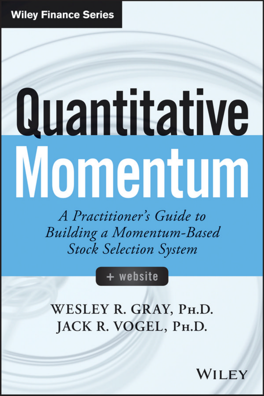
Ken’s fund compounded at 18 percent a year, and yet, the investors in the

fund lost 11 percent a year, a reection of the typical investor’s inability to

time effectively in and out of Ken’s fund (see Figure 2.3).11 When Ken’s fund

was underperforming (and the opportunity was high), they pulled capital;

when his fund was outperforming (and opportunity was low), they invested

❦

❦ ❦

❦

26 QUANTITATIVE MOMENTUM

20.00%

15.00%

10.00%

5.00%

18.00%

–11.00%

0.00%

–5.00%

–10.00%

–15.00%

Theoretical Buy and Hold Investor Actual Investor Performance

FIGURE 2.3 CGM Focus Fund from 1999 to 2009

more capital. On net, Ken looks like a genius, but few investors actually

beneted from Ken’s ability—a lose-lose proposition.

Ken’s Heebner’s experience highlights this conict of interest problem

for asset managers. The dynamics of this problem are explored in an illumi-

nating 1997 Journal of Finance paper by Andrei Shleifer and Robert Vishny,

appropriately called “The Limits of Arbitrage.”12 The takeaway from Ken

Heebner’s experience and Shleifer and Vishny’s insights is as follows: Smart

managers avoid long-term market opportunities if their investors are focused

on short-term performance.

And can you blame the managers? If their careers depend on their rel-

ative performance over a month, a year, or even every ve years, then asset

managers will clearly care more about short-term relative performance than

about long-term expected risk-adjusted returns. Whether they are proac-

tively protecting their jobs or the clients are actively driving the conversation

around near-sighted metrics, the end result is the same. Fund investors lose,

and prices are not always efcient.

Keys to Long-Term Active Management Success

“There are a lot of smart people ...so it’s not easy to win.”

—Charlie Munger, Vice Chairman Berkshire Hathaway13

❦

❦ ❦

❦

Why Can Active Investment Strategies Work? 27

Sustainable

Alpha

Sustainable

Investors

Long-Term

Performance

FIGURE 2.4 The Long-Term Performance Equation

We’ve outlined a few elements of the marketplace. First, some investors

are probably making poor investment decisions, and second, some managers

are unable to exploit genuine market opportunities due to incentives. We

encapsulate these elements in a simple equation for sustainable long-term

performance in Figure 2.4.

The long-term performance equation has two core elements:

■Sustainable alpha

■Sustainable investors

Sustainable alpha refers to an active stock selection process that system-

atically exploits mispricings caused by behavioral bias in the marketplace

(i.e., nds the worst poker players). In order for this “edge” to be sustain-

able, it cannot be arbitraged away in the long run. Typically, sustainable

edges are driven by strategies that require a long-horizon and indifference to

short-term relative performance in order to be successful. That requirement

brings us to our second element of the long-term performance equation: sus-

tainable investors. Sustainable investors cannot fall victim to the siren song

of short-term underperformance. If they do fall prey to short-termism, these

unsustainable investors will greatly enhance the arbitrage costs for their del-

egated asset manager, and will thus prevent the investors from protably

exploiting mispricing opportunities.

Based on the equation, if one can identify a process with an established

edge (i.e., sustainable alpha) that requires long-term discipline to exploit

(i.e., requires sustainable investors), it is likely that this process will serve as

a promising long-term strategy that will beat the market over time.

Moving from Theory to Practice Much of this discussion outlines an intel-

lectual framework for successful active investing. There is no discussion of

whether value investing is better than growth investing, or if high-frequency

trading is better than investing in pork belly futures. However, the building

blocks to identify sustainable performance are simple to follow:

■Identify a sustainable alpha process that can exploit bad players.

■Understand the limitations of good players.

■Exploit the opportunity by pairing a good process with sustainable

capital.

❦

❦ ❦

❦

28 QUANTITATIVE MOMENTUM

To put a little bit of meat on the bone, we provide an example of how

this construct works in the “value versus growth” debate, which is a familiar

discussion for most readers. To keep things simple and in line with academic

research practices, we consider value investing to be approximated roughly

by the practice of purchasing portfolios of rms with low prices to some fun-

damental price metric (e.g., a high book-to-market or B/M ratio). Growth

investing is the opposite approach—purchase rms with high prices relative

to fundamentals, with the expectation that fundamentals will grow rapidly.

Using Ken French’s data,14 we examine the returns from January 1, 1927, to

December 31, 2014, for a value portfolio (high B/M decile, value-weighted

returns), a growth portfolio (low B/M decile, value-weighted returns), and

the S&P 500 total return index. By value-weight, we mean that each stock is

given its weight in the portfolio, depending on the size of the rm. Results are

shown in Table 2.1. All returns are total returns and include the reinvestment

of distributions (e.g., dividends). Results are gross of fees.

The historical evidence is clear: value stocks from 1927 to 2014

have outperformed growth stocks—by a wide margin. The portfolio of

value stocks earns a compound annual growth rate of 12.41 percent

per year, whereas, the growth stock portfolio earns 8.70 percent per

year—approximately a 4 percent annual spread in performance. This

historical spread in returns, which has been repeatedly and consistently

observed over time, has been labeled the value anomaly by academic

researchers. Of course, academics argue over the reasons why the spread

is large (e.g., value investing might earn higher returns because it is simply

more risky or because of mispricing, as discussed earlier). This debate is

best captured by a 2008 interview with Eugene Fama where he describes

apersonalconversationwithAndreiShleiferoveraglassofwine.

15 Fama

highlights that Andrei believes the value premium is due to mispricing,

whereas Fama attributes the value premium to higher risk. Bottom line:

TABLE 2.1 Value versus Growth (1927 to 2014)

Value Growth SP500

CAGR 12.41% 8.70% 9.95%

Standard Deviation 31.92% 19.95% 19.09%

Downside Deviation 21.34% 14.41% 14.22%

Sharpe Ratio 0.41 0.35 0.41

Sortino Ratio (MAR =5%) 0.54 0.37 0.45

Worst Drawdown –91.67% –85.01% –84.59%

Worst Month Return –43.98% –30.65% –28.73%

Best Month Return 98.65% 42.16% 41.65%

Protable Months 60.51% 59.09% 61.74%

❦

❦ ❦

❦

Why Can Active Investment Strategies Work? 29

Great minds can disagree on the explanation, but nobody can dispute the

empirical fact that value stocks have outperformed growth stocks by a wide

margin over time.

We Have the Facts. Next Step: Identify Bad Players The data highlight that

value investing has higher expected returns than growth investing. But to

better understand whether value will beat growth in the future we need to

look through the sustainable active investing prism and identify if the spread

is due to risk (the efcient market explanation) or mispricing (the behavioral

nance explanation). For a valid mispricing argument, we need to identify

if there are market participants making systematically poor decisions with

respect to the purchase of value and growth stocks.

Lakonishok, Shleifer, and Vishny (LSV) explore this question in their

paper “Contrarian Investment, Extrapolation, and Risk.”16 LSV hypothe-

size that investors suffer from representative bias, a situation where investors

naively extrapolate past growth rates too far into the future. Figure 2.5 high-

lights the concept from the LSV paper using updated data from Dechow and

Sloan’s 1997 paper, “Returns to Contrarian Investment Strategies: Tests of

Naive Expectations Hypothesis.”17 The horizontal axis represents cheapness

and sorts securities into buckets, from left to right, based on whether stocks

are expensive (low book-to-market ratios) or cheap (high book-to-market

ratios). The vertical axis represents past ve-year earnings growth rates for

the respective valuation buckets. Stocks in Bucket 10 are the cheapest, and

they exhibited (on average) a negative 1percentearningsgrowthoverthe

preceding ve years.

Growth

Past Earnings Growth Rates

25.0%

20.0%

15.0%

10.0%

5.0%

0.0%

–5.0%

23456789Value

B/M Deciles

Past Earnings Growth Rates and Valuations

FIGURE 2.5 Investors Extrapolate Past Growth Rates into the Future

❦

❦ ❦

❦

30 QUANTITATIVE MOMENTUM

The relationship is almost perfectly linear. Cheap stocks have terrible

past earnings growth, whereas expensive stocks have had wonderful earn-

ings growth over the past ve years. No real surprise there, but it is interest-

ing to see how well the data ts this relationship.

Figure 2.5 underscores the general market expectation that past earn-

ings growth rates will continue into the future. Growth rms are expensive

because market participants believe past growth rates will continue. Oth-

erwise, why would they pay so much for these stocks? Meanwhile, value

stocks are cheap for what seems like a good a reason—the market believes

their poor past growth rates will continue as well.

But does this really happen? Do cheap stocks have poor realized future

earnings growth and do expensive stocks have strong realized future earn-

ings growth? This is an empirical question that can be tested with an exper-

iment. Do growth rms continue to grow faster, on average, or is there a

systematic aw in market expectations?

In Figure 2.6, we look at what happens to earnings growth over the

next ve years. Specically, did the value stocks continue to exhibit terrible

earnings growth as predicted? Did growth stocks maintain their terricearn-

ings growth?

No, they did not. The chart is evidence of systematically poor poker

playing. The realized earnings growth (dark bars) systematically reverts

to the average growth rate across the universe. Value stocks outperform

earnings growth expectations and growth stocks underperform their expec-

tations, systematically. Take a moment to study this profound observation.

18.0%

16.0%

14.0%

12.0%

10.0%

Future Earnings Growth Rates

8.0%

6.0%

4.0%

2.0%

0.0%

Growth 2 3 4 5 6

B/M Deciles

Future Earnings Growth Rates and Valuations

7 8 9 Value

FIGURE 2.6 Realized Growth Rates Systematically Mean-Revert

❦

❦ ❦

❦

Why Can Active Investment Strategies Work? 31

This unexpected deviation from expectations leads to price movements

that are favorable for cheap “value” stocks, and unfavorable for expensive

“growth” stocks. This deviation explains, at least in part, why expensive

stock investors underperform, cheap stock investors outperform, and

passive investors receive something in between.

To summarize: Markets, on average, throw value stocks under the bus

and clamor for growth stocks. From a poker playing perspective, buying

growth stocks and selling value stocks is an example of a systematically poor

strategy. Assuming that a great hand from the last round equals a winning

hand in the next round is a losing approach. But what are the best poker play-

ers doing about this value anomaly situation, and can these poker players

easily exploit the poor poker players?

Next Step: Identify the Actions of the Best Players It is unlikely that we will

ever be the smartest investors in the world. For example, George Soros,

Julian Robertson, Leon Cooperman, and Paul Tudor Jones will always be

smarter than we are. But if we aren’t going to be the best player at the invest-

ing table, how can we win against these high-powered investors? We can win

by nding those market opportunities where the smartest investors are reluc-

tant to participate. But why would a smart investor not want to participate in

a straightforward way to beat the market, such as through value investing?

As mentioned previously, smart investors often get endowed with large

amounts of capital from a large group of diverse investors (again, think

George Soros, Julian Robertson, Paul Tudor Jones, but also large institu-

tions such as BlackRock, Fidelity, and so forth). This makes sense on many

levels—investors want to give their money to smart people. The challenge

is that the really smart investors are often managing money on behalf of

investors that suffer from behavioral biases (System 1 thinkers). Shleifer

and Vishny highlight, and the Ken Heebner example conrms, that many

smart market participants are hamstrung by the short-term performance

measures imposed on them by their investors. “How did you perform against

the benchmark this quarter? What do your results look like year to date?

What macroeconomic trends are you exploiting this month?” All of these

questions are commonplace in the market. The threat of being red and

replaced with a passive portfolio of Vanguard funds is an implied threat.

When job security and client expectations trump long-term value creation,

funny things happen.

AremarkablepaperbyMarkusBrunnermeierandStefanNagel,“Hedge

Funds and the Technology Bubble,” highlights the warped incentives faced

by the smartest investors who deal with other people’s money.18 Contrary to

all textbook teachings related to efcient price formation, the smart money

sometimes can be incentivized to enhance mispricing, not trade against it!

❦

❦ ❦

❦

32 QUANTITATIVE MOMENTUM

Brunnermeier and Nagel nd that many hedge fund managers didn’t try to

capitalize on the mispricing between value and growth stocks in the Internet

Bubble of the late 1990s—they actually bought growth stocks and sold value

stocks. This action enabled them to more closely track the index—for a time.

Meanwhile, the poor hedge funds that stuck to their value investing guns,

for example, Julian Robertson of Tiger Funds, ended up with no assets under

management and a busted business model.

But Julian Robertson wasn’t the only famous value investor to lose his

proverbial shirt during the 1994 to 1999 time period. Around this time,

Barron’s famously stated the following regarding Warren Buffett’s relative

performance:19

“Warren Buffett may be losing his magic touch.”

Barron’s observation was, in many respects, fully warranted. Value

investors as a group were destroyed by the market in the late 1990s. Generic

value investing (shown in Figure 2.7) underperformed the broader market

by a large margin for six long years!

Obviously, being a value investor requires a patience and faith that few

investors possess. In theory, value investing is easy—buy and hold cheap

stocks for the long haul—but in practice, true value investing is almost

impossible.

$400

$350

$300

$250

$200

$150

$100

$50

1/1/1994

5/1/1994

9/1/1994

1/1/1995

5/1/1995

9/1/1995

1/1/1996

5/1/1996

9/1/1996

1/1/1997

5/1/1997

9/1/1997

1/1/1998

5/1/1998

9/1/1998

1/1/1999

5/1/1999

9/1/1999

Value of $100 Invested

Value Stocks SP500

FIGURE 2.7 Value Investing Can Underperform

❦

❦ ❦

❦

Why Can Active Investment Strategies Work? 33

Using Ken French’s data, we examined just how painful it was to

be a value investor in the late 1990s. We examine the returns from

January 1, 1994, to December 31, 1999, for a value portfolio (high

book-to-market decile, value-weighted portfolio returns), a growth portfo-

lio (low book-to-market decile, value-weighted portfolio returns), the S&P

500 total return index (SP500), and the Russell 2000 total return index

(R2K), a small-cap index. Results are shown in Table 2.2. All returns are

total returns and include the reinvestment of distributions (e.g., dividends).

Results are gross of fees.

The returns to the value portfolio were not bad on an absolute basis, but

on a relative basis, value was horric. Looking at the annual returns (shown

in Table 2.3), value investing lost almost every year to a simple passive mar-

ket allocation!

Aplain-vanillaindexfund(SP500)outperformsvalueve out of six

years in a row, sometimes by double-digit gures! To simulate what these

value managers went through, ask yourself this question:

If your asset managers underperformed a benchmark for ve out of

six years, at times by double digits, would you re them?

TABLE 2.2 Value Investing Can Underperform (1994–1999)

Value Growth SP500 R2K

CAGR 18.35% 27.71% 23.84% 13.39%

Standard Deviation 11.79% 16.53% 13.63% 16.96%

Downside Deviation 7.59% 11.25% 10.50% 14.27%

Sharpe Ratio 1.09 1.28 1.30 0.55

Sortino Ratio (MAR =5%) 1.66 1.87 1.67 0.64

Worst Drawdown –11.58% –16.33% –15.18% –29.78%

Worst Month Return –8.62% –14.92% –14.31% –19.42%

Best Month Return 8.05% 10.69% 8.04% 11.32%

Protable Months 68.06% 70.83% 73.61% 66.67%

TABLE 2.3 Annual Returns

Value Growth SP500 R2K

1994 –2.83% 2.53% 1.35% –1.82%

1995 36.47% 35.47% 37.64% 28.45%

1996 14.22% 23.20% 23.23% 16.49%

1997 32.52% 31.15% 33.60% 22.36%

1998 29.75% 44.23% 29.32% –2.55%

1999 5.45% 33.90% 21.35% 21.26%

❦

❦ ❦

❦

34 QUANTITATIVE MOMENTUM

For 99.9 percent of investors, that answer would be a resounding,

“Yes!” (and giving someone a six-year trial period is probably out of the

question to begin with). Most—if not all—professional asset managers

would be red, given this underperformance. Asset managers know this

evidence intuitively, and internalize the results by avoiding purist value

investing endeavors that could make them look like fools in the short run.

After viewing the six-year value investing pain train, we can identify two

key takeaways:

1. For a long-term investor, a six-year stretch of pain is a truly great thing.

Why? Because this will limit competition from the best pokers players,

for whom career risks trump performance considerations, and the weak

hands will be shaken out of the competition.

2. Sustainable active investing requires special investors. It requires that

investors be disciplined, have a long-term horizon, and be indifferent

to short-term relative performance. These unique investors are what we

had previously labeled sustainable investors in Figure 2.4.

Now, suspend reality for a moment and let’s imagine that an active value

manager had clients that didn’t run for the exits in 1999. What would their

hypothetical returns look like over the long run? As one can see in Table 2.4,

value quickly recovers and handily outperforms over the entire time period

thereafter. Table 2.4 shows the returns to the same portfolios from January

1, 2000, to December 31, 2014, the 15 years following the six-year period

of underperformance.

Sticking with the value strategy, although painful, was richly rewarded

with almost a 5 percent edge—per year—over the market benchmark (S&P

500) from 2000 to 2014.

TABLE 2.4 Summary Statistics (2000–2014)

Value Growth SP500 R2K

CAGR 9.12% 2.75% 4.45% 7.38%

Standard Deviation 24.05% 16.90% 15.22% 20.42%

Downside Deviation 17.73% 12.50% 11.42% 13.77%

Sharpe Ratio 0.41 0.14 0.24 0.36

Sortino Ratio (MAR =5%) 0.37 –0.07 0.05 0.31

Worst Drawdown –64.47% –58.21% –50.21% –52.89%

Worst Month Return –28.07% –16.13% –16.70% –20.80%

Best Month Return 36.64% 11.21% 10.93% 16.51%

Protable Months 58.89% 56.67% 60.56% 58.89%

❦

❦ ❦

❦

Why Can Active Investment Strategies Work? 35

TABLE 2.5 Summary Statistics (1994–2014)

Value Growth SP500 R2K

CAGR 11.68% 9.33% 9.65% 9.06%

Standard Deviation 21.27% 17.00% 14.92% 19.48%

Downside Deviation 16.23% 12.25% 11.19% 13.97%

Sharpe Ratio 0.50 0.45 0.51 0.41

Sortino Ratio (MAR =5%) 0.51 0.44 0.48 0.40

Worst Drawdown –64.47% –58.21% –50.21% –52.89%

Worst Month Return –28.07% –16.13% –16.70% –20.80%

Best Month Return 36.64% 11.21% 10.93% 16.51%

Protable Months 61.51% 60.71% 64.29% 61.11%

Over the entire cycle, patient and disciplined investors were rewarded.

Table 2.5 shows the results over the entire time period, measured from

January 1, 1994, to December 31, 2014.

What’s the bottom line? For a long-term investor, value investing was the

optimal decision relative to growth investing, but for many of the smartest

asset managers in the world, including the great Julian Robertson, value

investing was simply not feasible as a business model. These professionals

were often forced via the threat of investor redemptions to “diworsify” their

portfolios with overpriced growth stocks during the Internet Bubble. They

needed to keep up with the market and did so by doing what everyone else

was doing. This decision helped them keep their jobs, but prevented their

investors from maximizing their chances for success, even if some truly did

have a long-horizon, and discipline.

Putting It All Together

We’ve used value and growth investing as a laboratory to highlight how the

sustainable active investing framework can identify long-term winning strate-

gies. Value investing ts nicely in this paradigm, but has serious warts, notably

stretches of horrendous underperformance. The lesson from value investing

is that successful active investing is simple, but not easy. If active investing

were easy, everyone would do it, and if everyone were doing it, it probably

would not generate outsized risk-adjusted returns over the long haul.

In summary, our long-term performance equation from Figure 2.4 high-

lights two required elements for sustainable performance:

1. The sustainable process exploits systematic investor expectation errors.

2. The sustainable investor has a long horizon and a willingness to be

different.

❦

❦ ❦

❦

36 QUANTITATIVE MOMENTUM

These two pieces of the puzzle map back to the classic lessons of poker:

1. Identify the worst poker player at the table.

2. Identify the best poker players at the table.

And these classic lessons map into the two pillars of behavioral nance:

1. Understand behavioral bias and how investors form expectations.

2. Understand market frictions and how they affect market participants.

So the next time you hear a market participant suggest that one strat-

egy is better than another strategy, simply ask two basic questions: (1) Why

are the securities selected by this process mispriced? and (2) Why aren’t

other smart investors already exploiting the mispricing opportunity? With-

out solid answers to both questions, it is unlikely that the investment process

is sustainable.

GROWTH INVESTING STINKS, SO WHY DO IT?

We talked in the last section about how value stocks outperform growth

stocks, and showed that buying and holding growth stocks is a bad relative

bet. And yet, most fund complexes divide the investable universe into value

and growth stocks. To highlight the prevalence of the value/growth mindset

in the marketplace, Figure 2.8 is an example of the classic three-by-three

diagram, which splits the stock universe into nine buckets. The two axes are

size (vertical axis from large to small) and value (horizontal axis from value

to growth).

Figure 2.8, or some derivation of it, is used by almost every major invest-

ment rm in the United States. But if growth is a suboptimal investment

approach, why bother with a framework that suggests we consider growth

stocks as part of a portfolio? One answer to this question is likely related to

Size

Blend GrowthValue

Large

Medium

Small

Style

FIGURE 2.8 Value and Growth Chart

❦

❦ ❦

❦

Why Can Active Investment Strategies Work? 37

the fact that growth stocks provide some diversication benets for a portfo-

lio, even though they provide poor relative returns. We explicitly investigate

the diversication benets of growth in Table 2.6, in the context of the late

1990s (a period we examined in Table 2.2), which was a time when value

underperformed versus growth. We examine the performance of a monthly

rebalanced portfolio that invests half of the portfolio in the value portfolio

and half in the growth portfolio over the 1994 to 1999 time period.

At a high level, being a combo investor (value and growth) was a much

smarter career move over this period in the 1990s than being a pure value

investor. The combo investor did not achieve the performance of the pure

growth portfolio, but the results were closer to the broader market and the

probability of getting red was muted. The annual return gures in Table 2.7

bring this point home.

Unlike the pure value portfolio, which was a guaranteed ticket to the

unemployment line in 1999, the combo portfolio, while underwhelming rel-

ative to the market, would have been at least a salvageable situation in a

TABLE 2.6 Combining Value and Growth Lowers Volatility (1994–1999)

Value Growth

50% Value,

50% Growth SP500

CAGR 18.35% 27.71% 23.19% 23.84%

Standard Deviation 11.79% 16.53% 12.86% 13.63%

Downside Deviation 7.59% 11.25% 9.49% 10.50%

Sharpe Ratio 1.09 1.28 1.32 1.30

Sortino Ratio (MAR =5%) 1.66 1.87 1.78 1.67

Worst Drawdown –11.58% –16.33% –13.93% –15.18%

Worst Month Return –8.62% –14.92% –11.77% –14.31%

Best Month Return 8.05% 10.69% 7.97% 8.04%

Protable Months 68.06% 70.83% 70.83% 73.61%

TABLE 2.7 Annual Returns for Combo Portfolio

Value Growth

50% Value,

50% Growth SP500

1994 –2.83% 2.53% –0.09% 1.35%

1995 36.47% 35.47% 36.07% 37.64%

1996 14.22% 23.20% 18.77% 23.23%

1997 32.52% 31.15% 32.08% 33.60%

1998 29.75% 44.23% 37.15% 29.32%

1999 5.45% 33.90% 19.37% 21.35%

❦

❦ ❦

❦

38 QUANTITATIVE MOMENTUM

client meeting. Of course, we already know how this story ends. The benets

of combining the growth strategy with the value strategy over this unique

time period offered a great benet: diversication. The combo reduced the

pain versus a pure value approach.

Likewise, as seen in Table 2.8, the combo portfolio served an investment

manager well over the longer 1994 to 2014 period (examined previously in

Table 2.5), delivering higher risk-adjusted returns than the S&P 500 bench-

mark. For the period 1994 to 2014, the combo portfolio reduced the pain

versus a pure growth approach.

The other benet for these active managers is that they maintained their

careers through the tech bubble. Of course, the downside of this approach

was lower absolute returns due to the inclusion of the growth component,

which diluted the performance of an active value strategy throughout

the cycle.

But Can We Identify a Better Diversiﬁer?

As outlined above, investors and professional fund managers appreciate the

benets of including growth in a portfolio—especially during the period

under discussion—because value and growth had relatively low correla-

tions and thus created a portfolio with less benchmark drift and manageable

volatility. However, the inclusion of growth, while providing portfolio diver-

sication benets, has costs in the form of lower expected portfolio returns.

Growth investing is not a sustainable active strategy. In fact, it is just the

opposite—a sustainably poor strategy. But what is an investor to do? Ide-

ally, one could capture the diversication benets of a growth portfolio,

but accomplish the diversication benets with an active stock selection

TABLE 2.8 Combining Value and Growth Lowers Volatility (1994–2014)

Value Growth

50% Value,

50% Growth SP500

CAGR 11.68% 9.33% 10.86% 9.65%

Standard Deviation 21.27% 17.00% 17.42% 14.92%

Downside Deviation 16.23% 12.25% 12.87% 11.19%

Sharpe Ratio 0.50 0.45 0.53 0.51

Sortino Ratio (MAR =5%) 0.51 0.44 0.53 0.48

Worst Drawdown –64.47% –58.21% –56.63% –50.21%

Worst Month Return –28.07% –16.13% –22.10% –16.70%

Best Month Return 36.64% 11.21% 23.28% 10.93%

Protable Months 61.51% 60.71% 62.30% 64.29%

❦

❦ ❦

❦

Why Can Active Investment Strategies Work? 39

methodology that had characteristics that were more in line with the sus-

tainable active framework.

Fortunately, there is a potential solution to this problem: momentum

investing. In the early 1990s, academics such as Narasimhan Jegadeesh and

Sheridan Titman, in their 1993 paper “Returns to Buying Winners and Sell-

ing Losers: Implications for Market Efciency,” began to refocus on the old

concept of momentum, which refers to a general class of strategies in which

past returns can predict future returns.20 That is, if a stock has performed

relatively well over the past year, it will continue to perform relatively well

in the future. Researchers have done follow-on studies that nd the momen-

tum effect persists even when controlling for company size and value factors.

And the effect appears to hold over a 200-year time sample,21 and across

multiple asset classes, such as commodities, currencies, and even bonds.22

Moreover, researchers nd that momentum is relatively uncorrelated with

value, thus providing diversication benets. In short, it appears the evidence

for momentum is pervasive and provides similar diversication benets to

growth investing.

And while momentum investment strategies are well established in

the academic literature, these strategies are not commonly used in actively

managed funds, especially when compared with the large number of

“growth” funds found in the market. In fact, the immediate gut reaction

of most people to “momentum,” is that momentum investing IS growth

investing. Unfortunately, this reaction reects a misconception in the

market. Momentum and growth, while sometimes related, are certainly not

the same. Moreover, we believe that momentum, unlike growth, ts nicely

in the sustainable active framework, thus making it a much better diversier

alongside value, which is another sustainable strategy. The goal of the next

chapter is to explain why momentum investing, which is purely focused

on prices, is a better alternative to growth investing, which considers both

fundamentals and prices. Our mission is to convince the reader that the

evidence supports a move to a new style-box paradigm (Figure 2.9) that

replaces “growth” with “momentum.”

Blend MomentumValue

Large

Medium

Small

Size

Style

FIGURE 2.9 New Style Box Paradigm

❦

❦ ❦

❦

40 QUANTITATIVE MOMENTUM

SUMMARY

In order to assess the sustainability of an active strategy, we outlined the

sustainable active investing framework to better understand why certain

strategies work and why others do not. We then reviewed the classic value

versus growth debate, but viewed this argument through the lens of the sus-

tainable active framework. We discussed that value investing works, not

because Ben Graham said it would work, but because (1) it systematically

captures a mispricing in the market associated with poor expectations, and

(2) taking advantage of the mispricing is difcult.

Next, we addressed the question of why investors would ever rationally

invest in growth, given the long-term evidence of growth’s historical under-

performance. We highlighted a unique time period in the markets—the

Internet Bubble—where growth investing outperformed value and pre-

vented many professional investment managers from losing their jobs.

Next, there was a brief discussion of the benets (diversication) and

the costs (poor long-term performance) associated with growth investing.

Finally, we ended the chapter by proposing that investors replace growth

portfolios with momentum portfolios. The hope is that momentum can

provide similar diversication benets to a value-focused portfolio as a

growth portfolio does, and that momentum does so without hurting the

long-term expected performance of the portfolio. In the next chapter, we

describe momentum investing, highlight how it is different from growth

investing, and then describe why momentum may be a better complement

to value than growth.

NOTES

1. Wesley Gray, Embedded: A Marine Corps Advisor Inside the Iraqi Army, Naval

Institute Press, Annapolis, 2008.

2. Eugene F. Fama and Kenneth R. French, “The Cross Section of Expected Stock

Returns,” The Journal of Finance 47 (1992): 427–465.

3. Steven S. Crawford, Wesley R. Gray, and Andrew E. Kern, “Why Do Fund Man-

agers Identify and Share Protable Ideas,” Journal of Financial and Quantitative

Analysis, Forthcoming.

4. Nick Barberis and Richard Thaler, “A Survey of Behavioral Finance,” in:

G. M. Constantinides & M. Harris & R. M. Stulz (ed.), Handbook of the

Economics of Finance,1sted.,volume1,(NorthHolland:Elsevier,2003),

chapter 18, pp. 1053–1128.

5. Although widely attributed to Keynes, there is little evidence he actually made

this statement. See Jason Zweig, “Keynes: He Didn’t Say Half of What He

❦

❦ ❦

❦

Why Can Active Investment Strategies Work? 41

Said. Or Did He?” Wall Street Journal (February 11, 2011), blogs.wsj.com

/marketbeat/2011/02/11/keynes-he-didnt-say-half-of-what-he-said-or-did-he/,

accessed 2/28/2016.

6. Daniel Kahneman, Thinking, Fast and Slow (New York: Farrar, Straus and

Giroux, 2011).

7. J. Bradford DeLong, Andrei Shleifer, Lawrence Summers, and Robert Wald-

mann, “Noise Trader Risk in Financial Markets,” Journal of Political Economy

98 (1990): 703–738.

8. Larry Swedroe, “Behavioral Finance Falls Short,” April 24, 2015, ETF.com

.www.etf.com/sections/index-investor-corner/swedroe-behavioral-nance-falls

-short?nopaging=1, accessed 2/28/2016.

9. Barberis and Thaler. Of course, Bill Sharpe’s argument regarding the arithmetic

of active management also plays a role in explaining why active managers, as a

whole, can’t beat the market.

10. E. Laise, “Best Stock Fund of the Decade: CGM Focus,” Wall Street Journal

(December 31, 2009), www.wsj.com/articles/SB1000142405274870487680457

4628561609012716, accessed 12/29/2015.

11. Some of the spread in returns between dollar-weight returns and buy-and-hold

returns could be attributable to the return sequence experienced by the

CGM Focus Fund. See Michael Kitces’s October 3, 2012, piece on “Does the

DALBAR Study Grossly Overstate the Behavior Gap” for more information.

https://www.kitces.com/blog/does-the-dalbar-study-grossly-overstate-the

-behavior-gap-guest-post/, accessed 2/28/2016.

12. Andrei Shleifer and Robert W. Vishny, “The Limits of Arbitrage,” The Journal

of Finance 52 (1997): 35–55.

13. Charlie Munger, May 4, 2005, Wesco Financial Annual Meeting. Based on

notes from Whitney Tilson. www.tilsonfunds.com/wscmtg05notes.pdf, accessed

2/28/2016.

14. mba.tuck.dartmouth.edu/pages/faculty/ken.french/data_library.html, accessed

12/30/2015.

15. Eugene Fama Interview, 2008, American Finance Association. www.afajof.org

/details/video/2870921/Eugene-Fama-Interview.html, accessed 12/29/2015

16. Josef Lakonishok, Andrei Shleifer, and Robert W. Vishny, “Contrarian

Investment, Extraploation, and Risk,” The Journal of Finance 49(5) (1994):

1541–1578.

17. Patricia M. Dechow and Rishard G. Sloan, “Returns to Contrarian Investment

Strategies: Tests of the Naïve Expectations Hypothesis,” Journal of Financial

Economics 43 (1997): 3–27. As an aside, Dechow and Sloan 1997 argue that

the value anomaly is not driven by naive extrapolation by irrational investors

as LSV 1994 suggested, but rather, the outperformance of value stocks is driven

by market participants’ awed faith in analysts’ forecasts, which are systemat-

ically overoptimistic. We also note that the data associated with the valuation

metric used in Figure 2.5 is book-to-market. Other valuation metrics, such as

price-to-earnings, don’t paint a similarly compelling picture, but deeper analysis

into alternative valuation metrics still suggests that the value anomaly is partially

❦

❦ ❦

❦

42 QUANTITATIVE MOMENTUM

driven by mispricing caused by investor expectation errors and cannot be fully

explained by additional risk.

18. Markus Brunnermeier and Stefan Nagel, “Hedge Funds and the Technology

Bubble,” The Journal of Finance 59 (1993): 2013–2040.

19. Andrew Bary, 1999, “What’s Wrong, Warren?” Barron’s (1999), www.barrons

.com/articles/SB945992010127068546, accessed 12/29/2015.

20. Narasimhan Jegadeesh and Sheridan Titman, “Returns to Buying Winners and

Selling Losers: Implications for Stock Market Efciency,” The Journal of Finance

48 (1993), 65–91.

21. Chris Geczy and Mikhail Samonov, “Two Centuries of Price Return Momen-

tum,” Financial Analysts Journal (2016).

22. Clifford S. Asness, Tobias J. Moskowitz, and Lasse H. Pedersen, “Value and

Momentum Everywhere,” The Journal of Finance 68(3) (2013): 929–985.

❦

❦ ❦

❦

CHAPTER 3

Momentum Investing Is Not

Growth Investing

“The dumbest reason in the world to buy a stock is because it’s

going up.”

—Attributed to Warren Buffett1

We use the term momentum to mean a continuation of past relative

returns—past winners tend to be future winners, while past losers

tend to be future losers. Practitioners often refer to this class of strategies

as relative strength strategies, which have been around for a long time. In

fact, Robert Levy published a paper in 1967 called “Relative Strength as

a Criterion for Investment Selection.” Mr. Levy outlines his conclusion:

“The prots attainable by purchasing the historically strongest stocks are

superior to the prots from random selection.”2Oddly enough, research

on relative strength strategies went dormant following Levy’s contribution.

What happened? The efcient market hypothesis happened.

THE EFFICIENT MARKET MAFIA KILLS

RELATIVE STRENGTH

As we alluded to in Chapter 2, the efcient market hypothesis (EMH) was

developed at the University of Chicago in the 1960s and 1970s. The EMH

hypothesis subsequently ourished across academia. Under the semi-strong

form interpretation of the EMH, asset prices reect all publicly available

information so that there is no way for investors to consistently outperform

arandomlyselectedbasketofsecuritiesaftercontrollingforrisk.OrasEMH

proponent Burton Malkiel so eloquently put it in his 1973 classic, ARan-

dom Walk Down Wall Street: “A blindfolded monkey throwing darts at a

❦

❦ ❦

❦

44 QUANTITATIVE MOMENTUM

newspaper’s nancial pages could select a portfolio that would do just as

well as one carefully selected by experts.”3Thus, from an EMH perspective,

for all intents and purposes, Levy’s evidence on the performance of relative

strength strategies was an impossibility.

It seems that practitioners like Levy (who worked in the private sector

at the time his paper was published), were overtaken by the cult of aca-

demics focused on pursuing the efcient market hypothesis. Practitioners

were essentially banned from publishing in top-tier academic nance jour-

nals and academics pursuing research interests that went counter to the

EMH idea were driven from the emerging EMH temple.4The subsequent

25 years of published academic research entered a dark age, and discus-

sions of relative strength strategies were effectively banned, since space was

primarily reserved for EMH cheerleaders.

Yet, all was not well in the ivory tower. Anomalies that were inconsistent

with EMH began to emerge in the literature in the 1970s. For example, as

previously mentioned, Ben Graham, among others, had shown that buying

a basket of cheap stocks tended to outperform the market, and academics

began to formally examine the value effect. Evidence related to value and

other so-called anomalies began to accumulate, hinting that there might be

kinks in the EMH armor, but EMH proponents remained condent. How-

ever, around the same time that many EMH supporters were basking in

glory, Daniel Kahneman, working with Amos Tversky, started exploring

how human biases affected nancial decision making. Kahneman and Tver-

sky established some of the earliest connections between investors’ internal

behavioral biases and many of the observed anomalies that were being iden-

tied in the academic nance literature.

“MOMENTUM” RISES FROM THE ASHES

Finally, in the early 1990s, Narasimhan Jegadeesh and Sheridan Titman revi-

talized the ndings from Levy’s 1967 paper in their pioneering 1993 article

“Returns to Buying Winners and Selling Losers: Implications for Market

Efciency.” This paper essentially replicated the spirit of the analysis con-

ducted by Levy in 1967, but with the benetofmoredata,computational

power, and willingness on behalf of the establishment to publish research

that questioned EMH. By now, the cracks in the EMH armor were get-

ting bigger.

Interestingly enough, Jegadeesh and Titman never mention the word

momentum in their original paper, even though their paper is considered

by many to be the seminal work on modern-era stock selection momentum

strategies. We posit that the term momentum was adopted after Mark

❦

❦ ❦

❦

Momentum Investing Is Not Growth Investing 45

Carhart published his University of Chicago dissertation in The Journal of

Finance.Inthispaper,Carhartcreatesamomentum factor, which essentially

reected the relative strength of the stock selection strategies outlined in

Jegadeesh and Titman’s paper.5Soon after Carhart’s paper, momentum

became the new academic term for the age-old relative strength strategy.

With the oodgates open, researchers published a urry of papers on

momentum strategies. The evidence was so overwhelming that the anomaly

was crowned the “premier anomaly” by none other than Eugene Fama—an

original architect of the EMH theory.6

Remarkably, while modern-day academics refocused on the concepts of

stock selection momentum, many practitioners continued to be stuck in a

time warp. The reasons for this regressive behavior are likely related to the

practitioner training pipeline. The academics, who train all the MBAs that

go on to manage portfolios, were still being taught portfolio mathematics

so they could solve asset allocation decisions. Stock picking training was a

waste of time because it was a sucker’s game under a strict interpretation

of the EMH. And of course, for the MBA “rebels,” there was always the

value anomaly to pursue, which had been popularized by the intense suc-

cess of Warren Buffett, the folksy investment hero from Omaha, Nebraska.

Unlike value, however, there were no vibrant champions for momentum

investing—no Ben Graham, no Warren Buffett. To make matters worse, the

heroes associated with the value investing school of thought were, ironi-

cally, agreeing with the EMH academics when it came to momentum. Their

value investing approach was perfectly reasonable, but momentum invest-

ing was deemed a black art, a kind of voodoo magic, only practiced by fools

and heretics. Of course, all of this ew in the face of the actual evidence,

which suggests that momentum investing is an even better anomaly than

value investing.7

EMH enjoyed great success for many years, with reams of academic

papers showcasing how efcient markets had become. In many respects,

EMH had won the argument—prices are generally efcient. But this price

efciency is why the evidence on momentum investing was so disheartening

to the EMH school of thought. The value anomaly was one thing—perhaps

investors could beat the market if they used their intellect, did their in-depth

homework, and understood the nancial statements better than the next

investor. But the momentum anomaly was saying something completely dif-

ferent: Price momentum had nothing to do with fundamentals, so even a

halfwit could pursue a successful strategy focused solely on relative price

performance, since this simple metric seemed to predict future prices. This

nding conicted with even the weakest form of EMH. Houston we have a

problem.

❦

❦ ❦

❦

46 QUANTITATIVE MOMENTUM

BEHAVIORAL FINANCE THEORISTS EXPLAIN MOMENTUM

To the credit of academic researchers, the nancial economics eld moved

forward and the behavioral nance paradigm arose, phoenix-like, from the

ashes of EMH. This new paradigm held tightly to the EMH as a baseline

hypothesis, but relaxed assumptions regarding investor rationality and fric-

tionless markets, in order to understand and explain how and why prices

might deviate from their efcient levels. This framework laid the foundation

for the sustainable active investing concepts outlined in Chapter 2.

Hard-core value investors have a different kind of angst regarding

momentum, a kind of anxiety that is grounded in clouded reasoning and

areligiouszeal,asisevidencedbyquotationsfromvalueinvestingbooks

and personas. For example, Warren Buffett is reported to have said, “The

dumbest reason in the world to buy a stock is because it’s going up.” As a

rule of thumb, Buffett’s advice isn’t a bad rule, and Warren Buffett is clearly

an extraordinary investor whose insights are worthy of investigation. But

rules of thumb don’t always capture the nuance of a situation. Higher prices

may not always be an unreliable signal. For example, what if the intrinsic

value of a stock is higher than the new, higher price—is that not still a

value investment? Or perhaps there is a genuine positive feedback loop

associated with higher prices that in turn increases the intrinsic value of the

rm? High price movements may lower the cost of capital for a rm, allow

them to attract better human capital, or even generate free advertising, thus

increasing fundamental value, albeit in a reexive way. In short, growth

stocks, dened as stocks with high prices to fundamentals, are generally a

bad thing, but higher prices, per se, aren’t always a bad thing. In fact, they

are generally a positive development, all else equal.

Consider the following hypothetical scenario:

■Facebook has gone up 100 percent the past year and has a price to

earnings ratio of 15.

■Google has gone down 50 percent and has a price to earnings ratio of 15.

Which is the better buy? For a classic value investor, these stocks are

arguably the same from a valuation perspective since they both have the same

price to earnings ratio of 15. However, based on psychology, some investors

will “feel” like Google is a better opportunity, since value stocks are often

those that have declined in price. What value investor wants to buy a stock

that is up 100 percent? True value investors are genetically programmed to

be suspicious of strong upward price moves—we know because we are value

investors by nature! Strong upward price movements are typically a bad sig-

nal when it comes to a traditional value or distressed investing opportunity.

❦

❦ ❦

❦

Momentum Investing Is Not Growth Investing 47

Upward moves suggest things are not as cheap as they were before, and are

more expensive now, at least comparatively. But this feeling of disgust that is

associated with buying a high-ying stock is not specictovalueinvestors;

this distrust is also felt more generally by all investors—nobody wants to

be the sucker that bought after the price moved higher. In fact, people can

feel a contrary urge. If you own a stock that has gone up in value, you may

seek to realize the gain by selling it—after all, it feels good to realize a gain.

This effect is often termed the disposition effect.Thereisstrongempirical

evidence to support the theory that the disposition effect is related to the

momentum anomaly.8

Consider a stock that is at a 52-week high—many investors interpret

this to mean the stock is overvalued and unlikely to go higher, even if it

may still be cheap on a fundamental basis. The mainstream interpretation

is patently false: 52-week-high stocks greatly outperform 52-week-low

stocks.9But if many market participants have these kinds of biases, a

reasonable hypothesis is that there will be price pressure—unrelated to

fundamentals—that may prevent a security from reaching its true funda-

mental value because market participants perceive that, for some gut-based

reason, “the stock has already gone up too much.” This situation would

be a case where momentum investing is essentially a cousin, not an enemy,

of value investing. How so? Value investing’s edge is often characterized

as pessimism in the presence of poor short-term fundamentals, which

causes stocks to become too cheap relative to future expectations. Perhaps

momentum investing’s edge could be characterized as pessimism in the

presence of strong short-term fundamentals, which causes stocks to remain

too cheap to future expectations.

WAIT A MINUTE: MOMENTUM INVESTING IS JUST

GROWTH INVESTING, WHICH DOESN’T WORK!

Hold on, if we are arguing that stocks can be cheap due to pessimism related

to strong short-term fundamentals, isn’t that ... growth investing?

No.

But before clarifying, let’s review the psychology behind value versus

growth. In our prior discussion of value and growth, the evidence showed

that value beats growth. The reason for this spread is partly attributable to

mispricing from behavioral bias in the market. For example, the original

Lakonishok, Shleifer, and Vishny study mentioned in Chapter 2 showed

that price to fundamental ratios serve as a proxy for expectation errors

exhibited in the market. Recall that investors thought high past earn-

ings growth rates would continue for growth stocks, and low past earnings

❦

❦ ❦

❦

48 QUANTITATIVE MOMENTUM

growth rates would continue for value stocks. The evidence showed this

expected result did not in fact occur. Follow-on studies debate this core result

from Lakonishok, Vishny, and Shleifer’s original ndings,10 but these papers

fail to address more recent work, including Daniel and Titman’s 1997 paper

on value characteristics and stock returns, Piotroski and So’s 2012 paper

on the interaction between value investing returns and fundamentals, and

Jack’s 117-page dissertation, which is a deep-dive into the concepts outlined

in Piotroski and So’s work. These more recent papers conrm that the

value anomaly, while volatile and costly to exploit, is likely driven, in part,

by mispricing.11

Thus, on average, investors seem to over-extrapolate good news from

growth rms (rms with high price to fundamentals), driving them above

intrinsic value, and do the opposite with value rms (rms with low price to

fundamentals), driving them below intrinsic value. So in the value-investing

framework, growth investors seem to be too optimistic,givenstrongfun-

damentals. But are we now saying that momentum investors are too pes-

simistic, given strong prices? These positions seem to be in conict, but we

will explain.

Let us be clear: Momentum investing is not growth investing. Growth

investing, in accordance with the studies mentioned, is characterized

by securities that have high prices relative to past fundamentals (e.g.,

price-to-earnings ratio). We acknowledge that there are many alternative

ways to dene growth investing in practice (e.g., growth at a reasonable

price), but we will stick with the academic convention for the purposes of

our argument. In contrast to growth, we characterize momentum investing

as securities that have strong relative performance to all other securities,

independent of fundamentals. For example, a momentum strategy might

consider the cumulative returns of prices over the last 12 months relative to

other stocks, but earnings, or any other fundamental metric, would play no

part in the analysis. With momentum, prices aren’t everything; they are the

only thing.

We will argue that strong momentum signals, similar to low price to

fundamental ratios (i.e., value measures), are a proxy for investor expec-

tation errors, and help an informed investor systematically identify situa-

tions where behavioral bias is preventing securities, on average, from reach-

ing perceived fundamental value. Think back to the poor poker players in

the sustainable active investing framework in Chapter 2. As a rst step in

identifying sustainable active strategies, we need some market participants

to be less than rational in order to create a mispricing opportunity. We

will come back to “poor poker players” and the mechanics of how and

why momentum works later. However, this point regarding the difference

between the signal that characterizes momentum (i.e., price-only) versus

❦

❦ ❦

❦

Momentum Investing Is Not Growth Investing 49

growth (i.e., price relative to some fundamental) is extremely important to

understand to ensure that readers are not confused and think that growth

investing is the same thing as momentum investing.

The best way to make the point clear is with data. We examine the

overlap between a portfolio of mid-to-large market capitalization rms

selected on a generic momentum signal (top decile of rms with relative

strongest 12-month performance, skipping the previous month) and a

portfolio of rms selected based on a generic price to fundamental signal

(top decile of rms with the highest price-to-book ratio—or alternatively,

the book-to-market ratio, otherwise known as growth rms) for the period

between 1963 and 2013. Surprisingly, there is only a 21 percent overlap

between the names in the high momentum portfolios and the names in the

growth portfolio. Thus, many momentum stocks are not growth stocks, and

many growth stocks are not momentum stocks. In fact, a high momentum

stock can be a value stock, a growth stock, or anything in between.

DIGGING DEEPER INTO GROWTH VERSUS MOMENTUM

In the following analysis we dig a little deeper into the characteristics of

growth rms and high momentum rms. Our data sample includes all

rms on the New York Stock Exchange (NYSE), American Stock Exchange

(AMEX), and NASDAQ with the required data on CRSP and Compustat,

which are the academic gold standard for nancial data analysis. We only

examine rms with ordinary common equity on CRSP and eliminate all

REITS, ADRS, closed-end funds, utilities, and nancial rms. We incorpo-

rate CRSP delisting return data using the technique of Beaver, McNichols,

and Price.12 To be included in the sample, all rms must have a non-zero

market value of equity as of June 30 of year t.Weusebooktomarket(B/M)

as our annual indicator of “valuation” based on academic convention. Book

is computed on June 30 each year using the methodology from Fama and

French13 and the market capitalization on June 30. All rms with negative

book values are eliminated from the sample. We consider “growth” rms to

be those with the most expensive B/M ratios (i.e., lower is more expensive).

We calculate generic momentum by ranking all stocks monthly on their

cumulative 12-month returns, skipping the most recent month, similar to

Fama and French.

The tests are focused on all mid- and large-cap stocks, dened as stocks

with a market capitalization above the NYSE 40th percentile for market capi-

talization. This approach seeks to determine if the empirical results are appli-

cable to the broader universe of stocks and are robust to size and liquidity

effects over time. Our choice to focus on more liquid rms means that our

conclusions may not be applicable to small illiquid rms.

❦

❦ ❦

❦

50 QUANTITATIVE MOMENTUM

We follow a simulation approach that works as follows:

■Each month we randomly draw 30 “growth stocks” and 30 “momen-

tum” stocks from our top decile of growth stocks and high momentum

stocks.

■Repeat every month from 1963 to 2013 to create a monthly rebalance

portfolio of “growth” stocks and a monthly rebalanced portfolio of

“momentum” stocks.

■Calculate performance statistics on the growth strategy and the momen-

tum strategy from 1963 to 2013.

■Repeat the above steps 1,000 times.

The experiment above is equivalent to having a monkey, focused on

growth stocks, throw 30 darts at the growth stock dartboard every month

for 50 years, and another monkey, focused on momentum stocks, which will

throw 30 darts at the momentum stock dartboard every month for 50 years.

We’ll then have both the growth and the momentum monkey do this exercise

1,000 times, so at the end we will have a sample of 1,000 separate portfolio

manager monkeys from each camp.

Now some monkeys will perform well, and others will perform poorly,

simply based on luck. But recall that momentum monkeys always make their

picks the top momentum stock decile, and growth monkeys always make

their picks from the top growth stock decile.

First, Figure 3.1 shows the distribution of compound annual growth

rates for the growth monkeys and the momentum monkeys.

Relative to their monkey peers, some of the luckiest growth monkeys

did well, averaging approximately 14 percent over the period, and some

very unlucky momentum monkeys did poorly, averaging approximately

17 percent over the period. However, incredibly, over the 50-year period

there isn’t a single dart-throwing growth monkey who outperformed any

dart-throwing momentum monkey. This result is stunning. Typically, when

one runs a thousand simulations, one identies some overlap in the “tails,”

or extreme ends of the distribution. Clearly, from a compound return

perspective, momentum is different from growth.

Next, let’s look at a comparison of the volatility of the growth monkey

portfolios and the volatility of the momentum monkey portfolios. Perhaps

the return outperformance of momentum versus growth is compensation for

extra risk associated with a generic momentum strategy.

Figure 3.2 highlights little difference in annualized volatility for the port-

folios created using either a growth monkey or a momentum monkey to pick

stocks. The distribution is narrow.

❦

❦ ❦

❦

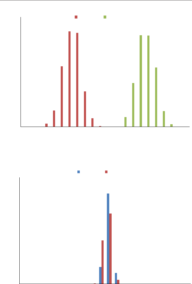
Momentum Investing Is Not Growth Investing 51

350 Growth Momentum

300

250

200

Frequency (n=1000)

Compound Annual Growth Rate

150

100

4.00%

5.00%

6.00%

7.00%

8.00%

9.00%

10.00%

11.00%

12.00%

13.00%

14.00%

15.00%

16.00%

17.00%

18.00%

19.00%

20.00%

21.00%

22.00%

23.00%

24.00%

FIGURE 3.1 CAGR: Growth Monkeys versus Momentum Monkeys

900

800

700

600

500

400

Frequency (n =1000)

Standard Deviation

300

200

100

15.00%

16.00%

17.00%

18.00%

19.00%

20.00%

21.00%

22.00%

23.00%

24.00%

25.00%

26.00%

27.00%

28.00%

29.00%

30.00%

31.00%

32.00%

33.00%

34.00%

35.00%

Growth Momentum

FIGURE 3.2 Volatility: Growth Monkeys versus Momentum Monkeys

❦

❦ ❦

❦

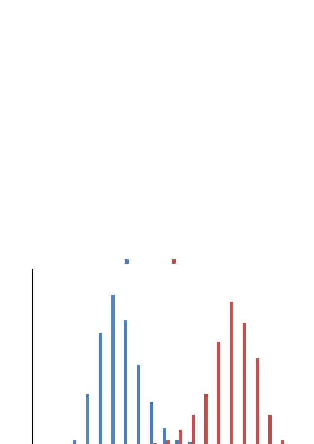
52 QUANTITATIVE MOMENTUM

But perhaps volatility doesn’t capture the true risk of the momentum

strategy relative to the growth portfolios? We examine the worst draw-

downs, or the worst peak-to-trough performance during the 50-year time

period, as an extreme tail event. Figure 3.3 tabulates the extreme loss sce-

narios across the thousand simulations for both the growth and momentum

strategies.

Note that higher drawdowns are reected on the left side of Figure 3.3,

while lower drawdowns are reected on the right. Because the light gray

bars are clustered on the left, the tail risk for growth, on average, is actu-

ally higher than for momentum, which is clustered on the right. There is

some overlap—some simulation runs where momentum has larger draw-

downs than growth—but these instances are few and far between. The over-

whelming number of observations shows higher drawdowns for the growth

monkeys than for the momentum monkeys.

To summarize, growth investing, as measured by high price to funda-

mentals, is not the same as momentum investing, as measured by strong past

relative performance. This conclusion is clearly seen in the historical char-

acteristics associated with each of these strategies, which shows that growth

and momentum are different animals.

300

250

200

150

Frequency (n=1000)

Maximum Drawdown

100

–97.00%

–94.50%

–92.00%

–89.50%

–87.00%

–84.00%

–82.00%

–79.00%

–77.00%

–74.00%

–72.00%

–69.00%

–67.00%

–64.00%

–62.00%

–59.00%

–57.00%

–54.00%

–52.00%

–49.50%

–47.00%

Growth Momentum

FIGURE 3.3 Drawdown: Growth Monkeys versus Momentum Monkeys

❦

❦ ❦

❦

Momentum Investing Is Not Growth Investing 53

BUT WHY DOES MOMENTUM WORK?

“We discovered the world wasn’t at before we understood and

agreed why.”

—Cliff Asness et al.14

Cliff Asness’s quote highlights that sometimes you can understand that

something is true before you fully understand why it is true, and agree with

others why it is true. So it goes with momentum investing, where the data

are clear that it works, but we lack clarity on exactly “why.” We attempt

to address this conundrum, but knowingly embrace the humility that our

thoughts can only hope to be directionally correct, at best. Value investing,

in contrast to momentum investing, is intuitive. The value approach is

intuitive because it is assumed that market prices drift around a so-called

intrinsic value, which is informed by fundamentals. Classic value investors

claim to earn their paycheck by timing the difference between fundamentals

and market prices. But what if the market decides to never update their

expectation about the intrinsic value of a rm (also known as a value trap)?

Assuming free cash ow distributions are distributed in the distant future,

avalueinvestorwon’twininthissituation.Thevalueinvestor,likeall

investors, needs market expectations to change in their favor for the strategy

to work. Value investing doesn’t work simply because the investor buys

cheap. Value investing works because cheap price-to-fundamental ratios, the

proxy for a systematic market expectation error, mean revert in favor of the

value investor, on average. The core argument behind momentum investing

works along the exact same lines. Momentum investing works because

the relative strength indicator is a proxy for a systematic expectation error

in the market that predictably reverts in the momentum investor’s favor,

on average.

To understand why momentum works, we leverage our sustainable

active framework to determine if a strategy will be successful over the

long term. The building blocks to identify sustainable performance were as

follows: (1) identify bad poker players, (2) understand the limitations of

the best poker players to exploit the bad poker players, and (3) exploit the

opportunity that presents itself. We showed that value, which has a strong

historical track record, has characteristics that suggest the past track record

could plausibly continue in the future.

Our analysis of the value anomaly through the lens of the sustainable

active investing framework raises a natural question: Is momentum, like

value, a sustainable investment approach? With our sustainable active

framework in hand, we can tackle this difcult question. But rst, we

should establish beyond any doubt that momentum—which isn’t the same

as growth investing—has worked, historically. To keep things simple and

❦

❦ ❦

❦

54 QUANTITATIVE MOMENTUM

in line with previous analysis, we consider “momentum investing” to be

roughly approximated by the practice of purchasing portfolios of rms

with strong relative performance over the past year. Using the momentum

portfolio data from Ken French’s website,15 we examine the returns from

January 1, 1927, to December 31, 2014, for a high momentum portfolio

(high momentum decile, value-weight returns), a value portfolio (high

B/M decile, value-weight returns), a growth portfolio (low B/M decile,

value-weight returns), and the S&P 500 total return index (SP500). Results

are shown in Table 3.1. All returns are total returns and include the

reinvestment of distributions (e.g., dividends). Results are gross of fees.

Momentum stocks have outperformed value stocks, growth stocks, and

the broader market by a large margin. The portfolio of momentum stocks

earns a compound annual growth rate of 16.85 percent per year, whereas,

the growth stock portfolio earns 8.70 percent per year—an 8 percent annual

spread in performance. This historical spread in returns is why momentum

has been deemed the premier anomaly by academic researchers. There are

obviously important considerations we avoid at this stage of our discussion,

such as transaction costs, but one fact is clear—momentum is the perfor-

mance king. Next question, is this performance sustainable?

Are Bad Players Creating the Momentum Anomaly?

With value, the core behavioral bias described was representative bias, which

drove a price overreaction to poor fundamentals that mean-revert over time.

This description is, of course, an oversimplication of the psychological

factors at work, but the collective academic evidence generally seems to

support the core thesis that the excess returns earned by value stocks are

not solely driven by additional risk—mispricing plays some role in describ-

ing the excess returns. With momentum, the collective evidence points in

TABLE 3.1 Momentum Performance (1927–2014)

Momentum Value Growth SP500

CAGR 16.85% 12.41% 8.70% 9.95%

Standard Deviation 22.61% 31.92% 19.95% 19.09%

Downside Deviation 16.71% 21.34% 14.41% 14.22%

Sharpe Ratio 0.66 0.41 0.35 0.41

Sortino Ratio (MAR =5%) 0.79 0.54 0.37 0.45

Worst Drawdown –76.95% –91.67% –85.01% –84.59%

Worst Month Return –28.52% –43.98% –30.65% –28.73%

Best Month Return 28.88% 98.65% 42.16% 41.65%

Protable Months 63.16% 60.51% 59.09% 61.74%

❦

❦ ❦

❦

Momentum Investing Is Not Growth Investing 55

the same direction as value—risk certainly plays some role in explaining the

excess returns, but mispricing plays a role as well. The behavioral premise

for momentum is that investors seem to underreact to positive news reected

in the strong relative performance. On the face of it, the behavior driving

value and momentum appear to contradict one another: Value is driven by

an overreaction problem, while momentum is driven by an underreaction

problem. What gives?

Avalidcritiqueofbehavioralnance researchers is that they want to

have their cake and eat it, too. In one instance we can lean on underre-

action bias and in the next instance we can lean on the overreaction bias.

The behavioral formula is too easy: (1) Grab a psychology textbook, and

(2) identify behavioral biases that tthedata.EugeneFamaissuedachal-

lenge to so-called behavioral nance researchers in his 1998 paper “Market

Efciency, Long-Term Returns, and Behavioral Finance:”16

Following the standard scienticrule,marketefciency can only be

replaced by a better model ...The alternative has a daunting task. It

must specify what it is about investor psychology that causes simul-

taneous underreaction to some types of events and overreaction to

others ...

Three sets of authors in three different papers17 – 19 immediately took

on the challenge. Daniel et al. and Barberis et al. focus on models driven

by documented psychological biases to derive predictions that hypothesize

excess returns for both value and momentum strategies. Hong and Stein also

tackle the problem, but from a slightly different angle. Whereas Daniel et al.

and Barberis et al. focus on investor psychology issues for individual market

participants, Hong and Stein focus on the interaction of different market par-

ticipants, which are assumed to either be fundamental or technical investors,

but few investors are both fundamental and technical. We recommend that

interested readers explore all of these papers since all three theories probably

play some role in explaining momentum, but we pay particular attention to

the Barberis et al. paper because it is arguably the approach with the most

empirical support.20

Barberis et al. conclude that value and momentum are driven by biases

that mirror one another. Value, as discussed previously, is driven by an over-

reaction problem, in which humans are too quick to draw conclusions from a

small amount of recent data. In contrast, momentum is driven by an under-

reaction issue, which is the opposite of overreaction. With underreaction,

humans are slow to update their views based on new evidence, which could

be due to a systematic behavior bias and/or due to the fact human beings

simply have limited cognitive power (i.e., “limited attention” as it is called

❦

❦ ❦

❦

56 QUANTITATIVE MOMENTUM

in academic literature). But what drives overreaction in one circumstance

and underreaction in another?

The challenge with any behavioral theory is in understanding what

triggers overreaction and what triggers underreaction; in other words, why

do market participants engage in behavioral “regime-shifting,” and can we

understand how and why they do this? Barberis et al. rely on Grifnand

Tversky’s work,21 which leads them to assume that good earnings news,

presented outside of, or in isolation from, a long sequence of good earnings

news, leads to an underreaction (i.e., conservatism) and that good earn-

ings news, presented inside of, or as part of, a long sequences of good

earnings news, lead to an overreaction (i.e., representativeness). Experimen-

tal evidence strongly supports the Barberis et al. theories. In 2002, Robert

Bloomeld and Jeffrey Hales conducted controlled trading experiments with

Cornell MBA students and found that business students engage in behavioral

regime-shifting, depending on how they perceive new information.22

Let’s put this issue in concrete, practical terms. Take a company with

alongstringofpositiveearningsannouncements.Whathappenswhen

investors see another strong positive earnings announcement? Investors

will predict the trend will continue, since this conclusion is representative

of the ongoing earnings trend observed. But investors overreact. They

become overly optimistic and bullish, and because they expect this strong

earnings growth to continue to occur in the future, they bid up the stock

to excessively high levels that become disconnected from fundamentals. At

this point, if there is a negative earnings event, investors are stunned since

this event is inconsistent with their optimism, and they sell, causing prices

to decline. This behavior is growth investing.

Now take a company with a more uneven recent earnings history. What

happens in this scenario when investors see a positive earnings surprise?

They are skeptical, conservative, and slow to update their beliefs. They are

hesitant to be bullish. After all, what if this is just a proverbial blip on the

radar, and future earnings will not be similarly strong? In this case, investors

can be said to underreact to strong earnings and underweight the informa-

tion content of the recent earnings. They are overly pessimistic and will not

bid the stock price higher, even though the news may still suggest it is under-

valued. Only over time do prices increase to fully reect the new fundamental

information. This behavior is momentum investing.

The conclusion by Barberis et al. is that both value and momentum

effects are plausible under a wide variety of parameter values (i.e., either

underreaction or overreaction clearly seems to prevail depending on recent

trends of historical earnings over several periods).

❦

❦ ❦

❦

Momentum Investing Is Not Growth Investing 57

Frankly, there is no denitive conclusion on the behavioral biases that

drive both value and momentum, and maybe there never will be. There does,

however, seem to be a general consensus that both of these anomalies are

driven, in part, by mispricing due to behavioral bias. Value and momentum

signals are simply a proxy for behavioral biases that drive systematic investor

expectation errors. The empirical evidence strongly supports this hypothe-

sis and is codied in the title of a 2013 paper by Asness, Moskowitz, and

Pedersen, “Value and Momentum Everywhere.”23

In a way, maybe we shouldn’t be too concerned with the specicmech-

anism that causes the poor players to contribute to an anomaly like value

or momentum. Maybe it doesn’t matter that we all understand and agree

on why momentum or value work. As investors we just care that it works.

And since momentum seems to work well, and we have covered how poor

players contribute to its cause, now we must address a basic question: Why

hasn’t the smart money already arbitraged the anomaly away?

What Do the Best Players Think about Momentum?

Similar to value investing, momentum investing requires a level of discipline

that few investors possess. Momentum does not work all the time and can

fail spectacularly. This harsh reality prevents many large pools of capital

from dipping their toe too far into the momentum pool. Momentum is sim-

ply too dangerous.

To make the point that momentum can sometimes be hazardous to

your wealth, we examine the pain of momentum investing during the

2008 nancial crisis and the follow-on period. We examine the returns

from January 1, 2008, to December 31, 2009, for a momentum portfolio

(high momentum decile, value-weight returns), a growth portfolio (low

B/M decile, value-weight returns), a value portfolio (high B/M decile,

value-weight returns), and the S&P 500 total return index (SP500). Results

are shown in Table 3.2. All returns are total returns and include the

reinvestment of distributions (e.g., dividends). Results are gross of fees.

On a relative basis, momentum underperformed by a substantial

amount. When we look at risk-adjusted statistics the performance is even

worse. Clearly, following an active momentum strategy involves strong

elements of investment advisor career risk, akin to active value strategies.

But it gets worse ...

In Table 3.3 we examine returns over the nancial crisis period and

we include the follow-on period: January 1, 2008, to December 31, 2014.

Results are gross of fees. Simple passive index funds outperform momentum

over a seven-year period!24

❦

❦ ❦

❦

58 QUANTITATIVE MOMENTUM

TABLE 3.2 Momentum Investing Can Underperform (2008–2009)

Momentum Growth Value SP500

CAGR –17.65% –8.52% –6.69% –10.36%

Standard Deviation 26.03% 23.45% 45.60% 23.24%

Downside Deviation 20.67% 17.38% 23.06% 17.37%

Sharpe Ratio –0.64 –0.30 0.05 -0.39

Sortino Ratio (MAR =5%) –1.01 –0.64 –0.09 -0.76

Worst Drawdown –51.25% –46.72% –61.04% –47.75%

Worst Month Return –15.19% –16.13% –28.07% –16.70%

Best Month Return 11.09% 9.92% 36.64% 9.42%

Protable Months 50.00% 54.17% 62.50% 54.17%

TABLE 3.3 Momentum Investing Can Underperform (2008–2014)

Momentum Growth Value SP500

CAGR 6.55% 8.69% 8.45% 7.44%

Standard Deviation 22.24% 17.13% 29.73% 16.75%

Downside Deviation 17.03% 12.92% 20.78% 13.30%

Sharpe Ratio 0.39 0.56 0.41 0.50

Sortino Ratio (MAR =5%) 0.23 0.37 0.36 0.27

Worst Drawdown –51.25% –46.72% –61.04% –47.75%

Worst Month Return –15.91% –16.13% –28.07% –16.70%

Best Month Return 14.93% 11.21% 36.64% 10.93%

Protable Months 61.90% 61.90% 59.52% 63.10%

Ask yourself the same question we posed with the results from a

hypothetical value investor from 1994 to 1999:

If your asset manager underperformed a benchmark for seven years,

at times by double digits, would you re them?

The answer is a resounding “Yes!” for most investors, which translates

into a resounding, “No way, Jose!” for professional asset managers con-

cerned about their careers. But the market frictions associated with exploit-

ing a momentum strategy extend beyond career risk. Unlike value, which is

a strategy that works when traded relatively infrequently (e.g., annual rebal-

anced portfolios have excess risk-adjusted returns), momentum is a strategy

that requires a higher degree of trading frequency to be effective (e.g., quar-

terly rebalanced portfolios have excess risk-adjusted returns, but annually

rebalanced portfolios do not). This trading frequency increases transaction

❦

❦ ❦

❦

Momentum Investing Is Not Growth Investing 59

costs, which can be prohibitive and limit the protability of the strategy, net

of trading costs. While a plausible limit of arbitrage, Frazzini et al. address

this question directly using data from over a trillion dollars in live trans-

actions from AQR Capital Management and nd that transaction costs for

efcient institutional investors cannot “explain away” their unwillingness to

pursue momentum strategies.25

Momentum Is Similar to Value, Not Growth

Momentum investing turns out to be more similar to value than to growth

from a performance perspective and from the viewpoint of our sustain-

able active investing framework. On the performance front, both value and

momentum have strong historical risk-adjusted returns and have been exten-

sively tested by academic researchers across different markets, asset classes,

and time periods. To explain this anomalous performance, the academic con-

sensus suggests that value and momentum premiums are driven by some

combination of hidden systematic risk-factors (a justied reason for higher

expected returns) and elements of mispricing (an unwarranted reason for

higher expected returns). On the mispricing front, value and momentum

metrics serve as signals to identify stocks suffering from market expecta-

tions that eventually move in favor of the value or momentum investor. This

mispricing aspect is paired with the harsh reality that there is a limited abil-

ity for large pools of smart money to arbitrage away value or momentum.

Many of these capital pools are conicted by the high volatility and extreme

career risk associated with pursuing active value and momentum strategies.

Presumably, value and momentum premiums will continue to have staying

power, under the assumptions that (1) value and momentum are fundamen-

tally riskier strategies, (2) investors continue to suffer from behavioral bias,

and (3) large-scale arbitrage is costly and difcult.26

SUMMARY

In this chapter, we explored the history of momentum research from its early

days as a respectable approach, through the dark ages following the golden

age of the EMH, and the more recent resurgence in academic interest. We

then explore the common misperception that growth investing, as dened

as buying stocks with high prices to fundamentals, is the same as momen-

tum investing, which is buying stocks with strong relative returns. Nothing

could be further from the truth. Buying expensive stocks is not the same as

buying stocks with strong relative performance: one strategy performs, the

other does not. Next, we investigated momentum through the lens of sus-

tainable active investing. Momentum strategy excess expected returns are

❦

❦ ❦

❦

60 QUANTITATIVE MOMENTUM

plausibly driven by investor behavioral errors, combined with limits of arbi-

trage, and thus reasonably support an argument for long-term sustainable

performance. Assuming we have convinced you that momentum, like value,

is arguably a sustainable anomaly, we now explore why these two particular

anomalies are really interesting when used together. In the next chapter, we

will explore why all portfolios should consider combining value and momen-

tum systems.

NOTES

1. Robert Bloch, The Warren Buffett Bible (New York: Skyhorse Publishing, 2015).

2. Robert Levy, “Relative Strength as a Criterion for Investment Selection,” The

Journal of Finance 22 (1967): 595–610.

3. Burton G. Malkiel, A Random Walk Down Wall Street (New York: Norton,

1973).

4. Jensen and Bennington take Levy’s work to task in “Random Walks and Tech-

nical Theories: Some Additional Evidence,” The Journal of Finance 25 (1970):

469–482.

5. Mark Carhart, “On Persistence in Mutual Fund Performance,” The Journal of

Finance 52 (1997): 57–82.

6. Eugene F. Fama and Kenneth R. French, “Dissecting Anomalies,” Journal of

Financial Economics 63 (2008): 1653–1678.

7. Ibid.

8. Justin Birru, “Confusion of Confusions: A Test of the Disposition Effect and

Momentum,” The Review of Financial Studies 28 (2015): 1849–1873.

9. Thomas George and Chuan-Yang Hwang, “The 52-Week High and Momentum

Investing,” The Journal of Finance 59 (2004): 2145–2176.

10. See James Davis, “The Cross-Section of Realized Stock Returns: The

Pre-COMPUSTAT Evidence,” The Journal of Finance 49 (1994), 1579–1593,

and Eugene F. Fama and Kenneth R. French, “Size and Book-to-Market Factors

in Earnings and Returns,” The Journal of Finance 50 (1995): 131–155.

11. See Kent Daniel and Sheridan Titman, “Evidence on the Characteristics of Cross

Sectional Variation in Stock Returns,” The Journal of Finance 52 (1997), 1–33,

Joseph Piotroski and Eric So, “Identifying Expectation Errors in Value/Glamour

Strategies: A Fundamental Analysis Approach,” The Review of Financial Studies

25 (2012), 2841–2875, and Jack Vogel, “Essays on Empirical Asset Pricing,”

dissertation Drexel University, 2014.

12. Beaver, William, Maureen McNichols, and Richard Price, “Delisting Returns

and Their Effect on Accounting-based Market Anomalies,” Journal of Account-

ing and Economics 43 (2007): 341–368.

13. Fama and French.

14. Cliff Asness, Andrea Frazzini, Ron Israel, and Toby Moskowitz, “Fact, Fiction,

and Momentum Investing,” The Journal of Portfolio Management 40 (2014):

75–92.

❦

❦ ❦

❦

Momentum Investing Is Not Growth Investing 61

15. mba.tuck.dartmouth.edu/pages/faculty/ken.french/data_library.html, accessed

12/30/2015.

16. Eugene F. Fama, “Market Efciency, Long-Term Returns, and Behavioral

Finance,” Journal of Financial Economics 49 (1998): 283–306.

17. Nicholas Barberis, Andrei Shleifer, and Robert Vishny, “A Model of Investor

Sentiment,” Journal of Financial Economics 49 (1998): 307–343.

18. Harrison Hong and Jeremy Stein, “A Unied Theory of Underreaction, Momen-

tum Trading, and Overreaction in Asset Markets,” The Journal of Finance 54

(1999): 2143–2184.

19. Kent Daniel, David Hirshleifer, and Avanidhar Subrahmanyam, “A The-

ory of Overcondence, Self-Attribution, and Security Market Under- and

Over-Reactions,” The Journal of Finance 53 (1998): 1839–1885.

20. Although, there is research that goes against the Barberis et al. theory. For

example, Alexander Hillert, Heiko Jacobs, and Sebastian Muller, “Media

Makes Momentum,” The Review of Financial Studies 27 (2014): 3467–3501.

The reality is that all of these theories probably play some role in explaining

the insurmountable evidence related to momentum, and momentum is clearly

created by some sort of behavioral bias, even if it doesn’t take the form of the

version outlined in Barberis et al.

21. Dale Grifn and Amos Tversky, “The Weighing of Evidence and the Determi-

nants of Condence,” Cognitive Psychology 24 (1992): 411–435.

22. Robert Bloomeld and Jeffrey Hales, “Predicting the Next Step of a Random

Walk: Experimental Evidence of Regime-Shifting Beliefs,” Journal of Financial

Economics 65 (2002): 397–414.

23. Cliff Asness, Toby Moskowitz, and Lasse Pedersen, “Value and Momentum

Everywhere,” The Journal of Finance 68 (2013): 929–985.

24. To make matters even more interesting, over the 2008 to 2014 period, growth

investing, ironically, was the best performer.

25. Andrea Frazzini, Ronen Israel, and Toby Moskowitz, “Trading Costs of Asset

Pricing Anomalies,” AQR working paper, 2014.

26. Assuming that some element of both the value and momentum premiums is due

to risk, we could see swings in these premiums in the future if risk preferences

change.

❦

❦ ❦

❦

CHAPTER 4

Why All Value Investors

Need Momentum

“[Momentum] happens around the world, except Japan.”

—Eugene Fama, 2008 American Finance Association

Interview1

“We nd that momentum in Japan is actually a success.”

—Cliff Asness, 2011 Journal of Portfolio Management2

Despite its simplicity, as a stand-alone investment strategy generic

momentum works well, but some might say it does not work everywhere.

One example of a “failure” of momentum is in Japanese equities ...more

on this in a moment. But the broad consensus from academic researchers,

who are arguably biased in favor of ndings that support the efcient

market hypothesis (EMH), is that the evidence supports the notion that

momentum-based stock picking strategies have beaten the market, even

after controlling for risk. In short, there is something special about momen-

tum. Even Eugene Fama, famous for his incredible empirical work on

efcient markets, suggested that momentum is the biggest embarrassment

to the efcient market theory, or in his own words, momentum is the

“premier anomaly.”3

MOMENTUM IS A MYTH

Nonetheless, the myth that momentum is “not real” continues to be widely

disseminated. For example, in a classic 2008 interview at the American

Finance Association, Richard Roll, a premier nancial economist in his own

right, interviewed Eugene Fama, the king of nancial economists. Roll and

❦

❦ ❦

❦

Why All Value Investors Need Momentum 63

Fama had a spirited discussion on the so-called value premium, which ended

in a stalemate over whether the extra return associated with cheap stocks

was compensation for extra risk or mispricing. Professor Roll then asked

the “gotcha” question, about the momentum premium. Fama responded,

begrudgingly, that momentum effects are pervasive in world stock markets,

but he was quick to point out that Japanese stocks seemed to be immune to

momentum effects. Roll responded in kind, and quipped that perhaps the

Japanese investors were “more rational.” Fama, tongue in cheek, chuckled,

and stated that he hoped that the poor results of momentum-based stock

selection in Japan were the rule when it came to momentum results, and he

hoped that the exceptions to the rule were simply a result of data dredging.4

ASNESS SEPARATES FACT FROM FICTION

But not everyone was happy with the high-level chatter among Roll and

Fama. Cliff Asness, the founder of AQR, a University of Chicago nance

PhD, and a former Fama student, was not interested in toeing the EMH party

line. Perhaps Asness watched the interview between Fama and Roll, because

a few years later in 2011, he published a paper in The Journal of Portfo-

lio Management deantly titled, “Momentum in Japan: The Exception that

Proves the Rule.”

Asness’s paper highlights a simple but sophisticated point related to

momentum. On the one hand, if one looks at a generic Japanese momen-

tum strategy in isolation, momentum appears ineffective. Asness, however,

aptly points out that strategies need to be assessed in the context of a port-

folio, so one can ascertain not only their stand-alone investment value, but

also understand their potential diversication benets for a portfolio. For

example, if one assessed a strategy of continuously purchasing three-month

put options on the stock market, the conclusion would be that the strat-

egy has negative returns and a ton of volatility. These results, however, do

not imply that put options are inefciently priced, but this conclusion only

becomes clear when we assess how put options act in the context of a portfo-

lio. Viewed through a portfolio lens, put options provide incredible diversi-

cation benets (i.e., insurance), and it becomes obvious why investors will

gladly accept negative expected returns for a put buying strategy.

In contrast to puts, momentum-based stock selection strategies won’t

provide extreme insurance-like diversication benets, but momentum

strategies can pack a punch as it relates to overall diversication. For

example, long-only momentum strategies are not perfectly correlated to

the broad equity market, and they have low correlations with classic value

strategies. These features make momentum strategies highly desirable in a

portfolio context when they are pooled with value strategies.

❦

❦ ❦

❦

64 QUANTITATIVE MOMENTUM

Moving along this line of reasoning, Asness shows that Japanese

investors, concerned about maximizing their portfolio’s expected

risk-adjusted return, would always invest a substantial amount of

their portfolio in a momentum strategy. This demonstrates a great insight,

and the paper makes the point clear. But the entire premise of the Asness

paper is that we need to try hard to highlight how valuable momentum

can be in Japan. A deeper investigation of the Asness results shows that

his analysis focuses on Japanese long/short portfolios, which are not the

typical sort of portfolio that many long-term investors would deploy.

These long/short portfolios suffer because the short side of the momentum

portfolio eats at the performance of the long-only momentum portfolio.

Asness doesn’t focus on long-only results, but we replicate and extend

his analysis using more traditional long-only portfolios in Table 4.1. We

show the results for the long-only Japanese momentum portfolio using

AQR’s data for this analysis.5The Japanese index is represented by the

MSCI Japan Total Return Index. The returns are from January 1, 1982,

through December 31, 2014. All returns are total returns and include the

reinvestment of distributions (e.g., dividends). Results are gross of fees.

A long-only momentum portfolio clearly works, outperforming the

index by a wide margin. This result is not entirely surprising, since momen-

tum works in just about every context where researchers can get access

to a reasonably long dataset. We understand why Asness focused on the

long/short momentum portfolio for his research purposes, but this focus con-

fuses investment audiences and muddies the issues. The reality is that generic

long-only momentum does work in Japan. And yes, Asness brings up a great

point that even in his context, investors should love long/short momentum

exposures, especially when pooled with long/short value exposures.

We explore Asness’s idea of combining value and momentum exposures

in more depth throughout the rest of this chapter (with an emphasis on

TABLE 4.1 Japanese Equity Market Performance (1982–2014)

Japan Momentum Japan Index

CAGR 5.82% 3.81%

Standard Deviation 23.10% 19.37%

Downside Deviation 13.57% 12.84%

Sharpe Ratio 0.18 0.08

Sortino Ratio (MAR =5%) 0.24 0.05

Worst Drawdown –65.95% –68.83%

Worst Month Return –21.88% –21.06%

Best Month Return 22.99% 19.97%

Protable Months 55.05% 53.54%

❦

❦ ❦

❦

Why All Value Investors Need Momentum 65

long-only results, not long/short). After being barraged with the facts, we

think reasoned investors will agree: Investors benet from momentum, and

value investors, the investors least likely to accept momentum, stand to really

benetfrommomentum.AndasthetitleofAsness’sjournalarticlehigh-

lights, a deeper analysis of momentum in Japan doesn’t put a damper on

momentum, it merely highlights its effectiveness.

EXPANDING YOUR HORIZONS WITH MOMENTUM

Modern portfolio theory, which outlines how an investor can mathemati-

cally compile a portfolio that will maximize expected returns for a given

level of risk, and the most famous spinoff from the theory, the Capital Asset

Pricing Model (i.e., CAPM), is best described by Fischer Black in the fol-

lowing way: “The [theory] is right. It just doesn’t work.”6The feel-good

construct, which we teach to our nance students each year, is a great learn-

ing tool. Simply input a vector of expected returns and a covariance matrix

associated with a set of assets or securities into your computer, and voilà, you

have the so-called optimal portfolio weights that maximize one’s expected

return for a given level of risk. Like all things viewed with the benetof

hindsight, the lessons from modern portfolio theory seem simple. However,

the underlying analysis behind the theory earned Harry Markowitz a Nobel

Prize for his original paper on optimal portfolio selection.

Even though some academics and practitioners—including us—often

rant about why one should be skeptical of complex portfolio optimization

theories, the core ideas that underlie modern portfolio theory are critical for

building successful investment programs. And that includes knowing when

to adopt—and when to discard—certain ideas. The punch line, or core

proposition, from modern portfolio theory is the so-called mean-variance

(MV) frontier, often called the efcient frontier. The MV frontier takes the

ingredients available—expected returns and the covariance matrixes across

assets—and maps out all the best expected combinations of risk and reward

an investor can achieve by shifting the weights among the assets under

investigation. Think of the MV frontier as the best recipes available for an

investor to maximize return and minimize risk, given the set of ingredients

available.

As an illustration of modern portfolio theory put into practice,

Figure 4.1 includes the historical returns and standard deviations associated

with four portfolios from 1927 to 2014 using Ken French data for the value

and momentum portfolios.7These portfolios are described below:

■SP500 =SP500 Total Return Index

■VALUE =Top decile value-weight portfolio formed on book-to-market

❦

❦ ❦

❦

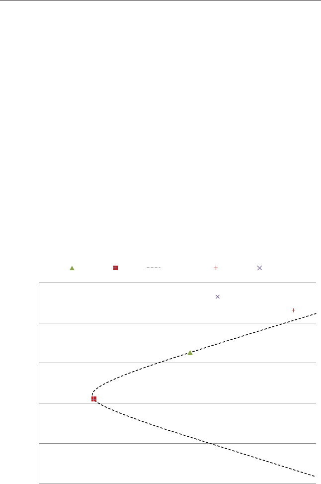
66 QUANTITATIVE MOMENTUM

■MOM =Top decile value-weight portfolio formed on 2-12 momentum

■LTR =Merrill Lynch 7–10 year Government Bond Index, spliced with

data from Ibbotson’s Stocks, Bonds, Bills, and Ination Yearbook.

We map out the efcient frontier using historical values for expected

returns and the covariance matrix. The results are gross of management

fee and transaction costs and all returns are total returns and include the

reinvestment of distributions (e.g., dividends). We impose short selling con-

straints such that no asset weights can be negative. For MV frontier pur-

poses, in Figure 4.1 we only allow the optimizer to invest in the S&P 500

Index and Treasury bonds.

Over the 1927 to 2014 period, domestic equities (SP500) have relatively

high expected returns and standard deviations, whereas domestic value equi-

ties (VALUE) and momentum equities (MOM) have high expected returns,

but extremely high volatility. Long-term bonds (LTR) have the lowest stan-

dard deviation, but have relatively lower expected returns.

Modern portfolio “works” in the sense that an investor can combine

generic stocks and bonds in a smart way and exploit the benets of diversi-

cation. We can visualize this nding via the mean variance (MV) frontier

20.0%

SP500 LTR MV Frontier VALUE MOM

15.0%

10.0%

5.0%

Expected Portfolio Return

Standard Deviation of the Portfolio

0.0%

5.0%

10.0%

15.0%

20.0%

25.0%

30.0%

35.0%

–5.0%

FIGURE 4.1 Modern Portfolio Theory Chart

❦

❦ ❦

❦

Why All Value Investors Need Momentum 67

(i.e., the dotted line), which highlights a “curve” in the line in the section

between the long-bond-only portfolio and the S&P 500-only. This curve rep-

resents the benetofdiversication, which allows a portfolio to achieve a

lower standard deviation for a given expected return.

In an ideal world, we could nd portfolios that would expand the MV

frontier and create opportunities with higher expected returns for a given

level of risk. Perhaps counter-intuitively, adding highly volatile assets such

as value and momentum, can expand the MV frontier, if the volatility asso-

ciated with the portfolio being added is unrelated to the other assets already

included in the portfolio.

We explore this concept further by allowing the mean variance opti-

mizer to allocate across not only the S&P 500 and bonds, but also our two

additional equity portfolios: value and momentum. Table 4.2 outlines the

stand-alone characteristics of the passive and the generic value and momen-

tum equity strategies from 1927 to 2014.

Do the returns associated with value and momentum provide enough

benettooffsettheirextremevolatility?Toanswerthisquestion,Figure4.2

shows how the MV frontier changes after adding momentum and adding

value.

The results are surprising. When we allow the optimizer to allocate to

value portfolios, we can expand the MV frontier. For a given level of risk,

as measured by standard deviation on the x-axis, a portfolio that includes

value offers a higher return. But if we also allocate to momentum, the fron-

tier is greatly expanded. Note, again, that for a given standard deviation, the

expected return is dramatically higher for portfolios that include both value

and momentum. Notably, in this case the optimizer recommends a zero per-

cent allocation to the passive index, highlighting that a portfolio with access

to bonds and long-only value and momentum equity exposures captures all

the benets of a portfolio—and then some—that only has access to a passive

TABLE 4.2 Asset Class Historical Results

SP 500 Value Mom LTR

CAGR 9.95% 12.41% 16.85% 5.45%

Standard Deviation 19.09% 31.92% 22.61% 6.92%

Downside Deviation 14.22% 21.34% 16.71% 4.43%

Sharpe Ratio 0.41 0.41 0.66 0.31

Sortino Ratio (MAR =5%) 0.45 0.54 0.79 0.12

Worst Drawdown –84.59% –91.67% –76.95% –20.97%

Worst Month Return –28.73% –43.98% –28.52% –8.41%

Best Month Return 41.65% 98.65% 28.88% 15.23%

Protable Months 61.74% 60.51% 63.16% 63.35%

❦

❦ ❦

❦

68 QUANTITATIVE MOMENTUM

20.0%

25.0%

30.0%

15.0%

10.0%

Expected Portfolio Return

Standard Deviation of the Portfolio

5.0%

0.0%

–5.0%

–10.0%

0.0%

5.0%

10.0%

15.0%

20.0%

25.0%

30.0%

35.0%

SP500 LTR MV Frontier VALUE MOM MV Frontier (Add VALUE) MV Frontier (Add VALUE + MOM)

FIGURE 4.2 Modern Portfolio Theory with Momentum

equity index portfolio (e.g., S&P 500). Momentum and value greatly expand

the investment opportunity set at every level of risk (as measured by standard

deviation). This evidence suggests that investors, regardless of their risk tol-

erance, can increase their expected risk and reward trade-offs by replacing

generic equity allocations with active momentum and value allocations.

MARRYING VALUE AND MOMENTUM

“... value and momentum are negatively correlated with each

other, both within and across asset classes.”

—Asness, Moskowitz, and Pedersen8

Cliff Asness, Toby Moskowitz, and Lasse Pedersen published a

remarkable paper in 2013 appropriately titled “Value and Momentum

Everywhere.” The research highlights an interesting, but not entirely

surprising, phenomenon— namely, that value and momentum premiums

are literally everywhere:

■US stocks

■UK stocks

❦

❦ ❦

❦

Why All Value Investors Need Momentum 69

■European stocks

■Japanese stocks

■Currencies

■Fixed income

■Commodities

We update the analysis from the original research paper using their

data and compile the results in Tables 4.3 and 4.4.9We examine long

only portfolio results for the four biggest equity markets—United States,

United Kingdom, Europe, and Japan—from 1982 through 2014. Data are

available for earlier periods on some markets, but for an apples-to-apples

comparison, we conduct the analysis over the period when data are

available for all markets.

First, the momentum results are tabulated in Table 4.3.

TABLE 4.3 Momentum Performance (1982–2014)

Momentum

Europe

Momentum

Japan

Momentum

CAGR 13.75% 13.69% 14.88% 5.82%

Standard Deviation 17.14% 19.84% 19.13% 23.10%

Downside Deviation 13.02% 14.11% 13.93% 13.57%

Sharpe Ratio 0.60 0.54 0.61 0.18

Sortino Ratio (MAR =5%) 0.73 0.70 0.77 0.24

Worst Drawdown –48.31% –60.71% –54.92% –65.95%

Worst Month Return –23.89% –27.16% –18.95% –21.88%

Best Month Return 17.65% 16.44% 18.56% 22.99%

Protable Months 65.66% 60.35% 64.90% 55.05%

TABLE 4.4 Value Performance (1982–2014)

US Value UK Value Europe Value Japan Value

CAGR 12.79% 12.59% 15.09% 11.11%

Standard Deviation 15.55% 20.02% 19.27% 21.67%

Downside Deviation 11.88% 12.87% 14.06% 11.91%

Sharpe Ratio 0.59 0.49 0.62 0.40

Sortino Ratio (MAR =5%) 0.70 0.69 0.78 0.66

Worst Drawdown –49.80% –54.65% –55.30% –41.35%

Worst Month Return –18.45% –21.02% –21.78% –15.34%

Best Month Return 15.40% 19.22% 18.04% 28.88%

Protable Months 66.16% 58.08% 64.65% 55.05%

❦

❦ ❦

❦

70 QUANTITATIVE MOMENTUM

Next, the value results are tabulated in Table 4.4.

For some context, over the same time period the US stock index (S&P

500 Total Return Index) earned a CAGR of 11.96 percent, the UK stock

index earned a CAGR of 9.60 percent, and the Japanese stock index returned

aCAGRof3.81percent.

When people observe something they cannot explain, they say, “It must

be something in the water;” clearly, these results also suggest there is some-

thing in the water, when it comes to value and momentum. Value shows up in

every equity market and momentum has strong performance in all markets.

We think this nding is partially explained by increased risk, but it is also

a manifestation of the sustainable active investing framework highlighted at

the beginning of this book. Some of the excess returns associated with value

and momentum are attributed to marketplace participants who are aficted

by behavioral bias, which creates mispricing opportunities. Those mispricing

opportunities continue to exist in the data because the investment opportu-

nities created by these strategies are hard to exploit via riskless arbitrage

trading activity.

But the evidence that value and momentum work across a wide variety

of assets and time periods is not entirely novel. What makes the Asness et al.

paper unique, and what we alluded to via our quick modern portfolio theory

lesson in the prior section, is that they explore the remarkable performance

of using value and momentum together, as a system.

In Table 4.5 we look at why value and momentum work well as a system.

The correlation matrix across global value and momentum equity portfolios

is low for long-only portfolios.

To highlight how the value and momentum system works, we look at

combination portfolios that invest 50 percent in value and 50 percent in

momentum, and rebalance the allocation monthly. The summary statistics

for the value and momentum portfolios for the period 1982 to 2014 are

tabulated in Table 4.6.

Risk-adjusted statistics are marginally improved across the board and

the global value and momentum (designated as Global V/M) delivers. But

summary statistics don’t capture the extent to which one could “stick with

TABLE 4.5 Correlation of Value and Momentum

Momentum

Europe

Momentum

Japan

Momentum

US Value 71% 56% 57% 26%

UK Value 53% 79% 63% 33%

Europe Value 55% 65% 84% 41%

Japan Value 29% 40% 41% 75%

❦

❦ ❦

❦

Why All Value Investors Need Momentum 71

TABLE 4.6 Value and Momentum Combination Portfolios

US UK Europe Japan Global V/M

CAGR 13.49% 13.37% 15.15% 8.76% 13.29%

Standard Deviation 15.14% 18.86% 18.43% 20.95% 15.08%

Downside Deviation 11.60% 12.93% 13.72% 11.88% 11.20%

Sharpe Ratio 0.64 0.54 0.64 0.31 0.63

Sortino Ratio (MAR =5%) 0.77 0.73 0.79 0.47 0.78

Worst Drawdown –48.95% –57.66% –55.04% –47.36% –49.72%

Worst Month Return –20.88% –24.09% –20.13% –18.44% –17.75%

Best Month Return 13.32% 16.74% 15.62% 25.24% 11.83%

Protable Months 64.90% 61.87% 64.14% 54.29% 63.64%

the program.” For example, value investing looks great over the long haul,

and there are some investors with the intestinal fortitude to hang on to a

deep value strategy through a ve-year stretch of underperformance, but

this fortitude is unrealistic for most investors. And the same goes for momen-

tum portfolios, which can sustain stomach-churning underperformance over

extended time periods. Thankfully, we can combine value and momentum

to reduce the torture associated with each of the strategies as a stand-alone

investment approach.

To assess the ability of combination value and momentum portfolios

to smooth the pain on the path to long-term expected performance, we

examine the spread between 5-year compound annual growth rates for a spe-

cicstrategyrelativetoitspassivebenchmark.Weexaminethecombination

portfolio, the momentum-only portfolio, and the value-only portfolio. The

results are in Figures 4.3 through 4.7.

First, let’s look at the United States (see Figure 4.3). These results are

over the 1982 to 2014 time period and use the value and momentum port-

folios identied in the Asness et al. paper. Value and momentum each have

multiple stretches where they underperform the benchmark over ve-year

cycles. The combination portfolio suffers periods when it underperforms

over a ve-year cycle, but grinds a long-term edge most of the time.

Next we look at the United Kingdom over the same period as the US

analysis (Figure 4.4). Value and momentum can underperform the bench-

mark over ve-year cycles. However, the combination portfolio minimizes

the pain along the way.

We look at Europe in Figure 4.5, which runs from 1999 to 2014, due to

data limitations on the passive index. Similar to prior analysis, value and

momentum combinations give the investor a smoother success rate over

ve-year cycles—especially in the most recent period analyzed.

❦

❦ ❦

❦

72 QUANTITATIVE MOMENTUM

15.00%

10.00%

5-Year Rolling CAGR Relative to the Index

Combo Spread Momentum Spread Value Spread

5.00%

0.00%

12/1/1986

1/1/1989

2/1/1991

3/1/1993

4/1/1995

5/1/1997

6/1/1999

7/1/2001

8/1/2003

9/1/2005

10/1/2007

11/1/2009

12/1/2011

1/1/2014

–5.00%

–10.00%

–15.00%

FIGURE 4.3 US Rolling Five-Year Spreads

15.00%

20.00%

25.00%

10.00%

5.00%

0.00%

–5.00%

–10.00%

5-Year Rolling CAGR Relative to the Index

Combo Spread Momentum Spread Value Spread

12/1/1986

1/1/1989

2/1/1991

3/1/1993

4/1/1995

5/1/1997

6/1/1999

7/1/2001

8/1/2003

9/1/2005

10/1/2007

11/1/2009

12/1/2011

1/1/2014

FIGURE 4.4 UK Rolling Five-Year Spreads

❦

❦ ❦

❦

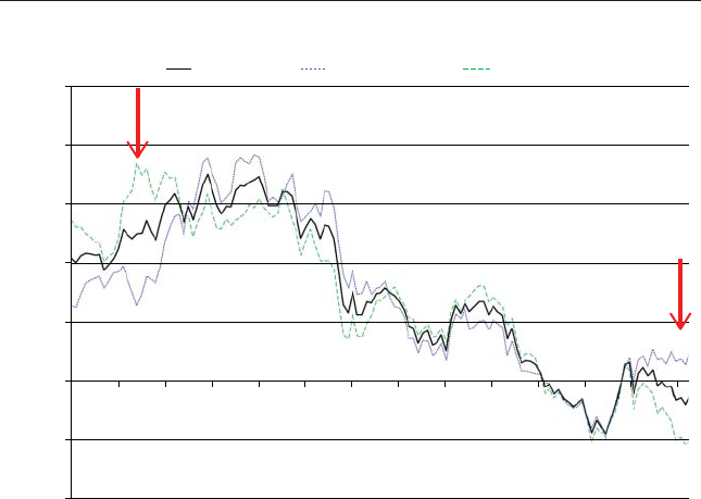
Why All Value Investors Need Momentum 73

15.00%

20.00%

25.00%

10.00%

5.00%

0.00%

–5.00%

–10.00%

5-Year Rolling CAGR Relative to the Index

Combo Spread Momentum Spread Value Spread

12/1/2003

10/1/2004

8/1/2005

6/1/2006

4/1/2007

2/1/2008

12/1/2008

10/1/2009

8/1/2010

6/1/2011

4/1/2012

2/1/2013

12/1/2013

10/1/2014

FIGURE 4.5 Europe Rolling Five-Year Spreads

We end with Japan (Figure 4.6), which runs from 1982 to 2014, where

value investing is king and momentum investing plays second ddle. Even

in Japan, the combination portfolio exploits the natural yin and yang rela-

tionship between value and momentum to create a robust long-term active

allocation.

Finally, we assess a global value and momentum portfolio and compare

this portfolio to a global value portfolio, a global momentum portfolio, and

aglobalindexportfolio(Figure4.7).Theanalysisrunsfrom1982to2014

and really highlights why value and momentum—working as a system—can

give active investors a reasonable way to consistently beat passive bench-

marks over longer horizons.11

The evidence suggests that a blended strategy, which combines both

value and momentum into a single portfolio, may prevent a value-only

investor or a momentum-only investor from suffering through extended,

long-term stretches of poor performance. Of course, not all pain can be

erased, and investors must always be aware that they will be required to

endure sustained stretches of volatility and underperformance, even with a

globally diversied value and momentum equity portfolio.

❦

❦ ❦

❦

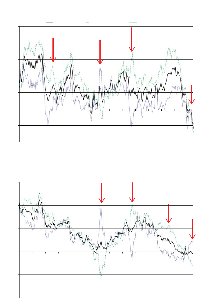
74 QUANTITATIVE MOMENTUM

15.00%

20.00%

25.00%

10.00%

5.00%

0.00%

–5.00%

–10.00%

5-Year Rolling CAGR Relative to the Index

Combo Spread Momentum Spread Value Spread

1/1/1989

12/1/1986

2/1/1991

3/1/1993

4/1/1995

5/1/1997

6/1/1999

7/1/2001

8/1/2003

9/1/2005

10/1/2007

11/1/2009

12/1/2011

1/1/2014

FIGURE 4.6 Japan Rolling Five-Year Spreads

15.00%

10.00%

5.00%

0.00%

–5.00%

–10.00%

12/1/1986

1/1/1989

2/1/1991

3/1/1993

4/1/1995

5/1/1997

6/1/1999

7/1/2001

8/1/2003

9/1/2005

10/1/2007

11/1/2009

12/1/2011

1/1/2014

5-Year Rolling CAGR Relative to the Index

Combo Spread Momentum Spread Value Spread

FIGURE 4.7 Global Rolling Five-Year Spreads

❦

❦ ❦

❦

Why All Value Investors Need Momentum 75

SUMMARY

In this chapter, we describe the benets of marrying the value religion and

the momentum religion. Each has its merits, but combining the two systems

into a unied portfolio really highlights the benets of value and momen-

tum. We showed that value and momentum tend to have a low correlation

across the globe and that creating a global value and momentum portfolio

seems to provide a potential solution for long-term active investors to beat

passive market-capitalization weighted indices over long periods of time.

All of the analysis to date has been done with generic value and generic

momentum exposures that are well established and understood in the aca-

demic literature. In the next section of the book, we’ll carefully investigate

how one might logically and empirically improve on the generic momentum

strategy.

NOTES

1. Eugene Fama Interview, American Finance Association, 2008. www.afajof.org

/details/video/2870921/Eugene-Fama-Interview.html, accessed 2/15/2016.

2. Cliff Asness, “Momentum in Japan: The Exception that Proves the Rule,” The

Journal of Portfolio Management 37 (2011): 67–75.

3. Eugene F. Fama and Kenneth R. French, “Dissecting Anomalies,” Journal of

Financial Economics 63 (2008): 1653–1678.

4. Simple improvements to a generic momentum strategy actually highlight that

momentum works in Japan. For example, see Denis Chaves, 2012, “Eureka!

A Momentum Strategy that also Works in Japan,” SSRN Working paper.

papers.ssrn.com/sol3/papers.cfm?abstract_id=1982100, accessed, 2/15/2016.

5. “Value and Momentum Everywhere: Portfolios, Monthly,” AQR (January

31, 2016), www.aqr.com/library/data-sets/value-and-momentum-everywhere

-portfolios-monthly, accessed 2/15/2016.

6. Fama interview.

7. Kenneth French, “Current Research Returns,” mba.tuck.dartmouth.edu/pages

/faculty/ken.french/data_library.html, accessed 2/15/2016. MOM is the top

decile value-weight portfolio formed on 2-12 momentum; VALUE is the

top decile value-weight portfolio formed on book-to-market.

8. Cliff Asness, Toby Moskowitz, and Lasse Pedersen, “Value and Momentum

Everywhere,” The Journal of Finance 68 (2013): 929–985.

9. “Value and Momentum Everywhere: Portfolios, Monthly.”

10. For the passive benchmark we examine MSCI Total Return Index data for the

respective market unless stated otherwise. Our European Index data begins in

1999, so we do not list its return from 1982 to 2014. Over the 1999–2014

❦

❦ ❦

❦

76 QUANTITATIVE MOMENTUM

time period, the European Value portfolio returned a CAGR of 9.17 percent,

the European Momentum portfolio returned a CAGR of 8.93 percent, and the

European Index returned a CAGR of 4.13 percent.

11. The global value portfolio is an equal-weight portfolio of the US, UK, European,

and Japanese value portfolios. The global momentum portfolio’s construction is

similar. The global value and momentum portfolio is an equal-weight portfolio

of the global value and the global momentum portfolio.

❦

❦ ❦

❦

PART

Two

Building a

Momentum-Based Stock

Selection Model

Part One explained why momentum is potentially a sustainable stock

selection method. The results discussed use a generic momentum strat-

egy that focuses on forming a portfolio of stocks that are the relatively

strongest based on their past 12 months of returns (skipping the last, or

most recent month). And while generic momentum works, as the label

implies, this form of momentum is rudimentary. In Part Two, we dig

further into the research on stock selection momentum and describe how

to build quantitative momentum, which is an effective and efcient way to

capture the momentum premium. Chapter 5, “The Basics of Building a

Momentum Strategy,” outlines the basics of generic momentum investing.

Chapter 6, “Maximizing Momentum: The Path Matters,” explains how

one can differentiate the generic momentum strategy by analyzing path

dependency. Chapter 7, “Momentum Investors Need to Know Their

Seasons,” discusses the seasonality component of momentum investing. In

Chapter 8, “Quantitative Momentum Beats the Market,” we synthesize the

previous ndings, detail the Quantitative Momentum strategy, and conduct

adetailedanalysisofthehistoricalresults.Finally,inChapter9,“Making

Momentum Work in Practice,” we examine how one can make momentum

investing work in practice.

❦

❦ ❦

❦

❦ ❦

❦

CHAPTER 5

The Basics of Building a

Momentum Strategy

“I contend that nancial markets are always wrong ...”

—George Soros, The Alchemy of Finance1

Part One of this book leaves us with a central message: Momentum should

be considered by all investors. And the great paradox is that faithful

value investors—those who are probably the least likely to actually imple-

ment a momentum approach—stand to gain the most by complementing

their value portfolio with a momentum strategy. Perhaps this is for the best,

and is a reason why value and momentum in combination—operating as

a system—will continue to provide expected long-term portfolio benets:

Each investment religion is too strict, and thus slow to embrace noncon-

forming ideas. But assuming we have moved past the religious debate

between value and momentum, or at least raised the curiosity level of

dyed-in-the-wool value investors, it is now time to get our hands dirty and

build a momentum approach that can be used in practice. We tackle this

subject by breaking this chapter into the following components:

■How to calculate generic momentum

■Describe how look-back windows affect momentum

■Describe how portfolio construction affects momentum

The remainder of this chapter is dedicated to outlining each of these

steps in greater detail.

❦

❦ ❦

❦

80 QUANTITATIVE MOMENTUM

HOW TO CALCULATE GENERIC MOMENTUM

How do we measure the “momentum” of a stock? The simple method is to

calculate the total return (including dividends) of a stock over some partic-

ular look-back period (e.g., the past 12 months).

Aquickexamplewilldemonstratetheconcept,usingthetotalreturnof

Apple’s stock in 2014. Here we calculate the cumulative return to Apple over

the past 12 months (the “look-back” period). To calculate the cumulative

return over the past 12 months, we take the net return streams from each

month and turn them into gross returns by adding 1. Thus, if Apple’s net

returns for January are –10.77 percent, Apple’s gross returns for January

are 0.8923 (–0.1077 +1).

Then, we multiply all the gross return series (i.e., months) and subtract

1tond the cumulative 12-month net return. For example, based on the

data from Apple in 2014, the cumulative returns in December (momentum

score; see Table 5.1) are calculated as follows:

(0.8923)(1.0575)(1.0200)(1.0994)(1.0787)(1.0277)(1.0287)(1.0775)

(0.9829)(1.0720)(1.1060)(0.9281)–1=40.62%

Clearly, Apple had a good year in 2014! For reference, the broad market

was up 13.46 percent in 2014. A similar exercise could be done over a differ-

ent look-back period, such as the past month, where the total return would

be –7.19 percent (i.e., the return over the past month). Other calculations

could be done over any look-back period we wanted to examine, such as

TABLE 5.1 Simple 12-Month Momentum Example for Apple

Stock Returns 1+Return Momentum

1/31/2014 –10.77% 0.8923

2/28/2014 5.75% 1.0575

3/31/2014 2.00% 1.0200

4/30/2014 9.94% 1.0994

5/30/2014 7.87% 1.0787

6/30/2014 2.77% 1.0277

7/31/2014 2.87% 1.0287

8/29/2014 7.75% 1.0775

9/30/2014 –1.71% 0.9829

10/31/2014 7.20% 1.0720

11/28/2014 10.60% 1.1060

12/31/2014 –7.19% 0.9281 40.62%

❦

❦ ❦

❦

The Basics of Building a Momentum Strategy 81

the past 3 months, 36 months, or even the past 5 years (60 months). This

calculation can be completed for any stock with a price return stream.

Now that we understand how to calculate generic momentum over a

particular time period, we can review some key results associated with dif-

ferent look-back windows.

THREE TYPES OF MOMENTUM

In this section, we examine how returns are inuenced by the look-back

period we use to calculate momentum. Academic researchers have already

thoroughly reviewed this topic and we summarize the main ndings associ-

ated with three key look-back windows:

1. Short-term momentum (e.g., 1-month look-back)

2. Long-term momentum (e.g., 5 years, or 60-month look-back)

3. Intermediate-term momentum (e.g., 12-month look-back)

We deliberately end the section with intermediate-term momentum, as

this is the momentum we plan to focus on for the rest of the book.

Short-Term Momentum

We dene short-term momentum as any momentum score that is measured

over a time period of (at most) one month. Two academic papers written in

1990 specically examine the topic of short-term momentum.

In the rst paper, Bruce Lehman investigates how stock returns using a

one-week look-back affect the next week’s returns over his sample period

from 1962 to 1986. His paper, titled “Fads, Martingales, and Market

Efciency,”2nds that portfolios of securities that had positive returns

(winners) in the prior week typically had negative returns in the next week

(–0.35% to –0.55% per week on average). Those stocks with negative

returns (losers) in the prior week typically had positive returns in the next

week (0.86% to 1.24% per week on average). This short-term reversal in

returns is difcult to reconcile with the efcient market hypothesis.

Asecondpaper,writtenbyNarasimhanJegadeesh,examinesthereturns

of stocks from month to month sample period between 1934 and 1987. His

paper, titled “Evidence of Predictable Behavior of Security Returns,”3nds a

similar reversal in returns: Last month’s winners are next month’s losers, and

vice versa. And the effect is large and signicant. The prior month’s winners

have an average future return (next month) return of –1.38 percent, while

the prior month’s losers have an average future return (next month) of 1.11

❦

❦ ❦

❦

82 QUANTITATIVE MOMENTUM

percent. This 2.49 percent spread in the two portfolios is difcult to reconcile

with the efcient market hypothesis.

Using data provided by Dartmouth Professor Ken French,4we examine

monthly returns from January 1, 1927, to December 31, 2014, for the

Short-Term Loser portfolio (low short-term return decile, value-weight

returns), the Short-Term Winner portfolio (high short-term return decile,

value-weight returns), the SP500 total return index, and the risk-free rate

of return (90-day T-bills). The short-term past performance is measured

over the previous month. Results are shown in Table 5.2. All returns are

total returns and include the reinvestment of distributions (e.g., dividends).

Results are gross of fees.

The data validates the theory: Short-term reversals are alive and well

across a long swath of history! Looking at the results in Table 5.2, we notice

the reversal in returns from month to month—the returns to the monthly

rebalanced portfolio of stocks with the worst returns from last month

(“Short-Term Loser”) generate a CAGR of 13.46 percent from 1927 to

2014, while the returns to the monthly rebalanced portfolio of stocks with

the best returns from last month (“Short-Term Winner”) earn a measly 3.21

percent. The returns to past-months’ winners are even less than the returns to

the risk-free rate of return. Figure 5.1 graphically depicts the outperformance

of the short-term loser portfolio relative to the short-term winner portfolio.

But the evidence doesn’t end there: In addition to these two earlier

papers, more recent research investigates more complex and nuanced

versions of the same idea.5The key takeaway is the same: Short-term

winners are losers in the near-term future, and short-term losers are winners

in the near-term future. Overall, when measuring momentum over a short

time horizon, one can expect to see a reversal in short-term future returns.

TABLE 5.2 Short-Term Momentum Portfolio Returns (1927–2014)

Short-Term

Loser

Short-Term

Winner SP500 Risk Free

CAGR 13.46% 3.21% 9.95% 3.46%

Standard Deviation 29.60% 24.18% 19.09% 0.88%

Downside Deviation 20.36% 16.83% 14.22% 0.48%

Sharpe Ratio 0.46 0.11 0.41 0.00

Sortino Ratio (MAR =5%) 0.59 0.06 0.45 –3.34

Worst Drawdown –81.48% –94.31% –84.59% –0.09%

Worst Month Return –32.66% –31.27% –28.73% –0.06%

Best Month Return 55.85% 63.65% 41.65% 1.35%

Protable Months 60.13% 56.06% 61.74% 98.01%

❦

❦ ❦

❦

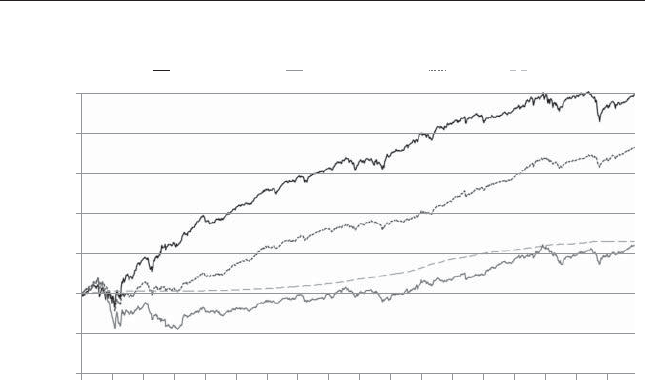
The Basics of Building a Momentum Strategy 83

$10

$100

$1,000

$10,000

Value of $ 100 Invested (Log Scale)

Short-Term Loser Short-Term Winner SP500 RF

$100,000

$1,000,000

$10,000,000

1/1/1927

12/1/1931

11/1/1936

10/1/1941

9/1/1946

8/1/1951

7/1/1956

6/1/1961

5/1/1966

4/1/1971

3/1/1976

2/1/1981

1/1/1986

12/1/1990

11/1/1995

10/1/2000

9/1/2005

8/1/2010

FIGURE 5.1 Short-Term Momentum Portfolio Returns

Long-Term Momentum

An alternative way to measure momentum is to use a look-back period

over a much longer time period and assess performance. Werner DeBondt

and Richard Thaler investigate this concept in their paper titled “Does the

Stock Market Overreact?”6The paper examines the future returns to past

long-term winners and long-term losers, where the winners and losers are

measured using look-back windows that range from three to ve years. Their

rst tests run from 1933 to 1980, and they track the performance of the past

winners and losers portfolios formed on a 36-month look-back. The results

show that “losers” outperform “winners” by 24.6 percent over the next

three years. This spread in performance is remarkable.

Asimilaranalysisisdonewhenmeasuringwinnersandlosersoverthe

past ve years. When examining the future returns, past losers outperform

past winners by 31.9 percent over the next ve years. Clearly, past losers

(when using a long-term momentum measure) outperform past winners.

Leveraging the same database that we used to examine short-term

reversals, we examined the returns from January 1, 1931, to December

31, 2014, for the Long-Term Loser portfolio (low long-term return decile,

value-weight returns), the Long-Term Winner portfolio (high long-term

return decile, value-weight returns), the SP500 total return index, and the

risk-free rate of return (90 day T-bills). The long-term past performance

is measured over the previous ve years (60 months), and the start date

❦

❦ ❦

❦

84 QUANTITATIVE MOMENTUM

TABLE 5.3 Long-Term Momentum Portfolio Returns (1931–2014)

Long-Term

Loser

Long-Term

Winner SP500 Risk Free

CAGR 14.30% 8.59% 10.13% 3.46%

Standard Deviation 30.37% 21.95% 18.92% 0.90%

Downside Deviation 17.98% 16.23% 13.91% 0.47%

Sharpe Ratio 0.47 0.33 0.43 0.00

Sortino Ratio (MAR =5%) 0.70 0.35 0.46 3.35

Worst Drawdown –71.24% –72.80% –74.48% –0.09%

Worst Month Return –40.77% –34.10% –28.73% –0.06%

Best Month Return 91.98% 30.74% 41.65% 1.35%

Protable Months 58.04% 58.83% 61.71% 97.92%

changes from 1927 to 1931 due to the necessary data requirement of

ve years of individual stock returns. Results are shown in Table 5.3. All

returns are total returns and include the reinvestment of distributions (e.g.,

dividends). Results are gross of fees.

Looking at the results in Table 5.3, we notice the reversal in long-term

returns—the returns to the monthly rebalanced portfolio of stocks with

the worst returns over the last ve years earns a CAGR of 14.30 percent

from 1931 to 2014, while the returns to the monthly rebalanced portfolio

of stocks with the best returns over the past ve years earns a CAGR of 8.59

percent. Figure 5.2 graphically depicts the outperformance of the long-term

loser portfolio relative to the long-term winner portfolio.

The literature and our updated results highlight that long-term momen-

tum, similar to short-term momentum, leads to return reversals in the

future. Why long-term reversal occurs is puzzling, and academic researchers

argue whether the cause is due to behavioral bias, additional risk, or market

frictions (e.g., capital gain taxes).7Next, we examine intermediate-term

momentum, which is the form of momentum that trends in the future and

isn’t reversed.

Intermediate-Term Momentum

In order to examine intermediate-term momentum, we form portfo-

lios based on a 6- to 12-month look-back. The results are different

from both short-term (e.g., a 1-month look-back) and long-term (e.g.,

60-month look-back) momentum, which exhibit return reversals. With

intermediate-term momentum, winners keep winning and losers keep

losing. The most well-known paper on this subject is the 1993 Narasimhan

Jegadeesh and Sheridan Titman paper “Returns to Buying Winners and

❦

❦ ❦

❦

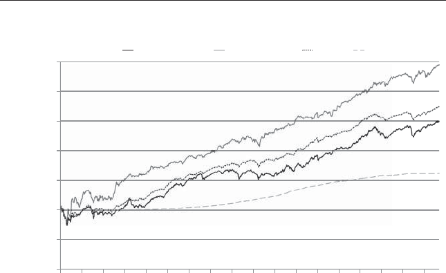
The Basics of Building a Momentum Strategy 85

$10

$100

$1,000

$10,000

Value of $100 Invested (Log Scale)

$100,000

$1,000,000

$10,000,000

12/1/1930

9/1/1935

6/1/1940

3/1/1945

12/1/1949

9/1/1954

6/1/1959

3/1/1964

12/1/1968

9/1/1973

6/1/1978

3/1/1983

12/1/1987

9/1/1992

6/1/1997

3/1/2002

12/1/2006

9/1/2011

Long-Term Winner Long-Term Loser SP500 RF

FIGURE 5.2 Long-Term Momentum Portfolio Returns

Selling Losers: Implications for Stock Market Efciency.”8In other words,

if a stock has done relatively well in the past, it will continue to do well in

the future.

The authors demonstrate that a momentum strategy (buying past “win-

ners” and selling past “losers”) performs well for an intermediate-term hori-

zon (3 to 12 months). They test this effect by constructing J-month/K-month

strategies: select stocks based on past Jmonths’ total returns and hold the

position for Kmonths (J=3,6,9,12;K=3,6,9,12).

Their main nding is that there is a continuation in returns when using

intermediate-term momentum. The best strategy (in their paper) is selecting

stocks based on past 12 months’ performance and holding the position

for 3 months. The average monthly spread in returns between the past

winners and past losers over the next 3 months is 1.31 percent, or almost

16 percent per year. However, they nd that the excess returns associated

with intermediate-term momentum portfolios are not long-lasting. For

example, the momentum premium dissipates for portfolios that hold

the same stocks for longer than 12 months after the initial formation

date. These results suggest that momentum portfolios calculated based

on intermediate-term look-backs and held as a long-term buy-and-hold

portfolio suffer a long-term reversal, which is similar to the results we

discussed earlier. Jegadeesh and Titman argue that the intermediate-term

momentum effect may occur if the market underreacts to information

❦

❦ ❦

❦

86 QUANTITATIVE MOMENTUM

about the short-term prospects (such as earning announcement) of rms,

but eventually overreacts to information about the long-term prospects.

With the data that we used to examine both short-term and long-term

reversals, we examine the returns from January 1, 1927, to December 31,

2014, for the Intermediate-Term Winner portfolio (high intermediate-term

return decile, value-weight returns), the Intermediate-Term Loser portfolio

(low intermediate-term return decile, value-weight returns), the SP500

total return index, and the risk-free rate of return (90-day T-bills). The

intermediate-term past performance is measured over the previous year,

ignoring last month’s return. So if we are forming a portfolio to trade on the

close of December 31, 2015, we would compute the total return from

the close of December 31, 2014, until the close of November 30, 2015, thus

ignoring December 2015 returns (due to short-term momentum reversal).

Results are shown in Table 5.4. All returns are total returns and include the

reinvestment of distributions (e.g., dividends). Results are gross of fees.

The tabulated results in Table 5.4 suggest strong evidence for a continu-

ation in intermediate-term returns—the returns to the monthly-rebalanced

portfolio of stocks with the best returns over the last year (ignoring last

month) returns a CAGR of 16.86 percent from 1927 to 2014. In contrast, the

returns to the monthly rebalanced portfolio of stocks with the worst returns

over the last year (ignoring last month) returns a CAGR of –1.48 percent.

The returns to past years’ losers (ignoring last month) are not only less than

the returns to the risk-free rate of return, they are negative! Figure 5.3 graph-

ically depicts the outperformance of the intermediate-term loser portfolio

relative to the intermediate-term winner portfolio.

Our results highlight that portfolios formed on intermediate-term

momentum exhibit a continuation of returns. Firms that have done well in

TABLE 5.4 Intermediate-Term Momentum Portfolio Returns (1927–2014)

Intermediate-Term

Winner

Intermediate-Term

Loser SP500 Risk Free

CAGR 16.86% –1.48% 9.95% 3.46%

Standard Deviation 22.61% 33.92% 19.09% 0.88%

Downside Deviation 16.71% 21.97% 14.22% 0.48%

Sharpe Ratio 0.66 0.02 0.41 0.00

Sortino Ratio

(MAR =5%)

0.79 –0.05 0.45 –3.34

Worst Drawdown –76.95% –96.95% –84.59% –0.09%

Worst Month Return –28.52% –42.26% –28.73% –0.06%

Best Month Return 28.88% 93.98% 41.65% 1.35%

Protable Months 63.16% 51.42% 61.74% 98.01%

❦

❦ ❦

❦

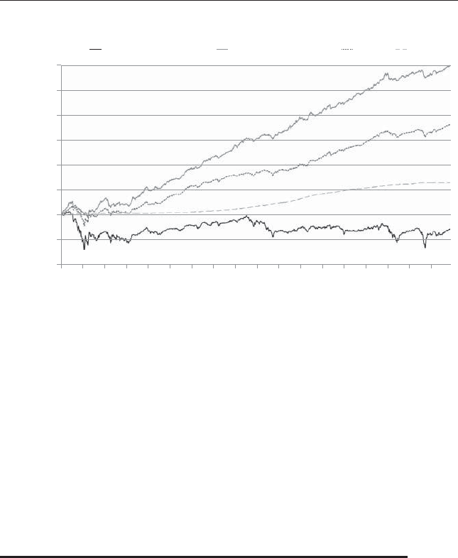
The Basics of Building a Momentum Strategy 87

$10

$100

$1,000

$10,000

Value of $ 100 Invested (Log Scale)

$100,000

$1,000,000

$10,000,000

1/1/1927

12/1/1931

11/1/1936

10/1/1941

9/1/1946

8/1/1951

7/1/1956

6/1/1961

5/1/1966

4/1/1971

3/1/1976

2/1/1981

1/1/1986

12/1/1990

11/1/1995

10/1/2000

9/1/2005

8/1/2010

Intermediate-Term Loser Intermediate-Term Winner SP500 RF

FIGURE 5.3 Intermediate-Term Momentum Portfolio Returns

the intermediate past will continue to do well in the future, while rms that

have done poorly will continue to perform poorly. However, as we discussed

earlier, this “continuation” effect does not work if we just buy-and-hold

intermediate-term momentum stocks. We must form the portfolio so that

the rebalance frequency can capture the abnormal returns associated with

the approach. In the next section, we examine how portfolio construction,

such as rebalance frequency and portfolio size, affects intermediate-term

momentum strategies.

WHY MOMENTUM PORTFOLIO CONSTRUCTION

MATTERS

The results in the original Jegadeesh and Titman paper highlight the impor-

tance of portfolio construction in the context of the momentum anomaly.

The authors identify that the holding period, or the rebalance frequency,

dramatically affects a momentum portfolio’s performance. As a general

rule, and putting transaction costs aside, the more frequent a portfolio is

rebalanced, the better the performance. In this section, we drill down on

exactly how portfolio construction affects intermediate-term momentum.

Intermediate-term momentum is the focus of our analysis throughout the

remainder of this book because this form of momentum is what researchers

consider to be the most anomalous and intriguing.

❦

❦ ❦

❦

88 QUANTITATIVE MOMENTUM

Let’s set up the experiment to assess how portfolio construction affects

performance. We examine the 500 largest rms each month from 1927

to 2014. We calculate the monthly momentum variable as the cumulative

returns over the past 12 months, ignoring the past month. This specic

intermediate-term momentum calculation method is the same approach

used by Ken French, the source of the data we used earlier. The last month

is ignored in our intermediate term momentum calculation to account for

the short-term reversal effect previously documented. If we included the

most recent month in the momentum metric we would increase the noise of

the metric and decrease the benets of the signal.

Looking back to our Apple momentum example (referring back to

Table 5.1), we construct our momentum variable (excluding the most recent

month) as the following:

(0.8923)(1.0575)(1.0200)(1.0994)(1.0787)(1.0277)(1.0287)(1.0775)

(0.9829)(1.0720)(1.1060)–1=51.51%

The key difference between this calculation and the one provided in

Table 5.1 is that we ignore the last month’s return (in this example, the

December returns). It should be pointed out that including the last month’s

return, which is more reasonable from both an empirical and theoretical per-

spective, does not signicantly alter the results—one could include the most

recent month in all momentum calculations and generate similar results.

Regardless, for the rest of the book, we focus on momentum calculations that

ignore the most recent month’s return when calculating intermediate-term

momentum.

In the following tests, we allow the portfolio construction to vary across

two dimensions. First, we examine the returns by varying the number of

rms in the portfolio. We allow the portfolio size to vary from 50 to 300

stocks. Second, we examine the returns by varying the holding periods after

portfolio formation. We allow the holding periods to vary from 1 month to

12 months.

We select the top Nnumber of rms ranked on momentum, every

month. Here, the number of stocks Ncan be 50, 100, 150, 200, 250, or

300. These rms are held in the portfolio for Tmonths. The holding period

(number of months) Tvaries from 1 to 12.

Portfolios with holding periods over 1 month are formed by creating

overlapping portfolios. Overlapping portfolios can be explained with an

example that uses a three-month holding period. On December 31, 2014, we

use one-third of our capital to buy high momentum stocks. These stocks stay

in the portfolio until March 31, 2015. On January 31, 2015, we use another

one-third of our capital to buy high momentum stocks. These stocks stay in

❦

❦ ❦

❦

The Basics of Building a Momentum Strategy 89

the portfolio until April 30, 2015. On February 28, 2015, we use another

one-third of our capital to buy high-momentum stocks. These stocks stay

in the portfolio until May 31, 2015. This process repeats every month. So

the return to the portfolio from February 28, 2015, to March 31, 2015, is

the returns to the stocks in the portfolio originally formed on December 31,

2014, January 31, 2015, and February 28, 2015. Overlapping portfolios are

formed to minimize seasonal effects. Unless otherwise stated, we use over-

lapping portfolios throughout the analysis in the remainder of the book for

holding periods of longer than one month. And similar to the robustness

of the results when we decide to include or exclude the most recent month

when calculating momentum measures, the use of the fancier overlapping

portfolio methodology versus a more generic standard “buy and rebalance

portfolio” does not signicantly drive results in one direction of the other.

Our analysis runs from January 1, 1927, to December 31, 2014.

All results are gross of fees. All returns are total returns and include the

reinvestment of distributions (e.g., dividends). Table 5.5 provides the CAGR

to the value-weighted portfolios. By value weighting, we mean that each

stock is given its “weight” in the portfolio, depending on the size of the

rm. Value weighting gives more weight to larger stocks and less weight to

smaller stocks. It is worth mentioning, however, that we focus our results

on the largest 500 US stocks, to minimize the effects that micro-cap stocks

would have on the portfolios.

TABLE 5.5 Momentum Portfolio Returns: Varying Holding Period and Number of

Firms in the Portfolio (1927–2014)

50-

Stock

Portfolio

100-

Stock

Portfolio

150-

Stock

Portfolio

200-

Stock

Portfolio

250-

Stock

Portfolio

300-

Stock

Portfolio

Universe

(500 Firms)

1-month hold 17.02% 14.40% 13.55% 12.69% 12.07% 11.50% 9.77%

2-month hold 16.05% 14.17% 13.23% 12.59% 11.98% 11.43% 9.77%

3-month hold 15.15% 13.81% 12.93% 12.25% 11.74% 11.23% 9.77%

4-month hold 14.54% 13.53% 12.78% 12.11% 11.63% 11.21% 9.77%

5-month hold 14.37% 13.31% 12.62% 12.04% 11.57% 11.17% 9.77%

6-month hold 13.93% 13.05% 12.37% 11.88% 11.46% 11.10% 9.77%

7-month hold 13.68% 12.80% 12.11% 11.66% 11.33% 10.99% 9.77%

8-month hold 13.38% 12.58% 11.89% 11.48% 11.19% 10.90% 9.77%

9-month hold 12.94% 12.24% 11.60% 11.23% 11.01% 10.77% 9.77%

10-month hold 12.62% 11.93% 11.37% 11.03% 10.85% 10.66% 9.77%

11-month hold 12.21% 11.61% 11.12% 10.81% 10.68% 10.52% 9.77%

12-month hold 11.78% 11.27% 10.83% 10.58% 10.48% 10.36% 9.77%

❦

❦ ❦

❦

90 QUANTITATIVE MOMENTUM

Acleartrendemerges—holdingfewerstocksandrebalancingmore

frequently leads to higher compound annual growth rates (CAGRs). The

ideal portfolio is highly concentrated (e.g., 50 stocks) and rebalanced

monthly (e.g., holding period equals one month). Of course, one must

consider trading costs, which have the potential to greatly affect returns.

To address the question of trading costs, we can examine a concentrated

momentum portfolio (e.g., 50 stocks) that is rebalanced every quarter

instead of every month—so we could form a portfolio that trades 4 times

a year, instead of 12 times a year (overlapping portfolios are not necessary

in real-world trading). This concentrated, but lower frequency rebalanced

portfolio has a CAGR of 15.15 percent over the 1927 to 2014 time frame.

The portfolio gives up a substantial amount of return, but comes with

alotlesstrading.Dependingontransactioncosts(discussedlater),one

could assess the trade-off between the benetofhigherexpectedreturns

associated with the monthly rebalanced against the lower transaction costs

of the quarterly rebalanced portfolio.

In the absence of granular detail on trading costs, when it comes to

monthly versus quarterly rebalancing, the winner is unclear. However, if we

compare any of these portfolios to the gross performance of a semiannually

rebalanced diversied 200-stock portfolio, the horse race among portfolio

constructs becomes more obvious. The CAGR for this low-frequency, “di-

worsied” portfolio is only 11.88 percent. The spread between this portfolio

construct and the other, more concentrated and more frequently balanced

portfolios is over 3 percent a year. If a momentum strategy annually rebal-

ances and holds heavily diluted portfolios (e.g., 300 stocks), the relative

performance is even worse.

If we assume the “all-in” rebalance costs are 0.50 percent per rebalance

for these momentum strategies, the CAGR on the 50-stock, quarterly rebal-

anced portfolio would fall from 15.15 percent to 13.15 percent (four trades

times 0.50 percent). Similarly, the 200-stock, semiannually rebalanced port-

folio’s CAGR would fall from 11.88 percent to 10.88 percent (two trades

times 0.50 percent). There is still a 2.27 percent edge to the higher concen-

trated, more frequently rebalanced portfolio.

The implementation of transaction costs in the previous analysis is sim-

ple in nature and meant to highlight the point that rebalance frequency

and portfolio concentration benets need to be considered in the context

of projected trading costs. For further discussion on this subject, there is a

paper by Lesmond, Schill, and Zhou in 2004, which claims that momentum

prots are illusory based on ad-hoc assumptions regarding trading costs.9

Korajczyk and Sadka also examine the issue, but consider market impact

costs. These authors estimate that momentum strategies have limited capac-

ity, estimated at roughly $5 billion.10 However, in response to this paper

❦

❦ ❦

❦

The Basics of Building a Momentum Strategy 91

and others, Andrea Frazzini, Ron Israel, and Toby Moskowitz published

research that leverages over a trillion dollars of live trading data from the

large institutional money manager AQR.11 Frazzini et al. nd that momen-

tum prots are robust to transaction costs and that the estimated transaction

costs used in prior research were possibly 10 times higher than real-world

transaction costs. Following the Frazzini et al. transaction cost analysis is

apaperin2015byFisher,Shah,andTitmanthatusesestimatedbid/ask

spreads from 2000–2013 to assess the trading costs associated with momen-

tum strategies.12 Their conclusions are that their “estimates of trading costs

... are generally much larger than those reported in Frazzini, Israel, and

Moskowitz, and somewhat smaller than those described in Lesmond, Schill,

and Zhou and Korajczyk and Sadka.” In short, the debate over transac-

tion costs is heated, but the consensus from the research seems to be that

momentum exists net of transaction costs, but the scalability is limited.

Clearly, there is a relationship between the number of rms, the holding

period, and returns. The results are almost identical when equal-weighting

the portfolios (higher CAGRs, similar pattern). And, of course, transaction

costs are always an important element to consider when implementing any

active strategy. Regardless, there are two important takeaways:

■Rebalance frequency: Holding the number of rms constant, the shorter

the holding period, i.e., the more frequently the portfolio is rebalanced,

the higher the CAGR.

■Avoid diworsication: Keeping the holding period constant, the fewer

rms in the portfolio, the higher the CAGR.

For a large, multibillion dollar asset manager, the results above are not

inspiring, since the manager’s scale alone prohibits them from pursuing the

more effective momentum strategies, which require higher turnover. How-

ever, for this same reason, the requirement that momentum be rebalanced

frequently and held in concentrated portfolios is great news when viewed

through the sustainable active framework. These characteristics make arbi-

trage costly for large pools of capital, thus ensuring a long expected life for

the higher frequency rebalanced versions of the momentum anomaly.

SUMMARY

This chapter details how to calculate a generic momentum metric. First,

we describe the three types of momentum strategies most commonly

examined: short-term look-back momentum, intermediate-term look-back

momentum, and long-term look-back momentum. Both short-term and

❦

❦ ❦

❦

92 QUANTITATIVE MOMENTUM

long-term momentum portfolios generate return reversals. However, port-

folios formed using intermediate-term look-back momentum calculations

generate a continuation of returns. This form of momentum is the most

compelling and robust as an investment approach. Finally, we highlight that

portfolio construction plays are large role in determining the effectiveness

of an intermediate-term momentum portfolio. We identify that momen-

tum portfolios should be reasonably concentrated and require frequent

rebalancing to maximize their effectiveness. In the chapters that follow, we

describe ways in which the generic intermediate-term momentum measure

can be improved.

NOTES

1. George Soros, The Alchemy of Finance (Hoboken, NJ: John Wiley & Sons,

2003), p. 5.

2. Bruce N. Lehmann, “Fads, Martingales, and Market Efciency,” The Quarterly

Journal of Economics 105 (1990): 1–28.

3. Narasimhan Jegadeesh, “Evidence of Predictable Behavior of Security Returns,”

The Journal of Finance 45 (1990): 881–898.

4. mba.tuck.dartmouth.edu/pages/faculty/ken.french/data_library.html, accessed

2/22/2016.

5. Zhi Da, Qianqui Liu, and Erst Schaumburg, “A Closer Look at the Short-Term

Return Reversal,” Management Science 60 (2014): 658–674.

6. Werner F. M. DeBondt and Richard Thaler, “Does the Stock Market Overre-

act?,” The Journal of Finance 40 (1985): 193–805.

7. Thomas George and Chuan-Yang Hwang, “Long-Term Return Reversals: Over-

reaction or Taxes?” The Journal of Finance 62 (2007): 2865–2896.

8. Narasimhan Jegadeesh and Sheridan Titman, “Return to Buying Winners and

Selling Losers: Implications for Stock Market Efciency,” The Journal of Finance

48 (1993): 65–91.

9. David A. Lesmond, Michael J. Schill, and Chunsheng Zhou, “The Illusory

Nature of Momentum Prots,” Journal of Financial Economics 71 (2004):

349–380.

10. Robert Korajczyk and Ronnie Sadka, “Are Momentum Prots Robust to Trad-

ing Costs?” The Journal of Finance 59 (2004): 1039–1082.

11. Andrea Frazzini, Ronen Israel, and Tobias J. Moskowitz, “Trading Costs of

Asset Pricing Anomalies,”working paper, 2015.

12. Gregg Fisher, Ronnie Shah, and Sheridan Titman, “Combining Value and

Momentum,” Journal of Investment Management, forthcoming.

❦

❦ ❦

❦

CHAPTER 6

Maximizing Momentum: The Path

Matters

“...as the formation period return accumulates gradually over

many days, the ow of information is continuous.”1

—Z. Da et al., The Review of Financial Studies

Chapter 5 highlighted that stocks with strong intermediate-term momen-

tum signals, generically calculated as the past 12-month cumulative

returns (skipping the most recent month), exhibit a strong continuation in

returns. The evidence is pervasive across multiple time periods and asset

classes. Given this empirical fact, a natural question arises: Can we do better

than the generic intermediate-term momentum indicator? Figuring out a

way to accomplish this goal can be difcult, especially when the risk of

optimization and data mining is high. However, academic researchers have

been studying this question for a while and have developed solutions that

improve on the generic momentum algorithm, while simultaneously show-

ing how the improvement relates to the theoretical behavioral foundations

for momentum’s existence. In other words, momentum improvements are

evidence-based enhancements developed through the lens of the sustainable

active framework, and not data mining run amok.

For over a year, we examined every respectable research piece on

momentum stock selection strategies we could nd and came to the general

conclusion that one of the core ways to improve on a generic momentum

strategy is to focus on the time-series characteristics of a momentum stock.

In other words, we need to look at the path through which a momentum

stock actually became classied as a momentum stock (see Appendix A

for information on some of the top competing ideas we examined and our

analysis).

❦

❦ ❦

❦

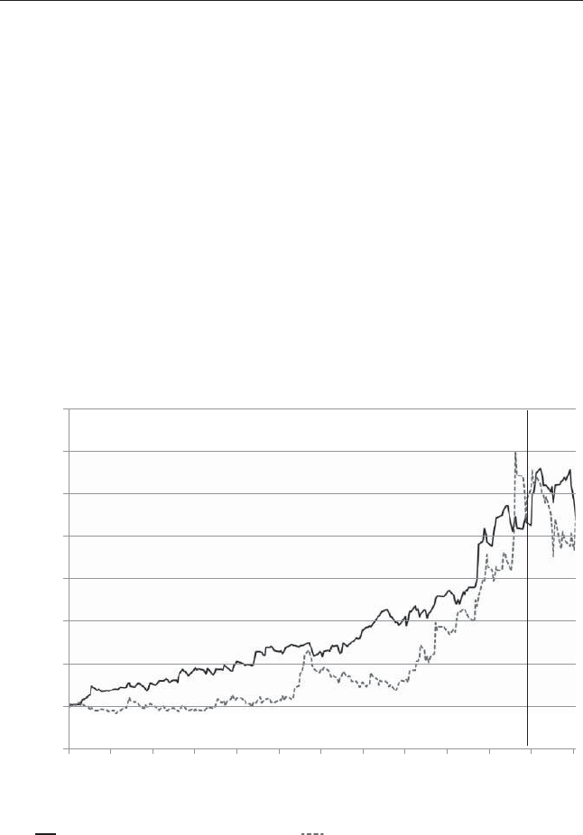
94 QUANTITATIVE MOMENTUM

An example can highlight the importance of the path dependency of

a momentum stock. Consider the so-called “Internet bubble,” which grew

during the late 1990s and eventually burst in 2000. There were many rms

with absurdly high generic momentum signals, as investors could not resist

buying Internet stocks at sky-high valuations. We chose to examine two

high-momentum stocks as of March 31, 2000 (this was near the end of the

bubble).

The rst rm we selected was Alliance Pharmaceutical Corp, a biotech

company. This biotech company was hoping to provide the market with

anewproduct,Oxygent,tohelpsupplyoxygentotissuesduringsurgery.

The second rm we examined was International Rectier Corp, a company

founded in 1947 that produced power management semiconductors. As of

March 31, 2000, both stocks were classied as high-momentum stocks.

Figure 6.1 plots the total cumulative returns over the past 12 months,

as of March 31, 2000. Two points to note: First, there is a vertical line on

$8.00

$7.00

$6.00

$5.00

$4.00

Total Cummulative Return

$3.00

$2.00

International Rectifier Corp Return Alliance Pharmaceutical Corp Return

$1.00

$0.00

4/30/1999

3/31/1999

5/31/1999

6/30/1999

7/31/1999

8/31/1999

9/30/1999

10/31/1999

11/30/1999

12/31/1999

1/31/2000

2/29/2000

3/31/2000

FIGURE 6.1 Alliance and International Rectier Past Performance

❦

❦ ❦

❦

Maximizing Momentum: The Path Matters 95

February 29, 2000. To calculate intermediate-term momentum we measure

up until February 29, 2000, because generic momentum calculations exclude

the most recent month. As of February 29, 2000, Alliance Pharmaceutical

was up 554 percent over the past year, while International Rectier Corp

was up 498 percent. Both stocks reect a value investor’s worst nightmare,

but a momentum investor’s dream.

The second point is that the two stock charts follow a different path.

Eyeballing the charts, we see that International Rectier Corp follows a

smoother path to high momentum, whereas Alliance Pharmaceutical Corp

has a more jumpy path. Tossing aside our ad-hoc eyeballing of the charts,

we can objectively quantify this observation. Assuming two stocks achieve

roughly the same momentum, one way to measure “jumpy versus smooth”

is to compute the percentage of days that have a positive return relative to

the percentage of days that have a negative return. We would expect rms

with a “smoother” momentum to have a higher percentage of positive return

days and a lower percentage of negative return days. We see this expectation

in the current situation: Measured over a year, Alliance Pharmaceutical had

a positive return 49 percent of the trading days and a negative return on

43 percent of the trading days, whereas International Rectier Corp had a

positive return on 55 percent of the trading days and a negative return on 40

percent of the trading days (total days don’t add up to 100 percent because

there is a percentage of days with no movement).

In the situation outlined above, we can see both visually and quan-

titatively that International Rectier had a smoother return stream. But

does the “smoother” high-momentum stock outperform the “jumpier”

high-momentum stock? We see the results of this cherry-picked example in

Figure 6.2.

Figure 6.2 documents the future three-month returns for both rms.

International Rectier Corp gains 46.9 percent and outperforms Alliance

Pharmaceutical, which loses 24.7 percent over the next 3 months. Of

course, we have cherry-picked this example to highlight that “smooth”

high-momentum stocks tend to perform better relative to “choppy”

high-momentum stocks. However, by the end of this chapter, we hope

to convince the reader that momentum path dependency matters. This

time-series aspect of momentum captures important information about

market participant behavior that can be systematically exploited to improve

upon a generic momentum strategy. To understand why, we examine the

performance of “lottery-like” stocks, which have return characteristics that

are similar to “jumpy” high-momentum stocks and placate the peculiar

demand for “lottery” payoffs by many market participants.

❦

❦ ❦

❦

96 QUANTITATIVE MOMENTUM

$8.00

$7.00

$6.00

$5.00

$4.00

Total Cumulative Return

$3.00

$2.00

$1.00

$0.00

3/31/1999

4/30/1999

5/31/1999

6/30/1999

7/31/1999

8/31/1999

9/30/1999

10/31/1999

11/30/1999

12/31/1999

1/31/2000

2/29/2000

3/31/2000

4/30/2000

5/31/2000

6/30/2000

$9.00

International Rectifier Corp Return Alliance Pharmaceutical Corp Return

FIGURE 6.2 Alliance and International Rectier Future Performance

THE PERFORMANCE OF LOTTERY STOCKS

Everyone loves a gamble, especially a long shot. And it’s not just retirees

who enjoy smoking cigarettes and pounding rum and cokes in front of the

slot machine—no, sir. Heck, we’ve personally lost money gambling in Vegas

and Atlantic City—and we’re supposed to know better!

So what gives?

Nick Barberis, in his theory paper “A Model of Casino Gambling,”

specically addresses why people go to casinos and how they behave once

they get there.2Setting aside the known expected utility benets of gam-

bling (i.e., “it’s fun”), the key assumption behind Barberis’s theory is that

there is something additional at play: Human beings suffer from an inabil-

ity to properly weigh their chances of success for low-probability events. In

other words, humans predictably overestimate their chances of winning the

lottery.

But when we step outside of the casino and take a small leap over to

the stock market, human behavior does not change. “Maxing Out: Stocks

as Lotteries and the Cross-Section of Expected Returns” by Turan G. Bali,

❦

❦ ❦

❦

Maximizing Momentum: The Path Matters 97

Nusret Cakici, and Robert F. Whitelaw examines how lottery-like stocks

perform.3Their central hypothesis is that investors irrationally overpay for

lottery-like gambles, assume their odds are higher than they are in reality,

and, thus, stocks with lottery-like characteristics will underperform on a

risk-adjusted basis.

To test this hypothesis, Bali et al. rst classify a subsample of stocks as

“lottery” stocks if these stocks had extreme market movements in the recent

past. Next, they examine the future performance of these lottery-like stocks.

The underlying assumption is that investors identify stocks with extreme

returns in the recent past as “lottery stocks” and bid these assets past funda-

mental value. The specicmeasuretheauthorslookattoidentifyalottery

stock is to rank stocks based on the maximum daily return over the previous

month (“MAX”).

An example can shed light on how the authors classify a stock as having

lottery-like characteristics. Pretend it is January 31, 2017, and our universe

consists of two stocks, Fast Money Inc. and Boring Money Inc. (Tickers:

FAST and SLOW, respectively). We form a long/short portfolio on Febru-

ary 1 that exploits the fact that investors overpay for lotteries. We identify

that FAST has a maximum daily return of 50 percent in the past month

and SLOW has a maximum daily return of 1 percent. Therefore, our port-

folio on February 1 will be short FAST (a lottery stock) and long SLOW (a

non-lottery stock).

Table 6.1 summarizes the results from their paper highlighting the aver-

age monthly returns of 10 portfolios ranked on their MAX ranking, which is

TABLE 6.1 Lottery Stock Results

Avg. Monthly

Return

(VW Portfolio)

4-Factor

Alpha (VW

Portfolio)

Average

MAX

Boring (1) 1.01% 0.05 1.30

21.00% 0.00 2.47

31.00% 0.04 3.26

41.11% 0.16 4.06

51.02% 0.09 4.93

61.16% 0.15 5.97

71.00% 0.03 7.27

80.86% –0.21 9.07

90.52% –0.49 12.09

Lottery (10) –0.02% –1.13 23.60

Long/Short (1–10) 1.03% 1.18

❦

❦ ❦

❦

98 QUANTITATIVE MOMENTUM

the maximum daily return over the past month. The top decile (“10”) rep-

resents “lottery” stocks and the bottom decile (“1”) reects the “boring”

stocks.

Not too shabby! A portfolio that buys boring stocks and shorts lottery

stocks generates a raw return of 1.03 percent a month, or roughly 12 percent

a year. Moreover, the four-factor alpha (which controls for market exposure,

as well as known return drivers such as size, value, and momentum) is 1.18

percent a month, or 14.4 percent a year. We have not included the costs of

implementation in these results, because that is beside the point. We are not

trying to suggest this strategy as a practical approach to forming a portfolio,

but merely to emphasize that market participants seem to misprice stocks

with lottery-like characteristics.

Lottery bias may also help explain the so-called beta anomaly.Academic

research has documented that low beta stocks tend to outperform high beta

stocks.4This nding is remarkable and is considered anomalous because a

central prediction of theoretical asset pricing models is that stocks exposed

to more market risk (i.e., high beta) should have higher expected returns

than stocks with lower market risk (i.e., low beta). A working paper by Bali

et al.5examines the relationship between beta and lottery demand. Specif-

ically, they try and understand how investor preferences for lotteries may

explain the beta anomaly. We summarize some data from the Bali et al. paper

and present the results in Table 6.2.

Table 6.2 tabulates results associated with portfolios that sort stocks

into 10 deciles based on beta, and then within each decile, sorts the portfolios

TABLE 6.2 Average Monthly Returns Sorting Stocks on Beta and the “Lottery”

Ranking

Low BetaDecile High BetaDecile

Boring (1) 0.35% 1.04%

20.75% 0.86%

30.73% 0.82%

40.85% 0.77%

50.95% 0.69%

60.97% 0.46%

71.03% 0.15%

80.91% 0.06%

90.46% –0.31%

Lottery (10) –0.01% –1.07%

Long/Short (1–10) –0.36% –2.11

Long/Short Alpha (4-factor) –0.83% –2.14%

❦

❦ ❦

❦

Maximizing Momentum: The Path Matters 99

based on their “lottery” ranking. We show the results to the top and bot-

tom beta deciles for expositional purposes. On average, high beta stocks

underperform relative to low beta stocks, which reects the so-called “low

beta anomaly.” But this average result is inconsistent across lottery rank-

ing. Low beta boring stocks earn less than high beta boring stocks, which

is in line with nance theory that suggests high beta stocks are riskier than

low beta stocks and should therefore earn higher expected returns. The real

anomalous results associated with the low beta effect are driven by stocks

with lottery characteristics. The lottery characteristic is especially powerful

among high beta stocks. For example, within the high beta decile, there is

a monotonically decreasing relationship on the average returns as the “lot-

tery” ranking increases. The authors explore this issue further and conduct

testing to determine if lottery demand can explain why high beta stocks

perform so poorly relative to low beta stocks. What they nd is not too

surprising, given what we know about the human mind: The lottery charac-

teristic associated with high beta stocks is a key driver of these stocks’ poor

performance. (Lottery bias also goes a long way towards explaining the low

beta anomaly, but this is a discussion for another day.)

But back to momentum strategies and why the research on lottery-like

stocks is important. Based on the evidence discussed in the original “Maxing

Out” paper, it appears investors are better off avoiding stocks with lottery

characteristics. We should incorporate this knowledge into our algorithm

when deciding which high-momentum stocks we want to purchase.6And

almost by design, high-momentum stocks with smoother momentum paths

will be less prone to lottery bias mispricing than stocks with jumpier paths.

We should also consider the research, which relates lottery stocks to high

beta stocks. As previously discussed, avoiding lottery-type stocks is a good

idea, but what about the concept of avoiding high-beta stocks as well? To

address that question we rst need a quick refresher on beta. Beta is simply

a measure of volatility, or systematic risk. And by design, high-momentum

stocks with smoother price paths will generally have lower betas, while

high-momentum stocks with choppier price paths will generally have higher

betas. So to some degree, by focusing on momentum stocks with smoother

price paths, we are avoiding an element of lottery bias, which aficts many

high ying generic momentum stocks.

What’s the bottom line? Lottery bias plays a role in market mispricing.

Stocks that are perceived as lotteries tend to do poorly because investors bid

them past fundamental value. One can measure lottery bias by a variety of

proxy metrics. We’ve discussed the MAX calculation and beta, and both of

these measures are helpful in identifying stocks we should avoid. One could

surely come up with many other permutations and nd similar results. But

when we step back and think about the big picture, really what we are trying

❦

❦ ❦

❦

100 QUANTITATIVE MOMENTUM

to do is identify the nature of a stock’s price path to glean information about

market participant behaviors. We will see in the following section that the

path to momentum prots is ... the path.

THE PATH TO MOMENTUM PROFITS

Consider the story of putting a frog in water. If the frog is placed in a pot

of boiling water, not surprisingly, the frog will immediately jump out. How-

ever, if the frog is placed in a pot of room temperature water, and this water

is gradually heated to the boiling point, the frog will sit in the water until it

is fully cooked. As least for our hypothetical frog, the path of water temper-

ature changes clearly matters for the eventual outcome.

Interestingly enough, research has found that the frog’s reaction to grad-

ual water temperature changes is analogous to how investors react to gradual

stock price changes. For example, if a stock has an immediate 100 percent

gain (i.e., dropping the frog in a pot of boiling water), the strong price

reaction immediately attracts investor attention, and the new stock price

will typically reect approximately fair value. However, if a stock gradu-

ally grinds along and achieves a 100 percent return (i.e., the water slowly

heats up over time), investors will pay less attention to the gradual stock

price movement and the security will likely be priced at less than fundamen-

tal value. In psychology terms, both the frog and human investors suffer

from “limited attention,” which simply reects the idea that our cognitive

resources are limited and our brains will focus on processing the information

that is most relevant at a given point in time. Determining what is “most rele-

vant” turns out to be a challenging question. Psychology research, however,

has found that dramatic changes in an environment, as opposed to small

changes, attract more cognitive resources, all else being equal.7

In 2014, Zhi Da, Umit Gurun, and Mitch Warachka8investigated the

limited attention of investors to gradual-information diffusion. The authors

hypothesize that there might be a relationship with the momentum anomaly.

They describe their frog-in-the-pan hypothesis:

Aseriesoffrequentgradualchangesattractslessattentionthan

infrequent dramatic changes. Investors therefore underreact to

continuous information.

Their conclusions after conducting a battery of empirical analysis are

fascinating: Momentum strategies that focus on the path-dependency of

momentum generate a much stronger momentum effect. In other words,

the evidence strongly supports the frog-in-the-pan hypothesis, and broadly

supports the theoretical behavioral arguments outlined in the Barberis et al.

❦

❦ ❦

❦

Maximizing Momentum: The Path Matters 101

1998 paper, which suggests that the momentum anomaly is driven by an

underreaction to positive news.9

Da, Gurun, and Warachka construct a proxy for information discrete-

ness (ID) that measures the relative frequency of small signals. A large ID

means more discrete information, and a small ID denotes continuous infor-

mation. For past winners with a high past return, a high percentage of pos-

itive returns (% positive >% negative) implies there are a large number of

small positive returns. The exact measure is described by the equation:

ID =sign(Past Return)∗[%negative −%positive]

To test their hypothesis Da et al. sequentially double-sort portfolios rst

on a 12-month formation-period returns, or what we refer to as “generic

momentum” in previous chapters and further described in Jegadeesh and

Titman.10 Next, they sort the stocks within these momentum portfolios on

their information discreteness variable over the 1927 to 2007 sample period.

We tabulate the most relevant results from the paper in Table 6.3, which

examine the six-month holding period returns to portfolios that are long

high momentum stocks and short low momentum stocks, while varying the

information discreteness measure.

The results are astonishing. Over a six-month holding period, long-short

momentum portfolios decrease monotonically from 5.94 percent for stocks

with continuous information to negative 2.07 percent for stocks with dis-

crete information. The three-factor alpha to long/short portfolios decreases

from 8.77 percent for long/short portfolios with continuous information to

negative 2.01 percent for long/short portfolios with discrete information—a

spread of 10.78 percent (over 20 percent on an annualized basis) with a

highly signicant t-stat.

We know from prior analysis in Chapter 5 that higher frequency rebal-

ancing translates into better performance for momentum strategies. The

authors examine this question in their paper. Figure 6.3 shows the monthly

TABLE 6.3 Frog-in-the-pan Results to Long/Short Momentum Portfolios

Return 3-Factor Alpha

Discrete –2.07% –2.01%

20.64% 3.53%

33.12% 5.05%

44.36% 6.71%

Continuous 5.94% 8.77%

Continuous–Discrete 8.01% 10.78%

❦

❦ ❦

❦

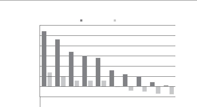
102 QUANTITATIVE MOMENTUM

3.00%

Three-factor Alpha

2.50%

2.00%

1.50%

1.00%

0.50%

0.00%

–0.50%

12345678910

–1.00%

Continuous Discrete

FIGURE 6.3 Frog-in-the-Pan Portfolio Alphas

alpha estimates to the long/short momentum portfolios (for both continu-

ous and discrete information) from 1 to 10 months after portfolio formation.

The results are consistent with the frog-in-the-pan hypothesis—continuous

momentum seems to account for the bulk of the momentum effect. A few

key points:

1. Higher prots: Long/short momentum portfolios with continuous infor-

mation have higher three-factor alphas than long/short momentum port-

folios with discrete information.

2. Longer persistence: Long/short momentum prots following continu-

ous information persist longer (the holding period can be extended with

limited decay), while long/short momentum prots following discrete

information are less persistent and more transitory.

Remarkably, by simply quantifying the nature of the path by which the

high momentum status is achieved, the momentum anomaly can be vastly

improved and focused on exploiting limited attention. Although this con-

clusion is not mentioned in the frog-in-the-pan paper, we also believe that

the performance bonus of path-focused momentum algorithms is because of

an indirect exploitation of the behavioral bias associated with lottery pref-

erences by market participants (discussed in the previous section).

And while the authors do a meticulous job of documenting why limited

attention may be a key insight in understanding the momentum anomaly,

they are not the only authors to empirically investigate this concept.

For example, a paper in 2000 by Hong, Lim, and Stein11 documents

that momentum prots are larger for stocks with low analyst coverage

❦

❦ ❦

❦

Maximizing Momentum: The Path Matters 103

and for small stocks. The authors argue that low analyst coverage and

small-cap stock characteristics serve as a proxy for stocks that attract less

attention, and therefore, are predicted to have higher momentum prots.

The disposition effect, or the tendency to hold onto losing stocks too long

and sell winning stocks too quickly, may also play a role in underreaction.

This theory is described in 1985 by Shefrin and Statman12 and has been

veried and explored in numerous empirical papers.13, 14

In addition, in our own tests we have found that splitting high momen-

tum portfolios on other measures of attention, such as trading volume15

(more trading volume should cause more attention), yield similar results.

Next we examine the results when incorporating the information discrete-

ness measure for our universe of stocks.

THE RESULTS

In Chapter 5 we highlighted that generic momentum premiums decay over

time, thus requiring a higher frequency rebalance (e.g., monthly rebalanced

portfolios beat annually rebalanced portfolios). However, more rebalancing

increases frictional costs. As a compromise, in this section we examine the

results associated with quarterly rebalanced portfolios. We focus our anal-

ysis on overlapping quarterly rebalanced portfolios as described in Chapter

5. We only examine mid-cap and large-cap rms.16 Portfolios are formed by

value-weighting the rms and the returns run from January 1, 1927, through

December 31, 2014.17

In Table 6.4, we sort stocks based on their cumulative 12-month past

returns (ignoring the most recent month), and buy a value-weighted basket

of stocks from the top decile (“Generic Momentum” in column 3). We

then split the portfolio of high generic momentum stocks into high-quality

momentum (in column 1) and low-quality momentum (column 2). The

momentum “quality” measure is the information discreteness measure, or

frog-in-the-pan measure, described earlier in the Da, Gurun, and Waracha

paper. Firms with higher-quality momentum are those with continuous

information, while rms with lower-quality momentum are those with

discrete information—to be perfectly clear, the portfolio of stocks in

columns 3 is split in half by our information discreteness measure to create

the portfolios in columns 1 and 2. The returns in Table 6.4 are gross of fees.

Using our own laboratory conditions, we replicate the nature of the

ndings from the Da, Gurun, and Waracha paper: Among high momentum

stocks, those with higher quality, or “smooth,” momentum (measured

via continuous information), show very strong relative performance. By

contrast, low quality, or “jumpy,” momentum stocks still outperform

the broad market, but show weaker performance. These results suggest

❦

❦ ❦

❦

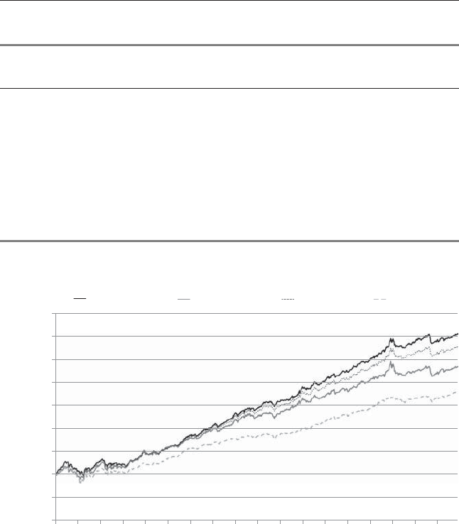
104 QUANTITATIVE MOMENTUM

TABLE 6.4 Quality of Momentum Portfolio Annual Results

High-Quality

Momentum

Low-Quality

Momentum

Generic

Momentum SP500

CAGR 17.14% 13.02% 15.56% 9.95%

Standard Deviation 23.45% 25.16% 23.61% 19.09%

Downside Deviation 16.98% 18.71% 17.42% 14.22%

Sharpe Ratio 0.65 0.48 0.59 0.41

Sortino Ratio (MAR =5%) 0.81 0.56 0.71 0.45

Worst Drawdown –74.60% –77.44% –73.90% –84.59%

Worst Month Return –29.23% –34.71% –30.00% –28.73%

Best Month Return 30.63% 37.15% 33.88% 41.65%

Protable Months 62.50% 61.08% 61.84% 61.74%

$1,000,000,000

$100,000,000

Value of $100 Invested (Log Scale)

$10,000,000

$1,000,000

$100,000

$10,000

$1,000

$100

$10

1/1/1927

2/1/1931

11/1/1936

10/1/1941

9/1/1946

8/1/1951

7/1/1956

6/1/1961

5/1/1966

4/1/1971

3/1/1976

2/1/1981

1/1/1986

12/1/1990

11/1/1995

10/1/2000

9/1/2005

8/1/2010

High-Quality Momentum Low-Quality Momentum Generic Momentum SP500

FIGURE 6.4 Quality of Momentum Portfolio Returns

that the generic momentum effect is driven by high-quality momentum

and diluted by low-quality momentum. The spread between high-quality

and low-quality momentum is large: over a multidecade time period

(1927–2014) the spread between the high (column 1) and low (column 2)

quality momentum portfolios is over 4 percent a year! This spread can be

seen visually in Figure 6.4. The high-quality momentum portfolio also has

better risk-adjusted returns (Sharpe and Sortino ratios) as well as lower

drawdowns. While all the momentum strategies outperform the S&P 500

❦

❦ ❦

❦

Maximizing Momentum: The Path Matters 105

(before fees), our key takeaway is that an effective momentum strategy

must consider the path by which stocks get their momentum.

SUMMARY

The chapter began with a simple example of the performance of two stocks

that were high “generic” momentum stocks during the Internet bubble. In

our anecdote, we noticed that the rm with a “smoother” path toward

high momentum status performed better in the future than the high momen-

tum stock with “jumpy” momentum. Next, we explored two reasons why

this anecdote may reect a more systematic effect in the market. First, we

examined how investors irrationally prefer lottery-like stocks, which have

“jumpy” historical price paths. The evidence suggests that we should avoid

these stocks because they tend to be overpriced. Second, we examined the

“frog-in-the-pan” limited attention hypothesis presented by the authors, Da

et al., which suggests that investors underreact to continuous information.

To conrm their hypothesis, the authors provide evidence that high momen-

tum stocks with smoother price paths to high momentum outperformed high

momentum stocks with more volatile paths to high momentum. Our inde-

pendent analysis of the Da et al. research corroborates their ndings. The

conclusion from the analysis is that the path by which momentum is achieved

determines the effectiveness of the strategy—smoother paths are preferable

to more volatile paths. This nding, that identifying “quality” momentum

can help separate good high momentum stocks from bad high momentum

stocks, can be explained via behavioral psychology:

■Avoid mispricing associated with lottery-like stocks.

■Exploit limited attention, which leads to systematic underreaction.

NOTES

1. Zhi Da, Umit G. Gurun, and Mitch Warachka, “Frog in the Pan: Continu-

ous Information and Momentum,” The Review of Financial Studies 27 (2014):

2171–2218.

2. Nicholas Barberis, “A Model of Casino Gambling,” Management Science 58

(2012): 35–51.

3. Turan G. Bali, Nustret Cakici, and Robert F. Whitelaw, “Maxing Out: Stocks

as Lotteries and the Cross-section of Expected Returns,” Journal of Financial

Economics 99 (2011): 427–446.

4. Andrea Frazzini and Lasse Heje Pedersen, “Betting Against Beta,” Journal of

Financial Economics 111 (2014): 1–25.

❦

❦ ❦

❦

106 QUANTITATIVE MOMENTUM

5. Turan G. Bali, Stephen Brown, Scott Murry, and Yi Tang, “Betting Against Beta

or Demand for Lottery?” Working paper, 2016.

6. Heiko Jacobs, Tobias Regele, and Martin Weber, “Expected Skewness and

Momentum” Working paper,2015.

7. Francesca Gina and Max H. Bazerman, “When Misconduct Goes Unnoticed:

The Acceptability of Gradual Erosion in Others’ Ethical Behavior,” Journal of

Experimental Social Psychology 45 (2009): 708–719.

8. Da, Gurun, Warachka.

9. Nicholas Barberis, Andrei Shleifer, and Robert Vishny, “A Model of Investor

Sentiment,” Journal of Financial Economics 49 (1998): 307–343.

10. Narasimhan Jegadeesh and Sheridan Titman, “Return to Buying Winners and

Selling Losers: Implications for Stock Market Efciency,” The Journal of Finance

48 (1993): 65–91.

11. Harrison Hong, Terence Lim, and Jeremy C. Stein, “Bad News Travels Slowly:

Size, Analyst Coverage, and the Protability of Momentum Strategies,” The

Journal of Finance 55 (2000): 265–295.

12. Hersh Shefrin and Meir Statman, “The Disposition to Sell Winners Too Early

and Ride Losers Too Long: Theory and Evidence,” The Journal of Finance 40

(1985): 777–790.

13. Justin Birru, “Confusion of Confusions: A Test of the Disposition Effect and

Momentum,” The Review of Financial Studies 28 (2015): 1849–1873.

14. Andrea Frazzini, “The Disposition Effect and Underreaction to News,” The

Journal of Finance 61 (2006): 2017–2046.

15. Charles M.C. Lee and Bhaskaran Swaminathan, “Price Momentum and Trading

Volume,” The Journal of Finance 55 (2000): 2017–2069.

16. To determine mid/large cap classications we use the 40th percentile for market

capitalization based on the sample of NYSE listed rms.

17. Portfolios formed by equal-weighting yield even stronger conclusions.

❦

❦ ❦

❦

CHAPTER 7

Momentum Investors Need to

Know Their Seasons

“... planetary aspects and sunspot activity have signicant power

predicting anomalies’ returns.”

—Robert Novy-Marx, Journal of Financial Economics1

Seasonality, broadly dened in the context of stock market research,

refers to the idea of building timing signals based on the calendar.

Turn on any nancial news outlet and there typically is a discussion about

seasonality. One of the more popular concepts is, “Sell in May and Go

Away,” which suggests that investors go to cash before June and get

back in to the market in November. However, a 2014 Novy-Marx paper

titled “Predicting Anomaly Performance with Politics, the Weather, Global

Warming, Sunspots, and the Stars,”2highlights an important point: One

needs to be skeptical of seasonality-type claims. Moreover, Cherry Zhang

and Ben Jacobsen review over 300 years of UK stock market data and con-

clude that documented seasonality effects should be digested with a healthy

dose of skepticism.3That said, a recent paper by Matti Keloharju, Juhani

Linnainmaa, and Peter Nyberg using the latest data and research techniques

shows that stock market return seasonalities exist in almost every asset

class, are remarkably persistent over time, and are extremely large.4At a

high level, seasonality makes sense: Institutional and behavioral incentives

plausibly can drive supply and demand shocks that create robust seasonality

effects. We consider the effects of window dressing and tax incentives in

this chapter.

But why are we even talking about seasonality and how is this

related to momentum investing? Let us explain. Five years ago, we started

working on what we considered a “unique” idea that related seasonality

to momentum investing. Our hypothesis was that window dressing and

107

❦

❦ ❦

❦

108 QUANTITATIVE MOMENTUM

tax-loss selling could be exploited to maximize the benets of a traditional

seasonality-agnostic momentum strategy. We conducted a battery of

empirical tests and summarized all our data. The results were stunning.

What was even more exciting was that fact that our idea had never been

published in what is considered a top-tier academic nance journal, a

descriptor that is typically reserved for The Journal of Finance,Journal

of Financial Economics,andtheReview of Financial Studies.Ofcourse,

as a last-minute check, we reviewed what academic researchers consider

to be the “nonserious research” journals, also referred to as the practi-

tioner journals (e.g., Financial Analyst Journal or The Journal of Portfolio

Management). Turns out, it was good we reviewed these journals. Richard

Sias had already published our results in a Financial Analyst Journal issue

in 2007.5Our initial reaction was disappointment, because as academic

researchers we had hoped we could publish a new idea, but at the same

time we were happy because our independent analysis of seasonality in

the context of momentum was conrmed—and already discovered—by

an independent party. So to make a long story short, Sias got to the front

of the line before we could get there. We like his idea, obviously, but to

really understand the results from Sias’s paper, we need to dig into some

marketplace incentives. We rst analyze the motivations behind window

dressing and tax-loss selling and then explore why they are important for

momentum investing in the sections that follow.

WINDOW DRESSING

In the retail business, window dressing refers to the practice of arranging

merchandise in a store window to make it appear as attractive as possible.

Window dressing works because it brings customers into the store, even if

the merchandise is not as good as it looks in the window. In the nancial

services industry, fund managers leverage the same concept.

The concept of window dressing goes back—literally—to the beginning

of formal economic research. Window dressing in economics, for readers

unfamiliar with the term, is a behavior exhibited by nance professionals to

mislead and cater to the whims of less sophisticated clients. The American

Economic Review, which is considered one of the oldest and most respected

scholarly journals in economics, was established in 1911. And in its initial

publication, Edwin Kemmerer,6an established economics professor and

advisor to foreign governments, mentions the term window dressing to

describe the New York money market near the end of the year.

Here is how window dressing works in practice: Fund managers know

they must report their holdings on quarterly statements, which will get

❦

❦ ❦

❦

Momentum Investors Need to Know Their Seasons 109

mailed to their clients. But the last thing poor-performing managers want

their clients to see is their loser stocks that underperformed the market.

In other words, they don’t want investors seeing loser stocks in their

“window,” which people will be viewing. To manage around this scenario,

just before the statement reporting date the manager will sell their loser

stocks and buy all the recent winning stocks so they look good on the

statement, which is analogous to a “window” for a bricks and mortar

retailer. Voila! The window now looks much more enticing.

Obviously, window dressing is not going to be a cure for bad perfor-

mance and this tactic is not going to trick sophisticated clients, but the fund

manager’s hope is that window dressing activity will at least make them

appear to have been doing something smart, and reduce client questions

when they receive their statements. For example, consider the two scenarios

between a client and a fund manager in 2002, following the bursting of the

Internet Bubble:

■Scenario 1: “Geez, you underperformed by 10 percent. And wow, you

owned Pets.com, which is down a lot? ... Why do you own that horrible

stock? You really must be an idiot!”

■Scenario 2: “Geez, you underperformed by 10 percent. But it looks like

you own Berkshire Hathaway—that is a stable value stock that has done

well. You probably had an unlucky stretch, but you seem like a good

manager.”

Clearly, the manager would much rather face the reaction in scenario 2

as opposed to the one in scenario 1.

Of course, this scenario sounds like a great story, but what is the evidence

that sneaky mutual fund managers actually engage in window dressing?

Some authors think window dressing represents an anecdotal story, but not

reality. For example, Gang Hu, David McLean, Jeff Pontiff, and Qinghai

Wang nd little evidence of window dressing by institutional investors.7Oth-

ers disagree. Consider Marcin Kacperczyk, Clemens Sialm, and Lu Zheng’s

paper “Unobserved Actions of Mutual Fund Managers.”8They create a tool

for addressing the window dressing hypothesis by creating a return gap mea-

sure. The return gap measure examines the difference between the realized

returns to the mutual fund and the returns to the buy-and-hold portfolio that

is most recently disclosed on the quarterly statement. The goal of the return

gap measure is to identify, as is aptly put in the title, the unobserved actions

of the mutual fund manager. The data suggests that some unobserved actions

may create value (e.g., manager stock-picking skill), while other unobserved

actions may destroy value (e.g., window dressing tactics). And the creation

and destruction of value appears to be persistent across time for each fund.

❦

❦ ❦

❦

110 QUANTITATIVE MOMENTUM

Unfortunately, the return gap is a relatively crude measure, and because there

are too many variables to control for in the environment, a better experiment

is needed to pinpoint window dressing.

David Solomon, Eugene Soltes, and Denis Sosyura9identify a better lab-

oratory to examine window dressing effects. Specically, they examine how

the media spotlight affects fund ows and window dressing. Their main nd-

ing is the following: “Investors reward funds that hold stocks with high past

returns, but only if these stocks recently received media coverage.” So funds

holding stocks with high-visibility winners attract more capital ows than

similar funds holding less visible winners. Any mutual fund manager armed

with this information has economic incentives to window dress—the data

shows it leads to more assets under management!

Window-dressing is a perplexing practice, and one would hope

that it is not that widespread. However, a 2004 study by Jia He, Lilian

Ng, and Qinghai Wang examines window-dressing behavior across a

variety of institutions.10 Their ndings support the window-dressing

hypothesis—institutions that act as external money managers (e.g., banks,

life insurance companies, mutual funds, and investment advisers) are more

likely to window dress their portfolios compared to institutions that act

as internal money managers (e.g., pension funds, colleges, universities,

and endowments). Not to beat a dead horse, but a more recent 2014

paper by Vikas Agarwal, Gerald Gay, and Leng Ling11 nds the following:

“Window dressing is associated with managers who are less skilled and

who perform poorly ... we nd that window dressing is value-destroying

and is associated, on average, with lower future performance.”

The collective evidence and incentives of fund managers suggest that

window dressing is likely part of the mutual fund landscape. Studies show

that this window dressing may lead to increased assets under management,

which explains why mutual fund managers partake in the activity. We’ll

explore why this window-dressing may matter for momentum investing, but

rst we turn our attention to the research on tax-motivated trading.

TAX-MOTIVATED TRADING

Sidney B. Wachtel published a paper in 1942 discussing how tax considera-

tions can lead to seasonality in stock returns from December to January.12

Michael S. Rozeff and William R. Kinney, Jr., published a more comprehen-

sive empirical investigation of Wachtel’s initial ideas in 1976.13 Rozeff and

Kinney examined stock returns from 1904 to 1974. Their main nding is one

that stands to this day—the “January” effect, or “turn of the year” effect

in stock markets. The turn of the year effect is the empirical observation

❦

❦ ❦

❦

Momentum Investors Need to Know Their Seasons 111

that stock prices increase during the month of January, and this increase is

statistically higher than the other months of the year. The core hypothesis for

the effect is related to tax incentives at year-end. End-of-year tax-loss selling

pressure is intuitive—one might expect to see a negative supply shock from

taxable individuals looking to book losses at the end of the year, which is

reversed in the new year. Although the “tax hypothesis” is intuitively appeal-

ing, research following Wachtel and Rozeff and Kinney argues that the effect

is complex and has all but disappeared since the early 1990s.14

Early skeptics of tax-induced seasonality include Richard Roll,15 Don

Keim,16 and Marc Reinganum,17 all of whom published papers in 1983.

Their work collectively found that the larger January returns are mainly

found in smaller rms and, therefore, may not be as pervasive as previously

thought. More recent studies, however, both published in 2004, leverage

smarter empirical techniques to tease out a robust relationship between

taxes and the turn of the year effect. These works include a paper by

Honghui Chen and Vijay Singal18 and another by Mark Grinblatt and

Tobias J. Moskowitz.19

But which investors drive tax-loss selling? Jay Ritter dug a bit further

into this question and examined the buying and selling of individual

investors near the turn of the year.20 By measuring the ratio of buys and

sells of individual investors, he found that individual investors sell more

near the end of the year, and buy more in the beginning of the year—so a

seasonal pattern exists for individual investors, who tend to hold smaller

stocks. James Poterba and Scott Weisbenner21 also found that tax-loss

selling is driven by individual investors, not institutions. This nding makes

sense, as many institutional investors do not pay taxes, and therefore make

buying and selling decisions without worrying about tax consequences

(wouldn’t that be nice!). Similarly, in 1997, Richard Sias and Laura Starks22

examined turn-of-the-year returns of stocks. They found that returns

of stocks with a higher level of individual interest underperform in late

December and outperform in early January relative to stocks with higher

levels of institutional interest. So it appears tax-loss selling (by individuals

as opposed to institutions) is behind the seasonality of returns for certain

stocks.

But not all research nds that tax-loss selling causes the turn-of-the-year

effect. For example, in 1983, Philip Brown, Donald Keim, Allan Kleidon,

and Terry Marsh23 examined the returns in the Australian equity markets. At

the time, Australia had similar tax laws to the United States, but a June–July

tax year. They found that Australian equity returns had a predicted effect on

July returns, but they also found the same January effect documented in US

markets. The authors’ ndings muddy the waters on the causal relationship

between tax-loss selling and the turn of the year effect and suggest that there

❦

❦ ❦

❦

112 QUANTITATIVE MOMENTUM

may be something else going on that explains the turn of the year effect. On

net, the research suggests that there is likely some connection between tax

incentives and seasonal stock returns at year-end, but researchers still don’t

fully understand the exact relationship.

GREAT THEORIES: BUT WHY DO WE CARE?

The window dressing and tax-related seasonality effects previously outlined

are interesting academic exercises. We now try to understand how these

incentives may drive seasonal effects that can improve momentum strategies.

As discussed previously, institutional investors have window dressing incen-

tives to buy winners before the quarter ends and sell losers. This behavior

leads us to our rst hypothesis:

■Hypothesis #1: Momentum prots are highest in quarter-ending

months, as window-dressing may cause institutional demand ows into

high momentum stocks and out of low momentum stocks.

Another hypothesis related to seasonality and momentum is that taxable

investors will want to sell losers and let winners ride at year-end to minimize

tax burdens. This leads us to our second hypothesis:

■Hypothesis #2: Tax incentives lead to strong momentum prots in

December as winners are unlikely to experience selling pressure and

losers are likely to suffer from selling pressure. However, these tax-

related ows will be reversed at the beginning of the year.

If we combine both the window-dressing and tax-minimization hypothe-

ses, we should see strong momentum prots in the months prior to a quarter

end (March, June, September, and December) and an especially protable

month prior to year-end (i.e., December). We should also see poor momen-

tum prots in January, when the tax incentives from the months prior retreat

and the demand for losing and winning stocks reverts to normal levels (e.g.,

losing stocks get a positive demand shock and winning stocks get a negative

demand shock).

Richard Sias tests all of the concepts outlined above. He nds strong evi-

dence to support the notion that momentum is a highly seasonal anomaly.24

To assess momentum prots, Sias forms long/short portfolios that are long

the top decile of stocks with the strongest past six-month holding period and

short the decile of stocks with the weakest past six-month holding periods.

Figure 7.1 showcases his long/short portfolio results.

❦

❦ ❦

❦

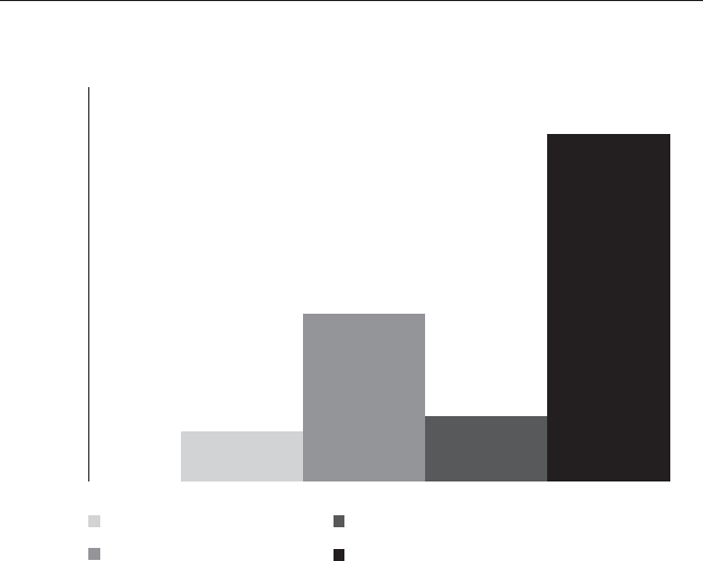
Momentum Investors Need to Know Their Seasons 113

3.50%

3.00%

2.50%

2.00%

1.50%

1.00%

0.50%

0.00%

Average Monthly Momentum Profits 1984 to 2004

All Months

All Months ex January

Non-Quarter-Ending Months ex January

Quarter-Ending Months

FIGURE 7.1 Momentum Seasonality from 1984 to 2004

Across all months, the average monthly prot from 1984 to 2004 is 0.45

percent per month, or roughly 5.4 percent a year. If one excludes January (“ex

January,” in Figure 7.1), the portfolio earns 1.50 percent a month, or approx-

imately 18 percent a year. January clearly matters, but so do quarter ending

months. Momentum prots for quarter ending months average 3.10 per-

cent a month, whereas non-quarter-ending months (excluding January) are

0.59 percent a month—a ve-fold difference! And the pattern was stronger

for stocks with high levels of institutional trading (where window-dressing

incentives are highest) and was particularly strong in December (where tax

incentives are strongest). The evidence is illuminating: Anyone devising a

momentum strategy should incorporate aspects of seasonality into their algo-

rithm. The results to long/short momentum portfolios in Figure 7.1 are in line

with the window dressing and tax minimization hypotheses—near the end of

aquarter,managerswindowdresstheirportfolios,sowinningstocksdowell

(because they are being bought) while losing stocks do poorly (because they

are being sold), and December has the strongest momentum returns across

all months with an average monthly protof5.52percent(reecting both

window dressing and tax pressures).

❦

❦ ❦

❦

114 QUANTITATIVE MOMENTUM

The evidence suggests that seasonality plays an important role in

momentum-based stock selection strategies. We will leave the nal com-

ments on the subject to Sias, who says it best: “Investors attempting to

exploit return momentum should focus their efforts on quarter-ending

months ...” In the next section we take Sias’s advice and examine how to

leverage seasonality to build a better stock selection momentum system.

MOMENTUM SEASONALITY: THE RESULTS

We start this section with a replication and extension of the results originally

found in the Sias 2007 paper. We examine all mid- and large-capitalization

stocks from January 1927 to December 2014. We examine the value-weight

returns to quarterly rebalanced momentum portfolios using similar

techniques from Chapters 5 and 6. The average monthly returns to the

high momentum and low momentum (decile) portfolios are tabulated in

Table 7.1.

The takeaways from our analysis are similar to the original Sias

paper. Examining the “Spread” column, January is a large “negative”

month for momentum as low momentum outperforms high momentum.

Quarter-ending months generally have the highest returns when comparing

the low and high momentum portfolios. March has a positive momentum

prot, but the outperformance compared to other months in the same

quarter, are muted relative to June, September, and December. But as Sias

points out in his original paper, the March result supports the window

TABLE 7.1 Average Returns by Month

Low Momentum High Momentum Spread (High – Low)

January 2.91% 1.19% –1.72%

February –0.24% 1.65% 1.89%

March 0.13% 1.86% 1.73%

April 1.33% 1.85% 0.53%

May 0.09% 0.82% 0.73%

June 0.01% 1.56% 1.55%

July 1.77% 1.21% –0.56%

August 1.96% 1.34% –0.62%

September –1.63% –0.20% 1.44%

October –0.54% 0.75% 1.28%

November 0.67% 2.39% 1.71%

December 0.19% 2.95% 2.76%

❦

❦ ❦

❦

Momentum Investors Need to Know Their Seasons 115

dressing hypothesis because institutions have a low incentive to window

dress until later in the calendar year.

We can more easily visualize the spread between the high momentum

average monthly returns and the low momentum average monthly returns

in Figure 7.2. The results are quantitatively and directly similar to those

found by Sias.

Our replication and extended analysis of the Sias results give us con-

dence in the robustness of the original results (we conduct our tests on

international data and come to similar conclusions). Now we need to identify

how we can take this knowledge and leverage it for a momentum strat-

egy. On one hand, we know that January is a large “negative” month for

momentum and should be avoided, but do we really want to sell all our high

momentum stocks at the end of December, buy all the low momentum stocks

before January, and then rebalance back into high momentum before Febru-

ary? In theory, this activity would make sense, but in practice this activity

would likely be difcult due to market liquidity and frictional costs.

Our own analysis of frictional costs and market liquidity suggest that

exploiting the December to January momentum effects are unrealistic for

areasonablysizedportfolio,sowe’llpuntonthisidea,butwecanstill

exploit momentum seasonality. We can build our system to take advan-

tage of quarter-ending window dressing as well as tax-induced incentives at

3.00%

Spread (High Momentum - Low Momentum)

2.50%

2.00%

1.50%

1.00%

0.50%

0.00%

–0.50%

January

February

March

April

May

June

July

August

September

October

November

December

–1.00%

–1.50%

–2.50%

FIGURE 7.2 Momentum Spread from 1974 to 2014

❦

❦ ❦

❦

116 QUANTITATIVE MOMENTUM

year-end. But how do we exploit this knowledge? Because momentum prof-

its are largest in quarter-ending months, and this is likely driven by managers

who are window dressing their portfolio, we hypothesize that rebalancing

before these quarter-ending months will yield the highest returns.

We test our hypothesis that smart rebalancing that exploits seasonal-

ity effects can improve a momentum strategy. Recall from Chapters 5 and

6 that we examine the results to momentum portfolios using overlapping

portfolios with a three-month holding period. To remind the reader, over-

lapping portfolios work as follows: We are standing at the end of the month

on December 31, 2014. We calculate a generic momentum metric and use

one-third of our capital to buy high-momentum stocks. These stocks stay in

the portfolio until March 31, 2015. On January 31, 2015, a month later, we

use another one-third of our capital to buy high-momentum stocks based on

momentum rankings on January 31, 2015. These stocks stay in the portfolio

until April 30, 2015. On February 28, 2015, a month later, we use another

one-third of our capital to buy high momentum stocks. These stocks stay

in the portfolio until May 31, 2015. This process repeats every month and

creates the overlapping portfolio effect. And the returns to the overlapping

portfolios reect a blend of the underlying portfolios being managed with

the overlapping portfolio, which minimizes seasonal effects.

Of course, in a test for seasonality and momentum, creating overlap-

ping portfolios—which are formed to minimize seasonal effects—is not the

correct approach. If we are deliberately trying to take advantage of seasonal

effects, we can examine quarterly nonoverlapping portfolios formed before

quarter-ending months. This portfolio formation is more intuitive to many

outside of academic research and has the ability to exploit quarterly momen-

tum effects. Specically, we assume we trade the nonoverlapping seasonal

momentum portfolio at the end of February, May, August, and November to

exploit the known momentum prots associated with March, June, Septem-

ber, and December. We hold this nonoverlapping portfolio for three months,

which means there are four rebalances per year. We compare the perfor-

mance of this portfolio against other nonoverlapping portfolios that do not

rebalance before quarter end months. Our hypothesis is that the nonover-

lapping quarterly rebalanced portfolio that exploits momentum seasonality

benets will perform better than the other portfolio constructs that are sea-

sonality agnostic.

Like prior tests, we only examine mid- and large-capitalization stocks

and portfolios are formed by value-weighting the rms. The analysis is from

March 1, 1927, through December 31, 2014.25 We follow the process from

Chapter 5, which is to (1) sort stocks based on their cumulative 12-month

past returns (ignoring the most recent month) and (2) examine the top decile

based on their past returns.

❦

❦ ❦

❦

Momentum Investors Need to Know Their Seasons 117

TABLE 7.2 Seasonality of Momentum Portfolio Annual Results

Smart

Rebalance

Average

Rebalance

Dumb

Rebalance

Agnostic

Rebalance

CAGR 15.97% 15.65% 15.06% 15.49%

Standard Deviation 23.99% 23.96% 23.90% 23.62%

Downside Deviation 17.93% 17.56% 17.70% 17.43%

Sharpe Ratio 0.60 0.59 0.57 0.59

Sortino Ratio (MAR =5%) 0.72 0.71 0.68 0.71

Worst Drawdown –74.19% –73.35% –77.43% –73.90%

Worst Month Return –30.09% –31.01% –30.45% –30.00%

Best Month Return 32.35% 39.53% 31.15% 33.88%

Protable Months 62.71% 62.14% 62.14% 61.86%

In Table 7.2, we examine the results to the strategy outlined above, by

varying the rebalance period, using these four portfolios:

■Smart Rebalance: The smartest seasonality rebalanced portfolio. This

portfolio is rebalanced on the close of trading in February, May, August,

and November.

■Average Rebalance: This portfolio is rebalanced on the close of trading

in January, April, July, and October.

■Dumb Rebalance: The least seasonality smart portfolio. This portfolio

is rebalanced on the close of trading in December, March, June, and

September.

■Agnostic Rebalance: The seasonality agnostic portfolio. This portfolio

is an overlapping portfolio rebalanced every month and held for three

months.

All the portfolio returns shown below are value-weighted. Table 7.2

shows the results.

The results in Table 7.2 conrm our hypothesis that momentum sea-

sonality can be exploited via smarter rebalancing, at the margin. If we look

at equal-weight portfolio results (not shown) the effects are magnied. The

smart rebalance portfolio exploits both window dressing and tax incentive

effects that drive momentum prots and thus performs the best among all

the portfolio constructs. The worst-performing portfolio is the portfolio that

systematically rebalances at the worst time from a momentum seasonality

perspective. Finally, the agnostic rebalanced portfolio and the average rebal-

ance portfolio have results that are in the middle between the smart and

dumb rebalanced portfolios. The lesson learned is simple: Focus on season-

ality when building momentum systems.

❦

❦ ❦

❦

118 QUANTITATIVE MOMENTUM

SUMMARY

In this chapter, we explore two institutional behaviors that potentially drive

seasonality effects in the stock market: window dressing and tax minimiza-

tion. Next, we highlight research that maps these two incentives to the prof-

itability of momentum. Finally, we conduct our own analysis of seasonality

and momentum prots. We end with an analysis of different rebalancing

techniques and how they affect the protability of generic momentum strate-

gies. Our key takeaway is that an investor can exploit the seasonality of

momentum prots by developing a rebalance program that is designed to

maximize performance.

NOTES

1. Robert Novy-Marx, “Predicting Anomaly Performance Politics, the Weather,

Global Warming, Sunspots, and the Stars,” Journal of Financial Economics 112

(2014): 137–146.

2. Ibid.

3. Cherry Zhang and Ben Jacobsen, “Are Monthly Seasonals Real? A Three Cen-

tury Perspective,” Review of Finance 17 (2013): 1743–1785.

4. Matti Keloharju, Juhani Linnainmaa, and Peter Nyberg, 2016, “Return Season-

alities,” The Journal of Finance, 71 (2016): 1557–1590.

5. Richard Sias, “Causes and Seasonality of Momentum Prots,” Financial Ana-

lysts Journal 63 (2007): 48–54.

6. Edwin W. Kemmerer, “Seasonal Variations in the New York Money Market,”

American Economic Review 1 (1911): 33–49.

7. Gang Hu, David McLean, Jeff Pontiff, and Qinghai Wang, “The Year-End

Trading Activities of Institutional Investors: Evidence from Daily Trades,” The

Review of Financial Studies 27 (2014): 1593–1614.

8. Marcin Kacperczyk, Clemens Sialm and Lu Zheng, “Unobserved Actions of

Mutual Funds,” The Review of Financial Studies 21 (2008): 2379–2416.

9. David H. Solomon, Eugene Soltes, and Denis Sosyura, “Winners in the Spotlight:

Media Coverage of Fund Holdings as a Driver of Flows,” Journal of Financial

Economics 113 (2014): 53–72.

10. Jia He, Lilian Ng, and Qinghai Wang, “Quarterly Trading Patterns of Financial

Institutions,” The Journal of Business 77 (2004): 493–509.

11. Vikas Agarwal, Gerald Gay, and Leng Ling, “Window Dressing in Mutual

Funds,” The Review of Financial Studies 27 (2014): 3133–3170.

12. Sidney B. Wachtel, “Certain Observations on Seasonal Movements in Stock

Prices,” The Journal of Business of the University of Chicago 15 (1942):

184–193.

13. Michael S. Rozeff and William R. Kinney, Jr., “Capital Market Seasonality: The

Case of Stock Returns,” Journal of Financial Economics 3 (1976): 379–402.

❦

❦ ❦

❦

Momentum Investors Need to Know Their Seasons 119

14. Andrew Szakmary and Dean Kiefer, “The Disappearing January/Turn of the

Year Effect: Evidence form Stock Index Futures and Cash Markets,” Journal

of Futures Markets 24 (2004): 755–784.

15. Richard Roll, “Vas Ist Das?,” The Journal of Portfolio Management 9 (1983):

18–28.

16. Donald B. Keim, “Size-related Anomalies and Stock Return Seasonality,” Jour-

nal of Financial Economics 12 (1983): 13–32.

17. Marc Reinganum, “The Anomalous Stock Market Behavior of Small Firms in

January,” Journal of Financial Economics 12 (1983): 89–104.

18. Honghui Chen and Vijay Singal, “All Things Considered, Taxes Drive the Jan-

uary Effect,” The Journal of Financial Research 27 (2004): 351–372.

19. Mark Grinblatt and Tobias J. Moskowitz, “Predicting Stock Price Movements

from Past Returns: The Role of Consistency and Tax-Loss Selling,” Journal of

Financial Economics 71 (2004): 541–579.

20. Jay R. Ritter, “The Buying and Selling Behavior of Individual Investors at the

Turn of the Year,” The Journal of Finance 43 (1988): 701–717.

21. James Poterba and Scott Weisbenner, “Capital Gains Tax Rules, Tax-Loss

Trading, and Turn-of-the-Year Returns,” The Journal of Finance 56 (2001):

353–368.

22. Richard Sias and Laura Starks, “Institutions and Individuals at the

Turn-of-the-Year,” The Journal of Finance 52 (1997): 1543–1562.

23. Philip Brown, Donald Keim, Allan Kleidon and Terry Marsh, 1983, “Stock

Return Seasonalities and the Tax-Loss Selling Hypothesis,” Journal of Financial

Economics 12 (2001): 105–127.

24. Richard Sias, 48–54.

25. In order to facilitate the “Smart Rebalance” portfolio, we lose January and

February of 1927, so the start date changes from January 1, 1927, to March

1, 1927.

❦

❦ ❦

❦

CHAPTER 8

Quantitative Momentum Beats

the Market

“... we slavishly follow the model. You do whatever it says no

matter how smart or dumb you think it is.”

– Jim Simons, Renaissance Technologies

The components and knowledge required to understand the quantitative

momentum system are outlined in Chapters 5 through 7. In Chapter 5,

we outline the generic relative strength momentum indicator commonly used

in academic research. Generic momentum is a starting point in the quantita-

tive momentum system. We calculate the generic momentum measure as the

total return (including dividends) of a stock over some particular look-back

period (e.g., the past 12 months) and skip the most recent month. We calcu-

late this measure for all stocks in our investment universe.

The next aspect of the quantitative momentum system relates to how we

differentiate among generic momentum stocks. If you recall, in Chapter 6 we

speak to the evidence on two aspects of investor behavior: (1) a preference

for lottery-like assets and (2) limited attention. We rst show the evidence

that holding stocks with large short-term “spikes” in performance gener-

ally underperform. This underperformance is the result of mispricing caused

by biased investors who overpay for lottery-like stock characteristics. Next,

we examine the so-called frog-in-the-pan momentum algorithm (FIP), which

attempts to quantify the path of a high momentum stock. The calculation

for the measure is described as follows:

FIP =sign(Past return)∗[%negative−% positive]

The FIP measure looks at the past 252 trading days for all high-

momentum stocks and tabulates the percentage of trading days with negative

returns and the percentage of trading days that are positive. These two

120

❦

❦ ❦

❦

Quantitative Momentum Beats the Market 121

calculation components are subtracted from one another and multiplied by

the sign of the generic momentum signal (i.e., 12-month total return, skipping

the rst month). For example, say stock ABC has a generic momentum

calculation of 50 percent. If 35 percent of the past 252 trading days are

negative, 1 percent of trading days are at, and 64 percent are positive,

then ABC’s FIP =+1∗[.35 – .64]=–0.29. The more negative the FIP, the

better. The FIP algorithm separates high momentum stocks into those that

have more continuous price paths (i.e., smooth, with a slow diffusion of

gradual information elements) versus those high momentum stocks that

have more discrete price paths (i.e., jumpy, with immediate information

elements). The FIP algorithm serves as a 2-for-1 benet, as it systematically

minimizes exposure to lottery-like stock characteristics and focuses on those

high momentum stocks that are most likely to be suffering from the core

reason why momentum stocks outperform: investors are systematically

underreacting to positive news.

Finally, in Chapter 7, we investigate seasonality and how it relates to

momentum strategies. The core nding from this chapter is that window

dressing and tax minimization incentives likely play a role in the time series

dynamics of the protability of momentum strategies. We discuss the dif-

culty of exploiting this seasonality evidence due to real-world concerns

related to frictional costs and trading complexity. However, we highlight

that this information can be indirectly leveraged by incorporating season-

ality knowledge into the rebalance program of a momentum strategy. Our

research highlights that timing momentum strategy rebalances, such that the

strategy trades ahead of window dressers and tax motivated investors, deliv-

ers a positive contribution to expected performance.

In the end, we boiled down our momentum process into ve sequential

steps (depicted in Figure 8.1):

1. Identify Investable Universe: Our universe generally consists of mid- to

large-capitalization U.S. exchange-traded stocks.

2. Generic Momentum Screen: We rank stocks within our universe based

on their past 12-month returns, ignoring the last month.

3. Momentum Quality Screen: We screen high-momentum stocks on the

“quality” of their momentum, which we measure via the FIP algorithm.

4. Momentum Seasonality Screen: We take advantage of seasonal aspects

applicable to momentum investing, which determines the timing of our

rebalance. We rebalance quarterly before quarter ending months.

5. Invest with Conviction: We seek to invest in a concentrated portfolio

of stocks with the highest quality momentum. This form of investing

requires disciplined commitment, as well as a willingness to deviate from

standard benchmarks.

❦

❦ ❦

❦

122 QUANTITATIVE MOMENTUM

1) Identify Investable Universe

2) Generic Momentum Screen

3) Momentum Quality Screen

4) Momentum Seasonality Screen

5) Invest with Conviction

We Seek to Buy Stocks with the Highest Quality Momentum

FIGURE 8.1 Quantitative Momentum Process

Ahypotheticalportfolioconstructionscenariowouldworkinthe

following way. Consider a universe of 1,000 stocks identied in step 1.

In step 2, we calculate generic momentum scores for each of the 1,000

securities and identify the top 10 percent, or 100 highest generic momentum

stocks. For step 3, we calculate the FIP score for the 100 high-momentum

names identied in step 2 and rank these 100 stocks on FIP, where lower

is better. We identify the top half, or 50 high-momentum stocks with the

smoothest momentum. In step 4, we determine the model portfolio and

conduct our rebalance at the end of February, May, August, and November

to exploit seasonality effects. Finally, in step 5, we implement the roughly

50-stock portfolio strategy with an equal-weight construction (to minimize

stock specicrisk)andprepareforhighrelativeperformancevolatilityand

the blessing (and curse) of long periods of relative outperformance (and

underperformance).

TRANSACTION COSTS

Transaction costs are commonly discussed as a core reason why momentum

is a failed investment practice left to the hypothetical day trading technical

❦

❦ ❦

❦

Quantitative Momentum Beats the Market 123

analysis heretics who lack brains. We covered some of the academic

research on the subject of momentum prots net of transaction costs in

Chapter 5. And while the academic research consensus is that transaction

costs matter for momentum strategies, as they do for any active investment

strategy, the myth of momentum strategies as being too expensive to exploit

is probably too strong. This “myth” is often preached by those who are

(1) unfamiliar with the research on the subject and (2) have never had

experience trading momentum strategies in practice. Cliff Asness et al.

attack this issue head on in their appropriately titled paper “Facts, Fiction,

and Momentum Investing.” Asness states succinctly that “you don’t have to

do much math to realize that momentum can easily survive trading costs.”2

We encourage interested readers to explore and compare the analysis of

momentum transaction costs presented in Frazzini, Israel, and Moskowitz,3

who analyze realized transaction costs data from AQR capital over a

sustained period of time, and Lesmond, Schill, and Zhou, who estimate

trading costs from daily and intra-day analysis via an academic exercise

that does not consider that professional investors have much lower trading

costs and implement strategies to minimize rebalance costs.4Of course,

extrapolating Asness’s research too far would also be foolish. Common

sense suggests that one cannot jam billions upon billions of dollars into

momentum strategies without recourse. If more disciplined capital is

deployed into momentum strategies over time, without a corresponding

decrease in transaction costs, the net benet to a momentum strategy may

become muted.

When testing the quantitative momentum algorithm, we must decide

at the outset of the investment simulation how we incorporate transaction

costs into our backtests. For simplicity, we incorporate a 1 percent manage-

ment fee, under the assumption that most investors would need to hire a

professional to implement a robust momentum strategy, and a 0.20 percent

rebalancing cost. Our 0.20 rebalance cost is assessed four times per year

for a quarterly rebalanced strategy, and this translates into a 0.80 percent

annual trading cost. The total management fee and trading costs sum up to

1.80 percent per year, which is what we use for all the analysis we present

in this chapter, unless stated otherwise.

Now, before the reader suffers a knee-jerk reaction that the fees should

be much higher or much lower, consider the fact that we already know this

estimate is unlikely to be the true estimate and will vary wildly. In prac-

tice, different investors will have different cost structures, tax situations, and

trading and execution skills. Cost assumptions for one group of investors

can be a degree of magnitude larger (or smaller) for another set of investors.

❦

❦ ❦

❦

124 QUANTITATIVE MOMENTUM

We are merely establishing a baseline cost estimate to take into account

the fact that costs will have some effect on the nal outcome. In our own

live trading of the quantitative momentum strategy, we have experienced

much lower trading costs than those assumed, but historically the trading

costs would have been much higher than those assumed. We hope that our

estimate is a “goldilocks” estimate—not too cold; not too hot; and perhaps

just right. We don’t claim to have the perfect answers and we encourage all

investors to gauge the expected costs of running these systems and adjust the

results accordingly.

THE PARAMETERS OF THE UNIVERSE

To ensure other researchers have enough information to replicate and inde-

pendently verify our results, we outline the details of the stock universe we

explore and the assumptions we make to conduct our analysis in Table 8.1.

Our universe is liquid and investable, requiring a minimum market capital-

ization at each rebalance period that is greater than the NYSE 40 percent

market capitalization breakpoint at the time of the rebalance. Our analysis

runs from March 1, 1927, through December 31, 2014,5and our data come

from the academic research gold standard for return data: CRSP (The Center

for Research in Security Prices).

TABLE 8.1 Universe Selection Parameters

Item Item Description

Market Capitalization NYSE 40% Breakpoint

Exchanges NYSE/AMEX/NASDAQ

Included Security Types Ordinary Common Shares

Excluded Industries None

Return Data Prices adjusted for dividends, splits, and

corporate actions

Delisting Algorithm “Delisting Returns and their Effect on

Accounting-Based Market Anomalies,” by

William Beaver, Maureen McNichols, and

Richard Price6

Portfolio Weights Market-capitalization weighted (VW, or

value-weight)

❦

❦ ❦

❦

Quantitative Momentum Beats the Market 125

QUANTITATIVE MOMENTUM ANALYSIS

We do a deep dive into the historical performance of the quantitative

momentum system. Our analysis is organized as follows:

■Summary statistics

■Reward analysis

■Risk analysis

■Robustness analysis

Summary Statistics

Table 8.2 sets out the standard statistical analyses of the quantitative

momentum strategy’s performance and risk prole, comparing it to the

generic momentum strategy (no seasonality, no FIP), and the Standard &

Poor’s 500 Total Return Index (S&P 500 TR Index). The returns shown

in Table 8.2 are net of 1.80 percent in fees for all three of the momentum

strategies, and the S&P 500 Index is gross of fees. We give the passive

index an unrealistic cost advantage (i.e., free) to ensure we are conservative

in our assessment of the results. All results are value-weight (sometimes

referred to as market-cap weight) to maintain consistency. An alternative

weighting scheme is to equal-weight the portfolio holdings. This alternative

equal-weighting scheme is benecial in two ways:

1. Diversication—You allocate the same percentage of capital to each

stock, so no one stock has a large weight in the portfolio.

2. Small-cap Effect—On average, the returns to smaller stocks has been

larger in the past, and for our portfolio, this means higher expected

returns.

Table 8.2 shows that the quantitative momentum strategy generated

acompoundannualgrowthrate(CAGR)of15.80percent,signicantly

outperforming the generic momentum performance of 13.45 percent. The

Quantitative Momentum strategy also outperformed the S&P 500, which

returned 9.92 percent.

The quantitative momentum portfolio achieved this return with a much

higher volatility than the benchmark portfolio, which is to be expected

because the portfolio is more concentrated than the passive benchmark (i.e.,

averages 43.9 stocks over the time period) and the strategy is designed to

❦

❦ ❦

❦

126 QUANTITATIVE MOMENTUM

TABLE 8.2 VW Quantitative Momentum Performance (1927–2014)

Quantitative

Momentum (Net)

Generic

Momentum

(Net)

S&P 500

Index

CAGR 15.80% 13.45% 9.92%

Standard Deviation 23.89% 23.62% 19.11%

Downside Deviation 17.56% 17.44% 14.22%

Sharpe Ratio 0.60 0.51 0.41

Sortino Ratio (MAR =5%) 0.72 0.60 0.44

Worst Drawdown –76.97% –75.81% –84.59%

Worst Month Return –31.91% –30.15% –28.73%

Best Month Return 31.70% 33.73% 41.65%

Protable Months 63.00% 61.39% 61.76%

be difcult to follow. Quantitative momentum had a standard deviation of

23.89 percent against the passive S&P 500 benchmark volatility measure of

19.11 percent. Despite the enhanced volatility, the risk-adjusted parameters

are still favorable for the quantitative momentum strategy. The strategy has

aSharperatioof0.60,considerablybetterthantheS&P500Sharperatio

of 0.41. The strategy also has a higher downside volatility, with downside

deviation at 17.56 percent to the benchmark’s 14.22 percent. However, the

higher returns compensate for the higher downside volatility, leading to an

exceptional Sortino ratio of 0.72 for the quantitative momentum strategy,

against 0.44 for the benchmark.

If we look at the worst drawdowns, which represent the worst possible

peak-to-trough returns associated with the various strategies, the quantita-

tive momentum strategy showcases that the strategy can be extraordinar-

ily painful! The worst drawdown suffered by the quantitative momentum

portfolio is –76.97 percent, which is the Great Depression drawdown (the

benchmark drawdown was an even worse –84.59 percent).

We must emphatically emphasize that investors need to be prepared

for the enhanced volatility and drawdown risks associated with momentum

strategies—that is a primary reason why this system is expected to work in

the future—but this enhanced risk is more than offset by additional expected

returns, which is what makes momentum anomalous.

Rewards Analysis

Consider Figure 8.2, which shows the cumulative performance of the quan-

titative momentum portfolio compared to the other strategies.

❦

❦ ❦

❦

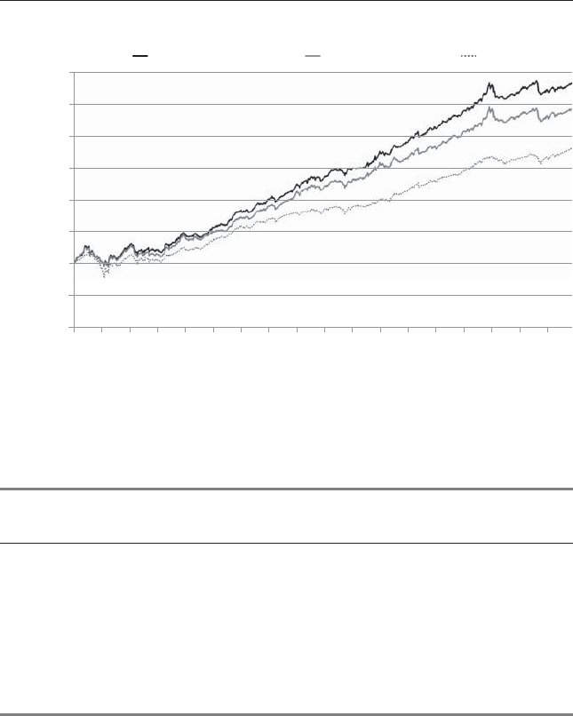
Quantitative Momentum Beats the Market 127

$100,000,000

$10,000,000

$1,000,000

$100,000

$10,000

$1,000

$100

$10

2/1/1927

1/1/1932

12/1/1936

11/1/1941

10/1/1946

9/1/1951

8/1/1956

7/1/1961

6/1/1966

5/1/1971

4/1/1976

3/1/1981

2/1/1986

1/1/1991

12/1/1995

11/1/2000

10/1/2005

9/1/2010

Value of $100 Invested (Log Scale)

Quantitative Momentum (Net) Generic Momentum (Net) SP500

FIGURE 8.2 Cumulative Value for Quantitative Momentum (1927–2014)

TABLE 8.3 CAGR Across Different Decades

Quantitative

Momentum (Net)

Generic

Momentum (Net)

S&P 500

Index

1930–1939 3.08% 1.64% –1.34%

1940–1949 11.01% 11.85% 9.15%

1950–1959 24.98% 21.31% 19.42%

1960–1969 20.50% 18.26% 7.84%

1970–1979 13.93% 13.21% 5.83%

1980–1989 24.48% 17.38% 17.61%

1990–1999 36.48% 30.21% 18.37%

2000–2009 –3.58% –4.88% –0.68%

Figure 8.2 illustrates the effects of compounding an edge over a long

period of time. The quantitative momentum portfolio’s small advantage

leads to a jaw-dropping spread relative to the passive benchmark.

Table 8.3 shows the compound annual growth rates (CAGR) of the

quantitative momentum portfolio and the competition over different

decades. The intent of this test is to examine the robustness of performance

across time.

❦

❦ ❦

❦

128 QUANTITATIVE MOMENTUM

Over eight full decades, the quantitative momentum portfolio

outperformed in seven of the eight. A concern some may have is that

the quantitative momentum portfolio lost in the most recent decade.

Perhaps momentum is dead because the smart arbitrageurs eliminated the

momentum premium? We can never eliminate this possibility; however, a

decade of underperformance is not unexpected. Geczy and Samonov nd

that long periods of poor relative performance occur on multiple occasions

in out-of-sample testing over the 1801 to 1926 time period.7Moreover,

as we explained earlier in the book, sticking to the algorithm is difcult

because of the high volatility and career risk. Second, if one examines the

net of fee results of the equal-weighted quantitative momentum portfolio

(not shown), this portfolio actually outperformed on a CAGR basis over

the 2000–2009 decade. Nonetheless, no sustainable system can work all

the time. And while Figure 8.2 makes quantitative momentum seem like a

“no-brainer,” a deeper dive into shorter windows highlights the fact that

there are periods of extreme relative underperformance over the 1927 to

2014 period. Momentum investing is simple, but not easy.

Here we look at a variety of measures to assess the performance across

rolling periods. Figures 8.3a and 8.3b show the rolling 5- and 10-year

CAGRs for the strategy. These gures show the relevant holding period

return at different points in time. A robust strategy will show consistent

outperformance regardless of timing; a “lucky” strategy may have extreme

outperformance in one time period but ounder in others.

Figures 8.3a and 8.3b illustrate how consistently the strategy beats the

Generic momentum portfolio and the S&P 500 on rolling 5- and 10-year

bases. Only rarely, and for brief periods, was it better to have been invested

in the others. Two periods of long-term underperformance include the Great

Depression period and the most recent period following the 2008 nancial

crisis. This underperformance is to be expected, and appreciated, because

these periods “shake out” weak hands. Over the long haul, a sustainable

process wins out.

Risk Analysis

As the previous analysis emphasizes, the power of momentum is an ability

to generate outsize returns that dwarf returns associated with passive

benchmarks. Unfortunately, outsized expected returns deliver enhanced

risks. The risk and reward trade-off for momentum is still favorable, but not

acknowledging the increased risk would be intellectually dishonest and set

up a prospective momentum investor with the improper expectations. We

examine the risks associated with quantitative momentum in the analysis

that follows.

❦

❦ ❦

❦

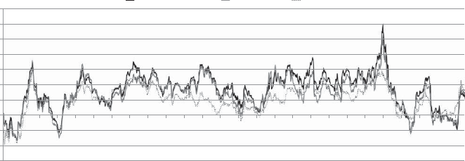
129

70.00%

60.00%

50.00%

40.00%

30.00%

20.00%

10.00%

0.00%

2/1/1932

5/1/1935

8/1/1938

11/1/1941

2/1/1945

5/1/1948

8/1/1951

11/1/1954

2/1/1958

5/1/1961

8/1/1964

11/1/1967

2/1/1971

5/1/1974

8/1/1977

11/1/1980

2/1/1984

5/1/1987

8/1/1990

11/1/1993

2/1/1997

5/1/2000

8/1/2003

11/1/2006

2/1/2010

5/1/2013

2/1/1932

5/1/1935

8/1/1938

11/1/1941

2/1/1945

5/1/1948

8/1/1951

11/1/1954

2/1/1958

5/1/1961

8/1/1964

11/1/1967

2/1/1971

5/1/1974

8/1/1977

11/1/1980

2/1/1984

5/1/1987

8/1/1990

11/1/1993

2/1/1997

5/1/2000

8/1/2003

11/1/2006

2/1/2010

5/1/2013

–10.00%

–20.00%

–30.00%

5-Year Rolling CAGRs

Quantitative Momentum (Net) Generic Momentum SP500

FIGURE 8.3a Five-Year Rolling CAGR for Quantitative Momentum

❦

❦ ❦

❦

130

50.00%

40.00%

30.00%

20.00%

10.00%

0.00%

–10.00%

10-Year Rolling CAGRs

Quantitative Momentum (Net) Generic Momentum (Net) SP500

2/1/1937

2/1/1910

2/1/1943

2/1/1946

2/1/1949

2/1/1952

2/1/1955

2/1/1958

2/1/1961

2/1/1964

2/1/1967

2/1/1970

2/1/1973

2/1/1976

2/1/1979

2/1/1982

2/1/1985

2/1/1988

2/1/1991

2/1/1994

2/1/1997

2/1/2000

2/1/2003

2/1/2006

2/1/2009

2/1/2012

2/1/1937

2/1/1910

2/1/1943

2/1/1946

2/1/1949

2/1/1952

2/1/1955

2/1/1958

2/1/1961

2/1/1964

2/1/1967

2/1/1970

2/1/1973

2/1/1976

2/1/1979

2/1/1982

2/1/1985

2/1/1988

2/1/1991

2/1/1994

2/1/1997

2/1/2000

2/1/2003

2/1/2006

2/1/2009

2/1/2012

FIGURE 8.3b Ten-Year Rolling CAGR for Quantitative Momentum

❦

❦ ❦

❦

Quantitative Momentum Beats the Market 131

Our risk analysis focuses on maximum drawdowns. The maximum

drawdown is dened as the maximum peak to trough loss associated with a

time series. Maximum drawdown captures the worst possible performance

scenario experienced by a buy and hold investor dedicated to a specic

strategy. The intuition behind maximum drawdown is simple: How much

can I lose?

Figure 8.4 shows the summary drawdown performance of quantitative

momentum across commonly assessed horizons of one month, one year, and

three years.

The quantitative momentum strategy protects capital better than the

competition based on the results in Figure 8.4. The strategy’s single-worst

drawdown was worse than the generic momentum strategy, but beat the

S&P 500. However, quantitative momentum did lose over rolling 1- and

12-month periods to the competition. The worst-case scenario for the strat-

egy over a 3-year period was again slightly better than the S&P 500. To be

clear—our portfolio is a long-only strategy, so it is expected to have similar

drawdowns when compared to the market.

Figures 8.5a and 8.5b show the rolling 5- and 10-year maximum draw-

downs for the strategy. These gures help researchers identify the frequency

and intensity of a strategy’s maximum drawdowns over a designated time

horizon (e.g., 5 years or 10 years). But why are rolling drawdowns a use-

ful analytical tool? Consider two strategies with similar worst drawdowns.

If one strategy experiences big drawdowns several times through history,

while the other experiences big drawdowns only once, this analysis helps us

identify this higher frequency of large drawdowns.

MaxDD

Monthly

12-Month

36-Month

Quantitative Momentum (Net) Generic Momentum (Net)

Drawdown Analysis

SP500

–10%

–20%

–30%

–40%

–50%

–60%

–70%

–80%

–90%

FIGURE 8.4 Summary Drawdown Analysis

❦

❦ ❦

❦

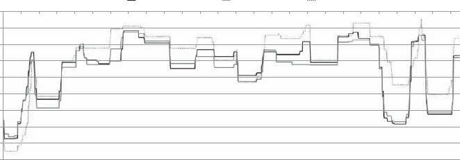
132

0.00%

–10.00%

–20.00%

–30.00%

–40.00%

–50.00%

–60.00%

–70.00%

–80.00%

–90.00%

2/1/1932

5/1/1935

8/1/1938

11/1/1941

2/1/1945

5/1/1948

8/1/1951

11/1/1954

2/1/1958

5/1/1961

8/1/1964

11/1/1967

2/1/1971

5/1/1974

8/1/1977

11/1/1980

2/1/1984

5/1/1987

8/1/1990

11/1/1993

2/1/1997

5/1/2000

8/1/2003

11/1/2006

2/1/2010

5/1/2013

5-Year Rolling MAXDD

Quantitative Momentum (Net) Generic Momentum (Net) SP500

FIGURE 8.5a Five-Year Rolling Max Drawdown for Quantitative Momentum

❦

❦ ❦

❦

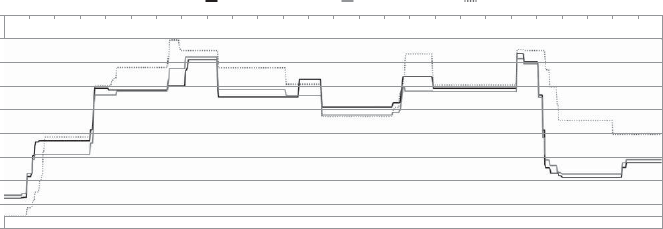
133

2/1/1937

2/1/1940

2/1/1943

2/1/1946

2/1/1949

2/1/1952

2/1/1955

2/1/1958

2/1/1961

2/1/1964

2/1/1967

2/1/1970

2/1/1973

2/1/1976

2/1/1979

2/1/1982

2/1/1985

2/1/1988

2/1/1991

2/1/1994

2/1/1997

2/1/2000

2/1/2003

2/1/2006

2/1/2009

2/1/2012

10-Year Rolling MAXDD

Quantitative Momentum (Net) Generic Momentum (Net) SP500

0.00%

–10.00%

–20.00%

–30.00%

–40.00%

–50.00%

–60.00%

–70.00%

–80.00%

–90.00%

FIGURE 8.5b Ten-Year Rolling Max Drawdown for Quantitative Momentum

❦

❦ ❦

❦

134 QUANTITATIVE MOMENTUM

The rolling drawdown analysis shows that the strategy suffers draw-

downs that can be larger than the competition. For example, in the after-

math of the Internet bubble, quantitative momentum took it on the chin,

especially compared to the broad index. Similarly, in the 2008 nancial

crisis, the quantitative momentum portfolio was hit a bit harder than the

broad index.

Finally, we end our analysis with an assessment of the relative

performance of quantitative momentum during the strategy’s worst 10

drawdowns. We compare the quantitative momentum drawdowns to the

performance of the passive index over the same time period. This analy-

sis gives us insight into the tail-risk correlations between the quantitative

momentum strategy and the passive market. Table 8.4 highlights two points:

First, quantitative momentum is a long-only equity strategy with huge

drawdowns. Second, the drawdowns are correlated with general market

drawdowns. Overall, the quantitative momentum portfolio will have large

drawdowns and periods of underperformance, and one should expect this at

the outset.

Robustness Analysis

In this section, we examine a variety of tests that look at a strategy from

different angles so that we can gain insight into the big picture and ascer-

tain that the summary statistics reect a broad reality that is not driven by

extreme outliers.

We rst analyze market cycle performance of the quantitative momen-

tum strategy compared to the other strategies over a variety of bull and bear

markets since 1927. Table 8.5 shows the dates used to calculate market cycle

returns.

TABLE 8.4 Top 10 Drawdown Analysis

Rank Date Start Date End Quantitative Momentum S&P 500TR Index

1 1/31/1929 5/31/1932 –76.97% –80.67%

2 2/29/2000 2/28/2003 –68.14% –35.14%

3 6/30/2008 2/28/2009 –62.12% –40.82%

4 3/31/1937 3/31/1938 –52.99% –51.11%

5 12/31/1972 9/30/1974 –38.68% –42.73%

6 11/30/1961 6/30/1962 –34.57% –21.97%

7 5/31/1946 6/30/1949 –31.69% –13.77%

8 9/30/1987 11/30/1987 –30.88% –28.00%

9 4/30/1940 4/30/1942 –30.81% –26.52%

10 11/30/1968 6/30/1970 –27.23% –29.23%

❦

❦ ❦

❦

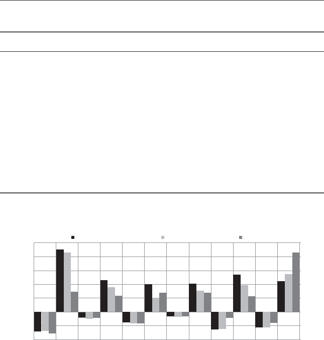
Quantitative Momentum Beats the Market 135

TABLE 8.5 Market Cycle Denitions

Month Begin Month End

Bear September-29 July-32

Bull June-62 February-66

Bear November-68 May-70

Bull May-70 December-72

Bear January-73 September-74

Bull June-82 December-84

Bear July-87 December-87

Bull December-87 June-90

Bear March-00 September-01

Bull October-01 July-07

Bear August-08 February-09

Bull March-09 December-14

Market Cycle Performance

Quantitative Momentum (Net) Generic Momentum (Net) SP500 250%

200%

150%

100%

50%

–50%

–100%

Bear: 9/1929–7/1932

Bull: 6/1962–2/1966

Bear: 11/1968–5/1970

Bull: 5/1970–12/1972

Bear: 1/1973–9/1974

Bull: 6/1982–12/1984

Bear: 7/1987–12/1987

Bull: 12/1987–6/1990

Bear: 3/2000–9/2001

Bull: 10/2001–7/2007

Bear: 8/2008–2/2009

Bull: 3/2009–12/2014

FIGURE 8.6 Market Cycle Performance for Quantitative Momentum

Figure 8.6 demonstrates that, on average, the strategy performed similar

to the S&P 500 in bear markets and outperformed the S&P 500 in bull

markets. Again, relative losses to the S&P 500 appear in the most recent bear

and bull markets. There are surely commentators that claim “momentum is

dead.” Great, we hope this commentary continues. While the strategy may

occasionally struggle for short—or even long—periods of time, momentum

systems provide a high chance of expected outperformance through a full

market cycle.

❦

❦ ❦

❦

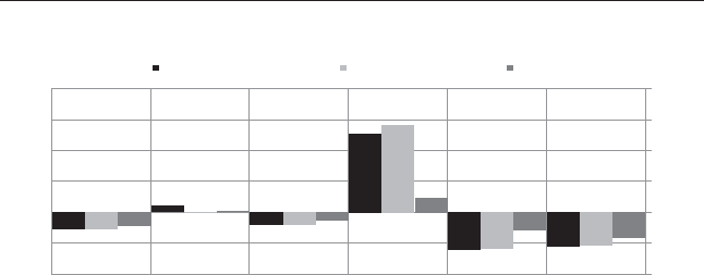
136 QUANTITATIVE MOMENTUM

200%

Short-Term Event Stress Tests

150%

100%

50%

–50%

–100%

Credit Crunch (Sep '08 - Feb '09)

NASDAQ Melt Down (Apr '00 - Sep '01)

NASDAQ Run Up (Jan '99 - Mar '00)

LTCM/Russian Default (Aug '98)

Asian Crisis (Aug '97 - Aug '98)

October 187 Crash

Quantitative Momentum (Net) Generic Momentum (Net) SP500

FIGURE 8.7 Short-Term Stress Event Tests for Quantitative Momentum

Figure 8.7 shows the relative performances during recent short-term

stress events of the quantitative momentum strategy and the other strate-

gies. This analysis examines how a strategy tends to perform through

extraordinary short-term market events. The model shows strong per-

formance compared to the other S&P 500 during the NASDAQ run-up,

but underperformance in the NASDAQ crash in 1998 and the 2008

nancial crisis.

Figures 8.8a and 8.8b show the rolling 5- and 10-year alpha for the

strategy. Alpha analysis is typically found in quantitative research articles

published in academic journals. The procedures researchers use to estimate

alpha can be complicated, but the idea is simple: How much average excess

return does a strategy create after controlling for a variety of risk factors?

To assess robustness, we estimate alpha using several different

asset-pricing models. We control for general market risk using the capital

asset pricing model;8we adjust for market, size, and value exposures with

the Fama and French three-factor model,9and we account for momentum

using the four-factor model.10,11 All of these factors can be found at Ken

French’s website.12

Figures 8.8a and 8.8b conrm that the quantitative momentum strategy

generates relatively consistent alpha estimates on a rolling 5- and 10-year

basis, regardless of the asset pricing model we choose. Not surprisingly,

the four-factor alpha is the smallest, as this model controls for exposure to

generic momentum. On a rolling 5-year basis there are only a few instances

where the strategy’s performance does not add value after controlling

❦

❦ ❦

❦

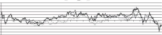
137

CAPM FF 4-Factor

2/1/1932

5/1/1935

8/1/1938

11/1/1941

2/1/1945

5/1/1948

8/1/1951

11/1/1954

2/1/1958

5/1/1961

8/1/1964

11/1/1967

2/1/1971

5/1/1974

8/1/1977

11/1/1980

2/1/1984

5/1/1987

8/1/1990

11/1/1993

2/1/1997

5/1/2000

8/1/2003

11/1/2006

2/1/2010

5/1/2013

2/1/1932

5/1/1935

8/1/1938

11/1/1941

2/1/1945

5/1/1948

8/1/1951

11/1/1954

2/1/1958

5/1/1961

8/1/1964

11/1/1967

2/1/1971

5/1/1974

8/1/1977

11/1/1980

2/1/1984

5/1/1987

8/1/1990

11/1/1993

2/1/1997

5/1/2000

8/1/2003

11/1/2006

2/1/2010

5/1/2013

5-Year Rolling Alphas

30.00%

20.00%

–20.00%

25.00%

–25.00%

15.00%

–15.00%

10.00%

–10.00%

5.00%

–5.00%

0.00%

FIGURE 8.8a

Five-Year Rolling Alpha for Quantitative Momentum

❦

❦ ❦

❦

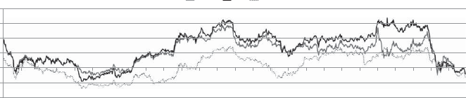
138

2/1/1937

2/1/1940

2/1/1943

2/1/1946

2/1/1949

2/1/1952

2/1/1955

2/1/1958

2/1/1961

2/1/1964

2/1/1967

2/1/1970

2/1/1973

2/1/1976

2/1/1979

2/1/1982

2/1/1985

2/1/1988

2/1/1991

2/1/1994

2/1/1997

2/1/2000

2/1/2003

2/1/2006

2/1/2009

2/1/2012

2/1/1937

2/1/1940

2/1/1943

2/1/1946

2/1/1949

2/1/1952

2/1/1955

2/1/1958

2/1/1961

2/1/1964

2/1/1967

2/1/1970

2/1/1973

2/1/1976

2/1/1979

2/1/1982

2/1/1985

2/1/1988

2/1/1991

2/1/1994

2/1/1997

2/1/2000

2/1/2003

2/1/2006

2/1/2009

2/1/2012

20.00%

15.00%

10.00%

5.00%

0.00%

–5.00%

–10.00%

10-Year Rolling Alphas

CAPM FF 4-Factor

FIGURE 8.8b Ten-Year Rolling Alpha for Quantitative Momentum

❦

❦ ❦

❦

Quantitative Momentum Beats the Market 139

TABLE 8.6 Asset Pricing Coefcient Estimates for Quantitative Momentum

Annual Alpha MKT-RF SMB HML MOM

CAPM 6.30% 1.02 —— —

Three-Factor 7.44% 1.05 0.17 –0.41 —

Four-Factor 0.85% 1.17 0.21 –0.16 0.55

for risk. The 10-year rolling chart tells the story vividly: Over the long-term,

quantitative momentum has generally added value for investor portfolios.

In this section, we calculate the formal beta estimates and alpha

estimates associated with our kitchen sink of asset pricing models. Table 8.6

shows the full sample coefcient estimates for the four asset-pricing

models. MKT-RF represents the excess return on the market-weight

returns of all New York Stock Exchange (NYSE)/American Stock Exchange

(AMEX)/NASDAQ stocks. SMB is a long/short factor portfolio that

captures exposures to small capitalization stocks. HML is a long/short

factor portfolio that controls for exposure to high book value-to-market

capitalization stocks. MOM is a long/short factor portfolio that controls

for exposure to stocks that have had great performance over the recent year.

The results are tabulated in Table 8.6 and coefcient estimates that are

signicant at the 5 percent condence level (two-tailed tests) are bolded.

Table 8.6 suggests that quantitative momentum generates between

approximately 6 or 7 percent per year in “alpha,” or performance not

explained by exposures to known expected return factors such as the

market, size, and value. When including the generic momentum factor,

the quantitative momentum portfolio does not provide any signicant

alpha, but does load positively on the momentum factor (MOM). The

alpha analysis suggests that the quantitative momentum strategies stronger

performance is related to higher beta exposure than the broader market

(MKT-RF beta slightly above 1), the system tends to be exposed to smaller

stocks (0.17 and 0.21 on the SMB factor), and very importantly, is not

value (HML is –0.41 and –0.16). If we compare the alpha statistics against

the generic momentum strategy, the relationship between HML is less

negative (i.e., diversication benets are not as high). Overall, from a factor

analysis perspective, quantitative momentum is no better or worse than

generic momentum, the strategy is simply different: The strategy delivers

ahigherbetaversionofthegenericmomentumstrategythatalsohasa

stronger diversication benetwhencoupledwithvaluestrategies.While

factor analysis is important, we believe this assessment should be coupled

with the results presented in Table 8.2, which reect more customary—and

intuitive—analytics.

❦

❦ ❦

❦

140 QUANTITATIVE MOMENTUM

A PEEK INSIDE THE BLACK BOX

Quantitative methods are often considered black box, and thus, shunned

by many in the investment community. Quants generally have earned the

negative assessment. Traditional “quants” make things too complex and

too opaque, when communication can be simple and radically transparent.

The logic portrayed is that by keeping strategies “proprietary,” the quants

can keep their intellectual property from being exploited and their investors

will be better off. In the context of unsustainable, always changing, trading

strategies, this result is certainly true. However, when discussing sustainable,

highly active long-term investment strategies, opacity and a general lack of

understanding lead to investor failure. At the pinnacle point of pain, when

the most disciplined and hardened active investors earn their keep, the active

investor with a clear mind, thorough understanding, and a strong conviction

for their process will win. Those who do not fully understand why a process

works are more likely to provide the active alpha to the clairvoyant investor

who can hold on to an active portfolio like grim death.

Table 8.7 lists the top 10 stocks selected by the model on November

30, 2014. This date would be the last rebalance of the portfolio in our

tests, which takes advantage of the seasonality by rebalancing at the end

of November 2014—since we hold the portfolio for three months, this ends

up being the portfolio as of December 31, 2014, as well. Table 8.7 also high-

lights the important summary statistics, such as the rm’s momentum score

(total return over the past twelve months ignoring the recent month), and

the percentage of positive days minus the percentage of negative return days

(remember, this is used to create the frog-in-the-pan variable).

Many of the names listed are well established, but they aren’t neces-

sarily the most exciting high-momentum names in the universe. A lot of

TABLE 8.7 December 31, 2014, Quantitative Momentum Portfolio Holdings

Stock Name Ticker Momentum (% Positive) – (% Negative)

International Rectier Corp. IRF 66.1% 24.3%

Marriott International Inc. MAR 62.6% 22.3%

N X P Semiconductors N V NXPI 61.6% 21.5%

Sandisk Corp SNDK 39.8% 21.1%

Dr. Pepper Snapple Group Inc. DPS 47.7% 20.3%

Southwest Airlines Co. LUV 87.0% 19.1%

Dynegy Inc. DYN 42.5% 18.3%

Pilgrims Pride Corp New PPC 73.4% 18.3%

Windstream Holdings Inc. WIN 44.7% 17.9%

Mallinckrodt Plc. MNK 77.4% 17.9%

❦

❦ ❦

❦

Quantitative Momentum Beats the Market 141

these rms are somewhat boring, but their price signals are highlighting that

there is a sustained amount of positive news driving their momentum. This

group of rms is in contrast to some of the higher prole momentum names

that do not make the cut: these include Tesla Motors, Monster Beverage,

Amgen, Green Mountain Coffee, and Solarwinds. All of these rms have

high momentum, but their path to momentum is more discrete and has come

via large short-term spikes in performance.

BEATING THE MARKET WITH QUANTITATIVE MOMENTUM

Momentum is clearly robust and has been studied and documented for many

years. The epitome of this sort of research was completed by Chris Geczy

and Mikhail Samonov, who conrm momentum’s historical track record via

an individual stock dataset that is over 200 years in length, stating “that

the momentum effect is not a product of data-mining.”13 In this chapter,

we present the results of our quantitative momentum system, which is a

reection of the research and concepts outlined in this book. Our solution

does not claim to be the “best” or the most “optimized,” but we do think

our process is reasonable and ties back to behavioral nance in a coherent

and logical way.14 But will the process work in the future? Nobody knows,

but recall in the rst four chapters of the book that we outlined a frame-

work for determining whether a historically strong strategy is sustainable

into the future. How can we be sure momentum is sustainable? We support

this proposition using the same arguments we use to understand why value

investing works. Namely, sustainable active investment strategies require the

following ingredients:

■A mispricing component

■A costly arbitrage component

As far as mispricing is concerned, as long as human beings suffer from

systematic expectation errors, prices will sometimes deviate from fundamen-

tals. In the context of value, this expectation error seems to be an overre-

action to negative news, on average; for momentum, the expectation error

is likely tied to an underreaction to positive news and predictable seasonal

effects. Value and momentum are really two sides of the same behavioral

bias coin.

But why aren’t momentum strategies (or value strategies) exploited

by all smart investors and arbitraged away? As we discussed, the speed

at which these mispricing opportunities are eliminated depends on the

cost of exploitation. Putting aside an array of transaction and information

❦

❦ ❦

❦

142 QUANTITATIVE MOMENTUM

acquisition costs (which are nonzero, but we will assume don’t matter for

the purpose of this argument), the biggest cost to exploiting long-lasting

mispricing opportunities are agency costs, or career risk concerns. The

career risk aspect is created because investors delegate a professional to

manage their capital on their behalf. Unfortunately, the investors that

delegate their capital to the professional fund managers often assess

the performance of their hired manager based on their short-term relative

performance to a benchmark. But this creates a warped incentive for

the professional fund manager. On the one hand, the fund manager wants

to exploit mispricing opportunities because of the high expected long-term

performance, but on the other hand, they can do so only to the extent to

which exploiting the mispricing opportunities does not cause their expected

performance to deviate too far—and/or for too long—from a standard

benchmark. In summary, strategies like value and momentum presumably

will continue to work because they sometimes fail spectacularly relative to

passive benchmarks. And if we follow along this line of reasoning, we only

need to assume the following to believe that momentum strategies, like

value strategies, are sustainable:

■Investors will continue to suffer behavioral bias.

■Investors who delegate will be short-sighted performance chasers.

We think these are two assumptions we can rely on for the foreseeable

future. And because of our faith in these assumptions, we believe there will

always be opportunities for process-driven, long-term focused, disciplined

investors. If we can internalize the lessons from the sustainable active frame-

work, our belief in this framework will grant us the discipline to stick with

strategies that many investors nd extremely uncomfortable. The ability to

stay disciplined to a process is arguably the most important aspect of being

a successful investor. How one actually invests is almost a secondary issue.

But as is highlighted in a quote attributed to Warren Buffett, “Investing is

simple, but not easy.”

NOTES

1. James Simmons, “Mathematics, Common Sense, and Good Luck: My Life and

Career,” MIT Seminar, January 24, 2011.

2. Cliff Asness, Andrea Frazzini, Ron Israel, and Toby Moskowitz, “Fact, Fiction,

and Momentum Investing,” The Journal of Portfolio Management 40 (2014):

75–92.

3. Andrea Frazzini, Ronen Israel, and Toby Moskowitz, “Trading Costs of Asset

Pricing Anomalies,”AQR working paper, 2014.

❦

❦ ❦

❦

Quantitative Momentum Beats the Market 143

4. David A. Lesmond, Michael J. Schill, and Chunsheng Zhou, “The Illusory

Nature of Momentum Prots,” Journal of Financial Economics 71 (2004):

349–380.

5. Similar to the end of Chapter 7, our analysis start date changes slightly from

January 1, 1927, to March 1, 1927, to facilitate the seasonal rebalance.

6. William Beaver, Maureen McNichols, and Richard Price, “Delisting Returns and

Their Effect on Accounting-based Market Anomalies,” Journal of Accounting

and Economics 43 (2007): 341–368.

7. Chris Geczy and Mikhail Samonov, “Two Centuries of Price Return Momen-

tum,” Financial Analysts Journal (2016).

8. William F. Sharpe, “Capital Asset Prices: A Theory of Market Equilibrium under

Conditions of Risk,” Journal of Finance 19(3) (1964): 425–442.

9. Eugene Fama and Kenneth French, “Common Risk Factors in the Returns on

Stocks and bonds,” Journal of Financial Economics 33 (1993): 3–56.

10. Mark Carhart, “On Persistence in Mutual Fund Performance,” Journal of

Finance 52 (1997): 57–82.

11. We also conduct analysis using the Fama and French ve-factor model, which

includes protability and investment factors. Since these factors are only avail-

able after 1963, we do not show these results in our calculations. In out-of-

sample tests (1963–2014), we include the 5-factor model and nd qualitatively

similar results.

12. mba.tuck.dartmouth.edu/pages/faculty/ken.french/data_library.html, accessed

3/1/2016.

13. Chris Geczy and Mikhail Samonov.

14. We have conducted many additional tests and analysis not mentioned in this

chapter. Please contact the authors at www.alphaarchitect.com/contact for addi-

tional results (e.g., annual returns).

❦

❦ ❦

❦

CHAPTER 9

Making Momentum Work in

Practice

“Everyone has a plan until they get punched in the mouth.”

—Attributed to “Iron” Mike Tyson

In the real world, going all-in on quantitative momentum is sure to try the

patience of even the most dedicated investor. Nobody has the discipline

to stick with the program—including us. We don’t even invest our own

capital this way. But we aren’t recommending that investors replace their

entire equity portfolio with a high-conviction momentum strategy. Momen-

tum is merely a component of a diversied equity portfolio. And as alluded

to in Chapter 4, momentum portfolios are best used in combination with

high-conviction value portfolios. The value and momentum combination

portfolio shortens stretches of multiyear relative underperformance associ-

ated with both stand-alone strategies and allows an investor to stick with an

equity investment program. Dedicating oneself to pure value investing or to

pure momentum investing is akin to sitting on a one-legged stool. So why not

sit on a stool with multiple legs? Identify a great value investment approach;

identify a promising momentum investment approach; and combine the two

efforts to serve as your all-weather equity portfolio.

A TWO-LEGGED STOOL: VALUE +MOMENTUM

To make the value and momentum combination portfolio more tangible,

we examine the approach we use for our own investment capital. We

combine the quantitative momentum algorithm outlined in this book with

an equally rigorously tested value strategy outlined in Wes’s book on the

subject of building systematic value strategies: Quantitative Value.1Put

144

❦

❦ ❦

❦

Making Momentum Work in Practice 145

simply, the quantitative value algorithm seeks to buy cheap, high-quality

value stocks. Each strategy typically holds around 40 momentum stocks

and 40 value stocks, leaving the investor with a high-conviction—but

diversied—portfolio of approximately 80 stocks. One could expand to

international markets to increase the portfolio size and enhance diversi-

cation, but we shelve that discussion to keep the analysis short and to

the point.

To assess performance of our quantitative value and momentum port-

folio, we examine a mid- to large-cap US traded universe and we focus

our analysis on the long-only portfolios. The portfolios are quarterly rebal-

anced and equal-weighted—here we deviate from the value-weight portfo-

lios shown in Chapter 8. We examine the returns from January 1, 1974,

to December 31, 2014, which is the time period when the historical data

available for the quantitative momentum and quantitative value algorithm

overlap. The combination portfolio weights are annually rebalanced on Jan-

uary 1 each year and equally allocated across value and momentum (a more

sophisticated investor could volatility-weight the exposures). All returns are

net of 2 percent in total annual fees, which is a rough estimate of manage-

ment fees, commissions, and market impact costs associated with rebalanc-

ing within and across the strategies.2

The results of the combination portfolio are presented in Table 9.1.

The combination portfolio has higher returns than either the stand-alone

value or momentum portfolios. On a risk-adjusted basis, the combination

portfolio is essentially equivalent to the quantitative value strategy. How-

ever, the summary statistics do not capture the survivability of a strategy.

To assess survivability, which we loosely dene as the degree to which an

TABLE 9.1 Combining Quantitative Value and Quantitative Momentum

Combination

Portfolio (Net)

Quantitative

Momentum

(Net)

Quantitative

Value

(Net)

S&P 500

TR Index

CAGR 18.10% 17.38% 16.98% 11.16%

Standard Deviation 21.38% 25.59% 18.58% 15.45%

Downside Deviation 14.96% 18.09% 12.71% 11.05%

Sharpe Ratio 0.66 0.57 0.68 0.45

Sortino Ratio (MAR =5%) 0.94 0.80 0.98 0.62

Worst Drawdown –60.16% –67.72% –51.91% –50.21%

Worst Month Return –26.56% –30.33% –25.62% –21.58%

Best Month Return 28.69% 34.67% 25.36% 16.81%

Protable Months 61.18% 61.79% 62.60% 61.59%

❦

❦ ❦

❦

146 QUANTITATIVE MOMENTUM

investor could hold onto a portfolio without “giving up,” we review the

rolling ve-year CAGRs relative to the passive S&P 500 total return index.

This analysis gives us a sense for how holding value and momentum can

minimize the frequency of long periods of underperformance associated with

stand-alone value or momentum.

Figure 9.1 highlights the benetofcombiningvalueandmomentumto

minimize the length and depth of ve-year relative underperformance peri-

ods. For example, quantitative value endures a deep and extended period of

poor relative performance in the late 1990s during the Internet bubble. On

the ip side, post–nancial crisis, quantitative momentum has had a long

bout of severe underperformance. To be clear, quantitative momentum, on a

standalone basis, had a period of underperforming by about 15 percent on a

CAGR basis over ve years (occurs in June 2013, so the 2008–2009 nancial

crisis is in this ve-year previous period). Imagine having that conversation

with your clients!

However, by combining the two strategies (represented by the solid

black line in Figure 9.1), an investor is able to shorten the length and depth

of long-term underperformance to a level that is more digestible to the

average investor. Another way to look at this problem is via a histogram

analysis. Figure 9.2 shows the histogram of ve-year relative performance

measured by CAGR for the pure momentum strategy and the combination

portfolio. There is a relatively frequent probability of losing to the index

over a ve-year window when invested in a pure momentum strategy;

however, the combination portfolio substantially limits the chance for a

long-winded underperformance streak.

For the long-horizon investor, replacing a passive equity portfolio with

ahigh-convictionvalueandmomentumsystemseemslikeareasonable

approach that can deliver strong expected returns relative to a passive

index. We leave the reader with an easy to remember rule of thumb:

Buy ’em cheap; buy ’em strong; and hold ’em long.

An Important Note on Portfolio Construction

The road to success with active value and momentum will obviously be

hair-raising, primarily because the possibility of poor long-term relative per-

formance prevents large pools of capital from exploiting the opportunity.

With that truth in hand, we must emphasize that the expected benets out-

lined are associated with high-conviction value and momentum portfolios,

because these high-conviction portfolios drive the relative performance risk.

And if there is no extreme relative performance pain, there is no extreme

expected performance gain. So-called “smart beta” funds, which hold large

❦

❦ ❦

❦

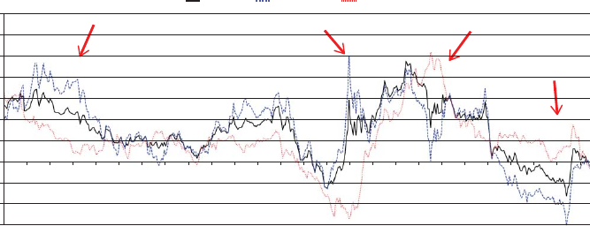
147

5-Year Rolling CAGR Relative to the Index

Combo (net) Quant Mom (net) Quant Value (net)

35.00%

30.00%

25.00%

0.00%

12/1/1978

5/1/1980

10/1/1981

3/1/1983

8/1/1984

1/1/1986

6/1/1987

11/1/1988

4/1/1990

9/1/1991

2/1/1993

7/1/1994

12/1/1995

5/1/1997

10/1/1998

3/1/2000

8/1/2001

1/1/2003

6/1/2004

11/1/2005

4/1/2007

9/1/2008

2/1/2010

7/1/2011

12/1/2012

5/1/2014

12/1/1978

5/1/1980

10/1/1981

3/1/1983

8/1/1984

1/1/1986

6/1/1987

11/1/1988

4/1/1990

9/1/1991

2/1/1993

7/1/1994

12/1/1995

5/1/1997

10/1/1998

3/1/2000

8/1/2001

1/1/2003

6/1/2004

11/1/2005

4/1/2007

9/1/2008

2/1/2010

7/1/2011

12/1/2012

5/1/2014

–5.00%

–10.00%

–15.00%

5.00%

10.00%

15.00%

20.00%

FIGURE 9.1 Rolling Five-Year Spreads

❦

❦ ❦

❦

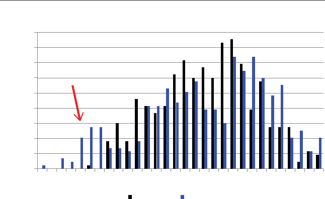
148 QUANTITATIVE MOMENTUM

5-Year Rolling CAGR Relative to Index

Frequency (percentage)

9.00%

8.00%

7.00%

6.00%

5.00%

4.00%

3.00%

2.00%

1.00%

0.00%

–13.75%

–12.50%

–11.25%

–10.00%

–8.75%

–7.50%

–6.25%

–5.00%

–3.75%

–2.50%

–1.25%

0.00%

1.25%

1.50%

3.75%

5.00%

6.25%

7.50%

8.75%

10.00%

11.25%

13.75%

15.00%

16.25%

17.50%

18.75%

20.00%

–21.25%

Combo (net) Quant Mom (net)

FIGURE 9.2 Histogram of Five-Year Spreads

diversied portfolios that tilt towards a characteristic like value or momen-

tum, are unlikely to deliver on their promise to achieve outperformance after

fees. These funds are nothing more than closet indexing structures that don’t

deliver enough active exposure benets to outweigh their expected costs.

But why avoid closet-indexing? Recall that the academic research and

internal analysis we’ve conducted throughout this book are associated with

portfolios that are concentrated on stocks with a desirable characteristic

(e.g., high momentum). The portfolios we analyze are typically designed to

hold less than 50 stocks to minimize “diworsication,” which occurs when

aportfolioisconstructedtobehavemorelikeapassiveindexandlesslike

aconcentratedcharacteristic-centricportfolio.Wehighlightedthenegative

effects of diworsication in Chapter 5 when we examined how portfolio

construction parameters, such as the number of holdings and rebalance

frequency, affect expected performance. The results from that analysis were

clear for those who wanted to capture the expected returns associated

with active momentum strategies: buy concentrated frequently rebalanced

portfolios.

So why don’t we see more truly active funds in the market? Unfortu-

nately, the interests of fund sponsors are not aligned with fund investors.

Above a certain fund size, additional fund assets erode performance as port-

folios move towards closet-indexing formations, but also grow manager fees.

This creates a conict of interest between investors, who want to maximize

performance, and managers, who just want more assets, even when this

❦

❦ ❦

❦

Making Momentum Work in Practice 149

hurts their performance.Closet-indexersareeasytospot—theirportfolios

typically have over 100 holdings, have market-cap weighted construction,

and have low frequency rebalancing. These portfolios constructs accommo-

date scale and facilitate asset collection efforts on behalf of the fund sponsor,

but they are unlikely to deliver the higher expected returns documented

throughout this book. The implicatons for active investors are clear: If one

is going to deviate from a passive index, and pay extra management fees,

embrace active risk and pay up for concentration, not closet-indexing.

A THREE-LEGGED STOOL: COMBO +TREND

But wait a minute: Even a two-legged stool isn’t completely stable! The quan-

titative value and momentum portfolio still suffer large drawdowns that go

hand-in-hand with buy-and-hold equity investments. For many investors,

with a long-horizon and a preference for simplicity, holding the combina-

tion value and momentum portfolio is a great equity solution. But for those

investors concerned about massive drawdowns, a buy-and-hold value and

momentum approach may not be appropriate. And to be clear, the large

drawdowns identied in the value and momentum approach outlined above

are not unique to this particular portfolio—the drawdown issue is associated

with all long-only stock portfolios.

To address the drawdown issue we discuss a basic way in which an

investor can create a more stable stool via a third leg—trend following. The

simplest trend-following rule is the long-term simple moving average rule.

To give the reader a taste for how this can work, consider the following rule:

■Moving average (12) =Average 12 month prices

■If S&P 500 TR Index – 12-month moving average (S&P 500 TR Index)

>0, go long the combination portfolio. Otherwise, go long safety

(T-bills).

The results of applying a simple trend-following risk management

overlay to the quantitative value and momentum portfolio are tabulated in

Table 9.2.

The trend-following overlay doesn’t enhance the risk-adjusted metrics

of the combination portfolio, but this analysis misses the dramatic shift

in the tail-risk prole of the combination system. The trend overlay limits

the exposure of the equity portfolio to large drawdowns. For example, the

maximum drawdown goes from 60.16 percent to 26.18 percent. Of course,

there are no free lunches—the trend-following investor gives up 1.5 per-

cent per year in compounded annual returns and the chance of enduring a

❦

❦ ❦

❦

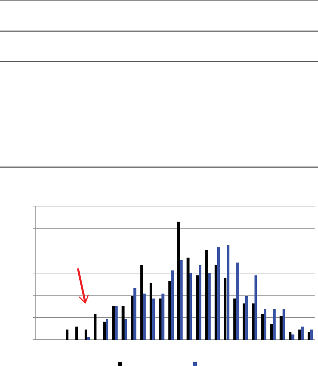
150 QUANTITATIVE MOMENTUM

TABLE 9.2 Combining Quantitative Value and Quantitative Momentum

Combination

w/Trend (Net)

Combination

(Net)

S&P 500

TR Index

CAGR 16.57% 18.10% 11.16%

Standard Deviation 17.97% 21.38% 15.45%

Downside Deviation 13.31% 14.96% 11.05%

Sharpe Ratio 0.67 0.66 0.45

Sortino Ratio (MAR =5%) 0.90 0.94 0.62

Worst Drawdown –26.18% –60.16% –50.21%

Worst Month Return –25.45% –26.56% –21.58%

Best Month Return 28.69% 28.69% 16.81%

Protable Months 70.93% 61.18% 61.59%

5-Year Rolling CAGR Relative to Index

Frequency (percentage)

8.00%

10.00%

12.00%

6.00%

4.00%

2.00%

0.00%

–13.75%

–12.50%

–11.25%

–10.00%

–8.75%

–7.50%

–6.25%

–5.00%

–3.75%

–2.50%

–1.25%

0.00%

1.25%

1.50%

3.75%

5.00%

6.25%

7.50%

8.75%

10.00%

11.25%

13.75%

15.00%

16.25%

17.50%

18.75%

20.00%

–21.25%

Combo w/Trend (net) Combo (net)

FIGURE 9.3 Histogram of 5-Year Spreads

bout of poor relative underperformance is enhanced with a trend-following

approach. Figure 9.3 shows the histogram of ve-year spreads between the

combination portfolio with trend following and the buy-and-hold combina-

tion portfolio.

Figure 9.3 highlights the “relative performance risk” of trend following.

On one hand, trend following protects against large tail-risk events, but the

system also enhances the tracking error relative to the index, which increases

the chances that an investor will not be able to stick to the investment pro-

gram over the long haul.

❦

❦ ❦

❦

Making Momentum Work in Practice 151

While not the focus of this book, we encourage investors concerned

about large equity drawdowns to read more about trend following. We can

also augment our rule of thumb to accommodate trend following:

Buy ’em cheap; buy ’em strong; and hold ’em long ...

but only when the trend is your friend.

CAREER RISK CONSIDERATIONS

Trend following, which serves to minimize the expected impact of

massive drawdowns, makes the potential for relative pain more likely.

Downside-protected strategies can underperform over ve-year periods on

acompoundreturnbasiswithhigherfrequencyandwithmoredepththan

buy-and-hold approaches. So while there are huge potential benets of

trend following, there are associated career risk considerations. In the end,

how much an investor dedicates to more active exposures really depends on

the willingness of an investor to eat periods of relative underperformance.

For some, relative performance is irrelevant; for others facing career risk

concerns, relative performance rules the day. The irony of this discussion is

that the efcient market hypothesis is right—there are no free lunches—but

the explanation is wrong (i.e., stock prices always reect fundamentals).

We’ve already highlighted that strategies like value and momentum are

areection of a world with mispricing. However, there is still no free

lunch. Markets are extremely competitive, and many investment risks, to

include things like “relative performance risk,” are priced risks in the real

world. Financial economic models might consider the relative risk premium

“alpha,” but to many market participants, relative performance risk is a

real, quantiable risk that marginal price setters will pay someone to take

off their hands.

Risk, it seems, is in the eyes of the beholder.

WHAT IF I CAN’T HANDLE POOR RELATIVE

PERFORMANCE?

Figure 9.1 highlights that even a concentrated value and momentum portfo-

lio can sustain ve-year periods of underperformance (e.g., Internet bubble

period and the post-2008 nancial crisis era). For many investors, this is

simply too much pain to endure, and any excess expected returns associated

with a willingness to bear that sort of “relative pain” are fairly earned by

those who have the stomach to deal with it. And a trend-following overlay

❦

❦ ❦

❦

152 QUANTITATIVE MOMENTUM

only makes the chance of enduring a long-stretch of relative pain even worse!

The ultimate solution is to eliminate barriers and accept relative performance

pain, but as we’ve discussed throughout this book, career risk concerns and

psychology problems prevent many investors from fully exploiting sustain-

able active strategies. After all, this is the reason certain active strategies

work in the rst place—they’re tough to follow!

We recognize that the high-conviction solution can never be deployed

by a large swath of the investing public. Nonetheless, not all is lost,

as investors have varying tolerances for relative performance pain. A

majority of investors can’t hold high conviction value and momentum,

but some investors can add a small piece of high conviction value and

momentum and bolt it on their passive allocation to the market. For

example, consider a nancial adviser who has a fairly sophisticated client

base, but these clients have limited assessment horizons and cling to

benchmarks. Large deviations from a benchmark—even with smarter

clients—can create angry clients very quickly: “Hey Mr. Adviser, why

are we losing by 10 percentage points relative to the S&P 500 index

this quarter? You’re red!” But maybe a smaller deviation (e.g., 2 per-

centage points off the S&P 500) is less of an issue? Perhaps the adviser

can survive the client performance meeting and explain why the risk of

underperformance is the cost of admission to longer-term expected outper-

formance. For investors in this situation, a core-satellite approach may be

warranted.

The core-satellite approach works as follows: The approach dedicates

alargechunkofcapitaltoapassivebenchmarkstrategy(the“core”)and

only adds a small component of an active strategy around the edges (the

“satellite”). By construction, a core-satellite approach will never deviate

too far from a benchmark. For example, in Figure 9.4 we create a port-

folio that is 80 percent allocated to the S&P 500 and 20 percent allocated

to the quantitative value and momentum portfolio described in the prior

section.

The gure shows that the core-satellite approach cannot eliminate rela-

tive pain. The core-satellite investor would still need to endure pain during

the Internet bubble period and the post-2008 nancial crisis period, but the

pain is more tolerable. Of course, the downside of the core-satellite approach

is a much lower long-term expected compounding rate than an undiluted

combination approach (see the “Combination (Net)” column relative to the

“Core-Satellite (Net)” column in Table 9.3, which outlines the summary

statistics from 1974 to 2014).

❦

❦ ❦

❦

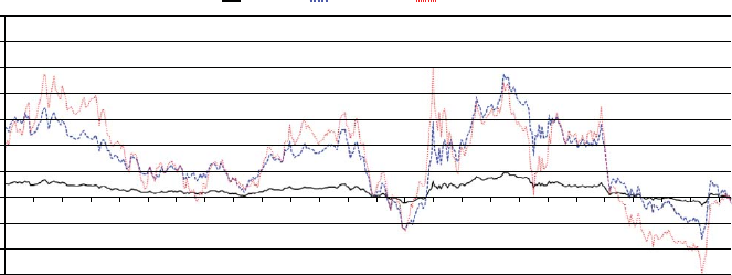
153

35.00%

30.00%

25.00%

0.00%

12/1/1978

5/1/1980

10/1/1981

3/1/1983

8/1/1984

1/1/1986

6/1/1987

11/1/1988

4/1/1990

9/1/1991

2/1/1993

7/1/1994

12/1/1995

5/1/1997

10/1/1998

3/1/2000

8/1/2001

1/1/2003

6/1/2004

11/1/2005

4/1/2007

9/1/2008

2/1/2010

7/1/2011

12/1/2012

5/1/2014

12/1/1978

5/1/1980

10/1/1981

3/1/1983

8/1/1984

1/1/1986

6/1/1987

11/1/1988

4/1/1990

9/1/1991

2/1/1993

7/1/1994

12/1/1995

5/1/1997

10/1/1998

3/1/2000

8/1/2001

1/1/2003

6/1/2004

11/1/2005

4/1/2007

9/1/2008

2/1/2010

7/1/2011

12/1/2012

5/1/2014

–5.00%

–10.00%

–15.00%

5.00%

10.00%

15.00%

20.00%

5-Year Rolling CAGR Relative to the Index

Combo (net) Quant Mom (net) Quant Value (net)

FIGURE 9.4 Histogram of Five-Year Spreads

❦

❦ ❦

❦

154 QUANTITATIVE MOMENTUM

TABLE 9.3 Core-Satellite Returns

Core-Satellite

(Net)

Combination

(Net)

Quantitative

Momentum

(Net)

S&P 500

TR Index

CAGR 12.66% 18.10% 17.38% 11.16%

Standard Deviation 16.04% 21.38% 25.59% 15.45%

Downside Deviation 11.48% 14.96% 18.09% 11.05%

Sharpe Ratio 0.52 0.66 0.57 0.45

Sortino Ratio (MAR =5%) 0.72 0.94 0.80 0.62

Worst Drawdown –51.86% –60.16% –67.72% –50.21%

Worst Month Return –22.35% –26.56% –30.33% –21.58%

Best Month Return 16.52% 28.69% 34.67% 16.81%

Protable Months 61.79% 61.18% 61.79% 61.59%

NOTES

1. Wesley Gray and Tobias Carlisle, Quantitative Value: A Practitioner’s Guide

to Automating Intelligent Investment and Eliminating Behavioral Errors,

(Hoboken, NJ: John Wiley & Sons, 2012).

2. We increase the total fee from 1.80 percent in Chapter 8 to 2.00 percent in

Chapter 9 to account for higher transaction costs associated with running an

equal-weight portfolio, as well as annually rebalancing between the quantitative

momentum and quantitative value portfolios.

❦

❦ ❦

❦

APPENDIX A

Investigating Alternative

Momentum Concepts

We’ve spent multiple years trying to understand how to capture a

sustainable long-term momentum premium. Although this book is

essentially a summary of our efforts, it is not meant to be a literature review

of momentum. If we went down that route, the book would be over a

thousand pages long and the reader would still be left with the question we

try to answer in this book: What is the “best” momentum strategy? Indeed,

anyone who takes the time to review the entire literature on momentum

might reasonably arrive at different conclusions. Nonetheless, because we

read every research paper we could nd on momentum, we thought we

should share the most interesting ideas, and why we chose to not include

them in our quantitative momentum process. We hope this will assist our

readers to better understand why we think our approach makes the most

sense as compared with the variations we discuss below. All of the results

presented use the same universe of stocks used through the book and the

focus is on long-only strategies.

The ideas presented and analyzed are as follows:

■How is momentum related to fundamentals?

■Is the 52-week high a better momentum signal?

■Can absolute strength improve relative strength momentum?

■Can the volatility of momentum be constrained?

■Do we even need stock selection momentum?

While there are many other interesting and promising ideas associated

with momentum, these appear to be the core areas that we identied that

were the most reasonable and compelling. We also hope to explain why, at

the margin, we think our approach is superior to these alternatives.

155

❦

❦ ❦

❦

156 INVESTIGATING ALTERNATIVE MOMENTUM CONCEPTS

HOW IS MOMENTUM RELATED TO FUNDAMENTALS?

In 1998, Nicholas Barberis, Andrei Shleifer, and Robert Vishny1published

atheoreticalmodeloninvestorsentiment,whichdescribedthepossibility

that behavioral biases drive underreaction and overreaction, which lead to

value and momentum effects. Value is essentially an overreaction to bad

news; momentum is an underreaction to good news. In a 1996 empirical

paper, Louis Chan, Narisimhan Jegadeesh, and Josef Lakonishok2nd that

the momentum anomaly is arguably driven, in part, by a sluggish response

to past news. In their own words, “Security analysts’ earnings forecasts ...

respond sluggishly to past news, especially in the case of stocks with the

worst past performance. The results suggest a market that responds only

gradually to new information.” Sometimes such new information is reected

in fundamentals.

Robert Novy-Marx takes the relationship between fundamentals

and momentum a bit further. In a working paper titled, “Fundamentally,

Momentum Is Fundamental Momentum,”3Novy-Marx tries to understand

why momentum strategies have historically outperformed. He nds that

price momentum is a manifestation of the earnings momentum anomaly.

In other words, the momentum anomaly works because investors system-

atically underreact to earnings surprises. Novy-Marx then shows that after

controlling for earnings momentum, price-based momentum is no longer

“anomalous.”

We investigate the results presented by Novy-Marx and discuss them

below. Let’s rst review the concept of price and earnings momentum, and

how portfolios based on these two strategies are formed:

■Price momentum: Stocks with the strongest past price performance tend

to outperform those with the weakest past price performance. Portfolios

are formed based on the past 12 months’ performance, while ignoring

the most recent month to avoid short-term reversals. This strategy is

what we recommend as the baseline “momentum” screen in our book

and is the typical way academic researchers describe momentum.

■Earnings momentum: Stocks with strong past earnings surprises out-

perform those with weak past earnings surprises. Earnings momentum

portfolios are formed based on past earnings surprises. Earnings surprise

is measured via two ways in the Novy-Marx paper:

1. Standardized unexpected earnings (SUE): SUE is dened as the

most recent year-over-year change in earnings per share, scaled by

the standard deviation of the earnings changes over the last eight

announcements.

❦

❦ ❦

❦

Investigating Alternative Momentum Concepts 157

2. Cumulative three-day abnormal returns (CAR3): CAR3 is dened as

the cumulative return in excess of the market over the three days

starting the day before the most recent earnings announcement and

ending at the end of the day following the announcement.

Using the portfolio construction outlined, Novy-Marx examines

cross-sectional (Fama-MacBeth) regressions of a rms’ returns on both

past performance and earnings surprises. The results suggest that price

momentum can be largely explained by earnings momentum.

Next, Novy-Marx looks at three long/short factor portfolios:

■UMD =long high-price momentum and short low-price momentum

stocks

■SUE =long high SUE and short low SUE stocks

■CAR3 =long high CAR3 and short low CAR3 stocks

To compare across the strategies, the long/short portfolios are all set to

have the same volatility (we scale them to match UMD) using our universe

of mid/large cap stocks. Mechanically, this means that leverage is deployed

to enhance the volatility of strategies with lower natural leverage (e.g., SUE

and CAR3) to match the natural volatility of the long/short price momentum

$10,000,000

Value of $100 Invested (Log Scale)

$1,000,000

$100,000

$10,000

$1,000

$100

$10

12/1/1974

3/1/1977

6/1/1979

9/1/1981

12/1/1983

3/1/1986

6/1/1988

9/1/1990

12/1/1992

3/1/1995

6/1/1997

9/1/1999

12/1/2001

3/1/2004

6/1/2006

9/1/2008

12/1/2010

3/1/2013

MOM EW L/S SUE EW Vol-matched CAR3 EW Vol-matched SP500

FIGURE A1.1 Fundamental Momentum Returns

❦

❦ ❦

❦

158 INVESTIGATING ALTERNATIVE MOMENTUM CONCEPTS

portfolio.4Figure A1.1 shows the performance of these three portfolios from

January 1, 1975, to December 31, 2014 (all portfolios are long/short portfo-

lios). We can see that both of the earnings momentum strategies dramatically

outperform the price momentum strategy.

Table 2 in the Novy-Marx paper shows the results of time-series regres-

sions: Panel A shows that UMD loads heavily on both SUE and CAR3. A few

key ndings: First, after controlling for earnings momentum and various

risk factors (e.g., market exposure, size exposure, and value exposure), price

momentum no longer produces alpha. Panels B and C of Table 2 show that

the alphas associated with SUE and CAR3 are highly signicant. Novy-Marx

concludes that earnings momentum “subsumes” price momentum, since it

seems to explain the entire effect.

But the paper’s assault on price momentum goes further. There are two

additional ndings in the paper:

1. Excluding the price momentum factor from earnings momentum factors

improves the earnings momentum performance, while excluding earn-

ings momentum from price momentum worsens the price momentum

performance. This is in the context of a long/short strategy run at a

scaled volatility of 10 percent.

2. Controlling for price momentum when constructing earnings momen-

tum strategies can help reduce volatility and eliminate crashes to a large

extent. (The price momentum strategy is known for being sensitive to

market cycles5and is more volatile in poor market environments.6)

In summary, Novy-Marx’s ndings highlight what has been known for

a while in academic research, namely, that the anomalous returns associated

with a price momentum strategy seem to be associated with an underreac-

tion to earnings news. However, Novy-Marx points out that price momen-

tum is not the right proxy to capture this underreaction effect, instead we

should be focused on earnings momentum metrics and the underreaction

to unexpected earnings surprises. According to Novy-Marx’s analysis, price

momentum doesn’t matter—earnings momentum does. However, this evi-

dence directly contradicts the analysis from Chan, Jegadeesh, and Lakon-

ishok, who show that both earnings momentum and price momentum play

aroleinidentifyinganomalousreturns.

Because the results of price momentum and earnings momentum are

mixed, we did our own investigation of this research under our own

research conditions. We focus on the universe of stocks we’ve used through-

out this book: mid- and large-cap US traded common stocks. We create the

portfolios described in Novy-Marx and examine the top and bottom decile

portfolios created from our universe based on price momentum, SUE, and

❦

❦ ❦

❦

Investigating Alternative Momentum Concepts 159

CAR3. Monthly rebalanced portfolios are formed by equal-weighting the

rms and the returns run from January 1, 1975, through December 31,

2014. Returns are shown gross of any fees.

Table A1.1 shows the top decile (long portfolio) for the measures, while

Table A1.2 shows the bottom decile (short portfolio) for the measures.

The price momentum and the SUE portfolio have the best top decile

performance (long leg in a long/short strategy), while price momentum has

the worst bottom performance (short leg in a long/short strategy). At rst

glance, one might assume that the best long/short portfolio would be asso-

ciated with the price momentum strategy, since the spread between the long

and the short portfolio is greatest. That assumption is wrong. We examine

the performance of monthly rebalanced long/short portfolios that go long

the top decile portfolio and short the bottom decile portfolio. The results

are tabulated in Table A1.3.

The results in Table A1.3 show that the price momentum long/short

portfolio has the highest compound annual growth rate (CAGR); however,

this strategy has the highest risk. On balance, the performance is relatively

weak on a risk-adjusted basis. In contrast, the SUE and CAR long/short port-

folios’ Sharpe and Sortino ratios are almost double that for the price momen-

tum long/short portfolio. To make matters worse, the drawdown for the

price momentum long/short portfolio (71.36%) is close to double that of the

TABLE A1.1 Top Decile Portfolio Summary Statistics

Price Momentum SUE CAR3 SP500

CAGR 19.81% 19.64% 16.79% 12.31%

Standard Deviation 25.73% 18.85% 22.28% 15.10%

Downside Deviation 18.21% 14.28% 15.40% 10.95%

Sharpe Ratio 0.65 0.80 0.60 0.53

Sortino Ratio (MAR =5%) 0.91 1.04 0.85 0.71

Worst Drawdown –58.59% –56.08% –59.05% –50.21%

TABLE A1.2 Bottom Decile Portfolio Summary Statistics

Price Momentum SUE CAR3 SP500

CAGR 6.07% 11.31% 8.12% 12.31%

Standard Deviation 26.48% 19.39% 23.06% 15.10%

Downside Deviation 18.00% 13.85% 16.44% 10.95%

Sharpe Ratio 0.17 0.40 0.25 0.53

Sortino Ratio (MAR =5%) 0.24 0.55 0.34 0.71

Worst Drawdown –80.96% –62.18% –69.51% –50.21%

❦

❦ ❦

❦

160 INVESTIGATING ALTERNATIVE MOMENTUM CONCEPTS

TABLE A1.3 Long/Short Momentum Portfolio Annual Returns

Price

Momentum

(L/S)

SUE

(L/S)

CAR3

(L/S) SP500

CAGR 14.59% 12.38% 12.83% 12.31%

Standard Deviation 25.28% 8.30% 8.04% 15.10%

Downside Deviation 21.94% 6.29% 6.13% 10.95%

Sharpe Ratio 0.48 0.87 0.95 0.53

Sortino Ratio (MAR =5%) 0.55 1.13 1.22 0.71

Worst Drawdown –71.36% –37.93% –29.26% –50.21%

SUE (37.93%) and CAR3 (29.26%) long/short portfolios. To summarize,

the long/short SUE and CAR3 portfolios look better than the price momen-

tum portfolio and this is the core evidence that Novy-Marx rests on to

highlight that price momentum is inferior to—and subsumed by—earnings

momentum.

Thus far, we have identied that long-only price momentum is a promis-

ing strategy, but long/short SUE and CAR3 are much better long/short

concepts. However, as we learned in Chapter 4, the stand-alone perfor-

mance of a strategy, while relevant, does not always tell us the complete

story. For example, in Chapter 4, we look at the performance of long/short

price momentum in Japan, which is a market where momentum is arguably

a poor performer on stand-alone basis. But this compartmentalized focus

on momentum ignores the fact that combining long/short momentum with

along/shortvalueapproachactuallyallowsaninvestortocreatethemost

robust portfolio market neutral portfolio. Why? Because long/short value

and momentum share an incredible attribute: they are strongly negatively

correlated. This means that the two strategies tend to work well at different

times. And this diversication benetassociatedwithmomentumcannotbe

captured by a Sharpe ratio. Sounds great, but how can we quantify this bene-

t? We take a simple factor analysis approach to ascertain how the three var-

ious long/short momentum strategies load on common risk factors related to

market risk, size risk, and value risk.7The results are shown in Table A1.4.

The factor analysis shows that all three strategies have alpha—which

has already been identied by previous research. However, we focus on the

value factor (HML), which identies the statistical relationship between a

given strategy and a generic long/short value portfolio. The price momen-

tum strategy has a highly signicant loading of –0.67, making it a prime

candidate for pairing with a value strategy. However, the earnings momen-

tum strategies, SUE and CAR3, have value loadings that are closer to zero.

❦

❦ ❦

❦

Investigating Alternative Momentum Concepts 161

TABLE A1.4 Long/Short Momentum Portfolio Factor Loadings

Price Momentum (L/S) SUE (L/S) CAR3 (L/S)

Alpha (annual) 0.16 0.08 0.09

p-value 0.0001 0.0000 0.0000

RM-RF –0.28 –0.03 –0.10

p-value 0.0128 0.4421 0.0024

SMB 0.45 –0.06 0.08

p-value 0.0377 0.2141 0.1644

HML –0.67 –0.10 –0.13

p-value 0.0013 0.1195 0.0160

The data suggest that these strategies may not be as useful, from a portfolio

perspective, for pooling with a value-centric portfolio.

To get a better feel for the practical implications of the analysis above,

we conduct an empirical test. Over the January 1, 1975, to December 31,

2014, sample period, we form four portfolios that allocate 50 percent to

value and 50 percent to momentum every month. The value portfolio is

represented by a portfolio that is long the top decile of rms ranked on

EBIT/TEV (Earnings before Interest and Taxes/Total Enterprise Value) and

rebalanced annually. The value portfolio is combined with the price momen-

tum strategy, the SUE strategy, the CAR3 strategy, and the frog-in-the pan

momentum portfolio (the four momentum-related strategies are all monthly

rebalanced). In Chapters 5 through 8, we recommend a quarterly rebalanced

portfolio, but here we use the monthly rebalanced portfolio to facilitate

afaircomparison.Chapters5to8alsoshowreturnsfrom1974–2014,

here we show returns from 1975–2014 due to data constraints on the SUE

portfolios. All return streams are shown gross of any fees or transaction

costs. Results are in Table A1.5.

TABLE A1.5 Value and Momentum Portfolio Annual Returns

50% Frog

Momentum/

50% Value

50% Price

Momentum/

50% Value

50% SUE/

50% Value

50% CAR/

50% Value

CAGR 20.54% 19.72% 19.25% 17.92%

Standard Deviation 19.55% 19.84% 17.62% 19.05%

Downside Deviation 14.36% 14.50% 13.48% 13.64%

Sharpe Ratio 0.81 0.77 0.82 0.71

Sortino Ratio (MAR =5%) 1.10 1.04 1.06 0.98

Worst Drawdown –52.55% –50.29% –50.06% –49.11%

❦

❦ ❦

❦

162 INVESTIGATING ALTERNATIVE MOMENTUM CONCEPTS

The combination portfolio of the frog-in-the-pan momentum portfolio

and the value portfolio produce the highest CAGR and Sortino ratios. The

SUE portfolio is also strong, with marginally weaker results. In short, while

the results Novy-Marx presents on SUE are intriguing, and certainly worth

consideration, when viewed through the practitioner lens, we believe this is

a much ado about nothing situation. The results aren’t powerful enough to

suggest that price momentum is dead.8

IS THE 52-WEEK HIGH A BETTER MOMENTUM SIGNAL?

The 52-week high metric is widely reported and readily available to

investors. But do investors respond rationally to this piece of information?

Investors may react irrationally to 52-week high signals because of anchor-

ing and framing biases. For example, irrational investors may take the

52-week high metric as a signal to sell without considering the fact that the

current price may undervalue the security on a fundamental basis.

Apaperwrittenin2012byMalcomBaker,XinPan,andJeffrey

Wurgler9examines the effect of reference points in mergers and acquisi-

tions. The ndings are quite astonishing—here is a summary taken from

the abstract:

Prior stock price peaks of targets affect several aspects of merger

and acquisition activity. Offer prices are biased toward recent peak

prices although they are economically unremarkable. An offer’s

probability of acceptance jumps discontinuously when it exceeds a

peak price.

So the peak price (52-week high) actually inuences the unconditional

probability of merger completion—that certainly wasn’t part of the efcient

market hypothesis textbooks we were reading in graduate school! Clearly,

the 52-week high affects merger and acquisition activity, but what about

using the metric for stock selection? Intuitively, the 52-week high will

be related to relative strength momentum measures that we’ve discussed

throughout the book. But is it a better measure than traditional momentum

calculations? In 2004, Thomas J. George and Chuan-Yang Hwang10 set out

to write a paper to address this question.

George and Hwang’s paper titled “The 52 Week High and Momentum

Investing,” nds that the 52-week-high strategy is better than traditional

momentum strategies. The conclusion of the paper is bold: “Returns

associated with winners and losers identied by the 52-week high strategy

are about twice as large as those associated with the other [momentum]

strategies.”

❦

❦ ❦

❦

Investigating Alternative Momentum Concepts 163

The authors explain their result by suggesting that when good news has

pushed a stock’s price near a 52-week high, investors are reluctant to bid

the price of the stock higher, even if the information warrants it. Essentially,

the weird feeling of buying a stock when the chart is at a peak prevents

stocks from reaching fundamentals. Fundamental information eventually is

incorporated into the stock price and the price moves up, resulting in a

“momentum-like” effect. Similarly, when bad news pushes a stock’s price

far from its 52-week high, traders are initially unwilling to sell the stock at

prices that are perceived to be “too low.” However, fundamental news is

eventually reected in the stock price, prices drop, and anomalous returns

are earned by shorting stocks near their 52-week lows.

What are we to make of these results? We spent the bulk of this book

explaining that a momentum strategy should be built using only the past

returns, while this paper claims that the prots can be doubled if one uses

a 52-week-high indicator. To better understand the strategy we replicate the

results from this paper and run them through our laboratory tests.

We rst examine the results from the original paper. The paper compares

three momentum strategies using a sample of all US traded stocks from 1963

to 2001:

1. Price momentum: The price momentum portfolio takes long (short)

positions in the 30 percent top (bottom) performing stocks based on

their past six months’ returns and is rebalanced every six months.11

2. Industry momentum:In1999,TobyMoskowitzandMarkGrinblatt

develop an industry momentum screen. The universe of stocks is split

into 20 industries, and a value-weight return is computed for each indus-

try. The industry momentum portfolio takes long (short) position in

stocks in the 30 percent top (bottom) performing industries.

3. 52-week-high momentum: The 52-week-high portfolio takes long (short)

positions in stocks whose current price is close to (far from) the 52-week

high. The distance from the 52-week high is measured by the price of

the stock one month ago divided by the 52-week high in the previous

year. So if we are standing on December 31, 2015, we divide the price on

November 30, 2015, by the 52-week high November 30, 2014–2015.

For the three strategies listed above, the stocks within the long and short

portfolios are equally weighted, held for six months, and reconstituted every

month (to create overlapping portfolios). In Table 2 of the original paper,

the authors nd that the prots to the three long/short momentum strategies

listed above are the highest (when excluding January) using the 52-week high

screen. The paper also investigates which strategy is most effective, after

controlling for various factors and market microstructure considerations.

❦

❦ ❦

❦

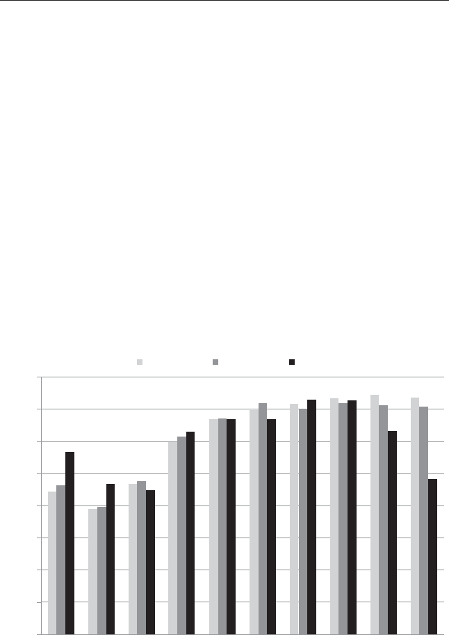
164 INVESTIGATING ALTERNATIVE MOMENTUM CONCEPTS

Regression results from Table 5 in the original paper show that 52-week

high winner/loser dummy is a good predictor of future return—better than

the past stock returns or industry factors.

The collective results suggest the 52-week high is a better trading signal

than price momentum. But what do the results look like using our uni-

verse of stocks? It should be pointed out that the George and Hwang paper

uses all stocks, and thus includes small-cap stocks, which can greatly skew

results. In contrast, we stick to a mid- and large-cap universe that is rela-

tively liquid and where the data are more robust. We form portfolios using

the 52-week-high screening variable, and place stocks into deciles based on

the ranking. Portfolios are reconstituted monthly, and are held for either

one month, three months, or six months. For the portfolios with three- and

six-month holding periods, overlapping portfolios are used. Portfolios are

formed by equal-weighting the rms, and the returns run from January 1,

1974, through December 31, 2014. Returns are shown gross of any fees. For

each decile, we plot the CAGR in Figure A1.2.

The results in Figure A1.2 document a few important ndings. First,

we notice that for the three- and six-month holding periods, there is a near

6-month hold 3-month hold 1-month hold

16.00%

14.00%

12.00%

10.00%

8.00%

6.00%

4.00%

2.00%

0.00%

Decile 1

(Furthest

Away

from 52-week

High)

Decile 2 Decile 3 Decile 4 Decile 5 Decile 6 Decile 7 Decile 8 Decile 9 Decile 10

(Closest

to 52-

week High)

FIGURE A1.2 Decile Returns to 52-Week High Screen

❦

❦ ❦

❦

Investigating Alternative Momentum Concepts 165

monotonic increase in the CAGR as one moves from decile 1 (furthest away

from 52-week high) up to decile 10 (closest to the 52-week high). This should

be expected as the paper goes long the top three deciles and shorts the bottom

three deciles to form the 52-week-high L/S portfolio discussed in the paper.

The paper also focuses their discussion around the portfolios that are held

for six months, which, not surprisingly, have the best performance. However,

for the monthly rebalanced version of the 52-week-high strategy, the results

break down dramatically. In other words, they fail a simple robustness test.

When results are fragile to reasonable changes in portfolio construction, we

get queasy that data mining may explain the analysis.

To make matters worse for the 52-week-high strategy, a basic long strat-

egy that buys the portfolio of stocks based on nearness to the 52-week

high isn’t that compelling. For example, the top decile 52-week-high port-

folio, held for 3 months, earns a 14.15 percent CAGR. Not bad, relative

to the market before transaction costs, but this CAGR is much lower than

the simple price momentum top decile portfolio (discussed in Chapter 5)

held for three months, which earned a 17.10 percent CAGR over the same

period.

Overall, we are impressed with the story behind the 52-week-high

concept, but we feel there is no robust evidence that the strategy is more

effective than relative strength price momentum strategies. Nevertheless,

the 52-week-high evidence does point in the general direction of the price

momentum anomaly and serves as another data point, which highlights

that momentum strategies likely exploit mispricing caused by marketwide

underreaction to news.

CAN ABSOLUTE STRENGTH IMPROVE RELATIVE

STRENGTH MOMENTUM?

“Absolute Strength: Exploring Momentum in Stock Returns,” by Huseyin

Gulen and Relitsa Petkova,13 has an interesting twist on standard relative

strength momentum strategies. As we’ve discussed throughout this book,

the academic research community captures the generic momentum strategy

by ranking rms on their past 12-month momentum (ignoring last month’s

return). Portfolios are then formed on these rankings. Most research papers

long the winners and short the losers. However, the classication of a “win-

ner” stock and a “loser” stock changes over time. During the Internet bub-

ble, to be classied as a “winner” a rm needed to have a past momentum

score of around 250 percent (near the peak). During the 2008 nancial crisis,

a “winner” stock would be any stock with a return above negative 5 percent.

Clearly, relative strength winners can have wide-ranging returns (the same

wide-ranging result is seen on relative strength losers).

❦

❦ ❦

❦

166 INVESTIGATING ALTERNATIVE MOMENTUM CONCEPTS

The authors explore the idea that perhaps a momentum strategy can

be improved by focusing on the “absolute” strength score. The idea is to

look back each month at the historical cutoffs for winners and losers, while

using all available returns to create the cutoffs. An example will illustrate the

methodology more clearly. Imagine it is January 31, 1965, and we examine

all the momentum scores (past 12-month momentum, skipping the most

recent month) for all stocks measured in January, using every year available

prior to 1965. This would be all the momentum scores on January 31, 1927,

January 31, 1928 ... , and January 31, 1965. From this sample set, identify

the 10th and 90th percentile values and use these as the “absolute” momen-

tum cutoffs. The cutoff analysis is completed each month, so the percentile

values are dynamic over time.

The absolute momentum cutoffs ensure that the denition of a winning

and a losing stock are more consistent over time. Using results from the paper,

the “winning” stock cutoff is near 60 percent, while the “losing” stock cutoff

is around negative 35 percent. Portfolios are formed using stocks that meet

the cutoff points. And while this approach has intuitive appeal, the portfolio

strategy will create stock portfolios with differing numbers of stock holdings.

In some cases, the number of stock holdings can be extreme. For example, a

gure from the original paper shows that during the 2008 nancial crisis, the

number of winners drops close to zero, while the number of losers goes above

1,500. A relative strength momentum rule on the other hand, will always buy

the top 10 percent and sell the bottom 10 percent of the universe. So if there

are 5,000 rms in the universe, the relative strength portfolio would buy 500

stocks and sell 500 stocks, keeping the portfolio size in balance.

Construction issues aside, how does this absolute momentum portfolio

perform? The author’s strategy that buys absolute strength winners and sells

absolute strength losers delivers a risk-adjusted return of 2.42 percent per

month from 1965 to 2014 and 1.55 percent per month from 2000 to 2014.

The baseline results to the long/short portfolios are impressive.

We’re a bit skeptical of the results based on the universe used by the

authors. Their universe includes microcaps stocks, which make up around

60 percent of the names in the CRSP universe, but only about 3 percent of

the market cap according to Fama and French 2008.14 Imagine trying to

long or short hundreds of microcap stocks!

To assess the validity of the absolute momentum results we decided to

perform the same analysis on a universe of mid- and large-cap US stocks.

We reconstruct the absolute momentum signal every month according the

cookbook outlined in the original paper. Figure A1.3 plots the breakpoints

over time. The return breakpoints are similar to those in the paper: the “win-

ning” stock cutoff is around 60 percent, while the “losing” stock cutoff is

around –35 percent. We only include stocks in the winner portfolio if they

❦

❦ ❦

❦

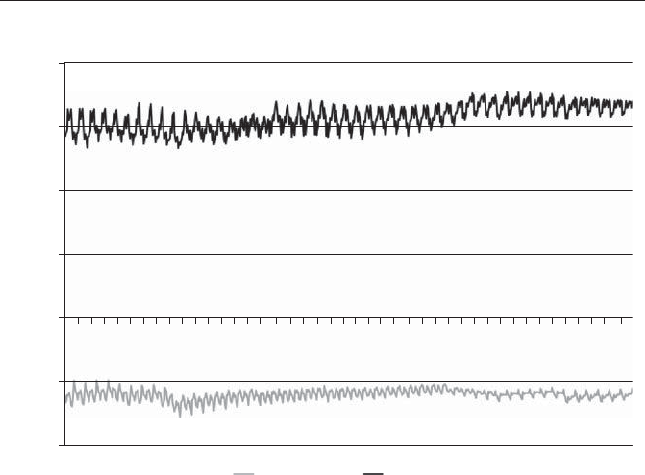
Investigating Alternative Momentum Concepts 167

80.0%

60.0%

40.0%

20.0%

0.0%

12/1/1964

2/1/1966

4/1/1967

6/1/1968

8/1/1969

10/1/1970

12/1/1971

2/1/1973

4/1/1974

6/1/1975

8/1/1976

10/1/1977

12/1/1978

2/1/1980

4/1/1981

6/1/1982

8/1/1983

10/1/1984

12/1/1985

2/1/1987

4/1/1988

6/1/1989

8/1/1990

10/1/1991

12/1/1992

2/1/1994

4/1/1995

6/1/1996

8/1/1997

10/1/1998

12/1/1999

2/1/2001

4/1/2002

6/1/2003

8/1/2004

10/1/2005

12/1/2006

2/1/2008

4/1/2009

6/1/2010

8/1/2011

10/1/2012

12/1/2013

–20.0%

–40.0%

Absolute Momentum Breakpoints

10th Percentile 90th Percentile

FIGURE A1.3 Absolute Momentum Breakpoints

are above the winner cutoff and only include stocks in the loser portfolio

if they are below the loser cutoff. As mentioned previously, this approach

introduces an odd portfolio construction element. Figure A1.4 highlights the

number of rms in the high and low absolute momentum portfolios across

time and compares these portfolio sizes to the standard price momentum

approach that buys the top 10 percent relative strength stocks and shorts

the bottom 10 percent relative strength stocks.

Similar to the original paper, there are extreme variations in portfolio

sizes. During the nancial crisis the absolute momentum portfolio is long

one rm in January 2009, while the absolute momentum portfolio is short

over 800 stocks.

We next assess the performance of the absolute momentum long/short

strategy. We examine long/short returns to the equal-weighted monthly

rebalanced portfolios from January 1965 to December 2014. All returns

shown are total returns but are gross of any fees and transaction costs. The

results are shown in Table A1.6.

The results are similar to the paper: the absolute momentum long/short

portfolio outperforms the relative strength portfolio on a variety of metrics.

To dig a bit deeper into the absolute momentum concept, we look at the

performance of the long and short portfolios, separately.

❦

❦ ❦

❦

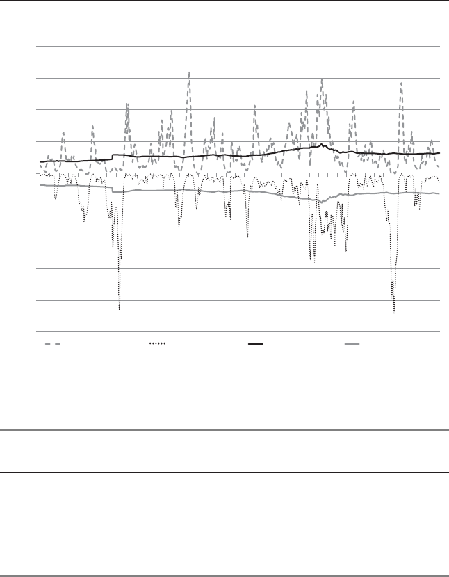
168 INVESTIGATING ALTERNATIVE MOMENTUM CONCEPTS

800

600

200

400

–200

–400

–600

–800

–1000

Number of Firms in the Portfolio Each Month

Abs. Str. Winners N Abs. Str. Losers N Rel. Str. Losers N Rel. Str. Winners N

1/1/1965

3/1/1966

5/1/1967

7/1/1968

9/1/1969

11/1/1970

1/1/1972

3/1/1973

5/1/1974

7/1/1975

9/1/1976

11/1/1977

1/1/1979

3/1/1980

5/1/1981

7/1/1982

9/1/1983

11/1/1984

1/1/1986

3/1/1987

5/1/1988

7/1/1989

9/1/1990

11/1/1991

1/1/1993

3/1/1994

5/1/1995

7/1/1996

9/1/1997

11/1/1998

1/1/2000

3/1/2001

5/1/2002

7/1/2003

9/1/2004

11/1/2005

1/1/2007

3/1/2008

5/1/2009

7/1/2010

9/1/2011

1/1/2014

11/1/2012

FIGURE A1.4 Absolute Momentum Number of Firms

TABLE A1.6 Absolute Momentum Long/Short Returns

Absolute

Strength (L/S)

Relative

Strength (L/S) SP500

CAGR 25.28% 17.97% 10.01%

Standard Deviation 23.26% 24.02% 15.04%

Downside Deviation 17.57% 20.58% 10.64%

Sharpe Ratio 0.88 0.61 0.38

Sortino Ratio (MAR =5%) 1.17 0.71 0.54

Worst Drawdown –68.27% –70.86% –50.21%

Table A1.7 shows the results to the four portfolios (Absolute Strength

Winners and Losers; Relative Strength Winners and Losers). Portfolios are

equal-weighted and rebalanced monthly from January 1965 to December

2014. All returns shown are total returns but are gross of any fees and trans-

action costs.

Examining the results, the long-only “winner” portfolios are similar and

there is little marginal benet of an absolute momentum strategy relative to

❦

❦ ❦

❦

Investigating Alternative Momentum Concepts 169

TABLE A1.7 Absolute Momentum Long-Only Portfolio Returns

Absolute

Momentum

Winner

Portfolio

Relative

Momentum

Winner

Portfolio

Absolute

Momentum

Loser

Portfolio

Relative

Momentum

Loser

Portfolio

CAGR 18.91% 18.74% –3.42% 2.40%

Standard Deviation 24.85% 25.11% 26.17% 26.20%

Downside Deviation 17.06% 17.41% 17.09% 17.39%

Sharpe Ratio 0.63 0.62 –0.19 0.03

Sortino Ratio (MAR =5%) 0.91 0.89 –0.29 0.04

Worst Drawdown –65.09% –58.40% –94.10% –82.01%

a classic price momentum strategy. The absolute momentum loser portfolio,

however, is much worse than the relative momentum loser portfolio.

These results suggest that the short leg drives the performance difference

between the long/short absolute momentum strategy and the long/short

relative momentum strategy.

Another potential issue is that the absolute momentum rule can create

portfolios with varying sizes from month to month. Alternatively, the rela-

tive strength signal creates a highly consistent Nin the portfolio from month

to month. Indirectly, the absolute momentum rule opens an investor up to a

lot of risk that may not be captured in a backtest. For example, in January

2009, the absolute momentum portfolio is long a single stock and the abso-

lute momentum portfolio is short over 800 stocks. We don’t know many

investors who would consider it prudent to hold a single stock portfolio.

Obviously, this didn’t have a huge effect historically, but out of sample this

could create serious consequences.

CAN THE VOLATILITY OF MOMENTUM

BE CONSTRAINED?

Anegativeaspecttomomentuminvestingisthefactthatahigh-momentum

portfolio tends to have large drawdowns and gut-wrenching volatility. On

the one hand, this is a terrible characteristic, but on the other hand, this is

why momentum is sustainable—it is not easy to “arbitrage.” But perhaps

there is a better way to manage the volatility of momentum strategies. Yufeng

Han, Guofu Zhou, and Yingzi Zhu make a good attempt in their paper,

“Taming Momentum Crashes: A Simple Stop-Loss Strategy.” The authors

apply a simple stop-loss rule to the classic long/short momentum portfolio.15

❦

❦ ❦

❦

170 INVESTIGATING ALTERNATIVE MOMENTUM CONCEPTS

The results are impressive. Using a 10 percent stop-loss rule, the authors drop

the maximum monthly loss from negative 49.79 percent to negative 11.36

percent and the Sharpe ratios are more than doubled.

The specics of the trading strategy can be summarized in three rules:

1. Rebalance the long and short book monthly by sorting stocks on their

past returns (the paper uses the last seven months’ returns, excluding the

most recent month).

2. Monitor the long portfolio daily: If a long position declines by Xpercent

(e.g., 10), sell the position and invest it in the risk-free rate until the end

of the month.

3. Monitor the short portfolio daily: If a short position rises by Xpercent

(e.g., 10), cover the position and invest any proceeds in the risk-free rate

until the end of the month.

Table A1.8 shows the original gures from the paper.

Not only does the portfolio have smaller monthly drawdowns, but

the average returns increase with the use of the stop-loss rules! If we

examine the winners minus losers (WML) long/short portfolio the average

monthly returns are highest using the 5 percent rule. Any strategy that can

lower drawdowns and increase returns is pretty compelling and worth a

second look.

TABLE A1.8 Equal-Weighted Stop-Loss Momentum Monthly Returns

Variable Avg Ret (%) Minimum (%)

Panel A: Original Momentum

Market 0.65 –29.10

Losers 0.24 –39.50

Winners 1.24 –33.06

WML 0.99 –49.79

Panel B: Stop Loss at 10%

Losers –0.42 –39.27

Winners 1.27 –12.87

WML 1.69 –11.36

Panel C: Stop Loss at 5%

Losers –0.83 –36.34

Winners 1.53 –8.48

WML 2.35 –8.94

❦

❦ ❦

❦

Investigating Alternative Momentum Concepts 171

Of course, nothing in nancial markets is ever easy, although sometimes

it looks that way. A downside of the stop-loss approach is that the strat-

egy requires daily analysis of every stock position, which may be quite

difcult—not to mention costly—for many investors to implement. Also,

from the perspective of a long-only investor, which is the focus of our book,

the benets to a stop-loss strategy are muted. For example, a momentum

strategy with a 10 percent stop-loss rule has a 1.27 percent average monthly

return, which is similar to a long-only buy and hold momentum strategy,

which earns a 1.24 percent average monthly return. That said, there is a

risk management benettoastop-lossapproach,whichwewillexaminein

more detail.

Similar to our prior analysis, we examine the stop-loss strategy under

our own research conditions. We examine a mid- to large-cap US traded

universe and we focus our analysis on the long-only portfolios. All returns

are gross, and no management fee or transaction costs are applied. We exam-

ine the returns from January 1, 1927, to December 31, 2013, to cover the

same sample period analyzed in the paper. We examine the following four

portfolios:

1. High momentum:Top10percentofrms ranked on their past momen-

tum (total return over the past 12 months ignoring last month). Portfolio

is monthly rebalanced and equal weighted.

2. High momentum with 10 percent stop-loss rule:Top10percentof

rms ranked on their past momentum (total return over the past 12

months ignoring last month). Portfolio is monthly rebalanced and equal

weighted. If during the month any individual stock position is down 10

percent, sell the security and remain in cash until the end of the month,

at which time the portfolio is rebalanced into the top 10 percent of

momentum rms.

3. High momentum with 5 percent stop-loss rule:Top10percentof

rms ranked on their past momentum (total return over the past 12

months ignoring last month). Portfolio is monthly rebalanced and equal

weighted. If during the month any individual stock position is down 5

percent, sell the security and remain in cash until the end of the month,

at which time the portfolio is rebalanced into the top 10 percent of

momentum rms.

4. SP500:TotalreturnoftheS&P500Index.

The results of the analysis are presented in Table A1.9.

The long-only generic momentum portfolio generates a much higher

CAGR than the risk-managed portfolios; however, the risk prole is arguably

❦

❦ ❦

❦

172 INVESTIGATING ALTERNATIVE MOMENTUM CONCEPTS

TABLE A1.9 Momentum Stop-Loss Performance

High

Momentum

High

Momentum

10% Stop-Loss

High

Momentum

5% Stop-Loss SP500

CAGR 19.34% 15.47% 15.29% 9.91%

Standard Deviation 24.78% 22.19% 18.31% 19.18%

Downside Deviation 18.26% 12.73% 8.36% 14.26%

Sharpe Ratio 0.70 0.61 0.68 0.41

Sortino Ratio (MAR =5%) 0.87 0.93 1.31 0.44

Worst Drawdown –71.73% –64.02% –48.11% –84.59%

better for the stop-loss systems. However, the risk prole is highly dependent

on the stop-loss rule examined, which hints toward a robustness issue. Rel-

ative to the 10 percent stop-loss rule, generic momentum is a better strategy,

but relative to a 5 percent stop-loss rule, generic momentum is worse on a

risk-adjusted basis.

On net, the stop-loss rule is interesting; however, risk management

via stop-loss is not the only option. One can apply a simple long-term

trend-following rule16 and/or a time-series momentum rule17 on a long-only

momentum strategy and avoid the complexity and operational commitment

required for a daily-assessed momentum portfolio. For example, consider

a simple time-series momentum trading rule that is long the momentum

portfolio if the past 12 month return on the S&P 500 is above the risk-free

rate, otherwise, the portfolio is investing in risk-free bonds.

Here are the four portfolios we test:

1. High momentum w/TSMOM:Top10percentofrms ranked on

their past momentum (total return over the past 12 months ignoring

last month). Portfolio is monthly rebalanced and equal weighted.

A 12-month time-series momentum-trading rule is applied each month.

2. High momentum: Top 10 percent of rms ranked on their past

momentum (total return over the past 12 months, ignoring last month).

Portfolio is monthly rebalanced and equal weighted.

3. High momentum with 10 percent stop-loss rule:Top10percentof

rms ranked on their past momentum (total return over the past

12 months ignoring last month). Portfolio is monthly rebalanced and

equal weighted. If during the month any individual stock position is

down 10 percent, sell the security and remain in cash until the end of

❦

❦ ❦

❦

Investigating Alternative Momentum Concepts 173

the month, at which time the portfolio is rebalanced into the top 10

percent of momentum rms.

4. High momentum with 5 percent stop-loss rule:Top10percentof

rms ranked on their past momentum (total return over the past

12 months ignoring last month). Portfolio is monthly rebalanced and

equal weighted. If during the month any individual stock position is

down 5 percent, sell the security and remain in cash until the end of the

month, at which time the portfolio is rebalanced into the top 5 percent

of momentum rms.

The returns run from January 1, 1928, to December 31, 2013 (we don’t

include 1927 because we need to use 12 months of data to get the TSMOM

rule). Results are gross of fees. All returns are total returns and include the

reinvestment of distributions (e.g., dividends).

The results from Table A1.10 highlight that a simple monthly reviewed

risk management rule applied at the portfolio level can achieve the same

level of risk control, but with a lot less complication, than daily-assessed

stop-loss rules.

If investors are interested in managing the volatility of their portfolio, we

recommend that investors rst focus on achieving the best possible long-only

momentum portfolio and combine it with the best possible long-only value

portfolio. Once that is achieved, and the investor is capturing the highest

expected equity premium on a risk-adjusted basis, the investor can deploy

risk-management rules at the portfolio level. Although a detailed discus-

sion of this approach is beyond the scope of this book, we recommend that

TABLE A1.10 Time-Series Momentum Performance

High

Momentum

TSMOM

High

Momentum

High

Momentum

10% Stop-Loss

High

Momentum

10% Stop-Loss

CAGR 16.57% 18.93% 15.06% 14.88%

Standard Deviation 20.97% 24.84% 22.23% 18.32%

Downside Deviation 16.80% 18.31% 12.75% 8.36%

Sharpe Ratio 0.68 0.69 0.59 0.66

Sortino Ratio

(MAR =5%) 0.75 0.85 0.91 1.26

Worst Drawdown –50.99% –71.73% –64.02% –48.11%

❦

❦ ❦

❦

174 INVESTIGATING ALTERNATIVE MOMENTUM CONCEPTS

investors focus on simple trend-following and time-series momentum type

rules to facilitate portfolio-level risk management.

NOTES

1. Nicholas Barberis, Andrei Shleifer, and Robert Vishny, “A Model of Investor

Sentiment,” Journal of Financial Economics 49 (1998): 307–343.

2. Louis Chan, Narisimhan Jegadeesh, and Josef Lakonishok, “Momentum Strate-

gies,” The Journal of Finance 51 (1996): 1681–1713.

3. Robert Novy-Marx, “Fundamentally, Momentum Is Fundamental Momen-

tum,” NBER Working Paper No. 20984.

4. For our universe of mid/large cap stocks, to match the volatility of the fundamen-

tal momentum portfolios (SUE and CAR3) with the price momentum (UMD)

portfolios, the fundamental momentum portfolios (SUE and CAR3) are required

to be three times long and three times short.

5. Tarun Chordia and Lakshmanan Shivakumar, “Earnings and Price Momen-

tum,” AFA 2003 Washington, DC Meetings.

6. Kent Daniel and Tobias Moskowitz. “Momentum Crashes,” Columbia Business

School Research Paper No. 14–36.

7. Eugene F. Fama and Kenneth R. French, “Common Risk Factors in the Returns

on Stocks and Bonds,” Journal of Financial Economics 33 (1993): 3–56.

8. Readers interested in more complex long/short portfolios should explore earn-

ings momentum strategies in more detail.

9. Malcolm Baker, Xin Pan, and Jeffrey Wurgler, “The Effect of Reference Point

Prices on Mergers and Acquisitions,” Journal of Financial Economics 106

(2012): 49–71.

10. Thomas J. George and Chuan-Yang Hwang, “The 52-Week High and Momen-

tum Investing,” The Journal of Finance 59 (2004): 1957–2444.

11. Narasimhan Jegadeesh and Sheridan Titman, “Returns to Buying Winners and

Selling Losers: Implications for Stock Market Efciency,” The Journal of Finance

48 (1993): 65–91.

12. Tobias J. Moskowitz and Mark Grinblatt, “Do Industries Explain Momentum?”

The Journal of Finance 54 (1999): 1249–1290.

13. Huseyin Gulen and Ralitsa Petkova, “Absolute Strength: Exploring Momentum

in Stock Returns,” working paper, accessed 1/31/2016.

14. Eugene F. Fama and Kenneth R. French, “Dissecting Anomalies,” The Journal

of Finance 63 (2008): 1653–1678.

15. Yufeng Han, Guofu Zhou, and Yingzi Zhu, “Taming Momentum Crashes: A

Simple Stop-Loss Strategy,” working paper, accessed 1/31/2016.

16. See Meb Faber, “A Quantitative Approach to Tactical Asset Allocation,” The

Journal of Wealth Management 9 (2007): 69–79.

17. Gary Antonacci, Dual Momentum Investing: An Innovative Strategy for Higher

Returns with Lower Risk (New York: McGraw-Hill, 2014).

❦

❦ ❦

❦

APPENDIX B

Performance Statistics

Deﬁnitions

Table A2.1 provides a denition of the performance statistics used through-

out the text.

TABLE A2.1 Performance Statistics Denitions

Statistics Description

CAGR Compound annual growth rate

Standard Deviation Sample standard deviation (annualized by square

root of 12)

Downside Deviation Sample standard deviation of all negative

observations (annualized by square root of 12)

Sharpe Ratio Monthly return minus risk-free rate divided by

standard deviation (annualized by square root of

12)

Sortino Ratio (MAR =5%) Monthly return minus minimum acceptable return

(MAR/12) divided by downside deviation

(annualized by square root of 12)

Worst Drawdown Worst peak-to-trough performance

Worst Month Return Worst monthly performance

Best Month Return Best monthly performance

Protable Months Proportion of monthly performances that have a

positive return

175

❦

❦ ❦

❦

About the Companion Website

This book includes a companion website, which can be found at www

.alphaarchitect.com. This website includes the following:

■A screening tool to nd momentum stocks described in the book

■Additional research on momentum investing

■A continually updated blog on developments in quantitative investing

■And much, much, more

176

❦

❦ ❦

❦

Index

Absolute momentum

breakpoints, 167

calculation of, 10

cutoff points, 166

nancial crisis and, 167

rms, number of, 168

long-only portfolio returns, 169

long/short returns, 168

portfolio performance, 166

rule, 169

validity of, 166

Absolute strength, 165–169

Agarwal, Vikas, 110

Alliance Pharmaceutical Corp.,

94–96

Alpha

relative risk premium, 154

sustainable, 27

Alpha analysis, quantitative

momentum and, 136–139

Alternative momentum concepts,

155–172

52-week high, 162–165

absolute strength improving

relative strength, 165–169

fundamentals and, 156–162

volatility of momentum,

169–174

American Finance Association, 62

American Stock Exchange (AMEX),

49, 139

Apple, 88, 90

AQR Capital Management, 59, 64,

91, 123

Arbitrage

dened, 23–24

investment strategy example, 24

limits to, 18, 24

quantitative momentum and,

141, 142

Asness, Cliff, 53, 57, 68, 70, 123

Asset class historical results, 67

Asset-class selection, trading rules

and, 11

Australian equity markets, 111

Baker, Malcom, 162

Bali, Turan G., 96–97

Barberis, Nicholas, 55, 56, 96,

100–101, 156

Barron’s,32

Baupost Group hedge fund, 7

Beaver, William, 49

Behavioral bias

identication of, 48

indirect exploitation of, 102

mispricing due to, 57

pillars of, 36

value, momentum and, 141

Behavioral errors, 60

Behavioral nance, 18–20

essence of, 21

investor psychology, 19–20

market mispricing and, 21

momentum and, 46–47

pillars of, 19, 36

poker comparison (see Poker

comparison)

177

❦

❦ ❦

❦

178 INDEX

Behavioral psychology, 100, 105

Behavioral theories, challenging, 56

Benchmark, passive, 70

Benchmark drift, 38

Benchmark portfolio, 125

Beta

dened, 99

“lottery-like” stocks and, 98–99

Beta anomaly, 98

Bias, EMH and, 62

Black, Fischer, 65

Black box, 140–141

Blended strategy, 73

Bloomeld, Robert, 56

B/M (book to market) ratios, 49

Brown, Philip, 111

Brunnermeier, Markus, 31, 32

Buffett, Warren, 6, 7, 8, 9, 16, 32,

45, 46, 142

CAGR (Compound Annual

Growth Rate)

52-week high screen and,

164–165

across different decades, 127

equal-weighting scheme and, 125

growth vs. momentum

monkeys, 51

intermediate-term returns and, 86

quantitative momentum and,

128, 129, 130

rebalancing and, 90

rolling ve-year, 146

value-weighted portfolios and, 88

Cakici, Nusret, 97

Capital Asset Pricing Model

(CAPM), 65, 136

Career risk

market frictions and, 58

momentum and, 59

quantitative momentum and,

152–154

Carhart, Mark, 44–45

CGM Focus Fund, 25–26

CGR, 70

Chan, Louis, 156

Chen, Honghui, 111

Closet indexing structures,

148–149

Combo portfolio, 68–74

annual returns for, 37–38

plus trend, 149–151

rolling 5-year spreads, 71–74

volatility and, 38

Compound Annual Growth Rate.

See CAGR (Compound Annual

Growth Rate)

Compustat, 49

Confusion De Confusions,3

“Continuation” effect, 86–87

Continuous information, 101, 103

Cooperman, Leon, 31

Core-satellite approach, 152

Costs

“all in”, 90

assumptions/estimates, 123–124

frictional, 103, 115

implementation, 24

mispricing opportunities and, 142

transaction (see Transaction

costs)

Cross-sectional momentum

about, 10

example using, 11

CRSP (Center for Research

in Security Prices), 49, 124

Cumulative three-day abnormal

returns (CAR3), 156–162

Cutoff analysis, 166

Da, Zhi, 100–101, 103, 105

Daniel, Kent, 48, 55

Data mining, 93, 141

DeBondt, Werner, 83

❦

❦ ❦

❦

Index 179

de la Vega, Joseph, 3–4, 6

De Long, Brad, 20

Discrete information, 101, 103

Disposition effect, 47, 103

Distributions, reinvestment of, 88

Diversication

equal-weighting scheme and, 125

stock selection strategies and, 63

Diversier, identication of, 38–39

Dividends, 88

“Diworsication”

avoidance of, 91

Internet bubble and, 35

minimization of, 148

Dojima Rice Market, 4–5

Downside-protected strategies, 151

Drawdown(s)

Great Depression, 126

growth vs. momentum

monkeys, 52

maximum, 131

rolling analysis of, 131–134

top 10 analysis, 134

Drawdown analysis, summary, 131

Druckenmiller, Stanley, 9

Dutch East India Company, 3

Earnings momentum, 156

EBIT/TEV (Earnings before Interest

and Taxes/Total Enterprise

Value), 161

Efcient Market Hypothesis

(EMH)

arbitrage and, 18–19, 21

bias and, 62

career risk and, 152, 154

establishment of, 15

momentum and, 45

real world markets and, 18

relative strength and, 43–44

strongest supporter of, 17

Equal-weighting portfolios, 91,

117, 125

Equation

information discreteness, 101

long-term performance, 27, 35

Equity markets, biggest, 69

Europe, rolling 5-year spreads,

71, 73

Evidence-based enhancements, 93

Evidence-based investing, age of,

8–9

Expectation error, 141

Facebook, 46

Fama, Eugene, 16, 17, 49, 55,

62–63, 136, 166

Fama-MacBeth, 157

52-week high, 162–165

Financial Analyst Journal,108

Financial crisis of 2008

absolute momentum and, 167

absolute momentum portfolio

and, 167

momentum and, 57, 58

post-2008 and, 151, 152

quantitative momentum and, 136

trough of, 16

“winner stocks” and, 165

Fisher, Gregg, 91

Fountain of Gold—The Three

Monkey Record of Money,

The,5

Four-factor alpha, 98, 136

Four-factor model, 136

Frazzini, Andrea, 59, 91, 123

French, Ken, 16, 33, 49, 54, 65, 88,

136, 166

Frictional costs, 103, 115

Frog-in-the-pan (FIP)

algorithm, 120–123, 140

hypothesis, 100–102

portfolio alphas, 102

results to long/short momentum

portfolios, 101

❦

❦ ❦

❦

180 INDEX

Fundamental analysis, emergence

of, 6–8

Fundamental investors, 15–17

Fundamental momentum

returns, 157

Fundamental risk, 24

Fundamentals, momentum and,

156–162

Gay, Gerald, 110

Gecay, Chris, 128, 141

Generic momentum

12-month momentum and, 165

calculation of, 80–81

dened, 101

quantitative momentum and, 120

Generic momentum effect, drivers

of, 104

George, Thomas J., 162, 164

Global rolling 5-year spreads,

73, 74

Google, 46

Graham, Benjamin, 6, 8, 14, 16, 40,

44, 45

Great Depression drawdown,

126

Greenblat, Joel, 16

Grifn, Dale, 56

Grinblatt, Mark, 111, 163

Growth

value and, 40 (see also Combo

portfolio)

value of, 36–38

“Growth” funds, momentum

compared to, 39

Growth investing

characterized, 48

vs. momentum investing, 49–52

momentum investing compared

to, 47–49

monkeys throwing darts and,

50–52

rationale for, 36–39

sustainable performance and,

35, 38

Gulen, Huseyin, 165

Gurun, Umit, 100–101, 103

Hales, Jeffrey, 56

Han, Yufeng, 168

He, Jia, 110

Heebner, Ken, 25–26, 31

High beta stocks, 98–99

High-conviction value, 146

High momentum portfolios,

stop-loss rule and, 172–173

High-momentum stocks, 94–96

Holding period, 87, 88, 89

Homma, Munehisa, 5, 6, 14

Hong, Harrison, 55, 102

Hu, Gang, 109

Hwang, Chuan-Yang, 162, 164

Implementation costs, 24

Index fund, plain-vanilla, 33

Indexing, closet, 148–149

Industry momentum, 163

Information

continuous, 101, 103

discrete, 101, 103

Information discreteness (ID),

101, 103

Intelligent Investor,The,6

Intermediate-term momentum,

84–88

International Rectier Corp.,

94–96

Internet Bubble

“diworsication” and, 35

growth investing and, 40

mispricing and, 32

overpriced growth stocks and, 35

path dependency and, 94–96

quantitative value and, 146

❦

❦ ❦

❦

Index 181

underperformance and, 151, 152

window dressing and, 109

“winner stocks” and, 165

Intrinsic value, 53

Investment formulas, 7

Investment strategies, long-term,

24–25

Investors, sustainable, 27

IQ/intelligence, 14–15

Israel, Ronen, 91, 123

Jacobsen, Ben, 107

“January” effect, 110–111

Japan

combination portfolio and,

73, 74

long/short price momentum

in, 160

momentum strategy and,

63–65

Japanese economy, Dojima Rice

Market, 4–5

Japanese equity market

performance, 64

Jegadeesh, Narasimhan, 39, 44, 45,

81, 84–87, 156

Jones, Paul Tudor, 31

Journal of Finance,26,45,108

Journal of Financial Economics,

108

Journal of Political Economy,20

Journal of Portfolio Management,

The,63,108

Kacperczyk, Marcin, 109

Kahneman, Daniel, 19, 44

Keim, Donald, 111

Keloharju, Matti, 107

Kemmerer, Edwin, 108

Keynes, John Maynard, 18

Kinney, William R., Jr., 110, 111

Klarman, Seth, 7, 8

Kleidon, Allan, 111

Korajczyk, Robert, 90, 91

Lakonishok, Josef, 47, 48, 156

Lefevre, Edwin, 5

Lehman, Bruce, 81

Lesmond, David A., 90, 91, 123

Levy, Robert, 43, 44

Lim, Terence, 102

“Limited attention”, 100, 105

Ling, Leng, 110

Linnainmaa, Juhani, 107

Livermore, Jesse, 5, 6, 14

Lo, Andrew, 9

Long/short momentum portfolio

factor loadings, 161

Long-term active management

success

bad players, identication of,

29–31

best players, actions of, 31–35

keys to, 26–35

theory to practice, 27–29

Long-term investor, six-year

investing pain train, 34

Long-term market opportunities,

short-term performance

and, 26

Long-term momentum, 83–84

Long-term performance equation,

27, 35

“Look-back” period, 90

Look-backs, intermediate-term, 85

Look-back windows, 83

Lottery bias, 98, 99

“Lottery-like” stocks

path dependency and, 95

performance of, 96–100

results, MAX ranking and, 97–98

Low beat stocks, 98–99

Malkiel, Burt, 6–8, 43–44

Margin of Safety,7

❦

❦ ❦

❦

182 INDEX

Market cycle

denitions, 135

performance, quantitative

momentum and, 135

Market exposure, 98

Market frictions, 24, 36

Market liquidity, 115

Market mispricing

behavioral nance and, 21

costs and, 142

Efcient Market Hypothesis

and, 18

enhancing, 31–32

long time frames and, 25

opportunities, 70

quantitative momentum and,

141–142

Market-timing, trading rules

and, 11

Markowitz, Harry, 65

Marsh, Terry, 111

MBA “rebels”, 45

McLean, David, 109

McNichols, Maureen, 49

Mean-variance (MV) frontier,

65–68

Mispricing. See Market mispricing

Modern portfolio theory, 65–68

chart, 66

with momentum, 68

Momentum

absolute (see Absolute

momentum)

adoption of term, 44–45

behavioral nance theorists on,

46–47

best players and, 57–59

concepts, alternative (see

Alternative momentum

concepts)

cross-sectional, 10, 11

dened, 39, 43

expanding horizons with, 65–68

generic (see Generic momentum)

growth compared to, 39

industry, 163

intermediate-term, 84–87

investing (see Momentum

investing)

long-term, 83–84

as “myth”, 62–63

as performance king, 54

performance of, 69

as “premier anomaly”, 62

revitalization of, 44–45

short-term, 81–83

time series, 10, 11

trading frequency and, 58–59

types of, 81–87

underperformance and, 57, 58

underreaction issue and, 55–56

value and, as system, 79

value and, correlation of, 70

value compared to, 59

value married to, 68–75

value plus, 144–149

why it works, 53–59

Momentum anomaly, 54–57, 102

Momentum effect, persistence

of, 39

Momentum factor (MOM), 139

Momentum investing

characterized, 48

vs.growthinvesting,49–52

growth investing compared

to, 47–49

monkeys throwing darts and,

50–52

pessimism and, 47

why it works, 53

“Momentum-like effect”, 163

Momentum performance,

1927–2014, 54

❦

❦ ❦

❦

Index 183

Momentum portfolio construction.

See Portfolio construction

Momentum portfolio returns

intermediate-term, 86–87

long-term, 84, 85

short-term, 82–83

Momentum portfolio(s), 146–149

annual results, quality of, 104

returns, quality of, 104

Momentum premium, 85

Momentum prots, 113

Momentum seasonality

from 1984–2004, 113

benets, 116

results, 114–117

Momentum spread, 115

Momentum stocks

outperformance and, 54

path dependency and, 94

time-series characteristics of, 93

Momentum stop-loss performance,

172

Momentum strategies

building, basics, 79–82

categories, 10

commonly examined, 91–92

excess expected returns, 59–60

intermediate-term horizon

and, 85

path dependency and, 105

seasonality and, 113

Monkeys throwing darts, 50–52

Moskowitz, Toby, 57, 68, 91, 111,

123, 163

MSCI Japan Total Return Index, 64

Nagel, Stefan, 31, 32

NASDAQ, 49

NASDAQ crash, 136

Newton, Sir Isaac, 14

New York Stock Exchange (NYSE),

49, 124, 139

Ng, Lilian, 110

Noise trader risk, 24

Noise traders, 20

Non-overlapping seasonal

momentum portfolio, 116

Novy-Marx, Robert, 107, 156,

157, 158, 162

Nyberg, Peter, 107

Opportunity in market, identifying,

Optimal portfolio weights, 65

Overlapping portfolio effect, 116

Overlapping portfolios, 88–89, 116

Overreaction triggers for, 56

Pan, Xin, 162

Paradigm, style box, 39

Passive benchmark, 70, 142

Path, 93–105

momentum prots and, 100–103

Path dependency

Internet Bubble and, 94–96

momentum stocks and, 94

Path-focused momentum

algorithms, 102

Pederson, Lasse, 57, 68

Performance

poor relative, quantitative

momentum and, 151–152

sustainable (see Sustainable

performance)

value investing and, 35

Performance statistics, 175

Petkova, Relitsa, 165

Plain-vanilla index fund, 33

Poker comparison, 21–26

arbitrage and, 23–24

best players and, 23–26

opportunity, identifying, 22

sustainable performance and, 36

worst players and, 23

❦

❦ ❦

❦

184 INDEX

Pontiff, Jeff, 109

Portfolio construction, 87–91

quantitative momentum and,

146–149

trend emergence, 90

value weighting and, 89

Positive news, underreaction

to, 121

Poterba, James, 111

Price, Richard, 49

Price momentum, 156, 163

Price momentum factor, 158

Protability, momentum and, 118

Prots

momentum, 113

momentum, path to, 100–103

Psychology, investor, 19–20

Put options, 63

“Quality” momentum, 105

Quantitative momentum, 120–142

alpha analysis, 136–139

analysis, 125–139

asset pricing coefcient estimates

for, 139

beating the market with,

141–142

black box and, 140–141

career risk and, 152–154

cumulative value for, 127

FIP algorithm and, 120–123, 140

generic momentum and, 120

parameters of universe and, 124

poor relative performance and,

151–152

portfolio construction, 146–149

portfolio holdings, 140

process, steps in, 121–122

quantitative value and, 145, 150

rewards analysis, 126–128

risk analysis, 128–134

robustness analysis, 134–139

rolling drawdown analysis,

131–134

short-term stress event tests

for, 136

summary statistics, 125–126

transaction costs and, 122–124

Quantitative value, 145, 150

Quantitative Value,144

Quantitative value algorithm,

145

“Quants”, 140

R2K, 33

Random Walk Down Wall Street,

A,6,43–44

Rebalancing

“all in” costs, 90

frequency of, 87, 91

frictional costs and, 103

portfolios and, 117

smart, 116

window dressing and, 116

Reinganum, Marc, 111

Reinvestment of distributions, 88

“Relative pain”, 151

“Relative performance risk”,

150, 154

Relative strength

absolute strength improving,

165–169

dened, 10

momentum rule, 166

Relative strength strategy, 45

Reminiscences of a Stock

Operator,5

Return gap measure, 109

Returns, core-satellite, 152, 154

Reversal in returns, 82

Review of Financial Studies,108

Risk

career (see Career risk)

fundamental, 24

❦

❦ ❦

❦

Index 185

noise trader, 24

“relative performance risk”,

150, 154

Risk arbitrage, 19, 24

Risk-factors. hidden systemic, 59

Ritter, Jay, 111

Robertson, Julian, 31, 32

Roll, Richard, 62–63, 111

Rolling 5-year spreads

Europe, 71, 73

global, 73, 74

Japan, 73, 74

United Kingdom (UK), 71, 72

United States (US), 71, 72

Rolling drawdown analysis,

131–134

Rozeff, Michael S., 110, 111

Russell 200 total return index.

See R2K

S&P 500

poor relative performance

and, 152

quantitative momentum and,

135, 136

S&P 500 Index, 66

S&P 500 Sharpe ratio, 126

S&P 500 total return index (S&P

500 TR Index), 57, 58, 70, 125

Sadka, Ronnie, 90, 91

Samonov, Mikhail, 128, 141

Schill, Michael J., 90, 91, 123

Scientic method, key aspect of, 9

Seasonal effects, minimization

of, 116

Seasonality, 107–118

building momentum systems

and, 117

great theories and, 112–114

momentum (see Momentum

seasonality)

momentum portfolio annual

results and, 117

tax-motivated trading, 110–112

window dressing, 108–110

Security Analysis,6

Shah, Ronnie, 91

Sharpe ratio, 104, 126, 159,

160, 170

Shefrin, Hersh, 103

Shipping costs, “frictional”, 19

Shleifer, Andrei, 20, 26, 31, 47,

48, 156

“Short rebate”, 24

Short selling, implementation costs

and, 24

Short-term momentum, 81–83

Short-term performance, long-term

market opportunities and, 26

Short-term reversal, 81

Sialm, Clemens, 109

Sias, Richard, 108, 111, 112,

114, 115

Singal, Vijay, 111

Small-cap effect, 125

“Smart beta” funds, 146

“Smart money”, 19

Smart rebalancing, 116, 117

So, Eric, 48

Soloman, David, 110

Soltes, Eugene, 110

Soros, George, 9, 31

Sortino ratio, 104, 126, 159

Sosyura, Denis, 110

South Sea Company, 14

SP500, 33

Speculators, 7

Standardized unexpected earnings

(SUE), 156–162

Starks, Laura, 111

Statistics, performance, 175

Statman, Meir, 103

Stein, Jeremy, 55

Stein, Jeremy C., 102

Stock picking training, 45

❦

❦ ❦

❦

186 INDEX

Stop-loss rule, 169–170

Stop-loss strategy, 169–174

equal-weighted stop-loss

momentum monthly returns,

170

momentum performance

and, 172

portfolios for, 171

time-series momentum

performance, 173

Style box paradigm, 39

Summers, Larry, 20

Survivability, 145

Sustainable active investing

framework

growth investing and, 35

momentum and, 39

overarching framework and,

9, 12

six-year investing pain train, 34

value and, 70

value investing and, 35

Sustainable alpha, 27

Sustainable investors, 27, 34

Sustainable performance

building blocks, 53

growth investing and, 35, 38

long-term equation and, 35

poker comparison and, 36

Tail-risk correlations, 134

“Tax hypothesis”, 111

Tax-induced seasonality, 111

Tax-loss selling, 108, 111

Tax-motivated trading, 110–112

smart rebalance portfolio

and, 117

theories and, 112–114

Technical analysis, history of, 3–6

Thaler, Richard, 83

Thinking, Fast and Slow,19

Three-factor model, 136

Time-series momentum

about, 10

example using, 11

Titman, Sheridan, 39, 44, 45, 48,

84–87, 91

Tracking error

long time frames and, 24, 25

short-term, 25

trend following and, 150

Trading frequency, momentum

and, 58–59

Transaction costs

quantitative momentum,

122–124

rebalancing and, 90

trading frequency and, 58–59

Trend, combo plus, 149 – 151

Trend-following

“relative performance risk”

of, 150

rule, 149, 151

Trend overlay, 149

Tudor Jones, Paul, 9

“Turn of the year” effect, 110–112

Turnover, 91

Tversky, Amos, 44, 56

Underperformance

momentum and, 57, 58

stretches of, 73

value investing and, 32–33

Underreaction

positive news and, 121

triggers for, 56

United Kingdom (UK), rolling

5-year spreads, 71, 72

United States (US), rolling 5-year

spreads, 71, 72

Universe selection parameters,

123

❦

❦ ❦

❦

Index 187

Value

equity markets and, 70

growth and, 36–38, 40 (see also

Combo portfolio)

high-conviction, 146

intrinsic, 53

momentum and, as system, 79

momentum and, correlation

of, 70

momentum compared to, 59

momentum married to, 68–75

overreaction problem and, 55

performance of, 69

plus momentum, 144–149

quantitative, 145

Value and momentum portfolio

annual returns, 161

Value anomaly, 53

Value debate, 16

Value effect, study of, 44

Value factor (HML), 160

Value investing

as intuitive, 53

pessimism and, 47

six-year investing pain train,

34–35

sustainable performance and, 35

underperformance and, 32–33

upward price moves and, 46–47

“Value” investors, 15–17

Value premium, 16

Value trap, 53

Value weighting, 88, 116

Vishny, Robert, 26, 31, 47, 48, 156

Vogel, Jack, 17, 18

Volatility

growth vs. momentum monkeys,

51–52

momentum and, 169–174

stretches of, 73

value, growth and, 37

value and growth combo, 38

VW quantitative momentum

performance, 126

Wachtel, Sidney B., 110, 111

Waldmann, Robert, 20

Wall Street Journal (WSJ), 25

Wang, Qinghai, 109, 110

Warachka, Mitch, 100–101, 103

Website

companion, 176

ValueInvestorsClub.com, 16

Weisbbennar, Scott, 111

Whitelaw, Robert F., 97

Window dressing

about, 108–110

smart rebalance portfolio

and, 117

theories and, 112–114

Winners minus losers (WMI), 170

Wurgler, Jeffrey, 162

Zhang, Cherry, 107

Zheng, Lu, 109

Zhou, Chunsheng, 90, 91, 123

Zhou, Guofu, 168

Zhu, Yingzi, 168

WILEY END USER LICENSE AGREEMENT

Go to www.wiley.com/go/eula to access Wiley’s ebook EULA.

(Wiley Finance) Wesley R. Gray, Jack Vogel Quantitative Momentum A Practitioner’s Guide To

(Wiley%20Finance)%20Wesley%20R.%20Gray%2C%20Jack%20R.%20Vogel-Quantitative%20Momentum_%20A%20Practitioner%E2%80%99s%20Guide%20to

Navigation menu

Versions of this User Manual:

Views

Navigation